Download - An overview of independent component analysis and its applications

Informatica 35 (2011) 63–81 63

An Overview of Independent Component Analysis and Its Applications

Ganesh R. Naik and Dinesh K KumarSchool of Electrical and Computer EngineeringRMIT University, AustraliaE-mail: [email protected]

Overview paper

Keywords: independent component analysis, blind source separation, non-gaussianity, multi run ICA, overcomplete ICA,undercomplete ICA

Received: July 3, 2009

Independent Component Analysis (ICA), a computationally efficient blind source separation technique,has been an area of interest for researchers for many practical applications in various fields of science andengineering. This paper attempts to cover the fundamental concepts involved in ICA techniques and reviewits applications. A thorough discussion of the applications and ambiguities problems of ICA has beencarried out.Different ICA methods and their applications in various disciplines of science and engineeringhave been reviewed. In this paper, we present ICA methods from the basics to their potential applicationsto serve as a comprehensive single source for an inquisitive researcher to carry out research in this field.

Povzetek: Podan je pregled tehnike ICA (Independent Component Analysis).

1 Introduction

The problem of source separation is an inductive inferenceproblem. There is not enough information to deduce thesolution, so one must use any available information to in-fer the most probable solution. The aim is to process theseobservations in such a way that the original source signalsare extracted by the adaptive system. The problem of sep-arating and estimating the original source waveforms fromthe sensor array, without knowing the transmission chan-nel characteristics and the source can be briefly expressedas problems related to BSS. In BSS the word blind refersto the fact that we do not know how the signals were mixedor how they were generated. As such, the separation isin principle impossible. Allowing some relatively indirectand general constrains, we however still hold the term BSSvalid, and separate under these conditions.

There appears to be something magical about blindsource separation; we are estimating the original sourcesignals without knowing the parameters of mixing and/orfiltering processes. It is difficult to imagine that one canestimate this at all. In fact, without some a priori knowl-edge, it is not possible to uniquely estimate the originalsource signals. However, one can usually estimate themup to certain indeterminacies. In mathematical terms, theseindeterminacies and ambiguities can be expressed as arbi-trary scaling, permutation and delay of estimated sourcesignals [1]. These indeterminacies preserve, however, thewaveforms of the original sources. Although these inde-terminacies seem to be rather severe limitations, in a greatnumber of applications these limitations are not essential,since the most relevant information about the source signals

is contained in the temporal waveforms or time-frequencypatterns of the source signals and usually not in their ampli-tudes or the order in which they are arranged in the outputof the system. However, for some applications especiallybiomedical signal models such as sEMG signals, there isno guarantee that the estimated or extracted signals haveexactly the same waveforms as the source signals.

Independent component analysis (ICA) is one of themost widely used BSS techniques for revealing hidden fac-tors that underlie sets of random variables, measurements,or signals. ICA is essentially a method for extracting in-dividual signals from mixtures. Its power resides in thephysical assumptions that the different physical processesgenerate unrelated signals. The simple and generic natureof this assumption allows ICA to be successfully applied indiverse range of research fields.

In this paper, we first set the scene of the blind sourceseparation problem. Then, Independent Component Anal-ysis is introduced as a widely used technique for solvingthe blind source separation problem. A general descriptionof the approach to achieving separation via ICA and theunderlying assumptions of the ICA framework and impor-tant ambiguities that are inherent to ICA are discussed insection 3. A description of specific details of different ICAmethods are given in Sections 4, and the paper concludeswith applications of BSS and ICA methods.

2 Blind source separation (BSS)

Consider a situation in which we have a number of sourcesemitting signals which are interfering with one another. Fa-

64 Informatica 35 (2011) 63–81 G.R. Naik et al.

miliar situations in which this occurs are a crowded roomwith many people speaking at the same time, interferingelectromagnetic waves from mobile phones or crosstalkfrom brain waves originating from different areas of thebrain. In each of these situations the mixed signals are of-ten incomprehensible and it is of interest to separate theindividual signals. This is the goal of Blind Source Separa-tion. A classic problem in BSS is the cocktail party prob-lem. The objective is to sample a mixture of spoken voices,with a given number of microphones - the observations, andthen separate each voice into a separate speaker channel -the sources. The BSS is unsupervised and thought of as ablack box method. In this we encounter many problems,e.g. time delay between microphones, echo, amplitude dif-ference, voice order in speaker and underdetermined mix-ture signal.

Herault and Jutten [2] proposed that, in a artificial neu-ral network like architecture the separation could be doneby reducing redundancy between signals. This approachinitially lead to what is known as independent componentanalysis today. The fundamental research involved only ahandful of researchers up until 1995. It was not until then,when Bell and Sejnowski [3] published a relatively sim-ple approach to the problem named infomax, that many be-came aware of the potential of ICA. Since then a wholecommunity has evolved around ICA, centralized aroundsome large research groups and its own ongoing confer-ence, International Conference on independent componentanalysis and blind signal separation. ICA is used today inmany different applications, e.g. medical signal analysis,sound separation, image processing, dimension reduction,coding and text analysis [4, 5, 6, 7, 8, 9, 10, 11, 12, 13, 14].

In ICA the general idea is to separate the signals, as-suming that the original underlying source signals are mu-tually independently distributed. Due to the field’s rela-tively young age, the distinction between BSS and ICAis not fully clear. When regarding ICA, the basic frame-work for most researchers has been to assume that the mix-ing is instantaneous and linear, as in infomax. ICA is of-ten described as an extension to PCA, that uncorrelatesthe signals for higher order moments and produces a non-orthogonal basis. More complex models assume for ex-ample, noisy mixtures, [15, 16], nontrivial source distribu-tions, [17, 18], convolutive mixtures [19, 20, 21], time de-pendency, underdetermined sources [22, 23], mixture andclassification of independent component [4, 24]. A generalintroduction and overview can be found in [25].

3 Independent component analysis

Independent Component Analysis (ICA) is a statisticaltechnique, perhaps the most widely used, for solving theblind source separation problem [25, 26]. In this sec-tion, we present the basic Independent Component Analy-sis model and show under which conditions its parameterscan be estimated.

3.1 ICA model

The general model for ICA is that the sources are gener-ated through a linear basis transformation, where additivenoise can be present. Suppose we have N statistically in-dependent signals, si(t), i = 1, ...,N. We assume that thesources themselves cannot be directly observed and thateach signal, si(t), is a realization of some fixed probabilitydistribution at each time point t. Also, suppose we observethese signals using N sensors, then we obtain a set of N ob-servation signals xi(t), i = 1, ...,N that are mixtures of thesources. A fundamental aspect of the mixing process is thatthe sensors must be spatially separated (e.g. microphonesthat are spatially distributed around a room) so that eachsensor records a different mixture of the sources. With thisspatial separation assumption in mind, we can model themixing process with matrix multiplication as follows:

x(t) = As(t) (1)

where A is an unknown matrix called the mixing matrixand x(t), s(t) are the two vectors representing the observedsignals and source signals respectively. Incidentally, thejustification for the description of this signal processingtechnique as blind is that we have no information on themixing matrix, or even on the sources themselves.

The objective is to recover the original signals, si(t),from only the observed vector xi(t). We obtain estimatesfor the sources by first obtaining the “unmixing matrix” W,where, W = A−1.

This enables an estimate, s(t), of the independentsources to be obtained:

s(t) =Wx(t) (2)

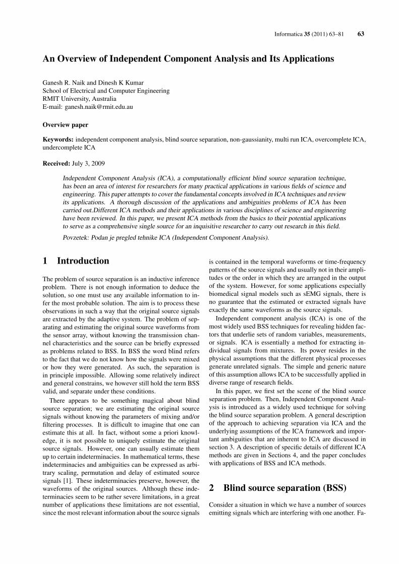
The diagram in Figure 1 illustrates both the mixingand unmixing process involved in BSS. The independentsources are mixed by the matrix A (which is unknown inthis case). We seek to obtain a vector y that approximatess by estimating the unmixing matrix W. If the estimate ofthe unmixing matrix is accurate, we obtain a good approx-imation of the sources.

The above described ICA model is the simple modelsince it ignores all noise components and any time delayin the recordings.

3.2 Independence

A key concept that constitutes the foundation of indepen-dent component analysis is statistical independence. Tosimplify the above discussion consider the case of two dif-ferent random variables s1 and s2. The random variable s1is independent of s2, if the information about the value ofs1 does not provide any information about the value of s2,and vice versa. Here s1 and s2 could be random signalsoriginating from two different physical process that are notrelated to each other.

AN OVERVIEW OF INDEPENDENT COMPONENT ANALYSIS AND. . . Informatica 35 (2011) 63–81 65

Figure 1: Blind source separation (BSS) block diagram. s(t) are the sources. x(t) are the recordings, s(t) are the estimatedsources A is mixing matrix and W is un-mixing matrix

3.2.1 Independence definition

Mathematically, statistical independence is defined interms of probability density of the signals. Consider thejoint probability density function (pdf) of s1 and s2 bep(s1,s2). Let the marginal pdf of s1 and s2 be denoted byp1(s1) and p2(s2) respectively. s1 and s2 are said to be in-dependent if and only if the joint pdf can be expressed as;

ps1,s2(s1,s2) = p1(s1)p2(s2) (3)

Similarly, independence could be defined by replacingthe pdf by the respective cumulative distributive functionsas;

E{p(s1)p(s2)}= E{g1(s1)}E{g2(s2)} (4)

where E{.} is the expectation operator. In the followingsection we use the above properties to explain the relation-ship between uncorrelated and independence.

3.2.2 Uncorrelatedness and Independence

Two random variables s1 and s2 are said to be uncorrelatedif their covariance C(s1,s1) is zero.

C(s1,s2) = E{(s1 −ms1)(s2 −ms2)}= E{s1s2 − s1ms2 − s2ms1 +ms1ms2}= E{s1s2}−E{s1}E{s2}= 0

(5)

where ms1 is the mean of the signal. Equation 4 and 5are identical for independent variables taking g1(s1) = s1.Hence independent variables are always uncorrelated. However the opposite is not always true. The above discussionproves that independence is stronger than uncorrelatednessand hence independence is used as the basic principle forICA source estimation process. However uncorrelatednessis also important for computing the mixing matrix in ICA.

3.2.3 Non-Gaussianity and Independence

According to central limit theorem the distribution of a sumof independent signals with arbitrary distributions tends to-ward a Gaussian distribution under certain conditions. Thesum of two independent signals usually has a distributionthat is closer to Gaussian than distribution of the two orig-inal signals. Thus a gaussian signal can be considered as aliner combination of many independent signals. This fur-thermore elucidate that separation of independent signalsfrom their mixtures can be accomplished by making thelinear signal transformation as non-Gaussian as possible.

Non-Gaussianity is an important and essential principlein ICA estimation. To use non-Gaussianity in ICA es-timation, there needs to be quantitative measure of non-Gaussianity of a signal. Before using any measures of non-Gaussianity, the signals should be normalised. Some of thecommonly used measures are kurtosis and entropy mea-sures, which are explained next.

– Kurtosis

Kurtosis is the classical method of measuring Non-Gaussianity. When data is preprocessed to have unit vari-ance, kurtosis is equal to the fourth moment of the data.

The Kurtosis of signal (s), denoted by kurt (s), is definedby

kurt(s) = E{s4}−3(E{s4})2 (6)

This is a basic definition of kurtosis using higher or-der (fourth order) cumulant, this simplification is based onthe assumption that the signal has zero mean. To simplifythings, we can further assume that (s) has been normalisedso that its variance is equal to one: E{s2}= 1.

Hence equation 6 can be further simplified to

kurt(s) = E{s4}−3 (7)

Equation 7 illustrates that kurtosis is a nomralised formof the fourth moment E{s4} = 1. For Gaussian signal,


E{s4} = 3(E{s4})2 and hence its kurtosis is zero. Formost non-Gaussian signals, the kurtosis is nonzero. Kur-tosis can be both positive or negative. Random variablesthat have positive kurtosis are called as super Gaussian orplatykurtotic, and those with negative kurtosis are calledas sub Gaussian or leptokurtotic. Non-Gaussianity is mea-sured using the absolute value of kurtosis or the square ofkurtosis.

Kurtosis has been widely used as measure of Non-Gaussianity in ICA and related fields because of its com-putational and theoretical and simplicity. Theoretically, ithas a linearity property such that

kurt(s1 ± s2) = kurt(s1)± kurt(s2) (8)

and

kurt(αs1) = α4kurt(s1) (9)

where α is a constant. Computationally kurtosis can becalculated using the fourth moment of the sample data, bykeeping the variance of the signal constant.

In an intuitive sense, kurtosis measured how "spikiness"of a distribution or the size of the tails. Kurtosis is ex-tremely simple to calculate, however, it is very sensitive tooutliers in the data set. It values may be based on only afew values in the tails which means that its statistical sig-nificance is poor. Kurtosis is not robust enough for ICA.Hence a better measure of non-Gaussianity than kurtosis isrequired.

– Entropy

Entropy is a measure of the uniformity of the distributionof a bounded set of values, such that a complete unifor-mity corresponds to maximum entropy. From the informa-tion theory concept, entropy is considered as the measureof randomness of a signal. Entropy H of discrete-valuedsignal S is defined as

H(S) =−∑P(S = ai)logP(S = ai) (10)

This definition of entropy can be generalised for acontinuous-valued signal (s), called differential entropy,and is defined as

H(S) =−∫

p(s)logp(s)ds (11)

One fundamental result of information theory is thatGaussian signal has the largest entropy among the othersignal distributions of unit variance. entropy will be smallfor signals that have distribution concerned on certain val-ues or have pdf that is very "spiky". Hence, entropy can beused as a measure of non-Gaussianity.

In ICA estimation, it is often desired to have a measureof non-Gaussianity which is zero for Gaussian signal andnonzero for non-Gaussian signal for computational sim-plicity. Entropy is closely related to the code length of therandom vector. A normalised version of entropy is givenby a new measure called Negentropy J which is defined as

J(S) = H(sgauss)−H(s) (12)

where sgauss is the Gaussian signal of the same covari-ance matrix as (s). Equation 12 shows that Negentropy isalways positive and is zero only if the signal is a pure gaus-sian signal. It is stable but difficult to calculate. Henceapproximation must be used to estimate entropy values.

3.3 Mathematical IndependenceMathematical properties of matrices were investigated tocheck the linear dependency and independency of globalmatrices (Permutation matrix P)

3.3.1 Rank of the matrix

Rank of the matrix will be less than the matrix size for lin-ear dependency and rank will be size of matrix for linearindependency, but this couldn’t be assured yet due to noisein the signal. Hence determinant is the key factor for esti-mating number of sources.

3.3.2 Determinant of the matrix

In real time applications Determinant value should be zerofor linear independency and should be more than zero(close to 1) for linear independency [27].

3.4 ICA Assumptions and AmbiguitiesICA is distinguished from other approaches to source sep-aration in that it requires relatively few assumptions on thesources and on the mixing process. The assumptions andof the signal properties and other conditions and the issuesrelated to ambiguities are discussed below:

3.4.1 ICA Assumptions

– The sources being considered are statistically inde-pendent

The first assumption is fundamental to ICA. As dis-cussed in Section 3.2, statistical independence is the keyfeature that enables estimation of the independent compo-nents s(t) from the observations xi(t).

– The independent components have non-Gaussian dis-tribution

The second assumption is necessary because of the closelink between Gaussianity and independence. It is impossi-ble to separate Gaussian sources using the ICA frameworkdescribed in Section 3.2 because the sum of two or moreGaussian random variables is itself Gaussian. That is, thesum of Gaussian sources is indistinguishable from a singleGaussian source in the ICA framework, and for this reasonGaussian sources are forbidden. This is not an overly re-strictive assumption as in practice most sources of interestare non-Gaussian.


– The mixing matrix is invertible

The third assumption is straightforward. If the mixing ma-trix is not invertible then clearly the unmixing matrix weseek to estimate does not even exist.

If these three assumptions are satisfied, then it is possi-ble to estimate the independent components modulo sometrivial ambiguities (discussed in Section 3.4). It is clearthat these assumptions are not particularly restrictive andas a result we need only very little information about themixing process and about the sources themselves.

3.4.2 ICA Ambiguity

There are two inherent ambiguities in the ICA framework.These are (i) magnitude and scaling ambiguity and (ii) per-mutation ambiguity.

– Magnitude and scaling ambiguity

The true variance of the independent components cannotbe determined. To explain, we can rewrite the mixing inequation 1 in the form

x = As

=N

∑j=1

a js j(13)

where a j denotes the jth column of the mixing matrix A.Since both the coefficients a j of the mixing matrix and theindependent components s j are unknown, we can transformEquation 13.

x =N

∑j=1

(1/α ja j)(α js j) (14)

Fortunately, in most of the applications this ambiguityis insignificant. The natural solution for this is to use as-sumption that each source has unit variance: E{s j2} = 1.Furthermore, the signs of the of the sources cannot be de-termined too. This is generally not a serious problem be-cause the sources can be multiplied by -1 without affectingthe model and the estimation

– Permutation ambiguity

The order of the estimated independent components isunspecified. Formally, introducing a permutation matrix Pand its inverse into the mixing process in Equation 1.

x = AP−1Ps

= A′s′ (15)

Here the elements of P s are the original sources, ex-cept in a different order, and A′ = AP−1 is another un-known mixing matrix. Equation 15 is indistinguishablefrom Equation 1 within the ICA framework, demonstrating

that the permutation ambiguity is inherent to Blind SourceSeparation. This ambiguity is to be expected U in separat-ing the sources we do not seek to impose any restrictionson the order of the separated signals. Thus all permutationsof the sources are equally valid.

3.5 PreprocessingBefore examining specific ICA algorithms, it is instructiveto discuss preprocessing steps that are generally carried outbefore ICA.

3.5.1 Centering

A simple preprocessing step that is commonly performedis to “center” the observation vector x by subtracting itsmean vector m = E{x}. That is then we obtain the centeredobservation vector, xc, as follows:

xc = x−m (16)

This step simplifies ICA algorithms by allowing us toassume a zero mean. Once the unmixing matrix has beenestimated using the centered data, we can obtain the actualestimates of the independent components as follows:

s(t) = A−1(xc +m) (17)

From this point on, all observation vectors will be as-sumed centered. The mixing matrix, on the other hand,remains the same after this preprocessing, so we can al-ways do this without affecting the estimation of the mixingmatrix.

3.5.2 Whitening

Another step which is very useful in practice is to pre-whiten the observation vector x. Whitening involves lin-early transforming the observation vector such that its com-ponents are uncorrelated and have unit variance [27]. Letxw denote the whitened vector, then it satisfies the follow-ing equation:

E{xwxTw}= I (18)

where E{xwxTw} is the covariance matrix of xw. Also,

since the ICA framework is insensitive to the variancesof the independent components, we can assume withoutloss of generality that the source vector, s, is white, i.e.E{ssT}= I

A simple method to perform the whitening transforma-tion is to use the eigenvalue decomposition (EVD) [27] ofx. That is, we decompose the covariance matrix of x asfollows:

E{xxT}=V DV T (19)

where V is the matrix of eigenvectors of E{xxT},and D is the diagonal matrix of eigenvalues, i.e. D =


diag{λ1,λ2, ...,λn}. The observation vector can bewhitened by the following transformation:

xw =V D−1/2V T x (20)

where the matrix D−1/2 is obtained by asimple component wise operation as D−1/2 =

diag{λ−1/21 ,λ−1/2

2 , ...,λ−1/2n }. Whitening transforms

the mixing matrix into a new one, which is orthogonal

xw =V D−1/2V T As = Aws (21)

hence,

E{xwxTw}= AwE{ssT}AT

w

= AwATw

= I

(22)

Whitening thus reduces the number of parameters to beestimated. Instead of having to estimate the n2 elements ofthe original matrix A, we only need to estimate the new or-thogonal mixing matrix, where An orthogonal matrix hasn(n−1)/2 degrees of freedom. One can say that whiteningsolves half of the ICA problem. This is a very useful stepas whitening is a simple and efficient process that signifi-cantly reduces the computational complexity of ICA. An il-lustration of the whitening process with simple ICA sourceseparation process is explained in the later section.

3.6 Simple Illustrations of ICATo clarify the concepts discussed in the preceding sectionstwo simple illustrations of ICA are presented here. Theresults presented below were obtained using the FastICAalgorithm, but could equally well have been obtained fromany of the numerous ICA algorithms that have been pub-lished in the literature (including the Bell and Sejnowsikialgorithm).

3.6.1 Separation of Two Signals

This section explains the simple ICA source separation pro-cess. In this illustration two independent signals, s1 and s2,

0 200 400 600 800 1000−1

−0.5

0

0.5

1

0 200 400 600 800 1000−1

−0.5

0

0.5

1Original source “ s2 ”

Original source “ s1 ”

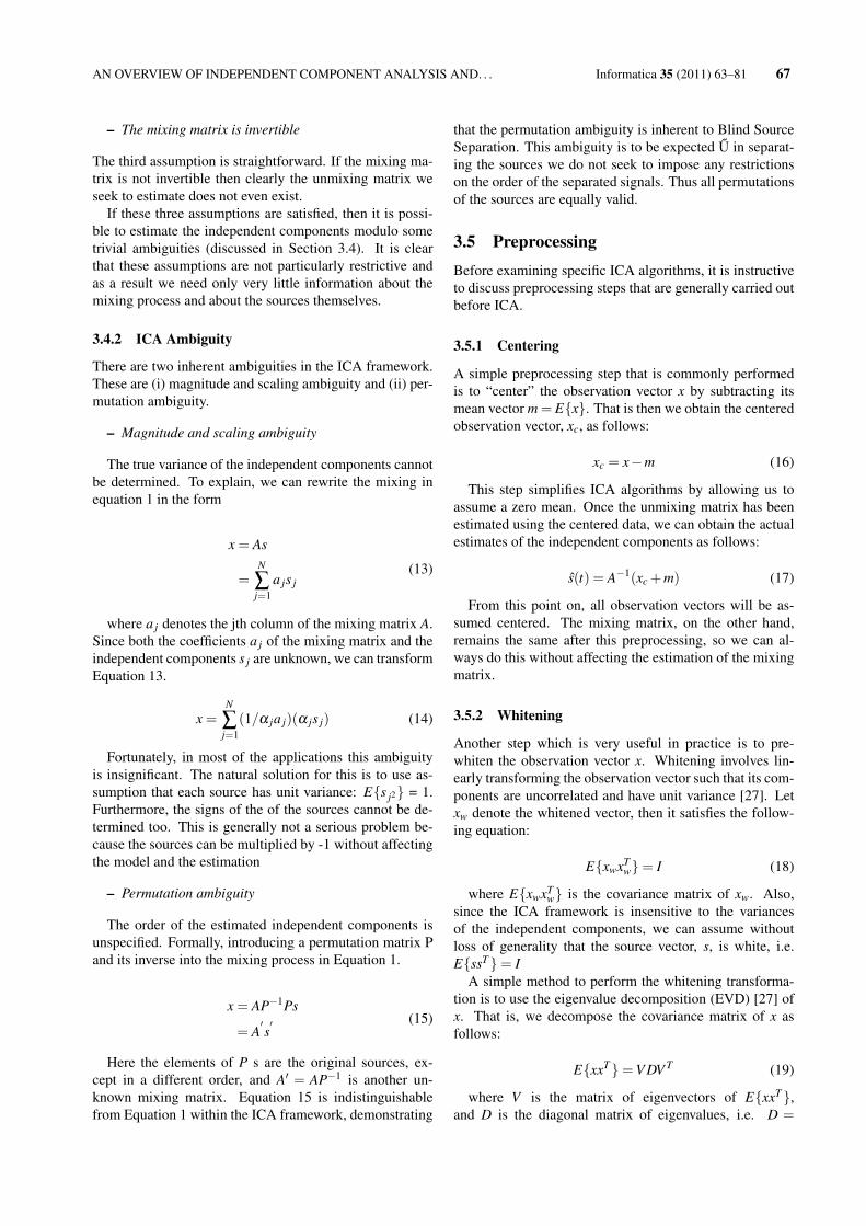
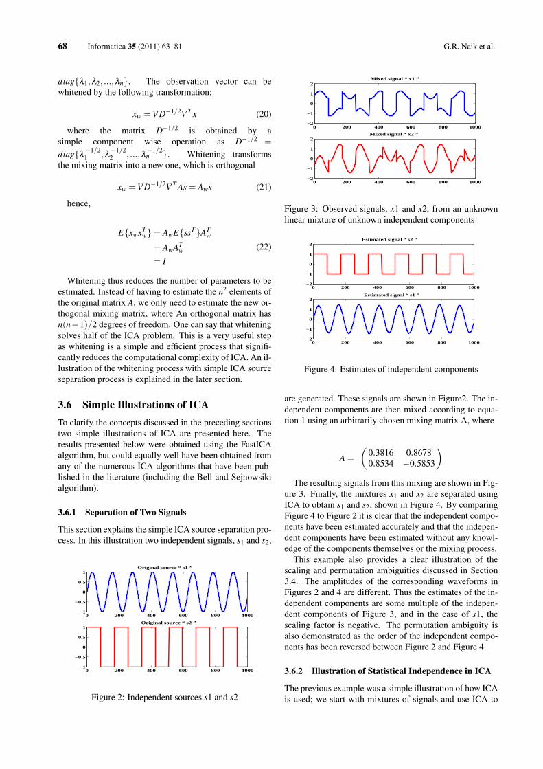
Figure 2: Independent sources s1 and s2

0 200 400 600 800 1000−2

−1

0

1

2Mixed signal “ x1 ”

Mixed signal “ x2 ”

0 200 400 600 800 1000−2

−1

0

1

2

Figure 3: Observed signals, x1 and x2, from an unknownlinear mixture of unknown independent components

0 200 400 600 800 1000−2

−1

0

1

2

0 200 400 600 800 1000−2

−1

0

1

2Estimated signal “ s1 ”

Estimated signal “ s2 ”

Figure 4: Estimates of independent components

are generated. These signals are shown in Figure2. The in-dependent components are then mixed according to equa-tion 1 using an arbitrarily chosen mixing matrix A, where

A =

(0.3816 0.86780.8534 −0.5853

)The resulting signals from this mixing are shown in Fig-

ure 3. Finally, the mixtures x1 and x2 are separated usingICA to obtain s1 and s2, shown in Figure 4. By comparingFigure 4 to Figure 2 it is clear that the independent compo-nents have been estimated accurately and that the indepen-dent components have been estimated without any knowl-edge of the components themselves or the mixing process.

This example also provides a clear illustration of thescaling and permutation ambiguities discussed in Section3.4. The amplitudes of the corresponding waveforms inFigures 2 and 4 are different. Thus the estimates of the in-dependent components are some multiple of the indepen-dent components of Figure 3, and in the case of s1, thescaling factor is negative. The permutation ambiguity isalso demonstrated as the order of the independent compo-nents has been reversed between Figure 2 and Figure 4.

3.6.2 Illustration of Statistical Independence in ICA

The previous example was a simple illustration of how ICAis used; we start with mixtures of signals and use ICA to


−2 −1.5 −1 −0.5 0 0.5 1 1.5 2−2

−1.5

−1

−0.5

0

0.5

1

1.5

2

s1

s2

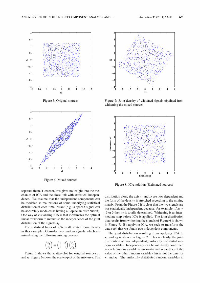
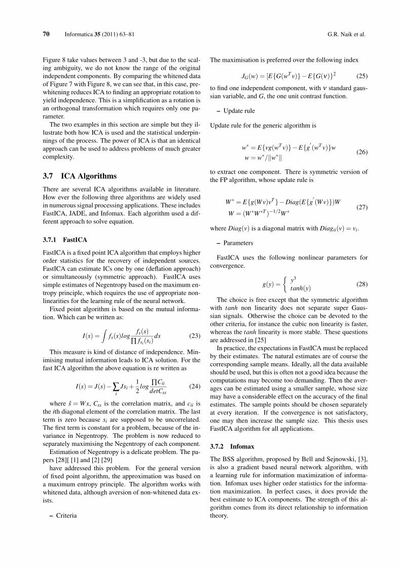
Figure 5: Original sources

−4 −3 −2 −1 0 1 2 3 4−2

−1.5

−1

−0.5

0

0.5

1

1.5

2

x1

x2

Figure 6: Mixed sources

separate them. However, this gives no insight into the me-chanics of ICA and the close link with statistical indepen-dence. We assume that the independent components canbe modeled as realizations of some underlying statisticaldistribution at each time instant (e.g. a speech signal canbe accurately modeled as having a Laplacian distribution).One way of visualizing ICA is that it estimates the optimallinear transform to maximise the independence of the jointdistribution of the signals Xi.

The statistical basis of ICA is illustrated more clearlyin this example. Consider two random signals which aremixed using the following mixing process:(

x1x2

)=

(1 21 1

)(s1s2

)Figure 5 shows the scatter-plot for original sources s1

and s2. Figure 6 shows the scatter-plot of the mixtures. The

−4 −3 −2 −1 0 1 2 3 4−4

−3

−2

−1

0

1

2

3

4

x1

x2

Figure 7: Joint density of whitened signals obtained fromwhitening the mixed sources

−4 −3 −2 −1 0 1 2 3 4−4

−3

−2

−1

0

1

2

3

4

Estimated s1

Est

imate

d s

2

Figure 8: ICA solution (Estimated sources)

distribution along the axis x1 and x2 are now dependent andthe form of the density is stretched according to the mixingmatrix. From the Figure 6 it is clear that the two signals arenot statistically independent because, for example, if x1 =-3 or 3 then x2 is totally determined. Whitening is an inter-mediate step before ICA is applied. The joint distributionthat results from whitening the signals of Figure 6 is shownin Figure 7. By applying ICA, we seek to transform thedata such that we obtain two independent components.

The joint distribution resulting from applying ICA tox1 and x2 is shown in Figure 7. This is clearly the jointdistribution of two independent, uniformly distributed ran-dom variables. Independence can be intuitively confirmedas each random variable is unconstrained regardless of thevalue of the other random variable (this is not the case forx1 and x2. The uniformly distributed random variables in


Figure 8 take values between 3 and -3, but due to the scal-ing ambiguity, we do not know the range of the originalindependent components. By comparing the whitened dataof Figure 7 with Figure 8, we can see that, in this case, pre-whitening reduces ICA to finding an appropriate rotation toyield independence. This is a simplification as a rotation isan orthogonal transformation which requires only one pa-rameter.

The two examples in this section are simple but they il-lustrate both how ICA is used and the statistical underpin-nings of the process. The power of ICA is that an identicalapproach can be used to address problems of much greatercomplexity.

3.7 ICA AlgorithmsThere are several ICA algorithms available in literature.How ever the following three algorithms are widely usedin numerous signal processing applications. These includesFastICA, JADE, and Infomax. Each algorithm used a dif-ferent approach to solve equation.

3.7.1 FastICA

FastICA is a fixed point ICA algorithm that employs higherorder statistics for the recovery of independent sources.FastICA can estimate ICs one by one (deflation approach)or simultaneously (symmetric approach). FastICA usessimple estimates of Negentropy based on the maximum en-tropy principle, which requires the use of appropriate non-linearities for the learning rule of the neural network.

Fixed point algorithm is based on the mutual informa-tion. Which can be written as:

I(s) =∫

fs(s)logfs(s)

∏ fsi(si)ds (23)

This measure is kind of distance of independence. Min-imising mutual information leads to ICA solution. For thefast ICA algorithm the above equation is re written as

I(s) = J(s)−∑i

Jsi +12

log∏Cii

detCss(24)

where s = Wx, Css is the correlation matrix, and cii isthe ith diagonal element of the correlation matrix. The lastterm is zero because si are supposed to be uncorrelated.The first term is constant for a problem, because of the in-variance in Negentropy. The problem is now reduced toseparately maximising the Negentropy of each component.

Estimation of Negentropy is a delicate problem. The pa-pers [28][ [1] and [2] [29]

have addressed this problem. For the general versionof fixed point algorithm, the approximation was based ona maximum entropy principle. The algorithm works withwhitened data, although aversion of non-whitened data ex-ists.

– Criteria

The maximisation is preferred over the following index

JG(w) = [E{G(wT v)}−E{G(ν)}2 (25)

to find one independent component, with ν standard gaus-sian variable, and G, the one unit contrast function.

– Update rule

Update rule for the generic algorithm is

w∗ = E{vg(wT v)}−E{g′(wT v)}w

w = w∗/∥w∗∥(26)

to extract one component. There is symmetric version ofthe FP algorithm, whose update rule is

W ∗ = E{g(Wv)vT}−Diag(E{g′(Wv)})W

W = (W ∗W ∗T )−1/2W ∗(27)

where Diag(v) is a diagonal matrix with Diagii(v) = vi.

– Parameters

FastICA uses the following nonlinear parameters forconvergence.

g(y) ={

y3

tanh(y)(28)

The choice is free except that the symmetric algorithmwith tanh non linearity does not separate super Gaus-sian signals. Otherwise the choice can be devoted to theother criteria, for instance the cubic non linearity is faster,whereas the tanh linearity is more stable. These questionsare addressed in [25]

In practice, the expectations in FastICA must be replacedby their estimates. The natural estimates are of course thecorresponding sample means. Ideally, all the data availableshould be used, but this is often not a good idea because thecomputations may become too demanding. Then the aver-ages can be estimated using a smaller sample, whose sizemay have a considerable effect on the accuracy of the finalestimates. The sample points should be chosen separatelyat every iteration. If the convergence is not satisfactory,one may then increase the sample size. This thesis usesFastICA algorithm for all applications.

3.7.2 Infomax

The BSS algorithm, proposed by Bell and Sejnowski, [3],is also a gradient based neural network algorithm, witha learning rule for information maximization of informa-tion. Infomax uses higher order statistics for the informa-tion maximization. In perfect cases, it does provide thebest estimate to ICA components. The strength of this al-gorithm comes from its direct relationship to informationtheory.


The algorithm is derived through an information max-imisation principle, applied here between the inputs and thenon linear outputs. Given the form of joint entropy

H(s1,s2) = H(s1)+H(s2)− I(s1,s2) (29)

Here for two variables s= g(Bx), it is clear that maximis-ing the joint entropy of the outputs amounts to minimisingmutual information I(y1,y2), unless it is more interesting tomaximise the individual entropies than to reduce the mu-tual information. This is the point, where the nonlinearfunction plays an important role.

The basic idea of the information maximisation is tomatch the slope of the nonlinear function with the inputprobability density function. That is

s = g(x,θ)≃∫ x

− inffx(t)dt (30)

In case of perfect matching fs(s) looks like an uniformvariable, whose entropy is large. If this is not possible be-cause the shapes are different, the best solution found insome case is to mix the input distributions so that the re-sulting mix matches the slope of the transfer function betterthan a single input distribution. In this case the algorithmdoes not converge, and the separation is not achieved.

– Criteria

The algorithm is a stochastic gradient ascent that max-imises the joint entropy (Eqn. 12).

– Update rule

In its original form, the update rule is

∆B = λ [[BT ]−1 +(1−2g(Bx+b0))xT ]

∆b = λ [1−2g(Bx+b0)](31)

– Parameters

The nonlinear function used in the original algorithm is

g(s) =1

1+ e−s (32)

and in the extended version, it is

g(s) = s± tanh(s) (33)

where the sign is that of the estimated kurtosis of thesignal.

The information maximization algorithm (often referredas infomax) is widely used to separate super-Gaussiansources. Infomax is a gradient-based neural network algo-rithm, with a learning rule for information maximization.Infomax uses higher order statistics for the informationmaximization. The information maximization is attainedby maximizing the joint entropy of a transformed vector.z = g(Wx), where g is a point wise sigmoidal nonlinearfunction.

4 ICA for different conditionsOne of the important conditions of ICA is that the num-ber of sensors should be equal to the number of sources.Unfortunately, the real source separation problem does notalways satisfy this constraint. This section focusses onICA source separation problem under different conditionswhere the number of sources are not equal to the numberof recordings.

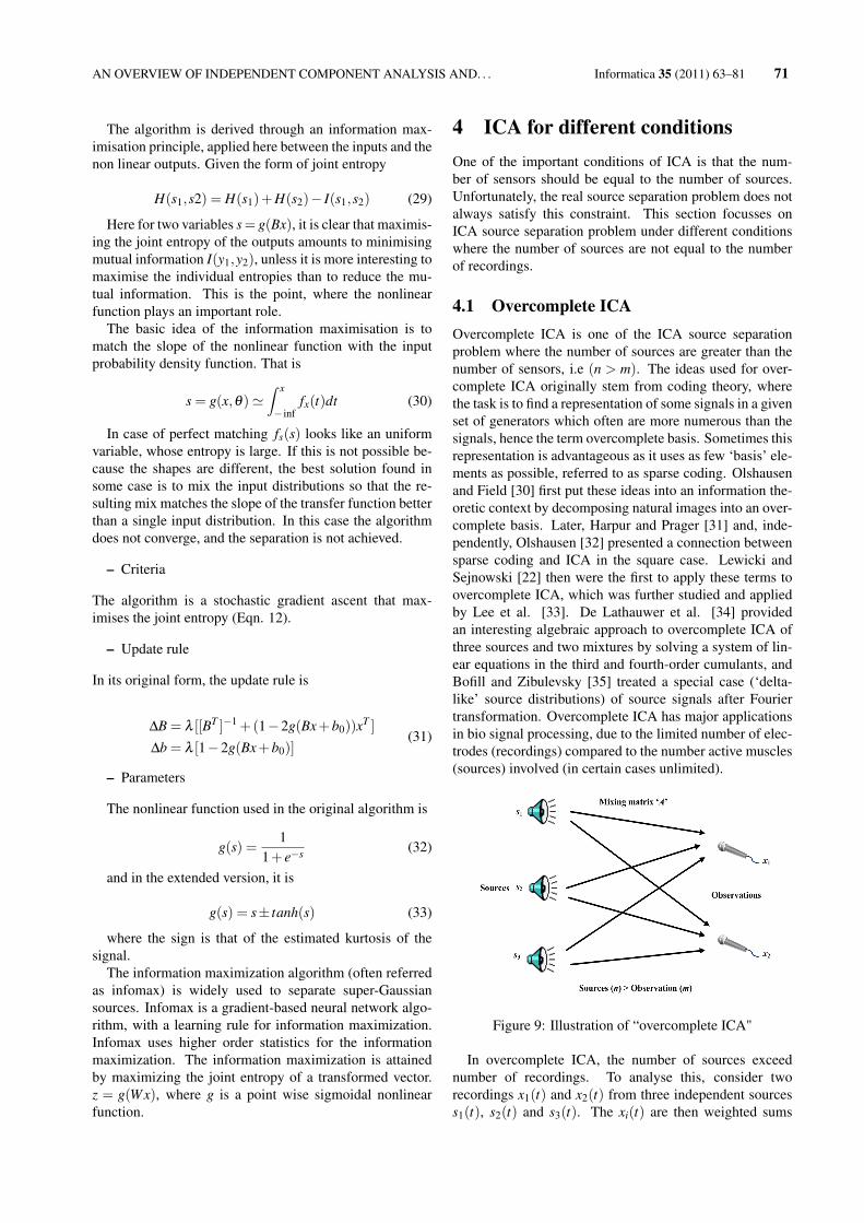
4.1 Overcomplete ICAOvercomplete ICA is one of the ICA source separationproblem where the number of sources are greater than thenumber of sensors, i.e (n > m). The ideas used for over-complete ICA originally stem from coding theory, wherethe task is to find a representation of some signals in a givenset of generators which often are more numerous than thesignals, hence the term overcomplete basis. Sometimes thisrepresentation is advantageous as it uses as few ‘basis’ ele-ments as possible, referred to as sparse coding. Olshausenand Field [30] first put these ideas into an information the-oretic context by decomposing natural images into an over-complete basis. Later, Harpur and Prager [31] and, inde-pendently, Olshausen [32] presented a connection betweensparse coding and ICA in the square case. Lewicki andSejnowski [22] then were the first to apply these terms toovercomplete ICA, which was further studied and appliedby Lee et al. [33]. De Lathauwer et al. [34] providedan interesting algebraic approach to overcomplete ICA ofthree sources and two mixtures by solving a system of lin-ear equations in the third and fourth-order cumulants, andBofill and Zibulevsky [35] treated a special case (‘delta-like’ source distributions) of source signals after Fouriertransformation. Overcomplete ICA has major applicationsin bio signal processing, due to the limited number of elec-trodes (recordings) compared to the number active muscles(sources) involved (in certain cases unlimited).

Figure 9: Illustration of “overcomplete ICA"

In overcomplete ICA, the number of sources exceednumber of recordings. To analyse this, consider tworecordings x1(t) and x2(t) from three independent sourcess1(t), s2(t) and s3(t). The xi(t) are then weighted sums


of the si(t), where the coefficients depend on the distancesbetween the sources and the sensors (refer Figure 9):

x1(t) = a11s1(t)+a12s2(t)+a13s3(t) (34)x2(t) = a21s1(t)+a22s2(t)+a23s3(t)

The ai j are constant coefficients that give the mixingweights. The mixing process of these vectors can be repre-sented in the matrix form as (refer Equation 1):

(x1x2

)=

(a11 a12 a13a21 a22 a23

)s1s2s3

The unmixing process and estimation of sources can bewritten as (refer Equation 2):s1

s2s3

=

w11 w12w21 w22w31 w32

(x1x2

)In this example matrix A of size 2×3 matrix and unmix-

ing matrix W is of size 3×2. Hence in overcomplete ICAit always results in pseudoinverse. Hence computation ofsources in overcomplete ICA requires some estimation pro-cesses.

4.1.1 Overcomplete ICA methods

There are two common approaches of solving the overcom-plete problem.

– Single step approach where the mixing matrix and theindependent sources are estimated at once in a singlealgorithm

– Two step algorithm where the mixing matrix and theindependent component values are estimated with dif-ferent algorithms.

Lewicki and Sejnowski [22] proposed the single step ap-proach, which is a natural solution to decomposition byfinding the maximum a posteriori representation of thedata. The prior distribution on the basis function coeffi-cients removes the redundancy in the representation andleads to representations that are sparse and are nonlinearfunctions of the data. The probabilistic approach to de-composition also leads to a natural method of denoising.From this model, they derived a simple and robust learningalgorithm by maximizing the data likelihood over the basisfunctions. Another approach in single step was proposedby Shriki et al. [36] using recurrent model, i.e., the es-timated independent sources are computed taking into ac-count the influence of other independent sources.

One of the disadvantage of single step approach is thatit is complex and computationally expensive. Hence manyresearchers have proposed the two step method, where themixing matrix is estimated in the first step and the sourcesare recovered in the next step. Zibulevsky et al. [35] pro-posed a sparse overcomplete ICA with delta distributions.

Fabian Theis [37, 38] proposed geometric overcompleteICA. Recently Waheed et. al [39, 40] demonstrated alge-braic overcomplete ICA. In this thesis Zibulevsky’s sparseovercomplete ICA is utilised, which is explained in the nextsection.

4.1.2 Sparse overcomplete ICA

Sparse representation of signals which is modeled by ma-trix factorisation has been receiving a great deal of inter-est in recent years. The research community has investi-gated many linear transforms that make audio, video andimage data sparse, such as the Discrete Cosine Transform(DCT), the Fourier transform, the wavelet transform andtheir derivatives. [41]. Chen et al. [42] discussed sparserepresentations of signals by using large scale linear pro-gramming under given overcomplete basis (e.g., wavelets).Olshausen et al. [43] represented sparse coding of im-ages based on maximum posterior approach but it wasZibulevsky et al. [35] who noticed that in the case of sparsesources, their linear mixtures can be easily separated us-ing very simple “geometric" algorithms. Sparse represen-tations can be used in blind source separation. When thesources are sparse, smaller coefficients are more likely andthus for a given data point t, if one of the sources is sig-nificantly larger, the remaining ones are likely to be closeto zero. Thus the density of data in the mixture space, be-sides decreasing with the distance from the origin shows aclear tendency to cluster along the directions of the basisvectors. Sparsity is good in ICA for two reasons. First thestatistical accuracy with which the mixing matrix A can beestimated is a function of how non-Gaussian the source dis-tributions are. This suggests that the sparser the sources arethe less data is needed to estimate A. Secondly the qualityof the source estimates given A, is also better for sparsersources. A signal is considered sparse when values of mostof the samples of the signal do not differ significantly fromzero. These are from sources that are minimally active.Zibulevsky et al. [35] have demonstrated that when thesignals are sparse, and the sources of these are indepen-dent, these may be separated even when the number ofsources exceeds the number of recordings. [35]. The over-complete limitation suffered by normal ICA is no longer alimiting factor for signals that are very sparse. Zibulevskyalso demonstrated that when the signals are sparse, it ispossible to determine the number of independent sourcesin a mixture of unknown signal numbers.

– Source estimation

The first step in two step approach is source separation.Here the source separation process is explained by takingsparse signal as an example. A signal is considered to besparse if its pdf is close to Laplacian or super-Gaussian. Inthis case, the basic ICA model in Equation 1 is modifiedto have more robust representation which can be expressedas,


x = As+ξ (35)

where ξ represents noise in the recordings. It is assumedthat the independent sources s can be sparsely representedin a proper signal dictionary

si =K

∑k=1

Cki φk (36)

where φk are the atoms or elements of the dictionary. Im-portant examples are wavelet-related dictionaries such aswavelet and wavelet packets [41]. Equation 36 can be ex-pressed in matrix notation as

s =CΦ (37)

by substituting Equation 37 into 35 gives

x = ACΦ+ξ (38)

The goal is to estimate the mixing matrix A and the coef-ficients C at the same time so that C is as sparse as possible.and X ≈ ACΦ, given only the observed data x and the dic-tionary ΦUsing maximum a posteriori approach, the above goal canbe expressed as

maxA,C

P(A,C|x) ∝ maxA,CP(x|A,C)P(A)P(C) (39)

Taking into account Equation 35 and Gaussian noise, theconditional probability P(x|A,C) can be expressed as

P(x|A,C) ∝ ∏i

exp[− (xi − (ACΦ)i)2

2σ2 ] (40)

Since C is assumed to be sparse, it can be approximatedwith the following pdf

pi(Cki ) ∝ exp[−(βih(Ck

i ))] (41)

and hence

p(C) ∝ ∏i,k

exp[−(βih(Cki ))] (42)

Assuming the pdf of P(A) to be uniform, Equation 39 cannow be simplified as

maxA,C

P(A,C|x) ∝ maxA,CP(x|A,C)P(C) (43)

Finally, the optimisation problem can be formed by substi-tuting 40 and 42 into 43, taking the logarithm and invertingthe sign

maxA,C

P(A,C|x) ∝ minA,C1

2σ2 |ACΦ− x∥2F+

∑i,k(βih(Ck

i ))(44)

There are several measures of sparsity. The simplestmeasure is the l0 norm. One of the drawback of this mea-sure is that, it is discontinuous and difficult to optimise, andalso very sensitive to noise. The closest approximation ofl0 is l1 norm. The validity of this measure can be shownby simplifying equation 44 under zero noise assumptionand under Laplacian prior distributions with h(Ck

i ) = |Cki |.

Under these assumptions the optimisation problem can bedecomposed into K smaller problems for each data point ck

at time pointk = 1...K as

minck

∑i|ck

i | (45)

subject to Ackφk = xk. If small signal s is sparse in timedomain then ck in equation 45 can be uploaded with sk.

minsk

∑i|sk

i | (46)

subject to Ask = xk. Equation 46 can be formulated as linearprogramming in basic form as

minsk

cT sk| (47)

subject to Ask = xk, sk ≥ 0 where sk ⇔ [uk;vk],A ⇔ [A;−A]and c ⇔ [1;1].

– Estimating the mixing matrix

The second step in two step approach is estimating themixing matrix. There exists various methods to computethe mixing matrix in sparse overcomplete ICA. The mostwidely used techniques are:

(i) C-means clustering

(ii) Algebraic method and

(iii) Potential function based method

All the above mentioned methods are based on the clus-tering principle. The difference is the way they estimate thedirection of the clusters. The sparsity of the signal plays animportant role for estimating the mixing matrix. A simpleillustration that is useful to understand this concept can befound in

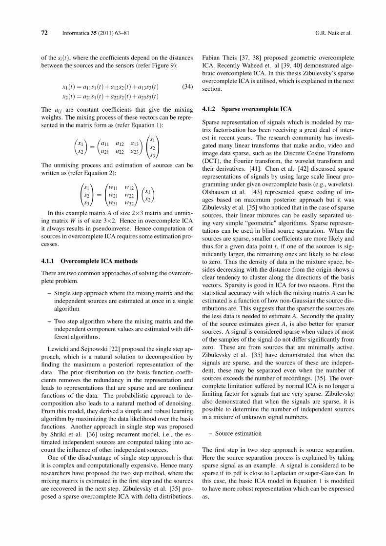
4.2 Undercomplete ICAThe mixture of unknown sources is referred to as under-complete when the numbers of recordings m, more thanthe number of sources n. In some applications, it is de-sired to have more recordings than sources to achieve betterseparation performance. It is generally believed that withmore recordings than the sources, it is always possible toget better estimate of the sources. This is not correct un-less prior to separation using ICA, dimensional reductionis conducted. This can be achieved by choosing the same


number of principal recordings as the number of sourcesdiscarding the rest. To analyse this, consider three record-ings x1(t), x2(t) and x3(t) from two independent sourcess1(t) and s2(t). The xi(t) are then weighted sums of thesi(t), where the coefficients depend on the distances be-tween the sources and the sensors (refer Figure 10):

Figure 10: Illustration of “undercomplete ICA"

x1(t) = a11s1(t)+a12s2(t)

x2(t) = a21s1(t)+a22s2(t) (48)x3(t) = a31s1(t)+a32s2(t)

The ai j are constant coefficients that gives the mixingweights. The mixing process of these vectors can be repre-sented in the matrix form as:x1

x2x3

=

a11 a12a21 a22a31 a32

(s1s2

)The unmixing process using the standard ICA requires a di-mensional reduction approach so that, if one of the record-ings is reduced then the square mixing matrix is obtained,which can use any standard ICA for the source estimation.For instance one of the recordings say x3 is redundant thenthe above mixing process can be written as:(

x1x2

)=

(a11 a12a21 a22

)(s1s2

)Hence unmixing process can use any standard ICA algo-

rithm using the following:(s1s2

)=

(w11 w12w21 w22

)(x1x2

)The above process illustrates that, prior to source signal

separation using undercomplete ICA, it is important to re-duce the dimensionality of the mixing matrix and identifythe required and discard the redundant recordings. Princi-pal Component Analysis (PCA) is one of the powerful di-mensional reduction method used in signal processing ap-plications, which is explained next.

4.2.1 Undercomplete ICA using dimensionalreduction method

When the number of recordings n are more than the num-ber of sources m, there must be information redundancy inthe recordings. Hence the first step is to reduce the dimen-sionality of the recorded data. If the dimensionality of therecorded data is equal to that of the sources, then standardICA methods can be applied to estimate the independentsources. An example of this stages methods is illustrated in[44].

One of the popular method used in dimensional reduc-tion method is PCA. PCA uses the decorrelated method toreduce the recorded data x using a matrix V

z =V x (49)

such that EzzT = I. The transformation matrix V is givenby

V = D12 ET (50)

where D and E are the Eigenvalue and Eigenvector decom-position of covariance matrix Cx

Cx = ED12 ET (51)

Now it can be proven that

E{zzT}=V E{xxT}V T

= D−1/2ET EDET ED−1/2

= I

(52)

The second stage is using any of the standard ICA al-gorithms discussed in Section 3.2 to estimate the sources.In fact, whitening process through PCA is standard prepro-cessing in ICA. It means that applying any standard ICA al-gorithms that incorporates PCA will automatically reducethe dimension before running ICA.

4.3 Sub band decomposition ICA

Despite the success of using standard ICA in many appli-cations, the basic assumptions of ICA may not hold for cer-tain situations where there may be dependency among thesignal sources. The standard ICA algorithms are not ableto estimate statistically dependent original sources. Oneproposed technique [13] is that while there may be a de-gree of dependency among the wide band source signals,narrow band filtering of these signals can provide indepen-dence among these signal sources. This assumption is truewhen each unknown source can be modeled or representedas a linear combination of narrow-band sub-signals. Subband decomposition ICA, an extension of ICA, assumesthat each source is represented as the sum of some indepen-dent subcomponents and dependent subcomponents, whichhave different frequency bands.


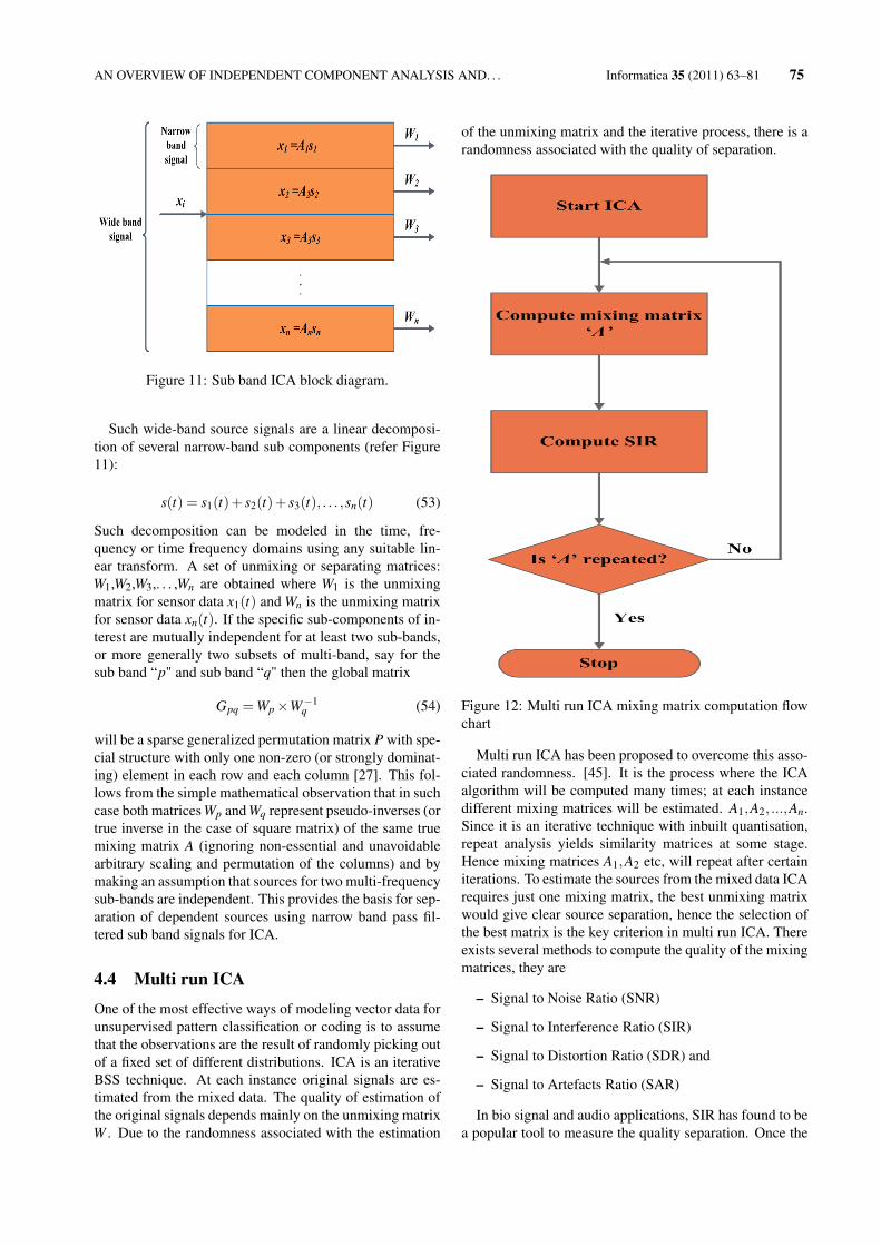
Figure 11: Sub band ICA block diagram.

Such wide-band source signals are a linear decomposi-tion of several narrow-band sub components (refer Figure11):

s(t) = s1(t)+ s2(t)+ s3(t), . . . ,sn(t) (53)

Such decomposition can be modeled in the time, fre-quency or time frequency domains using any suitable lin-ear transform. A set of unmixing or separating matrices:W1,W2,W3,. . . ,Wn are obtained where W1 is the unmixingmatrix for sensor data x1(t) and Wn is the unmixing matrixfor sensor data xn(t). If the specific sub-components of in-terest are mutually independent for at least two sub-bands,or more generally two subsets of multi-band, say for thesub band “p" and sub band “q" then the global matrix

Gpq =Wp ×W−1q (54)

will be a sparse generalized permutation matrix P with spe-cial structure with only one non-zero (or strongly dominat-ing) element in each row and each column [27]. This fol-lows from the simple mathematical observation that in suchcase both matrices Wp and Wq represent pseudo-inverses (ortrue inverse in the case of square matrix) of the same truemixing matrix A (ignoring non-essential and unavoidablearbitrary scaling and permutation of the columns) and bymaking an assumption that sources for two multi-frequencysub-bands are independent. This provides the basis for sep-aration of dependent sources using narrow band pass fil-tered sub band signals for ICA.

4.4 Multi run ICA

One of the most effective ways of modeling vector data forunsupervised pattern classification or coding is to assumethat the observations are the result of randomly picking outof a fixed set of different distributions. ICA is an iterativeBSS technique. At each instance original signals are es-timated from the mixed data. The quality of estimation ofthe original signals depends mainly on the unmixing matrixW . Due to the randomness associated with the estimation

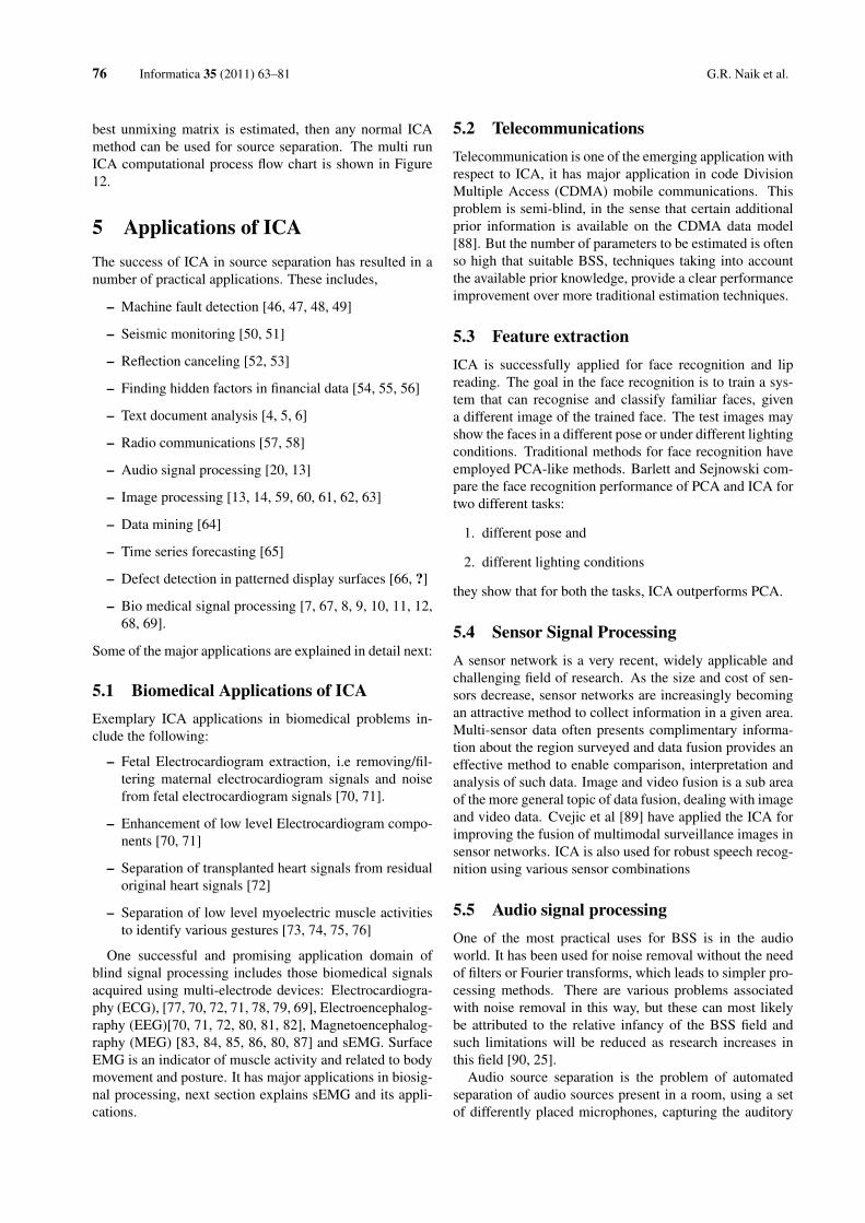
of the unmixing matrix and the iterative process, there is arandomness associated with the quality of separation.

Figure 12: Multi run ICA mixing matrix computation flowchart

Multi run ICA has been proposed to overcome this asso-ciated randomness. [45]. It is the process where the ICAalgorithm will be computed many times; at each instancedifferent mixing matrices will be estimated. A1,A2, ...,An.Since it is an iterative technique with inbuilt quantisation,repeat analysis yields similarity matrices at some stage.Hence mixing matrices A1,A2 etc, will repeat after certainiterations. To estimate the sources from the mixed data ICArequires just one mixing matrix, the best unmixing matrixwould give clear source separation, hence the selection ofthe best matrix is the key criterion in multi run ICA. Thereexists several methods to compute the quality of the mixingmatrices, they are

– Signal to Noise Ratio (SNR)

– Signal to Interference Ratio (SIR)

– Signal to Distortion Ratio (SDR) and

– Signal to Artefacts Ratio (SAR)

In bio signal and audio applications, SIR has found to bea popular tool to measure the quality separation. Once the


best unmixing matrix is estimated, then any normal ICAmethod can be used for source separation. The multi runICA computational process flow chart is shown in Figure12.

5 Applications of ICAThe success of ICA in source separation has resulted in anumber of practical applications. These includes,

– Machine fault detection [46, 47, 48, 49]

– Seismic monitoring [50, 51]

– Reflection canceling [52, 53]

– Finding hidden factors in financial data [54, 55, 56]

– Text document analysis [4, 5, 6]

– Radio communications [57, 58]

– Audio signal processing [20, 13]

– Image processing [13, 14, 59, 60, 61, 62, 63]

– Data mining [64]

– Time series forecasting [65]

– Defect detection in patterned display surfaces [66, ?]

– Bio medical signal processing [7, 67, 8, 9, 10, 11, 12,68, 69].

Some of the major applications are explained in detail next:

5.1 Biomedical Applications of ICAExemplary ICA applications in biomedical problems in-clude the following:

– Fetal Electrocardiogram extraction, i.e removing/fil-tering maternal electrocardiogram signals and noisefrom fetal electrocardiogram signals [70, 71].

– Enhancement of low level Electrocardiogram compo-nents [70, 71]

– Separation of transplanted heart signals from residualoriginal heart signals [72]

– Separation of low level myoelectric muscle activitiesto identify various gestures [73, 74, 75, 76]

One successful and promising application domain ofblind signal processing includes those biomedical signalsacquired using multi-electrode devices: Electrocardiogra-phy (ECG), [77, 70, 72, 71, 78, 79, 69], Electroencephalog-raphy (EEG)[70, 71, 72, 80, 81, 82], Magnetoencephalog-raphy (MEG) [83, 84, 85, 86, 80, 87] and sEMG. SurfaceEMG is an indicator of muscle activity and related to bodymovement and posture. It has major applications in biosig-nal processing, next section explains sEMG and its appli-cations.

5.2 TelecommunicationsTelecommunication is one of the emerging application withrespect to ICA, it has major application in code DivisionMultiple Access (CDMA) mobile communications. Thisproblem is semi-blind, in the sense that certain additionalprior information is available on the CDMA data model[88]. But the number of parameters to be estimated is oftenso high that suitable BSS, techniques taking into accountthe available prior knowledge, provide a clear performanceimprovement over more traditional estimation techniques.

5.3 Feature extractionICA is successfully applied for face recognition and lipreading. The goal in the face recognition is to train a sys-tem that can recognise and classify familiar faces, givena different image of the trained face. The test images mayshow the faces in a different pose or under different lightingconditions. Traditional methods for face recognition haveemployed PCA-like methods. Barlett and Sejnowski com-pare the face recognition performance of PCA and ICA fortwo different tasks:

1. different pose and

2. different lighting conditions

they show that for both the tasks, ICA outperforms PCA.

5.4 Sensor Signal ProcessingA sensor network is a very recent, widely applicable andchallenging field of research. As the size and cost of sen-sors decrease, sensor networks are increasingly becomingan attractive method to collect information in a given area.Multi-sensor data often presents complimentary informa-tion about the region surveyed and data fusion provides aneffective method to enable comparison, interpretation andanalysis of such data. Image and video fusion is a sub areaof the more general topic of data fusion, dealing with imageand video data. Cvejic et al [89] have applied the ICA forimproving the fusion of multimodal surveillance images insensor networks. ICA is also used for robust speech recog-nition using various sensor combinations

5.5 Audio signal processingOne of the most practical uses for BSS is in the audioworld. It has been used for noise removal without the needof filters or Fourier transforms, which leads to simpler pro-cessing methods. There are various problems associatedwith noise removal in this way, but these can most likelybe attributed to the relative infancy of the BSS field andsuch limitations will be reduced as research increases inthis field [90, 25].

Audio source separation is the problem of automatedseparation of audio sources present in a room, using a setof differently placed microphones, capturing the auditory


scene. The whole problem resembles the task a humanlistener can solve in a cocktail party situation, where us-ing two sensors (ears), the brain can focus on a specificsource of interest, suppressing all other sources present(also known as cocktail party problem) [20, 25].

5.6 Image ProcessingRecently, Independent Component Analysis (ICA) hasbeen proposed as a generic statistical model for images[90, 59, 60, 61, 62, 63]. It is aimed at capturing the sta-tistical structure in images that is beyond second order in-formation, by exploiting higher-order statistical structurein data. ICA finds a linear non orthogonal coordinate sys-tem in multivariate data determined by second- and higher-order statistics. The goal of ICA is to linearly transform thedata such that the transformed variables are as statisticallyindependent from each other as possible. ICA generalizesPCA and, like PCA, has proven a useful tool for findingstructure in data. Bell and Sejnowski proposed a methodto extract features from natural scenes by assuming linearimage synthesis model [90]. In their model, a set of digi-tized natural images were used. they considered each patchof an image as a linear combination of several underlyingbasic functions. Later Lee et al [91] proposed an imageprocessing algorithm, which estimates the data density ineach class by using parametric nonlinear functions that fitto the non-Gaussian structure of the data. They showeda significant improvement in classification accuracy overstandard Gaussian mixture models. Recently Antoniol etal [92] demonstrated that the ICA model can be a suitabletool for learning a vector base for feature extraction to de-sign a feature based data dependent approach that can beefficiently adopted for image change detection. In addi-tion ICA features are localized and oriented and sensitiveto lines and edges of varying thickness of images. Further-more the sparsity of ICA coefficients should be pointed out.It is expected that suitable soft-thresholding on the ICAcoefficients leads to efficient reduction of Gaussian noise[60, 62, 63].

6 ConclusionsThis paper has introduced the fundamentals of BSS andICA. The mathematical framework of the source mixingproblem that BSS/ICA addresses was examined in somedetail, as was the general approach to solving BSS/ICA.As part of this discussion, some inherent ambiguities ofthe BSS/ICA framework were examined as well as thetwo important preprocessing steps of centering and whiten-ing. Specific details of the approach to solving the mixingproblem were presented and two important ICA algorithmswere discussed in detail. Finally, the application domainsof this novel technique are presented. Some of the futuristicworks on ICA techniques, which need further investigationare discussed. The material covered in this paper is impor-tant not only to understand the algorithms used to perform

BSS/ICA, but it also provides the necessary background tounderstand extensions to the framework of ICA for futureresearchers.

References[1] L. Tong, Liu, V. C. Soon, and Y. F. Huang, “Inde-

terminacy and identifiability of blind identification,”Circuits and Systems, IEEE Transactions on, vol. 38,no. 5, pp. 499–509, 1991.

[2] C. Jutten and J. Karhunen, “Advances in blind sourceseparation (bss) and independent component analy-sis (ica) for nonlinear mixtures.” Int J Neural Syst,vol. 14, no. 5, pp. 267–292, October 2004.

[3] A. J. Bell and T. J. Sejnowski, “An information-maximization approach to blind separation and blinddeconvolution.” Neural Comput, vol. 7, no. 6, pp.1129–1159, November 1995.

[4] Kolenda, Independent components in text, ser.Advances in Independent Component Analysis.Springer-Verlag, 2000, pp. 229–250.

[5] E. Bingham, J. Kuusisto, and K. Lagus, “Ica and somin text document analysis,” in SIGIR ’02: Proceed-ings of the 25th annual international ACM SIGIRconference on Research and development in informa-tion retrieval. ACM, 2002, pp. 361–362.

[6] Q. Pu and G.-W. Yang, “Short-text classificationbased on ica and lsa,” Advances in Neural Networks -ISNN 2006, pp. 265–270, 2006.

[7] C. J. James and C. W. Hesse, “Independent compo-nent analysis for biomedical signals,” PhysiologicalMeasurement, vol. 26, no. 1, pp. R15+, 2005.

[8] B. Azzerboni, M. Carpentieri, F. La Foresta, and F. C.Morabito, “Neural-ica and wavelet transform for arti-facts removal in surface emg,” in Neural Networks,2004. Proceedings. 2004 IEEE International JointConference on, vol. 4, 2004, pp. 3223–3228 vol.4.

[9] F. De Martino, F. Gentile, F. Esposito, M. Balsi,F. Di Salle, R. Goebel, and E. Formisano, “Clas-sification of fmri independent components using ic-fingerprints and support vector machine classifiers,”NeuroImage, vol. 34, pp. 177–194, 2007.

[10] T. Kumagai and A. Utsugi, “Removal of artifacts andfluctuations from meg data by clustering methods,”Neurocomputing, vol. 62, pp. 153–160, December2004.

[11] Y. Zhu, T. L. Chen, W. Zhang, T.-P. Jung, J.-R. Du-ann, S. Makeig, and C.-K. Cheng, “Noninvasive studyof the human heart using independent componentanalysis,” in BIBE ’06: Proceedings of the Sixth IEEE


Symposium on BionInformatics and BioEngineering.IEEE Computer Society, 2006, pp. 340–347.

[12] J. Enderle, S. M. Blanchard, and J. Bronzino, Eds.,Introduction to Biomedical Engineering, Second Edi-tion. Academic Press, April 2005.

[13] A. Cichocki and S.-I. Amari, Adaptive Blind Signaland Image Processing: Learning Algorithms and Ap-plications. John Wiley & Sons, Inc., 2002.

[14] Q. Zhang, J. Sun, J. Liu, and X. Sun, “A novelica-based image/video processing method,” 2007, pp.836–842.

[15] Hansen, Blind separation of noicy image mixtures.Springer-Verlag, 2000, pp. 159–179.

[16] D. J. C. Mackay, “Maximum likelihood and covari-ant algorithms for independent component analysis,”University of Cambridge, London, Tech. Rep., 1996.

[17] Sorenson, “Mean field approaches to independentcomponent analysis,” Neural Computation, vol. 14,pp. 889–918, 2002.

[18] KabÂt’an, “Clustering of text documents by skewnessmaximization,” 2000, pp. 435–440.

[19] T. W. Lee, “Blind separation of delayed and con-volved sources,” 1997, pp. 758–764.

[20] ——, Independent component analysis: theory andapplications. Kluwer Academic Publishers, 1998.

[21] H. Attias and C. E. Schreiner, “Blind source separa-tion and deconvolution: the dynamic component anal-ysis algorithm,” Neural Comput., vol. 10, no. 6, pp.1373–1424, August 1998.

[22] M. S. Lewicki and T. J. Sejnowski, “Learning over-complete representations.” Neural Comput, vol. 12,no. 2, pp. 337–365, February 2000.

[23] A. Hyvarinen, R. Cristescu, and E. Oja, “A fast algo-rithm for estimating overcomplete ica bases for im-age windows,” in Neural Networks, 1999. IJCNN ’99.International Joint Conference on, vol. 2, 1999, pp.894–899 vol.2.

[24] T. W. Lee, M. S. Lewicki, and T. J. Sejnowski, “Un-supervised classification with non-gaussian mixturemodels using ica,” in Proceedings of the 1998 confer-ence on Advances in neural information processingsystems. Cambridge, MA, USA: MIT Press, 1999,pp. 508–514.

[25] A. Hyvarinen, J. Karhunen, and E. Oja, Indepen-dent Component Analysis. Wiley-Interscience, May2001.

[26] J. V. Stone, Independent Component Analysis : ATutorial Introduction (Bradford Books). The MITPress, September 2004.

[27] C. D. Meyer, Matrix Analysis and Applied Linear Al-gebra. Cambridge, UK, 2000.

[28] P. Comon, “Independent component analysis, a newconcept?” Signal Processing, vol. 36, no. 3, pp. 287–314, april 1994.

[29] A. Hyvrinen, “New approximations of differential en-tropy for independent component analysis and projec-tion pursuit,” in NIPS ’97: Proceedings of the 1997conference on Advances in neural information pro-cessing systems 10. MIT Press, 1998, pp. 273–279.

[30] Olshausen, “Sparse coding of natural images pro-duces localized, oriented, bandpass receptive fields,”Department of Psychology, Cornell University, Tech.Rep., 1995.

[31] G. F. Harpur and R. W. Prager, “Development oflow entropy coding in a recurrent network.” Network(Bristol, England), vol. 7, no. 2, pp. 277–284, May1996.

[32] B. A. Olshausen, “Learning linear, sparse, factorialcodes,” Tech. Rep., 1996.

[33] T. W. Lee, M. Girolami, M. S. Lewicki, and T. J. Se-jnowski, “Blind source separation of more sourcesthan mixtures using overcomplete representations,”Signal Processing Letters, IEEE, vol. 6, no. 4, pp. 87–90, 2000.

[34] D. Lathauwer, P. L. Comon, B. De Moor, and J. Van-dewalle, “Ica algorithms for 3 sources and 2 sensors,”in Higher-Order Statistics, 1999. Proceedings of theIEEE Signal Processing Workshop on, 1999, pp. 116–120.

[35] Bofill, “Blind separation of more sources than mix-tures using sparsity of their short-time fourier trans-form,” Pajunen, Ed., 2000, pp. 87–92.

[36] O. Shriki, H. Sompolinsky, and D. D. Lee, “An infor-mation maximization approach to overcomplete andrecurrent representations,” in In Advances in NeuralInformation Processing Systems, vol. 14, 2002, pp.612–618.

[37] F. J. Theis, E. W. Lang, T. Westenhuber, and C. G.Puntonet, “Overcomplete ica with a geometric al-gorithm,” in ICANN ’02: Proceedings of the Inter-national Conference on Artificial Neural Networks.Springer-Verlag, 2002, pp. 1049–1054.

[38] F. J. Theis and E. W. Lang, “Geometric overcompleteica,” in Proc. of ESANN 2002, 2002, pp. 217–223.


[39] K. Waheed and F. M. Salem, “Algebraic independentcomponent analysis: an approach for separation ofovercomplete speech mixtures,” in Neural Networks,2003. Proceedings of the International Joint Confer-ence on, vol. 1, 2003, pp. 775–780 vol.1.

[40] ——, “Algebraic independent component analysis,”in Robotics, Intelligent Systems and Signal Process-ing, 2003. Proceedings. 2003 IEEE InternationalConference on, vol. 1, 2003, pp. 472–477 vol.1.

[41] S. Mallat, A Wavelet Tour of Signal Processing. Aca-demic Press, 1998.

[42] S. S. Chen, D. L. Donoho, and M. A. Saunders,“Atomic decomposition by basis pursuit,” SIAM Rev.,vol. 43, no. 1, pp. 129–159, 2001.

[43] B. A. Olshausen and D. J. Field, “Sparse coding withan overcomplete basis set: a strategy employed byv1?” Vision Res, vol. 37, no. 23, pp. 3311–3325, De-cember 1997.

[44] M. Joho, H. Mathis, and R. Lambert, “Overdeter-mined blind source separation: Using more sensorsthan source signals in a noisy mixture,” 2000.

[45] G. R. Naik, D. K. Kumar, and M. Palaniswami,“Multi run ica and surface emg based signal process-ing system for recognising hand gestures,” in Com-puter and Information Technology, 2008. CIT 2008.8th IEEE International Conference on, 2008, pp.700–705.

[46] A. Ypma, D. M. J. Tax, and R. P. W. Duin, “Ro-bust machine fault detection with independent com-ponent analysis and support vector data description,”in Neural Networks for Signal Processing IX, 1999.Proceedings of the 1999 IEEE Signal Processing So-ciety Workshop, 1999, pp. 67–76.

[47] Z. Li, Y. He, F. Chu, J. Han, and W. Hao, “Fault recog-nition method for speed-up and speed-down processof rotating machinery based on independent compo-nent analysis and factorial hidden markov model,”Journal of Sound and Vibration, vol. 291, no. 1-2, pp.60–71, March 2006.

[48] M. Kano, S. Tanaka, S. Hasebe, I. Hashimoto, andH. Ohno, “Monitoring independent components forfault detection,” AIChE Journal, vol. 49, no. 4, pp.969–976, 2003.

[49] L. Zhonghai, Z. Yan, J. Liying, and Q. Xiaoguang,“Application of independent component analysis tothe aero-engine fault diagnosis,” in 2009 ChineseControl and Decision Conference. IEEE, June 2009,pp. 5330–5333.

[50] de La, C. G. Puntonet, J. M. Górriz, and I. Lloret,“An application of ica to identify vibratory low-levelsignals generated by termites,” 2004, pp. 1126–1133.

[51] F. Acernese, A. Ciaramella, S. De Martino,M. Falanga, C. Godano, and R. Tagliaferri, “Polari-sation analysis of the independent components of lowfrequency events at stromboli volcano (eolian islands,italy),” Journal of Volcanology and Geothermal Re-search, vol. 137, no. 1-3, pp. 153–168, September2004.

[52] H. Farid and E. H. Adelson, “Separating reflectionsand lighting using independent components analysis,”cvpr, vol. 01, 1999.

[53] M. Yamazaki, Y.-W. Chen, and G. Xu, “Separating re-flections from images using kernel independent com-ponent analysis,” in Pattern Recognition, 2006. ICPR2006. 18th International Conference on, vol. 3, 2006,pp. 194–197.

[54] M. Coli, R. Di Nisio, and L. Ippoliti, “Exploratoryanalysis of financial time series using independentcomponent analysis,” in Information Technology In-terfaces, 2005. 27th International Conference on,2005, pp. 169–174.

[55] E. H. Wu and P. L. Yu, “Independent componentanalysis for clustering multivariate time series data,”2005, pp. 474–482.

[56] S.-M. Cha and L.-W. Chan, “Applying independentcomponent analysis to factor model in finance,” inIDEAL ’00: Proceedings of the Second InternationalConference on Intelligent Data Engineering and Au-tomated Learning, Data Mining, Financial Engineer-ing, and Intelligent Agents. Springer-Verlag, 2000,pp. 538–544.

[57] R. Cristescu, T. Ristaniemi, J. Joutsensalo, andJ. Karhunen, “Cdma delay estimation using fast icaalgorithm,” vol. 2, 2000, pp. 1117–1120 vol.2.

[58] J. P. Huang and J. Mar, “Combined ica and fcaschemes for a hierarchical network,” Wirel. Pers.Commun., vol. 28, no. 1, pp. 35–58, January 2004.

[59] O. Déniz, M. Castrillón, and M. Hernández, “Facerecognition using independent component analysisand support vector machines,” Pattern Recogn. Lett.,vol. 24, no. 13, pp. 2153–2157, 2003.

[60] S. Fiori, “Overview of independent component anal-ysis technique with an application to synthetic aper-ture radar (sar) imagery processing,” Neural Netw.,vol. 16, no. 3-4, pp. 453–467, 2003.

[61] H. Wang, Y. Pi, G. Liu, and H. Chen, “Applicationsof ica for the enhancement and classification of po-larimetric sar images,” Int. J. Remote Sens., vol. 29,no. 6, pp. 1649–1663, 2008.

[62] M. S. Karoui, Y. Deville, S. Hosseini, A. Ouamri,and D. Ducrot, “Improvement of remote sensing mul-tispectral image classification by using independent


component analysis,” in 2009 First Workshop on Hy-perspectral Image and Signal Processing: Evolutionin Remote Sensing. IEEE, August 2009, pp. 1–4.

[63] L. Xiaochun and C. Jing, “An algorithm of imagefusion based on ica and change detection,” in Pro-ceedings 7th International Conference on Signal Pro-cessing, 2004. Proceedings. ICSP ’04. 2004. IEEE,2004, pp. 1096–1098.

[64] J.-H. H. Lee, S. Oh, F. A. Jolesz, H. Park, andS.-S. S. Yoo, “Application of independent componentanalysis for the data mining of simultaneous eeg-fmri: preliminary experience on sleep onset.” TheInternational journal of neuroscience, vol. 119,no. 8, pp. 1118–1136, 2009. [Online]. Available:http://view.ncbi.nlm.nih.gov/pubmed/19922343

[65] C.-J. Lu, T.-S. Lee, and C.-C. Chiu, “Financial timeseries forecasting using independent component anal-ysis and support vector regression,” Decis. SupportSyst., vol. 47, no. 2, pp. 115–125, 2009.

[66] D.-M. Tsai, P.-C. Lin, and C.-J. Lu, “An indepen-dent component analysis-based filter design for de-fect detection in low-contrast surface images,” Pat-tern Recogn., vol. 39, no. 9, pp. 1679–1694, 2006.

[67] F. Castells, J. Igual, J. Millet, and J. J. Rieta, “Atrialactivity extraction from atrial fibrillation episodesbased on maximum likelihood source separation,”Signal Process., vol. 85, no. 3, pp. 523–535, 2005.

[68] H. Safavi, N. Correa, W. Xiong, A. Roy, T. Adali,V. R. Korostyshevskiy, C. C. Whisnant, andF. Seillier-Moiseiwitsch, “Independent componentanalysis of 2-d electrophoresis gels,” ELEC-TROPHORESIS, vol. 29, no. 19, pp. 4017–4026,2008.

[69] R. Llinares and J. Igual, “Application of con-strained independent component analysis algorithmsin electrocardiogram arrhythmias,” Artif. Intell. Med.,vol. 47, no. 2, pp. 121–133, 2009.

[70] E. Niedermeyer and F. L. Da Silva, Electroen-cephalography: Basic Principles, Clinical Applica-tions, and Related Fields. Lippincott Williams andWilkins; 4th edition , January 1999.

[71] J. C. Rajapakse, A. Cichocki, and Sanchez, “Indepen-dent component analysis and beyond in brain imag-ing: Eeg, meg, fmri, and pet,” in Neural Informa-tion Processing, 2002. ICONIP ’02. Proceedings ofthe 9th International Conference on, vol. 1, 2002, pp.404–412 vol.1.

[72] J. Wisbeck, A. Barros, and R. Ojeda, “Application ofica in the separation of breathing artifacts in ecg sig-nals,” 1998.

[73] S. Calinon and A. Billard, “Recognition and repro-duction of gestures using a probabilistic frameworkcombining pca, ica and hmm,” in ICML ’05: Proceed-ings of the 22nd international conference on Machinelearning. ACM, 2005, pp. 105–112.

[74] M. Kato, Y.-W. Chen, and G. Xu, “Articulated handtracking by pca-ica approach,” in FGR ’06: Proceed-ings of the 7th International Conference on AutomaticFace and Gesture Recognition. IEEE Computer So-ciety, 2006, pp. 329–334.

[75] G. R. Naik, D. K. Kumar, V. P. Singh, andM. Palaniswami, “Hand gestures for hci using ica ofemg,” in VisHCI ’06: Proceedings of the HCSNetworkshop on Use of vision in human-computer inter-action. Australian Computer Society, Inc., 2006, pp.67–72.

[76] G. R. Naik, D. K. Kumar, H. Weghorn, andM. Palaniswami, “Subtle hand gesture identificationfor hci using temporal decorrelation source separa-tion bss of surface emg,” in Digital Image Comput-ing Techniques and Applications, 9th Biennial Con-ference of the Australian Pattern Recognition Societyon, 2007, pp. 30–37.

[77] M. Scherg and D. Von Cramon, “Two bilateralsources of the late aep as identified by a spatio-temporal dipole model.” Electroencephalogr ClinNeurophysiol, vol. 62, no. 1, pp. 32–44, January 1985.

[78] R. Phlypo, V. Zarzoso, P. Comon, Y. D’Asseler, andI. Lemahieu, “Extraction of atrial activity from theecg by spectrally constrained ica based on kurtosissign,” in ICA’07: Proceedings of the 7th internationalconference on Independent component analysis andsignal separation. Berlin, Heidelberg: Springer-Verlag, 2007, pp. 641–648.

[79] J. Oster, O. Pietquin, R. Abächerli, M. Krae-mer, and J. Felblinger, “Independent compo-nent analysis-based artefact reduction: appli-cation to the electrocardiogram for improvedmagnetic resonance imaging triggering,” Phys-iological Measurement, vol. 30, no. 12, pp.1381–1397, December 2009. [Online]. Available:http://dx.doi.org/10.1088/0967-3334/30/12/007

[80] R. Vigário, J. Särelä, V. Jousmäki, M. Hämäläinen,and E. Oja, “Independent component approach to theanalysis of eeg and meg recordings.” IEEE transac-tions on bio-medical engineering, vol. 47, no. 5, pp.589–593, May 2000.

[81] J. Onton, M. Westerfield, J. Townsend, andS. Makeig, “Imaging human eeg dynamics usingindependent component analysis,” Neuroscience &Biobehavioral Reviews, vol. 30, no. 6, pp. 808–822,2006.


[82] B. Jervis, S. Belal, K. Camilleri, T. Cassar, C. Bi-gan, D. E. J. Linden, K. Michalopoulos, M. Zervakis,M. Besleaga, S. Fabri, and J. Muscat, “The indepen-dent components of auditory p300 and cnv evoked po-tentials derived from single-trial recordings,” Physi-ological Measurement, vol. 28, no. 8, pp. 745–771,August 2007.

[83] J. C. Mosher, P. S. Lewis, and R. M. Leahy, “Mul-tiple dipole modeling and localization from spatio-temporal meg data,” Biomedical Engineering, IEEETransactions on, vol. 39, no. 6, pp. 541–557, 1992.

[84] M. Hämäläinen, R. Hari, R. J. Ilmoniemi, J. Knuu-tila, and O. V. Lounasmaa, “Magnetoencephalogra-phytheory, instrumentation, and applicationsto noninvasive studies of the working human brain,”Reviews of Modern Physics, vol. 65, no. 2, pp. 413+,April 1993.

[85] A. C. Tang and B. A. Pearlmutter, “Independent com-ponents of magnetoencephalography: localization,”pp. 129–162, 2003.

[86] J. Parra, S. N. Kalitzin, and Lopes, “Magnetoen-cephalography: an investigational tool or a routineclinical technique?” Epilepsy & Behavior, vol. 5,no. 3, pp. 277–285, June 2004.

[87] K. Petersen, L. K. Hansen, T. Kolenda, and E. Ros-trup, “On the independent components of functionalneuroimages,” in Third International Conference onIndependent Component Analysis and Blind SourceSeparation, 2000, pp. 615–620.

[88] T. Ristaniemi and J. Joutsensalo, “the performance ofblind source separation in cdma downlink,” 1999.

[89] N. Cvejic, D. Bull, and N. Canagarajah, “Improv-ing fusion of surveillance images in sensor networksusing independent component analysis,” ConsumerElectronics, IEEE Transactions on, vol. 53, no. 3, pp.1029–1035, 2007.

[90] A. J. Bell and T. J. Sejnowski, “The "independentcomponents" of natural scenes are edge filters.” Vi-sion Res, vol. 37, no. 23, pp. 3327–3338, December1997.

[91] T.-W. W. Lee and M. S. Lewicki, “Unsupervised im-age classification, segmentation, and enhancementusing ica mixture models.” IEEE transactions on im-age processing : a publication of the IEEE SignalProcessing Society, vol. 11, no. 3, pp. 270–279, 2002.

[92] G. Antoniol, M. Ceccarelli, P. Petrillo, and A. Pet-rosino, “An ica approach to unsupervised change de-tection in multispectral images,” in Biological andArtificial Intelligence Environments, B. Apolloni,M. Marinaro, and R. Tagliaferri, Eds. SpringerNetherlands, 2005, ch. 35, pp. 299–311.