


Bahasa
Halaman
Hukum

An Integrated Strategy for Analyzing Flow Conductivity
of Fractures in a Naturally Fractured Reservoir using a
Complex Network Metric
Elizabeth Santiago, Manuel Romero-Salcedo, Jorge X. Velasco-Hernández, Luis G.
Velasquillo, J. Alejandro Hernández
Instituto Mexicano del Petróleo, Av. Eje Central Lázaro Cárdenas Norte, 152
Col. San Bartolo Atepehuacan, Mexico-city, Mexico CP 07730
{esangel,mromeros,velascoj,lgvelas}@imp.mx
Abstract. In this paper a new strategy for analyzing the capability of flow
conductivity of hydrocarbon in fractures associated to a reservoir under study is
presented. This strategy is described as an integrated methodology which
involves as input data the intersection points of fractures that are extracted from
hand-sample fracture images obtained from cores in a Naturally Fractured
Reservoir. This methodology consists of two main stages. The first stage carries
out the analysis and image processing, whose goal is the extraction of the
topological structure from the system. The second stage is focused on finding
the node or vertex, which represents the most important node of the graph
applying an improved betweenness centrality measure. Once the representative
node is obtained, the intensity of intersection points of the fractures is
quantified. In this stage a sand box technique based on different radius for
obtaining an intensity pattern in the reservoir is used. The results obtained from
the integrated strategy allow us to deduce in the characterization of reservoir,
by knowing the possible flow conductivity in the topology of the fractures
viewed as complex network. Moreover our results may be also of interest in the
formulation of models in the whole characterization of the reservoir.
Keywords: flow conductivity of fractures, complex network metric, naturally
fractured reservoirs.
1 Introduction
One of the principal challenges in characterization of naturally fractured reservoirs
(NFR) in the hydrocarbon industry is the generation of a representative model of the
reservoir [1, 2, 3, 4]. This characterization requires putting together different data
sources about the whole reservoir [5, 6, 7]. One of the most important problems is the
determination of the nature, and disposition of heterogeneities that inevitably occurs
in petroliferous formations in order to determine the capability for fluid transport.
Different strategies have been developed to tackle this problem. Some authors have
2
focused on the analysis of the properties of the fluid flow [8, 9], others in the
modeling and simulation of fracture networks [10], and some others in the analysis of
topological properties by applying statistical techniques to the structure where the
fluid transport may occur [11]. In this last approach most authors use synthetically
generated fracture networks [26]. This paper deals with this last approach, but through
the extraction of parameters from original hand-sample images supplied by
geologists. These images correspond to a Gulf of Mexico oil reservoir, and will be
used as test examples for the determination of network topologies [12, 13]. In
particular, we present and discuss the application of a network metric, which
computes the number of the shortest paths that pass through a certain node [13]. In
this work, a new strategy for the identification of patterns on a set of fracture images
is presented. The processing and analysis of fracture hand-sample images uses the
methodology KDD (knowledge discovery in database) [14, 27] in order to find
patterns embedded in their topologies. We are particularly interested in the
importance of a node as related to its topological function within the network. The
methodology includes a metric designed to characterize and identify “an important
node”, and with it a new strategy is implemented to qualitatively asses flow capability
from the fracture images. The metric used here applies the notion of the vertex’s
importance in a graph that depends on many factors to be described later in this work.
Finally, a step of evaluation of this node is carried out to estimate the intensity of
intersection points of fractures.
The paper is organized as follows. In section 2, the general scheme of the proposed
methodology is described. The image preprocessing is also treated and the applied
methods are explained. In section 3, the analysis of nodes is evaluated and the
description of the improved betweenness centrality metric used is presented. In
section 4, we show our results, first applying the methodology to a set of four fracture
hand-sample images, and then applying it to a set of 100 fracture hand-sample
images. Finally, in section 5, the conclusions and future work are presented.
2 New Methodology for Characterizing the Topology of
Fractures in NFR
In the next paragraphs, a novel methodology for the analysis of the topological
structure of fracture networks is applied. Our input data are fracture images. The
preprocessing and analysis of fractures is applied to a set of 100 hand-sample fracture
images of cores (samples of rocks recovered from a formation of interest commonly
used for its study and evaluation) of the Gulf of Mexico. These images have a bmp
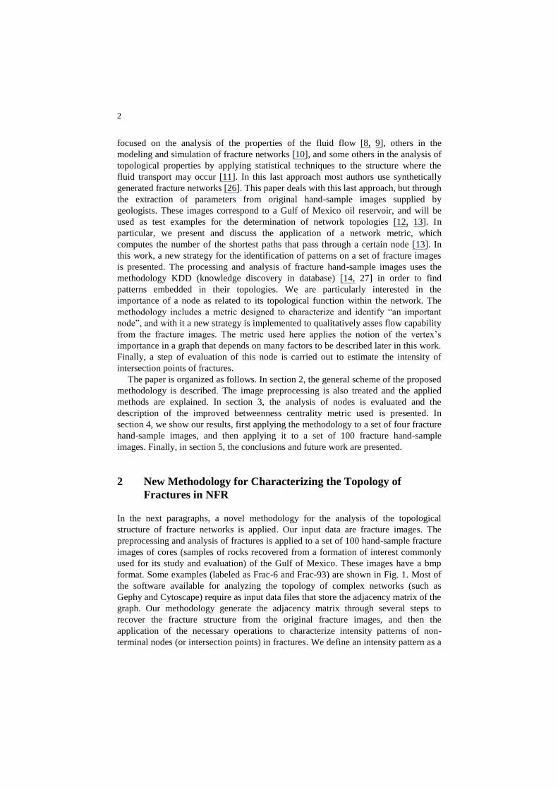
format. Some examples (labeled as Frac-6 and Frac-93) are shown in Fig. 1. Most of
the software available for analyzing the topology of complex networks (such as
Gephy and Cytoscape) require as input data files that store the adjacency matrix of the
graph. Our methodology generate the adjacency matrix through several steps to
recover the fracture structure from the original fracture images, and then the
application of the necessary operations to characterize intensity patterns of non-
terminal nodes (or intersection points) in fractures. We define an intensity pattern as a
3
tendency in the increase of number of nodes in different sizes of circles. The general
procedure is described below.
a) Frac-93
b) Frac-6
Fig. 1. Hand sample examples of fractures associated to NFR: a) Frac-93, and b) Fract-6 from
Jujo-Tecominoacán reservoir.
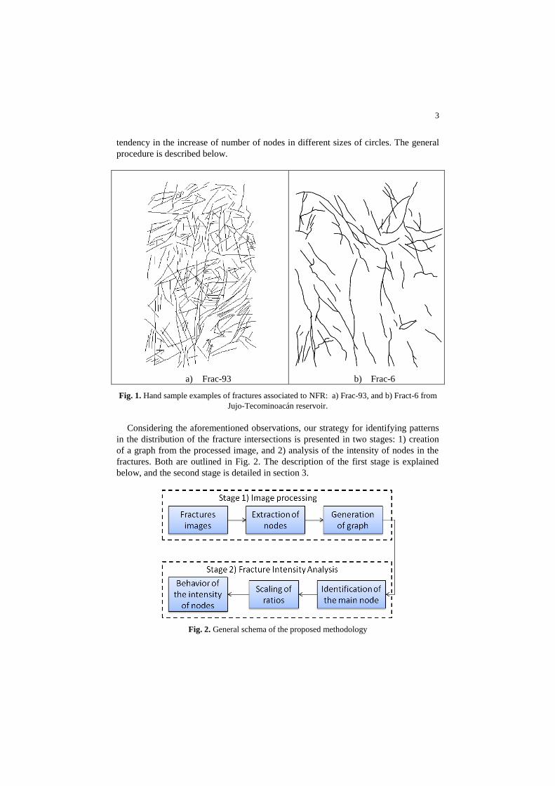
Considering the aforementioned observations, our strategy for identifying patterns
in the distribution of the fracture intersections is presented in two stages: 1) creation
of a graph from the processed image, and 2) analysis of the intensity of nodes in the
fractures. Both are outlined in Fig. 2. The description of the first stage is explained
below, and the second stage is detailed in section 3.
Fig. 2. General schema of the proposed methodology
4
The goal of the first stage is to obtain the adjacency matrix representative of the
topological structure of the fracture network. We do it in three steps. In the first step
the image is processed, applying a skeletonization process for recovering the structure
of the fracture in the whole hand-sample image. The second step identifies and
obtains the intersections and endpoints of each fracture image, what are known in
graph theory as non-terminal and terminal (leaves) nodes, respectively. The third step
generates a file that contains the adjacency matrix, where the recovery of all the nodes
and edges is done. It requires touring all the paths in the skelotonized fracture in order
to find the neighborhood nodes, i. e., to identify which nodes are linked to each node
for establishing the connection. Then, this matrix is used for building the graph. The
second stage indentifies patterns in the distribution of intersection points in the
fractures by means of the application of a centrality metric widely used in complex
networks. In the next section, the main idea and the definition of this metric are
explained.
3 Fracture Intensity Analysis
The second stage is shown in the dotted lower rectangle in Fig. 2. This stage is
subdivided into three steps. An important property of the fracture network is the
capability of transport fluids. In this case, the non-terminal nodes or intersections of
traces are considered. Thus, the strategy is to analyze different sizes of circular
regions from a particular node for evaluating precisely the amount of these nodes in
each region. It will allow us to identify any pattern in the increment of different sizes
of radius considering the number of intersection points computed. The first step of the
second stage is to select the most important node from the set of nodes stored in the
adjacency matrix. The earliest intuitive conception of point centrality was based upon
the structural properties of centrality. This idea was introduced by Bavelas [15], and
an essential tool for the analysis of networks is the centrality index which is based on
counting paths going through a node [16]. These measures define centrality in terms
of the degree to which a point falls on the shortest path between others, and therefore
it has a potential for controlling the communication of the network. One of these
metrics is the betweenness centrality measure which was proposed by Freeman [17],
and Antonisse [18]. In this work, an improved version [19] of this measure is applied,
which includes a more efficient and faster algorithm for large and very sparse
networks. This algorithm is based on an accumulation technique that solves the
single-source shortest-path problem, and thus exploits efficiently the sparsity of the
network incidence matrix. The traditional formulation for computing the betweenness
centrality index is accomplished in two steps: i) compute the length and the number of
shortest paths between all pairs, and ii) sum over all the pair-dependencies. For each
node i, in the network, the number of “routing” paths to all other nodes (i.e., paths
through which exist connectivity) going through i is counted, and this number
determines the centrality i. The most common index is obtained by taking only the
shortest paths as the routing paths. Formally the definition of betweenness centrality
of a node i, is given by (1):
5
where stands for summing each pair once, ignored the order, and equals
1 if the shortest path between nodes j and k passes through node i, and 0 otherwise. In
networks with no weight, i.e., where all edges have the same length, there may be
more than one shortest path. In this case, it is common to take , where is the number of shortest paths between j and k, and
is the number of those going through i. An improvement to this equation is
presented in (3), where the numerator of the pair-dependency in (2), , is
obtained by the Bellman criterion, , if the shortest paths between j and
k pass through i [19]. A high centrality score indicates that a vertex can be reached by
others on short paths, or that a vertex connects to others. In the methodology
proposed, this metric is applied for all the non-terminal nodes of each fracture image,
where the maximum value obtained is considered as the main node in the fracture
system.
The second step in stage two consists in the computation of the intensity of non-
terminal nodes that connect fractures. The idea is to carry out a sampling of the total
image area with concentric circles centered at a strategic node, in this case, taking the
most important node chosen by the betweenness centrality measure, and then to count
the number of non-terminal nodes comprised in each circle. This process is described
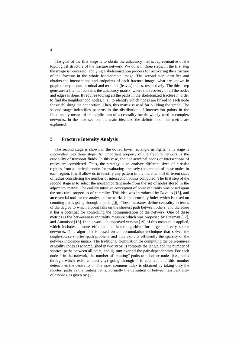
as follows. In Fig. 3 the intersection points among fractures are computed and
presented, and the metric of centrality is done (see Fig. 4 and Fig. 5). Once the most
important node in a graph is identified, it will be considered as the origin for the
sampling circles. The third step is to draw the tendencies of all non-terminal nodes.
4 Results
In experiment, 100 hand-sample fracture images of the Gulf of Mexico oil Reservoir
are considered. The images used were provided by experts of the geological area.
Applying the first stage of the strategy (see Fig. 2), all the images are processed for
recovering their fracture structure, in most cases required of the skeletonization
process. For convenience only two images are shown in Fig. 1. Fig. 3 presents the
resulting images after the application of the second step concerning to the
identification of the non-terminal nodes or intersection points related to the images in
. (1)
. (2)
if
otherwise (3)
6
Fig. 1, where the number of nodes is listed at the bottom of each image (61and 252
non-terminal nodes which correspond to Frac-6, and Frac-93, respectively). The next
step is the determination of the topological structure of the fractured network
employing the non-terminal nodes and the distance among their neighbors for its
building. For drawing the resultant graph, the Cytoscape tool [20, 21] has been used,
receiving as input data the adjacency matrix generated in the previous steps, this is
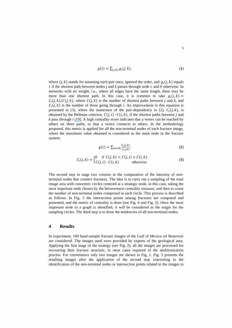
carried out for each hand-sample image. The resultant graphs of Frac-6 and Frac-52
(see Fig. 4 and 5, respectively) are represented using a hierarchical structure. The
number of conex components in Fract-6 is 17 and 30 conex components in Frac-93,
which they represent the connectivity of the fractures studied.
In the second stage, for obtaining the main node, first the improved betweenness
centrality measure is applied by using the Gephy tool [22, 23]. Then, the maximum
value obtained using this metric is selected from all nodes in the fracture, and this
maximum value of the corresponding node is considered the main node. To be precise
a main node is defined as a node that has the highest connectivity according to the rest
of the nodes in the fracture system, for this problem, the largest capability of transport
fluids. This procedure was repeated for each fracture image. In Fig. 4 and 5, the main
nodes are highlighted in black color, they correspond to nodes 7 and 25 in Frac-6, and
node 76 in Frac-93; their betweenness centrality values are 195 and 17567.1,
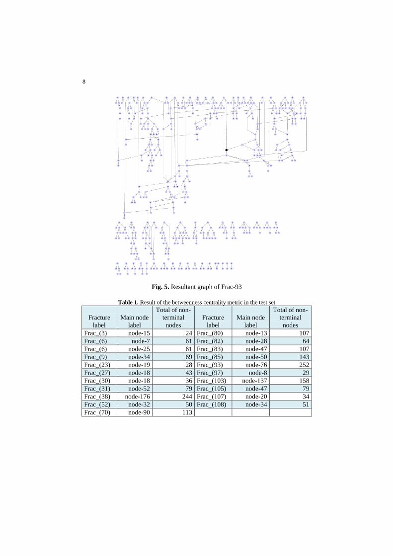
respectively. This operation was applied to the 100 test instances. In Table 1 only 20
fracture images are shown, where the first column presents the label of the image, the
second column indicates the label of the main node obtained by applying the
centrality metric, and the third column has the total number of non-terminal nodes
analyzed. It is important to comment that some fractures obtained two main points,
for example Frac-6 has 2 main nodes (7 and 25) since both have the same
betweenness centrality measure.
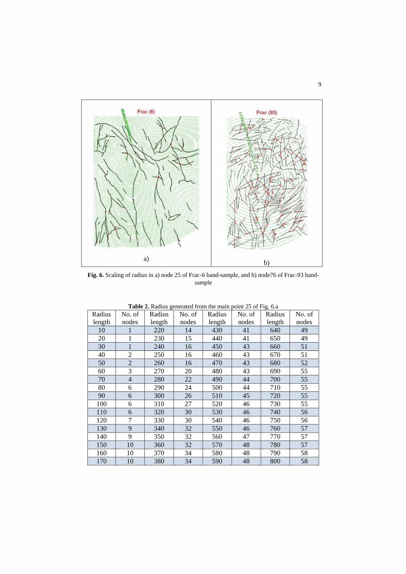
Once the main node of each fracture is found, the next step is the determination of
the distribution of the nodes in the whole network. In this experiment, we take the
node or nodes identified as “main nodes” according to the definition given above, and
use them as centers or concentric circles of increasing radius. The radii of the
sampling circles is increased (arbitrarily) in 10 pixels, taking as origin the main node
previously found. For instance, in Fig. 6a and 6b, the scaling of radius is shown,
where the main nodes 25 and 76 were taken from Table 1 (corresponding to Frac-6
and Fract-93, respectively). Considering the node-25 of Frac-6, an example of growth
of the number of non-terminal nodes in circular areas is presented in Table 2. The
initial size of the radius is 10 pixels, and the next circles were generated in augment of
10 pixels, i.e., 20, 30, 40 pixels and so on until covering all the non-terminal nodes in
the fracture image. In this instance, 84 regions were produced for covering the 61
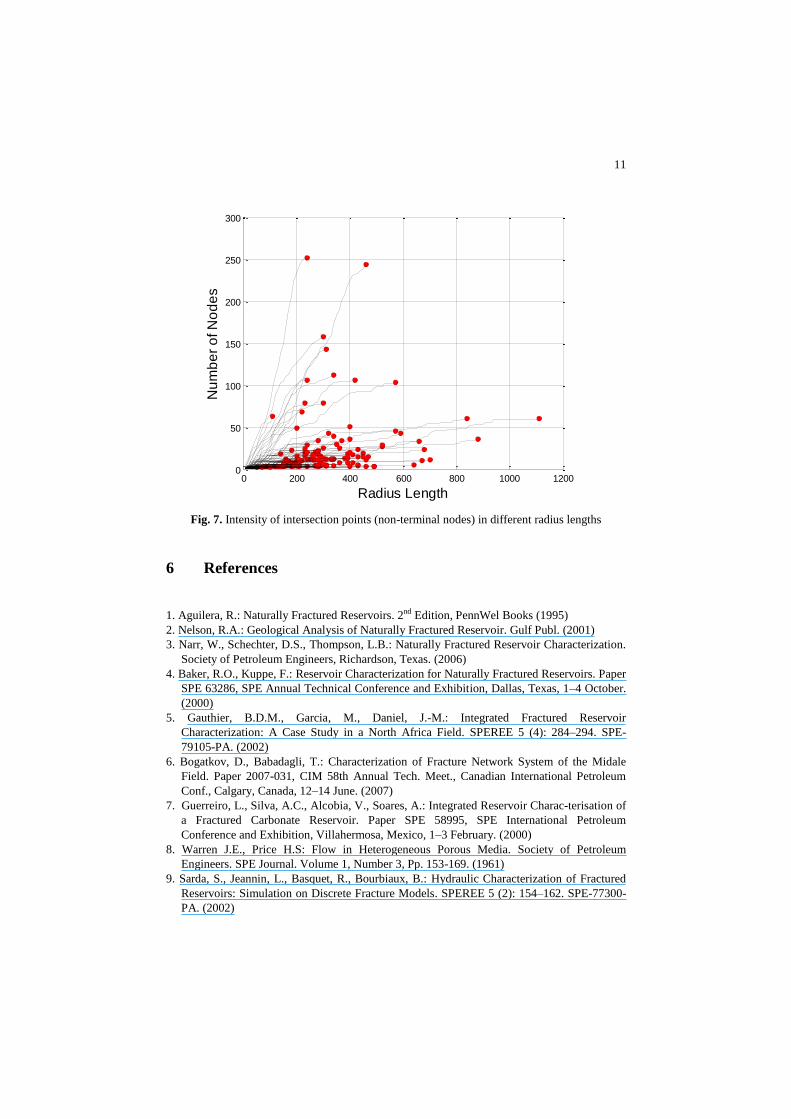
nodes initiating in node-25 of Frac-6. The empirical cumulative distribution of the
nodes of each image is shown in Fig. 7. In this figure each line represents the increase
of the intersection points (non-terminal nodes) of each of the 100 fracture images, the
axis of the coordinate is the distance of the radius in pixels, the axis of the abscise is
the amount of the nodes found in each region, and the circle at the end of the line
indicates the farthest node from the main node. Note in this figure that a general
description from the set of 100 images two groups can be identified: one group where
7
the intersection points of fractures (non-terminal nodes) are more scattered, and the
second group where the intersection points are nearer among them.
a) Frac-6
b) Frac-93
Fig. 3. Identification of intersection points (non-terminal nodes)
Fig. 4. Resultant graph of Frac-6
Frac-93.
Number of Intersection: 252
1
2
3
4
5
6
7
8
910
11
12
13
14
15
1617
18
19
20
21
22
23
24
25
26
27
28
29
30
31
32
33
34
35
36
37
38
39
40
41
42
43
44
45
46
47
4849
5051
52
53
54
55
56
57
58
59
60
61
62
63
64
6566
67
68
69
70
71
72
73
74
75
76
77
78
79
80
81
82
83
8485
86
87
88
89
90
91
92
93
94
95
96
97
98
99100
101
102103
104
105
106
107
108
109
110111
112113
114
115
116117118
119
120
121
122123
124
125126
127
128129
130
131
132
133
134
135
136137
138
139
140
141
142
143
144
145
146
147148
149150151
152
153
154
155
156
157
158
159
160
161
162
163164
165
166
167
168
169
170
171
172
173
174
175
176
177
178
179
180
181
182
183
184
185
186
187
188
189
190
191
192
193
194
195
196
197
198
199
200
201
202
203
204
205
206
207
208
209
210
211
212
213
214
215
216
217
218
219
220
221
222
223
224
225
226
227228
229
230
231
232
233
234
235
236
237
238
239
240
241
242
243
244
245246
247248249
250
251
252
8
Fig. 5. Resultant graph of Frac-93
Table 1. Result of the betweenness centrality metric in the test set
Fracture
label
Main node
label
Total of non-
terminal
nodes
Fracture
label
Main node
label
Total of non-
terminal
nodes
Frac_(3) node-15 24 Frac_(80) node-13 107
Frac_(6) node-7 61 Frac_(82) node-28 64
Frac_(6) node-25 61 Frac_(83) node-47 107
Frac_(9) node-34 69 Frac_(85) node-50 143
Frac_(23) node-19 28 Frac_(93) node-76 252
Frac_(27) node-18 43 Frac_(97) node-8 29
Frac_(30) node-18 36 Frac_(103) node-137 158
Frac_(31) node-52 79 Frac_(105) node-47 79
Frac_(38) node-176 244 Frac_(107) node-20 34
Frac_(52) node-32 50 Frac_(108) node-34 51
Frac_(70) node-90 113
9
a)
b)
Fig. 6. Scaling of radius in a) node 25 of Frac-6 hand-sample, and b) node76 of Frac-93 hand-
sample
Table 2. Radius generated from the main point 25 of Fig. 6.a
Radius
length
No. of
nodes
Radius
length
No. of
nodes
Radius
length
No. of
nodes
Radius
length
No. of
nodes
10 1 220 14 430 41 640 49
20 1 230 15 440 41 650 49
30 1 240 16 450 43 660 51
40 2 250 16 460 43 670 51
50 2 260 16 470 43 680 52
60 3 270 20 480 43 690 55
70 4 280 22 490 44 700 55
80 6 290 24 500 44 710 55
90 6 300 26 510 45 720 55
100 6 310 27 520 46 730 55
110 6 320 30 530 46 740 56
120 7 330 30 540 46 750 56
130 9 340 32 550 46 760 57
140 9 350 32 560 47 770 57
150 10 360 32 570 48 780 57
160 10 370 34 580 48 790 58
170 10 380 34 590 48 800 58
10
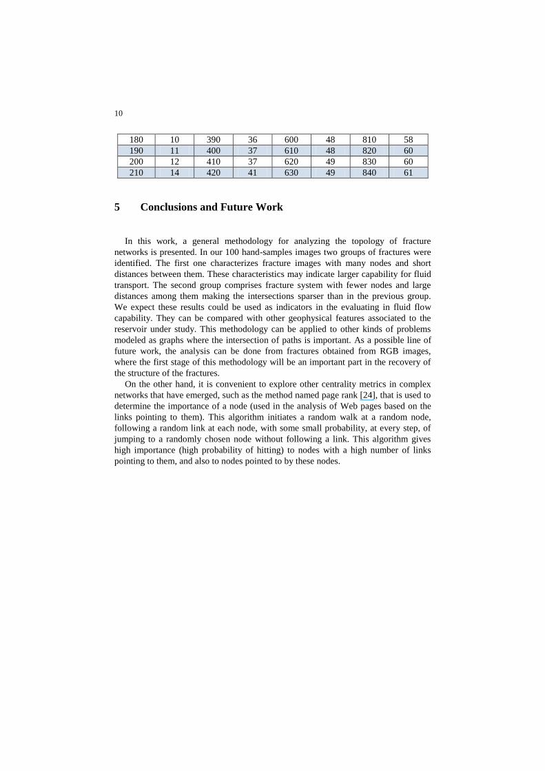
180 10 390 36 600 48 810 58
190 11 400 37 610 48 820 60
200 12 410 37 620 49 830 60
210 14 420 41 630 49 840 61
5 Conclusions and Future Work
In this work, a general methodology for analyzing the topology of fracture
networks is presented. In our 100 hand-samples images two groups of fractures were
identified. The first one characterizes fracture images with many nodes and short
distances between them. These characteristics may indicate larger capability for fluid
transport. The second group comprises fracture system with fewer nodes and large
distances among them making the intersections sparser than in the previous group.
We expect these results could be used as indicators in the evaluating in fluid flow
capability. They can be compared with other geophysical features associated to the
reservoir under study. This methodology can be applied to other kinds of problems
modeled as graphs where the intersection of paths is important. As a possible line of
future work, the analysis can be done from fractures obtained from RGB images,
where the first stage of this methodology will be an important part in the recovery of
the structure of the fractures.
On the other hand, it is convenient to explore other centrality metrics in complex
networks that have emerged, such as the method named page rank [24], that is used to
determine the importance of a node (used in the analysis of Web pages based on the
links pointing to them). This algorithm initiates a random walk at a random node,
following a random link at each node, with some small probability, at every step, of
jumping to a randomly chosen node without following a link. This algorithm gives
high importance (high probability of hitting) to nodes with a high number of links
pointing to them, and also to nodes pointed to by these nodes.
11
Fig. 7. Intensity of intersection points (non-terminal nodes) in different radius lengths
6 References
1. Aguilera, R.: Naturally Fractured Reservoirs. 2nd Edition, PennWel Books (1995)
2. Nelson, R.A.: Geological Analysis of Naturally Fractured Reservoir. Gulf Publ. (2001)
3. Narr, W., Schechter, D.S., Thompson, L.B.: Naturally Fractured Reservoir Characterization.
Society of Petroleum Engineers, Richardson, Texas. (2006)
4. Baker, R.O., Kuppe, F.: Reservoir Characterization for Naturally Fractured Reservoirs. Paper
SPE 63286, SPE Annual Technical Conference and Exhibition, Dallas, Texas, 1–4 October.
(2000)
5. Gauthier, B.D.M., Garcia, M., Daniel, J.-M.: Integrated Fractured Reservoir
Characterization: A Case Study in a North Africa Field. SPEREE 5 (4): 284–294. SPE-
79105-PA. (2002)
6. Bogatkov, D., Babadagli, T.: Characterization of Fracture Network System of the Midale
Field. Paper 2007-031, CIM 58th Annual Tech. Meet., Canadian International Petroleum
Conf., Calgary, Canada, 12–14 June. (2007)
7. Guerreiro, L., Silva, A.C., Alcobia, V., Soares, A.: Integrated Reservoir Charac-terisation of
a Fractured Carbonate Reservoir. Paper SPE 58995, SPE International Petroleum
Conference and Exhibition, Villahermosa, Mexico, 1–3 February. (2000)
8. Warren J.E., Price H.S: Flow in Heterogeneous Porous Media. Society of Petroleum
Engineers. SPE Journal. Volume 1, Number 3, Pp. 153-169. (1961)
9. Sarda, S., Jeannin, L., Basquet, R., Bourbiaux, B.: Hydraulic Characterization of Fractured
Reservoirs: Simulation on Discrete Fracture Models. SPEREE 5 (2): 154–162. SPE-77300-
PA. (2002)
0 200 400 600 800 1000 12000
50
100
150
200
250
300
Radius Length
Nu
mb
er
of N
od
es
12
10. Sarkar, S., Toksöz, M.N., Burns, D.R.: Fluid Flow Simulation in Fractured Reservoirs.
Research Report, Earth Resources Laboratory, Department of Earth, Atmospheric, and
Planetary Sciences, Massachusetts Institute of Technology, USA. (2004)
11. Cacas, M. C., Ledoux, E., de Marsily, G., Tillie, B.: Modeling fracture flow with a
stochastic discrete fracture network: calibration and validation. Water Resources Research,
26:479-489, (1990)
12. Newman, M.E.J. Networks: An Introduction. Oxford University Press. (2010)
13. Cohen, R., Havlin S.: Complex Networks: Structures, Robustness and Function. Cambridge
University Press. (2010)
14. Witten, I. H., Frank, E., Hall, M. A.: Data Mining Practical Machine Learning Tools and
Techniques. Third Edition. (2011)
15. Bavelas A.: A mathematical model for group structure. Applied Anthropology. 7: 16-39.
(1948)
16. Kolaczyk, E. D.: Statistical Analysis of Networks Data: Methods and Models. Springer
Series in Statistics. (2009)
17. Freeman Linton C.: A set of Measures of Centrality Based on Betweenness. Sociometry.
Vol. 40, No. 1, Pp. 35-41. (1977)
18. Anthonisse Jac M.: The rush in a graph. Amsterdam. Mathematisch Centrum
(mimeographed) (1971).
19. Brandes, U.: A Faster Algorithm for Betweenness Centrality. Journal of Mathematical
Sociology 25(2): 163-177. (2001).
20. Shannon, P., Markiel, A., Ozier, O., Baliga, N.S., Wang, J.T., Ramage, D., Amin, N.,
Schwikowski, B., Ideker, T.: Cytoscape: a software environment for integrated models of
biomolecular interaction networks. Genome Research, 13(11):2498-504, (2003)
21. Cytoscape Software. Available at http://www.cytoscape.org/
22. Bastian M., Heymann S., Jacomy MGephi: An Open Source Software for exploring and
manipulating Networks. International AAAI Conference on Weblogs and Social Media.
(2009)
23. Gephi software. Available at http://gephi.org/
24. Page, L., Brin, S., Motwani, R., Winograd, T.: The pagerange citation ranking: Bringing
order to the web, Technical report, Stanford InfoLab. (1999).
25. Yang, G., L. R. Myer, S. R. Brown, and N. G. W. Cook: Microscopic analysis of
macroscopic transport properties of single natural fractures using graph theory algorithms,
Geophys. Res. Lett., 22(11), 1429–1432, doi:10.1029/95GL01498. (1995).
26. Ghaffar, H.O., Nasseri, M.H.B, Young, R.P.: Fluid Flow Complexity in Fracture Network:
Analysis with Graph Theory and LBM. arXiv:1107.4918 [cs.CE]. (2012).
27. Usama M. Fayyad, Gregory Piatetsky-Shapiro, Padhraic Smyth, Ramasamy Uthurusamy.:
Advances in Knowledge Discovery and Data Mining. American Association for Artificial
Intelligence. AAAI Press. (1996).
Top Related
Copyright © 2022 FDOKUMEN

