378.791+G1+3477321OOP

DIVISION OF AGRICULTURAL SCIENCES

1; UNIVERSITY OF CALIFORNIA•;eie .k.

4.

• %,4„0 f AG

A Simulation Model of Grower-ProcessorCoordination in the Beet Sugar Industry

by

James N. Niles

and

Ben C. French

Waite Memorial C Division of

AgliculCollectionturai Ecenomks

CALIFORNIA AGRICULTURAL EXPERIMENT STATION

GIANNINI FOUNDATION OF AGRICULTURAL ECONOMICS

Giannini Foundation Research Report No. 321

MAY 1974

6. 9 ti

65 4./

4

•-•

ACKNOWLEDGMENTS

We are most appreciative of the cooperation of Spreckels Sugar Division in providing

consultation and access to data required for this study. Particularly helpful wereDon Swartz, Roger McEuen, and Don Riley. Thanks are due also to our colleagues,Gordon A. King (Agricultural Economics), Robert Loomis (Agronomy), andEdward Jesse (U. S. Economic Research Service), whose comments greatly aided theanalysis. The study was partially financed by grants from the National Science Foundation.

4

TABLE OF CONTENTS

Page

INTRODUCTION 1

2

4

6

7

8

10

11

11

13

Concepts and Definitions . . 13

How the Model Works 14

Behavioral Relationships 17

System Parameters 18

Noncost Parameters 19

Cost Parameters 20

Decision Rules--Existing System 22

Testing the Model 24

EXPERIMENTATION WITH THE MODEL 25

An Illustrative Simulation Experiment 25

Simulation Results 32

THE CALIFORNIA SUGAR BEET INDUSTRY

Cultural Factors

Harvest and Assembly Operations .

Factory Operations

Contract Arrangements

Government Influences

SPRECKELS SYSTEM

Factory and District Organization

MODELING THE PRODUCTION—PROCESSING SYSTEM

Page

Other Experiments 36

Tonnage and Acreage Decisions 36

Factory Supply Sources 38

Factory Starting Date Decisions 38

Standard Inventory Levels 38

Planting Dates 38

Quantity Harvested in Each District 38

" Quantity Harvested in Each Production Area in EachTime Period 39

Delivery Routes 39

Factory Operation . 39

Changes in Parameters 39

SUMMARY AND CONCLUSIONS 40

Nature of the Model 40

Uses of the Model 41

Suggestions for Further Analysis 42

Conclusions 42

APPENDIX A: Sequence of Computer Calculations 44

APPENDIX B: Specification and Estimation of BehavioralRelationships 50

APPENDIX C: Extraction Rates and Cost Parameters 69

APPENDIX D: Decision Rules and Decision Parameters—ExistingSystem 77

REFERENCES 100

ii

Table

1

2

3

5

6

8

9

10

11

Appendixtable

LIST OF TABLES

Harvested Acreage and Production of Sugar Beets in California andthe United States, 1968-1972

California Sugar Beet Production by County, 1970

Grower Payment Schedule for Sugar Beets

Ten—Year Averages of Outputs for the Model of the Existing System

Expected Slice Rates by Factory and Production Period: Case I

Acreage Restriction and Solution by Production Area

Matrix Formulation of Harvest by Production Area and Time Period

Simulated Performance of the Model of the Existing System. .

Simulated Performance of the Model of the Improved System •

Differences in Performance of the Models of the Existing and

Improved System • • .

Expected Slice Rates by Factory and Production Period: Case II

B-1 Yield Regression Equations

B-2 Proportions of Acreage That Become Available to Harvest, by

Production Area and Time Period

Page

3

5

9

26

28

29

30

33

34

35

37

53

56

B-3 Relation of Temperature During Beet Growth in Each Production

Area to Temperature in Base Stations 57

ill

Appendixtable Page

B-4 Normal Approximation to the Distribution of Average Maximum

Temperature During Beet Growth, °F. 58

B-5 Relation of Moisture Index Values in Selected Stations to Soil

Moisture at Davis 60

B-6 Probability Distribution of Net Change in Moisture Index Per Day

by Month, Davis, 1926-1970 62

B-7 Monthly Average Mean Temperatures, °F., 1951-1970 65

B-8 Type of Operation and Tonnage of Beets Sliced Per Day by Factory

Mean Value and Standard Deviation 66

B-9 Slice Reductions Due to Train Delays by Factory and Time Period 68

C—/ Yield and Clean Beet Percentages by Campaign and Production Area 70

C-2 Extraction Rates by Factory and Time Period. . 71

C-3 Number of Days in Each Period 71

C-4 Cost of Producing Fall and Spring Harvested Beets, 1971 Input Prices 72

C-5 Summary of Sugar Beet Cultural Costs Per Acre by Production Area 73

C-6 Sugar Beet Cultural Cost Per Acre by Time Period and Production

Area 74

C— 7 Computation of Representative Opportunity Cost for Spring Delayed

Harvest of Sugar Beets 75

C-8 Receiving Station, Rail, and Transport Costs by Receiving Station 76

iv

Appendixtable Page

D— 1 Expected Slice Rates by Factory and Production Period, Initial

Model 79

D— 2 Allocation of Total Acreage to Production Areas, Initial Model. 80

D— 3 Factory Source of Beets by District and Time Period 81

D— 4 Standard Inventory Levels by Factory and Time Period, Initial Model 83

D— 5 Decision Values That Determine Mean Planting Dates by Production

Area 84

D— 6 Wet Season Beet Harvest: Daily Proportion of Normal Harvest in

Relation to Moisture Index . . • • 89

D— 7 Normal Factory Requirements by Time Period 90

D— 8 Allocation of the Proportion of Quantity Harvested in District

Among Various Production Areas, Depending on the Moisture Index 93

D— 9 Proportion of Residual Quantity Harvested in D-4 in Specified

Production Areas and Various Time Periods 95

D-10 Delivery Routes From Production Areas to Receiving Stations 97

D-11 Preprogramming Decision Rules for Receiving Station to Factory

Shipments . . 99

LIST OF FIGURES

Figure

1 General Flow Chart 16

2 Decision Rule for Determining Quantity to be Harvested in Each

District for Each Semimonth Period During July—September . . 87

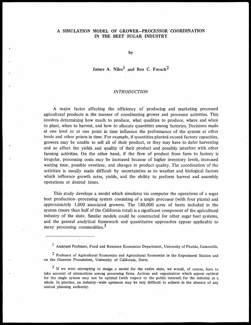
A SIMULATION MODEL OF GROWER—PROCESSOR COORDINATIONIN THE BEET SUGAR INDUSTRY

by

James A. Niles1 and Ben C. French2

INTRODUCTION

A major factor affecting the efficiency of producing and marketing processedagricultural products is the manner of coordinating grower and processor activities. Thisinvolves determining how much to produce, what qualities to produce, where and whento plant, when to harvest, and how to allocate quantities among factories. Decisions madeat one level or at one point in time influence the performance of the system at otherlevels and other points in time. For example, if quantities planted exceed factory capacities,growers may be unable to sell all of their product, or they may have to defer harvestingand so affect the yields and quality of their product and possibly interfere with otherfarming activities. On the other hand, if the flow of product from farm to factory isirregular, processing costs may be increased because of higher inventory levels, increasedwaiting time, possible overtime, and changes in product quality. The coordination of theactivities is usually made difficult by uncertainties as to weather and biological factorswhich influence growth rates, yields, and the ability to perform harvest and assemblyoperations at desired times.

This study develops a model which simulates via computer the operations of a sugarbeet production—processing system consisting of a single processor (with four plants) andapproximately 1,000 associated growers. The 180,000 acres of beets included in thesystem (more than half of the California total) is a significant component of the agriculturalindustry of the state. Similar models could be constructed for other sugar beet systems,and the general analytical framework and quantitative approaches appear applicable tomany processing commodities.3

1 Assistant Professor, Food and Resource Economics Department, University of Florida, Gainesville.

2 Professor of Agricultural Economics and Agricultural Economist in the Experiment Station andon the Giannini Foundation, University of California, Davis.

3 If we were attempting to design a model for the entire state, we would, of course, have totake account of interactions among processing firms. Actions and organization which appear optimalfor the single system may not be optimal (with respect to the public interest) for the industry as awhole. In practice, an industry—wide optimum may be very difficult to achieve in the absence of anycentral planning authority.

The study has three main objectives. The first is to formulate an analytical frameworkfor measuring cost and efficiency relationships associated with the scheduling componentof producing and processing agricultural commodities. This involves time, quality, anduncertainty dimensions that have been largely neglected or assumed away in traditionaltheoretical models of production which have focused only on parts of total systems. Thesecond objective is to provide a basis for evaluating the effects of changes in the systemon costs and returns to both producers and processors. The model developed serves asa tool for an improved system design and for evaluating the efficiency of the presentsystem. The third objective is to suggest ways in which some tools of managementscience--particularly computer simulation and linear programming--may be used toformulate improved decision rules and to choose among alternative decision strategies.

The first section of the report presents a brief description of the sugar beet industryof California. With this background, we then describe the specific production—processingsystem to be studied. This is followed by an explanation of how we formulated thecomputer model which simulates the economic behavior of this system. We then showhow the model may be used to evaluate potential gains (or losses) to growers and processorsfrom changes in decision rules or alterations of the system. The final section reviews theimplications of the analysis with respect to the efficiency of the present system and thepotential value of further research along these lines.

It is important to note that scheduling and allocation rules which are optimal forthe processor conceivably may be less than optimal for individual growers, the degreeof divergence depending on the location and environmental factors affecting each growerand the contractual arrangements under which growers are paid for their product. Theefficiency of a coordination system thus may vary with one's point of view. The publicinterest usually is best served by a system which minimizes the combined costs associatedwith the total production—processing system. Equity considerations may suggestcontractual arrangements which compensate producers who would otherwise incur highercosts or reduced returns under an improved total system. In any case, the analysis ofany coordination system must consider these potentially diverse interests.1

THE CALIFORNIA SUGAR BEET INDUSTRY

Sugar beets are a major California crop. In 1971 it was the tenth leading farm productwith an annual contribution of about $126 million to the state's economy [2] . Californialeads all states in sugar beet production. In the calendar year 1972, 31 percent of theproduction and 28 percent of the harvested acreage of the United States were in California.The comparable figures for 1968-1972 are shown in Table 1.

1 In a complete social welfare analysis, we would also need to consider the effects of alternativesystems on other interests such as labor and resource utilization. The impact would appear to be ratherminor in this case.

2

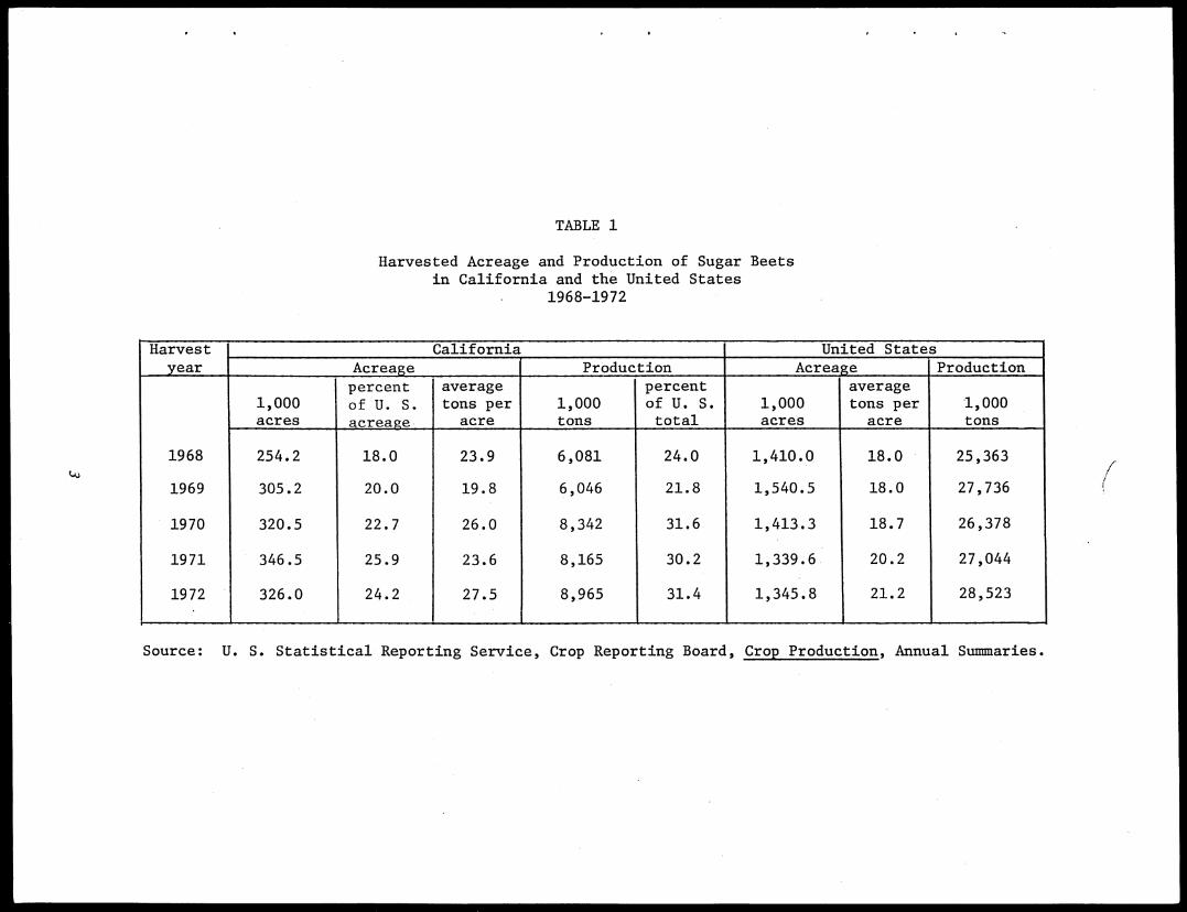
TABLE 1

Harvested Acreage and Production of Sugar Beetsin California and the United States

1968-1972

Harvestyear

California United StatesAcreage Production Acrease Production,

1,000acres

percentof U. S.acreage

averagetons per

acre

,

1,000tons

percentof U. S.total

1,000acres

averagetons per

acre1,000tons

1968 254.2 18.0

,

23.9 6,081

,

24.0 1,410.0

,

18.0 25,363

1969 305.2 20.0 19.8 6,046 21.8 1,540.5 18.0 27,736

1970 320.5 22.7 26.0 8,342 31.6 1,413.3 18.7 26,378

1971 346.5 25.9 23.6 8,165 30.2 1,339.6 20.2 27,044

1972 326.0 24.2 27.5 8,965 31.4 1,345.8 21.2 28,523

Source: U. S. Statistical Reporting Service, Crop Reporting Board, Crop Production, Annual Summaries.

Sugar beets are grown from Imperial County in the south to Tehama County inthe north. The leading counties of production are Imperial, Kern, Yolo, San Joaquin,Fresno, Solano, and Monterey. Table 2 shows each county's harvested acreage, percentof totals, tons per acre, percent of sugar, and number of farming units for the 1970crop.

Cultural Factors

The sugar beet (Beta Vulgaris L.) is a biennial plant. In the first year, the beet putson top growth and then follows with the development of a large taproot where the sugaris accumulated. In the next year, a seed stock shoots up (known as bolting), and theplant may utilize the sugar reserves accumulated in the previous year. Beets are typicallyharvested prior to the end of the first growing season; but in northern areas of California,beets may be "overwintered" and harvested in the spring, ideally before bolting.

The sugar beet is a cool—season, cold—hardy plant. It grows best in areas wherethe temperatures are moderate. In the hotter areas of California's interior valleys, thecrop is planted in the fall or winter and harvested in the late spring or summer.

Sugar beet production is measured in terms of tons of roots and pounds of sugarper acre. High sugar percentage is favored by cool night temperatures since lowertemperatures are conducive to sugar storage by inhibiting its utilization for plant growth.In either warm or cool climates, sugar percentage can be increased by causing the plantto become deficient in nitrogen and, thus, restricting growth.

Beet production is subject to several types of diseases and insect pests which haveimportant influences on yields and may restrict the location and time of planting. Ofparticular importance are three aphid—borne viruses--Beet Yellows, Beet Western Yellows,and Beet Mosaic. The California Department of Agriculture has estimated losses from theseviruses as high as $21 million per year [3] .

' Efforts to reduce the effects of these viruses have included research to develop resistantvarieties, determining best periods to apply insecticides, establishing planting times whichreduce the possibility of disease infestation, and establishing beet—free areas to restrictthe spread of diseases. Beet—free areas are areas where no beets are in the ground fora period of time. The harvest is completed before the heavy rains force a discontinuanceof harvest in the fall (frequently a target date of November 1 is used). This practiceeliminates the overwintered beets which serve as a source plant for the Virus Yellowscarrying aphids. Beet—free areas are located far enough away from nonbeet—free areasto eliminate migration of the aphid.

Other diseases that are significant are Curly Top Virus and Cercospora leaf spot.The Curly Top Virus is spread by an insect vector, the beet leafhopper, Cirulifer Tenellus

4

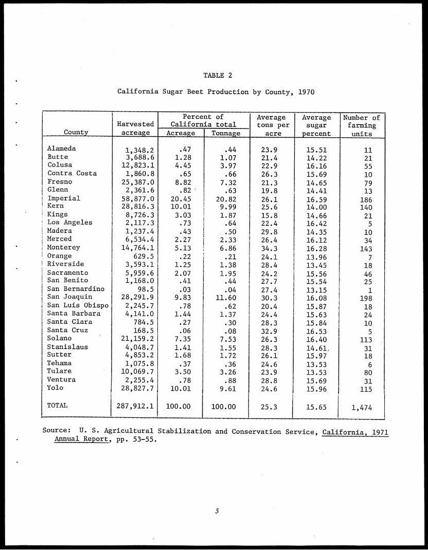
TABLE 2

California Sugar Beet Production by County, 1970

1

CountyHarvestedacreaze

Percent ofCalifornia total

Averagetons peracre

Averagesugarpercent

Number offarmingunitsAcreage Tonnaze

Alameda

,

1,348.2

:

.47 .44

,

23.9

,

15.51 11Butte 3,688.6 1.28 1.07 21.4 14.22 21Colusa 12,823.1 4.45 3.97 22.9 16.16 55Contra Costa 1,860.8 .65 .66 26.3 15.69 10Fresno 25,387.0 8.82 7.32 21.3 14.65 79,Glenn 2,361.6 .82 .63 19.8 14.41 13Imperial 58,877.0 20.45 20.82 I 26.1 16.59 186Kern 28,816.3 10.01 9.99 1 25.6 14.00 140Kings 8,726.3 3.03 1.87 15.8 14.66 21Los Angeles 2,117.3 .73 .64 22.4 16.42 5Madera 1,237.4 .43 .50 29.8 14.35 10Merced 6,534.4 2.27 2.33 26.4 16.12 34Monterey 14,764.1: 5.13 6.86 34.3 16.28 143Orange 629.5 .22 .21 24.1 13.96 7Riverside 3,593.1 1.25 1.38 28.4 13.45 18Sacramento 5,959.6 2.07 1.95 24.2 15.56 46San Benito 1,168.0 .41 .44 27.7 15.54 25San Bernardino 98.5 .03 .04 27.4 13.15 1San Joaquin 28,291.9 9.83 11.60 30.3 16.08 198San Luis Obispo 2,245.7 .78 .62 20.4 15.87 18Santa Barbara 4,141.0 1.44 1.37 24.4 15.63 24Santa Clara 784.5 .27 .30 28.3 15.84 10Santa Cruz 168.5 .06 .08 32.9 16.53 5Solano 21,159.2 7.35 7.53 26.3 16.40 113 .Stanislaus 4,048.7 1.41 1.55 28.3 14.61, 31Sutter 4,853.2 1.68 1.72 26.1 15.97 18Tehama 1,075.8 .37 .36 24.6 13.53 6Tulare 10,069.7 3.50 3.26 23.9 13.53 80Ventura 2,255.4 .78 .88 28.8 15.69 31Yolo 28,827.71 10.01 9.61 24.6 J 15.96 115

i1TOTAL 287,912.1 100.00 100.00 25.3 15.65 1 1,4741

Source: U. S. Agricultural Stabilization and Conservation Service, California, 1971Annual Report, pp. 53-55.

5

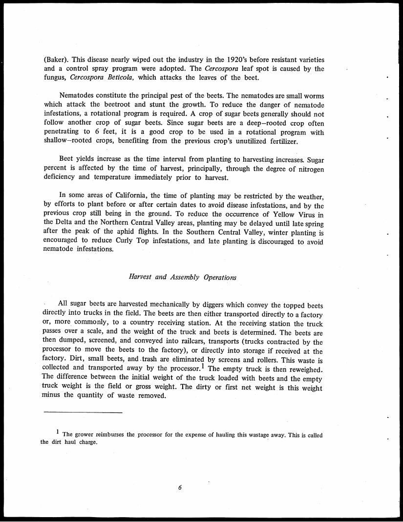
(Baker). This disease nearly wiped out the industry in the 1920's before resistant varietiesand a control spray program were adopted. The Cercospora leaf spot is caused by thefungus, Cercospora Beticola, which attacks the leaves of the beet.

Nematodes constitute the principal pest of the beets. The nematodes are small wormswhich attack the beetroot and stunt the growth. To reduce the danger of nematodeinfestations, a rotational program is required. A crop of sugar beets generally should notfollow another crop of sugar beets. Since sugar beets are a deep—rooted crop oftenpenetrating to 6 feet, it is a good crop to be used in a rotational program withshallow—rooted crops, benefiting from the previous crop's unutilized fertilizer.

Beet yields increase as the time interval from planting to harvesting increases. Sugarpercent is affected by the time of harvest, principally, through the degree of nitrogendeficiency and temperature immediately prior to harvest.

In some areas of California, the time of planting may be restricted by the weather,by efforts to plant before or after certain dates to avoid disease infestations, and by theprevious crop still being in the ground. To reduce the occurrence of Yellow Virus inthe Delta and the Northern Central Valley areas, planting may be delayed until late springafter the peak of the aphid flights. In the Southern Central Valley, winter planting isencouraged to reduce Curly Top infestations, and late planting is discouraged to avoidnematode infestations.

Harvest and Assembly Operations

All sugar beets are harvested mechanically by diggers which convey the topped beetsdirectly into trucks in the field. The beets are then either transported directly to a factoryor, more commonly, to a country receiving station. At the receiving station the truckpasses over a scale, and the weight of the truck and beets is determined. The beets arethen dumped, screened, and conveyed into railcars, transports (trucks contracted by theprocessor to move the beets to the factory), or directly into storage if received at thefactory. Dirt, small beets, and .trash are eliminated by screens and rollers. This waste iscollected and transported away by the processor.1 The empty truck is then reweighed.The difference between the initial weight of the truck loaded with beets and the emptytruck weight is the field or gross weight. The dirty or first net weight is this weightminus the quantity of waste removed.

1 The grower reimburses the processor for the expense of hauling this wastage away. This is calledthe dirt haul charge.

6

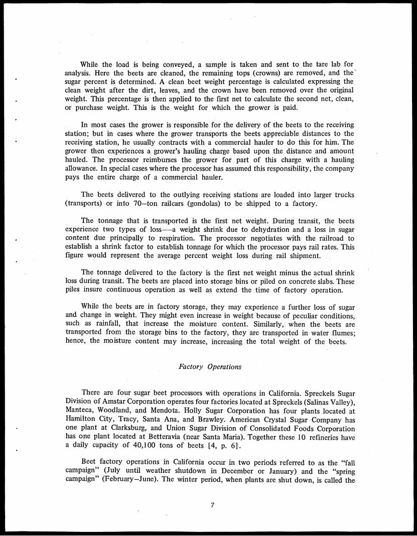
While the load is being conveyed, a sample is taken and sent to the tare lab foranalysis. Here the beets are cleaned, the remaining tops (crowns) are removed, and the'sugar percent is determined. A clean beet weight percentage is calculated expressing theclean weight after the dirt, leaves, and the crown have been removed over the originalweight. This percentage is then applied to the first net to calculate the second net, clean,or purchase weight. This is the weight for which the grower is paid.

In most cases the grower is responsible for the delivery of the beets to the receivingstation; but in cases where the grower transports the beets appreciable distances to thereceiving station, he usually contracts with a commercial hauler to do this for him. Thegrower then experiences a grower's hauling charge based upon the distance and amounthauled. The processor reimburses the grower for part of this charge with a haulingallowance. In special cases where the processor has assumed this responsibility, the companypays the entire charge of a commercial hauler.

The beets delivered to the outlying receiving stations are loaded into larger trucks(transports) or into 70—ton railcars (gondolas) to be shipped to a factory.

The tonnage that is transported is the first net weight. During transit, the beetsexperience two types of loss--a weight shrink due to dehydration and a loss in sugarcontent due principally to respiration. The processor negotiates with the railroad toestablish a shrink factor to establish tonnage for which the processor pays rail rates. Thisfigure would represent the average percent weight loss during rail shipment.

The tonnage delivered to the factory is the first net weight minus the actual shrinkloss during transit. The beets are placed into storage bins or piled on concrete slabs. Thesepiles insure continuous operation as well as extend the time of factory operation.

While the beets are in factory storage, they may experience a further loss of sugarand change in weight. They might even increase in weight because of peculiar conditions,such as rainfall, that increase the moisture content. Similarly, when the beets aretransported from the storage bins to the factory, they are transported in water flumes;hence, the moisture content may increase, increasing the total weight of the beets.

Factory Operations

There are four sugar beet processors with operations in California. Spreckels SugarDivision of Amstar Corporation operates four factories located at Spreckels (Salinas Valley),Manteca, Woodland, and Mendota. Holly Sugar Corporation has four plants located atHamilton City, Tracy, Santa Ana, and Brawley. American Crystal Sugar Company hasone plant at Clarksburg, and Union Sugar Division of Consolidated Foods Corporationhas one plant located at Betteravia (near Santa Maria). Together these 10 refineries havea daily capacity of 40,100 tons of beets [4, p. 6] .

Beet factory operations in California occur in two periods referred to as the "fallcampaign" (July until weather shutdown in December or January) and the "springcampaign" (February—June). The winter period, when plants are shut down, is called the

7

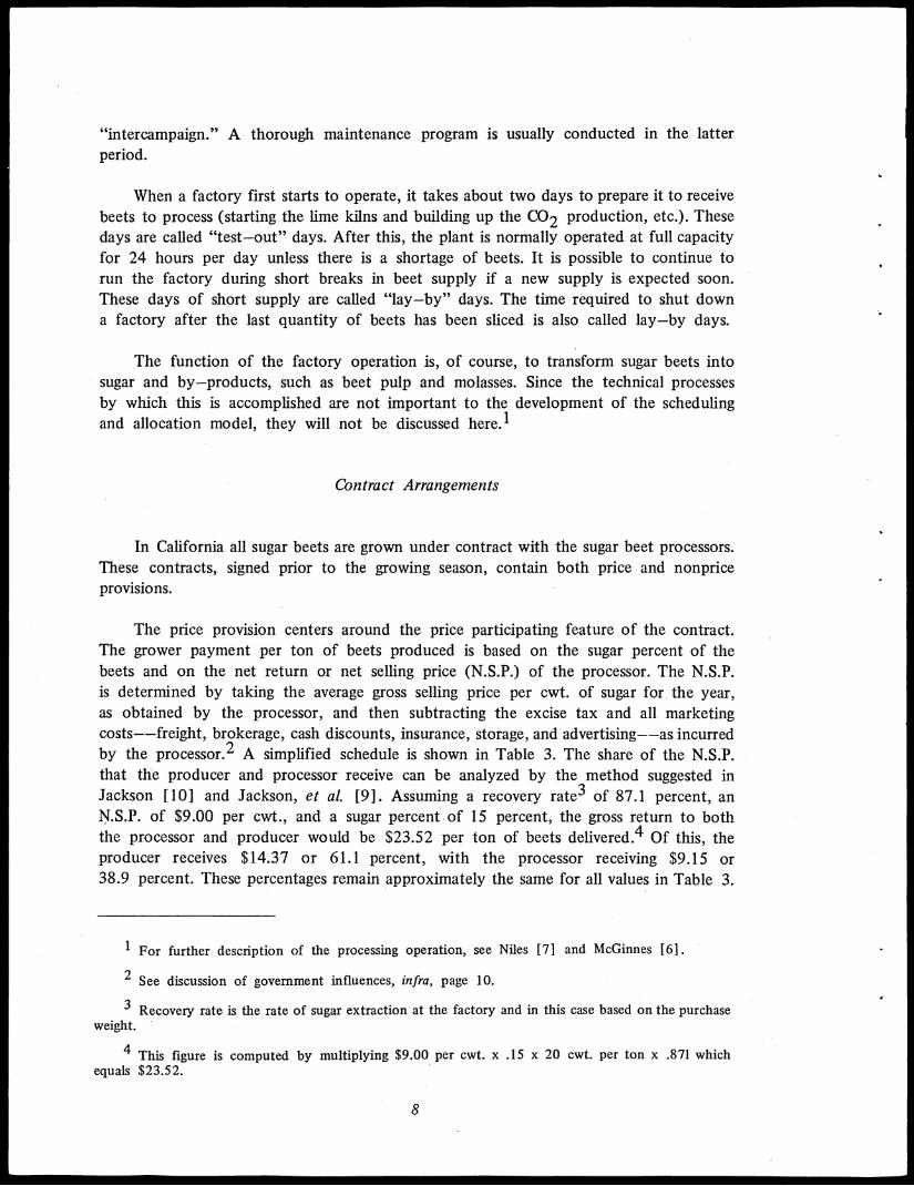
"intercampaign." A thorough maintenance program is usually conducted in the latter

period.

When a factory first starts to operate, it takes about two days to prepare it to receive

beets to process (starting the lime kilns and building up the CO2 production, etc.). Thesedays are called "test—out" days. After this, the plant is normally operated at full capacityfor 24 hours per day unless there is a shortage of beets. It is possible to continue torun the factory during short breaks in beet supply if a new supply is expected soon.These days of short supply are called "lay—by" days. The time required to shut downa factory after the last quantity of beets has been sliced is also called lay—by days.

The function of the factory operation is, of course, to transform sugar beets intosugar and by—products, such as beet pulp and molasses. Since the technical processesby which this is accomplished are not important to the development of the schedulingand allocation model, they will not be discussed here.1

Contract Arrangements

In California all sugar beets are grown under contract with the sugar beet processors.These contracts, signed prior to the growing season, contain both price and nonpriceprovisions.

The price provision centers around the price participating feature of the contract.The grower payment per ton of beets produced is based on the sugar percent of thebeets and on the net return or net selling price (N.S.P.) of the processor. The N.S.P.is determined by taking the average gross selling price per cwt. of sugar for the year,as obtained by the processor, and then subtracting the excise tax and all marketingcosts--freight, brokerage, cash discounts, insurance, storage, and advertising--as incurredby the processor.2 A simplified schedule is shown in Table 3. The share of the N.S.P.that the producer and processor receive can be analyzed by the method suggested inJackson [10] and Jackson, et al. [9]. Assuming a recovery rate3 of 87.1 percent, anN.S.P. of $9.00 per cwt., and a sugar percent of 15 percent, the gross return to boththe processor and producer would be $23.52 per ton of beets delivered.4 Of this, theproducer receives $14.37 or 61.1 percent, with the processor receiving $9.15 or38.9 percent. These percentages remain approximately the same for all values in Table 3.

1 For further description of the processing operation, see Niles [7] and McGinnes [6].

2 See discussion of government influences, infra, page 10.

3 Recovery rate is the rate of sugar extraction at the factory and in this case based on the purchaseweight.

4 This figure is computed by multiplying $9.00 per cwt. x .15 x 20 cwt. per ton x .871 whichequals $23.52.

8

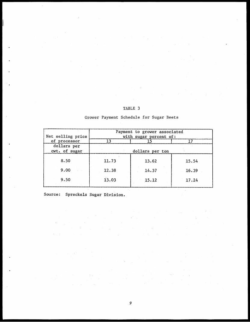
TABLE 3

Grower Payment Schedule for Sugar Beets

i1Net selling priceI of processor

Payment to grower associatedwith sugar percent of:

13 1 15 17dollars percwt. of sugar

_

dollars per ton

8.50

9.00

9.50

11.73

12.38

13.03

13.62

14.37

15.12

15.54

16.39

17.24

Source: Spreckels Sugar Division.

9

The grower receives an advance payment based on the expected N.S.P. shortly after deliveryof the product, with the final payment made after the marketing year is completed andthe N.S.P. determined.

The principal nonprice provisions of the contract pertain to delivery location anddate, who furnishes beet seed, product delivery specifications, payment of transportationcosts, right to inspect the crop, how sugar content is determined, dues deductions, andpesticide limitations.

The sugar beet processors employ fieldmen who work closely with the growers.Activities of the fieldmen include contracting, the coordination of the physical productflow from the producer to the processor, management assistance, and public relations forthe processor.

Government Influences

The sugar beet industry is subject to a number of government influences. Of particularrelevance to this study are production allotments known as "proportionate shares" basedprimarily on growers' history of production in recent years and the "conditional payments"received by growers who comply with the provisions of the U. S. Sugar Act.

The allotment programs and conditional payments are administered through the stateand county Agricultural Stabilization and Conservation Service (ASCS). When beetproduction is restricted, the local ASCS, following regulations and procedures of theU. S. Department of Agriculture (USDA), determines which farmers can grow beets andhow many acres. Beet acreage has not been limited in this manner since the 1966 crop.1In other years production is determined entirely by the contractual arrangements betweenthe producer and processor.

Conditional payments are based on the amount of commercially recoverable sugar.An average recovery rate of 87.1 percent at the time of the study is used to determinean average commercially recoverable amount of sugar from each grower's gross sugarproduction.2 The rate of conditional payment is on a sliding scale that depends uponthe amount of sugar produced. On the first 350 tons, the rate is 8 cents per pound and

1 Acreage limitations were established in October, 1969, for the 1970 crop. However, these wererescinded in April, 1970, because of lower than anticipated sugar from the 1969 crop and indicationsthat the total plantings would be less than the acreage tentatively allocated for the 1970 crop.

2 The applicable recovery rate is the average computed by the U. S. Department of Agriculturefor all sugar beets marketed under the "individual test" contracts in the United States. Individual testcontracts are those where each load delivered is sampled for sugar content. It is a five—year movingaverage which was 87.1 percent at the time of the study and is based on the purchase weight of thebeets delivered.

•

•

10

drops progressively to 3 cents per pound for all sugar produced in excess of 30,000 tons.In recent years conditional payments to California growers have averaged slightly above$2.00 per ton of beets purchased by the processor.

To qualify for the conditional payment, a grower must pay wages that equal or exceedthe minimum rate specified by the USDA; employ no child labor; and in years whenacreage is restricted, plant no more than his allotted acreage.

The money for this payment is obtained by levying an excise tax against the processorsand refiners (approximately 1/2 cent a pound of sugar). The program has resulted incollections exceeding all expenditures, including the cost of administering the program,with the surplus being retained by the Treasury.

The Secretary of Agriculture also determines each year whether the price paid bythe processor is "fair and reasonable" and whether the terms of the contracts are equitable.Sugar beet contracts are submitted annually to the USDA, and an analysis is made withregard to cost data on production and processing obtained by a field survey.

SPRECKELS SYSTEM

The system to be modeled in this study is the California operations of the SpreckelsSugar Division. As noted previously, Spreckels operates four factories and contracts withapproximately 1,000 growers who produce about 180,000 acres of sugar beets. Thissystem was selected for study because of its importance to California and the willingnessof Spreckels to cooperate by providing data and technical information.

Factory and District Organization

For operational purposes, Spreckels has organized its activities into four districts whichare further divided into 35 contract areas. Each district centers primarily around one ofthe four factories.

The Mendota District (D-4) contracts for beets in the central and southern SanJoaquin Valley --the area south of Manteca. Presently, it is the largest operating districtwith 85,000 acres or 50 percent of the total. There are 14 contract areas and 13 receivingstations.

Planting occurs from October to June. Harvest starts in the Bakersfield area aroundJuly 1 and continues northward as time progresses, moving into the lighter soils as thewinter rains slow harvest. Harvest is resumed in the spring in the extreme northern areas.

11

D-4 is the first district to start harvesting and supplies all four factories for theinitial periods. As other districts start to harvest more, the shipments of D-4 beets declineuntil D-4 is supplying only Mendota Factory (F-4). F-4 is the newest factory (completedin 1963) with a rated capacity of 4,200 tons per day.1

The Spreckels District (D-1) contracts for beets in the Salinas Valley area, stretchingdown to the Santa Maria area. The Imperial Valley has been placed in this district foradministrative purposes. The Salinas Valley has been historically California's most importantsugar beet producing area. It has a better climate (cooler) than the other valley areas,so the yield is considerably higher. However, urban expansion and the switch to highlyintensive crops has resulted in the decline in acreage in this area.

There are five contract (production) areas in D-1 with six receiving stations. Thisdistrict accounts for approximately 18,000 acres or 11 percent of Spreckels' Californiaacreage.

Planting occurs in this district from November to March, with harvest starting inAugust and continuing until completed in the Fall (about November 1). Imperial Valleybeets are planted in September and October and harvested in April to June. The Imperialbeets contracted by Spreckels are processed at the Mendota Factory (F-4) after D-4'slocal harvest has been completed. In July the Spreckels Factory (F-1) receives beets fromD-4, gradually becomes self—sufficient on D-1 beets, and then receives beets from D-3(Woodland). In the spring, it is run almost exclusively on D-3 beets.

F-1 is Spreckel's largest factory with a rated capacity of 6,500 tons per day. Itwas built in 1899 when there were more sugar beets grown in the area and is now outof proportion with respect to the acreage contracted by Spreckels in the area. To utilizethis capacity, beets are shipped into this factory from other areas after local harvest hasbeen completed. Otherwise, this factory would be shut down.

The Manteca District (D-2) contracts for beets from the Manteca area on the southto the Sacramento area on the north. There are seven contract areas and three receivingstations. This area has approximately 25,000 acres or 15 percent of the total.

Harvest starts around September 1, with harvest of the beet—free areas completedaround November 1. Harvest continues until rain prevents harvest and resumes in the springwhen the ground becomes dry enough.

The Manteca plant starts on D-4 beets and gradually shifts to D-2 beets as localharvest increases. By November 1, it is self—sufficient and remains so through the followingspring. The Manteca Factory (F-2) was erected in 1917 and possesses a rated capacityof 4,200 tons per day.

1 Rated capacity is the quantity of beets processed under "normal" 24—hour—per—day operating

conditions. The actual daily quantity may vary around this standard figure.

12

The Woodland District (D-3) contracts for beets in the areas of Sacramento andSolano counties and northward. There are nine contract areas and five receiving stationswith about 40,000 acres or 24 percent of the total.

Planting is in the spring (February—June), with harvest occurring in the fall untilrain prevents further harvest and again in the spring once the ground becomes dry enoughfor harvest.

The Woodland Factory (F-3) operates for approximately eight or nine months ofthe year. The year's operation typically starts in July, with the beets for processing comingfrom D-4. The harvesting of D-3 beets starts in August and, by October, D-3 suppliesall of the beets for F-3. In the late fall and throughout the following spring, D-3 suppliespart or all of the requirements of F-1 in addition to F-3. F-3 was erected in 1937and has a rated capacity of 3,600 tons per day.

MODELING THE PRODUCTION—PROCESSING SYSTEM

Concepts and Definitions

Models of economic systems consist of four well—defined elements: components,variables, functional relationships, and parameters.

The components of the beet sugar production—processing system are the threesubsystems for production, assembly, and processing. Production contains all activitiesinvolved in producing and harvesting beets. Assembly includes the activities required tomove the beets from the fields to the field stations and to the processing plants. Processingtransforms the beets into final products.

There are four types of variables in this system:

State variables define the state of the system at any point in time. Examples areacres available for harvest, moisture index, transit losses, and tons of beets delivered toa receiving station or to a factory.

Control variables (or decision variables) are those to which values must be assignedas part of the managerial decision process. Included are variables such as planting dates,factory starting dates, quantities to be harvested in a particular region, and quantitiesto be shipped from a particular region to a given factory.

Exogenous variables act on the system but are not influenced by it. Examples areweather events which may affect growth rates, yields, planting dates, or quantitiesharvested.

13

Endogenous variables are the performance measures of the system. They are generatedfrom the interaction of the system's exogenous, control, and state variables according tothe system's functional relationships. The endogenous variables in this model are annualaverage costs and average returns to growers, average costs of processors, combined averagecosts of the total system, and accumulated quantities of beets and sugar produced.

Functional relationships are the equations which describe the interaction amongvariables and components of the system. There are three types: behavioral equations,identities, and decision rules.

Behavioral equations are functional relationships which must be estimatedempirically or determined from technical specifications. An example is a yield equationwhich relates the tons of beets produced per acre to variables such as planting date, averagetemperature during growth, and time from planting to harvest. Probability distributionsof random variables, such as temperature, rainfall, and soil moisture, are also includedin the set of behavioral equations.

Identities are definitions or tautological statements about the components ofthe model which, along with the behavioral equations, are required to generate the behaviorof the system. (Examples: total production equals the sum of production by districts;ending inventory equals beginning inventory plus amount received less amount used.)

Decision rules are those by which management assigns values to the decisionvariables (control variables) of the system. These values may be expressed as functionsof the state variables of the system. For example, the starting date for F-1 is a functionof the expected tonnage to be harvested. In a number of cases, values assigned to decisionvariables remain constant regardless of the state of the system but may be varied amongsimulation runs.

Parameters are the constants of the system. There are three types. One type is thecoefficients of the behavioral equations--for example, the mean and standard deviationof a probability distribution. The second type consists of constants such as shrink factors,receiving station capacities, and transportation costs. The third type results from assigningconstant values to elements which, in some models, might be regarded as variables.Examples are receiving station cost per ton, hauling allowances, and harvest cost per tonin each production area. Also included are decision variables to which constant valueswere assigned as noted above.

How the Model Works

Our model of the sugar beet production—processing system is formulated to simulateon a computer the sequence of events and activities--and resulting costs and outputs--asthey might occur in any given season. Initially, the decision rules are specified so as to

14 -

approximate the rules used in the existing (historical) system. Because of the random

elements involved, a series of simulation runs is made from which are calculated averages

and measures of variation of the performance variables (average costs, etc.) of the system.

Rules and parameters then may be altered and the effects on the system performance

observed via simulation.

For decision purposes, each year may be viewed as consisting of three distinct time

periods: preplanting, planting, and harvest. These periods may overlap since planting may

occur in one production area while harvest occurs in another. The preplanting period is

the time before the seasonal plan becomes committed. The harvest period is separated

into a dry harvest (May—September) and a wet harvest (October—April) to coincide with

the normal dry and rainy periods. During the dry period, all computations are made on

a semimonth basis, while during the wet season they are made daily because of the uncertain

effects of weather events.1 Following initial decisions as to time and number of acres

planted in each of 35 producing areas, the model determines yields and quantities harvested

during each semimonth or daily period, allocates harvest quantities to 27 receiving stations,

and determines shipments from receiving stations to each of the four factories.

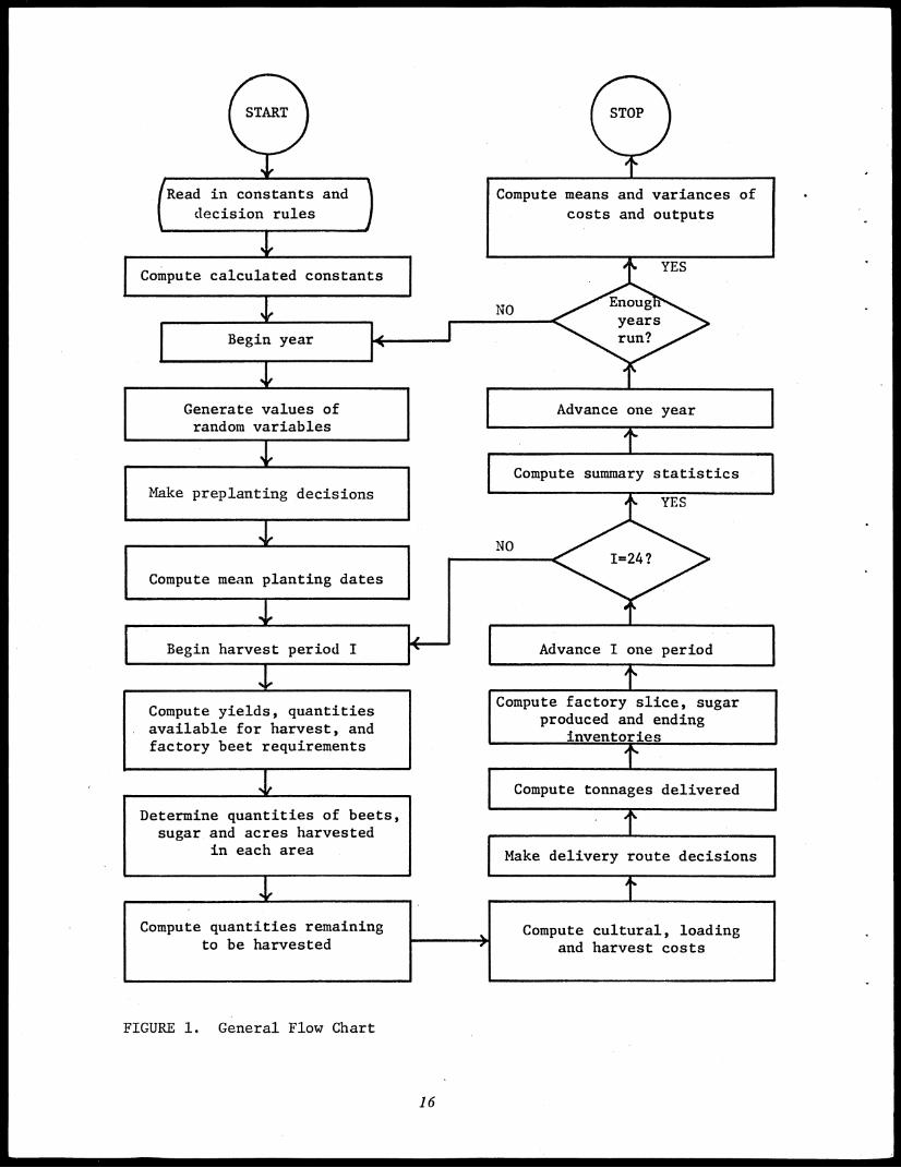
The calculations necessary to simulate the operations of the system are outlined in

Figure 1. A more detailed diagram is given in Appendix A. The program first reads in

values of constants and decision rules and calculates additional constants which may be

computed from the values read in. The first year is started by generating values of all

of the random variables for each semimonth or daily period for the entire year. Initialconditions and preplanting decisions are specified, and planting periods are determinedfor each producing area. The actual mean planting dates are determined as a functionof the moisture index.

The harvest period then begins. Yields and quantities available to harvest are computedby behavioral relationships.2 It is then necessary to determine if each factory is operatingand, if not, to decide if it should start.3 Beet requirements are computed for each factoryand decisions made as to quantities harvested in each district and production area. Duringthe wet season, these decisions are modified by values of the moisture index.

A series of identities then compute values relating to the state of the productionsubsystem such as acres harvested, sugar percent, accumulated tons and acres harvested,and quantities remaining to be harvested. Cultural and harvest costs are also computed.

1 During the dry season the weather events are highly predictable, so direct semimonth computations

may be expected to give almost the same results as daily computations summed over the same period.

The advantage of this is to greatly reduce the computational burden.

2 Explained in infra, page 17; also, Appendix B, infra, page 50.

3 See discussion of decision rules, infra, page 22.

15

(Read in constants and

decision rules

Compute calculated constants

Begin year

Compute means and variances of

costs and outputs

NO

Generate values ofrandom variables

Make preplanting decisions

Compute mean planting dates

Begin harvest period I

YES

Enougyearsrun?

Advance one year

Compute summary statistics

NO

Compute yields, quantitiesavailable for harvest, andfactory beet requirements

Determine quantities of beets,sugar and acres harvested

in each area

Compute quantities remainingto be harvested

YES

Advance I one period

Compute factory slice, sugarproduced and ending

inventories

Compute tonnages delivered

Make delivery route decisions

FIGURE 1. General Flow Chart

Compute cultural, loadingand harvest costs

•

16

Decisions are made next as to the route and method of shipment from productionareas to receiving stations and receiving stations to factories. The decision procedure isexplained in the later discussion of decision rules. Another series of identities or simpletechnical equations then is required to compute the results of implementing these decisions,including the quantities delivered adjusting the sugar losses in transit and quantities availablefor processing adjusting for storage losses at the factory.

The factory slice during each period is determined by adding a randomly distributedvariable to the normal quantity for the date. Another set of equations then determinesthe sugar in the beets sliced, total sugar produced, sugar not extracted (sugar in beetsless sugar produced), and ending inventories. The model also determines whether individualdays are operating days, test—out days, or lay—by days, or determines the number ofsuch days within each semimonth period during the dry season.

This completes the computations for one period, so time is advanced to the nextperiod and the process repeated. If the end of the season has been reached, the relevantvariables are summarized to obtain seasonal quantities, costs, and returns. When all annualcalculations have been completed, time is advanced one year, new random variables aregenerated, and another year of data obtained. When the desired number of years ofsimulation has been reached, operations cease; and the means and variances of the yearlyvalues are computed.

Behavioral Relationships

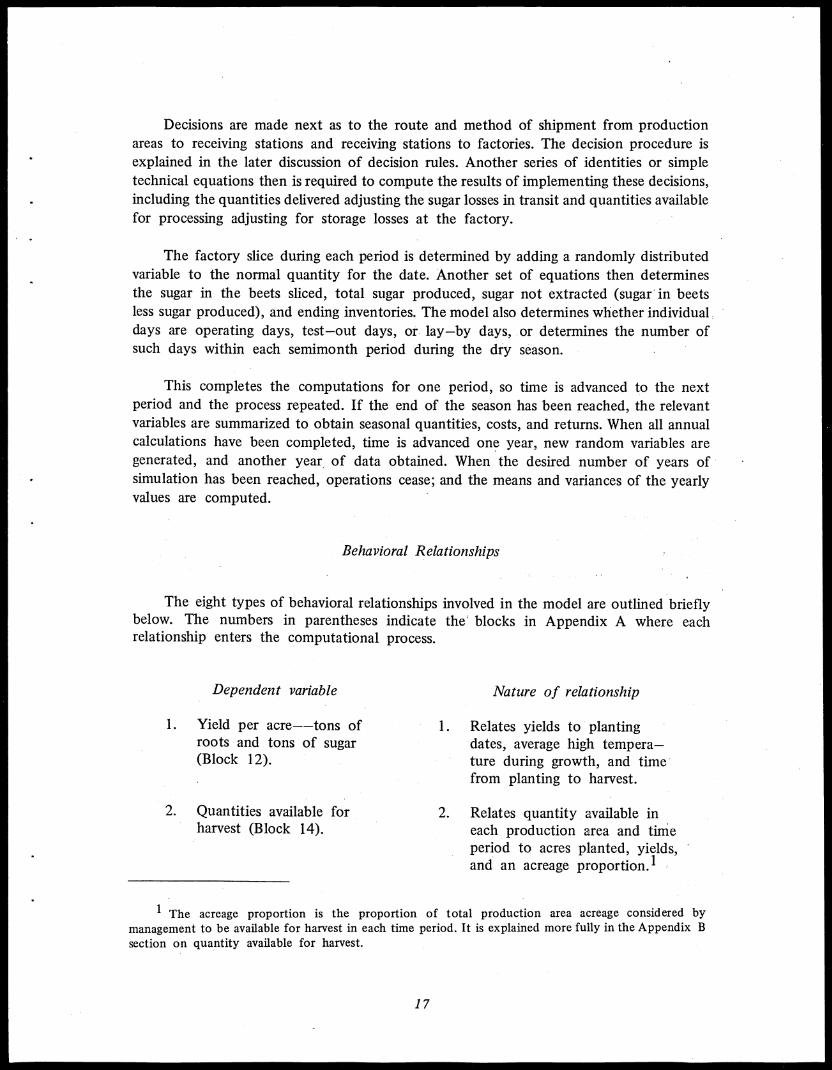
The eight types of behavioral relationships involved in the model are outlined brieflybelow. The numbers in parentheses indicate the' blocks in Appendix A where eachrelationship enters the computational process.

Dependent variable

1. Yield per acre--tons ofroots and tons of sugar(Block 12).

2. Quantities available forharvest (Block 14).

Nature of relationship

1. Relates yields to plantingdates, average high tempera—ture during growth, and timefrom planting to harvest.

2. Relates quantity available ineach production area and timeperiod to acres planted, yields,and an acreage proportion.'

1 The acreage proportion is the proportion of total production area acreage considered by

management to be available for harvest in each time period. It is explained more fully in the Appendix B

section on quantity available for harvest.

17

3. Average high temperatureduring growth (Blocks 4and 12).

4. Moisture index (Blocks 4,6, 10, 18, and 19).

5. Proportion of normal harvestachieved during wet periods(Block 19).

6. Transit and storage losses(Blocks 37, 42, and 43).

7. Tons sliced per day (Blocks 4and 45).

8. Rail delays (Blocks 4 and 45).

3. Probability distribution.

4. Probability distribution.

5. Probability distribution whichvaries with the level' of themoisture index.

6. Relates losses in weight andsugar content to temperatureduring transit and storage.

7. Probability distribution.

8. Probability distribution.

The various relationships are represented both in equation and tabular form.Relationships 1, 5, and 6 also have attached to them random elements with specifiedprobability distributions. The specific values of these relationships are given in Appendix B,along with explanations of the procedures used to estimate them. Relationship 5 isexplained and given in the appendix section on decision rules.

System Parameters

In addition to the parameters of the behavioral relationships, the model includesnoncost parameters which are mainly conversion factors; cost parameters which are averagecosts of performing the activities of the system at various levels, locations, and times;and constant values assigned to some decision or control variables. The latter is discussedin the section dealing with decision rules. The noncost and cost parameters are listedbelow followed by brief definitional or descriptive statements pertaining to each. Thenumbers in parentheses refer to the blocks in Appendix A where the constants enter thecomputational process, and the table references designate the appendix tables which givethe values of the constants where appropriate.

The costs used are "typical" average costs for each component of the model. Theywere derived from records of the processor, the studies of the Agricultural ExtensionService [8] , and consultation with the processor fieldmen and management. Althoughproduction and cost functions were not developed, the average costs estimates vary by

18

area, time period, factory, and with quality and yield variations. Thus, the actual costexperience for the total system and the major subsystems is affected by the values assignedto the decision variables and the random weather events.

Noncost Parameters

1. Expected yield (Block 8, Appendix Table C-1)

Average yield for each production area, 1965-1970.

2. Clean beet percentage (Block 32, Appendix Table C-1)

Percent of original weight remaining after removal of dirt, leaves, and crownleft on the beet after harvest and delivery, 1965-1970 average.

3. Estimated clean beet percentage (Block 17)

Average clean percentage for all areas. Value is 92.10.

4. Conversion rate to field weight (Block 24)

Rate of conversion from first net weight to field weight. Value is 1.03.

5. Sugar in crowns (Block 33)

Sugar carried into the factory in the crown or stem which remains on the beetbut is not counted in purchase weight. The crown adds 0.6 percentage pointsto the purchased sugar percent of the root.

6. Shrink factor (Block 55)

Loss of rail tonnage due to shrink in harvest. Used to compute the rail chargethe processor pays. Values are 31/2 percent, July 1—January 31; 4 percent,February 1—June 30; except always 41/2 percent for shipments from theImperial Valley.

7. Extraction rates (Block 46, Appendix Table C-2)

Conversion rate from sugar in beets sliced to sugar produced. Varies with timeand factory reflecting variations in beet quality.

8. Number of days in each semimonth period (Appendix Table C-3)

A specification of the modeling process.

19

Cost Parameters

A. Production

1. Cultural cost (Blocks 27 and 52, Appendix Tables C-4, C-5, and C-6)

Typical costs of growing beets in each area. Appendix Table C-4 gives a detailedbreakdown for one area; Appendix Table C-5 gives the summary estimates foreach production area; and Appendix Table C-6 gives the added costs incurreddue to keeping beets in the ground for a longer period--principally due toincreased interest cost and the necessity of additional irrigations. Costs areexpressed per acre so cost per ton varies with yield. Overhead costs, such astaxes, insurance, rent, and annual costs of equipment, buildings, and irrigationsystem, are not included.

2. Opportunity cost (Blocks 27 and 52, Appendix Table C-7)

Cost that a grower may incur if his beets have not been harvested in time toplant his next crop to the most profitable alternative. Only associated with springharvested beets. A representative figure was developed based on the differencein per acre return for tomatoes (an early spring crop) and field corn whichmay be planted later. The calculations given in Appendix Table C-7 providean estimate of $40.80 per acre as the "opportunity" cost.

3. Harvest cost (Blocks 27 and 52)

Cost grower pays for harvesting beets, including topping beets prior to harvestand loading charge of the hauler. Specified at typical commercial rates: Harvestcost (including topping) is $1.25 per ton (first net ton basis) in all areas. Loadingcharge is 85 cents per ton (field—weight basis) in all areas except 90 cents inAreas 25 and 30, 95 cents in Areas 26 and 33, and $1.00 in Area 35.

4. Acquisition cost (Block 52)

Cost to processor and payment to grower for beets purchased which varies withthe net selling price and sugar percent.' For modeling purposes N.S.P. is specifiedas $9.00 per cwt. of sugar. Transforming the contract provisions into equationform gives:

Acquisition cost per ton (second net weight) =

(4.5652 + .015 x sugar percent) x cwt. of sugar.

1 See supra, page 8.

20

The grower also receives an additional conditional payment.1 Assuming an87.1 percent average recovery rate (extraction rate) and a payment of 80 centsper cwt. of sugar, the conditional payment per ton (second net basis) is .27872times the sugar percent.

5. California Beet Growers Association dues (Block 52)

Amount grower pays to California Beet Growers Association. Collected by theprocessor and is currently 5 cents per ton (first net basis).

6. Grower's hauling cost (Block 52)

Amount grower pays to have his beets transported to the receiving station orfactory. Rate is 3 cents per ton (field weight) per mile. For each time periodand each production area, a mileage has been specified. These values wereobtained from the processor and reflect harvest in different locations withinthe same production area.

7. Hauling allowance (Block 52)

Amount the processor reimburses the grower for hauling beets to the nearestreceiving station. Specified at 2.5 cents per ton (first net basis) per mile. Themileage assumed is the same mileage as was used for the grower's hauling cost.If the grower hauls to a more distant station, the payment is 3.5 cents perton per mile (first net basis) for the additional mileage. This is approximatelythe same as the grower cost of 3 cents per ton per mile, field—weight basis.The charges used for this overhaul were the costs supplied by the processorbased upon an assumed average mileage of overhaul.

8. Dirt haul cost (Block 52)

Charge grower pays to processor to carry away the dirt accumulated at thereceiving station. Specified as 3 cents per ton (first net basis).

9. Tare lab cost (Block 55)*

Cost to the processor for operating labs where samples of each of the beetsdelivered are analyzed for clean beet percentage sugar percentage.

10. ReceiviriT station cost (Block 53, Appendix Table C-8)*

Variable cost per ton for operating the receiving stations.

1 See supra, page 10.

21

11. Transportation costs, receiving stations to factories (Blocks 28 and 55,

Appendix Table C-8)

Cost to processor for shipment via rail or transport truck.

12. Freight and truck unloading costs (Block 55)*

Cost to processor per ton for unloading freight cars and trucks at factory.

13. Piling and unpiling costs (Block 55)*

Cost to processor per ton at factory (actual weight basis) for additional storage

at factory.

14. Processing costs (Block 55)*

Includes variable material cost per ton, variable labor cost per ton, test—out

cost per day, and lay—by cost per day.

15. Coordination costs

Cost of field organization and administrative staff at processor headquarters.

Regarded as constant per season and so does not affect the model computations.

(*Figures used in the analysis are not disclosed at the request of the processor; contact

Spreckels Sugar Division for access to data.)

Decision Rules--Existing System

The model contains 10 types of decision or control variables--variables to which

values must be assigned as part of the managerial process. They appear in Appendix A

in Blocks 7, 10, 16, 18, 19, and 28. The nature of each rule is outlined briefly below.

More detailed explanations and the empirical basis for the rules are given in Appendix D.

22

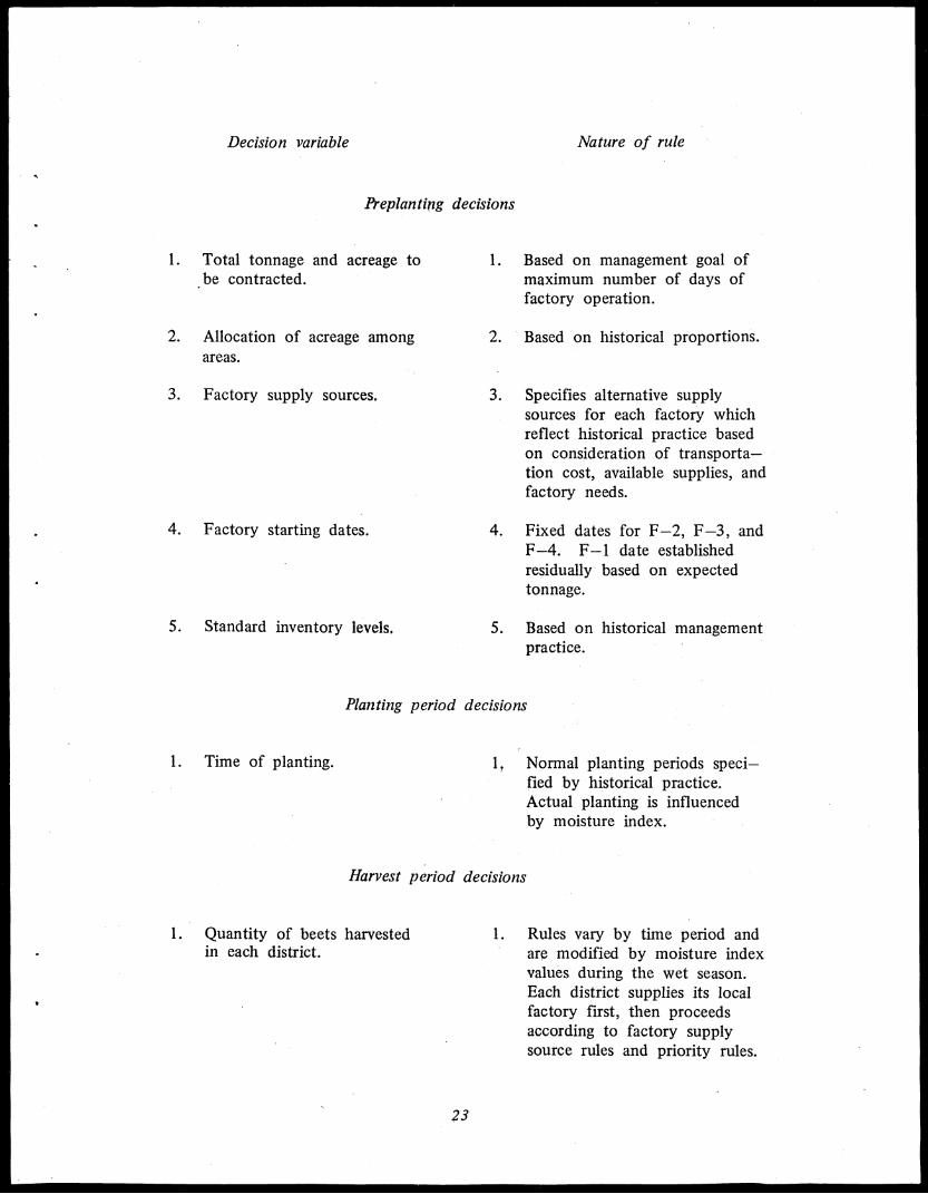
Decision variable Nature of rule

Preplanting decisions

1. Total tonnage and acreage to, be contracted.

1. Based on management goal ofmaximum number of days offactory operation.

2. Allocation of acreage among 2. Based on historical proportions.areas.

3. Factory supply sources. 3. Specifies alternative supplysources for each factory whichreflect historical practice basedon consideration of transporta—tion cost, available supplies, andfactory needs.

4. Factory starting dates. 4. Fixed dates for F-2, F-3, andF-4. F-1 date establishedresidually based on expectedtonnage.

5. Standard inventory levels, 5. Based on historical managementpractice.

1. Time of planting.

Planting period decisions

1? Normal planting periods speci—fied by historical practice.Actual planting is influencedby moisture index.

Harvest period decisions

1. Quantity of beets harvested 1. Rules vary by time period andin each district, are modified by moisture index

values during the wet season.Each district supplies its localfactory first, then proceedsaccording to factory supplysource rules and priority rules.

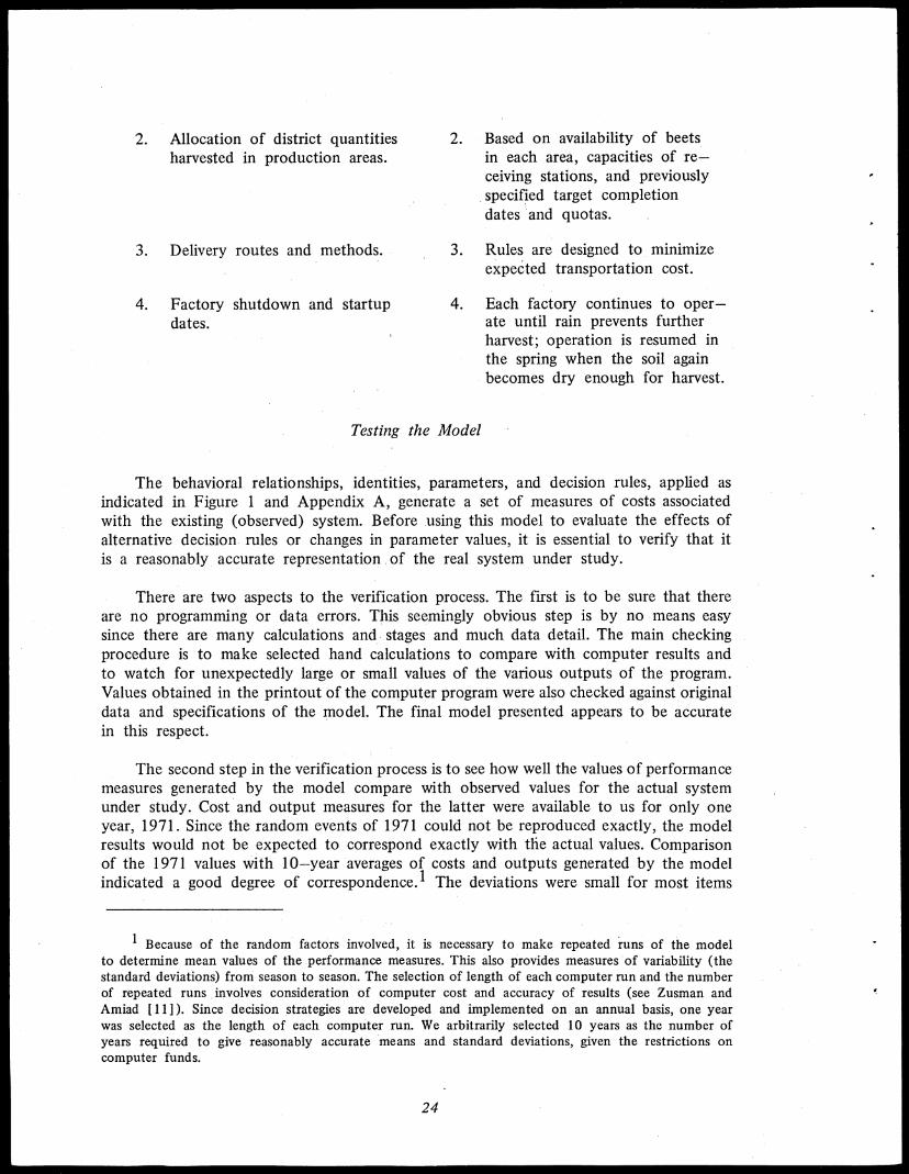
2. Allocation of district quantitiesharvested in production areas.

2. Based on availability of beetsin each area, capacities of re—ceiving stations, and previouslyspecified target completiondates and quotas.

3. Delivery routes and methods. 3. Rules are designed to minimizeexpected transportation cost.

4. Factory shutdown and startupdates.

4. Each factory continues to oper—ate until rain prevents furtherharvest; operation is resumed inthe spring when the soil againbecomes dry enough for harvest.

Testing the Model

The behavioral relationships, identities, parameters, and decision rules, applied asindicated in Figure 1 and Appendix A, generate a set of measures of costs associatedwith the existing (observed) system. Before using this model to evaluate the effects ofalternative decision rules or changes in parameter values, it is essential to verify that itis a reasonably accurate representation of the real system under study.

There are two aspects to the verification process. The first is to be sure that thereare no programming or data errors. This seemingly obvious step is by no means easysince there are many calculations and stages and much data detail. The main checkingprocedure is to make selected hand calculations to compare with computer results andto watch for unexpectedly large or small values of the various outputs of the program.Values obtained in the printout of the computer program were also checked against originaldata and specifications of the model. The final model presented appears to be accuratein this respect.

The second step in the verification process is to see how well the values of performancemeasures generated by the model compare with observed values for the actual systemunder study. Cost and output measures for the latter were available to us for only oneyear, 1971. Since the random events of 1971 could not be reproduced exactly, the modelresults would not be expected to correspond exactly with the actual values. Comparisonof the 1971 values with 10—year averages of costs and outputs generated by the modelindicated a good degree of correspondence.' The deviations were small for most items

1 Because of the random factors involved, it is necessary to make repeated runs of the modelto determine mean values of the performance measures. This also provides measures of variability (thestandard deviations) from season to season. The selection of length of each computer run and the numberof repeated runs involves consideration of computer cost and accuracy of results (see Zusman andAmiad [11] ). Since decision strategies are developed and implemented on an annual basis, one yearwas selected as the length of each computer run. We arbitrarily selected 10 years as the number ofyears required to give reasonably accurate means and standard deviations, given the restrictions oncomputer funds.

24

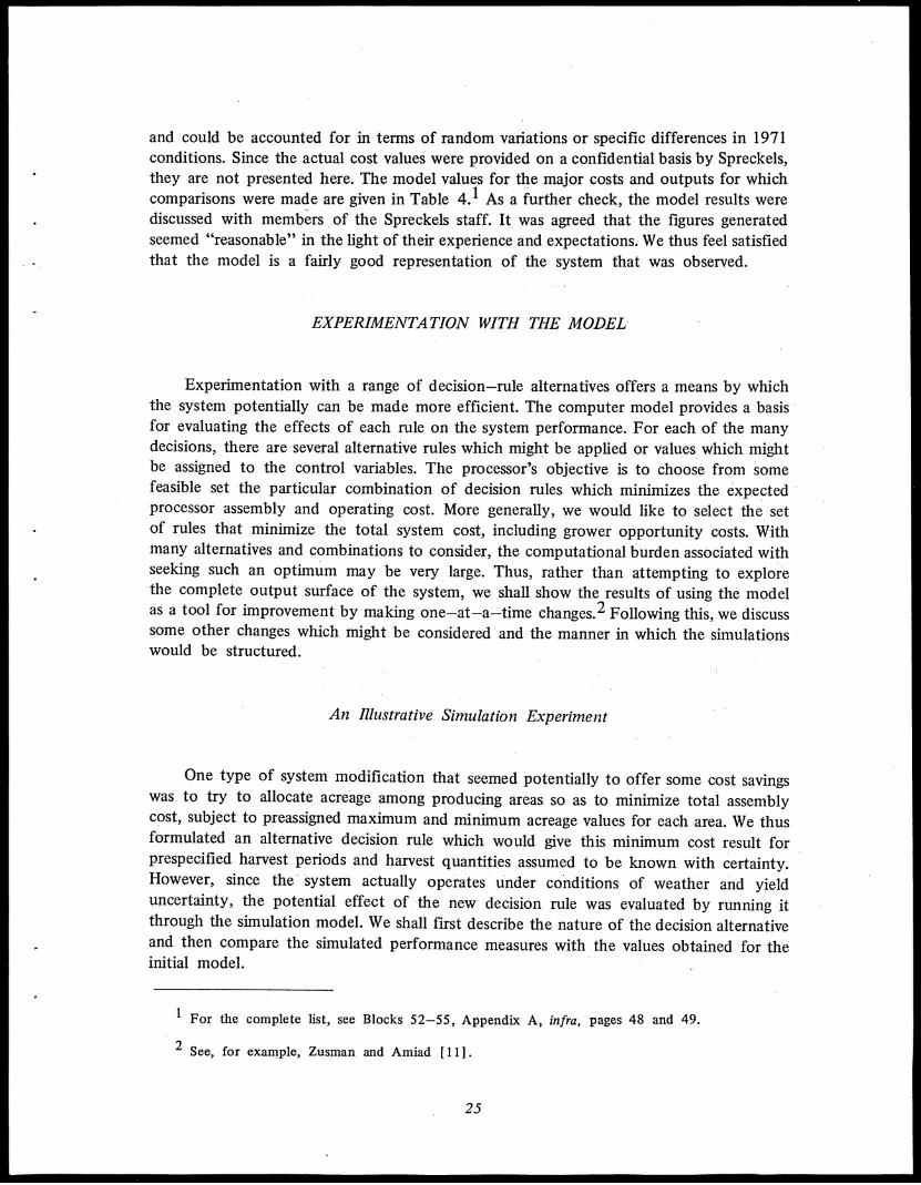
and could be accounted for in terms of random variations or specific differences in 1971conditions. Since the actual cost values were provided on a confidential basis by Spreckels,they are not presented here. The model values for the major costs and outputs for whichcomparisons were made are given in Table 4.1 As a further check, the model results werediscussed with members of the Spreckels staff. It was agreed that the figures generatedseemed "reasonable" in the light of their experience and expectations. We thus feel satisfiedthat the model is a fairly good representation of the system that was observed.

EXPERIMENTATION WITH THE MODEL

Experimentation with a range of decision—rule alternatives offers a means by whichthe system potentially can be made more efficient. The computer model provides a basisfor evaluating the effects of each rule on the system performance. For each of the manydecisions, there are several alternative rules which might be applied or values which mightbe assigned to the control variables. The processor's objective is to choose from somefeasible set the particular combination of decision rules which minimizes the expectedprocessor assembly and operating cost. More generally, we would like to select the setof rules that minimize the total system cost, including grower opportunity costs. Withmany alternatives and combinations to consider, the computational burden associated withseeking such an optimum may be very large. Thus, rather than attempting to explorethe complete output surface of the system, we shall show the results of using the modelas a tool for improvement by making one—at—a—time changes.2 Following this, we discusssome other changes which might be considered and the manner in which the simulationswould be structured.

An Illustrative Simulation Experiment

One type of system modification that seemed potentially to offer some cost savingswas to try to allocate acreage among producing areas so as to minimize total assemblycost, subject to preassigned maximum and minimum acreage values for each area. We thusformulated an alternative decision rule which would give this minimum cost result forprespecified harvest periods and harvest quantities assumed to be known with certainty.However, since the system actually operates under conditions of weather and yielduncertainty, the potential effect of the new decision rule was evaluated by running itthrough the simulation model. We shall first describe the nature of the decision alternativeand then compare the simulated performance measures with the values obtained for theinitial model.

1 For the complete list, see Blocks 52-55, Appendix A, infra, pages 48 and 49.

2 See, for example, Zusman and Amiad 1111.

25

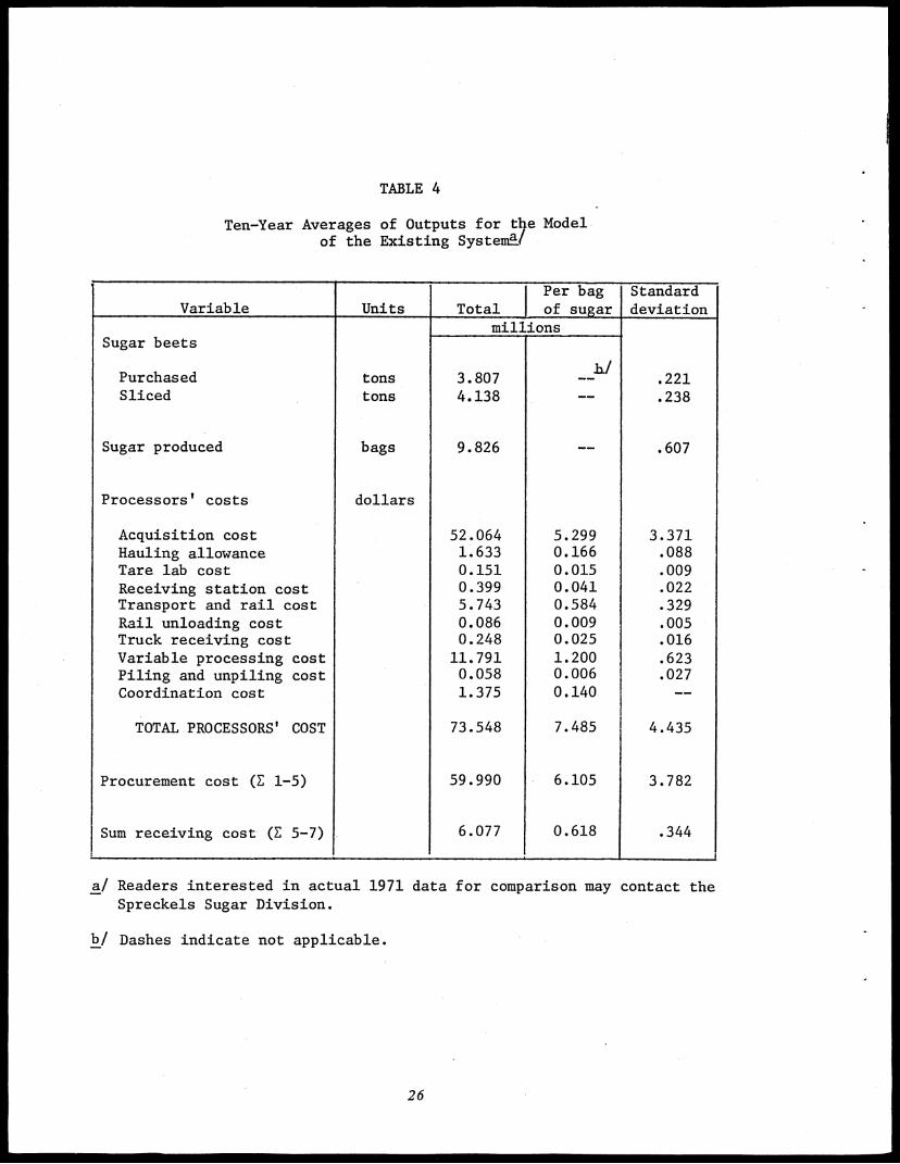
TABLE 4

Ten-Year Averages of Outputs for the Modelof the Existing System/

Variable

,

Units TotalPer bagof sugar

Standarddeviation

Sugar beetsmillions,

Purchased tons 3.807hi

.221Sliced tons 4.138 __ .238

Sugar produced

Processors' costs

bags

dollars

9.826 M. U. .607

Acquisition cost 52.064 5.299 3.371Hauling allowance 1.633 0.166 .088Tare lab cost 0.151 0.015 .009Receiving station cost 0.399 0.041 .022Transport and rail cost 5.743 0.584 .329Rail unloading cost 0.086 0.009 .005Truck receiving cost 0.248 0.025 .016Variable processing cost 11.791 1.200 .623Piling and unpiling cost 0.058 0.006 .027Coordination cost 1.375 0.140 --

TOTAL PROCESSORS' COST 73.548 7.485 4.435

Procurement cost (E 1-5) 59.990 6.105 3.782

Sum receiving cost E 5-7) 6.077 0.618 .344

'

a/ Readers interested in actual 1971 data for comparison may contact theSpreckels Sugar Division.

b/ Dashes indicate not applicable.

26

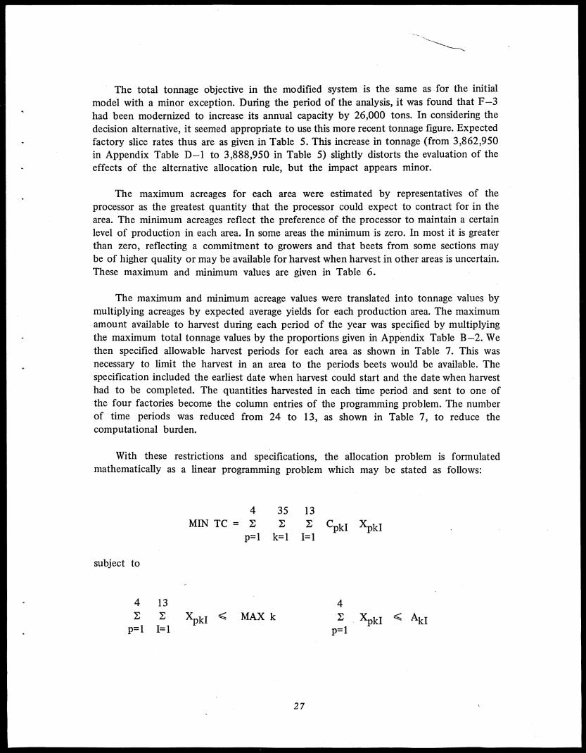
The total tonnage objective in the modified system is the same as for the initial

model with a minor exception. During the period of the analysis, it was found that F-3

had been modernized to increase its annual capacity by 26,000 tons. In considering the

decision alternative, it seemed appropriate to use this more recent tonnage figure. Expected

factory slice rates thus are as given in Table 5. This increase in tonnage (from 3,862,950

in Appendix Table D-1 to 3,888,950 in Table 5) slightly distorts the evaluation of the

effects of the alternative allocation rule, but the impact appears minor.

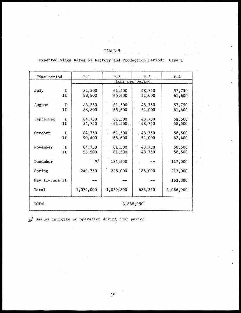
The maximum acreages for each area were estimated by representatives of the

processor as the greatest quantity that the processor could expect to contract for in thearea. The minimum acreages reflect the preference of the processor to maintain a certainlevel of production in each area. In some areas the minimum is zero. In most it is greaterthan zero, reflecting a commitment to growers and that beets from some sections maybe of higher quality or may be available for harvest when harvest in other areas is uncertain.These maximum and minimum values are given in Table 6.

The maximum and minimum acreage values were translated into tonnage values bymultiplying acreages by expected average yields for each production area. The maximumamount available to harvest during each period of the year was specified by multiplyingthe maximum total tonnage values by the proportions given in Appendix Table B-2. Wethen specified allowable harvest periods for each area as shown in Table 7. This wasnecessary to limit the harvest in an area to the periods beets would be available. Thespecification included the earliest date when harvest could start and the date when harvesthad to be completed. The quantities harvested in each time period and sent to one ofthe four factories become the column entries of the programming problem. The numberof time periods was reduced from 24 to 13, as shown in Table 7, to reduce thecomputational burden.

With these restrictions and specifications, the allocation problem is formulatedmathematically as a linear programming problem which may be stated as follows:

4 35 13MIN TC = E E CpkI XpkI

p=1 k=1 1=1

subject to

4 13 4E Xpu < MAX k XpkI AkI

p=1 1=1 p=1

27

TABLES

Expected Slice Rates. by Factory and Production Period: Case I

Time period F-1 F-2 1 F-3 F-4._ _tons per period

,_

July I 82,500 61,500 48,750 57,750II 88,800 65,600 52,000 61,600

August I 83,250 61,500 48,750 57,750II 88,800 65,600' '. 52,000 61,600

September I 84,750 61,500 48,750 58,500II 84,750 .61,500. 48,750 58,500

October I 84,750 61,500 48,750 58,500II 90,400 65,600 52,000 62,400

November I .84,750 61,500 - 48,750 58,500II 56,500 61;500 " 48,750 58,500

,December --a/ 184,500 ...._ 117,000

Spring 249,750 228,000 186,000 213,000

May II-June II 163,300

Total 1,079,000 1,039;800 683,250 1,086,900

,

TOTAL 3,888,950

a/ Dashes indicate no operation during that period.

28

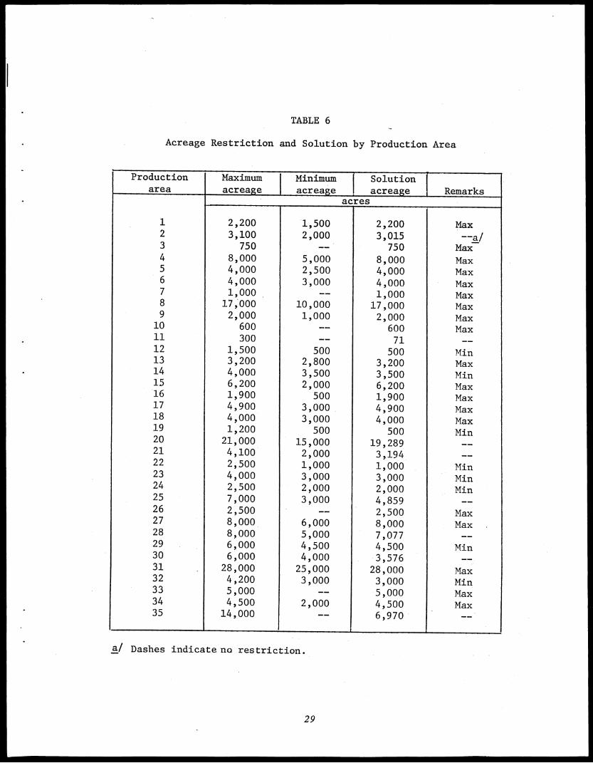
TABLE 6

Acreage Restriction and Solution by Production Area

Productionarea

Maximumacreaze

Minimumacreage

Solutionacreage_J Remarks

acres

1 2,200 1,500 2,200 Max2 3,100 2,000 3,015 --a/_...3 750 ...... 750 Max4 8,000 5,000 8,000 Max5 4,000 2,500 4,000 Max6 4,000 3,000 4,000 Max7 1,000 __ 1,000 Max8 17,000 10,000 17,000 Max9 2,000 1,000 2,000 Max10 600 ........ 600 Max11 300 __ 71 --12 1,500 500 500 Min13 3,200 2,800 3,200 Max14 4,000 3,500 3,500 Min15 6,200 2,000 6,200 Max16 1,900 500 1,900 Max17 4,900 3,000 4,900 Max18 4,000 3,000 4,000 Max19 1,200 500 500 Min20 21,000 15,000 19,289 --21 4,100 2,000 3,194 --22 2,500 1,000 1,000 Min23 4,000 3,000 3,000 Min24 2,500 2,000 2,000 Min25 7,000 3,000 4,859 --26 2,500 __ 2,500 Max27 8,000 6,000 8,000 Max .28 8,000 5,000 7,077 --29 6,000 4,500 4,500 Min30 6,000 4,000 3,576 --31 28,000 25,000 28,000 Max32 4,200 3,000 3,000 Min33 5,000 ..._ 5,000 Max34 4,500 2,000 4,500 Max35 14,000 ..._ 6,970

a/ Dashes indicate no restriction.

29

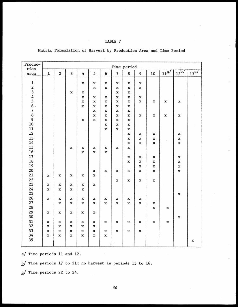
TABLE 7

Matrix Formulation of Harvest by Production Area and Time Period

Produc-tion - Time period .,

area 1 2 3 4 5 I 6 7 . 8 9 I 1011.4../

1212/

13-S1

1 x x x x x x2 x x x x x3 x x x x4 x x x x x x5 x x x x x x x x x

7 x x x x8 x x x x x x x9 x x x x x10 x x x11 x x x12 x x x x13 x x x x14 x x x x15 x x x x x x16 x x x17 x x x x18 x x x x19 x x x20 x x x x x x x21 x x x x x22 x x x23 x x x x x24 x x x x25 x26 x x x x x x x x x •27 x x x x x x x x28 x x29 x x x x x30 x31 x x x x x x x x x x x32 x x x x x33 x x x x x x x x x34 x x x x x x35 x

a/ Time periods 11 and 12.

b/ Time periods 17 to 21; no harvest in periods 13 to 16.

Cl Time periods 22 to 24.

1.1

30

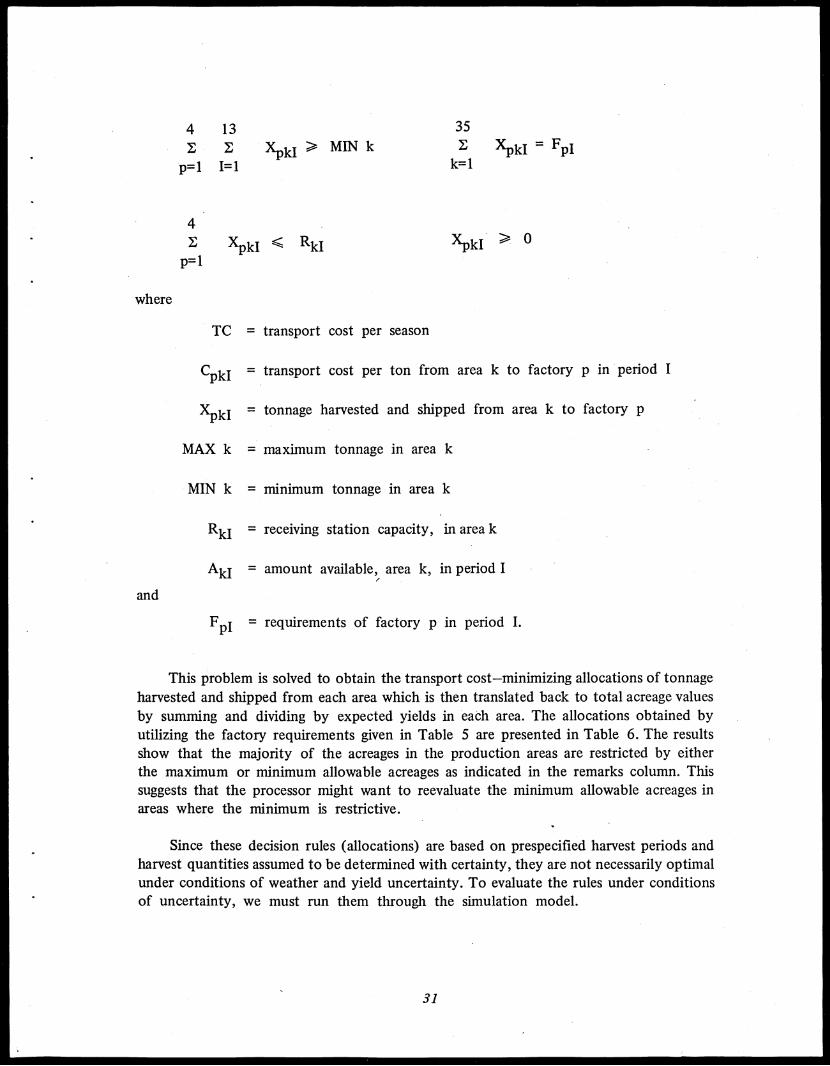
where

and

4 13I Ip=1 1=1

4

XpkI RkIp=1

MIN k

35

XpkI = FpIk=1

xpu

TC = transport cost per season

CpkI = transport cost per ton from area k to factory p in period I

XpkI = tonnage harvested and shipped from area k to factory p

MAX k = maximum tonnage in area k

MIN k = minimum tonnage in area k

RkI = receiving station capacity, in area k

AkI = amount available, area k, in period I

F = requirements of factory p in period I.

This problem is solved to obtain the transport cost—minimizing allocations of tonnage

harvested and shipped from each area which is then translated back to total acreage values

by summing and dividing by expected yields in each area. The allocations obtained by

utilizing the factory requirements given in Table 5 are presented in Table 6. The results

show that the majority of the acreages in the production areas are restricted by eitherthe maximum or minimum allowable acreages as indicated in the remarks column. Thissuggests that the processor might want to reevaluate the minimum allowable acreages inareas where the minimum is restrictive.

Since these decision rules (allocations) are based on prespecified harvest periods andharvest quantities assumed to be determined with certainty, they are not necessarily optimalunder conditions of weather and yield uncertainty. To evaluate the rules under conditionsof uncertainty, we must run them through the simulation model.

31

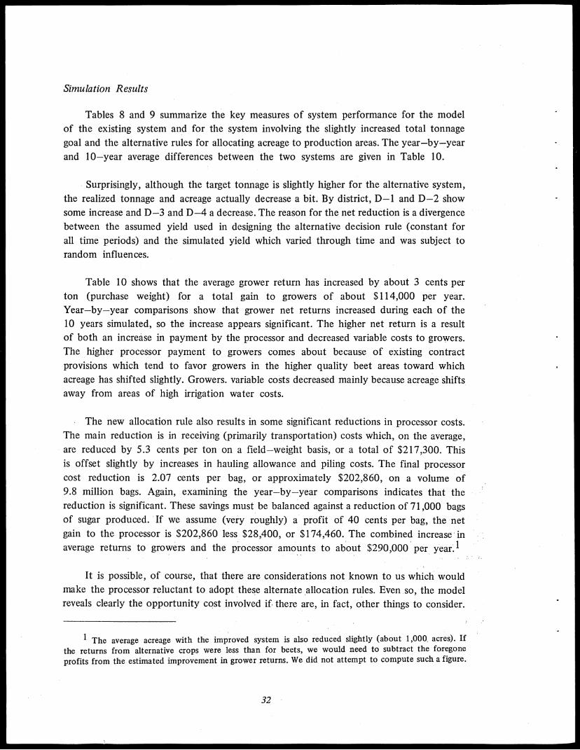
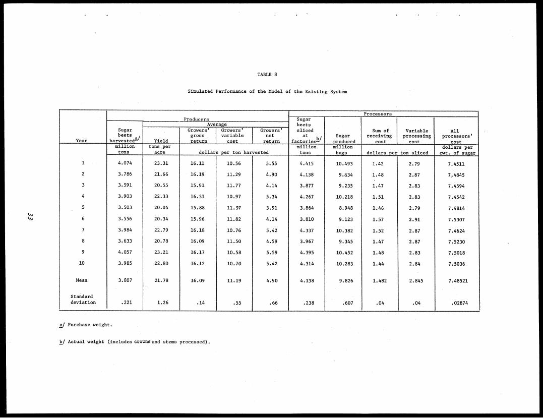
Simulation Results

Tables 8 and 9 summarize the key measures of system performance for the model

of the existing system and for the system involving the slightly increased total tonnage

goal and the alternative rules for allocating acreage to production areas. The year—by—year

and 10—year average differences between the two systems are given in Table 10.

Surprisingly, although the target tonnage is slightly higher for the alternative system,

the realized tonnage and acreage actually decrease a bit. By district, D-1 and D-2 show

some increase and D-3 and D-4 a decrease. The reason for the net reduction is a divergence

between the assumed yield used in designing the alternative decision rule (constant for

all time periods) and the simulated yield which varied through time and was subject to

random influences.

Table 10 shows that the average grower return has increased by about 3 cents per

ton (purchase weight) for a total gain to growers of about $114,000 per year.

Year—by—year comparisons show that grower net returns increased during each of the10 years simulated, so the increase appears significant. The higher net return is a resultof both an increase in payment by the processor and decreased variable costs to growers.

The higher processor payment to growers comes about because of existing contract

provisions which tend to favor growers in the higher quality beet areas toward which

acreage has shifted slightly. Growers. variable costs decreased mainly because acreage shiftsaway from areas of high irrigation water costs.

The new allocation rule also results in some significant reductions in processor costs.The main reduction is in receiving (primarily transportation) costs which, on the average,are reduced by 5.3 cents per ton on a field—weight basis, or a total of $217,300. Thisis offset slightly by increases in hauling allowance and piling costs. The final processorcost reduction is 2.07 cents per bag, or approximately $202,860, on a volume of9.8 million bags. Again, examining the year—by—year comparisons indicates that thereduction is significant. These savings must be balanced against a reduction of 71,000 bagsof sugar produced. If we assume (very roughly) a profit of 40 cents per bag, the netgain to the processor is $202,860 less $28,400, or $174,460. The combined increase inaverage returns to growers and the processor amounts to about $290,000 per year.1

It is possible, of course, that there are considerations not known to us which wouldmake the processor reluctant to adopt these alternate allocation rules. Even so, the modelreveals clearly the opportunity cost involved if there are, in fact, other things to consider.

1 The average acreage with the improved system is also reduced slightly (about 1,000. acres). If

the returns from alternative crops were less than for beets, we would need to subtract the foregone

profits from the estimated improvement in grower returns. We did not attempt to compute such a figure.

32

tA)

TABLE 8

Simulated Performance of the Model of the Existing System

Year

ProducersProcessors

Sugarbeetsslicedat

b/ factories-

Sugarproduced

Sum ofreceiving

cost

Variableprocessingcost

Allprocessors'

cost

Sugarbeets

/a harvested-

Average

- Yield

Growers'grossreturn

Growers'variable

cost

Growers'netreturn

million tons per million million dollars per ,

tons acre , dollars per ton harvested tons baDs dollars per ton sliced cwt. of sugar

1 4.074 23.31 16.11 10.56 5.55 4.415 10.493 1.42 2.79 7.4511

2 3.786 21.66 16.19 11.29 4.90 4.138 9.834 1.48 2.87 7,4845

3 3.591 20.55 15.91 11.77 4.14 3.877 9.235 1.47 2.83 7.4594

4 3.903 22.33 16.31 10.97 5.34 4.267 10.218 1.51 2.83 7.4542

5 3.503 20.04 15.88 11.97 3.91 3.864 8.948 1.46 2.79 7.4814

6 3.556 20.34 15.96 11.82 4.14 3.810 9.123 1.57 2.91 7.5307

7 3.984 22.79 16.18 10.76 5.42 4.337 10.382 1.52 2.87 7.4624

8 3.633 20.78 16.09 11.50 4.59 3.967 9.345 1.47 2.87 7.5230

9 4.057 23.21 16.17 10.58 5.59 4.395 10.452 1.48 2.83 7.5018

10 3.985 22.80 16.12 10.70 5.42 4.314 10.283 1.44 2.84 7.5036

Mean 3.807 21.78 16.09 11.19 4.90 4.138 9.826 1.482 2.845 7.48521

Standarddeviation .221 1.26 .14 .55 .66 .238 .607 .04 .04 .02874

_

a/ Purchase weight.

b/ Actual weight (includes crowasand stems processed).

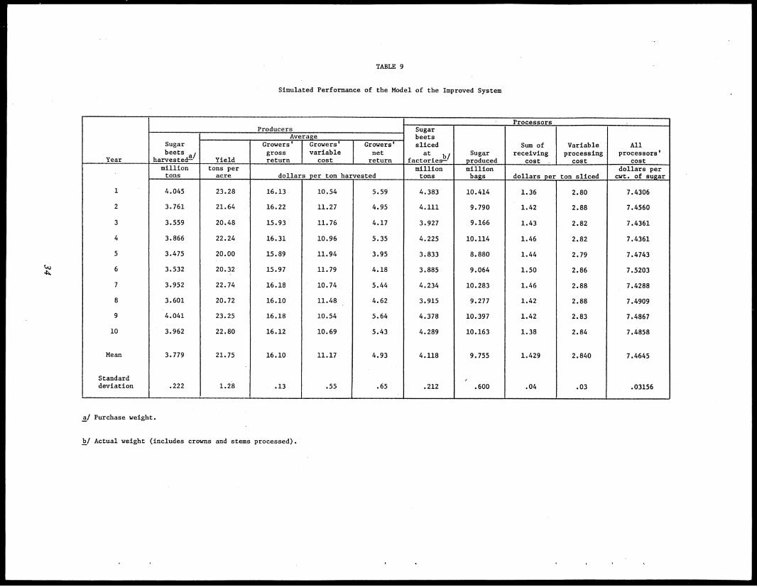
TABLE 9

Simulated Performance of the Model of the Improved System

Year ,

Producers- Processors .

Sugarbeetsslicedat bi

factories-1Sugarproduced

Sum ofreceiving

cost .

Variableprocessingcost

Allprocessors'

cost

Sugarbeets a/

harvested-

Average

Yield

,Growers'grossreturn

Growers'variable

cost

Growers'netreturn

million tons per million million_

dollars pertons acre dollars per ton harvested tons bags dollars per ton sliced cwt. of sugar

1 4.045 23.28 16.13

_

10.54 5.59 4.383

.

10.414 1.36 2.80 7.4306

2 3.761 21.64 16.22 11.27 4.95 4.111 9.790 1.42 2.88 7.4560

3 3.559 20.48 15.93 11.76 4.17 3.927 9.166 1.43 2.82 7.4361

4 3.866 22.24 16.31 10.96 5.35 4.225 10.114 1.46 2.82 7.4361

5 3.475 20.00 15.89 11.94 3.95 3.833 8.880 1.44 2.79 7.4743

6 3.532 20.32 15.97 11.79 4.18 3.885 9.064 1.50 2.86 7.5203

7 3.952 22.74 16.18 10.74 5.44 4.234 10.283 1.46 2.88 7.4288

8 3.601 20.72 16.10 11.48 . 4.62 3.915 9.277 1.42 2.88 7.4909

9 4.041 23.25 16.18 10.54 5.64 4.378 10.397 1.42 2.83 7.4867

10 3.962 22.80 16.12 10.69 5.43 4.289 10.163 1.38 2.84 7.4858

Mean 3.779 21.75 16.10 11.17 4.93 4.118 9.755 1.429 2.840 7.4645

Standarddeviation .222 1.28 .13 .55 .65 .212

,.600 .04 .03 .03156

a/ Purchase weight.

b/ Actual weight (includes crowns and stems processed).

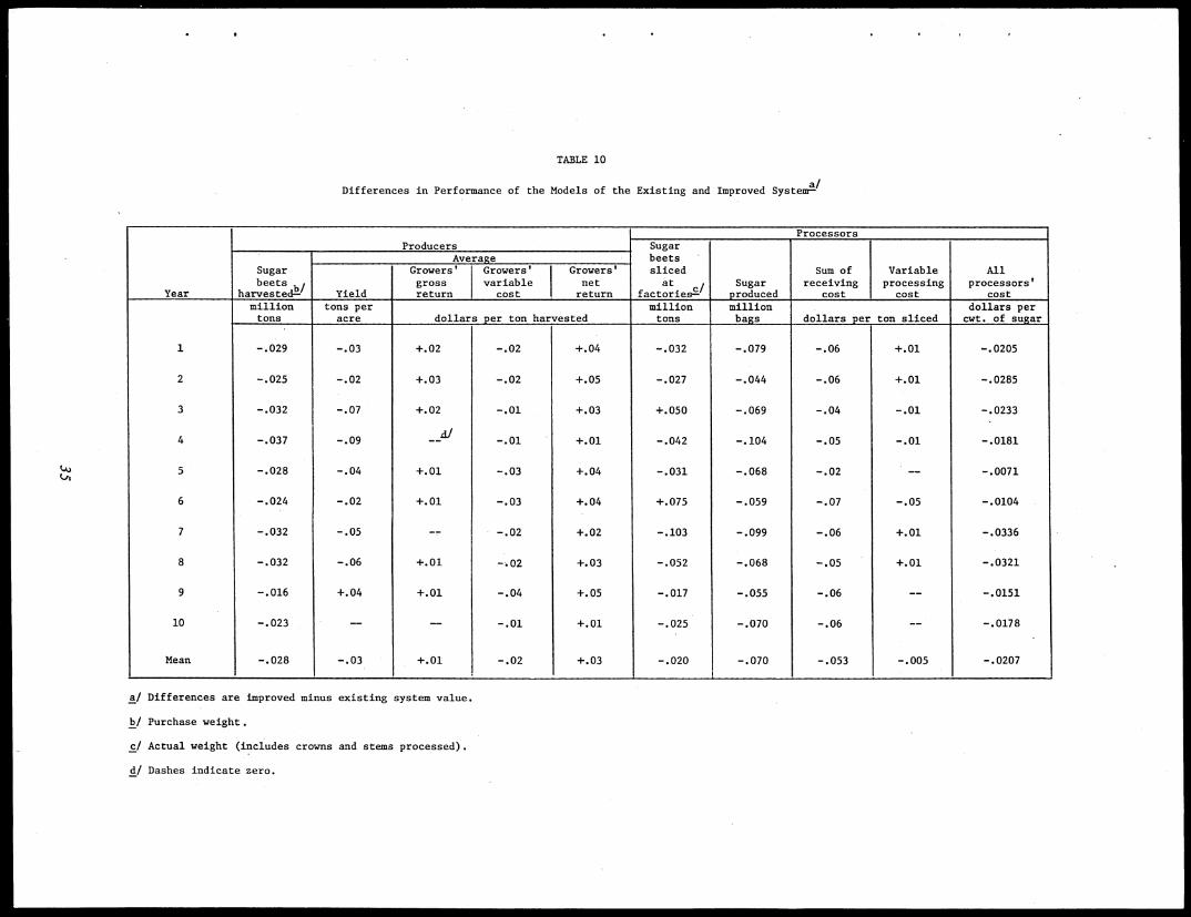
TABLE 10

aDifferences in Performance of the Models of the Existing and Improved System

/-

Year

ProducersProcessors

Sugarbeets .slicedat c/

factories-sSugarproduced

Sum ofreceiving

cost

Variableprocessing

cost

Allprocessors'

cost

Sugarbeets

b/harvested -

Average

Yield ,

Growers'grossreturn

Growers'variable

cost

Growers'netreturn

million tons per million million dollars pertons acre dollars yer ton harvested tons bags dollars per ton sliced cwt. of sugar

1 -.029

,

-.03 +.02 -.02 +.04 -.032

,

-.079 -.06 +.01 -.0205

2 -.025 -.02 +.03 -.02 +.05 -.027 -.044 -.06 +.01 -.0285

3 -.032 -.07 +.02 -.01 +.03 +.050 -.069 -.04 -.01 -.0233

4 -.037 -.09__.A/

-.01 +.01 -.042 -.104 -.05 -.01 -.0181

5 -.028 -.04 +.01 -.03 +.04 -.031 -.068 -.02 ...... -.0071

6 -.024 -.02 +.01 -.03 +.04 +.075 -.059 -.07 -.05 -.0104

7 -.032 -.05 __ -.02 +.02 -.103 -.099 -.06 +.01 -.0336

8 -.032 -.06 +.01 -.02 +.03 -.052 -.068 -.05 +.01 -.0321

9 -.016 +.04 +.01 -.04 +.05 -.017 -.055 -.06 -- -.0151

10 -.023 -- ...... -.01 +.01 -.025 -.070 -.06 -- -.0178

Mean -.028 -.03 +.01 -.02 +.03 -.020 -.070 -.053 -.005 -.0207

_., . . I

a/ Differences are improved minus existing system value.

b/ Purchase weight.

c/ Actual weight (includes crowns and stems processed).

d/ Dashes indicate zero.

Other Experiments

Exploration of other decision rule alternatives and systems changes may reveal

additional possibilities for improvement. Although we would expect the potential gains

to be modest in percentage terms, they may be significant in absolute amounts and seemlikely to be large in total relative to the cost of formulating and using this type of simulationmodel. Several other potential experiments are discussed below. We have not carried outthe actual computations since our goal is not primarily one of redesigning this particularsystem but rather to stimulate the thinking of managers and economic analysts concerningthe potential value and uses of this type of system modeling.

Tonnage and Acreage Decisions

Given the objective of producing maximum sugar (under current conditions) and facedwith possible restrictions on production in future periods, management planning clearlywould be enhanced by measures of the likely cost effects of decreases in production orefforts to increase production. Such measures may be obtained by varying the valuesassigned to total tonnage and the associated values of total acreage and acreage allocatedto each production area. Such changes must, of course, be consistent with factory andharvest capacities.

To illustrate how this might be modeled, consider the following alternative situations.

Case L Suppose that modifications of F-3 permit an increase in slice of 26,000 tonsof beets during the period July—November. Appendix Table D-1 values then might bemodified as in Table 5, with the F-3 column changed. As noted previously, thismodification was, in fact, considered and implemented during the period of the analysis.

Case IL Production is to be reduced by 534,800 tons with F-3 quantities stillspecified as in Table 5 and the reduction in tonnage coming from F-1. The expectedslice rates by factories and time periods thus might be as in Table 11. This reductionwas selected to make F-1 self—sufficient on beets harvested in D-1. This would eliminatethe costly transportation charges incurred when other districts ship to F-1.

Given these situations and specified expected slice rates, the acreage required wouldbe 173,801 for Case I and 148,772 for Case II. These acreages then must be allocatedto production areas. The proportions specified for the existing model could be used(Appendix Table B-2) or, perhaps more efficiently, the alternative method that minimizesexpected assembly costs of the processor subject to maximum and minimum acreagerestrictions for each area.

36

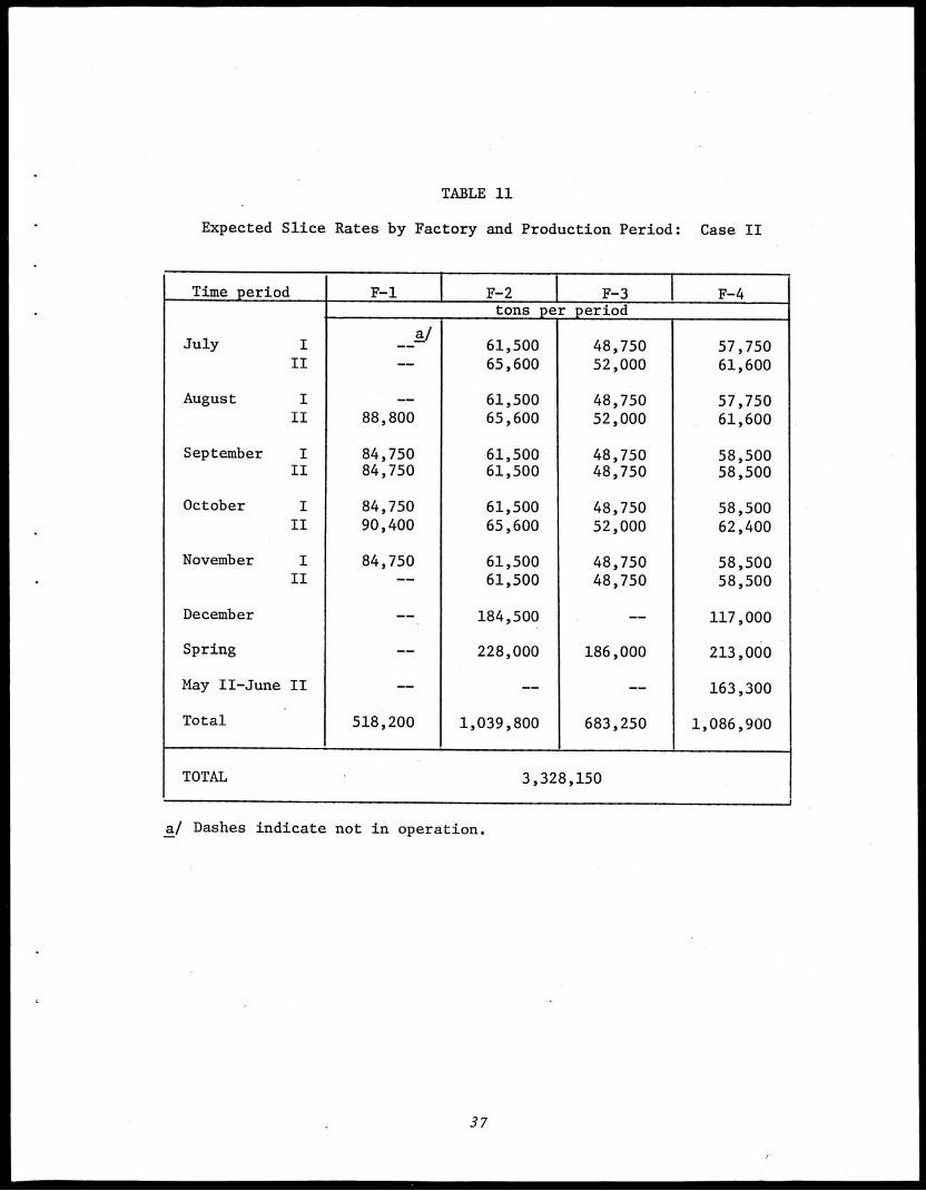
TABLE 11

Expected Slice Rates by Factory and Production Period: Case II

Time period F-1 F-2 I F-3 F-4tons per period

July Ia/. _

61,500 48,750 57,750II ...... 65,600 52,000 61,600

August I 61,500 48,750 57,750II 88,800 65,600 52,000 61,600

September I 84,750 61,500 48,750 58,500II 84,750 61,500 48,750 58,500

October I 84,750 61,500 48,750 58,500II 90,400 65,600 52,000 62,400

November I 84,750 61,500 48,750 58,500II 61,500 48,750 58,500

December _... 184,500 __ 117,000

Spring ...... 228,000 186,000 213,000

May II-June II __ __ __ 163,300

Total 518,200 1,039,800 683,250 1,086,900

TOTAL 3,328,150

1

a/ Dashes indicate not in operation.

37

Factory Supply Sources

The supply sources for each factory for the existing system are specified in

Appendix Table D-3. Many of these specifications are not subject to meaningful change.

However, there are some possible variations that might be considered, such as shifting

the date when D-3 replaced D-4 as the district which supplies any quantity that D-1

is unable to provide for F-1. Changes in Appendix Table D-3 would affect harvest period

decisions also as indicated in the discussion of the existing system decision rules.

Factory Starting Date Decisions

Opportunities for varying this decision variable are also somewhat limited, but it mightbe of interest to consider the effect of having F-1 start when the amount available toharvest in D-1 equals or exceeds the harvest level required for the operation of F-1.This would replace the more complex decision rule outlined for the existing system.

Standard Inventory Levels

The standard factory beet inventory levels specified for each period were determinedin the initial model on the basis of historical practice. It would be of interest to seehow variations in levels at different times might affect operating costs. These variationswould be aimed at reducing sugar losses during some period or, by increasing levels inthe winter, extending the period of factory operations.

Planting Dates

The method of assigning planting dates in the initial model was based on empiricalestimates that determined mean planting dates as a function of the value of the moistureindex. By using these critical levels, but varying the earliest date that the mean plantingdate could occur, changes in the normal planting periods could be assessed.

Quantity Harvested in Each• District

The existing decision rules reflect the management policy that requires D-2 and D-3to complete harvest at about the same time. The opportunity of this policy might beevaluated by replacing the rule specified for May—June with the rule specified forJuly —Septemb er.1

1 For rules for the existing systems, see Appendix D, infra, page 77.

38

Quantity Harvested in Each Production Areain Each Time Period

When the total acreage and allocation of acreage to production area changes, it isdesirable to make the associated changes in the decision parameters which determine thequantity harvested in each production area in each time period. For example, in theillustrative simulation experiment, changes were made in the proportions listed inAppendix Table D-9 as well as reducing the quantity of two D-4 areas previouslyoperating at receiving station capacity. Options for considering changes in the quantitiesharvested in D-1, D-2, and D-3 during the fall are limited to changes in the quantityavailable for harvest. The consequences of attempts of earlier harvest in these areas couldbe evaluated by the model.

Delivery Routes

The model could be utilized to evaluate the effects of constructing new receivingstations or alternatively closing existing stations (or any combination thereof). New costsestimates would have to be established for grower's hauling costs, hauling allowance, andtransit costs from the receiving station to the factories.

Factory Operation

It would be of interest to consider the effects on cost of shifting the first allowabledate for closing down factories from November II (I = 10) to December I (I = 11) andmoving the start—up date of F-1 from March II to March I, thus adding to the potentialof operation. This may be done by respecifying the allowable date that F-1 can openin the spring (a control variable in the program).

Changes in Parameters

Although the parameters of the model are not directly controllable in the sense ofdecision variables, management may find it useful to assess the potential effects of changesin some of these constants. For 'example, changes in expected yields may affect acreageand allocation decisions, and changes in transportation costs may affect delivery routesand methods, with resulting alterations in the total system cost. Answers to questionsconcerning such parameter changes may be obtained readily by simply changing theconstants of interest in the model. The computer then generates the measures of systemperformance. Since computer time is not free, the purposes and form of such parameterexplorations should, of course, be considered carefully in advance.

39

SUMMARY AND CONCLUSIONS

With advancing technology and continuing industrialization of agriculture, the separateproducing and marketing systems for many agricultural commodities, once coordinatedalmost entirely by prices, have evolved increasingly into sets of integrated systems forpurposes of output determination and scheduling of activities. 'Growers, processors, andconsumers all have an interest in the way these systems operate, for the methods ofcoordination affect returns to growers, costs of processors, and, ultimately, prices paidby consumers. Because of the interrelated activities involved and the many weather andbiological uncertainties, it is often very difficult to evaluate the expected consequencesof alternative coordination decision rules that might be adopted. One means of aidingthe decision process is to construct a model that simulates the behavior of the systemunder uncertainty and to use the model, via computer, to evaluate the effects of differentdecision rules or changes in the system. This study develops such a model for a sugarbeet production—processing system consisting of about 1,000 growers and a singleprocessor with four plants.

Nature of the Model

The model consists of a set of equations which determines the state of the systemat each discrete point in time as functions of previous states, random weather and biologicalfactors, and the values assigned to decision variables controlled by management, such asacres to be planted or harvested. The state of the system is measured by variables, suchas acres available to harvest, acres actually harvested, yield, and tons delivered to factories.Costs and returns to growers and processors, which are the primary measures of systemperformance, are determined by values of the state variables.

The model operates by first establishing rules which determine the values assignedto decision variables. These may be expressed as functions of the state of the systemor, in some cases, as predetermined constants. These rules and constants, along with otherconstants such as extraction factors and transport costs, are read into the computer. Thestate of the system for the first period (first half of July) is determined by the preplantingand planting decisions and by setting initial values of other state variables, such as beetinventories, at zero. Values are generated for weather events and other random variables.Yields and quantities available for harvest are determined by functional relationships, andthe quantities harvested are determined by the harvest period decision rules and weatherconditions. Other decision rules, behavioral relationships, and identities then determineshipment patterns, the quantities of beets sliced, and the sugar produced. The computeradvances time to the next period and continues these calculations sequentially for eachperiod until rain forces termination of the harvest. Operations are resumed again in thespring, according to the factory start—up rules, and continue until harvest in all areashas been completed which occurs by July 1. Accumulated cost and output values arethen computed for the year.

40

Because of the random elements involved, each year is different. Average values of

costs, returns and outputs and measures of variation are obtained by making repeatedsimulation runs for each decision situation.

The model was tested by comparing reported cost values with simulated valuesdetermined under generally similar conditions and by consulting with processor personnelconcerning the "reasonableness" of the results. We concluded that the initial model was,in fact, a reasonable representation of the real system modeled.

Uses of the Model

The principal value of the model is that it permits us to evaluate effects of changesin the system in a dynamic and uncertain framework without actually disturbing the systemitself. Decision rules are the most easily altered part of the system since they are directlycontrolled by management. Since the model includes 10 types of decisions, each withseveral alternative rules which plausibly might be considered, the potential number ofvariations is very large. Because of the considerable amount of computer time involved,we did not attempt to evaluate all of these possibilities. Instead, we selected one alternativethat seemed particularly promising to illustrate the experimental procedure and theoutcome and then suggested one or two alternative formulations for each type of decision.

The alternative decision rule considered pertains to the method of allocating acreagecontracted among producing areas. The new rule was derived by using linear programmingto minimize expected transportation costs to factories, subject to maximum and minimumacreage limitations in each production area. Harvest patterns were assumed to be knownwith certainty. The alternate decision rule then was evaluated under uncertain conditionsby the simulation procedure.

Comparing results with the original model suggested potential increases in returnsto growers averaging $114,000 per year and a reduction in processor costs averaging about$203,000 per year. Since production was slightly reduced, it was necessary to deductpotential profit losses of about $28,000 for the processor from these values, leaving apotential average net gain of about $290,000 per year. Year—to—year comparisons suggestthese average gains were not a chance result.

Other potential uses of the model are to (1) evaluate the effect of changes in systemparameters, (2) consider cost effects of organizational changes, such as adding anotherfactory or closing an existing one, and (3) evaluate the value of additional informationthat might be obtained (at a cost) concerning some of the random elements affectingthe system.

41

Parameter changes, such as variations in transportation cost, may be evaluated bysimply changing the constants of interest and then letting the computer generate newvalues of system—operating costs and output.

Consideration of organizational changes would require a few modifications and somereprogramming, but this would not be difficult. This type of modification would alsoprovide a means of evaluating alternative factory locations.

It may be possible, at some cost, to obtain improved predictions of yields or evenweather during particular years. In such cases alternative strategies or decision rules maylead to better outcomes than suggested for the case where only the prior probabilitiesare available. The model provides a means of generating the data needed to evaluate thevalue of such additional information and to suggest improved strategies.

With modifications to fit specific local environments, the model may be adaptedreadily to the analysis of other sugar beet systems.

Suggestions for Further Analysis

Although the model appears to be a good representation of the actual system, thereare some ways in which it might be refined or improved. First, with more detailed datait would be possible to improve the yield relationships. It would be desirable to haveyield data for smaller areas with information on fertilizer, spraying and irrigation practices,soil characteristics, and more precisely defined planting and harvest dates. If successfullyincorporated into the yield equations, this would permit a more accurate evaluation ofthe potential effects of overwintering and variations in planting and harvest dates whichperhaps could lead to improved harvest rules.

Another desirable extension would be some disaggregation of the grower component.The present model treats growers as a group in each area. If data pertaining to individualfarms could be obtained and included in the model, the distribution of effects of alternativedecision rules and policies could be more readily evaluated. Of course, this would alsoincrease the complexity and number of computations required but probably would bewell worth the added computer time.

Conclusions

Our experience in formulating and experimenting with this model leads finally tothree conclusions which we believe to be quite significant. First, the present real systemseems relatively efficient. Our experiments with the model did not and likely would notuncover any possibilities for spectacular improvements. Nor did we observe any

42

organizational characteristics which, if changed, are likely to lead to large reductions in

cost. In this sense, we conclude that the existing system is functioning very well.

On the other hand, the study did reveal the possibility of achieving some modestgains. Our second conclusion is that development of this type of modeling by the processoror by industry groups would offer a potentially very high return on investment. A research

expenditure of perhaps $20,000 to $40,000 the first year and probably less later couldeasily uncover possible costs savings of several times that amount. Most investors wouldbe exceedingly pleased with such returns.

Finally, we feel the development of this type of model would be a very useful exercise

for the staff of many processing firms. The act of formulating and using the model forcesa degree of rigor into thought processes that can provide greater insight into the natureof the operations. The systems thinking required and the interaction of the analyst withimaginative management seem likely to stimulate ideas that go well beyond the initialmodeling requirements. Although these intangible values are difficult to measure, theymay very well exceed the more directly quantified benefits.

43

..

,

APPENDIX A

Sequence of Computer Calculations

...

44

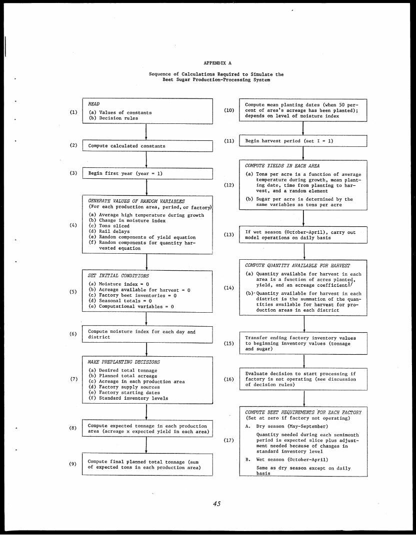
(1)

(2)

(3)

(4)

(5)

(6)

(7)

(8)

(9)

APPENDIX A

Sequence of Calculations Required to Simulate theBeet Sugar Production-Processing System

READ

(a) Values of constants(b) Decision rules

/

Compute calculated constants

Begin first year (year = 1)

GENERATE VALUES OF RANDOM VARIABLES(For each production area, period, or factory)

(a) Average high temperature during growth(b) Change in moisture index(c) Tons sliced(d) Rail delays(e) Random components of yield equation(0 Random components for quantity har-

vested equationI

SET INITIAL CONDITIONS

(a) Moisture index = 0(b) Acreage available for harvest = 0(c) Factory beet inventories = 0(d) Seasonal totals = 0(e) Computational variables = 0

,

Compute moisture index for each day anddistrict

1

MAKE PREPLANTING DECISIONS

(a) Desired total tonnage(b) Planned total acreage(c) Acreage in each production area(d) Factory supply sources(e) Factory starting dates(0 Standard inventory levels

Compute expected tonnage in each productionarea (acreage x expected yield in each area)

Compute final planned total tonnage (sumof expected tons in each production area)

(10)

(12)

(13)

(14)

(15)

(16)

Compute mean planting dates (when 50 per-cent of area's acreage has been planted);depends on level of moisture index

Begin harvest period (set I = 1)

COMPUTE YIELDS IN EACH AREA

(a) Tons per acre is a function of averagetemperature during growth, mean plant-ing date, time from planting to har-vest, and a random element

(b) Sugar per acre is determined by thesame variables as tons per acre

If wet season (October-April), carry outmodel operations on daily basis

COMPUTE QUANTITY AVAILABLE FOR HARVEST

(a) Quantity available for harvest in eacharea is a function of acres planted,yield, and an acreage coefficient-1J

(b)-Quantity available for harvest in eachdistrict is the summation of the quan-tities available for harvest for pro-duction areas in each district

Transfer ending factory inventory valuesto beginning inventory values (tonnageand sugar)

Evaluate decision to start processing iffactory is not operating (see discussionof decision rules)

COMPUTE BEET REQUIREMENTS FOR EACH FACTORY(Set at zero if factory not operating)

A. Dry season (May-September)

Quantity needed during each semimonthperiod is expected slice plus adjust-ment needed because of changes instandard inventory level

B. Wet season (October-April)

Same as dry season except on dailybasis

45

APPENDIX A--continued.

(18)

(19)

(20)

(21)

(22)

(23)

COMPUTE QUANTITIES HARVESTEDDISTRICT

A. Dry period

Decide on quantities

IN EACH

harvested in semi-determined byand amounts avail-

in each district (seerules)

daily as a func-index and normal

month period; amountsfactory requirementsable for harvestexplanation of decision

B. Wet period

Quantities determinedtion of moisturefactory requirements

COMPUTE QUANTITIES HARVESTEDPRODUCTION AREA

A. Dry period

Decide on quantities

IN EACH

to be harvestedamounts deter-

available forarea, re-expected

dates, and allo-explanation of

harvestedof daily quan-

the district andwhich vary with theindex

in semimonth period;mined by quantitiesharvest in the productionceiving station capacity,harvest completioncation quotas (seedecision rules)

B. Wet period

Determine daily quantitiesin area as a functiontity harvested inallocation ruleslevel of moisture

COMPUTE ACRES HARVESTED IN EACH PRODUCTIONAREA

Divide quantity harvested by current"semimonth period yield

COMPUTE SUGAR PERCENT FOR BEETS HARVESTEDIN EACH PRODUCTION AREA

Divide sugar produced per acre by tons peracre (from step 12)

1

COMPUTE ACCUMULATED TONS HARVESTED INEACH PRODUCTION AREA

Sum all quantities harvested up to andincluding the current period or day

1COMPUTE ACCUMULATED ACRES HARVESTED INEACH PRODUCTION AREA

Sum all acres harvested up to and in-cluding the current period or day

(24)

(25)

(26)

(27)

(28)

(29)

CONVERT TONNAGE HARVESTED TO FIRST NETAND FIELD WEIGHT BASIS

(a) First net weight (multiply purchase[second net] weight by constant cleanpercentage for each area)

(b) Field weight (multiply first net weightby a constant)

COMPUTE QUANTITIES REMAINING TO BEHARVESTED IN EACH PRODUCTION AREA

(a) Remaining acreage to harvest in eachproduction area (acres planted lessaccumulated acres harvested)

(b) Remaining tonnage to harvest in eachproduction area (remaining acreage xcurrent yield)

COMPUTE QUANTITIES REMAINING TO BEHARVESTED IN EACH DISTRICT

(a) Remaining acreage to harvest in eachdistrict (sum of remaining acreage forproduction areas in each district)

(b) Remaining tonnage to harvest in eachdistrict (sum of remaining tonnage forproduction areas in each district)

COMPUTE TOTAL COST BY PRODUCTION AREAAT END OF SEMEMONTH PERIOD

(a) Cultural cost (including opportunitycost; constant for each time period xnumber of acres harvested)

(b) Loading and harvest cost (linear func-tion of tons harvested)

MAKE DELIVERY ROUTE DECISIONS

(a) Quantity shipped from production areato receiving station

(b) Quantity shipped from receiving stationand .method of delivery (grower truck,rail, or transports; see explanationof decision rules)

1

If wet season (October-April), carry outmodel operations on a daily basis,2! withthe daily activities being summarized atthe end of the semimonth period

46

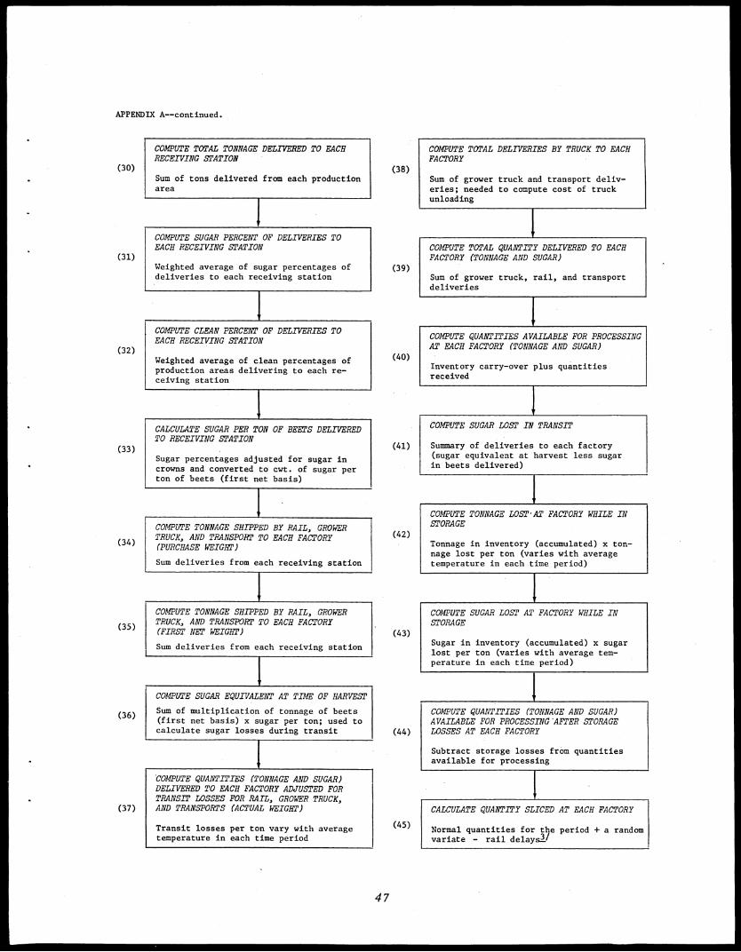
APPENDIX A--continued.

COMPUTE TOTAL TONNAGE DELIVERED TO EACHRECEIVING STATION

Sum of tons delivered from each productionarea

COMPUTE SUGAR PERCENT OF DELIVERIES TOEACH RECEIVING STATION

Weighted average of sugar percentages ofdeliveries to each receiving station

COMPUTE CLEAN PERCENT OF DELIVERIES TOEACH RECEIVING STATION

Weighted average of clean percentages ofproduction areas delivering to each re-ceiving station

CALCULATE SUGAR PER TON OF BEETS DELIVEREDTO RECEIVING STATION

Sugar percentages adjusted for sugar incrowns and converted to cwt. of sugar perton of beets (first net basis)

COMPUTE TONNAGE SHIPPED BY RAIL, GROWERTRUCK, AND TRANSPORT TO EACH FACTORY(PURCHASE WEIGHT)

Sum deliveries from each receiving station

COMPUTE TONNAGE SHIPPED BY RAIL, GROWERTRUCK, AND TRANSPORT TO EACH FACTORY(FIRST NET WEIGHT)

Sum deliveries from each receiving station

COMPUTE SUGAR EQUIVALENT AT TIME OF HARVEST

Sum of multiplication of tonnage of beets(first net basis) x sugar per ton; used tocalculate sugar losses during transit

COMPUTE QUANTITIES (L7ONIVIWE AND SUGAR)DELIVERED TO EACH FACTORY ADJUSTED FORTRANSIT LOSSES FOR RAIL, GROWER TRUCK,AND TRANSPORTS (ACTUAL WEIGHT)

Transit losses per ton vary with averagetemperature in each time period

(30) (38)

(31)

(32)

(33)

(34)

(35)

(36)

(37)

(39)

(40)

(41)

(42)

(43)

(44)

(45)

COMPUTE TOTAL DELIVERIES BY TRUCK TO EACHFACTORY

Sum of grower truck and transport deliv-eries; needed to compute cost of truckunloading

COMPUTE TOTAL QUANTITY DELIVERED TO EACHFACTORY (TONNAGE AND SUGAR)

Sum of grower truck, rail, and transportdeliveries

COMPUTE QUANTITIES AVAILABLE FOR PROCESSINGAT EACH FACTORY (TONNAGE AND SUGAR)

Inventory carry-over plus quantitiesreceived

COMPUTE SUGAR LOST IN TRANSIT

Summary of deliveries to each factory(sugar equivalent at harvest less sugarin beets delivered)

COMPUTE TONNAGE LOST AT FACTORY WHILE INSTORAGE

Tonnage in inventory (accumulated) x ton-nage lost per ton (varies with averagetemperature in each time period)

COMPUTE SUGAR LOST AT FACTORY WHILE INSTORAGE

Sugar in inventory (accumulated) x sugarlost per ton (varies with average tem-perature in each time period)

/

COMPUTE QUANTITIES (TONNAGE AND SUGAR)AVAILABLE FOR PROCESSING 'AFTER STORAGELOSSES AT EACH FACTORY

Subtract storage losses from quantitiesavailable for processing

CALCULATE QUANTITY SLICED AT EACH FACTORY

Normal quantities for the period + a randomvariate - rail delaysli

47

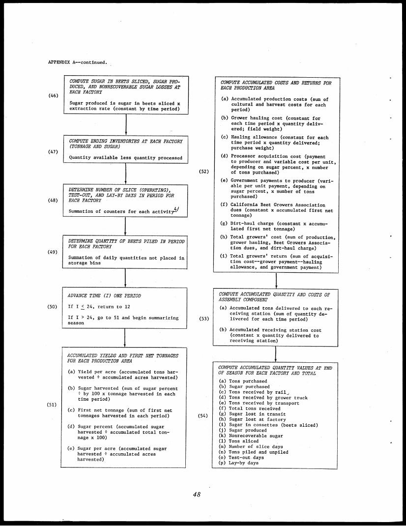
APPENDIX A--continued.

(46)

(47)

(48)

(49)

(50)

(51)

COMPUTE SUGAR IN BEETS SLICED, SUGAR PRO-DUCED, AND NONRECOVERABLE SUGAR LOSSES ATEACH FACTORY

Sugar produced is sugar in beets sliced xextraction rate (constant by time period)

COMPUTE ENDING INVENTORIES AT EACH FACTORY(TONNAGE AND SUGAR)

Quantity available less quantity processed

DETERMINE NUMBER OF SLICE (OPERATING),TEST-OUT, AND LAY-BY DAYS IN PERIOD FOREACH FACTORY

Summation of counters for each activity4/

DETERMINE QUANTITY OF BEETS PILED IN PERIODFOR EACH FACTORY

Summation of daily quantities not placed instorage bins

ADVANCE TIME (I) ONE PERIOD

If I < 24, return to 12

If I > 24, go to 51 and begin summarizingseason

ACCUMULATED YIELDS AND FIRST NET TONNAGESFOR EACH PRODUCTION AREA

(a) Yield per acre (accumulated tons har-vested + accumulated acres harvested)

(b) Sugar harvested (sum of sugar percent+ by 100 x tonnage harvested in eachtime period)

(c) First net tonnage (sum of first nettonnages harvested in each period)

(d) Sugar percent (accumulated sugarharvested + accumulated total ton-nage x 100)

(e) Sugar per acre (accumulated sugarharvested + accumulated acresharvested)

(52)

(53)

(54)

COMPUTE ACCUMULATED COSTS AND RETURNS FOREACH PRODUCTION AREA

(a) Accumulated production costs (sum ofcultural and harvest costs for eachperiod)

(b) Grower hauling cost (constant foreach time period x quantity deliv-ered; field weight)

(c) Hauling allowance (constant for eachtime period x quantity delivered;purchase weight)

(d) Processor acquisition cost (paymentto producer and variable cost per unit,depending on sugar percent, x numberof tons purchased)

(e) Government payments to producer (vari-able per unit payment, depending onsugar percent, x number of tonspurchased)

(f) California Beet Growers Associationdues (constant x accumulated first nettonnage)

Dirt-haul charge (constant x accumu-lated first net tonnage)

(h) Total growers' cost (sum of production,grower hauling, Beet Growers Associa-tion dues, and dirt-haul charge)

(i) Total growers' return (sum of acquisi-tion cost--grower payment--haulingallowance, and government payment)

(g)

COMPUTE ACCUMULATED QUANTITY AND COSTS OFASSEMBLY COMPONENT

(a) Accumulated tons delivered to each re-ceiving station (sum of quantity de-livered for each time period)

(b) Accumulated receiving station cost(constant x quantity delivered toreceiving station)

COMPUTE ACCUMULATED QUANTITY VALUES AT ENDOF SEASON FOR EACH FACTORY AND TOTAL

(a)(b)(c)(d)(e)(f)(g)(h)(i)

(j)(k)(1)(m)(n)(o)

(P)

Tons purchasedSugar purchasedTons received by rail,Tons received by grower truckTons received by transportTotal tons receivedSugar lost in transitSugar lost at factorySugar in cossettes (beets sliced)Sugar producedNonrecoverable sugarTons slicedNumber of slice daysTons piled and unpiledTest-out daysLay-by days

48

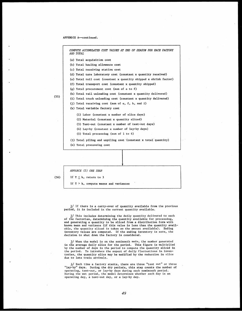
(55)

(56)

APPENDIX A--continued.

COMPUTE ACCUMULATED COST VALUES AT END OF SEASON FOR EACH FACTORYAND TOTAL

(a) Total acquisition cost

(b) Total hauling allowance cost

(c) Total receiving station cost

(d) Total tare laboratory cost (constant x quantity received)

(e) Total rail cost (constant x quantity shipped x shrink factor)

(f) Total transport cost (constant x quantity shipped)

(g) Total procurement cost (sum of a to f)

(h) Total rail unloading cost (constant x quantity delivered)

(i) Total truck unloading cost (constant x quantity delivered)

(j) Total receiving cost (sum of e, f, h, and i)

(k) Total variable factory cost

(1) Labor (constant x number of slice days)

(2) Material (constant x quantity sliced)

(3) Test-out (constant x number of test-but days)

(4) Lay-by (constant x number of lay-by days)

(5) Total processing (sum of 1 to 4)

(1) Total piling and unpiling cost 1(constant'x total quantity)

(m) Total processing cost

ADVANCE (T) ONE YEAR

If T < k, return to 3

If T > k, compute means and variances

1/ If there is a carry-over of quantity available from the previousperiod, it is included in the current quantity available.

2/ This includes determining the daily quantity delivered to eachof t.171.e factories, determining the quantity available for processing,and generating a quantity to be sliced from a distribution form withknown mean and variance (if this value is less than the quantity avail-able, the quantity sliced is taken as the amount available). Endinginventory values are computed. If the ending inventory is zero, thedecision to shut down the factory is considered.

3/ When the model is on the semimonth mode, the number generatedis the average daily slice for the period. This figure is multipliedby the number of days in the period to compute the quantity sliced inthe period. To introduce the aspect of daily fluctuations in inven-tories, the quantity slice may be modified by the reduction in slicedue to late train arrivals.

4/ Each time a factory starts, there are three "test out" or three"lay-by" days. During the dry periods, this step counts the number ofoperating, test-out, or lay-by days during each semimonth period.During the wet period, the model determines whether each day is anoperating day, a test-out day, or a lay-by day.

49

_

APPENDIX B

Specification and Estimation of Behavioral Relationships

50

APPENDIX B

Specification and Estimation of

Behavioral Relationships

The material that follows describes the methods used to estimate the several behavioralrelationships of the sugar beet system and presents the results obtained. The discussionalso explains how these relationships enter the model operation.

Yield Relationships

Yield of sugar beets may be measured in two ways: in tons of roots per acre andin pounds of sugar per acre contained in the beets. Equations are required for both typesof relationships.

Root yield, in tons per acre, was hypothesized to be a function of planting date,average high temperature during growth, length of time from planting until harvest, anda random variable associated with omitted biological, cultural, and weather factors. Plantingdate was the mean planting date--the date (expressed in weeks) when 50 percent ofthe acreage in the production area was planted.1 Temperature affects growth through itsaction on photosynthesis, respiration, and transpiration [5, Chapter 21. Average daily hightemperature during growth was used to represent this variable. The length of time fromplanting until harvest was the difference between harvest date and the mean planting date.

Data from the 35 production areas for 111/2 years (1960 to Fall, 1971) were usedto estimate the yield equations. The yield figures represent averages for all fields in agiven production area. This made the estimation difficult since there were variations withinareas in practices and in unobservable processes, such as fertilization, irrigation, sprayingfor insects, and weed control.

Initial efforts to estimate separate yield equations for each of the 35 productionareas proved unsatisfactory because of limited numbers of observations and limited rangesof values for the average data for each area. An alternative and more successful procedurewas to pool observations from all production areas to estimate a single equation withdummy variables added to shift the level for each area. After some exploration, the yieldrelationship was specified to have the following form:

1 This variable is explained in more detail in the section on decision rules; see supra, page 22.

51

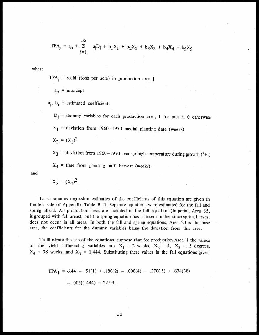
35TPAi = ao + ajD + b1 X1 + b2X2 + b3X3 + b4X

j=1

where

TPA- = yield (tons per acre) in production area j

and

ao = intercept

a- b• = estimated coefficients1

D. = dummy variables for each production area, 1 for area j, 0 otherwise

= deviation from 1960-1970 medial planting date (weeks)

X2 = (X1)2

= deviation from 1960-1970 average high temperature during growth (°F.)

X4 = time from planting until harvest (weeks)

X5 = (X4)2.

Least—squares regression estimates of the coefficients of this equation are given inthe left side of Appendix Table B-1. Separate equations were estimated for the fall andspring ahead. All production areas are included in the fall equation (Imperial, Area 35,is grouped with fall areas), but the spring equation has a lesser number since spring harvestdoes not occur in all areas. In both the fall and spring equations, Area 20 is the basearea, the coefficients for the dummy variables being the deviation from this area.

To illustrate the use of the equations, suppose that for production Area 1 the valuesof the yield influencing variables are X1 = 2 weeks, X2 = 4, X3 = .5 degrees,X4 = 38 weeks, and X5 = 1,444. Substituting these values in the fall equations gives:

TPAi = 6.44 — .51(1) + .180(2) — .008(4) — .270(.5) + .634(38)

— .005(1,444) = 22.99.

52

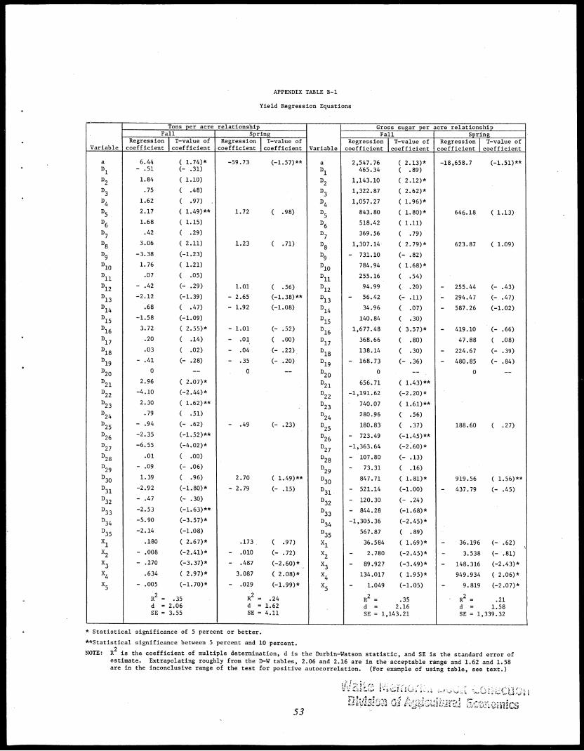
APPENDIX TABLE B-1

Yield Regression Equations

Variable

Tons per acre relationship Gross sugar per acre relationshipFall Spring Fall Spring

Regression T-value ofcoefficient coefficient

Regression T-value ofcoefficient coefficient

Regression T-value ofcoefficient coefficient Variable

Regression T-value ofcoefficient coefficient

a 6.44 ( 1.74)* -59.73 (-1.57)** a 2,547.76 ( 2.13)* -18,658.7 (-1.51)**D1

- 31).51 (- . D1 465.34 ( .89)

D2

1.84 ( 1.10) D2 1,143.10 ( 2.12)*

D3

.75 ( .48) D3 1,322.87 ( 2.62)*

D4

1.62 ( .97) . D4

1,057.27 ( 1.96)*

D5

2.17 ( 1.49)** 1.72 ( .98) D5

843.80 ( 1.80)* 646.18 ( 1.13)

D6

1.68 ( 1.15) D6

518.42 ( 1.11)

D7

.42 ( .29) D7

369.56 ( .79)

D8

3.06 ( 2.11) 1.23 ( .71) D8

1,307.14 ( 2.79)* 623.87 ( 1.09)

D9 -3.38 (-1.23) D

9- 731.10 (- .82)

D10

1.76 ( 1.21) 010

784.94 ( 1.68)*

D11

.07 ( .05) D11

255.16 ( .54)

D12

- .42 (- .29) 1.01 ( .56) D12 94.99 ( .20) - 255.44 (- .43)

D13

-2.12 (-1.39) - 2.65 (-1.38)** D13

- 56.42 (- .11) - 294.47 (- .47)

D14

.68 ( .47) - 1.92 (-1.08) 014 34.96 ( .07) - 587.26 (-1.02)

D15

-1.58 (-1.09) D15

140.84 ( .30)

D16

3.72 ( 2.55)* - 1.01 (- .52) D16

1,677.48 ( 3.57)* - 419.10 (- .66)

D17

.20 ( .14) - .01 ( .00) 017368.66 ( .80) 47.88 ( .08)

D18

.03 ( .02) - .04 (- .22) 018

138.14 ( .30) - 224.67 (- .39)

D19

- .41 (- .28) - .35 (- .20) D19

- 168.73 (- .36) - 480.85 (- .84)

D20

0 -- 0 -- 0200 -- 0 --

D21

2.96 ( 2.07)* D21 656.71 ( 1.43)**

D22

-4.10 (-2.44)* D22

-1,191.62 (-2.20)*

D23

2.30 ( 1.62)**. D

23740.07 ( 1.61)**

D24 .79 ( .51) D

24280.96 ( .56)

D25

- .94 (- .62) - .49 (- .23) 025180.83 ( .37) 188.60 ( .27)

D26

-2.35 (-1.52)** D26

- 723.49 (-1.45)**

D27

-6.55 (-4.02)* D27

-1,363.64 (-2.60)*

D28 .01 ( .00) D

28- 107.80 (_ .13)

029- .09 (- .06) D

29- 73.31 ( .16)

D30 1.39 ( .96) 2.70 ( 1.49)** D

30847.71 ( 1.81)* 919.56 ( 1.56)**

D31

-2.92 (-1.80)* - 2.79 (- .15) D31

- 521.14 (-1.00) - 437.79 (- .45)

D32

- .47 (- .30) D32 - 120.30 (- .24)

D33

-2.53 (-1.63)** D33

- 844.28 (-1.68)*

D34

-5.90 (-3.57)* D34

-1,305.36 (-2.45)*

D35

-2.14 (-1.08) D35

567.87 ( .89)

X 1

.180 ( 2.67)* .173 ( .97) X1 36.584 ( 1.69)* - 36.196 (- .62) ,

X2 - .008 (-2.41)* - .010 (- .72) X

2- 2.780 (-2.45)* - 3.538 (- .81)

X3

- .270 (-3.37)* - .487 (-2.60)* X3

- 89.927 (-3.49)* - 148.316 (-2.43)*

X4

.634 ( 2.97)* 3.087 ( 2.08)* X4

134.017 ( 1.95)* 949.934 ( 2.06)*

X5

- .005 (-1.70)* - .029 (-1.99)* X5 - 1.049 (-1.05) - 9.819 (-2.07)*

R2 = .35 R2 = .24 R2 = .35 • R2 = .21d = 2.06 d = 1.62 , d = 2.16 d = 1.58SE = 3.55 SE = 4.11 SE = 1,143.21 SE = 1,339.32

* Statistical significance of 5 percent or better.

**Statistical significance between 5 percent and 10 percent.

NOTE: R2 is the coefficient of multiple determination, d is the Durbin-Watson statistic, and SE is the standard error of

estimate. Extrapolating roughly from the D-W tables, 2.06 and 2.16 are in the acceptable range and 1.62 and 1.58are in the inconclusive range of the test for positive autocorrelation. (For example of using table, see text.)

-•U

1. 40$104.4'44:0 t.J

53

Although these equations leave a considerable amount of yield variation unexplained,most of the main coefficients are statistically significant at the 5 percent or better leveland have signs that seem consistent with our a priori expectations.

Similar equations were estimated using gross sugar per acre (pounds) as the dependentvariable. They are summarized in the right—hand side of Appendix Table B-1 and areinterpreted in a manner similar to the root yield equations.'

These equations were used in the model to generate yield variations associated withdecisions as to time of planting and harvest and with random variations due to temperatureand (indirectly) soil moisture conditions. In the actual simulation process, a further randomvariable was added to the yield values. It was generated from an assumed normaldistribution with zero mean and the standard error of estimate listed for each equation.

Recent introduction of a new Virus Yellows resistant variety appears to have raisedaverage yields above the levels indicated by our historical time series. Consultation withindustry personnel suggested this increase is about 15 percent, so all yield values wereincreased by this factor in the model applications.2

Quantity Available for Harvest

The amount of beets harvested on any date in any production area is limited bythe acres of beets that have reached the appropriate stage of growth. This quantity, inturn, depends on the number of acres planted, the date planted, and to some extenton weather factors, such as temperature, which may affect growth rates.

Our efforts to estimate this type of functional relationship were frustrated byincomplete measures of corresponding dates of planting and dates of availability.Consultation with the processor management suggested, however, that this would not bea serious practical limitation for modeling purposes. Because of the overriding need tokeep factories operating at capacity levels, the proportions of acreage regarded bymanagement as available for harvest in each area during each period remain fairly stable(for given general planting periods) even though planting dates may vary within the plantingperiods. Although the proportion of the acreage available remains constant, the quantityof the tonnage available to harvest in a period is allowed to vary from season to seasonas yields vary (see previous section).

1 Since the sugar content of beets is affected by nitrogen applications, it would have been desirableto include this as a variable in the analysis. However, we were unable to obtain sufficient time seriesdata to permit an estimate of the effect of this factor. It thus appears as an element of the unexplainedresiduals.

2 The increase in yield is based on field experiments. It was not possible to verify this figure againstmore recent reported commercial yields because of the limited observations and variability due to otherfactors affecting actual yields.

54

Proportions of acreage available for harvest in production areas 1-20 are given in

Appendix Table B-2. These values were determined by discussions with processor

management and reference to data on quantities actually harvested. The figures show,

for example, that 10.2 percent of the acreage in Area 1 is regarded as available for harvest

in period 4; another 13 percent becomes newly available in period 5; and so on. If all

acreage available is not harvested in one period, it is added to the amount available in

the next. When "remaining" is indicated in the table, all acreage remaining in the production

area becomes available to harvest.

Total acreage available is determined by multiplying acres planted by these

proportions. Total tonnage available for harvest is then obtained by multiplying the acreage

figure by predicted yields for the production period in which harvest occurs.

In Areas 21, 23, 24, 29, 32, and 34, all beets become available to harvest in period 1.Some beets in this area might be available earlier, but period 1 (July 1) is the normalstarting date. Areas 25 and 30 harvest only in the spring; beets become fully available(but subject to harvest capabilities limited by the moisture index) after period 14. Beetsbecome available for harvest in Area 35 after .period 21. For Areas 22, 26, 27, 28, 31,and 33, the quantities available to harvest are established through a different process whichwill be described later in the discussion of decision rules. Briefly, Areas 26, 27, and 31become theoretically 100 percent available in period 1, 33 percent in period 2,22 percent in period 7, and 28 percent in period 10 (Appendix Table D-9).

Temperature During Beet Growth

As noted in the discussion of yield relationships, a factor affecting yields is thetemperature during the period when beets are growing. To represent this variable, we used •a three—month average of daily maximum temperatures during peak growth period asmeasured at a nearby weather station. For most areas the appropriate three—month periodis June, July, and August; but in the earlier areas it is March, April, and May.

Probability distributions of these average temperatures were developed for eachproduction area based on historical weather records. Since our temperature observationswere somewhat limited for many of the local stations, we selected two stations with fairlylong weather records as base stations. This restriction also greatly reduced the numberof computations. Two base stations were selected so as to have these stations locatedin the immediate vicinity of the production areas that have similar growth and harvestperiods. The earlier harvest areas are located in the south so a station in the southernSan Joaquin Valley, Wasco, was selected for the spring average. Stockton was selectedas the station for northern (later harvesting) areas and summer average. Regressions thenwere fitted to relate temperatures in the other areas (using the shorter data series) tothe temperature in the base stations. The resulting equations are given inAppendix Table B-3. The table indicates, for example, that if the average June—August

55

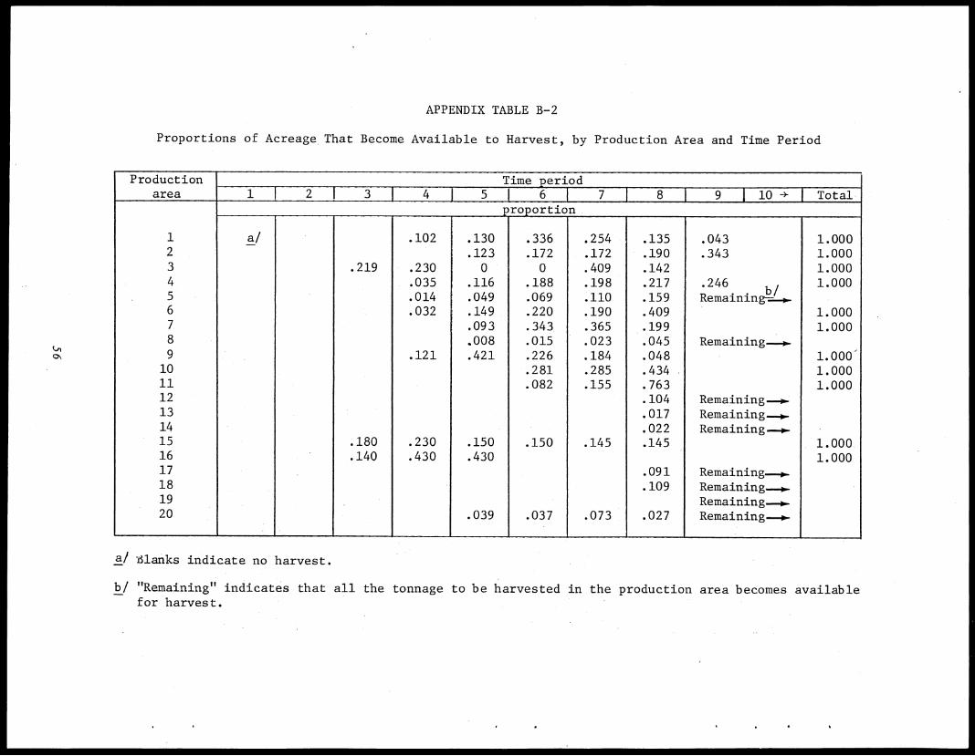
APPENDIX TABLE B-2

Proportions of Acreage That Become Available to Harvest, by Production Area and Time Period

Productionarea

Time period1 2 3

,4 1 5 I 6 7 . 8 . 9 1 10 -3- 1 Total,

Rroportion, ,

1 a/ .102 , .130 .336 .254 .135 .043 1.0002 .123 .172 .172 .190 .343 1.0003 .219 .230 0 0 .409 .142 1.00045

.035

.014.116.049

.188

.069.198.110

.217

.159.246

b/Remaining---:-4.

1.000

6 .032 , .149 .220 .190 .409 1.0007 .093 .343 .365 .199 1.0008 .008 .015 .023 .045 Remaining-4.9 .121 .421 .226 .184 .048 1.000'10 .281 .285 .434 . 1.00011 .082 .155 .763 1.00012 .104 Remaining--0-13 .017 Remaining--4..14 .022 Remaining-o-15 .180 .230 .150 .150 .145 .145 1.00016 .140 .430 .430 1.00017 .091 Remaining-4.18 .109 Remaining--4-19 Remaining-4-20 .039 .037 .073 .027 Remaining -..-

. . .

a/ -Blanks indicate no harvest.

b/ "Remaining" indicates that all the tonnage to be harvested in the production area becomes availablefor harvest.

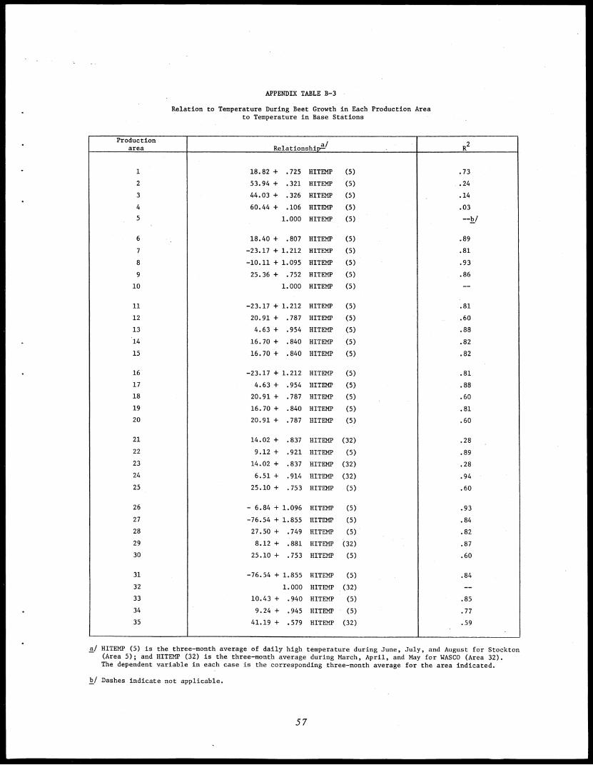
APPENDIX TABLE B-3

Relation to Temperature During Beet Growth in Each Production Areato Temperature in Base Stations

Productionarea

aRelationship

/ -

,

R2

1 18.82 + .725 HITEMP

,

(5) .73

2 53.94 + .321 HITEMP (5) , .24

3 44.03 + .326 HITEMP (5) .14

4 60.44 + .106 HITEMP (5) .03

5 1.000 HITEMP (5) --b/

6 18.40 + .807 HITEMP (5) .89

7 -23.17 + 1.212 HITEMP (5) .81

8 -10.11 + 1.095 HITEMP (5) .93

9 25.36 + .752 HITEMP (5) .86

10 1.000 HITEMP (5) --

11 -23.17 + 1.212 HITEMP (5) .81

12 20.91 + .787 HITEMP (5) .60

13 4.63 + .954 HITEMP (5) .88

.14 16.70 + .840 HITEMP (5) .82

15 16.70 + .840 HITEMP (5) .82

16 -23.17 + 1.212 HITEMP (5) .81

17 4.63 + .954 HITEMP (5) .88

18 20.91 + .787 HITEMP (5) .60

19 16.70 + .840 HITEMP (5) .81

20 20.91 + .787 HITEMP (5) .60

21 14.02 + .837 HITEMP (32) .28 ,

22 9.12 + .921 HITEMP (5) .89

23 14.02 + .837 HITEMP (32) .28

24 6.51 + .914 HITEMP (32) .94

25 25.10 + .753 HITEMP (5) .60

26 - 6.84 + 1.096 HITEMP (5) .93

27 -76.54 + 1.855 HITEMP (5) .84

28 27.50 + .749 HITEMP (5) .82

29 8.12 + .881 HITEMP (32) .87

30 25.10 + .753 HITEMP (5) .60

31 -76.54 + 1.855 HITEMP (5) .84

32 1.000 HITEMP (32) --

33 10.43 + .940 HITEMP (5) .85

34 9.24 + .945 HITEMP (5) .77

35 41.19 + .579 HITEMP (32) . .59

a/ HITEMP (5) is the three-month average of daily high temperature during June, July, and August for Stockton(Area 5); and HITEMP (32) is the three-month average during March, April, and May for WASCO (Area 32).The dependent variable in each case is the corresponding three-month average for the area indicated.

b/ Dashes indicate not applicable.

57

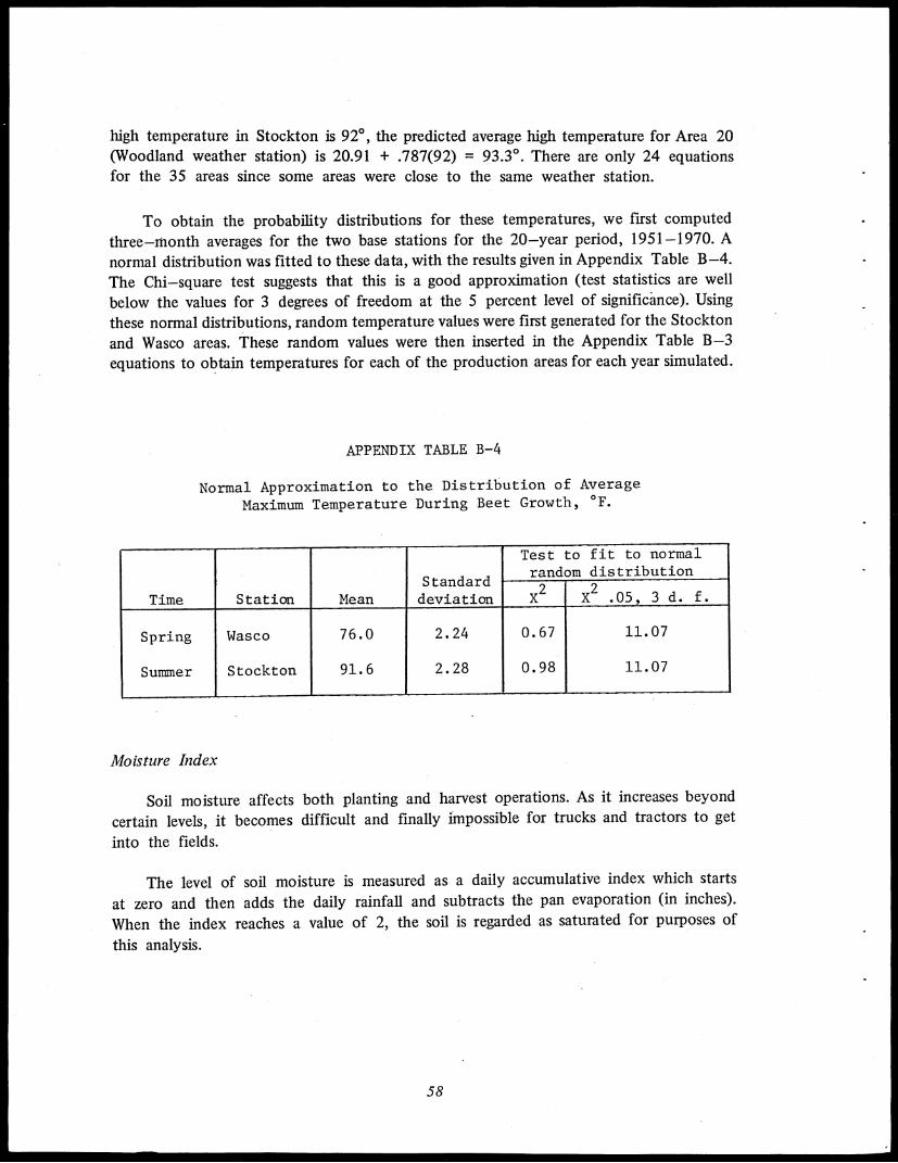
high temperature in Stockton is 92°, the predicted average high temperature for Area 20(Woodland weather station) is 20.91 + .787(92) = 93.3°. There are only 24 equationsfor the 35 areas since some areas were close to the same weather station.

To obtain the probability distributions for these temperatures, we first computed

three—month averages for the two base stations for the 20—year period, 1951-1970. A

normal distribution was fitted to these data, with the results given in Appendix Table B-4.

The Chi—square test suggests that this is a good approximation (test statistics are well

below the values for 3 degrees of freedom at the 5 percent level of significance). Using

these normal distributions, random temperature values were first generated for the Stockton

and Wasco areas. These random values were then inserted in the Appendix Table B-3

equations to obtain temperatures for each of the production areas for each year simulated.

APPENDIX TABLE B-4

Normal Approximation to the Distribution of Average

Maximum Temperature During Beet Growth, °F.

-

Standard'

.Test to fit to normalrandom distribution

X2

, X2 .05, 3 d. f.Time Station Mean deviation

Spring Wasco 76.0 2.24 0.67 11.07

Swum er Stockton 91.6 2.28 0.98 11.07

Moisture Index

Soil moisture affects both planting and harvest operations. As it increases beyond

certain levels, it becomes difficult and finally impossible for trucks and tractors to get

into the fields.

The level of soil moisture is measured as a daily accumulative index which starts

at zero and then adds the daily rainfall and subtracts the pan evaporation (in inches).

When the index reaches a value of 2, the soil is regarded as saturated for purposes of

this analysis.

58

Records of daily rainfall and evaporation were obtained from five weather stations

in the production regions of concern. These were Davis, Manteca, Los Banos, Kettleman

City, and Soledad. The number of observations was limited for some of these stations,

so Davis, with the longest records, was selected as a base area from which to compute

moisture values in the other areas. The procedure followed was the same as for the variable

temperature during growth--fitting regression equations to data for shorter periods to

obtain relationships between soil moisture values at Davis (the base area) and each of

the other stations. The results are given in Appendix Table B-5. These relationships were

estimated using daily observations (grouped by month) for the 1965-1970 seasons forManteca, Los Banos, and Kettleman City and the 1966-1970 seasons for Soledad.

The equations take the form:

where

and

Y = a + b1X1 + b2X2

= moisture index in area on given day

X1 — moisture index in Davis on given day

X2 = moisture index in area on previous day

a = intercept

bi = regression coefficient.

To illustrate the use of the equations, if the moisture index at the Davis station is 0.2on November 2 and had been 0.1 at Manteca on November 1, the predicted moistureindex for Manteca on November 2 is

.07 + .62(0.2) + .96(0.1) = .28.

The reason for including the previous day's value of the moisture index for the regionis to allow for carry—over effects from day to day. The Manteca values apply to theproducing areas in D-2, Los Banos to Areas 25 and 30, Kettleman City to the otherareas in D-4, Soledad to the areas in D-1, and Davis to the areas in D-3.

59

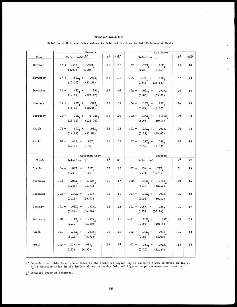
APPENDIX TABLE B-5

Relation of Moisture Index Values in Selected Stations to Soil Moisture at Davis

Month

.Manteca

• ,Los Banos

aRelationship

/ -- R

2SE-b/

,

Relationship R2 b/

SE-

October .02 + .51X1 + .92X

2

,

.76 .10 .02 + .29X1 + .91X

2.75 .10

(3.93) (7.05) (2.20) (6.86)

November .07 + .62X1 + .96X

2.92 .16 .05 + .07X

1 + .97X

2 .87 .23

(10.34) (37.59) (.84) (28.62)

December .01 + .48X1 + .99X

2.99 .07 .05 + .09X

1 + .97X

2.96 .15

(12.61) (121.42) (1.06) (59.87)

January .05 + .43X1 + .97X

2.95 .11 .04 + .13X

1 + .97X

2.94 .15

(11.00) (58.34) (1.27) (9.67)

February -.05 + .39X + 1.02X21

.99 .04 -.02 + .34X1 + 1.00X

2.99 .08

(15.31) (121.06) (6.96) (104.97)

March .02 + .60X1 + .98X

2.96 .12 .01 + .17X

1 + .91X

2.96 .08

(12.29) (51.82) (5.11) (49.67)

April .10 + .48X1 + .83X

2.71 .15 .07 + .17X

1 + .48X

2'.19 .15

(4.18) (9.39) (1.52) (2.83)

Kettleman City Soledad

Month Relationship R2

SE Relationship R2

SE

October .06 - .08X1 + .76X

2.37 .22 .07 + .13X

1 + .71X

2.51 .19

. (-.33) (3.02) (.57) (1.73)

November .03 + .08X1 + 1.02X

2.85 .17 .00 + .35X

1 + 1.11X

2.79 .14

(1.38) (25.71) (6.16) (18.42)

December .02 + .14X1 + .97X

2.95 .11 .03 + .17X

1 + .97X

2.96 .18

(2.21) (56.47) (1.55) (50.17)

January .01 + .06X + .97X21

.95 .13 .03 + .06X1 + .98X

2 .95 .17

(1.39) (56.76) (.79) (53.14)

February .00 + .11X1 + .99X

2.98 .11 -.01 + .26X

1 + .99X

2.99 .09

(1.30) (71.60) (3.98) (101.43)

March .01 + .28X1 + .93X

2.96 .11 .02 + .37X

1 + .93X

2.94 .13

(5.13) (43.75) (7.06) (38.00)

April .05 + .07X1 + .68X

2.35 .16 .07 + .31X

1 + .9

1X2

.82 .16

(.67) (4.33) (2.70) (12.34)

a/ Dependent variable is moisture index in the indicated region, X1 is moisture index at Davis on day D,

X2 is moisture index in the indicated region on day D-1, and figures in parentheses are t-ratios.

b/ Standard error of estimate.

•

60

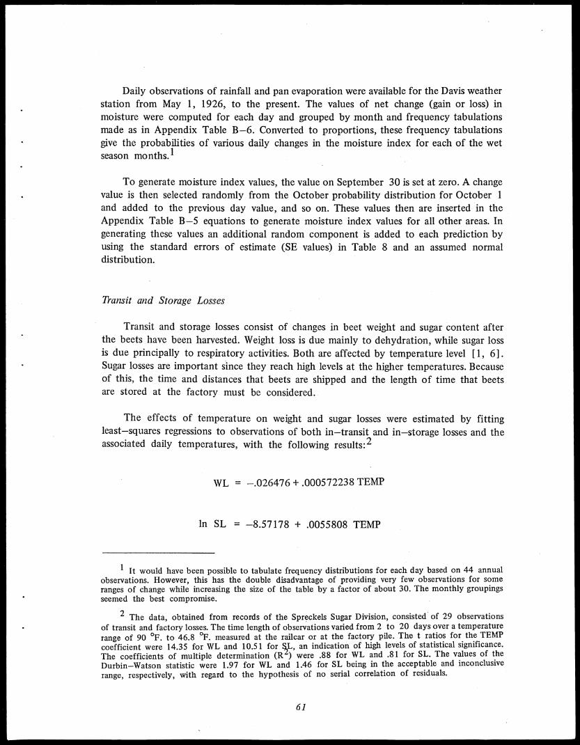
Daily observations of rainfall and pan evaporation were available for the Davis weatherstation from May 1, 1926, to the present. The values of net change (gain or loss) inmoisture were computed for each day and grouped by month and frequency tabulationsmade as in Appendix Table B-6. Converted to proportions, these frequency tabulationsgive the probabilities of various daily changes in the moisture index for each of the wetseason mo nths.1

To generate moisture index values, the value on September 30 is set at zero. A changevalue is then selected randomly from the October probability distribution for October 1and added to the previous day value, and so on. These values then are inserted in theAppendix Table B-5 equations to generate moisture index values for all other areas. Ingenerating these values an additional random component is added to each prediction byusing the standard errors of estimate (SE values) in Table 8 and an assumed normaldistribution.

Transit and Storage Losses

Transit and storage losses consist of changes in beet weight and sugar content afterthe beets have been harvested. Weight loss is due mainly to dehydration, while sugar lossis due principally to respiratory activities. Both are affected by temperature level [1, 61.Sugar losses are important since they reach high levels at the higher temperatures. Becauseof this, the time and distances that beets are shipped and the length of time that beetsare stored at the factory must be considered.

The effects of temperature on weight and sugar losses were estimated by fittingleast—squares regressions to observations of both in—transit and in—storage losses and theassociated daily temperatures, with the following results:2

WL = —.026476 + .000572238 TEMP

ln SL = —8.57178 + .0055808 TEMP

1 It would have been possible to tabulate frequency distributions for each day based on 44 annualobservations. However, this has the double disadvantage of providing very few observations for someranges of change while increasing the size of the table by a factor of about 30. The monthly groupingsseemed the best compromise.

2 The data, obtained from records of the Spreckels Sugar Division, consisted. of 29 observations

of transit and factory losses. The time length of observations varied from 2 to 20 days over a temperature

range of 90 °F. to 46.8 °F. measured at the railcar or at the factory pile. The t ratios for the TEMP

coefficient were 14.35 for WL and 10.51 for S,L, an indication of high levels of statistical significance.

The coefficients of multiple determination (Iti were .88 for WL and .81 for SL. The values of the

Durbin—Watson statistic were 1.97 for WL and 1.46 for SL being in the acceptable and inconclusive

range, respectively, with regard to the hypothesis of no serial correlation of residuals.

61

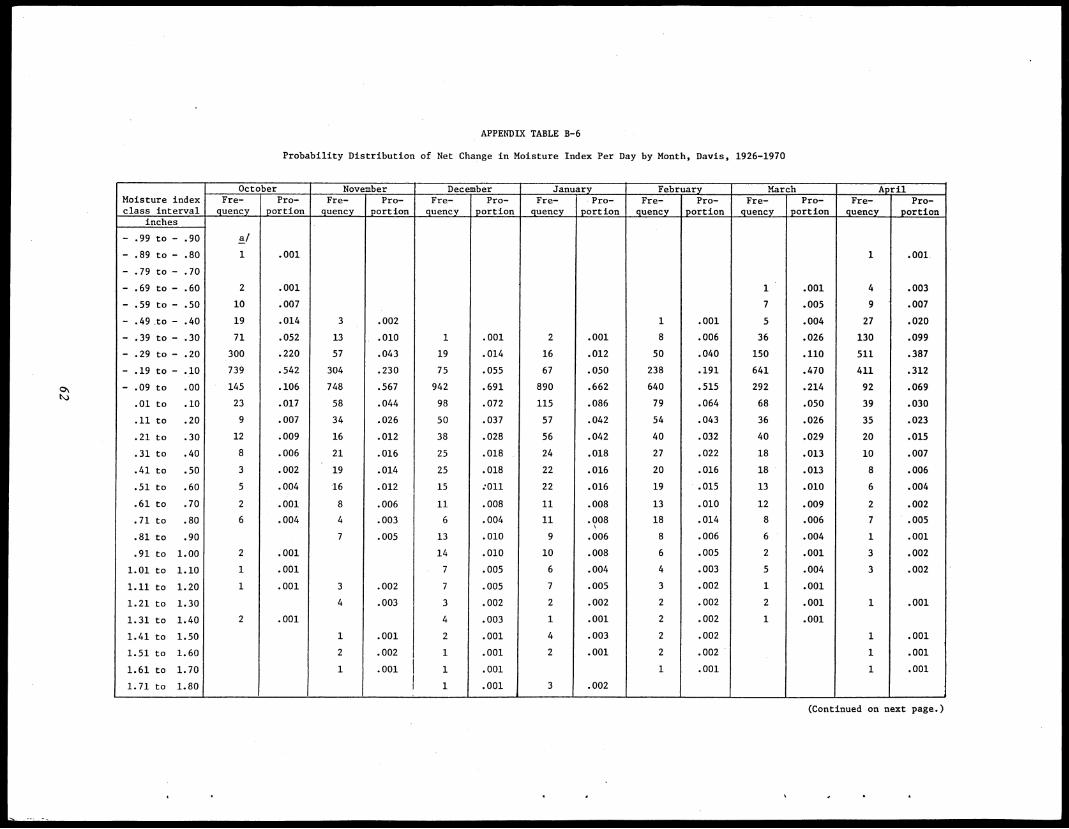
APPENDIX TABLE B-6

Probability Distribution of Net Change in Moisture Index Per Day by Month, Davis, 1926-1970

Moisture indexclass interval

October November December January February March AprilFre-quency

Pro-portion

Fre-quency

Pro-portion

Fre-quency

Pro- Fre-quency

Pro-portion

Fre-quency

Pro-portion

Fre-quency

Pro-portion

Fre-quency

Pro-portion

inches .

, _portion

- .99 to - .90 a/..._

- .89 to - .80 1 .001 1 .001

-.79 to- .70

- .69 to - .60 2 .001 1 . .001 4 .003

- .59 to - .50 10 .007 7 .005 9 .007

- .49 to - .40 19 .014 3 .002 1 .001 5 .004 27 .020

- .39 to - .30 71 .052 13 .010 1 .001 2 .001 8 .006 36 .026 130 .099

- .29 to - .20 300 .220 57 .043 19 .014 16 .012 50 .040 150 .110 511 .387

- .19 to - .10 739 .542 304 .230 75 .055 67 .050 238 .191 641 .470 411 .312

- .09 to .00 145 .106 748 .567 942 .691 890 .662 640 .515 292 .214 92 .069

.01 to .10 23 .017 58 .044 98 .072 115 .086 79 .064 68 .050 39 .030

.11 to .20 9 .007 34 .026 50 .037 57 .042 54 .043 36 .026 35 .023

.21 to .30 12 .009 16 .012 38 .028 56 .042 40 .032 40 .029 20 .015

.31 to .40 8 .006 21 .016 25 .018 24 .018 27 .022 18 .013 10 .007

.41 to .50 3 .002 ' 19 .014 25 .018 22 .016 20 .016 18 .013 8 .006

.51 to .60 5 .004 16 .012 15 :011 22 .016 19 .015 13 .010 6 .004

.61 to .70 2 .001 8 .006 11 .008 11 .008 13 .010 12 .009 2 .002

.71 to .80 6 .004 4 .003 6 .004 11 .908 18 .014 8 .006 7 .005

.81 to .90 7 .005 13 .010 9 .006 8 .006 6 .004 1 .001

.91 to 1.00 2 .001 14 .010 10 .008 6 .005 2 .001 3 .002

1.01 to 1.10 1 .001 7 .005 6 .004 4 .003 5 .004 3 .002

1.11 to 1.20 1 .001 3 .002 7 .005 7 .005 3 .002 1 .001

1.21 to 1.30 4 .003 3 .002 2 .002 2 .002 2 .001 1 .001

1.31 to 1.40 2 .001 4 .003 1 .001 2 .002 1 .001

1.41 to 1.50 1 .001 2 .001 4 .003 2 .002 1 .001 ,

1.51 to 1.60 2 .002 1 .001 2 .001 2 .002 . 1 .001

1.61 to 1.70 1 .001 1 .001 1 .001 1 .001

1.71 to 1.80 1 .001 3 .002

(Continued on next page.)

0\

APPENDIX TABLE B -6 - -continued.

Moisture indexclass interval,

October November • December January _

February March Aril

Fre-quency

Pro-portion

Fre-quency

Pro-portion

Fre-quency

.Pro-

portionFre-quency

Pro- Fre-quency

Pro-portion

Fre- 'quency

Pro-portion

Fre-quency ,

Pro-portion

inches_portion,

1.81 to 1.90 1 .001 1 .001 1 .001 1 .001

1.91 to 2.00 1 .001 1 .001 1 .001 1 .001

2.01 to 2.10 2 .001 1 .001

2.11 to 2.20 2 .001 1 .001

2.21 to 2.30 1 .001 1 .001

2.31 to 2.40 1 .001 - 1 .001 -

2.41 to 2.50 1 .001

2.51 to 2.60

2.61 to 2.70 .

2.71 to 2.80 1 .001 2 .001

2.81 to 2.90 1 .001

2.91 to 3.00 1 .001

3.01 to 3.10 1 .001

3.11 to 3.20

3.21 to 3.30 1 .001

3.31 to 3.40

3.41 to 3.50 1 .001

3.51 to 3.60

Total 1,364 1.000 1,320 1.000 1,363 1.000 1,346 1.000 1,243 1.000 1,364 1.000 1,319 1.000

Mean -.1421 -.0238 .0628 .0766 .0321 -.0616 -.1588

Standarddeviation .2100 .2136 .2941 .3189 .3035 .2314 .2193

a/ Blanks indicate zero.

Source: Computed from data from U. S. Department of Commerce, National Oceanic and Atmospheric Administration, Environmental Data Service, Climato-logical Data--California Section.

where

and

WL = weight loss per day expressed as a proportion of original weight

SL = sugar loss per day expressed as a proportion of original weight of sugarin the beets

TEMP = average daily temperature (°F.).

The weight loss was taken as a linear function of temperature, whereas the sugar

losses were expressed in natural logarithms.1 These equations were used to derive weight

and sugar losses for beets in transit and in storage at the factory (see Blocks 37, 42,

and 43 of Appendix A). Monthly averages of daily temperatures in areas of harvest

(Appendix Table B-7) rather than randomly determined temperatures were substituted

in these equations to obtain transit loss rates (loss per ton per day) for each area and

period. A random term was not added since fluctuations were relatively small. This value

was then multiplied by the estimated standard time (fractions of days) in transit for each

receiving station—factory combination to obtain the loss per ton for beets traveling that

route. Losses per ton per day in factory storage were also calculated using the average

monthly temperature for the weather station nearest the plant.

Tons Sliced Per Day

Because of breakdowns and variations in operating conditions, it is impossible for

a factory to always process exactly the same quantity of beets each day. To allow for

this, the model permits the daily slice (or average daily slice for semimonth periods) to

vary randomly according to a historically determined distribution.

Examination of daily records of quantity of beets sliced for the years 1965-1970

suggested the need for separate distributions for each of four seasonal time periods. These

are: first day of operation, start—up period (days 2-5), normal operation (semimonth

periods), and operation during raining periods (wet season). For the first day's operation,

the mean value was used with no variation; for the other three periods, a normal distribution

was specified with means and standard deviations as given in Appendix Table B-8.

Chi—square values for the goodness of fit of the normal distribution are also given in

the table. The test suggests that it is a good approximation.

1 For temperatures below 46.27 °F., the equation predicts a weight gain. Earlier we indicated that

weight gains are attributable to water absorption. The weight gain associated with low temperature reflects

the fact that low temperatures typically occur during rainy months. The degree of bias involved does

not appear to be serious.

64

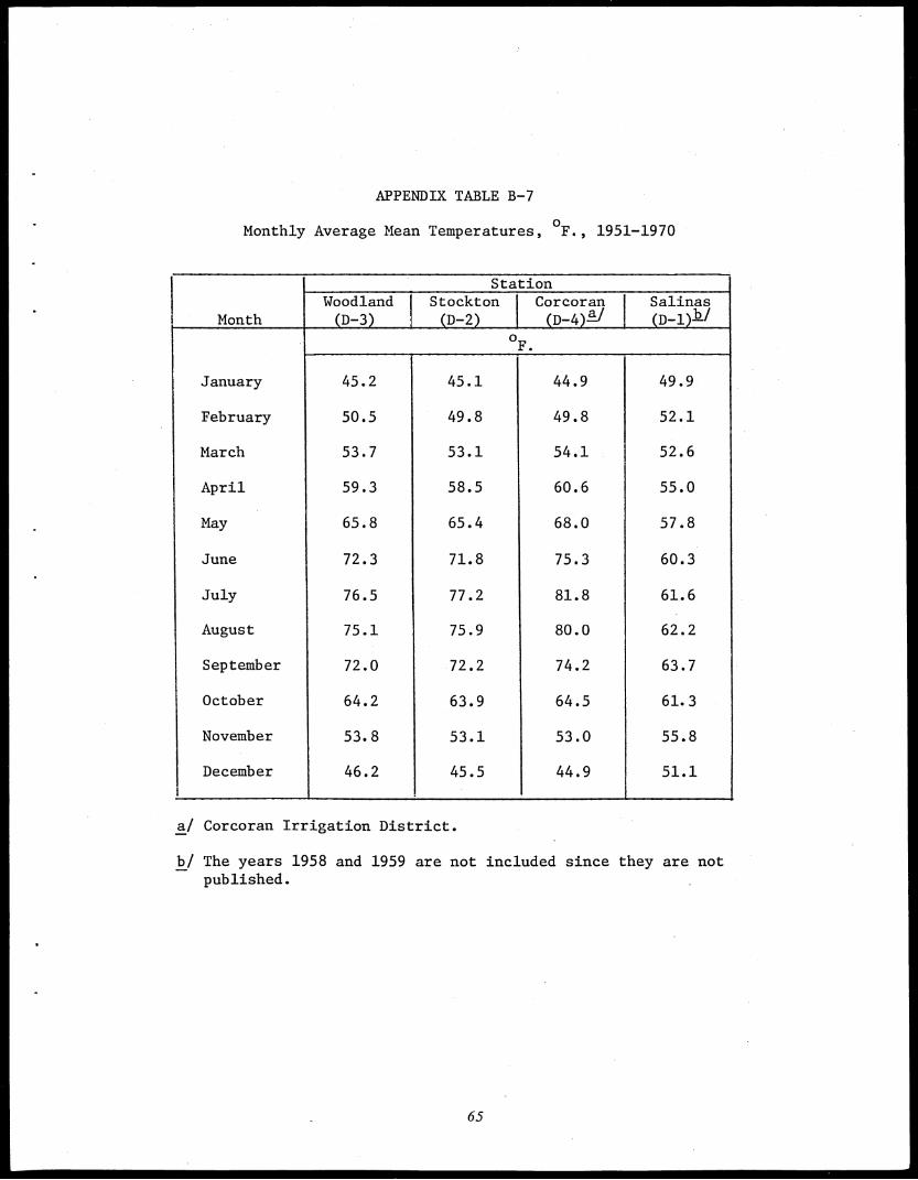
APPENDIX TABLE B-7

Monthly Average Mean Temperatures, °F., 1951-1970

Station

MonthWoodland I(D-3) I

Stockton I(a-z) 1

Corcoran I(a-4)- I

Salinas0-1>12/_

oF.

January 45.2 45.1 44.9 49.9

February 50.5 49.8 49.8 52.1

March 53.7 53.1 54.1 52.6

April 59.3 58.5 60.6 55.0

May 65.8 65.4 68.0 57.8

June 72.3 71.8 75.3 60.3

July 76.5 77.2 81.8 61.6

i August 75.1 75.9 80.0 62.2

September 72.0 72.2 74.2 63.7

October 64.2 63.9 64.5 61.3

November 53.8 53.1 53.0 55.8

December 46.2 45.5 44.9 51.1

:1

.

a/ Corcoran Irrigation District.

b/ The years 1958 and 1959 are not included since they are notpublished.

65

•••

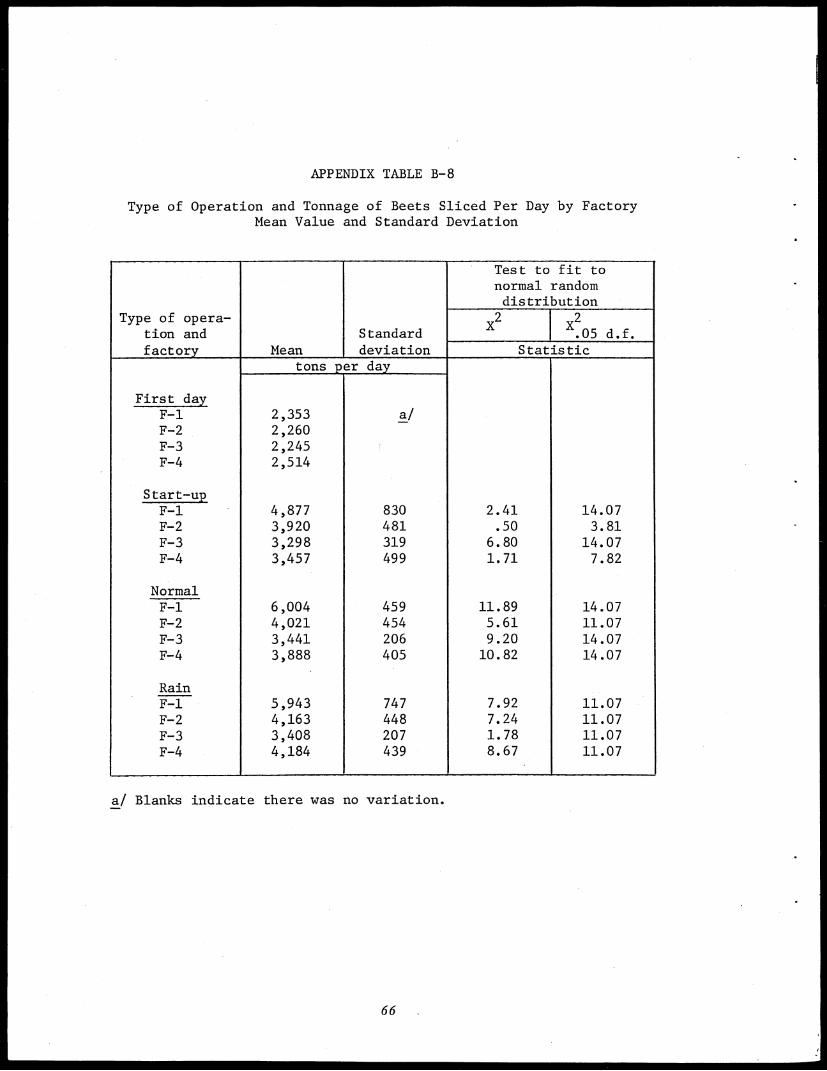
APPENDIX TABLE B-8

Type of Operation and Tonnage of Beets Sliced Per Day by FactoryMean Value and Standard Deviation

Type of opera-tion andfactory Mean

Standarddeviation

Test to fit tonormal randomdistribution

.05 d.f.Statistic_

tons per day,

First dayF-1 2,353 a/F-2 2,260F-3 2,245F-4 2,514

Start-upF-1 4,877 830 2.41 14.07F-2 3,920 481 .50 3.81F-3 3,298 319 6.80 14.07F-4 3,457 499 1.71 7.82

NormalF-1 6,004 459 11.89 14.07F-2 4,021 454 5.61 11.07F-3 3,441 206 9.20 14.07F-4 3,888 405 10.82 14.07

,

RainF-1 5,943 747 7.92 11.07F-2 4,163 448 7.24 11.07F-3 3,408 207 1.78 11.07F-4 4,184 439 8.67 11.07

,,

a/ Blanks indicate there was no variation.

. e

66 .

Rail Delays

During certain periods when the deliveries of beets to the factories consist entirelyor principally of deliveries via rail, late trains which are beyond the control of the processorcan cause reductions in the amount sliced if inventory levels are reduced to zero. Dataon reductions in slice due to late train arrivals were examined for the years 1965-1970and used to establish the frequency distributions given in Appendix Table B-9. The valuespertain to the tons of slice reduced in a semimonth period. In the periods not listedin the table, reductions in slice due to rail delays are not important since the patternand timing of local deliveries eliminate the problem. To generate the values for rail delaysused in the simulation model, a random number was generated which established theamount of the delay (based upon the proportions listed in Appendix Table B-9). Whenan interval is indicated, the midpoint of the class was used as the delay loss.

67

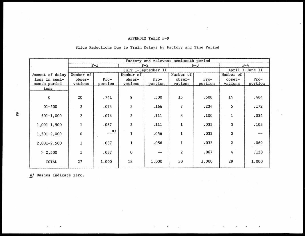
APPENDIX TABLE B-9

Slice Reductions Due to Train Delays by Factory and Time Period

Amount of delayloss in semi-month period

Factory and relevant semimonth period-F-1 1 F-2 F-3 : F-4

July I-September II April I-June IINumber of

obser-vations

Pro-portion

Number ofobser-

vationsPro-

portion

Number ofobser-

vationsPro-

portion

,Number ofobser-

vationsPro-

portion

tons

20 .741 9 .500 15 .500 14 .4840

01-500 2 .074 3 .166 7 .234 5 .172

501-1,000 2 .074 2 .111 3 .100 1 .034

1,001-1,500 1 .037 2 .111 1 .033 3 .103

1,501-2,000 0 _2 .-/ 1 .056 1 .033 0 --

2,001-2,500 1 .037 1 .056 1 .033 2 .069

> 2,500 1 .037 0 ....... 2 .067 4 .138

TOTAL 27 1.000 18 1.000 30 1.000 29 , 1.000

. . i 1

a/ Dashes indicate zero.

APPENDIX C

Extraction Rates and Cost Parameters

69

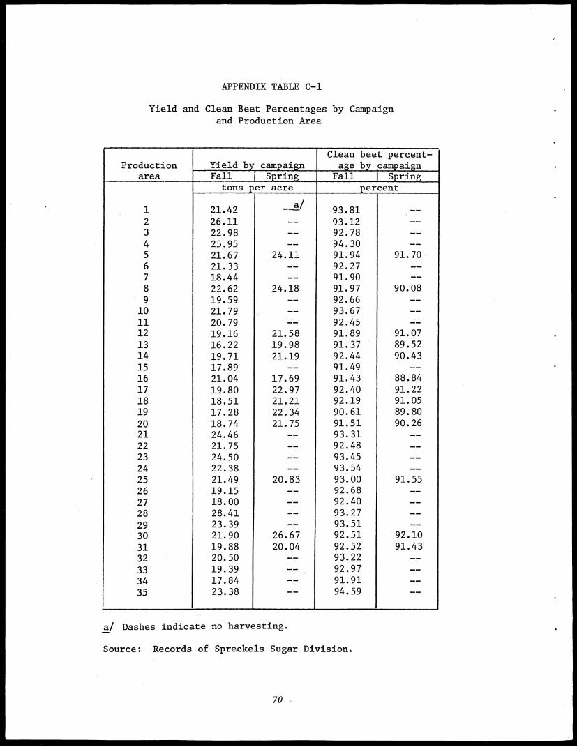
APPENDIX TABLE C-1

Yield and Clean Beet Percentages by Campaignand Production Area

Productionarea

Yield by campaignClean beet percent-age by campaign

Fall Spring Fall i Springtons per acre percent

1 21.42 93.81 ,__

2 26.11 _... 93.12 --3 22.98 ...... 92.78 --4 25.95 __ 94.30 --5 21.67 24.11 91.94 91.706 21.33 __ 92.27 .......

7 18.44 __ 91.90 --8 22.62 24.18 91.97 90.089 19.59 __ 92.66 --10 21.79 __ 93.67 --ii 20.79 __ 92.45 --12 19.16 21.58 91.89 91.0713 16.22 19.98 91.37 89.5214 19.71 21.19 92.44 90.4315 17.89 91.49 --16 21.04 17.69 91.43 88.8417 19.80 22.97 92.40 91.2218 18.51 21.21 92.19 91.0519 17.28 22.34 90.61 89.8020 18.74 21.75 91.51 90.2621 24.46 ..._ 93.31 --22 21.75 __ 92.48 --23 24.50 __ 93.45 --24 22.38 ...... 93.54 __

25 21.49 20.83 93.00 91.5526 19.15 __ 92.68 --27 18.00 __ 92.4028 28.41 __ 93.27 --

29 23.39 ........ 93.51 --30 21.90 26.67 92.51 92.10

31 19.88 20.04 92.52 91.4332 20.50 __ 93.22 --

33 19.39 __ 92.97 --34 17.84 __ 91.91 --35 23.38 __ 94.59 --

a! Dashes indicate no harvesting.

Source: Records of Spreckels Sugar Division.

70 -

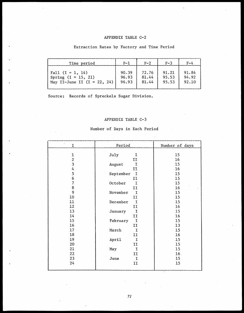
APPENDIX TABLE C-2

Extraction Rates by Factory and Time Period

Time period F-1.

F-2 F-3.

F-4

Fall (I = 1, 14)

,

90.39 72.76 91.21 91.84Spring (I = 15, 21) 96.93 81.44 95.53 94.92May II-June II (I = 22, 24) 96.93 81.44 95.53 92.10

Source: Records of Spreckels Sugar Division.

APPENDIX TABLE C-3

Number of Days in Each Period

. I Period Number of days

1 July I 152 II 163 August I 154 II 165 September I 156 II 15

7 October I 158 II 16 ,9 November I 1510 II 1511 December I 1512 II 1613 January I - 1514 II 1615 February I 1516 II 1317 March I 1518 II 1619 April I 1520 II 1521 May I 1522 II 1623 June I 1524 II 15

71

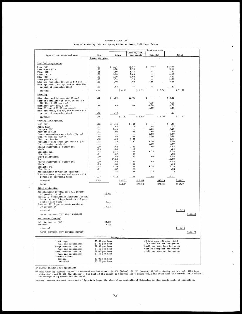
APPENDIX TABLE C-4

Cost of Producing Fall and Spring Harvested Beets, 1971 Input Prices

Type of operation and cost Time

Cost per acre

LaborTractor, fuel,

and repair Material Total

Seed bed preparation

hours per acre

Plow (1X) .67 $ 1.34 $3.87 $ --a/ $ 5.21

Land plane (2X) .50 1.00 2.90 3.90

Float (1X) .25 .50 1.45 1.95

Chisel (2X) .80 1.60 4.64 6.24

Disc (2X) .50 1.00 2.90 3.90

Springtooth (1X) .17 .34 .99 -- 1.33

List and fertilize (84 units N 9 90 .20 .40 .60 7.56 8.56

Move equipment, set up, and service (10percent of operating time) .31 .62 .62

Subtotal 3.40 $ 6.80 $17.35 $ 7.56 $ 31.71

Planting

Sled plant and incorporate (I man) .40 $ .80 $2.05 $ $ 2.85

Starter fertilizer (8-24-0, 16 units N200 lbs. @ $77 per ton) 7.70 7.70

Herbicide (10" ban, 5 lbs.) 6.00 6.00

Seed (3 lbs. 9 $1.50 per pound) 4.50 4.50

Move equipment, set up, and service (15percent of operating time) .06 .12 .12

Subtotal .46 $ .92 $ 2.05 $18.20 $ 21.17

Growing (in sequence)

Roll (1X) .20 $ .35 $ .30 $ $ .65

Ditch (1X) .03 .06 .17 __ .23

Irrigate (2X) -- 2.44 -- 4.75 7.19

Plow ditch (1X) .01 .02 .06 -- .08

Insect control--cutworm bait (fly on) -- -- -- 5.50 5.50

Thin--mechanical custom -- -- -- 12.00 12.00

First cultivation .30 .60 1.25 -- 1.85

Fertilize--side dress (50 units N @ 90 .25 .50 .90 4.50 5.90

Post thinning herbicide -- -- -- 4.00 4.00

Second cultivation--furrow out .30 .60 1.25 -- 1.85

Ditch .03 .06 .17 -- .23

Irrigate (2X) -- 2.44 -- 4.75 7.19

Plow ditch .01 .02 .06 -- .08

Third cultivation .30 .60 1.25 1.85

Hoe -- 15.00 -- 15.00

Fourth cultivation--furrow out .30 .60 1.25 1.85

Ditch .03 .06 .17 -- .23Irrigate (4X) -- 4.88 -- 9.50 14.38

Plow ditch .01 .02 .06 -- .08Miscellaneous irrigation equipment -- -- -- .25 .25

Move equipment, set up, and service (15percent of operating time) .27 4.12 4.12

Subtotal 2.04 $32.37 $ 6.89 $45.25 $ 84.51

TOTAL $40.09 $26.29 $71.01 $137.39

Other production

Miscellaneous growing cost (11 percentof growing costs) $9.30

Workmen's Compensation Insurance, SocialSecurity, and fringe benefits (12 per-cent of cash wage) 4.71

Interest ($110 per acre-41/2 months at10 percent)11/ 4.12

Subtotal $ 18.13

TOTAL CULTURAL COST (FALL HARVEST) $155.52

Additional (Spring)

Fall irrigation (1X) $3.60Interest 4.58

Subtotal $ 8.18

TOTAL CULTURAL COST (SPRING HARVEST) $163.70

Assumptions

Track layer $5.00 per hourFuel and maintenance $ .80 per hour

Large wheeled tractor $2.50 per hour

Fuel and maintenance $ .50 per hour

Small wheeled tractor $1.00 per hourFuel and maintenance $ .50 per hour

Tractor driverSkilled $2.00 per hourUnskilled $1.75 per hour

10-hour day, 100-acre field1/2 acre-foot per irrigation$4.75 per acre-foot for waterCost of irrigator and pickup$1.22 per acre per irrigation

a/ Dashes indicate not applicable.

b/ This quantity assumes $11,000 is borrowed for 100 acres: $4,000 (labor); $1,700 (water); $2,700 (thinning and hoeing); $200 (ap-

plication); and $2,400 (fertilizer). One-half of the amount is borrowed for 6 months while the other half is borrowed for 3 months,

an average of 41/2 months for the total.

Source: Discussions with personnel of Spreckels Sugar Division; also, Agricultural Extension Service sample costs of production.

-72

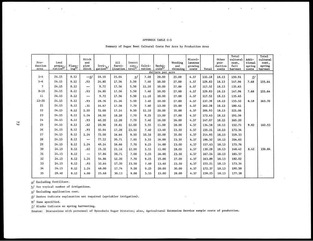
APPENDIX TABLE C-5

Summary of Sugar Beet Cultural Costs Per Acre by Production Area

Pro-ductionarea

Landprepaa,

ration-' ,PlanR,ing-1

-

Ditchandplowditch

Irri-b/gation-

Allferti-lization

Insectcons/trol-'

Culti-vation

Her147cide-

.

Weedingand

thinning

.

Miscel-laneousgrowingcosts Total

Otherpro-

ductioncosts

Totalculturalcost,fallharvest

Addi-tionalspringcosts

Totalculturalcost,

springharvest

dollars per acre

1-4,

24.15 8.12 --d/ 18.10 25.64 e/ 7.40 20.00 25.00 4.37 132.18 18.13 150.91 f/

5-6 24.15 8.12 .93 24.80 17.56 5.50 7.40 10.00 27.00 4.37 129.83 18.13 147.96 7.68 155.64

7 24.15 8.12 ..._. 9.72 17.56 5.50 11.10 10.00 27.00 4.37 117.52 18.13 135.65

8-10 24.15 8.12 .93 24.80 17.56 5.50 7.40 10.00 27.00 4.37 129.83 18.13 147.96 7.68 155.64

11 24.15 8.12 -- 9.72 17.56 5.50 11.10 10.00 27.00 4.37 117.52 18.13 135.65

12-20 24.15 8.12 .93 28.76 21.16 5.50 7.40 10.00 27.00 4.37 137.39 18.13 155.52 8.18 163.70

21 24.15 8.12 .31 54.67 17.56 7.70 7.40 13.00 25.00 4.37 162.28 18.13 180.41

22 24.15 8.12 1.55 72.00 17.14 9.50 11.10 20.00 35.00 4.37 206.93 18.13 221.06

23 24.15 8.12 1.24 58.50 18.10 7.70 9.25 15.00 27.00 4.37 173.43 18.13 191.56

24 24.15 8.12 .93 40.20 12.20 7.70 7.40 16.00 26.00 4.37 147.07 18.13 165.20

25 24.15 8.12 .62 20.96 19.81 12.00 5.55 11.00 28.00 4.37 134.58 18.13 152.71 9.82 162.53

26 24.15 8.12 .93 32.64 17.20 23.50 7.40 13.40 23.50 4.37 155.21 18.13 173.34

27 24.15 8.12 1.24 72.00 16.64 9.50 10.18 20.00 35.00 4.37 214.95 18.13 219.33

28 24.15 8.12 -- 77.12 20.71 7.00 5.55 16.00 23.50 4.37 186.52 18.13 204.65

29 24.15 8.12 1.24 49.14 16.66 7.70 9.25 14.00 23.00 4.37 157.63 18.13 175.76

30 24.15 8.12 .62 15.32 21.16 12.00 5.55 11.00 28.00 4.37 130.29 18.13 148.42 8.42 156.84

31 24.15 8.12 -- 57.84 20.71 7.00 5.55 16.00 23.50 4.37 167.24 18.13 185.37

32 24.15 8.12 1.24 54.86 12.20 7.70 9.25 15.00 27.00 4.37 163.89 18.13 182.02

33 24.15 8.12 .93 32.64 17.20 23.50 7.40 13.40 23.50 4.37 155.21 18.13 173.34

34 24.15 8.12 1.24 48.00 17.74 9.50 9.25 20.00 30.00 4.37 172.37 18.13 190.50

35 29.40 8.12 4.00 25.68 30.13 9.00 5.55 15.00 28.00 4.37 159.25 18.13 177.38

- 1

a/ Excluding fertilizer.

b/ For typical number of irrigations.

c/ Including application cost.

d/ Dashes indicate explanation not required (sprinkler irrigation).

e/ None specified.

f/ Blanks indicate no spring harvesting.

Source: Discussions with personnel of Spreckels Sugar Division; also, Agricultural Extension Service sample costs of production.

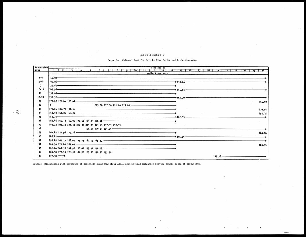
APPENDIX TABLE C-6

Sugar Beet Cultural Cost Per Acre by Time Period and Production Area

Productionarea

Time period.

112I3i4 1 51617 18- 19110,111121131141151161171181191201211221231dollars per acre

24 ,

1-4

5-6

7

8-10

11

12-20

21

22

23

24

25

26

27

28

29

' 30

31

32

33

34

35

150.91

147.96

.

135.65>155.64

147.96

135.65

)155.64

155.52

>

170.47 175.44

4

180.41

>163.70

'

s

165.50

174.01

155.15

213.06 217.06 221.06

s

179..86 185.71

158.50 161.85

152.71

191.56

165.20

225.06

s

162.46 165.18

183.33 192.33

164.42 171.98

148.42

167.90

201.33

175.76

170.62

210.33

173.34

219.33

195.01

176.06

223.83

199.83

162.53 >

237.33

204.65

242.33

>

s

160.64s

156.45 161.27

169.36 177.80

162.46.165.18

169.50 172.50

177.38 ----->

166.09

182.02

167.90

178.50

175.73 180.55 185.37

>156.84 s

s

165.14170.62

184.50

173.34

187.50

176.06

190.50 193.50

>

177.38

Source: Discussions with personnel of Spreckels Sugar Division; also, Agricultural Extension Service sample costs of production.

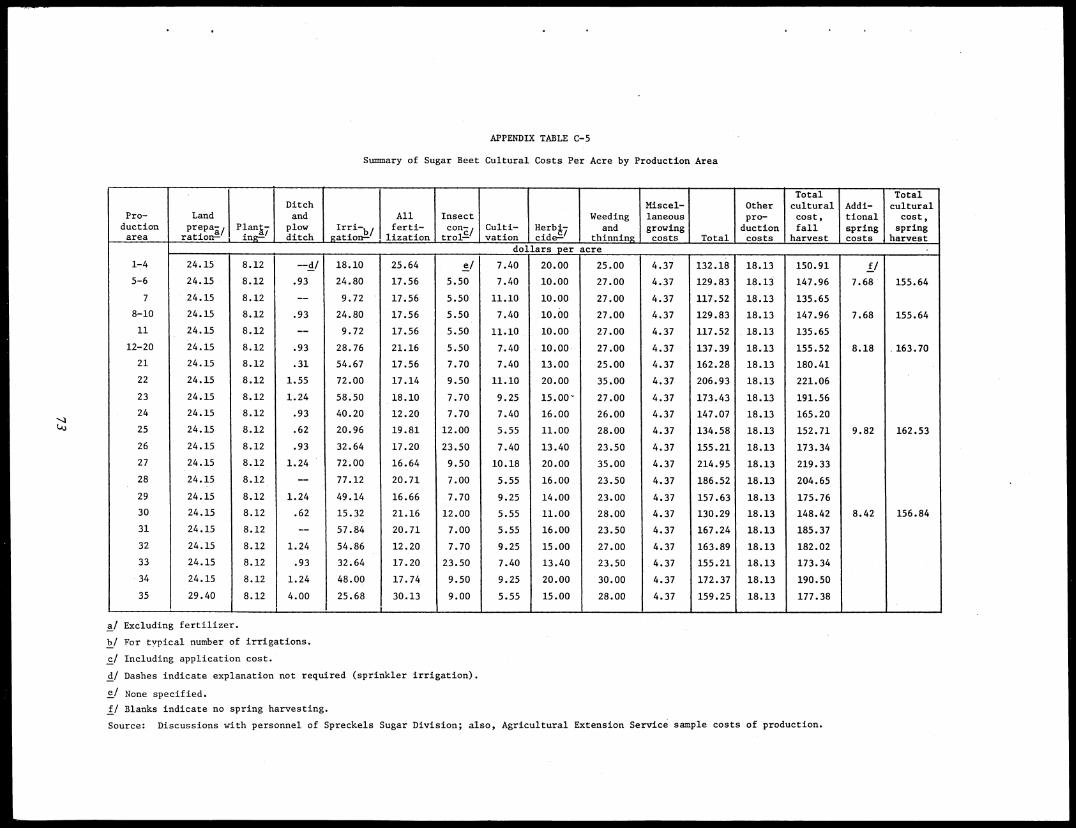
Lk)

APPENDIX TABLE C-5

Summary of Sugar Beet Cultural Costs Per Acre by Production Area

Pro-ductionarea ,

Landprepaa/

ration-' ,PlanR7ing-'

Ditchandplowditch _

Irri-b/gation-1

Allferti-lization

Insectcons/trol-1

Culti-vation

Her47cide-'

Weedingand

thinning

Miscel-laneousgrowingcosts Total

Otherpro-

ductioncosts

Totalculturalcost,fallharvest

Addi-tionalspringcosts

Totalculturalcost,

springharvest

. • dollars per acre

1-4 24.15 8.12 --d/ 18.10 25.64 e/ 7.40 20.00 25.00 4.37 132.18 18.13 150.91 f/

5-6 24.15 8.12 .93 24.80 17.56 5.50 7.40 10.00 27.00 4.37 129.83 18.13 147.96 7.68 155.64

7 24.15 8.12 __. 9.72 17.56 5.50 11.10 10.00 27.00 4.37 117.52 18.13 135.65

8-10 24.15 8.12 .93 24.80 17.56 5.50 7.40 10.00 27.00 4.37 129.83 18.13 147.96 7.68 155.64

11 24.15 8.12 ...... 9.72 17.56 5.50 11.10 10.00 27.00 4.37 117.52 18.13 135.65

12-20 24.15 8.12 .93 28.76 21.16 5.50 7.40 10.00 27.00 4.37 137.39 18.13 155.52 8.18 .163.70

21 24.15 8.12 .31 54.67 17.56 7.70 7.40 13.00 25.00 ' 4.37 162.28 18.13 180.41

22 24.15 8.12 1.55 72.00 17.14 9.50 11.10 20.00 35.00 4.37 206.93 18.13 221.06

23 24.15 8.12 1.24 58.50 18.10 7.70 9.25 15.00- 27.00 4.37 173.43 18.13 191.56

24 24.15 8.12 .93 40.20 12.20 7.70 7.40 16.00 26.00 4.37 147.07 18.13 165.20

25 24.15 8.12 .62 20.96 19.81 12.00 5.55 11.00 28.00 4.37 134.58 18.13 152.71 9.82 162.53

26 24.15 8.12 .93 32.64 17.20 23.50 7.40 13.40 23.50 4.37 155.21 18.13 173.34

27 24.15 8.12 1.24 72.00 16.64 9.50 10.18 20.00 35.00 4.37 214.95 18.13 219.33

28 24.15 8.12 -- 77.12 20.71 7.00 5.55 16.00 23.50 4.37 186.52 18.13 204.65

29 24.15 8.12 1.24 49.14 16.66 7.70 9.25 14.00 23.00 4.37 157.63 18.13 175.76

30 24.15 8.12 .62 15.32 21.16 12.00 5.55 11.00 28.00 4.37 130.29 18.13 148.42 8.42 156.84

31 24.15 8.12 -- 57.84 20.71 7.00 5.55 16.00 23.50 4.37 167.24 18.13 185.37

32 24.15 8.12 1.24 54.86 12.20 7.70 9.25 15.00 27.00 4.37 163.89 18.13 182.02

33 24.15 8.12 .93 32.64 17.20 23.50 7.40 13.40 23.50 4.37 155.21 18.13 173.34

34 24.15 8.12 1.24 48.00 17.74 9.50 9.25 20.00 30.00 4.37 172.37 18.13 190.50

35 29.40 8.12 4.00 25.68 30.13 9.00 5.55 15.00 28.00 4.37 159.25 18.13 177.38t

a/ Excluding fertilizer.

b/ For typical number of irrigations.

c/ Including application cost.

d/ Dashes indicate explanation not required (sprinkler irrigation).

e/ None specified.

f/ Blanks indicate no spring harvesting.

Source: Discussions with personnel of Spreckels Sugar Division; also, Agricultural Extension Service sample costs of production.

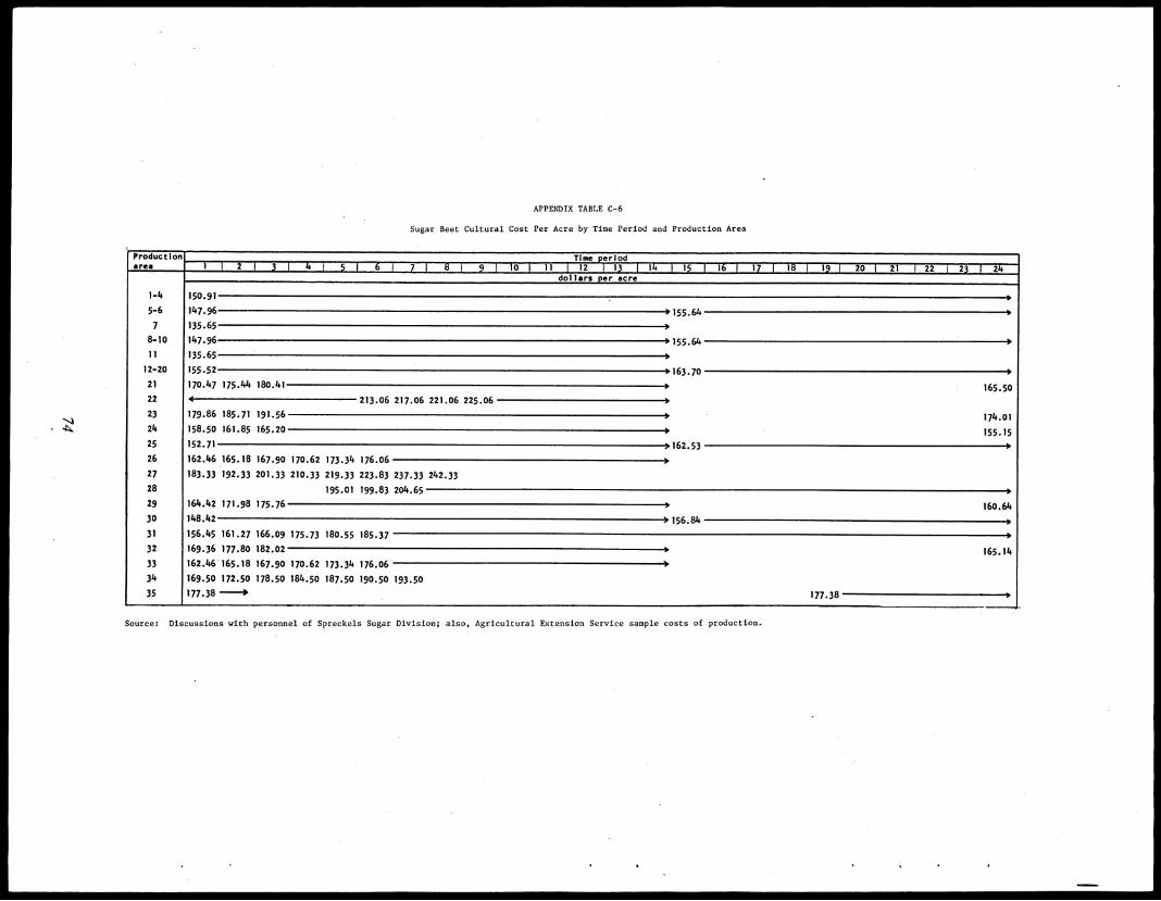
APPENDIX TABLE C-6

Sugar Beet Cultural Cost Per Acre by Time Period and Production Area

'Productionarea

Time period1 1 2 131415161718- 19110111112 1 13114115116117 1

dollars per acre18119120121122123124 '

1-4

5-6

7

8-10

11

12-20

21

22

23

24

25

26

27

28

29

30

31

32

33

34

35

150.91

147.96

>

135.65

>155.64

147.96

>

135.65

)155.64

155.52

170.47 175.44

<

180.41

>163.70 s

165.50

174.01

155.15

213.06 217.06 221.06

s

179..86 185.71

158.50 161.85

152.71

191.56

165.20

225.06 >

>

s

162.46 165.18

183.33 192.33

164.42 171.98

148.42

167.90

201.33

175.76

170.62

210.33

173.34

219.33

195.01

176.06

223.83

199.83

162.53 >

237.33

204.65

242.33

s

160.64>

156.45 161.27

169.36 177.80

162.46.165.18

169.50 172.50

177.38 -----,

166.09

182.02

167.90

178.50

175.73 180.55 185.37

156.84 s

>

165.14170.62

184.50

173.34

187.50

176.06

190.50 193.50

177.38 >

Source: Discussions with personnel of Spreckels Sugar Division; also, Agricultural Extension Service sample costs of production.

..11.01Man.

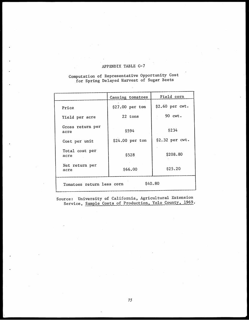
APPENDIX TABLE C-7

Computation of Representative Opportunity Cost

for Spring Delayed Harvest of Sugar Beets

Canning tomatoes

•

Field corn. -

Price

Yield per acre

Gross return peracre

Cost per unit

Total cost peracre

Net return peracre

$27.00 per ton

22 tons

$594

$24.00 per ton

$528

$66.00

$2.60 per cwt.

90 cwt.

$234

$2.32 per cwt.

$208.80

$25.20

, ...

Tomatoes return less corn $40.80

Source: University of California, Agricultural Extension

Service, Sample Costs of Production, Yolo County, 1969.

75

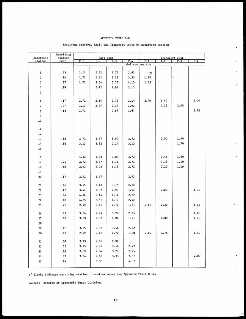
APPENDIX TABLE C-8

Receiving Station, Rail, and Transport Costs by Receiving Station

Receiving' station

Receivingstationcost

Rail cost Transport costF-1 F-2 F-3 I F-4 F-1 F-2 F-3 F-4

dollars per ton

1 .23 2.14 2.82 2.72 2.92 a

2 .14 1.71 2.92 3.13 3.33 1.60

3 .27 2.72 3.54 3.75 4.15 1.65'

4 .18 2.72 2.92 3.13

5

6 .17 2.72 2.14 2.72 2.14 2.40 1.60 2.00

7 .27 3.13 2.67 2.14 2.92 2.15 2.00

8 .13 2.72 2.67 2.67 2.75

9

10

11

12

13 .18 2 72 2.67 1.90 2.72 2.00 1.40

14 .16 3.13 2.82 2.14 3.13 1.70

15

16 4.22 2.58 3.00 3.72 2.45 1.60

17 .21 2.72 2.67 1.71 2.72 2.25 1.10

18 .18 2.92 2.25 1.71 2.72 2.10 1.10

19

20 .17 2.92 2.67 2.92

21 .16 3.95 3.13 3.75 2.72

22 .17 3.41 2.87 2.98 1.94 2.80 1.30

23 .14 4.14 3.44 4.14 2.72

24 .18 4.35 3.51 4.12 2.92

25 .25 2.92 2.61 2.72 1.71 2.60 2.20 1.15

26 .22 3.54 2.74 3.27 2.25 1.80

27 .15 3.33 2.82 2.92 1.71 2.80 1.10

28

29 .16 3.75 2.92 3.54 2.72

30 .21 2.92 2.25 2.72 1.90 2.60 1.75 1.50

31 .09 3.13 2.82 2.92

32 .13 3.75 2.92 3.54 2.72

33 .18 3.69 2.74 3.27 2.25

34 .27 3.54 2.82 3.33 2.67 2.00

35 .14 5.30 4.37

a/ Blanks indicate receiving station in another area; see Appendix Table D-10.

Source: Records of Spreckels Sugar Division.

76

APPENDIX D

- Decision Rules and Decision Parameters—Existing System

, 77

APPENDIX D

Decision Rules and Decision Parameters—Existing System

This appendix describes the derivation of the rules by which values are assigned to

the decision variables of the system, as initially modeled, and gives the empirical content

of these rules.

Preplanting Decision Rules

The five types, of preplanting decisions appear in Block 7 of Appendix A.

Total Tonnage and Acreage.--At the time of this study, the management goal was

to produce the amount of sugar that could be obtained by maximum use of available

factory capacity. Planned total tonnage per year thus is determined by summing expected

daily slice rates over the maximum number of days the plant may be expected to operate.

These values are summarized by time periods and factories in Appendix Table D-1. They

- reflect historical experience as to weather restrictions and anticipations of technical factory

changes. The initial model sets the total beet quantity goal at 3,862,950 tons. Dividing

this value by an expected average yield of 22.1 tons per acre gives a total acreage goal

of 174,794 acres. For modeling purposes, these control variables become constants in the

computational process rather than functions of state variables. If government regulations

were in effect or if management goals were to change, the values of the constants would

change. The model then could generate measures of the effects of such changes.

Allocation Among Production Areas.--In the initial model, we have allocated total

acreage among production areas according to proportions determined by historical processor

practices. The values as applied to the total acreage goal are given in Appendix Table D-2.

Factory Supply Sources.--During some periods of the year, each district (a group

of production areas) is unable to supply all of the beets needed by the factory in that

district while other districts may have excess supplies. The management practice has been

to specify a primary and alternate district supply source for each factory for each time

period and a set of priorities when more than one factory is supplied by a given district.

The decision rules by which interdistrict shipment patterns are determined are specified

in Appendix Table D-3. These rules reflect historical practices based on transportation

cost, available supplies, and factory need considerations and are somewhat interrelated

with the original allocations of acreages among production areas.

78

APPENDIX TABLE D-1

Expected Slice Rates by Factory and Production PeriodInitial Model

Time period F-1 F-2 F-3 F-4tons per period

July I 82,500 61,500 47,250 57,750II 88,800 65,600 50,400 61,600

August I 83,250 61,500 47,250 57,750II 88,800 65,600 48,800 61,600

September I 84,750 61,500 45,750 58,500II 84,750 61,500 45,750 58,500

October I 84,750 61,500 45,750 58,500II 90,400 65,600 48,800 62,400

November I 84,750 61,500 45,750 58,500II 56,500 61,500 45,750 58,500

December --a/ 184,500 -- 117,000

Spring 249,750 .228,000 186,000. 213,000

May II-June II __ __ __ 163,300

Total 1,079,000 1,039,800 657,250 1,086,900

TOTAL 3,862,950

_

a/ Dashes indicate no operation during that period.

Appendix Table D-3 shows that during July, D-4 supplies all factories. Asproduction starts in other areas, each factory is supplied first by quantities harvested inthe local district and then obtains any additional quantities needed from the alternatesources indicated in the table. From July through October, D-4 always has enough beetsto supply the factories for which it is the alternate source. In other periods the prioritiesare local districts first; then other districts as available. When D-2 supplies other factories,the priorities are F-2, F-4, and F-1.. When D-3 supplies other factories, the prioritiesare F-3, F-1, and F-4.

79

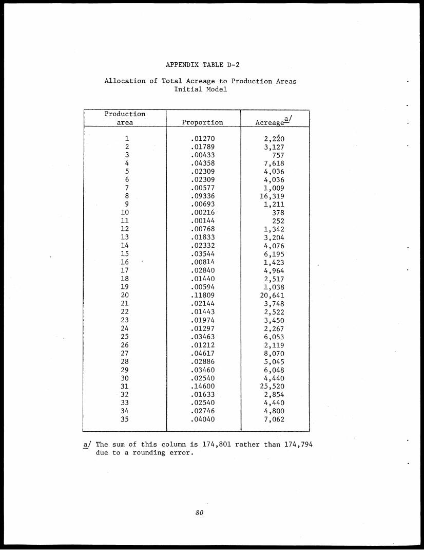
APPENDIX TABLE D-2

Allocation of Total Acreage to Production AreasInitial Model

Productionarea Proportion Acreage!'

/

1 .01270 2,202 .01789 3,1273 .00433 7574 .04358 7,6185 .02309 4,0366 .02309 4,0367 .00577 1,0098 .09336 16,3199 .00693 1,21110 .00216 37811 .00144 25212 .00768 1,34213 .01833 3,20414 .02332 4,07615 .03544 6,19516 .00814 1,42317 .02840 4,96418 .01440 2,51719 .00594 1,03820 .11809 20,64121 .02144 3,74822 .01443 2,52223 .01974 3,45024 .01297 2,26725 .03463 6,05326 .01212 2,11927 .04617 8,07028 .02886 5,04529 .03460 6,04830 .02540 4,44031 .14600 25,52032 .01633 2,85433 .02540 4,44034 .02746 4,80035 .04040 7,062

-

a/ The sum of this column is 174,801 rather than 174,794due to a rounding error.

80

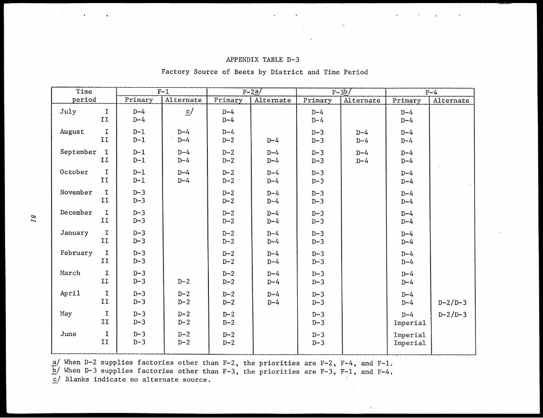
oo

APPENDIX TABLE D-3

Factory Source of Beets by District and Time Period

Timeperiod

F-1 F-2a/ F-3bi F-4Primary Alternate Primary Alternate Primary Alternate _ Primary Alternate

July I D-4 c/ D-4

,t

(.0 cn c

cn c'n cn

cn Cr)

Cr) Cr)

II II Il II II II II II II II II II

A A A A A A A A AA AA A A AA A A A A

A AA

D-4II D-4 D-4 D-4

August I D-1 D-4 D-4 D-4 D-4II D-1 D-4 D-2 D-4 D-4 Dzi

September I D-1 D-4 D-2 D-4 D-4 D-4II D-1 D-4 D-2 D-4 D-4 D-4

October I D-1 D-4 D-2 D-4 D-4II D-1 D-4 D-2 D-4 D-4 .

November I D-3 D-2 D-4 D-4II D-3 D-2 D-4 D-4

December I D-3 D-2 D-4 D-4II D-3 D-2 D-4 D-4

January I D-3 D-2 D-4 D-4II D-3 D-2 D-4 D-4

February I D-3 D-2 D-4 D-4II D-3 D-2 D-4 D-4

March I D-3 D-2 D-4 D-4II D-3 D-2 D-2 D-4 D-4

April I D-3 D-2 D-2 D-4 D-4II D-3 D-2 D-2 D-4 D-4 D-2/D-3

May I D-3 D-2 D-2 D-4 D-2/D-3II D-3 D-2 D-2 Imperial

June I D-3 D-2 D-2 ImperialII D-3 D-2 D-2 Imperial

a/ When D-2 supplies factories other than F-2, the priorities are F-2, F-4, and F-1.1.7 When D-3 supplies factories other than F-3, the priorities are F-3, F-1, and F-4.c/ Blanks indicate no alternate source.

Factory Starting Dates.--F-2, F-3, and F-4 are all specified to begin operations

on July 1 and are operated at maximum capabilities. Because of higher costs, the quantity

to be processed at F-1 (in the Salinas Valley) during July through October is determined

residually. If the total tonnage is less than the full capacity amount (3,862,950 tons in

this case), the reduction is taken from the F-1 fall operation. The expected number of

days of F-1 operation during this period is determined by dividing the residual quantity

by the average daily slice. The starting date for F-1 is then determined by subtracting

the expected number of days from 124 (November 1 is day 124) to establish the starting

date with July 1 being the earliest possible date.

As the year progresses from the planting period to near the harvest period, probable

yields become known with greater certainty; it, therefore, becomes possible to predict

more closely the actual tonnage to be harvested. This permits revision in the original starting

date calculations for F-1. To account for this in the actual modeling process, a random

factor was added to the original expected yield to obtain a revised estimate of total tonnage

which was used to determine the final starting date for F-1.1 In 8 out of 10 years

simulated, the final starting date remained at July 1.

Standard Inventory Levels.--Each factory maintains inventories of unprocessed beets

as a buffer for continuous operation as well as to extend operations. Management must

decide on the target levels of inventories which seem likely to minimize operating costs.

The level of inventory desired may vary throughout the season depending on the distance

of shipments and weather conditions which may affect the variability and predictability

of arrivals. Unnecessarily high inventory levels may increase storage costs and sugar losses,

while levels too low may involve costly shutdowns. For the initial model we have assigned

values based on the historical practices of the management. These are given in

Appendix Table D-4. Actual inventories may, of course, deviate considerably from these

values.

Planting Period Decision Rules

There is only one type of decision to be made during the planting period--the

time of planting in each producing area. The normal planting periods for the initial historical

model are given in Appendix Table D-5. Planting is then assumed to begin as early as

weather permits in the planting period and to continue unless interrupted by rain. The

pattern of actual planting within each area thus varies from year to year.

1 For a discussion on yield equations, see supra, page 52.

82

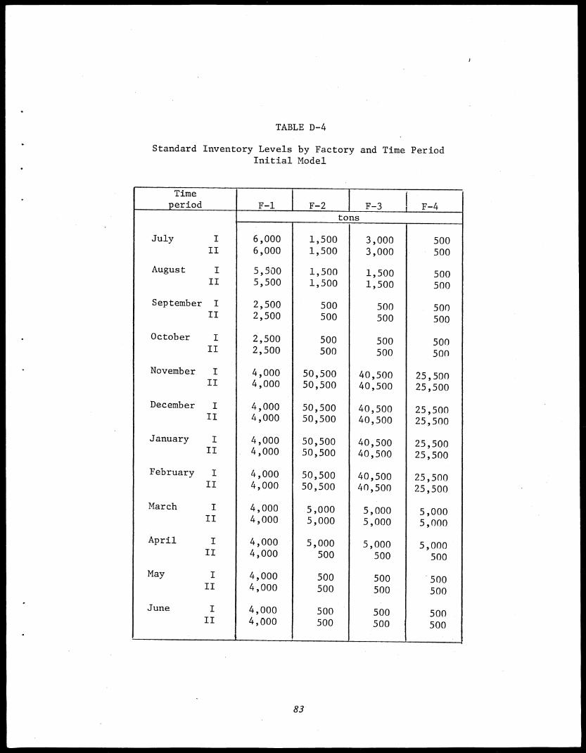
TABLE D-4

Standard Inventory Levels by Factory and Time PeriodInitial Model

Timeperiod

,

F-1 _ F-2 F-3 F-4tons

July I 6,000 1,500 3,000 500II 6,000 1,500 3,000 500

August I 5,500 1,500 1,500 500II 5,500 1,500 1,500 500

September I 2,500 500 500 500II 2,500 500 500 500

October I 2,500 500 500 500II 2,500 500 500 500

November I 4,000 50,500 40,500 25,500II 4,000 50,500 40,500 25,500

December I 4,000 50,500 40,500 25,500II 4,000 50,500 40,500 25,500

January I 4,000 50,500 40,500 25,500II 4,000 50,500 40,500 25,500

February I 4,000 50,500 40,500 25,500II 4,000 50,500 40,500 25,500

March I 4,000 5,000 5,000 5,000II 4,000 5,000 5,000 5,000

April I 4,000 5,000 5,000 5,000II 4,000 500 500 500

May I 4,000 500 500 500II 4,000 500 500 500

June I 4,000 500 500 500II 4,000 500 500 500 '

_ #

83

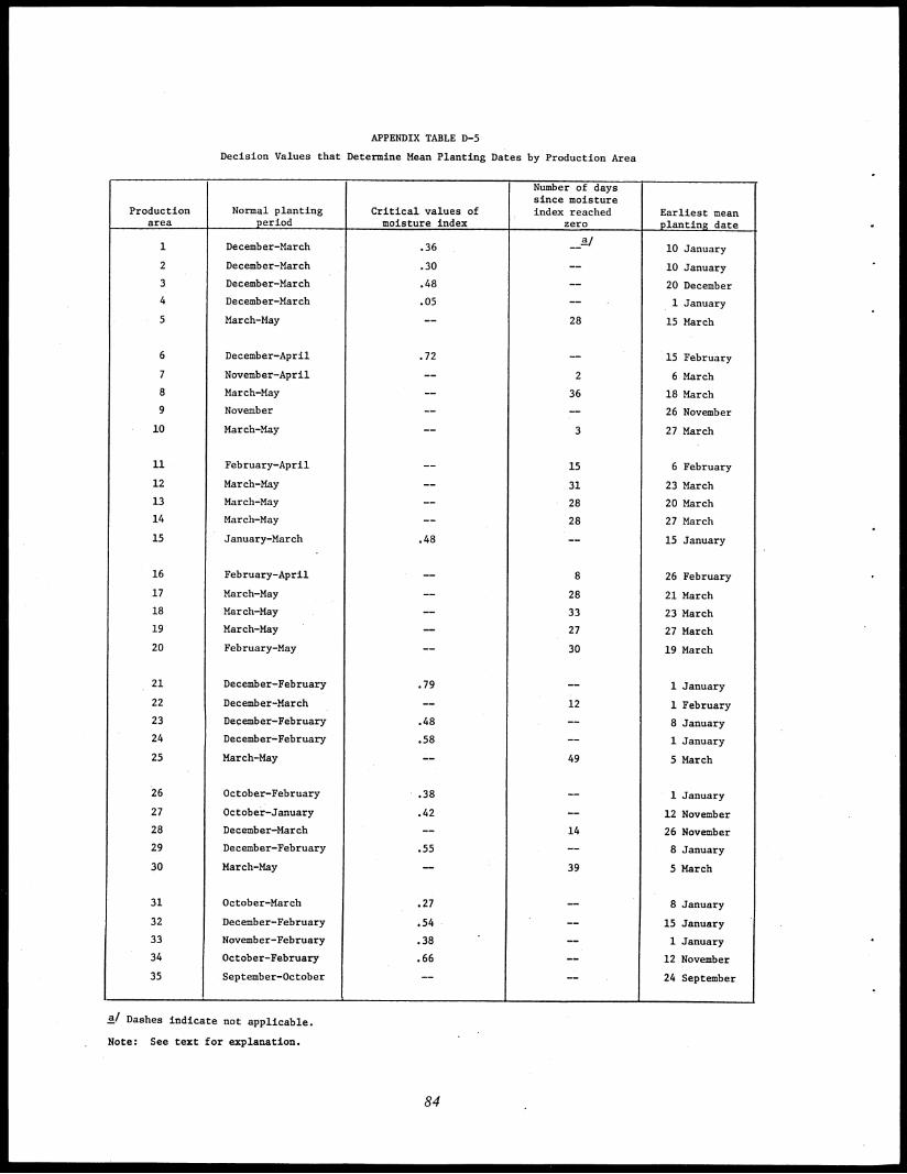
APPENDIX TABLE D-5

Decision Values that Determine Mean Planting Dates by Production Area

Productionarea

Normal plantingperiod

Critical values ofmoisture index

Number of dayssince moistureindex reached

zeroEarliest meanplanting date

1'

December-March .36a/ __

,

10 January

2 December-March .30 -- 10 January

3 December-March .48 -- 20 December

4 December-March .05 -- 1 January

5 March-May __ 28 15 March

6 December-April .72 -- 15 February

7 November-April -- 2 6 March

8 March-May -- 36 18 March

9 November -- -- 26 November

10 March-May __ 3 27 March

11 February-April -- 15 6 February

12 March-May -- 31 23 March

13 March-May -- 28 20 March

14 March-May -- 28 27 March

15 January-March .48 -- 15 January

16 February-April -- 8 26 February

17 March-May -- 28 21 March

18 March-May -- 33 23 March

19 March-May -- 27 27 March

20 February-May __ 30 19 March

, 21 December-February .79 -- 1 January

22 December-March -- 12 1 February

23 December-February .48 __ 8 January

24 December-February .58 __ 1 January

25 March-May -- 49 5 March

26 October-February .38 _.- 1 January

27 October-January .42 __ 12 November

28 December-March -- 14 26 November

29 December-February .55 -- 8 January

30 March-May -- 39 5 March

31 October-March .27 -- 8 January

32 December-February .54 __ 15 January

33 November-February .38 __ 1 January

34 October-February .66 -- 12 November

35 September-October -- __ 24 September

‘ , _

P/ Dashes indicate not applicable.

Note: See text for explanation.

84

Since the available planting and harvest data pertain only to production area totals,we were not able to model the planting decisions by individual fields or farms. Therefore,we formulated the model to establish a mean planting date (when 50 percent of the acreagehas been planted) for each area as a function of moisture index values.

Examination of records of weekly acres planted in each production area indicatedthat in some areas the mean planting date tended to occur at positive values of the moistureindex and in others only after the moisture index had dropped to zero. This may reflectdifferences in soil characteristics, delays to permit aphid flights to decline before planting,variations in moisture within production areas, and differences in planting distributionpatterns around the mean date.

For the first case (planting with positive moisture index values), critical values weredetermined as averages for recent years of the value of the moisture index when 50 percentof the area acreage has been planted. The moisture index declines as the soil drys, andthe date when it reaches the critical level is specified as the mean planting date for thatarea. These values are given in column 3 of Appendix Table D-5.

For the second case, the date when the moisture index drops to zero is used asa base. The critical value then is the average number of days from zero moisture until50 percent of the area acreage has been planted. The number of days from zero moisturewhich determine the mean planting date in particular areas is given in column 4 ofAppendix Table D-5. If at any time the sum of moisture values for five consecutivedays exceeds 0.50, the counting of number of days is started over when the moistureindex again drops to zero. This allows for a rainstorm to delay planting.

To insure that planting occurs only within the designated normal planting periods,a date was specified as the earliest at which 50 percent of an area's acreage could beplanted. These values are given in column 5 of Appendix Table D-5. Thus, the datewhen a critical value of the moisture index has been reached is specified as the meanplanting date only if it is the same as or later than the earliest mean planting date. Thereare no critical values for Areas 9 and 35. Planting occurs here prior to the heavy rains.Thus, the mean planting dates are the earliest possible dates.

Harvest Period Decision Rules

The four types of decisions to be made during the harvest period appear in Blocks 19,20, 28, and 16 of Appendix A. The first three types of decisions are interrelated.

Quantity of Beets Harvested in Each District.--The decision rules for determiningthe quantities to be harvested vary by time period and are modified by random weatherfactors during the wet season.

85

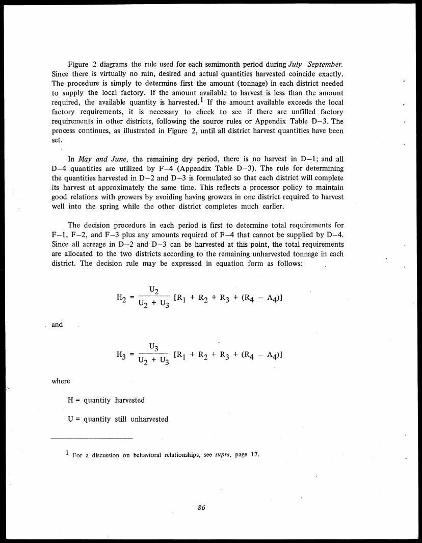
Figure 2 diagrams the rule used for each semimonth period during July—September.Since there is virtually no rain, desired and actual quantities harvested coincide exactly.The procedure is simply to determine first the amount (tonnage) in each district neededto supply the local factory. If the amount available to harvest is less than the amountrequired, the available quantity is harvested.1 If the amount available exceeds the localfactory requirements, it is necessary to check to see if there are unfilled factoryrequirements in other districts, following the source rules or Appendix Table D-3. Theprocess continues, as illustrated in Figure 2, until all district harvest quantities have beenset.

In May and June, the remaining dry period, there is no harvest in D-1; and allD-4 quantities are utilized by F-4 (Appendix Table D-3). The rule for determiningthe quantities harvested in D-2 and D-3 is formulated so that each district will completeits harvest at approximately the same time. This reflects a processor policy to maintaingood relations with growers by avoiding having growers in one district required to harvestwell into the spring while the other district completes much earlier.

The decision procedure in each period is first to determine total requirements forF-1, F-2, and F-3 plus any amounts required of F-4 that cannot be supplied by D-4.Since all acreage in D-2 and D-3 can be harvested at this point, the total requirementsare allocated to the two districts according to the remaining unharvested tonnage in eachdistrict. The decision rule may be expressed in equation form as follows:

. and

H2 =U2 +

U2

U3

[R1 + R2 + R3 + (R4 — A4)]

—2 4. u

3 [R1 + R2 + R3 + ( — A4)]

where

H = quantity harvested

U = quantity still unharvested

•

1 For a discussion on behavioral relationships, see supra, page 17.

86

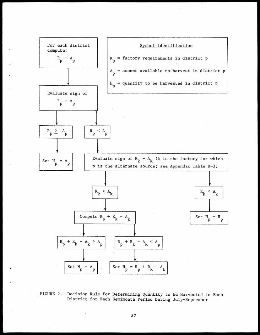
For each districtcompute:

R -AP P

Evaluate sign of

R -AP P

R > AP

Set H = AP P

Symbol identification

Rp = factory requirements in district p

A = amount available to harvest in district p

H = quantity to be harvested in district p

R <AP P

Evaluate sign of Rk - Ak (k is the factory for which

p is the alternate source; see Appendix Table D-3)

Rk Ak

Compute Rp + R

k

R + Rk - Ap p

1Set H = A

P P

R + Rk - Ak < Ap p

Set Hp = Rp + Rk - Ak

Rk Ak

Set H = RP P

FIGURE 2. Decision Rule for Determining Quantity to be Harvested in EachDistrict for Each Semimonth Period During July-September

87

and

R = factory requirement

A = amount available for harvest

subscripts refer to districts.

When Imperial is supplying F-4, the term, R4 — A4, drops out. The harvested quantitiesare then allocated to factories according to Appendix Table D-3 and the prioritiesspecified previously.

During the wet season, October—April, the desired harvest levels are modified byprobability values that vary randomly in relation to the level of the moisture index asshown in Appendix Table D-6. The table indicated, for example, that, if the moistureindex is between .75 and .99, the probability of zero harvest is .219; the probabilitythat it will be between 1 and 24 percent of normal is .290, and so on. The harvest decisionrule is as follows:

1. Determine normal daily factory requirements by reference toAppendix Table D-7.

2. Determine desired quantity harvested in each district as indicated in Figure 2.

3. Observe moisture index value generated for that date.

4. Enter Appendix Table D-6 to obtain the proportion of normal harvest for thatdate. Use midpoint values of proportion classes. If moisture index is zero, theproportion of normal harvest is 1.0.

5. Set quantity to be harvested equal to the desired quantity multiplied by theproportion of normal harvest.

Allocations of District Quantities Harvested to Production Areas.--Given thedecisions on district quantities, the next step is to allocate these quantities to the severalproducing areas within each district. These decisions are based on the availability of beetsto be harvested in each area, the capacities or receiving stations, previously specified targetcompletion dates, and a set of quotas. The decision rules are different for each districtand again are modified by moisture index during the wet season.

88

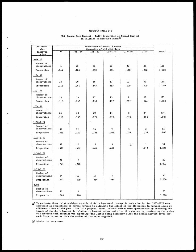
APPENDIX TABLE D-6

Wet Season Beet Harvest: Daily Proportion of Normal Harvestin Relation to Moisture Indexli

Moistureindexinterval

Proportion of normal harvest

Totalof all districts

0,Composite

.01-.24 .25-.49 .50-.74 .75-.99 1.00inches

.01-.24

Number ofobservations 6 25 31 19 20 34 135

Proportion .044 .185 .230 .141 .148 .252 1.000

.25-.49

Number ofobservations 13 29 16 17 12 23 110

Proportion .118 .264 .145 .155 .109 .209 1.000

.50-.74

Number ofobservations 24 33 17 13 8 16 111

Proportion .216 .298 .153 .117 .072 .144 1.000

.75-.99

Number ofobservations 25 33 20 14 8 14 114

Proportion .219 .290 .175 .123 .070 .123 1.000

1.00-1.24

Number ofobservations

.

31 21 16 9 5 3 85

Proportion .365 .247 .188 .106 .059 .035 1.000

1.25-1.49

Number ofobservations 32 20 3 3 b/ 1 59

Proportion .542 .339 .051 .051 .017 1.000

1.50-1.74

Number ofobservations 21 8 29

Proportion .724 .276 1.000

1.75-1.00

Number ofobservations 34 12 17 4 67

Proportion .507 .179 .254 .060 1.000

2.00

Number ofobservations 21 4 25

Proportion .840 .160 1.000

- - I

a/ To estimate these relationships, records of daily harvested tonnage in each district for 1965-1970 wereexpressed as proportions of normal harvest to eliminate the effect of the difference in harvest level atdifferent times of the year. For this purpose, normal ,harvest values were approximated by examining thelevels of the day's harvest in relation to harvest before and after this day and by considering the numberof factories each district was supplying--the latter being necessary since the normal harvest level foreach district varies with the number of factories supplied.

b/ Blanks indicate zero.

89

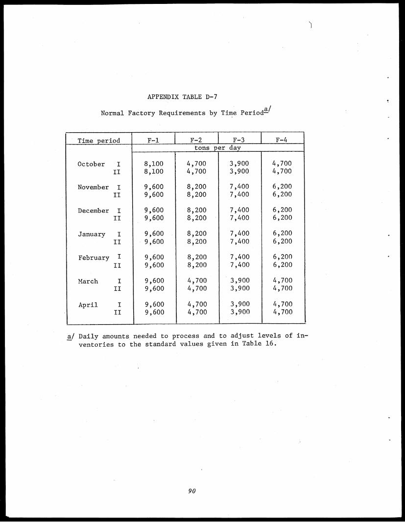
APPENDIX TABLE D-7

Normal Factory Requirements by Time Period'

Time period F-1 F-2 _ F-3 F-4tons per day

, ,

October I 8,100 4,700 3,900 4,700II 8,100 4,700 3,900 4,700

November I 9,600 8,200 7,400 6,200II 9,600 8,200 7,400 6,200

December I 9,600 8,200 7,400 6,200II 9,600 8,200 7,400 6,200

January I 9,600 8,200 7,400 6,200

II 9,600 8,200 7,400 6,200

February I 9,600 8,200 7,400 6,200

II 9,600 8,200 7,400 6,200

March I 9,600 4,700 3,900 4,700II 9,600 4,700 3,900 4,700

April I 9,600 4,700 3,900 4,700II 9,600 4,700 3,900 4,700

. ,

a/ Daily amounts needed to process and to adjust levels of in-

ventories to the standard values given in Table 16.

90

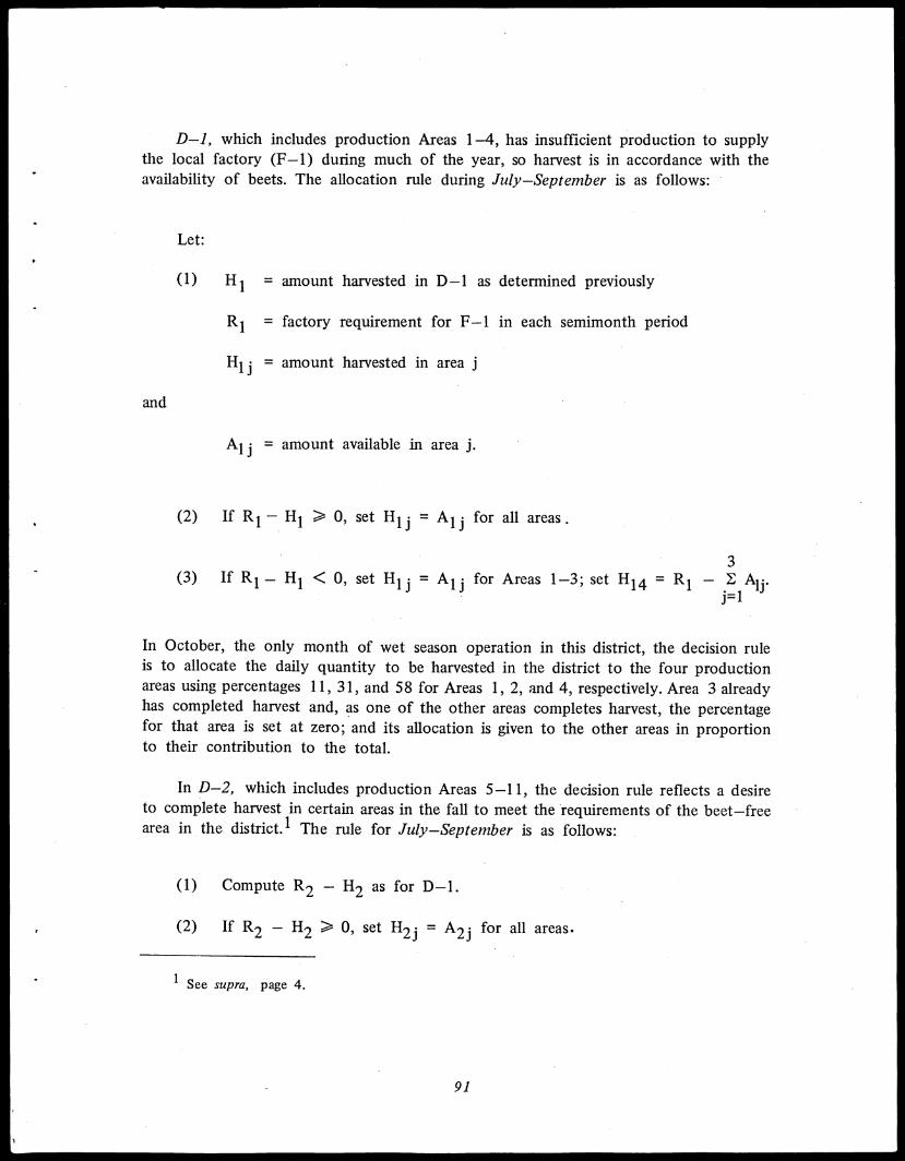
D-1, which includes production Areas 1-4, has insufficient production to supplythe local factory (F-1) during much of the year, so harvest is in accordance with theavailability of beets. The allocation rule during July—September is as follows:

and

Let:

(1) H = amount harvested in D-1 as determined previously

R1 = factory requirement for F-1 in each semimonth period

I-11i = amount harvested in area j

A1 j = amount available in area j.

(2) If R1 — H1 0, set Hu = A1 j for all areas.

3(3) If R1 — H1 < 0, set H1 = Au for Areas 1-3; set H1 = R —

J=1

In October, the only month of wet season operation in this district, the decision ruleis to allocate the daily quantity to be harvested in the district to the four productionareas using percentages 11, 31, and 58 for Areas 1, 2, and 4, respectively. Area 3 alreadyhas completed harvest and, as one of the other areas completes harvest, the percentagefor that area is set at zero; and its allocation is given to the other areas in proportionto their contribution to the total.

In D-2, which includes production Areas 5-11, the decision rule reflects a desireto complete harvest in certain areas in the fall to meet the requirements of the beet—freearea in the district.' The rule for July—September is as follows:

(1) Compute R2 — H2 as for D-1.

(2) If R2 — H2 0, set H2i = A2i for all areas.

1 See supra, page 4.

91

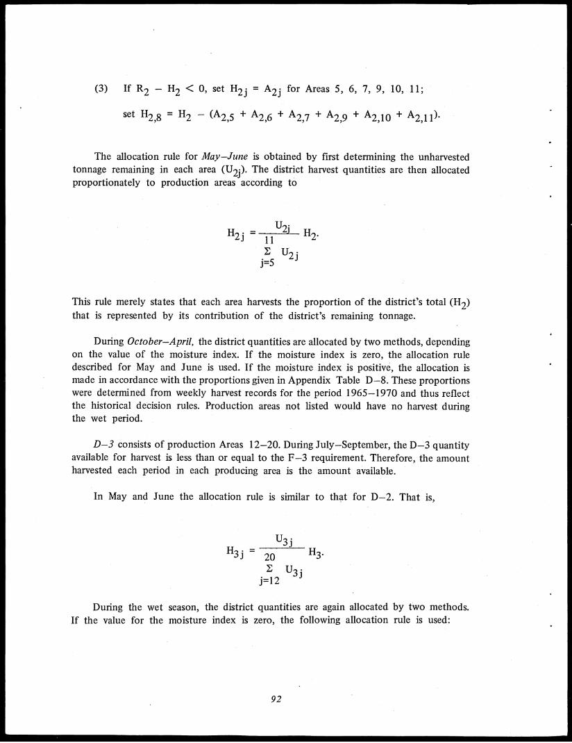
(3) If R2 — H2 < 0, set H

set H2, - (A2,5

for Areas 5, 6, 7, 9, 10, 11;

+ A2,6 + A2,7 + A2,9 + A2,10 + A2,11).

The allocation rule for May—June is obtained by first determining the unharvestedtonnage remaining in each area (Uzi). The district harvest quantities are then allocatedproportionately to production areas according to

H2i

This rule merely states that each area harvests the proportion of the district's total (H2)

that is represented by its contribution of the district's remaining tonnage.

During October—April, the district quantities are allocated by two methods, dependingon the value of the moisture index. If the moisture index is zero, the allocation ruledescribed for May and June is used. If the moisture index is positive, the allocation ismade in accordance with the proportions given in Appendix Table D-8. These proportionswere determined from weekly harvest records for the period 1965-1970 and thus reflectthe historical decision rules. Production areas not listed would have no harvest duringthe wet period.

D-3 consists of production Areas 12-20. During July—September, the D-3 quantityavailable for harvest is less than or equal to the F-3 requirement. Therefore, the amountharvested each period in each producing area is the amount available.

In May and June the allocation rule is similar to that for D-2. That is,

• =-)-1 20

Uj=12

U3 j

•

H3.

During the wet season, the district quantities are again allocated by two methods.

If the value for the moisture index is zero, the following allocation rule is used:

92

••

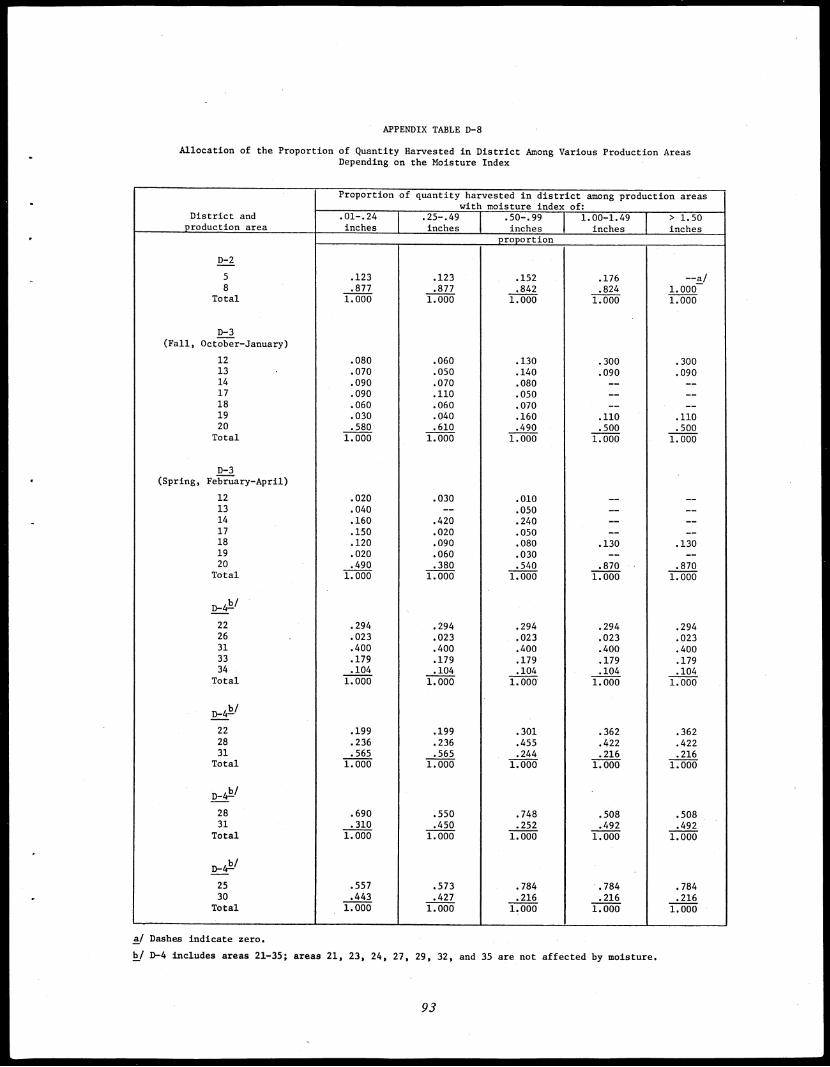
APPENDIX TABLE D-8

Allocation of the Proportion of Quantity Harvested in District Among Various Production AreasDepending on the Moisture Index

,

District andproduction area

Proportion of quantity harvested in district among production areaswith moisture index of:

.01-.24inches

.25-.49 iinches i

.50-.99 Iinches i

-1.00-1.49inches

> 1.50inches

D-2

proportion

5 .123 .123 .152 .176 --a/8 .877 .877 .842 .824 1.000

Total 1.000 1.000 1.000 1.000 1.000

D-3(Fall, October-January)

12 .080 .060 .130 .300 .30013 - .070 .050 .140 .090 .09014 .090 .070 .080 __. --17 .090 .110 .050 -- --18 .060 .060 .070 -- --19 .030 .040 .160 .110 .11020 .580 .610 .490 .500 .500Total 1.000 1.000 1.000 1.000 1.000

D-3 .(Spring, February-April)

12 .020 .030 .010 -- --13 .040 -- .050 __ --14 .160 .420 .240 .__ --17 .150 .020 .050 -- --18 .120 .090 .080 .130 .13019 .020 .060 .030 ...... --20 .490 .380 .540 .870 .870Total 1.000 1.000 1.000 1.000 1.000

D-411/

22 .294 .294 .294 .294 .29426 . .023 .023 .023 .023 .02331 .400 .400 .400 .400 .40033 .179 .179 .179 .179 .17934 .104 .104 .104 .104 .104

Total 1.000 1.000 1.000 1.000 1.000

D-4b/-

22 .199 .199 .301 .362 .36228 .236 .236 .455 .422 .42231 .565 .565 .244 .216 .216

Total 1.000 1.000 1.000 1.000 1.000

D-4h/•

28 .690 .550 .748 .508 .508 .31 .310 .450 .252 .492 .492Total

b/D-4-

1.000 1.000 1.000 1.000 1.000

25 .557 .573 .784 .784 .78430 .443 .427 .216 .216 .216Total 1.000 1.000 1.000 1.000 1.000

a/ Dashes indicate zero.

II/ D-4 includes areas 21-35; areas 21, 23, 24, 27, 29, 32, and 35 are not affected by moisture.

93

I-1/ • =H320

AP•j=12

AP•

where AP • is acres planted in area j, and H is acres harvested. This rule merely statesthat each area harvests the proportional of the district's total that is represented by itscontribution to the district's total acreage.

When the moisture index is positive, the district harvest quantities determinedpreviously are allocated to the production areas as indicated by the proportions inAppendix Table D-8.

The D-4 harvest allocation rules for July—September reflect a desire to harvest hotclimate areas at maximum receiving station capacity to complete harvest before the qualityof the crop drops. For Areas 21, 23, 24, 29, 32, and 34, the rule is to set the quantityharvested (H4j) equal to receiving station capacity. The rule for Areas 22, 26, 27, 28,31, and 33 is

H4i = Pzu [H4 — (H A z 4- H4,23 + H4,24 ÷ H4,29 4- H4,32 ÷ 144,34)]

where P4i is an allocation proportion which reflects availability of beets in different areas

at different times and the desire to complete harvest in areas likely to be affected by

rain. This rule may be clarified by pointing out that the harvest in D-4 is composed

of twoS parts--the quantity allocated to areas operating at receiving station capacity (the

total of the values within the parentheses) and a residual quantity allocated to the remaining

stations. The values of P4j are given in Appendix Table D-9. The nonavailability of beets

to harvest is indicated by proportions not being listed for that area. The values of time

period 10 continue until the fall harvest is completed. When an area completes harvest,

the P4i value for that area is set at zero, and its allocation proportion is given to other

areas in proportion to their contribution to the total.

When the model is operating on a daily basis (October—April), the allocation of

the district harvest to areas depends on the value of the moisture index. If the moisture

index is zero, the allocation is made on the basis of the proportions in

Appendix Table D-9. If the moisture index is positive, the allocation is determined by

applying the proportions given in Appendix Table D-8. In Appendix Table D-8 there

are four sets of proportions for D-4. The computer program counts the number of areas

in D-4 where harvest remains and branches to the appropriate set of proportions. If there

are over five areas remaining, the top set is used. If there are only five, it branches to

the second set; and if there are either three or four left, it branches to the second set.

If there are less than three areas, then it branches to the bottom set.

94\

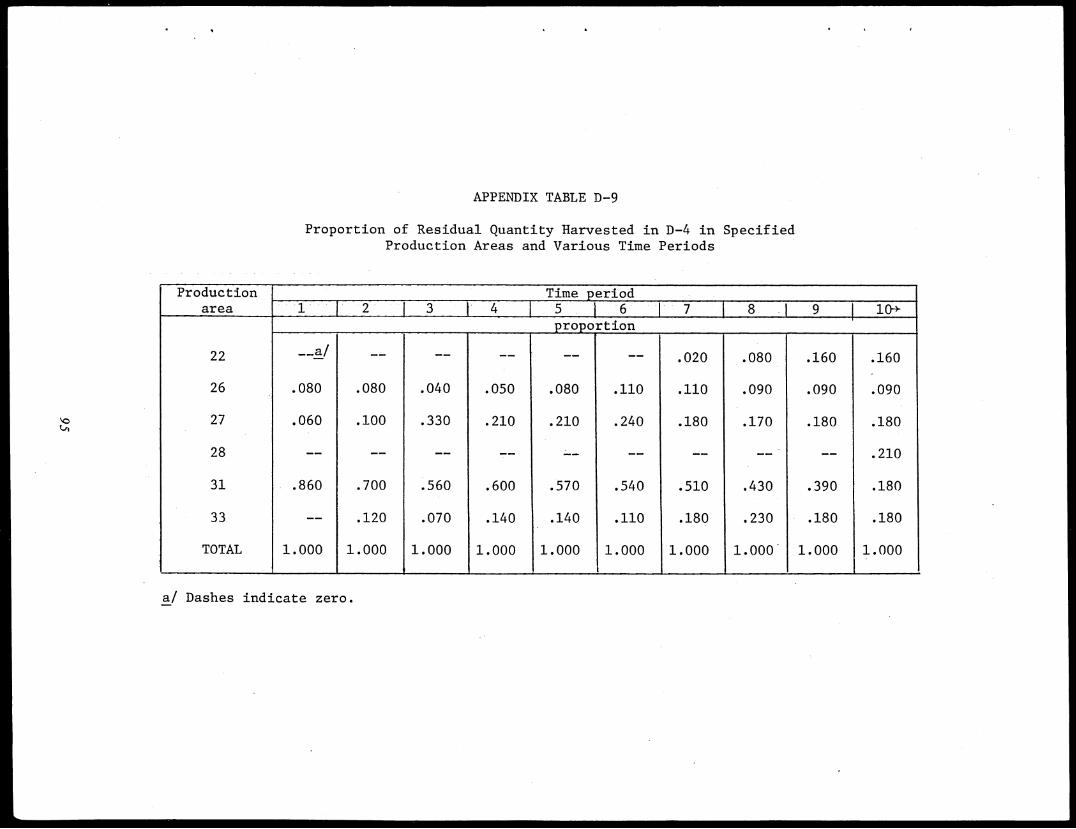
‘.0

APPENDIX TABLE D-9

Proportion of Residual Quantity Harvested in D-4 in SpecifiedProduction Areas and Various Time Periods

Productionarea

' Time period_ 1 12 J3 1 k 5 1 6 1 7 8 .1 9 I 104, ,

proportion

22 __a/ ....... __ ..._ __ -- .020 .080 .160 .160

26 .080 .080 .040 .050 .080 .110 .110 .090 .090 .090

27 .060 .100 .330 .210 .210 .240 .180 .170 .180 .180

28 ....._, .__. ........ ....._ - __ __ __ -- .210

31 .860 .700 .560 .600 .570 .540 .510 .430 .390 .180

33 -- .120 .070 .140 .140 .110 .180 .230 .180 .180

,, TOTAL,

1.000 1.000 1.000 1.000 1.000 1.000 1.000 1.000 1.000 1.000

a/ Dashes indicate zero.

For Area 35 (Imperial), the quantity harvested is the quantity needed to operateF-4 (Appendix Table D-3).

Delivery Routes and Methods.--Two types of decisions are involved: routes fromproduction areas to receiving stations (R.S.) and routes and means of shipment fromreceiving stations to factories.

1. Production areas to receiving stations: The 35 production areas deliverthe harvested beets to 27 receiving stations. Each station is numbered according to thearea in which it is located. Appendix Table D-10 gives the route assignments specifiedby the processor based on past experience. During periods of low volume or when certainfactories are being supplied, it may be economical to shut down some receiving stationsand to divert trucks to other stations or directly to the factory. There are four stationsso affected--13, 14, 17, and 18. The rules for determining these alternate routes areas follows:

Area 13

During February—June, deliver to R.S. 13

During July—January (if harvesting), deliver to R.S. 20 if going to factory 3; deliverto R.S. 17 if going elsewhere

Area 14

Deliver to R.S. 20 if going to F-3

Deliver to R.S. 14 if going elsewhere

Area 17

Deliver to R.S. 20 if going to F-3

Deliver to R.S. 17 if going elsewhere

Area 18

Deliver to R.S. 20 if going to F-3

Deliver to R.S. 18 if going elsewhere

96

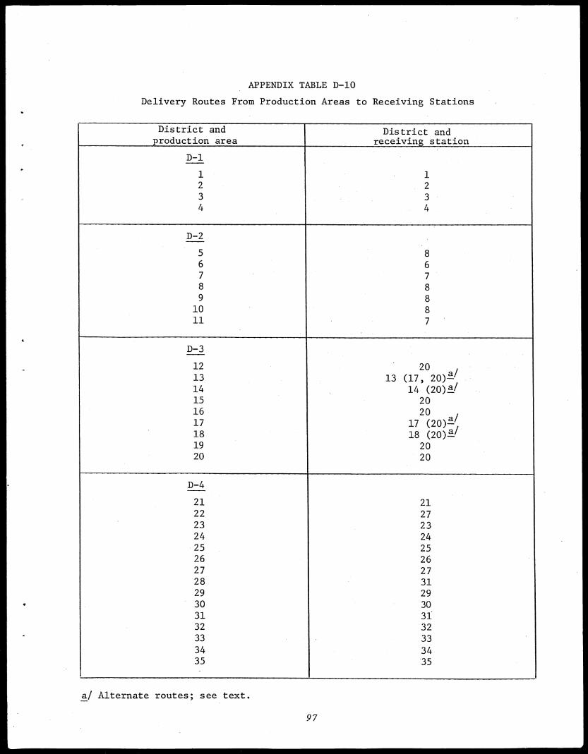
APPENDIX TABLE D-10

Delivery Routes From Production Areas to Receiving Stations

District andproduction area

District andreceivin.g. station

D-1

1 12 23 34 4

D-2

5 86 67 78 89 810 811 7

_

D-3

12 2013 13 (17, 20) 114 14 (20)!15 2016 2017 --,17 (20)118 18 (20)!19 2020 20

D-4

21 2122 2723 2324 2425 2526 2627 2728 3129 2930 3031 3132 3233 3334 3435 35

a/ Alternate routes; see text.

97

2. Receiving station to factory: The shipment patterns and methods oftransportation from receiving stations to factories are derived for each period as a linearprogramming solution which minimizes total transportation cost subject to the restrictionsimposed by harvest decisions, factory requirements, and the source restrictions specifiedin Appendix Table D-3. Since the quantities harvested and factory needs change, a newsolution is required for each period. In practice, the restrictions imposed by the previoussource decisions specified in Appendix Table D-3, plus inspection of the transportationcost matrix (Appendix Table C-8), enable us to greatly reduce the size of the problemto be solved and make it unnecessary to obtain new solutions for all periods. Thepreprogramming restrictions thus obtained are summarized in Appendix Table D-11. Ifthere are any quantities left unallocated after applying these rules, a linear programmingsolution is obtained to determine the final optimal routing.

Factory Shutdown and Startup Dates.--Each factory continues to operate in thefall until rain prevents 'further harvest and then resumes operation in the spring whenthe soil again becomes dry enough for harvest. The rules for stopping and starting areas follows:

1. Fall shutdown: If the date is November 15 or later and the district moistureindex reaches or exceeds a critical level, harvest stops. The factory continues to operateuntil its inventory of beets is sliced and then shuts down. For control within the computerprogram, artificial variables are assigned values which indicate that harvest has stoppedand then that the factory has been shut down. The critical moisture values, based on1965-1970 average experience, are 1.19 inches for D-2; 1.07 inches for D-3; .82 inchesfor D-4. D-1 is not included since harvest has been completed by this time. However,D-3 is supplying F-1 at this time so, when harvest stops in D-3, F-1 must shut downalso.

2. Spring startup: The processor goal is to start up as soon after a prespecifieddate as possible. A certain level of inventory must be accumulated first. The dates andinventory requirements based on historical practice are as follows:

Factory Date Required inventory(tons)

F-1 March II 5,550

F-2 March I 4,100

F-3 March I 3,150

F-4 March I 3,850

A control variable in the computer program is set to indicate that the factory can bereopened when a specified date is reached. At the same time, harvest operations are allowedto resume with processing starting when the factory inventory reaches the required level.

98

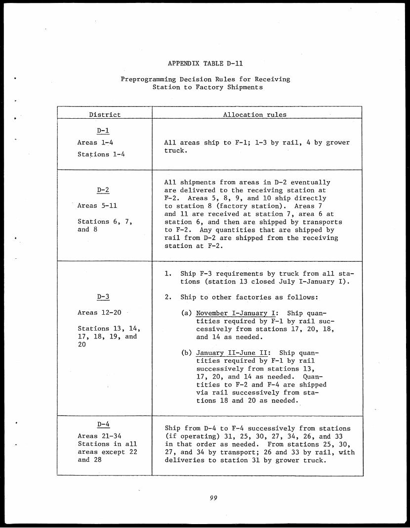
APPENDIX TABLE D-11

Preprogramming Decision Rules for ReceivingStation to Factory Shipments

District Allocation rules,

D-1

All areas ship to F-1; 1-3 by rail, 4 by growertruck.

Areas 1-4

Stations 1-4

D-2All shipments from areas in D-2 eventuallyare delivered to the receiving station atF-2. Areas 5, 8, 9, and 10 ship directlyto station 8 (factory station). Areas 7and 11 are received at station 7, area 6 atstation 6, and then are shipped by transportsto F-2. Any quantities that are shipped byrail from D-2 are shipped from the receivingstation at F-2.

Areas 5-11

Stations 6, 7,and 8

D-3

1. Ship F-3 requirements by truck from all sta-tions (station 13 closed July I-January I).

2. Ship to other factories as follows:

(a) November I-January I: Ship quan-Areas 12-20

Stations 13, 14,17, 18, 19, and20

tities required by F-1 by rail suc-cessively from stations 17, 20, 18,and 14 as needed.

(b) January II-June II: Ship quan-tities required by F-1 by railsuccessively from stations 13,17, 20, and 14 as needed. Quan-tities to F-2 and F-4 are shippedvia rail successively from sta-tions 18 and 20 as needed.

D-4Ship from D-4 to F-4 successively from stations(if operating) 31, 25, 30, 27, 34, 26, and 33in that order as needed. From stations 25, 30,27, and 34 by transport; 26 and 33 by rail, withdeliveries to station 31 by grower truck.

Areas 21-34Stations in allareas except 22and 28

99

REFERENCES

[1] Barr, C. Guinn, Mervine, E. M., and Bice, R. A. "A Preliminary Report on the

Effect of Temperature and Beet Conditions on Respiration and Loss of Sugar

from Beets in Storage." American Society of Sugar Beet Technologists,

Proceedings Issue, 1940, pp. 52-63.

[2] California Crop and Livestock Reporting Service. California Agriculture, 1971.

Sacramento, 1972.

[3] California Department of Agriculture. Press release. October 28, 1971.

[4] Hills, F. J., and Johnson, S. S. The Sugar Beet Industry in California. University

of California, Agricultural Experiment Station Bulletin No. 562. Berkeley, 1973.

[5] Johnson, Russell, T., et al. (eds.). Advances in Sugar Beet Production: Principles

and Practices. Ames: Iowa State University Press, 1971.

[6] McGinnis, R. A. (ed.). Beet—Sugar Technology. 2d ed. Fort Collins, Colorado:

Beet Sugar Development Foundation, 1971.

[7] Niles, James A. "Analysis of Systems of Coordinating Agricultural Production

and Processing Operations with Special Reference to Beet Sugar Scheduling."

Unpublished Ph.D. dissertation, Department of Agricultural Economics,

University of California, Davis, 1972.

[8] University of California, Agricultural Extension Service. "Cost of Producing Sugar

Beets." Various counties and dates.

[9] U. S. Agricultural Marketing Service. Marketing Sugar Beets, by Donald Jackson,

et al. AMS-137. 1956.

[10] U. S. Economic Research Service. Economics of Sugar Beet Marketing, by Donald

Jackson. ERS-49. 1962.

[11] Zusman, Pinhas, and Amiad, Amotz. "Simulation: A Tool for Farm Planning ,

Under Conditions of Weather Uncertainty," Journal of Farm Economics,

Vol. 47, No. 3 (August, 1965), pp. 574-594.

100

GENERAL BACKGROUND REFERENCES

California Beet Growers Association, Ltd. The California Sugar Beet. Stockton, California,

1968-1971 issues.

California Department of Water Resources. Hydrologic Data: 1963. Bulletin No. 130-63.

Sacramento, 1963, and subsequent issues.

Cottrell, R. H. Beet Sugar Economics. Caldwell, Idaho: Caxton Printers, Ltd., 1952.

Hills, F. J., and Reed, A. D. An Introduction to the Sugar Beet Industry in California.

University of California, Agricultural Experiment Station Leaflet No. 121. Berkeley, 1960.

Huculak, A. "Die Optimierung der Kampagnadauer unter Besonderer Beriicksichtigung des

Riibentransportes," Zeitschrift fur die Zuckerindustrie, Vol. 19, No. 8 (August, 1969),

pp. 434-444.

Lange, W. Harry. "The Integrated Control Approach to the Suppression of Yellow and

Mosaic of Sugar Beets." The California Sugar Beet, 1969. Stockton, California: Beet

Growers Association, Ltd., 1969, pp. 20 and 36.

Liisf, George 0. G., and Kneese, Allen V. The Economics of Water Utilization in the Beet

Sugar Industry. Baltimore: The Johns Hopkins Press, 1968.

Moody, L. A. "Production Allocation in the Beet Sugar Industry." Proceedings of the

Second International Conference on Operational Research. London: English

Universities, Ltd., 1960, pp. 237-250.

Moore, J. R. "Economic Implications of Share Contracts for Sugar Beets," Journal of

Farm Economics, Vol. 44, No. 2 (May, 1962), pp. 388-397.

Mund, Vernon A. Sugar Production and Marketing--With Special Reference to the

Hawaiian Cane and Western Beet Industries. Honolulu: University of Hawaii, Economic

Research Center, 1966.

Naylor, Thomas H. Computer Simulation Experiments with Models of Economic Systems.

New York: John Wiley & Sons, Inc., 1971.

101

(ed.). The Design of Computer Simulation Experiments. Durham, North

Carolina: Duke University Press, 1969.

Naylor, Thomas H., and Finger, J. M. "Verification of Computer Simulation Models,"

Manggement Science, Vol. 14, No. 2 (October, 1967), pp. B-92 to B-101.

Schalit, Michael. Guide to the Literature of the Sugar Industry. Amsterdam: Elsevier

Publishing Co., 1970.

Sorensen, Eric E., and Gilheany, James F. "A Simulation Model for Harvest Operations

Under Stochastic Conditions," Management Science, Vol. 16, No. 8 (April, 1970),

pp. B-549 to B-565.

Spreckels Sugar Division. Spreckels Sugar Beet Bulletin, Vols. 16-35. San Francisco,

1952-1971.

U. S. Department of Agriculture, Agricultural Stabilization and Conservation Service.

California: 1971 Annual Report. 1972.

U. S. Department of Commerce, National Oceanic and Atmospheric Administration,

Environmental Data Service. Climatological Data: California Section, Vols. 30-76.

1926-1972.

U. S. Economic Research Service. Vertical Coordination in Agriculture, by Ronald L.

Mighell and Lawrence A. Jones. AER-19. 1963.

U. S. Statistical Reporting Service, Crop Reporting Board. Crop Production. Annual

summaries.

Van Horn, Richard L. "Validation of Simulation Results," Management Science, Vol. 1

No. 5 (January, 1971), pp. 247-258.

102

378.794G43477321c.2

4/78

Niles, dames NA simulation model of

,rowel-processor coordin-ation in the beet sugarpndustry.

DATEISSUED TO

378.794G43477721c.2 Niles, ames N

A simulation model ofgrower-processor coordinatjion in the beet sugarindustry.

Waite Memoik uu LoilectioiDIVISIOR of AvieuRural Lcoaomics