lable at ScienceDirect

Energy 36 (2011) 3179e3188

Contents lists avai

Energy

journal homepage: www.elsevier .com/locate/energy

A simple and efficient algorithm to estimate daily global solar radiation fromgeostationary satellite data

Ning Lu a,*, Jun Qin b, Kun Yang b, Jiulin Sun a

a State Key Laboratory of Resources and Environmental Information System, Institute of Geographic Sciences and Natural Resources Research, Chinese Academy of Sciences,Beijing 100101, ChinabKey Laboratory of Tibetan Environment Changes and Land Surface Processes, Institute of Tibetan Plateau Research, Chinese Academy of Sciences, P.O. Box 2871, Beijing 100085,China

a r t i c l e i n f o

Article history:Received 22 October 2010Received in revised form1 February 2011Accepted 2 March 2011Available online 2 April 2011

Keywords:Global solar radiationArtificial neural networkGeostationary satelliteData compression

* Corresponding author. No.11A, Datun Road, ChaoTel./fax: þ86 10 6488 9981.

E-mail addresses: ning.robin@gmail.com (N. Lu(J. Qin), yangk@itpcas.ac.cn (K. Yang), sunjl@lreis

0360-5442/$ e see front matter � 2011 Elsevier Ltd.doi:10.1016/j.energy.2011.03.007

a b s t r a c t

Surface global solar radiation (GSR) is the primary renewable energy in nature. Geostationary satellitedata are used to map GSR in many inversion algorithms in which ground GSR measurements merelyserve to validate the satellite retrievals. In this study, a simple algorithm with artificial neural network(ANN) modeling is proposed to explore the non-linear physical relationship between ground daily GSRmeasurements and Multi-functional Transport Satellite (MTSAT) all-channel observations in an effort tofully exploit information contained in both data sets. Singular value decomposition is implemented toextract the principal signals from satellite data and a novel method is applied to enhance ANN perfor-mance at high altitude. A three-layer feed-forward ANN model is trained with one year of daily GSRmeasurements at ten ground sites. This trained ANN is then used to map continuous daily GSR for twoyears, and its performance is validated at all 83 ground sites in China. The evaluation result demonstratesthat this algorithm can quickly and efficiently build the ANN model that estimates daily GSR fromgeostationary satellite data with good accuracy in both space and time.

� 2011 Elsevier Ltd. All rights reserved.

1. Introduction

Surface global solar radiation (GSR) is the primary renewableenergy, knowledge of which is essential for many applications suchas solar energy conservation, architectural design, agriculturalproduction and surfaceeatmosphere interaction [1e6]. Accurateinformation on the spatial distribution of GSR is also crucial for siteselection of solar power plants [7], but GSR is usually measured ata limited number of ground sites. These scantmeasurements are notadequately representative of the regional characteristics of GSR,since it changes with the variations of clouds and aerosols. Remotesensing has been the only feasible means to estimate GSR on largescales. Because of changes in the solar zenith angle and atmosphericconditions, GSR changes over the course of hours. The geostationarysatellites, such as the Multi-functional Transport Satellite (MTSAT)and the Geostationary Environmental Satellite (GOES) have highertemporal resolutions compared with polar-orbiting satellites andhave therefore long been used to capture GSR diurnal variability.

yang, Beijing 100101, China.

), shuairenqin@gmail.com.ac.cn (J. Sun).

All rights reserved.

The daily signals recorded by the instruments onboard geosta-tionary satellites, contain diurnally changing information withregard to the atmosphere and the earth’s surface. Since sunlightpasses through the atmosphere and is reflected by the surface, allthe instantaneous physical processes of solar radiation diffusionand absorption are implicitly contained in the satellite data througha complicated non-linear relationship. Many inversion algorithmsbased on physical properties have been proposed to determine thisnon-linear relationship and then estimate GSR from satellite data[8e16]. They formulate the radiative transfer processes either byparameterized expressions or look-up tables based on radiativetransfer models. A number of theoretical assumptions are made intheir work, involving cloud and aerosol types, cloud thermody-namic phases, particle sizes and shapes, water vapor amounts,directional properties of surface reflectance and Gaussian distri-bution for narrowband to broadband conversion. However, anyunrealistic and/or unreasonable assumptions might lead to largeerrors in GSR estimates, and only visible channel data is used forGSR inversion in most cases. Ground GSR measurements merelyserve to validate the retrieval results.

To construct the non-linear relationship of radiative transferprocesses without making various assumptions (e.g., physical-based algorithms) and fully exploit the information from both the

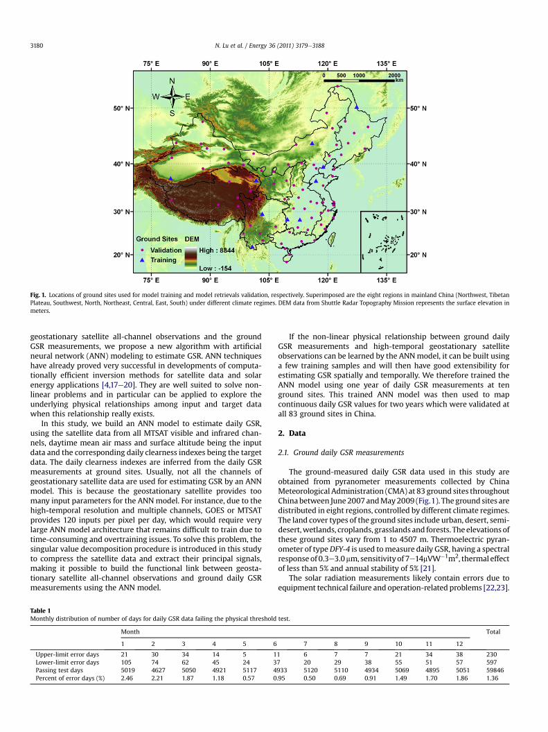
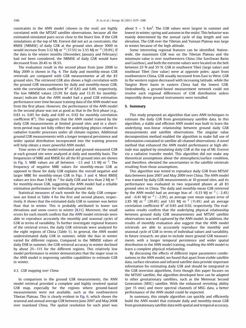
Fig. 1. Locations of ground sites used for model training and model retrievals validation, respectively. Superimposed are the eight regions in mainland China (Northwest, TibetanPlateau, Southwest, North, Northeast, Central, East, South) under different climate regimes. DEM data from Shuttle Radar Topography Mission represents the surface elevation inmeters.

N. Lu et al. / Energy 36 (2011) 3179e31883180

geostationary satellite all-channel observations and the groundGSR measurements, we propose a new algorithm with artificialneural network (ANN) modeling to estimate GSR. ANN techniqueshave already proved very successful in developments of computa-tionally efficient inversion methods for satellite data and solarenergy applications [4,17e20]. They are well suited to solve non-linear problems and in particular can be applied to explore theunderlying physical relationships among input and target datawhen this relationship really exists.

In this study, we build an ANN model to estimate daily GSR,using the satellite data from all MTSAT visible and infrared chan-nels, daytime mean air mass and surface altitude being the inputdata and the corresponding daily clearness indexes being the targetdata. The daily clearness indexes are inferred from the daily GSRmeasurements at ground sites. Usually, not all the channels ofgeostationary satellite data are used for estimating GSR by an ANNmodel. This is because the geostationary satellite provides toomany input parameters for the ANNmodel. For instance, due to thehigh-temporal resolution and multiple channels, GOES or MTSATprovides 120 inputs per pixel per day, which would require verylarge ANN model architecture that remains difficult to train due totime-consuming and overtraining issues. To solve this problem, thesingular value decomposition procedure is introduced in this studyto compress the satellite data and extract their principal signals,making it possible to build the functional link between geosta-tionary satellite all-channel observations and ground daily GSRmeasurements using the ANN model.

Table 1Monthly distribution of number of days for daily GSR data failing the physical threshold

Month

1 2 3 4 5 6

Upper-limit error days 21 30 34 14 5 1Lower-limit error days 105 74 62 45 24 3Passing test days 5019 4627 5050 4921 5117 4Percent of error days (%) 2.46 2.21 1.87 1.18 0.57 0

If the non-linear physical relationship between ground dailyGSR measurements and high-temporal geostationary satelliteobservations can be learned by the ANNmodel, it can be built usinga few training samples and will then have good extensibility forestimating GSR spatially and temporally. We therefore trained theANN model using one year of daily GSR measurements at tenground sites. This trained ANN model was then used to mapcontinuous daily GSR values for two years which were validated atall 83 ground sites in China.

2. Data

2.1. Ground daily GSR measurements

The ground-measured daily GSR data used in this study areobtained from pyranometer measurements collected by ChinaMeteorological Administration (CMA) at 83 ground sites throughoutChinabetween June2007andMay2009 (Fig.1). The ground sites aredistributed in eight regions, controlled by different climate regimes.The land cover types of the ground sites include urban, desert, semi-desert,wetlands, croplands, grasslands and forests. The elevations ofthese ground sites vary from 1 to 4507 m. Thermoelectric pyran-ometer of typeDFY-4 is used tomeasure daily GSR, having a spectralresponseof 0.3e3.0mm, sensitivityof 7e14mVW�1m2, thermal effectof less than 5% and annual stability of 5% [21].

The solar radiation measurements likely contain errors due toequipment technical failure and operation-related problems [22,23].

test.

Total

7 8 9 10 11 12

1 6 7 7 21 34 38 2307 20 29 38 55 51 57 597933 5120 5110 4934 5069 4895 5051 59846.95 0.50 0.69 0.91 1.49 1.70 1.86 1.36

Fig. 2. Flowchart of the algorithm building the neural network model.

N. Lu et al. / Energy 36 (2011) 3179e3188 3181

These errors contribute to an inefficient ANN model and poor esti-mation performance. To minimize the uncertainties of the daily GSRmeasurements, the physical threshold test proposed by Shi et al. [24]was performed, at first. The upper-limit for daily GSRwas set as dailysolar radiationat the topof atmosphere; the lower-limitwas set as3%of daily solar radiation at the top of atmosphere. Table 1 summarizesthe results of the physical threshold test for the daily GSR measure-ments and shows that the greatest occurrence of erroneous data isduring thewintermonths. The average percentage of erroneous datais 1.36% for the ground daily GSRmeasurements between June 2007andMay2009.Only thedailyGSRmeasurements that passed the testare used for the ANNmodeling and validation.

2.2. MTSAT data

The MTSAT of Japan Meteorological Agency was launched inFebruary 2005, and put into operation on 28 June 2005. It is posi-tioned at 104�E above the equator and observes Asia-Pacific region.The onboard imager scans the full-disk of the earth once per hourand provides images with five channels: one visible channel (VIS,0.55e0.90 mm), two split-window channels (IR1, 10.3e11.3 mm; IR2,11.5e12.5 mm), one water vapor channel (IR3, 6.5e7.0 mm) and oneshortwave infrared channel (IR4, 3.5e4.0 mm). The spatial resolu-tion of MTSAT data is 1 � 1 km2 for the visible channel, and4 � 4 km2 for all the other infrared channels. Together with thevisible channel data, satellite data of all the infrared channels areused in this study to estimate continuous daily GSR.

3. Methods

3.1. Artificial neural network modeling

ANN modeling builds a functional relationship between inputand target data. The input data consists of principal components of

MTSAT satellite all-channel data, daytime mean air mass andground site altitude. The target data corresponding to the inputdata at each ground site is the daily clearness index that can beexpressed as:

K ¼ GG0

(1)

where K denotes daily clearness index, G denotes ground-measureddaily GSR, and G0 daily solar radiation at the top of atmosphere.The formulas that calculate G0 and daytime mean air mass aregiven in Appendix A.

The feed-forward ANN used in this study consists of threelayers: input layer, hidden layer and output layer. The input nodesin the input layer include vectors of input data which correspondsto one output node with a vector of target data in the output layer.The weight and bias are associated with the connection from aninput node to a hidden-layer node using a transfer function of thehyperbolic tangent sigmoid function. The transfer function in theoutput layer is a linear transfer function. It has been demonstratedthat any non-linear mapping can be represented by a one-hidden-layer ANN with sigmoid functions [25,26].

In ANNmodeling, the combination of input and target data pairsis split into three parts: a training dataset (account for 60% of thecombination) to determine ANN weights and biases, a testingdataset (20%) to validate the effectiveness of the early stoppingcriterion and assess network operations on the dataset not used inthe training and validation and a validation dataset (20%) to eval-uate ANN performance and decide when to stop training [27].A Bayesian regulation backpropagation method was used to itera-tively find the weights and biases that minimize a cost function ofsum squared error (SSE) over a set of training data. Theweights andbiases were first initialized using the Nguyen-Widrow initializationmethod [28]. After initialization, the derivatives of the SSE withrespect to the weights and biases were calculated, and were then

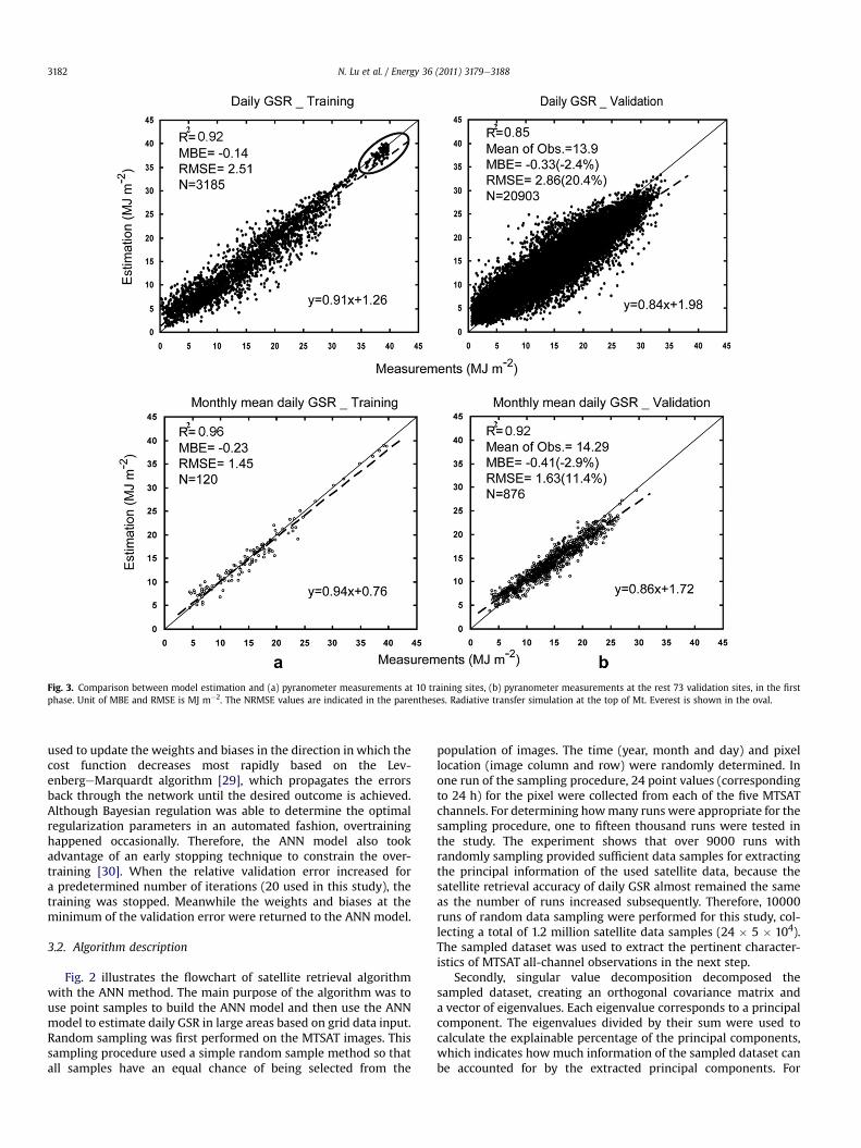
Fig. 3. Comparison between model estimation and (a) pyranometer measurements at 10 training sites, (b) pyranometer measurements at the rest 73 validation sites, in the firstphase. Unit of MBE and RMSE is MJ m�2. The NRMSE values are indicated in the parentheses. Radiative transfer simulation at the top of Mt. Everest is shown in the oval.

N. Lu et al. / Energy 36 (2011) 3179e31883182

used to update the weights and biases in the direction in which thecost function decreases most rapidly based on the Lev-enbergeMarquardt algorithm [29], which propagates the errorsback through the network until the desired outcome is achieved.Although Bayesian regulation was able to determine the optimalregularization parameters in an automated fashion, overtraininghappened occasionally. Therefore, the ANN model also tookadvantage of an early stopping technique to constrain the over-training [30]. When the relative validation error increased fora predetermined number of iterations (20 used in this study), thetraining was stopped. Meanwhile the weights and biases at theminimum of the validation error were returned to the ANN model.

3.2. Algorithm description

Fig. 2 illustrates the flowchart of satellite retrieval algorithmwith the ANN method. The main purpose of the algorithm was touse point samples to build the ANN model and then use the ANNmodel to estimate daily GSR in large areas based on grid data input.Random sampling was first performed on the MTSAT images. Thissampling procedure used a simple random sample method so thatall samples have an equal chance of being selected from the

population of images. The time (year, month and day) and pixellocation (image column and row) were randomly determined. Inone run of the sampling procedure, 24 point values (correspondingto 24 h) for the pixel were collected from each of the five MTSATchannels. For determining howmany runs were appropriate for thesampling procedure, one to fifteen thousand runs were tested inthe study. The experiment shows that over 9000 runs withrandomly sampling provided sufficient data samples for extractingthe principal information of the used satellite data, because thesatellite retrieval accuracy of daily GSR almost remained the sameas the number of runs increased subsequently. Therefore, 10000runs of random data sampling were performed for this study, col-lecting a total of 1.2 million satellite data samples (24 � 5 � 104).The sampled dataset was used to extract the pertinent character-istics of MTSAT all-channel observations in the next step.

Secondly, singular value decomposition decomposed thesampled dataset, creating an orthogonal covariance matrix anda vector of eigenvalues. Each eigenvalue corresponds to a principalcomponent. The eigenvalues divided by their sum were used tocalculate the explainable percentage of the principal components,which indicates howmuch information of the sampled dataset canbe accounted for by the extracted principal components. For

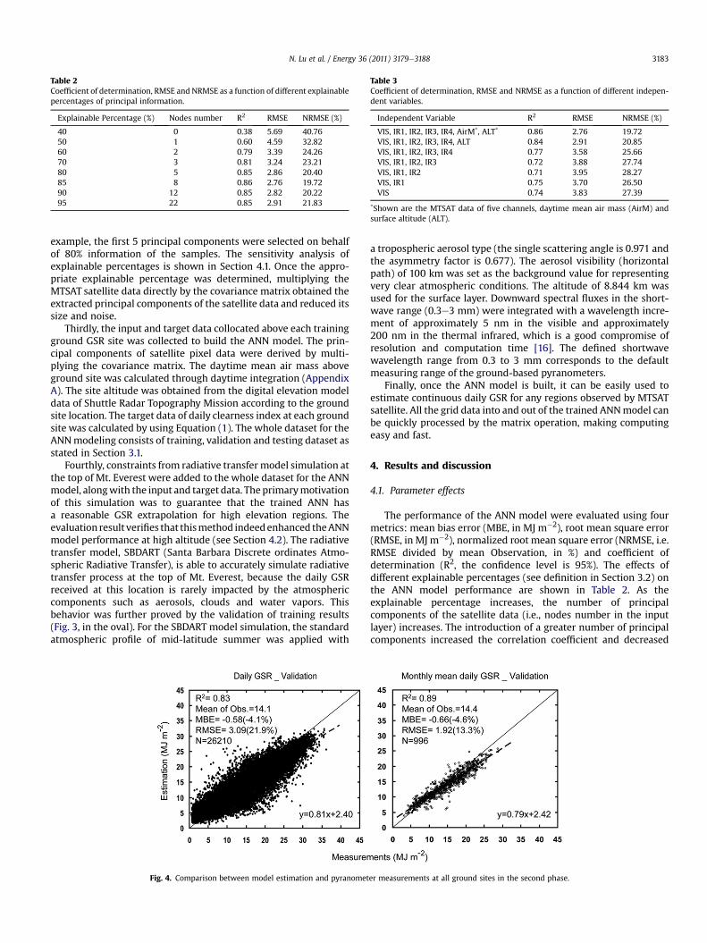
Table 2Coefficient of determination, RMSE and NRMSE as a function of different explainablepercentages of principal information.

Explainable Percentage (%) Nodes number R2 RMSE NRMSE (%)

40 0 0.38 5.69 40.7650 1 0.60 4.59 32.8260 2 0.79 3.39 24.2670 3 0.81 3.24 23.2180 5 0.85 2.86 20.4085 8 0.86 2.76 19.7290 12 0.85 2.82 20.2295 22 0.85 2.91 21.83

Table 3Coefficient of determination, RMSE and NRMSE as a function of different indepen-dent variables.

Independent Variable R2 RMSE NRMSE (%)

VIS, IR1, IR2, IR3, IR4, AirM*, ALT* 0.86 2.76 19.72VIS, IR1, IR2, IR3, IR4, ALT 0.84 2.91 20.85VIS, IR1, IR2, IR3, IR4 0.77 3.58 25.66VIS, IR1, IR2, IR3 0.72 3.88 27.74VIS, IR1, IR2 0.71 3.95 28.27VIS, IR1 0.75 3.70 26.50VIS 0.74 3.83 27.39

*Shown are the MTSAT data of five channels, daytime mean air mass (AirM) andsurface altitude (ALT).

N. Lu et al. / Energy 36 (2011) 3179e3188 3183

example, the first 5 principal components were selected on behalfof 80% information of the samples. The sensitivity analysis ofexplainable percentages is shown in Section 4.1. Once the appro-priate explainable percentage was determined, multiplying theMTSAT satellite data directly by the covariance matrix obtained theextracted principal components of the satellite data and reduced itssize and noise.

Thirdly, the input and target data collocated above each trainingground GSR site was collected to build the ANN model. The prin-cipal components of satellite pixel data were derived by multi-plying the covariance matrix. The daytime mean air mass aboveground site was calculated through daytime integration (AppendixA). The site altitude was obtained from the digital elevation modeldata of Shuttle Radar Topography Mission according to the groundsite location. The target data of daily clearness index at each groundsite was calculated by using Equation (1). The whole dataset for theANNmodeling consists of training, validation and testing dataset asstated in Section 3.1.

Fourthly, constraints from radiative transfer model simulation atthe top of Mt. Everest were added to the whole dataset for the ANNmodel, alongwith the input and target data. The primarymotivationof this simulation was to guarantee that the trained ANN hasa reasonable GSR extrapolation for high elevation regions. Theevaluation result verifies that thismethod indeedenhanced theANNmodel performance at high altitude (see Section 4.2). The radiativetransfer model, SBDART (Santa Barbara Discrete ordinates Atmo-spheric Radiative Transfer), is able to accurately simulate radiativetransfer process at the top of Mt. Everest, because the daily GSRreceived at this location is rarely impacted by the atmosphericcomponents such as aerosols, clouds and water vapors. Thisbehavior was further proved by the validation of training results(Fig. 3, in the oval). For the SBDART model simulation, the standardatmospheric profile of mid-latitude summer was applied with

Fig. 4. Comparison between model estimation and pyranomet

a tropospheric aerosol type (the single scattering angle is 0.971 andthe asymmetry factor is 0.677). The aerosol visibility (horizontalpath) of 100 km was set as the background value for representingvery clear atmospheric conditions. The altitude of 8.844 km wasused for the surface layer. Downward spectral fluxes in the short-wave range (0.3e3 mm) were integrated with a wavelength incre-ment of approximately 5 nm in the visible and approximately200 nm in the thermal infrared, which is a good compromise ofresolution and computation time [16]. The defined shortwavewavelength range from 0.3 to 3 mm corresponds to the defaultmeasuring range of the ground-based pyranometers.

Finally, once the ANN model is built, it can be easily used toestimate continuous daily GSR for any regions observed by MTSATsatellite. All the grid data into and out of the trained ANNmodel canbe quickly processed by the matrix operation, making computingeasy and fast.

4. Results and discussion

4.1. Parameter effects

The performance of the ANN model were evaluated using fourmetrics: mean bias error (MBE, in MJ m�2), root mean square error(RMSE, in MJ m�2), normalized root mean square error (NRMSE, i.e.RMSE divided by mean Observation, in %) and coefficient ofdetermination (R2, the confidence level is 95%). The effects ofdifferent explainable percentages (see definition in Section 3.2) onthe ANN model performance are shown in Table 2. As theexplainable percentage increases, the number of principalcomponents of the satellite data (i.e., nodes number in the inputlayer) increases. The introduction of a greater number of principalcomponents increased the correlation coefficient and decreased

er measurements at all ground sites in the second phase.

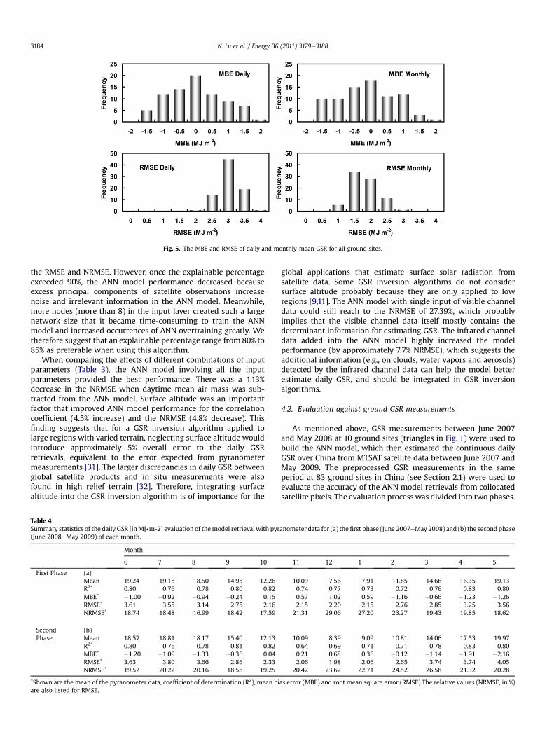
Fig. 5. The MBE and RMSE of daily and monthly-mean GSR for all ground sites.

N. Lu et al. / Energy 36 (2011) 3179e31883184

the RMSE and NRMSE. However, once the explainable percentageexceeded 90%, the ANN model performance decreased becauseexcess principal components of satellite observations increasenoise and irrelevant information in the ANN model. Meanwhile,more nodes (more than 8) in the input layer created such a largenetwork size that it became time-consuming to train the ANNmodel and increased occurrences of ANN overtraining greatly. Wetherefore suggest that an explainable percentage range from 80% to85% as preferable when using this algorithm.

When comparing the effects of different combinations of inputparameters (Table 3), the ANN model involving all the inputparameters provided the best performance. There was a 1.13%decrease in the NRMSE when daytime mean air mass was sub-tracted from the ANN model. Surface altitude was an importantfactor that improved ANN model performance for the correlationcoefficient (4.5% increase) and the NRMSE (4.8% decrease). Thisfinding suggests that for a GSR inversion algorithm applied tolarge regions with varied terrain, neglecting surface altitude wouldintroduce approximately 5% overall error to the daily GSRretrievals, equivalent to the error expected from pyranometermeasurements [31]. The larger discrepancies in daily GSR betweenglobal satellite products and in situ measurements were alsofound in high relief terrain [32]. Therefore, integrating surfacealtitude into the GSR inversion algorithm is of importance for the

Table 4Summary statistics of the daily GSR [inMJ,m-2] evaluation of themodel retrieval with pyr(June 2008eMay 2009) of each month.

Month

6 7 8 9 10

First Phase (a)Mean 19.24 19.18 18.50 14.95 12.26R2* 0.80 0.76 0.78 0.80 0.82MBE* �1.00 �0.92 �0.94 �0.24 0.15RMSE* 3.61 3.55 3.14 2.75 2.16NRMSE* 18.74 18.48 16.99 18.42 17.59

SecondPhase

(b)Mean 18.57 18.81 18.17 15.40 12.13R2* 0.80 0.76 0.78 0.81 0.82MBE* �1.20 �1.09 �1.33 �0.36 0.04RMSE* 3.63 3.80 3.66 2.86 2.33NRMSE* 19.52 20.22 20.16 18.58 19.25

*Shown are the mean of the pyranometer data, coefficient of determination (R2), mean biare also listed for RMSE.

global applications that estimate surface solar radiation fromsatellite data. Some GSR inversion algorithms do not considersurface altitude probably because they are only applied to lowregions [9,11]. The ANN model with single input of visible channeldata could still reach to the NRMSE of 27.39%, which probablyimplies that the visible channel data itself mostly contains thedeterminant information for estimating GSR. The infrared channeldata added into the ANN model highly increased the modelperformance (by approximately 7.7% NRMSE), which suggests theadditional information (e.g., on clouds, water vapors and aerosols)detected by the infrared channel data can help the model betterestimate daily GSR, and should be integrated in GSR inversionalgorithms.

4.2. Evaluation against ground GSR measurements

As mentioned above, GSR measurements between June 2007and May 2008 at 10 ground sites (triangles in Fig. 1) were used tobuild the ANN model, which then estimated the continuous dailyGSR over China from MTSAT satellite data between June 2007 andMay 2009. The preprocessed GSR measurements in the sameperiod at 83 ground sites in China (see Section 2.1) were used toevaluate the accuracy of the ANN model retrievals from collocatedsatellite pixels. The evaluation process was divided into two phases.

anometer data for (a) the first phase (June 2007eMay 2008) and (b) the second phase

11 12 1 2 3 4 5

10.09 7.56 7.91 11.85 14.66 16.35 19.130.74 0.77 0.73 0.72 0.76 0.83 0.800.57 1.02 0.59 �1.16 �0.66 �1.23 �1.262.15 2.20 2.15 2.76 2.85 3.25 3.56

21.31 29.06 27.20 23.27 19.43 19.85 18.62

10.09 8.39 9.09 10.81 14.06 17.53 19.970.64 0.69 0.71 0.71 0.78 0.83 0.800.21 0.68 0.36 �0.12 �1.14 �1.91 �2.162.06 1.98 2.06 2.65 3.74 3.74 4.05

20.42 23.62 22.71 24.52 26.58 21.32 20.28

as error (MBE) and root mean square error (RMSE).The relative values (NRMSE, in %)

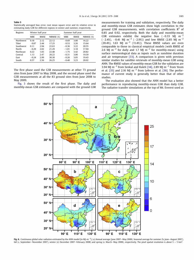
Table 5Statistically averaged bias error, root mean square error and its relative error inestimating daily GSR for different regions in winter and summer, respectively.

Regions Winter half year Summer half year

MBE RMSE NRMSE (%) MBE RMSE NRMSE (%)

Northwest 0.18 2.12 22.12 �0.69 3.00 16.22Tibet �0.87 2.44 17.25 �0.53 3.26 15.64Southwest 0.11 2.94 22.63 �0.36 3.22 20.55North �0.29 2.02 21.29 �1.01 3.18 17.94Northeast 0.22 1.83 22.48 �1.75 3.42 20.82Central 1.13 2.47 28.22 �0.31 3.00 19.59East �0.24 2.99 30.30 �0.26 3.05 19.43South 0.57 2.56 26.25 �0.40 3.23 20.02

N. Lu et al. / Energy 36 (2011) 3179e3188 3185

The first phase used the GSR measurements at other 73 groundsites from June 2007 to May 2008, and the second phase used theGSR measurements at all the 83 ground sites from June 2008 toMay 2009.

Fig. 3 shows the result of the first phase. The daily andmonthly-mean GSR estimates are compared with the ground GSR

Fig. 6. Continuous global solar radiation estimated by the ANN model [in MJ,m�2]. (a) Annuafall (c, SeptembereNovember 2007), winter (d, December 2007eFebruary 2008) and sprin

measurements for training and validation, respectively. The dailyand monthly-mean GSR estimates show high correlation to theground GSR measurements, with correlation coefficients R2 of0.85 and 0.92, respectively. Both the daily and monthly-meanGSR estimates exhibit the negative bias (�0.33 MJ m�2

(�2.4%), �0.41 MJ m�2 (�2.9%)) and low RMSE (2.85 MJ m�2

(20.4%), 1.63 MJ m�2 (11.4%)). These RMSE values are evencomparable to those in classical empirical models (with RMSE of2.6 MJ m�2 for daily and 1.7 MJ m�2 for monthly-mean) usingsurface meteorological data as inputs such as sunshine durationand air temperature [33]. A comparison is given with previoussimilar studies for satellite retrievals of monthly-mean GSR usingANN. The RMSE values of monthly-mean GSR for the validation are3.94 MJ m�2 from Senkal and Kuleli [34], 2.89 MJ m�2 from Yeomet al. [35] and 2.16 MJ m�2 from Lefevre et al. [36]. The perfor-mance of current study is generally better than that of otherstudies.

The evaluation also showed that the ANN model has a betterperformance in reproducing monthly-mean GSR than daily GSR.The radiative transfer simulations at the top of Mt. Everest used as

l average (June 2007eMay 2008). Seasonal average for summer (b, JuneeAugust 2007),g (e, MarcheMay 2008), respectively. The pixel spatial resolution is about 5 � 5 km2.

N. Lu et al. / Energy 36 (2011) 3179e31883186

constraints in the ANN model (shown in the oval) are highlycorrelated with the MTSAT satellite observations, because all theestimated-simulated pairs occur close to the bisect line. If the GSRsimulations at the top of Mt. Everest did not act as constraints, theRMSE (NRMSE) of daily GSR at the ground sites above 3000 mwould increase from 3.12 MJ m�2 (17.5%) to 3.55 MJ m�2 (19.9%). Ifthe data in the winter months (December, January and February)had not been considered, the NRMSE of daily GSR would havedecreased from 20.4% to 18.5%.

The evaluation result in the second phase from June 2008 toMay 2009 is shown in Fig. 4. The daily and monthly-mean GSRretrievals are compared with GSR measurements at all the 83ground sites. The retrieved GSR also shows a high correlation withthe ground GSR measurements for daily and monthly-mean GSR,with the correlation coefficient R2 of 0.83 and 0.89, respectively.The low NRMSE values (21.9% for daily and 13.3% for monthly-mean) indicate that the ANN model had a good GSR estimationperformance over time because training data of the ANNmodel wasfrom the first phase. However, the performance of the ANN modelin the second phase was not as good as that in the first phase (e.g.,0.83 vs. 0.85 for daily and 0.89 vs. 0.92 for monthly correlationcoefficient R2). This suggests that the ANN model trained by thedaily GSR measurements at limited ground sites and in a short-term period may not fully reflect the underlying physics related toradiative transfer processes under all climate regimes. Additionalground GSR measurements with a longer temporal persistence andwider spatial distribution incorporated into the training processwill help obtain a more powerful ANN model.

Time series of the model-estimated and ground-measured GSRat each ground site were analyzed at daily and monthly basis. Thefrequencies of MBE and RMSE for all the 83 ground sites are shownin Fig. 5. MBE values are all between �1.5 and 1.5 MJ m�2. Thefrequency of negative MBE values for monthly-mean GSR asopposed to those for daily GSR explains the overall negative andlarger MBE for monthly-mean GSR in Figs. 3 and 4. Most RMSEvalues are less than 3 MJ m�2 for daily GSR and less than 2 MJ m�2

for monthly-mean GSR, suggesting the ANN model had a reliableestimation performance for individual ground site.

Statistical measures of each month for the daily GSR compar-ison are listed in Table 4 for the first and second phases, respec-tively. It shows that the estimated daily GSR in summer was betterthan that in winter. This is probably attributed to lower sunelevations and snow covers in winter [8,11]. Moreover, the smallerrors for each month confirm that the ANN model retrievals wereable to reproduce accurately the monthly and seasonal cycles ofGSR in terms of variability. To further investigate regional featuresof the retrieval errors, the daily GSR retrievals were analyzed forthe eight regions of China (Table 5). In general, the ANN modelunderestimated daily GSR in summer, while the bias in wintervaried for different regions. Compared to the NRMSE values ofdaily DSR in summer, the GSR retrieval accuracy in winter declinedby about 2%e11% for the different regions. This relatively lowmodel performance in winter demonstrates that the major issue inthe ANN model is improving satellite capabilities to estimate GSRin winter.

4.3. GSR mapping over China

In comparison to the ground GSR measurements, the ANNmodel retrieval provided a complete and highly resolved spatialGSR map, especially for the regions where ground-basedmeasurements were not available, such as the southwesternTibetan Plateau. This is clearly evident in Fig. 6, which shows theseasonal and annual average GSR between June 2007 andMay 2008over mainland China. The spatial resolution for each pixel was

about 5 � 5 km2. The GSR values were largest in summer andlowest inwinter, spring and autumn in themidst. This behavior wasmainly determined by the annual cycle of day length and sunelevation. The GSR over the Tibetan and Yunnan Plateau was largein winter because of the high altitude.

Some interesting regional features can be identified. Nation-wide, the maximum GSR was on the Tibetan Plateau and theminimum value is over southwestern China (the Szechwan Basinand Guizhou), and both the extreme values were located on the beltbetween 25�N and 35�N. GSR in southwest Tibet (large value) andsoutheast Tibet (low value) were at opposite poles; apart fromsouthwestern China, GSR usually increased from East to West. GSRin the western region decreased with increasing latitude, while theYangtze River basin in eastern China had the lowest GSR.Undoubtedly, a ground-based measurement network could notresolve such regional differences of GSR distribution unlessimpossibly dense ground instruments were installed.

5. Summary

This study proposed an algorithm that uses ANN techniques toestimate the daily GSR from geostationary satellite data. In thisalgorithm, a stable and efficient ANN model was built to learn theunderlying non-linear relationship between ground daily GSRmeasurements and satellite observations. The singular valuedecomposition method enabled the algorithm to make full use ofinformation contained in satellite all-channel observations. A novelmethod that enhanced the ANN model performance at high alti-tude was applied by simulating daily GSR at the top of Mt. Everestvia a radiative transfer model. This algorithm did not make anytheoretical assumptions about the atmospheric/surface condition,and therefore, obviated the uncertainties in the satellite retrievalsresulting from those assumptions.

This algorithm was tested to reproduce daily GSR from MTSATdata between June 2007 and May 2009 over China. The ANNmodelwas trained by daily GSR measurements at 10 ground sites, and itsperformance was evaluated in two separated phases at all 83ground sites in China. The daily and monthly-mean GSR retrievedby the ANN model had an average bias of �0.33 MJ m�2 (�2.4%)and �0.41 MJ m�2 (�2.9%), an average root mean square error of2.85 MJ m�2 (20.4%) and 1.63 MJ m�2 (11.4%) and an averagecorrelation coefficient R2 of 0.85 and 0.92, respectively. The eval-uation results confirm that the underlying physical relationshipbetween ground daily GSR measurements and MTSAT satelliteobservations was well captured by the ANN model. In addition, theresults of monthly evaluation also suggest that the ANN modelretrievals are able to accurately reproduce the monthly andseasonal cycle of GSR in terms of individual values and variability.In future research, we plan to include more ground GSR measure-ments with a longer temporal persistence and wider spatialdistribution in the ANNmodel training, enabling the ANNmodel tolearn a complete physical relationship.

By discussing the effects of different input parameters combi-nations in the ANNmodel, we found that apart fromvisible satellitedata, surface elevation and infrared satellite data provide importantinformation for estimating daily GSR and should be integrated inthe GSR inversion algorithms. Even though this paper focuses onthe MTSAT satellite, the algorithm developed here can be adaptedto other geostationary satellites, such as the Meteosat SecondGeneration (MSG) satellite. With the enhanced revisiting ability(per 15 min) and more spectral channels of MSG data, a betterperformance of the ANN model could be expected.

In summary, this simple algorithm can quickly and efficientlybuild the ANN model that estimate daily and monthly-mean GSRfromgeostationary satellite datawith spatial and temporal accuracy.

N. Lu et al. / Energy 36 (2011) 3179e3188 3187

Acknowledgments

This work was in part supported by the National Natural ScienceFoundation of China (No. 41001215), the National Key Project ofScientific and Technical Supporting Programs Funded by Ministryof Science & Technology of China (No. 2008BAC40B01) and the R&DSpecial Fund for Public Welfare Industry, National EnvironmentalProtection Administration (No. 200909018). The authors wouldalso like to thank China Meteorological Administration and KochiUniversity for the data support.

Appendix A

The daily solar irradiation at the TOA, G0 in MJ m�2, can bedetermined using the following equations [19]:

G0 ¼ 24� 3600p

I0k�cosfcos dsinus þ pus

180sinfsin d

�(2)

where I0 is the solar constant set as 1367 W m�2, k is the eccen-tricity correction factor of the Earth’s orbit, f (degree) is the latitudeof the location, d (degree) is the solar declination angle,us (degrees)is the sunset hour angle.

Appropriate formulation for the eccentricity correction factork for each day of the year can be calculated using [37]:

k ¼ 1þ 0:033 cos�360dn365

�(3)

where dn is the day number counted from the beginning of the year.The declination d and sunset hour angle us for each day of the

year is calculated from [38,39]:

d ¼ 23:45 sin�360

284þ dn365

�(4)

us ¼ cos�1ð�tanftan dÞ (5)

Given local latitude, longitude, date and time, the solar elevationh can be calculated following [40]

sinh ¼ sinfsin dþ cosfcos dcosg (6)

g ¼ 15ðhr þmn=60þ ss=3600� 12þ De=60Þ þ j (7)

De ¼ 60½ � 0:0002786þ 0:1228 cosðhþ 1:498Þ� 0:1654 cosð2h� 1:2615Þ � 0:005354 cosð3h� 1:1571Þ�

(8)

h ¼ 2p365

ðdn � 1Þ (9)

where j (degree) is the local longitude, g (degree) is the hour angle,De (minutes) is the equation of time, and hr : mn : ss is the UTC time,and h (radians) is the fractional year.

Once the solar elevation h is determined, the air mass at a giventime is calculated following [41]:

m ¼ 1=hsin hþ 0:15ð57:296hþ 3:885Þ�1:253 (10)

Daytime mean air mass can then be obtained by integratingEq.(10) for air mass from sunrise to sunset [42].

References

[1] KumarR,Umanand L. Estimationof global radiationusing clearness indexmodelfor sizing photovoltaic system. Renewable Energy 2005;30(15):2221e33.

[2] Oliver M, Jackson T. Energy and economic evaluation of building-integratedphotovoltaics. Energy 2001;26(4):431e9.

[3] Roebeling R, van Putten E, Genovese G, Rosema A. Application of meteosatderived meteorological information for crop yield predictions in Europe.International Journal of Remote Sensing 2004;25(23):5389e401.

[4] Benghanem M, Mellit A. Radial basis function network-based prediction ofglobal solar radiation data: application for sizing of a stand-alone photovoltaicsystem at Al-Madinah, Saudi Arabia. Energy 2010;35(9):3751e62.

[5] Bakirci K. Correlations for estimation of daily global solar radiation with hoursof bright sunshine in Turkey. Energy 2009;34(4):485e501.

[6] Berbery EH, Mitchell KE, Benjamin S, Smirnova T, Ritchie H, Hogue R, et al.Assessment of land-surface energy budgets from regional and global models.Journal of Geophysical Research 1999;104(D16):19329e48.

[7] Mondol JD, Yohanis YG, Norton B. Solar radiation modelling for the simulationof photovoltaic systems. Renewable Energy 2008;33(5):1109e20.

[8] Pinker RT, Tarpley JD, Laszlo I, Mitchell KE, Houser PR, Wood EF, et al.Surface radiation budgets in support of the GEWEX Continental-ScaleInternational Project (GCIP) and the GEWEX Americas prediction Project(GAPP), including the North American land data Assimilation system(NLDAS) project. Journal of Geophysical Research 2003;108(D22). doi:10.1029/2002JD003301.

[9] Ceballos JC, Bottino MJ, de Souza JM. A simplified physical model for assessingsolar radiation over Brazil using GOES 8 visible imagery. Journal ofGeophysical Research 2004;109(D02211). doi:10.1029/2003JD003531.

[10] Deneke H, Feijt A, van Lammeren A, Simmer C. Validation of a physicalretrieval scheme of solar surface irradiances from narrow-band satelliteradiances. Journal of Applied Meteorology 2005;44(9):1453e66.

[11] Deneke H, Feijt A, Roebeling R. Estimating surface solar irradiance fromMETEOSAT SEVIRI-derived cloud properties. Remote Sensing of Environment2008;112(6):3131e41.

[12] Liang S, Zheng T, Liu RG, Fang HL, Tsay SC, Running S. Estimation of incidentphotosynthetically active radiation from moderate resolution imaging spec-trometer data. Journal of Geophysical Research 2006;111(D15208). doi:10.1029/2005JD006730.

[13] Li X, Pinker RT, Wonsick MM, Ma Y. Toward improved satellite estimates ofshort-wave radiative fluxesdFocus on cloud detection over snow: 1. Meth-odology. Journal of Geophysical Research 2007;112(D07208). doi:10.1029/2005JD006698.

[14] Laszlo I, Ciren P, Liu H, Kondragunta S, Tarpley D, Goldberg M. Remote sensingof aerosol and radiation from geostationary satellites. Advances in SpaceResearch 2008;41(11):1882e93.

[15] Zheng T, Liang S, Wang K. Estimation of incident photosynthetically activeradiation from GOES visible imagery. Journal of Applied Meteorology andClimatology 2008;47(3):853e68.

[16] Lu N, Liu R, Liu J, Liang S. An algorithm for estimating downward shortwaveradiation from GMS 5 visible imagery and its evaluation over China. Journal ofGeophysical Research 2010;115(D18102). doi:10.1029/2009JD013457.

[17] Aires F, Prigent C, Rossow WB, Rothstein M. A new neural network approachincludingfirst guess for retrieval of atmosphericwater vapor, cloud liquidwaterpath, surface temperature, and emissivities over land from satellite microwaveobservations. Journal of Geophysical Research 2001;106(D14):14887e907.

[18] Tedescoa M, Pulliainenb J, Takalab M, Hallikainenb M, Pampaloni P. Artificialneural network-based techniques for the retrieval of SWE and snow depthfrom SSM/I data. Remote Sensing of Environment 2004;90(1):76e85.

[19] Elminir HK, Azzam YA, Younes FI. Prediction of hourly and daily diffusefraction using neural network, as compared to linear regression models.Energy 2007;32(8):1513e23.

[20] Wan K, Tang HL, Yang L, Lam JC. An analysis of thermal and solar zone radi-ation models using an Angstrom-Prescott equation and artificial neuralnetworks. Energy 2008;33(7):1115e27.

[21] China Meteorological Administration. Meteorological radiation observationmethod (in Chinese). Beijing: Meteorological Press; 1996.

[22] Younes S, Claywell R, Muneer T. Quality control of solar radiation data:Present status and proposed new approaches. Energy 2005;30(9):1533e49.

[23] Moradi I. Quality control of global solar radiation using sunshine durationhours. Energy 2009;34(1):1e6.

[24] Shi GY, Hayasaka T, Ohmura A, Chen ZH, Wang B, Zhao JQ, et al. Data qualityassessment and the long-term trend of ground solar radiation in China.Journal of Applied Meteorology and Climatology 2008;47(4):1006e16.

[25] Hornik K, Stinchcombe M, White H. Multilayer feed-forward networks areuniversal approximators. Neural Networks 1989;2(5):359e66.

[26] Cybenko G. Approximation by superpositions of a sigmoidal function.Mathematics of Control, Signals, and Systems 1989;2(4):303e14.

[27] Prechelt L. Automatic early stopping using cross validation: quantifying thecriteria. Neural Networks 1998;11(4):761e7.

[28] Nguyen D, Widrow B. Improving the learning speed of 2-layer neuralnetworks by choosing initial values of the adaptive weights. Proceedings ofInternatinal Joint Conference on Neural Networks 1990; vol. 3: 21e26.

[29] Gill PE, Murray W, Wright MH. The Levenberg-Marquardt method. London:Academic Press; 1981.

N. Lu et al. / Energy 36 (2011) 3179e31883188

[30] Blackwell WJ, Chen FW. Neural networks in atmospheric remote sensing.Massachusetts: Artech House; 2009.

[31] World Meteorological Organization. Guide to meteorological instruments andmethods of observation. Switzerland: WMO-No. 8. 7th ed.; 2008.

[32] YangK, PinkerRT,MaY,Koike T,WonsickMM,Cox SJ, et al. Evaluationof satelliteestimates of downward shortwave radiation over the Tibetan Plateau. Journal ofGeophysical Research 2008;113(D17204). doi:10.1029/2007JD009736.

[33] Yang K, Koike T, Ye B. Improving estimation of hourly, daily, and monthlysolar radiation by importing global data sets. Agricultural and Forest Meteo-rology 2006;137(1):43e55.

[34] Senkal O, Kuleli T. Estimation of solar radiation over Turkey using artificialneural network and satellite data. Applied Energy 2009;86(7e8):1222e8.

[35] Yeom JM, Han KS, Kim YS, Jang JD. Neural network determination of cloudattenuation to estimate insolation using MTSAT-1R data. International Journalof Remote Sensing 2008;29(21):6193e208.

[36] LefevreM,Wald L,Diabete L. Using reduceddata sets ISCCP-B2 fromtheMeteosatsatellites to assess surface solar irradiance. Solar Energy 2007;81(2):240e53.

[37] Yorukoglu M, Celik AN. A critical review on the estimation of daily global solarradiation from sunshine duration. Energy Conversion and Management 2006;47:2441e50.

[38] Cooper PI. The absorption of solar radiation in solar stills. Solar energy 1969;12(3):313e31.

[39] Luque A, Hegedus S. Handbook of photovoltaic science and engineering.Chichester: Wiley; 2003.

[40] Shukuya M. Light and heat in the built environment (in Japanese). Tokyo:Maruzen Inc.; 1993.

[41] Leckner B. The spectral distribution of solar radiation at the earth’s surface-elements of a model. Solar Energy 1978;20(2):143e50.

[42] Yin X. Optical air mass: daily integration and its applications. Meteorology andAtmospheric Physics 1997;63(3e4):227e33.