A rational sediment transport scaling relation based on

dimensionless stream power

B.C. Eaton ∗ M. Church †

Accepted for publication in ESPL on 11 November 2010

Abstract

The concept of stream channel grade—according to which a stream channel reachwill adjust its gradient, S, in order to transport the imposed sediment load having mag-nitude, Qb, and characteristic grain size, Db, with the available discharge, Q (Mackin,1948; Lane, 1955)—is one of the most influential ideas in fluvial geomorphology. Herein,we derive a scaling relation that describes how externally imposed changes in eitherQb or Q can be accommodated by changes in the channel configuration, described bythe energy gradient, mean flow depth, characteristic grain size and a parameter de-scribing the effect of bed surface structures on grain entrainment. One version of thisscaling relation is based on the dimensionless bed material transport parameter (W ∗)presented by Parker and Klingeman (1982). An equivalent version is based on a newdimensionless transport parameter (E∗) using dimensionless unit stream power. Thisversion is nearly identical to the relation based on W ∗, except that it is independent offlow resistance. Both versions of the scaling relation are directly comparable to Lane’soriginal relation. In order to generate this stream power-based scaling relation, wederived an empirical transport function relation relating E∗ to dimensionless streampower using data from a wide range of stable, bed load-dominated channels: the formof that transport function is based on the understanding that, while grain entrainmentis related to the forces acting on the bed (described by dimensionless shear stress),sediment transport rate is related to the transfer of momentum from the fluid to thebed material (described by dimensionless stream power).

1 Introduction

Mackin (1948) introduced the concept of stream channel grade, whereby a stream adjusts itsgradient so as to just pass the imposed water and sediment loads. Lane (1955) summarizedthe interactions that produce stream grade using the conceptual relation Q · S ∝ Qb ·D,

∗Corresponding Author, brett.eaton@ubc,ca, Department of Geography, The University of BritishColumbia†church@geog.ubc.ca, Department of Geography, The University of British Columbia

1

wherein Q is the formative discharge, S is the stream gradient, Qb is the bed materialload transported by the river and D is the calibre of sediment in transport. This relationindicates qualitatively how a change in one of the driving variables (sediment load, forexample) is accommodated by by a change in one or other of the response variables (suchas the stream gradient or the calibre of the load). Church (2006) argued that Lane’srelation can be slightly modified and recast in dimensionless terms as Qb/Q ∝ dS/D,d being the mean hydraulic depth of flow. Church interpreted this modified form as aphysically based statement that bed material load concentration is proportional to thedimensionless shear stress acting upon the bed (that is, to Shields’ number). The mainpurpose of both these relations is to structure one’s thinking about how rivers adjust tomaintain a graded condition, not to make quantitative predictions. In this paper, ananalogous scaling relation describing the graded state is derived based on the equationsgoverning open channel hydraulics and sediment transport.

Most bed material transport laws are based on the magnitude of boundary shear stressand either a critical or a reference shear stress. In many of these laws, the boundaryforce is represented non-dimensionally using the dimensionless shear stress (τ∗) and thetransport rate is represented using a dimensionless sediment transport parameter, such asthat proposed by Einstein (1950) or Parker and Klingeman (1982). While entrainment isclearly best thought of as a process that is driven by the forces acting on the boundary, itis less clear why the total sediment transport rate should be a consequence of the forcesexerted on individual grains.

Indeed, Bagnold (1966) conceived of sediment transport as a phenomenon related to thepower of a stream. In this paper, we show that, by considering sediment transport to be aprocess primarily related to the power of a stream, we arrive at a dimensionless sedimenttransport parameter that is simpler than that proposed by Parker and Klingeman (1982),and that is more easily related to Lane’s graded relation. We also demonstrate that theexisting body of work that seeks to identify the threshold of motion in terms of a criticaldimensionless shear stress or Shields number (θc) can be used to define the reference streampower necessary to generate a working empirical sediment transport law. We calibrate ourstream power-based transport law using data from gravel bed streams and experimentalflumes in which the sediment transport rate was judged to be relatively stable.

2 A graded state relation using τ ∗

2.1 Flow resistance and specific discharge

Regardless of the form of sediment transport law to be used, the first element of thederivation of a graded state relation is adoption of a flow resistance law, which relates thefriction at the channel boundary to the mean flow velocity. While there are many to choosefrom, all depend on the ratio between the depth of flow and some measure of the boundary

2

roughness. We adopt the general power law proposed by Ferguson (2007),

< =U

u∗= a

[d

Db

]b(1)

in which < is the flow resistance value given by the ratio U/u∗, wherein U is the meanstream velocity (U = Q/Bd, in which B is the width of the stream), u∗ is the shear velocity(averaged over the entire wetted perimeter), and Db is a representative grain size for thebed surface (often taken to be the D84 of the surface, but sometimes taken to be themedian bed surface size). According to Ferguson (2007), the coefficient a and exponent bactually vary with the relative submergence of the bed (d/D84, the reciprocal of relativeroughness), such that “deep” flows are consistent with a = 7 - 8 and b = 1/6 (values thatcorrespond to the commonly used Manning-Strickler flow resistance law), while “shallow”flows are consistent with a = 1 - 4 and b = 1. Shear velocity is defined by the relationu∗ =

√τ/ρ, wherein ρ is the fluid density. For steady uniform flow, we can therefore relate

shear velocity to the channel geometry as follows:

u∗ =√gdS (2)

wherein g is the acceleration of gravity, which recovers Chezy’s formula—adjusted forrelative grain size—from (1). Adoption of the uniform flow approximation restricts ouranalysis strictly to the description of regular prismatic channels and practically to thedescription of average conditions in channels much wider than they are deep. The use ofwidth-averaged parameters is consistent with our goal of developing a scaling relation thatdescribes channel grade for a river reach, but it is not consistent with the local estimationof shear stress at a particular point in the channel.

The second element of this derivation is to combine the equation describing flow resis-tance with the continuity equation to estimate stream discharge. By combining (1) and(2) we can calculate the specific discharge, q,

q = a√gd3S

[d

Db

]b(3)

since, according to steady state continuity, q = Q/B = Ud, B being the width of the flow.For convenience, we equate Db in (3) with the median bed surface grain size, D50, sincethis is the reference grain size used in most bed material transport formulae.

2.2 Sediment transport parameter (W ∗)

In this section, we use the shear stress-based bed material transport parameter, W ∗ (pro-posed by Parker and Klingeman, 1982), to develop a graded relation because it is used inmany of the existing shear stress-based transport laws.

3

Equation (3) allows us to calculate q as a function of the average flow geometry (ex-pressed in d and S) and the size of sediment along the channel boundary (Db). Usingthe dimensionless transport parameter proposed by Parker and Klingeman (1982), we canestimate the volumetric flux of bedload per unit width, qb, as a function of d, S and Db aswell. The transport parameter, W ∗, is defined as follows:

W ∗ =q∗b

τ∗ 3/2(4)

wherein q∗b is the Einstein (1950) dimensionless bed material transport parameter (q∗b =

qb/(√RgD

3/2b , in which R is the submerged specific gravity of the sediment) and τ∗ is

the Shields dimensionless shear stress. Since bed material transport takes place mainlyon the surface of the bed, the median bed surface grain size is selected to represent thecharacteristic grain size, Db. The exponent 3/2 is motivated by the observation that manybedload transport equations employ a measure of fluid force raised to the 3/2 power (Parkerand Klingeman, 1982). τ∗ is defined as follows:

τ∗ =τ

g(ρs − ρ)Db=

dS

RDb(5)

In this equation, Db is again the median size of the bed surface, ρs refers to the density ofthe bed material, and ρ is the density of the fluid.

Many empirical sediment transport laws can be written as functions of W ∗ and τ∗,once a critical (θc) or reference (τ∗r ) dimensionless shear stress is defined. The initialexperimental work done by Shields was based on identifying the absolute threshold (θc)for sediment transport, below which no transport occurs. Shields used spherical particles,all with the same diameter: other researchers have confirmed the general correspondencebetween Shields’ results and the entrainment of the median surface grain size. They havealso recognized that threshold conditions are difficult to define practically, particularlyfor a bed comprising a mixture of grain sizes and shapes, and so have adopted a referencedimensionless shear stress (τr) that gives rise to a small but measurable reference transportrate. For example, Shields threshold is used in the Meyer-Peter and Muller (1948) transportequation, which can be written

W ∗ = 8

[1− θc

τ∗

]3/2(6)

wherein θc = 0.047 is the value of the critical Shields number estimated by Meyer-Peterand Muller (1948). The sediment transport equation first presented by Parker (1979) andthen modified by Wilcock (2001) uses a reference dimensionless shear stress, and can bewritten

W ∗ = 11.2

[1− 0.846

√τ∗rτ∗

]4.5(7)

4

in which, according to Wilcock (2001), τ∗r varies with the proportion of sand in the bed,reaching a value of ≈ 0.04 for relatively clean gravel beds. Parker (1990) and Wilcock andCrowe (2003) have also used essentially the same variables (W ∗ and τ∗, in combinationwith a reference dimensionless stress) to develop empirical fractional sediment transportlaws. For the sake of developing a graded relation, the choice of empirical equations isnot important, and we will continue without specifying an empirical equation by which toestimate W ∗, since all of them are similar.

In order to construct a graded relation, we are interested in the volumetric transportrate, qb which can be derived by substituting (5) into (4) and rearranging, giving

qb =W ∗√g[dS]3/2

R(8)

2.3 An initial graded state relation

One means of thinking about river grade is to consider the relative amount of sedimenttransport that can be achieved by a given volume of water, which is given by the volumetricsediment concentration (ζ = Qb/Q). The modified version of Lane’s relation presented byChurch (2006) (i.e., Qb/Q ∝ dS/Db) implies that the amount of geomorphic work per unitof flow depends on the force exerted on the boundary by the flow (since τ ∝ dS) and theentrainment threshold for the bed material with a characteristic grain size, Db (since thecritical shear stress, τc, is linearly proportional to Db for gravel). On a width-averagedbasis, we can define the volumetric sediment transport concentration in terms of qb and q,and we can estimate ζ by combining (3) and (8), which yields

ζ =qbq

=1

aR

[Db

d

]bW ∗S (9)

wherein W ∗ must be some empirical function of τ∗, such as (6) or (7), if we are to calculateζ. Rearranging (5) and substituting for S in (9) gives a relation similar to Lane’s originalrelation,

Qb

Q= a−1

[Db

d

]1+b

F (τ∗) (10)

wherein F (τ∗) is an empirical function of the dimensionless shear stress. Using (6) we canwrite F (τ∗) as follows:

F (τ∗) = 8τ∗[1− θc

τ∗

]3/2(11)

while using (7) gives

F (τ∗) = 11.2τ∗

[1− 0.846

√τ∗rτ∗

]4.5(12)

5

The relative complexity of the functions for estimating F (τ∗) make it impractical to furthersimplify (10) to the point that it can be directly compared with Lane’s relation. Neverthe-less, there are some insights that can be gained from inspection of (10).

The most obvious point is that, as F (τ∗) increases, so too does the sediment concen-tration, Qb/Q. This is effectively the argument underlying the rational version of Lane’srelation developed by Church (2006), which is based on a consideration of the dimensionlessentrainment conditions (Qb/Q ∝ dS/Db ∝ τ∗). Equation (10) also indicates that Qb/Qvaries nonlinearly with flow strength, since F (τ∗) is a nonlinear function of τ∗.

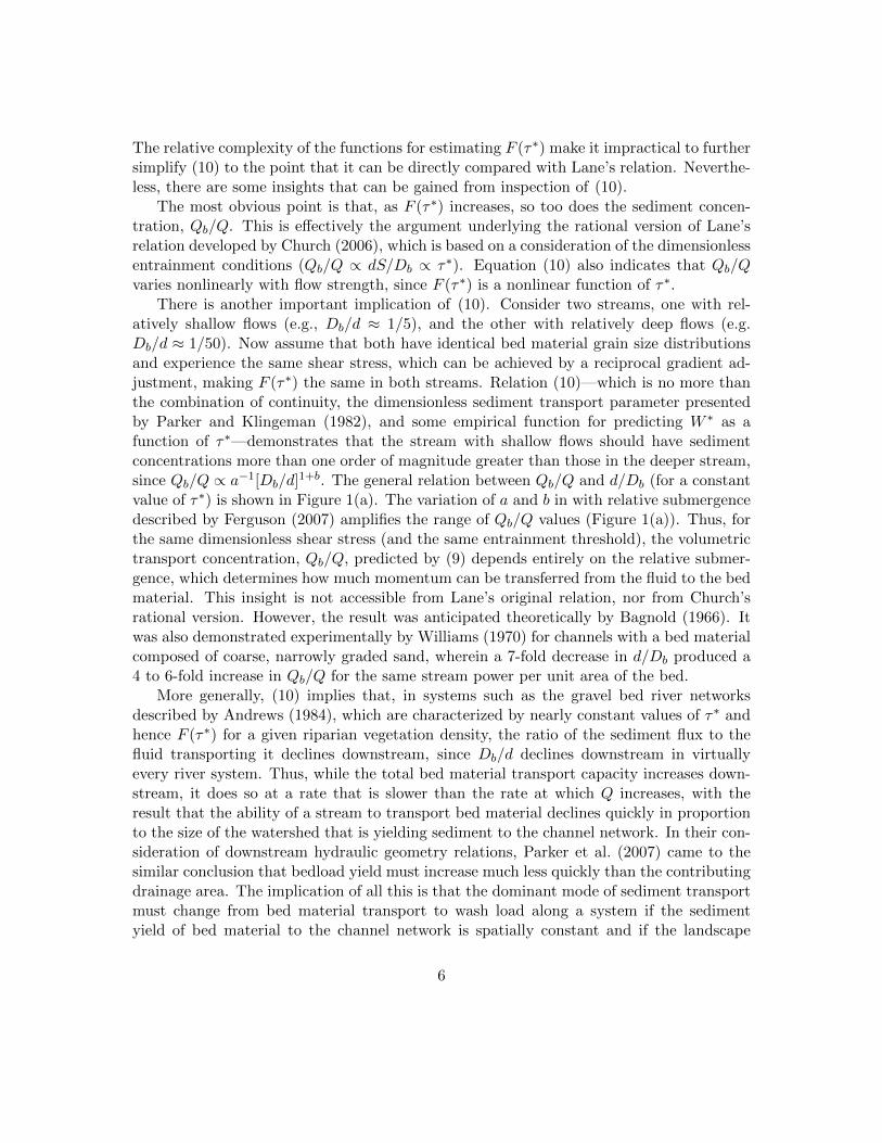
There is another important implication of (10). Consider two streams, one with rel-atively shallow flows (e.g., Db/d ≈ 1/5), and the other with relatively deep flows (e.g.Db/d ≈ 1/50). Now assume that both have identical bed material grain size distributionsand experience the same shear stress, which can be achieved by a reciprocal gradient ad-justment, making F (τ∗) the same in both streams. Relation (10)—which is no more thanthe combination of continuity, the dimensionless sediment transport parameter presentedby Parker and Klingeman (1982), and some empirical function for predicting W ∗ as afunction of τ∗—demonstrates that the stream with shallow flows should have sedimentconcentrations more than one order of magnitude greater than those in the deeper stream,since Qb/Q ∝ a−1[Db/d]1+b. The general relation between Qb/Q and d/Db (for a constantvalue of τ∗) is shown in Figure 1(a). The variation of a and b in with relative submergencedescribed by Ferguson (2007) amplifies the range of Qb/Q values (Figure 1(a)). Thus, forthe same dimensionless shear stress (and the same entrainment threshold), the volumetrictransport concentration, Qb/Q, predicted by (9) depends entirely on the relative submer-gence, which determines how much momentum can be transferred from the fluid to the bedmaterial. This insight is not accessible from Lane’s original relation, nor from Church’srational version. However, the result was anticipated theoretically by Bagnold (1966). Itwas also demonstrated experimentally by Williams (1970) for channels with a bed materialcomposed of coarse, narrowly graded sand, wherein a 7-fold decrease in d/Db produced a4 to 6-fold increase in Qb/Q for the same stream power per unit area of the bed.

More generally, (10) implies that, in systems such as the gravel bed river networksdescribed by Andrews (1984), which are characterized by nearly constant values of τ∗ andhence F (τ∗) for a given riparian vegetation density, the ratio of the sediment flux to thefluid transporting it declines downstream, since Db/d declines downstream in virtuallyevery river system. Thus, while the total bed material transport capacity increases down-stream, it does so at a rate that is slower than the rate at which Q increases, with theresult that the ability of a stream to transport bed material declines quickly in proportionto the size of the watershed that is yielding sediment to the channel network. In their con-sideration of downstream hydraulic geometry relations, Parker et al. (2007) came to thesimilar conclusion that bedload yield must increase much less quickly than the contributingdrainage area. The implication of all this is that the dominant mode of sediment transportmust change from bed material transport to wash load along a system if the sedimentyield of bed material to the channel network is spatially constant and if the landscape

6

5 10 20 50 100

5e-05

2e-04

1e-03

5e-03

d Db

QbQ

Ferguson (2007)Strickler-Manning

(a)

5 10 20 50 100

0.01

0.05

0.20

1.00

d Db

QbQS

(b)

Figure 1: (a)The sediment concentration, Qb/Q is plotted against the relative submergence,d/Db for streams having the same dimensionless shear stress (τ∗ = 0.08). (b) The bedmaterial sediment efficiency, η = Qb/QS is plotted against the relative submergence, d/Db

for streams having the same dimensionless shear stress (τ = 0.08). Both the Strickler-Manning flow resistance law (1), in which a = 7.3 and b = 1/6, and the continuouslyvarying power function presented by Ferguson (2007) were used to calculate Qb/Q andQb/QS.

7

is at steady state. Sklar et al. (2006) modelled this transition by considering the rate ofgrain abrasion during transport, and Eaton and Church (2007) observed it in numericalestimates of Qb for a wide range of empirical hydraulic geometry datasets, and ascribed itto the combined effects of weathering in situ and abrasion during transport.

Another way to think about river grade is to invoke the concept of bedload transportefficiency, η, defined to be the ratio between the work done by a stream (which is ∝ Qb)and the power of the stream (∝ QS). Rearranging equation (9) gives

η =Qb

QS=

1

aR

[Db

d

]bW ∗ (13)

This description of the graded state indicates that the transport efficiency has a first orderdependence on τ∗ (via the empirical relation W ∗), and a second order dependence onrelative submergence via the flow resistance equation. The upshot is that η is nearly thesame in shallow and deep streams having the same dimensionless shear stress. The valueof η is plotted against d/Db in Figure 1(b). Both panels of Figure 1 have y-axes that spantwo orders of magnitude to facilitate direct comparison: while the ratio Qb/Q varies overtwo orders of magnitude for the selected range of d/Db, the efficiency (Qb/QS) is nearlyconstant, varying only by a factor of two. The two panels of Figure 1 demonstrate thatthe volumetric sediment concentration declines quickly as d/Db increases for a constantdimensionless shear stress (panel a), while the transport efficiency declines only sightly(panel b) for the same flow conditions. To achieve a truly constant transport efficiency,the dimensionless shear stress cannot remain constant, and it is more convenient to usedimensionless stream power instead of dimensionless shear stress as a measure of the relativeflow strength, as described in the following section.

3 A transport function using ω∗

In this section we define a dimensionless stream power (ω∗) and a dimensionless sedi-ment transport parameter (E∗) that is similar to the parameter proposed by Parker andKlingeman (1982), but is based on q∗b and ω∗. We use these dimensionless parameters inconjunction with a reference dimensionless stream power (ω∗◦) that depends on the criticalShields number (θc) to develop a new empirical bed material transport relation.

The result presented in (13) is reminiscent of R.A. Bagnold’s ideas regarding bedloadtransport (Bagnold, 1966). Bagnold made the analogy between bedload transport by ariver and mechanical efficiency. After testing his ideas against empirical data, Bagnold(1980) concluded that the efficiency of a stream varied with the power of the stream, andthat bedload transport rate was proportional to the excess unit stream power (ω− ω◦)3/2,where ω = τU = ρgdSU and ω◦ is the critical stream power for sediment entrainment. Oneproblem with Bagnold’s formulation is the difficulty to define the threshold for entrainment.Another problem with Bagnold’s approach is the introduction of reference grain sizes,

8

flow depths and transport rates in order to calculate an adjusted transport rate. Martinand Church (2000) were able to remove the reference values and derive a rational andcomputationally convenient form of the equation. Another way of achieving the same resultis to introduce a dimensionless stream power and use that to develop a new dimensionlesstransport parameter analogous to W ∗.

3.1 A new dimensionless transport parameter, E∗

In order to define a new dimensionless transport parameter that encapsulates Bagnold’sview of sediment transport as a stream power-related phenomenon, we must first definea dimensionless unit stream power, ω∗. Combining the definitions of dimensionless depth(d∗ = d/Db) and velocity (V ∗ = U/

√gRDb) presented by Parker (1979), with the rate

of potential energy expenditure per unit of water relative to the submerged unit weightof sediment (S∗ = ρgS/ρgR) we define the dimensionless stream power as ω∗ = d∗V ∗S∗.Expressed in dimensional terms, the equation for ω∗ is

ω∗ =gdSU

[gRDb]3/2(14)

Since ω = ρgdSU , we can write (14) in terms of ω and Db alone:

ω∗ =ω

ρ[gRDb]3/2(15)

The main advantage of using dimensionless stream power to represent the relative flowstrength is that ω can be estimated from measurements of discharge (Q), width (B) andgradient (S) of the stream (ω = ρgQS/B = ρgqS), whereas estimates of τ require that aflow resistance equation be employed to estimate the water depth. This means that ω∗ canbe determined directly from the continuity equation, while it is necessary to invoke a flowresistance equation to relate τ∗ to discharge, thereby introducing additional uncertaintyattached to the chosen flow resistance equation. This is the basic practical differencebetween a stream power-based approach and a shear stress-based approach. The necessityto specify a flow resistance equation is particularly problematic in steep, shallow streamswhere the water surface is strongly influenced by local roughness elements, making itdifficult to estimate the mean depth.

We can use (1), (2) and (5) to relate ω∗ to τ∗ (following a similar analysis by Ferguson,2005). The general relation has the form

ω∗ = <τ∗ 3/2 (16)

For the sake of clarity, we have used < to represent the flow resistance parameter insteadof the power law function in (1).

The fact that ω∗ ∝ τ∗ 3/2 in (16) is suggestive, particularly when we recall that thedefinition of W ∗ in (4) involves normalizing the Einstein dimensionless transport parameter

9

q∗b by τ∗ 3/2. If, as Bagnold suggests, sediment transport is more aptly related to streampower than to shear stress, a more rational dimensionless transport parameter is written

E∗ =q∗bω∗

(17)

which, in terms of the variables d and S becomes

E∗ =Rqb

<√g[ds]3/2(18)

A comparison of (18) and (8) demonstrates that E∗ = W ∗/<. So, for relatively deepchannels (wherein < is relatively constant), E∗ and W ∗ will be nearly equivalent, but inshallow, steep channels (wherein < varies to a greater degree), E∗ and W ∗ will diverge.

E∗ can also be expressed in terms of q and S, which removes the necessity of invokinga flow resistance law and which is more relevant to the development of a graded staterelation.

E∗ =RqbqS

(19)

It follows from (19) that E∗ = Rη, where η is the sediment transport efficiency parameterused in (13). Thus E∗ is equivalent to the sediment transport efficiency parameter alreadyin common use.

3.2 A reference dimensionless stream power

Before we can generate an empirical transport relation in terms of E∗ and ω∗, it is necessaryto define a reference dimensionless stream power value (ω∗◦) in order to collapse the datato a common relation. We define this reference value as a function of the critical Shieldsnumber, θc. However, for a given stream, θc can vary, and thus is interpreted herein asan important adjustable system parameter (referred to herein as the bed state parameter)affecting the sediment transport rate for a given set of flow conditions. The value of θcis affected by the development of bed imbrication (Johnston, 1922; Laronne and Carson,1976), pebble clusters (Brayshaw, 1985; Reid et al., 1992) stone lines (Church et al., 1998)and stone cells (Laronne and Carson, 1976; Church et al., 1998). These structures developand decay over time, primarily in relation to the sequence of flows acting upon the bed(Hassan and Church, 2000). The formation of bed surface structures is most favourablewhere there is a wide range of grain sizes, with surface structure development becomingless prevalent as the bed becomes better sorted. To the extent that bed material becomesbetter sorted with increasing system size, the effect of surface structures may also be scaledependent. These potential scale effects cannot be accounted for so long as θc is heldconstant. By recognizing that gravel-bed rivers can adjust their bed state and therebyinfluence the entrainment threshold, it is appropriate for our purposes to interpret θc notas a constant, but as a variable that describes the bed state (Church et al., 1998), which

10

is one avenue by which a system may adjust to changes in streamflow and/or sedimentsupply.

It is also important to consider what the value of θc actually tells us about a systemwhen it is applied on a width-averaged basis, as is done here. θc defines the flow conditionsat which the median surface size (D50) can be mobilized by the mean boundary shear stress,τ . However for width-averaged dimensionless stresses less than θc, it is not true that nosediment entrainment will take place: grains finer than the D50 may be entrained, thoughthis process is inhibited by the hiding effect described by Parker and Klingeman (1982);and the D50 may be entrained in those parts of the channel where the shear stress is greaterthan average. As a result, entrainment does not cease altogether once τ∗ falls below θc, butthe proportion of the bed and the range of grain sizes that can be entrained both shrinkand the transport rate declines sharply. Furthermore, the threshold for entrainment is notthe same as the threshold for the maintenance of transport, once a grain is entrained. Forexample, Fenton and Abbott (1977) demonstrated experimentally that θc falls to valuesaround 0.01 when particles are exposed above the bed rather than hiding within it, as isthe case for grains already entrained and in transport. For example, if θc = 0.04 for thesurface D50 and τ∗ = 0.04, such that the local bed is just at the entrainment threshold,then particles that are already in transport will continue moving when exposed to themean boundary shear stress, so long as they are no larger than about four times the D50,implying that the local sediment transport rate depends on both the ability of the flowto entrain sediment from the bed locally and the supply of already-moving grains arrivingfrom elsewhere upstream.

We use (16) to relate ω∗◦ and the critical dimensionless shear stress, θc, thereby permit-ting us to take advantage of the extensive work that has been done on entrainment.

ω∗◦ = θc3/2< (20)

Clearly, it is necessary to employ a flow resistance value (<) at the threshold of entrainmentto relate ω∗◦ to θc, so the stream power-based approach is not entirely independent ofthe choice of flow resistance equation. However, flow resistance is only relevant for theconditions at the threshold state, and variations in flow resistance for discharges in excessof the critical value do not affect a stream-power based model.

3.3 An empirical relation between E∗ and ω∗

Adapting the ideas proposed by Bagnold (1966) to our dimensionless variables and refer-ring to the common form of empirical transport equations (e.g., equations (6) and (7)),it seems reasonable to hypothesize that our transport parameter, E∗, is a function of theratio ω∗/ω∗◦. In order to test our approach, we use the bedload transport dataset presentedby Gomez and Church (1988), which includes data from Clearwater River (Jones and Seitz,1980), Elbow River (Hollingshead, 1971), Mountain Creek (Einstein, 1944), Snake River(Jones and Seitz, 1980), and Tanana River (Burrows and Harrold, 1981). It also includes

11

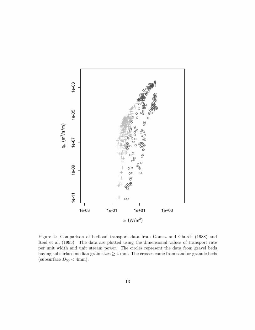
data from laboratory experiments reported by Ikeda (1983), Johnson (1943), Meyer-Peterand Muller (1948), Paintal (1971) and Wilcock (1987). This dataset represents a carefulcompilation of relatively homogeneous data from laboratory experiments and field investi-gations that reflect equilibrium transport conditions in coarse sand and gravel-bed channels.The reported data are associated with steady state flow conditions, and represent the totaltransport rate, integrated across the channel. We have also included the dataset from Na-hal Yatir (Reid et al., 1995), a desert stream that appears to transport bed material at anearly constant sediment transport efficiency with no structural constraint. The transportrates for all data are plotted against unit stream power in Figure 2. The data are groupedinto a subset from gravel beds (for which the bed subsurface D50 ≥ 4 mm) and from sandand granule beds (D50 < 4 mm). The data are quite scattered, with large differencesbetween and within the two subsets.

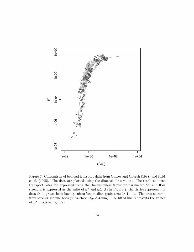
The dimensionless data are plotted in Figure 3, wherein E∗ is plotted against ω∗/ω∗◦. Inorder to calculate the dimensionless stream power parameters, it is necessary to estimateDb, since only subsurface grain size distributions were provided in the Gomez and Church(1988) dataset. For the gravel-bed subset (D50 ≥ 4 mm), Db in (14) and (20) was calculatedassuming an armour ratio of 2 (after Hassan et al., 2006). Since armouring requires areasonably wide range of bed grain sizes it was assumed that the sand and granule-bedchannels did not armour to the same degree as the gravel-bed channels. The plottingpositions for the sand and granule-bed subset (D50 < 4 mm) were calculated assumingan armour ratio of ≈ 1.5, since this is what Eaton and Church (2004) observed in theirexperiments with sand-granule mixes. Reid et al. (1995) report both the bed and subsurfaceD50: in Nahal Yatir, the bed surface has a distribution similar to that of the subsurface,and is consistent with an armour ratio of 1. For all of the data, we specified a single valuefor θc of 0.045 when calculating ω∗◦, whilst recognizing that variations in the true value ofθc will tend to scatter the data.

The dimensionless data in Figure 3 plot much closer together than do the dimensionaldata (Figure 2), essentially collapsing to a single relation. The data are scattered about therelation, but this is not surprising given the assumptions that have been made about thedegree of armouring in the Gomez and Church (1988) dataset and about the representativevalue of θc for all the datasets. The general trend of the dimensionless data is quite steepfor ω∗/ω∗◦ values close to unity, but levels out asymptotically as ω∗/ω∗◦ increases and themaximum efficiency is approached.

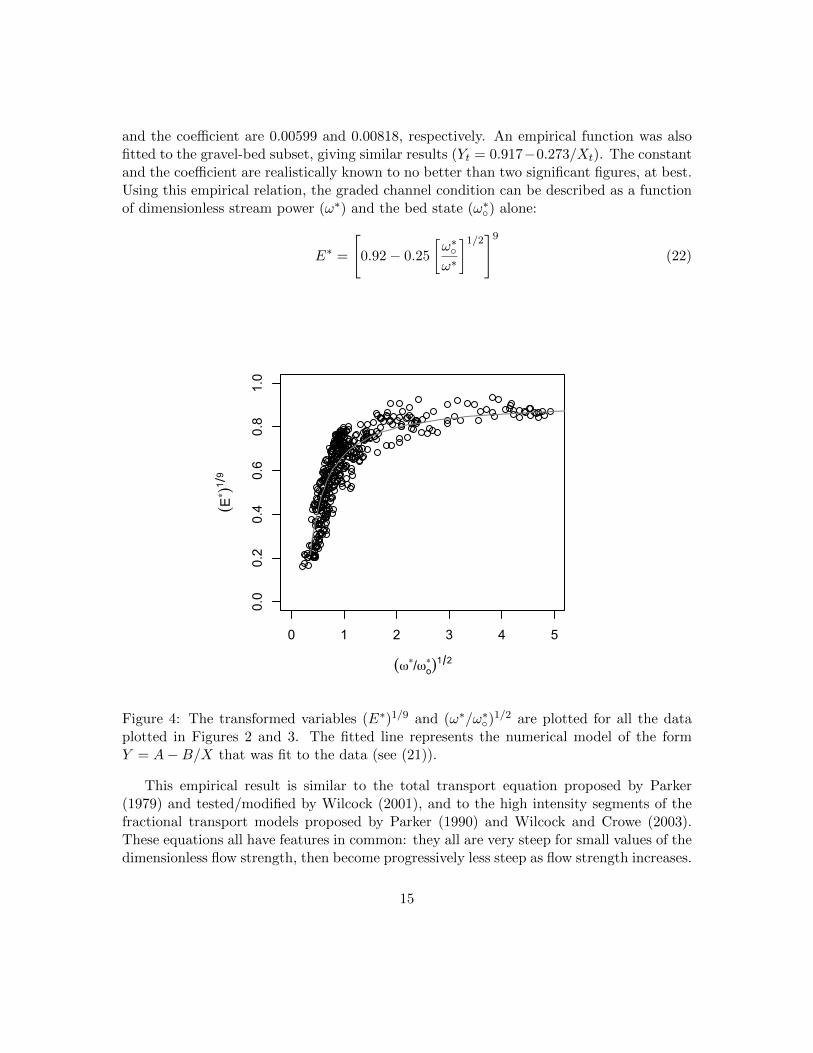
We have derived an empirical relation between E∗ and ω∗/ω∗◦ using all of the availabledata. The equation was fit numerically to transformed variables (Yt = E∗ 1/9 and Xt =[ω∗/ω∗◦]

1/2), assuming a model of the form Yt = A/Xt +B. The transformed variables areshown in Figure 4, as is the fitted equation. The fitted equation is:

Yt = 0.921− 0.250

Xt(21)

The standard error for the estimates of Yt is 0.086, and the standard errors for the constant

12

1e-03 1e-01 1e+01 1e+03

1e-11

1e-09

1e-07

1e-05

1e-03

! (W m2)

q b(m

3sm)

Figure 2: Comparison of bedload transport data from Gomez and Church (1988) andReid et al. (1995). The data are plotted using the dimensional values of transport rateper unit width and unit stream power. The circles represent the data from gravel bedshaving subsurface median grain sizes ≥ 4 mm. The crosses come from sand or granule beds(subsurface D50 < 4mm).

13

1e-02 1e+00 1e+02 1e+04

1e-08

1e-06

1e-04

1e-02

1e+00

!!/!o!

E!

Figure 3: Comparison of bedload transport data from Gomez and Church (1988) and Reidet al. (1995). The data are plotted using the dimensionless values. The total sedimenttransport rates are expressed using the dimensionless transport parameter E∗, and flowstrength is expressed as the ratio of ω∗ and ω∗◦. As in Figure 2, the circles represent thedata from gravel beds having subsurface median grain sizes ≥ 4 mm. The crosses comefrom sand or granule beds (subsurface D50 < 4 mm). The fitted line represents the valuesof E∗ predicted by (22).

14

and the coefficient are 0.00599 and 0.00818, respectively. An empirical function was alsofitted to the gravel-bed subset, giving similar results (Yt = 0.917−0.273/Xt). The constantand the coefficient are realistically known to no better than two significant figures, at best.Using this empirical relation, the graded channel condition can be described as a functionof dimensionless stream power (ω∗) and the bed state (ω∗◦) alone:

E∗ =

[0.92− 0.25

[ω∗◦ω∗

]1/2]9(22)

0 1 2 3 4 5

0.0

0.2

0.4

0.6

0.8

1.0

(!!/!o!)1 2

(E! )19

Figure 4: The transformed variables (E∗)1/9 and (ω∗/ω∗◦)1/2 are plotted for all the data

plotted in Figures 2 and 3. The fitted line represents the numerical model of the formY = A−B/X that was fit to the data (see (21)).

This empirical result is similar to the total transport equation proposed by Parker(1979) and tested/modified by Wilcock (2001), and to the high intensity segments of thefractional transport models proposed by Parker (1990) and Wilcock and Crowe (2003).These equations all have features in common: they all are very steep for small values of thedimensionless flow strength, then become progressively less steep as flow strength increases.

15

For (22), E∗ asymptotically approaches an upper limit of about 0.5 (E∗ → [0.92±0.01]9 ≈0.47± 0.05) as ω∗/ω∗◦ becomes large. The transport efficiencies in Nahal Yatir reported byReid et al. (1995) reached similar levels (E∗max = 0.53 for their dataset), which supportsthis empirically derived asymptote.

4 A general graded relation

In order to generate a relation similar to Lane’s using our dimensionless stream powerapproach, we must first approximate the relation between E∗ and ω∗/ω∗◦ using a power lawof the form E∗ ∝ [ω∗/ω∗◦]

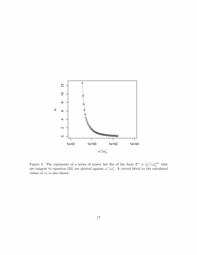
x1 , in which x1 increases as relative flow strength decreases. SinceFigure 3 is a log-log plot, the slope of a straight line tangent to (22) is equal to the exponentof the power law that approximates (22) at that point (c.f. Crosato and Mosselman, 2009).The exponents of a series of power law fits tangent to (22) are shown in Figure 5, alongwith a fitted curve describing the variation of x1 with ω∗/ω∗◦. The fitted curve has the form

x1 = 4.28/ [log (ω∗/ω∗◦) + 1.54]2.41 (23)

Using this algebraically convenient approximation and recalling that E∗ ∝ Qb/QS, we canwrite a conceptual summary relation describing stream channel gradation using dimension-less variables:

Qb

QS∝[ω∗

ω∗◦

]x1

(24)

Unlike (13), this equation does not depend on the relative submergence, and Qb/QS isconstant so long as ω∗/ω∗◦ is constant. By substituting (14) and (20), cancelling variables,and removing constants, we arrive at the following statement for river grade using the morefamiliar variables d, Db, S, and the bed state parameter (Shields number) θc :

Qb

QS∝[dS

Dbθc

](3/2)x1

(25)

This approximate form of (22) is a version of Lane’s relation that is physically consistentwith what we know about bed material transport and open channel hydraulics.

We can take the same approach to the empirical relation between W ∗ and τ∗ to arriveat an analogous grade relation. Plotting W ∗ and τ∗/θc (Fig. 6), reveals a familiar pattern.The empirical equation fit to those data is

W ∗ =

[1.42− 0.52

√θcτ∗

]1/9(26)

which is similar to other empirical equations, such as (6) and (7). A comparison of Figs.3 and 6 suggests that the data are slightly more scattered when expressed using W ∗ and

16

1e-02 1e+00 1e+02 1e+04

02

46

810

12

!! !o!

x 1

Figure 5: The exponents of a series of power law fits of the form E∗ ∝ [ω∗/ω∗◦]x1 that

are tangent to equation (22) are plotted against ω∗/ω∗◦. A curved fitted to the calculatedvalues of x1 is also shown.

17

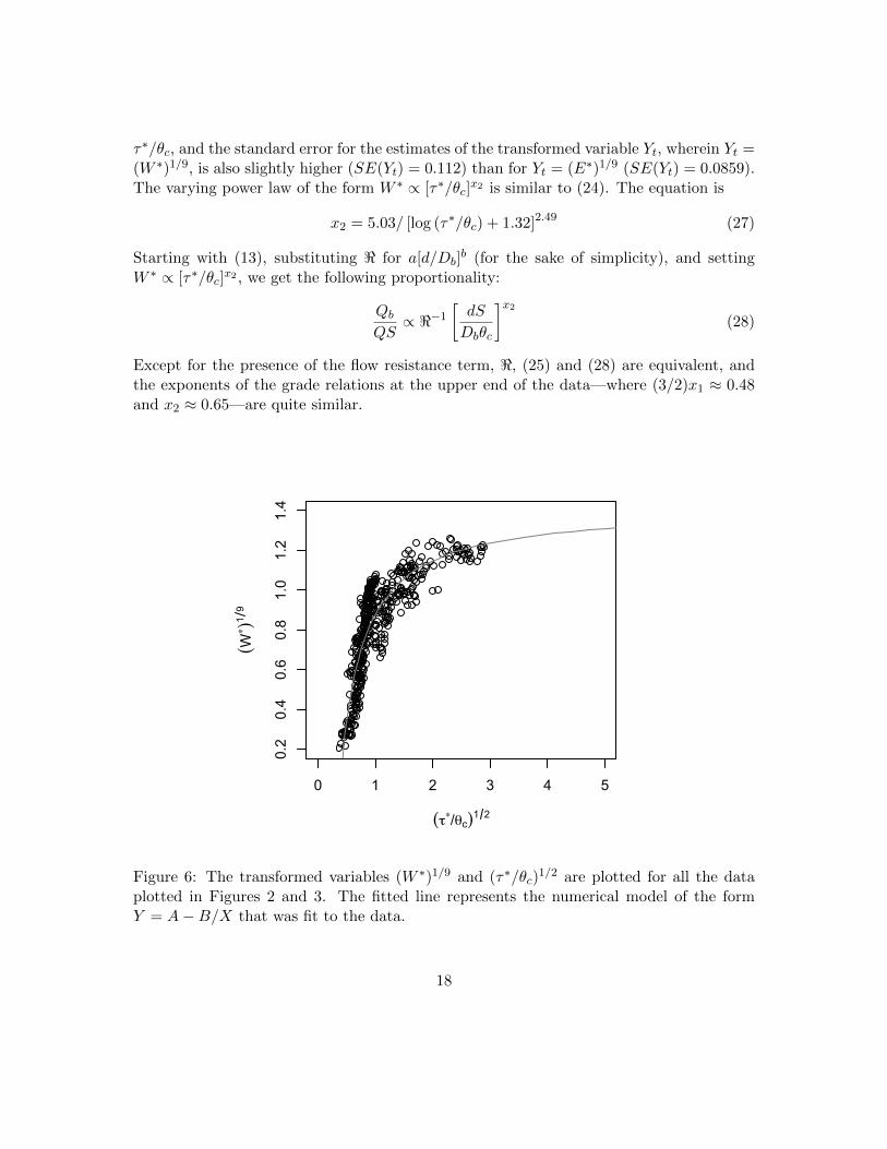
τ∗/θc, and the standard error for the estimates of the transformed variable Yt, wherein Yt =(W ∗)1/9, is also slightly higher (SE(Yt) = 0.112) than for Yt = (E∗)1/9 (SE(Yt) = 0.0859).The varying power law of the form W ∗ ∝ [τ∗/θc]

x2 is similar to (24). The equation is

x2 = 5.03/ [log (τ∗/θc) + 1.32]2.49 (27)

Starting with (13), substituting < for a[d/Db]b (for the sake of simplicity), and setting

W ∗ ∝ [τ∗/θc]x2 , we get the following proportionality:

Qb

QS∝ <−1

[dS

Dbθc

]x2

(28)

Except for the presence of the flow resistance term, <, (25) and (28) are equivalent, andthe exponents of the grade relations at the upper end of the data—where (3/2)x1 ≈ 0.48and x2 ≈ 0.65—are quite similar.

0 1 2 3 4 5

0.2

0.4

0.6

0.8

1.0

1.2

1.4

(!!/!c)1 2

(W! )19

Figure 6: The transformed variables (W ∗)1/9 and (τ∗/θc)1/2 are plotted for all the data

plotted in Figures 2 and 3. The fitted line represents the numerical model of the formY = A−B/X that was fit to the data.

18

5 Discussion

Based on our analysis, a general form of Lane’s relation can be derived from sedimenttransport theory using a dimensionless stream power approach (after Bagnold, 1966), (25),that is consistent with the equivalent relation based on the dimensionless shear stressapproach, (28), although (28) is complicated by the persistent flow resistance term, <.We therefore propose (25) as a general graded relation. It relates bed material transportefficiency (Qb/QS) to parameters describing the channel itself, comprising the mean depth,characteristic grain size, gradient, and a parameter that represents the effects of bed surfacestructures on sediment entrainment. Due to its relative completeness and simplicity, thisform can be used to consider the reach response to imposed changes in Q, Qb, or evento forced changes in S. In this sense, it relates the imposed flow and sediment variablesdirectly to channel grade.

Consider the response of a meandering stream that is artificially straightened, therebyincreasing the channel gradient. Equation (25) can be rearranged to read S1+(3/2)x1 ∝(Qb/Q)(θcDb/d)(3/2)x1 . The first point to make is that for the same proportional changein S, the relative magnitude of the system response will be greater for streams closer tothreshold conditions (where x1 is large) than it will be for streams that experience highrelative flows (where x1 approaches 0). The general point is that the importance of thesurface grain size, surface structures and channel shape (which determines d) are greaternear threshold than they are away from it (and their occurrence is more evident nearthreshold).

For a stream in which ω∗ >> ω∗◦ (a condition most common in sand-bed streams withcohesive banks but possible in other channels with relatively strong banks as well), themost likely response to an increase in S will be a concomitant increase in the bed materialtransport capacity (Qb) which will reestablish grade over time by reducing S via degrada-tion. Changes to the bed surface are unlikely to be dominant under these conditions, evenif the range of grain sizes in the bed material is large enough to make a bed surface responsepossible. Changes in the mean hydraulic depth, d, would realistically require a change inchannel shape (although d does depend on S), so assessing the magnitude and directionof such a change requires additional information about the channel boundary in generaland the stability of the channel banks in particular. Changes in d could be important,depending on the magnitude of the adjustment. While (25) does not address the problemof bank strength and stable channel shape, the variable d in (25) directs our attention tothis problem.

Grade in streams that are close to threshold (a condition typical of most gravel-bedstreams) may be influenced by all of the system parameters in (25). An increase in S wouldincrease the transport capacity, triggering degradation. However, since the system is closeto threshold, size selective transport could produce a coarsening of the bed surface if thebed material contains a sufficiently wide range of grain sizes, and bed surface structurescould become well developed, increasing the bed state parameter (critical Shields number)

19

for entrainment. Both these effects could influence the degree of degradation that wouldoccur, and limit the system’s ability to return to the original channel gradient. Talbotand Lapointe (2002a) documented the response of the meandering, gravel-bedded SainteMarguerite River to straightening. They observed that the system responded by adjustingthe gradient (via vertical degradation and limited lateral migration) and by increasingcharacteristic surface grain size. Overall, the bed texture response appears to have beenmore important than the changes is channel gradient and, using a 1D sediment transportmodel, they predicted that the former channel gradient will not be reattained because ofthe influence of the bed surface adjustment (Talbot and Lapointe, 2002b).

Depending on the nature of the channel boundaries, the channel shape might change aswell, and thereby influence the pathways by which a stream reestablishes grade. For exam-ple, when channel banks are as erodible as the channel bed, the channel slope appears tobe the dominant response (e.g. Schumm and Khan, 1972; Eaton and Church, 2004). Whenthe boundaries are not erodible, significant changes in bed surface texture become apparent(e.g. Dietrich et al., 1989; Eaton and Church, 2009). The response also clearly depends onthe flow conditions and flow history, since surface structures are formed preferentially atmodestly competent flows (Church et al., 1998).

The analysis in this paper also has general implications for how we think about sedimenttransport scaling relations. The development of the stream power approach highlights thefact that there are two distinct issues controlling the scaling relation between bed materialtransport and the flow strength. When conditions are close to threshold (i.e, τ∗ ≈ θc),then grain entrainment mediates the sediment transport rate. In gravel bed streams,the development of a coarse surface layer (Parker and Klingeman, 1982) and of structuresamongst the grains in the surface layer (Church et al., 1998) both influence the bed materialtransport rate. The result is that the sediment transport rates vary by several orders ofmagnitude for flow conditions close to threshold. The temporal variation in the bed statelikely contributes to the scatter of the measured sediment transport efficiencies, whichoften covers as much as one order of magnitude for the same dimensionless stream power.However, for sufficiently strong flows, E∗ tends toward a constant value. The empiricaldata presented by Rickenmann (1997) demonstrate this flow-dependent influence of bedstate, since the transport data are quite variable for low flows (ranging over more than oneorder of magnitude for the same flow), but then tend to converge at higher flows. Whilethe form of the empirical functions for estimating F (τ∗) suggest this general effect, it isexplicit in (25), which states that for ω∗ >> ω∗◦, the volume of sediment transported by astream depends entirely on the power of the stream, not on the size of the sediment beingtransported. Thus, transport becomes entirely a flow resistance phenomenon, in whichbed material transport is controlled by the rate at which momentum can be transferredfrom the fluid to the boundary materials, not by the force required to entrain the bed. Inreality, most streams are influenced by both the force-based entrainment threshold and thepower-based momentum transfer. More exactly, bed material transport is a product of thetransfer of momentum from the fluid to the boundary that is mediated by the boundary

20

entrainment threshold. Thus, it is more logical to express flow strength using stream powerthan using shear stress. However, as (16) clearly states, both are closely related.

In the end, however, graded state relations can be established in explicit form only byresort to empirical curve fitting. Given the high degree of correlation that exists amongst Q,Qb, d and S, it is not surprising that grade relations derived using dimensionless shear stressand dimensionless stream power are nearly identical. Rationally, the shear stress-basedarguments seems best suited to establish the practical threshold of motion (and Shields’relation is an integral part of the Church (2006) representation of Lane’s relation), whilethe stream power-based arguments seem best suited to estimate bed material transport.

6 Conclusions

By combining a bed material sediment transport law (defined either in terms of dimension-less stream power or dimensionless shear stress) with continuity and a flow resistance law,we can arrive at conceptual summary relations (equations (25) and (28)) describing chan-nel grade that are very similar to the original relation proposed by Lane (1955). The shearstress-based equation (28) retains a dependence on the flow resistance value, <. The otherscaling relation (25) was derived using a new dimensionless sediment transport parameter(E∗ = RQb/QS) which is based on the ideas about stream power proposed by Bagnold(1966): it is slightly simpler than (28) since it is independent of the flow resistance value<:

Qb

QS∝[dS

Dbθc

](3/2)x1

This form relates the sediment transport efficiency (Qb/QS) to parameters that describethe potential system adjustments: the mean hydraulic depth, d, represents the potentialeffect of changing the channel shape or size; the channel gradient, S, represents the po-tential for the system to respond to change via vertical aggradation/degradation or lateralmigration that increases/decreases channel sinuosity; the characteristic surface grain size,Db, represents the potential for the degree of surface armouring to adjust; and the bedstate parameter, θc, represents the potential for surface structure development to affectchannel grade by modifying the entrainment threshold. The relation demonstrates that:

1. the original form of Lane’s relation (which included all but two of the variables) wasvery nearly complete;

2. the addition of flow depth proposed by Church (2006) is valid and necessary, as isthe recognition that the bed state parameter, θc, is also important;

3. the effect of changes in slope is greater than the effect of proportionally similarchanges in d, Db or θc, since S occurs in the numerator on one side of the equationand the denominator on the other; and

21

4. the relation changes systematically as the relative flow strength changes, since theexponent x1 > 10 for very low ω∗/ω∗◦ values, while x1 → 0 as ω∗/ω∗◦ gets large andefficiency approaches the empirically determined limit value of 0.5 (which is consistentwith the efficiencies reported by Reid et al. (1995) for Nahal Yatir).

Because (25) is expressed using the basic variables describing a reach and because it isindependent of flow resistance, it is best suited to considerations of reach-scale responseto imposed changes in sediment supply or formative discharge, or engineered changes instream channel gradient. It is a powerful summary relation that can be used to structureone’s thinking about fundamental problems in fluvial geomorphology as well as aboutchannel alteration and restoration plans.

Acknowledgements

The idea for this paper originated from discussions in the field with Ian Rutherfurd re-garding channel gradation, and we would like to thank him for this initial inspiration. Thepaper was much improved as a result of comments from Rob Ferguson and an anonymousreviewer.

References

Andrews ED. 1983. Entrainment of gravel from naturally sorted riverbed material. Geo-logical Society of America Bulletin 94: 1225–1231.

Andrews ED. 1984. Bed-material entrainment and hydraulic geometry of gravel-bed riversin Colorado Geological Society of America Bulletin 95: 371–378.

Bagnold RA. 1966. An approach to the sediment transport problem from general physics,Professional Paper 422I. United States Geological Survey: Washington, DC.

Bagnold RA. 1980. An empirical correlation of bedload transport rates in flumes andnatural rivers. Proceedings of the Royal Society of London. Series A, Mathematical andPhysical Sciences 372 (1751): 453–473.

Brayshaw AC. 1985. Bed microtopography and entrainment thresholds in gravel-bed rivers.Geological Society of America Bulletin 96: 218 – 223.

Burrows R, Harrold P. 1981. Sediment transport in the Tanana River near Fairbanks,Alaska, Water Resources Investigations Report 83-4064. United States Geological Survey:Washington, DC.

Church M. 2006. Bed material transport and the morphology of alluvial river channels.Annual Review of Earth and Planetary Sciences. 34: 325–354.

22

Church M, Hassan MA, Wolcott JF. 1998. Stabilizing self-organized structures in gravel-bed stream channels: field and experimental observations. Water Resources Research34 (11): 3169–3179.

Crosato A, Mosselman E. 2009. Simple physics-based predictor for the number of riverbars and the transition between meandering and braiding. Water Resources Research45: W03424. doi:10.1029/2008WR007242.

Dietrich WE, Kirchner JW, Ikeda H, Iseya F. 1989. Sediment supply and the developmentof the coarse surface layer in gravel-bedded rivers. Nature 340: 215–217.

Eaton BC, Church M. 2004. A graded stream response relation for bedload domi-nated streams. Journal of Geophysical Research - Earth Surface 109: F03011. doi:10.1029/2003JF000062.

Eaton BC, Church M. 2007. Predicting downstream hydraulic geometry: a test of ratio-nal regime theory. Journal of Geophysical Research - Earth Surface 112: F03025. doi:10.1029/2006JF000734.

Eaton BC, Church M. 2009. Channel stability in bed load-dominated streams withnonerodible banks: inferences from experiments in a sinuous flume. Journal of Geo-physical Research - Earth Surface 114: F01024. doi: 10.1029/2007JF000902.

Einstein HA. 1944. Bedload transportation in Mountain Creek, Technical Bulletin 55. SoilConservation Service, United States Department of Agriculture: Washington, DC.

Einstein HA. 1950. The bed-load function for sediment transportation in open channelflows, Technical Bulletin 1026. Soil Conservation Service, United States Department ofAgriculture: Washington, DC.

Fenton JD, Abbott JE. 1977. Initial movement of grains on a stream bed: the effect ofrelative protrusion. Proceedings of the Royal Society of London 352: 523 – 537.

Ferguson RI. 2005. Estimating critical stream power for bedload transport calculations ingravel-bed rivers. Geomorphology 70: 33–41.

Ferguson RI. 2007. Flow resistance equations for gravel- and boulder-bed streams. WaterResources Research 43: W05427. doi: 10.1029/2006WR005422.

Ferguson RI, Church M, Weatherly H. 2001. Fluvial aggradation in Vedder River: testinga one-dimensional sedimentation model. Water Resources Research 37 (12): 3331–3347.

Gomez B, Church M. 1988. A catalogue of equilibrium bedload transport dat for coarse sandand gravel-bed channels. Department of Geography, The University of British Columbia:Vancouver.

23

Hassan MA, Church M. 2000. Experiments on surface structure and partial sediment trans-port on a gravel bed. Water Resources Research 36 (7): 1885–1895.

Hassan MA, Egozi R, Parker G. 2006. Experiments on the effect of hydrograph character-istics on vertical grain sorting in gravel bed rivers. Water Resources Research 42: doi:10.1029/2005WR004707.

Hollingshead A. 1971. Sediment transport measurements in gravel river. Journal of theHydraulics Division-ASCE 97: 1817–1834.

Ikeda H. 1983. Experiments on bedload transport, bedforms and sedimentary structuresusing fine gravel in the 4 metre wide flume, Paper 2. Environmental Research Centre:University of Tsukuba.

Johnson J. 1943. Laboratory investigations on bedload transportation and bed roughness,Technical Paper 50. Soil Conservation Service, United States Department of Agriculture:Washington, DC.

Johnston WA. 1922. Imbricated structure in rivers-gravels. American Journal of Science5-4: 387-390.

Jones M, Seitz H. 1980. Sediment transport in the Snake and Clearwater Rivers in thevicinity of Lewiston, Idaho, Open-file report 80-690. United States Geological Survey:Washington, DC.

Lane EW. 1955. The importance of fluvial morphology in river hydraulic engineering.American Society of Civil Engineers, Proceedings 81: 1–17.

Laronne JB, Carson MA. 1976. Interrelationships between bed morphology and bed-material transport for a small, gravel-bed channel. Sedimentology 23 (1): 67–85.

Mackin JH. 1948. Concept of the graded river, Geological Society of America Bulletin 59:463–512.

Martin Y, Church M. 2000. Re-examination of Bagnold’s empirical bedload formulae. EarthSurface Processes and Landforms 25 (9): 1011–1024.

Meyer-Peter E, Muller R. 1948. Formulas for bed-load transport. In International Associ-ation of Hydrological Research, Proceedings, Stockholm; 39-64.

Paintal A. 1971. Concept of critical shear stress in loose boundary open channels. Journalof Hydraulic Research 9: 91–113.

Parker G. 1979. Hydraulic geometry of active gravel rivers. Journal of the HydraulicsDivision-ASCE 105: 1185–1201.

24

Parker G. 1990. Surface-based bedload transport relation for gravel rivers. Journal of Hy-draulic Research 28 (4): 417–436.

Parker G. Klingeman, P. C., 1982. On why gravel bed rivers are paved. Water ResourcesResearch 18 (5): 1409–1423.

Parker G, Wilcock PR, Paola C, Dietrich WE, Pitlick J. Physical basis for quasi-universalrelations describing bankfull hydraulic geometry of single-thread gravel bed rivers. Jour-nal of Geophysical Research - Earth Surface 112: F04005. doi: 10.1029/2006JF000549.

Reid I, Frostick LE, Brayshaw AC. 1992. Microform roughness elements and the selectiveentrainment and entrapment of particles in gravel-bed rivers. In Dynamics of Gravel-bedRivers, Billi P, Hey R, Thorne C, Tacconi P (eds). John Wiley and Sons Ltd: Chichester;253 – 265.

Reid I, Laronne JB, Powell DM. 1995. The Nahal Yatir bedload database: sediment dy-namics in a gravel-bed ephemeral stream. Earth Surface Processes and Landforms 20:845 – 857.

Rickenmann D. 1997. Sediment transport in Swiss torrents. Earth Surface Processes andLandforms 22: 937 – 951.

Schumm SA, Khan HR. 1972. Experimental study of channel patterns. Geological Societyof America Bulletin 83: 1755–1770.

Sklar L, Dietrich WE, Foufoula-Georgiou E, Lashermes B, Bellugi D. 2006. Do gravel bedriver size distributions record channel network structure? Water Resources Research 42:W06D18. doi:10.1029/2006WR005035.

Talbot T, Lapointe M. 2002a. Modes of response of a gravel bed river to meander straight-ening: the case of the Sainte-Marguerite River, Saguenay region, Quebec, Canada. WaterResources Research 38: 1073. doi: 10.1029/2001WR000324.

Talbot T, Lapointe M. 2002b. Numerical modeling of gravel bed river response to meanderstraightening: the coupling between the evolution of bed pavement and long profile.Water Resources Research 38: 1074. doi: 10.1029/2001WR000330.

Wilcock PR. 1987. Bed-load transport of mixed-size sediment, Ph.D. thesis. MassachusettsInstitute of Technology: Cambridge.

Wilcock PR. 2001. Toward a practical method for estimating sediment-transport rates ingravel-bed rivers. Earth Surface Processes and Landforms 26: 1395–1408.

Wilcock PR. 2001. Toward a practical method for estimating sediment-transport rates ingravel-bed rivers. Journal of Hydraulic Engineerign 129 (2): 120–128.

25

Williams G. 1970. Flume width and water depth effects in sediment-transport experiments,Professional Paper 562-H. United States Geological Survey: Washington, DC.

26