Comput. Methods Appl. Mech. Engrg. 200 (2011) 1421–1431

Contents lists available at ScienceDirect

Comput. Methods Appl. Mech. Engrg.

journal homepage: www.elsevier .com/locate /cma

A hierarchical framework for statistical model calibration in engineeringproduct development

Byeng D. Youn a,⇑, Byung C. Jung b, Zhimin Xi b, Sang Bum Kim c, W.R. Lee d

a Department of Mechanical and Aerospace Engineering, Seoul National University, Gwanak 599, Gwanak-Gu, Seoul 151-742, Republic of Koreab Department of Mechanical Engineering, University of Maryland at College Park, College Park, MD 20742, USAc LG Electronics PRI, 19-1 Cheongho-ri, Jinwi-myeon, Pyeongtaek-si, Gyeonggi-do 451-713, Republic of Koread Korea Electric Power Research Institute (KEPRI), Daejon 305-760, Republic of Korea

a r t i c l e i n f o

Article history:Received 28 November 2009Received in revised form 17 December 2010Accepted 20 December 2010Available online 24 December 2010

Keywords:Statistical model calibrationHierarchical calibration frameworkUncertainty propagationLikelihood functionEigenvector dimension reductionCellular phone system

0045-7825/$ - see front matter � 2010 Elsevier B.V. Adoi:10.1016/j.cma.2010.12.012

⇑ Corresponding author. Tel.: +82 2 880 7114; fax:E-mail addresses: bdyoun@snu.ac.kr (B.D. Youn),

zxi@umd.edu (Z. Xi), sangbum@lge.com (S.B. Kim), ma

a b s t r a c t

As the role of computational models has increased, the accuracy of computational results has been ofgreat concern to engineering decision-makers. To address a growing concern about the predictive capa-bility of the computational models, this paper proposes a hierarchical model calibration procedure with astatistical model calibration technique. The procedure consists of two activities: (1) calibration planning(top-down) and (2) calibration execution (bottom-up). In the calibration planning activity, engineersdefine either physics-of-failure (PoF) mechanisms or system performances of interest. Then, an engi-neered system can be decomposed into subsystems or components of which computational modelsare better understood in terms of PoF mechanisms or system performances of interest. The calibrationplanning activity identifies vital tests and predictive models along with both known and unknown modelinput variable(s). The calibration execution activity takes a bottom-up approach, which systematicallyimproves the predictive capability of the computational models from the lowest level to the highest usingthe statistical calibration technique. This technique compares the observed test results with the predictedresults from the computational model. A likelihood function is used for the comparison metric. In the sta-tistical calibration, an optimization technique is integrated with the eigenvector dimension reduction(EDR) method to maximize the likelihood function while determining the unknown model variables.As the predictive capability of a computational model at a lower hierarchy level is improved, thisenhanced model can be fused into the model at a higher hierarchical level. The calibration executionactivity is then continued for the model at the higher hierarchical level. A cellular phone is used to dem-onstrate the hierarchical calibration framework of the computational models presented in this paper. It isconcluded that the proposed hierarchical model calibration can effectively enhance the ability of thecomputational model to predict the system reliability of the cellular phone system.

� 2010 Elsevier B.V. All rights reserved.

1. Introduction

As the role of computational models has increased, the accuracyof the computational results becomes important to analysts whomake decisions based on these predicted results. Model validationto assess and improve the predictive capability of computationalmodels has been an essential step for engineered system analysisand design. Among various works on model validation, the surveyarticles of Oberkampf and Trucano [1], Oberkampf et al. [2], Thack-er [3], Babuska and Oden [4], AIAA [5] and ASME [6] explain thestate-of-the-art concepts and processes in detail. Variabilities(and uncertainties) in material properties, physical quantities,

ll rights reserved.

+82 2 880 8302.bcjung@umd.edu (B.C. Jung),erong@kepri.re.kr (W.R. Lee).

loading conditions, manufacturing tolerances and measurementerror are the main factors that can result in adversely predictivecomputational models. Thus, an understanding of the variability(and uncertainty) sources is important for the success of modelvalidation [7,8]. Although there is increasing consistency in the for-mal definition of the validation process, there is still open discus-sion about the steps of the process, which can vary depending onthe different characteristics of the engineering problems.

To improve the predictive capability of computational model,model calibration techniques have been developed [9–12] in re-cent years. Model calibration adjusts a set of unknown model inputvariables associated with a computational model so that the agree-ment is maximized between the predicted (or simulated) and ob-served (or experimental) responses (or outputs) [12,13]. In adeterministic sense, model calibration involves the adjustment ofa few model variables to minimize the discrepancy between the

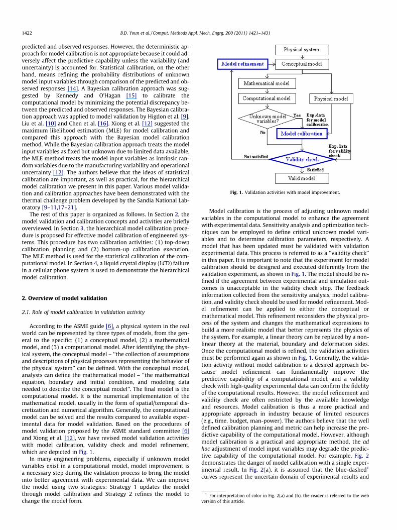
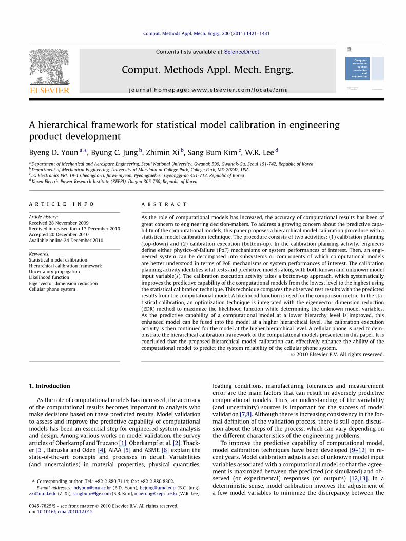
Fig. 1. Validation activities with model improvement.

1422 B.D. Youn et al. / Comput. Methods Appl. Mech. Engrg. 200 (2011) 1421–1431

predicted and observed responses. However, the deterministic ap-proach for model calibration is not appropriate because it could ad-versely affect the predictive capability unless the variability (anduncertainty) is accounted for. Statistical calibration, on the otherhand, means refining the probability distributions of unknownmodel input variables through comparison of the predicted and ob-served responses [14]. A Bayesian calibration approach was sug-gested by Kennedy and O’Hagan [15] to calibrate thecomputational model by minimizing the potential discrepancy be-tween the predicted and observed responses. The Bayesian calibra-tion approach was applied to model validation by Higdon et al. [9],Liu et al. [10] and Chen et al. [16]. Xiong et al. [12] suggested themaximum likelihood estimation (MLE) for model calibration andcompared this approach with the Bayesian model calibrationmethod. While the Bayesian calibration approach treats the modelinput variables as fixed but unknown due to limited data available,the MLE method treats the model input variables as intrinsic ran-dom variables due to the manufacturing variability and operationaluncertainty [12]. The authors believe that the ideas of statisticalcalibration are important, as well as practical, for the hierarchicalmodel calibration we present in this paper. Various model valida-tion and calibration approaches have been demonstrated with thethermal challenge problem developed by the Sandia National Lab-oratory [9–11,17–21].

The rest of this paper is organized as follows. In Section 2, themodel validation and calibration concepts and activities are brieflyoverviewed. In Section 3, the hierarchical model calibration proce-dure is proposed for effective model calibration of engineered sys-tems. This procedure has two calibration activities: (1) top-downcalibration planning and (2) bottom-up calibration execution.The MLE method is used for the statistical calibration of the com-putational model. In Section 4, a liquid crystal display (LCD) failurein a cellular phone system is used to demonstrate the hierarchicalmodel calibration.

1 For interpretation of color in Fig. 2(a) and (b), the reader is referred to the webversion of this article.

2. Overview of model validation

2.1. Role of model calibration in validation activity

According to the ASME guide [6], a physical system in the realworld can be represented by three types of models, from the gen-eral to the specific: (1) a conceptual model, (2) a mathematicalmodel, and (3) a computational model. After identifying the phys-ical system, the conceptual model – ‘‘the collection of assumptionsand descriptions of physical processes representing the behavior ofthe physical system’’ can be defined. With the conceptual model,analysts can define the mathematical model – ‘‘the mathematicalequation, boundary and initial condition, and modeling dataneeded to describe the conceptual model’’. The final model is thecomputational model. It is the numerical implementation of themathematical model, usually in the form of spatial/temporal dis-cretization and numerical algorithm. Generally, the computationalmodel can be solved and the results compared to available exper-imental data for model validation. Based on the procedures ofmodel validation proposed by the ASME standard committee [6]and Xiong et al. [12], we have revised model validation activitieswith model calibration, validity check and model refinement,which are depicted in Fig. 1.

In many engineering problems, especially if unknown modelvariables exist in a computational model, model improvement isa necessary step during the validation process to bring the modelinto better agreement with experimental data. We can improvethe model using two strategies: Strategy 1 updates the modelthrough model calibration and Strategy 2 refines the model tochange the model form.

Model calibration is the process of adjusting unknown modelvariables in the computational model to enhance the agreementwith experimental data. Sensitivity analysis and optimization tech-niques can be employed to define critical unknown model vari-ables and to determine calibration parameters, respectively. Amodel that has been updated must be validated with validationexperimental data. This process is referred to as a ‘‘validity check’’in this paper. It is important to note that the experiment for modelcalibration should be designed and executed differently from thevalidation experiment, as shown in Fig. 1. The model should be re-fined if the agreement between experimental and simulation out-comes is unacceptable in the validity check step. The feedbackinformation collected from the sensitivity analysis, model calibra-tion, and validity check should be used for model refinement. Mod-el refinement can be applied to either the conceptual ormathematical model. This refinement reconsiders the physical pro-cess of the system and changes the mathematical expressions tobuild a more realistic model that better represents the physics ofthe system. For example, a linear theory can be replaced by a non-linear theory at the material, boundary and deformation sides.Once the computational model is refined, the validation activitiesmust be performed again as shown in Fig. 1. Generally, the valida-tion activity without model calibration is a desired approach be-cause model refinement can fundamentally improve thepredictive capability of a computational model, and a validitycheck with high-quality experimental data can confirm the fidelityof the computational results. However, the model refinement andvalidity check are often restricted by the available knowledgeand resources. Model calibration is thus a more practical andappropriate approach in industry because of limited resources(e.g., time, budget, man-power). The authors believe that the welldefined calibration planning and metric can help increase the pre-dictive capability of the computational model. However, althoughmodel calibration is a practical and appropriate method, the adhoc adjustment of model input variables may degrade the predic-tive capability of the computational model. For example, Fig. 2demonstrates the danger of model calibration with a single exper-imental result. In Fig. 2(a), it is assumed that the blue-dashed1

curves represent the uncertain domain of experimental results and

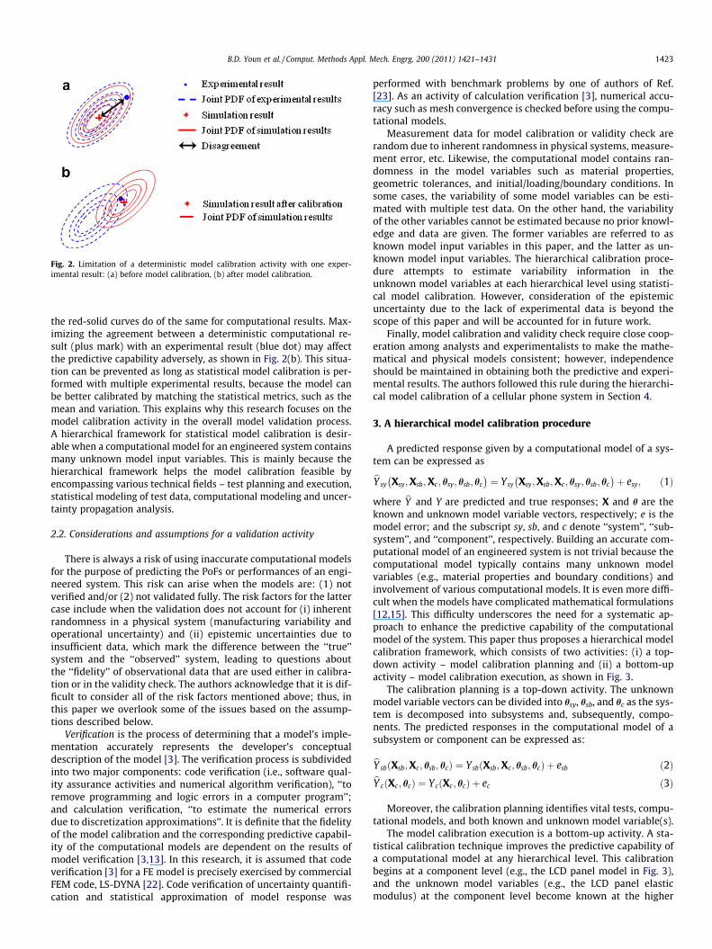
Fig. 2. Limitation of a deterministic model calibration activity with one exper-imental result: (a) before model calibration, (b) after model calibration.

B.D. Youn et al. / Comput. Methods Appl. Mech. Engrg. 200 (2011) 1421–1431 1423

the red-solid curves do of the same for computational results. Max-imizing the agreement between a deterministic computational re-sult (plus mark) with an experimental result (blue dot) may affectthe predictive capability adversely, as shown in Fig. 2(b). This situa-tion can be prevented as long as statistical model calibration is per-formed with multiple experimental results, because the model canbe better calibrated by matching the statistical metrics, such as themean and variation. This explains why this research focuses on themodel calibration activity in the overall model validation process.A hierarchical framework for statistical model calibration is desir-able when a computational model for an engineered system containsmany unknown model input variables. This is mainly because thehierarchical framework helps the model calibration feasible byencompassing various technical fields – test planning and execution,statistical modeling of test data, computational modeling and uncer-tainty propagation analysis.

2.2. Considerations and assumptions for a validation activity

There is always a risk of using inaccurate computational modelsfor the purpose of predicting the PoFs or performances of an engi-neered system. This risk can arise when the models are: (1) notverified and/or (2) not validated fully. The risk factors for the lattercase include when the validation does not account for (i) inherentrandomness in a physical system (manufacturing variability andoperational uncertainty) and (ii) epistemic uncertainties due toinsufficient data, which mark the difference between the ‘‘true’’system and the ‘‘observed’’ system, leading to questions aboutthe ‘‘fidelity’’ of observational data that are used either in calibra-tion or in the validity check. The authors acknowledge that it is dif-ficult to consider all of the risk factors mentioned above; thus, inthis paper we overlook some of the issues based on the assump-tions described below.

Verification is the process of determining that a model’s imple-mentation accurately represents the developer’s conceptualdescription of the model [3]. The verification process is subdividedinto two major components: code verification (i.e., software qual-ity assurance activities and numerical algorithm verification), ‘‘toremove programming and logic errors in a computer program’’;and calculation verification, ‘‘to estimate the numerical errorsdue to discretization approximations’’. It is definite that the fidelityof the model calibration and the corresponding predictive capabil-ity of the computational models are dependent on the results ofmodel verification [3,13]. In this research, it is assumed that codeverification [3] for a FE model is precisely exercised by commercialFEM code, LS-DYNA [22]. Code verification of uncertainty quantifi-cation and statistical approximation of model response was

performed with benchmark problems by one of authors of Ref.[23]. As an activity of calculation verification [3], numerical accu-racy such as mesh convergence is checked before using the compu-tational models.

Measurement data for model calibration or validity check arerandom due to inherent randomness in physical systems, measure-ment error, etc. Likewise, the computational model contains ran-domness in the model variables such as material properties,geometric tolerances, and initial/loading/boundary conditions. Insome cases, the variability of some model variables can be esti-mated with multiple test data. On the other hand, the variabilityof the other variables cannot be estimated because no prior knowl-edge and data are given. The former variables are referred to asknown model input variables in this paper, and the latter as un-known model input variables. The hierarchical calibration proce-dure attempts to estimate variability information in theunknown model variables at each hierarchical level using statisti-cal model calibration. However, consideration of the epistemicuncertainty due to the lack of experimental data is beyond thescope of this paper and will be accounted for in future work.

Finally, model calibration and validity check require close coop-eration among analysts and experimentalists to make the mathe-matical and physical models consistent; however, independenceshould be maintained in obtaining both the predictive and experi-mental results. The authors followed this rule during the hierarchi-cal model calibration of a cellular phone system in Section 4.

3. A hierarchical model calibration procedure

A predicted response given by a computational model of a sys-tem can be expressed asbY sy Xsy;Xsb;Xc; hsy; hsb; hc� �

¼ Ysy Xsy;Xsb;Xc; hsy; hsb; hc� �

þ esy; ð1Þ

where bY and Y are predicted and true responses; X and h are theknown and unknown model variable vectors, respectively; e is themodel error; and the subscript sy, sb, and c denote ‘‘system’’, ‘‘sub-system’’, and ‘‘component’’, respectively. Building an accurate com-putational model of an engineered system is not trivial because thecomputational model typically contains many unknown modelvariables (e.g., material properties and boundary conditions) andinvolvement of various computational models. It is even more diffi-cult when the models have complicated mathematical formulations[12,15]. This difficulty underscores the need for a systematic ap-proach to enhance the predictive capability of the computationalmodel of the system. This paper thus proposes a hierarchical modelcalibration framework, which consists of two activities: (i) a top-down activity – model calibration planning and (ii) a bottom-upactivity – model calibration execution, as shown in Fig. 3.

The calibration planning is a top-down activity. The unknownmodel variable vectors can be divided into hsy, hsb, and hc as the sys-tem is decomposed into subsystems and, subsequently, compo-nents. The predicted responses in the computational model of asubsystem or component can be expressed as:

bY sb Xsb;Xc; hsb; hcð Þ ¼ Ysb Xsb;Xc; hsb; hcð Þ þ esb ð2ÞbY c Xc; hcð Þ ¼ Yc Xc; hcð Þ þ ec ð3Þ

Moreover, the calibration planning identifies vital tests, compu-tational models, and both known and unknown model variable(s).

The model calibration execution is a bottom-up activity. A sta-tistical calibration technique improves the predictive capability ofa computational model at any hierarchical level. This calibrationbegins at a component level (e.g., the LCD panel model in Fig. 3),and the unknown model variables (e.g., the LCD panel elasticmodulus) at the component level become known at the higher

Fig. 3. Hierarchical model calibration activity of cellular phone system.

1424 B.D. Youn et al. / Comput. Methods Appl. Mech. Engrg. 200 (2011) 1421–1431

hierarchical levels (e.g., the LCD module and cellular phone systemin Fig. 3). The predictive capability of the computational modelscan recursively be enhanced as:

Component : bY c Xc; hcð Þ ¼ Yc Xc; hcð Þ þ ec

)statistical calibration

X�c ¼ Xc; hcalc

h iSubsystem : bY sb Xsb;X

�c ; hsb

� �¼ Ysb Xsb;X

�c ; hsb

� �þ esb

)statistical calibration

X�sb ¼ Xsb; hcalsb

h iSystem : bY sy Xsy;X

�c ;X

�sb; hsy

� �¼ Ysy Xsy;X

�c ;X

�sb; hsy

� �þ esy

)statistical calibration

X�sy ¼ Xsy; hcalsy

h ið4Þ

After the model calibration, an unknown variable vector, h, be-comes a known variable vector, hcal. The augmented parametervector X⁄ is introduced to simplify the notation as the computa-tional models at all levels are aggregated into a system. X⁄ indi-cates a new known random variable vector that includes X andhcal at a given hierarchical level. This statistical calibration tech-nique compares the observed test results with the predicted ones.A likelihood function is used for the comparison metric. In the sta-tistical calibration, an optimization technique is employed todetermine the unknown model variables of a computational modelin a statistical manner at any hierarchical level while maximizingthe likelihood function. The improved model in a lower hierarchi-cal level can then be fused into that at a higher hierarchical level,and the calibration execution continues for the model at the higherlevel. The authors acknowledge that it is difficult to assure the pre-dictive capability of an improved model without the assumptionthat the randomness in the true response (Y) primarily comes fromthe randomness in random model variables. For this reason, it ismandatory that the guidelines for the validation experiment ad-dressed in many well-known validation papers [1–3,6] should beaccompanied to reduce the measurement error and unexpectedexperimental error during the model calibration activities.

3.1. Model calibration planning (top-down)

The hierarchical model calibration process begins with modelcalibration planning, in which the three models of a system are de-fined as shown in Fig. 1: conceptual model, mathematical modeland computational model. The planning is composed of three pri-mary parts: (i) model decomposition planning, (ii) statistical model

calibration planning, and (iii) experiment planning for model vari-able characterization. The authors of this paper, representing bothindustry and academia, closely collaborated and shared expertisefor the calibration planning. This effort attempted to demonstratethe feasibility of the hierarchical model calibration with the cellu-lar phone model.

(i) Model decomposition planning: The model decomposition canbe planned based on ample understanding of the primary failuremechanisms (or PoIs) observed in a system (or top) level. Warrantyreports or customer surveys are important for better understand-ing the failure mechanisms. Such information helps identify vitalcomputational models, experimental tests, and modeling detailsat any hierarchical level.

We performed this study with a cellular phone system. Theobjective of this study is to develop a valid computational modelthat can be used to predict the reliability of a cellular phone systemagainst a dent test as shown in Fig. 4. The cellular phone systemhas two primary failure mechanisms related to the LCD module:LCD panel fracture and driver integrated circuit (IC) failure in theLCD module, as shown in Fig. 3. The computational models thatsimulate the LCD failure in the cellular phone system include sixunknown model variables (h), such as material properties andinterface conditions. To make the system model calibration afford-able, the computational model of the cellular phone system wasdecomposed into subsystem(s) and component(s). This decompo-sition planning was designed to isolate the failure mechanismsand identify unknown model variables along the system hierarchy.First, separation of the LCD module (subsystem) from the cellularphone (system) isolated the Driver IC failure mechanism. A dentfailure test (destructive testing) was performed to replicate thefailure in the module. The dent simulation model was developedwith LS-DYNA software [22], as shown in Fig. 5. Subsequently,the decomposition of the LCD panel (component) from the LCDmodule (subsystem) isolated the LCD panel failure mechanism. A3-point bending failure test (destructive testing) was designed toreplicate the LCD panel breakage. Correspondingly, the 3-pointbending simulation model was developed using an explicit methodin the LS-DYNA software, as shown in Fig. 6.

(ii) Statistical model calibration planning: As explained in Sec-tion 2, the ad hoc adjustment of model variables to enhance theagreement of computational model with experimental data maydegrade the predictive capability of the system model. Model cal-ibration must be carefully planned using expert opinion and a sen-sitivity study, which determine the most significant but unknown

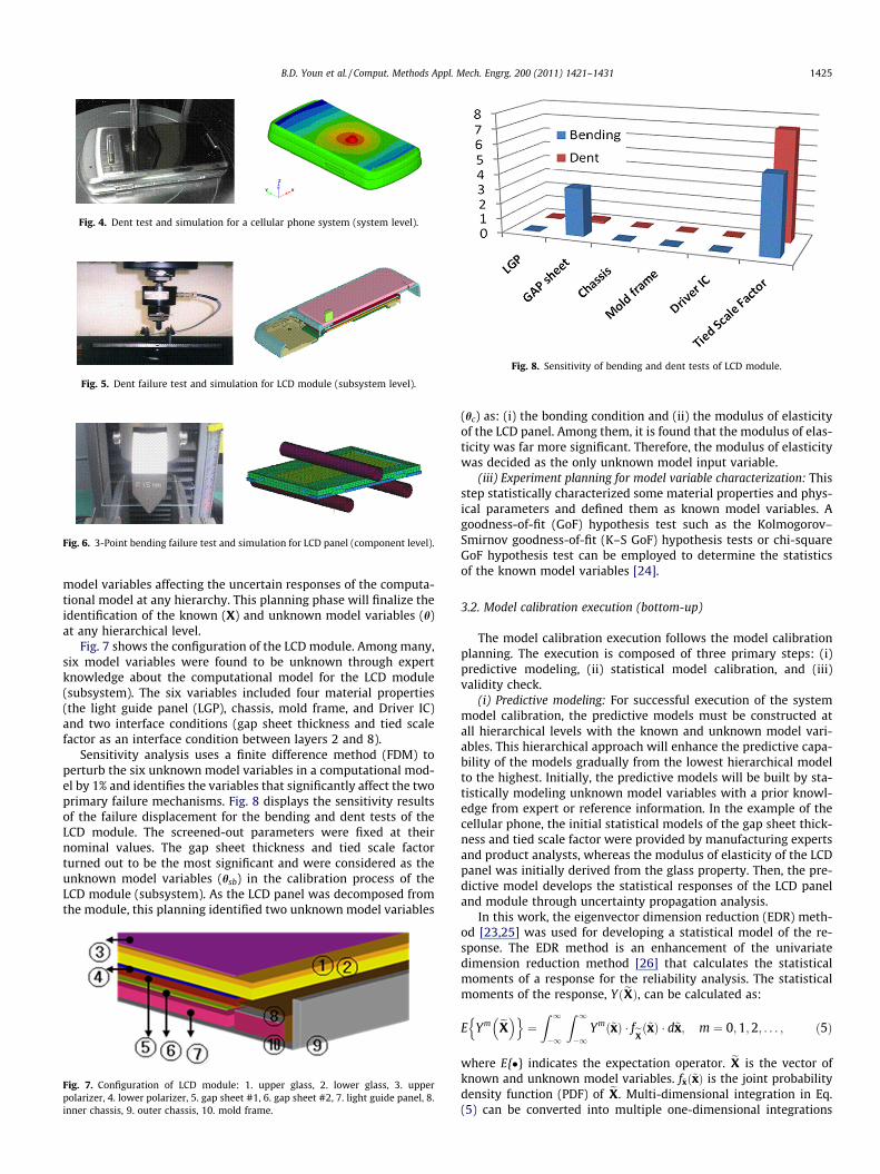
Fig. 4. Dent test and simulation for a cellular phone system (system level).

Fig. 5. Dent failure test and simulation for LCD module (subsystem level).

Fig. 6. 3-Point bending failure test and simulation for LCD panel (component level).

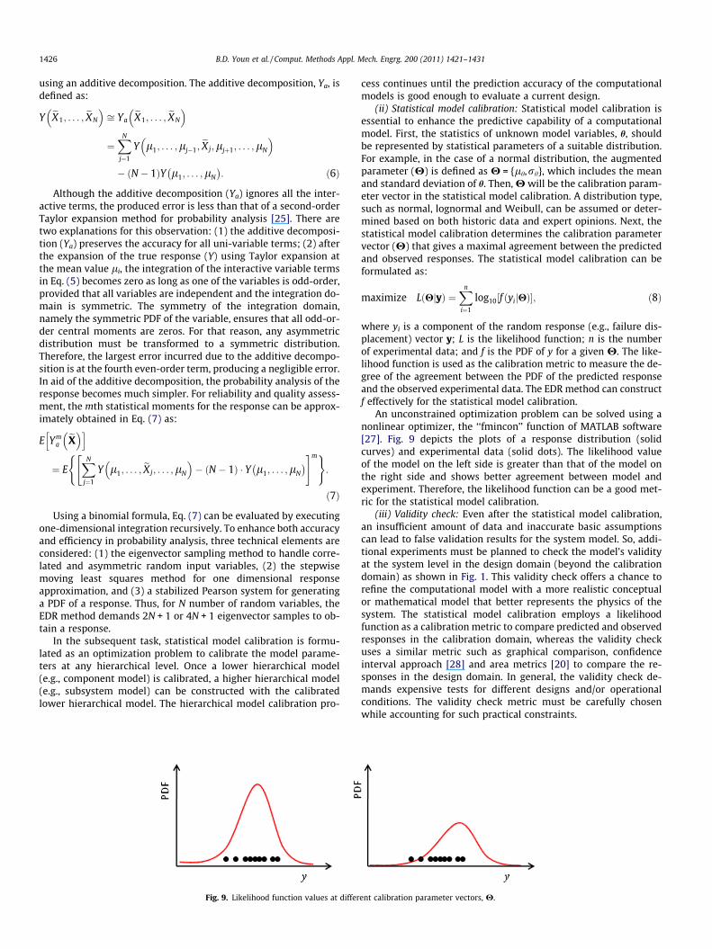
Fig. 8. Sensitivity of bending and dent tests of LCD module.

B.D. Youn et al. / Comput. Methods Appl. Mech. Engrg. 200 (2011) 1421–1431 1425

model variables affecting the uncertain responses of the computa-tional model at any hierarchy. This planning phase will finalize theidentification of the known (X) and unknown model variables (h)at any hierarchical level.

Fig. 7 shows the configuration of the LCD module. Among many,six model variables were found to be unknown through expertknowledge about the computational model for the LCD module(subsystem). The six variables included four material properties(the light guide panel (LGP), chassis, mold frame, and Driver IC)and two interface conditions (gap sheet thickness and tied scalefactor as an interface condition between layers 2 and 8).

Sensitivity analysis uses a finite difference method (FDM) toperturb the six unknown model variables in a computational mod-el by 1% and identifies the variables that significantly affect the twoprimary failure mechanisms. Fig. 8 displays the sensitivity resultsof the failure displacement for the bending and dent tests of theLCD module. The screened-out parameters were fixed at theirnominal values. The gap sheet thickness and tied scale factorturned out to be the most significant and were considered as theunknown model variables (hsb) in the calibration process of theLCD module (subsystem). As the LCD panel was decomposed fromthe module, this planning identified two unknown model variables

Fig. 7. Configuration of LCD module: 1. upper glass, 2. lower glass, 3. upperpolarizer, 4. lower polarizer, 5. gap sheet #1, 6. gap sheet #2, 7. light guide panel, 8.inner chassis, 9. outer chassis, 10. mold frame.

(hc) as: (i) the bonding condition and (ii) the modulus of elasticityof the LCD panel. Among them, it is found that the modulus of elas-ticity was far more significant. Therefore, the modulus of elasticitywas decided as the only unknown model input variable.

(iii) Experiment planning for model variable characterization: Thisstep statistically characterized some material properties and phys-ical parameters and defined them as known model variables. Agoodness-of-fit (GoF) hypothesis test such as the Kolmogorov–Smirnov goodness-of-fit (K–S GoF) hypothesis tests or chi-squareGoF hypothesis test can be employed to determine the statisticsof the known model variables [24].

3.2. Model calibration execution (bottom-up)

The model calibration execution follows the model calibrationplanning. The execution is composed of three primary steps: (i)predictive modeling, (ii) statistical model calibration, and (iii)validity check.

(i) Predictive modeling: For successful execution of the systemmodel calibration, the predictive models must be constructed atall hierarchical levels with the known and unknown model vari-ables. This hierarchical approach will enhance the predictive capa-bility of the models gradually from the lowest hierarchical modelto the highest. Initially, the predictive models will be built by sta-tistically modeling unknown model variables with a prior knowl-edge from expert or reference information. In the example of thecellular phone, the initial statistical models of the gap sheet thick-ness and tied scale factor were provided by manufacturing expertsand product analysts, whereas the modulus of elasticity of the LCDpanel was initially derived from the glass property. Then, the pre-dictive model develops the statistical responses of the LCD paneland module through uncertainty propagation analysis.

In this work, the eigenvector dimension reduction (EDR) meth-od [23,25] was used for developing a statistical model of the re-sponse. The EDR method is an enhancement of the univariatedimension reduction method [26] that calculates the statisticalmoments of a response for the reliability analysis. The statisticalmoments of the response, YðeXÞ, can be calculated as:

E Ym eX� �n o¼Z 1

�1

Z 1

�1Ym ~xð Þ � feX ~xð Þ � d~x; m ¼ 0;1;2; . . . ; ð5Þ

where E{�} indicates the expectation operator. eX is the vector ofknown and unknown model variables. f~xð~xÞ is the joint probabilitydensity function (PDF) of eX. Multi-dimensional integration in Eq.(5) can be converted into multiple one-dimensional integrations

1426 B.D. Youn et al. / Comput. Methods Appl. Mech. Engrg. 200 (2011) 1421–1431

using an additive decomposition. The additive decomposition, Ya, isdefined as:

Y eX1; . . . ; eXN

� �ffi Ya

eX1; . . . ; eXN

� �¼XN

j¼1

Y l1; . . . ;lj�1;eXj;ljþ1; . . . ;lN

� �� N � 1ð ÞY l1; . . . ;lN

� �: ð6Þ

Although the additive decomposition (Ya) ignores all the inter-active terms, the produced error is less than that of a second-orderTaylor expansion method for probability analysis [25]. There aretwo explanations for this observation: (1) the additive decomposi-tion (Ya) preserves the accuracy for all uni-variable terms; (2) afterthe expansion of the true response (Y) using Taylor expansion atthe mean value li, the integration of the interactive variable termsin Eq. (5) becomes zero as long as one of the variables is odd-order,provided that all variables are independent and the integration do-main is symmetric. The symmetry of the integration domain,namely the symmetric PDF of the variable, ensures that all odd-or-der central moments are zeros. For that reason, any asymmetricdistribution must be transformed to a symmetric distribution.Therefore, the largest error incurred due to the additive decompo-sition is at the fourth even-order term, producing a negligible error.In aid of the additive decomposition, the probability analysis of theresponse becomes much simpler. For reliability and quality assess-ment, the mth statistical moments for the response can be approx-imately obtained in Eq. (7) as:

E YmaeX� �h i

¼ EXN

j¼1

Y l1; . . . ; eXj; . . . ;lN

� �� ðN � 1Þ � Y l1; . . . ;lN

� �" #m( ):

ð7Þ

Using a binomial formula, Eq. (7) can be evaluated by executingone-dimensional integration recursively. To enhance both accuracyand efficiency in probability analysis, three technical elements areconsidered: (1) the eigenvector sampling method to handle corre-lated and asymmetric random input variables, (2) the stepwisemoving least squares method for one dimensional responseapproximation, and (3) a stabilized Pearson system for generatinga PDF of a response. Thus, for N number of random variables, theEDR method demands 2N + 1 or 4N + 1 eigenvector samples to ob-tain a response.

In the subsequent task, statistical model calibration is formu-lated as an optimization problem to calibrate the model parame-ters at any hierarchical level. Once a lower hierarchical model(e.g., component model) is calibrated, a higher hierarchical model(e.g., subsystem model) can be constructed with the calibratedlower hierarchical model. The hierarchical model calibration pro-

Fig. 9. Likelihood function values at differ

cess continues until the prediction accuracy of the computationalmodels is good enough to evaluate a current design.

(ii) Statistical model calibration: Statistical model calibration isessential to enhance the predictive capability of a computationalmodel. First, the statistics of unknown model variables, h, shouldbe represented by statistical parameters of a suitable distribution.For example, in the case of a normal distribution, the augmentedparameter (H) is defined as H = {lh,rh}, which includes the meanand standard deviation of h. Then, H will be the calibration param-eter vector in the statistical model calibration. A distribution type,such as normal, lognormal and Weibull, can be assumed or deter-mined based on both historic data and expert opinions. Next, thestatistical model calibration determines the calibration parametervector (H) that gives a maximal agreement between the predictedand observed responses. The statistical model calibration can beformulated as:

maximize L Hjyð Þ ¼Xn

i¼1

log10 f yijHð Þ½ �; ð8Þ

where yi is a component of the random response (e.g., failure dis-placement) vector y; L is the likelihood function; n is the numberof experimental data; and f is the PDF of y for a given H. The like-lihood function is used as the calibration metric to measure the de-gree of the agreement between the PDF of the predicted responseand the observed experimental data. The EDR method can constructf effectively for the statistical model calibration.

An unconstrained optimization problem can be solved using anonlinear optimizer, the ‘‘fmincon’’ function of MATLAB software[27]. Fig. 9 depicts the plots of a response distribution (solidcurves) and experimental data (solid dots). The likelihood valueof the model on the left side is greater than that of the model onthe right side and shows better agreement between model andexperiment. Therefore, the likelihood function can be a good met-ric for the statistical model calibration.

(iii) Validity check: Even after the statistical model calibration,an insufficient amount of data and inaccurate basic assumptionscan lead to false validation results for the system model. So, addi-tional experiments must be planned to check the model’s validityat the system level in the design domain (beyond the calibrationdomain) as shown in Fig. 1. This validity check offers a chance torefine the computational model with a more realistic conceptualor mathematical model that better represents the physics of thesystem. The statistical model calibration employs a likelihoodfunction as a calibration metric to compare predicted and observedresponses in the calibration domain, whereas the validity checkuses a similar metric such as graphical comparison, confidenceinterval approach [28] and area metrics [20] to compare the re-sponses in the design domain. In general, the validity check de-mands expensive tests for different designs and/or operationalconditions. The validity check metric must be carefully chosenwhile accounting for such practical constraints.

ent calibration parameter vectors, H.

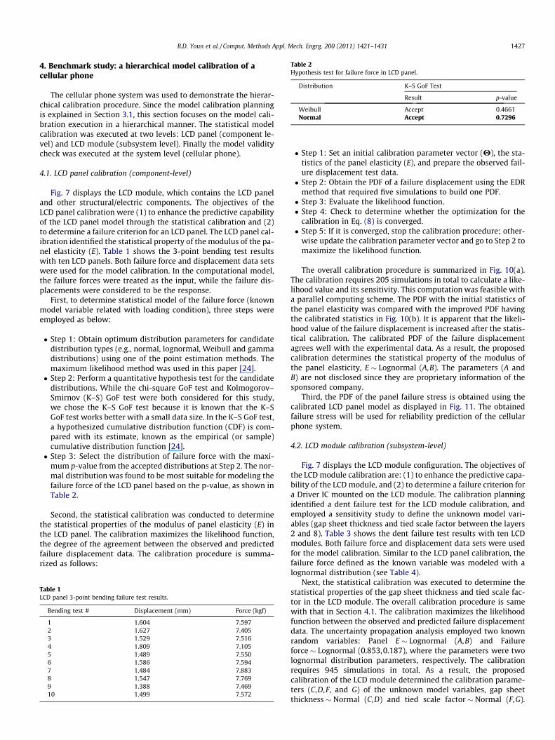
Table 2Hypothesis test for failure force in LCD panel.

Distribution K–S GoF Test

Result p-value

Weibull Accept 0.4661Normal Accept 0.7296

B.D. Youn et al. / Comput. Methods Appl. Mech. Engrg. 200 (2011) 1421–1431 1427

4. Benchmark study: a hierarchical model calibration of acellular phone

The cellular phone system was used to demonstrate the hierar-chical calibration procedure. Since the model calibration planningis explained in Section 3.1, this section focuses on the model cali-bration execution in a hierarchical manner. The statistical modelcalibration was executed at two levels: LCD panel (component le-vel) and LCD module (subsystem level). Finally the model validitycheck was executed at the system level (cellular phone).

4.1. LCD panel calibration (component-level)

Fig. 7 displays the LCD module, which contains the LCD paneland other structural/electric components. The objectives of theLCD panel calibration were (1) to enhance the predictive capabilityof the LCD panel model through the statistical calibration and (2)to determine a failure criterion for an LCD panel. The LCD panel cal-ibration identified the statistical property of the modulus of the pa-nel elasticity (E). Table 1 shows the 3-point bending test resultswith ten LCD panels. Both failure force and displacement data setswere used for the model calibration. In the computational model,the failure forces were treated as the input, while the failure dis-placements were considered to be the response.

First, to determine statistical model of the failure force (knownmodel variable related with loading condition), three steps wereemployed as below:

� Step 1: Obtain optimum distribution parameters for candidatedistribution types (e.g., normal, lognormal, Weibull and gammadistributions) using one of the point estimation methods. Themaximum likelihood method was used in this paper [24].� Step 2: Perform a quantitative hypothesis test for the candidate

distributions. While the chi-square GoF test and Kolmogorov–Smirnov (K–S) GoF test were both considered for this study,we chose the K–S GoF test because it is known that the K–SGoF test works better with a small data size. In the K–S GoF test,a hypothesized cumulative distribution function (CDF) is com-pared with its estimate, known as the empirical (or sample)cumulative distribution function [24].� Step 3: Select the distribution of failure force with the maxi-

mum p-value from the accepted distributions at Step 2. The nor-mal distribution was found to be most suitable for modeling thefailure force of the LCD panel based on the p-value, as shown inTable 2.

Second, the statistical calibration was conducted to determinethe statistical properties of the modulus of panel elasticity (E) inthe LCD panel. The calibration maximizes the likelihood function,the degree of the agreement between the observed and predictedfailure displacement data. The calibration procedure is summa-rized as follows:

Table 1LCD panel 3-point bending failure test results.

Bending test # Displacement (mm) Force (kgf)

1 1.604 7.5972 1.627 7.4053 1.529 7.5164 1.809 7.1055 1.489 7.5506 1.586 7.5947 1.484 7.8838 1.547 7.7699 1.388 7.46910 1.499 7.572

� Step 1: Set an initial calibration parameter vector (H), the sta-tistics of the panel elasticity (E), and prepare the observed fail-ure displacement test data.� Step 2: Obtain the PDF of a failure displacement using the EDR

method that required five simulations to build one PDF.� Step 3: Evaluate the likelihood function.� Step 4: Check to determine whether the optimization for the

calibration in Eq. (8) is converged.� Step 5: If it is converged, stop the calibration procedure; other-

wise update the calibration parameter vector and go to Step 2 tomaximize the likelihood function.

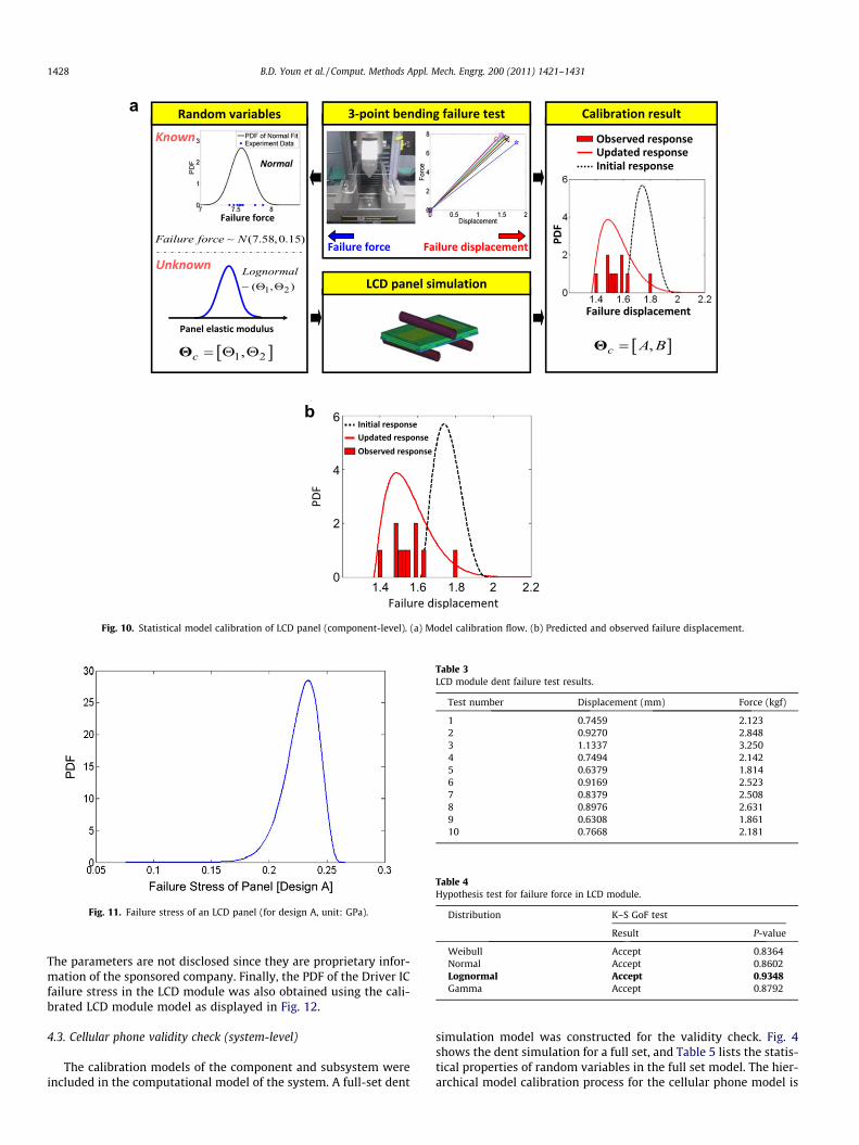
The overall calibration procedure is summarized in Fig. 10(a).The calibration requires 205 simulations in total to calculate a like-lihood value and its sensitivity. This computation was feasible witha parallel computing scheme. The PDF with the initial statistics ofthe panel elasticity was compared with the improved PDF havingthe calibrated statistics in Fig. 10(b). It is apparent that the likeli-hood value of the failure displacement is increased after the statis-tical calibration. The calibrated PDF of the failure displacementagrees well with the experimental data. As a result, the proposedcalibration determines the statistical property of the modulus ofthe panel elasticity, E � Lognormal (A,B). The parameters (A andB) are not disclosed since they are proprietary information of thesponsored company.

Third, the PDF of the panel failure stress is obtained using thecalibrated LCD panel model as displayed in Fig. 11. The obtainedfailure stress will be used for reliability prediction of the cellularphone system.

4.2. LCD module calibration (subsystem-level)

Fig. 7 displays the LCD module configuration. The objectives ofthe LCD module calibration are: (1) to enhance the predictive capa-bility of the LCD module, and (2) to determine a failure criterion fora Driver IC mounted on the LCD module. The calibration planningidentified a dent failure test for the LCD module calibration, andemployed a sensitivity study to define the unknown model vari-ables (gap sheet thickness and tied scale factor between the layers2 and 8). Table 3 shows the dent failure test results with ten LCDmodules. Both failure force and displacement data sets were usedfor the model calibration. Similar to the LCD panel calibration, thefailure force defined as the known variable was modeled with alognormal distribution (see Table 4).

Next, the statistical calibration was executed to determine thestatistical properties of the gap sheet thickness and tied scale fac-tor in the LCD module. The overall calibration procedure is samewith that in Section 4.1. The calibration maximizes the likelihoodfunction between the observed and predicted failure displacementdata. The uncertainty propagation analysis employed two knownrandom variables: Panel E � Lognormal (A,B) and Failureforce � Lognormal (0.853,0.187), where the parameters were twolognormal distribution parameters, respectively. The calibrationrequires 945 simulations in total. As a result, the proposedcalibration of the LCD module determined the calibration parame-ters (C,D,F, and G) of the unknown model variables, gap sheetthickness � Normal (C,D) and tied scale factor � Normal (F,G).

1.4 1.6 1.8 2 2.2

6

4

2

0

a

b

Fig. 10. Statistical model calibration of LCD panel (component-level). (a) Model calibration flow. (b) Predicted and observed failure displacement.

Fig. 11. Failure stress of an LCD panel (for design A, unit: GPa).

Table 3LCD module dent failure test results.

Test number Displacement (mm) Force (kgf)

1 0.7459 2.1232 0.9270 2.8483 1.1337 3.2504 0.7494 2.1425 0.6379 1.8146 0.9169 2.5237 0.8379 2.5088 0.8976 2.6319 0.6308 1.86110 0.7668 2.181

Table 4Hypothesis test for failure force in LCD module.

Distribution K–S GoF test

Result P-value

Weibull Accept 0.8364Normal Accept 0.8602Lognormal Accept 0.9348Gamma Accept 0.8792

1428 B.D. Youn et al. / Comput. Methods Appl. Mech. Engrg. 200 (2011) 1421–1431

The parameters are not disclosed since they are proprietary infor-mation of the sponsored company. Finally, the PDF of the Driver ICfailure stress in the LCD module was also obtained using the cali-brated LCD module model as displayed in Fig. 12.

4.3. Cellular phone validity check (system-level)

The calibration models of the component and subsystem wereincluded in the computational model of the system. A full-set dent

simulation model was constructed for the validity check. Fig. 4shows the dent simulation for a full set, and Table 5 lists the statis-tical properties of random variables in the full set model. The hier-archical model calibration process for the cellular phone model is

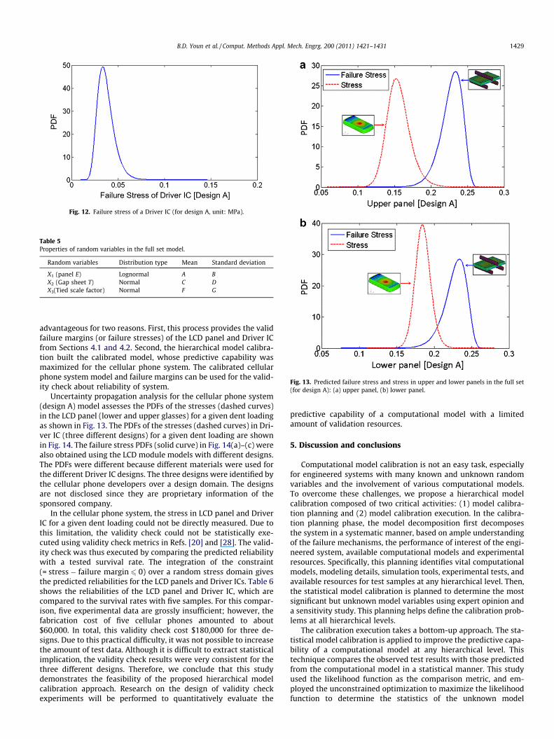
Fig. 12. Failure stress of a Driver IC (for design A, unit: MPa).

Table 5Properties of random variables in the full set model.

Random variables Distribution type Mean Standard deviation

X1 (panel E) Lognormal A BX2 (Gap sheet T) Normal C DX3(Tied scale factor) Normal F G

Fig. 13. Predicted failure stress and stress in upper and lower panels in the full set(for design A): (a) upper panel, (b) lower panel.

B.D. Youn et al. / Comput. Methods Appl. Mech. Engrg. 200 (2011) 1421–1431 1429

advantageous for two reasons. First, this process provides the validfailure margins (or failure stresses) of the LCD panel and Driver ICfrom Sections 4.1 and 4.2. Second, the hierarchical model calibra-tion built the calibrated model, whose predictive capability wasmaximized for the cellular phone system. The calibrated cellularphone system model and failure margins can be used for the valid-ity check about reliability of system.

Uncertainty propagation analysis for the cellular phone system(design A) model assesses the PDFs of the stresses (dashed curves)in the LCD panel (lower and upper glasses) for a given dent loadingas shown in Fig. 13. The PDFs of the stresses (dashed curves) in Dri-ver IC (three different designs) for a given dent loading are shownin Fig. 14. The failure stress PDFs (solid curve) in Fig. 14(a)–(c) werealso obtained using the LCD module models with different designs.The PDFs were different because different materials were used forthe different Driver IC designs. The three designs were identified bythe cellular phone developers over a design domain. The designsare not disclosed since they are proprietary information of thesponsored company.

In the cellular phone system, the stress in LCD panel and DriverIC for a given dent loading could not be directly measured. Due tothis limitation, the validity check could not be statistically exe-cuted using validity check metrics in Refs. [20] and [28]. The valid-ity check was thus executed by comparing the predicted reliabilitywith a tested survival rate. The integration of the constraint(= stress � failure margin 6 0) over a random stress domain givesthe predicted reliabilities for the LCD panels and Driver ICs. Table 6shows the reliabilities of the LCD panel and Driver IC, which arecompared to the survival rates with five samples. For this compar-ison, five experimental data are grossly insufficient; however, thefabrication cost of five cellular phones amounted to about$60,000. In total, this validity check cost $180,000 for three de-signs. Due to this practical difficulty, it was not possible to increasethe amount of test data. Although it is difficult to extract statisticalimplication, the validity check results were very consistent for thethree different designs. Therefore, we conclude that this studydemonstrates the feasibility of the proposed hierarchical modelcalibration approach. Research on the design of validity checkexperiments will be performed to quantitatively evaluate the

predictive capability of a computational model with a limitedamount of validation resources.

5. Discussion and conclusions

Computational model calibration is not an easy task, especiallyfor engineered systems with many known and unknown randomvariables and the involvement of various computational models.To overcome these challenges, we propose a hierarchical modelcalibration composed of two critical activities: (1) model calibra-tion planning and (2) model calibration execution. In the calibra-tion planning phase, the model decomposition first decomposesthe system in a systematic manner, based on ample understandingof the failure mechanisms, the performance of interest of the engi-neered system, available computational models and experimentalresources. Specifically, this planning identifies vital computationalmodels, modeling details, simulation tools, experimental tests, andavailable resources for test samples at any hierarchical level. Then,the statistical model calibration is planned to determine the mostsignificant but unknown model variables using expert opinion anda sensitivity study. This planning helps define the calibration prob-lems at all hierarchical levels.

The calibration execution takes a bottom-up approach. The sta-tistical model calibration is applied to improve the predictive capa-bility of a computational model at any hierarchical level. Thistechnique compares the observed test results with those predictedfrom the computational model in a statistical manner. This studyused the likelihood function as the comparison metric, and em-ployed the unconstrained optimization to maximize the likelihoodfunction to determine the statistics of the unknown model

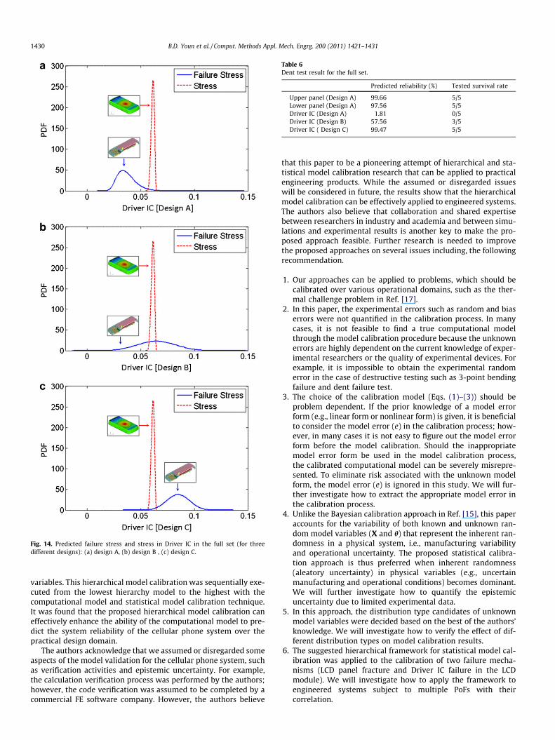
Fig. 14. Predicted failure stress and stress in Driver IC in the full set (for threedifferent designs): (a) design A, (b) design B , (c) design C.

Table 6Dent test result for the full set.

Predicted reliability (%) Tested survival rate

Upper panel (Design A) 99.66 5/5Lower panel (Design A) 97.56 5/5Driver IC (Design A) 1.81 0/5Driver IC (Design B) 57.56 3/5Driver IC ( Design C) 99.47 5/5

1430 B.D. Youn et al. / Comput. Methods Appl. Mech. Engrg. 200 (2011) 1421–1431

variables. This hierarchical model calibration was sequentially exe-cuted from the lowest hierarchy model to the highest with thecomputational model and statistical model calibration technique.It was found that the proposed hierarchical model calibration caneffectively enhance the ability of the computational model to pre-dict the system reliability of the cellular phone system over thepractical design domain.

The authors acknowledge that we assumed or disregarded someaspects of the model validation for the cellular phone system, suchas verification activities and epistemic uncertainty. For example,the calculation verification process was performed by the authors;however, the code verification was assumed to be completed by acommercial FE software company. However, the authors believe

that this paper to be a pioneering attempt of hierarchical and sta-tistical model calibration research that can be applied to practicalengineering products. While the assumed or disregarded issueswill be considered in future, the results show that the hierarchicalmodel calibration can be effectively applied to engineered systems.The authors also believe that collaboration and shared expertisebetween researchers in industry and academia and between simu-lations and experimental results is another key to make the pro-posed approach feasible. Further research is needed to improvethe proposed approaches on several issues including, the followingrecommendation.

1. Our approaches can be applied to problems, which should becalibrated over various operational domains, such as the ther-mal challenge problem in Ref. [17].

2. In this paper, the experimental errors such as random and biaserrors were not quantified in the calibration process. In manycases, it is not feasible to find a true computational modelthrough the model calibration procedure because the unknownerrors are highly dependent on the current knowledge of exper-imental researchers or the quality of experimental devices. Forexample, it is impossible to obtain the experimental randomerror in the case of destructive testing such as 3-point bendingfailure and dent failure test.

3. The choice of the calibration model (Eqs. (1)–(3)) should beproblem dependent. If the prior knowledge of a model errorform (e.g., linear form or nonlinear form) is given, it is beneficialto consider the model error (e) in the calibration process; how-ever, in many cases it is not easy to figure out the model errorform before the model calibration. Should the inappropriatemodel error form be used in the model calibration process,the calibrated computational model can be severely misrepre-sented. To eliminate risk associated with the unknown modelform, the model error (e) is ignored in this study. We will fur-ther investigate how to extract the appropriate model error inthe calibration process.

4. Unlike the Bayesian calibration approach in Ref. [15], this paperaccounts for the variability of both known and unknown ran-dom model variables (X and h) that represent the inherent ran-domness in a physical system, i.e., manufacturing variabilityand operational uncertainty. The proposed statistical calibra-tion approach is thus preferred when inherent randomness(aleatory uncertainty) in physical variables (e.g., uncertainmanufacturing and operational conditions) becomes dominant.We will further investigate how to quantify the epistemicuncertainty due to limited experimental data.

5. In this approach, the distribution type candidates of unknownmodel variables were decided based on the best of the authors’knowledge. We will investigate how to verify the effect of dif-ferent distribution types on model calibration results.

6. The suggested hierarchical framework for statistical model cal-ibration was applied to the calibration of two failure mecha-nisms (LCD panel fracture and Driver IC failure in the LCDmodule). We will investigate how to apply the framework toengineered systems subject to multiple PoFs with theircorrelation.

B.D. Youn et al. / Comput. Methods Appl. Mech. Engrg. 200 (2011) 1421–1431 1431

7. The authors will also investigate the situation in which ‘‘compo-nent’’ and ‘‘subsystem’’ data are available but ‘‘system’’ data arenot, or vice versa.

Acknowledgements

The authors would like to acknowledge that this research is par-tially supported by LG Electronics Gift Fund and US National Sci-ence Foundation (NSF) under Grant No. GOALI-0729424.

References

[1] W.L. Oberkampf, T.G. Trucano, Verification and validation in computationalfluid dynamics, Prog. Aerospace Sci. 38 (3) (2002) 209–272.

[2] W.L. Oberkampf, T.G. Trucano, C. Hirsch, Verification, validation, and predictivecapability in computational engineering and physics, Appl. Mech. Rev. 57 (5)(2004) 345–384.

[3] B.H. Thacker, S.W. Doebling, F.M. Hemez, M.C. Anderson, J.E. Pepin, E.A.Rodriguez, Concepts of model verification and validation, LA-14167, LosAlamos National Laboratory, Los Alamos, 2004.

[4] I. Babuska, J.T. Oden, Verification and validation in computational engineeringand science: basic concepts, Comput. Methods Appl. Mech. Engrg. 193 (36–38)(2004) 4057–4066.

[5] AIAA, P.T.C., Guide for the verification and validation of computational fluiddynamic simulations, AIAA Guide G-077-98, 1998.

[6] ASME, P.T.C., Guide for verification and validation in computational solidmechanics, ASME, New York, 2006.

[7] B.H. Thacker, M.C. Anderson, P.E. Senseny, E.A. Rodriguez, The role ofnondeterminism in model verification and validation, Int. J. Mater. Prod.Technol. 25 (1) (2006) 144–163.

[8] R.G. Hill, T.G. Trucano, Statistical validation of engineering andscientific models: background, SAND99-1256, Sandia National Laboratories,1999.

[9] D. Higdon, C. Nakhleh, J. Gattiker, B. Williams, A Bayesian calibration approachto the thermal problem, Comput. Methods Appl. Mech. Engrg. 197 (29–32)(2008) 2431–2441.

[10] F. Liu, M.J. Bayarri, J.O. Berger, R. Paulo, J. Sacks, A Bayesian analysis of thethermal challenge problem, Comput. Methods Appl. Mech. Engrg. 197 (29–32)(2008) 2457–2466.

[11] J. McFarland, S. Mahadevan, Multivariate significance testing and modelcalibration under uncertainty, Comput. Methods Appl. Mech. Engrg. 197 (29-32) (2008) 2467–2479.

[12] Y. Xiong, W. Chen, K. Tsui, D.W. Apley, A better understanding of modelupdating strategies in validating engineering models, Comput. Methods Appl.Mech. Engrg. 198 (15–16) (2009) 1327–1337.

[13] T.G. Trucano, L.P. Swiler, T. Igusa, W.L. Oberkampf, M. Pilch, Calibration,validation, and sensitivity analysis: what’s what, Reliab. Engrg. Syst. Safe. 91(10–11) (2006) 1331–1357.

[14] K. Campbell, Statistical calibration of computer simulations, Reliab. Engrg.Syst. Safe. 91 (10–11) (2006) 1358–1363.

[15] M.C. Kennedy, A. O’Hagan, Bayesian calibration of computer models, J. R. Stat.Soc. B 63 (3) (2002) 425–464.

[16] W. Chen, K. Tsui, S. Wang, A design-driven validation approach using Bayesianprediction models, J. Mech. Des. 140 (2) (2008) 021101.

[17] K.J. Dowding, M. Pilch, R.G. Hills, Formulation of the thermal problem, Comput.Methods Appl. Mech. Engrg. 197 (29–32) (2008) 2385–2389.

[18] B.M. Rutherford, Computational modeling issues and methods for the‘‘regulatory problem’’ in engineering – Solution to the thermal problem,Comput. Methods Appl. Mech. Engrg. 197 (29–32) (2008) 2480–2489.

[19] R.G. Hill, K.J. Dowding, Multivariate approach to the thermal challengeproblem, Comput. Methods Appl. Mech. Engrg. 197 (29–32) (2008) 2442–2456.

[20] S. Ferson, W.L. Oberkampf, L. Ginzburg, Model validation and predictivecapability for the thermal challenge problem, Comput. Methods Appl. Mech.Engrg. 197 (29–32) (2008) 2408–2430.

[21] M.D. Brandyberry, Thermal problem solution using a surrogate modelclustering technique, Comput. Methods Appl. Mech. Engrg. 197 (29–32)(2008) 2390–2407.

[22] F. Pan, J. Zhu, A.O. Helminen, R. Vatanparast, Three point bending analysis of amobile phone using LS-DYNA explicit integration method, in: 9th InternationalLS-DYNA Users Conference, June 4–6, Dearborn, MI, USA, 2006.

[23] B.D. Youn, X. Zhimin, P. Wang, The eigenvector dimension reduction (EDR)method for sensitivity-free uncertainty quantification, Struct. Multidiscip.Optim. 37 (1) (2008) 13–28.

[24] M. Modarres, M. Kaminskiy, V. Krivtsov, Reliability Engineering and RiskAnalysis: A Practical Guide, CRC Press, New York, 1999.

[25] B.D. Youn, P. Wang, Bayesian reliability-based design optimization usingeigenvector dimension reduction (EDR) method, Struct. Multidiscip. Optim. 36(2) (2008) 107–123.

[26] S. Rahman, H. Xu, A univariate dimension-reduction method for multi-dimensional integration in stochastic mechanics, Probabilist. Engrg. Mech. 19(4) (2004) 393–408.

[27] Matlab Help Documentation, Matlab 7.5 (R2007b), Optimization Toolbox.[28] T. Buranathiti, J. Cao, W. Chen, L. Baghdasaryan, Z.C. Xia, Approaches for model

validation: Methodology and illustration on a sheet metal flanging process, J.Manuf. Sci. Engrg. 128 (2) (2006) 588.

B.D. Youn is an assistant professor in the School of Mechanical and AerospaceEngineering at Seoul National University. He received his B.S. degree in mechanicalengineering from Inha University, his M.S. degree in mechanical engineering fromKAIST, Korea and his Ph.D. from the University of Iowa, USA. He is the two-timewinner of the Best Paper Award from ASME International Design EngineeringTechnical Conference (IDETC) in 2001 and 2008. His research interests includecomputer model verification and validation, prognostics and health management,reliability analysis and reliability-based design, and energy harvester design.

Byung C. Jung received his B.S. in mechanical engineering from Hanyang Univer-sity, his M.S. degree in mechanical engineering from KAIST, Korea, in 2002 and2004, respectively. He is currently pursuing his Ph.D. in mechanical engineeringfrom the University of Maryland at College Park. His research interests are verifi-cation and validation of computer models in a statistical manner and design of asustainable energy harvester for wireless sensors.

Zhimin Xi received his B.S. and M.S. degree in mechanical engineering from BeijingUniversity of Science and Technology in 2001 and 2004, respectively. He is the one-time winner of the Best Paper Award from ASME International Design EngineeringTechnical Conference (IDETC) in 2008. He is currently pursuing his Ph.D. inmechanical engineering from the University of Maryland at College Park. Hisresearch interests are reliability analysis and reliability-based design optimization.

Sangbum Kim received M.S. and Ph.D. degrees in mechanical engineering fromKang-won National University, Korea, in 1998 and 2002, respectively. He is cur-rently working as a chief engineer in the Design Research Group at ProductionResearch Institute, LG Electronics, Korea. His current researches include shock/impact analysis and optimized design of electronic products, especially for mobilehand set and flat panel TV. Before joining LG Electronics in 2006, he had experi-enced and managed in the area of automotive crashworthiness, human modeling,and occupant safety at ESI, Korea.

Wook-Ryun Lee received his M.S. degree in mechanical engineering from Chung-nam National University in 2004 and his B.S. degree from Yonsei University in 1997.He is currently a senior researcher in the Power Generation Laboratory of theResearch Institute in the Korea Electric Power Corporation, Daejeon, Korea. Hisresearch interests are control of noise and vibration generated from power plants,and electrical energy storage using superconducting flywheels.