


Bahasa
Halaman
Hukum


Al-Manaseer, Akthem Adbulkarim (1983) A nonlinear finite element study of reinforced concrete beams. PhD thesis. http://theses.gla.ac.uk/1491/ Copyright and moral rights for this thesis are retained by the author A copy can be downloaded for personal non-commercial research or study, without prior permission or charge This thesis cannot be reproduced or quoted extensively from without first obtaining permission in writing from the Author The content must not be changed in any way or sold commercially in any format or medium without the formal permission of the Author When referring to this work, full bibliographic details including the author, title, awarding institution and date of the thesis must be given
Glasgow Theses Service http://theses.gla.ac.uk/
A NONLINEAR FINITE ELEMENT STUDY
OF REINFORCED CONCRETE BEAMS
by
Akthem AbdulkarimL:! ýl-Manaseer, B. Sc.
A thesis submitted for the degree of
Doctor of Philosophy
Department of Civil Engineering
University of Glasgow
August, 1983

TO
Ymj Parents
and
my Teachers

iii
ACKNOWLEDGMENTS
The work described in this thesis was carried out in the
Department of Civil Engineering at the University of Glasgow under
the general direction of Professor A. Coull whose help and interest
is gratefully acknowledged.
I wish to express my indebtedness to my supervisor, Dr. D. V.
Phillips for his valuable guidance, advice and constant encouragement
throughout the work.
Many thanks are due to:
Professor H. B. Sutherland whose help was most appreciated.
Dr. P. Bhatt and Dr. D. R. Green for their interest and useful
discussions.
The computer staff of the Civil Engineering Department, especially
Miss A. MacKinnon, Miss C. John and Mrs. A. McVey for their advice
and help.
The staff members of Glasgow University Computing Service in particular
Dr. W. Sharp and Mrs. D. Worster for their help in some matters
relating to programming.
Many friends whose help and advice will never be forgotten.
Mrs. L. Williamson for her efficient typing.
Finally, my thanks are reserved for my family for their boundless
patience, continual encouragement and financial support throughout the
years.
iv SU14NMY
This thesis describes the development of plane stress, nonlinear
finite element method of analysis for reinforced concrete beams. These
include simple, deep, and T-beams, failing in flexure and in shear.
The nonlinear response is assumed to be caused by concrete cracking,
nonlinear biaxial stress-strain relations, and by the yielding of steel
reinforcement.
The smeared crack approach was used with two models for post
cracking behaviour, one with a tension stiffening effect and the other
with no-tension stiffening. The endochronic theory with some adaptations
was used to account for all other uncracked zones.
8-noded isoparametric elements were used for concrete represen-
tation and 3-noded isoparametric elements for steel. A modified Newton-
Raphson approach, was used for solving the nonlinear problem with both
the constant and variable stiffness methods. This was based on the
evaluation of a tangential elasticity matrix. The unbalanced nodal
forces were obtained by the method of residual forces and convergence
was checked using either a force or a displacement criteria.
A nonlinear finite element program was developed where all the
required aspects to model the reinforced concrete structures were
included. It was a main contention of this work that the nonlinear
solution parameters had such an important influence on the solution
process that an extensive study was required to determine their effects.
This was carried out on simple and complex beams, and Suitable guide
lines were established. In particular tension stiffening effects were
investigated and rejected in favour of a method with no-tension

V
stiffening used in conjunction with controls on other solution parameters,
Other parameters such as order of Gauss rule, shear retention factor,
convergence tolerance, etc. were also studied in detail.
An investigation into the behaviour of a range of deep beams
including perforated deep beams and beams which were heavily reinforced,
was undertaken. These beams failed both in shear and flexure. In
most cases crack pattern, stress distribution, and load deflection
curves were used to validate, (or otherwise), the performance of the
proposed models and program.
Finally a method is proposed for analysing T-beams using plane
stress elements where the flange is treated separately and is connected
to the veb by a fictitious element. Other approximations are introduced
in order to treat the problem as a two dimensional structure.

C0NTENTS Page No.
ACKNOWLEDGEMENTS iii
SUMMARY iv
CONTENTS vi
NOTATION x
CHAPTER 1- INTRODUCTION
1.1 General
1.2 Scope and purpose
CHAPTER 2- FINITE ELEMENT FORMULATION
2.1 Introduction 9
2.2 Basic steps in the finite element method 11
2.2.1 Selection of element type and
discretization of the continuum 11
2.2.2 Shape functions 15
2.2.3 Element properties 15
2.2.4 Assembly of element properties 16 2.2.5 Solution of the system of equations 17
2.2.6 Final calculation 17
2.3 Isoparametric elements 18 2.3.1 Introduction 18 2.3.2 Isoparametric 8-noded strain element 20
2.3.3 Isoparametric 3-noded strain element (bar element) 25
2.3.4 Numerical integration 28
CHAPTER 3- NONLINEAR METHOD'OF SOLUTION 3.1 Introduction 38
3.2 Numerical Techniques for Nonlinear Analysis 42
3.2.1 Basic formulation 42
3.2.2 Incremental method 43
3.2.3 Iteration method 44
3.2.4 Mixed method 48
3.3 Comparison of Basic Methods 48
3.4 Method used in this Work 49
vii
Page No.
3.5 Convergence Criteria 50
3.5.1 Force convergence criterion 50
3.5.2 Displacement convergence criteria 51
3.5.3 General discussion on convergence criteria 52
3.6 Basic Steps in the Nonlinear Method Used 53
3.7 Frontal Equation Solving Routine 55
CHAPTER 4- REVIEW OF CONCRETE AND STEEL BEHAVIOUR AND ITS
PREVIOUS MODELLING
4.1 Introduction 62
4.2 Mathematical description of the behaviour of
reinforced concrete 63
4.2.1 The behaviour of concrete 63
4.2.2 Modelling steel reinforcement 68
4.2.3 The bond-slip phenomenon between steel and
concrete 68
4.3 Mechanical behaviour of concrete under different
states of loading 70
4.3.1 Uniaxial stress behaviour 71
4.3.2 Biaxial. stress behaviour 74
4.3.3 Triaxial stress behaviour 77
4.3.4 Definition of dilatation of concrete 78
4.3.5 Hydrostatic pressure sensitivity 78
4.3.6 Shear across cracks 79
4.4 Mechanical behaviour of steel 80
4.4.1 Brief description of steel behaviour 8o
4.4.2 Bond-slip and dowel action 81
4.5 General conclusions 82
CHAPTER 5- MATHEMATICAL MODELLING OF THE CONSTITUTIVE
LAWS FOR REINFORCED CONCRETE
5.1 Introduction 103
5.2 The endochronic model 105
5.2.1 Historical review 105
5.2.2 Basic assumption of the endochronic theory 107
5.2.3 Application to metals 110

viii
Page No
5.2.4 Application to concrete ill
5.2.5 Summary of the equations of the endochronic
theory 117 5.2.6 Numerical procedure for applying the
endochronic theory 119
5.2.7 Stress-strain curves obtained using the
endochronic model 123
5.3 The cracking model 124
5.3.1 Procedure for the first cracking model 126
5.3.2 Procedure for the second cracking model 130 5.4 The uniaxial-compression model 135 5.5 The crushing model 136
5.6 Theoretical model for steel 137
CHAPTER 6- NUMERICAL STUDY OF VARIOUS PARAMETERS AFFECTING
NONLINEAR SOLUTIONS
6.1 Introduction 156 6.2 Description of the deep beam used in the
numerical study 158 6.3 Parameters affecting the number of iterations and
the convergence rate 159 6.3.1 Load criterion 162 6.3.2 Displacement criteria 166 6.3.3 Discussion on load and displacement criteria 168
6.4 Constant and variable stiffness methods 169 6.5 Gauss rule 173 6.6 Shear retention factor 177 6.7 Tension stiffening 18o 6.8 Conclusions 186 6.9 Burns & Siess shallow beam J-4 188
CHAPTER 7- APPLICATION TO DEEP BEAMS
7.1 Introduction 260
7.2 Solid deep beams 262
7.2.1 General review 262
7.2.2 Cervenka panel wall W-2 266

ix
Page No. 7.2.3 Lin deep beams 101 and 102 268 7.2.4 Lin deep beam 204 271
7.3 Deep beams with openings 277 7.3.1 General review 277 7.3.2 Memon deep beam B-5 280 7.3.3 Memon deep beam B-7 282
7.4 Conclusions 285
CHAPTER 8- APPLICATION TO T-BEAMS
8.1 Introduction 351 8.2 General description of T-beams behaviour 352 8.3 Proposed theoretical model 354 8.4 Selection of axis of separation 357 8.5 Description of beans tested 358 8.6 Description of results 359 8.7 Conclusions 367
CHAPTER 9- CONCLUSIONS AND RECOMMENDATIONS
9.1 General observations and conlcusions 403
9.2 Reco=endations for future work 4o8
APPENDIX A Equations of Endochronic theory for concrete 411
APPENDIX B Brief description of the program ' 415

x
NOTATION
Major symbols used in the text are listed below, others are defined
as they first appear. Some symbols have different meanings in different
contexts; these are clearly defined.
General svmbols:
{)I{IT Curly brackets denote column and row vectors
E3 ]T Square brackets denote rectangular matrices
In both cases T over the brackets denotes the
transpose;
-1 over square matrices denotes the inverse
Straight brackets denote the absolute value
det Denotes the determinant of a square matrix
Scalars:
A Cross sectional area of steel s dA Elementary area
dv Elementary volume
E Modulus of elasticity for concrete C E Modulus of elasticity for steel s E Strain hardening modulus for steel w fl Uniaxial compressive strength of concrete C
f Cube' strength of concrete cu f Stress in steel s ft t Tensile strength of concrete
f Yield stress of steel y G, G Shear modulus 0
hf Height of flange for a T-beam
119 129 13 First, second and third invariants of the symbol
that follows in parenthesis
J2 Second invariant of the deviator of the symbol
that follows in parenthesis
K, K Bulk modulus

Pe Strain energy of an element e
Pi, Pi(&%n) Pi(&) Shape functions
Pý Norm of the total applied load I
Qs Computed ultimate load
t Thickness of an element; time
tf Thickness of flange for a T-beam
U i"i Component of displacement at node i
U, v Component of displacement in x, y
X Distance from the outer side of a flange in a
T-beam
x9y Global cartesian coordinates in planer problems
X*, Y* Principal axes
w Imposed potential energy due to external load
w Measured ultimate load U
z* z, zt, z Intrinsic time parameters 0
a Aggregate interlocking factor
C, C, Damage parameters
XIVIX Dilatation parameters 0 41E, Distortion parameters
n't Normalized local curvilinear coordinates'
E Strain
Cc Concrete strain
El Uniaxial. cracking strain of concrete c
e Uniaxial. crushing strain-of concrete cu
C Mean strain
es Steel strain
C Volumetric strain v
C xx, C Yx Strain components in global directions Y yy
C1, C29C3 Principal strains
xi

xii
VVc Poisson's ratio for concrete
Cr Stress vector
a Stress in concrete c
a Mean stress M
a Steel stress s
a xx
a yy 'T XY
Stress component in global directions
ay Yield stress of steel
Glsa2la3 Principal stresses
Cr maxila med2omin
I
Vectors and Matrices:
EB] ,
[B ý Strain matrix [DI
, [D
CI Elasticity matri)(
{Fje Nodal forces at nodes of an element e
{, je Nodal forces vector due to initial strains C 0
{F) Nodal forces vector due to initial stress 0
{Fj Nodal forces vector due to distributed load per p
unit volume
{Fj Nodal forces vector due to boundary pressure 9
{Fj Nodal forces vector due to external load
{F B Nodal forces vector for steel bars
{F u
Unbalanced nodal forces vector
{g) Components of boundary pressure
[ij Jacobian matrix rirl
LN 9 rK " UI-0 I,
[K-1 Overall stiffness matrix
[K Ie ,
EKBI Element stiffness matrix

xiii
{P Vector of total applied load
{P Vector of distributed load per unit volume
{R Rj- Vector of total imposed load LA
[R ] Rotation matrix
{61 Overall displacement vector
{6 B) 1{6 )i9{61
U Nodal displacements
{6 e Nodal displacements associated with element e
0 )i Vector of residual nodal forces
{01' {aln Total stress vector
{a 1 Initial stress vector
{a B1 Stress vector for bar element p {a 'n Inelastic stress vector
{a 'n Stress vector in cracked direction
[a pIn
Principal stress vector
{C1 '{C}n Total strain vector
{C 01
Initial strain vector
{C B1 Strain vector for bar element
{C c'n
Strain vector in cracked direction
{C PIn Principal strain vector
Tensors:
6.. ij
6ij' 6kt
c kk
p ijkt
CF ij p
CF ij
Kronecker delta
Strain tensor
Volumetric strain tensor
Fourth order tensor
Stress tensor
Inelastic stress tensor

xiv
* kk Hydrostatic stress tensor
* ij Deviatoric strain tensor
e-ý Elastic part of deviatoric strain tensor Ij
e. ý Inelastic part of deviatoric strain tensor ij
S. - Deviatoris stress tensor ij
S. ý Inelastic deviatoric stress tensor ij
General abbreviations:
C First cracking load
CD Specified convergence tolerance (displacement)
CF Specified convergence tolerance (force)
1C First cracking model
2C Second cracking model
COOP Convergence tolerance
C. S. M. Constant stiffness method
DC1 First displacement criterion
DC2 Second displacement criterion
F. D. C. Failure indicated by displacement criterion
F. L. C. Failure indicated by load criterion
G. R. Gauss rule
I Maximum limit of iterations
I. N. L. Iterations not limited
Incr. No. Increment number
IT =1 Stiffnessuare updated at the beginning of the first
iteration of each increment
IT =2 Stiffnesselare updated at the beginning of second
iteration of each increment
IT =1&2 Stiffnessuare updated at the beginning of the first
and second iteration of each increment
LC Load criterion
xv
max. Maximum
1 Mat. One type of concrete is used
2 Mat. Two types of concrete are used to account for
confinement
N. C. No convergence obtained
No. of Iter. Number of iterations
N. T. S. No tension stiffening
Ref. Reference
T. M. 1 Flange rotation method
T. M. 2 Side elevation method
V. S. M. 1 Similar to IT =1&2
V. S. M. 2 Stiffnesses are updated at the beginning of each
iteration
Y Load at first yield
Svmbols used for crack Dlots:
Single open crack
Double open crack
Single closed crack
Double closed crack
Yielding of steel
Crushing of concrete
N. B. 1 All dimensions in the figures are in mm, units unless
otherwise stated.
N. B. 2 C CU = 0.0035 for simple beans
CCU = 0.0040 for deep beams
unless otherwise stated.
N

CHAPTER 1
INTRODUCTION
1.1 General
1.2 Scope and purpose
CHAPTER 1
INTRODUCTION
1.1 General
From early times builders have used material to cement stone or
brick together. The first cementing material was probably mud. Some-
times this was mixed with straw to increase its strength, as was used
in ancient Egypt. Other civilizations, too, have developed this
concept of using two or more materials together to complement each
other. For instance the Babylonians and Assyrians used naturally
occurring bitumens to bind stones together.
Looking to modern times, we see that these ancient ideas are still
being used. Concrete reinforced with steel is similar to straw mixed
with mud. One reason why concrete is such an important construction
material is because of its ability to combine with steel.
Before a reinforced structure can be designed or analysed,
sufficient knowledge about the materials is required. In recent years,
significant advances have been made in the understanding of concrete
behaviour. However this is still incomplete. Disparities in experi-
mental results are often observed due to difficulties in-obtaining
consistent test procedures and test specimens and due to the natural
variability of concrete itself.
On the other hand, the behaviour of steel reinforcement is more
easily measured. This is because this behaviour is predominantly uniaxil
However complexities do arise. Bond-slip between steel and concrete,
dowel action under shear deformation etc. can significantly influence
behaviour. Work is still in progress to improve understanding of these
effects.

2
Development in the power of modern computing hardware has made
possible the inclusion of highly complex material behaviour into
methods of analysis. For reinforced concrete this would include, for
example, cracking, softening and crushing of concrete, multiaxial
stress response of concrete, yielding and rupture of reinforcement,
bond-slip between steel and concrete. A basic aim of an analytical
method is to predict such behaviour as efficiently as possible and as
accurately as is necessary. This implies knowing what aspects of
behaviour to include and which to discard in any given situation.
The most powerful general analytical method now available in
structural analysis is the finite element method. Its basic concepts
and methodology are now well established and have been published widely.
New applications are being developed continuously particularly in non-
linear analysis. It has proved a remarkably adaptable method, capable
of including various levels of behaviour, from relatively simple to
complex. It is the most useful method to employ in a general study of
reinforced concrete behaviour.
A successful analysis of the nonlinear behaviour of reinforced
concrete requires the following aspects to be considered:
(1) A realistic material model for concrete and steel and their
interaction.
(2) An efficient discretization technique to solve the basic continuum
problem (i. e. the finite element method).
(3) An efficient and reliable solution technique (i. e. the method which
is used to solve the nonlinear problem).

3
Because behaviour is so complex, approximations have to be introduced.
Each aspect defined above will have its own varying degree of complexity.
The true behaviour of concrete has to be modelled by approximate theories
and by test data which is subject to scatter. The finite element method
is a discretization process and therefore an approximation to true behaviour.
The elements (size and type) are chosen to approximate some structural
behaviour which is also approximate (e. g. plane stress, thin plate bending,
etc. ). The numerical processes used (e. g. integration rules, equation
solving techniques) introduce approximations and numerical errors. Non-
linear solution procedures introduce further approximations because they
are usually iterative procedures which require controls on convergence,
solution step sizes, etc.
Taken together all these approximations could cause significant
departures from the true behaviour. They have to be chosen carefully
to avoid dubious solutions. To do this it is important to understand
the nature of the approximations, how they affect solutions and how they
interact.
It might be expected that the better these approximations, the more
accurate the final solution. However, because of interaction between
these parameters defining each approximation, certain effects might be
duplicated. Then the more complex procedures might not give better
results. For instance it will be shown that post cracking behaviour
can be approximated to give certain overall responses. Yet these can
be reproduced by controlling other numerical solution parameters instead.
This type of interaction has not been given as much attention as material
modelling. Neither has it been used to advantage on a rational basis to
achieve more economic solutions.

It
The general trend in the development of methods of analysis for
reinforced concrete has been to introduce more and more complications
to represent detailed aspects of behaviour. But there must be doubt
as to whether this is possible to do accurately or if it is even
necessary. Quite often the effects being simulated are difficult to
check, for instance aggregate interlocking along cracks or tension
stiffening between discrete cracks. This trend must mean more expensive
solutions.
Simpler approximations usually give cheaper solutions. But then it
is necessary to establish practical limits of accuracy and suitability.
In setting these limits, it is obviously best to compare predicted
behaviour with quantities which have practical engineering significance.
For reinforced concrete analysis, these would include strains, displace-
ments, stresses, cracking patterns, failure mechanisms etc. If such a
comparison shows that two different sets of approximations give similar
solutions, then it would make sense to accept the cheaper and simpler
method, even if the other could be given a stronger physical basis.
If detailed parametric studies are to be made on certain classes
of structures, then the method of analysis must be economic to use.
The simplest approximations and devices must be found which gives the
required information as accurately as necessary.
In this thesis, the behaviour of different types of reinforced
concrete beams have been studied. These include heavily reinforced
deep beams with and without openings, and various type of T-beams.
The beams failed both in shear and in flexure. Many of the available
methods for designing and analysing such beams are based on empirical
5
formulae. Moreover these empirical formulae are normally derived for
one type of beam and are not applicable if changes are made to geometry,
arrangement of reinforcement, loading conditions etc.
It is both difficult and expensive to undertake comprehensive
experimental studies which can isolate the influence of certain parameters
so that they can be included in general theories. The finite element
method should be able to isolate more conveniently these specific
parameters for study. This would assist in preparing suitable practical
guidelines for design and simple analysis.
In order to prepare for parametric studies, different types of
approximations need to be considered. Most structures are essentially
three dimensional. Moreover it is often possible to predict significant
behaviour by using cheaper two dimensional approximations such as plane
stress. For many structures it is obvious how to make such an approxi-
mation. Other situations are not so obvious although it would be very
advantageous if such procedures could be worked out. The T-beams in
this study were analysed by an adaptation of the plane stress concept.
1.2 Scope and purpose:
A main aim of this work was to develop a nonlinear plane stress
finite element program which can analyse a wide range of reinforced
concrete beams subjected to short term loading up to failure conditions.
Another aim was to use this in conjunction with other simple approximate
techniques to analyse flanged beams and to determine their limits of
applicability. This work has also been coupled with devising efficient
data handling processes. The ultimate purpose of this was to establish
6
an economical program and procedures to undertake parametric studies
of bean behaviour.
Three types of elements have been used; an 8-noded isoparametric
element for concrete representation, a 3-noded axial element forsteel,
and an "8-noded" spring pseudo-element for representing web-flange
connections in T-sections. Details of these elements are explained in
Chapters 2 and
A review of nonlinear methods of solution and a description of the
method used in this analysis is presented in Chapter 3., For the
solution of the linear equations a frontal technique is employed because
of its proven efficiency and wide application, whilst a variant of the
modified Newton-Raphsdn method with both the constant and variable
stiffness methods has been used to solve the nonlinear equations.
In Chapter 4a detailed survey of available literature on the
experiinental behaviour of concrete and steel and its mathematical
modelling is given. This is followed in Chapter 5 by a description
of the models used to represent their behaviour in this work.
The endochronic theory of concrete is used to represent various
aspects of concrete behaviour and a variant is developed to suit two
dimensional plane stress problems. It is used to represent behaviour
in the compression-compression zone, and in the tension-compression
and tension-tension zones up to the cracking stage. One of the ,
advantages of this model is that it does not distinguish between the
elastic and plastic ranges and therefore does not require a yield
surface. The model will act almost linearly at low load levels and
plastic deformation is accounted for automatically.
7
For cracking and post cracking behaviour of concrete, the smeared
cracking approach is used. This has been used in numerous finite
element structural problems, but its performance in combination with
numerical and material parameters (such as convergence tolerance,
convergence criteria, numerical integration, method of updating the
stiffness, shear retention factor, etc. ) has not received much detailed
attention. In this thesis a study of these numerical parameters and
their interaction on the predicted structural behaviour will be given.
In particular the use of tension stiffening stress-strain curves to
represent post cracking behaviour (i. e. a gradual release of stresses
in the direction perpendicular to cracks after the development of a crack)
will be investigated. Tension stiffening produces a stiffer response
in the load deflection curve at high load levels. However other
numerical parameters can also produce a stiffer load deflection curve
and it will be shown that these could be just as efficiently used as
tension stiffening. This will be discussed in Chapter 6.
For steel reinforcement a bi-linear uniaxial model with some strain
hardening effects has been employed. It is well known that steel
behaviour can be represented quite adequately by such a model.
Other inelastic effects (such as creep and shrinkage of concrete
and cyclic loading, etc. ) are not included. Although these are potentialll,
important in an overall assessment of a concrete structure, they are
beyond the scope of this thesis.,
Another important factor which should be considered is that of data
handling; input must be as straightforward and simple as possible even
for the analysis of complex structures. Irregular mesh generators and

8
frequent error checks on input data have been developed; and such
procedures minimise errors significantly.
Presentation of output and the ease of interpretation of these
results are also important, from the user standpoint. For this purpose
graphical output has many advantages and in this work graphical
facilities were introduced to plot cracking patterns, principal stresses,
and contours of stress distributions.
The theories, program and related procedures have been used to
analyse different types of beara such as simple and deep beans with and
without openings, panel walls, and T-beams. These analyses have been
compared with results of other researchers and this will be covered in
Chapters 6- 8.
Finally, general conclusions and recommendations are presented in
Chapter 9.

CHAPTER 2
FINITE ELEMENTFORNMATION
2.1 Introduction
2.2 Basic steps in the finite element method
2.2.1 Selection of element type and
discretization of the continuum
2.2.2 Shape functions
2.2.3 Element properties
2.2.4 Assembly of element properties
2.2.5 Solution of the system of equations
2.2.6 Final calculation
2.3 Isopaxametric elements
2.3.1 Introduction
2.3.2 Isoparametric 8-noded strain element
2.3.3 Isoparametric 3-noded strain element
(bar element)
2.3.4 Numerical integration

CHAPTER 2 FINITE ELEMENT FORMULATION
2.1 Introduction: 9
The concept of the finite element method was originally introduced
for structural analysis by Turner et alS 1)
and Argyris and Kelsey (2)
in the mid-50's. The name "finite element" was originally coined in a
paper by Clough (3)
in 1960, in which the technique was presented for
plane stress analysis.
Since then general progress has been so rapid that the method
is now one of the most powerful tools available in structural analysis.
It has also been recognized as a general numerical method for approxi-
mately solving various system of partial differential equations with
known boundary conditions. Thus its application cover a wider range
of physical problems other than structural. For instance, problem
arising in such fields as fluid mechanics, nagneto- and electro-dynamics,
temperature fields, etc., can be solved.
Zienkiewicz (4)
covers the mainstream of these developments and
includes a wide bibliography of the publications reflecting these
activities.
The method is a general discretization procedure for solving
continuum problems defined by certain classes of mathematical statements.
The continuum is subdivided into finite regions termed "elements",
each of which possess a finite number of unknown parameters which
approximate the values of the field variables which define the problem.
These field variables may be scalars, vectors, or high order tensors.
These elements connect with each other through comrwn points existing
on their boundaries at which continuity and compatibIlity of the field
variables are enforced. These commn points are termed "nodes". A
set of functions are chosen to define the variation of the required

10
field variable within each element in terms of the unknown nodal values.
In structural mechanics problems, the unknown field variables can
be displacements, stresses, or both. This gives rise to the displace-
ment (stiffness) method, the force (flexibility) method, or the hybrid
method respectively. The displacement method is the most widely used
because of its relative ease of formulation compared to the other methods,
although advocates of the hybrid method claim that it is as easy to
formulate, and perhaps nore accurate(5). This research uses the
displacement method, and further details will be explained in the next
section.
The finite element method is unique in the way it can formulate
the properties of individual elements of any type of problem. One of
its main attractions is the ease with which it can be applied to problems
with geometrically complicated boundaries.
The price that must be paid for this flexibility is in the amount
of numerical computation required. Usually a large nunber of simul-
taneous equations have to be solved; if more elements and nodes are
included for increased accuracy, then more equations will result.
However, modern methods of equation solving e. g. thefrontal solutions, (6,7)
banded solutions , etc., have been evolved to solve these equations
as economically as possible, and it is well within the power of nodern
computers to solve large sets of equations.
The routine solution of linear problems by the finite element
method, has been well established. For instance program for solving
problems in the theory of elasticity, thin and thick plate theory, and
in 3-D etc., have all been developed and have now reached a high degree
of sophistication.

11
In recent years the most intensive work has taken place in solving
nonlinear problems. The general procedure for solving such problems
is to approximate the nonlinear behaviour by a series of linear
solutions. Hence the linear solution procedure is a basic and important
part of any nonlinear solution method. Nowadays there are numerous
texts (4,6-18)
which describe the various linear methods and their
applications in great detail; so a-detailed description is unnecessary
here, and a brief summary only will follow in the next'section.
2.2 Basic steps in the finite element method:
A derivation of the displacement linear elastic finite element
method will be given in conjunction with the formulation of isopara-
metric elements in section 2.3. First, however, the basic steps will
be described in general terms.
2.2.1 Selection of element type and disCretization of the continuum:
The first step is to decide on the type of element to be used,, '
and then to subdivide the continuum or solution region into a suitable
number of elements with associated nodes. In general the following
points are considered in element selection:
(A) Element type:
The selection of the element will be related to the type of problem
to be solved. Generally these can be grouped into four classes:
1. Plane stress/plane strain/Axisyrometric (i. e. mathematically a
2ý-Dproblem).
2. Plate bending.
3. Shells.
4. Three dimensional (solid analysis).

12
In each group different levels of accuracy can be obtained. This
depends on the number of nodal points and corresponding degrees of
freedom which are associated with the element type. Nodal points are
usually placed on the boundaries of the elements, although internal
nodes can also be included in certain elements in order to increase
efficiency. Usually the higher the order of element (i. e. the more
degrees of freedom), the =re accurate and expensive it is.
It would be expected that a solution would be rmre accurate if
more elements were used (i. e. if a finer mesh was used). However,
certain basic requirements have to be satisfied when selecting an
element type to ensure convergence to the correct solution as the
mesh becomes finer. These can be listed as follows:
1. The displacement field within an element must be continuous.
2. The displacement model must include the constant strain states
of the element, i. e. the element should be able to reproduce
a constant strain field, if the nodal displacements require it.
3. The element should be able to reproduce rigid-body motions, i. e.
when nodal degrees of freedom correspond to rigid-body motion,
the element must exhibit zero strain and zero nodal forces.
This is a special case of the constant strain criteria.
4. Elements should be compatible, i. e. there should be no inter-
element gaps or overlaps. Elements that violate these require-
ments in a mesh are called "incompatible" or "nonconforming".
However an incompatible element can be valid and convergence is
obtainable, if the incompatibilities disappear with increasing
mesh refinement and the element approaches a state of constant
strain.

13 An element should have no preferred direction. In other words,
an element should be geometrically invariant, and give the
same results in whatever direciion it is orientated.
Elements edges can be straight or curved; this usually depends
on the number of nodes defining the element edges. For example,
straight edged elements will result from 3-noded triangles or 4-noded
rectangular elements; curved edged elements will result from 8-noded
quadrilateral isoparametric elements, because each edge is defined
by three nodes. In this work curved edged plane stress/plane strain
elements are used: an 8-noded isoparametric element for concrete
representation and a 3-noded isoparametric element for steel repre-
sentation. The reasons for this selection will be discussed later
in section 2.3.1.
(B) Element size:
In general the finer the mesh the better the accuracy, but at
the same time the larger the computational effort required. The
number of elements to be used will be decided by the type of structure
to be analysed, but generally more elements are required in regions
where stresses vary rapidly than in regions where they'vary gradually.
However, for complex elements coarser meshes will produce efficiencies
as good as fine meshes for simpler elements i. e. less elements are
needed.
In structural concrete the steel rein6rumtnt may have an effect
on the way the mesh is selected. Commonlysteel is represented by
placing bar elements along the side of the element. This means that
the element configuration could be controlled by the position of the
14
reinforcement. Formulations which allow the steel to, pass internally
through an element (19)
do not have this problem but it is at the
expense of slightly greater complexity of formulation and data input.
Smeared reinforcement formulation where the steel and concrete is
presented as one homogeneous material also avoids this problem (20)
$
but separate information on the concrete and steel is not usually
obtainable.
In'this thesis for ease of formulation bar elements are used
which coincide with the sides of the elements.
(C) Elemnt aspect rati :
The aspect ratio for two dimensional elements is defined as the
ratio of the largest dimension of the element to the smallest dimension.
The optimum aspect ratio at any location within the mesh depends
largely upon the difierence in rate of change of displacements in
different directions. For instance if the displacements vary at
about the same rate in each direction, the closer the aspect ratio
to unity the better the quality of the solution. Desai (14)
carried
out a study using different aspect ratios to analyse a beam bending
problem. In the study*four noded rectangular elements were used, and
he found that as long as the aspect ratioswere near unity, accuracy
was better.
A study on the aspect ratio for the 8-noded isoparametric element
was also conducted in this research. A simply supported elastic beam
was analysed using aspect ratios from 0.2 to o. 94 with different mesh
sizes and with 2x2 and 3x3 Gauss rules. It was concluded that the
effect of changing the aspect ratio, for the range between 0.5 and 0.94
15
had a minor effect on the accuracy of the displacement field using
2x2 and 3x3 Gauss rules. For narrow elements with an aspect ratio
of 0.2, the accuracy in the displacement field was more affected,
especially when using the*2 x2 Gauss rule, and improvement was obtained
in this case when the 3x3 Gauss rule was used.
In practical reinforced concrete analysis it is unusual to select
elements which have an aspect ratio of unity because the steel
configuration will apply other constraints. However it is advisable
to keep this ratio as near to unity as possible. Indeed large values,
which imply long narrow elements, should be avoided because numerical
problems may arise in the calculations of the stiffness, some of which
might become very small.
2.2.2 Shape functions:
A shape function defines the variation of the field variable,
and its derivatives, through an element in terms of its values at the
nodes. Therefore shape functions are closely related to the number of
nodes and hence type of element.
Often, although not always, polynomials are selected as shape
functions because they are relatively easy to manipulate mathematically,
particularly with regard to integration and differentiation. However, the
degree of polynomial chosen will clearly depend on the nutuber of nodes
and the degrees of freedom associated with the element.
2.2.3 Element properties:
After establishing the finite element model (i. e., once the
element type and its shape function have been selected), element
properties have to bedetermined. These are expressed in terms of

16
matrices and related to the nodal parameters and material properties
of the element. Some common matrices are the strain and stress matrices
which define the strain and stress respectively at specific poi*nts in
the element in terms of its nodal displacements, the elasticity matrix
which is used to relate stresses to strains at certain points, and so
on.
Some of these inatrices combine to define the stiffness matrix
which forms part of the basic equation governing the overall behaviour
of the element. This equation expresses the relation between displace-
ments and forces at element nodes in terms of the element stiffness.
{Fle = [Kle {6)e
where {F le = vector of unknown element force,
Me = element stiffness matrix,
,, je = vector of unknown displacements.
This equation is general and valid for all elements.
Two main concepts are commonly used to derive this equation:
functional (energy) methods and weighted residual methods. Details (4,18)
of these methods are given in most finite element texts .A
brief explanation of the energy method will be explained later in this
chapter.
2.2.4-Assembly of element properties:
Element properties have to be assembled to express the behaviour
of the entire solution region or system, or in other words, the element
matrix equations have to be combined in some fashion.
In the structural displacement method, the assembly process is
3.7
based on the laws of compatibility and equilibrium. It is required
, that the body remains continuous, which means that neighbouring points
should remain in the neighbourhood of each other after the load is
applied. Also displacements of two adjacent points must have identical
values for compatibility to be satisfied. The matrix equation for
the system has the same form as the equations for an individual element
except that they now contain terms associated with all nodes.
This equation is then nodified to take into account any boundary
condition of the problem. These are the physical constraints or supports
that must exist so that the structure or continuum has a unique solution.
2.2.5 Solution of the system of equations:
The equations assembled in the previous section will have the
form: {F) = [K] {61 (2.2)
where total imposed loading vector.
[K] = the overall property matrix (stiffness matrix).
overall displacement vector.
Commonly these equations are solved for the unknown variables by using
either a direct solution method (e. g. Gauss elimination) or an iterative
method (e. g. Gauss-Seidal). The method used in this research is a form
of the direct solution technique and is termed the frontal method (6)
This method will be described in more detail in section 3-7.
2.2.6 Final calculation:
After solving the equations a complete solution of the problem,
11 is obtained by evaluating quantities depending on the solved unknown
18
field variables. For example in stress analysis, calculation of strains
follow from evaluation of the unknown nodal displacenents and hence
stresses can be calculated.
2.3 Iso2arametric elements:
2.3.1 Introduction:
The family of isoparametric elements was first introduced by Taig (21)
(22,23) and Irons It is called isoparametric because the same inter-
polation function used for defining the displacement variation within the
element is also used to define the element geometry.
The basic procedure is to express the element coordinates and element
displacements by functions expressed in terms of the natural coordinates
of the element. A natural coordinate system is a local system defined
by the element geometry and not by the element orientation in the global
system. Moreover these systems are usually arranged such that the
natural coordinate has unit magnitude at primary external boundaries,
i. e. normalization is used.
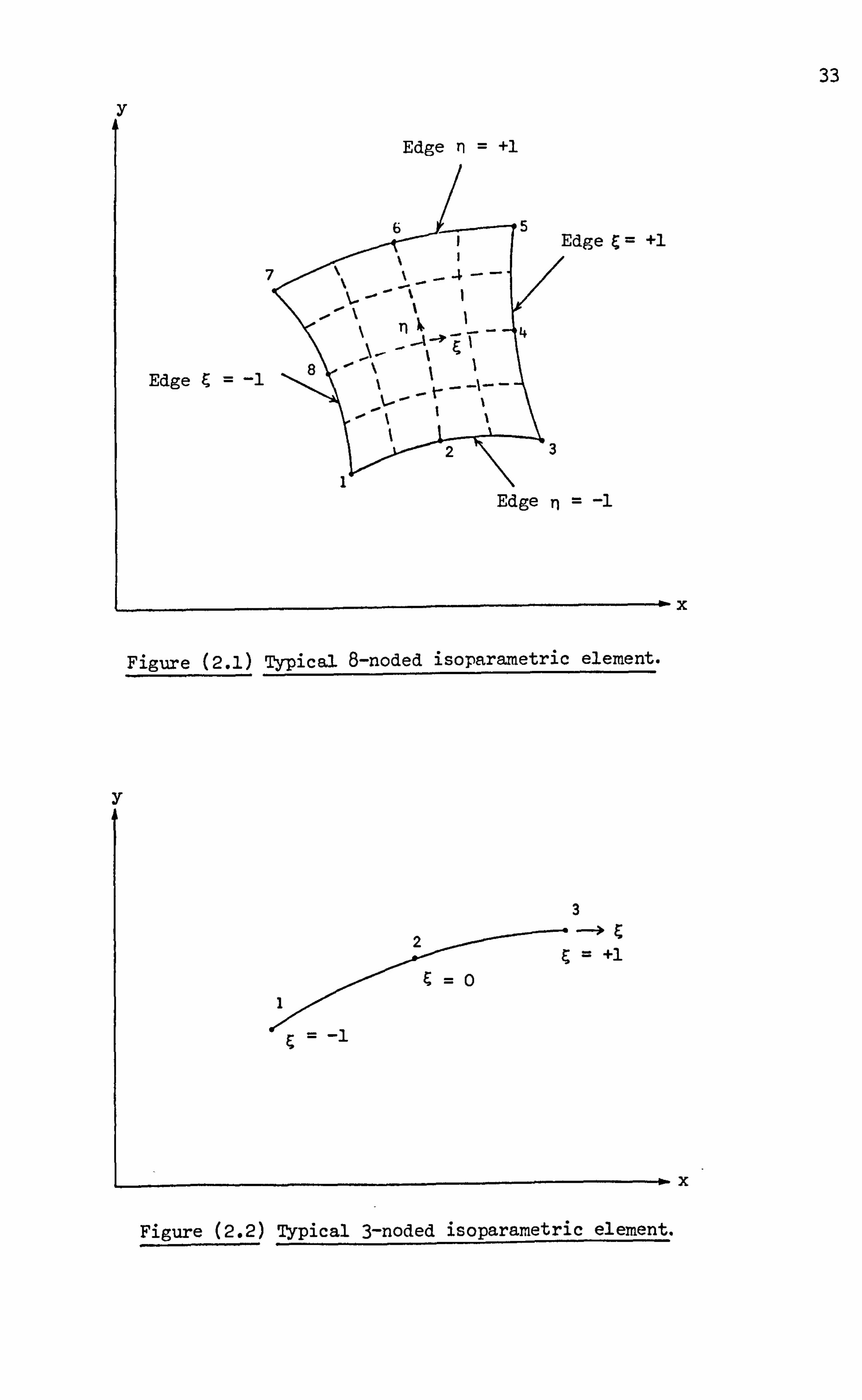
As has been previously mentioned two types of isoparametric element
are used in this work. These elements$ based on strain (displacement)
assumptions, are the eight noded isoparametric element for concrete
representation and the three noded isoparametric element for steel
representation. Figure (2.1) and Figure (2.2) show these two elements
and their natural coordinate systems. Note that the natural coordinates
in general are not orthogonal to the global system.
A different family of isoparametric elements, based on stress- (17)
assumptions, has been introduced by Robinson , who called them

19
"isoparametric stress elements". In these the shape functions also
represent the stress variation through the element. However these
elements are not widely used as yet and thus in this work only the
strain shape function elements are employed., Details will be explained
in the following section; first however the reasons for using
isoparametric elements will be summarized.
1. For a given number of degrees of freedom, complex isoparametric
elements are far nore accurate and versatile than simple elements.
Moreover a considerable saving of computty effort is obtained,
even though a complex element requires more time to formulate.
This is because it requires fewer elements compared with more
simple elements.
2. Data preparation is considerably reduced with complex elements,
although this can be neutralized to a certain extent by automatic
mesh generator schemes.
3. Numerical integration makes the evaluation of the characteristics
of curved, complex elements straightforward.
The simultaneous description of element geometry and displacement
variation by the shape functions leads to efficient and reduced
computing effort.
Curved element sides preclude the necessity for mesh refinements
where the boundaries of a structure are curved. However sometimes
the reduced number of complex elements may not be adequate to
represent all the geometries of a particular problem.
In nonlinear cracking problems isoparametric elements can predict . 411 6ý
a number of cracks in a single element without losinglits stiffness,
and these cracks can form part of different-cracked zones.
20
Decay of residual forces in the nonlinear analysis should be
distributed more rapidly than in simple elements, because they
cover a wider area.
In linear elasticity for the 8-noded isoparametric element, the
displacement field is not significantly affected for different
aspect ratios in the range between 0.5 and 1.0.
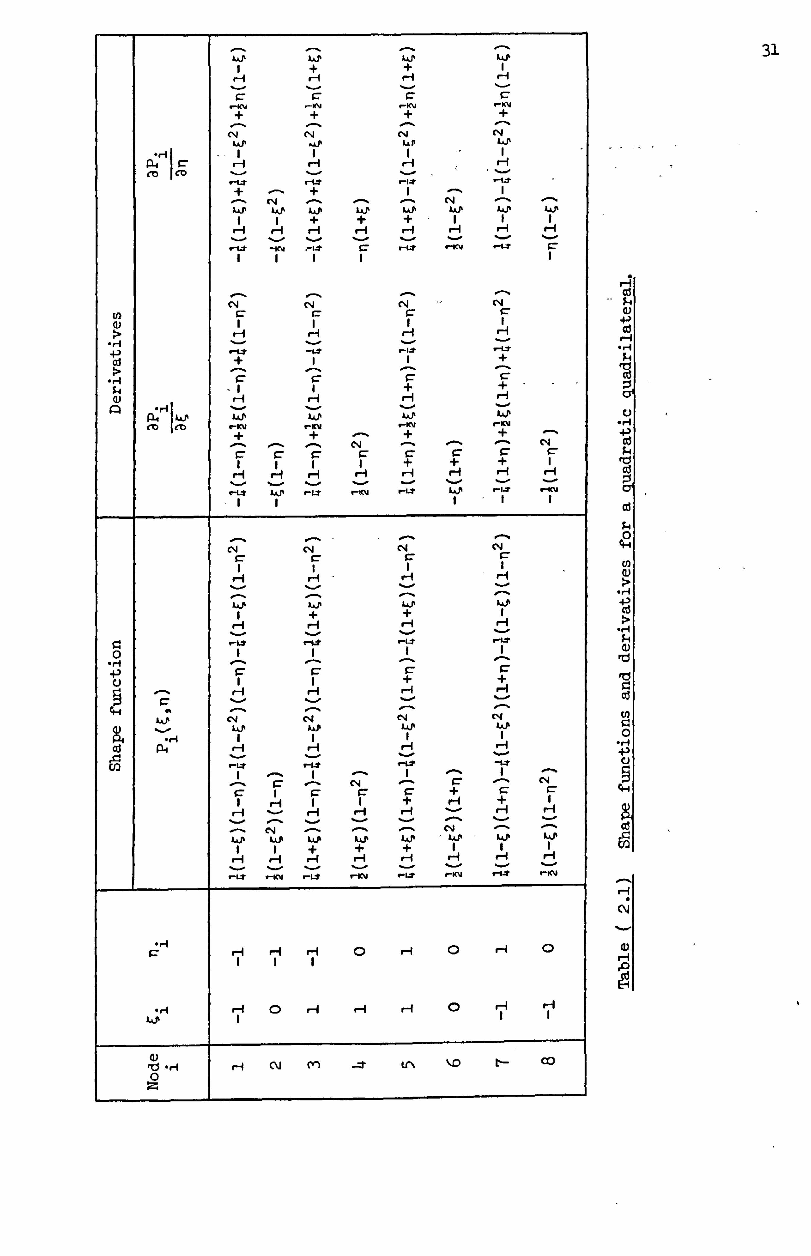
2.3.2 Isoparametric 8-noded strain element:
(a) Shape functions:
The shape functions and their derivatives are given in Table ( 2.1)
where P i(E, n), i=1,8 are the shape functions in the curvilinear
coordinate E and n. These shape functions are part of the so-called
serendipity family (4)
, and they are shown pictorially in Figure (2.3).
The properties of these shape functions are such that:
p1 if (i = j)
and p0 if (i: ý j).
The element has 2-degrees of freedom at each node, namely the displace-
ments ui, vi, giving a total of 16 degrees of freedom. Thus the
displacements at a point within the element is given by:
8 P. (&, n) ui
(2-3) 1
Pi (C'n) vi (2.4)
It should be noted that the displacements u and v are parallel to the
x and y and not the & and n axes. Similarly the position of a point
within the element in global coordinates is given by:
8 X=j Pi Q, n) xi (2-5)
8 y=EP. (&, n) yi (2.6)
11
21
(b) Stress and strain evaluation:
The strains within the element are readily expressed in terms of
the derivatives, of the displacements, i. e.
fe) ={c xx E yy y XY IT (2-T)
f 1-u 2-V (3 u+ý V) ax ay ay ax
Substituting equations(2-3) and (2.4) into equation (2.7) leadsto:
{cl (B] {61 (2.8)
where {61 ={ ul 9v1 U2 " V2 *... Ui, vi .... un, Vn1T
= Element nodal deformation vector
and [B] =[BI (E 9TO B2(EgTl)---- Bi(&,, n) B (&, n) ]
the strain matrix
- ap i x
in which: -ýx 0
3P.
B0 Dy (2.9)
ap i ap
ay ax
Since the interpolation functions P1 are defined in terms of the
curvilinear coordinates & and a transformation from local to global
coordinates is. required in equation (2.9). It is well known that the
cartesian and the curvilinear derivatives are related by:
57 [j] 5T
(2.10) a ay an
22
where [J] is the Jacobian matrix defined by:
ax ay
(2.11) ax an
_j Differentiating equation (2.5) and (2.6) in accordance with
equation (2.11) gives: Xi YJ
DPI apz a P. ap nx
-- -------- --- i---
2 Y2
api 3P2 ap apn - -------- -**'* ý-n x an an an i Yi
Lxy nn
The derivatives of equation (2.9) are now obtained using equation
(2.10) and equation (2.12), i. e.
ap ap
ax [j] (2-13)
ap
an ay 'pi
Stress-strain relations for linear elasticity is given by:
fal = -fe 0)) {00} (2.14)
T where fu} =fa
xx G yy T XY
}
faOI =v *mstd stress vector existing prior to loading.
H= tangen tial elasticity natrix.
(C 01=
initial strain vector.
(2.121
23
In general, the stress field can be obtained by substituting equation
(2.8) into equation (2.14) i. e.
f cy I= [D] ( [B] f61-fc0 1) + fa 01
(2-15)
In nonlinear problems equation (2-15) in effect provides týe key for
adjusting the solution to obey the given constitutive law. This
will be explained in the next chapter.
(c) Element stiffness and force evaluation:
Element stiffnesses are derived from the variatlonal principal of
minimum total potential energy. In this the total potential energy
P of a structure is defined in terms of the field variable, and is
then minimized with respect to this field variable, subject to specific
boundary conditions. When the. potential energy is at its minimum then
equilibrium conditions are satisfied.
If the strain energy of an element is Pe, (which will be in terms of
the nodal displacements), and the imposed potential energy due to external
load is W, then the total potential energy can be defined as:
Epe+W.
The minimized condition with respect to displacements can then be written
as:
ap E pe aw 0 (2.16)
3161 a, 6 )e 3[6)
The element contribution to this energy is:
ap e= [K ]e �, e �, )e (2.17)
DWe

24
where 16 1e the displacements associated with the element,
{6} the global displacements,
[Kj e the stiffness matrix of the element,
{F e the fictitious forces acting on the element
nodes which can be further defined by:
( (F e+ {F je c0
(2.18)
where {Fe= the nodal force vector due to initial strains, C0
F le = the nodal force vector due to initial stresses. a 0
The minimization of the imposed load is expressed as:
aw= (F} + {F} - (F} (2.19) Didl
where F) = the nodal forces due to distributed load p
per unit volume,
F) = the nodal forces due to any distributed external 9
load on boundary elements,
F) = any external load acting on nodes.
Substituting equations (2-17), (2.18) and (2.19 )into equation (2.16)
gives the minimized condition as follows:
no, of elements ap
Kle {6)e+ le + Z([ {F {F e+ {F} + {F} - {F} =0 (2.20) 3{0 1C0a0p9
or r"' {6 }= {R L"i (2.21)
which represents the assembly of the final equilibrium equations together
with prescribed boundary conditions.

25
It can be shown that
fK ejET [D] [B] dv (2.22) B] v
{F e =_f E B] T EDI fcol dv (2.23) c0V
{Fj, e =jT dv (2.24) 1
[B] 0 0v
{F}p = 2: {Fje =E- EPi(E, n) ]T 1p, dv (2.25) p
fv
{Fjg =Z {F e=r -f Epi (&, n)
IT { g} dA (2.26) 9
JA
where {P distributed load per unit volume,
{g )= component of boundary pressure.
For 2-dimensional problems the incremental volume dv is:
dv = t. dx. dy.
where t= the thickness of the element.
The relation between the Cartesian and the curvilinear coordinates is:
dx. dy = det [J]. d&-dTj
in which det [J] is the determinant of the Jacobian matrix.
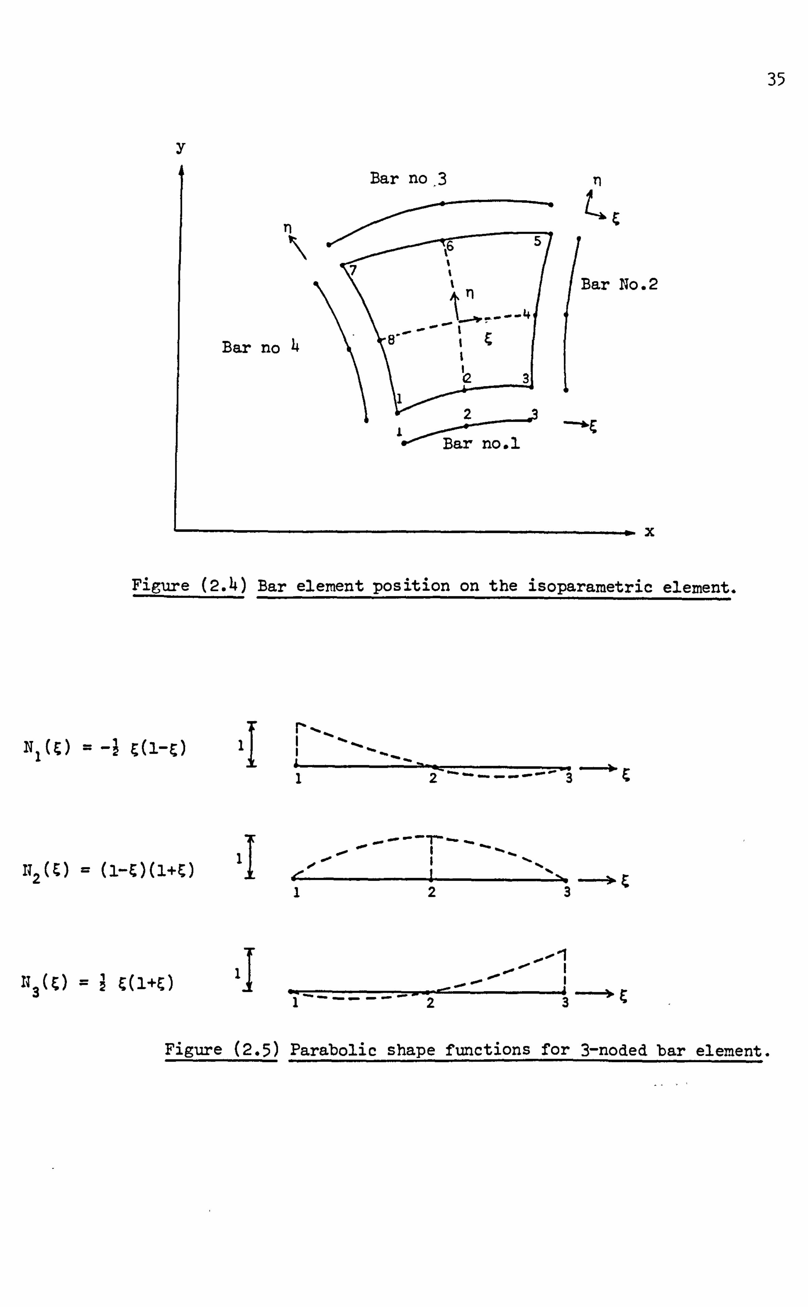
2.3.3 Isoparametric 3-noded strain element (bar element):
Bar elements are identified with a particular isoparametric 8-noded
element, and any combination of four bars can be placed along the sides
of an 8-noded element as shown in Figure (2.4). In general the bar
elements will be defined by a single natural coordinate and thus the
formulation for any one of these four possible positions of bar is
identical.
26
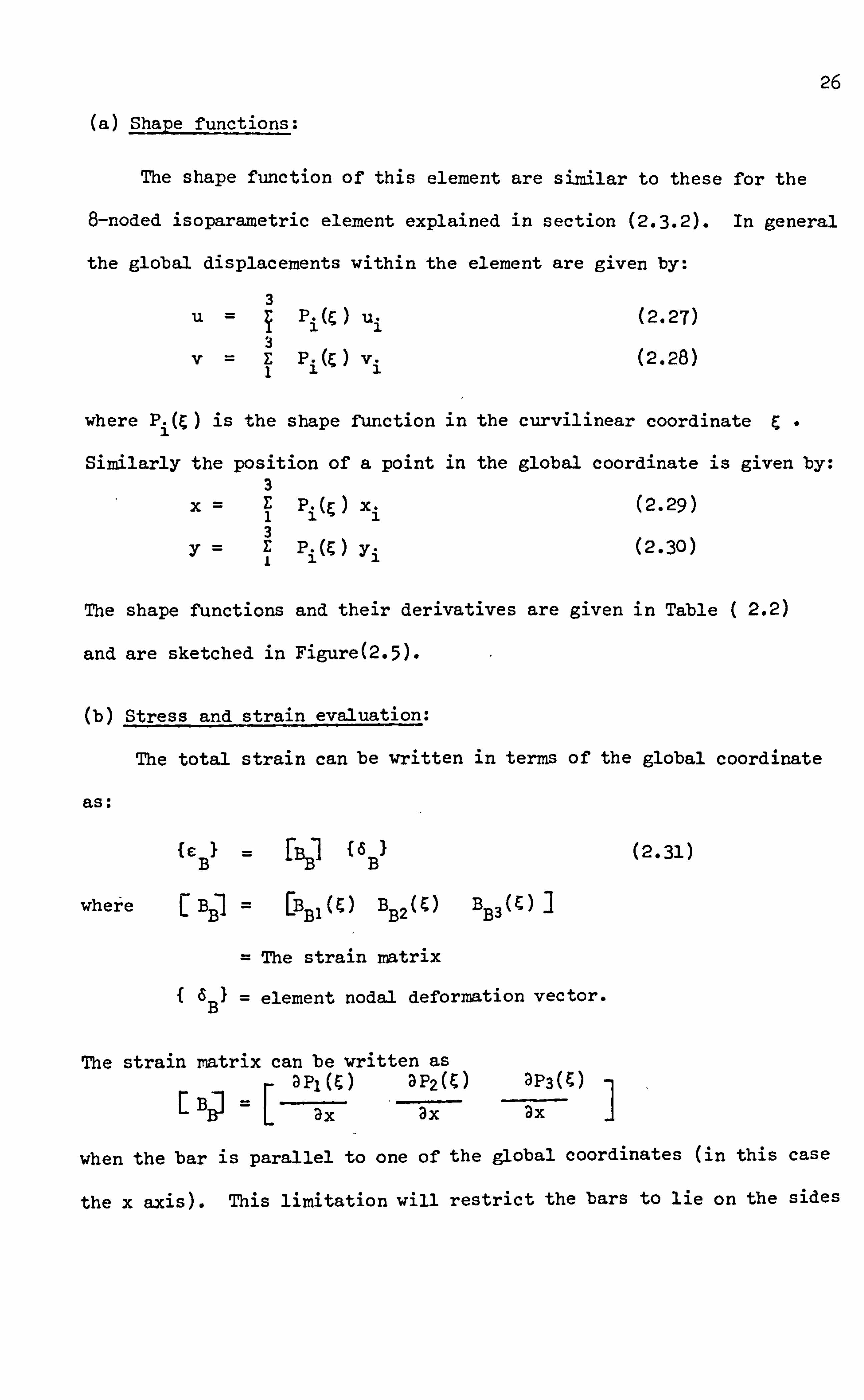
(a) Shape functions:
The shape function of this element are similar to these for the
8-noded isoparametric element explained in section (2.3.2). In general
the global displacements within the element are given by:
3 U Pi (C ) ui (2.27)
V=EPMv (2.28) 1ii
where P1 (E) is the shape function in the curvilinear coordinate &.
Similarly the position of a point in the global coordinate is given by: 3
X=E P-M X. (2.29) 111 3
YEP. (E ) Yi (2-30) 11
The shape functions and their derivatives are given in Table ( 2.2)
and are sketched in Figure(2-5).
(b) Stress and strain evaluation:
The total strain can be written in terms of the global coordinate
as:
BI EBB' 16
B) (2-31)
where BB B3(&) ýB IBB1(ý) BB2( E)
= The strain matrix
BI= element nodal deformation vector.
The strain ratrix can be written as api(O 3P2(0 3P3(C)
EBý =I ax ax ax
when the bar is parallel to one of the global coordinates (in this case
the x axis). This limitation will restrict the bars to lie on the sides

27
of rectangular elements only.
The value of
ap i(E) 1 ap i(E) (2-32) -5-x ý2 7 5&
where J ax apl aP2 aP3 (2-33) ac a& -1 ' 3& -2 * a& X3
Therefore:
apl aP2(ý) aP3 CB.
j BI :-1
For stress calculations only the modulus of elasticity of the bar
is required. Thus the stress is obtained by
{a I=E Bs (2-34)
whqre {a B' = stress vector at the nodes of the bar.
(c) Element stiffness and forces evaluation:
The expression for stiffness and force evaluation is basically
the same as for the two dimensional element, except integration is
carried out in one direction only. This can be expressed for the
stiffness as
=T dx =ET EK AEB ASES[p ý] Jdg (2-35) ssB
j
0
where A cross section area of the bar used. 8
L total length of the bar.
For internal forces the calculation can be expressed by:
r-M -1 = jL IT 1+1 [BB, T Jd& (2-36) LýBJ IBB {cyB 1 dx ((YB)
0
where [F BI = vector of nodal forces for the bar.
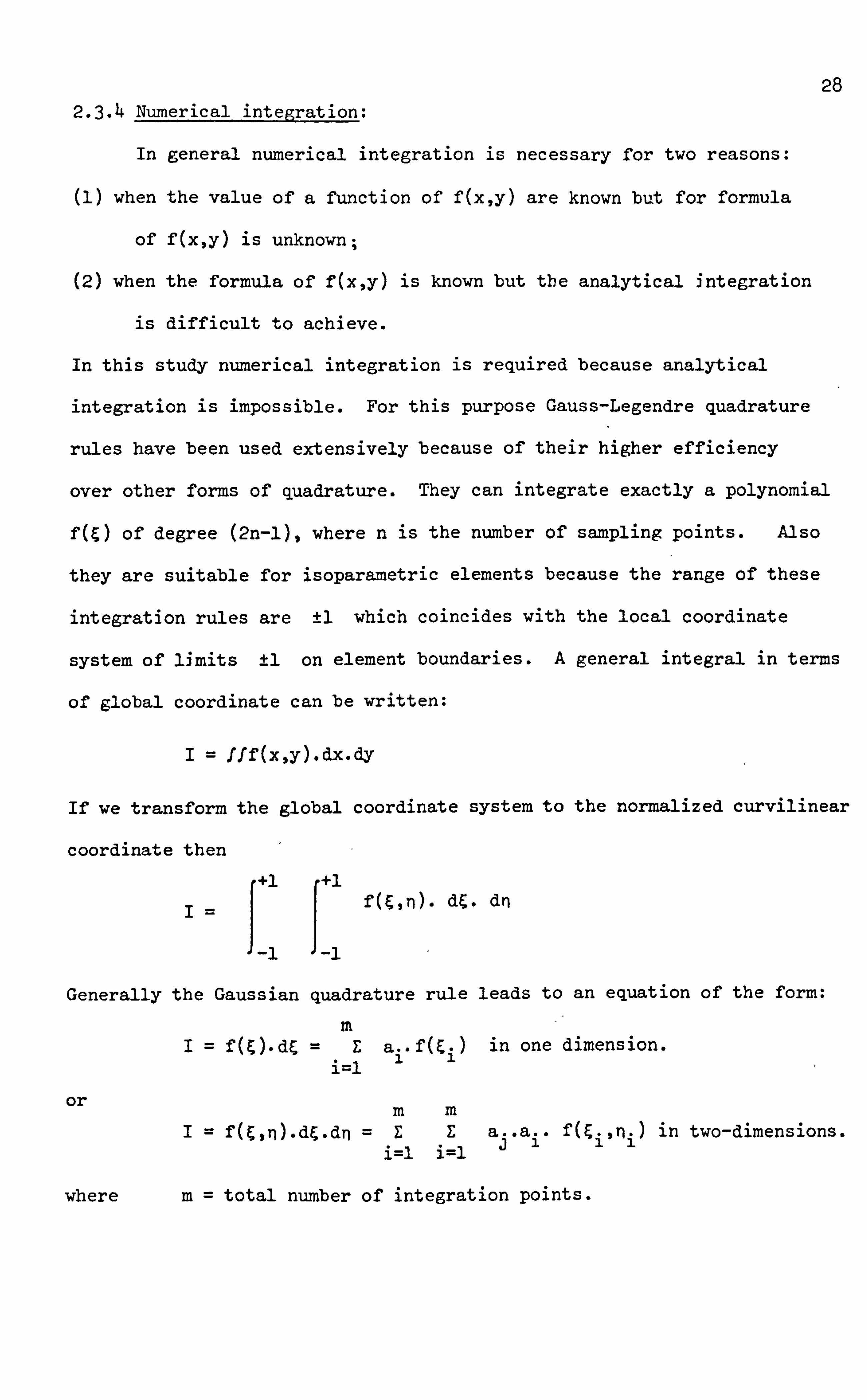
28 2.3.4 Numerical integration:
In general numerical integration is necessary for two reasons:
(1) when the value of a function of f(x, y) are known but for formula
of f(x, y) is unknown;
(2) when the formula of f(x, y) is known but the analytical integration
is difficult to achieve.
In this study numerical integration is required because analytical
integration is impossible. For this purpose Gauss-Legendre quadrature
rules have been used extensively because of their higher efficiency
over other forms of quadrature. They can integrate exactly a polynomial
f(&) of degree (2n-1), where n is the number of sampling points. Also
they are suitable for isoparametric elements because the range of these
integration rules are ±1 which coincides with the local coordinate
system of limits ±1 on element boundaries. A general integral in terms
of global coordinate can be written:
I= fff(x, y). dx. dy
If we transform the global coordinate system to the normalized curvilinear
coordinate then
+1 +1 d&. dn
Generally the Gaussian quadrature rule leads to an equation of the form:
M Ia in one dimension.
or Mm Iý f(Cjn). dý. dn =EEa0a f(&i, rji) in two-dimensions.
i=1 i=1
where m= total number of integration points.

29
ai, a The ith and jth weighting factor.
Ei'q coordinate of the ith integration point.
The value of ai and Ci associated with the Gaussian quadrature rules
are tabulated in Table ( 2-3). It is easy to show that with n sampling (4)
points, a polynomial of degree 2n-1 could be evaluated exactly
A point which should be considered in the selectian of the order
of integration rule is possible matrix singularity. If the total number
of unknowns in the structure-exceeds the total number of independent
variables applied at the integration points, then the stiffness matrix
will be singular (4).
For any one element the more Gauss points used (i. e. the higher
order of integration rule), the more computational time required,
so it is important to know the minimum order of rule to give the
required accuracy. It is found that for exact integration 3x3
rule is required. However as element size decreases it would be expected
that lower order rules would be adequate, but then it is necessary to
determine the minimum rule that still satisfies the constant strain
convergence criterion. In this limit, interelement, "forces" due to a
constant stress become
{FI=f[B J17 fal dv .
Thus for convergence to the true result numerical integration must be
capable of performing this integral exactly which in fact implies that:
f dv -f det [J] dC dn
must be integrated exactly. For a parabolic element it is found that

30
(4,8) a2x2 point rule is the minimum required But this may not
be the case for nonlinear analysis because local irregularities might
be overlooked due to the inherent averaging process. 14ore integration
points than the minimum required. may be needed to adequately describe
the crack pattern and hence monitor the nonlinearized material
properties with closer precision.
Further details of Gauss rule selection will be discussed in
Chapter
&AP Z; z AAP 1
1 4
I _KM _KIJ -K J -IN
C*. i cli
LO fi &AP 4fi
co CO
IAP LO W W 1.0 &AP + + +- I I I H H H
_L* _icm -I-t 9: -L* -KV _Ur $=
N 04 C: C
4-) Cd + I +
+
a) 1, r-, + H r-I
p a: ri
UP l
w - &0
- w
- W
co et) KV +
-KY + -KV
+ r-n
+
+ + +
r I I r-q ri r-i r-i r-I Lfi 1-t-T K\I
04 04 C-4 C*4
r-I
UP UP Lo w
0
ci + +
W LO Cj
X0 W 04 LO
CI4
A Cd
I H
I I H
00
97 c
cr 97 +
C14
I + +
cli Akp
- X0
- w
- LO
N 4.0
z
+ r-I
+ r-I
+ r-i
I r_4
1 I 1-4
Ur ýJýcy
K\I 14
r_4 1
r-I 1
r-I 1
0 V-1 0 r-i
0
r-I 0 r-I r_4 r-4 0 r-I
(D , d., I r_4 C\j M --I Lr\ \D tý_ co
1
0
1 ; 2.1
1
w �-I 192 a
31

32
Shape function Derivatives Node
P. (t a pi
1 3Ei
1 -1 + 2& 2
2 0 -2E
3 +1 1+2E 2
Table ( 2.2) Shape functions and their derivatives for a 3-noded bar element.
m ai f(zj
2 0
2 43
2 w'3
3 5 9
2 8 9 0
6 9
4 Z3-0
-- 174.8
36 7 7
2 /30
+ 3+ v4.8 2 7
3 + vr3 0 2 36 7
4 1+ 3C0 2 36 + 3- 4. -8
7
Table ( 2.3) Weighting factors and Gaussian sampling point positions.
33
y
Figure (2.1) Typical 8-noded isoparametric element.
y
Figure (2.2) Typical 3-noded isoparametric element.
x
x

34
11
/n
/fl
1T
e
/fl
11
Figure (2.3) Shape functions of serendipity family for parabolic element.
35
y
Bar no
Bar no 4
6- 2 L
Bar no. 1
TI t,
c
Bar No. 2
-ill&
x
Figure (2.4) Bar element position on the isoparametric element.
=- (i-) 11 __________________________
12-3
T----- -r ----
= (i-)(i+) 11 _'_
123
IJ (Z) = 21 z(i+z) 11
Figure (2-5) Parabolic shape functions for 3-noded bar element.

36
REFERENCES
1. Turner, M. J.; Clough, R. W.; Martin, H. C.; Topp, L. J.,
"Stiffness and deflection analysis of complex structures. "
J. Aero. Sci., Vol. 23,805-823,1956.
2. Argyris, J. H.; Kelsey, G., "Energy theorems and structural analysis".
Butterworth, 1960. (Collection of papers published in Aircraft
Engineering in 1954 and 1955).
3. Clough, R. W., "The finite element method in plane stress analysis".
Proc. 2nd conf. on Electronic Computation, ASCE, New York,
345-377,1960.
4. Zienkiewicz, O. C., "The finite element method". McGraw-Hill, 3rd
ed., 1977.
5. Spilker, R. L.; 'Pian, T. H'. H., VlHybridý-s tress models for I elastic-
plastic analysis by the initiai-stres's approach". Int. J.
Num. Meth. Eng., Vol. 14,359-378,1979. -
6. Irons, B.; Ahmed, S., "Techniques of finite elements". Wileý, ' 1981.
7. Hinton, E., Owen D. R. J., "Finite element progra mming". Academic,
1977.
8. Cook, R. D., "Concepts and applications of finite element analysisit.
Wiley, 2nd ed., 1981.
9. Cheung, Y. K.; Yeo, M. F. "A practical introduction to finite
element analysis". Pitman, 1979.
10. Smith, I. M., "Programming the finite element method with application
to geomechanics". Wiley, 1982.
11. Hinton, E.; Owen, D. R. J., "An introduction to finite element
computations". Pineridge, 1979.
12. Owen, D. R. J.; Hinton, E., "Finite elements in plasticity".
Pineridge, 1980.
37
13. Brebbia, C. A.; Connor, J. J., "Fundamentals of finite element
Techniques". Butterworth, 1973.
14. Desai, C. S.; Abel, J. F., "Introduction to the finite element
method". van Nostrand, 19Tý-
15. Rao, S. S., "The finite element method in engineering". Pergamon
1982.
16. Tong, P.; Rossettos J. N., "Finite element method". M. I. T., 19TT. 17- i4eov 18. Desai, C. S., "Elementary finite element method". Prentice-Hall,
1979.
19. Phillips, D. V., "Non linear analysis of structural concrete by
finite element methods". Ph. D. Thesis, University of Wales,
1973.
20. Krishnamoorthy, C. S.; Panneerselvam, A., "A finite element model
for non-linear analysis of reinforced concrete framed structures".
The Struct. Eng., Vol-55, No-8,331-338, Aug., 19TT.
21. Taig, I. C., "Structural analysis by the matrix displacement method".
Engl. Electric Aviation report No-SO17,1961.
22. Irons, B. M., "Numerical integration applied to finite element
methods". Conf. use of digital computers in Struct. Eng., Newcastle
University, 1966.
23. Irons, B. M., "Engineering application of numerical integration in
stiffness method". J. A. I. A. A., Vol. 14,2035-203T, 1966.
24. Chen, E. Y. T.; Schnobrich, W. C., "Material modelling of plain concrete".
IABSE Colloquium in advanced mechanics in reinforced concrete,
Delft, 1981.

CHAPTER
NONLINEAR METHOD OF SOLUTION
3.1 Introduction
3.2 Numerical Techniques for Nonlinear Analysis
3.2.1 Basic formulation
3.2.2 Incremental method
3.2.3 Iteration method
3.2.4 Mixed method
3.3 Comparison of Basic Methods
3.4 Method Used in this Work
3.5 Convergence Criteria
3.5.1 Force convergence criterion
3.5.2 Displacement convergence criteria
3.5.3 General discussion on convergence criteria
3.6 Basic Steps in the Nonlinear Method Used
3.7 Frontal Equation Solving Routine

CHAPTER 3 38
NONLINEAR METHOD OF SOLUTION
3.1 Introduction:
This chapter presents the method used for solving the nonlinear'
problems described in this study and briefly compares this with others.
A nonlinear solution is obtained by solving a series of linear problems
in which the appropriate nonlinear conditions are satisfied to a specific
degree of accuracy. This method is used because of the lack of a general
approach for solving nonlinear equations.
A nonlinear structural problem must obey the basic laws of continuum
mechanics, i. e. equilibrium, compatibility, and the constitutive
relations of the material. Displacement compatibility is automatically
satisfied in the displacement finite element technique. Common nodes
between elements ensure continuity and compatibility of displacements
along internal element boundaries (including the nodes) and polynomial
shape functions ensure continuity and single valued displacements inter-
nally. Therefore it becomes only necessary to enforce that the nonlinear
constitutive relations are correctly satisfied whilst at the same time
preserving the equilibrium of the structure.
One way of achieving this is to first of all ensure that at any
loading stage the stresses are consistent with the calculated displace-
ment field and given constitutive relations. These stresses will then
be statically equivalent to a set of internal nodal forces which should
be in equilibrium with the external force system. Generally these
forces are not the same and the differencesbetween them are termed
tv - it (1)
. residual forces' which have to be removed to achieve equilibrium.
In general for a particular load level, a number of successive
linear solutions are required to remove the residual forces to a desired
degree of accuracy. The method is obviously iterative in nature and

39
the final results will depend on the factors associated with the
iterative process, for example the increment size, accuracy1required,
the exact type of solution process employed etc. Clearly it is
impossible to obtain a unique solution to a particular problem because
of these many factors.
There can be several causes of nonlinear behaviour in a structure,
which can be divided into two classes:
1. Nonlinear naterial behaviour,
2. Geometric changes (i. e. large deformations) in the structure,
including changing boundary conditions.
Stress-strain relations are a major source of nonlinearity. These
can vary from short-term nonlinear relationships between stress and
strain such as plasticity, cracking, nonlinear elasticity, etc., to
time-dependent effects such as creep, Vticoelastic behaviour, shrinkage,
etc. In concrete, cracks even exist before any external loading has
been applied. (2,3)
'This is due to effects such as segregation, water
gain, and bond cracks at the matrix-aggregate interface.
The second source of nonlinearity is when deflections are
sufficiently large that the equilibrium equations based on the original
geometry are no longer valid and need to be modified to account for
the new geometry. This affects the force-displacement equations,
because additional internal forces are generated due to the deflected
geometry. Also if the large displacements cause large strains, then
additional higher order terms must be included in the mnthematical
definition of strain. This results in nonlinear strain-displacement
equations. (4,5)
Changes in the external boundary conditions are, ins, sense, another

4o
source of geometric nonlinearity. For example, beams on elastic
foundations in which the size and location of contact zones between
beam and foundation depends on the nature of the applied force. In
certain circumstances, reinforced concrete structures present another
example where boundary conditions change with varying load. Cracking
and crushing cause separation of adjacent parts of the structure,
which can be interpreted as a new geometric configuration, and this
interpretation can be included in analytical procedures, such as the
spring element method of Ngo et al. (6)
In this'study only nonlinearity caused by the short-term nonlinear
behaviour of concrete and steel is considered. These include the
tensile cracking of concretej, ' the nonlinear stress-strain relations of
concrete in compression and the yielding and work-hardening of steel.
Exact details of the laws representing this behaviour will be given
later in Chapter 5.
However, in general, the solution of a nonlinear problem is highly
dependent on these material laws, and data used. A more accurate law
ought to give a more accurate solution. But as mentioned above, the
solution can also be highly dependent on the nonlinear procedure employed.
Furthermore, the finite element approximations itself, e. g. element
type, mesh size, Gauss rule etc., may lead to further inaccuracies.
These sources of error in the nonlinear process are inter-related
in the sense that one type of approximation might counter balance another;
or they might reinforce each other. In some cases certain approximations
might cause a more flexible structure, such as lower order Gauss rules;
other approximations might cause a more stiff structure, such as a
coarse mesh; some approximations might affect the ultimate strength
41
such as the given tensile strength. Herein lies a major difficulty
in solving a nonlinear reinforced concrete problem. With a material
as variable as concrete, it is difficult enough to assess the accuracy
of the material laws and data in a given situation. Add to this the
effects of the basic numerical procedure, especially when dealing with
cracking, and it becomes very difficult indeed to know how accurate
the solution is.
It is fairly obvious that the more complex the material law the
more expensive the solution; the more accurate the nonlinear method
(i. e. small load increments, many iterations, low convergence tolerances,
etc. ), the more expensive the solution; the finer the finite element
mesh or the more sophisticated the element, the wre expensive the
solution. Therefore if the analyst had unrestricted computing resources
it would seem probable that an accurate solution could be obtained.
Since this is not possible, approxinations of varying degree have
to be introduced to obtain an economic solution. Then the inter-
relationships mentioned above come into operation. It could be argued
that certain procedures are incorporated so that a numerical solution
can be adjusted to fit the known solution. These then become a sort
of numerical device, even if a physical significance can be argued
for them, for exarQle tension stiffening. The problem then is what to
do when the solution is not known beforehand, and guidelines are
obviously necessary. It becomes important to investigate the effects
of these "devices" on a solution; their accuracy, their economy and
their interdependence.
If two different solution techniques give at any stage similar
results within a desired accuracy (e. g. deflections, crack zones,

42
crushing zones, stress and strain distributions etc. ), then obviously
the cheaper solution is =re acceptable, whatever devices were used
to get there., i. e. the ends justify the neans.
These points will be elaborated further when specific problems
will be presented later, particularly in Chapter
3.2 Numerical Techniques for Nonlinear Analysis:
3.2.1 Basic formulation:
The solutions of nonlinear problems by the finite element method
are usually attempted by one of three basic techniques:
1. Incremental (step-wise procedure).
2. Iterative (Newton method).
3. Incremental-iterative (mixed procedure).
The general basis of each method is similar. For problems
where only the material behaviour is nonlinear, the relationship
between stress and strain is assumed to be of the form:
f(cr, c) =
The element stiffness matrix is a function of the material
properties and can be written as:
CK], = k(cr, F-)
The'external nodal forces {R I are related to the nodal displace-
ments {S) through the stiffnesses of the element and can be expressed
by:
{R I= EK ] {61
which on inversion becomes:
[K J-1 [R}
or Ek(cr, e) 1-1 {R)
43
This derivation illustrates the basic nonlinear relationship between
{61 and (RI , due to the influence of the material law on [K
Equation (3-1) is solved by a succession of linear approximations:
The different methods of applying these linear approximations will in
general lead to different load-displacement paths influencing the final
solution. These methods will now be discussed in more detail.
3.2.2 Incremental method ý4,7,8)
The basis of the incremental method is the subdivision of the total
applied load vector into smaller load increments, which do not necessarily
need to be equal. During each load increment the equation:
{R) =[ K] {61
is assumed to be linear, i. e. a fixed value of [ K] is assumed using
material data existing at the end of the previous increment. Nodal
displacements can then be obtained for each increment and these are
added to the previously accumulated displacements. The process is
repeated until the total load is reached.
The accuracy of this procedure depends on the increment size;
the smaller the increments the better the accuracy, but at the same time
the more computational effort required. A modification of this method
is the "midpoint Runge-Kutta" method. (4)
In this, the first step is
to apply half the load increment and to calculate new stiffnesses
corresponding to the total stresses at this value. These stiffnesses
are then utilized to compute an approximation for the full load increment.
The incremental method in its original and modified form do not
account for force redistribution during the application of the incre-
mental load (i. e. no iteration process exists to restore equilibrium).

44
3.2.3 Iteration method: (4,5,7,8)
In the iteration method, the full load is applied in one increment.
Stresses are evaluated at that load according to the material law.
This gives equivalent forces which may not be equal to the external
applied forces, i. e. equilibrium is not necessarily satisfied. Then,
the portion of the total loading that is not balanced is calculated as
the difference between the total applied load vector and internal nodal
forces. These are the unbalanced nodal forces {F I which are'then used U
to compute an additional increment of displacements, and hence new stresses,
which give a new set of equivalent nodal forces. This process is repeated
until equilibrium is approximated to a certain degree of accuracy. When
this stage is reached the total displacement is calculated by summing
the displacements from each iteration.
There are many variations of this basic process and a solution
depends in many ways on the method used for computation of the stiffness
matrix EKI and the unbalanced nodal forces {F I.
A) Computation of unbalanced'nodal forces:
In general, the linear constitutive law can be written in the form:
{cr) = [D] ({cl -{c01)+ {CFO) (3.2)
where [D] is a constant, linear elastic matrix, {a 01 and {c
01 are
initial stress and strain vectors. Equation (3.2) is in essence the
linear, approximation for the nonlinear relation:
f (a, E) = (3.3)
in any linear iteration. By adjusting any of the quantities [D J, fe 011
or [a 01,
Equation (3.2) can be made to approximate Equation (3-3).

45
If {C 01
is adjusted the process becomes the It initial strain" method (8)
and is used when strains are expressed in terns of stress. If {ao}
is adjusted, the process is called the "initial stress" method (8)
. and is
used when stress can be given in terns of strain.
In the initial strain method the Equation (3.2) is simplified to:
{a) = FD ] Qcl -{ co)) (3.4)
Assuming {e 01=0
initially, Equation (3.4) is solved with an
appropriate ED I matrix and strain {c Al
I to obtain a certain level
of stress {aA) where:
{aAj =fD] {cA, ) .
The strain which should have occurred is:
f CA21 {OAl
The difference between the strains:
{ Eo} = {EA2} - {cAl}
is used as an initial strain in Equation (3.4), and the equivalent
unbalanced nodal forces {F ) are calculated from:
(F u1=- Jv [B ]TEB 1 (E:
01 dv
These forces are removed by applying them to the structure which causes
a correction to (6) . This process is repeated until {c 01 or {F
U
becomes negligible.
The steps in the initial stress method are very similar. The
Equation (3.2) is now simplified to:
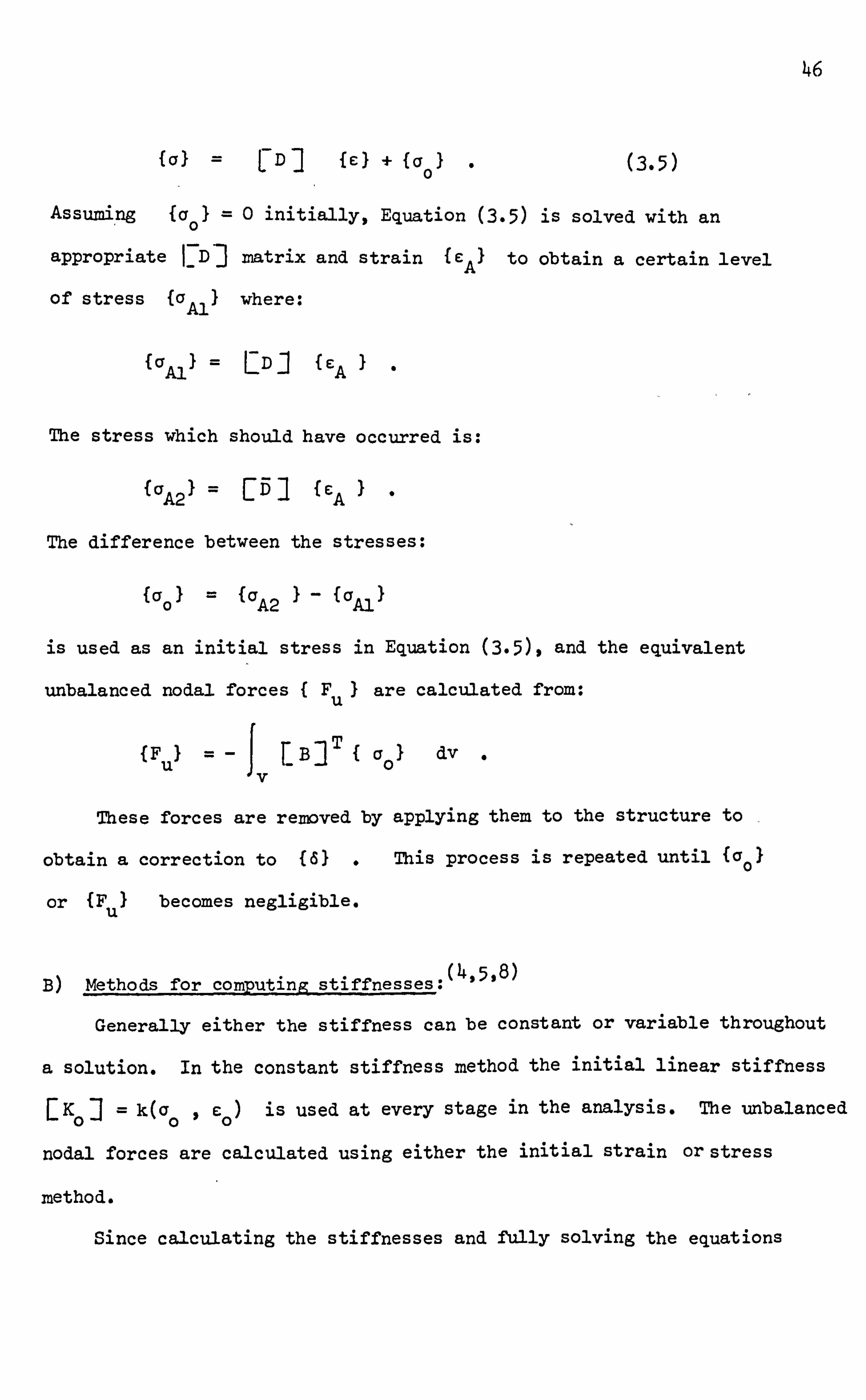
46
{CFI = [D] {E: j + {CF 0}.
(3.5)
Assuming {a 01=0
initially, Equation (3-5) is solved with an
appropriate I-D] matrix and strain {e Al to obtain a certain level
of stress {a Al
I where:
{a Al
IA1-
The stress which should have occurred is:
1a A21 ý ý5 1fcA)*
The difference between the stresses:
{a o1ý
{aA2 1-{a Al)
is used as an initial stress in Equation (3-5), and the equivalent
unbalanced nodal forces {FuI are calculated from:
{F u)=-
Jv [B ]T {a01 dv .
These forces are removed by applying them to the structure to -
obtain a correction to (6) . This process is repeated until {ao)
or {F u)
becomes negligible.
B) Methods for computing stiffnesses: (4,5,8)
Generally either the stiffness can be constant or variable throughout
a solution. In the constant stiffness method the initial linear stiffness
EK 0]=
k(Cr 0, C0) is used at every stage in the analysis. The unbalanced
nodal forces are calculated using either the initial strain orstress
method.
Since calculating the stiffnesses and fully solving the equations

47
is an expensive operation, this method has economic advantages because
the stiffness is calculated only once. Also a synmetric positive-
definite natrix: will always exist. (9,11,22)
Its main disadvantage is
that it usually requires a high number of iterations to achieve the
desired accuracy, especially when cracking and yielding of reinforcement
has occurred. This is due to the sudden and large changes that are
caused in the stiffnesses. It has been suggested that acceleration (9,11,22)
processes could be used to speed up the solution, although
these have not always met with success.
In the variable stiffness method, a linear solution is performed
but the rD ] matrix is adjusted during the iteration process. This
can be done either by using a secant modulus approach or a tangential
modulus approach. The initial strain or stress method can be used
for the computationof the unbalanced nodal forces.
If the stiffnesses are updated during all iterations then the
method is a form of the well known "Newton Raphson" method. In general
the variable stiffness method requires considerably less iterations
than the constant stiffness method, although a full solution is more
expensive than a resolution with a constant stiffness.
However, problems could arise as reductions in stiffness could
lead to negative or zero terms on the leading diagonal of the stiffness
matrix. This difficulty is usually avoided by ensuring positive
stiffness coefficients, and by using the residual nodal force vector
concept to simulate any further loss of stiffness.
A cheaper variation of the variable stiffness approach can be
obtained by using a modified "Newton Raphson" method, where the stiffnesses
are only updated during certain iterations.
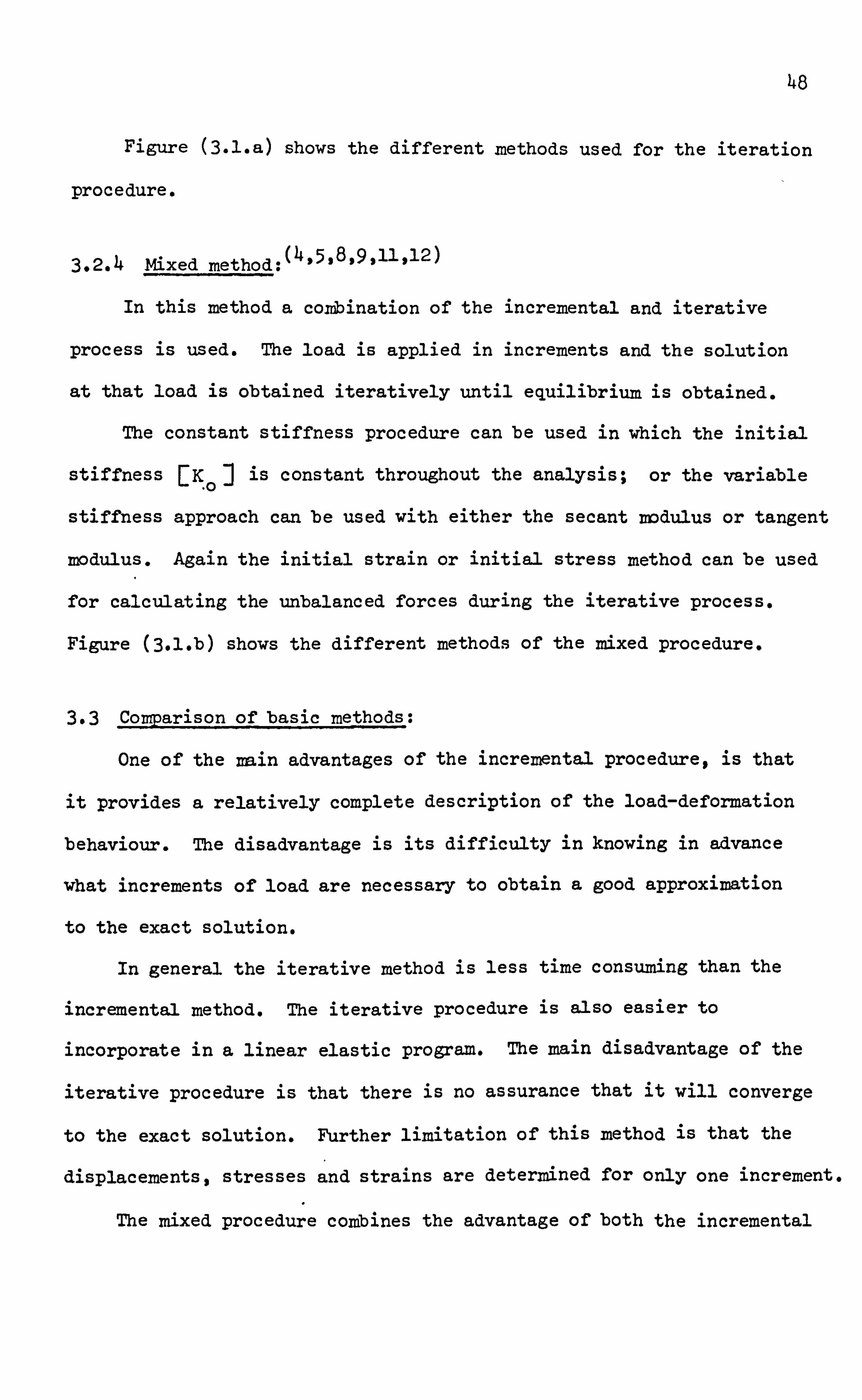
48
Figure (3-l. a) shows the different methods used for the iteration
procedure.
3.2.4 Mixed method: (4,5,8,9,11,12)
In this method a combination of the incremental and iterative
process is used. The load is applied in increments and the solution
at that load is obtained iteratively until equilibrium is obtained.
The constant stiffness procedure can be used in which the initial
stiffness EK. 0
J is constant throughout the analysis; or the variable
stiffness approach can be used with either the secant modulus or tangent
modulus. Again the initial strain or initial stress method can be used
for calculating the unbalanced forces during the iterative process,
Figure (3-l. b) shows the different methods of the mixed procedure.
3.3 Comparison of basic methods:
One of the nain advantages of the incremental procedure, is that
it provides a relatively complete description of the load-deformation
behaviour. The disadvantage is its difficulty in knowing in advance
what increments of load are necessary to obtain a good approximation
to the exact solution.
In general the iterative method is less time consuming than the
incremental method. The iterative procedure is also easier to
incorporate in a linear elastic program. The main disadvantage of the
iterative procedure is that there is no assurance that it will converge
to the exact solution. Further limitation of this method is that the
displacements, stresses and strains are determined for only one increment.
The mixed procedure combines the advantage of both the incremental
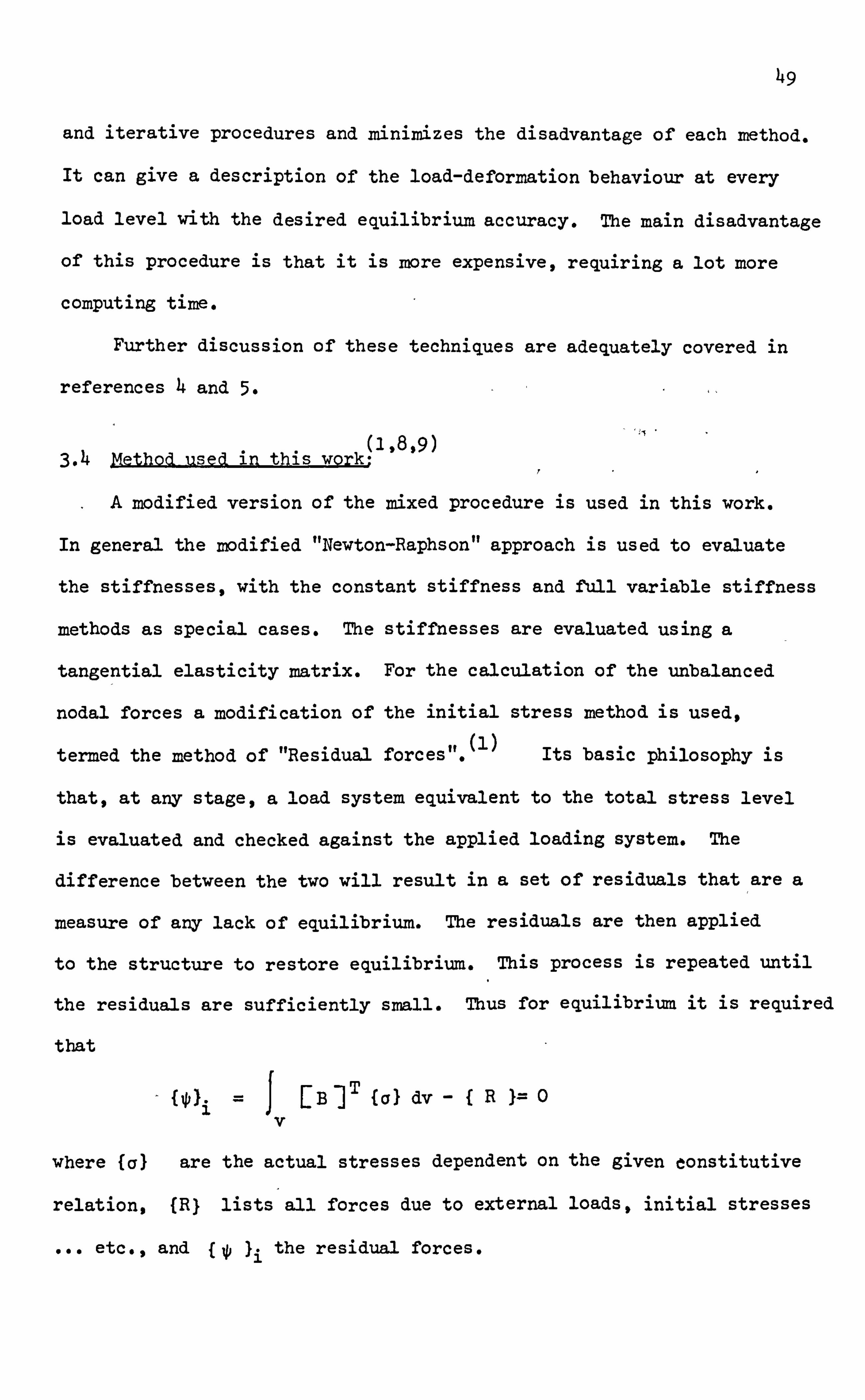
49
and iterative procedures and minimizes the disadvantage of each method.
It can give a description of the load-deformation behaviour at every
load level with the desired equilibrium accuracy. The main disadvantage
of this procedure is that it is more expensive, requiring a lot more
computing time.
Further discussion of these techniques are adequately covered in
references 4 and 5.
3.4 Method used in this work (1,8,9)
A modified version of the mixed procedure is used in this work.
In general the rDdified "Newton-Raphson" approach is used to evaluate
the stiffnesses, with the constant stiffness and full variable stiffness
methods as special cases. The stiffnesses are evaluated using a
tangential elasticity matrix. For the calculation of the unbalanced
nodal forces a modification of the initial stress method is used,
termed the method of "Residual forces". (')
Its basic philosophy is
that, at any stage, a load system equivalent to the total stress level
is evaluated and checked against the applied loading system. The
difference between the two will result in a set of residuals that are a
measure of any lack of equilibrium. The residuals are then applied
to the structure to restore equilibrium. This process is repeated until
the residuals are sufficiently small. Thus for equilibrium it is required
that
Wi =i EB ]l {cF) dv R J= 0
v
where fa) are the actual stresses dependent on the given constitutive
relation, fRj lists all forces due to external loads, initial stresses
. o. etc., and {ý Ji the residual forces.

50
The use of the method of residual forces in the evaluation of the
excess forces will ensure that residuals are not cilmilative, which nay
not be the case when using the initial stress meethod. (119)
. (8,9,11,13,14,15)
3.5 Convergence criteria.
It is important to include reliable criteria which will check
for the gradual elimination of the residual forces and terminate the
iterative process when convergence to the desired accuracy has been
achieved. The user specifies this accuracy by giving quantitative
values known as convergence tolerances. In other words the user
specifies the degree of accuracy of equilibrium that is acceptable.
The convergence criteria can be based on various quantities; either
directly on the unbalanced forces, or indirectly on displacement. incre-
ments, or on changes in stress values. In this thesis two options for
convergence are used. A displacement convergence criteria and a force
convergence criterion.
It is difficult and expensive to check the decay of displacements
or residual forces for every degree of freedom therefore some overall
evaluation is preferable. This is achieved by using norms. Those
used in this work will now be defined.
3.5.1 Force convergence criterion:
This criterionassumes that convergence is achieved if:
C P-* F
where norm of the residuals

51
and Pý = norm of the total applied loads
= /I
PIT IP i
CFa specific convergence tolerance
3.5.2 Displacement convergence criteria:
Two types of displacement criteria are used in which:
A) Convergence is achieved if;
AS i <C D
where norm of the displacements which have taken place
during an iteration.
6T A -,
61 ii
and norm of the total displacements from the
beginning
T i
CD=a specific convergence tolerance
B) Convergence is achieved if ;
A6 <C D
where norm of the total displacement in the increment
at which the structure is analysed.
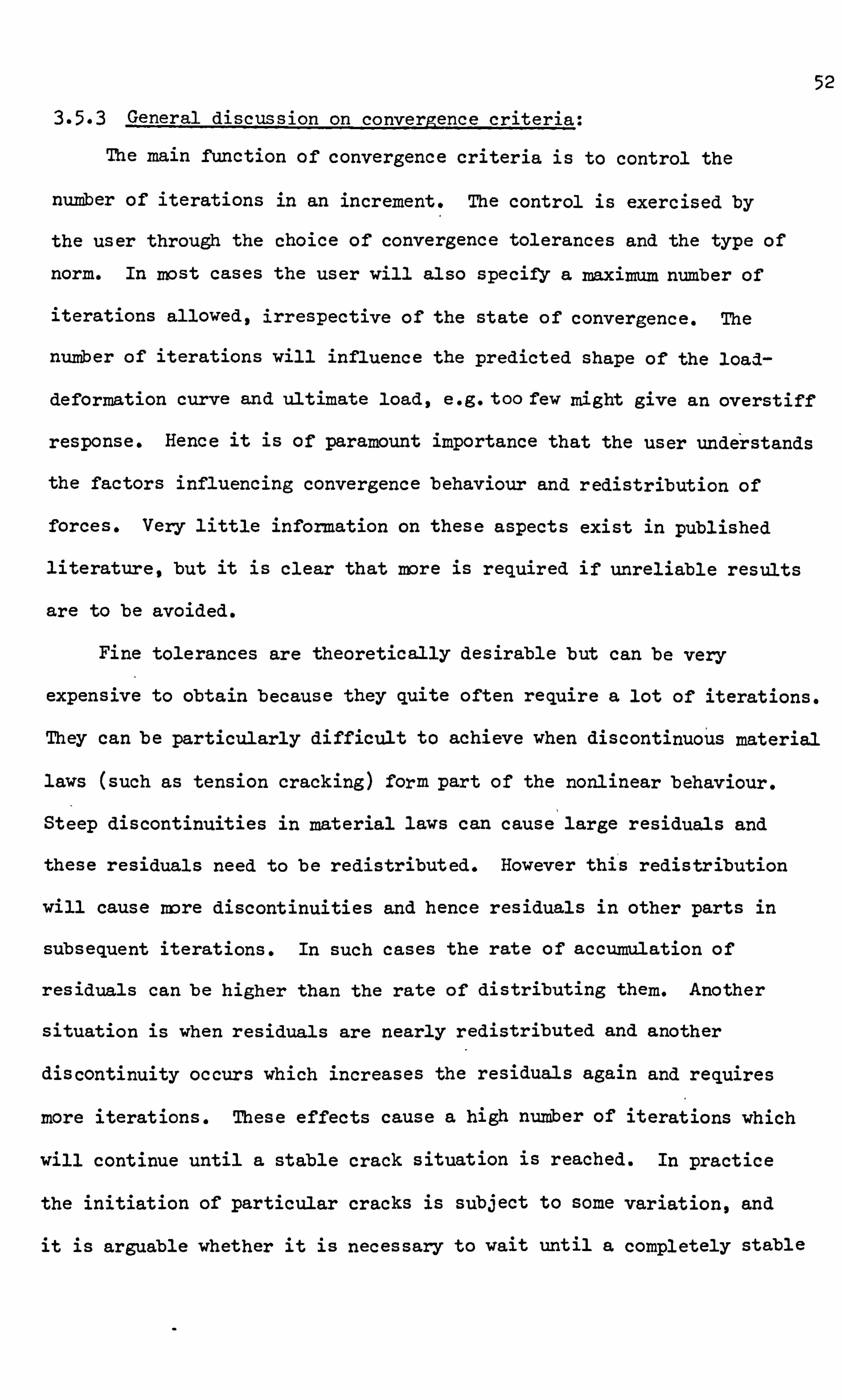
52
3.5.3 General discussion on convergence criteria: The main function of convergence criteria is to control the
number of iterations in an increment. The control is exercised by
the user through the choice of convergence tolerances and the type of
norm. In most cases the user will also specify a maxim= number of
iterations allowed, irrespective of the state of convergence. The
number of iterations will influence the predicted shape of the load-
deformation curve and ultimate load, e. g. too few might give an overstiff
response. Hence it is of paramount importance that the user understands
the factors influencing convergence behaviour and redistribution of
forces. Very little information on these aspects exist in published
literature, but it is clear that more is required if unreliable results
are to be avoided.
Fine tolerances are theoretically desirable but can be very
expensive to obtain because they quite often require a lot of iterations.
They can be particularly difficult to achieve when discontinuous material
laws (such as tension cracking) form part of the nonlinear behaviour.
Steep discontinuities in material laws can cause large residuals and
these residuals need to be redistributed. However this redistribution
will cause more discontinuities and hence residuals in other parts in
subsequent iterations. In such cases the rate of accumulation of
residuals can be higher than the rate of distributing them. Another
situation is when residuals are nearly redistributed and another
discontinuity occurs which increases the residuals again and requires
more iterations. These effects cause a high number of iterations which
will continue until a stable crack situation is reached. In practice
the initiation of particular cracks is subject to some variation, and
it is arguable whether it is necessary to wait until a completely stable

53
crack situation has been achieved in any increment by using very
fine tolerances. Therefore retarding the rate of crack propagation
by specifying large tolerances or smaller number of mxim= iterations
could lead to satisfactory results.
In this work the load convergence criterionis the most commonly
used because it works directly on equilibrium requirements. Also the
displacement criterion can sometimes give misleading indicatiow of
convergence. For instance its norm could be small and decreasing yet at
the same time the residual forces could be increasing due to local
changes in stiffnesses.
Finally the rate of convergence depends on the method used in
the solution, it is well known that constant stiffness will lead to
slow convergence and this could lead to an expensive solution. (14)
An accelerator process may be included to give a faster convergence,
but problems may arise such as there being no guarantee that the
solution will be the same as the unaccelerated solution. The accelerator
process also can lead to premature instability of the solution. (9)
A more detailed discussion of these points and a numerical
comparison of the use-of convergence criteria will be given in Chapter
6.
3.6 Basic steps in the nonlinear method used:
Apply an increment of load A[R} n and calculate the first estimate
of the incremental displacement
AM n 4'- Ez1 -1 &{
. R}
n
where [K] , can be the initial elastic stiffness, or a tlý, ngential
stiffness based on conditions prevailing at the start of the increment.

54
2'. Calculate the total displacement and strain.
{6} n
ý- {6}n-1, + A(6)n
{c}n ý- {C }n-1 +AI {C) n
3. Calculate the total stress {aIn using the appropriate constitutive law:
f(a, e) =0
Find the equivalent nodal forces'due-to {a) n
then calculate
the residuals
Wi jv
Bf {a} n
dv - {R} n
where {R} is the total external load.
Check if residuals or displacements satisfy the convergence
criteria. ' If they do apply a new load increment A{R} n+1 and
repeat from (1).
If not, apply the residuals and calculate the corrective
-displacement A{61 ni c aused by them from
AW ni
K
where RI is the initial-elastic stiffness, or a tangent al
stiffness based on conditions prevailing at the start of the
iteration.
Go to step 2 and repeat the process until convergence conditions
are satisfied.
A flow chart of this process is shown in Figure (3.2).

55
3-7 Frontal equation solving routine:
The simultaneous equation solving routine plays a major role in
the efficiency of a finite element program. This is particularly true
in a nonlinear finite element program because a lot of processing time
is used in solving and resolving equations.
In this research a version of the frontal solution will be used.
It was originally introduced by Irons ý18 )
and subsequently modified
by Hinton and Owen(17). Further improvements have been made in this
work which will be described later.
The frontal solution is a very efficient direct solution process.
Its main attraction is that variables are introduced at a later stage
and eliminated earlier than in most other methods. Additional to this
is its efficiency in the way it handles the core storage, i. e. a
large number of elements can be used without the need for large storage.
This is important especially when complex structures have to be analysed.
The front solver is never efficient than a band solver,
and for the majority of cases is very much more efficient, especially
for problems in which elements with mid side nodes are used. (11)
The main difference between a frontal and a banded solution is
that the frontal solver does not store as many zero coefficients inside
the band. The storage allocation in a banded solver is determined by
the order in which the nodes are presented for assembly. But in a
front solver the storage is determined by the order in which elements
are presented. Thus for the frontal solver node numbering is irrelevant
and it is the element numbering that is all important. (17,19)
The main idea of the frontal solution is to assemble the equations
and eliminate the variables at the same time. As soon as the coefficients

56
of an equation are completely assembled from the contributions of all
relevant elements, the corresponding variable can be eliminated.
This means the total stiffness matrix of the structure is never formed
as such, since after elimination the reduced equation is immediately
transferred to back-up disc store.
The core contains, at any given instant, the upper triangular
part of a square matrix containing the equations which are being
formed at that particular time. These equations, their corresponding
nodes and degree of freedom are termed the "Front". The number of the
unknowns in the front is the "frontwidth" . The maximum size of
problem which can be solved is governed by the "Maximum Frontwidth".
The equations, nodes and degrees of freedom belonging to the front
are termed "active"; those which are yet to be considered are "inactive";
those which have passed through the front and have been eliminated are
said to be "deactivated".
During the assembly-elimination process the elements are considered
each in turn according to a prescribed order. Whenever a new element
is called in, its stiffness coefficients are read from disc file and
mimmed either into existing equations, if the nodes are already active,
or into new equations which have to be included in the front if the
nodes are being activated for the first time. If some nodes are appearing
for the last time, the corresponding equations can be eliminated and
stored away on a disc file and are thus deactivated. In so doing they
free space in the front which can be employed during assembly of the
next element.
Although in itself the frontal solution is efficient, the periphery
operations of transfer to a backing disc file is inefficient because

57
transfer is a very slow and costly operation, especially with a high
number of elements. This situation can be improved by storing the
reduced equations corresponding to the eliminated variables in core,
in a temporary array termed a "Buffer area". As soon as this area is
full the information is transferred to disc. The introduction of the
buffer area may reduce the cost by about 50% compared with the use of
ordinary backing disc store. In this research it was found that
transfer to disc was very rarely required, but this, of course, depends
on the size of the main core storage of the computer used.
The front width in this work was set equal to a maximum of 100,
which allows: i about 200 isoparametric elements, to be solved. This is
considerably large for this type of element.
The use of this subroutine in other computers may require change
of the buffer area with respect to the size of the computer used.
The-buffer area in this program was set equal to 250,000.
References 16,17,19,20,21,22 give more detail about the
frontal technique.
0
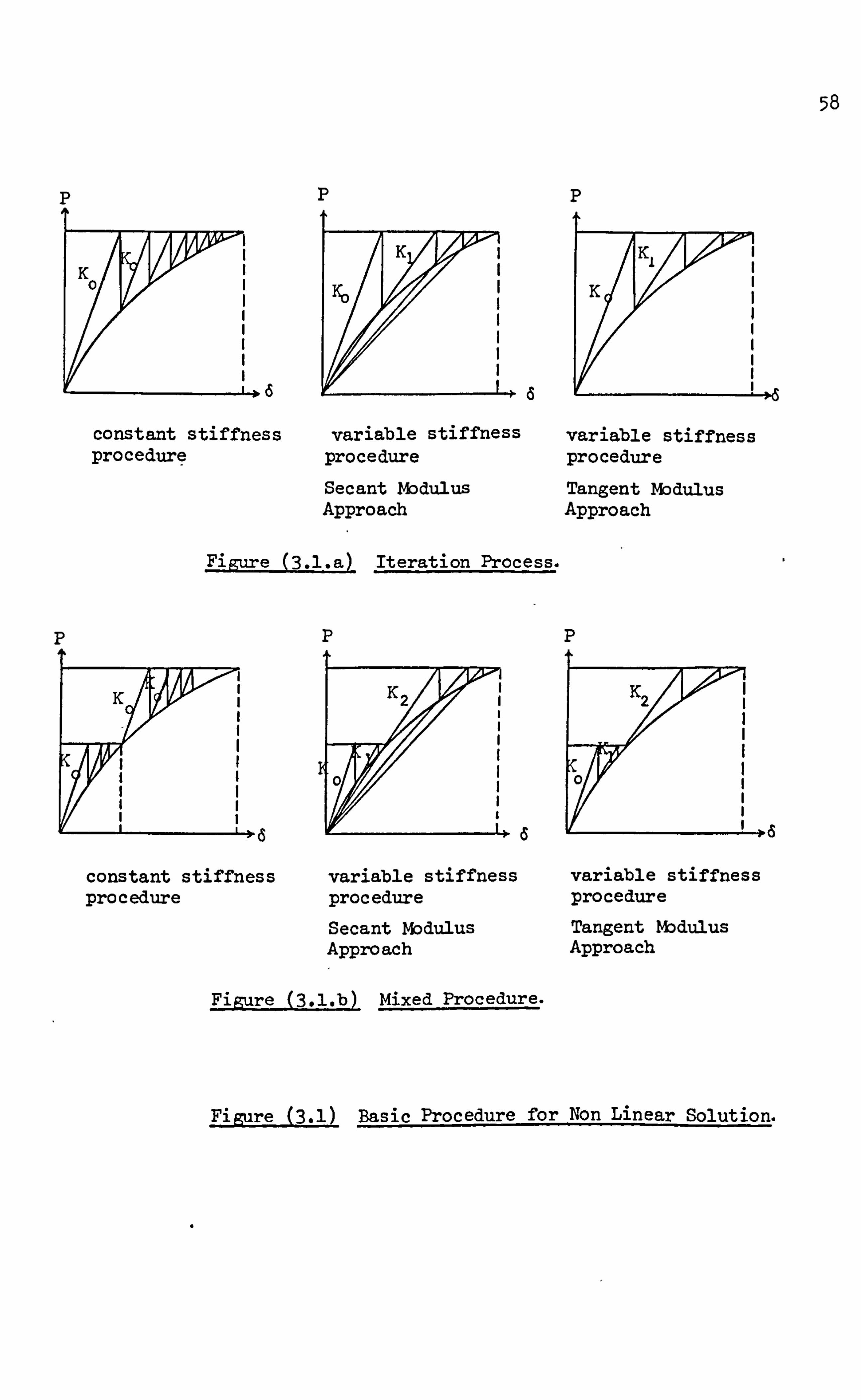
58
P
6
constant stiffness procedure
P
variable stiffness procedure Secant Modulus Approach
6
Figure (3.1. a) Iteration Process.
P
6
constant stiffness procedure
P
variable stiffness procedure Secant Modulus Approach
a
Figure (3.1. b) Mixed Procedure.
P
variable stiffness procedure Tangent Modulus Approach
P
variable stiffness procedure
Tangent ýbdulus Approach
6
Figure (3.1) Basic Procedure for Non Linear Solution.

59
START
ead oblem Pc rIData
Apply lst load of
( check yes Calculate if stiffness a1c. ; Ls the stiffness reqd.
No
II lAfa)n [KI-1 AIR)n
Apply new f
AfRj =AWnM n-l + A{61
n
InI
feln m fc)n--l + Afc),,
I calculate total stresses
Set up {a),, from f(a, c) =0
A{R) t
calculate residuals
=fv [B31 {a )n dv - {Rj n
check if check total no. No r for
of iteration/ rg onvergence
s cc
ýs reacheý/
yes 7es converged
check write I-To if all output
increment and load is
plot
STOP
Figure (3.2) Flow Chart for Non Linear Procedure used in this Analysis

6o REFERENCES
1. Nayak, G. C., "Plasticity and large deformation problems by finite
element method". Ph. D. Thesis, University of Wales, Swansea, 1971.
2. Mindess, S.; Young, F. J., "Concrete". Prenýice-Ha. U, 1981.
3. Nevi1le, A. M., "Properties of concrete". Pitman, 3rd ed., 1981.
4. Desai, C. S.; Abel, J. F., "Introduction to the finite element
method". Van Nostrand, 1972.
Cook, R. D., "Concepts and applications of finite element analysis".
Wiley, 2nd ed., 1981.
Ngo, D.; Franklin, H. A.; Scordelis, A. C., "Finite element study of
reinforced concrete beams with diagonal tension cracks".
Report No. UC-SESM 70-19, University of California, Dec., 1970.
7. Martin, H. C.; Carey, G. F., "Introduction to finite element analysis".
Tata McGraw-Hill, 19T5.
8. Zienkiewicz, O. C., "The finite element method". McGraw-Hill,
3rd ed., 19TT.
Phillips, D. V., "Non linear analysis of structural concrete by
finite element methods". Ph. D. Thesis', University of Wales, 19T3.
10. Zienkiewicz, O. C.; Valliappan, S.; King, I. P., "Elasto-plastic
solution of engineering problems; initial stress finite element
approach". Int. J. Num. Meth. Eng., Vol-1,75-100,1969.
Co . pe, R. J.; Rao, P. V.; Clark, L. A., "Nonlinear design of concrete
bridge slab using finite element procedures". Nonlinear Design
of Concrete Structures, CSE-ASCE-ACI-CEB International Symposium,
University of Waterloo, Ontario, Canada, 3T9-40T, Aug., 1979.
12. Tezcan, S. S.; Mahapatra, B. C.; Mathews, C. I., "Tangent stiffness
matrices for finite elements". IABSE, Vol-30-I, 1970.

61
13. Cope, R. J.; RaoP. V.; Edwards, K. R., "Nonlinear finite element
analysis techniques for concrete slabs". Numerical methods
for nonlinear problems, Proc. of the Int. Con. f.
held in University College, Swansea, 445-456, -Sep ., 198o.
14. Cope, R. J.; Rao, P. V., "Discussion on reference 22 ". Proc.
Inst. Civ. Eng., Vol. 69, Part 2,873-874, Sep., 1980.
15. Cedolin, L.; Nilson, A. H., "A convergence study of iterative
methods applied to finite element analysis of reinforced concrete".
Int. J. Num. - Meth. Eng., Vol. 12,43T-451,19T8.
16. Hinton, E.; Owen, D. R. J., "An introduction to finite element
computations". Pineridge, 19T9.
17. Hinton, E.; Owen, D. R. J., "Finite element programming", Academic,
19TT - 18. Irons, B. M., "A frontal solution program for finite element
analysis". Int. J. Num. Meth. Eng., Vol. 2,2-32,19TO.
19. Cheung, Y. K.; Yeo, M. F., "A practical 'introduction to finite
element analysis". Pitman, 19T9.
20. Alizadeb, A.; Will, G. T., "A substructured frontal solver and its
application to localized material nonlinearity". - Comp. &
Struct., Vol. 10,225-2319 19T9.
21. Razzaque, A., "Automatic reduction of Frontwidth for finite element
analysis". Int. J. Num. Meth. Eng., Vol-15,1315-1324,1080.
22. Duncan, W.; Johnarry, T., "Furtlier studies on the constant stiff-
ness method of nonlinear analysis of concrete structures".
Proc. Inst. Civ. Eng., Part 2, Vol. 67,951-969,1979.
23. Irons, B.; Ahmed, S., "Techniques of finite elements". Wiley, 1981.

CKAPTEý 4
REVIEW OF CONCRETE AND STEEL
BEHAVIOUR AND ITS PREVIOUS MODELLING
4.1 Introduction
4.2 Mathematical description of the behaviour of
reinforced concrete
4.2.1 The behaviour of concrete
4.2.2 Modelling steel reinforcement
4.2.3 The bond-slip phenomenon between steel and
concrete
4.3 Mechanical behaviour of concrete under different
states of loading
4.3.1 Uniaxial. stress behaviour
4.3.2 Biaxial stress behaviour
4.3.3 Triaxial, stress behaviour
4.3.4 Definition of dilatation of concrete
4.3.5 Hydrostatic pressure sensitivity
4.3.6 Shear across cracks
4.4 Mechanical behaviour of steel
4.4.1 Brief description of steel behaviour
4.4.2 Bond-slip and dowel action
4.5 General conclusions
CHAPTER 4 62 REVIEW OF CONCRETE AND STEEL
BEHAVIOUR AND ITS PREVIOUS MODELLING
4.1 Introduction:
A reliable prediction of the behaviour of reinforced concrete
structures requires a knowledge of the behaviour of concrete in its
elastic, inelastic and nonlinear ranges. A good material law should
be able to produce the deformation behaviour of the structure accurately
but this depends on the experimental data available. Recently, more
and more experimental knowledge has become available regarding the
deformation and strength properties of concrete under various loading
systems. The accuracy of this data however, is often in question
because of uncertainties concerning the efficiency of the various
testing systems used to achieve given states of stress within specimens.
Preferably the information obtained experimentally should be
combined with some basic theory in order to produce a set of mathe-
matical formulae for use in analysis. Nowadays the power of computers
is such that accurate and complex laws can be incorporated without too
much difficulty. The main problem is in defining a suitable law. In
recent years a lot of work has been carried out in modelling concrete
and there are several ways of achieving this. A good summary is given
(85) by Chen
One recent development in particular is where the material behaviour
of concrete is defined in terms of several internal state variables.
Known as the "endochronic theory", it appears to be very promising for
describing concrete behaviour under a wide range of loading conditions.
It is this method which will be particularly developed in this work.
The purpose of this chapter is to review the various methods
available for defining the constitutive material laws for reinforced
concrete. It will also include a discussion of relevant information
about concrete and steel behaviour.
63
4.2 Mathematical description of the behaviour of reinforced concrete:
In the mathematical modelling of reinforced concrete there are
three main areas to be examined.
1. The behaviour of concrete.
2. The response of steel reinforcement.
3. The bond-slip phenomenon between steel and concrete.
Each of these points will be discussed separately in the following
sections.
4.2.1 The behaviour of concrete:
Various mathematical approaches are available for defining the
stress-strain behaviour of reinforced concrete under different stress
states. In this section a general description of these models will
be given. However behaviour in tension zones, particularly cracking,
is usually modelled separately and therefore this will be discussed
separately. In fact tension cracking in general has a dominating
effect on the nonlinear response and the compression model quite often
takes secondary importance.
The mathematical approaches can be classified as follows:
(A) Curve fitting:
This method has been used predominately to describe uniaxial
stress-strain data and numerous references are available. (6,7,8,10,11,12,72
i. (16) (68) (85) Reviews are also given by Popovics , Sargin and Chen
Basically the method describes the uniaxial stress in terms of
the strain in that direction using curve fitting techniques. The
advantage of this method is that it is very easy to use in comparison
to other methods. Its basic disadvantage is the lack of any underlying
theory. It is simply a matter of fitting curves and formulae to a given

64
set of data. It is therefore doubtful whether extrapolation is possible
for other concrete structures under different states of stress.
(B) Physical model of the concrete microstructure:
The basis of this method is to use a numerical method, such as
the finite element method, to provide information on the behaviour of
a material specimen. The specimen can be made up of difficult components,
such as mortar, aggregate, aggregate/mortar, interface bond in concrete,
and each component is given its own intrinsic properties. An example
of this method is given in reference 45. Its advantage is that it can
provide information on the behaviour of the different components in one
specimen. However, this is not needed for general analysis and in any
case it would be excessively expensive because of the computer time
required to define the behaviour of all the components.
(C) Characterization based on a measure of damage:
This method was introduced by Romstadt (49)
, when he proposed a
multilinear constitutive model for concrete under biaxial stress. The
uniaxial stress strain curve for concrete was first divided into four
regions, corresponding to the four major zones of microcracking activity.
The biaxial stress space was then divided into four corresponding
regions on the assumption that each represented equal amounts of damage
in each zone. This damage is approximated by assuming constant
mechanical behaviour in each zone. (i. e. for each region constant
tangent value of Young's modulus and Poisson's ratio were found from the
chord moduli for the corresponding region of the uniaxial stress-strain
curve). The concept of regions with constant moduli is attractive
computationally, but it seems unlikely that the dilatation and other
properties of concrete can be ad-equately described. The theory was

65
developed for biaxial stress states only, but it is possible that the
concept could be generalised to multiaxial stress states.
(D) Nonlinear elasticity: ý
In this approach the bulk modulus, shear modulus, Poisson's
ratio, and Young's modulus, of concrete are expressed in terms of
stress/strain variables, such as deviatoric stresses or strains,
stress or strain invariants, normal and shear octahedral strains, etc.
These relationships are obtained from experimental data. The moduli
are usually used to formulate an isotropic matrix to represent the
behaviour of concrete at a certain load level. Hypoelastic and hyper-
elastic models are examples of this approximation.
Good results have been obtained using this method, but the
disadvantage is that the data obtained from experimental tests may not
be suitable for other types of analysis, where the conditions are
different. Numerous examples of this approach can be found in references
29,47,48,65,67 and it is explained in more detail in reference 85.
(E) Modified plasticity theory:
This concept has been extended from metals to concrete and is based
on the principles of the classical theory of plasticity . Examples of
this method are given in references 62,63,64. Although some fairly
good results have been obtained, the main disadvantage of this method
is that some of the characteristics of classical plasticity are not
valid for concrete such as the isotropic hardening of the yield surface,
the large ductility, the constant plastic volume requirement etc. Also
some of concrete's characteristics are difficult to represent in plasticity
theory, such as stress softening after peak stress, cracking and cyclic
loading. However these problems can be solved by using different laws.

66
M Endochronic theory:
An example of this theory is given in reference 49. Its basic
concept is to use a pseudo-time'scale called intrinsic (or endochronic)
time, to define deformation in terms of strain and stress. It is
capable of measuring the rate of change or damage of the internal
structure of a material subjected to deformation. The endochronic
model for concrete is based on an extensive set of functions which fit
experimentally observed effects such as inelasticity, strain softening
and hardening, hysteretic behaviour, etc. Since it is the endochronic
method which is adopted in this thesis, details of its mathematical
formulation will be given in the next chapter, when its advantages and
disadvantages will also be explained.
(G) Tension and cracking model:
In general, cracked concrete is usually modelled by a linear
elastic fracture relationship. Two fracture criteria are most commonly
used: the maximum principal stress criterion; and the maximum principal
strain criterion. When a principal stress or strain exceeds its limiting
value a crack is assumed to occur in a plane normal to the direction of
the offending principal stress or strain. The maximum stress criterion
is more commonly used than the maximum strain criterion, although it has
been reported that the maximum strain criterion can predict stiffer (4)
behaviour than the maximum principal stress criterion
In finite element analysis three different approaches have been
employed for crack modelling. These are classified as follows:
(1) Smeared cracking approach: (4,20)
In this, cracks are assumed to be smeared throughout the region in
a continuous fashion, such that across the region there are an infinite
67
number of cracks of infinite crack width. This model assumes that the
concrete becomes an orthotropic material after the first crack has
occurred. It is, the most common model used and will also be used in
this work because it is capable of predicting general description of
concrete behaviour. A fuller, more detailed, description will be given
in Chapter 5.
(2) Discrete cracking MOdel: (86,8T)
In thisthe nodes of adjacent elements are assumed to be separated
when a crack occurs. One obvious difficulty in such an approach is
that the location and orientation of the cracks are not known in
advance and so, geometrical restrictions are imposed by the preselected
finite element mesh. This can be improved to some extent by redefinition
of element nodes, but such techniques are extremely complex and time
consuming. However, this model can be useful in obtaining details of
the local behaviour of structures.
Fracture mechanics model: (91,92)
The success of fracture mechanics in solving various types of
cracking problems, has led to its use in finite element analysis of
reinforced concrete structures. Fracture mechanics may be defined
as the study of the stress and displacement fields in the region of
crack tips in materials which are elastic, homogeneous, and isotropic,
particularly at the onset of unstable crack growth (or fracture).
The advantage of this method is that it will enable us to understand
the mechanical behaviour of concrete more clearly, particularly with
microcracking and cement/aggregate interfacial problems. The development
of this method is still in progress and a lot of work is required to
evaluate its validity.

68
4.2.2 Modelling steel reinforcement:
Steel reinforcement is generally assumed to transmit axial forces
only and thus the description of its stress-strain relationship is
fairly straightforward.
For simplicity in design and analysis it is usual to idealize
the stress-strain curve for steel. Various different idealizations
have been used and some of the more common are shown in Figure (4.1b).
Normally a uniaxial elastic stress-strain curve, with a strain
hardening effect is used in most structural analysis. However, for
cyclic, and large strain problems an additional complexity must be
included to take into account unloading and reloading effects.
4.2.3 The bond-slip phenomenon between steel and concrete: I
The bond-slip relationship between concrete and, reinforced steel
exists because of the adhesion, friction, and mechanical interlock
between concrete and steel. One of the most common methods used to
represent bond-slip is the use of linkage elements. The main idea
is to include a linkage element which connects the nodes of steel and
concrete finite elements. This linkage element is composed of two
springs perpendicular to each other which allow the transfer of forces
between the separate nodes. Each spring must be given a certain
stiffness, obtained from experimental tests. Normally a nonlinear
bond-slip relationship, obtained from a pullout test, is assigned
to the spring parallel to the bar, and a very high stiffness is given
to the spring perpendicular to the bar to prevent any separation between
the bar and the concrete.
69
An advantage of this element is that it has no physical dimension,
i. e. it allows two different deformations to occur at a common node.
One disadvantage is that it is difficult to incorporate, especially
when a high number of reinforcing bars are used at different layers.
Also it is difficult to give a realistic value for the stiffness of
the springs perpendicular to the bar. Details of this method can be
found in references 86,87,88.
Another way of accounting for bond is to use a gradual stiffening
curve for concrete after cracking has occurred, and is usually called
"tension stiffening". This approach is based on the fact that if the
opening of a crack occurs at the same time as bond failure, it will
cause some movement between the bar and the concrete. This will then
cause the shear force at the contact surface between the cracks to
feed tension stresses -into the concrete. The concrete, attached to
the bar will contribute to the overall stiffness of the system. This
contribution is accounted for by the gradual stiffening curve mentioned
above.
An alternative way of representing this stiffening effect is to -
increase the steel stiffness and stress. This additional steel stress,
corresponding to the same strain in the steel, represents the total
tensile force carried by both the steel and concrete between the
cracks.
In this thesis linkage elements are not used because of the high
cost of including this element, especially for heavily reinforced
structures, and also because of the lack of unified mathematical model
for the bond-slip relationship.
Although tension stiffening can be defined on physical grounds,
70
it is essentially a numerical device rather than a bond devis--e. Other
numerical devices will be suggested on the basis of convergence criterion
and will be discussed in more detail in Chapter 6.
4.3 Mechanical behaviour of'concrete under different states of loading:
Concrete is a carefully proportioned mixture of cement, water,
fine aggregate, and coarse aggregate. As soon as the components of
concrete have been mixed together, the cement and water react to produce
a cementing gel (cement paste) which bonds the fine and coarse aggregates
into a stone-likematerial. The chemical reaction between the cement
and water is an exothermic reaction producing significant quantities
of heat termed hydration.
The strength of concrete is a function of the strength of the
cement, the aggregate, and the interaction between the components.
The water-cement ratio is also a major variable influencing the strength
of the concrete. When the water-cement ratio is large, a dilute,
high-shrinking, weak gel is produced. Concrete containing such gels
is low in strength and lacks resistance to deterioration by weathering.
Typical stress-strain curves of aggregate and cement paste are
demonstrated in Figure(4.2). It is clear that the relationship is
linear except at high stress levels. The moduli of elasticity for
the aggregate and the cement paste are quite different. However the
combined response of these materials is markedly nonlinear. This is
mainly due to the nature of the cement-aggregate bond and interirp. of
microcracking when this bond breaks down. It has been found that a
reduction in bond strength leads to an increase in the nonlinearity
of the stress-strain curves. Stronger concretes exhibit a more linear

71
stress-strain curve, and the curve also becomes more linear when the
aggregate stiffness approaches the stiffness of the matrix.
In the next section a review of the work done on the stress-strain
behaviour and strength of concrete under short term loading will be
given. This will be described under three stress states: uniaxial,
biaxial and triaxial.
4.3.1 Uniaxial stress behaviour;
(a) Compression region:
A typical stress-strain curve for concrete subjected to uniaxial
compression is shown in Figure (4-3). In general, a typical curve
will show an almost'linear relationship up to about 30% of its ulti-
mate load. Although bond cracks will already exist, they are quite
stable at low stresses and have little tendency to propagate. In
addition, there is probably some additional crack initiation at highly
localized tensile strain concentrations; -, these cracks also remain
stable at low loads, but their formation probably accounts for the
slight nonlinearity of the stress-strain curve even at low stresses.
Between about 30% and 50% of the ultimate stress, the cracks
begin to propagate, but at a very slow rate. Most of the crack
growth remains in the interfacial region between the aggregate and
mortar. The system of bond cracks multiplies and grows in a stable
fashion, and the stress-strain curve begins to show increasing
curvature.
At this stage, there is very little cracking in the cement
matrix. However, once the stress exceeds about 50% of the ultimate,

72
cracks begin to extend into the matrix. A much more extensive
and continuous crack system begins to develop as matrix cracks
connect the originally isolated bond cracks.
Finally, beyond about 75% of the ultimate stress more rapid
crack growth occurs in the matrix, and the crack system eventually
becomes unstable causing failure.
The uniaxial compressive strength of concrete is the most
common measure for assessing the quality of concrete. In the UK,
the characteristic cube strength of concrete, f cu ,
is used.
This is based on the strength of standard 150 mm cubes 28 days
after mixing; 100 mm cubes are sometimes used if the nominal
maximum size of the aggregate does not exceed 25 nm.
Generally in the USA 150 mm x 300 cylindrical specimens
are tested giving the cylindrical compressive strength fc. These
cylinders have a height to diameter ratio of 2, (l)
and the
cylinder strength is usually about 70-90% of the cube strength.
The difference is due to the friction forces which develop
between the platen plates of the testing machine and the contact
face of the test specimen. These end forces produce a multiaxial
stress state which increases the apparent compressive strength
of concrete. The multiaxial stress cffects are significant
throughout the cube; in the cylinder, the specific height to
width ratio will minimize this effect (89).
Much experimental work has been done on the shape of the
uniaxial stress-strain curves, for examples see references 2,5-16,18-21,
68-72,85.

73
Conclusions can be summarized as follows: The stress-strain
relationship is influenced by the size and shape of-the specimen
and test procedure. This is difficult to formulate since it is
affected by a large number of factors. For example a longer
duration of loading leads to an increase in strains and a decrease
in strength and initial modulus of elasticity.
The other important factors affecting the stress-strain curve
are concrete strength, type of cement, type of aggregate, mix
properties, method of curing and age. For example the stronger
the concrete strength the steeper the slope of ascending and
descending branches of the stress-strain curve.
(b) Tension region:
The shape of the tensile stress-strain curve is much more (23 - 25)
linear than the compressive curve. This is because the
stable crack propagation stage is much shorter and cracks travel
very rapidly through the mortar matrix and around the aggregate (4)
pasteinterface It is difficult to measure the direct tensile
strength of concrete, mainly because of the difficulty of applying
a truly concentric pull. A method for measuring the indirect
tensile strength is sometimes referred to as the "Splitting tensile
strength".
The test consists of loading a cylinder of 150 mx 300 mm,
across its diameter until failure occurs by splitting across the vertical
74
plane. The splitting tensile strength is then calculated with respect
to the maximum load applied and length and diameter of the cylinder.
Generally, for practical purposes, the splitting tensile strength
11 (89) can be taken as /8 to /12 of the cube strength . The tensile
strength in flexure is known as the modulus of rupture and is obtained
by testing a plain concrete beam under synmetrical two point loading
applied at one third-span points. It is only a hypothetical stress
based on the assumption of linear elastic behaviour up to the instant
of rupture. The modulus of ruptureover estimates the true tensile
strength of the concrete and is used only as a comparative measure.
The modulus of rupture is usually about 11 times the splitting cylinder
strength (89)
. More details on the tensile strength of concrete can be
found in references 23-28,72,73,85,89.
4.3.2 Biaxial stress behaviour:
A biaxial stress condition occurs if the principal stresses are
acting in two directions only, and the third principal stress is zero.
Early experiments were focussed primarily on the strength of concrete.
But in recent years, more research has been done on the deformation
and microcracking properties of concrete under biaxial loading.
Detailed reviews have been compiled from time to time:
' (54) (43) (41) (4) Hilsdorf Rosenthal et al. Kupfer et al Phillips
(84) Gerstle et al. . etc.
The measured response of concrete under biaxial stress appears
to be subject to large variations which depends on testing and measuring
techniques, even under working stress levels(77). It has been difficult
to obtain consistent behaviour for concrete under these states. Labib(3)
75
has summarized the main parameters influencing these ýnconsistencies
as follows:
Characteristics of the concrete, such as the fractions of
concrete and paste volume, aggregate particle size, distribution
properties of aggregate and cement paste, and the bond at the
aggregate-paste interface.
2. The size and shape of the specimen.
3. The moisture condition and temperature distribution throughout
the specimen.
4. The influence of machine platens on the stress and strain
distribution of the specimen.
Typical stress-strain curves for concrete under biaxial states of
stress in compression-compression, tension-compression and tension-
tension regions are shown in Figures (4.4), (4-5) and (4.6). These
were obtained from the experimental tests of Kupfer et al. (41)
, where
normal weight concrete specimens of dimension 20 x 20 x5 cm. were
tested. For comparison uniaxial stress-strain curves are also shown
in these figures.
The relationships are essentially linear up to 40% of the failure
stress, with only a small amount of permanent deformation due to
microcracking taking place. Some authors refer to this point as the
"initial discontinuity point" or "elastic limit". In two dimensional
principal stress space this elastic limit is represented by envelope
1 in Figure (4-7). For stress states outside this envelope, larger
cracks form, internal disruption of the material structure takes place,
and substantial permanent deformations are produced. Envelopes 2,3, and

76
in Figure (4.7) show the limits for other important points in the
stress-strain relationship.
In this thesis only the conclusions obtained from various
experimental tests will be given. The test procedures themselves can (41) be found elsewhere, for example in, Kupfer et al. , Rosenthal et al
ý43)'
(45) (46) (47) (52) Buyukoztark et al. , Atan et al. , Liu et al. , Tasuji et al.
and Cedolin et al. (67).
The conclusions can be sunmiarized as follows:
1. The ultimate strength of concrete under biaxiai compression is
greater than that under uniaxial compression. The main reason
for this increase is due to the confinement, of, microcracks.
The ultimate strength increase under biaxial compression, is
dependent on the ratio of principal stresses, and appears to be
maximum (up to about 25% higher than the uniaxial value) at a
stress ratio of about 0.5, diminishing somewhat as the ratio is
increased to unity.
The compressive stress at failure in the region of combined
compression and tension decreases as the tensile stress increases.
The biaxial tensile strength of concrete is approximately equal
to its uniaxial strength, and stress-strain curves are similar
in shape in both uniaxial and biaxial tension.
The variation of Poisson's ratio from biaxial tension (0.18) to
biaxial compression (0.2) is negligible.
The concrete strain corresponding to maximum stress varies from
0.002 (uniaxial) to 0.003 (biaxial).
Volumetric strain behaviour is described separately in Section
4.3.4.
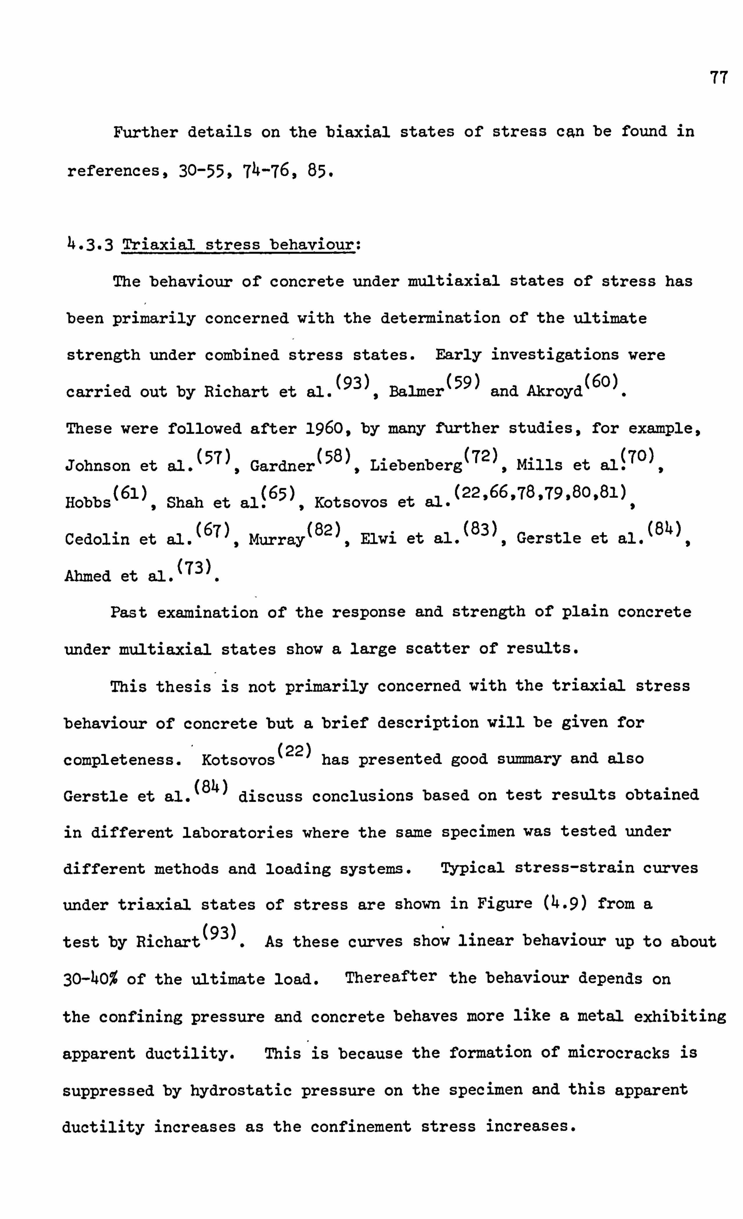
77
Further details on the biaxial states of stress can be found in
references, 30-55,74-76,85.
4.3.3 Triaxial stress behaviour:
The behaviour of concrete under multiaxial states of stress has
been primarily concerned with the determination of the ultimate
strength under combined stress states. Early investigations were
carried out by Richart et al. (93),
Balmer(59) and Akroyd (6o)
. These were followed after 1960, by many further studies, for example,
Johnson et al. (57),
Gardner(58) , Liebenberg (72)
, Mills et al! 70)
Hobbs (61),
Shah et al ! 65),
Kotsovos et al. (22,66,78,79,80,81)
,
Cedolin et al. (67)
, Murray (82)
, Elwi et al. (83)
, Gerstle et al. (84)
(73) Ahmed et al.
Past examination of the response and strength of plain concrete
under multiaxial states show a large scatter of results.
This thesis is not primarily concerned with the triaxial stress
behaviour of concrete but a brief description will be given for
completeness. '
Kotsovos (22)
has presented good summary and also
Gerstle et al. (84)
discuss conclusions based on test results obtained
in different laboratories where the same specimen was tested under
different methods and loading systems. Typical stress-strain curves
under triaxial states of stress are shown in Figure (4.9) from a
(93) test by Richart . As these curves show linear behaviour up to about
30-40% of the ultimate load. Thereafter the behaviour depends on
the confining pressure and concrete behaves more like a metal exhibiting
apparent ductility. This is because the formation of microcracks is
suppressed by hydrostatic pressure on the specimen and this apparent
ductility increases as the confinement stress increases.
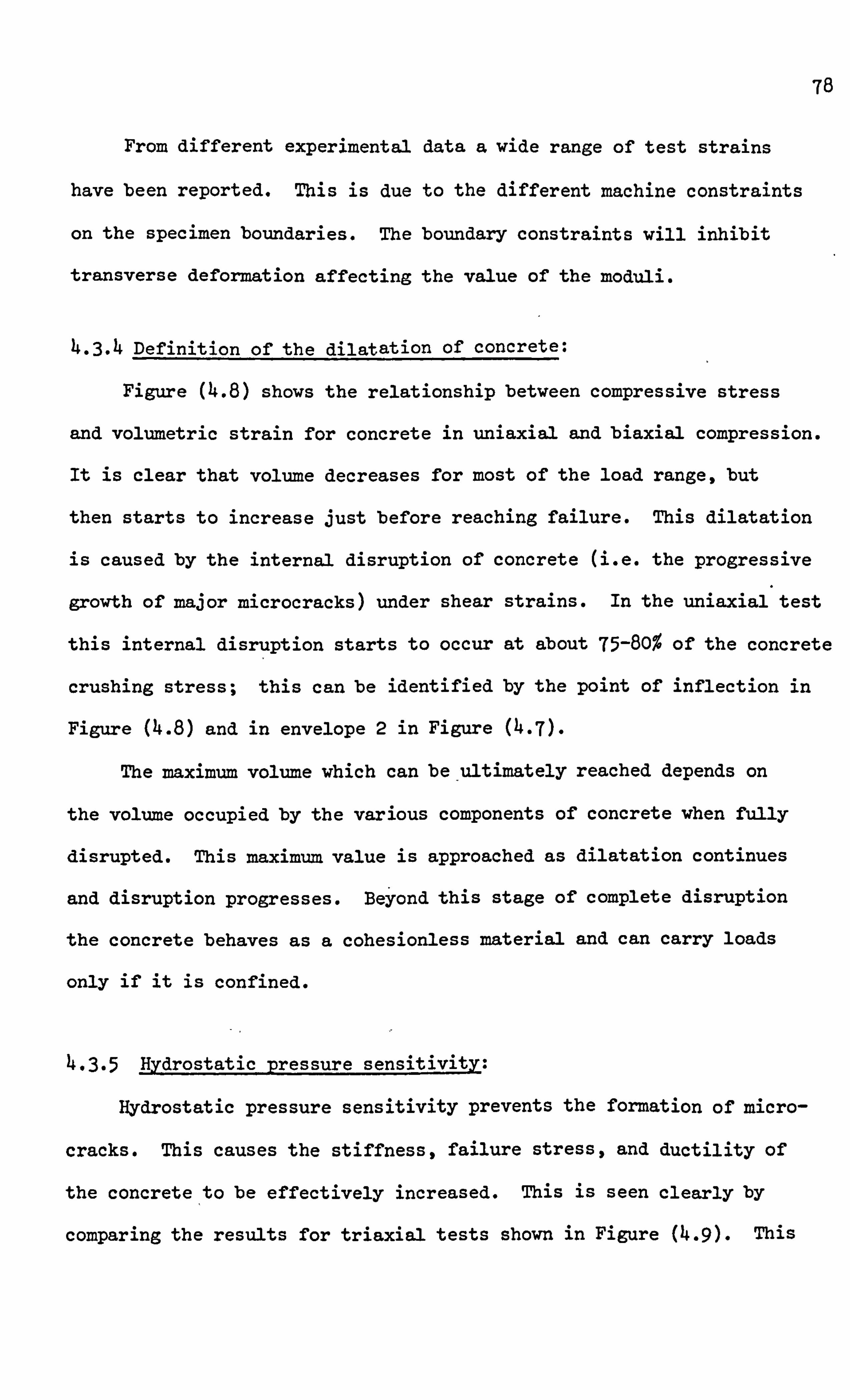
78
From different experimental data a wide range of test strains
have been reported. This is due to the different machine constraints
on the specimen boundaries. The boundary constraints will inhibit
transverse deformation affecting the value of the moduli.
4.3.4 Definition of the dilatation of concrete:
Figure (4.8) shows the relationship between compressive stress
and volumetric strain for concrete in uniaxial and biaxial compression.
It is clear that volume decreases for most of the load range, but
then starts to increase just before reaching failure. This dilatation
is caused by the internal disruption of concrete (i. e. the progressive
growth of major microcracks) under shear strains. In the uniaxial, test
this internal disruption starts to occur at about 75-80% of the concrete
crushing stress; this can be identified by the point of inflection in
Figure (4.8) and in envelope 2 in Figure (4-7).
The maximilm volume which can beultimately reached depends on
the volume occupied by the various components of concrete when fully
disrupted. This maximum value is approached as dilatation continues
and disruption progresses. Beyond this stage of complete disruption
the concrete behaves as a cohesionless material and can carry loads
only if it is confined.
4.3-5 Hydrostatic pressure sensitivity:
Hydrostatic pressure sensitivity prevents the formation of micro-
cracks. This causes the stiffness, failure stress, and ductility of
the concrete to be effectively increased. This is seen clearly by
comparing the results for triaxial. tests shown in Figure (4.9). This
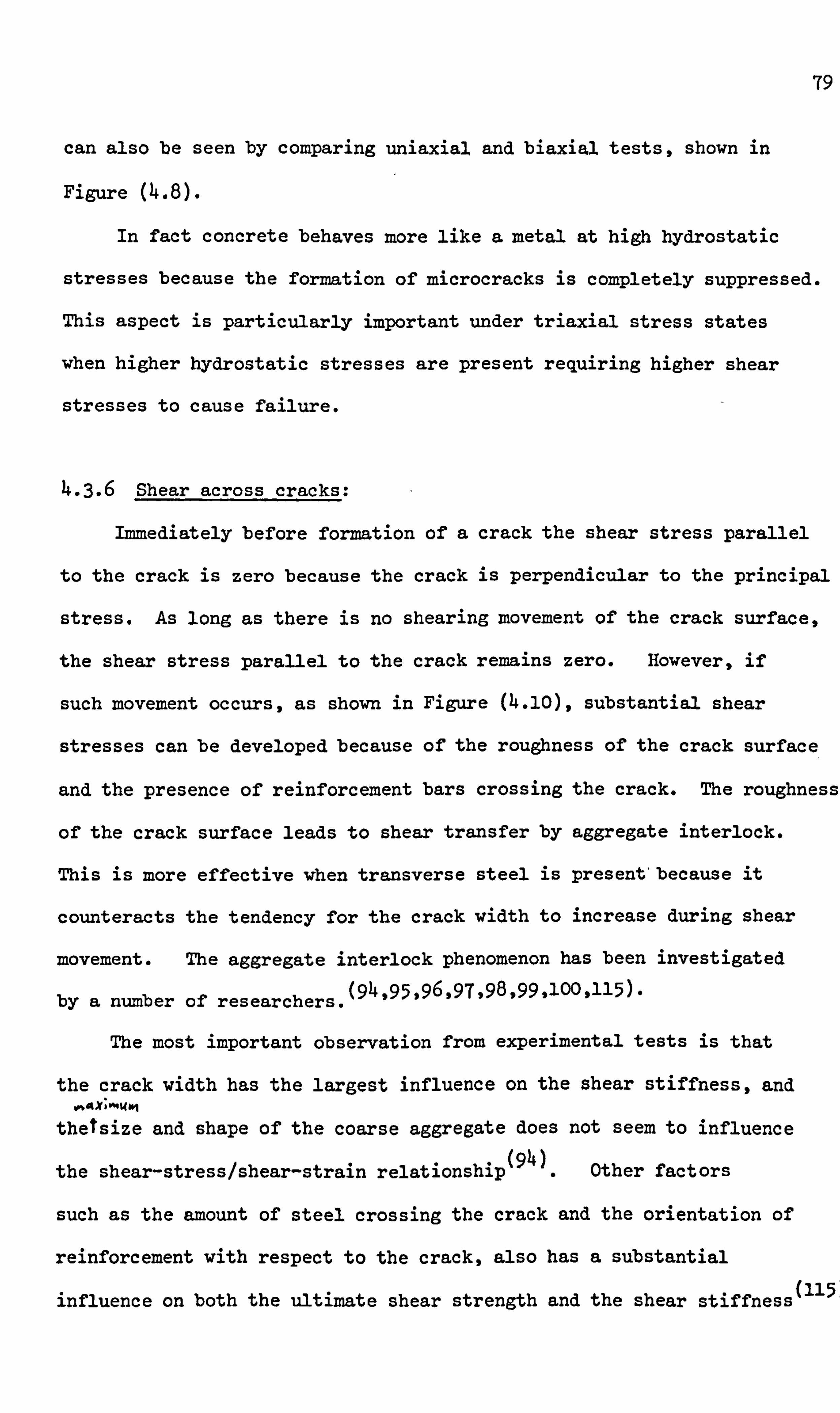
79
can also be seen by comparing uniaxial and biaxial tests, shown in
Figure (4.8).
In fact concrete behaves more like a metal at high hydrostatic
stresses because the formation of microcracks is completely suppressed.
This aspect is particularly important under triaxial stress states
when higher hydrostatic stresses are present requiring higher shear
stresses to cause failure.
4.3.6 Shear across cracks:
Immediately before formation of a crack the shear stress parallel
to the crack is zero because the crack is perpendicular to the principal
stress. As long as there is no shearing movement of the crack surface,
the shear stress parallel to the crack remains zero. However, if
such movement occurs, as shown in Figure (4.10), substantial shear
stresses can be developed because of the roughness of the crack surface
and the presence of reinforcement bars crossing the crack. The roughness
of the crack surface leads to shear transfer by aggregate interlock.
This is more effective when transverse steel is present'because it
counteracts the tendency for the crack width to increase during shear
movement. The aggregate interlock phenomenon has been investigated
by a number of researchers. (94,95,96,9T, 98,99,100,115).
The most important observation from experimental tests is that
the crack width has the largest influence on the shear stiffness, and #,.. Kxb. "Wm
thetsize and shape of the coarse aggregate does not seem to influence
(94) the shear-stress/shear-strain relationship Other factors
such as the amount of steel crossing the crack and the orientation of
reinforcement with respect to the crack, also has a substantial
influence on both the ultimate shear strength and the shear stiffness(115

80
4.4 Mechanical behaviour of'steel:
4.4.1 Brief description of steel*behaviour:
Since steel reinforcement is predominantly uniaxial, it is
generally not necessary to introduce the complexity of a multiaxial,
constitutive relationship for steel.
A typical uniaxial stress-strain diagram for steel is shown in
Figure (4.1a). Initially the relationship is linear and elastic
until the "proportional limit" P is reached. For a further small
range of stress increase, the strain is still elastic but no longer
linearly related. The "yield point" Y is then reached and this marks
the start of plastic deformation. The difference between P and Y is
slight for most steels and is usually neglected in practical applications.
Beyond the yield point, plastic flow occurs with strain increasing at a
much greater rate. Generally, stress must be increased to cause further
deform tion, a condition termed strain or work hardening. Eventually
a maximilm stress is reached at point V, after which a descending tail
rapidly occurs to fracture at F.
Some materials, such as mild steel, exhibit a small but sharp drop
in load after yield to a lower yield level. Thereafter strains increase
plastically at more or less constant load to about ten times the yield
strain. At this point the material begins to work harden, and clearly
the lower yield point should be used for calculation purposes.
For practical purposes steel exists in various forms. Basically
these are:
1. Plain round hot-rolled bars of either, mild steel, medium-strength
steel, or high strength steel. Yield stresses vary from about
250 N/mm2 (34,000 lb/jn2)' to 360 N/mM2 (52,000 lb/in2), whilst

81
the corresponding ultimate strengths vary from 460 NIMM2 (67,000
lb/in2) to 600 N/mm2 (88,000 lb/in2).
2. Cold worked bars or. drawn wire of mild, or more usually, high
tensile steel bars. Such reinforcement exhibits considerably
higher yield stresses (or proof stresses since most bars of this
type do not have a definite yield point). Twisted round or square
bars normally have proof stresses depending on the size of
diameter and range from 410 N1mm 2 (6o, ooo lb/in2) to 480 N/mm2
(70,000'lb/in2).
The Young modulus of steel is about 200 x 103 NIMM2 (30 x 106 lb/in2
4.4.2 Bond-slip and dowel action:
Bond stress is the name assigned to the shearing stress parallel
to the bar axis on the steel-concrete interface. This bond transfers
the force from the steel bar to the surrounding concrete and vice versa.
The bond between concrete and steel results from chemical adhesion,
friction and mechanical interaction between the concrete and the steel.
For plain reinforced bars, chemical adhesion and friction are the
major contributory factors to the bond strength (i. e. the ultimate
load that is obtained before bond failure), while mechanical interaction
plays a minor role. Considerable slip has been observed between the
steel bar and the concrete, suggesting the loss of adhesion at relatively
low stresses, (101)
and that the subsequent bond resistance is due to
the frictional drag on the bar at locations without adhesion. Bond
failures in specimens reinforced with plain bars were characterized
by the extraction of the bar from the concrete specimen.
Deformed bars were introduced to alter this behaviour pattern and

82
the projecting deformations, ribs or lugs, add to the bond resistance
by bearing on the concrete and thereby minimizing slip considerably.
As shown in Figure (4.31)the bond resistance for a deformed bar is
activated at the lug interface by bearing pressure, which can be
resolved into two components. One component acts parallel to the bar
tending to shear the concrete along a cylindrical failure surface,
while the second component acts radially and tends to create longitudinal
splitting. The latter mode of failure is the more common.
Scordelis (102)
has also given the following as factors which
affect the ultimate bond strengths; type of loading, confining lateral
reinforcement or pressure, concrete cover, bar spacing, location of
splices.
Reinforced bars also act as dowels as shown in Figure (4.12), when
major shear deformation occurs after the development of tension cracking
and the bar will take concentrated shear force.
Many factors can effect the dowel action such as various bar
diameters, specimen geometry, length of the reinforcement and its
arrangement and cover of the concrete. Dowel effect becomes more
important especially under cyclic loading and more work is required
to be done.
Reviews on bond and dowel problems can be found in references
21., 101 - 116.
4.5 General Conclusions:
1. Reinforced concrete structures under realistic loading are
subjected to a great number of influences such as tension cracking,
multiaxial response, bond slip, dowel action, aggregate interlocking

83
etc. An accurate inclusion of all these factors ýn a computer
program would appear to be quite impossible even though these
factors and the interaction between them, must have some effect on
the result of an analysis.
For the time being, because we do not have complete information
regarding the different factors influencing the behaviour of concrete
and steel interaction, it is more useful to use the available information
in as simple a form as possible, rather than introducing complexities
which still reply on approximation to known behaviour and, data.
2. There is a fair scatter of test results for strength and deformation
properties of concrete. This causes difficulties in forming adequate
md, thematical laws.
3. More experimental tests are required under biaxial states of
stress to enable a clearer picture of concrete behaviour to emerge.
4. Because tension cracking has a dominant effect on the nonlinear
response, care must be taken in developing methods which describe
cracking behaviour.
5. In order to obtain realistic mathematical models, it is necessary
to include the following factors in some fashion:
(a) A suitable multiaxial compression failure criterion.
(b) A realistic multiaxial cracking criterion in tension and suitable
post-cracking behaviour.
(c) An accurate model for representing stress-strain behaviour
for all multiaxial, stress ranges.
84
(d) An adequate stress-$train curve for steel.
(e) An accurate representation for bond problems between the
steel reinforcement and concrete.
6. A unified representation of uniaxial, biaxial and triaxial
concrete response appears possible at low load stress levels but
may break down near failure.
Concrete response to multiaxial stress states at working levels
can be considered as linear elastic material for engineering purposes.
8. Most studies have been carried out on uniaxial modelling because
of the availability of wide range of experimental work. For biaxial
and triaxial modelling the problem is more difficult and requires
more complexity to. model the behaviour satisfactorily.
9. There are several'approaches used to describe mathematically
the stress-strain behaviour of concrete. The endochronic approach
will be used in this thesis because it appears to have much potential
for wide and accurate application.

a Cold worked high strength steel bar
vP= Proportional limit Y= Initial yield point
yFV= Ultimate stress F= Fracture point
v
Mild steel bar F
y
Figure (4.1a) Typical stress-strain curve.
a
a I
C S Elastic strain hardening
approximation
cr
a y
cy y 0.8cr
a
CY y
C S
C S
Trilinear approximation Complete curve
Figure (4.1b) Idealized stress-strain curves.
Figure (4.1) Stress-strain curve for steel reinforcement.
S
Cs
Elastic semi-perfect plastic approximation
85
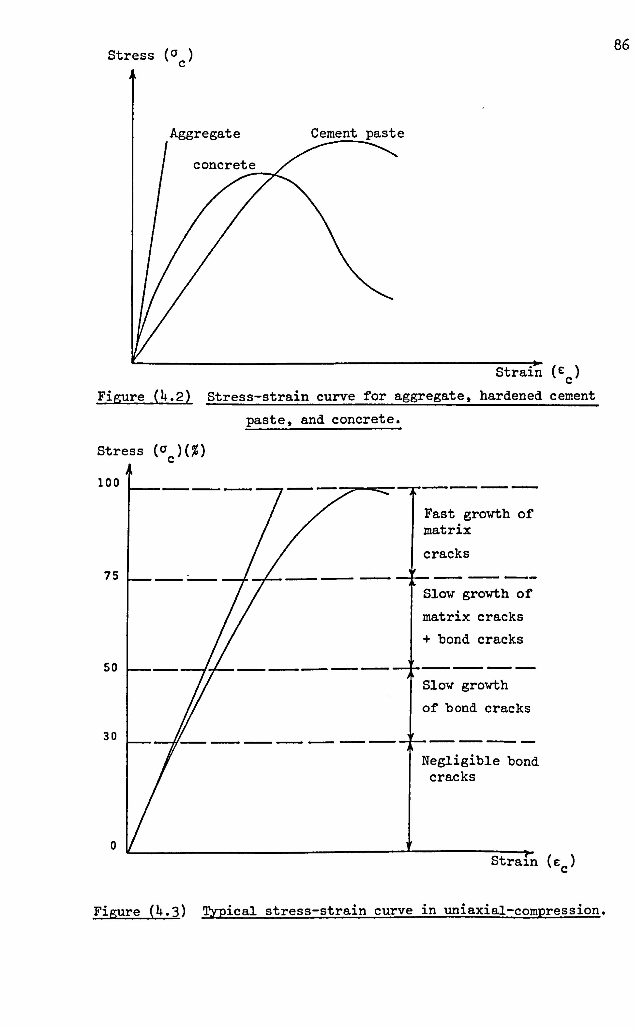
Stress (c C)
Strain (cc)
Figure (4.2) Stress-strain curve for aggregate, hardened cement
paste, and concrete.
Stress (a
100
Fast growth of matrix
cracks 7S -E- -- --
Slow growth of
matrix cracks
+ bond cracks
so r- Slow grovth
of bond cracks
30 r If - 44 Negligible bond
cracks
0 Strain (c
C)
86
Figure (4-3) Typical stress-strain curve in uniaxial-compression.

a1/ fc, f' = 32.8 N/mm
11-3 c
3 11-2
3 100 El. C,
E2=c3 \ I,. Od -. Cl
4h +G
k, j al ap
C) + Cr2 C-4
Scm - A -1/-0.52 c4m
I-IIIVI11 6*1 96: 2 3, e3
+T-0 +3-0 +2-0 +1-0 0 -1-0 -2-0 -3-0 -4-0 113M/M r
tensile strain compressive strain Figure (4.4) Experimental stress-strain curves for (41)
biaxial compression. (Kupfer et al. ).
al/;, - c fe = 32.8 JI/nm +1-2
1*0 c
0,9
e Zý- 3 0-8 cl '1 0-7
e2 Y3 F- L
0-6 + CY 01 /Cr2 l 005
+a2 0.052 ci
cm ........ -1/0 1 03 20CM
-4- 11-1y1111E: 1 , r; 2
- 9C3
+7-* 0 +I-U +U. b u _U -b _ilu _ZIU -3*U mm/m
tensile strain compressive strain
87
Figure'(4.5) Experimental stress-strain curves for biaxial tension-compression. (Kupfer et al)"-'
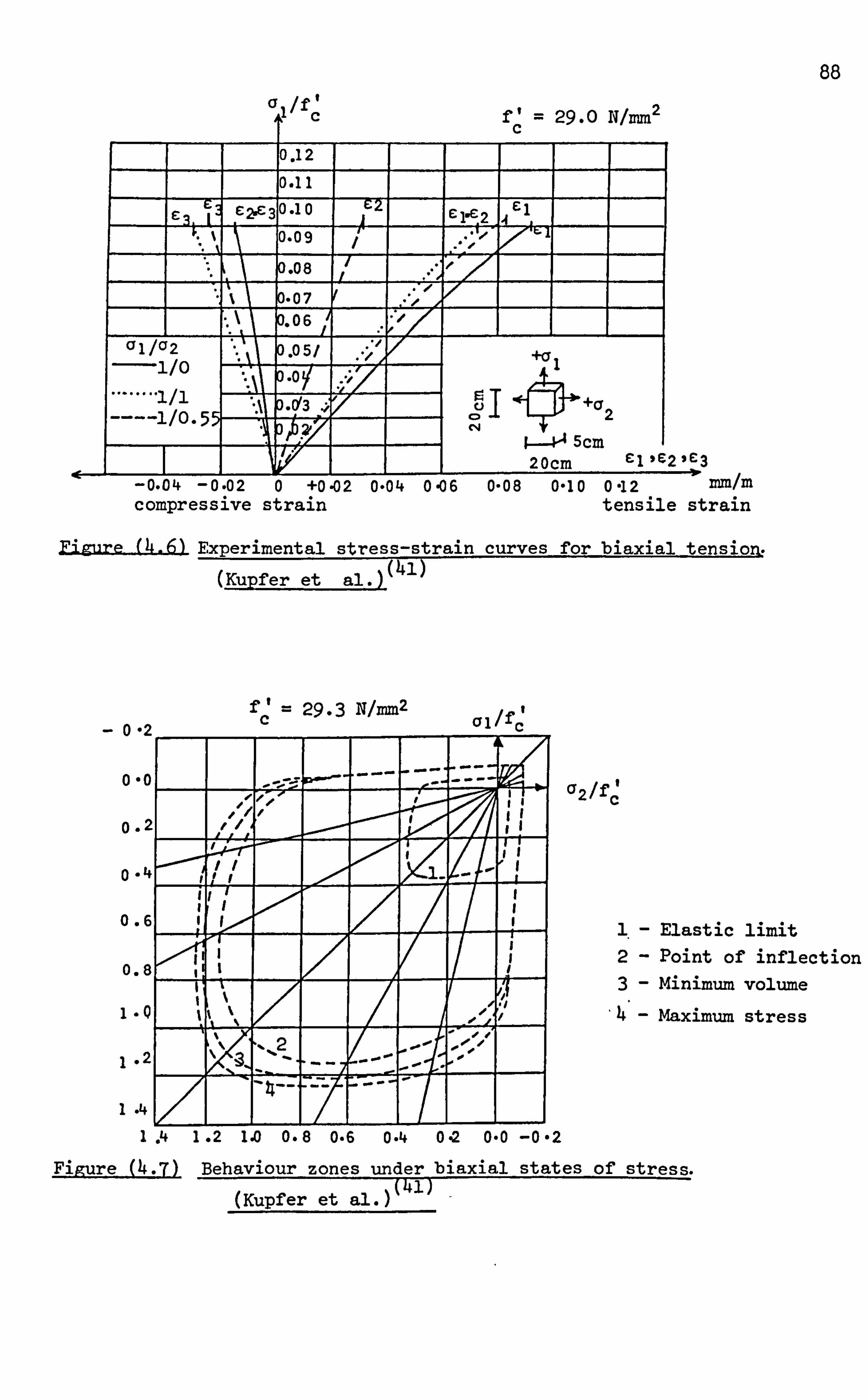
88
01/f C f' 29.0 N/mm 2
c
0.12
E_ 10.10
0.11
Eq, I, C2ýE30*10 C Pý 2 0.09
_T_ 3.08
)-07 ). 06
Cy 1 /Cy 2.. I % ). 051 +al
........ -V rl +Cr IY3
----1/0.55 2
77 SCM 20cm C11'629r:. 3 .
IP
No 0.04 -0 02 0 +0-02 0-04 0-06 0-08 0-10 0-12 mm/m
compressive strain tensile strain
Figure (4.6) Experimental stress-strain curves for biaxial tensio
(Kupfer et al. ) (41)
- 0-2
o "c 0.
o . 11
O. E
E
a2/f
l. - Elastic limit 2- Point of inflection 3- Minimum volume 4- Maximum stress
1 .4 [/ I-II/II/III
1 .41 .21.0 0-8 0-6 0-4 0-2 0-0 -0-2 Figure (4.7) Behaviour zones under biaxial states of stress.
7 (Kupfer et al. ) (41
_
ft = 29.3 N/MM2 I c Gilff-
A f

89
Of ,
CF I /CF2 -1.0
-1/-l - e-5
-1/0 -0.8
-0.7 +CFI -0.6
0.5 2 -0.4
-0.3
-0.2
-0.1
2
4
fC = 32.06 11/mm 2
3
1- Elastic limit 2- Point of inflection 3- Minimum volume 4- Maximum stress
I
AV v
+ 1ý 0'0 -110 -2 4D
-JO - MM/M
volume increase volume decrease
Figure (4.8) Volumetric strain of concrete under uniaxial -80. and biaxial compression. (EuRfer et al-F'ý'
19.6 N/mm2 f2 cP= -13.86 N) mm
-70 -0 2= C13
-60
cli -50 2 -7-52 N rm
0 -40
to -JU -P- -3-T9 N/mm
20
p=0 -10 p
0. (11
ý-O . 00 5.,.
C -0.010 -0.015 Axial strain I
Figure (4.9) Axial stress-strain curve for triaxial compression test by Richart et al. 033
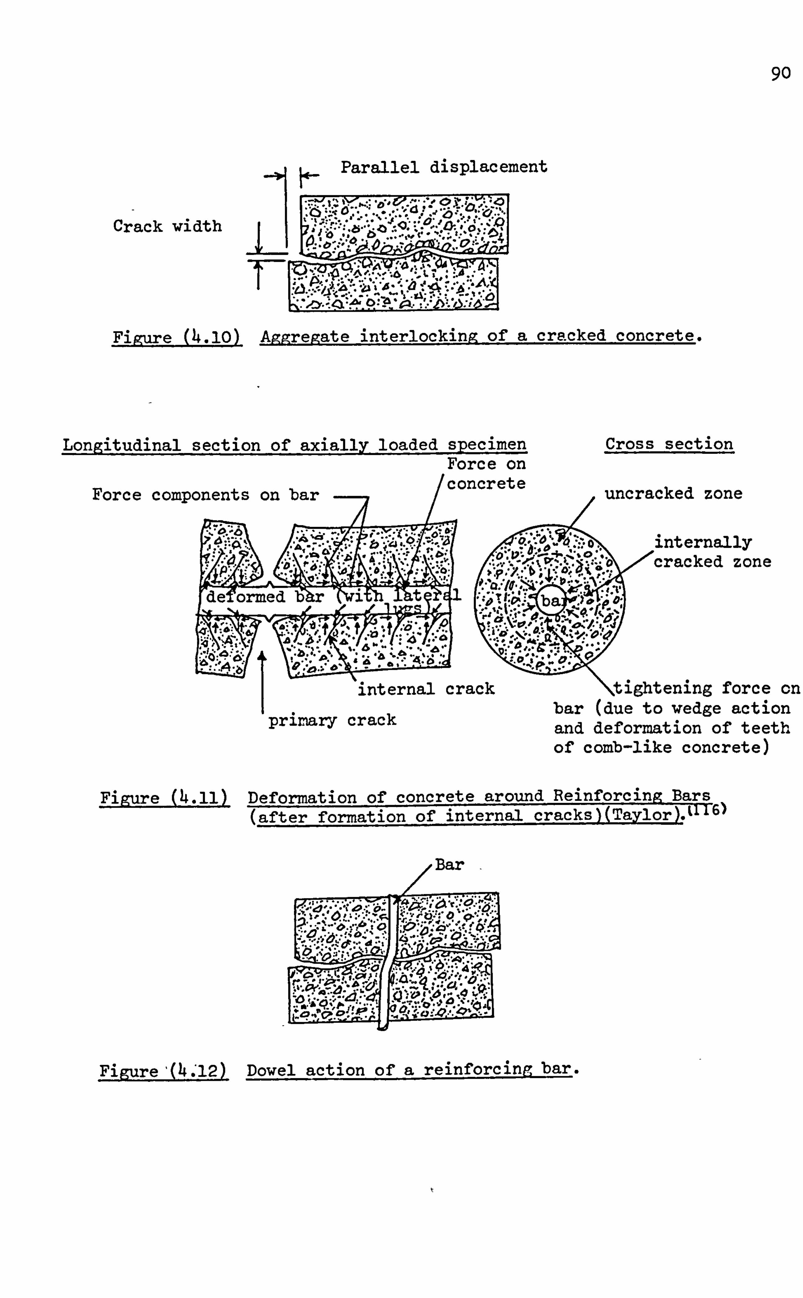
90
Parallel displacement
07. Crack width "0",
Figure (4.121 Aggregate interlocking of a cracked concrete.
Longitudinal section of axially loaded specimen Force on
Force components on bar concrete
Cross section
uncracked zone
, internally cracked zone
internal crack
prinary crack
Ntightening force on bar (due to wedge action and deformation of teeth of comb-like concrete)
Figure (4.11) Deformation of concrete around Reinforcing Bars (after formation of internal cracks)(T lor). tlibl
Figureý(4.12) Dowel action of a reinforcing bar.

91
. REFERENCES.
1. Park, R.; Paulay, T., "Reinforced concrete structures". Wiley 1975.
2. R, ýsch, H., I'Versuche zur festigkeit der biegedruckzone
(Experiments concerning the strength of the compression zone
in bending)". Deutscher Ausschuss fur stahlbetont Heft 120,
Berlin, 1955.
3. Labib, F., "Nonlinear analysis of the bond and crack distribution
in reinforced concrete members". Ph. D. Thesýis, University, of London,
Sep., 1976.,
4. Phillips, D. V., "Nonlineax analysis of structural concrete by
finite element method". Ph. D. Thesis, University of Wales, 1973.
5. Shah, S. P.; Winter, G., "Inelastic behaviour and fracture of
concrete". J. ACI, Vol. 63,925-930, Sep ., 1966.
6. Desayi, P.; Krishnan, S., "Equation for the stress strain curve
-for concrete". J. ACI. Vol. 619 345-350, May, 1964-
7- Saenz, L. P., "Discussion on reference 611. J. ACI, Vol. 61,1229-1235,
Sep., 1964.
8. Tulin, L. G.; Gerstle, X. H., "Discussion on reference 6% J. ACIt
vol. 61,1236-1238, Sep., 1964-
9. Smith, G. M.; Young, L. E., "Ultimate flexural analysis. based on
stress-strain curve of cylinders". J. ACI, Vol-53,597-610t
Dec., 1956.
10. Richard, R. M.; Abbott, B. J., I'Verstile elastic plastic stress-
strain formula". J. of Eng. Mech. Div., ASCE, 511-515,, Aug-PI975-
11. Popovics, S., "A numerical approach to the complete stress-strain
curve for concrete". Cement &. Conc. Res., Vol-3,583-599,1973-

92
12. Ramberg, W.; Osgood, W. R., "Description of stress-strain curve
by three parameters". Technical Note No. 902f National
Advisory Committee for Aeronauticsj Washington, D. C., 1943.
13. Hognested, E., "A study of combined bending and axial load in
reinforced concrete members". Bulletin No-3990 Eng. Experimental
Station, University of Illinois, 1951.
14. Bresler, B., "Reinforced concrete engineering". Vol. 1, Wiley, 1974-
15. Kent, D. C. -; Park, R., "Flexural members with confined concrete".
J. of Struct. Div., ASCE, Vol. 97,1969-1990, July, 1971-
16. Popovics, S., "A review of stress-strain relationship for concrete".
j. Aci, vol. 67,243-248, March, 1970-
17. Malhotra, V. M., "Are 4x8 inch concrete cylindersas good as
6x 12 inch cylinders for quality control of concrete". J. ACI,
Vol-73,33-36, Jan., 1976.
18. Comit4 Europeen du Bgtonp "International recommendation for the
design and construction of concrete structures". Cement
Conc. Res., 1970-
19. Neville, A. M. 9 "Properties of concrete". Pitman# 1981.
20. Faherty, K. P., "An analysis of reinforced and prestressed
concrete by finite element method". Ph. D. Thesis, University
of Iowa, 1972.
21. Johnston, D. W. -; Zia, P., "Analysis of dowel action". J. of
Struct. Div., ASCE, Vol-97,1611-16309 MaY, 1971-
22. ' Kotsovos, M. C. 9 "Mathematical description of the deformation
behaviour of concrete under generalise stress state".
Interim report, Imperial College, London, Dec. 9 1978.
93
23. Hughes, B. P.; Champman, G. P., "The complete stress-strain curve
for concrete in direct tension". Rilem Bulletin No-30,
95-989 Maxch, 1966.
24. Todd, J. D., "The determination of tensile stress-strain curve
for concrete". Proc. Inst. Civ. Eng., Part 1, Vol-4,201-211,
March, 1955.
25. Hughes, B. P.; Ashv J. E., "Short term loading and deformation of
concrete in uniaxial tension and pure torsion". Mag. Conc.
Res., Vol. 20,145-154, Sep., 1968.
1 26. Evans, R. H.; Marathe, M. S., "Microcracking and stress-strain
curve for concrete in tension". Material and Struct., Res.
and Testing No. 1,61-64, Feb. f 1968.
27- Komlos, K., "Determination of the tensile strength of concrete".
The Indian Conc. J., Vol-42,68-76, Feb., 1968.
28. Madu, R. M., "Characterization of the stress-strain curves for
reinforced concrete under uniaxial tension". Mag. Cone. Res.,
Vol. 27,210-218, Dec., 1975-
29. Coon, M. D.; Evans, R. J., "Incremental constitutive law and their
associated failure criteria with application to plain concrete".
Int. J. Solids & Struct., Vol-8,1169-1183,1972.
30. Wastlund, G., "New evidence regarding the basic strength properties
of concrete". Betongq Vol. 3, Stockholmo 189-205,1937-
31- Iyengar, K. T. S. R.; Chandrashekhara, X.; Krishnaswamyg K. T.,
"Strength of concrete under biaxial compression". J. ACIO
vol. 62,239-249, Feb.., 1965.
32. Vile, G. W. D.; Sigvaldasont O. T., "Discussion on reference 31"-
i. Aci, vol. 62v 1192-1195, Sep., 1965.
94
33. Bellamyt C. J., "Strength of concrete under combined stresses".
, T. ACIp Vol-58,367-381, Oct., 1961.
34- Vile, G. W. D., "The strength of concrete under short term biaxial
stresses". Int. Conf. on Structural of Concretet London,
Sep., 1965.
35. Weigler, H.; Becker, G., llUber das bruch Und veformungsverhalten
von beton bei Mehrachsiger Beanspruchung". Der Bauingenieur, -
Heft 10,390-396,1961.
36. Bresler, B., Pister, K. S., "Strength of concrete under combined
stresses". J. -ACI,
Vol-559 321-345, Sep., 1958.,
37. Goode, C. D.; Helmy, M. A., "The strength of concrete under
combined shear and direct stress". Mag. Cone. Res. 9 Vol. 19, ,
105-112, June, 1967.
38. McHenry, D.; Karni, J., "Strength of concrete under combined
tensile and c=pressive stress". J. ACI, Vol. 299 829-839,
April, 1958.
39. Smith, G. M., "Failure of concrete under combined tensile and
compressive stresses". J. ACI, Vol. 25,137-1409 ()Ct-, 1953-
40. Krishnaswamy, K. T., "Strength of concrete under combined tensile-
compressive stress". Materiaux et contructions, Vol. 2,
187-194,1969.
41. Kupfer, H.; Hilsdorf, H. K., "Behaviour of concrete under biaxial
stresses". J. ACI, Vol. 66,656-666, Aug., 1969.
42. Pandit, G.; Zimmerman, R. M., "Discussion on reference 41",
ACI, Vol. 67,194-197, Feb., 1970-
43. Rosenthal, I.; Clucklich, J., "Strength of concrete under biaxial
stress". J. ACI, Vol. 67,903-914, Nov., 1970-
95
44. Krishnaswamay, K. T.; Pandit, G. S., "Discussion on reference 43"-
J. ACI, Vol. 68,404-4o6, may, 1971.
45. Buyukozturk, -O.;
Nilson, A. H.; Slate, F. O., "Stress-strain response
and fracture, of a concrete model in biaxial loading". J. ACI,
vol. 68,590-598, Aug., 1971-
46. Atan, Y.; Slate, F. O., "Structural lightweight concrete under
biaxial compression". J. ACI, Vol-70o 182-185, March, 1973-
47. Liuv T. C. Y.; Nilson, A. H.; Slate, F. O. 9 "Stress-strain response
and fracture of concrete in uniaxial and biaxial compression".
J. ACI, vol. 69,291-2959 MaYt 1972.
48. Kupfer, H.; Gerstle, K. H. ý "Behaviour of concrete under biaxial
stresses". J. of Eng. Mech. Div., ASCE, Vol. 99,853-a66, Aug-, 1973-
49. Rosmstad, K. M.; Taylor, M. A.; Herrmann, L. R., "Numerical biaxial
characterization for concrete". J. of Eng. Mech. Div. 9, ASCE,
Vol-10OP 935-948, Oct., 1974.
50. Darwin, D.; Pecknold, D. A., "Nonlinear biaxial stress-strain law
for concrete". J. of Eng. Mech. Div., ASCE, Vol-103,229-241,
APril, 1977.
51. Andenaes, E.; Gerstle, K.; Ko, H. Y., "Response, of mortax and
concrete to biaxial compression ". J. of Eng. Mech. Div.,
ASCE, Vol-103,515-526, Aug., 1977.
52. Tasujiq M. E.; Slatet F. O.; Nilson, A. H. t "Stress strain response
and fracture of concrete in biaxial loading". J. ACI, Vol-75,
3o6-312, July, 1978.1
53. Cedolin, L.; -Deipoli, S., "Finite element studies of shear-
critical R/c beams". J. of Eng. Mech. Div., ASCE, V01-103,
395-410, June, 1977.

96
54. Hilsdorf, H., "The experimental determination of the biaxial
strength of concrete". (Die Bestimmung Derzweiachsigen-
festigkeit von Beton) Proc., Vol-1739 Deutscher Ausschuss fur
Stahlbeton, Berlin, 1965.
55. Rajagopalan, K., "Discussion on reference 51"- J- of Eng. Mech.
Div., ASCE, Vol-104,715-, June, 1978-
56. Mills, L. L.; Zimmerman, R. M., "Compressive strength of plain
concrete under multiaxial loading conditions". J. ACI, Vol. 67,
802-8071 qct., 1970.
57. Johnson, R. P.; Lowe, P. G. 9 "Behaviour of concrete under biaxial
and triaxial, stresses". Int. Conf. on Struct., Solid Mech.
and Eng. Design in Civil Eng. Materials, Paper NO. 899
Southampton University, April, 1969.
58. Gardner, N. J., "Triaxial behaviour of concrete". J. ACI, Vol. 66,
136-146, Feb., 1969.
59. Balmer, G. G., "Shearing strength of concrete under high triaxial
stress-computation of Mohr's envelope as a curve". Report
No. Sp-23, Denver, Colorado, Oct-9 1949-
60. Akroyd, T. N. W., "Concrete under triaxial stress". Mag. Cone.
Res., Vol-13,111-118, Nov., 1961.
61. Hobbs, D. W., "Strength and deformation properties of plain concrete
subject to combined stress". Cement &. Con. Association,
Report No-42, July, 1974-
62. Chen, A. C. T.; Chen, W. F., "Constitutive relations for concrete".
J. of Eng. Mech. Div., ASCE, Vol-101,465-481, Aug., 1971.
63. Chen, A. C. T.; Chen, W. F., "Constitutive equations and punch
indentation of concrete". J. of Eng. Mech. Div., ASCE0. Vol. 1010
889-906, Dec., 1975-
97
64. Chen, A. C. T., "Constitutive relations of concrete and punch
indentation problems, '. Ph. D. Thesis, Lehigh University, 1973-
65. Palaniswamy, R.; Shag, S. P., "Fracture and stress-strain relation-
ship of concrete under triaxial compression". J. of, Strct.
Div., ASCE, Vol. 100,901-916, May, 1974-
66. Kotsovos, M. D.; Newmant J. B., "Behaviour of concrete under multi-
axial stress". J. ACI, Vol-74,443-446, Sep.. 1977.
67. Cedolin, L.; Crutzen, Y. R. J.; Deipoli, S. 9 "Triaxial stress-strain
relationship for concrete". J. of Eng. Mech. Div., ASCE, Vol.
103P 423-439, June, 1979- 68. Sargin, M., "Stress-strain relationships for concrete and the
analysis of structural concrete relationships", Solid Mech.
Div., University of Waterloo, Canada, 1971-
69. Sahlin, S., "Effect of far-advanced compressive strains of concrete
in reinforced concrete beams subjected to bending moments.
Betong Vol-40, Stockholmv 1955-
70- Young, L. E., "Simplifying ultimate flexural theory of maximizing
the moment of the stress block". J. ACI, Vol-57o 549-556,
Nov. , 1960.
71. Kriz., L. B.; Lee, S. L., "Ultimate strength of over reinforced
beams". J. of Eng. Mech. Div., ASCE, 95-105, June, 1960.
72. Leibenberg, A. C., "A stress-strain function of concrete subjected
to short term loading". Mag. Conc. Res. 0 Vol. 619 345-350,
March, 1964.
73. Ahmad, S. H.; Shah, S. P., "Complete triaxial stress-strain curves
for concrete". J. of Struct. Div., ASCE, Vol-108,728-742,
April, 1982.

98
74. Ottosen, N. S. v "Constitutive model for short time loading of
concrete". J. of Eng. Mech. Div., ASCE, Vol-105,127-141,
Feb., 1979-
75. Murray, D. W.; Chitnuyanondh, L.; Rijub-Agha, Y. R.; Wong, C.,
"Concrete plasticity theory for biaxial stress analysis".
J. of Eng. Mech. Div., ASCE, Vol-105t 989-1005, Dec., 1979.
76. Tasuji, M. E.; Nilson, A. H.; Slate, F. O., "Blaxial stress-strain
relationships for concrete". Mag. Cono. Res. 9 Vol-31,217-2249
1979.
77. Gerstle, K. H., "Simple formulation of biaxial concrete behaviour".
-T. ACI, Vol-78,62-68, Jan. -Feb. 9 1981.
78. Kotsovos, M. D. ; Newman, J. B., "A mathematical description of
the deformation behaviour of concrete under complex loading".
Mag. Conc. Res., Vol-31,77-90, June, 1979,
79. Kotsovos, M. D., "Effect of stress path on the behaviour of
concrete under triaxial stress states". J. ACI, Vol-76,
213-2239 Feb., 1979-
80. Kotsovos, M. D., "A mathematical description of the strength
properties of concrete under generalized stressp Mag. Cone.
Res., Vol-31,151-158, Sept. 1979-
81. Kotsovos, M. D.; Newman, J. B., "Mathematical description of
deformational behaviour of concrete under generalized stress
beyond ultimate strength". J. ACI, Vol-779 340-346, Sept-Oct.,
1980. 82. Murray, D. W., "Octahedral based incremental stress strain
matriCes". J. of Eng. Mech. Div., ASCE, Vol-1059 501-513,
Aug., 1979-

99
83. Elwi, A. A.; Murrayt D. W. 9 "A 3D hypoelastic concrete constitutive
relationship". J. of Eng. Mech. Div. t ASCEO Vol-105t 623-641t
Aug. , 1979.
84. Gerstle, K. H.; Aschl, H.; Bellotti, R.; Bertacchi, P.; Kotosovos,
M. D.; Ko, H.; Linse, D.; Newmant J. B.; Rossi, P.; Schickert,
G.; Taylor, M. A.; Traina, L. A.; Winkler, H.; Zimmermang R. M.
"Behaviour of concrete under multiaxial stress states".
J. of Eng. Mech. Div., ASCE, Vol. 106,1383-1403, Dec., 1980.
85- Chen, W. P. v "Plasticity in reinforced concrete". McGraw-Hill,
1982.
86. Ngo, D.; Prankline, H. A.; Scordelist A. C. 1, "Finite element study
of reinforced concrete beams with diagonal tension cracks".
Report No. UC-SESM 70-199 University of Californiat Dec. t1970. 87. Ngo, D.; Scordelis, A. C., "Finite element analysis of reinforced
concrete beams". J. ACI, Vol. 64t 162-163t March, 1967-
88. NilsontA. H. t "Nonlinear analysis of reinforced concrete by the
finite element method". J. ACI, Vol. 65,757-766t Sep. . 1968.
89. 'Kong, E. K.; Evans, R. H., "Reinforced and prestressed concrete".
Thomas Nelson, 1981.
90. Bazant, Z. P., Bhat, P. D., "Endochronic. theory of inelasticity
and failure of concrete". J. of Eng. Mech. Div.,, Vol. 102,
331-344, Aug., 1976.
91. Hillemier, B.; Hilsdorf, H. K., "Fracture mechanics studies of
concrete compounds". Cement &. Cono Res., Vol- 79 523-536,1977-
92. Bazant, Z. P., Cedolin, L., "Blunt crack band propagation in finite
element analysis". J. of Eng. Mech. t Div., ASCEt V01-105,
297-3159 April, 1979.

100
93. Richaxt, F. E.; Iýrandtzaegt A.; Brown, R. L. t "A study of the
failure of concrete under combined comIrcessive stresses".
Balletin No-185, Eng. Experimental Stationt University of
Illinois, 1928.
94- Paulay, T.; Loeber, P. J., "Shear transfer by aggregate interlock".
Proc. of the Shear Symposium, ACI Publication SP-42t Vol. 1,
1-15v 1973.
95. Morrell, P. J. B.; Chia, C. H. v "A method of determining the contri-
bution of aggregate interlock forces to the shear resistance
of singly reinforced concrete beams". Proc. Inst. Civ. Eng.,
Paxt 2, Vol. 69,885-861,1980.
96. Fardis, M. N.; Buyukozturk, 0., "Shear transfer model for reinforced
concrete". J. of Eng. Mech. Div. g ASCE, Vol-105,255-275P
April, 1979.
97- Walraven, J. C., "Pandamental analySis of aggregate interlock".
J. of Struct. Div., ASCE, Vol-107,2245-22709 Nov., 1981.
98. Gerstle, K. H., "Material modelling of reinforced concrete".
IABSE Colloquium on The Advanced Mechanics of Reinforced
Concrete, Introductory Report, Delft, 41--62,1981.,
99. Walraven, J. C.; Vos, E.; Reinhardt, H. W., "Experiments on shear
transfer, in cracks in concrete". Report NO-5-79-3t Part 1,
Delft University, 1979-
100. Reinhardt, H. W.; Walraven, J. C. 9 "Crack in concrete subject to
shear". J. of Struct. Div., ASCE, Vol. 108,207-224t Jan., 1982
101. Mylrea, T. D., "Bond and anohoragell. J- ACIP Vol-44t 521-5529
March, 1948.
101
102. Scordelis, A. C., "General report - Basic Problem". IASS Symposium
on the nonlinear behaviour of reinforced concrete spatial
stractures, Vol-3.35-70v JulY, 1978-
103. Lutz, L. A.; Gergely, P., "Mechanics of Bond and slip of defo=ed bars
in concrete". J. ACI, Vol. 64,711-721v Nov-,,, 1967-
104- Perry, E. S.; Jundi, N., "Pullout bond stress distribution under
static and dynamic repeated loadings". J. ACI, Vol. 66,377-380,
May, 1969.
105. Nilsont A. H. t "Bond stress-slip relations in reinforced concrete".
Report No-345, Cornell Universityv Dqo., 1971.
106. Testa, R. B.; Stubbs, N., "Bond failure and inelastic response of
concrete". J. of Eng. Mech. Div., ASCE, Vol-103,295-3109
April, 1977.
107- Mirza, S. M.; Houde, J., "Study of bond stress-slip relationships
in reinforced concrete". J. ACIq Vol-769 19-46t jan., 1979.
108. Kemp, E. L.; Wilhelm W. J., "InVestigation of the parameters
influencing bond cracking". J. ACI, Vol-76o 47-71 , Jan., 1979-
109. Jimenez, R.; White, R. N.; Gergely, P., "Bond and dowel capacities
of reinforced concrete". J. ACIP Vol-76P 73-92, Jan., 1979-
110. Tassios, T. P.; Yannopoulos, P. J., "Analytical studies on reinforced
concrete members under cyclic loading based on bond stress-
slip relationshipsts. j. ACI9 Vol-78,206-216, MayýJune, 1981.
111. Somayaji, S.; Shah, S. P., "Bond stress versus slip relationship
and crpLcking response of tension members". J. ACIq Vol-78,
217-225, May--June, 1981.
112. Edwards, A. D.; Yannopoulos, P. J., "Local bond-stress-slip
relationships under repeated loading". Vol-30,62-72, June, 1978-
102
113. Tepfers, R. 9 "Lapped tensile reinforcement splices". J. of
Struct. Div. ', ASCE, Vol. 1089 283-3019 Jan., 1982.
114. Venkateswarlug B.; Gesund, H., 'Tracking and bond-slip in
concrete beams". J. of Struct. Div. t ASCE# V01.98,2663-2685P
Dec., 1982.
115- Mattock, A. H., "Shear transfer in concrete having reinforcement
at an angle to the sheax plane". ACI Publioation SP-42,
Vol. 2,17-42,1973.
116. Taylor, H. P. T., "Shear stresses inreinforced concrete beams
without shear reinforcement". Technical Reportq TRA 407,
Cem. & Con. Association, London, Feb., 1968.
CHAPTER 5
MATHEMATICAL MODELLING OF THE
CONSTITUTIVE LAWS FCR REINFCRCED CONCRETE
5-1 Introduction
5.2 The endochronic model
5.2.1 Historical review
5.2.2 Basic assumption of the endochronic theory
5.2.3 Application to rAetals
5.2-4 Application to concrete
5.2-5 Summary of the equations of the endochronic theory
5.2.6 Numerical procedure for applying the endochronic
theory
5.2-7 Stress-strain curves obtained using the endochronic
model
5.3 The cracking model
5.3.1 Procedure for the first cracking model
5.3.2 Procedure for the second cracking model -
5-4 The uniaxial-compression model
5-5 The crushing model
5.6 Theoretical model for steel

103 CHAPTER 5
MATHEMATICAL MODELLING OF THE CONSTITUTIVE LAWS FOR REINFORCED CONCRETE
5.1 Introduction:
In this chapter the mathematical models used for concrete and
steel will be explained in detail. A brief summary of the models will
be given first in this section.
For the concrete there are various conditions to consider which
depend on the state of stress and ýhe state of cracking, and different
models are used to represent these various aspects of behaviour.
Before the start of cracking, the endochronic model is used to represent
all states of stress. But as cracks develop different paths are
selected; a cracking model to represent cracking behaviour, a uniaxial-
compression model to represent regions of uniaxial-compression, and
failure conditions to represent the crushing of concrete.
(1) The endochronic model:
This model is used for the description of concrete behaviour in
the stress regions of biaxial-compression, tension-compression, and
tension-tension before the development of cracks. The same formulation
is used to describe all, these states. The endochronic theory was first
presented for concrete by Bazant, et al ! 1). in 1974 and has since been
improved in various ways. It will be explained in detail in section 5.2.
(2) The cracking model:
A separate cracking model is required because the endochronic theory
aspresented in this thesis does not apply for tensile cracking. Although
it is possible to include this by changing some functions in the model,
it is more realistic to introduce an independent criterion for tensile
cracking. (4)
The cracking model is primarily based on the maximum
stress criterion using the uniaxial tensile strength of concrete V as t

104
a measure for crack initiation. However the maximum principal strain
criterion is also included for certain cases as explained later.
For post cracking, two different models have been investigated. One
assumes a sudden drop in stress in the plane perpendicular to the crack
direction after a crack has occurred, and the other assumes a gradual
release of the stress in this direction. Aggregate interlocking along
a crack is represented by a simple factor.
This is sometimes called the shear retention factor and retains
some shear capacity after cracking. The smeared crack approach is used to
represent the material after cracking. This will be discussed in
detail in section 5-3.
(3) The uniaxial-compression model:
The model proposed by Popovics (20)
for uniaxial-compression is
used in regions where a crack has occurred and compressive strains
exist in the direction parallel to the crack. The reason for this
procedure is because it is difficult to use the endochronic theory
when a separate cracking model is included. It is difficult to change
material parameters from a biaxial, state into a uniaxial, state. This
model is explained in section 5.4.
(4) The crushing model:
A separate model is used to represent crushing of concrete.
The onset of crushing is based on a crushing strain envelope for
uniaxial, and biaxial conditions. It is applicable for all states of
stress and was formulated in this way to avoid having separate models
for the Popovics and endochronic procedures. Further details are
explained in Section 5-5.
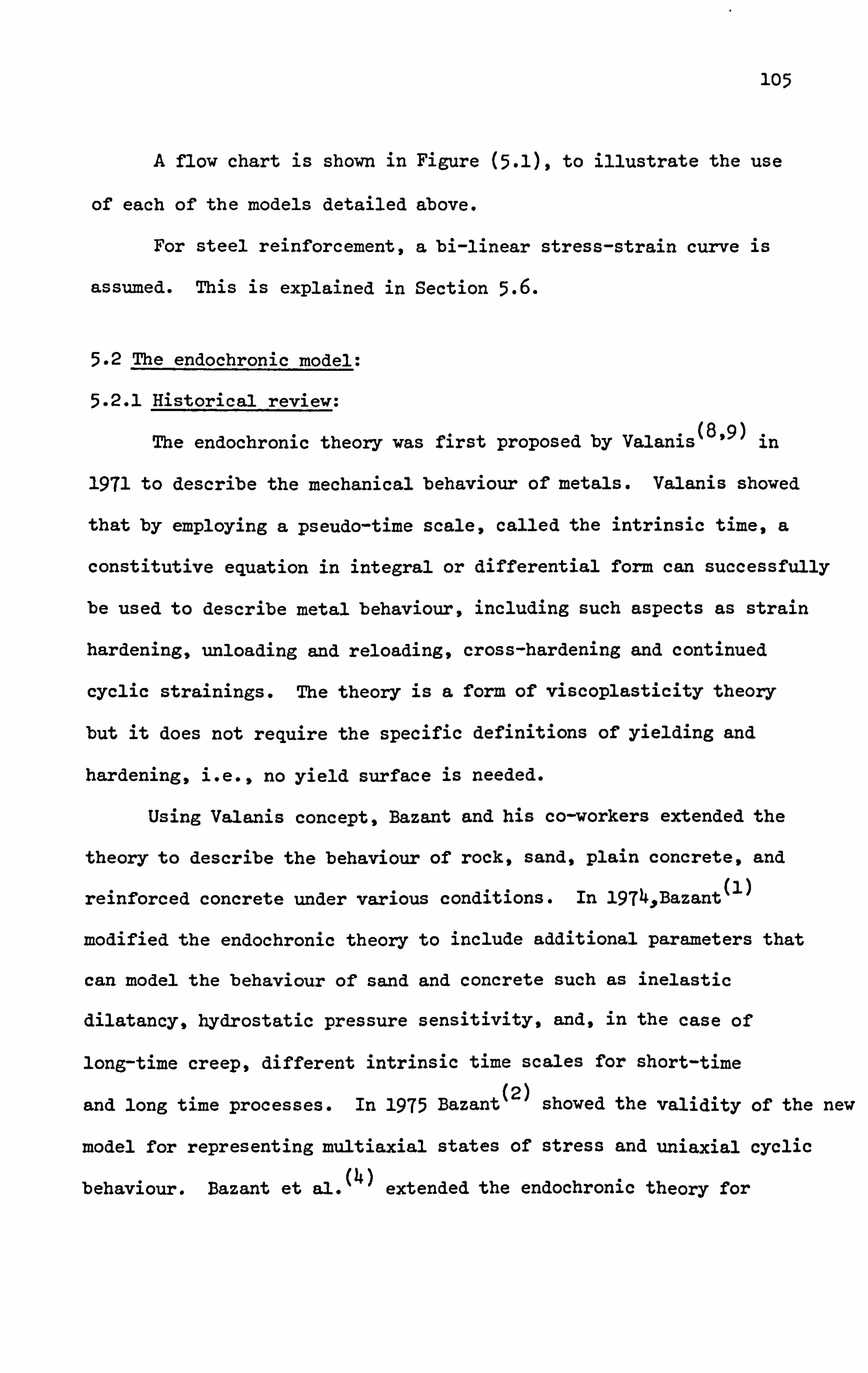
105
A flow chart is shown in Figure (5-1), to illustrate the use
of each of the models detailed above.
For steel reinforcement, a bi-linear stress-strain curve is
assumed. This is explained in Section 5.6.
5.2 The endochronic model:
5.2.1 Historical review:
The endochronic theory was first proposed by Valanis(8'9) in
1971 to describe the mechanical behaviour of metals. Valanis showed
that by employing a pseudo-time scale, called the intrinsic time, a
constitutive equation in integral or differential form can successfully
be used to describe metal behaviour, including such aspects as strain
hardening, unloading and reloading, cross-hardening and continued
cyclic strainings. The theory is a form of viscoplasticity theory
but it does not require the specific definitions of yielding and
hardening, i. e., no yield surface is needed.
Using Valanis concept, Bazant and his co-workers extended the
theory to describe the behaviour of rock, sand, plain concrete, and
reinforced concrete under various conditions. In 1974,, Bazant(l)
modified the endochronic theory to include additional parameters that
can model the behaviour of sand and concrete such as inelastic
dilatancy, hydrostatic pressure sensitivity, and, in the case of
long-time creep, different intrinsic time scales for short-time
and long time processes. In 1975 Bazant (2)
showed the validity of the new
model for representing multiaxial states of stress and uniaxial cyclic
behaviour. Bazant et al. (4)
extended the endochronic theory for

106
analysing the nonlinear behaviour of sand under conditions of cyclic
shear.
Further modifications were carried out by Bazant et al. for
concrete nonlinear behaviour in references 3,5,6,10. This thesis
develops a version presented by Bazant et al. in reference 10. This
incorporates a wide range of'concrete properties such as the stress-
strain curves under uniaxial, biaxial and triaxial stress states for
different strengths, their failure envelopes, strain softening
behaviour, inelastic strains due to hydrostatic compression, lateral
strains and volume expansion, and dependance of material parameters
on the strength. Bazant's version also incorporates other aspects
such as cyclic loading behaviour and creep response but these were not
used in this work.
Certain shortcomings of this model have been reported. For
example, the original model(3) was found to givemuch too steep an
unloading curve and too mild a degradation of elastic moduli when large
creep strains occurred. Also when unloading was reversed to reloading
the slope became smaller when it should have become steeper. Also,
when a low stress, cyclic loading was followed by a high stress load,
the response was too stiff. (13-15,17,18)
Some recent papers(13,18)
have been concerned with trying to modify the theory to deal with
these shortcomings.
The theory is still under active study and improvement. (7,10,13,14,,
18,24) However it has evolved far enough to represent concrete
behaviour for the problems dealt with in this thesis. Indeed different
versions of the theory have already been used in practical applications

107
of finite element analysis for concrete structures, for exmaple
references 11,12,19.
The endochronic model in this work has been modified to be
suitable for two dimensional finite element analysis. Special
techniques are used to obtain the appropriate solutions, as will
be explained in Section 5.2.6.
5.2.2 Basic assumption of the endochronic'theo -8) As explained in the previous section the endochronic theory
does not require the use of the concept of a yield surface and suggests
instead physical interpretations in terms of damage, microcracking
and internal friction. The phenomenon of distinct yielding is most
common in metals and makes a sudden transition from a linear-elastic
to a nonlinear plastic stress-strain response. But yielding is often
a gradual transition, which makes it difficult to state precisely when
it has occurred.
Thus the absence of a yield surface makes the endochronic theory
useful for representing this type of behaviour. Instead, the theory
includes plastic deformations whenever deformation takes place and
this is useful for materials such as concrete which tend to have
inelastic strains from the early stages, although initially of course they
are small compared to elastic deformations.
The theory is based upon the observation that the state of stress
at a point in a plastic material depends on the set of the previous states
of deformation oP- all points in its neighbourhood; but it does'not
depend on the rapidity at which such deformation states have succeeded
one another. In the case of such rate independent behaviouran absolute
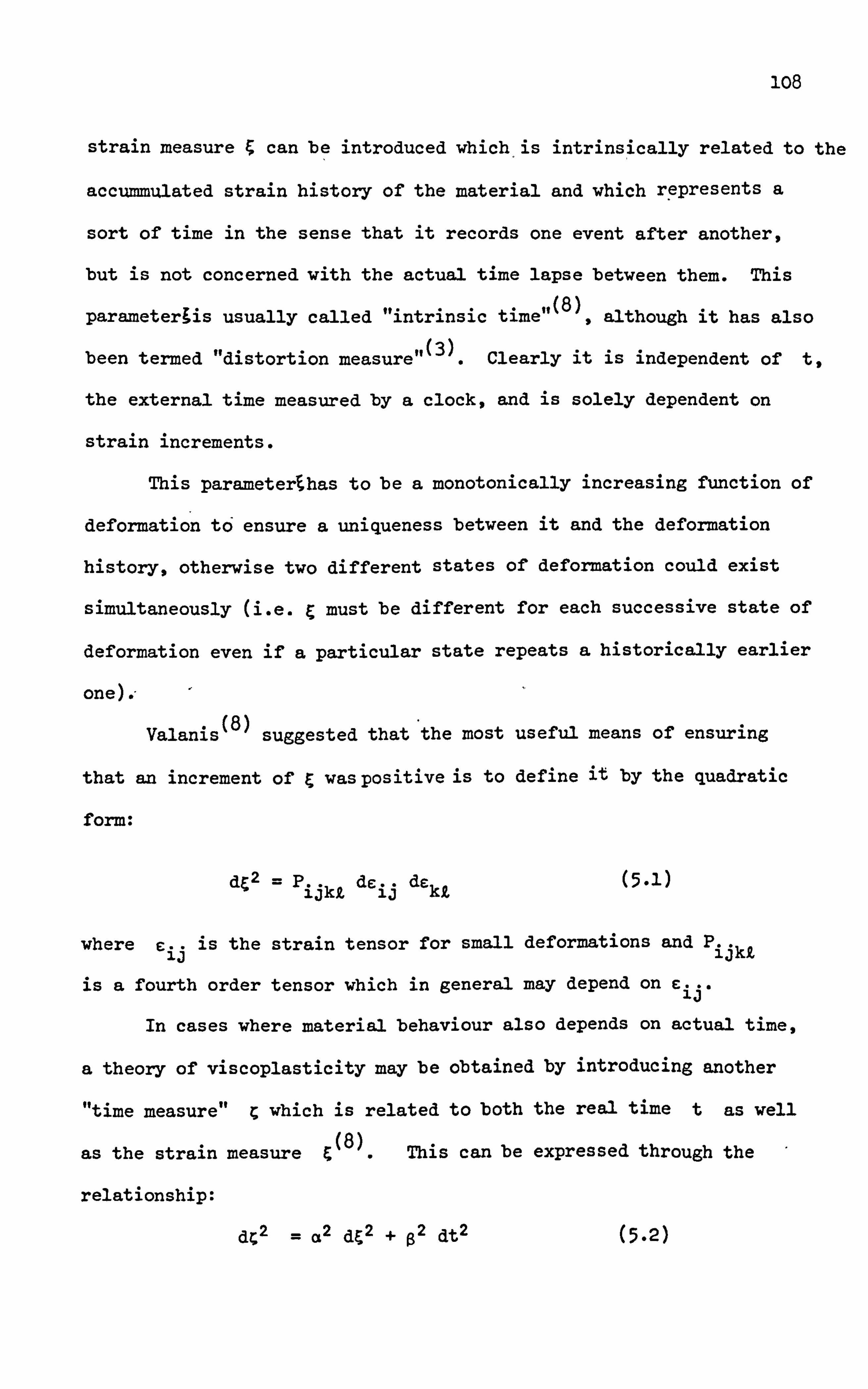
108
strain measure ; can be introduced which. is intrinsically related to the
accummulated strain history of the material and which represents a
sort of time in the sense that it records one event after another,
but is not concerned with the actual time lapse between them. This
parameterjis usually called "intrinsic time" (8),
although it has also
been termed "distortion measure" (3).
Clearly it is independent of t,
the external time measured by a clock, and is solely dependent on
strain increments.
This parameterthas to be a monotonically increasing function of
deformation to ensure a uniqueness between it and the deformation
history, otherwise two different states of deformation could exist
simultaneously (i. e. & must be different for each successive state of
deformation even if a particular state repeats a historically earlier
one). -
Valanis(8) suggested that*the most useful means of ensuring
that an increment of C was positive is to define it by the quadratic
form:
d&2 =p ijkl deij dekk
where cij is the strain tensor for small deformations and P ijkt
is a fourth order tensor which in general may depend on cij.
In cases where material behaviour also depends on actual time,
a theory of viscoplasticity may be obtained by introducing another
"time measure" C which is related to both the real time t as well
as the strain measure & (8).
This can be expressed through the
relationship:
dý2 = a2 d&2 + a2 dt2 (5.2)

log
where (I and a are scalar-valued material parameters, and C is
called the "Intrinsic time measure", because of the analogy between
& and real time. The total "time" is a function of the "time measure"
and is called the "intrinsic time scale" z. i. e.
Z= ZW ; dz > 0; 0eý<- (5-3)
This scale is a property of the material at hand. The function z and
the operator P ijkk of equation (5-1) must be chosen so that the
observed material behaviour is modelled. As will be seen later,
the stress is a function of the strain history as defined by the
intrinsic time scale, z, and therefore the theor7 has been called
it endochronic theory".
From basic thermodynamic principles, Valanis (8)
obtained two
relationships for the total deviatoric and hydrostatic stresses which
form the basis of endochronic theory. These are as follows:
z Deviatoric stresses S2 G(Z-Z*)deiý(z*) (5.4)
z 0
z Hydrostatic stresses a kk
3 K(z-z*)de kk(z*) (5-5)
z 0
where z= intrinsic time scale at initial state 0
Z* = intrinsic time at z Z* <z
z= intrinsic time scale
G= G(z) = Shear modulus
K= K(z) = Bulk modulus

110
S. - + = stress tensor ij ij 3
C.. eý . + = strain tensor ij Ij 3
The function G(z) and K(Z) must be chosen such that experimental
data are modelled by Equations (5.4) and (5-5).
5.2.3 Application to metals: (9)
The endochronic theory was originally applied by Valanis to model
the behaviour of metals rather than concrete. These earlier theories
included behaviour which was more relevant to metals but nevertheless
will be briefly discussed here before showing the adaptation for concrete.
The basic assumptions for metals were as follows:
1. Time effects were neglected (i. e. z= z(&) );
2. It was assumed that plastic deformations were incompressible and
that the material behaves elastically under pressure. Thereby
equation (5-5) becomes, a 3Kekk where K is a constant; kk
3. It was assumed that the apparent shear modulus was given by the
single exponential term G(z) = G. e-ctz where G0 is the initial
shear modulus; thereby Equation (5.4) was reduced to the differential
equation:
de.
dS ij_ +aS ij
dz (5.6)
ij - 2G 0
2G 0
In Equation (5.6) dS ij is the elastic deviatoric strain
2G 0aS.
- dz increment of classical plasticity. ij is interpreted as 2G
0

ill
the plastic strain increment and resembles the Prandtl-Reuss equations.
The difference between the endochronic and the Prandtl-Reuss theory
lieb,, in-the role played by dz.
In the Prandtl-Reuss theory dz can be either positive, zero or
negative and z is identified with the yield surface (z = z(S ij )
representing the loading function). Plastic deformation occurs only
after the yield surface is reached and dz > 0. When dz <o plastic
deforination does not occur.
In the endochronic theory, however, dz is always positive for
a deforming material, and is not related to a yield surface. Hence,
contrary to the Prandtl-Reuss theory, "Plastic" deformations are
present in the endochronic plasticity theory whenever deformation takes
place.
Valanis(9) applied this theory to model complex experimental
results for metals and good comparisons were obtained.
5.2.4 Application to concrete:
Bazant et al! 10)
extended the theory to concrete. Characteristics
which had not been included for metals were now considered. These
were:
1. Inelastic volumetric strain behaviour (i. e. introducing inelastic
dilatancy).
2. Shear compaction effects.
Hydrostatic pressure sensitivity and strain-hardening and softening
effects which are related to the intrinsic time z.
The dependence of tangent moduli (G and K) on dilatation.

112
Introducing more than one intrinsic time (i. e. &, &', z, z') to
account for differences in behaviour under deviatoric and
hydrostatic stress states.
In contrast to metals, which behave linearly under hydrostatic
stress, concrete undergoes inelastic deformation. Bazant et al.
introduced an inelastic volumetric strain increment into the volumetric
stress-strain relationship, while retaining the deviatoric stress-strain
relationship in the same form as for metals. i. e.:
ds. - Deviatoric strain = de.. = de.. e+ de P-1.1
+ ýý
dz (5-7) ij- ij ii 2G 2G
ep dam
Volumetric strain = d&391 = de n+
dcm = 3k
am dz' ] +(dco + dX +W+
am3K (5-8)
in which
e de ij
Elastic part of deviatoric strain increment.
de ij
p Inelastic part of deviatoric strain inctement.
e de m
Elastic part of volumetric strain increment.
P de m
Inelastic part of volumetric strain increment.
Cm=e kk/3 mean strain.
am= CY kk/3 mean stress.
eij - cij -6 ij Cm "2 deviatoric strain tensor.
S ij = oij - 6ij cym = deviatoric stress tensor.
6ii = Kronecker delta.
0

113
Inelastic dilatancy.
Shear compaction.
z z' Intrinsic times for distortion and compaction.
Four parts have been identified as forming the plastic part of
the mean strain (i. e. inelastic volumetric strains) which can be
written as:
a dz' dc
mp= de 0+ dÄ + dÄ '+m 3K
(5-9)
dc 0 accounts for stress-independent inelastic strain, such as thermal
dilatation and shrinkage. However these effects will not be given
any further attention in this work and are assumed equal to zero.
The parameter X represents a measure of the inelastic volumetric
strain due to shear strains and has been called "Inelastic dilatancy"
by Bazant et al. This effect is manifested in uniaxial compression
tests by the increase of Poisson Ratio up to and over 0.5 when failure
is imminent. An increase of A, i. e. dX can be expressed as follows:
dX = £(X) (5-10)
where E(X) is a "dilatancy-hardening function" and is represented
graphically in Figure (5.2. a). This function is linearly related to
X and becomes equal to zero when A approaches a maximum value, Xo.
Such a maximum value must exist because there is a certain maximum
volume that concrete can reach after it is fully crushed. L(X, c, a)
is a "dilatancy-softening function" and is assumed to depend on
11 (a) (i. e. first invariant of the stress tensor) and J2 (c) (i. e.

114
second invariant of deviatoric strain). The presence of II (a)
incorporates the fact that dilatancy must vanish at very high
hydrostatic pressure, because no cracks can open (Figure (5.2. b)).
The function of J2 (e) is used because the deviatric strains cause
microcracking. This function, Figure (5.2. c), assures that there
is no appreciable dilatancy in cyclic compression for low strains, but
allows it to be quite pronounced, but gradual, when load cycles reach
into high stresses.
Bazant et al. found from practical experience that X has a very
profound effect on predicted behaviour (i. e. shape of the hysteresis
loops) and the Poisson's ratio under cyclic loading. dE in Equation
(5-10) was also included because this will relate dilatancy to the
deviatoric strain increment (represented by dE ) and is apparently
necessary as a further measure of microcracking.
Variable A' represents the shear compaction which appears at the
beginning of inelastic deformation and represents the departure from
the hydrostatic pressure line as shown in Figure (5.2. d). This inelastic
deformation occurs in the zone between envelope 1 and 2 of Figure (4-7)
and is defined in a similar function to Equation (5-10), i. e.
dXI = 1'(11) LI(X', c, a)d& (5-11)
The function 1'(X') prevents XI from exceeding a certain limit,
andthe function LI(XI, c, a) causes dX' to vanish for large shear strain
(i. e. large J2 (c)) when shear compaction ceases.
The parameter z' is the intrinsic time associated with volume
change, and models inelastic volumetric strains due to hydrostatic stress
(i. e. the cumulative damage sustained by the concrete due to volume change).
115
This effect is mainly important at high hydrostatic pressure. The
parameter z' was defined by:
I-. dn ' dz' =-ýl - (5.12)
Z2 h(n' )Z2
where dn' = H(c)dt' (5-13)
The softening function H(a) increases the inelastic volume change
if the hydrostatic compression grows but becomes constant at higher
compression levels. The less inclined medium portion of the hydrostatic
curve is governed by the linear term in h(nl) and the subsequent
stiffening is achieved by the quadratic term in h(n').
The values of dC and dý' were reduced by Valanis(9) and
Bazant et al. (10)
to:
1/2
d& J2 (de 11121 dej i dej (5.14) ij 3. j
where J2(dc) = second invariant of the deviatoric strain increment
tensor de... ij
and d&l = II, (de)l= Idekkl = Idell + dC22 + de331 (5-15)
where II(de) = first invariant of the strain tensor increment de ij
The functions X, L, XI, Li, h and H and constant z2 are listed in
Appendix A.
The inelastic part of the deviatoric strain takes into account
the sensitivity of these strains to hydrostatic pressure and attempts
to present its strain-hardening and softening behaviour i. e.

116
S.. deij 13 dz 2G (5.16)
where z is the intrinsic time, representing the cumulative damage
sustained by concrete due to distortion. Bazant et al. expressed
it as:
dz = dc
= dn (5-17)
Z1 f( Tj 9C 9G) Z
where dn = F(c, a) dC (5.18)
The functions f and F were chosen to model the hydrostatic
pressure sensitivity and the effect of strain hardening and softening
behaviour. For simplicity a diagram is shown in Figure (S. I. e) which
illustrates their effect on a unia; ial compressive stress-strain
curve. These functions and the constant z, are also listed in
Appendix A.
The tangent moduli (G and K) are assumed to be dependent only
on the inelastic dilatation X. The functions are selected such that
G and K decrease as A grows because, as explained earlier, X represents
the inelastic dilatancy due to shear strain and has a predominant effect
on microcracking. This affects indirectly the value of Poisson's
Ratio and hence G and K. The following functions were assumed to be
suitable representations:
K=K O(A) (5-19)
and G=G O(X) (5.20)
in which O(X) =1 (5.21) 1+ c5X
E and K Initial elastic Bulk modulus 0
0 3(1-2v)

117
E 0 G= Initial elastic shear modulus =
02 (1+ v)
Eo = Initial Young's modulus.
v= Initial Poisson's ratio.
The value of c5 was deduced from experimental measurements and
was found to be equal to 150. The value of ý(X) is chosen in such a
way that G and K cannot become negative for any value of X and that it
will yield a slower decrease of G and K with X at high values of X.
5.2.5 Summary of the equation of the endochronic theory:
The endochronic theory equations used in this work can now be
summarized as follows:
Deviatoric strain: deij , ! aý S
: Lj dz
(5.22) '2 2G + 2G
Volumetric strain: dem = dcym
+ de 0+ dX + dX' + amdz'
(5.23) 3K 3K
where dz = dn (5.24)
ZI f(n, c, a)zi
dn = F(c, a)dý (5.25)
dz'= dC' dn (5.26)
Z2 h(rl')Z2
dnl= h(cr) W (5.27)
dg = fJ2(dc)
=ý1 de.. de. - (5.28) 2 ij ij
dg'= ýjjl(dc)12= Idcll+dr22+dF-331 (5.29)
dX = £(X) L(X, F-, cr)dg (5-30)
dX'= (5-31)
The remaining functions not defined above are listed in Appendix A.

118
Hence Bazant et al. have modelled the essential features of concrete.
This involved isolating and idealizing in a rational manner the many
aspects of concrete behaviour at different levels of load and at different
stress states. Then suitable functions were chosen to qualitatively
represent each individual part of this behaviour.
The parameters included in these functions were then determined by
suitable optimization procedures based on available experimental data.
However the theory as presented is difficult to modify because of
the complexity of the form of the equations and the difficulty of knowing
just how the constants were determined. There appears to be much
interdependence between various parameters and the different effects they
represent. This makes it difficult to clarify the relative significance
of each parameter and would appear to lead to over-complex relations.
For similar reasons it is also difficult to judge the relative
significance of the high number of experimental constants in the
endochronic equations.
Simplifications need to be introduced so that the theory becomes
more accessible to, and can be more easily modified by, other researchers
and engineers. However, despite these remarks the theory has proved
both accurate and efficient, and can represent a wide range of different
concrete behaviour.
Comparisons between experimental results and those using the
endochronic theory are presented in the next section. This will include
a new set of experimental data not investigated by Bazant.

lig
5.2.6 Numerical procedure for applying the endochronic theory:
An iterative process is required to obtain a good approximation
of the stresses for a calculated strain increment associated with a
specific increment of load. This is because the different incremental
state variables (i. e. d& , dý', dn dn' dz dzI dX dXI ) are nn n' n' n' n' n' n
unknown for the current increment. Therefore the determination of the
appropriate moduli (G and K) and the final states of stress cannot be
reached directly.
The basic procedure is shown in Figure (5-3) for a uniaxial case.
Starting from point A the incremental variables dE n and d&I
n are
initially evaluated using the current incremental strain. Stresses and
strains are obtained at half the current increment (n-D using the initial
values of G and K. From these new values for the softening and hardening
functions of the endochronic theory are obtained from which the incremental
variables dnn' dn' n, and total values at half the current increment
nn-l' n'n-j are evaluated. These are used to evaluate the incremental
values of dz n and dzI
n Finally dX
n and dXI n are evaluated using the
values obtained at A and V which are initially assumed to be n-2 n-I
equal to X n-l and XI
n-l* The values of dX
n and dX n are used to evaluate
a new set of Xi and VI which in turn are used to evaluate the new n-2 n-2 G, and K The values of dz dzI d), dXI ,G _j,
K _1 are n-2 n-, n n' n' n' nnn
then used to evaluate the incremental stresses at the end of the increment
(i. e. point 1 in Figure (5-3 )). This process is continued until the
difference between the endochronic state variables and the total stresses
at the beginning and the end of this cycle is as small as desired. The
main steps are described in the following:
120
Set up the 42 material constants defined in Appendix A. These
remain unchanged throughout the whole analysis.
2. For any particular load level {Pln-1 there will exist total strains
{Eln-l' total stresses {aj n-l'
dilatation parameters X n-l'
X1 n-l
and intrinsic time parameter nn-l' T' I n-l' at each point in the
material. These are zero before any application of load.
Material constants G n-1 %K n-l
also exist from which the tangential
matrix [D] n-l can be calculated. Initially these are the elastic
constants GK
A load increment A{Pj n
is applied from which the current incremental
_strainsA{cl n and stresses Afal n
are calculated using the current
I tangential material matrix. i. e.
Afcrln "ý [Dln_l A(Eln (5-32)
Then a first estimate of the total stress vector is calculated
for the current increment i. e.
foln "ý {Gln-1 + Afcr}n (5-33)
Calculate the total strains {c) n-j and stresses {Oln-I which
exist at half the current strain increment i. e.
{Eln-I {F-)n-1 + 0.5 Alc'n (5-34)
{cy}n-21 {G}n-I + 0.5 A{a)n (5-35)
5- Calculate the incremental variables AE n'
AV n'
AT'n"A"In , Az n'
AzIn'
AX n'
AV n
for the whole increment using equations (5.22 - 5.31).
n1 are then used to evaluate where n n-j' n'n-2 Azn' Az'n n-j
n+ O-5An and n' n' + O-5An' n-l n n-2 n-1 n*

121
Using 4ý n calculate A
n-j from the equation A
n-j '2 A n-l
+ 0.5 AX n
to evaluate the new shear modulus G n- 1 and Bulk modulus K which n
exist at this point using equations (5-19 - 5.21).
6. Define the deviatoric and hydrostatic parts of some ficticious
plastic stress increment by
AS uP= 2G Aeij P (5-36)
Acrm P=
3KACm P (5-37)
Then by substituting the expression for inelastic strains from
equation (5-7) and (5-8) into equations (5-36) and (5-37) the following
expression for inelastic stress increments are obtained:
AS ij p=s
ij Az (5-38)
Acr mp = WAX +AX') +am AZI (5-39)
Equations (5-7) and (5.8) can be written in terms of deviatoric
and volumetric stresses as:
ASij + AS- -P = 2G Ae ij ii (5.4o)
Aam + &am p= 3K Ac m (5.41)
and can then be rewritten as a relation between the total stresses and
strains increments as:
p Aa
Ij +Acr
ii =D ijk, e Ackj (5.42)
in which
Ao ij = AS
ij +6 ij Au in
(5-43)
Aaij p= Asij p+6 ij
AG mp
(5.44)

122
D lJkZ
Ac ki = 2GAeij + 3K6 ij I'm (5-45)
Equation (5.42) ý; 'can be written in matrix form as:
p Ala) + Ala I D] A161 (5.46)
nnE n-2 n
where [D] is the elasticity matrix based on the current values of
shear and bulk modulus which is, in this procedure, evaluated at the
mid point of the current increment.
The sum A{a I +A{a PI is initially the estimated linear stress
nn increment which consists of a ficticious inelastic stress A{a
PI and
n
the current stress increment A{a) and is illustrated in Figure (5-3 n
The values of {Aa PI can be evaluated using equations (5.38) and
n (5-39), and an initial estimate will be calculated for A(a). from which n
the total stress {a is calculated.
7. A convergence criterion suggested by Bazant has been used. This
is defined by:
I axx -a xx j< Ic
F*a xx I BAT)
where CF=0.1%. a xx
is the cartesian stress calculated from equation
(5-33) and a XOX is the cartesian stress calculated at the end of the
iteration process defined in step (6).
If equation (5.47) has not converged then go to step (4) and set up
v xx (5-33) and a XOX
is the cartesian stress calculated at the end of the
iteration process defined in step (6).
A{G}n =A[Cr}nand repeat. Alternatively if a certain number of iterations
were exceeded then go to step (8).
123
8. Update the endochronic variables (i. e.. A n'
At n,
n n'
n, n
from
Xn=X n-1
+ AX ... etc. ) to be used for the next increment.
A flow chart is shown in Figure (5.4) to illustrate this
numerical process.
5.2.7 Stress strain curves obtained using the endochronic model ý10)
(21) Experimental data obtained by Hognested et al. 1955
Kupfer et al-1969 (22),
and Tasuji et al. 1978 (23 )
are used in this
section to examine the validity of the endochronic model for predicting
the uniaxial and biaxial response of concrete. The first two references
were part of the experimental data used by Bazant et al. in optimizing the
endochronic equations, the last reference gives a new set of data for
comparison.
Figure(5.5) compares Hognested et al's-experimental results
for uniaxial compressive stress-strain data for different strengths
(20.7,32.1 and 42.7 N/mm2) with the endochronic model and Popovics
formulae (which will be discussed later in this chapter). As can be
seen the endochronic model exhibits very close comparison with this data.
Popovic's formulae also show a good fit with the experimental data.
Figure (5.6) illustrates volumetric strain changes against the uniaxial
stress/strength ratio obtained from tests by Kupfer et al.. The accuracy
of the endochronic model is also demonstrated here.
The experimental biaxial volume change against stress/strength
ratios presented by Kupfer et al. are shown in Figure (5-7). These
are compared with the endochronic model for different values of Young's
modulus and Poisson's ratio. Again fairly good fits are obtained but
124
it would appear that the endochronic equations for volume change are
fairly sensitive to changes in Young's modulus and Poisson's ratio.
The comparison with the experimental work of Tasuji et al. are shown
in Figures (5.8 - 5.10) for the stress ratios of 0.2,0.5 and 1.0 with
V equal to 33.3 NIMM2. Again the endochronic model predicts this c
data fairly closely. The figures also show the endochronic prediction
for V equal to 20.2, and 42.7 N/Mm2 which are the same values used c by Hognested et al. under uniaxial conditions. However., there are no
experimental results to compare these with, and they serve only to
illustrate the different curves that can be obtained. Finally Figure
(5-11) shows the good agreement between the endochronic model and
Tasuji et alls. experimental biaxial ultimate strength envelope.
To conclude, this short study demonstrates that the endochronic
model can successfully predict various aspects of the uniaxial and
biaxial behaviour of concrete under short term monotonic, conditions. I
5.3 The cracking model:
As mentioned previously the cracking model is based on the smeared
crack approach. This implies that an infinite number of cracks occur
at a specific point if a certain cracking criterion is satisfied. This
approach is used because it is capable of predicting the load deflection
behaviour, general stress-strain distribution, and general cracking
behaviour for most categories of reinforced concrete structures (i. e.
specific local behaviour in the vicinity of discrete cracks is not the
subject of this work).
The basic assumptions for this model are as follows:

125
1. Concrete is assumed to be a homogeneous and isotropic material
before a crack develops and follows the endochronic constitutive
laws as previously described.
2. A crack is assumed to occur in a plane perpendicular to the
direction of the principal stress or strain which caused this
crack as shown in Figure
Concrete will convert to orthotropic behaviour once a crack foms.
This is represented mathematically by changing the tangential
matriX to represent the new orthotropic state. Some shear stresses
will be retained in the new orthotropic matrix due to the effect
of aggregate interlocking between cracked concrete.
Two models have been used to represent the uniaxial tensile stress-
strain behaviour of concrete in the direction perpendicular to the
crack after a crack has occurred. The first model assumes that
stresses will drop immediately to zero after a certain failure
criterion is satisfied. This is shown in Figure (5-13).
The second model assumes a gradual release of stresses will occur
after a certain failure criterion is satisfied. This is the tension
stiffening model and is shown in Figure (5.14). As explained
previously the reason for assessing two different cracking models
was to compare the effect of these models on the general behaviour
of the structure when they acted in conjunction with varoius
numerical procedures.
Two fracture criteria are used; "the maximum principal stress"
criterion and "the maximum principal strain" criterion.
126
For the first model the maximum principal stress criterion is
used exclusively.
For the second cracking model both the maximum principal stress
and strain criterion are used. This is to prevent numerical problems
in calculating the stress when the maximum stress criterion alone was
used with tension stiffening. The problem was caused by the sudden change
in stiffness from an isotropic state to an orthotropic state after crack
formation which leads to the elimination of Poisson's ratio effects.
Figure (5-15) illustrates this point. However, inclusion of the strain
criterion removes this problem because the strain criterion will ensure
that the strains also reach the peak point on the uniaxial stress-strain
curve.
The main steps for each model are summarized in the next two
sections:
5.3.1 Procedure for the first cracking model:
1. Enter with the values of strains {0 n-l' stresses {CY)n-l' and
initial crack conditions. At the beginning of the analysis
{C)n-1 and (a) n-1 are zero and the material is uncracked.
2. Apply a load increment of AM n
from which the incremental strains
A{C) n and stresses Mal
n are calculated.
Calculate the total strains and stresses from:
{c)n ý {Cln-1 + A{cln (5.48)
{aln = {cyln-1 + A{Gln (5.49)
If the concrete is initially uncracked then:
127
(A) Calculate the principal angle ot c
from the equation:
--1 tan-1 [ 2T
XY j
c20 xx- 0 yy
(5-50)
This angle is shown in Figure (5.16), and lies between -45 0 and
45
Calculate the total principal stresses {a PIn using the following
equation:
{a pIn :" LIR-1 jT {a)
n (5-51)
where ER] is a transformation matrix and is equal to:
C2 S2 Sc,
Ell] S2 C2 -Sc (5-52)
_-2Sc 2Sc C2-S2
and c= cos acq S= Sin ac.
The matrix [R] is used to calculate the principal stresses because
it allows the stresses to be orientated in the proper direction with
respect to the angle ac.
(C) If {a ) >, f, in any single direction then a crack occurs pnt
perpendicular to the direction of {G P)n
The angle ac is then
fixed as the permanent crack direction and the tangential elasticity
matrix [Dc is updated as follows:
00
r c]
E2 0 (5-53)
0 aG-

128
if a crack occurs perpendicular to axis (1) in Figure (5.16),
El 00
and [D] 000 (5-54) C
-0 0 aG
if a crack occurs perpendicular to axis (2) in Figure (5.16). El and E2
are the tangential moduli of concrete in the direction parallel to the
single crack, and a is a shear factor defining the shear resistance
parallel to the crack due to aggregate interlocking.
Its value is a predetermined constant which can be set between
0.0 and 1.0, usually 0-5-
(D) If 10 P)
>' f t'
in both directions then two cracks occur at the
same time perpendicular to each other. The angle ac is fixed
as before and the new tangential matrix is updated to:
000
CDJ 000 (5-55)
00 cLG
5. If cracks already exist then
(A) Use the fixed angle of crack ac and transform the Cartesian
stresses and strains into the crack direction by:
-1 T {crcln ER j {0}
n (5-56)
{c c }n 'o [R ] {cln (5-57)
(B) If one crack already exists then check whether it is open or
closed (a crack is assumed to close if the normal strain across
the crack is compressive). When the crack is closed then set up
129
LDCJ to:
El 00
[D c]0
E2 0 (5-58)
-0 0 aG_
where E, and E2 are the restored elasticity moduli before cracking.
(C) Check whether a second inplane crack already exists, if not, test
whether it occurs using:
{a } >1 ff cnt
and update PC] to:
000
[D 000 (5-59) c-
L-0 0 aG
-1 If it already exists, examine whether both cracks are open or
closed by checking whether {c dn is compressive in both directions.
If the strain only on axis (1) in Figure (5.16) is compressive
then set up [Dj to:
E, 00
000 (5.60) C
-0 0 aG_
If the strain only on axis (2) in Figure (5-16) is compressive then
set up ED I to: c
00
E2.0 (5.61)
0 aG_
130
and if the strains on both axis (1) and (2) are compressive then set
up [Dj to:
El 00
EDJ 0 E2 0 (5.62) c
L-0 0 aG
Update the new Cartesian stresses according to the new tangential
matrix from:
fal n2
ERI T [De] ER] 'c1n (5-63)
5.3.2 Procedure for the second cracking model:
1. Calculate (c) n'
{a)n using the same first three stages as in the
previous model.
2. If the concrete is initially uncracked then:
(A) Calculate the principal angle ac as in the first cracking model.
(B) Calculate the total principal strains and stresses using the
following equations:
pn {c)
n (5.64)
pn [R-1] fa)
n (5.65)
(C) if [a } >, fI and {c } >, cc, then a crack occurs pntpn
perpendicular to the direction of the maximum principal stress or
strain. Fix angle ac as the permanent angle of crack and
calculate the new stresses in the direction perpendicular to the
crack on the principal axis using the following equation:
131
a -4 ,, (ci cc)
for cc (5-66) ft - ft A (C E') Ac
Gi = 0.0 for ei > CA (5-67)
where e1 and a1 represents the strain and stress in the direction
perpendicular to the crack. cA is shown in Figure (5.14) and
represents the value of strain at which the stress finally becomes
zero in the part-cracking range.
(D) Calculate the stress in the direction parallel to the crack a,
and the assumed retained shear stress T from:
E.
and T aG
(5.68)
(5.69)
where j refers to the direction parallel to the crack and y is the
calculated shear strain value. The updated stresses can then be
written as: Gi
{a cIn
Oj (5-70)
T
if the crack occurred perpendicular to axis (1) in Figure (5.16).
And Cr i,
ai (5-71) cn
T
if the crack occurred perpenaicular to axis (2) in Figure (5.16).
(E) The new Cartesian stresses can then be calculated from:
[R] T fa c)
(5-72)

132
(F) Steps C to E are also used to check whether two cracks have
occurred at the same load level and if so stresses will be
updated accordingly in both directions.
(G) For the stiffness calculation in subsequent iterations [D c]
is
set equal to:
-00 0-
[Dcj 0E (5-73) 20
00 aG_
when a crack occurs perpendicular to axis (1) in Figure (5.16), or is
set equal to:
E, 00
ED] 000 (5-74) c
LO 0 aG _1
if a crack occurs perpendicular to axis (2) in Figure (5.16).
When cracks occur in two directions then:
000
[D 000 (5-75) c
-0 0 aG_
3. If cracks already exist then:
(A) Use the fixed angle of crack ac and transform the Cartesian strains
and stresses into the crack direction:
{C [R] {C) (5-76) Cnn
{Gc'n ": [R-1 ] {a} n
(5-77)
133
(B) If one crack exists then check whether the strain perpendicular
to the crack is changed from the descending to the ascending part
of the stress-strain curve, then update the stress on the principal
angle from
c}n « lDcl {Ec}n
E, 00
where [D ]0 E2 0 (5-78) c
-0 0 otG_
and calculate the new cartesian stresses from:
faln = [R jT lcrdn (5-79)
For stiffness calculations in subsequent iterations [Dc]is set
equal to:
000
ED 0 E2 0 (5.80)
0 aG-
when the change of strain occurs perpendicular to axis (1) in
Figure (5.16), and
El
[D c]0
when the change of strain oc
Figure (5.16).
This criterion is used
0
0
0
curs
ins-
0
0 (5-81)
aG-
perpendicular to axis (2) in
tead of using a criterion for crack

134
closing, and when the strains become negative then the tangential
modulus for the compression zone is used.
(C) To check whether a crack exists in a second direction the same
procedure for checking a crack in the first direction is used
except that [Dj for the stiffness calculation is set up so
that:
000
[DC] 000 (5.82)
-0 0 aG_
If a second crack already exists, then check if the strain in any
single direction or. both directions changes from the descending to
the ascending part of the curve. Then calculate the stresses using:
LDC- {adn j{ edn (5.83)
where 00 0-
[D 0 E2 0 (5.84) c
-0 0 aG_
if the strain changes on axis (1) in Figure (5.16), or
El 0 0-
I Dcj 000 (5-85)
-0 0 aG-
if the strain changes on axis (2) in Figure (5.16).
If the strains in both directions change set up:
El 00
ED 0 E2 0 (5.86) c
-0 0 aG_
135
The new Cartesian stresses are then updated from equation (5-83)
by using:
{01n = ER ]TI cr dn (5-87)
For stiffness calculation [DC] remains as in equation (5.82).
5.4 The uniaxial-compression model:
Once a crack has occurred and remains open a uniaxial state of
stress will exist parallel to the crack. If this stress is compressive,
the simple uniaxial-compressive model proposed by Popovics (20)
is used.
This model is a curve fitting method represented by the following
equations:
fI L-- n for c :ýc (5.88) Cc0 n-l+(c/co )n 0
ft for c<c<c (5.89) c0 cu
a=0.0 for c >, ccu (5-90)
where a= is the compressive stress in psi at strain c
Co = strain at maximum stress,
f, = uniaxial compressive cylindrical strength in psi C
n=0.0004 V+1. C
C= uniaxial crushing strain of concrete Cu
For C0 the following equation was suggested by Popovics:
k. (fc') 0* 25 x 10-4 (5-91)
136
where k is a function of the type of mineral aggregate and the applied
test method. From experimental data Popovics suggests values in the
range of 2.12 - 2.85 for concrete. In this thesis a value of 2.7 will
be used which was obtained from analysis of data taken from the work
(21) of Hognested et al.
The tangential modulus of elasticity for the uniaxial curve is
given by:
c/co )n n(n-1) fc, for c$c (5.92)
C(n-1+(c/c 0
)ni 2 Fc)
ET=0.0 for c>c0 (5-93)
The model is compared with experimental values obtained by Hognested
et al. in Figure (5-5). It is also compared with the endochronic
model and good agreement is obtained in both cases.
5-5 The crushing model:
The crushing model can follow one of two paths depending on
the state of cracking.
1. Where the point is cracked, crushing is assumed to occur if
the compressive strains parallel to the crack exceeds the
crushing strain of concrete in uniaxial compression. Once
crushing has occurred the stiffness matrix of the concrete is
assumed to be zero at that point.

137
2. Where the point is not cracked, one of two crushing criteria
can be selected. The first assumes that if the compressive
principal strains in any direction exceed the uniaxial compressive
strain of concrete, then the material has crushed. This criterion
is shown in Figure (5-17).
Alternatively the second criterion assumes that crushing occurs
if a surface representing the compressive strains exceeds
the uniaxial compressive strain of concrete. This crushing
surface is defined by:
C(C) 22
C1 - CIC2 + C2 -CCU (5.94)
where C1 C2 are the principal strains and e is the uniaxial cu
compressive crushing strain of concrete. The surface is shown in
Figure (5-18).
When a tensile strain exists in one direction and compressive
strain in the other direction, then crushing is assumed to occur
when the compressive strain exceeds the uniaxial compressive crushing
strain of concrete.
5.6 Theoretical Model for Steel:
Steel behaviour is modelled by a uniaxial bilinear stress-strain
curve with the strain hardening effect as shown in Figure (5-19).
When steel reaches the uniaxial yield stress fy in tension or
compression, yielding is assumed to occur. For the calculation of
stresses the following equations are used:
fs =EsCs when fs '< fy (5-95)
E fs = E2ý
(f; - fy )+ fy fs : I. fy (5.96) s

138
f= uniaxial stress of steel at strain c ss fy= yield stress of steel.
Es. = Young modulus of steel.
Ew= Hardening modulus of steel.
f, = Stress value if no yielding is assumed after f sy
No reloading criterion is assumed in this model and stresses
are assumed only to follow the curve of Figure (5-19).
For stiffness calculation before yielding Es is included, but
once the steel is yielded this value is replaced by the hardening
modulus of steel.

Start
Check r ss s str:
c es tts
state (Region)
compression Tension
compression compression Region Region
/ Check for crack Developmen
Yes
Use cracking model for tension,
Popovics formula or compression
use endochronic
model
For uniaxial
compression heck for crush using crushing
model
Two
Use crackingl model in b6th directions
Use cracking model in one direction, use linear
stress in other direction
Stop
(4 �+)
Tension
Tension
Region
139
Check or rack
Developmen
No Yes D
How many cracks
One
nme 5,1 Flow chart of the concrete material model.

L
X (b)
I ia)
hydrostatic Cr kk pressure
shear compaction effect (i. e.
represented by P)
(C)
a
(d)
Strain hardening and softening functions effect
(e)
C. = variable constant
f= constant P= constant f= variable P= variable
J2 (e )e kk
14o
C
Figure 5.2 Diagram of some characteristic functions.
(a) A0

141
veached ,. rement
Figure 5.3 Procedure for updating the stresses for a uniaxial
case using the endochronic model.
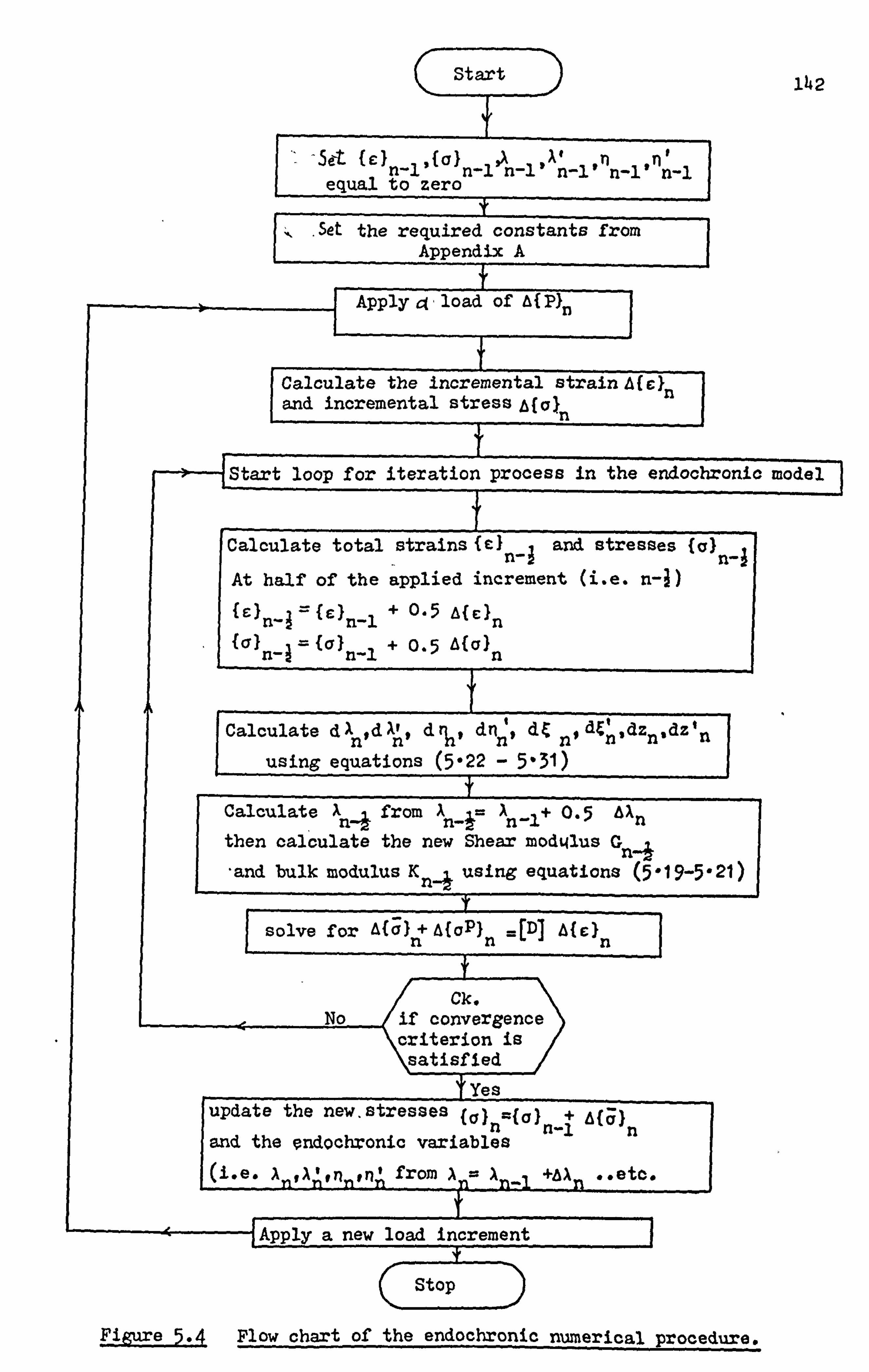
Start 142
5et I
equal to zero F. 'el thee required constants from
Appendix A
-A Load of A{ pin
Calculate the incremental strain A[ cIn and incremental stressmain
iStart loop for iteration process in the endochronic model I
Calculate total - strains {C I
n-I and stresses (a) n-I
At half of the applied increment (i. e. n-J) {0
n-I = {c)n-1 + 0*5 A{cln {a)
n-i= {aln-I + 0-5 A{O)n
Calculate d -1 td Xv 9d%, d' dC d&' dz dz 1 nn nn I nO n' n, n
I
using equations (5*22 - 5-31)
1
Calculate ýi, -5 AXn from Ah-J7 An-. I+ 0 then calculate the new Shear modt4lus Gn4 -and bulk modulus Kn. 4 using equations (5*19-5,21)
solve for A(a) +A(GP} (D] A{C} Inn=n
Ck. if convergence criterion is ýsatisfied
T Yes update the new. stresses (,, ) ={a, )+
n n-l n and the Pndochronic variables (i. e. X_, A_Itn_tn_l from A_= A__., +AX_ .. ete .
Uvolv a new load increment I
Stop
Figure 5.4 Plow chart of the endochronic numerical procedure.

143
-4!
-4c
-35
-30
-25 CV
W
44 En
-IS
-10
-S
-SO Uniaxial compression
o Hognested et al. ExElrimenta
X Popovic -Theoretical
- Endochronictheory
x
03
x ),, 2
3
IV 2 42-7 N/mm ', : 2 fg 32 NIMM2 3f
C' . 20:
17 NIMM2
-0.00 1 -0.00 2 -0.00 3 -0.0 04 -0.00S -0.006 -0.00A Strain
Pigure (5*5) Fit of uniaxial test data of Hognested et al.

144
-1.2
-1.1
-1.0
0
(0
-0.5
-0.4
-0.3
-0.2
-0. i
Uniaxial compression
= 32-1 N/InM2 o Kupfer et al., f c
Endochronic theory
0 0
1 fe' = 42*7 N/mm2 2 2P= 32-1 NIMM
3 f7 = 20*7 N/MM2 c
-1 -2 -4
Volumetric strain, (10-4)
Figure (5-6) Volume change diagrams for uniaxial test.

145
-1.2
-1.0
to -0.6
- Old
-0.4
-0.2
0
/0 0
Biaxial compression 0 Kupfer et al. q- =32-1 R/MM2
2 Endochronic theory a la, . 1-0
TE = 31*7xlo3N/MM2 v= 0-20 2E C= 27: 6xlo3N/=2 v= 0-20 fc'-, 32-IN/mm2
c 3E c=
27 6xlo3N/MM2 v= 0-18
-6 -10 -12 -14 -16 -16 -20 -22 Volumetric strain (10-4)
Figure (5-7) Volume change diagrams for biaxial test.
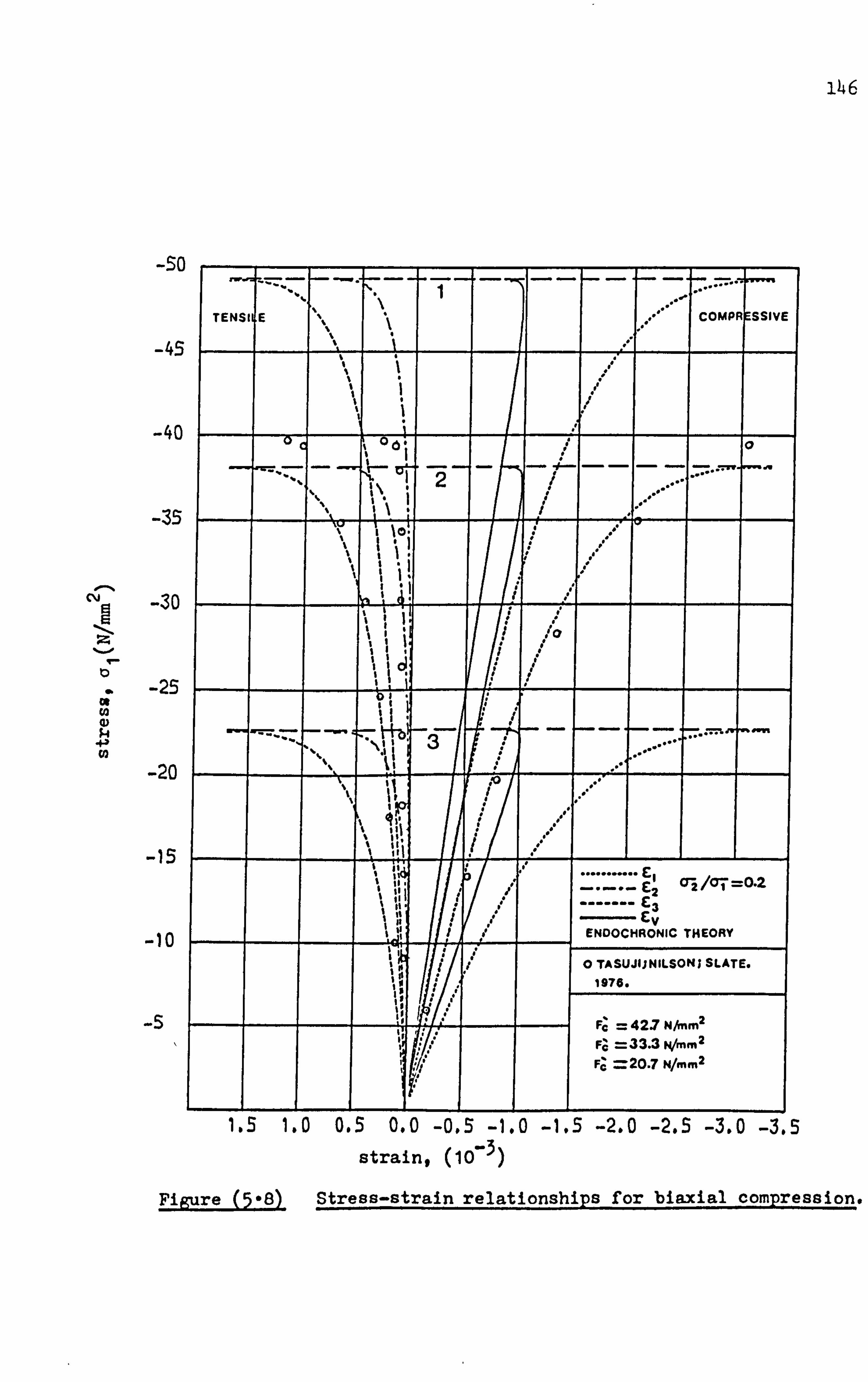
146
-50
-45
-40
-35
. -N C\j
-30 i; ý
-25 (a
-20
-15
-10
TENSI IE c OMPI SSIVE , SSI,
I It I
0 06; 1 0
"T ' -2
% % % Iý1 .1 1ý %
11 0.
lit
- I
ol .-) cr. - 0.2 C 2/CT= 2
r-3 I ", 1 EV 1 ENDOCHRONIC THEORY
0 TASUJUNILSON; SLATE.
1976.
2 7N Fý 42 /, nm . = Fj =33.3 N/rnrn2
F; =20.7 N/rnrn2
1.5 1.0 0.5 0.0 -0.5 -1.0 -1.5 -2.0 -2.5 -3.0 -3.5 strain, (10-3)
Figure (5-8) Stress-strain relationships for biaxial compression.
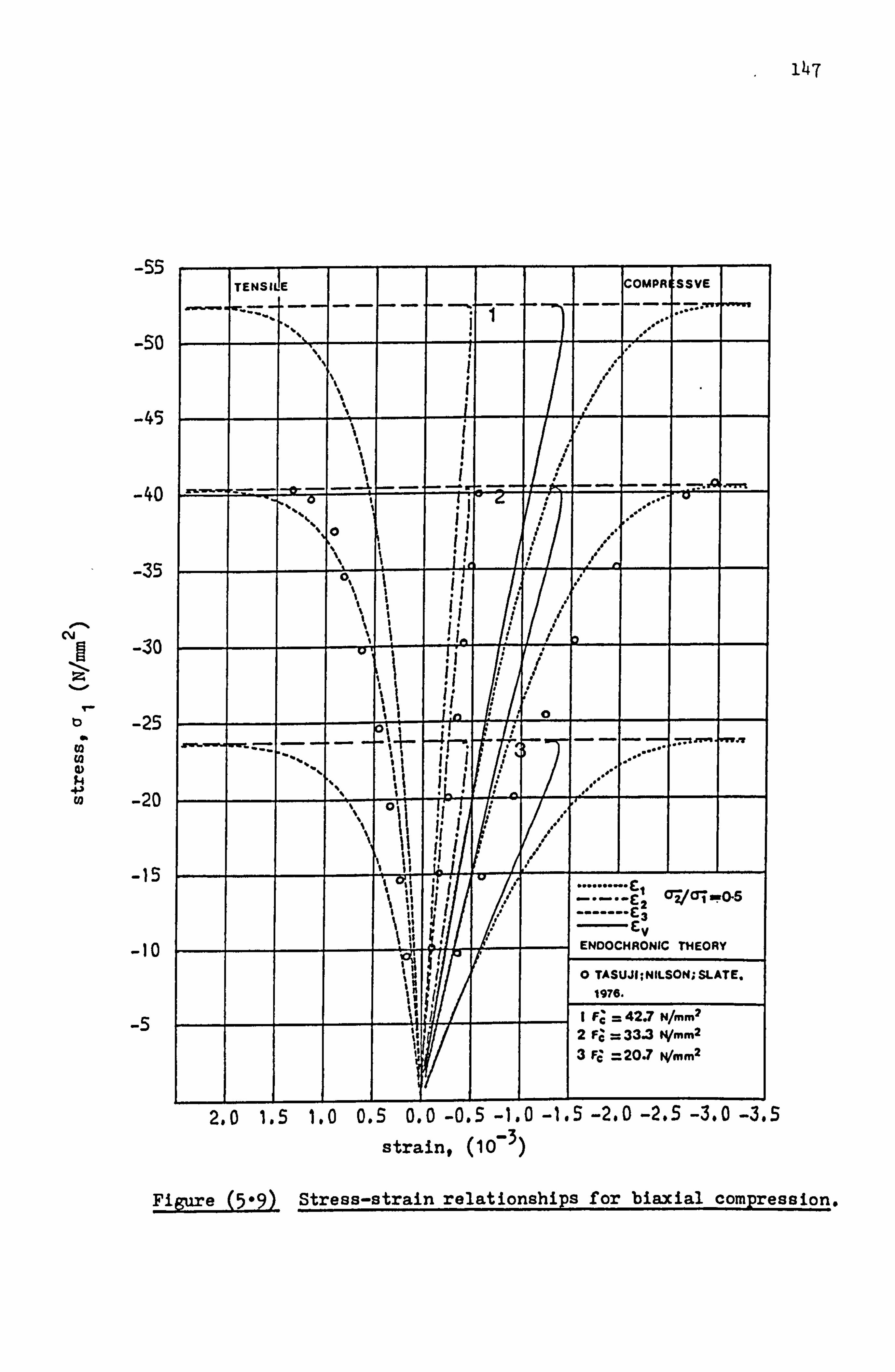
147
-55
-50
-45
-40
-35
1-1 CY
-30
iý-
-25
CD $4
W -20
-15
-10
-5
TENSI LIE COMPR ESSVE
ot
WWL 0
% to U ava-, -Fo-5 C; ENDOCHRONIC THEORY
Ii 10 14 0 TASUJI-. NILSON; SLATE. 1976.
I F; = 42.7 H/mm2 2 Fa = 33.3 N/MM2
3 Fj =20.7 N/MM2
2.0 1.5 1.0 0.5 0.0 -0.5 -1.0 -1.5 -2.0 -2.5 -3.0 -3.5 strain, (10-3)
Figure (5*9)- Stress-strain relationships for biaxial compression.

148
-55
-SC
-45
-40 . 1-%
m (0
-23
-20
-15
-10
-5
TENSI tE COMPF ESSIVE
%%
l y O's I Iý
, . ,
cq2 1a; = to ------- C3
IEI=IE2 - cv ENDOCHRONIC THEORY
0 TASUJI; NILSON; SLATE.
1976.
t IF; = 42.7 N/MM2 2 F; = 33.3 N/Mm2 3 F; = 20.7 N/rnm 2
2.0 1.5 1.0 0.5 0.0 -0.5 -1.0 -1.5 -2.0 -2.5 -3.0 -3.5 strain, (10-3)
Figure (5*1 Stress-strain-relationships for biaxial compression.

149
-0.2
0.1
0.4
a2
fe c
O-E
0-8
1.0
1.2
fc'=33-3 N/
OENDOCHRON
nM2
C THEOJW
1.2 1-0 0-8 0.6 0.4 0.2 0 -0.2 al ff c
Figure (5-11) Biaxial ultimate strength envelope of concrete.
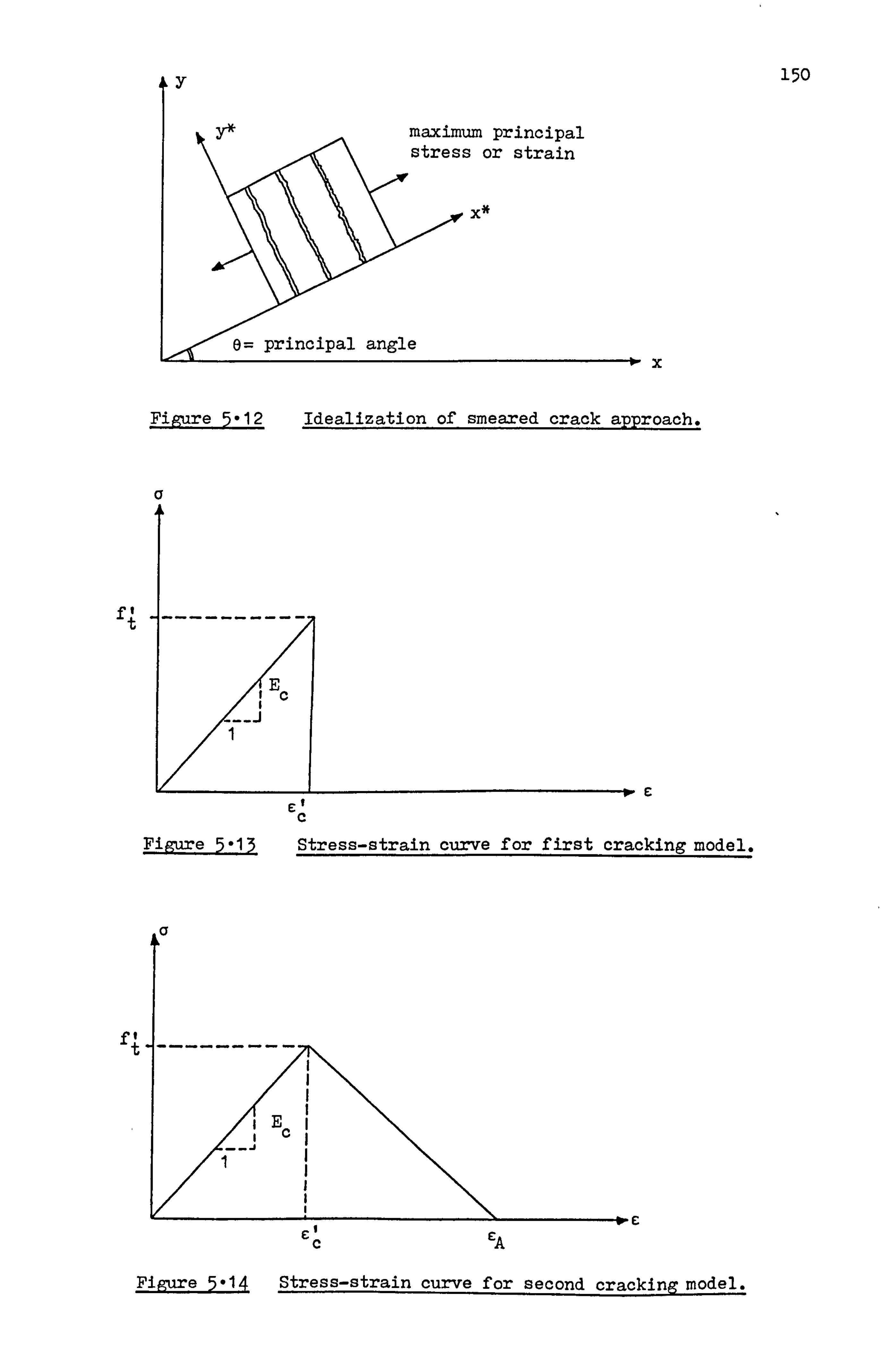
I
Y* maximum principal stress or strain
x*
1", <' 0= principal angle
FigL=e 5-12 Idealization of smeared crack approach.
cr
eI c
C
Fig=e 5-13 Stress-strain curve for first cracking model.
fT
f.;;
C
Pigare 5-14 Stress-strain curve for second cracking model.
150
E,
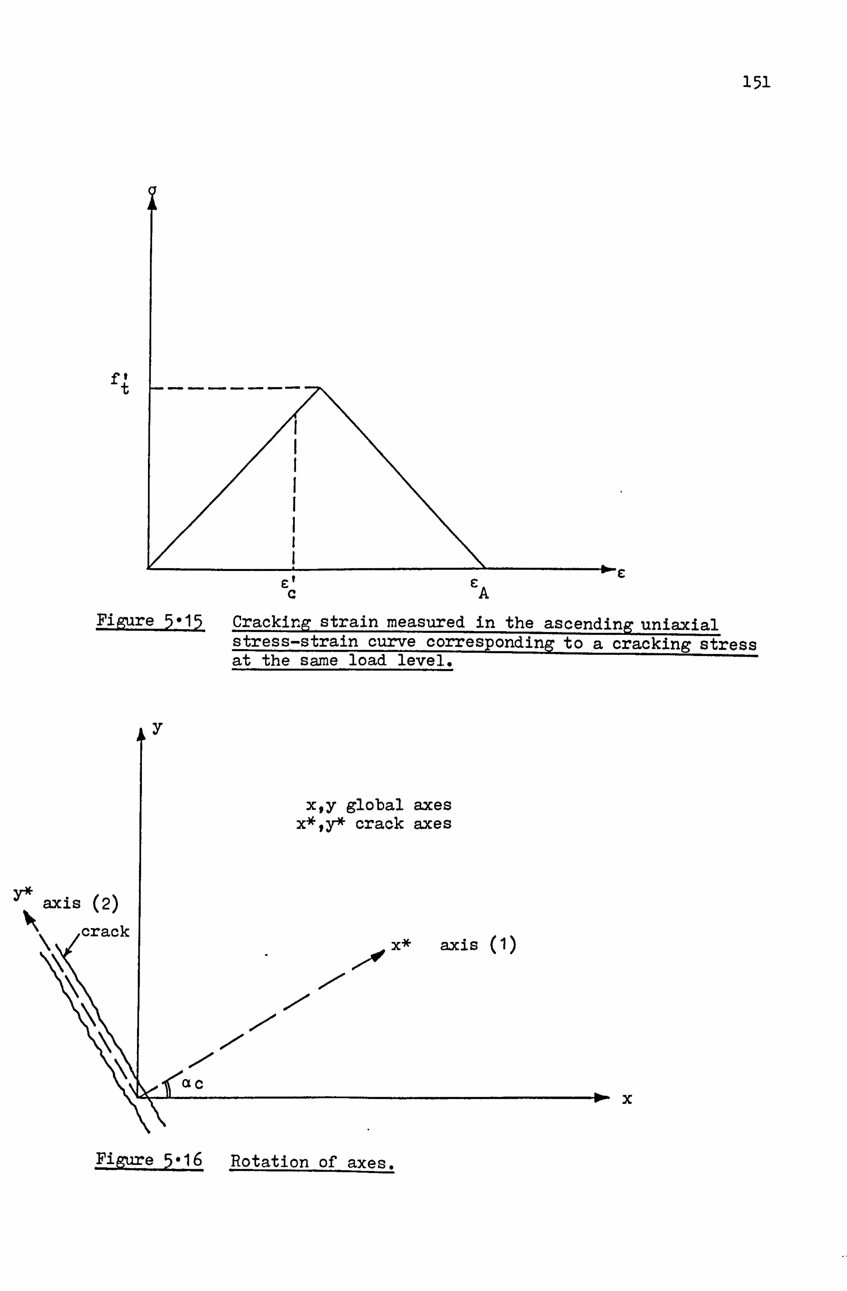
151
Y*a
\
f.
Figure 5-15 Cracking strain measured stress-strain curve corr at the same load level.
in the ascendi to a
uniaxial , ckinR stress
x
Figure 5-16 Rotation of axes.
Etc cA

C Cu
// 152
Cl
/'uncrushed
-C crushed cu
Figure 5-17 First criterion for crushing.
r: '2
E je C2- 0 j-i 2 AU
uncrushed
cu
/ lyll�
cl
crushed
Figure 5*18 Second criterion for crushing.
f-
ff s
fs fy
If 10 Cs
Figure 5-19 Mathematical uniaxial stress-strain curve for steel reinforcement.

153
1. Bazant, Z. P., "A new approach to inelasticity and failure of
concrete, sandt and rock: Endochronic theory". Proc. Soc.
of Eng. Sci., llth annual meeting, Duke University, Durham,
158-159, Nov., 1974.
2. Bazant, Z. P., "Some questions of material inelasticity and failure
in the design of concrete structures for nuclear reactors".
Trans. 3rd Int. Conf. on Struct. Mech. in Reactor Tech., London,
Vol-3, Paper Hl/l, Sep. 0 1975-
3. Bazantq Z. P.; Bhatt P. D., "Endochronic theory of inelasticity and
failure of concrete". J. of Eng. Mech. Div., ASCE, Vol. 102,
701-722, Aug., 1976.
4. Bazant, Z. P.; Krizerk, R. J., "Endochronic constitutive law for
liquefaction of sand". J. of Eng. Mech. Div., ASCE, Vol. 102,
225-238, April, 1976.
5. Bazant, Z. P.; Bhat, P. D.; Shieh, C., "Endochronic theory for
inelasticity and failure analysis of concrete structures".
Report No. 1976-12/2599 Northwestern University, Illinois,
Dec., 1976.
6. Bazant, Z. P.; Bhat, P. D., "Prediction of hysteresis of reinforced
concrete beams". J. of Struct. Div., ASCE, Vol-103,153-167,
Jan., 1977-
7. Bazant, Z. P., "Endochronic inelasticity and incremental plasticity, '.
Int. J. Solids & Struct-9 Vol-14,691-714,1978-
8. Valanis, K. C., "A theory of viscoplasticity without a yield surface".
Part I, General Theory, Archives of Mechanics, Vol. 23,517-551,
1971.
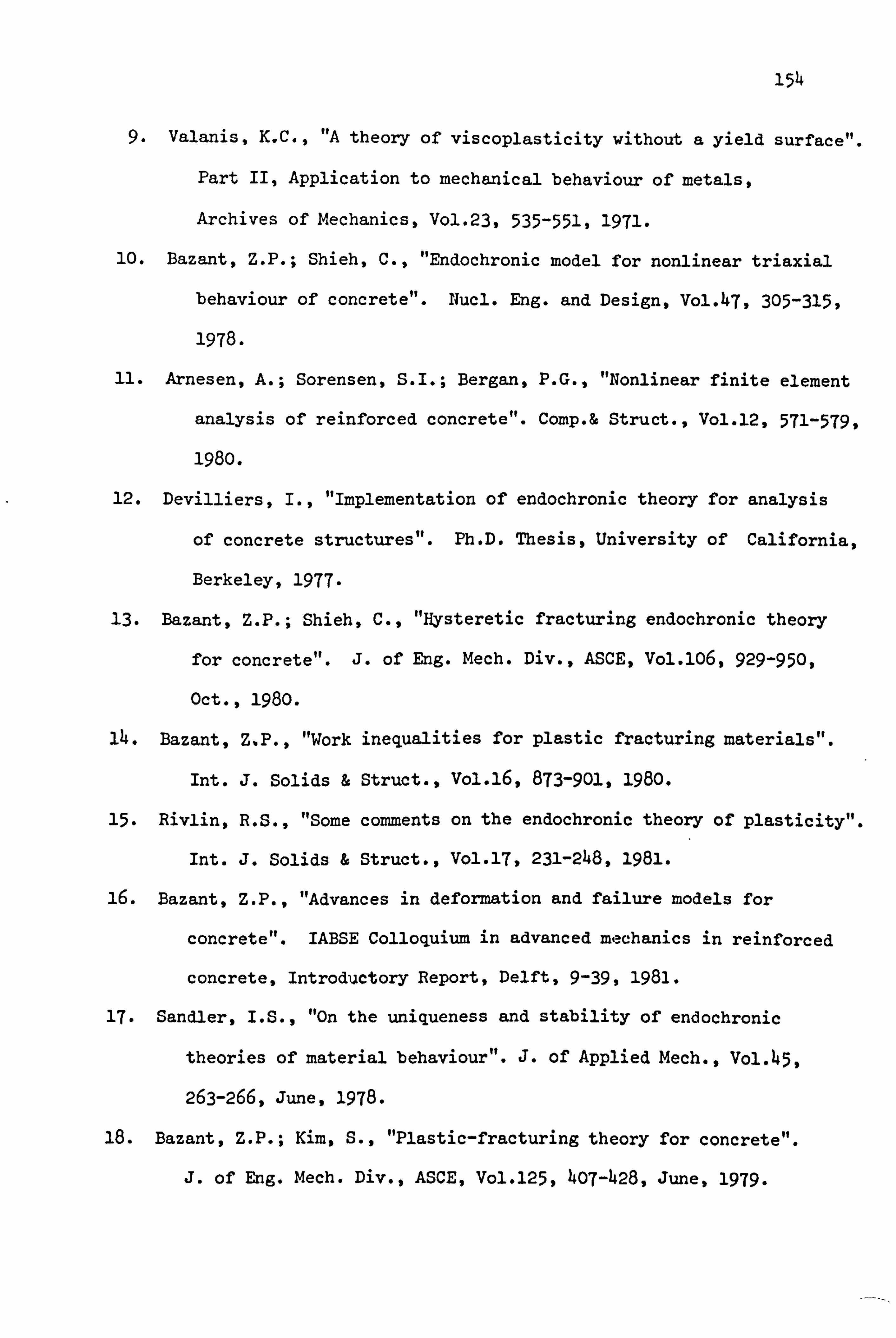
154
9. Valanis, K. C., "A theory of viscoplasticity without a yield surface".
Part II, Application to mechanical behaviour of metals,
Archives of Mechanics, Vol. 23,535-551,1971.
10. Bazant, Z. P.; Shieh, C., "Endochronic model for nonlinear triaxial
behaviour of concrete". Nucl. Eng. and Design, Vol. 47,305-315,
1978.
11. Arnesen, A.; Sorensen, S. I.; Bergan, P. G., "Nonlinear finite element
analysis of reinforced concrete". Comp. & Struct., Vol. 12,571-579,
1980.
12. Devilliers, I., "Implementation of endochronic theory for analysis
of concrete structures". Ph. D. Thesis, University of California,
Berkeley, 1977.
13. Bazant, Z. P.; Shieh, C., "Hysteretic fracturing endochronic theory
for concrete". J. of Eng. Mech. Div., ASCE, Vol. 106,929-950,
Oct., 1980.
14. Bazant, Z. P., "Work inequalities for plastic fracturing materials".
Int. J. Solids & Struct., Vol. 16,873-901,1980.
15. Rivlin, R. S., "Some comments on the endochronic theory of plasticity".
Int. J. Solids & Struct., Vol-17,231-248,1981.
16. Bazant, Z. P., "Advances in deformation and failure models for
concrete". IABSE Colloquium in advanced mechanics in reinforced
concrete, Introductory Report, Delft, 9-39,1981.
17. Sandler, I. S., "On the uniqueness and stability of endochronic
theories of material behaviour". J. of Applied Mech., Vol. 45,
263-266, June, 1978.
18. Bazant, Z. P.; Kim, S., "Plastic-fracturing theory for concrete".
J. of Eng. Mech. Div., ASCE, Vol. 125,407-428, June, 1979.

155
19. Sorensen, S. I., "Endochronic theory in nonlinear finite element
analysis of reinforced concrete". Report No. 78-1, Trondheim
University, March, 1978.
20. Popovics, S., "A numerical approach to the complete stress-strain
curve of concrete". Cement & Con. Research, Vol-3,583-599,1973.
21. Hognested, E.; Hanson, N. W.; McHenry, D., "Concrete stress
distribution in ultimate strength design". J. ACI, Vol. 27,
455-479, Dec., 1955.
22. Kupfer, H.; Hilsdorf, H. K.; Busch, H., "Behaviour of concrete
under biaxial stresses". J. ACI, Vol. 66,656-666, Aug., 1969.
23. Tasuji, M. E.; Slate, F. O.; Nilson, A. H., "Stress strain response
and fracture of concrete in biaxial loading". J. ACI, Vol-75,
306-312, July, 1978.
24. Dungar, R.; Nuh, S. "Endochronic-critical state models for sand".
J. of Eng. Mech. Div., ASCE, Vol. 106,951-968, oct., 198o.
NUMERICAL STUDY OF VARIOUS PARAMETERS
AFFECTING NONLINEAR SOLUTTONS
6.1 Introduction
6.2 Description of the deep beam used in
the numerical study
6.3 Parameters affecting the number of
iterations and the convergence rate
6.3.1 Load criterion
6.3.2 Displacement criteria
6.3.3 Discussion on load and displacement
criteria
6.4 Constant and variable stiffness methods
6.5 Gauss rule
6.6 Shear retention factor
6.7 Tension stiffening
6.8 Conclusions
6.9 Burns & Siess shallow beam J-4

CHAPTER 6 NUMERICAL STUDY OF VARIOUS PARAMETERS, 156
AFFECTING NONLINEAR SOLUTIONS
6.1 Introduction:
The usefulness of the finite element method for nonlinear analysis
very much depends on the various numerical parameters which influence
the solution. It is important to understand how these influence
solutions and how they interact. Otherwiselnumerical problems could
arise which could cause divergence of a solution, or worse, give
erroneous results even though convergence had been achieved.
Numerical parameters can be classified into three groups;
solution parameters, quasi-material parameters, and actual material
parameters. The quasi-material parameters are factors which are
treated as if they were material properties but in fact are really
numerical devices used to produce a required effect. Actual material
parameters are measurable properties of a material such as the tensile
strength of concrete. The most important of these parameters investi-
gated in this work are:
(1) Solution parameters:
(a) Convergence factors and criteria.
(b) Number of iterations required to achieve an acceptable
solution.
(c) Method of updating the stiffness (constant or variable).
(d) Order of Gauss rule.
(e) Mesh size.
(2) Quasi-material parameters:
(a) Aggregate interlocking effects.
(b) Tension stiffening effects.
157
Actual material pArameters;
(a) Crushing criterion of concrete.
(b) Tensile strength of concrete.
(c) Young's modulus.
The object of this chapter is to establish guidelines for the
nonlinear method presented here and to check the effects of the
numerical parameters in the first two groups. Those in the third
group will be discussed in later chapters as and when they arise.
Many of the above parameters are related to each other indirectly
and in many circumstances it may 6epossible to obtain the same results
by controlling different parameters. However, this is not a general
rule. Also, one parameter could affect another parameter directly.
For example, it is well known that reducing the increment size will
give much faster convergence in that increment.
Information on numerical studies has only been presented by a
few authors. Scordelis(l) made a comprehensive review of the available
finite element methods of analysis for reinforced concrete structures.
It involved information regarding such numerical parameters as tension
stiffening, aggregate interlocking, dowel and shear effects. In his
conclusions he stated that although much progress has been made in
the modelling of concrete behaviour in recent years, many aspects still
remain unsolved.
Gerstle (2)
also overviewed the current state of knowledge.
This included an assessment of the influence of both the elastic and
inelastic material behaviour. He concluded that for the time being it
is impossible to model reinforced concrete behaviour completely, because
a lot of the parameters have still not been studied in sufficient detail.

158
He also concluded that systematic investigations of different influences,
with the aim of establishing a list of priorities for specific cases,
are still necessary to achieve the required compromise between reality
and simplicity.
Other authors including Phillips (3),
Nilson et al ! 4),
Duncan et al! 5)
Cope et al ! 6,7,8,9),
and Crisfield (10)
have also studied the effects
of different numerical parameters. These will be discussed in later
sections.
The numerical study in this chapter will be based mainly on a (11)
single span deep beam tested by Ramakrishnam . This beam was chosen
because a reasonable computer time was required for a full nonlinear
analysis. Although this beam exhibited a flexural failure, the
conclusions obtained were used in the next chapter as a guideline for
the analysis-of beams failing in shear. Further numerical studies are
also reported there and these confirm the findings of this chapter.
At the end of this chapter, a study of a simple beam tested
experimentally by Burns and Siess (12)
will also be reported. This
beam has often been used by various authors as a standard case and
therefore it affords a useful test for the methods proposed in this
thesis.
6.2 DescriT)tion- of the deeD Beam used in the numerical stud
Figure (6.1) illustrates the single span reinforced deep bean A-1
(11) which was one of several tested experimentally by Ramakrishnam et al
The beam has a length of 686.0mm (27.0 in. ) an overall depth of 381.0mm
(15 in) and was tested under two concentrated point loads. Only main
tensile steel was used and this was kept as low as possible. To avoid

159
local failure at the load and support points special reinforcement
cages were provided. A summary of the given and assumed properties
of the beam are shown in Table (6.1).
The behaviour of the beam is affected by the yielding of the low
percentage reinforcement. The experimental failure mode is effectively
flexural, and failure occurred at a load of 107.6 M. The experimental
crack pattern is also shown in Figure (6.1).
In the finite element analysis only one half of the beam was
analysed because of its symmetry. In the study 16 parabolic elements
were used, as shown in Figure (6.1). A mesh convergence study showed
that this relatively coarse mesh was adequate under elastic conditions,
and it was assumed that it would be sufficient for the nonlinear analysis.
The reinforcement was approximated by bar elements lying between the
internal sides of the parabolic element.
A standard pattern of 16 load increments was specified for the
total analysis; coarse increments of 9.9 M (1 ton) for the first 10
increments, and 5 finer ones of 1.9 kN(d. 2 ton) closer to failure
conditions. The finer increments were used to ensure that the ultimate
load could be predicted within 2% since failure was expected within
that range. However a final coarse increment of 9.9 k1l (1 ton) was
also available just in case failure did not occur within the fine
increment range, ensuring that a total load of 119.5 M was available,
if necessary. The analysis was stopped if failure had not occurred
by this load value.
6.3 Parameters affecting the number of iterations and the convergence
rate:
The number of iterations, convergence criteria and tolerances may
160
greatly affect the numerical solution path. Various authors have
reported on these effects. Phillips (3)
found that using the constant
stiffness method produced slow convergence, especially after crack
development. For the variable stiffness method he found that it was
not necessary to ensure exact convergence within an increment. This
was justified on the grounds that about 7-8 iterations were necessary
to allow the major changes in conditions to be taken into account (i. e.
stiffness changes and redistribution of stress due to cracking), that
errors did not accumulate but were automatically carried forward by
the concept of calculating residual forces from total stresses, and
that the largest proportion of residuals (50-75%) were redistributed
in the first two or three iterations.
Nilson et a, 14)
carried out a numerical study on convergence
for a simply supported beam. These authors stated that the important
contribution to behaviour was also obtained mainly from the first one
or two cycles. However, it was found that it was important to have a
larger number of cycles (the authors specified 10) to provide
realiable information on local stress conditions in the vicinity of the
cracks, and on the extent of cracking. A guideline was given for the
iterations and increments required, but no generality was claimed
because the study was limited to one simple beam.
Duncan et alf5) used the constant stiffness method and found
that using small load steps rather than exactly satisfying static
equilibrium at each load level a fast convergence form can be obtained.
Also he found that when load increment sizes were too small and static
equilibrium was satisfied, then the accuracy of the model deteriorated.
He attributed this to the inexactness of the boundary conditions.
161
However Duncan was criticized by Cope et al ý13)
for neglecting static
equilibrium because it could produce a range of solutions from which
there was no criterion for distinguishing the correct one.
. Cope et alSV carried out a study of reinforced concrete slab
behaviour. In this study iterations were performed at each increment
until specified equilibrium and displacement norms were satisfied.
Results showed that predictions of behaviour under serviceability
loading, and to at least 50% overload, could be obtained with reasonable
values for the norms. But for a reasonable prediction of behaviour
as collapse approached, it was judged that a limit of 300 iterations
was necessary.
Cope et alS9) carried out a further study of bridge slab design
which included an investigation of various numerical parameters. It
was found that nonlinear numerical techniques applied to concrete
structures is complicated by the lack of uniformity in stiffness
degradation and by the different load - unload paths. These features
make it particularly difficult to specify norms to automatically
control the number of iterations to be performed.
It is clear that the convergence and iteration processes have a
significant effect on an analysis, and these need to be studied in more
detail. Generally the problem can be classified into three main groups:
(A) Effect of using different convergence criteria. In this work the
load and displacement criterion explained in Chapter 3 will be
compared.
(B) Effect of using different convergence tolerances or convergence
operators (here termeACOOP for simplicity). Values varying from
1% to 20% are studied.

162
(C) Effect of limiting the number of iterations for specific
convergence tolerances. This will be discussed only for the
load criterion because the displacement criteria used in this
work were found to be unreliable indicators of the decay of
residuals.
In this section the following conditions were kept constant
throughout the analysis:
(1) The first cracking model was used (i. e. there is no tension
stiffening). Tension stiffening will be discussed in a later
section.
(2) The method V. S. M. 1 was used. This assumes stiffnesses are updated
at the beginning of the first and second iteration in each
increment. Other methods are discussed later.
(3) The three point Gauss rule was used. The effect of varying
this parameter will be discussed later.
(4) The shear retention factor was kept constant and equal to 0.5.
The effect of different values of this parameter are discussed
in a separate section.
6.3.1 Load criterion:
Different load deflection curves using the load criterion LC
(as described in section 3.5-1) are compared for convergence tolerances
of 20%, 15%, 10% and 5% in Figure (6.2). Predicted failure loads are
compared in Table (6.2). Iterations were continued until convergence
to the specified tolerance was obtained. It can be observed that
COOP = 20% gave the best fit to the experimental load deflection curve
and also gave the closest ultimate load.

163
The actual convergence value obtained and the maximum number of
iterations required for each increment are also shown in Table. (6.2).
For COOP = 5%. the first cracking load occurred one increment earlier,
at 49.8 kN compared to COOP equal to 20%, 15%, and 10%. This was
because an extra iteration was required to redistribute the inelastic
stresses of the endochronic law for the more severe convergence factor,
causing a slightly different load path to be followed.
Comparison of the crack pattern plotted for different load levels
are shown in Figures (6.3-6.6). These load levels represent the most
important stages of the behaviour. Yielding of steel and crushing of
concrete are also indicated.
It can be observed that different convergence rates can cause
different crack patterns for the same load level. However these
patterns become more similar at the final load stages. It was also
observed that in most cases the finer the convergence tolerance,
the more cracks developed at earlier stages. But there are exceptions
to this; an example of this is shown in Figure (6-5) and (6.6) for
values of COOP = 10% and 15%, where more cracks have developed in
the case of 15%. The main numerical reason for this is due to the
delay of the load increment in which most of the cracks appeared and
to the variation of the total number of iterations required to achieve
convergence as illustrated in Table (6.2). However this type of
problem may not be observed clearly for very fine tolerances because
most of the cracks will be developed at an early stage, unless restrained
by some other numerical device.
To study the effect of the number of iterations, analyses were
carried out where the maximum number of iterations was limited to 10
164
and 30. Different load deflection curves using the load criterion
are compared for convergence tolerances of 20%, 15%, 10% and 5% in
Figures (6-7) and (6.8). Predicted failure loads are compared in
Table (6-3) and (6.4). It can be observed that the load deflection
curve was not affected when COOP = 20% because the maximum number of
iterations required was 9. It appears that limiting the number of
iterations to 30 improved the load deflection curve and predicted
failure load. This improvement was even better when a limitation of
10 iterations was specified. However when a maximum number of 30
iterations was specified convergence rates were not affected up to
the yielding stage except for COOP = 5% as shown in Table (6-3).
But when a maximum of 10 iterations was specified, the limit was applied
after the development of the first cracks, as shown in Table (6.4).
Figures (6.9), (6.10) and (6.11), (6.12) show the decay of residuals
obtained throughout the iterations at load increment of 79.6 M and 89.6
M. It appears that the convergence rate was generally in the range
of 10 - 30% for all the cases and that decay of these forces was slow.
Different load deflection curves are compared for convergence
tolerances of 20% and 5% in Figure (6.13), when I. N. L. denotes
"iterations not Limited" and "I" "maximum number of iteration limited"
in the analysis. It can be observed that COOP = 20% gave the best
fit to the experimental load deflection curve and also gave the closest
ultimate load.
Further comparison was carried out for the horizontal stresses
at the midspan section of the beam described in Figure (6.13), as shown
in Figures (6.14) and (6.15). It was observed that the variation in
the stress distribution at lower loads is higher than at the higher
load levels. This is because the effect of crack development is more

165
significant at the lower load levels.
The following points arise from this study of the load criterion:
(1) For a high convergence of 20%, even at the 10 iterations limit,
the observed load deflection, ultimate load, and crack pattern
are not affected because the number of iterations never exceed 9.
For a lower convergence of 15% or less these were better for 10
than 30 iterations or for no limits on the number of iterations.
(2) The ultimate loads were not significantly changed when the maximu-m
number of iterations was limited to 30 and 10, for values of
COOP -2 15%, 10%, and 5%. For an unlimited number of iterations
the ultimate load was considerably less.
(3) It appears that a more accurate analysis is obtained if a certain
proportion of residual forces are retained within the structure
at each load increment as this slows down the rate of cracking.
The residuals will be largest at nodes of elements in which cracks
have occurred. Limiting the number of iterations is one method
of maintaining forces in the structure. This effect is important
after initial stages of cracking. However no obvious criterion
exists to specify these limitations.
(4) Using the high convergence tolerance is another method of maintaining
the forces in the structure. It can give a constant measure of
the residual forces existing in the structure and it can be used
instead of limiting the number of iterations. However tension
stiffening is also another method of maintaining residuals and will
be discussed later.
(5) Different stress distributions are obtained at low load levels for
COOP equal to 5% and 20% but this difference lessens at higher load
166
levels. This is because most of the cracking of concrete developed
at the previous load levels and the main effect is that the stress
history path has been delayed.
6.3.2 Displacement criteria:
Different load deflection curves using the first displacement
criterion DC1 (as described in Section 3.5.2) are compared for conver-
gence tolerances of 10%, 5% and 1% in Figure (6.16). Predicted failure
loads are compared in Table (6.5). Iterations were continued until
convergence to the specified tolerance was obtained. It can be observed
that COOP = 10% gave the best fit to the experimental load displacement
curve and also gave the closest ultimate load. The differences in the
predicted ultimate load and the load deflection curves for COOP = 10%
and 5% were not very significant.
The actual convergence value obtained and the maximum number of
iterations required for each increment are also shown in Table (6-5).
It can be observed that the number of iterations required for COOP = 10%
and 5% were in a narrow range, and a much higher number of iterations
was required when COOP was set equal to 1%. However the load criterion
was used as the indicator for failure because the displacement criterion
does not necessarily give any indication of an increase in residuals.
Even though the displacement criterion might be satisfied, there can
still be some very high residual forces not distributed: it appears
that the load criterion is necessary for a more accurate estimate of
the ultimate load for the size of load increment used here.
Load deflection curves using the second displacement criterion
DC2 (as described in Section 3-5.2) are also compared for COOP = 10%,

167
5% and 1% in Figure (6.17). Predicted failure loads are compared in
Table (6.6). Iterations were continued until convergence to the
specified tolerance was obtained. It can be observed that COOP = 10%
gave the best fit to the experimental load deflection curve and gave
the closest ultimate load.
The actual convergence value obtained and the maximum number of
iterations required for each increment are also shown in Table (6.6).
By comparing Table (6.5) and Table (6.6) it appears that the total
number of iterations required to achieve convergence in the case of
10%, and 5% was much higher when using DC2 than when using DC1.
When COOP was equal to 1% almost similar numbers of iterations were
required. Failure was also recognized in these cases by using the load
criterion.
Points raised by the displacement criteria can be summarized as
follows:
(1) Ef fectively, it is another method of retaining residuals and
delaying their redistributions especially when used with high
convergence tolerances.
(2) The first displacement criterion DC1 converges more rapidly
than the second displacement criterion DC2 at convergence
tolerances of 5% and 10%. But for convergence tolerance of 1%
the total number of iterations required were similar. This is
because the denominator in DU is the total displacement existing
at the current stage while in DC2 the denominator has a smaller
value because it is the displacement of the current increment.
(3) Both displacement criteria overestimate the ultimate load at the
tolerances investigated, and the load criterion was necessary to
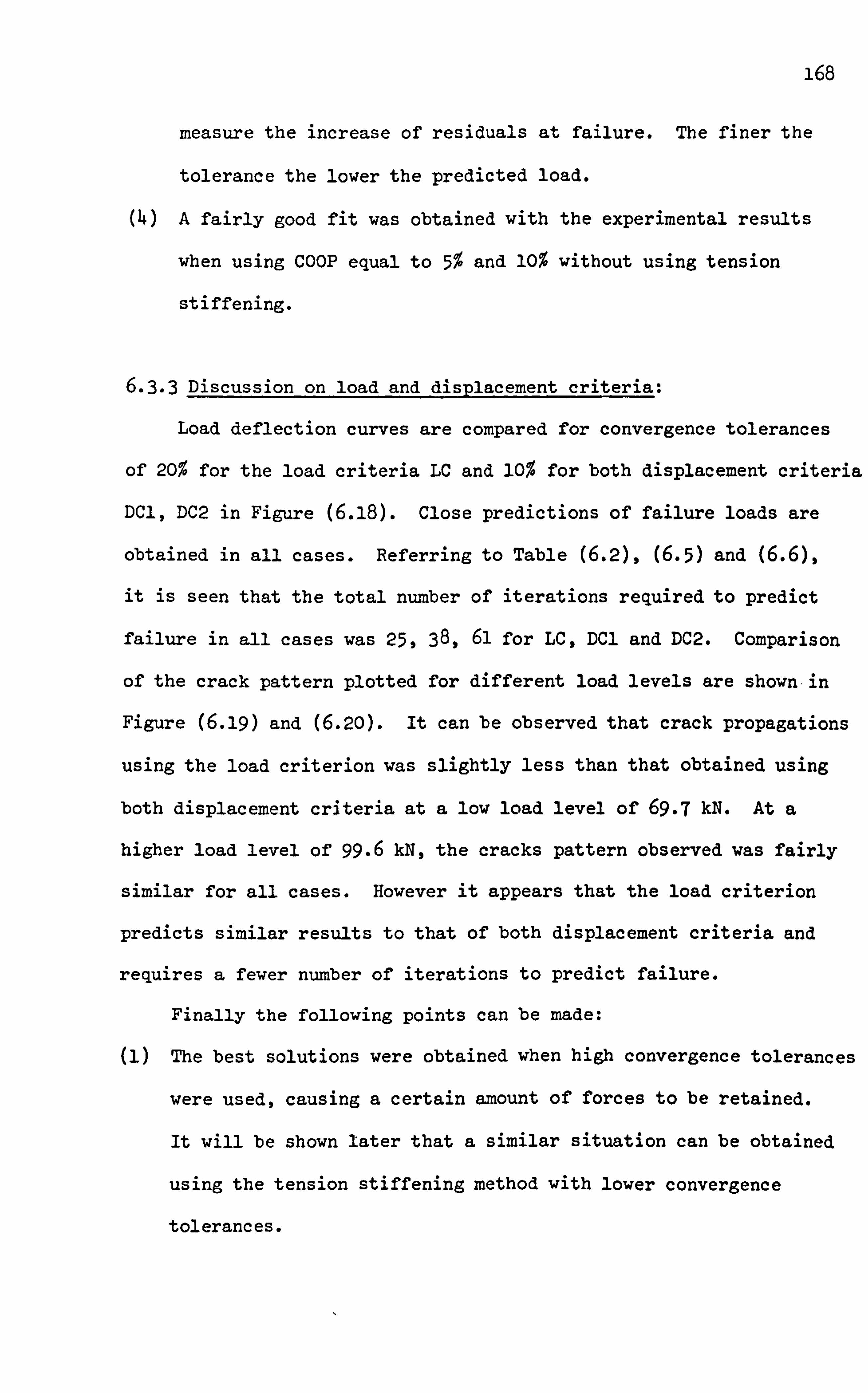
168
measure the increase of residuals at failure. The finer the
tolerance the lower the predicted load.
A fairly good fit was obtained with the experimental results
when using COOP equal to 5% and 10% without using tension
stiffening.
6.3.3 Discussion on load and displacement criteria:
Load deflection curves are compared for convergence tolerances
of 20% for the load criteria LC and 10% for both displacement criteria
DC1, DC2 in Figure (6.18). Close predictions of failure loads are
obtained in all cases. Referring to Table (6.2), (6-5) and (6.6),
it is seen that the total number of iterations required to predict
failure in all cases was 25,38,61 for LC, DU and DC2. Comparison
of the crack pattern plotted for different load levels are shown, in
Figure (6.19) and (6.20). It can be observed that crack propagations
using the load criterion was slightly less than that obtained using
both displacement criteria at a low load level of 69.7 M. At a
higher load level of 99.6 M, the cracks pattern observed was fairly
similar for all cases. However it appears that the load criterion
predicts similar results to that of both displacement criteria and
requires a fewer number of iterations to predict failure.
Finally the following points can be made:
(1) The best solutions were obtained when high convergence tolerances
were used, causing a certain amount of forces to be retained.
It will be shown later that a similar situation can be obtained
using the tension stiffening method with lower convergence
tolerances.

169
(2) The load criterion requires less iterations than the displacement
criteria for a similar crack pattern and load deflection curves
for the convergence rates investigated.
(3) The selection of the convergence criteria and convergence
tolerance is very important in predicting the behaviour of
reinforced concrete, and must be considered carefully, otherwise
the solution may follow a significantly different path.
6.4 Constant and variable stiffness methods:
A nonlinear solution is highly dependent on the way in which the
stiffness of the structure is handled. The constant stiffness and the
variable stiffness methods are the most widely used in finite element
analysis. Each method has its own intrinsic advantages and disadvantages
and these are explained in references 3 and 6. A brief review on the
application of these methods was covered in the previous section.
The constant stiffness method as earlier explained produces slow
convergence and normally a high number of iterations are required to
reproduce the load deflection behaviour. Accelerator schemes have
sometimes been used (3,6,9)
to reduce the number of iterations required
to reach a specified equilibrium stage, but they may cause instability
(3) of the solution These are not used in this work, because they
add an additional numerical parameter which may complicate the numerical
study.
The constant and variable stiffness methods have been used extensively
by many authors, but comparison of their influence has not been reported
widely, especially when used with different numerical parameters.
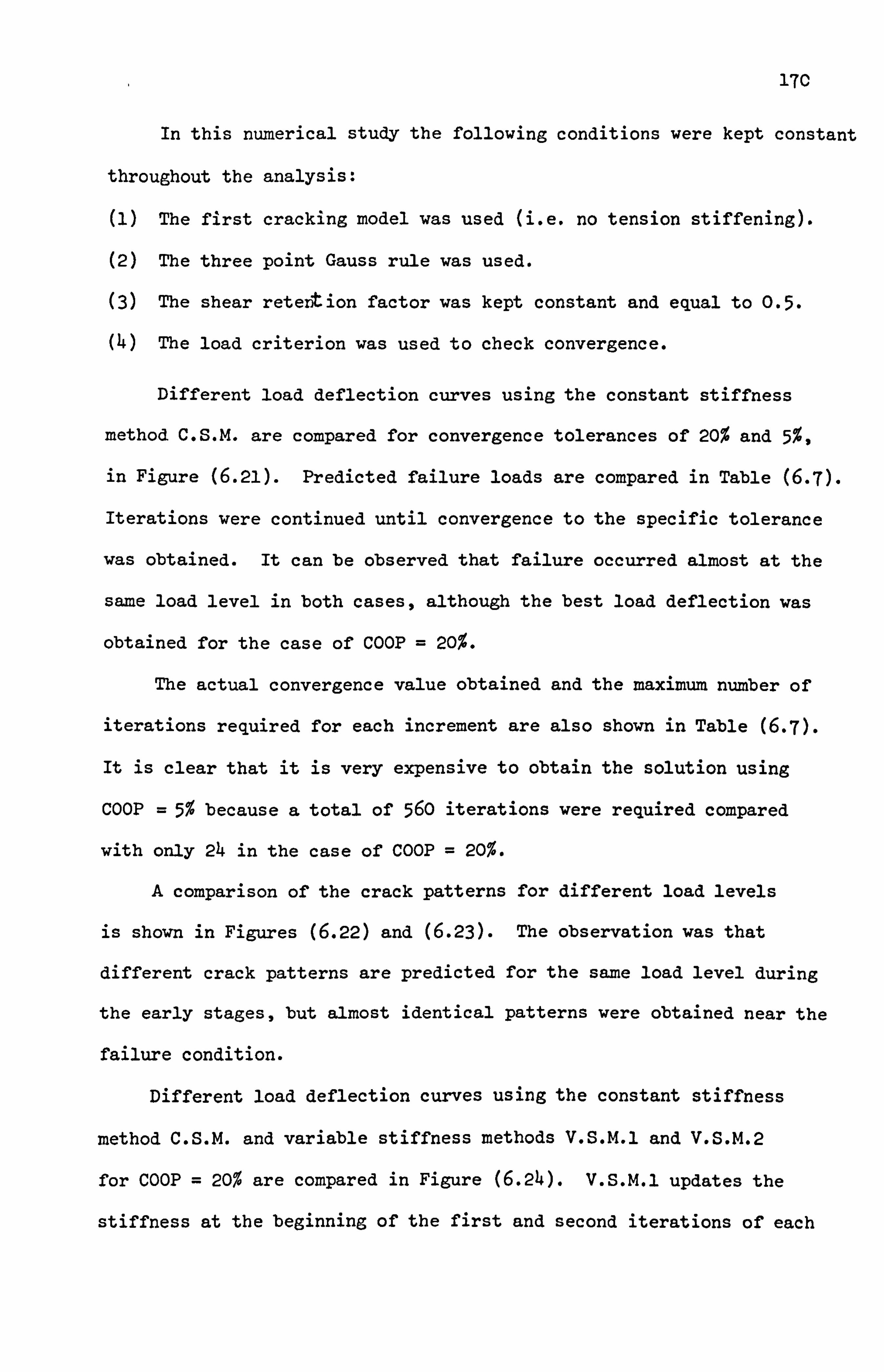
17C
In this numerical study the following conditions were kept constant
throughout the analysis:
(1) The first cracking model was used (i. e. no tension stiffening).
(2) The three point Gauss rule was used.
(3) The shear retextion factor was kept constant and equal to 0.5.
(4) The load criterion was used to check convergence.
Different load deflection curves using the constant stiffness
method C. S. M. are compared for convergence tolerances of 20% and 5%,
in Figure (6.21). Predicted failure loads are compared in Table (6-T).
Iterations were continued until convergence to the specific tolerance
was obtained. It can be observed that failure occurred almost at the
same load level in both cases, although the best load deflection was
obtained for the case of COOP = 20%.
The actual convergence value obtained and the maximum number of
iterations required for each increment are also shown in Table (6-7).
It is clear that it is very expensive to obtain the solution using
COOP = 5% because a total of 560 iterations were required compared
with only 24 in the case of COOP = 20%.
A comparison of the crack patterns for different load levels
is shown in Figures (6-22) and (6.23). The observation was that
different crack patterns are predicted for the same load level during
the early stages, but almost identical patterns were obtained near the
failure condition.
Different load deflection curves using the constant stiffness
method C. S. M. and variable stiffness methods V. S. M. 1 and V. S. M. 2
for COOP = 20% are compared in Figure (6.24). V. S. M. 1 updates the
stiffness at the beginning of the first and second iterations of each
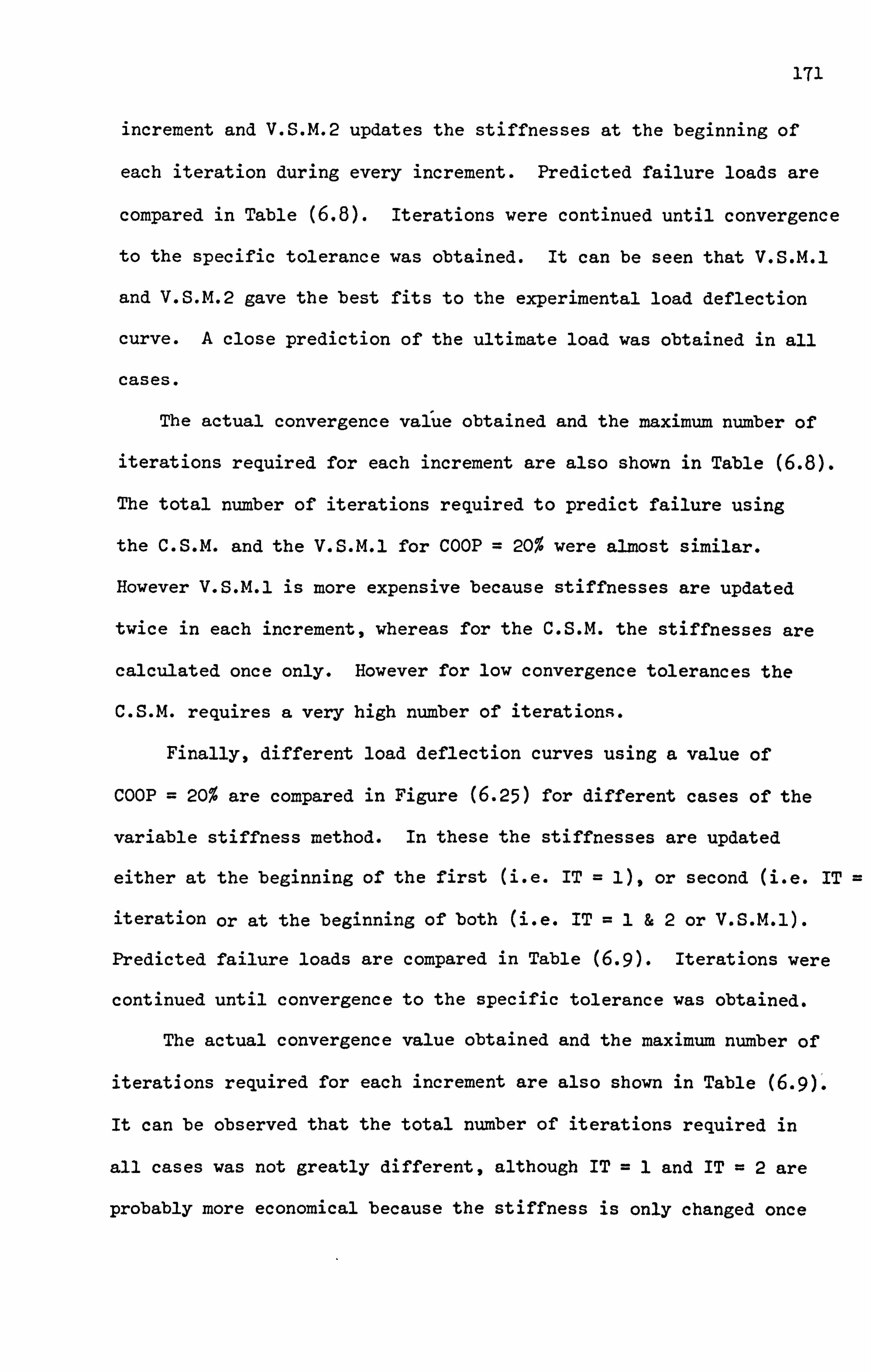
171
increment and V. S. M. 2 updates the stiffnesses at the beginning of
each iteration during every increment. Predicted failure loads are
compared in Table (6.8). Iterations were continued until convergence
to the specific tolerance was obtained. It can be seen that V. S. M. 1
and V. S. M. 2 gave the best fits to the experimental load deflection
curve. A close prediction of the ultimate load was obtained in all
cases.
The actual convergence value obtained and the maximum number of
iterations required for each increment are also shown in Table (6.8).
The total number of iterations required to predict failure using
the C. S. M. and the V. S. M. 1 for COOP = 20% were almost similar.
However V. S. M. 1 is more expensive because stiffnesses are updated
twice in each increment, whereas for the C. S. M. the stiffnesses are
calculated once only. However for low convergence tolerances the
C. S. M. requires a very high number of iterations.
Finally, different load deflection curves using a value of
COOP = 20% are compared in Figure (6.25) for different cases of the
variable stiffness method. In these the stiffnesses are updated
either at the beginning of the first (i. e. IT 1), or second (i. e. IT
iteration or at the beginning of both (i. e. IT 1&2 or V. S. M. 1).
Predicted failure loads are compared in Table (6.9). Iterations were
continued until convergence to the specific tolerance was obtained.
The actual convergence value obtained and the maximum number of
iterations required for each increment are also shown in Table (6.9)'.
It can be observed that the total number of iterations required in
all cases was not greatly different, although IT =1 and IT =2 are
probably more economical because the stiffness is only changed once
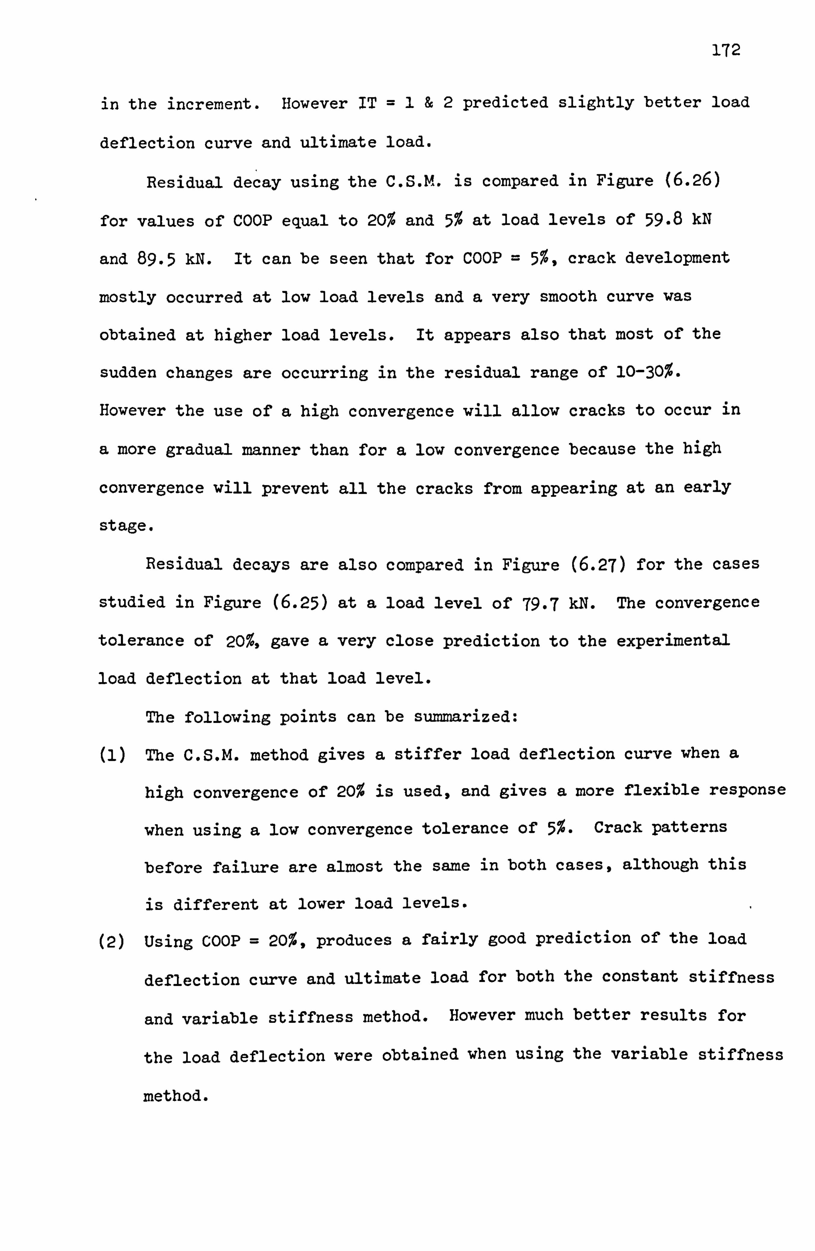
172
in the increment. However IT =1&2 predicted slightly better load
deflection curve and ultimate load.
Residual decay using the C. S. M. is compared in Figure (6.26)
for values of COOP equal to 20% and 5% at load levels of 59.8 kN
and 89.5 kN. It can be seen that for COOP = 5%, crack development
mostly occurred at low load levels and a very smooth curve was
obtained at higher load levels. It appears also that most of the
sudden changes are occurring in the residual range of 10-30%.
However the use of a high convergence will allow cracks to occur in
a more gradual manner than for a low convergence because the high
convergence will prevent all the cracks from appearing at an early
stage.
Residual decays are also compared in Figure (6.27) for the cases
studied in Figure (6.25) at a load level of 79.7 kN. The convergence
tolerance of 20%, gave a very close prediction to the experimental
load deflection at that load level.
The following points can be summarized:
(1) The C. S. M. method gives a stiffer load deflection curve when a
high convergence of 20% is used, and gives a more flexible response
when using a low convergence tolerance of 5%. Crack patterns
before failure are almost the same in both cases, although this
is different at lower load levels.
(2) Using COOP = 20%, produces a fairly good prediction of the load
deflection curve and ultimate load for both the constant stiffness
and variable stiffness method. However much better results for
the load deflection were obtained when using the variable stiffness
method.
173
(3) The V. S. M. 1 method found to be better than the C. S. M. and the
V. S. M. 2 methods because it predicted better load deflection
curve than the C. S. M. method and is cheaper than the V. S. M. 2
method. However, IT =1&2 (i. e. the V. S. M. 1 method) also
gives a slightly better prediction of the ultimate load than
using IT =1 and IT = 2.
6.5 Gauss rule:
The best order of Gauss rule to be used is usually decided after
numerical tests, since the profits and pitfalls of a particular rule
are hard to foresee. Often it is best to use as low an order as
possible because this will require less solution time than a higher
rule. Other advantages are that low orders tend to soften an element,
thus countering the overly stiff behaviour associated with an assumed
displacement field. Softening comes about when some higher-order
terms that would otherwise contribute to strain energy happen to vanish
at the Gauss points of a low-order rule. In other words, with fewer
sampling points, some of the more complicated deformation modes offer
less resistance (However, it is possible that certain modes will offer
more resistance). (14)
In general 2x2 Gauss rules are required as the minimum order (15) (16)
for the parabolic quadrilateral under linear elastic conditions
However Bathe et alý19), and Cook (14)
found that for non-rectangular
elements or elongated quadrilaterals the 3x3 Gauss rules are required.
This is because the low integration rules may produce zero energy
deformation modes (i. e. a pattern of nodal degreesof freedom which
produces a strdin field that is zero at all points) which can misrepresent

174
element volume.
Irons et al! 17)
also reported that the 8-noded isoparametric
element can have what he terms "Spurious mechanisms" when 2x2 Gauss
rules are used, (i. e. an element which can deform without generating
strain energy).
It was found by Bathe (16)
that an accurate response prediction
in nonlinear analysis frequently required a higher order integration
than that required in a linear analysis. This is because a higher
integration rule is frequently required in order to capture the onset
and spread of the material nonlinear condition accurately enough.
Specifically, since the material nonlinearities are only measured at
the integration points of the element, the use of relatively low
integration order may mean that the spread of the materially nonlinear
conditions through the element is not represented accurately. The use
of high order numerical integration also reduces the number of possible
uncertainties that can enter into the interpretation of the results of
a complex analysis, and should therefore be used until sufficient
experience with the response of the structure has been obtained. At
that time the use of reduced integration together with less elements
to idealise the structure may be considered.
These points have also been stated by Chen et al. (18)
, who found
that integration points can only be reliable in cases where sampling
points are not far away from each other and recommended, that reduced
integration rules must be used with care. He also recommended that
occasionally it is better to have more integration points in order to
describe the crack pattern more accurately. However the selection
depends very much on the problem and its actual stress distribution.
175
In spite of these problems, certain workers have obtained acceptable
results using the low integration rules for nonlinear analysis.
Phillips (3)
found that 2x2 Gauss rules can be adopted to predict
satisfactory results for the 8'noded parabolic element. Cope et alS7)
also found that using 2x2 Gauss quadrature with quadratic inter-
pretation functions restricting material properties variation to a
bi-linear form over an element ensure no additional numerical errors
are introduced into an analysis by retaining that order of quadrature.
Obviously there is some uncertainty regarding which integration
rule to use. In this section a study was carried out to ascertain the
effect of changing the order of the integration rule for the program
developed in this work. The shear retention factor was made equal to
0.0 and 0.5, in order to examine its contribution when used with
different order of Gauss rule. For instance a=0.0 can produce a soft
load deflection while 4x4 Gauss rules can produce a stiff load
deflection.
The following conditions were kept constant throughout the analysis:
(1) The first cracking model was used (i. e. no tension stiffening).
(2) The method V. S. M. 1 was used.
(3) The load criterion LC was used to check convergence and COOP
was set equal to 20%.
Different load deflection curves using a value of a equal to
0.0 are compared for different orders of Gauss rule of 2x2,3 x3
and 4x4 in Figure (6.28). Iterations were continued until convergence
to the specified tolerance was obtained. It was observed that failure
was grossly underestimated; divergence rapidly occurring after the
start of cracking. However a more stiffer load deflection was obtained
as the order of Gauss rule increased.
176
Different load deflection curves using a value of a equal to
0.5 are compared for different orders of Gauss rules of 2x2,3 x, 3
and 4x4 in Figure (6.29). The actual convergence value and the
maximum number of iterations required for each increment are shown
in Table (6.1o). It can be observed that 3x3 gave the best fit to
the experimental load deflection curve and also gave the closest
ultimate load. However the 4x4 Gauss rule gave a stiffer prediction
in the load deflection curve after the start of cracking, but ultimate
failure load was as that using the 3x3 Gauss rule.
Comparison of the crack pattern plotted for the 3X3 and 4x4
Gauss rules at two different load levels are shown in Figure (6-30).
It can be observed that less cracks appeared for the 4x4 Gauss rule
at low load levels although an almost similar pattern was produced
at higher loads. However when the 2x2 Gauss rule was used-an under-
estimation of the failure load also occurred, in a similar fashion
to that when a was equal to zero.
The 2x2 Gauss rule was investigated for a finer mesh of 36
elements as shown in Figure (6-31). The 36 elements provided more
Gauss rules over the depth and the width of the beam. The actual
convergence value and the maximum number of iterations required for
each increment are also shown in Table (6.10).
It was observed that although the predicted failure load was
better for the finer mesh it still grossly underestimated the experi-
mental failure load. However failure occurred after two increments
from the start of cracking when the fine mesh was used.
The crack patterns at failure for both cases are compared in
Figure (6-32). The cracks propagated in an unexpected manner, in
fact some cracks appeared and propagated outside the maximum bending

177
moment. This suggests that the 2x2 Gauss rule may not be a reliable
rule to use in the nonlinear analysis, and confirms the findings of (10)
Chen et al
The following points can be made:
(1) Care must be taken when using low integration rules because
numerical problems may arise causing the solution to diverge.
(2) Changing the order of integration when a is set equal to 0.0
does not significantly improve the predicted results.
(3) When a was not equal to zero, the 3x3 and 4x4 Gauss rules
gave the best prediction to the load deflection and ultimate
load but the 2x2 Gauss rule still gave an inferior result.
It would appea r that it is the order of Gauss rule which is
crucial rather than the total number of sampling points throughout
the continuum. However this matter requires further investigation.
6.6 Shear reten-ion factor:
As previously explainedthe shear reten ion factor is an assumed
numerical factor which is included in the theoretical cracking
model, to take into account the reduction in shear modulus after the
development of a crack. The new shear modulus is defined as Gc = aG,
where a is the shear reten ion factor, G the shear modulus before
cracking, and Gc the modified shear modulus. a has been used by
many investigators. For example Phillips (3)
used values of a equal
to 0.0,0.5, and 1.0 and found that when a was equal to zero an
underestimation of the failure load was obtained, but for a equal to
0.5, and 1.0 reasonable predictions for ultimate load could be obtained.

178
Suidan et al ! 20)
used a constant value of 0.5 in his analysis and
obtained good agreement with the experimental results. Hand et al ý21)
found that shear retention was necessary to preserve numerical stability
in some cases. Values of 0.2 and 0.4 were used in his analysis, and
no large differences arose from using these two values. Other authors
assumed that this factor varies with respect to the physical phenomenon (22,23,24).
For example Cedolin ei al ý22 )
assumed that the value of
GC decreases linearly with the crack width and that it reaches a very
small value when the crack is wide.
Al-Mahaidi (23) investigated the reduction of shear modulus due
to cracking, which had been used by different analysts. He found a
considerable range varying from 50% to only 10% for very wide cracks.
The particular value chosen for a between 0.0 and 1.0 does not
appear to be critical but values greater than zero are necessary to
prevent numerical difficulties, which may occur due to the zero terms
in the diagonal stiffness matrix. The presence of a is realistic
since it represents the retention of some shear due to the aggregate
interlock that occurs across an open crack. However the reduced
shear modulus Gc more nearly represents a number of springs parallel
to the crack rather than the physical reality of a rough crack in
concrete.
In general terms the use of a has proved to give satisfactory
results for different analyses.
In this section values of a equal to 0.0,0.01,0-05,0.2,0.5
and 1.0 will be compared. Also the effect of varying a on convergence
and number of iterations will be studied. In this section the following
conditions were kept constant throughout the analysis.
179
(1) The first cracking model was used (i. e. no tension stiffening).
(2) The method V. S. M. 1 was used.
(3) The three point Gauss rule was used.
(4) The load criterion was used to check convergence and a convergence
tolerance of 20% was used.
Different load deflection curves using values of a equal to
0.01,0.05,0.5, and 1.0 are compared in Figure (6-33), and values of
0.0,0.2,0.5 and 1.0 are compared in Figure (6-34). Predicted failure
loads are compared in Table (6.11) for a equal to 0.01,0-05.0.2,
0.5 and 1.0. Iterations were continued until convergence to the
specified tolerance was obtained. The actual convergence value
obtained and the maximum number of iterations for each increment are
also shown in Table (6.11). It can be observed that a=0.5 gave the
best fit to the experimental load deflection curve.
Howeveri it seems that when a is increasing towards 1.0 a
stiffer prediction is obtained. When a was equal to 0.0 a drastic
underestimation of the failure load was obtained with instability of
the solution. The following points can be summarized:
(1) The shear retention factor is an important parameter, and a
value of zero should not be assumed because numerical problems
appear at the stage when most of the cracks occur.
(2) As a increases towards 1.0, stiffer load deflection curves are
obtained. The best load deflection curve was when a equal toO-5-
(3) The total number of iterations required to achieve convergence
to a value of 20% for the tested value of a fell within a narrow
range, and the minimum number was required when a was set equal
to 1.0.

180
The wide range of a varying between 0.01 and 1-0 did not
significantly affect the predicted load deflection curves. If
this is the case then there is no point in using more complicated
methods for varying the shear on cracking surfaces unless local
behaviour is required. This would seem to suggest that a is a
numerical device rather than an approximation to a physical
phenomenon.
6.7 Tension stiffening: N (25) Tension stiffening was first introduced by Scanlon to account
for the tensile stiffening effect of concrete between cracks. He
assumed that after concrete reaches its ultimate tensile strength, a
primary crack will form, but the cracked concrete carries some tensile
stresses perpendicular to the crack direction. As the load increases,
more cracks will form, but the amount of tensile stresses carried by the
concrete progressively decreases. -
In another study by Gilbert et al 126,27)
different shapes were
used to represent the tension stiffening effect. These are shown in
Figure (6-35). Gilbert et al. also proposed a second method to account
for the tension stiffening indirectly. This assumed that the retention
of stresses after the development of a crack is represented by increasing
the steel stresses as illustrated in the modified stress-strain curves
shown in Figure (6-36). The additional stress in the steel approximates
the tensile forces carried by both the steel and the concrete between
the cracks. The added stress is lumped at the level of the steel
and oriented in the same direction for reasons of convenience. The
results obtained using the modified approach for the stress-strain curve

181
of steel were found to be as good as those obtained using the first
method, but are in fact cheaper to obtain. Gilbert et al. also
showed that the load deflection curves obtained using tension
stiffening or the modified approach for steel gave much better
results than that with no tension stiffening.
Lin et al ! 28)
found that tension stiffening has a significant
influence on the post cracking response of under-reinforced concrete
structures, but not on the behaviour at the ultimate stage.
Scordelis (1)
also reported that tension stiffening gives a more
accurate representation of stiffness for the deflection calculations,
but will underestimate the maximum steel stress at an actual crack
within an element, and that tension stiffening will become more
difficult to represent for biaxial and triaxial stress states.
Cope et al ý6)
investigated the effect of tension stiffening on
concrete bridge decks and found that its effect is most significant
for low reinforcement percentages. The agreement was less significant
for a higher steel percentage. He suggested that further experimental
work was required to understand the behaviour of tension stiffening.
Mang et al ! 29 )
reported that neglecting tension stiffening may
significantly underestimate the ultimate load.
Shirai et al! 30 )
assumed in his study that the bond resistance
between concrete and the reinforcement bars after crack formation
gives some resistance to concrete. He called this the tension
stiffening effect, and its resistance gradually deteriorated with an
increase in the number of cracks. A polynomial was proposed to
represent the descending branch which is a function of the steel
property.
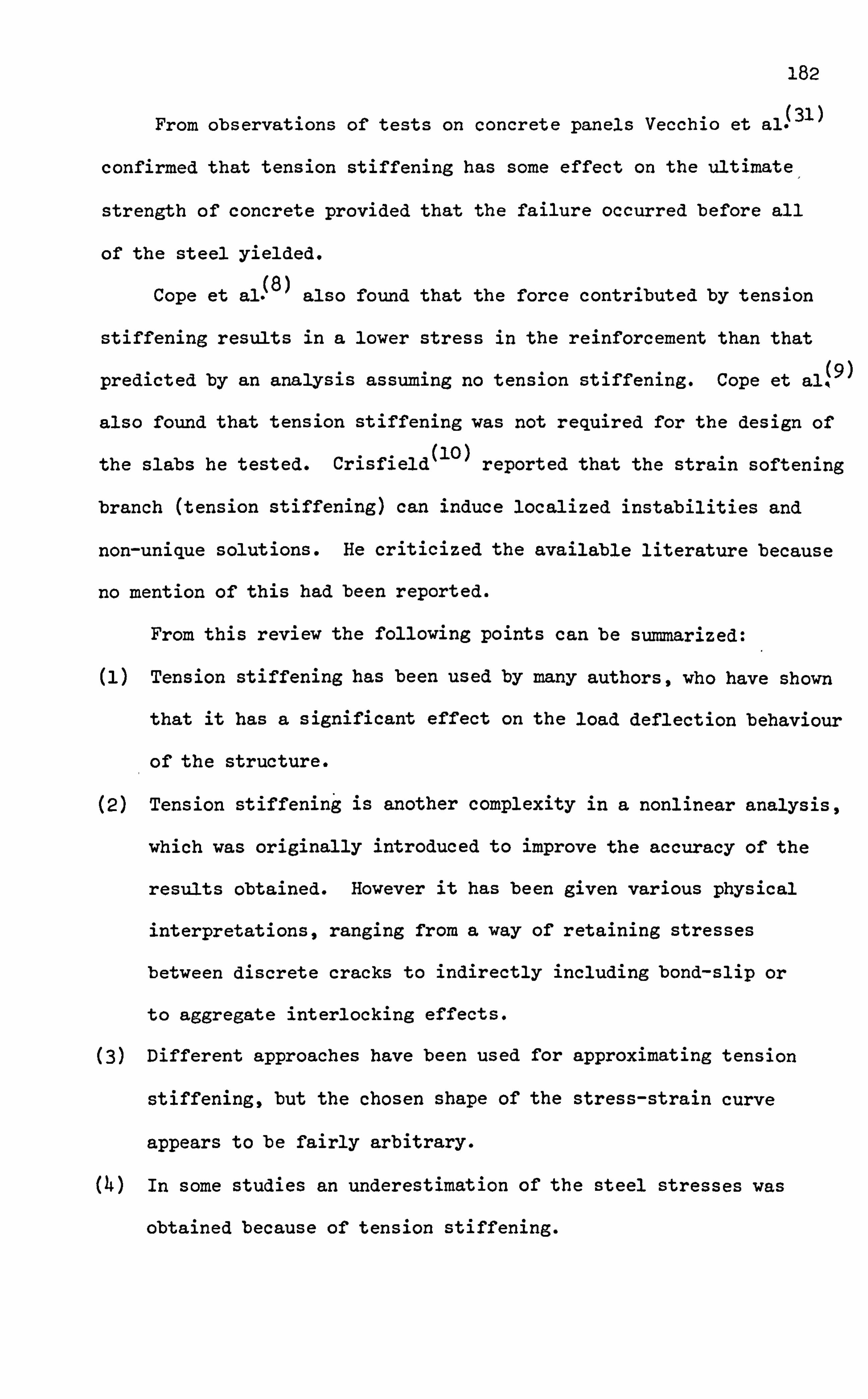
182
From observations of tests on concrete panels Vecchio et als3l)
confirmed that tension stiffening has some effect on the ultimate,
strength of concrete provided that the failure occurred before all
of the steel yielded.
Cope et al S8)
also found that the force contributed by tension
stiffening results in a lower stress in the reinforcement than that (9)
predicted by an analysis assuming no tension stiffening. Cope et allk
also found that tension stiffening was not required for the design of
the slabs he tested. Crisfield(lo) reported that the strain softening
branch (tension stiffening) can induce localized instabilities and
non-unique solutions. He criticized the available literature because
no mention of this had been reported.
From this review the following points can be summarized:
(1) Tension stiffening has been used by many authors, who have shown
that it has a significant effect on the load deflection behaviour
of the structure.
(2) Tension stiffening is another complexity in a nonlinear analysis,
which was originally introduced to improve the accuracy of the
results obtained. However it has been given various physical
interpretations, ranging from a way of retaining stresses
between discrete cracks to indirectly including bond-slip or
to aggregate interlocking effects.
(3) Different approaches have been used for approximating tension
stiffening, but the chosen shape of the stress-strain curve
appears to be fairly arbitrary.
(4) In some studies an underestimation of the steel stresses was
obtained because of tension stiffening.

183
The aim of this section is to study the effect of'Using a
particular tension stiffening stress-strain curve (shown in Figure
(5-14), and represented by the, second cracking model) on the behaviour
of the deep bean, and to try to identify the numerical processes
involved. The following points will be investigated:
(A) The interaction of the convergence rate and the tension
stiffening model.
(B) The effect of having different values of cAi. e. the strain at
which the stress is equal to zero in the descending part of the
stress-strain curve of concrete in tension. (It is assumed that
this effect represents different shapes of tension stiffening
curves).
(C) A comparison between the tension stiffening model and no tension
stiffening model.
The following conditions were kept constant throughout the
analysis:
(1) The method V. S. M. 1 was used.
(2) The three point Gauss rule was used.
(3) The shear retention factor was kept constant and equal to 0.5.
(4) The load criterion was used to check convergence.
Different load deflection curves using a value of e *-- 5E I are Ac
compared for convergence tolerances of 20%, 5% and 1% in Figure (6.37).
Predicted failure loads are compared in Table (6.12). Iterations were
continued until convergence to the specified tolerance was obtained.
It can be observed that a valueof COOP = 5% gave the best fit to the
experimental load deflection curve and also gave the closest ultimate
load. But it is clear that tension stiffening has a profound effect

184
on the solution.
The actual convergence value obtained and the maximum number of
iterations required for each increment are also shown in Table (6.12).
When COOP was equal to 20% only one iteration was required to reach
convergence until the steel yielded. This shows that a high convergence
factor with tension stiffening may overestimate the ultimate load and
stiffness. It was also observed that using a small tolerance of 1%
may underestimate the ultimate load and stiffness. This shows again
however that the convergence tolerance is an important parameter in
the control of the load deflection curve.
Comparison of the crack pattern plotted for different load levels
is shown in Figure (6-38) and (6-39). It can be observed that using
the high convergence of 20% with tension stiffening caused a different
crack pattern from that of 5% and 1% at high load levels.
Different load deflection curves using a value Of CA = 10 Cc'
are compared for convergence tolerances of 20%, 5%, 1% and 0.01% in
Figure (6.40). Predicted failure loads are compared in Table (6.13).
Iterations were continued until convergence to the specified tolerance
was obtained or'a limit of 350 iterations had been reached. It can be
observed that COOP = 0.01% gave the closest prediction to the ultimate
load.
The actual convergence value obtained and the maximum number of
iterations required for each increment are also shown in Table (6.13).
It can be seen that the use of high convergence produces stiffer
results in the load deflection curve after the development of a crack.
When a value of COOP = 20% was used, yielding was not even observed up

185
to a load of 119.5 XN. However when COOP was set equal to 0.01% a total
of 1142 iterations were required with a limitation of 350 set as a
maximum. However an almost similar load deflection curve was observed
when COOP was set equal to 1% and a maximum of 162 iterations were
required.
Comparisons ofthe crack pattern plotted for different load levels
are shown in Figures (6.41) and (6.42). It was observed that COOP = 1%
and 0.01% gave similar patterns.
Finally different load deflection curves for a value of eAý 25C C
are compared in Figure (6.43) for values of COOP equal to 20%, 5%, 1%
and 0.01%. Iterations were continued until convergence to the specified
tolerance was obtained. It can be observed that the predicted results
overestimate the experimental load deflection curve in all cases and
the analysis was stopped at a load of 119.5 M.
To show the effect of changing eA, different load deflection
curves for equal values of COOP are shown in Figures (6.14 - 6.46).
It can be seen that as eA increases so the stiffnesses and ultimate
load increases. It also shows that the use of tension stiffening
depends very much on such arbitrary values at c A' that it makes
tension stiffening curves an uncertain device.
The following points can be summarized:
(1) Tension stiffening is a method of retaining some amount of stress
which is not released when cracks occur.
(2) The tension stiffening method can produce satisfactory results
when compared with experimental curves, but is very much inter-
related to the convergence tolerance used and the value of cA
(which is assumed to be a measure of the shape of the tension
stiffening curve).

186
When tension stiffening is used with a high convergence tolerance
of 20% an overestimation of the ultimate load and a stiff load
deflection curve, was produced. A small convergence produced an
underestimation of the ultimate load but thevalue of cA should control
this.
A final comparison was carried out in Figure (6.47) for, COOP = 20%
with no tension stiffening, COOP = 5% with cA = 5c' , and COOP c
with cA = l0ec' . Predicted failure loads are compared in Table (6.14).
It can be observed that the no tension stiffening case gave the best
fit to the experimental load deflection curve. The total displacement
with tension stiffening was closer to the ultimate load deflection
although the load deflection curve was stiffer. The number of iterations
required is also shown in Table (6.14). No tension stiffening required
only 25 iterations while 5c' required 58 iterations and l0e, required CC 162 iterations.
Comparison of the crack patterns for these cases are plotted in
Figures (6.48 - 6.50). Very little difference is observed in these
cases which implies that no tension stiffening with a high convergence
rate gives similar results to the inclusion of tension stiffening
with lower convergence rates.
6.8 Conclusions:
The main conclusions to be drawn from this chapter are as follows:
A high convergence tolerance can give satisfactory results if
tension stiffening is not used. A value of COOP = 20% was
suggested in this work when using the load criterion. The load
criterion also gave a more realiable measure of the decay of the
residuals than the displacement criterion used here.

187
(2) Tension stiffening can produce satisfactory results but care
must be taken when choosing the value of convergence tolerance
and the value of strain at which the stress drops to zero.
However it would appear that tension stiffening can be
satisfactorily replaced by using a no tension stiffening stress-
strain law with a higher convergence tolerance. This is because
they both have the effect of retaining residual forces. It also
has a considerable advantage in that it requires far less
iterations and hence computer time.
(3) The V. S. M. 1 method where the stiffnesses are updated at the
beginning of the first and second iteration of each increment
predicted the best results in all cases studied.
(4) The shear retention factor is an important numerical device and
the wide range varying between 0.01 - 1.0 did not produce a
significant effect on the load deflection curve. There is no
point in using more complication for this variable in the smeared
cracking approach and a value of 0.5 is suggested.
(5) Care must be taken in selecting the order of numerical integration
in the prediction of nonlinear behaviour, because numerical
problems can exist when using low integration rules. However,
a3x3 Gauss rule was found to be a realiable rule for the
prediction of the concrete behaviour.
The conclusions are further tested for more complex beams
failing in shear in the next chapters and will be largely
confirmed again.

188
6.9 Burns & Siess shallow beam J-4 (12).
The analysis of this beam independently assesses the conclusions
drawn so far in this thesis. The beam has also been tested by various
other authors (20,32,33,34)
and so gives additional comparisons. The
beam was tested under concentrated load and is shown in Figure (6.5l)-
Details of the material properties are shown in Table (6.1).
Because of symmetry. only half of the beam will be considered.
The finite element mesh used is shown in Figure (6-52) and the load
was applied at nodal point 103.
The following assumptions were made in the analysis:
(1) The stirrups were neglected and only main steel was provided.
(2) The first cracking model was used (i. e. there was no tension
stiffening).
(3) The load criterion was used with a convergence tolerance of 20%.
(4) The method V. S. M. 1 was used.
(5) The shear retention factor was set equal to 0-5.
(6) The 3x3 Gauss rule was used.
(7) The load was applied in equal increments of 10.0 kN until failure
occurred.
Different load deflection curves obtained from various authors (20,32,
33,34) are compared with the present analysis in Figure (6.53).
Iterations were continued until convergence to the specified tolerance
was obtained. Figure (6-54) gives a clearer comparison with Sorenson's
results and the results obtained in this work.
It was observed during the experiment that the cracking started
at a load level of approximately 40.0 kN while the reinforcement steel
yieldelat4load of 156.0 kN. In this analysis., the start of cracking was
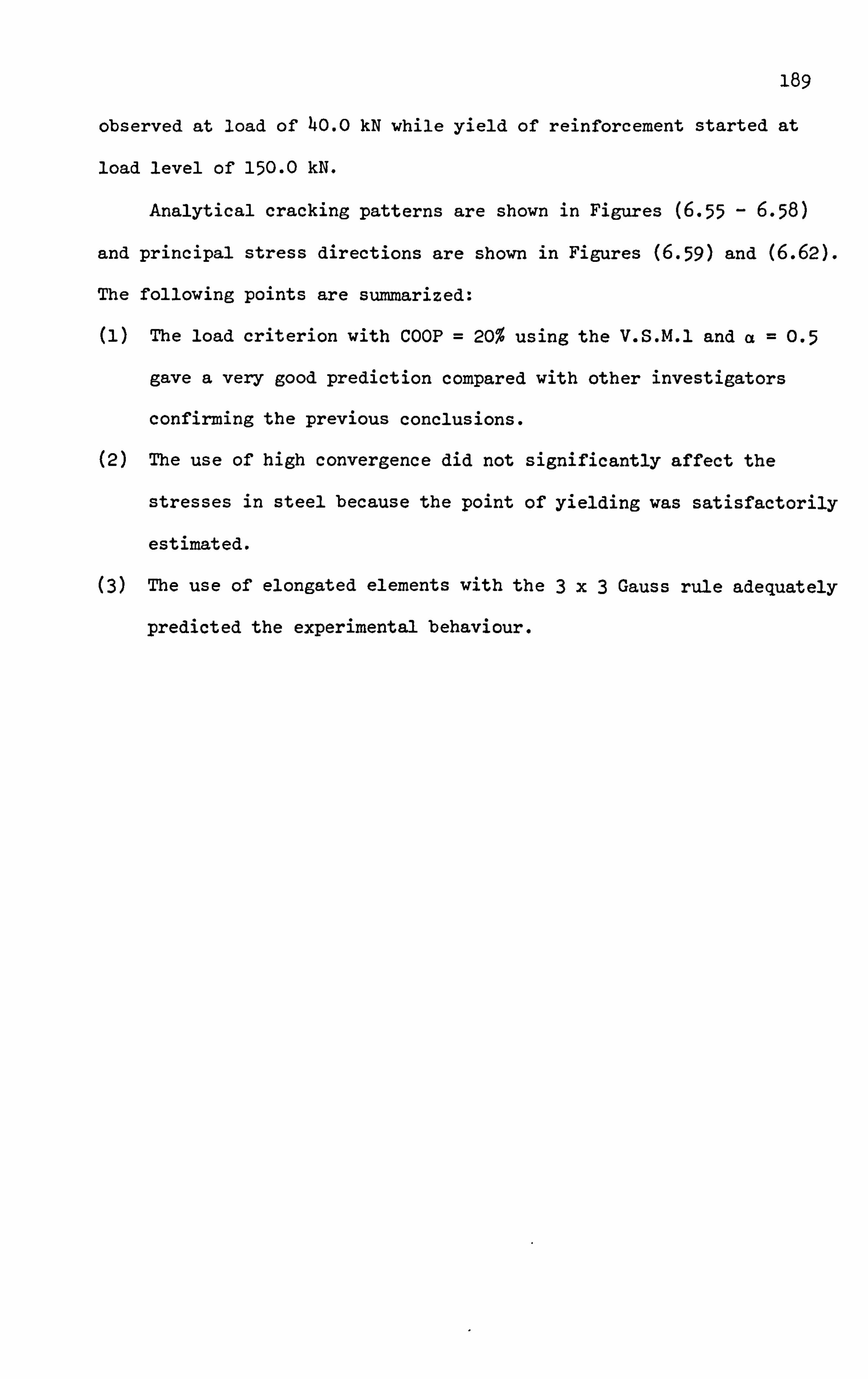
189
observed at load of 40.0 kN while yield of reinforcement started at
load level of 150.0 M.
Analytical cracking patterns are shown in Figures (6-55 - 6.58)
and principal stress directions are shown in Figures (6-59) and (6.62).
The following points are summarized:
(1) The load criterion with COOP = 20% using the V. S. M. 1 and a=0.5
gave a very good prediction compared with other investigators
confirming the previous conclusions.
(2) The use of high convergence did not significantly affect the
stresses in steel because the point of yielding was satisfactorily
estimated.
The use of elongated elements with the 3x3 Gauss rule adequately
predicted the experimental behaviour.
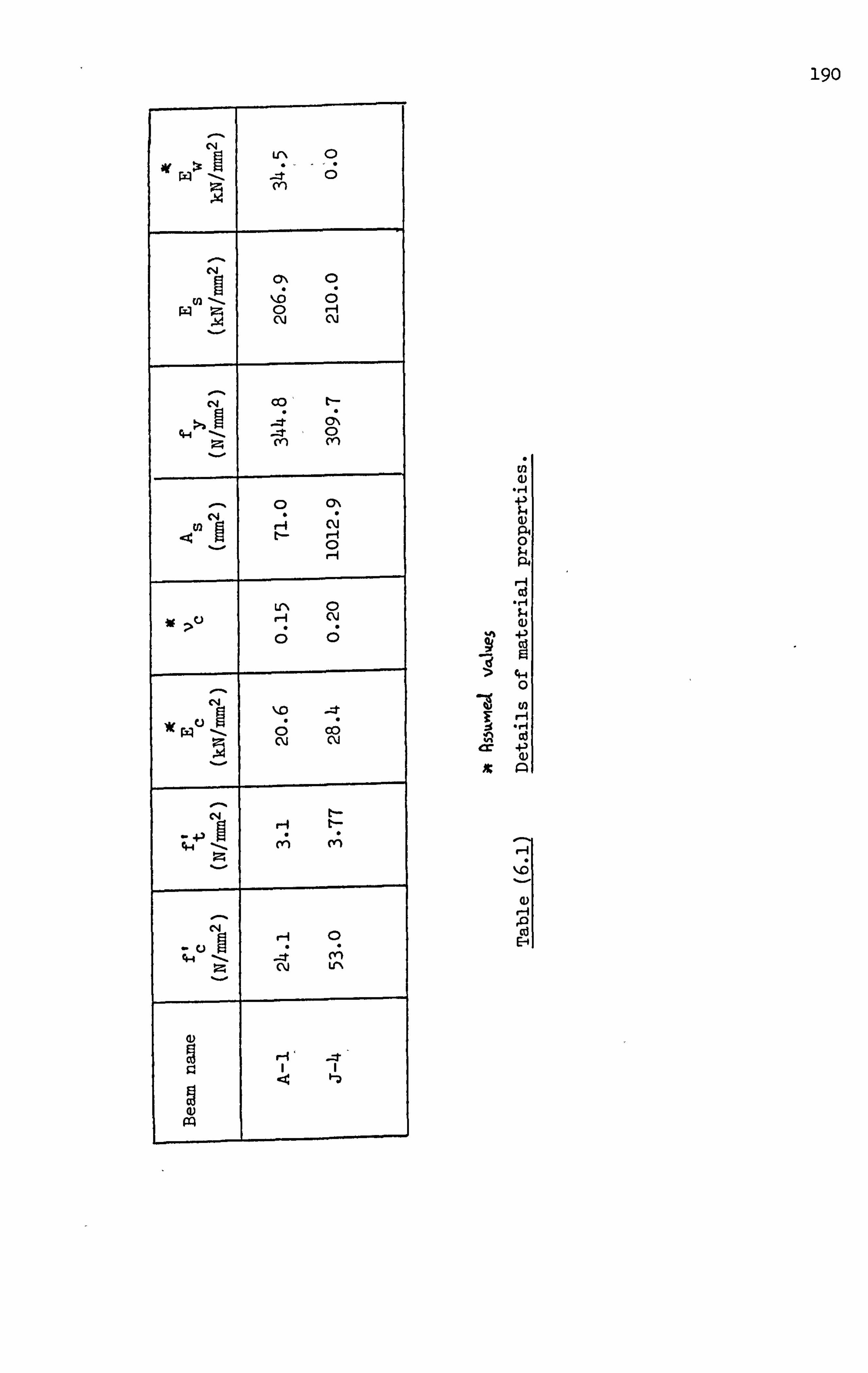
190
iv
5 (n
ul ýlo
0 CM
0 r-i CM
CC)' t-
C\i
w >C) H
C) CM
CM CM
; -; ij m (n
: 2. - 03 U'\
pl
r-q cd H
0
H
cd
P
r1
4)
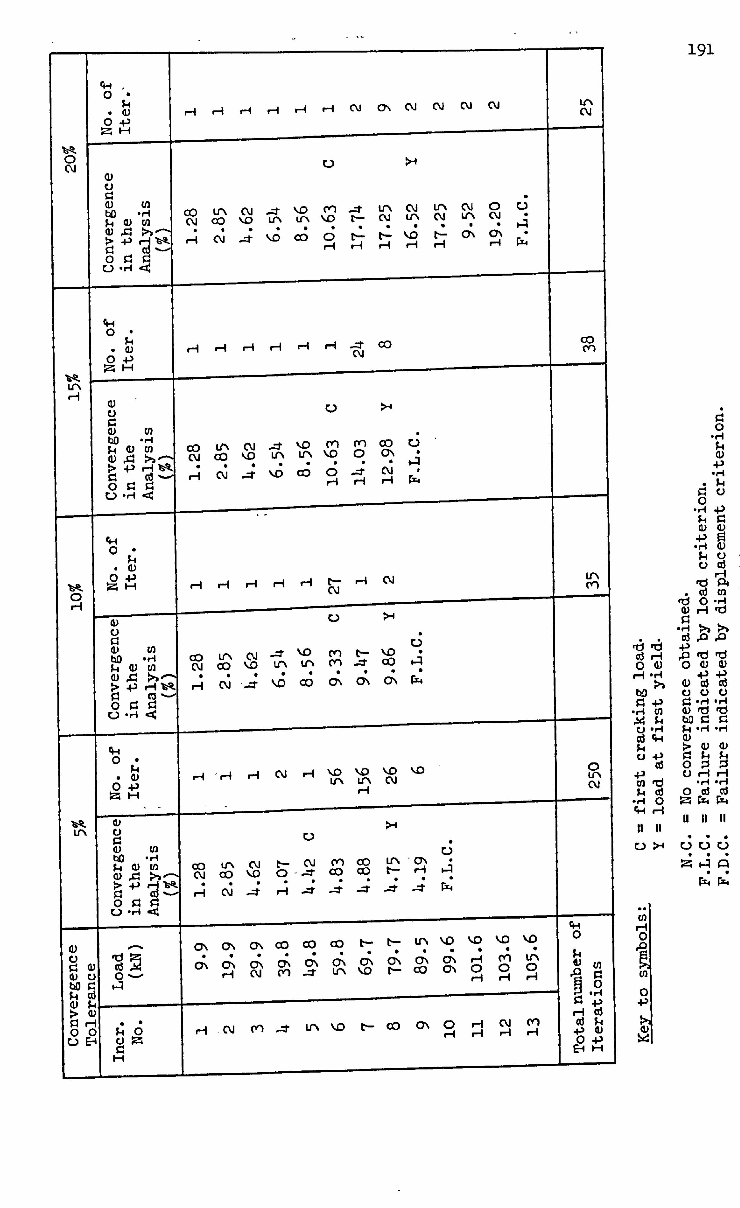
0
. c) r-i H r-i H r-4 9--1 CM O\ CM CM C\i cm Lr\ CU
0 4-)
0 u :i CU
a)
ho ., 1 00 Ul\ (M -t %. 0 Ul
(Yl % 0 _e t-
ttl\ CU
C%i Lr\
Ul\ CU
N Ul\
C) CU
0 P (L) rn (M CD %. 0 UN \ I i 0) gl. »- > 4-1 f-4 %A lý cý -4 1.
ý Ilý (ý
-i tz
4 tz r-i
li; r-1
tz r-i
cý cý r-i
- p4
r3 cj - r - 0 %3 93 L) .H9
f4-1 0
a) r-1 r-i r-i r-1 r-i H _: t Co CD ý CU
UN
0) ul bo -r-1 P a) Co Co Ltl% N -: t %Z (n (VI Co u ' 0) 4 >b , CM CO %ID UN LA %. 0 0 M A
+) r-i %-% >O. cj - i
cý -4 lý cý c; -4 cý - p 0 $Z Z: r-i r-i 4
C)
r-i r-1 H cu
C\i
tD ri Co Lr\ N -e '. 0 I
M m
t- -t
%Z OD
. 4
9-4 a) u] cm Co ýID Lr\ V N - (D J., >ä .
4J > . . . .
1,0 .
CD 1; 1 cý P: O. 0 gi 0. u.
4-t 0ý
(L) r-i , i Cj l %ýD %. 0 -
%ýo \M - 0 W\
Lr\ U % cm C\i
>f Lr\ t)
9: u
r; $-, a) ul Co Ul\ C%i t- CU «i CD
Co Co
Lr\ t--
' CY, % f-1 u) x. >b - CU CC) ýo (D -
Cd A (ý -4 A :r -zr -: t 0 Z: Z:
4) - O\ O\ C% CO CD CO t-- t- u-% %, 0 \ýo ý, 0 %ýD 0
C) Z: Q
rd 5 ) Cd cý cý cý cý cý cý ý o\ - O\ cr, O\ -i C) m 0
UN 0
(L) t ) 0- r-i C%j cvl -e Lr\ .D t - Co r-i H
bß 0
> 51 00 cm (Yl --. r Lr\ IID t-- CC) ch 0
r-i r-i mi
N r-i
M
r-i $-4
-0 c) L) E- 4 e) Z 0
, ýi n5 ci r-1 0 0) r-1
tl) x ý4 t) ., l 0 4-4 ý4 ci 4-)
ci
cn d 94 ci
-r-i 0 t+4 r-i
C;
z ý4 p
r4 P4
U) mi 0
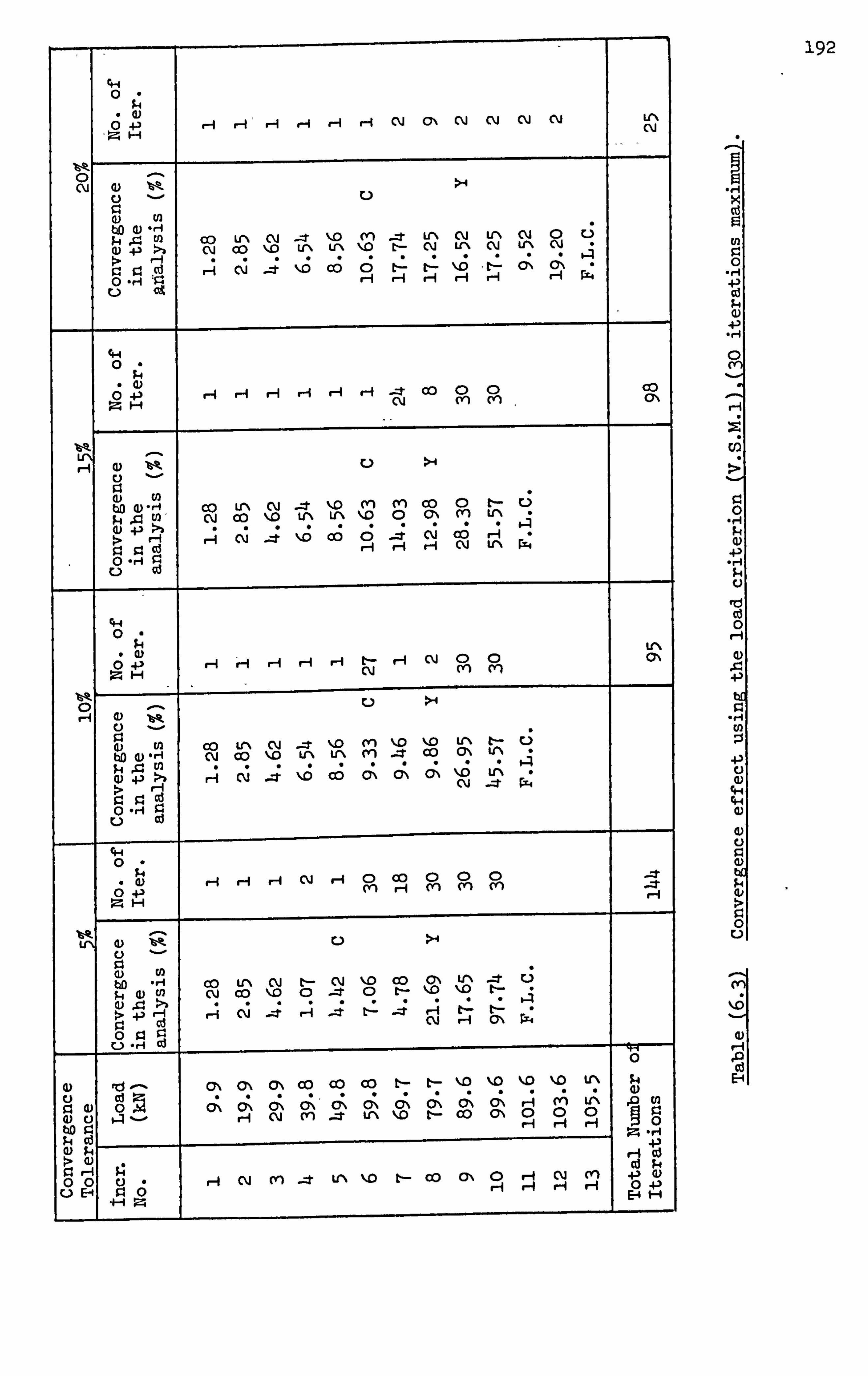
0
4J r-i r-t 1-1 ei r-i ri CM 0% C\i CM cm cu UN cli
. N4 e-i
cu U) >A
(L) ul to Q) ri 14 J., til Co Ul\ CM _e %. 0
- (Yl _e UN cm
l LN cu
UN 0 cu c3 Q) 4-1 >3 CM CD \M Lr\ U % \Z LI- CM U \ cu
C0 cý (ý tz r.: �ý ý e. 1 :;, 0, -i - p4 0. H : ý3 r-i mi r-1 H H r
0
4.3 r-i H r-i r-i r-i r-i _e C\i 00 0
Pl 0 (V)
Co O\
tA a) V% >A
to 0) *r, CO Ul\ cu _e "0 Pl (n Co 0 t. - ' IL; $., Ici to, cu OD \M tf\ LA %0 0 CY% (Yl U \ . 4 (L) 4J >ä >H A Cý C i UN 93 93 0 H r-i % 0 ri
0
t- CM r-1 C\i 0 0 Ch
H
:i
0) t12 W a) *rl
CO CM
LA OD
CM "0 .2 Ul\
\D UN
m m
\D it
%. 0 OD
UN O\
t- UN
C-) .
ý, jl. D,
q) +> >-& A cý -4 \, ý cý cý cý cý �0 .
tA 4
: >H cli _e r. Z: 0
0 . (L) r-i r-i r-1 cli H 0 CC) 0 0 C)
(n _: t _e 0 -P
tk
93 0) to to -H
Ei to s- CD C\i
Lr\ CD
CM %ýo
t-- 0
C\i je
ý, 0 0
CD t-
O\ �o
u-, %D -e L--
rý ,
Q) 'cl >..
> 42 -, A Cý -4 A t.
1
A tz 0, 0. Cd cu
0 91 cd
0
4) Id - o\ O\ O\ CO OD Co t- t- %ýo %. 0 %10 %, 0 tr\ ý4
(U 0 cý cý (ý cý, c; % cý cý Cý a
A 0 A 0 u-, 0 0 0 0) c) 4ý r-i N Pl --t W\ .0 t- CD \
H r-4 r-i 0 bD 93
Cd
00 0 r-i CM (n -1 UN %I0 t- Co C)\ 0 r-i
H r-i
cu H
(n r-i
4> 0) 0 43 u E-1 91 E-4 H pl
., j
0
.,. j
m
192
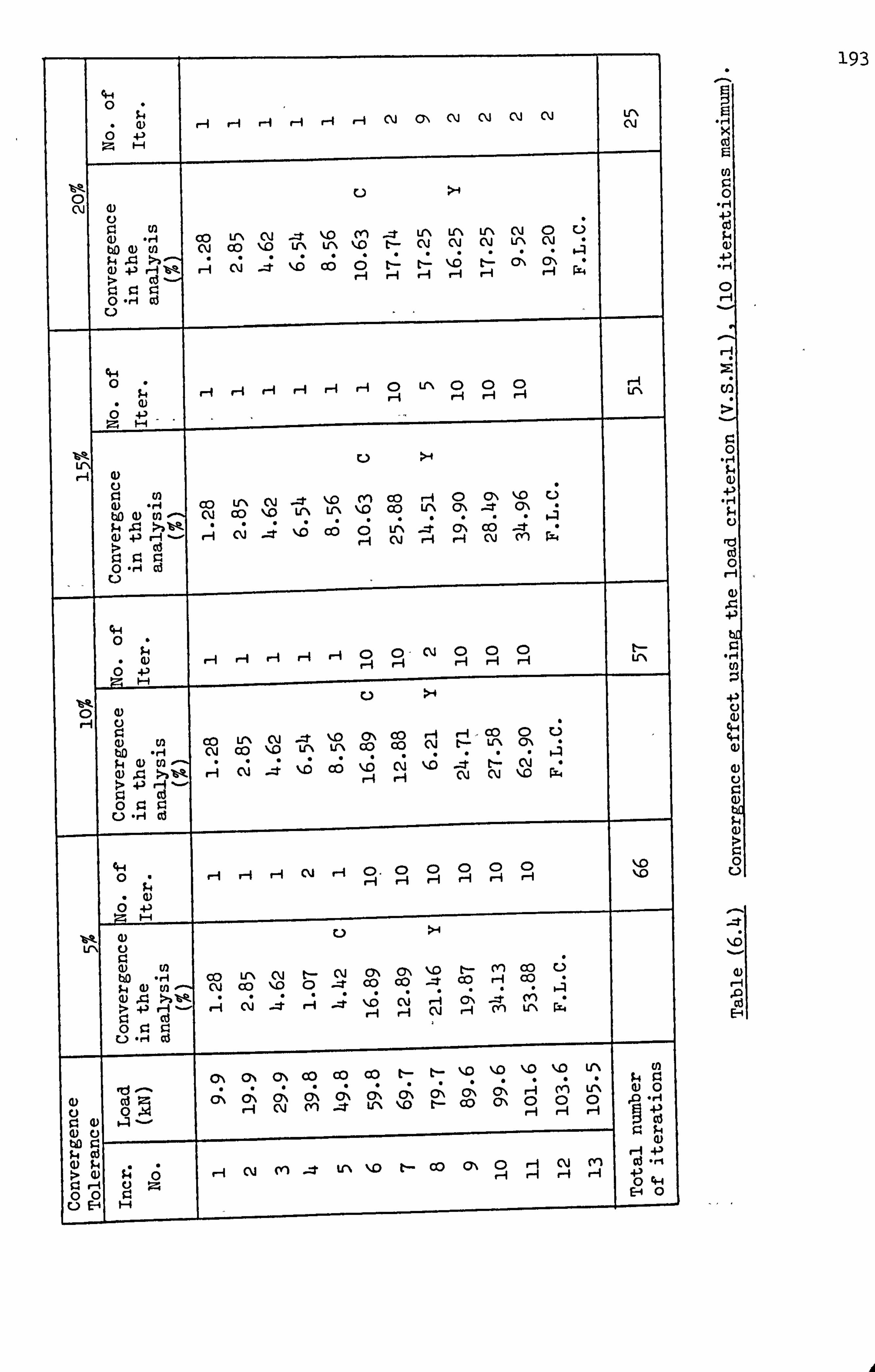
ýA 0
0 r-1 r-i r-i r-1 r-i 1-4 C%i CY\ C\i C\i C\i CM Ul\ C%i
C\i a) C) 9: 4) . 11 CO Lr»% N -t "0 m
\ -t - Lr\ C\j
Ul% Cm
UN C\i
cm Lr\
0 cm
r-) bo (1) (n CM CID \Z VN UN ýo t - p x31 >-. - 0 4-1 r-i
. r-1 cý cý c3 t-i
mi ti
1 m; r-1
ti H
cý cý
CO gi r.
0 -r-1 ci
r-i r-i r-i (D UN 0 0 0 Lr\ 9)
C)
XA
C) ci 0) r-1 CD Lr\ cm -zr l
%. 0 M %M
CO CC)
r-i Ul\ 0 O\
O\ _: t
1,0 CY\
U
bo 0) rn ý cu OD ýlo U \ ir\ . . . . 13
P 4.1 :,, a) -P r-i rý Cý -4
. 1,0 CD 0 u-,
CU -: t ri (7, H
cc) CM
> r-1
0
. (L) r-i r-1 i H r-i (D 0- CM 0 H
CD mi
0 r-4
t-
0 -#1
H t)
(1) Di CD UN N --t %ýo -
o\ Co CD
-i cq H t-- - CO
Lr\ 0 o\
U
tio H C\j co \jD Lr\ v % CD . . : i $-l 9) to -
Q) 4 >b %-% A cý -4 .ý cý ý, 0 C\j i ý, 0 -e CU t CM cý %Z - ý 4J rj - e
0 r. r. 0
0. r-i r-i H Cm r-i C) - 0 i
(D -i
0 r-1
C) ri
(D r-i
%I0 r--1 r r
0 41
Lr\ 0 r. 0) ul bß li CD UN CM t" cm o\ 0%
CD \. 0 :,
t-- Co
m i
Co Co
u
p (L) ul , cu CD �0 0 -: t CD - r. ' » te, 43 H -A cli
_e A -; ýlý cz Cm r-1 (Y) UN 0 H r-1
0 ci r. ti H ci
(> (> CY% CC) CD cc) t- t-- .
%ýo .
ý, 0 \. 0 1,0 Lr\ Ln 94 r.
(L) 13 ý Cd 52
. cý . o\
. m CU
. o\ (Y) cý -: t
;, tr\ cý �0 cy, t-- 0, co cy\ 0% i 0
A C) u; C) v0 14 t) 0 r-1 0.
> a) s4 CY (n --r U-ý \JD t- CO 0\ CM M cd +-,
0. H 00
o Z:
0 E--4 0
u E-4 H
0
0 -r4
4-l' . rj
cd 0
rl 0)
+' C) '1)
4-4 4-I
a)
0
193

194
0
-P CM cli CM CY C\i CM _: t _: t Pl (n cn C*i CM CY (n M CO
;4
ek
0 C) 0 Lr% to W vi ; -, r. ' %A cu cu t- r-i (DD CY% CYN \o
Lr\ alý 0
CY ID
M CD\
alý UN
O\ \o
\o �o
%. 0 CD
t-- -: t
ri (L) P- e \o cy\ 0 CM M -e (>
. . 00
ý r. ä
d c; A A A cý Lý t! LA Cý
A %ý bl t! M (> 43 r-1 0 ri 4-4
0
4-1 0
Z ri cu cy cy CM cu cy Co UN m (n m cm (*1 (1 rn le C\i
:i UN
to to _H CM cu t- r-1 OD CY\ (n CY%
CD %D CD
(n t-
0 CY
O\ Ch
Lr\ :t
CO CM
Co M
0 r-1 ý-, (L) rh \D O\ 0 cu m _: t (A _
(1) A- » ; ý ; ;
A cý j; (A rA ; A A A cz ';
A
0 %q , +> e it c - ' ' 0 53 Z
0 cy CY m cn -: t O\
cu C%i -i
et H
cu H -e (n
0 CM
r 0 43
ri a) :i C) gi 0 tD f. 1 CM cm CO %D Co ni r-i 0% -t CO UN ;. 4 CL) to NM O\ 0% ri r-t Ch 112 cý 9 cý 9) c: >bl >r c; c; c; . 0 . C) . 0 0 0 0 0 ri
0 53 . uH 1
to
cý cý IlýI 112 OD CD t- t- \D \D \D \D \o \o \o
. Lr%
. m 93 (L) 0
CL) C)
rd ý 05 Ch -ol 0, 011 (ý cý Ul\ cý % 0 ý; 1 t. - cý 00 cý O\ 14 C) A 0 LA C) tz 0
o\ 0
ch r-i
0. -ri 9 -ý Z: 0 WC,
3 r-i CM Pl _: t . ri ri r-1 H H tD 93
44
p r-1 0 r. r-i i cu cn -zr Lr% lýD t- Co 0% 0 -A cu
H m -1
-e -i u'% ri
\o ri
+> 0 4-f
00 t) - ri r-1 r r E-4 0 t) EI r. 0
r4
tID
I.
r.
LP
%4; V
F-I
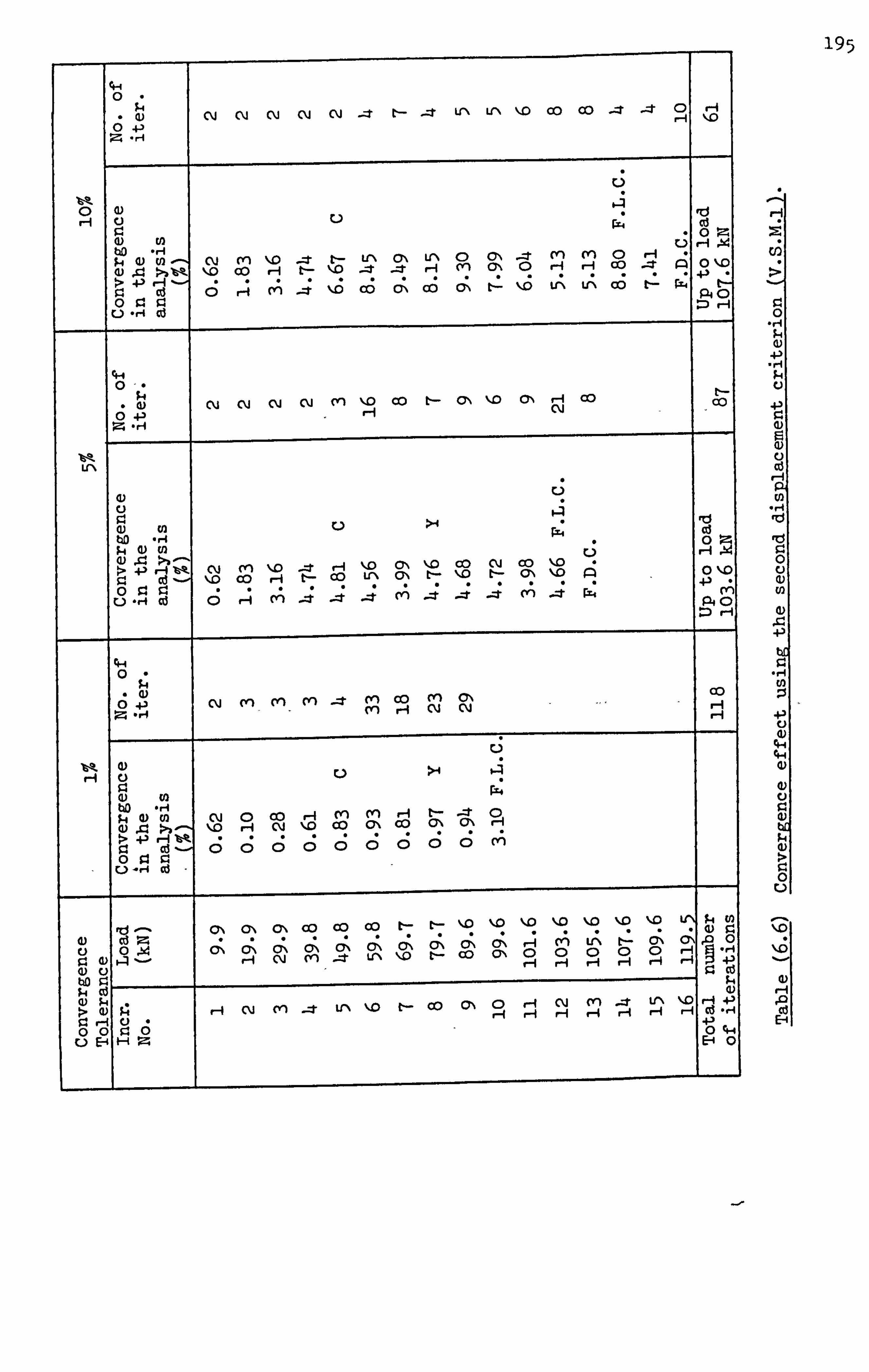
0
W CM C\i CM CM C\i -t t- -t Lr\ L(, % "0 Co OD _e -_J, 0 r-i ý
%A 0 td 0Z ri r-i X
bD p (1) (a - CU M %, 0 t- UN
- O\ U-N 0
cn cý -e 0
M r-i
(Y) r-i
0 CO -, e: r iý 0 �o
>p %A ', 0 CD r-i t- %I0 :r -: t r-i * * , ý, 'C"d' -
(ý A A
-4 %ý cý cý cý c;, L. - �0 tr,
ý, cý tz rz 4 t-
A0 0 r. r.
L) - r-i
CH 0-.
P .w CU C%i C\i C\i (Yl %. 0 Co LI- C\ %Z 0% H Co t. - Co
0 4-2 H cy
te Lr\
>I ci 0 5
H t--% Cm M \. 0 -2 - H OD
\Z UN
C% 0IN
\M t--
Co \M
CM t--
00 all
%. 0 \D 0 %D
cd - \Z CD H t 43 0 Z: r.
4-4 C)
cli (n rn Pl -: t m CC) m
C\i 0, % cli
Co
bß ri ý. f 0) m C\j C) OD r-4 ni m H OD
t- m
jt C)\ a) c: - %-ý H CM %D Co (:
-p tk - 0 C) 0 c; c;
0 93 r.
- O\ oN a', co CD CD L-- t- \M 1,0 *
tA .
$-4 Co (U $Z
4) 0
1 Z b4 0 cý cý cý cý cý cý cý cý cý cý
3 A c)
A 0
uý o
tz (D
c % C: )
cý -i
00 g -, i
r. (1) _ FA - ýI ci (y) -e u-% \b t- Co C N a) u
9) At H CM «1 -: t UN %, 0 t-- OD Cý 0 r-i CM Pl -e tr\ �o r-i 4-1 0 -H ý r-i C) 41 0 00
U gi
Cl)
r.
9)
a) 4. )
. f-I
\D
Cc E-4
195
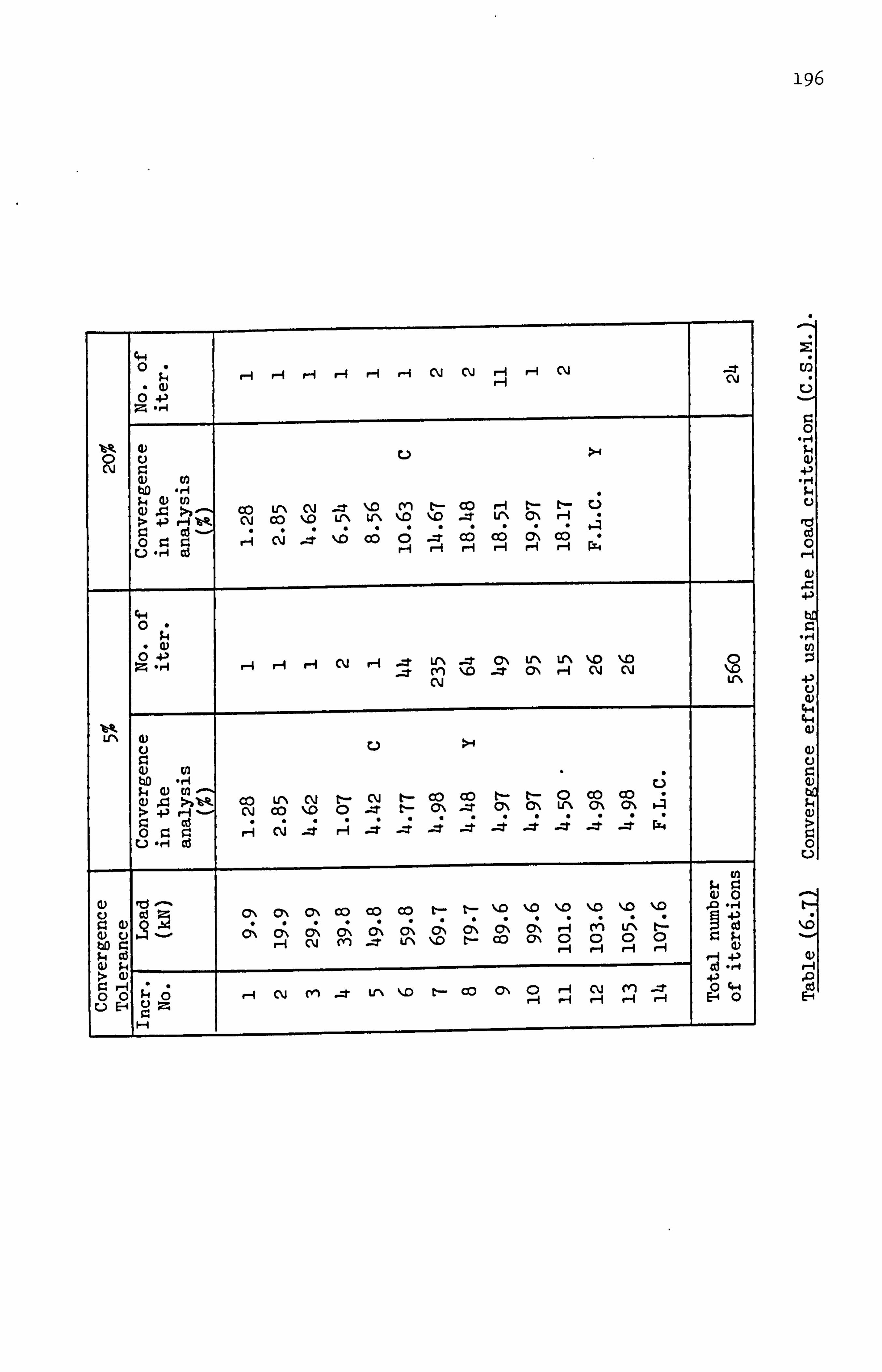
196
0 $-4 r-I r-i H r-4 r--i H C\j C\j H r-I C\j
C\j . 0) r-I
0 4-)
0 ci L) >4 C%i 0
w V) bD -H $4 (D (L) Cl
In ý,.. ý CC) Lr\ C\j _: r \0
UN m
\D tl-
\Z co
:r I
Lr\ t-- a\
tý- H
4-1 r-i %-k C\j co \D Lr\ _
0 V. 0 r4 Cý ;
1.6 0ý 6
r-i _; r-4
Cý H
Cý r-I
Cý r-I
Cý H P4
0. r-I Cd
0
(D 4.2
;4 rj r-4 r-4 H Cq r-I ý* _: r
Lr\ CY)
:r %D
0\ -*
Lr\ ON
Lrl% r-4
ýNo C\j
%D C\j
C\j UN
Lr\ >I
V. 4)
0 k CD 0) '0
(n ý*tlk CC) Lr-% C%i t-- C\j
. t- t-
co CC) r
t- ", \
t-- 0\
0 Lr\
CC) ", \
CC) C\ ý)- +) C\, cc) \, D o -I -.
r.
00 cc
0 r-I Cý _; r4 _; _; -4 _; -4 -4 -4 _; -4 r4
a) 0 CD V
4)
to Cd C\ 0\ C\ co CC) CC) t. - tl- \D %0
ý %ýo
; \. D
A \. D
A \D
: 0t r. 0) 1 3- Cý (: ý Cý \ Cý\ CY) Cý -r :; \ Lr\ Cý \JD (ý\ tl- C; CC) C 01, 0 0
L 0 t. 0 r. $4
bD 0 ýi C j _ r-I H H H (D $4 Cd 0) $-
f-I 43
4-ý
00 o r-4 C\j (Y*) -t Lr\ %. D t-- co C\ 0 r-I H C\j H
m f-i
_-. r ýf 0 COA
E-4 0 L) E-4
cI
0
r.
a)
0 0
I-
'-I
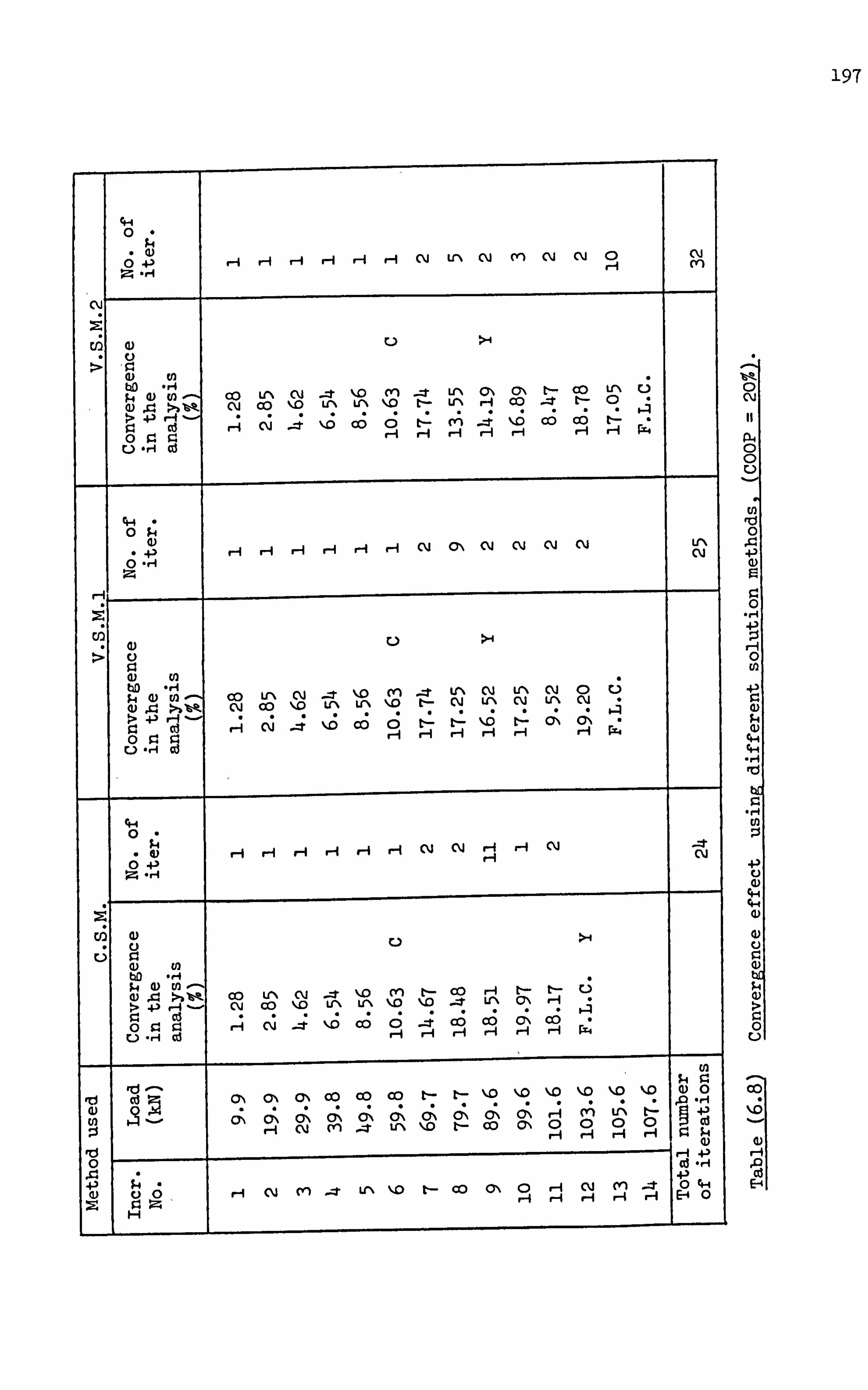
197
0
4J r-i r-i r-i r-i -i H CM UN C\i m C\i N 0 CM
CM
:i
P (1) M- Co Ul\ C%i --t %. 0 m _: t Lr\ l
C), % (: cl- -
Co --
Lr% 0
ci
a) AC: 16-e C\i OD %I0 Lr\ Lr\ %I0 t-- Lf \ H Co _ :t t 43
cý -4 ý; <x; (ý tz r; -4 -ý ýý cý -i tz -1 - 94 0 r. r. r-i r-1 r-i r-i r-i r r
H cd
0
r-1 r-i r-i r-1 CM CY\ CM C\i C\i CU Lr\ CM
0 r-1
93 hD -ri P0 ul - co Lr\ cm -e 1,0 (n --: t -
tr\ C\i
CU Ul\
UN C\i
CU Ul\
0 CU
U a) 0 >b te CM OD %ýO Lr\ Lr\ \. 0 tý
>ý 42 A cý m; cý cý bi 0 0
.
0
r-i ri CY Cli r-i ri Cli CU
>f
bD -, 4 p a) rn - 4) 10
>b let Co u', cm % --: t Lr\
\Z Ul\
M %D
t-- \JD
Co _e
r-i U'\
t, - CY\
t- H
CJ
4-) 4- cu CD D
0 r. Z., r-i cm _e %Z Co (D _e H cý -1 cý 1-4 cýI f-1 cý H - rm4 C-) -ri ci r-1 r
Id 05 cy% O\ o\ CD OD CD b- r- \. O \o \. 0 ýo %Z (1) 0
m ch O\ (IN O\ l %
O\ 0, r1 0
m 0
LN 0
t-- 0
9ý
0 r-i cy vi _e tf % I0 t-- CD %
4-31 0 . C., 4J G) t) 0 r-i Oj (n ;t Lr\ \Z t. - Co O\ 0
14 r-4 CU m -: t
ýI 0 4-1 Eri 0
U) Id 0
J., 43 a) rg
rd
co
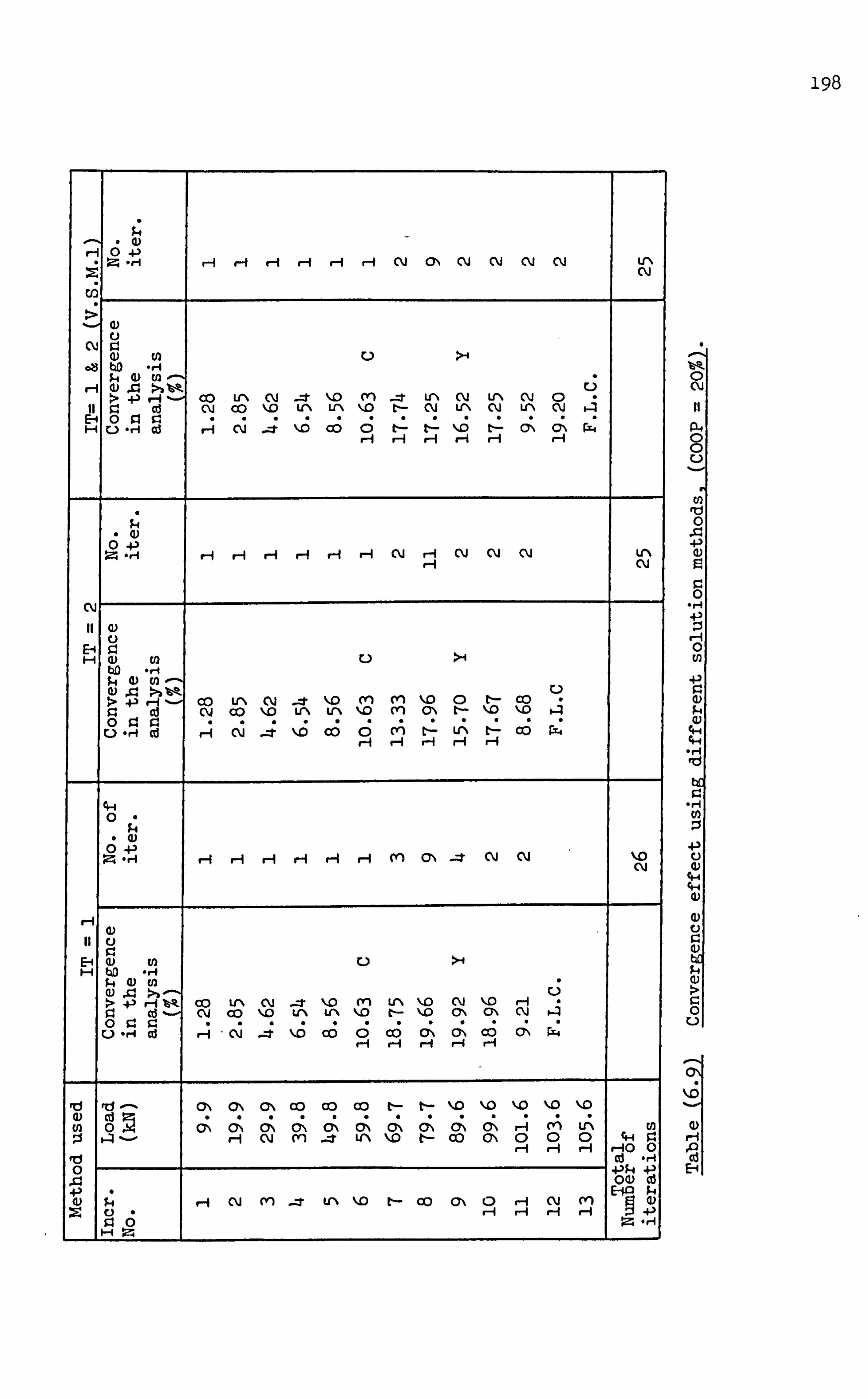
198
- 4) ý
r-1 r-i r-i r-t r-i r-f CU M CY N CY C\i UN CU
>A
ei CO Lr% N -e ý, 0 M -e Lr\ CM Lr\ CM C) Cd CM CD %M Lr\ Lr\ "0 t- cm UN cu U'\ N
E-1 0 91 51 z z ! H ci A cý cý c; t t ý,
ý t- cý cý r.:
ri r-1 r-i rq CU r-1 C\i C%i Cm UN CU
C\i
E4 r. H 9) (11 u >I
tß -rt k (V rA - (L) ci >. 3 t" cý > 4-3 r-i - CO tr\ C%i -2 %M ni rn %ýo 0 LI- CC) rl ci OJ CO \O u-% Lr% ý, 0 (n O\ L-- ýe %. 0 4 0 91 r. '
1-1 cli _e "0 CA tz uý t-: cý r.: H r-i H r-i
0
Z ri H i r-i r-i rý ri M CM CM %Z C%i
r-4
>f
04 >b - c -p r-i %rk OD Lr\ CM _e "0 (n Ul\ \Z cm %. 0 r-i
cd - (, %j CD ý, 0 tr\ UN 1,0 t-- \ýo CY\ ch CIJ 4 0 r. r.
c-) -H cd A - cm --t �0 cý c; ý cý cý cý cý r.:
,d d- CY\ O\ O\ OD Co OD t- t-- "0 %0 "0 %10 %IC) a) ci (n
m 0 cý cý (;, cý (ý cý cý cý 1; A LA 10
N m -2 Lr\ %, 0 t- Co c% o 0 o rH r. r-i r-i ri rio 0
Iti H 0 4-1
OQ) ci Ein, $-4
r-i cm m -e UN %m L-- 00 cy\ 0 r-i cu (n 1)
C14 0 0 0
a) cl-I
. 'l
a,

CH $4
cn . 0)
0 4-11 r-I r-I r-i H r-I H r-A C\l t- N C\j C\j N +) C\l r. 0)
H 4) a) ()
H ho -H 1., 4) U) 0 C\j N t-- H t- (Y\ co co r-I m 0 Cý 0) 0 ý-t - CY) 0\ tl- ý10 t- 0 UN t- L-- 110 CY\ C\ +1 tk ; ý ý ; r-I
Cý -4 M; C8 C C C co 00 S1. r-i r-I H r-i r-i H H pt4
0
o (D r-i r-I r-I r-i r-4 r-i C\i c\ C\j C\j C\j C\j to 0 43 C\l 4JI
H 0) 0 a) C)
9.1 %Z (1) co H bD -r-4
1ý4 (U to 00 L(l\ C\j --J* %ýo (Y) --t
Lf\ CM LrN C\j 0
0 ýý - 0) C\J CC) \ýo Lr\ LrN ý, o E-- C\j Lr\ C\j Lr\ N . . :> +ý H %--I I ! 6 I ý . ý-l V4 Cd - r4 Cý 0ý 6 t- t '. t- C C\ 0 914 r. ýi r-i r-I r-I H r 0 cd
0
- (D H 'r-I H r-I r-i C\J CO Lfl\ to 0 4.1 r-i C\j 4. 'J
CM (D
0
C\l \. D
(U ri) b. 0 -r-4 M $4 4) w _zr 01 cr\ co -: T U"\ -: r (u 4 : ý-, - C\j -t co %, o t-- zr Lr\
+) -4 " - ý ý : 0 'd - C\j Cý Cý 0 C \ r. 0 51 0 r-4 r-i H
0 -r-I cd
0
r-I H r-i r-I H rn 0 +1 t ; E;
Cli (L)
C\j a) a) w bD ., I a) ul tý-
tý- C\j C\ 0 Lr\ 1.4 ýo
cd t-- C; r.: 0 $1 0
0 -r-I cd
C C (0 C 1ý t- 11 (1)
ý ý ý ý : 7 (D 0 0- Cr\ C\ 0\ cr\ 0\ 0\ CY\ CY\ C\ C\ rl m UN 43. r-4 g ý4 'i C\j m --t U-\ %ýo L-- CC) 0. \ o C) o 9 -ý r-4 r-i ý4 0 $4
0 C , * r , r-4 C\j m _; r UN \D tý- co CP\ 0 r-4 N m
0 -1 r-4 r-i r-I c
l
q - o
0
43
pq 4. ) 0 r. 0 (U 0
r-I .
Cl)
6
HI
1: 1) H
199

4-1 0
Q) r-i r-i r-i r-A r-i r-i C\i Co 1-4 cm CM cm
4J
, a) (1) . r, 4 cli 30 Lr\
Co CU
M: ) -: t tr\ \Z UN
M ýlo r-i r-
UN (n
(Yl (n .2 O\
Co 0
\lo (Yl 4
to ul
1-, IJ >, - Q) r-i %A cý 'xý (3 t-i (;, cý -j m; 9: I ' 51 r.
0 2 al r-i H H r-i f-1 r-1 cu O\ C\i CM cli C\i Lrý
C\i C) 42
uý a)
C) 0) U) rý 11
to H $-, iv U) CD Lr\ cu _: t I
%M l
m \ D _-: t t-
Lr\ C\i
C\i Ul\
Vl\ C\i
CU UN
0 cli
(L) 4.1 CM CD %. 0 L N U \ J > te Z: Cd - (ý tz tz m; t-: cý cý Pt: 0 9: r. r-i H r-i r-t r-4 H
0 r-1 r-4 r-4 CM CY C\i CM CM CNJ Co
41 .
cý g u >f C) gi Q) ta
11 b. 0 li 0M CD LN cu _e %. 0
UN «1 �o
0 \Z
\D CM
LA r-,
ON 0
UN Lr\
CM -: ý lý -
4 >b ý CM CD \D W\ 4-1 r-1 tz
- r4 cý -4 %ý; cý c; t- .2 CD ýz4
0 r. 2 r-i r-i H r-i
0
r-i r-i r-1 r-i cu m m cu C%i C\i C\i Co CY
43
Lr\ (1)
u >A 2 C)
; -, (1) >, - Co u. \ c%i -: t �0 cn %
a', Lr\
�-0 t- r-1 0
m CM
cu CY%
H 0 r-1 t--
a) 4 mi %PI CM Co %ýo " Lr\ 0 4.3
%Z H CM it %I0 OD 0 ý, H
cý i
%ý r-i
cz r-i
\. ý H
cý H
p: 0 g: Cd m
CJ ri
0
0) r-1 H r-i r-1 r-i mi CU %. 0 r-f CU t- cu
4-2
gi a) 10 cý W -ri
ul 00 Ul\ C%i -1 \M M ri 0\
v UN r-i
O > C\i CC) %Z
"0 A , Co C Z$
7 4-1 - 0 '! cy --zr �0 -ý d t: - cý t. 1 cý P,
0 c: g; r-i r-i H ) -, 1 cd
0 . ri U) u2 9: Cd 5 CY% (> (: Co CD CC) e- tý- %ýo
* %I0
* %10 "0 %ýo %M p 9:
11) 0 09
+> 0
5 40 4 cý (ý cý cý
ý cý -
CY \ CO
CY \ ch
r-1 0 (VI 0
VN C)
tý- 0
A. -r-1
(L) 43 1 f-i cu m _-: t tr\ ,0 t r-i r-A r-i r-i $-, t ) --
4-1
a) t) ý r-i CM (n zt UN \M t-- OD (3\ 0 H
r-i r-1
CM mi
«1 r-i
zt r-1
cj ., l 4J 0 E-9 0
i-I
Ct)
4-) 0 Cd
q.
4-3
Id
r-4 P Cdl
E-4
200
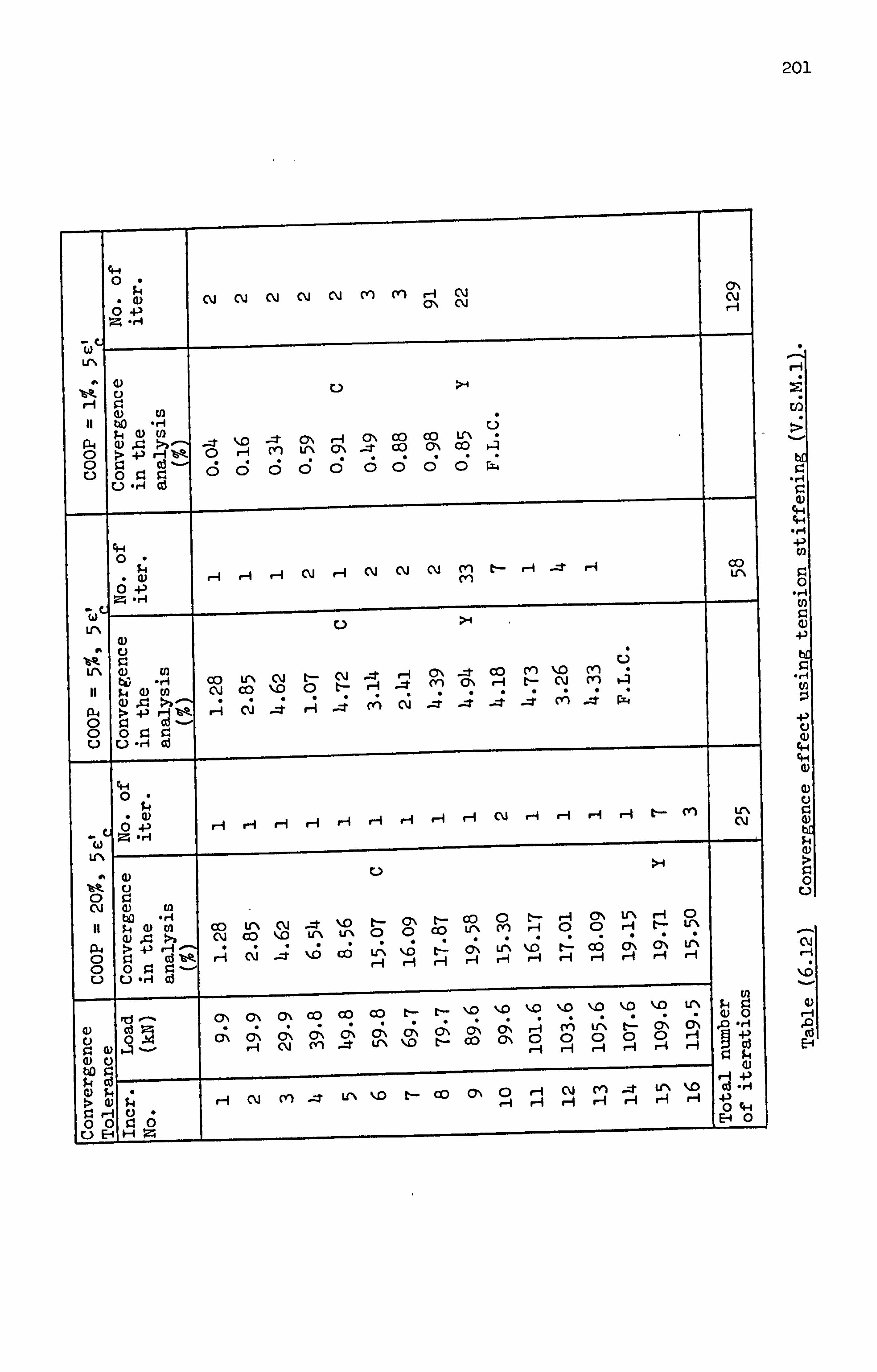
201
CH 0
. a) cu cu cm C\i C\i m pl r--i C\i C\i 0 4-2
O\ cm r-i
IL
UN
:i
ul
12, (L) c3 >, ý _-: t %ýo -: t M O\ Lr\
r-i 0\ (: _e
00 Co
Co CY\
VN CD
+I,
0 ,'-
0 0. r. (5 c; ci d d 1: 3 (S (S d ýk:
0
i C%j -q Cm C\i ei ri L-- r-i -e r-i Co (1) r-1 mi r- ý
C 1 Lr\ -
UN (L) (n
W -, 4 cc) Lr" N L-- Cy -e 21 H A
O\ (n -e cy,
CD H
M t--
%, 0 Cm
m rn
p (L) to cu CD D 0 t1 r Z p4
a) 4 >b - r-i CM -e r-i
. -2 A cZ -4 4 -4 -i A -4 P
00Z: u ri ci
0
r-i mi r-1 cu H r-i rA r-i t-- m Lr\ C%i
4J
LIN >A
t;
C c\, M b. 0 -r-i p a) m CD tr\ CM -e \. 0 t-- C% t-- CC)
WN 0 M
t'- H r-1 (D
ON 0
LN r-1
mi tý- 0 tr\
Q> C\i CD ýn Ln v\ o 0 .
CC) . . . . . . . . .
ö P
te , ci >O A cý -4 £; cý uý ý, 0 t-- cy, u-, %, 0 t-- co O\ c% Ln . 0 r.
0, (> o\ OD CC) CC) t-- L-- \D %Z %M \M \, 0 %M 'ýD Lr\ .
14 r. (1) 0
a) ,dý W 52 0
% cý cý cý cý
. c\ . CYN (7% CY%
cy CD 0 uý 0 tz 0 C> o
cý, r-i
p ri C)
r-1 cm «i Zt Lr\ 1.0 t- cc) \
C d 43 $ 4 CM «i :t trN %m t-- OD Cý% 0 r-1 CY Pl --. r
-1 tr% -1
1,0 r-1
c3 -, t 4-1 (L ) r-1 - r-1 r-i r-1 r-i r f 0 4-1
ý 00
I ej - 93 0 1 E-f 0
LCLE- 1HZ
., q 401 0
4., C)
c-i
cli
r-i
E-1
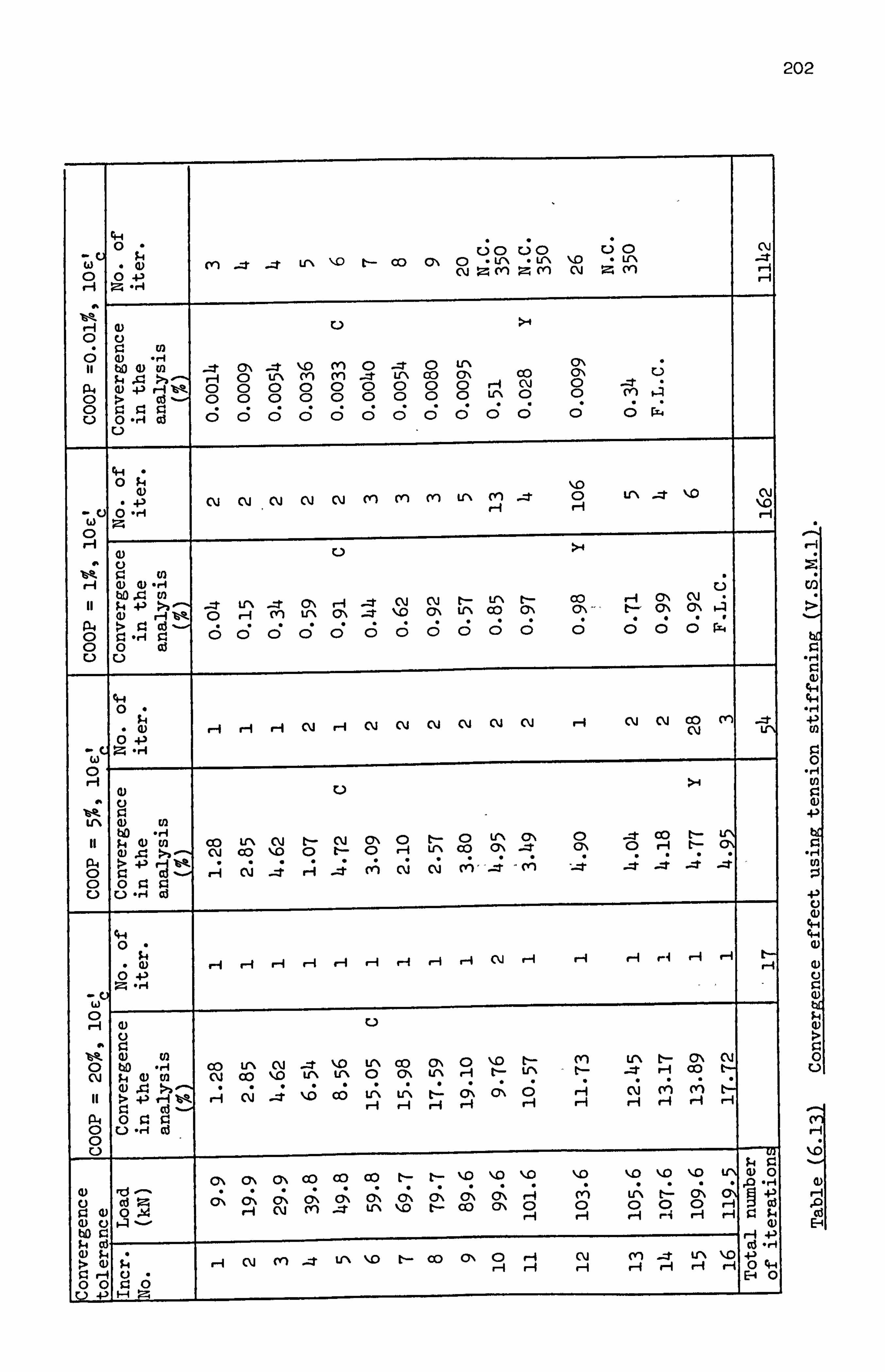
202
0 60 60 o N w . 0) m --: r -f U"\ \0 t-- OD M 0
C\j - LrN
zm - Lr*\
m \0 N
. Lr\ zm --t
r-i 0 0 4-3 H
H CD 0 C)
II (D t: to 4) m
>) - $-I sl _: t r-I
ON 0 -=t Lr\
\D CY)
m CYI
0
__-r _zr Lr\
0 co
Lr\ C7\ co CN 6
P-f . W 43 r-I WR , 0 0 0 0 0 C) 0 0 0 0
r-i U'\
C\j 0
0 0 -T m
. *4 0 cd - 0 0 0 0 0 0 0 0
. . . . 0 u
ý 93 93
0 ri ci 6 6 C; C; 6 c; c; c;
. o o o 0 0 r..
U
0 ý4 4)
4-3 C\j C\j C\j C\j C\j m m (y) Lr\ CY) _zt 0
-i Lr\ C\j
\. O -C 0 -ri r-4 r H (') ;4 A 0 -
>-4
r-I a) W-H C; 11
bo 0w ý4 40' >'j ý -T Lr\ --T 0\ r-4 -: T C\J
"o C\j C\
t'- Lf'%
Lr\ CO
t'- C\
CO C\ -1
r-q tý-
ON 0\
C\j C\
- ý4 4) r-i %-, 0 H M Lr\ Cp\ -t
114 0 ý *ro ol - 4 r4l 0 6 cý (: 5 c; (3 C3 (: 5 C; C; 0 0 ci
0 $4 (1) H r-I r-I C\j r-I C\j C\j N CIJ CIJ C\J r-4 C\j C\j co
C\j m _: r Ln
0 43
w
Lr\ (L) Efl
11 to -rl p (D ca co Lr\ C\j
\ t-- C\i
- 0\ 0
0 -i
tý- U'\
0 co
UN ON
CN 0 ON -t 0
CC) H
t- t-
U'N CN
(U .0
>a Cý co ýo o t r 4-1
I.,
. C\i
.
_zr
A
-4 CA Cý Cý CA -4 -4 -4
0 0 93 r.
C-) C-) -ý4 cd
0
(D r-I r-4 H r-I V-1 r-4 ýq r-I r-i Cli H r-I C-4 r-A -4 H
4-)'
w 0
U
0 tio . 14 co Lf\ C\i _-r \D Lr\ 00 CY\ 0 \D l-
tý YN
(Y) - t-
UN T
t H
CY\ 00
C\j t-
C\j p 0) w C\j co \, o UN Lr\ 0 C7\ UN r-4 E . .
- (U S., >, ý
4-51 ? -A Wt .
r-I .
C\j .
_-: r .
%0 .
OD .
V\ .
Lr\ .
t- .
0\ O\ 0 H H
Cý H
CA r-i
A
H ti H
o Cd P4 0 r. 0 0 u 14 ci 0 0 ui
- JL4 0
C\ C\ C\ co co co t-- tý- \. D \, D ý-o \. D \D \10 \. D WN Q) 0 ra. r. 4
(D 0
rC$ - cd z (ý\ (ý Cý Cý
- -Cý\ %
Cý Cý (: I Q
(A 0
LA 0
t: - 0
Cý 0
(ý r-i
9t
93 (L) 0 b4 r-I C\j m --: t U \ ,o t- co \ r-I r-i ýi r-i r-i r-i 0 IL4
W ci ý4 4) tio V. r, 4 4-3 P Cd Cd r. 4 (D ý4
W ý 4 -4 C\j m _: r UN ý10 tý- OD 0\ 0
r-I -4 H
C\j r-i
M r-f
-: I* r-I
Lr\ H
\0 r-i
43 0 4-4
r-4 CJ E-4 0 00
6 V.
" 4-3 "
F-I
r.
0
(Vi H
\0
0) i-1
Ei

203
0 U3
4
4
. 0) ýi r-4 rl ýi r-I ri C\j ON N N C\j C\j UN C\j E 0 4-3
0 Oj 0) C. )
C) r.
PL4 0
a) . r-I tko En $. 4 0) ýý - co Lr\ C\j _: r \. D m _: r Lr\ C\l UN C\j 0
C;
0 4) 10 r-I tp, C\j co \D UN Lr\ %10 t- C\j Lr\ C\j Lr\ C\j ý-l o
-, 901.1 - ý Cý Cý C; tL t.: tL Cý Cý r.: 00 Cd rl r-i H H r-i r-i
4-4 0
. 0) r-I r-I H C\j r-A C\j C\j C\j m t- H _-: T H CC) Lr\
V Z 0 4a m ,
) UN
m tto tf) co tr\ C\j t- C\j _: t r-4
:T ON m -: r O\
CO r-4
M t-
\-O C\j
M cn
- 1.4 pq - $4 (1) > N CC) \0 0 t- r-i
. . . . 0 0
4 o)
'o %A
4.3 Cd Cý _; r4 _; CA Cý ý; -zt -: t -1 ýA L) r. 0
0 r. Cd C-) -r-I
CH 0
. 4) C\j Cj C\j C\j C\j cy-) cn m U-\ m -t '-D 0 Lr\ -t ý, o C\j \ D
CJ 0 +3 ý
0
11 tto r4 $4 0) to
, --ýr \D -zr m O'\ UN r-4 C: Y\ --. r 41
C\j %. D
C\j C7\
t- Lr\
U-% co
t- 01%
CO m rA tl-
CY\ ON
C\l C7\ P-t
0 0
o) X. >3 4-ý ý t-
0
(: ý-
r-I Cý c; C7 C;
- (s
6 6 ci c; c; 6 C; 6 C; Pý
o 0 V.
Cy\ 0\ CY\ co co co tý- t- Lý\ \. 9 \. 9 %10 %10 %ýo 110 UN 0) 0
U Cd z Cý Cý\ (:; \ (Y\ 0\ r-I m 0
L'ý 0 t: - 0 (ý\ 0 Cý r-I
0 tr
0 4) 0
lbe4 H (M cn
-* LrN %lo t-- co 0\ 0
ri r-i H H r-I H r. P 4) cj 0 bD
cd . r4
4) JL4 H C\j CV) --Jl Lr\ ý10 t- co a\ 0 r-I , CM cn _-r
Lr\ \0 43 4
0 r-1 ' ) r-i r-4 r-A ri H H r-i -4 0 E-4 0
oo r. i4 1
Q E-
., j
4-4 4-, . r-I 4-ý 0
I-Il
r-l

2o4
2
le A t2
b=76.2rnvn (W, '. Itk)
1 No. 3a iný mild steel 10.0 MMO
I
685.8
81 8 Ip L127.0
107.95 0d 107-95 0 0_ _63.
S...
flexural crack at failure
Experimental crack pattern mesh used
i
Figure (6-1) Details of deep beam A-1.
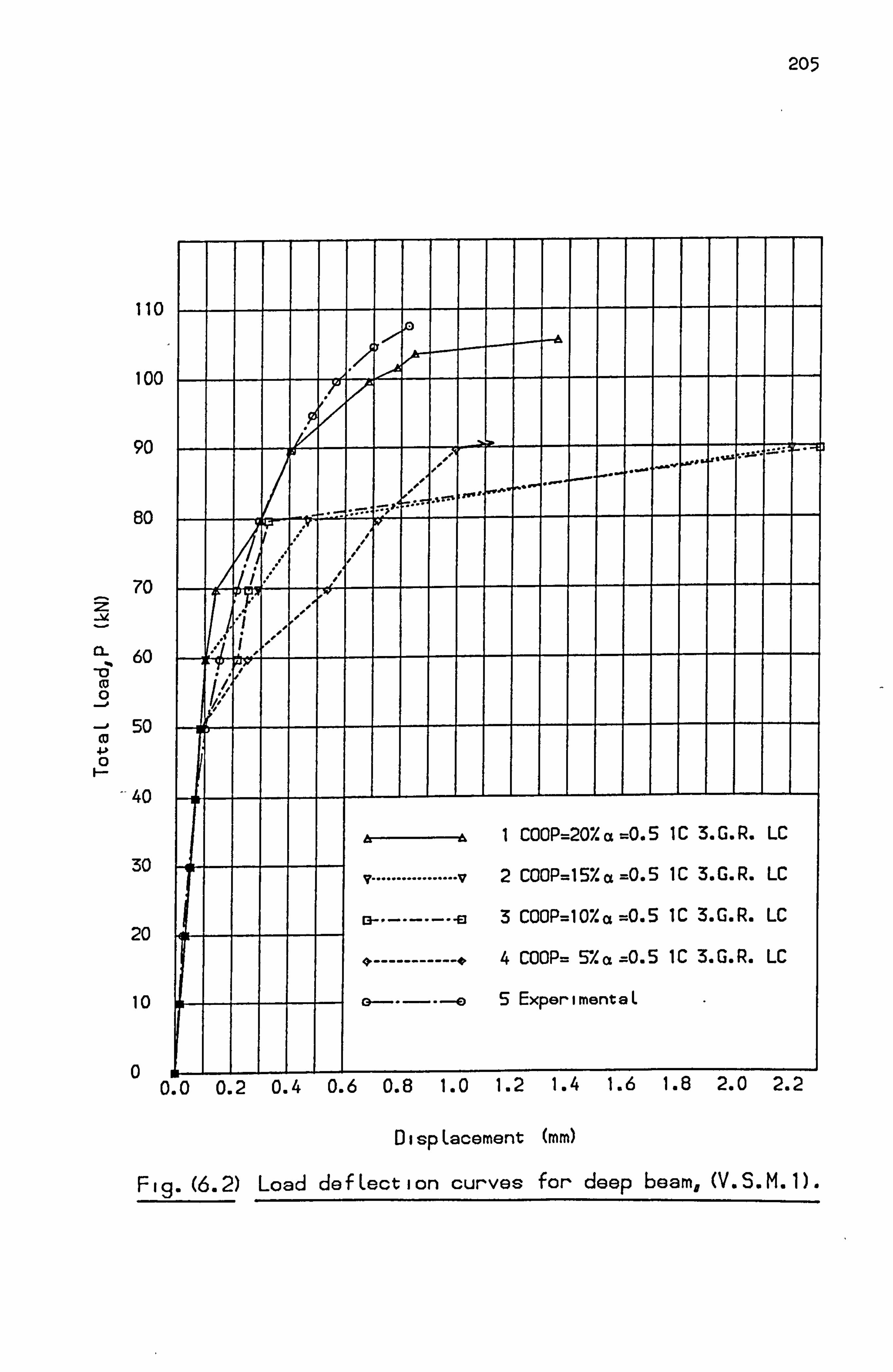
205
110
100
90
so
70
60
0 50
co 4A 0
40
30
20
10
0LIII. 0.0 0.2 0.4 0.6 0.8 1.0 1.2 1.4
T l '
hI COOP=20Z a =0 51C3. G. R. LC
v ................ v2 COOP=l5Xct=O. 5 IC 3. G. R. LC
El --------- 03 COOP=10%a =0.5 IC 3. G. R. LC
4 ------------ *4 COOP= 5*/. a =0.5 IC 3. G. R. LC
5 ExperimentaL
1.6 1 tj 2. U 2.2
Di sp Lacement (mm)
Fig. (6.2) Load defLection curves for deep beam, (V. S. M. 1).
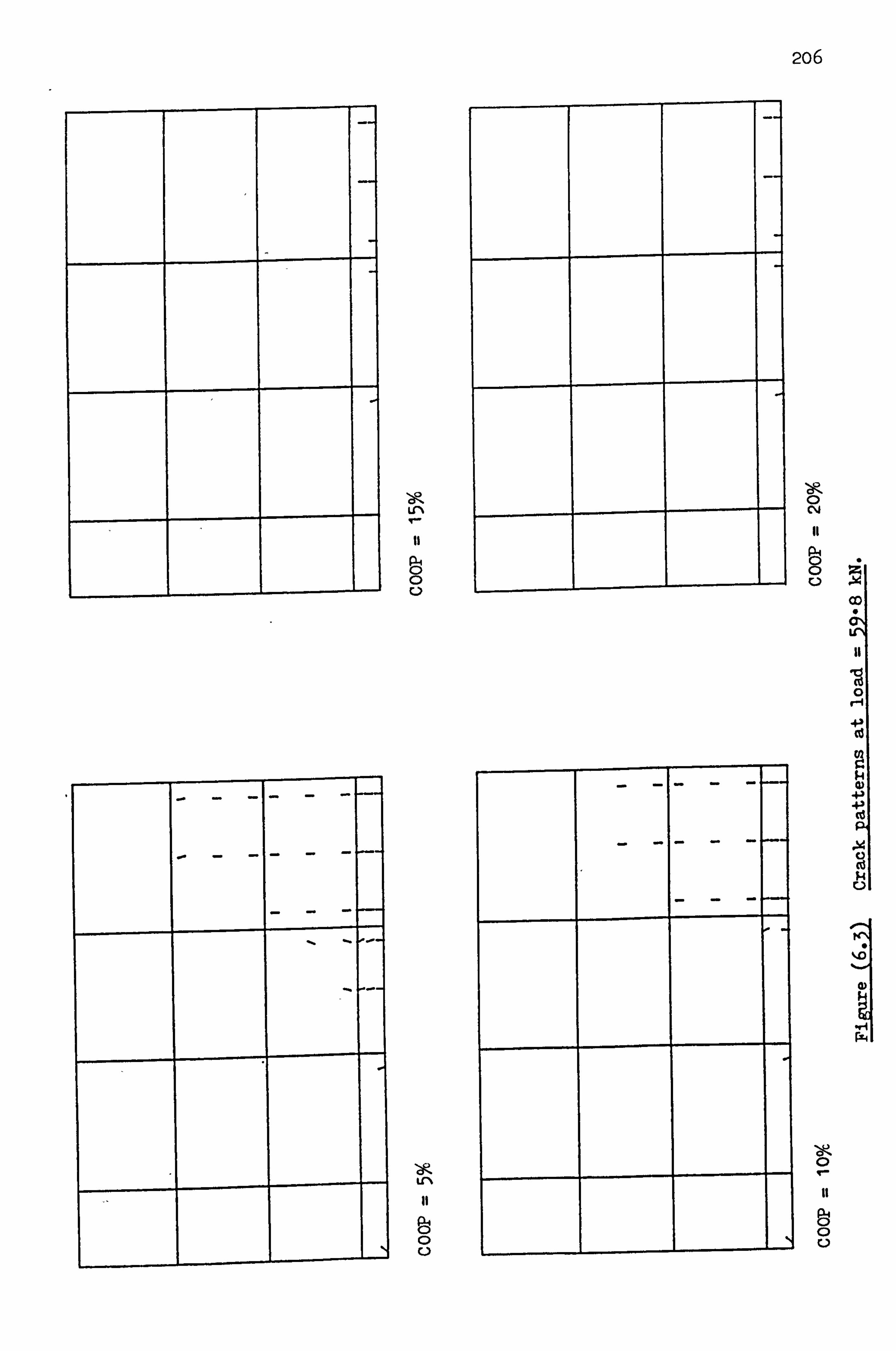
2o6
LrN
le, 0 C\j
11
NO - C)
. 54
.
PL4
"IP 01 VN
11
C-)
lC*l
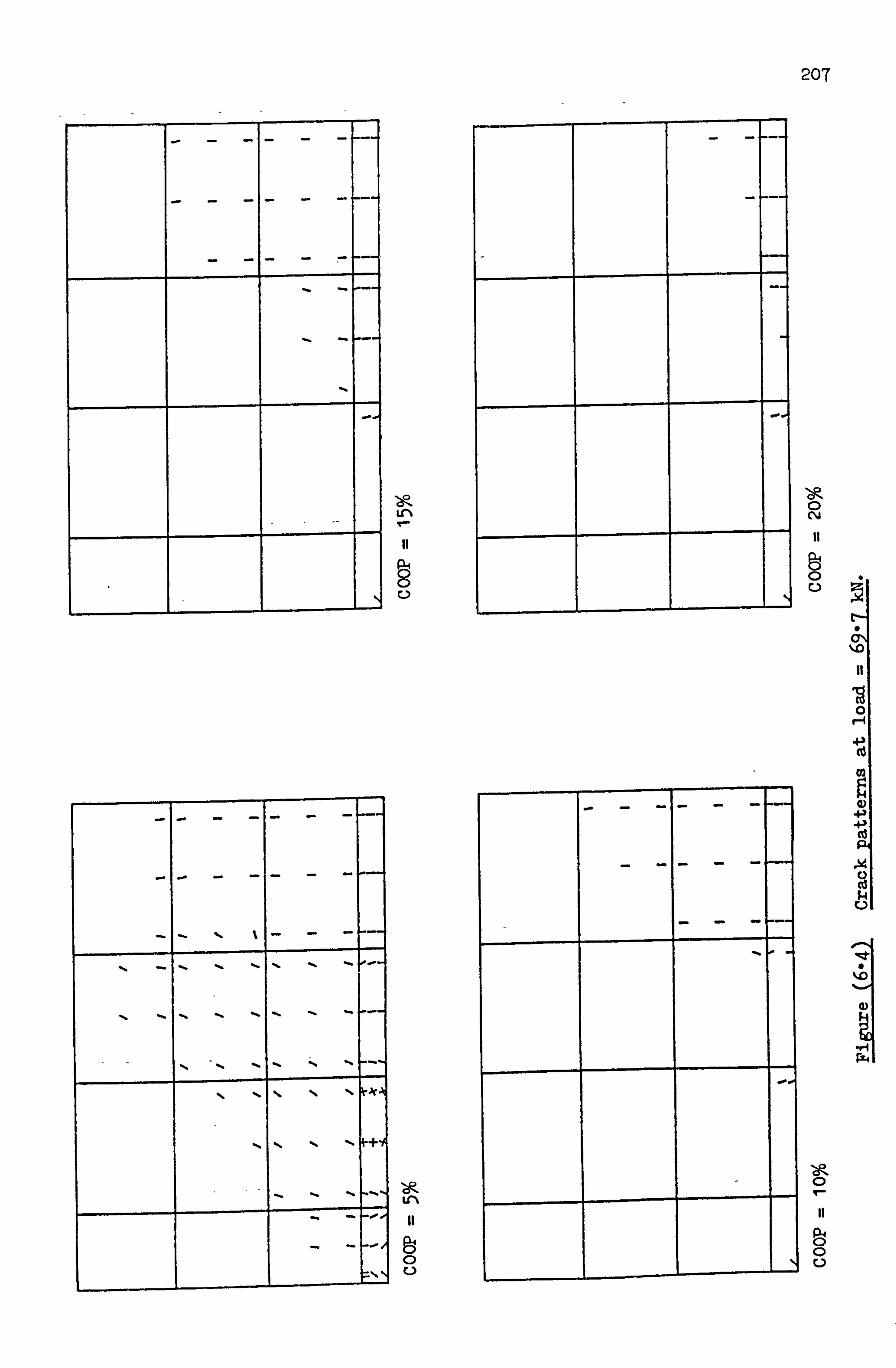
207
'ZA
P--4
8
cli it
It 19 0
- . - t - - - -
- -. -. -. "_ -. - . -'
-- -. -. - - - -
-- -. -.
-
- - %
-
LCI%
11
fj
0 0
Cd
(D
42
, aK
0-ý Itt

---.
1-0 el
PO4
11"i
208
, alp, 0 04
11
P4
8 c)
N .
11 19
Aoi p04
- '-
0
0 C,
0 H
44
(D +3 4J
.X 0
rX4 I
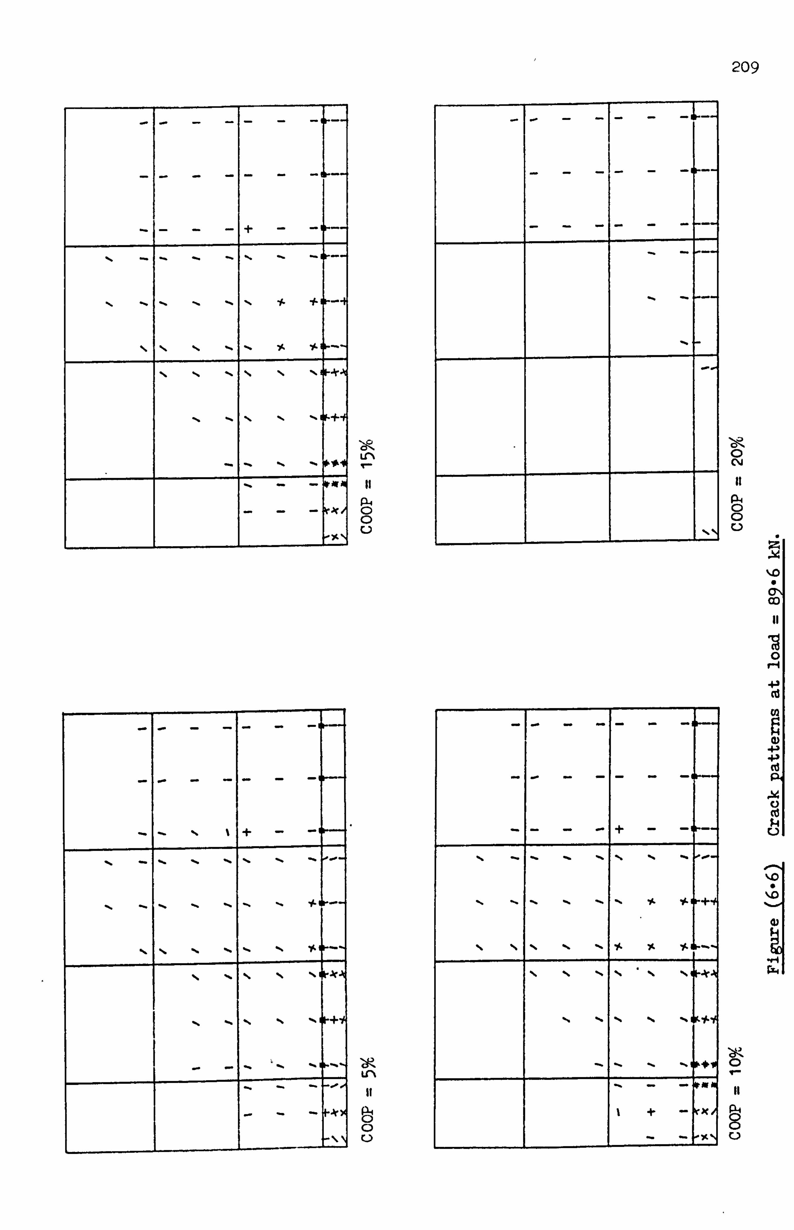
209
- - - 0,11L A "CI 0,
P4 0
0
P4 0 0
11 19
- - - 7 - - -ýý
ýK
1011
ArA
0 H
+3 Cd
(D 43 4.10
ýK
P-4
co
SI
WI -4

210
10(
90
80
70
60 0 0
... 0 50 0
40
30
20
10
0
- ----- --------- ...
------ .........
......... ........
v zx " L TI * ' E -,
1 COOP=2OX ct=0.5 IC 3. G. R. LC
................. V2 COOP=ISX a=0.5 IC 3. G. R. LC
13 ......... 03 COOP-IOX cl-O. S IC 3. G. R. LC
------------- 04 COOP= 5X a=0.5 IC 3. G. R. LC
5 Ex erimontaL 1
II I
p 0
0.0 O's 1.0 1.5 2.0 2.5 3.0 3.5 4.0
DispLacement NO (Iterations ý 30)
Fig. (6.7) Load defLection curves for deep boam,, (V. S. M. 1).

211
101
90
80
70
60
50
40
30
20
10
0
hA1 COOP=207. a=0.5 IC 3. G. R. LC
v .................. v2 COOP= I 5X a =O. 51C3. G. R. LC
ta ---------- a3 COOP=1OX a=0.5 IC 3. G. R. LC
------------- 4 COOP= SX a=0.5 IC 3. G. R. LC
5E L xperimente
0I ___________________________
0.0 U.;? U. 4 0.6 0.8 1.0 1.2 1.4 1.6
DispLacement (mm) (Iterations ý 10)
Fig. (6.8) Load defLection curves for deep beam, (V. S. M. 1).
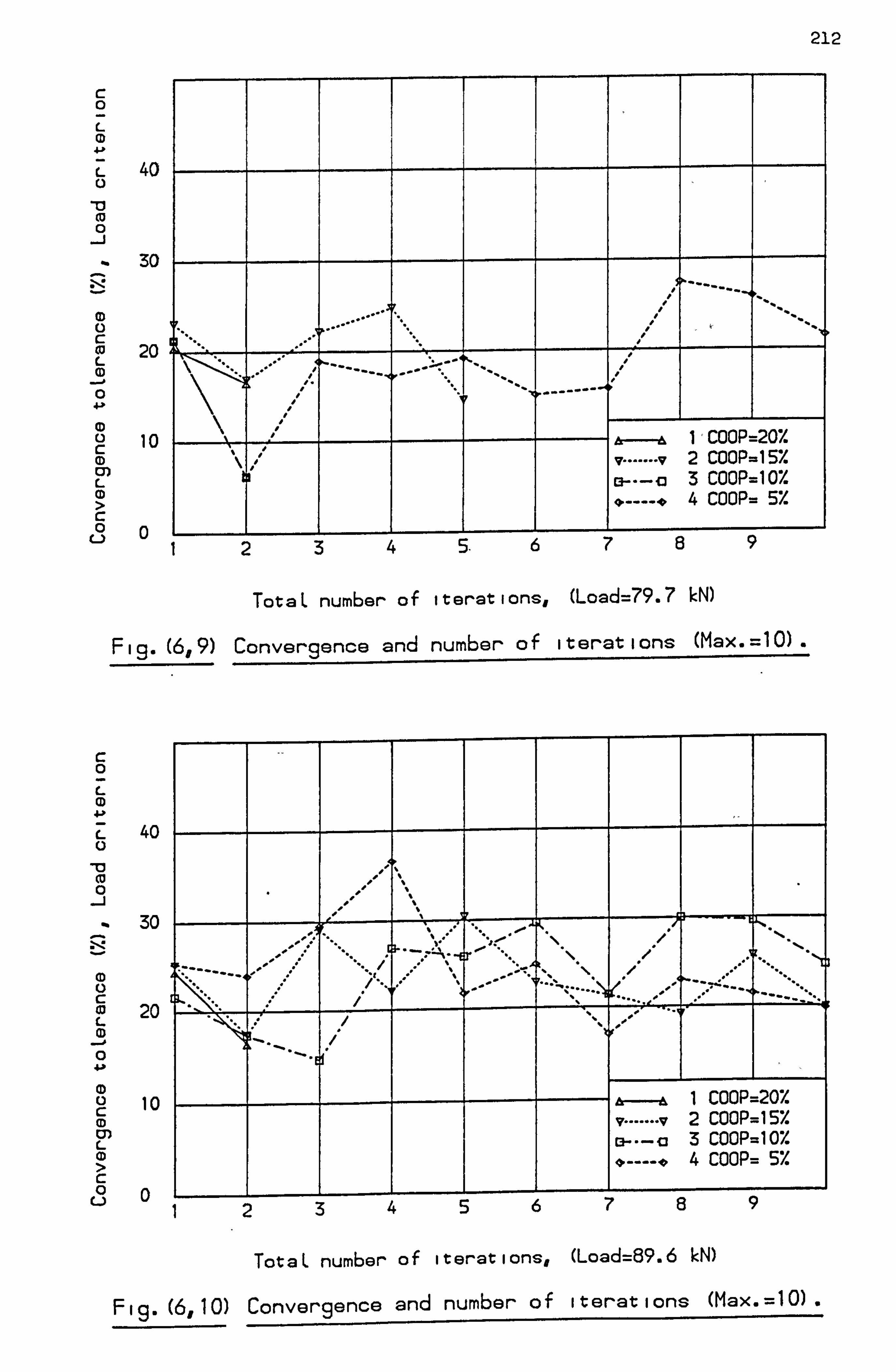
212
c 0 L (D
L 40
0 30
(a 20 d L CD
0 4ý
CD 10
(D U) L (D
c
-Q n
-- ---------
1, COOP=20% \ , 2 COOP=15% 1 1 M-0 3 COOP=10%
4 COOP= 57.
Li -1
TotaL number of iterations, (Load=79.7 kN)
Fi! 3. (6,9) Convergence and number of iterations (Max. =10).
40
30
20
10
L Aý
A t
1 COOP=20% v ...... v2 COOP=15Y. D- 13 3 COOP=10%
4 COOP= 5%
Li
TotaL number of iterations, (Load=89.6 kN)
Fig. (6,10) Convergence and number of iterations (Max. =10).

213
c 0 (D 4ý
40
-0 ca 0 30
c a) 20 L a) 0 40
(D U 10 c CD U) L CD
c 0
L-) 0
At I COOP=20X v ........ v2 COOP=157.
3 COOP=107. 4 COOP= 57.
.. .............
0369 12 is le 21 24 27
TotaL number of iterations, (Load=79.7 kN)
Fig. (6,11) Convergence and number of iterations (Max. =30).
c 0 L CD 4-1
L 40
0 30
P
c 10 20 L
10
(D m L (D
c
qn
I It . 1; .. ., R,
..,: \.
I i r- 1 ]4 00-
Y-V*li . Ilk, 'o
1 COOP 207 = . 2 COOP=157. 3 COOP=10% 4 COOP= 57.
036 9 12 15 18 21 24 27
TotaL number of iterations, (Load=89.6 kN)
r- -- I/ In% --j -f IKA--- 7n%
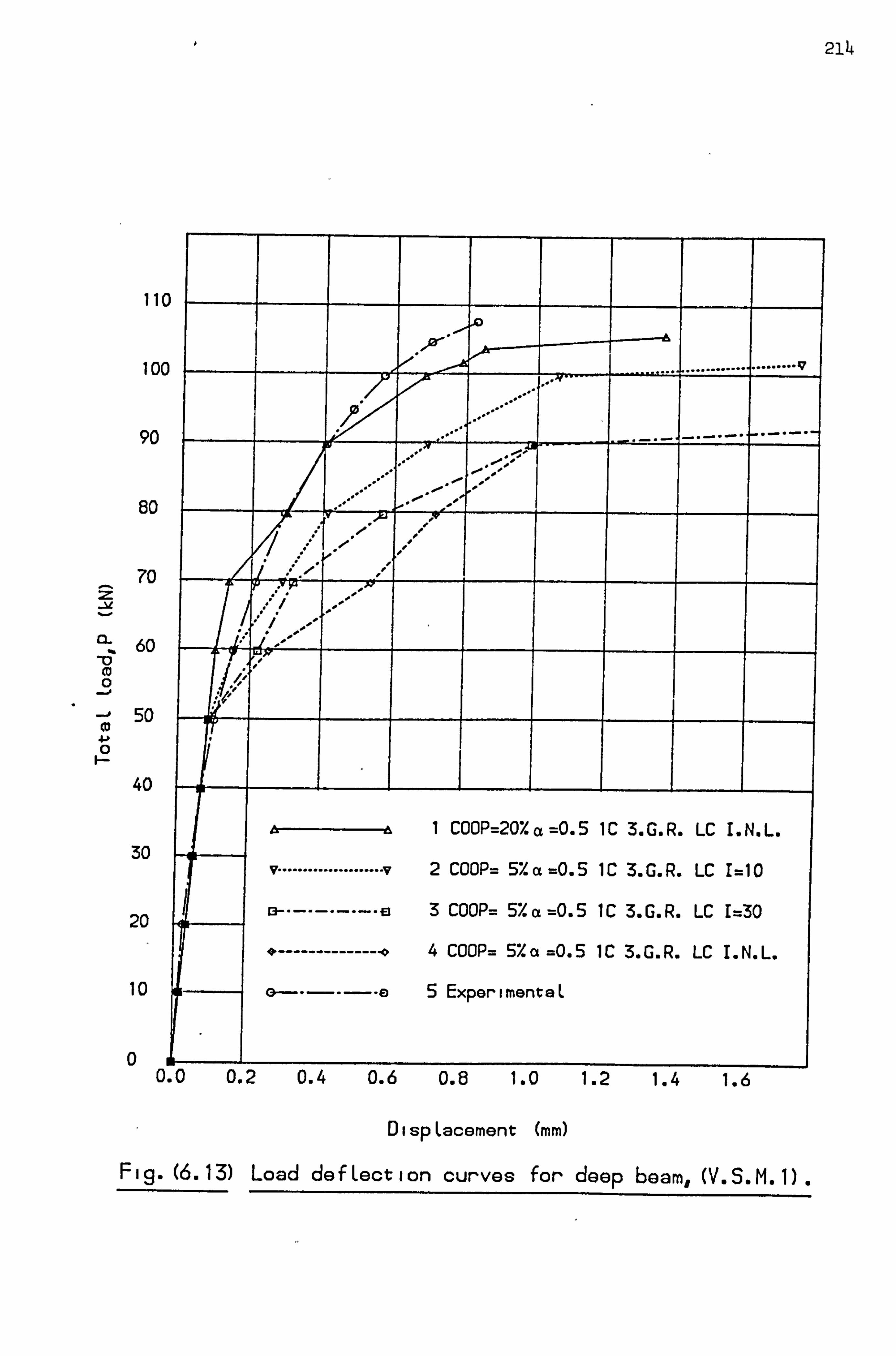
214
ll(
I oc
90
80
70
13- 60
0 -. I -j 50 CD 4-- 0
40
30
20
10
0 4- 0.0 U. 2 U. 4 U. 6 0.6 1.0 1.2 1.4 1.6
DispLacement (mm)
Fig. (6.13) Load defLection curves for deep beam, (V. S. M. 1).
.... .........
1 COOP=20Xa =0.5 1C 3. G. R. LC I. N. L.
v .................... V2 COOP= 57. a =0.5 1C 3. G. R. Lc r=lo
13 ---------- El 3 COOP= 57. a =0.5 IC 3. G. R. LC 1=30
4 --------------- 04 COOP= 57. a =0.5 1C 3. G. R. LC I. N. L.
5E L C) -- -----a xperimenta
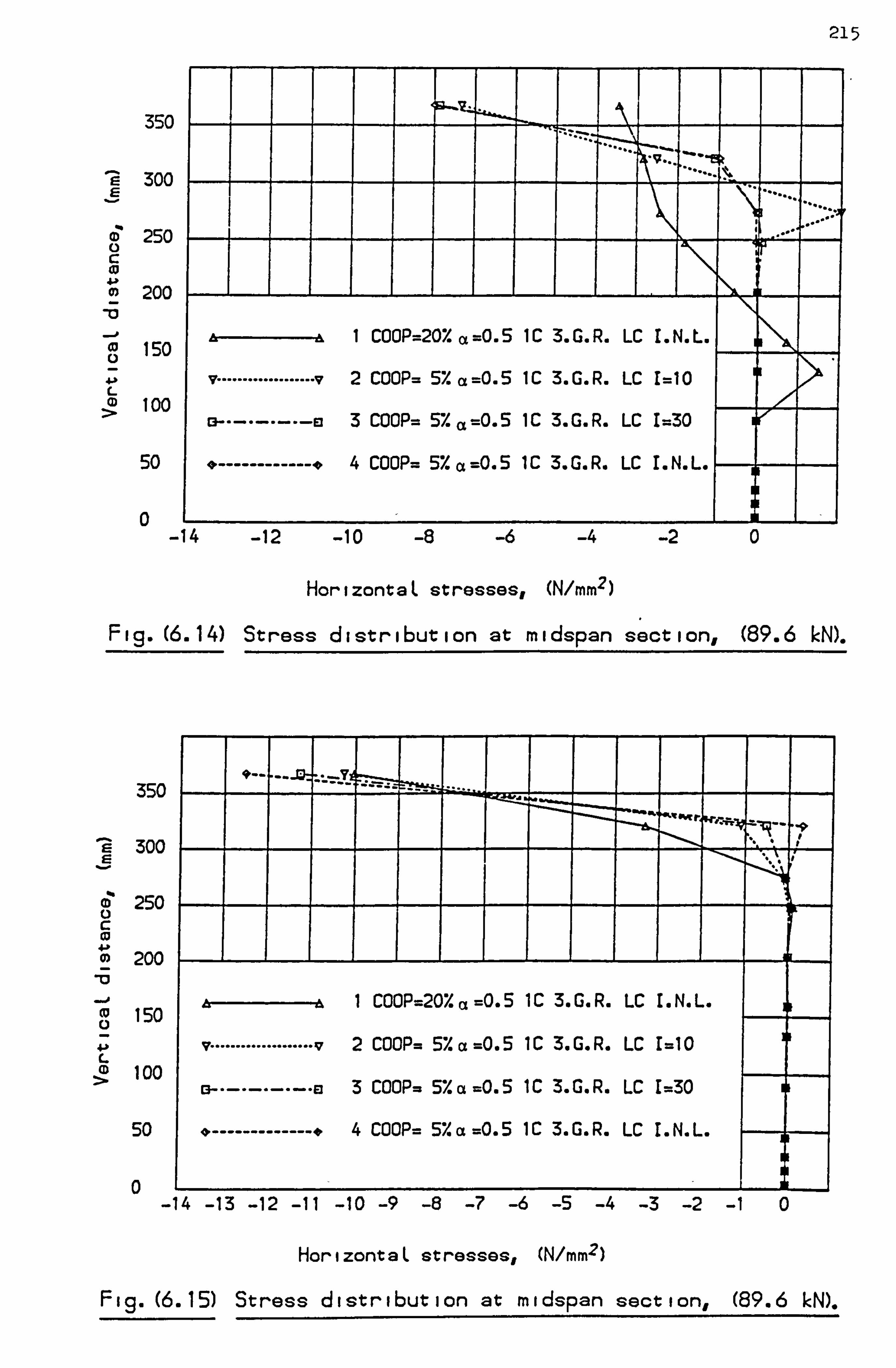
215
350
300
250
200
(0 iso
100
50
0
I COOP=20% a=0.5 IC 3. G. R. LC I. N. L.
v .................. v2 COOP= 5% a=O-5 IC 3. G. R. LC I=10
E3 3 COOP= 5% a=0.5
------- - -- 4 COOP 0 5 5%
1C 3. G. R. LC 1=30
1C 3 G R LC I N L - - - . = a= . . . . . .
-14 -12 -10 -8 -6 -4 -2 0
HorizontaL stresses, (N/mm2)
Fig. (6.14) Stress distribution at midspan section, (89.6 M.
350
300
250
200
-.. 0 M 150 0 41 L
100
50
0
I COOP=20% a =0- 5 1C 3. G. R. LC I. N. L.
* ................... 17 2 COOP= 5% a =0.5 IC 3. G. R. LC 1=10 M
* ----------- a3 COOP= 5%a=0.5 1
4 -------------- 04 COOP= 5%a=0 51
C 3. G. R.
C3 G R
LC 1=30
LC I N L . - . . . . .
-14 -13 -12 -11 -10 -9 -8 -7 -6 -5 -4 -3 -2 -1 0
HorizontaL stresses, (N/mm2)
Fig. (6.15) Stress distribution at midspan section, (89.6 M.

216
lic
100
90
80
70
60
--0 50
40
30
20
10
iF- 0.0 0.2 0.4 0.6 0.6 1.0 1.2 1.4
DispLacement (mm)
, /11.
4 1 . ".
-V
ool
vi
1 COOP=107. a=0.5 IC 3. G. R. DC1
v ................ J7 2 COOP= 57. a=0.5 IC 3. G. R. DC1
13---- ----S '3 COOP= 17. a =O. 51C3. G. R. DC1
------------ 4 Ex erimentaL q p
Fig. (6.16) Load deftection curves for deep beam,, (V. S. M. 1).

217
110
100
90
so
70
60
50
40
30
20
10
0
.0
..... ......
A1 COOP=10% a=0.5 1C 3. G. R. OC2
................. v2 COOP= 5% a=0.5 1C 3. G. R. DC2
93- ------- -0 3 COOP= 17. a=0.5 IC 3. G. R. OC2
erimentaL ----------- 4 Ex p
0.0 0.2 0.4 0.6 0.8 1.0 1.2 1.4
DispLacement (mm)
Fig. (6.17) Load defLection curves for deep beam, (V. S. M. 1).
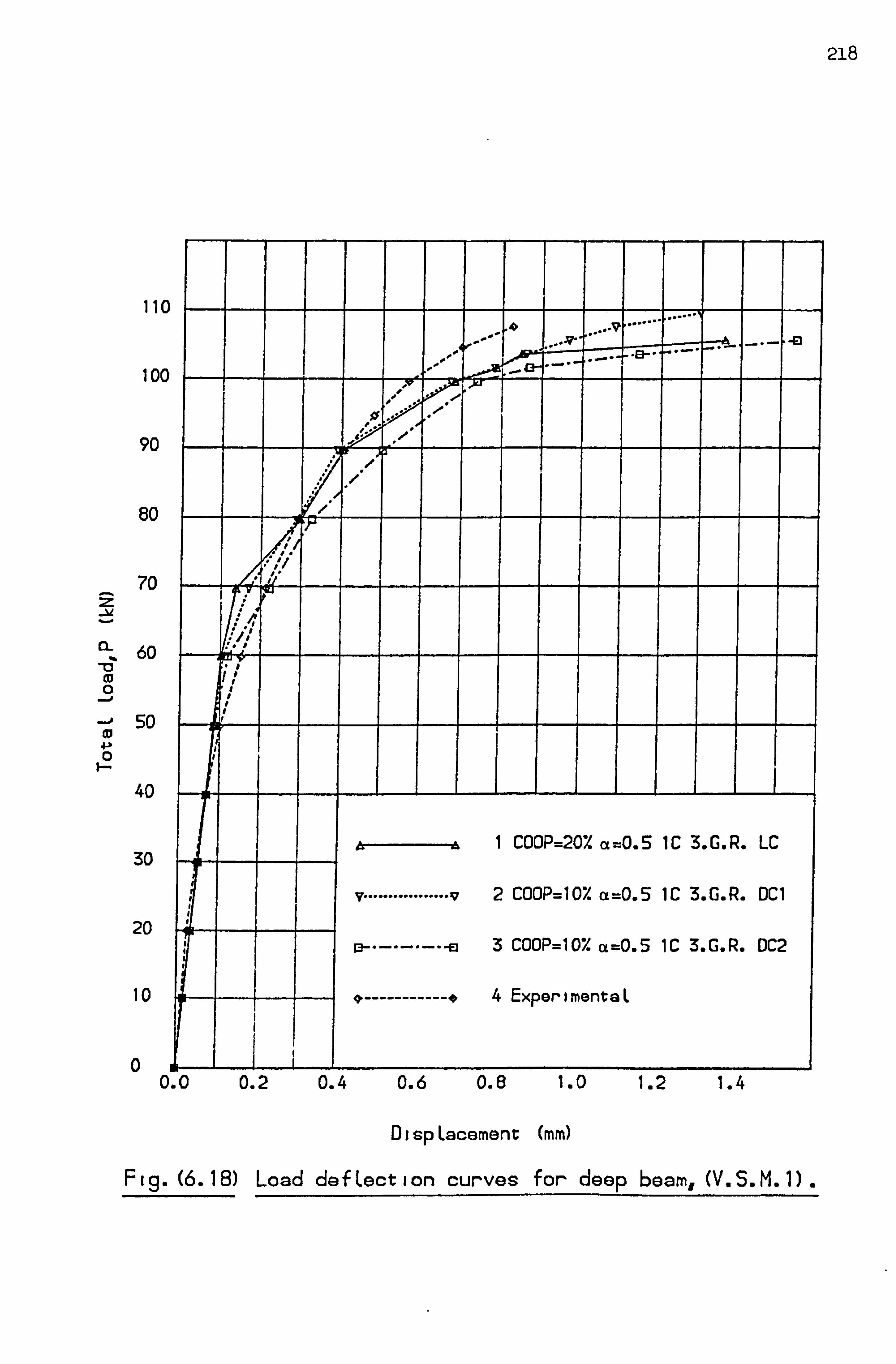
218
lic
100
90
80
70
60 m
50
40
30
20
10
0
........ ........ .
F7
1 COOP=20X a=0.5 1C 3. G. R. LC
v ................ v2 COOP=107. a=0.5 1C 3. G. R. DC1
13 ........ El 3 COOP=107. a=0.5 1C 3. G. R. DC2
4 Ex erimentaL ------------ p
0.0 0.2 0.4 0.6 0.8 1.0 1.2 1.4
DispLacement (mm)
Fig. (6.18) Load defLection curves for deep beam, (V. S. M. 1).

219
__________ I II
____ ________ 1_i ii Load criterion, COCP = 20%
II
______ _____________________
III
. 1_ III IIIt
Displacement criterion 1. COOP = 10yo
71 IT Displacement criterion 2. COCP = 10%
Figure (6-19) crack patterns at load = 6907 kN-

220
_____ _________ I I I
_____ __________
I
I
I
I
I
I
I
I
_____
/I
/I
/
I
I
I
I
I
I
I
I
I
I
I /
_______
I
____________ I
I I I
Load criteriont COOP = 20%
_____ 1 1I
I I
_____ _________ __ ____ ___
I
II
/ / � II
/ / / I II
/ I I I I II / I.
-
____________
I I
I t I I
I _____ __________
Displacement criterion 19 COOP = 10%
I II
/
I
'. .
II
1I
/
/
/
/
1
/
/
I
/
/
/
I
I
I
II
II
II .c I T �
Displacement criterion 2. COOP = 10%
Figure (6-20) Crack patterns at load = 99-6 kN.
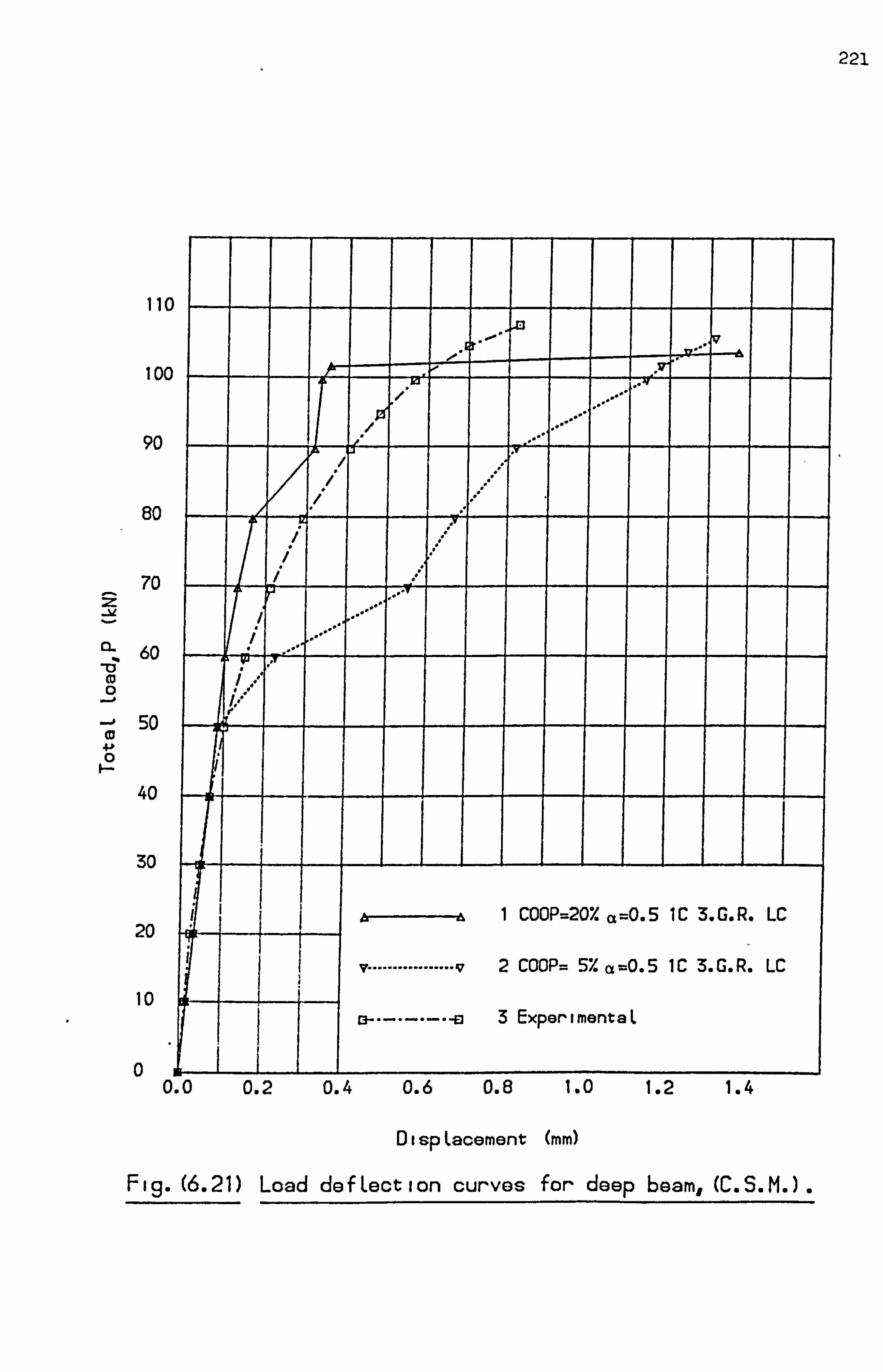
221
IIc
100
90
80
70
60
40
30
20
10
k- 0.0
0v
I 1
.61 COOP=207- a =O. 51C3. G. R. LC
v ................ v2 COOP= 5% a=0.5 IC 3. G. R. LC
13-- ------El 3 ExperimentaL
0.2 0.4 0.6 0.8 1.0 1.2 1.4
DispLacement (mm)
Fig. (6.21) Load defLection curves for deep beam, (C. S. M. ).
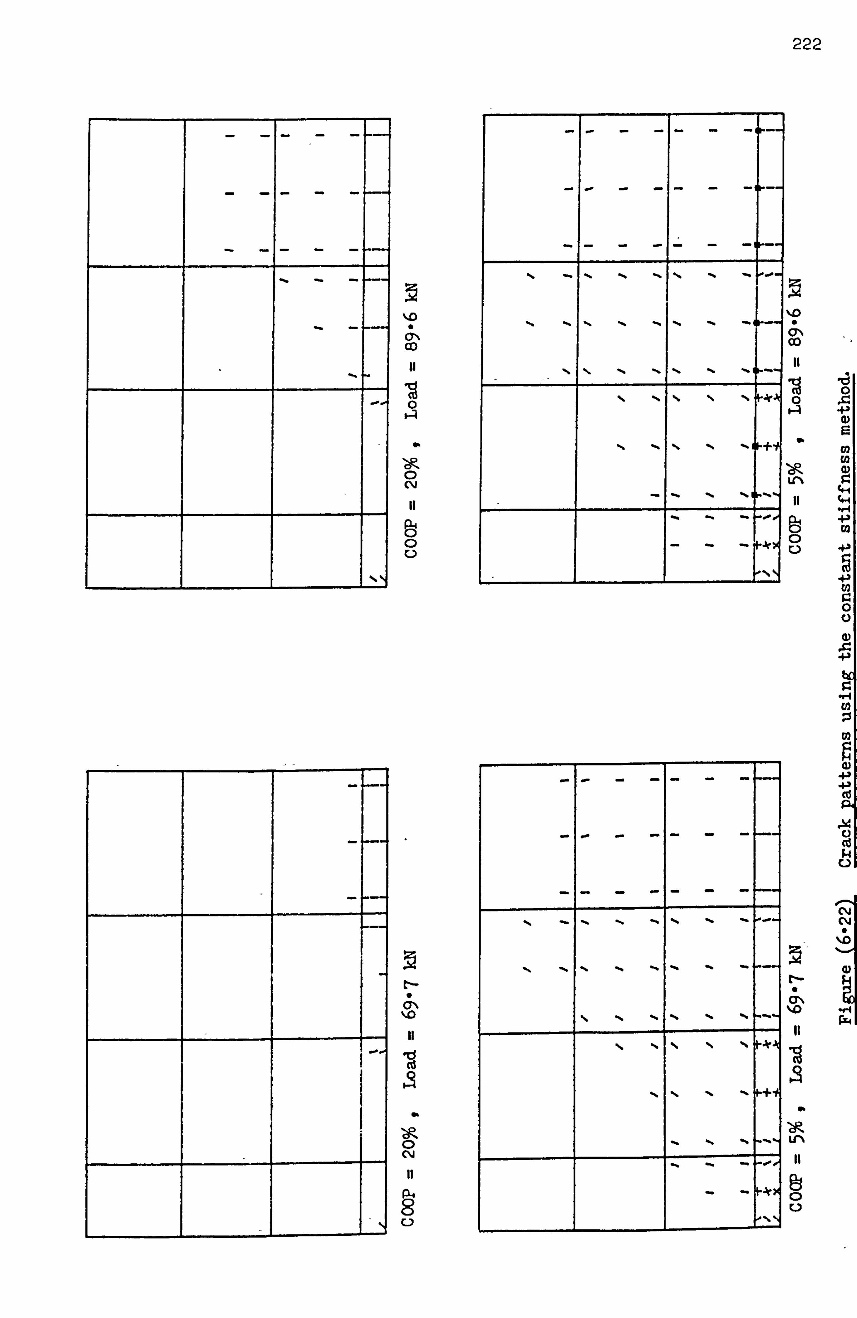
--I---
m %. 0
CD 11
19 0
cli
11
'64 0 0
N5
ýlo
11
Ici cd
CY
11
P4 8
ci
F+q
INN
- -.. - - . -
" -. -. -. . - -. -
-. . -
" -. *J
%
- - -
- -
222
n
00
n S
C. '
II
S
�I
0 C.,
0ý 04 04
(D

- - 'k 'w
Cd
0 C\j
0 0
, rý
.9
0 cli 11
P014
0 C. )
%A N
IL I 1--ý
jr 'A

224
cu
110
100
90
80
70
60
so
40
1 COOP=207. a=0.5 IC &G. R. LC C. S. M. 30
V .................... 72 COOP=207. ct=0.5 IC &G. R. LC V. S. M. I 20
93 ---------- El 3 COOP=207. ct=0.5 IC &G. R. LC V. S. M. 2
10 4E L --------------- 0 xperimenta
0 0.0 0.2 0.4 0.6 0.8 1.0 1.2 1.4
DispLacement (mm)
Fig. (6.24) Load deftection curves for deep beam.
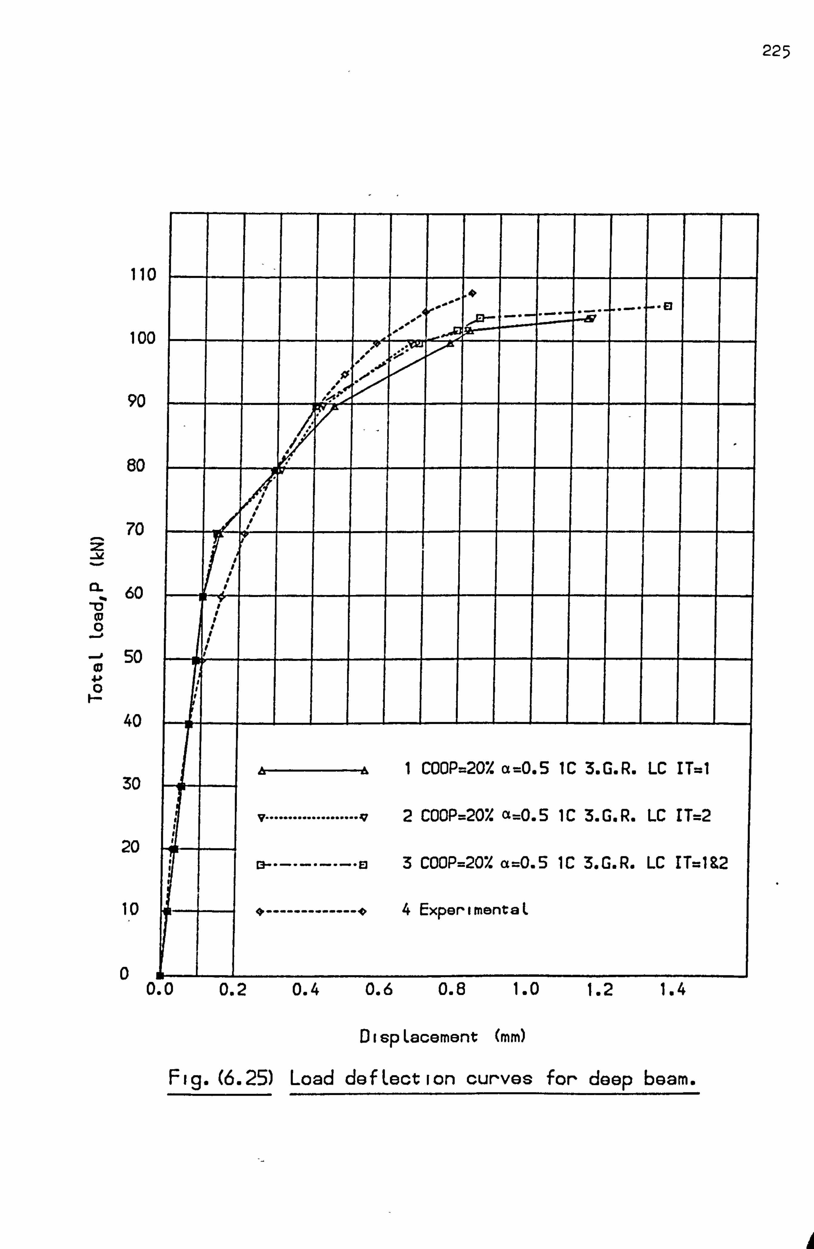
225
110
100
90
so
70
60
--0 so
40
30
20
10
0
--El
1 COOP=207. a=0.5 IC 3. G. R. LC IT=l
V ................... J7 2 COOP=20Y. a=0.5 1C 3. G. R. LC IT=2
1 I M -- -------- El 3 COOP=207. (x=0.5 1C 3. G. R. LC IT=1&2
4E erimentaL ---------------0 xp
0.0 0.2 0.4 0.6 0.8 1.0 1.2 1.4
DispLacement (mm)
Fig. (6.25) Load defLection curves for deep beam.
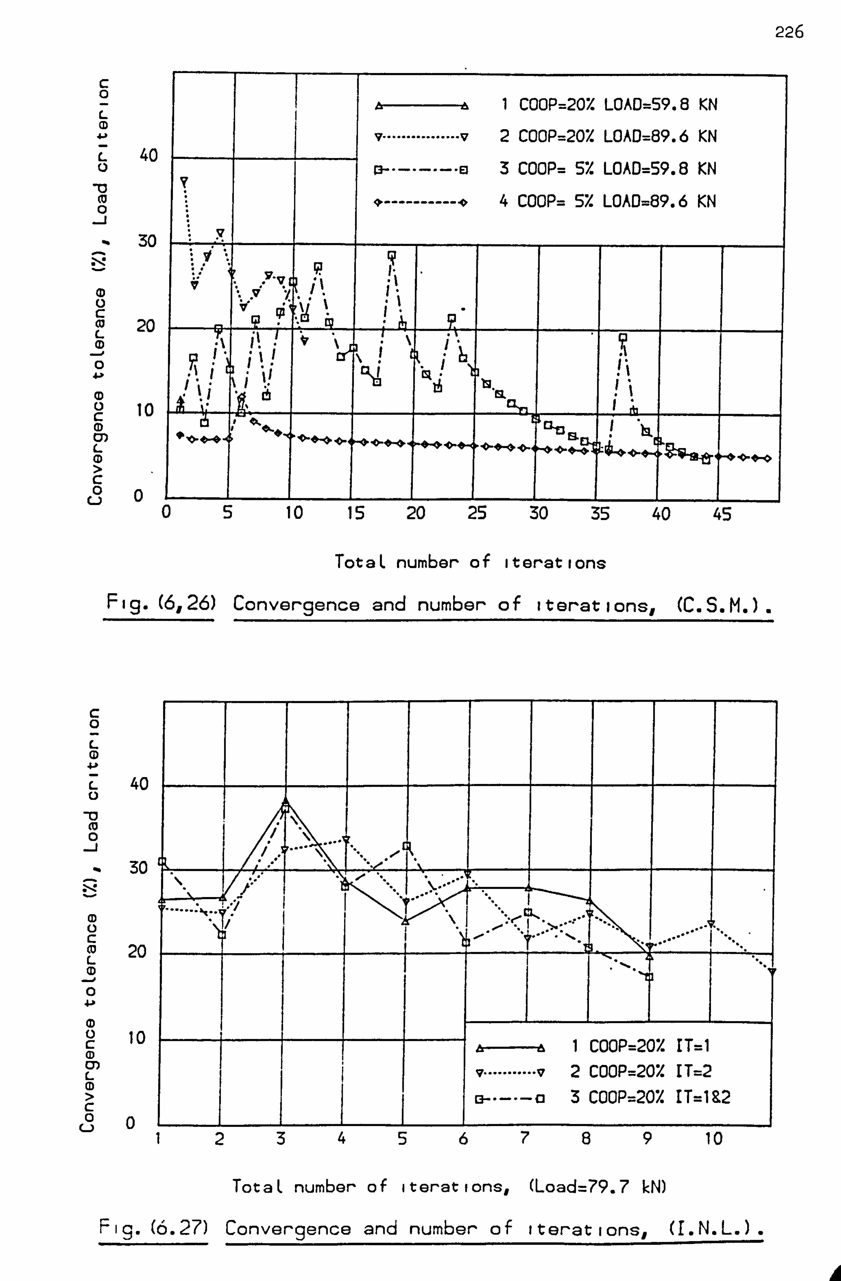
226
40
30
(0 20
10
0
A 1 COOP=20% LOAD=59.8 KN
v ............... v 2 COOP=20% LOAD=89.6 KN
El 3 COOP= 5% LOAD=59.8 KN
9. -----------0 4 COOP= 5% LOAD=89.6 KN
L
*-, *. ý ,0 -00 . . Co.. " . 0. 13 . 0-
hL
05 10 15 20 25 30 35 40 45
TotaL number of iterations
Fig. (6,26) Convergence and number of iterations, (C. S. M. ).
c
40
30
m 20 L
10
Q ()
1 COOP=207. IT=l
........... 2 COOP=20% IT=2 3 COOP=20% IT=1&2
%. -j 1 10
TotaL number of iterations, (Load=79.7 kN)
Fig. (6.27) Convergence and number of iterations,,

227
(U
110
100
90
80
70 -- - if- jr
60
so
40
30
20 1 COOP=207 a =0.0 1C2. G. R. LC 16 E Laments
v ..................... V2 COOP=20% a =0.0 1C3. G. R. LC 16 E Laments 10 cl -- ------- -- V3 COOP=20% a=0.0 IC 4. G. R. LC 16 ELement5 '0 --------------- 04 ExperimentaL
0. 0 0.2 0.4 0.6 0.8 1.0 1.2 1.4
DispLacement (mm)
F 19. (6.28) Load do f Lect ion curves for deep beam, (V. S. M. 1).
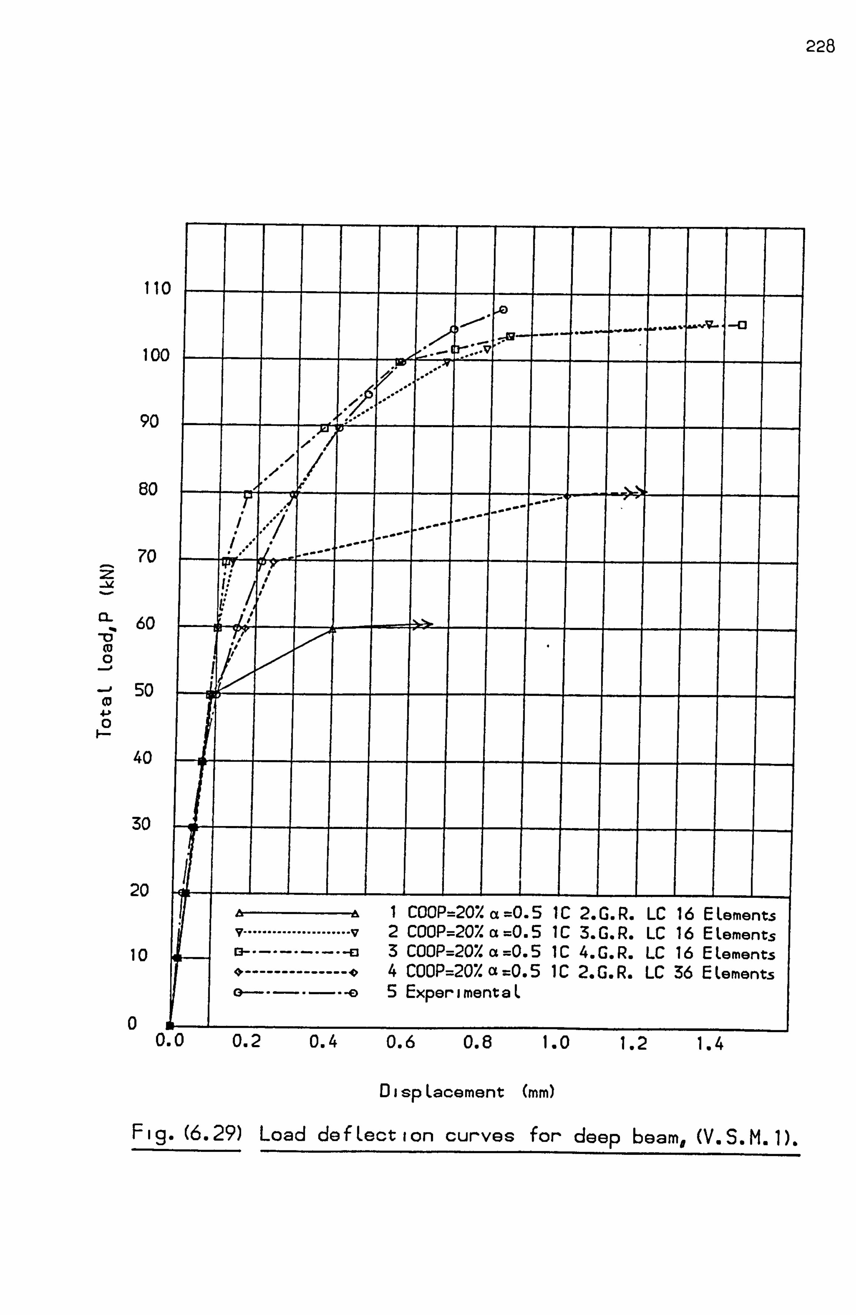
228
110
100 90
80
70
rL 60 D CD 0
-0
--p 50 4J 0
40
30
A 1 COOP =207 a =0. 51C2. G. R. LC 1 6R emen ts V-111- ............ ... v 2 COOP =20% a=0. 5 IC 3. G. R. LC 1 6 EL emen ts [a -- ------- -- U 3 COOP= 207. a=0. 5 IC 4. G. R. LC 1 6 EL emen ts 4 ------------- --- 0 4 COOP= 207. a=0. 5 1C 2. G. R. LC 3 6 EL emen ts 0---- -- 0 5E xper imen taL
0 0. 0 0.2 0.4 0.6 0.8 1.0 1.2 1.4
DispLacement (mm)
Fig. (6.29) Load deftection curves for deep beam, (V. S. M. 1).
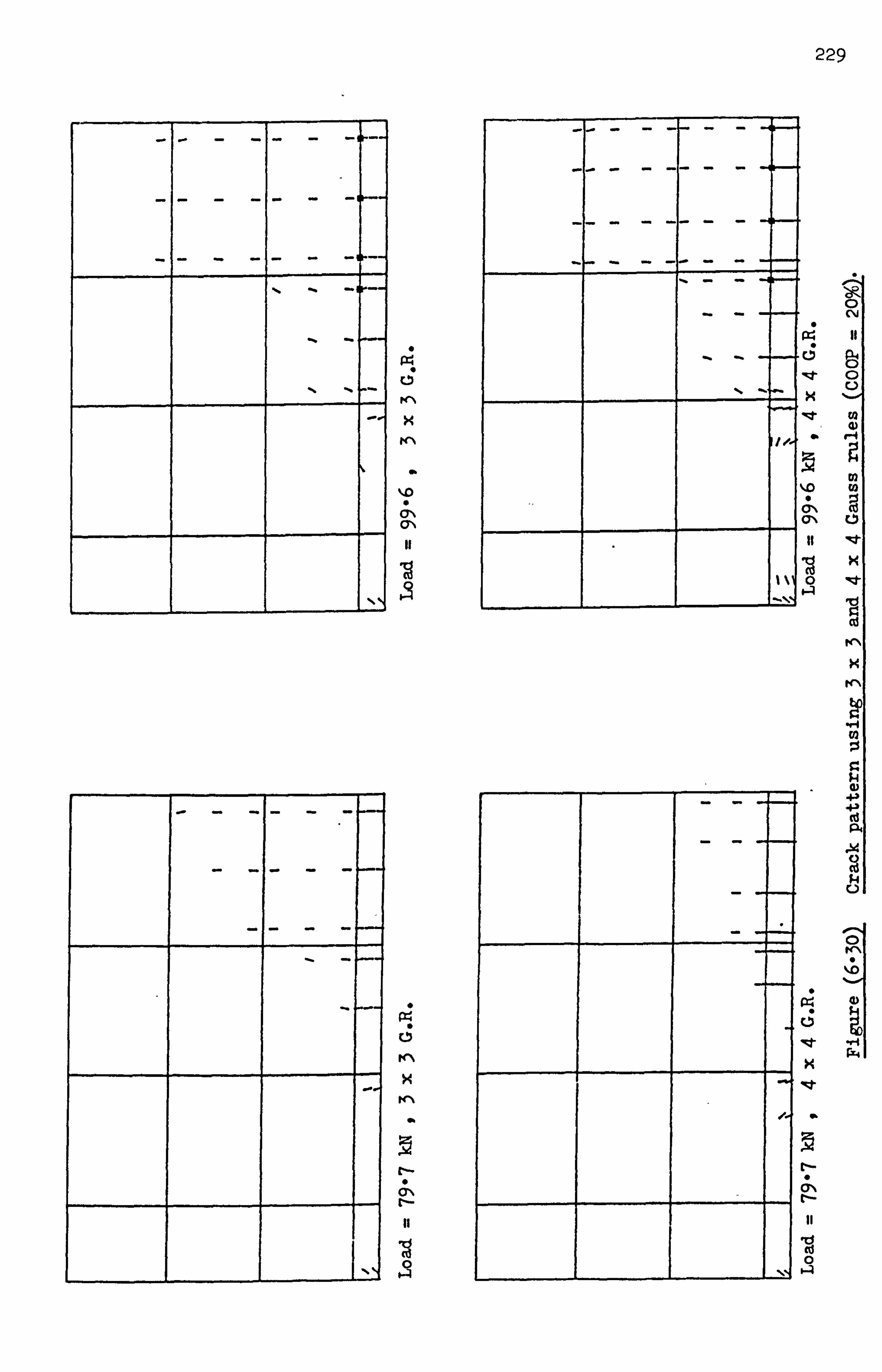
229
11
CN cr%
P; 1ý PC\
x
cr\ r-
11
19
0 64
1/
-D
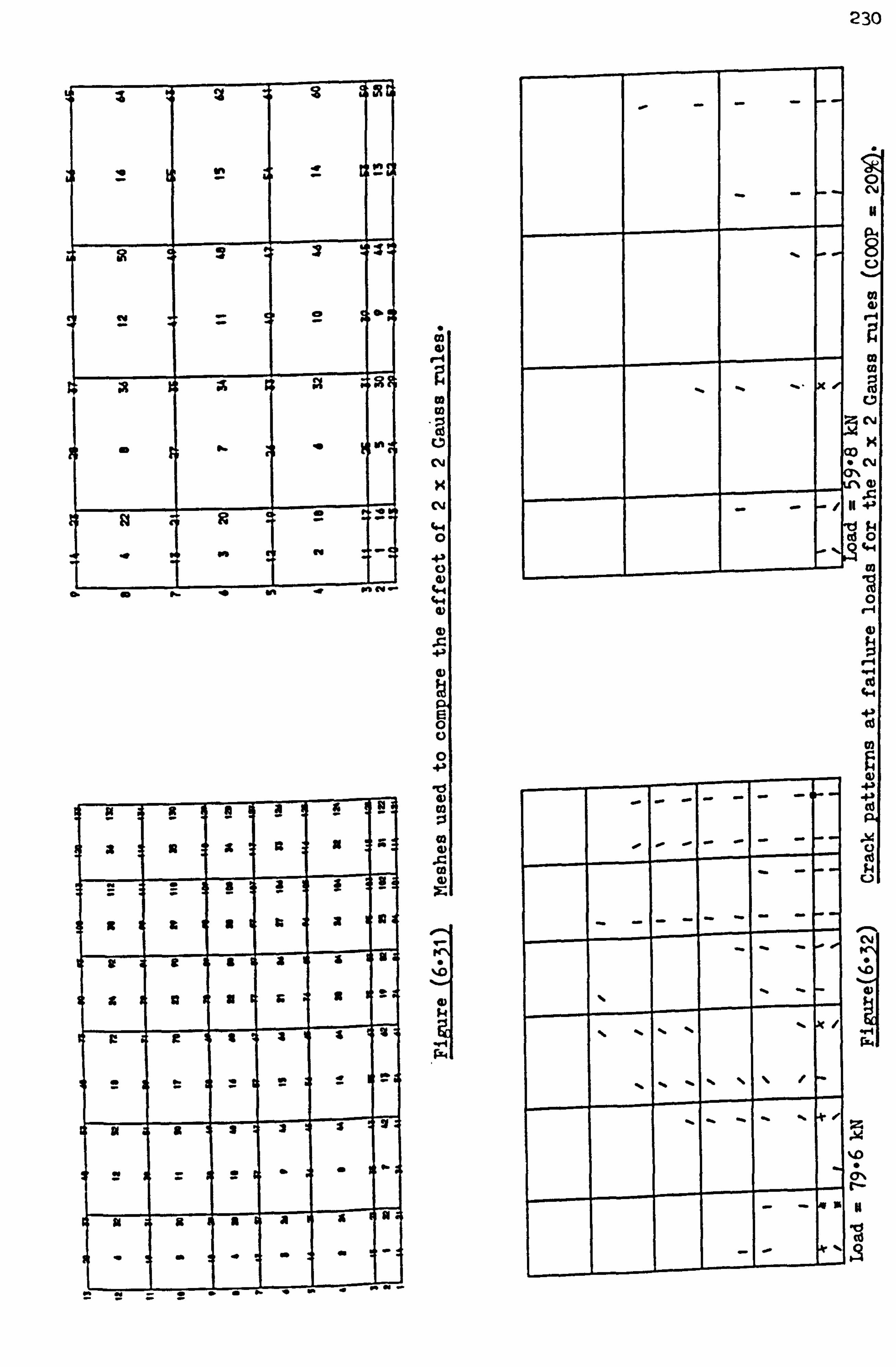
ImI i &. on,
-
T 1... a *
!
a
-- . I - i
I
I
*
- = e S
-i_ -I- -j T
co cly
m
CY
14-4 0
W
230
U
r 91
N
4J
$4 0
0 9-4
-4 to
CH
44
co
M
14
CY
%D
ON
In
10 a)
%D
ON Lf%

231
2
-0 0 0
4J 0
110
100
90
so
-.. --. .0
'L. 1 "E .. V
_- _____ _____________ _; *"
I'
II 70
60 i/
so
40
1 COOP-20X(x. 0.01 IC 3. G. R. LC 30
2 COOP=20XCL=0.05 1C 3. G. R. LC
20 [3 ........ 03 COOP=202 a -0.50 IC 3. G. R. LC
----------- 4 CCOP=20X aml. 00 IC 3. G. R. LC
10 5 ExperimentaL L
0.0 0.2 0.4 0.6 0.8 1.0 1.2 1.4
Disp(acement (mm)
Fig. (6.33) Load deftection curves for deep beam, (V. S. M. 1).
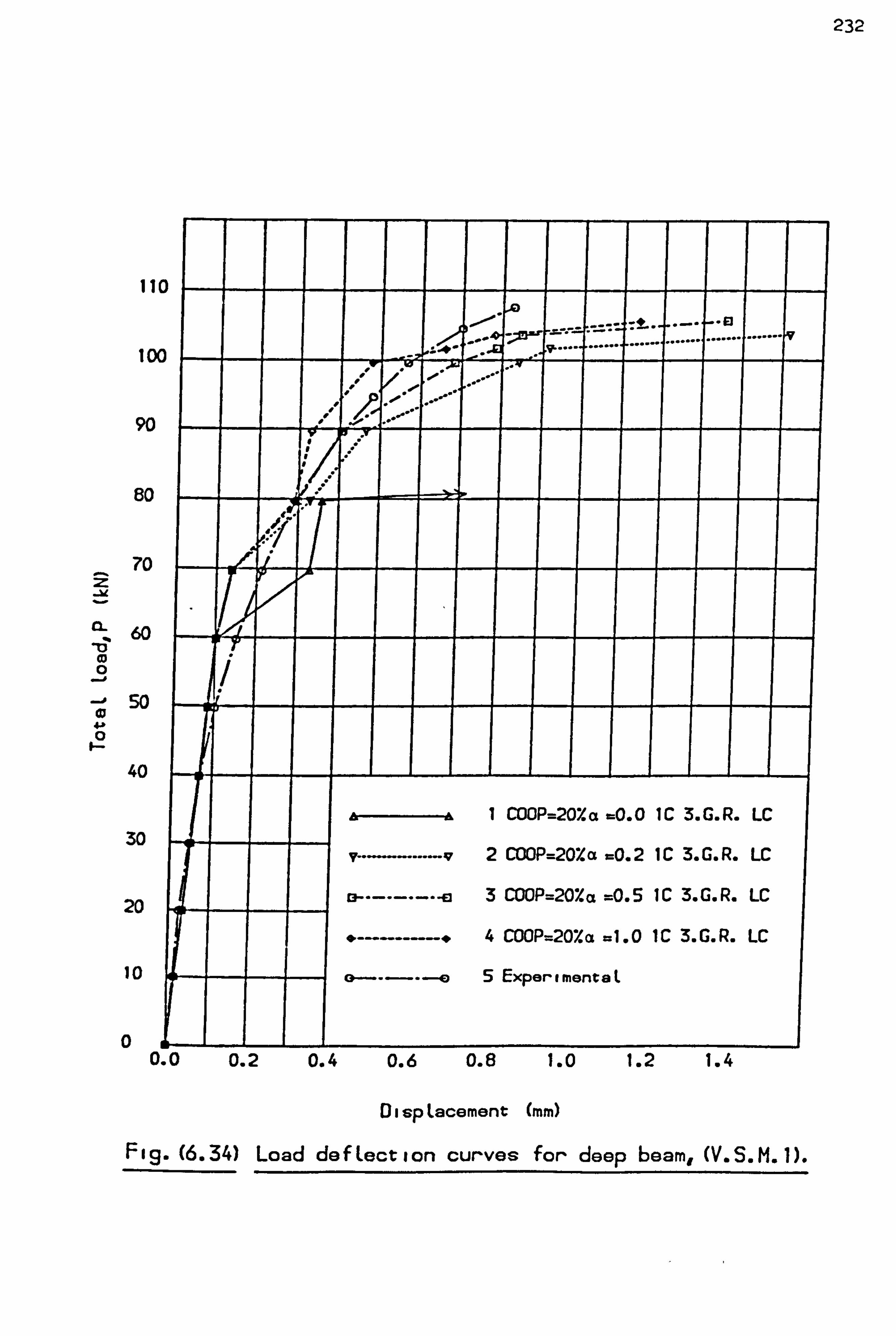
232
2
Co
-. i
110
100 =. - : *-. . -. El
- - -
....... ...... ....... ....
.... ......
.... ......
90
80
70
60
so
40
Ar --------- --A I CDOP=2OXa -0.0 IC 3. G. R. LC 30
2 CCOP=2OXa =0.2 IC 3. G. R. LC
20 13 ........ a3 COOP=2OXa =0.5 IC 3. G. R. LC
4 COCP=2OXa -1.0 IC 3. G. R. LC
10 I a. --a 5 ExpertmentaL
0 ---1
11
0. 0 0.2 0.4 0.6 0.8 1.0 1.2 1.4
DispLacement NO
Fi! g. (6.34) Load deftection curves for deep beam, (V. S. M. 1).
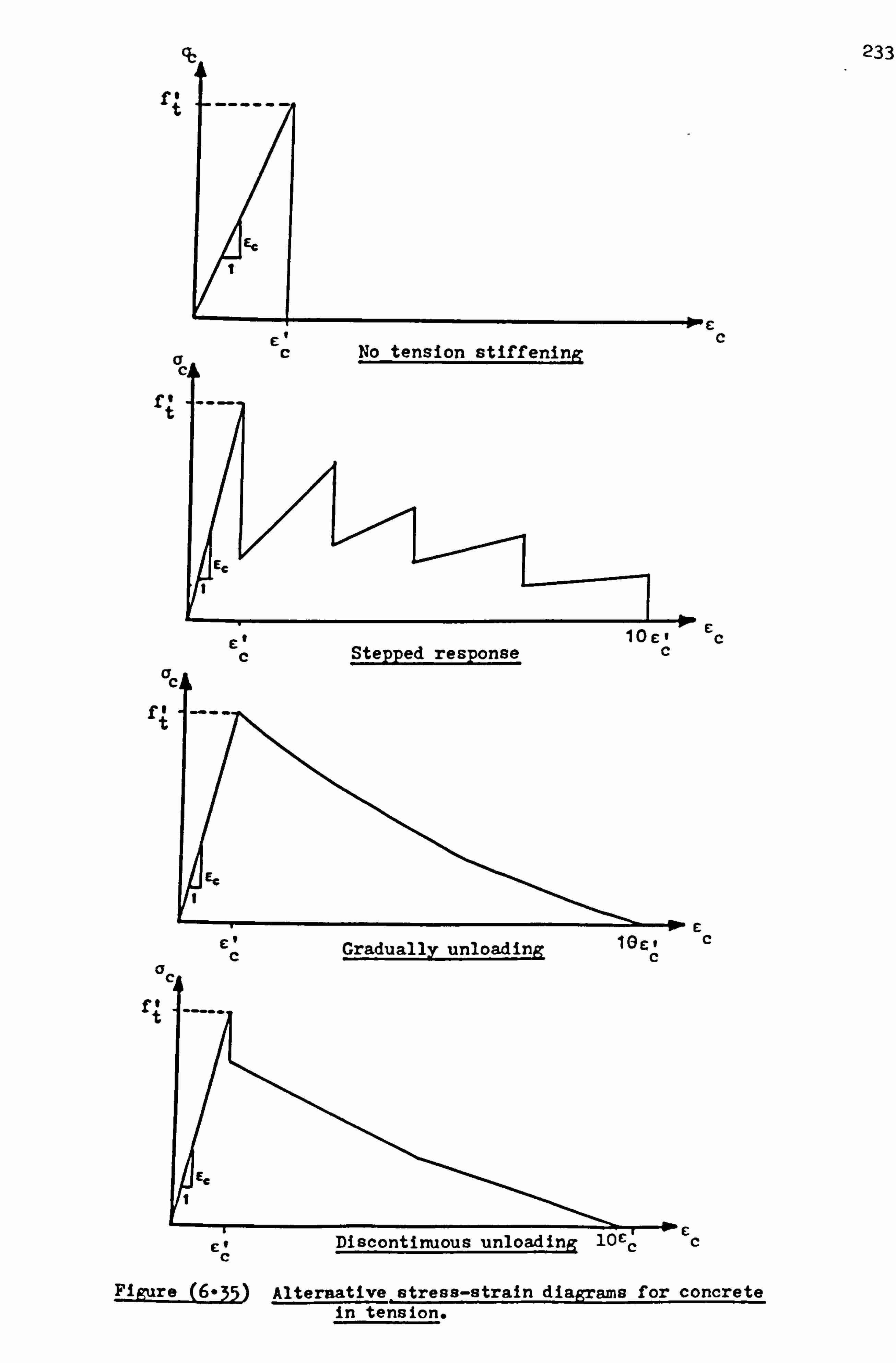
f.
f,
f
C C
C C
C C
£ C
233
Figure (6-35) Alternative stress-strain diagrams for concrete in tension.
C, I. )Tri +DvQirlvl
Ct loci C Stepped response C
cI C Gradually unloading loco
C
Ct Discontinuous unloadin IULC c
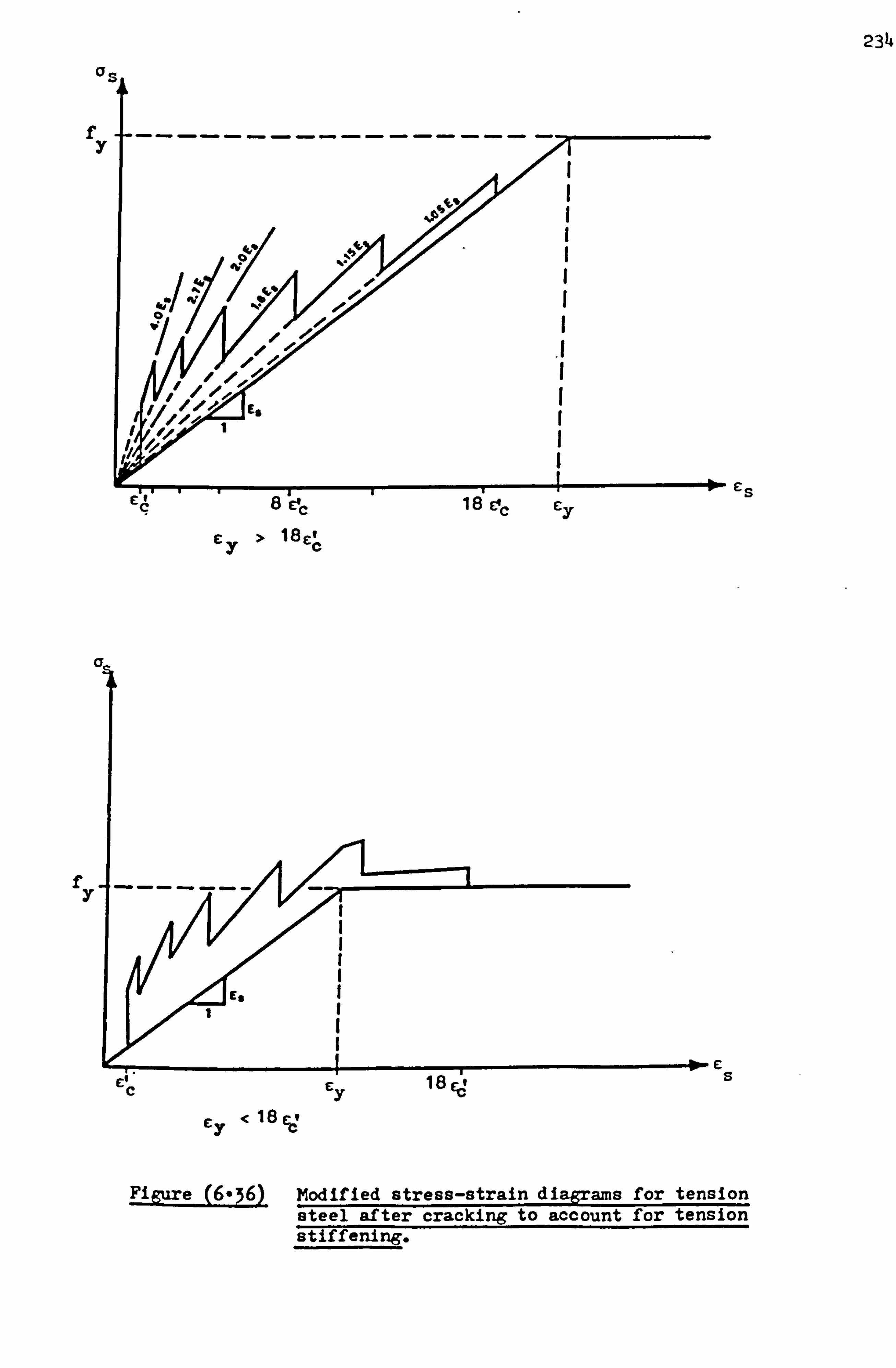
234
as
f I
18C 1
1 7
< 18Y y V
Cs
C S
Figure (6-36) Modified stress-strain diagrams for tension steel after cracking to account for tension stiffening.

235
110
lw ............
90 I
so
70
60 -13 1# 4a 11 0
50
40
1 CDOP=20Z a-0.5 2C 3. G. R. LC e -S': ' 30 A c
2 COOP= SZ a . 0.5 2C 3. G. R. LC c =5c' Ac 20
13 .......... (1 3 COOP= IZ a=0.5 2C 3. G. R. LC =Scl
10 4E nt L --- - ---------- 0 xperime a
0 0.0 0.1 0.2 0.3 0.4 0.5 0.6 0.7 0.8 0.9
DispLacement (mm)
Fig. (6.37) Load defLection curves for deep beam, (V. S. M. 1).
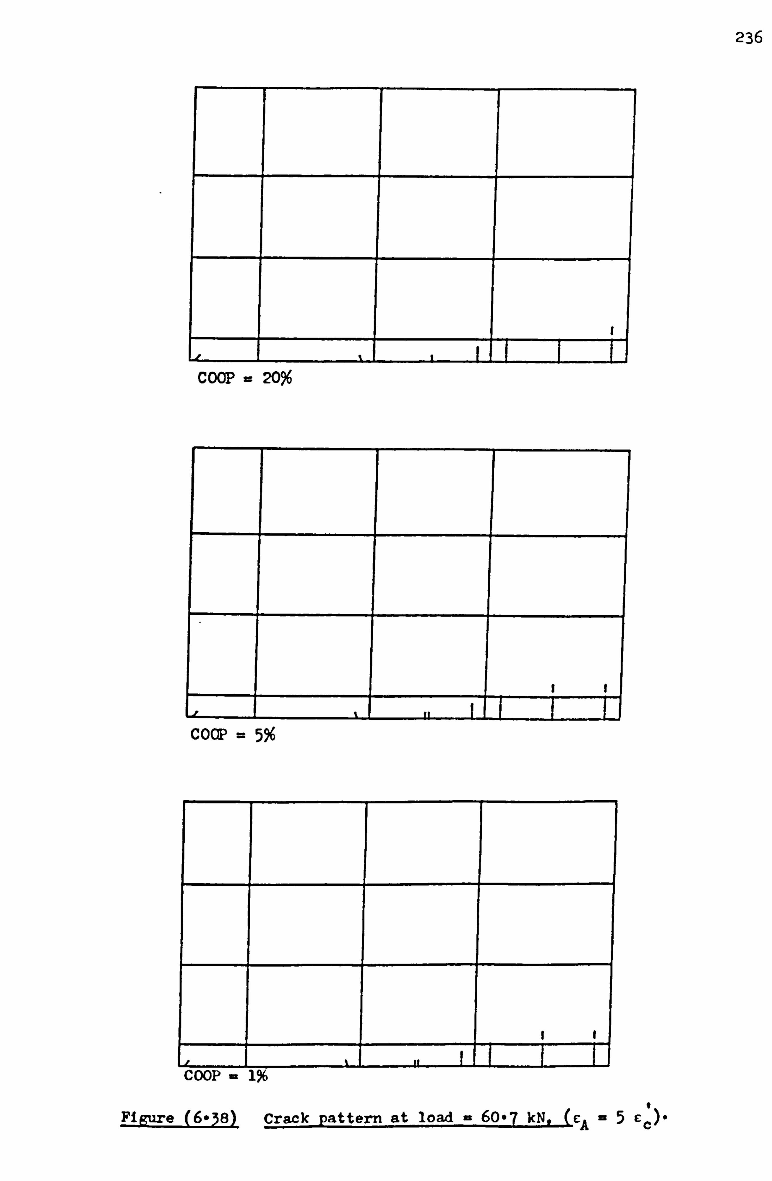
236
COOP 20%
F
COCP
COOP Figure (6-38) Crack pattern at load = 60*7 kN, (cA -5 cc')-
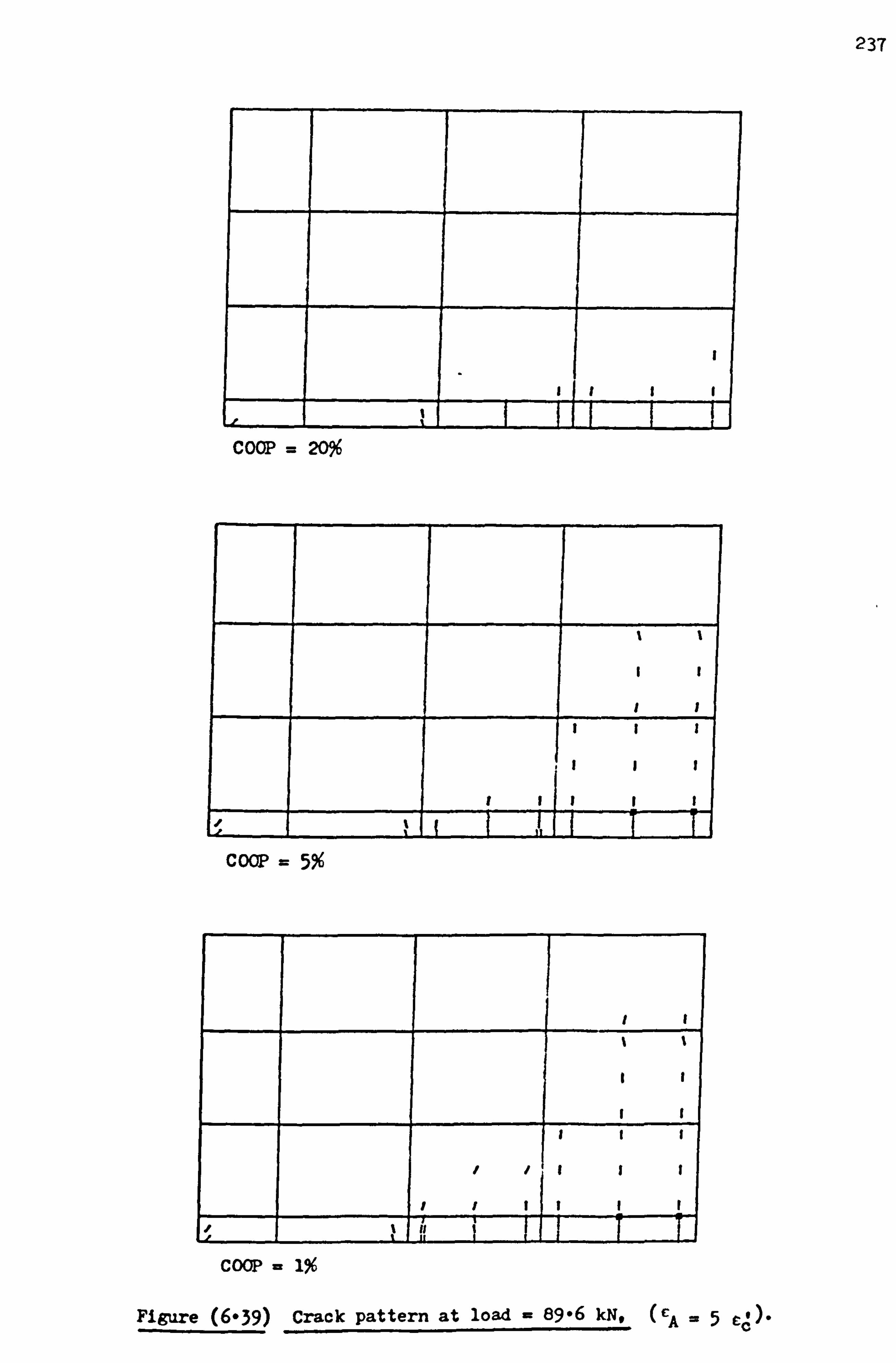
237
COCP 20%
I I
_____ _ ________ I I
_________
II I
II I
______ I II II I
___ ___________________ ______ _________________________________ II
___ 'Li IT _________________________________ _____
COCP = 5%
I t
I I
I I
SI I
// II I
I ISI I I
____ _____________
'
______________________
I II It
_ __ _____ _________________ __ ________
COOP -
Figure (6*39) Crack pattern at load - 89-6 kN, (A -5 cc)-
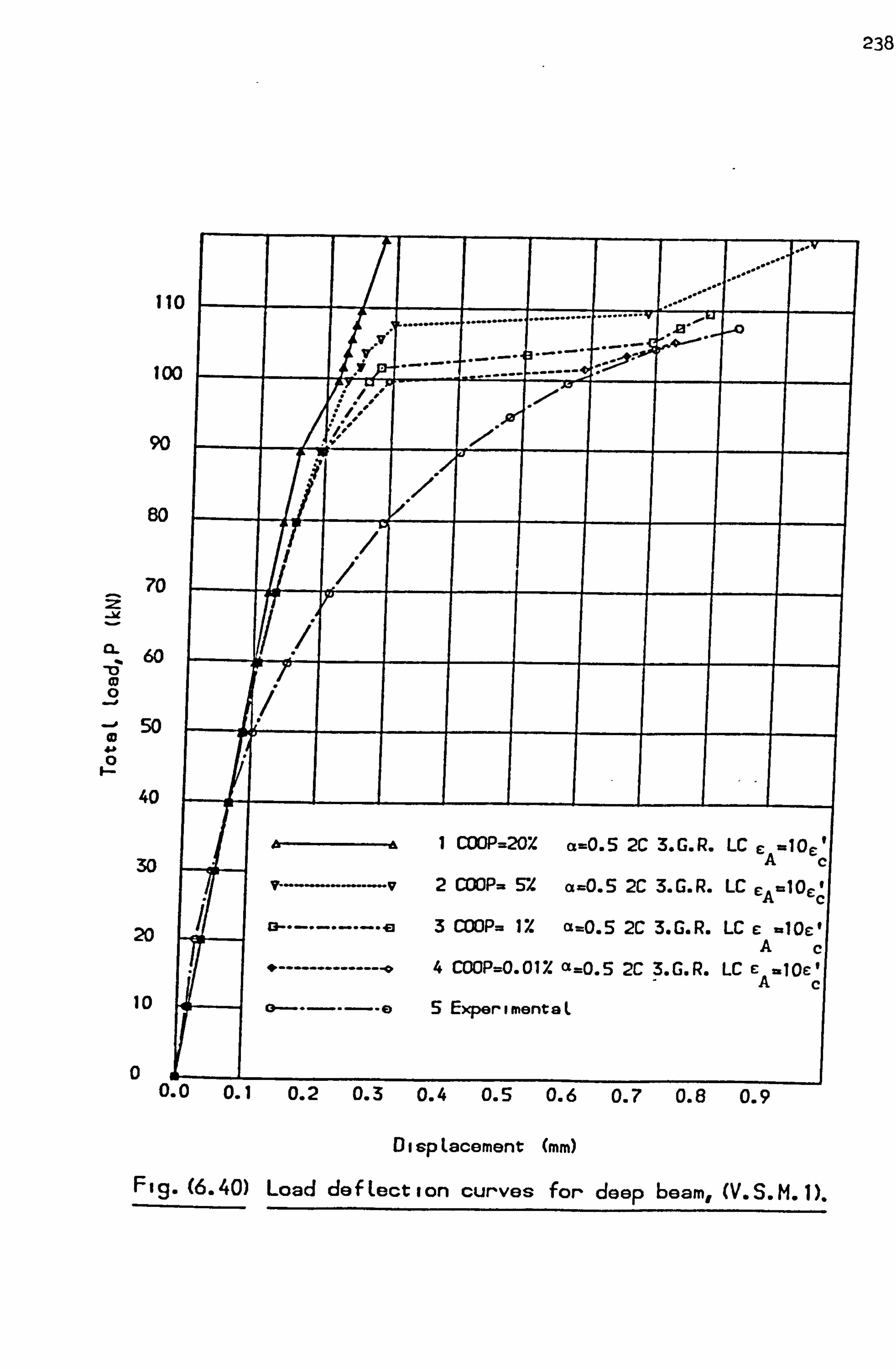
238
110
........ ......... ..... *. 100
-------- ------- 90
80
70
Cl- % 60
"t) m 0
YI
-10 50 - CD
40
1 COOP=20X a-0.5 2C 3. G. R. LC c lo loc 30 A c
--. -V 2 coop. S-2 a -0.5 2C 3. G. R. LC C 221 O l A c 20 ----------- o 3 COOP= IX (, =O. S 2C 3. G. R. LC c -10cl Ac
-- - ---------- 0 4 COOP=O. Olx (1=0.5 2C 3. G. R. LC E =10c'
10 0 5 ExperimentaL
0 0.0 0.1 0.2 0.3 0.4 0.5 0.6 0.7 0.8 0.9
DispLacement (mm)
Fig. (6.40) Load deftection curves for deep beam, (V. S. M. 1).
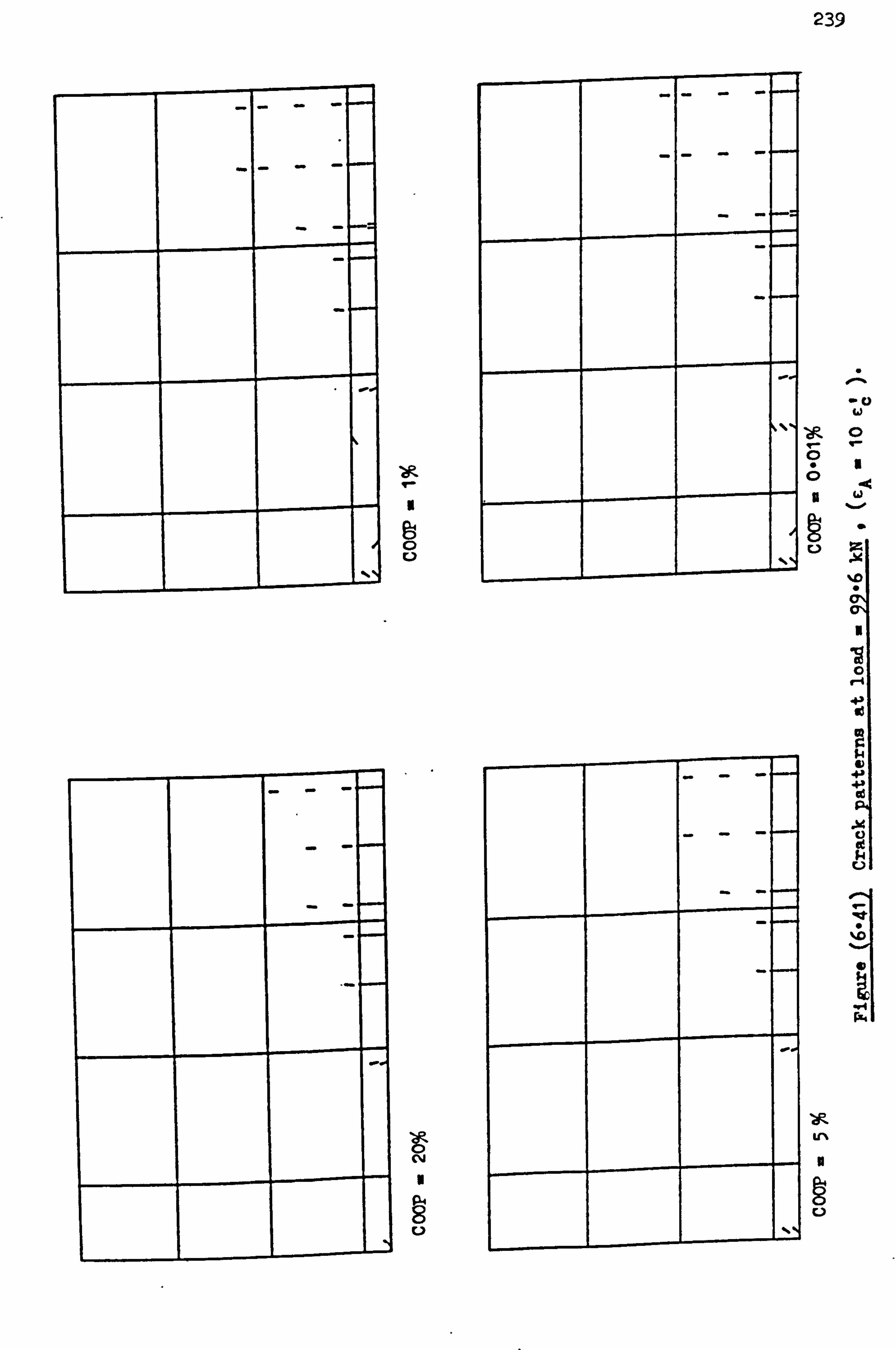
I
0
9- CY 8
10
239
-o 0
�- '-
0 "I 0 U
S
"
+X 10
C)
c )i
%D
ýA Lr%
9

- k -
llp
p04 0 C-)
- k
-I---
ýK 0 CY 11
P-4 0 0 0
IJ
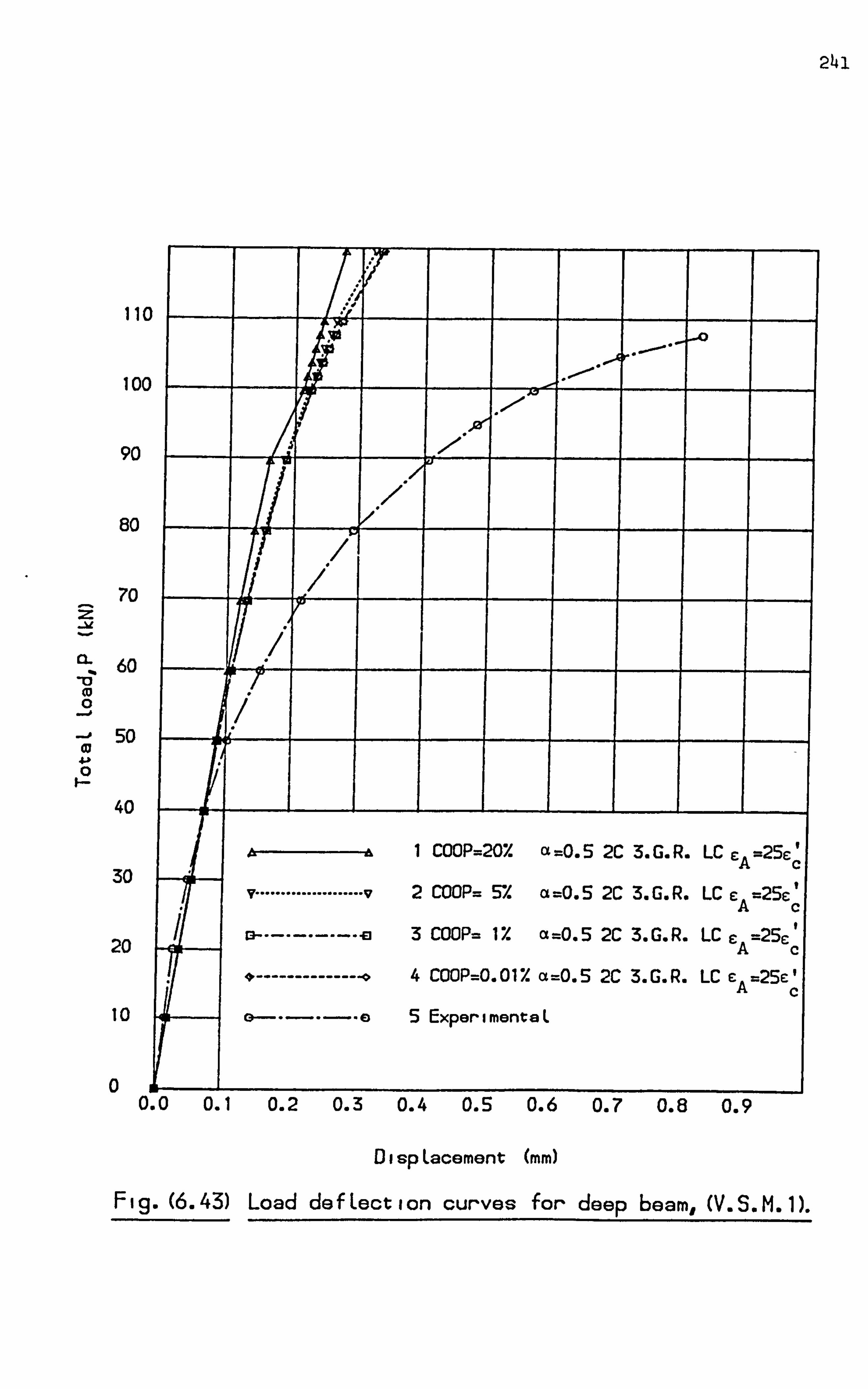
241
110 -0
100
r 90
., ca
* 80 /
70 0
60 -0 (D 1 0
50
0
40
1 COOP=20X a =O. 5 2C 3. G. R. LC cA =25c 30 e
V*""**** ..... * ...... v2 COOP= 5*/. a =O. 5 2C 3. G. R. LC c =25c ' A c
20 M ----------- m3 COOP= 1Xa =0.5 2C 3. G. R. LC cA =25c ' c
-------------- *4 COOP=0.017. a=0.5 2C 3. G. R. LC c =25E' 10 C 5E t L ) 40 xperimen e
0 0. 0 0. 1 0.2 0.3 0.4 0.5 0.6 0.7 0.8 0.9
DispLacement (mm)
Fig. (6.43) Load defLection curves for deep beam, (V. S. M. 1).
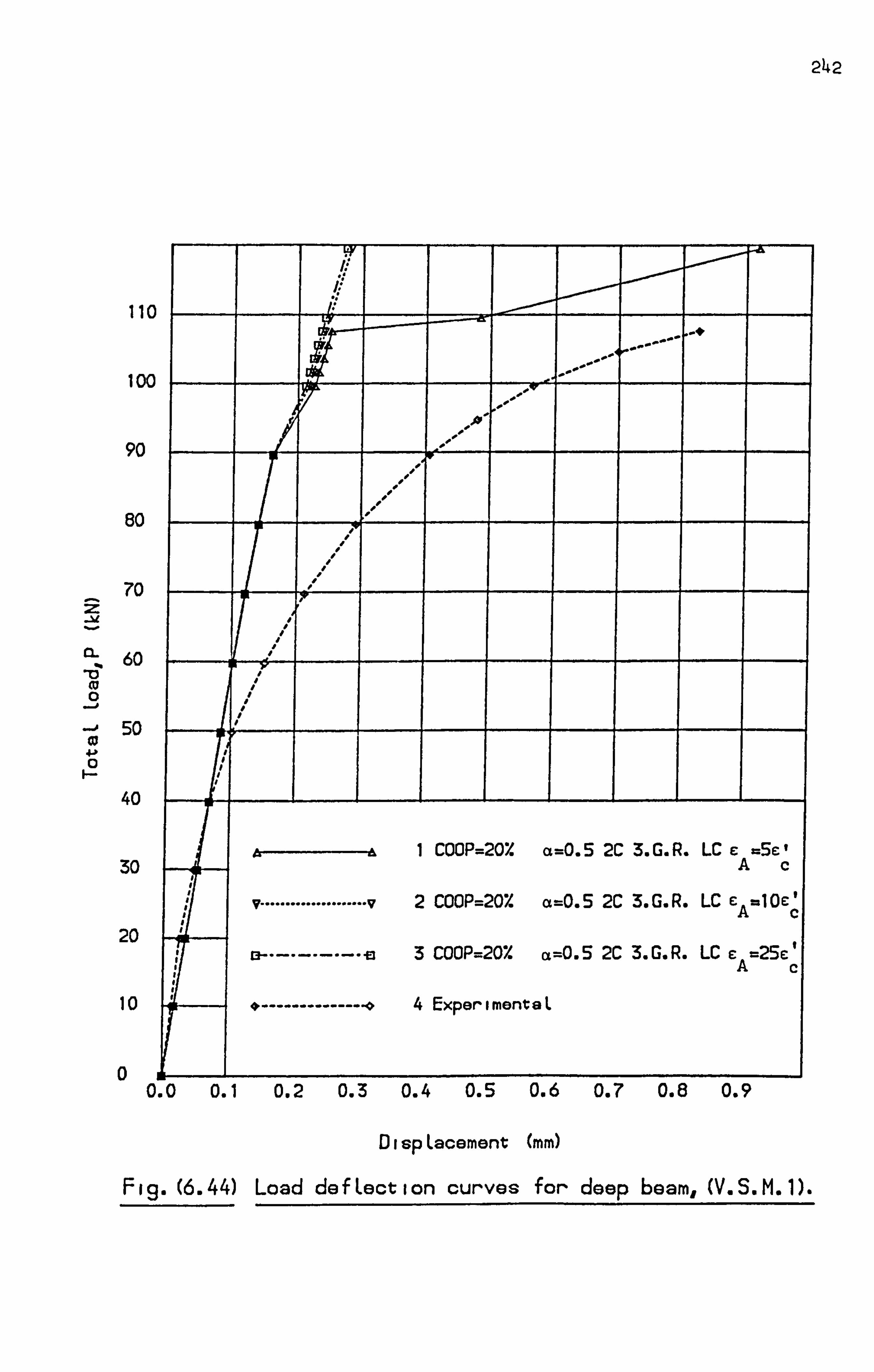
242
110
100
90
80
70
60
50
40
30
20
10
0
VY -&
EVA
f IA
f -If 0
I f f I I
1 COOP=20% a=O. 5 2C 3. G. R. LC e =5e Ac
=10C v .................... v2 COOP=20% a=0.5 2C 3. G. R. LC c A
M -- ------- -- El 3 COOP=207. a=0.5 2C 3. G. R. LC c =25c'
4E rimentaL * -------------- * xpe
0.0 0.1 0.2 0.3 0.4 0.5 0.6 0.7 0.8 0.9
DispLacement (mm)
Fig. (6.44) Load defLection curves for deep beam, (V. S. M. 1).
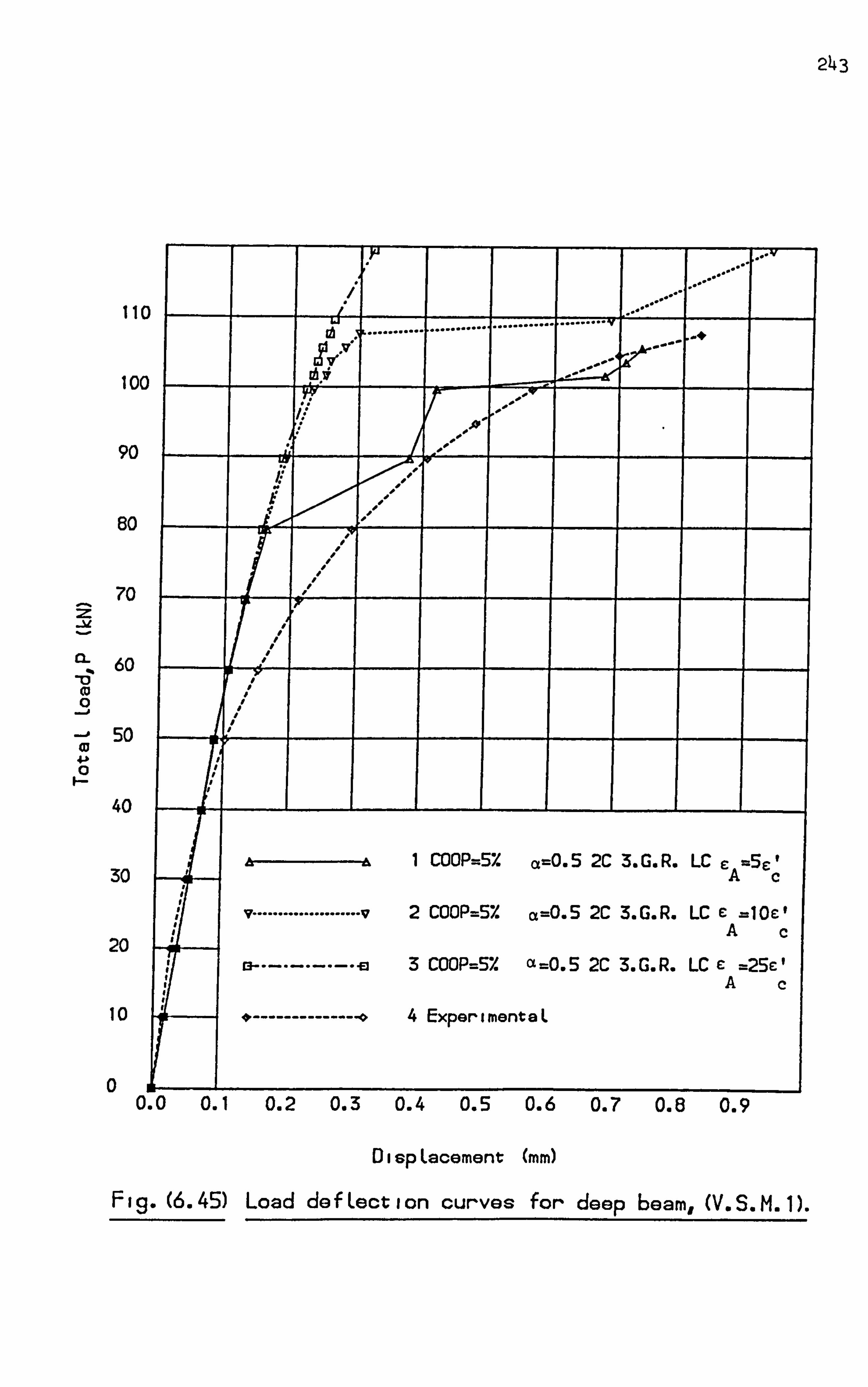
243
110 : L ........... ..
100
hl
90 I'll
80
70
60 (D 0
-. 0 50 A
l CD 4-b 0
40
1 COOP=Sx a=0.5 2C 3. G. R. LC C ý56: 30 A c 1 V .................... V2 COOP=SZ a=0.5 2C 3. G. R. LC c =10c,
20 13 .......... ým 3 COOP=52 a=0.5 2C 3. G. R. LC C =25E'
10 4E t L -------------- xpertmen a
0 0. 0 0. 1 0.2 0.3 0.4 0.5 0.6 0.7 0.8 0.9
DispLacement (mm)
Fig. (6.45) Load defLection curves for- deep beam, (V. S. M. 1).

244
IIc
100
90
80
70
92- w
60 _C) 0 0
_A 50 0 4. P
40
30
20
10
0
La 0 ....
v
... - -+
... .......... .
iN
?v
11
le
1 COOP= 1Xa =O. 5 2C 3. G. R. LC c =5 e A c
v .................... v2 COOP=l% a =0.5 2C &G. R. LC cA=10c ' c
--------- -- a3 COCIP=17. a =0.5 2C 3. G. R. LC ce25c'
- 4E t L ------------ - xperimen a
0.0 0.1 0.2 0.3 0.4 0.5 0.6 0.7 0.8 0.9
DispLacement NO
F 19. - (6.46) Load do f Loot i on curves f or deep beam, W. S. M. 1).
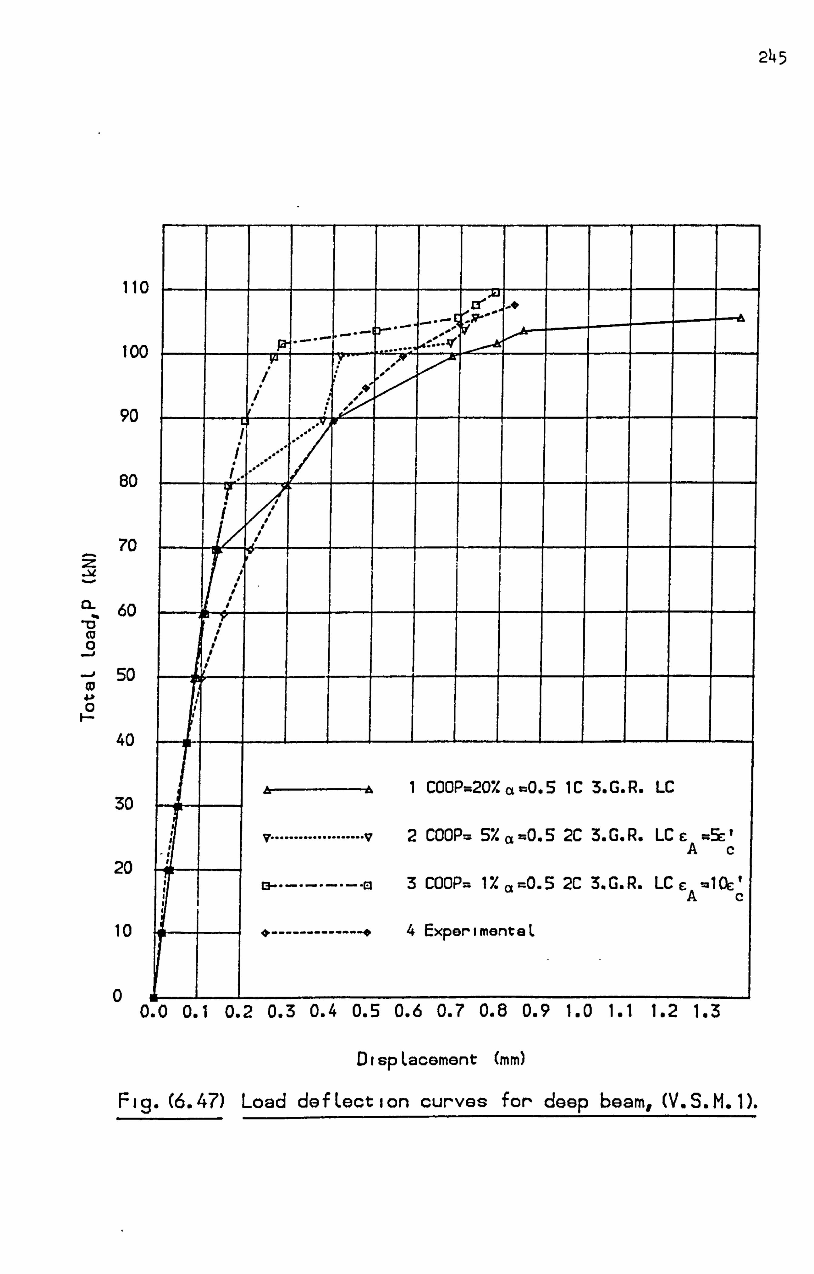
245
110
100
90
80
70
60
40
30
20
10
0
1 COOP=20X a=0.5 1C 3. G. R. LC
2 COOP= 57. a =O. 5 2C 3. G. R. LC c =5ý Ac
[2ý -- -------- El 3 COOP= 1Y. a=0.5 2C 3. G. R. LCc ý3 10E '
- --------- 04 Ex erimentaL --- 4 p
0.0 0.1 0.2 0.3 0.4 0.5 0.6 0.7 0.8 0.9 1.0 1.1 1.2 1.3
DispLacement (mm)
Fig. (6.47) Load defLection curves for deep beam, (V. S. M. 1).

246
II
___ _____ I I I I COOP = 20%, N. T. S,
COOP = 5%, cA =5E: c'
Coop = 19/01 E: A = 10 cc'
Figure (60481 1 Crack patterns at load - 69*7 kN.

247
I I
I II
I II I II
/ I I II
/1 I I II
___
t _____ II I
COOP = 20%9 N. T. S.
T I COOP = 5%, £A =5
F- c'
COOP = 1% , CA '2 10 c C,
Figure (6-49) Crack patterns at loads = 89-6 kN.
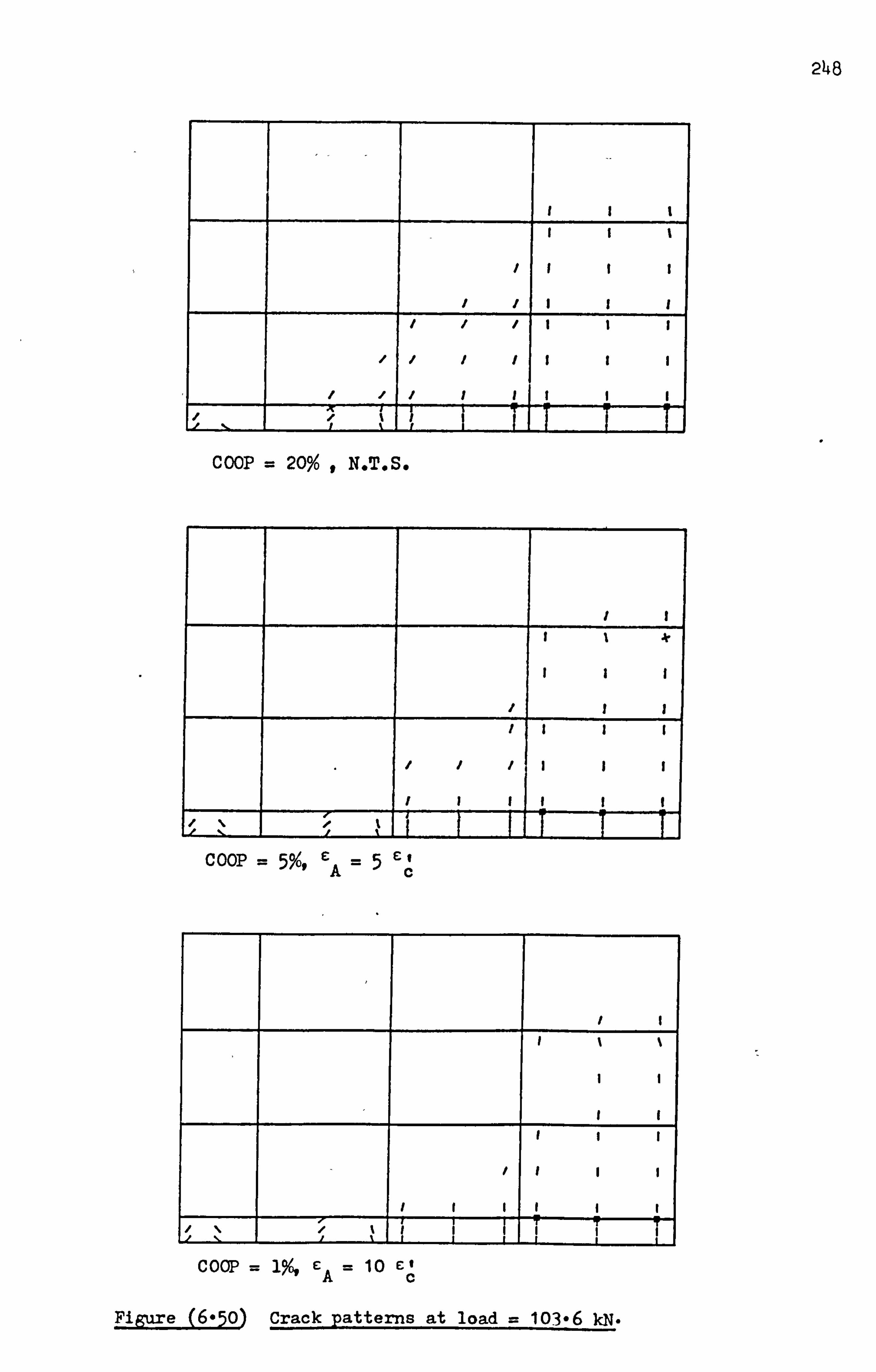
248
_____ ______ ___ I I II I
/ II I
____ ______ __ / / II I
I / / II I
/ / / I II I
/ / / I I II I / ______
. / I
I I t
I I I
I I I I I
__________ ___
COOP = 20% t N. T. S.
_ ____ ______ __ __ ______ I I
I
_ ___ /
I
3
I
1 1 II I
/ II II I
_ ____ I II II I
1
__
\
____ ' / t ' f
___ i ______ _ i ______ ______
Cf COOP = 5Y6, CA =5c
I I
I I
_ ____ _______ __ I I
_____ ____ I I I
I I I I
II I I I I / I
� '_
� I
' t
I II II
I I I
I i I
i I
Coop = 1%, CA = 10 CC'
Figure (6-50 crack patterns at load = 103-6 kN.
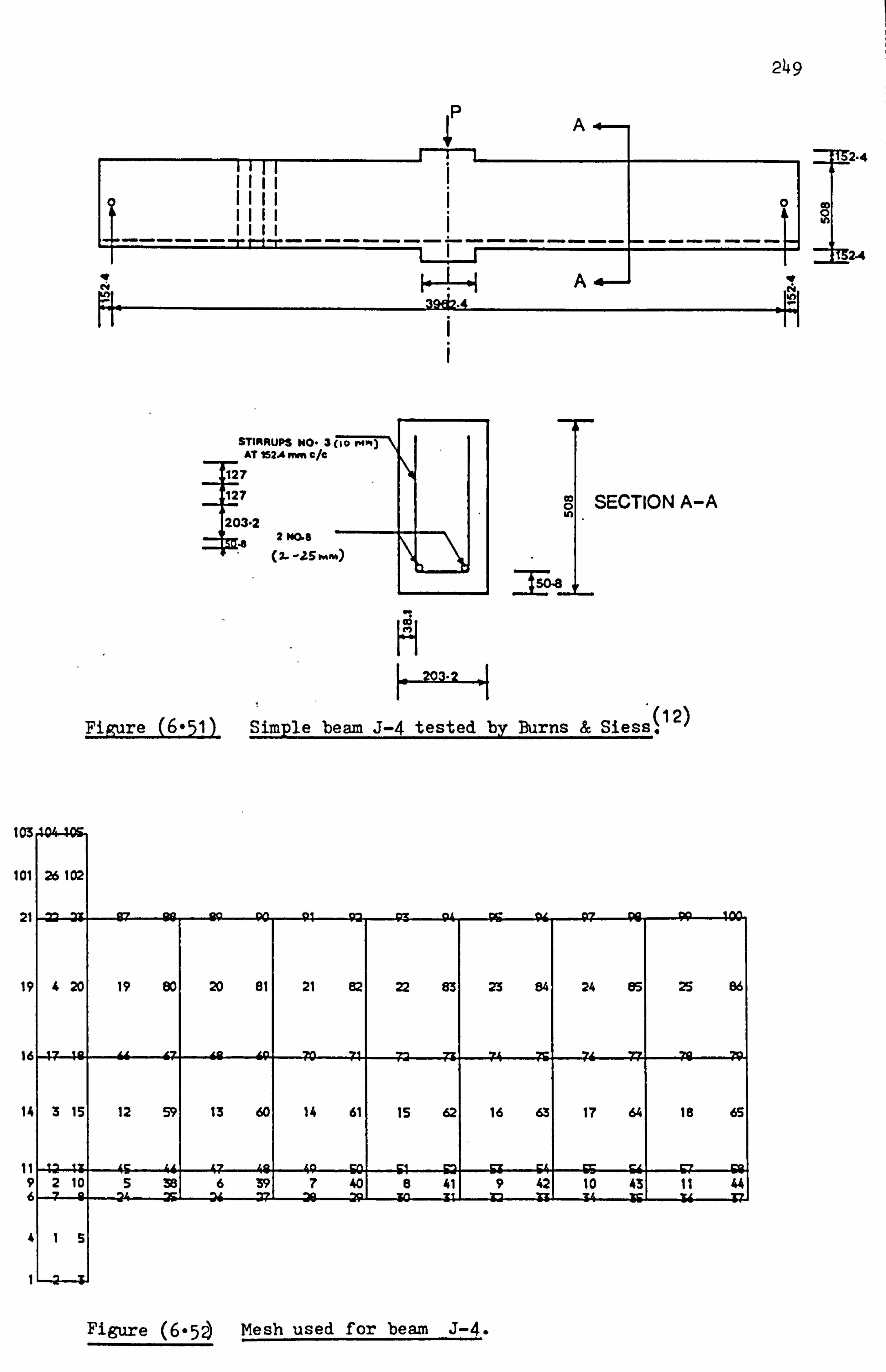
249
jn2-4
00
1 M2.4
39d2-4
STIRRUPS MO- 3 AT 152A rnrn C/C
1 127
127
203-2
42 NO-& 2. -15 vAm
co 0 SECTION A-A in
: Es"L
co
Figure (6-511 Simple beam J-4 tested by Burns & Siessý 12)
103 40440 So.
26102
92 PO p! 92 95 .1 94 99!
4 20
P is
19 80
Aý 17
20 81 21 82
4 ;4
22 63 23 84 24 es 25 86
3 is 12 59 13 60 14 61
0
----
is 62
Q
----
16 63
ý
17 64 is 65
2 10 35 2S
.-
6 39 24
. 7 40 20 29
6 - so ti, 42
ý
ý 33
1 10 43 34 Is
11 I IA
101
21
19
Id
14
11 9
Figure (605ý Mesh used for beam J-4.
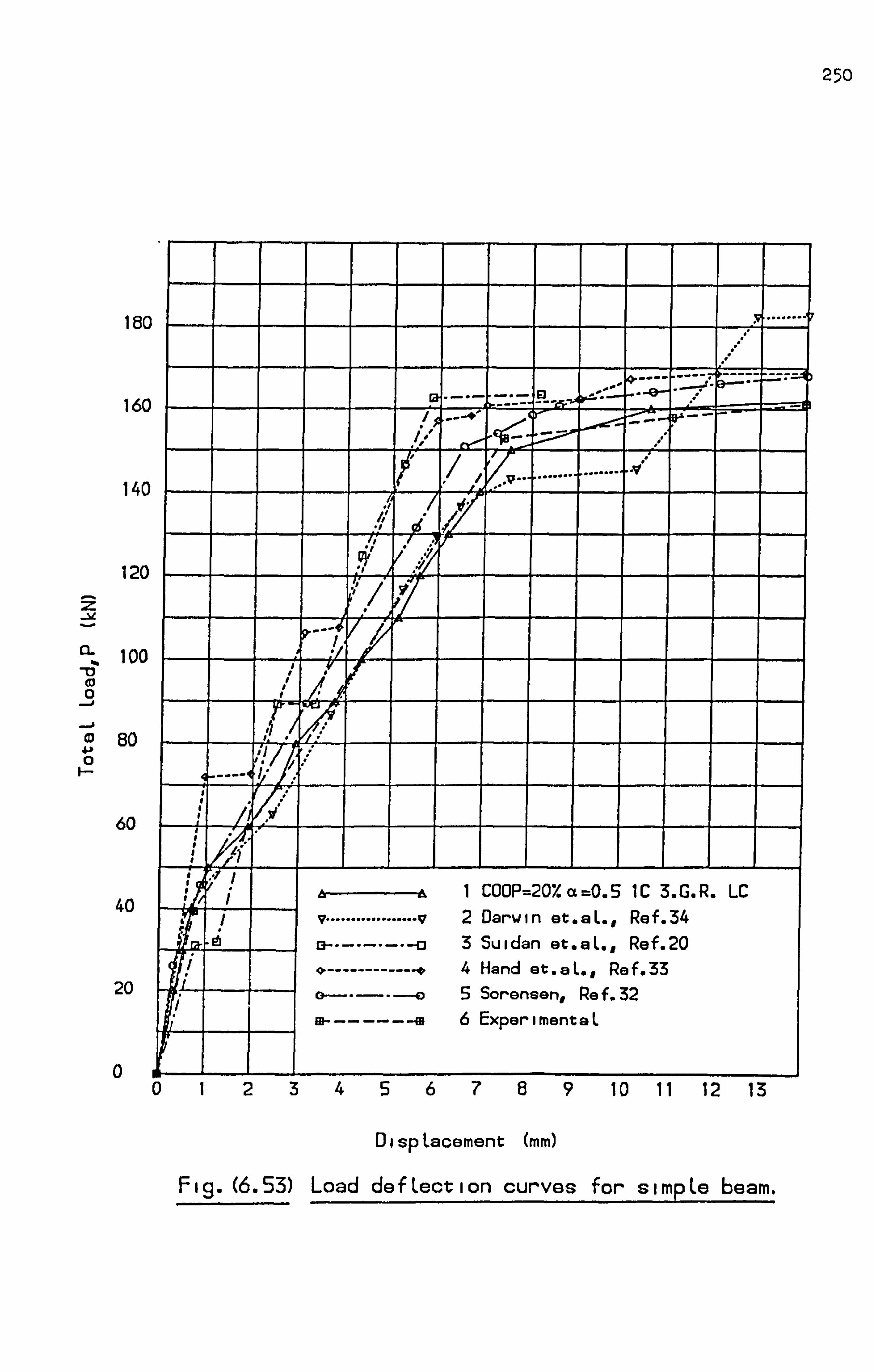
250
180
160
140
120
loo
-. j CD so 4-P
60
40
20
0
--- -------
... ......... ......... .. v
Al
vy I
1 COOP=20% a =0.5 1C3. G. R. LC
v ................. v2 Darwin et. aL., Ref. 34 m --------- a3 Suidan et. aL., Ref. 20 a ------------- *4 Hand et. aL., Ref. 33 05 Sorensen, Ref. 32
6 ExperimentaL
10 11 12 13
DispLacement NO
Fig. (6.53) Load defLection curves for simpLe beam.
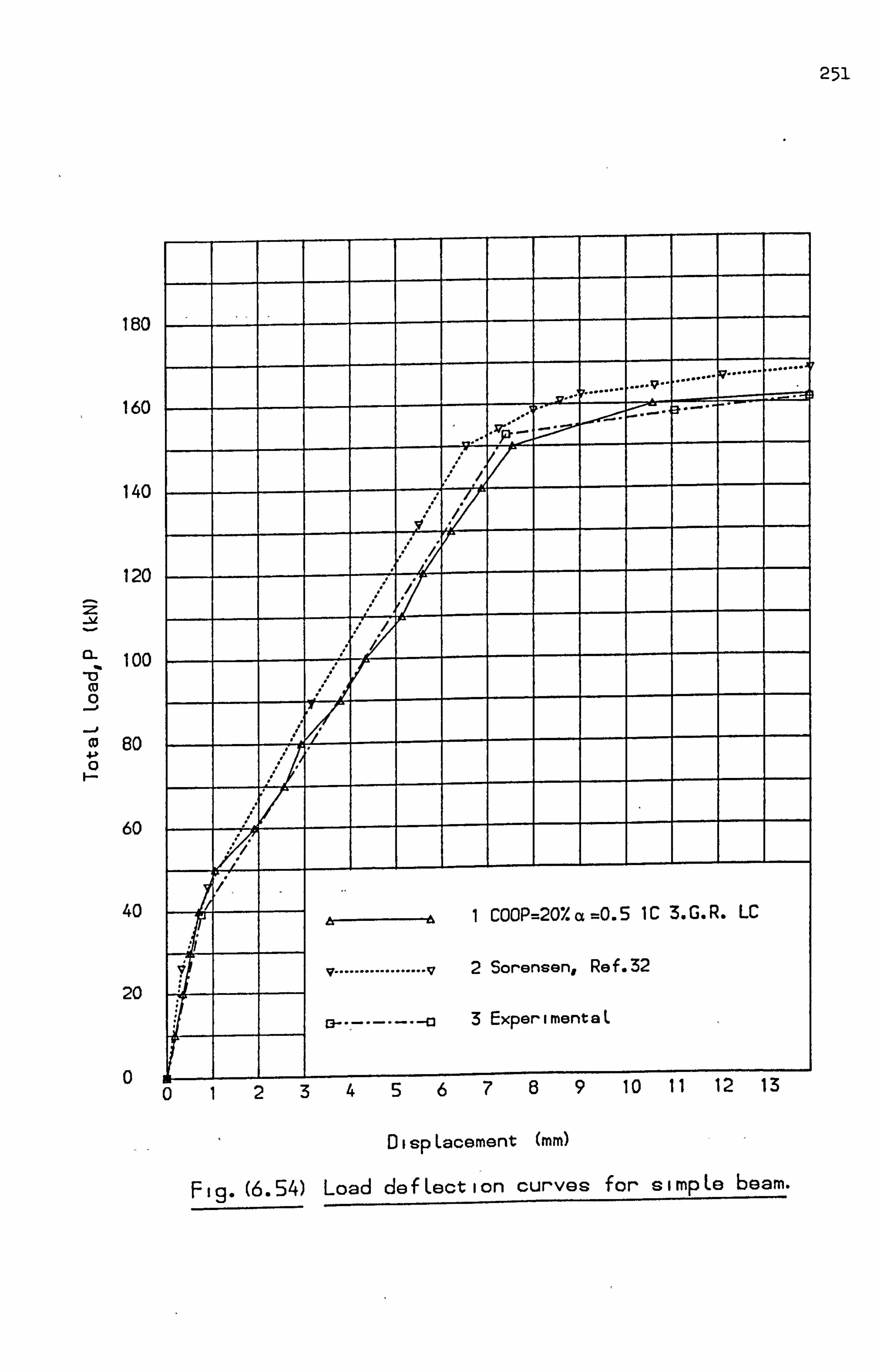
251
180
160
140
120
loo co 0
-, j CD 60 4--
60
40
20
0
I A -
LC R . 1 COOP=207. a=0.5 1C 3. G.
v ................. v2 Sorenson, Ref. 32
3 ExperimentaL
lu 111Z la
DispLacement (mm)
Fig. (6.54) Load defLection curves for simpLe beam.
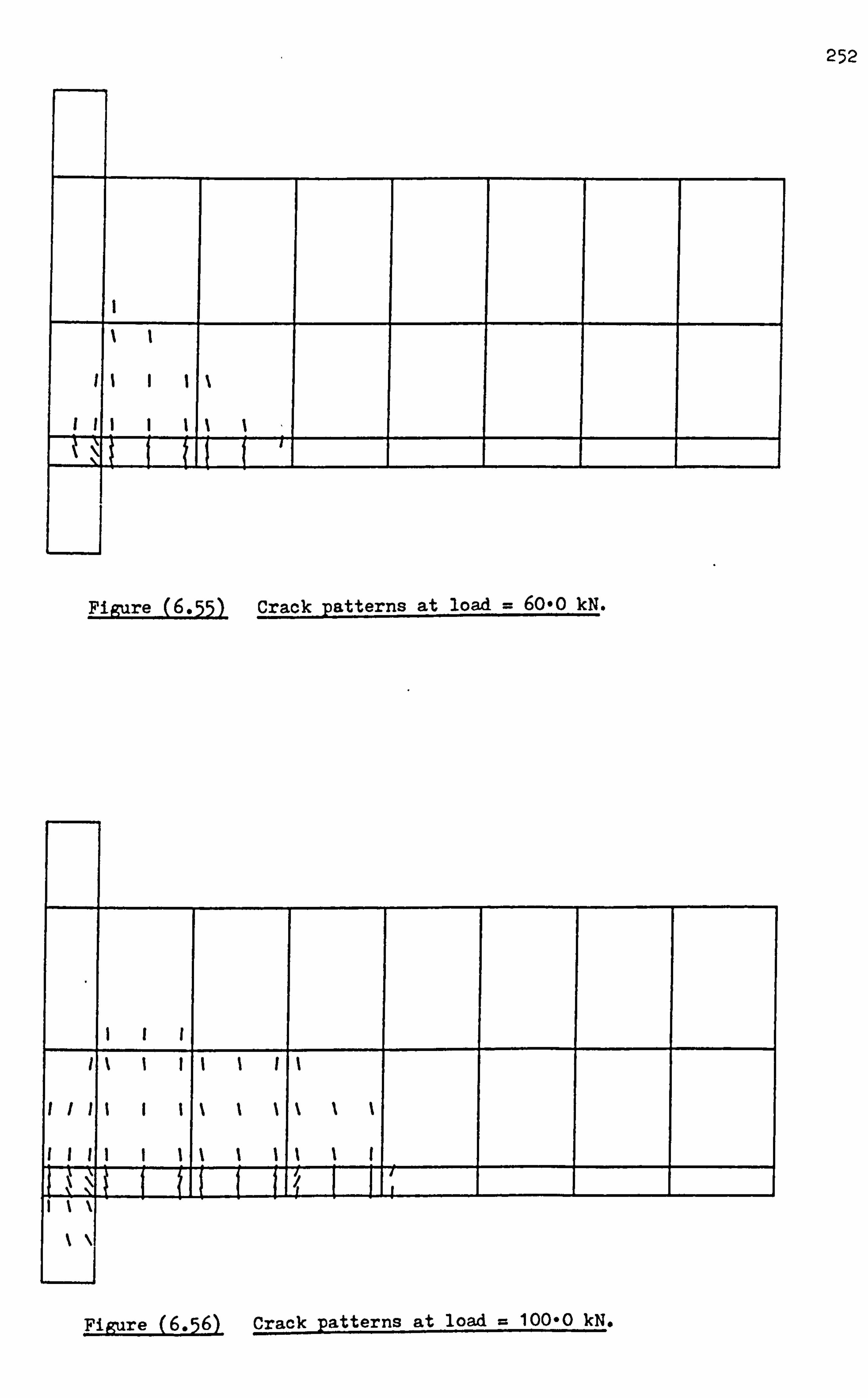
252
Figure (6.55) Crack patterns at load = 60-0 kN.
LL H I -I
Figure (6. L6) Crack patterns at load = 100-0 kN.

253
I I II I t % %
1 1 1
I
1I
I
l
I I
I
1 I
tt
I ? } _ __ _
_ ____ ____ _____
Figure (6.57) Crack patterns at load = 140*0 kN.
I
t i
/
l
\
l II 1 1 1 II I I
l i
I
l
l
t
ll
I1
i
t
1
I
1
I
1
tI
1%
I
I
II
II l \
i 1 1
I ' '
__ __ _ _____ _____
Figure (6-58) Crack patterns at load = 160-0 kN.

ft lb
2 Scale: lmm 0-18 NIMM tension), (- compression)
Figure (6-59) Principal stress directions at load =- 16-0 kN.
II =Zr -
Scale: lmm 2-- 1949 H/MM2 tension), (- compression)
254
Figure (6-60) Principal stress directions at load - 60-0 kN.
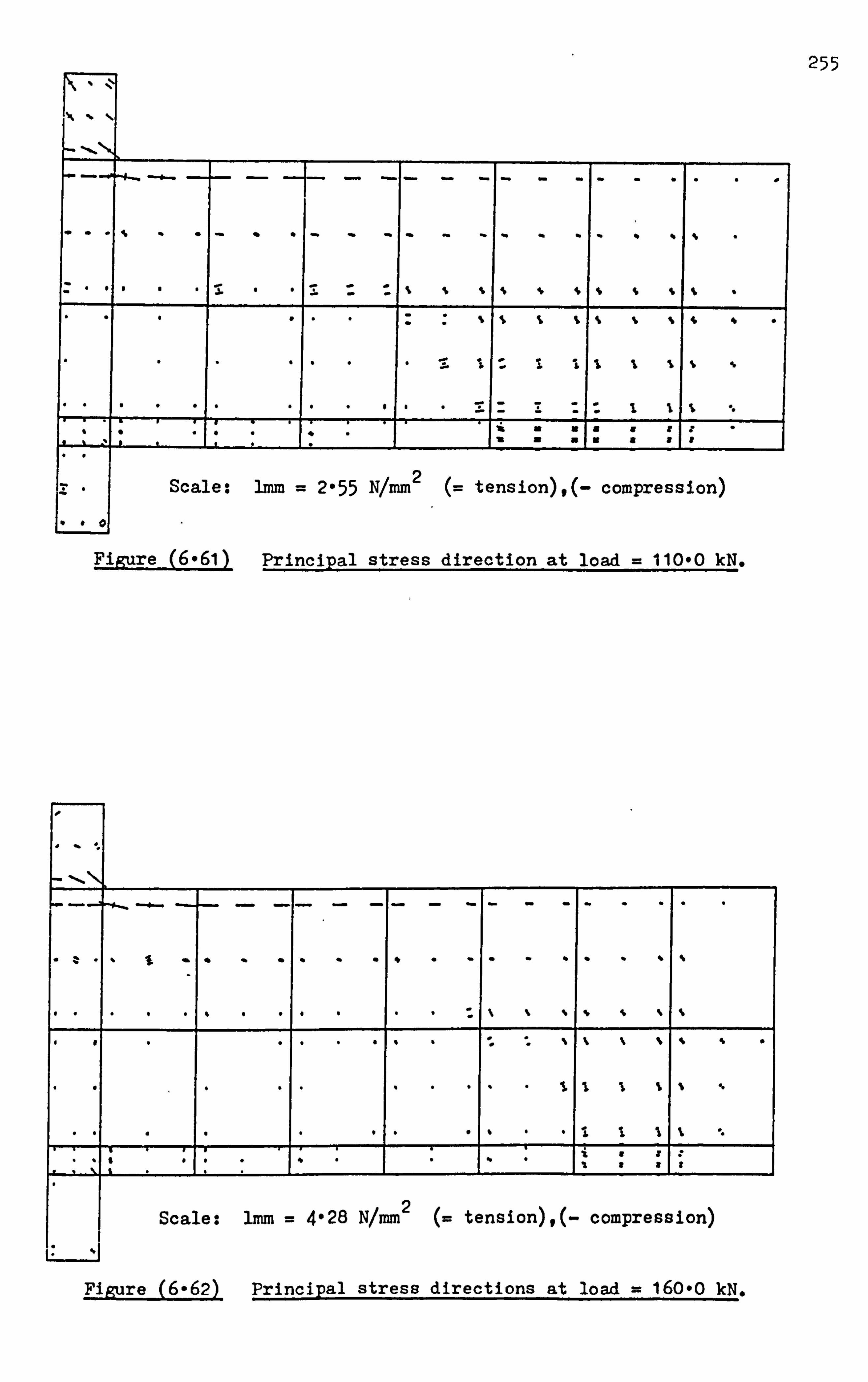
Scale: lmm 2055 N/MM2 tension), (- compression)
Figure (6-61) Principal stress direction at load = 110-0 kN.
Scale: 1MM 4-28 N/mm 2 tension), (- compression)
255
Figure (6-62), Principal stress directions at load = 160-0 kN.

256
1. Scordelis, A. C., "General report - Basic Problem". IASS Symposium
on the nonlinear behaviour of reinforced concrete spatial
structures, Vol-3,35-70, JulY, 1978.
2. Gerstle, K. H., "Material modelling of reinforced concrete". IABSE
Colloquium on The Advanced Mechanics of Reinforced Concrete,
Introductory Report, Delft, 41-61,1981.
3. Phillips, D. V., "Nonlinear analysis of structural concrete by
finite element method". Ph. D. Thesis, University of Wales, 1973.
4. Nilson, A. H; Cedolin, L., "A convergence study of iterative methods
applied to finite element analysis of reinforced concrete".
Int. J. Num. Meth. Eng., Vol. 12,437-451,1978.
5. Duncan, W.; Johnarry, T., "Further studies on the constant stiffness
method of nonlinear analysis of concrete structures". Proc.
Inst. Civ. Eng., Part 2,951-969, Dec., 1979.
6. Cope, R. J.; Rao, P. V.; Clark, L. A., "Nonlinear design of concrete
bridge slabs using finite element procedures". Nonlinear
Design of Concrete Structures, CSE-ASCE-ACI-CEB International
Symposium, University of Waterloo, Ontario, Canada, 379-407,
Aug., 1979.
7. Cope. R. J.; Rao, P. V.; Edwards, K. R., "Nonlinear finite element
analysis techniques for slabs". Numerical methods for nonlinear
problems, Proc. of the Int. Conf. held in University College,
Swansea, 445 456, Sept. 1980.
8. Cope, R. J.; Rao, P. V.; Clark, L. A.; Norris, P.; "Modelling of
reinforced concrete behaviour for finite element analysis of
bridge slabs. " Proc. of the Int. Conf. held in University College,
Swansea, 457-470, Sept. 1980.

257
9. Cope, R. J.; Rao, P. V., "Nonlinear finite element strategies for
Bridge slabs", IABSE Colloquium on The Advanced Mechanics of
Reinforced Concrete, Final Report, Delft, 273-288,1981.
10. Crisfield, M. A., "Local instabilities in the nonlinear analysis
of reinforced concrete'beams and slabs". Proc. Inst. Civ.
Eng., Part 2, Vol-73,135-145,1982.
11. Ramakrishnan, V.; Ananthanarayana, Y., "Ultimate strength of
deep beams in shear", J. ACI, Vol-55,87-98, Feb., 1968.
12. Burns, N. H.; Siess, C. P., "Load deformation characteristics of
beam-column connections in reinforced concrete". Report No. 234,
University of Illinois, Jan., 1962.
13. Cope, R. J.; Rao, P. V.; "Discussion on reference 5". Proc. Inst.
Civ. Eng., Vol. 69, Part 2,873-874, Sept. -, 1980.
14. Cook, R. D., "Concepts and applications of finite element analysis".
Wýley, 2nd ed., 1981.
15. Zienkiewicz, O. C., "The finite element method". McGraw-Hill, 3rd
ed. , 1977.
16. Bathe, K. J., "Finite element procedures in engineering analysis".
Prentice-Hall, 1982.
17. Irons, B.; Ahmed, S. "Techniques of finite elements". Wiley, 1981.
18. Chen, E. Y. T.; Schnobrich, W. C., "Material modelling of plain
concrete". IABSE Colloquium on The Advanced Mechanics of
Reinforced Concrete, Final Report, Delft, 31-52,1981.
19. Bathe, K. J.; Wilson, E. L., "Numerical methods in finite element
analysis". Prentice-Hall, 1976.
20. Suidan, M.; Schnobrich, W. C., "Finite element analysis of reinforced
concrete". J. of Struct. Div., ASCE, Vol. 99,2109-2122, Oct., 1973.
258
21. Hand, F. R.; Pecknold, D. A.; Schnobrich, W. C., "Nonlinear layered
analysis of RC plates and shells". J. of Struct. Div., ASCE,
vol. 99,1491-1505, July. 1973.
22. Cedolin, L.; Dei Poli, S., "Finite element studies of shear
critical R/C beams". J. of Eng. Mech. Div., ASCE, Vol-103,
395-410, June, 1977.
23. Al-Mahaidi, R. S. H., "Nonlinear finite element analysis of reinforced
concrete deep members". Report No-79-1, Cornell University,
Jan. , 1979.
24. Buyukozturk, 0.; Connor, J. J.; Leombruni, P., "Research on modelling
shear transfer in reinforced nuclear structures". Nucl. Eng.
and Design, Vol. 59,67-84,1979.
25. Scanlon, A.; Murray, D., "Time dependent reinforced concrete slab
deflections". J. of Struct. Div., ASCE, Vol. 100,1911-1924,
Sep-. , 1974.
26. Gilbert, R. I.; Warner, R. F., "Nonlinear analysis of reinforced
concrete slabs with tension stiffening". Report No. R-167,
University of New South Wales, Australia, Jan., 1977.
27. Gilbert, R. I.; Warner, R. F., "Tension stiffening in reinforced
concrete slabs". J. of, Struct. Div., ASCE, Vol. 104,1885-1900,
Dec., 1978.
28. Lin, C. S.; Scordelis, A. C., "Nonlinear analysis of RC shell of
general form". J. of Struct. Div., ASCE, Vol-101,523-538,
March, 1975.
29. Mang, H. A.; Floegl, H., "Tension stiffening concept for reinforced
concrete surface structures". IABSE Colloquium on The Advanced
Mechanics of Reinforced Concrete, Final Report, Delft, 331-349,1981
259
30. Shirai, N.; Sato, T., "Inelastic analysis of reinforced concrete
shear wall structures - Material modelling of reinforced concrete".
IABSE Colloquium on The Advanced Mechanics of Reinforced Concrete,
Final Report, Delft, 197-210,1981.
31. Vecchio, F.; Collins, M. P., "Stress-strain characteristics of
reinforced concrete in pure shear". IABSE Colloquium on The
Advanced Mechanics of Reinforced Concrete, Final Report, Delft,
211-225,1981.
32. Sorensen, s. i., "Endochronic theory in nonlinear finite element
analysis of reinforced concrete. " Report No-78-1, Trondheim
University, March, 1978.
33. Hand, F. R.; Pecknold, D. A.; S,, c6iobrich, W. C., "A layered finite
element nonlinear analysis of reinforced concrete plates and
shells". Technical Report UILU-ENG-72-2011, University of
Illinois, Aug., 1972.
34. Darwin, D.; Pecknold, D. A., "Inelastic model for cyclic biaxial
loading of reinforced concrete". Report No. 409, University
of Illinois. - July, 1974.
CHAPTER
APPLICATION TO DEEP BEAMS
7.1 Introduction
7.2 Solid deep beams
7.2.1 General review
7.2.2 Cervenka panel wall W-2
7.2.3 Lin deep beams 101 and 102
7.2.4 Lin deep beam 204
7.3 Deep beams with openings
7.3.1 General review
7.3.2 Memon deep beam B-5
7.3.3 Memon deep beam B-7
7.4 Conclusions

260
CHAPTER
APPLICATION TO'DEEP BEAMS
7.1 Introduction:
Deep beams are found in various types of structure and have different
useful applications. In modern construction, for example, departmental
stores, hotels, municipal buildings and so on, it is often desirable to
have the lower floor entirely free of columns. It may be simpler to
utilise the external and partition walls as deep beams to span across
the column free space and carry the whole building above them instead of
using a heavy frame construction.
As there is a gradual transition from shallow beam behaviour to
deep beam behaviour a distinct classification of deep beams is not
strictly possible. Typically they are characterised by low span/depth
ratios, L/D varying from less than 1 to about 5, and are usually relatively
thin. Vertical normal stresses and shear stresses are more significant
than flexural stresses, and strain distribution across a vertical section
is not usually linear even under elastic conditions. The difficulties
with these beams, especially ones having a span to depth ratio less than
about 2, are that the simple theory of bending is not applicable in analysis,
and that the stresses are highly effected by the application of the
external loads and the location of the supports.
The behaviour of these beams depends on many factors such as,
span/depth ratio, percentage of tension and compression reinforcements,
amount and arrangement of web reinforcement, etc. These aspects are
discussed in references 1-16, and are summarised in Section 7.2.1. One
special type of deep beam is the web opening deep beam. It is only in the
261
last decade or so that any significant research has been carried out on
a practical scale for these beams. This type of beam will be discussed
in a later section of this chapter.
The purpose- of this chapter is to examine the conclusions obtained
from the previous chapter in the analysis of complex deep beans with and
without openings failing in shear, and to study the effect of varying
different numerical parameters on the nonlinear solution. The program
will be used to predict different aspects of the behaviour of these beams.
Stress distributions, crack patterns, and load deflection curves will be
plotted and compared with available experimental results. This will then
complete the appraisal of the proposed method of analysis on a compre-
hensive range of deep beam types and behaviour.
The following beams, tested experimentally by different authors,
will be analysed.
(1) Cervenka(') panel wall W-2 failing by flexural-shear.
This type of failure is characterised by a combination of diagonal
cracks and flexural cracks as shown in Figure (7.1. a).
(2) Lin (2)
deep beam 101 failing by diagonal-compression,.
This type of failure starts with an inclined crack developing
along the line joining the load and support points, after which parallel
inclined cracks start to appear. The final failure occurs due to the
destruction of the portion of concrete between these two cracks. This is
shown in Figure (7.1. b).
(3) Lin (2)
deep bean 102 failing by'shear-compression.
This failure is due to the penetration of the inclined crack towards
the compression zone at the top of the beam. The beam fails by crushing

262
above the upper end of the inclined crack. This is shown in Figure
(7-1-C).
(4) Lin deep beam 204 failing by splitting-shear.
The failure is characterised by the growth of the inclined cracks
which join the inside edge of the support point and outside edge of the
loading point. The main cause of such failure was due to the high
compression force in support region and the lack of confinement of
concrete beyond the region where the reinforcement terminated under
loading point. This is illustrated in Figure (7.1. d).
(5) Memon (3)
deep beam B-5 with web opening failing by diagonal -compressio
This type of beam fails as described in 2 and shown in Figure
(7.1. e).
(6) Memon(3) deep beam B-7 with web opening failing by diagonal-compression
This beam fails in a similar manner to beam B-5.
T. 2 Solid deep beams:
7.2.1 General review:
Complete recent reviews on solid deep beams have been reported in
(2) (3) detail by Lin and Memon The work on deep beams will be discussed
in two categories; first the theoretical studies will be discussed and
then the experimental work.
Early theoretical work on this topic examined the change in stress
from engineer's theory of bending as span to depth ratio increased.
Dischinger (4)
in 1932 presented a Fourier series solution for beams of
decreasing span to depth ratio resting on a series of supports as a
continuous beam. In 1951 Chow et al. (5)
produced a method of analysing
263
the stress distribution in deep beams of finite length by superimposing
two stress functions, namely a Fourier series and the principal of
least work. ' Other investigators, Ulham (6)
, Chow et al. have obtained
solutions using the finite difference method to provide information
on the stress distribution. Gy I zman et al. (8)
, Archer et al. (9)
used
strain energy methods for determining stresses.
Most of these theoretical models have assumed that reinforced concrete
is'homogeneous and isotropic. In fact the stress-strain response of
reinforced concrete in situations where cracking occurs is more complicated
than these simple elastic homogeneous models predict. Some investigators,
(6) (T) for example Chow et al. and Ulhman , have based design recommen-
dations on this simplified model. However cracking of the beam may lead
to a redistribution of stresses which may invalidate the results of
the elastic analysis upon which the design was based. The stress distri-
bution is best determined by experimental tests, which can then be further
examined by a finite element model to give complementary information.
Many investigators have studied the behaviour of solid beams
experimentally. For example Leonhart et al. (10)
summarized various
research work on deep beams, and studied simply supported deep be
under different load conditions, and various arrangements of reinforce-
ment. Concrete strains measured on the beam surface were converted to
stresses, and found to give a good agreement with the theoretical
elastic prediction at low load levels. Arching action was apparent from
concrete and steel strain'measured in all tests, and the crack widths
were found to be noticeably reduced by distributing the main tension cord
over the bottom part of the beam.

264
A formula which was dependent on the stress distribution in the
concrete was proposed to calculate the main tension steel. De-Paiva
et al. (11)
studied simply supported deep beams with span/depth ratios
varying from two to six. He found that the type and the amount of web
reinforcement provided had no significant effect on the formation of
the cracks or on the failure modes. However, the presence of such web
reinforcement did significantly reduce the amount of visible damage to
the beam. De-Paiva et al. also found that increasing the quantity of
main reinforcement will change the failure mode, for instance changes
from flexural to shear failure modes were reported. He also found that
an increase in concrete strength increased the shear capacity but did
not increase flexural capacity. I
Ramakrishnan et al ý12)
studied different single span deep beams.
In his-experiments he obtained shear failures which were actually
diagonal tensile failures caused by splitting and there was little
sign of any shear or sliding taking place during the process. He also
proposed an equation to predict the value of ultimate shear for theý
case in which a beam fails in a diagonal tension mode.
Kong et al. (13,14)
tested a very wide range of deep beams with
different span/depth ratios ranging from 1 to 3 and clear shear span/
depth ratios ranging from 0.23 to O. T. From the results of these
tests the authors showed that the percentage of web reinforcement had
a great influence on the development of inclined cracks, contradicting
De Paiva et al. results.
Manuel et al. (15)
found that the ultimate strength appears to be
significantly influenced by changing the span/depth ratio and clear
shear span/depth ratio. He also found that the extent of arch action
265
for a beam of constant shear span at any load level is reduced as the
length of the beam increases.
Lin (2)
tested 11 simply supported norm 1 weight concrete deep
beams under central concentrated top loads. The beams were divided
into two main groups, one group with span/depth ratio of 1.8 and one
group with 0.9. The main objective of the test was to examine the
effect of concrete strength and orientation of reinforcement directions.
Concrete strength was found to be very important in these beems as an
increase of its value produced an increase of the ultimate strength.
An increase in the amount of reinforcement was found not to have an
important influence on the load at which diagonal cracks appear, but
has the advantage of restricting the crack width and thus increasing
the ultimate load.
Smith et al! 16) tested 52 deep beam under two point loads in
order, to study the effect of vertical and horizontal web reinforcement,
shear span/depth ratio on inclined cracks, ultimate shear strength etc.
The results also indicated that web reinforcement produces no effect
on the form tion of inclined cracks and seems only to moderately affect
the ultimate shear strength. Also they found that the addition of
vertical web reinforcement improves the ultimate shear strength but the
addition of horizontal web reinforcement had little or no influence.
In recent years there has been a growing interest in the analysis
and design of deep beams, and many publications have appeared. However
the behaviour is complex and still requires more investigation and
confirmation because there are many variables which. have not been well
studied, including different distribution of loads and different angle of
inclination for reinforcement. These should be identified and studied

266
by both experimental investigations and by the use of the finite
element method.
The use of the finite element method on deep beam has been
reported by some investigators, references 1,17-21,27. It has been
found that the finite element method is a useful tool in studying deep
beam behaviour, but its potential is still being developed (as in-
this work).
7.2.2 Cervenka panel wall W-2 W:
Cervenka carried out tests on different panel walls. In this
section the panel W-2, shown in Figure (7.2), will be analysed. Because
of symmetry only half of the beam will be considered. Details of the
finite element mesh are shown in Figure (7-3). Material properties
for concrete and steel are shown in Tables (7-1) and (7.2).
In the analysis the following assumptions were made:
(1) The first cracking model was used (i. e. no tension stiffening).
(2) The method V. S. M. 1 was used.
(3) . The-three point Gauss rule was used.
The shear retention factor was kept constant at 0.5.
The load criterion was used to check convergence.
(6) The load was applied in equal increments of 5.0 kN until
failure occurred.
Different load deflection curves are compared for convergence
tolerances of20% and 10% in Figure (7.4). Iterations were continued
until convergence to the specified tolerance was obtained. It can be
observed that COOP =10% gave a better estimate than COOP = 20%, but in
general a stiffer prediction was obtained for both when compared with the
267
experimental and theoretical work of Cervenka. The COOP of 10% was
more expensive than that of 20% because many more iterations were
required. However the differences in the load deflection curves were
not great; COOP of 20% overestimated the ultimate load by 8% which
is quite acceptable, as COOP equals 10% overestimated the ultimate load
by 4%. The Cervenka load deflection curve under estimated the ultimate
load by 4%, but it appears that he changed the positions of the applied
load so that it was on the ends of the thick flange. This could give
a slight difference in the lever arms which may have some effect on the
structural behaviour and the-stiffness of the load-deflection curve. ý
Horizontal stress distributions at midspan are compared in Figure (7-5)
for COOP = 20% and 10%. It-can be observed that the variation of the
stress distribution is significant at low load levels. However this
distribution becomes more similar at higher load levels-when most of
the cracks have developed.
Crack patterns for COOP = 20% at load levels of 50.0 kN and 75.0 kN
are shown in Figures (7.6) and (7-7), and comparisons with the experi-
mental results at higher load levels are shown in Figures (7-8 - 7.11).
Good agreement was obtained. Positions where steel yields and concrete
crushes are also shown in the Figures.
The following points can be made:
(1) Using the parameters suggested in previous chapters for the numerical
solution, fast convergence was obtained without any difficulties
until the failure load was obtained. It appears that these parameters
which were suggested from different failure modes, also produced
a good prediction for the behaviour of this beam.
268
(2) When using COOP = 10%, a softer load deflection curve was obtained
compared with COOP = 20%. This shows again the importance of
this parameter on the prediction of the load deflection curve
and ultimate load.
There was no need for tension stiffening to obtain a good estimate
of the load deflection curve and other aspects of behaviour.
7.2.3 Lin deep beams 101 and 102 (2)
:
Beams 101 and 102 have simi2ar dimensions and are shown in Figures
(7-12). The beams were simply supported on an effective span of 900.0
mm and were loaded at the centre. These beams were provided with the
same amount of reinforcement, but different concrete mixes were used.
All the beam were provided with bearing plates at the support and load
points. Local cages were provided to increase the bearing capacity at
the support and load point. Details of concrete and steel-properties
are shown in Tables (7-3) and (7.4).
Because of symmetry only half of the beams will be considered.
The finite element mesh is shown in Figure (7-13).
The following assumptions were made in the analysis:
(1) The first cracking model was used (i. e. no tension stiffening).
(2) The method V. S. M. 1 was used.
(3) The three point Gauss rule was used.
(4) The shear retention factor was set equal to 0.5.
(5) The load criterion was used to check convergence, and iterations
were continued until the specified convergence tolerance was obtained.
(6) The load was applied in equal increments of 24.5 kN-until failure
occurred.

269
Two methods were proposed to account for the materialftpresentation
in this analysis; 1 Mat. which assumes that all elements used in the
analysis will have a similar property description for concrete;
2 Mat. which assumes that concrete has a different strength, which'is
to be higher than the proposed value in the region under the point of
application of load where cages were' provided. This is because concrete
has a higher effective strength when confined by a cage under the load
and this would prevent premature failure in that region.
Different load deflection curves for beam 101 are compared for
COOP = 15% and 20%, (1 Mat. ), in Figure (7-14). It can be observed
that the predicted load deflection curve was stiffer in its response
and failure was underestimated for both cases. The same beam was also
analysed'assuming, the effect of confinement is considered, i. e. 2 Mat.,
and a higher value of modulus of elasticity equal to 34.5 kN/mm2 was
used for element 25 in Figure (7-13). The predicted load deflection
curve, i. e. Figure (7.14), 2 Mat., was also as stiff in its response
as that predicted when using 1 Mat. -, but there was some improvement
in the-predicted ultimate load. ' However, the predicted ultimate load
was still underestimated. It appears that the shapes of the load
deflection curves have atsimilar description to that obtained experimen-
tally. This variation could be obtained if values of concrete properties
such as the modulus of elasticity, or compressive strength of concrete
were not measured accurately, in the experimental work, and since no
check can be made on these values, it is difficult to judge their
accuracy. The other reason could be the approximation in the finite
element method, for example the steel reinforcement in areas where cages
were provided could have a different description from that in the

270
experiment, or the effect of the steel plates provided at the support
and under the points of load.
Different load deflection curves are compared using 1 Mat. and 2 Mat.,
for beam 102 in Figure (7-15). This beam was tested experimentally using
a lower concrete compressive strength than that for beam 101 as shown
in Table (7-3). It can be seen that stiff load deflection curves were
also obtained for both cases. The 2 Mat. mesh predicted a better estimate
of ultimate load than the 1 Mat. This'shows again that it can be
important to account for the confining effect where cages are used.
Crack patterns for beam 101 (2 Mat. ) with a value of COOP = 20%
are shown in Figures (7.16 - 7.20) and the experimental failure crack
pattern is shown in Figure (7.21). It can be observed that at low load
levels vertical cracks appeared in the central half section and were
located Lear the'midspan. Also a few cracks appeared near the half
clear shear span section. On further increase in load, the central
vertical cracks extended vertically and the off-centre cracks inclined
towards the centre line of the beam. These inclined cracks developed
at further increase of load producing struts between the support points
and the loading points. After this yielding occurred followed by crushing
of the concrete along the strut during the final stages.
The predicted crack pattern was in good agreement with the experimental
pattern at failure as shown in Figures (T. 20) and (7.21). Stress dis-
tribution at the midspan section at different load levels is shown in
Figure (7.22). It can be seen that at the elastic load level, there
was some nonlinearity in the stresses at the top of the beam. However
as cracks started to appear the stresses dropped to zero for the cracked
region and compressive stresses increased in the top of the beam.
271
Horizontal, vertical and shear contour strains are shown for
load levels of 171.5 kN and 392.0 kN in Figures (7.23 - 7.28). It
can be seen that the zero contour horizontal strain shifts upward
when the load is increased. This is accompanied by tensile strains
developing in regions of the midspan section. For the vertical strain
contours it appears that most of the areas have a compressive strain
at the lower load level. This changes at the higher load level where
tensile strains developýin the areas between the point of load and supporl
In areas of the support a more complex distribution of strains was
obtained. The shear strain contours show that their effect, is not
important in the midspan section and edges of the beam but that their
effect is most significant on the line joining the point of load and
support. These figures show how the strains can vary in these beans
and will give a picture of the complexity of this type of structure.
For the time being the finite element method is the only choice for
describing these strains.
7.2.4 Lin deep bean 204 (2)
:
This beam was simply supported on a span of 900.0 mm and has a
depth of 1000.0 mm. Details of beam dimensions are shown in Figure
(7.29). The loading as well as the bearing plate were the same as
beams 101 and 102. Details of concrete and steel properties are shown
in Tables (7-3) and (7.4). Because of symmetry only half of the beam
was considered. The finite element mesh is shown in Figure (7-30).
The following assumptions were made in the analysis:
272
(1) The method V. S. M. 1 was used.
(2) The shear retention factor was set equal to 0-5.
(3) The load criterion was used to check convergence.
(4) The load was applied in equal increments of 49.1 kN until
failure occurred.
Different load deflection curves for (1 Mat. ) and (2 Mat. ) are
compared in Figure (7-31) for the 2x2,3 x 3, and 4x4 Gauss rules.
Iterations were continued until COOP reached a value of 20%. It can
be observed for the cases when 1 Mat. was used, underestimation of
the ultimate load was obtained. However as the order of Gauss rule was
iDcreased a stiffer prediction of the ultimate load was observed.
When 2 Mat. was assumed (i. e. effect of confinement was considered by
increasing the value of the modulus of elasticity of concrete to 34.5
kN/mm 2 in element 65, Figure (7-30)) in the analysis a better estimate
of the ultimate load was observed in all cases. It can be seen that
the 2x2 Gauss rules(2 Mat. ) gave a similar load deflection curve to
that obtained for the 4x4 Gauss rules (1 Mat. ). The best load
deflection and ultimate load was observed for the 3x3 Gauss rule,
and a slight overestimation of the ultimate load was observed for the
4x4 Gauss rule.
Different load deflection curves are compared in Figure (7-32)
using different values of COOP of 20%, 15%, 10% and 5%. Iterations
were continued until convergence to the specified tolerance was obtained.
It can be observed that COOP = 20% gave a fairly good fit to the
experimental load deflection curve and also gave the closest ultimate
load. However only a slight underestimation was produced for other
values of COOP less than 20%.
273
The effect of tension stiffening is shown in Figure (7.33) where
different load deflection curves are compared using 2 Mat. Two values
of COOP of 20% and 5% were used, and eA was checked for 5C C, , loc
CIS
end 3000 Underestimation of the ultimate load was obtained in all c
cases. It appears that increasing the value of CA produced a stiffer
response as found in the previous chapter. Also for the same value
of cA it was found that reducing the value of COOP produced a more
flexible response. It appears that tension stiffening is not reliable
in predicting the ultimate load, and very poor results were obtained
for this heavily reinforced beam. This could be due to the effect of
the tension stiffening causing the steel stresses to be underestimated,
but the poor prediction of the load deflection curves is quite surprising,
This point will require further study.
Different load deflection curves using both cracking models are
compared in Figure (7-34) for different values of crushing strains.
The effects of confinement were considered in some cases and the 3x3
Gauss rule was used for integration with COOP = 20%. It can be
observed that the second cracking model produced a much stiffer load
deflection curve compared with the first cracking model. It can also
be seen that when the crushing strain of concrete is increased to
0.008, overestimation of the load deflection curve was produced. In
all cases the use of 2 Mat. was much better in predicting the ultimate
load.
Crack patterns for COOP = 20%, 1C, 3. G. R., c cu
ý oxo4,2 Mat. are
shown in Figures (7.35 - 7.37), and the experimental crack pattern at
failure is shown in Figure (7-38). Fairly good agreement was obtained
at failure. A similar description for crack development was obtained
274
as that for beam 101 except that a more well-defined crack was observed
at the half clear shear span at failure. Crushing of concrete under
the point of load application was the main cause of failure in this beam.
Horizontal, stress distribution at the midspan section for different
load levels, is shown in Figure (T-39). It can be observed that a few
tensile stresses have developed in the top half of the beams. These
are caused mainly by the effect of shear cracks between the support
and the point of application of load.
Experimental and theoretical horizontal strain distributions are
plotted at midspan and half clear-shear span for different load levels
in Figures (7.40 - 7.43). It appears that fairly good agreement was
obtained for the strains at the midspan section but there was some
variaticn in the strain distributions at the half clear shear span
especially at high load levels. However this variation could be due
to other effects such as dowel or bond forces which become more signi-
ficant at higher load levels or it could also be due to the slightly
different positions at which the finite element and experimental strains
were measured.
Experimental and theoretical strain distributions are plotted at
midspan and half clear shear span for different load levels in Figures
(7.44 - 7.47). Fairly good agreement was obtained at the midspan
section, but there was some variation in the vertical strain distribution
especially at high load. levels. The reason for this variation could also
be as explained in the previous paragraph.
Strain distributions along the bottom bar obtained experimentally
and using the finite element method are shown in Figures (7.48) and (7.49)
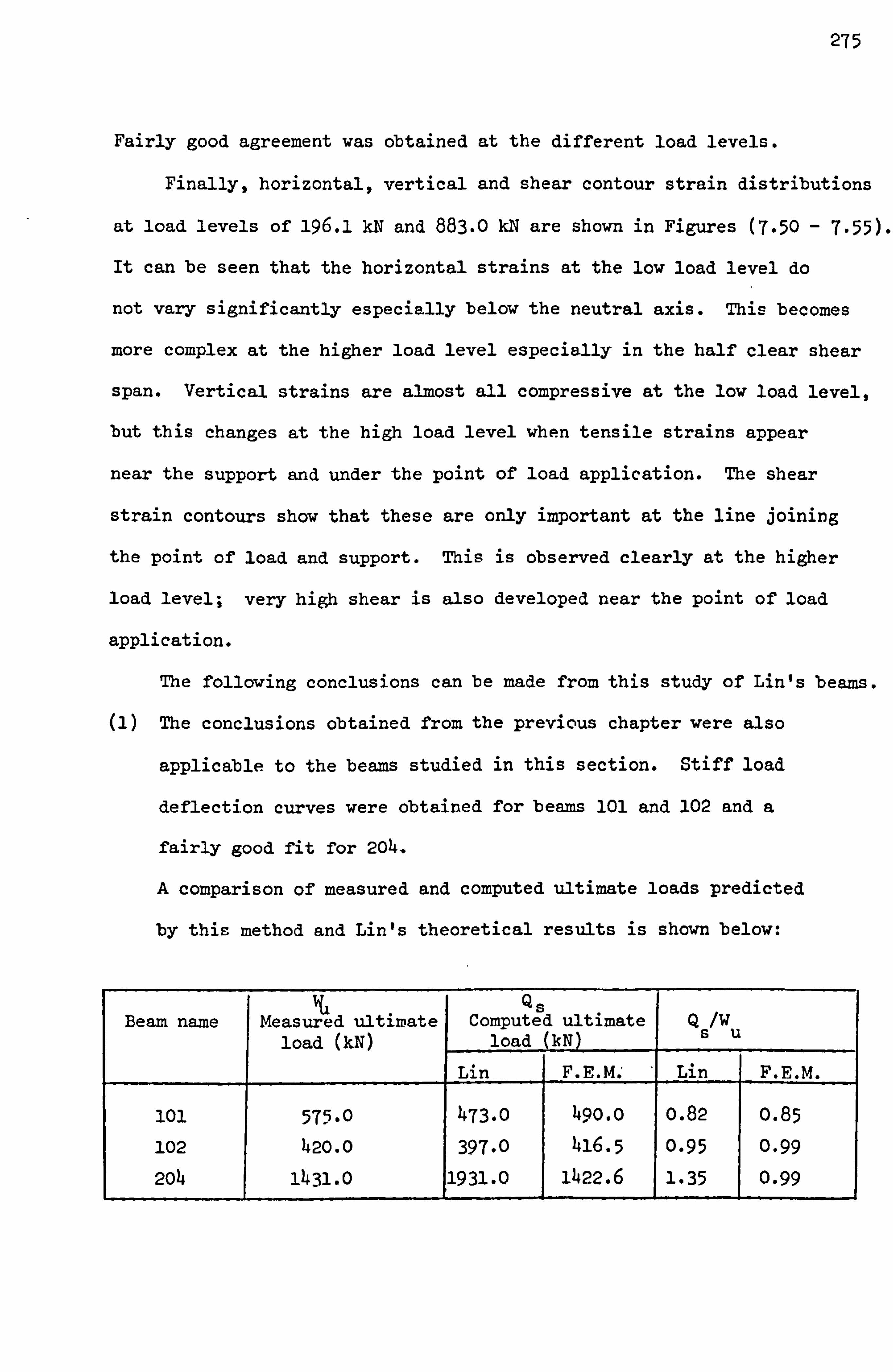
275
Fairly good agreement was obtained at the different load levels.
Finally, horizontal, vertical and shear contour strain distributions
at load levels of 196.1 kN and 883.0 kN are shown in Figures (7-50 - 7.55).
It can be seen that the horizontal strains at the low load level do
not vary significantly especially below the neutral axis. This becomes
more complex at the higher load level especially in the half clear shear
span. Vertical strains are almost all compressive at the low load level,
but this changes at the high load level when tensile strains appear
near the support and under the point of load application. The shear
strain contours show that these are only important at the line joining
the point of load and support. This is observed clearly at the higher
load level; very high shear is also developed near the point of load
application.
The following conclusions can be made from this study of Lin's beams.
(1) The conclusions obtained from the previous chapter were also
applicable to the beams studied in this section. Stiff load
deflection curves were obtained for beams 101 and 102 and a
fairly good fit for 204.
A comparison of measured and computed ultimate loads predicted
by this method and Lin's theoretical results is shown below:
Beam name wa
Measured ultimate load (kN)
Qs Computed ultimate
load (kN) Qs/Wu
Lin F. E. M. ' Lin F. E. M.
101 575-0 473.0 49o. o 0.82 0.85
102 420.0 397.0 416.5 0.95 0.99
2o4 1431.0 1931.0 1422.6 1.35 0.99

276
Better predictions were obtained for the proposed model than
those obtained by Lin's model. For beam 101, it seems that deformation
occurred at a high load level which neither model could predict.
(2) The effect of approximating the confinement of concrete was
important for these beams. This was not required for the Cervenka
panel wall or for the deep bean tested in the previous chapter.
It also produced a slightly stiffer load deflection curve but
this was not very significant. It is not yet known when this
confining effect is important and when it is not. However it
appears that for the bean of L/D = 0.9, its effect has much more
importance than when the L/D = 1.8.
(3) Tension stiffening was tested for beam 204, and gave a stiff load
deflection curve and gross underestimation of the ultimate load.
It appears that this method was not reliable for predicting the
behaviour of this type of beam but this requires much more
investigation, including a check on the strain and stresses in
concrete and steel.
(4) Crack patterns for beams 101 and 204 were in good agreement with
experimental results at failure loads. Strain distributions were
tested for beam 204 and found to have a better agreement vith the
experimental results at the midspan section. Less agreement was
obtained at the half clear shear span. Steel strain distribution
in the bottom bar was fairly well predicted. However it seems
that the results in general were well predicted with a minimum
complexity in the models.
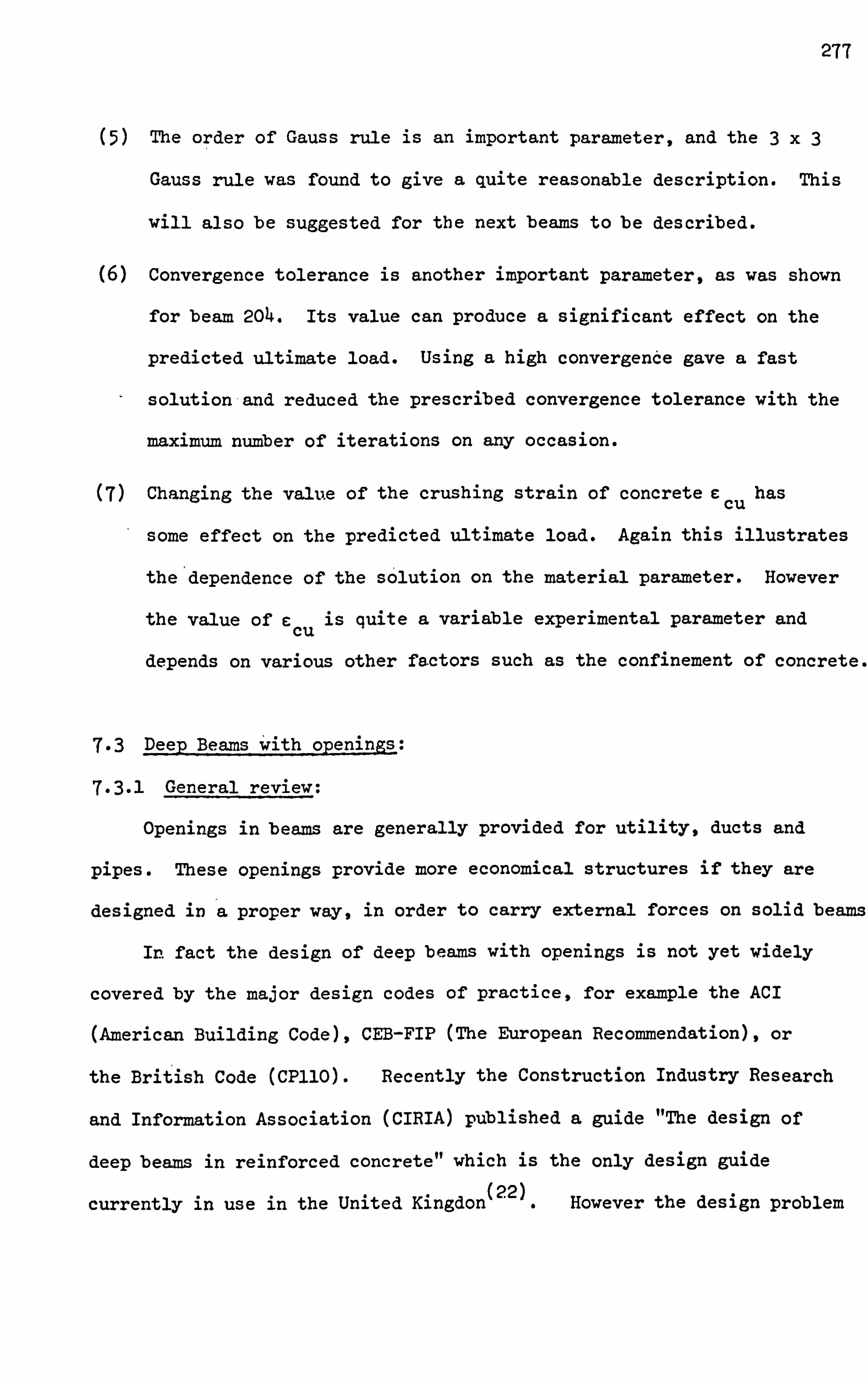
277
(5) The order of Gauss rule is an important parameter, and the 3x3
Gauss rule was found to give a quite reasonable description. This
will also be suggested for the next beams to be described.
(6) Convergence tolerance is another important parameter, as was shown
for beam 204. Its value can produce a significant effect on the
predicted ultimate load. Using a high convergence gave a fast
solution-and reduced the prescribed convergence tolerance with the
maximum number of iterations on any occasion.
(7) Changing the value of the crushing strain of concrete c cu has
some effect on the predicted ultimate load. Again this illustrates
the dependence of the solution on the material parameter. However
the value of c cu is quite a variable experimental parameter and
depends on various other factors such as the confinement of concrete.
7.3 Dee2 Beams with openings:
7.3.1 General review:
Openings in beams are generally provided for utility, ducts and
pipes. These openings provide more economical structures if they are
designed in a proper way, in order to carry external forces on solid be
In fact the design of deep beams with openings is not yet widely
covered by the major design codes of practice, for example the ACI
(American Building Code), CEB-FIF (The European Recommendation), or
the British Code (CP110). Recently the Construction Industry Research
and Information Association (CIRIA) published a guide "The design of
deep beams in reinforced concrete" which is the only design guide (22)
currently in use in the United Kingdon However the design problem
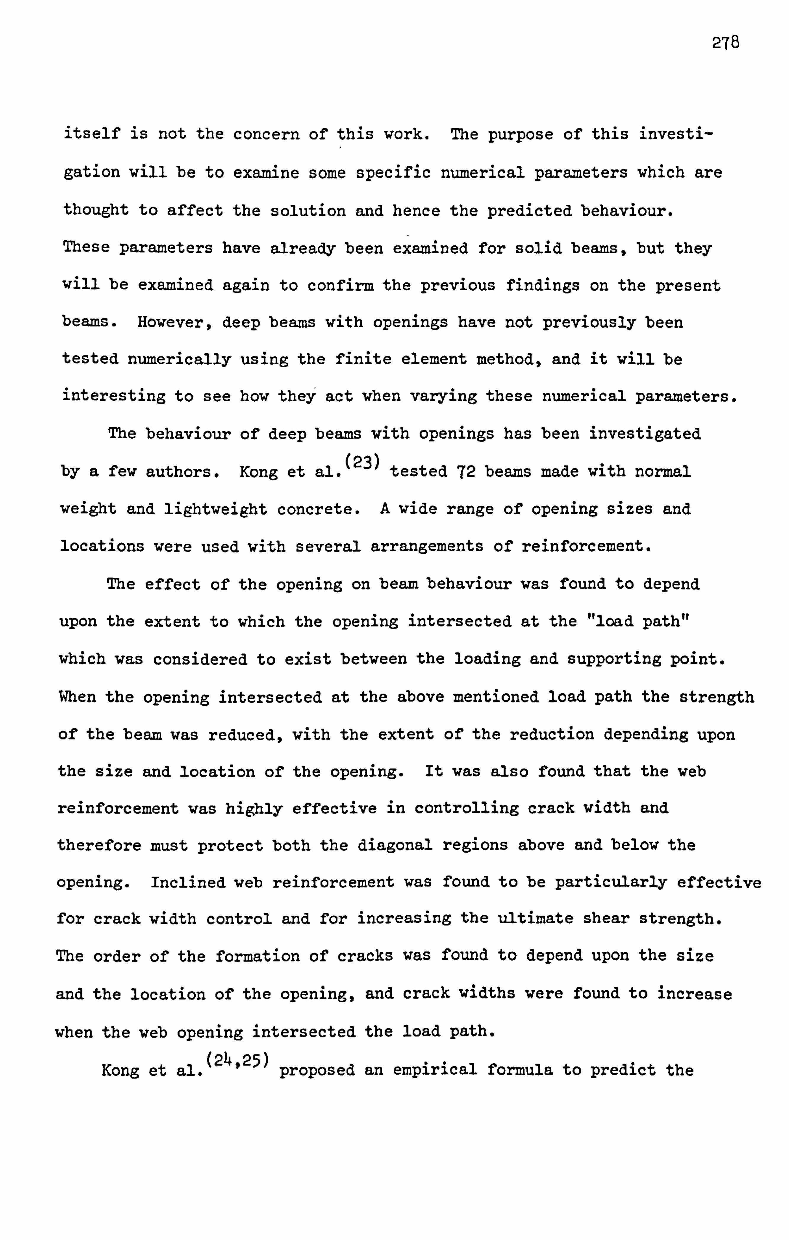
278
itself is not the concern of this work. The purpose of this investi-
gation will be to examine some specific numerical parameters which are
thought to affect the solution and hence the predicted behaviour.
These parameters have already been examined for solid beams, but they
will be examined again to confirm the previous findings on the present
beams. However, deep beams with openings have not previously been
tested numerically using the finite element method, and it will be
interesting to see how they' act when varying these numerical parameters.
The behaviour of deep beams with openings has been investigated
by a few authors. Kong et al. (23)
tested 72 beams made with normal
weight and lightweight concrete. A wide range of opening sizes and
locations were used with several arrangements of reinforcement.
The effect of the opening on beam behaviour was found to depend
upon the extent to which the opening intersected at the "load path"
which was considered to exist between the loading and supporting point.
When the opening intersected at the above mentioned load path the strength
of the bean was reduced, with the extent of the reduction depending upon
the size and location of the opening. It was also found that the web
reinforcement was highly effective in controlling crack width and
therefore must protect both the diagonal regions above and below the
opening. Inclined web reinforcement was found to be particularly effective
for crack width control and for increasing the ultimate shear strength.
The order of the formation of cracks was found to depend upon the size
and the location of the opening, and crack widths were found to increase
when the web opening intersected the load path.
Kong et al. (24,25)
proposed an empirical formula to predict the

279
ultimate shear strength for these types of beams. Kubic (26)
tested
26 light and normal weight concrete deep beams. He found that a deep
beam with a web opening which interrupts the flow of stresses due to
intersection of load path with the opening deformed mainly by the rotation
of the three blocks of the beam; one above the opening, another below
the opening and the third between the opening and the end of the beam.
He confirmed the previous findings of Kong et al. that the location of
the web opening can effect the crack propagation. He found that the
inclined web reinforcement was more effective in controlling the maxi
crack width than the orthogonal reinforcement of horizontal bars and
vertical stirrups. A review of the available work on deep beams with
openings was also reported in this study. A theoretical model was
proposed to predict the ultimate flexural and shear strength of these
beams, but the model was applicable only to the case when the opening
intersects the line joining the load and support point.
Memon(3) carried out a wide survey, on the existing literature of
deep beams with openings and different theoretical methods of solution.
He concluded that the elastic methods of analysis are not sufficient
to provide useful information on the post cracking behaviour and the
ultimate strength. He also noted that the present design rules for
these types of beams. are defined empirically because of their complexity.
From the tests he carried out a formula for the prediction of ultimate
strength was proposed, but he restricted this to the cases he tested
and suggested that further tests should be carried out before the formula
could have a general use.
The next-section will discuss two of Memon's beams in more detail,
in conjunction with the finite element analysis.
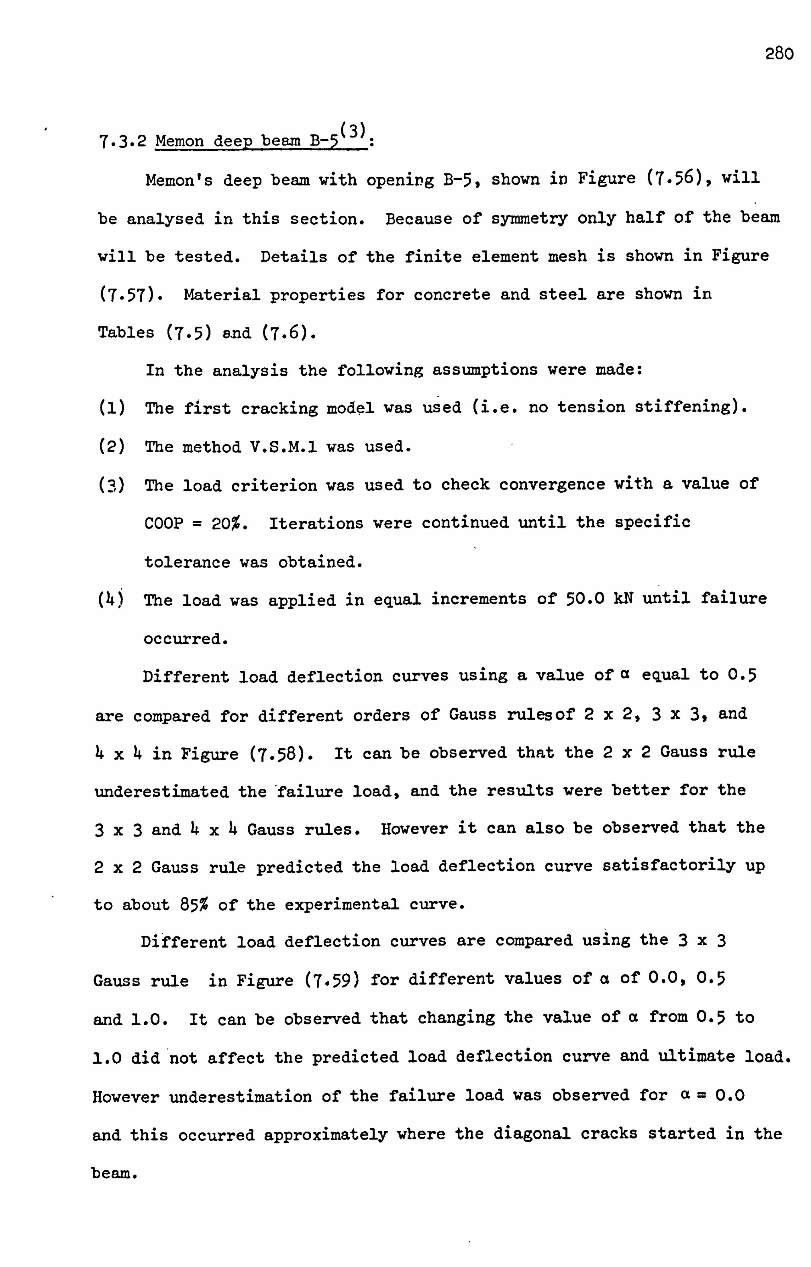
280
7.3.2 Memon deep beam B-5(_3):
Memon's deep beam with opening B-5, shown in Figure (7-56), will
be analysed in this section. Because of symmetry only half of the beam
will be tested. Details of the finite element mesh is shown in Figure
(7-57). Material properties for concrete and steel are shown in
Tables (7-5) and (7.6).
In the analysis the following assumptions were made:
(1) The first cracking model was used (i. e. no tension stiffening).
(2) The method V. S. M. 1 was used.
0) The load criterion was used to check convergence with a value of
COOP = 20%. Iterations were continued until the specific
tolerance was obtained.
The load was applied in equal increments of 50.0 kN until failure
occurred.
Different load deflection curves using a value of a equal to 0-5
are compared for different orders of Gauss rulesof 2x2,3 X 3, and
4 x, 4 in Figure (7-58). It can be observed that the 2x2 Gauss rule
underestimated the'failure load, and the results were better for the
3x3 and 4x4 Gauss rules. However it can also be observed that the
2x2 Gauss rule predicted the load deflection curve satisfactorily up
to about 85% of the experimental curve.
Different load deflection curves are compared using the 3x3
Gauss rule in Figure (7-59) for different values of a of 0.0,0.5
and 1.0. It can be observed that changing the value of a from 0.5 to
1.0 did'not affect the predicted load deflection curve and ultimate load.
However underestimation of the failure load was observed for a=0.0
and this occurred approximately where the diagonal cracks started in the
beam.

281
Different load deflection curves are compared using the 3x3
Gauss rule and a=0.5 in Figure (7.60) for different values of
crushing strains. It can be observed that changing the value of the
crushing strain of concrete c cu has some effect on the final ultimate
load. The best estimate was obtained for a valve of c cu = o=4, and
it is suggested that a suitable adjustment to this value would give
the exact ultimate load.
Crack patterns are plotted for COOP = 20%, 3. G. R., a=0.5,
e cu = 0.004 at different load levels in Figures (7.61 - 7.65)-
Experimental crack patterns are also shown in Figure (7.66). It can
be observed that flexural cracks started in the initial stages in
regions of maximum tensile strains above the opening. These propagated
at higher load levels (see Figure (T. 62)) and cracks started to appear
in the bottom of the beam. At further increases of load the flexural
cracks became deeper and diagonal cracks started to appear in the
mid shear span section. At the final stages these propagated, and
crushing appeared near the opening followed by the yielding of steel
above the opening. Good agreement with the experimental results was
obtained at failure load as shown in Figures (7.65) and (7.66).
Principal stress directions are plotted in Figures (7.67) and (7.68).
It can be observed that at the high load level, a pure compressive region
was developed between the point of load and the support acting as a
column in the beam. Horizontal strains obtained in the midspan section
for the experimental and. finite element analysis are shown in Figures
(7.69 - 7-74) at different load levels. It can be observed that fairly
good agreement was obtained up to a load of 600.0 M. Between 600.0 M,
282
and 1000.0 kN a large variation was observed.. This represents the
stage at which the cracks are developing in the section below the
opening, and shows that these cracks mostly occurred in the finite
element method between a load of 900.0 kN and 1000.0 M. After that
load, and as the failure load was reached, agreement with the experimental
result improved, and was within about 30% in the worst condition.
Vertical strains near the opening measured both experimentally and
using the finite element method are shown in Figures (7-75 - 7.8o) at
different load levels. Fairly good agreement was obtained for these
strains at all the load levels observed.
Steel load-strain curves for the top bar (i. e. above the opening)
and for the bottom bar in the beam are shown in Figures (7.81) and (7.82).
Good agreement was obtained for the top bar especially close to failure.
For the bottom bar the agreement was less satisfactory, and the sudden
change between loads of 900.0 kN and 1000.0 kN was associated with that
change observed in Figure (7-72) in the horizontal strains which. represent
the stage when most cracks appeared in the beam, as shown in Figure
(7.64).
7-3.3 Memon deep beams B-7(3):
This beam has similar dimensions to beam B-5 except that the width
of opening was reduced to 400.0 mm, (see Figure (7-57)for mesh used)
and has a higher concrete strength. Details of concrete properties are
shown in Table (7-5). ' The steel provided was the same as that for beam
B-5. The same numerical assumptions made for beam B-5 were used in
this analysis. The value of crushing strain was assumed to be equal
to 0.004. Comparisons between the analytical and experimental load

283
deflection curves are shown in Figure (7.83)- It can be seen that
fairly good agreement was obtained in the predicted load deflection and
ultimate load. The ultimate load was higher than that predicted in
B-5, this is either due to the increase in the strength of the concrete,
or due to the reduction in the opening size.
No description will be given for the crack and stress distributions,
since the beam failed in a similar manner to that described for beam B-5.
The following points can be made about the study of deep beans with
openings:
(1) Nonlinear analysis was carried out for the first time on these
types of beams using the suggestions from the previous chapter. Good
predictions of the load deflection curves and ultimate loads were obtained.
A comparison of measured and computed ultimate loads predicted by this
method and Memon's theoretical results are shown below:
wu Qs Beam name Measured ultimate Computed ultiirate Q /w
load (kN) load (kN) u s Memon F. E. M. Memon F. E. M.
B-5 16oo. o 1102.0 1550-0 o. 68 0-97 B-7 1.700-0 1314.0 3.650.0 0-77 0-97
The finite element method gave better estimates for both beams-
These predicted results will give guidelines for further investigations
to study the same type of beams with different load conditions and
openings, and also those with different material properties.
(2) Changing the order of integration rule had less significant effect

284
on the prediction of the load deflection curve and ultimate load,
than the deep bean failing in flexure tested in the previous chapter.
However the low integration Gauss rules did produce an underestimation
of the ultimate load. The use of the 3x3 Gauss rule was also found
to be best when analysing this type of beam.
(3) When the shear retention factor a was set equal to 0.5 or 1.0,
the load deflection curves and the ultimate load were not affected.
When a was set equal to zero the failure load was underestimated. This
failure occurred suddenly after the development of the diagonal cracks
observed at the half clear shear span. It appears that setting the
value of a=0.5 was the best value for all beans, and that a=0.0
can cause some numerical difficulties.
(4) Increasing the crushing strain of concrete from 0.004 to 0.008 can
produce a stiffer response and overestimate the ultimate 3oad. This
shows again the importance of material parameters on, the predicted
behaviour. Suggestions are made that the value of 0.004 is satisfactory
for the tested beams. Thisis based on the grounds that confinement can
produce a higher concrete strength and hence crushing will be delayed.
(6)ý No tension stiffening was required and convergence was satisfactorily
obtained in both beams without any difficulties.
(7) The development of flexural cracks at the midspan section can greatly
affect the predicted finite element horizontal strain distribution below
the opening. However this crackiDg effect is found to be less significant
on the predicted vertical strain distribution near the opening. Horizontal
load strains for longitudinal steel below the opening was also affected
by the development of flexural cracks at midspan section. A suggested

285
explanation for this is that if the applied load increments were less
than 50.0 M, it would allow a more gradual crack development and hence
a more gradual change in strains. However this was not tested out.
The value of V can also have some effect on this but it was assumed t
to be the same as that measured experimentally.
7.4 Conclusions:
A numerical study was carried out on some of the parameters
influencing the solution of different types of deep beams failing in
sheak. It was assumed that the method V. S. M. 1 was the best method to
use from the observations obtained from the previous chapter. Some of
the parameters which were suggested in the previous chapter to give
the best solutions on beems failing in flexure were again investigated
on the ones failing in shear in this chapter. The following points were
noted:
(1) The first cracking model was used on all tested beams and found to
produce a fairly good estimate of the ultimate load in all cases.
However the load deflection curve was sometimes overstiff, - This could
be due to the effect of material properties since a similar shape for
the load deflection was obtained when compared with the experimental
ones. Tension stiffening was tested for one bean of L/D = 0.9 which was
heavily reinforced. The results showed a drastic underestimation of
the ultimate load. It appears that tension stiffening was not capable
of producing a good prediction for the experimental results in this
beam. Further investigation to this matter may be required. However
the no tension stiffening model produced good prediction as was found

286
in previous chapters, and it is suggested that this model is quite
capable of preventing the complex aspect of the behaviour. Moreover
it is far cheaper in computer running time.
(2) Using the shear retention factor a 0.5 and 1.0 did not signi-
ficantly change the shape of the load deflection curve. When this was
set equal to zero failure was underestimated and occurred when the
diagonal cracks started to appear. This parameter was only tested_, for
the deep beam with opening B-5 and was assumed equal to 0.5 in all
other beans. A value of a=0.5 was able to satisfactorily predict
the behaviour of these complex beams without great difficulty.
(3) The 3x3 Gauss rule was found to be the best in predicting the
ultimate load, and a reasonable load deflection curve. The 2x2 Gauss
rule must not be used, because it was found not to be adequate to
describe the crack pattern and monitor the nonlinearized material
properties with close precision.
(4) The load criterion was used with COOP = 20% in most cases. 'This
value gave a fast convergence without any obvious difficulties. Lower
values were investigated and were found to affect the predicted ultimate
load to some extent. For beam 204 which failed in pure shear, the
load deflection curve was not significantly affected at lower loads.
However these lower values covered a value which affected the Cervenka
panel load deflection curve, where the failure was due to a combination
of flexure and shear cracks. It was found, for that beam, that a change
of COOP from 10% to 20% only produced a change of 4-8% in the predicted
ultimate load. COOP = 10% required a total number of 173 iterations
whereas COOP = 20% required only 55.
287
(5) Changing the values of the crushing strain of concrete can effect
the shape of the load deflection at high load levels before failure
and can produce different ultimate loads. This shows the iraportance of
material parameters on the solution and these must be considered
carefully.
(6) The predicted ultimate load using the finite element model was
found to be much better than that obtained using different formulae as
proposed by the different investigators from their experimental tests.
This method gives more generality, with a stronger mathematical basis.
Moreover it can produce detailed information which seems to be of
acceptable accuracy when compared with experimental tests.
(7) The effect of increasing the concrete strength in order to account
for the effect of confinement under the loading point was important
for all the Lin deep beams. This was not required for Memon deep beams
with openings. This may be due to the different type of load application
since two point loads were applied for Memon beams, and only single loads
were applied to the Lin beams. This matter may be difficult to judge
in practical applications, but obviously needs to be borne in mind.
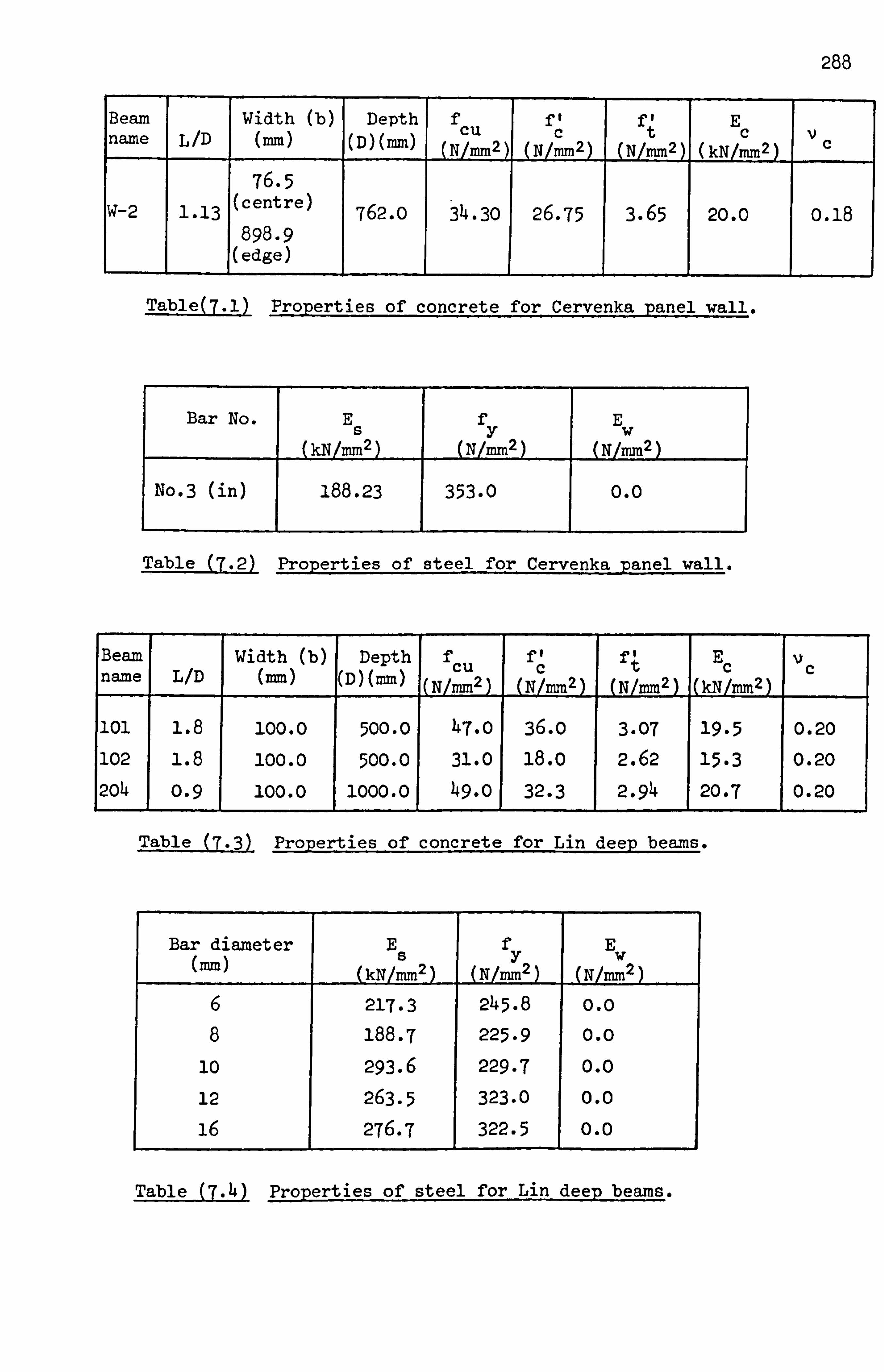
288
Beam Width (b) Depth f ff ff E name L /D (mm) (D)(mm) cu
(N/mm2) c
(N/mm2) t
(N/mm2) c
(kN/mm2) c
76.5 W-2 1.13
(centre) 762.0 34-30 26-75 3.65 20.0 o. 18
898.9 (edge)
I
Table(7.1) Properties of concrete for Cervenka panel wall.
Bar No. E f E s
(kN/MM2) y
(NI 2) w
(NIMM2)
No-3 (in) 188.23 353.0 0.0
Table (7.2) Properties of steel for Cervenka panel wall.
Beam Width (b) Depth f ff f , E name L/D (mm) (D) (=) cu
(N/MM2) c t c c
101 1.8 100.0 500.0 47.0 36.0 3.07 19.5 0.20
102 1.8 100.0 500.0 31.0 18.0 2.62 15.3 0.20
2o4 -I
0.9 I 100.0 1000.0 I 49.0
I 32.3
I 2.94 I 20.7
I 0.20
Table (7-3), Properties of concrete for Lin deep beams.
Bar diameter (mm)
E
(kN/MM2)
f
(N/MM2)
E
(N/mm2)
I
6 217.3 -
245.8 0.0 8 188.7 225.9 0.0
10 293.6 229.7 0.0 12 263.5 323.0 0.0 16 276.7 I
322.5 -
0.0 I
Table (7.4) Properties of steel for Lin deep beams.
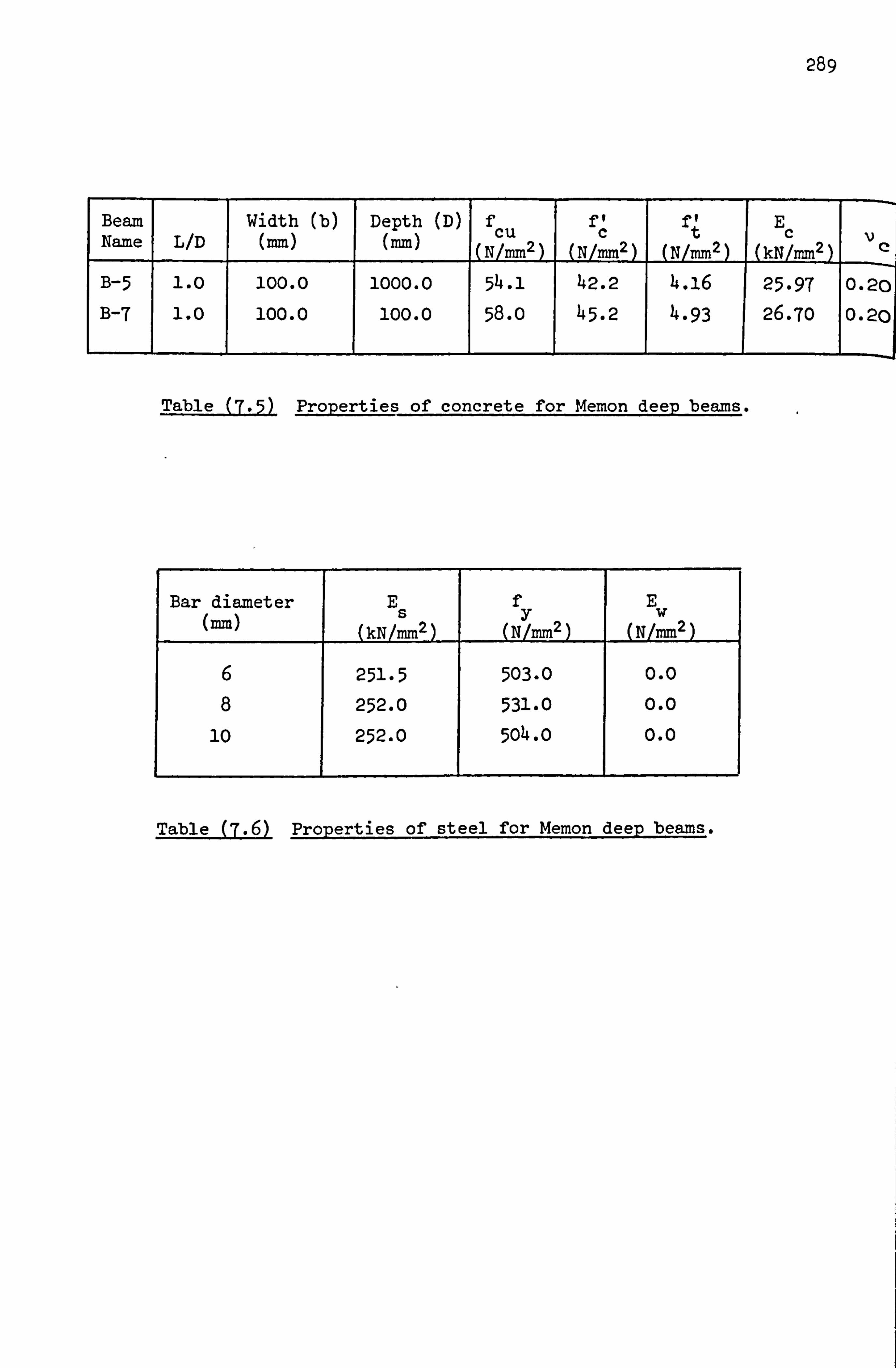
289
Beam Width (b) Depth (D) f ff E Name L/D (mm) (mm) cu
(N/mm2) c
(N/mm2) (N/MM2) (kN/1=2) c v
B-5 1.0 100.0 1000.0 54.1 42.2 4.16 25-97 0.20
B-7 1.0 100.0 100.0 58.0 45.2 4.93 26-70 0.20
Table (7.5) Properties of concrete for Memon deep beams.
Bar diameter E f E (nm)
(kN/mm2)-- (N/mm2) w
(N/MM2)
6 251.5 503.0 0.0
8 252.0 531.0 0.0
10 252.0 504.0 0.0
Table (7.6) Properties of steel for Memon deep beams.

290
crushing
(e) Diagonal - compression.
Figure (7*11 Failure modes for tested beams.
(a) Flexure - shear. (b) Diagonal - compression.
(c) Shear - compression. (d) Splittin&-shear.

291
e4 (0
As rfx S, (t
PANEL I PANEL 2
863-6 Old 863-6
ELEVATION
rype -f-Y I
t j, Flot-I piW 50-CC
I 're .0 SID I. SWI " ", olld 6. b. I SL .., P4ngl re; Joveerleft
10 Rk
n2 Fn., I -. i a0 U.
-T U.
100
"W'
762 762
SECTION A-A
-, I
A
Figure (7'? l Details of Cervenka panel wall W-2.
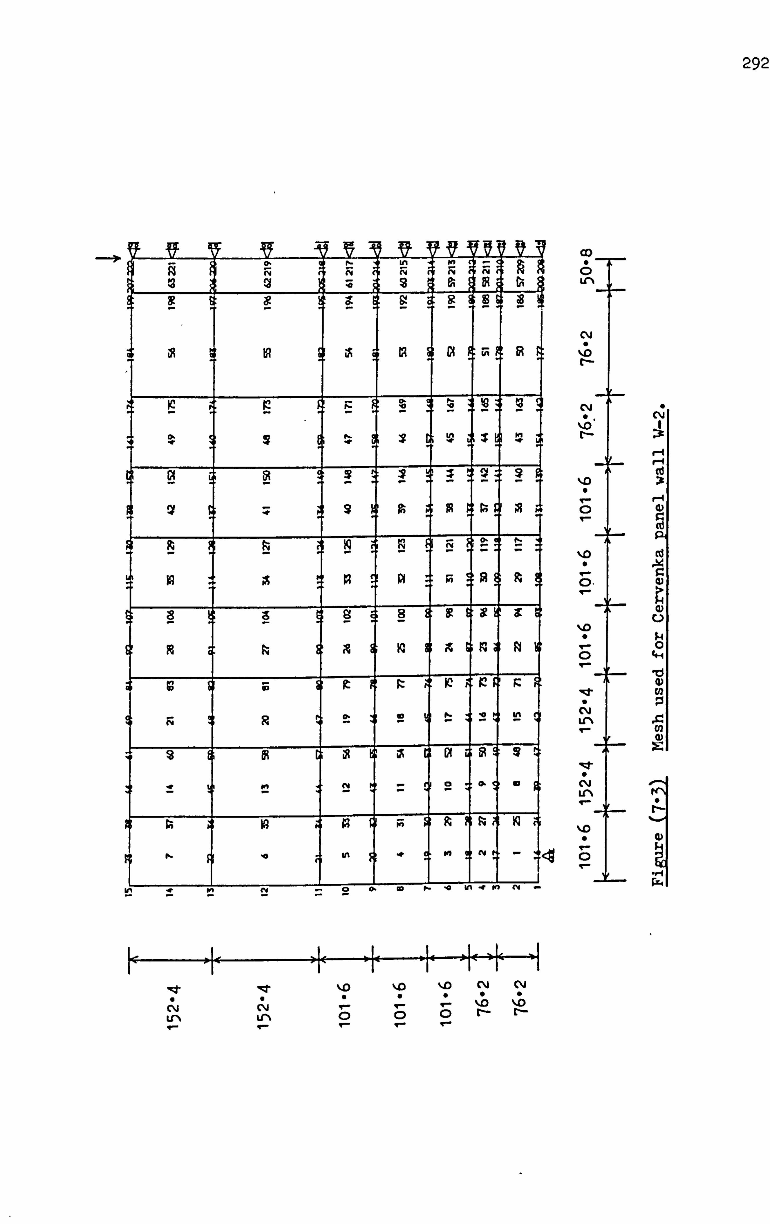
292
N Ln on
!3 ri 1 :3 2 U; fA - -H IR IR ix IR
t le ; : $2 1 ! F: %! % is a *I
19 ;x 13 PI - : F, IR R RI
S
kR
c V IR C :II
c !w
Di X iR A 13
CV
-
I' IF
cli VIA
C%j
1ý Cý
CD, 6 U-N
C\j
CY 0 0. C%i
%0 1
\o 39
ý10 Cd
U
$4 0
C\j Lr%
ca 0)
I I rE.
Ln
T- 1 ý i ý
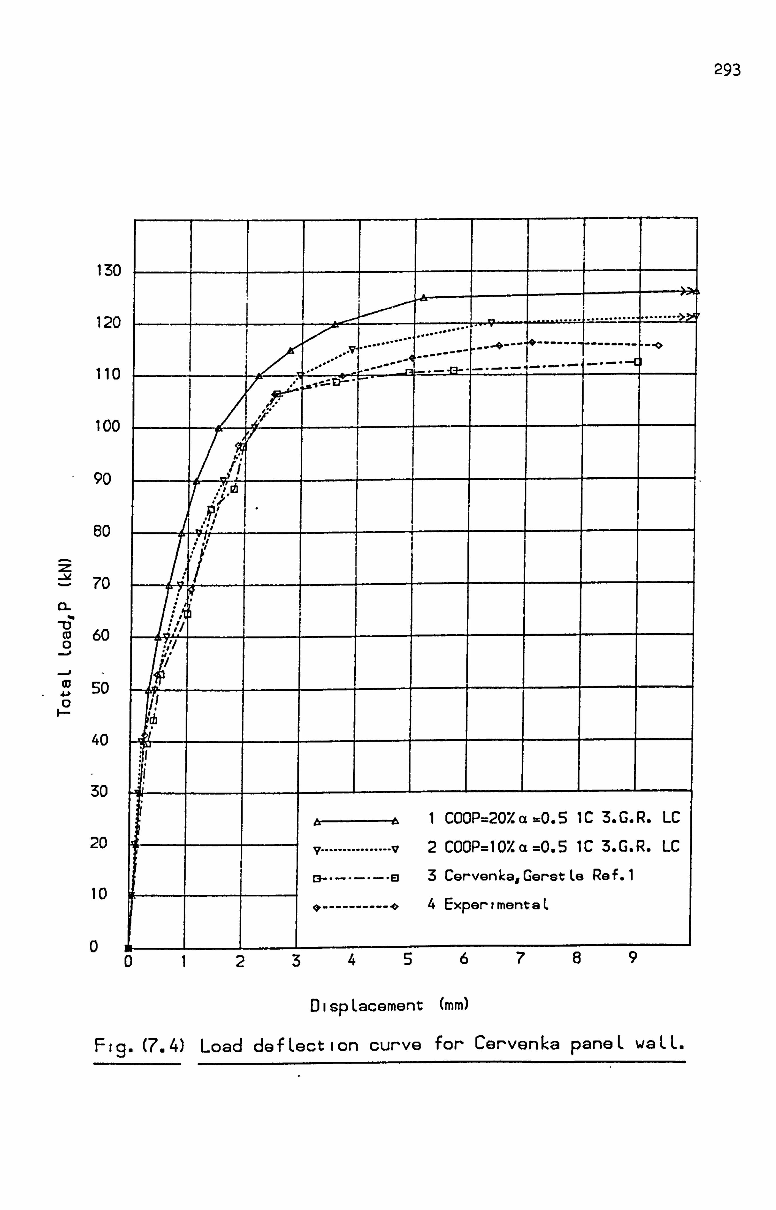
293
130
120
110
100
90
80
70
60 -. j
so
40
30
20
10
0
------ I........... ....... ......... >
........... .......... .. --- ------
I
-------- ---
iY
1 COOP=20% a =0.5 1C3. G. R. LC
v ........ 2 COOP=10%a=0.5 1C 3. G. R. LC
E3 -------- El 3 Cervenka, GerstLe Ref. 1
q ------------ *4 ExperimentaL
tj y
DispLacement (mm)
Fig. (7.4) Load defLection curve for Cervenka paneL waLL.
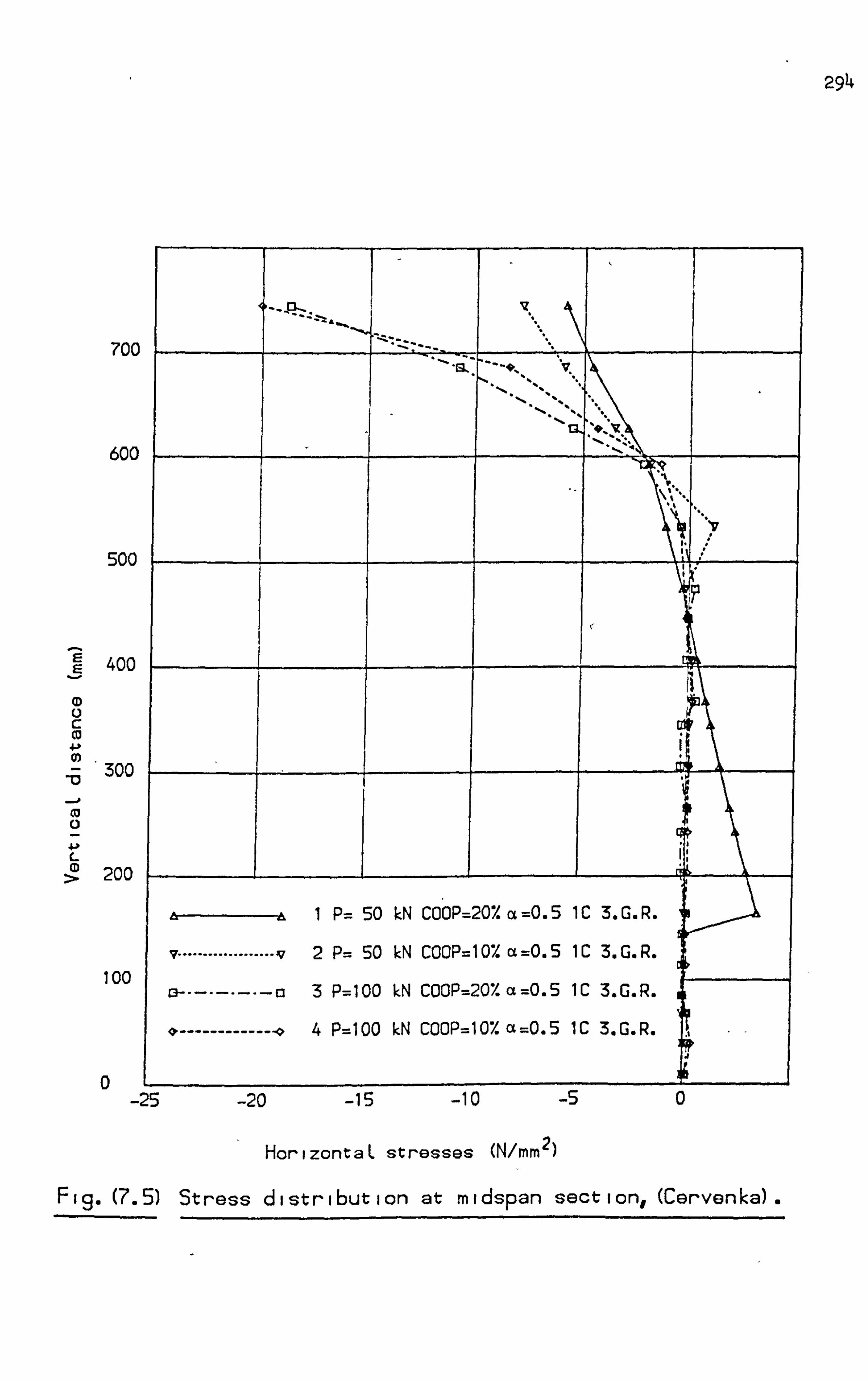
294
700
600
500
400
(0 4. -1 0)
. - 300 73
L ID :> 200
100
0
A1 P= 50 kN COOP=207 a=0.5 1C 3. G. R.
v .................. v2 P= 50 kN COCP=107. a=O. S 1C 3. G. R.
13 ---------a3 P=100 kN COOP=20% a=0.5 1C 3. G. R.
-------------- *4 P=100 kN COOP=107. a=0.5 1C 3. G. R.
-25 -20 -15 -10 -5
HorizontaL stresses (NIMM2)
Fig. (7.5) Stress distribution at midspan section,, (Cervenka).
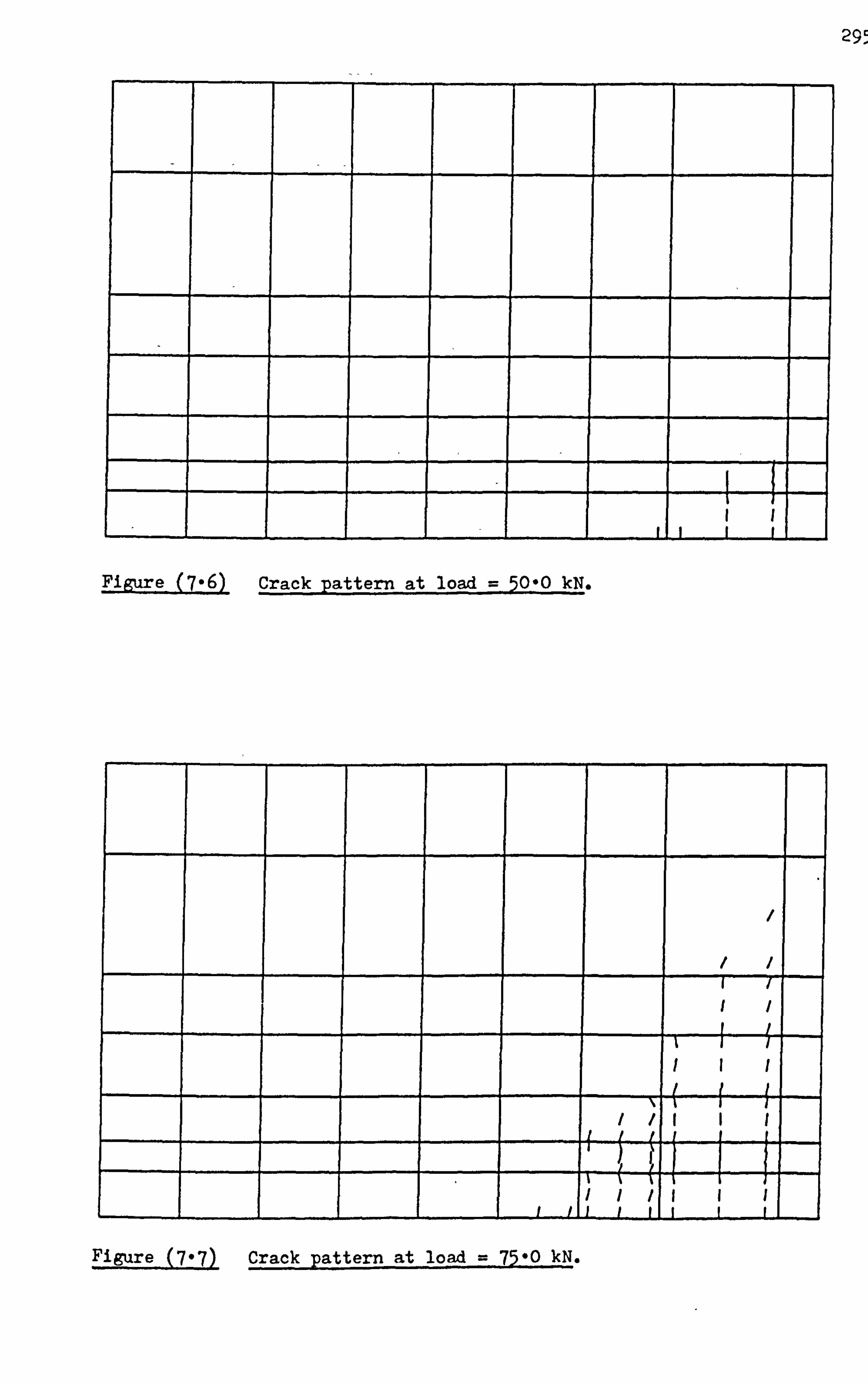
29f
Figure (7-6) Crack pattern at load = 50-0 kN.
____ ____ ____ ____
/
//
____ ____ ____ ____ ____ ____
I I- I/ I/ ____
tII- III
/I
I III
____ ç - __ _ -
_____ - ___ ____ I/ II / L�
II
i L Figure (797) Crack pattern at load = 75*0 kN.

296
Figure (7-8) Experimental crack pattern at load = 106-8 kN.
I ,
7-7--3F
T -f f if
I Ti -k I
Fi, gure (7-9) Crack Pattern at load = 105-0 kN.

297
Figure (7-10) Experimental crack pattern at load = 113-4 kN.
Ecu = 0.003
-- - 777 7 T 7 I Ar
iff i
zZ I T TT -K T
, T TI T77 tl Pigure (7-11) Crack pattern at load = 120-0 kN.

ý co . -
,, co -II I( === 3
o (0
z 0 I- 0 w U)
(0 I-
0 I-
0
Sn
to
co
ad z 0
LLJ vi 0 C-7
V
0 0 Co 0e 10 1
F -1,
co
0 U, 0
0 0 in

299
- (T w 39L :9 -M V Ju V 39 IF
i 4) Ln 1 .mr i-C Y 0.0 ) rl- 14 ol Ol c - Ol c - Ol C . CO 0 ) CO a
Ln 1 . -: r N W) r i rj - --c 0 ) r1i a ) r1i a ) (V a
D. co fl - 10 U l -41 N ) CIJ - -0C
1) 0 1ý . Ol 00 rý- -40
N
I )- -4 - -4 - -N
- c ) 01. a r- -4 ) Ln ;; r 10 14 ) Ln U l Ln U l Ln U l Ln u
Ln C U YC l . W) a ) CIJ 1ý :
f4 Y C%j 0C P -0 U
IT -. 4r N ;
N 3 pe) N
0K 14
0- ( ) fQ
1 co ' t4 .NC ) 10 C
r- Ln W) r i-0 01 0) CV r i CN r i CN r s r-i r i-'.
uI
l Lr % CD 0 CD
0 S
0
cz 0
T- (a
P4

300
600
500
400
300
--0 (0 4. p 200
100
0 .111 0.0 0.5 1.0 1.5 2.0 2.5 3.0 3.5
01 sp Lacement (mm)
Fig. (7.14) Load defLection curve for Lin beam 101.
600
Soo
400 CL
300 0
-i 200
100
A- 0.0
.... ......
lp
1 COOP=l 57.1 Mat. cc =0.5 1C3. G. R.
v ................ 72 COOP=207.1 Mat. a =0.5 1C 3. G. R.
0 ---------- a3 COOP=207.2 Mat. a =0.5 1C3. G. R.
4 ------------ *4 ExperimentaL
ZT-
/ . 1o COOP=207 1 Mat. a =0.5 1C 3. G. R.
v ................. 72 COOP=20% 2 Mat. a =0.5 IC 3. G. R.
M --------- a3 ExperimentaL
0.5 1.0 1.5 2.0 2.5 5.0 5. t)
Dt sp Lacement (mm)
1 ND
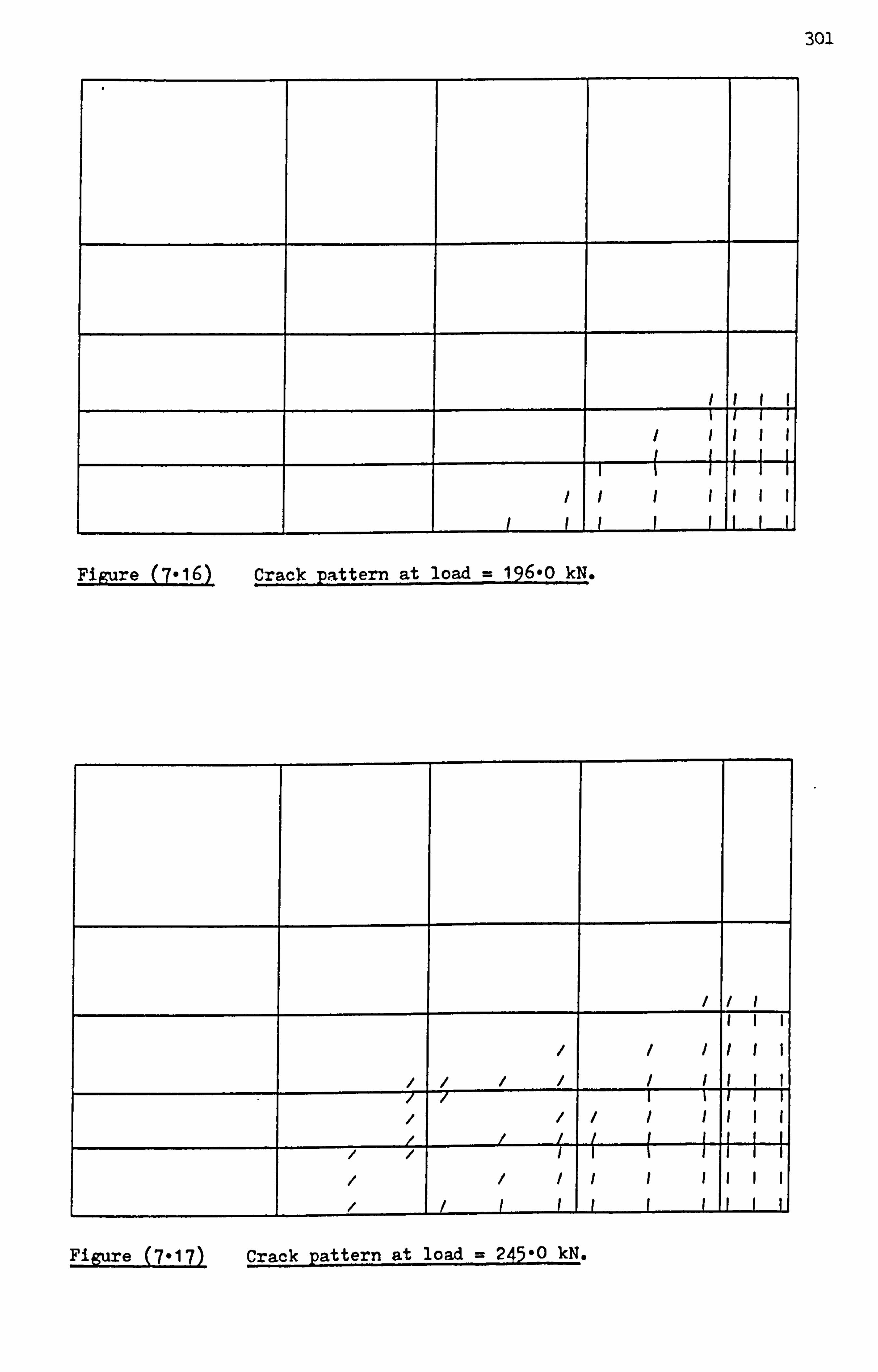
301
1 11 11
Figure (7-16) Crack pattern at load = 196-0 kN.
___ ____ ___ I /I
/ / /
/
/
/
/
I
l
III
II I
ili __________ /
/ 1
/ / I I I
III ll I
______________
/
/
I
/
/
I
/
I
I I
I
I
I
I
I lII
III
Fi re (7-17) Crack pattern atload = 245-0 kN.
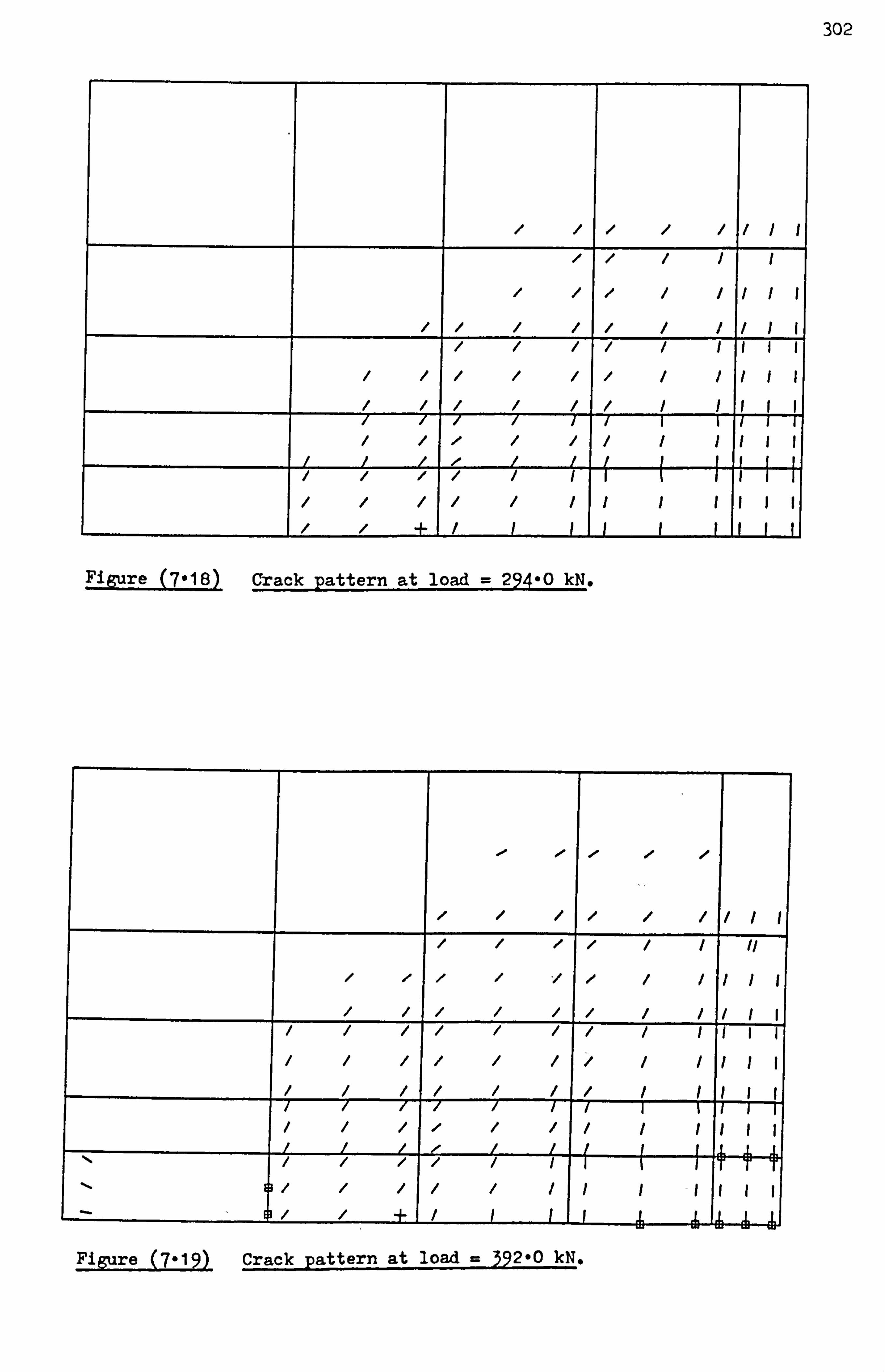
302
--r T- 7-T
+
Figure (7918) Crack pattern at load = 294-0 M.
N / / / / / / I- -F- 1, I
Figure (7019) Crack pattern at load = 392*0 kN.

30'
IB 1 19 M +x
- z LI L
7 7 T T-- T--- T
0 0 -0
4 4 T T
7 T T TT T I ý, El * % / I I I II I
I- + EP * *. -jL ýk II I I I I1 1 .
Figi=e (7*20) Crack pattern at failure load = 490-0 kN.
FiMire (7-21) Experimental crack pattern at load = 575.0 kN.
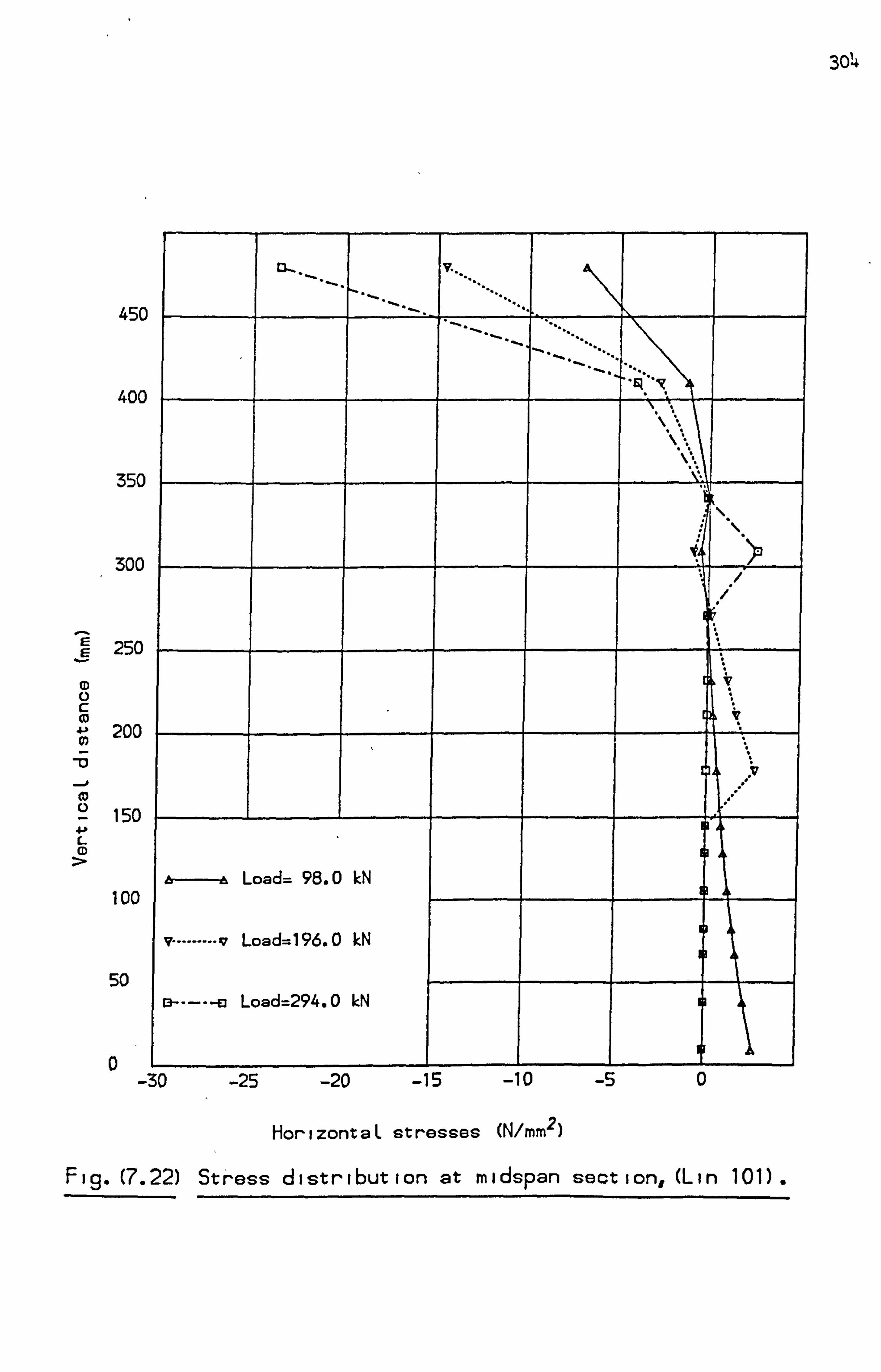
3o4
450
400
350
300
r= 250
200 0)
150 L CD
100
50
0
Load= 98.0 kN
v Load=196.0 kN
Load=294.0 kN
-30 -25 -20 -15 -10 -5 0
HorizontaL stresses (N/mm2)
Fig. (7.22) Stress distribution at midspan section, (Lin 101).
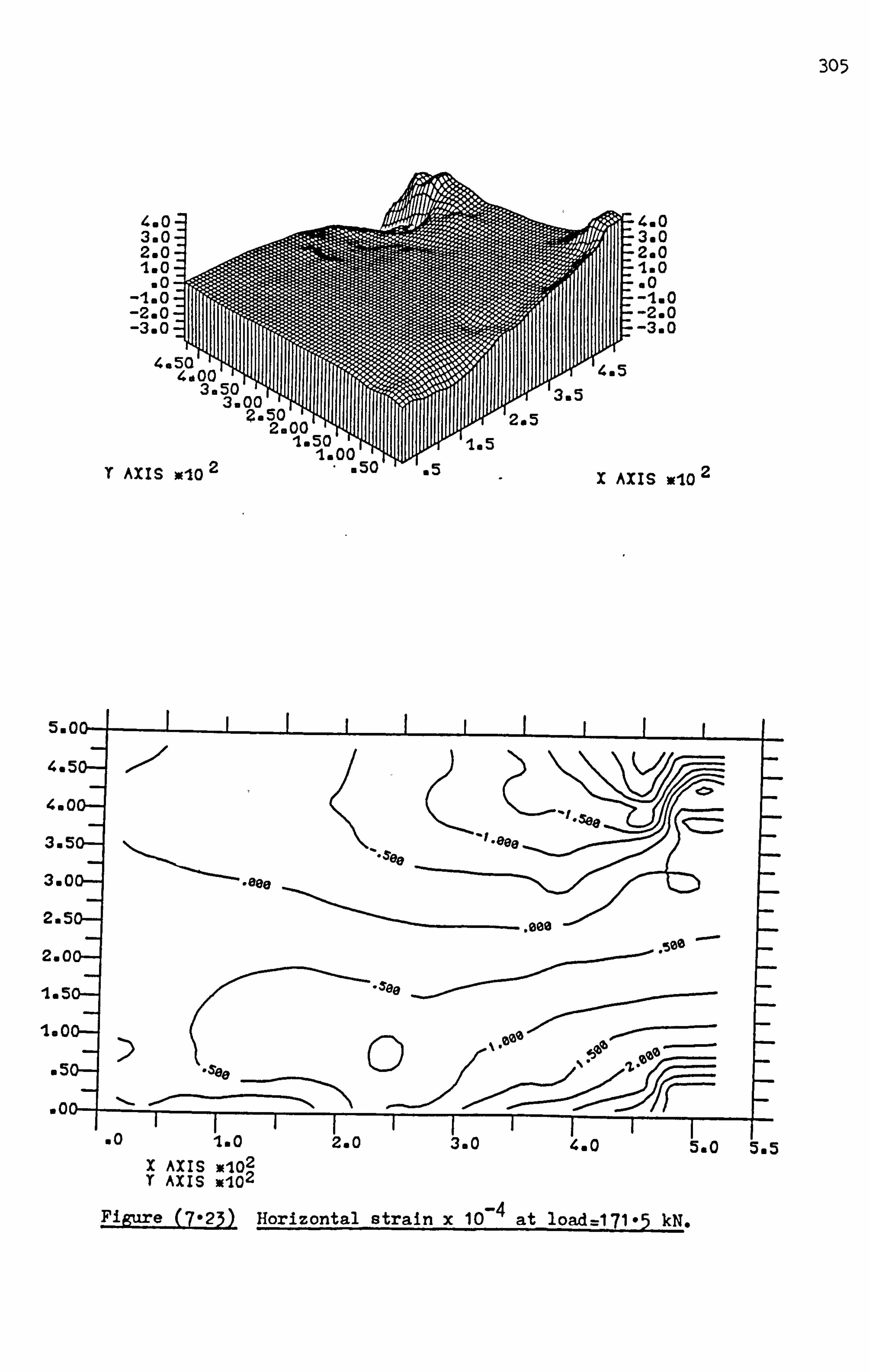
305
4.0 3@0 200 120 110 -1.0 -2wO -3mO
X AXIS wlO 2
5.0 11
4m5
4000-
3.50- -eee 3ea 3.00- eee
2.5
2.0 see
SOe
lb 0
B50-
. 00-
go -1.0 ý. o j. 0 k. o ý. o 5'. 5 X AXIS : 102 T AXIS 102
Figure (7923) Horizontal strain x 10-4 at load=171*5 kN.
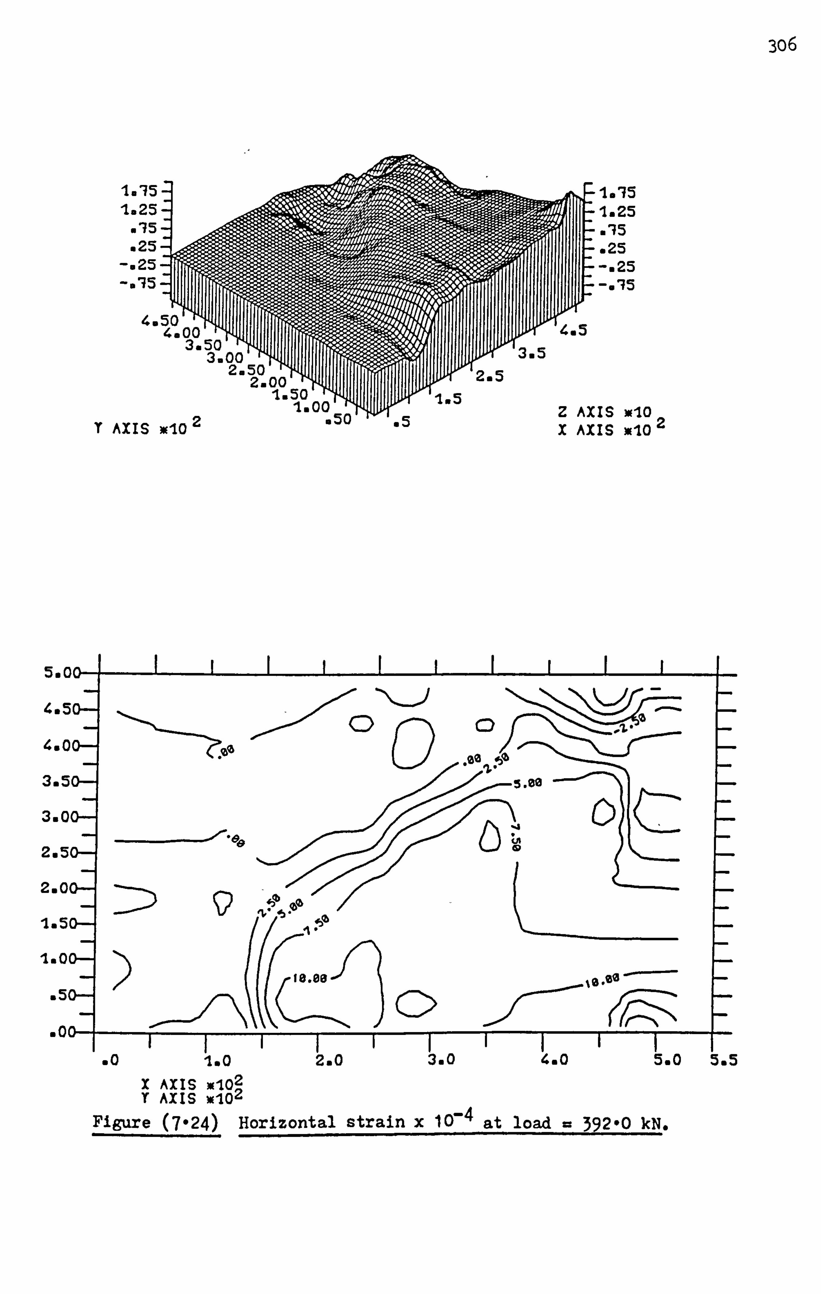
3o6
1.15 1.25
w15 n25
-w25 -m15
4.50 , 4uO
iN q
5 0 E5
OR 2.00
1.50 )
qý, I"
1000 T AXIS wlO
2,50
1015 la25
ol 5
825 -m25 -a'15
Z AXIS wlO 2 X AXIS wlO
5wOO-1 1 L-
4e5O-
4sOO-
-`ý- "ýo
3.50-
3.00-
2m5O-
2.00-
- jb1b 1m50- 61b
-1.00- so--
s50- C>
. 00-
so 100 2.0 3.0 4.0 5.0 5.5
X AXIS -102 T AXIS k, -102
Figure (7-24) Horizontal strain x 10-4 at load = 392-0 kN.
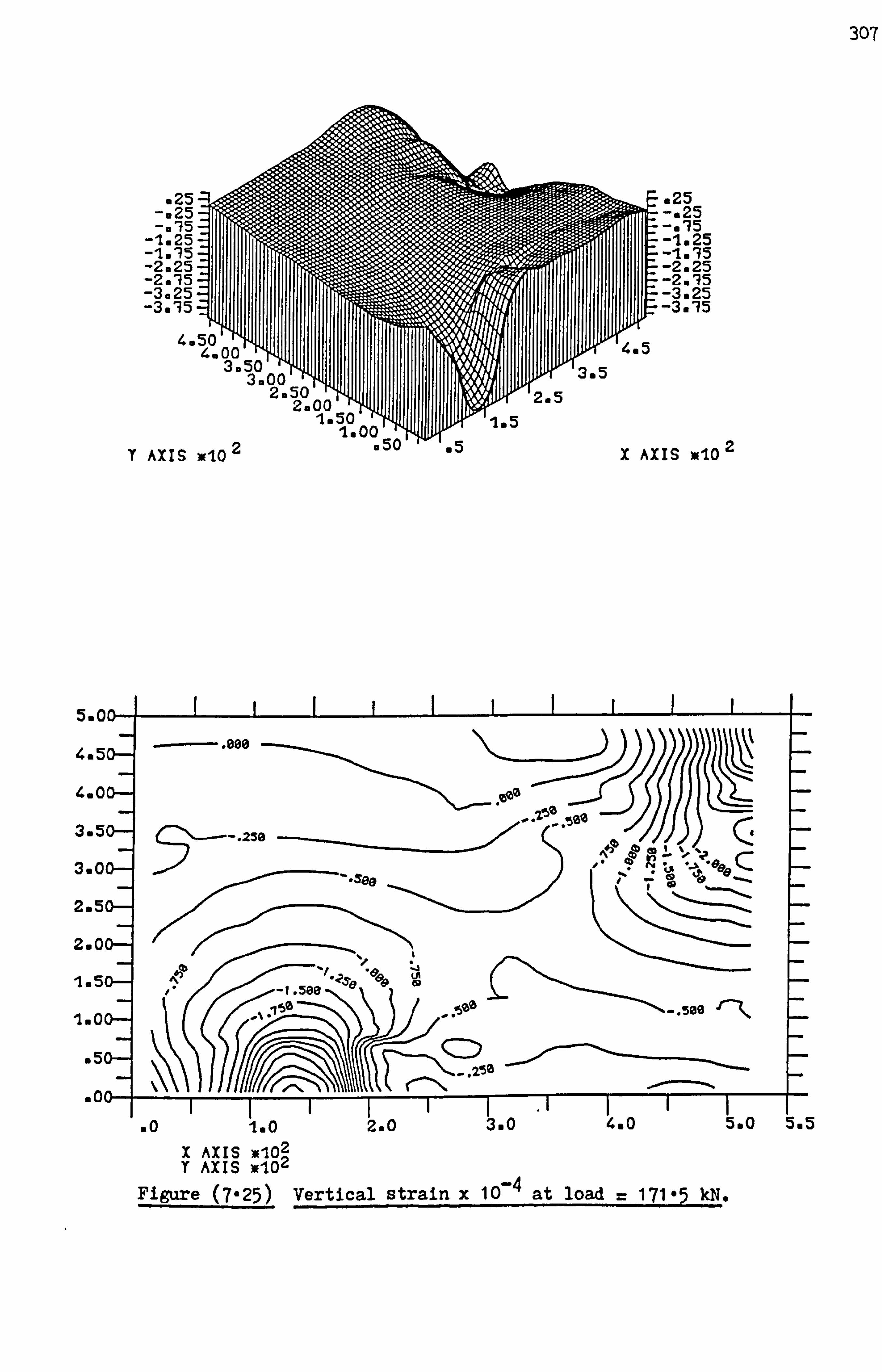
307
5. C
4.111
4uC
3. Z
3. C
2.5
200
la5
Iwo
a5
.0
. 25 -o25 -@'75
-1.25 -IwI5 -2o25 -2@'75 -3o25 -3a'35
4a
T AXIS w-10 4 Oýw 0. )
s25 -. 25 -. 115 -1.25 Im'75 -2o25 -205 -3.25 -3o'15
X AXIS W102
--. see
Aell Ilb
-see CO
Cl? 508
.. Slbll -. 500 f-, tl
56 ..................
................... ......... ..... ... ...
1.0 2mO 3@0 4mO 5,0 5.5
X AXIS : -102 Y AXIS 102
Figure (7-25) Vertical strain x 10-4 at load = 17105 kN.
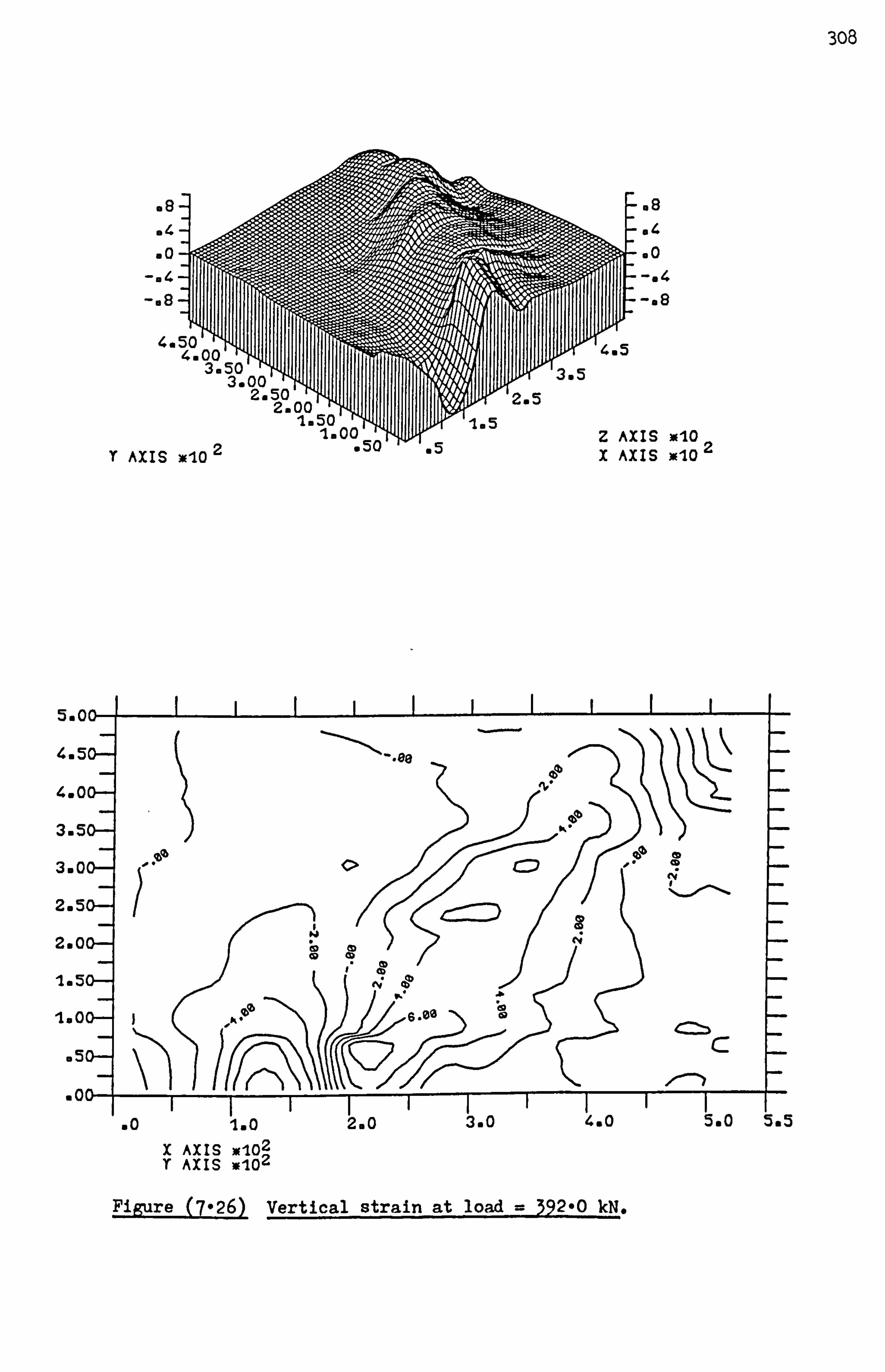
308
4.00' ' 3m5O
3eOO 2m50
TV
"
q"
2.01) 1050
1.00 Y AXIS x102 s50
es a4
-94 -es
Z AXIS : 10 2 X AXIS 10
540
4.50- 'blb
4600-
3.50-
-, ýblb 65 3.00-
2.50-
2800- *1 4 CD
lw50-
Zlb 6.00 1000-
. 50-
. 00-
0 ý. o ý. o j. 0 4.0 5.0 Sm5
X AXIS W102 T AXIS *-102
Figure (7-26) Vertical strain at load = 392-0 kN.
08 m4 so
-. 4
-08
4.50' 4.0 IF
3a
N5
33 Qo 51
O)l E50
2.100
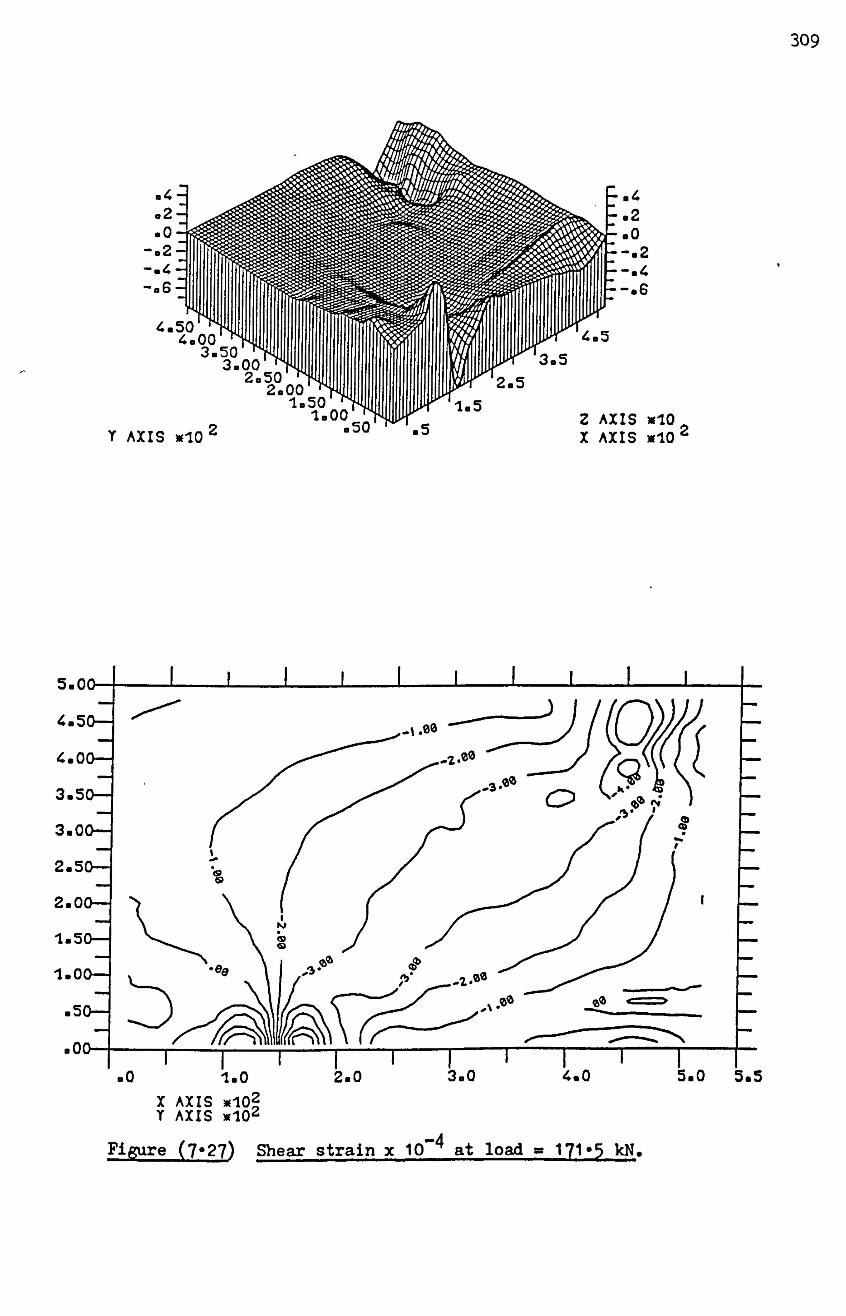
309
5. C
4.5
4wO
3.5
3.0
2.5
2.0
1&5
1.01
.5
001
.0i. o 9.0 3.0 4eO 500 505
X AXIS -102 Y AXIS 3K . 102
Figure (7-27) Shear strain x 10-4 at load = 171-5 M.
m4 82 00 -@2
Z AXIS xlO X AXIS W10
elb -3
A'b
ID
4o5 3.5
.5 165

310
1.5 .5
-o5 -1.5 -2.5 -3o5 -4.5
4.
T AXIS )m-10 ' a ýiv aD
1.5
-1.5 -2.5 -3o5 -4w5
Z AXIS 10 2 X AXIS
: 10
5.0
4o5O--
4uOO-
3.5 -20-eO
3aOO-
- '. 0 2.50-
- 2.00-
1.50- CA jb(b
1000-
. 50-
. 00- r-> II
00 2.0 3@0 4oO 5.0 5m5 X AXIS 102 T AXIS 102
Figure (7-28) Shear strain x 10-4 at load 392-0 M.

A 4
2-6
2-6
2. ýS
2-10
2-10
2ý10
2-10
2-12
2-8 2-12
2-10 2-16
60
40
TO
40
SECTION A-/
I-100-1 r--l
Figure (7*291 Details of Lin deep beam 204.
311
900 1-050
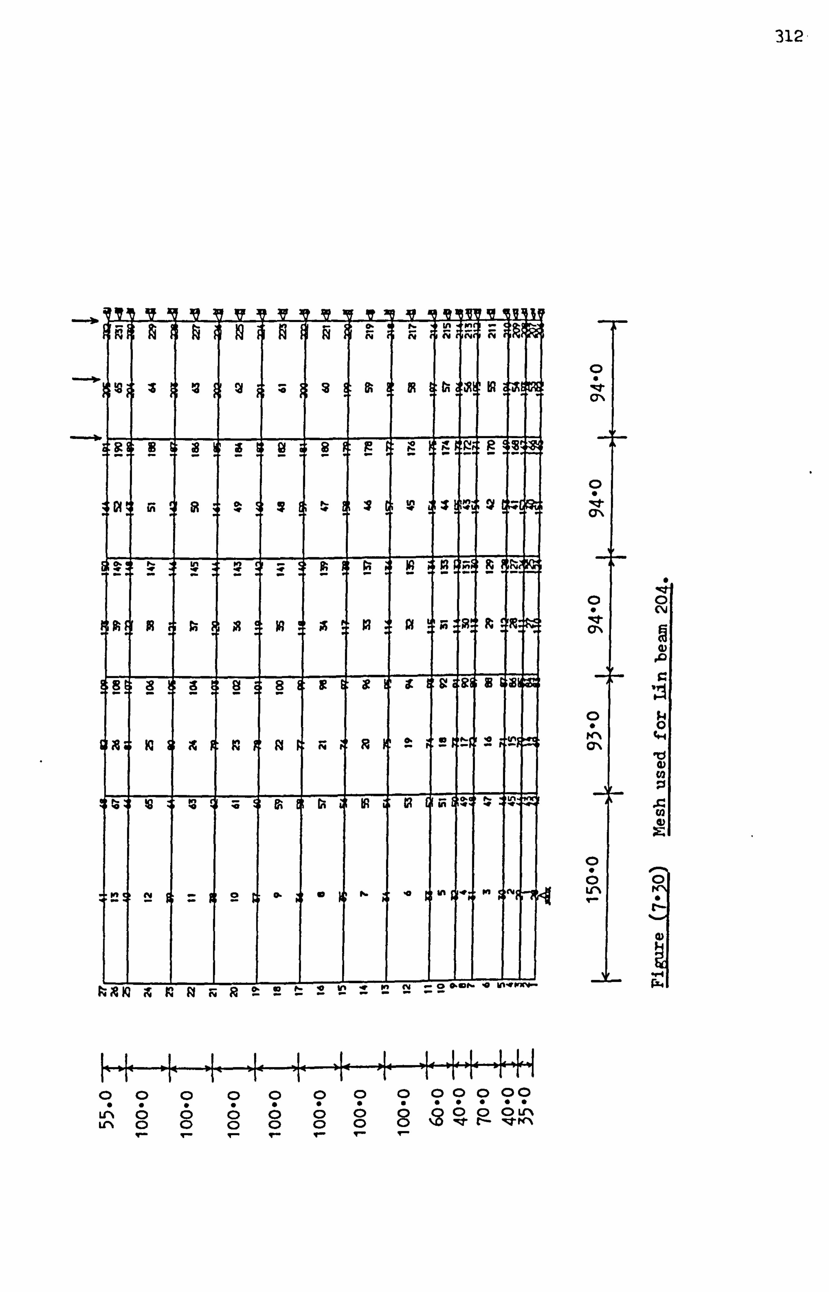
312
U RI A 4p An1 1 fi 1 i 4), 1 1 0 t- 5 F4 V 10 ; &Fic ýV
iew =-- ev t
U-1 o
-
c 11 ;S at pi . aF : F. s : ;21 ýaI Fý; 9" ;V
in
R A IR X
;aR 8K s el c 81 r1 :91 ! 4% 1 G! i 91 Is I isl ý&
IR; ; r. I t4 2 P
IR tR i I ;if V,
U, I
k; Q IQ it RRRRtEt2VZ 'z U! ==
t1 0 ol I " H VT
9 -
? VA
ý) -
? TA
I? IT
C? ?? Lfl% " 0 0 0 0 0 0 8 00 C) Ln U % 0 0 0 q- C) V- 0 Ir- c
0 4 ON
C\j
cr, %
14 0
CH
10 4)
Ln
.1

313
1400
1200
1000
2 19
";. Boo m
CD 4J.
ýo 600
400
200
0
->>
e4 Xý gro,
1 COOP=20% I Hat. a=0.5 IC 2. G. R.
v ................. 72 COOP=202 1 Mat. a=0.5 1c 3. G. R.
a --------- a3 COOP=207. I Mat. a=0.5 1c 4. G. R.
------------ *4 COOP=20% 2 Mat. a =0.5 IC 2. G. R.
5 COOP=20% 2 Mat. a =0.5 1c &G. R.
6 COOP=20% 2 Mat. a=0.5 1c 4. G. R.
7 ExporimentaL
0.0 0.2 0.4 0.6 0.8 1.0 1.2 1.4
DispLacament (mm)
Fig. (7.31) Load defLection curves for Lin deep beam 204.
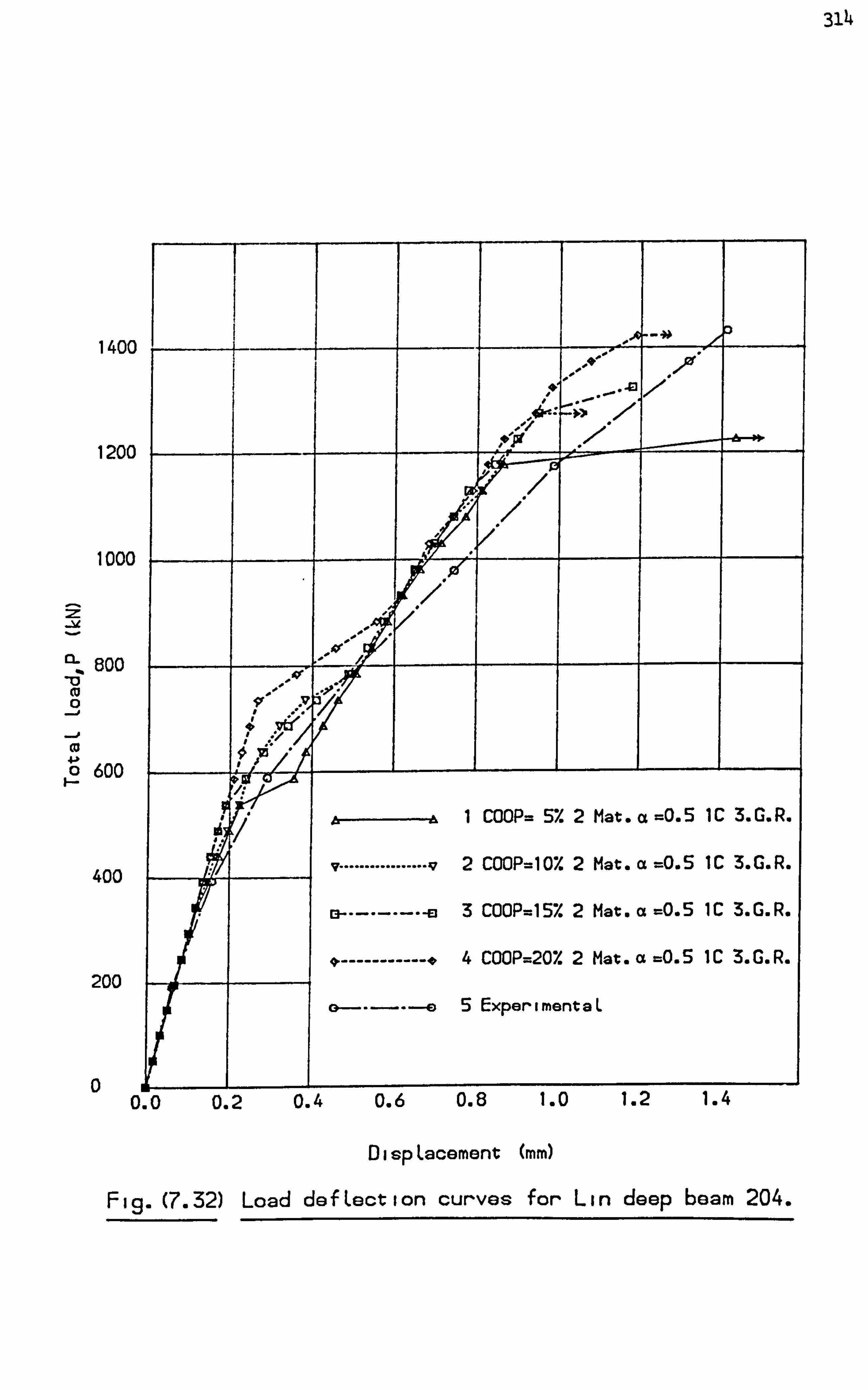
314
1400
1200
1000
Qý Boo _ID
44
ýo 600
400
200
0
. )Z(
/*
0 of a -A
1 COOP= 5% 2 Mat. a =0.5 1C 3. G. R.
v ................ 9 2 COOP=10% 2 Mat. a =0.5 IC 3. G. R.
--------- a3 COOP=15% 2 Mat. a =O-5 IC 3. G. R.
------------ *4 COOP=20% 2 Mat. a =0.5 IC 3. G. R.
05 ExperimentaL
0.0 0.2 0.4 0.6 0.8 1.0 1.2 1.4
DispLacement NO
Fig. (7.32) Load defLection curves for Lin deep beam 204.
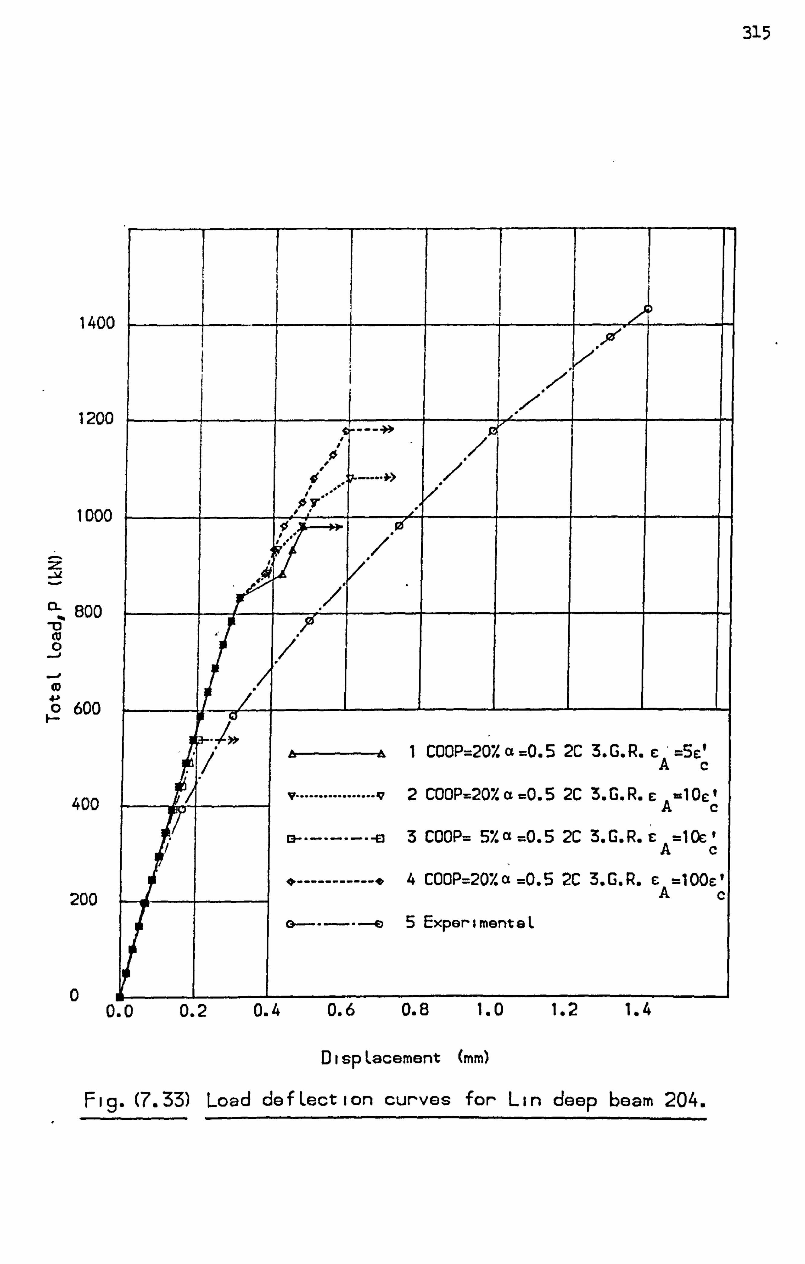
315
1400
1200
1000
800
--f --i (9 4-.
Fo 600
400
200
0
/*
a-. 1431 h1 COOP=20% a =O. 5 2C 3. G. R. c =5c' A C
V ................. V2 COOP=207.01 =O. 5 2C 3. G. R. c =loci AC
--------- a3 COOP= 5%a=0.5 2C 3. G. R. c = loc, AC
10 ------------- 04 COOP=20% a =O. 5 2C 3. G. R. c =1 00c' A
5 ExperimentaL
0.0 0.2 0.4 0.6 0.8 1.0 1.2 1.4
Di sp Lacement (mm)
Fig. (7.33) Load defLection curves for Lin deep beam 204.

316
1400
1200
1000
z
800 _0 (U
__j ca 4-*
, c) 600
400
200
0
.v.. ;3
7ý X I
, .* V*cr /
4 jil,
I COOP=20X 1 Mat. 1C ccu=0.004
v ................ q2 COOP=207.2 Mat. 1C Ccu=0.008
0 ........ 03 COOP=20% 2 Mat. 1C ccu=0.004
------------ *4 COOP=20% 2 Mat. 2C ccu=0.004
--o 5 ExperimentaL
ll-- 0.0 0.2 0.4 0.6 0.8 1.0 1.2 1.4
DispLacement NO
Fig. (7.34) Load defLection curves for Lin deep beam 204.

317
Figure (7-351 Crack pattern at load = 490-6 M.
__ __ __ / �
�/ ______ __ __ __
/ 1
/ // //
I /
_ __________ ___________________ ___ _____ ___
/ /
/ 1
// // 11
/ 1 ______
___________ __ ___
/
_
I /
, /
/ / /
/ 1 /
// // I/
/ /
_ ______ ___________
/
/
/
1 / 1
/ / 1
/ / /
// 1/ /1
I / 1
i / /
____________
/ / / /
/ 1 /
/ / /
/ / /
I i /
// i/ 1i
/ / /
I / /I
____________
J /
�
/
I
/ /
I-
/ 1
I
/ /
/ /
// 1/
/ i
/ i
-- / / / / H_ _
____ _ _
H ______________
/ / / / / / ____
/ I t
__
f
__ I
_ I
__
I
- ______________ _________ 1 ___
Figure (7-36)_ Crack Pattern at load = 883*0 kN.

318
gi g
Figure (7037) Crack pattern at load = 1422*6 M.
Fi e (7*38) Experimental crack patterns at load = 1431.0 kN.

319
900
800
700
600
ii e 500
ID 0
4ý 400 0)
-0
0 300
4-b
200
100
0
3
Load= 392.3 kN
v ......... v Load= 583.4 M
Load= 784.6 kN
0 Load=1176.8 M
-27 -24 -21 -18 -15 -12
HorizontaL stresses (N/mm2)
Fi. g. (7.39) Stress distribution at midepan section, (Lin 204).,

320
800
E
600 (0 41 0)
-0 400
0 44 C-
(D
200
-0.10
I& Load=196.1 kN
v .......... v Load=392.3 kN
a Load=S88.4 kN
-------- * Load=784.6 kN
0a Load=980.7 kN
Fig. (7.40) Concrete surface strain for Lin deep beam 204.
800
E E
a) o 600 c (a . 10 0
-0 --0 400
4. ) L CD
200
01 -0.10
C). -. -- *,. Cl, V A Load=196.1 kN -.
v .......... v Load=392.3 kN
m--a Load=588.4 kN
-------- * Load=784.6 kN
11 '4 %lo a. Load=980.7 kN
0 -*, 'o
-0.05 0.00 0.05 0.10 0.15
HorizontaL strain at midspan section (7. ) - Exp.
-0.05 0.00 0.05 0.10 0.15
HorizontaL strain at midspan section (7. ) - F. E. M.
Fig. (7.41) Concrete surface strain for Lin deep beam 204.

321
800
E
600 cu 41 0)
-0 400
0 4J. L CD
200
-0.04 0.00 0.04 0.08 0.12 0.16
HorizontaL strain at haLf cLear shear span section M- Exp.
Fig. (7.42) Concrete surface strain for Lin deep beam 204.
Soo,
-iý C-
600
0 _C)
--0 400
41 L (D
200
01 -0.04 0.00 0.04 0.08 0.12 0.16
HorizontaL strain at haLf cLear span section (7. ) - F. E. M.
Load=196.1 kN
v ........... v Load=392.3 kN D-----f3 Load=588.4 kN
-------- * Load=784.6 kN
0 Load=980.7 kN
qp, ' A -& Load=196.1 kN 4( v .......... v Load=392.3 kN
Load=588.4 kN
-------- Load=784.6 kN Load=980.7 kN
41 i
3; 0-
Fig. (7.43) Concrete surface strain for Lin deep beam 204.
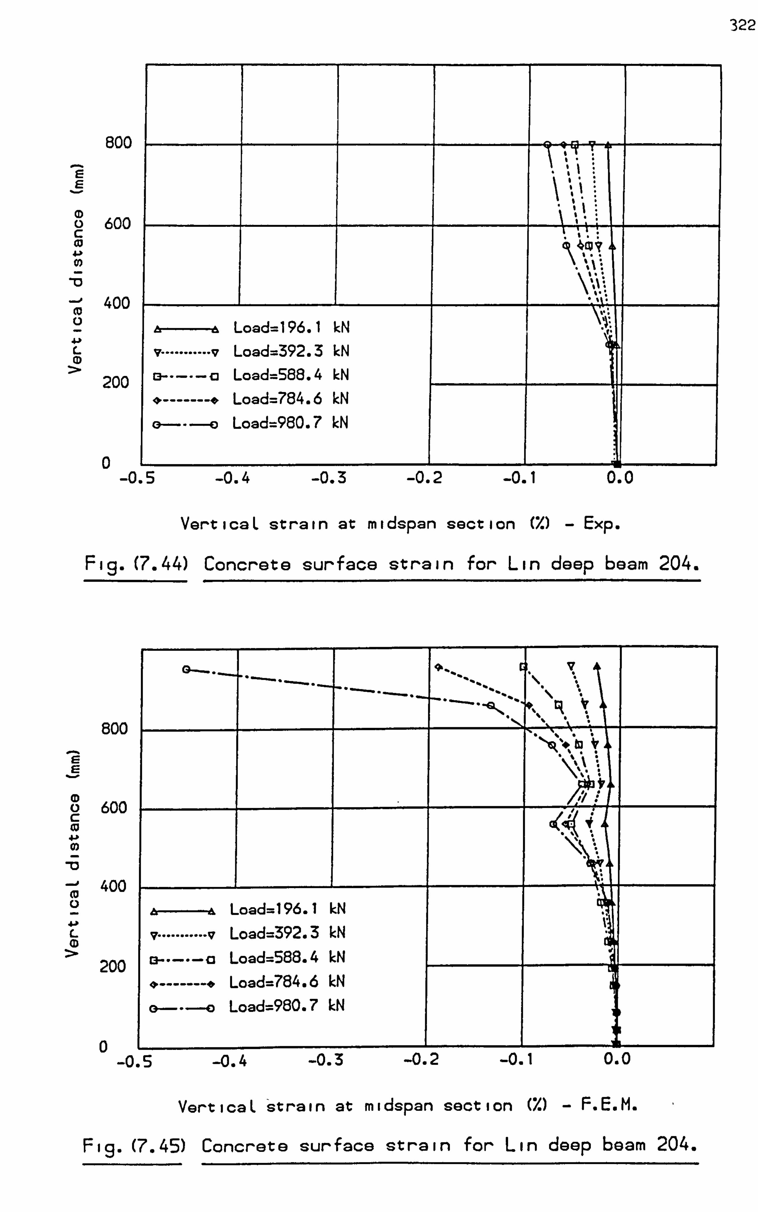
322
Boo
E E
600
0
-0 400
m 0 4-P L CD
200
-0.5 -0.4 -0.3 -0.2 -0.1 0.0
VerticaL strain at midspan section (Z) - Exp.
Fig. (7.44) Concrete surface strain for Lin deep beam 204.
800
2 E
600
0)
-0 400
CD
200
-0.5
Load= 196.1 kN
v .......... v Load=392.3 kN C3-- -- - C3 Load=S88.4 kN
,* -------- * Load=784.6 kN
0 Load=980.7 kN
"R
\x
Load=196.1 kN
v .......... v Load=392.3 kN
0-. -. -cl Load=588.4 kN
.0 -------- * Load=784.6 kN
0. o Load=980.7 M
-0.4 -0.3 -0.2 -0.1 0.0
VerticaL strain at midspan section W-F. E. M.
Fig. (7.45) Concrete surface strain for Lin deep beam 204.

323
800
E
600
400
44 L
CD
200
-0.05
Load=196.1 kN
........... V Load=392.3 kN
C3 Load=588.4 kN Load=784.6 kN Load=980.7 kN
fl
f
0.00 0.05 0.10 0.15
VerticaL strain at haLf cLear shear span section (7. ) - Exp.
-, Fia. (7.46) Concrete surface strain for Lin deep beam 204.
Boo
E
600
0 -13 -0 400
4. > L
CD
200
-0.05
A Load=196.1 kN
v .......... v Load=392.3 kN (3------(3 Load=588.4 kN
o -------- Load=784.6 kN
G Load=980.7 W
Ll
3
0.00 0.05 0.10 0.15
VerticaL strain at. haLf cLear shear span section (7. ) - F. E. M.
Fig. (7.47) Concrete surface strain for Lin deep beam 204.

324
0.16
0.12
0. OB
0.04
0.00 Ta
0 50 100 150 200 250 300 350 400
Distance from the support (mm) - F. E. M.
Fig. (7.48) Strain distribution aLong the bottom bar, (Lin 204).
0.16
0.12
C
0 C). 08
0.04
0.00 1 A-1 'L IIIIII 0 so 100 150 200 250 300 350 400
Distance from the support NO - Exp.
Fig. (7.49) Strain distribution aLong the bottom bar, (Lin 204).
At Load= 196.1 kN v ...... v Load= 392.3 kN 13- --0 Load= 588.4 kN * ---- ýO Load= 784 6 kN . * .0 Load= 980.7 M M- - -M Load=1176.8 M
-48-
yr
/ /p, . / -*
4 -40 1ý *
(3
-V ........
A Load= 196.1 kN vv Load= 392.3 M 13---, D Load= 588.4 M
Load= 784 6M . 0 ., 8 Load= 980.7 M E&- - -M Load=1176.8 M
1 I I
4 1 1- -- -, -- -- - I
EEI- -- -- --
--- -------- --------- ----- --- --------- --------- --------
--. - --, El .. ...... ...... I ------ ------
........ ............
............
..... . ............ ............. .....
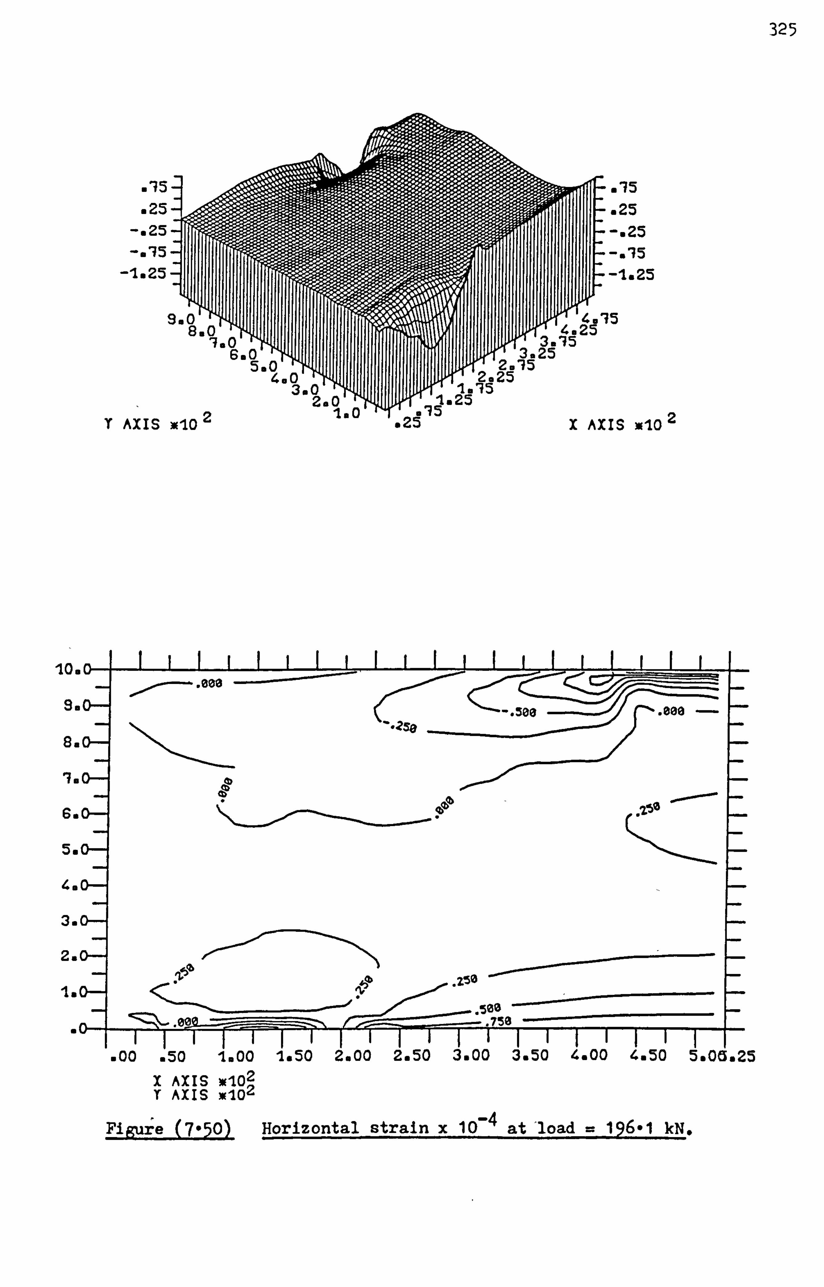
325
. 115
. 25
-m25 -. 15
-Im25
Sao, 820
zo
a 619 5mO
-1
1
4.0 300
200 Y AXIS xlO
2
. 15
. 25
-. 25
-6115 -1823
P T' '4o'35 lllý 4w25
3 '15 i2i
p3m a1 02
2029 lo'15
llu25
*250 X AXIS x102
10.
9.0-
a. 01
680-
5sO-
4oO-
3.0-
2aO-
ISO-
750
-00 . 50 -1.00 la50 2.00 2.50 3,00 3.50 4mOO 4.50 5aOfSo25 X AXIS W'102 T AXIS 102
Figuýe (7-50) Horizontal strain x 10-4 at'load =196-1 kN.

326
102
08 94 wo
-n4 -98
9.0,1 800
ISO Sao
ýN
5a
40Q 4aQ NO
2. Q T AXIS *10
2 -. LOW
ion -Ael
Sao- emo-
1.0-
6.0 T, Olb ?)
5mG-
4mG-
3. G_
2aG- lb lb
1. G_
- . 0- 111
4tTý-T-T-T I T-=
00 . 50 -1.00 1.50 2.00 2*50 3,00 3.50 4600 4a5O 5@00s25
X AXIS W102 T AXIS W102
Figure (7*511 Horizontal'strain x 10-4 at load = 883-0 kN.
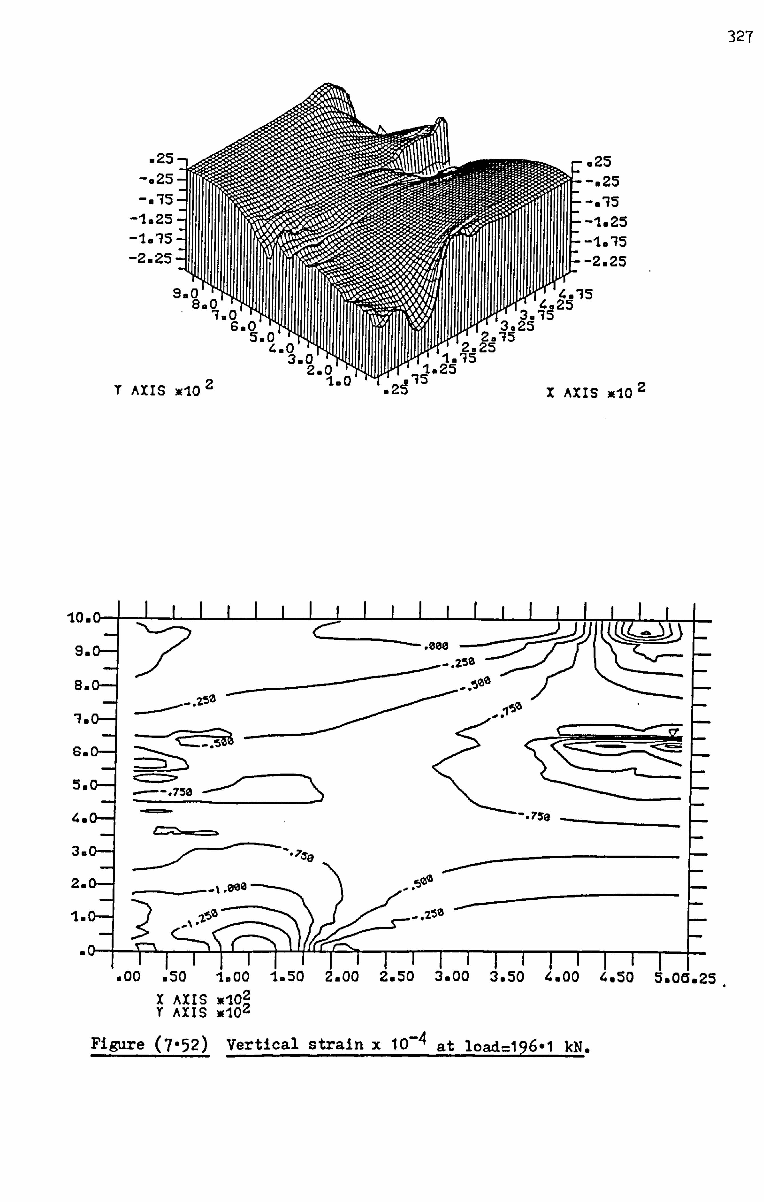
327
. 25
-. 25
-015 -1a25 -1915 -2.25
920' Igo
0 5,0
4.0 3.0
2.0 T AXIS x102
-10 U
. 25
-o25 -. 15
-1@25 -1.15 -2m25
4115 4o2
3 2j15 u 2:
f 3j 25
od2g
2 5i* '15
I I al 5 . 102i
F-.
;!, i '75
02i X AXIS m102
25e 8.0- -!! ze
emo-
3so-
- 4.0-
3mO-
2w
in
:::
ý- . 250
moo w50 1.00 1.50 2.00 Zm50 3000 3@50 4*00 4.50 te0d@25
X AXIS : 102 T AXIS 102
Figure (7052) Vertical strain x 10-4 at load=196-1 kN.
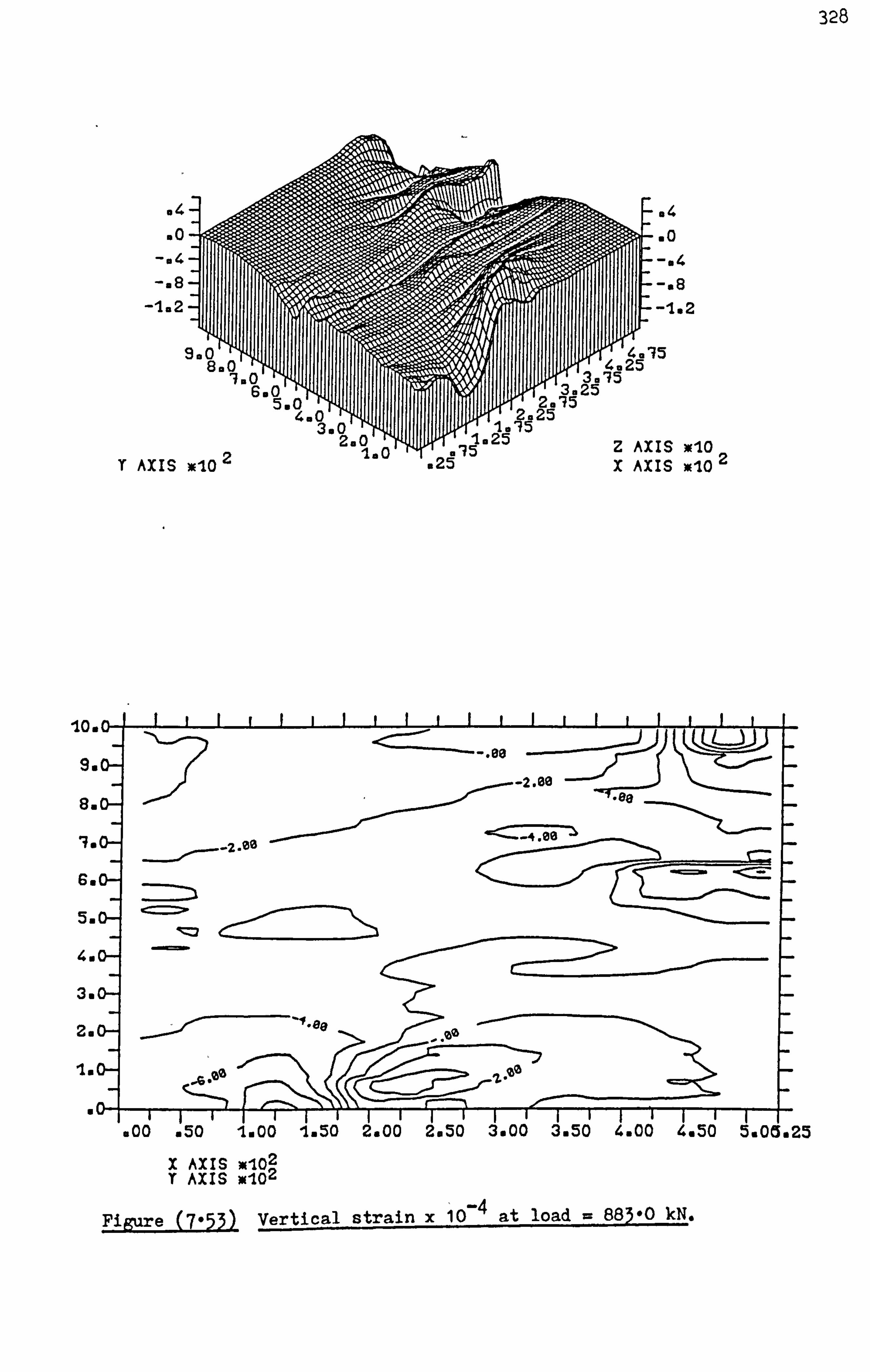
328
a4
-o4
-28
-1a2
900' 8
600 '100
00
M804.0
3oO, 29q
ý T AXIS )KIO
2 'Lou
-08 -102
W, 405 4o25
3 '1 PR2jl5 3a25 jj2 '15
1,2125
7 llo'75 J '9 . 25 2 AYT!
'4025 s'15
m3n25 pg
'15 , 2, a 25 1!
a 2.5 a'15
2 AXIS wIO 25 X AXIS *10
2
. 108
.......................................... . ................................... =0
Sao-
5.
4wO-
3@0-
2m
Im
a goo 050 1.00 1.50 2600 2.50 3mOO 3w5O 4.00 4e5O 5605025
X AXIS M102 T AXIS W102
Figure (7053) Vertical strain x 10-4 at load = 883oO kN.
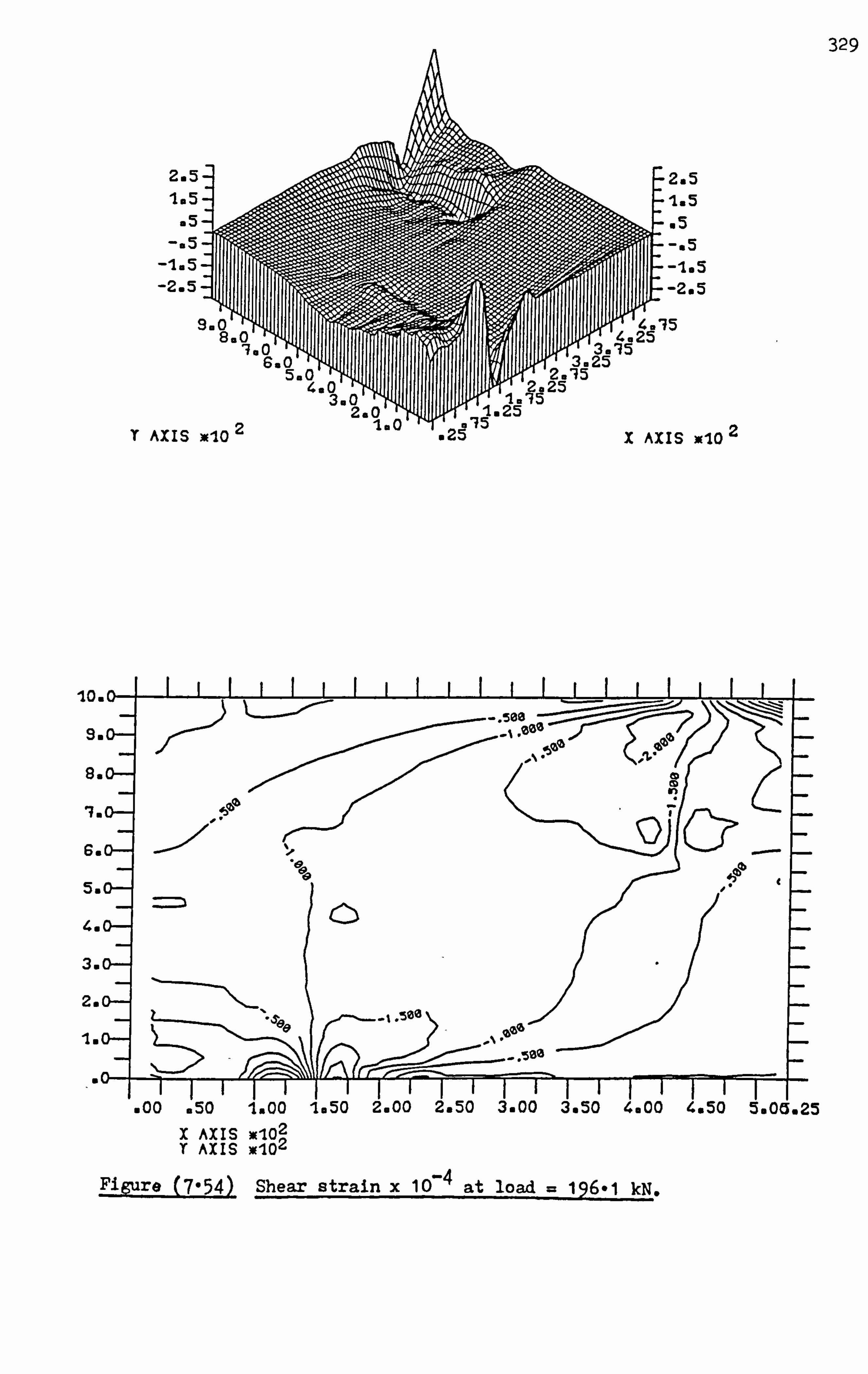
329
2m5 In5
m5 -&5
-1.5 -2.5
9.0, 8a
10 0 '10 6a 05
q.
O 0
ýrq
4.114 3.0
2ao
10.
90
S.
170
so
5a
4.
3.
2m
in
T AXIS x1o 21aQ
Zblb 'bo
4b
----I I
C)
% All
01 I---j-l IIIIIIIIIIIIIIIII -]- woo . 50 1,00 lo50 2.00 2a5O 3.00 3@50 4@00 4*50 5mOdo25
X AXIS X102 Y AXIS 1102
Figure (7-54) Shear strain x 10-4 at load = 196-1 kN.

330
2moo Is50 1000
m50 Soo
-w50 -1000 lw50 -2.00 2.50
900' Be ýqo
4.0 3.0
T AXIS Kjo 2 Is U
100
S.
8*
1.1
6.1
58(
4o(
3. (
2. C
.I
2 50
4 _'1"
-_ 4a
L LP
0- 00 1.00 1&50 2&00 2s5O 3wOO 3w5O 4mOO
X AXIS W102 T AXIS W102
Figure (7055) Shear strain x 10-4 at load = 883-0 kN.
m50 5.06a25

331
1150 1-100-1
60 r- 60
90
60
60
100
120
120
100
so so ýo
Figure (7-56) Details of Memon deep beam B-5.
SECTION
1000
tA A-A

332
1 0 Alp I TI TII lipl Fir u p DF DR. ?TN F f f ýi ý (ý
p Ev ; .0 F. :!! .,
! (
-; 7 , 94
51 ýc
1
rA, Aj ý rh Vc rn ,
5! IB 9 Q V It I
51 A 4N ý; un
:8ý i :3 t tR Z ; rn C Gn
c -V 3 In t C, 3 :; l
A p? Mg 4 ;%a m; ;Rf iAp ig ? ý -, P Rý :Rý C2 , :2ý
19 2 A m2 pf R
; 8E 19 Ic 9K 11. IT S! a ?5 aa i C8 ý Iat I &I ; ; SF : P, p
Ir CA r.
il RR &R RF : It i a P f, ý tj
ist VIC C-4 c
CY "I
LA ýln C4 IQ 74 RR F4 x====ý: ;- ; -; Wý --
-1 - -1 1 .- LJ . -1
UN 0 0 -, o
0 a%
0 %D
Lf-% CO
Lr% r-
-
0 cli
FA
0 C%l co ý, o
0 U-N
U'N CO
C- " "
C- C- '0 �0
" C- C- '0 '0
ol Lrl% %.. 0
0
0 LrI. Lr% co r^
cr%
LCI% T-
S
9
Id

333
1800 1600
1400
1200
looo
Boo
2 11, 1 ý 2.
1
- 600
Y
400 V
16 1 COOP=20X a=0.5 1C 2. G. R.
0 ------- v2 COOP=20X a=0.5 1C 3. G. R. 200
13 -------- 13 3 COOP=20%a=0.5 1C 4. G. R.
I* ------------ a- 4 ExperimentaL
0 0.00 0.05 0.10 0.15 0.20 0.25 0.30 0.35 0.40 0.45
01 sp Lacement (mm)
Fig. (7.58) Load deftection curves for Memon deep beam B-5.

334
1800
1600
1400
1200
1000 V -0 1 1
Boo
600
400
I COOP=20X a=0.0 IC 3. G. R.
V ... . .......... V2 COOP=20X a=0.5 1C 3. G. R. 200
-------- a3 COOP=207. a=1.0 IC 3. G. R.
ntaL -- .4 Ex er-im --------- C p e
0 ---- -- - .-- .-I 0.00 0.05 0.10 0.15 0.20 0.25 U. 50 0.55 U. 4U U. 45
DispLacement (mm)
Fig. (7. S9) Load defLection curves for Memon deep beam B-5.

335
180C
1600
1400
1200
(0
--0
600
400
200
0
1 COOP=20% a=0-5 IC Ccu=0.0035
v.................. v2 COOP=20% a=0.5 1c ccu=0.0040 13 ---------a3 COOP=20% a=0.5 1c ccu=0.0080
-- ----- 4E i t L ---- * - xper men a
00 0. 05 0. 10 0.15 0.20 0.25 0.30 0.35 0.40 0.4S
DispLacement NO
Fig. (7.60) Load defLection curves for Memon deep beam B-5.
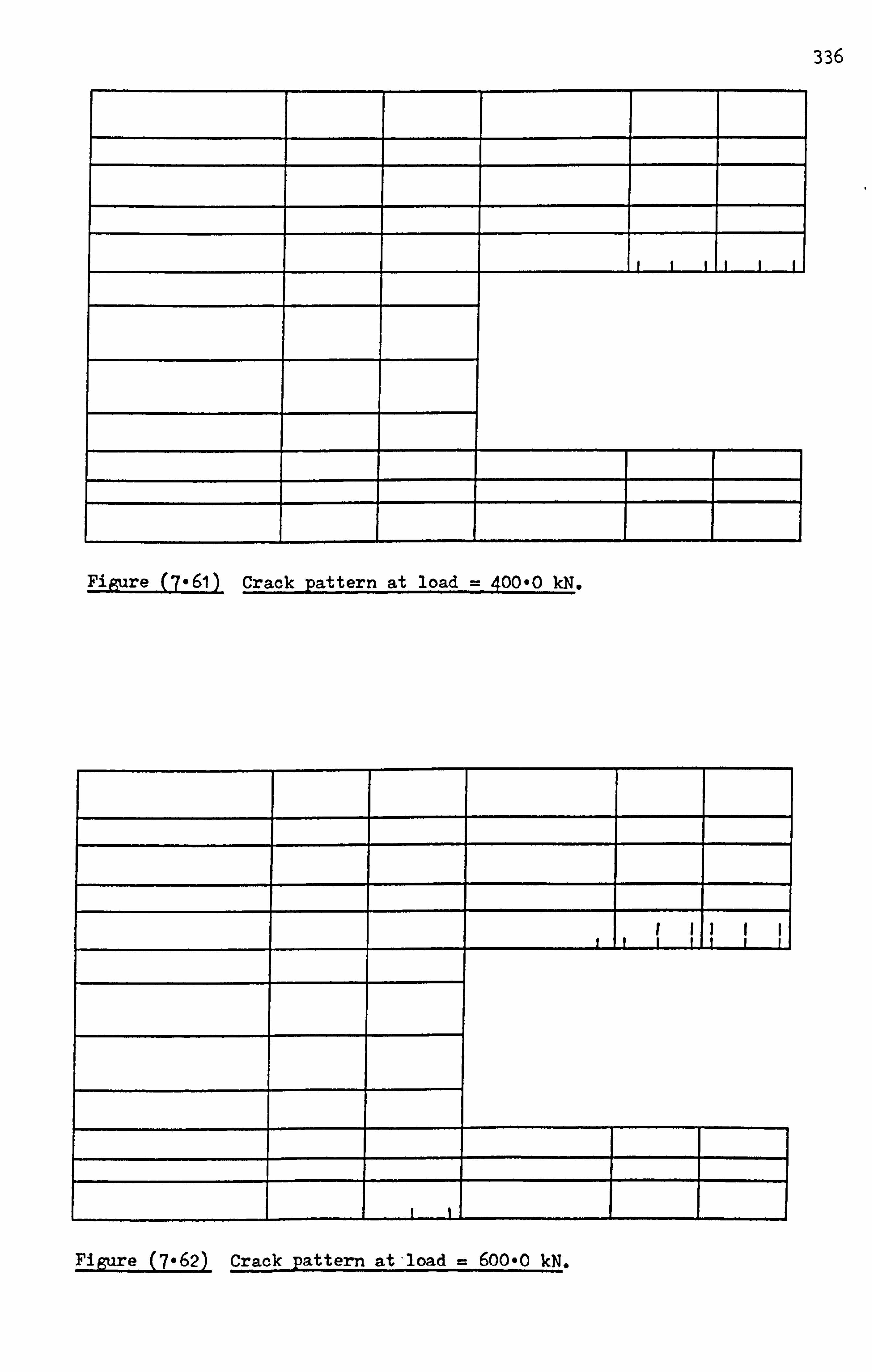
336
Figure (7-61) Crack pattern at load = 400-0 M.
Figure (7-62) Crack pattern at-load = 600-0 kN.

337
Figure (7-63) Crack pattern at load = 900-0 kN.
/ I
I
!I r II
I _____________ _ ___ __ / I III tI ii
____________ _ ___ _ _ ____
I I ! I __________ t t Figure (7-64) Crack pattern at load = 1000-0 kN.

338
z z
4-1
Figure (7-65) Crack pattern at load = 1350-0 kN.
Figure (7-66) Experimentai crack pattern at load = 1600-0 kN.

339
.. I , 7 - -T k, x -t- x -- -----
X x /I
r f
f 1
Scale: 1 mm = 1-2 N/mm' (= tension), (- Compression)
Figure (7-67) Principal stress direction at load = 150-0 M.
--- -7 -7- 71-
ol
T- I
I1- ---. -�� ---. ----�
Figure (7-68) Principal stress direction at load = 1350-0 kN.

340
150
120
90
60
30
01 0.000 0.002 0.004 0.006 0.008 0.010
HorizontaL strain at midspan section M- Exp. tottowl ýIdk"ýe
Fig. (7.69) Concrete surface strain for Memon deep beam B-5.
150
120 C) C w
90
60
30
01 0.000 0.002 0.004 0.006 U. uud U. UIU
HorizontaL strain at midspan section (7. ) - F. E. M. 6 *Itop" F1417,7e-
Fig. (7.70) Concrete surface strain for Memon deep beam B-5.
Load=100.00 kN v Load=200.00 kN
a-. -a Load=300.00 kN Load=400.00 kN
.0 Load=500.00 kN
a .v 13 ýo \)O
Load-100.00 kN v ...... v Load=200.00 kN 13-43 Load=300.00 kN
Load=400.00 kN .0 Load=500.00 kN

341
150
120
c 0 90
_0
60 44 L CD
30
0
I& Load=600.00 M v ....... q Load=700.00 kN
Load=800.00 M ------- 0 Load=900.00 kN
d 1000 0 kN G ---o Loa = .
0.00 0.04 0.08 0.12 0.16
HorizontaL strain at midspan section M- Exp. BOUOM Fla-lie.
Fig. (7.71) Concrete surface strain for Memon deep beam B-5.
ISO
120 0 0 C 0
0 90
-i; (U
60
30
0
h Load=600.00 M v ........ q Load=700.00 kN
Load=800.00 kN Load=900.00 kN
-i" o . -0 Load=1000.0 kN
.0
0.00 0.04 U. ud U. Id U. 10
HorizontaL strain at midspan section W-F. E. M. Aolib., Fl, "Iya
Fig. (7.72) Concrete surface strain for Memon deep beam B-5.
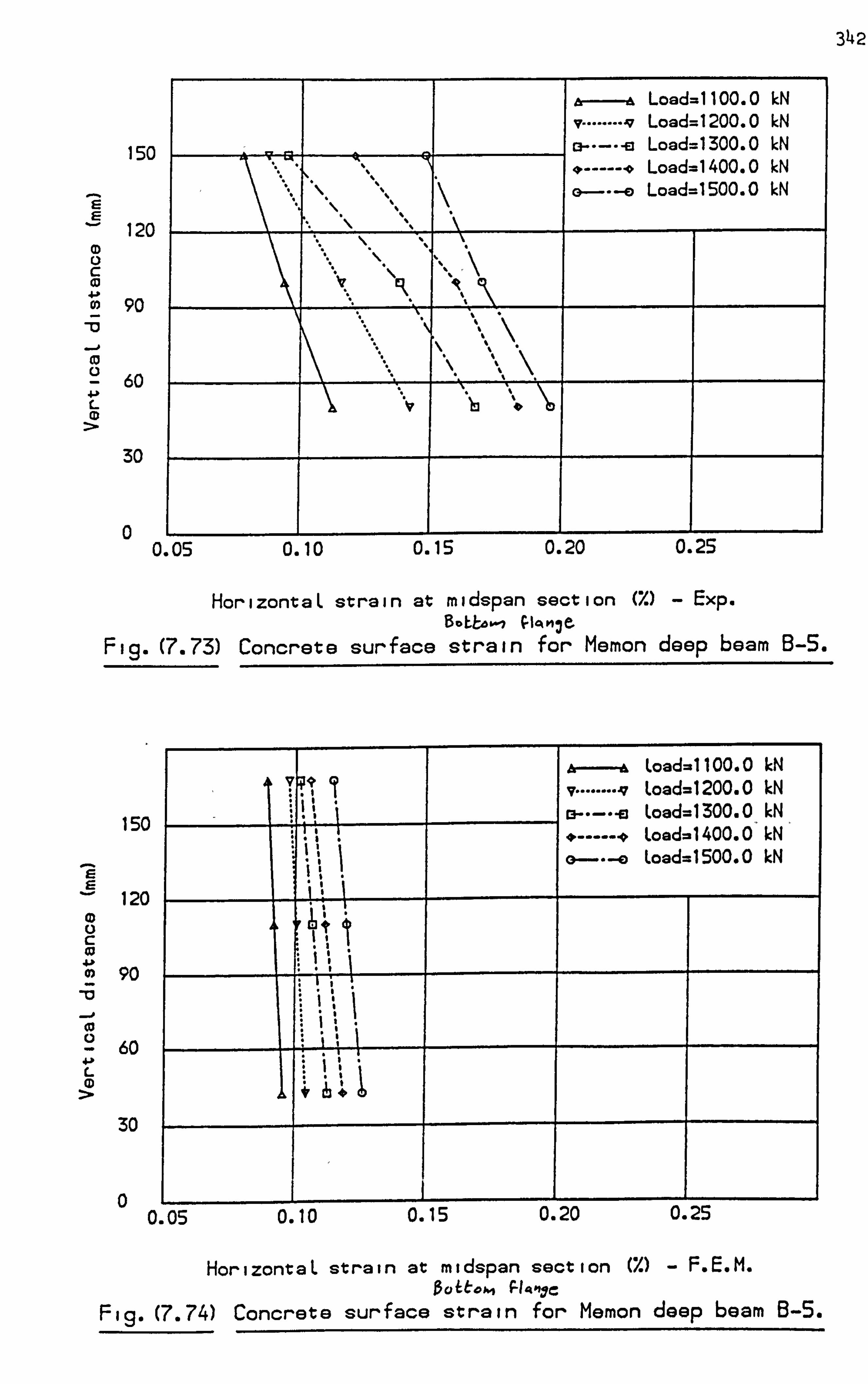
342
150
120
90
60
30
0
h Loed=1100.0 M v ........ q Load=1200.0 kN Cý-----o Load=1300.0 M ------- * Load=1400.0 M
. -C) Load=1500.0 kN
0.05 0.10 0.15 0.20 U. 25
HorizontaL strain at midspan section M- Exp. BoLba'-I 0-: ý M3 e
Fig. (7.73) Concrete surface strain for Memon deep beam B-5.
150
120
0 90 -0 -. 0 (a a
60 4-P L
30
0
h Load=1100.0 kN v7 Load=1200.0 kN
Load=1300.0- M, + ------ C. Loed=1400.0 kN G ---G Load=1500.0 kN
0.05 0.10 0.15 U. 20 U. 2t)
HorizontaL strain at midspan section (Y. ) - F. E. M. autto" Pla-Ile
Fig. (7.74) Concrete surface strain for Memon deep beam B-5.
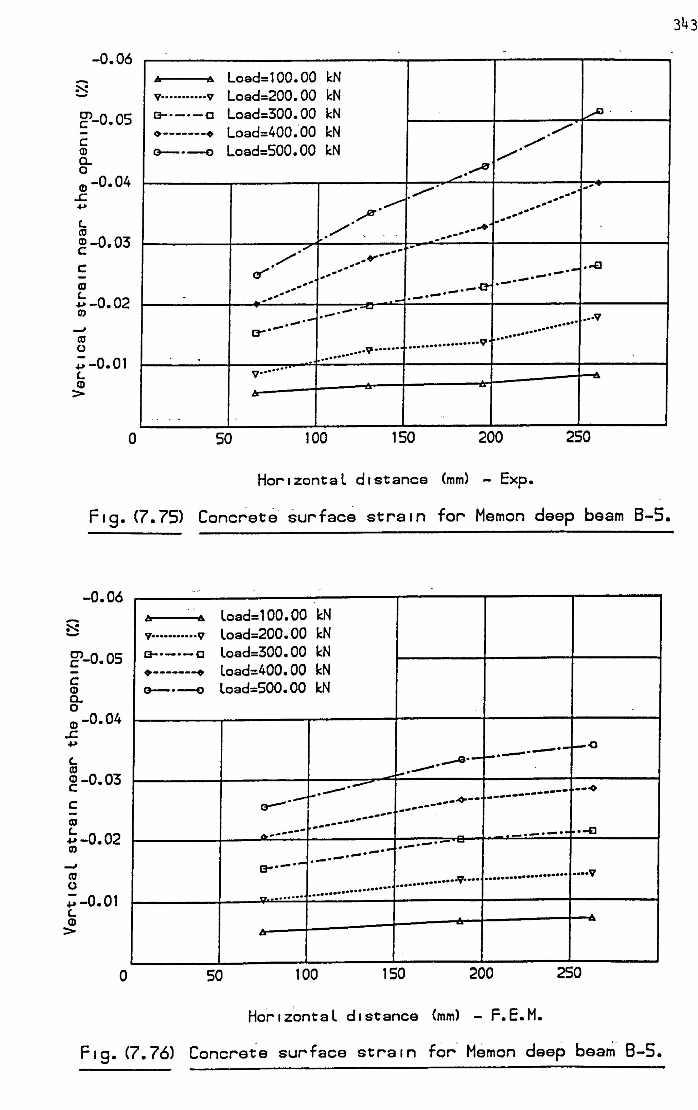
343
-0.06 p
CY) 0.05
c (D CL 0
(D -0.04 _c 4ý
ID-0.03
0 L 4. » -0.02 0)
41-0.01
A, --* Load=100.00 M
v .......... v Load=200.00 M 13-----a Load=300.00 kN
-------- * Load=400. '00 kN Load=500.00 kN
....... ... v
.......... ....... ..................
v. ....
V*l ........
------ -&- -A ------- --ý --., &
0 50 100 150 200 250
HorizontaL distance (mm) - Exp.
Fig. (7.75) Concrete'surface strain for Memon deep beam B-5.
-0.06
c -0.05 c CD CL 0
0-0.04
-0.03
0 L 4.11-0.02
4. -0.01 L .9
toad=100.00 kN 7 .......... v Load=200.00 kN
-a Load=300.00 kN 0 --------- e Load=400.00 kN
toad=500.00 kN
0---. . �.
--
-_ __ 4 ---- ------------- ý --0
..... ..............
............... 7 .... .................... ....
0 50 100 150 200 250
Horiz I ontaL distance (mm) - F. E. M.
Fiq. (7.76) Concrete surface strain for'Memon deep beam B-S.

344
-0.12
cIo c (D CL 0
(D -0- 08
0-0.06
0 L
-0.04
C
4» -0.02 L
Ar- &, Load=600.00 kN A v ........ v Load=700.00 kN '
Load=800.00 kN
4 ------- * Load=900.00 kN o ---o Load=1000.0 kN Ile
or Er
0 so 100 iso 200 250
HorizontaL distance NO - Exp.
-Fig. (7.77) Concrete surface strain for Memon deep beam B-S.
-0.12
C-0.10 c CD CL 0
ID -0.08
-C . &A,
0 -0.06 c
.-> -0.04
., ý, -0.02
ä Load=600.00 kN v ........ v Load=700.00 kN
Load=800.00 kN ------- > Load=900.00 kN
0 . -B, Load=1000.0 kN
----- --- --- ---------
............... ....
.............. .....
0 50 100 150 200 250
HorizontaL distance (mm) - F. E. M.
Fig. (7.78) Concrete surface strain for Memon deep beam B-5.
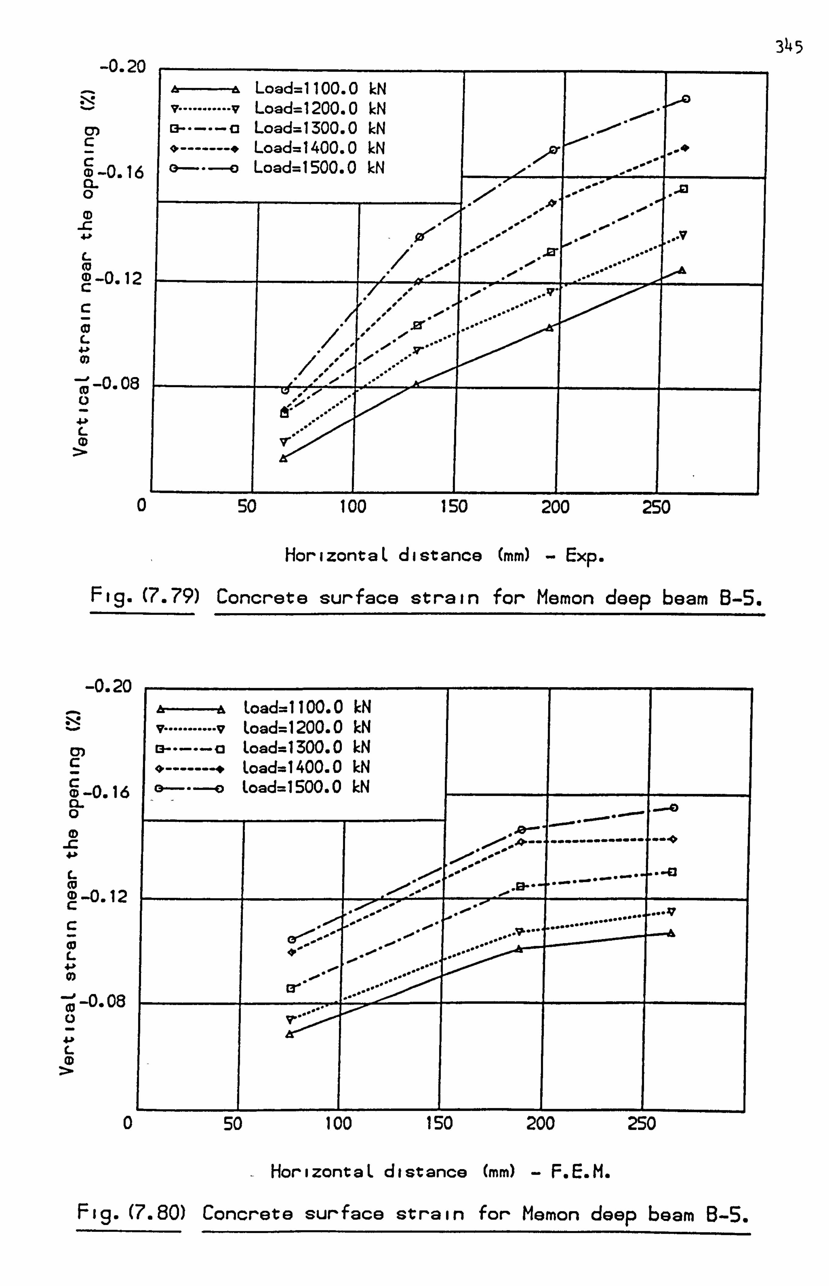
C, C
-0.20 At Load=1100.0 kN v .......... v Load=1200.0 M 13-----a Load=1300.0 M 4 -------- * Load=1400.0 M 0- Load=1500.0 kN
jar"
J2r
(D-0.16 CL 0
(D -C 4j,
-0.12 C (IU
0
-O. O8 U
CD
0 so 100 ISO 200 250
HorizontaL distance (mm) - Exp.
Fig. (7.79) Concrete surface strain for Memon deep beam B-5.
-0.20
C, c c (D -0.16 CL 0
ID -C 4-0
-0.12
0 0)
0-0.08 a
4. & L
A Load=1100.0 M v .......... v Load=1200.0 M m--a Load=1300.0 kN
Load=1400.0 M 0 Load=1500.0 M
I jo ---- ------------- ---- 0,
... .... .............
0 50 100 iso 200 250
HorizontaL distance (mm) - F. E. M.
345
Fig. (7.80) Concrete surface strain for Memon deep beam B-5.
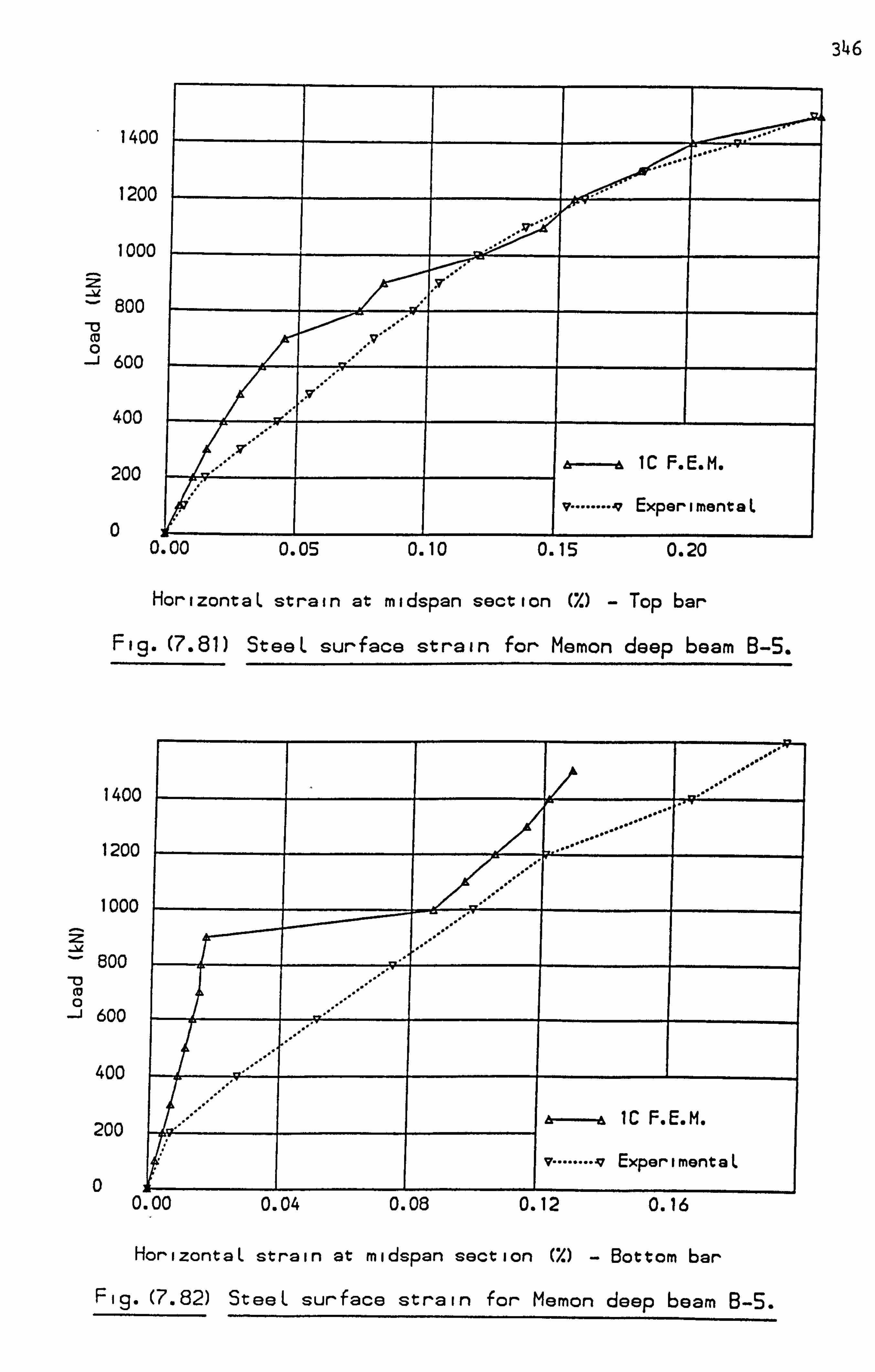
346
1400
1200
1000
zý 800 _C) m 0 600
400
200
0
IC F. E. M.
v ......... 7 ExperimentaL
0.00 0.05 0.10 0.15 0.20
HorizontaL strain at midspan section (7. ) - Top bar
Fig. (7.81) SteeL surface strain for Memon deep beam B-S.
1400
1200
1000
800
600
400
200
0 0
IC F. E. M.
v ......... 7 ExperimentaL
00 0- 04 0. 08 0.12 f)-IA
HorizontaL strain at midspan section (7. ) - Bottom bar
Fig. (7.82) SteeL surface strain for Memon deep beam B-S.
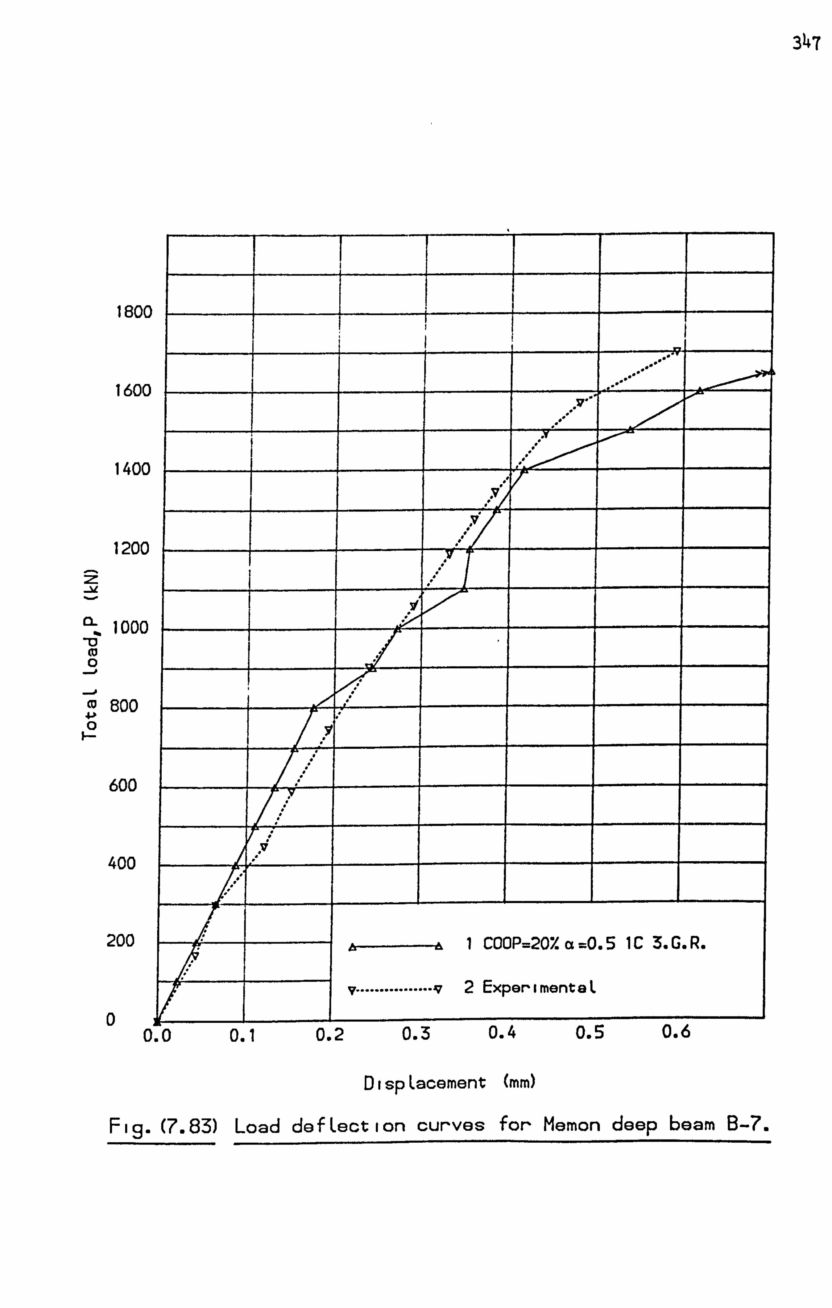
347
1800
1600
1400
1200
-�
ll- looo c 0
800
600
400
200
0
1 COOP=207. a=0.5 1C 3. G. R.
v ............... v2 ExperimenteL
0 0. 1 0.2 0.3 0.4 0.5 0.6
DispLacement (mm)
Fiq. (7.83) Load defLection curves for Memon deep beam B-7.

3148
REFERENCES
Cervenka, V., "Inelastic finite element analysis of reinforced
concrete panels under inplane loads". Ph. D. Thesis, University
of Colorado, 1970.
2. Lin, C. K., "Ultimate strength design of deep beams". M. Sc. Thesis,
University of Glasgow, 1979.
3. Memon G. H. I* "Ultimate strength design of perforated deep beams".
M-Sc. Thesis, University of Glasgow.
4. Dischinger, F., "Beitrag zur theorie der halbscheibe und des
wandartigen balkens". Int. Association for Bridge and Structural
Engineering, Zurich, Vol. 1,1932.
5. Chow, L.; Conway, H. D.; Morgan, G. W., "Analysis of deep beams".
J. of Applied Mech., ASME, Vol. 18,163-lT2, June, 1951.
6. Uhlam, H. L. B., "The theory of girdek walls with special reference
to reinforced concrete design". The Struct. Eng., Vol-30, lT2-181,
Aug., 1952.
7. Chow, L.; Conway, H. D.; Winter, G., "Stresses in deep beams".
J. of Struct. Div., ASCE, Vol-78,17, May, 1952.
8. Guzman, A. M., Luisoni, C-J., "Solution variacional del problema. de
la viga rectangular simplements apoyada de gran altura".
Cienciay Technica, Bueonos Aires 111,1948.
9. Archer, F. E.; Kitchen, E. M., "Strain energy method for the solution of
deep beams". Civil Eng. & Public Works review, V01.52,1375-1378,
Dec. 1957.
10. Leonhardt, F.; Walther, R., "Deep beams". Wandartige Triger, Deutscher
Ausschus Fur Stahlbeton, Bulletin 178, Berlin 1966, CIRIA
Translation, Jan., 1970.
349
11. De-Paiva, H. A. R.; Siess, C. P., "Strength and behaviour of deep beams
in shear". J. of Struct. Div., ASCE, Vol. 91,19-41, Oct., 1965.
12. Ramakrishnan, V.; Ananthanarayan, Y., "Ultimate strength of deep
beams in shear". J. ACI, Vol. 65,8T-98, Feb., 1968.
13. Kong, F. K.; Robins, P. J.; Cole, D. F., "Web reinforcement effects on
lightweight concrete deep beams". J. ACI, Vol. 68,514-520, July,
1971.
14. Kong, F. K.; Robins, P. J., "Shear strength of reinforced concrete
deep beans". Concrete, Vol. 6,34-36, March, 1972.
15. Manuel, R. F.; Slight, B. W.; Suter, G. T., "Deep beam behaviour
affected by length and shear span variations". J. ACI, Vol. 68,
954-958, Dec., 1971-
16. Smith, K. N.; Vantsotis, "Shear-strength of deep beams". J. ACI,
Vol. 79,201-213, May-June, 1982.
17. Robins, P. H.; Kong, F. K., "Modified finite element method applied
to RC deep beams". Civil Eng. & Public Work Review, Vol. 68,
963-966, Nov., 19T3.
18. Buyukozturk, 0., "Nonlinear analysis of reinforced concrete structures".
Comp. & Struct., Vol-T, 149-156, Feb., 1977.
19. Cedolin, L.; Dei Poli, S.; Kapru, S., "Finite element analysis of
reinforced concrete deep beams", Costruzioni in Cemento Armato,
Studie Rendiconti, Vol. 14, Thechnical University of Milan, 19TT.
20. Taner, N. ; Fazio, P. P.; Zielinski, Z. A. , "Strength and behaviour of
beam-panels-tests and analysis". J. ACI, Vol-74,511-520, Oct., 1977.
21. Niwi, J.; Maekawa, K.; Okamura, H., "Nonlinear finite element analysis
of deep beams". IABSE Colloquium on The Advanced Mechanics of
Reinforced Concrete, Final Report, Delft, 625-638.

350
22. Ove Arup & Partners, "The design of deep beams in reinforced concrete".
Construction Industry Research and Information Association, CIRIA
Guide 2, London, Jan., 1977.
23. Kong, F. K.; Sharp, G. R., "Shear strength of lightweight reinforced
concrete deep beams with web openings". The Struct. Eng., Vol-51,
267-275,1973.
24. Kong, F. K.; Sharp, G. R., "Structural idealization for deep beams
with web openings". Mag. Conc. Res., Vol. 29,81-91, June, 1977-
25. Kong, F. K.; Sharp, G. R.; Appleton, S. C.; Beaumont, C. J.; Kubik, L. A.,
"Structural idealization for deep beams with web openings: further
evidence'. '. Mbg. Conc. Res., Vol-30,89-95, June, 1978.
26. KubiL, L. A., "Predicting the strength of reinforced concrete deep
beams with web opening". Proc. Inst. Civ. Eng., Part 2,939-958,
Dec., 1980.
27. Phillips, D. V., "Nonlinear analysis of structural concrete by finite
element method". Ph. D. Thesis, University of Wales, 1973.

CHAPTER
APPLICATION TO T-BEAMS
8.1 Introduction
8.2 General description of T-beans behaviour
8.3 Proposed theoretical model
8.4 Selection of axis of separation
8-5 Description of beans tested
8.6 Description of results
8.7 Conclusions

351
CHAPTER 8
APPLICATION TO T-BEAMS
8.1 Introduction:
, The behaviour of T-beams is generally in the three dimensional
category. This is because the flange exists in a plane perpendicular
to the web. The objective of this chapter is to investigate whether
the essential features of the behaviour of T-beams can be obtained
by using a simple two dimensional plane stress approximation, which
would be cheaper than using a three dimensional approach, or by using
shell or plate approximations. This is especially attractive when it
is considered that more expensive complex nonlinear approximations are
not guaranteed to give satisfactory results anyway because of the
influence of numerical parameters, material properties etc., as the
previous chapters have shown.
Only a few investigators have reported the use of the finite element
method to analyse T-beans. Cope et alSl) used a composite shell element
where compatibility of in-plane rotational displacement at common mesh
lines of elements in different planes were ignored. The effect of
changing the amount of reinforcement and the effect of-web width on
shear strength was studied. Deflections were underestimated in some
beams at the beginning, but in general the predicted cracking patterns
and failure loads agreed well with experimental results.
Razagpur et al. (2)
studied the effect of shear transfer at the,
web-flange connection and the interaction of this shear with the
transverse bending.; The analysis was carried out using a combination
of in-plane quadrilateral elements and quadrilateral plate bending
elements. Satisfactory results were obtained in most situations except
in the prediction of the stresses in the flange reinforcement, where
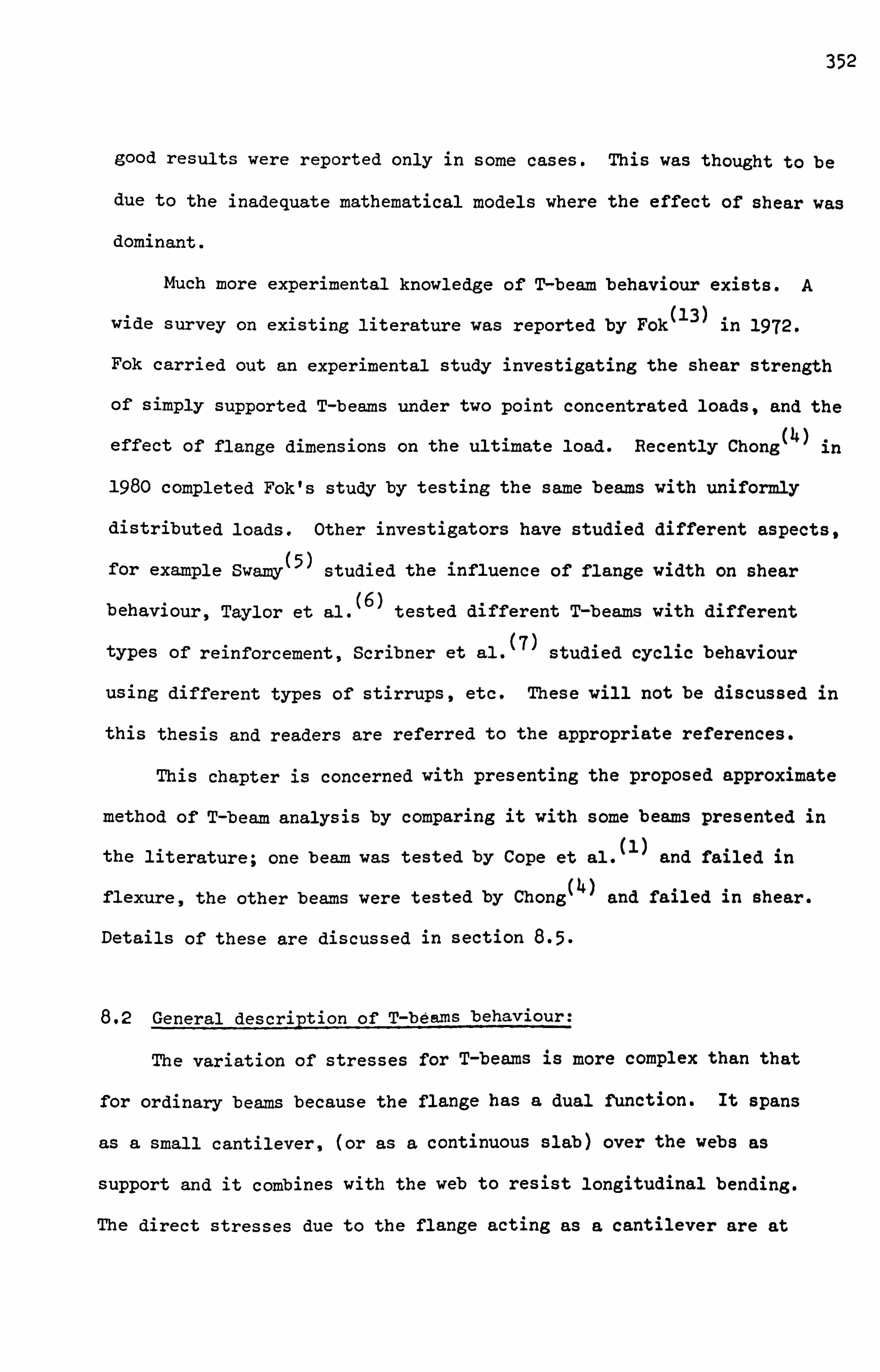
352
good results were reported only in some cases. This was thought to be
due to the inadequate mathematical models where the effect of shear was
dominant.
Much more experimental knowledge of T-beam behaviour exists. A
wide survey on existing literature was reported by Fok (13)
in 1972.
Fok carried out an experimental study investigating the shear strength
of simply supported T-beams under two point concentrated loads, and the
effect of flange dimensions on the ultimate load. Recently Chong (4)
in
1980 completed Fok's study by testing the same beams with uniformly
distributed loads. Other investigators have studied different aspects,
for example Swamy(5) studied the influence of flange width on shear
behaviour, Taylor et al. (6)
tested different T-beams with different
types of reinforcement, Scribner et al. (7)
studied cyclic behaviour
using different types of stirrups, etc. These will not be discussed in
this thesis and readers are referred to the appropriate references.
This chapter is concerned with presenting the proposed approximate
method of T-beam analysis by comparing it with some beams presented in
the literature; one beam was tested by Cope et al. (1)
and failed in
flexure, the other beams were tested by Chong (4)
and failed in shear.
Details of these are discussed in section 8-5.
8.2 General description of T-b6ams behaviour:
The variation of stresses for T-beams is more complex than that
for ordinary beams because the flange has a dual function. It spans
as a small cantilever, (or as a continuous slab) over the webs as
support and it combines with the web to resist longitudinal bending.
The direct stresses due to the flange acting as a cantilever are at

353
right angles to the stresses caused by longitudinal beam action, and
there is little interaction between them. Typical variation in direct
strain distribution under elastic conditions is illustrated in Figure
(8.1), and compressive, shear and trajectory principal stress distri-
butions are illustrated in Figures (8.2 - 8.4). The distribution of
steel, cracking effects and the multiaxial compressive response of
concrete are likely to affect these stresses and produce somewhat
different behaviour. Some of these effects are not yet well understood
and require further investigation.
The variation in flange compressive stress occurs because of shear
deform tions in the flange (shear lag), which reduces the longitudinal
compressive strain with increasing distances from the web. The
differences in longitudinal compressive stress resulting from different
distributions of load, can be explained by referring to Figure (8-5).
Under the action of a point load, Figure (8-5. a), the shear flow at the
flange edge (i. e. connected to the web) is large right up to the point
of the load, and the compression induced by shear flows near the midspan
section cannot spread far across the flange. In contrast, the shear
flows for the distributed load in Figure (8-5. b) are predominantly applied
at the ends of the flange, and the compression they induce has most of
the length of the flange to spread out. However, a rigorous analysis
of the effect of load distribution and flange shape is extremely complex.
The distribution of longitudinal compressive stresses across the
thickness of the flange become more uniform as the ultimate load is
reached. This is because the concrete stress-strain curve shows a
smaller variation of stress with strain at high stress levels.
354
As for transverse bending stresses, their effect is normally less
significant than that of ot her stresses produced in narrow flanged T-
beams as long as no loading is applied to the plane of the overhanging
flanges. If this was the case, cracks could occur in the top of the
flange over the web-flange junction, which would significantly affect
behaviour.
In general, the stress distribution in T-beams depends on the relative
dimension of the cross-section of the beam, the span, the arrangement
of reinforcement, the type of material used and the type of loading.
8.3 Proposed theoretical model:
The model is based on a two dimensional plane stress approach and
Obviously introduces various techniques to achieve satisfactory results
for what is essentially a three dimensional problem. The model is based
(8) (9) on suggestions made by Iversen . and Macleod et al. . for linear-
elastic behaviour. The method allows the shear stress developed in the
web, due to the effect of bending in the longitudinal direction to be
transferred to the flange. This will cause the stresses across the width
of the flange to vary allowing longitudinal bending effects to be taken
into account. This is illustrated in Figure (8.6).
The effect of bending in the direction perpendicular to the plane
of the web and the flange is ignored. This is illustrated in Figure
(8-7). This is not important in the web unless some torsional effects
exist. For the flange this effect becomes more important for thicker
or wider flanges, or when some forces are applied on the overhanging
flanges. However once the assumption is made to ignore bending in the
plane of the flange, the problem can be treated as a two dimensional
plane stress problem.

355
The method assumes that the centre of gravity of the load is
applied at the centre of the web-flange connection and behaviour will
be essentially symmetric about the centre line of the beam. Also,
because of symmetry, only one half of the T-beam needs to be analysed.
In order to make the planes of the web and flange coincide, the flange
is effectively rotated through 90 0 as shown in Figure (8.8). The position
of the axis of rotation is another assumption to be made in the analysis.
These assumptions should adequately approximate the longitudinal and
shear stress distributions in the flange and the web. The transverse
stress in the flange will only be crudely approximated but its effect
is assumed to be less significant, as previously explained.
A fictitious element composed of different linkage elements (i. e.
similar'to the element used by Ngo et al. (10) ) having different stiffnesses
in different directions, is used to connect the web to the flange.
As shown in Figure (8.9) the element is assumed to be dimensionless and
consists of eight nodal points connected by a series of springs which
have high stiffnesses in the x-direction and small stiffnesses in the
y-direction in the xy plane. The fictitious element is placed in the
region between the web and the flange, and acts as a device to transfer
forces for different degrees of freedom. A high stiffness of 0.1E + 10
is used for springs parallel to the web-flange in the x-direction (i. e.
k 3h' k 4h' k 7h- k 8h in Figure (8-9)) to ensure compatibility. A small
stiffness of 0.1E - 10 is used for springs in the y-direction of the
plane (i. e. 'k 3v' k 4v' k 7v'
k 8v in Figure (8.9)) to prevent any transfer
of forces. Small values are given to avoid any numerical problems which
may arise due to zero diagonals. The boundary conditions are assumed
to be as shown in Figure (8.10). Rollers were provided in the flange
356
because symmetry requires that only half the flange need be analysed.
The main reasons for using the "8-noded" fictitious element rather
than a simple "2-noded" spring element was to avoid difficulties in
implementing it in the program. It meant that the mesh generator and
frontal solution could be used without modification. It also has the
possibility of being used for approximating bond-slip, aggregate inter-
(10) locking, or other cracking aspects in much the same way as the Ngo et al.
linkage element, but the extra stiffnesses offer the prospect of a better
approximation to actual behaviour. However this aspect was not developed
in this work.
The procedure for the analysis can be summarized as follows:
(1) Assume the effect of bending is ignored in the z-direction for
the web, and in the y-direction for the flange as shown in Figure
(8-7).
(2) Rotate the flange through an angle of 900 from the zy plane to
the xy plane in order to keep the web and the flange in the same
plane (see Figure (8.8)).
(3) Connect the web to the flange using the fictitious element shown
in Figure (8.9), to allow transfer of forces from the web to the
flange in the horizontal direction.
(4) Apply the load on the web and restrain the flange vertical movement
in the xy plane as shown in Figure (8.10).
(5) In the calculation of residual nodal forces in the web-flange
connection, check only for horizontal forces on the line parallel
to the longitudinal direction. These forces should only be added
in that direction. Other directions are ignored because they are
out of Plane.
357
The method is not capable of analysing loads acting on the flange
outside the web-flange connection, and will assume that the strain
and hence the stress distribution through the thickness of the flange
is constant. This will effect the development of cracks in the flange
in a nonlinear analysis as will be shown later. Also it would imply
that the approximation would become less reliable for flanges of
increased thickness.
8.4 Selection of axis of separation:
A problem in the idealization is to determine the best position at
which the flange is separated from the web. This position will
influence the results of an analysis by causing the effective second
moment of area and other geometric properties, and hence the estimate
of the ultimate load, to be under- or over-estimated.
Five different cases were investigated in which the centroidal
axis and the second moment of area were calculated. These were studied
to decide a web depth and a flange breadth which would give similar
values to the correct ones for the actual T-beam. It is then assumed
that this will give reasonable results in the finite element method.
It was also assumed that the sections is solid concrete and steel
were ignored. The different cases studied are shown in Figure (8.11)
and these were tested for the beams shown in Figure (8.12), which
represent the different dimensions for the beams investigated in this
analysis.
Case 1 Figure (8.1l. a):
Exact value.

358
Case 2 Figure (8.1l. b):
This case assumes that the rotated flange gives a contribution to
the second moment of area of Af (L2- Y )2.
Case 3 Figure (8.1l. a):
This case assumes that the rotated flange gives a contribution to
the second moment of area of Af (Ll- y-)2.
. Case 4 Figure (8.1i. c):
This case assumes that the rotated flange gives a contribution to
the second moment of area of A fl (L2- y )2 +A f2
(L3- y )2
Case 5 Figure (8.1l. d):
This case assumes that the rotated flange gives a contribution to
the second moment of area of Af (L3-y
The different cases studied for the beams shown in Figure (8.12)
are tabulated in Table (8.1). The best estimate, from Cases 2-5, which
was nearest to the exact value was found to be case 5. This is fairly
obvious in a sense, because it allows the constraint imposed by the
flange to contribute to the overall stiffness which has been depleted by
removing a part of the web at the top.
8.5 Description of beams tested:
In this study, one beam tested by Cope et al. ('),
and another five
beams tested experimentally by Chong (4)
. will be analysed. These will
be studied in three groups; Cope et al. beam B-2 failing in flexure;
Chong's beams B-10, E-10 and H-10 failing in shear; Chong's beams E-13
and G-14 which also failed in shear. The second group differ from the
359
third group in the way the stirrups were provided; the second group
were provided with stirrups at the end and middle of the span to carry
the main reinforcement, while the third group were provided with stirrups
throughout the span to resist shear forces.
Details of beam B-2 and the mesh used are shown in Figure (8-13).
Details and the mesh used for beams B-10, E-10, H-10, E-13, and G-14
are shown in Figures (8.14 - 8.16) and Tables (8.2) and (8-3). Details
of material properties for concrete and steel are shown in Tables (8.4)
and (8-5).
In these analyses the same assumptions as concluded from the previous
chapters, were used as follows:
(1) The first cracking model was used (i. e. no tension stiffening).
(2) The method V. S. M. 1 was used.
(3) The load criterion was used with COOP = 20%, and iterations were
continued until this value was obtained.
(4) The aggregate interlocking factor a was kept constant at 0-5-
(5) The load was applied in increments of 5.0 kN for the first two
groups, and in increments of 10.0 kN for the third group.
8.6 Description of results:
Group A:
Beam B-2 was tested by Cope et al-(l), under concentrated point
load applied on the midspan of the beam. This beam failed in flexure
at a load of 127.0 M. The experimental load deflection curve as
reported by the authors was discontinued at a lower load level, but the
ultimate load was still recorded. It was found in the experimental work

360
that there was some evidence of local crushing of concrete in the top
flange at failure.
As can be seen from Figure (8.13), 84 elements were used; 36
elements for the web; 36 elements for the flange and 12 elements as
fictitious elements to connect the web to the flange.
Different load deflection curves are compared for values of V t
ranging from 0.2 V to its full value in Figure (8-17). The reason for t
studying this variation of V is that microcracking which existed t
experimentally at the initial stages might have effected the value of
V and therefore the value assumed in the analysis might not give the t
exact prediction of the cracking behaviour.
It can be seen that a value of V equal to 6% of f gave the best t cu
possible prediction for the load deflection curve and ultimate load. In
this case failure was obtained at a load of 125.0 M, showing close
agreement with the experimental value of 127.0 M. Figure (8-17) also
shows the finite element results obtained by Cope et al. (l)
for a value
of V= 2% of f using a different type of element. It appears that a t cu stiff load deflection curve and a higher ultimate load is produced as
the value of V becomes smaller than that specified experimentally. t Different crack patterns are plotted in Figures (8.18 - (8.21) for the
case of ft' = 6% of f cu .
The cracks initiated as flexure cracks and
propagated with a small inclination towards the point of load application.
A few cracks appeared later in the compression flange near the connected
area. Yielding was observed at the high bending moment area which
indicated failure. This caused divergence of the solution which stopped
the analysis. Crushing occurred afterwards in the top flange, but this
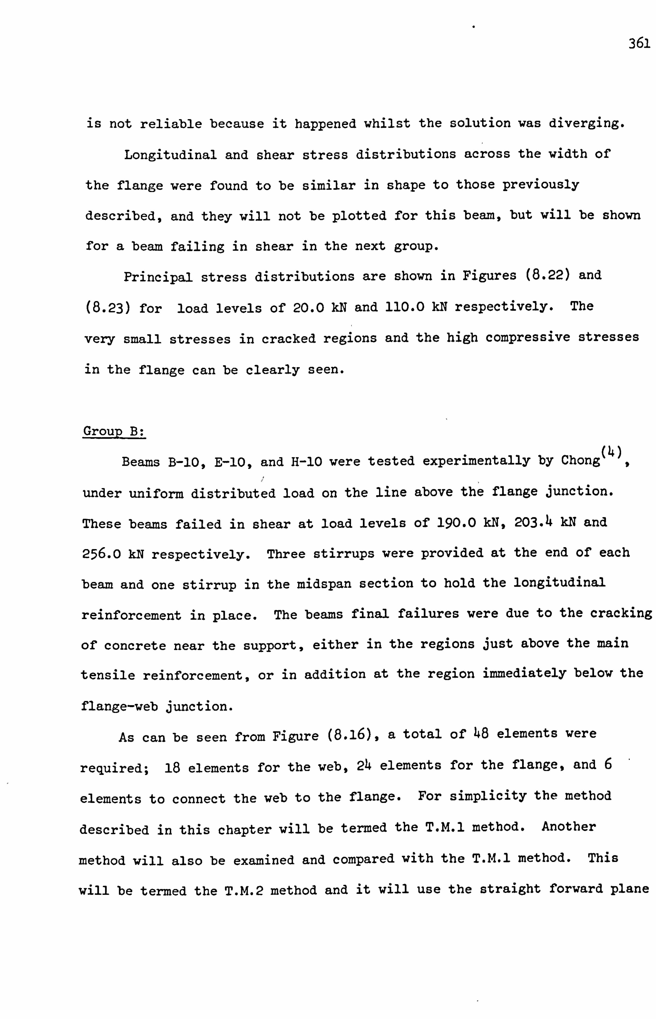
361
is not reliable because it happened whilst the solution was diverging.
Longitudinal and shear stress distributions across the width of
the flange were found to be similar in shape to those previously
described, and they will not be plotted for this bean, but will be shown
for a beam failing in shear in the next group.
Principal stress distributions are shown in Figures (8.22) and
(8-23) for load levels of 20.0 kN and 110.0 kN respectively. The
very small stresses in cracked regions and the high compressive stresses
in the flange can be clearly seen.
Group B:
Beams B-10, E-10, and H-10 were tested experimentally by Chong (4)
under uniform distributed load on the line above the flange junction.
These beams failed in shear at load levels of 190.0 M, 203.4 kN and
256.0 kN respectively. Three stirrups were provided at the end of each
beam and one stirrup in the midspan section to hold the longitudinal
reinforcement in place. The beams final failures were due to the cracking
of concrete near the support, either in the regions just above the main
tensile reinforcement, or in addition at the region immediately below the
flange-web junction.
As can be seen from Figure (8.16), a total of 48 elements were
required; 18 elements for the web, 24 elements for the flange, and 6
elements to connect the web to the flange. For simplicity the method
described in this chapter will be termed the T. M. 1 method. Another
method will also be examined and compared with the T. M. 1 method. This
will be termed the T. M. 2 method and it will use the straight forward plane

362
stress approximation with different thickness for the web and flange.
This means that the stresses and displacements will be constant throughout
the width of the flange. The T. M. 1 method will be used for all beams
in this group whilst the T. M. 2 method will be used for beams B-10, and E-10
only.
Different load deflection curves are compared for beams B-10, E-10,
and H-10 in Figures (8.24 - 8.26). It can be observed that using the
experimental values of concrete properties produced a stiffer load
deflection curve at the initial stages of loading. This was even more
significant at the higher load levels especially before the failure stage.
Also, it can be seen that the load deflection curves obtained by using
the T. M. 2 method for the beans B-10 and E-10 were similar to those
obtained by using the T. M. 1 method. The ultimate loads were overestimated
for beams B-10 and E-10 when using the T. M. 1 method. This was much more
so for these beams when the T. M. 2 method was used.
It appears that the stiff load deflection curve at the lower load
levels using the T. M. 1 method was not simply due to the approximations
assumed in that method, because the T. M. 2 method produced almost similar
curves at those load levels. This stiff response could be due to other
effects such as the inexact experimental value of Young's modulus which
may produce this type of variation, or to other effects such as the
existence of microcracking at the initial stages of loading which cannot
be approximated early in the finite element model. This could be further
confirmed if both methods show a similar crack pattern in the web in the
initial stages. Since similar crack patterns were obtained experimentally
in all these beams, only beam E-10 will be discussed. Different crack
patterns are shown in Figures (8.27 - 8.30) using the T. M. 1 method. It

363
can be observed that the beam developed flexural tension cracks at
low load levels near the midspan section.
Further increase of load caused the appearance of diagonal cracks
which were inclined at an angle of about 45 0 to the beam axis. As this
load is increased more cracks developed towards the compression zone
accompanied by other cracks developing downward to the soffit or plunge.
In the compression zone, after cracks had reached the underside of the
flange, they started to propagate along the flange itself. The existence
of these cracks led to a stage at which the beam was unable to sustain
any increase in load. From Figure (8-30) it is clear that the failure
is in shear and crushing appeared in the region immediately below the
flange-web junction. This description of the crack propagation is very
similar to the experimental descriptions except that there were some
cracks reaching the outer side of the flange in the experimental results
which this method could not produce. This could be another reason why
a stiff load deflection curve was obtained compared with the experimental
one.
Principal stress directions at two different load levels are shown
in Figures (8-31) and (8.32). The existence of tension stresses in the
web at the low load level can be seen. These stresses disappear at
higher load levels when most of the cracks have appeared. Arching action
is very clear in Figure (8-32).
Different crack patterns are plotted in Figures (8-33 - 8.36) with
the T. M. 2 method. It can be observed that the crack propagations in the
flange at the low load levels are similar to that described by the T. M. 1
method. However at higher load levels web shear cracks develop towards
the flange but no cracks were predicted in the flange itself. After that,
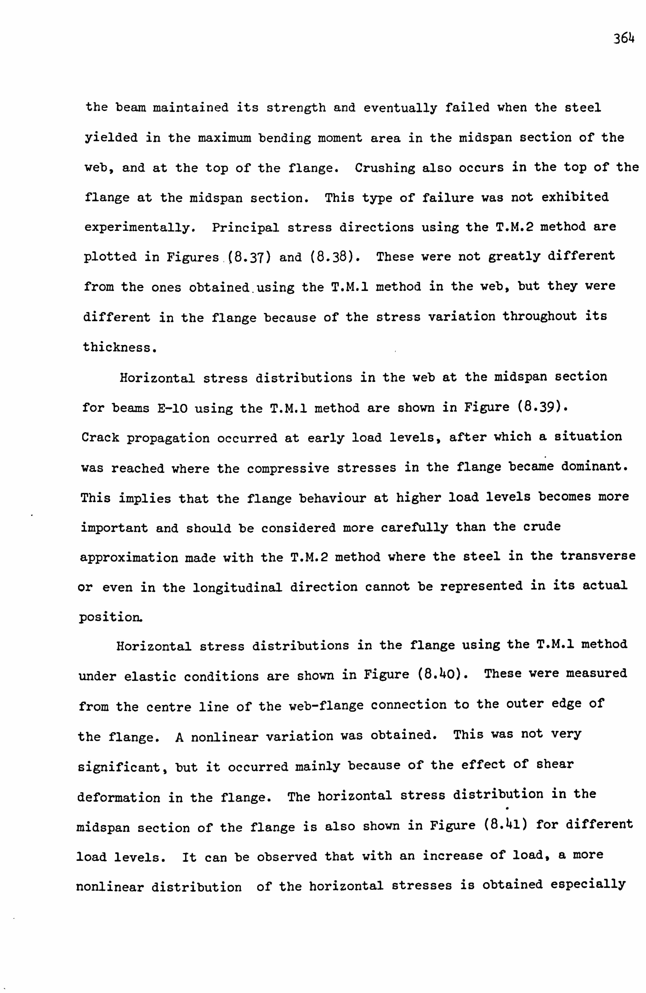
364
the beam maintained its strength and eventually failed when the steel
yielded in the maximum bending moment area in the midspan section of the
web, and at the top of the flange. Crushing also occurs in the top of the
flange at the midspan section. This type of failure was not exhibited
experimentally. Principal stress directions using the T. M. 2 method are
plotted in Figures, (8-37) and (8-38). These were not greatly different
from the ones obtained, using the T. M. 1 method in the web, but they were
different in the flange because of the stress variation throughout its
thickness.
Horizontal stress distributions in the web at the midspan section
for beams E-10 using the T. M. 1 method are shown in Figure (8-39).
Crack propagation occurred at early load levels, after which a situation
was reached where the compressive stresses in the flange became dominant.
This implies that the flange behaviour at higher load levels becomes more
important and should be considered more carefully than the crude
approximation made with the T. M. 2 method where the steel in the transverse
or even in the longitudinal direction cannot be represented in its actual
position.
Horizontal stress distributions in the flange using the T. M. 1 method
under elastic conditions are shown in Figure (8.40). These were measured
from the centre line of the web-flange connection to the outer edge of
the flange. A nonlinear variation was obtained. This was not very
Significant, but it occurred mainly because of the effect of shear
deformation in the flange. The horizontal stress distribution in the
midspan section of the flange is also shown in Figure (8.41) for different
load levels. It can be observed that with an increase of load, a more
nonlinear distribution of the horizontal stresses is obtained especially

365
under the load itself. This is because the higher load levels produced
higher strains in the midspan section than that obtained on the edges of
the flanges, and since the stresses become more nonlinearly related to
the strains at the high load levels, this type of distribution can be
expected.
Shear stress distributionsat different load levels in the midspan
section of the flange are shown in Figure (8.42). These appear to have
a maximum value at about one third of the width of the half flange and
reduce linearly to the outside of the flange. The maximum value was
obtained near the position of the compression reinforcement. This
figure also shows how complex this variation actually is.
Group C:
Beans *E-13 and G-14 were tested by Chong (4)
, under uniformly
distributed load on the line above the flange junction. These beams
failed in shear at load levels of 322.0 kN and 326.1 kN respectively.
As shown in Figures (8.14. b) and (8-14. c), these beams differed from
the beams in group B in that they were provided with web reinforcement
in the form of vertical stirrups. Beam E-13 was provided with 4 mm
stirrups and beam G-14 with 5 mm stirrups. Beam G-14 also has a wider
flange of 500.0 mm than that of 300.0 mm described for the other beams.
Load deflection curves for both beams are compared in Figures (8.43)
and (8.44) for the T. M. 1 method. Although the load deflection curves
were predicted fairly well, poor agreement was obtained for the ultimate
load. Failure was due to the yielding of stirrups in the web at a distance
of 800.0 mm from the midspan section. This failure is a valid character-
istic of beams failing in shear with vertical stirrups, and occurs because

366
of the effect of shear cracks developing in the shear span section.
For beam G-14 different load deflection curves are also compared
in Figure (8.44) using different values of V. The change in this value t
did not produce any major effect on the load deflection curve and ultimate
load. This was not the case for the beam which failed in flexure. It
appears that the change in the predicted ultimate load in the beam failing
in flexure was caused by the different loads at which the longitudinal
reinforcement yielded at the midspan section. The steel stresses seem
to be significantly affected at this position according to when the
flexural cracks occurred which itself depends on the value of V. However t
for the beam failing in shear, this was caused by the yield of vertical
stirrups in the top of the web near the support. The stresses in these
stirrups-were not greatly affected by the initiation of the flexural
cracks and the change of V did not produce a major change in the stirrup t
stresses.
Crack patterns will be described for only one beam because a similar
pattern was observed experimentally for both beams. These are shown for
beam E-13 in Figures (8.45 - 8.48); flexural cracks appeared initially
followed by diagonal cracks. The diagonal cracks appeared both as
extensions of flexural cracks, and as isolated inclined web-shear cracks.
The web shear cracks propagated towards the flange and the support
regions, as the load increased. Failure occurred when stirrups yielded
in the web and divergence of the solution occurred. The description
is similar to that observed experimentally.
Principal stress directions are shown in Figures (8.49) and (8.50)
for load levels of 50.0 kN and 250.0 M. It can be seen that the tension
stresses are very small in regions where cracks have developed. At high

367
loads compression stresses become more significant and arching action
is very clear. Also, very high compressions were developed near the
support which caused the vertical steel to yield and cause failure.
8.7 Conclusions:
Using the plane stress approximation, a simple method was proposed
to analyse different types of T-beams. The general trend in the shape
of the load deflection curves was relatively acceptable but they did not
always compare well with the experimental results. However the range
of error in ultimate load was fairly reasonable. A comparison of
measured and computed ultimate loads are shown below:
Beam name wu
measured ultimate load (kN)
QS
computed ultimate load (kN)
QS /W u
B-2 127.0 125.0 0.98 B-10 190.0 215.0 1.13 E-10 203.4 225.0 1.11
H-10 256.2 250.0 o. 98 E-13 322.0 280.0 0.87
G-14 326.0 270.0 L
0.83
The method requires more investigation regarding the improvement of the
shape of the load deflection curve and in checking the validity of the
stress distribution in the web and flange, compared with experimental
results. Different values of Young's modulus should be examined, and the
effect of using different values of the strain hardening part of the
steel on the load deflection curve should be checked. The effect of
flange behaviour also appears to be significant and should be examined
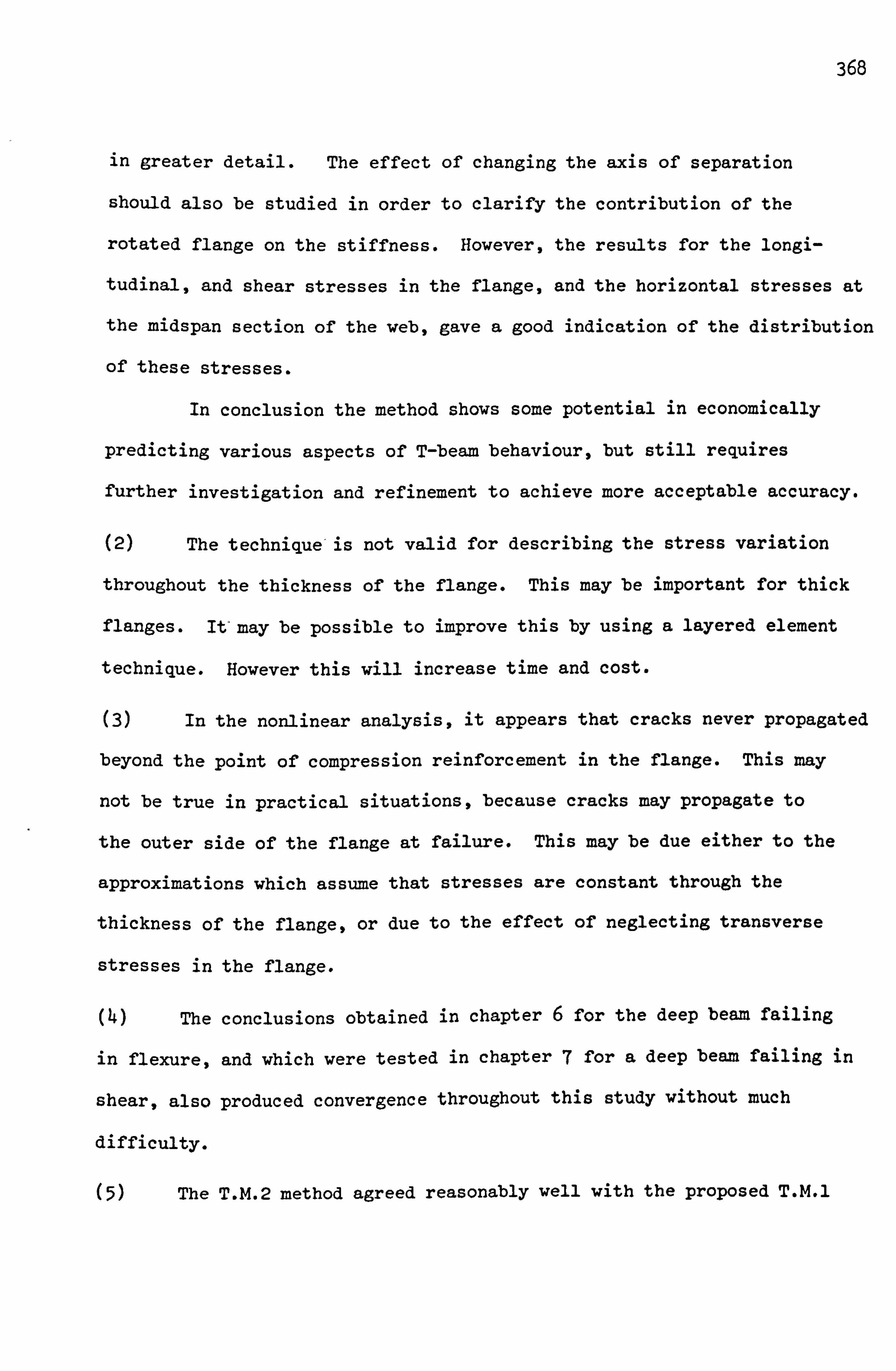
368
in greater detail. The effect of changing the axis of separation
should also be studied in order to clarify the contribution of the
rotated flange on the stiffness. However, the results for the longi-
tudinal, and shear stresses in the flange, and the horizontal stresses at
the midspan section of the web, gave a good indication of the distribution
of these stresses.
In conclusion the method shows some potential in economically
predicting various aspects of T-beam behaviour, but still requires
further investigation and refinement to achieve more acceptable accuracy.
(2) The technique-is not valid for describing the stress variation
throughout the thickness of the flange. This may be important for thick
flanges. It'may be possible to improve this by using a layered element
technique. However this will increase time and cost.
(3) In the nonlinear analysis, it appears that cracks never propagated
beyond the point of compression reinforcement in the flange. This may
not be true in practical situations, because cracks may propagate to
the outer side of the flange at failure. This may be due either to the
approximations which assume that stresses are constant through the
thickness of the flange, or due to the effect of neglecting transverse
stresses in the flange.
(4) The conclusions obtained in chapter 6 for the deep beam failing
in flexure, and which were tested in chapter 7 for a deep beam failing in
shear, also produced convergence throughout this study without much
difficulty.
(5) The T. M. 2 method agreed reasonably well with the proposed T. M. 1

369
method for the stiffness of the load deflection curve. This implies
that approximations in the T. M. 1 method were not solely responsible
for the shape of the load deflection curve compared with the experimental
situation and the stiff response obtained in some curves could therefore
be due to other factors.
The T. M. 1 method was better in predicting the ultimate load than
the T. M. 2 method. This suggests the importance of flange behaviour on
a solution especially during the final load stages. This is because the
T. M. 1 method used a better approximation for the flange whereas the
web simulation was similar in both methods. In particular the role of
any crack development could be crucial. For the T. M. 1 method this would
be better simulated by using a layered element technique or by reducing
the stiffness of the flange elements by some indirect means. This would
require the identification of suitable parameters for determining cracks
in the flange. Or, less importantly, the T. M. 2 method could be improved
by using more elements through the depth of the flange.
(7) It appears that the steel is a major factor governing failure
in most of these beams. As steel started to yield (either in the stirrups
or in the main tension reinforcement) failure occurred.
(8) The method developed in this chapter could also be used to
analyse the nonlinear behaviour of L-beam and box girder structures
with thin flanges. Certain changes in boundary conditions need to be
considered, and further study would be required to work out the approxi-
mations.

370
Bean name Centroidal axis/
Second moment of Case 1 Case 2 Case 3 Case 4 Case 5 area
Rao B-2 y mm 150.5 143.2 155.3 144.1 154.4 I MM4 118.9E6 96.8E6 134.9E6 99-5E6 123.4E6
xx 1
Chong B-10 y nun 145.0 137.5 150.0 138.4 14o. 8 Im4
II 88.1E6 70.8E6 100.8E6 72.9E6 91-3E6 - xx
Chong E-10 mm 150.0 135.0 160.0 136.9 153.5
E-13 MM4 I 91.8E6 6o. 8E6 115.2E6 64.6E6 92. OE6 xx
Chong H-10 y mm 152.0 128.0 168. o 131.0 154.5 =4 I 92.6E6 47.8E6 126.7E6 53.6E6 87-9E6
XX ChongG-14 y mm 165.0 146.3 18o. o 147.6 166.7
I MM4 109.8E6 69.8E6 144. OE6 72.9E6 lo6.7E6 xx I I I I I
Table (8.1) Selection of axis of rotation.
Beam name Total height
(mm) Web width
(mm)
tf Flange thickness
(mm)
hf Flange width
Rao B-2 250 120 4o 360
Chong B-10 240 100 4o 300
Chong E-10 240 100 6o 300
Chong H-10 240 100 80 300
Chong E-13 240 100 60 300
Chong G-14 240 100 6o 500
Table (8.2) Beam dimensions.

371
Beam name Xi X2
I X3 X4 X5 X6
1 X7 Xe X9
B-10 4o. o 90.0 90.0 0.0 40.0 36.7 36.7 36.6 370.0
E-10 4o. o 85.0 85.0 0.0 40.0 36.7 36.7 36.6 36o. o H-10 4o. o 80.0 80.0 0.0 40.0 36.7 36.7 36.6 350.0
E-13 40.0 85.0 85.0 0.0 40.0 36.7 36.7 36.6 36o. 0
G-14
I
4o. o I
85.0
-
85-0' 0.0 40.0 70-0
I
70.0
I
70.0
I
46o. o
--- --I Table (8-3) Details for mesh dimensions of Chong beams.
Beam name f (N/MM2) cu
V (N/MM2) c
fl (N/MM2) t EC(N/MM2) v c
Rao B-2 48. o 37.4 4.8 . 35 x 105 0.20
Chong B-10 37.2 29.0 4.2 . 25x 105 o. 18 Chong E-10 33.2 25.9 4. o . 24x 105 0.18 Chong H-10 35.0 27.3 4.1 . 25x 105 o. 18 Chong E-13 33.6 26.2 4. o . 24x 105 o. 18 Chong G-14 38-5 30.0 4.3 , 26 x 105 o. 18
Table (8.4) Concrete properties.
Beam name Bar description fy (N/mm2) Es (N/MM2) Ew (N/MM2)
Rao Longitudinal 340 . 20x 106 0.0
beam Stirrups 495' . 22 x 106 0.0
Chong Longitudinal 479 lgx 106 57.23
beams Stirrups 622 . 21x 106 82-50
Compression 399 . 20x 106 0.0
Table (8.5) Steel properties.

372
compression tension compression
neutral axis of flange
. -. -. -. -. -. neutral axis of web
7-- __ -'== -
ension
Figure (8*1) Direct strain distribution in a T-beam.
Figure (8*2) Variation of compression stresses above the
neutral axis for a T-beam.
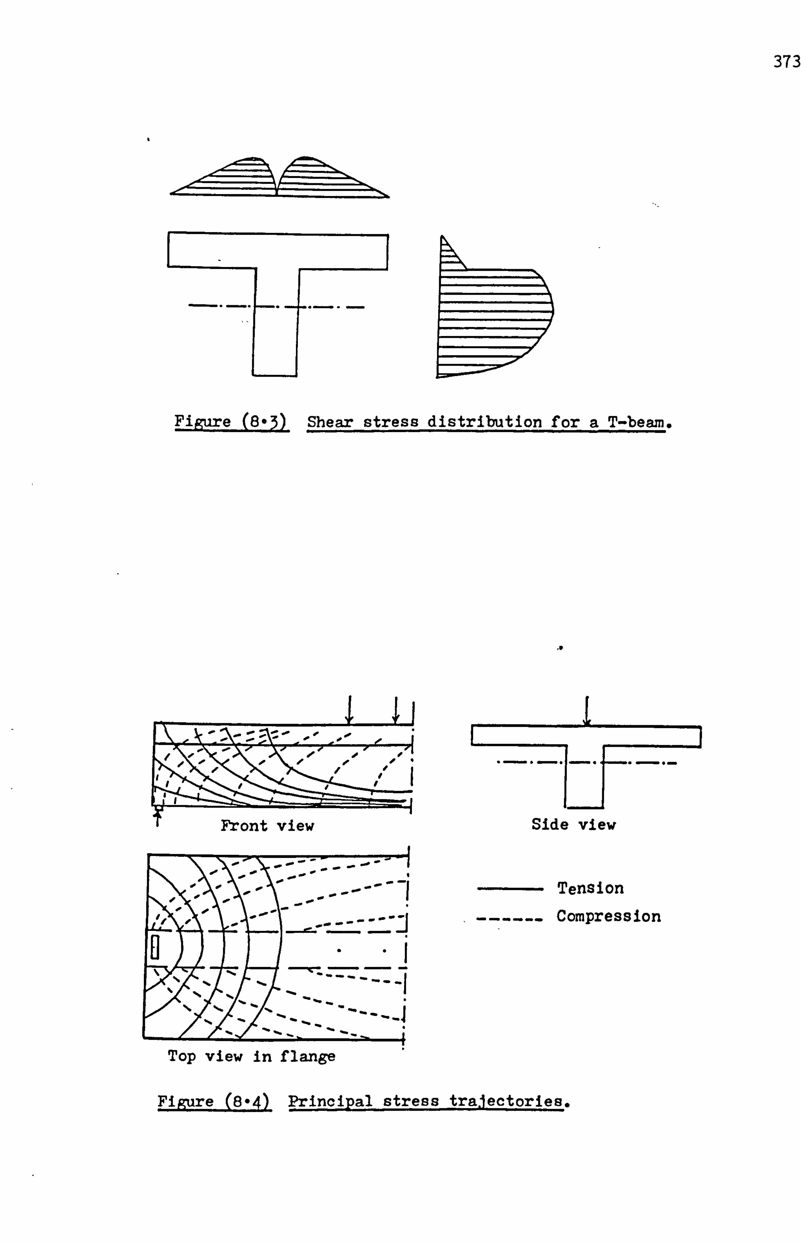
373
Figure (8*3) Shear stress distribution for a T-beam.
Ax
Front view
9---
1
Top view in flange
Side view
Tension Compression
Figure (8-4) Principal stress trajectories_.

374
F. D.
-C-
1-
--J6
2- ---j" -p- -y- x- -Z- ýw- -K--
(a) concentrated load
2W
1.4 '"A.
1 II I- I -. --
III I -- +4 "% .I
I, _. - . ---/-i.
J... -.. I- 1-c- IV- 4w- -w-
(b) distributed load
Rigure (8-5) Different stress distribution in the flange.
-
II, tI ________
00 J
deflected web
Figure (8-6) Bending and shear transfer from the web to the flange.
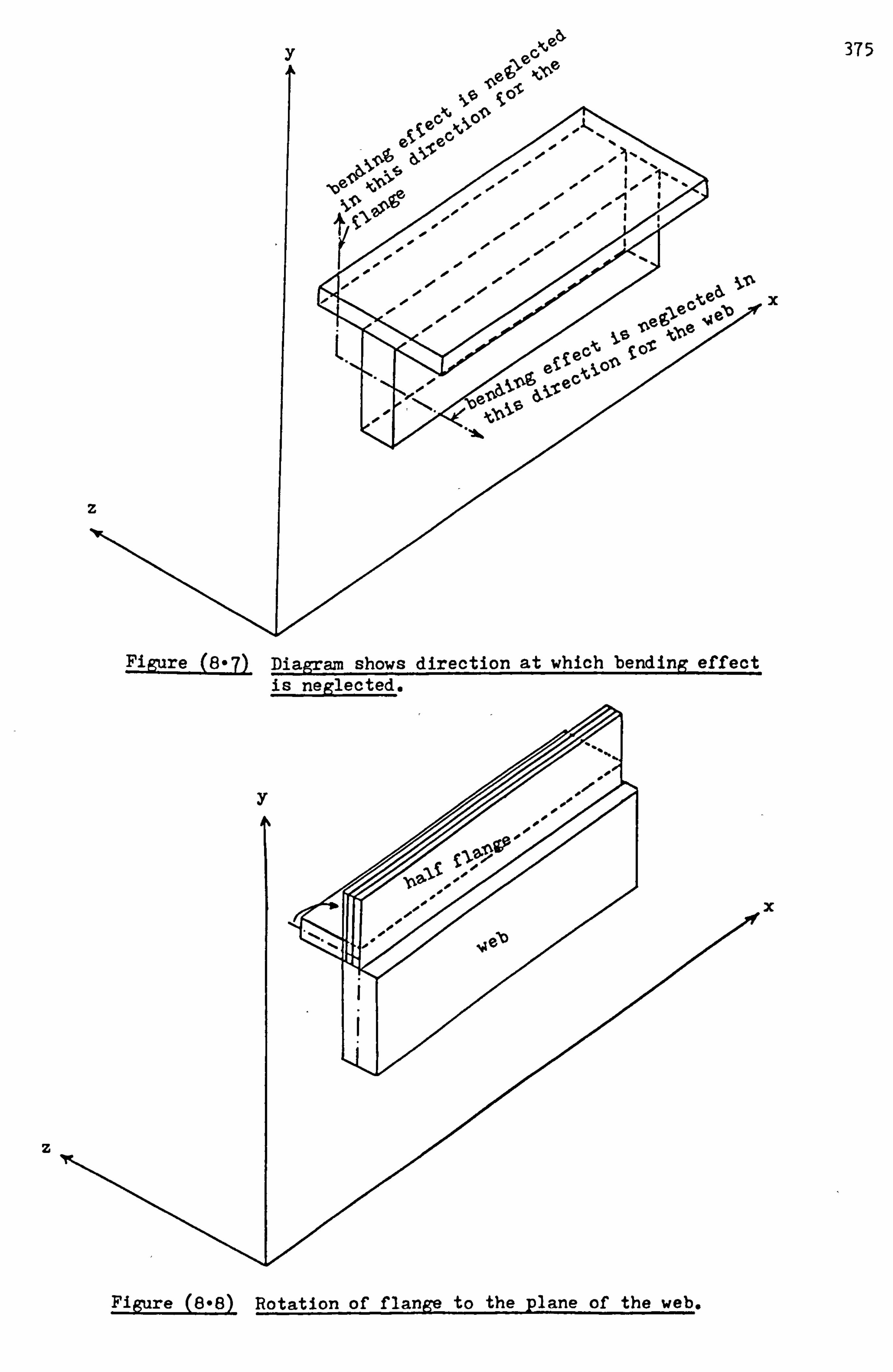
y eG
10,
. 01
0 .0
te& x eo "o je L.
Sect 'I- t OX
e
z
Figure (8-7) Diagram shows direction at which bending effect is neglected.
�7X
375
Figure (8-8) Rotation of flange to the plane of the web.
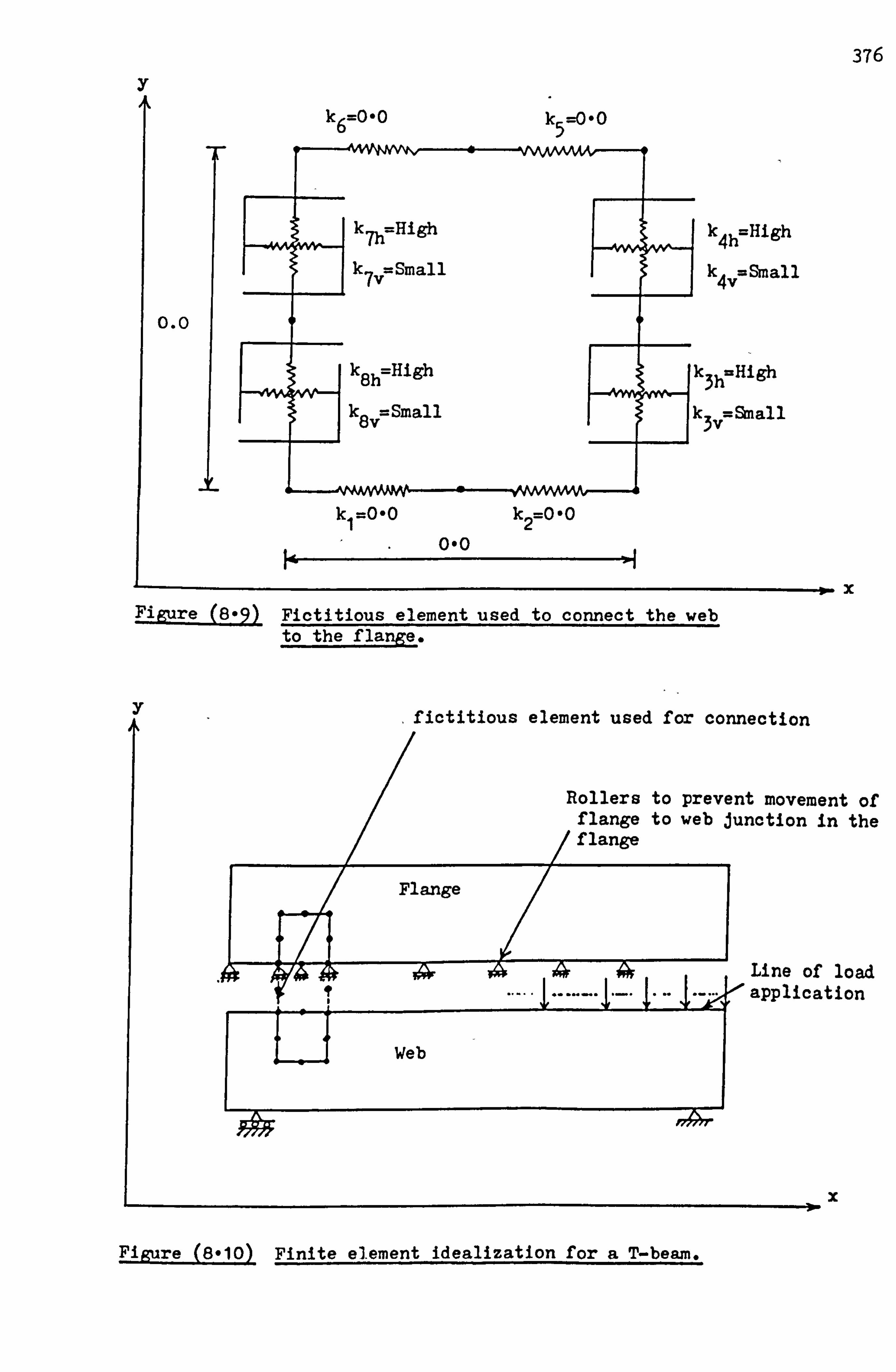
376 y
k 62'-O'o k5 --0-0
k 4h =High
k 4v =Small
0.0
k 3h7High
k 3v =Small
i4 0-0
Figure_(_8-9), Fictitious element used to connect the web to the flange.
I fictitious element used for connection
x
t movement of notion in the
Line of load application
x
Figure (8-10) Finite element idealization for a T-beam.
k1 =0-0 k2 =0-0
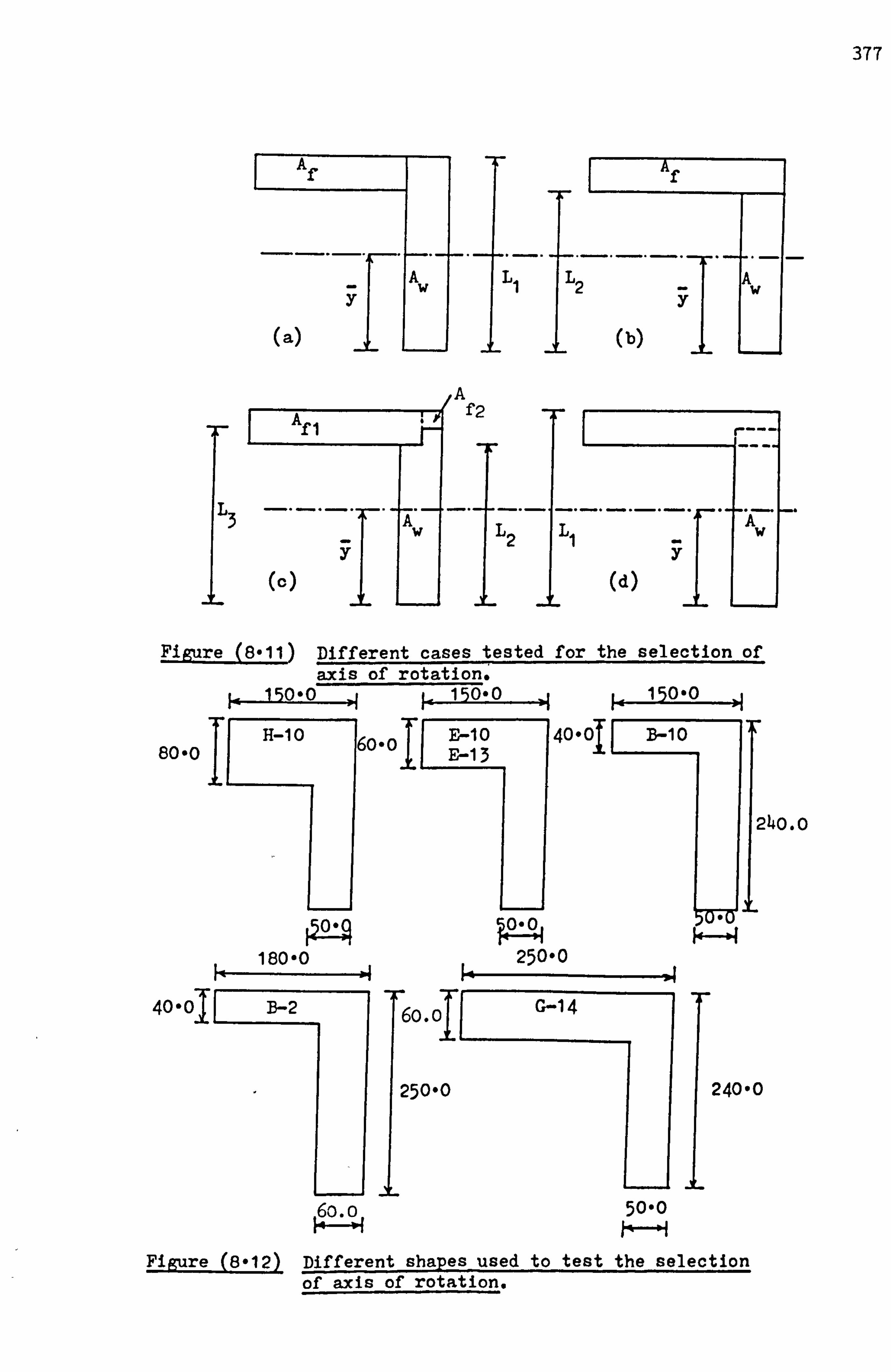
377
L3
11 (C)
L in; y
(b)
eA f2
L2LI y
(d)
Figure (8oll) Different cases tested for the selection of axis of rotation.
80-0
150 -0 150-0 15000
H-1 0 090,400 ol
180-0
40-olL B-2 1
6o. o
50-0.
25000
T G-1 4 6o.
25000
5000
240.0
L
24000
Figure 8*12) Different shapes used to test the selection of axis of rotation.

376
5mm 360
-7 C- 10 4
a- 40.,
2101 lomm a 100 C/o
Emm
10
3_T 20mm
-f - 120 01
Section A-A .- -- - . -- t, In
ýr 40
L
210
I
L--30, 14 150
'1 16 __ _1650 1
Half elevation -1
1 01
1021
28 281
, 1§9 150 50 , +0150 l, 1 4.1 , L, 150 1ý150, jf. 1500. jlf
. 50 ý 1,150 -1 J50 ý 10150
Mesh used
Figure (8-13) Details of Co2e & Rao T-beam B-2.

379
h
h1f
(b)'-Beam F-13
--- -I
hfT
Beam G-14
(a) Beam B-10,, E-10, H-10
75 C/C
-r
240
41
75 C/C
240
JL
. r5 C/C
240
Figure (8914) Details of ChonK T-beams.
2400 ol
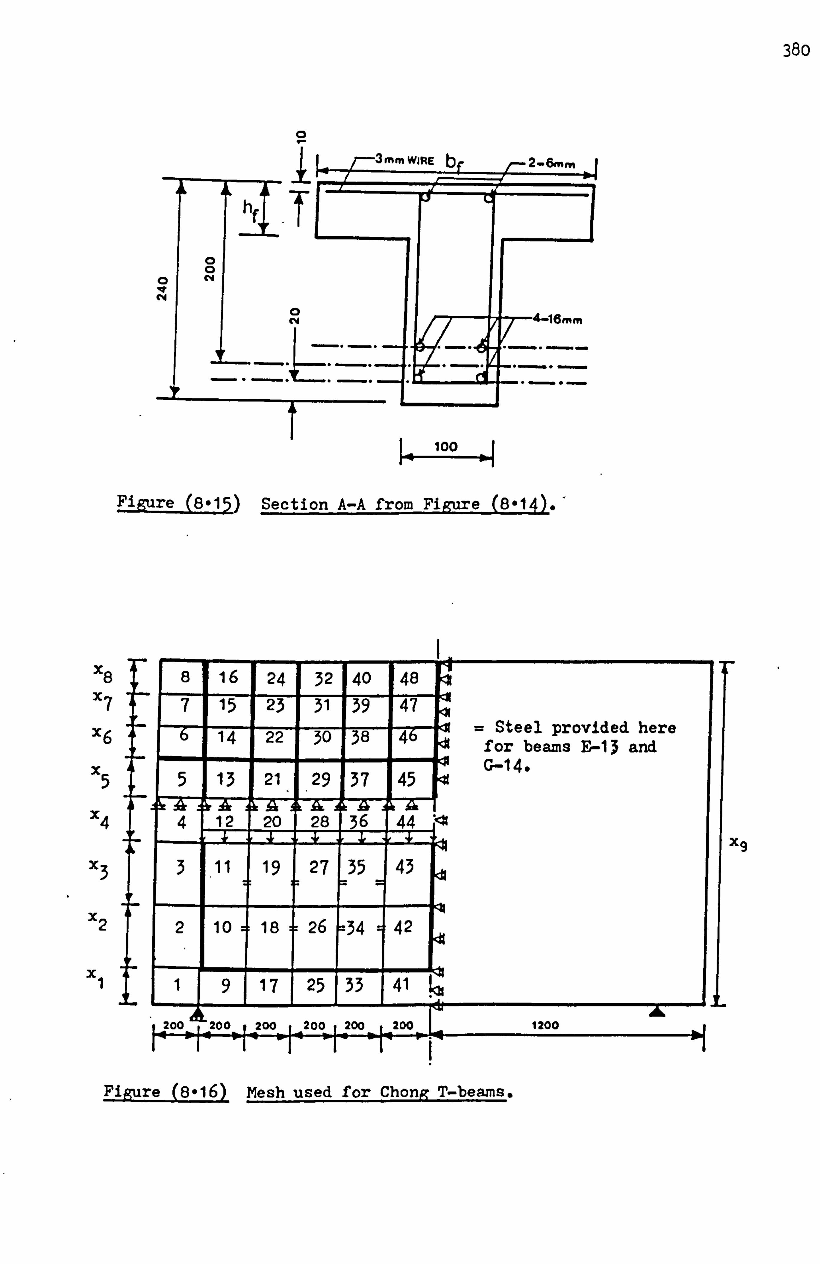
380
1 I
c4
C, 4
1
mm WIRIE ör o-- 2- 6m nn
0 C4
x8 x7
x6
x5
x4
x3
x2
Figure (8-15) Section A-A from Figure (8*14)-'
8 16 24 32 40 48 7 15 23 31
I
39
I
47 Ot l id dh 14 22-- 30 38 4; 7- ee prov e ere
for beams F-13 and 5 13 21 29 37 45
G-14.
4 12 20 28 36 44 4i -41 . 1 4C
3 19 1 27 =35
43
2 10 18 26 =34 42
1 9 17 25 33 41 AL A6
1-100_ 1_.? Oo_ 1_201ý 1_ýOo_ L-200_ 1200
X9
Figure (8-16) Mesh used for Chong T-beams.
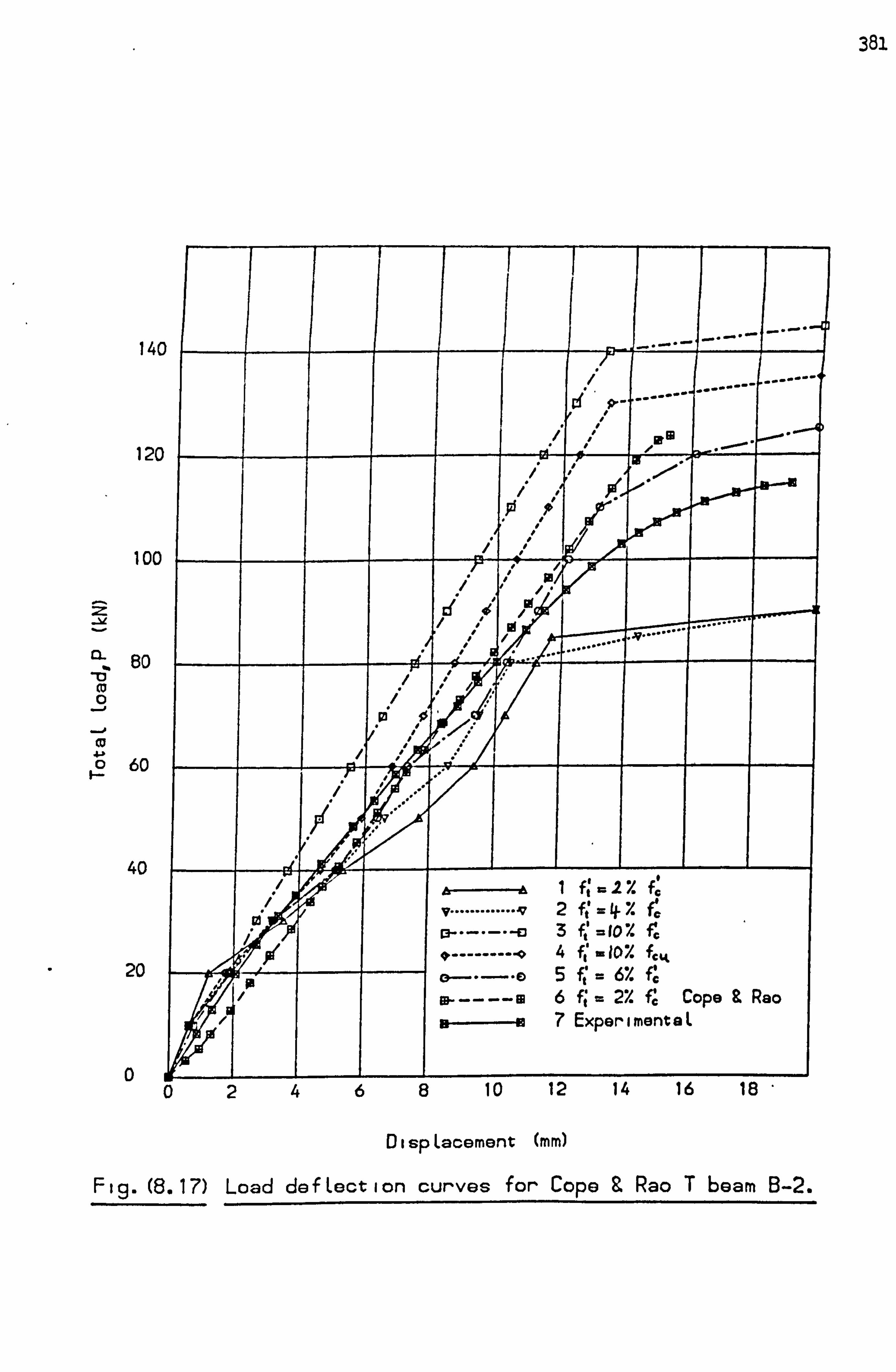
381
IM
12C
100
eo
4-
FO 60
40
20
- ------- -------- OL
Sp-41
/ 19
............. ........ ......
i f, -. 2 7. f.,
v ............. 2 ft' 4 7. ....... El 3 f, ' 10 7. r, ---------- *4 fl, ID7. f"
, P, I 431----ID 5 ft' =67. re 6 ft' =27. PC cope & Rao 7 ExperimentaL
8 10 12 14 16 IS
DispLacement (mm)
Fig. (8.17) Load defLection curves for Cope & Rao T beam B-2.
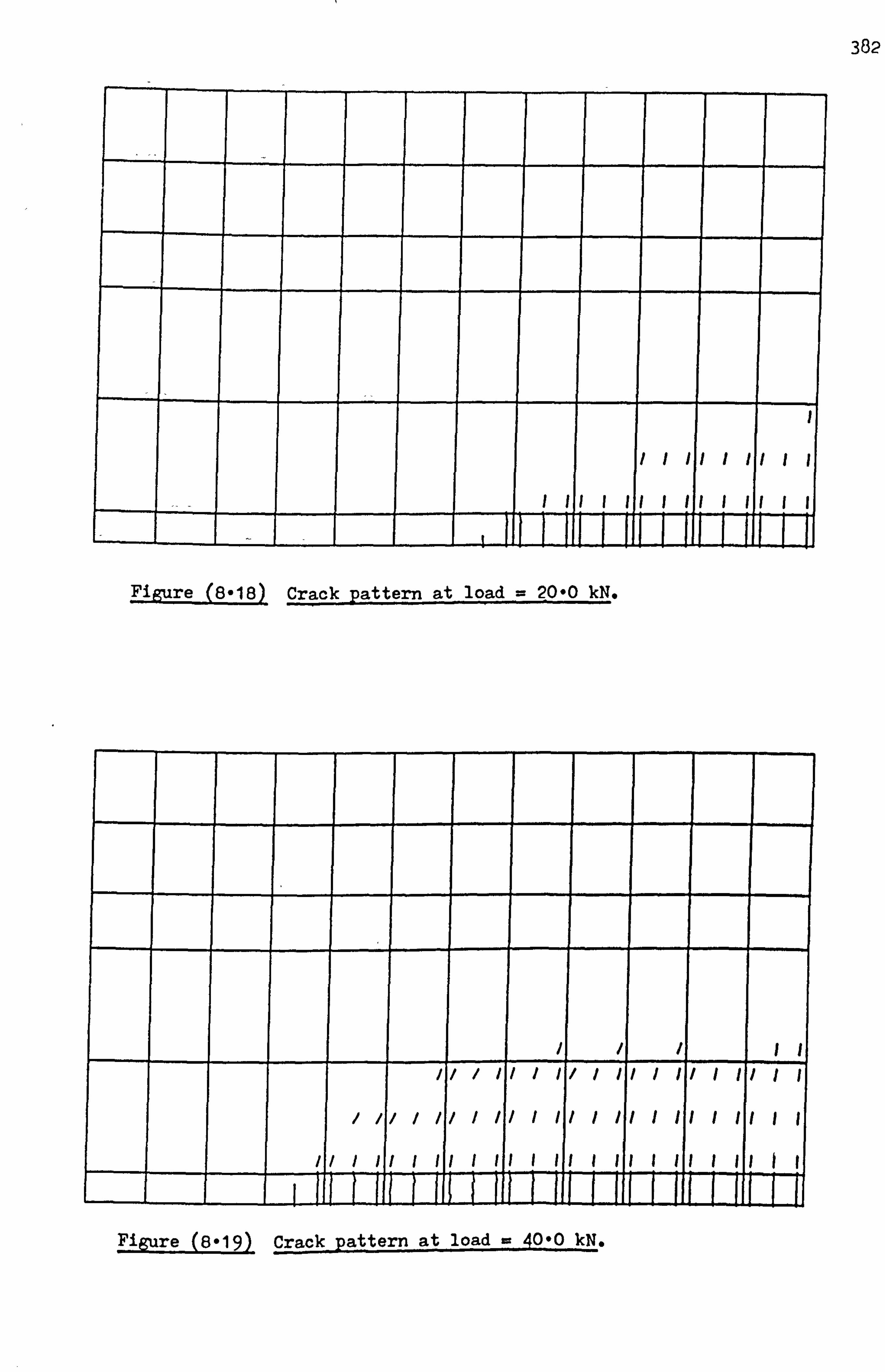
382
/I II I II 1I
_____ _____ _____ _____ _____ _____ _____ I II I II I II I II II
_______1JIIIi. IIfLiIt Figure (8-18) Crack pattern at load = 20-0 M.
I I
I i
___ _ _ _ / /
_ _ _/ _ _ _ I,
/ 1/ /
1
/
/
/
/
/
II
II
/
I
//
II
/
/
I
I
I
I
/
I
I
I
I
I
I
I
I
I
I
I
II
II
__ ____ I ii iI I H H H I H i H _H Figure (8-19) Crack pattern at load = 40_90 kN.

383
___ ___ _ __ / I I I I I I / II
____ ___
___ _
i
__
1
ii
_
/
i
_
1
l
_ /
/
I
_
I
I
__ //
//
II
1
/
I
/
I
I
II
1/
II
I
I
I
I
I
I
I
I
I
/
/
I
I
I
I
F
I
I
I
I
I
I
I
I
I
I
I
I
I
I
I
I
I
I
I
t
I
II
II
__ _ ___
_ H ) I J H J H H ffl h I I I H I I H I
Figure (8*20) Crack pattern at load = 50-0 kN.
/ / d
_ _ _ _ __ __ _ _ _ _ _ __ _ _ _ ___
___
_
/
/
_ _
/
_ __
/
_ _ _
' / /
_
'
_
/
_
/ , / / , / / , / 1 , / / , // , I
/
g
/
/
/ ///
�
�/
/
/
�
/
//
/1
/
/
//
/I
/
I
/
/
/
I
/
I
/
I
I
I
/
I
I
I
/
I
I
I
/
I
I
I
/
I
Il
II I I
t
I
_
l lH
I H _ I I H L i th u H H H i l l Figure (8921) Crack pattern at load = 120-0 kN.
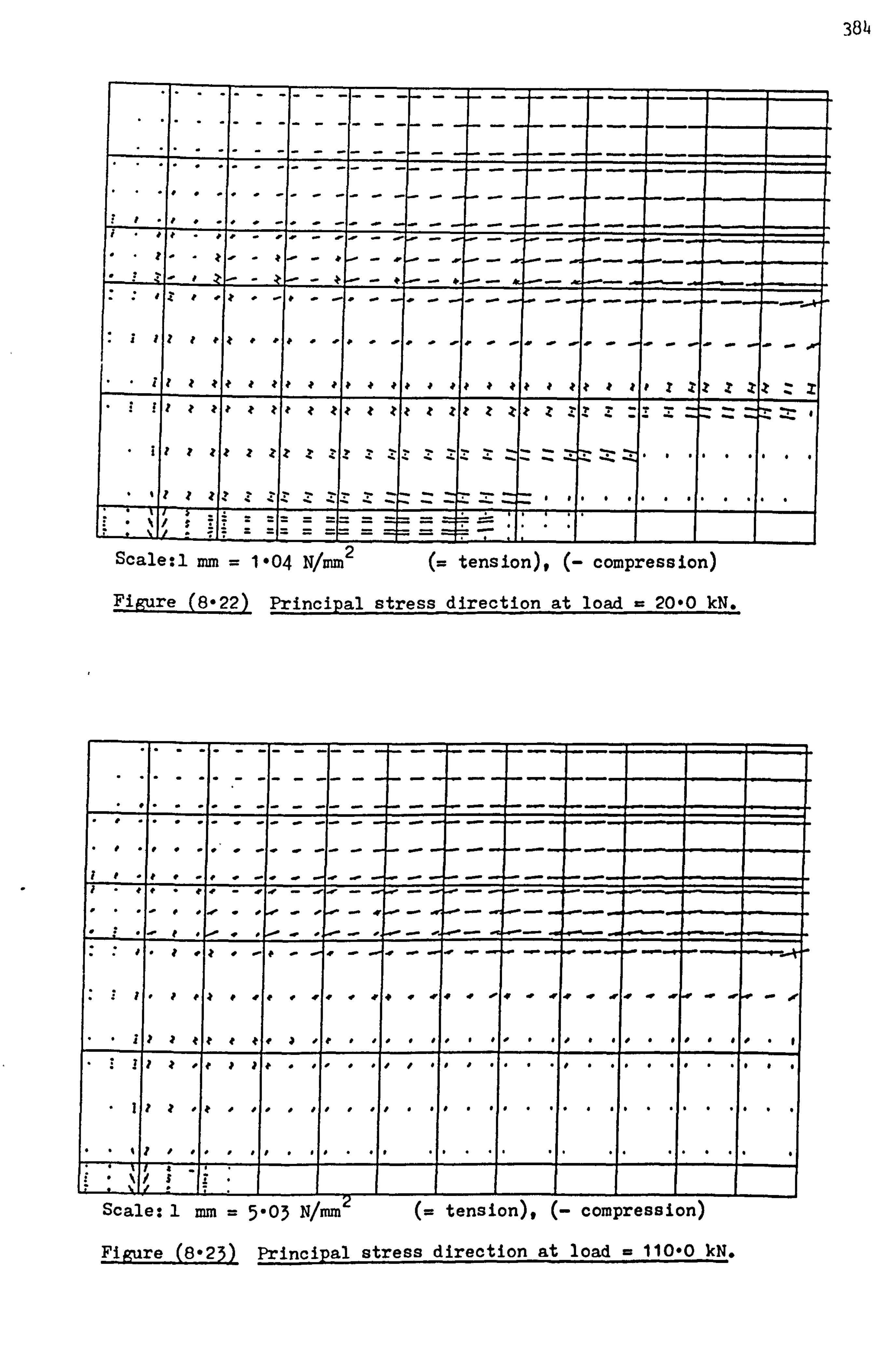
384
1P
--- - -- -
I
- x 41 Zxz 11 X
IT
I X-Z - -Z 7 T7 1 .1 ý' 't tt t '% 't tttt ' '. " -Z I* z . 14 1z: -- ZzZ -- :: '-- ZC#
iI-, -, 't , zz zzzzz 4- z zz -7- - :: Z: zz
'4 Z z-_
Scale: 1 mm 1 *04 NIMM2 tension), compression)
Figure (8o22) Principal stress direction at load = 20*0 kN.
. . . . . . . . . .
. ... . . . . . . . .. . .. .
1
7
Scale: 1 mm = 5'03 N/mmý' (= tension), (- compression)
Figure (8-23) Principal stress direction at load = 110-0 kN.

385
250
200
)3
lp
150
0
4J 0 lzr
100
50
I T. M. 1 (F Lange rot at i on)
v ................... 17 2 T. M. 2 (S i de 9 Levat i on) 13 ........ a3 Experime ntaL
0 0 10 15 lev
Di sp Lacoment (mm)
Fig. (8.24) Load defLection curves for Chong T beam B-10.
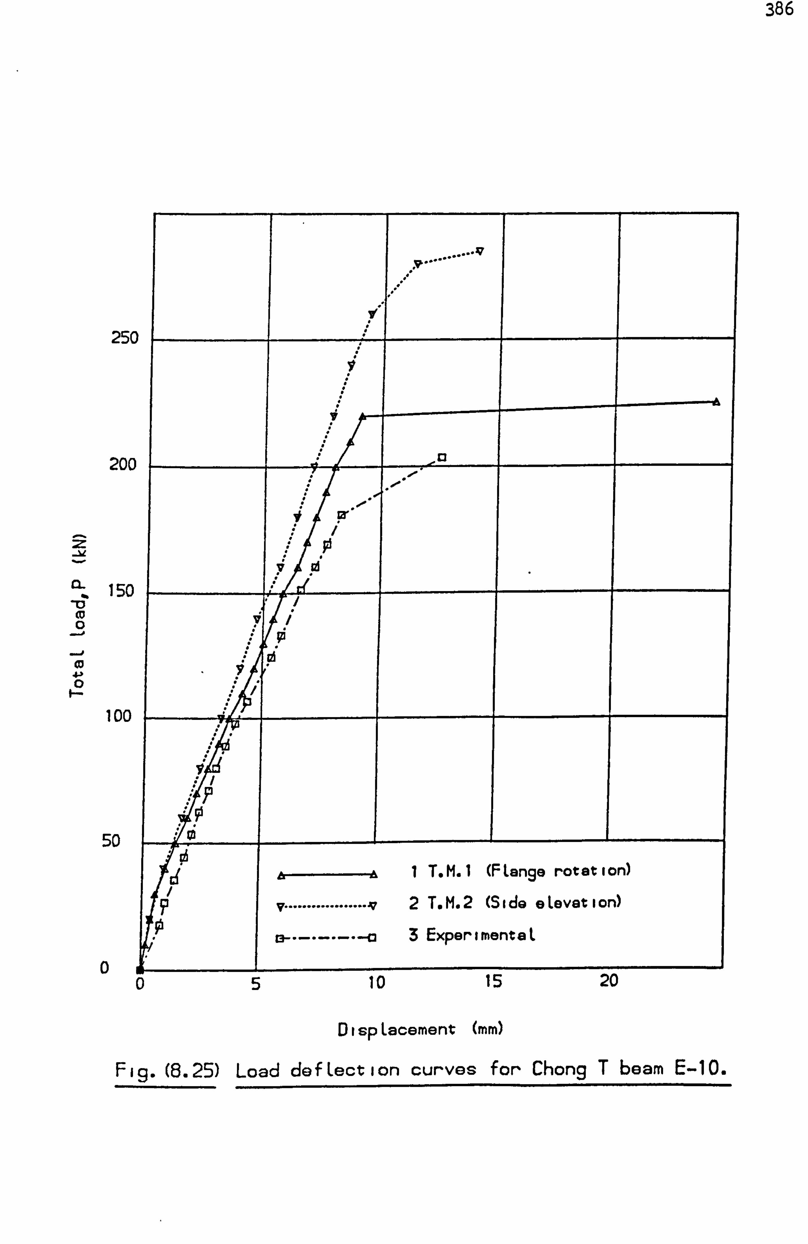
386
4ý
25(
20C
150
100
50
0
. _13
ur
.1J .0
w cd
1 T. M. 1 (FLange rotation)
v .................. 72T. M. 2 (Side eLevation) 13 ......... C3 3 ExperimentaL
5 10 is 20
Di sp Lacement (mm)
Fig. (8.25) Load defLection curves for Chong T beam E-10.
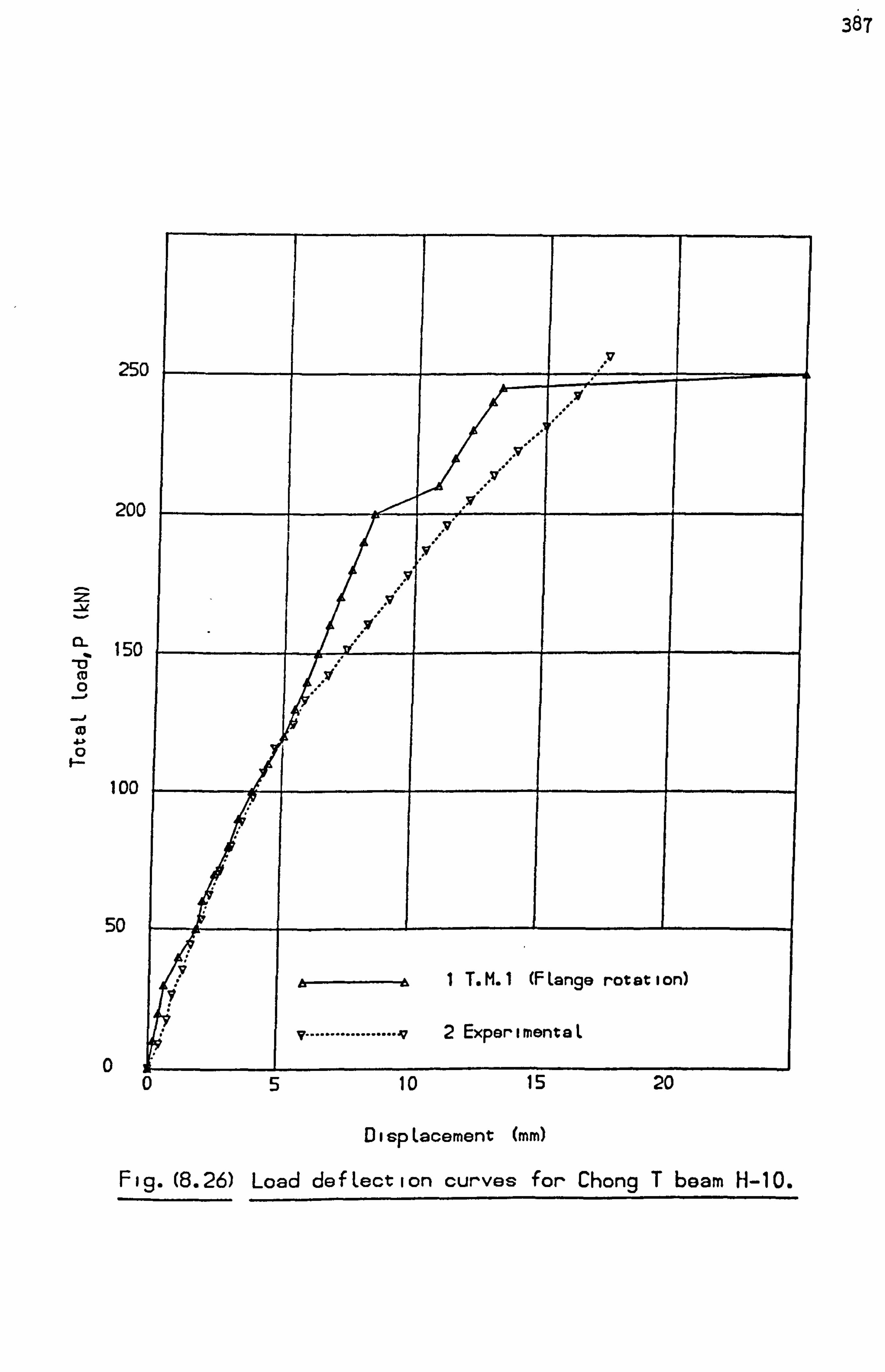
38T
25(
20C
2 Zýl CL 150
0
--0 (0
100
50
Di sp Lacement (rnm)
Flg. (8.26) Load defLection curves for Chong T beam H-10.
5 10 is 20

388
IIIIII
I% ll 1 11 111
Figure (8*27) Crack pattern at load = 50*0 M,
/ I I ______ ______ ______
/
//
-//
//I
III
II
III
III - _
II
III
III
______ ______
II II
% III
1 III III
III III III
Figure (8-281 Crack pattern at load = 75*0 kN.
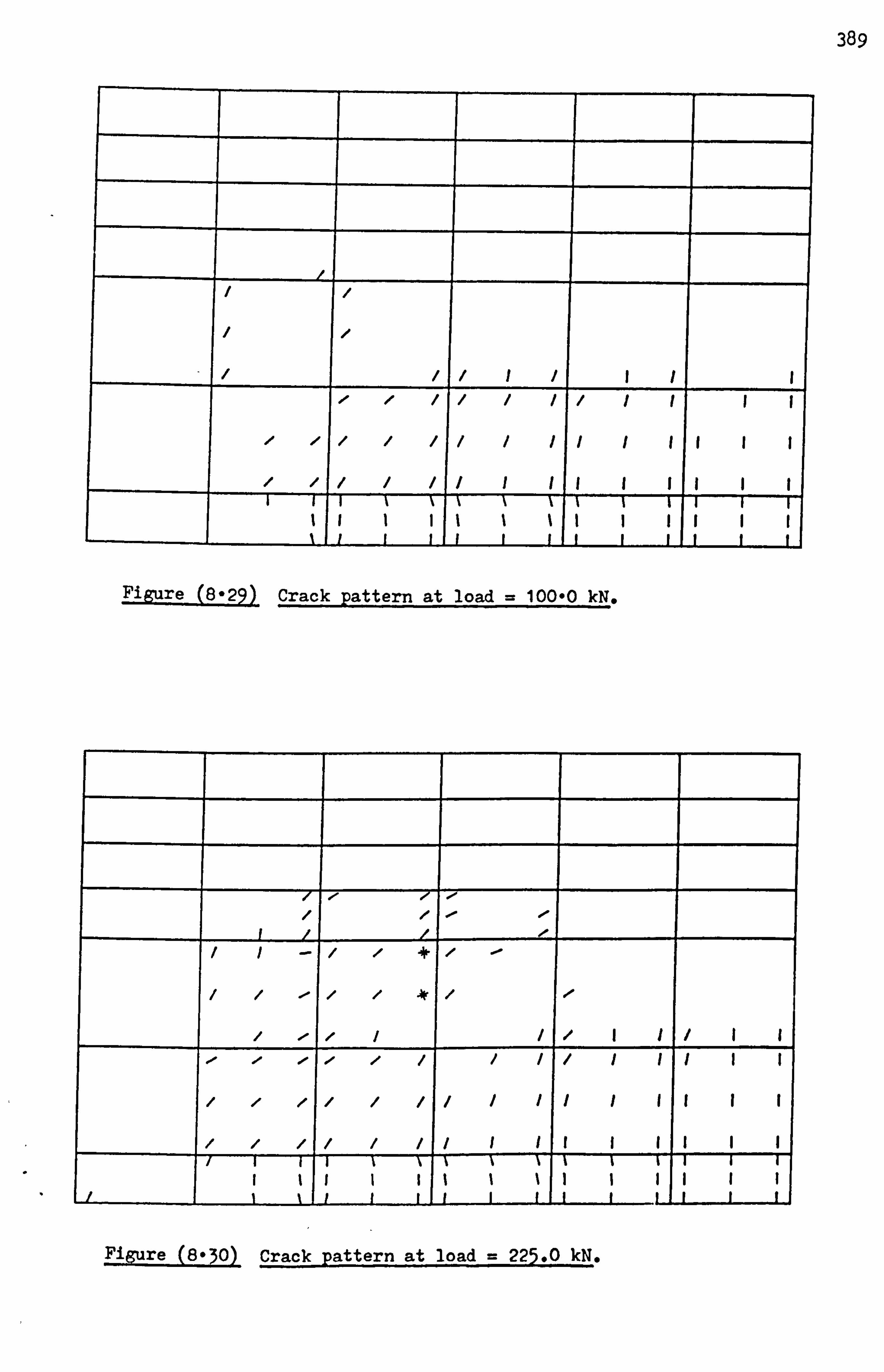
389
I___
I I
/
/
______ __ - __ __
/
/
I I I / I I
______
�
'
�
/
/
/
1
/
/
/
1
1
I
/
/
I
/
/
I
I
I
I
I
I
I
/
I
I
II
II II
II II
__
I
___
I
__
I I I
I I
t I
'i
I t II
i I
I I
IIII II II II II
Figure (8*29) Crack pattern at load = 100*0 M.
______ I
/ / /
- / -
/ __ __ __ ______
______
I
/
/
/
/
-
-
-
__
/
�
'
__
/
I
__
4
*
,
/
-
/
/
/ I 1 /II
______
�-
/
/
�
/
/
1
/
/
'
1
/
/
/
i
I
i
I
/
/
I
I
I
I
I
!
t
/
I
I
I
I
I
III
III
III
.1
I I I
I t
I I 1
% I I
\ I il
'
t l
't
I % I
I I
I I
I I__
III III III
Figure (8*30) Crack pattern at load = 225.0 kN.

390
zI z kc * '? - - z ,--
I I x -Z. Iz, -Z zt z : z- ZZ
Scale: ' il mm = 0-82 NIMM2 (= tension), (- compression)
FiKure (8-31), Principal stress direction at load - 50-0 M.
AV
If
-x X- -- - I Scale: 1 mm = 3*76 NImm 2 tension), (- compression)
Figure (8-32) Principal stress direction at load = 225.0 kN.
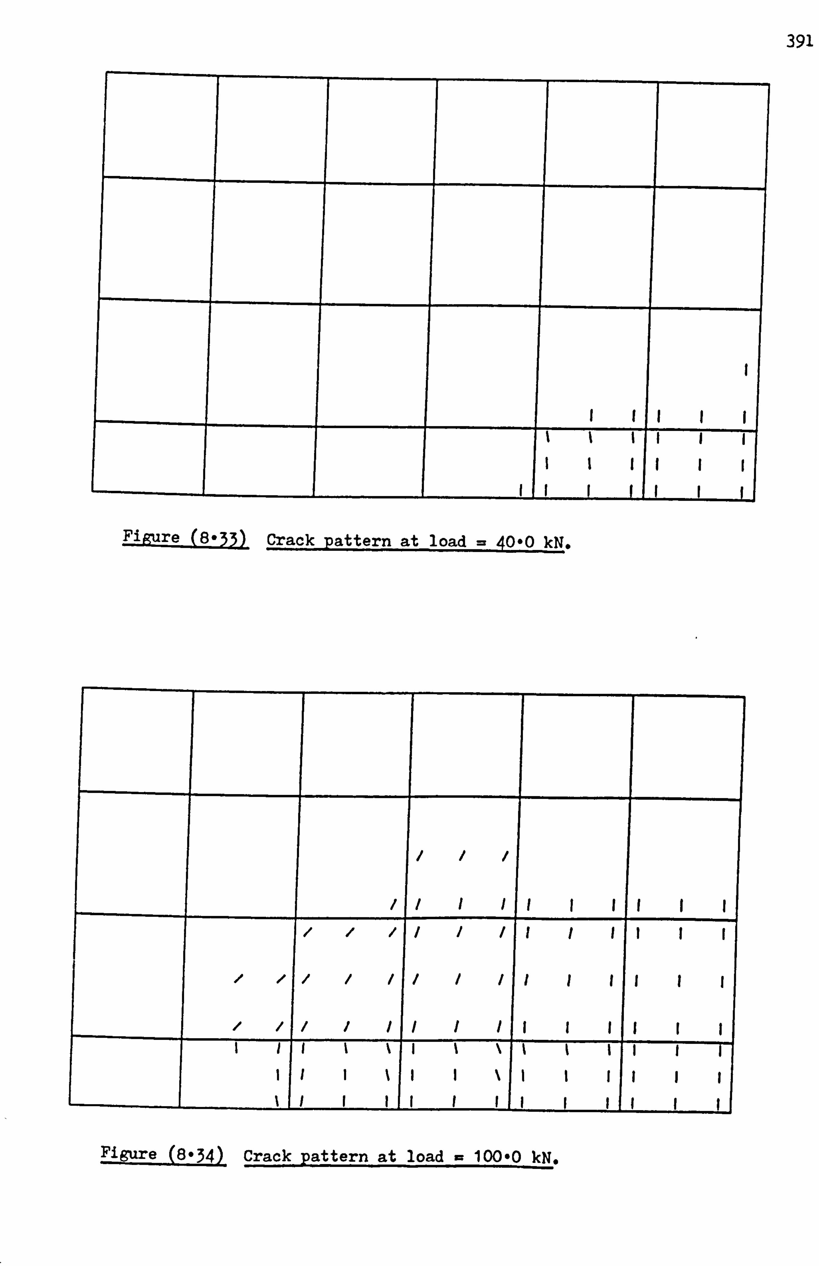
39
Figure (8933) Crack pattern at load = 40-0 kN.
/ / /
i i I I I I II II
/ / / 1 / / 1 I It II
' ' I / / / / I I I II II
/ / 1 / I I I I l I It II I I t I I I I IIIII
I I
I
, I I
I I
I I
I
I '
Il I
l I II II I II II
Figure (8*34) Crack pattern at load = 100*0 kN.

392
0- / 10, / / . 01 0.1 00 . 00
Figure (8e35) Crack pattern at load = 250-0 kN.
40,
Figure (8936)- Crack pattern at load =285.0 kN.
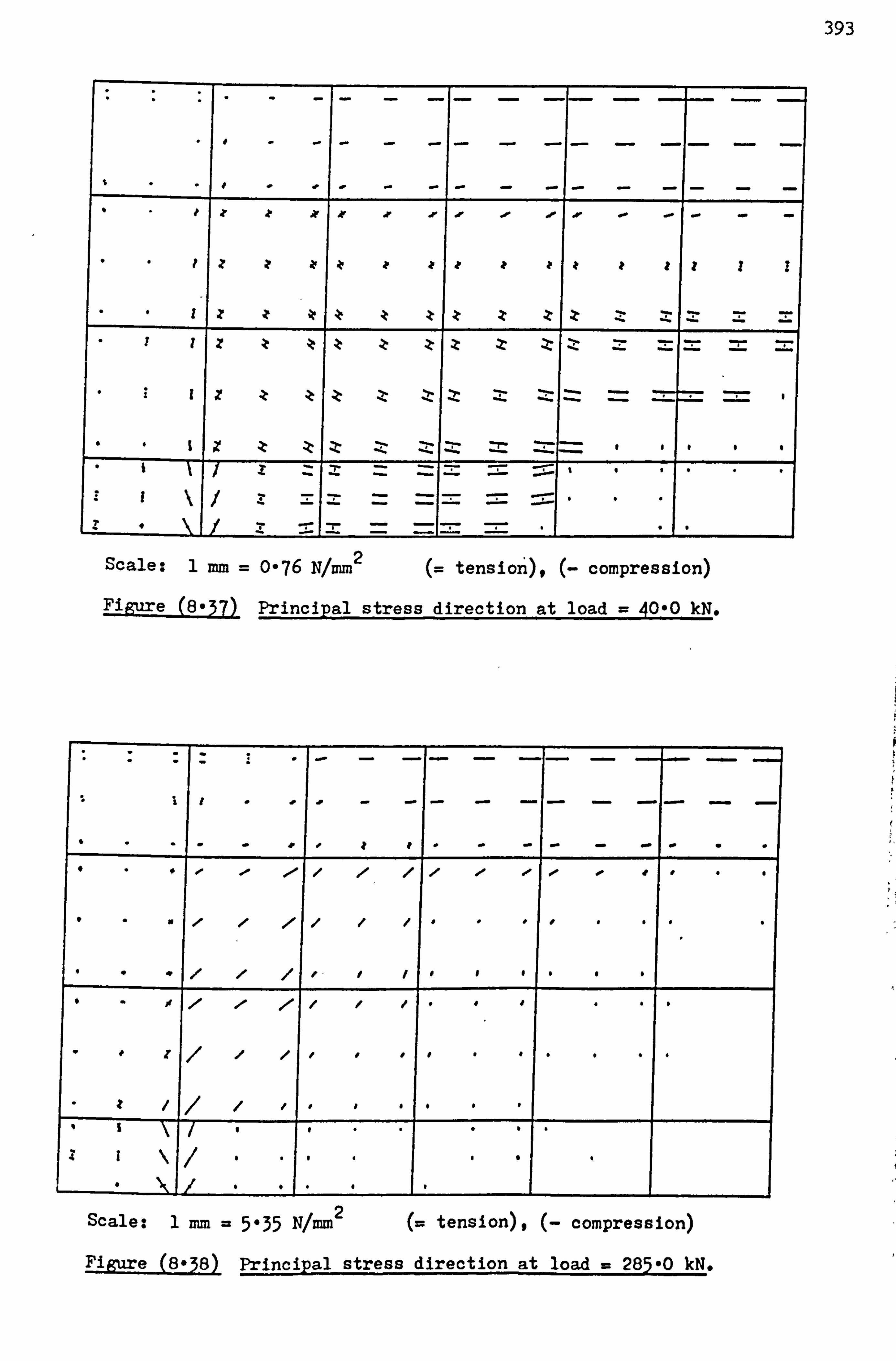
393
F f
Av Ar AI . 0.
III? F
X Z zz
EE Scale: 1 mm = 09 76 NIMM 2 tension), (- compression) Figure (8037) Princi pal stress direction at load = 40-0 kN.
Scale: I mm 5035 Nlmm 2 tension), compression)
Figure (8-38) Principal stress direction at load = 285-0 kN.
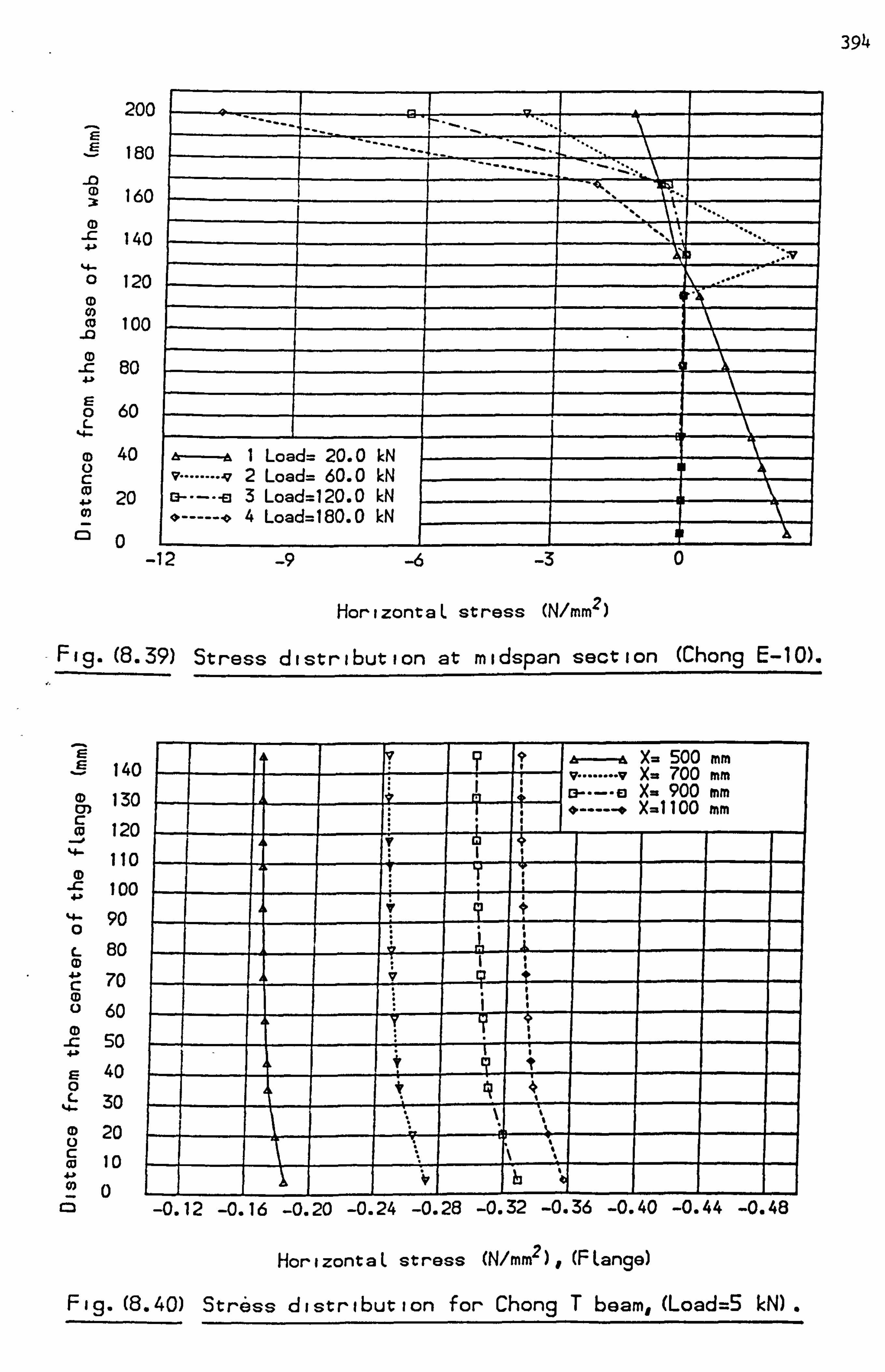
394
200
180
-0 :x 160
140
120
0) 100
80
60
40
20 0
1--, ce.
l' Z--.
I Load= 20.0 M v2 Load= 60.0 kN
3 Load=120.0 M 4 Load=180.0 M
-12 -3 0
HorizontaL stress (N/mm2)
Fig. (8.39) Stress distribution at midspan section (Chong E-10).
140
130
120
110 100
4- 90 0 C- 80 0 4ý C 70 (D
60
-C 50 4ý
C- 40 0
4c- 30
CD 20 0 c co 10
o cm
X= 500 mm i vv X= 700 rnm
m X= 900 mm --o X-1 100 Inm
-0.12 -0.16 -0.20 -0.24 -0.28 -0.32 -0.36 -0.40 -0.44 -0.48
HorizontaL stress (N/mm2),, (FLange)
Fig. (8.40) Str6ss distribution for Chong T beam, (Load=S M.
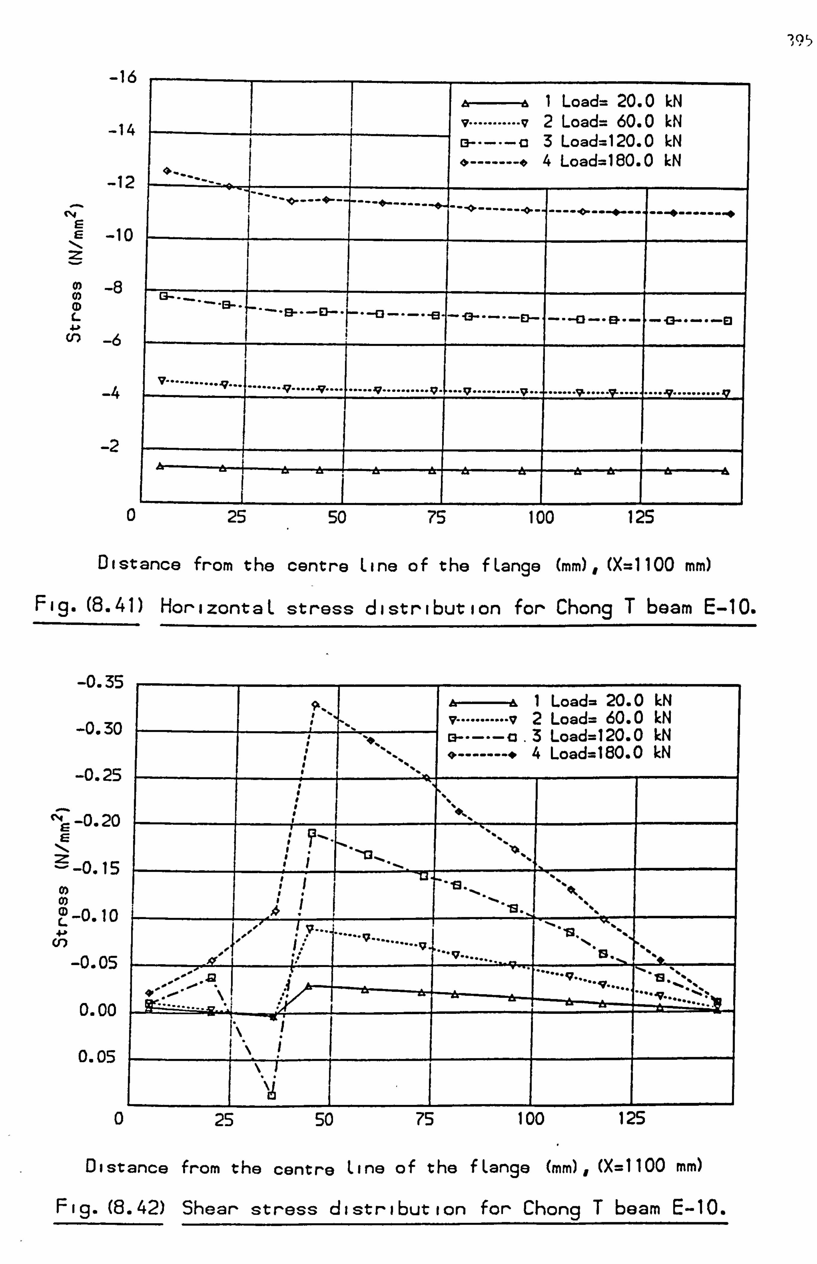
1 J95
-16
-14
-12
-10
(D
-4
Is 1 Load= 20.0 M v ........... v2 Load= 60.0 M
1, 3 Load=120.0 M
0 ------- 04 Load=180.0 M
!1 - --110. --- * --- ---- - ----- -- "0 -------- *---
V ........... 17 .. ....... ...... 7 ... ...... 9 .......... Qj 7 .......... 9 ... ....... IgL ..... Vt .... 4 ..... 17 ......... Q
3&
0 25 50 75 100 125
01 st ance from t he cant re Li ne oft he f Lange (mm) , (X= 1100 mm)
Fig. (8.41) HorizontaL stress distribution for Chong T beam E-10.
-0.35
-0.30
-0.25
-0.20
L
0.05
A, I Load- 20.0 kN v .......... v2 Load= 60.0 kN
3 Load=120.0 M q -------- 4 Load=180.0 M
... .......
711
. 42 .. ......
.. is
...
0 25 so 75 100 125
Distance from the centre Line of the Range (mm), (X=1100 mm)
Fig. (8.42) Shear stress distribution for Chong T beam E-10.

396
30(
25C
200
12-
100
50
0
DispLacement (mm)
Fig. (8.43) Load deftection curves for Chong T beam E-13.
10 15 2u
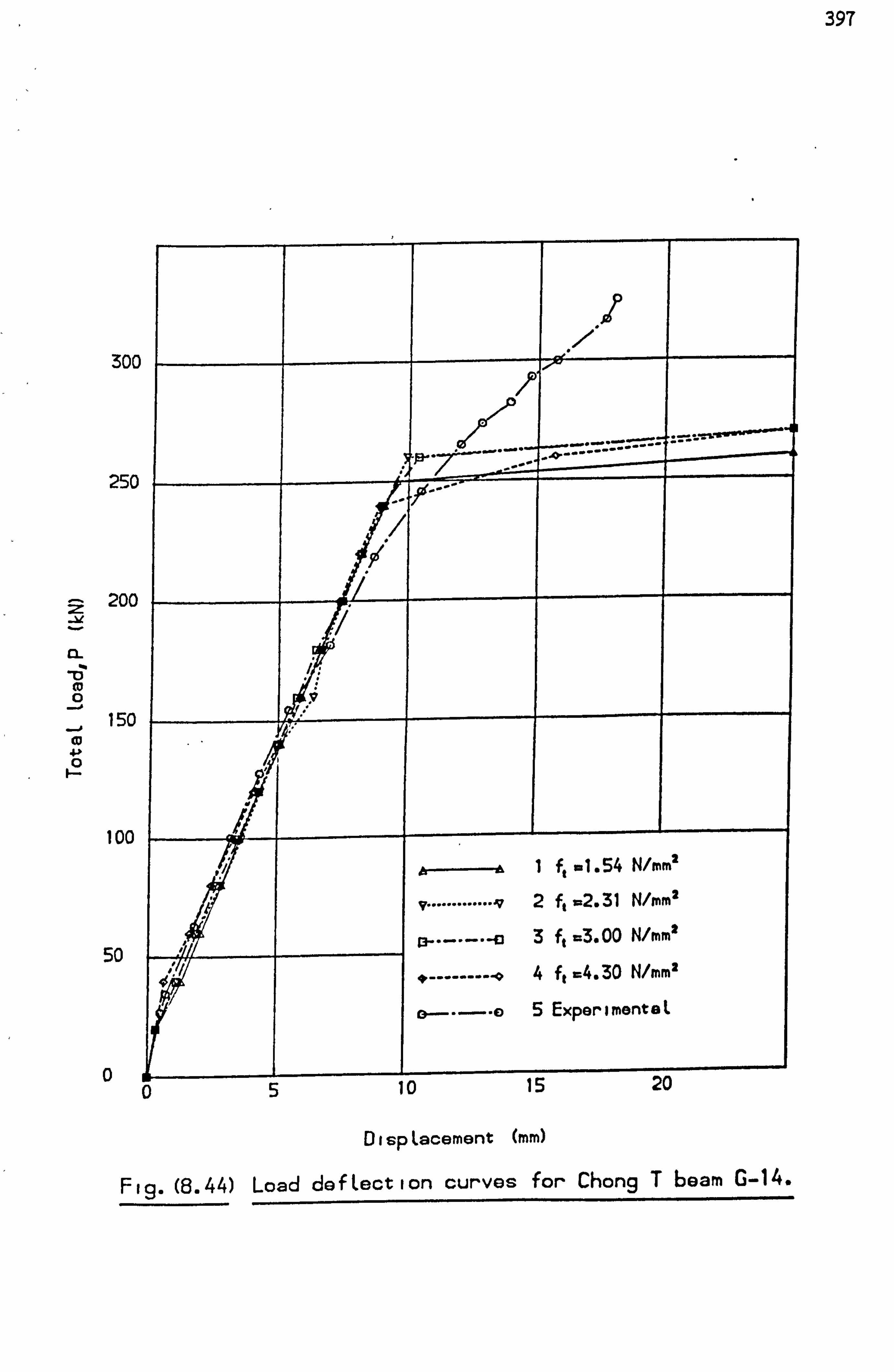
39T
300
250
5i 200 Zýl
to
cu
100
50
0
- F---
P. I lar- A1 ft =1 . 54 N/mm 2
v ............ 2 f, -2.31 N/mm2
93 ----- -- 43 3 ft . 3.00 N/mm2
4. W 2
't --------- 04f, =4.30 N/mm
5 ExperimenteL
ju ID cv
DispLacement (mm)
Fig. (8.44) Load defLection curves for Chong T beam G-14.

398
E 1 F- ,
Figurq_(8,, 45) Crack pattern at load = 50-0 kN.
E E ,
/ t i l l
Figure (8*46) Crack pattern at load = 90-0 M.

399
If
Figure (8-47) Crack pattern at load = 120-0 kN.
I I I F- I
Pig2re (8948) Crack pattern at load = 250-0 kN.

4oo
x1Z z ý( -Z z -: t zz -Zý zt --7* 11-
Izz. -ýt -: ý zzý zz- Zý- z: -z -I..
i
Ir - -Z -: t- -I, - ZZ :::: I
Scale: 1 mm = 0-86 N1mm 2 tension), compression)
FigUre (8-49) Principal stress direction at load = 50*0 kN.
z
I#. " 'r '01 --
01
Scale: 1 mm 5-22 N/mm2 tension), compression) Figure (8-50) Principal stress direction at load a 250*0-kN*
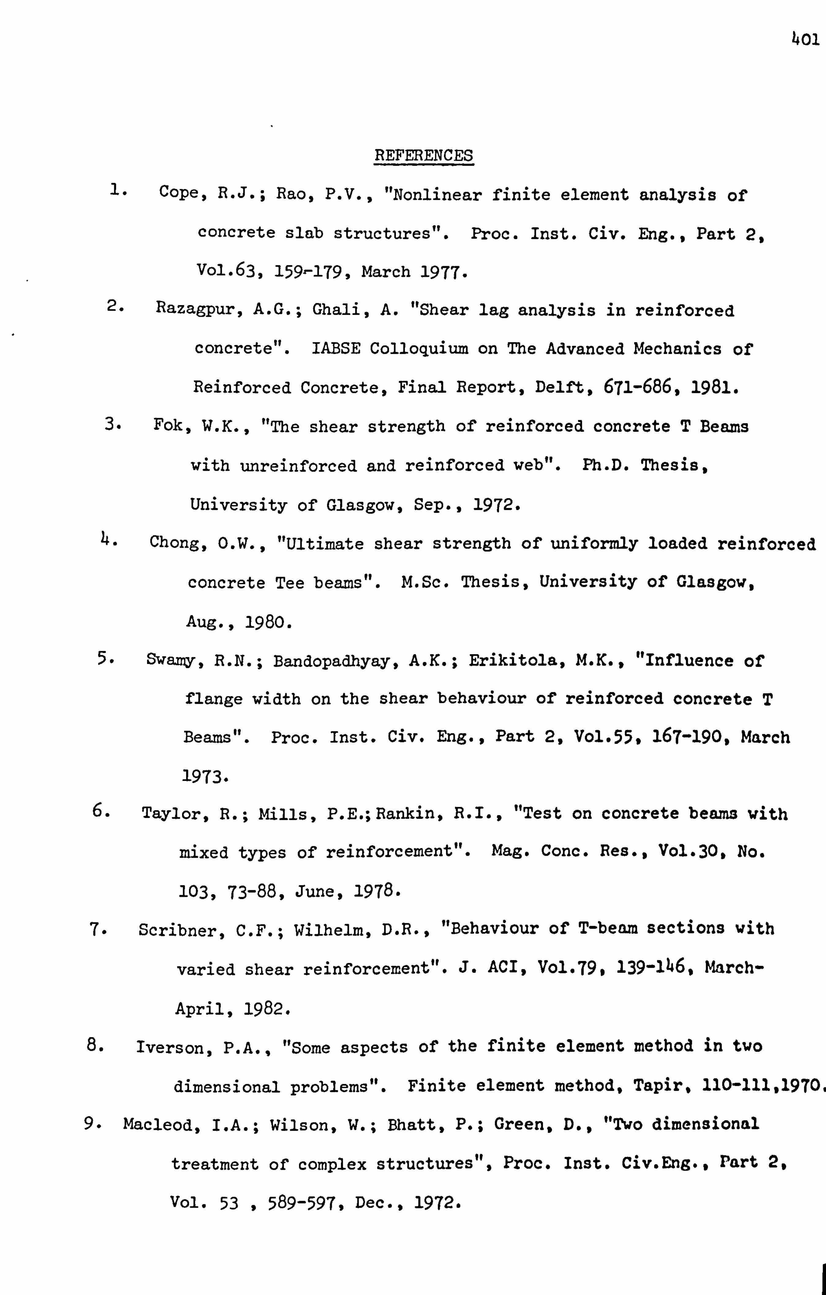
4oi
1- Cope, R. J.; Rao, P-V., "Nonlinear finite element analysis of
concrete slab structures". Proc. Inst. Civ. Eng., Part 2,
Vol. 63,159-179, March 1977.
2. Razagpur, A. G.; Ghali, A. "Shear lag analysis in reinforced
concrete". IABSE Colloquium on The Advanced Mechanics of
Reinforced Concrete, Final Report, Delft, 671-686,1981.
3. Fok, W. K., "The shear strength of reinforced concrete T Beams
with unreinforced and reinforced web". Ph. D. Thesis,
University of Glasgow, Sep., 1972.
4. Chong, O. W., "Ultimate shear strength of uniformly loaded reinforced
concrete Tee beams". M. Sc. Thesis, University of Glasgow,
Aug. , 1980.
5. Swamy, R. N.; Bandopadhyay, A. K.; Erikitola, M. K., "Influence of
flange width on the shear behaviour of reinforced concrete T
Beams". Proc. Inst. Civ. Eng., Part 2, Vol-55,16T-190, March
1973.
Taylor, R.; Mills, P. E.; Rankin, R. I., "Test on concrete beams with
mixed types of reinforcement". Mag. Conc. Res., Vol-30, No.
103,73-88, June, 1978-
7. Scribner, C. F.; Wilhelm, D. R., "Behaviour of T-beam sections with
varied shear reinforcement". J. ACI, Vol-79* 139-146, March-
April, 1982.
8. Iverson, P. A., "Some aspects of the finite element method in two
dimensional problems". Finite element method, Tapir, 110-111,1970,
9. Macleod, I. A.; Wilson, W.; Bhatt, P.; Green, D., "Two dimensional
treatment of complex structures", Proc. Inst. Civ. Eng., rart 2.
Vol. 53 , 589-597, Dec., 1972.
402
10. Ngo, D.; Scordelis, A. C., "Finite element analysis of reinforced
concrete beams". J. ACI, Vol. 64,152-163, March, 1967.

CHAPTER
CONCLUSIONS AND RECOMMENDATIONS
9.1 General observations and conclusions
9.2 Recommendations for future work
403
CHAPTER 9 CONCLUSIONS AND RECOMMENDATIONS
9.1 General observations and conclusions;
The main observations and conclusions obtained from this thesis
can be summarised as follows:
(1) The effect of numerical parameters in a nonlinear analysis are
complex and significantly important in the prediction of the
behaviour of reinforced concrete structures. These parameters
must be defined clearly in any analysis so that a solution may
be judged in relation to them, otherwise there might be an element
of doubt in the adequacy of the results. Misuse of these parameters
can lead to different solutions for load deflection curves, ultimate
loads, cracking patterns and stress distributions. Variations can
be obtained even if a single parameter is changed. In particular
the following parameters were found to affect the results of an
analysis:
(a) Solution parameters: - Convergence factor, convergence criteria
number of iterations, nonlinear solution method, order of
integration, aggregate interlocking, and tension stiffening;
(b) Quasi - material parameters: - aggregate interlocking and tension
stiffening.
(2) Care must be taken when using low integration rules in a nonlinear
analysis, because numerical problems may arise causing the solution
to diverge. This was found for beams failing both in flexure and
shear. It is well known that a2x2 Gauss rule is the minimum
required for a parabolic element, but this was found to be
insufficient for a nonlinear analysis because it appears that
higher orders are required to monitor the nonlinearized material
ft

4o4
properties with closer precision. In this work a3x3 Gauss rule
was found to be quite adequate. However it appears that the order
of Gauss rule is crucial rather than the total number of sampling
points throughout the continuum.
Shear retention factor a was examined for beams failing in both
flexure and shear and it appears that using a value of 0.5 was
satisfactory in both cases. This factor is quite adequate when
used with the smeared crack approach and no further complications
are required. The wide range of a between 0.01 and 1.0 did not
significantly affect the predicted load deflection curves although
as a increased towards 1.0 a slightly stiffer prediction was
obtained. A value of a=0.0 produced very poor results. This
would seem to suggest that a is a numerical device rather than an
approximation to a physical phenomenon.
No-tension stiffness cracking models produce large residual forces
in comparison to the applied loads due to the discontinuity in the
tension material law. Generally most cracks appear in the first
two or three iterations of an increment. However, a crack could
appear after a number of iterations have been applied, if the
solution was close to convergence. This produces new residuals
which are transferred to neighbouring nodal points even though a
state of equilibrium has been almost reached at other points.
This causes a completely new cycle of iterations to start because
of the size of the new residuals. In general it is not significant
whether these later cracks occur in the current or in the following
increment. In such circumstances it is better to prevent the
405
occurrence of these cracks. This might be achieved if very small
load increments were applied but on the other hand this tends to
considerably increase the cost of the solution. However this
point was not studied in detail in this work..
Alternatively iterations can be arbitrarily stopped after a given
number of cycles but this is less satisfactory because the state
of convergence is not known. Some authors have suggested the use of
tension stiffening to counter this type of difficulty and satis-
factory results have been reported. However this thesis suggests
instead the use of a known but relatively high convergence tolerance
with no-tension stiffening.
(5) Tension stiffening has been proposed by different authors and has
been given various physical interpretations, ranging from a way of
retaining stresses between discrete cracks to indirectly including
bond-slip or aggregate interlocking effects. Moreover various
models have been used for approximating this effect. It appears
that the chosen shape of the stress-strain curve in the post
cracking range is fairly arbitrary. This again suggests that it is
a numerical device rather than a physical phenomenon.
Tension stiffening can be replaced by a no-tension stiffening
model with high convergence tolerance. This is because both
approaches have the effect of retaining residual forces within
the continuum, the former indirectly and the latter directly.
However the no-tension stiffening model with high convergence
has a considerable advantage in that it requires far less iterations
and hence less computer time. Moreover, the results obtained using
4o6
tension stiffening methods are highly dependent on the combined
effect of convergence tolerance and the value of strain at which
the stress drops to zero, whereas the no-tension stiffening
method depends only on the convergence tolerance which implies
less complications.
A no-tension stiffening model using a 20% tolerance with the load
criterion is suggested as the best combination.
The V. S. M. 1 method (where the stiffnesses are updated at the
beginning of the first and second iteration of each increment)
was found to be better than both the C. S. M. method and V. S. M. 2
method in predicting the load deflection curve and ultimate load
for a convergence tolerance of 20%. This conclusion must be slightly
guarded because it has only been tested for a beam which failed in
flexure.
A general nonlinear solution procedure was established which gave
satisfactory results although it may not necessarily be the best
in a particular situation. This procedure uses the following:
(a) The variable stiffness method (V. S. M. 1) where the stiffness are
updated at the beginning of the first and second iterations.
(b) Between 20 to 30 load increments depending on the problem.
(c) The 3x3 Gauss rule.
(d) The no-tension stiffening cracking model.
(e) The constant shear retention factor with a value of a=0.5-
(f) The load criterion to check convergence to a tolerance of 20%.
(g) Iterations to continue until convergence is obtained; if convergence
is not obtained by 30 iterations then failure is assumed to have
occurred.
407
(9) The endochronic theory Of Concrete as Presented by Bazant iS
difficult to modify because of the complexity of the form of
equations and the difficulties of knowing just how the constants
were determined. There appears to be much interdependence between
the various parameters and the different effects they represent.
Simplifications need to be introduced so that the theory
becomes more accessible, and can be more easily modified. However,
despite these remarks the theory has proved both accurate and
efficient in the prediction of concrete behaviour investigated in
this work.
(10) Changing the values of the crushing strain of concrete affects the
shape of the load deflection curve close to failure and can produce
different ultimate loads. It is important to use a suitable value
but this might be difficult to judge where confinement exists,
particularly where reinforcement is closely spaced.
(11) The device of increasing the concrete strength in order to account
for confinement caused by closely spaced reinforcement, such as
under loading points, was found to be important in the analysis of
some beams. Again this matter may be difficult to judge in practical
applications, but obviously needs to be borne in mind.
(12) Despite the efficiency of the frontal solution, the peripheral
operations of transfer to a backing disc file was found to be
inefficient in a nonlinear analysis because disc transfers are very
slow and costly. The introduction of the buffer area greatly
improved this process and minimized the cost. However, the selection
of buffer areas is highly dependent on the size of the main core

4o8
storage of the computer used and has to be carefully chosen.
(13) A simple method was proposed to analyse T-beam structures. Certain
approximations were required in order to treat the structure as a
two dimensional problem. The flange was treated separately from
the web and was connected to the web through a fictitious element
which transfers appropriate forces. Special boundary conditions
and the selection of the point of separation of flange and web
were important parameters. The method allows the prediction of the
distribution of horizontal and shear stresses across the width of
flange. The same numerical parameters proposed in the previous studies
were used and full convergence was obtained for all solutions.
The results obtained for T-beams failing in flexure and shear
showed different degrees of accuracy. The shape of the load deflection
curves were relatively acceptable but they did not always compare
well with the experimental results. The range of error in ultimate
loads was fairly reasonable. Crack patterns in the webs were
satisfactory, but they were not so in the flanges. Stress distributions
in the flange were as expected. The approximation shows potential in
predicting various aspects of the behaviour of T-beans, but requires
further study and refinement.
9.2 Recommendations for future work:
This section recommends further work as follows:
(1) Reinforcing bar elements which can pass through the concrete element
instead of the sides could be introduced. This will allow the use
of less concrete elements and approximate the bar positions more

4og
,4
accurately. Hence cheaper solutions could be obtained, and more
complex structures analysed. Also better aspect ratios could be
selected which may give improved solutions.
(2) The effect of the different parameters used in the endochronic model
should be studied in more detail to examine their relative signifi-
cance in a finite element analysis. However, more important is that
the endochronic theory is still under active development. Changes
which appeared recently were found to be very efficient in handling
more complex concrete behaviour such as cyclic loading and creep.
Including new versions of this model would extent this program so
that a much wider range of concrete behaviour could be studied.
(3) Further investigations are required to study the effect of varying
the order of Gauss rule using different elements and mesh sizes
under nonlinear conditions.
(4) Further studies on the calculation of residual forces at the nodes
and checking their decay is required. It would be useful to confirm
what influence cracks have on the decay of residuals using both
methods of tension and no-tension stiffening, especially with
different convergence tolerances and load increment sizes for a
similar problem. This would provide more information and confirmation
of the conclusion made in this work.
The program in its present form is suitable for detailed numerical
studies of different types of plane concrete structures. Numerical
investigations could be carried out to study, for example, deep
beams with openings of different geometry and loading conditions.

41o
The use of the irregular mesh generator and plotting routines
developed in this program will ease this process.
The 8-noded element developed for the web-flange connection of the
T-beams could be developed for other purposes such as introducing
a bar between two concrete elements, similar to linkage elements.
This would allow different nodes for the concrete and the steel
which could then be connected by different stiffnesses which would
account for such behaviour as bond-slip, dowel action etc.
More detailed investigations are required to compare the experimental
and theoretical stress distributions in the T-beams. For instance
a layered element technique could be introduced for the flange in
order to approximate the variation of stresses through the flange
thickness. The method developed could also be extended for L-beams
and box girder structures by introducing suitable modifications to
the boundary conditions.
The numerical procedure and models devised in this thesis could be
tested for axisymmetric, and three-dimensional applications. In
particular, the numerical parameters studies could be repeated for
these cases.

APPENDIX
APPENDIX A Equations of Endochronic theory for concrete
APPENDIX B Brief description of the program
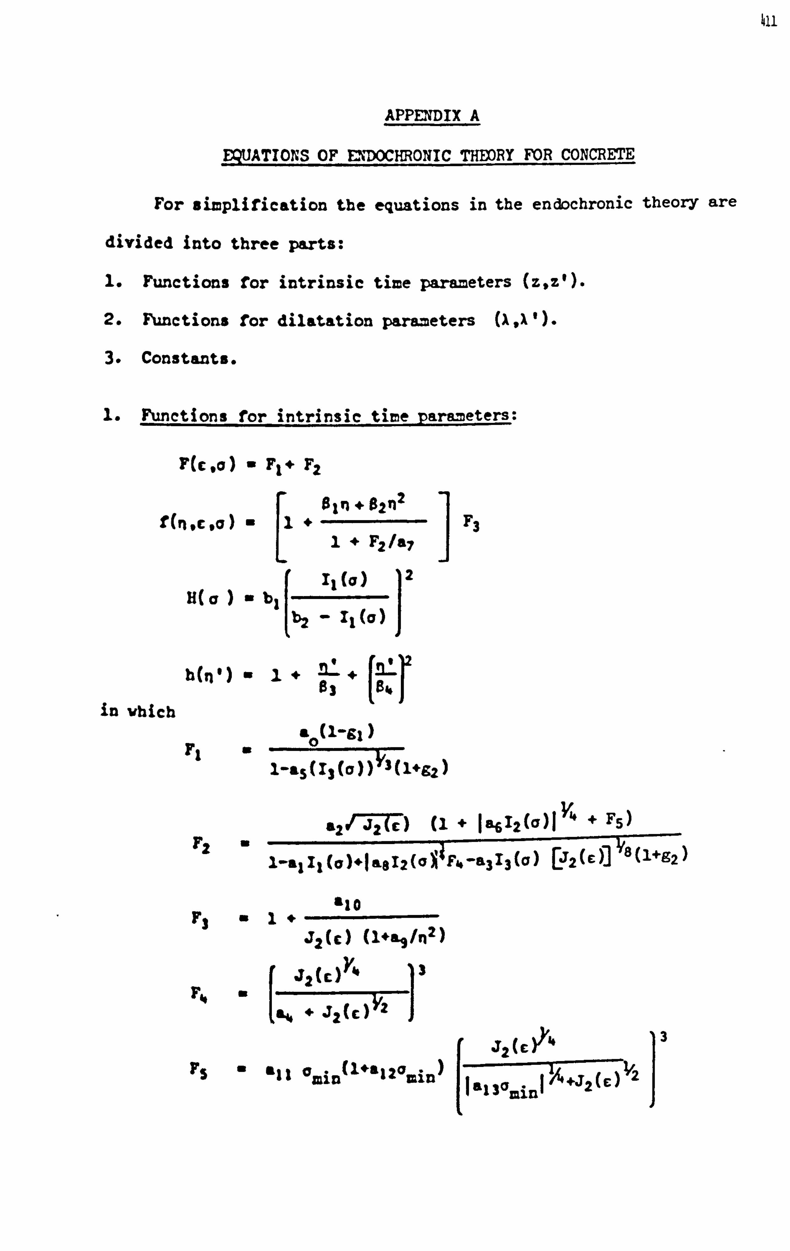
411
APPENDIX A
EQUATIONS OF ENDOCHRONIC THEORY FOR CONCRETE
For simplification the equations in the endochronic theory are
divided into three p&rts:
1. Functions for intrinsic time parameters (z, z').
2. Functions for dilatation parameters
Constants.
I. Functions for intrinsic time parameters:
F(C, 0) - Fc F2
F3 1+ F2 /a7
11 (Cr)
(CY)
12 H(C b
++ of
in vhich
03
r84
40 (I-gl
a/ -jTC-) +1 &6 12 (cr
V4 + FS
22 F,
I-alli(a)+IILS12((IlýF4-a3I3(CY) EJ2(C)l 8(1+92)
F4
), y4
PS a al 1 ty min (: a120 zein
) 1a130miniýý+, T2(C) y2
1
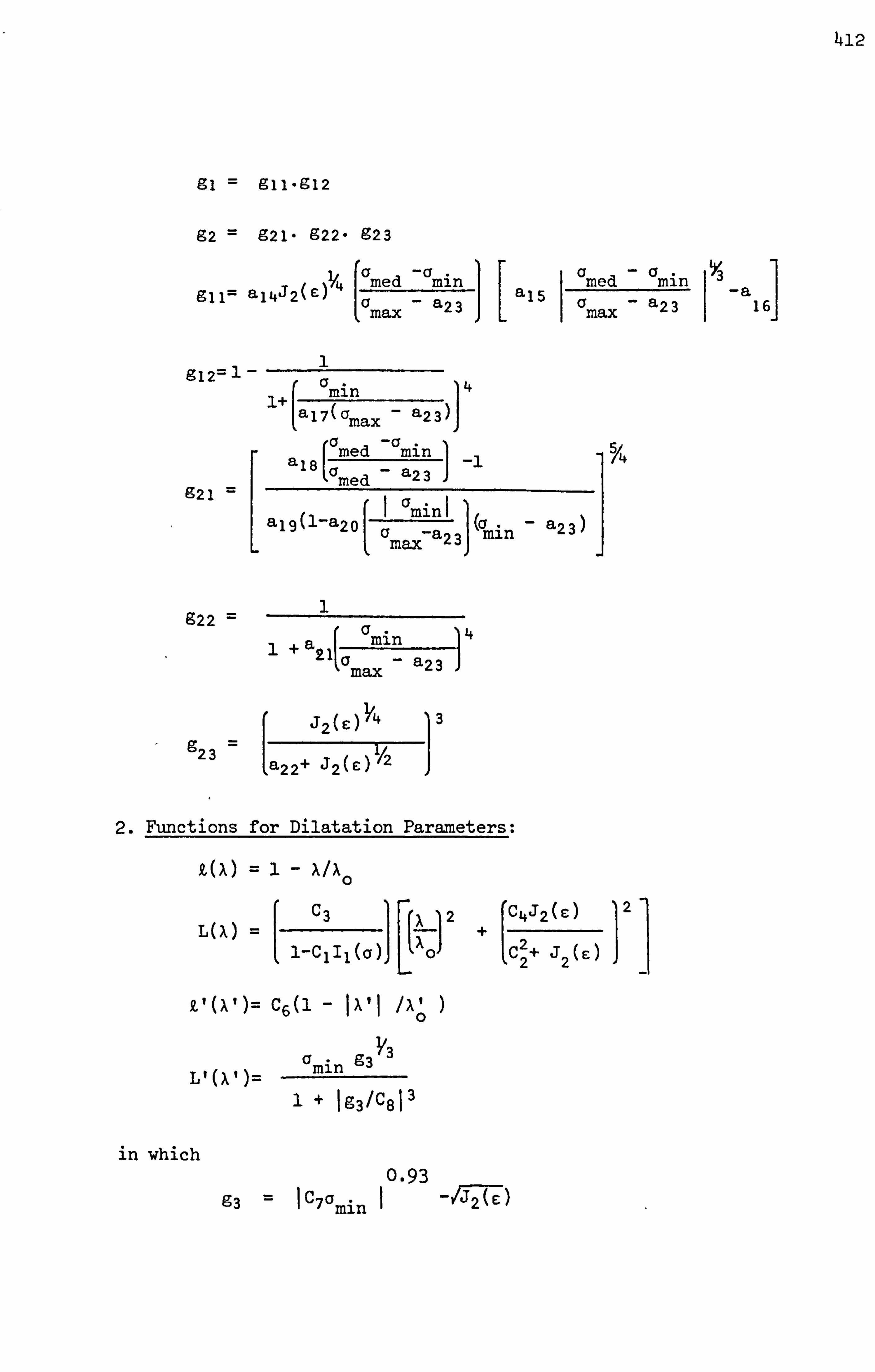
412
91 -` 911-912
92 ý 921- 922- 923
-0 1aa ly, amed
min med 3 gll= al4J2( C)
ý4 a 1.5 _
in a
a max - a23
IIa
max f- 16
z= 1-1 gl: l+ -a min
- a23) 4 1
a17(Gmax
a18f cy med -a min ý4
ýa med - a23
1
921 =
alg(1-a20
1 amini (amin - a23)
L cr
max-a23
11
922 : -- 1a
+ min
ME - a2d
J2(c) 3
g 23 a22+ J2(C
Functions for Dilatation Parameters:
Mx) =i- x/x C3 r(X
12 +
(C4J2(C) 12
2 ý
l-clIi(cr),
1
L 0, IC
2+i 2(E)
9,1 W: C6(' - Ixtl hl )
min 93
ý3
+ 193/C8 13
in which 0.93
YJ (C) 93 = IC70min I- Y2(C
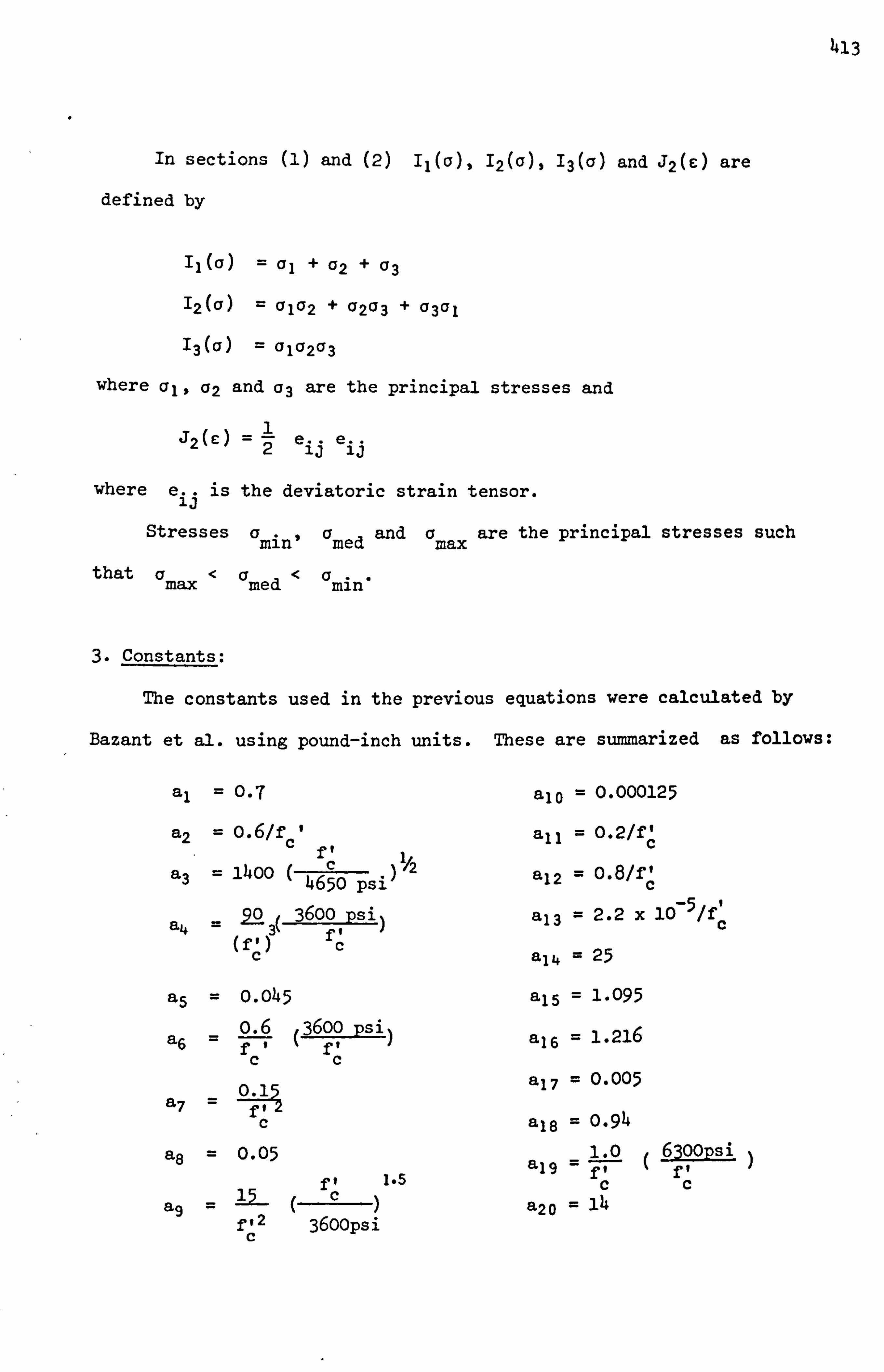
413
In sections (1) and (2) II(O)s 12(0)s 13(a) and J2(c) are defined by
Il (Cr )ý C11 + C12 + Cr3
, 2(cy) ý 0102 + a2G3 + a3GI
13 (Cy )=0 1(12C73
where a, , CF2 and C73 are the principal stresses and
J2(6) =1e.. e.. 2 Ij Ij
where e.. is the deviatoric strain tensor. ij
Stresses a min'
a med
and a max
are the principal stresses such
that a max
<a med
<a min*
3. Constants:
The constants used in the previous equations were calculated by
Bazant et al. using pound-inch units. These are summarized as follows:
a, = 0.7
a2 = 0.61f c
a3 = 1400 46C Y2
50 Psi 2-0 3600 Psi) a4 3 f, (fl) c c
alo = 0.000125
all = 0.2/f I c
a12 = 0.8/fl c a13 = 2.2 x 10⁻⁵ If
a14 = 25
aS = 0.045 o. 6 3600 psi a6 f ft c c
0.15 a - - 7f t 2
c
a8 = 0.05
15 ft 1.5 C ag =
ft2 360opsi c
a15 = 1.095
a16 = 1.216
a17 = 0.005
a18 = 0.94
alg = 1.0 ( 630opsi F7- ff cc
a20 = 14
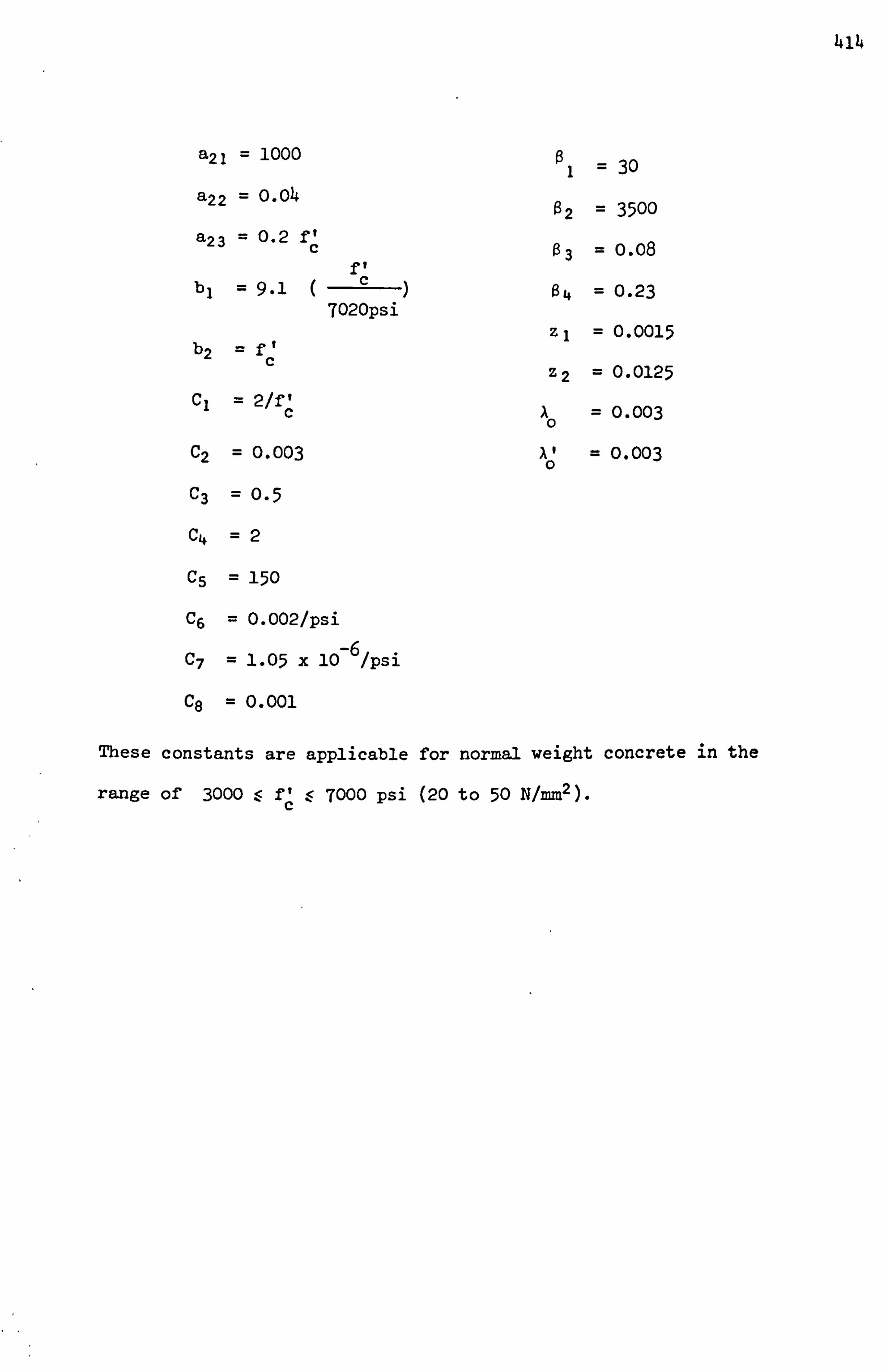
414
a21 : -- 1000
a2 2=0.04
a23 = 0.2 f1 c
ff bl = 9.1 c
7020psi
b2 ý rl c
C, = 2/f c
C2 = 0.003
C3 = 0.5
C4 =2
C5 = 150
C6 = 0.002/psi
C7 = 1.05 x 10⁻⁶ /psi
C8 = 0.001
ß1 = 30
ß2 = 3500
ß3 = 0.08
ß4 = 0.23
zi = 0.0015
Z2 = 0.0125
A = 0.003 O
A1 = 0.003
These constants are applicable for normal weight concrete in the
range of 3000 <V< 7000 Psi (20 to 50 N/mm2). c
415
APPENDIX B
BRIEF DESCRIPTION OF THE PROGRAM
The program analyses nonlinear plane-stress problems using 8-noded
isoparametric elements for concrete and 3-noded isoparametric elements
for steel. The incremental iterative method is used to solve the
nonlinear equations. The linear equations are solved by a Frontal
technique, described by Hinton and Owen*. This was modified to include
buffer storage areas in order to reduce the cost of analysis. The
program also includes the endochronic theory, and different cracking,
and crushing, models. Input and output were developed to be at a
minimum and the selected output can be chosen as required.
Mesh generators are included for irregular and regular shapes of
structure including the T-beam. problems using fictious elements.
Routines were built in for automatic plotting of meshes, crack patterns,
principal stresses, contour stresses, and load deflection curves using
the available GHOST and GINO plotting packages mounted on the ICL 2976
at Glasgow University.
A list of all subroutines is shown next followed by a brief
description of their use. A chart which illustrates the relationship
between each subroutine is provided at the end of this section.
Q * Hinton, E.; Owen, D. R. J., "Finite element programming". Academic, 1977-

416
I
1. FES
2. INPUT
3. CONSTANT
4. GAUSSQ
5. LOADPS
6. FILL
7. FILL1
8. FILL2
9. NODEXY
10. RECTMG
11. GIN
12. INBLOC
13. GENER
14. GMESH
15. SFRQ
16. CHECK1
17. CHECK2
18. ECHO
19. INCREMENT
20. INPUT1
21. INPUT2
22. GOOUT2
23. GOOUT1
24. SFR2
25. JACOB2
26. BMATPS
27. MDDPS
28. DMAT
29. DCRACK1
30. TMATRIX
31. BDB
32. DBE
33. STREPS
34. IFC
35. ENDOCA
36. ENDOC
37. CRUSH
38. Pop
39. ELASTIC
4o. PRINCIPAL
41. EMEM
42. SFRB
43. TEST
44. JACOB1
45. MODB
46. COUNT
47. STREB
48. DECIDES
49. IFCB
50. OUTPUTB
51. DECIDE
52. STIFPS
53. FRONT
54. GOOUT
55. PLMESH
56. SPACE
57. PLMESK
58. PLTXY
59. PLOW I
417
(1) Program FES:
This is the main controlling subroutine from which all other
subroutines are called.
(2) Subroutine INPUT:
This reads the required information for geometry, boundary
conditions, material properties for concrete and steel, and calls
the required subroutines for data checking and mesh generation.
Subroutine CONSTANT:
This sets up the initial values for all material property constants
and stores them in the appropriate, arrays by calling subroutine
FILL.
Subroutine GAUSSQ:
This sets up the sampling (Gauss) point positions and weighting .
factors for numerical integration. The order of Gauss rule is
restricted to either 2x2,3 x3 or 4x4.
Subroutine LOADPS:
This reads applied pressure and concentrated loads and distributes
them onto specific nodes. It also handles gravity and temperature
loads under elastic conditions.
Subroutine FILL:
This stores the updated material parameters, in the proper positions.
It also stores the angle of each crack and its identity (closed or
open), and its type (single or double).
Subroutine FILU:
This subroutine stores the total stresses and strains.
Subroutine FILL2:
This stores the endochronic variables to be used in other increments.
418
Subroutine NODEXY:
The'main purpose of this subroutine is to calculate the midside
nodal coordinates for straight sided elements when no automatic
mesh generator is used.
(10) Subroutine RECTMG:
This generates nodal coordinates and nodal connections for
rectangular meshes only. Properties for different materials can
be generated.
(11) Subroutine GIN:
This is the main subroutine calling the required routines for
generating irregular (or regular) shaped meshes for the 8-noded
element. It calls subroutines INBLOC, GENER, GMESH, SFRQ-
(12) Subroutine INBLOC:
This reads input data defining the main structure outline within
whic ,ha mesh will be generated.
(13) Subroutine GENER:
This perfox the mesh subdivision, for the given irregular (or
regular) blocks, and eliminates repeated nodal points which occur
during the mesh generating process.
(14) Subroutine GMESH:
This outputs the generated mesh and nodal connections calculated
in the previous subroutine GENER.
Subroutine SFRQ:
This sets up the required shape functions for mesh generating
(which in general could be different from the shape functions
defining the element properties).
419
(16) Subroutine CHECkl:
This checks the control parameters read in subroutine INPUT to
ensure that they all have values ranging within the specified
description in the manual. Any error detected is given an
appropriate number which can be checked.
(17) Subroutine CHECK2:
This checks any identical information given with regard to coordinates
and nodal connections. The most useful check in this subroutine is
the one which ensures that the maximum frontwidth does not exceed
the value specified in subroutine FRONT.
(18) Subroutine ECHO:
This is called if anY error is detected in CHEM or CHECK2. The
main purpose is to stop the program and to print out any remaining
unread Input data.
(19) Subroutine INCREMENT:
This subroutine calls all the required routines for the nonlinear
analysis, and for plotting the results. Also all stress, displace-
ment and numerical control parameters are printed.
(20) Subroutine INPUT1:
This outputs the main control data of the finite element analysis.
(21) Subroutine INPUT2:
This subroutine outputs the documentary information which defines
the printed output.
22) Subroutine GOOUT2:
This subroutine outputs the nonlinear control numerical parameters.
(23) Subroutine GOOUT1:
This outputs the convergence information at each increment.
420
(24) Subroutine SFR2:
This calculates the shape functions and their derivatives for the
8-noded element.
(25) Subroutine JACOB2:
This calculates the coordinates of all gauss points, and the
Jacobian. matrix, its determinant and inverse for the 8-noded
element.
(26) Subroutine BMATPS:
This subroutine calculates the strain matrix EBJ for the 8-noded
element.
(27) Subroutine MODPS:
This subroutine reads the material properties from subroutine FILL
ana sets up the elasticity matrix, for stiffness calculations.
(28) Subroutine DMAT:
This sets up the elasticity matrix for the calculation of stresses.
(29) Subroutine DCRACKI:
This sets up the required cracking matrix in the cracked directions
for each gauss point.
(30) Subroutine TMATRIX:
This subroutine calculates the transformation matrix which is used
to transform the stresses and strains to the required directions.
(31) Subroutine BDB:
This subroutine transforms the elasticity matrix to the cracked
direction and back for the 8-noded element.
(32) Subroutine DBE:
This calculates the stress matrix [DBJ for the 8-noded element.

421
(33) Subroutine STREPS:
This calculates the stresses at the Gauss points for the 8-noded
element.
(34) Subroutine IFC:
This subroutine calculates the internal equivalent nodal forces
for the 8-noded element.
(35) Subroutine ENDOCA:
This subroutine updates the stresses for all regions using the
endochronic theory and checks the cracking and crushing of concrete.
(36) Subroutine ENDOC:
This sets up the endochronic equations to be used in subroutine
ENDOCA.
(37) Subroutine CRUSH:
This subroutine checks for crushing of concrete using the required
criteria.
(38) Subroutine POP:
This calculates the uniaxial stresses for a known value of strain
using Popovics formula for concrete.
(39) Subroutine ELASTIC:
This subroutine calculates the stresses due to a defined [D] and
fel matrix.
(40) Subroutine PRINCIPAL:
This calculates the principal stresses and strains and their
directions.
(41) Subroutine EMEM:
This calculates and prints out the maximum and minimum major and
minor principal strains and stresses for the 8-noded element
throughout the whole mesh.
422
(42) Subroutine SFRB:
This subroutine calculates the shape functions and their derivatives
for the 3-noded element.
(43) Subroutine TEST:
This subroutine selects the proper shape function for the four
3-noded elements which can be attached to the sides of the 8-noded
element.
(44) Subroutine JACOB1:
This calculates the coordinates of all Gauss points for the 3-noded
element and sets up the Jacobian matrix, its determinant and inverse.
(45) Subroutine MODB:
This calculates the stress matrix [DB] for the 3-noded element.
(46) Subroutine COUNT:
This sets up the 3-noded element stiffness in similar positions
to an 8-noded element.
(47) Subroutine STREB:
This is used to calculate the stresses for the 3-noded element at
the required Gauss points.
(48) Subroutine DECIDES:
This subroutine calculates the total stresses for the 3-noded steel
element and checks for its yielding.
(49) Subroutine IFCB:
This calculates the internal equivalent nodal forces for the 3-noded
element.
(50) Subroutine OUTPUTB:
This outputs the final stresses and strains for the 3-: noded elements.

423
(51) Subroutine DECIDE:
This analyses the steel as a separate 8-noded two dimensional
element with strain hardening included.
(52) Subroutine STIFPS:
This calls the required subroutines to calculate the stiffnesses
for the 8-noded element and 3-noded element and adds them into
the appropriate places in the stiffness matrix.
(53) Subroutine FRONT:
This solves the simultaneous equations by means of Gauss elimination
and back substitution. The Front solution is used and a modified
buffer storage facility is included.
(54) Subroutine GOOUT:
This outputs the required information for using the plotting routines.
This includes a description of all parameters used to plot meshes,
cracks and stresses.
(55) Subroutine PLMESH:
This subroutine plots the mesh, crack patterns and stress
distributions in the two and three dimensional space, using the
available GHOST routines (i. e. a general package for Plotting).
(56) Subroutine SPACE:
This sets up the required plotting scales because the available
GHOST package only plots on a specified distorted scale. (This
would not usually be needed and is peculiar to the operating
system on which this program was developed).
(57) Subroutine PLMESK:
This subroutine plots contour lines for horizontal, vertical and
shear stresses for rectangular shapes using the GINO plotting
package in the two and three dimensional space (The GINO package
is also a general plotting routine, having better facilities
for plotting contours than GHOST).
424
(58) Subroutine PLTXY:
This plots any two variables using the GHOST routines and is
normally used to plot the load displacement curves.
(59) Subroutine PLOTT:
This subroutine plots stress-strain curves on the line printer.
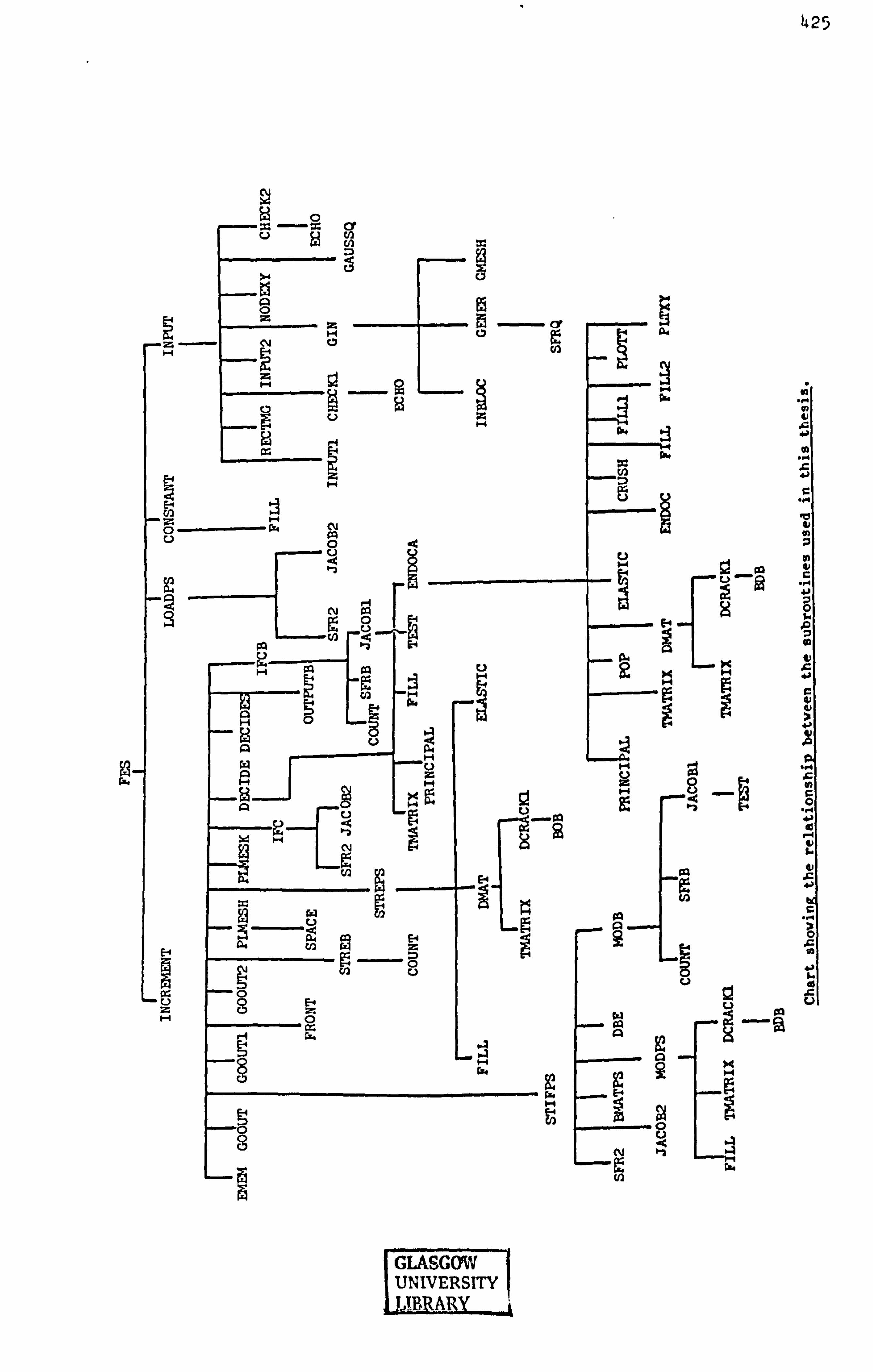
425
W 0 -
>4
rl
CM ca
1-4
L4
cli 0
14 pq (V
L) CM
f2- Dk
E 4 w
93 - E-4
0 C. )
w -0
U
94
cm Rý ul
tý E3 ad
11 ow
U
C. ) z0 E4 �-4
--1
-L L
I GLASIGOW U: NNIlkVIERSITY LABRARY
Top Related
Copyright © 2022 FDOKUMEN

