Zero-One Law for Regular Languages - T2R2 - 東京工業大学

論文 / 著書情報Article / Book Information

題目(和文) 正規言語の零壱則

Title(English) Zero-One Law for Regular Languages

著者(和文) 新屋良磨

Author(English) Ryoma Sin'ya

出典(和文) 学位:博士(理学), 学位授与機関:東京工業大学, 報告番号:甲第10103号, 授与年月日:2016年3月26日, 学位の種別:課程博士, 審査員:鹿島亮,小島定吉,南出靖彦,渡辺治,寺嶋郁二,金沢誠

Citation(English) Degree:Doctor (Science), Conferring organization: Tokyo Institute of Technology, Report number:甲第10103号, Conferred date:2016/3/26, Degree Type:Course doctor, Examiner:,,,,,

学位種別(和文) 博士論文

Type(English) Doctoral Thesis

Powered by T2R2 (Tokyo Institute Research Repository)

http://t2r2.star.titech.ac.jp/

ZEROONE LAW FORREGULAR LANGUAGES正規⾔語の零壱則

Ryoma Sin’ya

Tokyo Institute of Technology,

Department of Mathematical and Computing Sciences.

This thesis is an exposition of the author’s research on automata theory and zero-one laws which had been done in 2013–2015 at Tokyo Institute of Technology andTélécom ParisTech. Most of the results in the thesis have been already published in[58, 57].

Copyright c©2016 Ryoma Sin’ya. All rights reserved.

Copyright c©2015 EPTCS. Reprinted, with permission, from Ryoma Sin’ya, “AnAutomata Theoretic Approach to the Zero-One Law for Regular Languages: Algo-rithmic and Logical Aspects” [58], In: Proceedings Sixth International Symposiumon Games, Automata, Logics and Formal Verification, September 2015, pp.172–185.

Copyright c©2014 Springer International Publishing Switzerland. Reprinted, withpermission, from Ryoma Sin’ya, “Graph Spectral Properties of Deterministic FiniteAutomata” [57], In: Developments in Language Theory Volume 8633 of the seriesLecture Notes in Computer Science, August 2014, pp.76–83.

PROLOGUE

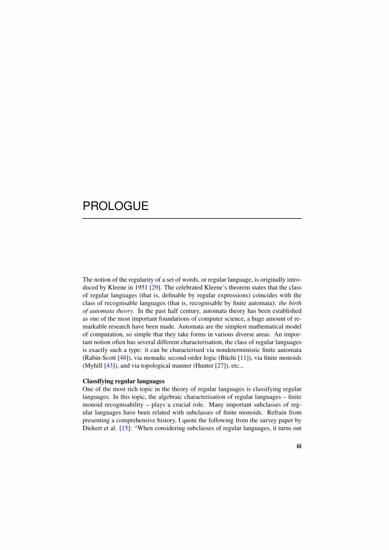
The notion of the regularity of a set of words, or regular language, is originally intro-duced by Kleene in 1951 [29]. The celebrated Kleene’s theorem states that the classof regular languages (that is, definable by regular expressions) coincides with theclass of recognisable languages (that is, recognisable by finite automata): the birthof automata theory. In the past half century, automata theory has been establishedas one of the most important foundations of computer science, a huge amount of re-markable research have been made. Automata are the simplest mathematical modelof computation, so simple that they take forms in various diverse areas. An impor-tant notion often has several different characterisation, the class of regular languagesis exactly such a type: it can be characterised via nondeterministic finite automata(Rabin-Scott [48]), via monadic second-order logic (Büchi [11]), via finite monoids(Myhill [43]), and via topological manner (Hunter [27]), etc...

Classifying regular languagesOne of the most rich topic in the theory of regular languages is classifying regularlanguages. In this topic, the algebraic characterisation of regular languages – finitemonoid recognisability – plays a crucial role. Many important subclasses of reg-ular languages have been related with subclasses of finite monoids. Refrain frompresenting a comprehensive history, I quote the following from the survey paper byDiekert et al. [15]: “When considering subclasses of regular languages, it turns out

iii

iv PROLOGUE

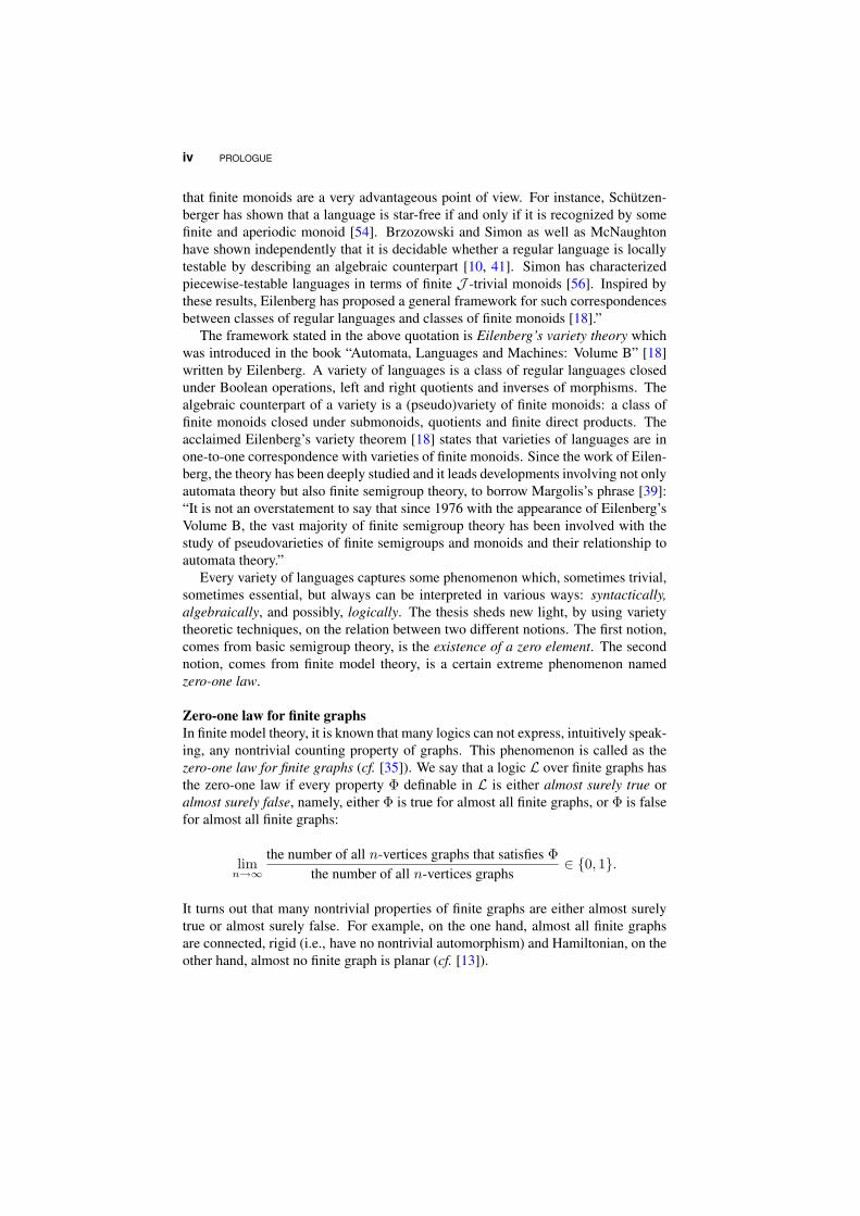
that finite monoids are a very advantageous point of view. For instance, Schützen-berger has shown that a language is star-free if and only if it is recognized by somefinite and aperiodic monoid [54]. Brzozowski and Simon as well as McNaughtonhave shown independently that it is decidable whether a regular language is locallytestable by describing an algebraic counterpart [10, 41]. Simon has characterizedpiecewise-testable languages in terms of finite J -trivial monoids [56]. Inspired bythese results, Eilenberg has proposed a general framework for such correspondencesbetween classes of regular languages and classes of finite monoids [18].”

The framework stated in the above quotation is Eilenberg’s variety theory whichwas introduced in the book “Automata, Languages and Machines: Volume B” [18]written by Eilenberg. A variety of languages is a class of regular languages closedunder Boolean operations, left and right quotients and inverses of morphisms. Thealgebraic counterpart of a variety is a (pseudo)variety of finite monoids: a class offinite monoids closed under submonoids, quotients and finite direct products. Theacclaimed Eilenberg’s variety theorem [18] states that varieties of languages are inone-to-one correspondence with varieties of finite monoids. Since the work of Eilen-berg, the theory has been deeply studied and it leads developments involving not onlyautomata theory but also finite semigroup theory, to borrow Margolis’s phrase [39]:“It is not an overstatement to say that since 1976 with the appearance of Eilenberg’sVolume B, the vast majority of finite semigroup theory has been involved with thestudy of pseudovarieties of finite semigroups and monoids and their relationship toautomata theory.”

Every variety of languages captures some phenomenon which, sometimes trivial,sometimes essential, but always can be interpreted in various ways: syntactically,algebraically, and possibly, logically. The thesis sheds new light, by using varietytheoretic techniques, on the relation between two different notions. The first notion,comes from basic semigroup theory, is the existence of a zero element. The secondnotion, comes from finite model theory, is a certain extreme phenomenon namedzero-one law.

Zero-one law for finite graphsIn finite model theory, it is known that many logics can not express, intuitively speak-ing, any nontrivial counting property of graphs. This phenomenon is called as thezero-one law for finite graphs (cf. [35]). We say that a logic L over finite graphs hasthe zero-one law if every property Φ definable in L is either almost surely true oralmost surely false, namely, either Φ is true for almost all finite graphs, or Φ is falsefor almost all finite graphs:

limn→∞

the number of all n-vertices graphs that satisfies Φthe number of all n-vertices graphs

∈ {0, 1}.

It turns out that many nontrivial properties of finite graphs are either almost surelytrue or almost surely false. For example, on the one hand, almost all finite graphsare connected, rigid (i.e., have no nontrivial automorphism) and Hamiltonian, on theother hand, almost no finite graph is planar (cf. [13]).

PROLOGUE v

The famed Fagin’s theorem [20] states that first-order logic for finite graphs hasthe zero-one law. Moreover, any first-order definable property is almost surely true ifand only if it is true on a certain infinite graph: the random graph. Fagin’s beautifulcharacterisation leads to the fact that, for any first-order sentence Φ, it is decidablewhether Φ is almost surely true or not (cf. Corollary 12.11 in [35]). After the workof Fagin, much ink has been spent on the zero-one law for logics over finite graphs.It is now known that many stronger logics (e.g., logic with a fixed point operator[7], finite variable infinitary logic [32] and certain fragments of second-order logic[33]) have the zero-one law. Here I would like to emphasise the remarkable factabout the zero-one law. It is known that finite satisfiability (i.e., the existence of afinite model) of first-order definable property for finite graphs is undecidable due toTrakhtenbrot’s theorem [65]. Thus, for a given first-order sentence Φ, while it isundecidable whether Φ is true for all finite graphs, it is decidable whether Φ is truein almost all finite graphs! All these results can be easily extended to arbitrary finiterelational structures (cf. [35]).

By contrast, though many logics have the zero-one law, their extensions withlinear order no longer have it. In fact, while first-order logic over finite graphs hasthe zero-one law, its extension with a linear order does not [14].

Zero-one law for regular languagesA logic over finite words is one of the most important instance of logics with linearorder in computer science. The question then naturally arises as to which logicalfragments over finite words, or class of languages, have the zero-one law? The maintopic of the thesis is this one: the zero-one law for finite words, or more emblemat-ically, the zero-one law for regular languages. We call a language (i.e., set of finitewords) L zero-one, or obeys the zero-one law, if L is either almost empty or almostfull, namely, either L contains almost all finite words, or L does not contain almostall finite words:

limn→∞

the number of all words of length n in L

the number of all words of length n∈ {0, 1}.

The original motivation of this work is the following question: is there a nice (de-cidable) characterisation of the class of regular zero-one languages? In this thesisI give an algebraic and automata theoretic characterisation of the zero-one law forregular languages. Roughly speaking, I prove the following “Zero-One Theorem”(precise statement is Theorem 2.3.1, Chapter 2): a regular language L is zero-oneif and only if its syntactic monoid has a zero element, or equivalently L or its com-plement includes a language of the form A∗wA∗ for some word w. The proof givesan effective automata characterisation of the zero-one law for regular languages, andit leads to a linear time algorithm for testing whether a given regular language iszero-one if it is given by an n-states deterministic automaton.

The key points of the proof of Zero-One Theorem are closure properties of theclass of zero-one languages and Eilenberg’s lemma which was crucial in Eilenberg’svariety theorem.

vi PROLOGUE

Structure of the thesisThe thesis consists of six chapters. In Chapter 1, I give the necessary definitions andterminology of basic automata theory. Chapter 2 provides a detailed exposition of thenotion of the zero-one law for regular languages. The main result of the thesis – Zero-One Theorem – will be stated in this chapter (Theorem 2.3.1). Closure properties ofthe class of all zero-one languages are investigated in Chapter 3. Eilenberg’s lemmais also given in this chapter. An automata theoretic proof of Zero-One Theorem isgiven in Chapter 4. In this chapter, I introduce two new classes of automata: zeroautomata and quasi-zero automata. These classes of automata play a crucial role inthe proof. Chapter 5 describes a linear time algorithm for testing whether a givenregular language is zero-one (Theorem 5.1.1). Some logical aspects of the zero-onelaw for regular languages are also described in this chapter. Zero-One Theorem givesus a simple necessary and sufficient condition for a regular language to be zero-one,however, it is not true beyond regular languages. Simple counterexamples, zero-onelanguages whose syntactic monoid have no zero element, are given in Chapter 6. Inthis chapter, a new technique for proving non-regularity of languages is established.

I try to keep all chapters as self-contained as possible. At the end of each chapter, Iprovide “Bibliographic Notes” which can serve as a reader’s guide to explore relatedworks and topics. I use square brackets as an equivalent to “respectively”, as in thefollowing sentence: a language L is almost full [almost empty] if it contains [doesnot contain] almost all finite words.

R. SIN’YA

Tokyo, November 2015

ACKNOWLEDGMENTS

I gratefully acknowledge helpful discussions with Prof. Ryo Kashima on severalpoints in the thesis. Special thanks also go to Prof. Yasuhiko Minamide and Prof.Makoto Kanazawa whose meticulous comments were an enormous help to me. Iwould like to acknowledge the encouragements of my colleagues, Naosuke Mat-suda, Yoshiki Nakamura, and Takuro Umekita. My senior colleague Takeo Uramotointroduced me to the variety theory and has encouraged me throughout this research.I wish to express my gratitude to Prof. Masami Ito for his valuable advice. Gratefulacknowledgement is made to The Wiley Publishing Company which provided thisbeautiful LATEXtemplate.

I am grateful to Prof. Jacques Sakarovitch whose comments and suggestionswere innumerably valuable throughout the course of my study. I decided to dive intoautomata theory, when I was a first year master’s student, because I met his excellentbook “Elements of Automata Theory” [50].

vii

CONTENTS

Prologue iii

Acknowledgments vii

1 Preliminaries 1

1.1 Regular Languages 21.2 Automata and Counting 31.3 Monoids and Morphisms 61.4 Bibliographic Notes 6

2 ZeroOne Law for Regular Languages 8

2.1 ZeroOne Languages: ZO and ZOReg 92.2 Languages with Zero: Z and ZReg 102.3 ZeroOne Theorem: ZOReg = ZReg 112.4 Bibliographic Notes 11

3 Closure Properties of ZO and Eilenberg’s Lemma 13

3.1 Closure Properties of ZO 143.2 Eilenberg’s Lemma 15

viii

CONTENTS ix

3.3 Consequence of Eilenberg’s Lemma for ZOReg 163.4 Bibliographic Notes 17

4 Equivalence of ZOReg and ZReg 18

4.1 Zero Automata 194.2 Proof of ZeroOne Theorem (1) 21

4.2.1 1© ⇒ 2© (AL is zero ⇒ L is with zero) 214.2.2 2© ⇒ 3© (L is with zero ⇒ L or L contains an ideal

language) 214.2.3 3© ⇒ 4© (L or L contains an ideal language ⇒ L

obeys the zeroone law) 214.2.4 4© ⇒ 1© (L obeys the zeroone law ⇒ AL is zero) 22

4.3 QuasiZero Automata 234.4 Proof of ZeroOne Theorem (2) 24

4.4.1 1© ⇒ 5© (A/∼ is zero ⇒ A is quasizero) 244.4.2 5© ⇒ 1© (A is quasizero ⇒ A/∼ is zero) 24

4.5 Bibliographic Notes 25

5 Algorithmic and Logical Aspects of ZOReg 26

5.1 Linear Time Algorithm for Testing Membership 275.2 Logical Fragments over Finite Words 275.3 Bibliographic Notes 30

6 Beyond Regular Languages 32

6.1 ZeroOne Theorem for Proving NonRegularity 336.2 Counterexamples 34

6.2.1 Palindromes 346.2.2 Dyck Language 34

6.3 Bibliographic Notes 35

Epilogue 36

References 38

CHAPTER 1

PRELIMINARIES

Mais c’est plutôt le sens figuré qui m’intéresse. La théorie des automates comme connais-sance de base, fondamentale, connue de tous et utilisée partous qui fait partie du «paysageintellectuel » depuis si longtemps qu’on ne l’y remarquerait plus. Et pourtant, elle y est,elle le structure, elle l’organise; la connaître permet de s’y orienter.

—Jacques Sakarovitch, “Éleménts de theorie des automates”.

I am more interested, however, in the figurative sense: automata theory as a basic, fun-damental subject, known and used by everyone, which has formed part of the intellectuallandscape for so long that it no longer noticed. And yet, there it is, structuring it, organisingit: and knowing it allows us to orient ourselves.

—(English translation, “Elements of Automata Theory”[50]).

All automata considered in the thesis are deterministic finite, complete, and acces-sible (precise definition is given in this chapter). We refer the reader to [50, 34, 46]for background material.

Zero-One Law for Regular Languages.By Ryoma Sin’ya Copyright c© 2016

1

2 PRELIMINARIES

1.1 Regular Languages

Let A be a nonempty finite set called an alphabet, whose elements are called letters.A finite sequence of elements of A is called a finite word over A, or just a word. Wedenote the sequence (a0, a1 · · · an) by mere juxtaposition:

a0a1 · · · an.

For a word w = a0a1 · · · an, the length of w is denoted by |w| = n + 1. Wedenote by A∗ the set of all words over A, and denote by An the set of all words oflength n over A. A set of words is endowed with the operation of the concatenation,which associates with two words u = a0a1 · · · ai and v = b0b1 · · · bj the worduv = a0a1 · · · aib0b1 · · · bj . The concatenation is obviously associative. It has anidentity, the empty word, denoted by ε, which is the empty sequence: |ε| = 0. Notethat A∗ always includes the empty word. We say that a word v is a factor of a wordw if, there exists x, y in A∗ such that w = xvy. For the word w = a0a1 · · · an, wedenote by wr = anan−1 · · · a0 the reversal of w.

A language over A is a set of words over A, that is, a subset of A∗. The setof all words A∗ over A is called the full language. We denote by L = A∗ \L thecomplement of L. The class of regular languages over A is the smallest class oflanguages that contains emptyset ∅ and each of the singleton {a} for a ∈ A, and thatis closed under the following three operations:

union: L ∪ K;

concatenation: LK = {vw | v ∈ L,w ∈ K};

Kleene star: L∗ =∪n∈N

Ln = {ε} ∪ L ∪ LL ∪ LLL ∪ · · · .

We shall identify the singleton {w} with its unique element w in A∗. It is well knownthat the class of regular languages enjoys good closure properties (e.g., closed underthe complement and intersection).

If a language L over A satisfies A∗LA∗ = L, then L is called an ideal language.The language A∗wA∗ for a word w in A∗ is called the ideal language generated byw. A∗wA∗ can be regarded as the set of all words that contain w as a factor. A wordw is forbidden for a language L if it is a factor of no element of L, i.e., A∗wA∗∩L =∅. Dually, a word w is admissible for a language L if every word containing w as afactor is in L, i.e., A∗wA∗ ⊆ L.

Let L be a language over A and let u be a word of A∗. The left [right] quotientu−1L [Lu−1] of L by u is defined by:

u−1L = {v ∈ A∗ | uv ∈ L} [Lu−1 = {v ∈ A∗ | vu ∈ L}].

The well-known Myhill-Nerode theorem [44] states that every regular language hasonly a finite number of left and right quotients.

AUTOMATA AND COUNTING 3

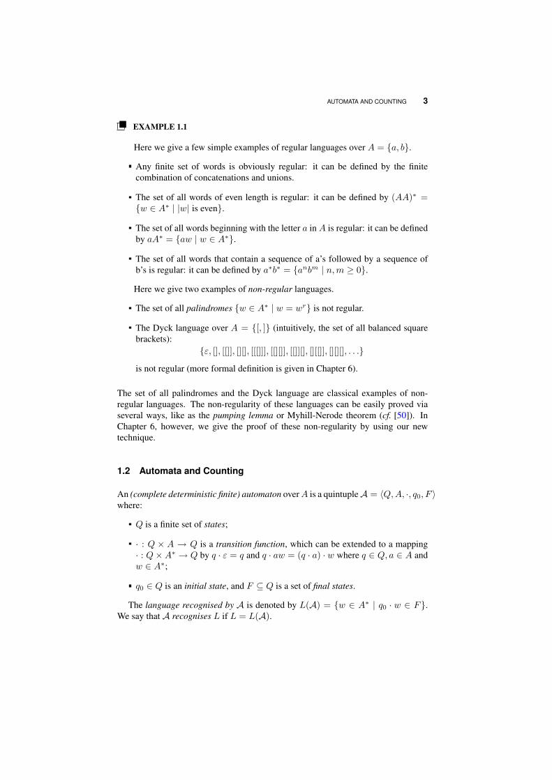
EXAMPLE 1.1

Here we give a few simple examples of regular languages over A = {a, b}.

Any finite set of words is obviously regular: it can be defined by the finitecombination of concatenations and unions.

The set of all words of even length is regular: it can be defined by (AA)∗ ={w ∈ A∗ | |w| is even}.

The set of all words beginning with the letter a in A is regular: it can be definedby aA∗ = {aw | w ∈ A∗}.

The set of all words that contain a sequence of a’s followed by a sequence ofb’s is regular: it can be defined by a∗b∗ = {anbm | n,m ≥ 0}.

Here we give two examples of non-regular languages.

The set of all palindromes {w ∈ A∗ | w = wr} is not regular.

The Dyck language over A = {[, ]} (intuitively, the set of all balanced squarebrackets):

{ε, [], [[]], [][], [[[]]], [[][]], [[]][], [][[]], [][][], . . .}

is not regular (more formal definition is given in Chapter 6).

The set of all palindromes and the Dyck language are classical examples of non-regular languages. The non-regularity of these languages can be easily proved viaseveral ways, like as the pumping lemma or Myhill-Nerode theorem (cf. [50]). InChapter 6, however, we give the proof of these non-regularity by using our newtechnique.

1.2 Automata and Counting

An (complete deterministic finite) automaton over A is a quintuple A = 〈Q,A, ·, q0, F 〉where:

Q is a finite set of states;

· : Q × A → Q is a transition function, which can be extended to a mapping· : Q × A∗ → Q by q · ε = q and q · aw = (q · a) · w where q ∈ Q, a ∈ A andw ∈ A∗;

q0 ∈ Q is an initial state, and F ⊆ Q is a set of final states.

The language recognised by A is denoted by L(A) = {w ∈ A∗ | q0 · w ∈ F}.We say that A recognises L if L = L(A).

4 PRELIMINARIES

EXAMPLE 1.2

In this thesis, an automaton is illustrated by its transition diagram like Figure1.1. Each final state will be indicated by an outgoing edge without a label, andthe initial state will be indicated by an incoming edge without a label. One caneasily observe that the automaton in Figure 1.1 has q0 as its initial and finitestate, and recognises the language (TITECH)∗.

q0

q1 q2

q3

q4q5

T

I

T

E

C

H

1

Figure 1.1 An automaton recognising (TITECH)∗.

It is a basic fact that, for any regular language L, there exists a unique automatonrecognises L which has the minimum number of states: the minimal automaton of Land we denote it by AL. For each pair of states p, q in Q, we say that q is reachablefrom p if, there exists a word w such that p · w = q. A is called accessible ifevery state q in Q is reachable from the initial state q0. In this thesis, all consideredautomata are accessible. The following theorem is fundamental.

Theorem 1.2.1 (Kleene [29, 30]) A language L is regular if and only if it is recog-nised by an automaton.

The counting function γn(L) of a language L counts the number of all words oflength n in L:

γn(L) = |{w ∈ L | |w| = n}| = |L ∩ An|.If L is a regular language, we can represent its counting function γn(L) by usingthe nth power of a certain matrix related to an automaton that recognises L. Moreprecisely, for any regular language L and any automaton A = 〈Q, A, ·, q0, F 〉 thatrecognises L, the following equation holds:

γn(L) = IMnF

where M is the |Q| × |Q| matrix, I and F are the row and column vectors defined asfollows:

Mi,j = |{a ∈ A | qi · a = qj}|, Ii =

{1 if i = 0,

0 if i 6= 0,Fi =

{1 if qi ∈ F,

0 if qi /∈ F.

M is called the adjacency matrix of A, I [F ] is called the initial [final] vector of A.Since (Mn)i,j equals to the number of all paths of length n from qi to qj , the righthand side of Equation 1.1 equals to the number of all paths of n from the initial stateto final states, that is, the number of all words of length n in L.

AUTOMATA AND COUNTING 5

EXAMPLE 1.3

q0 q1 q2b

a

ba+ ba

1

Figure 1.2 An automaton Afib.

Consider the automaton Afib which recognises L = {a, ba}∗ illustrated inFigure 1.2. Let:

M =

1 1 01 0 10 0 2

, I =[1 0 0

], F =

100

are its adjacency matrix, initial and final vectors. Then the followings hold.

γ0(L) = |{ε}| = 1,

γ1(L) = |{a}| = 1,

γ2(L) = |{aa, ba}| = 2,

γ3(L) = |{aaa, aba, baa}| = 3,

γ4(L) = |{aaaa, aaba, abaa, baaa, baba}| = 5,

...

γn(L) = IMnF =[1 0 0

]1 1 01 0 10 0 2

n 1

00

=[1 0 0

]S

2 0 00 1

2 (1 −√

5) 00 0 1

2 (1 +√

5)

n

S−1

100

where S =

0 12 (1 −

√5) 1

2 (1 +√

5)0 1 11 0 0

=

1√5

(

1 +√

52

)n+1

−

(1 −

√5

2

)n+1

The last equation means that γn(L) equals to the (n + 1)st Fibonacci number.

6 PRELIMINARIES

1.3 Monoids and Morphisms

A monoid M is a set equipped with an associative binary operation and the identityelement 1 that satisfies m1 = 1m = m for all m in M. In particular, the full languageA∗ is called the free monoid over A: its identity element is ε, and it is equipped withthe concatenation as an associative binary operation. A morphism is a map φ from amonoid M into a monoid N that satisfies φ(1M ) = 1N where 1M [1N ] is an identityof M [N ], and φ preserves the binary operation:

φ(xy) = φ(x)φ(y)

for every x, y in M . We say that a monoid M recognises a language L over A if,there exist a morphism φ : A∗ → M and a subset P of M such that:

φ−1(P ) = L.

An element 0 of M is said to be a zero if, 0x = x0 = 0 holds for all x in M . Amonoid M that have a zero element is said to be a monoid with zero.

EXAMPLE 1.4

Let Ml = {1, a, b} be a finite monoid with the identity 1 whose product isdefined as ax = a and bx = b for all x in Ml. Let A = {a, b} be an alphabetand φ : A∗ → Ml be a morphism such that φ(a) = a and φ(b) = b. Then Ml

recognises three regular languages aA∗, bA∗ and {ε}:

aA∗ = φ−1(a), bA∗ = φ−1(b), φ−1(1) = {ε}.

The syntactic congruence of a language L over A is the equivalence relation ∼L

defined on A∗ by u ∼L v if and only if xuy ∈ L ⇔ xvy ∈ L holds for all x, y in A∗.The quotient A∗/∼L is called the syntactic monoid of L and the natural morphismφL : A∗ → A∗/∼L is called the syntactic morphism of L. Let A = 〈Q,A, ·, q0, F 〉be an automaton. Each word w in A∗ defines the transformation w : q 7→ q · won Q. The transition monoid of A is the transformation monoid generated by thegenerators a : q 7→ q · a in A. It is well known that the syntactic monoid of a regularlanguage is equal to the transition monoid of its minimal automaton. The followingwell-known theorem states that the converse is also true.

Theorem 1.3.1 (Myhill [43]) A language L is regular if and only if it is recognisedby some finite monoid. In particular, L is regular if and only if its syntactic monoidis finite.

1.4 Bibliographic Notes

Kleene used the term regular events and in his 1951 paper “Representation of eventsin nerve nets and finite automata” [29] wrote: “We would welcome any suggestions

BIBLIOGRAPHIC NOTES 7

as to a more descriptive term”. After that, in the later version of the paper [30],the above phrase was deleted. The definition of the syntactic monoid was firstlyintroduced by Schützenberger in 1956 [53]. It later appeared in the paper by Rabinand Scott [48], where the notion is credited to Myhill. For a semigroup S and itssubset T , the principal congruence determined by T is the equivalent relation ≡T

defined on S by u ≡T v if and only if xuy ∈ T ⇔ xvy ∈ T holds for all x, y inS (cf. [28]). The syntactic congruence is a particular case of a principal congruence(when S = A∗). The notion of principal congruence has been studied, albeit withsometimes different meanings, from early 1940s: by Dubreil in 1941 [17], Teissierin 1951 [64], Pierce in 1954 [45]. A more detailed and complete history can be foundin [12].

CHAPTER 2

ZEROONE LAW FOR REGULARLANGUAGES

ある形式文法の族を導入した際に，まずそこで定義される言語の族の閉包性を調べ，決定問題を考え，正則集合との関係を見るという理論展開の鋳型はこのとき (Bar-Hillelet al. [3])にできたといえる．

—Setsuo Arikawa, “数理言語学入門” (Japanese translation of [26]).

In this chapter, we provides a detailed exposition of the notion of the zero-one lawfor regular languages. The main result of the thesis – Zero-One Theorem – will bestated in this chapter (Theorem 2.3.1).

8 Zero-One Law for Regular Languages.By Ryoma Sin’ya Copyright c© 2016

ZEROONE LANGUAGES: ZO AND ZOREG 9

2.1 ZeroOne Languages: ZO and ZOReg

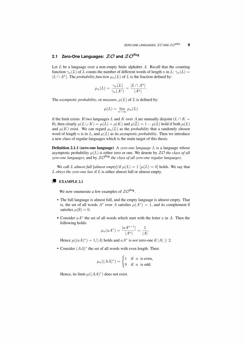
Let L be a language over a non-empty finite alphabet A. Recall that the countingfunction γn(L) of L counts the number of different words of length n in L: γn(L) =|L ∩ An|. The probability function µn(L) of L is the fraction defined by:

µn(L) =γn(L)γn(A∗)

=|L ∩ An||An|

.

The asymptotic probability, or measure, µ(L) of L is defined by:

µ(L) = limn→∞

µn(L)

if the limit exists. If two languages L and K over A are mutually disjoint (L ∩ K =∅), then clearly µ(L ∪ K) = µ(L) + µ(K) and µ(L) = 1 − µ(L) hold if both µ(L)and µ(K) exist. We can regard µn(L) as the probability that a randomly chosenword of length n is in L, and µ(L) as its asymptotic probability. Then we introducea new class of regular languages which is the main target of this thesis.

Definition 2.1.1 (zero-one language) A zero-one language L is a language whoseasymptotic probability µ(L) is either zero or one. We denote by ZO the class of allzero-one languages, and by ZOReg the class of all zero-one regular languages.

We call L almost full [almost empty] if µ(L) = 1 [µ(L) = 0] holds. We say thatL obeys the zero-one law if L is either almost full or almost empty.

EXAMPLE 2.1

We now enumerate a few examples of ZOReg.

The full language is almost full, and the empty language is almost empty. Thatis, the set of all words A∗ over A satisfies µ(A∗) = 1, and its complement ∅satisfies µ(∅) = 0.

Consider aA∗ the set of all words which start with the letter a in A. Then thefollowing holds:

µn(aA∗) =|aAn−1||An|

=1|A|

.

Hence µ((aA)∗) = 1/|A| holds and aA∗ is not zero-one if |A| ≥ 2.

Consider (AA)∗ the set of all words with even length. Then:

µn((AA)∗) =

{1 if n is even,0 if n is odd.

Hence, its limit µ((AA)∗) does not exist.

10 ZEROONE LAW FOR REGULAR LANGUAGES

Thus, for some regular language L, the asymptotic probability µ(L) is either zeroor one, for some, like L = aA∗ where |A| ≥ 2, µ(L) could be a real numberbetween zero and one, and for some, like L = (AA)∗, it may not even exist. It ispreviously known that there exists a cubic time algorithm computing µ(L) for anyregular language L if L is given by an n-states automaton [8] and µ(L) is alwaysrational [4, 51] (see Section 2.4).

Remark 2.1.1 Technically speaking, the function µ defined here is not a measureof the standard definition in measure theory (cf. [63]). The µ defined here obviouslysatisfies the following properties:

µ(∅) = 0, µ(L) = 1 − µ(L) if µ(L) exists.

the (finite) additivity: whenever two languages K, L are disjoint and both µ(K)and µ(L) exist, then µ(K ∪ L) = µ(K) + µ(L).

the (finite) subadditivity: µ(K ∪ L) ≤ µ(K) + µ(L) if both µ(K) and µ(L)exist.

the monotonicity: K ⊆ L implies µ(K) ≤ µ(L) if both µ(K) and µ(L) exist.

But µ does not satisfy the countable additivity. That is, µ(∪

w∈A∗{w}) = µ(A∗) =1, although µ({w}) = 0 holds for each word w in A∗.

2.2 Languages with Zero: Z and ZReg

In this thesis, we show that the following class of languages exactly captures thezero-one law for regular languages.

Definition 2.2.1 A language with zero is a language whose syntactic monoid has azero element. We denote by Z the class of all languages with zero, and by ZReg theclass of all regular languages with zero.

EXAMPLE 2.2

We now enumerate a few examples related with ZReg.

The trivial monoid M = {1} is actually with zero: the identity element 1 isalso a zero element. Hence the full language and the empty language over Aare languages with zero, because the syntactic monoid of these languages is thetrivial monoid.

Let L = A∗aA∗ be the set of all words that contain a as a factor. One caneasily verify that the syntactic monoid of L is the two element monoid withzero ML = {0, 1} and φ−1

L (0) = A∗aA∗. The identity element 1 represents“any word that does not contain a”, and the zero element 0 represents “any wordthat contains at least one a”. Thus L = A∗aA∗ is with zero.

ZEROONE THEOREM: ZOREG = ZREG 11

Consider aA∗ the set of all words which start with the letter a in A. The syn-tactic monoid of aA∗ is the monoid Ml defined in Example 1.4. Since Ml doesnot have a zero element, aA∗ is not with zero.

2.3 ZeroOne Theorem: ZOReg = ZReg

Now we give a precise statement of the our main result. The definition of two classesof automata – zero automata and quasi-zero automata – will be given in Chapter 4.

Theorem 2.3.1 (Zero-One Theorem) Let L be a regular language and AL be theminimal automaton of L. Then the following five conditions are equivalent.

1© AL is zero.

2© L is with zero.

3© L or L contains an ideal language.

4© L obeys the zero-one law.

5© L is recognised by a quasi-zero automaton.

The remarkable fact is that, ZOReg = ZReg holds even though these two notionsseem completely different from each other; ZOReg is defined by the asymptotic be-havior of its probability, ZReg is defined by the existence of a zero of its syntacticmonoid. The proof of this theorem is given in Chapter 4. We will prove this theo-rem as a cyclic chain of implications: 1© ⇒ 2© ⇒ 3© ⇒ 4© ⇒ 1©, and 1© ⇔ 5©independently. We should notice that the most difficult part of this proof is the impli-cation 4© ⇒ 1©, while the former part 1© ⇒ 2© ⇒ 3© ⇒ 4© is easy. The key pointof this difficult part is closure properties of ZO which stated in the next chapter. Twoautomata characterisation 1© and 5© play a crucial role in the proof.


Densities and algebraic coding theoryThe notion of probability µn for regular languages has been studied by Berstel [4]from 1973, Salomaa and Soittola [51] from 1978 in the context of the theory of for-mal power series. They proved that µn(L) has finitely many accumulation pointsand each accumulation point is rational. Another approach, based on Markov chaintheory, was presented by Bodirsky et al. [8]. They investigate the algorithmic com-plexity of computing accumulation points of L and introduced an O(n3) algorithmto compute µ(L) for any regular language L (and hence whether L is zero-one), if Lis given by an n-states automaton. There is an alternative definition of the asymptoticprobability of L over A:

µ∗(L) = limn→∞

∑ni=0 |L ∩ Ai|∑n

i=0 |Ai|.

12 ZEROONE LAW FOR REGULAR LANGUAGES

In fact, Berstel uses this definition of µ∗ in his first research on this topic [4]. How-ever, for any language L over A, µ∗(L) exists if and only if µ(L) exists and theyare equal by well-known Stolz–Cesáro theorem and its partial converse (cf. Theorem1.22 and 1.23 in [42]). Thus our Zero-One Theorem does not depend on the defini-tion we use.

A similar notion, density of a language have also been studied in algebraic codingtheory (cf. [5, 6]). A probability distribution π on A∗ is a function π : A∗ → [0, 1]such that π(ε) = 1 and

∑a∈A π(wa) = π(w) for all w in A∗. As a particular

case, the uniform Bernoulli distribution is a morphism from A∗ into [0, 1] such thatπ(a) = 1/|A| for all a in A. We denote by A(n) = {w ∈ A∗ | |w| < n} the setof all words of length less than n over A. The density δ(L) of L then defined by thefollowing:

δ(L) = limn→∞

1n

π(L ∩ A(n)

)where π is a probability distribution on A∗. A monoid M is called well foundedif it has a unique minimal ideal, if moreover this ideal is the union of the minimalleft ideals of M , and also of the minimal right ideals, and if the intersection of aminimal right ideal and of a minimal left ideal is a finite group. An elementaryresult from analysis shows that if π is the uniform Bernoulli distribution and µ(L)exists, then δ(L) = limn→∞

1n

∑ni=0 µi(L) also exists and δ(L) = µ(L) holds. The

converse, however, does not hold (e.g., δ((AA)∗) = 1/2). In their book [6], Berstelet al. proved Theorem 13.4.5 which states that, for any well founded monoid M andmorphism φ : A∗ → M , δ(φ−1(m)) has a limit for every m in M . Furthermore,this density is non-zero if and only if m in the minimal ideal K of M from whichwe obtain δ(φ−1(K)) = 1. Since every monoid with zero is well founded, Theorem13.4.5 implies that, every language with zero is zero-one (i.e., 2© ⇒ 4©, “easy part”of our Zero-One Theorem). Some other related results can be found in the theoryof probabilities on algebraic structures initiated by Grenander [25] and Martin-Löf[40].

The point to observe is that the techniques presented in this thesis are purelyautomata theoretic. We did not use, to prove Zero-One Theorem, any probabilitytheoretic tools: like as measure theory, formal power series, Markov chain, algebraiccoding theory, etc. This point deserves explicit emphasise.

Languages defined by the counting functionThere exist other classes of languages related to zero. We call the language A∗ is full.If the counting function of a language L has bounded density, i.e., γn(L) = O(1)with respect to n, then L is called slender. A language is sparse if it has a polynomialdensity, i.e., γn(L) = O(nk) for some k > 0. Finally, a language L is calledcoslender if its complement is slender, and a language L is called cosparse if itscomplement is sparse. Gehrke, Grigorieff and Pin [23] proved that both the class ofall sparse or cosparse languages and the class of all slender or coslender languagesare closed under Boolean operations, left and right quotients. Moreover, they showedthat these two class of languages can be defined by certain profinite equation relatedto zero. Details of these results can be found in the book by Pin [46].

CHAPTER 3

CLOSURE PROPERTIES OF ZO ANDEILENBERG’S LEMMA

Wherever there is an algebraic structure for recognizing languages, there is an Eilenbergtheorem. This theorem gives a bijective mapping between classes of languages with goodclosure properties (language varieties) and classes of monoids with good closure properties(monoid varieties).

—Mikołaj Bojanczyk and Igor Walukiewicz, “Forest Algebras” [9].

In formal language theory, good closure properties of a class of languages some-times imply a good structural theorem of that class. The key points of the proof ofZero-One Theorem are closure properties of the class of all zero-one languages ZO.In this chapter, we introduce Eilenberg’s lemma which is based on certain closureproperties of a class of languages.

Zero-One Law for Regular Languages.By Ryoma Sin’ya Copyright c© 2016

13

14 CLOSURE PROPERTIES OF ZO AND EILENBERG’S LEMMA

3.1 Closure Properties of ZO

We first introduce the following lemma.

Lemma 3.1.1 Let L be a language over A and w be a word in Ak for some k ≥ 0.Then the asymptotic probability of L exists if and only if the asymptotic probability ofthe language wL [Lw] exists. Moreover, these limits satisfy the equation µ(wL) =µ(Lw) = |A|−kµ(L).

Proof : Since wL and Lw clearly have the same counting function, we only have toprove the case of wL. For every u, v in Ak such that u 6= v, the two languages uLand vL are mutually disjoint and these counting functions coincides:

γn(uL) = γn(vL) =

{0 n < k,

γn−k(L) n ≥ k.

This shows that uL and vL have the same asymptotic probability if its exists. Wecan easily verify that the following equation holds for any language L over A andk ≥ 0:

µn+k(AkL) =|AkL ∩ An+k|

|An+k|=

|Ak(L ∩ An)||AkAn|

=|L ∩ An||An|

= µn(L).

It follows from what has been said that µ(AkL) exists if and only if µ(L) exists andin that case they are equal µ(AkL) = µ(L). Hence it follows that µ(uL) exists ifand only if µ(L) exists by the following equation:

µ(L) = µ(AkL

)=∑

u∈Ak

µ(uL) = |A|kµ(uL).

Now we prove that ZO enjoys good closure properties that are necessary to applyEilenberg’s lemma introduced in the next section.

Proposition 3.1.1 ZO is closed under Boolean operations, left and right quotients.

Proof : It is obvious that ZO is closed under complement since µ(L) = 1−µ(L) ∈{0, 1}. Next we assume that µ(L) = µ(K) = 0, then µ(L∪K) = 0 is obvious fromthe subadditivity of µ:

µ(L ∪ K) ≤ µ(L) + µ(K) = 0.

Then one can easily verify that the following hold for L,K in ZO:

µ(L ∩ K) = min(µ(L), µ(K)),

µ(L ∪ K) = max(µ(L), µ(K)).

EILENBERG’S LEMMA 15

We then prove that ZO is closed under left quotients. We only have to considerthe left quotient by a letter a−1L since every left quotient w−1L = (a0 · · · an)−1L isa successive application of letter quotients a−1

n · · · (a−10 L). First we assume µ(L) =

0. One can easily verify that aa−1L = L∩aA∗ ⊆ L and hence µ(aa−1L) = µ(L) =0 for each letter a. In addition, µ(aa−1L) coincides with µ(a−1L) for each letter a,because µ(aa−1L) = |A|−1µ(a−1L) = 0 by Lemma 3.1.1 whence µ(a−1L) = 0.

Next we assume µ(L) = 1. Then µ(L) = 0 and:

a−1L = {w ∈ A∗ | aw ∈ L}= {w ∈ A∗ | aw /∈ L} = a−1L

holds. We therefore obtain:

µ(a−1L) = 1 − µ(a−1L)= 1 − µ(a−1L) = 1 − 0 = 1.

We can prove that ZO is closed under right quotients by the same manner.

Since the class of regular languages is closed under Boolean operations and quo-tients, the following corollary follows from Proposition 3.1.1.

Corollary 3.1.1 ZOReg is closed under Boolean operations, left and right quotients.

Proposition 3.1.2 ZO is not closed under inverses of morphisms.

Proof : Let L = (aa)∗ be a language over A = {a, b}, let φ : A∗ → A∗ be themorphism such that φ(a) = φ(b) = a. One can easily verify µ(L) = 0 and henceL is in ZOReg. Then the inverse image of L is φ−1((aa)∗) = (AA)∗, but (AA)∗ isnot in ZO as we stated in Example 2.2.

Corollary 3.1.2 ZOReg is not closed under inverses of morphisms.

The counterexample given in Proposition 3.1.2 can be found in Pin’s book [46].He uses it to prove that ZReg is not closed under inverses of morphisms.

3.2 Eilenberg’s Lemma

Let AL = 〈Q,A, ·, q0, F 〉 be an automaton. For any subset P of Q, the past of P isthe language denoted by Past(P ) and defined by:

Past(P ) = {w ∈ A∗ | q0 · w ∈ P}.

Dually, the future of a subset P of Q is the language denoted by Fut(P ) and definedby:

Fut(P ) = {w ∈ A∗ | ∃p ∈ P, p · w ∈ F}.

16 CLOSURE PROPERTIES OF ZO AND EILENBERG’S LEMMA

It is well known that, an (accessible) automaton A is minimal if and only if thefollowing condition holds:

∀p, q ∈ Q(p = q ⇔ Fut(p) = Fut(q)

). (M)

In the next chapter, to prove Zero-One Theorem, we will use the following tech-nical but important lemma.

Lemma 3.2.1 Let AL = 〈Q, A, ·, q0, F 〉 be the minimal automaton of a languageL. Then for any subset P of Q, its past Past(P ) can be expressed as a finite Booleancombination of languages of the form Lw−1 where w in A∗.

Proof : We only have to prove that, for any state q in Q, its past Past(q) can beexpressed as a Boolean combination of languages of the form Lw−1. Our goal isto prove the following equation with the usual conventions

∩w∈∅ Lw−1 = A∗ and∪

w∈∅ Lw−1 = ∅:

Past(q) =

∩w∈Fut(q)

Lw−1

\

∪w/∈Fut(q)

Lw−1

. (3.1)

The finiteness of this Boolean combination follows from Myhill-Nerode theorem.We prove first that the left hand side is contained in the right hand side. Let v be

a word in Past(q). If a word w in Fut(q), then vw in L by the definition, and hencev in Lw−1. If a word w not in Fut(q), then vw not in L by the definition, and hencev not in Lw−1. It follows that the left hand side is contained in the right hand side inEquation (3.1).

Then we prove that the right hand side is contained in the left hand side. Letv be a word in right hand side. Let p be the state satisfying q0 · v = p, that is, vis a word in Past(p). For any w in Fut(q), by the form of Equation (3.1), v is inLw−1 from which we get vw in L whence p · w in F . That is, w also belongs toFut(p). Conversely, for any w not in Fut(q), vw is not in L and thus v not in Lw−1.That is, w does not belong to Fut(p). It follows that p and q have the same futureFut(p) = Fut(q) from which we get p = q by Condition (M) of the minimality ofAL. Hence we obtain v in Past(q) and thus the right hand side is contained in theleft hand side in Equation (3.1).

3.3 Consequence of Eilenberg’s Lemma for ZOReg

We will use the following lemma, which is a direct consequence of Lemma 3.2.1 andProposition 3.1.1.

Lemma 3.3.1 Let L be a regular language in ZOReg, AL = 〈Q,A, ·, q0, F 〉 be itsminimal automaton. Then, for any subset P of Q, its past Past(P ) is also in ZOReg.

Proof : By Lemma 3.2.1, for any subset P of Q, its past Past(P ) can be expressedas a finite Boolean combination of languages of the form Lw−1. It follows that


Past(P ) obeys the zero-one law, since L is in ZOReg and ZOReg is closed underBoolean operations and quotients by Corollary 3.1.1.


Lemma 3.2.1 shows us an importance of the Boolean operations taken in tandem withquotients. While this lemma is known as a folklore (cf. [19]), which is an “automatonversion” of a key lemma in Eilenberg’s variety theorem, we have not found anyliterature that includes a complete proof. The proof given in this thesis is essentiallybased on “Proof of Theorem 3.2 and 3.2s” in Eilenberg’s Volume B [18]. The originalEilenberg’s lemma states about a monoid, not an automaton, as the following kind.

Lemma 3.4.1 (Eilenberg [18]) Let ML be the syntactic monoid of a regular lan-guage L over A, and let φL : A∗ → ML be the syntactic morphism of L. Thenfor each element m of ML, its inverse φ−1

L (m) can be expressed as a finite Booleancombination of languages of the form u−1Lv−1 where u, v in A∗.

Eilenberg used this lemma to prove his variety theorem: the existence of the one-to-one correspondence between varieties of languages and varieties of finite monoids.

Technically speaking, ZOReg is not a variety. Recall that a variety of languages isa class of regular languages closed under Boolean operations, left and right quotientsand inverses of morphisms. Proposition 3.1.2 shows that ZOReg is not closed underinverses of morphisms. Since the work of Eilenberg, the theory have been extendedseveral times by relaxing the definition of a variety of languages. Straubing [60] in-troduced the notion of C-varieties: here C denotes some natural class of morphisms.A similar notion was introduced independently by Ésik and Ito [19]. The definitionof a C-variety of languages is similar to Eilenberg original definition except that itonly requires closure under inverse images of morphisms belonging to C. More re-cently, Gehrke et al. [23] proved that any lattice of languages (a class of regularlanguages closed under union and intersection) can be defined by a set of profiniteequations, a result that subsumes Eilenberg’s variety theorem. See [46, 61, 47] formore details.

CHAPTER 4

EQUIVALENCE OF ZOReg AND ZReg

The Variety Theorem provides the framework for talking about recognisable languages andfinite monoids. It says that if you have a pseudovariety of finite monoids then there willbe an associated variety of languages, although it will not tell you what these languageslook like; that involves extra work and depends on the properties of the pseudovariety ofmonoids in question. Likewise, if you have a variety of languages, the Theorem tells usthat there is an associated pseudovariety of finite monoids, but again it will not tell us whatthey look like; you have to do extra work.

—Mark V. Lawson, “Finite Automata” [34].

An automata theoretic proof of Zero-One Theorem is given in this chapter. Inthis chapter, we introduce two classes of automata: zero automata and quasi-zeroautomata. Zero automata plays major role in the proof of the difficult implication4© ⇒ 1©.

18Zero-One Law for Regular Languages.By Ryoma Sin’ya Copyright c© 2016

ZERO AUTOMATA 19

4.1 Zero Automata

Let A be an automaton 〈Q, A, ·, q0, F 〉. We write p →∗ q if a state q is reachablefrom a state p. It is clear that the reachability relation →∗ forms a preorder overQ, that is, a reflexive and transitive relation over Q. The equivalence relation ↔∗

defined on Q by p ↔∗ q if and only if p →∗ q and q →∗ p hold. A subset P ofQ is called strongly connected component if every state q in P is reachable fromevery other state in P , i.e., , p ↔∗ q holds for every p, q in P . A state q in Q issaid to be sink, if q · a = q holds for every letter a in A. We say that a subset Pof Q is sink, if it is strongly connected and there is no transition from any state p inP to a state which does not in P . That is, Q \ P are not reachable from P . Thefamily of all sink components of A is denoted by Sink(A). A sink component P istrivial if it consists of some single state P = {p}. We shall identify a singleton {p}with its unique element p. Sink components can be regarded as maximal equivalenceclasses with respect to ↔∗ over Q. That is, if P is sink, then P is strongly connectedand p →∗ q implies q in P for every p in P and q in Q. Note that, since everyfinite set equipped with a preorder has at least one maximal equivalence class, every(complete) automaton has at least one sink component. One can easily verify that,for every state q, there exists a sink component that is reachable from q. A word w isa synchronising word of A if, there exists a certain state q in Q, p · w = q holds forevery state p in Q. That is, w is the constant map from Q to q. We call an automatonsynchronising if it has a synchronising word. Note that any synchronising automatonhas at most one sink state. As we will prove in the next section, the following classof automata captures precisely the zero-one law for regular languages.

Definition 4.1.1 ([49]) A zero automaton is a synchronising automaton with a sinkstate.

EXAMPLE 4.1

Figure 4.1 Zero and nonzero automata

Consider two automata A0 and A1 illustrated in Figure 4.1. A0 is a zeroautomaton but A1 is not, though both automata have a sink state q5. A synchro-nisation word of A0 is aabb: one can easily verify that qi · aabb = q5 for every

20 EQUIVALENCE OF ZOREG AND ZREG

Figure 4.2 Synchronising word vn−1 = w0 · · ·wn−1 in the proof of Lemma 4.1.1

state qi. It is clear that A1 in Figure 4.1 does not have a synchronising wordsince it has two sink components. The only difference between A0 and A1 isthe transition result of q4 · a; which equals to q5 in A0, while which equals to q3

in A1. We can easily verify that, A0 has a unique sink component q5, while A1

has two sink components {q3, q4} and q5.

The definition of zero automata can be rephrased as follows.

Lemma 4.1.1 Let A = 〈Q,A, ·, q0, F 〉 be an automaton. Then A is zero if andonly if A has a unique sink component and it is trivial, i.e., Sink(A) = {{p}} for acertain sink state p.

Proof : First we assume A is zero with a sink state p. Then there exists a synchro-nising word w and it clearly satisfies q · w = p for each q in Q since p is sink. Thisshows that there is no sink component in Q \ p.

Now we prove the converse direction, we assume A has a unique sink componentand it is trivial, say p. We can verify that for every state q in Q, there exists a wordw in A∗, such that q · w = p. Indeed, if there does not exist such word w for someq, then the set of all reachable states from q : {r ∈ Q | ∃w ∈ A∗, q · w = r} mustcontains at least one sink component which does not contain p. This contradictswith the uniqueness of the sink component p in A. The existence of a synchronisingword w is guaranteed, because we can concretely construct it as follows. Let n bethe number of states n = |Q| and let Q = {q0, · · · , qn−1 = p}. We define a wordsequence wi inductively by w0 = uq0 and wi = u(qi·vi−1) where each uqi is ashortest word satisfying qi · uqi = p, and vi−1 is the word of the form w0 · · ·wi−1.As shown in Figure 4.2, we can easily verify that the word vn−1 = w0 · · ·wn−1 is asynchronising word satisfying q · vn−1 = p for each q in Q.

For example, consider the zero automaton A0 in Figure 4.1. Then each uqi , wqi

and vqi are defined as follows.

uqi wqi vqi

q0 aab aab aabq1 ab b aabbq2 b ε aabbq3 aa ε aabbq4 a ε aabb

The obtained word vq4 = aabb is a synchronising word of A0.

PROOF OF ZEROONE THEOREM (1) 21

4.2 Proof of ZeroOne Theorem (1)

We show the implication 1© ⇒ 2© ⇒ 3© ⇒ 4© ⇒ 1©. The former implication1© ⇒ 2© ⇒ 3© ⇒ 4© is easy, but we include a complete proof here to be self-

contained.

4.2.1 1© ⇒ 2© (AL is zero ⇒ L is with zero)

Let AL = 〈Q,A, ·, q0, F 〉 be the minimal automaton of L and assume that AL iszero with a sink state p. Let M be the transition monoid of AL and φ : A∗ → Mbe the syntactic morphism of L. Then we can verify that M has a zero element 0 asthe transformation 0 : q 7→ p for all q in Q, that is, 0 is the constant map from Qto p. The existence of 0 is guaranteed since AL is synchronising. Indeed, for anysynchronising word w, φ(w) = 0 holds. One can easily verify that m0 = 0m = 0for all m in M . This proves that M the syntactic monoid of L has the zero.

4.2.2 2© ⇒ 3© (L is with zero ⇒ L or L contains an ideal language)

Let L be a regular language in ZReg, M be its syntactic monoid with a zero element0 and φ : A∗ → M be its syntactic morphism. Choose a word w0 from the preimageof 0: w0 ∈ φ−1(0). Note that the word w0 is always exists by the definition of thesyntactic monoid.

Now we prove that L contains the ideal language A∗w0A∗ if w0 is in L. By thedefinition of zero, we have

φ(xw0y) = φ(x)φ(w0)φ(y) = φ(x)0φ(y) = 0

for any words x, y in A∗. That is, if w contains w0 as a factor, then φ(w) = φ(w0) =0 holds and hence w also in L. This implies that the language of the form A∗w0A∗,the set of all words that contains w0 as a factor, is contained in L. Dually, we canprove that L contains A∗w0A∗ if w0 is not in L.

4.2.3 3© ⇒ 4© (L or L contains an ideal language ⇒ L obeys thezeroone law)

We assume that L contains A∗wA∗ for some word w. The probability µn(A∗wA∗)is nothing but the probability that a randomly chosen word of length n contains was a factor. The infinite monkey theorem (cf. Note I.35 in [21]), sometimes calledBorges’s theorem, ensures that µn(A∗wA∗) tends to one if n tends to infinity.

Infinite Monkey Theorem. Take any fixed finite set Π of words in A∗. A randomword in A∗ of length n contains all the words of the set Π as factors with probabilitytending to one exponentially fast as n tends to infinity.

This and the monotonicity of µ shows µ(L) = µ(A∗wA∗) = 1. Conversely, if thecomplement L contains A∗wA∗, one can easily verify that µ(L) = 1 − µ(L) = 0.


4.2.4 4© ⇒ 1© (L obeys the zeroone law ⇒ AL is zero)

Let L be a regular language in ZOReg and AL = 〈Q,A, ·, q0, F 〉 be its minimalautomaton, let Sink(AL) = {P1, · · · , Pk} for some k ≥ 1. Our goal is to provek = 1 and Sink(AL) = {{p}} for a certain sink state p. It follows that AL is zeroby Lemma 4.1.1.

For any sink component Pi, there exists a word wi such that q0 ·wi in Pi becauseAL is accessible. Lemma 3.1.1 and µ(A∗) = 1 implies:

µ(wiA∗) = |A|−|wi|µ(A∗) = |A|−|wi| > 0. (4.1)

Since Pi is sink, the language wiA∗ is contained in Past(Pi). For each Past(Pi)

has the asymptotic probability and it is either zero or one by Lemma 3.3.1. Themonotonicity of µ and Inequation (4.1) imply:

µ(Past(Pi)) = 1 (4.2)

holds for every sink component Pi.Now we prove k = 1. By Equation (4.2), we can easily verify that

µ

(k∪

i=1

Past(Pi)

)=

k∑i=1

µ(Past(Pi)) = k

holds because AL is deterministic and thus all Past(Pi) are mutually disjoint. Thisclearly shows k = 1, that is, there exists a unique sink component, say P , in AL:Sink(AL) = {P}.

Next we let P = {p1, · · · , pn} and prove n = 1. Since P satisfies µ(Past(P )) =1 by Equation (4.2), there exists exactly one state p in P that satisfies µ(Past(p)) = 1by Lemma 3.3.1. Further, because P is strongly connected, for every state pi in P ,there exists a word wi such that p · wi = pi and thus Past(pi) contains Past(p)wi.Lemma 3.1.1 and µ(Past(p)) = 1 implies:

µ(Past(p)wi) = |A|−|wi|µ(Past(p)) = |A|−|wi| > 0. (4.3)

Each Past(pi) has the asymptotic probability and it is either zero or one by Lemma3.3.1. The monotonicity of µ and Inequation (4.3) imply:

µ(Past(pi)) = 1 (4.4)

holds for every pi in P . From Equation (4.4), we obtain:

µ(Past(P )) =n∑

i=1

µ(Past(pi)) =n∑

i=1

1 = n = 1,

because AL is deterministic and thus all Past(pi) are mutually disjoint. We nowobtain n = 1, that is, P is singleton and hence Sink(AL) = {p}. That is, AL iszero.

QUASIZERO AUTOMATA 23

4.3 QuasiZero Automata

Let A = 〈Q,A, ·, q0, F 〉 be an automaton. The Nerode equivalence ∼ of A is therelation defined on Q by p ∼ q if and only if Fut(p) = Fut(q). One can easily verifythat ∼ is actually a congruence, in the sense that p ∼ q implies p · w ∼ q · w forall w ∈ A∗. Hence it follows that there is a well defined new automaton A/∼, thequotient automaton of A:

A/∼= 〈Q/∼, A, ·, [q0], F/∼〉

where [q] is the equivalence class modulo ∼ of q, S/∼= {[q] | q ∈ S} is the set of theequivalence classes modulo ∼ of a subset S ⊆ Q, and where the transition function· : Q/∼ ×A → Q/∼ is defined by [p] · a = [p · a]. We define the natural mappingφ : Q → Q/∼ by φ(q) = [q]. Condition (M) for minimal automata implies that, forany automaton A, its quotient automaton A/∼ is the minimal automaton of L(A).We shall identify the quotient automaton A/∼ with the minimal automaton of L(A)(cf. [50]).

We now introduce a new class of automata which is a generalisation of the classof zero automata.

Definition 4.3.1 (quasi-zero automaton) An automaton A = 〈Q,A, ·, q0, F 〉 is quasi-zero if either

∪Sink(A) ⊆ F or

∪Sink(A) ∩ F = ∅ holds.

Since every zero automaton A satisfies∪

Sink(A) = {p} for a certain state p(Lemma 4.1.1), every zero automaton is quasi-zero.

Before proving the equivalence 1© ⇔ 5© in Zero-One Theorem, we introduce thefollowing lemma.

Lemma 4.3.1 Let A = 〈Q,A, ·, q0, F 〉 be an automaton and A/∼ be its quotientautomaton. Then the following hold:

1. For any sink component P in A, P/∼ is also a sink component in A/∼.

2. For any sink component R in A/∼, there is at least one sink component P in Asatisfying P/∼= R.

Proof : (1) Let P be a sink component in A. Since P is strongly connected, foreach pair of states [p], [q] in P/∼, there exists a word w satisfying p · w = q andhence [p] · w = [p · w] = [q]. That is, [p] →∗ [q] holds and one can easily verify that[q] →∗ [p] also holds. This shows that P/∼ is strongly connected. Moreover, for any[p] in P/∼ and for any word w, [p] · w = [p · w] is also in P/∼ because P is sink andp · w is in P . That is, P/∼ is sink component in A/∼.

(2) Let R be a sink component in A/∼ and S be its preimage S = φ−1(R).Clearly, for any state s in S and for any word w, s · w is in S since [s · w] = [s] · wis in R. Since every finite set equipped with a preorder has at least one maximalequivalence class, S has at least one sink component, say P . Let p be a state in P .Since R is strongly connected, for any state in [r] in R, there exists a word w suchthat [p] · w = [p · w] = [r]. This shows that for every state [r] in R, there exists astate p · w in P for some w because P is sink. That is, P/∼= R.


4.4 Proof of ZeroOne Theorem (2)

The following proposition shows that the minimal automaton of any quasi-zero au-tomaton is zero and vice versa (this justifies the term “quasi-zero”). This propositionshows exactly the equivalence 1© ⇔ 5© in Zero-One Theorem.

Proposition 4.4.1 An automaton A = 〈Q,A, ·, q0, F 〉 is quasi-zero if and only ifA/∼ is zero.

4.4.1 1© ⇒ 5© (A/∼ is zero ⇒ A is quasizero)

Let p be the unique sink state of A/∼. To prove this direction, it is enough to considerthe case when p ∈ F/∼, i.e., Fut(p) = A∗. We now show∪

Sink(A) ⊆ F (4.5)

by contradiction. Let us assume that Inclusion (4.5) does not hold, that is, we assumethere exists a non-final state q in

∪Sink(A). Let P be the sink component of A that

contains q. Since P is sink, φ(P ) is also sink in A/∼ by Lemma 4.3.1. Moreover,φ(P ) does not contain the sink state p, because q /∈ F implies that, for any state q′

in P , Fut(q′) 6= A∗ from which we obtain Fut([q′]) 6= Fut(p) and [q′] 6= p. That is,A/∼ has at least two sink components φ(P ) and p. This is contradiction.

4.4.2 5© ⇒ 1© (A is quasizero ⇒ A/∼ is zero)

To prove this direction, it is enough to consider the case when∪

Sink(A) ⊆ F . SinceA is quasi-zero, all states in

∪Sink(A) have the same future A∗, i.e., Fut(q) = A∗

for every state q in∪

Sink(A), because∪

Sink(A) ⊆ F implies q ·w ∈ F for everystate q in

∪Sink(A) and every word w. This implies that

(∪Sink(A)

)/∼ consists of

a single equivalence class, say p. Moreover, this equivalence class p is a sink state inA/∼ by the definition of sink and Condition (M) of the minimality of A/∼. We nowshow that, by contradiction, A/∼ has only one sink component p:∪

Sink(A/∼) = {p} (4.6)

from which we obtain A/∼ is zero by Lemma 4.1.1. Let us assume that Equation(4.6) does not hold, that is, we assume there exists another sink component R in A/∼that does not contain p. By Lemma 4.3.1, there exists a sink component P in Asuch that P/∼= R. This implies that P 6⊆ F because R does not contain p. Thisis contradicts with the assumption

∪Sink(A) ⊆ F . This completes the proof of

Zero-One Theorem.



From the proof in this chapter, we can obtain the followings as a corollary.

Corollary 4.5.1 Let L be a regular language and AL be the minimal automaton ofL. Then the following four conditions are equivalent.

1. L is almost full.

2. L contains an ideal language.

3. AL is zero and its sink state is final.

4. L is recognised by a quasi-zero automaton A such that all states in∪

Sink(A)are final.

The direction 3© ⇒ 4© of Zero-One Theorem is nothing but the well knownInfinite Monkey Theorem, as we proved in Section 4.2.3. The remarkable fact of thistheorem is that its converse 4© ⇒ 3© is also true. Things are, however, getting morecomplicated if we consider beyond regular languages. There exist several simplecounterexamples that imply ZO 6= Z and we will explain such languages in Chapter6.

In contrast to the class of monoids with zero, their natural counterpart, the class ofzero automata has not been given much attention. To the best of our knowledge, onlyfew studies (e.g., [49]) have investigated zero automata in the context of the theoryof synchronising word for Cerný’s conjecture.

CHAPTER 5

ALGORITHMIC AND LOGICALASPECTS OF ZOReg

There are many brilliant surveys on formal language theory. Quite many surveys coverfirst-order and monadic second-order definability. But there are also nuggets below. Thereare deep theorems on proper fragments of first-order definability.

—Diekert et al., “A Survey on Small Fragments of First-Order Logic over Finite Words” [15].

In this chapter, we describes a linear time algorithm for testing whether a givenregular language is zero-one if it is given by an n-states automaton (recall that allautomata considered in the thesis are deterministic). Some logical aspects of thezero-one law for regular languages are also investigated.


LINEAR TIME ALGORITHM FOR TESTING MEMBERSHIP 27

5.1 Linear Time Algorithm for Testing Membership

The equivalence of zero-automata and the zero-one law gives us an effective algo-rithm. For a given n-states automaton A, we can determine whether L(A) obeys thezero-one law by the following steps: (i) Minimise A to obtain its minimal automatonA/∼. (ii) Calculate the family of all strongly connected components P of A/∼. (iii)Check whether P contains exactly one strongly connected sink component and it istrivial, i.e., whether A/∼ is a zero automaton (Lemma 4.1.1). It is well known thatHopcroft’s automaton minimisation algorithm has an O(n log n) time complexityand Tarjan’s strongly connected components algorithm has an O(n + n|A|) = O(n)complexity where n|A| means the number of edges. Hence we can minimise A toobtain A/∼ in O(n log n) on the step (i), and can calculate P in O(n) on the step (ii).One can easily verify that the step (iii) above can be done in O(n). To sum up, wehave an O(n log n) algorithm for testing whether a given regular language obeys thezero-one law.

We can obtain, however, more efficient algorithm by avoiding minimisation. Quasi-zero automata gives us more effective algorithm.

Theorem 5.1.1 There is an O(n) algorithm for testing whether a given regular lan-guage is zero-one, if its is given by an n-states automaton.

Proof : For a given n-states automaton A, we can determine whether L(A) obeysthe zero-one law by the following steps: (i) Calculate the family of all strongly con-nected components P of A. (ii) Extract all strongly connected sink components fromP to obtain Sink(A). (iii) Check whether, in

∪Sink(A), either all states are final or

all states are non-final, i.e., whether A is quasi-zero. By Zero-One Theorem, L(A)obeys the zero-one law if and only if A is quasi-zero. Hence this algorithm is correct.All steps (i) ∼ (iii) can be done in O(n), this ends the proof.

5.2 Logical Fragments over Finite Words

We denote by MSO[<] monadic second-order logic over finite words and denoteby FO[<] first-order logic over finite words. We can interpret words as logicalstructures with a linear order composed of a sequence of positions labeled overa finite alphabet A, < denotes the linear order over the natural numbers. Givena word w = a0a1 · · · an in A∗ where each ai is a letter, we define the structureMw = 〈U,<, (Pa)a∈A〉 of w as follows: the universe U is {0, 1, · · · , n} which cor-responds to positions in the word, < the usual linear order on the natural numbers,and the unary predicate Pa of a letter a in A is defined as:

Pa(i) is true ⇔ ai = a.

We shall identify each predicate Pa as the set of positions Pa = {i ∈ U | ai = a}.For a logical sentence Φ of some logic L, we denote by L(Φ) the language definedby Φ:

L(Φ) = {w ∈ A∗ | Mw |= Φ}.

28 ALGORITHMIC AND LOGICAL ASPECTS OF ZOREG

We say that a language L is definable in a logic L if, there exists a sentence Φ of Lsuch that L(Φ) = L.

EXAMPLE 5.1

The structure of a word w = abaab is defined by

Mw = 〈{1, 2, 3, 4, 5}, <, Pa, Pb〉

where < is the usual ordering, and Pa[Pb] contain positions in w where a[b]occurs: that is, Pa = {1, 3, 4} and Pb = {2, 5}.

We can easily observe that first-order logic over finite words FO[<] does not havethe zero-one law.

EXAMPLE 5.2

A simple counterexample is the language aA∗ which can be defined by theFO[<] sentence ΦaA∗ = ∃i

(Pa(i) ∧ ∀j(i ≤ j)

). aA∗ satisfies µn(aA∗) =

1/|A| as we stated in Example 2.2, hence ΦaA∗ does not obey the zero-one lawin general. It follows that FO[<] does not have the zero-one law.

We summarise well-known logical and algebraic characterisations of classes of lan-guages, including the class of zero-one languages ZOReg, in Table 5.1. We usestandard abridged notation for the following first-order fragments over finite words:

FOn[<] for first-order logic with distinct n variables;

Σn[<] for FO formulas with n blocks of quantifiers and starting with a blockof existential quantifiers;

BΣn[<] for the Boolean closure of Σn[<].

Details and full proofs of these results can be found in a very nice survey [15] byDiekert et al. A monomial over A is a language of the form A∗

0a1A∗1a2 · · · akA∗

k

where ai in A and Ai is a subset of A for each i. A monomial A∗0a1A

∗1a2 · · · akA∗

k isunambiguous if for all w ∈ A∗

0a1A∗1a2 · · · akA∗

k there exists exactly one factorisationw = w0a1w1aw · · · akwk with wi in A∗

i for each i. A language L over A is called:

star-free if it is expressible by union, concatenation and complement, but doesnot use Kleene star;

polynomial if it is a finite union of monomials;

unambiguous polynomial if it is a finite disjoint union of unambiguous mono-mials;

simple polynomial if it is a finite union of languages of the form A∗a1A∗a2 · · · akA∗.

piecewise testable if it is a finite Boolean combination of simple polynomials;

LOGICAL FRAGMENTS OVER FINITE WORDS 29

Table 5.1 Language Hierarchy

Languages Monoids Logic

regular finite MSO[<]

star-free aperiodic FO[<]

polynomials Σ2[<]

unambiguous polynomials DA FO2[<]

zero-one zero ?

piecewise testable J -trivial BΣ1[<]

simple polynomial Σ1[<]

B{A∗ | A ⊆ Σ} semilattice FO1[<]

The question then arises as to which fragments of FO[<] over finite words have thezero-one law. The algebraic characterisation of the zero-one law partially answersthis question. Since every J -trivial syntactic monoid has a zero element (cf. [46]),Zero-One Theorem leads to the following corollary.

Corollary 5.2.1 The Boolean closure of existential first-order logic over finite wordshas the zero-one law.

One can easily verify that the sentence ΦaA∗ in example 5.2, which only uses twovariables i and j, is in FO2[<]. It follows that FO2[<] does not have the zero-onelaw, hence Corollary 5.2.1 shows us a “separation” between FO2[<] and BΣ1[<]. Itmust be noted that the class of zero-one languages ZOReg and unambiguous polyno-mials are incomparable. To take a simple example, consider two languages (aa)∗ andaA∗ over A = {a, b}. The language (aa)∗ is zero-one but not unambiguous polyno-mial since its syntactic monoid is not aperiodic (i.e., having no nontrivial subgroup).Conversely, aA∗ is not zero-one but unambiguous polynomial since it is definable inFO2[<] as we have stated in Example 5.2. An interesting open problem is whetherthere exists a logical fragment that exactly captures the zero-one law (Figure 5.1).

Figure 5.1 Logical fragments and ZOReg

30 ALGORITHMIC AND LOGICAL ASPECTS OF ZOREG


Zero-one law for finite graphs That first-order logic has the zero-one law wasproved first by Glebskii et al. in 1969 [24], and independently by Fagin in 1976[20]. As Kolaitis and Vardi put it: “ In the past, 0-1 laws for various logics L wereproved by establishing first a transfer theorem for L of the following kind:

There is a certain infinite structure R over the vocabulary σ such that for anyproperty P expressible in L we have:

R |= P ⇔ P is almost surely true.

This method was discovered by Fagin (1976) in his proof of the zero-one law for first-order logic on finite structures.” And such infinite structure R is called the randomstructure. There are other known methods for proving the zero-one law: the quan-tifier elimination (i.e., every formula with just one quantifier in front of it is almosteverywhere equivalent to a quantifier-free formula) and game theoretic approaches(e.g., pebble games). [32]. These three methods are rely on the extension axiomsintroduced by Gaifman [22]. Blass, Gurevich, and Kozen [7], and independently,Talanov and Knyazev [62] proved that first-order logic with a fixed point operatorhas the zero-one law. Kolaitis and Vardi [32] gave three different proofs for the zero-one law for finite variable infinitary first-order logic; the first proof is by the transfertheorem, the second proof is by the quantifier elimination, and the third proof is bythe pebble games. The study of the zero-one law for fragments of existential second-order logic was initiated by Kolaitis and Vardi [31] and they provide a survey on thistopic [33]. We refer to Chapter 12 of the book [35] by Libkin for more details.

Zero-one law and logical fragments over finite wordsEhrenfeucht has shown that first-order logic with linear order has the convergencelaw: every definable property has an asymptotic probability (the proof can be foundin Lynch [36]). Lynch [37] proved that first-order logic with unary functions also hasthe convergence law.

The connection between logic and languages firstly discovered by Büchi in 1960[11]. He gave an effective transformations of MSO[<] sentences into finite automataand vice versa. This shows that the definability in MSO[<] captures exactly the classof regular languages. Since the work of Bühi, many connections between logic andlanguages have been shown as we summarised in Table 5.1. Some results about thezero-one law for finite words considered in this thesis is also given by Lynch [38].He proved that first-order logic over finite words has the convergence law, that is,in our terms, µ(L) exists for every first-order definable language L. Moreover, heproved that monadic second-order logic over finite words has the following weakconvergence law: for every regular language L, there is a positive integer a such thatfor all non-negative integer b < a:

limn→∞

µan+b(L)


exists. Lynch uses the game theoretic approach (Ehrenfeucht-Fraïssé game) andMarkov chains [38]. The second result is related to the previous result by Bers-tel [4], Salomaa and Soittola [51]: µn(L) has finitely many accumulation pointsand each accumulation point is rational for any regular language L. We refer thereader to Compton’s comprehensive survey about zero-one laws for various logicsand structures [13] for more history on this topic.

CHAPTER 6

BEYOND REGULAR LANGUAGES

Concevons qu’on ait dressé un million de singes á frapper au hasard sur les touches d’unemachine á ècrire et que, sous la surveillance de contremaîtres illettrés, ces singes dacty-lographes travaillent avec ardeur dix heures par jour avec un million de machines à écrirede types variés. Les contremaîtres illettrés rassembleraient les feuilles noircies et les re-lieraient en volumes. Et au bout d’un an, ces volumes se trouveraient renfermer la copieexacte des livres de toute nature et de toutes langues conservés dans les plus riches bib-liothéques du monde. Telle est la probabilité pour qu’il se produise pendant un instanttrès court, dans un espace de quelque étendue, un écart notable de ce que la mècaniquestatistique considère comme la phénomène le plus probable.

—Émile Borel, “La mécanique statistique et l’irréversibilité”.

The implication 3© ⇒ 4© of Zero-One Theorem is nothing but the well-knownInfinite Monkey Theorem. In general, it is very difficult to extend some result aboutregular languages into beyond regular languages. Many deep results in the theory ofregular languages, of course, heavily depend on the regularity of regular languages.Zero-One Theorem is not true beyond regular languages. Some counterexamples aregiven in Section 6.2. These languages obey the zero-one law but are not with zero.This implies that ZO properly contains Z , while ZOReg coincides with ZReg.


ZEROONE THEOREM FOR PROVING NONREGULARITY 33

6.1 ZeroOne Theorem for Proving NonRegularity

First of all, we prove that Z is contained in ZO. This is easy and the followingproposition is folklore (cf. [61]), but we include the proof for self-containedness.

Proposition 6.1.1 A language L over A is with zero if and only if L or L containsan ideal language.

Proof : The “only if” part is what we exactly proved in Section 4.2.2. Note that wedid not use any assumption of the regularity of L in Section 4.2.2. Now we prove the“if” part. Let ML be the syntactic monoid of L and φL be the syntactic morphismof L. We can assume that L contains an ideal language, say A∗wA∗ for some wordw, without loss of generality. Then, for any v, x, y in A∗, xwy, xvwy and xwvyare obviously in A∗wA∗. Hence w, vw and wv are all equivalent on the syntacticcongruence of L: φL(vw) = φL(wv) = φL(w). Because φL is surjective, we obtainthe following equation for all x in ML:

xφL(w) = φL(w)x = φL(w).

This implies that φL(w) is a zero element of ML.

Proposition 6.1.1 and Infinite Monkey Theorem immediately imply the following.

Corollary 6.1.1 ZO contains Z .

Zero-One Theorem implies that if L is in ZO but not in Z , then L is not reg-ular. Before proving the non-regularity of the set of all palindromes and the Dycklanguage, we sum up the above discussion in the following lemmata. Recall that aword w is forbidden [admissible] for a language L if A∗wA∗∩L = ∅ [A∗wA∗ ⊆ L]holds.

Lemma 6.1.1 (Zero Lemma) Let L be an almost empty language over A. If L doesnot have a forbidden word, then L is not regular.

Proof : From the assumption µ(L) = 0, we can easily verify that L does not containan ideal language by Infinite Monkey Theorem. Assume that L does not have aforbidden word. Then for any word w not in L, the ideal language A∗wA∗ is notdisjoint from L: A∗wA∗ ∩L 6= ∅. Hence every ideal language is not contained in L.That is, if L is almost empty and does not have a forbidden word, then L is not withzero. Since L is in ZO but not in Z , L is not regular by Zero-One Theorem.

Corollary 6.1.2 Let L be an almost full language over A. If L does not have anadmissible word, then L is not regular.

34 BEYOND REGULAR LANGUAGES

6.2 Counterexamples

6.2.1 Palindromes

Recall that the set of all palindromes P over A is defined as follows:

P = {w ∈ A∗ | w = wr}.

Note that, if A is singleton (|A| = 1), then P = A∗ and hence P is regular.

Proposition 6.2.1 The set of all palindromes P over A is not regular if A consistsof at least two letters.

Proof : One can easily verify that:

µn(P ) =

|A|n/2

|A|n = 1|A|n/2 if n is even,

|A|×|A|(n−1)/2

|A|n = 1|A|(n−1)/2 if n is odd.

Hence its limit µ(P ) converges to zero. That is, P is almost empty. Moreover, forevery word w in A∗, the word wwr is in P . This shows that P does not have aforbidden word. Hence P is not regular by Zero Lemma.

Corollary 6.2.1 P is in ZO but not in Z .

Corollary 6.2.2 ZO properly contains Z .

6.2.2 Dyck Language

Recall that the Dyck language D over A = {[, ]} is the set of all balanced squarebrackets:

D = {ε, [], [[]], [][], [[[]]], [[][]], [[]][], [][[]], [][][], . . .}.

Here we give a more formal definition of D. Let w be a word over A = {[, ]}. Wedefine the trim function Trim : A∗ → A∗ that maps a word w to more shorter wordby deleting all factors of the form [] in w. For example, the words [], [[] and [[]][][ aremapped by deleting all doubly underlined factors [] as follows:

Trim([]) = ε, Trim([[]) = [, Trim([[]]][][) = []][.

It is clear that by the definition of Trim, for every word w, Trim has the fixed pointby starting with w: there exists some m ≥ 1 that satisfies Trimn(w) = Trimm(w)for all n ≥ m, and we call such Trimm(w) the reduced word of w. We denote byTrim∗(w) the reduced word of w. Then the Dyck language D can be defined asfollows:

D = {w ∈ A∗ | Trim∗(w) = ε}.


Proposition 6.2.2 The Dyck language D over A = {[, ]} is not regular.

Proof : It is well known that γ2n(D) for each n ≥ 1:

γ2(D) = 1, γ4(D) = 2, γ6(D) = 5, γ8(D) = 14, · · ·

is equal to the nth Catalan number which has Θ( 4n

n3/2 ) asymptotic complexity (cf. [21]).Thus we obtain the following equation:

µn(D) =

{Θ(

1n3/2

)if n is even,

0 if n is odd.

Hence its limit µ(D) converges to zero. That is, D is almost empty. Now we showthat D does not have a forbidden word. Let w be an arbitrary word in A∗. Bydefinition, the reduced word of w is of the form:

Trim∗(w) =]n[m

for some n, m ≥ 0. Then the word [nw]m is in D since the following equation holds:

Trim∗([nw]m) = Trim∗([n]n[m]m) = ε.

Hence D is not regular by Zero Lemma.

Corollary 6.2.3 D is in ZO but not in Z .


It is well known that the syntactic monoid of the Dyck language D is infinite andhas two generators p, q satisfying pq = 1 and qp 6= 1. This monoid is called bicyclicmonoid, and D can be represented by the inverse of the identity 1 of the bicyclicmonoid: D = φ−1

D (1) (cf. [52]). It is also known that the free monoid over A is thesyntactic monoid of the set of all palindromes P over A, if A consists of at least twoletters (cf. Theorem 2.2.5 in [16], Exercises 27 of Section 4.9 in [55]). That is, thesyntactic congruence ∼P of P is the identity: u ∼P v ⇔ u = v for all words u, vin A∗. A language whose syntactic congruence is the identity, like as P , is calleddisjunctive (cf. [28, 16]).

EPILOGUE

In this thesis, the class of regular zero-one languages was characterised in variousways: (i) syntactic monoids with zero (ii) ideal languages (iii) zero automata and(iv) quasi-zero automata. The last characterisation – quasi-zero automata – givesus a linear time algorithm for testing the zero-one law. I can conclude that, fromthe algebraic point of view, the zero-one law for regular languages is completelyunraveled.

One line of extension of my results is investigating zero-one laws beyond reg-ular languages. For example, characterising the zero-one law for visibly pushdownlanguages (VPLs), for deterministic context-free languages (DCFLs), for unambigu-ous context-free languages (UCFLs), and for context-free languages (CFLs). Visiblypushdown languages are introduced by Alur et al. [1] in 2004, and it is known thatthe class of VPLs enjoys good closure properties (e.g., Boolean operations, Kleenestar, and concatenation). Moreover, VPLs has a congruence-based characterisationthat resembles the syntactic congruence for regular languages [2].

Another line of extension of my results is investigating zero-one laws for anotherstructures. For example, characterising the zero-one law for regular tree languages(cf. [9]), ω-regular languages.

The key points of Zero-One Theorem are the closure properties of ZO (closedunder Boolean operations and quotients), and this points are also applicable beyondregular languages, and possibly, for another structures.

36

EPILOGUE 37

Once again, I would like to emphasise the fact about the zero-one law which wasstated in PROLOGUE:

It is known that the finite satisfiability (i.e., the existence of a finite model) of first-order definable property for finite graphs is undecidable due to Trakhtenbrot’s the-orem [65]. Thus, for a given first-order sentence Φ, while it is undecidable whetherΦ is true for all finite graphs, it is decidable whether Φ is true for almost all finitegraphs!

In this sense we can regard the zero-one law as a theoretically nice approximationof the satisfiability problem. Though regular languages are very tractable (manydecision problems are decidable) and no approximation would be needed in mostcases, this point of view – theoretically nice approximation of some decision problem– might be worthwhile for more intractable language classes. In particular, it is wellknown that the universality problem (deciding whether a given language is full) forCFLs is undecidable (cf. [59]). Zero-one laws beyond regular languages could be aninteresting subject for research in future.

REFERENCES

[1] Rajeev Alur, Viraj Kumar, P. Madhusudan & Mahesh Viswanathan (2004): Visibly push-down languages. In: Proceedings of the 36th Annual ACM Symposium on Theory ofComputing, Chicago, IL, USA, June 13-16, 2004, ACM Press, pp. 202–211.

[2] Rajeev Alur, Viraj Kumar, P. Madhusudan & Mahesh Viswanathan (2005): Congruencesfor Visibly Pushdown Languages. In Luís Caires, GiuseppeF. Italiano, Luís Monteiro,Catuscia Palamidessi & Moti Yung, editors: Automata, Languages and Programming,Lecture Notes in Computer Science 3580, Springer Berlin Heidelberg, pp. 1102–1114.

[3] Yehoshua Bar-Hillel, Micha Perles & Eli Shamir (1961): On Formal Properties of Sim-ple Phrase Structure Grammars. Zeitschrift für Phonetik, Sprachwissenschaft und Kom-munikationsforschung 14, pp. 143–172.

[4] Jean Berstel (1973): Sur la densité asymptotique de langages formels. In: InternationalColloquium on Automata, Languages and Programming (ICALP, 1972), North-Holland,France, pp. 345–358.

[5] Jean Berstel & Dominique Perrin (1985): Theory of codes. Pure and applied mathemat-ics, Academic Press, Orlando, San Diego, New York.

[6] Jean Berstel, Dominique Perrin & Christophe Reutenauer (2009): Codes and Automata(Encyclopedia of Mathematics and Its Applications), first edition. Cambridge UniversityPress, New York, NY, USA.

[7] Andreas Blass, Yuri Gurevich & Dexter Kozen (1985): A Zero-One Law for Logic witha Fixed-Point Operator. Information and Control 67(1-3), pp. 70–90.


REFERENCES 39

[8] Manuel Bodirsky, Tobias Gärtner, Timo von Oertzen & Jan Schwinghammer (2004):Efficiently Computing the Density of Regular Languages. In Martín Farach-Colton, ed-itor: LATIN 2004: Theoretical Informatics, Lecture Notes in Computer Science 2976,Springer Berlin Heidelberg, pp. 262–270.

[9] Mikołaj Bojanczyk & Igor Walukiewicz (2008): Forest algebras. In: Logic and Au-tomata: History and Perspectives [in Honor of Wolfgang Thomas]., pp. 107–132.

[10] Janusz A. Brzozowski & Imre Simon (1971): Characterizations of Locally TestableEvents. In: SWAT (FOCS), IEEE Computer Society, pp. 166–176.

[11] Julius Richard Büchi (1960): Weak second-order arithmetic and finite automata. Z.Math. Logik und Grundl. Math. 6, pp. 66–92.

[12] Alfred H. Clifford & Gordon B. Preston (1967): The Algebraic Theory of Semigroups,Volume II. Mathematical Surveys, American Mathematical Society, Providence, RhodeIsland.

[13] Kevin J. Compton (1989): Laws in Logic and Combinatorics. In Ivan Rival, editor:Algorithms and Order, NATO ASI Series 255, Springer Netherlands, pp. 353–383.

[14] Kevin J. Compton, C.Ward Henson & Saharon Shelah (1987): Nonconvergence, unde-cidability, and intractability in asymptotic problems. Ann. Pure Appl. Logic 36, pp.207–224.

[15] Volker Diekert, Paul Gastin & Manfred Kufleitner (2008): A Survey on Small Fragmentsof First-Order Logic over Finite Words. International Journal of Foundations of Com-puter Science 19(3), pp. 513–548.

[16] Pal Domosi, Sándor. Horváth & Masami Ito (2014): Context-Free Languages and Prim-itive Words. World Scientific Publishing Company Pte Limited.

[17] Paul Dubreil (1941): Contribution à la théorie des demi-groupes. Mémoires del’Académie des sciences 63, pp. 1–52.

[18] Samuel Eilenberg & Bret Tilson (1976): Automata, languages and machines. Volume B.Pure and applied mathematics, Academic Press, New-York, San Franciso, London.

[19] Zoltán Ésik & Masami Ito (2003): Temporal Logic with Cyclic Counting and the Degreeof Aperiodicity of Finite Automata. Acta Cybernetica 16(1), pp. 1–28.

[20] Ronald Fagin (1976): Probabilities on Finite Models. J. Symb. Log. 41(1), pp. 50–58.

[21] Philippe Flajolet & Robert Sedgewick (2009): Analytic Combinatorics, first edition.Cambridge University Press, New York, NY, USA.

[22] Haim Gaifman (1964): Concerning measures in first order calculi. Israel Journal ofMathematics 2(1), pp. 1–18.

[23] Mai Gehrke, Serge Grigorieff & Jean-Éric Pin (2008): Duality and Equational Theory ofRegular Languages. In: Proceedings of the 35th International Colloquium on Automata,Languages and Programming, Part II, ICALP ’08, Springer-Verlag, Berlin, Heidelberg,pp. 246–257.

[24] Y. V. Glebskii, D. I. Kogan, M. I. Liogonkii & V. A. Talanov (1969): Range and degree ofrealizability of formulas in the restricted predicate calculus. Cybernetics 5, pp. 142–154.

[25] Ulf Grenander (1963): Probabilities on algebraic structures. Wiley, New York.

[26] Maurice Gross & André Lentin (1970): Notions sur les grammaires formelles. Collec-tion Programmation, Gauthier-Villars.

40 REFERENCES

[27] Robert P. Hunter (1988): Certain Finitely Generated Compact Zero Dimensional Semi-groups. Journal of the Australian Mathematical Society (Series A) 44, pp. 265–270.

[28] Helmut Jürgensen (2001): Disjunctivity. In Masami Ito, Gheorghe Paun & Sheng Yu,editors: Words, Semigroups, and Transductions, World Scientific, pp. 255–274.

[29] Stephen C. Kleene (1951): Representation of events in nerve nets and finite automata.Rand Corporatin.

[30] Stephen C. Kleene (1956): Representation of events in nerve nets and finite automata.In Claude Shannon & John McCarthy, editors: Automata Studies, Princeton UniversityPress, Princeton, NJ, pp. 3–41.

[31] Phokion G. Kolaitis & Moshe Y. Vardi (1987): The Decision Problem for the Proba-bilities of Higher-order Properties. In: Proceedings of the Nineteenth Annual ACMSymposium on Theory of Computing, STOC ’87, ACM, New York, NY, USA, pp. 425–435.

[32] Phokion G. Kolaitis & Moshe Y. Vardi (1992): Infinitary logics and 0-1 laws. Informa-tion and Computation 98(2), pp. 258–294.

[33] Phokion G. Kolaitis & Moshe Y. Vardi (2000): 0-1 Laws for Fragments of ExistentialSecond-Order Logic: A Survey. In Mogens Nielsen & Branislav Rovan, editors: MFCS,Lecture Notes in Computer Science 1893, Springer, pp. 84–98.

[34] Mark V. Lawson (2005): Finite Automata. Birkhäuser.

[35] Leonid Libkin (2004): Elements of Finite Model Theory. SpringerVerlag.

[36] James F. Lynch (1980): Almost sure theories. Ann. Mathematical Logic 18, pp. 91–135.

[37] James F. Lynch (1985): Probabilities of first-order sentences about unary functions.Trans. Amer. Math. Soc. 287, pp. 543–568.

[38] James F. Lynch (1993): Convergence laws for random words. Australas. J. Combin. 7,pp. 145–156.

[39] Stuart W. Margolis (2014): The q-theory of finite semigroups: history and mathematics.

[40] Per Martin-Löf (1965): Probability theory on discrete semigroups. Zeitschrift fürWahrscheinlichkeitstheorie und Verwandte Gebiete 4(1), pp. 78–102.

[41] Robert McNaughton (1974): Algebraic Decision Procedures for Local Testability. Math-ematical Systems Theory 8(1), pp. 60–76.

[42] Marian Muresan (2009): A concrete approach to classical analysis. CMS books inmathematics , Springer.

[43] John R. Myhill (1957): Finite Automata and the Representation of Events. TechnicalReport WADC TR-57-624, Wright-Paterson Air Force Base.

[44] Anil Nerode (1958): Linear automaton transformations. Proceedings of the AmericanMathematical Society 9(4), pp. 541–544.

[45] Richard S. Pierce (1954): Homomorphisms of Semigroups. Annals of Mathematics 59,pp. 287–291.

[46] Jean-Éric Pin: Mathematical foundations of automata theory. Available at http://www.liafa.jussieu.fr/~jep/PDF/MPRI/MPRI.pdf.

[47] Jean-Éric Pin (1986): Varieties of formal languages. Plenum Publishing Corp., NewYork. With a preface by Marcel-Paul Schützenberger, Translated from the French by A.Howie.

http://www.liafa.jussieu.fr/~jep/PDF/MPRI/MPRI.pdf

http://www.liafa.jussieu.fr/~jep/PDF/MPRI/MPRI.pdf

REFERENCES 41

[48] Michael O. Rabin & Dana S. Scott (1959): Finite Automata and Their Decision Prob-lems. IBM J. Res. Dev. 3(2), pp. 114–125.

[49] Igor Rystsov (1997): Reset words for commutative and solvable automata. TheoreticalComputer Science 172(1–2), pp. 273–279.

[50] Jacques Sakarovitch (2009): Elements of Automata Theory. Cambridge University Press,New York, NY, USA.

[51] Arto Salomaa & Matti Soittola (1978): Automata Theoretic Aspects of Formal PowerSeries. Springer-Verlag New York, Inc., Secaucus, NJ, USA.

[52] Mark V. Sapir (2014): Combinatorial algebra syntax and semantics. Springer Mono-graphs in Mathematics, Springer, Cham.

[53] Marcel-Paul Schützenberger (1956): Une théorie algébrique du codage. SéminaireDubreil. Algèbre et Théorie des Nombres 9, pp. 1–24.

[54] Marcel-Paul Schützenberger (1965): On finite monoids having only trivial subgroups.Information and Control 8(2), pp. 190–194.

[55] Jeffrey Shallit (2008): A Second Course in Formal Languages and Automata Theory,first edition. Cambridge University Press, New York, NY, USA.

[56] Imre Simon (1975): Piecewise Testable Events. In: Proceedings of the 2nd GI Confer-ence on Automata Theory and Formal Languages, Springer-Verlag, London, UK, UK,pp. 214–222.

[57] Ryoma Sin’ya (2014): Graph Spectral Properties of Deterministic Finite Automata. InArseny M. Shur & Mikhail V. Volkov, editors: Developments in Language Theory, Lec-ture Notes in Computer Science 8633, pp. 76–83.

[58] Ryoma Sin’ya (2015): An Automata Theoretic Approach to the Zero-One Law for Reg-ular Languages: Algorithmic and Logical Aspects. In: Proceedings Sixth InternationalSymposium on Games, Automata, Logics and Formal Verification, GandALF 2015, pp.172–185.

[59] Michael Sipser (2006): Introduction to the theory of computation: second edition, sec-ond edition. PWS Pub., Boston.

[60] Howard Straubing (2002): On Logical Descriptions of Regular Languages. In SergioRajsbaum, editor: LATIN 2002: Theoretical Informatics, Lecture Notes in ComputerScience 2286, Springer Berlin Heidelberg, pp. 528–538.

[61] Howard Straubing & Pascal Weil (2015): Varieties. CoRR abs/1502.03951.

[62] V. A. Talanov & V. V. Knyazev (1986): The asymptotic truth value of infinite formulas(in Russian). In: All-Union seminar on discrete mathematics and its applications, pp.56–61.

[63] Terence Tao (2011): An Introduction to Measure Theory. Graduate studies in mathemat-ics, American Mathematical Soc.

[64] Marianne Teissier (1951): Sur les équivalences regulières dans les demi-groupes.Comptes rendus de l’Académie des sciences 232, pp. 1987–1989.

[65] Boris Trakhtenbrot (1950): The Impossibility of an Algorithm for the Decidability Prob-lem on Finite Classes. In: Proceedings of the USSR Academy of Sciences (in Russian),70, pp. 569–572.

Zero-One Law for Regular Languages - T2R2 - 東京工業大学

Documents

Transcript of Zero-One Law for Regular Languages - T2R2 - 東京工業大学