ÿþT O W A R D S H Y B R I D M E T H O D S F O ...
238
TOWARDS HYBRID METHODS FOR SOLVING HARD COMBINATORIAL OPTIMIZATION PROBLEMS Iv´ an Javier Dot´ u Rodr´ ıguez September 2006
-
Upload
khangminh22 -
Category
Documents
-
view
0 -
download
0
Transcript of ÿþT O W A R D S H Y B R I D M E T H O D S F O ...
TOWARDS HYBRID METHODS FOR SOLVING HARD
COMBINATORIAL OPTIMIZATION PROBLEMS
Ivan Javier Dotu Rodrıguez
September 2006

I certify that I have read this dissertation and that, in my opinion, it
is fully adequate in scope and quality as a dissertation for the degree
of Doctor of Philosophy.
Alvaro del Val Latorre Principal Adviser
ii
Abstract
Combinatorial Optimization is a branch of optimization in applied mathematics and
computer science, related to operations research, algorithm theory and computational
complexity theory that sits at the intersection of many fields, such as artificial intelli-
gence, mathematics and software engineering. Combinatorial optimization problems
commonly imply finding values to a set of variables which are restricted by a set
of constraints, in some cases in order to optimize a certain function (optimization)
and in others only to find a valid solution (satisfaction). Combinatorial optimization
algorithms solve instances of problems that are believed to be hard in general by
exploiting the usually large solution space of these instances. They can achieve this
by reducing the effective size of the search space and by exploiting it efficiently.
In this thesis we focus on Combinatorial Optimization Algorithms which fall into
the field of Artificial Intelligence (although the line that separates this field from Op-
erations Research is very fine), instead of algorithms from the Operations Research
field. Thus, methods such as Integer Programming (IP) or Branch and Bound (BB)
are not considered. The goal of this thesis is to show that different approaches can be
better suited for different problems, and that hybrid techniques which include mech-
anisms from different frameworks can benefit from their advantages while minimizing
their drawbacks. All this is shown throughout this thesis by solving hard combina-
torial optimization problems, such as quasigroup completion, social golfers, optimal
Golomb rulers, using a variety of techniques, which lead to a hybrid algorithm for
finding Golomb rulers that incorporates features of Genetic Algorithms, Local Search,
Constraint Programming and even Clustering.
iii
Resumen
La Optimizacion Combinatoria es una rama de la optimizacion en matematica apli-
cada y de la informatica, relacionada con la investigacion operativa, la teorıa de algo-
ritmos y la teorıa de complejidad computacional, que se encuentra en la interseccion
de varios campos, tales como la inteligencia artificial, las matematicas y la ingenierıa
del software. Los problemas de optimizacion combinatoria suelen consistir en encon-
trar valores para un conjunto de variables que estn restringidas por un conjunto de
restricciones, en algunos casos para optimizar una funcion dada (optimizacion) y en
otros tan solo para encontrar una solucion valida (satisfaccion). Los algoritmos de
optimizacion combinatoria resuelven instancias de problemas considerados difıciles
en general gracias a una exploracion inteligente del espacio de busqueda, en parte
reduciendolo, en parte recorriendolo de una forma eficiente.
En esta tesis nos centramos en los algoritmos de optimizacion combinatoria que
se consideran dentro del campo de la Inteligencia Artificial (aunque es cierto que la
linea que lo separa del campo de la investigacion operativa es muy fina), en vez de
en algoritmos de investigacion operativa. Ası pues, metodos como la programacion
entera o el ”Branch-and-Bound” no van a ser tratados. El objetivo de esta tesis es
mostrar que diferentes tecnicas pueden ser mas adecuadas para diferentes problemas,
y que tecnicas hıbridas que incluyen mecanismos de diferentes paradigmas se pueden
beneficiar de las ventajas e intentar minimizar los inconvenientes de los mismos. Todo
esto se muestra en esta tesis con la resolucion de problemas difıciles de optimizacion
combinatoria como completitud de cuasigrupos, golfista social, Golomb rulers, usando
varias tecnicas, que dan lugar al desarrollo de un algoritmo hıbrido para encontrar
Golomb rulers, que incorpora aspectos de algoritmos geneticos, busqueda local, pro-
gramacion con restricciones e incluso clustering.
iv

Acknowledgements
I would like to thank everybody who has made this work possible. Especially my
advisor Alvaro del Val and my advisor in my stays at Brown University (RI, USA)
Pascal Van Hentenryck. Also, all the people with whom I have collaborated in research
yielding several publications: they are my advisor himself, Pascal Van Hentenryck,
Manuel Cebrian, and the people at Lleida: Carlos Ansotegui, Cesar Fernandez and
Felip Manya. Also the people in Malaga: Carlos Cotta and Antonio J. Fernandez. I
would also like to thank the people in my research group (Diego Moya and Ivan de
Prado) for every little detail.
I also have to mention the people who have helped in this work maybe even not
knowing it, sometimes making their codes available and sometimes kindly giving them
to us under our demand; they are Carla Gomes, Christian Bessiere, Peter van Beek
and also all the authors of the SAT solvers tested. Also, people that have helped with
advice and/or discussions like Meinolf Sellmann and Warwick Harvey.
Finally, I must thank all the people who are around me every day or almost every
day, from my family, friends, girlfriend to my colleagues at the lab, here in Madrid
and in Brown.
Thank you all!
v

Contents
Abstract iii
Acknowledgements v
1 Introduction 1
1.1 Motivation . . . . . . . . . . . . . . . . . . . . . . . . . . . . . . . . . 1
1.2 Problems Addressed . . . . . . . . . . . . . . . . . . . . . . . . . . . 3
1.3 Contributions . . . . . . . . . . . . . . . . . . . . . . . . . . . . . . . 4
1.3.1 Quasigroup Completion with Systematic Search . . . . . . . . 5
1.3.2 SAT vs. CSP comparison . . . . . . . . . . . . . . . . . . . . 5
1.3.3 Scheduling Social Golfers with Local Search . . . . . . . . . . 6
1.3.4 Finding Near-Optimal Golomb Rulers with a Hybrid Evolution-
ary Algorithm . . . . . . . . . . . . . . . . . . . . . . . . . . . 7
1.3.5 Scatter Search and Final Hybrid . . . . . . . . . . . . . . . . . 8
1.4 Publications . . . . . . . . . . . . . . . . . . . . . . . . . . . . . . . . 9
I Formal Preliminaries 23
2 Pure Approaches 24
2.1 CSPs . . . . . . . . . . . . . . . . . . . . . . . . . . . . . . . . . . . . 24
2.1.1 Definitions . . . . . . . . . . . . . . . . . . . . . . . . . . . . . 24
2.1.2 Constraint Optimization Problems . . . . . . . . . . . . . . . 26
2.1.3 Constraint algorithms: Complete Search . . . . . . . . . . . . 26
vi
2.1.4 Local Search . . . . . . . . . . . . . . . . . . . . . . . . . . . . 33
2.2 SAT . . . . . . . . . . . . . . . . . . . . . . . . . . . . . . . . . . . . 45
2.2.1 Satisfiability . . . . . . . . . . . . . . . . . . . . . . . . . . . . 46
2.2.2 Complete procedures . . . . . . . . . . . . . . . . . . . . . . . 47
2.2.3 Local Search-based Procedures . . . . . . . . . . . . . . . . . 49
2.3 Evolutionary and Genetic Algorithms . . . . . . . . . . . . . . . . . . 50
2.3.1 Genetic Algorithms . . . . . . . . . . . . . . . . . . . . . . . . 51
2.3.2 Representation . . . . . . . . . . . . . . . . . . . . . . . . . . 52
2.3.3 Evaluation Function . . . . . . . . . . . . . . . . . . . . . . . 54
2.3.4 Initial Population . . . . . . . . . . . . . . . . . . . . . . . . . 54
2.3.5 Parent Selection . . . . . . . . . . . . . . . . . . . . . . . . . . 54
2.3.6 Reproduction . . . . . . . . . . . . . . . . . . . . . . . . . . . 55
2.3.7 Mutation . . . . . . . . . . . . . . . . . . . . . . . . . . . . . 57
2.3.8 Selection of the New Generation . . . . . . . . . . . . . . . . . 58
2.3.9 Termination . . . . . . . . . . . . . . . . . . . . . . . . . . . . 59
2.3.10 Evolutionary Models . . . . . . . . . . . . . . . . . . . . . . . 59
3 Hybrid Approaches 61
3.1 CP and LS . . . . . . . . . . . . . . . . . . . . . . . . . . . . . . . . . 61
3.1.1 A general view . . . . . . . . . . . . . . . . . . . . . . . . . . 62
3.1.2 Local Search enhancements for Complete Search . . . . . . . . 65
3.1.3 Introducing Complete Search mechanisms in Local Search . . 73
3.1.4 The PLM Framework . . . . . . . . . . . . . . . . . . . . . . . 78
3.1.5 The Satisfiability Problem (SAT) . . . . . . . . . . . . . . . . 80
3.2 Memetic Algorithms . . . . . . . . . . . . . . . . . . . . . . . . . . . 85
3.2.1 Introducing Local Search . . . . . . . . . . . . . . . . . . . . . 86
3.2.2 A Memetic Algorithm . . . . . . . . . . . . . . . . . . . . . . 87
3.2.3 Scatter Search: A Popular MA . . . . . . . . . . . . . . . . . 91
3.3 Genetic Algorithms and CP . . . . . . . . . . . . . . . . . . . . . . . 93
3.3.1 Handling Constraints . . . . . . . . . . . . . . . . . . . . . . . 93
3.3.2 Heuristic based methods . . . . . . . . . . . . . . . . . . . . . 95
vii
3.3.3 Adaptive based methods . . . . . . . . . . . . . . . . . . . . . 98
3.3.4 MAs for solving CSPs . . . . . . . . . . . . . . . . . . . . . . 99
II Preliminary Work on Pure and Hybrid Approaches 101
4 CP and SAT for the Quasigroup Completion Problem 102
4.1 Quasigroups . . . . . . . . . . . . . . . . . . . . . . . . . . . . . . . . 105
4.1.1 Quasigroup Completion Problem . . . . . . . . . . . . . . . . 105
4.2 Modelling and solving QCPs as a CSP . . . . . . . . . . . . . . . . . 107
4.2.1 Not-equal implementation . . . . . . . . . . . . . . . . . . . . 107
4.2.2 Redundant models . . . . . . . . . . . . . . . . . . . . . . . . 108
4.2.3 Combining the Models . . . . . . . . . . . . . . . . . . . . . . 109
4.2.4 Variable and Value Ordering . . . . . . . . . . . . . . . . . . . 112
4.2.5 First experiments on balanced instances . . . . . . . . . . . . 113
4.2.6 Compiling AC to FC with redundant constraints . . . . . . . . 117
4.3 Introducing SAT to the QCP . . . . . . . . . . . . . . . . . . . . . . 121
4.3.1 SAT and CSP Encodings . . . . . . . . . . . . . . . . . . . . . 121
4.3.2 Experimental results on random QWH instances . . . . . . . . 123
4.3.3 Comparing models . . . . . . . . . . . . . . . . . . . . . . . . 125
4.3.4 Satz’s heuristic in QCPs . . . . . . . . . . . . . . . . . . . . . 128
4.3.5 New experimental results on random QWH instances . . . . . 130
4.4 Lessons learnt . . . . . . . . . . . . . . . . . . . . . . . . . . . . . . . 132
5 Local Search for the Social Golfer Problem 133
5.1 Solving the Social Golfer Problem . . . . . . . . . . . . . . . . . . . . 134
5.2 The Social Golfer . . . . . . . . . . . . . . . . . . . . . . . . . . . . . 135
5.2.1 The Modeling . . . . . . . . . . . . . . . . . . . . . . . . . . . 135
5.2.2 The Neighborhood . . . . . . . . . . . . . . . . . . . . . . . . 137
5.2.3 The Tabu Component . . . . . . . . . . . . . . . . . . . . . . 137
5.2.4 The Tabu-Search Algorithm . . . . . . . . . . . . . . . . . . . 138
5.3 Experimental Results . . . . . . . . . . . . . . . . . . . . . . . . . . . 139
viii
5.4 A Constructive Heuristic . . . . . . . . . . . . . . . . . . . . . . . . . 142
5.5 Experimental Results using the Constructive Heuristic . . . . . . . . 144
5.5.1 The odd− odd− w Instances . . . . . . . . . . . . . . . . . . . 144
5.5.2 Hard Instances . . . . . . . . . . . . . . . . . . . . . . . . . . 145
5.5.3 Summary of the Results . . . . . . . . . . . . . . . . . . . . . 146
5.6 Lessons learnt . . . . . . . . . . . . . . . . . . . . . . . . . . . . . . . 148
6 A Memetic Algorithm for the Golomb Ruler Problem 149
6.1 Finding Golomb Rulers . . . . . . . . . . . . . . . . . . . . . . . . . . 150
6.2 Golomb Rulers of Fixed Lengths . . . . . . . . . . . . . . . . . . . . . 152
6.2.1 Modeling . . . . . . . . . . . . . . . . . . . . . . . . . . . . . 153
6.2.2 The Tabu Search . . . . . . . . . . . . . . . . . . . . . . . . . 154
6.2.3 The Hybrid Evolutionary Algorithm . . . . . . . . . . . . . . 155
6.3 Near Optimal Golomb Rulers . . . . . . . . . . . . . . . . . . . . . . 160
6.3.1 The Difficulty . . . . . . . . . . . . . . . . . . . . . . . . . . . 160
6.3.2 Generalizing the Hybrid Evolutionary Algorithm . . . . . . . . 160
6.3.3 Experimental Results . . . . . . . . . . . . . . . . . . . . . . . 162
6.4 Lessons learnt . . . . . . . . . . . . . . . . . . . . . . . . . . . . . . . 163
III The Last Hybrid 165
7 Adding CP and Clustering to Solve the Golomb Ruler Problem 166
7.1 Scatter Search for the Golomb Ruler Problem . . . . . . . . . . . . . 167
7.1.1 Diversification Generation Method . . . . . . . . . . . . . . . 169
7.1.2 Local Improvement Method . . . . . . . . . . . . . . . . . . . 169
7.1.3 Solution Combination Method . . . . . . . . . . . . . . . . . . 171
7.1.4 Subset Generation and Reference Set Update . . . . . . . . . 172
7.2 Experimental Results . . . . . . . . . . . . . . . . . . . . . . . . . . . 173
7.3 New Improvements . . . . . . . . . . . . . . . . . . . . . . . . . . . . 176
7.3.1 Solution Combination by Complete Search . . . . . . . . . . . 177
7.3.2 Diversity in the Population: Clustering . . . . . . . . . . . . . 180
ix
7.4 Final Experimental Results . . . . . . . . . . . . . . . . . . . . . . . 182
7.5 Summary . . . . . . . . . . . . . . . . . . . . . . . . . . . . . . . . . 183
7.5.1 Lessons learnt revisited . . . . . . . . . . . . . . . . . . . . . . 183
8 Conclusions and Future Work 186
8.1 Conclusions . . . . . . . . . . . . . . . . . . . . . . . . . . . . . . . . 186
8.2 Future Work . . . . . . . . . . . . . . . . . . . . . . . . . . . . . . . . 188
8.2.1 CSP and SAT . . . . . . . . . . . . . . . . . . . . . . . . . . . 188
8.2.2 Local Search for Scheduling Social Tournaments . . . . . . . . 189
8.2.3 Golomb Rulers . . . . . . . . . . . . . . . . . . . . . . . . . . 190
8.2.4 Developing Hybrids . . . . . . . . . . . . . . . . . . . . . . . . 190
A GRASP and Clustering 196
A.1 Greedy Randomized Adaptive Search Procedures (GRASP) . . . . . . 196
A.1.1 Reactive GRASP . . . . . . . . . . . . . . . . . . . . . . . . . 197
A.2 Clustering . . . . . . . . . . . . . . . . . . . . . . . . . . . . . . . . . 198
A.2.1 Clustering Algorithms . . . . . . . . . . . . . . . . . . . . . . 199
A.2.2 Distance Measure . . . . . . . . . . . . . . . . . . . . . . . . . 200
Bibliography 202
x

List of Tables
4.1 Experimental results for the bichannelling model, MAC, no value or-
dering. . . . . . . . . . . . . . . . . . . . . . . . . . . . . . . . . . . . 114
4.2 Comparison of various models using MAC and no value ordering. . . 115
4.3 The min-domain value ordering heuristics at the phase transition, using
MAC. . . . . . . . . . . . . . . . . . . . . . . . . . . . . . . . . . . . 116
4.4 The ch3 and ch2 models compared, with value ordering. . . . . . . . . 119
4.5 Comparison of Chaff, Berkmin, Satzoo and Satz on the 3-D encoding.
Time in seconds, mean of solved instances. Cutoff 12000 seconds. 1
GHz. . . . . . . . . . . . . . . . . . . . . . . . . . . . . . . . . . . . 123
4.6 Comparison of Satz on the 3-D encoding and GAC-vo. Time in sec-
onds. Cutoff 12000 seconds. 1 Ghz. . . . . . . . . . . . . . . . . . . . 124
4.7 Comparison of GAC-HLA, MAC-HLA and Satz. Time in seconds,
mean of solved instances. Cutoff 12000 seconds. 1 Ghz. . . . . . . . . 127
4.8 Comparison of MAC-LA and MAC-HLA. Time in seconds, mean of
solved instances. Cutoff 12000 seconds. 1 Ghz. . . . . . . . . . . . . . 127
5.1 A solution for the problem 5− 5− 6 . . . . . . . . . . . . . . . . . . 135
5.2 Number of Iterations for SGLS with Maximal Number of Weeks.
Bold Entries Indicate a Match with the Best Known Number of Weeks. 141
5.3 CPU Time in Seconds for SGLS with Maximal Number of Weeks.
Bold Entries Indicate a Match with the Best Known Number of Weeks. 141
5.4 The initial configuration for the problem 4− 3− 3 . . . . . . . . . . . 142
5.5 The initial configuration for the problem 5− 5− 6 . . . . . . . . . . . 142
5.6 Results on the odd− odd− w Instances . . . . . . . . . . . . . . . . . 146
xi

5.7 Comparison between SGLS and SGLS-CH. . . . . . . . . . . . . . . . 147
5.8 Experimental Results of SGLS-CH on the New Solved Instances. . . . 147
5.9 Summary of the Results for SGLS-CH with Maximal Number of Weeks.
Bold entries represent a match or an improvement over existing so-
lutions.
The status is new (for improvement), hard (> 10 seconds), and easy
(≤ 10 seconds). . . . . . . . . . . . . . . . . . . . . . . . . . . . . . . 148
6.1 Experimental Results of grhea for Rulers from 5 to 14 Marks. . . . . 159
6.2 Experimental Results for the grohea Algorithm. Time in minutes. . 162
7.1 Relative distances to optimum for different probabilities of the MA and
the algorithms groheaand hgrasp. Globally best results (resp. glob-
ally best median results) for each instance size are shown in boldface
(resp. underlined). Results of hgrasp are not available for 10 marks. 174
7.2 Relative distances to optimum for different probabilities of the MA0.1
and the improved algorithm MA+. Globally best results (resp. glob-
ally best median results) for each instance size are shown in boldface
(resp. underlined). . . . . . . . . . . . . . . . . . . . . . . . . . . . . 182
xii
List of Figures
2.1 A Generic Local Search Algorithm . . . . . . . . . . . . . . . . . . . 34
2.2 Iterated Local Search . . . . . . . . . . . . . . . . . . . . . . . . . . . 41
2.3 Simulated Annealing . . . . . . . . . . . . . . . . . . . . . . . . . . . 41
2.4 Guided Local Search . . . . . . . . . . . . . . . . . . . . . . . . . . . 42
2.5 The Generic Local Search Revisited . . . . . . . . . . . . . . . . . . . 43
2.6 The Davis-Putnam procedure. . . . . . . . . . . . . . . . . . . . . . . 47
2.7 Stochastic Local Search. φ is the input formula . . . . . . . . . . . . 49
2.8 A Generic Genetic Algorithm . . . . . . . . . . . . . . . . . . . . . . 52
3.1 EA performance view from [156] . . . . . . . . . . . . . . . . . . . . . 86
3.2 A GA scheme and possible ways of hybridization . . . . . . . . . . . . 88
3.3 A generic SS algorithm diagram . . . . . . . . . . . . . . . . . . . . . 91
4.1 Mean solution time on QCPs of order 30, 35 and 40 with (vo1) and
without (vo0) value ordering. . . . . . . . . . . . . . . . . . . . . . . 116
4.2 The variable selection heuristic of Satz for PROP (x, 4) . . . . . . . . 128
4.3 Percent solved for the main solvers. . . . . . . . . . . . . . . . . . . 131
5.1 Algorithm SGLS for Scheduling Social Golfers . . . . . . . . . . . . . 140
5.2 The Constructive Heuristic for Scheduling Social Golfers . . . . . . . 143
6.1 Algorithm grls for Finding Golomb Rulers . . . . . . . . . . . . . . 156
6.2 Algorithm grhea for Finding Golomb Rulers . . . . . . . . . . . . . 158
6.3 Algorithm grohea for Near-Optimal Rulers . . . . . . . . . . . . . . 161
xiii
7.1 A generic SS algorithm diagram . . . . . . . . . . . . . . . . . . . . . 168
7.2 Pseudocode of the TS algorithm . . . . . . . . . . . . . . . . . . . . . 171
7.3 (Top) Computational effort (measured in number of TS invocations)
to find the best solution. (Bottom) Statistical comparison of the com-
putation effort. In each cell, the results (‘+’=significant, ‘−’=non-
significant) correspond from left to right to instance sizes from 10 up
to 16. . . . . . . . . . . . . . . . . . . . . . . . . . . . . . . . . . . . . 175
A.1 The GRASP pseudocode . . . . . . . . . . . . . . . . . . . . . . . . . 197
A.2 The Greedy Randomized Construction pseudocode . . . . . . . . . . 198
xiv
Chapter 1
Introduction
Combinatorial Optimization is a branch of optimization in applied mathematics and
computer science, related to operations research, algorithm theory and computational
complexity theory that sits at the intersection of many fields, such as artificial intelli-
gence, mathematics and software engineering. Combinatorial optimization problems
commonly imply finding values to a set of variables which are restricted by a set
of constraints, in some cases in order to optimize a certain function (optimization)
and in others only to find a valid solution (satisfaction). Combinatorial optimization
algorithms solve instances of problems that are believed to be hard in general (most
of them are at least NP-complete [41]) by exploiting the usually large solution space
of those instances. They are able to achieve this by reducing the effective size of the
search space and by exploiting it efficiently.
1.1 Motivation
The goal of this thesis is to show that different approaches can be better suited for
different problems, and that hybrid techniques which include mechanisms from differ-
ent frameworks can benefit from their advantages while minimizing their drawbacks.
All this is shown throughout this thesis by solving hard combinatorial optimization
problems , such as quasigroup completion, social golfers, optimal Golomb rulers, us-
ing a variety of techniques, which lead to a hybrid algorithm for finding Golomb
1
CHAPTER 1. INTRODUCTION 2
rulers that incorporates features of Genetic Algorithms, Local Search, Constraint
Programming and even Clustering. As can be seen from this enumeration, our focus
is on algorithms that fall into the field of Artificial Intelligence (although the line
that separates this field from Operations Research is very fine), instead of algorithms
from the Operations Research field. Algorithms from Operations Research such as
Integer Programming (IP) or Branch and Bound (BB), which have also been studied
extensively for optimization problems are, however, not studied in this thesis.
The constraint paradigm is a useful and well-studied framework for expressing
many problems of interest in Artificial Intelligence. The first research presented
here deals with modelling Constraint Satisfaction Problems (CSPs), in particular
for a well-known problem named Quasigroup Completion Problem (QCP). From this
benchmark problem and comparing several modelling and solving methods we are
able to yield important conclusions for a more general kind of problems, known as
Multiple Permutation Problems. There has also been interest in the comparison be-
tween CSP and SAT techniques; discussing whether one can be more appropriate for
a specific field or for another. We provide this comparison for this specific problem.
Local Search is known to be a powerful technique especially for dealing with op-
timization problems or problems with a significantly large search space. The second
research work presented deals with modelling and solving social tournaments, in par-
ticular the Social Golfer Problem. The results presented here are significantly better
than other complex approaches in the literature. It also raises the issue of symmetries
in Local Search and presents a clever and simple heuristic to obtain initial solutions
that boosts performance.
Genetic Algorithms are population based algorithms that mimic biological pro-
cesses. Memetic Algorithms are hybrids that introduce Local Search to yield better
results and converge to higher quality solutions. The next research work presented in
this thesis deals with solving a very hard combinatorial optimization problem known
as Golomb Ruler. The research developed here focuses on modelling and solving
optimal and near-optimal Golomb Rulers, providing high quality results that are
consistently superior to those presented in other Genetic Algorithms in the literature.
Finally, A Hybrid Memetic Algorithm known as Scatter Search is enriched with
CHAPTER 1. INTRODUCTION 3
Constraint Programming and Clustering techniques to further improve the results
obtained in the previous research over the Golomb Ruler Problem as well.
In the next sections we introduce the problems dealt with troughout the whole
research, we establish the boundaries of our work and present its main contributions.
1.2 Problems Addressed
Many real life problems fall into the category of Combinatorial Optimization Prob-
lems. In this thesis we solve different problems with different techniques and ulti-
mately develop a hybrid that encloses them all.
The Quasigroup Completion Problem (QCP) is a very challenging benchmark
among combinatorial problems, which has been the focus of much recent interest in the
area of constraint programming [101]. It has a broad range of practical applications
such as conflict-free wavelength routing in wide band optical networks, statistical
design, and error correcting codes [101]; it has been put forward as a benchmark which
can bridge the gap between purely random instances and highly structured problems
[100]; and its structure as a multiple permutation problem [229, 118] is common to
many other important problems in constraint satisfaction. Thus, solutions that prove
effective on QCPs have a good chance of being useful in other problems with similar
structure.
The social golfer problem has attracted significant interest since it was first posted
on sci.op-research in May 1998. It is a highly combinatorial and symmetric prob-
lem and it is not surprising that it has generated significant attention from the con-
straint programming community (e.g., [72, 209, 178, 200, 199, 13, 184]). Indeed, it
raises fundamentally interesting issues in modeling and symmetry breaking, and it has
become one of the standard benchmarks for evaluating symmetry-breaking schemes.
Recent developments (e.g., [13, 184]) approach the scheduling of social golfers using
innovative, elegant, but also complex, symmetry-breaking schemes.
Finding Golomb rulers is an extremely challenging combinatorial problem which
has received considerable attention over the last decades. Golomb rulers have appli-
cations in a wide variety of fields including radio communications ([27, 114]), x-ray
CHAPTER 1. INTRODUCTION 4
crystallography ([26]), coding theory ([56, 139]), and radio astronomy. Moreover,
because of its highly combinatorial nature,1 it has become a standard benchmark
to evaluate and compare a variety of search techniques. In particular, genetic algo-
rithms, constraint programming, local search, and their hybridizations have all been
applied to the problem of finding Golomb rulers (e.g., [43, 76, 173, 176, 210, 213]).
In this thesis we are going to introduce pure approaches of dealing with combina-
torial problems such as Constraint Satisfaction Problems (CSPs), The Satisfiability
Problem (SAT), Local Search (LS) and Genetic Algorithms (GAs). We will also in-
troduce hybrid approaches, namely CSP and LS, GA and LS (which is also known as
Memetic Algorithms) and GAs that incorporate Constraint Satisfaction techniques.
We are going to present research on these paradigms on different hard combinatorial
optimization problems and finally develop a hybrid that incorporates them all and
that yields results higher in quality for a hard combinatorial problem. We also include
an appendix to briely describe some techniques used thorugh out the thesis, in par-
ticular Greedy Randomized Adaptive Search Procedures (GRASP) and Clustering.
1.3 Contributions
This research comes to prove that different techniques may be better suited for deal-
ing with different combinatorial problems, and instead of devoting research on very
specialized techniques within each field, we rather concentrate on problem solving,
using whichever technique is most suited. We also aim to show that all these tech-
niques can cooperate in a single algorithm to yield high quality results. Thus, the
scope of this research is problem modelling, problem solving, and hybrid developing
with CSP, LS and Genetic Algorithm’s techniques.
The main contributions of our work, in that sense, are diverse. This thesis deals
mainly with problem solving, and thus, every chapter reports top results in the lit-
erature for the various problems addressed. Also, a hybrid algorithm is presented as
well, and altough it is problem oriented it can be easily generalized to deal with many
1The search for a 19-mark Golomb ruler took approximately 36,200 CPU hours on a Sun Sparcworkstation using a very specialized algorithm [56].

CHAPTER 1. INTRODUCTION 5
different combinatorial optimization problems.
Therefore, the research presented in this thesis contributes to the state-of-the-art
in presenting high quality results for the Quasigroup Completion Problem, the Social
Golfer Problem and the Golomb Ruler Problem; as well as introducing an effective
hybrid algorithm that within a Memetic Algorithm (MA) template introduces CSP
and Clustering features. Thus, the main contributions are:
1.3.1 Quasigroup Completion with Systematic Search
First, we present several techniques that together allow us to solve significantly larger
QCPs than previously reported in the literature. Specifically, [101] reports that QCPs
of order 40 could not be solved by pure constraint programming approaches, but could
sometimes be solved by hybrid approaches combining constraint programming with
mixed integer programming techniques from operations research. We show that the
pure constraint satisfaction approach can solve many problems of order 45 close to
the transition phase, which corresponds to the peak of difficulty. Our solution builds
upon some known ideas, such as the use of redundant modelling [36] with primal and
dual models of the problem connected by channelling constraints [229], with some new
twists. In addition, we present a new value ordering heuristic which proves extremely
effective, and that could prove useful for many other problems with multiple models.
Finally, we show how redundant constraints can be used to “compile arc consistency
into forward checking”, that is, to ensure that the latter has as much pruning power
as the former but at a much lesser cost in constraint checks.
It is interesting to note that our approach involves only binary constraints, which
seems to go against common wisdom about their limitations —when contrasted with
the use of non-binary constraints such as alldiff [188]— in solving quasigroup com-
pletion problems [215].
1.3.2 SAT vs. CSP comparison
Second, we perform a systematic study of modelling choices for quasigroup comple-
tion, testing a variety of solvers and heuristics on various SAT and CSP encodings.
CHAPTER 1. INTRODUCTION 6
The clear winner is the SAT 3D-encoding, specially with the solver Satz [144], closely
followed by the solver Satzoo [62] on the same encoding. As these two solvers are
quite different (one uses a strong form of lookahead in its heuristic, but no back-
jumping or learning, while the other relies heavily on the last two), the 3D encoding
appears to be quite robust as a representation. On the other hand, CSP models
perform significantly worse with the two solvers we tried, and standard SAT encod-
ings generated from the CSP models are simply too large in practice. These results
strongly suggest that the 3D encoding can turn out to be quite competitive in other
permutation problems (many of which arise in quite practical problems [118]) when
compared with the currently preferred channelling models.
The reasons for this appear to be twofold. First, we can show that the 3D en-
coding (which is basically the “SAT channelling model” of [118] extended to multiple
permutations and dual models) exactly captures the channelling models of QCPs as
defined in this thesis, but in a much more concise way, by collapsing primal and dual
variables. Further, we can show that the 3D encoding captures the “support SAT
encoding” of the channelling model, hence by results of [89], that unit propagation
on the 3D encoding achieves the same pruning as arc consistency (MAC) in the CSP
channelling model. These results appear easy to extrapolate to other permutation
problems (or similar ones with ”channelling constraints”), which have received a lot
of recent attention [35, 229, 118]. Second, empirically, we identify Satz’s UP heuristic
as crucial to its success in this domain; as shown by the fact that, when importing the
heuristic into our CSP solvers, we obtain significant improvements in their scalability.
1.3.3 Scheduling Social Golfers with Local Search
This research proposes a local search algorithm for scheduling social golfers, whose
local moves swap golfers within the same week and are guided by a tabu-search
meta-heuristic. The local search algorithm matches, or improves upon, the best
solutions found by constraint programming on all instances but 3. It also found the
first solutions to 11 instances that were previously open for constraint programming.2
2For the current statuses of the instances, see Warwick Harvey’s web page athttp://www.icparc.ic.ac.uk/wh/golf.
CHAPTER 1. INTRODUCTION 7
Moreover, the local search algorithm solves almost all instances easily in a few seconds
and takes about 1 minute on the remaining (harder) instances. The algorithm also
features a constructive heuristic which trivially solves many instances of the form
odd− odd− w and provides good starting points for others.
The main contributions of this chapter are as follows.
1. It shows that local search is a very effective way to schedule social golfers. It
finds the first solutions to 11 instances and matches, all other instances solved
by constraint programming but 3. In addition, almost all instances are solved
in a few seconds, the harder ones taking about 1 minute.
2. It demonstrates that the local search algorithm uses a natural modeling and
does not involve complex symmetry-breaking schemes. In fact, it does not take
symmetries into account at all, leading to an algorithm which is significantly
simpler than constraint programming solutions, both from a conceptual and
implementation standpoint.
3. The experimental results indicate a nice complementarity between constraint
programming and local search, as some of the hard instances for one technology
are trivially solved by the other.
1.3.4 Finding Near-Optimal Golomb Rulers with a Hybrid
Evolutionary Algorithm
This work proposes a novel hybrid evolutionary algorithm for finding near-optimal
Golomb rulers in reasonable time. The algorithm embeds a local search into a genetic
algorithm and outperforms earlier genetic algorithms, as well as constraint program-
ming algorithms and their hybridizations with local search. In particular, the algo-
rithm quickly finds optimal rulers for up to 13 marks and was able to find optimal
rulers for 14 marks, which is clearly out of reach for the above mentioned algorithms.
The algorithm also finds near-optimal rulers in reasonable time, clearly indicating the
effectiveness of hybrid evolutionary algorithms on this highly combinatorial applica-
tion. Of particular interest is the conceptual simplicity and elegance of the algorithm.
CHAPTER 1. INTRODUCTION 8
Even though there are solutions for higher number of marks for other complete
search approaches, evolutionary algorithms have the advantage of providing good
quality solutions in a short period of time. This is a main contribution of this re-
search as well, providing high quality solutions (improving all previous evolutionary
approaches) in a few seconds or minutes.
The main technical contribution of the novel hybrid evolutionary algorithm is its
focus on feasibility. Indeed, the main step of the evolutionary algorithm is to find a
Golomb ruler of a specified length (or smaller), using constraint violations to guide the
search. Near-optimal rulers are obtained indirectly by solving a sequence of feasibility
problems.
1.3.5 Scatter Search and Final Hybrid
We present a hybrid EA designed to find optimal or near-optimal Golomb Rulers.
This algorithm makes use of both an indirect approach and a direct approach in
different stages of the search. More specifically, the indirect approach is used in the
phases of initialization and restarting of the population and takes ideas borrowed from
the GRASP-based evolutionary approach published in [43]. The direct approach is
considered in the stages of recombination and local improvement; particularly, the
local improvement method is based on the tabu search (TS) algorithm described in
the previous chapter. Experimental results show that this algorithm succeeds where
other evolutionary algorithms did not. Our algorithm systematically finds optimal
rulers for up to 13 marks. OGRs up to 15 marks (included) can now be found.
Moreover, the algorithm produces Golomb rulers for 16 marks that are very close to
the optimal value (i.e., 1.1% far), thus improving significantly the results previously
reported in the EA literature.
At this point, we try to improve the performance of this algorithm in different
ways:
• Complete Search: we use complete search techniques to combine the indi-
viduals in the population, using constraint programming features such as propa-
gation. While this technique does not necessarily translates into the generation
CHAPTER 1. INTRODUCTION 9
of high quality individuals, it is nevertheless able to produce valid solutions and
even optimal solutions.
• Clustering: this technique, on the other hand, is introduced in order to
acquire a higher degree of diversity in the population. Instead of maintaining
the best individuals in the population, we divide it into different clusters and
then choose the best in each of the clusters.
These two techniques allow, first, to implement a novel hybrid algorithm which
can be easily generalized to deal with several other problems, and second, to yield
results that are even better in quality than the allready top results obtained with the
Scatter Search alone.
The results are outstanding, we are now able to solve a 16 marks ruler and to
consistently solve every 14 marks rulers. The algorithm is tested using different sets
of parameters referred to the clustering mechansism and the results are consistently
superior to the previous algorithm without the improvements.
1.4 Publications
Finally we present the main publications that this thesis yielded. We are going to
classify them into the chapters to which the research is related. Also, the ”Others”
section indicates papers published during the Ph.D. time that are not included in
this thesis; and ”Under Submission” referres to papers that have been submitted to
conferences from which we are awaiting the outcome.
CSP and SAT
• Carlos Ansotegui, Alvaro del Val, Ivn Dotu, Cesar Fernandez y Felip Manya,
”Modeling Choices in Quasigroup Completion: SAT vs. CSP”. In AAAI’04
Proceedings, San Jose ,California, USA, July 2004.
• Ivan Dotu, Alvaro del Val and Manuel Cebrian, ”Redundant Modeling for the
QuasiGroup Completion Problem”. In CP’03 Proceedings, Kinsale, Ireland,
CHAPTER 1. INTRODUCTION 10
September 2003.
• Ivan Dotu, Alvaro del Val and Manuel Cebrian, ”Channeling Constraints and
Value Ordering in the QuasiGroup Completion Problem”. In IJCAI’03 Pro-
ceedings, pages 1372-1373, Acapulco, Mexico, August 2003.
LS for Scheduling Social Tournaments
• Ivan Dotu and Pascal Van Hentenryck, ”Scheduling Social Tournaments Lo-
cally”. To appear in AI Communications Special Issue on Constraint Program-
ming for Planning and Scheduling, 2006.
• Ivan Dotu, Alvaro del Val and Pascal Van Hentenryck, ”Scheduling Social Tour-
naments”. In Proceedings of CP-05, Sitges, Spain, October 2005.
• Ivan Dotu and Pascal Van Hentenryck, ”Scheduling Social Golfers Locally”. In
CPAIOR’05 Proceedings, Prague, May 2005.
Genetic Algorithms for the Golomb Ruler Problem
• Ivan Dotu and Pascal Van Hentenryck, ”A Simple Hybrid Evolutionary Algo-
rithm for Finding Golomb Rulers”. In IEEE CEC’05 Proceedings, Edimburgh,
September 2005.
Scatter Search and Final Hybrid
• Carlos Cotta, Ivan Dotu, Antonio J. Fernandez and Pascal Van Henteryck, ”A
Memetic Approach for Golomb Rulers”. To appear in Proceedings of PPSN’06,
Reykjavik, Iceland, 2006.
Others
• Ivan Dotu and Pascal Van Hentenryck, ”A Note on Low Autocorrelation Binary
Sequences”. To appear in Proceedings of CP’06, Nantes, France, September
2006.

CHAPTER 1. INTRODUCTION 11
• Manuel Cebrian and Ivan Dotu, ”GRASP-Evolution for CSPs”. To appear in
Proceedings of GECCO’06, Seattle, USA, July 2006.
• Manuel Cebrian and Ivan Dotu, ”A simple Hybrid GRASP-Evolutionary Algo-
rithm for CSPs”. In Proceedings of LLCS’05 Workshop in CP-05, Sitges, Spain,
October 2005.
• Ivan Dotu, Juan de Lara, ”Rapid Prototyping by Means of Meta-Modelling and
Graph Grammars. An Example with Constraint Satisfaction”. In Jornadas de
Ingeniera del Software y Bases de Datos, JISBD-03. Alicante, Spain, November
2003.
Under Submission
• Carlos Cotta, Ivan Dotu, Antonio J. Fernandez and Pascal Van Henteryck,
”Scheduling Social Golfers with Memetic Evolutionary Programming”. Sub-
mitted to HM’06, Canary Islands, October 2006.
CHAPTER 1. INTRODUCTION 12
Introduccion
La Optimizacion Combinatoria es una rama de la optimizacion en matematica apli-
cada y de la informatica, relacionada con la investigacion operativa, la teorıa de algo-
ritmos y la teorıa de complejidad computacional, que se encuentra en la interseccion
de varios campos, tales como la inteligencia artificial, las matematicas y la ingenierıa
del software. Los problemas de optimizacion combinatoria suelen consistir en encon-
trar valores para un conjunto de variables que estan restringidas por un conjunto de
restricciones, en algunos casos para optimizar una funcion dada (optimizacion) y en
otros tan solo para encontrar una solucion valida (satisfaccion). Los algoritmos de
optimizacion combinatoria resuelven instancias de problemas considerados difıciles
en general gracias a una exploracion inteligente del espacio de busqueda, en parte
reduciendolo, en parte recorriendolo de una forma eficiente.
Motivacion
El objetivo de esta tesis es mostrar que diferentes enfoques pueden ser mas adecuados
para diferentes problemas, y que las tecnicas hıbridas que incorporan mecanismos
de distintos paradigmas pueden beneficiarse de sus ventajas e intentar minimizar sus
defectos. Todo esto se muestra en esta tesis con la resolucion de problemas difıciles de
optimizacion combinatoria como completitud de cuasigrupos, golfista social, Golomb
rulers, usando varias tecnicas, que dan lugar al desarrollo de un algoritmo hıbrido para
encontrar Golomb rulers, que incorpora aspectos de algoritmos geneticos, busqueda
local, programacion con restricciones e incluso clustering. Como se desprende de esta
enumeracion, nuestro interes esta en los algoritmos de optimizacion combinatoria que
se consideran dentro del campo de la Inteligencia Artificial (aunque es cierto que la
linea que lo separa del campo de la investigacion operativa es muy fina), en vez de
en algoritmos de investigacion operativa. Ası pues, metodos como la programacion
entera o el ”Branch-and-Bound” que han sido ampliamente estudiados para problemas
de optimizacion, no van a ser, sin embargo, estudiados en esta tesis.
El paradigma de la programacion con restricciones es un marco muy util y muy
CHAPTER 1. INTRODUCTION 13
estudiado para expresar muchos problemas de interes para la Inteligencia Artificial.
El primer trabajo de investigacion presentado aquı trata la modelizacion de proble-
mas de restricciones (CSPs), en concreto para un problema muy concocido, llamado
Quasigroup Completion Problem (QCP). Desde este problema y comparando varios
modelos y metodos de resolucion, somos capazes de extraer importantes conclusiones
para un tipo de problema mas general como es el de los problemas de permutaciones.
Tambien es sabido el interes en la comparacion entre tecnicas de CSP y de SAT;
discutir cual es mas adecuada para ciertos tipos de problema. Nosotros realizamos
esta comparacion para este problema en concreto.
La busqueda local es conocida como una tecnica poderosa para resolver, espe-
cialmente, porblemas de optimizacion, ası como problemas con espacios de busqueda
significativamente grandes. El segundo trabajo presentado en la tesis aborda el mode-
lado y resolucion de calendarizacion de torneos sociales, mas concretamente el ”Social
Golfer Problem”. Los resultados aquı presentados son significativamente superiores a
otros metodos complejos que se encuentran en la literatura. Ademas, motiva el tema
de la simetrıa en la busqueda local y presenta una heurıstica simple e inteligente para
generar soluciones iniciales que mejora la eficiencia del algoritmo.
Los algoritmos geneticos son algoritmos basados en poblaciones que imitan pro-
cesos biologicos. Los algoritmos memeticos son hıbridos que introducen busqueda
local para producir mejores resultados y converger a soluciones de mayor calidad. El
trabajo de investigacion en este caso trata de resolver un problema de optimizacion
combinatoria muy difıcil conocido como Golomb Ruler. La investigacion desarrollada
aquı se centra en el modelado y resolucion de Golomb Rulers optimos y cuasi-optimos,
y produjo resultados de gran calidad que son consistentemente superiores a los pro-
ducidos por otros algoritmos geneticos que se encuentran en la literatura.
Finalmente, enriquecemos un algoritmo memetico conocido como Scatter Search
con la introduccion de tecnicas de programacion con restricciones y clustering para
mejorar todavıa ma sa los ya de por sı buenos resultados de la investigacion anterior
sobre el Golomb Ruler Problem.
En las proximas secciones introducimos los problemas estudiados en esta tesis,
establecemos los lımites de la misma y presentamos sus contribuciones principales.
CHAPTER 1. INTRODUCTION 14
Problemas estudiados
Muchos problemas de la vida real se encuentran dentro de la categorıa de problemas
de optimizacion combinatoria. En esta tesis resolvemos diferentes problemas con
diversas tecnicas y finalmente desarrollamos un hıbrido que las engloba a todas ellas.
El problema de completitud de cuasigrupos (QCP) es uno de los mas competitivos
problemas de combinacion, y ha sido el centro de reciente interes dentro del area
de la programacion con restricciones [101]. Tiene una ancho rango de aplicaciones
practicas como el enrutado de longitud de onda libre de conflictos en redes opticas
de ancha banda, diseno estadistico, codigos de correccion de errores [101]; se ha
considerado un problema que puede estar en un lugar entre las instancias puramente
aleatorias y los problemas con gran estructura [100]; su estructura de problema de
multiples permutaciones [229, 118] es comun a muchos otros problemas de satisfaccion
de restricciones. Ası pues, soluciones que resulten efectivas para QCPs tiene muchas
posibilidades de ser utiles en otros problemas de estructura similar.
El problema del ”Social Golfer” ha atraido un interes significativo desde que se in-
cluyo en sci.op-research en Mayo de 1998. Es un problema altamente combinatorio
y simetrico, y no es sorprendente que haya atraido tanta atencion en la comunidad
de la programacion con restricciones (e.g., [72, 209, 178, 200, 199, 13, 184]). De
hecho, destapa aspectos fundamentalmente interesantes en modelizacion y rotura de
simetrıas, y se ha convertido en un problema estandar para evaluar metodos de rotura
de simetrıas. Recientes investigaciones [13, 184]) se acercan al problem del ”Social
Golfer” usando esquemas innovadores, elegantes, pero tambien complefos, de rotura
de simetrıas.
Encontrar ”Golomb rulers” es un problema combinatorio extremadamente com-
plicado que ha recibido una atencion considerable en las ultimas decadas. Este
problema tiene aplicaciones practicas en gran variedad de campos incluyendo radio-
comunicaciones ([27, 114]), cristalografıa de rayos X ([26]), teorıa de codigos ([56,
139]), y radio- astronomıa. Ademas, debido a su extrema naturaleza combinatoria3
ha llegado a ser un problema estandar para evaluar y comparar una gran variedad de
3La busqueda de un ”Golomb ruler” para 19 marcas tardo aproximadamente 36,200 CPU horasen una Sun Sparc workstation usando un algoritmo muy especializado [56].
CHAPTER 1. INTRODUCTION 15
metodos de busqueda. En concreto, algoritmos geneticos, programacion con restric-
ciones, busqueda local, y sus hibridizaciones han sido aplicados a este problema (e.g.,
[43, 76, 173, 176, 210, 213]).
En esta tesis vamos a introducir metodos puros para la resolucion de problemas
de combinatoria tales como los problemas de satisfaccion de restricciones (CSPs),
el problema de la satisfacibilidad (SAT), la busqueda local (LS), y los algoritmos
geneticos (GAs). Tambien introduciremos metodos hıbridos, como CSP y LS, GA
y LS (conocido como algoritmos memeticos) y GAs que incorporan tecnicas de pro-
gramacion con restricciones. Vamos a presentar trabajos de investigacion en estos
paradigmas para resolver problemas de combinacion difıciles, para finalmente desar-
rollar un hıbrido que incorpora todas esas tecnicas para producir resultados de gran
calidad para uno de estos problemas. Tambien incluimos un apenice donde intro-
ducimos brevemente dos tecnicas que se usan en el ultimo hıbrido desarrollado, en
concreto ”Greedy Randomized Adaptive Search Procedures” (GRASP) y Clustering.
Contribuciones
Este trabajo de investigacion intenta demostrar que diferentes tecnicas pueden ser mas
adecuadas para diferentes problemas ed combinacion, y, en vez de centrar tanto es-
fuerzo en desarrollar tecnicas muy especializadas en cada campo, es preferible concen-
trarnos en la resolucion de problemas con la tecnica que sea mas adecuada. Tambien
nos interesa mostrar como todas esas tecnicas puede cooperar en un unico algoritmo
para producir resultados de gran calidad.
Las principales contribuciones de este trabajo son varias. Esta tesis trata de re-
solver problemas, y en ese sentido cada capıtulo presenta resultados lıderes en calidad
en la literatura para varios problemas. Ademas, presentamos tambien un algoritmo
hıbrido que, aunque esta orientado al problema que tratamos, es facilmente general-
izable para poder ser aplicado a diferentes problemas de combinatoria.
Por lo tanto, el trabajo presentado en esta tesis contribuye al estado del arte al
presentar resultados de gran calidad para el problema de completitud de cuasigrupos,
el Social Golfer y el Golomb ruler; tambien es una contribucion el desarrollo de un

CHAPTER 1. INTRODUCTION 16
algoritmo hıbrido que introduce aspectos de CSPs y de clustering en el esquema de
un algoritmo memetico. Ası pues, las contribuciones principales de esta tesis son:
Completitud de Cuasigrupos con busqueda completa
Primero, presentamos varias tecnicas que conjuntamente nos permiten resolver QCPs
significativamente mas grandes que los presentados previamente en la literatura. En
concreto, [101] afirma que QCPs de orden 40 no se pueden resolver con tecnicas puras
de programacion con restricciones, pero sı con tecnicas hıbridas que combinen la pro-
gramacion con restricciones co la programacion entera de investigacion operativa.
Aquı mostramos que un metodo puro puede resolver varios problemas de orden 45
cercanos a la fase de transicion, que corresponde con el pico de dificultad. Nuestro
metodo esta construido sobre conceptos como el del modelado redundante [36] con
modelos primal y dual y restricciones de canalizacion para unirlos [229], pero con al-
gunas modificaciones innovadoras. Adicionalmente presentamos una nueva heurıstica
de ordenacion de valores que resulta muy efectiva, y que podrıa serlo tambien para
muchos otros problemas de permutaciones multiples. Finalmente, mostramos como
cierta restricciones redundantes se pueden utilizar para compilar arco consistencia en
”forward checking”, lo que significa asegurar que el ultimo tendra el mismo poder de
propagacion que el primero pero con menos chequeos de consistencia.
Es interesante recalcar que nuestro modelo no solo incluye restricciones binarias,
lo que parece ir en contra del conocimiento comun acerca de sus limitaciones —al
contrastar con el uso de restricciones no binarias como alldiff [188]— en este problema
[215].
Comparacion SAT vs. CSP
En segundo lugar, realizamos un estudio sistematico de las opciones de modelado
para la completitud de cuasigrupos, probando una gran variedad de resolutores y
heurısticas en diversas codificaciones SAT y CSP. La clara ganadora es la codifi-
cacion 3D de SAT, especialmente con el resolutor Satz [144], seguido del resolutor
CHAPTER 1. INTRODUCTION 17
Satzoo [62] en la misma codificacion. Debido a que estos dos resolutores son bas-
tante diferentes, la codificacion 3D aparece como muy robusta. Por otro lado, los
modelos CSP son muy inferiores en los dos resolutores probados, y los modelos SAT
generados de manera estandar a partir de los modelos CSP son sencillamente demasi-
ado grandes en la practica. Todo esto sugiere que la codificacion 3D puede ser muy
competitiva para otros problemas de permutacion (muchos de los cuales aparecen en
problemas practicos [118]) si los comparamos a los habitualmente preferidos modelos
de canalizacion.
Parece que hay una doble explicacion para lo anterior. Primero, podemos de-
mostrar que la codificacion 3D (que es basicamente el “SAT channelling model” de
[118] extendido para permutaciones multiples y modelos duales) capturar exacta-
mente los modelos de canalizacion de QCPs definidos, pero de una forma mucho mas
concisa: colapsando variables primales y duales. Ademas, podemos demostrar que la
codificacion 3D captura la codificacion SAT de soportes del modelo de canalizacion, y,
por lo tanto, por el resultado de [89], la propagacion unitaria en 3D consigue el mismo
nivel de poda que la arco-consistencia en el modelo de canalizacion CSP. Parece que
estos resultados son facilmente extrapolables a otros problemas de permutacion que
han recibido gran atencion recientemente ([35, 229, 118]). En segundo lugar, hemos
identificado empıricamente la importancia crucial de la heurıstica de Satz para su
eficacia en este dominio; lo cual se demuestra por el hecho de que, al importar esta
heurıstica a los resolutores de CSP, se obtienen mejoras significativas.
Resolviendo el Problema del Golfista Social con Busqueda Lo-
cal
Este trabajo propone un algoritmo de busqueda local para generar un calendario para
golfistas sociales, cuyos movimientos consisten en intercambiar golfistas en la misma
semana, y esta guiado por una metaheurıstica de tipo tabu. El algoritmo empata o
mejora todas las soluciones encontradas mediante programacion con restricciones para
todas excepto 3 instancias. Tambien encuentra nuevas soluciones para 11 instancias

CHAPTER 1. INTRODUCTION 18
que estaban abiertas para la programacion con restricciones.4 Ademas, el algoritmo
resuelve practicamente todas las instancias en pocos segundos y tarda alrededor de
un minuto en las instancias restantes. Tambien se incorpora una heurıstica construc-
tiva que resuelve de forma trivial muchas instancias del tipo impar − impar − w, y
constituye un buen punto de partida para el resto.
Las principales contribuciones de este trabajo son:
1. Muestra que la busqueda local es un metodo muy efectivo para el problema del
golfista social. Encuentra la primera solucion para 11 instancias, y empata con
la mejor solucion en el resto excepto por 3 instancias. Ademas, casi todas las
instancias se resuelven en apenas unos segundos.
2. Demuestra que el algoritmo de busqueda local usa un modelo natural del prob-
lema sin esquemas complejos de rotura de simetrıas. De hecho, no tiene para
nada en cuenta las simetrıas, dando lugar a un algoritmo mucho mas simple
que los desarrollados dentro de la busqueda completa para CSPs, desde ambos,
el punto de vista conceptual y el de la implementacion.
3. Los resultados experimentales indican cierta complementariedad entre la busqueda
completa y la busqueda local dentro de la programacion con restricciones, ya
que unas instancias difıciles para una tecnologıa son faciles para la otra.
Encontrando ”Golomb Rulers” Cuasi-Optimos con un Algo-
ritmo Evolutivo Hıbrido
Este trabajo propone un nuevo algoritmo evolutivo hıbrido para encontrar ”Golomb
rulers” cuasi-optimos en un tiempo razonable. El algoritmo incorpora una busqueda
local dentro de un algoritmo genetico, y sobrepasa a algoritmos geneticos anteri-
ores, ası como a algoritmos de programacion con restricciones hıbridos de busqueda
completa y local. En concreto, el algoritmo encuentra reglas de hasta 13 marcas
4Para el estado actual de las distintas instancias, vease la pagina web de Warwick Harveyhttp://www.icparc.ic.ac.uk/wh/golf.
CHAPTER 1. INTRODUCTION 19
rapidamente, y tambien fue capaz de encontrar el optimo para 14 marcas, lo que es-
taba fuera del alcanze de los mencionados algoritmos. El algoritmo tambien encuentra
reglas cuasi-optimas en un tiempo razonable, indicando la efectividad de los agorit-
mos evolutivos hıbridos en esta aplicacion altamente combinatoria. Es de particular
interes la simplicidad conceptual y la elegancia del algoritmo.
A pesar de que hay soluciones de mayor numero de marcas con otros enfoques de
busqueda completa, los algoritmos evolutivos tiene la ventaja de generar soluciones
de alta calidad en poco tiempo. Esta es tambien una de las mayores contribuciones,
generar soluciones de gran calidad (mejorando los resultados de otros enfoques evo-
lutivos anteriores) en pocos segundos o minutos.
La mayor contribucion tecnica radica en un nuevo hıbrido que se centra en la
validez. De hecho, el paso principal del algoritmo evolutivo es encontrar reglas de
una longitud especıfica (o menor) usando violaciones de restricciones para guiar la
busqueda. Las reglas cuasi-optimas se encuentra resolviendo una secuencia de prob-
lemas de satisfaccion.
Scatter Search y el Hıbrido Final
Aquı presentamos un algoritmo evolutivo hıbrido para encontrar ”Golomb rulers”
optimos o cuasi-optimos. Este algoritmo usa un enfoque indirecto y uno directo
en diferentes etapas de la busqueda. Mas concretamente, el enfoque indirecto se
usa en las fases de inicializacion y re-inicializacion de la poblacion, haciendo uso
de ideas prestadas del enfoque basado en GRASP publicado en [43]. El enfoque
directo se usa en las etapas de recombinacion y mejora local; en concreto, el metodo
de mejora local esta basado en una busqueda tabu. Los resultados experimentales
muestran que este algoritmo es capaz de encontrar reglas optimas hasta 13 marcas
sistematicamente. Ahora se encuentran reglas optimas de hasta 15 marcas (incluida).
Ademas, el algoritmo genera reglas de 16 marcas que son muy crecanas al optimo
(1.1% lejos), ası pues, mejorando sensiblemente el estado del arte.
En este momento, intentamos mejorar la eficacia del algoritmo de diferentes man-
eras:
CHAPTER 1. INTRODUCTION 20
• Busqueda Completa: usamos tecnicas de busqueda completa para combinar
individuos de la poblacion, haciendo uso de mecanismos de la programacion con
restricciones tales como la propagacion. Esta tecnica no implica necesariamente
que se generen individuos de gran calidad, pero si es, sin embargo, capaz de
producir soluciones validas e incluso optimas.
• Clustering: esta tecnica se introduce en este caso para conseguir mayor
diversidad en la poblacion. En vez de mantener los mejores individuos en la
poblacion, dividimos esta en distintos clusters y elegimos los mejores individuos
de cada cluster.
Estas dos tecnicas introducidas nos permiten, por una parte, crear un novedoso
algoritmo hıbrido que es facilmente generalizable para resolver muchos otros prob-
lemas de combinatoria, y, por otra parte, conseguir resultados de mayor calidad a
los presentados antes de dichas incorporaciones, que ya eran resultados de maxima
calidad para este dominio.
Los resultados son verdaderamente sobresalientes, ahora somos capaces de resolver
reglas de 16 marcas, y encontrar el optimo para hasta 14 marcas sistematicamente.
Ademas, el algoritmo se ha probado usando distintos conjuntos de parametros refer-
entes al clustering y los resultados son consistentemente superiores a los del algoritmo
previo sin mejoras.
Publicaciones
Finalmente presentamos las principales publicaciones que ha generado esta tesis. Las
vamos a clasificar en los distintos capıtulos a los que pertenecen dentro de la tesis.
Ademas, se aade una seccion de ”Otros” en la que se incluyen otras publicaciones
obtenidas durante el tiempo de doctorado que no han sido finalmente reflejadas en
esta tesis y otra de ”Esperando Notificacion”, para artıculos que han sido enviados a
conferencias y se esta esperando la notificacion.
CHAPTER 1. INTRODUCTION 21
CSP y SAT
• Carlos Ansotegui, Alvaro del Val, Ivn Dotu, Cesar Fernandez y Felip Manya,
”Modeling Choices in Quasigroup Completion: SAT vs. CSP”. In AAAI’04
Proceedings, San Jose ,California, USA, July 2004.
• Ivan Dotu, Alvaro del Val and Manuel Cebrian, ”Redundant Modeling for the
QuasiGroup Completion Problem”. In CP’03 Proceedings, Kinsale, Ireland,
September 2003.
• Ivan Dotu, Alvaro del Val and Manuel Cebrian, ”Channeling Constraints and
Value Ordering in the QuasiGroup Completion Problem”. In IJCAI’03 Pro-
ceedings, pages 1372-1373, Acapulco, Mexico, August 2003.
Busqueda Local para Torneos Sociales
• Ivan Dotu and Pascal Van Hentenryck, ”Scheduling Social Tournaments Lo-
cally”. To appear in AI Communications Special Issue on Constraint Program-
ming for Planning and Scheduling, 2006.
• Ivan Dotu, Alvaro del Val and Pascal Van Hentenryck, ”Scheduling Social Tour-
naments”. In Proceedings of CP-05, Sitges, Spain, October 2005.
• Ivan Dotu and Pascal Van Hentenryck, ”Scheduling Social Golfers Locally”. In
CPAIOR’05 Proceedings, Prague, May 2005.
Algoritmos Evolutivos para el ”Golomb Ruler Problem”
• Ivan Dotu and Pascal Van Hentenryck, ”A Simple Hybrid Evolutionary Algo-
rithm for Finding Golomb Rulers”. In IEEE CEC’05 Proceedings, Edimburgh,
September 2005.
CHAPTER 1. INTRODUCTION 22
Scatter Search y el Hıbrido Final
• Carlos Cotta, Ivan Dotu, Antonio J. Fernandez and Pascal Van Henteryck, ”A
Memetic Approach for Golomb Rulers”. To appear in Proceedings of PPSN’06,
Reykjavik, Iceland, 2006.
Otros
• Ivan Dotu and Pascal Van Hentenryck, ”A Note on Low Autocorrelation Binary
Sequences”. To appear in Proceedings of CP’06, Nantes, France, September
2006.
• Manuel Cebrian and Ivan Dotu, ”GRASP-Evolution for CSPs”. To appear in
Proceedings of GECCO’06, Seattle, USA, July 2006.
• Manuel Cebrian and Ivan Dotu, ”A simple Hybrid GRASP-Evolutionary Algo-
rithm for CSPs”. In Proceedings of LLCS’05 Workshop in CP-05, Sitges, Spain,
October 2005.
• Ivan Dotu, Juan de Lara, ”Rapid Prototyping by Means of Meta-Modelling and
Graph Grammars. An Example with Constraint Satisfaction”. In Jornadas de
Ingeniera del Software y Bases de Datos, JISBD-03. Alicante, Spain, November
2003.
Esperando Notificacion
• Carlos Cotta, Ivan Dotu, Antonio J. Fernandez and Pascal Van Hentenryck,
”Scheduling Social Golfers with Memetic Evolutionary Programming”. Sub-
mitted to HM’06, Canary Islands, October 2006.

Part I
Formal Preliminaries
23
Chapter 2
Pure Approaches
In this chapter we are going to introduce the main frameworks this thesis deals with:
Constraint Satisfaction Problems (CSPs) and the algorithms to solve them both Com-
plete Search (CP) and Local Search (LS), the Satisfiability Problem (SAT) and Evo-
lutionary Computation (EC). Note that the SAT problem will not be part of the final
hybrid presented in this thesis, however, it is important for its relevancy within the
CSP framework, and also because it has been used in preliminary work for this thesis.
This chapter is thus devoted to the introduction of pure approaches.
2.1 CSPs
We now review the framework of Constraint Satisfaction Problem (CSP) and some
of the main available search methods and techniques.
2.1.1 Definitions
Definition 2.1. A Constraint Satisfaction Problem (CSP) P = (X,D,C) is defined
by a set of variables X = {x1, ..., xn}, a set of n finite value domains D = {D1, ..., Dn},and a set of c constraints or relations C = {R1, ..., Rc}.
Definition 2.2. A constraint Rx is a pair (vars(Rx), rel(Rx)) defined as follows:
24
CHAPTER 2. PURE APPROACHES 25
• vars(Rx) is an ordered subset of the variables, called the constraint scheme. The
size of vars(Rx) is known as the arity of the constraint. A binary constraint
has arity equal to 2; a non-binary constraint has arity greater than 2. Thus, a
binary CSP is a CSP where all constraints have arity equal or less than 2.
• rel(Rx) is a set of tuples over vars(Rx), called the constraint relation, that
specifies the allowed combinations of values for the variables in vars(Rx). A
tuple over an ordered set of variables X = {x1, ..., xk} is an ordered list of values
(a1, . . . , ak) such that ai ∈ dom(xi), i = 1, . . . , k.
Solving a CSP means finding an assignment for each variable that does not violate
any constraint.
Definition 2.3. A constraint graph associates a vertex with each variable and has
an edge between any two vertices whose associated variables are related by the same
constraint.
Definition 2.4. An assignment of values to variables is a set of individual assign-
ments, {Xi ← vi}, where no variable occurs more than once.
An assignment can be either partial, if it includes a proper subset of the variables,
or total, if it includes every variable.
Definition 2.5. We say that an assignment is consistent if it does not violate any
constraint.
A solution to a CSP is then a total consistent assignment. Thus, the task of
finding a solution to a CSP or proving that it does not have any can be referred as
the task of achieving total consistency.
Example 1. The n-queens problem is usually expressed as a CSP. The problem con-
sists on placing n queens on an n× n chess board, in such a way that no two queens
attack each other. It can be naturally expressed as a binary CSP where each variable
is associated with a board row, and its assignment denotes the board column where
the queen is placed. Constraints restrict the valid positions for each pair of queens:

CHAPTER 2. PURE APPROACHES 26
two queens cannot be placed in the same column nor in the same diagonal (note that
they cannot be placed in the same row either, although this is already guaranteed by
the representation).
2.1.2 Constraint Optimization Problems
With this same technology we can model constraint optimization problems. These
are constraint satisfaction problems where not only we search for a solution but for
the one that optimizes a given criterion:
Definition 2.6. A Constraint Optimization Problem P = (X,D,C, f) is defined by
a set of variables X = {x1, ..., xn}, a set of n finite value domains D = {D1, ..., Dn},a set of c constraints or relations C = {R1, ..., Rc}, and a function f to be optimized
(minimized or maximized).
Note that the function f represents an optimization criteria, it referres to the
quality of the solution. Sometimes, it can be presented as a soft constraint which the
solution can violated but that decreasing its violations increases the quality of the
solution. However, we are going to assume that the criterion is a function f without
loss of generality.
2.1.3 Constraint algorithms: Complete Search
Once a problem of interest has been formulated as a constraint satisfaction problem,
a solution can be found with a general purpose constraint algorithm. CSPs are NP-
complete [84]. Many constraint algorithms are based on the principles of search and
deduction. Complete Search stands for the fact that the search covers the whole search
space, and thus, it is guaranteed to find a solution. The most effective constraint
satisfaction algorithms are based on:
Search based backtracking
The term search is used to characterize a large category of algorithms which solve
problems by guessing an operation to perform or an action to take, possibly with the
CHAPTER 2. PURE APPROACHES 27
help of a heuristic. A good guess results in a new state that is nearer the goal. If
the operation does not result in progress towards the goal, it can be retracted and
another guess made. For CSPs, search is exemplified by the backtracking algorithm.
Backtracking search assigns a value to an uninstantiated variable, thereby extending
the current partial solution. It explores the search space in a depth-first manner.
If no legal value can be found for the current variable, the previous assignment is
retracted, which is called a backtrack. In the worst case, the backtracking algorithm
requires exponential time in terms of number of variables, but only linear space. The
backtracking algorithm was first described more than a century ago, and since then
it has been reintroduced several times [24].
Consistency based algorithms
Other kinds of algorithm to solve a CSP rely on applying reasoning that transforms
the problem into an equivalent but more explicit form. The most frequently used
type of these algorithms is known as constraint propagation or consistency enforc-
ing algorithms [148, 81]. These procedures transform a CSP problem by deducing
new constraints, tightening existing constraints, and removing values from variable
domains. In general, a consistency enforcing algorithm will extend some partial so-
lution of a subproblem to some surrounding subproblem by guaranteeing a certain
degree of local consistency, defined as follows.
Definition 2.7. A CSP problem is 1-consistent if the values in the domain of each
variable satisfy all the unary constraints.
Definition 2.8. A problem is k-consistent, k ≥ 2, iff given any consistent partial
instantiation of any k − 1 distinct variables, there exists a consistent instantiation of
any single additional variable [80].
The terms node-, arc-, and path-consistency [148] correspond to 1-, 2-, 3-consistency,
respectively.
Definition 2.9. Given an ordering of the variables, a problem is directional k-
consistent iff any subset of k − 1 variables is k-consistent relative to every single
variable that succeeds the k − 1 variables in the ordering [52].
CHAPTER 2. PURE APPROACHES 28
A problem that is k-consistent for all k is called globally consistent.
The complexity of enforcing i-consistency is exponential in i [42]. Considering this
high cost, there is a trade-off between the effort spent in pre-processing (enforcing
local consistency at each search node) and the time savings that it may produce.
Regarding CSPs (and also binary CSPs), arc-consistency –or weaker forms of arc-
consistency– are commonly used to detect and remove unfeasible values before and
during the search. Their interest is due to having low time and space requirements.
Look-ahead Algorithms
Search algorithms can be combined with consistency enforcement algorithms detect-
ing dead-ends at earlier levels in the search tree. The idea is to enforce local consis-
tency at each node during the search. If the current node is in a dead-end and the
search does not detect it, achieving some level of consistency may lead to its discov-
ery, saving the search from visiting unsuccessfully deeper nodes of the current subtree.
This process is generally called lookahead or propagation of the current assignment.
In practice, algorithms that perform a limited amount of propagation are among
the most effective. Forward Checking (FC) [110] is a simple, yet powerful algorithm
for constraint satisfaction. It propagates the effect of each assignment by pruning
inconsistent values from future variables1. When a future domain becomes empty,
FC backtracks because there is no value for one (or more) future variable consistent
with the current partial assignment.
On the other hand, there is an algorithm that maintains arc-consistency during
search (denoted MAC [195]) which requires more computational effort than FC at
each search state. MAC filters arc-inconsistent values simplifying the search space,
and if this propagation process causes an empty domain, then the subproblem is
unsolvable. Given that MAC can prune more values than FC, it has better dead-
end detection capabilities. This means that MAC can backtrack in nodes where FC
would continue searching at deeper levels. In general, MAC is not the most effective
algorithm on easy problems because tree reduction does not pay off the computational
1Future variable is the term we use to denote a variable that has not been instantiated yet at agiven search node, while past variable is a variable that has already been instantiated
CHAPTER 2. PURE APPROACHES 29
overhead, while on hard problems, maintaining arc-consistency is often cost effective.
Look-back Algorithms
There are some other ways in which the basic Backtracking (BT) strategy can be
improved by keeping track of previous phases of search (for this reason they are
known as look-back algorithms):
Backmarking (BM) [86] avoids the repetition of some consistency checks. When
BT assigns the current variable it checks the consistency of this assignment with past
variables. If any of these tests fails, BM records the point of the failure in a maximum
check level array. Suppose that the algorithm backtracks up to some variable, then
deepens in the tree and attempts again to assign the same variable. In this situation
it is known that the current assignment is consistent with past variables up to the
maximum check level as far as their assignment has not been changed. BM avoids
the repetition of these already performed checks.
Backjumping (BJ) [87], improves BT by making a more suitable decision of which
variable has to backtrack to. BJ only differs from BT at those nodes where a dead-
end is detected. Instead of backtracking to the most recently instantiated variable,
BJ jumps back to the deepest past variable that the current variable was checked
against, which corresponds to the earliest constraint causing the conflict. When the
current variable is not responsible for the dead-end detection, no jump is done. In
that case BJ backtracks chronologically.
Conflict-Directed Backjumping (CBJ) [183] improves BJ by following a more so-
phisticated jumping strategy. The conflict set of a variable is formed by past variables
with which a consistency check failed with some value of the considered variable.
When all the values have been attempted for the current variable, CBJ jumps to the
deepest variable in its conflict set. This variable is removed from the conflict set of the
current variable, and this new conflict set is added to the conflict set of the variable it
jumps to. With this approach, jumps can be done at those nodes where backtracking
occurs not because a dead-end is detected, but because all values have already been
attempted. In addition, more than one jump can be done along the same path from
a detected dead-end to the root.
CHAPTER 2. PURE APPROACHES 30
Learning Algorithms
There are other algorithms that use a technique called constraint recording or learn-
ing.
An opportunity to learn new constraints is presented whenever the backtracking
algorithm encounters a dead-end. Had the problem included an explicit constraint
prohibiting this conflict set, the dead-end would have never been reached. The learn-
ing procedure records a new constraint that makes explicit an incompatibility that
already existed implicitly in a given set of variable assignments. Note therefore that
nothing new is learnt, except information that logically follows from the specification
of the problem. These new constraints are usually called nogoods .
In learning algorithms, the savings from possibly reducing the amount of search by
finding out earlier that a given path cannot lead to a solution must be balanced against
the cost of processing at each search node a more extensive database of constraints.
Learning algorithms may be characterized by the way they identify smaller conflict
sets. Learning can be deep or shallow. Deep learning records only the minimal conflict
sets. Shallow learning allows nonminimal conflict sets to be recorded as well. Learning
algorithms may also be characterized by how they bound the arity of the constraints
recorded. Constraints involving many variables are less frequently applicable, require
additional memory to store, and are more expensive to consult than constraints having
fewer variables. The algorithm may record a single nogood or multiple nogoods per
dead-end, and it may allow learning at leaf dead-ends only or at internal dead-ends
as well.
Heuristics
If backtrack is used to solve CSPs, then another issue is the order in which variables
are considered for instantiation. There is overwhelming evidence that the ordering
in which variables are chosen for instantiation can have substantial impact on the
algorithms’ efficiency (see e.g. [51]). The same happens with the order in which an
algorithm tries the domain values for the current variable. Heuristics for variable or
value ordering can be grouped into two categories:
CHAPTER 2. PURE APPROACHES 31
• Static orderings: A static heuristic establishes an ordering before search starts,
and maintains this ordering throughout all of the search.
• Dynamic orderings: A dynamic heuristic makes selections dynamically during
search.
A well-known static heuristic involves ordering variables by their degree in the
constraint graph. The idea is to consider first the most constrained variables (those
with more edges in the constraint graph) because they are likely to be more difficult to
assign. Inconsistencies are expected to be found at early tree levels, where recovering
from mistakes is less costly. Variables with few constraints have more freedom in
the values they can take, so it is easier to find a good value for them. With this
heuristic their assignment is delayed to deep tree levels. This static variable ordering
is denoted maximum degree ordering heuristic.
Dynamic variable orderings are generally much more effective than static ones,
since they can take into account the current state of the search to decide what to do
next. The most popular variable ordering heuristic selects the variable with the mini-
mum number of values in its current domain [110]. This heuristic, denoted minimum
domain (MD), is usually applied with look-ahead algorithms, because the actual size
of domains is available to the heuristic at no additional cost.
The performance of MD is often improved with the addition of some information
from the graph topology. For instance, [83] breaks ties among variables in the MD
heuristic by using a graph degree. [22] select the variable having the lowest ratio
domain cardinality divided by degree in an attempt to combine both dynamic and
static information. Other approaches also consider dynamic degree information, as
the constraint graph is simplified as search proceeds.
Value ordering has not attracted the attention of the CSP community as much. It
is generally believed that good values are those which are more likely to participate in
solutions. This idea is developed in [52] where they propose a value ordering heuristic
which relies on a tree-relaxation of the problem to estimate the goodness of a value.
A different approach for value ordering is followed in [138, 88, 83]. Within the
context of look-ahead algorithms, values are ordered by the pruning effect that they
CHAPTER 2. PURE APPROACHES 32
have on future domains. This approach requires the propagation of each possible
assignment to obtain the size of the resulting domains.
While there are quite successful domain-independent variable ordering heuristics,
the current state of research suggest that good value ordering heuristics are likely to
be highly problem-specific.
Optimization Techniques
Solving Optimization Problems with complete search techniques usually implies bor-
rowing techniques from Operations Research (OR) such as Branch-and-Bound (BB)
to intertwin them with constraint algorithms.
We are not going to give a comprehensive review of these techniques since it is
not the focus of this thesis (hybrid optimization methods will be described in the
next chapter), but we are going to present some of the most popular techniques in
the literature.
Optimization problems can be solved using a number of different techniques within
the constraint satisfaction paradigm. Full lookahead ([110]) is popular because it is
easy to implement and works on a large variety of problems. Essex algorithms ([220]),
which are a variation on Freuder’s solution synthesis techniques2 ([80]), significantly
ouperform lookahead algorithms on the N-Queens problem. Of special interest is the
technique presented in ([17, 16]) where constraint satisfaction, branch-and-bound and
solution synthesis techniques are integrated.
2Solution synthesis is a method used to generate all solutions to a CSP. That is, all assignments ofvalues to variables that satisfy the problem’s constraints produced by a solution synthesis algorithm.Often, this set of solutions can be further judged according to some separate criteria to obtain theoptimal solution.

CHAPTER 2. PURE APPROACHES 33
2.1.4 Local Search
Local search is a different paradigm for solving combinatorial optimization problems.
It differs from the constraint satisfaction techniques that perform a complete search
in the way in which the search is performed. We can say it sacrifices completeness
in return for better performance in a number of problems. Instead of performing a
complete search of the search-tree which guarantees finding the optimal, it explores
local neighborhoods to find near optimal solutions fast. In some problems it can reach
the optimum although it cannot be proven by the mechanism itself. It is usually
well-suited for large-scale problems and for optimization problems, rather than for
satisfiability.
Local Search evolved on its own but it was quickly incorporated as a class of
algorithm to solve CSPs. We now review the main aspects of this framework:
The LS Algorithm
A typical LS algorithm starts with an initial solution (either randomly or heuristically
generated) and it moves to neighbooring solutions in order to optimize the value of
a function f . This function f measures the quality of a solution. In constraint
satisfaction it is usually the number of constraint violations; thus, the algorithm will
try to minimize f , reaching a solution when f = 0 (no constraint violations). In
optimization problems it is usually the function to be optimized, although it can be
mixed with constraint violations if we allow the algorithm to move through unfeasible
solutions.
The main operation of a LS algorithm is moving from a solution s to one of
its neighbors. This new solution s′ to which the algorithm will move, can be found
within the set of neighbors N(s) called neighborhood of s. Sometimes, a legality of a
move might be defined. In that case, the LS algorithm will identify which moves are
legal at a certain time, and then choose one of them as the new solution. Thus, the
algorithm selects (S selection operator) a legal neighbor (L legality operator) from
the neighborhood N(s) of s.
Figure 2.1 depicts a generic LS algorithm. The search starts from an initial state
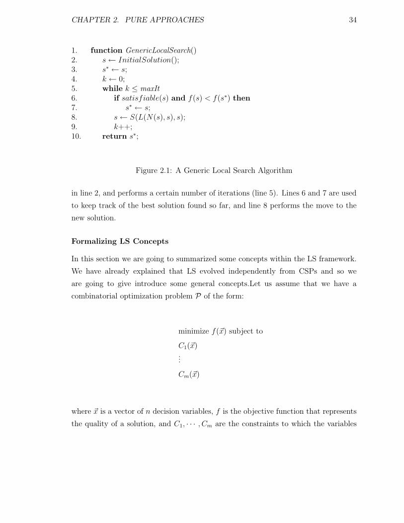
CHAPTER 2. PURE APPROACHES 34
1. function GenericLocalSearch()2. s← InitialSolution();3. s∗ ← s;4. k ← 0;5. while k ≤ maxIt6. if satisfiable(s) and f(s) < f(s∗) then7. s∗ ← s;8. s← S(L(N(s), s), s);9. k++;10. return s∗;
Figure 2.1: A Generic Local Search Algorithm
in line 2, and performs a certain number of iterations (line 5). Lines 6 and 7 are used
to keep track of the best solution found so far, and line 8 performs the move to the
new solution.
Formalizing LS Concepts
In this section we are going to summarized some concepts within the LS framework.
We have already explained that LS evolved independently from CSPs and so we
are going to give introduce some general concepts.Let us assume that we have a
combinatorial optimization problem P of the form:
minimize f(~x) subject to
C1(~x)...
Cm(~x)
where ~x is a vector of n decision variables, f is the objective function that represents
the quality of a solution, and C1, · · · , Cm are the constraints to which the variables
CHAPTER 2. PURE APPROACHES 35
are subject. Based on all that we can now define:
Definition 2.10. A solution to P is an assignment x of all the variables in ~x. The
set of solutions is denoted by LP .
Definition 2.11. A feasible solution to P is a solution x that satisfies the constraints
C1, · · · , Cm. The set of feasible solutions is denoted by LP .
Definition 2.12. The set of optimal solutions to P , denoted by L∗P is defined as
L∗P = {s ∈ LP | f(s) = mink∈LP
f(k)} (2.1)
Note that in this case we use the term solution to name a complete assignment of
values to variables, and feasible solution to a solution that satisfies the constraints.
Rembember than in the constraint satisfaction framework a solution corresponds to
a feasible solution here.
Definition 2.13. A search space for P is a set LP such that LP ⊆ LP ⊆ N n.
Note that the search space may vary from one algorithm to the other. It is part of
the modeling of the problem, in some cases we might want to move within the space
of feasible solutions, where LP = LP ; or we might want to enforce some constraints
and leave others to be part of the objective function f , i.e. permit violations of those
constraints and try to minimize them during search. For a constraint satisfaction
problem, when violations are non-existent, it means we have a solution; for constraint
optimization problems it means that we have found a feasible solution.
Definition 2.14. A neighborhood is a pair 〈LP , N〉 where LP is a search space and
N is a mapping N : LP −→ 2LP that defines set of reachable solutions N(s) ⊆ LPfrom solution s.
Definition 2.15. A solution s is locally optimal with respect to LP if
f(s) ≤ mini∈N(s)
f(i)
The set of local optimal solutions is denoted L+P .
CHAPTER 2. PURE APPROACHES 36
Escaping from local optima is one of the issues that has been getting the most atten-
tion within this framework, and it is the cause of LS algorithms introducing interesting
legality and selection criteria.
Definition 2.16. A neighborhood is a pair 〈LP , N〉 where LP is a search space and
N is a mapping N : LP −→ 2LP that defines set of reachable solutions N(s) ⊆ LPfrom solution s.
Definition 2.17. A legality condition L is a function (2LP ×LP) −→ 2LP that filters
sets of solutions from the search space.
Definition 2.18. A selection rule S(M, s) is a function (2LP × LP) −→ LP where
M = L(N(s), s), that chooses an element si from M and decides whether to accept
it or to keep the current solution s.
Definition 2.19. A local search algorithm for P is a succession of solutions
s0 → s1 → . . .→ sk
such that
si+1 = S(L(N(si), si), si) (1 ≤ i ≤ k) (2.2)
It is very common that such a local search algorithm produces a final solution sk
that belongs to L+P . In the next section we are going to introduce heuristics and
metaheuristics, whose role is to direct the search towards high-quality local optima,
and specially those in L∗P if possible.
Heuristics
All the heuristics here are based on the template depicted in figure 2.1, and assuming
that it receives the parameters f , N and the legality and selection rules L and S.
We are also going to assume that we are always dealing with minimization problems,
so that the goal is to minimize f .
Heuristics typically choose the next neighbor based on local information, basically
the current solution and its neighborhood, which translates into providing different

CHAPTER 2. PURE APPROACHES 37
selection mechanisms and different legality conditions. For example, we can define
three different legality conditions, where N is assumed to be the neighborhood of S:
1. function L-Improvement(N, s)2. return {n ∈ N | f(n) < f(s)};
which only allows to move to a neighbor with a strictly superior quality.
1. function L-ImprovementAndWalk(N, s)2. return {n ∈ N | f(n) ≤ f(s)};
which allows moves where the value of the objective function is the same.
1. function L-All(N, s)2. return N ;
or the last case in which any kind of move is allowed.
CHAPTER 2. PURE APPROACHES 38
Systematic Heuristics This type of heuristic performs an exploration of the neigh-
borhood in order to decide which neighbor is going to become the next solution. The
main relevant ones being:
Best Neighbor: this heuristic chooses the neighbor with the best value of the
objective function:
1. function S-Best(N, s)2. N ∗ ← {n ∈ N | f(n) = mins∈N f(s)};3. return {n ∈ N ∗};
where n can be chosen randomly with probability 1|N∗| , where | N ∗ | is the num-
ber of elements in N ∗. A Best-Improvement LS algorithm can thus be specified by
instantiating the generic local search in the following manner:
1. function BestImprovement(s)2. return GenericLocalSearch(f,N,L-Improvement,S-Best)
First Neighbor: sometimes, the search space is too large to completely scan
it in order to find the best neighbor. The First-Neighbor heuristic chooses the first
neighbor which improves the value of the objective function. It assumes a function
lex(n) that specifies the lexicographic order of a neighbor n when scanning the neigh-
borhood:
1. function S-First(N, s)2. return {n ∈ N} minimizing lex(n);
A First-Improvement LS algorithm can thus be specified by instantiating the generic
local search to use the first-neighbor heuristic as selection rule:

CHAPTER 2. PURE APPROACHES 39
1. function FirstImprovement(s)2. return GenericLocalSearch(f,N,L-Improvement,S-First)
Random Walks The Random Walks heuristic randomly selects a candidate from
the neighborhood and decide whether to select it or not (instead of performing an
exploration of the neighborhood).
Random Improvement: this is the simplest example of a random walk, it
consists on accepting a neighbor if it improves the current solution:
1. function S-RandomImprovement(N, s)2. select {n ∈ N};3. if f(n) < f(s) then4. return n;5. else 6. return s;
In line 2, n can be randomly selected with probability 1|N | , where | N | is the number of
elements in N . Note also that in line 6 the current solution is returned, which means
that s is implicitly part of the neighborhood. The random nature of this approach
seems critical in some applications ([6]). A RandomImprovement LS algorithm can
thus be specified by instantiating the generic local search in the following manner:
1. function RandomImprovement(s)2. return GenericLocalSearch(f,N,L-All,S-RandomImprovement)
The Metropolis Heuristic: is a variant of Random Walks that allows oc-
cassional degradation of the value of the objective function. It selects a random
candidate, if it does not degrade the objective function the candidate is returned, if
it does, then it is accepted with a small probability
exp(frac−(f(n)− f(s))t)
CHAPTER 2. PURE APPROACHES 40
that depends on the distance between the objective functions, and on a parameter t
called temperature. Assuming a function True(f(n), f(s), t) that checks this proba-
bility, the Metropolis heuristic can be specified by:
1. function Metropolis(N, s, t)2. select {n ∈ N};3. if f(n) ≤ f(s) then4. return n;5. else if True(f(n), f(s), t)6. return n;7. else6. return s;
Again, n can be randomly selected with probability 1|N | , where | N | is the number of
elements in N .
Metaheuristics
The heuristics presented in the previous section aim exclusively at choosing the next
solution within the neighborhood in order to provide high quality local optima. But
local optima are not necessarily global optima, and thus, some mechanism is needed
to escape from them. These mechanisms are known as metaheuristics.
All the metaheuristics here are also based on the template depicted in figure 2.1,
and assuming that it receives the parameters f , N and the legality and selection rules
L and S. We are also going to assume that we are always dealing with minimization
problems, so that the goal is to minimize f .
In the following we will present some of the most characteristic metaheuristic that
can be found on the literature:
Iterated Local Search The idea behind this metaheuristic is to iterate a specific
local search from different points in the search space. Sometimes, the starting points
can be generated from the last local minima reached on the previous iteration.
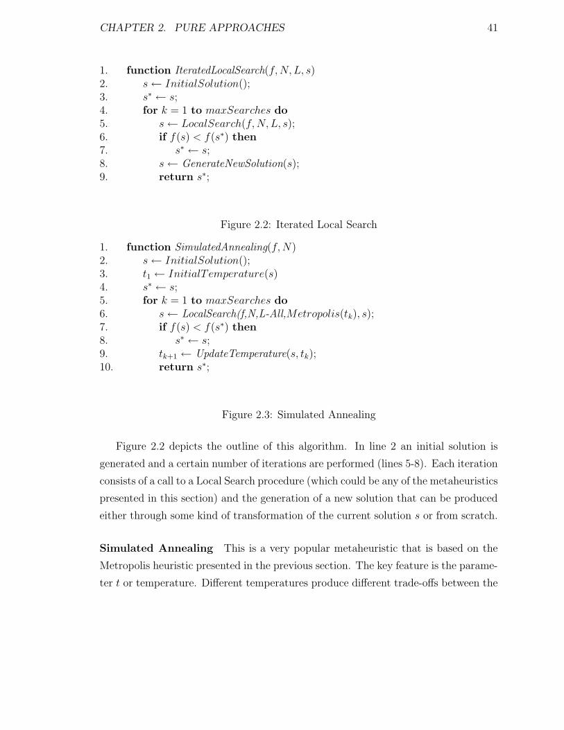
CHAPTER 2. PURE APPROACHES 41
1. function IteratedLocalSearch(f,N, L, s)2. s← InitialSolution();3. s∗ ← s;4. for k = 1 to maxSearches do5. s← LocalSearch(f,N, L, s);6. if f(s) < f(s∗) then7. s∗ ← s;8. s← GenerateNewSolution(s);9. return s∗;
Figure 2.2: Iterated Local Search
1. function SimulatedAnnealing(f,N)2. s← InitialSolution();3. t1 ← InitialTemperature(s)4. s∗ ← s;5. for k = 1 to maxSearches do6. s← LocalSearch(f,N,L-All,Metropolis(tk), s);7. if f(s) < f(s∗) then8. s∗ ← s;9. tk+1 ← UpdateTemperature(s, tk);10. return s∗;
Figure 2.3: Simulated Annealing
Figure 2.2 depicts the outline of this algorithm. In line 2 an initial solution is
generated and a certain number of iterations are performed (lines 5-8). Each iteration
consists of a call to a Local Search procedure (which could be any of the metaheuristics
presented in this section) and the generation of a new solution that can be produced
either through some kind of transformation of the current solution s or from scratch.
Simulated Annealing This is a very popular metaheuristic that is based on the
Metropolis heuristic presented in the previous section. The key feature is the parame-
ter t or temperature. Different temperatures produce different trade-offs between the
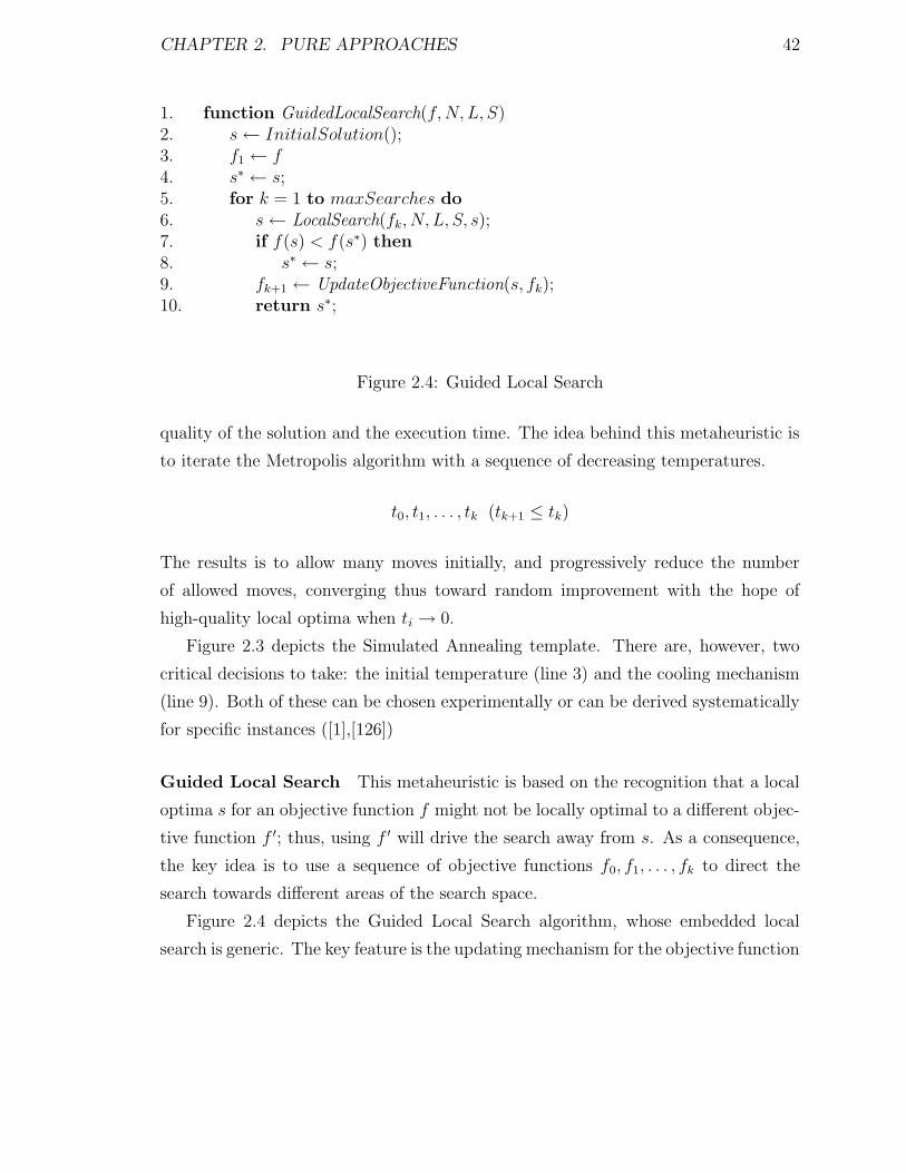
CHAPTER 2. PURE APPROACHES 42
1. function GuidedLocalSearch(f,N, L, S)2. s← InitialSolution();3. f1 ← f4. s∗ ← s;5. for k = 1 to maxSearches do6. s← LocalSearch(fk, N, L, S, s);7. if f(s) < f(s∗) then8. s∗ ← s;9. fk+1 ← UpdateObjectiveFunction(s, fk);10. return s∗;
Figure 2.4: Guided Local Search
quality of the solution and the execution time. The idea behind this metaheuristic is
to iterate the Metropolis algorithm with a sequence of decreasing temperatures.
t0, t1, . . . , tk (tk+1 ≤ tk)
The results is to allow many moves initially, and progressively reduce the number
of allowed moves, converging thus toward random improvement with the hope of
high-quality local optima when ti → 0.
Figure 2.3 depicts the Simulated Annealing template. There are, however, two
critical decisions to take: the initial temperature (line 3) and the cooling mechanism
(line 9). Both of these can be chosen experimentally or can be derived systematically
for specific instances ([1],[126])
Guided Local Search This metaheuristic is based on the recognition that a local
optima s for an objective function f might not be locally optimal to a different objec-
tive function f ′; thus, using f ′ will drive the search away from s. As a consequence,
the key idea is to use a sequence of objective functions f0, f1, . . . , fk to direct the
search towards different areas of the search space.
Figure 2.4 depicts the Guided Local Search algorithm, whose embedded local
search is generic. The key feature is the updating mechanism for the objective function
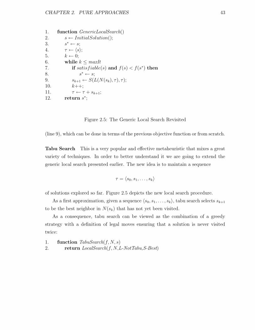
CHAPTER 2. PURE APPROACHES 43
1. function GenericLocalSearch()2. s← InitialSolution();3. s∗ ← s;4. τ ← 〈s〉;5. k ← 0;6. while k ≤ maxIt7. if satisfiable(s) and f(s) < f(s∗) then8. s∗ ← s;9. sk+1 ← S(L(N(sk), τ), τ);10. k++;11. τ ← τ + sk+1;12. return s∗;
Figure 2.5: The Generic Local Search Revisited
(line 9), which can be done in terms of the previous objective function or from scratch.
Tabu Search This is a very popular and effective metaheuristic that mixes a great
variety of techniques. In order to better understand it we are going to extend the
generic local search presented earlier. The new idea is to maintain a sequence
τ = 〈s0, s1, . . . , sk〉
of solutions explored so far. Figure 2.5 depicts the new local search procedure.
As a first approximation, given a sequence 〈s0, s1, . . . , sk〉, tabu search selects sk+1
to be the best neighbor in N(sk) that has not yet been visited.
As a consequence, tabu search can be viewed as the combination of a greedy
strategy with a definition of legal moves ensuring that a solution is never visited
twice:
1. function TabuSearch(f,N, s)2. return LocalSearch(f,N,L-NotTabu,S-Best)
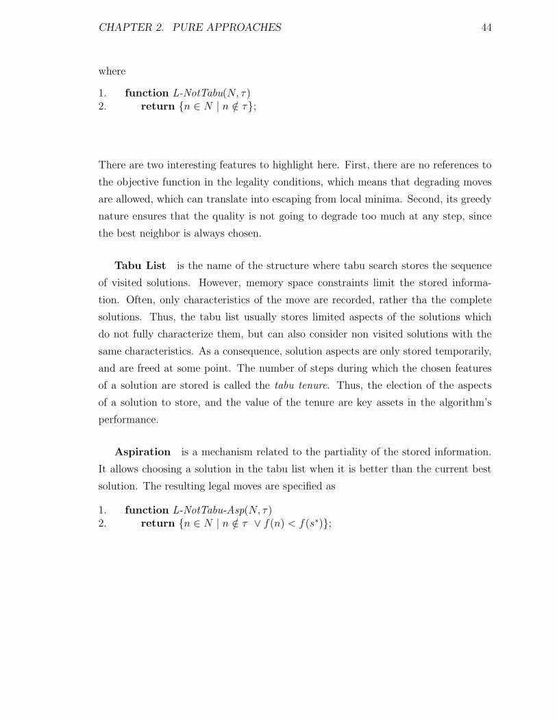
CHAPTER 2. PURE APPROACHES 44
where
1. function L-NotTabu(N, τ)2. return {n ∈ N | n /∈ τ};
There are two interesting features to highlight here. First, there are no references to
the objective function in the legality conditions, which means that degrading moves
are allowed, which can translate into escaping from local minima. Second, its greedy
nature ensures that the quality is not going to degrade too much at any step, since
the best neighbor is always chosen.
Tabu List is the name of the structure where tabu search stores the sequence
of visited solutions. However, memory space constraints limit the stored informa-
tion. Often, only characteristics of the move are recorded, rather tha the complete
solutions. Thus, the tabu list usually stores limited aspects of the solutions which
do not fully characterize them, but can also consider non visited solutions with the
same characteristics. As a consequence, solution aspects are only stored temporarily,
and are freed at some point. The number of steps during which the chosen features
of a solution are stored is called the tabu tenure. Thus, the election of the aspects
of a solution to store, and the value of the tenure are key assets in the algorithm’s
performance.
Aspiration is a mechanism related to the partiality of the stored information.
It allows choosing a solution in the tabu list when it is better than the current best
solution. The resulting legal moves are specified as
1. function L-NotTabu-Asp(N, τ)2. return {n ∈ N | n /∈ τ ∨ f(n) < f(s∗)};
CHAPTER 2. PURE APPROACHES 45
Long-Term Memory: we know that the tabu list abstracts a small suffix of
the solution sequence, and cannot capture long-term information. As a consequence,
tabu search cannot ensure that the search will not focus on low quality solutions, or
that it will spend too much time on the same region of search space. Thus, tabu
search algorithms typically implement two different mechanism to avoid the previous
problems:
• Intensification consists on storing high-quality solutions during the search and
returning to them periodically, thus, allowing a more extensive exploration of
the regions where the best solutions have been found.
• Diversification provides a means to explore more diverse regions of the search
space. There are many ways to achieve this goal, such as using iterated local
search to perturb or to restart the search, or using strategic oscillation, which
consists of changing the objective function in order to balance the time spent
in the feasible and infeasible regions ([6]).
There are other more complex metaheuristics in the literature such as Variable
Neighborhood Search (VNS) [161] or Ant Colony Optimization (ACO) [57]. Also,
hybrid evolutionary approaches are sometimes considered as metaheuristic, but we
will explore such methods in the next chapter.
Most of the figures and templates in this section can also been found with higher
detail in [115].
2.2 SAT
Consider the following problem:
Example 2. I’m hungry and I would like something to eat. My father says I must
eat meat or else don’t eat fish. My mother says I must eat fish, vegetable or both. My
girlfriend asks me not to eat either vegetables or meat or both. What can I eat?
CHAPTER 2. PURE APPROACHES 46
This problem can be represented as a propositional satisfiability problem. We can
express the three constraints by means of a propositional formula,
(M ∨ ¬F ) ∧ (F ∨ V ) ∧ (¬V ∨ ¬M)
where M, F and V are Boolean variables which are true if and only if I eat respectively,
Meat, Fish, and Vegetables. A solution to the problem is a satisfying assignment, an
assignment of truth values to the Boolean variables that satisfies the propositional
formula. In this case, there are just two satisfying assignments (out of eight possible).
These either assign M and F to true and V to false, or assign M and F to false and
V to true. That is, I can either eat both Meat and Fish, and not Vegetables, or I can
eat only Vegetables and neither Meat nor Fish.
Whilst propositional satisfiability is a very simple problem, it is a cornerstone
in the theory of computational complexity. Propositional satisfiability was the first
problem shown to be NP-complete [41].
2.2.1 Satisfiability
Propositional satisfiability (SAT) is the problem of deciding if there is an assignment
for the variables in a propositional formula that makes the formula true. Many AI
problems can be encoded quite naturally into SAT (eg. planning [137], constraint
satisfaction, vision interpretation [189], diagnosis,hardware verification and design,
. . . ).
Much research into SAT considers problems in conjunctive normal form (CNF).
A formula is CNF if and only if it is a conjunction of clauses; a clause is a disjunction
of literals, where a literal is a negated or un-negated Boolean variable. A clause
containing just one literal is called a unit clause. A clause containing no literals is
called the empty clause and is interpreted as false. k-Sat is the class of decision
problems in which all clauses are of length k. k-SAT is NP-complete for any k ≥ 3
but is polynomial for k = 2 [84]. Other polynomial classes of SAT problems exist
including Horn-SAT (in which each clause contains no more than one positive literal),
renamable Horn-SAT and several other generalizations.
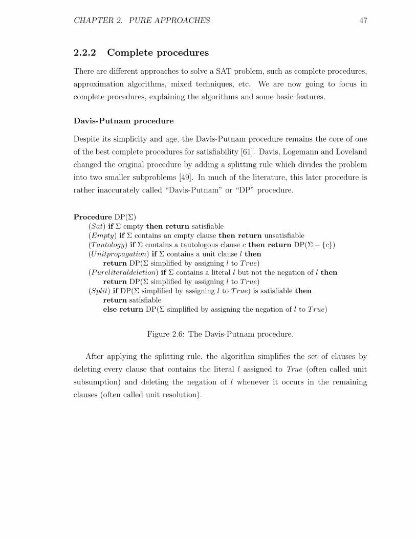
CHAPTER 2. PURE APPROACHES 47
2.2.2 Complete procedures
There are different approaches to solve a SAT problem, such as complete procedures,
approximation algorithms, mixed techniques, etc. We are now going to focus in
complete procedures, explaining the algorithms and some basic features.
Davis-Putnam procedure
Despite its simplicity and age, the Davis-Putnam procedure remains the core of one
of the best complete procedures for satisfiability [61]. Davis, Logemann and Loveland
changed the original procedure by adding a splitting rule which divides the problem
into two smaller subproblems [49]. In much of the literature, this later procedure is
rather inaccurately called “Davis-Putnam” or “DP” procedure.
Procedure DP(Σ)(Sat) if Σ empty then return satisfiable(Empty) if Σ contains an empty clause then return unsatisfiable(Tautology) if Σ contains a tautologous clause c then return DP(Σ− {c})(Unitpropagation) if Σ contains a unit clause l then
return DP(Σ simplified by assigning l to True)(Pureliteraldeletion) if Σ contains a literal l but not the negation of l then
return DP(Σ simplified by assigning l to True)(Split) if DP(Σ simplified by assigning l to True) is satisfiable then
return satisfiableelse return DP(Σ simplified by assigning the negation of l to True)
Figure 2.6: The Davis-Putnam procedure.
After applying the splitting rule, the algorithm simplifies the set of clauses by
deleting every clause that contains the literal l assigned to True (often called unit
subsumption) and deleting the negation of l whenever it occurs in the remaining
clauses (often called unit resolution).
CHAPTER 2. PURE APPROACHES 48
Branching heuristics
The DP algorithm is non-deterministic as we can choose the literal upon which to
branch. A popular and cheap branching heuristic is MOM’s heuristic. This picks the
literal that occurs most often in the minimal size clauses. Ties are usually broken
with a static random ordering.
The Jeroslaw-Wang heuristic [129] estimates the contribution each literal is likely
to make in order to satisfy the clause set. Each literal is scored as follows: for each
clause c the literal appears in, 2−|c| is added to the literal’s score, where |c| is the
number of literals in c. The split rule is then applied to the literal with the highest
score.
Hooker and Vinay, after investigating the Jeroslaw-Wang score function ([120])
claimed for a “simplification hypothesis”, that it is best to branch into simpler sub-
problems with fewer and shorter clauses after unit propagation. The simplification
hypothesis suggests a “two-sided” Jeroslaw-Wang rule which performs better than
the original.
There more recently proposed branching heuristics 3, like the Variable State In-
dependent Deacying Sum (VSIDS) heuristics found in Chaff solver [165]. Some of its
features are:
• Choose the literal that has the highest score to branch.
• Initial score of a literal is its literal count in the initial clause database.
• Score is incremented by 1 when a new clause containing that literal is added.
• Periodically, divide all scores by a constant.
Intelligent backtracking and learning
The standard DP procedure performs chronological backtracking, exploring one branch
of the search tree completely before backtracking and exploring the other. We can
3See http:// research.microsoft.com/users/lintaoz/SATSolving/satsolving.htm for a good SATSolving Mini Course by Linato Zhang
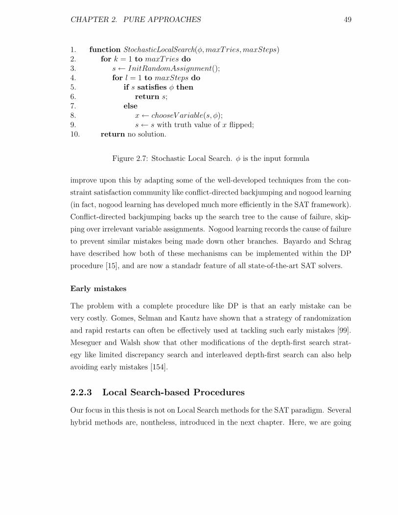
CHAPTER 2. PURE APPROACHES 49
1. function StochasticLocalSearch(φ,maxTries,maxSteps)2. for k = 1 to maxTries do3. s← InitRandomAssignment();4. for l = 1 to maxSteps do5. if s satisfies φ then6. return s;7. else8. x← chooseV ariable(s, φ);9. s← s with truth value of x flipped;10. return no solution.
Figure 2.7: Stochastic Local Search. φ is the input formula
improve upon this by adapting some of the well-developed techniques from the con-
straint satisfaction community like conflict-directed backjumping and nogood learning
(in fact, nogood learning has developed much more efficiently in the SAT framework).
Conflict-directed backjumping backs up the search tree to the cause of failure, skip-
ping over irrelevant variable assignments. Nogood learning records the cause of failure
to prevent similar mistakes being made down other branches. Bayardo and Schrag
have described how both of these mechanisms can be implemented within the DP
procedure [15], and are now a standadr feature of all state-of-the-art SAT solvers.
Early mistakes
The problem with a complete procedure like DP is that an early mistake can be
very costly. Gomes, Selman and Kautz have shown that a strategy of randomization
and rapid restarts can often be effectively used at tackling such early mistakes [99].
Meseguer and Walsh show that other modifications of the depth-first search strat-
egy like limited discrepancy search and interleaved depth-first search can also help
avoiding early mistakes [154].
2.2.3 Local Search-based Procedures
Our focus in this thesis is not on Local Search methods for the SAT paradigm. Several
hybrid methods are, nontheless, introduced in the next chapter. Here, we are going
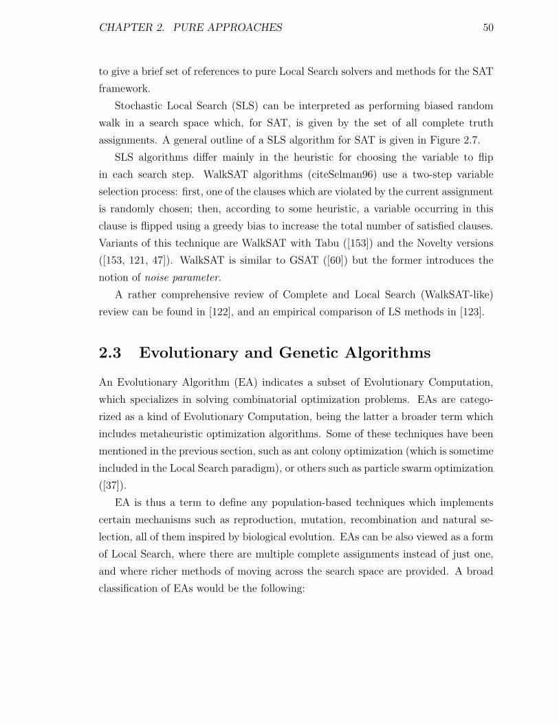
CHAPTER 2. PURE APPROACHES 50
to give a brief set of references to pure Local Search solvers and methods for the SAT
framework.
Stochastic Local Search (SLS) can be interpreted as performing biased random
walk in a search space which, for SAT, is given by the set of all complete truth
assignments. A general outline of a SLS algorithm for SAT is given in Figure 2.7.
SLS algorithms differ mainly in the heuristic for choosing the variable to flip
in each search step. WalkSAT algorithms (citeSelman96) use a two-step variable
selection process: first, one of the clauses which are violated by the current assignment
is randomly chosen; then, according to some heuristic, a variable occurring in this
clause is flipped using a greedy bias to increase the total number of satisfied clauses.
Variants of this technique are WalkSAT with Tabu ([153]) and the Novelty versions
([153, 121, 47]). WalkSAT is similar to GSAT ([60]) but the former introduces the
notion of noise parameter.
A rather comprehensive review of Complete and Local Search (WalkSAT-like)
review can be found in [122], and an empirical comparison of LS methods in [123].
2.3 Evolutionary and Genetic Algorithms
An Evolutionary Algorithm (EA) indicates a subset of Evolutionary Computation,
which specializes in solving combinatorial optimization problems. EAs are catego-
rized as a kind of Evolutionary Computation, being the latter a broader term which
includes metaheuristic optimization algorithms. Some of these techniques have been
mentioned in the previous section, such as ant colony optimization (which is sometime
included in the Local Search paradigm), or others such as particle swarm optimization
([37]).
EA is thus a term to define any population-based techniques which implements
certain mechanisms such as reproduction, mutation, recombination and natural se-
lection, all of them inspired by biological evolution. EAs can be also viewed as a form
of Local Search, where there are multiple complete assignments instead of just one,
and where richer methods of moving across the search space are provided. A broad
classification of EAs would be the following:

CHAPTER 2. PURE APPROACHES 51
• Genetic Algorithms: the most popular kind of EA, it looks for a solution
within a population of strings of numbers which evolves through recombination
methods that include mutation and selection operators.
• Evolutionary Programming: it consists on fixing the structure of the
program and letting the parameters evolve during time.
• Genetic Programming: here the solutions are in the form of computer
programs which fitness corresponds to the ability of solving a computational
problem.
• Evolution strategy: which maintains a representation of vectors of real
numbers and typically includes self-adaptive mutation rates.
• Learning classifier system: instead of a fitness function they implement a
rule utility decided by a reinforcement learning technique.
This categorization is neither extensive nor exclusive, and its only pretension is
to introduce the subfield of the Evolutionary Algorithms. To learn more about EAs
and Evolutionary Computation conslut [69]. In the next subsections we are going to
focus on Genetic Algorithms (GAs).
2.3.1 Genetic Algorithms
Everybody seems to agree on the fact that Holland was the father of the GAs. His
early works (in 1962) on adaptive systems laid the foundation for latter developments.
Moreover, his book Adaptation in Natural and Artificial Systems ([119]) was the
first to present the concept of adaptive digital systems using mutation, selection and
crossover as a problem-solving strategy. However, this research was conceived by
Holland as a means of studying adaptive behavior and not as a function optimization
method. To learn more about the history of GAs consult [96].
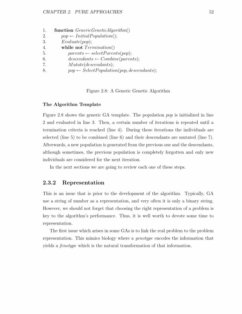
CHAPTER 2. PURE APPROACHES 52
1. function GenericGeneticAlgorithm()2. pop← InitialPopulation();3. Evaluate(pop);4. while not Termination()5. parents← selectParents(pop);6. descendants← Combine(parents);7. Mutate(descendants);8. pop← SelectPopulation(pop, descendants);
Figure 2.8: A Generic Genetic Algorithm
The Algorithm Template
Figure 2.8 shows the generic GA template. The population pop is initialized in line
2 and evaluated in line 3. Then, a certain number of iterations is repeated until a
termination criteria is reached (line 4). During these iterations the individuals are
selected (line 5) to be combined (line 6) and their descendants are mutated (line 7).
Afterwards, a new population is generated from the previous one and the descendants,
although sometimes, the previous population is completely forgotten and only new
individuals are considered for the next iteration.
In the next sections we are going to review each one of these steps.
2.3.2 Representation
This is an issue that is prior to the development of the algorithm. Typically, GA
use a string of number as a representation, and very often it is only a binary string.
However, we should not forget that choosing the right representation of a problem is
key to the algorithm’s performance. Thus, it is well worth to devote some time to
representation.
The first issue which arises in some GAs is to link the real problem to the problem
representation. This mimics biology where a genotype encodes the information that
yields a fenotype which is the natural transformation of that information.
CHAPTER 2. PURE APPROACHES 53
Sometimes, this distinction does not appear if the information and the represen-
tation are one and the same thing, which happens often. However, as we will latter
see, it is important to explicitly make this distinction since the genotype is used for
individuals interaction, but the fenotype is needed to calculate the real value of the
evaluation function. Every unit of information stored in the genotype is typically
named gene.
The second issue is what kind of structures do we need to use to represent our
genotype and/or fenotype (Note that, many times, the fenotype is not actually im-
plemented, and it might be only calculated when the evaluation function needs it).
In general, we can distinguish several types of representation:
• Binary Representation: this is the simplest representation we can find. It
consists on a binary sequence, i.e., a sequence of 1’s and 0’s. While this tech-
nique is very commonly used, it is not always the best suited approach. Its main
drawback is based on the genotype-to-fenotype mapping. For example, when
the 1’s and 0’s represent boolean variables, the genotype-to-fenotype mapping
is direct: a 1 represents a true variable and a 0 represents a false one. Instead,
if for example, we are representing numbers with binary sequences, we can en-
counter problems derived from the fact that the distances between the numbers
and between their representations do not match. Observe that the distance
between 3 and 4 is only 1, while if we are representing the numbers as a 4-bits
sequence, the distance between 0011 and 0100 is not 1 anymore. Here, as in the
next types of representation, we have to decide the length of the string.
• Integer Representation: to avoid problems like the one previously stated,
we can safely represent the individuals as sequences of integers. This is probably
a better suited representation for complex problems. The only issue here would
be to decide whether those integers can be finite or infinite.
• Real or Floating-Point Representation: which consists of a string of real
values. This approach is typically better suited for genes that come from a
continuous distribution.
CHAPTER 2. PURE APPROACHES 54
There are other more complex representations such as: strings of letters (which
is basically equivalent to that of a finite integer representation) and permutation
representations (see [69], p. 41–42).
2.3.3 Evaluation Function
Closely related to the representation, the issue of the evaluation function arises. This
function associates a value to every individual in the population, and corresponds to
the quality of that individual. Thus, different representations of the same problem
may have different evaluation functions, since this is typically calculated from the
values of the genes of each individual and through the genotype-to-fenotype mapping.
The evaluation function is often referred to as fitness function in the Evolutionary
Computation field.
2.3.4 Initial Population
Once the representation is fixed, the first issue in developing the algorithm is that of
the initial population. This is typically performed by randomly generating individuals
so that the population can cover wider areas of the search space.
Nonetheless, there are other more specialized methods. A very common approach
is to generate the individuals in a greedy manner, which means that every individual
is constructed in a way such that at every time, the next gene is given the value that
optimizes the evaluation function for that individual. Occasionally, the solutions may
be somehow seeded in areas where solutions are likely to be found.
2.3.5 Parent Selection
Selection is the method through which certain elements in the population are chosen
to be combined. This selection mechanism tries, in general, to choose parents that
are likely to produce a high-quality descendant. Typically, two individuals are chosen
two reproduce and yield descendants. Different kinds of selection mechanism are:
CHAPTER 2. PURE APPROACHES 55
• Fitness Proportional Selection: consists of giving a certain probability
to be chosen for every individual. This probability depends directly on the
absolute fitness of the individual ([119]). The main drawback of this mechanism
is that the best candidates are very likely to take over the whole population very
quickly. This method is often called roulette-wheel selection.
• Ranking Selection: this method is very similar to the previous one. The
difference is that, in this case, the individuals are ranked according to their
fitness, and then probabilities are given based on the ranking rather than on
the fitness itself ([11]).
• Tournament Selection: this is may be the simplest mechanism, and also
the least time-consuming. It consists on choosing k individuals completely at
random, and then selecting the two individuals with highest fitness function.
Obviously, the complexity of this method depends on the value of k.
There are many other methods, mainly variations of the ones described above.
Again, the reader is referred to [69] for more details.
Multiparent Selection Is to worth mentioning that some algorithms implement a
multiparent selection scheme. This means that, independently of the selection method
they use, more than two parents are selected for combination. We detail the kind of
combination methods for this type of selection in the next section.
2.3.6 Reproduction
This operator is in charge of combining the parents in such a way that a high quality
individual (descendant) will be obtained. This mechanism is also known as crossover.
In some GAs, this operator is able to generate more than one descendant (usually
two), but we will assume from now on that only one descendant is going to be gen-
erated. Thus, different crossover operators are:
• One point crossover: this is the most popular method. It consists on choos-
ing a point randomly, and copying the genes of a parent, from the beginning

CHAPTER 2. PURE APPROACHES 56
until this point, to the descendant, and the genes of the other parent from that
point till the end.
As an example, imagine we have two parents of the form:
σ1 = 〈 0 1 0 0 1 1 1 1 0 〉σ2 = 〈 0 0 0 1 1 0 1 0 0 〉
and k = 5 is the crossover point, the descendant would either be
〈 0 1 0 0 1 / 0 1 0 0 〉
or
〈 0 0 0 1 1 / 1 1 1 0 〉
Note that extending this operator to generate two descendants is trivial.
• Multiple point crossover: is based on the previous operator, and its only
difference is that instead of 1 point, several k points are chosen randomly. Then,
to generate a descendant it would copy the genes of each parent in turns after
each crossover point.
• Uniform crossover: is slightly different than the previous one. It treats each
gene independently and decides from which parent it is going to be inherited
(typically with the same probability).
These methods are the most common ones in the literature. Other more complex
ones can also be found. It is also very common to implement a type of uniform
crossover where instead of proabilities, the decision criteria is based on the fitness of
the descendant.
Multiparent Combination
As we mentioned in the previous subsection it is also possible (although not very
common) to implement a multiparental combination. Instead of 2 parents, k parents
are selected and combined. Thus, combination methods for this option tend to be
CHAPTER 2. PURE APPROACHES 57
different from those of the traditional scheme. These methods can be categorized as
follows:
• Generalizing uniform crossover ([166]).
• Generalizing multiple point crossover ([64]).
• Generalizing arithmetic combination operators ([221]).
To know more about the efficiency and suitability of this type of combination on
certain structures of the search space (landscapes) consult [68].
2.3.7 Mutation
This operator is the source of great diversity. It is based in the biological fact that
some genes can mutate for different reasons, and thus, the descendant can acquire
genes that are from neither of its parents. The most common ones are:
• Random bit modification: consists on changing the value of some bits with
a given probability. The operator changes the value of every bit in the sequence
with a certain probability. If the representation is binary, the effect is that of
flipping a bit, either from 0 to 1 or from 1 to 0.
• Swap mutation: simply selects two genes (at random) in the sequence and
swaps their values. Imagine the individual:
〈 0 [1] 0 [0] 1 0 1 0 0 〉
and the swapping genes 1 and 3, the mutated individual would be
〈 0 [0] 0 [1] 1 0 1 0 0 〉
• Insert mutation: chooses two genes at random and moves the second one
next to the first. Again, if we have the individual
〈 0 [1] 0 0 [1] 0 1 0 0 〉
CHAPTER 2. PURE APPROACHES 58
and the inserting genes 1 and 4, the mutate individual would be
〈 0 [1] [1] 0 0 0 1 0 0 〉
• Scramble mutation: selects a region in the sequence and randomly scrambles
its values. For example,
〈 [0 1 0 0] 1 0 1 0 0 〉
and the region from 0 to 3, a possible mutate individual would be
〈 [1 0 0 0] 1 0 1 0 0 〉
Note that all these operators can be applied to any kind of representation, even
though the illustrations assume a binary representation.
Many other complex and specialized mutation operators can be found in the lit-
erature, including the ones where the mutation is not random but biased by the
subsequent value of the fitness function of the individual.
2.3.8 Selection of the New Generation
As we have previously introduced, this is the mechanism that replaces the last pop-
ulation by a new one. In order to do so, some algorithms completely replace the
previous population for the new set of descendants or offspring. However, this is
usually not a very effective technique, and GAs normally implement mechanism to
generate the new population from both, the previous one and the offspring. Among
these mechanism we can distinguish:
• Fitness based: selection focuses on keeping the individuals with higher fitness
for the next generation.
• Generations based: selection takes into account the number of generations
passed since its creation, and replaces then those individuals which have been
in the population for a larger amount of generations.

CHAPTER 2. PURE APPROACHES 59
• Replace Worst: some techniques tend to replace the worst x individuals in
each step. Many of these techniques do not present a generational model as
shown in figure 2.8, but a different model explained in section 2.3.10.
A technique associated with this operator (independent of the mechanism type) is to
always maintain the highest quality individual in the population. This technique is
usually referred to as elitism.
2.3.9 Termination
The termination condition indicates when it is time for the algorithm to stop. At this
point, the algorithm will usually return the best individual according to its fitness
function. We can distinguish two kinds of termination condition:
• Objective reached: when a GA is implemented to reach a certain goal (i.e.,
a solution of a certain quality), reaching that goal should be the indication for
the algorithm to stop.
• External conditions: However, the previous case is very rarely achieved,
due to the stochastic nature of these algorithms. Therefore, a different criteria
must be used. Different conditions include:
– Fixed number of generations reached.
– Maximum time allowed reached.
– Fitness improvement does not occur for a certain period of time/generations.
– Manual inspection.
– A combination of the above.
2.3.10 Evolutionary Models
This last issue deals with the structure of the algorithm rather than with the nature
of its operators. There two well-known kinds of evolutionary models:
CHAPTER 2. PURE APPROACHES 60
• Generational Model: this is the model corresponding to figure 2.8. In each
generation a set of parents are selected to generate a new population of the same
size as the previous one. This new population is often called offspring. The old
population will be replaced by the new one (offspring) or by a combination of
both (as explained in section 2.3.8).
• Steady State Model: in this model the population is not replaced at once.
Instead, only a certain number λ of old individuals is changed. The percentage
λ/γ (where γ is the size of the population) of replaced solutions is called the
generational gap. This technique was introduced in [232] and has been widely
studied and applied since then ([228, 193]).
For a more technical point of view on Evolutionary Computation and Evolution strate-
gies consult [23].
Chapter 3
Hybrid Approaches
Our final hybrid incorporates features from Constraint Programming, Local Search
and Genetic Algorithms. Since hybrids incorporating these three techniques are al-
most non-existent, we are going to review some state-of-the-art approaches that com-
bine these techniques two by two. Thus, in this chapter we are going to review
different hybrids divided into three sections:
• Constraint Programming and Local Search hybrids, including SAT procedures.
• Memetic Algorithms which introduce Local Search in Genetic Algorithms.
• Genetic Algorithms and Constraint Programming hybrids.
3.1 CP and LS
Many combinatorial problems can be represented and solved within the general frame-
work provided by Constraint Satisfaction Problems (CSP), which allows a very nat-
ural modeling of many practical applications, such as planning, scheduling, time
tabling, vehicle routing, etc.
Search algorithms for solving CSPs are usually categorized into local search and
systematic search algorithms. Since both approaches have their own advantages,
combining them appears very promising. As a result, there is a growing interest in the
development of new hybrid algorithms that combine the strength of both techniques.
61
CHAPTER 3. HYBRID APPROACHES 62
3.1.1 A general view
Let us review the definition of a Constraint Satisfaction Problem; a CSP P =
(X,D,C) is defined by a set of variables X = {x1, ..., xn}, a set of n finite value
domains D = {D1, ..., Dn}, and a set of c constraints or relations C = {R1, ..., Rc}.A constraint Rx is a pair (vars(Rx), rel(Rx)) defined as follows:
• vars(Rx) is an ordered subset of the variables, called the constraint scheme. The
size of vars(Rx) is known as the arity of the constraint. A binary constraint
has arity equal to 2; a non-binary constraint has arity greater than 2. Thus, a
binary CSP is a CSP where all constraints have arity equal or less than 2.
• rel(Rx) is a set of tuples over vars(Rx), called the constraint relation, that
specifies the allowed combinations of values for the variables in vars(Rx). A
tuple over an ordered set of variables X = {x1, ..., xk} is an ordered list of values
(a1, . . . , ak) such that ai ∈ dom(xi), i = 1, . . . , k.
Solving a CSP means finding an assignment for each variable that does not violate
any constraint.
Algorithms for solving CSPs fall into one of two families: systematic algorithms
and local search algorithms.
Systematic algorithms typically start from an empty variable assignment that is
extended in a systematic way by adding individual tentative assignments until either
a solution is found or the problem is detected inconsistent (there is no solution for the
problem). Crucial to the efficiency of these methods is that each decision (branch) is
immediately propagated by local consistency techniques which prune the search space
(mainly, though not only) by deleting values from variables’ domains. Backtracking
occurs when a dead-end is reached, typically because the propagation mechanism
made a variable’s domain empty (produced a domain-wipeout, as it is called). The
biggest problem of this approach is that it requires an important computational effort
and therefore it encounters some difficulties with large scale problems; it also might
suffer from early mistakes in the search which can cause a whole subtree to be explored
with no success. These methods are usually improved by adding specific techniques
CHAPTER 3. HYBRID APPROACHES 63
such as look-back enhancements (backjumping, learning) or look-ahead mechanisms
(filtering techniques, variable or value ordering heuristics).1 Thus, we can say that
these algorithms are complete, systematic, and they search through the space of
partial assignments.
Local search algorithms mainly rely on the use of heuristics to efficiently explore
interesting areas of the search space. They typically start from a complete variable
assignment and perform an incomplete exploration of the search space by repairing
unfeasible complete assignments. Local search algorithms are capable of following a
local gradient in the search space. Even though these methods can better deal with
large-scale problems of certain kinds, their main drawbacks are that they are not
guaranteed to find a solution even if there is one, cannot collect all solutions, and
cannot detect inconsistency. Thus, we can say that these algorithms are incomplete,
non-systematic (they usually follow a local gradient which does not ensure exhaustive
exploration), and they search through the space of complete assignments, moving from
one to another according to certain predefined rules of “neighbourhood”.
In terms of the field terminology, local search stands for the simple strategy of
performing local changes to a starting solution in order to decrease a given cost
function. The special heuristics that guide this process, mainly to avoid or escape
local minima are called ”meta-heuristics”. However, for simplicity, we will refer to
them as local search algorithms through all the review. If the reader is interested in
meta-heuristics we recommend [159] for an extensive review.
A promising idea for producing more efficient and robust algorithms consists in
combining these paradigms in order to take advantage of their respective assets. Many
existing proposals provide different forms of hybridization between both methods, but
they often deal with very specific classes of problems and also mix satisfaction and
optimization. We are going to categorize those hybrid approaches into three different
branches:
1. The loosest form of integration is to use both local and systematic search,
1Industrial applications of constraint modeling, in particular, have proved the importance ofspecialized filtering techniques for predefined global constraints, e.g. that some variables have alldifferent values, or cardinality constraints such as “each machine can have at most k shifts” thatarise frequently in practice.

CHAPTER 3. HYBRID APPROACHES 64
but separately, e.g. perform local search after or before systematic search,
interleaved or in parallel. Portfolio or time-slicing techniques may for example
allocate time and processing power to each of a variety of solvers, which may
be local or systematic, according to various strategies. While there are often
computational advantages to be gained from this approach, it does not represent
a real degree of integration, and is therefore left outside the scope of this chapter.
2. Perform systematic search improved by local search. We distinguish three di-
rections within this category:
• Over complete assignments. Typically for optimization or repair-like tech-
niques.
• Over partial assignments. In construct and repair approaches.
• Over global constraints. Local search is basically used to prune support
values in global constraints.
3. Perform local search improved by complete search. We can distinguish three
different branches within this category:
• Use complete search to explore the neighborhood.
• Use consistency techniques to prune the search space.
• Record nogoods (learnt constraints that represent an explanation of do-
main wipe-outs found during search) in order to achieve completeness.
It is also worth mentioning a recently proposed general framework to enclose all these
methods: PLM, which stands for Propagation, Learning and Move. The authors
claim that any algorithm can be decomposed in these three components. Thus, any
method could be implemented by specifying each of these three elements.
The chapter is organized as follows. Section 2 and 3 review hybrid approaches
from the second and third categories respectively. Section 4 describes the PLM frame-
work. Section 5 introduces hybrid methods for the SAT problem which we also found
interesting to address. A necessary discussion about hybridization (what has been
CHAPTER 3. HYBRID APPROACHES 65
done and what we believe should be pursued in the future) is presented in section 6.
Finally, section 7 is dedicated to conclusions and future work.
3.1.2 Local Search enhancements for Complete Search
Complete search and constraint programming algorithms have been the most used
methods for solving constraint satisfaction problems. After the proved superiority
of local search methods in many problem instances, trying to incorporate features
from local search into complete search was a goal that seemed worth pursuing. As
introduced in the previous section we will distinguish among three different branches
within this hybridization category.
Local search over complete assignments
This type of method is particularly suited for optimization purposes. It is very
straightforward to perform local search from an initial solution obtained by system-
atic search to improve its fitness. Usually, in the constraint programming framework,
this issue would be tackled using branch and bound techniques. However, this can
result in a useless exploration of the search space where visiting different branches will
not lead to a substantial change in the cost function. Thus, it seems very promising
to introduce local search mechanisms to more efficiently explore the neighborhood of
the constructed solution.
Local search can also be applied to a set of global search generated solutions.
Global search will only be used as a way to produce several initial solutions on which
a local search improvement phase is performed. In this context, it is important to
generate starting solutions that are diverse enough for the later exploration. Limited
Discrepancy Search ([112]) is an interesting way of generating a diversified initial set
of solutions.
We will not further explore this branch of hybrid algorithms since it does not
represent a clear effort for integration. Local search is typically performed over con-
structed solutions, thus, both methods can even share the same information structure.
A more interesting idea is to perform local search at internal nodes of the search tree,

CHAPTER 3. HYBRID APPROACHES 66
i.e. local search over partial assignments, an idea we tackle in the next subsection.
Local search over partial assignments
This is a very interesting kind of hybridization because the degree of integration
achieved is more sophisticated. These methods typically perform an iterative exten-
sion of a consistent partial assignment until all problem variables are instantiated.
If the tentative extension reaches a dead-end, it is necessary to backtrack and pro-
duce alternative instantiations. At this point we can find methods which perform a
reparative stage, while others introduce the local search like techniques to remove in-
consistent variables instead of backtracking. Also, some methods implement a CP-like
search (instead of a greedy construction) to extend the consistent partial assignment
and to prune the search space as well.
A construction and repair approach Merging constructive and reparative fea-
tures into hybrid search has been investigated in different ways. Distinguishing among
these various forms of hybrid search is a matter of stating the degree of integration
between the two approaches. We can find methods where the integration is loose,
different constructive and reparative modules exchange information while operating
independently ([168],[236]). In other approaches we encounter a higher degree of in-
tegration, where the reparative process employs constructive methods to explore the
neighborhood ([197],[194]).
A Construction and Repair approach with a higher degree of integration is pre-
sented in [34]. They introduce a general hybrid method named CR, and then proceed
to specify it in order to provide a fully operational search method called CNR.
CR is a generic search framework which integrates both constructive and repar-
ative features as operators. Search is then performed in two alternating stages. A
construction stage where a consistent partial assignment is iteratively extended until
inconsistency or complete consistency is proved. And a repair stage which modifies
the current inconsistent assignment until it becomes consistent.
CNR stands for Construction and Neighborhood Repair search, and it represents
an instantiation of the CR framework described above. In the constructive stage,
CHAPTER 3. HYBRID APPROACHES 67
an implementation of the extend function is provided. It includes both variable and
value ordering heuristics, as well as a consistency function which performs a modified
version of arc-consistency. In the reparative stage a neighborhood of an assignment
is specified. At each time, a member of the neighborhood will be selected greedily
according to a cost function f . This cost function evaluates partial assignments
taking into account not only the number of variables with empty domains but also
how constrained the assignment is. They also provide different repair operators which
give rise to different neighborhoods.
The experimental results shown in [34] correspond to the open-shop scheduling
problem. The algorithm is tested on three sets of benchmarks from the literature:
Taillard instances ([217]), Brucker instances ([29]) and Gueret & Prins instances
([105]). The algorithm’s performance is compared against five different methods:
the genetic algorithm of Prins ([182]), the Tabu Decision-Repair algorithm of Jussien
and Lhomme ([133]), two Tabu search methods of Alcaide ([5]) and Liaw ([146]), and
the Branch-and-Bound algorithm of Gueret and Prins ([104]). Authors assure that
their algorithm outperforms all these methods in every instance except for a single
9X9 one; and it also yields strictly better solution quality for every 10X10 instance.
Improving The Scalability of Backtracking Other methods aim at improving
the scalability of backtracking through the integration of local search techniques. An
early example is based on dynamic backtracking [92], an “intelligent” backtracking
technique able to backtrack to a variable without removing the remaining assign-
ments, while dynamically reorganizing the search tree. Partial Order Dynamic Back-
tracking ([93]), improves the scalability of Dynamic Backtracking without sacrificing
completeness. The main feature that introduces with respect of DB is the allowance
of greater flexibility in the choice of the backtracking variable.
Another hybrid approach is to use systematic backtracking techniques in a non-
systematic ways. In [143], Iterative Sampling is introduced. It simply consists of
restarting a constructive search every time inconsistency is proved. However, this
approach requires a lower degree of integration. It is nonetheless worth mentioning
that variations on this approach have been shown to outperform both local search
CHAPTER 3. HYBRID APPROACHES 68
and backtracking methods on certain problems ([46],[99]).
A new approach called Incomplete Dynamic Backtracking (IDB) is described in
[177]. IDB is inspired by Dynamic Backtracking and Partial Order Dynamic Back-
tracking, and is able to jump back to an earlier variable without removing the remain-
ing assignments. It allows total flexibility in the choice of the variable to backtrack
with, and it also records no information about the visited search space, thus sacrific-
ing completeness. The authors claims that this form of backtracking is indeed a local
search in a space of consistent partial assignments.
IDB’s schema is quite simple: it proceeds by randomly selecting unassigned vari-
ables, and assigning values to them following a certain value ordering heuristic; when
a dead-end is reached it backtracks by randomly removing several assignments. Ter-
mination is only guaranteed when a solution is found.
More specifically, IDB implements forward checking as a form of constraint prop-
agation. It is thus important to adapt this consistency technique to a random unas-
signment of variables, since it has to be capable of leaving the state of those variables
as if forward checking had been only applied to the currently assigned variables. It
also implements a minimum-domain (MD) heuristic for variables selection, while val-
ues are only selected if they do not generate any conflicts and if propagating them
causes no domain wipeout. Among these allowed values, the one that was assigned
the last, is selected where possible. However, IDB attempts to use a random different
value for one variable every time a dead-end is reached.
Another issue is how to unassign variables when inconsistency has been proven.
IDB provides a heuristic that consists of selecting variables with the largest current
domain, breaking ties randomly.
Finally, in order to adapt this schema to optimization problems, ideas from the
Constraint Programming framework are borrowed. It simply restarts the search after
each solution until the first dead-end occurs, reusing then as many assignments from
the previous solution as possible.
The approach is tested through several known problems: the n-queens, the Golomb
ruler and the maximum cliques problem. The n-queens problem is used mainly to
CHAPTER 3. HYBRID APPROACHES 69
introduce the algorithm; on the Golomb ruler it improved the scaling of constrained-
based approaches and achieved better solutions than genetic algorithms. On maxi-
mum cliques, it outperformed many different algorithms and was only inferior to a
sophisticated local search method ([14]).
Scheduling and Timetabling In many cases we find very specific approaches to
deal with very specific problems. Some of them are easily extended to a general
cases, while others introduce various problem-tailored rules that are very hard to
generalize. Thus, it is interesting to study those methods within the context of the
type of problems they focus on. In this particular subsection, many methods have
been devoted to solving Scheduling and Timetabling problems.
Scheduling and Timetabling problems are often tackled with constraint program-
ming techniques, and as in other application areas, hybridization appeared promising.
Some of the approaches described next deal specifically with this application area,
and are not always easy to extend to a more general domain.
In [214] authors employ a propose and revise rule-based approach to the course
timetabling problem. Every time the construction reaches a dead-end a local change
rule attempts to find a possible assignment for the unscheduled activity. They only
perform a single step before restarting the construction, and their aim is only to
accommodate the pending activity.
Another approach is to use a heuristic constructive mechanism in order to find
an initial solution, and then apply a local search technique to improve it. In [235],
authors implement an algorithm to solve a timetabling problem by means of com-
bining an arc-consistency based construction and a min-conflict hill climbing stage.
The construction phase accepts constraint violations, and when a complete solution
is produced, the hill-climbing phase reduces the overall penalty.
A very interesting algorithm is described in [197]. It is similar to the other tech-
niques introduced above, i.e., it constructs a tentative solution until a dead-end is
reached, and then it performs a local search phase over the partial instantiation
reached. However, it has two new features:
1. It performs a full run of local search, instead of a fixed number of local changes.
CHAPTER 3. HYBRID APPROACHES 70
It also relies on well-studied local search algorithms, instead of implementing a
set of problem specific moves.
2. It introduces a look-ahead factor that adds information to the cost function,
in order to provide a better guidance towards more promising areas in the
search space, not only taking into account feasibility but also possibility of the
partial solution to be completed. This look-ahead factor is based in the min-
conflicts heuristic, which counts the number of uninstantiated values for every
uninstantiated variable.
This approach features the possibility to be applied to both search and optimization
problems. This is achieved due to the flexibility of the score function which allows
different combinations of weights to take into account feasibility, optimality (if neces-
sary) and look-ahead in many proportions. Depending on the weights given to each
aspect the search would be directed towards different regions: for example, a high
weight for feasibility would direct the search towards feasible regions (which authors
argue not to be efficient due to the extreme risk to get trapped on local minima).
This technique is applied to solve the course timetabling problem. The author
implemented three different versions: with random hill climbing, steepest hill climb-
ing and min-conflict hill climbing ([160]). The results show that combined methods
perform better than pure local search methods, and the best of them is the one that
introduces min-conflict hill climbing. The algorithm is also applied to tournament
scheduling yielding results that confirm the same conclusion.
Unfortunately, a considerable amount of research is devoted to algorithms specif-
ically tailored to the problem at hand. Even though it can result in a very effective
algorithm that outperforms previous works, it is hard to extract conclusions from it.
A very specific approach for a timetabling problem is presented in [48]. This paper
describes an algorithm for an examination timetabling problem used at the ”Ecole
des Mines de Nantes”.It is a constraint-based approach that introduces local repair
techniques. An extra feature that this problem presents is that the timetable has to
be generated in less than 1 minute.
CHAPTER 3. HYBRID APPROACHES 71
The problem it tackles consists of scheduling examinations composed of four sub-
jects. For every day, for every subject, every candidate has to be assigned to one
examiner during one period.
The algorithm solves the problem in two consecutive steps:
1. A first step called preassignment that reduces the domains of the variables
making them consistent with a defined set of required constraints.
2. A second step called final assignment which assigns a period to every candidate
from the preassigned domains.
In the preassignment step the domains of the variables are reduced following this
criteria:
• Every examiner should have the same number of candidates.
• Each candidate takes an exam in the language he chooses.
• No candidate should meet an examiner who comes from the same school.
• All candidates are then preassigned each to four examiners (one for each sub-
ject).
In the final step the algorithm searches for a solution. The method attempts
to assign every variable following a smallest domain heuristic. When a dead-end is
reached, several specific local repair techniques are applied: free assigned candidates
that would be consistently assigned in the current state to the current examiner;
extend the previous technique to other examiners; swap already assigned examiners
and check the consistency of the resulting instantiation; and finally, swap examiners
without checking.
The program was validated on fifty hand-made instances plus thirteen real ones.
Since the problem is very specific they do not provide any comparison. However, they
are able to solve instances in less than a second (for the real ones), and eight seconds
at most for the hand-made ones.
CHAPTER 3. HYBRID APPROACHES 72
Over Global Constraints
In the last years, the constraint programming community has shown a great interest
in global constraints. CP models have become more and more focused on a few
number of global constraints. For instance, the Travelling Salesman Problem (TSP)
has been centred on one single TSP constraint ([19]). Moreover, Knapsack constraints
([219],[73]), or flow constraints ([28],[21]) have lately been developed.
Constraint propagation on these global constraints is usually improved by a spe-
cialized filtering algorithm. These algorithms are usually based on Operation Re-
search polynomial algorithms. Well known global constraints such as AllDifferent
and Cardinality Constraints have been thoroughly studied as well ([188],[227],[185]).
Consequently, some effort has lately been centered on developing local search
techniques as filtering algorithms for global constraints. Thus, global constraints for
local search rise as a compromise between the generality of low-level CSP-based local
search and the efficiency of problem-tailored local search encodings.
A very straightforward approach for the Dynamic Job-Shop Scheduling problem
is introduced in [167]. A global search control selects among a set of global con-
straints that implement their selection of heuristic, their improvement heuristic and
their update functions; variables employ a common interface that links all the global
constraints and permits updating their states.
Results for the dynamic job-shop scheduling are provided as well. Based on these
experimental results, authors intend to boost performance by implementing various
extra features: randomization to escape local minima and plateaus; random walks
(random moves in the search space which disregard the cost function value) that
can be included by allowing a second improvement heuristic for each constraint that
performs the mentioned variation of a random variable; a taboo list is used for the
global search control’s constraint selection. They also provide different heuristics
(using more knowledge or being more offensive) and show a comparison among them.
Another interesting approach is described in [20]. Authors implement a Branch
and Move technique which consists of using the support of the main global constraint
of the problem as a guide for the branching strategy.
The approach divides the problem into several global constraints. It selects the

CHAPTER 3. HYBRID APPROACHES 73
main global constraint of the problem and an element of its support (a variable-value
pair which is consistent with the current domains). This element has associated a
function that signifies the distance to the current support with respect to all other
constraints. This distance is a measure of the quality of the pair, i.e. how far is the pair
from being consistent to each constraint; if the function is null it means the element
is a solution, otherwise the algorithm selects a constraint with maximum value for the
mentioned function, and then the algorithm branches on a constraint whose support
set does not include the element. The search proceeds by successively considering
sub problems (including the branching constraint and including the complementary
decision).
Local search is introduced before each element’s choice. A descent procedure is
applied to a neighborhood structure for the main constraint.
Authors also provide an empirical comparison for the TV-break problem. The
algorithm is compared against other CP, LS and Mixed Integer Programming (MIP)
methods. It is claimed that the approach finds good solutions very quickly, and it
is always better than the other approaches except for a few instances where the CP
approach is equal or better.
3.1.3 Introducing Complete Search mechanisms in Local Search
Alternatively to the approaches discussed in the previous section, where complete
search is enhanced through local search, one might try instead to introduce complete
search characteristics into local search. This might be motivated by efficiency reasons
and also as a way to address the lack of completeness of local search. In this case we
differentiate three different branches:
CP for neighborhood exploration
In the last years, local search techniques have been more and more directed towards
the use of larger and more complicated neighborhoods. However, the standard way
of searching the best neighbor is to iterate over the neighborhood, testing its fitness
and/or its feasibility. Moreover, real world problems usually require several side
CHAPTER 3. HYBRID APPROACHES 74
constraints, which yield a smaller feasible space. Thus, getting stuck on local minima
is more likely to happen, and exploring those neighborhoods by simple enumeration
becomes ineffective.
A very referenced work ([204]) introduces a new search method named Large
Neighborhood Search (LNS). LNS is a hybrid approach for solving vehicle rout-
ing problems. It explores a large neighborhood which consists of removing and re-
inserting visits using a constraint based tree search. Also, it uses Limited Discrepancy
Search (LDS [112]) to re-insert visits. It is basically a technique that moves through
the search space in a local search fashion, but that uses constraint propagation to
evaluate the cost and legality of the move.
The algorithm is basically a process of continual relaxation and re-optimization. It
achieves this through a technique of relaxing and re-inserting visits. The re-insertion
process makes use of the full power of constraint propagation and heuristics. A branch
and bound technique is used to examine the whole search tree for the re-insertion of
minimum cost. Variable ordering heuristics reduce the size of the search tree, while
value ordering heuristics guide the search towards a solution. Finally, in order to
explore the search tree, the algorithm includes LDS which directs the search towards
an increasing number of discrepancies (i.e. number of branches taken against the
value ordering heuristic).
The algorithm is then applied to solve the capacitated vehicle routing problem and
the same problem with time windows. LNS is compared against the best methods
implemented in the field of Operations Research, and it is extremely competitive: both
in its average performance and in terms of its ability to produce new best solutions.
CP for search space pruning
A way of pruning or reducing the search space is to add symmetry constraints to a
symmetric problem. However, this has lately been proved as an inefficient technique
for local search ([179]).
Many local search approaches implement a technique to reduce the search space,
mainly for optimization problems: limit the neighborhood to only feasible assignments
([107]). Others ([6]) feature a strategy which consists of allowing unfeasible navigation

CHAPTER 3. HYBRID APPROACHES 75
but only for a given number of steps.
However, in [171] we find an interesting approach that combines CP models of
the neighborhood and powerful propagation techniques. As the authors argue, the
paper proposes a novel way of looking at local search algorithms for combinatorial
optimization problems. The approach introduces a neighborhood exploration used
instead of performing branch and bound search.
This adaptation of local search to the constraint programming framework relies
on a particular neighborhood structure. Local search will iterate a branch and bound
like search on a different search space. The exploration of the branch and bound
strategy is translated to an examination of the neighborhood of a solution. Moreover,
modeling constraints and lower bounds will help prune the search space over the
whole neighborhood.
The approach is called branch and bound because it branches on a certain variable
and it also bounds the cost of partially constructed neighborhoods. Recording the cost
of the best neighbor found so far and computing lower bounds for partial neighbors
is therefore a way to reduce the unexplored neighborhood.
This technique is very interesting because it implies the description of two different
models: a CP model of the problem and a neighborhood model of a solution. There
exists a one-to-one mapping between the set of solutions of the CP model and the set
of neighbors which communicate through interface constraints. Local search is then
formulated as a sequence of CP tree searches on auxiliary problems.
While the algorithm is searching for a neighbor the original model is also active,
which can result in a propagation that can also reduce the search space. Thus,
constraints are used not only for testing feasibility but also for removing sets of
infeasible neighbors during search. Ultimately, the neighborhood exploration will
tend to find the neighbor that optimizes a given cost function.
In order to evaluate the approach, it is tested on the Traveling Salesman Problem
with Time Windows (TSPTW), with instances from the literature and the model
described in ([172]). The resulting observations are vague, though the authors claim
that the pruning yields savings on the number of neighbors.
This type of approach has a clear advantage: there is a clear separation between

CHAPTER 3. HYBRID APPROACHES 76
problem modeling and problem solving which facilitates the addition of side con-
straints, very common in real-life problems.
Nogood recording to achieve completeness
There are not many approaches that attempt to implement a complete local search
algorithm. Furthermore, apart from tabu search, most of the local search approaches
are memoryless. However, we will see in the SAT section that this goal has been
pursued in that field.
Nonetheless, we can find a complete local search approach in the local search
literature ([91]). This method introduces a new neighborhood search heuristic which,
making effective use of memory structure, achieves completeness. The approach called
complete local search with memory (CLM) keeps track of the visited solutions in order
to prevent the search from exploring them again at later stages. Memory stands for a
special space for storing solutions generated by the heuristics; its size is the number
of solutions that it can store.
The algorithm is based on maintaining three different lists of solutions:
• A LIVE list which contains available solutions.
• A DEAD list which stores solutions that were LIVE at some stage.
• and A NEWGEN list for new solutions that are generated by the heuristic
during the current state.
The method starts with initial solution which is stored in LIVE. Then, iterates by
choosing and exploring a given number of solutions from LIVE, transferring them to
DEAD; at the same time good quality neighbors are generated. These neighbors are
checked for membership in any of the three lists, if non of the lists contains them they
are stored in NEWGEN. After all solutions have been explored, they are transferred
from NEWGEN to LIVE.
Different stopping rules are studied in the paper. Whenever one of them is reached
a generic local search is applied to every solution in LIVE and the optimal solutions
CHAPTER 3. HYBRID APPROACHES 77
are added to DEAD. Finally, the heuristic returns the best solution found in DEAD.
The choice of the stopping rule will substantially perturbate algorithm’s performance.
The experimental setting is designed to compare the algorithm against tabu search
on the traveling salesman problem (TSP) and the subset sum problem (SSP). After
some parameter tuning effort, the algorithm yielded better quality solutions than
tabu search and took less time for the TSP; however, for the SSP, tabu search was
slightly slower but achieved marginally better results on the average.
Another very promising approach is that of Weak-commitment search ([233]).
Even though it might not fit in this category, it represents an effort in developing
complete local search algorithms. Weak-commitment search is able to revise bad
decisions without exhaustive search, while maintaining completeness and featuring
the possibility of introducing various heuristics to operate once a consistent partial
solution is constructed.
It is a very special technique where two parallel sets of variables are maintained:
vars-left and partial- solution. Vars-left is initialized to a tentative solution while
partial-solution is assigned to an empty set. The algorithm will proceed by moving
variables from one set to the other, while recording abandoned partial solutions as
nogoods. The search iterates the following steps:
1. Check if all variables in vars-left are consistent with the nogoods. If so, the
current assignment is a solution.
2. Choose a variable and value pair in vars-left that violates some constraints and
create a set with the values that are consistent with partial-solution.
3. If the set is empty and partial-solution is also empty, it means that there exists
no solution; if partial-solution is not empty, it is added as a nogood and all its
elements transferred to vars-left.
4. If the set of consistent values is not empty, the variable and value pair is removed
from vars-left and a value that minimizes the number of constraint violations
with vars-left is assigned to the variable and both added to partial-solution.
CHAPTER 3. HYBRID APPROACHES 78
The author provides a comparison of the algorithm against the min-conflict back-
tracking and the breakout algorithm ([162]), on problems such as the n-queens, the
graph-coloring and the 3-SAT problem. An extensive discussion of the performance
of the methods on every domain is provided as well. As a summary, it is enough to
say that weak-commitment is 3 to 10 times more efficient than both other approaches.
3.1.4 The PLM Framework
In this section we describe the PLM framework which was introduced in [134] and
[135]. As we have mentioned before, the authors claim that any algorithm (either
systematic or local) can be decomposed into three components: a Propagation com-
ponent, a Learning component and a Moving component. They also show that this
generic framework is a useful basis for new search algorithms that combine constraint
programming and local search; yielding a family of algorithms which they call the
decision-repair family.
The Three Components
We are going to briefly summarize the three different search components:
• The Propagation component is used to propagate information when a decision
is made during search. They divide this component into two operators: a
filtering operator which removes parts of the search space that do not contain
any feasible solutions, and a checking operator which checks if a solution can
exist.
• The Learning component is used as a mechanism to avoid the exploration of
states that have been proved not to contain a solution. This component also
has two operators: recording and forgeting.
• The Moving component, whose aim is to explore the search space. There
are two moving operators as well: a repair operator to be used when a dead-
end is reached and a extend operator which incorporates new information when

CHAPTER 3. HYBRID APPROACHES 79
not enough information about the existence of a solution, or lack thereof, is
provided.
They also provide a taxonomy of search algorithms introduced to characterize any
given technique using different values for the three components.
The Propagation component Its filtering operator can take different values such
as: a simple consistency check, forward-checking, arc-consistency, bound-consistency,
etc.
Its checking operator can be non-existent or pragmatic (as in [131]).
The Learning Component This component is only characterized by the lifetime
of the recorded information: not used, single use, time-bounded use, size-bounded
use, etc.
The Moving Component In this case two different types of movements can be
achieved: a backtrack-like type of move, and a jump-like move (which is the case of
local search algorithms that jump from a given state to a neighboring one).
With this taxonomy authors provide a characterization of several known algorithms,
such as BT, MAC, MAC-CBJ, GSAT, etc.
The Decision-Repair Family
In [135], the authors also present a new family of algorithms by specifying the three
PLM components. It is based on the idea of combining the propagation-based nature
of mac-dbt ([132]) and the freedom given by a local search algorithm such as tabu
search ([95]).
In terms of the PLM framework, this family would be characterized by: starting
with an empty set of decisions; using a standard filtering algorithm for reducing the
variables domains; recording explanations for the encountered dead-ends and storing
them in a tabu list; forgetting the oldest explanation when the tabu list is full;
classically extending the information by adding new decisions (variable assignment,
CHAPTER 3. HYBRID APPROACHES 80
domain splitting, etc.); and repairing by heuristically selecting a decision to undo
from the last computed explanations.
A decision-repair algorithm (DS) is tested on the open-shop scheduling problem.
Hard instances are generated using results presented in [105], and the algorithm is
compared against an intelligent backtracker ([104]) and a genetic algorithm ([182]).
DS is better than both approaches up to size 9X9, while for 10X10 instances it is still
better than the backtracker but it is matched by the genetic algorithm.
3.1.5 The Satisfiability Problem (SAT)
The development of hybrid approaches for SAT is clearly of interest for the topic
of this thesis. The time-line for hybrid SAT methods is similar to that for their
analogues in constraint satisfaction. After the appearance of local search algorithms
that outperformed complete search methods for certain instances, the need for hy-
bridization raised as a great opportunity. The main direction initially followed was
randomization techniques for complete search solvers. Afterwards, a new direction
focused on developing a more sophisticated integration. We can distinguish two dif-
ferent branches:
• Adding new learnt clauses in order to achieve completeness and/or boost per-
formance
• Improving stochastic local search on structured problems by efficiently handling
variable dependencies.
We briefly review some of these methods in the next subsections.
Randomizing complete search solvers
The heavy-tailed cost distribution phenomenon is the cause of unpredictability in
running times for complete search algorithms ([98]). Randomization is meant to
eliminate heavy-tails and thus boost complete search methods performance. A few
works have been centered on randomization; in [46], authors implement an algorithm
that employs a variable order randomization and a restart strategy. However, it is not
CHAPTER 3. HYBRID APPROACHES 81
until [98] when the first explanation for the potential success of this kind of strategy
is provided.
The approach described in [99] is characterized by two different techniques:
Randomization In systematic procedures a consistent assignment is iteratively
extended. A new unassigned variable is heuristically selected at each time. If different
variables appear to be equally good, a fixed rule is applied to choose one of them.
It is there, in that step of tie-breaking, where randomization is applied. It simply
consists of choosing among the equally ranked choices at random.
However, it is possible that, for certain heuristic functions, no equally ranked
variables appear. In order to deal with this, authors introduce a new parameter to
the algorithm. It is meant to provide a certain percentage of the highest score to be
considered equally good. This expands the choice-set for random tie-breaking.
With these features they ensure that each run of the algorithm on the same in-
stance will differ in the order in which choices will be made. They claim it can be
advantageous to terminate the search when it appears to be stuck. Therefore, they
are forced to introduce a cutoff parameter to limit the search to a given number of
backtracks.
Restarts After the mentioned cutoff, the search is restarted from scratch, i.e. restart-
ing at the root of the search tree. Authors claim that this strategy clearly prevents
the algorithm from getting trapped in the long tails on the right of the heavy-tailed
distribution.
The performance of this technique is mainly determined by the value of the cutoff
parameter. Authors argue that a low value could be used to exploit the left part of
the distribution, and thus allowing the algorithm to solve several instances after a
sufficient number of restarts. A thoroughly study of the impact of the cutoff value on
the algorithm performance is provided as well.
CHAPTER 3. HYBRID APPROACHES 82
Adding new clauses
After finding in the 90’s that local search performs well for many SAT problems, the
following approaches focused on developing a strategy for escaping local minima. A
first approach was to dynamically increase the weights of clauses as search progresses
([162],[203]). However, a more powerful and promising technique was introduced in
[33] and [234]. Both approaches suggested that adding implied clauses is explicitly
better then adding duplicate clauses, and it also achieves the same effect as in clause
weighing.
In [33], adding new clauses is viewed as a way to make the slope of the search space
smoother than the simple weighting. Authors claim that this approach is roughly
four to ten times faster than weighting in terms of the number of search steps, for
the specific weighting scheme they use.
The algorithm (ANC) works as any local search algorithm with a weight strategy.
Moreover, as authors have pointed out, increasing the weight of a clause can be seen
equivalent to adding another equal clause to the formula. The only problems is how
to find these new clauses. The solution adopted in this case is to select resolvents of
two clauses, a widely used technique in nogood recording in systematic SAT solvers.
This method is compared against a similar approach (WEIGHT) developed by the
same authors ([32]). They present different kinds of instance: a completely random
kind of formula, a hard random-generated type that makes use of AIM Generators
([8]), and a few natural ones on fault diagnosis of VLSI design. ANC is significantly
better than WEIGHT in terms of moves, but no time comparison is provided, and
ANC is supposed to spend a larger amount of time per move.
Even though [162] argued that increasing the cost of visited local minima can
eventually solve a satisfiable instance but cannot easily detect unsatisfiability, [75]
showed that local search can become complete by adding new clauses and without
embedding it in a tree-like framework.
Thus, how to generate new implied clauses is the key feature for achieving com-
pleteness in [75]. Authors ensure that no local minima are left after all possible
implied clauses have been generated. It is clear that this approach can suffer from
CHAPTER 3. HYBRID APPROACHES 83
worst-case exponential space complexity, but authors argue that, in practice, the al-
gorithm usually either finds a satisfying assignment or generates the empty clause
before that can happen.
The algorithm scheme resembles that of many local search algorithms for SAT.
The search proceeds by iteratively changing the value of a single variable in the
current assignment. Randomness is not fundamental, and therefore the search moves
to a neighboring assignment only if it is strictly better. When this is not possible it
means that a local minimum has been reached. At this moment, the clause generator
must produce a new implied clause, and it is critical that this is achieved in finite
time.
The clause generator provided is called Neighborhood Resolution. For each literal
in every violated clause a different clause critically satisfied by the negation of the
literal is searched; a new clause is generated by resolving the two clauses. If this new
clause is not empty it is added to the formula. The authors develop several theorems
to prove that this approach is complete.
Furthermore, several other features are discussed: unit propagation when a unite
clause is generated; equivalent literal detection as a limited form of equivalence rea-
soning; a resolution between similar clauses, if they only differ on the polarity of a
single literal; and appropriate data structures with the help of doubly-linked lists.
The empirical evaluation for this approach is one of the most complete we have
seen. It is based on the instances and the protocol of the 2003 SAT Competition
([207], [124]). Thus, the algorithm is compared against many state-of-the-art solvers
using a broad collection of 996 problems. Comparison demonstrates that Complete
Local Search (CLS) is of practical interest. It is very competitive, and it yields close
results (mostly better) to local search methods on problems where local search is
more efficient, and relatively close results to complete search methods on handmade
and industrial instances. Authors claim that had it entered the competition, it would
have achieved the best solver on satisfiable random instances award. It is only out-
performed by RSAPS ([127]) on few random series.
Another complete local search method for SAT is presented in [206]. It is based

CHAPTER 3. HYBRID APPROACHES 84
on the approach described above, and it differs in the way they generate new im-
plied clauses. It also uses a form of resolution but over an ordering of propositional
variables, which potentially can greatly reduce the number of generated resolvents
without sacrificing completeness.
Improving local search by handling variable dependencies
Stochastic local search approaches for SAT became prominent when independently
Selman, Levesque, and Mitchell ([202]) as well as Gu ([103]) introduced algorithms
based on hill-climbing. One form of improving stochastic local search is to efficiently
handle variable dependencies, and it is also one of the ten challenges proposed by
[201]. Combining systematic and stochastic search was suggested as a way to achieve
it. GSAT ([202]), a local search algorithm for SAT was combined with dynamic back-
tracking ([92]) in [93]. TSAT ([55]) integrates the extraction of variable implications
to a tabu search method.
Another interesting approach is described in [106]. The main idea is to use vari-
able dependencies to construct implications and equivalences between literals. This
is achieved by combining two well-known algorithms such as Walksat ([153]) and Satz
([145]). The algorithm proceeds by iteratively extending the current assignment using
Satz. When a fixed depth in the search tree is reached it constructs the literal impli-
cation graph. The implication graph is reduced to its collapsed strongly connected
components graph. Every component is viewed as an equivalence class which is rep-
resented by a single literal. Furthermore, the transitive closure of the implication is
generated. Walksat is applied to the reduced formula along with a tabu list to forbid
any cycling. The process continues until either a solution is found or a fixed depth of
the Satz tree is reached.
The hybrid WalkSatz algorithm is then compared against Walksat and Satz on sev-
eral problems: latin squares, DIMACS instances, superscalar processor verification,
Beijing-Challenge benchmarks, and Kautz & Selman planning problems. In general,
compared to Walksat, WalkSatz reduces the number of flips required to reach a solu-
tion, and presents a good behavior when solving hard instances. However, Satz seems
to perform significantly better, at least in terms of computation time.
CHAPTER 3. HYBRID APPROACHES 85
It is also worth mentioning UnitWalk ([117]), which combines local search and
unit clause elimination as well. It is, indeed, based on Walksat and GSAT, mingling
the ideas of both algorithms into a single one. UnitWalk has been one of the most
successful algorithms for random instances in the past SAT competitions2.
3.2 Memetic Algorithms
Memetic Algorithms (MAs) is a population-based approach for heuristic search in
optimization problems. Some researchers view them as hybrid genetic algorithms.
The first use of the term Memetic Algorithm in the literature was in 1989 in [163],
where a heuristic that incorporated Simulated Annealing with a cooperative game
between agents, and the use of a crossover operator was applied to the Traveling
Salesman Problem.
It has been argued that it is essential to incorporate some form of domain knowl-
edge into evolutionary algorithms in order to arrive at a highly effective search
([102, 79, 10]). In [156] an assumption is given to support this fact. We can see
in figure 3.1 the possibility of combining problem-specific heuristics and an Evolu-
tionary Algorithm (EA) into a hybrid algorithm. It is also assumed that the amount
of problem-dependant information is variable and can be adjusted: the more informa-
tion, the more the curve will resemble a problem-specific method, the less information
the more it will approach to a EA method.
Sometimes, an EA is applied to a problem where there is already large amounts
of information available. It seems a good idea to use this information to create
specialized operators and/or good solutions. In these cases it is common knowledge
that a hybrid EA performs better than any of the techniques it incorporates alone.
Note that this is not reflected in figure 3.1.
Another issue which is often used as a motivation by researchers is Dawkins’ idea
of ”memes” ([50]). These are viewed as units of cultural transmission rather than
biological transmission (genes). These ”memes” are also selected for reproduction
based on some measure of quality (typically either utility or popularity). Since the
2http://www.satcompetition.org
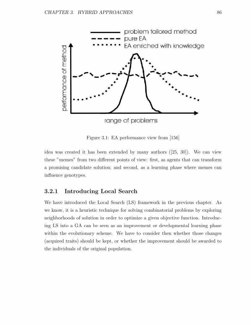
CHAPTER 3. HYBRID APPROACHES 86
Figure 3.1: EA performance view from [156]
idea was created it has been extended by many authors ([25, 30]). We can view
these ”memes” from two different points of view: first, as agents that can transform
a promising candidate solution; and second, as a learning phase where memes can
influence genotypes.
3.2.1 Introducing Local Search
We have introduced the Local Search (LS) framework in the previous chapter. As
we know, it is a heuristic technique for solving combinatorial problems by exploring
neighborhoods of solution in order to optimize a given objective function. Introduc-
ing LS into a GA can be seen as an improvement or developmental learning phase
within the evolutionary scheme. We have to consider then whether those changes
(acquired traits) should be kept, or whether the improvement should be awarded to
the individuals of the original population.
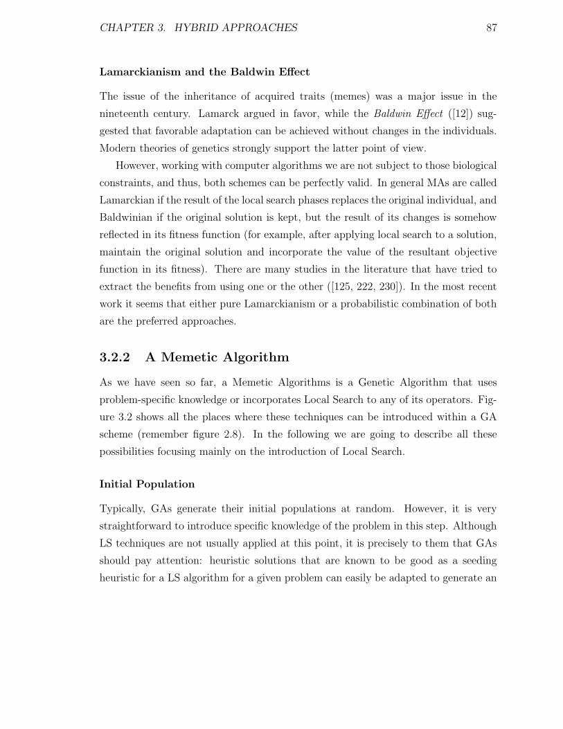
CHAPTER 3. HYBRID APPROACHES 87
Lamarckianism and the Baldwin Effect
The issue of the inheritance of acquired traits (memes) was a major issue in the
nineteenth century. Lamarck argued in favor, while the Baldwin Effect ([12]) sug-
gested that favorable adaptation can be achieved without changes in the individuals.
Modern theories of genetics strongly support the latter point of view.
However, working with computer algorithms we are not subject to those biological
constraints, and thus, both schemes can be perfectly valid. In general MAs are called
Lamarckian if the result of the local search phases replaces the original individual, and
Baldwinian if the original solution is kept, but the result of its changes is somehow
reflected in its fitness function (for example, after applying local search to a solution,
maintain the original solution and incorporate the value of the resultant objective
function in its fitness). There are many studies in the literature that have tried to
extract the benefits from using one or the other ([125, 222, 230]). In the most recent
work it seems that either pure Lamarckianism or a probabilistic combination of both
are the preferred approaches.
3.2.2 A Memetic Algorithm
As we have seen so far, a Memetic Algorithms is a Genetic Algorithm that uses
problem-specific knowledge or incorporates Local Search to any of its operators. Fig-
ure 3.2 shows all the places where these techniques can be introduced within a GA
scheme (remember figure 2.8). In the following we are going to describe all these
possibilities focusing mainly on the introduction of Local Search.
Initial Population
Typically, GAs generate their initial populations at random. However, it is very
straightforward to introduce specific knowledge of the problem in this step. Although
LS techniques are not usually applied at this point, it is precisely to them that GAs
should pay attention: heuristic solutions that are known to be good as a seeding
heuristic for a LS algorithm for a given problem can easily be adapted to generate an
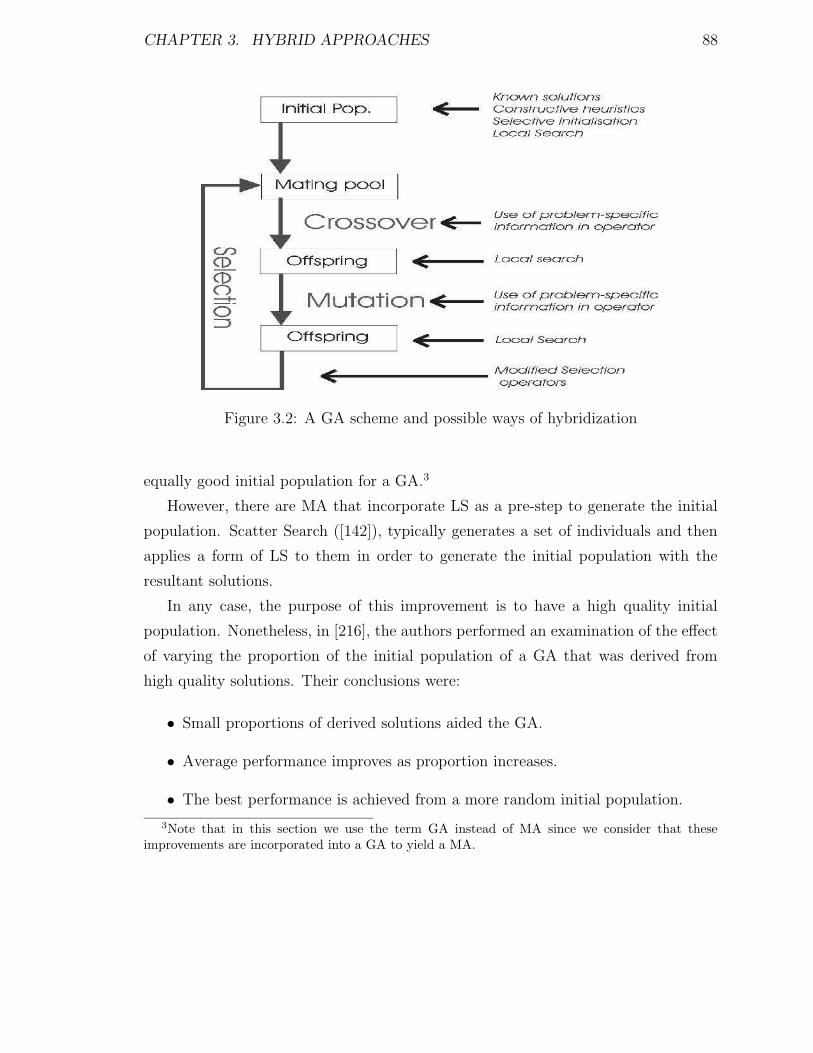
CHAPTER 3. HYBRID APPROACHES 88
Figure 3.2: A GA scheme and possible ways of hybridization
equally good initial population for a GA.3
However, there are MA that incorporate LS as a pre-step to generate the initial
population. Scatter Search ([142]), typically generates a set of individuals and then
applies a form of LS to them in order to generate the initial population with the
resultant solutions.
In any case, the purpose of this improvement is to have a high quality initial
population. Nonetheless, in [216], the authors performed an examination of the effect
of varying the proportion of the initial population of a GA that was derived from
high quality solutions. Their conclusions were:
• Small proportions of derived solutions aided the GA.
• Average performance improves as proportion increases.
• The best performance is achieved from a more random initial population.
3Note that in this section we use the term GA instead of MA since we consider that theseimprovements are incorporated into a GA to yield a MA.

CHAPTER 3. HYBRID APPROACHES 89
Thus, we can conclude that as the proportion increases, so does the average per-
formance but at the same time, the variance in performance decreases.
Local Search as Crossover and/or Mutation
This idea is very straightforward: apply a certain LS technique as a Crossover or
Mutation operator. Mutation and LS are intrinsically the same kind of technique,
they change the genotype of the individuals. The difference is that mutation is random
and LS is heuristic.
Some approaches in the literature report good results when introducing LS at
this point. For example, in [223], a modified one point crossover operator used for
protein structure prediction is introduced. The modified operator made use of some
problem-specific knowledge by explicitly testing all the possible different orientations
of the two fragments to recombine in order to find the most energetically favorable.
If no feasible conformation was found, a different crossover point was chosen and
the process repeated. This can be seen as a simple introduction of LS into the
recombination operator.
In [130], the authors propose a simple crossover hill-climber in which all the
possible offsprings arising from one point crossover are constructed and the best
chosen.
In [82], a more complex approach is presented: a distance preserving crossover
operator for the Traveling Salesman Problem (TSP). The intelligent part of the op-
erator is based on a nearest-neighbor heuristic to join together the subtours inherit
from the parents, thus, explicitly exploiting instance-specific edge length information.
Local Search applied to the outcome of recombination
The most common technique of hybridization of GAs is via the application of one or
more steps of improvement to individuals of the population during the evolutionary
cycle. LS is typically applied to whole solutions created by mutation or crossover.
Perhaps surprisingly, the effort to use GAs to evolve artificial neural networks gave
a great deal of insight into the role of learning, Lamarckianism and the Baldwin effect
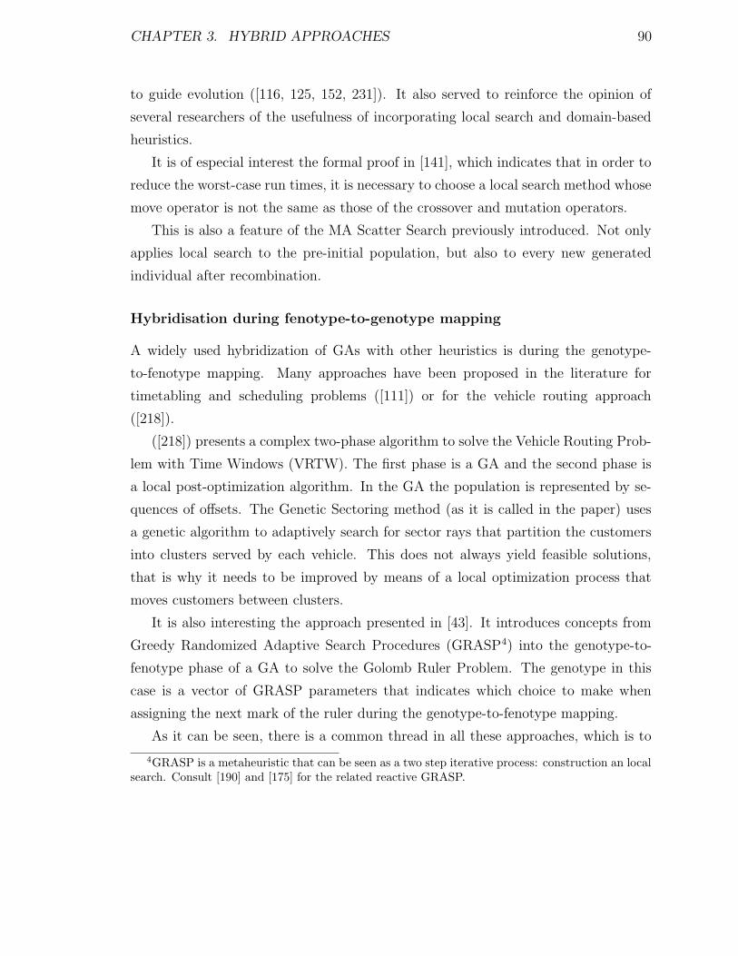
CHAPTER 3. HYBRID APPROACHES 90
to guide evolution ([116, 125, 152, 231]). It also served to reinforce the opinion of
several researchers of the usefulness of incorporating local search and domain-based
heuristics.
It is of especial interest the formal proof in [141], which indicates that in order to
reduce the worst-case run times, it is necessary to choose a local search method whose
move operator is not the same as those of the crossover and mutation operators.
This is also a feature of the MA Scatter Search previously introduced. Not only
applies local search to the pre-initial population, but also to every new generated
individual after recombination.
Hybridisation during fenotype-to-genotype mapping
A widely used hybridization of GAs with other heuristics is during the genotype-
to-fenotype mapping. Many approaches have been proposed in the literature for
timetabling and scheduling problems ([111]) or for the vehicle routing approach
([218]).
([218]) presents a complex two-phase algorithm to solve the Vehicle Routing Prob-
lem with Time Windows (VRTW). The first phase is a GA and the second phase is
a local post-optimization algorithm. In the GA the population is represented by se-
quences of offsets. The Genetic Sectoring method (as it is called in the paper) uses
a genetic algorithm to adaptively search for sector rays that partition the customers
into clusters served by each vehicle. This does not always yield feasible solutions,
that is why it needs to be improved by means of a local optimization process that
moves customers between clusters.
It is also interesting the approach presented in [43]. It introduces concepts from
Greedy Randomized Adaptive Search Procedures (GRASP4) into the genotype-to-
fenotype phase of a GA to solve the Golomb Ruler Problem. The genotype in this
case is a vector of GRASP parameters that indicates which choice to make when
assigning the next mark of the ruler during the genotype-to-fenotype mapping.
As it can be seen, there is a common thread in all these approaches, which is to
4GRASP is a metaheuristic that can be seen as a two step iterative process: construction an localsearch. Consult [190] and [175] for the related reactive GRASP.
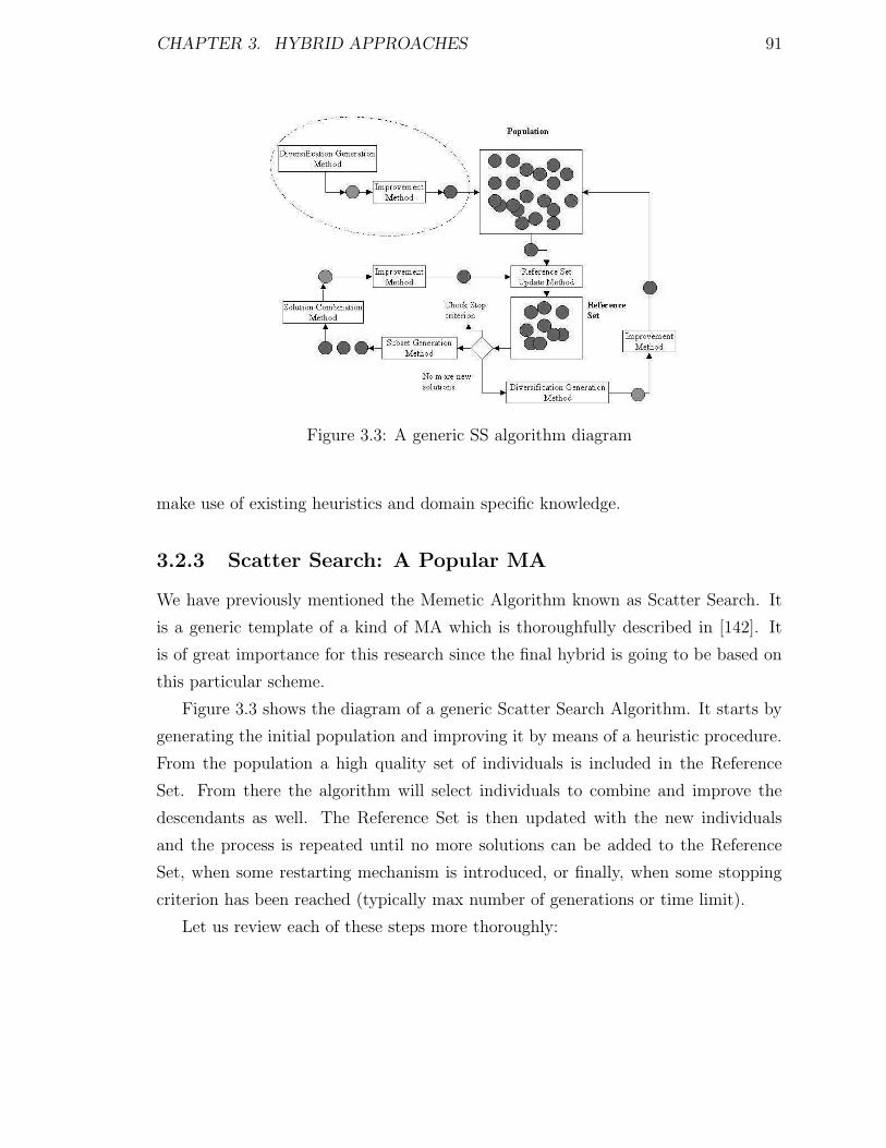
CHAPTER 3. HYBRID APPROACHES 91
Figure 3.3: A generic SS algorithm diagram
make use of existing heuristics and domain specific knowledge.
3.2.3 Scatter Search: A Popular MA
We have previously mentioned the Memetic Algorithm known as Scatter Search. It
is a generic template of a kind of MA which is thoroughfully described in [142]. It
is of great importance for this research since the final hybrid is going to be based on
this particular scheme.
Figure 3.3 shows the diagram of a generic Scatter Search Algorithm. It starts by
generating the initial population and improving it by means of a heuristic procedure.
From the population a high quality set of individuals is included in the Reference
Set. From there the algorithm will select individuals to combine and improve the
descendants as well. The Reference Set is then updated with the new individuals
and the process is repeated until no more solutions can be added to the Reference
Set, when some restarting mechanism is introduced, or finally, when some stopping
criterion has been reached (typically max number of generations or time limit).
Let us review each of these steps more thoroughly:

CHAPTER 3. HYBRID APPROACHES 92
Diversification Generation Method
In this step a starting set of solutions is generated. Through some mechanism, a
certain level of diversity is guaranteed. This is usually achieved by generating high
quality solutions and diverse solutions as separate goals. These solutions will now be
improved in order to be transferred to the Reference Set.
Improvement Method
After the pre-initial population has been generated or whenever a new individual is
created, an improvement method is applied to the solution. This method is usually
a heuristic local search procedure such as tabu search or simulated annealing.
Reference Set Update Method
The Reference Set is now filled with the solutions with higher quality from the previous
steps. The notion of quality here is not limited to the value of an objective function,
diversity is a key factor to decide whether a solution must be kept on the reference
set or not.
Subset Generation Method
This steps will define the subsets of individuals of the reference set to be latter
recombined. These are the generic subsets to be generate:
• All 2-individuals subsets.
• 3-individuals subset generated from the 2-individuals subsets by adding the best
solution not included in the subset.
• 4-individuals subsets generated in the same fashion from the 3-individuals sub-
sets.
• The subsets consisting of the best n elements, being n = 5 to the size of the
reference set.

CHAPTER 3. HYBRID APPROACHES 93
Note that some subsets can be repeated, simple and efficient techniques to avoid
that are presented in [94].
Solution Combination Method
This method consists of combining the individuals of the previously generated subsets.
It is typically dependant of the specific problem. It can also generate one or more
solutions depending on its implementation. It is also important that the new solutions
are generated in a deterministic fashion; then, that will be recorded in order not to
combine the same subsets in subsequent iterations.
3.3 Genetic Algorithms and CP
In this section we are going to review state-of-the-art approaches that introduce Con-
straint Programming techniques into GAs. Note that this section could fall into the
category described in the previous section; these approaches can be seen as Memetic
Algorithms, since they are GAs that incorporate problem-specific knowledge in some
steps of the evolutionary scheme. In this case, this knowledge falls into the field of
Constraint Programming, and thus, we have decided to separate it and describe it in
a different section.
3.3.1 Handling Constraints
The first issue to describe is constraint handling. Remember that in a constraint
satisfaction problem (CSP) we are given a set of variables, where each variable has a
domain of values, and a set of constraints acting between variables. The problem con-
sists of finding an assignment of values to variables in such a way that the restrictions
imposed by the constraints are satisfied.
We can also define a CSP as a triplet < X,D,C >, where X = {x1, . . . , xn}is the set of variables, D = {D1, . . . , Dn} is the set of nonempty domains for each
variable xi, and C = {C1, . . . , Cm} is the set of constraints. Each constraint is defined
over some subset of the original set of variables {x1, . . . , xn} and specifies the allowed
CHAPTER 3. HYBRID APPROACHES 94
combinations of these variable values. Thus, solving the CSP is equivalent to finding
a complete assignment for the variables in X with values from their respective domain
set D, such that no constraint Ci ∈ C is violated.
The issue is thus, how to handle these constraints: either directly or indirectly
[63].
• Direct handling leaves the constraints as they are, and enforces them somehow
during the execution of the algorithm; while,
• Indirect handling involves transforming the constraints into an optimization
objective (included in the fitness function), which the EA will pursue.
Direct handling is not generally oriented for EA due to the lack of an optimization
function in the CSP, which would result in no guidance towards the objective. Thus,
indirect handling is the best suited approach for EA, although a mixed strategy where
some constraints are enforced and some are transformed into an optimization criteria
is suited as well.
Whenever a direct handling approach is chosen, the algorithm will have to face
many problems, especially because the combination and mutation operators are blind
to the constraints, and recombination of two feasible solutions can yield an infeasible
one. Approaches to solve this are:
• Repair infeasible individuals.
• Eliminate infeasible individuals.
• Maintain feasiblity with special purpose operators.
• Transforming the search space.
Repairing infeasible solutions implies developing a repair operator which is very
problem-dependant. If implemented properly can nontheless produce efficient results
(see [158] for a comparative study). Eliminating infeasible individuals is not very
efficient and hardly ever used. Maintaining feasiblity is also very problem-specific;
note that in order to maintain this, the initial population needs to be feasible, which
CHAPTER 3. HYBRID APPROACHES 95
is in itself NP-hard sometimes, and obviously not an option when dealing with con-
straint satisfaction problems5. Finally, transforming the search space can simplify
the problem and allow an efficient GA. The new search space is decoded to create
feasible solutions and it also allows a free search for the GA.
On the other hand, indirect constraint handling is typically performed by adding
penalties to constraint violations. These penalties are incorporated into the objective
function in order to drive the search towards a feasible solution. Constraint penal-
ties represent distance to feasibility. This approach is usually the best suited for
constraint satisfaction problems because it is general, and allows the problem to be
transformed into an optimization problem. However, it is sometimes complicated to
merge penalties with objective function. It is also known to perform poorly for sparse
problems.
In the next sections we will review different GAs for solving constraint satisfaction
problems, divided into three different groups:
• Heuristic based methods.
• Adaptive based methods.
• Memetic Algorithms for CSPs.
Note that all the techniques present either an indirect or a mixed direct and
indirect constraint handling approach.
3.3.2 Heuristic based methods
The methods reviewed here have in common the fact that they all extract heuristic
knowledge from the structure of the constraints to be incorporated in the GAs.
Heuristic Genetic Operators
This technique has been introduced in [65, 66]. It studies the possibility to incorporate
exiting CSP heuristics into genetic operators. These operators are mutation and
5If we were trying to find a feasible solution for a problem and the initial population was feasible,then the problem would be already solved

CHAPTER 3. HYBRID APPROACHES 96
multi-parent crossover, which are guided by the same heuristic: select the variables
which appear in more constraint violations and instantiate them with the value that
minimizes these violations.
Thus, the mutation operator will select a certain number of variables in the in-
dividual and will change their values so as to minimize the number of constraint
violations. The multi-parent crossover will proceed similarly, only that in this case
only the values found in any of the parents will be taken into consideration.
Knowledge Based Fitness
In this case, information about the constraint network is incorporated in the fitness
function and in the genetic operators (see [191, 192]) as well.
The fitness function is called arc-fitness and it consists of the sum of the error
evaluations of the violated constraints. The error evaluations of a constraint is the
number of variables in its scope plus the number of variables conected to them in the
constraint network.
The mutation operator (called arc-mutation) simply selects a variable randomly
and instantiates it with the value that minimizes the sum of error evaluations. The
crossover operator which is called constraint dynamic adaptive arc-crossover basically
constructs a new individual by focusing on constraints and selecting the values of the
variables in those constraints from one parent or the other in order to minimize the
fitness function as well.
Moreover, it includes a heuristic parent selection mechanism that divides the pop-
ulation in three different groups, based on the value of their objective functions.
The Glassbox Approach
In [150, 151, 44] it is described a GA to solve CSPs based on pre and post-processing
techniques. In particular, in [150], the algorithm developed relies on the transforma-
tion of the constraints into a canonical form. This rewriting of constraints is called
constraint processing and is performed in two steps:
1. Elimination of functional constraints.
CHAPTER 3. HYBRID APPROACHES 97
2. Decomposition of the CSP into primitive constraints in the form of inequalities.
With all the constraints in primitive form, a single repair-based heuristic is applied.
This heuristic is called dependency propagation and it attempts to repair violated
constraints in random order.
Note that at the end of the repairing process the individual might not be a feasible
solution, since repairing violated constraints can produce other constraint violations.
Coevolutionary Approach with Heuristics
In [109, 108], we can find a coevolutionary algorithm where the host population is
parasited on by a population of schemata. Schemata are individuals which have some
of their variables instantiated with an unknown value. The interaction between the
population is performed using two mechanisms:
• Superposition: a parasite finds a match in the host population and it simply
instantiates the unknown variables with the values of its host. This is performed
in order to calculate the fitness function of the parasite individuals.
• Transcription: it randomly chooses variables of an individual and replaces
their values with the unknown values of the parasite population.
The host fitness function is not only based on constraint violations, but it is
also normalized to a range from 0 to 1 taking into account the number of violated
constraints versus the total number of constraints. The host mutation and crossover
operators are standard (random mutation and one-point crossover).
Hybrid GRASP-Evolution
The method presented in [31] is slightly different from the rest of the approaches
in this category. The algorithm does not present any specific-problem features, but
it incorporates a novel genotype-to-fenotype mapping. The population is a set of
GRASP parameter vectors as in [43]. In the same manner, the value of each parameter
defines the exact candidate to select, instead of a range for a random selection as in the
CHAPTER 3. HYBRID APPROACHES 98
general case in GRASP. This is due to the stochastic genotype-to-phenotype mapping
that would yield, which will, thus, add a level of complexity in the algorithm.
The initial problem is transformed into that of finding an optimal ordering for the
variables that will yield a feasible solution. Thus, the vector of GRASP parameters
allows to choose, among the ranked variables, which one is going to be instantiated
next.
The basic procedure for assigning a variable within the genotype-to-fenotype map-
ping is as follows:
1. Present the variables available for selection.
2. Apply the dom/degree heuristic to these variables.
3. Define the resultant Restricted Candidate List.
4. Select the candidate variable that the GRASP parameters vector indicates.
5. Instantiate the variable with the best value possible.
6. Reflect this selection and instantiation in the correspondant position of a vector
that represents an actual tentative solution of the problem.
3.3.3 Adaptive based methods
All the methods included in this category share the common emphasis on adaptation
features rather than on heuristic operators.
The Coevolutionary Approach
This approach has been tested on many different problems ([169, 170]). Interestingly,
it has been aplied to solve CSPs in [71, 226]. It consists of two populations that evolve
in a predator-prey model: a population of candidate solutions and a population of
constraints.
The fitness of the individuals of both populations is based on a history of en-
counters. Encounters are matchings between constraint and individual which reward
CHAPTER 3. HYBRID APPROACHES 99
the individual if it satisfies the constraint, or reward the constraint otherwise. This
results in a higher fitness for constraints that are often violated, which means that
the algorithm will focus on harder constraints.
Mutation and crossover are only performed in the population of candidate solu-
tions. The crossover operator aims at generating diverse individuals.
Step-Wise Adpatation of Weights
The Step-Wise Adaptation of Weights (SAW) mechanism was introduced in [70, 225]
as an improved version of the weight adaptation mechanism presented in [67]. The
basic idea behind this mechanism is that constraints that are not satisfied and vari-
ables causing constraint violations after number of steps must be hard, and so they
should be given higher weights.
This algorithm presents a steady state model with a representation based on per-
mutation models. A permutation is transformed into a solution by a decoder that
simply instantiates variables, in the order in which they occur in the chromosome,
with the first feasible value; if this feasible value does not exist, the variable is then
left uninstantiated. Uninstantiated variables are penalized and the fitness of a chro-
mosome is the sum of all these penalties.
3.3.4 MAs for solving CSPs
We have separated these techniques because they not only introduce CSP like mech-
anisms but also Local Search. These are the most similar approaches to our final
hybrid. They are, however, different in the sense that they only incorporate knowl-
edge of the constraint network for solving a CSP, instead of actually including a
CP-like procedure within the algorithm.
Genetic Local Search
A Genetic Local Search Algorithm for solving CSPs is presented in [151]. The basic
scheme consists of the application of genetic operators to a population of local optima
CHAPTER 3. HYBRID APPROACHES 100
produced by a LS algorithm. The process is iterated until either a solution is generated
or the maximum number of generations is reached.
The LS algorithm used is a Repair and Improve heurisitic: it repairs the pop-
ulation by extracting and extending every candidate, and improves it by applying
arc-consistency, deleting and extending.
Since the algorithm deals with feasible partial instantiations, in this case, the
fitness functions corresponds to the number of instantiated variables on the individual.
Evolving Hill-Climbers
In [58, 59] we find a GA with a very small population (that is why it is called micro-
evolutionary) whose population is a set of hill-climbers.
Every candidate solution contains four different fields:
• Field 1: is a chromosome containing each object.
• Field 2: is the fitness of the individual.
• Field 3: determines the heursitic-based mutation operator.
• Field 4: is the individual’s family identification number6.
The evaluation function determines the individual’s fitness by substracting the
weights of all violated constraints. The algorithm evolves the population using sev-
eral crossover and mutation operators, and also applying an adaptation scheme that
awards the operators that yield superior offsprings.
Most of these methods are compared using random binary CSPs in [45]. Other
classifications are available in the literature ([157, 155]).
6Family or relatedness is a mechanism to reduce the number of duplicates within the population

Part II
Preliminary Work on Pure and
Hybrid Approaches
101

Chapter 4
CP and SAT for the Quasigroup
Completion Problem
The Quasigroup Completion Problem (QCP) is a very challenging benchmark among
combinatorial problems, which has been the focus of much recent interest in the
area of constraint programming. It has a broad range of practical applications [101];
it has been put forward as a benchmark which can bridge the gap between purely
random instances and highly structured problems [100]; and its structure as a multiple
permutation problem [229] is common to many other important problems in constraint
satisfaction. Thus, solutions that prove effective on QCPs have a good chance of being
useful in other problems with similar structure.
In this chapter, we present several techniques within the constraint programming
and SAT frameworks that together allow us to solve significantly larger QCPs than
previously reported in the literature. Specifically, [101] reports that QCPs of order 40
could not be solved by pure constraint programming approaches, but could sometimes
be solved by hybrid approaches combining constraint programming with mixed integer
programming techniques from operations research. We show that the pure constraint
satisfaction approach can solve many problems of order 45 in the transition phase,
which corresponds to the peak of difficulty. Our solution builds upon some known
ideas, such as the use of redundant modeling [36] with primal and dual models of
the problem connected by channeling constraints [229], with some new twists. For
102

CHAPTER 4. CP AND SAT FOR THE QUASIGROUP COMPLETION PROBLEM103
example, we will consider models consisting of only channeling constraints, without
any primal or dual constraints, and we demonstrate empirically for the first time the
usefulness of channeling constraints linking several pairs of models of a problem, an
idea that was considered, but only theoretically, in [35] and [212]. In addition, we
present a new value ordering heuristic which proves extremely effective, and that could
prove useful for many other problems with multiple models. The idea underlying this
heuristic, which originates in the work of [35, 211] for single permutation problems,
is that selecting a value for (say) a primal variable is in practice in the presence of
channeling constraints also a choice of the dual variables corresponding to that value;
therefore we can use variable selection heuristics on the dual variables to choose
the value to assign to the previously chosen primal variable. Finally, we show how
redundant constraints can be used to “compile arc consistency into forward checking”,
that is, to ensure that the latter has as much pruning power as the former but at a
much lesser cost in constraint checks.
It is interesting to note that our approach involves only binary constraints, which
seems to go against common wisdom about their limitations —when contrasted with
the use of non-binary constraints such as alldiff [188]— in solving quasigroup comple-
tion problems [215]. It is certainly an interesting issue, which we plan to address in
the future, whether the use of alldiff could yield even better results than our approach
when coupled with other ideas in this work.1
The idea of redundant modeling was first introduced by [36]. The benefits of
adding redundant constraints to some given model to improve pruning power were
well-known in the literature, but [36] went a step further by considering the redundant
combination of full models of a problem, where the models may involve different sets
of variables. This combination is achieved by specifying how the various models
relate to each other through channeling constraints, which provide a mapping among
assignments for the different models. The combined model contains the original but
redundant models as submodels. The channeling constraints allow the sub-models to
cooperate during constraint-solving by propagating constraints among the problems,
1Besides the obvious computational limitations in running large experimental suites of hard QCPproblems, we were limited in this aspect by the unavailability of open source alldiff code.
CHAPTER 4. CP AND SAT FOR THE QUASIGROUP COMPLETION PROBLEM104
providing an extra level of pruning and propagation which results in a significant
improvement in performance.
Another important modeling idea that we use is that of permutation problems (see
e.g. [211, 229]). A constraint satisfaction problem (CSP) is a permutation problem
if it has the same number of variables as values, all variables have the same domain
and each value can be assigned to a unique variable. Thus, any solution can be seen
as assigning a permutation of the values to the variables. In the same manner, a
multiple permutation problem has some (possibly overlapping) sets of variables, each
of which is a permutation problem. QCP is a paradigmatic example of a multiple
permutation problem.
Moreover, we perform a systematic study of modelling choices for quasigroup
completion, testing a variety of solvers and heuristics on various SAT and CSP en-
codings. The clear winner is the SAT 3D-encoding, specially with the solver Satz
[144], closely followed by the solver Satzoo [62] on the same encoding. As these two
solvers are quite different (one uses a strong form of lookahead in its heuristic, but
no backjumping or learning, while the other relies heavily on the last two), the 3D
encoding appears to be quite robust as a representation. On the other hand, CSP
models perform significantly worse with the two solvers we tried, and standard SAT
encodings generated from the CSP models are simply too large in practice. These
results strongly suggest that the 3D encoding can turn out to be quite competitive in
other permutation problems (many of which arise in quite practical problems [118])
when compared with the currently preferred channelling models.
The reasons for this appear to be twofold. First, we can show that the 3D en-
coding (which is basically the “SAT channelling model” of [118] extended to multiple
permutations and dual models) exactly captures the channelling models of QCPs as
defined in this thesis, but in a much more concise way, by collapsing primal and dual
variables. Further, we can show that the 3D encoding captures the “support SAT
encoding” of the channelling model, hence by results of [89], that unit propagation
on the 3D encoding achieves the same pruning as arc consistency (MAC) in the CSP
channelling model. These results appear easy to extrapolate to other permutation
problems (or similar ones with ”channelling constraints”), which have received a lot
CHAPTER 4. CP AND SAT FOR THE QUASIGROUP COMPLETION PROBLEM105
of recent attention [35, 229, 118]. Second, empirically, we identify Satz’s UP heuristic
as crucial to its success in this domain; as shown by the fact that, when importing
the heuristic into our CSP solvers, we obtain significant improvements in their scala-
bility. Further, the improvements are much smaller if we only use lookahead to detect
potential wipeouts (i.e. for “failed literal detection”), but choose variables instead by
some other standard heuristic such as min-domain.
The rest of the chapter is organized as follows: first we introduce Quasigroups
and the QCP problem, then we detail the modeling and heuristic used and give
experimental results; Afterwards, we introduce SAT models and solvers, compare
results against CSP solvers and introduce SAT features in our CSP solver to provide
a new comparison. Finally, we present the lessons learnt from this research.
4.1 Quasigroups
A quasigroup is an ordered pair (Q, ·), where Q is a set and · is a binary operation
on Q such that the equations a · x = b and y · a = b are uniquely solvable for every
pair of elements a, b in Q [101]. The order n of the quasigroup is the cardinality of
the set Q. A quasigroup can be seen as an n × n multiplication table which defines
a Latin Square, i.e. a matrix which must be filled with “colors” (the elements of the
set Q) so that the colors of each row are all distinct, and similarly for columns.
Early work on quasigroups focused on quasigroup existence problems, namely
the question whether there exist quasigroups with certain properties, solving several
significant open mathematical problems [208]. We focus instead on the quasigroup
completion problem (QCP), which is the (NP-complete [38]) problem of coloring a
partially filled Latin square.
4.1.1 Quasigroup Completion Problem
Imagine you have an empty Latin square, and that you color some of its cells and left
some others empty. Trying to extend that partial coloring to a solution (if possible)
defines the Quasigroup Completion Problem.
CHAPTER 4. CP AND SAT FOR THE QUASIGROUP COMPLETION PROBLEM106
QCP share with many real world problems a significant degree of structure, while
at the same time allowing the systematic generation of difficult problems by randomly
filling the quasigroup with preassigned colors. It is thus ideally suited as a testbed
for constraint satisfaction algorithms [100]. Experimental studies of the problem
have confirmed its interest for research, by for example helping to discover important
patterns in problem difficulty such as heavy-tailed behavior [98].
Instances of QCP
It is also important to introduce types of instances for the quasigroup completion
problem. Not only in order to establish a framework for the experiments, but also
because the study of its hardness and its complexity are within the state of the art in
this problem. There also a need of a source of satisfiable instances for the evaluation
of some algorithms.
Under this perspective we can differentiate two kinds of instances for this problem:
QCP We have introduced the QCP problem in the initial sections, and it is an
NP-complete problem [38] which has an interesting phase transition phenomenon
with an associated easy-hard-easy pattern as a function of the fraction of number of
preassigned colors. This kind of instances that we will refer to as QCP from now on,
are generated in a way that can be solvable or not. This means that we cannot assure
its solvability because of the way they are generated.
Within this kind we can distinguish between those instances which are trivially
unsolvable, which means that the preassignment itself violates one ore more con-
straints; and those which we do not know its solvability until a complete algorithm
terminates without finding a feasible solution.
QWH As mentioned above, there is a need for hard solvable instances, in order to
have a source for evaluating for example local search algorithms. The quasigroup with
holes (QWH) problem was proposed in [2] as a way to fill this need.
CHAPTER 4. CP AND SAT FOR THE QUASIGROUP COMPLETION PROBLEM107
QWH instances are given this name because of the way they are generated 2: (1)
first generate a complete Latin square according to the Markov chain Monte Carlo
approach proposed by Jacobson and Mathews [128]; punch a fraction p of “holes”
in the Latin square in an uniformly distributed manner. The resulting partial Latin
square is guaranteed to be solvable. We can also find two different types of instances
within QWH:
Random This kind of instances are generated punching holes at random. This
was the first kind of instances generated and studied, thus we know that its phase
transition coincides with d1.6× n1.55e holes for order n.
Balanced Lately, this kind of instances have been studied and it seems that they
are much harder than random ones. They are generated in a way that the number of
holes in each row and in each column is more or less the same.
4.2 Modelling and solving QCPs as a CSP
Our first step through improving efficiency solving QCPs is due to an effort to make
competitive an initial implementation for this problem that yielded very poor results
when compared with the literature. Guided by this objective and after studying
some techniques and approaches applied to solve QCPs (those introduced in previous
sections) we found an implementation and an heuristic that yields promising results.
4.2.1 Not-equal implementation
First of all we introduce the initial implementation of the problem, to which we will
refer as the primal model.
This model represents cells of the Quasigroup as variables whose domains are the
set of possible colors to be assigned:
2We thank Carla Gomes for providing us with the lsencode generator, which was used for gener-ating satisfiable instances for the experiments that are presented in the next sections
CHAPTER 4. CP AND SAT FOR THE QUASIGROUP COMPLETION PROBLEM108
xi,j ∈ {1, .., n}∀ i, j
xi,j = k ∀i, j such that QCPi,j = k
not− equal(xi,1, xi,2), not− equal(xi,1, xi,3), ..., not− equal(xi,1, xi,n) ∀i
not− equal(x1,j, x2,j), not− equal(x1,j, x3,j), ..., not− equal(x1,j, xn,j) ∀j
It is important to note that we first choose a not-equal implementation instead of
an alldiff one. This election was maintained for all the experiments from now on.
4.2.2 Redundant models
Redundancy is a double-edged sword: it can help propagation by allowing more values
to be pruned at any given point in the search, but it can also hinder it by forcing
it to process a larger set of constraints. Fortunately, more fine grained distinctions
are possible, as we might choose to combine only parts of various models. We could
not speak of combining models if we don’t use their respective sets of variables, but
it will often be advantageous (as we will see) to drop some of the constraints from
one or more models that become redundant when making the combination. If we do
this, however, we must be careful to ensure the correctness and completeness of the
combined model.
Several models can be defined for QCPs, as described next. While all models have
the same logical status, it is common to distinguish between primal and dual models.
The distinction is only a matter of perspective, specially in permutation problems,
where variables and values are completely interchangeable.
Primal Model This is the model introduced before, and we will refer to it as pr
model for short.
Row Dual Model There are different ways to formulate dual models for a multiple
permutation problem. Here we consider dual models for each of the permutation
subproblems (as opposed to a single dual model of the primal problem), and group
CHAPTER 4. CP AND SAT FOR THE QUASIGROUP COMPLETION PROBLEM109
them by row and column, to obtain two complete models of QCPs. In the row dual
model, the problem is reformulated as the question of which position (column) in
a given row has a given color. The row dual variables are the set R = {rik | 1 ≤i ≤ n, 1 ≤ k ≤ n} where rik is the kth color in the ith row. The domain of each
variable is again the set D = {j | 1 ≤ j ≤ n}, but now the values represent columns,
i.e. the positions in row i where color k can be placed. The row dual constraints
are similar to the primal constraints. There are n2 constraints of the form rik 6= ril,
where rik, ril ∈ R and l 6= k, which means that two colors in the same row must
not be assigned to the same column; and n2 constraints of the form rik 6= rjk where
rik, rjk ∈ R and i 6= j, which means that the same color in different rows must not
be assigned to the same column. Alternatively, we could have alldiff(ri1, . . . , rin) for
every row i, and alldiff(r1k, . . . , rnk) for every color k.
A simple symmetry argument shows that this model also fully characterizes the
problem.
Column Dual Model The second dual model is composed of the set of dual models
for each column permutation constraint, representing the colors in each column. The
column dual variables are the set C = {cjk | 1 ≤ j ≤ n, 0 ≤ k ≤ n} where cjk is the
kth color in the jth column. All variables have domain D = {i | 1 ≤ k ≤ n}, where i
represents the rows where color k can be placed in the jth column. Similar to the row
dual model, we have column dual constraints of the form cjk 6= cjl where cjk, cjl ∈ Cand k 6= l, which means that two colors in the same column must not be assigned to
the same row; and of the form cjk 6= clk where cjk, clk ∈ C and j 6= l, which means
that the same color in different columns must not be assigned to the same row.
This model also fully characterizes the problem. We refer to the combination of
both dual models as the dl model.
4.2.3 Combining the Models
A channelling constraint for two models M1 = (X1, F1, C1) and M2 = (X2, F2, C2) is
a constraint relating variables of X1 and X2 [36]. We will consider the following kinds
of channelling constraint:
CHAPTER 4. CP AND SAT FOR THE QUASIGROUP COMPLETION PROBLEM110
• Row Channelling Constraints: Constraints for the n row permutation con-
straints, linking the primal model with the row dual model:
xij = k ⇔ rik = j.
• Column Channelling Constraints: Corresponding to the n column permutation
constraints, they link the primal and the dual column models:
xij = k ⇔ cjk = i.
• Triangular Channelling Constraints: These constraints link both dual models,
closing a “triangle” among the three models:
cjk = i⇔ rik = j.
Given two or more redundant, complete models, we can obtain a combined model
by simply implementing all the models and linking them by channelling constraints.
Thus the full combined model or pr-dl-ch2-model resulting from the above models
is the model consisting of primal and dual variables and constraints, linked together
by row and column channelling constraints.3 More generally, as long as a combined
model includes a complete model of the problem as a submodel, we are free to add any
set of variables or constraints from other models, with the only requirement that in
order to add a constraint all its variables must belong to the combined model. Thus,
for example, given the primal variables and constraints, we may choose to add any
number of dual and channelling constraints as long as the corresponding variables are
also added. For example, we may decide to use only the row dual variables together
with the row dual constraints and/or row channelling constraints. Nothing is lost by
not including parts of the dual models, since all the necessary information is present
in the primal model.
In fact we can take this as far as removing all primal and dual constraints! Walsh
[229] shows that arc consistency on the channelling constraints for a permutation
3We don’t consider adding the triangular constraints until later.
CHAPTER 4. CP AND SAT FOR THE QUASIGROUP COMPLETION PROBLEM111
problem dominates in pruning power over arc consistency over the binary not-equal
constraints. Intuitively, this means that nothing is gained by adding the not-equal
constraints once we have the channelling constraints. Note that this doesn’t prove the
superiority of a model with only channelling constraints over, say, the primal model,
as the former also has many more variables and constraints; this issue is empirically
examined later. It is important however to show that the model consisting of primal
and dual variables, with only row and column channelling constraints, but without
the primal or dual constraints (i.e. alldiff or not-equal) is also a complete model of
the problem. We refer to this model as the bichannelling model or ch2:
Proposition 4.2.3.1. The bichannelling model is equivalent to the primal model,
hence it provides a full characterization of QCPs.
Proof. If the two models had the same set of variables and associated domains, we
could define equivalence just as having the same set of solutions. Since that’s not
the case here, we need to provide instead a one-to-one mapping between solutions of
either model.
Let us say that a primal assignment, or P-assignment for short, is an assignment
of values to all the primal variables, and a PD-assignment an assignment to all primal
and dual variables.
The proposition can then be phrased more exactly in terms of the following two
claims.
Claim 1: Any P-assignment A which satisfies the (primal) alldiff constraints can
be extended to a PD-assignment B which satisfies the channelling constraints. To
extend A to B, we just pick each label xij = k from A and set rik = j and cjk = i in
B. To see that B is well-defined, note that every rik gets assigned, since A must use
all available colors in order to fill row i in accordance with the primal constraints;
and that any given rik is assigned at most once, since otherwise we would have
xij = xih for distinct columns j and h, in contradiction with the fact that A satisfies
the primal constraints. Similarly for any cjk. Hence B is well-defined, and it satisfies
the channelling constraints by construction.

CHAPTER 4. CP AND SAT FOR THE QUASIGROUP COMPLETION PROBLEM112
Claim 2: Any PD-assignment B satisfying the row and column channelling con-
straints, is such that its primal subset A satisfies the primal constraints. Suppose
not. Then B assigns the same value k to two primal variables xij and xih for j 6= h
(or the completely symmetric case where it is row indexes that vary). But since B
satisfies the row channelling constraints, B should satisfy rik = j and rik = h, which
is impossible.
Yet another combined model we will consider later is the trichannelling model,
or ch3 for short, which adds the triangular channelling constraints to ch2, but still
keeps away from the primal and dual constraints. Given the above proposition, ch3
is also a complete model, and redundantly so.
4.2.4 Variable and Value Ordering
It is well know that the order in which we make our choices as to which variable
to instantiate, and with which value, can have a major impact in the efficiency of
search. As already pointed out, all the results reported here use the min-domain
variable ordering heuristic (often denoted dom), which at each search node chooses a
variable with the smallest domain to instantiate. The reason for this is simply that we
obtained better results with it than with other alternatives we tried. These included
more fine-grained heuristics such as dom+degree and dom/degree, yielding further
confirmation to previous results by [36] and [211] on simple permutation problems.
These other heuristics would often make no difference with respect to dom,4 but
when they did it was most often to the worse. (We did not perform a systematic
comparison, though.) We also considered a number of variants of the above which
took into account the (primal or dual) model to which variables belong, e.g. selecting
only among primal variables, or only among primal variables unless some dual variable
had a singleton domain, etc. These variants would often significantly underperform
the previous ones, so we didn’t pursue them further.
4This is not much of a surprise, since the degree of a variable (number of constraints in whichit is initially involved) cannot discriminate much among variables in a QCP; though this could alsodepend on details of implementation such as whether constraints are generated for variables thatare explicitly or implicitly assigned by the initial coloring.
CHAPTER 4. CP AND SAT FOR THE QUASIGROUP COMPLETION PROBLEM113
[35] introduced a min-domain value ordering heuristic to apply when dual vari-
ables are available during the search. The idea is to choose the value such that the
corresponding dual variable has the smallest current domain. To generalize this idea
to multiple permutation problems, we need a way to take into account the two dual
models. The one that worked best is what we might call the min-domain-sum value
selection heuristic (or more briefly vdom+, the ’v’ standing for value). Once a primal
or dual variable is selected, we need to choose a value for it. Since any such value cor-
responds to one specific variable from each of the two other models, we select the value
whose corresponding two variables have a minimal “combined” domain. Specifically,
say we have chosen xij. Then we choose a color k from its currently active domain
for which the sum of the current domain sizes of rik and cjk is minimal among the
currently available colors for xij. Similarly, if the chosen variable is a dual one, say
rik, we choose a column j for this variable as a function of the current domain sizes
of the corresponding variables xij and cjk.
4.2.5 First experiments on balanced instances
Our initial results on the various models were in fact quite favorable to the bichan-
nelling model. In order to present them, we need to say a few words about the ex-
periments in this section. First, in order to make our results comparable with others
appearing in the literature, all instances were generated using the lsencode generator
of QCPs. This generator begins by randomly coloring an empty quasigroup using a
local search algorithm, and then randomly decoloring some cells. Hence all problems
in our suites have a solution. All instances are of the “balanced” kind, which are
known to be the hardest [101]; and most instances correspond to problems with 60%
cells preassigned, which is close to the transition phase and corresponds to a peak
in problem hardness. Second, all experiments here are run with a slightly optimized
variant of van Beek’s GAC library, which comes as part of the CSP planning system
CPLAN [224], and which implements generalized arc consistency (though in our case
we only need its binary version, which is equivalent to the MAC algorithm [22]). As
discussed below, neither CBJ nor nogood learning seem to help in QCP, contrary to
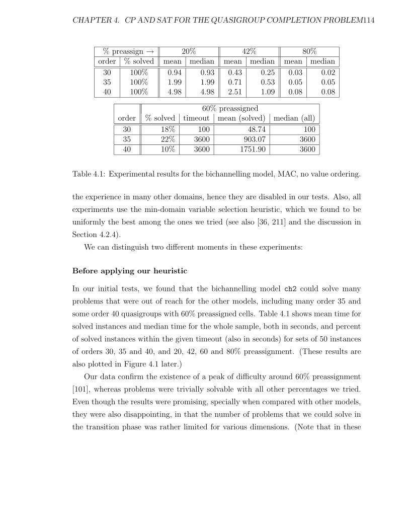
CHAPTER 4. CP AND SAT FOR THE QUASIGROUP COMPLETION PROBLEM114
% preassign → 20% 42% 80%order % solved mean median mean median mean median
30 100% 0.94 0.93 0.43 0.25 0.03 0.0235 100% 1.99 1.99 0.71 0.53 0.05 0.0540 100% 4.98 4.98 2.51 1.09 0.08 0.08
60% preassignedorder % solved timeout mean (solved) median (all)
30 18% 100 48.74 10035 22% 3600 903.07 360040 10% 3600 1751.90 3600
Table 4.1: Experimental results for the bichannelling model, MAC, no value ordering.
the experience in many other domains, hence they are disabled in our tests. Also, all
experiments use the min-domain variable selection heuristic, which we found to be
uniformly the best among the ones we tried (see also [36, 211] and the discussion in
Section 4.2.4).
We can distinguish two different moments in these experiments:
Before applying our heuristic
In our initial tests, we found that the bichannelling model ch2 could solve many
problems that were out of reach for the other models, including many order 35 and
some order 40 quasigroups with 60% preassigned cells. Table 4.1 shows mean time for
solved instances and median time for the whole sample, both in seconds, and percent
of solved instances within the given timeout (also in seconds) for sets of 50 instances
of orders 30, 35 and 40, and 20, 42, 60 and 80% preassignment. (These results are
also plotted in Figure 4.1 later.)
Our data confirm the existence of a peak of difficulty around 60% preassignment
[101], whereas problems were trivially solvable with all other percentages we tried.
Even though the results were promising, specially when compared with other models,
they were also disappointing, in that the number of problems that we could solve in
the transition phase was rather limited for various dimensions. (Note that in these

CHAPTER 4. CP AND SAT FOR THE QUASIGROUP COMPLETION PROBLEM115
pr pr-dl pr-dl-ch2 ch2time checks time checks time checks time checks1.45 1.30 1.93 1.69 1.90 1.69 1 1
Table 4.2: Comparison of various models using MAC and no value ordering.
cases, median time is the same as timeout because less than 50% of instances were
solved.) Nevertheless, we decided to pursue further the bichannelling model based on
the somewhat anecdotal evidence of its clear superiority over other models. As the
following sections show, we succeeded in this goal.
For the sake of a more systematic comparison, we present here a simple comparison
of the various models. Due to limited available time, we chose the 29 easiest problems
(as measured with the approaches developed later) for order 30 quasigroups with
60% preassignment. These are still relatively difficult problems close to the phase
transition: the ch2-model took a total of 6624 seconds on the 19 problems (66%)
in the sample that were solved with all tested models in less than 1800 seconds,
yielding an average of 348.6 seconds per solved problem, and a mean (over the whole
sample) of 574.16s. Table 4.2 shows the result of a comparison between various
models on this sample. The table provides the ratios in the accumulated data in time
and constraint checks over the solved problems, relative to the performance of ch2.
Note that all models tried exactly the same number of assignments in all problems,
empirically confirming the fact that arc consistency has identical pruning power in
all four models.
We conjecture that these ratios will increase with problem difficulty. But there
is little point on belaboring these data, as much better solutions are available, as
discussed in the following sections.
Introducing value ordering
The results when the first combined model was used with the min-domain-sum value
ordering heuristic were quite surprising, as it outperformed previous tests in three
orders of magnitude in some cases. For example, for the instance bqwh-35-405-5.pls
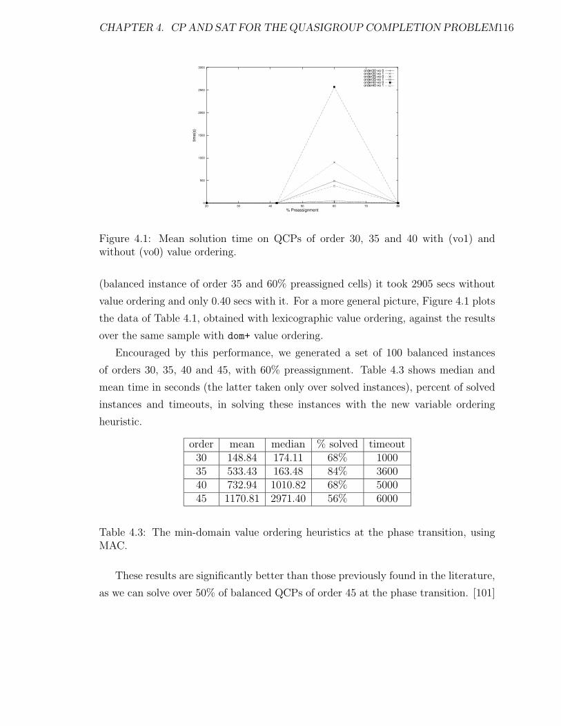
CHAPTER 4. CP AND SAT FOR THE QUASIGROUP COMPLETION PROBLEM116
0
500
1000
1500
2000
2500
3000
20 30 40 50 60 70 80
time(
s)
% Preassignment
order30-vo 0order30-vo 1order35-vo 0order35-vo 1order40-vo 0order40-vo 1
Figure 4.1: Mean solution time on QCPs of order 30, 35 and 40 with (vo1) andwithout (vo0) value ordering.
(balanced instance of order 35 and 60% preassigned cells) it took 2905 secs without
value ordering and only 0.40 secs with it. For a more general picture, Figure 4.1 plots
the data of Table 4.1, obtained with lexicographic value ordering, against the results
over the same sample with dom+ value ordering.
Encouraged by this performance, we generated a set of 100 balanced instances
of orders 30, 35, 40 and 45, with 60% preassignment. Table 4.3 shows median and
mean time in seconds (the latter taken only over solved instances), percent of solved
instances and timeouts, in solving these instances with the new variable ordering
heuristic.
order mean median % solved timeout30 148.84 174.11 68% 100035 533.43 163.48 84% 360040 732.94 1010.82 68% 500045 1170.81 2971.40 56% 6000
Table 4.3: The min-domain value ordering heuristics at the phase transition, usingMAC.
These results are significantly better than those previously found in the literature,
as we can solve over 50% of balanced QCPs of order 45 at the phase transition. [101]
CHAPTER 4. CP AND SAT FOR THE QUASIGROUP COMPLETION PROBLEM117
reports that pure constraint programming approaches, even when using specialized
forms of arc consistency for non-binary alldiff constraints and a commercial solver,
could not solve any problem of order 40 in the phase transition.
We considered other ways of combining domain sizes such as minimizing the prod-
uct of the corresponding domain sizes (min-domain-product or vdom*), and their cor-
responding maximizing versions, without success. Perhaps there is no deep reason
why vdom+ was so clearly superior to vdom*. Maximizing versions were clear under-
performers, and there is a reasonable explanation for it. For concreteness, consider
choosing a value with the maximal combined domain of the corresponding variables,
e.g. a value k for a primal variable xij such that domain-size(rik)+domain-size(cjk) is
maximal (over the colors available for xij at the current stage of search). While large
domain sizes are usually indication of less tightness, and thus could be conjectured
to capture the idea, often cited in connection with value ordering, of selecting a value
which is “more likely to lead to a solution”, in this case they have exactly the opposite
effect. When xij = k is the maximal labelling according to this criteria, the domains
of rik and cjk are immediately pruned into singletons. Hence a maximizing choice
produces maximal pruning, which is the opposite of what is desired. And conversely,
heuristics such as vdom+ choose values that produce the least pruning.
4.2.6 Compiling AC to FC with redundant constraints
Our next and last step (in this subsection) in improving our solution derived from an
examination of the pruning behavior of the bichannelling model with arc consistency.
Suppose xij is assigned k at some point during the search. The GAC implementation
of CPlan begins by checking arc consistency for constraints with a single uninstan-
tiated variable, i.e. doing forward checking, which forces the domains of rik and cjk
to become the singletons {j} and {i} respectively, and also prunes, for each h 6= k, j
from rih, and i from cjh. Arc consistency will further discover (if not already known
at this stage of the search):
• xih 6= k for any column h 6= j, since otherwise rik = h 6= j;
• hence also chk 6= i for any column h 6= j, since otherwise xih = k;
CHAPTER 4. CP AND SAT FOR THE QUASIGROUP COMPLETION PROBLEM118
• similarly, xhj 6= k for any row h 6= i, since otherwise rik = h 6= j;
• hence also rhk 6= j for any row h 6= i, since otherwise xhj = k;
It is not difficult to show that GAC cannot prune any more values as a result of an
assignment to a primal variable, unless one of the listed prunings reduces a domain
to a singleton. All these are useful prunings, but GAC does much more work than
needed to obtain them. Each one of the pruned values – one for each xih, xhj, chk, rhk,
potentially 4(n− 1) pruned values and variables from a single assignment – requires
GAC to check all the constraints in which the corresponding variables are involved,
namely 2(n− 1) or (n− 1) constraints for, respectively, the primal and dual pruned
variables (further, in the CPlan implementation all affected variables have all their
values tested, even if at most one will be pruned). This is wasted effort, as no addi-
tional pruning is achieved. One can however observe that most of the pruning power
can be derived simply by assigning the variables whose domain became singletons
(either directly through channelling constraints or indirectly when pruning a single
value results in a singleton) and doing forward checking on them. To see that the
remaining values pruned by GAC (namely the second and fourth items above) are
also pruned by FC with the trichannelling model, observe that chk 6= i since otherwise
rik = h 6= j using the corresponding triangular channelling constraint, and similarly
rhk 6= j since otherwise cjk = h 6= i.
We remark that the same effect can be achieved in different ways, e.g. the bichan-
nelling model supplemented with the dual not-equal constraints also allows forward
checking to derive the same consequences.
Results with the trichannelling model Table 4.4 compares the bichannelling
model ch2, using only row and column channelling constraints with GAC, versus the
trichannelling model ch3 with the three kinds of channelling constraints using only
FC, in both cases with the min-domain-sum value ordering. Each sample consists
again of 100 balanced instances with 60% preassignment;the accumulated values are
over the problems solved by both approaches within the given timeout. The median
times are on the other hand over the whole sample. Accumulated times are in seconds
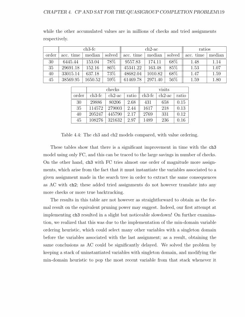
CHAPTER 4. CP AND SAT FOR THE QUASIGROUP COMPLETION PROBLEM119
while the other accumulated values are in millions of checks and tried assignments
respectively.
ch3-fc ch2-ac ratiosorder acc. time median solved acc. time median solved acc. time median
30 6445.44 153.04 78% 9557.83 174.11 68% 1.48 1.1435 29691.18 152.16 86% 45341.22 163.48 85% 1.53 1.0740 33015.14 637.18 73% 48682.04 1010.82 68% 1.47 1.5945 38569.95 1650.52 59% 61469.78 2971.40 56% 1.59 1.80
checks visitsorder ch3-fc ch2-ac ratio ch3-fc ch2-ac ratio
30 29886 80206 2.68 431 658 0.1535 114572 279003 2.44 1617 218 0.1340 205247 445790 2.17 2769 331 0.1245 108276 321632 2.97 1489 236 0.16
Table 4.4: The ch3 and ch2 models compared, with value ordering.
These tables show that there is a significant improvement in time with the ch3
model using only FC, and this can be traced to the large savings in number of checks.
On the other hand, ch3 with FC tries almost one order of magnitude more assign-
ments, which arise from the fact that it must instantiate the variables associated to a
given assignment made in the search tree in order to extract the same consequences
as AC with ch2; these added tried assignments do not however translate into any
more checks or more true backtracking.
The results in this table are not however as straightforward to obtain as the for-
mal result on the equivalent pruning power may suggest. Indeed, our first attempt at
implementing ch3 resulted in a slight but noticeable slowdown! On further examina-
tion, we realized that this was due to the implementation of the min-domain variable
ordering heuristic, which could select many other variables with a singleton domain
before the variables associated with the last assignment; as a result, obtaining the
same conclusions as AC could be significantly delayed. We solved the problem by
keeping a stack of uninstantiated variables with singleton domain, and modifying the
min-domain heuristic to pop the most recent variable from that stack whenever it
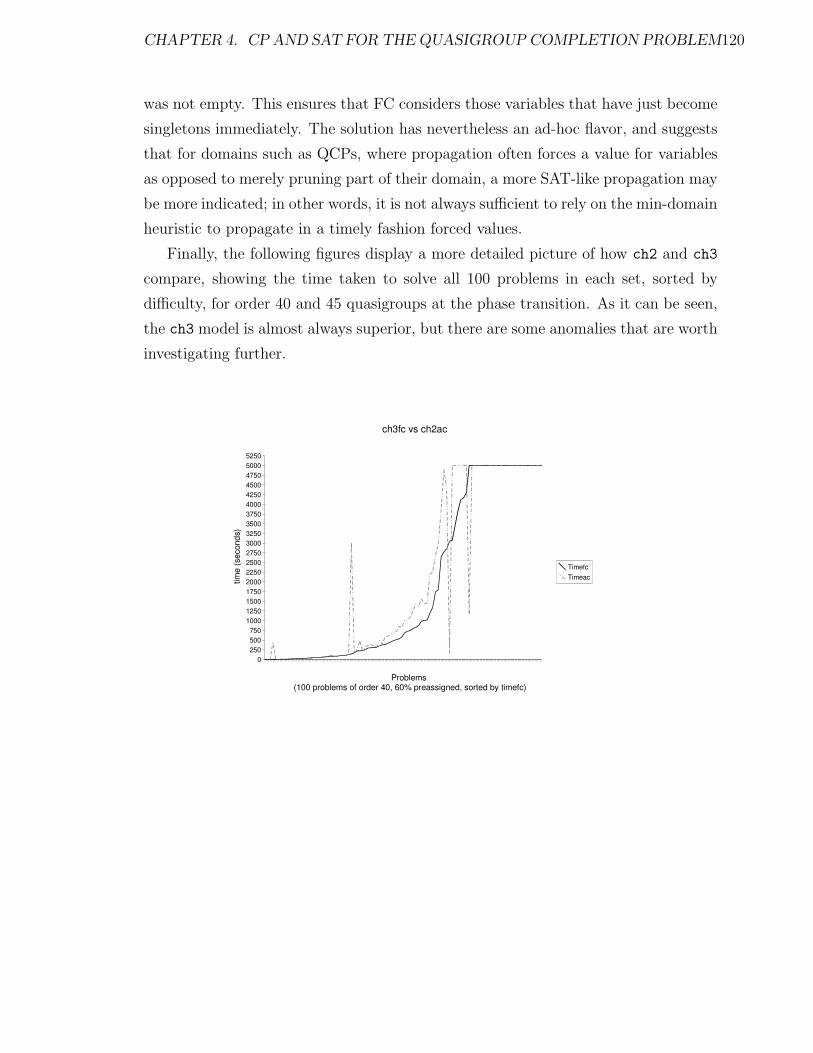
CHAPTER 4. CP AND SAT FOR THE QUASIGROUP COMPLETION PROBLEM120
was not empty. This ensures that FC considers those variables that have just become
singletons immediately. The solution has nevertheless an ad-hoc flavor, and suggests
that for domains such as QCPs, where propagation often forces a value for variables
as opposed to merely pruning part of their domain, a more SAT-like propagation may
be more indicated; in other words, it is not always sufficient to rely on the min-domain
heuristic to propagate in a timely fashion forced values.
Finally, the following figures display a more detailed picture of how ch2 and ch3
compare, showing the time taken to solve all 100 problems in each set, sorted by
difficulty, for order 40 and 45 quasigroups at the phase transition. As it can be seen,
the ch3 model is almost always superior, but there are some anomalies that are worth
investigating further.
0250500750
100012501500175020002250250027503000325035003750400042504500475050005250
ch3fc vs ch2ac
TimefcTimeac
Problems (100 problems of order 40, 60% preassigned, sorted by timefc)
time
(sec
onds
)
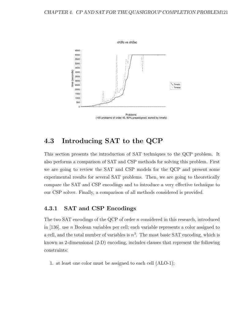
CHAPTER 4. CP AND SAT FOR THE QUASIGROUP COMPLETION PROBLEM121
0
500
1000
1500
2000
2500
3000
3500
4000
4500
5000
5500
6000
6500
ch3fc vs ch2ac
TimefcTimeac
Problems (100 problems of order 45, 60% preassigned, sorted by timefc)
time
(sec
onds
)
4.3 Introducing SAT to the QCP
This section presents the introduction of SAT techniques to the QCP problem. It
also performs a comparison of SAT and CSP methods for solving this problem. First
we are going to review the SAT and CSP models for the QCP and present some
experimental results for several SAT problems. Then, we are going to theoretically
compare the SAT and CSP encodings and to introduce a very effective technique to
our CSP solver. Finally, a comparison of all methods considered is provided.
4.3.1 SAT and CSP Encodings
The two SAT encodings of the QCP of order n considered in this research, introduced
in [136], use n Boolean variables per cell; each variable represents a color assigned to
a cell, and the total number of variables is n3. The most basic SAT encoding, which is
known as 2-dimensional (2-D) encoding, includes clauses that represent the following
constraints:
1. at least one color must be assigned to each cell (ALO-1);
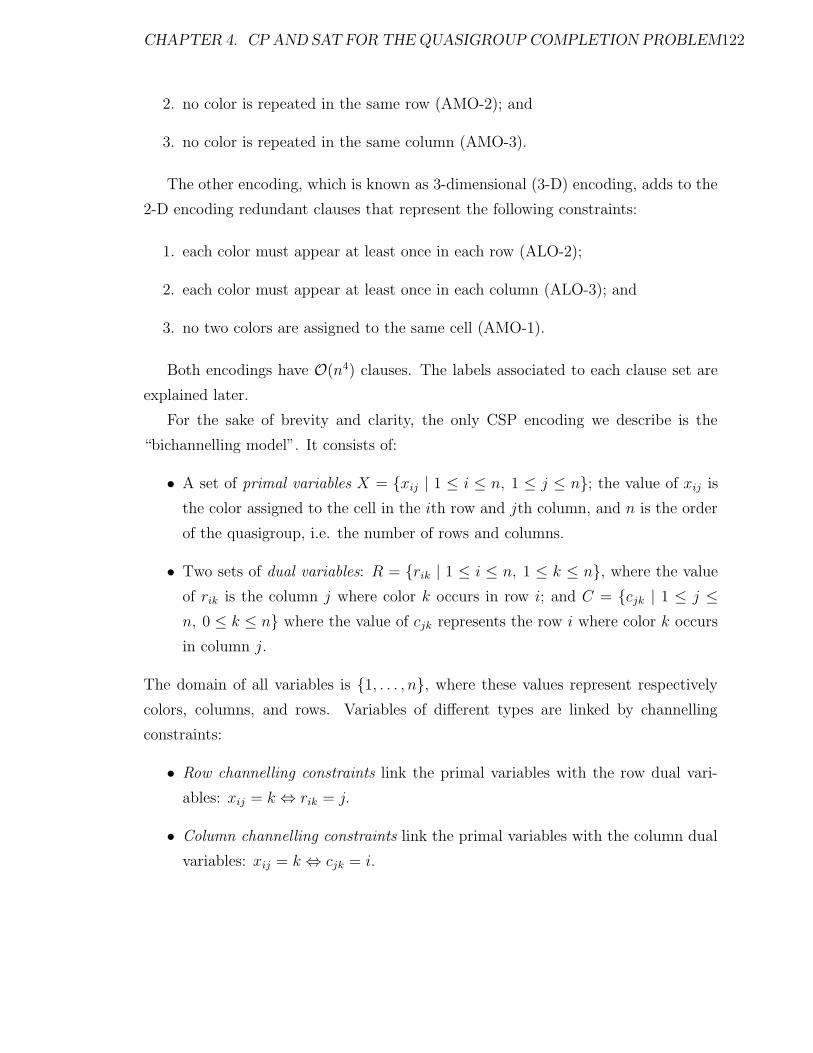
CHAPTER 4. CP AND SAT FOR THE QUASIGROUP COMPLETION PROBLEM122
2. no color is repeated in the same row (AMO-2); and
3. no color is repeated in the same column (AMO-3).
The other encoding, which is known as 3-dimensional (3-D) encoding, adds to the
2-D encoding redundant clauses that represent the following constraints:
1. each color must appear at least once in each row (ALO-2);
2. each color must appear at least once in each column (ALO-3); and
3. no two colors are assigned to the same cell (AMO-1).
Both encodings have O(n4) clauses. The labels associated to each clause set are
explained later.
For the sake of brevity and clarity, the only CSP encoding we describe is the
“bichannelling model”. It consists of:
• A set of primal variables X = {xij | 1 ≤ i ≤ n, 1 ≤ j ≤ n}; the value of xij is
the color assigned to the cell in the ith row and jth column, and n is the order
of the quasigroup, i.e. the number of rows and columns.
• Two sets of dual variables: R = {rik | 1 ≤ i ≤ n, 1 ≤ k ≤ n}, where the value
of rik is the column j where color k occurs in row i; and C = {cjk | 1 ≤ j ≤n, 0 ≤ k ≤ n} where the value of cjk represents the row i where color k occurs
in column j.
The domain of all variables is {1, . . . , n}, where these values represent respectively
colors, columns, and rows. Variables of different types are linked by channelling
constraints:
• Row channelling constraints link the primal variables with the row dual vari-
ables: xij = k ⇔ rik = j.
• Column channelling constraints link the primal variables with the column dual
variables: xij = k ⇔ cjk = i.
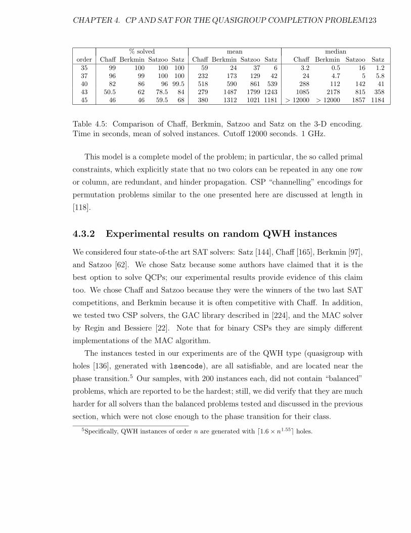
CHAPTER 4. CP AND SAT FOR THE QUASIGROUP COMPLETION PROBLEM123
% solved mean medianorder Chaff Berkmin Satzoo Satz Chaff Berkmin Satzoo Satz Chaff Berkmin Satzoo Satz
35 99 100 100 100 59 24 37 6 3.2 0.5 16 1.237 96 99 100 100 232 173 129 42 24 4.7 5 5.840 82 86 96 99.5 518 590 861 539 288 112 142 4143 50.5 62 78.5 84 279 1487 1799 1243 1085 2178 815 35845 46 46 59.5 68 380 1312 1021 1181 > 12000 > 12000 1857 1184
Table 4.5: Comparison of Chaff, Berkmin, Satzoo and Satz on the 3-D encoding.Time in seconds, mean of solved instances. Cutoff 12000 seconds. 1 GHz.
This model is a complete model of the problem; in particular, the so called primal
constraints, which explicitly state that no two colors can be repeated in any one row
or column, are redundant, and hinder propagation. CSP “channelling” encodings for
permutation problems similar to the one presented here are discussed at length in
[118].
4.3.2 Experimental results on random QWH instances
We considered four state-of-the art SAT solvers: Satz [144], Chaff [165], Berkmin [97],
and Satzoo [62]. We chose Satz because some authors have claimed that it is the
best option to solve QCPs; our experimental results provide evidence of this claim
too. We chose Chaff and Satzoo because they were the winners of the two last SAT
competitions, and Berkmin because it is often competitive with Chaff. In addition,
we tested two CSP solvers, the GAC library described in [224], and the MAC solver
by Regin and Bessiere [22]. Note that for binary CSPs they are simply different
implementations of the MAC algorithm.
The instances tested in our experiments are of the QWH type (quasigroup with
holes [136], generated with lsencode), are all satisfiable, and are located near the
phase transition.5 Our samples, with 200 instances each, did not contain “balanced”
problems, which are reported to be the hardest; still, we did verify that they are much
harder for all solvers than the balanced problems tested and discussed in the previous
section, which were not close enough to the phase transition for their class.
5Specifically, QWH instances of order n are generated with d1.6× n1.55e holes.
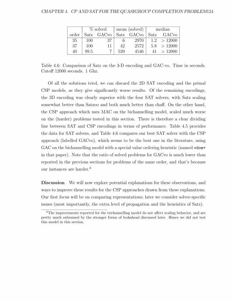
CHAPTER 4. CP AND SAT FOR THE QUASIGROUP COMPLETION PROBLEM124
% solved mean (solved) medianorder Satz GACvo Satz GACvo Satz GACvo
35 100 37 6 2970 1.2 > 1200037 100 11 42 2572 5.8 > 1200040 99.5 7 539 4546 41 > 12000
Table 4.6: Comparison of Satz on the 3-D encoding and GAC-vo. Time in seconds.Cutoff 12000 seconds. 1 Ghz.
Of all the solutions tried, we can discard the 2D SAT encoding and the primal
CSP models, as they give significantly worse results. Of the remaining encodings,
the 3D encoding was clearly superior with the four SAT solvers, with Satz scaling
somewhat better than Satzoo and both much better than chaff. On the other hand,
the CSP approach which uses MAC on the bichannelling model, scaled much worse
on the (harder) problems tested in this section. There is therefore a clear dividing
line between SAT and CSP encodings in terms of performance. Table 4.5 provides
the data for SAT solvers, and Table 4.6 compares our best SAT solver with the CSP
approach (labelled GACvo), which seems to be the best one in the literature, using
GAC on the bichannelling model with a special value ordering heuristic (named vdom+
in that paper). Note that the ratio of solved problems for GACvo is much lower than
reported in the previous sections for problems of the same order, and that’s because
our instances are harder.6
Discussion We will now explore potential explanations for these observations, and
ways to improve these results for the CSP approaches drawn from these explanations.
Our first focus will be on comparing representations; later we consider solver-specific
issues (most importantly, the extra level of propagation and the heuristics of Satz).
6The improvements reported for the trichannelling model do not affect scaling behavior, and arepretty much subsumed by the stronger forms of lookahead discussed later. Hence we did not testthis model in this section.

CHAPTER 4. CP AND SAT FOR THE QUASIGROUP COMPLETION PROBLEM125
4.3.3 Comparing models
In order to compare our models formally, we need a small detour through SAT en-
codings of CSP models, a third modelling option that we have not considered so far.
In this context, the many-valued CSP variables are represented by means of a set
of boolean variables, one for each possible assignment. So, for example, a primal
variable xij becomes a set of boolean variables xij = 1, . . . , xij = n. The semantics of
CSP domains is then captured by including one ALO (“at least one”) clause for each
variable, specifying that the variable must take at least one of its possible values, and
O(n2) AMO (“at most one”) clauses which specify, for every pair of possible values of
a variable, that they can not be satisfied simultaneously. In our bichannelling model,
we would have variables xij = k, rik = j and cjk = i, for each triple j, k, i, for a total
of 3n3 variables.
Define the minimal support encoding of the bichannelling model as that consist-
ing of AMO-ALO clauses for the three variable types, together with the channelling
clauses ¬xij = k∨rik = j and ¬rik = j∨xij = k, which directly encode the equivalence
xi1 = j ⇔ rij = k which defines the constraint between xij and rik (and similarly for
column channelling constraints). Clearly, the channelling clauses completely charac-
terize the channelling constraints, hence the minimal support encoding is a complete
model.
The support encoding, as defined in [89], encodes a constraint between two vari-
ables X and Y by adding, for each possible value v of X, the clause ¬X = v ∨ Y =
v1∨ . . .∨Y = vk, where v1, . . . , vk is a list of all values w in the domain of Y such that
(v, w) satisfies the constraint, i.e. a list of supports for the assignment X = v. For the
bichannelling model, we can observe that the channelling clauses of the minimal sup-
port encoding already encode the supports for xij = k and rik = j. For values v 6= k,
the supports for xij = v are given by the clause ¬xij = v ∨∨h∈{1,...,n},h6=j rik = h, and
for values v 6= j, the supports for rik = v are given by ¬rik = v∨∨h∈{1,...,n},h6=k xij = h.
Proposition 4.3.3.1. Unit resolution obtains the same results on the minimal sup-
port encoding as in the support encoding of the bichannelling model.
Proof. Consider e.g. the constraint between xi1 and ri2 (a similar analysis holds
CHAPTER 4. CP AND SAT FOR THE QUASIGROUP COMPLETION PROBLEM126
for column channelling constraints). Since the channelling clauses are preserved in
the minimal encoding, it suffices to show that the effect of unit propagation on the
additional support clauses is also obtained without them. For v 6= 2 we have the
support clause ¬xi1 = v ∨ ∨h∈{1,...,n},h6=1 ri2 = h. We consider two cases. First,
suppose ri2 = 2, . . . , ri2 = n are all false; we must show that unit resolution on the
remaining clauses imply ¬xi1 = v. Unit resolution on the ALO for ri2 obtains ri2 = 1,
which together with the channelling clauses yield xi1 = 2, and with the AMO for xi1,
¬xi1 = v. Second, suppose xi1 = v is true and, say, ri2 = 1 through ri2 = n − 1
are all false; we need to show that ri2 = n follows by unit resolution. Now, xi1 = v
implies through AMO ¬xi1 = 2, and thus ¬ri2 = 1 using the channelling clauses.
This together with the hypothesis of the case and the ALO for ri2 allows us to obtain
ri2 = n, as desired.
Our second observation is that the binary theory consisting of the channelling
clauses for all constraints can be simplified using a strongly connected components
(SCC) algorithm such as in [53]. The SCCs will consist precisely of the triplets of
boolean variables of the form xij = k, rik = j and cjk = i. The SCC-based algorithm
would then replace each such triplet by a single variable, which we may appropriately
call xijk, as in the 3D SAT encodings, and perform the appropriate replacements in
the remaining clauses. The result is the following:
• The ALO and AMO clauses for the CSP variables become clauses of the 3D-
encoding. Specifically, the clauses labelled ALO-k and AMO-k (1 ≤ k ≤ 3)
in the 3D-encoding are the result of rewriting the ALO and AMO clauses for
the primal variables (k=1), row dual variables (k=2) and column dual variables
(k=3) in the minimal channelling encoding.
• The channelling clauses become tautologies after variable replacement, so they
can be eliminated.
The SCC-simplification formally captures the intuitive idea that the triplet of
variables xij = k, rik = j and cjk = i all “mean the same” –color k is in cell (i, j)–,
and hence that each triplet can be “collapsed” into a single boolean variable xijk, as
done in the 3D encoding (and in the “SAT channelling model” of [118]).
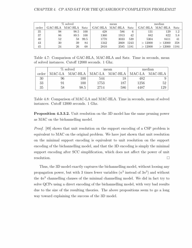
CHAPTER 4. CP AND SAT FOR THE QUASIGROUP COMPLETION PROBLEM127
% solved mean medianorder GAC-HLA MAC-HLA Satz GAC-HLA MAC-HLA Satz GAC-HLA MAC-HLA Satz
35 98 98.5 100 428 586 6 131 129 1.237 86 89.5 100 1360 1913 42 882 822 5.840 52 58 99.5 1770 3033 539 5304 8411 4143 30 39 84 1342 2668 1243 > 12000 > 12000 35845 24 26 68 2810 3585 1181 > 12000 > 12000 1184
Table 4.7: Comparison of GAC-HLA, MAC-HLA and Satz. Time in seconds, meanof solved instances. Cutoff 12000 seconds. 1 Ghz.
% solved mean medianorder MAC-LA MAC-HLA MAC-LA MAC-HLA MAC-LA MAC-HLA
30 96 100 544 18 482 933 91 100 1753 187 1256 5235 58 98.5 2714 586 4487 129
Table 4.8: Comparison of MAC-LA and MAC-HLA. Time in seconds, mean of solvedinstances. Cutoff 12000 seconds. 1 Ghz.
Proposition 4.3.3.2. Unit resolution on the 3D model has the same pruning power
as MAC on the bichannelling model.
Proof. [89] shows that unit resolution on the support encoding of a CSP problem is
equivalent to MAC on the original problem. We have just shown that unit resolution
on the minimal support encoding is equivalent to unit resolution on the support
encoding of the bichannelling model, and that the 3D encoding is simply the minimal
support encoding after SCC simplification, which does not affect the power of unit
resolution.
Thus, the 3D model exactly captures the bichannelling model, without loosing any
propagation power, but with 3 times fewer variables (n3 instead of 3n3) and without
the 4n3 channelling clauses of the minimal channelling model. We did in fact try to
solve QCPs using a direct encoding of the bichannelling model, with very bad results
due to the size of the resulting theories. The above propositions seem to go a long
way toward explaining the success of the 3D model.

CHAPTER 4. CP AND SAT FOR THE QUASIGROUP COMPLETION PROBLEM128
For each free variable x such that PROPz(x) is true do(let F ′ and F ′′ two copies of the formula F under consideration)
F ′ := unit-propagation(F ′ ∪ {x});F ′′ := unit-propagation(F ′′ ∪ {¬x});If 2 ∈ F ′ and 2 ∈ F ′′ then return ”F is unsatisfiable”If 2 ∈ F ′ then x:=0, F := F ′′
else if 2 ∈ F ′′ then x:=1, F := F ′
If 2 6∈ F ′ and 2 6∈ F ′′ thenlet w(x) denote the weight of xw(x) := number of times that non-binary clauses of F
have been reduced when deriving F ′
w(¬x) := number of times that non-binary clauses of Fhave been reduced when deriving F ′′
For each free variable x doH(x) := w(x) ∗ w(¬x) ∗ 1024 + w(x) + w(¬x);
Branch on the free variable x with greatest H(x)
Figure 4.2: The variable selection heuristic of Satz for PROP (x, 4)
4.3.4 Satz’s heuristic in QCPs
We now turn to solver and domain-specific features that may explain the observed
performance. Thus our next step was to analyze in depth the behavior on QCP
instances of the best solver, Satz, so as to incorporate new propagation techniques and
heuristics into the CSP solvers from the insights gained. Before going into details, let
us recall the variable selection heuristic that implements Satz, which combines MOMS
(Maximum Occurrences in clauses of Minimum Size) and UP (Unit Propagation)
heuristics. In both heuristics, the goal is to maximize the power of unit propagation.
MOMS picks one variable among those that occur the most often in minimal size
clauses, since these are more likely to result in propagation. UP goes a step further
by actually measuring the number of propagations from each choice. It examines
each variable p occurring in a given CNF formula φ by respectively adding the unit
clauses p and ¬p to φ, and independently making two unit propagations, which are
used to derive a score for each variable. As a secondary effect, UP detects so-called
failed literals in φ, which when satisfied falsify φ in a single unit propagation.
CHAPTER 4. CP AND SAT FOR THE QUASIGROUP COMPLETION PROBLEM129
In order to reduce the time required to propagate all literals, Satz applies UP to
a restricted number of variables that occur in binary clauses by applying a unary
predicate, called PROPz, which is defined as follows:
Definition 4.1. Let φ be a CNF formula; let PROP (x, i) be a binary predicate which
is true iff variable x occurs both positively and negatively in binary clauses of φ, and
there are at least i occurrences of x in binary clauses of φ; and let T be an integer.
PROPz(x) is defined to be the first of the three predicates PROP (x, 4), PROP (x, 3), true
(in this order) whose denotational semantics contains more than a fixed number T of
variables. T is set to 10 in Satz.
After applying unit propagation to a restricted number of variables and detecting
failed literals, the heuristic of Satz weights literals with different criteria depending
on the predicate applied. For example, when PROP (x, 4) is applied, the heuristic
scores each literal (x,¬x) with the number of times that non-binary clauses have
been reduced when propagating the literal. The pseudocode of the variable selection
heuristic of Satz for PROP (x, 4) is shown in Figure 4.2. Function H(x) is used to
reach a good balance between weights of positive literals and weights of negative
literals.
When solving QCP instances using the 3-D encoding with Satz, we observed that
Satz almost always uses the predicate PROP (x, 4), which requires x to occur in both
positive and negative binary clauses, with at least 4 occurrences in total. A closer
look at the 3-D encoding reveals that Boolean variables that fulfill PROP (x, 4) model
CSP variables with domain size 2. The reason is that positive literals only occur in the
ALO-1, ALO-2 and ALO-3 constraints, hence the only way to have x occur positively
in a binary clause is when one of these clauses becomes binary, in which case the
corresponding (primal or dual) CSP variable has domain size 2. Further, it is easy
to show that the variables in such positive binary clauses have at least three other
negative occurrences from AMO clauses, so that PROP (x, 4) holds. This analysis led
us to incorporate the technique of failed literals and the heuristic of Satz into CSP
solvers as follows:
1. For each free CSP variable of domain size 2, we propagate each value of the
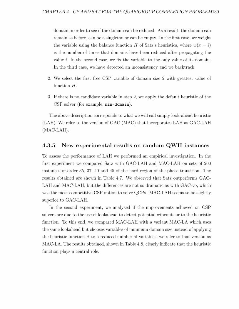
CHAPTER 4. CP AND SAT FOR THE QUASIGROUP COMPLETION PROBLEM130
domain in order to see if the domain can be reduced. As a result, the domain can
remain as before, can be a singleton or can be empty. In the first case, we weight
the variable using the balance function H of Satz’s heuristics, where w(x = i)
is the number of times that domains have been reduced after propagating the
value i. In the second case, we fix the variable to the only value of its domain.
In the third case, we have detected an inconsistency and we backtrack.
2. We select the first free CSP variable of domain size 2 with greatest value of
function H.
3. If there is no candidate variable in step 2, we apply the default heuristic of the
CSP solver (for example, min-domain).
The above description corresponds to what we will call simply look-ahead heuristic
(LAH). We refer to the version of GAC (MAC) that incorporates LAH as GAC-LAH
(MAC-LAH).
4.3.5 New experimental results on random QWH instances
To assess the performance of LAH we performed an empirical investigation. In the
first experiment we compared Satz with GAC-LAH and MAC-LAH on sets of 200
instances of order 35, 37, 40 and 45 of the hard region of the phase transition. The
results obtained are shown in Table 4.7. We observed that Satz outperforms GAC-
LAH and MAC-LAH, but the differences are not so dramatic as with GAC-vo, which
was the most competitive CSP option to solve QCPs. MAC-LAH seems to be slightly
superior to GAC-LAH.
In the second experiment, we analyzed if the improvements achieved on CSP
solvers are due to the use of lookahead to detect potential wipeouts or to the heuristic
function. To this end, we compared MAC-LAH with a variant MAC-LA which uses
the same lookahead but chooses variables of minimum domain size instead of applying
the heuristic function H to a reduced number of variables; we refer to that version as
MAC-LA. The results obtained, shown in Table 4.8, clearly indicate that the heuristic
function plays a central role.
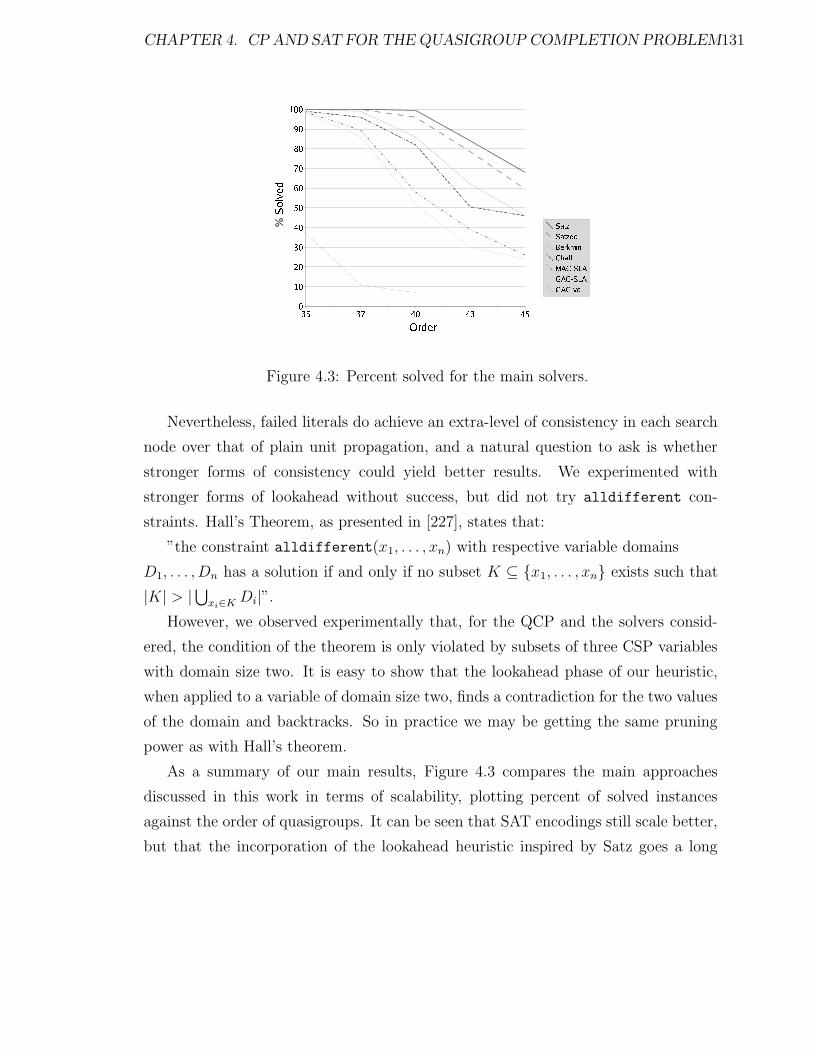
CHAPTER 4. CP AND SAT FOR THE QUASIGROUP COMPLETION PROBLEM131
Figure 4.3: Percent solved for the main solvers.
Nevertheless, failed literals do achieve an extra-level of consistency in each search
node over that of plain unit propagation, and a natural question to ask is whether
stronger forms of consistency could yield better results. We experimented with
stronger forms of lookahead without success, but did not try alldifferent con-
straints. Hall’s Theorem, as presented in [227], states that:
”the constraint alldifferent(x1, . . . , xn) with respective variable domains
D1, . . . , Dn has a solution if and only if no subset K ⊆ {x1, . . . , xn} exists such that
|K| > |⋃xi∈K Di|”.
However, we observed experimentally that, for the QCP and the solvers consid-
ered, the condition of the theorem is only violated by subsets of three CSP variables
with domain size two. It is easy to show that the lookahead phase of our heuristic,
when applied to a variable of domain size two, finds a contradiction for the two values
of the domain and backtracks. So in practice we may be getting the same pruning
power as with Hall’s theorem.
As a summary of our main results, Figure 4.3 compares the main approaches
discussed in this work in terms of scalability, plotting percent of solved instances
against the order of quasigroups. It can be seen that SAT encodings still scale better,
but that the incorporation of the lookahead heuristic inspired by Satz goes a long

CHAPTER 4. CP AND SAT FOR THE QUASIGROUP COMPLETION PROBLEM132
way toward bridging the gap between the best CSP model available to date, GAC-vo,
and the SAT approaches.
4.4 Lessons learnt
Constraint Satisfaction and SAT techniques are very powerful techniques for solving
optimization problems. They rely on propagation techniques to reduce the search
space and on heuristic to drive the search efficiently. Here is the list of useful lessons
we have learnt:
• Both techniques seem to be specially suited for satisfaction rather than for
optimization.
• Both approaches strongly rely on propagation mechanisms, and their efficiency
on a given problem seems to be related to the specific trade-off between search
and propagation.
• Heuristics have a huge impact on both techniques, although it is not possible
to find the optimal heuristic to apply to any problem, nor even to any instance
of the same problem.
• They seem not to be suited for very large search space, due to their complete
nature, and their impossibility to generate near-optimal solutions.
• They are however necessary when we need to find the optimal solution or all
the solutions of a problem.
Chapter 5
Local Search for the Social Golfer
Problem
The social golfer problem has attracted significant interest since it was first posted
on sci.op-research in May 1998. It consists of scheduling n = g × p golfers into g
groups of p players every week for w weeks so that no two golfers play in the same
group more than once. An instance of the social golfer is specified by a triple g−p−w,
where g is the number of groups, p is the size of a group, and w is the number of
weeks in the schedule.
The scheduling of social golfers is a highly combinatorial and symmetric problem
and it is not surprising that it has generated significant attention from the constraint
programming community (e.g., [72, 209, 178, 200, 199, 13, 184]). Indeed, it raises
fundamentally interesting issues in modeling and symmetry breaking, and it has be-
come one of the standard benchmarks for evaluating symmetry-breaking schemes.
Recent developments (e.g., [13, 184]) approach the scheduling of social golfers using
innovative, elegant, but also complex, symmetry-breaking schemes.
This research approaches the problem from a very different angle. It proposes a
local search algorithm for scheduling social golfers, whose local moves swap golfers
within the same week and are guided by a tabu-search meta-heuristic. The local
search algorithm matches, or improves upon, the best solutions found by constraint
programming on all instances but 3. It also found the first solutions to 11 instances
133
CHAPTER 5. LOCAL SEARCH FOR THE SOCIAL GOLFER PROBLEM 134
that were previously open for constraint programming.1 Moreover, the local search al-
gorithm solves almost all instances easily in a few seconds and takes about 1 minute on
the remaining (harder) instances. The algorithm also features a constructive heuristic
which trivially solves many instances of the form odd − odd − w and provides good
starting points for others.
The rest of the chapter is organized as follows. After reviewing some related
work it starts by describing the basic local search algorithm, including its underlying
modeling, its neighborhood, its meta-heuristic, and its experimental results. It then
presents the constructive heuristic and reports the new experimental results when
the heuristic replaces the random configurations as starting points of the algorithm.
Finally, the chapter concludes by giving a set of lessons learnt.
5.1 Solving the Social Golfer Problem
There is a considerable body of work on scheduling social golfers in the constraint
programming community. References [13, 184] describe state-of-the art results using
constraint programming and are excellent starting points for more references. See also
[199] for interesting theoretical and experimental results on the social golfer problem,
as well as the description of SBDD, a general scheme for symmetry breaking. Agren
[3] describes a tabu-search algorithm for scheduling social golfers, where the neighbor-
hood consists of swapping the value of a single variable and where all constraints are
explicit. The results are also far in quality and performance from those reported here.
The neighborhood used in this research, which implicitly maintain the group and week
structures, and the randomized tabu-list strategy are fundamental in scheduling hard
instances. Another local search approach is introduced in [180], where the symmetry
breaking is shown counter-productive for local search and adding symmetries (super-
symmetries) is proposed instead. Hybrid local search and constraint programming
approaches have been tried on the social golfer problem [177]. In both cases, the
results are significantly dominated by those presented in this chapter. The idea of
1For the current statuses of the instances, see Warwick Harvey’s web page athttp://www.icparc.ic.ac.uk/wh/golf.
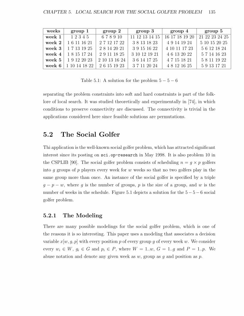
CHAPTER 5. LOCAL SEARCH FOR THE SOCIAL GOLFER PROBLEM 135
weeks group 1 group 2 group 3 group 4 group 5week 1 1 2 3 4 5 6 7 8 9 10 11 12 13 14 15 16 17 18 19 20 21 22 23 24 25week 2 1 6 11 16 21 2 7 12 17 22 3 8 13 18 23 4 9 14 19 24 5 10 15 20 25week 3 1 7 13 19 25 2 8 14 20 21 3 9 15 16 22 4 10 11 17 23 5 6 12 18 24week 4 1 8 15 17 24 2 9 11 18 25 3 10 12 19 21 4 6 13 20 22 5 7 14 16 23week 5 1 9 12 20 23 2 10 13 16 24 3 6 14 17 25 4 7 15 18 21 5 8 11 19 22week 6 1 10 14 18 22 2 6 15 19 23 3 7 11 20 24 4 8 12 16 25 5 9 13 17 21
Table 5.1: A solution for the problem 5− 5− 6
separating the problem constraints into soft and hard constraints is part of the folk-
lore of local search. It was studied theoretically and experimentally in [74], in which
conditions to preserve connectivity are discussed. The connectivity is trivial in the
applications considered here since feasible solutions are permutations.
5.2 The Social Golfer
Thi application is the well-known social golfer problem, which has attracted significant
interest since its posting on sci.op-research in May 1998. It is also problem 10 in
the CSPLIB [90]. The social golfer problem consists of scheduling n = g × p golfers
into g groups of p players every week for w weeks so that no two golfers play in the
same group more than once. An instance of the social golfer is specified by a triple
g − p − w, where g is the number of groups, p is the size of a group, and w is the
number of weeks in the schedule. Figure 5.1 depicts a solution for the 5− 5− 6 social
golfer problem.
5.2.1 The Modeling
There are many possible modelings for the social golfer problem, which is one of
the reasons it is so interesting. This paper uses a modeling that associates a decision
variable x[w, g, p] with every position p of every group g of every week w. We consider
every wi ∈ W , gi ∈ G and pi ∈ P , where W = 1..w, G = 1..g and P = 1..p. We
abuse notation and denote any given week as w, group as g and position as p.
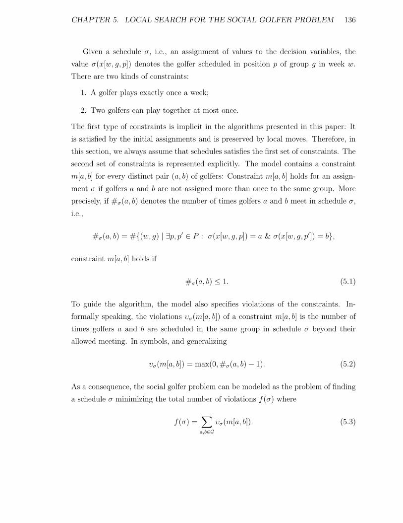
CHAPTER 5. LOCAL SEARCH FOR THE SOCIAL GOLFER PROBLEM 136
Given a schedule σ, i.e., an assignment of values to the decision variables, the
value σ(x[w, g, p]) denotes the golfer scheduled in position p of group g in week w.
There are two kinds of constraints:
1. A golfer plays exactly once a week;
2. Two golfers can play together at most once.
The first type of constraints is implicit in the algorithms presented in this paper: It
is satisfied by the initial assignments and is preserved by local moves. Therefore, in
this section, we always assume that schedules satisfies the first set of constraints. The
second set of constraints is represented explicitly. The model contains a constraint
m[a, b] for every distinct pair (a, b) of golfers: Constraint m[a, b] holds for an assign-
ment σ if golfers a and b are not assigned more than once to the same group. More
precisely, if #σ(a, b) denotes the number of times golfers a and b meet in schedule σ,
i.e.,
#σ(a, b) = #{(w, g) | ∃p, p′ ∈ P : σ(x[w, g, p]) = a & σ(x[w, g, p′]) = b},
constraint m[a, b] holds if
#σ(a, b) ≤ 1. (5.1)
To guide the algorithm, the model also specifies violations of the constraints. In-
formally speaking, the violations υσ(m[a, b]) of a constraint m[a, b] is the number of
times golfers a and b are scheduled in the same group in schedule σ beyond their
allowed meeting. In symbols, and generalizing
υσ(m[a, b]) = max(0,#σ(a, b)− 1). (5.2)
As a consequence, the social golfer problem can be modeled as the problem of finding
a schedule σ minimizing the total number of violations f(σ) where
f(σ) =∑
a,b∈Gυσ(m[a, b]). (5.3)
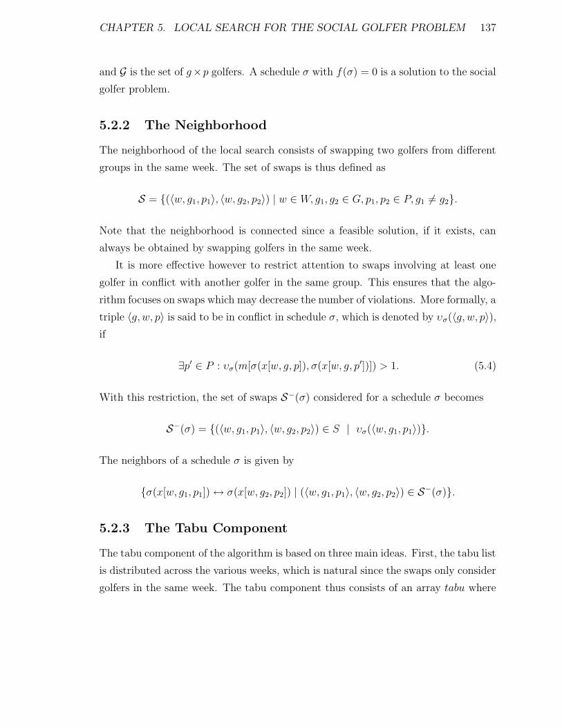
CHAPTER 5. LOCAL SEARCH FOR THE SOCIAL GOLFER PROBLEM 137
and G is the set of g×p golfers. A schedule σ with f(σ) = 0 is a solution to the social
golfer problem.
5.2.2 The Neighborhood
The neighborhood of the local search consists of swapping two golfers from different
groups in the same week. The set of swaps is thus defined as
S = {(〈w, g1, p1〉, 〈w, g2, p2〉) | w ∈ W, g1, g2 ∈ G, p1, p2 ∈ P, g1 6= g2}.
Note that the neighborhood is connected since a feasible solution, if it exists, can
always be obtained by swapping golfers in the same week.
It is more effective however to restrict attention to swaps involving at least one
golfer in conflict with another golfer in the same group. This ensures that the algo-
rithm focuses on swaps which may decrease the number of violations. More formally, a
triple 〈g, w, p〉 is said to be in conflict in schedule σ, which is denoted by υσ(〈g, w, p〉),if
∃p′ ∈ P : υσ(m[σ(x[w, g, p]), σ(x[w, g, p′])]) > 1. (5.4)
With this restriction, the set of swaps S−(σ) considered for a schedule σ becomes
S−(σ) = {(〈w, g1, p1〉, 〈w, g2, p2〉) ∈ S | υσ(〈w, g1, p1〉)}.
The neighbors of a schedule σ is given by
{σ(x[w, g1, p1])↔ σ(x[w, g2, p2]) | (〈w, g1, p1〉, 〈w, g2, p2〉) ∈ S−(σ)}.
5.2.3 The Tabu Component
The tabu component of the algorithm is based on three main ideas. First, the tabu list
is distributed across the various weeks, which is natural since the swaps only consider
golfers in the same week. The tabu component thus consists of an array tabu where
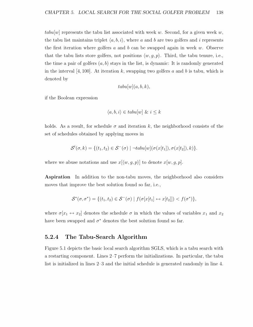
CHAPTER 5. LOCAL SEARCH FOR THE SOCIAL GOLFER PROBLEM 138
tabu[w] represents the tabu list associated with week w. Second, for a given week w,
the tabu list maintains triplet 〈a, b, i〉, where a and b are two golfers and i represents
the first iteration where golfers a and b can be swapped again in week w. Observe
that the tabu lists store golfers, not positions 〈w, g, p〉. Third, the tabu tenure, i.e.,
the time a pair of golfers (a, b) stays in the list, is dynamic: It is randomly generated
in the interval [4, 100]. At iteration k, swapping two golfers a and b is tabu, which is
denoted by
tabu[w](a, b, k),
if the Boolean expression
〈a, b, i〉 ∈ tabu[w] & i ≤ k
holds. As a result, for schedule σ and iteration k, the neighborhood consists of the
set of schedules obtained by applying moves in
St(σ, k) = {(t1, t2) ∈ S−(σ) | ¬tabu[w](σ(x[t1]), σ(x[t2]), k)}.
where we abuse notations and use x[〈w, g, p〉] to denote x[w, g, p].
Aspiration In addition to the non-tabu moves, the neighborhood also considers
moves that improve the best solution found so far, i.e.,
S∗(σ, σ∗) = {(t1, t2) ∈ S−(σ) | f(σ[x[t1]↔ x[t2]]) < f(σ∗)},
where σ[x1 ↔ x2] denotes the schedule σ in which the values of variables x1 and x2
have been swapped and σ∗ denotes the best solution found so far.
5.2.4 The Tabu-Search Algorithm
Figure 5.1 depicts the basic local search algorithm SGLS, which is a tabu search with
a restarting component. Lines 2–7 perform the initializations. In particular, the tabu
list is initialized in lines 2–3 and the initial schedule is generated randomly in line 4.
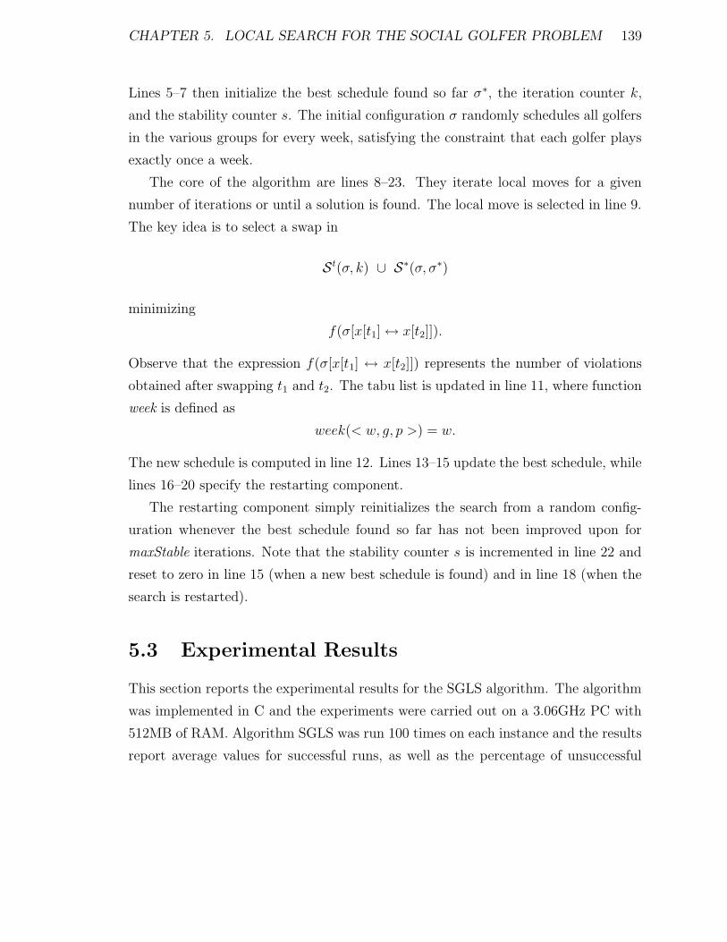
CHAPTER 5. LOCAL SEARCH FOR THE SOCIAL GOLFER PROBLEM 139
Lines 5–7 then initialize the best schedule found so far σ∗, the iteration counter k,
and the stability counter s. The initial configuration σ randomly schedules all golfers
in the various groups for every week, satisfying the constraint that each golfer plays
exactly once a week.
The core of the algorithm are lines 8–23. They iterate local moves for a given
number of iterations or until a solution is found. The local move is selected in line 9.
The key idea is to select a swap in
St(σ, k) ∪ S∗(σ, σ∗)
minimizing
f(σ[x[t1]↔ x[t2]]).
Observe that the expression f(σ[x[t1] ↔ x[t2]]) represents the number of violations
obtained after swapping t1 and t2. The tabu list is updated in line 11, where function
week is defined as
week(< w, g, p >) = w.
The new schedule is computed in line 12. Lines 13–15 update the best schedule, while
lines 16–20 specify the restarting component.
The restarting component simply reinitializes the search from a random config-
uration whenever the best schedule found so far has not been improved upon for
maxStable iterations. Note that the stability counter s is incremented in line 22 and
reset to zero in line 15 (when a new best schedule is found) and in line 18 (when the
search is restarted).
5.3 Experimental Results
This section reports the experimental results for the SGLS algorithm. The algorithm
was implemented in C and the experiments were carried out on a 3.06GHz PC with
512MB of RAM. Algorithm SGLS was run 100 times on each instance and the results
report average values for successful runs, as well as the percentage of unsuccessful

CHAPTER 5. LOCAL SEARCH FOR THE SOCIAL GOLFER PROBLEM 140
1. SGLS(W,G,P )2. forall w ∈ W3. tabu[w]← {};4. σ ← random configuration;5. σ∗ ← σ;6. k ← 0;7. s← 0;8. while k ≤ maxIt & f(σ) > 0 do9. select (t1, t2) ∈ S t(σ, k) ∪ S∗(σ, σ∗)
minimizing f(σ[x[t1]↔ x[t2]]);10. τ ← random([4,100]);11. tabu[week(t1)]←
tabu[week(t1)] ∪ {〈σ(x[t1]), σ(x[t2]), k + τ〉};12. σ ← σ[x[t1]↔ x[t2]];13. if f(σ) < f(σ∗) then14. σ∗ ← σ;15. s← 0;16. else if s > maxStable then17. σ ←random configuration;18. s← 0;19. forall w ∈ W do20. tabu[w] = {};21. else22. s++;23. k++;
Figure 5.1: Algorithm SGLS for Scheduling Social Golfers
runs (if any).
Tables 5.2 and 5.3 report the experimental results for SGLS when trying to match
the constraint-programming results. Note that no explicty comparison is given for
constraint-programming approaches since all the methods in the literature merely
report single instances usually solved for a lower number of weeks. Given a number
of groups g and a group size p, the tables only give the results for those instances
g−p−w maximizing w since they also provide solutions for w′ < w. Table 5.2 reports
the number of iterations (moves), while Table 5.3 reports the execution times. Bold
entries indicate that SGLS matches the best known number of weeks for a given

CHAPTER 5. LOCAL SEARCH FOR THE SOCIAL GOLFER PROBLEM 141
size 3 size 4 size 5 size 6 size 7 size 8 size 9 size 10g w I w I w I w I w I w I w I w I6 8 282254.0 6 161530.3 6 16761.5 3 15.8 - - - - - - - -7 9 12507.6 7 274606.0 5 102.9 4 100.4 3 23.4 - - - - - -8 10 653.9 8 323141.5 6 423.7 5 1044.9 4 237.5 4 153301.6 - - - -9 11 128.3 8 84.4 6 52.7 5 55.5 4 44.8 3 27.7 3 43.9 - -10 13 45849.1 9 100.2 7 80.8 6 110.7 5 94.6 4 61.8 3 36.1 3 53.3
Table 5.2: Number of Iterations for SGLS with Maximal Number of Weeks.Bold Entries Indicate a Match with the Best Known Number of Weeks.
size 3 size 4 size 5 size 6 size 7 size 8 size 9 size 10g w T %F w T %F w T w T w T w T w T w T6 8 48.93 6 6 47.75 6 107.18 3 0.01 - - - - - - - -7 9 3.06 7 107.62 8 5 0.07 4 0.09 3 0.03 - - - - - -8 10 0.23 8 207.77 9 6 0.37 5 1.21 4 0.39 4 360.00 - - - -9 11 0.08 8 0.09 6 0.09 5 0.13 4 0.14 3 0.09 3 0.19 - -10 13 30.82 9 0.16 7 0.19 6 0.34 5 0.41 4 0.33 3 0.20 3 0.39
Table 5.3: CPU Time in Seconds for SGLS with Maximal Number of Weeks.Bold Entries Indicate a Match with the Best Known Number of Weeks.
number of groups and a given group size. The percentage of unsuccessful runs is
shown between parentheses in Table 5.3.
As can be seen from the tables, Algorithm SGLS finds solutions to all the instances
solved by constraint programming except 4. Moreover, almost all entries are solved
in less than a second. Only a few instances are hard for the algorithm and require
around 1 minute of CPU time. Interestingly, algorithm SGLS also solves 7 new
instances (with format 〈g− s−w〉: 9− 4− 9, 9− 5− 7, 9− 6− 6, 9− 7− 5, 9− 8− 4,
10− 5− 8 and 10− 9− 4. Those are not shown in the tables but more detail on these
are given below.
It is interesting to observe that algorithm SGLS does not break symmetries and
does not exploit specific properties of the solutions. This contrasts with constraint-
programming solutions that are often quite sophisticated and involved. See, for in-
stance, the recent papers [13, 184] which report the use of very interesting symmetry-
breaking schemes to schedule social golfers.
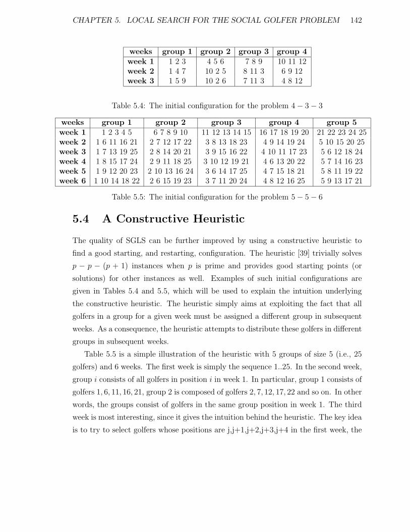
CHAPTER 5. LOCAL SEARCH FOR THE SOCIAL GOLFER PROBLEM 142
weeks group 1 group 2 group 3 group 4week 1 1 2 3 4 5 6 7 8 9 10 11 12week 2 1 4 7 10 2 5 8 11 3 6 9 12week 3 1 5 9 10 2 6 7 11 3 4 8 12
Table 5.4: The initial configuration for the problem 4− 3− 3
weeks group 1 group 2 group 3 group 4 group 5week 1 1 2 3 4 5 6 7 8 9 10 11 12 13 14 15 16 17 18 19 20 21 22 23 24 25week 2 1 6 11 16 21 2 7 12 17 22 3 8 13 18 23 4 9 14 19 24 5 10 15 20 25week 3 1 7 13 19 25 2 8 14 20 21 3 9 15 16 22 4 10 11 17 23 5 6 12 18 24week 4 1 8 15 17 24 2 9 11 18 25 3 10 12 19 21 4 6 13 20 22 5 7 14 16 23week 5 1 9 12 20 23 2 10 13 16 24 3 6 14 17 25 4 7 15 18 21 5 8 11 19 22week 6 1 10 14 18 22 2 6 15 19 23 3 7 11 20 24 4 8 12 16 25 5 9 13 17 21
Table 5.5: The initial configuration for the problem 5− 5− 6
5.4 A Constructive Heuristic
The quality of SGLS can be further improved by using a constructive heuristic to
find a good starting, and restarting, configuration. The heuristic [39] trivially solves
p − p − (p + 1) instances when p is prime and provides good starting points (or
solutions) for other instances as well. Examples of such initial configurations are
given in Tables 5.4 and 5.5, which will be used to explain the intuition underlying
the constructive heuristic. The heuristic simply aims at exploiting the fact that all
golfers in a group for a given week must be assigned a different group in subsequent
weeks. As a consequence, the heuristic attempts to distribute these golfers in different
groups in subsequent weeks.
Table 5.5 is a simple illustration of the heuristic with 5 groups of size 5 (i.e., 25
golfers) and 6 weeks. The first week is simply the sequence 1..25. In the second week,
group i consists of all golfers in position i in week 1. In particular, group 1 consists of
golfers 1, 6, 11, 16, 21, group 2 is composed of golfers 2, 7, 12, 17, 22 and so on. In other
words, the groups consist of golfers in the same group position in week 1. The third
week is most interesting, since it gives the intuition behind the heuristic. The key idea
is to try to select golfers whose positions are j,j+1,j+2,j+3,j+4 in the first week, the
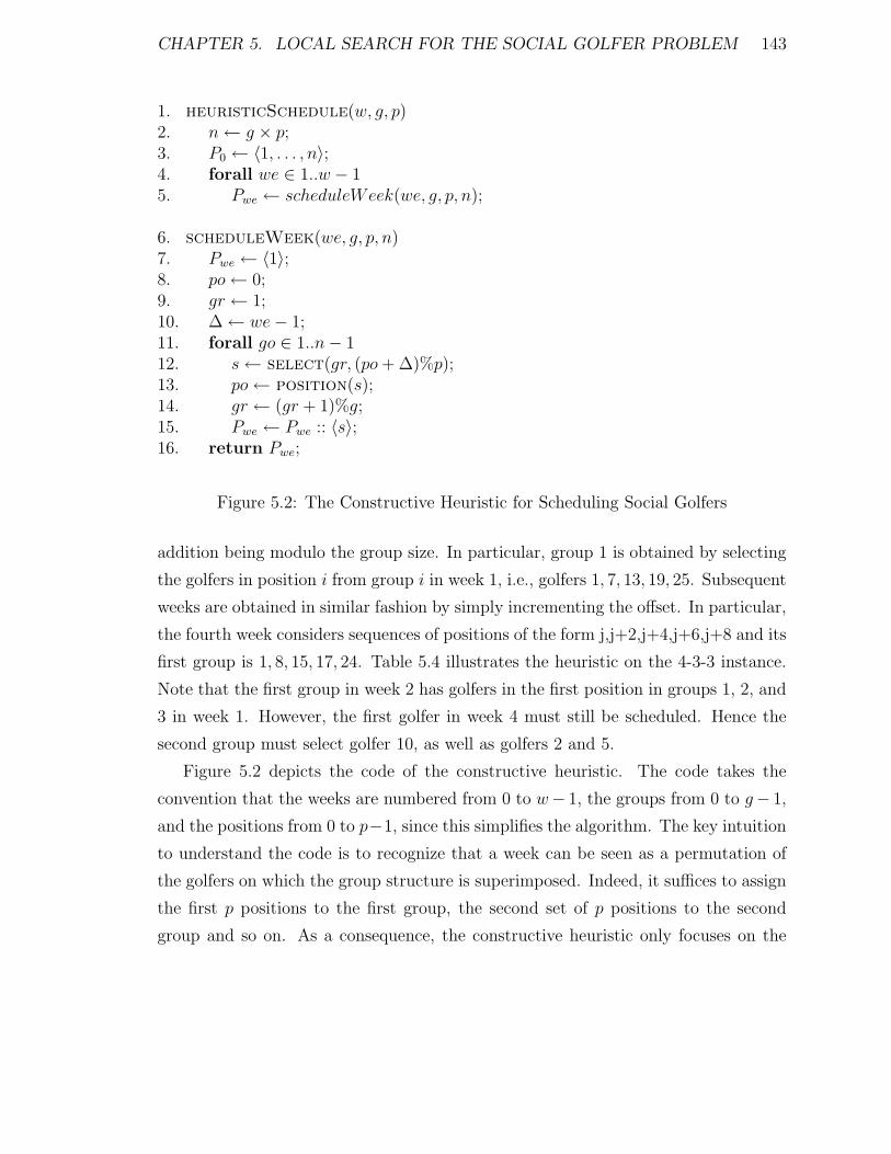
CHAPTER 5. LOCAL SEARCH FOR THE SOCIAL GOLFER PROBLEM 143
1. heuristicSchedule(w, g, p)2. n← g × p;3. P0 ← 〈1, . . . , n〉;4. forall we ∈ 1..w − 15. Pwe ← scheduleWeek(we, g, p, n);
6. scheduleWeek(we, g, p, n)7. Pwe ← 〈1〉;8. po← 0;9. gr ← 1;10. ∆← we− 1;11. forall go ∈ 1..n− 112. s← select(gr, (po+ ∆)%p);13. po← position(s);14. gr ← (gr + 1)%g;15. Pwe ← Pwe :: 〈s〉;16. return Pwe;
Figure 5.2: The Constructive Heuristic for Scheduling Social Golfers
addition being modulo the group size. In particular, group 1 is obtained by selecting
the golfers in position i from group i in week 1, i.e., golfers 1, 7, 13, 19, 25. Subsequent
weeks are obtained in similar fashion by simply incrementing the offset. In particular,
the fourth week considers sequences of positions of the form j,j+2,j+4,j+6,j+8 and its
first group is 1, 8, 15, 17, 24. Table 5.4 illustrates the heuristic on the 4-3-3 instance.
Note that the first group in week 2 has golfers in the first position in groups 1, 2, and
3 in week 1. However, the first golfer in week 4 must still be scheduled. Hence the
second group must select golfer 10, as well as golfers 2 and 5.
Figure 5.2 depicts the code of the constructive heuristic. The code takes the
convention that the weeks are numbered from 0 to w− 1, the groups from 0 to g− 1,
and the positions from 0 to p−1, since this simplifies the algorithm. The key intuition
to understand the code is to recognize that a week can be seen as a permutation of
the golfers on which the group structure is superimposed. Indeed, it suffices to assign
the first p positions to the first group, the second set of p positions to the second
group and so on. As a consequence, the constructive heuristic only focuses on the
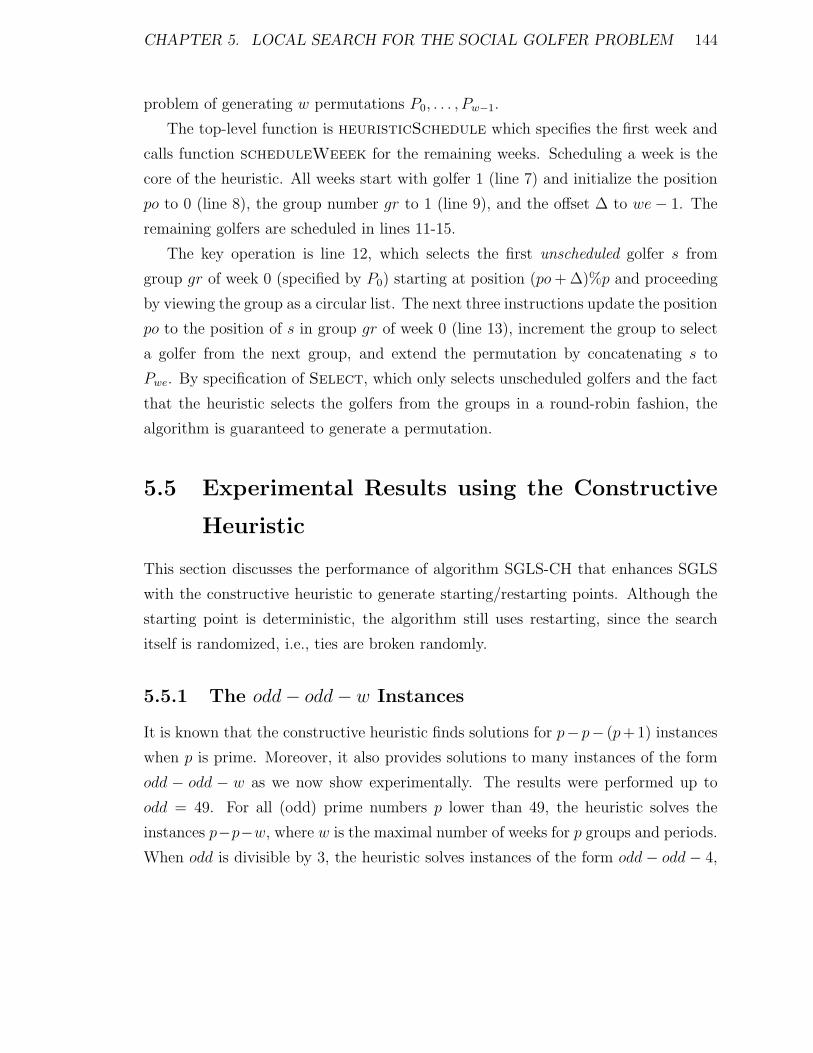
CHAPTER 5. LOCAL SEARCH FOR THE SOCIAL GOLFER PROBLEM 144
problem of generating w permutations P0, . . . , Pw−1.
The top-level function is heuristicSchedule which specifies the first week and
calls function scheduleWeeek for the remaining weeks. Scheduling a week is the
core of the heuristic. All weeks start with golfer 1 (line 7) and initialize the position
po to 0 (line 8), the group number gr to 1 (line 9), and the offset ∆ to we− 1. The
remaining golfers are scheduled in lines 11-15.
The key operation is line 12, which selects the first unscheduled golfer s from
group gr of week 0 (specified by P0) starting at position (po+ ∆)%p and proceeding
by viewing the group as a circular list. The next three instructions update the position
po to the position of s in group gr of week 0 (line 13), increment the group to select
a golfer from the next group, and extend the permutation by concatenating s to
Pwe. By specification of Select, which only selects unscheduled golfers and the fact
that the heuristic selects the golfers from the groups in a round-robin fashion, the
algorithm is guaranteed to generate a permutation.
5.5 Experimental Results using the Constructive
Heuristic
This section discusses the performance of algorithm SGLS-CH that enhances SGLS
with the constructive heuristic to generate starting/restarting points. Although the
starting point is deterministic, the algorithm still uses restarting, since the search
itself is randomized, i.e., ties are broken randomly.
5.5.1 The odd− odd− w Instances
It is known that the constructive heuristic finds solutions for p− p− (p+ 1) instances
when p is prime. Moreover, it also provides solutions to many instances of the form
odd − odd − w as we now show experimentally. The results were performed up to
odd = 49. For all (odd) prime numbers p lower than 49, the heuristic solves the
instances p−p−w, where w is the maximal number of weeks for p groups and periods.
When odd is divisible by 3, the heuristic solves instances of the form odd− odd− 4,
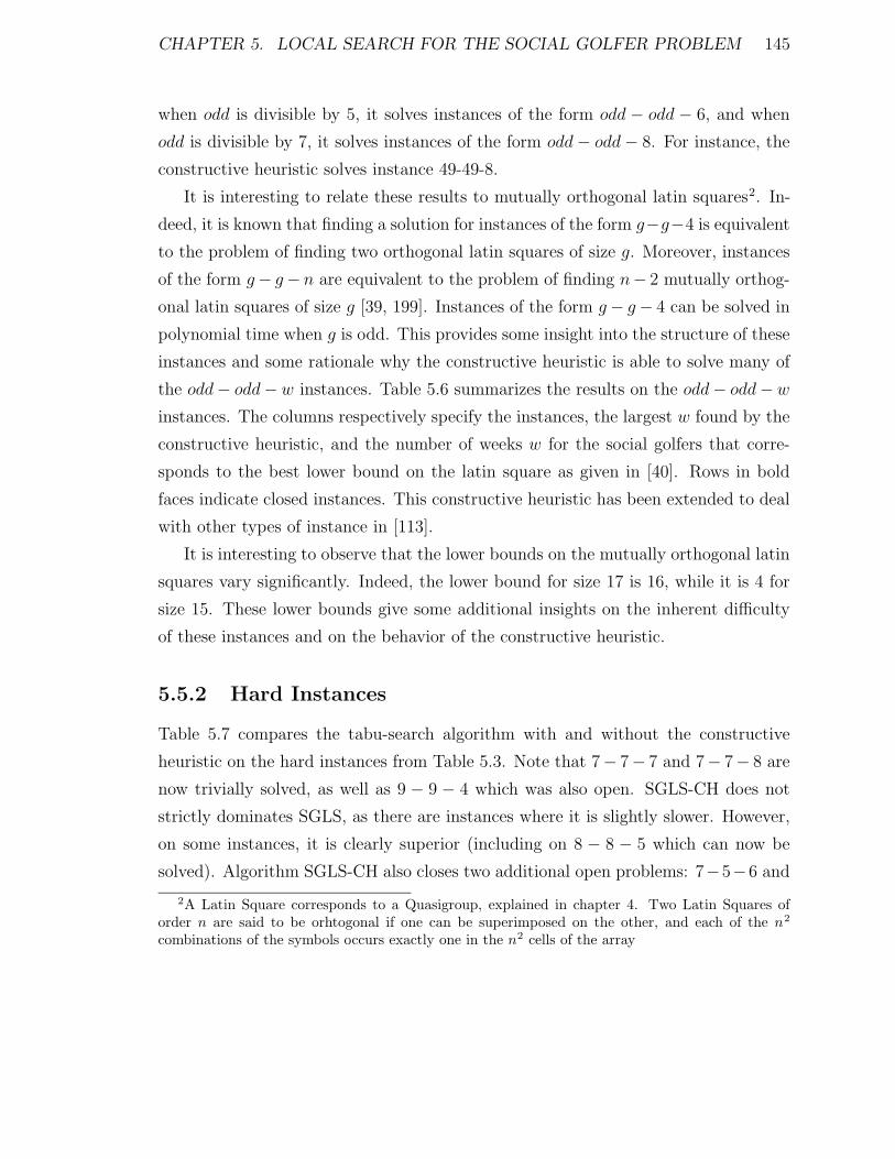
CHAPTER 5. LOCAL SEARCH FOR THE SOCIAL GOLFER PROBLEM 145
when odd is divisible by 5, it solves instances of the form odd − odd − 6, and when
odd is divisible by 7, it solves instances of the form odd− odd− 8. For instance, the
constructive heuristic solves instance 49-49-8.
It is interesting to relate these results to mutually orthogonal latin squares2. In-
deed, it is known that finding a solution for instances of the form g−g−4 is equivalent
to the problem of finding two orthogonal latin squares of size g. Moreover, instances
of the form g− g− n are equivalent to the problem of finding n− 2 mutually orthog-
onal latin squares of size g [39, 199]. Instances of the form g− g− 4 can be solved in
polynomial time when g is odd. This provides some insight into the structure of these
instances and some rationale why the constructive heuristic is able to solve many of
the odd− odd− w instances. Table 5.6 summarizes the results on the odd− odd−winstances. The columns respectively specify the instances, the largest w found by the
constructive heuristic, and the number of weeks w for the social golfers that corre-
sponds to the best lower bound on the latin square as given in [40]. Rows in bold
faces indicate closed instances. This constructive heuristic has been extended to deal
with other types of instance in [113].
It is interesting to observe that the lower bounds on the mutually orthogonal latin
squares vary significantly. Indeed, the lower bound for size 17 is 16, while it is 4 for
size 15. These lower bounds give some additional insights on the inherent difficulty
of these instances and on the behavior of the constructive heuristic.
5.5.2 Hard Instances
Table 5.7 compares the tabu-search algorithm with and without the constructive
heuristic on the hard instances from Table 5.3. Note that 7− 7− 7 and 7− 7− 8 are
now trivially solved, as well as 9 − 9 − 4 which was also open. SGLS-CH does not
strictly dominates SGLS, as there are instances where it is slightly slower. However,
on some instances, it is clearly superior (including on 8 − 8 − 5 which can now be
solved). Algorithm SGLS-CH also closes two additional open problems: 7−5−6 and
2A Latin Square corresponds to a Quasigroup, explained in chapter 4. Two Latin Squares oforder n are said to be orhtogonal if one can be superimposed on the other, and each of the n2
combinations of the symbols occurs exactly one in the n2 cells of the array
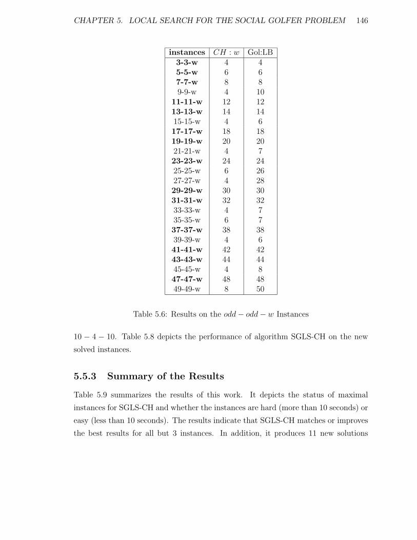
CHAPTER 5. LOCAL SEARCH FOR THE SOCIAL GOLFER PROBLEM 146
instances CH : w Gol:LB3-3-w 4 45-5-w 6 67-7-w 8 89-9-w 4 10
11-11-w 12 1213-13-w 14 1415-15-w 4 617-17-w 18 1819-19-w 20 2021-21-w 4 723-23-w 24 2425-25-w 6 2627-27-w 4 2829-29-w 30 3031-31-w 32 3233-33-w 4 735-35-w 6 737-37-w 38 3839-39-w 4 641-41-w 42 4243-43-w 44 4445-45-w 4 847-47-w 48 4849-49-w 8 50
Table 5.6: Results on the odd− odd− w Instances
10 − 4 − 10. Table 5.8 depicts the performance of algorithm SGLS-CH on the new
solved instances.
5.5.3 Summary of the Results
Table 5.9 summarizes the results of this work. It depicts the status of maximal
instances for SGLS-CH and whether the instances are hard (more than 10 seconds) or
easy (less than 10 seconds). The results indicate that SGLS-CH matches or improves
the best results for all but 3 instances. In addition, it produces 11 new solutions
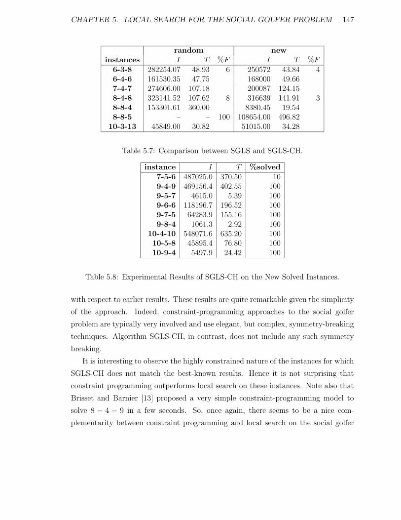
CHAPTER 5. LOCAL SEARCH FOR THE SOCIAL GOLFER PROBLEM 147
random newinstances I T %F I T %F
6-3-8 282254.07 48.93 6 250572 43.84 46-4-6 161530.35 47.75 168000 49.667-4-7 274606.00 107.18 200087 124.158-4-8 323141.52 107.62 8 316639 141.91 38-8-4 153301.61 360.00 8380.45 19.548-8-5 – – 100 108654.00 496.82
10-3-13 45849.00 30.82 51015.00 34.28
Table 5.7: Comparison between SGLS and SGLS-CH.
instance I T %solved7-5-6 487025.0 370.50 109-4-9 469156.4 402.55 1009-5-7 4615.0 5.39 1009-6-6 118196.7 196.52 1009-7-5 64283.9 155.16 1009-8-4 1061.3 2.92 100
10-4-10 548071.6 635.20 10010-5-8 45895.4 76.80 10010-9-4 5497.9 24.42 100
Table 5.8: Experimental Results of SGLS-CH on the New Solved Instances.
with respect to earlier results. These results are quite remarkable given the simplicity
of the approach. Indeed, constraint-programming approaches to the social golfer
problem are typically very involved and use elegant, but complex, symmetry-breaking
techniques. Algorithm SGLS-CH, in contrast, does not include any such symmetry
breaking.
It is interesting to observe the highly constrained nature of the instances for which
SGLS-CH does not match the best-known results. Hence it is not surprising that
constraint programming outperforms local search on these instances. Note also that
Brisset and Barnier [13] proposed a very simple constraint-programming model to
solve 8 − 4 − 9 in a few seconds. So, once again, there seems to be a nice com-
plementarity between constraint programming and local search on the social golfer
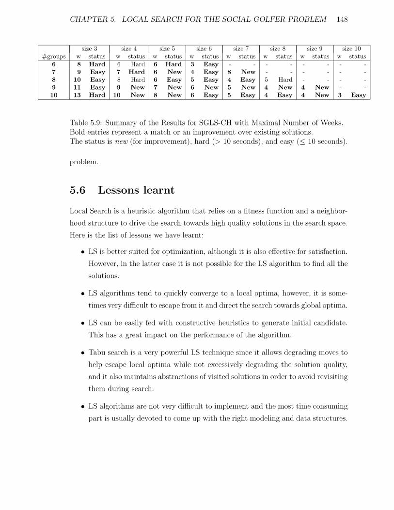
CHAPTER 5. LOCAL SEARCH FOR THE SOCIAL GOLFER PROBLEM 148
size 3 size 4 size 5 size 6 size 7 size 8 size 9 size 10#groups w status w status w status w status w status w status w status w status
6 8 Hard 6 Hard 6 Hard 3 Easy - - - - - - - -7 9 Easy 7 Hard 6 New 4 Easy 8 New - - - - - -8 10 Easy 8 Hard 6 Easy 5 Easy 4 Easy 5 Hard - - - -9 11 Easy 9 New 7 New 6 New 5 New 4 New 4 New - -10 13 Hard 10 New 8 New 6 Easy 5 Easy 4 Easy 4 New 3 Easy
Table 5.9: Summary of the Results for SGLS-CH with Maximal Number of Weeks.Bold entries represent a match or an improvement over existing solutions.The status is new (for improvement), hard (> 10 seconds), and easy (≤ 10 seconds).
problem.
5.6 Lessons learnt
Local Search is a heuristic algorithm that relies on a fitness function and a neighbor-
hood structure to drive the search towards high quality solutions in the search space.
Here is the list of lessons we have learnt:
• LS is better suited for optimization, although it is also effective for satisfaction.
However, in the latter case it is not possible for the LS algorithm to find all the
solutions.
• LS algorithms tend to quickly converge to a local optima, however, it is some-
times very difficult to escape from it and direct the search towards global optima.
• LS can be easily fed with constructive heuristics to generate initial candidate.
This has a great impact on the performance of the algorithm.
• Tabu search is a very powerful LS technique since it allows degrading moves to
help escape local optima while not excessively degrading the solution quality,
and it also maintains abstractions of visited solutions in order to avoid revisiting
them during search.
• LS algorithms are not very difficult to implement and the most time consuming
part is usually devoted to come up with the right modeling and data structures.

Chapter 6
A Memetic Algorithm for the
Golomb Ruler Problem
Finding Golomb rulers is an extremely challenging combinatorial problem which has
received considerable attention over the last decades. An n-mark Golomb ruler is an
ordered sequence of n distinct nonnegative integers 〈m1, . . . ,mn〉 (mi < mi+1) such
that all distances
mj −mi (1 ≤ i < j ≤ n) (6.1)
are distinct. Each integer mi corresponds to a mark on the ruler and the length of
the ruler is the difference mn −m1. By convention, the first mark m1 can be placed
in position 0, in which case the length is given by mn. An n-mark Golomb ruler is
optimal if there exists no n-mark Golomb ruler of smaller length.
Golomb rulers have applications in a wide variety of fields including radio commu-
nications ([27, 114]), x-ray crystallography ([26]), coding theory ([56, 139]), and radio
astronomy. Moreover, because of their highly combinatorial nature,1 they have be-
come a standard benchmark to evaluate and compare a variety of search techniques.
In particular, genetic algorithms, constraint programming, local search, and their
hybridizations have all been applied to the problem of finding Golomb rulers (e.g.,
[43, 76, 173, 176, 210, 213]).
1The search for a 19-mark Golomb ruler took approximately 36,200 CPU hours on a Sun Sparcworkstation using a very specialized algorithm [56].
149
CHAPTER 6. A MEMETIC ALGORITHM FOR THE GOLOMB RULER PROBLEM150
This research proposes a novel hybrid evolutionary algorithm for finding near-
optimal Golomb rulers in reasonable time. The algorithm embeds a local search into
a genetic algorithm and outperforms earlier genetic algorithms, as well as constraint
programming algorithms and their hybridizations with local search. In particular, the
algorithm quickly finds optimal rulers for up to 13 marks and was able to find opti-
mal rulers for 14 and 15 marks, which is clearly out of reach for the above mentioned
algorithms. The algorithm also finds near-optimal rulers in reasonable time, clearly
indicating the effectiveness of hybrid evolutionary algorithms on this highly combi-
natorial application. Of particular interest is the conceptual simplicity and elegance
of the algorithm.
Even though there are solutions for higher number of marks for other complete
search approaches, evolutionary algorithms have the advantage of providing good
quality solutions in a short period of time. This is a main contribution of this re-
search as well, providing high quality solutions (improving all previous evolutionary
approaches) in a few seconds or minutes.
The main technical contribution of the novel hybrid evolutionary algorithm is its
focus on feasibility. Indeed, the main step of the evolutionary algorithm is to find a
Golomb ruler of a specified length (or smaller), using constraint violations to guide the
search. Near-optimal rulers are obtained indirectly by solving a sequence of feasibility
problems.
The rest of this chapter starts by a brief overview of related work. It then presents
presents the local search and the hybrid evolutionary algorithms for finding Golomb
rulers of a specified length, before generalizing the algorithm to find near-optimal
rulers and concluding with the lessons learnt.
6.1 Finding Golomb Rulers
Two main approaches can be essentially considered for tackling the Optimal Golomb
Ruler (OGR) problem with EAs. The first one is the direct approach, in which the
EA conducts the search in the space SG of all possible Golomb rulers. The second
one is the indirect approach, in which an auxiliary Saux space is used by the EA. In

CHAPTER 6. A MEMETIC ALGORITHM FOR THE GOLOMB RULER PROBLEM151
this latter case, a decoder [140] must be utilized in order to perform the Saux −→ SGmapping. Examples of the former (direct) approach are the works of Soliday et al.
[213], and Feeney [76]. As to the latter (indirect) approach, we can cite the work
by Pereira et al. [173] (based on the notion of random-keys [18]), and Cotta and
Fernandez [43] (based on ideas from GRASP [190]). This latter paper is specifically
interesting since generalizations of the core idea presented there have been used in
this work. To be precise, the key idea was using a problem-aware procedure (inspired
in GRASP) to perform the genotype-to-phenotype mapping. This method ensured
the generation of feasible solutions, and was shown to outperform other previous
approaches.
In 1995, Soliday, Homaifar and Lebby [213] used a genetic algorithm on different
instances of the Golomb ruler problem. They chose a direct approach where each
chromosome is composed by a permutation of n − 1 integers that represents the
sequence of the n− 1 lengths of its segments. Two evaluation criteria were followed:
the overall length of the ruler, and the number of repeated measurements. This latter
quantity was used in order to penalize infeasible solutions. The mutation operator
consisted of either a permutation in the segment order, or a change in the segment
lengths. As to crossover, it was designed to guarantee that descendants are valid
permutations.
Later, Feeney studied the effect of hybridizing genetic algorithms with local im-
provement techniques to solve Golomb rulers [76]. The direct representation used con-
sisted of an array of integers corresponding to the marks of the ruler. The crossover
operator was similar to that used in Soliday et al.’s approach although a sort pro-
cedure was added at the end. The mutation operator consisted in adding a random
amount in the range [−x, x] -where x is the maximum difference between any pair
of marks in any ruler of the initial population– to the segment mark selected for
mutation. As it will be shown later, we can use a similar concept in order to de-
fine a distance measure on the fitness landscape. Pereira et al. presented in [173]
an indirect approach based EA using the notion of random keys [18] o codify the
information contained in each chromosome. The basic idea consists of generating n
random numbers (i.e., the keys) sampled from the interval [0, 1] and ordered by its
CHAPTER 6. A MEMETIC ALGORITHM FOR THE GOLOMB RULER PROBLEM152
position in the sequence 1, . . . , n; then the keys are sorted in decreasing order. The
indices of the keys thus result in a feasible permutation of {1, · · · , n}. A similar
evaluation criteria as described in [213] was followed. They also presented an alter-
native algorithm that adds a heuristic, favoring the insertion of small segments. A
related approach has been presented in [43]. This proposal incorporates ideas from
greedy randomized adaptive search procedures (GRASP) [190] in order to perform
the genotype-to-phenotype mapping. More precisely, the mapping procedure pro-
ceeds by placing each of the n− 1 marks (the first mark is assumed to be a1 = 0) one
at a time; the (i + 1)th mark can be obtained as ai+1 = ai + li, where li > 1 is the
i−th segment length. Feasible segment lengths (i.e., those not leading to duplicate
measurements) can be sorted in increasing order. Now, the EA needs only specifying
at each step the index of a certain segment within this list (obviously, the contents of
the list are different in each of these steps). This implies that each individual would
be a sequence 〈r1, · · · , rn−1〉, where ri would be the index of the segment used in the
i−th iteration of the construction algorithm. Notice that in this last placement step it
does not make sense to pick any other segment length than the smallest one. For this
reason, rn−1 = 1; hence, solutions need only specify the sequence 〈r1, · · · , rn−2〉. This
representation of solutions is orthogonal [186], i.e., any sequence represents a feasible
solution, and hence, standard operators for crossover and mutation can be used to
manipulate them. This GRASP-based approach was reported to perform better than
the previous (indirect and direct) approached mentioned.
6.2 Golomb Rulers of Fixed Lengths
This section describes hybrid evolutionary algorithm for finding Golomb rulers of
specified lengths. It starts with the problem modeling, then describes the local search
and the hybrid evolutionary algorithms, and concludes with the experimental results.

CHAPTER 6. A MEMETIC ALGORITHM FOR THE GOLOMB RULER PROBLEM153
6.2.1 Modeling
The problem modeling in the hybrid evolutionary algorithm is natural and associates
a decision variable mx with every mark x. Given a ruler σ, i.e., an assignment of values
to the decision variables, the value σ(mx) denotes the position of mark x within the
ruler. Since the length l of the ruler is known in this section, the values σ(m1) and
σ(mn) are fixed to 0 and l respectively. There are three kinds of constraints in the
Golomb ruler:
1. The marks have different positions in the ruler.
2. The marks are ordered, i.e., σ(mi) < σ(mi+1).
3. The distances dij = mj −mi (j > i) are all different.
The first two types of constraints are implicit in the algorithms presented in this
work: They are satisfied by the initial assignments and are preserved by local moves
and genetic operators. The goal of the algorithms is thus to satisfy the third set of
constraints.
To guide the search, the algorithms use a notion of constraint violations on the
distances. The violation υσ(d) of a distance d in a n-mark ruler σ is the number
of times distance d appears between two marks in the ruler σ beyond its allowed
occurrences, i.e.,
υσ(d) = max(0,#{dij = d | 1 ≤ i < j ≤ n} − 1) (6.2)
where dij = σ(mj) − σ(mi). The violations υ(σ) of a n-mark ruler σ is simply the
sum of the violations of its distances d, i.e.,
υ(σ) =∑
d∈Dυσ(d) (6.3)
where D = {di,j | 1 ≤ i < j ≤ n}. Obviously, a ruler σ with υ(σ) = 0 is a solution
to the Golomb ruler problem.
CHAPTER 6. A MEMETIC ALGORITHM FOR THE GOLOMB RULER PROBLEM154
6.2.2 The Tabu Search
We now turn to the tabu search algorithm for finding Golomb rulers of specified
lengths.
The Neighborhood The moves in the local search consists of changing the value
of a single mark. Since the marks are ordered, a mark x can only take a value in the
interval
Iσ(x) = [σ(mx−1) + 1, σ(mx+1)− 1].
As a consequence, the sets of possible moves is
M(σ) = {(x, p) | 0 < x < n & p ∈ Iσ(x)}.
Observe that σ(m1) and σ(mn) are fixed to 0 and l.
The Tabu Component The tabu component of the local search prevents a mark
from being reassigned the same value for a number of iterations. The tabu list thus
consists of a triplet 〈x, p, i〉, where x is a mark and p is a possible position for mark
x and i represents the first iteration where mark x can be assigned to p again. The
tabu tenure, i.e., the number of iteration (x, p) stays in the list, is dynamic and is
randomly generated in the interval [4, 100]. For a ruler σ and an iteration k, the set
of legal moves is thus defined as
M+(σ, k) = {(x, p) ∈ M(σ) | ¬tabu(x, p, k)}.
where tabu(x, p, k) holds if the assignment mx ← p is tabu at iteration k. The tabu
status can be overridden whenever an assignment would reduce the smallest number
of violations found so far. In other words, if σ∗ is the ruler with the smallest number
of violations found so far, the neighborhood also includes the moves
M∗(σ, σ∗) = {(x, p) ∈ M(σ) | υ(σ[mx ← p]) < υ(σ∗)}
CHAPTER 6. A MEMETIC ALGORITHM FOR THE GOLOMB RULER PROBLEM155
where σ[mx ← p] denotes the ruler σ where variable mx is assigned to p.
The Tabu-Search Algorithm We are now ready to present the basic local search
algorithm grls. The algorithm, depicted in Figure 6.1, a tabu search with an inten-
sification component2. Lines 2-6 perform the initializations. In particular, the tabu
list is initialized in line 2, the initial ruler is generated randomly in line 3, while lines
5 and 6 initialize the iteration counter k, and the stability counter s. The initial
configuration σ randomly assigns values for all marks, satisfying the constraints that
each mark is assigned to a different value and are ordered. Moreover, the position of
the first mark is 0 and the position of the last mark is the length l of the ruler. The
best ruler found so far σ∗ is initialized to σ. The core of the algorithm are lines 7-21
which perform local moves for a number of iterations or until a solution is found. The
local move is selected in line 8. The key idea is to select the best assignment in the
neighborhood
M+(σ, k) ∪ M∗(σ, σ∗),
i.e., the non-tabu moves and those which improve the best ruler. Observe that the
expression υ(σ[mx ← v]) represents the number of violations obtained after assigning
p to mark x. The tabu list is updated in line 10, and the new ruler is computed in
line 11. Lines 12-14 update the best ruler, while lines 15-18 specify the intensification
component. The intensification component simply reinitializes the search from the
best available ruler whenever no improvement in the number of violations took place
for maxStable iterations. Note that the stability counter s is incremented in line 20
and reset to zero in line 14 (when a new best ruler is found) and in line 17 (when the
search is restarted).
6.2.3 The Hybrid Evolutionary Algorithm
We now turn to the hybrid evolutionary (HE) algorithm for finding Golomb rulers
of specified lengths. The algorithm maintains a population of rulers and performs
2Remember that intensification consists of maintaining a list of good solutions that the algorithmwill revisit at some point during the search
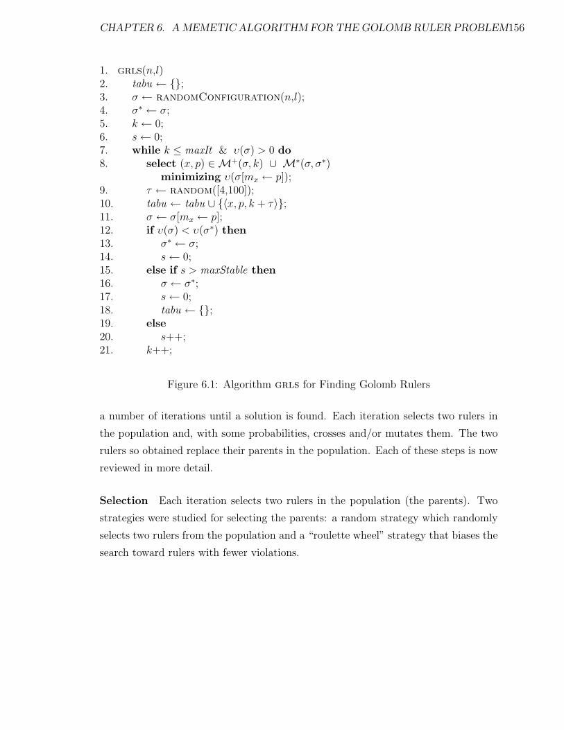
CHAPTER 6. A MEMETIC ALGORITHM FOR THE GOLOMB RULER PROBLEM156
1. grls(n,l)2. tabu ← {};3. σ ← randomConfiguration(n,l);4. σ∗ ← σ;5. k ← 0;6. s← 0;7. while k ≤ maxIt & υ(σ) > 0 do8. select (x, p) ∈M+(σ, k) ∪ M∗(σ, σ∗)
minimizing υ(σ[mx ← p]);9. τ ← random([4,100]);10. tabu ← tabu ∪ {〈x, p, k + τ〉};11. σ ← σ[mx ← p];12. if υ(σ) < υ(σ∗) then13. σ∗ ← σ;14. s← 0;15. else if s > maxStable then16. σ ← σ∗;17. s← 0;18. tabu ← {};19. else20. s++;21. k++;
Figure 6.1: Algorithm grls for Finding Golomb Rulers
a number of iterations until a solution is found. Each iteration selects two rulers in
the population and, with some probabilities, crosses and/or mutates them. The two
rulers so obtained replace their parents in the population. Each of these steps is now
reviewed in more detail.
Selection Each iteration selects two rulers in the population (the parents). Two
strategies were studied for selecting the parents: a random strategy which randomly
selects two rulers from the population and a “roulette wheel” strategy that biases the
search toward rulers with fewer violations.
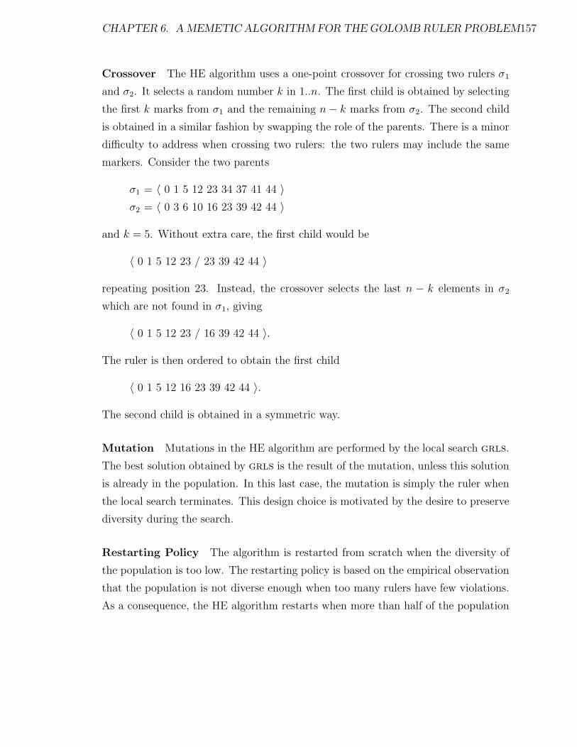
CHAPTER 6. A MEMETIC ALGORITHM FOR THE GOLOMB RULER PROBLEM157
Crossover The HE algorithm uses a one-point crossover for crossing two rulers σ1
and σ2. It selects a random number k in 1..n. The first child is obtained by selecting
the first k marks from σ1 and the remaining n− k marks from σ2. The second child
is obtained in a similar fashion by swapping the role of the parents. There is a minor
difficulty to address when crossing two rulers: the two rulers may include the same
markers. Consider the two parents
σ1 = 〈 0 1 5 12 23 34 37 41 44 〉σ2 = 〈 0 3 6 10 16 23 39 42 44 〉
and k = 5. Without extra care, the first child would be
〈 0 1 5 12 23 / 23 39 42 44 〉
repeating position 23. Instead, the crossover selects the last n − k elements in σ2
which are not found in σ1, giving
〈 0 1 5 12 23 / 16 39 42 44 〉.
The ruler is then ordered to obtain the first child
〈 0 1 5 12 16 23 39 42 44 〉.
The second child is obtained in a symmetric way.
Mutation Mutations in the HE algorithm are performed by the local search grls.
The best solution obtained by grls is the result of the mutation, unless this solution
is already in the population. In this last case, the mutation is simply the ruler when
the local search terminates. This design choice is motivated by the desire to preserve
diversity during the search.
Restarting Policy The algorithm is restarted from scratch when the diversity of
the population is too low. The restarting policy is based on the empirical observation
that the population is not diverse enough when too many rulers have few violations.
As a consequence, the HE algorithm restarts when more than half of the population
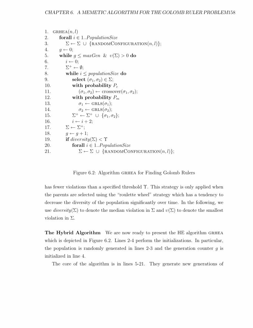
CHAPTER 6. A MEMETIC ALGORITHM FOR THE GOLOMB RULER PROBLEM158
1. grhea(n, l)2. forall i ∈ 1..PopulationSize3. Σ← Σ ∪ {randomConfiguration(n, l)};4. g ← 0;5. while g ≤ maxGen & υ(Σ) > 0 do6. i← 0;7. Σ+ ← ∅;8. while i ≤ populationSize do9. select (σ1, σ2) ∈ Σ;10. with probability Pc11. (σ1, σ2)← crossover(σ1, σ2);12. with probability Pm13. σ1 ← grls(σ1);14. σ2 ← grls(σ2);15. Σ+ ← Σ+ ∪ {σ1, σ2};16. i← i+ 2;17. Σ← Σ+;18. g ← g + 1;19. if diversity(Σ) < Υ20. forall i ∈ 1..PopulationSize21. Σ← Σ ∪ {randomConfiguration(n, l)};
Figure 6.2: Algorithm grhea for Finding Golomb Rulers
has fewer violations than a specified threshold Υ. This strategy is only applied when
the parents are selected using the “roulette wheel” strategy which has a tendency to
decrease the diversity of the population significantly over time. In the following, we
use diversity(Σ) to denote the median violation in Σ and υ(Σ) to denote the smallest
violation in Σ.
The Hybrid Algorithm We are now ready to present the HE algorithm grhea
which is depicted in Figure 6.2. Lines 2-4 perform the initializations. In particular,
the population is randomly generated in lines 2-3 and the generation counter g is
initialized in line 4.
The core of the algorithm is in lines 5-21. They generate new generations of
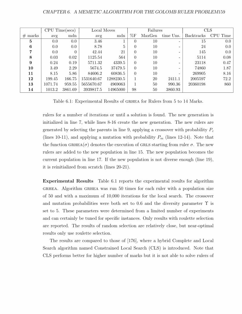
CHAPTER 6. A MEMETIC ALGORITHM FOR THE GOLOMB RULER PROBLEM159
CPU Time(secs) Local Moves Failures CLS# marks avg mdn avg mdn %F MaxGen time Uns. Backtracks CPU Time
5 0.0 0.0 3.46 1 0 10 - 15 0.06 0.0 0.0 8.78 5 0 10 - 24 0.07 0.0 0 42.44 21 0 10 - 145 0.08 0.03 0.02 1125.54 564 0 10 - 5114 0.089 0.24 0.19 5711.32 4339.5 0 10 - 23118 0.4710 3.49 2.29 5674.5 37479.5 0 10 - 74860 1.8711 8.15 5.86 84606.2 60836.5 0 10 - 269905 8.1612 199.45 166.75 1531640.67 1288230.5 1 20 2411.1 2005597 72.213 1071.74 959.55 5655670.67 4969063 1 50 990.36 20360198 86014 1013.2 3861.69 3939817.5 14965000 98 50 3860.93
Table 6.1: Experimental Results of grhea for Rulers from 5 to 14 Marks.
rulers for a number of iterations or until a solution is found. The new generation is
initialized in line 7, while lines 8-16 create the new generation. The new rulers are
generated by selecting the parents in line 9, applying a crossover with probability Pc
(lines 10-11), and applying a mutation with probability Pm (lines 12-14). Note that
the function grhea(σ) denotes the execution of grls starting from ruler σ. The new
rulers are added to the new population in line 15. The new population becomes the
current population in line 17. If the new population is not diverse enough (line 19),
it is reinitialized from scratch (lines 20-21).
Experimental Results Table 6.1 reports the experimental results for algorithm
grhea. Algorithm grhea was run 50 times for each ruler with a population size
of 50 and with a maximum of 10,000 iterations for the local search. The crossover
and mutation probabilities were both set to 0.6 and the diversity parameter Υ is
set to 5. These parameters were determined from a limited number of experiments
and can certainly be tuned for specific instances. Only results with roulette selection
are reported. The results of random selection are relatively close, but near-optimal
results only use roulette selection.
The results are compared to those of [176], where a hybrid Complete and Local
Search algorithm named Constrained Local Search (CLS) is introduced. Note that
CLS performs better for higher number of marks but it is not able to solve rulers of
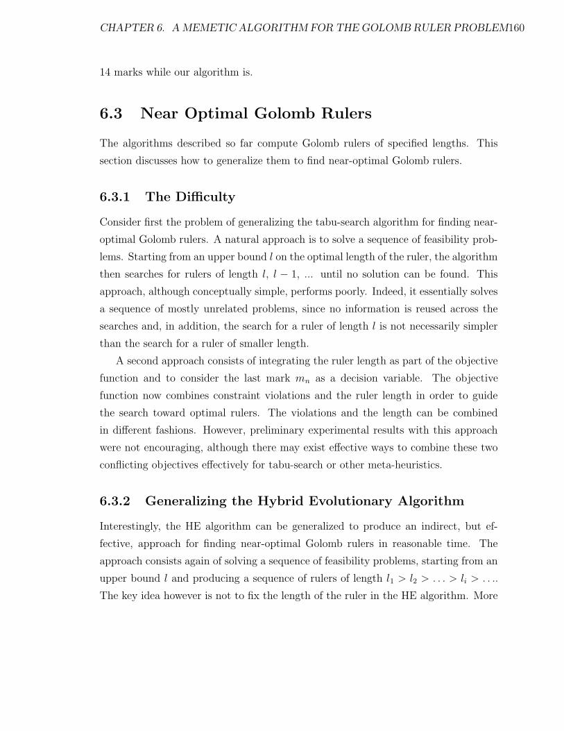
CHAPTER 6. A MEMETIC ALGORITHM FOR THE GOLOMB RULER PROBLEM160
14 marks while our algorithm is.
6.3 Near Optimal Golomb Rulers
The algorithms described so far compute Golomb rulers of specified lengths. This
section discusses how to generalize them to find near-optimal Golomb rulers.
6.3.1 The Difficulty
Consider first the problem of generalizing the tabu-search algorithm for finding near-
optimal Golomb rulers. A natural approach is to solve a sequence of feasibility prob-
lems. Starting from an upper bound l on the optimal length of the ruler, the algorithm
then searches for rulers of length l, l − 1, ... until no solution can be found. This
approach, although conceptually simple, performs poorly. Indeed, it essentially solves
a sequence of mostly unrelated problems, since no information is reused across the
searches and, in addition, the search for a ruler of length l is not necessarily simpler
than the search for a ruler of smaller length.
A second approach consists of integrating the ruler length as part of the objective
function and to consider the last mark mn as a decision variable. The objective
function now combines constraint violations and the ruler length in order to guide
the search toward optimal rulers. The violations and the length can be combined
in different fashions. However, preliminary experimental results with this approach
were not encouraging, although there may exist effective ways to combine these two
conflicting objectives effectively for tabu-search or other meta-heuristics.
6.3.2 Generalizing the Hybrid Evolutionary Algorithm
Interestingly, the HE algorithm can be generalized to produce an indirect, but ef-
fective, approach for finding near-optimal Golomb rulers in reasonable time. The
approach consists again of solving a sequence of feasibility problems, starting from an
upper bound l and producing a sequence of rulers of length l1 > l2 > . . . > li > . . ..
The key idea however is not to fix the length of the ruler in the HE algorithm. More
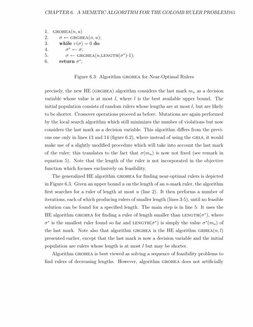
CHAPTER 6. A MEMETIC ALGORITHM FOR THE GOLOMB RULER PROBLEM161
1. grohea(n, u)2. σ ← grghea(n, u);3. while υ(σ) = 0 do4. σ∗ ← σ;5. σ ← grghea(n,length(σ∗)-1);6. return σ∗;
Figure 6.3: Algorithm grohea for Near-Optimal Rulers
precisely, the new HE (grghea) algorithm considers the last mark mn as a decision
variable whose value is at most l, where l is the best available upper bound. The
initial population consists of random rulers whose lengths are at most l, but are likely
to be shorter. Crossover operations proceed as before. Mutations are again performed
by the local search algorithm which still minimizes the number of violations but now
considers the last mark as a decision variable. This algorithm differs from the previ-
ous one only in lines 13 and 14 (figure 6.2), where instead of using the grls, it would
make use of a slightly modified procedure which will take into account the last mark
of the ruler; this translates to the fact that σ(mn) is now not fixed (see remark in
equation 5). Note that the length of the ruler is not incorporated in the objective
function which focuses exclusively on feasibility.
The generalized HE algorithm grohea for finding near-optimal rulers is depicted
in Figure 6.3. Given an upper bound u on the length of an n-mark ruler, the algorithm
first searches for a ruler of length at most u (line 2). It then performs a number of
iterations, each of which producing rulers of smaller length (lines 3-5), until no feasible
solution can be found for a specified length. The main step is in line 5: It uses the
HE algorithm grghea for finding a ruler of length smaller than length(σ∗), where
σ∗ is the smallest ruler found so far and length(σ∗) is simply the value σ∗(mn) of
the last mark. Note also that algorithm grghea is the HE algorithm grhea(n, l)
presented earlier, except that the last mark is now a decision variable and the initial
population are rulers whose length is at most l but may be shorter.
Algorithm grohea is best viewed as solving a sequence of feasibility problems to
find rulers of decreasing lengths. However, algorithm grohea does not artificially
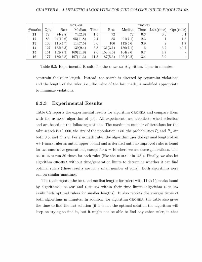
CHAPTER 6. A MEMETIC ALGORITHM FOR THE GOLOMB RULER PROBLEM162
hgrasp grohea#marks Opt Best Median Time Best Median Time Last(time) Opt(time)
11 72 74(2.8) 74(2.8) 1.5 72 72 0.3 0.3 0.112 85 94(10.6) 95(11.8) 2.4 85 91(7.1) 2.3 1 1.813 106 111(4.7) 114(7.5) 3.6 106 112(5.6) 3.9 2 1.714 127 135(6.3) 139(9.4) 5.3 131(3.1) 136(7.1) 6 3.2 40.715 151 162(7.3) 169(11.9) 7.6 158(4.6) 164(8.6) 8.7 4.7 -16 177 189(6.8) 197(11.3) 11.3 187(5.6) 195(10.2) 13.4 5.9 -
Table 6.2: Experimental Results for the grohea Algorithm. Time in minutes.
constrain the ruler length. Instead, the search is directed by constraint violations
and the length of the ruler, i.e., the value of the last mark, is modified appropriate
to minimize violations.
6.3.3 Experimental Results
Table 6.2 reports the experimental results for algorithm grohea and compare them
with the hgrasp algorithm of [43]. All experiments use a roulette wheel selection
and are based on the following settings. The maximum number of iterations for the
tabu search is 10, 000, the size of the population is 50, the probabilities Pc and Pm are
both 0.6, and Υ is 5. For a n-mark ruler, the algorithm uses the optimal length of an
n+1-mark ruler as initial upper bound and is iterated until no improved ruler is found
for two successive generations, except for n = 16 where we use three generations. The
grohea is run 30 times for each ruler (like the hgrasp in [43]). Finally, we also let
algorithm grohea without time/generation limits to determine whether it can find
optimal rulers (these results are for a small number of runs). Both algorithms were
run on similar machines.
The table reports the best and median lengths for rulers with 11 to 16 marks found
by algorithms hgrasp and grohea within their time limits (algorithm grohea
easily finds optimal rulers for smaller lengths). It also reports the average times of
both algorithms in minutes. In addition, for algorithm grohea, the table also gives
the time to find the last solution (if it is not the optimal solution the algorithm will
keep on trying to find it, but it might not be able to find any other ruler, in that
CHAPTER 6. A MEMETIC ALGORITHM FOR THE GOLOMB RULER PROBLEM163
case, we report time to find the last valid ruler). The last column reports the time of
grohea to find optimal rulers.
The results are particularly impressive. First observe that grohea systematically
finds optimal rulers up to 11 marks very quickly. Algorithm hgrasp does not find
optimal rulers systematically even for 10 marks and never finds optimal rulers for 11
marks. Algorithm grohea also finds optimal rulers for 12 and 13 marks in less than
two minutes and for 14 marks in about 40 minutes. Algorithm grohea also improves
the near-optimal solutions significantly. For 14 marks, the best solutions of grohea
are with 3.1% of the optimal rulers (instead of 6.3% for hgrasp) in about 6 minutes.
They are with 4.6% and 5.6% for 15 and 16 marks in about 9 and 13 minutes. These
represent improvements ranging from 1.4% to 3.2% compared to hgrasp. Similar
results are obtained for median values as well.
A fundamental benefit of grohea is its ability to improve its solutions over time,
which does not seem to be the case of prior generic and/or hybrid evolutionary al-
gorithms. Contrary to grohea, earlier algorithms were not able to find optimal
solutions for 13 and 14 marks. Algorithm grohea also finds a solution of length
153 in about an hour on 15 marks (151 is the optimal length), showing that better
solutions can be found when the algorithm is given more time. This is particularly
interesting given the natural modeling and conceptual simplicity of the algorithm.
It is also important to stress that these results were obtained without tuning of
the parameters. In particular, larger instances are likely to benefit from longer tabu
searches and, possibly, more sophisticated crossovers. But the results clearly indicate
the potential of hybrid evolutionary algorithms for finding near-optimal rulers.
6.4 Lessons learnt
Genetic Algorithms are population-based algorithms that are easily hybridized with
LS techniques. Contrary to the opinion of many researchers within the combinatorial
optimization field, they can be very efficient when solving hard problems, and espe-
cially when generating fast near-optimal solutions. Here is the list of lessons we have
learnt:
CHAPTER 6. A MEMETIC ALGORITHM FOR THE GOLOMB RULER PROBLEM164
• GAs are very useful to provide a framework in which to maintain a set of diverse
and high quality solutions.
• Recombination operators can sometimes yield valid, optimal or near-optimal
solutions.
• When solving hard combinatorial problems they greatly benefit from the incor-
poration of LS techniques that allow a faster convergence.
• A fast convergence of the population is also problematic. Restarts and other
mechanism are needed in order to regenerate the population and drive the search
towards different regions in the search space. However, it is not always straight-
forward to implement the right restarting condition.
• The Local Search is greatly enriched by having a population of diverse solutions.
LS typically improves a solution until it gets stuck on a local optima, when the
algorithm commonly restarts and attempts to improve a different solution. In
this case, we can see it as if the LS had a set of good solutions available at any
time to be optimized in turns.
• GAs can not only incorporate LS procedures to improve the efficiency of their
recombination operators, but also use information yielded by those processes to
dynamically adapt themselves.

Part III
The Last Hybrid
165
Chapter 7
Adding CP and Clustering to Solve
the Golomb Ruler Problem
In this section a new hybrid algorithm is presented in two steps: first a very so-
phisticated memetic algorithm; and second, the introduction of CP and clustering
techniques to boost performance. As in the previous chapter, the problem we are
going to be dealing with is that of the Golomb Ruler. Remember that Golomb Rulers
[9, 26] are a class of undirected graphs that, unlike usual rulers, measure more discrete
lengths than the number of marks they carry. More formally, a n-mark Golomb ruler
is an ordered sequence of n distinct nonnegative integers 〈m1, . . . ,mn〉 (mi < mi+1)
such that all distances mj −mi (1 6 i < j 6 n) are distinct. Each integer mi corre-
sponds to a mark on the ruler and the length of the ruler is the difference mn −m1.
By convention, the first mark m1 can be placed in position 0, in which case the length
is given by mn.
The particularity of Golomb Rulers that on any given ruler, all differences between
pairs of marks are unique makes them really interesting in many practical applications
(cf. [76, 187]). It turns out that finding optimal or near-optimal Golomb rulers (a n-
mark Golomb ruler is optimal if there exists no n-mark Golomb ruler of smaller length)
is an extremely challenging combinatorial problem. To date, the highest number of
marks for which the optimal Golomb ruler (OGR) is known is 23 marks1 [205, 198].
1The search for an optimal 19-marks Golomb ruler took approximately 36,200 CPU hours on
166
CHAPTER 7. ADDING CP AND CLUSTERING TO SOLVE THE GOLOMB RULER PROBLEM167
Finding optimal Golomb rulers has thus become a standard benchmark to evaluate
and compare a variety of search techniques. In particular, evolutionary algorithms
(EAs), constraint programming (CP), local search (LS), and their hybridizations have
all been applied to this problem (e.g., [76, 43, 173, 176, 210, 213]).
In these next sections, we present a hybrid EA designed to find optimal or near-
optimal Golomb Rulers. This algorithm makes use of both an indirect approach and
a direct approach in different stages of the search. More specifically, the indirect
approach is used in the phases of initialization and restarting of the population and
takes ideas borrowed from the GRASP-based evolutionary approach published in
[43]. The direct approach is considered in the stages of recombination and local
improvement; particularly, the local improvement method is based on the tabu search
(TS) algorithm described in the previous chapter. Experimental results show that this
algorithm succeeds where another evolutionary algorithms did not. OGRs up to 15
marks (included) can now be found. Moreover, the algorithm produces Golomb rulers
for 16 marks that are very close to the optimal value (i.e., 1.1% far), thus improving
significantly the results previously reported in the EA literature. Finally, we show
the last improvements which rely on clustering to achieve diversity in the reference
set and complete search to attempt to find optimal rulers at the recombination step.
These enhancements produce superior results, and the new hybrid is now capable of
solving rulers up to 16 marks. The chapter concludes with a brief summary and a
review of all the lessons learnt throughout the thesis and how they are reflected in
this last hybrid.
7.1 Scatter Search for the Golomb Ruler Problem
Scatter search (SS) is a metaheuristic based on population-based search whose origin
can be traced back to the 1970s in the context of combining decision rules and prob-
lem constraints [142]. Figure 7.1 depicts the SS template. Among the salient features
a Sun Sparc workstation using a very specialized algorithm [56]. Optimal solutions for 20 up to23 marks were obtained by massive parallelism projects, taking several months for each of thoseinstances [187, 85].
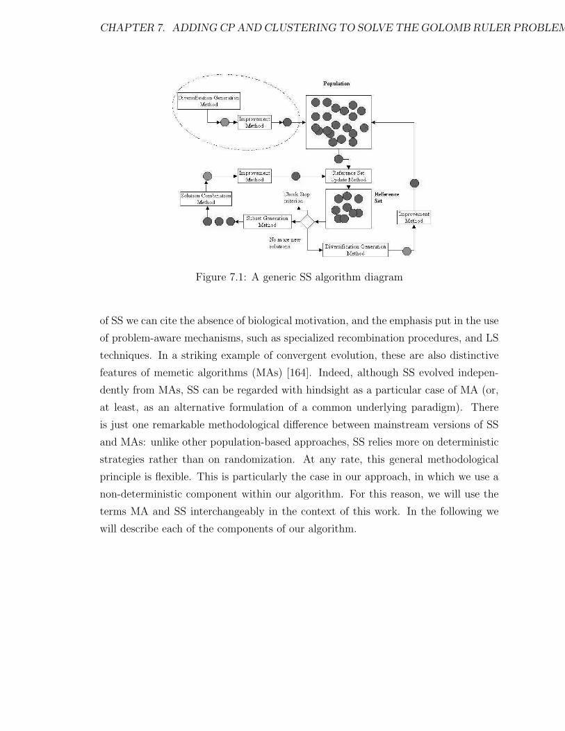
CHAPTER 7. ADDING CP AND CLUSTERING TO SOLVE THE GOLOMB RULER PROBLEM168
Figure 7.1: A generic SS algorithm diagram
of SS we can cite the absence of biological motivation, and the emphasis put in the use
of problem-aware mechanisms, such as specialized recombination procedures, and LS
techniques. In a striking example of convergent evolution, these are also distinctive
features of memetic algorithms (MAs) [164]. Indeed, although SS evolved indepen-
dently from MAs, SS can be regarded with hindsight as a particular case of MA (or,
at least, as an alternative formulation of a common underlying paradigm). There
is just one remarkable methodological difference between mainstream versions of SS
and MAs: unlike other population-based approaches, SS relies more on deterministic
strategies rather than on randomization. At any rate, this general methodological
principle is flexible. This is particularly the case in our approach, in which we use a
non-deterministic component within our algorithm. For this reason, we will use the
terms MA and SS interchangeably in the context of this work. In the following we
will describe each of the components of our algorithm.
CHAPTER 7. ADDING CP AND CLUSTERING TO SOLVE THE GOLOMB RULER PROBLEM169
7.1.1 Diversification Generation Method
The diversification generation method serves two purposes in the SS algorithm con-
sidered: it is used for generating the initial population from which the reference set
will be initially extracted, and it is utilized for refreshing the reference set whenever
a restart is needed.
The generation of new solutions is performed by using a randomized procedure
that tries to generate diverse solutions. The basic method utilizes the GRASP-
decoding techniques introduced in [43]. Solutions are incrementally constructed as
follows: in the initial step, only mark m1 = 0 is placed; subsequently, at each step
i an ordered list is built using the n first integers l1, · · · , ln such that placing a new
mark mi = mi−1 + lj, 1 6 j 6 n, would result in a feasible Golomb ruler. A random
element is drawn from this list, and used to place mark mi. The process is iterated
until all marks have been placed. Notice that this results in a feasible solution.
A variant of this process is used in subsequent invocations to this method for
refreshing the population. This variant is related to an additional dynamic constraint
that is imposed in the algorithm: in any solution, it must hold that mn < L, where L
is the length of the best feasible Golomb ruler found so far. To fulfill this constraint,
new solutions are constructed by generating two feasible rules following the procedure
described before, and submitting them to the combination method (see Sect. 7.1.3),
which guarantees compliance with the mentioned constraint.
7.1.2 Local Improvement Method
The improvement method is responsible for enhancing raw solutions produced by
the diversification generation method, or by the solution combination method. In
this case, improvement is achieved via the use of a tabu-search algorithm. This TS
algorithm works on tentative solutions that may be infeasible, i.e., there may exist
some repeated distances between marks. The goal of the algorithm is precisely to
turn infeasible rulers into feasible ones, respecting the dynamic constraint mn < L.
Whenever this is achieved, a new incumbent solution is obviously found.
To guide the search, the algorithm uses a notion of constraint violations on the
CHAPTER 7. ADDING CP AND CLUSTERING TO SOLVE THE GOLOMB RULER PROBLEM170
distances. The violation υσ(d) of a distance d in a n-mark ruler σ is the number
of times distance d appears between two marks in the ruler σ beyond its allowed
occurrences, i.e.,
υσ(d) = max(0,#{dij = d | 1 6 i < j 6 n} − 1) (7.1)
where dij = mj − mi. The overall violation υ(σ) of a n-mark ruler σ is simply the
sum of the violations of its distances d, i.e., υ(σ) =∑
d∈D υσ(d), where D = {dij |1 6 i < j 6 n}.
The moves in the local search consists of changing the value of a single mark.
Since marks are ordered, a mark mx can only take a value in the interval Iσ(x) =
[mx−1 +1,mx+1−1]. As a consequence, the set of possible moves isM(σ) = {(x, p) |(1 < x < n) ∧ (p ∈ Iσ(x))}. Observe that m1 is fixed to 0, and mn is not allowed
to grow. To prevent cycling, a tabu list of movements is kept. The list stores triplets
〈x, p, i〉, where x is a mark, p is a possible position for mark x, and i represents the
first iteration where mark x can be assigned to p again. The tabu tenure, i.e., the
number of iterations (x, p) stays in the list, is dynamic and randomly generated in
the interval [4, 100]. For a ruler σ and an iteration k, the set of legal moves is thus
defined as
M+(σ, k) = {(x, p) ∈ M(σ) | ¬tabu(x, p, k)}.
where tabu(x, p, k) holds if the assignment mx ← p is tabu at iteration k. The tabu
status can be overridden whenever an assignment reduces the smallest number of
violations found so far. Thus, if σ∗ is the ruler with the smallest number of violations
found so far, the neighborhood also includes the moves
M∗(σ, σ∗) = {(x, p) ∈ M(σ) | υ(σ[mx ← p]) < υ(σ∗)}
where σ[mx ← p] denotes the ruler σ where variable mx is assigned to p. To intensify
the search, the current solution is reinitialized to the initial ruler σ0 (in the actual TS
run) whenever no improvement in the number of violations took place for maxStable
iterations. The algorithm returns the best solution σ∗ found. Fig. 7.2 shows the
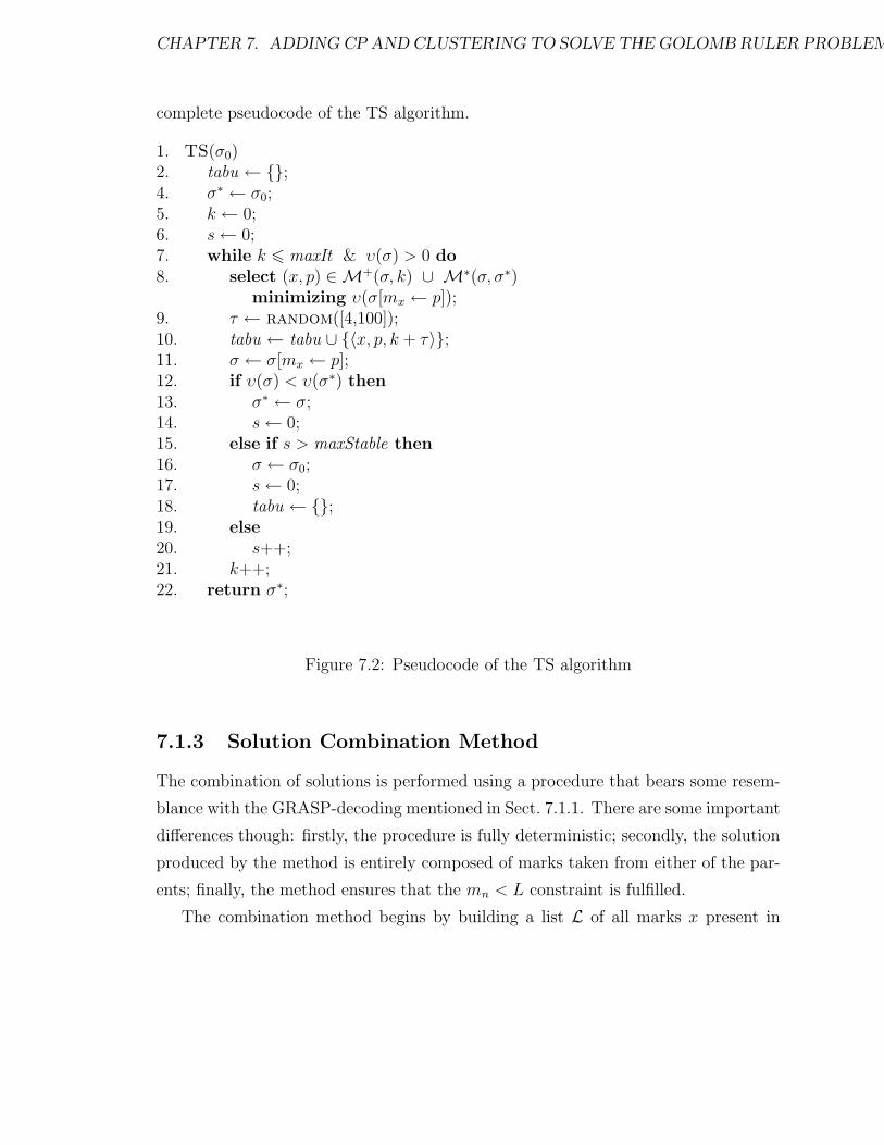
CHAPTER 7. ADDING CP AND CLUSTERING TO SOLVE THE GOLOMB RULER PROBLEM171
complete pseudocode of the TS algorithm.
1. TS(σ0)2. tabu ← {};4. σ∗ ← σ0;5. k ← 0;6. s← 0;7. while k 6 maxIt & υ(σ) > 0 do8. select (x, p) ∈M+(σ, k) ∪ M∗(σ, σ∗)
minimizing υ(σ[mx ← p]);9. τ ← random([4,100]);10. tabu ← tabu ∪ {〈x, p, k + τ〉};11. σ ← σ[mx ← p];12. if υ(σ) < υ(σ∗) then13. σ∗ ← σ;14. s← 0;15. else if s > maxStable then16. σ ← σ0;17. s← 0;18. tabu ← {};19. else20. s++;21. k++;22. return σ∗;
Figure 7.2: Pseudocode of the TS algorithm
7.1.3 Solution Combination Method
The combination of solutions is performed using a procedure that bears some resem-
blance with the GRASP-decoding mentioned in Sect. 7.1.1. There are some important
differences though: firstly, the procedure is fully deterministic; secondly, the solution
produced by the method is entirely composed of marks taken from either of the par-
ents; finally, the method ensures that the mn < L constraint is fulfilled.
The combination method begins by building a list L of all marks x present in
CHAPTER 7. ADDING CP AND CLUSTERING TO SOLVE THE GOLOMB RULER PROBLEM172
either of the parents, such that x < L 2. Then, starting from m1 = 0, a new mark x
is chosen at each step i such that (i) mi−1 < x, (ii) there exist n − i marks greater
than x in L, and (iii) a local optimization criterion is optimized. This latter criterion
is minimizing∑i−1
j=1 υσ(x − mj)2 + (x − mi−1), where σ is the partial ruler. This
expression involves minimizing the number of constraints violated when placing the
new mark, as well as the subsequent increase in length of the ruler. The first term is
squared to raise its priority in the decision-making.
7.1.4 Subset Generation and Reference Set Update
This subset generation method creates the groups of solutions that will undergo com-
bination. The combination method used is in principle generalizable to an arbitrary
number of parents, but we have considered the standard two-parent recombination.
Hence the subset generation method has to form pairs of solutions. This is done ex-
haustively, producing all possible pairs. It must be noted that since the combination
method utilized is deterministic, it does not make sense to combine again pairs of
solutions that were already coupled before. The algorithm keeps track of this fact to
avoid repeating computations.
As to the reference set update method, it must produce the reference set for the
next step by using the current reference set and the newly produced offspring (or by
using the initial population generated by diversification at the beginning of the run
or after a restart). Several strategies are possible here. Quality is an obvious criterion
to determine whether a solution can gain membership to the reference set: if a new
solution is better than the worst existing solution, the latter is replaced by the former.
In the OGR, we consider that a solution x is better than a solution y if the former
violates less constraints, or violates the same number of constraints but has a lower
length. It is also possible to gain membership of the reference set via diversity. To do
so, a subset of diverse solutions (i.e., distant solutions to the remaining high-quality
solutions in the set – an appropriate definition of a distance measure is needed for this
purpose) is kept in the reference set, and updated whenever a new solution improves
2It might happen that the number of such marks were not enough to build a new ruler. In thatcase, a plain solution with length ∞ (that is, the worst possible value) is returned.

CHAPTER 7. ADDING CP AND CLUSTERING TO SOLVE THE GOLOMB RULER PROBLEM173
the diversity criterion.
If at a certain iteration of the algorithm no update of the reference set takes place,
the current population is considered stagnated, and the restart method is invoked3.
This method works as follows: let µ be the size of the reference set; the best solution
in the reference set is preserved, λ = µ(µ − 1)/2 solutions are generated using the
diversification generation method and the improvement method, and the best µ − 1
out of these λ solutions are picked and inserted in the reference set.
7.2 Experimental Results
To evaluate our memetic approach, a set of experiments for problem sizes ranging from
10 marks up to 16 marks has been realized. In all the experiments, the maximum
number of iterations for the tabu search was set to 10, 000, the size of the population
and reference set was 190 and 20 respectively, and the arity of the combination method
was 2. The reference set is only updated on the basis of the quality criterion. One
of the key points in the experimentation has been analyzing the influence of the
local search strategy with respect to the population-based component. To this end,
we have experimented with partial Lamarckism [125], that is, applying the local
improvement method just on a fraction of the members of the population. To be
precise, we have considered a probability pts for applying LS to each solution. The
values pts ∈ {0.1, 0.2, 0.4, 0.6, 0.8, 1.0} have been considered. All algorithms were run
20 times until an optimal solution was found, or a limit in the whole number of
evaluations was exceeded. This number of evaluations was set so as to allow a fixed
average number e of LS invocations (e = 10, 000 TS runs). Thus, the number of
evaluations was limited in each of the instances to e/pts. This is a fair measure since
the computational cost is dominated by the number of TS invocations.
Table 7.1 reports the experimental results for the different instances considered.
Row MAxx corresponds to the execution of the MA with a local improvement rate
3Notice that the TS method used for local improvement is not deterministic. Thus, it might bepossible that further applications of TS on the stagnated population resulted in an improvement.However, due to the computational cost of this process, it is advisable to simply restart.
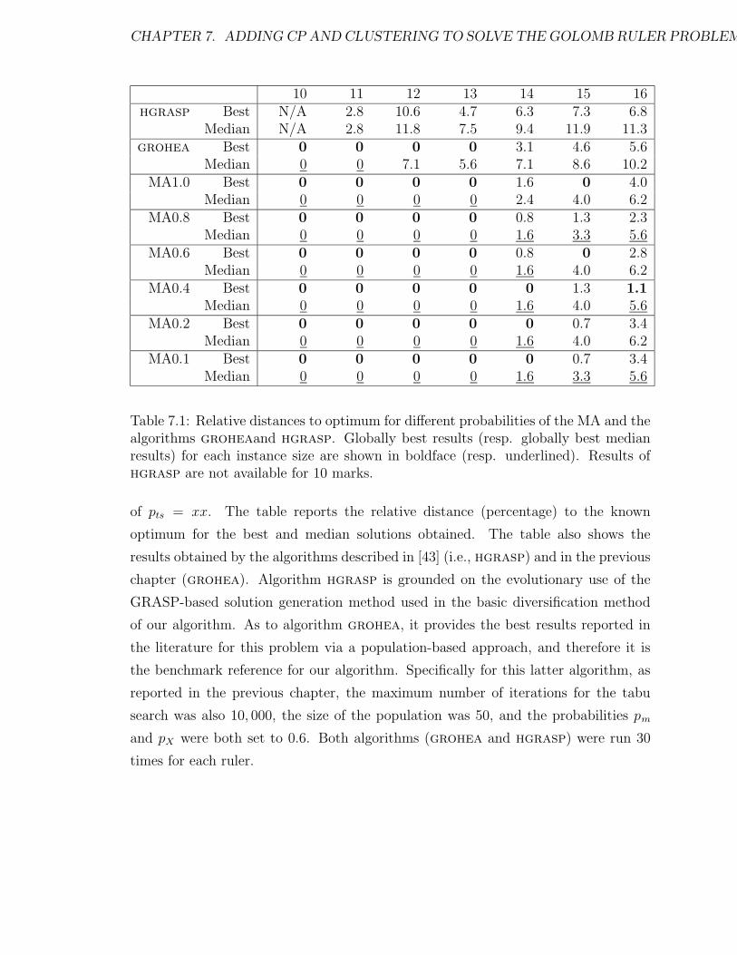
CHAPTER 7. ADDING CP AND CLUSTERING TO SOLVE THE GOLOMB RULER PROBLEM174
10 11 12 13 14 15 16hgrasp Best N/A 2.8 10.6 4.7 6.3 7.3 6.8
Median N/A 2.8 11.8 7.5 9.4 11.9 11.3grohea Best 0 0 0 0 3.1 4.6 5.6
Median 0 0 7.1 5.6 7.1 8.6 10.2MA1.0 Best 0 0 0 0 1.6 0 4.0
Median 0 0 0 0 2.4 4.0 6.2MA0.8 Best 0 0 0 0 0.8 1.3 2.3
Median 0 0 0 0 1.6 3.3 5.6MA0.6 Best 0 0 0 0 0.8 0 2.8
Median 0 0 0 0 1.6 4.0 6.2MA0.4 Best 0 0 0 0 0 1.3 1.1
Median 0 0 0 0 1.6 4.0 5.6MA0.2 Best 0 0 0 0 0 0.7 3.4
Median 0 0 0 0 1.6 4.0 6.2MA0.1 Best 0 0 0 0 0 0.7 3.4
Median 0 0 0 0 1.6 3.3 5.6
Table 7.1: Relative distances to optimum for different probabilities of the MA and thealgorithms groheaand hgrasp. Globally best results (resp. globally best medianresults) for each instance size are shown in boldface (resp. underlined). Results ofhgrasp are not available for 10 marks.
of pts = xx. The table reports the relative distance (percentage) to the known
optimum for the best and median solutions obtained. The table also shows the
results obtained by the algorithms described in [43] (i.e., hgrasp) and in the previous
chapter (grohea). Algorithm hgrasp is grounded on the evolutionary use of the
GRASP-based solution generation method used in the basic diversification method
of our algorithm. As to algorithm grohea, it provides the best results reported in
the literature for this problem via a population-based approach, and therefore it is
the benchmark reference for our algorithm. Specifically for this latter algorithm, as
reported in the previous chapter, the maximum number of iterations for the tabu
search was also 10, 000, the size of the population was 50, and the probabilities pm
and pX were both set to 0.6. Both algorithms (grohea and hgrasp) were run 30
times for each ruler.
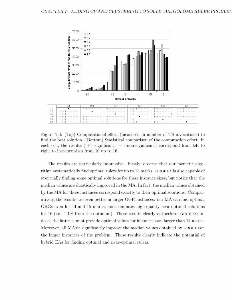
CHAPTER 7. ADDING CP AND CLUSTERING TO SOLVE THE GOLOMB RULER PROBLEM175
0.1 0.2 0.4 0.6 0.8 1.00.1 • − + +−−−− + + +−−−− + + +−−−− + + +−−−− + + +−−−−0.2 − + + −−−− • − − −−−−− + +−−−−− + +−−−−− + + +−−−−0.4 + + +−−−− −−−−−−− • + +−−−−− +−−−−− + + +−−−−−0.6 + + +−−−− + +−−−−− + +−−−−− • + +−−−−− + + +−−−−0.8 + + +−−−− + +−−−−− +−−−−− + + +−−−−− • + +−−−−−1.0 + + +−−−− + + +−−−− + +−−−−− + + +−−−− + +−−−−− •
Figure 7.3: (Top) Computational effort (measured in number of TS invocations) tofind the best solution. (Bottom) Statistical comparison of the computation effort. Ineach cell, the results (‘+’=significant, ‘−’=non-significant) correspond from left toright to instance sizes from 10 up to 16.
The results are particularly impressive. Firstly, observe that our memetic algo-
rithm systematically find optimal rulers for up to 13 marks. grohea is also capable of
eventually finding some optimal solutions for these instance sizes, but notice that the
median values are drastically improved in the MA. In fact, the median values obtained
by the MA for these instances correspond exactly to their optimal solutions. Compar-
atively, the results are even better in larger OGR instances: our MA can find optimal
ORGs even for 14 and 15 marks, and computes high-quality near-optimal solutions
for 16 (i.e., 1.1% from the optimum). These results clearly outperform grohea; in-
deed, the latter cannot provide optimal values for instance sizes larger than 14 marks.
Moreover, all MAxx significantly improve the median values obtained by groheaon
the larger instances of the problem. These results clearly indicate the potential of
hybrid EAs for finding optimal and near-optimal rulers.

CHAPTER 7. ADDING CP AND CLUSTERING TO SOLVE THE GOLOMB RULER PROBLEM176
We have also conducted statistical tests to ascertain whether there are signifi-
cant performance differences between the different LS application rates. This has
been done using a non-parametric Wilcoxon ranksum test (results are not normally
distributed). Except in three head-to-head comparisons for 14 marks (pts = 1.0 vs
pts = 0.8 and pts = 0.1, and pts = 0.4 vs pts = 0.1), there is no statistically significant
difference (at the standard 0.05 level) in any instance size for the different values of
pts. While this is consistent with the fact that the average number of TS invocations
is constant, it raises the issue of whether the associated computational cost is the
same or not. The answer to this question can be seen in Fig. 7.3. As expected, the
computational cost increases with the size of the problem. Quite interestingly, the
average cost decreases for 16 marks. This behavior owes to the higher difficulty of
the problem for this latter size: the algorithm quickly reaches a near-optimal value
(a remarkable result), and then stagnates (longer runs would be required to improve
the solutions from that point on). The table at the bottom of Fig. 7.3 shows the
outcome of the statistical comparison between the computational cost of the MAxx
for a given instance size. As it can be seen, the differences are almost always signifi-
cant for the lower range of sizes, and progressively become non-significant as the size
increases. For 16 marks, there is just one case of statistically significant difference
of computational cost (pts = 0.4 vs pts = 0.8). Since the small values of pts imply a
lower computational cost for instance sizes in the low range, and there is no significant
difference in either quality or computational cost with respect to higher values of pts
in the larger instances, it seems that values pts ∈ {0.1, 0.2} are advisable.
7.3 New Improvements
The algorithm presented this far yields very impressive results, however, we want
to pursue it further. There are two aspects (among others) that we can improve
very straightforwardly. First, we realized that Constraint Programming can be of
help at some point. Second, we believe that diversity in the population is almost as
important as the quality of it. Let us then introduce the new features incorporated
into our algorithm:
CHAPTER 7. ADDING CP AND CLUSTERING TO SOLVE THE GOLOMB RULER PROBLEM177
7.3.1 Solution Combination by Complete Search
Recombination methods are usually introduced in order to generate new high quality
and diverse individuals. Our current recombination mechanism achieves these goals,
however what we pursue here is something different. We are trying to generate optimal
solutions with this operator.
We have been dealing with values of marks through all this research. Now we turn
to look into the distances between marks. We realized that a complete search pro-
cedure that incorporates propagation techniques would be perfectly suited to search
for a solution when fed with the appropriate distances. Complete Search procedures
tend to be very inefficient with very large search spaces, however we can limit that
in this case by only taking into account the distances between marks of the two indi-
viduals to be combined. For example, imagine we have the two rulers of 9 marks to
be combined:
σ1 = 〈 0 1 5 13 23 34 47 50 55 〉σ2 = 〈 0 2 7 11 12 24 30 40 47 〉
The distances between marks of both rulers are
[ 1, 2, 3, 4, 5, 6, 7, 8, 10, 11, 12, 13]
Note that we only consider distances between two consecutive marks i, j where
i + 1 = j. To fully characterize the problem we need to take all the distances into
account, however these are the distances that we are going to restrict.
Thus, we use those distances to feed a complete search procedure whose goal is
to quickly attempt to generate valid rulers (hopefully optimal). In order to do that
we need to formulate the problem as a CSP. Now, the variables are distances Dij
between marks (where i < j). The domain of the variables Dij where i + 1 = j is
reduced to the values previously shown. The rest of the variables can take any value

CHAPTER 7. ADDING CP AND CLUSTERING TO SOLVE THE GOLOMB RULER PROBLEM178
within 1..m where m is the length of the ruler4. The set of constraints is as follows:
Dij 6= Dkl ∀ i 6= k and j 6= l
Since we are going to execute this procedure within the MA cycle, we can take
advantage of dynamic information, such as the length λ of the shortest valid ruler
in the population. This is explicitly indicated in the procedure by introducing a
constraint:
min(lk) < λ
where min(lk) is the minimum length possible for a partial ruler k.
Empirical Observations
We have now fully characterized the problem our complete search procedure is going
to be dealing with. However we found two options at this point:
• Use a Constraint Programming solver,
• or take advantage of the data structures already implemented in our algorithm.
The first option implies we can plug a black-box to our MA to which we pass a set
of distances and then expect a solution or a confirmation that no valid solution can be
found. We can take advantage of efficient propagation techniques and sophisticated
heuristics.
On the other hand, taking advantage of the structures already implemented, we
can focus on instantiating only variables Dij corresponding to distances between
consecutive marks; if we instantiate the variables in the same order as they would
physically appear in the ruler, we can easily calculate the rest of the distances and
thus, check the validity of the partial solution very quickly. This can be viewed as
limiting the search variables to the ones representing distances between consecutive
marks and using a lexicographic variable ordering heuristic. Note that in this case
4Note that the value of m is not important as we will soon clarify

CHAPTER 7. ADDING CP AND CLUSTERING TO SOLVE THE GOLOMB RULER PROBLEM179
we do not need to worry about the value of m, upper bound in the value of the non-
consecutive distances, since we are not focusing the search on them, but only on the
consecutive ones.
Both approaches were tested and we found that the latter was consistently faster
than the former; as it allows us to ignore non-consecutive distance variables. Still,
the reduction of the search space was not enough to yield a very fast mechanism.
Remember that we implement this procedure as a combination operator, and thus,
we cannot devote more than a few seconds to it.
In our experimental tests we discovered that, when reducing the search space to
consider only the consecutive distances of the optimal ruler, the procedure was able
to find a solution in less than a second for up to 14 marks, and less than 5 seconds
for 15 and 16 marks. However, introducing more distances slowed down the process
exponentially, and if within those distances a valid solution was not possibly found,
the time cost grew inmensely.
The final procedure
After a few more experiments we designed the next mechanism:
1. Select the two rulers to be combined.
2. Calculate the consecutive distances5
3. Randomly select n+ 3 distances from the previous step, being n the number of
marks in the ruler (which is 4 distances more than needed).
4. Run the complete search procedure with those distances, with a time limit of 4
seconds.
5. If a valid solution was found, return it, if not call the old recombination mech-
anism.
5Note that some distances might be repeated; for example, in two 15 mark rulers (14 consecutivedistances) we typically find around 20 different distances.
CHAPTER 7. ADDING CP AND CLUSTERING TO SOLVE THE GOLOMB RULER PROBLEM180
Note that this procedure can also find near optimal rulers if the chosen distances
permit it. Obviously, we can be missing some potential optimal rulers by randomly
selecting n + 3 distances, but we found it to be the best trade-off between time and
efficiency. That is, if there was a valid solution for the given distances, the complete
search procedure would almost always find it within the given time limit.
7.3.2 Diversity in the Population: Clustering
We also realized that the population got stuck very frequently. The solutions provided
by the LS mechanism were of high quality, and thus converged very quickly to the
same region of the search space. Restarts were required to drive the search towards
different regions. Since the population was selected in an elitist fashion, many times,
the algorithm was unable to generate better individuals that could be included in the
reference set.
Diversity is thus a key aspect of a population in order to provide the algorithm with
individuals different enough as to generate new solutions of relatively high quality.
In this sense we directed our efforts towards implementing a clustering algorithm.
Clustering deals with finding a structure in a collection of unlabeled data, and it can
be considered the most important unsupervised learning mechanism; a loose definition
of clustering could be ”the process of organizing objects into groups whose members
are similar in some way”. A cluster is therefore a collection of objects which are
”similar” among them and are ”dissimilar” to the objects belonging to other clusters.
In our population we have individuals that are vectors of marks, however, we are
going to transform them into distances between marks as in the previous subsection.
Our goal is thus to group individuals with similar sets of distances in the same cluster.
The algorithm for clustering is very simple; imagine we consider τ clusters:
1. Transform the vectors of marks into vectors of distances. Actually, in binary
vectors that indicate whether a distance is included in the individual or not.
For example, the individual representing a 9 marks ruler
σ1 = 〈 0 1 5 13 23 34 47 50 55 〉

CHAPTER 7. ADDING CP AND CLUSTERING TO SOLVE THE GOLOMB RULER PROBLEM181
will be transformed into
x(σ1) = [ 1 0 1 1 1 0 0 1 0 1 1 0 1 0 0 0 ... ]
where a 1 in x(σ1)[i] indicates that the distance i is included in the individual
σ1, where i rangs from 1 to three times the number of marks6.
2. Calculate τ random centroids. The centroids are the vectors that represent the
clusters, their central points. Thus, the centroids are vectors of the same length
as the individuals that characterize a cluster. If we already had the vectors
separated in clusters, the centroid of a cluster ki would be a vector:
centroid(ki) = [a1
| ki |a2
| ki |. . .
al| ki |
] (7.2)
where | ki | is the number of vectors in cluster ki and aj is the number of vectors
in cluster ki in which thet j-th bit is set to 1. Since we have no clusters yet we
calculate the centroids randomly.
3. Assign every vector to its nearest centroid, creating thus the clusters. The
distance measure we use is that of the cosine of the angles formed by the vector
and the centroid, and it is explained in the Clustering section of the appendix.
4. Recalculate the centroids with the now real information of the vectors in the
clusters.
5. Repeat steps 3 and 4 until no centroid is changed in step 4 or until a maximum
number of iterations is reached, in our case 10.
Our population is now divided into clusters. This fact itself does not ensure diver-
sity in the Reference Set. To maintain a high degree of diversity without harnessing
its quality we rank the vectors in every cluster and then select the best ω individuals
from each cluster, and we include them in the Reference Set.
6This limit l was imposed after the observation that optimal rulers try to incorporate the lowestdifferent distances between consecutive marks so that the ruler’s length is minimized
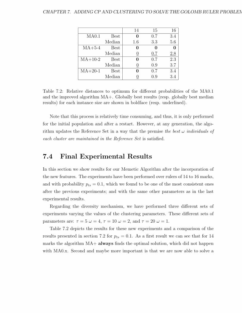
CHAPTER 7. ADDING CP AND CLUSTERING TO SOLVE THE GOLOMB RULER PROBLEM182
14 15 16MA0.1 Best 0 0.7 3.4
Median 1.6 3.3 5.6MA+5-4 Best 0 0 0
Median 0 0.7 2.8MA+10-2 Best 0 0.7 2.3
Median 0 0.9 3.7MA+20-1 Best 0 0.7 3.4
Median 0 0.9 3.4
Table 7.2: Relative distances to optimum for different probabilities of the MA0.1and the improved algorithm MA+. Globally best results (resp. globally best medianresults) for each instance size are shown in boldface (resp. underlined).
Note that this process is relatively time consuming, and thus, it is only performed
for the initial population and after a restart. However, at any generation, the algo-
rithm updates the Reference Set in a way that the premise the best ω individuals of
each cluster are maintained in the Reference Set is satisfied.
7.4 Final Experimental Results
In this section we show results for our Memetic Algorithm after the incorporation of
the new features. The experiments have been performed over rulers of 14 to 16 marks,
and with probability pts = 0.1, which we found to be one of the most consistent ones
after the previous experiments; and with the same other parameters as in the last
experimental results.
Regarding the diversity mechanism, we have performed three different sets of
experiments varying the values of the clustering parameters. These different sets of
parameters are: τ = 5 ω = 4, τ = 10 ω = 2, and τ = 20 ω = 1.
Table 7.2 depicts the results for these new experiments and a comparison of the
results presented in section 7.2 for pts = 0.1. As a first result we can see that for 14
marks the algorithm MA+ always finds the optimal solution, which did not happen
with MA0.x. Second and maybe more important is that we are now able to solve a
CHAPTER 7. ADDING CP AND CLUSTERING TO SOLVE THE GOLOMB RULER PROBLEM183
16 marks ruler. Also note that all the median values of MA+ are superior to those
produced by MA0.1. MA+5-4 seems to dominate the rest of the instances of MA+.
7.5 Summary
To summarize our newly born algorithm we must remember that it is based on a
Scatter Search ([142]) scheme, which uses GRASP features for initialization and re-
combination, and introduces a tabu search mechanism for improving individuals. This
algorithm is enriched with a complete search procedure also used for recombination
whose purpose is basically to try to reach an optimal solution at any point in the
execution of the algorithm (rather than provide high quality individuals). Finally,
the diversity of the population is ensured by means of a clustering algorithm that
divides the individuals in different clusters, and a selection mechanism that chooses
the best ω individuals from each cluster to be part of the reference set.
A different point of view is the following: A Local Search and a Complete Search
mechanism feed each other through a common population whose diversity is main-
tained by a clustering technique. According to this, tabu search and the complete
search recombination would be exchanging solutions in order to find the optimal
one, obtaining and returning these solutions to a diversified population. Moreover, a
GRASP mechanism helps constructing the initial population and conserving it (creat-
ing high quality and also diverse individuals). All this, sustained by a Scatter Search
scheme that holds everything together.
7.5.1 Lessons learnt revisited
Here is a brief explanation of how we have dealt with some of the lessons learnt during
the previous chapters, and how those lessons are reflected in this final hybrid:
• Constraint programming is especially suited for satisfaction problems; even
though this is an optimization problem we have transformed it into a satis-
faction one in the sense that we only ask for a feasible solution to the complete
search procedure (to be found among the selected distances).
CHAPTER 7. ADDING CP AND CLUSTERING TO SOLVE THE GOLOMB RULER PROBLEM184
• Propagation and Heuristics are key features in the constraint programming
framework; however, we have limited our heuristics here in order to take ad-
vantage of the already existent data structures, although we have maintained a
form of propagation related to the available distances and to the length of the
potential ruler.
• Constraint Satisfaction techniques encounter many difficulties when dealing
with very large search spaces. Note that the definition of search space depends
on the number of variables and also on the size of the domains. While we cannot
reduce the number of variables, we have reduced the number of values that the
complete search procedure has to deal with; thus, harnessing completeness for
the sake of speed.
• LS greatly benefits from the introduction of constructive heuristics as initial
solution generators. In this case, both the GRASP initialization procedure and
the GRASP recombination operator allow the LS to init the search from high
quality solutions.
• LS techniques have the major drawback of getting stuck on local optima. The
introduction of clustering an the resultant diversity of the population allow the
LS procedure to be fed with diverse and high quality solutions, each of which
have relatively high probabilities to yield a solution or at least not to converge
to the same region in the search space.
• Memetic Algorithms present the danger to quickly converge to the same region
of the search space without finding optimal solutions. It is sometimes hard to
decide when to restart the population in order to regenerate it. Scatter Search
provides a natural way to deal with this issue: restart when no new solutions
can be introduced in the reference set. This, and the new diversity mechanism
ensure that the algorithm will maintain a diverse population and will restart in
the exact moment in which this is not possible to achieve anymore.
• Finally, we have discussed about the LS being fed with diverse and high quality

CHAPTER 7. ADDING CP AND CLUSTERING TO SOLVE THE GOLOMB RULER PROBLEM185
solutions. In this case, diversity is maintained thanks to the clustering and se-
lection techniques, and the quality is maintained by the GRASP recombination
operator. Also, the complete procedure benefits from this diversity and high
quality, it constantly considers different sets of distances with relatively high
probabilities to contain a solution (this is perturbed by the random selection of
a certain number of them, before they are passed to the complete procedure).
Chapter 8
Conclusions and Future Work
This last chapter is devoted to the conclusiones derived from the research developed
for this thesis, and to the future work that follows from every research in every field
including hybrids.
8.1 Conclusions
Throughout this thesis we have presented several approaches to solve different hard
combinatorial optimization problems. We have succeeded in developing effective tech-
niques to solve these problems, and we have also created a new hybrid that incor-
porates mechanisms from the Constraint Programming, Local Search and Genetic
Algorithm’s frameworks.
Within the CSP framework we have introduced two novel aspects in redundant
modelling for multiple permutation problems:
• A novel value ordering heuristic which takes into account the primal and both
dual models, and which generalizes for multiple permutation problems ideas in-
troduced in ([35, 211] for simple permutation problems. The speedup produced
by this heuristic is quite remarkable, up to three orders of magnitude in some
cases.
• The use of channelling constraints linking more than a single pair of models
186

CHAPTER 8. CONCLUSIONS AND FUTURE WORK 187
to provide forward checking with the same pruning power as arc consistency
at a much smaller cost in constraint checks, and thus in performance, provided
that ordering effects are taken into account in the min-domain variable selection
heuristic.
We have also shown that SAT encodings allow for much more scalable solutions in
QCP problems, in particular when compared to previous results in the literature. We
have explained this performance by properties of the representation and by solver-
specific features; and we have shown that those features can also be fruitfully exploited
in CSP models to get much better CSP solutions than before.
In the next research work we have reconsidered the scheduling of social golfers, a
highly combinatorial and symmetric application which has raised significant interest
in the constraint programming community. It presented an effective local search algo-
rithm which found the first solutions to 11 new instances and matched, or improved
upon, all instances solved by constraint programming solutions but 3. Moreover, the
local search algorithm was shown to find almost all solutions in less than a couple of
seconds, the harder instances taking about 1 minute. The algorithm also features a
constructive heuristic which trivially solves many instances of the form odd−odd−w.
Finding Golomb rulers is an extremely challenging optimization problem with
many practical applications that have been approached by a variety of search methods
in recent years. It combines hard and dense feasibility constraints and an optimization
function to minimize the length of the ruler. Related to this, we have presented:
• A hybrid evolutionary algorithm grohea to find near-optimal Golomb rulers
in reasonable time. The algorithm is conceptually simple and uses a natural
modeling. It incorporates a tabu-search algorithm for mutation and a one-point
crossover to cross two rulers. It optimizes the length of the rulers indirectly by
solving a sequence of feasibility problems.
• We have presented a memetic approach for finding near-optimal Golomb rulers
at an acceptable computational cost. The MA combines, in different stages of
the algorithm, a GRASP-like procedure (for diversification and recombination)

CHAPTER 8. CONCLUSIONS AND FUTURE WORK 188
and tabu search (for local improvement) within the general template of scatter
search. The results of the MA have been particularly good, clearly outper-
forming other state-of-the-art evolutionary approaches for this problem. One of
the aspects on which our analysis has been focused is the influence of the LS
component. We have shown that lower rates of Lamarckianism achieve the best
tradeoff between computational cost and solution quality.
• We have introduced several improvements to the previous algorithm (complete
search and clustering) to yield outstanding results: we are able to solve a 16
marks ruler and to consistently solve every 14 mark rulers. The algorithm
tested using different sets of parameters referred to the clustering mechanism is
consistently superior to the previous algorithm without the improvements.
Finally, we have presented a new hybrid algorithm. This algorithm is based on
a Scatter Search template and includes a complete search inherited technique to
combine individuals, and a clustering procedure which we apply to our population in
order to achieve a higher degree of diversity. Results of this hybrid for the Golomb
Ruler Problem are superior to those presented in previous chapters in this thesis.
8.2 Future Work
There are many issue to persue within this thesis. Remember that every chapter deals
with a different kind of problem and a different kind of technique. Thus, possible
future work in each of these different research works will be the following:
8.2.1 CSP and SAT
Many issues remain to be explored. While we did try a number of alternatives to the
presented value ordering heuristics without success, others may be more successful.
There are some anomalies in the behavior of the ch3-fc approach vs ch2-ac which
could be symptoms of more subtle effects than the ordering effects reported above,
and which need to be explored. There is finally the issue of why CBJ and nogood
CHAPTER 8. CONCLUSIONS AND FUTURE WORK 189
learning did not help in this problem, which may in part suggest that in a sense
randomness dominates over structure in QCPs, but which should at any rate be an
incentive to develop more effective implementations of these techniques so that at
least they do not hurt when they do not help.
It would be interesting to see whether the combination of the ideas of this paper
with either alldiff constraints or Operations Research techniques could yield further
improvements in our ability to solve larger QCPs. For example, we mentioned that
the same effect achieved by introducing triangular channelling constraints would be
achieved by reintroducing instead the dual not-equal constraints, which in turn could
be replaced by dual alldiff constraints.
On the other hand while we can explain Satz’s performance and exploit its features
in CSP approaches, a similar study could be carried out for satzoo. This might help
in understanding the role of CBJ and learning in QCPs, as they do not help with
QCPs formulated as CSPs (as mentioned above). Moreover, we plan to study the
effect of many-valued models [7] as an intermediate and potentially more concise
representation between SAT and CSP.
8.2.2 Local Search for Scheduling Social Tournaments
Let us first point out a number of interesting observations. First, the social golfer is
a problem where the properties of the instances seem to determine which approach
is best positioned to solve them. In particular, hard instances for constraint pro-
gramming are easy for local search and viceversa. There are of course other applica-
tions where this also holds. What is interesting here is the simplicity of local search
compared to its constraint programming counterpart and the absence of symmetry-
breaking schemes in local search. Whether this observation generalizes to other,
highly symmetric, problems is an interesting issue for future work. See, for instance,
[180, 181] for early results along these lines.
Moreover, we are interested by the effect of the seeding heuristic. It not only
constructs optimal solutions for several instances, but represents an effective starting
point for the algorithm. However, we believe that a deeper study on its effects should
CHAPTER 8. CONCLUSIONS AND FUTURE WORK 190
be performed in order to adapt the heuristic to certain instances and to develop new
intensification and diversification mechanisms.
8.2.3 Golomb Rulers
We are currently exploring alternatives for some of the operators used in our al-
gorithm. Preliminary experiments with multi-tier reference sets –i.e., including a
diversity section– do not indicate significant performance changes. A deeper analysis
is nevertheless required here. In particular, it is essential that the particular dis-
tance measure used to characterize diversity correlate well with the topology of the
search landscape induced by the reproductive operators. Defining appropriate dis-
tance measures in this context (and indeed, checking their usefulness in practice) will
be the subsequent step. However, the clustering mechanism achieves a high degree of
diversity that might be sufficient.
As for the final hybrid resulting of the introduction of the new improvements,
there is a very obvious observation: the SS and the LS deal with marks, while the
Clustering and Complete Search deal with distances. We plan to make it uniform and
possibly implement all the techniques so they can deal with distances. More efficient
clustering techniques are also worth being studied.
8.2.4 Developing Hybrids
On the other hand, we are still also very interested in developing new hybrid algo-
rithms. We are currently devoting some research on hybrid local search and constraint
programming algorithms. Namely, we are experimenting with a form of Limited Dis-
crepancy Search ([112]) for Local Search. We are also in the first stages of development
of a LS algorithm which will incorporate a heuristic based on constraint propagation.
Memetic Algorithms are still of great interest as well.
CHAPTER 8. CONCLUSIONS AND FUTURE WORK 191
Conclusiones y Trabajo Futuro
Este ultimo capıtulo esta dedicado a las conclusiones generadas por cada trabajo de
investigacion, ası como al trabajo futuro a realizar en cada campo, incluyendo en el
desarrollo de hıbridos.
Conclusiones
En esta tesis hemos presentado diversos enfoques para resolver problemas de opti-
mizacion combinatoria. Hemos tenido exito al crear tecnicas efectivas para resolver
este tipo de problemas, y hemos creado tambien un nuevo hıbrido que incorpora
mecanismos de la programacion con restriccciones, de la busqueda local y de los
algoritmos evolutivos.
Dentro del campo de los CSP hemos introducido dos aspectos novedosos en el
modelado redundante de problemas de multiples permutaciones:
• Una nueva heurıstica de ordenacion de valores que tiene en cuenta los modelos
primal y dual, y que generaliza las ideas introducidas en ([35, 211] para proble-
mas de multiples permutaciones. La ganancia en cuanto a tiempo de resultados
es bastante notable, llegando a ser de hasta 3 ordenes de magnitud en algunos
casos.
• El usar restricciones de canalizacion uniendo mas de dos modelos para conseguir
que forward checking tenga el mismo poder de poda que arco-consistencia, a
un menor precio en terminos de chequeos de restricciones, y, por lo tanto, en
eficiencia.
Tambien hemos mostrado como las codificaciones SAT permiten una mayor escal-
abilidad de soluciones en el problema de completitud de cuasigrupos, en concreto, al
compararlo con resultados previos disponibles en la literatura. Hemos explicado esos
resultados en terminos de la representacion y de los resolutores, y hemos demostrados
que estas caracterısitcas pueden ser tambien importadas al enfoque CSP para obtener
resultados superiores.
CHAPTER 8. CONCLUSIONS AND FUTURE WORK 192
En el siguiente trabajo de investigacion hemos reconsiderado la calendarizacion de
golfistas sociales, un problema altamente combinatorio y simetrico que ha generado
gran interes en la comunidad de la programacion con restricciones. Hemos presentado
un algoritmo de busqueda local que encuentra la primera solucion para 11 instancias, y
empata con el resto, excepto por 3 instancias, con los resultados conseguidos mediante
otras tecnicas de programacion con restricciones. Ademas el algoritmo de busqueda
local encuentra las casi todas las soluciones en menos de un par de segundos, mientras
que instancias difıciles apenas tardan un minuto. El algoritmo tambien incorpora una
heurıstica constructiva que resuelve muchas instancias de la forma impar−impar−wtrivialmente.
Encontrar Golomb rulers es un problema de optimizacion combinatoria muy difıcil
que tiene diversas aplicaciones practicas y que se tratado desde diferentes enfoques
en los ultimos tiempos. Combina restricciones duras y densas de satisfaccion con un
funcion a minimizar que corresponde a la longitud de la regla. En relacion con esto
hemos presentado:
• Un algoritmo evolutivo hıbrido grohea para encontrar reglas cuasi-optimas
en un tiempo razonable. El algoritmo es conceptualmente simple y usa un
modelo natural. Incorpora una busqueda tabu como operador de mutacion y
una recombinacion de un punto. Optimiza la longitud de las reglas mediante la
resolucion de una sequencia de problemas de satisfaccion.
• Hemos presentado un enfoque memetico a un coste computacional aceptable.
El algoritmo combina un procedimiento tipo GRASP y busqueda local dentro
del esquema del ”Scatter Search”. Los resultados son claramente superiores a
resultados previos del estado del arte. Un aspecto en el que nos hemos cen-
trado es en el metodo de mejora local y su influencia en los resultados. Hemos
mostrado como tasa bajas de Lamarckianismo consiguen el mejor balance entre
coste computacional y calidad en la solucion.
• Hemos introducido diversas mejoras al algoritmo anterior (busqueda completa y
clustering), consiguiendo grandes resultados: siendo capaces de resolver reglas
de hasta 16 marcas, y resolviendo hasta 14 marcas sistematicamente. Este
CHAPTER 8. CONCLUSIONS AND FUTURE WORK 193
nuevo algoritmo se ha probado usando distintos parametros para el mecanismo
de clustering siendo consistentemente superior al algoritmo previo en cada caso.
Finalmente, hemos presentado un nuevo hıbrido que esta basado en el esquema del
Scatter Search y que incluye busqueda completa para la recombinacion y clustering
para obtener un mayor grado de diversidad en la poblacion. Los resultados obtenidos
son superiores a cualquier resultado presentado en capıtulos anteriores en la tesis.
Trabajo Futuro
Hay muchos temas que abordar despues de esta tesis. Recordad que cada capıtulo
trata diferentes problemas con diferentes tecnicas. Ası pues, el possible trabajo futuro
en cada uno de estos aspectos es:
CSP y SAT
Hay muchos aspectos a explorar. A pesar de que probamos diversas alternativas de
ordenacion de valor sin exito, serıa interesante utilizar otras nuevas. Tambien hay
ciertas anomalıas en el compartamiento de los modelos uno frente a otro que podrıan
ser causados por algo mas que la ordenacion y que merece la pena sean estudiadas.
Otro aspecto es porque CBJ y el aprendizaje de ”nogoods” no es de ninguna ayuda,
lo cual puede significar que la aleatoriedad domina sobre la estructura en QCPs.
Serıa tambien interesante ver si la combinacion de otras ideas como la restriccion
alldiff o tecnicas de investigacion operativa pueden ayudar a mejorar los resultados.
Por ejemplo, hemos mostrado que el efecto de introducir las restricciones de canal-
izacion triangulares es el mismo que reintroducir las desigualdades duales, lo que se
podrıa reemplazar por alldiff duales.
Por otro lado, tras explicar la eficacia de Satz y aprovechar sus caracterısticas, serıa
interesante realizar el mismo estudio para el resolutor Satzoo. Esto podrıa ayudar a
entender el efecto de CBJ y aprendizaje en QCPs. Ademas, planeamos estudiar el
efecto de modelos multi-valuados [7] como un metodo intermedio y potencialmente
mas conciso.
CHAPTER 8. CONCLUSIONS AND FUTURE WORK 194
Busqueda Local para Calendarizacion de Torneos Sociales
Antes de nada hay que indicar una serie de observaciones interesantes. Primero, el
golfista social es un problema donde las propiedades de las instancias parecen deter-
minar que enfoque es mejor para resolverlas. En concreto, instancias difıciles para
CSPs con busqueda completa son faciles para la busqueda local y viceversa. Hay
otros dominios en los que esto tambien ocurre. Lo interesante aquı es la sencillez de
la busqueda local comparada con la completa, en la que se encuentran mecanismos
de rotura de simetrıas muy complejos. El hecho de que esta observacion pueda gener-
alizarse para problemas altamente simetricos es para estudiar en el futuro. Consultad,
por ejemplo, [180, 181] para trabajo en esta lınea.
Ademas, estamos interesados en el efecto de la heurıstica constructiva. No solo
construye soluciones optimas para varias instancias, sino que ademas constituye un
punto de partida efectivo para el algoritmo. Sin embargo, habrıa que realizar un
estudio mas detallado para poder adaptar la heurıstica a otras instancias y desarrollar
nuevos metodos de intensificacion y diversificacion.
Golomb Rulers
Actualmente estamos estudiando alternativas a ciertos operadores. El uso de subcon-
juntos de mas de dos individuos para la recombinacion es una posibilidad a investigar.
De momento, el incluir una zona de diversidad no cambia los resultados. En cualquier
caso serıa importante hacer un estudio mas detallado de la medida de distancia que
caracteriza la diversidad de la poblacion y que debe hallarse correctamente relacionada
con la topologıa del espacio de busqueda. Serıa interesante definir otros tipos de me-
didas distancia mas apropiadas. Sin embargo, parece que el uso de clustering como
mecanismo para conseguir diversidad es suficientemente efectivo.
En cuanto al hıbrido final resultante de la introduccion de las nuevas mejoras,
hay una observacion directa: Scatter Search y tabu manejan marcas mientras que
clustering y la busqueda completa utilizan distancias entre marcas. Serıa conveniente
conseguir que esto sea uniforme y posiblemente, traducir todo a distancias entre mar-
cas. Tambien serıa interesante estudiar otros mecanismos de clustering mas eficientes.

CHAPTER 8. CONCLUSIONS AND FUTURE WORK 195
Desarrollo Hıbridos
Por otro lado, todavıa estamos muy interesados en la creacion de nuevos algoritmos
hıbridos. Actualmente estamos desarrollando hıbridos de busqueda completa y lo-
cal para CSPs. Por ejemplo, estamos experimentando con una forma de ”Limited
Discrepancy Search” ([112]) para busqueda local. Tambien estamos en las primeras
etapas de desarrollo de un algoritmo de busqueda local que incorporara un heuristica
basada en la propagacion de restricciones. Ademas, los algoritmos memeticos siguen
siendo de interes.
Appendix A
GRASP and Clustering
In this appendix we are going to briefly introduce two techniques that have been
used in the last hybrid developed for this thesis. Since this techniques are not the
focus of our research, but only tools we have utilized to improve the efficiency of our
technique, we believe that a brief appendix is better suited to introduce them.
A.1 Greedy Randomized Adaptive Search Proce-
dures (GRASP)
The GRASP (Greedy Randomized Adaptive Search Procedure) metaheuristic can be
viewed as an iterative process, each iteration consisting of two phases: construction
and local search ([78]). The construction phase builds a solution whose neighborhood
is investigated by the local search procedure. During the whole process, the best
solution is updated and returned at the end of a certain number of iterations. Figure
A.1 illustrates the basic GRASP procedure.
Any local search algorithm can be incorporated to improve a solution: tabu search
and simulated annealing ([54, 147]), large neighborhoods ([4]) or variable neighbor-
hood search ([161]). However, we are interested in the greedy construction phase,
where a tentative solution is built in a greedy fashion.
Randomly generated solutions are usually of a poor quality, while greedy generated
196
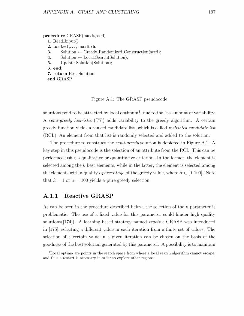
APPENDIX A. GRASP AND CLUSTERING 197
procedure GRASP(maxIt,seed)1. Read Input()2. for k=1,. . . , maxIt do3. Solution ← Greedy Randomized Construction(seed);4. Solution ← Local Search(Solution);5. Update Solution(Solution);6. end;7. return Best Solution;end GRASP
Figure A.1: The GRASP pseudocode
solutions tend to be attracted by local optimum1, due to the less amount of variability.
A semi-greedy heuristic ([77]) adds variability to the greedy algorithm. A certain
greedy function yields a ranked candidate list, which is called restricted candidate list
(RCL). An element from that list is randomly selected and added to the solution.
The procedure to construct the semi-greedy solution is depicted in Figure A.2. A
key step in this pseudocode is the selection of an attribute from the RCL. This can be
performed using a qualitative or quantitative criterion. In the former, the element is
selected among the k best elements; while in the latter, the element is selected among
the elements with a quality αpercentage of the greedy value, where α ∈ [0, 100]. Note
that k = 1 or α = 100 yields a pure greedy selection.
A.1.1 Reactive GRASP
As can be seen in the procedure described below, the selection of the k parameter is
problematic. The use of a fixed value for this parameter could hinder high quality
solutions([174]). A learning-based strategy named reactive GRASP was introduced
in [175], selecting a different value in each iteration from a finite set of values. The
selection of a certain value in a given iteration can be chosen on the basis of the
goodness of the best solution generated by this parameter. A possibility is to maintain
1Local optima are points in the search space from where a local search algorithm cannot escape,and thus a restart is necessary in order to explore other regions.
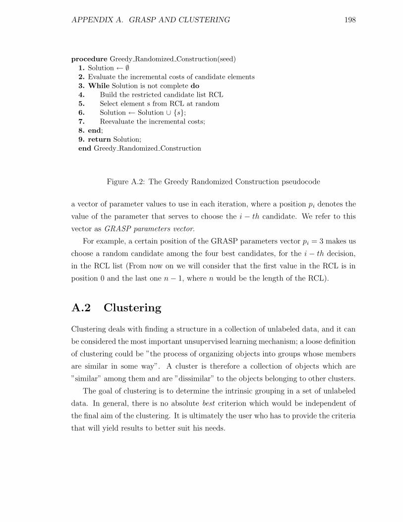
APPENDIX A. GRASP AND CLUSTERING 198
procedure Greedy Randomized Construction(seed)1. Solution ← ∅2. Evaluate the incremental costs of candidate elements3. While Solution is not complete do4. Build the restricted candidate list RCL5. Select element s from RCL at random6. Solution ← Solution ∪ {s};7. Reevaluate the incremental costs;8. end;9. return Solution;end Greedy Randomized Construction
Figure A.2: The Greedy Randomized Construction pseudocode
a vector of parameter values to use in each iteration, where a position pi denotes the
value of the parameter that serves to choose the i − th candidate. We refer to this
vector as GRASP parameters vector.
For example, a certain position of the GRASP parameters vector pi = 3 makes us
choose a random candidate among the four best candidates, for the i − th decision,
in the RCL list (From now on we will consider that the first value in the RCL is in
position 0 and the last one n− 1, where n would be the length of the RCL).
A.2 Clustering
Clustering deals with finding a structure in a collection of unlabeled data, and it can
be considered the most important unsupervised learning mechanism; a loose definition
of clustering could be ”the process of organizing objects into groups whose members
are similar in some way”. A cluster is therefore a collection of objects which are
”similar” among them and are ”dissimilar” to the objects belonging to other clusters.
The goal of clustering is to determine the intrinsic grouping in a set of unlabeled
data. In general, there is no absolute best criterion which would be independent of
the final aim of the clustering. It is ultimately the user who has to provide the criteria
that will yield results to better suit his needs.

APPENDIX A. GRASP AND CLUSTERING 199
However, when implementing a clustering algorithm, several requirements should
be satisfied: scalability, possibility of dealing with different types of attribute, discov-
ering clusters with arbitrary shape, ability to deal with noise, insensivity to order of
input records, high dimensionality, interpretability and usability (among others).
Current clustering techniques suffer from the following drawbacks:
• They do not usually address all the requirements adequately and concurrently.
• Time complexity is a major problem when dealing with large number of data.
• In many occasions, the effectiveness depends on the definition of distance.
• Distance has to be define when it is not obvious, which might be difficult,
especially when dealing with multi-dimensional spaces.
• The result of the clustering algorithm can be interpreted in different ways.
A.2.1 Clustering Algorithms
Clustering Algorithms can be classified as follows:
• Exclusive Clustering.
• Overlapping Clustering.
• Hierarchical Clustering.
• Probabilistic Clustering.
In the first case data are grouped in an exclusive ways, this means that every
individual piece of information is included in one cluster and cannot be include in
another one. On the contrary, the second type uses fuzzy sets to cluster data, so
every point belongs to different clusters with a certain degree of memebership. The
hierarchical clustering algorithm is based on the union between the two nearest clus-
ters; the beginning condition is performed by setting every point as a cluster, and
after a few iterations it reaches the final cluster. Finally, the last type of clustering
algorithm relys on a completely probabilistic approach.
APPENDIX A. GRASP AND CLUSTERING 200
K-Means Algorithm
This is one of the most popular clustering algorithms that fall in the category of
Exclusive Clustering. Since this is the clustering method used in our hybrid, we are
going to briefly detail it here.
It is indeed one of the simplest unsupervised learning algorithms ([149]). The
procedure follows a simple and easy way to classify a given data set through a certain
number of clusters k fixed a priori. The main idea is to define k centroids, each
one corresponding to each clustering. The next step is to associate each point to
its nearest centroid. This yields a first grouping of the data. At this point we need
to re-calculate the k new centroids as barycenters of the clusters resulting from the
previous step. After the new centroids have been calculated, each point needs to be
re-associate to a centroid again. The algorithm now iterates this process until either
no cluster changes for any point occur or a stopping criterion is reached.
This algorithm aims at minimizing an objective function, in this case a squared
error function:
J =k∑
j=1
n∑
i=1
‖x(j)i − cj‖2 (A.1)
where ‖x(j)i − cj‖2 is a chosen distance measure between a data point x
(j)i and the
cluster centroid cj, indicating the distance of the n data points from their respective
cluster centres.
A.2.2 Distance Measure
As we have previuosly stated, defining the distance measure is a problematic task.
If the components of the data instance vectors are all in the same physical units
(metric), then it is possible that the simple Euclidean distance metric is sufficient to
group similar distances. However, even in this case, the Euclidean distance can be
misleading. It is dependant from the range: if one metric spans the range [0.0, 0.5]
and another spans [0.0, 100.0], the maximum deviation in the first would have little
effect on the total distance, while even a modest separation in the second would have
a much larger effect. To remove this dependency it is important to standarize the

APPENDIX A. GRASP AND CLUSTERING 201
values. In order to achieve this, the following steps must be taken:
1. Sum the values of the metric over all objects and divide the sum by the number
of objects.
2. Substract this average value from the metric in all objects.
3. Sum the squares of these new values, divide the sum by the total number of
objects and take its square-root. This is the standard deviation of the new
values.
4. Divide the metric by the standard deviation in each object.
Assume now that each object is described by a real-valued array of metrics of
length K, the i-th object xi has the array xki for k = 1, 2, . . . , K. The general form
for the distance, which is called the LN norm, between object i and centroid j is
LNij = [
K∑
k=1
| xki − xkj |p]1/p (A.2)
When p = 1 this distance measure is known as the Manhattan distance, while for
p = 2 it is known as the Euclidean distance.
Binary Data
When dealing with binary arrays of data, the distance measures defined so far are
not valid. Even though there are many possibilities, the simplest one is to use the
cosine similarity function ([196]). The cosine similarity function CSij between object
i and j treats the objects as vectors and it calculates the cosine of the angle between
these vectors. This similarity, which is also known as the Ochini coefficient, is given
by the expression
CSij =
∑Kk=1 xkixkj√∑K
k=1 x2ki
∑Kki=1 x
2kj
(A.3)
Note that as the objects become more similar, CSij approaches 1.0.

Bibliography
[1] E. Aarts and P. van Laarhoven. Statistical cooling: A general approach to
combinatorial optimization problems. Philps Journal of Research, 40:193–226,
1985.
[2] D. Achlioptas, C. Gomes, H. Kautz, and B. Selman. Generating satisfiable
problem instances. In Proceedings of the 17th National Conference on Artificial
Intelligence, AAAI-2000, Austin/TX, USA, pages 256–261. AAAI Press, 2000.
[3] M. Agren. Solving the social golfer using local search.
peg.it.uu.se/ saps02/MagnusAgren/, 2003.
[4] R.K. Ahuja, J.B. Orlin, and D. Sharma. New neighborhood search structures
the capacitated minimum spanning tree problem. Technical report, University
of Florida, 1998.
[5] D. Alcaide, J. Sicilia, and D. Vigo. A tabu search algorithm for the open shop
problem. Trabajos de Investigacion Operativa, 5:283–297, 1997.
[6] A. Anagnostopoulos, L. Michel, P.V. Hentenryck, and Y. Vergados. A simulated
annealing approach to the traveling tournament problem. In CP-AI-OR’03,
Lecture Notes in Computer Science, Montreal, Canada, May 2003. Springer-
Verlag.
[7] C. Ansotegui, F. Manya, R. Bejar, and C. Gomes. Solving many-valued sat
encodings with local search. In Proceedings of the Workshop on Probabilis-
tics Approaches in Search, 18th National Conference on Artificial Intelligence,
AAAI-2002, Edmonton, Canada, 2002, 2002.
202
BIBLIOGRAPHY 203
[8] Y. Asahiro, K. Iwama, and E. Miyano. Random generation of test instances
with controlled attributes. In 2nd DIMACS Challenge Workshop, 1993.
[9] W.C. Babcock. Intermodulation interference in radio systems. Bell Systems
Technical Journal, pages 63–73, 1953.
[10] T. Back, U. Hammel, and H.P. Schwefel. Evolutionary computation: Com-
ments on the history and current state. IEEE Transactions on Evolutionary
Computation, 1(1):3–17, 1997.
[11] J.E. Baker. Reducing bias and inefficiency in the selection algortihm. In 2nd
Int. Conference on Genetic Algorithms and Their Applications, pages 14–21,
1987.
[12] J.M. Baldwin. A new factor in evolution. American Naturalist, 30, 1896.
[13] N. Barnier and P. Brisset. Solving kirkman’s schoolgirl problem in a few seconds.
Constraints, 2005.
[14] R. Battiti and M. Protasi. Reactive local search for the maximum clique prob-
lem. Algorithmica, 29(4):610–637, 2001.
[15] R. Bayardo and R. Schrag. Using csp look-back techniques to solve exceptionally
hard sat instances. In Proceedings of the Second Int. Conference on Principles
and Practice of Constraint Programming, CP-96, 1996.
[16] S. Beale. Using branch-and-bound with constraint satisfaction in optimization
problems. In NCAI-97, pages 209–214, 1997.
[17] S. Beale, S. Nirenburg, and K. Mahesh. Hunter-gatherer: Three search tech-
niques integrated for natural language semantics. In AAAI-96, 1996.
[18] J. Bean. Genetic algorithms and random keys for sequencing and optimization.
ORSA, Journal on Computing, 6:154–160, 1994.
[19] N. Beldiceanu and E. Contejean. Introducing global constraints in chip. Math-
ematical and Computer Modelling, 20(12):97–123, 1994.
BIBLIOGRAPHY 204
[20] T. Benoist and E. Bourreau. Improving global constraints support by local
search. In CP-03 Workshop on Cooperative Solvers (COSOLV-03), 2003.
[21] T. Benoist, E. Gaudin, and B. Rottembourg. Constraint programming con-
tribution to benders decomposition: A case study. In CP-02, pages 603–617,
2002.
[22] C. Bessiere and J.C. Regin. Mac and combined heuristics: Two reasons to for-
sake fc (and cbj?) on hard problems. In 2nd International Conference on Prin-
ciples and Practice of Constraint Programming, CP-96, pages 61–75. Springer,
LNCS, 1118, 1996.
[23] H-G. Beyer and H-P. Schwefel. Evolution strategies. Natural Computing, 1:3–52,
202.
[24] J.R. Bitner and E.M. Reingold. Backtracking programming techniques. Com-
munications of the ACM, 18(11):651–656, 1975.
[25] S. Blackmore. The Meme Machine. Oxford University Press, 1999.
[26] G.S. Bloom and S.W. Golomb. Aplications of numbered undirected graphs.
Proceedings of the IEEE, 65(4):562–570, 1977.
[27] E. Blum, F. Biraud, and J. Ribes. On optimal synthetic linear arrays with appli-
cations to radioastronomy. IEEE Transactions on Anntenas and Propagation,
pages 108–109, 1974.
[28] A. Bockmayr, N. Pisaruk, and A. Aggoun. Network flow problems in constraint
programming. In CP-01, pages 196–210, 2001.
[29] P. Brucker, J. Hurink, B. Jurich, and B. Wostmann. A branch-and-bound
algorithm for the open-shop scheduling problem. Discrete Applied Mathematics,
76:43–59, 1997.
[30] L. Bull, O. Holland, and S. Blackmore. On meme-gene coevolution. Artificial
Life, 6:227–235, 2000.
BIBLIOGRAPHY 205
[31] M. Cebrian and I. Dotu. Grasp-evolution for csps. In To appear GECCO-06,
Seattle, USA, July 2006.
[32] B. Cha and K. Iwama. Performance test of local search algorithms using new
types of random cnf formulas. In IJCAI-95, volume 1, pages 304–310, 1995.
[33] B. Cha and K. Iwama. Adding new clauses for faster local search. In AAAI-96,
pages 332–337, 1996.
[34] K. Chatzikokolakis, G. Boukeas, and P. Stamatopoulos. Construction and re-
pair: A hybrid approach to search in csps. SETN, 3025:342–351, 2004.
[35] B.M.W. Cheng, K.M.F. Choi, J.H.M. Lee, and J.C.K Wu. Constraint propaga-
tion by redundant modeling: an experience report. Constraints, pages 167–192,
1999.
[36] B.M.W. Cheng, J.H.M. Lee, and J.C.K Wu. Speeding up constraint propagation
by redundant modeling. In 2nd International Conference on Principles and
Practice of Constraint Programming, CP-96, pages 91–103. Springer, LNCS
1118, 1996.
[37] M. Clerc. Particle Swarm Optimization. ISTE, 2006.
[38] C. Colbourn. The complexity of completing partial latin squares. Discrete
applied Mathematics, pages 25–30, 1984.
[39] C. Colbourn and Dinitz. The CRC Handbook of Combinatorial Design. CRC
Press, Boca Raton, FL, 1996.
[40] C.J. Colbourn and J.H. Dinitz. Mutually orthogonal latin squares: A brief
survey of constructions. Journal of Statistical Planning and Inference, 95:9–48,
2001.
[41] S.A. Cook. The complexity of theorem proving procedures. In Proceedings of
the 3rd Annual ACM Symposium on the theory of Computation, pages 151–158,
1971.

BIBLIOGRAPHY 206
[42] M. Cooper. An optimal k-consistency algorithm. Artificial Intelligence, 41:89–
95, 1989.
[43] C. Cotta and A.J. Fernandez. A hybrid grasp - evolutionary algorithm approach
to golomb ruler search. In Xin Yao et al., editors, Parallel Problem Solving From
Nature VIII, number 3242 in Lecture Notes in Computer Science, pages 481–
490. Springer, 2004.
[44] B.G.W. Craenen, A.E. Eiben, E. Machiori, and E. Steenbeek. Combining local
search and fitness function adaptation in a ga for solving constraint satisfaction
problems. In GECCO-2000, 2000.
[45] B.G.W. Craenen, A.E. Eiben, and J.I. van Hemert. Comparing evolutionary
algorithms on binary constraint satisfaction problems. IEEE Transactions on
Evolutionary Computation, 7(5):424–445, 2003.
[46] J.M. Crawford and A.B. Baker. Experimental results on the application of
satisfiability algorithms to scheduling problems. In NCAI’94, volume 2, pages
1092–1097, 1994.
[47] A. Dave, D. Tompkins, and H. Hoos. Novelty+ and adaptive novelty+. In SAT
Competition, 2004.
[48] P. David. A constraint-based approach for examination timetabling using local
repair techniques. In PATAT-97, pages 169–186, 1998.
[49] M. Davis, G. Logemann, and D. Loveland. A machine program for theorem-
proving. Comms. ACM, pages 394–397, 1962.
[50] R. Dawkins. The Selfish Gene. Oxford University Press, 1976.
[51] R. Dechter and I. Meiri. Experimental evaluation of preprocessing algorithms
for constraint satisfaction problems. Artificial Intelligence, 68:211–241, 1994.
[52] R. Dechter and J. Pearl. Network-based heuristics for constraint satisfaction
problems. Artificial Intelligence, 34:1–38, 1988.
BIBLIOGRAPHY 207
[53] A. del Val. Simplifying binary propositional theories into connected components
twice as fast. In LPAR’01, Proceedings of the Eigth International Conference on
Logic for Programming, Artificial Intelligence and Reasoning. LNCS, Springer-
Verlag, 2001.
[54] H. Delmaire, J.A. Dıaz, E. Fernandez, and M. Ortega. Reactive grasp and tabu
search based heuristics for the single source capacitated plant location problem.
INFOR, 37:194–225, 1999.
[55] B. Devendeville, L. Saois, and E. Gregoire. Recherche locale: ver une exploita-
tion des proprietes structurelles. In JNPC-00, pages 243–244, 2000.
[56] A. Dollas, W. T. Rankin, and D. McCracken. A new algorithm for golomb ruler
derivation and proof of the 19 mark ruler. IEEE Transactions on Information
Theory, 44:379–382, 1998.
[57] M. Dorigo, V. Maniezzo, and A. Colorni. Ant system: Optimization by a colony
of cooperating agents. IEEE Transactions on Systems, Man, and Cybernetics–
Part B, 26(1):29–41, 1996.
[58] G. Dozier, J. Bowen, and D. Bahler. Solving small and large constraint satis-
faction problems using a heuristic-based micro-genetic aglorithm. In 1st IEEE
Conference on Evolutionary Computation, pages 306–311, 1994.
[59] G. Dozier, J. Bowen, and D. Bahler. Solving randomly generated constraint
satisfaction problems using a micro-evolutionary hybrid that evolves a popula-
tion of hill climbers. In 3rd IEEE Conference on Evolutionary Computation,
pages 614–619, 1995.
[60] O. Dubois, P. Andre, Y. Boufkhad, and J. Carlier. Can a very simple algorithm
be efficient for solving the sat problem? In Proceedings of the Second DIMACS
Challenge, 1993.
[61] O. Dubois, P. Andre, Y. Boufkhad, and J. Carlier. Sat versus unsat. In Pro-
ceedings of the Second DIMACS Challenge, 1993.

BIBLIOGRAPHY 208
[62] N. Een and N. Sorensson. Satzoo. http://www.math.chalmers.se/˜ een/Satzoo/,
2003.
[63] A.E. Eiben. Evolutionary algorithms and constraint satisfaction: Definitions,
survey, methodology, and research directions. Theoretical Aspects of Evolution-
ary Computation, pages 13–58, 2001.
[64] A.E. Eiben, P-E. Rahu’e, and Z. Ruttkay. Genetic algortihms with multi-parent
recombination. In 3rd Conference on Parallel Problem Solving from Nature,
pages 78–87, 1994.
[65] A.E. Eiben, P.E. Raue, and Zs. Ruttkay. Heuristic genetic algorithms for con-
strained problems. part i: Principles. Technical report, Vrije Universiteit Ams-
terdam, 1993.
[66] A.E. Eiben, P.E. Raue, and Zs. Ruttkay. Solving constraint satisfaction prob-
lems using genetic algorithms. In 1st IEEE Conference on Evolutionary Com-
putation, pages 542–547, 1994.
[67] A.E. Eiben, P.E. Raue, and Zs. Ruttkay. Constrained problems. Practical
Handbook of Genetic Algorithms, pages 307–365, 1995.
[68] A.E. Eiben and C.A. Schippers. Multi-parent’s niche: n-ary crossover on nk-
landscapes. In 4th Conference on Parallel Problem Solving from Nature, pages
319–328, 1996.
[69] A.E. Eiben and J.E. Smith. Introduction to Evolutionary Computing. Natural
Computing Series. Springer, 2003.
[70] A.E. Eiben and J.K. van der Hauw. Adaptive penalties for evolutionary graph-
coloring. In Artificial Evolution, pages 95–106, 1998.
[71] A.E. Eiben, J.I. van Hemert, E. Machiori, and E. Steenbeek. solving binary
constraint satisfaction problems using evolutionary algorithms with an adaptive
fitness function. In PPSN-1998, pages 196–205, 1998.

BIBLIOGRAPHY 209
[72] T. Fahle, S. Schamberger, and M. Sellmann. Symmetry breaking. In CP-01,
volume 2293 of LNCS, pages 93–107. Springer Verlag, 2001.
[73] T. Fahle and M. Sellmann. Cost based filtering for the constrained knapsack
problem. Annals of Operations Research, 115:73–94, 2002.
[74] H. Fang, Y. Kilani, J. H. M. Lee, and P. J. Stuckey. Reducing search space in
local search for constraint satisfaction. In Eighteenth National Conference on
Artificial Intelligence, pages 28–33, Edmonton, Alberta, Canada, 2002.
[75] H. Fang and W. Ruml. Complete local search for propositional satisfiability. In
NCAI-04, pages 161–166, 2004.
[76] B. Feeney. Determining optimum and near-optimum golomb rulers using genetic
algorithms. Master thesis, Computer Science, University College Cork, October
2003.
[77] T.A. Feo and M.G.C. Resende. A probabilistic heuristic for a computationally
difficult set covering problem. Operations Research Letters, 8:67–71, 1989.
[78] T.A. Feo and M.G.C. Resende. Greedy randomized adaptive search procedures.
Journal of Global Optimization, 6:109–133, 1995.
[79] B. Freisleben and P. Merz. New genetic local search operators for the traveling
salesman problem. In 4th International Conference on Parallel Problem Solving
from Nature - PPSN IV, pages 890–900, 1996.
[80] E.C. Freuder. Synthesizing constraint expressions. Comm. ACM, 21(11):958–
965, 1978.
[81] E.C. Freuder. A sufficient condition for backtrack-free search. J. ACM,
29(1):24–32, 1982.
[82] B. Friesleben and P. Merz. A genetic local search algorithm for solving the
symmetric and asymmetric traveling salesman problem. In CEC-96, pages 616–
621, 1996.

BIBLIOGRAPHY 210
[83] D. Frost and R. Dechter. Lookahead value ordering for constraint satisfaction
problems. In Proceedings of IJCAI-95, pages 572–578, 1995.
[84] M.R. Garey and D.S. Johnson. Computers and Intractability: A Guide to the
Theory of NP-Completeness. W.H. Freeman, 1979.
[85] M. Garry, D. Vanderschel, et al. In search of the opti-
mal 20, 21 & 22 mark golomb rulers. GVANT project,
http://members.aol.com/golomb20/index.html, 1999.
[86] J. Gaschnig. A general backtracking algorithm that eliminates most redundant
tests. In Proceedings of IJCAI-77, pages 457–462, 1977.
[87] J. Gaschnig. Experimental case studies of backtrack vs. waltz-type vs. new
algorithms for satisficing assignment problems. In Proceedings of Canadian
Artificial Intelligence Conference, pages 268–277, 1978.
[88] P.A. Geelen. Dual viewpoint heuristics for binary constraint satisfaction prob-
lems. In ECAI’92, pages 572–578, August 1995.
[89] I. Gent. Arc consistency in sat. In Proceedings of the 15th European Conference
on Artificial Intelligence (ECAI), Lyon, France, 2002.
[90] I. Gent and T. Walsh. Csplib: A benchmark library for constraints.
http://csplib.org, 1999.
[91] D. Ghosh and G. Sierksma. Complete local search with memory. Technical
report, University of Groningen, 2000.
[92] M.L. Ginsberg. Dynamic backtracking. JAIR, pages 25–46, 1993.
[93] M.L. Ginsberg and D.A. McAllester. Gsat and dynamic backtracking. In 4th
International Conference on Principles of Knowledge Representation and Rea-
soning 1994, pages 226–237, 1994.
[94] F. Glover. A template for scatter search and path relinking. Lecture Notes in
Computer Science, 1363:13–54, 1997.
BIBLIOGRAPHY 211
[95] F. Glover and M. Laguna. Modern heuristic techniques for combinatorial prob-
lems. Blackwell Scientific Publishing, 1993.
[96] D. Golberg. Genetic Algorithms in Search, Optimization and Machine Learning.
Addison-Wesley, 1989.
[97] E. Goldberg and Y. Novikov. Berkmin: A fast and robust sat-solver. In Proc.
of DATE’02, 2002.
[98] C. Gomes, B. Selman, and N. Crato. Heavy-tailed phenomena in satisfiability
and constraint satisfaction problems. Journal of Automated Reasoning, 24(1–
2):67–100, 2000.
[99] C. Gomes, B. Selman, and H. Kautz. Boosting combinatorial search through
randomization. In Proceedings of the 15th National Conference on on Artificial
Intelligence, pages 431–437, 1998.
[100] C. Gomes and D. B. Shmoys. Completing quasigroups or latin squares: A struc-
tured graph coloring problem. In Proc. Computational Symposium on Graph
Coloring and Extensions, 2002.
[101] C. Gomes and D. B. Shmoys. The promise of lp to boost csp techniques for
combinatorial problems. In CP-AI-OR’02, pages 291–305, 2002.
[102] J.J. Grefenstette. Incooperating problem speci
c knowledge into genetic algorithms. Genetic Algorithms and Simulated An-
nealing, pages 42–60, 1987.
[103] J. Gu. Efficient local search for very large-scale satisfiability problems. ACM
SIGART Bulletin, 3(1):8–12, 1992.
[104] C. Gueret, N. Jussien, and C. Prins. Using intelligent backtracking to improve
branch and bound methods: an application to open-shop problems. European
Journal of Operational Research, 127(2):344–354, 2000.
BIBLIOGRAPHY 212
[105] C. Gueret and C. Prins. A new lower bound for the open-shop problem. Annals
of Operations Research, 92:165–183, 1999.
[106] D. Habet, C.M. Li, L. Devendeville, and M. Vasquez. A hybrid approach for
sat. In CP-02, pages 172–184, 2002.
[107] D. Habet and M. Vasquez. Saturated and consistent neighborhood for selecting
and scheduling photographs of agile earth observing satellite. In Fifth Meta-
heuristics International Conference, 2003.
[108] H. Handa, N. Baba, O. Katai, and T. Sawaragi. Solving constraint satisfaction
problems by using coevolutionary genetic algorithms. In 4th IEEE Conference
on Evolutionary Computation, pages 21–26, 1998.
[109] H. Handa, N. Baba, O. Katai, T. Sawaragi, and T. Horiuchi. Genetic algorithm
involving coevolution mechanism to search for effective genetic information. In
4th IEEE Conference on Evolutionary Computation, 1997.
[110] R. Haralick and G. Elliot. Increasing tree search efficiency for constraint-
satisfaction problems. Artificial Intelligence, 14(3):263–313, 1980.
[111] E. Hart, P.Ross, and J. Nelson. Solving a real-world problem using an evolving
heuristically driven schedule builder. Evolutionary Computation, 6(1):61–81,
1998.
[112] W. Harvey and M. Ginsberg. Limited discrepancy search. In 14th IJCAI, pages
607–615. Morgan Kaufmann, 1995.
[113] W. Harvey and T. Winterer. Solving the molr and social golfers problems. In
11th International Conference on Constraint Programming (CP-2005), Stiges,
Spain, September 2005.
[114] B. Hayes. Collective wisdom. American Scienist 86, pages 118–122, 1998.
[115] P. Van Hentenryck and L. Michel. Constraint-Based Local Search. MIT Press,
2005.
BIBLIOGRAPHY 213
[116] G.E. Hinton and S.J. Nowlan. How learning can guide evolution. Complex
Systems, 1:495–502, 1987.
[117] E.A. Hirsch and A. Kojevnikov. Unitwalk: a new sat solver that uses local
search guided by unit clause elimination. Annals of Mathematics and Artificial
Intelligence, 43(1–4):91–111, 2005.
[118] B. Hnich, B. M. Smith, and T. Walsh. Dual modelling of permutation and
injection problems. Journal of Artificial Intelligence Research, 2004. to appear.
[119] J.H. Holland. Adaption in Natural and Artificial Systems. MIT Press, 1975.
[120] J.N. Hooker and V. Vinay. Branching rules for satisfiability. Journal of Auto-
mated Reasoning, 15:359–383, 1995.
[121] H. Hoos. On the run-time behavior of stochastic local search algorithms for sat.
In 16th NCAI-96, pages 661–666, 1999.
[122] H. Hoos and T. Stutzle. Systematic vs. local search for sat. In KI-99, pages
279–293, 1999.
[123] H. Hoos and T. Stutzle. Local search algorithms for sat: an empirical evaluation.
Journal of Automated Reasoning, 24:421–481, 2000.
[124] H.H. Hoos and T. Stuzle. Satlib: An online resource for research on sat. In
SAT-00, pages 283–292, 2000.
[125] C. Houck, J.A. Joines, M.G. Kay, and J.R. Wilson. Empirical investigation of
the benefits of partial lamarckianism. Evolutionary Computation, 5(1):31–60,
1997.
[126] M. Huang, F. Romeo, and A. Sangiovanni-Vincentelli. An efficient general
cooling scheduling for simulated annealing. In IEEE International Conference
on Computer-Aided Design, Santa Clara, CA, November 1986.
[127] F. Hutter, D.A.D. Tompkins, and H.H. Hoos. Scaling and probabilistic smooth-
ing. efficient dynamic local search for sat. In CP-02, pages 233–248, 2002.
BIBLIOGRAPHY 214
[128] M.T. Jacobson and P. Mathews. Generating uniformly distributed random latin
squares. Journal of Combinatorial Designs, 4(6):405–437, 1996.
[129] R.E. Jeroslow and J. Wang. Solving propositional satisfiability problems. An-
nals of Mathematics and Artificial Intelligence, 1:167–187, 1990.
[130] T. Jones. Evolutionary Algorithms, Fitness Landscapes and Search. PhD thesis,
The University of New Mexico, 1995.
[131] N. Jussien. e-constraints: explanation-based constraint programming. In CP-01
Workshop of User-Interaction in Constraint Sarisfaction, 2001.
[132] N. Jussien, R. Debruyne, and P. Boizumault. Maintaining arc-consistency
within dynamic backtracking. In CP-00, pages 249–261, 2000.
[133] N. Jussien and O. Lhomme. Local search with constraint propagation and
conflict-based heuristics. Artificial Intelligence, 139:21–45, 2002.
[134] N. Jussien and O. Lhomme. Unifying search algorithms for csp. Technical
report, Ecole des Mines de Nantes, France, 2002.
[135] N. Jussien and O. Lhomme. Combining constraint programming and local
search to design new powerful heuristics. In MIC-03, pages 281–287, 2003.
[136] H. Kautz, Y. Ruan, D. Achlioptas, C. Gomes, B. Selman, and M. Stickel. Bal-
ance and filtering in structured satisfiable problems. In Proceedings of the In-
ternational Joint Conference on Artificial Intelligence, IJCAI’01, Seattle/WA,
USA, pages 351–358, 2001.
[137] H. Kautz and B. Selman. Planning as satisfiability. In ECAI-92, pages 359–363,
1992.
[138] N. Keng and D. Yun. A planning/scheduling metodology for the constrained
resource problem. In Proceedings of IJCAI-89, pages 998–1003, 1989.
[139] T. Klove. Bounds and construction for difference triangle sets. IEEE Transac-
tions on Information Theory, 35:879–886, July 1989.
BIBLIOGRAPHY 215
[140] S. Koziel and Z. Michalewicz. A decoder-based evolutionary algorithm for con-
strained parameter optimization problems. In T. Baeck, A.E. Eiben, M. Schoe-
nauer, and H.-P. Schwefel, editors, Parallel Problem Solving from Nature V,
volume 1498 of Lecture Notes in Computer Science, pages 231–240. Springer-
Verlag, 1998.
[141] N. Kranogor. Studies in the Theory and Design Space of Memetic Algorithms.
PhD thesis, University of the West of England, 2002.
[142] M. Laguna and R. Martı. Scatter Search. Methodology and Implementations in
C. Kluwer Academic Publishers, 2003.
[143] P. Langley. Systematic and nonsystematic search strategies. In 1st Int. Con-
ference on AI Planning Systems, 1992.
[144] C. M. Li and Anbulagan. Look-ahead versus look-back for satisfiability prob-
lems. In Proceedings of the 3rd International Conference on Principles of Con-
straint Programming, CP’97, Linz, Austria, pages 341–355. Springer, LNCS
1330, 1997.
[145] C.M. Li and Anbulagan. Heuristic based on unit propagation for satisfiability.
In CP-97, pages 342–356, 1997.
[146] C.F. Liaw. A tabu search algorithm for the open shop scheduling problem.
Computers and Operations Research, 26:109–126, 1999.
[147] X. Liu, P.M. Pardalos, S. Rajasekaran, and M.G.C. Resende. A grasp for
frequency assignment in mobile radio networks. Mobile networks and computing,
52:195–201, 2000.
[148] A.K. Mackworth. Consistency in networks of relations. Artificial Intelligence,
8(1):99–118, 1977.
[149] J.B. MacQueen. Some methods for classification and analysis of multivariate
observations. In 5th Berkeley Syposium on Mathematical Statistics and Proba-
bility, pages 281–297, 1967.
BIBLIOGRAPHY 216
[150] E. Marchiori. Combining constraint processing and genetic algorithms for con-
straint satisfaction problems. In 7th International Conference on Genetic Al-
gorithms, pages 330–337, San Francisco, CA, 1997.
[151] E. Marchiori and E. Steenbeek. A genetic local search algorithm for random
binary constraint satisfaction problems. In ACM Symposium on Applied Com-
puting, 2000.
[152] G. Mayley. Landscapes, learning costs and genetic assimilation. Evolutionary
Computation, 4(3):213–234, 1996.
[153] D. McAllester, B. Selman, and H. Kautz. Evidence for invariants in local search.
In 14th NCAI-97, pages 321–326, 1997.
[154] P. Meseguer and T. Walsh. Interleaved and discrepancy based search. In Pro-
ceedings of the 13th ECAI, 1998.
[155] Z. Michalewicz. A survey of constraint handling techniques in evolutionary
computation methods. In 4th Int. Conference on Evolutionary Programming,
pages 135–155, 1995.
[156] Z. Michalewicz. Genetic Algorithms + Data Structures = Evolution Programs.
Springer, 1996.
[157] Z. Michalewicz and M. Attia. Evolutionary optimization of constrained prob-
lems. In 3rd Int. Conference on Evolutionary Programming, pages 98–108, 1994.
[158] Z. Michalewicz and M. Schoenauer. Evolutionary agorithms for constraint pa-
rameter optimization problems. Evolutionary Computation, 4(1):1–32, 1996.
[159] P. Mills, E. Tsang, Q. Zhang, and J. Ford. A survey of ai-based meta-heursitics
for dealing with local optima in local search. Technical report, Department of
Computer Science, University of Essex, 2004.
[160] S. Minton, M.D. Johnston, A.B. Philips, and P. Laird. Minimizing conflicts:
a heuristic repair method for constraint satisfaction and scheduling problems.
Artificial Intelligence, 58:161–205, 1992.
BIBLIOGRAPHY 217
[161] M. Mladenovic and P. Hansen. Variable neighborhood search. Computers in
Operations Research, 24:1097–1100, 1997.
[162] P. Morris. The break-out method for escaping from local minima. In AAAI-93,
pages 40–45, 1993.
[163] P. Moscato. On evolution, search, optimization, genetic algorithms and mar-
tial arts: Towards memetic algorithms. Technical report, Caltech Concurrent
Computation Program, Pasadena, California, 1989.
[164] P. Moscato and C. Cotta. A gentle introduction to memetic algorithms. In
F. Glover and G. Kochenberger, editors, Handbook of Metaheuristics, pages
105–144. Kluwer Academic Publishers, 2003.
[165] M. Moskewicz, C. Madigan, Y. Zhao, L. Zhang, and S. Malik. Chaff: Engineer-
ing an efficient sat solver. In 39th Design Automation Conference, 2001.
[166] H. Muhlenbein. Parallel genetic algortihms, population genetics and combi-
natorial optimization. In 3rd Int. Conference on Genetic Algorithms, pages
416–421, 1989.
[167] A. Nareyek. Using global constraints for local search. In DIMACS Workshop
on Constraint Programming and Large Scale Discrete Optimization, 1994.
[168] A. Nareyek, S.F. Smith, and C.M. Ohler. Integrating local-search advice in-
tro refinement search (or not). In CP 2003 Third International Workshop on
Cooperative Solvers in Constraint Programming, pages 29–43, 2003.
[169] J. Paredis. Co-evolutionary computation. Artificial Life, 2(4):355–375, 1995.
[170] J. Paredis. Coevolving cellular automata: Be aware of the red queen. In 7th
International Conference on Genetic Algorithms, San Francisco, CA, 1997.
[171] G. Peasant and M. Gendreau. A view of local search in constraint programming.
In CP-96, pages 353–366, 1996.
BIBLIOGRAPHY 218
[172] G. Peasant, M. Gendreau, J-Y. Potvin, and J-M. Rousseau. An optimal algo-
rithm for the traveling salesman problem with time windows using constraint
logic programming. Technical report, Centre du reserche sur les transports,
University of Montreal, 1996.
[173] F.B. Pereira, J. Tavares, and E. Costa. Golomb rulers: The advantage of evolu-
tion. In F. Moura-Pires and S. Abreu, editors, Progress in Artificial Intelligence,
11th Portuguese Conference on Artificial Intelligence, number 2902 in Lecture
Notes in Computer Science, pages 29–42. Springer-Verlag, 2003.
[174] M. Prais and C.C. Ribeiro. Parameter variation in grasp procedures. Investi-
gacion Operativa, 9:1–20, 2000.
[175] M. Prais and C.C. Ribeiro. Reactive grasp: an application to a matrix decom-
position problem in tdma traffic assignment. INFORMS Journal on Computing,
12:164–176, 2000.
[176] S. Prestwich. Trading completeness for scalability: Hybrid search for cliques
and rulers. In Third International Workshop on the Integration of AI and OR
Techniques in Constraint Programming for Combinatorial Optimization Prob-
lems (CPAIOR-2001), 2001.
[177] S. Prestwich. Combining the scalability of local search with the pruning tech-
niques of systematic search. Annals of Operations Research, 115:51–72, 2002.
[178] S. Prestwich. Randomized backtracing for linear pseudo-boolean constraint
problems. In CP-AI-OR’02, pages 7–19, Le Croisic, France, March 2002.
[179] S. Prestwich and A. Roli. Symmetry breaking and local search spaces. In
CPAIOR-05, 2005.
[180] S.D. Prestwich. Supersymmetric modeling for local search. In Second Interna-
tional Workshop on Symmetry in Constraint Satisfaction Problems, 2002.
[181] S.D. Prestwich. Negative effects of modeling techniques on search performance.
Annals of Operations Research, 118:137–150, 2003.
BIBLIOGRAPHY 219
[182] C. Prins. Competitive genetic algortihms for the open-shop scheduling problem.
Mathematical Methods of Operations Research, 52(3):389–411, 2000.
[183] P. Prosser. Hybrid algorithms for the constraint satisfaction problem. Compu-
tational Intelligence, 9(3):268–299, 1993.
[184] J.F. Puget. Symmetry breaking revisited. Constraints, 2005.
[185] C. Quimper, P. van Beek, A. Lopez-Ortiz, A. Golynski, and S.B. Sadjad. An
efficient bounds consistency algorithm for the global cardinality constraint. In
CP-03, pages 600–614, 2003.
[186] N.J Radcliffe. Equivalence class analysis of genetic algorithms. Complex Sys-
tems, 5:183–205, 1991.
[187] W.T. Rankin. Optimal golomb rulers: An exhaustive parallel search implemen-
tation. Master thesis, Duke University Electrical Engineering Dept., December
1993.
[188] J-C. Regin. A filtering algorithm for constraints of difference in csps. In AAAI-
94, pages 363–367, 1994.
[189] R. Reiter and A. Mackworth. A logical framework for depiction and image
interpretation. Artificial Intelligence, 41(2):125–155, 1989.
[190] M.G.C Resende and C.C Ribeiro. Greedy randomized adaptive search proce-
dures. In F. Glover and G. Kochenberger, editors, Handbook of Metaheuristics,
pages 219–249. Kluwer Academic Publishers, 2003.
[191] M.C. Riff-Rojas. Using the knowledge of the constraint network to design an
evolutionary algorithm that solves csp. In 3rd IEEE Conference on Evolutionary
Computation, pages 279–284, 1996.
[192] M.C. Riff-Rojas. Evolutionary search guided by the constraint network to solve
csp. In 4th IEEE Conference on Evolutionary Computation, pages 337–348,
1997.
BIBLIOGRAPHY 220
[193] A. Rogers and A. Prugel-Bennett. Modelling the dynamics of a steady state
genetic algortihm. In Foundations of Genetic Algorithms, pages 57–68, 1999.
[194] N Roos, Y.P. Ran, and H.v.d.H. Combining local search and constraint prop-
agation to find a minima change solution for a dynamic csp. In AIMSA-00,
2000.
[195] D. Sabin and E.C. Freuder. Contradicting conventional wisdom in constraint
satisfaction. In Proceedings of ECAI-94, pages 125–129, 1994.
[196] G. Salton. Automatic Text Processing: The Transformation, Analysis and Re-
trieval of Information by Computer. Addison-Wesley, 1989.
[197] A. Schaerf. Combining local search and look-ahead for scheduling and constraint
satisfaction problems. In IJCAI-97, pages 1254–1259, 1997.
[198] W. Schneider. Golomb rulers. MATHEWS: The Archive of Recreational Math-
ematics, http://www.wschnei.de/number-theory/golomb-rulers.html,
2002.
[199] M. Sellmann. Reduction Techniques in Constraint Programming and Combina-
torial Optimization. PhD thesis, University of Paderborn, Germany, 2003.
[200] M. Sellmann and W. Harvey. Heuristic constraint propagation – using local
search for incomplete pruning and domain filtering of redundant constraints for
the social golfer problem. In CP-AI-OR’02, pages 191–204, Le Croisic, France,
March 2002.
[201] B. Selman, H. Kautz, and D. McAllester. Ten challenges in propositional rea-
soning and search. In IJCAI-97, pages 50–54, 1997.
[202] B. Selman, H.J. Levesque, and D. Mitchell. A new method for solving hard
satisfiability problems. In NCAI-92, pages 440–446, 1992.
[203] Y. Shang and B.W. Wah. A discrete lagrangian-based global-search strategy
in discrete langrangian methods for solving satisfiability problems. Journal of
Global Optimization, 10(1):1–40, 1997.
BIBLIOGRAPHY 221
[204] P. Shaw. Using constraint programming and local search methods to solve
vehicle routing problems. In CP-98, pages 417–431, 1998.
[205] J. B. Shearer. Golomb ruler table. Mathematics Department, IBM Research,
http://www.research.ibm.com/people/s/shearer/grtab.html, 2001.
[206] H. Shen and H. Zhang. Antoher complete local search method for sat. In
LPAR-05, pages 595–605, 2005.
[207] L. Simon. The sat-03 contest results site.
http://www.lri.fr./simon/contest03/results, 2003.
[208] J. Slaney, M. Fujita, and M. Stickel. Automated reasoning and exhaustive
search: Quasigroup existence problems. Computers and Mathematics with Ap-
plications, 29:115–132, 1995.
[209] B. Smith. Reducing symmetry in a combinatorial design problem. In CP-AI-
OR’01, pages 351–359, Ashford, Kent UK, April 2001.
[210] B. Smith, K. Stergiou, and T. Walsh. Modelling the golomb ruler problem,
1999.
[211] B. M. Smith. Modeling a permutation problem. In Proceedings of ECAI’2000
Workshop on Modeling and Solving Problems with Constraints, 2000.
[212] B. M. Smith. Dual models in constraint programming. Technical report, School
Computing Research Report 2001.02, University of Leeds, 2001.
[213] S.W. Soliday, A. Homaifar, and G.L. Lebby. Genetic algorithm approach to the
search for golomb rulers. In L.J. Eshelman, editor, 6th International Conference
on Genetic Algorithms (ICGA-95), pages 528–535. Morgan Kaufmann, 1995.
[214] G. Solotorevsky, E. Gudes, and A. Meisels. Raps: A rule-based language spec-
ifying resource allocation and time-tabling problems. IEEE Transactions on
Knowledge and Data Engineering, 6(5):681–697, 1994.

BIBLIOGRAPHY 222
[215] K. Stergiou and T. Walsh. The difference all-difference makes. In Proc. IJ-
CAI’99, 1999.
[216] P. Surry and N. Radcliffe. Innoculation to initialise evolutionary search. In
Evolutionary Computing: AISB-96 Workshop, pages 269–285, 1996.
[217] E. Taillard. Benchmarks for basic scheduling problems. European Journal of
Operations Research, 64:278–285, 1993.
[218] S.R. Thangiah, R. Vinayagamoorty, and A.V. Gubbi. Vehicle routing and dead-
lines using genetic and local algorithms. In 5th Int. Conference on Genetic
Algorithms, pages 506–515, 1993.
[219] M. Trick. A dynamic programming approach for consistency and propagation
for knapsack constraints. In CPAIOR-01, pages 113–124, 2001.
[220] E. Tsang and N. Foster. Solution synthesis in the constraint satisfaction prob-
lem. Technical report, University of Essex, 1990.
[221] S. Tsutsui. Multi-parent recombination in genetic algorithms with search space
boundary extension by mirroring. In 5th Conference on Parallel Problem Solving
from Nature, pages 428–437, 1998.
[222] P.D. Turney. How to shift bias: lessons from the baldwin effect. Evolutionary
Computation, 4(3):271–295, 1996.
[223] R. Unger and J. Moult. A genetic algortihm for 3d protein folding simulations.
In 5th Int. Conference on Genetic Algorithms, pages 581–588, 1993.
[224] P. van Beek and X. Chen. Cplan: A constraint programming approach to
planning. In AAAI’99, pages 585–590, 1999.
[225] J.K. van der Hauw. Evaluating and improving steady state evolutionary algo-
rithms on constraint satisfaction problems. Master thesis, Leiden University,
1996.

BIBLIOGRAPHY 223
[226] J.I. van Hemert. Aplying adaptive evolutionary algorithms to hard problems.
Master thesis, Leiden University, 1998.
[227] W.J. van Hoere. The alldifferent constraint: A survey. In Proceedings of the
6th Annual Workshop of the ERCIM Working Group on Constraints, Prague,
2001.
[228] F. Vavak and T.C. Fogarty. Comparison of steady state and generational genetic
algortihms for use in nonstationary environments. In ICEC-96, pages 192–195,
1996.
[229] T. Walsh. Permutation problems and channeling constraints. In LPAR-2001,
2001.
[230] L.D. Whitely, S. Gordon, and K.E. Mathias. Lamarckian evolution, the baldwin
effect, and function optimisation. In 3rd Conference on Parallel Problem Solving
from Nature, pages 6–15, 1994.
[231] L.D. Whitely and F. Gruau. Adding learning to the cellular development of
neural networks: evolution and the baldwin effect. Evolutionary Computation,
1:213–233, 1993.
[232] L.D. Whitely and J. Kauth. Genitor: a different genetic algortihm. In Rocky
Mountain Conference on Artificial Intelligence, pages 118–130, 1988.
[233] M. Yokoo. Weak-commitment search for solving constraint satisfaction prob-
lems. In AAAI-94, pages 313–318, 1994.
[234] M. Yokoo. Why adding more constraints makes a problem easier for hill-
climbing algorithms: Analyzing landscapes of csps. In CP-97, pages 356–370,
1997.
[235] M. Yoshikawa, K. Kaneko, T. Yamanouchi, and M. Watanabe. A constraint-
based high school scheduling system. IEEE Expert, 11(1):63–72, 1996.

BIBLIOGRAPHY 224
[236] J. Zhang and H. Zhang. Combining local search and backtracking techniques
for constraint satisfaction. In AAAI-96, pages 369–374, 1996.