Citation: Chandrahas, N.S.;

Choudhary, B.S.; Teja, M.V.;

Venkataramayya, M.S.; Prasad,

N.S.R.K. XG Boost Algorithm to

Simultaneous Prediction of Rock

Fragmentation and Induced Ground

Vibration Using Unique Blast Data.

Appl. Sci. 2022, 12, 5269. https://

doi.org/10.3390/app12105269

Academic Editor: Lina M. López

Received: 25 April 2022

Accepted: 22 May 2022

Published: 23 May 2022

Publisher’s Note: MDPI stays neutral

with regard to jurisdictional claims in

published maps and institutional affil-

iations.

Copyright: © 2022 by the authors.

Licensee MDPI, Basel, Switzerland.

This article is an open access article

distributed under the terms and

conditions of the Creative Commons

Attribution (CC BY) license (https://

creativecommons.org/licenses/by/

4.0/).

applied sciences

Article

XG Boost Algorithm to Simultaneous Prediction of RockFragmentation and Induced Ground Vibration Using UniqueBlast DataN. Sri Chandrahas 1,2, Bhanwar Singh Choudhary 1,* , M. Vishnu Teja 3, M. S. Venkataramayya 2

and N. S. R. Krishna Prasad 2

1 Department of Mining Engineering, IIT (ISM) Dhanbad, Dhanbad 826004, India; srichandrahas@mrec.ac.in2 Department of Mining Engineering, Malla Reddy Engineering College, Hyderabad 500100, India;

iiic@mrec.ac.in (M.S.V.); nsrkprasad@mrec.ac.in (N.S.R.K.P.)3 Mai-Nefhi College of Engineering and Technology, Mai-Nefhi P.O. Box 5230, Eritrea; mvteja1995@gmail.com* Correspondence: bhanwarschoudhary@iitism.ac.in

Abstract: The two most frequently heard terms in the mining industry are safety and production.These two terms put a lot of pressure on blasting engineers and crew to give more while consumingless. The key to achieving the optimum blasting results is sophisticated bench analysis, which mustbe combined with design blast parameters for good fragmentation and safe ground vibration. Thus,a unique solution for forecasting both optimum fragmentation and reduced ground vibration usingrock mass joint angle and blast design parameters will aid the blasting operations in terms of costsavings. To arrive at a proper understanding and a solution, 152 blasts were carried out in variousmines by adjusting blast design parameters concerning the measured joint angle. The XG Boost,K-Nearest Neighbor, and Random Forest algorithms were evaluated, and the XG Boost outputs wereshown to be superior in terms of Mean Absolute Percentage Error (MAPE), Root Mean SquaredError (RMSE), and Co-efficient of determination (R2) values. Using XG Boost, the decision-tree-basedensemble Machine Learning algorithm that uses a gradient-boosting framework and a simultaneousformula was developed to predict both fragmentation and ground vibration using joint angle and thesame set of parameters.

Keywords: rock joints; drones; XG Boost; fragmentation; PPV

1. Introduction

The use of explosive energy in blasting affects both rock fragmentation and inducedground vibration. Rock movement may be desired, and manifests in amuck profile suitablefor the loading equipment. The complete and proper utilization of explosive energy is themain objective in this process; energy used in achieving proper fragmentation automaticallyreduces negative aspects such as ground vibration. Positive blast results can be obtainedby equalizing the energy of the explosive to the strength of the rock, optimum designparameters, and geospatial positioning of the blast holes.

There are many equations in blasting to make use of explosive energy properly toyield a safe and effective blast, but most formulas are designed based on controllableparameters such as burden, spacing, bench height, hole diameter, stemming, decking, firingpattern, and quantity of explosive, etc. Many researchers have revealed that uncontrollableparameters such as joints and bedding planes, rock compressive and tensile strengths alsosignificantly affect the performance of the blast in terms of fragmentation and groundvibration. The daunting task of any blasting engineer is to ensure that the selected blastdesign parameters meet all post-blast requirements and the targeted fragmentation of anenterprise. Blast-induced ground vibrations are a major issue to be tackled.

The presence of geological discontinuities in a rock mass can significantly influenceboth rock fragmentation and ground vibration [1–3]. Joints are among the most common

Appl. Sci. 2022, 12, 5269. https://doi.org/10.3390/app12105269 https://www.mdpi.com/journal/applsci

Appl. Sci. 2022, 12, 5269 2 of 25

defects in the rock mass and are also defined as planes of weakness. Jointed rock givespoorer fragmentation than un-jointed rock, as stress waves dissipate and gases escapefrom joints and create an imbalance in attenuation and produce uneven fragmentation [4].Likewise, rock joint angles have a substantial impact on shockwave propagation postblasting [5]. There is a pronounced impact of joint orientation on mean fragmentation sizeand ground vibration [6–10]. Good fragmentation is obtained when the orientation of thefree face is parallel to and on the dip side of the principle joint planes [11,12]. Similarly,the rate of attenuation depends on the incidence angle of the joint face [13–15]. Usually, ajoint angle of 90 generates the very fast attenuation of stress wave [16]; however, with anincrease in joint angle, the attenuation rate of vibration velocity increases and decreases theefficiency of fragmentation. Thus, alteration in joint angle has a potential effect on the blastresults [10,17]. Joint intensity also influences blasting results [16].

Blast design parameters such as spacing burden ratio, firing pattern, and explosivequantity pose a substantial impact on both rock fragmentation and ground vibration [17].Poor blast design results in desensitization of explosives and detonator damage [18]. Ge-ological aspects such as open joints, discontinuities, and voids are the cause behind thepremature detonation and detonator damage due to the merging of side-by-side blast holes;in the case of surface, blasting would explain the cause–effect relationship. Similarly, exces-sive burden results in fly rock; therefore, burden and/or spacing of the decks should besufficient to avoid the risk of fly rock and over ground vibrations. According to thumb rules,considering a minimum 8 to 25 ms delay between charges in the same row and betweenrows prevents blast shock overlap and could result in fewer ground vibrations [18].

A firing pattern provides a synchronized opportunity for the explosive charges toexercise their combined effect. Thus, firing pattern provides a free face, to the upcomingblast holes in some order, with the blast progression. A firing pattern determines themovement and direction of the rock throw. The firing pattern reflects a substantial effecton twin products of blasting, i.e., fragmentation and ground vibration. During the blasttrials, it was observed that the V pattern had better fragmentation, probably due to in-flightcollision between broken rock fragments [18]. Analogously, investigations found that firingpatterns can significantly influence and govern both fragmentation and ground vibrationresults [19].

Soft computing approaches such as self-learning, adaptive recognition, and nonlineardynamic processing can substantially aid in the resolution of intractable and perplexinggeotechnical problems [20–26]. Many researchers have employed artificial intelligence-based algorithms such as ANN, FIS, GEP, Regression, XG Boost, Random Forest, AMC,and K-NN to solve and predict rock fragmentation and resultant ground vibration [27–30].Nevertheless, none of these models have delivered a unique formula for predicting frag-mentation and ground vibration using joint angle and blast design parameters, so anattempt has been made by the authors in this direction.

Two models—FIS, an artificial intelligence approach, and regression—were developedto forecast rock fragmentation using 415 blast design datasets in an Iranian mine and theresearch indicated that the FIS model performed well in predicting results [23]. Similarly,various methods showed that models can accurately forecast rock fragmentation based oninput factors such as burden, spacing, and explosive quantity, among others [31]. Analo-gously, the Gene Expression Programming (GEP) model was used to predict Peak ParticleVelocity (PPV) in Malaysian mines. A total of 102 datasets of blast design parameterssuch as burden-to-spacing ratio, stemming, hole-depth, a maximum charge per delay,and powder factor were fed into the trained model, and the GEP produced good R2 andRandom Mean Square Error (RMSE) metrics and predicted well [32]. On 93 blasts of data,algorithms such as SVM, XG Boost, Random Forest, and K-NN were employed, and theresults showed that XG Boost predicted the closest PPV value among all of them [33,34].

Appl. Sci. 2022, 12, 5269 3 of 25

Objectives

The main objectives of the research are to predict the ground vibration and fragmenta-tion using tools such as XG Boost, K-Nearest Neighbor, and Random Forest algorithms.

2. Materials and Methods2.1. Predictability and Assessment of Blast Results

Traditionally, the blast results are assessed mostly after observing the muck profileand the fragments by way of estimation. After the excavator handles the blast material,the time taken for handling the material is noted, too; the rock fragments that are toodifficult to handle are kept aside. Thus, the post-blast analysis is not properly quantified,and is prone to error, due to non-standard methods used. Nowadays, in mining, ArtificialIntelligence (AI) and Machine Learning (ML) are being used for quick and accurate analysis.STRAYOS software is used for the analysis of the video input of the blast area, producinga joint pattern after analysis. Fragmentation is analyzed through STRAYOS software andO-PITBLAST software is used in designing the blast.

2.2. A Brief of the Mine and Blast Site

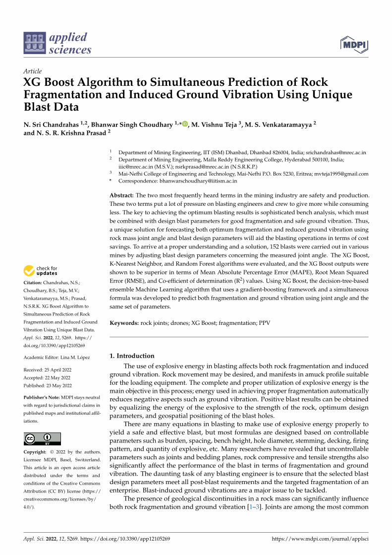
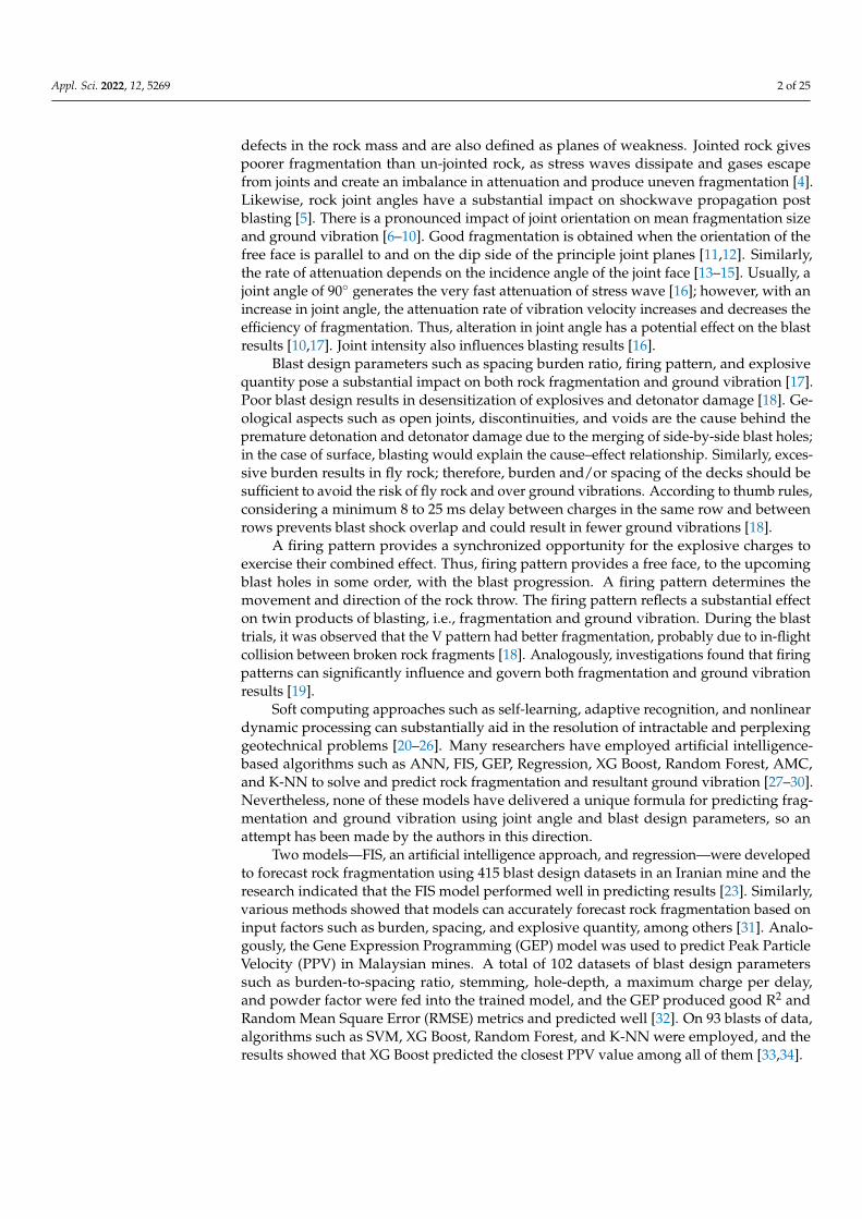
Opencast mine I of Ramagundam III Area, Singareni Collieries Company Limited,Telangana, India is the mine where the studies were conducted. Figures 1–3 shows thesite location on an Indian map, its Google map position, and experimental overburdenbenches.The mine was previously worked through underground methods but later wasconverted to an opencast mine. In the study area, overburden benches were 12 m high.Rock strata are comprised of sandstone and alluvium soil. The average density of sandstonewas 2.3 g/cc.

a. Identification of bench structural geo-property through UAV:

For the reconfiguration of the new blast design, extensive work was under taken todetermine the rock condition and joint intensity. DJI Mavic Unmanned Aerial Vehicle(UAV) was used to detect joint planes.

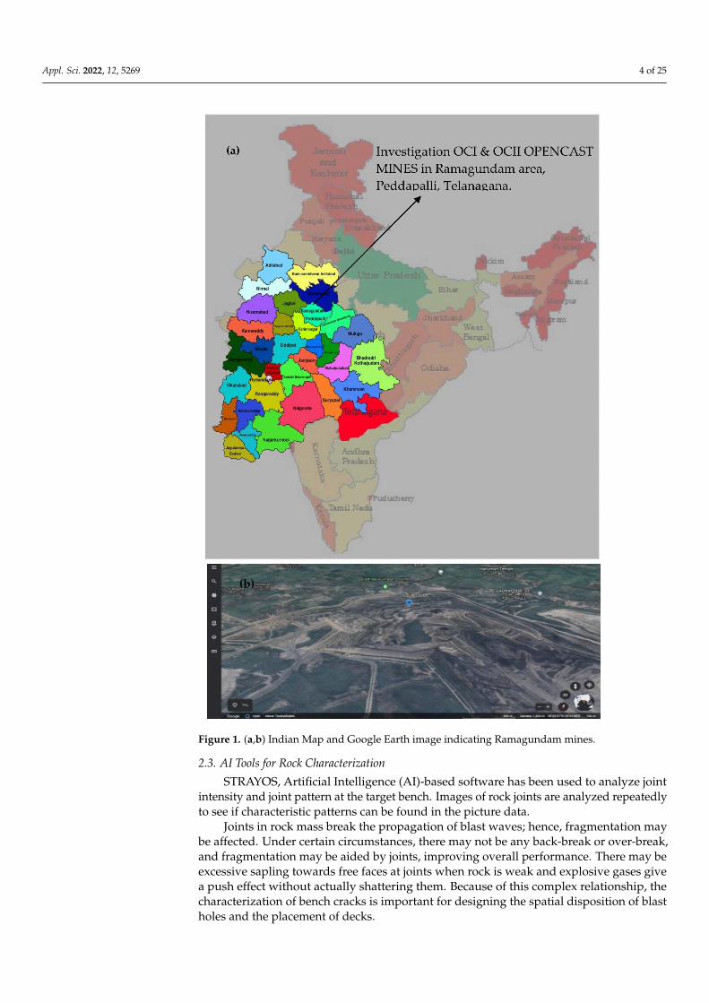
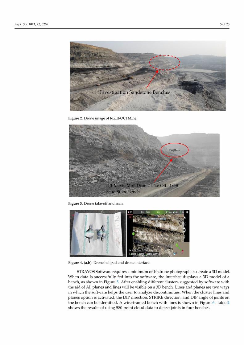
The UAV was capable of capturing and recording photos and videos at 4K resolution.It can run for 25 min in the air with a single battery charge and weighs 258 g. Calibrationwas performed to fix signal problems, allowing for a better take-off of the drone placed onthe helipad shown in Figure 4a, as well as the bench scanning test shown in Figure 3.

The drone operated with mobile application LITCHI in FIRST-PERSON VIEW (FPV)mode with 18 satellite signal poles, as shown in Figure 4b.

The UAV flew through the bench range at a height of 100 feet, with a 75 percentoverlap. To get error-free images, the camera angle was set to 45 degrees so as to focus onthe bench’s top edge and the beginning of the bench floor. In order to maintain accuracy, atleast four to five images were taken at the same time in order to generate multiple pointcloud data for use in STRAYOS software to generate a 3D model. In total, 580 photos werecaptured from 1 de-coaled,2B seam, 3A coal seam, and 3A de-coaled.

b. Geo–technical properties of the site:

To design blasts in O-PITBLAST SOFTWARE, geo-rock attributes are required. Tocomplete the task, rock samples were collected from each proposed site and tested ina laboratory. Table 1 shows the results of various tests, such as uniaxial compressive,Young Modulus, and Poisson’s tests. The average mineralogical composition of sandstonewas calcite 43–50%, quartz 14–18%, feldspar 13–15%, and the remaining 20–25% in acombination of clay, mica, and dolomite.

Appl. Sci. 2022, 12, 5269 4 of 25Appl. Sci. 2022, 12, x FOR PEER REVIEW 4 of 28

Figure 1. (a,b) Indian Map and Google Earth image indicating Ramagundam mines.

(b)

Figure 1. (a,b) Indian Map and Google Earth image indicating Ramagundam mines.

2.3. AI Tools for Rock Characterization

STRAYOS, Artificial Intelligence (AI)-based software has been used to analyze jointintensity and joint pattern at the target bench. Images of rock joints are analyzed repeatedlyto see if characteristic patterns can be found in the picture data.

Joints in rock mass break the propagation of blast waves; hence, fragmentation maybe affected. Under certain circumstances, there may not be any back-break or over-break,and fragmentation may be aided by joints, improving overall performance. There may beexcessive sapling towards free faces at joints when rock is weak and explosive gases givea push effect without actually shattering them. Because of this complex relationship, thecharacterization of bench cracks is important for designing the spatial disposition of blastholes and the placement of decks.

Appl. Sci. 2022, 12, 5269 5 of 25Appl. Sci. 2022, 12, x FOR PEER REVIEW 5 of 28

Figure 2. Drone image of RGIII-OCI Mine.

a. Identification of bench structural geo-property through UAV:

For the reconfiguration of the new blast design, extensive work was under taken to

determine the rock condition and joint intensity. DJI Mavic Unmanned Aerial Vehicle

(UAV) was used to detect joint planes.

The UAV was capable of capturing and recording photos and videos at 4K resolu-

tion. It can run for 25 min in the air with a single battery charge and weighs 258 g. Cali-

bration was performed to fix signal problems, allowing for a better take-off of the drone

placed on the helipad shown in Figure 4a, as well as the bench scanning test shown in

Figure 3.

Figure 3. Drone take-off and scan.

Figure 4. (a,b): Drone helipad and drone interface.

Figure 2. Drone image of RGIII-OCI Mine.

Appl. Sci. 2022, 12, x FOR PEER REVIEW 5 of 28

Figure 2. Drone image of RGIII-OCI Mine.

a. Identification of bench structural geo-property through UAV:

For the reconfiguration of the new blast design, extensive work was under taken to

determine the rock condition and joint intensity. DJI Mavic Unmanned Aerial Vehicle

(UAV) was used to detect joint planes.

The UAV was capable of capturing and recording photos and videos at 4K resolu-

tion. It can run for 25 min in the air with a single battery charge and weighs 258 g. Cali-

bration was performed to fix signal problems, allowing for a better take-off of the drone

placed on the helipad shown in Figure 4a, as well as the bench scanning test shown in

Figure 3.

Figure 3. Drone take-off and scan.

Figure 4. (a,b): Drone helipad and drone interface.

Figure 3. Drone take-off and scan.

Appl. Sci. 2022, 12, x FOR PEER REVIEW 5 of 28

Figure 2. Drone image of RGIII-OCI Mine.

a. Identification of bench structural geo-property through UAV:

For the reconfiguration of the new blast design, extensive work was under taken to

determine the rock condition and joint intensity. DJI Mavic Unmanned Aerial Vehicle

(UAV) was used to detect joint planes.

The UAV was capable of capturing and recording photos and videos at 4K resolu-

tion. It can run for 25 min in the air with a single battery charge and weighs 258 g. Cali-

bration was performed to fix signal problems, allowing for a better take-off of the drone

placed on the helipad shown in Figure 4a, as well as the bench scanning test shown in

Figure 3.

Figure 3. Drone take-off and scan.

Figure 4. (a,b): Drone helipad and drone interface. Figure 4. (a,b): Drone helipad and drone interface.

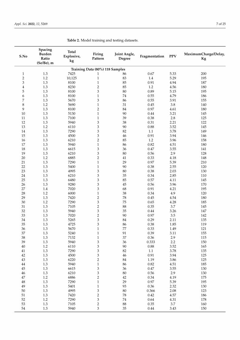
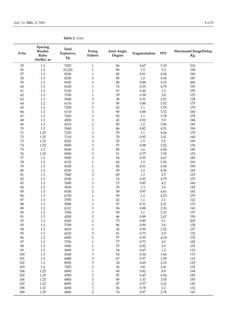
STRAYOS Software requires a minimum of 10 drone photographs to create a 3D model.When data is successfully fed into the software, the interface displays a 3D model of abench, as shown in Figure 5. After enabling different clusters suggested by software withthe aid of AI, planes and lines will be visible on a 3D bench. Lines and planes are two waysin which the software helps the user to analyze discontinuities. When the cluster lines andplanes option is activated, the DIP direction, STRIKE direction, and DIP angle of joints onthe bench can be identified. A wire-framed bench with lines is shown in Figure 6. Table 2shows the results of using 580-point cloud data to detect joints in four benches.

Appl. Sci. 2022, 12, 5269 6 of 25

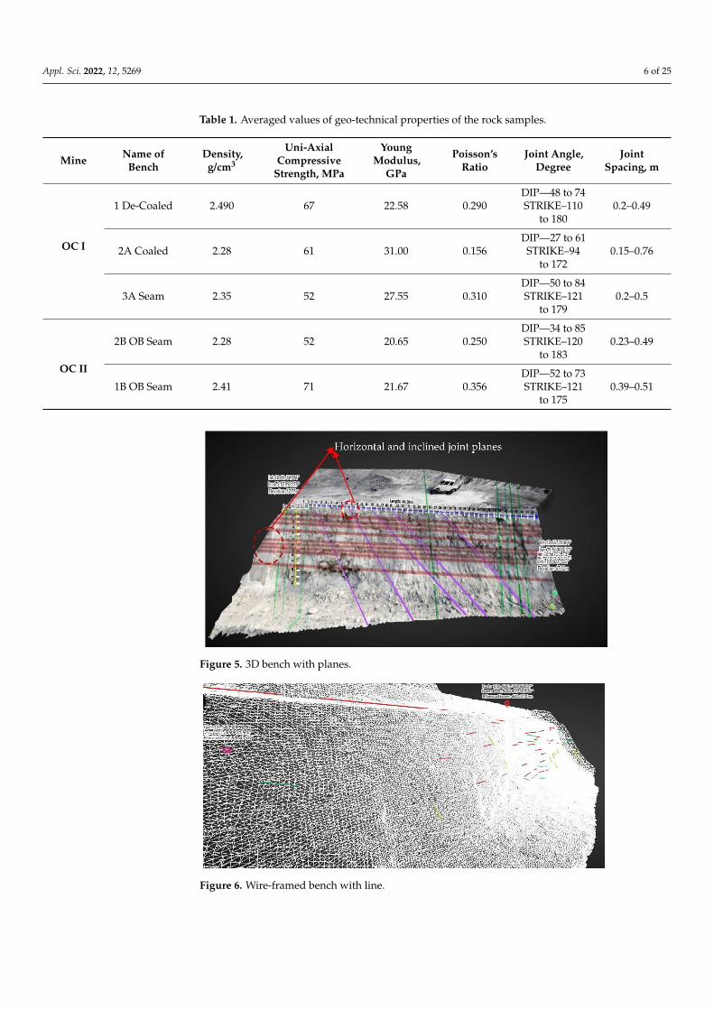
Table 1. Averaged values of geo-technical properties of the rock samples.

Mine Name ofBench

Density,g/cm3

Uni-AxialCompressive

Strength, MPa

YoungModulus,

GPa

Poisson’sRatio

Joint Angle,Degree

JointSpacing, m

OC I

1 De-Coaled 2.490 67 22.58 0.290DIP—48 to 74STRIKE–110

to 1800.2–0.49

2A Coaled 2.28 61 31.00 0.156DIP—27 to 61STRIKE–94

to 1720.15–0.76

3A Seam 2.35 52 27.55 0.310DIP—50 to 84STRIKE–121

to 1790.2–0.5

OC II

2B OB Seam 2.28 52 20.65 0.250DIP—34 to 85STRIKE–120

to 1830.23–0.49

1B OB Seam 2.41 71 21.67 0.356DIP—52 to 73STRIKE–121

to 1750.39–0.51

Appl. Sci. 2022, 12, x FOR PEER REVIEW 7 of 28

cluster lines and planes option is activated, the DIP direction, STRIKE direction, and DIP

angle of joints on the bench can be identified. A wire-framed bench with lines is shown in

Figure 6. Table 2 shows the results of using 580-point cloud data to detect joints in four

benches.

Figure 5. 3D bench with planes.

Figure 6. Wire-framed bench with line.

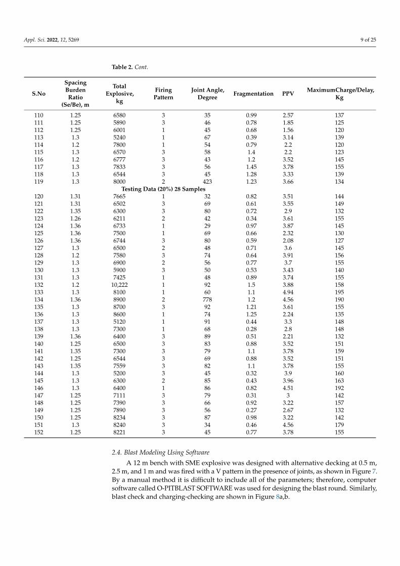
Table 2. Model training and testing datasets.

S.No Spacing Burden

Ratio (Se/Be), m

Total

Explosive, kg

Firing

Pattern

Joint Angle,

Degree Fragmentation PPV

Maximum

Charge/Del

ay, Kg

Training Data (80%) 118 Samples

1 1.3 7425 1 86 0.67 5.33 200

2 1.2 10,125 1 83 1.4 5.29 195

3 1.3 8100 1 85 0.91 4.94 187

4 1.3 8230 2 85 1.2 4.56 180

5 1.3 8100 3 80 0.89 5.15 195

6 1.3 8100 1 74 0.55 4.79 186

7 1.3 5670 3 86 0.55 3.91 155

8 1.2 5690 1 31 0.45 3.8 140

9 1.3 8100 2 84 0.97 4.61 180

10 1.3 5130 1 90 0.44 3.21 145

11 1.3 7100 1 39 0.38 2.8 125

Figure 5. 3D bench with planes.

Appl. Sci. 2022, 12, x FOR PEER REVIEW 7 of 28

cluster lines and planes option is activated, the DIP direction, STRIKE direction, and DIP

angle of joints on the bench can be identified. A wire-framed bench with lines is shown in

Figure 6. Table 2 shows the results of using 580-point cloud data to detect joints in four

benches.

Figure 5. 3D bench with planes.

Figure 6. Wire-framed bench with line.

Table 2. Model training and testing datasets.

S.No Spacing Burden

Ratio (Se/Be), m

Total

Explosive, kg

Firing

Pattern

Joint Angle,

Degree Fragmentation PPV

Maximum

Charge/Del

ay, Kg

Training Data (80%) 118 Samples

1 1.3 7425 1 86 0.67 5.33 200

2 1.2 10,125 1 83 1.4 5.29 195

3 1.3 8100 1 85 0.91 4.94 187

4 1.3 8230 2 85 1.2 4.56 180

5 1.3 8100 3 80 0.89 5.15 195

6 1.3 8100 1 74 0.55 4.79 186

7 1.3 5670 3 86 0.55 3.91 155

8 1.2 5690 1 31 0.45 3.8 140

9 1.3 8100 2 84 0.97 4.61 180

10 1.3 5130 1 90 0.44 3.21 145

11 1.3 7100 1 39 0.38 2.8 125

Figure 6. Wire-framed bench with line.

Appl. Sci. 2022, 12, 5269 7 of 25

Table 2. Model training and testing datasets.

S.No

SpacingBurdenRatio

(Se/Be), m

TotalExplosive,

kg

FiringPattern

Joint Angle,Degree Fragmentation PPV MaximumCharge/Delay,

Kg

Training Data (80%) 118 Samples1 1.3 7425 1 86 0.67 5.33 2002 1.2 10,125 1 83 1.4 5.29 1953 1.3 8100 1 85 0.91 4.94 1874 1.3 8230 2 85 1.2 4.56 1805 1.3 8100 3 80 0.89 5.15 1956 1.3 8100 1 74 0.55 4.79 1867 1.3 5670 3 86 0.55 3.91 1558 1.2 5690 1 31 0.45 3.8 1409 1.3 8100 2 84 0.97 4.61 18010 1.3 5130 1 90 0.44 3.21 14511 1.3 7100 1 39 0.38 2.8 12512 1.3 5940 3 38 0.31 2.21 12213 1.2 6110 3 90 0.88 3.52 14514 1.3 7290 3 82 1.1 3.78 14915 1.3 4500 3 46 0.91 3.94 14616 1.3 6210 2 85 1.2 3.96 15817 1.3 5940 1 86 0.82 4.51 18018 1.3 6615 3 36 0.47 3.55 14119 1.3 6210 3 80 0.56 2.9 12820 1.2 6885 2 41 0.33 4.18 14821 1.3 7290 1 29 0.97 5.39 21022 1.3 5400 1 90 0.38 2.55 12023 1.3 4995 3 80 0.38 2.03 13024 1.3 6210 3 35 0.34 2.85 11025 1.3 6480 3 85 0.57 4.11 14526 1.3 9280 3 45 0.56 3.96 17027 1.4 7020 3 68 0.91 4.21 19528 1.2 6000 1 38 0.34 4.9 12029 1.3 7420 2 78 0.45 4.54 18030 1.2 7290 3 75 0.65 4.28 18531 1.3 7105 2 88 0.35 3.7 14532 1.3 5940 3 35 0.44 3.26 14733 1.3 7020 2 90 0.97 3.5 14234 1.3 5265 3 84 0.29 2.11 13535 1.3 4725 3 86 0.38 1.85 11936 1.3 5670 1 77 0.33 1.49 12137 1.3 5240 1 91 0.39 3.11 15538 1.3 7132 1 37 0.36 2.9 11539 1.3 5940 3 36 0.333 2.2 15040 1.2 6110 3 90 0.88 3.52 16541 1.3 7290 3 82 1.1 3.78 13542 1.3 4500 3 46 0.91 3.94 12543 1.3 6220 2 84 1.19 3.86 12544 1.3 5940 1 86 0.82 4.51 18545 1.3 6615 3 36 0.47 3.55 13046 1.3 6210 3 80 0.56 2.9 13047 1.2 6886 2 42 0.34 4.19 17548 1.3 7290 1 29 0.97 5.39 19549 1.3 5401 1 93 0.36 2.32 13050 1.3 4995 3 80 0.366 2.08 12351 1.3 7420 2 78 0.42 4.57 18652 1.2 7290 3 74 0.64 4.31 17853 1.3 7105 2 88 0.35 3.7 16054 1.3 5940 3 35 0.44 3.43 150

Appl. Sci. 2022, 12, 5269 8 of 25

Table 2. Cont.

S.No

SpacingBurdenRatio

(Se/Be), m

TotalExplosive,

kg

FiringPattern

Joint Angle,Degree Fragmentation PPV MaximumCharge/Delay,

Kg

55 1.3 7425 1 86 0.67 5.33 21056 1.2 10,222 1 80 1.5 5.2 19857 1.3 8100 1 85 0.91 4.94 19058 1.3 8230 2 85 1.2 4.56 18759 1.3 8100 3 80 0.89 5.15 20060 1.3 8100 1 74 0.55 4.79 19561 1.3 5120 1 91 0.44 3.3 15562 1.3 7100 1 39 0.38 2.8 13563 1.3 5940 3 38 0.31 2.21 12864 1.2 6110 3 90 0.88 3.52 17565 1.3 7290 3 82 1.1 3.78 17966 1.2 6110 3 90 0.88 3.52 16067 1.3 7260 3 82 1.1 3.78 17868 1.3 4500 3 45 0.92 3.9 18469 1.3 6210 2 85 1.2 3.96 18570 1.3 5940 1 86 0.82 4.51 19071 1.25 7230 3 79 1.1 4.26 17972 1.25 7110 3 78 0.92 3.41 16073 1.25 8222 3 55 1.5 5.2 19574 1.25 8900 3 57 0.98 3.22 13975 1.3 8240 3 89 1.6 4.56 18576 1.25 8500 3 51 0.77 3.78 17077 1.3 9500 3 54 0.55 4.67 18578 1.2 8125 1 60 1.5 5.29 21079 1.3 8100 1 82 0.91 4.94 19080 1.3 8230 2 59 1.2 4.56 18381 1.3 7880 3 69 1.2 2.5 12582 1.3 8100 1 74 0.55 4.79 17083 1.3 7688 3 72 0.85 4.2 16084 1.2 5690 1 70 1.3 3.9 14585 1.3 8100 2 58 0.97 4.61 16586 1.3 6130 1 90 1.2 4.23 15587 1.3 7555 1 42 1.1 2.1 12288 1.3 5988 3 57 0.31 4.21 17089 1.2 6121 3 94 0.88 2.33 14390 1.3 7356 3 59 1.1 2.31 13791 1.3 4200 3 46 0.99 2.67 15092 1.3 6345 2 73 0.89 5.1 20593 1.3 5789 1 86 0.99 3.6 13894 1.3 6618 3 42 0.59 3.22 13795 1.3 6220 3 81 0.73 2.9 13296 1.2 6845 2 57 0.99 4.18 17697 1.3 7256 1 77 0.73 4.5 18298 1.3 5400 1 55 0.92 2.9 13599 1.3 4998 3 34 0.67 1.2 110

100 1.3 6240 3 54 0.34 1.66 115101 1.3 6480 3 67 0.57 1.59 112102 1.3 8956 3 34 0.69 2.33 129103 1.4 7455 3 54 0.8 2.41 132104 1.25 6890 1 60 0.82 4.9 194105 1.35 4789 2 87 0.45 4.54 185106 1.25 6800 3 89 1.33 3.55 155107 1.32 8905 2 87 0.57 3.41 145108 1.32 6000 3 56 0.78 2.2 132109 1.25 6800 2 74 0.97 2.78 143

Appl. Sci. 2022, 12, 5269 9 of 25

Table 2. Cont.

S.No

SpacingBurdenRatio

(Se/Be), m

TotalExplosive,

kg

FiringPattern

Joint Angle,Degree Fragmentation PPV MaximumCharge/Delay,

Kg

110 1.25 6580 3 35 0.99 2.57 137111 1.25 5890 3 46 0.78 1.85 125112 1.25 6001 1 45 0.68 1.56 120113 1.3 5240 1 67 0.39 3.14 139114 1.2 7800 1 54 0.79 2.2 120115 1.3 6570 3 58 1.4 2.2 123116 1.2 6777 3 43 1.2 3.52 145117 1.3 7833 3 56 1.45 3.78 155118 1.3 6544 3 45 1.28 3.33 139119 1.3 8000 2 423 1.23 3.66 134

Testing Data (20%) 28 Samples120 1.31 7665 1 32 0.82 3.51 144121 1.31 6502 3 69 0.61 3.55 149122 1.35 6300 3 80 0.72 2.9 132123 1.26 6211 2 42 0.34 3.61 155124 1.36 6733 1 29 0.97 3.87 145125 1.36 7500 1 69 0.66 2.32 130126 1.36 6744 3 80 0.59 2.08 127127 1.3 6500 2 48 0.71 3.6 145128 1.2 7580 3 74 0.64 3.91 156129 1.3 6900 2 56 0.77 3.7 155130 1.3 5900 3 50 0.53 3.43 140131 1.3 7425 1 48 0.89 3.74 155132 1.2 10,222 1 92 1.5 3.88 158133 1.3 8100 1 60 1.1 4.94 195134 1.36 8900 2 778 1.2 4.56 190135 1.3 8700 3 92 1.21 3.61 155136 1.3 8600 1 74 1.25 2.24 135137 1.3 5120 1 91 0.44 3.3 148138 1.3 7300 1 68 0.28 2.8 148139 1.36 6400 3 89 0.51 2.21 132140 1.25 6500 3 83 0.88 3.52 151141 1.35 7300 3 79 1.1 3.78 159142 1.25 6544 3 69 0.88 3.52 151143 1.35 7559 3 82 1.1 3.78 155144 1.3 5200 3 45 0.32 3.9 160145 1.3 6300 2 85 0.43 3.96 163146 1.3 6400 1 86 0.82 4.51 192147 1.25 7111 3 79 0.31 3 142148 1.25 7390 3 66 0.92 3.22 157149 1.25 7890 3 56 0.27 2.67 132150 1.25 8234 3 87 0.98 3.22 142151 1.3 8240 3 34 0.46 4.56 179152 1.25 8221 3 45 0.77 3.78 155

2.4. Blast Modeling Using Software

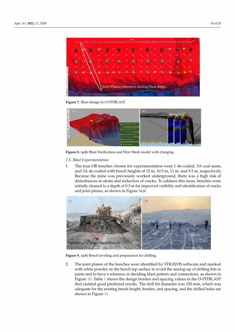
A 12 m bench with SME explosive was designed with alternative decking at 0.5 m,2.5 m, and 1 m and was fired with a V pattern in the presence of joints, as shown in Figure 7.By a manual method it is difficult to include all of the parameters; therefore, computersoftware called O-PITBLAST SOFTWARE was used for designing the blast round. Similarly,blast check and charging-checking are shown in Figure 8a,b.

Appl. Sci. 2022, 12, 5269 10 of 25Appl. Sci. 2022, 12, x FOR PEER REVIEW 8 of 28

Figure 7. Blast design in O-PITBLAST.

Figure 8. (a,b) Blast Verification and Wire Mesh model with charging.

2.5. Blast Experimentation

1. The four OB benches chosen for experimentation were 1 de-coaled, 3A coal seam,

and 3A de-coaled with bench heights of 12 m, 10.5 m, 11 m, and 9.5 m, respectively.

Because the mine was previously worked underground, there was a high risk of

disturbances in strata and induction of cracks. To address this issue, benches were

initially cleaned to a depth of 0.3 m for improved visibility and identification of

cracks and joint planes, as shown in Figure 9a,b.

Figure 9. (a,b) Bench leveling and preparation for drilling.

2. The joint planes of the benches were identified by STRAYOS software and marked

with white powder on the bench top surface to avoid the seizing-up of drilling bits

in joints and to have a reference in deciding blast pattern and connections, as shown

in Figure 10. Table 1 shows the design burden and spacing values in the

O-PITBLAST that yielded good predicted results. The drill bit diameter was 150

mm, which was adequate for the existing bench height, burden, and spacing, and

the drilled holes are shown in Figure 11.

Figure 7. Blast design in O-PITBLAST.

Appl. Sci. 2022, 12, x FOR PEER REVIEW 11 of 28

Figure 7. Blast design in O-PITBLAST.

Figure 8. (a,b) Blast Verification and Wire Mesh model with charging.

2.5. Blast Experimentation

1. The four OB benches chosen for experimentation were 1 de-coaled, 3A coal seam,

and 3A de-coaled with bench heights of 12 m, 10.5 m, 11 m, and 9.5 m, respectively.

Because the mine was previously worked underground, there was a high risk of

disturbances in strata and induction of cracks. To address this issue, benches were

initially cleaned to a depth of 0.3 m for improved visibility and identification of

cracks and joint planes, as shown in Figure 9a,b.

Figure 9. (a,b) Bench leveling and preparation for drilling.

2. The joint planes of the benches were identified by STRAYOS software and marked

with white powder on the bench top surface to avoid the seizing-up of drilling bits

in joints and to have a reference in deciding blast pattern and connections, as shown

in Figure 10. Table 1 shows the design burden and spacing values in the

O-PITBLAST that yielded good predicted results. The drill bit diameter was 150

mm, which was adequate for the existing bench height, burden, and spacing, and

the drilled holes are shown in Figure 11.

Joint Planes reference during blast dsign

Figure 8. (a,b) Blast Verification and Wire Mesh model with charging.

2.5. Blast Experimentation

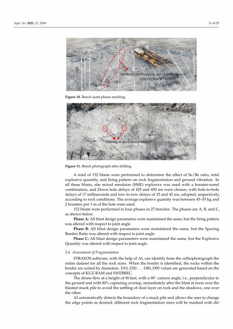
1. The four OB benches chosen for experimentation were 1 de-coaled, 3A coal seam,and 3A de-coaled with bench heights of 12 m, 10.5 m, 11 m, and 9.5 m, respectively.Because the mine was previously worked underground, there was a high risk ofdisturbances in strata and induction of cracks. To address this issue, benches wereinitially cleaned to a depth of 0.3 m for improved visibility and identification of cracksand joint planes, as shown in Figure 9a,b.

Appl. Sci. 2022, 12, x FOR PEER REVIEW 11 of 28

Figure 7. Blast design in O-PITBLAST.

Figure 8. (a,b) Blast Verification and Wire Mesh model with charging.

2.5. Blast Experimentation

1. The four OB benches chosen for experimentation were 1 de-coaled, 3A coal seam,

and 3A de-coaled with bench heights of 12 m, 10.5 m, 11 m, and 9.5 m, respectively.

Because the mine was previously worked underground, there was a high risk of

disturbances in strata and induction of cracks. To address this issue, benches were

initially cleaned to a depth of 0.3 m for improved visibility and identification of

cracks and joint planes, as shown in Figure 9a,b.

Figure 9. (a,b) Bench leveling and preparation for drilling.

2. The joint planes of the benches were identified by STRAYOS software and marked

with white powder on the bench top surface to avoid the seizing-up of drilling bits

in joints and to have a reference in deciding blast pattern and connections, as shown

in Figure 10. Table 1 shows the design burden and spacing values in the

O-PITBLAST that yielded good predicted results. The drill bit diameter was 150

mm, which was adequate for the existing bench height, burden, and spacing, and

the drilled holes are shown in Figure 11.

Joint Planes reference during blast dsign

Figure 9. (a,b) Bench leveling and preparation for drilling.

2. The joint planes of the benches were identified by STRAYOS software and markedwith white powder on the bench top surface to avoid the seizing-up of drilling bits injoints and to have a reference in deciding blast pattern and connections, as shown inFigure 10. Table 1 shows the design burden and spacing values in the O-PITBLASTthat yielded good predicted results. The drill bit diameter was 150 mm, which wasadequate for the existing bench height, burden, and spacing, and the drilled holes areshown in Figure 11.

Appl. Sci. 2022, 12, 5269 11 of 25Appl. Sci. 2022, 12, x FOR PEER REVIEW 12 of 28

Figure 10. Bench–joint planes marking.

Figure 11. Bench photograph after drilling.

A total of 152 blasts were performed to determine the effect of Se/Be ratio, total

explosive quantity, and firing pattern on rock fragmentation and ground vibration. In all

these blasts, site mixed emulsion (SME) explosive was used with a booster-nonel

combination, and Down hole delays of 425 and 450 ms were chosen, with hole-to-hole

delays of 17 milliseconds and row-to-row delays of 25 and 42 ms, adopted, respectively,

according to rock conditions. The average explosive quantity was between 45–55 kg and

2 boosters per 1 m of the hole were used.

152 blasts were performed in four phases in 27 benches. The phases are A, B, and C,

as shown below.

Phase A: All blast design parameters were maintained the same, but the firing

pattern was altered with respect to joint angle.

Phase B: All blast design parameters were maintained the same, but the Spacing

Burden Ratio was altered with respect to joint angle.

Phase C: All blast design parameters were maintained the same, but the Explosive

Quantity was altered with respect to joint angle.

2.6. Assessment of Fragmentation:

STRAYOS software, with the help of AI, can identify from the orthophotograph the

entire dataset for all the rock sizes. When the border is identified, the rocks within the

border are sorted by diameters. D10, D20…D80, D90 values are generated based on the

concepts of KUZ-RAM and SWEBREC.

The drone flew at a height of 90 feet, with a 90° camera angle, i.e., perpendicular to

the ground and with 80% capturing overlap, immediately after the blast at noon over the

blasted muck pile to avoid the settling of dust layer on rock and the shadows, one over

the other.

Figure 10. Bench–joint planes marking.

Appl. Sci. 2022, 12, x FOR PEER REVIEW 12 of 28

Figure 10. Bench–joint planes marking.

Figure 11. Bench photograph after drilling.

A total of 152 blasts were performed to determine the effect of Se/Be ratio, total

explosive quantity, and firing pattern on rock fragmentation and ground vibration. In all

these blasts, site mixed emulsion (SME) explosive was used with a booster-nonel

combination, and Down hole delays of 425 and 450 ms were chosen, with hole-to-hole

delays of 17 milliseconds and row-to-row delays of 25 and 42 ms, adopted, respectively,

according to rock conditions. The average explosive quantity was between 45–55 kg and

2 boosters per 1 m of the hole were used.

152 blasts were performed in four phases in 27 benches. The phases are A, B, and C,

as shown below.

Phase A: All blast design parameters were maintained the same, but the firing

pattern was altered with respect to joint angle.

Phase B: All blast design parameters were maintained the same, but the Spacing

Burden Ratio was altered with respect to joint angle.

Phase C: All blast design parameters were maintained the same, but the Explosive

Quantity was altered with respect to joint angle.

2.6. Assessment of Fragmentation:

STRAYOS software, with the help of AI, can identify from the orthophotograph the

entire dataset for all the rock sizes. When the border is identified, the rocks within the

border are sorted by diameters. D10, D20…D80, D90 values are generated based on the

concepts of KUZ-RAM and SWEBREC.

The drone flew at a height of 90 feet, with a 90° camera angle, i.e., perpendicular to

the ground and with 80% capturing overlap, immediately after the blast at noon over the

blasted muck pile to avoid the settling of dust layer on rock and the shadows, one over

the other.

Figure 11. Bench photograph after drilling.

A total of 152 blasts were performed to determine the effect of Se/Be ratio, totalexplosive quantity, and firing pattern on rock fragmentation and ground vibration. Inall these blasts, site mixed emulsion (SME) explosive was used with a booster-nonelcombination, and Down hole delays of 425 and 450 ms were chosen, with hole-to-holedelays of 17 milliseconds and row-to-row delays of 25 and 42 ms, adopted, respectively,according to rock conditions. The average explosive quantity was between 45–55 kg and2 boosters per 1 m of the hole were used.

152 blasts were performed in four phases in 27 benches. The phases are A, B, and C,as shown below.

Phase A: All blast design parameters were maintained the same, but the firing patternwas altered with respect to joint angle.

Phase B: All blast design parameters were maintained the same, but the SpacingBurden Ratio was altered with respect to joint angle.

Phase C: All blast design parameters were maintained the same, but the ExplosiveQuantity was altered with respect to joint angle.

2.6. Assessment of Fragmentation

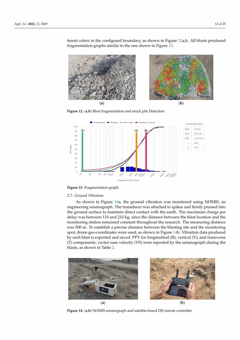
STRAYOS software, with the help of AI, can identify from the orthophotograph theentire dataset for all the rock sizes. When the border is identified, the rocks within theborder are sorted by diameters. D10, D20 . . . D80, D90 values are generated based on theconcepts of KUZ-RAM and SWEBREC.

The drone flew at a height of 90 feet, with a 90 camera angle, i.e., perpendicular tothe ground and with 80% capturing overlap, immediately after the blast at noon over theblasted muck pile to avoid the settling of dust layer on rock and the shadows, one overthe other.

AI automatically detects the boundary of a muck pile and allows the user to changethe edge points as desired; different rock fragmentation sizes will be marked with dif-

Appl. Sci. 2022, 12, 5269 12 of 25

ferent colors in the configured boundary, as shown in Figure 12a,b. All blasts producedfragmentation graphs similar to the one shown in Figure 13.

Appl. Sci. 2022, 12, x FOR PEER REVIEW 13 of 28

AI automatically detects the boundary of a muck pile and allows the user to change

the edge points as desired; different rock fragmentation sizes will be marked with dif-

ferent colors in the configured boundary, as shown in Figure 12a,b. All blasts produced

fragmentation graphs similar to the one shown in Figure 13.

(a) (b)

Figure 12. (a,b) Blast fragmentation and muck pile Detection.

Figure 13. Fragmentation graph.

2.7. Ground Vibration

As shown in Figure 14a, the ground vibration was monitored using NOMIS,an en-

gineering seismograph. The transducer was attached to spikes and firmly pressed into

the ground surface to maintain direct contact with the earth. The maximum charge per

delay was between 110 and 210 kg, since the distance between the blast location and the

monitoring station remained constant throughout the research. The measuring distance

was 500 m. To establish a precise distance between the blasting site and the monitoring

spot, drone geo-coordinates were used, as shown in Figure 14b. Vibration data produced

by each blast is exported and saved. PPV for longitudinal (R), vertical (V), and transverse

(T) components, vector sum velocity (VS) were reported by the seismograph during the

blasts, as shown in Table 2.

(a) (b)

Figure 12. (a,b) Blast fragmentation and muck pile Detection.

Appl. Sci. 2022, 12, x FOR PEER REVIEW 13 of 28

AI automatically detects the boundary of a muck pile and allows the user to change

the edge points as desired; different rock fragmentation sizes will be marked with dif-

ferent colors in the configured boundary, as shown in Figure 12a,b. All blasts produced

fragmentation graphs similar to the one shown in Figure 13.

(a) (b)

Figure 12. (a,b) Blast fragmentation and muck pile Detection.

Figure 13. Fragmentation graph.

2.7. Ground Vibration

As shown in Figure 14a, the ground vibration was monitored using NOMIS,an en-

gineering seismograph. The transducer was attached to spikes and firmly pressed into

the ground surface to maintain direct contact with the earth. The maximum charge per

delay was between 110 and 210 kg, since the distance between the blast location and the

monitoring station remained constant throughout the research. The measuring distance

was 500 m. To establish a precise distance between the blasting site and the monitoring

spot, drone geo-coordinates were used, as shown in Figure 14b. Vibration data produced

by each blast is exported and saved. PPV for longitudinal (R), vertical (V), and transverse

(T) components, vector sum velocity (VS) were reported by the seismograph during the

blasts, as shown in Table 2.

(a) (b)

Figure 13. Fragmentation graph.

2.7. Ground Vibration

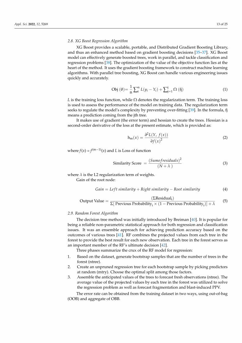
As shown in Figure 14a, the ground vibration was monitored using NOMIS, anengineering seismograph. The transducer was attached to spikes and firmly pressed intothe ground surface to maintain direct contact with the earth. The maximum charge perdelay was between 110 and 210 kg, since the distance between the blast location and themonitoring station remained constant throughout the research. The measuring distancewas 500 m. To establish a precise distance between the blasting site and the monitoringspot, drone geo-coordinates were used, as shown in Figure 14b. Vibration data producedby each blast is exported and saved. PPV for longitudinal (R), vertical (V), and transverse(T) components, vector sum velocity (VS) were reported by the seismograph during theblasts, as shown in Table 2.

Appl. Sci. 2022, 12, x FOR PEER REVIEW 13 of 28

AI automatically detects the boundary of a muck pile and allows the user to change

the edge points as desired; different rock fragmentation sizes will be marked with dif-

ferent colors in the configured boundary, as shown in Figure 12a,b. All blasts produced

fragmentation graphs similar to the one shown in Figure 13.

(a) (b)

Figure 12. (a,b) Blast fragmentation and muck pile Detection.

Figure 13. Fragmentation graph.

2.7. Ground Vibration

As shown in Figure 14a, the ground vibration was monitored using NOMIS,an en-

gineering seismograph. The transducer was attached to spikes and firmly pressed into

the ground surface to maintain direct contact with the earth. The maximum charge per

delay was between 110 and 210 kg, since the distance between the blast location and the

monitoring station remained constant throughout the research. The measuring distance

was 500 m. To establish a precise distance between the blasting site and the monitoring

spot, drone geo-coordinates were used, as shown in Figure 14b. Vibration data produced

by each blast is exported and saved. PPV for longitudinal (R), vertical (V), and transverse

(T) components, vector sum velocity (VS) were reported by the seismograph during the

blasts, as shown in Table 2.

(a) (b)

Figure 14. (a,b) NOMIS seismograph and satellite-based DJI remote controller.

Appl. Sci. 2022, 12, 5269 13 of 25

2.8. XG Boost Regression Algorithm

XG Boost provides a scalable, portable, and Distributed Gradient Boosting Library,and thus an enhanced method based on gradient boosting decisions [35–37]. XG Boostmodel can effectively generate boosted trees, work in parallel, and tackle classification andregression problems [38]. The optimization of the value of the objective function lies at theheart of the method. It uses the gradient boosting framework to construct machine learningalgorithms. With parallel tree boosting, XG Boost can handle various engineering issuesquickly and accurately.

Obj (θ)=1n ∑n

i L(yi − Yi) + ∑jj=1 Ω (fj) (1)

L is the training loss function, while Ω denotes the regularization term. The training lossis used to assess the performance of the model on training data. The regularization termseeks to regulate the model’s complexity by preventing over-fitting [39]. In the formula, fjmeans a prediction coming from the jth tree.

It makes use of gradient (the error term) and hessian to create the trees. Hessian is asecond-order derivative of the loss at the present estimate, which is provided as:

hm(x) =∂2L(Y, f (x))

∂ f (x)2 (2)

where f (x) = f (m−1)(x) and L is Loss of function

Similarity Score =(Sumo f residuals)2

(N + λ )(3)

where λ is the L2 regularization term of weights.Gain of the root node:

Gain = Le f t similarity + Right similarity − Root similarity (4)

Output Value =(ΣResiduali)

Σ[ Previous Probabilityi × (1 − Previous Probabilityi)] + λ(5)

2.9. Random Forest Algorithm

The decision tree method was initially introduced by Breiman [40]. It is popular forbeing a reliable non-parametric statistical approach for both regression and classificationissues. It was an ensemble approach for achieving prediction accuracy based on theoutcomes of various trees [41]. RF combines the projected values from each tree in theforest to provide the best result for each new observation. Each tree in the forest serves asan important member of the RF’s ultimate decision [42].

Three phases summarize the crux of the RF model for regression:

1. Based on the dataset, generate bootstrap samples that are the number of trees in theforest (ntree).

2. Create an unpruned regression tree for each bootstrap sample by picking predictorsat random (mtry). Choose the optimal split among those factors.

3. Assemble the anticipated values of the trees to forecast fresh observations (ntree). Theaverage value of the projected values by each tree in the forest was utilized to solvethe regression problem as well as forecast fragmentation and blast-induced PPV.

The error rate can be obtained from the training dataset in two ways, using out-of-bag(OOB) and aggregate of OBB.

Appl. Sci. 2022, 12, 5269 14 of 25

K-NN Algorithm

It is a popular approach in machine learning for tackling regression and classificationproblems. It was developed by Altman NS [43]. The K-NN method finds the testing pointand classifies it based on its nearest neighbors (k-neighbors). From the training data, thealgorithm teaches nothing. It solely retains the weights of its functional space neighbors.When anticipating a new observation, it looks for comparable findings and computes thecloseness to those neighbors.

In geosciences, the K-NN algorithm has been widely utilized to predict rock fragmenta-tion, back break, and ground vibration [33]. KNN primarily employs the weighted averagevalue of the k-nearest neighbors; the computation begins by calculating the distance be-tween the uncertain and labeled neighbors using Equation (6), and then the neighbors’numbers are re-arranged by raising the distance and RMSE using the cross-validation method.Finally, the average inverse distance between K-Nearest Neighbors will be computed.

D(xtr, xt) = ∑ni=1 wn(xtr,n − xt,n) (6)

Above n denotes the number of features, xtr,n & xt,n represent the nth feature of trainingand testing data, and Wn presents the weight of the nth feature.

3. Results and Discussions

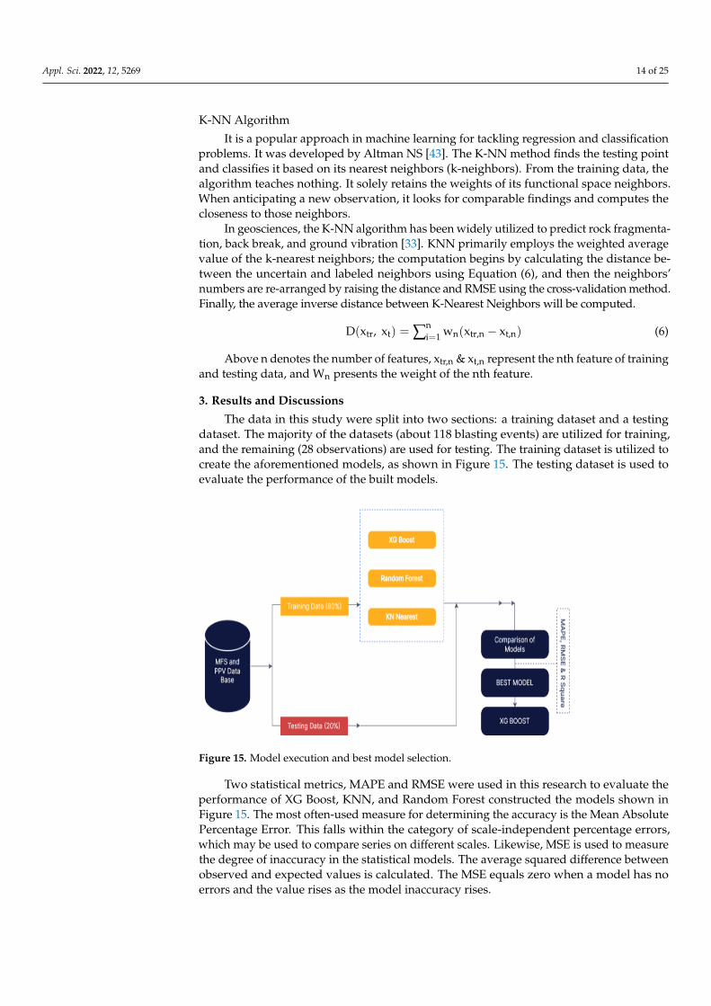
The data in this study were split into two sections: a training dataset and a testingdataset. The majority of the datasets (about 118 blasting events) are utilized for training,and the remaining (28 observations) are used for testing. The training dataset is utilized tocreate the aforementioned models, as shown in Figure 15. The testing dataset is used toevaluate the performance of the built models.

Appl. Sci. 2022, 12, x FOR PEER REVIEW 16 of 28

A number of data here represented by n, yi & yi denote the actual and forecasted

vales and y denotes the mean. Metrics such as MAPE, RMSE, and R2 were computed on

both training and testing datasets to evaluate the performance and accuracy of the model

to decide the final algorithm and to develop a formula to predict fragmentation and

ground vibration. The values are presented in Table 3.

Figure 15. Model execution and best model selection.

Table 3. MAPE, RMSE, and R2 results.

Metric

Type

XG Boost Regression Random Forest KN Nearest

Fragmentation

Training Testing Training Testing Training Testing

MAPE 24 22.5 21.2 20.1 19.2 18.1

RMSE 0.0854 3.873 0.0021 4.221 0.0031 5.321

R2 0.953 0.9125 0.89 0.67 0.9 0.87

Peak Particle Velocity

MAPE 19 18.4 17.5 15.8 16.9 14.32

RMSE 0.0056 2.8890 0.0041 3.78 0.0886 4.88

R2 0.96 0.932 0.79 0.65 0.83 0.72

According to Table 3 and Figure 16, XG Boost algorithms perform well in both

fragmentation and peak particle velocity based on metric values of MAPE, RMSE, and R2

in both 80% training and 20% testing data. Fragmentation and peak particle velocity were

measured in the field, and the XG Boost, Random Forest, and KNN models predicted

values using the testing data shown in Figure 17. The predicted values of the XG Boost

model were very close to the measured values of both fragmentation and peak particle

velocity. In this study, the XG Boost regression method was finalized and utilized to

forecast the simultaneous formula for fragmentation and PPV.

Figure 15. Model execution and best model selection.

Two statistical metrics, MAPE and RMSE were used in this research to evaluate theperformance of XG Boost, KNN, and Random Forest constructed the models shown inFigure 15. The most often-used measure for determining the accuracy is the Mean AbsolutePercentage Error. This falls within the category of scale-independent percentage errors,which may be used to compare series on different scales. Likewise, MSE is used to measurethe degree of inaccuracy in the statistical models. The average squared difference betweenobserved and expected values is calculated. The MSE equals zero when a model has noerrors and the value rises as the model inaccuracy rises.

Appl. Sci. 2022, 12, 5269 15 of 25

The following equations were used to calculate MAPE and MSE in this study.

MSE =1n ∑n

i=1 (yi − Yi)2 (7)

Here, n represents a number of data points; yi denotes observed values and Yi are thepredicted values. Hence, MSE is the average squared difference between the actual andpredicted value.

MAPE =100%

n ∑nt=1

∣∣∣∣ At − Ft

At

∣∣∣∣ (8)

where At denotes the current value and Ft denotes the predicted value. The differencebetween them is divided by the actual value of At. This ratio’s absolute value is added foreach projected point in time and divided by the number of fitted points (n).

R2 = 1 −∑ i

(yi −

ˆy1

)2

∑ i(

yi −−y)2 (9)

A number of data here represented by n, yi &ˆ

yi denote the actual and forecasted vales

and−y denotes the mean. Metrics such as MAPE, RMSE, and R2 were computed on both

training and testing datasets to evaluate the performance and accuracy of the model todecide the final algorithm and to develop a formula to predict fragmentation and groundvibration. The values are presented in Table 3.

Table 3. MAPE, RMSE, and R2 results.

MetricType

XG Boost Regression Random Forest KN Nearest

Fragmentation

Training Testing Training Testing Training Testing

MAPE 24 22.5 21.2 20.1 19.2 18.1

RMSE 0.0854 3.873 0.0021 4.221 0.0031 5.321

R2 0.953 0.9125 0.89 0.67 0.9 0.87

Peak Particle Velocity

MAPE 19 18.4 17.5 15.8 16.9 14.32

RMSE 0.0056 2.8890 0.0041 3.78 0.0886 4.88

R2 0.96 0.932 0.79 0.65 0.83 0.72

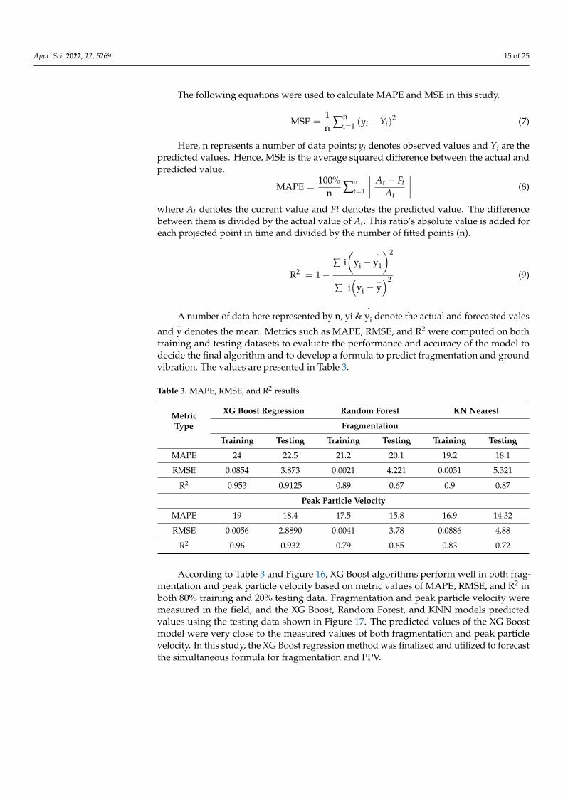
According to Table 3 and Figure 16, XG Boost algorithms perform well in both frag-mentation and peak particle velocity based on metric values of MAPE, RMSE, and R2 inboth 80% training and 20% testing data. Fragmentation and peak particle velocity weremeasured in the field, and the XG Boost, Random Forest, and KNN models predictedvalues using the testing data shown in Figure 17. The predicted values of the XG Boostmodel were very close to the measured values of both fragmentation and peak particlevelocity. In this study, the XG Boost regression method was finalized and utilized to forecastthe simultaneous formula for fragmentation and PPV.

Appl. Sci. 2022, 12, 5269 16 of 25Appl. Sci. 2022, 12, x FOR PEER REVIEW 17 of 28

Figure 16. Performance of MAPE, RMSE, and R2 on testing data.

Figure 17. Fragmentation and PPV results comparison between measures models and predicted.

XG Boost Regression

To avoid modeling complexity, two stopping methods, maximum tree depth and n

rounds, were selected in the current XG Boost Regression Model. Choosing significant

numbers for maximum tree depth and n rounds would result in excessive development

of the tree and an over-fitting issue. Therefore, to avoid this problem, the maximum tree

depth was set to 1–3 and n rounds to 50, 100, and 150. A trial-and-error approach was

used with a range of two values to get the best combination of these two parameters. The

dataset was randomly sorted into training (80%) and testing (20%). For the training set,

K-fold cross-validation was used to determine the optimum model parameters. The

training set was divided into 10 parts of about equal size for 10-fold cross-validation, of

which 9 parts were used for training and 1 part utilized for validation. This method was

repeated 10 times repeatedly, and the average of these values was used to get the pre-

dicted forecast accuracy.

The initial prediction began by taking into account the mean of the dependent var-

iables, MFS and PPV, from the dataset. The residual values from the previous prediction

points were then computed. Furthermore, utilizing (80%) of the data, the model was

Figure 16. Performance of MAPE, RMSE, and R2 on testing data.

Appl. Sci. 2022, 12, x FOR PEER REVIEW 17 of 28

Figure 16. Performance of MAPE, RMSE, and R2 on testing data.

Figure 17. Fragmentation and PPV results comparison between measures models and predicted.

XG Boost Regression

To avoid modeling complexity, two stopping methods, maximum tree depth and n

rounds, were selected in the current XG Boost Regression Model. Choosing significant

numbers for maximum tree depth and n rounds would result in excessive development

of the tree and an over-fitting issue. Therefore, to avoid this problem, the maximum tree

depth was set to 1–3 and n rounds to 50, 100, and 150. A trial-and-error approach was

used with a range of two values to get the best combination of these two parameters. The

dataset was randomly sorted into training (80%) and testing (20%). For the training set,

K-fold cross-validation was used to determine the optimum model parameters. The

training set was divided into 10 parts of about equal size for 10-fold cross-validation, of

which 9 parts were used for training and 1 part utilized for validation. This method was

repeated 10 times repeatedly, and the average of these values was used to get the pre-

dicted forecast accuracy.

The initial prediction began by taking into account the mean of the dependent var-

iables, MFS and PPV, from the dataset. The residual values from the previous prediction

points were then computed. Furthermore, utilizing (80%) of the data, the model was

Figure 17. Fragmentation and PPV results comparison between measures models and predicted.

XG Boost Regression

To avoid modeling complexity, two stopping methods, maximum tree depth and nrounds, were selected in the current XG Boost Regression Model. Choosing significantnumbers for maximum tree depth and n rounds would result in excessive developmentof the tree and an over-fitting issue. Therefore, to avoid this problem, the maximum treedepth was set to 1–3 and n rounds to 50, 100, and 150. A trial-and-error approach was usedwith a range of two values to get the best combination of these two parameters. The datasetwas randomly sorted into training (80%) and testing (20%). For the training set, K-foldcross-validation was used to determine the optimum model parameters. The training setwas divided into 10 parts of about equal size for 10-fold cross-validation, of which 9 partswere used for training and 1 part utilized for validation. This method was repeated 10times repeatedly, and the average of these values was used to get the predicted forecastaccuracy.

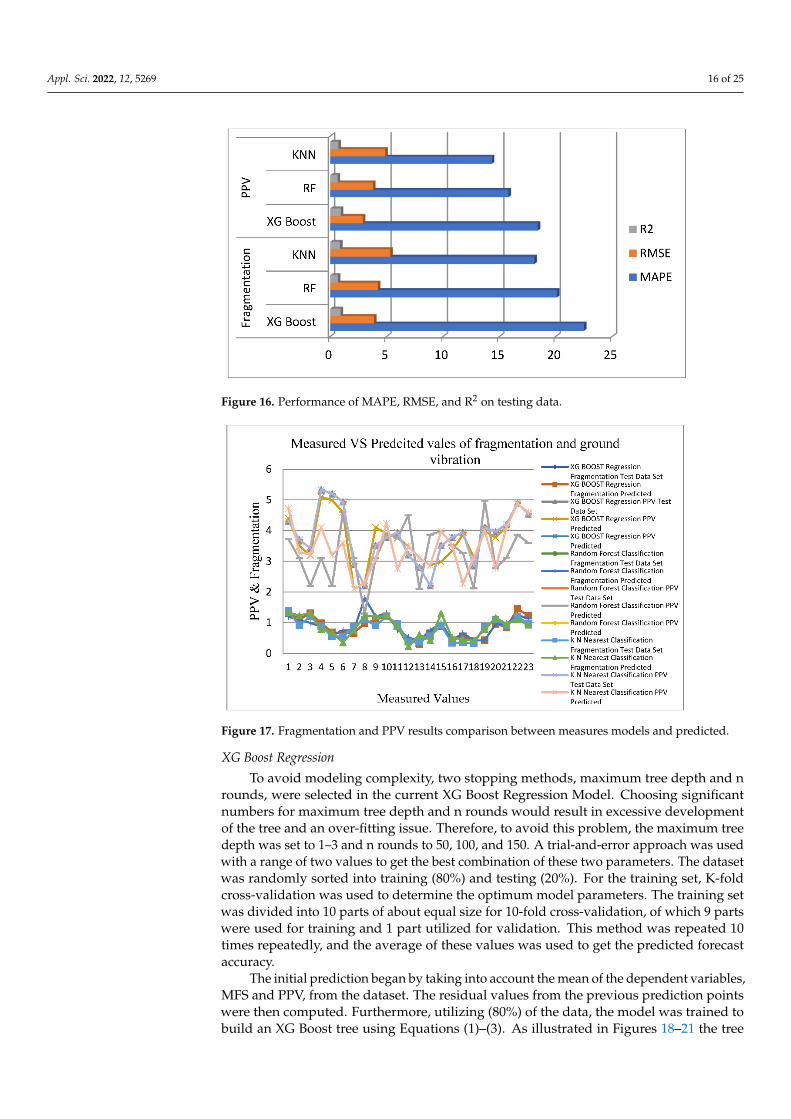
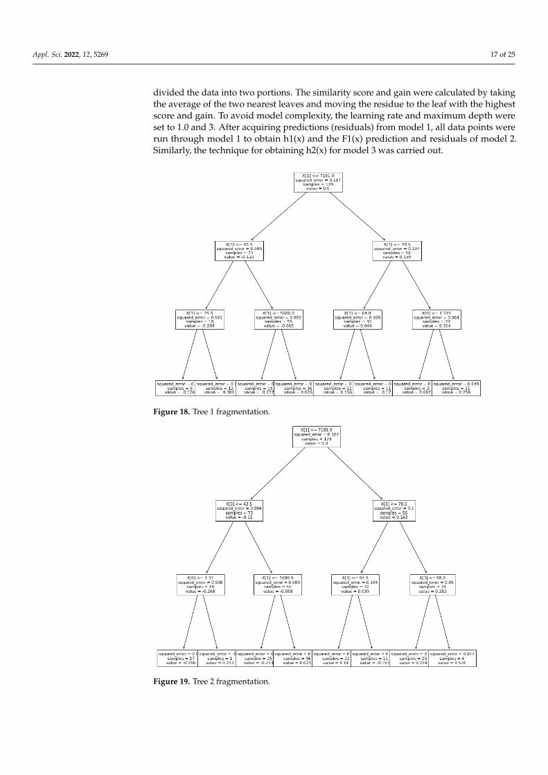
The initial prediction began by taking into account the mean of the dependent variables,MFS and PPV, from the dataset. The residual values from the previous prediction pointswere then computed. Furthermore, utilizing (80%) of the data, the model was trained tobuild an XG Boost tree using Equations (1)–(3). As illustrated in Figures 18–21 the tree

Appl. Sci. 2022, 12, 5269 17 of 25

divided the data into two portions. The similarity score and gain were calculated by takingthe average of the two nearest leaves and moving the residue to the leaf with the highestscore and gain. To avoid model complexity, the learning rate and maximum depth wereset to 1.0 and 3. After acquiring predictions (residuals) from model 1, all data points wererun through model 1 to obtain h1(x) and the F1(x) prediction and residuals of model 2.Similarly, the technique for obtaining h2(x) for model 3 was carried out.

Appl. Sci. 2022, 12, x FOR PEER REVIEW 18 of 28

trained to build an XG Boost tree using Equations (1)–(3). As illustrated in Figures 18–21

the tree divided the data into two portions. The similarity score and gain were calculated

by taking the average of the two nearest leaves and moving the residue to the leaf with

the highest score and gain. To avoid model complexity, the learning rate and maximum

depth were set to 1.0 and 3. After acquiring predictions (residuals) from model 1, all data

points were run through model 1 to obtain h1(x) and the F1(x) prediction and residuals of

model 2. Similarly, the technique for obtaining h2(x) for model 3 was carried out.

The final empirical formulas for predicting fragmentation and peak particle velocity

are provided in Equations (10) and (11), which were generated from the trained model

using Figure 18. The flow chart created utilizing the weight–age of the Se/Be ratio, Total

explosive quantity (TE), Firing Pattern (FP), and joint angle degree (JAD) in terms of

squared errors, samples, and prediction values from the trees shown in Figures 18–21.

Maximum Charge per Delay was not considered since the output iterations did not bal-

ance accuracy in anticipating fragmentation and PPV as the numbers ranged from 110 to

210 kg with little fluctuation, as shown in Table 2.

Fragmentation = 0.77 + 0.1(Tree 1) + 0.1(Tree 2) (10)

PeakParticleVelocity = 3.60 + 0.1(Tree 1) + 0.1(Tree 2) (11)

where tree 1 and 2 are final prediction values of models.

Figure 18. Tree 1 fragmentation. Figure 18. Tree 1 fragmentation.

Appl. Sci. 2022, 12, x FOR PEER REVIEW 19 of 28

Figure 19. Tree 2 fragmentation.

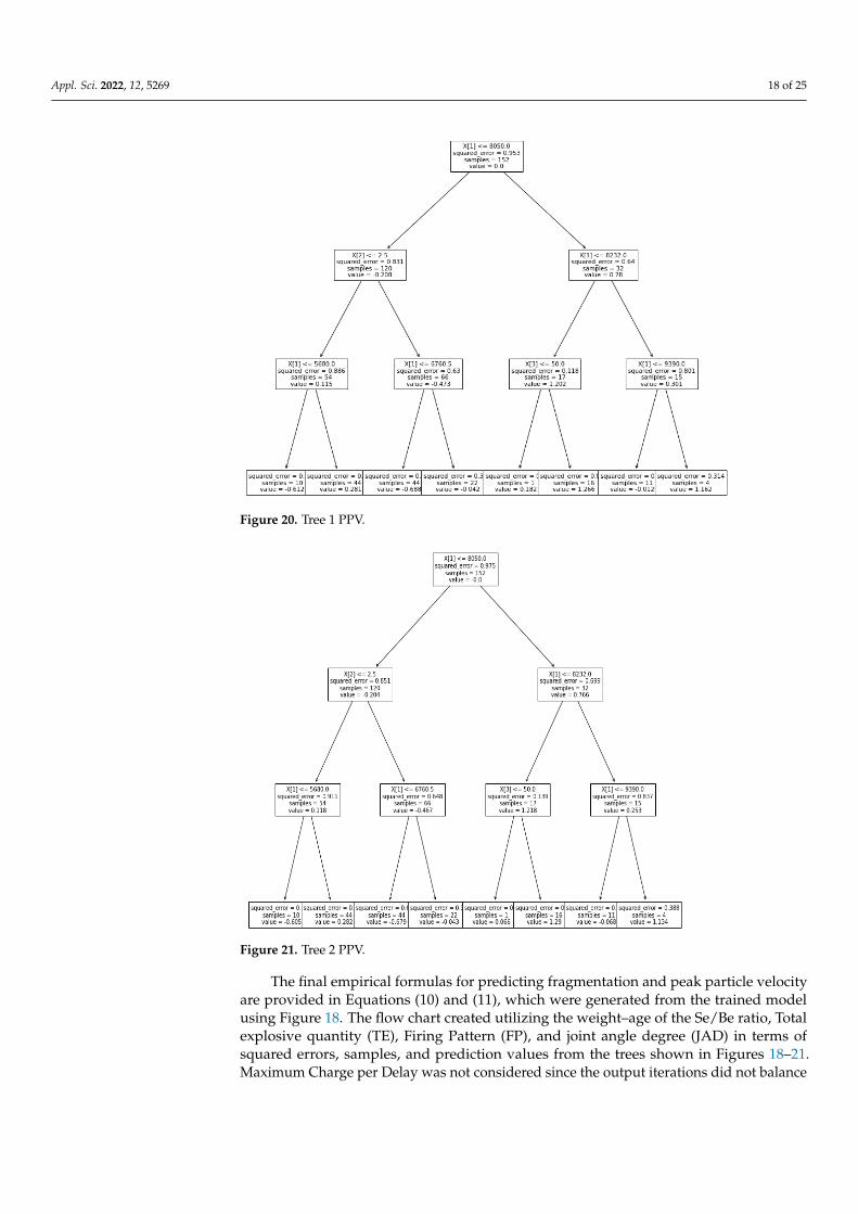
Figure 20. Tree 1 PPV.

Figure 19. Tree 2 fragmentation.

Appl. Sci. 2022, 12, 5269 18 of 25

Appl. Sci. 2022, 12, x FOR PEER REVIEW 19 of 28

Figure 19. Tree 2 fragmentation.

Figure 20. Tree 1 PPV. Figure 20. Tree 1 PPV.

Appl. Sci. 2022, 12, x FOR PEER REVIEW 20 of 28

Figure 21. Tree 2 PPV.

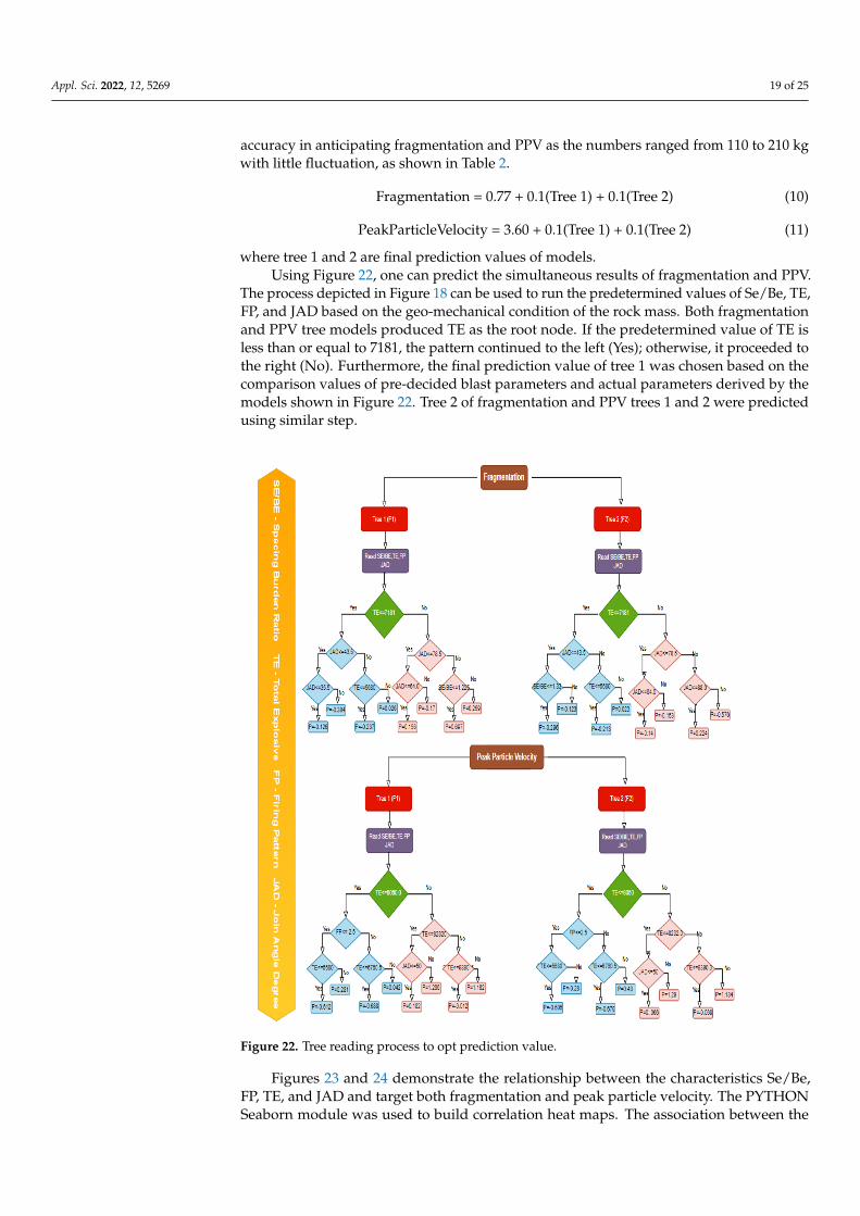
Using Figure 22, one can predict the simultaneous results of fragmentation and PPV.

The process depicted in Figure 18 can be used to run the predetermined values of Se/Be,

TE, FP, and JAD based on the geo-mechanical condition of the rock mass. Both frag-

mentation and PPV tree models produced TE as the root node. If the predetermined

value of TE is less than or equal to 7181, the pattern continued to the left (Yes); otherwise,

it proceeded to the right (No). Furthermore, the final prediction value of tree 1 was cho-

sen based on the comparison values of pre-decided blast parameters and actual parame-

ters derived by the models shown in Figure 22. Tree 2 of fragmentation and PPV trees 1

and 2 were predicted using similar step.

Figure 21. Tree 2 PPV.

The final empirical formulas for predicting fragmentation and peak particle velocityare provided in Equations (10) and (11), which were generated from the trained modelusing Figure 18. The flow chart created utilizing the weight–age of the Se/Be ratio, Totalexplosive quantity (TE), Firing Pattern (FP), and joint angle degree (JAD) in terms ofsquared errors, samples, and prediction values from the trees shown in Figures 18–21.Maximum Charge per Delay was not considered since the output iterations did not balance

Appl. Sci. 2022, 12, 5269 19 of 25

accuracy in anticipating fragmentation and PPV as the numbers ranged from 110 to 210 kgwith little fluctuation, as shown in Table 2.

Fragmentation = 0.77 + 0.1(Tree 1) + 0.1(Tree 2) (10)

PeakParticleVelocity = 3.60 + 0.1(Tree 1) + 0.1(Tree 2) (11)

where tree 1 and 2 are final prediction values of models.Using Figure 22, one can predict the simultaneous results of fragmentation and PPV.

The process depicted in Figure 18 can be used to run the predetermined values of Se/Be, TE,FP, and JAD based on the geo-mechanical condition of the rock mass. Both fragmentationand PPV tree models produced TE as the root node. If the predetermined value of TE isless than or equal to 7181, the pattern continued to the left (Yes); otherwise, it proceeded tothe right (No). Furthermore, the final prediction value of tree 1 was chosen based on thecomparison values of pre-decided blast parameters and actual parameters derived by themodels shown in Figure 22. Tree 2 of fragmentation and PPV trees 1 and 2 were predictedusing similar step.

Appl. Sci. 2022, 12, x FOR PEER REVIEW 21 of 28

Figure 22. Tree reading process to opt prediction value.

Figures 23 and 24 demonstrate the relationship between the characteristics Se/Be, FP,

TE, and JAD and target both fragmentation and peak particle velocity. The PYTHON

Seaborn module was used to build correlation heat maps. The association between the

dependent and independent variables is strong. Se/Be ratio, TE, and JAD are coefficients

mapped with fragmentation, while FP, TE, and JAD are coefficients mapped with PPV,

the same characteristics generated from both trees in fragmentation and PPV segments.

Figure 22. Tree reading process to opt prediction value.

Figures 23 and 24 demonstrate the relationship between the characteristics Se/Be,FP, TE, and JAD and target both fragmentation and peak particle velocity. The PYTHONSeaborn module was used to build correlation heat maps. The association between the

Appl. Sci. 2022, 12, 5269 20 of 25

dependent and independent variables is strong. Se/Be ratio, TE, and JAD are coefficientsmapped with fragmentation, while FP, TE, and JAD are coefficients mapped with PPV, thesame characteristics generated from both trees in fragmentation and PPV segments.

Appl. Sci. 2022, 12, x FOR PEER REVIEW 22 of 28

Figure 23. Correlation matrix of fragmentation.

Figure 24. Correlation matrix of PPV.

A Taylor diagram, shown in Figure 25, was used for rigorous evolution, which al-

lows for more robust comparisons between models. Taylor multi-metrics outperform a

single model in terms of accuracy. It may exhibit several criterion outputs in a single

figure, which is a great way to grasp the findings. An XG Boost model depicts a good

coefficient value among the other two models.

Figure 23. Correlation matrix of fragmentation.

Appl. Sci. 2022, 12, x FOR PEER REVIEW 22 of 28

Figure 23. Correlation matrix of fragmentation.

Figure 24. Correlation matrix of PPV.

A Taylor diagram, shown in Figure 25, was used for rigorous evolution, which al-

lows for more robust comparisons between models. Taylor multi-metrics outperform a

single model in terms of accuracy. It may exhibit several criterion outputs in a single

figure, which is a great way to grasp the findings. An XG Boost model depicts a good

coefficient value among the other two models.

Figure 24. Correlation matrix of PPV.

A Taylor diagram, shown in Figure 25, was used for rigorous evolution, which allowsfor more robust comparisons between models. Taylor multi-metrics outperform a singlemodel in terms of accuracy. It may exhibit several criterion outputs in a single figure, whichis a great way to grasp the findings. An XG Boost model depicts a good coefficient valueamong the other two models.

Appl. Sci. 2022, 12, x FOR PEER REVIEW 23 of 28

Figure 25. Taylors Diagram.

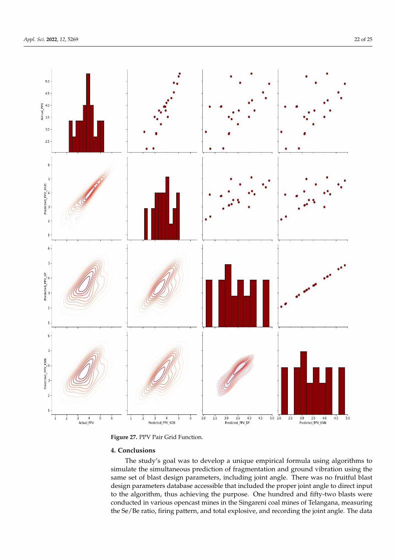
Using Python’s seaborn function, a pair grid was utilized to depict pair-wise con-

nections in datasets. Pair grid provides greater versatility than the pair plot shown in

Figures 26 and 27. Pair grid assigned each variable in a dataset to a column and row on a

multi-axes grid. A variety of axes level-plotting functions were employed to create a bi-

variate plot in the upper and lower triangles, with the marginal distribution of each var-

iable in the diagonals. Furthermore, the hue parameter was utilized to express an extra

level of conditions that plots various subplots in different hues.

Figure 25. Taylors Diagram.

Using Python’s seaborn function, a pair grid was utilized to depict pair-wise con-nections in datasets. Pair grid provides greater versatility than the pair plot shown in

Appl. Sci. 2022, 12, 5269 21 of 25

Figures 26 and 27. Pair grid assigned each variable in a dataset to a column and row ona multi-axes grid. A variety of axes level-plotting functions were employed to create abivariate plot in the upper and lower triangles, with the marginal distribution of eachvariable in the diagonals. Furthermore, the hue parameter was utilized to express an extralevel of conditions that plots various subplots in different hues.

Appl. Sci. 2022, 12, x FOR PEER REVIEW 24 of 28

Figure 26. Fragmentation Pair Grid Function. Figure 26. Fragmentation Pair Grid Function.

Appl. Sci. 2022, 12, 5269 22 of 25Appl. Sci. 2022, 12, x FOR PEER REVIEW 25 of 28

Figure 27. PPV Pair Grid Function.

4. Conclusions

The study’s goal was to develop a unique empirical formula using algorithms to

simulate the simultaneous prediction of fragmentation and ground vibration using the

same set of blast design parameters, including joint angle. There was no fruitful blast

Figure 27. PPV Pair Grid Function.

4. Conclusions

The study’s goal was to develop a unique empirical formula using algorithms tosimulate the simultaneous prediction of fragmentation and ground vibration using thesame set of blast design parameters, including joint angle. There was no fruitful blastdesign parameters database accessible that included the proper joint angle to direct inputto the algorithm, thus achieving the purpose. One hundred and fifty-two blasts wereconducted in various opencast mines in the Singareni coal mines of Telangana, measuringthe Se/Be ratio, firing pattern, and total explosive, and recording the joint angle. The data

Appl. Sci. 2022, 12, 5269 23 of 25

was used to train three models: XG Boost, Random Forest, and KNN, which were thenevaluated using three metrics: MAPE, RMSE, and R2. XG Boost model was selected.

• Use of O-PITBLAST SOFTWARE aided in the design of blasting and provided prelimi-nary warnings for iterations.

• Available technical tools such as STRAYOS SOFTWARE are helpful in identifying thejoint angle for rock mass characterization as well as fragmentation analysis

• A Correlation matrix was used to understand relationships between dependent andindependent variables, and it proved to be quite useful.

• The XG Boost Regression Algorithm was found to be useful for creating an empiricalformula to forecast simultaneous fragmentation and peak particle velocity utilizingjoint angle and other blast design parameters such as Se/Be ratio, Total Explosive, andFiring Pattern while keeping the charge per delay constant.

• Empirical formulas of fragmentation and ground vibration are substantial in predict-ing results.

Fragmentation = 0.77 + 0.1(Tree 1) + 0.1 (Tree 2)Peak Particle Velocity = 3.60 +0.1(Tree 1) +0.1(Tree 2)

Author Contributions: Conceptualization, methodology, investigation, software and writing—original draft preparation has been conducted by N.S.C.; supervision and formal analysis havebeen conducted by B.S.C., writing—review and editing done by M.V.T., M.S.V. and N.S.R.K.P. Allauthors have read and agreed to the published version of the manuscript.

Funding: This research received no external funding.

Informed Consent Statement: Informed consent was obtained from all subjects involved in the study.

Data Availability Statement: Available in https://github.com/SriChandrahas/XGBoost-Public/blob/6c14d4a4ae26f6c8f3c6e2763594235c5145eee2/XGBOOST_FRAG.ipynb (accessed on 20 April 2022).

Acknowledgments: I would like to express my heartfelt gratitude to my mentor, B.S. Choudhary,Associate Professor, IIT (ISM) Dhanbad, for meticulously tracking and adding his research inputs tothis paper. I am always grateful to my college IIT (ISM) Dhanbad. I would like to express my gratitudeto the Principal, Director, and management of Malla Reddy Engineering College, Hyderabad forallocating adequate time to carry out research.

Conflicts of Interest: The authors declare no conflict of interest.

References1. Aziznejad, S.; Esmaieli, K. Effects of joint intensity on rock fragmentation by Impact. In Proceedings of the 11th International

Symposium on Rock Fragmentation by Blasting, Sydney, Australia, 24–26 August 2015.2. Ash, R.L. The Influence of Geological Discontinuities on Rock Blasting. Ph.D. Thesis, University of Minnesota, Minneapolis, MN,

USA, 1973.3. Hakan, A.K.; Konuk, A. The effect of discontinuity frequency on ground vibrations produced from bench blasting: A case study.

Soil Dyn. Earthq. Eng. 2008, 28, 686–694. [CrossRef]4. Yahyaoui, S.; Hafsaoui, A.; Aissi, A.; Benselhoub, A. Relationship of the discontinuities and the rock blasting results. J. Geol. Geogr.

Geoecol. 2018, 26, 208–218. [CrossRef]5. Wu, Y.; Hao, H.; Zhou, Y.; Chong, K. Propagation characteristics of blast-induced shock waves in a jointed rock mass. Soil Dyn.

Earthq. Eng. 1998, 17, 407–412. [CrossRef]6. Chakraborty, A.; Jethwa, J.; Paithankar, A. Effects of joint orientation and rock mass quality on tunnel blasting. Eng. Geol. 1994, 37,

247–262. [CrossRef]7. Bakar Abu, M.Z.; Tariq, S.M.; Hayat, M.B.; Zahoor, M.K.; Khan, M.U. Influence of Geological Discontinuities Upon Fragmentation

by Blasting. Pak. J. Sci. 2013, 65, 414–419.8. Singh, P.; Roy, M.; Paswan, R.; Sarim, M.; Kumar, S.; Jha, R.R. Rock fragmentation control in opencast blasting. J. Rock Mech.

Geotech. Eng. 2016, 8, 225–237. [CrossRef]9. Lyana, K.N.; Hareyani, Z.; Shah, A.K.; Hazizan, M.H. Effect of Geological Condition on Degree of Fragmentation in a Simpang

Pulai Marble Quarry. Procedia Chem. 2016, 19, 694–701. [CrossRef]10. Singh, D.P.; Apparao, V.; Saluja, S.S. A laboratory study on effect of joints on rock fragmentation. American rock mechanics

association. In Proceedings of the 21st U.S. Symposium of Rock Mechanics (USRMS), Rolla, MO, USA, 28–30 May 1980.11. Belland, J.M. Structure as a Control in Rock Fragmentation Coal Lake Iron Ore Deposited. Can. Min. Met. Bull. 1968, 59, 323–328.

Appl. Sci. 2022, 12, 5269 24 of 25

12. Talhi, K.; Bensaker, B. Design of a model blasting system to measure peak p-wave stress. Soil Dyn. Earthq. Eng. 2003, 23, 513–519.[CrossRef]

13. Lewandowski, T.H.; Luan Mai, V.K.; Danell, E. Influence of discontinuities on presplitting effectiveness. In Rock Fragmentation byBlasting: Proceedings of the Fifth International Symposium on Rock Fragmentation by Blasting, FRAGBLAST-5; Mohanty, B., Ed.; CRCPress: Montreal, QC, Canada, 1996; pp. 217–232. [CrossRef]

14. Worsey, P.N.; Qu, S. Effect of joint separation and filling on pre-split blasting. In Proceedings of the 3rd Mini Symposium onExplosives and Blasting Research, Miami, FL, USA, 5 February 1987; pp. 26–40.

15. Whittaker, B.S.; Singh, R.N.; Sun, G. Fracture Mechanics Applied to Rock Fragmentation due to blasting. In Rock FractureMechanics. Principles, Design and Applications Development in Geotechnical Engineering; Elsevier Science Ltd.: Amsterdam, TheNetherlands, 1992; Chapter 13; Volume 71, pp. 443–479.

16. Li, J.; Ma, G. Analysis of blast wave interaction with a rock joint. Rock Mech. Rock Eng. 2010, 43, 777–787. [CrossRef]17. Chandrahas, S.; Choudhary, B.S.; Krishna Prasad, N.S.R.; Musunuri, V.; Rao, K.K. An Investigation into the Effect of Rockmass

Properties on Mean Fragmentation. Arch. Min. Sci. 2021, 66, 561–578. [CrossRef]18. Choudhary, B.S. Firing Patterns and Its Effect on Muckpile Shape Parameters and Fragmentation in Quarry Blasts. Int. J. Res. Eng.

2013, 2, 32–45. [CrossRef]19. Sasaoka, T.; Takahashi, Y.; Hamanaka, A.; Wahyudi, S.; Shimada, H. Effect of Delay Time and Firing Patterns on the Size

of Fragmented Rocks by Bench Blasting. In Proceedings of the 28th International Symposium on Mine Planning and EquipmentSelection—MPES 2019; Springer: Berlin/Heidelberg, Germany, 2019; pp. 449–456. [CrossRef]

20. Atici, U. Prediction of the strength of mineral admixture concrete using multivariable regression analysis and an artificial neuralnetwork. Expert Syst. Appl. 2011, 38, 9609–9618. [CrossRef]

21. Tonnizam Mohamad, E.; Hajihassani, M.; Jahed Armaghani, D.; Marto, A. Simulation of blasting—Induced air overpressure bymeans of artificial intillegene neural networks. Int. Rev. Model. Simul. 2012, 5, 2501–2506.

22. Xie, C.; Nguyen, H.; Bui, X.N.; Choi, Y.; Zhou, J.; Nguyen Trang, T. Predicting rock size distribution in mine blasting usingvarious novel soft computing models based on meta-heuristics and machine learning algorithms. Geosci. Front. 2021, 12, 101108.[CrossRef]

23. Monjezi, M.; Rezaei, M.; Yazdian Varjani, A. Prediction of rock fragmentation due to blasting in Gol-E-Gohar iron mine usingfuzzy logic. Int. J. Rock Mech. Min. Sci. 2009, 46, 1273–1280. [CrossRef]

24. Singh, T.N.; Verma, A.K. Sensitivity of total charge and maximum charge per delay on ground vibration. Geomat. Natl. HazardsRisk 2010, 1, 259–272. [CrossRef]

25. Sharma, L.K.; Singh, R.; Umrao, R.K.; Sharma, K.M.; Singh, T.N. Evaluating the modulus of elasticity of soil using soft computingsystem. Eng. Comput. 2016, 33, 497–507. [CrossRef]

26. Bahrami, A.; Monjezi, M.; Goshtasbi, K.; Ghazvinian, A. Prediction of rock fragmentation due to blasting using artificial neuralnetwork. Eng. Comput. 2011, 27, 177–181. [CrossRef]

27. Sayadi, A.; Manojezi, M.; Talebi, N.; Khandelawal, M. A comparative study on the application of various artificial neural networksto simultaneous prediction of rock fragmentation and back break. J. Rock Mech. Geotech. Eng. 2013, 5, 318–324. [CrossRef]

28. Dindarloo, S.R. Peak particle velocity prediction using support vector machines: A surface blasting case study. J. S. Afr. Inst. Min.Metall. 2015, 115, 637–643. [CrossRef]

29. Ebrahimi, E.; Monjezi, M.; Khalesi, M.R.; Armaghani, D.J. Prediction and optimization of back-break and rock fragmentationusing an artificial neural network and a bee colony algorithm. Bull. Eng. Geol. Environ. 2015, 75, 27–36. [CrossRef]

30. Monjezi, M.; Bahrami, A.; Yazdian Varjani, A. Simultaneous prediction of fragmentation and flyrock in blasting operation usingartificial neural networks. Int. J. Rock Mech. Min. Sci. 2010, 47, 476–480. [CrossRef]

31. Shirani Faradonbeh, R.; Armaghani, D.J.; Majid, M.A.; Tahir, M.M.; Murlidhar, B.R.; Monjezi, M.; Wong, H.M. Prediction ofground vibration due to quarry blasting based on gene expression programming: A new model for peak particle velocityprediction. Int. J. Environ. Sci. Technol. 2016, 13, 1453–1464. [CrossRef]

32. Longjun, D.; Xibing, L.; Ming, X.; Qiyue, L. Comparisons of random forest and support vector machine for predicting blastingvibration characteristic parameters. Procedia Eng. 2011, 26, 1772–1781. [CrossRef]

33. Nguyen, H.; Bui, X.-N.; Bui, H.-B.; Cuong, D.T. Developing an XGBoost model to predict blast-induced peak particle velocity inan open-pit mine: A case study. Acta Geophys. 2019, 67, 477–490. [CrossRef]

34. Friedman, J.H. Greedy function approximation: A gradient boosting machine. Ann. Stat. 2001, 29, 1189–1232. [CrossRef]35. Friedman, J.H. Stochastic gradient boosting. Comput. Stat. Data Anal. 2002, 38, 367–378. [CrossRef]36. Chen, M.; Liu, Q.; Chen, S.; Liu, Y.; Zhang, C.-H.; Liu, R. XGBoost-Based Algorithm Interpretation and Application on Post-Fault

Transient Stability Status Prediction of Power System. IEEE Access 2019, 7, 13149–13158. [CrossRef]37. Friedman, J.; Hastie, T.; Tibshirani, R. Additive logistic regression: A statistical view of boosting (with discussion and a rejoinder

by the authors). Ann. Stat. 2000, 28, 337–407. [CrossRef]38. Chen, T.; He, T. Xgboost: Extreme Gradient Boosting; R Package Version 04-2; 2015. Available online: https://cran.microsoft.com

(accessed on 12 April 2022).39. Gao, W.; Wang, W.; Dimitrov, D.; Wang, Y. Nano properties analysis via fourth multiplicative ABC indicator calculating. Arab. J.

Chem. 2018, 11, 793–801. [CrossRef]40. Breiman, L. Random forests. Mach. Learn. 2001, 45, 5–32. [CrossRef]

Appl. Sci. 2022, 12, 5269 25 of 25

41. Vigneau, E.; Courcoux, P.; Symoneaux, R.; Guérin, L.; Villière, A. Random forests: A machine learning methodology to highlightthe volatile organic compounds involved in olfactory perception. Food Qual. Prefer. 2018, 68, 135–145. [CrossRef]

42. Gao, W.; Guirao, J.L.; Basavanagoud, B.; Wu, J. Partial multidividing ontology learning algorithm. Inf. Sci. 2018, 467, 35–58.[CrossRef]

43. Altman, N.S. An introduction to kernel and nearest-neighbor nonparametric regression. Am. Stat. 2019, 46, 175–185.