PNWD-3676 WTP-RPT-132 Rev. 0

Technical Basis for Predicting Mixing and Flammable Gas Behavior in the Ultrafiltration Feed Process and High-Level Waste Lag Storage Vessels with Non-Newtonian Slurries J. R. Bontha L. K. Jagoda C. W. Stewart C. D. Johnson D. E Kurath K. S. Koschik P. A. Meyer D. L. Lessor S. T. Arm F. Nigl C. E. Guzman-Leong R. L. Russell M. S. Fountain G. L. Smith M. Friedrich W. Yantasee S. A. Hartley S. T. Yokuda December 2005 Prepared for Bechtel National, Inc. under Contract No. 24590-101-TSA-W000-00004

LEGAL NOTICE This report was prepared by Battelle – Pacific Northwest Division (Battelle) as an account of sponsored research activities. Neither Client nor Battelle nor any person acting on behalf of either: MAKES ANY WARRANTY OR REPRESENTATION, EXPRESS OR IMPLIED, with respect to the accuracy, completeness, or usefulness of the information contained in this report, or that the use of any information, apparatus, process, or composition disclosed in this report may not infringe privately owned rights; or Assumes any liabilities with respect to the use of, or for damages resulting from the use of, any information, apparatus, process, or composition disclosed in this report. References herein to any specific commercial product, process, or service by trade name, trademark, manufacturer, or otherwise, does not necessarily constitute or imply its endorsement, recommendation, or favoring by Battelle. The views and opinions of authors expressed herein do not necessarily state or reflect those of Battelle.

Completeness of Testing

This report describes the results of work and testing specified by Test Specification 24590-WTP-TSP-RT-04-0002, Rev. 0 and Test Plan TP-RPP-WTP-385, Rev. 0. The work and any associated testing followed the quality assurance requirements outlined in the Test SpecificationlPlan. The descriptions provided in this test report are an accurate account of both the conduct of the work and the data collected. Test plan results are reported. Also reported are any unusual or anomalous occurrences that are different from expected results. The test results and this report have been reviewed and verified.

Approved: fi Gordon H. Beeman, Manager WTP R&T Support Project

/+&r- Date

iii

Testing Summary The U.S. Department of Energy (DOE) Office of River Protection’s Waste Treatment Plant (WTP) will process and treat radioactive waste that is stored in tanks at the Hanford Site. Pulse jet mixers (PJMs) along with air spargers and steady jets generated by recirculation pumps have been selected to mix the high-level waste (HLW) slurries in several tanks: the HLW lag storage (LS) vessels, the HLW blend vessel, and the ultrafiltration feed process (UFP) vessels. These mixing technologies are collectively called PJM/hybrid mixing systems. The work in this report addresses the mixing and gas retention and release tests conducted in a half-scale replica of the LS vessel constructed in one of the large tanks in the high bay of the Battelle – Pacific Northwest Division (PNWD) 336 Building test facility. The tank was equipped with 1) PJMs and sparger arrays representative of the LS vessel; 2) auxiliary systems for providing air to the test equipment and injecting hydrogen peroxide and tracer; 3) and instrumentation and data acquisition systems to monitor the gas volume fraction, evaluate mixing, and operate the system. The testing used a kaolin/bentonite clay simulant with non-Newtonian rheological properties representative of actual waste slurries. Objectives Table S.1 summarizes the objectives and results of this testing.

Table S.1. Summary of Test Objectives and Results

Test Objective Objective

Met? Discussion Demonstrate Normal Vessel Operation: Demonstrate the normal operating cycle, which consists of continuous PJM operation and intermittent sparge operation (1 hr full sparge followed by 2 hr idle sparge). Determine long-term accumulated gas volume and quality of mixing (percent of vessel contents actively mixed)

Yes As discussed in Section 6.2.1 of this report, the normal operating cycle consisted of continuous PJM operation at half-stroke plus intermittent sparge operation. Following the scaling rules, the cycle time for the intermittent sparge operation was reduced by the scaling factor of 2, so full sparge was on for ½ hr followed by 1 hr of idle sparge. A solution of 30 wt% hydrogen peroxide was injected continuously into the simulant. The test was con-tinued until cyclically repeatable steady-state operation was achieved. The average minimum gas volume fraction, αMIN, was ~ 0.70 vol%, and the maximum gas volume fraction, αMAX, was ~ 1.09 vol% based on an average of the last six operational cycles.

As discussed in Section 6.4, mixing tests were conducted with PJMs operating at half-stroke with full sparging and a simulant height-to-diameter ratio (H/D) of 0.93–0.94. To monitor the mixing process, a sodium chloride tracer was either added as a dilute solution on top of the simulant or injected as a concentrate near the bottom of the tank. Grab samples were obtained and analyzed with ion chromatography (IC). The mixing test was followed by PJMs operating at full stroke with full sparging to homogenize the tracer in the simulant. A log variance approach was used to determine the 95% mixing time, which, based on this analysis, was found to be about 5 hr when concentrated tracer was injected near the tank bottom. The blending time was about 9 hr when tracer was added on top of the simulant. The longer time for blending than for time to mix is due to increased difficulty in fully mixing a lower-density material (water) on top of the high-density simulant.

iv

Test Objective Objective

Met? Discussion Demonstrate Post-Design Basis Event (DBE) Vessel Operations: Demonstrate the post-DBE operating cycle, which consists of intermittent PJM operation (2 hr on followed by 12 hr off) and inter-mittent sparge operation (2 hr full on followed by 12 hr idle). Determine long-term accumulated gas volume and quality of mixing (percent of vessel contents actively mixed).

Yes. As discussed in Section 6.2.2, the post-DBE cycle consisted of repeated cycles of 1 hr full sparging and PJM operation followed by 2 hr idle sparging and no PJM operation. The peroxide injection rate during Run 3 was con-tinuous at ~382 mL/min during the first 55 min of PJM and full sparging operation and off for the rest of the cycle. The idle sparging period was shortened to 2 hr because most of the peroxide added during the full sparging operation had decomposed. After steady state was attained, the run continued several cycles longer to ensure that minor fluctuations in the data were due to periodic oscillations and not indicative of any slow transients. The test concluded with a reduction in the hydrogen peroxide flow rate to 50 mL/min for one post-DBE cycle. Results show maximum gas volume fraction varying from 2.46 to 3.20 vol% with an average of ~2.79 vol%, based on the last 10 cycles. The minimum gas volume fraction varied from 0.90 to ~1.23 vol% with an average of ~1.08 vol% (based on the last 10 cycles). For the quality of mixing and the time to mix, see discussion of the objectives for normal operations and near-term accident response (NTAR).

Demonstrate Near Term Accident Response (NTAR) Operations: Demonstrate the loss-of-PJM operating scenario, which consists of inter-mittent sparging (no PJM mixing, full sparge for 2 hr, idle sparge for 12 hr). Determine the quality of mixing; in particular, the volume of unmixed heel that may result. Determine long-term accumulated gas volume.

Yes. As discussed in Section 6.2.3, the NTAR demonstration comprised repeated cycles of 1 hr full sparging followed by 2 hr of idle sparging and no PJM operation. The hydrogen peroxide injection rate was continuous at ~382 mL/min during the first 55 minutes of full sparging and off for the rest of the cycle. The idle sparging period was shortened to 2 hr because most of the peroxide added during full sparging had decomposed. The test was con-ducted for a minimum of 8 operational cycles (11 were actually completed) to simulate 100 hr of NTAR operation. One additional NTAR cycle was conducted with reduced peroxide flow of ~50 mL/min. The run concluded with a sparger only holdup test with peroxide flow rate of ~90 mL/min. The results of the NTAR run show that the maximum gas volume fraction (which occurs at the end of the idle sparging period), αMAX, varied from 2.4 to 2.75 vol% with an average of ~2.55 vol% based on the last three cycles. The minimum gas volume fraction (occurs during the full sparging period), αMIN, varied from 1.26 to 1.29 vol% with an average of 1.28 vol% based on the last three cycles. As discussed in Section 6.4, the sparger-only mixing test was conducted with spargers at full flow and simulant H/D of 0.81. A sodium chloride tracer was added on top of the simulant to monitor mixing progress. Grab samples were taken periodically and analyzed with IC. The mixing test was followed by PJMs operating at full stroke with full sparging to homogenize the tracer concentration in the simulant. A log variance approach was used to deter-mine the 95% mixing time, which, based on this analysis for the portion of the simulant that mixed, ranged from about 5 to 28 hr.

The unmixed volume in the full-flow sparger tests ranged from 34 to 42% with an average of 37% at a simulant H/D of 0.81. The unmixed volume includes that in the PJMs and the sparge heel. This result is somewhat larger than the unmixed volume of 27% calculated in Appendix B.

Note: The PJM and sparger operation cycle times presented in the Test Objectives represent actual plant cycletimes. For the testing described in this document, cycle times were scaled by the scale factor of 2. The idle spargeperiods in the post-DBE and NTAR tests were further shortened to accommodate the relatively rapid hydrogenperoxide decomposition rate.

v

Test Exceptions A summary description of the test exceptions applied to these tests is shown in Table S.2

Table S.2. Test Exceptions

Test Exceptions Description of Test Exceptions 24590-WTP-TEF-RT-04-033 This test exception modified the objectives and success criteria provided in the

test exception to ensure compatibility with the approved test plan. The objectives were modified to exclude the determination of gas release rates from gas holdup data and to include obtaining mixing quality information. The success criteria were modified to delete the determination of gas release rates from gas holdup data and to delete the determination that the WTP design hydrogen safety limits would not be exceeded for the test to be successful.

24590-WTP-TEF-RT-04-037 This test exception modified some of the test parameters and run sequences. The post-DBE and NTAR tests were modified to reduce the hydrogen peroxide injection rate for a portion of the test, and the normal operations steps before and after the post-DBE and NTAR operations were deleted. The range of allowable yield stress of the simulant was changed from 30 ± 3 Pa to 25–50 Pa. Gas release tests were added for three mixing modes: 1) spargers on full flow (no PJMs), 2) PJMs with idle sparging, 3) spargers on idle (no PJMS). Gas holdup tests were added for two mixing modes: 1) PJMs and spargers on idle starting with no retained gas and 2) spargers on full flow (no PJMs).

Results and Performance Against Success Criteria The R&T success criteria are discussed in Table S.3.

Table S.3. Success Criteria

Success Criteria How Testing Did or Did Not Meet Success Criteria Sufficient gas generation to enable measurable gas retention and the associated release when the mixing systems are operated

As discussed in Section 6.2.1, Normal Operations Test, the continuous addition of 30 wt% hydrogen peroxide at a rate of 95 mL/min during the normal operations test provided readily measurable average gas volume fractions of αMIN = ~0.70 vol% and αMAX = ~1.09 vol%.

The demonstration that cyclically repeatable, steady state operation of the test has been achieved.

As discussed in Section 6, cyclically repeatable steady state operation was achieved in the normal operations and the post-DBE tests. The NTAR test was conducted for a minimum of 8 operational cycles (11 cycles were actually completed) to simulate a maximum of 100 hr of NTAR operation.

Determination of sparger-induced holdup before hydrogen peroxide injection begins.

As discussed in Section 6.1, Cakeout and PJM/Sparger Holdup Test, the short-term sparger holdup with the PJMs at half-stroke and spargers on full flow ranged from 0.43 to 0.69 vol% with an average of about 0.55 vol%. The short term sparger-only holdup test indicated a similar short-term holdup of about 0.5 vol%. Short-term sparger holdup is due to the relatively large sparge air bubbles as they rise through the simulant. Within the experimental uncertainty of measurement (±0.2%) there was no detectable long-term sparger holdup.

vi

Quality Requirements Battelle – Pacific Northwest Division’s (PNWD) Quality Assurance Program is based on require-ments defined in U.S. Department of Energy (DOE) Order 414.1A, Quality Assurance, and 10 CFR 830, Energy/Nuclear Safety Management, Subpart A – Quality Assurance Requirements (a.k.a. the Quality Rule). PNWD has chosen to implement the requirements of DOE Order 414.1A and 10 CFR 830, Subpart A by integrating them into the Laboratory's management systems and daily operating processes. The procedures necessary to implement the requirements are documented through PNWD's Standards-Based Management System (SBMS). PNWD implements the RPP-WTP quality requirements by performing work in accordance with the PNWD WTP Support Project quality assurance project plan (QAPjP) approved by the RPP-WTP Quality Assurance (QA) organization. This work was performed to the quality requirements of NQA-1-1989 Part I, Basic and Supplementary Requirements, NQA-2a-1990 Part 2.7 and DOE/RW-0333P Rev. 13, Quality Assurance Requirements and Description (QARD). These quality requirements are implemented through PNWD's WTP Support Project (WTPSP) Quality Assurance Requirements and Description Manual. The analytical requirements are implemented through WTPSP’s Statement of Work (WTPSP-SOW-005) with the Radiochemical Processing Laboratory (RPL) Analytical Service Operations (ASO). Experiments that were not method-specific were performed in accordance with PNWD’s procedure QA-RPP-WTP-1101, “Scientific Investigations,” and QA-RPP-WTP-1201, “Calibration Control System,” ensuring that sufficient data were taken with properly calibrated measuring and test equipment to obtain quality results. Reportable measurements of distance were made using standard commercially available equipment (e.g., tape measure, scale) and required no traceable calibration requirements. All other test equipment generating reportable data were calibrated according to the PNWD’s WTPSP Quality Assurance program. The DASYLab software used to acquire data from the sensors was verified and validated by PNWD WTPSP staff prior to use, and BNI conducted an acceptance surveillance of the verification and validation activities with no problems noted. PNWD addresses internal verification and validation activities by conducting an independent technical review of the final data report in accordance with PNWD procedure QA-RPP-WTP-604. This review verifies that the reported results are traceable, that inferences and conclusions are soundly based, and that the reported work satisfies the Test Plan objectives. This review procedure is part of PNWD's WTPSP Quality Assurance Requirements and Description Manual. Research and Technology Test Conditions A series of tests was performed in a half-scale (HS) LS vessel (eight PJMs and seven spargers) to demonstrate that suitable gas release and mixing is reestablished under normal operating conditions after a DBE such as loss of power. The tests covered the variables and range of operating conditions to demonstrate that design goals can be met. High (>30 Pa) rheology clay slurry was used as the simulant. Hydrogen peroxide was injected into the slurry and decomposed, generating oxygen gas to simulate the hydrogen gas mixture generation. Test runs were made with PJMs and spargers and spargers only operating over duty cycles that are being considered for plant operation. Specific test runs, conditions, and data recorded were provided in the test plan reviewed and approved by WTP management.

vii

Table S.4. R&T Test Conditions

R&T Test Conditions Were Test Conditions Followed? Intermittent sparging during normal operations (a test replicating the proposed LS vessel normal operation with intermittent spargers and continuous PJM operation): Operate the PJMs continuously and spargers intermittently to show that full mixing is reestablished with sparger activation and any gas accumulation is released, confirming the mixing duration is adequate. Perform enough testing to demonstrate repeatability.

Yes. See Sections 6.2.1 (normal operations) and 6.4 (mixing) for results. The test with low rheology (yield stress = 5–10 Pa) was not completed because enough data were obtained for modeling plant-scale behavior from the high rheology test. The gas holdup test with PJMs and spargers on idle flow starting from a degassed state was not completed because enough data were obtained from the normal operations test and other holdup tests.

Post-DBE design (a test replicating the intended post-DBE operations: intermittent sparging and coincident PJM operation; initial intermittent frequency and duration determined by time to reach the lower flammability level): Show that mixing has been reestablished and gas released, confirming the mixing time is adequate. Continue testing, if needed, until the frequency and duration produce the required gas control. Perform sufficient testing to demonstrate repeatability.

Yes. See Sections 6.2.2 (post-DBE) and 6.4 (mixing) for the results. The test with low rheology (yield stress = 5–10 Pa) was not completed because sufficient data were obtained for modeling plant-scale behavior from the high rheology test.

Intermittent sparging and no PJM mixing NTAR (a test simulating the proposed post-DBE mode of intermittent sparging and no PJM operation until ~100 hr): Estimate volume and area of vessels mixed by spargers. Start PJMs and demonstrate that full mixing is reestablished and gas is released. Perform sufficient testing to demonstrate repeatability.

Yes. See Sections 6.2.3 (NTAR), 6.3 (gas release tests) and 6.4 (mixing) for results. The NTAR test with low rheology (yield stress = 5–10 Pa) was not completed because enough data were obtained for modeling plant-scale behavior from the high rheology test. The gas release test with idle spargers only (no PJMs) was not completed because enough data were obtained from the NTAR test.

Simulant Use The simulant used was selected based on actual waste slurry rheology measurements(a) that indicate the WTP non-Newtonian waste stream can be represented by a Bingham plastic rheology model, which is represented by

yτ = κγ + τ& (S.1) where τ = shear stress κ = consistency factor

γ& = shear rate or strain rate τy = Bingham yield stress, the assumed minimum stress required to initiate fluid movement as determined by a flow curve obtained by fitting rheological data using a Bingham plastic rheological model.

(a) The development and selection of non-Newtonian waste simulants for use in WTP PJM testing are summarized in Poloski et al. (2004a).

viii

The non-Newtonian waste stream upper bounding rheological values of τy = 30 Pa and κ = 30 cP were identified based on limited data from actual waste slurries that can be represented by a Bingham plastic rheology model (Poloski et al. 2004a). These values provide the basis for initially developing and selecting the simulant used for this testing. Mixing tests with actual waste are neither planned nor within the scope of the current efforts due to the difficulty of obtaining and working with actual waste samples. Should new or extended insight into actual waste properties become available, careful comparison with the properties of the simulants used in the current tests is recommended, and the potential impacts on PJM performance should be investigated. Plant-Scale Gas Retention and Release Scale-up Methodology Scale-up principles and mathematical models for predicting plant-scale gas retention and release (GR&R) behavior based on small-scale prototype test results have been demonstrated by Russell et al. (2005). These principles and mathematical models have been applied to develop a scale-up methodology based on data from the half-scale lag storage tests and the small-scale UFP prototype tests, including the effect of uncertainties in the recorded data as well as the scaling process itself. Ideally, the smaller-scale tests should mimic the full-scale system exactly according to the scaling principles. In the context of WTP process vessels, this means that the mixing systems, operating modes, and the simulant slurry must all match the plant system. While no small-scale test can meet all these criteria, the LS tests came closer than the UFP tests, as discussed below. LS Scale-up–GR&R The HSLS tests were designed specifically to match the design and expected operation of the full-scale LS vessel. The gas inventory model embodying the scaling principles was fit by error minimization to data from tests representing normal operations, post-DBE operations, and NTAR. Embedded in a Monte Carlo simulation, this model fit provides probability distributions of the gas release rate constants for the four primary vessel operating modes (PJMs + full sparging, PJMs + idle sparging, full sparging, and idle sparging). A scale-up methodology was developed to extend the distributions of the gas release rate constants for the HS test to estimate the maximum (αMAX) and minimum (αMIN) gas volume fractions and their difference (∆α =αMAX -αMIN) for cyclic operations in the full-scale plant vessel. The scale up included the effect of observed variation of the bubble rise velocity with slurry yield stress, the product of gas generation and slurry depth and the anti-foaming agent (AFA). These effects are included as a probability distribution in a second Monte Carlo simulation on the gas inventory model with inputs representing the full-scale vessel. UFP Scale-up-GR&R The scale-up methodology developed for the HSLS data was extended to the UFP vessel. Because no data are available to represent cyclic operations in a large-scale UFP test vessel, scale-up calculations must be based on the 1/4-scale UFP prototype tests conducted in the PNWD Applied Process Engineering Laboratory (APEL) test facility in February 2004 (Russell et al. 2005). While this increases the

ix

extrapolation distance and associated uncertainty, it also makes the resulting probability distribution conservative. The gas release rate constants derived from the HSLS data were extended to the plant-scale UFP vessel maintaining the same relationship between values representing the four operating modes and assuming that the 1/4-scale UFP data represented the PJM + idle sparging mode. The same functional variations with slurry yield stress, product of slurry depth and gas generation rate and anti-foam factor were applied. However, an additional uncertainty factor on this relationship was also added in the Monte Carlo simulation.

Plant-Scale Mixing Times and Fraction Mixed Predictions Scale-up principles for predicting mixing times based on small-scale test results were applied to the data from the HSLS tests to predict plant-scale mixing times. The PJM design and operation was conducted according to the scale laws developed in Bamberger et al. (2005). The sparging system used during the testing was designed according to the scaling principles outlined in Poloski et al. (2005). Table S.5 is a summary of the mixing results applied to plant scale. The unmixed sparge heel at full scale is estimated to be 34 to 38% (@ H/D = 0.81), corresponding to unmixed volumes of 85,000 to 97,000 L of waste. For comparison, the unmixed sparge heel was estimated by calculation to be 27% at a fill level of H/D = 0.81. Mixing times for sparger-only operation are estimated to be 10–50 hr at full scale. For PJM operation at half-stroke with spargers, the unmixed volume in the vessel is estimated to be in the range of 0 to 17,260 L. This unmixed volume is assumed to be inside the PJMs. Mixing times for half-stroke PJMs and spargers are expected to be on the order of 10 hr at full scale; blending times for the addition of dilute liquid on top of the vessel contents are expected to be greater than 18 hr at full scale. The full-scale mixing time estimates presented here are for continuous operation of the two modes: sparge-only and spargers with PJMs operating at half-stroke with idle sparging. During intermittent mixing in normal operation, the mixing mode varies. Hence, the results should be interpreted in light of non-steady operation. For intermittent normal operation, the actual mixing time will be less than that for continuous mixing of PJMs at half-stroke with full sparging (10 hr) multiplied by 3 [the ratio of the duty cycle (3 hr) to the PJMs at half-stroke with full sparging on time (1 hr)], or a mixing time of <30 hr.

Table S.5. Summary of Mixing Results Applied to Full Scale

Time to 95% mixed (hr)

Unmixed volume (%)

Simulant H/D

Unmixed Volume (L)

Yield stress (Pa)

Consistency (cP)

Spargers only on full flow 10-50 34–38 0.81–0.93 85000–97000 34–47 31–41

PJMs @ half-stroke with full-flow sparging 10 0–6 0.93 0–17260 35–47 35–41

>18 (blend time) 0 0.94 0 34 33

x

Discrepancies and Follow-on Tests

While the current test data using clay simulant provide an adequate basis to account for physical scale-up to plant operation, the difference in GR&R behavior between clay with gas generated by hydrogen peroxide decomposition and radioactive waste slurry containing AFA with gas generated by radio-thermal process is not known. Small-scale gas retention and release tests using clay and AZ-101 chemical simulant with and without AFA are planned to quantify the difference.

The uncertainty in the UFP scale-up predictions is higher relative to the lag storage vessel scale-up

due to a lack of test data for intermittent cyclic operations. Performing cyclic operational tests in the 1:4.9-scale APEL UFP prototype test vessel with clay simulant could reduce the uncertainty in scaling up this vessel.

Due to the need to reduce the number of PJM overblows in the WTP, it is possible that the PJMs will

be operated at half-stroke. There was some evidence from the HSLS testing that this may lead to an unmixed slug in the pulse tubes. Additional testing to define the rate of mixing in pulse tubes operated at half-stroke is recommended. References Bamberger JA, PA Meyer, JR Bontha, CW Enderlin, DA Wilson, AP Poloski, JA Fort, ST Yokuda, HD Smith, F Nigl, M Friedrich, DE Kurath, GL Smith, JM Bates, and MA Gerber. 2005. Technical Basis for Testing Scaled Pulse Jet Mixing Systems for non-Newtonian Slurries. WTP-RPT-113 Rev. 0, Battelle – Pacific Northwest Division, Richland, Washington. Poloski AP, PA Meyer, LK Jagoda, and PR Hrma. 2004. Non-Newtonian Slurry Simulant Development and Selection for Pulse Jet Mixer Testing. WTP-RPT-111 Rev. 0 (PNWD-3495), Battelle – Pacific Northwest Division, Richland, Washington. Poloski AP, ST Arm, JA Bamberger, B Barnett, R Brown, BJ Cook, CW Enderlin, MS Fountain, M Friedrich, BG Fritz, RP Mueller, F Nigl, Y Onishi, LA Schienbein, LA Snow, S Tzemos, M White, and JA Vucelik. 2005. Technical Basis for Scaling of Air Sparging Systems for Mixing in non-Newtonian Slurries. WTP-RPT-129 Rev. 0 (PNWD-3541), Battelle – Pacific Northwest Division, Richland, Washington. Russell RL, SD Rassat, ST Arm, MS Fountain, BK Hatchell, CW Stewart, CD Johnson, PA Meyer, and CE Guzman-Leong. 2005. Final Report: Gas Retention and Release in Hybrid Pulse Jet Mixed Tanks Containing Non-Newtonian Waste Simulants. WTP-RPT-114 Rev. 1, Battelle – Pacific Northwest Division, Richland, Washington.

xi

Acknowledgments The authors want to thank all the individuals who contributed to the success of this task. We especially want to thank the testing crew, who put in many long shifts to keep the tests going 24 hours a day, six days a week. Dedicated members of the testing crew include Judith Bamberger, Jagan Bontha, Brent Barnett, Bill Buchmiller, Teresa Carlon, Bill Combs, Bryan Cook, Kate Deters, Carl Enderlin, Stephanie Felch, Michele Friedrich, Bob Fulton, Mark Gerber, Consuelo Guzman-Leong, Rich Hallen, Lynette Jagoda, Gary Josephson, Theresa Koehler, Eric Mast, Royce Mathews, Franz Nigl, Yasou Onishi, Keith Peterson, Lawrence Schienbein, Harry Smith, S.K. Sundaram, Spyro Tzemos, Dale Wallace, Mike White, and Wayne Wilcox. The authors also want to thank the staff from the Analytical Services Organization for providing rapid analyses of the tracer samples including: Karl Pool, Mike Urie, and Marilyn Steele.

The authors would also like to thank the data analysis team members who are not listed as authors;

this includes Jim Fort and S. K. Sundaram. The authors also appreciate the efforts of the half-scale lag storage test stand design and construction crew, which included Vic Epperly, Dale Flowers, Rod Jones, Bob Turner, and Ken Koschik. The authors would also like to thank Sheila Bennett for her valuable editorial support. Finally we would like to thank Chrissy Charron for project office support; Teri Claphan, Diane Leitch, Laurie Martin, Kim Collins and Kathy Whelan for procurement support, and Barry Sachs and Kirsten Meier for Quality Assurance support.

Finally, we thank the PJM Steering Committee for evaluating the testing results as they became

available and providing direction on the conduct of testing. The PJM Steering Committee consisted of Steve Barnes (Committee Chairman, WTP R&T), Hani Abodishish (WTP R&T), Aaron Bronner (WTP Engineering), Clarence Corriveau (WTP Engineering), Gerry Chiaramonte (Pretreatment Engineering), Eric Slaathaug (Pretreatment Engineering), Karen Hornbuckle (WTP R&T), Don Larson (WTP R&T), Walt Tamosaitis (Manager WTP R&T), Don Alexander (DOE-ORP), Paul Fallows (AEA), Hector Guerrero (SRNL), Gary Smith (PNWD), Gordon Beeman (PNWD, Project Manager, WTPSP), and Art Etchells (Du Pont Consultant).

The following co-authors of this report were also members of the steering committee: Dean Kurath

(PNWD, Task Manager, PJM Testing), Perry Meyer (PNWD, Chief Scientist, PJM Testing), and Chuck Stewart (PNWD, Principal Investigator, Gas Holdup and Release Testing).

xii

xiii

Nomenclature 4PJM Four pulse jet mixers

a Interfacial area per unit volume of slurry

A Cross-sectional area of the slurry surface

Ag H2O2 reaction rate constant

AR Gas release rate constant

AS Gas generation rate constant

acfm Actual cubic feet per minute

AFA Anti-foaming agent

APEL Applied Process Engineering Laboratory

atm Atmosphere (unit of pressure)

B Constant

BNI Bechtel National, Inc.

C Instantaneous concentration

C* Saturated solution concentration

Co Initial concentration at time zero

C30 Constant for incorporating uncertainty in conversion of bubble rise velocity to 30-Pa equivalent slurry

C∞ or Cf Average value of final sample concentration

C*j,t Normalized concentration at location j and time t

Cj,t Sample concentration at location j and time t

C0 Average value of initial sample concentration

Cp H2O2 concentration

cm/s Velocity units expressed in distance per time

cP Centipoise

CRV Concentrate receipt vessel

D Tank diameter

DACS Data acquisition and control system

DBE Design basis event

DOE U.S. Department of Energy

d0 PJM nozzle diameter (m)

DP Decomposition rate of hydrogen peroxide

xiv

F30 Factor for correcting bubble rise velocity to a 30-Pa equivalent slurry

F30* Modified adjustment factor

Fk Fraction of total gas release

FL Fraction of gas release described by long time constant

F0 Densimetric Froude number

FW Bubble rise velocity reduction factor due to presence of anti-foaming agent

gc Standard acceleration of gravity ( = 32.x174 ft/sec = 9.80665 m/s2)

gm Moles of gas generated per unit volume of gas-free slurry per unit time

gv Specific volumetric gas-generation rate at the average in situ hydrostatic pressure and gas-bubble (slurry) temperature (m3 gas/m3 gas-free slurry/s)

gv,a Specific volumetric gas-generation rate

gv,a,O2 Steady state specific volumetric O2 gas generation rate at the slurry surface resulting from H2O2 decomposition at ambient pressure

Gm Molar gas-generation rate

GR&R Gas retention and release

H Slurry level in the tank; assumed constant for small gas fractions (α <10 vol%)

HSLS Half-scale lag storage

H/D Height-to-diameter ratio

HLW High-level waste

H2O2 Hydrogen peroxide

IC Ion chromatography

IPS Mass injection rate of hydrogen peroxide solution

ID Inside diameter

ISE Ion-selective electrodes

JPP Jet pump pair

K Kelvin (unit of absolute temperature)

k Mass transfer coefficient

kl Liquid side mass transfer coefficient

(kla)H kla products for H2

(kla)O kla products for O2

L Liter (unit of volume)

Li,j Surface level measurement I at jth data point

Lj Average of all level measurements at jth data point.

xv

LAW Low-activity waste

LFL Lower flammability level

LRB Laboratory record book

LS HLW lag storage vessel

L(t) Surface level at time t measured from tank rim (inches)

m Slope for scale-up extrapolation of bubble rise velocity versus gvH

M Molarity (moles chemical per L solution)

Mp Molecular weight of H2O2 (34.0 g/mol)

min Minute (unit of time)

mol Quantity of chemical in gram-moles

N Number of PJM cycles or number of bubbles

N Total number of level measurement data points in a test

NaNO3 Sodium nitrate

nb Number density of bubbles

ng Number of moles of gas present in the bubbles per unit volume of slurry

Nc Number of PJM cycles

Ng Total number of moles of gas in the slurry

NO2 Number of moles of O2 present in the simulant as gas bubbles

Np Gram-moles of hydrogen peroxide

Npjm Number of PJMs in a tank for a specific test configuration

NR Gas release number

NV PJM peak average nozzle velocity for half-stroke operation

nm Nanometer

NTAR Near-term accident response

O2 Oxygen

OD Outside diameter

p Average in situ pressure at H/2 (Pa)

P0 Pressure head in the bubble column at 0 gas flow

pa Headspace pressure (Pa)

Patm Atmospheric pressure

Pb Pressure recorded by the bottom pressure transducer

Ph Measure hydrostatic pressure

Po Manufacturer’s reference pressure

xvi

PS Standard atmospheric pressure

Pa Pascal

ps Hydrogen peroxide solution

PJM Pulse jet mixer

PNWD Battelle – Pacific Northwest Division

ppm Parts per million

psi Pounds per square inch

PVC Polyvinyl chloride

QA Quality assurance

QAPjP PNWD Waste Treatment Plant Support Project Quality Assurance Project Plan

Qps Average volumetric flow rate of H2O2 solution

Qsi Measured sparger air flow rate

r Radius

rpjm Radius of the PJM

R Ideal gas constant (0.08206 L-atm/mol-K)

R Tank radius

R2 Residual square

RL Release rate constant for long duration component

Rm Total molar gas-release rate (moles of gas released per second)

Rn Nozzle radius

Rv Volumetric gas-release rate from the slurry at the surface (m3 gas/s)

RF Radio frequency

Rey Yield Reynolds number

Re0 Jet Reynolds number

RMS Root-mean-square

ROB Region of bubbles

S Scale factor, S = test dimension/full-scale dimension

S0 Strouhal number

scfm Standard cubic feet per minute—14.7 lb per square inch absolute (psia), 68°F, and 0% relative humidity

SRNL Savannah River National Laboratory

t Time

TB Blend time

xvii

tD PJM drive time

Tend Time at end of pulse tube pressurization

Tm Mixing time

TMAX Time at point of maximum pulse tube discharge velocity

T0 Manufacturer’s reference temperature

TP Prime nozzle discharge time

TS Measured sparger inlet temperature

T Slurry and gas bubble temperature (K)

u Gas superficial velocity (cm/s)

U Nozzle velocity evaluated from PJM tube pressure

UF Bubble rise velocity in full-scale system

ucr Average bubble rise velocity throughout bubble column

U0 Peak average PJM nozzle drive velocity (m/s)

Upeak Peak average PJM drive velocity

UR Average bubble rise velocity at the slurry surface (m/s)

UT Bubble rise velocity in test system

UFP Ultrafiltration feed process vessel

V Tank volume

Vadjustment Volume adjustment to account for evaporation, sample removal, peroxide addition

vbH Average bubble volume at the slurry surface (m3)

Vbs Total bubbly-slurry volume (m3)

Vcurrent Volume at current time

VHS Tank headspace volume

Vinitial Volume measured under no-gas condition

VR Total release volume

Vs Gas-free or initial slurry volume (m3)

VT(L) Total slurry volume (L) corresponding to surface level L (inches) measured from tank rim

Vtank Tank volume when the PJMs are full of fluid

W Total tank weight (lbm)

Wcakeout Amount of simulant deposited on walls

Wcurrent Current measured total HSLS tank weight

Wempty Initial measured empty HSLS tank weight

WLevel Based Simulant weight computed from simulant level, volume-level relationship, and density

xviii

wps Mass flow rate of H2O2 solution

Wp Mass of unreacted H2O2 in simulant

W p Integral time average of the unreacted H2O2

Wps Total mass of H2O2 solution

Ws Mass of the simulant

WTP Waste Treatment Plant

WTPSP Waste Treatment Plant Support Project

x& Liquid velocity flow in pulse tube

x Length at displaced liquid in pulse tube

xavg,∞ Final average mixed fraction at end of mixing mode tested

xd,t Percent mixed sample j at time t

xold Length at displaced liquid in pulse tube from previous time step

xp Weight fraction of H2O2 in solution

Z Vertical coordinate

ZOI Zone of influence

α Average retained gas-volume fraction (m3 gas/m3 bubbly slurry)

αcrit Total allowable gas release fraction

αH Gas-volume fraction at the slurry surface

αi Average retained gas volume fraction (m3 gas/m3 gas-free slurry)

αLFL Gas volume fraction in the slurry that would raise the headspace hydrogen concentration to the lower flammability limit if all were released instantaneously

αMAX Maximum gas volume fraction during a cyclic operation

αMIN Minimum gas volume fraction during a cyclic operation

α0 Initial gas-volume fraction prior to a gas-release test

αss Steady-state gas-volume fraction; gas holdup (m3 gas/m3 bubbly slurry)

α(t) Time-varying gas volume fraction

Αweightadjusted Corrected gas-volume factor

γ& Shear rate or strain rate

∆Li Average difference or offset of level measurement i from average over an entire test

∆Li,rms Root-mean-square fluctuation in level measurement

ΔPbt Differential pressure between the two pressure transducers in the bubble column

∆t Sampling time

xix

κ Bingham plastic consistency (mPa-s)

ρ Density

ρps Density of the hydrogen peroxide solution

ρs Gas-free slurry density (kg/m3); assumes well-mixed slurry with no settling

τ Shear stress in rheology measurements

τ0 Yield stress

τL Time constant for long duration component

τM Time constant for medium duration component

τR Gas release time constant

τS Time constant for short duration component

τss Shear strength measured by a shear vane

τy Bingham yield stress

z Dimensionless distance (z/H)

xx

xxi

Contents Testing Summary ......................................................................................................................................... iii Acknowledgments........................................................................................................................................ xi Nomenclature.............................................................................................................................................xiii 1.0 Introduction ......................................................................................................................................... 1.1

1.1 The PJM Mixing Technology ..................................................................................................... 1.3 1.2 Overview of WTP non-Newtonian PJM Test Program............................................................... 1.5

1.2.1 Simulant Development......................................................................................................... 1.6 1.2.2 Mixing Measurement Methods ............................................................................................ 1.6 1.2.3 Scaling Methodology ........................................................................................................... 1.6 1.2.4 Sparging ............................................................................................................................... 1.8 1.2.5 Scaled Prototypic Testing at Reduced Scale ........................................................................ 1.9

1.3 Testing Approach, Scope, and Objectives................................................................................... 1.9 1.4 Report Scope ............................................................................................................................. 1.10

2.0 Quality Requirements.......................................................................................................................... 2.1 3.0 Test Configuration Description ........................................................................................................... 3.1

3.1 Test Equipment Description........................................................................................................ 3.1 3.1.1 HSLS Tank........................................................................................................................... 3.1 3.1.2 PJM Assembly ..................................................................................................................... 3.3 3.1.3 Sparger Assembly ................................................................................................................ 3.5

3.2 Auxiliary Systems ....................................................................................................................... 3.7 3.2.1 PJM Control Manifold ......................................................................................................... 3.7 3.2.2 Sparger Air Manifold ........................................................................................................... 3.7 3.2.3 Air Supply System ............................................................................................................... 3.8 3.2.4 Hydrogen Peroxide/Chloride Tracer Injection Manifold ..................................................... 3.9

3.3 Analytical Instruments and Methods......................................................................................... 3.10 3.3.1 Tank Level Measurement................................................................................................... 3.13 3.3.2 PJM Level Measurement.................................................................................................... 3.13 3.3.3 Pressure Measurement ....................................................................................................... 3.13 3.3.4 Sparger Air Flow Rate ....................................................................................................... 3.14 3.3.5 Temperature Measurement................................................................................................. 3.14 3.3.6 Hydrogen Peroxide Mass Flow Rate.................................................................................. 3.14

3.4 Data Acquisition and Control System (DACS)......................................................................... 3.15 3.5 Simulant Description and Determination of Physical and Rheological Properties ................... 3.16

3.5.1 Simulant Description.......................................................................................................... 3.16 3.5.2 Rheological Measurements ................................................................................................ 3.18 3.5.3 Equipment Capabilities and Sensor Selection.................................................................... 3.19 3.5.4 Density Measurements ....................................................................................................... 3.19

4.0 Test Approach and Operations ............................................................................................................ 4.1 4.1 Scaled Testing Approach ............................................................................................................ 4.1 4.2 PJMs Operation Mode................................................................................................................. 4.2 4.3 Main Sparger and Idle Sparger Air Flow Rates .......................................................................... 4.3 4.4 Gas Holdup and Release Tests .................................................................................................... 4.3

xxii

4.4.1 Simulation of Gas Generation Mechanism .......................................................................... 4.3 4.4.2 Hydrogen Peroxide Injection Approach............................................................................... 4.7 4.4.3 Criterion for Steady State..................................................................................................... 4.9 4.4.4 Cakeout and PJM Sparger Holdup Test (HSLS-0) .............................................................. 4.9 4.4.5 Normal Operations Test (HSLS-1) .................................................................................... 4.10 4.4.6 Post-DBE Operations Test (HSLS-2) ................................................................................ 4.10 4.4.7 NTAR Operations Tests (HSLS-3) .................................................................................... 4.10 4.4.8 Gas Release Tests (HSLS-8, 9) .......................................................................................... 4.11

4.5 Mixing Tests (HSLS-4)............................................................................................................. 4.11 4.5.1 Chloride Tracer Technique................................................................................................. 4.11 4.5.2 Chloride Tracer Injection/Addition Approach ................................................................... 4.12 4.5.3 Grab Sampling Approach................................................................................................... 4.12 4.5.4 Determination of Steady State............................................................................................ 4.15 4.5.5 Mixing Test Approach (HSLS-4)....................................................................................... 4.16

5.0 Analysis Methods ................................................................................................................................ 5.1 5.1 Gas Volume Fraction Analysis.................................................................................................... 5.1

5.1.1 Simulant Level ..................................................................................................................... 5.1 5.1.2 Submerged Pressure Sensors................................................................................................ 5.2 5.1.3 Density Measurements ......................................................................................................... 5.3

5.2 PJM Nozzle Velocity from PJM Tube Pressure.......................................................................... 5.3 5.2.1 Definition of Peak Average Velocity ................................................................................... 5.3 5.2.2 Nozzle Velocity Evaluation from Pulse Tube Pressure Data............................................... 5.4 5.2.3 Peak Average Nozzle Velocity Prediction for HSLS Test Runs.......................................... 5.5

5.3 Sparger Air Flow......................................................................................................................... 5.7 5.4 Mixing Test Analysis .................................................................................................................. 5.8

5.4.1 Time to Mix.......................................................................................................................... 5.8 5.4.2 Quality of Mixing............................................................................................................... 5.10

6.0 Results ................................................................................................................................................. 6.1 6.1 Cakeout and PJM/Sparger Holdup Test (HSLS-0) ..................................................................... 6.1

6.1.1 Test Description ................................................................................................................... 6.1 6.1.2 Test Conditions .................................................................................................................... 6.2 6.1.3 Cakeout Test Results............................................................................................................ 6.3 6.1.4 Retained Gas Volume Fraction Results ............................................................................... 6.3

6.2 Gas Retention and Release Operations Results........................................................................... 6.7 6.2.1 Normal Operations Test (HSLS-1) ...................................................................................... 6.7 6.2.2 Post-DBE Test (HSLS-2) ................................................................................................... 6.12 6.2.3 N-TAR Test (HSLS-3) ....................................................................................................... 6.15

6.3 Gas Release Tests (HSLS-8 and -9) .......................................................................................... 6.19 6.3.1 Test Description ................................................................................................................. 6.19 6.3.2 Test Conditions .................................................................................................................. 6.21

6.4 Mixing Tests (HSLS-4)............................................................................................................. 6.25 6.4.1 Test Description ................................................................................................................. 6.28 6.4.2 Test Conditions .................................................................................................................. 6.28 6.4.3 Mixing Results ................................................................................................................... 6.29 6.4.4 Summary of Mixing Results .............................................................................................. 6.44

7.0 Scale-up to Plant Conditions ............................................................................................................... 7.1

xxiii

7.1 Scaling Principles and Applicable Data ...................................................................................... 7.1 7.1.1 Scaling Laws ........................................................................................................................ 7.1 7.1.2 Applicable Small-Scale Test Data........................................................................................ 7.4 7.1.3 HSLS Data Used for Scale-up.............................................................................................. 7.7

7.2 Gas Inventory Model................................................................................................................. 7.10 7.3 HSLS Data Uncertainty Analysis.............................................................................................. 7.12 7.4 Scale-up Method for the LS Vessel........................................................................................... 7.15

7.4.1 Scale-up Methodology ....................................................................................................... 7.19 7.4.2 Results of Scale-up Calculations and Plant-Scale Model .................................................. 7.24

7.5 Extension to UFP Vessel Scale-up............................................................................................ 7.24 7.6 Scale-up of Mixing Results ....................................................................................................... 7.26

7.6.1 Scale-up of Mixing Effectiveness ...................................................................................... 7.26 7.6.2 Scale-up of Mixing Times.................................................................................................. 7.27 7.6.3 Scale-up of Blend Time...................................................................................................... 7.28 7.6.4 Scale-up Results ................................................................................................................. 7.28

8.0 Conclusions ......................................................................................................................................... 8.1 9.0 References ........................................................................................................................................... 9.1 Appendix A - Pulse Jet Mixer Nozzle Velocity from Pressure ................................................................ A.1 Appendix B - CAD Approach to Estimating the Sparger Heel: Description of the 3D Model ................B.1 Appendix C - Gas Volume Fraction Analysis Details ...............................................................................C.1

xxiv

Figures

1.1 RPP-WTP Basic Process Flow Sheet .............................................................................................. 1.2 1.2 Example of Cavern Formation in non-Newtonian Waste................................................................ 1.3 1.3 Illustration of Sparger Fluid Mechanics Concepts in non-Newtonian Fluids ................................. 1.4 1.4 Illustration of Hybrid PJM/Sparger Mixing Concept ...................................................................... 1.5 1.5 Relative Size of 4PJM Mixing System Vessels Used for Validation of Scaling Approach ............ 1.7 1.6 Relative Size of 4PJM Mixing System Vessels Used for Validating the Scaling Approach,

Scaled Process Test Vessels and Full-scale Vessels........................................................................ 1.8 3.1 Drawing of the HSLS Tank............................................................................................................. 3.2 3.2 Schematic Showing the Modification of the HSLS Tank Drain ..................................................... 3.3 3.3 Schematic of the Plan View of the PJM/Sparger Cluster Assembly ............................................... 3.4 3.4 Schematic of the Elevation View of the PJM/Sparger Cluster Assembly....................................... 3.5 3.5 Schematic Showing the PJM Assembly Details.............................................................................. 3.6 3.6 Drawing Showing the PJM and Sparger Locations in the HSLS Tank........................................... 3.6 3.7 Schematic of the Sparger Nozzle..................................................................................................... 3.7 3.8 Schematic of the Sparger Manifold ................................................................................................. 3.8 3.9 Simplified Schematic of the Air Supply System ............................................................................. 3.9 3.10 Plan View Showing the Hydrogen Peroxide Injection Points in the HSLS Tank ......................... 3.10 3.11 Plan View of the HSLS Tank Showing the Hydrogen Peroxide Injection System ....................... 3.11 3.12 Yield Stress Variation During the HSLS Testing.......................................................................... 3.18 3.13 Typical Simulant Rheogram.......................................................................................................... 3.19 4.1 Illustration of the Scaling Relationship Between Half- and Full-Scale Gas Holdup

Behavior During the Normal Operations Mixing Scenario............................................................. 4.2 4.2 Illustration of the Scaling Relationship Between Half- and Full-Scale Gas Holdup

Behavior During the Post-DBE and NTAR Mixing Scenarios ....................................................... 4.2 4.3 Strategy for Shortening the Off Period During Post-DBE and NTAR Testing............................... 4.8 4.4 Schematic of Plan View Showing Where Grab Samples Were Collected .................................... 4.15 5.1 Typical Nozzle Velocity Profile During Pressure Discharge Process............................................. 5.3 5.2 Nozzle Velocity Time Distributions Evaluated from Pressure Data and Tank Level

Data from Laser 3 in HSLS-0 Run 0 ............................................................................................... 5.5 5.3 Nozzle Velocity Time Distributions Evaluated from Pressure Data and Tank Level

Data from Laser 3 in HSLS-0 Run 1 ............................................................................................... 5.6 5.4 Nozzle Velocity Time Distributions Evaluated from Pressure Data and Tank Level Data

from Lasers 1 and 3 in HSLS-0 Run 3 ............................................................................................ 5.6 5.5 Experimentally Measured Chloride Ion Concentration Data and Calculated Log Variance

for HSLS-4 Run 2............................................................................................................................ 5.9 6.1 Gas Holdup for HSLS-0 Test Run 1................................................................................................ 6.5 6.2 Gas Holdup for HSLS-0 Test Run 2................................................................................................ 6.6 6.3 Gas Holdup for HSLS-0 Test Run 3................................................................................................ 6.6

xxv

6.4 Representative Set of the Average PJM Pressures During HSLS-1 Testing................................... 6.8 6.5 A Representative Set of Average Full-Sparging Air Flow Rates at the Nozzle .............................. 6.9 6.6 Hydrogen Peroxide Injection Flow Rate Data................................................................................. 6.9 6.7 HSLS Weight Measurements from the HSLS Tank Weight Computer ........................................ 6.10 6.8 Gas Volume Fraction During HSLS-1 .......................................................................................... 6.11 6.9 Representative Set of the Average Full Sparging Air Flow Rate at the Nozzle ............................ 6.13 6.10 Hydrogen Peroxide Injection Flow Rate Data............................................................................... 6.14 6.11 HSLS Weight During HSLS-2 ...................................................................................................... 6.14 6.12 Gas Volume Fraction During HSLS-2 .......................................................................................... 6.16 6.13 Representative Set of the Average Full Sparging Air Flow Rate at the Nozzle ............................ 6.17 6.14 Hydrogen Peroxide Injection Flow Rate Data............................................................................... 6.18 6.15 HSLS Weight During HSLS-3 ...................................................................................................... 6.18 6.16 Gas Volume Fraction During HSLS-3 .......................................................................................... 6.20 6.17 HSLS-8 Test Average Full Sparging Air Flow Rate at the Nozzle ............................................... 6.22 6.18 HSLS-9 Test Average Full Sparging Air Flow Rate at the Nozzle ............................................... 6.22 6.19 Hydrogen Peroxide Injection Flow Rate Data for HSLS-8 Test ................................................... 6.23 6.20 Hydrogen Peroxide Injection Flow Rate Data for HSLS-9 Test ................................................... 6.23 6.21 HSLS-8 Weight Measurements from the HSLS Tank Weight Computer..................................... 6.24 6.22 HSLS-9 Weight Measurements from the HSLS Tank Weight Computer..................................... 6.24 6.23 Gas Volume Fraction During HSLS-8 .......................................................................................... 6.26 6.24 Gas Volume Fraction During HSLS-9 .......................................................................................... 6.27 6.25 Chloride Tracer Concentration Profiles for HSLS-4 Run 1 .......................................................... 6.30 6.26 Vol% Mixed Results for HSLS-4 Run 1 ....................................................................................... 6.31 6.27 Chloride Tracer Concentration Profiles for HSLS-4 Run 2 .......................................................... 6.32 6.28 Volume Percent Mixed Data for HSLS-4 Run2............................................................................ 6.33 6.29 Log Variance Data for HSLS-4 Run 2 .......................................................................................... 6.34 6.30 Chloride Tracer Concentration Profiles for HSLS-4 Run 6 .......................................................... 6.35 6.31 Volume Mixed Data for HSLS-4 Run 6........................................................................................ 6.36 6.32 Log Variance Data for HSLS-4 Run 6 .......................................................................................... 6.37 6.33 Chloride Tracer Concentration Profiles for HSLS-4 Run 3 .......................................................... 6.38 6.34 Chloride Tracer Concentration Profiles for HSLS-4 Run 4 .......................................................... 6.39 6.35 Chloride Tracer Concentration Profiles for HSLS-4 Run 5 .......................................................... 6.39 6.36 Percent Volume Mixed Data for HSLS-4 Run 3 ........................................................................... 6.40 6.37 Percent Volume Mixed Data for HSLS-4 Run 4 ........................................................................... 6.41 6.38 Volume Percent Mixed Data for HSLS-4 Run 5 ........................................................................... 6.42 6.39 Log Variance Data for HSLS-4 Run 3 .......................................................................................... 6.43 6.40 Log Variance Data for HSLS-4 Run 4 .......................................................................................... 6.43 6.41 Log Variance Data for HSLS-4 Run 5 .......................................................................................... 6.44 7.1 Example of HSLS-2 Level and Weight Data .................................................................................. 7.9 7.2 Example of HSLS-2 Gas Volume Fraction Data............................................................................. 7.9

xxvi

7.3 Empirical Cumulative Distributions of Level Fluctuations........................................................... 7.14 7.4 Histogram of Gas Release Rate Constants from HSLS Data ........................................................ 7.15 7.5 Comparison of HSLS-1 Data to Model Prediction........................................................................ 7.16 7.6 Comparison of HSLS-2 Data to Model Prediction........................................................................ 7.17 7.7 Comparison of HSLS-3 Data with Model Prediction.................................................................... 7.18 7.8 Variation of UR with Yield Stress and Consistency in APEL 4PJM Tests.................................... 7.20 7.9 Adjustment of UR to a 30 Pa Yield Stress Based on APEL 4PJM tests ........................................ 7.20 7.10 Variation of UR Versus Gas Generation and Depth....................................................................... 7.22 7.11 Extrapolation of APEL UFP UR to Full Scale ............................................................................... 7.25

xxvii

Tables S.1 Summary of Test Objectives and Results.......................................................................................... iii S.2 Test Exceptions .................................................................................................................................. v S.3 Success Criteria .................................................................................................................................. v S.4 R&T Test Conditions .......................................................................................................................vii S.5 Summary of Mixing Results Applied to Full Scale........................................................................... ix 3.1 Specifications of the PJM and Sparger Air Requirements Provided by BNI .................................. 3.9 3.2 List of the Primary Analytical Instruments Used in the HSLS Testing......................................... 3.12 3.3 List of the Secondary Instruments Used in the Present Testing .................................................... 3.12 3.4 Location of the Various Laser Level Sensors in the HSLS Tank.................................................. 3.13 3.5 DACS Output Files, Contents, Logging Frequencies, and Sample Averaging Used .................... 3.16 3.6 Pertinent Simulant Properties for Clay Mixture Used in HSLS Testing ....................................... 3.17 4.1 Objectives and Target Test Conditions for the Gas Holdup and Release Tests

Conducted in the HSLS Test Configuration.................................................................................... 4.5 4.2 Objectives and Target Run Conditions for the Mixing Tests Conducted in the

HSLS Test Configuration .............................................................................................................. 4.13 5.1 Calculated Peak Average Velocities for HSLS Test ....................................................................... 5.7 5.2 Comparison of Final Tracer Concentrations ................................................................................. 5.11 6.1 Simulant Properties for HSLS-0...................................................................................................... 6.2 6.2 Simulant Cakeout Test Data, HSLS-0............................................................................................. 6.4 6.3 Simulant Properties for HSLS-1...................................................................................................... 6.7 6.4 Simulant Properties for HSLS-2.................................................................................................... 6.12 6.5 Simulant Properties for HSLS-3.................................................................................................... 6.17 6.6 Simulant Properties for HSLS-8.................................................................................................... 6.21 6.7 Simulant Properties for HSLS-9.................................................................................................... 6.21 6.8 Order of HSLS-4 Mixing Runs Performed and the Steps Involved in Each ................................. 6.28 6.9 Operating Conditions for HSLS-4 Mixing Runs........................................................................... 6.29 6.10 Sparger-only Mixing Volume Percent........................................................................................... 6.38 6.11 Sparger-Only Mixing Times Using Log Variance Method........................................................... 6.44 6.12 Summary of Mixing Results.......................................................................................................... 6.45 7.1 Small-Scale Gas Holdup Tests and Results..................................................................................... 7.6 7.2 Level Measurement Uncertainty Calculation ................................................................................ 7.13 7.3 Gas Release and Gas Generation Rate Constants Derived from HSLS Data................................ 7.14 7.4 Back-Extrapolation of HSLS Data to UFP Conditions ................................................................. 7.26 7.5 Summary of Mixing Results Applied to Full Scale....................................................................... 7.29

1.1

1.0 Introduction The Hanford Site contains 177 single- and double-shell tanks holding radioactive waste. The U.S. Department of Energy (DOE) Office of River Protection’s Waste Treatment Plant (WTP) is being designed and built to pretreat and then vitrify a large portion of these wastes. The WTP consists of three primary facilities (Figure 1.1): a pretreatment facility, a low-activity waste (LAW) vitrification facility, and a high-level waste (HLW) vitrification facility. The pretreatment facility will receive waste feed from the Hanford tank farms and separate it into 1) a high-volume, low-activity, liquid process stream stripped of most solids and radioisotopes and 2) a much smaller volume of HLW slurry containing most of the solids and most of the radioactivity. In the pretreatment facility, solids and radioisotopes will be removed from the waste by precipitation, filtration, and ion exchange processes to produce the LAW stream. The slurry of filtered solids will be blended with the 137Cs ion exchange eluate (Sr/TRU precipitate submerged bed scrubber solids) to produce the HLW stream. The HLW and LAW vitrification facilities will convert these process streams into glass, which is poured directly into stainless steel canisters. The process streams significant to this report are those containing relatively high concentrations of solids and that are expected to be found in the ultrafiltration feed processing vessels (UFP) and HLW lag storage (LS) and blend vessels located in the pretreatment facility. These concentrated waste slurries are expected to exhibit a non-Newtonian rheology that can be represented by a simple Bingham plastic model. With this model the slurries are characterized by a yield stress and a consistency factor. The presence of the yield stress means that a certain amount of shear must be applied before the material begins to move. Many slurries also have gel-like properties and behave like very weak solids. This behavior is characterized as shear strength that is typically greater than the yield stress. When an applied force exceeds the shear strength, the slurries act like a fluid and begin to flow. Several of the vessels in which the non-Newtonian slurries are to be processed will be mixed using pulse jet mixer (PJM) technology, air sparging, and steady jets generated by recirculation pumps. These technologies have been selected for use in so-called “black cell” regions of the WTP where maintenance will be unavailable for the operating life of the plant. These technologies were selected because they lack moving mechanical parts that would require maintenance. The recirculation pumps will be in an accessible area outside the black cells. This combination of mixing technologies is collectively referred to as a PJM/hybrid mixing system. Adequate mixing of the tank contents will be needed for several reasons, including maintaining a reasonable degree of homogeneity in process vessels, limiting solids settling and stratification, improving heat transfer, and mixing in various process solutions that are typically added to the top of the vessel contents. Examples of process solutions include water, caustic, and nitric acid eluent from cesium ion exchange. All of these solutions have densities less than the concentrated slurries, so vigorous mixing at the surface is needed to overcome the buoyancy of the less dense fluids. Mixing will also provide for the safe, controlled release of flammable gases generated by radiolysis and thermolysis in the waste slurries. Hydrogen is the primary flammable gas of concern. Other gases that will be generated in significant quantities include (but are not limited to) methane, carbon dioxide, nitrogen, and N2O. Bubbles formed from these gases will generally disengage from and rise out of low-strength slurries with low concentrations of solids. The concentrated slurries with a significant yield

Figure 1.1. RPP-WTP Basic Process Flow Sheet

HLW GlassFormers &Reductants

Melter FeedPreparation

HLWMelter

SBS WESP HEME HEPA

HLWGlass

Product

LAW GlassProduct

Condensateto LERF/ETF

CesiumConcentrates

AgM

LAW Vitrification PlantPretreatment Plant

HLW Vitrification Plant

LAW andHLW Feed

Receipt

WasteFeed

Evaporator

LAW GlassFormers &Reductants

LAWMelter

SBS WESP

Ultrafiltration

Strontium &TRU

Precipitation

HEPA

Melter FeedPreparation

HLWBlendingVessel

Cs IonExchange

TreatedLAW

Evaporator

Liquid

Condensate

Solids

Concentrate

Condenser

CausticScrubber

HLW VitrificationVessel Ventilation

PJM - Pulse Jet Mixer RFD - Reverse Flow Diverter SBS - Submerged Bed Scrubber SCR - Selective Catalytic Reduction TCO - Thermal Catalytic Oxidation WESP - Wet Electrostatic Precipitator

AgM - Silver Mordenite ETF - Effluent Treatment Facility HEME - High Efficiency Mist Eliminator HEPA - High Efficiency Particulate Air Filter HLW - High-level waste LAW - Low-activity waste LERF - Liquid Effluent Disposal Facility

Offgas

Pulse Jet Ventilation HEPA

TCO SCR

Acronym List

PTStack

HEME HEPA ThermalOxidizer

CarbonAdsorber

PretreatmentVessel

Ventilation LAWStack

HLWStack

RFD/PJM Exhaust Demister HEPA

DoubleShell Tanks

evap.bypass

for feeds> 5M Na-

LAW VitrificationVessel Ventilation

Condenser

Offgas

Condensate

Concentrate

CarbonBed

TCO SCR CausticScrubber

CarbonBedLaboratory

WasteRecycle

1.2

HLW Pretreated Sludge

HLW Melter Feed

1.3

stress and yield strength will trap the gas bubbles in situ and allow buildup of 20–40 vol% of retained gas in a stagnant state. This could lead to a sudden release of the gases and the formation of a flammable gas mixture in the headspace of the tank and/or the plant ventilation system. Based on an assessment of the plant flow sheet and rheological data from actual tank wastes, seven tanks were projected to contain non-Newtonian slurries: two UFP vessels, two HLW LS vessels, a HLW blend tank, and two HLW concentrate receipt vessels (CRV). The LS and blend vessels are very similar in size and geometry and are generally treated the same for testing purposes. The HLW CRVs have been removed from the plant design and are mentioned here only for completeness.

1.1 The PJM Mixing Technology The concept behind PJM mixing technology involves a pulse tube coupled with a jet nozzle (Figure 1.2). One end of the tube is immersed in the tank, while periodic pressure, vacuum, and venting are supplied to the opposite end. Changing the applied pressure creates three operating modes for the pulse tube: 1) the drive mode, where pressure is applied to discharge the contents of the PJM tube at high velocity through the nozzle; 2) the refill mode, where vacuum is applied to refill the pulse tube; and 3) the equilibration mode, where the pressure is vented to the atmosphere and the pulse tube and tank approach the same fill level. The PJM system uses these operating modes to produce a sequence of drive cycles that provide mixing in the vessel. PJM operating parameters—applied pressure, nozzle exit velocity, nozzle diameter, and drive time—along with the rheological properties of the fluid being mixed, all contribute to the effectiveness of mixing within the vessel.

Turbulent mixing cavern

Center cluster of PJMs

Stagnantregion

Figure 1.2. Example of Cavern Formation in non-Newtonian Waste

1.4

One essential phenomenon observed in mixing non-Newtonian fluids is the formation of a cavern in the mixing zone, as illustrated in Figure 1.2. A cavern is essentially an enclosed region in the non-Newtonian fluid near the mixing jet that is highly agitated and turbulent during portions of the mixing cycle. The cavern is surrounded by material that is essentially stationary. The transition between these two regions can be very abrupt. The cavern forms because the fluid velocity in the jet decreases with distance from the nozzle. At some point fluid velocities are so low that the resulting flow-induced fluid stresses are no longer able to overcome the shear strength of the non-Newtonian material that allows it to gel. No flow occurs outside the boundary of the cavern. As the jet discharge increases, fluid velocities increase and the cavern volume grows. As the strength of the non-Newtonian material increases, the cavern becomes smaller. Tilton and Russell (1982) describe the fluid mechanics of air sparging systems in non-Newtonian fluids as having the two primary flow regions illustrated in Figure 1.3. In the region of bubbles (ROB), fluid flows with the bubbles as they rise. Outside the ROB, in the zone of influence (ZOI), the fluid flow is reversed, running opposite the direction of bubble rise. Farther outside the ZOI is a region of fluid that is unaffected by the air sparger system. This fluid flow pattern is driven entirely by buoyant forces due to the density difference between sparged air and the test fluid. Tilton describes the fluid flow regime in the ROB as typically being turbulent, while the ZOI region experiences laminar flow. The fluid outside the ZOI is quiescent. These regions are separated by boundary layers that act as transitions between the various regions and flow regimes.

DOWN-FLOWING ZONE OF

INFLUENCE

SPARGED AIR BUBBLE

MATERIAL NOT AFFECTED BY

SPARGING

ROB

ZOI

SPARGE TUBE

UP-FLOWING REGION OF

BUBBLES

Figure 1.3. Illustration of Sparger Fluid Mechanics Concepts in non-Newtonian Fluids

The combination of a PJM and air sparging results in a hybrid system in which the PJM mixes the bottom portion of the vessel and air sparging transfers material between the top portion of the vessel and the turbulent PJM mixing region. In this manner, the entire contents of the vessel should be exposed to turbulent mixing. An illustration of this mixing concept is shown in Figure 1.4. A typical WTP PJM

1.5

SPARGED AIR BUBBLE

PJM PULSE TUBE

UP-FLOWING REGION OF

BUBBLES

PJM MIXING CAVERN

SPARGER TUBE

Figure 1.4. Illustration of Hybrid PJM/Sparger Mixing Concept

hybrid system provides a significant overlap between the PJM-induced cavern and the bottom of the sparger-mixed regions. The sparger layout also provides an array of sparge tubes close enough that the ZOI regions overlap and quiescent regions in between sparge tubes are eliminated. Steady jets induced by recirculation pumps offer the possibility to mix various portions of the tank depending on the location, the number of nozzles, and where they are pointed. Nozzles pointed at the floor of the tanks tend to induce mixing caverns similar to the PJMs. If downward-pointing nozzles are high enough in the tank they can entrain fluids from the upper portion of the tank to the lower portion. Nozzles near the bottom of the tank and pointing upward can entrain fluids from near the bottom of the tank to the upper regions of the tank.

1.2 Overview of WTP non-Newtonian PJM Test Program In June 2003, the PJM Task Team developed an integrated strategy for scaled testing to demonstrate mixing in WTP vessels containing non-Newtonian fluids.(a) The scaled PJM mixing system tests were intended to provide information on the operating parameters critical for uniform movement (total mobilization) of these non-Newtonian slurries. In addition, the WTP project funded work to determine WTP-specific hydrogen generation rate source terms and gas transport characteristics in representative scaled test stand mixing configurations during PJM operation. The gas transport testing included gas retention and release (GR&R) characteristics within non-Newtonian slurries during mixing operations to

(a) Smith GL, H Abodishish, P Meyer, and A Bronner. June 17, 2003. Action Plan: WTP Pulsed Jet Mixing and Hydrogen Release for Process Vessels Containing Non-Newtonian Slurries. 24590-WTP-PL-RT-04-0002, BNI, Richland, Washington.

1.6

1) support development of PJM mixing systems, 2) understand these characteristics within the selected mixing system, and 3) allow for development of normal operation and post-design basis event (DBE) mixing strategies. The scaled testing strategy incorporated simulant development, scaling tests, and scaled prototypic testing. The following is an overview of the WTP non-Newtonian PJM test program. It is provided in this report so the reader can see how the results of this report fit into the overall program.

1.2.1 Simulant Development To assess the mixing performance and GR&R behavior in the test vessels, extensive use was made of a Laponite-based simulant and a kaolin/bentonite clay simulant. The Laponite-based simulant is a synthetic clay that forms a transparent aqueous slurry. While this simulant was not used in the work documented in this report, it was useful for testing because it allowed direct visual observation of mixing and GR&R behavior. The kaolin/bentonite clay is opaque but more closely matches the rheology of the particulate waste slurries. Both simulants are inexpensive, nonhazardous, and exhibit pertinent actual waste physical and rheological properties. A further advantage of the kaolin/bentonite clay is that it provides catalytic surfaces for the decomposition of hydrogen peroxide to generate in situ oxygen bubbles for testing GR&R behavior. The kaolin/bentonite clay simulant was used throughout the testing documented in this report. The technical basis for the development and selection of these simulants is provided in Poloski et al. (2004a).

1.2.2 Mixing Measurement Methods Several methods for assessing mixing were developed and implemented during the course of testing, including the use of chemical tracers and radiofrequency (RF) tags. The RF tags are added to the simulant on or below the surface. Their location was monitored with antennas placed around and in the tanks. The chemical tracer method involved adding either dye or sodium chloride to the simulant and monitoring the concentration distribution as a function of mixing time (Poloski et al. 2004b). The sodium chloride tracer was used exclusively in the mixing tests documented in this report. Unlike the dye, the chloride anion that was monitored via chemical analyses is not absorbed by the clay, which greatly simplifies analysis of the results and increases the accuracy.

1.2.3 Scaling Methodology Small-scale testing is a common approach used successfully in the many fields of applied fluid dynamics. The success of the approach relies on the fact that system performance depends on certain physical parameters or groups of parameters. If the relationship of these parameters can be preserved at different geometric scales (i.e., large and small), the essential behavior of the system will be the same at both. This principle is referred to as “similarity” in the theory of fluid dynamics engineering. In complex fluid dynamic problems, there can be many nondimensional parameter groups, but often the essential behavior of the phenomenon is dominated by only a few key parameters. In this situation, small-scale testing can produce results that are very close to large-scale behavior. Understanding the ability to scale the PJM process is complicated because unsteady jet phenomena and jet interactions with non-Newtonian fluids are both complex processes in their own right. However, an understanding of how these processes

1.7

scale will significantly affect the selection of vessel configuration and operating parameters for the systems to be used in the WTP. To evaluate the ability to scale these phenomena, tests were conducted at three scales: large scale, 1/4-scale, and 1/9-scale (Bamberger et al. 2005). The relationship of these three scales is shown in Figure 1.5. Understanding the scaling relationship in the results of these tests allows testing to be conducted at reduced scales so that the performance of actual prototypic mixing systems can be evaluated. Thus, other PJM systems can also be tested at reduced scale to establish PJM geometries and operating configurations that meet WTP process needs. This understanding of scaling PJM operation for mobiliza-tion and mixing of non-Newtonian fluids permits evaluation of the performance of actual system configurations planned for use at the WTP with relative ease and reduced cost. The WTP vessels will generally differ from the 4PJM mixing systems in vessel height, diameter, number of PJMs, and operating conditions as well as the rheological properties of slurries. However, the scaling methodology derived from testing the 4PJM systems will be directly applicable to designing full-scale vessels and testing them at reduced scale. The WTP will use PJM techniques to maintain and mobilize slurries in suspension in the LS and UFP vessels and the CRV. These three vessels (which represent seven actual plant vessels containing non-Newtonian slurries) generally differ from the 4PJM mixing system configurations in height, diameter, and number of PJMs and operate with different slurries. The size relationship among the vessels is shown in Figure 1.6. It is advantageous to have a general scaling methodology that can be applied to the design of PJM systems for all of these vessels. With that goal in mind, a series of non-Newtonian mixing experiments was defined to be conducted at three scales to experimentally support the ability to use scaled experiments to define these processes. The technical basis for scale-up of non-steady mixing induced by PJMs is theoretical modeling, dimensional analysis, and mixing tests. Theoretical modeling involved developing a physically based model that predicted the height of a mixing cavern resulting from pulsed jets in non-Newtonian fluids.

Large-Scale 4PJM Test

Vessel

~1/4-Scale 4PJM Test Vessel

APEL

~1/9-Scale 4PJM Test Vessel

SRNL

~12,000 gal 12 ft. Diameter

15 ft. Height

~250 gal 3 ft Diameter

5 ft Height ~30 gal 1.5 ft Diameter

2.5 ft Height

~12,000 gal 12 ft Diameter

15 ft Height

Figure 1.5. Relative Size of 4PJM Mixing System Vessels Used for Validation of Scaling Approach

1.8

Full-Scale LS Vessel

~70,000gal

Full-Scale UFP Vessel ~22,000gal

Full-Scale CRV Vessel ~15,000gal

Large-Scale 336 4PJM Vessel ~12,000gal

1/2 Scale LS Vessel (336 4PJM vessel reconfigured) ~12,000gal

1/4-Scale UFP Vessel

~350gal

~1/4-Scale LS Vessel (APEL)

~1,000gal

1/4-Scale CRV Vessel

(SRNL) ~230gal

~1/4-Scale APEL 4PJM

Vessel ~130gal

1/9-Scale SRNL 4PJM

Vessel ~30gal

Full-Scale WTP Vessels Scaled Prototypic Test Vessels 4PJM Vessels for Scaling Validation

Figure 1.6. Relative Size of 4PJM Mixing System Vessels Used for Validating the Scaling

Approach, Scaled Process Test Vessels and Full-scale Vessels. Volumes shown are nominal batch volumes; actual vessel volumes are somewhat larger.

Dimensional analysis identified the important dimensionless parameters and guided the experimental design. Mixing tests were conducted at three physical scales to prove that testing at a reduced scale was adequate for assessing mixing performance. The scales included large-scale (nearly full scale) tests at the 336 Building, ~1/4-scale tests at the Applied Process Engineering Laboratory (APEL), and small-scale (~1/9) tests at Savannah River National Laboratory (SRNL) (formerly Savannah River Technology Center). Each of these geometrically similar vessels had a mixing system comprising four geometrically similar PJMs. Mixing results were compared to demonstrate that testing at a reduced scale is a conservative way to predict full-scale mixing performance in WTP vessels (Bamberger et al. 2005). In a similar fashion, theoretical analysis and scaling tests were also performed on mixing systems with GR&R. Results were again compared at the three physical scales to demonstrate scale-up laws for GR&R behavior (Russell et al. 2005). The tests involved generation of oxygen in situ by the decomposition of hydrogen peroxide that was mixed into the simulant. Removal of in situ gas by the PJM/hybrid mixing systems was determined as a function of mixing time.

1.2.4 Sparging Several nearly full-scale tests were conducted in an approximately 10,000-gallon tank with single- and multiple sparge tube systems to characterize the mixing and gas release performance of air-sparged systems in simulants with non-Newtonian rheology. The tests defined the mixing ZOI for a single sparge tube and demonstrated mixing the tank contents with a multiple sparge tube array. Tests were conducted to characterize the gas release characteristics of the air sparge system with the clay simulant. In these tests, oxygen was generated in situ by the decomposition of peroxide that was mixed into the simulant.

1.9

The removal of the in situ gas by the air sparging system was determined as a function of mixing time. These large-scale tests (reported in Poloski et al. 2005) allow the sparging system to be designed with minimal scale-up.

1.2.5 Scaled Prototypic Testing at Reduced Scale Another component of the scaled test strategy was testing prototypic vessels at reduced scale. The seven vessels designed to contain and mix non-Newtonian simulants are adequately represented by a subset of three: the UFP and LS vessels and the CRV. Reduced-scale models at ~1/4 scale were fabricated that maintained the essential prototypic features, including vessel and PJM geometry, number of PJMs, operational parameters, and major vessel internals. These reduced-scale prototypic vessels allow us to assess the performance of the baseline design, obtain information on key operating parameters, and identify PJM configurations with improved performance. The initial phase of prototypic vessel tests to assess mixing focused on the use of PJMs only. These tests are reported in Bates et al. (2004). The second phase of testing, which evaluated various PJM/hybrid mixing designs, is reported in Johnson et al. (2005). The results of GR&R tests are reported in Russell et al. (2005).

1.3 Testing Approach, Scope, and Objectives While the testing summarized in Section 1.2 addresses most of the issues associated with mixing and management of flammable gas, some WTP engineering issues, such as the need to define the sizing of backup air compressors and diesel generators that are important to safety, the decision on removal of recirculation pumps from the LS and blend vessels, and the need for redundant infrastructure for operating the PJMs, needed additional testing. The testing objectives were as follows:

• Demonstrate the normal operating cycle, which consists of continuous PJM operation and intermittent sparge operation (1 hr full sparge followed by 2 hr of idle sparge). Determine long-term accumulated gas volume and quality of mixing (percent of vessel contents actively mixed).

• Demonstrate the post-DBE operating cycle, which consists of intermittent PJM operation (2 hr on followed by 12 hr off) and intermittent sparge operation (2 hr full on followed by 12 hr idle). Determine long-term accumulated gas volume and quality of mixing (percent of vessel contents actively mixed).

• Demonstrate the loss-of-PJM operating scenario [near term accident response (NTAR)], which consists of intermittent sparging (no PJM mixing, full sparge for 2 hr, idle sparge for 12 hr). Determine the quality of mixing, especially the volume of unmixed heel that may result and the long-term accumulated gas volume.

This report addresses the mixing and GR&R tests conducted in a half-scale replica of the LS vessel that was constructed in one of the large tanks in the high bay of PNWD’s 336 Building test facility. The tank was equipped with PJMs/sparger arrays representative of the LS vessel; auxiliary systems to provide air to the test equipment and inject peroxide and tracer; and instrumentation and data acquisition systems to monitor the gas volume fraction, evaluate mixing, and operate the system.

1.10

As in much of the previous testing a kaolin/bentonite simulant was used. While other simulants are available, their use was precluded because of cost, safety, or environmental issues. Oxygen was generated in situ by the decomposition of hydrogen peroxide that was mixed into the simulant. The use of hydrogen and other gases expected in the WTP was precluded by safety concerns and the lack of a method for generating the gases in situ. The sodium chloride tracer was used to monitor the progress and extent of mixing.

1.4 Report Scope This report addresses the mixing and GR&R tests conducted in a half-scale replica of the LS vessel that was constructed in one of the large tanks available in the 336 test facility. The data obtained from these tests are combined with results from other work to provide a scale-up to WTP conditions. In this report, Section 2 lists the quality assurance requirements under which this work was conducted; Section 3 presents the test configuration; Section 4 describes the test approach and operations; and Section 5 discusses the data analysis and reduction methods. Section 6 presents the results of each of the tests, and Section 7 contains the scale-up to plant conditions. Appendixes provide details and supplemental information.

2.1

2.0 Quality Requirements Battelle – Pacific Northwest Division’s (PNWD) Quality Assurance Program is based on the require-ments defined in the U.S. Department of Energy (DOE) Order 414.1A, Quality Assurance and 10 CFR 830, Energy/Nuclear Safety Management, Subpart A—Quality Assurance Requirements (a.k.a. the Quality Rule). PNWD has chosen to implement the requirements of DOE Order 414.1A and 10 CFR 830, Subpart A by integrating them into the Laboratory's management systems and daily operating processes. The procedures needed to implement the requirements are documented through PNWD's Standards-Based Management System. PNWD implements the WTP quality requirements by performing work in accordance with the PNWD WTP Support Project quality assurance project plan (QAPjP) approved by the WTP Quality Assurance (QA) organization. This work was performed to the quality requirements of NQA-1-1989 Part I, Basic and Supplementary Requirements, NQA-2a-1990 Part 2.7, and DOE/RW-0333P Rev. 13, Quality Assurance Requirements and Description. These quality requirements are implemented through PNWD's WTP Support Project (WTPSP) Quality Assurance Requirements and Description Manual. The analytical requirements are implemented through WTPSP’s Statement of Work (WTPSP-SOW-005) with the Radiochemical Processing Laboratory Analytical Services Operations. Experiments that were not method-specific were performed in accordance with PNWD procedures QA-RPP-WTP-1101, “Scientific Investigations,” and QA-RPP-WTP-1201, “Calibration Control System,” ensuring that sufficient data were taken with properly calibrated measurement and test equipment to obtain quality results. Reportable measurements of distance were made using standard commercially available equipment (e.g., tape measure, scale) and needed no traceable calibration requirements. All other test equipment generating reportable data were calibrated according to the PNWD’s WTPSP Quality Assurance program. The DASYLab software used to acquire data from the sensors was verified and validated by PNWD WTPSP staff prior to use, and BNI conducted an acceptance surveillance of the verification and validation activities with no problems noted. PNWD addresses internal verification and validation activities by conducting an independent technical review of the final data report in accordance with PNWD procedure QA-RPP-WTP-604. This review verifies that the reported results are traceable, that inferences and conclusions are soundly based, and that the reported work satisfies the Test Plan objectives. This review procedure is part of PNWD's WTPSP Quality Assurance Requirements and Description Manual.

3.1

3.0 Test Configuration Description The HSLS holdup and mixing tests were conducted in one of the large tanks available in the high-bay of PNWD's 336 test facility. The tank was equipped with 1) PJM/sparger assemblies, 2) auxiliary systems for providing air to the test equipment and for injecting hydrogen peroxide and chloride tracer, and 3) instruments to monitor gas holdup and release behavior and to evaluate the mixing effectiveness of the PJMs and sparger assemblies. This section provides a detailed description of the test configuration, auxiliary systems, and the instruments used in the half-scale lag storage (HSLS) testing.

3.1 Test Equipment Description Gas holdup and mixing tests were conducted in the large elliptical dish-bottomed tank available in the 336 test facility. The test tank was equipped with PJM/sparger assemblies furnished by Bechtel National Inc. (BNI). The test tank was also equipped with several injection lines for injecting the hydrogen peroxide (to simulate gas generation) and chloride tracer (to evaluate mixing times and effectiveness of mixing). Gas holdup and mixing tests were conducted under different operating conditions for the PJMs and spargers. The controller for operating the PJMs and the jet pump pair (JPP) assembly for regulating the air flow to the pulse tubes were also provided by BNI. The operation and the regulation of the air flow to the spargers were achieved using a sparger control manifold fabricated by PNWD. Finally, the injection of the hydrogen peroxide and the chloride tracer was achieved using a hydrogen peroxide/chloride tracer injection manifold also fabricated by PNWD. The following sections describe the various components of the test equipment. The uncertainty for all measurements obtained with a tape measure is ±0.5 inches.

3.1.1 HSLS Tank The HSLS tank shown in Figure 3.1 is one of the three large-scale tanks available in the 336 test facility. The HSLS tank is a stainless steel cylinder of 12.75-ft ID and 15-ft depth. The bottom of the tank is elliptically shaped with a 2:1 elliptical head. There is a catwalk or observation bridge 3 ft above the top of the tank that contains a 2 × 2.5-ft port (covered) for installing test equipment. There is another catwalk ~40-ft above the top of the tank that was used to support the air hoses to the PJMs. An observation deck runs along a 60º section of the circumference of the tank about 3 ft below the top of the tank. The HSLS tank is positioned on three load cells that were used to monitor the weight of the tank and its contents. The HSLS tank had an 8-inch OD (7.75-inch ID) drain port at the bottom center of the tank for adding or removing material during loading or disposal operations (Figure 3.2). This drain port could disrupt the fluid flow patterns from the center PJM nozzle discharging vertically downward. Therefore, the drain port was covered with a 14-inch-diameter, 0.375-inch-thick steel cover plate. The cover plate was raised 0.7 inches from the bottom of the tank to enable transfer of the simulant in and out of the tank. The modified floor of the tank is shown in Figure 3.2.

3.2

12ft. 9in. ID

13ft. 1in. OD

2in. W.T.

BRIDGE

2:1 ELLIPTICALBOTTOM TANKHEAD

36 in

179

in

LOAD CELL(1 OF 3)

Figure 3.1. Drawing of the HSLS Tank

3.3

8" TANK DRAIN(7.75in. ID)

3/8" T. x 14in. DIA. SST PLATE.70in. GAP 1.25in. (Tank Floor to Top of Plate)

Figure 3.2. Schematic Showing the Modification of the HSLS Tank Drain

3.1.2 PJM Assembly The pulse tubes were half-scale replicas of the PJMs in the HLW LS vessels in the WTP. All scaling and fabrication of the PJMs was done by BNI. Drawings of the plan and elevation views of the as-received PJM/sparger assembly are shown in Figures 3.3 and 3.4. The PJM assembly was received as a cluster of eight PJMs arranged with one pulse tube at the center and the other seven pulse tubes spaced equally around the center at a pitch diameter of 64 inches. A shroud was placed around the perimeter PJMs to prevent the slurry from entering the area between the PJMs. The shroud had a fill port at the top and a drain (with plug) at the bottom and was filled with water to reduce buoyancy. Figure 3.5 shows the details of the center and perimeter PJMs. The center PJM was a 98.9-inch-long cylindrical section of 24-inch OD Schedule 10 pipe (23.5-inch ID). It was elliptically (2:1) rounded at the top end with an opening for a 2-inch Schedule 80 flange connection. The bottom end of the pulse tube was tapered at an included angle of 60º and had a 2-inch-ID, 15.4-inch-long nozzle welded to it that pointed vertically down.

3.4

Figure 3.3. Schematic of the Plan View of the PJM/Sparger Cluster Assembly

The perimeter PJMs consisted of a 90-inch-long cylindrical section of 24-inch-OD (23.5-inch ID) Schedule 10 pipe. Like the center PJM, the top end was elliptically (2:1) rounded and had an opening for a 2-inch Schedule 80 flange connection. The bottom end of the pulse tube was tapered at an included angle of 60º; a 2-inch-ID, 12-inch-long nozzle was welded to it that pointed downward and outward at an angle of 45º from vertical. The PJM cluster was positioned in the HSLS tank on two cross beams that traversed the length of the tank. Details of the location of the PJM nozzles off the tank floor are shown in Figure 3.6. Shim packs (shown in yellow in Figures 3.3 and 3.4) provided along with the PJM cluster assembly were used to adjust the position of the PJM nozzles within 3.5 inches of the tank floor. Because of the modifications made to the tank drain port, the center PJM nozzle was shortened by ~1 inch to maintain a minimum off-the-floor nozzle clearance of 3 inches. Once the PJM cluster assembly was positioned in the tank, lateral adjustment jacks (provided along with the PJM cluster assembly shown in Figure 3.4) were used to secure the PJMs in place and prevent lateral motion.

3.5

Figure 3.4. Schematic of the Elevation View of the PJM/Sparger Cluster Assembly

3.1.3 Sparger Assembly In addition to the PJMs, the HSLS tank was equipped with a set of seven spargers that were equally spaced around the perimeter at a pitch diameter of 110 inches (see Figures 3.3 and 3.4) and ~ 6 inches above the tank floor (Figure 3.6). The sparger tubes were made from 1.5-inch Schedule 10 stainless steel pipe (1.682-inch ID) with 45º angle grooves cut at the discharge end, as shown in Figure 3.7.

3.6

19.0 in.

Pulse Tube (all 8 have the same dimensions except that the center PJM tube is taller than the perimeter tubes)

2:1 elliptical head (same for all 8 PJMs), 0.25 in. wall thickness

90 in.

60°

6.0 in.

15.4 in.

98.9

in.

PJM shroud, which sealsoff the space between PJMs

0.375 in.

24-inch schedule 10 SS pipe23.5 in. ID, 24.0 in. OD

Drawing Not to Scale

45°

1

2 in. ID Steel Nozzle1

2 in. Schedule 80 Steel pipe & flanges out the top of all pulse tube heads

2

2

1

12 in.

CL CL32 in. 32 in.

Figure 3.5. Schematic Showing the PJM Assembly Details

PERIMETERPJM NOZZLE (7)

CENTER PJMNOZZLE (1)

6.0±0.5 "

SPARGER TUBENOZZLE (7)

Figure 3.6. Drawing Showing the PJM and Sparger Locations in the HSLS Tank

3.7

4 SIDES (TYP.)

0.75in.

45°

Figure 3.7. Schematic of the Sparger Nozzle

3.2 Auxiliary Systems This section provides a detailed description of the auxiliary systems used to operate the PJMs and spargers and to inject the hydrogen peroxide/chloride tracer into the tank.

3.2.1 PJM Control Manifold The PJM operation was controlled using a system provided by BNI. Although the WTP controller has the capability of operating the PJMs in the plant prototypic mode, it was only used to operate the PJMs in a fixed timer mode. In this mode, the drive, vent, vacuum, and delay times were prespecified, and the controller action was switched from one phase to another at the appropriate time. The timer mode for the controller function was used primarily to keep the cycle times constant. This enabled comparisons among tests with different gas generation rates. During the operation of the PJMs, the pulse tubes were filled with the simulant by applying a vacuum. The simulant was then expelled from the pulse tubes with compressed air. The suction and discharge of the simulant to and from the pulse tubes was regulated by a set of eight JPPs mounted on two skids at ground level beside the tank. The JPP skid assemblies were furnished by BNI.

3.2.2 Sparger Air Manifold The air flow to the spargers was regulated through a manifold located on the mezzanine adjacent to the HSLS tank. A schematic of the manifold is shown in Figure 3.8. The manifold consists of two lines for regulating the air flow under normal (main) operation and idle (reduced flow) operation. Although solenoid valves were included in the manifold to automatically switch sparger air flow from the main to

3.8

S

S

CHECK VALVES(10 EA. SIZE)

HEDLAND FLOWMETERS (10)

IDLE SPARGER ROTAMETERS (10)

IDLE SPARGER LINES (10)

MAIN SPARGERLINES (10)

1 1/2" COMPRESSED AIR SUPPLY

INLET DIGITALPRESSURE

GAGES (10)

INLET DIGITALPRESSURE

GAGES (10)

1/2" INSTRUMENT AIR

FLOW CONTROLVALVES (10)

Figure 3.8. Schematic of the Sparger Manifold

the idle flow loop, switching was performed manually using ball valves included in the headers of the two flow loops. Flow meters are present on the primary and idle flow lines for each sparger, along with pressure gauges and temperature sensors at the inlet and outlet of the flow meters to enable conversion of the air flow rates from actual flow rates (acfm) to standard flow rates (scfm) at 1 atmosphere and 70oF.

3.2.3 Air Supply System The air system for operating the PJMs and spargers was designed using preliminary air flow requirement information provided by BNI and summarized in Table 3.1. The air system was designed using the air flow requirements listed in the table and is shown schematically in Figure 3.9. The system consisted of two 1600 cfm compressors (with a supply pressure of 150 psig) connected to six 250-gallon air receiver tanks.(a) The air from the receiver tanks was fed to a 3200 cfm air filter, which then fed to the two JPP skids and the sparger manifold. Part of the air from the filter was routed to a 50-cfm air dryer that fed the air-actuated solenoid valves on the JPP skids and the bubbler system.

(a) Although the system was designed to operate with two compressors, it was determined during the early phase of the testing that a single compressor was sufficient.

3.9

Table 3.1. Specifications of the PJM and Sparger Air Requirements Provided by BNI

System No. of Units Air Requirement/Unit (scfm) Total Air Requirement (scfm)PJMs 8 252 2016 Spargers 7 42(a) 294(a)

Total 2310 (a) Initial sparger air requirements provided by BNI were higher than required to support operation of the scaled test system.

1600 CFM Air Compressors

Delivering @ 150 psig

250 Gal Vertical Air Receiver Tanks (6)

Air Filter 3200 CFM Capacity

To JPP Skid # 1

To JPP Skid # 2

To Sparger Manifold

To Air Dryer for Instrument Air to JPP Skids

Figure 3.9. Simplified Schematic of the Air Supply System

3.2.4 Hydrogen Peroxide/Chloride Tracer Injection Manifold Schematics of the plan and elevation views of the hydrogen peroxide injection system are shown in Figures 3.10 and 3.11. The hydrogen peroxide was injected at seven separate locations within the highly

3.10

Sparger (7)

Peroxide Injection Point (7)

Figure 3.10. Plan View Showing the Hydrogen Peroxide Injection Points in the HSLS Tank

mixed region of the tank above the spargers and the PJM nozzles. These injection locations ensured a reasonably uniform distribution of the hydrogen peroxide throughout the mixed region of the tank. The hydrogen peroxide injection lines were placed between adjacent sparger tubes and were routed along the wall of the tank until the desired elevation of ~6 inches above the bottom of the sparger tube was reached. The lines were then extended radially toward the center of the tank. The hydrogen peroxide was metered into the tank at radial positions between each of the seven spargers using seven flow controllers and a small pump, as shown in Figure 3.10. In addition to monitoring the volume, the cumulative weight of the hydrogen peroxide injected was tracked using a MicroMotion Coriolis mass flow meter. Two methods of chloride tracer injection were used during the mixing tests. Initially, the chloride tracer was injected through the hydrogen peroxide injection system. However, it appears that some of the concentrated chloride tracer was held up in the sparge heel and/or inside the pulse tubes, which made it difficult to completely close the mass balance for the mixing effectiveness determination. Therefore, during the latter part of the mixing tests, the chloride tracer, along with dilution water, was spread on top of the simulant before the start of a mixing test.

3.3 Analytical Instruments and Methods Several types of instruments and methods were used during HSLS testing. The instruments are classified as “primary” and “secondary.” Primary instruments are those used to monitor gas holdup and release behavior and to evaluate the mixing effectiveness of the PJMs and sparger assemblies. An example of a primary instrument is the laser level sensor, which monitors the buildup of gas and its

3.11

6 in

TY

P

Ø1/4" SST TUBING PEROXIDE INJECTION

LINE (1 OF 7)

AIR SPARGERTUBE TYP

PEROXIDE INJECTION MANIFOLD

SUPPORT STRUT

Figure 3.11. Plan View of the HSLS Tank Showing the Hydrogen Peroxide Injection System

release during the PJM/sparger operational scenarios. Other examples are the flow meters, pressure transducers, and thermocouples used in the sparger manifold to determine the sparger air flow rates for testing. Secondary instruments provided additional information for operating equipment and trouble-shooting. An example of a secondary instrument is the capacitance level probe in the PJMs, which gave the test operator an indication of the fill/discharge behavior of the simulant in the pulse tubes. Another example is the pressure transmitter on the drive and suction side of the JPP skid. The primary and secondary instruments used in the testing are listed in Tables 3.2 and 3.3, respectively.

3.12

Table 3.2. List of the Primary Analytical Instruments Used in the HSLS Testing

Parameter Sensor Type Manufacturer Model Qty Range Unit Accuracy PJM Pressure Pressure transmitter E+H PMP 135-A4G01R4R 8 0 to 150 psia ± 0.75 psia Tank Surface Level Laser level transmitter Optech Sentinal 3100 4 0.2 to 150 m ± 5 mm Tank Temperature Type J thermocouple Superior Sensors SA2-J412-1U-168 2 -100 to 300 °C ± 2 °C Tank Weight Load cells BLH Z-Blok, 100K lb 3 0 to 300k lb ± 100 lb Sparger Inlet Air Pressure Pressure transmitter Cecomp F4L100PSIA 7 0 to 100 psia ± 0.25 psia Sparger Outlet Air Pressure Pressure transmitter Cecomp F4L30PSIA 7 0 to 30 psia ± 0.075 psia Sparger Air Inlet Temperature Type T thermocouple Eustis MCT41U60000M0 3 0 to 200 °C ± 1 °C Sparger Air Outlet Temperature Type T thermocouple Eustis MCT41U60000M0 3 0 to 200 °C ± 1 °C Main Sparge Air Flow Rate Flow meter Hedland H791B-100-EL 7 10 to 100 scfm ± 2 scfm Idle Sparge Air Flow Rate Rotameter Dwyer RMC-103-SSV 7 20 to 200 scfh ± 3.6 scfh Peroxide Volumetric Flow Rate Rotameter Dwyer RMA-32-SSV-VIT 7 5 to 50 mL/min ± 2 mL/min Scales under Peroxide Drum Scale Arlyn Scales 320M 1 0 to 1000 lb ± 5 lb Weight Weighing balance Mettler-Toledo AE200 1 0 to 200 g ± 0.0001 g Weight Weighing balance Sartorius BP3100S 1 0 to 3000 g ± 0.01 g Weight Weighing Balance Sartorius E12000S 1 0 to 10000 g ± 0.1 g

Table 3.3. List of the Secondary Instruments Used in the Present Testing

Parameter Sensor Manufacturer Model Range Unit Accuracy PJM Level 1 Capacitance Level Probe Drexelbrook 700-0002-057 0 to 144 in. ± 1% nominal PJM Suction 1 Pressure Pressure Transmitter Cecomp F4L100PSIA 0 to 100 psia ± 0.25 psia PJM Discharge 2 Pressure Pressure Transmitter Cecomp F4L100PSIG 0 to 100 psig ± 0.25 psig Peroxide Flow Rate Rotameters Dwyer RMA-32-SSV-VIT 5 to 50 mL/min ± 2 mL/min Peroxide Total Mass Flow Rate(a) Coriolis flow sensor MicroMotion CMF 010 0 to 3 lb/min ± 0.1% of flow ratePeroxide Total Vol. Flow Rate(a) Coriolis flow sensor MicroMotion CMF 010 0 to 1.4 L/min ± 0.1% of flow rateBarometric Pressure Digital Pressure Transmitter Cecomp F4L30PSIG 0 to 30 psia ± 0.075 psia Digital Video Video Cameras Canon ZR70 MCA N/A N/A N/A (a) Also used for measuring salt water injection

3.13

3.3.1 Tank Level Measurement The buildup of gas in the simulant and its release during the PJM and sparger operation was determined using four Sentinel Model 3100 (Optech Industrial Products, Ontario, Canada) laser level sensors. Each sensor has a range of 0.2 to 150 m (0.66 to 492 ft) with an absolute accuracy of ±5 mm and a resolution of 1 mm. These sensors were mounted on the support beams holding the PJM cluster and positioned ~6 ft from the rim of the tank, pointing at different positions within the tank. The elevation of the sensors from the tank rim and the radial position at which the tank surface level was measured by the four laser level sensors used in this testing are listed in Table 3.4. The signal from the laser level sensors was fed to the data acquisition and control system (DACS) via a USB connector. In addition to the laser level measurements, the simulant height was also measured periodically using a tape measure and manually recorded on data sheets.

Table 3.4. Location of the Various Laser Level Sensors in the HSLS Tank

Sensor Elevation (ft)(a)

Pitch Diameter (in.) Location

Laser 1 6 110 Between PJMs 1 and 2 Laser 2 6 110 Between PJMs 3 and 4 Laser 3 6 120 Between PJMs 5 and 6 Laser 4 6 110 Between PJMs 6 and 7 (a) All elevations are measured from the tank rim.

3.3.2 PJM Level Measurement The change of the liquid height in each pulse tube was individually measured using 12-ft-long Teflon coated capacitance liquid level sensors fabricated by Drexelbrook, Inc. These sensors were mounted in the center of each pulse tube through one end of a cross fitting and routed through a ~4-ft-long spool piece connected to the top of the pulse tube. These spool pieces made it possible to place the sensor heads above the simulant level in the tank. During PJM operation, liquid/simulant completely filled the pulse tubes and entered ~10 ft into the air/vacuum lines. This ensured that all PJMs were completely full before starting the drive cycle. Once the liquid/simulant entered the air/vacuum line, the level probe reading became saturated at the maximum value of 140 inches.(a) However, this fluid contribution to the nozzle velocity should be negligible because the liquid volume is a relatively small fraction of the total discharged volume of a pulse tube.

3.3.3 Pressure Measurement Several pressure transducers were used in the test configuration to measure the pressure inside the pulse tube and at the inlet and outlet of the sparger manifold as well as barometric pressure. The pressure sensors and their ranges are discussed in this section. (a) This is less than the 144-inch range of the level probes because 4 inches of the level probe sensor is concealed behind the fittings used to fasten the probe to the PJM.

3.14

• The pressure inside the pulse tubes was measured using Endress + Hauser Model PMP 135-A4G01R4R with an operating pressure range of 0 to 150 psia and an accuracy of ±0.5% of full scale (±0.75 psia).

• The pressure at the inlet of the main sparger line was measured using Cecomp Model F4L100PSIA with an operating pressure range of 0 to 100 psia and an accuracy of ±0.25% of full scale (±0.25 psia).

• The pressure at the outlet of the sparger manifold was measured using Cecomp Model F4L30PSIA with an operating pressure range of 0 to 30 psia and an accuracy of ±0.25% of full scale (±0.075 psia).

• The barometric pressure in the 336 high bay was measured using Cecomp Model F4L30PSIA with an operating pressure range of 0 to 30 psia and an accuracy of ±0.25% of full scale (±0.075 psia).

3.3.4 Sparger Air Flow Rate The air flow rate through the main sparger lines was measured using Hedland Model H791B-100-EL flow meters with an operating range of 10 to 100 scfm as measured at an inlet pressure of 100 psig and 70ºF. The accuracy of these flow meters was ±2% of full scale (or ±2 scfm as measured at inlet pressure of 100 psig and 70ºF). The air flow rate through the idle sparger lines was measured using Dwyer Model RMC-103-SSV flow meters with an operating range of 20 to 200 scfh measured at an outlet pressure of 1 atm and a temperature of 20ºC. The accuracy of these flow meters was ±2% of full scale (or ±4 scfh).

3.3.5 Temperature Measurement Several temperature sensors were used to measure tank temperature, sparger inlet/outlet air temperature, and ambient temperature. The temperature sensors and their range are discussed here.

• The tank temperature was measured at two locations covering the upper and lower halves of the simulant using Superior Sensors Model SA2-J412-1U-168 Type J thermocouples with an operating range of -100 to 300ºC. The accuracy of these sensors was ±2ºC.

• The sparger air temperature at the inlet of the main sparger line was measured using a Eustis Model MCT41U6000M0 Type T thermocouple with an operating range of 0 to 200ºC and an accuracy of ±1ºC.

• The sparger air temperature at the outlet of the sparger lines was measured using a Eustis Model MCT41U6000M0 Type T thermocouple with an operating range of 0 to 200ºC and an accuracy of ±1ºC.

3.3.6 Hydrogen Peroxide Mass Flow Rate The hydrogen peroxide mass flow rate was monitored by recording the weight of the hydrogen peroxide drum as a function of time. The weight was measured using an Arlyn Scales Model 320M platform scale with an operating range of 0 to 1000 lb and an accuracy of ±5 lb. The time was recorded using a handheld watch synchronized with the computer clock on the DACS. The hydrogen peroxide

3.15

mass and the volumetric flow rate were also monitored using a MicroMotion Model CMS 010 Coriolis mass flow meter, which outputs the mass and volumetric flow rates simultaneously.

3.4 Data Acquisition and Control System (DACS) All data from the experiments, i.e., tank/PJM liquid levels, PJM/JPP pressures, flow rates, pressure, and temperature of the sparger air, tank and ambient temperatures, chloride ion concentration, hydrogen peroxide volumetric and mass flow rates, and tank weight were monitored continuously and recorded digitally on a computer using DASYLab, Version 8.0 DACS software. All channels on the DACS were sampled at 60 Hz frequency and the data averaged over one-second intervals. These one-second averages were electronically recorded in the data log files. The electronic data files were saved as ASCII or text files. Each electronic entry in the file included a date/time stamp, and the file included a header that contains information regarding the test objective, rheology of the simulant, and the PJM/sparger operating conditions at a minimum. All electronic data files written to the DACS computer were copied to and stored on a password-protected server on the PNWD intranet in the HSLS directory. Duplicate raw data files were maintained on removable media for backup in case the server went down. All DACS raw data files on the server, DACS computer, and removable media were protected as “read only.” Except for archived files, it was neither practical nor useful to write all DACS output data continuously or at the same frequency for these long-term tests. Different analyses required different file content and recording frequencies. To accommodate these various needs, several different DACS output files were written during the tests. These are listed in Table 3.5 and discussed below. GAS data were written to file continuously during testing at a frequency high enough to capture at least one data logging event during the PJM pause phase prior to the next drive phase (nominally once every 10 seconds). This file contains data required to calculate gas holdup and mass balance. This includes primarily tank and PJM level, pressure, tank weight, and water and hydrogen peroxide injection rates. ARCHIVE data consisting of all output data were written to file continuously at 1 Hz in sequential files approximately of 40,000 lines each. This file was intended to provide backup detail in case some phenomenon or problem needed to be investigated at a later time. PJM data were written to file at 10 Hz for approximately 30-minute periods (18,000 records) after the start and near the end of each test. This file was written at a higher frequency to provide the detail needed for computing PJM nozzle velocities. It contains PJM pressure and level and tank level data. STATIC data were written to file once per minute, averaged over one minute, for short periods where static tank conditions needed to be recorded for specific purposes, as required by the Test Instruction. For example, a five-minute STATIC file might be written to establish a pretest static level or during a test to monitor sparger air flow rates. This file includes GAS data plus sparger and chloride ion electrode data. The averaging requirements for each data file also vary. The specifications for each DACS output file are summarized in Table 3.5. The sampling rate for data collection for all files is 60 Hz.

3.16

Table 3.5. DACS Output Files, Contents, Logging Frequencies, and Sample Averaging Used in Testing

File Type/Name Contents Logging Frequency (a) Period Average GAS Test ID-G-MMDD-n MM = month DD = day n = sequence no. (one per test unless DACS recording is interrupted)

PJM level (8) Tank temperature (2) Ambient air temperature Ambient pressure H2O2 total mass flow H2O2 total volume flow Water total mass flow Water total volume flow Submerged pressure sensors (6) Tank level (4) Tank mass

At a frequency high enough to ensure at least one data logging event during the PJM pause phase prior to the next drive phase (nominally once every 10 seconds).

Continuous during testing

10 sec

ARCHIVE Test ID-A-MMDD-n

All DACS output data 1 Hz Continuous in sequential files of ~40,000 lines each

1 sec

PJM Test ID-P-MMDD-n

PJM Level (8) PJM Pressure (8) Tank Level (4)

10 Hz 30 min at start and end of test and per need

0.1 sec

STATIC Test ID-S-MMDD-n

Sparge air flow (7) Sparge outlet pressure (7) Sparge temperature (3) Tank temperature (2) Ambient air temperature Ambient air pressure Tank mass Chloride ion (5) Tank level (4) Submerged pressure sensors (6)

1 min Per need, generally short duration (<5 min)

1 min (600 samples)

(a) The sampling rate for all files is 60 Hz.

3.5 Simulant Description and Determination of Physical and Rheological Properties

3.5.1 Simulant Description

To assess the mixing performance and gas retention and release behavior in the test vessels, a kaolin/bentonite clay simulant was used. It is inexpensive, nonhazardous, and representative of pertinent actual waste in its physical and rheological properties. A further advantage of the kaolin/bentonite clay is that it provided catalytic surfaces for the decomposition of hydrogen peroxide to generate in situ oxygen bubbles for testing gas-retention and release behavior. The kaolin/bentonite clay simulant was used throughout the testing documented in this report. The technical basis for the development and selection of this simulant is provided in (Poloski et al. 2004a).

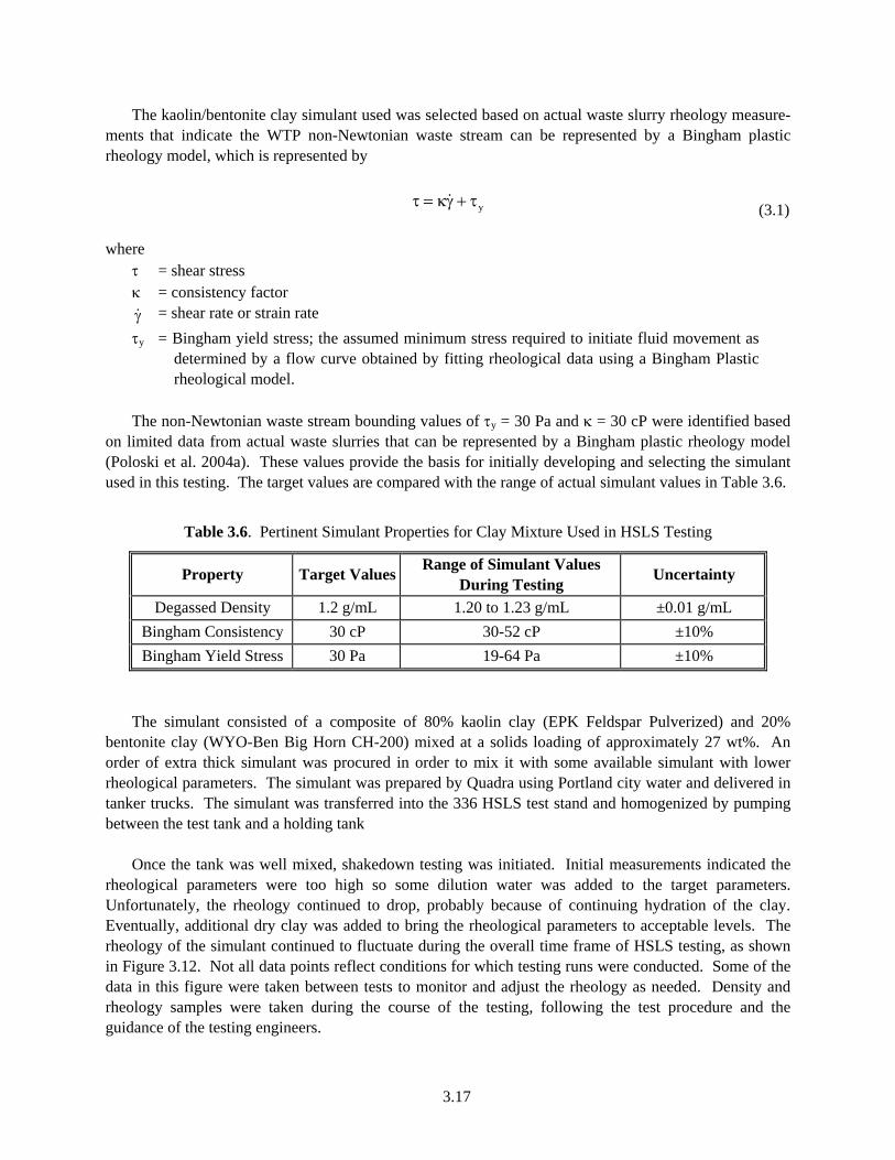
3.17

The kaolin/bentonite clay simulant used was selected based on actual waste slurry rheology measure-ments that indicate the WTP non-Newtonian waste stream can be represented by a Bingham plastic rheology model, which is represented by

yτ = κγ + τ& (3.1) where τ = shear stress

κ = consistency factor γ& = shear rate or strain rate τy = Bingham yield stress; the assumed minimum stress required to initiate fluid movement as

determined by a flow curve obtained by fitting rheological data using a Bingham Plastic rheological model.

The non-Newtonian waste stream bounding values of τy = 30 Pa and κ = 30 cP were identified based on limited data from actual waste slurries that can be represented by a Bingham plastic rheology model (Poloski et al. 2004a). These values provide the basis for initially developing and selecting the simulant used in this testing. The target values are compared with the range of actual simulant values in Table 3.6.

Table 3.6. Pertinent Simulant Properties for Clay Mixture Used in HSLS Testing

Property Target Values Range of Simulant Values During Testing Uncertainty

Degassed Density 1.2 g/mL 1.20 to 1.23 g/mL ±0.01 g/mL Bingham Consistency 30 cP 30-52 cP ±10% Bingham Yield Stress 30 Pa 19-64 Pa ±10%

The simulant consisted of a composite of 80% kaolin clay (EPK Feldspar Pulverized) and 20% bentonite clay (WYO-Ben Big Horn CH-200) mixed at a solids loading of approximately 27 wt%. An order of extra thick simulant was procured in order to mix it with some available simulant with lower rheological parameters. The simulant was prepared by Quadra using Portland city water and delivered in tanker trucks. The simulant was transferred into the 336 HSLS test stand and homogenized by pumping between the test tank and a holding tank

Once the tank was well mixed, shakedown testing was initiated. Initial measurements indicated the rheological parameters were too high so some dilution water was added to the target parameters. Unfortunately, the rheology continued to drop, probably because of continuing hydration of the clay. Eventually, additional dry clay was added to bring the rheological parameters to acceptable levels. The rheology of the simulant continued to fluctuate during the overall time frame of HSLS testing, as shown in Figure 3.12. Not all data points reflect conditions for which testing runs were conducted. Some of the data in this figure were taken between tests to monitor and adjust the rheology as needed. Density and rheology samples were taken during the course of the testing, following the test procedure and the guidance of the testing engineers.

3.18

HSLS Simulant Rheology in Test Stand Oct - Dec 2004

0

10

20

30

40

50

60

70

24-Oct 3-Nov 13-Nov 23-Nov 3-Dec 13-Dec

Sample Date and Time

Yie

ld S

tress

(Pa)

Figure 3.12. Yield Stress Variation During the HSLS Testing

3.5.2 Rheological Measurements

Rheology samples were taken at several points, often in conjunction with other samples. The samples were collected with a syringe on a long pole, as described in Section 4.5.3, or with the compression molds used to collect density samples. They were taken from various depths in the tank. Rheograms, or plots of shear stress versus shear rate, are required to characterize non-Newtonian fluids. Rheograms provide flow data over a range of shear rates rather than at one specific shear rate. A rheometer ramps up the shear stress or the shear rate to a chosen value while measuring and recording the dependent parameter.

The HSLS simulant rheology testing was primarily done by testing from 0-1000 s-1 over 5 min (up

curve), holding at 1000 s-1 for 1 min, and then testing from 1000-0 s-1 over 5 min (down curve). Some rheograms were tested with only a 2-min ramp cycle when a quick indication of the current rheology was needed. However, the HSLS testing data were measured with 5-min ramp cycles. All rheograms were obtained at 25oC. A typical rheogram from the simulant is shown in Figure 3.13.

Over the testing range of 0 to ~100 s-1, there is a noticeable variation between the up and down ramping data that was less pronounced from ~100 to 1000 s-1. This hysteresis is a product of the shear strength in the simulant that must be overcome when the sample is placed under a shearing force. This number would best represent the simulant at startup conditions, not operating conditions. For this reason the down ramping data are used for obtaining the Bingham plastic rheological parameters and reported in this document. The hold portion of the testing is done to determine whether there was significant thixotropy in the sample, and none was seen during HSLS testing with this simulant.

3.19

Typical Rheogram of HSLS Simulant

Bingham Curve Fitτ = 0.0431γ. + 31.138

0

10

20

30

40

50

60

70

80

0 200 400 600 800 1000 1200

Shear Rate (1/s)

Shea

r Str

ess

(Pa)

Up Ramp (0-1000 1/s) Hold Step - 1000 1/s) Down Ramp (1000-0 1/s) Linear (Down Ramp (1000-0 1/s))

Figure 3.13. Typical Simulant Rheogram

A Bingham curve fit was used to characterize the down ramping set of the rheogram data to obtain

the Bingham yield and consistency. For the above sample, the yield was 31.1 Pa and the consistency was 43.1 mPa-s or cP. The uncertainty associated with these parameters is ±10%.

3.5.3 Equipment Capabilities and Sensor Selection

The rheometer used for all shear stress versus shear rate testing was a TA Instruments AR 2000 model with a concentric cylinder sensor. This model is a controlled stress rheometer equipped with an air bearing and a Peltier plate for temperature control. All rheograms were obtained at 25oC. The instrument is performance checked with calibration standard oils at least once a month. During HSLS testing this was performed three times, and each time the instrument tested well within the required ±10% of the known standard value.

3.5.4 Density Measurements

Density measurements of the HSLS simulant were obtained at several points during testing. The density was determined by measuring the mass of containers with known tare weights and volume filled with simulant. Two types of containers were used, 750 mL pycnometers and plastic compression molds.

3.20

Pycnometers are devices of known precise volumes used specifically for measuring density. They produce consistent repeatable results with a minimal amount of data scatter. This was the method used to obtain the majority of the degassed density data for HSLS testing. Pycnometers have narrow necks and need to be filled slowly with a funnel to prevent plugging by the simulant. This prevented their use for obtaining samples directly from the tank. Simulant samples were taken from the tank and stirred to ensure that all gas had been released before they were transferred into tared pycnometers and weighed.

To obtain the density of samples from various depths in the tank directly with a container of known volume and weight, a special sampler was designed that could use large cylindrical compression molds to obtain samples in situ and to measure with them with as little disturbance to the material as could be achieved. The volumes on these molds were verified using a sample of the HSLS simulant taken from the 336 tank just before initial testing began. This simulant was degassed and characterized with the pycnometers, then used to calibrate the volume of each uniquely labeled compression mold.

Retained gas can affect the rheology and density of the simulant, so in laboratory testing before and during the first few days of HSLS testing, various methods of degassing simulant samples were tested, performed, and compared. These methods included shaking, stirring, and putting the sample under vacuum for various times and under various agitations. It was determined that periodic stirring of large samples or vigorous shaking of small samples was enough to degas them to below a rheologically detectable level. This method of degassing was therefore adopted for the rest of the HSLS testing.

4.1

4.0 Test Approach and Operations

4.1 Scaled Testing Approach

The HSLS test program used the same geometric scaling approach as the scaled testing supporting the PJM non-Newtonian tests performed at PNWD and SRNL. The scaled testing approach has the following elements (Barnes 2004):

• All linear dimensions are reduced by the scale factor(s) (ratio of plant scale to test scale). These include vessel diameter, fill level, PJM nozzle diameter, etc.

• PJM discharge velocities are the same at both reduced and full scale.

• All imposed times are reduced by the scale factor(s) except where necessary to meet experimental objectives. These include PJM drive time, intermittent sparge times, etc.

For tests performed in this manner, the fluid mixing results and gas release rates (i.e., exponential decay of gas content following restart of mixing) follow the linear scale factor(s) directly. However, the steady-state gas holdup is proportional to both the scale factor and the in situ volumetric gas generation rate (gv).

An example of the scaling principle for the normal operations mixing scenario is shown in Figure 4.1. In the normal operations mode, PJM operation is continuous while sparger operation is intermittent. For the full plant-scale LS vessel, this consists of repeated cycles of 1 hr of full sparging followed by 2 hr of idle sparging.(a) Mixing system operation is indicated by the horizontal bars in the figure. Also shown in Figure 4.1 is the half-scale operational cycle. Here the sparger operation is scaled by the scale factor, i.e., 1/2 hr of full sparging followed by 1 hr of idle flow conditions. If the in situ gas generation rate is doubled in the half-scale test, gas will accumulate more rapidly in the simulant during the idle sparge period; but, because the accumulation occurs over half the time, it will achieve approximately the same peak value of retained gas fraction (indicated by αMAX in Figure 4.1). In addition, after full sparge operation resumes, gas will be released at a faster rate in the half-scale test than at full scale. However, because the release occurs over half the total time, the minimum gas fraction (indicated by αMIN in Figure 4.1) would be approximately the same for the half-scale test.

In the post-DBE operations mode, both PJM and sparger operation are intermittent. For the full-plant-scale LS vessel, this consists of repeated cycles of 2 hr(b) of PJMs and full sparging followed by 12 hr of idle sparging only. In the near-term accident response (NTAR) operations mode, the PJMs are off and sparger operation is intermittent. For the full plant-scale LS vessel, this consists of repeated cycles of 2 hr of full sparging followed by 12 hr of idle sparging only. For the post-DBE and NTAR operations mode, the same scaling behavior discussed above for normal mode generally applies to the operating scenarios. This is shown in Figure 4.2. As discussed in Section 4.4.2, the mixing-off times were adjusted (shortened) to accommodate the fairly rapid decomposition of the hydrogen peroxide.

(a) Idle sparging consists of a reduced air flow rate primarily intended to keep the sparge tubes from plugging. (b) At the direction of BNI, the 2-hr mixing time was reduced to 1 hr for scale-up to plant conditions (Section 7).

4.2

1 hr 2 hr 3 hr 4 hr

αmax

αmin

5 hr 6 hr

Full-scale sparge operation1/2 scale sparge operationPJM operation

Full-scale behaviorwith generation rate g

1/2-scale behaviorwith generation rate 2g

Figure 4.1. Illustration of the Scaling Relationship Between Half- and Full-Scale Gas Holdup Behavior During the Normal Operations Mixing Scenario

4 hr 6 hr 8 hr 10 hr

αmax

αmin

12 hr 14 hr

Full-scale sparge & PJM operation1/2 scale sparge & PJM operation

Full-scale behaviorwith generation rate g

1/2-scale behaviorwith generation rate 2g

2 hr Figure 4.2. Illustration of the Scaling Relationship Between Half- and Full-Scale Gas Holdup Behavior During the Post-DBE and NTAR Mixing Scenarios

The general approach used in performing the HSLS gas holdup tests involved the following steps:

• Select/adjust the gas generation rate to give αMAX- αMIN roughly equal to αcrit where αcrit is the total allowable releasable gas fraction (~0.6% normal operations, ~2.4% post-DBE operations).(a)

• Run the test until long-term, repeatable gas buildup and release is observed.

4.2 PJMs Operation Mode

During all the gas holdup/release and mixing tests performed in the HSLS test system, the PJMs were operated in a manner such that the target peak average velocity was ~11 ± 1 m/s after ~1/2 of the normal PJM volume(b) was discharged during the drive phase. This mode of operation, generally referred to as

(a) As discussed in the results of Section 6.2, an αcrit of ~0.39% was obtained for the normal operations test, and an αcrit of ~1.71% was obtained for post-DBE operations. The reduced αcrit was sufficiently large that the experimental objectives were met. (b) The full stroke of operation typically corresponds to ~85% of the PJM volume.

4.3

the half stroke, was agreed upon by the Steering Committee as a worst-case scenario for demonstrating the safe operation of the WTP. The drive time for the half stroke operation was determined by evaluating the PJM nozzle velocities and terminating the drive after peak average velocity was observed.

During the mixing tests, the PJMs were operated at both half stroke and full stroke. The full-stroke

operation with full sparging was used to degas the simulant after gas generation experiments and to homogenize the tank contents at the end of the mixing tests to provide a uniform chloride tracer concen-tration in the simulant. Final samples of the completely mixed simulant were needed for determining the volume percent mixed during the course of the mixing tests and to check for closure of the mass balance on the injected chloride tracer.

4.3 Main Sparger and Idle Sparger Air Flow Rates

During all the HSLS gas release and mixing tests, the spargers were operated such that the target air flow rates at each sparger nozzle were 18.8 ± 2 and 1 ± 0.5 acfm during full and idle sparging conditions, respectively. These air flow rates were calculated by BNI as the approximate equivalent of the rate at the surface of the slurry in the WTP LS vessel, after accounting for the differences in hydrostatic pressure between the HSLS test stand and the full-scale plant vessel.

4.4 Gas Holdup and Release Tests

The gas holdup tests performed in the HSLS test system to demonstrate the normal, post-DBE, and NTAR operational scenarios, along with the test objectives and the target operating conditions (actual operating conditions are given with the results in Section 6) for the PJMs and spargers and hydrogen peroxide injection are listed in Table 4.1.(a) Also listed in Table 4.1 are two additional gas release tests performed to obtain gas release rates and to determine the unmixed volume in the sparger heel and in the PJMs. The following is a detailed description of the basis for using hydrogen peroxide for in situ gas generation, method of hydrogen peroxide injection, and the approaches used in the different tests.

4.4.1 Simulation of Gas Generation Mechanism

In the HSLS tests, in situ hydrogen gas generation was simulated using the technique based on decomposition of H2O2 on catalytic surfaces according to the following reaction: 2H2O2 ↔ 2H2O + O2 (4.1) This approach was used in the gas holdup and release tests in the APEL and 336 test facilities (Russell et al. 2005). According to the reaction stoichiometry, two moles of H2O2 decompose to produce 1 mole of O2 and 2 moles of H2O. Using this relationship, the nominal H2O2 solution concentration (30 wt%), and ideal gas law considerations, the equivalent volume of O2 gas generation can be determined from decomposition of a given mass of H2O2.

(a) The conditions given in Section 4 are generally the target experimental conditions. Actual conditions are reported with the results in Section 6.

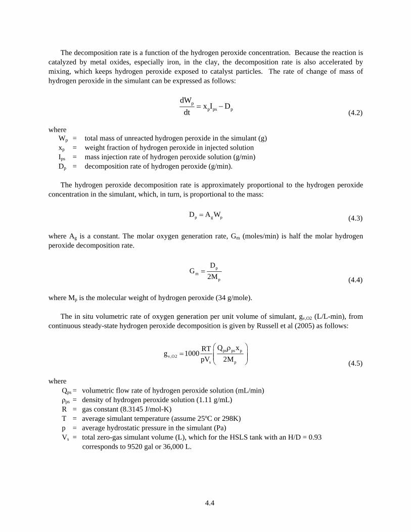
4.4

The decomposition rate is a function of the hydrogen peroxide concentration. Because the reaction is catalyzed by metal oxides, especially iron, in the clay, the decomposition rate is also accelerated by mixing, which keeps hydrogen peroxide exposed to catalyst particles. The rate of change of mass of hydrogen peroxide in the simulant can be expressed as follows:

dWp

dt= xpIps − Dp (4.2)

where Wp = total mass of unreacted hydrogen peroxide in the simulant (g) xp = weight fraction of hydrogen peroxide in injected solution Ips = mass injection rate of hydrogen peroxide solution (g/min) Dp = decomposition rate of hydrogen peroxide (g/min).

The hydrogen peroxide decomposition rate is approximately proportional to the hydrogen peroxide concentration in the simulant, which, in turn, is proportional to the mass:

p g pD A W= (4.3) where Ag is a constant. The molar oxygen generation rate, Gm (moles/min) is half the molar hydrogen peroxide decomposition rate.

pm

p

DG

2M=

(4.4) where Mp is the molecular weight of hydrogen peroxide (34 g/mole).

The in situ volumetric rate of oxygen generation per unit volume of simulant, gv,O2 (L/L-min), from continuous steady-state hydrogen peroxide decomposition is given by Russell et al (2005) as follows:

ps ps pv,O2

s p

Q xRTg 1000pV 2M

⎛ ⎞ρ= ⎜ ⎟⎜ ⎟

⎝ ⎠ (4.5) where Qps = volumetric flow rate of hydrogen peroxide solution (mL/min) ρps = density of hydrogen peroxide solution (1.11 g/mL) R = gas constant (8.3145 J/mol-K) T = average simulant temperature (assume 25ºC or 298K) p = average hydrostatic pressure in the simulant (Pa) Vs = total zero-gas simulant volume (L), which for the HSLS tank with an H/D = 0.93

corresponds to 9520 gal or 36,000 L.

4.5

Table 4.1. Objectives and Target Test Conditions for the Gas Holdup and Release Tests Conducted in the HSLS Test Configuration

PJMs Spargers Gas Gen. Rate

Test ID Run #/ Order(a)

Engineering Purpose/ Objectives

Run Configuration(b) Run Objective H/D τy

(Pa)

Peak Avg Noz.

Vel. (m/s)

PJM Cycle Time(sec)

Operational Cycling

Normal(acfm per

tube)

Idle (acfm

per tube)

Operational Cycling

Peroxide Injection Rate

(total) (mL/min)

gplant (L/L-Day)

gtest (L/L-Day)

Approach Criteria for Test Completion

HSLS-1 1 Normal Operations: Needed to make decision on removing recirculation mixing pumps from LS and blend vessels.

Holdup test with PJMs + full sparging

1) Determine steady-state holdup for PJMs + full sparging

0.93 31-37 11 ±1 120 Continuous 18.8 ±2 - Continuous full

Continuous @ 90 mL/min

0.012 >>0.012 Determine gas holdup with continuous PJM and full sparger operation

Constant simulant level/holdup or as directed by PJM Steering Committee (turn off mixing every 0.5-1 hr to obtain accurate level measurements)

2 Holdup test PJMs + idle sparging

1) determine steady-state holdup for PJMs with spargers on idle, 2) verify peroxide addition rate, 3) set start point for normal operations

0.93 31-33 11 ±1 120 Continuous - 1 ±0.5 Continuous idle

Continuous @ 90 mL/min

0.012 >>0.012 Determine gas holdup with continuous PJMs and idle sparger operation

Constant simulant level/holdup or as directed by PJM Steering Committee (turn off mixing every 0.5-1 hr to obtain accurate level measurements)

3 Normal operations 1) replicate intended normal operations, 2) demonstrate gas release by intermittent sparging and continuous PJMs, 3) demon-strate steady periodic behavior

0.93 32-35 11 ±1 120 Continuous 18.8 ±2 1 ±0.5 0.5 hr full and 1 hr idle

Continuous @ 90 mL/min

0.012 >>0.012 Continue test with required PJM and sparger operating conditions and hydrogen peroxide injection such that long term repeatable behavior is observed

Maximum and minimum holdup/ level values indicate no observable trends for a minimum of 3 PJM/ sparger operational cycles then run for 5 more cycles or as directed by PJM Steering Committee

HSLS-2 3 Post-DBE Operations: Define sizing of backup ITS (important to safety) air compressors and diesel generators

Post-DBE 1) replicate post-DBE operations, 2) demonstrate gas release by intermittent PJM/sparging, 3) demonstrate steady periodic behavior

0.93 42-43 11 ±1 120 1 hr on and 2 hrs off

18.8 ±2 1 ±0.5 1 hr on and 2 hr idle

382 mL/hr (for 55 min) total mixing time = 1 hr

0.012 >>0.012 Continue test with required PJM and sparger operating conditions and hydrogen peroxide injection such that long term repeatable behavior is observed

Maximum and minimum holdup values indicate no observable trends for a minimum of 3 PJM/sparger operational cycles or as directed by the PJM Steering Committee

3 NA Determine the alpha min (αmin) corresponding to a constant peroxide injection rate

0.93 42-43 11 ±1 120 mix for 1 hr with peroxide injection

18.8 ±2 1 ±0.5 Full sparge for 1 hr then idle for 1 hr

50 mL/min for 1 hr

0.012 >>0.012 Inject hydrogen peroxide for 1 hr then turn PJMs off and set spargers to idle flow. Monitor in situ gas growth for 2 hr then turn on PJMs and full sparging to degas simulant.

Completion of specified test steps.

HSLS-3 3a NTAR Operations: Assess need for redundant racks, valves, compres-sors, and diesel generators for PJM operations.

NTAR operations 1) replicate intended NTAR operations, 2) demonstrate gas release by intermittent sparging and no PJMs, 3) demonstrate steady periodic behavior

0.93 43-44 -- -- -- 18.8 ±2 1 ±0.5 1 hr on and 2 hr idle

382 mL/min (for 55 min) total mixing for 1 hr

0.012 >>0.012 Continue tests until long term repeatable behavior is observed.

Conduct test for a minimum of 8 operational cycles to simulate 100 hr of WTP NTAR operation or as directed by PJM Steering Committee.

3b NA Determine the alpha min (αmin) corresponding to a constant peroxide injection rate

0.93 43-44 11 ±1 120 Mix for 1 hr with peroxide injection

18.8 ±2 1 ±0.5 Full sparge for 1 hr then idle for 1 hr

50 mL/min for 1 hr

0.012 >>0.012 Inject hydrogen peroxide for 1 hr then turn PJMs off and set spargers to idle flow. Monitor in situ gas growth for 2 hrs

Completion of specified test steps.

3c NA Generate additional data to determine the gas holdup when only the main spargers are operating.

0.93 43-44 - - - 18.8 ±2 - Continuous Continuous @ 90 mL/min

0.012 >>0.012 Continue test with spargers only and determine gas holdup

Continue for 15 hours or until steady state was observed.

HSLS-8 1 Gas Release Test Gas release test: full sparging and no PJMs

Obtain data on gas release with full sparging; estimate unmixed volume

0.93 42-43 - - - 18.8 ±2 - Continuous 200mL/min for 2 hr with PJMs + full sparging

- - Mix tank with PJMs and full sparging for 2 hr, add hydrogen peroxide at 200 mL/min for 2 hr with PJMs and full sparging, mix for 5 min, stop PJMs and go to shutdown sparging until gas holdup is constant, full sparging to release gas

HSLS-9 1 Gas Release Test Gas release test: PJMs + idle sparging

Obtain data on gas release with PJMs and spargers on idle; estimate unmixed volume

0.93 41-42 11 ±1 120 Continuous - 1 ±0.5 Continuous 350 mL/min for 2 hr with PJMs + full sparging

- - Mix tank with PJMs and full sparging for 2 hr, add hydrogen peroxide at 350 mL/min for 2 hr with PJMs and full sparging, mix for 5 min, stop PJMs and go to shutdown sparging till gas holdup is constant, PJMs + idle sparging to release gas

(a) Run numbers reflect the original test matrix numbering. The test matrix was modified by the steering committee during the course of testing. The original numbering was maintained for traceability. (b) Definition of run configurations: - Normal Operations: represents normal plant operations with PJM on continuously and spargers cycling between full (18.8 acfm) and idle (1 acfm). - Post DBE: represents plant operations in post-DBE (design basis event). In this configuration, the mixing modes cycle between PJMs with full sparging (18.8 acfm per sparge tube) and spargers on idle (1 acfm per sparge tube). - NTAR (near term accident response): represents plant operations in the event the PJM mixing mode is temporarily lost. In this configuration, sparging is the only means of mixing. The spargers cycle between full (18.8 acfm per sparge tube) and idle (1 acfm per sparge tube). - NA: Not applicable. - Holdup test: determines the steady-state holdup of gas with a specified mixing configuration. - Gas release test: determines the gas release profile with a specified mixing configuration.

4.7

Solving Eq. (4.5) for the hydrogen peroxide flow rate gives:

pps v,O2 s

ps p

2MpQ 0.001g VRT x

⎛ ⎞⎛ ⎞= ⎜ ⎟⎜ ⎟⎜ ⎟ρ⎝ ⎠⎝ ⎠ (4.6)

In Eq. (4.5) and (4.6) the gas-free simulant volume has not been corrected by the relatively small

added volume of water introduced by injection of hydrogen peroxide solution (for example, a hydrogen peroxide injection rate of 280 mL/min will produce a 1 wt% water dilution per day). Some of this volume change is offset by the volume of water lost by evaporation during sparger operation.

4.4.2 Hydrogen Peroxide Injection Approach

The gas generation analysis on selected tank wastes (Tsang 2004) estimates that the full-scale gas generation rates in the WTP LS vessels is on the order of 0.006 L/L day.(a) The target hydrogen peroxide injection rate used in the present testing, ~30 gal/day or ~90 mL/min, gives a gas generation rate of 0.35 L/L-day (from Eq. 4.6).

A major complication with the scaled testing approach is the need to approximate the continuous and uniform volumetric gas generation of the WTP plant using hydrogen peroxide decomposition in the scaled tests. The hydrogen peroxide solution must be injected so that it is mixed throughout the vessel by the mixing systems to approximate continuous and uniform gas generation. The system for the hydrogen peroxide injection was discussed in Section 3; this section deals with the different approaches used for injecting the hydrogen peroxide for the different operational scenarios tested.

In the normal operation scenario, hydrogen peroxide was added continuously to the PJM cavern, which experiences continuous mixing from the PJMs. Some spatial periodic nonuniformity may result during periods of idle sparging, but continuous gas generation can still be assumed.

For the post-DBE and NTAR operating scenarios, mixer operation was intermittent. Because the hydrogen peroxide solution can be mixed effectively only when mixing is “on,” excess hydrogen peroxide must be “spiked” during the short mixing-on period and allowed to decompose and provide gas generation during the idle-sparge, mixing-off period. In Eq. (4.2), the total gas generation rate over a post-DBE and NTAR operation cycle can adequately represent the plant conditions if 1) the varying rates

(a) Based on later direction from BNI, the gas generation rate for scale-up to the plant LS vessel was specified as 2.06×10-5 moles of hydrogen per liter of waste per hour, with hydrogen making up 25% of the total gas generated for a total of 8.24×10-5 moles/L-h (0.033 L of gas per liter of waste per day at depth). For comparison, the actual hydrogen peroxide injection rate of 95 mL/min used for the normal operations portion of the HSLS-1 test produced 7.63×10-4 moles/L-h (0.37 L/L-d), about a factor of 5 higher than the scaled generation rate (2 times the plant rate). The 50 mL/min injection rate represented in the post-DBE and NTAR tests produced 4.01×10-4 moles/L-h (0.19 L/L-d), about three times the scaled plant rate. The gas generation rate for the plant UFP vessel was specified as 2.08×10-5 moles of hydrogen per liter of waste per hour with hydrogen making up 25% of the gas generated for a total of 8.32×10-5 moles/L-h (0.039 L of gas per L of waste per day at depth). The gas generation rate in the normal operations portion of the HSLS-1 test was five times higher than the scaled generation rate (2 times the plant rate), and the rate represented in the post-DBE and NTAR tests was about twice the scaled plant rate.

4.8

of hydrogen peroxide injection and depletion (gas generation) are such that the time-averaged hydrogen peroxide mass in the simulant is approximately constant (i.e., the average rate of change of hydrogen peroxide mass is zero), and 2) roughly the same total retained gas volume is achieved at the end of the non-mixed period as for a uniform gas generation rate. The hydrogen peroxide concentration at the end of the accelerated injection period is necessarily higher, which also makes the gas generation rate artificially high for some portions of the testing (via Eq. 4.3 and 4.4). However, this is balanced by the lower gas generation rate as hydrogen peroxide is depleted toward the end of the nonmixing period. Hence, a constant gas generation rate in a system with intermittent mixing can be represented, on the average, by intermittent hydrogen peroxide injection at a cycle-averaged rate that matches the desired uniform gas generation rate.

For the hydrogen peroxide injection system used in the HSLS test configuration, which has seven injection points, seven times the average flow of hydrogen peroxide solution would be required for a test with a 1-hr mixing-on period followed by a 6-hr idle-sparge, mixing-off period. Furthermore, the hydrogen peroxide solution was injected only for the first 55 minutes of the mixing-on period to ensure adequate mixing before starting the idle-sparge, mixing-off period. This increases the flow rate to 7.6 times the average (i.e., a target injection rate of 382 mL/min under this regimen would provide an average of 50 mL/min of hydrogen peroxide solution for a 7-hr cycle).

One additional adjustment was required to adequately simulate a constant gas generation rate during the post-DBE and NTAR operations. It was found that hydrogen peroxide decomposes fairly rapidly, and most of the excess injected during the mixing-on period was depleted long before the end of the 6-hr idle-sparge, mixing-off period. This would have resulted in an extended period of essentially static conditions with very low gas generation rates. To maintain an approximately uniform generation rate while maintaining an equivalent maximum gas volume fraction, the idle-sparge, mixing-off period was shortened so that the estimated gas generation rate at the end was roughly equal to the desired overall average. For HSLS test conditions, a 2-hr idle-sparge, mixing-off period was equivalent to the scaled 6 hr, as illustrated in Figure 4.3.

Full 6 Hr Of f Period

2 Hr Of fPeriod

Figure 4.3. Strategy for Shortening the Off Period During Post-DBE and NTAR Testing

4.9

4.4.3 Criterion for Steady State At the start of the tests, a criterion of ±0.25 inch change in the static liquid level for a minimum of three measurements(a) was chosen as the basis to establish steady state in the gas holdup behavior. The tank static liquid level was measured by stopping the PJMs and switching the spargers to idle flow as necessary for a brief time (generally <5 minutes) and manually measuring the liquid level in the tank as well as recording the level indicated by the laser level probes. At each static level measurement point, this criterion was determined to generally not be practical for establishing the realization of steady state. Therefore, the static liquid levels along with the gross weight of the tank were used to generate a continuous real-time plot of the gas holdup versus time. The gas holdup data were reviewed by the Steering Committee to determine whether an acceptable steady state was achieved or whether the test should be continued further to differentiate slow transients from periodic oscillations in the data.

4.4.4 Cakeout and PJM Sparger Holdup Test (HSLS-0) Because the gas volume fraction is determined on the basis of simulant level measurements in the tank and the simulant mass, the factors that affect these variables needed to be characterized. The three main factors are the following:

• Water loss due to evaporation: During the HSLS gas holdup and mixing tests, water was lost from the tank due to evaporation and stripping by the sparger air. The rate of water loss was a function of several variables including the free surface area of the tank, sparger air flow rates, temperature, and humidity, and temperature of the simulant.

• Simulant cakeout on the tank walls and support structures: Another concern during the testing was the deposition of the simulant on the walls of the tank. Continued deposition during the test could have led to a large accumulation and would have an adverse effect on measuring gas fractions. HSLS-0 Run 0 was focused on determining the caked-out mass of the simulant and the water lost due to evaporation. The run was carried out for 6 hr with PJMs and full sparging operating continuously. Every 2 hr, the spargers and PJMs were shut down for a static measurement of the simulant level.

• Retained gas due to PJMs and sparger operation. In addition to cakeout, the air introduced by the PJMs and spargers could have influenced the measured gas fraction during the gas holdup and release tests. Therefore, initial gas holdup tests with no hydrogen peroxide injection (i.e., no in situ gas generation), were conducted to determine the gas holdup for the PJMs/full sparging (HSLS-0 Run 1), PJMs/idle sparging (HSLS-0 Run 2), and full sparging only conditions (HSLS-0 Run 3). Run 1 was carried out for ~4.5 hr, Run 2 for ~3.5 hr, and Run 3 for ~5 hr. The initial static level at the start of each run and also periodic (~every 30 minutes) measurements of the static levels were also made throughout each run.

(a) For simple gas holdup tests with the PJMs and full spargers, PJMs and idle spargers, or spargers only operating, the criterion was a ±0.25-inch change in the static liquid level for a minimum of three measurements ½ to 1 hr apart. For tests involving the normal, post-DBE, or NTAR operations, the criterion was a ±0.25-inch change in three subsequent minimum and maximum tank level values.

4.10

4.4.5 Normal Operations Test (HSLS-1) Test HSLS-1 lists the PJM/sparger operating conditions and experimental approach for the normal operation test scenarios. The gas holdup and release test performed under the normal operations demonstration test consisted of three runs. The focus of Run 1 (see HSLS-1, Run 1 in Table 4.1) was to determine the gas holdup with continuous PJM/sparger operation and a continuous hydrogen peroxide target injection rate of 90 mL/min. Run 1 was continued until a steady state gas holdup was established, when the spargers were set under idle flow conditions (PJMs still operating continuously) and then Run 2 was initiated (see HSLS-1 Run 1 in Table 4.1). The focus of Run 2 (see HSLS-1, Run 2 in Table 4.1) was to determine the maximum gas holdup with continuous PJM and idle sparger operation. The target hydrogen peroxide injection rate during Run 2 was the same as in Run 1, i.e., continuous at 90 mL/min. Run 2 was carried out until a steady max-imum gas holdup was observed. The steady-state condition for Run 2 became the initial starting point for Run 3, the actual normal operations demonstration test (HSLS-1 Run 3, Table 4.1). The target hydrogen peroxide injection rate during Run 3 was the same as in Runs 1 and 2, continuous at 90 mL/min. After steady state was ascertained, the run continued for several more cycles until the Steering Committee was confident that the fluctuations in the data were not hiding a slow transient and a periodic steady state had been achieved.

4.4.6 Post-DBE Operations Test (HSLS-2) Test HSLS-2 lists the PJM/sparger operating conditions and experimental approach for the post-DBE operations test scenarios. The focus of Run 3 (see HSLS-2, Run 3 in Table 4.1) was to demonstrate the post-DBE operational scenario. As discussed in Section 4.4.2, the post-DBE test was conducted with a 3-hr cycle consisting of mixing with PJMs and full spargers for 1 hr and with idle spargers only for the remaining 2 hr. The hydrogen peroxide was injected continuously at a total target flow rate of 382 mL/min for the first 55 minutes of the cycle when the PJMs and spargers were on and then switched off during the remaining 2 hr and 5 minutes. The test was continued until steady state was ascertained by the Steering Committee. During the last cycle, the hydrogen peroxide was injected at a target rate of 50 mL/min for the 1-hr period while the PJMs and full spargers were on. After the hydrogen peroxide injection was stopped the spargers were switched to idle, and the growth of in situ gas was measured for the next 2 hours. The purpose of the reduction in the peroxide injection rate for the last cycle was to obtain data at a gas generation rate more typical of the expected plant generation rate.

4.4.7 NTAR Operations Tests (HSLS-3) Test HSLS-3 lists the PJM/sparger operating conditions and experimental approach for the NTAR operations test scenarios. This set of tests consisted of two runs, the NTAR test and a sparger only gas holdup test. The focus of Runs 3a and 3b (see HSLS-3 Runs 3a and 3b in Table 4.1) was to demonstrate the NTAR operations test. The test was conducted for a minimum of eight operational cycles (actual was 11 cycles) to simulate 100 hr of WTP NTAR operations. During the last cycle, the hydrogen peroxide was injected at a target rate of 50 mL/min for the 1-hr period when the PJMs and full spargers were on and then the hydrogen peroxide was turned off and the spargers were switched to idle. The gas growth

4.11

was measured for 2 hr. The purpose of the reduction in the peroxide injection rate for the last cycle was to obtain data at a gas generation rate more typical of the expected plant generation rate.

Run 3c (see HSLS-3 Run 3c in Table 4.1) was a gas holdup test with main spargers only. The focus of this test was to generate additional data to determine the gas holdup when only the main spargers were operating. The test was performed immediately after the last PJMs/spargers off period of HSLS-3 Run 3b. In addition, hydrogen peroxide injection was continuous at a total rate of 90 mL/min (same as that in normal operations test HSLS-1). The run continued for ~15 hr, until steady state was observed.

4.4.8 Gas Release Tests (HSLS-8, 9) Tests HSLS-8 and -9 indicate the PJM/sparger operating conditions for the two gas release tests performed in the HSLS test system. The objectives of the HSLS-8 test were to generate additional gas release data when only the main spargers were operating and to use these data to determine the unmixed heel volume. The test was started after degassing the tank for several hours with the PJMs and full sparging and no hydrogen peroxide injection. After the tank was degassed, it was mixed for an additional 2 hr, during which the hydrogen peroxide was injected at a constant rate of 200 mL/min. After 2 hr, the PJMs were turned off and the sparger air flow set to the shutdown flow rate (~0.3 acfm) and the gas was allowed to grow until the simulant level was constant indicating the hydrogen peroxide decomposition was complete. Then the main spargers were turned on and the gas release measured until there was no change in the simulant level in the tank. The objectives of test HSLS-9 were to generate additional gas release data when the PJMs and idle spargers were operating and to use these data to determine the unmixed volume in the pulse tubes. The test was started after degassing the tank for several hours with the PJMs and full sparging and no hydrogen peroxide injection. After the tank was degassed, it was mixed for an additional 2 hr, during which the hydrogen peroxide was injected at a constant rate of 350 mL/min. After 2 hr, the PJMs were turned off and the sparger air flow set to the shutdown flow rate (~0.3 acfm) and the gas was allowed to grow until the simulant level was constant indicating the peroxide decomposition was complete. Then the PJMs and spargers on idle were turned on and the gas release was measured until there was no change in the simulant level in the tank.

4.5 Mixing Tests (HSLS-4) The mixing runs performed in the HSLS test system along with the objectives, operating conditions for the PJMs and spargers, and chloride tracer addition approach are listed in Table 4.2. The following is a detailed description of the basis for choosing the chloride tracer, method of tracer addition, and the approaches used in the different runs.

4.5.1 Chloride Tracer Technique A chloride tracer technique with periodic grab sampling from four different locations within the tank and analysis of the grab samples by ion chromatography (IC) was used to measure the effectiveness of mixing in terms of the time to mix and the unmixed slurry volume. The reason for the choice of the

4.12

chloride tracer over the other techniques is that the chloride ions are not absorbed by the clay molecules and they partition completely into the aqueous phase of the simulant (Poloski et al. 2004a). To determine the chloride concentration, the clay samples were centrifuged to separate the solids phase from the aqueous phase. The aqueous phase was then analyzed for chloride ion concentration using IC. This technique has the sensitivity of measuring the chloride concentrations as low as 10 ppb, and during all HSLS mixing tests, the chloride concentrations were between 10 ppm and 200 ppm.

4.5.2 Chloride Tracer Injection/Addition Approach During the initial mixing runs (HSLS-4 Runs 1 and 2 in Table 4.2), the hydrogen peroxide injection lines were used for adding chloride tracer (concentrated salt solution containing ~20 to 25 wt% NaCl dissolved in water). But, because of the accumulation of small amounts of chloride tracer in the sparger heel and entrapment within the dead-volume of the pulse tube during the half-stroke mode of operation, this method of addition was abandoned, and the chloride tracer was added directly to the top of the simulant.

4.5.3 Grab Sampling Approach

During the mixing tests, grab samples were collected periodically from the four sample locations; shown as L1, L2, L3, and L5. The plan view of the sampling locations is shown in Figure 4.4. Due to the extremely limited accessible space on the tank, the grab sampling locations shown in Figure 4.4 were chosen not based on their radial position in the tank but on the ease of collecting the samples.

For all mixing tests, the grab samples obtained at locations 3 and 5 (Figure 4.4) were taken at an

elevation of ~3 ft (actual was 2 ft 9 in. ±6 in.), and the grab samples obtained from location 1 were taken at an elevation of ~7 ft (actual was 6 ft 9 in. ±6 in.) as measured from the tank floor. For HSLS-4, Runs 1 and 2, which were conducted with a simulant H/D of 0.93, the fourth sample (location 2) was collected at an elevation 11 ft (actual was 10 ft 9 in. ±6 in.) from the tank floor. For HSLS-4, Runs 3, 4, and 5, which were conducted at a lower H/D of 0.8, grab sampling location 2 fell outside the maximum level of simulant in the tank. Therefore, for these runs, the fourth sample was collected at an elevation of ~9-ft from the tank floor. This sample location is referred to as location 2B. Grab samples were collected before the test started and then approximately every 30 minutes throughout the test. As the testing progressed, the period over which the samples were drawn was increased to between 1 and 2 hr.

Grab samples were taken using a 100-mL syringe mounted at one end of a long pipe. The plunger on the syringe could be operated by a person standing on the bridge above the tank. Four syringes/pipe configurations were used for each sampling location where grab samples were collected. The size of each syringe/pipe sampler was such that the sample was collected at approximately the same location all the time. Because of the long lengths of the sampler pipe (~10 to 20 ft), 2-inch-OD PVC tubes mounted along the railing of the bridge were used to guide the sampler to the appropriate location. However, there is still some uncertainty about the exact location from which the samples were collected, and it is estimated to be within ±6 inches of the elevation listed above for the different sampling locations.

4.13

Table 4.2. Objectives and Target Run Conditions for the Mixing Tests Conducted in the HSLS Test Configuration

PJMs Spargers

Test ID Run # Engineering

Purpose/ Objective

Run Configuration Run Objective H/D τy

(Pa)

Peak Avg. Nozzle

Velocity(m/s)(a)

PJM Cycle Time(sec)

Operational Cycling

Normal(acfm

per tube)

Idle (acfm per

tube)

Operational Cycling

Tracer Injection Rate (total) Approach Criteria for Test Completion

HSLS-4 1 Mixing Runs: Determine mixing times and quality of mixing

Spargers only (high rheology ~45 Pa)

Determine mixing time with spargers only operating. Determine unmixed heel volume.

0.93 ~47 - - None 18.8 ±2 - Continuous Chloride tracer injected (spike of ~20 ppm change in the final simulant concentration) through hydrogen peroxide injection tubes

Inject chloride tracer as a spike and continue test until no significant variation exists in measured ion-selective electrodes (ISE) voltages.

ISE voltage output fluctuations between 95% and 105% of final equilibrium value or as directed by the PJM Steering Committee. Need to take final grab samples.

2 PJMs @ 1/2 stroke + full sparging

Determine mixing time with PJMs and spargers operating.

0.93 33 ±3 11 ±1 120 Continuous 18.8 ±2 - Continuous Chloride tracer injected (spike of ~20 ppm change in the final simulant concentration) through hydrogen peroxide injection tubes

Inject chloride tracer as a spike and continue test until no significant variation exists in chloride concentration measured by IC.

Chloride concentration 95% and 105% of final equilibrium value or as directed by PJM Steering Committee. Need to mix tank with PJMs @ full stroke and collect final mixed samples.

3 Spargers only Determine mixing time with spargers only operating. Determine unmixed heel volume.

0.8 33 ±3 - - None 18.8 ±2 - Continuous Chloride tracer added on top of simulant in 1 in. of dilution water in a quantity to cause an ~20 ppm change in the final simulant concentration

Add chloride tracer as a spike and continue test until no significant variation exists in chloride concentration measured by IC.

Chloride concentration 95% and 105% of final equilibrium value or as directed by PJM Steering Committee. Need to mix tank with PJMs @ full stroke and collect final mixed samples.

4 Spargers only (repeat of Run 3)

Determine mixing time with spargers only operating. Determine unmixed heel volume.

0.8 33 ±3 - - None 18.8 ±2 - Continuous Chloride tracer added on top of simulant in 1 in. of dilution water in a quantity to cause an ~20 ppm change in the final simulant concentration

Add chloride tracer as a spike and continue test until no significant variation exists in chloride concentration measured by IC.

Chloride concentration 95% and 105% of final equilibrium value or as directed by PJM Steering Committee. Need to mix tank with PJMs @ full stroke and collect final mixed samples.

5 Spargers only (repeat #2 of Run 3)

Determine mixing time with spargers only operating. Determine unmixed heel volume.

0.8 33 ±3 - - None 18.8 ±2 - Continuous Chloride tracer added on top of simulant in 1 in. of dilution water in a quantity to cause an ~20 ppm change in the final simulant concentration

Add chloride tracer as a spike and continue test until no significant variation exists in chloride concentration measured by IC.

Chloride concentration 95% and 105% of final equilibrium value or as directed by PJM Steering Committee. Need to mix tank with PJMs @ full stroke and collect final mixed samples.

6 PJMs @ 1/2 stroke and full sparging (variant of Run 2)

Determine mixing time with PJMs and spargers operating with dilution water and salt tracer added on top of simulant.

0.93 33 ±3 11 ±1 120 Continuous 18.8 ±2 - Continuous Chloride tracer added on top of simulant in 2 in. of dilution water in a quantity to cause an ~20 ppm change in the final simulant concentration

Add chloride tracer with 2 in. of dilution water on top of simulant. Mix until no significant variation exists in chloride concentration measured by IC.

Chloride concentration 95% and 105% of final equilibrium value or as directed by PJM Steering Committee. Need to mix tank with PJMs @ full stroke and collect final mixed samples.

4.15

Figure 4.4. Schematic of Plan View Showing Where Grab Samples Were Collected

While the mixers were operating, the syringe with the plunger pushed all the way down was lowered and left at the appropriate sampling depth, and the other end was clamped to the railing of the bridge. At the appropriate sampling time, the PJMs were switched off and spargers switched to the idle flow loop where the flow rate was ~1 acfm. Then the plunger was slowly pulled out to fill up the syringe with the clay slurry. Then the syringe was removed from the tank and emptied into a sample bottle. The syringe was rinsed and then returned to its sampling position with the plunger all the way down.

4.5.4 Determination of Steady State

Grab samples collected during the mixing tests were sent in batches of 16 to 24 samples for analysis by IC for the chloride ion concentration. The turnaround time for IC analysis was typically 12 hr. The chloride concentration versus time data was reviewed by the Steering Committee to determine whether an acceptable steady state was achieved or the test should be continued to further differentiate slow transients from analytical uncertainty in the data.

4.16

4.5.5 Mixing Test Approach (HSLS-4)

The mixing test classified as test HSLS-4 included six runs. Each run was performed with the objective of determining the unmixed volume and the time to mix for the particular mixing mode tested. Each test began with mixing the tank completely for a minimum of 2 hr with PJMs at full stroke and spargers at full flow rate. Then the PJMs were turned off and the spargers were set to the shutdown flow rate (~0.3 acfm). A measured amount of chloride tracer salt solution was then added to the tank in the manner described in Section 4.5.2 for the different runs. After the chloride tracer was added, the mixing was started depending on the particular run being performed. For HSLS-4 Runs 1, 3, 4, and 5, only the main spargers were operating. For HSLS-4 Runs 2 and 6, the PJMs (at half stroke) and main spargers operated simultaneously.

After the start of each mixing run, periodic grab samples were collected from the four sampling locations, typically every ~0.5 hr during the initial phase (typically <6 hr) and from then on every 1 to 2 hr. After steady state was ascertained by the Steering Committee, the mixing mode was switched to PJMs at full stroke and spargers at full flow rate, and the tank was mixed for a minimum of 2.5 hr. During this time, additional grab samples were collected from the four sampling locations every 0.5 to 1 hr. After the tank was mixed with the PJMs and full spargers, the mixing was stopped and final grab samples were collected from each sampling location.

5.1

5.0 Analysis Methods

5.1 Gas Volume Fraction Analysis

Several approaches were used to estimate the gas volume fraction in kaolin-bentonite clay. These included surface level changes recorded both by Optech laser-based level monitors and personnel with tape measures, submerged pressure sensors which record variances in static head pressures, and density measurements conducted on aliquots taken during testing.

5.1.1 Simulant Level

Simulant level measurements were obtained and recorded in several ways:

• Manual hand measurements, using a tape measure, recording the simulant level to rim distance at a single point only during periods when PJMs were off and spargers were on idle. This period is referred to as the “static” period. The measurement location remained consistent during all testing.

• Manually observed and recorded laser level data obtained from the “DACS SCREEN” during the “static” periods. Values displayed were 60 sample running averages and DACS operators simply recorded values reported on the screen.

• The DACS log files, “STATIC,” “GAS,” “PJM,” and “ARCHIVE,” report laser-level data at varying frequencies and after varying running averages were applied. The “STATIC” period laser level data are comparable to the manual hand measurements. The “GAS” and “ARCHIVE” files have 600 sample and 60 sample running averages applied at 10 second and 1 second logging frequencies, respectively. These two files contained the most meaningful and useful real-time level data of all the DACS files. Data logged in the “PJM” file was high frequency and was not logged except for 30 minute periods at the beginning of each run.

Each laser level value was processed in Microsoft Excel® according to three “analyst defined” criteria

specified to remove outliers, non-static periods, and erroneous laser level signals. In addition, average surface levels were only computed when all four laser level signals were deemed valid. Furthermore, the reduced data was also screened with a method that extracted the maximum surface level for subsequent gas fraction calculations. The maximum laser level value was captured during the brief period where the PJMs were full and just before the PJMs started their drive period (i.e., the delay phase). Complete details of these analyses and data reduction techniques are provided in Appendix C.

Gas fractions were calculated using estimated simulant volumes (V) obtained through maximum simulant level measurements and a volume-level correlation that uses a linear equation for distances less than 35 inches below the tank rim and a cubic equation for distances greater than 35 inches. These two correlations are Cubic Equation (H > 35 inches):

5.2

32 0627628.076934.753661.601521.50763)( HHHHV −+−= (5.1)

Linear Equation (H < 35 inches): H09654.2981649.46961)H(V −= (5.2) where V is the volume of simulant in liters and H is the distance below the tank rim in inches. The gas volume fraction, referred to as α (alpha), was then calculated using this equation:

current initial

current

V VV

−α = (5.3)

where Vcurrent represents the measured volume at “current” time and Vinitial equals the volume measured under “no gas” conditions.

Volume adjustments were necessary because Vinitial, our reference “no gas” volume, changed slightly over time due to evaporation, sample removal, and H2O2 additions. To account for these variations, gas volume adjustments were made using the weight of simulant, in pounds, and the average simulant density to calculate a volume by

s

adjustment 2.2WV

ρ= (5.4)

where ρS is the simulant density in kg/L and W is the weight of simulant in pounds. Combining Eq. (5.3) and (5.4) to generate the equation:

( )current initial adjustment

weight adjustedcurrent

V V VV

− −α = (5.5)

serves to provide a final retained gas fraction value for this analysis.

Large fluctuations in HSLS weight data, when recorded by the DACS, were first observed in HSLS-1 analysis. These large weight fluctuations introduced wide variations in gas fraction values and created uncertainty. To minimize this problem, real-time DACS-recorded HSLS weight measurements were smoothed using a 4 minute forward and backward running average.

5.1.2 Submerged Pressure Sensors

Five high accuracy (0.05% of full-scale) pressure transducers were installed and provided an alternative approach to measuring gas fraction during testing. Upon analysis of the pressure sensor data, it was discovered that the sensors were providing erroneous readings believed to be caused by simulant clogging the sensor opening. Little or no quantitative or qualitative information was gained and gas analysis using pressure sensor data was abandoned.

5.3

5.1.3 Density Measurements

Frequent density measurements during the course of each experiment were originally taken to provide a secondary “check” of gas fraction levels. However, difficulties in obtaining representative samples, loss of entrained gas from samples, and uncertainties in comparing density measurements, resulted in density values that only reflect “degassed” or “zero gas” states. These density measurements were instrumental in making the reference “no gas” volume adjustments, which compensated for evaporation, sample removal, and H2O2 additions.

5.2 PJM Nozzle Velocity from PJM Tube Pressure

5.2.1 Definition of Peak Average Velocity During PJM operation, air pressure was used to drive the liquid inside the pulse tubes through the nozzles to mobilize and mix the tank contents. The data obtained in the measurements of the PJM test runs included the PJM tube pressure of a steady periodic time series. The measured tube pressure was used to determine the nozzle (orifice) velocities of the pulse tubes. The typical nozzle velocity profile as a function of time during the pressure discharge process of each sampling cycle is shown in Figure 5.1.

tPR ill

ti e

m

e

dP s ri i

t ofres ri at

I tD l a n

a

n tccel a n

ri a yhar

uh r

a

rz

er

isc

isca

n

Ez on

S n ofD r

ial

r

n ial

re

on ge

Pmisc a of

i

IA er

Dxim

D

0

ef

U

m

U x

U d

tmax

nsu at

taP su

erece tio

E dh

ertio

mge

Mge

tend

Figure 5.1. Typical Nozzle Velocity Profile During Pressure Discharge Process

In Figure 5.1, pt (= end maxt t− ) is defined as the prime discharge time. The peak average velocity

peakU is defined as

5.4

dtUt1U end

max

t

tpeak ∫ρ

= (5.6)

where t is time, and U is the nozzle velocity evaluated from the PJM tube pressure, as discussed in the following section.

5.2.2 Nozzle Velocity Evaluation from Pulse Tube Pressure Data The pressure data obtained in the PJM tests consisted of a periodic time function. To remove fluctuations, the average of the measured pressure data was taken over the sampling cycles for each PJM tube followed by the additional average taken over all of the PJM tubes. The averaged pressure was used to evaluate the nozzle velocity by applying Bernoulli’s equation with the form drag effect taken into account.

Bernoulli’s equation taking account of the form drag effect is given (refer to Appendix A for the details of derivation and time-stepping solution) as

( )4

2t ini atm f

n

1 RP g(L x H) P 1 k 1 x2 R

⎡ ⎤⎛ ⎞⎢ ⎥+ ρ − − − = ρ + −⎜ ⎟⎢ ⎥⎝ ⎠⎣ ⎦

& (5.7)

where x& is the liquid velocity flow inside the PJM tube, x is the length of the displaced liquid inside the PJM tube, tP is the averaged PJM tube pressure, atmP is the atmospheric pressure, iniL is the initial liquid level height inside the PJM tube, H is the liquid level height inside the tank, ρ is the liquid density, gc is 29.81(m / s) , fk is the empirically determined form drag loss coefficient, R is the tube radius, and nR

is the nozzle radius. The coefficient 2

n

RR

⎛ ⎞⎜ ⎟⎝ ⎠

is recognized as the area ratio, the ratio of the pulse tube area

to the pulse tube nozzle area.

Along with Eq. (5.7), the nozzle velocity U is evaluated as

2

n

RU xR

⎛ ⎞= ⎜ ⎟

⎝ ⎠& (5.8)

and the length of the displaced liquid x from time stepping is evaluated as oldx x t x= + Δ & (5.9) where tΔ is the sampling time and oldx is the length of the displaced liquid at the previous pressure measurement time.

5.5

5.2.3 Peak Average Nozzle Velocity Prediction for HSLS Test Runs Microsoft Excel macros were developed in the Visual Basic language to produce the peak average nozzle velocity defined in Eq. (5.6) by applying the Bernoulli’s equation with a form drag term (Eq. 5.7) along with Eq. (5.8) and (5.9). The macros are described in detail in a user’s manual.(a) For the PJM test runs in the HSLS equipment, the form drag loss coefficient, kf, was determined as 0.28 (see Appendix A for the determination of kf). For the HSLS test runs, the tank liquid level data were obtained by using lasers located in four separate positions during PJM operations. These measured laser level data were used to evaluate nozzle velocities by applying the finite difference method (see Appendix A for the details of the laser-based tank level data and their use). Figures 5.2, 5.3, and 5.4 show the nozzle velocity time distributions evaluated from the pressure data and the tank level data for comparison in the HSLS-0 series of test runs. In addition, included in Figures 5.2, 5.3, and 5.4 are the peak average velocities evaluated from the pressure data via the macros. For HSLS-0 runs 0 and 1, the tank level data from the laser 3 measurements were used whereas the averaged liquid level taken over the laser 1 and 3 measurements was used for Run 3. The averages of pressure and tank liquid level were taken typically over 14 cycles. In addition, for the tank liquid level data, 20 iterations of the binomial coefficient smoothing were applied. All cases show that the evaluated nozzle velocities are in good agreement; therefore, the developed Microsoft Excel macros and the determined form drag loss coefficient kf of 0.28 were validated.

The predicted peak average velocities evaluated from the pressure data for the entire HSLS test runs are summarized in Table 5.1.

Velocity vs. Time; HSLS0-P-041026, run 0 (k=0.28 & Peak average velocity= 11.9 m/s)

-4

-2

0

2

4

6

8

10

12

14

20 25 30 35 40 45 50

Time (seconds)

Nozz

le (

Ori

fice

) V

elo

city

(m

/s

From pressure data

From tank level data, viaLaser #3

Figure 5.2. Nozzle Velocity Time Distributions Evaluated from Pressure Data and Tank Level

Data from Laser 3 in HSLS-0 Run 0 (a) Yokuda ST. 2004. “PJM Data Processing Macros, Version: 6.0.” Battelle – Pacific Northwest Division, Richland, Washington.

5.6

Velocity vs Time; HSLS0-P-041026, run 1 (k=0.28 & Peak average velocity=11.9 m/s)

-4

-2

0

2

4

6

8

10

12

14

0 5 10 15 20 25 30 35

Time (seconds)

Nozzle

(O

rifi

ce)

Velo

cit

y (

m/s)

From pressure data

From tank level data, viaLaser #3

Figure 5.3. Nozzle Velocity Time Distributions Evaluated from Pressure Data and

Tank Level Data from Laser 3 in HSLS-0 Run 1

Velocity vs Time; HSLS0-P-1027, run 3

(k=0.28 & Peak average velocity=11.9 m/s)

-4

-2

0

2

4

6

8

10

12

14

5 10 15 20 25 30 35

Time (seconds)

Nozzle

(O

rifi

ce)

Velo

cit

y (

m/s)

From pressure data

From tank level data, viaLaser #1 & #3

Figure 5.4. Nozzle Velocity Time Distributions Evaluated from Pressure Data and

Tank Level Data from Lasers 1 and 3 in HSLS-0 Run 3

5.7

Table 5.1. Calculated Peak Average Velocities for HSLS Test

Test (sequence-P-date) (P = PJM) Run PJM Stroke

Length Calculated Peak Average

Velocities (m/s) HSLS0-P-041026 0 Full 11.9 HSLS0-P-041026 1 Full 11.9 HSLS0-P-1027 3 Full 11.9 HSLS1-P-1029 NA Full 11.6 HSLS1-P-1108 (1 compressor) 1 & 2 Half 11.8 HSLS1-P-1108 (2 compressors) 1 & 2 Half 12.0 HSLS1-P-1109 3 Half 12.1 HSLS2-P-1115 3 Half 12.2 HSLS2-P-1115 3 Half 12.1 HSLS2-P-1115 3 Half 12.0 HSLS8-P-1122 1 Half 12.1 HSLS9-P-1123 1 Half 12.0 HSLS4-P-1201 1 Half 12.2 HSLS4-P-1209 2 Half 12.0 HSLS4-P-1213 6 Half 12.1 HSLS4-P-1213 6 Full 11.9 HSLS4-P-1215 3 Full 11.8 HSLS4-P-1217 4 Full 11.8 HSLS4-P-1217 5 Full 11.8

5.3 Sparger Air Flow

Sparger flow rates (acfm) were calculated using Eq. (5.10) and (5.11). Eq. 5.10 was provided by the Hedland Company and converts the indicated scfm reading from Hedland’s reference conditions (100 psig, 70oF) to scfm based on standard conditions defined as 1 atmosphere and 70oF. Eq. (5.11) adjusts scfm determined in Eq. (5.10) to the acfm at the bottom (outlet) of the sparge tubes. Qscfm Qsi (Psi *To) /(Po *(Ts 460))= + (5.10) where Parameter Value Units Parameter Description

Qsi ft3/min measured sparger air flow rate Psi psia measured sparger inlet pressure To 530 oR manufacturer’s reference temperature Po 7.14 psia manufacturer’s reference pressure Ts oF measured sparger inlet temperature.

5.8

After the flow rate (scfm) was calculated, the ideal gas law, average exit sparger temperature, and hydrostatic pressure were used to calculate the actual conditions in acfm. The hydrostatic pressure was measured at the beginning of each test by recording the pressure at each sparger outlet pressure transducer during idle sparging. Once the hydrostatic pressure values were obtained, the DACS operator entered the average hydrostatic pressure (psia) into the appropriate DASYLab equation module so that acfm flow rates would be calculated and recorded in the “STATIC” log files, as shown in Eq. (5.11): Qacfm Qscfm *((Te 460) / To)*(Ps /(Ph)= + (5.11) where Te is the average outlet temperature, To is Hedland’s reference temperature, Ps is the standard atmospheric pressure, 14.7 psia, and Ph is the measured hydrostatic pressure, psia.

It should be noted that there were three sparge air inlet temperature readings and two sparge air outlet temperature readings. Inlet temperatures were averaged, and the inlet temperature average value was used in Eq. (5.10) to calculate sparger scfm values. Analogously, outlet temperatures were averaged, and the outlet temperature average value was used in Eq. (5.11) to calculate sparger acfm values.

5.4 Mixing Test Analysis A chloride tracer technique with periodic grab sampling from four different locations within the tank and analysis of the grab samples by IC was used to measure the effectiveness of mixing in terms of the time to mix and the unmixed slurry volume. This section discusses how the chloride ion concentration data from the samples collected before, during, and after the completion of a run were used to determine the mixing time and effectiveness. The testing approach is discussed in Section 4.5 and the results are presented in Section 6.4.

5.4.1 Time to Mix In the present analysis, the mixing time is defined as the time required for the chloride ion concentration to reach and remain between 95 and 105% of the final equilibrium value. The approach used for determining the mixing time involves computing the RMS probability log variance (also referred to as the log variance) of chloride ion concentration as measured by IC using the analysis outlined in Edward et al. (2004). There are two main advantages to using the log variance approach as opposed to estimating the time to mix from the concentration data. First, it is easier to pick the time to mix from the log variance data, and second, the log variance approach weights all the data toward the locations showing the largest concentration deviation to ensure that all regions of interest are fully mixed.(a) The log variance at time t is calculated using the following relationship:

n

* 21j,tnt

j 1Log Variance log (C 1)

=

⎡ ⎤= −⎢ ⎥

⎣ ⎦∑ (5.12)

(a) The final concentration is defined as that observed at the end of the mixing mode but not the final concentration determined from fully mixing the tank or using the mass balance approach discussed in Section 5.4.2.

5.9

where *j,tC is the normalized concentration at sample location j and time t and is defined as follows:

j,t o*j,t

o

C CC

C C∞

−=

− (5.13)

In Eq. (5.13), Co and C∞ are the average values of the initial and final samples,(a) respectively, at all of the sample locations, and Cj,t is the sample concentration at location j and time t. From Eq. (5.12), the time to mix to achieve 95 to 105% of the final equilibrium concentration corres-ponds to the time when the log variance is less than or equal to -2.6 (obtained by substituting 0.95 for

*j,tC in Eq. 5.12). An example of determining the mixing time based on log variance approach using the

measured chloride ion concentrations from samples collected during the HSLS-4 Run 2 is illustrated in Figure 5.5. It can be seen in Figure 5.5 that the mixing time corresponding to a log variance value ≤-2.6 is ~5 hr.

0

10

20

30

40

50

60

70

80

1:00 2:00 3:00 4:00 5:00 6:00 7:00 8:00 9:00 10:00 11:00 12:00 13:00 14:00

Mixing Time (hr:min)

Cl C

onc

(ppm

)

-4.0

-3.5

-3.0

-2.5

-2.0

-1.5

-1.0

-0.5

Log

Varia

nce

Loc 1: Elev. 7-ft Loc 2: Elev. 11-ft Loc 3: Elev. 3-ft Loc 5: Elev. 3-ft Log Variance

95% Mixed

Figure 5.5. Experimentally Measured Chloride Ion Concentration Data and Calculated Log

Variance for HSLS-4 Run 2

(a) The average of the last set of samples taken at the end of the mixing mode tested was used as the final sample concentration (C∞).

5.10

5.4.2 Quality of Mixing For the analysis of the results presented in this report, the quality of mixing (or percent of tank volume mixed), was calculated from the relationship developed by Poloski et al. (2004a) and is given by

f oj,t

j,t o

C CX *100%C C

⎡ ⎤−= ⎢ ⎥

−⎢ ⎥⎣ ⎦

(a) (5.14)

where Xj,t = percent mixed of sample j at time t Cf = chloride concentration of the final homogenized simulant at the end of the run C0 = chloride ion concentration of initial baseline simulant with adjustment for dilution water

if necessary Cj,t = chloride concentration of the j-th tank sample at time t. The unmixed volume in the tank can be calculated from Eq. (5.14) using the following relationship: avg,Unmixed Heel 100 X ∞= − (5.15) where Xavg,∞ is the final average (average of one or two samples from each location) mixed fraction at the end of the mixing mode tested. Application of Eq. (5.14) and (5.15) requires the determination of the fully mixed concentration at the end of the run. This concentration can be determined either by mixing the tank thoroughly at the end of the run and collecting grab samples for chloride analysis with IC (the IC approach) or by calculating the final concentration using a mass balance approach (referred to as the mass balance approach) based on the amount of tracer added and the simulant volume. Each of the approaches has its drawbacks. For example, the grab sampling approach depends on the ability to completely homogenize the tank at the end of the run. The mass balance approach is more difficult to implement because of the need to carefully track all tracer additions and changes in the simulant volume. This difficulty is exacerbated because the mass of the tracer is orders of magnitude below the mass of the simulant. When analyzing the mixing test results, both the IC and mass balance approaches were investigated for determining the final fully mixed concentration in the tank at the end of each mixing run. For the IC approach (grab sampling at the end of the mixing run followed by IC analysis), the tank was mixed with both PJMs (at full stroke) and full sparging for a minimum of 2.5 hr. This extensive mixing appears to have provided a reasonably homogeneous simulant mixture. In one case (Run 3) samples taken prior to the next run (Run 4) were used because homogeneity of the simulant at the end of the run was questionable. For the mass balance approach, a careful accounting of the mass of the simulant and the mass of the tracer added to the tank were maintained throughout the test.

(a) This definition is the inverse of Eq. (5.13). With Eq. (5.14), the percent mixed is defined such that tracer concentrations greater than the final tracer concentration result in percent mixed values less than 100%. Tracer concentrations greater than the final concentration occur in regions where the initial concentrated tracer is being mixed into regions of lower concentration. Tracer concentrations less than the final concentration found in regions where the concentrated tracer has not yet arrived result in percent mixed values greater than 100%.

5.11

The tracer concentrations were determined using both approaches for all of the HSLS-4 mixing runs, in the order the runs were performed, as listed in Table 5.2. It can be seen from the data that both the sampling approach and the mass balance approach provide similar results. The vol% mixing results are presented using both approaches in Section 6.4.

Table 5.2. Comparison of Final Tracer Concentrations

Final Fully Mixed Concentration (ppm or μg/mL) Run Order

IC (Sampling) Approach Mass Balance Approach(a) 1 23 23 2 64 64 6 87 87 3 119 114 4 139 138 5 171 168

(a) Mass balance approach was based on the initial concentration as determined by IC at the start of each run.

6.1

6.0 Results There were three primary test objectives that were intended to demonstrate 1) normal vessel operations, 2) post-DBE vessel operations, and 3) NTAR operations. These tests provide data for demonstrating that LS vessels, the blend tank, and the UFP vessel plenum hydrogen concentrations will be less than 1% during normal operations and 4% during post-DBE conditions (Hersum and McGilton 2003). The information gathered in the tests was used to develop a model that can make predictions in the WTP. These tests were conducted at large scale to minimize scaling. The normal vessel operations test was to demonstrate the normal operating cycle, which consisted of continuous PJM operation and intermittent sparger operation. The post-DBE vessel operations test was to demonstrate the post-DBE operating cycle, which consisted of intermittent PJM and sparge operation. Both of these tests determined long-term accumulated gas volume and quality of mixing (percent of vessel contents actively mixed). The NTAR test was to demonstrate the loss-of-PJM operating scenario, which consists of intermittent sparging. The quality of mixing, particularly the volume of unmixed heel and long-term accumulated gas volume, was observed. The test conditions are discussed in detail in Section 4, and relevant details are repeated in this section with each set of results. The results of the following tests are discussed:

• Cakeout and PJM/Sparger Holdup Test (HSLS-0): These results are discussed in Section 6.1 and include an assessment of simulant cakeout and short- and long-term sparger holdup.

• Normal Operations Test (HSLS-1): These results are discussed in Section 6.2.1 and include a holdup test with PJMs and full sparging, a holdup test with PJMs and idle sparging, and the normal operations test.

• Post-DBE Test (HSLS-2): The results of the post-DBE test are discussed in Section 6.2.2.

• NTAR Test (HSLS-3): These results are discussed in Section 6.2.3 and include the NTAR demonstration followed by a full-flow sparging-only holdup test.

• Gas Release Tests (HSLS-8, -9): These results are discussed in Section 6.3 and include gas release tests with full sparging and with PJMs plus idle sparging.

• Mixing tests (HSLS-4): These results are discussed in Section 6.4 and include mixing tests with PJMs operating at half-stroke with full-flow sparging and full-flow sparging only.

6.1 Cakeout and PJM/Sparger Holdup Test (HSLS-0)

6.1.1 Test Description Because the gas volume fraction is determined on the basis of simulant level measurements in the tank and the simulant mass, the factors that affect these variables needed to be characterized. The following are the three main factors:

6.2

• Water loss due to evaporation: During the HSLS gas holdup and mixing tests, water is lost from the tank by evaporation, mainly induced with the sparger air flow. The rate of water loss is a function of several variables, including the free surface area of the tank, sparger air flow rates, temperature and humidity of the sparge air and the air above the tank, and the temperature of the simulant.

• Simulant cakeout on the tank walls and support structures: Another concern during testing was the deposition of simulant on the walls of the tank. Simulant could continue to accumulate on these surfaces as a function of the sparger air flow rate and the test duration. A large accumulation could have an adverse impact on HSLS testing. HSLS-0, Run 0 focused on determining the caked-out mass of simulant and water lost due to evaporation. The run was carried out for 6 hr with PJMs at full-stroke and full sparging operating continuously. Every 2 hr, the spargers and PJMs were shut down for a static measurement of the simulant level.

• Retained gas due to PJMs and sparger operation. In addition to cakeout, the air introduced by the PJMs and spargers could influence the measured gas fraction during gas holdup and release tests. Therefore, initial holdup tests with no hydrogen peroxide injection (i.e., no in situ gas generation) were conducted to determine the gas holdup for the PJMs/full sparging (HSLS-0 Run 1), PJMs/idle sparging (HSLS-0 Run 2), and full sparging only conditions (HSLS-0 Run 3). Run 1 was carried out for ~4.5 hr, Run 2 for ~3.5 hr, and Run 3 for ~5 hr. The initial static level at the start of each run and periodic (~every 30 minutes) measurements of the static levels were also made throughout each run.

6.1.2 Test Conditions The simulant properties at the start, during, and at completion of the HSLS-0 test are provided in Table 6.1. All tests were run with the PJMs operating at full-stroke with an average nozzle velocity of 11.9 m/s (see Table 5.1). The average air flow rate at the sparger nozzle was ~20 acfm(a) and 1 acfm under full-flow and idle-flow conditions, respectively.

Table 6.1. Simulant Properties for HSLS-0

Run Yield Stress(a) (Pa)

Consistency(a) (cP)

Simulant Density(b)

(g/cm3) Initial (pre-test) 40 39 1.21 0 34 35 1.2(c) 1 No data No data 1.20 2 31 33 1.20 3 29 34 1.20 (a) Yield stress and consistency values have an accuracy of ± 10%. (b) Density values have an accuracy of ±0.01 (g/cm3). (c) Reference “no gas” volume, changed slightly over time due to evaporation, sample removal, and H2O2 additions.

(a) The full-flow sparge air flow rates are rounded off to two significant figures. Calibration results indicate that the average flow rates deviate a maximum of 6% for an uncertainty of about 1 acfm.

6.3

6.1.3 Cakeout Test Results

When the simulant was added to the tank in preparation for HSLS-0 Run 0, it was mixed first with idle and then with full-flow sparging until the desired fill level was reached. This was done to blend a high-rheology simulant with a low-rheology simulant to achieve the target yield stress for the HSLS tests. During the filling/blending operations, some amount of material splashed onto the walls.

The amount of cakeout before starting HSLS-0 Run 0 was accounted for in the present analysis. The

primary data for quantifying cakeout and water evaporation losses are tank weight, simulant level, and density. Cakeout is estimated according to Eq. (6.1). The measurements were made at the start of the run and about every 2 hr when the PJMs and full sparging were turned off. Table 6.2 lists the simulant level, calculated simulant weight, and cakeout and water evaporation losses encountered during HSLS-0. The evaporation loss was assumed to be simply the cumulative change in total tank weight accounting for additions and transfers. Some of the mass change attributed to evaporation is due to loss of simulant as aerosol. This was not quantified because it is thought to be relatively insignificant. Cakeout Current Empty Level BasedW (lb) [(W W ) W ]= − − (6.1) where

WCurrent = the current measured total HSLS tank weight WEmpty = the initial measured empty HSLS tank weight WLevel Based = the current simulant weight computed from simulant level, the volume-

level relationship, and density.

The data in Table 6.2 show that most simulant deposition occurred immediately after the tank was filled with simulant. After that, the cakeout reached a more or less stable steady state. Apparently, fresh deposition is in equilibrium, with simulant sliding and flaking off vertical surfaces back onto the active mixed simulant. The data in Table 6.2 also indicate that the water evaporation rate varied from 4 to 23 lb/hr depending on simulant and ambient temperatures. The evaporation rate was much less than this during Run 3 (full sparging), probably due to relatively low temperatures during testing. Based on the low evaporation losses observed in the HSLS-0 test, the plan for adding water to the tank to make up for evaporation losses was abandoned.

6.1.4 Retained Gas Volume Fraction Results

HSLS-0 testing included three runs designed to investigate potential short- and long-term holdup from PJM and full-flow sparger operation (Run 1), PJM and idle sparging (Run 2) and full-flow sparging only (Run 3). No hydrogen peroxide was added, and density measurements verified a “no gas” state prior to testing. Static level measurements were taken at the start of each run and ~every 30 minutes throughout each run.

Gas holdup was observed as a rise in simulant level. The gas accumulation of interest was that generated in situ by hydrogen peroxide decomposition and needs to be separated from any short- or long-term holdup caused by the operation of the PJMs or spargers (full or idle flow). For Runs 1 to 3, gas holdup calculations were based on laser level probe measurements taken during the delay phase of the PJMs, when the simulant level was at its lowest point.

6.4

Table 6.2. Simulant Cakeout Test Data, HSLS-0

Run Sequence

Elapsed Time (min)

Operating Mode

HSLS Weight (lb)(e)

Simulant Level from Tank Rim

(in.)(a)

Simulant Weight

(lb)

Cumulative Evaporation Weight Loss

(lb)

Amount of Cakeout

(lb)(e)

-- -- 76,040 Empty 0 -- 0 -- Full sparging 174,320 Initial fill 34(b) 98,273 0(c) 650 0 -- 174,280 35.0 98,234 -39 1380

281 Full sparging & PJMs

174,250 34.5 98,203 -70 970

408 -- 174,200 34.8 95,154 -119 1120

Run 0

527 -- 174,150 34.5 98,109 -164 880 0 -- 173,440 35.5 97,400 -873(d) 1080

36 -- 173,440 35.4 97,396 -877 990 Run1

74 -- 173,430 35.4 97,390 -883 980 0 Idle sparging

and PJMs 173,420 35.4 97,375 -898 960

41 -- 173,420 35.5 97,375 -898 10560 88 -- 173,410 35.6 97,365 -908 1140

Run 2

128 -- 173,400 35.6 97,356 -917 1140 0 Full sparging 173,390 35.9 97,351 -922 1380

43 -- 173,390 35.8 97,349 -924 1220 91 -- 173,390 35.5 97,349 -924 1030

130 -- 173,390 35.8 97,345 -928 1220 176 -- 173,380 35.3 97,341 -932 870

Run 3

185 -- 173,380 35.8 97,340 -933 1210 (a) Manual tape measurements had an accuracy of 1/16 inch. Values are rounded off to the nearest 1/10 inch. Experimental uncertainty in these measurements is estimated at 1/4 inch. (b) The tank level and weight were recorded 90 minutes apart after the tank fill, with 6 minutes of full sparging during that time. Level includes whatever cakeout occurred during full sparging prior to this time. (c) Weight loss due to sparging evaporation during simulant transfers is ignored because it cannot be quantified. (d) The change in mass between Runs 0 and 1 is due to simulant transfer out of the tank. (e) Absolute accuracy of the scale is 100 lb. Differences have greater accuracy and reported values are rounded off to the nearest 10 lb.

The effect of operating both full sparging and PJMs at full-stroke (HSLS-0, Run 1) on the baseline simulant level and the calculated gas volume fraction is illustrated in Figure 6.1. It can be seen from Figure 6.1 that there was a large increase in the gas volume fraction to 1.2 vol% immediately after full-flow sparging began. This large increase is attributed to erroneous level readings from the #3 laser level monitor. The problem was not seen after this point. The second period of full sparging and full-stroke PJM operation delivered an average short-term holdup (also referred to as sparger holdup) of 0.55 vol% (holdup vol% minus baseline vol%) and ranged from 0.43 to 0.69 vol%. The third period of sparging had comparable results. It can also be seen in this figure that when both PJMs at full-stroke and full sparging

6.5

0

0.25

0.5

0.75

1

1.25

1.5

0 10 20 30 40 50 60 70 80 90 100 110 120

HSLS-0 Run 1 Holdup(PJMs ON & Full Sparging)

Gas

Vol

ume

(%)

Elapsed Time (min)

Idle Sparging ONPJMs OFF

Full Sparging ONPJMs ON

Full Sparging ONPJMs ON

Full Sparging ONPJMs ON

Idle Sparging ONPJMs OFF

Figure 6.1. Gas Holdup for HSLS-0 Test Run 1

were turned off, the simulant level and gas fraction returned quickly to the initial starting point within the uncertainty of measurement (±0.25 inches or ± 0.2 vol% for the level and gas fraction, respectively). This result indicates that there was no significant long-term holdup caused by operating the PJMs and spargers.

The effect of operating PJMs at full-stroke and idle sparging (HSLS-0, Run 2) on the baseline simulant level and the calculated gas volume fraction is illustrated in Figure 6.2. From this figure it can be seen that within the uncertainty of the measurements, operating the spargers in idle flow with full-stroke PJM operation created little or no long-term PJM/sparger-induced holdup. The four spikes to significantly negative gas fractions are not physically possible and have been linked to the initial suction drive mode of the PJMs during startup.

The effect of full-flow sparger operations (HSLS-0, Run 3) on the baseline simulant level and the calculated gas volume fraction is illustrated in Figure 6.3. The behavior observed in Run 3 is almost identical to that observed in Run 1, where both the full stroke PJMs and full sparging are operating. The calculated average gas fraction for the sparge-only operation was 0.50 vol% (holdup vol% minus baseline vol%) over four cycles. In addition, it can be seen that once full sparging was turned off, the simulant level and gas fraction return to the baseline within the experimental uncertainty of measurement (±0.2 vol%), indicating that there was little or no long-term PJM/sparger-induced holdup.

6.6

-0.48

-0.4

-0.32

-0.24

-0.16

-0.08

0

0.08

0.16

0.24

0 20 40 60 80 100 120 140 160 180 200

HSLS-0 Run 2 Holdup(PJMs ON & Idle Sparging ON)

Gas

Vol

ume

(%)

Elapsed Time (min)

Idle Sparging ON

PJMs OFF and re-startedafter "static" level measurements

Figure 6.2. Gas Holdup for HSLS-0 Test Run 2

-0.2

0

0.2

0.4

0.6

0.8

0 20 40 60 80 100 120 140 160 180

HSLS-0 Run 3 Holdup(Full Sparging Only)

Gas

Vol

ume

(%)

Elapsed Time (min)

Full Sparging ON Full Sparging ON Full Sparging ONFull Sparging ON

Figure 6.3. Gas Holdup for HSLS-0 Test Run 3

6.7

6.2 Gas Retention and Release Operations Results

6.2.1 Normal Operations Test (HSLS-1)

6.2.1.1 Test Description

The objective of the HSLS-1 test series was to demonstrate the normal operational cycle, which consists of continuous PJM operation at half-stroke with intermittent sparge operation. The test consisted of three runs:

• Run 1, which verified that the planned ~90 mL/min hydrogen peroxide addition rate (actual flow averaged 94 mL/min) would create a measurable and constant change in gas volume fraction when the PJMs and spargers were operating continuously. The run continued until a steady-state gas volume fraction was established.

• Run 2, which established the maximum gas volume fraction with continuous half-stroke PJM and idle sparging operation. The peroxide injection rate during Run 2 was the same as in Run 1, i.e., continuous at ~90 mL/min. Run 2 continued until steady-state gas volume fraction was observed.

• Run 3, which was focused on demonstrating the actual normal operation cycle. For the HSLS test configuration this consisted of repeated cycles of 0.5 hr of full sparging followed by 1 hr of idle sparging (half-scale representation of 1 hr full sparging and 2 hr idle sparging in the plant). The PJMs were operated continuously at half-stroke. The peroxide injection rate during Run 3 was the same as in Runs 1 and 2, i.e., continuous at ~90 mL/min. After steady state was achieved, the run continued several cycles longer to ensure that minor fluctuations in the data were due to periodic oscillations and not indicative of any slow transients.

6.2.1.2 Test Conditions

Before the start of the HSLS-1 Run 1, the simulant was thoroughly mixed for a period of ~2 hr with

continuous PJMs and sparging, and the initial rheology and density were measured. The simulant properties during the test are provided in Table 6.3.

Table 6.3. Simulant Properties for HSLS-1

Run Yield Stress(a) (Pa)

Consistency(a) (cP)

Simulant Density(b)

(g/cm3) 1 34 46 1.23 2 33 46 no data 3 35 45 no data

Final (post-test) 35 44 no data (a) Yield stress and consistency values have an accuracy of ± 10%. (b) Density values have an accuracy of ± 0.01 (g/cm3).

6.8

6.2.1.3 Gas Volume Fraction Results PJM Operating Conditions: During all runs of the HSLS-1 test, the PJMs operated continuously at half-stroke with the BNI controller for the drive time, vent, vacuum, and delay times set to 10, 17, 20, and 69 seconds, respectively. The total cycle time was 120 seconds.(a) The target drive and vacuum side pressure for all of the JPPs were 3.5 and 1.4 bar (~51.1 and ~20.4 psia), respectively. Figure 6.4 depicts a representative set of the pulse tube pressures during one run. The average nozzle velocities calculated from the pulse tube pressures were 11.8 to 12.0 m/s (see Table 5.1). Sparger Flow Rates: The spargers operated continuously at full flow during Runs 1 and 2 and intermittently (½ hr at full flow and 1 hr at idle flow) during Run 3. Throughout the test, the air flow rates at the sparger nozzle were on average ~18 acfm and 1 acfm for full and idle sparging conditions, respectively. Figure 6.5 shows a representative set of the air flow rates at the sparger nozzle during the full sparging operation. Hydrogen Peroxide Addition: During all HSLS-1 test runs, hydrogen peroxide was added continu-ously at ~94 mL/min.(b) Figure 6.6 shows the hydrogen peroxide flow rate as measured by the MicroMotion mass flow meter.

10

15

20

25

30

35

0 1 2 3 4 5 5 6 7 8 9

PJM

Pre

ssur

e (p

si)

Elapsed Time (min) Figure 6.4. Representative Set of the Average PJM Pressures During HSLS-1 Testing

(a) Durations given are for the times specific valves were open. Additional delays associated with the PJM controller add 4 seconds, for a total cycle time of 120 seconds. (b) Periodically, it was necessary to turn off the hydrogen peroxide injection to change out the peroxide drum. This operation generally lasted a few minutes, then the pump was turned on again. The peroxide flow rates generally fluctuated during the startup of the pump after barrel change-out but quickly stabilized at the target value. If necessary, flow adjustments were made to meet the target flow rate.

6.9

0

5

10

15

20

0 30 60 90 120 150 180 210 240 270 300

Full

Spar

ging

Flo

w R

ate

(acf

m)

Elapsed Time (min)

Figure 6.5. A Representative Set of Average Full-Sparging Air Flow Rates at the Nozzle

0

20

40

60

80

100

120

0 450 900 1350 1800 2250 2700 3150 3600 4050 4500

Hyd

roge

n Pe

roxi

de In

ject

ion

Flow

(mL/

min

)

Elapsed Time (min)

Figure 6.6. Hydrogen Peroxide Injection Flow Rate Data

6.10

HSLS Weight: Gas volume fraction calculations are based on the difference between pre- and current-gas volumes. Over the course of an experiment a decrease or increase in volume can occur by evaporation, sample removal, and hydrogen peroxide addition. Measuring the HSLS tank weight allows compensatory weight adjustments to correct the calculated gas volume fractions.

Figure 6.7 illustrates the weight change observed during three runs executed during HSLS-1 testing. This figure shows that hydrogen peroxide addition was not compensated for by evaporation loss (mostly due to sparging). The period immediately following the start of Run 2 highlights the effect hydrogen peroxide injection had on weight during idle sparging when evaporation and cakeout rates were low.

Figure 6.8 shows the gas volume fraction determined from the average of four laser level sensors recorded continuously on the data acquisition system and the average of four laser level sensors and a manual tape measurement recorded approximately every 0.5 hr with the PJMs turned off and spargers switched to idle flow. The large scatter in the continuous laser level data, particularly during Runs 1 and 3, indicates a highly turbulent simulant level due full-flow sparger operation. Because of the large scatter in the continuous data, the gas fraction information was taken from level measurements made under static conditions (PJMs off and spargers switched to idle flow).

175100

175200

175300

175400

175500

175600

0 400 800 1200 1600 2000 2400 2800 3200 3600 4000 4400

HSLS-1 Weight During Normal Operating Conditions

HS

LS W

eigh

t (lb

s)

Elapsed Time (min)

Run1 Started

Run2 Started

Run3 Started

Figure 6.7. HSLS Weight Measurements from the HSLS Tank Weight Computer

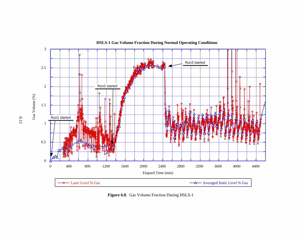
6.11

0

0.5

1

1.5

2

2.5

3

0 400 800 1200 1600 2000 2400 2800 3200 3600 4000 4400

HSLS-1 Gas Volume Fraction During Normal Operating Conditions

Laser Level % Gas Averaged Static Level % Gas

Gas

Vol

ume

(%)

Elapsed Time (min)

Run1 started

Run3 started

Run2 started

Figure 6.8. Gas Volume Fraction During HSLS-1

6.12

Figure 6.8 shows that the gas holdup during Run 1 (consisting of continuous PJMs and full sparging) varied between 0.22 and 0.41 vol% with an average of 0.36 vol% based on the last six static level measurements before Run 2 began. In Run 2 (consisting of continuous PJM operation at half-stroke and idle sparging), the average steady-state gas holdup (αss) was 2.55 vol% based on the last six static level measurements before Run 3 began. During Run 3 (representing the scaled normal operational cycle consisting of continuous PJMs at half-stroke and intermittent spargers) the average minimum gas volume fraction (αMIN) was 0.70 vol%, and the maximum average gas volume fraction (αMAX) was 1.09 vol% based on the maximum and minimum static level measurements for the last six cycles.

6.2.2 Post-DBE Test (HSLS-2)

6.2.2.1 Test Description

The objective of this test was to demonstrate the post-DBE cycle, which consists of continuous half-stroke PJM operation and intermittent sparger operation. The test had one run, Run 3, which demonstrated the actual post-DBE cycle, consisting of repeated cycles of 1 hr of full sparging and PJM operation at half-stroke followed by 2 hr of idle sparging without PJM operation. The idle sparging period was shortened to 2 hr (from the scaled 6 hr) because most of the peroxide added during the full sparging operation decomposed during the shorter period. The peroxide injection rate during Run 3 was continuous at ~382 mL/min during the first 55 minutes of PJM and full sparging operation and off for the rest of the cycle, which would be equivalent to a continuous 50 mL/min over the scaled 7-hr cycle. After steady state was ascertained, the run continued several cycles longer to ensure that minor fluctuations in the data were due to periodic oscillations and not to any slow transients. The test concluded with a reduction in the hydrogen peroxide flow rate to 50 mL/min with full sparging and PJM operating at half-stroke for one post-DBE cycle.

6.2.2.2 Test Conditions

Initial Test Conditions: Prior to the start of the HSLS-2, Run 3, the simulant was thoroughly mixed for ~1.5 hr with continuous PJMs at half-stroke and full sparging, and the initial rheology and simulant density were measured. The simulant properties during the test are provided in Table 6.4.

Table 6.4. Simulant Properties for HSLS-2

Run Yield Stress(a)

(Pa) Consistency(a)

(cP) Simulant Density(b)

(g/cm3) 3 42 46 1.23

Final 43 47 1.23 (a) Yield stress and consistency values have an accuracy of ± 10%. (b) Density values have an accuracy of ± 0.01 (g/ cm3).

6.13

PJM Operating Conditions: During Run 3 of the HSLS-2 test, the PJMs operated continuously at half-stroke with the BNI controller for the drive time, vent, vacuum, and delay times set to 10, 17, 20, and 69 seconds, respectively. Total cycle time was 120 seconds. The drive and vacuum side pressure for all of the JPPs were 3.5 and 1.4 bar, respectively. The average nozzle velocity calculated from the pulse tube pressures was 12.1 m/s (see Table 5.1).

Sparger Flow Rates: The spargers were operated intermittently (1 hr at full flow rate and 2 hr at idle flow rate) during Run 3. Throughout the test, the air flow rates at the sparger nozzle were on average ~19 acfm and 1 acfm for full and idle sparging conditions, respectively. Figure 6.9 shows a representative set of air flow rates at the sparger nozzle during full sparging operation.

Hydrogen Peroxide Addition: During Run 3 of the HSLS-2 test, the hydrogen peroxide was added intermittently at a flow rate of ~382 mL/min. Figure 6.10 shows the hydrogen peroxide flow rate mea-sured by the MicroMotion mass flow meter. The outliers seen in Figure 6.10 between 1200 and 1600 and 2700 and 2900 minutes occur during hydrogen peroxide change-outs.

HSLS Weight: Figure 6.11 illustrates the weight change observed during the Run 3 of the HSLS-2 test. The steady increase in weight was due to hydrogen peroxide injection exceeding evaporation losses due to sparging.

0

5

10

15

20

2100 2110 2120 2130 2140 2150

Full

Spar

ging

Flo

w R

ate

(acf

m)

Elapsed Time (min)

Figure 6.9. Representative Set of the Average Full Sparging Air Flow Rate at the Nozzle

6.14

0

50

100

150

200

250

300

350

400

0 400 800 1200 1600 2000 2400 2800 3200 3600 4000

Hyd

roge

n Pe

roxi

de In

ject

ion

Flow

(mL/

min

)

Elapsed Time (min)

Figure 6.10. Hydrogen Peroxide Injection Flow Rate Data

175100

175200

175300

175400

175500

175600

0 400 800 1200 1600 2000 2400 2800 3200 3600 4000 4400

HSLS-2 Weight During Post-DBE Operating Conditions

HS

LS W

eigh

t (lb

s)

Elapsed Time (min)

H2O2 Injection ~382ml/min

H2O2 Rate ~50ml/minFull sparging ON

PJMs ON

H2O2 OFFFull sparging ON

PJMs ON

Figure 6.11. HSLS Weight During HSLS-2

6.15

6.2.2.3 Gas Volume Fraction Results

The gas volume fraction was obtained through manual and laser level measurements and the volume-level relationship for the HSLS tank. Figure 6.12 shows a plot of the gas volume fraction as a function of time during Run 3 of the HSLS-2 test series. The gas fraction data in this figure were adjusted to account for mass changes. The data between 0 and 3595 minutes represent the repeating cyclic operation with intermittent PJMs at half-stroke, full sparging, and a ~382 mL/min hydrogen peroxide injection rate. Testing continued until there was no observable trend in gas fraction. At 3751 minutes, the hydrogen peroxide flow rate was reduced to ~50 mL/min for one post-DBE cycle. The simulant was then degassed with full sparging and PJM operation.

The data in Figure 6.12 show the gas volume fraction determined from the average of the four laser level sensors recorded continuously on the data acquisition system and the average of four laser level sensors plus one manual tape measurement recorded ~every 0.5 hr with the PJMs turned off and spargers switched to idle. The large scatter in the continuous laser level data indicates the highly turbulent nature of the simulant level due the main sparger operation. Because of the large scatter in the continuous data, the gas fraction information was taken from the level measurements recorded under static conditions. The maximum gas fraction calculated from static levels (αMAX) varied from 2.46 to 3.20 vol% with an average of 2.79 vol% based on the last 10 cycles. The minimum gas volume fraction (αMIN) during Run 3 varied between 0.90 and 1.23 vol% with an average of 1.08 vol% based on the last 10 cycles.

6.2.3 N-TAR Test (HSLS-3)

6.2.3.1 Test Description The objective of the HSLS-3 test series was to demonstrate the NTAR cycle. Run 3a demonstrated NTAR operation with repeated cycles of 1 hr of full sparging followed by 2 hr of idle sparging, and no PJM operation during the test. (Like HSLS-2, the scaled 6-hr idle period was reduced to accommodate rapid hydrogen peroxide decomposition). The peroxide injection rate during Run 3a was continuous at ~382 mL/min during the first 55 minutes of full sparging and off for the rest of the cycle. The test was conducted for a minimum of eight operational cycles (11 cycles were actually completed) to simulate 100 hr of WTP NTAR operation. The post-DBE portion of the test concluded with Run 3b, one NTAR cycle at a reduced hydrogen peroxide flow rate of ~50 mL/min to obtain data at a gas generation rate more typical of the expected plant generation rate. Run 3c was the last step in Run 3 and consisted of a full sparging, no-PJM holdup test with a continuous hydrogen peroxide injection rate of ~90 mL/min.

6.2.3.2 Test Conditions

Initial Test Conditions: Before the start of HSLS-3 Run 3, the simulant was thoroughly mixed with continuous full sparging, and the initial rheology and simulant density were measured (Table 6.5). The simulant properties during the test are provided in Table 6.5.

Sparger Flow Rates: The spargers were operated intermittently (1 hr at full flow and 2 hr at idle flow)

during Run 3a. The air flow rates at the sparger nozzle were on average ~19 acfm and 1 acfm for full and idle sparging conditions, respectively. Figure 6.13 shows a representative set of air flow rates at the sparger nozzle during full sparging operation.

6.16

0

0.5

1

1.5

2

2.5

3

3.5

4

0 400 800 1200 1600 2000 2400 2800 3200 3600 4000 4400

HSLS-2 Gas Volume Fraction During Post-DBE Operating Conditions

Laser Level % Gas Averaged Static Level % Gas

Gas

Vol

ume

(%)

Elapsed Time (min)

H2O2 OFF, Idle Sparging ON, PJMs OFFGas Growth Period

H2O2 Rate ~382ml/min, Full sparging ON, PJMs ONGas Release Period

H2O2 OFFFull Sparging ON

PJMs ON

H2O2 Rate ~50ml/minFull Sparging ON

PJMs ON

Figure 6.12. Gas Volume Fraction During HSLS-2

6.17

Table 6.5. Simulant Properties for HSLS-3

Run Yield Stress(a) Consistency(a) Simulant Density(b) Initial 43 47 1.23

3 44 47 1.23 (a) Yield stress and consistency values have an accuracy of ±10%. (b) Density values have an accuracy of ±0.01 (g/cm3).

Hydrogen Peroxide Addition: During Run 3a of the HSLS-3 test, hydrogen peroxide was added intermittently at a flow rate of ~382 mL/min. Figure 6.14 shows the hydrogen peroxide flow rate measured by the MicroMotion mass flow meter. At approximately 2,000 minutes, the hydrogen peroxide injection rate was decreased to ~50 mL/min (Run 3b) for one NTAR cycle to obtain data at a gas generation rate more typical of the expected plant generation rate. Later, at ~2,200 minutes (Run 3c), the hydrogen peroxide injection rate was increased to ~90 mL/min for a sparge-only holdup test until post-test degassing started. The outliers seen in Figure 6.14 between 0 and 300 and 1200 and 1500 minutes occurred during hydrogen peroxide change-outs.

HSLS Weight: Figure 6.15 illustrates the weight change observed during Run 3 of the HSLS-3 test.

A weight increase was generally observed during all periods where the hydrogen peroxide injection rate was ~382 mL/min, and the weight decreased when peroxide was not being injected. From 3100 to 3371 minutes, a weight loss of 140 lb (31 lb/hr), attributed to evaporation, was measured during the degassing step with PJMs and full sparging in operation.

0

5

10

15

20

0 300 600 900 1200 1500 1800 2100 2400 2700 3000

Full

Spar

ging

Flo

w R

ate

(acf

m)

Elapsed Time (min)

Figure 6.13. Representative Set of the Average Full Sparging Air Flow Rate at the Nozzle

6.18

0

50

100

150

200

250

300

350

400

0 300 600 900 1200 1500 1800 2100 2400 2700 3000

Hyd

roge

n Pe

roxi

de In

ject

ion

Flow

(mL/

min

)

Elapsed Time (min)

Figure 6.14. Hydrogen Peroxide Injection Flow Rate Data

175150

175200

175250

175300

175350

175400

175450

175500

0 400 800 1200 1600 2000 2400 2800 3200 3600

HSLS-3 Weight During NTAR Operating Conditions

HS

LS W

eigh

t (lb

s)

Elapsed Time (min)

Idle spargingH2O2 OFF

Idle spargingH2O2 OFF

Full spargingH2O2 ON

Full spargingH2O2 ON ~50ml/min

Full spargingH2O2 ON ~90ml/min

Full spargingPJMs ON

H2O2 OFF

Idle spargingH2O2 OFF

Full spargingH2O2 ONFull sparging

H2O2 ON

Figure 6.15. HSLS Weight During HSLS-3

6.19

6.2.3.3 Gas Volume Fraction Results

Figure 6.16 plots the gas volume fraction as a function of time for Run 3 of the HSLS-3 test series. In this figure, the gas volume fraction data between 0 and 1980 minutes represents the holdup achieved during Run 3a with repeating cyclic operation of full sparging, no PJMs, and a ~382 mL/min hydrogen peroxide injection rate. From 1980 to 2200, an additional NTAR cycle was completed at a reduced hydrogen peroxide rate of 50 mL/min to obtain data at a gas generation rate more typical of the expected plant generation rate. At 2200 minutes, the hydrogen peroxide flow rate was increased to 90 mL/min with full sparging operation and continued until 3100 minutes. Degassing followed this period, concluding HSLS-3 testing.

Displayed in Figure 6.16 is Run 3 of HSLS-3, consisting of intermittent full sparging and no PJM operation. The figure indicates that the maximum gas volume fraction (αMAX) varied from 2.40 to 2.75 vol% with an average of 2.55 vol% based on the last three cycles. The minimum gas volume fraction (αMIN) varied from 1.26 to 1.29 vol% with an average of 1.28 vol% based on the last three cycles.

6.3 Gas Release Tests (HSLS-8 and -9)

6.3.1 Test Description

The HSLS-8 and 9 tests obtained gas release data with full sparging and with PJMs and idle sparging, respectively. The HSLS-8 gas release test consisted of:

• mixing the tank simulant with PJMs and full sparging for 2 hr • injecting hydrogen peroxide at ~200 mL/min for 2 hr while operating the PJMs and full sparging • changing over to shutdown sparging until a steady simulant level indicated most of the hydrogen

peroxide had decomposed • initiating gas release with full sparging (no PJMs) for a minimum of 4 hr or until all gas was

released. The HSLS-9 gas release test consisted of:

• mixing the tank simulant with PJMs and full sparging for 2 hr • injecting hydrogen peroxide at ~350 mL/min for 2 hr while operating the PJMs and full sparging • changing over to shutdown sparging until a steady simulant level indicated most of the hydrogen

peroxide had decomposed • initiating gas release with PJMs at half-stroke with idle sparging for a minimum of 4 hr or until

all gas was released.

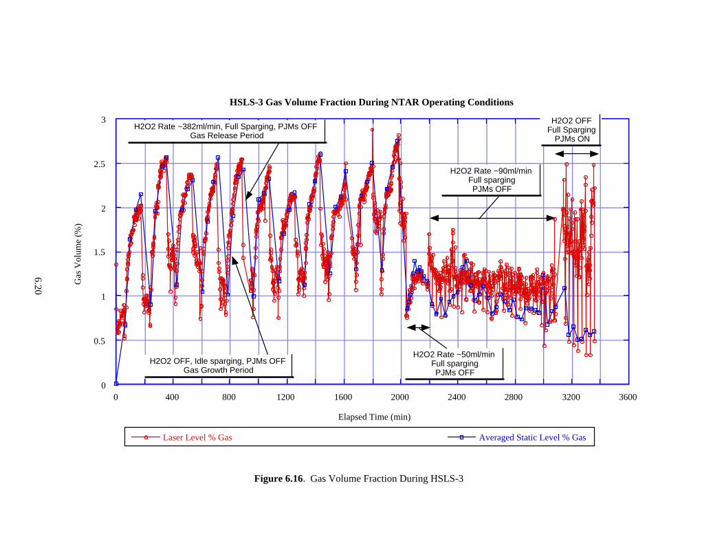
6.20

0

0.5

1

1.5

2

2.5

3

0 400 800 1200 1600 2000 2400 2800 3200 3600

HSLS-3 Gas Volume Fraction During NTAR Operating Conditions

Laser Level % Gas Averaged Static Level % Gas

Gas

Vol

ume

(%)

Elapsed Time (min)

H2O2 Rate ~50ml/minFull spargingPJMs OFF

H2O2 OFFFull Sparging

PJMs ON

H2O2 OFF, Idle sparging, PJMs OFFGas Growth Period

H2O2 Rate ~382ml/min, Full Sparging, PJMs OFFGas Release Period

H2O2 Rate ~90ml/minFull spargingPJMs OFF

Figure 6.16. Gas Volume Fraction During HSLS-3

6.21

6.3.2 Test Conditions Initial Test Conditions: After completing the HSLS-3 test, the simulant Bingham yield stress was

60.2 Pa, which exceeded the target yield stress for the HSLS-8 and -9 tests. Consequently, the clay was diluted with approximately 3,500 lb of water while mixing with the PJMs and full sparging. Before the HSLS-8 and -9 tests began, the simulant was thoroughly mixed for ~2 hr with continuous PJMs and full sparging, and the initial rheology and simulant density were measured. The fill height in the tank was then adjusted to correspond to an H/D of ~0.93. The simulant properties during the HSLS-8 and -9 tests are provided in Tables 6.6 and 6.7, respectively.

Table 6.6. Simulant Properties for HSLS-8

Run Yield Stress(a) (Pa)

Consistency(a)

(cP) Simulant Density(b)

(g/cm3) Initial 42 39 1.21

1 43 39 1.22 Final 42 39 1.22

(a) Yield stress and consistency values have an accuracy of ± 10%. (b) Density values have an accuracy of ± 0.01 (g/ cm3).

Table 6.7. Simulant Properties for HSLS-9

Yield Stress(a) (Pa)

Consistency(a)

(cP) Simulant Density(b)

(g/cm3) Initial 42 40 1.22 Run 1 42 39 1.21 Final 42 39 1.22

(a) Yield stress and consistency values have an accuracy of ± 10%. (b) Density values have an accuracy of ± 0.01 (g/ cm3).

PJM Operating Conditions: During the HSLS-9 test, the PJMs were operated at half-stroke with the BNI controller for the drive time, vent, vacuum, and delay times set to 10, 17, 20, and 69 seconds, respectively. The total cycle time was 120 seconds.(a) The drive and vacuum side pressure for all of the JPPs were 3.5 and 1.4 bar, respectively. The average nozzle velocity calculated from the pulse tube pressures was 12.0 m/s (see Table 5.1). Sparger Flow Rates: The spargers were operated during mixing before hydrogen peroxide addition for the HSLS-8 and -9 tests. The full sparger air flow rates at the sparger nozzle were ~19 acfm on average for HSLS-8 and 9. The HSLS-8 and 9 air flow rates at the sparger were on average 1 acfm and 0.29 acfm for idle and shutdown sparging conditions, respectively. Figures 6.17 and 6.18 show the air flow rate at the sparger nozzle during full sparging operation. (a) Durations given are for the times specific valves were open. Additional delays associated with the PJM controller add 4 seconds for a total cycle time of 120 seconds.

6.22

0

5

10

15

20

0 60 120 180 240 300 360 420

Full

Spar

ging

Flo

w R

ate

(acf

m)

Elapsed Time (min)

Figure 6.17. HSLS-8 Test Average Full Sparging Air Flow Rate at the Nozzle

0

5

10

15

20

0 60 120 180 240 300

Full

Spar

ging

Flo

w R

ate

(acf

m)

Elapsed Time (min)

Figure 6.18. HSLS-9 Test Average Full Sparging Air Flow Rate at the Nozzle

6.23

Hydrogen Peroxide Addition: During the HSLS-8 and -9 tests, hydrogen peroxide was added continuously for 2 hr at a flow rate of ~200 mL/min and ~350 mL/min, respectively. Figures 6.19 and 6.20 show the hydrogen peroxide flow rate for tests HSLS-8 and 9, respectively, as measured by the MicroMotion mass flow meter.

0

50

100

150

200

250

0 30 60 90 120

Hyd

roge

n Pe

roxi

de In

ject

ion

Flow

(mL/

min

)

Elapsed Time (min)

Figure 6.19. Hydrogen Peroxide Injection Flow Rate Data for HSLS-8 Test

0

100

200

300

400

0 60 120 180 240 300

Hyd

roge

n Pe

roxi

de In

ject

ion

Flow

(mL/

min

)

Elapsed Time (min)

Figure 6.20. Hydrogen Peroxide Injection Flow Rate Data for HSLS-9 Test

6.24

HSLS Weight: Figures 6.21 and 6.22 illustrate the weight change observed during the HSLS-8 and -9 tests. Full sparging with no PJM operation during HSLS-8 (Figure 6.21) provided a weight loss of roughly 80 lb over 434 minutes. This weight loss is attributed to evaporation and falls within a previously observed evaporation rate range of 4 to 23 lb/hr. However, a 60 lb weight loss occurred during the corresponding period in HSLS-9 (Figure 6.22), with only PJMs operating at half-stroke and idle sparging.

174700

174720

174740

174760

174780

174800

174820

0 40 80 120 160 200 240 280 320 360 400 440

HSLS-8 Weight During Full Flow Sparging Only

HS

LS W

eigh

t (lb

s)

Elapsed Time (min)

Full sparging ONPJMs OFFH2O2 OFF

Shutdown sparging ONPJMs OFFH2O2 OFF

Full sparging ONPJMs ON

H2O2 ON ~200ml/min

Figure 6.21. HSLS-8 Weight Measurements from the HSLS Tank Weight Computer

174640

174660

174680

174700

174720

174740

174760

0 100 200 300 400 500 600 700 800 900 1000 1100 1200 1300 1400

HSLS-9 Weight During PJMs and Idle Sparging Operations

HS

LS W

eigh

t (lb

s)

Elapsed Time (min)

Full sparging ONPJMs ON

H2O2 ON ~350ml/min

Shutdown sparging ONPJMs OFFH2O2 OFF

Idle sparging ONPJMs OFFH2O2 OFF

Idle sparging ONPJMs ON

H2O2 OFF

Figure 6.22. HSLS-9 Weight Measurements from the HSLS Tank Weight Computer

6.25

6.3.2.1 Gas Volume Fraction Results

Figures 6.23 and 6.24 show the gas volume fraction as a function of time during HSLS-8 and -9, respectively. During the period ranging from 25 to 155 minutes in HSLS-8, a hydrogen peroxide flow rate of ~200 mL/min was maintained while both PJMs and full sparging were on. At 155 minutes, PJMs were shut down and sparging was reduced to shutdown flow. After the accumulated gas reached a steady-state level, full sparging was resumed at 313 minutes. At 434 minutes, gas release induced by full sparging was complete. The gas volume fraction indicated by the laser level is greater than the gas volume fraction indicated by the static level measurements during the peroxide addition step and gas release step because the laser level measurements include the short-term holdup due to sparge air. The static level measurements are obtained when the PJMs were off and the spargers on IDLE.

During the HSLS-9 test from 6 to 120 minutes, a hydrogen peroxide flow rate of approximately 350 mL/min was maintained while both PJMs and full sparging were on. At 125 minutes, the PJMs were shut down and sparging was reduced to shutdown flow. The PJMs were started at 615 minutes with idle sparging flow.

The initial gas fraction during H2O2 addition and mixing (sparging and PJMs on) in HSLS-8 was 0.64 vol% based on the static level measurement at 155 minutes. Based on the last four static level measurements just before gas release started, the maximum gas fraction (αMAX) varied between 1.59 and 1.79 vol% with an average of 1.67 vol%. After degassing with full sparging only and just prior to the start of HSLS-9, the average minimum gas fraction (αMIN) was 0.7 vol% based on static level measurements at 344 and 374 minutes. The initial gas fraction during H2O2 addition and mixing (sparging and PJMs on) in HSLS-9 was 0.95 vol% based on the static level measurement at 128 minutes At the start of the gas release test the average gas volume fraction was 3.84 vol%. At the time the test was terminated the average gas volume fraction was 0.42 vol%. After degassing with PJMs and spargers on full flow the final minimum gas fraction (αMIN) was recorded at 0.15 vol%.

6.4 Mixing Tests (HSLS-4) Six mixing runs were performed to determine the time to mix and the percent mixed during various modes of the PJMs and sparger operation. The operational modes of PJMs and sparger operation tested during the HSLS-4 test sequence are listed in Table 6.8 in the order the runs were conducted. The last step in each run involved mixing with PJMs at full stroke with full sparging to homogenize the chloride tracer concentration in the simulant. The approach for conducting the mixing tests is discussed in Section 4.5 and the data analysis method in Section 5.4. This section presents the results obtained.

6.26

0

0.25

0.5

0.75

1

1.25

1.5

1.75

2

0 40 80 120 160 200 240 280 320 360 400 440

HSLS-8 Gas Fraction During Full Sparging and No PJMs

Laser Level % Gas Averaged Static Level % Gas

Gas

Vol

ume

(%)

Elapsed Time (min)

Full sparging ONPJMs ON

H2O2 ON ~200ml/min

Shutdown sparging ONPJMs OFFH2O2 OFF

Full sparging ONPJMs OFFH2O2 OFF

Figure 6.23. Gas Volume Fraction During HSLS-8

6.27

0

0.5

1

1.5

2

2.5

3

3.5

4

0 100 200 300 400 500 600 700 800 900 1000 1100 1200 1300 1400

HSLS-9 Gas Fraction During PJMs On and Idle Sparging Operations

Laser Level % Gas Averaged Static Level % Gas

Gas

Vol

ume

(%)

Elapsed Time (min)

Shutdown sparging ONPJMs OFFH2O2 OFF

Full sparging ONPJMs ON

H2O2 ON ~350ml/min

Idle sparging ONPJMs ON

H2O2 OFF

Figure 6.24. Gas Volume Fraction During HSLS-9

6.28

Table 6.8. Order of HSLS-4 Mixing Runs Performed and the Steps Involved in Each

Order Step 1 Step 2 Step 3 Tracer injection method

1 Spargers only Spargers + PJMs (@ half stroke)

Spargers + PJMs(@ full stroke)

Peroxide injection lines

2 Spargers + PJMs (@ half stroke)

Spargers + PJMs (@ full stroke)

-- Peroxide injection lines

6 Spargers + PJMs (@ half stroke)

Spargers + PJMs (@ full stroke)

-- Tracer + dilution water added on top of simulant

3 Spargers only Spargers + PJMs (@ full stroke)

-- Tracer + dilution water added on top of simulant

4 Spargers only Spargers + PJMs (@ full stroke)

-- Tracer + dilution water added on top of simulant

5 Spargers only Spargers + PJMs (@ full stroke)

-- Tracer + dilution water added on top of simulant

6.4.1 Test Description The objectives of the six mixing runs conducted during the HSLS-4 test were

• Run 1: The primary objectives were to determine time to mix and volume of the unmixed heel using a simulant with a yield stress of ~45 Pa and only the spargers operating. A secondary objective was to determine whether the tank could be fully mixed with full sparging and PJMs operating at half stroke.

• Run 2: The objectives of this run were to determine the time to mix and the effectiveness of mixing with PJMs operating at half stroke with full sparging.

• Run 3, 4, and 5: The objectives of these runs were to determine the time to mix and the volume of the unmixed sparge heel using a simulant with a yield stress of 33±3 Pa. These three runs were conducted with only full flow sparging (no PJM operation).

• Run 6: The objectives of this run were to determine the time to mix and the effectiveness of mixing when a low density material was added to the top of the tank. This test was conducted with the PJMs operating at half stroke with full sparging.

6.4.2 Test Conditions The simulant properties and operating conditions are listed in Table 6.9. The simulant volume was estimated from static level measurements and a level versus volume correlation. There are some slight differences between the volume and the H/D due to round-off error.

6.29

Table 6.9. Operating Conditions for HSLS-4 Mixing Runs

Simulant Properties Operating Conditions Run Order Yield Stress

(Pa) Consistency

(cP) Density (kg/m3) H/D Simulant Vol

(L) Air Flow Rate

(acfm) PJM Nv

(a)

(m/s) 1 47 41 1.21 0.93 35960 18 12.2 2 35 35 1.21 0.93 35850 18 12.0 6 34 33 1.21 0.94 36270 18 12.1 3 38 34 1.20 0.81 31460 19 -- 4 34 31 1.21 0.81 31610 18 -- 5 34 31 1.21 0.81 31630 18 --

(a) Nv = PJM peak average nozzle velocity for half-stroke operation.

6.4.3 Mixing Results The volume percent mixed was calculated using Eq. (5.14), as discussed in Section 5.4.2. With this equation the percent mixed is defined such that tracer concentrations greater than the final tracer concentration in the homogenized simulant result in percent mixed values less than 100%. Tracer concentrations greater than the final concentration occur in regions where the initial concentrated tracer is being mixed into regions of lower concentration. Tracer concentrations less than the final concentration occur in regions where the concentrated tracer has not yet arrived and result in apparent percent mixed values greater than 100%. The vol% mixed results are presented using the two approaches described in Section 5.4.2. In one approach the final chloride concentration is determined from the average chloride concentrations obtained from the IC analyses. This approach is called the “IC approach.” In the other approach the final chloride concentration is determined using a mass balance and the known amount of tracer added. This approach is called the “mass balance” approach. The uncertainty associated with the vol% mixed results appears to be on the order of 10% or less based on a visual examination of the scatter in the data as well as a comparison of the mass balance and the IC approaches. The time to mix was determined using the log variance approach discussed in Section 5.4.1. Small errors in the chloride ion concentration data could skew the time to mix toward relatively high numbers because of the weighting approach used in calculating the log probability. Therefore, when the majority of the log variance data fell below -2.6 for 95% mixed and below -2 for 90% mixed, any single outlying points were ignored. Mixing times corresponding to 90 and 95% mixed are provided. Given the considerable variability in the results, the time to mix is rounded off to the nearest hour.

6.4.3.1 HSLS-4 Run 1 The chloride ion concentrations determined by IC are shown in Figure 6.25. In conducting this run the tracer was added through the peroxide injection tubes with the spargers on. An initial set of grab samples was taken at a mixing time of 3 hr, 55 minutes. Mixing with PJMs at half-stroke with full sparging was initiated at a mixing time of 4 hr, 52 minutes and continued until a total mixing time of over 18 hr was achieved. During this mixing step the chloride concentrations were reasonably constant at approximately 23 to 24 ppm. The final step consisted of mixing with PJMs at full stroke with full-flow sparging for approximately 2 hr, 20 minutes to homogenize the contents. At the end of the final mixing step, the chloride concentration dropped slightly, indicating that mixing with the PJMs at half-stroke

6.30

14

16

18

20

22

24

26

0:00 2:00 4:00 6:00 8:00 10:00 12:00 14:00 16:00 18:00 20:00 22:00

Mixing Time (hr:min)

Loc 1: Elev. 7-ft Loc 2: Elev. 11-ft Loc 3: Elev. 3-ft Loc 5: Elev. 3-ft

Start Mixing with Full Spargers

Swith to PJMs at HalfStroke and Full Sparging

Switch to PJMs at FullStroke and Full Sparging

Expected Final Concentration

Figure 6.25. Chloride Tracer Concentration Profiles for HSLS-4 Run 1

with full sparging did not completely mix the simulant. The final concentration based on the IC analyses was also lower than the concentration expected based on the amount of tracer added. The original plan for monitoring the mixing tests was to use ion selective electrodes (ISEs) to determine when a steady-state chloride concentration was achieved. The ISEs were to provide continuous concentration measurements from probes placed at four different locations in the tank. After steady state was ascertained from the ISE probe readouts, grab samples would be collected to confirm that steady state had been achieved and to determine the volume percent mixed. However, the ISE probe technique was insensitive to the chloride ion concentration changes in the tank. This is illustrated by the chloride ion concentrations shown in Figure 6.25. In this figure, the second set of grab samples taken at a mixing time of 3 hr, 55 minutes corresponds to the point when it was determined from the ISE readouts that steady state was reached. It can be seen from the results of the next set of grab samples that the chloride concentration had increased, indicating that steady state had not been achieved, as indicated by the ISEs. Therefore, for the remaining runs, the determination of steady state was based on the IC analysis of the grab samples. This introduced a challenge in determining the end of a run because the IC analyses had a turnaround time of several hours. The volume percent mixed data for the HSLS-4 Run 1 are shown in Figure 6.26. Some of the results from the sampling period at a mixing time of 3 hr, 55 minutes are off scale and not shown. From the concentration data in Figure 6.25 it can be seen that premature determination of steady state at the end of the full sparging-only period makes it difficult to determine the volume percent mixed for this step in the run. The mass balance approach shown in the top chart results in final percent mixed values that are too

6.31

60

70

80

90

100

110

120

0:00 2:00 4:00 6:00 8:00 10:00 12:00 14:00 16:00 18:00 20:00 22:00

Mixing Time (hr:min)

Loc1: Elev. 7-ftLoc2: Elev. 11-ft Loc3: Elev. 3-ft Loc5: Elev. 3-ft

Start Mixing with Full Spargers

Switch to PJMs at HalfStroke and Full Sparging

Switch to PJMs at FullStroke and Full Sparging

Run 1 % Mixed based on mass balance approach

60

70

80

90

100

110

120

0:00 2:00 4:00 6:00 8:00 10:00 12:00 14:00 16:00 18:00 20:00 22:00

Mixing Time (hr:min)

Loc1: Elev. 7-ftLoc2: Elev. 11-ft Loc3: Elev. 3-ft Loc5: Elev. 3-ft

Start Mixing with Full Spargers

Switch to PJMs at HalfStroke and Full Sparging

Switch to PJMs at FullStroke and Full Sparging

Run 1 % Mixed based on IC approach

Figure 6.26. Vol% Mixed Results for HSLS-4 Run 1

6.32

high (>100%) because the final chloride concentration determined by the mass balance approach was greater than the final measured concentration. The source of this discrepancy could not be determined but could be due to analytical uncertainty or uncertainty in the amount of tracer added. Because the sparger-only phase of the test was prematurely terminated, it can only be stated that the time to mix was greater than 4 hr, 52 minutes (~5 hr). The data in Figure 6.26 indicate that the percent mixed increased about 6% when switching from PJMs at half-stroke with full sparging to PJMs at full stroke with full sparging. This implies that there was an umixed volume of ~6% of the total simulant volume when operating with PJMs at half-stroke with full sparging. The most likely place for this unmixed volume to be is in the pulse tubes.

6.4.3.2 HSLS-4 Run 2 The measured chloride ion concentrations and the computed volume percent mixed data for HSLS-4 Run 2 are shown in Figures 6.27 and 6.28, respectively. In this run, the tracer was added through the peroxide injection lines with the PJMs at half-stroke with full sparging. After about 13 hr of mixing, the PJMs were adjusted to full stroke with full sparging. It can be seen from the data in Figure 6.27 that immediately after the tracer was added and the mixing started, with the PJMs at half-stroke and full sparging, the concentration rapidly approached steady state and then remained at the expected value for the rest of the test. The same behavior is displayed in the volume percent mixed plot in Figure 6.28. It can also be seen that, within the uncertainty of the measurement, no significant difference exists in the volume percent mixed between operation with full spargers and PJMs at half-stroke and PJMS at full stroke. This suggests that there was no unmixed volume in the pulse tubes. It is possible that the lower simulant rheology for this run (compared to Run 1) (yield stress of 34 Pa versus 47 Pa for Run 1) allowed mixing of the simulant in the pulse tubes.

30

40

50

60

70

80

90

0:00 4:00 8:00 12:00 16:00 20:00 24:00 28:00 32:00

Mixing Time (hr:min)

Loc 1: Elev. 7-ft Loc 2: Elev. 11-ft Loc 3: Elev. 3-ft Loc 5: Elev. 3-ft

Start Mixing with PJMs at Half Strokeand Full Sparging

Switch to PJMs atFull Stroke and Full Sparging Stop Mixing

Expected Final Concentration

Figure 6.27. Chloride Tracer Concentration Profiles for HSLS-4 Run 2

6.33

50

60

70

80

90

100

110

120

0:00 4:00 8:00 12:00 16:00 20:00 24:00 28:00 32:00

Mixing Time (hr:min)

Loc 1: Elev. 7-ft Loc 2: Elev. 11-ft Loc 3: Elev. 3-ft Loc 5: Elev. 3-ft

Start Mixing with PJMs at Half Strokeand Full Sparging

Switch to PJMs atFull Stroke and Full Sparging

Stop Mixing

Run 2: % mixed based on mass balance approach

50

60

70

80

90

100

110

120

0:00 4:00 8:00 12:00 16:00 20:00 24:00 28:00 32:00

Mixing Time (hr:min)

Loc 1: Elev. 7-ft Loc 2: Elev. 11-ft Loc 3: Elev. 3-ft Loc 5: Elev. 3-ft

Start Mixing with PJMs at Half Strokeand Full Sparging

Switch to PJMs atFull Stroke and Full Sparging

Stop Mixing

Run 2: % mixed based on IC approach

Figure 6.28. Volume Percent Mixed Data for HSLS-4 Run 2

6.34

The log variance data for the HSLS-4, Run 2 is shown in Figure 6.29. From the data in this figure, the 90% mixing time is ~3 hr and the 95% mixing time is ~5 hr.

-4.0

-3.5

-3.0

-2.5

-2.0

-1.5

0:00 1:00 2:00 3:00 4:00 5:00 6:00 7:00 8:00 9:00 10:00 11:00 12:00 13:00 14:00

Mixing time (hr:min)

Log

Varia

nce

95% mixed

90% mixed

Figure 6.29. Log Variance Data for HSLS-4 Run 2

6.4.3.3 HSLS-4 Run 6

The next test performed after HSLS-4 Run 2 was Run 6. This test was very similar to Run 2 with the exception that 2 inches of dilution water and the tracer were added on top of the simulant. Mixing was then initiated with the PJMs at half-stroke with full sparging. The final step was to mix the tank for about 3 hr with the PJMs at full stroke with full sparging. The measured chloride ion concentrations and the computed volume percent mixed data for this run are shown in Figures 6.30 and 6.31, respectively. Unlike the results obtained with HSLS-4 Run 2, where the salt concentration and volume percent mixed quickly reached a steady-state value, the results from HSLS-4 Run 6 indicate an interesting oscillatory behavior, possibly because the salt tracer was added not as a mixed homogeneous solution of the dilution water but at a few discrete points above the layer of the dilution water in the tank. Therefore, in this run there might be two mixing phenomena occurring simultaneously. The first is the rapid blending of the high-density (~1150 kg/m3) salt tracer solution with the simulant of similar density (~1200 kg/m3); the second could be the relatively slower blending of the low-density (~1000 kg/m3) dilution water with the simulant. These different rates of blending of the two components could have resulted in the oscillatory behavior in the observed tracer concentration. This sort of mixing behavior could result in relatively long mixing times if a homogenous mixture is the goal.

6.35

60

65

70

75

80

85

90

95

0:00 4:00 8:00 12:00 16:00 20:00 24:00 28:00

Mixing Time (hr:min)

Loc 1: Elev. 7-ft Loc 2: Elev 11-ft Loc 3: Elev. 3-ft Loc 5: Elev. 3-ft

Start Mixing with Full Sparging and PJMs at Half Stroke.

Switch to Full Sparging and PJMs

at Full Stroke

Stop Mixing

Expected Final Concentration

Figure 6.30. Chloride Tracer Concentration Profiles for HSLS-4 Run 6

Figure 6.31 also provides some evidence that there was a small amount of tracer that was not completely mixed until the end of the test. This is indicated by the slight drop in percent mixed (about 3%) when the mixing mode was changed from PJMs at half-stroke with full-sparging to PJMs at full stroke with full-sparging. Before the end of the run, the percent mixed is greater than 100% when the tracer concentration is less than the final value. This behavior is often seen in regions of the simulant where the concentrated tracer has not yet arrived and could indicate that the tank was not fully mixed at the end of the run. The difference between the measured chloride concentrations at the end of mixing with PJMs at half-stroke with full sparging and the final homogenized sample was only 0.8 ppm, which was about 4% of the tracer added. The log variance data for HSLS-4 Run 6 is shown in Figure 6.32. It can be seen from the data in this figure that the 90% mixing time is <1 hr and the 95% mixing time is ~9 hr.

6.36

60

70

80

90

100

110

120

0:00 2:00 4:00 6:00 8:00 10:00 12:00 14:00 16:00 18:00 20:00 22:00 24:00 26:00 28:00

Mixing Time (hr:min)

Loc 1: Elev. 7-ft Loc 2: Elev. 11-ft Loc 3: Elev. 3-ft Loc 5: Elev. 3-ft

Start Mixing with Full Sparging and PJMs at Half Stroke.

Stop MixingSwitch to Full

Sparging and PJMs at Full Stroke

Run 6: % mixed based on mass balance approach

60

70

80

90

100

110

120

0:00 2:00 4:00 6:00 8:00 10:00 12:00 14:00 16:00 18:00 20:00 22:00 24:00 26:00 28:00

Mixing Time (hr:min)

Loc 1: Elev. 7-ft Loc 2: Elev. 11-ft Loc 3: Elev. 3-ft Loc 5: Elev. 3-ft

Start Mixing with Main Sparging and PJM at Half Stroke.

Stop MixingSwitch to Full Sparging and PJMs

at Full Stroke

Run 6: % mixed based on IC approach

Figure 6.31. Volume Mixed Data for HSLS-4 Run 6

6.37

-4.0

-3.5

-3.0

-2.5

-2.0

-1.5

0:00 1:00 2:00 3:00 4:00 5:00 6:00 7:00 8:00 9:00 10:00 11:00 12:00 13:00 14:00 15:00 16:00

Mixing time (hr:min)

95% Mixed

90% Mixed

Figure 6.32. Log Variance Data for HSLS-4 Run 6

6.4.3.4 HSLS-4 Runs 3, 4, 5

HSLS-4 Runs 3, 4, and 5 are full-flow sparger-only mixing tests performed to determine the time to mix and the unmixed sparger heel volume. The tracer and dilution water (about 1 inch) were added on top of the simulant the same way as in HSLS-4 Run 6 except that the mass of dilution water added was 1/2 of the amount used in Run 6. The sparger-only mixing tests were performed in triplicate to assess the variability of the results. The results of the tracer concentration profiles for Runs 3, 4, and 5 are shown in Figures 6.33, 6.34, and 6.35, respectively. Interestingly, all the concentration profiles show oscillatory behavior similar to the HSLS-4 Run 6, although for these runs the oscillations dampen out much more quickly, probably because of the smaller mass of dilution water. The results of the volume percent mixed tests for Runs 3,(a) 4, and 5 are shown in Figures 6.36, 6.37, and 6.38, respectively.(b) The percent mixed at the end of the sparger-only mixing phase can be determined along with an estimate of the unmixed volume percent (Table 6.10) based on the data in Figures 6.28, 6.29, and 6.30. The unmixed simulant volume is thought to reside in the pulse tubes and in a sparge heel below the spargers. These values may be compared with an estimate of the unmixed volume percent of 27% determined by calculation in Appendix B.

(a) For Run 3, samples taken before the next run (Run 4) were used to determine the final chloride concentrations since homogeneity of the simulant at the end of Run 3 was questionable. (b) Results from sample location 3 for Runs 3, 4 and 5 were not used in these plots because samples obtained from this location were apparently taken from the unmixed sparge heel.

6.38

Table 6.10. Sparger-Only Mixing Volume Percent

Run Volume Mixed % Unmixed volume % Mass Balance Approach IC Approach Mass Balance Approach IC Approach

3 66 66 34 34 4 61 62 39 38 5 58 66 42 34

The log variance data for the three runs are plotted in Figures 6.39, 6.40, and 6.41, respectively.(a) The 95% mixing time for Run 5 is given as >6 hr because the 95% mixing time criterion was not reached before the experiment ended. The 90 and 95% mixing times are listed in Table 6.11.

80

90

100

110

120

130

140

0:00 4:00 8:00 12:00 16:00 20:00 24:00 28:00 32:00 36:00 40:00

Mixing Time (hr:min)

Cl C

onc.

(ppm

)

Loc 1: Elev. 7-ftLoc 2A/2B: Elev. 8.5/9-ftLoc 3: Elev. 3-ftLoc 5: Elev. 3-ft

Start Mixing with Full Sparging

Switch to PJMs at Full Stroke and Full

SpargingEnd of Run

Expected Final Concentration

First samples taken at start

of Run 4

Figure 6.33. Chloride Tracer Concentration Profiles for HSLS-4 Run 3

(a) Results from sample location 3 for Runs 3, 4 and 5 were not used in these plots since samples obtained from this location were apparently taken from the unmixed sparge heel.

6.39

100

110

120

130

140

150

160

170

180

0:00 1:00 2:00 3:00 4:00 5:00 6:00 7:00 8:00 9:00 10:00

Mixing Time (hr:min)

Loc 1: Elev. 7-ft Loc 2B: Elev. 9-ft Loc 3: Elev 3-ft Loc 5: Elev. 3-ft

Stop Mixing Switch to PJMs at Full Stroke and Full

Sparging

Start Mixing with Full Spargers

Expected Final Concentration

Figure 6.34. Chloride Tracer Concentration Profiles for HSLS-4 Run 4

130

140

150

160

170

180

190

200

210

220

230

0:00 1:00 2:00 3:00 4:00 5:00 6:00 7:00 8:00 9:00 10:00

Mixing Time

Loc 1: Elev. 7-ft Loc 2B: Elev. 9-ft Loc 3: Elev. 3-ft Loc 5: Elev. 3-ft

Switch to PJMs at Full Stroke and Full

Sparging

Start Mixing with Full Spargers

Stop Mixing

Expected Final Concentration

Figure 6.35. Chloride Tracer Concentration Profiles for HSLS-4 Run 5

6.40

0

20

40

60

80

100

120

0:00 4:00 8:00 12:00 16:00 20:00 24:00 28:00 32:00 36:00 40:00

Mixing Time (hr:min)

Loc 1: Elev. 7-ft Loc 2A/2B: Elev. 8.5/9-ft Loc 3: Elev. 3-ft Loc 5: Elev. 3-ft

End of RunSwitch to PJMs at

Full Stroke and Full Sparging

Start Mixing with Full Sparging

Run 3: % mixed based on mass balance approach

First samples taken at start

of Run 4

0

20

40

60

80

100

120

0:00 4:00 8:00 12:00 16:00 20:00 24:00 28:00 32:00 36:00 40:00

Mixing Time (hr:min)

Vol.

Mix

ed (%

)

Loc 1: Elev. 7-ft Loc 2A/2B: Elev. 8.5/9-ft Loc 3: Elev. 3-ft Loc 5: Elev. 3-ft

End of RunSwitch to PJMs at

Full Stroke and Full Sparging

Start Mixing with Full Sparging

Run 3: % mixed based on IC approach

First samples taken at start

of Run 4

Figure 6.36. Percent Volume Mixed Data for HSLS-4 Run 3

6.41

0

20

40

60

80

100

120

0:00 1:00 2:00 3:00 4:00 5:00 6:00 7:00 8:00 9:00 10:00

Mixing Time (hr:min)

Vol.

Mix

ed (%

)

Loc 1: Elev. 7-ft Loc 2B: Elev. 9-ft Loc 3: Elev. 3-ft Loc 5: Elev. 3-ft

Start Mixing with Full Spargers

Switch to PJMs at Full Stroke and Full Sparging

Stop Mixing

Run 4: % mixed based on mass balance approach

0

20

40

60

80

100

120

0:00 1:00 2:00 3:00 4:00 5:00 6:00 7:00 8:00 9:00 10:00

Mixing Time (hr:min)

Vol.

Mix

ed (%

)

Loc 1: Elev. 7-ft Loc 2B: Elev. 9-ft Loc 3: Elev. 3-ft Loc 5: Elev. 3-ft

Start Mixing with Full Spargers

Switch to PJMs at Full Stroke and Full Sparging

Stop Mixing

Run 4: % mixed based on IC approach

Figure 6.37. Percent Volume Mixed Data for HSLS-4 Run 4

6.42

0

20

40

60

80

100

120

0:00 1:00 2:00 3:00 4:00 5:00 6:00 7:00 8:00 9:00Mixing Time

Loc 1: Elev. 7-ft Loc 2B: Elev. 9-ft Loc 3: Elev. 3-ft Loc 5: Elev. 3-ft

Start Mixing with Full Spargers

Switch to PJMs at FullStroke and Full

Sparging

Stop Mixing

Run 5: % mixed based on mass balance approach

0

20

40

60

80

100

120

0:00 1:00 2:00 3:00 4:00 5:00 6:00 7:00 8:00 9:00Mixing Time

Loc 1: Elev. 7-ft Loc 2B: Elev. 9-ft Loc 3: Elev. 3-ft Loc 5: Elev. 3-ft

Start Mixing with Full Spargers

Switch to PJMs at FullStroke and Full

Sparging

Stop Mixing

Run 5: % mixed based on IC approach

Figure 6.38. Volume Percent Mixed Data for HSLS-4 Run 5

6.43

-4.0

-3.5

-3.0

-2.5

-2.0

-1.5

0:00 2:00 4:00 6:00 8:00 10:00 12:00 14:00 16:00 18:00 20:00 22:00 24:00 26:00 28:00 30:00

Mixing time (hr:min)

Log

Varia

nce

95% Mixed

90% Mixed

Figure 6.39. Log Variance Data for HSLS-4 Run 3

-4.0

-3.5

-3.0

-2.5

-2.0

-1.5

0:00 1:00 2:00 3:00 4:00 5:00 6:00 7:00

Mixing Time (hr:min)

Log

Varia

nce

95% Mixed

90% Mixed

Figure 6.40. Log Variance Data for HSLS-4 Run 4

6.44

-4.0

-3.5

-3.0

-2.5

-2.0

-1.5

-1.0

-0.5

0:00 1:00 2:00 3:00 4:00 5:00 6:00 7:00

Mixing Time (hr:min)

95% Mixed

90% Mixed

Figure 6.41. Log Variance Data for HSLS-4 Run 5

Table 6.11. Sparger-only Mixing Times Using Log Variance Method

Run 90% Mixing Time (hr)

95% Mixing Time (hr)

3 14 23-28 4 1 5 5 3 >6

6.4.4 Summary of Mixing Results A summary of the mixing results is shown in Table 6.12 along with some of the key experimental parameters. The time to mix for the various mixing modes was determined with the log variance approach using a 95% mixing criterion. The mixing times for Runs 1 and 6 are given as greater-than values because the 95% mixing criterion was not reached by the end of the test. A visual examination of the concentration and volume percent mixed plots generally shows an initial rapid rise in tracer concentration followed by a slow (often oscillatory) approach to steady-state values. The 95% mixing time for the sparger-only operation ranged from 5 hr to as much as 28 hr. The 95% mixing time for operation with PJMs at half-stroke with full sparging ranged from 5 to 9 hr.

6.45

Table 6.12. Summary of Mixing Results

Unmixed Volume (%) Run

Time to 95% mixed

(hr) MB IC

Simulant H/D

Simulant Volume

(L)(a)

Yield stress (Pa)

Consistency (cP)

Spargers only on full flow 1 > 5 ND(b) 0.93 35960 47 41 3 23-28 34 34 0.81 31460 38 34 4 5 39 38 0.81 31610 34 31 5 > 6 42 34 0.81 31630 34 31

PJMs @ half stroke with full flow sparging 1 NA 6 6 0.93 35960 47 41 2 5 0 0 0.93 35850 35 35 6 9 0(c) 0.94 36270 34 33

(a) There are some differences between the simulant volume and the H/D due to round-off error. (b) An unmixed volume estimate could not be determined because the test did not run long enough to reach a steady-state condition. (c) Both the mass balance (MB) and IC approaches suggested there may have been some tracer that was not well mixed at the end of the run.

The mixing times with dilution water and tracer added on top (Run 6) appeared to be longer than the case where the tracer was injected near the bottom (Run 2). This is probably due to the increased difficulty in fully mixing a low density material (water) on top of the denser simulant (1.2 g/mL). Complete homogenization of the simulant was generally achieved by mixing for at least 2.5 hr with the PJMs at full stroke with full-sparging at the end of the tests. There was some evidence of a small unmixed volume in Run 1. It is likely that this unmixed volume was due to a slug of simulant moving up and down in the pulse tubes. There was no evidence for an unmixed volume in Runs 2 and 6, possibly due to the lower rheology of the simulant being used that would have been easier to mix in the pulse tubes. It appeared that a small amount of tracer (~4%) remained unmixed at the end of mixing with PJMs at half-stroke and full-sparging in Run 6. The unmixed volume in the full-flow sparger tests (Runs 3, 4, and 5) ranged from 34 to 42% with an average value of 37% at a simulant H/D of 0.81. The unmixed volume includes the volume in the PJMs and the sparge heel. This result is somewhat larger than the unmixed volume of 27% estimated by the calculation in Appendix B.

7.1

7.0 Scale-up to Plant Conditions This section describes how the results of the half-scale LS tests and earlier tests of a 1:4.3-scale vessel (Russell et al. 2005) can be applied to predict GR&R behavior at full plant scale. The scale-up process uses a gas mass conservation model fit to the HSLS test data and based on scaling relationships derived from the basic principles of gas bubble dynamics. A method for estimating GR&R characteristics for the UFP vessel based on available small-scale test data is also outlined. Section 7.1 summarizes the principles by which available small- and large-scale test data can be scaled up to predict the behavior of the full-scale LS vessel. The derivation of the gas retention and release model as described in Section 7.2, and Section 7.3 describes the HSLS data reduction and uncertainty analysis. Section 7.4 describes the calculations that can be applied to scale-up HSLS test data to the full-scale LS and blend vessels for normal operations and for the post-DBE and NTAR scenarios. The extension of these methods to the data available for the UFP vessel is described in Section 7.5.

7.1 Scaling Principles and Applicable Data The fundamental scaling assumption for gas retention and release is that the retained gas exists as relatively small, discrete bubbles whose behavior is determined by the condition of the simulant or waste slurry independent of scale. This assumption allows the scaling laws for gas holdup and release to be derived directly from integral mass conservation equations. The scaling laws are applied to gas generation and release rate parameters derived from small-scale tests of the same geometry and conditions and are verified to within a reasonable uncertainty range by test data at multiple scales. The two components of the scaling process, the scaling laws and available LS test data, are covered in this section.

7.1.1 Scaling Laws This section summarizes the detailed derivation of gas holdup and release scaling principles given in Russell et al. (2005). A simple model for bubble migration in well-mixed slurries explains the basic elements of gas retention and release associated with operation of hybrid PJM plus sparger systems in non-Newtonian slurries. Though portions of such a hybrid system are intermittently mixed due to the cyclic nature of PJM operation, time- and space-averaged values of gas release rates and rates of change of gas content can be applied such that the well-mixed model is applicable to the pulsed system. Gas molecules are generated continuously within the liquid phase in radioactive waste slurry. The solution quickly supersaturates, bubbles nucleate, and existing bubbles grow. The gas retention and release model considers only the gas in bubbles. The retained gas fraction, α, is defined as the average gas volume fraction existing as bubbles in the slurry and is determined from the ideal gas law:

gRT np

α = (7.1)

where ng is the number of moles of gas present in bubbles per unit total volume (gas plus slurry), R is the gas constant (0.08206 L-atm/gram-mole-K), T is the local waste temperature, and p is the local pressure.

7.2

Assuming that the gas is well mixed throughout the slurry on a mole basis, ng is uniform, and the gas fraction varies only with local temperature and pressure (though the temperature will also likely be uniform in a relatively well-mixed system). If T and p are taken as average quantities in the slurry, α is the average gas fraction. The average pressure, p, is approximated by

2/Hgpp csa ρ+= (7.2)

where pa is the headspace pressure, ρs is the average density of gas-free slurry, gc is the standard acceleration of gravity, and H is the slurry depth. Applying molar conservation to the gas in the total volume of slurry results in the following:

gm m

dNG R

dt= − (7.3)

where Ng is the total number of moles of gas in the slurry, Gm is the total molar gas generation rate (moles of gas generated per second), and Rm is the total molar gas release rate from the slurry (moles of gas released per second). Assuming the gas fraction is small (α <10 vol%) and the slurry volume is approximately constant, Eq. (7.3) can be written in terms of volume-specific quantities as

g as m s v

dn pV g V Rdt RT

= − (7.4)

where Vs is the volume of gas-free slurry (i.e., the volume of liquid and solid only), gm is the moles of gas generated per unit volume of gas-free slurry per unit time, and Rv is the total volumetric release rate of gas at the surface. Substituting the gas volume fraction α for ng using Eq. (7.1) and rearranging,

vm

a a s

Rp d RTgp dt p V

α= − (7.5)

Assuming that the gas release occurs as bubbles rise and break at the surface, the volumetric release rate is defined by Rv = nbvbHURA = αHURA (7.6) where nb is the bubble number density (number of bubbles per unit total slurry volume), vbH is the average bubble volume at the simulant surface, αH is the gas volume fraction at the slurry surface, UR is the rise velocity of the bubbles at the surface, and A is the area of the slurry surface. In a predominantly cylindrical tank, A ≈ Vs/H. The tank average and surface gas volume fractions are related by α = (pa/p)αH and the volumetric gas generation rate, gv, and the in situ average hydrostatic pressure is related to gm by gv = gm(RT/p). Applying these definitions reduces Eq. (7.5) to a first-order ordinary differential equation for the average gas fraction:

Rv

Ud g 0dt H

αα+ − = (7.7)

7.3

which has the solution:

R R0 v

R

U UH(t) exp( t) g (1 exp( t))H U H

α = α − + − − (7.8)

where α0 is the initial gas volume fraction at t = 0. The time dependence of the gas fraction α is completely characterized by the initial gas volume fraction, the time constant τR = H/UR, and the gas generation rate. The bubble rise velocity, UR, cannot be calculated or directly measured but can be determined empirically as a function of the slurry mixing system (e.g., PJM duty cycle, PJM nozzle diameter and velocity, slurry rheology) from gas holdup tests. The gas holdup, αss, is defined as the gas volume fraction retained at steady state with continuous gas generation. Evaluating Eq. (7.8) at long times gives the following expression for the holdup:

ss v v RR

Hg gU

α = = τ (7.9)

The steady-state holdup increases in direct proportion to increasing generation rate and slurry depth and decreases with increasing bubble rise velocity. Because bubbles are roughly the same size and rise at roughly the same speed at any scale, Eq. (7.9) also implies that the gas generation rate must vary inversely with the slurry depth to achieve the same holdup at different test scales. Eq. (7.8) and (7.9) contain the fundamental scaling principle for gas bubble holdup and release. These processes are completely characterized by the rate constant UR/H (inverse of the time constant τR), the initial gas fraction (for gas release transients), and gas generation rate (for steady-state holdup). All of these quantities are known or can be calculated except for the bubble rise velocity, UR, which must be determined experimentally. The value of UR derived from small-scale test data is the fundamental basis for scale-up to plant dimensions. Though the bubble rise velocity is roughly constant, there are predictable trends that need to be considered in scaling analysis. The bubble rise velocity increases (i.e., the time constant decreases) with the gas bubble diameter and decreases as the non-Newtonian Bingham model yield stress and consistency increase. The bubble growth rate and therefore the average bubble size increase with the gas generation rate. At a constant growth rate, bubble size increases with transit time, which is directly proportional to slurry depth. Therefore, the bubble rise velocity at the surface may increase in proportion to both the gas generation rate and depth. It is not obvious whether scaling the gas generation rate alone accounts for all these effects. To investigate this we solve the steady-state version of the bubble mass conservation equation (Eq. 7.4) as a function of the vertical coordinate. We assume that the molar gas generation rate per unit volume, gm, temperature, density, and rheology are uniform and the number of bubbles, N, is constant (the bubble population is in equilibrium, with as many leaving the surface as being nucleated in the slurry). Though there is no method to calculate the bubble rise velocity accurately in non-Newtonian fluids, we assume that the bubble rise velocity is proportional to the square of the equivalent spherical diameter

7.4

following Stokes’ law for creeping flow. This means that the velocity is proportional to the bubble volume to the 2/3 power, and the bubble volume is given by the ideal gas law. Applying these assumptions to the basic conservation equation and introducing a dimensionless distance, η = z/H, yields an expression for the bubble rise velocity as a function of η (η = 1 at z = H, η = 0 at z = 0), where z is the vertical coordinate:

25

m

s

a

HgU( ) B g1 H(1 )p

⎡ ⎤⎢ ⎥η⎢ ⎥η =

ρ⎢ ⎥+ − η⎢ ⎥⎣ ⎦

(7.10)

where all the constants and proportionalities have been subsumed into B. We are interested in the ratio of the bubble rise velocity in a test, UT, to that in the full-scale system, UF. Forming this ratio from Eq. (7.10) and introducing the scale factor, S = HF/HT, we have

UTUF

(η) = 1S

gm,T

gm,F

1HF

+gρspa

(1− η)

1HF

+gρspa

S(1− η)

⎡

⎣

⎢ ⎢ ⎢ ⎢

⎤

⎦

⎥ ⎥ ⎥ ⎥

25

(7.11)

If the ratio of molar gas generation rates is made proportional to S, the ratio of velocities at the surface (η = 1) is exactly equal to 1 at all scales. The bubble rise velocity below the surface (η < 1) is greater in smaller-scale tests (UT/UF = 1.14 at η = 0 in a ½-scale test where S = 2). If the average volumetric, rather than molar, gas generation rate is scaled as S to achieve the same holdup via Eq. (7.9), the ratio is unity at mid-depth and the average bubble rise velocity is equal at all scales. However, the bubble rise velocity at the surface is slightly less in smaller-scale tests (UT/UF = 0.93 at η = 1 in a 1/2 scale test). This would have the effect of overestimating the full-scale holdup by roughly 7%. This result assumes that the bubble rise velocity is directly proportional to a power of the bubble volume, as in Stokes flow. It is more likely that the relationship is not so direct, and the effects of pressure and gas generation do not cancel out as neatly as the analysis implies. The bubble rise velocities derived from the test data do show some dependence on the gas generation rate and slurry depth, as discussed in Section 7.4; nevertheless, the overall scaling principle expressed by Eq. (7.9) remains valid at first order and adequately explains the relationships between tests and full-scale gas retention behavior.

7.1.2 Applicable Small-Scale Test Data The HSLS tests were designed specifically to represent the plant vessel and operational modes and form the best basis for predicting plant-scale gas retention and release behavior (Section 7.1.3). Other small-scale holdup test data also provide insights and show trends that are not available from the HSLS

7.5

tests.(a) Holdup tests conducted in the 1:4.3 scale LS, the 1:4.9 scale UFP vessels, and the approximately 1:4 scale (with respect to the large scale 4 PJM test stand in the 336 facility) 4PJM vessel, all in the PNWD APEL test facility, are used in the scale-up calculations described in Section 7.4.(b) These tests are described in detail by Russell et al. (2005) and are summarized in Table 7.1. The bubble rise velocity, which is the key scale-up variable, is calculated from the holdup, simulant depth and gas generation rate via Eq. (7.9). There were important differences in the various mixing systems among the tests. In LS test sequence 14, three of the seven outer PJM nozzles were canted upward at 135˚ and four downward at 45˚, while all seven outer PJM nozzles were set at 45˚ downward in sequence 15A. At the same time, LS sequence 14 operated four of eight air spargers without recirculation, while LS sequence 15A used four recirculation nozzles instead of spargers. Both UFP tests used the same PJM system, but sequence 5 used single-nozzle recirculation, while sequence 6 had a single sparger near the center PJM. Sequence 6 also used a deeper simulant. All APEL 4PJM tests used only their four PJMs without sparging or recirculation. Because bubbles can rise only during the time the slurry is mobile, the effective bubble rise velocity should also vary with the extent and intensity of slurry mobilization produced by the mixing system.(c) Variables affecting mobilization effectiveness include the number of spargers and air flow rates, the number of recirculation nozzles and flow rates, the PJM drive cycle and intensity (e.g., the ratio of drive time to total cycle time, the number of PJMs, the PJM nozzle diameter, and drive velocity), as well as the tank diameter, depth of the simulant, and simulant rheology. There are insufficient data to quantify the influence of each of these parameters separately, but holdup should be less with both spargers and PJMs operating than with only the PJMs, for example. In any event, the small- and large-scale LS tests were run with similar rheology and comparable mixing systems, so the fundamental effect of the gas generation rate and slurry depth to increase the bubble rise velocity should be discernable. The most important information provided by the LS and APEL 4PJM tests is the variation of bubble rise velocity with gas generation rate. The UFP tests also show the variation of bubble rise velocity with simulant depth at the same gas generation rate. The APEL 4PJM tests show how simulant rheology affects the bubble rise velocity. The UFP tests also supply the only available scaling basis for predicting gas retention and release behavior in the plant-scale UFP vessel.

(a) Many gas release tests were also conducted. However, gas release test data are more difficult to analyze, and the cyclic plant-scale operation mode (e.g., 1 hr with spargers plus PJMs followed by 2 hr with PJMs only) is probably best characterized as a series of approaches to different steady-state holdup conditions. (b) Data from tests conducted in the PNWD 336 4PJM vessel and the SRNL small-scale 4PJM vessel were not used in the scale-up calculations. (c) Mixing in this context refers to the hydraulic mobilization or fluidization of a non-Newtonian slurry, not necessarily to homogenization.

7.6

Table 7.1. Small-Scale Gas Holdup Tests and Results

Test/Date Simulant PJM Layout and Drive Velocity

Spargers Operating

Recirc. Nozzles

Gas Generation, gv(mL/L-min)

[gvH (mm/min)]

Holdup, αSS

(vol%)

Bubble Rise Velocity, UR

(m/min)

(UR/H) (1/min)

1.62 [2.13] 0.59 0.36 0.27 LS Seq. 14, Run 3 2/6/04

H, H/D: 1.31 m, 0.74 τy, κ: 36 Pa, 27 cP

Cluster 7 (3-135˚ and 4-45˚) around 1 (0˚) @ 17 m/s

4 (#1, 3, 5, 7) @ ~3 acfm None

3.72 [4.88] 1.17 0.41 0.31

1.62 [2.12] 0.79 0.27 0.20 LS Seq. 15A, Run 3 2/14/04

H, H/D: 1.31 m, 0.74 τy, κ: 35 Pa, 26 cP

Cluster 7 (all-45˚) around 1 (0˚) @ 16 m/s None 4 @ ~454

L/min total 3.73 [4.42] 1.40 0.31 0.24 UFP Seq. 5, Run 3 2/12/04

H, H/D: 1.20 m, 1.4 τy, κ: 36 Pa, 20 cP

Trifoil (3-45˚) around 1 (0˚) @ 16 m/s None 1 @ ~340

L/min 4.20 [5.04] 3.43 0.14 0.12

UFP Seq. 6, Run 3 2/13/04

H, H/D: 1.55 m, 1.8 τy, κ: 36 Pa, 20 cP

Trifoil (3-45˚) around 1 (0˚) @ 16 m/s

One center @ ~3 acfm None 3.67 [5.69] 3.47 0.16 0.10

APEL 4PJM 12/15/03

H, H/D: 0.77 m, 0.9 τy, κ: 40 Pa, 21 cP 4 (0˚) @ 10.3 m/s 3.72 [2.86] 1.61 0.18 0.23

APEL 4PJM 1/27/04

H, H/D: 0.77 m, 0.9 τy, κ: 13 Pa, 22 cP 4 (0˚) @ 10.4 m/s 3.73 [2.87] 0.87 0.33 0.43

APEL 4PJM 2/19/04

H, H/D: 0.77 m, 0.9 τy, κ: 7 Pa, 9 cP 4 (0˚) @ 9.9 m/s 3.63 [2.80]

1.07 0.26 0.34

3.55 [2.73] 0.91 0.25 0.39 APEL 4PJM 2/25/04

H, H/D: 0.77 m, 0.9 τy, κ: 18 Pa, 14 cP 4 (0˚) @ 10.5 m/s

None None

7.21 [5.55] 1.35 0.34 0.53

7.7

7.1.3 HSLS Data Used for Scale-up The HSLS tests simulated the full range of operating modes planned for the LS vessel in the WTP rather than simple holdup or release tests performed in the small-scale vessels (though some of these were included before and after operations tests). These tests included normal operation, post-DBE operation, and NTAR conditions. HSLS-1 simulated normal operation, where 30 minutes of simultaneous operation of PJMs at half-stroke and full sparging alternated with 60 minutes of PJMs at half-stroke plus idle sparging. HSLS-1 also included steady-state holdup tests with PJMs at half-stroke and full sparging (Run 1) and with PJMs at half-stroke plus idle sparging (Run 2). However, the results of Run 2 were not usable because the more intense mixing of Run 1 spread hydrogen peroxide to regions that were not mixed well by PJMs with idle sparging in Run 2. It is likely that the unreleased gas from decomposition of this remnant hydrogen peroxide artificially raised the holdup. The cyclic normal operation mode (Run 3) began from the relatively high holdup (2.5 vol%) of Run 2. About five cycles (~ 8 hr) were required to establish an approximately steady periodic repeating state. Seventeen normal operation cycles were performed (~ 26 hr) followed by several hours of degassing. The gas generation rate for all three runs was the same at 0.26 mL/L-min (mL of gas generated per L of simulant per minute), corresponding to a hydrogen peroxide injection rate of 95 mL/min, about an order of magnitude less than typical small-scale holdup tests. The HSLS-2 test alternated 1 hr of PJMs at half-stroke plus full sparging with 2 hr of idle sparging to simulate the post-DBE operation scenario.(a) This test began from a degassed state and required four cycles (~12 hr) to reach a quasi-steady repeating periodic state. Sixteen cycles (48 hr) were accomplished in HSLS-2, followed by one cycle at reduced peroxide injection (50 mL/min) and about 8 hr of degassing. The gas generation rate for cyclic operation averaged 0.313 mL/L-min (hydrogen peroxide injection at 382 mL/min during 55 minutes of mixing with PJMs at half-stroke plus full sparging, averaging 117 mL/min over the full 3-hr cycle). The HSLS-3 cycle was similar to that of HSLS-2 with 1 hr of full sparging and 2 hr of idle-sparge mode to simulate the NTAR scenario. This test also began from a degassed stated but required only about two cycles (~6 hr) to reach a quasi-steady state. Nine cycles (27 hr) were run, followed by one cycle at reduced peroxide injection (50 mL/min). The gas generation rate was the same as HSLS-2. A holdup test with full-spargers only and a gas generation rate of 0.24 mL/L-min (90 mL/min hydrogen peroxide injection) followed the last cycle. Like the HSLS-1 Run 2 holdup test, the gas fractions are higher than expected. Though the cause is not known, it may be that the more than 30 hr of prior cyclic operation propagated hydrogen peroxide into the sparger heel, and the additional gas generation created an artificially high holdup.

(a) This cycle approximates 1 hr of PJMs at half-stroke plus full sparging and 6 hr of idle sparging (2 and 12 hr at plant scale) to accommodate the characteristics of hydrogen peroxide decomposition as explained in Section 3. HSLS-3 cyclic operation was similarly adjusted to a 1 + 2-hr cycle.

7.8

Taken together, the HSLS tests provide data from which the gas release rate constants for all operating modes expected in the full-scale plant (PJMs plus full sparging, PJMs plus idle sparging, full sparging only, and idle sparging only) can be determined using the gas inventory model described in Section 7.2. Also, the maximum and minimum gas volume fractions occurring in each cycle indicate qualitatively how the plant may behave. The most reliable tank level data are the measurements recorded manually on data sheets during brief static periods when the spargers were shut down. These data avoid the fluctuating sparger holdup and minimize the effect of the laser level sensors saturating and giving erroneous readings. Readings were taken approximately every 30–60 minutes, providing 4–5 data points for each 90-minute (normal operations) or 3-hr (post-DBE and NTAR) cycle and on the order of 100 data points over the full course of each test series. The data consist of a reading of the tank weight and five simulant level readings—one manual tape measurement and readings of the four laser level sensors from the DACS screen. All six values were typically recorded over about a 2-minute period and represent the same simulant state for all practical purposes. An example of these data, including the average level, for the first 30 hr of the HSLS-2 test is shown in Figure 7.1. The gas volume fraction was computed from the average of all five level readings, weighting the manual tape and laser measurements equally. The total simulant volume was calculated from the average level using the volume-height relationship derived before testing from a water-fill test. The gas volume was corrected for changes in weight to account for the cumulative effects of hydrogen peroxide addition and water loss by evaporation. The expression for the gas volume fraction, α(ti), for the data point recorded at elapsed time ti is

( )( )

( ) ( ) ( )i 0i T 0

sT i

W t W t1t 1 V L tV L t

⎧ − ⎫α = − ⎡ ⎤ +⎨ ⎬⎣ ⎦ ρ⎡ ⎤ ⎩ ⎭⎣ ⎦

(7.12)

where

VT[L(ti)] = total simulant volume calculated from the average level reading, L(ti), from the data point recorded at ti.

VT[L(t0)] = total simulant volume calculated from the average level reading, L(t0), from the data point recorded at t0 representing the initial zero-gas state

W(t0) = initial tank weight from the zero-gas data point recorded at t0 W(ti) = tank weight from the data point recorded at ti ρs = degassed density determined from simulant samples analyzed during the test.

The gas fractions corresponding to the data shown in Figure 7.1 are plotted in Figure 7.2.

7.9

32

33

34

35

36

37

175100

175150

175200

175250

175300

175350

0 360 720 1080 1440 1800

Manual levelLaser #1

Laser #2Laser #3

Laser #4Average level

Tank weight

Surf

ace

leve

l (in

) Tank weight (lb)

Elapsed time (min) Figure 7.1. Example of HSLS-2 Level and Weight Data

0.0

0.5

1.0

1.5

2.0

2.5

3.0

0 360 720 1080 1440 1800

Gas

Vol

ume

Frac

tion

(vol

%)

Elapsed time (min)

αMAX

αMINIdle sparge

periodPJM + full

sparge period

Figure 7.2. Example of HSLS-2 Gas Volume Fraction Data

7.10

7.2 Gas Inventory Model The gas inventory model is the vehicle for analyzing the HSLS data and applying the scaling principles described in Section 7.1 to predict full-scale plant behavior. It is based on global conservation of the total number of moles of gas existing as bubbles in the slurry as expressed by Eq. (7.3). A solution to this equation (with an additional equation to track the mass of hydrogen peroxide used to generate oxygen gas as explained below) has been used to model combined gas holdup and release tests in small-scale tests modeling LS and UFP vessels (Russell et al. 2005). Essentially the same model was applied to simulate the cyclic operation modes of the HSLS large-scale test series and can be applied to predict the gas holdup and release characteristics at full plant scale. This section presents the model and the implementation of a Monte Carlo uncertainty analysis, which is a necessary precursor to actual scale-up predictions. The average gas volume fraction in the slurry is determined from the number of moles by the ideal gas law via Eq. (7.1) written in terms of the total number of moles as follows:

g

sbs

g

N RT 1V pV p 1N RT

α = =+

(7.13)

where Vbs is the volume of bubbly slurry (total of liquid, solid, and gas bubbles). Similarly, Eq. (7.6) can be expressed in terms of a molar release rate as

Rm bs

UpR VRT H

= α (7.14)

Substituting Eq. (7.13) for the gas volume fraction,

Rm g

UR NH

⎛ ⎞= ⎜ ⎟⎝ ⎠

(7.15)

Decomposition of hydrogen peroxide into oxygen and water supplied the volumetric gas generation in the HSLS and smaller-scale tests. The catalyzed hydrogen peroxide decomposition reaction in the kaolin-bentonite clay simulant generates one mole of oxygen gas for every two moles of hydrogen peroxide and is approximately first order for low concentrations. Therefore, the average oxygen generation is assumed proportional to the number of moles of hydrogen peroxide in the simulant. Thus, the total molar gas generation, Gm, is expressed as

pm g

p

WG A

M= (7.16)

where Ag = a gas generation rate constant (1/min) Wp = mass of unreacted hydrogen peroxide in the simulant (g) Mp = molecular weight of hydrogen peroxide (34 g/mole).

7.11

During a test, 30 wt% hydrogen peroxide solution is injected into the simulant near the bottom of the tank at a constant rate. Hydrogen peroxide accumulates in the simulant until it is balanced by the increasing decomposition rate and resulting oxygen generation rate. After injection stops, the accumulated mass of hydrogen peroxide is depleted by continued gas generation. Therefore, the mass of unreacted hydrogen peroxide in the simulant must be tracked. Assuming the gas bubbles in the slurry consist only of oxygen, and all the oxygen in the simulant is generated by hydrogen peroxide decomposition with no losses to the atmosphere, the conservation equations for hydrogen peroxide mass and moles of oxygen gas are expressed as

pp ps ps g p

dWx Q 2A W

dt= ρ − (7.17)

where xp = mass fraction of hydrogen peroxide in the injected solution ρps = density of the hydrogen peroxide solution (g/mL) Qps = volumetric flow rate of the injected solution (mL/min). Substituting parameter definitions Eq. (7.15) and (7.16) into gas mass conservation Eq. (7.3) produces

g p Rg g

p

dN W UA Ndt M H

= − (7.18)

This equation applies to tests where hydrogen peroxide is used to generate gas. The gas generation term in Eq. (7.18) requires a simultaneous solution of Eq. (7.17) for the hydrogen peroxide mass. The following solutions are obtained by integrating the two equations between times t1 and t2:

g 2 1 g 2 12A (t t ) 2A (t t )p ps psp 2 p 1

g

x QW (t ) W (t )e 1 e

2A− − − −ρ

⎡ ⎤= + −⎣ ⎦ (7.19)

R 2 1 R 2 1p gA (t t ) A (t t )g 2 g 1

p R

W AN (t ) N (t )e 1 e

M A− − − −⎡ ⎤= + −⎣ ⎦ (7.20)

where AR = (UR/H), assumed constant (1/min)

W p = the integral time average of Eq. (7.19) between t1 and t2, given by

p ps ps p 2 p 1p

g g 2 1

x Q W (t ) W (t )W

2A 2A (t t )ρ −

= −−

(7.21)

The average slurry gas volume fractions corresponding to Ng(t) were computed with Eq. (7.13). For

simulating plant-scale operations using an assigned constant molar gas generation rate, Gm, a simplified version of Eq. (7.20) is used without having to solve for the hydrogen peroxide mass, as follows:

7.12

R 2 1 R 2 1A (t t ) A (t t )mg 2 g 1

R

GN (t ) N (t )e 1 eA

− − − −⎡ ⎤= + −⎣ ⎦ (7.22)

As with Eq. (7.20), the gas volume fraction is calculated from Ng(t) with Eq. (7.13).

7.3 HSLS Data Uncertainty Analysis The gas release and gas generation rate constants, Ag and AR in Eq. (7.19) and (7.20), were determined from HSLS test data by minimizing the sum of the squared difference between the predictions of the gas volume fractions from Eq. (7.20) and (7.13) and those calculated from simulant levels and tank weights recorded during the tests via Eq. (7.12). The error minimization process consisted of adjusting the constants Ag and AR with the SOLVER function in Microsoft Excel.(a) Estimates for the two constants, Ag and AR, were developed to represent each of the four operation modes of the HSLS tests (see Section 7.1). Constants for the PJMs at half-stroke + full sparge mode were derived from HSLS-1, Runs 1 and 3, and HSLS-2 data, constants for the PJMs at half-stroke + idle sparge mode from HSLS-1, Run 3. HSLS-3 provided constants for the full-sparge-only mode, and constants for the idle-sparge mode were derived from HSLS-2 and HSLS-3 data. The four gas release rate constants (hydrogen peroxide decomposition rate constants are not needed) derived from the HSLS data are then scaled up for plant-scale predictions (Section 7.4). The values of the four rate constants from the error minimization solution capture the variability of the data recorded from four tests (HSLS-1 runs 1 and 3, HSLS-2, and HSLS-3; see Section 7.1.3 and Figure 7.2). However, the recorded simulant level and tank weight data used to calculate the gas volume fraction are also uncertain (Figure 7.1). The manual simulant level measurements have an estimated error on the order of ± 1/4 inch, and the laser level sensor readings have a similar uncertainty from random fluctuations of the clay simulant surface as sparger bubbles create craters and ridges. The actual uncertainty in each of the five level measurements was quantified by calculating the root-mean-square (RMS) difference, ∆Li,rms, between each measurement and the average of all five over the set of all manually recorded data from the three HSLS tests, a possible total of 306 points (though not all of the five measurements were recorded at each point). This operation is expressed as follows:

1/ 2

N 2

i,rms i, j j ij 1

1L L L LN =

⎧ ⎫⎡ ⎤Δ = − − Δ⎨ ⎬⎣ ⎦

⎩ ⎭∑ (7.23)

where ∆Li,rms = RMS fluctuation in level measurement i, i=1,5 N = total number of data points of measurement i evaluated (maximum of 306) Li,j = level measurement i for the jth data point Lj = average of the five level measurements at data point j.

(a) Microsoft Excel 2004 for Mac®, Version 11.1, on a Macintosh PowerBook G4 running OS 10.3.5.

7.13

L j =

15

Li, ji=1

5∑

∆Li = average difference, or “offset”, Li,j - Lj over all N data points

ΔLi =

1N

Li, j − L j( )j=1

N∑

The results of this evaluation are listed in Table 7.2, and the empirical cumulative distributions are plotted in Figure 7.3. Offsets ranged from 0.215 inches for laser 3 to -0.346 inches for laser 4. The maxi-mum RMS fluctuation was ± 0.452 inches on laser 1; the minimum was ± 0.231 for manual measurement. Compared with the manual tape, the laser reading fluctuations are more likely to be negative, skewing the distribution to the left and slightly below the median. This causes the normal distribution computed from the RMS fluctuation, shown as the diagonal line in Figure 7.3, to overestimate positive fluctuations. The laser sensors tend to saturate in the powerful reflection from the clay surface, randomly sending zero or negative output. Though the human observer screens out this effect in recording a reading from the DACS screen, it still appears to affect the data, particularly laser 1. This effect is not a bias or offset, which has been removed in Eq. (7.23), but an artifact of the shape of the distribution.

Table 7.2. Level Measurement Uncertainty Calculation

Level Measurement Offset (in.) RMS Fluctuation (in.) Manual + 0.087 ± 0.231 Laser #1 - 0.135 ± 0.452 Laser #2 + 0.183 ± 0.276 Laser #3 + 0.215 ± 0.269 Laser #4 - 0.346 ± 0.279

During the water filling test that established the volume-height relationship for the HSLS tank, the tank weight load cells were in error by +11 to -17 lb when 150 lb of weight was added and removed periodically. The calibrated absolute accuracy of the load cells is ±100 lbm in the test range. However, the gas volume fraction calculation uses the difference between weights, not an absolute weight. Therefore, the weight uncertainty was assigned a conservative standard deviation of ±33 lbm, representing the precision, not the accuracy, of the reading. These uncertainties were propagated through the data reduction calculation (Section 7.1.3) and the gas inventory model (Section 7.2) using a Monte Carlo simulation with 10,000 realizations of the data. Each realization consisted of a full set of manually recorded data for all three HSLS tests with each of the five level measurements and weight recorded at each point assigned a random outcome of its distribution. The level measurement uncertainties were applied as normal distributions with the mean set to the recorded reading and a standard deviation equal to the RMS fluctuation calculated by Eq. (7.23) listed in Table 7.2. The weight uncertainty was similarly expressed as a normal distribution with mean at the recorded reading and a ±33 lbm standard deviation.

7.14

-2.0 -1.5 -1.0 -0.5 0.0 0.5 1.0 1.5 2.0.01

.1

1

5102030

5070809095

99

99.9

99.99

Manual

L1 (data)

L2L3L4

Fluctuation (in)

Perc

ent

95% ConfidenceInterval

L1 (norm)

Figure 7.3. Empirical Cumulative Distributions of Level Fluctuations

The least-squares error minimization fit of the gas inventory model to the recorded data from the HSLS-1 normal operation (plus the Run 1 holdup test), HSLS-2 post-DBE, and HSLS-3 NTAR tests produced the gas release rate constants and hydrogen peroxide decomposition rate constants listed in Table 7.3. Performing the fit for each of the 10,000 realizations of the data uncertainty distributions described above created approximately normal probability distributions. The median, 2.5th percentile, and 97.5th percentile values of these distributions are also listed in the table. Histograms of the distributions are given in Figure 7.4.

Table 7.3. Gas Release and Gas Generation Rate Constants Derived from HSLS Data

AR (1/min) Ag (1/min) Mode Nominal 2.5th percentile Median 97.5th percentile Median

PJM(a) + Full Sparge 0.0480 0.0398 0.0478 0.0611 0.0040 PJM(a) + Idle Sparge 0.0159 0.0111 0.0158 0.0248 0.0035 Full Sparge 0.0445 0.0353 0.0445 0.0578 0.0042 Idle Sparge 0.0071 0.0055 0.0071 0.0092 0.0054 (a) Based on data obtained with PJMs operating at half-stroke.

No independent data set is available to formally validate the model for the kinds of cyclic operations used in the HSLS tests. However, the fact that a single set of four constants (“median” column in Table 7.3) fit the data in three different tests serves as reasonable validation that the gas inventory model captures the dominant physical processes occurring during the tests. The RMS error in gas volume fraction for HSLS-1, -2, and -3 using these four constants was 0.09, 0.24, and 0.17 vol%, respectively. The corresponding R2 values were 0.81, 0.89, and 0.93, respectively. Visual comparisons of the model predictions and the data for the three tests are shown in Figures 7.5, 7.6, and 7.7.

7.15

0.00 0.01 0.02 0.03 0.04 0.05 0.06 0.07

PJM + full sparge0.048PJM only

0.0158

Idle sparge0.0071

Full sparge0.0445

Gas Release Rate Constant (1/min)

Incr

easi

ng p

roba

bilit

y

Figure 7.4. Histogram of Gas Release Rate Constants from HSLS Data(a)

The model fit to the HSLS data is a compromise that matches all the data as well as possible though it may miss specific areas. For example, the model overpredicts the PJM + full sparger holdup in HSLS-1 Run 1 but closely matches the cyclic operations using the same mode in HSLS-1 Run 3 and HSLS-2. As discussed above, the PJM plus idle sparge holdup test in HSLS-1 Run 2 was compromised by hydrogen peroxide left over from Run 1 and was not included in the fit. The full sparge holdup test following HSLS-3 was excluded for what may be a similar cause. However, the model predicts the same holdup in both this and HSLS-1 Run 1, as expected, because of the similarity of the gas release rate constants for full sparge and PJM plus full sparge operation.

7.4 Scale-up Method for the LS Vessel Reduction and statistical analysis of the HSLS test data resulted in probability distributions for gas release rate constants representing four operating modes: PJMs and full sparging, PJMs and idle sparging, full sparging only, and idle sparging only.(a) The task is to develop a method to scale up these four parameters via the mass balance model (see Section 7.2) to predict plant-scale gas retention and release behavior incorporating both the uncertainty in the reduced data and the uncertainty in the scaling process itself.

(a) Based on data obtained with PJMs operating at half-stroke.

7.16

0.00

0.25

0.50

0.75

1.00

1.25

1.50

1.75

2.00

2.25

2.50

2.75

3.00

0 360 720 1080 1440 1800 2160 2520 2880 3240 3600 3960 4320 4680

HSLS1 Data

HSLS1 Model

Gas

Vol

ume

Frac

tion

(vol

%)

Elapsed Time (min)

Run 1(Holdup test

PJM + full sparge)

Run 2(Holdup testPJM + idle

sparge)

Run 3(Normal operation:

30 min. PJM + full sparge, 60 min. PJM + idle sparge)

Deg

ass,

shut

dow

n

Figure 7.5. Comparison of HSLS-1 Data to Model Prediction

7.17

0.00

0.25

0.50

0.75

1.00

1.25

1.50

1.75

2.00

2.25

2.50

2.75

3.00

3.25

0 360 720 1080 1440 1800 2160 2520 2880 3240 3600 3960

HSLS2 DataHSLS2 Model

Gas

Vol

ume

Frac

tion

(vol

%)

Elapsed Time (min)

Post-DBE operation: (60 min. PJM + full sparge,

120 min. idle sparge) Last cycle at 50 mL/minhydrogen peroxide flow

Deg

ass,

shut

dow

n

Figure 7.6. Comparison of HSLS-2 Data to Model Prediction

7.18

0.00

0.25

0.50

0.75

1.00

1.25

1.50

1.75

2.00

2.25

2.50

2.75

3.00

0 360 720 1080 1440 1800 2160 2520 2880 3240

HSLS3 Data

HSLS3 Model

Gas

Vol

ume

Frac

tion

(vol

%)

Elapsed Time (min)

NTAR operation: (60 min. full sparge, 120 min. idle sparge)

Last cycle at 50 mL/minhydrogen peroxide flow

Full spargeholdup test

Deg

ass,

shut

dow

n

Figure 7.7. Comparison of HSLS-3 Data with Model Prediction

7.19

7.4.1 Scale-up Methodology The gas release rate constants are equal to UR/H, the empirical bubble rise velocity at the surface, UR, divided by the simulant depth, H (an approximation for Vs/A). If UR were constant, the full-scale gas release rate constants would be proportional to the scale factor, S (ratio of plant vessel linear dimension to test vessel linear dimension). That is,

URH

⎛

⎝ ⎜

⎞

⎠ ⎟

Plant

=URH

⎛

⎝ ⎜

⎞

⎠ ⎟

HSLS

HHSLSHPlant

⎛

⎝ ⎜

⎞

⎠ ⎟ =

URH

⎛

⎝ ⎜

⎞

⎠ ⎟

HSLS

1SHSLS

(7.24)

However, the accumulated 1/4 and half-scale test data show that UR varies with both slurry yield stress and the product gvH. This requires additional calculations before Eq. (7.24) can be applied. Four APEL 4PJM holdup tests were conducted at nearly the same gas generation rates with variations only in simulant rheology. The variation of the bubble rise velocity, UR, with the Bingham plastic yield stress and consistency factor for these four tests is shown in Figure 7.8. The bubble rise velocity does not appear to be correlated to the consistency factor but clearly decreases with increasing yield stress. The influence of yield stress is accommodated by adjusting the bubble rise velocity for each test to its equivalent value at 30 Pa, the limiting yield stress for full-scale plant operation. Assuming that the other tests follow the trend of the APEL 4PJM results, as determined by the linear curve fit in Figure 7.8, the adjustment is expressed by

R,4PJMR,test R ,test R ,test 30

R,4PJM

U (30Pa)U (30Pa) U (XPa) U (XPa)F

U (XPa)⎡ ⎤

= =⎢ ⎥⎢ ⎥⎣ ⎦

(7.25)

where UR,test(30Pa) = equivalent UR at 30 Pa yield stress UR,test(XPa) = UR at test conditions with yield stress = X Pa UR,4PJM(30Pa) = value of UR at a yield stress of 30 Pa in the APEL 4PJM tests UR,4PJM(XPa) = value of UR at a yield stress of X Pa in the APEL 4PJM tests F30 = [UR,4PJM(30Pa)/UR,4PJM(XPa)], a factor that corrects the bubble rise velocity to the

30-Pa equivalent slurry where UR,4PJM(τy) = 0.3347 - 0.003587τy (7.26)

Figure 7.9 gives the value of the adjustment factor, F30, as a function of the yield stress used in the test. The nominal correction factors for the APEL LS and UFP tests run with simulant having 35–36 Pa yield stress are 1.09–1.1. The HSLS tests with a yield stress averaging 43 Pa have a correction factor of 1.23.

7.20

0.2

0.2

0.3

0.3

0.4

5 10 15 20 25 30 35 40 45

Tau

KappaU

R (m

/min

)

τy (Pa) or κ (cP)

UR = 0.3347 - 0.003587 τy

UR = 0.28 �- 0.00083κ

Figure 7.8. Variation of UR with Yield Stress and Consistency in APEL 4PJM Tests

0.7

0.8

0.9

1.0

1.1

1.2

1.3

1.4

1.5

10 15 20 25 30 35 40 45 50

UR

(30

Pa)/U

R (X

Pa)

Yield stress (Pa)

HSLS 42 Pa

APEL LS 35 Pa

APEL UFP 36 Pa

Plant Reference30 Pa

Figure 7.9. Adjustment of UR to a 30 Pa Yield Stress Based on APEL 4PJM tests

This correction is uncertain in that 1) the relation between yield stress and UR seen in the APEL 4PJM tests may not apply elsewhere; 2) the consistency factor likely has a stronger effect on UR than the APEL 4PJM data show, though it is not clear how the two factors would be combined if it did; and 3) bubbles may behave differently in waste slurry than in clay of the same rheology. This uncertainty may be at least partially captured by recasting the adjustment factor, F30, in the following form:

7.21

( )30* 30 30F 1 C F 1= + − (7.27) where C30 is a constant with values following a normal distribution from zero (no influence of yield stress on UR) to 2 (twice the effect of yield stress as derived from APEL 4PJM data) with a mean of 1 (same effect as APEL 4PJM data). Bubble rise velocities derived from 1/4-scale holdup tests in several vessels increase with both gas generation rate and slurry depth. Figure 7.10 plots UR, adjusted to 30 Pa yield stress, versus the product of the volumetric gas generation rate, gv, and slurry depth, H. Each of the two data points from APEL LS sequences 14 (LS 14) and 15 (LS 15) and APEL 4PJM represent different gas generation rates while the two UFP data points are from tests with different simulant depths. The slopes of the lines between each pair of data points are very similar, assuming that UR varies linearly with the product, gvH. These data imply that linear extrapolation at the same slope can be applied to determine the bubble rise velocity for plant-scale conditions from that derived from HSLS tests (shown at “X” on the plot). The extrapolation is expressed by ( ) ( )R,plant R,HSLS v vplant HSLS

U U m g H g H⎡ ⎤= + −⎣ ⎦ (7.28)

where

UR,HSLS = bubble rise velocity derived from HSLS data for operation of both spargers and PJMs (Section 7.1)

(gvH)plant = product of gas generation and slurry depth specified for the plant-scale LS tank (gvH)HSLS = product of gas generation and slurry depth used in HSLS tests m = constant slope following a normal distribution with mean and standard deviation equal to

that of the four tests shown on Figure 7.10, truncated at ± three standard deviations. Extrapolations using the mean and upper and lower limits of the slope result in the range of bubble rise velocities for the plant-scale LS vessel shown by “+” in Figure 7.10.(a) The uncertainty in the slope results in a relatively small variation in the result because the extrapolation from half-scale data is short. The last but possibly largest source of uncertainty in scaling HSLS tests results up to full-scale is the potentially different gas retention behavior of clay versus waste slurry containing an anti-foaming agent (AFA) and of bubbles with a significant fraction of hydrogen (generated by radio-thermal processes in the waste) versus bubbles with a large fraction of oxygen (generated by hydrogen peroxide decomposition in the tests).(b)

(a) In the figure, the plant-scale gas generation rate was 0.0336 L/L-day. (b) The gas bubbles in the waste are expected to be less than 50% hydrogen due to co-generation of nitrogenous gases (25% hydrogen is assumed in this report) and the gas bubbles in the clay tests contain less than 100% oxygen due to ex-solution of dissolved air introduced by sparging.

7.22

0.1

0.2

0.3

0.4

0.5

0 1 2 3 4 5 6

LS 15LS 14

APEL 4PJMUFP

HSLS1, 2, 3LS Plant

UR

(m/m

in)

gvH (mm/min)

UR = 0.022gvH

UR = 0.022gvH

UR = 0.033gvH

UR = 0.028gvH

Figure 7.10. Variation of UR Versus Gas Generation and Depth

The difference between clay simulant test results and actual waste behavior is accommodated in the scale-up calculation by dividing the final result of the foregoing calculations by a bubble rise velocity reduction factor, FW. Because the value of FW is unknown at this time, it is appropriate to represent it by a uniform probability distribution with a range from, say, X to Y (bubble rise velocity in clay tests is X to Y times that in actual waste). Available evidence suggests that X ≅ 1 and Y > 1, as discussed below. The FW factor actually accounts for three semi-independent effects on the bubble rise speed: 1) the difference between the clay simulant and actual waste at the same rheology, 2) the effect of the AFA, and 3) the effect of differences in the bubble gas composition. Thus, FW can be expressed as a product of three components, FW = Fwaste FAFA Fgas. The Fwaste factor could theoretically be determined from tests comparing the results of gas holdup tests in clay simulant to similar tests with radioactive waste slurry. However, this test is not possible, so a chemical simulant is used as a surrogate for actual waste. The specific chemical simulant was designed to match the characteristics of Tank AZ-101 waste samples, which, in turn, represents one of several categories of waste that will be treated in the WTP. This implies that Fwaste should be considered as the product of two subfactors, one, say, FAZ-101, describing the difference between the behavior of clay simulant and AZ-101 chemical simulant (which can be determined by testing) and another, Factual, for the difference between AZ-101 simulant and actual waste (which must be assumed). The project has assumed that Factual = 1.0 so that Fwaste = FAZ-101. Currently there are insufficient data to determine a reasonable value for FAZ-101 though bubble column tests (Russell et al. 2005) indicate it may be close to 1.0.

7.23

The effect of the AFA, FAFA, can similarly be quantified by comparing holdup tests with and without AFA added, ideally using both clay and AZ-101 simulant. Though bubble column tests at PNWD (Russell et al. 2005) indicate that AFA may reduce the bubble rise velocity significantly, the value of FAFA is unknown. Finally, there is no physical mechanism whereby different gas compositions would measurably affect the rise speed of small, in situ generated bubbles (Clift et al. 1978). The gas composition affects mass transfer to and from the surrounding fluid (Ahmed and Semmens 2000), and density can alter the breakup rate of larger bubbles (Wilkinson and Dierendonk 1990). These processes set the bubble size which, in turn, determines the rise speed. The PNWD bubble column holdup test results (Russell et al. 2005) varied with bubble gas composition, but the differences may also have resulted from flow regime changes. More analysis is needed to establish a value for Fgas, though the evidence indicates it is also close to 1.0. Combining Eq. (7.25) through (7.28) with Eq. (7.24) and including the FW factor yields an expression describing the overall scale-up calculation for the gas release rate constant for PJM + full sparger operation:

( )

( ) ( )

RHSLS 30 30

R HSLS

Plant W plantv vplant HSLS

UH 1 C F 1U 1HH F H

m g H g H

⎧ ⎫⎛ ⎞ ⎡ + − ⎤⎜ ⎟⎪ ⎪⎣ ⎦⎪ ⎪⎛ ⎞ ⎝ ⎠= ⎨ ⎬⎜ ⎟⎝ ⎠ ⎪ ⎪⎡ ⎤+ −⎪ ⎪⎣ ⎦⎩ ⎭

(7.29)

where the quantities listed below are varied according to probability distributions in a Monte Carlo simulation as follows:

(UR/H)HSLS = The PJM + full sparging gas release rate constant representing HSLS tests. Output distribution obtained from the Monte Carlo simulation for data reduction described in Section 7.3 (see Table 7.3 and Figure 7.4).

C30 = Yield stress effect uncertainty factor. Normal distribution between 0 and 2 with mean 1. F30 = 1.23 from Figure 7.9

m = Slope of linear extrapolation of UR with gvH. Normal distribution with mean 0.026 and standard deviation 0.005 (reference Figure 7.10), truncated at three standard deviations.

FW = Waste-to-clay bubble rise velocity reduction factor. Uniform distribution from 1 to X. The plant-scale gas release rate constants for the other operations (PJMs + idle sparging, full sparging only, and idle sparging only) are assumed to follow the same ratio to the PJM plus full-sparge (P + S) value as found in the HSLS tests. That is,

R

HSLS,otherR R

Rplant ,other plant,P S

HSLS,P S

UHU UUH HH

+

+

⎛ ⎞⎜ ⎟⎝ ⎠⎛ ⎞ ⎛ ⎞=⎜ ⎟ ⎜ ⎟ ⎛ ⎞⎝ ⎠ ⎝ ⎠⎜ ⎟⎝ ⎠

(7.30)

7.24

where (UR/H)HSLS,other are output distributions from the Monte Carlo simulation for data reduction described in Section 7.3 (see Table 7.3 and Figure 7.4).

7.4.2 Scale-up Calculations and Plant-Scale Model The actual plant-scale predictions of minimum and maximum gas volume fractions are made by using the scaled-up gas release rate constants above as input to the gas inventory model. For plant-scale predictions the model can be simplified considerably because gas generation rates are constant, and tracking the hydrogen peroxide inventory is not required. Only the gas inventory and gas volume fraction Eq. (7.22) and (7.13) must be solved. Also, there is no need to obtain values from the model at specific data points other than the end points of the various cycles. Because the gas inventory equation is closed, it need only be evaluated at these end points where the gas release rate constant changes to reflect different operating modes. We recommend that the initial gas volume fractions for the post-DBE and NTAR simulations be set at the last αMAX value from the normal operations calculation. To obtain a scale-up prediction correctly incorporating all the uncertainties described above, we recommend that a Monte Carlo simulation be performed where Eq. (7.29) and (7.30) are applied for each of the 10,000 sets of gas release rate constants produced by the HSLS data uncertainty analysis, while values of the scale-up extrapolation parameters are chosen from their respective distributions. This will provide 10,000 sets of nine output values, αMAX, αMIN, and �MAX - αMIN, at the repeating steady state for normal operations, post-DBE, and 100-hour point for the NTAR scenario. The 97.5th percentile from each distribution, which is the upper bound of the 95% confidence interval, is a standard level of conservatism recommended as the reported value.

7.5 Extension to UFP Vessel Scale-up The method for scaling up test results for the UFP vessel would follow the same procedure as the LS vessel described in Section 7.4 except that no data are available for a half-scale or other large-scale test that includes the cyclic operation planned for the WTP. The only data representing the UFP tank were produced by steady-state holdup tests in a 1:4.9 scale prototype. The difference in scale, as well as the gas generation rate used in the test, greatly increases the distance the data must be extrapolated. This is illustrated in Figure 7.11, which shows the extrapolation of the bubble rise velocity using the same range of slopes representing the influence of the gvH product.(a) To prevent the extrapolation from producing unphysical negative bubble rise velocities, the slope can assigned a uniform distribution between the minimum and mean slope values or otherwise truncated to a reasonable minimum. The available test data lack representative cyclic operation in the four operating modes designed for the plant makes the analysis difficult. However, assuming the uncertainty and the relationships between the gas release rate constants are similar, the results of the LS analysis can be applied to the small-scale UFP data. Realizations of the nominal gas release rate constant, AR, from UFP test data are developed from the HSLS uncertainty analysis by the relationship

(a) The plant-scale gas generation rate used in the figure is 0.0389 L/L-day.

7.25

0.0

0.1

0.1

0.2

0.2

0.3

0 1 2 3 4 5 6

UFP HSLS1, 2, 3 LS Plant UFP Plant

UR

(m/m

in)

gvH (mm/min)

Figure 7.11. Extrapolation of APEL UFP UR to Full Scale

( ) ( )( ) ( ) ( ) ( )

( )R,HSLS R,UFPMC data

R,UFP R,UFP R,HSLSMC data MCR,HSLS R,HSLSdata data

A AA A A

A A= = (7.31)

where (AR,UFP)MC = realization of AR for UFP scale-up analysis (AR,HSLS)MC = realization of AR from LS Monte Carlo analysis (AR,HSLS)data = median (mean) value of AR from recorded HSLS data (AR,UFP)data = median (mean) value of AR from recorded UFP data, AR = 0.102 1/min from

UFP sequence 6, Run 3. Assuming that the UFP small-scale test represented the PJM plus full sparger mode, the ratio of UFP to HSLS in Eq. (7.31) is (AR,UFP)data/(AR,HSLS)data = 0.102/0.048 = 2.1 However, it is another uncertainty in the UFP scale-up that is not present in the LS analysis. It is unclear whether the small-scale UFP test best represents the PJM + full sparging or the PJM + idle sparging operating mode. In the latter case, the ratio would be (AR,UFP)data/(AR,HSLS)data = 0.102/0.0159 = 6.4 In an attempt to gain some insight, the four nominal AR values from the HSLS tests were back-extrapolated to compare with those calculated from the UFP test results. The back-extrapolation used the same methods as the forward extrapolation in the LS scale-up calculation. The results and comparison with UFP data are shown in Table 7.4. The UR/H values for both UFP, sequence 5 (PJMs plus one recirculation nozzle) and sequence 6 (PJMs plus one sparger), are about 3/2 of the UR/H values for PJMs

7.26

Table 7.4. Back-Extrapolation of HSLS Data to UFP Conditions

Extrapolated to UFP Seq. 5 Extrapolated to UFP Seq. 6 Mode HSLS UR/H

(1/min) UR @ 30 Pa (m/min)

UR/H (1/min)

UR @ 30 Pa (m/min)

UR/H (1/min)

PJM + Full Sparge 0.0480 0.316 0.2640 0.333 0.2150 PJM + Idle Sparge 0.0159 0.0873 0.0712 Idle Sparge 0.0071 0.0392 0.0320 Full Sparge 0.0445

0.2440

0.1990

UFP Data 0.157 0.1310 0.175 0.1130 plus idle sparging extrapolated from HSLS, and about half those of the PJMs plus full sparge UR/H values. These results indicate that the UFP tests represent an operating mode somewhere between the two HSLS modes. To account for this uncertainty, the UFP/HSLS factor can reasonably be assigned a uniform distribution between 2.1 and 6.4 in the Monte Carlo scale-up analysis. Besides this additional uncertainty distribution and the adjustment to the gvH slope distribution, the recommended method for UFP scale-up follows Eq. (7.29) and (7.30).

7.6 Scale-up of Mixing Results In this section, the mixing results presented in Section 6.4 are applied to plant-scale conditions. This includes mixing times for the various modes of operation as well as the unmixed volumes resulting from sparge-only operation. The tests were designed and operated according to scaling laws developed in earlier phases of the PJM test program. PJM operation was conducted according to the scale laws developed in Bamberger et al. (2005). Geometric scaling was used with all critical linear dimensions of the vessel and internals reduced by a scale factor of 2. The full-scale PJM velocity and simulant rheology were preserved in the testing. Consequently, the two most meaningful nondimensional parameters governing PJM mixing were preserved—the yield Reynolds number (Reτ) and the Strouhal number (S0). Additionally, the jet Reynolds number (Re0) was reduced by the scale factor in the tests, resulting in slightly conservative mixing performance. The sparging system used during the testing was designed according to the scaling principles outlined in Poloski et al. (2005). The number of sparge tubes was reduced by the scale factor squared (4), while the average superficial velocity (total sparge air flow rate divided by vessel surface area) was held constant. Additionally, the same sparge tube spacing principles used in the full-scale design were used in the half-scale tests. This resulted in the same degree of overlap of the sparge zones of influence.

7.6.1 Scale-up of Mixing Effectiveness Because the key components of the tests were designed according to the scale laws mentioned above, estimations of mixing effectiveness at full scale are possible. Operational modes that produced complete mixing at reduced scale resulted in mixing at full scale with at least as high a quality. Ideally, the

7.27

percentage of the vessel mixed from sparge-only operation should be at least as large as from full scale. However, the fact that there is a different number of sparge tubes at full-scale may change the result somewhat because the unmixed heel likely has an egg crate-shaped pattern resulting from the interactions of individual sparge ZOIs (see Appendix B for typical ZOI shapes). Given the geometric scaling approach and basic behavior of sparge ZOIs, we expect the percent unmixed heel at full scale to be less than or equal to the percent unmixed heel at half-scale at a given H/D. This implies the volume at full scale will be greater than or equal to the heel volume at half-scale multiplied by the scale factor cubed. This is expressed formally as (percent mixed)FS ≥ (percent mixed)HS (7.32) (unmixed volume)FS ≤ 8(unmixed volume)HS (7.33) where the subscripts FS and HS refer to full-scale and half-scale, respectively.

7.6.2 Scale-up of Mixing Times Nondimensional mixing times for PJM-induced mixing were shown in Bamberger et al. (2005) to be a function of the key nondimensional parameters: )Re,S,(Refd/Ut 0000m τ= (7.34)

where tM is the mixing time, U0 is the PJM velocity, and d0 is the nozzle diameter. Because the yield Reynolds number ( τRe ) and the Strouhal number ( 0S ) are the same at both half- and full scale, Eq. (7.34) suggests that the nondimensional mixing time will depend only on the jet Reynolds number ( 0Re ). Because mixing is known to improve with increasing jet Reynolds number, it follows that the nondimensional mixing time at full scale will be equal to or smaller than nondimensional mixing times at small scale. The scale law for dimensional mixing times due to PJM operation can therefore be written HSmFSm )t(2)t( ≤ (7.35) Eq. (7.35) applies to PJM mixing. For sparge operation, no such scale law for mixing time has been developed. However, it is reasonable that Eq. (7.35) conservatively bounds sparge operation mixing time for the following reason. If the half-scale mixing tests were scaled in two dimensions (i.e., increasing vessel diameter but keeping the height the same), the number of spargers would increase, keeping the superficial velocity constant. Each individual sparge ZOI would be more or less identical at both scales. Hence the mixing time from sparge operation would not depend on scale factor. However, when the vessel height is allowed to scale, the mixing time for a given sparge ZOI would increase because there are clearly longer distances for the fluid to travel from the bottom to the top of the spargers. This distance is proportional to the scale factor. However, the performance of spargers is known to improve as the vessel height increases due to the greater expansion of the sparge air as it rises. Hence we expect that the mixing time due to sparge operation will be larger at full scale than at half-scale, but not by as much as the scale factor.

7.28

For the half-scale hybrid mixing system tests results, Eq. (7.32), (7.33), and (7.34) provide conservative scale laws for interpreting mixing results at full scale.

7.6.3 Scale-up of Blend Time Blending involves the addition of materials to the surface of the vessel. The time it takes to blend the added material with the original contents of the vessel is the blend time. If the added material has the same density and is miscible, the blend time should be approximately the same as the ordinary slurry mixing time and Eq. (7.35) would apply for scale-up. However, if the added material is of a lower density than the vessel contents (i.e., water added to clay slurry), the blend time depends on the densimetric Froude number (F0):

ρρΔ

=/Hg

UFc

0 (7.36)

where ρ is the density of the bulk vessel contents, Δρ is the difference in density of the bulk contents and the added material, H is the fill level, gc is the gravitational constant, and U is a characteristic mixing system velocity. For PJM mixing, U is the PJM velocity, U0. For sparging, U could be the superficial velocity or average velocity of the major sparge bubbles. The effects of densimetric Froude number on scaling were discussed in Bamberger et al. (2005). The densimetric Froude number will be smaller at full-scale than at half-scale due to the dependence on vessel fill level. In general, the smaller the densimetric Froude number, the longer the mixing time. The functional form for this dependence has not been established for the PJM test program; however, it is correct to assume the blend time will always be greater than the ordinary slurry mixing time. Hence we can write the scale-up law for blend time (tB): HSBFSB )t(2)t( > (7.37)

7.6.4 Scale-up Results In this section the mixing results summarized in Section 6.4 are applied to full-scale according to the scale laws presented above. Results are summarized in Table 7.5. The unmixed sparge heel in the full-scale LS vessel is estimated to be 34 to 38% (@ H/D = 0.81), corresponding to unmixed volumes of 85,000–97,000 L of waste. For comparison, the unmixed sparge heel was estimated by calculation to be 27% at a fill level of H/D = 0.81 (see Appendix B). Mixing times for sparger-only operation are estimated to be 10–56 hr at full scale. For PJM operation at half-stroke with spargers, the unmixed volume in the vessel is estimated to range from 0 to 17,260 L. This unmixed volume is assumed to be inside the PJMs. The unmixed volume may be related to the higher than normal rheology exhibited by the simulant. Mixing times for half-stroke PJMs and spargers are expected to be on the order of 10 hr at full scale; blending times for top addition of dilute liquid are expected to be greater than 18 hr at full scale.

7.29

Table 7.5. Summary of Mixing Results Applied to Full Scale

Run Time to 95% Mixed (hr)

Unmixed Volume (avg of IC, MB)

(%)

Simulant H/D

Unmixed Volume(a)

(L) Yield Stress

(Pa) Consistency

(cP)

Spargers only on full flow 1 > 10 ND(b) 0.93 ND(b) 47 41 3 46-56 34 0.81 85570 38 34 4 10 38.5 0.81 97360 34 31 5 >12 38 0.81 96150 34 31

Range 10-56 34–38 0.81–0.93 85000-97000 34–47 31–41 PJMs @ half-stroke with full-flow sparging

1 NA 6 0.93 17260 47 41 2 10 0 0.93 0 35 35

Range 10 0–6 0.93 0–17260 35-47 35–41 6 >18 (blend time) 0(c) 0.94 0 34 33

(a) There are some differences between the simulant volume and the H/D due to round-off error. (b) Unmixed volume estimate could not be determined because the test did not run long enough to reach a steadystate condition. (c) Both the mass balance and IC approaches suggested there may be some tracer that was not well mixed at theend of the run. The full-scale mixing time estimates presented here are for continuous operation of the two modes; sparge-only and spargers with PJMs operating at half-stroke. During intermittent mixing of normal operations, the mixing mode varies. Hence, the results should be interpreted in light of non-steady operation. For intermittent normal operation, the actual mixing time will be less than the mixing time for continuous mixing of PJMs at half-stroke with full sparging (10 hr) multiplied by 3 [the ratio of the duty cycle (3 hr) to the PJMs at half-stroke with full sparging on time (1 hr)], or a mixing time of < 30 hr.

8.1

8.0 Conclusions Gas Retention and Release:

• Scale-up principles and mathematical models for predicting plant-scale gas retention and release behavior based on small-scale prototype test results (Russell et al. 2005) have been developed with data from the half-scale LS tests and the small-scale UFP prototype tests. The model includes the effect of uncertainties in the recorded data as well as in the scaling process itself.

• Since the half-scale LS tests were designed specifically to match the design and operation of the full-scale LS vessel, the gas inventory model closely followed data from tests representing normal operations, post-DBE operations, and NTAR and provided gas release rate constants for the primary vessel operating modes (PJMs at half-stroke + full sparging, PJMs at half-stroke + idle sparging, full sparging, and idle sparging).

• Because the small-scale UFP prototype tests did not match the plant-scale mixing system configuration or the operation as closely as the half-scale LS tests did, the uncertainty in the predicted plant-scale UFP gas volume fractions are expected to be higher and exacerbated by the wider extrapolation in scale (1:4.9 versus 1:2).

• Performing cyclic operation tests in the 1:4.9 scale APEL UFP prototype test vessel could reduce the uncertainty in scale-up predictions for this vessel.

Mixing times and fraction mixed:

• Scale-up principles for predicting mixing times (Bamberger et al. 2005) based on small-scale test results with non-settling slurries have been applied to the data from the half-scale LS tests to predict plant-scale mixing times for the LS vessel. For full-flow sparging with no PJM operation, the plant-scale time to 95% mixed for the LS vessel is estimated to range from 10 to 56 hr for the fraction of the vessel contents that was mixed. For PJM operation at half-stroke with full sparging, the plant-scale 95% mixing time is estimated to be on the order of 10 hr, while the blending time (for addition of dilute liquid on top of the tank contents) is estimated to be 18 hr. These estimates are for continuous operation of the mixing modes.

• For full sparger-only operation (no PJMs), the unmixed sparge heel in the plant-scale LS vessel is estimated to be 34 to 38% (@ H/D = 0.81), corresponding to unmixed volumes of 85,000–97,000 L of waste. For comparison, the unmixed sparge heel is calculated as 27% at an H/D of 0.81.

• For PJM operation at half-stroke with full sparging, the unmixed volume in the plant-scale LS vessel is estimated to range from 0 to 17,260 L of waste. The unmixed volume is assumed to be inside the pulse tubes. An unmixed volume for PJM operation at half-stroke with full sparging was observed experimentally only during a test with simulant exhibiting rheological parameters above the bounding values. The yield stress was 47 Pa versus a bounding value of 30 Pa.

9.1

9.0 References Ahmed T and MJ Semmens. 2000. “Gas Transfer from Small Spherical Bubbles in Natural and Industrial Systems.” Journal of Environmental Systems, 28(3):101-125. Bamberger, JA, PA Meyer, JR Bontha, CW Enderlin, DA Wilson, AP Poloski, JA Fort, ST Yokuda, HD Smith, F Nigl, M Friedrich, DE Kurath, GL Smith, JM Bates, and MA Gerber. 2005. Technical Basis for Testing Scaled Pulse Jet Mixing Systems for non-Newtonian Slurries. WTP-RPT-113 Rev 0, PNWD-3551, Battelle – Pacific Northwest Division, Richland, Washington. Barnes S. 2004. “Hybrid Mixing System Test Data Supporting the Ultrafiltration Feed Process (UFP-VSL-00002A/2B), HLW Lag Storage (HLP-VSL-00027A/B), and HLW Blend (HLP-VSL-00028) Vessel Configurations.” 24590-PTF-RPT-RT-04-0003 Rev 0, Bechtel National Inc., Richland, Washington. Bates JM, JW Brothers, JM Alzheimer, DE Wallace, and PA Meyer. 2004. Test Results for Pulse Jet Mixers in Prototypic Ultrafiltration Feed Process and High-Level Waste Lag Storage Vessels. WTP-RPT-110 Rev. 0 (PNWD-3496), Battelle – Pacific Northwest Division, Richland, WA. Brown DAR, PN Jones, and JC Middleton. 2003. “Experimental Methods.” Handbook of Industrial Mixing, Ch. 4, pp. 145–201. EL Paul, SM Kresta, and VA Atiemo-Obeng (eds.). Wiley and Sons, New York. Edward PL, VA Atiemo-Obeng, and SM Kresta (eds.). 2004. Handbook of Industrial Mixing—Science and Practice, Ch. 4, pp. 167–178. Wiley and Sons, New York. Hersum T and H McGilton. April 18, 2003. Preliminary Safety Analysis Report to Support Construction Authorization; Pt Facility Specific Information. 24590-WTP-PSAR-ESH-01-002-02 RA, Bechtel National Inc., Richland, Washington Johnson MD, MA Gerber, JR Bontha, AP Poloski, RT Hallen, SK Sundaram, and DE Wallace. 2005. Hybrid Mixing System Test Results for Prototype Ultrafiltration Feed Process and High-Level Waste Lag Storage Vessels. WTP-RPT-128 Rev. 0, Battelle – Pacific Northwest Division, Richland, Washington. Poloski AP, PA Meyer, LK Jagoda, and PR Hrma. 2004a. Non-Newtonian Slurry Simulant Development and Selection for Pulse Jet Mixer Testing. WTP-RPT-111 Rev 0 (PNWD-3495), Battelle – Pacific Northwest Division, Richland, Washington. Poloski AP, LA Snow, and ST Arm. 2004b. Chemical Tracer Techniques for Assessing Mixing Performance in Non-Newtonian Slurries for WTP Pulsed Jet Mixer Systems. WTP-RPT-121 Rev 0 (PNWD-3494), Battelle – Pacific Northwest Division, Richland, Washington. Poloski AP, ST Arm, JA Bamberger, B Barnett, R Brown, BJ Cook, CW Enderlin, MS Fountain, M Friedrich, BG Fritz, RP Mueller, F Nigl, Y Onishi, LA Schienbein, LA Snow, S Tzemos, M White, and JA Vucelik. 2005. Technical Basis for Scaling of Air Sparging Systems for Mixing in non-

9.2

Newtonian Slurries. WTP-RPT-129 Rev 0 (PNWD-3541), Battelle – Pacific Northwest Division, Richland, Washington. Russell RL, SD Rassat, ST Arm, MS Fountain, BK Hatchell, CW Stewart, CD Johnson, PA Meyer, and CE Guzman-Leong. 2005. Final Report: Gas Retention and Release in Hybrid Pulse Jet-Mixed Tanks Containing non-Newtonian Waste Simulants. WTP-RPT-114 Rev. 1, PNWD-3552, Battelle – Pacific Northwest Division, Richland, Washington. Tilton HN and TWF Russell. November 29, 1982. “Designing Gas-Sparged Vessels for Mass Transfer.” Chemical Engineering, pp. 61-68. Tsang I. August 19, 2004. “Total Gas Generation Rate for HLP-VSL-00028.” CCN: 092321, Bechtel National Inc., Richland, Washington. Wilkinson PM and LL Van Dierendonck. 1990. “Pressure and Gas Density Effects on Bubble Breakup and Gas Holdup in Bubble Columns.” Chemical Engineering Science, 45(8):2309–2315.

Appendix A

Pulse Jet Mixer Nozzle Velocity from Pressure

A.1

Appendix A - Pulse Jet Mixer Nozzle Velocity from Pressure

A.1 Overview In tests in which pulse jet mixers (PJMs) are used in a cycle to stir and mix tank contents, nozzle velocities can be inferred by a number of methods. Measurements of liquid levels in the tank or in the PJMs can be used to infer nozzle velocity, assuming conservation of volume and validity of finite differencing to obtain velocities from successive liquid levels. Alternatively, the pressure as a function of time in the PJM headspace can be used to calculate nozzle velocity as a function of time during the cycle. Applying a finite difference method to liquid levels can result in noisy inferred velocities, even though the liquid level behavior is quantitatively correct on the time scale of a pulse. Calculating nozzle velocity from pressure offers the advantage of simpler measurements and a more noise-free velocity prediction, but some calibration is required to determine the contribution of friction to the energy balance. We describe the balance equations and procedure used to produce nozzle velocity predictions from pressure, including the calibration procedure for PJM tests run in the Half-Scale Lag Storage (HSLS) facility. The measurements used in this calibration were distances from overhead-mounted lasers to the simulant surface and the pressure as a function of time during a pulse. Both pressure and distance measurements were averaged over a number of cycles to give representative histories within a cycle. The procedure used the HSLS-0 and HSLS-4 test sequences and predicted nozzle velocity within a cycle for the HSLS-4 half- and full-stroke tests. Friction coefficients applicable to other tests in the HSLS facility with similar nozzle geometry and simulants were also obtained. A.2 Balance Equations for PJM Fluid Consider the period of time in which the liquid level is within the uniform cross-section part of a PJM. We assume conservation of liquid volume, so APJM(dx/dt) = APJM x& = Aou, where APJM is PJM cross-section area, Ao is nozzle area, u is nozzle velocity, and (dx/dt) or x& is velocity of the PJM liquid surface inside the PJM cylinder. We can write a balance equation on power in the form

( )[ ]

xxLQxA

AKQ

xxA

AQQPxLgP

o

PJM

o

PJM

&&&

&&

)(21

21

21

22

222

2

−+⎥⎥⎦

⎤

⎢⎢⎣

⎡⎟⎟⎠

⎞⎜⎜⎝

⎛+

⎥⎥⎦

⎤

⎢⎢⎣

⎡−⎟⎟

⎠

⎞⎜⎜⎝

⎛=−−+

ρρ

ρρρ

(A.1)

where P, P2 = pressure in the PJM overhead space and in the tank liquid outside the PJM nozzle (P-P2)Q = net power applied by external pressure on the PJM liquid contents Q = volume flow rate in PJM cross section or out of PJM nozzle L = initial or reference level of liquid surface in PJM, measured up from nozzle level

A.2

x = instantaneous position of PJM liquid level, measured positive downward from initial or reference liquid level

ρ = liquid density g = acceleration of gravity ρg(L-x)Q = power exerted by the flow if liquid at flow rate xAQ PJM &= at added gravitational

pressure head ρg(L-x) from a column of liquid of instantaneous length L-x and cross section APJM at velocity x&

22

21 x

AA

O

PJM &⎟⎟⎠

⎞⎜⎜⎝

⎛ρ = kinetic energy per unit volume carried out of the nozzle by liquid

2

21 x&ρ = kinetic energy per unit volume carried by liquid before entering nozzle constriction

region

22

21 x

AA

KO

PJM &⎟⎟⎠

⎞⎜⎜⎝

⎛ρ = Energy per liquid volume dissipated by wall friction and turbulence, according to

classical form loss model K = friction form loss coefficient for flow through the nozzle region, possibly different for forward or backward flow

xxLQ &&)( −ρ = Power applied to give column of length L-x acceleration x&& , product of a force

PJMAxxL &&)( −ρ and a velocity x& , with xAQ PJM &= P2 = Pressure in tank outside of the nozzle, given by P2 = Patm + ρgH , where H is the height of the liquid level in the tank measured upward from the nozzle level It has been demonstrated that the acceleration term xxLQ &&)( −ρ can typically be neglected for PJM operation in Waste Treatment Plant vessels or their scaled versions. Equation A.1 has tank pressure at nozzle level affected by tank level H according to:

P2 = Patm + ρgH = Patm + ρg HO + x NPJMsAPJM

Atan k

⎛

⎝ ⎜

⎞

⎠ ⎟ (A.2)

In Eq. (A.2), NPJMs is the number of PJMs operating, Atank is tank cross-sectional flow area in the current range of tank liquid surface motion, and Ho is the tank liquid level at the initial or reference condition when x = 0. The change in pressure with tank level during a pulse is typically not very important. Eq. (A.1) and (A.2) have the dependence on tank level and PJM liquid level entering only through the combination H-L. Hence an important initial condition in simulations of a PJM cycle is the value of Ho-L, which by definition is coincident with x = 0. In simulating tests in which liquid is drawn previous to each pulse up into the air supply tubes supplying the PJMs from above, we note very little liquid moves at the start of the pulse until the liquid level descends to the tops of the main parts of the PJMs, and also that Eq. A.1 and A.2 are valid only after the liquid level drops to the tops of the PJMs, where the flow area becomes APJM. Hence it is useful to define the reference conditions by x = 0 at that instant and to set Ho-L to the appropriate value at that instant.

A.3

A.3 Solution Procedure Eq. (A.1), with defining Eq. (A.2) for P2, can be used to obtain instantaneous velocities x& and to step PJM liquid surface position x through a cycle. Assuming pressure P(t) in the PJM headspace is known at a time when position x is also known, and neglecting inertial reaction, 2x& can be found from

ρρ

ρρ

21

21)1(

)/()()(2

tan2

−⎟⎟⎠

⎞⎜⎜⎝

⎛+

+−−−+=

o

PJM

kPJMPJMsoatm

AA

K

AAxNHgPxLgtPx& (A.3)

from which we obtain x& with correct algebraic sign by ( ) )]/()()([ tan

2kPJMPJMsoatm AAxNHgPxLgtPsignxsqrtx +−−−+= ρρ&& (A.4)

We assume in Eq. (A.3) that we choose K as the forward or backward form loss coefficient depending on the sign of the numerator in Eq. (A.3). With the value of x& from Eq. (A.4), we obtain a first-order estimate x1,t2 of x at time t2 by xttxx t &)( 22,1 −+= (A.5) Using an Excel spreadsheet, we performed a second-order refinement of this first-order estimate to obtain x2 at time t2. We proceed in this manner to obtain x and x& values at each time point for which data are stored. Nozzle velocity u is obtained at each time point from u = (APJM/AO) x& . Calculated points x(t) from this pressure-based calculation can be compared with level-based values, and both forward flow and backflow values of K determined for optimum agreement. Alternatively, nozzle velocities u = (APJM/AO) x& from the pressure-based calculation can be compared with ones inferred from finite differencing of tank level data, u = (ΔH/Δt)Atank/(NPJMsAPJM). An advantage of the comparison of x(t) rather than u data is that the x(t) comparison can be made for data whose noise level is excessively enhanced by differencing. A.4 Calibration Using HSLS-0 and HSLS-4 Tests Pressure and laser tank level values recorded at 0.1-second time increments were used in this calibration. The laser distance measuring instruments do not actually measure new values as rapidly as 0.1-second increments, so some smoothing of the distance measurements is an absolute necessity to obtain velocities from finite differencing. The HSLS-0 series of tests had PJM operation only, while the HSLS-4 tests had continuous sparger operation during the PJM cycles used for calibration. The recorded data over the entire 120-second PJM cycle were used in this calibration, with the possible exception of the last few seconds. There seemed to be a relative delay in the recorded response of the laser-measured tank level compared with applied pressure. This delay may be an artifact of the recording system, though a physical delay may contribute, such as a finite propagation time from the

A.4

addition of liquid at the PJM outlet to the development of a corresponding uniform level increase in the tank. In aligning the data, we shift either the tank level data or the pressure data to make the onset of the pressure pulse and tank level rise agree. This was the x = 0 reference point, and the H-L value at that instant was taken as 0.2 m, a value known from the fill level of the tank. The initial fill level of the tank is known to be 0.2 m above the tops of seven of the eight PJMs. The slightly different geometry for the eighth PJM at array center was ignored. The ignoring of the last few seconds of a cycle is done in some cases because the data shifting resulted in non-overlap of data near cycle end. In some cases, data were added at cycle end, assuming periodicity. The data at cycle end were not considered critical because emphasis was placed on the PJM ejection pulse and the main backfill period. In choosing forward and backward friction form loss coefficients KF and KB to fit the data for the HSLS-0 and HSLS-4 runs, we fit the data for each of the four measuring lasers separately, then discarded the fitted values for lasers that exhibited systematic problems. The laser-based tank level data were smoothed by replacing each data value by its weighted average and a number of neighboring data values. We chose to use the even-order binomial coefficient weighting, with the sum of coefficients normalized to unity. For order 2 binomial coefficient smoothing, the weightings are (1/4, 2/4, 1/4), where the current data point gets a 2/4 weighting in the sum, and the earlier and later data points get a ¼ weighting. For order 4 binomial coefficient weighting, the weightings are (1/16, 4/16, 6/16, 4/16, 1/16), where 6/16 is the weighting of the current data point, 4/16 is the weighting of the first data point behind and ahead of the current point, and 1/16 is the weighting of the 2nd point ahead of or behind the current data point. The corresponding coefficients for order 6 binomial coefficient smoothing are (1/64, 6/64, 15/64, 20/64, 15/64, 6/64, 1/64). The smoothing of the x values was not critical for fitting the laser-based tank level data, but 16 or more iterations of smoothing of the position data was necessary before finite differencing would give interpretable velocity data, and even then the velocity data graph was noisy. Figure A.1 plots x values for test HSLS-0 Run 3, laser 1, at KF and KB values chosen by inspection. Figure A.2 shows the corresponding nozzle velocity values deduced from tank level data and from the pressure-based calculations with these same KF and KB values. The negative velocities in the pressure-based calculation in Figure A.2 prior to pulse onset at 10 seconds come from assigning to inflow a negative gauge pressure properly assignable to the drawing of liquid into the air supply tubes above the PJMs. Similar fits to those of Figures A.1 and A.2 were done with other HSLS-0 and HSLS-4 runs and with measurements from other lasers. Plots of the PJM liquid x values comparable to Figure A.1 and of nozzle velocity u values comparable to Figure A.2 were inspected by three people to arrive at visual optimum K values for each case. Automated minimizations of error over a defined range were done for some cases to confirm the optimum KF and KB values. The values found and their averages are summarized in Table A1.

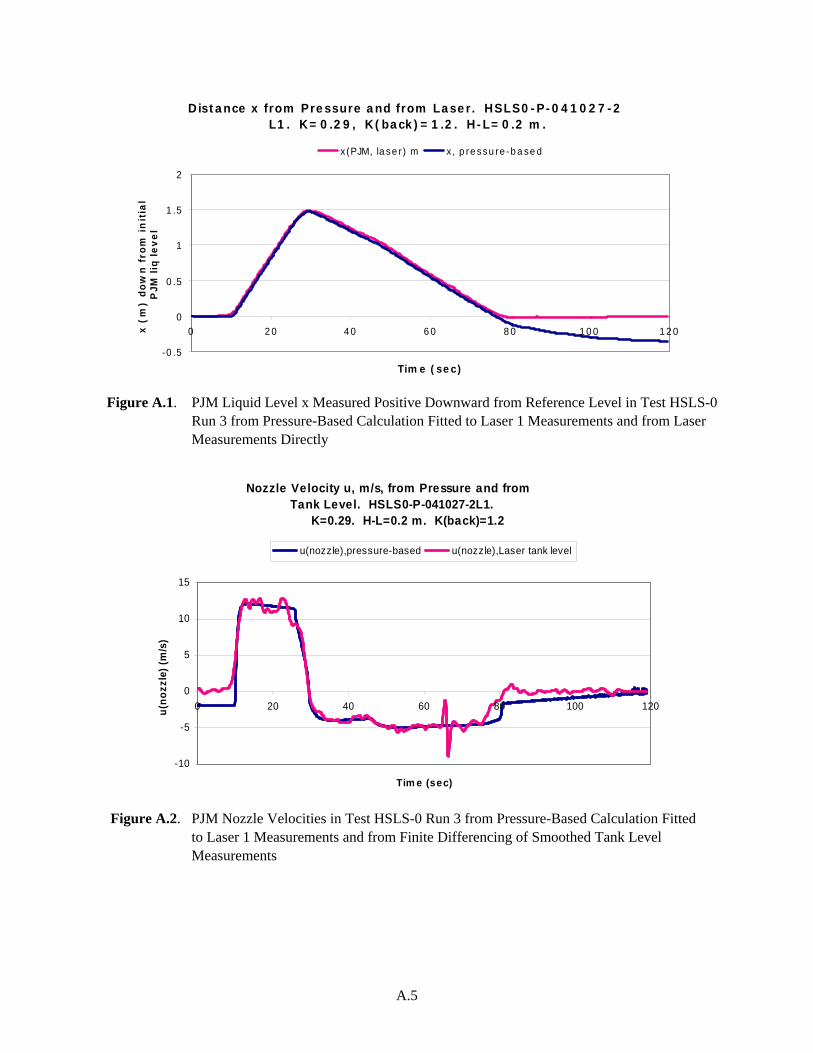
A.5

Distance x from Pressure and from Laser. HSLS0-P-041027-2 L1. K=0.29, K(back)=1.2. H-L=0.2 m.

-0.5

0

0.5

1

1.5

2

0 20 40 60 80 100 120

Time (sec)

x (

m)

do

wn

fro

m i

nit

ial

PJM

liq

le

ve

lx(PJM, laser) m x, pressure-based

Figure A.1. PJM Liquid Level x Measured Positive Downward from Reference Level in Test HSLS-0 Run 3 from Pressure-Based Calculation Fitted to Laser 1 Measurements and from Laser Measurements Directly

Nozzle Velocity u, m/s, from Pressure and from

Tank Level. HSLS0-P-041027-2L1. K=0.29. H-L=0.2 m. K(back)=1.2

-10

-5

0

5

10

15

0 20 40 60 80 100 120

Tim e (sec)

u(no

zzle

) (m

/s)

u(nozzle),pressure-based u(nozzle),Laser tank level

Figure A.2. PJM Nozzle Velocities in Test HSLS-0 Run 3 from Pressure-Based Calculation Fitted to Laser 1 Measurements and from Finite Differencing of Smoothed Tank Level Measurements

A.6

Table A.1. Optimized Friction Factors K Found for HSLS-0 and HSLS-4 Runs

Run File Name Run Laser KF KB

HSLS0-P-041026-1 HSLS-0 run 0 3 0.26 1.05 HSLS0-P-041026-1 HSLS-0 run 0 2 0.29 1.05 HSLS0-P-041027-2 HSLS-0 run 3 1 0.29 1.2 HSLS0-P-041027-2 HSLS-0 run 3 3 0.22 1.15 HSLS0-P-041027-7 HSLS-0 run 1 2 0.30 1.1 HSLS0-P-041027-7 HSLS-0 run 1 3 0.23 1.05 HSLS4-P-1213-3 HSLS-4 run 6 2 0.26 1.05 HSLS4-P-1213-3 HSLS-4 run 6 3 0.28 1.05 HSLS4-P-1213-3 HSLS-4 run 6 4 0.36 0.95 HSLS4-P-1213-2 HSLS-4 run 6 3 0.295 1.25 HSLS4-P-1213-2 HSLS-4 run 6 4 0.32 1.05 Average -- -- 0.282 1.086

A.5 Predictions for HSLS4 Half- and Full-Stroke Tests Nozzle velocities were calculated for the HSLS-4 half stroke (HSLS4-P-1213-2) and full stroke (HSLS4-P-1213-3) tests using the average forward and backward K values reported in Table A.1. Figure A.3 shows the pressure-based nozzle velocity through a cycle from this calculation for the half-stroke case. The nozzle velocity deduced from finite differencing of 16-fold smoothed tank level as measured by laser 3 is shown for comparison. Figure A.4 shows the pressure-based nozzle velocity during the positive pulse period. Figure A.5 shows the x values (PJM reference-to-current liquid level distance) as computed from pressure using the average K values from Table A.1 and as deduced from laser 3 measurements. The Figure A.5 level (x) plots confirm these K values as plausible, even though one could not do so from the u plots of Figure A.4. Figure A.6 shows pressure-based nozzle velocity through a cycle for the full stroke test HSLS-4-P-1213 Run 6 from the pressure-based calculation using the average K parameters. The nozzle velocity deduced from finite differencing of 16-fold smoothed tank level as measured by laser 3 is shown for comparison. Figure A.7 shows the pressure-based nozzle velocity during the positive pulse period. Figure A.8 shows the x values (PJM reference-to-current liquid level distance) as computed from pressure using the average K values from Table A.1 and as deduced from laser 3 measurements, again supporting the validity of the average K values. A.6 Sensitivity of Predicted Velocities to K Values Eq. (A.3) and (A.4) can be seen to imply that nozzle velocity u calculated from pressure scales as (1+K)-1/2. The K values found in Table A.1 have a standard deviation of 0.04. This implies an uncertainty on the order of 2% in the nozzle velocities coming from the uncertainty in the K values.

A.7

Nozzle Ve locity u, m/s, from Pressure and from Tank Leve l. HSLS4-P-1213-2 L3. Half-Stroke

K=0.282. H-L=0.2 m. K(back)=1.086

-10

-5

0

5

10

15

20

0 20 40 60 80 100 120

Tim e (sec)

u(no

zzle

) (m

/s)

u(nozzle),Laser tank level u(nozzle),p-based,physical

Figure A.3. Nozzle Velocity from Pressure-Based Calculation and Laser-Based Tank Level During Cycle for HSLS-4 Run 6 Half-Stroke Test (average K values [Table A.1] used)

Nozzle Velocity u (m/s) vs Time. HSLS4-P-1213-2. Half-Stroke.

-4

-2

0

2

4

6

8

10

12

14

15 17 19 21 23 25 27 29 31 33 35

Time (sec)

No

zzle

Ve

loci

ty u

(m

/s)

Figure A.4. Nozzle Velocity from Pressure-Based Calculation During Pulse for HSLS-4 Run 6

Half-Stroke Test

A.8

Distance x from Pressure and from Laser. HSLS4-P-1213-2L3. K=0.282, K(back)=1.086. H-L=0.2 m.

-0.4

-0.2

0

0.2

0.4

0.6

0.8

1

1.2

0 20 40 60 80 100 120

Time (sec)

x (

m)

do

wn

fro

m i

nit

ial

PJM

liq

le

ve

lx(PJM, laser) m x, pressure-based

Figure A.5. PJM Liquid Level x (reference surface level to current level) During Cycle for HSLS-4

Run 6 Half-Stroke Test (from pressure-based calculation and laser-based tank level)

u(nozzle), m/s, from Pressure and from Tank Level. HSLS4-P-1213-3. Full Stroke

K=0.282. H-L=0.2 m. K(back)=1.086

-8

-4

0

4

8

12

16

0 20 40 60 80 100 120

Time (sec)

u(no

zzle

) (m

/s)

u(nozzle),Laser tank level u(nozzle),p-based,physical

Figure A.6. Nozzle Velocity from Pressure-Based Calculation and Laser-Based Tank Level

During Cycle for HSLS-4 Run 6 Full-Stroke Test (average K values [Table A.1] used)

A.9

Nozzle Velocity u (m/s) vs Time. HSLS4-P-1213-3. Full Stroke.

-6

-4

-2

0

2

4

6

8

10

12

14

15 20 25 30 35 40 45

Time (sec)

No

zzle

Ve

loci

ty u

(m

/s)

Figure A.7. Nozzle Velocity from Pressure-Based Calculation During Pulse for HSLS-4 Run 6

Full-Stroke Test (average K values from Table A.1 used)

Distance x from Pressure and from Laser. HSLS4-P-1213-

3. K=0.282, K(back)=1.086. H-L=0.2 m.

-0.5

0

0.5

1

1.5

2

0 20 40 60 80 100 120 140

Time (sec)

x (

m)

do

wn

fro

m i

nit

ial

PJM

liq

le

ve

l

x(PJM, laser) m x, pressure-based

Figure A.8. PJM Liquid Level x (reference surface level to current level) During Cycle for HSLS-4

Run 6 Full-Stroke Test (from pressure-based calculation and laser-based tank level)

Appendix B

CAD Approach to Estimating the Sparger Heel: Description of the 3D Model

B.1

Appendix B - CAD Approach to Estimating the Sparger Heel: Description of the 3D Model

In addition to determining the unmixed simulant volume in the sparger heel and PJM tubes during the

sparger-only mixing tests (HSLS-4 Runs 3–5),(a) a three-dimensional (3D) model of the HSLS test configuration was developed using SolidWorks 2005 3D modeling software to provide an alternative calculation/assessment. In this model, the geometry of the tank and PJM cluster was modeled using a combination of as-built measurements and vendor specifications provided in Section 3 of the main report. In constructing the 3D model, the tank and internals were assumed to be symmetrical, and some small internals were not included (probes, PJM cluster stabilizer hardware/arms, water/peroxide injection lines, flat cover plate over bottom drain hole). The region where mixed fluid existed was added to the model as the air sparger zone of influence (ZOI) profile. The sparger ZOI profiles for the seven sparge tubes for a nominal air flow rate of 18.8 acfm(b) per sparge tube were calculated using equations provided by Poloski et al. (2005) and are shown in Figure B.1. These values were input directly to SolidWorks to create the 3D solid model profile. The ZOI profile is for a single sparge tube and is used with the assumption that the adjacent ZOIs do not interact below the line of intersection.

HSLS MIXING TEST ZOI PROFILE

-20

0

20

40

60

80

100

120

140

0 5 10 15 20 25 30 35 40 45 50

Radial Distance from Sparger nozzle (in.)

Verti

cal D

ista

nce

from

Spa

rge

Noz

zzle

(in.

)

Figure B.12. Sparger ZOI Profile for Nominal Air Flow Rate of 18.8 acfm

(a) Unmixed volume was determined during mixing tests using a chloride tracer; see results in Section 6.4. (b) Target flow rate for the testing. Actual flow rates were somewhat different (see Section 6 for details).

B.2

The zones of mixed and unmixed fluid in the 3D model are shown in Figures B.2 to B.4. Figure B.2 is a cross-sectional view of the HSLS tank model showing the sparger ZOI and the unmixed sparger heel. Figure B.3 is the tank model as seen looking up from the bottom of the vessel. Figure B.4 shows the sparger heel plus the unmixed volume in the PJMs. The mass properties utility of SolidWorks calculated volumes of the sparge heel and the unmixed volume within the PJMs as 3400 and 5230 L, respectively, for an H/D ratio of 0.81. At this H/D ratio, the average total simulant volume in the tank is 31780 L, giving a total unmixed volume fraction of 27%.

Figure B.2. Cross-Sectional View of HSLS Tank Showing Sparger Mixing Zone and Heel

B.3

Figure B.13. View from Bottom of the Tank Showing Sparger Mixing Zone and Heel. The

unmixed region is between the solid areas surrounding the seven sparge tubes. The light area in between the PJMs is part of the shroud enclosure.

Reference Poloski AP, ST Arm, JA Bamberger, B Barnett, R Brown, BJ Cook, CW Enderlin, MS Fountain, M Friedrich, BG Fritz, RP Mueller, F Nigl, Y Onishi, LA Schienbein, LA Snow, S Tzemos, M White, and JA Vucelik. 2005. Technical Basis for Scaling of Air Sparging Systems for Mixing in non-Newtonian Slurries. WTP-RPT-129 Rev 0 (PNWD-3541), Battelle – Pacific Northwest Division, Richland, Washington.

B.4

Figure B.14. View of Unmixed Fluid in the Sparger Heel and Within the PJM

Appendix C

Gas Volume Fraction Analysis Details

C.1

Appendix C - Analysis Details

C.1 Gas Volume Fraction Obtained from Simulant Level

Simulant level measurements were obtained and recorded in several ways:

• Manual hand measurements, using a tape measure, recorded the simulant level to rim distance at a single point only during periods when PJMs were off and the spargers were on idle. This period is referred to as the “static” period. The measurement location remained consistent over all testing.

• Manually observed and recorded laser level data obtained from the “DACS SCREEN” during the “static” period. Values displayed were 60 sample running averages and DACS operators simply recorded values reported on the screen.

• The DACS log files, “STATIC,” “GAS,” “PJM,” and “ARCHIVE,” report laser level data at varying frequencies and after varying running averages were applied. The “STATIC” period laser level data are comparable to the manual hand measurements. The “GAS” and “ARCHIVE” files have 600- and 60-sample running averages applied and 10- and 1-second logging frequencies, respectively. These two files contained the most meaningful and useful real-time level data of all the DACS files. Data logged in the “PJM” file was high frequency and was not logged except for 30-minute periods at the beginning of each run.

In the analysis of HSLS-1, the “ARCHIVE” log file data were used for real-time tank level

monitoring. In subsequent testing, HSLS-2, HSLS-3, HSLS-8, and HSLS-9, the “GAS” log file data were used. Raw data are sampled into DasyLab at 60 Hz.

Each laser level value was processed according to three “analyst defined” criteria to remove outliers, nonstatic periods, and erroneous laser level signals. The first criterion was

21

2110

10

10

10

∑

∑+

−

+

−−i

ii

i

ii

i

S

SS

>0.02 (C.1a)

3

31

1

1

1

∑

∑+

−

+

−−i

ii

i

ii

i

S

SS

>0.02 (C.1b)

C.2

where Si represents the current laser level value. Eq. (C.1a) is used for “ARCHIVE” log files, and Eq. (C.1b) is used for “GAS” log files. The two equations differ in the number of samples used but have equivalent analysis time periods (20 seconds). The second criterion focused on removing erratic laser-level values and the values recorded during PJM suction or drive periods through the general equations:

221

10

10 >−∑+

−

i

ii

i

SS (C.2a)

232 >−

∑−

i

ii

i

SS (C.2b)

where the value of 2 represents a 2-inch distance. Eq. (C.2a) is used with “ARCHIVE” log files, and Eq. (C.2b) is used for “GAS” log files, while both consider an equivalent time period. A third criterion was used to determine the average simulant level. If 1 or more individual laser level values failed the criterion set in Eq. (C.1) and (C.2), the average laser level was not computed and would not serve as a valid data point. The Excel result, determined through Eq. (C.3), was reported as a “FALSE” value if the average was not computed. The average laser level was calculated using

( )

1 2 3 41 2 3 4i i i ii i i ii avg

S S S S S only if S ,S ,S ,S pass Eq.(A.1)and (A.2)4

+ + += (C.3)

where superscripts 1–4 represent laser-based level monitors 1–4, respectively.

The maximum laser-level value was captured during the brief period when the PJMs were full and just before they began their drive period (i.e., the delay phase). The following approach was devised to isolate this period of interest. Forward-backward running averages using the equations

121

60

60∑+

−=

i

ii

i

SRA (C.4a)

13

6

6∑

+

−=

i

ii

i

SRA (C.4b)

were computed, and then a maximum value in that same range was computed with the MAX function. In generic Excel notation, the equation to determine the maximum of the range was ):( 6060 +−= iii SSMAXMAX (C.5a) ):( 66 +−= iii SSMAXMAX (C.5b)

C.3

where Eq. (C.4a) and (C.5a) were used with “ARCHIVE” log files, and Eq. (C.4b) and (C.5b) were used for “GAS” log files. Both analysis periods represent 2 minutes. The next step was to screen each value according to the “argument”: =IF(Si (avg)="FALSE", "FALSE", IF((Si (avg) - RAi)>0.85*(MAXi-RAi), Si (avg),"FALSE") (C.6)

In words, the argument above first checks to see if a valid Si (avg) was calculated. If yes, then the

argument tests whether the difference between Si (avg) and RAi is greater than 0.85% of the difference between MAXi and RAi. If the latter is “TRUE,” Si (avg) is reported in that cell; otherwise a “FALSE” value is reported.

The 0.85 value used in Eq. (C.6) is referred to as the “near peak” criterion value and enables the user to determine the maximum laser level during the appropriate time period (delay phase of the PJM cycle). While selecting a “near peak” criterion, the value was varied from 0.75 to 0.95, and we concluded that small variations in this value did not alter the conclusions that would be drawn from a raw data set.

The final argument used in this analysis simply tests whether the result of Eq. (C.6) equals MAXi. If so, a “TRUE” value is reported in the cell; otherwise a “FALSE” value is reported. The Excel argument is represented by

=IF(Si (avg)="FALSE","FALSE", IF((Si (avg) - RAi)>0.85*(MAXi-RAi), IF(Si (avg)=MAXi,"TRUE","FALSE"), "FALSE")) (C.7)

A snapshot of representative results generated from this analysis on HSLS-1 is displayed in Table C.1.

Table C.1. Reduced HSLS-1 Data

Raw Time

Elapsed Time

Max Level (in)

HSLS Weight

Max Identifier

4:37:17 5.000 36.23 173777.36 False 4:37:27 5.167 36.26 173779.68 False 4:37:37 5.333 36.34 173789.36 False 4:37:47 5.500 36.36 173791.72 False 4:37:57 5.667 36.36 173796.36 False 4:38:07 5.833 36.36 173796.12 False 4:38:17 6.000 36.36 173799.80 False 4:38:27 6.167 36.38 173792.40 True 4:38:37 6.333 36.33 173799.08 False 4:38:47 6.500 36.33 173802.24 False 4:38:57 6.667 36.23 173801.96 False 4:39:07 6.833 36.26 173795.08 False 4:39:17 7.000 36.22 173790.48 False 4:39:27 7.167 36.26 173793.52 False 4:39:37 7.333 36.35 173796.36 True 4:39:47 7.500 36.31 173789.00 False 4:39:57 7.667 36.33 173786.40 False

C.4

The five columns of data are “sorted” in ascending order by the “max identifier” column. All “FALSE” data points are deleted, and maximum simulant surface levels remain for subsequent calculations of gas fraction.

Gas fractions were calculated using estimated simulant volumes obtained through “maximum” simulant level measurements and a volume-level correlation that uses a linear equation for distances less than 35 inches below the tank rim and a cubic equation for distances greater than 35 inches. These two correlations are

Cubic equation (H > 35 inches) 32 H0627628.0H76934.7H53661.601521.50763)H(V −+−= (C.8)

Linear equation (H < 35 inches) H09654.2981649.46961)H(V −= (C.9) where V is the volume of simulant in liters and H is the distance below the tank rim in inches. The gas volume fraction, referred to as α (alpha), was then calculated using the equation:

current initial

current

V VV

−α = (C.10)

where Vcurrent represents the measured volume at “current” time and Vinitial equals the volume measured under “no gas” conditions.

Volume adjustments were necessary because Vinitial, our reference “no gas” volume, changed slightly over time due to evaporation, sample removal, and H2O2 additions. To account for these variations, gas fraction adjustments were made using the weight of simulant, in pounds, and the average simulant density to calculate a volume by adjustment

S

WV 2.2= ρ (C.11)

where ρS is the simulant density in kg/L and W is the weight of simulant in pounds. Combining Eq. (C.10) and (C.11) to generate the following equation provides a final gas volume fraction value for this analysis:

( )current initial adjustment

weight adjustedcurrent

V V VV

− −α = (C.12)

PNWD-3676 WTP-RPT-132 Rev. 0

Distr.1

Distribution

No. of Copies OFFSITE

No. of Copies ONSITE

1 Savannah River National Laboratory Richard Edwards Savannah River National Laboratory Westinghouse SA Aiken, SC 29808-0001

20 Battelle – Pacific Northwest Division S. T. Arm P7-28 J. R. Bontha K6-24 M. Friedrich K5-16 M. S. Fountain P7-27 C. E. Guzman-Leong K5-22 L. K. Jagoda K6-24 C. D. Johnson K6-96 D. E. Kurath P7-28 K. S. Koschik J2-09 P. A. Meyer K7-15 F. Nigl K7-15 R. L. Russell K6-24 G. L. Smith H4-02 C. W. Stewart K7-15 W. Yantasee K8-93 S. T. Yokuda K7-15 Project Office (2) P7-28 Information Release (2) K1-06

7 Bechtel National, Inc. H. A. Abodishish H4-02 S. M. Barnes H4-02 A. S. Bronner H4-02 C. E. Corriveau Jr. H4-02 D. E. Larson H4-02 J. Talbott (2) H4-02