Written Comments - Oregon.gov
532
State of Oregon Department of Environmental Quality Written Comments Aug. 2, 2021 Clean Truck Rules 2021 Rulemaking Advisory Committee Meeting Commenters Clean Air Healthy Communities Coalition Engine Manufacturers Association (EMA) Nikola Titan Freight
-
Upload
khangminh22 -
Category
Documents
-
view
0 -
download
0
Transcript of Written Comments - Oregon.gov

State of Oregon Department of Environmental Quality
Written Comments Aug. 2, 2021 Clean Truck Rules 2021 Rulemaking Advisory Committee Meeting
Commenters
Clean Air Healthy Communities Coalition Engine Manufacturers Association (EMA) Nikola Titan Freight

Dear Department of Environmental Quality Staff,
The undersigned groups appreciate the opportunity to show our support for the adoption of both the Advanced Clean Truck (“ACT”) rule and Heavy-Duty Omnibus (“HDO”) rule this year in Oregon. Below you will find general comments in support of the rules, answers to questions and concerns posed at the second Rulemaking Advisory Committee (“RAC”) on August 5, 2021, and comments on the Department of Environmental Quality’s (“DEQ”) draft Statement of Fiscal and Economic Impact (“Statement”).
I. Oregon should adopt the ACT and HDO rules by the end of 2021.
Securing Oregon’s swift and orderly transition to an electric truck future while slashing diesel truck pollution is a public health, equity, and climate imperative that can grow the economy and lead to quality jobs. The ACT and HDO rules are powerful and complementary tools that must be adopted together to curb toxic diesel pollution and jumpstart the zero-emission medium- and heavy-duty vehicle (“MHDV”) market. The ACT rule will ensure more zero-emission MHDVs are available for sale in Oregon, while the HDO rule will reduce emissions from new fossil fuel MHDVs that continue to be sold. It is vital that as the ACT rule helps us transition to ZEV trucks, the continued sale of fossil fuel vehicles are as clean as possible. The rules work in tandem and send a clear market signal around which industry, government, and other stakeholders can plan and mobilize investments.
We cannot afford to delay or postpone the adoption of both rules, especially the HDO rule given the tremendous public health benefits it will bring to Oregonians, for the following reasons:
• Although heavy duty vehicles comprise 10 percent of all vehicles on the road in the US,
they account for nearly 25 percent of total U.S. climate pollution from transportation, and 45 percent of NOx emissions.
• Fossil fuel pollution is linked to higher rates of cancer, heart disease, respiratory disorders and premature death. This pollution disproportionately harms low-income and Black, Indigenous, and people of color (“BIPOC”) communities, who often live adjacent to highways, ports and other pollution hot spots due to racist housing, land use and economic policies.
• These rules, if paired with targeted environmental justice and equity policies, can yield substantial near and long-term public health and economic benefits to low-income and BIPOC Oregonians disproportionately suffering from the burdens of fossil fuel pollution.

• Every year, in Oregon alone, diesel engine exhaust is responsible for an estimated 176 premature deaths, 25,910 lost work days and annual costs from exposure of up to $3.5 billion.
• Workers routinely exposed to diesel exhaust have a greater risk of lung cancer and other illnesses due to breathing polluted air (this accounts for 29,000 Oregonians in the workforce).
• Adoption of the ACT and HDO rules is estimated to yield 156 fewer premature deaths, 118 avoided hospital and emergency room visits, over 83,000 avoided minor medical cases (including, for example, acute bronchitis and exacerbated asthma), and over $1.8 billion in health costs by 2050.
To improve the public health of Oregonians, ensure Oregon achieves its greenhouse gas
reduction targets in the transportation sector and mitigate extreme weather events fueled by climate change (heatwaves, climate fires, floods), DEQ should do everything in its power to ensure prompt adoption of the ACT rule and Low-NOx Omnibus rule. II. Responses to questions posed at the RAC on August 5th, 2021.
ACT Rule: Early Credits
We strongly support limiting early crediting to Model Year 2024. This would minimize the potential negative impact early crediting could have on the rule’s stringency and as a result its benefits. Also, offering one year of early crediting is consistent with what other Section 177 states are considering, notably New Jersey. ACT Rule: Fleet Reporting Applicability
While the current fleet reporting threshold requirement is set at 50, we urge DEQ to
lower the vehicle threshold to allow for the state to capture accurate data that will help:
• Identify areas with high rates of freight traffic and, consequently, diesel pollution, allowing Oregon to target clean transportation policies to the communities that need relief most;
• Shed light on exploitative labor practices, such as misclassifying drivers as independent contractors. Misclassification is rampant in the trucking industry, particularly in the drayage segment. These trucks are among the oldest and dirtiest vehicles on the road and are excellent for zero-emission technology given their short-haul, idling, and stop-and-go operations. Due to misclassification, many drivers lack financial resources to upgrade their equipment to reduce diesel pollution or buy a zero-emission truck. DEQ will need the most granular information possible to direct funding and regulations towards entities that control fleets to make sure they comply with emissions reductions and electrification goals rather than shifting the responsibility to drivers who often do not have the resources to comply. Adopting the rule could turn a historically polluting industry into a source of high quality, green jobs in trucking, manufacturing, and charging infrastructure installation; and

• Help utilities make better informed electric utility investments today to install the charging infrastructure necessary to support MHD ZEVs. It will also enhance utility distribution system planning efforts that are vital in the transition to clean vehicles as a well-designed grid can lower bills for all customers by avoiding expensive system upgrades.
Based on data collected by the Oregon Department of Transportation, only 1.6 percent of the
medium- and heavy-duty carriers have 51 or more vehicles in their fleet and would be responsible for reporting. Lowering the vehicle threshold would allow for the state to capture accurate data that will help scale the adoption of zero-emission vehicles. While the overwhelming majority of fleets contain five vehicles or fewer (82.3 percent of fleets), that granularity of reporting may prove prohibitive for DEQ. Therefore, the reporting threshold should be set at five or more vehicles to cover nearly 20 percent of Oregon’s fleets. Additionally, Oregon DEQ should consider asking fleet owners and operators to report:
• Vehicle identification numbers (“VIN”) for the trucks they own and the VINs operating under the companies’ DOT numbers;
• Any contractor-owned vehicles when contractors lease their services to the company in question. This includes make, model, weight class, model year, year added to fleet, body type, odometer reading, own/rent/lease, duty cycle, weight/volume limited, where parked overnight, on-site vs. off-site fueling, and maintenance; and
• Information on idling practices, rates, and any company idling policies. All vehicles should be identified as contractor or company owned.
The trucking industry is highly inequitable and, in many segments, become a financially
precarious industry since federal deregulation in the 1980s. Since that time carriers large and small have shifted capital and operating costs to workers, buoying balance sheets while re-assigning risk to low-income, poorly capitalized truckers. Transfer of capital and operational risk in the industry creates fundamental barriers to efficiency investments and advanced technology adoption, as corroborated by numerous studies.1, 2, 3
We urge staff to consider expanding the reporting requirement to capture all necessary
industry economic patterns, incentives, and barriers to technological adoption. Specifically, DEQ should focus on vehicle asset risk and management patterns in the industry. To understand the determinants of technology adoption, DEQ should understand the nature and extent of key determinants of asset risk, including contracting, asset versus non-asset-based fleets, truck leasing practices, contractor financial capacity, and the extent of driver misclassification. These elements help determine the economics of fleet transitions. HDO Rule: Transit Agency Exemptions
1 North American Council for Freight Efficiency. Barriers to the Increased Adoption of Fuel Efficiency Technologies in the North American On--‐Road Freight Sector. 2013. Available online: https://www.theicct.org/sites/default/files/publications/ICCT-NACFE-CSS_Barriers_Report_Final_20130722.pdf 2 US EPA Working Paper #14-02: Heavy Duty Trucking and the Energy Efficiency Paradox. 2014. Available online: https://www.epa.gov/sites/production/files/2014-12/documents/heavy-duty_trucking_and_the_energy_efficiency_paradox.pdf 3 Viscelli, Steve. The Big Rig: Trucking and the Decline of the American Dream. UC Press. In print. 2016.

Fossil fuel powered transit is a major source of pollution, especially at the local level, and
should not be exempted from the HDO rule. Moreover, the low speeds and stop-and-go nature of transit routes make them perfect for electrification. To better address the exemption question and pollution from transit vehicles, we strongly urge DEQ to adopt the Innovative Clean Transit rule to gradually transition Oregon’s transit agencies to 100 percent ZEVs. III. Responses to concerns posed at the RAC on August 5th, 2021.
Response to argument for delaying rule adoption:
DEQ should seek to adopt the ACT rule this year and should reject invitations to delay adoption. Under Section 177 of the Clean Air Act, states must “adopt such standards at least two years before commencement of such model year (as determined by regulations of the Administrator).” As outlined by a separate comment letter attached as Appendix A, there is ambiguity regarding when a Model Year begins for MHDVs. To minimize the risk of missing critical time to accelerate ZEV adoption and reduce greenhouse gas emissions and toxic pollutants, DEQ should adopt the rules by the end of 2021. Response to argument that the HDO rule incentivizes natural gas trucks:
The concern that the HDO rule will cause natural gas trucks to displace ZEVs is not
relevant as it is not the purpose of the HDO rule to encourage ZEV deployment. That role falls to the ACT rule, through which only ZEVs can meet compliance. The HDO rule is a necessary environmental justice and public health regulation that ensures that while we transition to ZEVs, the fossil fuel MHDVs that continue to be sold in Oregon are as clean as possible. Further, to realize the incentives in the HDO rule, manufacturers must also certify their natural gas vehicles and it is unclear if they will do so. Response to argument to wait for federal action:
President Biden signed an Executive Order on August 5th, 2021 that, among other things,
directs the EPA Administrator to promulgate GHG and criteria pollutant emission standards for MHDV to begin by 2027. While this is an important federal action, the details of the potential federal rules remain unclear. Even if a strong ZEV sales mandate and low NOx rule are adopted next year, because of federal lead time requirements, states would have to wait until Model Year 2027 for the rules to take effect, possibly missing out on several years of critical emission reduction and public health benefits. Oregon has the opportunity to take action and commit to adopting the ACT and HDO rules this year, setting us on a faster trajectory to achieving GHG emissions reductions and lowering toxic diesel emissions that harm public health. IV. Comments on the draft Statement of Fiscal and Economic Impact (“Statement”).
We greatly appreciate DEQ staff’s hard work to develop a comprehensive and robust draft Statement. Below are suggestions to further quantify expected impacts from adoption as well as the latest information on costs and benefits.

Affected Parties (pg. 2-3 of the Statement) There are several affected parties that should also be explicitly referenced or expanded:
• Electric utilities. Greater battery electric vehicle (“BEV”) deployment supported by the rules will increase demand for electricity resulting in increased revenue for electric utilities. Additionally, BEVs—batteries on wheels—offer the potential to provide grid services and flexible demand that could enhance grid resiliency, reliability, and greater renewable energy penetration.
• Electric consumers. BEVs, regardless of who owns them, can shrink electric bills for all utility customers by improving electric grid utilization from charging during periods of low demand. A 2019 report found that in the utility service territories with the highest level of BEV penetration (Pacific Gas & Electric and Southern California Edison), utility revenue from BEV charging significantly exceeded system costs, putting downward pressure on electric rates for both BEV-owners and non-BEV owners.4
• Businesses associated with the ZEV ecosystem. The clean technology sector, anchored by strong regulations, is one of Oregon’s most critical industries that supports nearly 57,000 jobs statewide—50 percent of which are based outside the Portland metro area.5 Clean technologies, such as ZEVs, are a valuable source of innovation. Adopting rules to accelerate the transition to clean technologies will grow Oregon’s businesses associated with the ZEV ecosystem, such as electric charging infrastructure providers and ZEV maintenance electricians.
• Particular attention should be paid to electric vehicle battery manufacturers. As the production of e-mobility and renewable energy is scaled up, so is the need for the many raw materials for green energy, which come disproportionately from developing countries. Parallel to sourcing considerations, without recycling and/or reuse policies, the benefits of electric vehicle batteries wane when considering battery end of life. If they end up in a landfill, battery cells could release toxins and heavy metals. Fortunately, vehicle batteries can be used in second-life applications6 and contain high-value materials,7 and the public and private sector are investing significant resources in developing a robust battery reuse/recycle industry.8, 9 However, supportive state policies are needed to further promote end of life management. Although rampant throughout the fossil fuel supply chain as well, the environmental degradation and human rights abuses along the green energy supply chain casts a shadow and we must not perpetuate industrial injustices. These issues are consistently framed as “outside of the scope” of most impact analyses. While these rulemakings are moving in the right direction, there needs to be continued dialogue and action around sourcing of raw materials to create batteries and how we reuse/recycle batteries once they reach end of use. As we transition away from fossil fuels—and the long history of human rights abuses associated with it—we must ensure that clean transportation goes hand-in-hand with good supply chain governance.
4 https://www.synapse-energy.com/sites/default/files/EVs-Driving-Rates-Down-8-122.pdf 5 https://e2.org/reports/clean-jobs-oregon-2019/ 6 https://blog.ucsusa.org/hanjiro-ambrose/the-second-life-of-used-ev-batteries/ 7 https://www.anl.gov/article/recell-center-could-save-costly-nickel-and-cobalt-transform-battery-recycling-worldwide 8 https://www.energy.gov/eere/articles/battery-recycling-prize-phase-iii-rules-released 9 https://www.bloomberg.com/news/articles/2021-02-25/used-ev-batteries-are-heading-to-factories-and-farms

Subsequent policies should include cradle-to-grave compliance regulations on battery manufacturing that contains strong labor, human rights, and environmental protections.
• The public. DEQ rightfully identified the benefits to the public from reduced greenhouse gas emissions and criteria pollution by adopting the rules. However, the Statement should also include the economic benefits to the public resulting from lower fuel and maintenance costs from ZEVs as well as the potential for high-quality job creation. The macroeconomic impact of fuel and maintenance cost savings and depressed electricity rates is difficult to quantify but consequential. According to one study from California, “these savings will be diverted to other expenditures, most of which go to in-state services” that are “the most labor-intensive and skill-diverse in the economy” and “cannot be outsourced.”10 Shifting expenditures from fossil fuels, which is less labor-intensive than the service industry, will act as a direct stimulus to Oregon’s economy.
Fiscal and Economic Impact: General Assumptions (pg. 3)
We strongly support DEQ’s decision to rely on CARB’s analysis, where possible, for determining the impact of adopting the rules on Oregon. CARB spent nearly a decade of research and analysis to ensure they are technically feasible and cost-effective. CARB’s analysis is definitive, although the outputs are California-specific and based on the best available information at the time. New studies that build on CARB’s work and are Oregon-specific should also be included in the Statement. In particular, a recently released report by MJ Bradley & Associates (“MJB&A”) that evaluates and monetizes the impact of Oregon adopting the ACT and HDO rules. The report is referenced extensively in the following comments and is included as Appendix B to our letter. Fiscal and Economic Impact: Overall Impact of the Rules (pg. 3)
While we agree with DEQ’s conclusion that the proposed rulemaking will have a positive
fiscal impact, based on the latest research, we believe DEQ’s analysis is conservative, and the benefits far exceed those identified and quantified in the Statement. Moreover, we encourage DEQ to better account for the rules’ benefits by including the impacts on affected parties listed above.
An additional benefit to include is the impact the rules will have on related on policies and investments. The ACT rule’s sales mandate provides a clear schedule for minimum ZEV deployment. This certainty allows the public and private sector to better plan and make strategic investments today. For example, in New Jersey, where they recently solicited public comments on adopting the ACT rule, the Board of Public Utilities (“BPU”) released a MHDV straw proposal that will unlock millions of dollars in ZEV charging infrastructure investments and fuel savings.11 A key justification for BPU releasing the MHDV straw proposal was the state’s action to adopt the ACT rule. Oregon can and should expect adopting the ACT rule to unlock additional resources and infrastructure investments.
10 https://ww2.energy.ca.gov/2018publications/CEC-500-2018-013/CEC-500-2018-013.pdf 11 https://www.nj.gov/bpu/pdf/publicnotice/Notice%20Medium%20Heavy%20Duty%20EV%20Straw%20Proposal.pdf

Notably, Class 2b-3 ZEVs with gross vehicle weight ratings less than 14,000 pounds are eligible for the federal EV tax credit up to $7,500.12 Since the federal tax credit value declines after manufacturers sell a certain number of EVs nationwide, regulations such as the ACT Rule that compels EV sales will help Oregon capture a greater portion of federal tax credits. Public: Benefits of the regulations: CO2 emissions reductions and Criteria air pollutant emission reductions (pg. 5)
According to the MJB&A report, Oregon’s MHDVs are responsible for around 42
percent of annual GHGs, 70 percent of NOx emissions, and 64 percent of PM2.5 from all on-road vehicles. By adopting the ACT and HDO rules, MJB&A estimate that Oregon can reduce MHDV GHG emissions by 49.7 million metric tons (“MMT”) amounting to a monetized value of $8.1 billion over the next 30 years. Over the same time period, the rules are expected to reduce NOx emission by 223,200 metric tons (“MT”) and PM2.5 by 1,290 MT. Reducing criteria pollution has real-world impacts, potentially avoiding 156 premature deaths, 118 hospital visits, and 83,579 minor health complications, such as acute bronchitis and exacerbated asthma, by 2050. Monetized, these benefits amount to $1.82 billion by 2050.
These results are substantially higher than DEQ’s and the International Council on Clean
Transportation’s (ICCT) for GHG reductions, however, ICCT’s NOx and PM2.5 reductions are above those of MJB&A. The differences likely come from assumptions regarding how the electric grid mix decarbonizes over time (changes to the grid mix in the MJB&A report are based on Oregon’s recent law, HB 202113), quantifying upstream fossil fuel emission reductions, and the extended timeline of the MJB&A analysis (through 2050). As such, the MJB&A report provides a valuable additional data points to include in the Statement. Large businesses – businesses with more than 50 employees: Total cost of ownership for ZEV vehicles (pgs. 6-7) In developing and comparing the total cost of ownership (“TCO”) of MHD ZEVs there are several nuances DEQ should take into consideration:
• Although electric truck purchase prices are rapidly declining, they remain higher than most comparable diesel trucks. However, electric trucks are attractive on a TCO basis due to fuel cost savings from charging with potentially less expensive electricity and anticipated 50 percent lower maintenance costs than a comparable diesel or gasoline vehicle.14 In many cases, these savings will compensate for higher up-front vehicle costs.
• Due to manufacturing efficiencies from economies of scale and decreasing battery prices, the initial purchase prices of ZEVs are expected to continue falling. Currently, batteries are the single most expensive component of an electric truck. According to Bloomberg New Energy Finance, battery costs have decreased by 89 percent over the past ten years and continue to drop.15 Upfront vehicle costs will continue to fall as battery prices decline over the rules’ implementation schedule.
12 https://www.irs.gov/businesses/plug-in-electric-vehicle-credit-irc-30-and-irc-30d 13 https://olis.oregonlegislature.gov/liz/2021R1/Measures/Overview/HB2021 14 https://escholarship.org/uc/item/7s25d8bc#article_main 15 https://about.bnef.com/blog/battery-pack-prices-cited-below-100-kwh-for-the-first-time-in-2020-while-market-average-sits-at-137-kwh/

• Electric trucks’ residual values are expected to be higher than used diesel trucks because a purchaser will receive a more reliable truck with much lower fuel and maintenance costs.16
• Meanwhile, financial institutions are exploring ways to pull forward expected fuel and maintenance savings to reduce electric MHDV purchase prices further.17 Since most MHDVs are financed, even when including the finance costs, truck owners acquiring new BEVs can begin receiving positive savings and cash flow from day one compared with similar fossil fuel vehicles due to substantial fuel and maintenance cost savings.
• It is unrealistic to assume fleets will be responsible for ZEV infrastructure costs. Already in Oregon utilities have been approved to spend nearly $20 million on, in part, Level 2 and DC fast charging (“DCFC”) stations—charging levels that Class 2b-3 BEVs can utilize—with another $6 million in pending applications.18 Moreover, with the passage of the federal Infrastructure Investment and Jobs Act, there will likely be over $26 billion in spending on EV-related items, including charging infrastructure. Oregon can expect to benefit from some of this federal spending on charging infrastructure. More importantly, the private sector such as Siemens, ABB, Greenlots (Shell), Electrify America, Black & Veatch, Burns & McDonald, Trillium, Love’s, ENELx, and Power Flex are continuing to leverage private capital to install private and public charging stations all over the country. For example, Electrify America installed charging stations at 400 stations nationally, with another 220 in process, and plans to install 800 by 2022. Recent installations include high-power 350 kW charging stations. Additionally, the National Association of Truck Stop Operators (NATSO) launched a National Highway Charging Collaborative to extend EV charging to every corner of the nation. Over the next decade, the Collaborative will leverage $1 billion in capital to deploy charging at more than 4,000 travel plazas and fuel stops that serve highway travelers and rural communities by 2030.19
• Many electric truck makers and dealers have financing divisions or subsidiaries and many of these will finance not only the trucks but also their infrastructure costs through leases and other methods. Two examples are Volvo Trucks of North America20 and Peterbilt.21
• Infrastructure costs are extremely dependent on vehicle type, duty cycle, charging needs, and location. While the Titan Freight example is certainly useful information, it is not indicative of prices across Oregon’s MHDV fleet. Further, as the above example from New Jersey shows, the potential for utilities to absorb a greater share of the infrastructure cost may materialize over the course of the regulation.
State Agencies and Local Governments (pgs. 10-11)
DEQ points out increasing MHD ZEVs will decrease fossil fuel consumption and reduce state and local fuel tax revenue. However, staff should also include the impact on state revenue of more ZEVs paying Oregon’s EV fee. Further, in many cases electricity is subject to local utility taxes that pay for local services, including the maintenance of local roads. Increasing electricity consumption from ZEVs could result in increased local tax revenue.
16 https://www.oberoninsights.com/insights/residual-value 17 https://www.forbes.com/sites/sebastianblanco/2019/04/18/proterra-ready-for-electric-bus-battery-leasing-with-200-million-credit-facility/?sh=4f2a81ae2314 18 https://www.atlasevhub.com/materials/electric-utility-filings/ 19 https://www.natsoaltfuels.com/EVCharging.php 20 https://www.volvotrucks.us/trucks/vnr-electric/ 21 https://www.peterbilt.com/about/news-events/news-releases/PACCAR-extends-zero-emissions-leadership

Thank you for your leadership and consideration of our comments. Sincerely, Members of the Clean Air, Healthy Communities Coalition Ranfis Giannettino Villatoro Oregon Policy Coordinator BlueGreen Alliance Hieu Le Campaign Representative Sierra Club Sergio Lopez Energy, Climate and Transportation Coordinator Verde Aimee Okotie-Oyekan Environmental and Climate Justice Coordinator NAACP Eugene Springfield Victoria Paykar Oregon Transportation Policy Manager Climate Solutions Mary Peveto Executive Director Neighbors for Clean Air Patricio Portillo Clean Vehicles and Fuels Advocate Natural Resources Defense Council Brad Reed Campaign Manager Renew Oregon Amelia Schlusser Staff Attorney Green Energy Institute at Lewis & Clark Law School
Akashdeep Singh Western States Policy Advocate Union of Concerned Scientists Sara Wright Transportation Program Director Oregon Environmental Council

Appendix A

August 17, 2021 Northeast States for Coordinated Air Use Management 89 South Street, Suite 602 Boston, MA 02111 Re: Response to Misleading Arguments Urging States to Delay Adoption of California
Medium- and Heavy-Duty Emission Standard The undersigned organizations are aware of recent comments and letters shared by truck
manufacturers and trucking associations requesting that states delay adoption of California’s medium- and heavy-duty vehicle (“M/HDV”) emission standards. These letters mischaracterize and misinform. This document offers our response and rationale for why states should move forward with adoption as soon as possible. States should adopt the rules as soon as possible to avoid risk from uncertain “model year” definitions.
The Truck and Engine Manufacturers’ Association (“EMA”) is urging Section 177 States to delay adoption of California’s Advanced Clean Trucks (“ACT Rule”) and Heavy-Duty Omnibus Rule (“HDO Rule”). In our view, there is no reason for delay; indeed, there is every reason for haste given the additional climate and air pollution harm from inaction.
EMA’s letters concern Section 177’s requirement that States seeking to enforce a
California motor vehicle engine standard must “adopt [the California] standards at least two years before commencement of such model year (as determined by regulations of the Administrator).” 42 U.S.C. § 7507(2). In accordance with this statutory provision, in 1995, EPA promulgated regulations that defined “model year” for the purpose of Section 177. 40 C.F.R. § 85.2301 et seq. (“Determination of Model Year for Motor Vehicles and Engines Used in Motor Vehicles under Section 177 . . . of the Clean Air Act”). That definition allows a model year to start as early as January 2 of the preceding calendar year. 40 C.F.R. § 85.2304(a). EPA recently amended this Section 177 definition to clarify that it applies to “all motor vehicles regulated under 40 CFR part 86, subpart S,” whereas “heavy-duty motor vehicles and heavy-duty motor vehicle engines regulated under 40 CFR part 86, subpart A, and 40 CFR parts 1036 and 1037” should instead use the “definitions and related provisions in 40 CFR parts 1036, 1037, and 1068.” Id. (as amended by Improvements for Heavy-Duty Engine and Vehicle Test Procedures, and Other Technical Amendments, 86 Fed. Reg. 34308 (June 29, 2021)).
In their letters, EMA asserts that the definition of “model year” that applies for the purpose of ACT Rule adoption is a distinct definition found in 40 CFR Part 1037, 40 C.F.R. §
1037.801 – EPA regulations promulgated under Clean Air Act Section 202, not Section 177 – and in some CARB regulations, Cal. Code Regs. tit. 13, § 1963(15); id. tit. 17, § 95662(a)(16). These regulations define “model year” to be the same as the “calendar year” in most situations. Id. Thus, according to EMA, States can adopt of the ACT and HDO Rules by December 31, 2021 – two years before January 1, 2024 – and still have the rules go into effect in Model Year 2024, which starts with the 2024 calendar year under this definition.
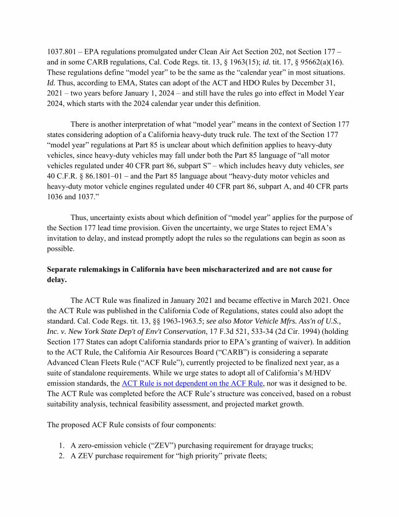
There is another interpretation of what “model year” means in the context of Section 177 states considering adoption of a California heavy-duty truck rule. The text of the Section 177 “model year” regulations at Part 85 is unclear about which definition applies to heavy-duty vehicles, since heavy-duty vehicles may fall under both the Part 85 language of “all motor vehicles regulated under 40 CFR part 86, subpart S” – which includes heavy duty vehicles, see 40 C.F.R. § 86.1801–01 – and the Part 85 language about “heavy-duty motor vehicles and heavy-duty motor vehicle engines regulated under 40 CFR part 86, subpart A, and 40 CFR parts 1036 and 1037.” Thus, uncertainty exists about which definition of “model year” applies for the purpose of the Section 177 lead time provision. Given the uncertainty, we urge States to reject EMA’s invitation to delay, and instead promptly adopt the rules so the regulations can begin as soon as possible. Separate rulemakings in California have been mischaracterized and are not cause for delay.
The ACT Rule was finalized in January 2021 and became effective in March 2021. Once the ACT Rule was published in the California Code of Regulations, states could also adopt the standard. Cal. Code Regs. tit. 13, §§ 1963-1963.5; see also Motor Vehicle Mfrs. Ass'n of U.S., Inc. v. New York State Dep't of Env't Conservation, 17 F.3d 521, 533-34 (2d Cir. 1994) (holding Section 177 States can adopt California standards prior to EPA’s granting of waiver). In addition to the ACT Rule, the California Air Resources Board (“CARB”) is considering a separate Advanced Clean Fleets Rule (“ACF Rule”), currently projected to be finalized next year, as a suite of standalone requirements. While we urge states to adopt all of California’s M/HDV emission standards, the ACT Rule is not dependent on the ACF Rule, nor was it designed to be. The ACT Rule was completed before the ACF Rule’s structure was conceived, based on a robust suitability analysis, technical feasibility assessment, and projected market growth. The proposed ACF Rule consists of four components:
1. A zero-emission vehicle (“ZEV”) purchasing requirement for drayage trucks; 2. A ZEV purchase requirement for “high priority” private fleets;

3. A ZEV purchase requirement for public fleets; and 4. A requirement that all new medium- and heavy-duty vehicle sales must be ZEV by 2040
(“100% by 2040”).
Each component is separate. Once finalized by CARB, States can opt into any or all of California’s suite of M/HDV regulations. In other words, States can choose to adopt whatever mix of the following they deem appropriate: the ACT Rule, any or all of the ZEV purchase requirements for specific fleets (drayage, “high priority”, or public), and/or 100% by 2040. For example, a state could adopt the ACT Rule now, in 2023 adopt the ZEV purchase requirement for drayage fleets, and, in 2037, adopt the 100% by 2040 requirement (to comply with lead time requirement).
The 100% by 2040 target is prompted by rapid advancements in zero-emission technology in the past year, new zero-emission vehicle commitments by truck manufacturers, a desire to send a clearer market signal, and to better match the urgency to address the climate and air pollution crises that disproportionately impact low-income communities and communities of color. In fact, it is hardly out of step with natural market evolution: a group of prominent European truck manufacturers already committed to the same timeline at the end of 2020.
It may be tempting to simply say these are all one rule, however, that would be incorrect. They serve different purposes, regulate different entities, and leverage different compliance mechanisms. They may originate from the same agency and seek to accomplish similar objectives, but, as with other CARB programs, they are distinct standards, each one affording States flexibility but not imposing any obligation to adopt another.
Recent federal action reinforces the need for states to adopt California’s vehicle emission standards as soon as possible.
President Biden’s recent Executive Order (“EO”) on Strengthening American Leadership in Clean Cars and Trucks was welcome news. Contrary to some industry assertions, this federal action serves to reinforce, rather than undermine, the rationale for states to move forward as quickly as possible to adopt California’s M/HDV emission standards.
First, the EO directs the EPA Administrator to coordinate the agency’s activities “with
the State of California as well as other States that are leading the way in reducing vehicle emissions, including by adopting California’s standards.” This suggests the Biden Administration intends for states who adopt California’s vehicle emission standards to have a seat at the federal rulemaking table, ensuring their priorities are considered and folded into federal policymaking and potentially inspiring more ambitious national standards. At the same time, few details about the forthcoming EPA standards have been released, while state standards

present a certain path to secure emission reductions. National standards by themselves can be complemented by state leadership that, holistically, aids in the achievement of climate and clean air objectives. For example, states can move forward with a M/HDV ZEV sales penetration date and a ZEV sales mandate. Moreover, the details of a potential federal low NOx rule still remain unclear. Even if a strong ZEV sales mandate and low NOx rule are adopted next year, because of federal lead time requirements, states would have to wait until Model Year 2027 for the rules to take effect, possibly missing out on several years of critical emission reduction and public health benefits.
While Biden’s recent EO was clearly a step in the right direction, it demonstrates how far the pendulum can swing from administration to administration. Will a future president simply reverse course and drag states that do not adopt California’s standards backward? States can retain a degree of certainty irrespective of federal standards by adopting any or all of California’s MHDV emission standards as laid out above—a certainty that will be critical in meeting various clean air and decarbonization mandates.

Appendix B

Oregon Clean Trucks ProgramAn Analysis of the Impacts of Zero-Emission Medium- and Heavy-Duty Trucks on the Environment, Public Health, Industry, and the Economy
an ERM Group company

Oregon Clean Trucks Program / 2
Acknowledgments Lead Authors: Dana Lowell, Amlan Saha, Miranda Freeman, Doug MacNair, David Seamonds, and Ellen Robo.
This report summarizes the projected economic, climate, and public health benefits of actions that the state of Oregon could take to increase the sale of low- and no-emission medium- and heavy-duty trucks in the state over the next 30 years.
This report was developed by M.J. Bradley & Associates for the Natural Resources Defense Council and the Union of Concerned Scientists.
About M.J. Bradley & AssociatesMJB&A, an ERM Group company, provides strategic consulting services to address energy and environmental issues for the private, public, and nonprofit sectors. MJB&A creates value and addresses risks with a comprehensive approach to strategy and implementation, ensuring clients have timely access to information and the tools to use it to their advantage. Our approach fuses private sector strategy with public policy in air quality, energy, climate change, environmental markets, energy efficiency, renewable energy, transportation, and advanced technologies. Our international client base includes electric and natural gas utilities, major transportation fleet operators, investors, clean technology firms, environmental groups, and government agencies. Our seasoned team brings a multi-sector perspective, informed expertise, and creative solutions to each client, capitalizing on extensive experience in energy markets, environmental policy, law, engineering, economics, and business. For more information, we encourage you to visit our website, www.mjbradley.com.
© M.J. Bradley & Associates, an ERM Group company, 2021
For questions or comments, please contact:
This report is available at www.mjbradley.com.
Dave SeamondsSenior ConsultantM.J. Bradley & [email protected]
Simon MuiDeputy DirectorClean Vehicles & Fuels GroupNatural Resources Defense [email protected]
Sam WilsonSenior Vehicles AnalystUnion of Concerned [email protected]

Oregon Clean Trucks Program / 3
ContentsAcknowledgments ....................................................................................................................................... 2
Introduction ................................................................................................................................................. 4
Policy Scenarios ........................................................................................................................................... 6
Oregon Results ............................................................................................................................................ 9
Oregon M/HD Vehicle Fleet ................................................................................................................... 9
Changes in Fleet Fuel Use .................................................................................................................... 12
Public Health and the Environment ...................................................................................................... 12
Air Quality Impacts ....................................................................................................................... 12
Public Health Benefits ................................................................................................................... 14
Climate Benefits ............................................................................................................................. 15
Economic Impacts ................................................................................................................................ 16
Costs and Benefits to Fleets ........................................................................................................... 16
Electric Utility Impacts .................................................................................................................. 18
Jobs, Wages, and GDP ................................................................................................................... 19
Required Public and Private Investments ...................................................................................... 21
Net Societal Benefits ...................................................................................................................... 22
Appendix: Oregon Grid Mix and Energy Cost Assumptions ............................................................... 25

Oregon Clean Trucks Program / 4
IntroductionM.J. Bradley & Associates was commissioned by the Natural Resources Defense Council and the Union of Concerned Scientists to evaluate the costs and benefits of state-level requirements for manufacturers that Oregon could adopt to increase sales of no- and low-emission medium- and heavy-duty (M/HD) trucks and buses. The analysis examines all on-road vehicles registered in Oregon with greater than 8,501 pounds gross vehicle weight, encompassing vehicle weight classes from Class 2b though Class 8. This is a diverse set of mostly commercial vehicles that includes heavy-duty pickups; school and shuttle buses; sanitation, construction, and other types of work trucks; and freight trucks ranging from local delivery vans to tractor-trailers that weigh up to 80,000 pounds when loaded.
Collectively the Oregon M/HD fleet includes almost 380,500 vehicles that annually travel more than 6.6 billion miles and consume almost 0.8 billion gallons of petroleum-based fuels.
In Oregon, M/HD vehicles are currently responsible for an estimated 9.3 million metric tons (MMT) of greenhouse gas (GHG) emissions annually—approximately 42 percent of all GHGs from the on-road vehicle fleet.1 In Oregon M/HD vehicles are also responsible for 70 percent of the nitrogen oxide (NOx) and 64 percent of the particulate matter (PM2) emitted by on-road vehicles, both of which contribute to poor air quality and resulting negative health impacts in many urban areas, including low-income and disadvantaged communities that are often disproportionately affected by emissions from freight movement due to their proximity of transportation infrastructure to the communities.
Prior work by MJB&A conducted in consultation with the New Jersey Environmental Justice Alliance and members of the Coalition for Healthy Ports NY NJ demonstrated that emissions from diesel trucks and
1 The remainder of emissions are from passenger cars and light trucks. This includes tailpipe emissions and “upstream” emissions from fuel production and transport.
2 In this report all references to PM are particulate matter with mean aerodynamic diameter less than 2.5 microns (PM2.5).

Oregon Clean Trucks Program / 5
buses emit higher levels of air pollution, which can lead to even greater health concerns in populations more directly exposed to diesel emissions.3 Communities located adjacent to ports and related goods-movement infrastructure (e.g., warehouses, logistics centers, rail yards, etc.) experience higher levels of truck traffic, both from surrounding thruways and on local streets, which exacerbates health concerns. Since these emissions are local in their effects, policies to reduce transportation emissions from medium- and heavy-duty vehicles can significantly improve the health and well-being of communities in urban areas or around transportation corridors, which are often home to people of color or low income or those who are otherwise vulnerable or disadvantaged.
For the study of Oregon, MJB&A modeled three Clean Truck policy scenarios with increasing levels of ambition. Under the least aggressive scenario—state adoption of California’s Advanced Clean Truck (ACT) rule (allowable under the Clean Air Act)—estimated cumulative net societal benefits total almost $21.4 billion (in constant 2020$) through 2050, compared with the baseline scenario.4 These net societal benefits include the monetized value of climate and public health benefits resulting from reduced GHG, NOx, and PM emissions in the state, including up to 79 fewer premature deaths and 63 fewer hospital visits from breathing polluted air. Net societal benefits also include net cost savings to fleets from operating zero-emission trucks, and savings to all residential and commercial electricity customers due to lower electric rates made possible by the additional electricity sales for electric vehicle charging. Under the ACT scenario, by 2050 annual cost savings for Oregon fleets are estimated to be more than $1.1 billion, and annual bill savings for electric utility customers in the state could reach an estimated $128 million.
The most aggressive policy scenario (100 x 40 ZEV + Clean Grid, discussed below) results in turnover of virtually the entire Oregon M/HD fleet to zero-emission vehicles (ZEVs) by 2050, together with a shift to cleaner electricity generation sources. Cumulative net societal benefits through 2050 increase to more than $35.6 billion under this scenario, and there will be an estimated 186 fewer premature deaths and 144 fewer hospital visits. In 2050 estimated annual fleet cost savings also increase, to $1.9 billion, and electric customer annual bill savings increase to an estimated $202 million.
The modeling tools used for this analysis could not apportion these estimated benefits to individual communities within the state, but prior work indicates that emission reductions from M/HD trucks and buses would provide the greatest benefits in areas in close proximity to freight corridors and other transportation infrastructure. As such, communities that are currently disproportionately impacted by transportation are expected to receive a higher share of the public health benefits, as long as zero emission trucks and buses are deployed equivalently across the state.
Implementation of the modeled scenarios will require significant changes to the national economy, as manufacturing of internal combustion engine vehicles is replaced by manufacturing of electric and fuel cell vehicles, and production and sale of petroleum fuels is replaced by increased production and sale of electricity and hydrogen. This analysis indicates that this transition will have positive macroeconomic effects, including increased net jobs and gross domestic product (GDP), as well as increased wages for the new jobs that will be added, relative to the jobs that will be replaced.
Compared with the baseline scenario, net national job gains under the most aggressive policy scenario total 988 in 2035, accompanied by a $101 million increase in GDP that year. By 2045 there is a slight net job and GDP loss due to total fleet fuel and maintenance cost savings. Average wages for the new jobs created under the ZEV transition are expected to be, on average, 85% higher than average wages for the jobs that will be replaced.
3 MJB&A, Newark Community Impacts of Mobile Source Emissions: A Community-Based Participatory Research Analysis, November 2020, http://www.njeja.org/wp-content/uploads/2021/04/NewarkCommunityImpacts_MJBA.pdf.
4 All values cited in this report are in constant 2020$, unless otherwise stated.

Oregon Clean Trucks Program / 6
Policy ScenariosThis report summarizes the projected environmental and economic effects of STATE adopting policies requiring manufacturers to sell a greater number of M/HDV low- and no-emission vehicles over the next 30 years. Three specific Clean Truck policy scenarios, representing increasing levels of ambition, were evaluated.
• ACT Rule: Oregon adopts requirements analogous to those adopted by California under the Advanced Clean Trucks Rule, which requires an increasing percentage of new trucks purchased in the state to be ZEVs beginning in the 2025 model year. The percentage of new vehicles that must be ZEV varies by vehicle type, but for all vehicle types the required ZEV percentage increases each model year between 2025 and 2035 (see Figure 1).
• ACT Rule plus NOx Omnibus Rule: In addition to adopting the ACT Rule, Oregon adopts requirements analogous to those adopted by California under the Heavy-Duty Omnibus Rule (referred to herein as the NOx Omnibus Rule). This rule requires an additional 75 percent reduction in nitrogen oxide (NOx) emissions from the engines in new gasoline and diesel trucks sold between model year 2025 and 2026, and a 90 percent reduction for trucks sold beginning in the 2027 model year.5
• 100 x 40 ZEV + Clean Grid: In addition to adopting the ACT and NOx Omnibus Rules, Oregon takes further actions to ensure more rapid and continued increases in new ZEV sales, such that virtually all new trucks are ZEV by 2040 (see Figure 1), with Class 2b–3 achieving 100 percent ZEV sales in 2038 and Class 4–8 (non-tractors) achieving 100 percent ZEV sales in 2035.
Full implementation of Oregon’s “100% Clean Energy” bill (House Bill 2021, signed July 2021) is assumed for all three scenarios. The law requires electricity sold in Oregon to be 100% derived from zero-emitting sources by 2040.
All three of these Oregon policy scenarios are compared with a baseline “business as usual” scenario in which all new trucks sold in the state continue to meet existing EPA NOx emission standards and ZEV sales increase only marginally, never reaching more than 1 percent of new vehicle sales each year.6
The analysis assumes that M/HD annual vehicle miles traveled (VMT) in Oregon will continue to grow by approximately 0.8 percent annually through 2050, as projected by the Energy Information Administration (EIA), as the economy and population continue to grow. The modeled policy scenarios do not include freight system enhancements or mode shifting to slow the growth of, or reduce, M/HD truck miles; this would be expected to provide additional emission reductions.
The analysis was conducted using MJB&A’s STate Emission Pathways (STEP) Tool. The climate and air quality impacts of each policy scenario were estimated on the basis of changes in M/HD fleet fuel use and include both tailpipe emissions and “upstream” emissions from production of the transportation fuels used in each scenario. These include petroleum fuels used by conventional internal combustion engine vehicles (gasoline, diesel, natural gas) and electricity and hydrogen used by ZEVs, which are assumed to include both battery electric (EV) and hydrogen fuel cell electric (FCV) vehicles.
5 Reductions are relative to current federal EPA new engine emission standards. This rule does not require additional PM reductions but includes anti-backsliding provisions to ensure that PM emissions do not increase compared with engines designed to meet current federal standards.
6 The baseline ZEV sales assumptions are consistent with projections in the Energy Information Administration’s Annual Energy Outlook 2021.

Oregon Clean Trucks Program / 7
To evaluate climate impacts, the analysis estimated changes in all combustion related GHGs, including carbon dioxide (CO2), methane (CH4), and nitrous oxide (N2O). To evaluate air quality impacts, the analysis estimated changes in total nitrogen oxide (NOx) and particulate matter (PM) emissions and resulting changes in ambient air quality and health metrics such as premature deaths, hospital visits, and lost workdays.
The economic analysis estimated the change in annual M/HD fleet-wide spending on vehicle purchase, charging/fueling infrastructure to support ZEVs, vehicle fuel, and vehicle and infrastructure maintenance under each scenario. Currently ZEVs are more expensive to purchase than equivalent gasoline and diesel vehicles, but they have lower fuel and maintenance costs. Over time the incremental purchase cost of ZEVs is also projected to fall. Technologies required to meet the more stringent NOx standards of the NOx Omnibus Rule are also projected to increase purchase costs for compliant vehicles.
On the basis of estimated changes in fleet spending, the analysis estimated the macroeconomic effects of each scenario on national jobs, wages, and gross domestic product (GDP).
Figure 1 Annual Zero-Emission Vehicle Sales in Clean Truck Policy Scenarios
0
20%
40%
60%
80%
100%
Combination Trucks
Class 4-8
Class 2b-3
0
20%
40%
60%
80%
100%
Combination Trucks
Class 4-8
Class 2b-3
2025 20502045204020352030
% new trucks
ZEV ACT Rule
% new trucks
ZEV 100 x 40 ZEV
2025 20502045204020352030
Single-Unit TrucksClass 2b-3Class 4-8Combination Trucks
Single-Unit TrucksClass 2b-3Class 4-8Combination Trucks
0
20%
40%
60%
80%
100%
Combination Trucks
Class 4-8
Class 2b-3
0
20%
40%
60%
80%
100%
Combination Trucks
Class 4-8
Class 2b-3
2025 20502045204020352030
% new trucks
ZEV ACT Rule
% new trucks
ZEV 100 x 40 ZEV
2025 20502045204020352030
Single-Unit TrucksClass 2b-3Class 4-8Combination Trucks
Single-Unit TrucksClass 2b-3Class 4-8Combination Trucks

Oregon Clean Trucks Program / 8
The analysis also estimated the impact of each scenario on Oregon’s electric utilities, including the total statewide change in power demand (kW) and energy consumption (kWh) for M/HD EV charging, as well as the additional revenue and net revenue that would be received by the state’s electric utilities for providing this power. On the basis of projected utility net revenue, the analysis estimates the potential effect on state electricity rates for residential and commercial customers.
In addition, the analysis estimated the total number of vehicle chargers that will be required to support the increase in M/HD EVs under each scenario—both depot-based chargers and shared public chargers—compared with the existing charging network in the state.
For a full description of the modeling approach and sources of assumptions used for this analysis, see the report: Clean Trucks Analysis: Costs & Benefits of State-Level Policies to Require No- and Low-Emission Trucks, Technical Report—Methodologies and Assumptions, May 2021 (https://mjbradley.com/clean-trucks-analysis).
The Oregon electric grid mix and energy cost assumptions used can also be found in the Appendix to this report.

Oregon Clean Trucks Program / 9
Oregon ResultsThe sections below detail the results of the Oregon Clean Trucks analysis, beginning with a description of the current Oregon M/HDV fleet and the projected fleet under each modeled policy scenario. This is followed by a summary of the environmental and public health benefits of each scenario and the economic impacts of the modeled fleet transitions.
Oregon M/HD Vehicle Fleet Table 1 summarizes the current M/HD fleet in Oregon State, broken down by the four major vehicle types used to frame the Clean Trucks analysis.
Table 1 Current Oregon M/HD Fleet
Vehicle Type No. of VehiclesAnnual VMT
(billion miles)
Annual Fuel (million gallons)
Heavy-Duty Pickup and Van
Class 2b105,871 1.19 63.7
Bus
Class 3–821,382 0.39 48.6
Single-Unit Work and Freight Truck
Class 3–8
212,346 2.61 321.7
Combination Truck
Class 7–840,879 2.45 359.9
TOTAL 380,478 6.636 793.9

Oregon Clean Trucks Program / 10
Approximately 28 percent of the in-use M/HD fleet are Class 2b vehicles (8,500–10,000 in gross vehicle weight rating, GVWR), which are mostly heavy-duty pickup trucks and vans.7 These vehicles account for 18 percent of annual M/HD miles and 8 percent of annual fuel use. Approximately 6 percent of the fleet are buses, which account for 6 percent of annual VMT and 6 percent of annual fuel use. This includes relatively small shuttle buses (class 3–5) as well as school buses, transit buses, and intercity/charter coach buses.8 Fifty-six percent of the fleet are single-unit freight and work trucks, which account for 39 percent of annual VMT and 41 percent of annual fuel use. These vehicles come in a wide variety of sizes (Class 3–8) and have a wide variety of uses, from vans and box trucks used to deliver freight, to sanitation and construction trucks, to boom-equipped utility trucks. Only 11 percent of the fleet are combination truck-tractors, but these vehicles account for 37 percent of annual VMT and 45 percent of annual fuel use, since approximately two-thirds of these vehicles are used primarily for long-distance freight hauling and typically log many more daily and annual miles than other M/HD vehicles.
Today less than 1 percent of the national M/HD fleet is powered by electricity or alternative fuels (natural gas and propane). Approximately 64 percent of the fleet have diesel engines and 36 percent use gasoline.9 The largest Class 7 and 8 vehicles are almost all diesel, while almost 50 percent of the smaller Class 2b–5 trucks have gasoline engines, with most of the remainder diesel.
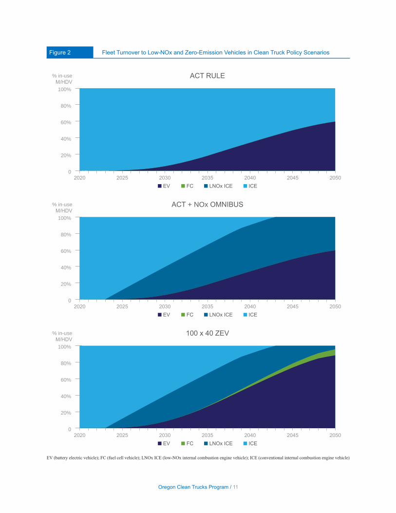
Figure 2 summarizes the modeled turnover of the Oregon in-use fleet to zero-emission and low-NOx trucks under the three Clean Truck policy scenarios. Fleet turnover to new trucks is based on historical average turnover rates and projected fleet growth rates, along with the new vehicle ZEV purchase percentages shown in Figure 1. Approximately 6.1 percent of existing Class 2b trucks and 4.7 percent of Class 3–8 trucks and buses are retired each year and replaced with new vehicles.10 The ACT + NOx Omnibus scenario and the 100 x 40 ZEV + Clean Grid scenario further assume that all new vehicles purchased in 2024 and later years that are not ZEV will have low-NOx engines compliant with the NOx Omnibus standards.
As shown, under the ACT Rule policy scenario, 34.0 percent of the in-use M/HD fleet will turn over to ZEV by 2040, and 59.6 percent are ZEV by 2050; all of these ZEVs are assumed to be electric vehicles. Under the ACT + NOx Omnibus policy scenario, the same percentage of the fleet turns over to ZEV, but the remaining internal combustion engine vehicles in the fleet turn over to low-NOx engines by 2044. Under the 100 x 40 ZEV + Clean Grid policy scenario, 52.7 percent of the in-use fleet turns over to ZEV by 2040 and 95.6 percent do so by 2050. This scenario assumes that new ZEVs will include both EV and fuel cell vehicles powered by hydrogen. In 2050, 7.3 percent of in-use ZEVs are assumed to be FCV and 88.4 percent are EV.
7 A very small percentage of these vehicles are large SUVs.8 Note that the ACT Rule does not include ZEV requirements for transit buses, as these vehicles are covered by a separate Innovative Clean Transit regulation in
California.9 These figures are based on state registration data collected by IHS Markit.10 This is a long-term average. Actual annual turnover is highly correlated to economic conditions and can vary widely from year to year.
Oregon Clean Trucks Program / 11
Figure 2 Fleet Turnover to Low-NOx and Zero-Emission Vehicles in Clean Truck Policy Scenarios
% in-useM/HDV
2020 2050204520402025 2030 2035
ACT RULE
■ EV ■ FC ■ LNOx ICE ■ ICE
0
20%
40%
60%
80%
100%
% in-useM/HDV
2020 2050204520402025 2030 2035
ACT + NOx OMNIBUS
■ EV ■ FC ■ LNOx ICE ■ ICE
0
20%
40%
60%
80%
100%
% in-useM/HDV
2020 2050204520402025 2030 2035
100 x 40 ZEV
■ EV ■ FC ■ LNOx ICE ■ ICE
0
20%
40%
60%
80%
100%
EV (battery electric vehicle); FC (fuel cell vehicle); LNOx ICE (low-NOx internal combustion engine vehicle); ICE (conventional internal combustion engine vehicle)

Oregon Clean Trucks Program / 12
Changes in Fleet Fuel UseUnder all modeled Clean Truck policy scenarios, a significant portion of the Oregon M/HD fleet is assumed to turn over to EV and FCV trucks and buses. This will result in replacement of petroleum fuels—primarily gasoline and diesel fuel—with electricity and hydrogen.11
Under the baseline scenario, total petroleum fuel use by the Oregon M/HD fleet in 2050 is projected to be 700 million gallons. Under the ACT Rule policy scenario, petroleum fuel use in 2050 falls to an estimated 340 million gallons (-51 percent), and cumulative reductions in diesel and gasoline use by the M/HD fleet total 4.5 billion gallons between 2020 and 2050. This petroleum fuel is replaced by 81.9 million megawatt-hours (MWh) of electricity between 2020 and 2050. Electricity use for M/HD EV charging in 2050 is estimated to be 7.1 million MWh, a 18 percent increase to estimated baseline electricity use by Oregon residential and commercial customers that year (39.1 million MWh).
Adding the NOx Omnibus Rule to the ACT Rule does not result in additional reductions in petroleum fuel use.
Under the 100 x 40 ZEV + Clean Grid scenario, estimated petroleum fuel use by the M/HD fleet in 2050 falls to 50 million gallons (-93 percent), and cumulative reductions in diesel and gasoline use by the M/HD fleet total 7.5 billion gallons between 2020 and 2050. This petroleum fuel is replaced by 121.7 million MWh of electricity and 1.1 billion kilograms of hydrogen between 2020 and 2050. Electricity use for M/HD EV charging in 2050 is estimated to be 10.8 million MWh, and 28 percent increase to estimated baseline electricity use by Oregon residential and commercial customers that year.
Public Health and the EnvironmentThe modeled Clean Trucks policy scenarios produce significant reductions in NOx, PM, and GHG emissions from the M/HD fleet, even after accounting for the emissions from producing the electricity and hydrogen needed to power ZEVs. NOx and PM reductions will improve local air quality, particularly in urban areas, resulting in public health benefits from reduced mortality and hospital visits. As noted earlier, low-income and disadvantaged communities are often disproportionately impacted by emissions from freight movement, due to the proximity of the transportation infrastructure to many of these communities.12
Air Quality ImpactsFigures 3 and 4 show estimated annual M/HD fleet NOx and PM emissions, respectively, under the baseline scenario and the modeled Clean Truck policy scenarios. Under the baseline scenario, annual M/HD fleet NOx emissions are projected to fall by 42 percent and annual fleet PM emissions are projected to fall 71 percent through 2045, as the current fleet turns over to new gasoline and diesel trucks with cleaner engines that meet more stringent EPA new engine emissions standards. After 2045 baseline annual NOx and PM emissions are then projected to start rising again as annual fleet VMT continues to grow.
11 A small number of M/HD trucks and buses in Oregon currently use natural gas.12 MJB&A, Newark Community Impacts.

Oregon Clean Trucks Program / 13
Figure 3 Projected M/HD Fleet NOx Emissions
MT
2020 2050204520402025 2030 2035
BaselineACTACT + NOx Omnibus100 x 40 ZEV + Clean Grid
0
5,000
10,000
15,000
20,000
25,000100 x40 XEV + Clean Grid
ACT + NOx OMN
ACT
Baseline
MT
2020 2050204520402025 2030 20350
100
200
300
400
500
600
700
800 100 x40 XEV + Clean Grid
ACT + NOx OMN
ACT
Baseline
BaselineACTACT + NOx Omnibus100 x 40 ZEV + Clean Grid
Figure 4 Projected M/HD Fleet PM Emissions

Oregon Clean Trucks Program / 14
Compared with the baseline, by 2050 the ACT rule is estimated to reduce annual fleet NOx and PM emissions by 49 percent and 50 percent, respectively, as diesel and gasoline trucks are replaced with electric vehicles. Adding the NOx Omnibus Rule will further reduce annual fleet NOx emissions due to turnover of the diesel and gasoline portion of the fleet to new vehicles with low-NOx engines; by 2050 annual NOx emissions are projected to be 89 percent lower than under the baseline if both the ACT and NOx Omnibus Rules are implemented.
The 100 x 40 ZEV + Clean Grid scenario has the lowest fleet emissions due to replacement of virtually all gasoline and diesel trucks and buses with EVs and FCVs by 2050, when annual NOx and PM emissions are estimated to be 97 percent and 87 percent lower, respectively, than baseline emissions.
Over the next 30 years, cumulative NOx and PM emission reductions from the ACT Rule (compared with the baseline scenario) total 84,000 metric tons (MT) and 1,290 MT, respectively. Additional cumulative NOx reductions from the NOx Omnibus Rule are estimated at 139,200 MT over the same time. Cumulative NOx and PM emission reductions from the 100 x 40 ZEV + Clean Grid scenario (compared with the baseline) are projected to total 234,700 MT and 2,100 MT, respectively.
Public Health BenefitsThe reduced annual NOx and PM emissions under the Clean Truck policy scenarios will reduce ambient particulate levels in the air, which will reduce the negative health effects on Oregon residents breathing in these airborne particles.13 Estimated public health impacts include reductions in premature mortality and fewer hospital admissions and emergency room visits for asthma. There will also be reduced cases of acute bronchitis, exacerbated asthma, and other respiratory symptoms, and fewer restricted activity days and lost workdays. Cumulative estimated reductions in these health outcomes in Oregon under the modeled Clean Truck policy scenarios are shown in Table 2; these benefits were estimated using the U.S. Environmental Protection Agency’s CO-Benefits Risk Assessment (COBRA) Health Impacts Screening and Mapping Tool. While this analysis did not apportion estimated public health benefits to specific communities within the state, they are expected to disproportionately accrue to those communities in close proximity to freight infrastructure, since these communities are disproportionately impacted by current emissions from M/HD truck traffic.
Table 2 Cumulative Public Health Benefits of Clean Truck Policy Scenarios, 2020–2050
Health Metric ACT Rule ACT + NOx Omnibus 100 x 40 ZEV + Clean Grid
Avoided Premature Deaths 79 156 186
Avoided Hospital Visitsa 63 118 144
Avoided Minor Casesb 43,411 83,579 100,647
Monetized Value, 2020$ (millions) $927 $1,820 $2,172
a Includes hospital admissions and emergency room visits.
b Includes reduced cases of acute bronchitis, exacerbated asthma, and other respiratory symptoms, and reduced restricted activity days and lost workdays.
13 PM is directly emitted to the atmosphere from combustion sources as solid particles. NOx is emitted from combustion sources as a gas but contributes to the formation of secondary particles via chemical reactions in the atmosphere. Both direct and secondary particles have negative health effects when taken into the lungs.

Oregon Clean Trucks Program / 15
The monetized value of cumulative public health benefits from the ACT Rule over the next 30 years totals more than $900 million. Adding the NOx Omnibus Rule would increase the monetized value of cumulative net public health benefits to $1.8 billion. The monetized value of cumulative public health benefits under the 100 x 40 ZEV + Clean Grid policy scenario totals $2.2 billion through 2050.
Climate BenefitsFigure 5 illustrates estimated annual M/HD fleet GHG emissions under the baseline scenario and the modeled Clean Truck policy scenarios. As shown, under the baseline scenario annual M/HD fleet GHG emissions are projected to fall by 11 percent through 2050 as the current fleet turns over to new, more efficient gasoline and diesel trucks that meet more stringent EPA new engine and vehicle emission standards.
Compared with the baseline, by 2050 the ACT rule is estimated to further reduce annual fleet GHG emissions by 49 percent, as diesel and gasoline trucks are replaced with electric vehicles; adding the NOx Omnibus Rule does not produce additional fleet GHG emissions beyond those achieved by the ACT Rule.
The 100 x 40 ZEV + Clean Grid scenario has the lowest fleet emissions due to replacement of virtually all gasoline and diesel trucks and buses with EV and FCV by 2050, when annual fleet GHG emissions are estimated to be 87 percent lower than baseline emissions.
Figure 5 Projected M/HD Fleet GHG Emissions
MT(million)
2020 2050204520402025 2030 20350
2
4
6
8
10100 x40 XEV + Clean Grid
ACT + NOx OMN
ACT
Baseline
BaselineACTACT + NOx Omnibus100 x 40 ZEV + Clean Grid
Over the next 30 years, cumulative GHG emission reductions from the ACT Rule (compared with the baseline scenario) total 49.7 million MT. Cumulative GHG emission reductions from the 100 x 40 ZEV + Clean Grid scenario (compared with the baseline) are projected to total 82.3 million MT. These estimates of GHG reductions from each policy scenario account for reductions in petroleum fuel use (gasoline, diesel fuel) by the M/HD fleet as well as increased emissions from electricity and hydrogen production to fuel the EVs and FCVs that will replace gasoline and diesel trucks and buses.

Oregon Clean Trucks Program / 16
Using the social cost of greenhouse gases as estimated by the federal government’s Interagency Working Group, these estimated cumulative GHG reductions have a monetized value of $8.1 billion for the ACT Rule policy scenario and $13.4 billion for the 100 x 40 ZEV + Clean Grid policy scenario.14 The social value of GHG reductions represents potential societal cost savings from avoiding the negative effects of climate change, if GHG emissions are reduced enough to keep long-term warming below 2 degrees Celsius from preindustrial levels.15
In July 2021, Oregon passed House Bill 2021 requiring retail electricity providers to aggressively reduce greenhouse gas emissions associated with electricity sold to Oregon customers. Emissions must be reduced to 80 percent by 2030, 90 percent by 2035, and 100 percent by 2040 relative to the average emissions from 2010, 2011, and 2012. The grid mix used for all scenarios in this analysis meets the requirements of the legislation. In 2020, the grid mix is 2.8 percent coal-fired generation, 16.6 percent natural gas–fired generation, and 80.6 percent renewable generation sources.16 The renewable portion of the grid mix increases to 94.5 percent by 2030 and 100 percent by 2040. The assumed Oregon grid mix for electricity production each year is shown in the Appendix.
Economic ImpactsThis section summarizes projected economic impacts of the modeled Clean Truck policy scenarios, including changes in annual operating costs for Oregon fleets; impacts to Oregon electric utilities and their customers; net societal benefits; and macroeconomic effects on jobs, wages, and gross domestic product from the transition to low-NOx and zero-emission trucks and buses. This section also estimates the required public and private investment in electric vehicle charging infrastructure to support the electric M/HD fleet under each scenario.
Costs and Benefits to FleetsFor all the modeled Clean Truck policy scenarios, this analysis estimated annual incremental costs associated with purchase and use of M/HD ZEVs compared with baseline conventional vehicles with combustion engines that operate on petroleum fuels (gasoline, diesel). These costs include the incremental purchase cost of the new ZEVs added each year (instead of new combustion vehicles), the cost of installing the charging and hydrogen fueling infrastructure required by these new ZEVs, and net fuel and maintenance costs for all ZEVs in the fleet, both those newly purchased each year and those purchased in prior years and still in use.
Net fuel costs include reductions in purchases of diesel fuel and gasoline (due to fewer combustion vehicles), offset by the increased purchase of electricity and hydrogen to power ZEVs. Net maintenance costs include net savings in annual vehicle maintenance for the ZEVs in the fleet compared with combustion vehicles, offset by annual costs to maintain the charging and hydrogen fueling infrastructure needed to support in-use ZEVs.
14 For the social cost values used, see MJB&A, Clean Trucks Analysis: Costs & Benefits of State-Level Policies to Require No- and Low-Emission Trucks, Technical Report—Methodologies & Assumptions, May 2021, https://mjbradley.com/clean-trucks-analysis.
15 The Interagency Working Group developed GHG social cost estimates using a range of discount rates. These values are based on the 95th percentile results using a 3 percent discount rate, which is in the middle of the range of estimated values. The monetized value of cumulative GHG reductions under each policy scenario would be 72 percent lower if using the lowest published social cost values, and three times greater if using the highest published values.
16 For this analysis, coal-fired generation includes oil and biomass. Zero-emitting sources include nuclear and renewable sources such as wind, solar, and hydropower.

Oregon Clean Trucks Program / 17
■ Charger Maintenance
■ Chargers
■ Incremental Vehicle Purchase
■ Net Fuel Cost
■ Incremental Vehicle Maintenance
Net Life Cycle Costs
2020$/Vehicle
$80,000
$60,000
$40,000
$20,000
0
-$20,000
-$40,000
-$60,000
-$80,000
-$100,000 MY2025 MY2030 MY2035 MY2040
Figure 6 Projected Lifetime Incremental Costs for Oregon ZEVs Compared With Combustion Vehicles
Figure 6 shows projected average lifetime incremental costs for new ZEVs purchased in Oregon compared with lifetime costs for combustion vehicles purchased in the same model year; the bars show fleet average values for all Class 2b–8 ZEVs purchased each year under the 100 x 40 ZEV scenario. Incremental fuel and maintenance costs are discounted lifetime costs, assuming 21-year vehicle life, and 6 percent annual discount rate. Vehicle financing, which is often used by fleets when purchasing vehicles, was not considered in this analysis.
As shown, the average M/HD ZEV in Oregon is projected to produce over $76,000 in discounted fuel and maintenance cost savings over its lifetime. For ZEVs purchased in the very near term, this savings may not be enough to offset the projected incremental cost of vehicle purchase and fueling infrastructure for some ZEVs, resulting in net increased lifetime costs compared with those of combustion vehicles. However, by 2030 incremental ZEV purchase costs are projected to fall significantly, such that the average ZEV will reach lifetime cost parity with combustion vehicles, when discounted lifetime fuel and maintenance savings are considered. By 2040, the average ZEV purchased that year is projected to produce almost $60,000 in discounted lifetime net savings (2020$) compared with the costs of an equivalent combustion vehicle.

Oregon Clean Trucks Program / 18
It is important to reiterate that the values in Figure 6 are fleet average values, which mask a significant amount of variability across vehicle types and among different fleets of the same vehicle type. Also note that the utility impact analysis (in the next section) indicates that the cost of providing power to charge M/HD EVs is lower than expected utility revenue under current rate structures. This suggests that Oregon could consider changes to rates that would not only be fairer for fleets, but also lower electricity costs for M/HD EV charging, thus reducing net fleet operating costs further than estimated here. However, this would reduce the potential benefits that would accrue to other ratepayers from M/HD vehicle charging (see discussion below).
M/HD ZEVs in some fleets will likely achieve lifetime cost parity with combustion vehicles much earlier than 2030, while others may lag. In addition, this analysis, and the values shown in Figure 6, assume no government incentives for vehicle purchase or development of fueling infrastructure. If existing and potential incentives are considered, or policies such as improved electricity rates for fleets, then actual net costs to fleets will be lower, resulting in cost parity sooner.
Electric Utility ImpactsCurrent annual electricity sales to residential and commercial customers in Oregon total 34.7 million MWh and are projected to grow to 39.1 million MWh in 2050.17
Under the ACT Rule policy scenario, additional annual electricity sales for M/HD EV charging are estimated to total 0.63 million MWh in 2030, rising to 7.11 million MWh in 2050. This incremental load represents 1.7 percent and 19.4 percent of the total electricity demand in 2030 and 2050, respectively. Incremental monthly peak charging demand under this scenario is estimated at 135 MW in 2030, rising to 1,790 MW in 2050.
Under the 100 x 40 ZEV policy scenario, incremental peak charging demand is estimated at 205 MW in 2030, rising to 2,600 MW in 2050, and annual incremental electricity sales are estimated to be 0.90 million MWh in 2030, rising to 10.8 million MWh in 2050 (2.4 percent and 27.5 percent of the total electricity demand, respectively).
This analysis estimated the revenue that Oregon electric utilities would receive from these incremental electricity sales, the marginal generation and transmission costs of providing this power, and the net revenue that utilities would earn (net revenue = revenue – marginal cost). The estimated marginal cost includes costs associated with procuring the necessary additional peak generation and transmission capacity to serve the load ($/MW) as well as marginal generation and transmission energy costs ($/MWh).
Figure 7 summarizes estimated annual utility net revenue from M/HD EV charging under the modeled Clean Truck policy scenarios. Under the ACT Rule scenario, annual utility net revenue is projected to be $14.4 million in 2030, rising to $78.9 million in 2040 and $127.6 million in 2050. Under the 100 x 40 ZEV scenario, utility net revenue is projected to be $21.7 million in 2030, rising to $115.6 million in 2040 and $202.1 million in 2050.
17 This growth assumption is from the EIA 2021 Annual Energy Outlook. It does not include sales to large industrial customers.

Oregon Clean Trucks Program / 19
2020$Million
0
50
100
150
200
250
20502045204020352030
■ ACT
■ ACT + NOx Omnibus
■ 100 x 40 ZEV + Clean Grid
Figure 7 Projected Annual Utility Net Revenue From M/HD EV Charging
In general, a utility’s costs to maintain its distribution infrastructure increase each year with inflation, and these costs are passed on to utility customers in accordance with rules established by the Oregon Public Utility Commission via periodic increases in residential and commercial electric rates. However, projected utility net revenue from increased electricity sales for M/HD EV charging would lower distribution rates ($/kWh), since fixed annual distribution system costs would be spread over a larger base of energy sales.
This analysis indicates that under the 100 x 40 ZEV scenario, by 2050 incremental utility net revenue from M/HD EV charging could potentially reduce average residential and commercial electricity rates in Oregon by as much as 3.7 percent ($0.0101/kWh in 2020$). This could save the average Oregon household $110 per year and the average commercial customer $650 per year on their electricity bills (2020$).18
Jobs, Wages, and GDPThe transition from gasoline and diesel M/HD vehicles to ZEVs will have significant impacts on the U.S. economy, with substantial job gains in many industries (e.g., battery and electric component manufacturing, charging infrastructure construction, electricity generation), accompanied by fewer jobs in other industries (e.g., engine manufacturing, oil exploration and refining, gas stations, auto repair shops).19
This analysis used the IMPLAN model to estimate these macroeconomic effects of the modeled Oregon Clean Truck policy scenarios based on estimated changes in spending in various industries (relative to the baseline scenario). These estimates of spending changes by industry were developed from the fleet cost analysis. For example, under the modeled Clean Truck policy scenarios, more money will be spent to manufacture batteries and electric drive components for ZEVs, but less will be spent to manufacture gasoline and diesel engines, and transmissions. Similarly, less money will be spent by fleets to purchase petroleum fuels, but more will be spent to purchase electricity and hydrogen.
18 Figures are based on average annual electricity use of 10,940 kWh per housing unit and 64,340 kWh per commercial customer in Oregon. 19 For example, in-state charging infrastructure is estimated to increase by 626 jobs in 2045 under the most aggressive scenario.

Oregon Clean Trucks Program / 20
The IMPLAN analysis also includes the effects of induced economic activity due to consumers having more money to spend, thanks to return of utility net revenue in the form of lower electric rates, and net fleet cost savings returned as lower shipping costs for goods, resulting in lower consumer prices for those goods.
The IMPLAN analysis was run at the national level, but assuming only the industry spending changes (from application of the policy scenarios) occurring due to M/HD vehicle purchase and use in Oregon. Estimated national effects would be significantly greater if the modeled policy scenarios were applied to the entire U.S. M/HD fleet.
Table 3 offers a summary of estimated macroeconomic effects of the modeled Clean Truck scenarios on jobs, GDP, and wages.
Compared with the baseline scenario, adoption of the ACT + NOx Omnibus policy scenario in Oregon will increase national net jobs through 2040, while the 100 x 40 ZEV + Clean Grid scenario will increase national net jobs through at least 2045. The loss in 2045 is largely due to the reductions in spending on diesel fuel and decreases in the costs of M/HDV ZEVs over time, resulting in decreased spending and investments in the out years. Both scenarios also increase annual GDP in all years. For both scenarios in all years, the average wages for new jobs added to the economy 85 percent higher than the average wages for jobs that are replaced. This is because the largest number of added jobs are in electrical component manufacturing and in construction of charging infrastructure, requiring many well-paid electricians and electrical engineers, while the largest job losses are in vehicle repair—due to lower maintenance required by ZEVs—as well as relatively low-paid retail workers at gas stations.
Table 3 Macroeconomic Effects of Oregon Clean Truck Policy Scenarios
MetricACT + NOx Omnibus 100 x 40 ZEV + Clean Grid
2035 2045 2035 2045
Net Change in Jobs 777 (158) 981 (688)
Net Change in GDP 2020$ (million) $79 ($59) $101 ($159)
Average Annual Compensation
Added Jobs $84,970 $78,904 $85,272 $79,054
Replaced Jobs $45,585 $49,311 $45,959 $49,932
Today many components used in electric and fuel cell vehicles—most notably batteries, but also many electric drivetrain components—are manufactured outside the United States and imported for final vehicle assembly. The percentage of imported content is higher for ZEV drivetrains today than for conventional drivetrains (gasoline and diesel engines, and transmissions). The scale of U.S. macroeconomic effects from the modeled Clean Truck policy scenarios will depend on how the nascent M/HD ZEV industry develops; for this analysis, MJB&A assumed that all incremental spending on ZEV batteries and electric drivetrain components would be in the United States, with no imported content. As such, the results summarized in Table 3 represent a high-end estimate of what is possible from the ZEV transition, with the right federal and state policy supports in place to incentivize development of U.S.-based ZEV component manufacturing. If vehicle manufacturers continue to rely primarily on imported batteries and electric drivetrain components, the net job and GDP gains will be lower than those summarized here.

Oregon Clean Trucks Program / 21
This macroeconomic analysis only includes direct, indirect, and induced impacts from changes in M/HD vehicle manufacturing and use, and from consumer re-spending of net utility revenue and fleet cost savings returned as lower prices for electricity and shipped goods. It does not include any effects on freight industry growth and investment due to lower operating costs, or any macroeconomic effects associated with the estimated climate and air quality (health) benefits of the modeled Clean Truck policy scenarios.
Required Public and Private InvestmentsOn the basis of a detailed charging model that considers typical daily usage patterns for different vehicle types, this analysis assumes that most M/HD ZEVs in Oregon will use overnight charging at their place of business, though about 10 percent will need to rely on a publicly accessible network of higher-power chargers.20 The exception are combination trucks, 70 percent of which are assumed to require high-power public chargers since they are used primarily for long-haul freight operations.
Table 4 summarizes estimated charging infrastructure required to support M/HD electric trucks and buses under the Clean Truck policy scenarios.
Table 4 Projected Charging Infrastructure Required for Clean Truck Policy Scenarios
MetricACT Rule 100 x 40 ZEV
2035 2045 2050 2035 2045 2050
Cumulative Charge Ports
57,980 172,433 217,107 86,940 274,458 338,851 338,851
815 2,414 3,061 1,196 3,709 4,661 4,661
634 1,694 2,146 930 3,426 4,697 4,697
Cumulative Investment, 2020$ (million)
$337 $952 $1,273 $506 $1,557 $2,124 $2,124
$256 $673 $896 $374 $1,259 $1,761 $1,761
Depot chargers will need to be 10–50 kW per port depending on vehicle type. The smaller 150 kW public chargers are needed primarily to support single-unit freight trucks, while the higher-capacity 500 kW public chargers are needed mostly for combination trucks.
As of June 2021, there were 163 publicly accessible charging stations in the state of Oregon with a total of 407 direct current fast-charging (DCFC) ports (>50 kW).21 Almost 40 percent of these DCFC ports are Tesla superchargers that can be used only by Tesla owners. Statewide, there are only 248 DCFC ports fully available to any vehicle.
Under the ACT Rule policy scenario, Oregon’s fleet owners will have to invest an average of $51 million per year (2020$) between 2025 and 2050 to purchase and install depot-based charging infrastructure. The government and private investors will need to invest an average of $36 million per year over the same time period to build out a publicly accessible charging network across the state to serve the EV M/HD truck fleet.
20 See the methodology report for a detailed discussion of M/HD EV charging needs.21 These numbers are from the U.S. Department of Energy’s Alternative Fuel Data Center public charger database.

Oregon Clean Trucks Program / 22
Under the 100 x 40 ZEV scenario, fleet investments in depot charging infrastructure from 2025 to 2050 will need to increase to an average of $85 million per year, and public and private investments in the public charging network will need to rise to an average of $70 million per year.
Net Societal BenefitsThe net societal benefits from the modeled Oregon Clean Truck policy scenarios include the monetized value of public health and climate benefits, net cost savings for fleets, and net utility revenue from electricity sales for EV charging.
Figures 8–10 present projected annual net societal benefits under the ACT Rule, ACT + NOx Omnibus Rule, and 100 x 40 ZEV + Clean Grid scenarios, respectively. Under all three Clean Truck policy scenarios, near-term fleet costs are higher than fleet costs under the baseline.22 However, after approximately 2030 all policy scenarios show annual net societal benefits, despite net fleet costs, due to growing utility net revenue in addition to public health and climate benefits. After approximately 2035 there is an annual net savings in fleet costs from operating ZEVs instead of diesel and gasoline trucks, and net societal benefits grow quickly.23
Figure 8 Projected Annual Net Societal Benefits From ACT Rule Policy Scenario
22 If an individual truck owner finances a vehicle, it would better equalize payments for increased vehicle price and fuel savings, resulting in a better balancing of cash flow. On a net fleet-wide basis, however, the cost of financing reduces total net fleet savings.
23 Note that fleet-wide annual net savings under the Clean Truck policy scenarios lag average ZEV life-cycle cost parity to combustion vehicles by about 5 years. This is because even after life-cycle cost parity is achieved, most ZEVs will still have higher up-front purchase costs (vehicle plus charger) than combustion vehicles; these higher costs are then paid back over the next few years via fuel and maintenance cost savings.
■ Air Quality Benefits
■ Climate Benefits
■ Utility Net Revenue
■ Net Incremental Fleet Costs
Net Societal Benefits
2020$Millions
$2,500
$2,000
$1,500
$1,000
$500
0
-$5002050204520402025 2030 2035

Oregon Clean Trucks Program / 23
Figure 9 Projected Annual Net Societal Benefits From ACT + NOx Omnibus Policy Scenario
■ Air Quality Benefits
■ Climate Benefits
■ Utility Net Revenue
■ Net Incremental Fleet Costs
Net Societal Benefits
2020$Millions
$2,500
$2,000
$1,500
$1,000
$500
0
-$5002050204520402025 2030 2035
■ Air Quality Benefits
■ Climate Benefits
■ Utility Net Revenue
■ Net Incremental Fleet Costs
Net Societal Benefits
2020$Millions
$4,000
$3,500
$3,000
$2,500
$2,000
$1,500
$1,000
$500
0
-$5002050204520402025 2030 2035
Figure 10 Projected Annual Net Societal Benefits From 100 x 40 ZEV + Clean Grid Policy Scenario

Oregon Clean Trucks Program / 24
Under the ACT Rule scenario, by 2050 annual net societal benefits are estimated to be $2.1 billion, including $1.1 billion in net fleet savings and $128 million in utility net revenue. Cumulative estimated societal net benefits under this scenario total $5.1 billion between 2020 and 2050.
Under the ACT + NOx Omnibus scenario, by 2050 annual net societal benefits are estimated to be $2.1 billion, including $1.0 billion in net fleet savings and $128 million in utility net revenue. Cumulative estimated societal net benefits under this scenario total $5.1 billion between 2020 and 2050.
Under the 100 x 40 ZEV + Clean Grid scenario, by 2050 annual net societal benefits are estimated to be $3.6 billion, including $1.9 billion in net fleet savings and $202 million in utility net revenue. Cumulative estimated societal net benefits under this scenario total $8.6 billion between 2020 and 2050.

Oregon Clean Trucks Program / 25
APPENDIX Oregon Grid and Energy Cost Assumptions
Figure A1 Oregon Business as Usual Grid Mix Assumptions
These grid mix assumptions were applied to all of the scenarios in this analysis. The grid mix meets the requirements set by the Oregon House Bill 2021.
Figure A2 Oregon Average Fuel Costs
2020 2050204520402025 2030 2035
■ Zero-Emitting ■ Natural Gas ■ Coal
0.0
0.2
0.4
0.6
0.8
1.0
1.2
0
20%
40%
60%
80%
100%
2020 2050204520402025 2030 20350
$1.00
$2.00
$3.00
$4.00
$5.00Hydrogen
Electricity
Diesel
GasolineGasoline 2020$/galDiesel 2020$/galElectricity 2020$/kWh x 10Hydrogen 2020$/kg
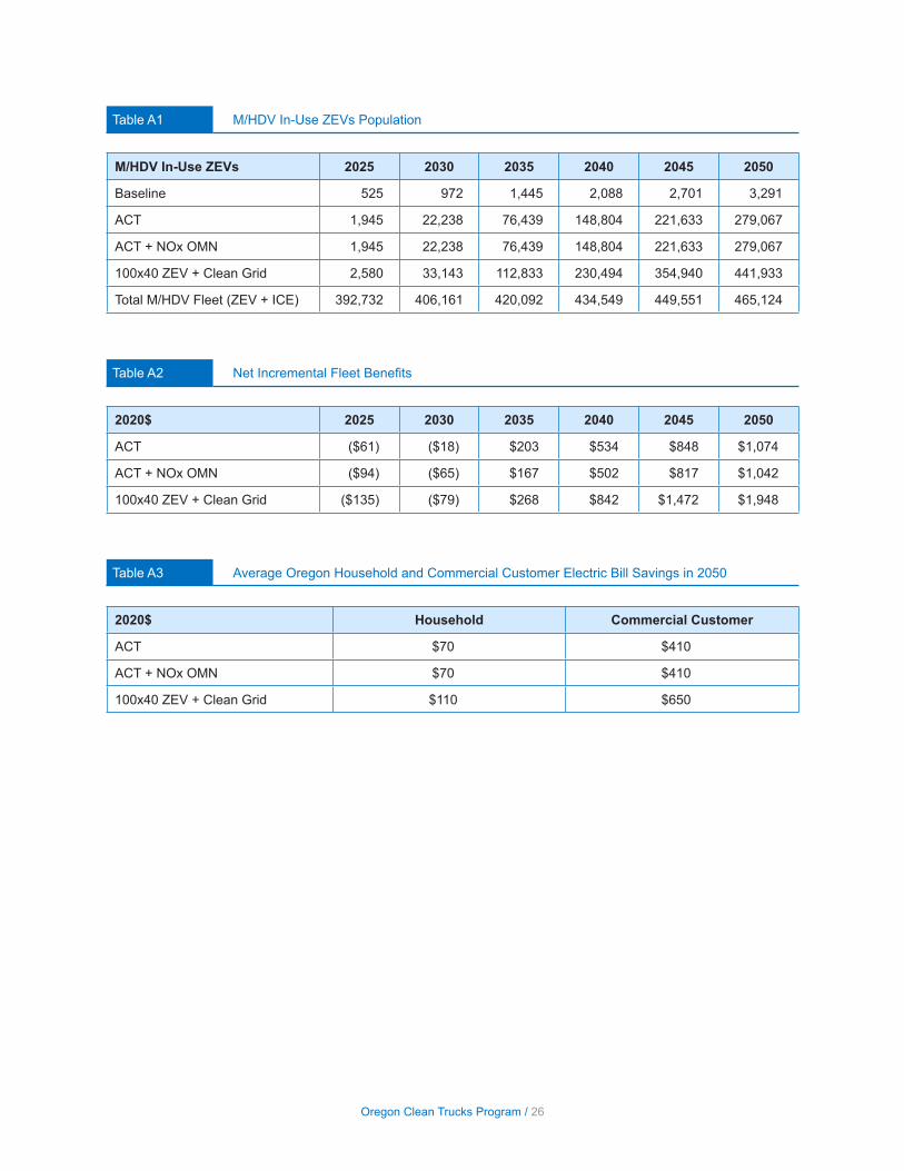
Oregon Clean Trucks Program / 26
Table A1 M/HDV In-Use ZEVs Population
M/HDV In-Use ZEVs 2025 2030 2035 2040 2045 2050
Baseline 525 972 1,445 2,088 2,701 3,291
ACT 1,945 22,238 76,439 148,804 221,633 279,067
ACT + NOx OMN 1,945 22,238 76,439 148,804 221,633 279,067
100x40 ZEV + Clean Grid 2,580 33,143 112,833 230,494 354,940 441,933
Total M/HDV Fleet (ZEV + ICE) 392,732 406,161 420,092 434,549 449,551 465,124
Table A2 Net Incremental Fleet Benefits
2020$ 2025 2030 2035 2040 2045 2050
ACT ($61) ($18) $203 $534 $848 $1,074
ACT + NOx OMN ($94) ($65) $167 $502 $817 $1,042
100x40 ZEV + Clean Grid ($135) ($79) $268 $842 $1,472 $1,948
Table A3 Average Oregon Household and Commercial Customer Electric Bill Savings in 2050
2020$ Household Commercial Customer
ACT $70 $410
ACT + NOx OMN $70 $410
100x40 ZEV + Clean Grid $110 $650

Dear Department of Environmental Quality Staff,
The undersigned entities appreciate the opportunity to show our support for the adoption of both the AdvancedClean Truck (ACT) rule and Low-NOx Omnibus rule this year in Oregon. Below you will find general commentsin support of the Clean Truck Rules as well as answers to questions and concerns posed at the firstRulemaking Advisory Committee on July 12th, 2021:
Securing Oregon’s swift and orderly transition to an electric truck future while slashing diesel truck pollution is apublic health, equity, and climate imperative that can grow the economy and lead to quality jobs. The ACT andLow-NOx rules are powerful and complementary tools that must be adopted together to curb toxic dieselpollution and jumpstart the zero-emission medium- and heavy-duty (MHD) truck market. To improve thepublic health of Oregonians, ensure Oregon achieves its greenhouse gas reduction targets in thetransportation sector and mitigate extreme weather events fueled by climate change (heatwaves,climate fires, floods), DEQ should do everything in its power to ensure prompt adoption of California’sACT rule and Low-NOx Omnibus rule.
Ensure all Oregonians have the right to breathe clean air.● Toxic diesel pollution is linked to higher rates of cancer, heart disease, respiratory disorders and
premature death. This pollution disproportionately harms low-income and Black, Indigenous,and people of color (BIPOC) communities, who often live adjacent to highways, ports and otherpollution hot spots due to racist housing, land use and economic policies.
● Every year, in Oregon alone, diesel engine exhaust is responsible for an estimated 176premature deaths, 25,910 lost work days and annual costs from exposure of $3.5 billion.
● Workers routinely exposed to diesel exhaust have a greater risk of lung cancer and otherillnesses due to breathing polluted air (this accounts for 29,000 Oregonians in the workforce)
Get Oregon on track to meet its climate targets.● Climate pollution from Oregon’s transportation sources have been increasing year after year,
with Oregon’s transportation sector now comprising over 40 percent of our state’s total globalwarming pollution.
● Although heavy duty vehicles comprise 10 percent of all vehicles on the road in the US, theyaccount for nearly 25 percent of total U.S. climate pollution from transportation, and 45 percentof NOx emissions.
● Cleaning up the MHD sector is also necessary to meet the Governor’s greenhouse gas (GHG)reduction targets set in the Oregon Climate Action Plan (Executive Order 20-04) and the MHDMOU.
● Climate change fueled extreme weather events are already affecting and taking the lives ofOregonians in the form of extreme heatwaves, mega fires and floods. Scientists say that theseextreme weather events are “boosted” by human-caused global warming. This exemplifies theimmediate need of government entities to swiftly transition us out of the fossil fuel era.
Achieve an equitable and just transition to support quality jobs and grow the economy.● According to estimates in California, savings realized by fleet owners and consumers who
choose electric options will be largely reinvested and directed toward local, labor-intensive

services, providing a boost to regional economies. Furthermore, the process of building outcharging infrastructure is likely to support high-quality jobs—that should include skills trainingand good wages and benefits—and boost the state’s economy. The ACT rule is estimated toproduce around 8,000 net new jobs by 2040 in California.
Responses to questions posed at the RAC on July 12th, 2021:
● Allowing Manufacturers to begin earning credits prior to 2025 MY:○ The purpose of early credits is to get more zero-emission vehicles (ZEVs) on Oregon’s
roads sooner. However, truck manufacturers are unlikely to sell more ZEVs for earlycredits and instead will end up receiving credits for actions already planned, creating abigger credit pool and diluting the rule’s ZEV sales requirements. If Oregon does offerearly credits, it should be limited to one year (MY 2024), similar to New Jersey’sproposal.
○ The Clean Air Act requires that states' adoption of California’s emission standards mustbe identical for each model year. Nothing in the Clean Air Act prevents Oregon fromadjusting the years when manufacturers can begin to earn their credits and modifyingthe fleet reporting requirement, since these components of the ACT rule do not meet thedefinitions of having to be identical to California. This aligns with a Section 177 state’senforcement discretion. Further, the identicality provision's purpose is to prevent thecreation of a "third vehicle." Therefore, the focus should be on whether a provisionpermits a third vehicle rather than whether it is word-for-word identical.
● Fleet Reporting Requirement:○ This requirement can shed light on trucking labor practices and possibly lead to more
equitable outcomes for truck drivers, where misclassification is rampant andfamily-sustaining wages remain elusive. Adopting the rule could turn a historicallypolluting industry into a source of high quality, green jobs in trucking, manufacturing, andcharging infrastructure installation.
○ The collected data will also help identify areas with high rates of freight traffic and,consequently, diesel pollution, allowing Oregon to target clean transportation policies tothe communities that need relief most.
○ Utilities need this data to make informed electric utility investments today to install thecharging infrastructure necessary to support pollution-free vehicles.
○ While the current fleet reporting threshold requirement is set at 50, it is based onCalifornia’s much larger trucking fleet and is too high for Oregon. Based on datacollected by the Oregon Department of Transportation, only 1.6% of the medium- andheavy-duty carriers have 51 or more vehicles in their fleet and would be responsible forreporting. Lowering the vehicle threshold would allow for the state to capture accuratedata that will help scale the adoption of zero-emission vehicles. While the overwhelmingmajority of fleets contain 5 vehicles or fewer (82.3% of fleets), that granularity ofreporting may prove prohibitive for DEQ. Therefore the reporting threshold should be setat 5 or more vehicles to cover nearly 20% of Oregon’s fleets.
● Exempting transit agencies or manufacturers/dealerships and should the exemption bepermanent and/or yearly reporting requirements:

○ Transit is a major source of pollution, particularly at the local level. Moreover, the lowspeeds and stop-and-go nature of transit routes make them perfect for electrification.California exempted transit agencies because of an existing standard, the InnovativeClean Transit (ICT) rule, requiring an increasing number of new bus purchases bezero-emission beginning in 2023 and reaching 100% by 2029. To best address theneeds and objectives of Oregon, DEQ should consider adopting the ICT rule alongsidethe ACT and Low NOx Omnibus rules.
Responses to concerns posed at the RAC on July 12th, 2021:
● Total Cost of Ownership:○ Today, on a total cost of ownership basis and without incentives, certain zero-emission
trucks are cost-competitive if not less expensive than their fossil fuel equivalents. Mostclasses of vehicles are expected to achieve total cost of ownership parity by 2030.
■ In many cases, these savings will compensate for higher up-front vehicle costs. Itis important to remember that upfront vehicle costs will continue to fall as batteryprices decline. According to Bloomberg New Energy Finance, battery costs havedecreased by 89 percent over the past ten years and continue to drop.Additionally, electric trucks’ residual values are expected to be higher than useddiesel trucks because a purchaser will receive a more reliable truck with muchlower fuel and maintenance costs.
○ DEQ can also explore federal funding opportunities in the next couple of years leadingup to the beginning of implementation (2025), to incentivize electric truck adoption andpush for equitable solutions that assist small businesses in the transition and phase outof dirty diesel engines.
■ An example that DEQ can explore to lessen total cost burden on small Oregonianbusinesses and organizations is New Jersey’s recently launched, New JerseyZero Emission Incentive Program. NJ ZIP is a $15 million dollar pilot programthat will fund 100 to 300 vouchers ranging in value from $25,000 to $100,000 tobusinesses and institutional organizations for the purchase of new medium-dutyZEVs.
● Delaying Rule Adoption:○ DEQ should seek to adopt the ACT rule this year and should reject invitations to delay
adoption. Under Section 177 of the Clean Air Act, states must “adopt such standards atleast two years before commencement of such model year (as determined byregulations of the Administrator).” Under EPA regulations, the “model year” can extendas far back as January 2 of the prior year. Therefore, Model Year 2025 can start as earlyas January 2, 2024, and if DEQ wants the rules to apply for Model Year 2025, it mustadopt the California rules before January 2, 2022. Waiting to adopt the ACT post-2021,means Oregon will lose an additional year(s) of needed compliance, therefore missingout on critical time to accelerate ZEV adoption and reduce greenhouse gas emissionsand toxic pollutants.
Thank you for your leadership and consideration of our comments.

Sincerely,
Victoria PaykarOregon Transportation Policy ManagerClimate Solutions
Amy SchlusserStaff AttorneyGreen Energy Institute at Lewis & Clark Law School
Patricio PortilloTransportation AnalystNatural Resources Defense Council
Mary PevetoExecutive DirectorNeighbors for Clean Air
Sara WrightTransportation Program DirectorOregon Environmental Council
Brad ReedCampaign ManagerRenew Oregon
Hieu LeCampaign RepresentativeSierra Club
Sergio LopezEnergy, Climate and Transportation CoordinatorVerde
And members of the Clean Air, HealthyCommunities Coalition

A Non Governmental Organization in Special Consultative Status with the Economic and Social Council of the United Nations
333 West Wacker Drive, Suite 810 Chicago, Illinois, 60606
Phone/Fax: (312) 929-1970 www.truckandenginemanufacturers.org
August 16, 2021
VIA EMAIL Rachel Sakata ([email protected]) Eric Feely ([email protected]) State of Oregon Department of Environmental Quality 700 NE Multnomah Street, Suite 600 Portland, Oregon 97232
RE: Oregon DEQ’s Proposed Adoption of CARB’s ACT and Omnibus Low-NOx Rules
Dear Rachel and Eric:
The Truck and Engine Manufacturers Association (EMA) appreciates the opportunity to submit additional initial comments regarding the Department of Environmental Quality’s (DEQ’s) proposed rulemakings to accelerate the deployment of medium-duty (MD) and heavy-duty (HD) zero-emission vehicles (ZEVs). These initial comments are a follow-up to EMA’s prior comments, including those submitted through the Advisory Committee process. As we have explained on several occasions, while EMA fully supports the DEQ’s push toward ZEV trucks, we strongly oppose the proposed opt-ins to the California Air Resources Board’s (CARB’s) Advanced Clean Trucks (ACT) Regulation, as well as CARB’s Omnibus Low-NOx Regulations, as the means to reach that shared objective. Of note, EMA was actively engaged in the rulemaking process for both of those CARB regulations.
EMA represents the world’s leading manufacturers of MD and HD on-highway trucks and engines. EMA member companies design and manufacture highly-customized vehicles to perform a wide variety of commercial functions, including interstate trucking, regional freight shipping, local parcel pickup and delivery, refuse hauling, and construction – to name a few. EMA member companies are investing billions of dollars to develop MD and HD ZEVs, and fully support expanding the market in Oregon for those zero-emission vehicles. EMA and its members agree that ZEVs are and need to be the future of the commercial trucking industry. However, as detailed below, state-specific opt-ins to programs designed to meet California’s unique air quality needs and economic capabilities are not well-suited to the shared goal of accelerating the deployment of ZEV trucks in Oregon and elsewhere across the country.
i) Oregon has another year to consider opting-in to CARB’s Rules
As an initial matter, the DEQ should recognize that it has until the end of 2022 to takeaction on the proposed opt-in to CARB’s ACT Rule without violating the Clean Air Act’s (CAA) two-year opt-in leadtime requirement in advance of the anticipated 2025 model year effective date. The fact that the DEQ has another full year to consider this matter stems from how the definition of “model year” applies in the context of the ACT Rule. Under the ACT Rule,

State of Oregon Department of Environmental Quality August 16, 2021 Page 2
the term “model year” equates with calendar year. As a result, Oregon can defer acting on the pending opt-in initiative until next year and will still have two full “model years” (i.e., calendar years) in advance of an effective date in 2025, and so will still be in compliance with the two-year opt-in lead-time provision of subsection (1) of CAA section 177. The most relevant definition of “model year” is found in the ACT Rule itself. Specifically, the ACT Rule (see CCR Title 13 section 1963 (c)(15)) references a provision of CARB’s “Phase 2” greenhouse gas (GHG) regulations as providing the applicable definition of “model year.” That provision (CCR Title 17 section 95662(a)(16)) defines model year, as follows:
“Model year” means one of the following for compliance with this subarticle. Note that manufacturers may have other model year designations for the same vehicle for compliance with other requirements or purposes:
(A) For tractors and vocational vehicles [which can include Class 2b-3 vehicles] with a date of manufacture on or after January 1, 2021, the vehicle’s model year is the calendar year corresponding to the date of manufacture; (emphasis added).
This directly applicable definition makes it clear that even though the term “model year” may have different applications for compliance with other regulatory requirements or purposes, as it relates to the ACT Rule, the term “model year” equates with calendar year. Accordingly, if Oregon is looking to implement the ACT Rule starting in the 2025 “model year,” that implementation will, by definition, apply to tractors and vocational vehicles (which can include Class 2b-3 vehicles) manufactured in the 2025 calendar year. Given that, so long as Oregon adopts the ACT Rule before the end of the 2022 calendar year, it will provide the requisite two-years leadtime before the start of the 2025 calendar year.
The applicable and controlling federal definition of “model year” leads to the same conclusion. The relevant EPA definition of “model year” is found in EPA’s Phase 2 greenhouse gas (GHG) regulations. Under the Agency’s Phase 2 regulations, “model year” means:
(i) For tractors and vocational vehicles [which can include Class 2b-3 vehicles] with a date of manufacture on or after January 1, 2021, the vehicle’s model year is the calendar year corresponding to the date of manufacture. (40 C.F.R. §1037.801(i); emphasis added.)
This federal regulation matches the directly applicable CARB ACT regulation, and again makes it clear that model years and calendar years are the same for these purposes. This conclusion is further reinforced by the manner in which the ACT Rule phases-in. Under the ACT Rule, a HDOH vehicle manufacturer’s obligation to produce and sell a certain percentage of ZEV trucks in a given model/calendar year is based on the number of

State of Oregon Department of Environmental Quality August 16, 2021 Page 3
conventionally-fueled trucks that a manufacturer sells in that same calendar year. In that regard, sections 1963.1(a) and 1963.1(a) of the ACT Rule provide that:
[A] manufacturer shall annually incur deficits based on the manufacturer’s annual sales volumes of on-road vehicles produced and delivered for sale in California. Deficits are incurred when the on-road vehicle is sold to the ultimate purchaser in California…
[A] manufacturer must retire a number of ZEV or NZEV credits that equals or exceeds their total annual deficits each model year … (emphasis added).
Under these operative provisions of the ACT Rule, and by way of example, vehicles
manufactured before the 2025 model year would not factor-in to the calculation of the ACT Rule’s ZEV-truck percentage-sales requirements for the 2025 model year, since those requirements would be based on manufactures’ annual vehicle sales in 2025, not before. In fact, that percentage-sales requirement could not be fully calculated until the end of the 2025 calendar year (again, not before) when a manufacturer’s total annual sales of conventionally-fueled trucks could be calculated.
Thus, it is clear from the operative definitions, and from the manner in which the ACT
Rule phases-in, that model year and calendar year are synonymous as it relates to the implementation of the ACT Rule. Consequently, it is equally clear that Oregon can wait until the end of the 2022 calendar year and still provide two full years of lead-time before implementing the ACT Rule in the 2025 “model year.” Additional CAA leadtime issues will impact any allowable implementation dates, but those issues are discussed further below.
There are other important reasons to defer acting on the proposed opt-in to the ACT Rule.
More specifically, CARB has announced its intent to substantially revise the ACT rule in the summer of 2022 to double the Rule’s ZEV-truck requirements to a 100% ZEV-truck sales mandate from and after 2040, or perhaps as early as 2035, which will amount to a major revision of the ACT Rule. (See CARB Notice of Public Workshop, dated August 3, 2021; Workshop scheduled for September 9th.) Oregon would need to adopt those same revisions to the ACT Rule to maintain the “identicality” required under Section 177 of the CAA. This is a significant change of circumstances. Accordingly, it only makes sense for the DEQ to wait and see what the final revised ACT Rule looks like before moving to opt-in to it, especially since waiting to assess that final rule and its impacts will not jeopardize the targeted effective date in 2025. ii) CARB’s ACT Rule is not well-suited to the accelerated deployment of MD and HD
ZEVs in Oregon
Previously, EMA sent to the DEQ copies of the detailed comments that EMA filed with CARB regarding its adoption of the ACT Rule. We refer to you those comments again. As they describe, EMA’s over-arching concern is that the structure of CARB’s ACT Regulation threatens to hinder, not promote, the emerging market for zero-emission commercial vehicles. In brief, the ACT Rule amounts to a naked sales mandate that requires manufacturers to sell a prescribed
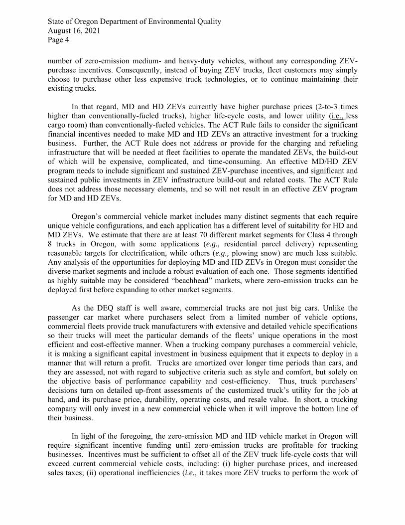
State of Oregon Department of Environmental Quality August 16, 2021 Page 4
number of zero-emission medium- and heavy-duty vehicles, without any corresponding ZEV-purchase incentives. Consequently, instead of buying ZEV trucks, fleet customers may simply choose to purchase other less expensive truck technologies, or to continue maintaining their existing trucks.
In that regard, MD and HD ZEVs currently have higher purchase prices (2-to-3 times higher than conventionally-fueled trucks), higher life-cycle costs, and lower utility (i.e., less cargo room) than conventionally-fueled vehicles. The ACT Rule fails to consider the significant financial incentives needed to make MD and HD ZEVs an attractive investment for a trucking business. Further, the ACT Rule does not address or provide for the charging and refueling infrastructure that will be needed at fleet facilities to operate the mandated ZEVs, the build-out of which will be expensive, complicated, and time-consuming. An effective MD/HD ZEV program needs to include significant and sustained ZEV-purchase incentives, and significant and sustained public investments in ZEV infrastructure build-out and related costs. The ACT Rule does not address those necessary elements, and so will not result in an effective ZEV program for MD and HD ZEVs. Oregon’s commercial vehicle market includes many distinct segments that each require unique vehicle configurations, and each application has a different level of suitability for HD and MD ZEVs. We estimate that there are at least 70 different market segments for Class 4 through 8 trucks in Oregon, with some applications (e.g., residential parcel delivery) representing reasonable targets for electrification, while others (e.g., plowing snow) are much less suitable. Any analysis of the opportunities for deploying MD and HD ZEVs in Oregon must consider the diverse market segments and include a robust evaluation of each one. Those segments identified as highly suitable may be considered “beachhead” markets, where zero-emission trucks can be deployed first before expanding to other market segments. As the DEQ staff is well aware, commercial trucks are not just big cars. Unlike the passenger car market where purchasers select from a limited number of vehicle options, commercial fleets provide truck manufacturers with extensive and detailed vehicle specifications so their trucks will meet the particular demands of the fleets’ unique operations in the most efficient and cost-effective manner. When a trucking company purchases a commercial vehicle, it is making a significant capital investment in business equipment that it expects to deploy in a manner that will return a profit. Trucks are amortized over longer time periods than cars, and they are assessed, not with regard to subjective criteria such as style and comfort, but solely on the objective basis of performance capability and cost-efficiency. Thus, truck purchasers’ decisions turn on detailed up-front assessments of the customized truck’s utility for the job at hand, and its purchase price, durability, operating costs, and resale value. In short, a trucking company will only invest in a new commercial vehicle when it will improve the bottom line of their business.
In light of the foregoing, the zero-emission MD and HD vehicle market in Oregon will require significant incentive funding until zero-emission trucks are profitable for trucking businesses. Incentives must be sufficient to offset all of the ZEV truck life-cycle costs that will exceed current commercial vehicle costs, including: (i) higher purchase prices, and increased sales taxes; (ii) operational inefficiencies (i.e., it takes more ZEV trucks to perform the work of

State of Oregon Department of Environmental Quality August 16, 2021 Page 5
conventionally-fueled trucks); (iii) lower residual values; (iv) required investments in new maintenance facilities, training, and parts inventories; and (v) significant investments to install and maintain the necessary charging and refueling infrastructure. Additionally, incentives must be available for an extended period of time so fleets can rely on them in implementing their long-term business plans. The DEQ also must consider the substantial challenges of developing the requisite charging and refueling infrastructure to support zero-emission MD and HD battery-electric trucks —something that CARB’s ACT Rule failed to do. Charging stations are expensive (more than $350,000), and must be located at fleet terminals and other depots where trucks are typically parked, and, as noted, developing that infrastructure will be complicated and time-consuming. Moreover, fleets will need to expand the charging infrastructure over time if they plan to deploy additional battery-electric trucks. Since it may take 24 to 48 months from concept to a having a fully functional charging station in place, the DEQ should establish a primary near-term objective of incentivizing and assisting in the development of a sufficiently widespread charging infrastructure to enable the deployment of battery-electric commercial vehicles. Additionally, for fleet applications where fuel-cell electric vehicles may be the better option, hydrogen fueling stations will be needed. In sum, the ACT Rule, with its unilateral ZEV sales mandates and nothing more, is not the regulatory platform on which Oregon should build its program to accelerate the deployment of MD and HD ZEVs. iii) CARB’s Omnibus Rule is cost-prohibitive and infeasible, and should not be a
component of Oregon’s ZEV strategy
The DEQ also is proposing to opt-in to CARB’s Omnibus Low-NOx Regulations in tandem with the ACT Rule. EMA previously submitted to the DEQ our detailed comments and concerns regarding the infeasibility and cost-prohibitiveness of the Omnibus Regulations, and we refer you again to those comments as well. As those comments explain very thoroughly, Oregon should not adopt or opt-in to the Omnibus Regulations for numerous reasons, including the following:
a. First and foremost, the Omnibus Rule is not yet final; it is still undergoing significant revisions and has not been submitted to California’s Office of Administrative Law (OAL) for approval. In that regard, CARB must complete its rulemaking process, and must submit its full Omnibus rulemaking file, including its Final Statement of Reasons, to the OAL by October 21, 2021. (See Cal. APA, sections 11346.4(b), 11346.9 and 11347.3(c).) The OAL then will have 30 days to review the Omnibus Rule to ensure consistency with the basic rulemaking criteria of “necessity, authority, clarity, consistency, and nonduplication,” not substance. (See Cal. APA, section 11349.1.) That will extend the Omnibus rulemaking process out to November 22, 2021, by which date OAL will need to send the final Omnibus Rule to the California Secretary of State (SoS) for publication in the California Code of Regulations. (See Cal. APA, section 11349.3(b).) For rules submitted to the SoS between September 1st and November 30th, the effective date for those rules is January 1st, which in this case would be January 1, 2022. (See Cal. APA,

State of Oregon Department of Environmental Quality August 16, 2021 Page 6
section 11343.4.) Strictly speaking, that amounts to only one year of leadtime prior to 2024 when the Omnibus regulations are slated to take effect, and maybe even less depending on how one might apply the definition of “model year” in the context of low-NOx regulations. That is a clear violation of the federal CAA’s four-year leadtime requirement. (See CAA, section 202(a)(3)(C).)
There is an additional leadtime issue as well. The California Governor’s COVID-related executive orders also provide that for rulemakings in the time-window at issue, OAL can take up to 120 days, not 30 days, to complete its review of final rulemaking packages before sending them on to the SoS for publication. If OAL takes that full extended time, the Omnibus Regulations would not be transmitted to the SoS until January 29, 2022. Regulations transmitted to the SoS on that date would not become effective until April 1, 2022, which, again, would clearly violate the applicable four-year leadtime mandate.
The net result is that the DEQ cannot opt-in to a CARB rule that is not final, and, in any event, cannot lawfully opt-in to a CARB rule that fails to provide the federally-mandated leadtime. Indeed, CARB’s underlying failure to provide sufficient leadtime for the Omnibus regulations should disqualify CARB from receiving a federal preemption waiver for those regulations. Consequently, the DEQ’s current opt-in proposal would be unlawful.
b. The Omnibus Regulations are cost-prohibitive. Multiple independent studies have been conducted to assess the costs and benefits of the Omnibus Rule. Those five studies, copies of which are attached, include: (i) a cost study prepared by ACT Research showing that the resultant cost increase for heavy-duty vehicles will be approximately $58,000 per vehicle (ii) a supplemental study by ACT Research critiquing the Standardized Regulatory Impact Analysis (SRIA) that CARB prepared for the Omnibus Regulations; (iii) a cost study that CARB commissioned the National Renewable Energy Laboratory (NREL) to prepare, which shows that the Omnibus regulations will increase the purchase price of heavy-duty vehicles by up to $47,000 per vehicle (mostly due to the costs ascribed to CARB’s extended “useful life” requirements and extended emission warranties); (iv) a recent cost assessment prepared by Ricardo establishing that even if nationwide truck-sales volumes are applied, the Omnibus regulations will increase the cost of heavy-duty trucks by $35,000 per vehicle, again mostly due to the extended FUL and warranty requirements; and (v) an updated report from NERA Economic Consulting showing (at pages 41-44) that the monetized benefits of adopting CARB’s Omnibus regulations in Oregon will total no more than approximately $1,300 per vehicle.
c. The conclusion from the relevant independent expert cost and benefit studies is that the costs of adopting the Omnibus regulations in Oregon will exceed their benefits by a factor of as high as 44 ($58,000÷$1,300). Regulations that are cost-prohibitive to such an extreme extent are invalid under Oregon law, and cannot qualify for a federal preemption waiver under the CAA.
d. The Omnibus low-NOx emission standards and related requirements also are inherently infeasible, especially since CARB will be providing only one full-year of leadtime for the 2024-2026 MY standards and requirements, which itself is a violation of the CAA.

State of Oregon Department of Environmental Quality August 16, 2021 Page 7
e. CARB failed to demonstrate the feasibility of the proposed 2024-2026 MY and 2027 MY and later low-NOx emission standards and related requirements.
f. The Omnibus Regulations, when coupled with the ACT Rule, will cause fleet operators in Oregon to accelerate their purchases of new HD vehicles before the 2024 MY, and to refrain from purchasing new HD vehicles after the 2024 MY (a “pre-buy/no-buy” response), which will significantly diminish the assumed benefits of opting-in to the CARB Regulations. ACT Research has estimated that the expected pre-buy/no-buy response will impact more than 40% of the new truck market.
g. The Omnibus Regulations likely will compel some HDOH engine and vehicle manufacturers to exit the California market starting in advance of the 2024 MY, which, in turn, would result in a lack of CARB-compliant MD and HD trucks in Oregon, if Oregon opts-in to those regulations.
h. If HDOH diesel trucks are forced out of the California and Oregon markets as expected, that will frustrate the implementation of the ACT Rule, since the HD ZEV-sales mandates under that Rule are calculated as a percentage of new HD diesel truck sales, which will be significantly reduced, if not eliminated, due to the Omnibus Regulations.
For all of the foregoing reasons, the DEQ should not include CARB’s Omnibus Regulation as an element of Oregon’s strategy to promote the deployment of MD and HD ZEVs. CARB’s Omnibus Regulations will suppress the sales of CARB-compliant conventionally-fueled vehicles, which in turn will reduce the efficacy of the ACT Rule, since, as noted, the percentage-sales requirements of that rule are based on the number of sales of conventional trucks. Thus, the net effect of CARB’s Rule, if adopted in Oregon, is more likely to frustrate rather than foster Oregon’s objective to accelerate ZEV truck sales.
iv) The DEQ’s fiscal/economic impact analysis is insufficient and does not support adoption of the Omnibus Regulations
As noted above, the DEQ cannot opt-in to a CARB rule that is not yet final. More specifically, the Omnibus Rule is still undergoing revisions, and will not be final until sometime in 2022, after California OAL approval. The DEQ therefore will have to defer action on the Omnibus Rule until next year. The DEQ’s currently proposed 2024 effective date for the Omnibus regulations (see section 340-261-0040) is not consistent with the two-year leadtime requirements of CAA section 177 (let alone the four-year leadtime provision of CAA section 202(a)(3)(C)), especially since a different definition of “model year” applies to that rule. Consequently, the earliest lawful effective date for the Omnibus opt-in will be the 2026 model year. That date, however, will need to be extended to the 2027 model year due to the underlying four-year leadtime requirement that applies to CARB’s Omnibus Regulations. Oregon’s fiscal analysis fails to take this required timeline into account.
As also noted, CARB is considering very significant revisions to the ACT Rule to require 100% ZEV truck sales in 2040, or even as early as 2035. The DEQ should wait to consider the adoption of the ACT Rule in its final form. (See CARB Notice of Public Workshop on ACF/ACT Rules, scheduled for September 2nd.)

State of Oregon Department of Environmental Quality August 16, 2021 Page 8
The DEQ’s fiscal/economic “analysis” covers opt-ins to both CARB’s ACT and Omnibus Rules. But, as noted, the ACT Rule is in the process of being reconsidered to require 100% ZEV truck sales by 2040, or even as early as 2035, and the Omnibus Rule will not be final until 2022. Thus, the DEQ’s analysis is necessarily looking at rules that are still subject to significant revision. Moreover, the DEQ cannot assume a 2024 effective date for the rules. The ACT Rule cannot take effect until the 2025 calendar year. For the Omnibus Rule, it will not be final until 2022, which, for the purpose of that rule, is the 2023 MY. Under the two-year leadtime requirement of the CAA, the DEQ cannot begin to enforce the Omnibus Rule until the 2026 model year, at the earliest. The DEQ’s fiscal/economic analysis needs to be revised accordingly.
With respect to the substance of the fiscal/economic impact analysis, the DEQ’s “analysis” amounts to a wholesale reliance on the analysis that CARB did to quantify the benefits and impacts of its rules in California, not Oregon. The DEQ simply took CARB’s numbers and scaled them down using a simplistic VMT-based factor (calculated by dividing the number of vehicle miles traveled (VMT) by HD/MD trucks in Oregon by the number of HD/MD VMT in California). The DEQ conducted no new Oregon-specific cost-benefit analysis of its own whatsoever. That direct and simplistic transposition of CARB’s numbers to Oregon is insufficient as the basis for an administrative rulemaking of this magnitude for numerous reasons, including that: there is a different MD/HD vehicle mix in California than in Oregon, along with different traffic patterns and vehicle speeds; there are different vehicle ages, mileage accruals and emission profiles in California; the new-vehicle sales and penetration rates are different in California, especially considering the unique California Truck and Bus Rule; there are different vehicle replacement rates in California than in Oregon; there are different vehicle-idling emission rates and durations in California; there are different impacts from out-of-state vehicles; and there are different EGU emission profiles, different market capacities to absorb increased marginal costs, and much different air quality impacts in California, as opposed to Oregon. The DEQ’s analysis takes none of those critical differences into account.
The DEQ’s VMT-based analysis assumes that the proposed opt-in to the ACT rule will result in CO2-equivalent reductions of 2.4 MMT “per-year” starting in 2024 and continuing out to 2040. That cannot be correct. The ACT rule phases-in on an increasing basis year-over-year out to 2035, which means that any CO2 reductions will ramp-up over time, and will not be a flat number each year. In addition, the DEQ’s assumed cumulative reduction calculation is substantially overstated, since it is nearly 6-times more that the CO2E reductions that New Jersey calculated for its proposed opt-in to the ACT Rule. Again, that cannot be correct. New MD/HD vehicle sales and VMTs in Oregon are not 6-times more than in New Jersey.
The DEQ fails to note what percentage of targeted CO2E reductions as of 2040 will result from the opt-in to the ACT Rule. It is likely less than 2 percent, a de minimus impact that cannot justify the very significant costs and market disruptions of the ACT Rule.
The DEQ states that, using its simplistic VMT-based scaling approach, NOx reductions from the Omnibus Rule will be 3.9 tons per day (tpd) in 2040. That estimate is inherently overstated, since it does not account at all for the massive pre-buy/no-buy that will occur in response to any opt-ins to CARB’s Omnibus and ACT rules. It also fails to account for the actual

State of Oregon Department of Environmental Quality August 16, 2021 Page 9
penetration rate for new HD/MD vehicles in Oregon. More specifically, the actual penetration rate for 2010-compliant Class 3-8 vehicles in Oregon is still less than 50%, more than a decade after the 2010 standards took effect. Consequently, since the DEQ’s analysis fails to consider the manner in which the HD/MD vehicle market will actually respond to Oregon’s opt-in to CARB standards, that analysis, simplistic as it is to begin with, is inherently deficient.
The DEQ’s analysis also fails to account for the likelihood that some manufacturers will simply choose to exit the relatively small Oregon market for new HD/MD vehicle sales in order to avoid selling non-competitively priced products in the State, and to avoid the disruptive constraints of state-specific ZEV-trucks sales requirements. Similarly, the DEQ’s “benefits” analysis completely overlooks the fact that truck purchasers in Oregon likely will buy any needed new heavy-duty vehicles in advance of the implementation of CARB’s standards (a “pre-buy”), which will be followed by a long deferral of any new truck purchases after the California standards take effect in Oregon (the ensuing “no-buy”). Alternatively, truck owners may simply retain their older vehicles for as long as possible, or will make any new truck purchases out-of-state. The net result is that the emissions reductions that the DEQ has assumed will not occur given the anticipated response of the heavy-duty vehicle market to the adoption of CARB’s very costly standards in Oregon.
In terms of estimated costs, again premised solely on VMT-based scaling, the DEQ’s analysis significantly misstates the marginal cost of ZEV trucks. ZEV trucks cost 2-to-3 times more than conventionally-fueled trucks. The DEQ’s postulated marginal costs ($14,000 to $87,000 per vehicle) are not based in reality. In addition, ZEV trucks require very expensive recharging or refueling stations that take multiple years to permit and install, and also require new maintenance and service facilities equipped with new tools and capabilities. Further, HD recharging stations cost considerably more than $355,000 once all permitting and installation costs are taken into account.
The DEQ’s VMT-based assessment of the extended warranty costs at issue also is significantly understated. CARB’s initial “Step 1” extended warranty costs are currently being quoted by OEMs at $1500 to $3500 per vehicle. Those warranty costs will rise to approximately $30,000 per vehicle by 2031. (See ACT Research, NREL and Ricardo cost studies.) Moreover, CARB’s underlying analysis of warranty costs – the only analysis the DEQ relies on – is fundamentally incorrect because:
• CARB’s methodology is based on the assumption that the unscreened emission warranty claims rates that have pertained over the most recent five-year period will be fully predictive of the warranty claims rates that will pertain to the new engines, aftertreatment systems, components and close-coupled packaging that will be required to comply with CARB’s 2024 and 2027 model year standards over the significantly extended useful life and emissions warranty periods. (See, e.g., CARB Warranty Cost Study, pp. ES-1 and ES-5.) That assumption is not supported by the warranty-claims increases that have followed the initial implementation years of every prior emissions-related rulemaking of this type, and does not comport with manufacturing practices and supplemental product improvements that are learned about and implemented after new stringent emission standards take effect. Moreover, CARB’s assumption makes no separate

State of Oregon Department of Environmental Quality August 16, 2021 Page 10
accommodations for the increased componentry and complexity of the close-coupled multi-element aftertreatment systems that their new standards will dictate. That is simply not reasonable. It is for those reasons that EMA assumed a 20% higher emissions warranty claims rate during the initial years after the phase-in of CARB’s Omnibus 2024 and 2027 model year standards. CARB’s (and DEQ’s) disregard of that reality is inherently unreasonable.
• CARB’s warranty-cost methodology appears to use nationwide production volumes (not California-only production volumes) to dilute the per-vehicle/engine costs of CARB’s extended emission warranty requirements. (See Id., pp. 20, 32-33.) That is not reasonable. CARB’s own regulations make clear (see, e.g., CCR Title 13, section 2035) that CARB’s extended emissions warranty program will apply only to CARB-certified and California-registered vehicles up through the 2027 model year. CARB’s (and DEQ’s) analysis is fundamentally flawed in this regard as well.
• Using nationwide production numbers, CARB assumes that the Step 1 warranty costs will only amount to $285 per engine. (See Id., ES-1.) That assumption is belied by the actual cost numbers that OEMs have reported for the Step 1 warranties that they are currently selling for the 2022 MY pursuant to CARB’s regulations (e.g., a cost increase of $2,500 for 11-13L engines). CARB’s disagreement with those actual reported/announced cost increases does not detract from the fact that the increased costs that OEMs have reported to CARB are real costs, being passed on to real vehicle/engine purchasers, starting with real product orders that are being processed now. CARB’s continued assertion of assumed artificially-low Step 1 warranty cost increases in the face of countervailing actual cost information is manifestly unreasonable.
• CARB’s assumed emissions warranty baseline is not the current standard regulatory emissions warranty, but rather a hypothetical “average” extended warranty that various fleet operators might have elected to buy in the past. That is not a fair baseline to use to assess the impacts of moving from one regulated baseline to another. A hypothetical fleet operator’s past calculus of whether to pay more in today’s market for more miles of warranty coverage is not germane to an assessment of the actual baseline cost differential of moving the regulated emissions warranty requirements from one range of mileage/years to a much greater range of mileage/years in the future. That change in regulatory baselines has an ascertainable cost increase. Whether fleet operators have shown a past willingness to take on a portion of that cost increase does not reduce the overall ascertainable cost increase of changing the regulatory requirements; it simply reveals that the market likely will be inelastic enough to accommodate a portion of those costs without changing vehicle-purchasing decisions. CARB’s (and DEQ’s) use of that marginal inelasticity in demand to discount the actual cost impact of its extended warranty regulations is simply not justified or reasonable.
• CARB’s warranty-cost rationale is internally inconsistent. On the one hand, CARB assumes that an extended warranty of approximately 200,000 miles (moving from a regulated warranty of 100,000 miles to an extended regulated warranty of 350,000 miles) will only result in a cost increase of $285 per engine. Yet at the same time, CARB asserts

State of Oregon Department of Environmental Quality August 16, 2021 Page 11
that a residual emissions warranty of 200,000 miles would increase the resale value of a truck by $2,000. (See Id., ES-6.) This implies that a used vehicle purchaser is willing to pay nearly ten-times more than the actual cost of the residual warranty at issue. That does not add-up. One of CARB’s numbers is off by a factor of ten. The actual facts at issue reveal it to be CARB’s unreasonably-low $285 number.
• In sum, CARB’s (and DEQ’s) warranty cost analysis overlooks and disregards the key input from engine and vehicle manufactures – input that includes the actual costs of Step 1 warranties – in order to try to justify the massive cost increases that CARB’s Omnibus Low-NOx Regulations will cause. That is an unreasonable outcome, but it does not change what stakeholders have known about CARB’s (and DEQ’s) warranty cost estimates from the outset – they were and remain understated by an order of magnitude.
The DEQ’s overall VMT-based scaled result is that the opt-in rules will cause per-truck cost increases of only $433 to $8,841. That number is absurdly low, and is belied by the detailed cost assessments performed by ACT Research, NREL and Ricardo, which all conclude that the per-truck cost increases from CARB’s rules will total approximately $58,000 if assessed using California-only sales volumes, and approximately $35,000 if assessed using nationwide sales volumes. Thus, the DEQ’s simplistic cost estimates are understated by an order of magnitude.
As noted above, there are multiple reasons why the DEQ’s non-Oregon-specific fiscal analysis cannot withstand scrutiny. By way of example, the DEQ does not even provide an estimate of how many new CARB-certified conventionally-fueled trucks will be sold and registered in Oregon on an annual basis from and after the 2024 model year, also factoring in the expected pre-buy/no-buy response. Without any attempted accurate estimate of those in-State new truck sales, the potential emissions benefits from opting-in to CARB’s rules cannot be assessed in a reasonable manner. Similarly, without that basic new-truck sales number, the number of ZEV trucks that could be sold in Oregon under the ACT Rule from and after 2025 cannot be estimated reasonably, since ZEV-truck sales under the ACT Rule are wholly dependent on the number of sales of new conventionally-fueled CARB-certified trucks from and after 2025.
The fact that the DEQ does not even attempt to include this most basic information (or any other actual Oregon-specific cost-benefit information for that matter) in its fiscal analysis demonstrates beyond any doubt that the analysis at issue is wholly inadequate to support the proposed rulemakings.1
v) Oregon would be better served by advocating for next-tier nationwide HDOH standards as a “bridge” to ZEVs
While we do not support the DEQ’s potential opt-ins to California’s ACT and Omnibus Regulations, EMA and its members fully recognize that zero-emission vehicles (ZEVs) are key to the future of the commercial trucking industry. Accordingly, as noted previously, EMA
1 According to Polk Data Services, average annual heavy-duty truck sales in Oregon over the past five years have been only approximately $3,000 units. The market impacts in Oregon of opting-in to CARB’s rules, including the expected pre-buy/no-buy impacts, likely would dramatically reduce that already-low annual sales number.

State of Oregon Department of Environmental Quality August 16, 2021 Page 12
member companies are investing billions of dollars to develop and bring to market MD and HD ZEVs. Our efforts alone, however, will not achieve success. A broad-based transition of the trucking industry to ZEVs will take a determined and concerted effort by federal and state policymakers, manufacturers, trucking fleets, utilities, and other key stakeholders. During that period of transition, new cost-effective interim standards to reduce NOX and GHG emissions from conventionally-fueled trucks will be necessary to bridge the gap to the longer-term development and deployment of commercial ZEVs.
More specifically, next-tier nationwide emission-reduction regulations for conventionally-fueled trucks will be key to establishing a cost-effective bridge to heavy-duty and medium-duty ZEVs. To that end, the DEQ along with the other MOU States should work with EMA to advocate for next-tier EPA regulations for HD and MD vehicles and engines that include the following elements:
• Meaningful reductions in the tailpipe NOX standard.
• New test procedures focused on reducing emissions under lightly-loaded operating conditions typical of urban centers.
• Additional NOX control under extended idle conditions.
• Next generation “in-use” compliance-assurance protocols to control emissions over a broader range of real-world operating conditions.
• Program elements to ensure compliance over multiple years.
• Continued reduction of GHG emissions.
• Flexible emissions credits to incentivize ZEVs.
While several of CARB’s Omnibus program elements are directionally consistent with those EMA envisions for EPA’s next-tier nationwide rule, CARB will be implementing those elements with unreasonably short timelines, questionable technical feasibility, unsustainable cost-benefit metrics, and material adverse impacts on new vehicle prices and sales volumes. The overall impacts of CARB’s new Omnibus regulations are likely to have extremely negative consequences. In that regard, commercial fleets have not reacted positively in the past to the deployment of major new emissions-control technologies on an accelerated timeline, and, as a result, we fully expect that the significant “pre-buy/no-buy” scenarios that occurred in 2007 with respect to commercial vehicles will be experienced again in California, as well as in any opt-in states.
In addition, and as noted above, commercial vehicle and engine manufacturers likely will
be so overwhelmed by the scope, stringency, and timing of CARB’s new ACT and Omnibus requirements that there is a strong possibility that several major manufacturers will exit the California market. Those that remain may only be able to offer limited product options to minimize costs and risks. At the recent Board hearing on the Omnibus regulations, CARB staff

State of Oregon Department of Environmental Quality August 16, 2021 Page 13
conceded that only two heavy-duty engine manufacturers have committed to even try to develop CARB-compliant products. States outside of California should work to avoid (not opt-in to) those types of adverse market outcomes. Otherwise, the consequences could be severe – both environmentally and economically.
If CARB-compliant products are not available in Oregon, or if the market does not accept the substantially increased costs associated with the few CARB-compliant products that might be available, fleet operators will accelerate their purchase of new federally-certified vehicles in Oregon, or acquire new trucks in adjacent non-opt-in states, rely more on the used truck market, or simply retain their existing fleet vehicles longer. All of those actions will have a negative impact on air quality and delay progress in the attainment of air quality goals. In addition, to the extent that fleet operators are compelled to acquire new vehicles out-of-state, that would result in a cascading series of negative economic impacts as well. In particular, truck dealerships in Oregon would face significant adverse consequences, and if Oregon-based fleet operators were to choose to relocate out-of-state, significant in-state job losses would result across the wide-ranging trucking sector, including within the goods-movement, warehousing, and truck-servicing and repair sectors.
A far more effective bridge to widespread commercial MD and HD ZEV sales and
deployment is through a cost-effective nationwide EPA-implemented lower-NOX program. Future federally-certified lower-NOX HD/MD engines and vehicles will ensure that businesses and municipalities in each state have access to the full range of powertrain and vehicle solutions they are accustomed to purchasing today. They will not be forced to pay premium prices for new products, to purchase outside their brand preference, or to seek purchase opportunities in neighboring states. They can maintain profitability without resorting to purchasing used, higher-emitting vehicles, or maintaining their existing fleet longer without the environmental benefits gained from new vehicle purchases.
The significant nationwide NOX reductions from an EPA lower-NOX program for
commercial vehicles and engines would address any remaining nearer-term air quality attainment issues in Oregon. To the extent that there might be other local needs to reduce emissions from NOX “hotspots” within the State (e.g., ports), those local needs could be best addressed through more specific approaches, such as targeted accelerated fleet turnover programs, utilization of alternative fuels, deployment of zero-emission vehicles and equipment at specific facilities, utilization of the State’s purchasing and contracting power to acquire ZEV trucks, and other targeted incentive programs, rather than through the adverse statewide economic and environmental impacts that would result from the adoption of CARB’s Omnibus program. Accordingly, Oregon should work for the implementation of EPA’s next-tier HD/MD regulations as the best option for achieving the State’s air quality goals during the bridge years before significant ZEV-truck market penetration takes hold.
Significant in that regard, on August 5th, the Biden Administration announced its decision
to publish final next-tier emission standards for HD/MD vehicles by December 2022, with those standards taking effect in 2027. That EPA rule will be followed by “Phase 3” GHG standards taking effect in 2030, which likely will continue to accelerate the deployment of ZEV trucks on a nationwide basis. While the details of those EPA programs will need to be negotiated to ensure

State of Oregon Department of Environmental Quality August 16, 2021 Page 14
cost-effective outcomes, the DEQ should align its programs with those inherently more effective nationwide regulations. Thus, and for this additional reason, the pending opt-in rulemaking should, at the very least, be deferred to allow for a thorough assessment of the efficacy of EPA’s anticipated regulations for HD/MD trucks. vi) The recommended roadmap to a commercial ZEV future
Transitioning the commercial trucking industry to ZEVs demands a strategic and concerted effort by state and federal policymakers, manufacturers, trucking fleets, utilities, and others. More specifically, successfully bridging to a medium- and heavy-duty ZEV future will require the following steps:
Undertake technical and economic research to:
• Determine the level of incentives needed to overcome the financial barriers to purchasing ZEVs and converting commercial fleets to zero emissions.
• Identify the funding and other potential impediments to building out the necessary electric charging/hydrogen fueling infrastructure.
• Assess the optimal commercial vehicle market segments most suitable for the near-term deployment of ZEVs; properly prioritize and allocate resources for early deployment in those market segments; and establish reasonable pathways to the broader adoption of commercial ZEVs.
• Determine the optimal long-term ZEV power source for each commercial vehicle market segment and the corresponding infrastructure needs (i.e., electricity and/or hydrogen), including generation and storage.
Establish practical, implementable, and effective policies to:
• Incentivize trucking fleet transitions to ZEVs.
• Accelerate the turnover/retirement of older, high-emitting commercial vehicles.
• Target the commercial vehicle applications and markets most suitable for near-term transition to ZEVs.
• Fund construction of the unique charging/fueling infrastructure needed for MD and HD ZEVs, including electricity grid modernization and decarbonization.
• Implement new EPA lower-emission standards for conventionally-fueled trucks on a nationwide basis to allow for broad near-term NOX and GHG reductions and to help manage the longer-term transition (the bridge) to commercial ZEVs.
• Utilize carbon neutral liquid fuels for interim GHG reductions.

State of Oregon Department of Environmental Quality August 16, 2021 Page 15
vii) Legal Issues that could preclude Oregon’s opt-in to CARB’s ACT and Omnibus Rules
There are a number of potential legal and procedural issues that may preclude Oregon from opting-in to CARB’s ACT and Omnibus Low-NOx Rules. More specifically, Oregon likely does not meet the opt-in criteria in Section 177 of the federal Clean Air Act (CAA). It also appears that Oregon likely will not be able to justify the fiscal impacts of adopting CARB’s Rules as required under the applicable Oregon rulemaking statutes.
The Requirements of the Clean Air Act
Oregon likely does not meet the opt-in criteria of CAA Section 177
Oregon is in attainment with the 2008 national ambient air quality standards (NAAQS) for ozone (75 ppb), and with the current 70 ppb ozone NAAQS. In that regard, EPA has not designated any portion of Oregon as a nonattainment area with respect to the 70 ppb ozone standard. As the DEQ confirms on its Air Quality home page, the air quality in Portland –– the design value site of interest in Oregon –– “meets all federal air quality health standards.”
Section 177 applies only in those instances where a State that is in nonattainment with a NAAQS (i.e., for ozone) needs to include more stringent California standards as SIP measures to demonstrate NAAQS-attainment. That is not the case here, so section 177 does not apply.
The specific terms of CAA section 177 (42 U.S.C. §7507) are as follows:
New motor vehicle emission standards in nonattainment areas
Notwithstanding section 7543(a) of this title [the CAA section relating to the preemption of state standards] any State with plan provisions approved under this part [“Part D - Plan Requirements for Nonattainment Areas”] may adopt and enforce for any model year standards relating to the control of emissions from new motor vehicles or new motor vehicle engines and take such other actions as are referred to in section 7543(a) of this title respecting such vehicles if ––
(1) Such standards are identical to the California standards for which a [preemption] waiver has been granted for such model year; and
(2) California and such State adopt such standards at least two years before commencement of such model year (as determined by regulations of the Administrator). (Emphasis added.)
The foregoing statutory language clearly indicates that the option for States to utilize section 177 is limited to those States that have EPA-approved SIPs and that need to include more stringent California standards as SIP provisions in order to bring the States’ nonattainment areas into attainment with the applicable NAAQS, including for ozone. The heading to section 177 – “New motor vehicle emission standards in nonattainment areas” – reinforces that conclusion. In

State of Oregon Department of Environmental Quality August 16, 2021 Page 16
that regard, CAA section 171(2) (42 U.S.C. § 7501(2)) defines a nonattainment area to mean “for any air pollutant, an area which is designated ‘nonattainment’ with respect to that pollutant.” Given that definition, a State that is demonstrating compliance with the NAAQS through an EPA-approved “maintenance plan” would not be eligible for an opt-in under Section 177, since the submission of a maintenance plan applies to a State “which has attained the national primary ambient air quality standard for that pollutant.” (42 U.S.C. § 7505a.)2
The Second Circuit Court of Appeals has reinforced the foregoing conclusion, noting that
“[i]t was in an effort to assist those states struggling to meet federal pollution standards that Congress directed in 1977 that other states could promulgate regulations requiring vehicles sold in their state to be in compliance with California’s emission standards.” Motor Vehicle Manufacturers Ass’n v. New York State of Dept. of Environ. Conservation, 17 F.3rd 521 (2nd Cir. 1994). (Emphasis Added.) “Section 177 was inserted into the Act in 1977 so that states attempting to combat their own pollution problems could adopt California’s more stringent emission controls.” Id.
The relevant legislative history of section 177 also makes it clear that opt-ins to
California’s mobile source standards are only available to States that need to utilize California standards to address persistent NAAQS-nonattainment issues. More specifically, as explained in the 1977 House (Report No. 95-294), CAA section 177 was initially referred to as “Section 221” in the proposed 1977 amendments to the CAA. In its explanation of Section 221 (now, Section 177), the House Committee stated that “a State which is subject to the [new] vehicle inspection and maintenance requirements [I/M] of [proposed] section 208 of the [1977 CAA amendments] is authorized to adopt and enforce new motor vehicle emission standards which are identical to California standards for which a waiver is given under section 209(b) of the act.” (H.R. 95-294, p. 431.) Significantly, the application of proposed section 208, which mandated that States adopt I/M programs, was expressly limited to the “29 air quality regions predicted to exceed the national primary ambient air quality standards.” In other words, the House understood and intended that the option to adopt California standards was limited to those States that would be in nonattainment but for their inclusion of California’s more stringent standards in their SIPs. (Id. at 224.) The House Committee Report went on to note as follows:
[T]he Committee is concerned that preemption [of state standards] (section 209(a) of the Act) now interferes with legitimate police powers of the States, prevents effective protection of public health, and limits economic growth and employment opportunities in non-attainment areas for automotive pollutants. Id. at 244 (emphasis added).
The accompanying Senate Report (S.R. 95-127) for the relevant amendments to the CAA in 1977 contained similar statements regarding the scope and availability of CAA section 177. Of particular note in that regard is the statement of Senator Anderson:
2 It appears that the DEQ adopted a maintenance plan for the superseded one-hour ozone NAAQS back in 2007 for the Portland-Kaiser Area. The air quality issues addressed under that 14 year-old plan have been resolved.

State of Oregon Department of Environmental Quality August 16, 2021 Page 17
One issue of particular concern to me is the limitation in section 209 of the waiver from the State preemption provision for automobile emission standards only for the State of California . . . . I believe, communities and States with substantial cleanup problems should be allowed the option of protecting the public in their jurisdiction by requiring accelerated cleanup [through California standards]. (S.R. 98-127, p.93.) (Emphasis added.)
Thus, the relevant House and Senate Reports demonstrate that the potential opt-ins envisioned under what would become CAA section 177 were intended to apply only to those States that were still predicted to be in nonattainment with the NAAQS, and so were compelled to adopt more stringent California mobile sources standards as components of their accelerated NAAQS-attainment efforts, specifically as plan provisions in their SIPs. The underlying premise for California’s ability to seek a waiver of federal preemption under section 209(b) of the CAA is that the State faces “compelling and extraordinary” air quality challenges. (42 U.S.C. §7543(b)(1)(B).) That same premise carries over under section 177 for potential opt-in States aswell. Where a State does not face its own similar compelling air quality needs, the opt-inafforded under Section 177 – and the implicit waiver of the otherwise controlling provisions offederal preemption that apply for vehicles that move in interstate commerce – is simply notavailable.
It is clear from all of the foregoing that a State’s opt-in to California regulations under Section 177 is authorized only when the California regulations at issue are necessary components of the State’s NAAQS attainment demonstration. Again, that is simply not the case here.
Accordingly, Oregon cannot and will not rely on any potential opt-ins to demonstrate attainment with the current ozone NAAQS, and in fact, Oregon already is in attainment with the current standard. The net result is that since Oregon does not need to use opt-ins to CARB’s Rules as SIP provisions to demonstrate ozone attainment, Oregon is not authorized to opt-in to those Rules under CAA section 177.
Section 177 does not authorize opt-ins to CARB’s GHG standards
EPA has directly addressed the question of whether CAA section 177 authorizes States to opt-in to CARB regulations directed at the reduction of greenhouse gas (GHG) emissions, as opposed to criteria pollutants for which NAAQS have been established, and for which States have specific attainment obligations under the CAA. EPA has concluded that States cannot use section 177 to adopt CARB GHG-oriented regulations. More specifically, EPA has determined that “CAA section 177 is in fact intended for NAAQS attainment planning and not to address global air pollution.” (84 FR 51351.) Oregon is not authorized to contradict that determination of section 177’s scope.
Since CARB’s ACT Rule is a regulation principally aimed at reducing GHGs, as would be Oregon’s opt-in rulemaking, Oregon is not authorized to opt-in to the ACT Rule under CAA section 177.

State of Oregon Department of Environmental Quality August 16, 2021 Page 18
Oregon’s proposed opt-in does not meet Section 177’s “identicality” requirement
The definitions set forth in the DEQ’s draft opt-in regulations would apply the CARB rules to any covered vehicles that are “leased, rented out, licensed, delivered for sale, or sold” in Oregon. (See, e.g., Section 340-257-0020.) That requirement is overbroad and inconsistent with CARB’s regulations, which apply only to new vehicles sold, delivered to purchasers, and registered in California. As drafted, the DEQ’s regulations are not identical to CARB’s, which would violate subsection (1) of CAA section 177.
Similarly, the DEQ is proposing to allow for the generation of ZEV credits starting in 2024. (See section 340-257-0090.) That also is inconsistent with CARB’s ACT regulations, which allow for ZEV-credit generation starting this year, in 2021 – which amounts to a three-year credit-generation ramp-up. The DEQ’s proposed opt-in would, in effect, be more stringent than CARB’s, and so would violate CAA section 177 on this basis as well.
The Applicable Oregon Rulemaking Statutes
In any rulemaking, the DEQ must prepare a detailed fiscal impact analysis of the proposed rule, along with an assessment of potential adverse impacts on small businesses. (See ORS § 183.335-36; DOJ Admin. Rules, Chapter 127.) A thorough benefit-cost analysis (BCA) is a core component of what is required. In this case, as noted above, the costs of Oregon’s opt-ins to CARB’s ACT and Omnibus Rules would far outweigh any putative benefits from doing so. And, as also detailed earlier, the DEQ’s fiscal impact analysis in this case is inherently deficient, and cannot sustain the proposed rulemakings.
EMA previously engaged independent experts to assess the costs and benefits of CARB’s Omnibus Rule, both as applied in California and as potentially applied in the other 49 States. ACT Research (and more recently Ricardo) assessed the incremental costs of CARB’ Rule on a per-truck basis, and NERA Consulting quantified the potential corresponding public health benefits on a per-truck basis.
ACT found that, based on new truck sales volumes in California, CARB’s Omnibus Low-NOx Rule would increase the price of a new truck in California by approximately $58,000, using a 7% discount rate. Since new truck sales volumes in Oregon are substantially less than in California, using that per-truck cost increase to assess the cost of Oregon’s potential opt-in to the Omnibus Rule is a conservative approach.
On the benefits side, NERA quantified the public health benefits (i.e., avoided premature deaths) that could be attributed to the reductions in ozone and secondary PM emissions from implementation of an Omnibus Rule, and then calculated those benefits on a per-truck basis, both for California and for States outside of California as well. For Oregon, those benefits amount to approximately $1,300 per-truck ($1,200 per-truck from secondary PM reductions, and $100 per-truck from ozone reductions).
Comparing the likely benefits and costs in Oregon from an opt-in to CARB’s Omnibus Low-NOx Rule yields a cost-benefit ratio (or a negative benefit-cost ratio) of approximately 44-to-1, on a conservative basis. Rulemakings that would have such extremely inverted economic

State of Oregon Department of Environmental Quality August 16, 2021 Page 19
consequences cannot meet the criteria for valid administrative regulations. And that is even before the other downstream consequences of a potential opt-in are taken into account.
More specifically, ACT found that given the substantial per-truck cost increases that will result from the Omnibus Low-NOx Rule, it can be expected that truck fleet operators (in addition to retaining their current vehicles longer, or buying new vehicles out-of-state) will accelerate their purchases of new trucks before the Omnibus Rule takes effect (a “pre-buy”), and will refrain from buying new trucks after the Omnibus Rule takes effect (a “no-buy”). The likely net result will be that the anticipated pre-buy/no-buy will shift 40% or more of the new truck market to accelerated purchases prior to the implementation of the Omnibus Rule, which will proportionally and significantly dilute any potential benefits from the CARB Rules, including under the ACT Rule since the extent of the ZEV-sales mandate is derived from the level of sales of conventionally-fueled trucks.
In addition, it can be anticipated that once the Omnibus Rule takes effect in Oregon, truck dealerships in the State will see their businesses suffer, long-haul fleet operators may choose to move out-of-state, and trucking-related job losses will occur. All of those adverse outcomes will only compound the already upside-down cost-benefit calculus for the contemplated opt-in.
In sum, opting-in to CARB’s Omnibus Low-NOx Rule would be cost-prohibitive. The calculus for CARB’s ACT Rule is similar if not even more inverted. Since such opt-ins are not authorized under CAA section 177 to begin with, it seems clear that Oregon is not authorized to adopt and opt-in to CARB’s Rules.
viii) Conclusion
There is no doubt that ZEVs are the future of the commercial trucking industry, andEMA’s suggested roadmap identifies realistic and necessary steps to develop and bring to market medium- and heavy-duty ZEVs. Policymakers and other stakeholders should collaborate on those targeted and holistic strategies to successfully establish the commercial ZEV market. In the meantime, a complementary nationwide EPA bridge program is needed—and is in the works—to reduce NOX emissions from conventionally-fueled commercial vehicles.
Increasing the market penetration of ZEV trucks requires the iterative and multi-pronged approach spelled out in our roadmap, including, among other things: (i) identifying the trucking fleet applications best-suited to a nearer-term transition to ZEV trucks –– the “beachhead” markets; (ii) implementing robust incentive programs to enable the identified beachhead fleets to acquire and maintain ZEV trucks; (iii) researching and building-out the necessary ZEV infrastructure to support the beachhead ZEV fleets; and (iv) coordinating with other agencies, including EPA, to expand the deployment of ZEV trucks across other applications, using sufficient public resources and incentives to expand the necessary ZEV infrastructure and offset the higher total cost of ownership of commercial ZEVs.
CARB’s ACT and Omnibus Low-NOx Rules are not well-suited to implementing the necessary multi-prong approach, or to achieving our common goal for the accelerated deployment of MD and HD ZEV trucks. Rather, those Rules impose both infeasible ZEV-sales mandates on manufacturers (without accounting in any way for the necessary incentives and

State of Oregon Department of Environmental Quality August 16, 2021 Page 20
infrastructure deployment, and without including any corresponding ZEV-purchase strategies), and also establish unreasonably stringent, expensive and infeasible NOx standards. As a result, a ZEV-deployment strategy that is centered around CARB’s Rules will more likely frustrate rather than foster the acquisition and use of ZEV trucks in Oregon, will hurt the State’s economy, and will impede any envisioned environmental gains (i.e., due to delayed fleet turnover or increased out-of-state truck purchases). The roadmap that EMA has outlined offers a better and more collaborative way forward.
We look forward to further discussions regarding these critically important issues, and stand ready to assist the DEQ in advancing a cost-effective program to accelerate the roll-out of ZEV-technology trucks and lower-emission commercial vehicles.
Respectfully Submitted,
TRUCK AND ENGINE MANUFACTUERES ASSOCIATION
cc: Ali Mirzakhalili ([email protected]) Michael Orman ([email protected])

DRAFT
RESPONSE TO STANDARDIZED
REGULATORY IMPACT ANALYSIS FOR PROPOSED
CARB HEAVY-DUTY EMISSIONS REGULATIONS
P R E PA R E D F O R :
TRUCK & ENGINE MANUFACTURERS ASSOCIATION
333 WEST WACKER DRIVE
CHICAGO, ILL INOIS ▪ 60606
July 29, 2020

2
ACT Research Company (ACTR) appreciates the opportunity to submit the following comments in response to the Standardized Regulatory Impact Assessment (SRIA) associated with the Proposed Heavy-Duty Engine and Vehicle Omnibus Regulation and Associated Amendment that the California Air Resources Board published on June 23, 2020, which was amended on July 10, 2020.
ACTR is a boutique research firm focused on surface transportation dynamics and commercial vehicle demand. ACTR’s customers include leading MD and HD vehicle manufacturers, the commercial vehicle industry’s supply base, investors in transportation and machinery companies, transportation companies, and other groups of stakeholders who need to understand the impact of economic activity on trucking industry profitability, and by extension, demand for medium- and heavy-duty on-highway vehicles.
ACTR’s decision to provide comments on the CARB SRIA relates to a study the company undertook at the behest of the Engine Manufacturers Association (EMA) in early 2020. The resulting study was an upfront cost and total cost of ownership (TCO) analysis relating to the impact of the California Air Resource Board’s (CARB) Omnibus Low-NOx standard proposals and the U.S. Environmental Protection Agency’s (EPA) advanced notice of proposed rulemaking (ANPRM) published in the Federal Register on January 21, 2020, entitled “Control of Air Pollution from New Motor Vehicles: Heavy-Duty Engine Standards.” Given the similarities in the CARB and EPA proposals surrounding NOx and warranty extension, we believe our analysis adds to the discourse surrounding CARB’s proposed Regulation.
ACTR has been and will continue to be a supporter of CARB and EPA efforts to improve air quality. We applaud the 99% and 98% reductions in particulates and NOx, respectively that have occurred over the past quarter-century. And in contrast to the costly final mandates that reduced PM and NOx, the more recent GHG Phase 1 and Phase 2 (to date) regulations have pushed industry stakeholders to deliver tremendous advances in on-highway fuel economy at nominal cost, thereby benefitting both the environment and the buyers of new commercial vehicles.
While we at ACTR recognize the need to continue reducing emissions levels from all sources, we also believe that accuracy in accounting is needed for regulators to make the most optimal decisions possible in plotting the way forward on emissions regulations. It is in that spirit that we believe a better accounting needs to be made in regard to CARB’s current proposal to improve air quality. Based on our modeled conclusions, it is ACTR’s opinion that CARB’s accounting for the cost impact of the proposed regulation is incomplete on several fronts, including:
1) Market sizing 2) R&D accounting 3) Useful life accounting for new technologies and downtime impact 4) Warranty accounting
Over the course of this submission, ACTR will lay out where we believe the accounting as presented in the SRIA fails to capture the true costs of this regulatory proposal. If our analysis is correct, this regulation is likely to cause significant market disruptions as trucking companies actively work to minimize their exposure to new vehicles that will leave them at an operating cost disadvantage to their competition.

3
Market Size and Structure. Although we do not have a fully transparent understanding of the sales projections driven by CARB’s EMFAC model, we disagree with the use of 2013 as the year from which to draw conclusions about the current and future commercial vehicle market size and structure.
• Based on OEM data, we estimate natural gas had a Class 8 market share nationally of 3%-4% in 2013-2014, and has since trended down to 2% in the past two years (see chart). Of course, we recognize that California represents an out-sized proportion of natural gas truck sales, but in the SRIA, CARB assumes HD Otto-cycle engines including natural gas were 43.6% of the heavy heavy-duty (Class 8) market in 2013. We are confident in asserting that this proportion has fallen considerably in the years since, and a more current weighting would increase the diesel units subject to low-NOx standards, which would increase overall costs in the calculation.
• We agree with CARB’s earlier sales volume methodology which took into account the smaller market outlook resulting from the Advanced Clean Truck (ACT) Regulation. But we disagree with the changes made as recommended by the California Department of Finance (page IX-7), to adhere to a legal baseline which will include the mandated zero emissions vehicles under the ACT Regulation. This may have mixed implications for cost outputs, but suggests per-unit costs are understated. The cost study conducted by ACTR used the smaller market size under the ACT Regulation, which lowered overall costs but raised per-unit costs, though the targets in the ACT Regulation have been raised since our study was conducted.
• CARB’s SRIA Does not Consider the Likelihood of Pre-buy/No-buy. We agree with the need to include increased DEF consumption costs and financing costs, as CARB did in the SRIA. However, note that costs to truckers were not included in ACTR’s manufacturing cost analysis, but were included in our Pre-buy/No-buy analysis. In our view, the largest blind spot in CARB’s SRIA is the

4
failure to consider the industry’s instinctive avoidance response to the prospect of costly and risky new regulations. • The higher DEF consumption rate is one of several additional cost factors that should be
considered for the trucking industry, separate from manufacturing costs. These include the taxes on the higher cost of a truck, which is a 12% Federal Excise Tax plus state taxes, and costs to insure the more expensive vehicle, typically 5% of the purchase price per year.
• As a result, for every $1 increase in the purchase price of the vehicle, the equipment costs to the operator are likely to rise by $1.40 - $1.75, depending on one’s assumptions about the operating lifecycle. Hence, we think DEF costs are a very small fraction of the non-manufacturing costs of the Omnibus Low-NOx rulemaking proposal which would be borne by the trucking industry.
o In the cost study ACT Research performed for the EMA, we considered how the preceding costs plus the higher base vehicle prices would impact the trucking industry. Instead of arguing about assumptions, we took a macroeconomic approach.
• We concluded that in this highly fragmented and cyclical industry, which is largely dependent
upon market freight rates, a pre-buy is likely with elevated demand for equipment built before the regulations take place. Trucking is a low-margin industry which abhors risk. Considerable historical precedent shows any significant price increase and technological change will likely drive a pre-buy in this industry. This will add excess capacity to the market and drive down freight rates, with a material adverse effect on earnings for the trucking industry. We have expertise in these freight rate sensitivities through Freight Forecast service, and we estimate the subsequent decline in truckload rates would cost the industry between $6.5 billion and $8.6 billion in the 2027-2028 timeframe. Further, the combination of the effects of the pre-buy and cost of lower freight rates would materially reduce the industry’s ability and willingness to purchase new vehicles after regulations take effect, thereby delaying the benefits of the regulation.
R&D. CARB’s SRIA assigns minimal Research and Development (R&D) costs to the achievement of its proposals, ranging from $78-$85 per unit on Medium Heavy-Duty (MHD) vehicles to $354-$356 per unit on Heavy Heavy-Duty (HHD) vehicles (page IX-10). The underlying sales figures from CARB’s EMFAC model are not clear, and the total R&D costs are not broken out in the aggregate table IX-32.
• The Original Equipment Manufacturer (OEM) study conducted by ACT Research yielded an estimate of $603 million of R&D costs to meet the HHD MY2027 standards proposed for California, only modestly less than the $715 million estimated for full national programs. While the core processes are unchanged regardless of whether it is a partial or national standard, the OEMs intended to reduce the offerings available in California to achieve these modest savings.
• Based on OEM feedback that these costs would be amortized over three- to four-year product cycles, this translates to about $38,000 per unit for the HHD market beginning in MY2027. The

5
CARB SRIA does not explain how it arrives at its significantly lower R&D figure, though we acknowledge there is significant managerial accounting discretion to extend the amortization period and lower the per unit costs. Extending the regulations to a national basis reduces these per-unit costs to just under $2,800 per unit in our model, even keeping with the OEMs’ three- to four-year amortization periods, which highlights the benefit of harmonized national standards over regional ones.
Useful Life. Producing aftertreatment systems to meet tighter standards, increasing the Useful Life (UL) of those systems, and providing a warranty on those systems are three of the distinct challenges presented by the proposed Omnibus Low NOx regulations. CARB’s assertion that increased UL is included in the Technology Costs is disconnected from reality because, for example, Cylinder Deactivation technology is not currently commercially viable and will likely require at least one full replacement to be expected/budgeted in order to meet the UL proposal.
• The OEM survey conducted by ACT Research, which accounted for all major manufacturers, yielded an estimate of $176 million of indirect costs to meet the MY2027 UL provisions in the CARB regulatory proposal for Heavy Heavy-Duty (HHD) vehicles, which added $11,178 of cost per vehicle under our market sizing parameters. It also yielded a similar result for MY2031, and smaller cost figures for medium-duty. These costs are missing from the CARB SRIA.
Warranty. In assigning $930 of incremental repair costs for HHD vehicles in order to extend warranties from 350,000 miles from Step 1 to 600,000 miles, where no warranty data exists, in MY2031, CARB’s warranty analysis (SRIA, page IX-19 to IX-25) materially contradicts the results of both the ACT Research and the NREL cost analyses that was added to the SRIA on July 10, 2020. We also see the $159 estimate for incremental repair costs beginning MY2027 for HHD vehicles as deeply flawed, again considering the unproven nature of the new technologies expected to be employed, particularly cylinder deactivation.
• The feedback from manufacturers used as input for both studies is that the extended warranty provisions would effectively require the manufacturers to account for almost a full aftertreatment system replacement for every vehicle, or about $8,000 per HHD unit. NREL’s average cost scenario for 12-13L engines included a $23,424 per unit incremental warranty cost, but this appears to include the extended useful life provisions as well, which we detailed separately.
• We do not agree with linear extrapolation of warranty costs into the extended warranty periods based on MY2013 data.
o These data represent significantly lower-cost MY2013 emissions systems, not the more costly systems envisioned in the regulation, thus we believe this methodology fails to account for the warranty cost on the added components.
o We believe CARB’s assumption (page IX-22) “that components would continue to fail at the same rate for the duration of the lengthened warranty period” is flawed. Based on feedback from manufacturers during our survey, our experience analyzing the trucking industry, and the Fleet Advantage study charted below, it appears to us to be common knowledge that maintenance costs increase significantly over time. In addition, the Southwest Research Institute (SwRI) Low NOx Stage 3 testing program only tested up to 435,000 miles (page III-7).

6
• The warranty mileage baseline is well above reality, in our view, and ignores the cost incurred by the trucking industry for extended warranties above the regulatory baseline. This methodology understates warranty costs for California and would much more materially understate warranty costs on a national basis where the baseline is below CARB’s Step 1 baseline.
o For MY2027, CARB assumed 40% of HHD trucks are purchased with 500,000-mile warranties, reducing the distance to the 600,000-mile warranty proposal. This ignores the considerable costs some fleets pay for extended warranties and overstates current industry practice. Our research suggests that extended warranties are typically for 400,000 miles, and the take rate is likely less than 40%.
o In reality, the industry standard base warranty is 250,000 miles, and the EPA regulatory baseline is 100,000 miles. Because these are significantly lower than the 350,000-mile CARB Step 1 baseline which will be in effect as of 2022, this is material when considering extending these provisions to the national level. Incremental warranty costs per unit on a national basis from the proposed regulations would thus be significantly higher than the estimates in CARB’s SRIA.
o Based on CARB’s assumption (however questionable) that it can calculate warranty costs linearly, and our view that the incremental warranty costs should be based on the 350,000-mile Step 1 baseline, we should be accruing for an incremental 250,000 miles of warranty coverage, whereas CARB’s analysis includes 190,000 (adding the 40% at 500,000 miles raises the baseline to 410,000 miles). Thus, CARB’s analysis misses about 24% of the regulatory increase in warranty cost.
Technology path. The direct engine and aftertreatment component cost output of $11,347 from the ACTR study, which combined MY2024 and MY2027, was well above the comparable figure from CARB’s SRIA of $6,429 ($1,611 in MY2024 and $4,818 in MY2027). The main source of difference is that the

7
manufacturers did not all choose the same technology path, corresponding to the one laid out in CARB’s proposal, though a portion did. With the consideration that CARB’s proposals are supposed to be technology neutral, with no picking of winners or losers, an estimate that considers more than one technology path is preferable, in our view.
Other. We do not purport to being experts on managing large manufacturing companies, as our expertise is primarily in data analysis and forecasting for the transportation and commercial vehicle industries. However, we question CARB’s assumptions throughout the Standardized Regulatory Impact Analysis (SRIA) cost analysis that the important work of compliance with these emissions regulations is relegated to a single junior engineer earning just $70 per hour. Adding any internal oversight, which seems important from our perspective, would add further incremental compliance costs. In addition, we took particular exception with the doubts CARB cast on the NREL study (page IX-73) by questioning its quality because of a small sample size. CARB knows well the number of major truck OEMs, and while the same could be said of our study, it covered every OEM of consequence. And the results of the ACTR study fell very close to the NREL study, both in stark constrast to the CARB SRIA.
To conclude, ACTR’s analysis suggests that the new purchase price of an HHD vehicle will rise by $69,930 in MY2027 from the current baseline in a California-only scenario, which falls to $25,825 on a national basis. CARB’s SRIA does not add up the estimated costs to present them on a per unit basis in total, which seems very pertinent in our view. Nonetheless, adding up the costs in CARB’s SRIA, we reach roughly $10,000 per unit for MY2027, though this is not clear given the lack of transparency on market sizing (note: we combined the MY2024 proposals into our MY2027 as the MY2024 timeframe was deemed infeasible from a planning and testing perspective). CARB’s numbers do not account for the higher total-cost-of-ownership burden that will be borne by the trucking industry (on ACTR CA-only estimates, $8,392 from 12% FET, $5,070 from 7.25% state taxes, etc.), and eventually, consumers. If we are even “ballpark” correct in our cost assessment, the cost increases at issue have the potential to meaningfully move the trucking industry away from vehicles that meet CARB’s proposed mandates, thereby reducing the regulations’ benefit for several years, especially if the regulations requiring significantly more expensive trucks aligns with the peak of an economic cycle. If that happens, we can expect an even larger prebuy ahead of the mandate, and an extended post-mandate delay, which would invalidate much of CARB’s cost analysis and delay the anticipated benefits.

FINAL DRAFT
COST STUDY: PROPOSED HEAVY-DUTY
ENGINE AND VEHICLE EMISSIONS REGULATIONS
P R E PA R E D F O R :
TRUCK & ENGINE MANUFACTURERS ASSOCIATION
333 WEST WACKER DRIVE
CHICAGO, ILL INOIS ▪ 60606
March 19, 2020
Contents

2
Page(s)
Executive Summary .................................................................................................................................... 3
Summary Tables of Cost Study Outputs ............................................................................................... 3-5
Methodology ........................................................................................................................................... 6-10
• General • Discount rates • Inflation • Market Sizing • State versus Federal Considerations • MY2024 Feasibility Issues
Medium- and Heavy-Duty Cost Details ................................................................................................ 9-13
• Direct & Indirect Manufacturing Costs • MY2027 and MY2031
Pre-buy/No-buy Analysis ..................................................................................................................... 14-19
• Introduction • Pre-buy Model • Freight Rate Impact • Trucking Industry Sizing and Earnings Impact
Sensitivity Analysis Under Pre-buy/No-buy ...................................................................................... 20-23
Conclusions .......................................................................................................................................... 23-24

2
ACT Research Cost Study of the Proposed Omnibus Low-NOx Rulemaking
Executive Summary
Based on a survey of the commercial vehicle and engine manufacturing industry completed in Q1, 2020, this study presents ACT Research’s best estimates of the sum of the direct and indirect costs of meeting the goals of the California Air Resources Board (CARB) Omnibus Low-NOx Rulemaking (Omnibus Regulations), as also referenced in the ANPRM for EPA’s Cleaner Trucks Initiative (CTI). We present estimates for costs of both a nationwide and a California-only program.
This study’s focus is on the costs (including per-vehicle costs) that the truck and engine manufacturing industry likely will incur to comply with the proposed Omnibus Regulations. The study’s primary conclusion is that full compliance with the proposed low-NOx emission standards and other requirements, assuming they track the proposed Omnibus Regulations, will cost the truck and engine manufacturing sector a Net Present Value (NPV) of $9.1 – $13.0 billion.
Assuming the proposed Omnibus Regulations are implemented, manufacturers ultimately will recoup most of those costs through higher vehicle prices. It is the trucking industry that will bear most of the increased costs going forward. Longer-term, the trucking industry eventually will be able to pass the higher costs of compliance on to the shipping community, which in turn will pass them on to consumers. However, given the highly competitive nature of the trucking industry, we also detail the costs of the very likely scenario of a substantive equipment “pre-buy/no-buy” to avoid, at least initially, the higher truck and engine costs associated with the proposed Omnibus Regulations. In ACT’s modeling, the resulting overcapacitization in the freight hauling industry (due to pre-buys of vehicles) likely will yield aggregate pre-buy impacts between $6.5 - $8.6 billion in 2019 dollars, solely as a result of lower freight rates due to overcapacity, and there will be little opportunity to recoup the lost shipping revenues during the periods of overcapacity.
The combined regulatory impact on the manufacturing sector and trucking companies falls between NPVs of $15.6 and $21.6 billion.
Our estimates do not model the increased costs out into perpetuity. Rather, our cost estimates are focused on the two key years when costs are likely to rise significantly: 2027 and 2031. In our analysis, fixed costs were allocated over multi-year product programs. In addition, we have not tried (yet) to estimate the long-run costs to the trucking industry from deploying higher-cost equipment. The costs studied here are solely for the truck and engine manufacturing sector, and just include the pre-buy related effects on trucking. In our judgement, adding the long-run costs on trucking, while likely worth a more thorough analysis, would effectively be double-counting the costs we have estimated for the manufacturers. We include an analysis of the costs for the trucking industry in the Pre-buy/No-buy section, but only to inform our modeling regarding the degree of excess capacity. It should be noted that the increased taxes, insurance costs, financing costs, and emissions fluid costs that trucking companies will face are not included in this aggregate cost estimate of $15.6 to $21.6 billion.

2
Summary Tables. Tables 1-3 summarize the results of our cost study. Our findings related to the costs associated with the MY2027 step of the proposed Omnibus Regulations are itemized in Table 1: Cost Estimates to Meet Proposed MY2027 Vehicle Standards. In MY2027 at the national level, and using the 3% and 7% discount rates to bracket the ranges, we estimate the proposed emissions requirements would cost the industry $1.8 – $2.4 billion for medium-heavy duty vehicles and engines, and $4.5 – $6.1 billion for heavy-heavy duty vehicles and engines, which sums to $6.3 billion at a 7% discount rate, and $8.5 billion at a 3% rate. On a per-unit basis, the cost of compliance ranges from $17,610 to $23,886 for heavy-heavy-duty (HHD) diesel vehicles, and $11,752 to $15,940 for medium-heavy-duty (MHD) diesel vehicles. The total cost figures are smaller for a California-only program, but per-unit costs rise sharply because of the relatively small number of units sold in California.
Table 1: Cost Estimates to Meet Proposed MY2027 Vehicle Standards
Source: ACT Research Co., LLC: Copyright 2020
The cost estimates itemized in Table 2 summarize the results of our cost study for MY2031 compliance. Those costs are primarily related to meeting the extended useful life and emission warranty provisions of the proposed Omnibus Regulations. The cost figures amount to additions to the baseline MY2027 costs (in Table 1), and show the incremental cost estimates for MY2031. For HDD vehicles, our survey indicated an additional $8,352 – $13,194 in costs per truck, depending on the discount rate utilized. For MHD vehicles, the additional costs would range from $3,689 – $5,827 per truck. Combining the HHD and the MHD diesel model outputs, we estimate a discounted cost that ranges between $2.7 – $4.4 billion for the MY2031 proposals on a nationwide basis.

2
Table 2: Additional Cost Estimates to Meet Proposed MY2031 Vehicle Standards
Source: ACT Research Co., LLC: Copyright 2020
Table 3 aggregates the cost estimates for the MY2027 and MY2031 cost models, reflecting our estimates of the combined costs of the proposed Omnibus Regulations. On a nationwide basis, the total combined cost of the Omnibus Regulations for both MHD and HHD vehicles is $9.1 billion to $13.0 billion, depending on whether a 7% or 3% discount rate is utilized. On a per-unit basis, the nationwide cost for HHD vehicles ranges from $25,963 at a 7% discount rate, to $37,079 at the 3% rate. For MHD vehicles, the per-unit costs range from $15,441 to $22,767, respectively. On a California-only basis, the aggregate total costs range from $1.3 – $1.8 billion, which are much smaller than the nationwide costs, but some expense line-items like R&D were relatively fixed. Therefore, on a per-unit basis, the per-unit cost increases range from $57,905 to $80,821 per HHD vehicle, and from $51,365 to $71,878, per MHD vehicle.
Table 3: Cost Estimates to Meet Proposed Combined MY 2027 and MY2031 Vehicle Standards
Source: ACT Research Co., LLC: Copyright 2020

2
Methodology
This cost study was performed using federal guidelines that correspond to EPA’s Guidelines for Economic Analysis and OMB Circular A-4. The baseline assumptions for our analysis are that:
1) Heavy-duty truck manufacturers would continue to work toward meeting the established GHG-2,
2) but would otherwise not explicitly target a. incremental NOx emissions reductions, b. improved low-load SCR performance, or c. longer useful lives for aftertreatment systems.
In light of the pending GHG-2 regulations, we used professional judgement to discount some of the cost inputs that we received from manufacturers, if those inputs did not take into account the improved fuel economy and reductions in fuel consumption, which will help to meet the proposed Omnibus Regulations.
We followed the methods specified by the Environmental Protection Agency (EPA) and the Office of Management and Budget (OMB) to conform to the government’s Social Cost definition, though we have noted where we otherwise would differ with those methods (i.e., inflation and discount rates). We have also presented below an additional set of values that discount the future costs at the private weighted average cost of capital, which for this industry is quite high. Our “Private Cost” estimates below are only alternative results, not EPA/OMB recommended results, and so are not included in the summary tables above.
ACT Research’s cost estimates are based upon industry inputs consisting mainly of confidential business information (CBI), and as a result, specific technology solutions will not be discussed here except to note that those anticipated solutions were not uniform. As explained below, we used conservative analytical judgements where possible. For example, the current regulatory baseline for warranty coverage is 100,000 miles (five years, 3,000 hours). However, our research confirmed that the industry standard for new heavy-duty trucks is a 2-year/250,000-mile warranty that is built into the price. As a result, our study uses 250,000 miles as the baseline, resulting in lower incremental costs than otherwise would have been the case had we used the more common government research practice regarding the existing regulatory baseline.
Discount Rates, Social and Private. Consistent with EPA and OMB guidelines to discount future costs back to their present value at 3% and 7% discount rates in order to determine NPV, we have presented our results discounted at both of those rates. However, considering the significant uncertainty involved in estimating the future costs at issue, we also present the results of our cost estimates discounted using an alternative private cost methodology. The private cost methodology provides for the use of the Weighted Average Cost of Capital (WACC) for the truck and engine manufacturing industry as our discount rate. In calculating the 10% WACC, we used

2
current equity values, as of January 2020, and debt and interest rates from the manufacturers’ most recent annual reports.
Accordingly, in addition to utilizing the 3% and 7% social cost discount rates, we also present an alternative cost estimate (in Table 4) using our more conservative 10% WACC discount rate. While this is more conservative than the social cost methodology, we believe it accounts for some of the uncertainty inherent in this study, including: significant uncertainty about the future state of emissions-control technology, and regarding the most likely compliance pathways that manufacturers may follow. For example, we are estimating that manufacturers will need to budget for two replacements to aftertreatment systems in the life of their trucks in order to comply with the extended useful life and warranty provisions of the Omnibus Regulations. However, between now and MY2027, it is possible that durability could be improved to remove some of those costs. It also is possible that replacement aftertreatment systems will not last as long on older engines, which also is reflected in this cost study.
In light of these and other uncertainties, the alternative 10% WACC-based discount rate could be a reasonable way to estimate more conservatively the unknown variables pertaining to the various potential cost inputs and impacts. The larger alternative discounting mechanism that we have used, in essence, could serve fairly well in lieu of a more formal sensitivity analysis at a point in time when specific technology paths are not yet known.
Inflation methodology. We used inputs in 2019 dollars as it was the year our cost survey was initiated, adjusting for the OEMs who responded in 2018 dollars using the BEA’s GDP Price Deflator. We thought it would be fair to use a lower inflation rate or perhaps even deflationary figure given the historical experience in this industry, but EPA (through EMA) indicated that the GDP Deflator is the standard. Adhering to EPA’s recommended use of the GDP Deflator may inflate the estimated cost of the Omnibus Regulations, leaving room for further study.
Heavy-Heavy Duty Market Sizing. We used 2018 vehicle manufacturer (OEM) market shares as our baseline and assumed those shares as a constant into the future. However, instead of using the 2018 market size and simply rolling it forward, we took into account the fact that 2018 was the fifth-largest year ever for U.S. Class 8 truck production. As it happens, two of the higher production years were 2005 and 2006, with 2006 being the biggest U.S. Class 8 production year ever. Not coincidentally, those two “top-five” years occurred immediately ahead of the expensive EPA07 emissions standards for heavy-duty trucks and engines. We will discuss this “pre-buying” issue later in this report.
To provide a representative baseline, we used a five-year trailing average of U.S. Class 8 truck production (HHD diesel), or 239,000 units, and scaled it up at 1% per-year to account for economic growth, and adjusted for freight productivity. While freight demand grows over time

2
as the population grows, shippers also find ways to improve design and packaging in ways that require fewer truckloads for a given set of goods. As a result, our analysis uses a MY2027 U.S. Class 8 nationwide market size estimate of 257,000 units.
For the California market, based on industry inputs, we used a baseline of just under 7% of nationwide industry sales, and scaled that starting point down by 7.5% in MY2027 to reflect assumed progress toward CARB’s target of 15% zero-emission heavy duty tractors by 2030. We therefore estimate that California will represent just over 6% of nationwide HHD sales in MY2027.
For MY2031, we continued to scale nationwide HHD sales up by a 1% cumulative annual growth rate, bringing the nationwide HHD market to 267,000 units. We also continued with the assumption that California would achieve its 2030 target of 15% zero emissions heavy-duty vehicles, taking California down under 6% of nationwide HHD duty diesel truck sales.
Medium-Heavy Duty Market Sizing. For the MHD market, we used a trailing five-year average of U.S. sales of 142,000 units per-year, scaled up at 1% per-year to account for economic growth and adjusted freight productivity, in line with the above discussion regarding the HHD market. That resulted in a nationwide MHD market size of 152,000 units.
For the California market, we used a baseline of just under 7% of nationwide industry sales, also based on industry inputs, and scaled that down by 20% in MY2027 to reflect progress toward CARB’s target of 50% zero-emission MHD vehicles by 2030. We estimate that California will represent just over 5% of nationwide MHD sales in MY2027.
For MY2031, we continued to scale nationwide MHD sales up at a 1% cumulative annual growth rate, and we made the assumption that California would achieve its target of 50% zero-emission vehicles, taking California down to 3.5% of nationwide MHD diesel truck sales.
State versus Federal Considerations. Based on this cost study, we conclude that the local benefits of California-only regulations do not justify the very significant costs that would impact trucking-related business on a nationwide basis. Due to the relatively small number of trucks sold in California, the research and development costs of advanced aftertreatment on a per-unit basis could be unacceptably high. Our survey of OEMs showed that only about 7% of heavy-duty trucks are sold in California, significantly less than the State’s share of GDP.
Our cost survey also shows that the industry would spend $715 million on research and development for the proposed standards nationally, and $603 million on a California-only standard. The difference between the two totals reflects that fewer models would be offered under a California-only scheme. However, on a per-unit basis, using the market size detailed previously and amortizing the costs over an industry-standard three-year product platform cycle,

2
those R&D costs amount to about $2,800 per-unit at a national level and $38,200 per-unit if the regulations applied only to California.
MY2024 Infeasibility. We are not providing separate estimates for the MY2024-26 elements of the proposed Omnibus Regulations because we did not receive indications that manufacturers can, or will, develop and introduce the technologies that could be used to meet those proposed standards by the 2024MY at reliable product-quality levels. The industry respondents to our survey cited numerous feasibility problems with the MY2024 time horizon. We believe that for some key vehicle categories, the standards proposed under the Omnibus Regulations are technically infeasible within the lead time allowed. Accordingly, we have not fully estimated the costs for the initial phase of the Omnibus Regulations for tractors and vocational vehicles. The lack of sufficient lead times for the development of the required additional technologies would result in significant risks of quality issues later in vehicle life. Simply stated, we could not develop any realistic cost estimates for a near-term regulatory program that manufacturers indicated is essentially unworkable. We believe that the MY2024 proposals would result in a decrease in the in-use reliability and durability of new heavy-duty vehicles, and we cannot accurately quantify the costs that would be associated with such problems. Instead, we merely note that unit costs would likely be greater than the costs we have estimated in this study for a nationwide MY2027 and MY2031 standard.
Heavy-Heavy Duty MY2027 Costs. We estimate in Table 4 that the low-NOx standards proposed for MY2027, including a carry-forward of the MY2024 proposals, would cost HHD truck manufacturers $6.6 billion on a nationwide level, or $25,825 per-unit, in 2019 dollars. For California, our cost estimate of $1.1 billion for the HHD vehicle sector equates to $69,930 per-unit. That level of price increase would in all likelihood significantly reduce the choices of vehicles available in the California market, and could force some smaller volume manufacturers out of the California market. On an inflation-adjusted and discounted basis, using the 3% and 7% discount rates recommended in the EPA and OMB guidelines, the net present value of the HHD costs associated with the Omnibus Regulations on a nationwide basis is $17,600 – $23,900 per HHD vehicle, and $4.5 – $6.1 billion for the HHD industry. For California-only, the net present value ranges from $47,700 – $64,700 per HHD vehicle, and $750 million to $1.02 billion for the HHD industry. Note that in the far-right column of Table 4, we present the cost figures discounted at the 10% WACC, and those costs are considerably lower and could be a better way to account for the uncertainties relating to the possible incorporation of unforeseen technology improvements in the coming years.
Direct Costs. The direct costs included in the foregoing estimates incorporate specific changes to engines, aftertreatment systems and on-board diagnostics. Those costs do not represent any specific technology path, but rather a weighted average of the various manufacturers’ inputs.

2
Those inputs add up to $7,900 per-unit for HHD diesel vehicles nationally, and $11,350 per-unit in California in 2019 dollars. The net present value of those figures is $5,375 – $7,290 nationally, and $7,740 – $10,500 in California, using the 3 and 7% discount rates to bracket the ranges. (See Table 4.)
Indirect Costs. The industry estimated $603 million in R&D costs to meet the MY2027 requirements (including the MY2024 elements) of the Omnibus Regulations in California, and $715 million for a nationwide program. Using inputs from the manufacturers, we amortized the R&D costs over the typical program life in the industry of three to four years.
The other indirect costs were primarily associated with the proposed extended warranty and useful life periods, as well as the related compliance-enforcement programs. The warranty and useful life costs are largely variable, but the compliance programs and R&D requirements are largely fixed. Some manufacturers may plan to find savings by offering fewer vehicle options, but applying those fixed costs to California’s 15,800-unit HHD market still results in major per-unit cost increases relative to the 257,000-unit nationwide market.
Table 4: Cost Estimates to Meet Proposed Combined MY2027 Standards for HHD Vehicles
Source: ACT Research Co., LLC: Copyright 2020

2
Medium-Heavy Duty MY2027. We estimate (in Table 5) that the low-NOx standards contemplated for MY2027, including the MY2024 proposals, would cost $2.6 billion on a nationwide basis, or $17,230 per-unit. On a California-only basis, the program would cost $500 million, which equates to $60,820 per-unit. That level of price increase would in all likelihood significantly reduce the choices available in the California truck market, thereby decreasing competition by forcing some low-volume manufacturers out of the market. The net present value of those figures is $1.8 – $2.4 billion for the MHD industry on a nationwide basis, or $11,750 – $15,940 per-vehicle, using the 3% and 7% discount rates. For California-only, the net present value ranges from $330 – $450 million at the discounted cost rates, which boost the per-unit costs to $41,500 – $56,250. Those MHD costs are largely similar to the cost estimates for HHD diesel vehicles. While smaller in absolute terms, they represent similar proportional price increases relative to new vehicle prices.
Table 5: Cost Estimates to Meet Proposed Combined MY2027 Standards for MHD Vehicles
Source: ACT Research Co., LLC: Copyright 2020
Heavy-Heavy Duty MY2031. We also estimate (in Table 6) that the additional low-NOx requirements for MY2031, using the MY2027 proposals as a baseline, would cost HHD truck manufacturers an additional $4.0 billion on a national level, or $14,830 per-unit, in 2019 dollars. For California, our estimate of $275 million in costs equates to $18,150 per-unit. While there may be modest aftertreatment changes associated with the MY2031 step, there are no additional engine or on-board diagnostics requirements. The costs at issue are almost exclusively related to

2
further extensions to the emissions warranty and useful life periods. On an inflation-adjusted and discounted basis, using the 3% and 7% discount rates recommended by EPA and OMB, the net present value cost ranges from $8,350 – $13,200 per HHD vehicle, for a total of $2.2 – $3.5 billion for the HHD industry at the national level. For California, we estimate the MY2031 proposed requirements would increase the cost of a HHD truck by $10,220 – $16,140. Note again that in the far-right column, we present the cost figures discounted at the 10% WACC. These costs are considerably lower and, again, could better reflect the uncertainties relating to the possible incorporation of unforeseen technology improvements in the coming years.
Table 6: Cost Estimates to Meet Proposed Combined MY2031 Standards for HHD Vehicles
Source: ACT Research Co., LLC: Copyright 2020
Medium-Heavy Duty MY2031. We estimate (in Table 7) that the Omnibus Requirements proposed for MY2031 would cost MHD truck and engine makers an additional $1.0 billion on a national level, or $6,550 per-unit. For California, the projected $100 million cost increase equates to $17,560 per-unit. As noted above in the Market Sizing section, we assume a smaller diesel-powered market size in California in 2031 due to the implementation of CARB’s ZEV rules. The net present value of these costs (using the 3% and 7% discount rates) is $615 – $935 million for the MHD industry on a nationwide basis, or $3,700 – $5,800 per MHD vehicle, and $60 – $90

2
million in California, or $9,900 – $15,600 per vehicle. The costs were largely similar to the estimates calculated for HHD diesel vehicles. While smaller in absolute terms, they represent similar proportional price increases.
Table 7: Cost Estimates to Meet Proposed Combined MY2031 Standards for MHD Vehicles
Source: ACT Research Co., LLC: Copyright 2020
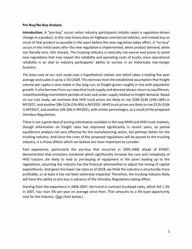
2
Pre-Buy/No-Buy Analysis
Introduction. A “pre-buy” occurs when industry participants initially reject a regulation-driven change in a product, in this case heavy-duty on-highway commercial vehicles, and instead buy as much of that product as possible in the years before the new regulation takes effect. A “no-buy” occurs in the initial years after the new regulation is implemented, when product demand, while not literally zero, falls sharply. The trucking industry is naturally risk-averse and prone to avoid new regulations that may impact the reliability and operating costs of trucks, since operational reliability is so vital to industry participants’ ability to survive in an historically low-margin business.
The base case of our cost study uses a hypothetical market size which takes a trailing five-year average and scales it up by a 1% CAGR. This borrows from the established assumption that freight volume per capita is very stable in the long-run, so freight grows roughly in line with population growth. It also borrows from our view that truck supply and demand always return to equilibrium, notwithstanding intermittent periods of over and under supply relative to freight demand. Based on our cost study, we estimate that HHD truck prices are likely to rise $18k-$24k (14%-18%) in MY2027, and another $8k-$13k (5%-8%) in MY2031. MHD truck prices are likely to rise $12k-$16k in MY2027, and another $4k-$6k in MY2031, with similar percentages, as a result of the proposed Omnibus Regulations.
There is not a great deal of pricing information available in the new MHD and HHD truck markets, though information on freight rates has improved significantly in recent years, so partial equilibrium analysis not very effective for the manufacturing sector, but perhaps better for the trucking industry. And since the costs of the proposed regulations will be passed to the trucking industry, it is those effects which we believe are most important to consider.
Past experience, particularly the pre-buy that occurred in 2005-2006 ahead of EPA07, demonstrates that emissions standards which significantly increase the cost and complexity of HHD tractors are likely to lead to pre-buying of equipment in the years leading up to the regulations, assuming the industry has the financial wherewithal to adjust the timing of capital expenditures. And given the lower tax rates as of 2018, we think the industry is structurally more profitable, or at least it has not been adversely impacted. Therefore, the trucking industry likely will have the ability to pre-buy in advance of the Omnibus Regulations taking effect.
Starting from the experience in 2006-2007, the trend in contract truckload rates, which fell 1.3% in 2007, has risen 3% per-year on average since then. That amounts to a 4%-type opportunity cost for the industry. (See chart below.)

2
With that opportunity cost in mind, we believe the proposed Omnibus Regulations would precipitate the largest-ever pre-buy for medium-heavy and heavy-heavy duty trucks and tractors. The primary repercussions of a pre-buy would be two years of vehicle underproduction in 2027 and 2028 to counterbalance the likely overproduction in 2025 and 2026. While we can make a case that R&D costs are ultimately recouped over time thanks to higher vehicle prices, not all costs are recoverable. There would be significant costs for the OEMs and their employees in terms of the inefficiencies that come with a rapid ramp-up to meet an artificial demand bubble followed by a demand collapse in the period of capacity rebalancing that leads to layoffs and production cuts.
While the vehicle and engine manufacturers will have to handle major market disruptions relating to nonmarket-driven demand impacts, the HHD market has an additional constituency that likely will be severely impacted by the proposed rule-making. The anticipated pre-buy, like the one that occurred ahead of EPA’07 in 2005–2006, is likely to result in significant and unnecessary capacity additions in the HHD trucking industry. A large portion of those truckers operates on a for-hire basis and is dependent upon market rates to move freight. The lower freight rates which will inevitably result from the regulation-driven overcapacity bubble will have a significant adverse financial impact on the nation’s truckers, with an estimated impact of $6.5 – $8.6 billion at net present value.

2
Pre-Buy Model. Using a multi-factor relational model based on a significant history of industry activity before and after the introduction of new emissions regulations, we estimate (in Table 8) the industry will pre-buy 64,800 (4,200 + 60,600) additional HHD tractors and 25,300 (2,600 + 22,700) MHD vocational trucks in 2025 – 2026 ahead of the MY2027 regulations. This adds up to 90,100 total Class 8 vehicles over the two-year pre-buy. Ahead of the MY2031 standards, we estimate another pre-buy of 35,000 (4,200 + 30,700) HHD tractors and 11,600 (2,300 + 9,200) HHD vocational trucks in 2029 – 2030. Vocational trucks are similar to MHD vehicles in that they are typically a component of a job (construction/dump/cement) and are not directly subject to market rates, so the modeled freight rate effects exclude vocational trucks. Overcapacity in MHD vocational trucks will primarily impact manufacturers who will have to lay off workers and lower supplier orders. However, in the HHD tractor market, there likely will be very significant price impacts on freight rates.
Table 8: Prebuy Size Estimates in Units and Percent
The HHD tractor pre-buy model starts with the base tractor price, adds in the 12% Federal Excise Tax (FET) and an average 8% for State and Local taxes. We then raise the sticker price by the cost of meeting the proposed standards, using $23,885 (18% of base), which we settled on because that cost increase was near the center of the range of the $30,300 per-unit value undiscounted at the 2% inflation rate, and the $17,600 per-unit value using a 7% discount rate. We taxed the $23,885 at the FET + state tax rate, added in three years of insurance at a rate of 5% of the truck cost each year, and added financing costs at an interest rate of 5% for half of the value of the
MY2027 $ Change Op.
Costs
MY2027 % Change Op.
Costs
Anticipated Prebuy:
2025
Share of new
Market
Anticipated Prebuy:
2026
Share of new
MarketUS Class 8 Tractor 35,103$ 18.3% 4,219 2.7% 60,622 39.9%US Class 8 Vocational 35,190$ 14.6% 2,620 4.7% 22,667 36.9%US Total Class 8 6,838 3.2% 83,290 39.0%
Source: ACT Research Co.,LLC: Copyright 2020
MY2031 $ Change Op.
Costs
MY2031 % Change Op.
Costs
Anticipated Prebuy:
2029
Share of new
Market
Anticipated Prebuy:
2030
Share of new
MarketUS Class 8 Tractor 12,491$ 6% 4,234 2% 26,717 13%US Class 8 Vocational 14,536$ 6% 2,344 4% 9,236 14%US Total Class 8 6,578 3% 35,953 14%
Source: ACT Research Co.,LLC: Copyright 2020

2
vehicle. This totals about $35,000 of added upfront costs for the HHD vehicle purchaser in MY2027, and another $12,000 in MY2031. (See Table 8.)
Fuel economy considerations all play a role in the model. After considerable discussion, we included the impending fuel economy improvements associated with GHG-2 regulations in MY2027, even though most of those fuel economy improvements will be in effect prior to the Omnibus Regulations. In our cost analysis from the manufacturers’ perspective, we did not include costs or benefits for the GHG-2 regulations, except as we understand the state of the market to be in MY2027. To estimate the social cost to the trucking industry, however, our model’s purpose is to reflect the conditions impacting the industry in MY2027 and MY2031. We considered both the improvements in fuel efficiency and additional use of diesel emissions fluid (DEF), finding that the 4% improvement in fuel efficiency expected in MY2027 from GHG-2 regulations would more than offset a doubling of the DEF dosing rate. Moving from a 2.5% to a 5% DEF dosing rate on a 90,000 mile per-year truckload application would use 233 additional gallons per-year at a cost of about $665, but the 4% fuel efficiency improvement saves $1,300 per-year at 440 gallons in this application. We are not using those estimates as benefits relating to the Omnibus Regulations, but rather to refine our analysis of the potential magnitude of a pre-buy.
Regarding maintenance costs, some of the technology solutions anticipated for the proposed Omnibus Regulations are targeted towards improving the durability of aftertreatment systems, which could have the effect of lowering maintenance expenses in some instances. However, the overall increase in the complexity of the engine and aftertreatment systems likely will require more frequent maintenance for these trucks through their life-cycles, not less. Given the high degree of uncertainty, however, we have not included explicit estimates of maintenance expenses, except to say that there are positives and negatives from a fleet perspective, and as noted earlier in our report, the higher warranty and useful life costs are included in the estimated sticker price increases.
Tractor Pre-Buy. The sum of the multiple costs result in a “willingness to buy” factor, which is the percentage change in total cost of ownership (TCO) of the vehicle before and after the regulation. At a cost of $35,100 in MY2027, the net TCO impact is 18% of the pre-regulation purchase price. Based on historical pre-buys and assuming reasonable industry profit margins leading into the new regulatory mandates, we estimate that the 18% increase will drive an additional 3% of HHD tractor sales in 2025 (4,200 units), and a 40% pre-buy in 2026 (60,600 units). The $12,500 net TCO increase due to the proposed MY2031 standards, which amounts to an additional 6% price/TCO increase, will drive another 2% of tractor sales in 2028 (4,200 units) and an additional 15% pre-buy in 2029 (30,700 units). (See Table 8.)

2
Table 9: Retail Sales and Pre-Buy History and Forecast in the U.S. Class 8 Tractor Market
Freight Rate Impact. Adding these 65,000 “pre-bought” tractors into our population models, where we estimate 1.4 million HHD tractors engaged in truckload and/or less-than-truckload freight hauling, amounts to a 4.5% increase in capacity or supply into the industry. Our freight pricing models indicate that the sensitivity of truckload contract pricing is roughly -64% relative to capacity additions when modeled econometrically with demand and regulatory factors included. In other words, a 1% increase in freight-hauling capacity lowers pricing by .64%, so a 4.5% increase in capacity, as expected in this case, would lower truckload pricing by 2.9%.
Trucking Industry Sizing and Earnings Impact. According to the U.S. Census Bureau’s Quarterly Services Survey, the U.S. trucking industry is on pace for $195 billion in revenue (NAICS code: 4841, General Freight Trucking) in 2019. Using a trailing 5-year industry growth rate of 3% to extrapolate to 2026, the industry should be generating $240 billion of revenue in 2026. A 2.9% pricing impact on a $240 billion segment of the economy would be a cost to aggregate trucking industry earnings of $6.9 billion on an annual basis, and it would likely last 18-24 months. Thus,

2
the total impact on the trucking industry would likely be $10.4 – $13.8 billion of lost earnings in 2026 – 2027. This discounts back to $6.5 - $8.6 billion in 2019 dollars at 7%.
We have focused here on the for-hire market reported on by the Census Bureau. Our estimates do not include effects on the private fleet segment of the trucking industry, which makes up just over half of the tractor fleet, but generally hauls freight for a single company. Private fleets are generally a cost center inside companies that ship goods, with few booking revenue for their services. As a result, we did not include that part of the market in estimating financial impacts.
Vocational Pre-buy. The main focus of our analysis (in Table 8) is on the tractor portion of the heavy-duty Class 8 market, since, over the past decade, tractors have represented 75% of the Class 8 vehicles sold in the US, compared to 25% for the Class 8 market’s vocational segment. Significantly higher miles traveled per-year for tractors mean shorter lengths of ownership due to reliability/downtime issues as miles accrue. On the vocational side of the market, localized vocational applications (P&D, construction, government) mean fewer miles per-year and longer first-buyer ownership. And, as previously discussed, unlike the tractor market, where every vehicle is a profit center, the vocational truck is often a tool used to facilitate a non-transportation related business. Thus, there is significantly more volatility in US tractor demand from year to year compared to the vocational truck portion of the market.
In that regard, like the MHD market, we do not typically view the vocational portion of the HHD market as a candidate for pre-buying. But in terms of vocational equipment pre-buying ahead of EPA07, ACT’s modeling suggests that a prebuy did occur ahead of that regulatory mandate. Vocational buyers and dealers accounted for 30% of the 92,000 units of prebuying that occurred in 2005 and 2006, or 5 percent higher than the segment’s long-run market share. We have concluded that the majority of that prebuy resulted from vocational fleet buyers actively working to avoid the EPA07 emissions mandate.
Using our model, the sharp rise in vehicle costs ahead of the MY2027 mandates in this case indicates that vocational truck buyers will pre-buy approximately 26,000 units in 2025 and 2026. (See Table 8.) At $35,200 in MY2027, the net TCO impact is 15% of the pre-regulation purchase price. That includes a $24,000 price increase, plus taxes, insurance, financing and diesel emissions fluid costs. The net result is that we estimate that the increased costs will drive an additional 5% of vocational tractor sales in 2025 (2,600 units) and a 37% pre-buy in 2026 (22,700 units), which totals to a pre-buy of 25,300 units. For the MY2031 mandate step, the model projects another 4% pre-buy in 2029 (2,300 units) with an additional 14% pre-buy in 2030 (9,200 units) due to a $14,500 net TCO increase for the MY2031 proposed standards, which amounts to an additional 6% price/TCO increase. Combined, the MY2031 vocational Class 8 prebuy sums to 11,600 units.
When combined, the projected US Class 8 prebuy for trucks and tractors rises to 90,100 units ahead of the MY2027 regulatory step, with 6,800 units pulled into 2025 and 83,300 units pulled into 2026. The prebuy represents a 3% increase above modeled 2024 demand and a 39% jump

2
above modeled levels in 2025. For the MY2031 mandate, the model anticipates 6,600 units being pulled into 2029, and an additional pre-buy of 39,900 Class 8 units in 2030. Prebuying as a percentage of the market is 3% in 2028 and 15% in 2029.
Sensitivity Analysis: Costs Using Pre-buy/No-buy Scenario. The tables below (Tables 10-11) provide a sensitivity analysis from the base case costs of the Omnibus Regulations (see Tables 4-7) which assumed a normalized demand environment. Having established that a normalized demand environment is very unlikely, we show below how the cost estimates change when we envision the significantly depressed post-pre-buy market in MY2027 that we think is more likely. In short, the total costs to the manufacturers fall significantly because most of the costs vary with production levels, but the per-unit costs rise because some of those costs are fixed, mainly R&D and compliance program costs.
For HHD vehicles in MY2027 (see Table 10), these industry Total Cost Increase figures are approximately 52% lower than the National costs presented in the base case discussed earlier in this report, and 53% lower on a California basis. (See Tables 4-7.) That is primarily because of a 38% lower vehicle-build forecast.
However, on a per-unit basis, the MY2027 costs are approximately 3% and 31% higher on a National and California-only basis, respectively. Those percentages are consistent across inflation and discount rates.
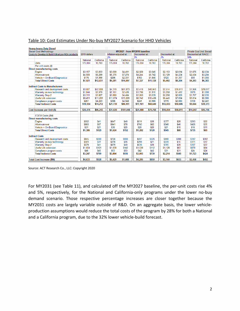
2
Table 10: Cost Estimates Under No-buy MY2027 Scenario for HHD Vehicles
Source: ACT Research Co., LLC: Copyright 2020
For MY2031 (see Table 11), and calculated off the MY2027 baseline, the per-unit costs rise 4% and 5%, respectively, for the National and California-only programs under the lower no-buy demand scenario. Those respective percentage increases are closer together because the MY2031 costs are largely variable outside of R&D. On an aggregate basis, the lower vehicle-production assumptions would reduce the total costs of the program by 28% for both a National and a California program, due to the 32% lower vehicle-build forecast.

2
Table 11: Cost Estimates Under No-buy MY2031 Scenario for HHD Vehicles
Source: ACT Research Co., LLC: Copyright 2020
Dealer Pre-buy. While we have discussed truckers as the primary drivers of pre-buying, there is another group that is also likely to contribute to pre-buying activity ahead of the MY2027 standard –– truck dealers. Based on the experience ahead of EPA’07, we would expect that U.S. MHD and HHD commercial vehicle dealers would likely increase inventory levels aggressively in advance of the proposed MY2027 regulations. Dealers’ ability to add to stock, however, would largely be determined by the availability of manufacturers’ production capacity. Dealers’ pre-buy decisions would be based on several factors:
First, is the cost of pre- versus post-mandate vehicles. With the sharply higher costs likely for the MY2027 vehicles, having lower priced units in inventory should facilitate dealer sales for several months into the post-mandate period.
Second, given the risks that early post-mandate purchasers might face with respect to the reliability of early post-mandate vehicles, most truckers would prefer to let someone else act as the beta-tester for real-world usage. Dealers carrying pre-mandate

2
inventories could provide their risk-averse customers with a competitive edge early in the post-mandate period.
Looking back to the last major pre-buy in 2006, MHD and HHD vehicle dealers both added to inventories over the course of that year. Based on ACT Research data collection, MHD inventory levels rose from 49,500 units at the end of December 2005, to 70,500 units at the end of 2006. A baseline 6% year to year increase in MHD Classes 5-7 retail sales in the U.S. does not explain the 42% inventory increase across 2006.
Reviewing changes to HHD vehicle inventories ahead of EPA07, from December 2005 to January 2007, U.S. Class 8 inventories rose from 42,200 units to 54,600 units, a 29% increase compared to a 12% increase in U.S. Class 8 retail sales from 2005 to 2006. Arguably the HHD dealer inventory pre-buy should have been larger in 2006, but final demand from trucking companies in the U.S. and Canada pushed the North American Class 8 manufacturing to unprecedented levels. In 2006, total North American Class 8 production rose to 376,000 units, 31,000 units higher than the second-best year ever, 2019.
Thus, we suspect that, as was the case in 2006, it will not be a lack of desire on the part of dealers to add inventory that limits Class 8 inventory-building ahead of the MY2027 regulation. Rather, it will be strong purchasing demand on the part of truck fleet operators that will limit dealers’ ability to acquire and maintain those stocks.
Conclusions. The tables set forth below summarize the results of our cost study.
Table 12: Aggregate Costs, Discounted to NPV at 7%
Our results show that on a nationwide base, using a 7% discount rate, the Omnibus Regulations will yield per-vehicle cost increases for HHD vehicles totaling $26,000 ($17,600 in 2027, and $8,400 in 2031), and per-vehicle cost increases for MHD vehicles totaling $15,400 ($11,800 in 2027, and $3,700 in 2031). The aggregate costs to the industry will be $16.7 billion ($13.9 billion in 2027, and $2.8 billion in 2031). This consists of $9.1 billion of manufacturing costs ($6.3 billion

2
in 2027, and $2.8 billion in 2031) and $7.6 billion of pre-buy/no-buy costs (all focused on 2027) on the trucking industry.
On a California-only basis, our results show, again using a 7% discount rate, that the Omnibus Regulations will yield per-vehicle price increase for HHD vehicles totaling $57,900 ($47,700 in 2027, and $10,200 in 2031), and per-vehicle price increases for MHD vehicles totaling $51,400 ($41,500 in 2027, and $9,900 in 2031). The aggregate cost to the vehicle and engine manufacturing industry will be $1.35 billion ($1.14 billion in 2027, and $0.22 billion in 2031).
All in, the aggregate cost to the vehicle and engine manufacturing industry from the Omnibus Regulations, not including the additional costs to vehicle purchasers and operators would be $9.1 billion, and the lost earnings for the trucking industry would be $7.6 billion, bringing the total cost to $17.1 billion. Those very significant cost impacts call into question whether the Omnibus Regulations could be cost-effective, especially on a nationwide basis.

NREL is a national laboratory of the U.S. Department of Energy Office of Energy Efficiency & Renewable Energy Operated by the Alliance for Sustainable Energy, LLC This report is available at no cost from the National Renewable Energy Laboratory (NREL) at www.nrel.gov/publications.
Contract No. DE-AC36-08GO28308
Technical Report NREL/TP-5400-76571 May 2020
On-Road Heavy-Duty Low-NOx Technology Cost Study Lauren A. Lynch, Chad A. Hunter, Bradley T. Zigler, Matthew J. Thornton, and Evan P. Reznicek
National Renewable Energy Laboratory

NREL is a national laboratory of the U.S. Department of Energy Office of Energy Efficiency & Renewable Energy Operated by the Alliance for Sustainable Energy, LLC This report is available at no cost from the National Renewable Energy Laboratory (NREL) at www.nrel.gov/publications.
Contract No. DE-AC36-08GO28308
National Renewable Energy Laboratory 15013 Denver West Parkway Golden, CO 80401 303-275-3000 • www.nrel.gov
Technical Report NREL/TP-5400-76571 May 2020
On-Road Heavy-Duty Low-NOx Technology Cost Study Lauren A. Lynch, Chad A. Hunter, Bradley T. Zigler, Matthew J. Thornton, and Evan P. Reznicek
National Renewable Energy Laboratory
Suggested Citation Lynch, Lauren, A. Chad A. Hunter, Bradley T. Zigler, Matthew J. Thornton, and Evan P. Reznicek. 2020. On-Road Heavy-Duty Low-NOx Technology Cost Study. Golden, CO: National Renewable Energy Laboratory. NREL/TP-5400-76571. https://www.nrel.gov/docs/fy20osti/76571.pdf.

NOTICE
This work was authored by the National Renewable Energy Laboratory, operated by Alliance for Sustainable Energy, LLC, for the U.S. Department of Energy (DOE) under Contract No. DE-AC36-08GO28308. Funding provided by the California Air Resources Board under Funds-In Agreement number 16MSC005/FIA-17-1855. The views expressed herein do not necessarily represent the views of the DOE, the U.S. Government, or the California Air Resources Board.
This report is available at no cost from the National Renewable Energy Laboratory (NREL) at www.nrel.gov/publications.
U.S. Department of Energy (DOE) reports produced after 1991 and a growing number of pre-1991 documents are available free via www.OSTI.gov.
Cover Photos by Dennis Schroeder: (clockwise, left to right) NREL 51934, NREL 45897, NREL 42160, NREL 45891, NREL 48097, NREL 46526.
NREL prints on paper that contains recycled content.
iii This report is available at no cost from the National Renewable Energy Laboratory at www.nrel.gov/publications.
Disclaimer The statements and conclusions in this report are those of the contractor and not necessarily those of the California Air Resources Board. The mention of commercial products, their source, or their use in connection with material reported herein is not to be construed as actual or implied endorsement of such products.

iv This report is available at no cost from the National Renewable Energy Laboratory at www.nrel.gov/publications.
Acknowledgments The authors would like to thank Rasto Brezny from the Manufacturers of Emission Controls Association (MECA), Chris Sharp from Southwest Research Institute (SwRI), George Mitchell and James Sanchez of the U.S. Environmental Protection Agency (EPA), and all of the participating Tier 1 suppliers and engine original equipment manufacturers for their collaboration and information provided in support of this study. This study would not have been possible without the strong support and engagement of those industry partners who participated in supplying incremental cost information. The authors would also like to thank Brian Bush for his development and support of the Scenario Evaluation and Regionalization Analysis model, Margaret Mann for her contributions and input, and Whitney Yeldell for her diligence and attention to detail while editing this report.
This report was written in fulfillment of the California Air Resources Board/U.S. Department of Energy National Renewable Energy Laboratory agreement 16MSC005/FIA-17-1855 under the sponsorship of the California Air Resources Board. Work was completed as of March 2020.

v This report is available at no cost from the National Renewable Energy Laboratory at www.nrel.gov/publications.
List of Acronyms ASC ammonia slip catalyst
CARB California Air Resources Board
DEF diesel exhaust fluid
DOC diesel oxidation catalyst
DPF diesel particulate filter
EGR exhaust gas recirculation
EMFAC EMission FACtor model
EPA U.S. Environmental Protection Agency
FTP Federal Test Procedure
FUL full useful life
g/bhp-hr grams per brake horsepower-hour
GHG greenhouse gas
GVWR gross vehicle weight rating
HD heavy-duty
HDO heavy-duty Otto-cycle
HHDD heavy heavy-duty diesel
hp horsepower
LHDD light heavy-duty diesel
LLC low-load certification
LO-SCR light-off selective catalytic reduction
MECA Manufacturers of Emission Controls Association
MHDD medium heavy-duty diesel
MY model year

vi This report is available at no cost from the National Renewable Energy Laboratory at www.nrel.gov/publications.
NH3 ammonia
NOx oxides of nitrogen
NREL National Renewable Energy Laboratory
OBD on-board diagnostics
OEM original equipment manufacturer
OOS out of state
PM particulate matter
PNA passive NOx absorber
R&D research and development
SCAB South Coast Air Basin
SCR selective catalytic reduction
SCRF selective catalytic reduction on filter
SERA Scenario Evaluation and Regionalization Analysis
SET-RMC Supplemental Emission Test with Ramped Mode Cycles
SI spark ignition
SwRI Southwest Research Institute
TWC three-way catalyst

vii This report is available at no cost from the National Renewable Energy Laboratory at www.nrel.gov/publications.
Executive Summary The National Renewable Energy Laboratory (NREL) conducted a cost analysis for emission control technologies under contract to the California Air Resources Board (CARB). CARB sought incremental cost analysis for emission control technologies for on-road heavy-duty (HD) engines used in vehicles greater than 14,000 pounds (lb) gross vehicle weight rating (GVWR) to achieve oxides of nitrogen (NOx) emissions rates significantly lower than those required by current emissions standards (CARB 2017). This low-NOx emission technology cost analysis comprised two main tasks:
• Task 1: An incremental cost analysis for engine and exhaust aftertreatment systems • Task 2: An engine and exhaust aftertreatment life-cycle cost analysis incorporating
incremental upfront costs and operating costs. The incremental cost analysis included a review of current and under-development engine and exhaust aftertreatment technologies that could achieve 0.02 grams per brake horsepower-hour (g/bhp-hr) NOx on certification test cycles, including a proposed updated certification test cycle that includes additional low-load operating conditions. Diesel, natural gas, and gasoline HD engine applications were studied. Three diesel technology package combinations of engine and exhaust aftertreatment options were selected based on research in progress at Southwest Research Institute (SwRI), also funded by CARB. The three diesel technology packages were intended to bracket potential cost ranges across two engine displacement levels: ~6–7 liters (L) and ~12–13 L. Representative technology packages for HD natural gas (12 L) and gasoline (6 L) engines were also defined, each with a single displacement level providing a tie point to similar diesel options.
Diesel engines were the primary consideration, as they comprise the majority of HD engines. In addition to studying three diesel technology packages across two engine displacement levels, incremental cost bracketing also included model year (MY) 2023 versus 2027 introduction, U.S. versus California-only implementation, and current full useful life (FUL) versus extended FUL and warranty. Direct and indirect incremental costs were broken down to as discrete a level as possible while maintaining data confidentiality. The calculation of incremental costs was limited by a small number of respondents.
The surveyed original equipment manufacturers (OEMs), Tier 1 suppliers, and trade organizations such as the Manufacturers of Emission Controls Association (MECA) responded with incremental cost, not validation that 0.02 g/bhp-hr emissions levels or specific technology packages are feasible. Engine OEM participation was crucial, as only they could provide estimates for indirect costs that represented a significant portion of the total cost. Incremental costs are largely driven by indirect costs associated with engineering research and development costs and warranty costs. The indirect costs are highly dependent on production volumes over which to amortize research and development costs. Indirect costs due to warranty are high, reflecting high uncertainty with new technology and the introduction timeframes. The incremental costs were not adjusted to reflect a retail markup due to the complexity with which pricing decisions are made.
The average incremental cost for the 6–7-L diesel engines for MY 2023 with current FUL ranged from $3,685 to $5,344, but the absolute low and high bounds were between ~$2,000 and over

viii This report is available at no cost from the National Renewable Energy Laboratory at www.nrel.gov/publications.
$9,000. Extending FUL and warranty moved the average incremental costs to a range of $15,370 to $16,245, with tighter low and high bounds (constrained in part by the limited number of responses). The average incremental cost for the 12–13-L diesel engines for MY 2023 with current FUL ranged from $5,340 to $6,063, but the absolute low and high bounds were between ~$3,000 and over $10,000. Extending FUL and warranty moved the average incremental costs to a range of $28,868 to $47,042, with much wider low and high bounds (driven in part by the limited number of responses). The natural gas 12-L engine application was unable to be studied in detail, but OEM feedback indicated the anticipated incremental cost for natural gas engines and aftertreatment technology is within 10% of the low-cost diesel technology package incremental cost for equivalent displacement, possibly due to requiring a moving average window method to assess emission compliance. The gasoline engine 6-L application was also unable to be studied in detail due to lack of OEM feedback, but comparatively low incremental costs were estimated.
A life-cycle cost analysis was completed to understand the full costs to the owner of the vehicles with a 0.02 g/bhp-hr NOx technology package outside of the direct upfront vehicle cost increase. The life-cycle cost analysis sought to incorporate costs associated with the following elements: initial incremental purchase cost, fuel consumption changes (changes in fuel economy), diesel exhaust fluid (DEF) consumption changes, and the maximum FUL of the aftertreatment package (major overhaul intervals). Thus, the life-cycle costs depend on the vehicle type (mileage), region, fuel, engine displacement, maximum useful life, fuel economy change, DEF consumption change, and discount rate.
Three scenarios were defined to evaluate the bounds of the life-cycle costs across all parameters evaluated. For the three scenarios evaluated (Low-Cost, Mid-Cost, High-Cost), the life-cycle costs were evaluated for each EMission FACtor (EMFAC) model vehicle type (CARB 2018b), aggregated to a representative average and calculated across the vehicle fleet for the MY 2027 vehicles. The analysis showed that EMFAC vehicles can have significantly different life-cycle costs and that the spread depends on the scenario evaluated: approximately a $4,000 spread across vehicle types in the Low-Cost scenario, while the High-Cost scenario had nearly a $40,000 difference. This large spread was found to be due to the number of aftertreatment package replacements needed throughout the vehicle lifetime. The aggregated, representative average life-cycle costs for the Mid-Cost scenario were estimated to be $12,700 for the 6-L diesel engine, $13,200 for the 12-L diesel engine, $4,800 for the 12-L natural gas engine, and $800 for the 6-L gasoline engine. The total life-cycle costs to California vehicle owners for the MY 2027 vehicles were estimated to range between $92 million and $1.2 billion, depending on the scenario (Low-Cost or High-Cost) realized.
The sensitivity analysis indicated that the manufacturing volume may be the most important parameter impacting the life-cycle cost; however, limited data were received from the external stakeholders surveyed. The next most important parameter was the assumption of extended FUL and extended warranty, as the increase in aftertreatment lifetime may not exceed the vehicle’s travel requirement, which results in larger replacement costs over the vehicle’s life. However, one may expect that the higher upfront purchase incurred by the vehicle owner should effectively be offset by the repair savings over the lifetime of the vehicle. Next, the aftertreatment cost bound (low/high error bars on the incremental cost data), fuel economy improvement, and

ix This report is available at no cost from the National Renewable Energy Laboratory at www.nrel.gov/publications.
discount rate were found to have a moderate impact on the life-cycle cost. Lastly, the region and DEF consumption change were found to have minimal influence on the life-cycle cost.
The results of this cost analysis reflect the specific technology and aftertreatment FUL assumptions on which the study was based. In particular, the incremental cost of moving from a 0.2g/bhp-hr to 0.02 g/bhp-hr standard is expected to be non-linear due to diminishing returns on technology performance. Extrapolating the results beyond this specific study and outside of these specific assumptions is not recommended and should only be done with careful attention to the scope and limits of this study.

x This report is available at no cost from the National Renewable Energy Laboratory at www.nrel.gov/publications.
Table of Contents Executive Summary .......................................................................................................................... vii Abstract .............................................................................................................................................1 Project Background and Objective ......................................................................................................2 Project Summary ...............................................................................................................................4 1 Task 1: Engine Incremental Cost Analysis ....................................................................................6
1.1 Representative Engine Platform Approach ..........................................................................6 1.2 Identifying Potential Diesel Technologies to Achieve 0.02 g/bhp-hr NOx ..............................9 1.3 Identifying Potential Gasoline and Natural Gas Technologies to Achieve 0.02 g/bhp-hr NOx .. ........................................................................................................................................ 11 1.4 NREL Survey of Potential Technologies to Achieve 0.02 g/bhp-hr NOx ................................ 12
1.4.1 Definition of Baseline Costs of Current Technologies With 2018 EPA Certification ............. 12 1.4.2 NREL Initial Incremental Cost Estimates ............................................................................... 13 1.4.3 First Survey Responses for Incremental Costs of Potential Diesel Technologies .................. 19 1.4.4 Incremental Costs of Potential Technologies with Extended FUL and Warranty, and California-Only Volumes ......................................................................................................................... 25 1.4.5 Incremental Cost Survey Response Observations ................................................................. 31 1.4.6 Incremental Costs for Natural Gas and Gasoline Technology Packages ............................... 32
1.5 Low-, Average-, and High-Cost Estimates .......................................................................... 33 1.5.1 Low-, Average-, and High-Cost Estimates for MY 2023 with Current FUL and Warranty ..... 33 1.5.2 Low-, Average-, and High-Cost Estimates for MY 2027 with Extended Warranty and Extended Useful Life ............................................................................................................................... 35
1.6 Summary of Incremental Cost Analysis ............................................................................. 37 2 Task 2: Engine Life-Cycle Costs .................................................................................................. 38
2.1 Maximum Full Useful Life Analysis .................................................................................... 38 2.2 Approach ......................................................................................................................... 38
2.2.1 Scenario Evaluation and Regionalization Analysis (SERA) Model ......................................... 39 2.2.2 Data Sources .......................................................................................................................... 40 2.2.3 SERA Model Validation .......................................................................................................... 42 2.2.4 Manufacturing Volume Analysis ........................................................................................... 43
2.3 Parameters Investigated .................................................................................................. 43 2.3.1 Scenario Analysis ................................................................................................................... 44 2.3.2 Sensitivity Analysis ................................................................................................................ 46
2.4 Results ............................................................................................................................. 47 2.4.1 Case Study: T7 Tractor and T6 OOS Small Vehicle Life-Cycle Costs ...................................... 47 2.4.2 Scenario Analysis Results ...................................................................................................... 54 2.4.3 Sensitivity Analysis Results .................................................................................................... 59
2.5 Life-Cycle Cost Analysis Summary and Conclusions ........................................................... 60 3 Conclusions ............................................................................................................................. 62 References ....................................................................................................................................... 64 Appendix A. Selected Results for Specific EMFAC Vehicles of Interest to CARB .............................. 65 Appendix B. EMFAC Vehicle Disaggregation ................................................................................. 67

xi This report is available at no cost from the National Renewable Energy Laboratory at www.nrel.gov/publications.
List of Figures Figure 1. Schematic of proposed low- and average-cost diesel aftertreatment technology ........................ 10 Figure 2. Schematic of proposed high-cost diesel aftertreatment technology ............................................ 11 Figure 3. Summary of 6–7-L potential technology packages for MY 2023 with current FUL .................. 34 Figure 4. Summary of 12–13-L potential technology packages for MY 2023 with current FUL .............. 35 Figure 5. Summary of 6–7-L potential technology packages for MY 2027 with extended FUL and
warranty ................................................................................................................................. 36 Figure 6. Summary of 12–13-L potential technology packages for MY 2027 with extended FUL and
warranty ................................................................................................................................. 36 Figure 7. The general SERA stock model data flow ................................................................................... 39 Figure 8. Data flow and analysis using the SERA model for life-cycle cost analysis ................................ 42 Figure 9. SERA model validation against the CA Vision 2.1 model .......................................................... 43 Figure 10. Annual present value cost for a T7 Tractor 12-L diesel engine designed for current full useful
life (435,000 miles; top) and extended full useful life (1,000,000 miles; bottom) for MY 2027 in the South Coast Air Basin with a 2.5% increase in DEF consumption, a discount rate of 7%, and national manufacturing volumes .......................................................................... 48
Figure 11. Annual present value cost for a T6 OOS small 6–7-L diesel engine designed for current full useful life (110,000 miles; top) and extended full useful life (550,000 miles; bottom) for MY 2027 in the South Coast Air Basin with a 2.5% increase in DEF consumption, a discount rate of 7%, and national manufacturing volumes .......................................................................... 48
Figure 12. Total present value cost for the T7 Tractor and T6 OOS small vehicles with diesel engine aftertreatment technology as a function of incremental steps between current FUL and extended FUL for two scenarios: replacements at end of FUL (orange) and no replacements (blue) ...................................................................................................................................... 50
Figure 13. Present value cost for different Class 6 and Class 8 diesel engine aftertreatment technologies with current full useful life ..................................................................................................... 51
Figure 14. Present value cost for different Class 6 and Class 8 diesel engine aftertreatment technologies with extended full useful life.................................................................................................. 52
Figure 15. Present value cost for the T7 Tractor and T6 OOS small trucks with diesel engines designed for current full useful life at both California and national manufacturing volumes ............... 53
Figure 16. Present value cost for the T7 Tractor and T7 OOS small trucks with diesel engine aftertreatment technologies designed for current FUL as a function of region ...................... 54
Figure 17. Present value cost for the T7 Tractor and T7 OOS small trucks with diesel engine aftertreatment technologies designed for extended FUL and warranty as a function of region ................................................................................................................................................ 54
Figure 18. Present value life-cycle cost for all EMFAC vehicles in the low-cost scenario, segmented by fuel type and engine displacement (DSL = diesel, GAS = gasoline) ..................................... 55
Figure 19. Present value life-cycle cost for all EMFAC vehicles in the mid-cost scenario, segmented by fuel type and engine displacement (DSL = diesel, GAS = gasoline, CNG = compressed natural gas) ............................................................................................................................. 56
Figure 20. Present value life-cycle cost for all EMFAC vehicles in the high-cost scenario, segmented by fuel type and engine displacement (DSL = diesel) ................................................................ 57
Figure 21. EMFAC vehicle sales-weighted average present value cost for 6-L and 12-L diesel engine technologies under the three cost scenarios described in Table 23 ........................................ 57
Figure 22. Scenario analysis for a 12-liter compressed natural-gas and 6-liter gasoline engine ................ 58 Figure 23. Total California fleet life-cycle cost for the MY 2027 vehicles for each scenario analyzed ..... 58 Figure 24. Sensitivity diagram for the diesel 6–7-L and 12–13-L engines relative to the mid-cost scenario
................................................................................................................................................ 59 Figure 25. Sensitivity diagram for the gasoline 6-L engine relative to the mid-cost scenario .................... 60 Figure 26. Sensitivity diagram for the natural-gas 12-L engine relative to the mid-cost scenario ............. 60

xii This report is available at no cost from the National Renewable Energy Laboratory at www.nrel.gov/publications.
List of Tables Table 1. Current and Proposed Extended Full Useful Life and Warranty for Engine Life-Cycle Cost
Analysis .................................................................................................................................... 5 Table 2. Engine Platform Analysis for Incremental Cost Analysis .............................................................. 7 Table 3. NREL Estimates of Potential Low-Cost Diesel Technology Package 6–7 L ............................... 14 Table 4. NREL Estimates of Potential Low-Cost Diesel Technology Package 12–13 L ........................... 15 Table 5. NREL Estimate of Potential Average-Cost Diesel Technology Package 6–7 L........................... 16 Table 6. NREL Estimates of Potential Average-Cost Diesel Technology Package 12–13 L ..................... 17 Table 7. NREL Estimates of Potential High-Cost Diesel Technology Package 6–7 L .............................. 18 Table 8. NREL Estimates of Potential High-Cost Diesel Technology Package 12–13 L .......................... 19 Table 9. Survey Responses for Potential Low-Cost Diesel Technology Package 6–7 L ............................ 20 Table 10. Survey Responses for Potential Low-Cost Diesel Technology Package 12–13 L ...................... 21 Table 11. Survey Responses for Potential Average-Cost Diesel Technology Package 6–7 L ................... 22 Table 12. Survey Responses for Potential Average-Cost Diesel Technology Package 12–13 L ............... 23 Table 13. Survey Responses for Potential High-Cost Diesel Technology Package 6–7 L ......................... 24 Table 14. Survey Responses for Potential High-Cost Diesel Technology Package 12–13 L ..................... 25 Table 15. Survey Responses for Potential Low-Cost Diesel Technology Package 6–7 L with Extended
FUL, Extended Warranty, and California-Only Volumes ..................................................... 26 Table 16. Survey Responses for Potential Low-Cost Diesel Technology Package 12–13 L with Extended
FUL, Extended Warranty, and CA Volumes ......................................................................... 27 Table 17. Survey Responses for Potential Average-Cost Diesel Technology Package 6–7 L with Extended
FUL, Extended Warranty, and California-Only Volumes ..................................................... 28 Table 18. Survey Responses for Potential Average-Cost Diesel Technology Package 12–13 L with
Extended FUL, Extended Warranty, and California-Only Volumes ..................................... 29 Table 19. Survey Responses for Potential High-Cost Diesel Technology Package 6–7 L with Extended
FUL, Extended Warranty, and California-Only Volumes ..................................................... 30 Table 20. Survey Responses for Potential High-Cost Diesel Technology Package 12–13 L with Extended
FUL, Extended Warranty, and California-Only Volumes ..................................................... 31 Table 21. Data Sources Used in Life-Cycle Cost Analysis ........................................................................ 41 Table 22. Life-Cycle Cost Parameters Investigated in this Study .............................................................. 44 Table 23. Scenario Definitions for Bounding Analysis .............................................................................. 45 Table 24. Example Vehicle Sales Weighted Average ................................................................................ 46

1 This report is available at no cost from the National Renewable Energy Laboratory at www.nrel.gov/publications.
Abstract The National Renewable Energy Laboratory (NREL) conducted a cost analysis for emission control technologies under contract to the California Air Resources Board (CARB). CARB sought incremental cost analysis for emission control technologies for on-road heavy-duty (HD) engines used in vehicles greater than 14,000 pounds (lb) gross vehicle weight rating (GVWR) to achieve oxides of nitrogen (NOx) emissions rates significantly lower than those required by current emissions standards. Specifically, incremental costs (without any retail price markup) were estimated for representative diesel, natural gas, and gasoline engine and emission aftertreatment systems that were selected to represent potential technology packages that could achieve 0.02 grams per brake horsepower-hour (g/bhp-hr) NOx on certification test cycles, including a proposed updated certification test cycle that includes additional low-load operating conditions. NREL surveyed stakeholders including industry association groups, Tier 1 suppliers, and engine original equipment manufacturers (OEMs) to estimate incremental direct and indirect costs. Incremental costs were considered for current engine full useful life (FUL) definitions, as well as with proposed increased FUL and warranty periods. The incremental costs were subsequently incorporated in life-cycle cost analyses examining the incremental engine and aftertreatment costs along with life-cycle costs over the various engine FUL scenarios. Life-cycle costs analysis included the incremental upfront cost, fuel consumption changes (changes in fuel economy), diesel exhaust fluid (DEF) consumption changes, and the maximum FUL of the aftertreatment package (major overhaul intervals).

2 This report is available at no cost from the National Renewable Energy Laboratory at www.nrel.gov/publications.
Project Background and Objective Current emission standards for heavy-duty diesel engines, established by the United States Environmental Protection Agency (EPA) for 2010, specify a limit of 0.20 grams per brake horsepower-hour (g/bhp-hr) NOx. This standard represents a 90% reduction from the previous benchmark of 2.0 g/bhp-hr and applies to both heavy-duty diesel engines and heavy-duty Otto-cycle engines used in vehicles greater than 14,000-lb GVWR.
Diesel-engine manufacturers utilize a variety of technologies in order to meet these standards, primarily among them being selective catalytic reduction (SCR). Natural-gas engine manufacturers use SCR for lean-burn engines and three-way catalysts (TWCs) for stoichiometric engines. Both of these methods reduce NOx emissions by removing them from the engine-out exhaust prior to exiting the tailpipe. These manufacturers have used lessons learned from other applications such as stationary-source and light-duty vehicles to meet current NOx emission requirements, and as these technologies mature there are opportunities to reduce emissions even further.
The California Air Resources Board (CARB), together with the Southwest Research Institute (SwRI), is currently funding several research programs to investigate the feasibility of achieving NOx emissions less than the 2010 limit of 0.20 g/bhp-hr. The first (“Stage 1”) project is a $1.6 million research contract between CARB and SwRI to evaluate improved engine emission control calibration, enhanced aftertreatment technologies and configurations, improved aftertreatment thermal management, urea dosing strategies, and engine management practices for two heavy-duty engines: one natural-gas engine with a TWC and one diesel engine with a diesel particulate filter (DPF) and SCR. The target emission rate for this project, which was finalized in December 2016, is 0.02 g/bhp-hr NOx.
CARB is also contracting a $1.05 million “Stage 2” project with SwRI to further optimize the diesel engine aftertreatment system for low engine-load duty cycles typical of city driving. Stage 2 objectives are to develop a supplemental low-load certification test cycle that will, along with the Federal Test Procedure (FTP), ensure NOx control under nearly all driving conditions and evaluate metrics for in-use testing under low-load operations. The “Stage 3” project, currently in the planning stage, will complement the Stage 1 and Stage 2 efforts with testing on an additional engine that is representative of likely future engine configurations.
Alongside current emission standards, CARB and EPA both require that heavy-duty engines meet these standards throughout their entire useful life. The useful life period is defined according to a vehicle’s GVWR, and for heavy-duty engines ranges from 110,000–435,000 miles. The useful life period for Otto-cycle and light heavy-duty diesel engines (14,001–19,500-lb GVWR) is 110,000 miles/10 years; for medium heavy-duty diesel engines (19,501–33,000-lb GVWR) 185,000 miles/10 years; and for heavy heavy-duty diesel engines (greater than 33,000-lb GVWR) 435,000 miles/10 years, or 22,000 hours.
Well-maintained on-road diesel engines can operate significantly beyond their currently defined useful life periods (e.g., many heavy-duty diesel engines currently operate upwards of 800,000 miles to over a million miles), and CARB is taking this reality into consideration as it evaluates the consequences of lowering its NOx emission targets. Engine durability becomes a critical

3 This report is available at no cost from the National Renewable Energy Laboratory at www.nrel.gov/publications.
factor with longer useful life definitions, particularly in preventing “upstream” engine component failures that can damage “downstream” emission control system components and cause excess emissions of criteria pollutants such as particulate matter (PM) and NOx. Therefore, manufacturers will need to improve the durability of their engines and emission control systems by developing higher-quality parts and assembly methods and replacement of components and/or subsystems.
CARB is expected to propose new standards to be implemented by 2024, which will set even lower NOx emission standards and add new certification test cycles to ensure emission control at low-load operations. Adding this new test cycle to the certification requirement is expected to drive further improvements to aftertreatment hardware and engine control and calibration.
With these new emission standards of approximately 0.02 g/bhp-hr NOx in mind, it is important to examine the direct and indirect costs of implementing new technologies, both the incremental costs to original equipment manufacturers and the costs of using the technology packages throughout the engines’ useful life. These costs can be divided by category, including the specific technologies for achieving the NOx standard, the costs to increase durability (extended useful life), and the costs of the on-board diagnostics (OBD) hardware and calibration works impacted by the changes. This cost analysis will use specific emission control and engine technologies identified by SwRI in Stages 1 and 2, along with testing that is representative of likely future engine configurations.

4 This report is available at no cost from the National Renewable Energy Laboratory at www.nrel.gov/publications.
Project Summary This project was defined by two tasks—Task 1: Engine Incremental Cost Analysis and Task 2: Engine Life-Cycle Costs. For Task 1, NREL reviewed current technologies and technology packages that are being examined as part of the SwRI projects, Stages 2 and 3, as provided by CARB. NREL identified and reviewed likely emission control and engine technologies to meet 0.02 g/bhp-hr NOx requirements with CARB staff based on Stage 2 and 3 efforts from SwRI testing of potential future engine configurations. These technologies were then defined as the potential technologies and the starting point of developing a low-NOx technology incremental cost analysis from 2018 baseline costs.
NREL then evaluated these potential technologies and technology packages for engine plus aftertreatment incremental cost analysis via a series of surveys sent to Tier 1 suppliers, trade organizations, and engine OEMs. The surveys defined the potential technologies broken into engine components, emission control components, subsystems, and indirect costs. The combination of incremental costs (over the 2018 baseline) associated with developing and integrating the specified lower NOx emission control technologies into the engines, the costs of increasing the durability of these engines and their emission control systems, and the costs of directly impacted OBD hardware and calibration works of these specified technology packages were then examined to understand the total incremental cost implications to Tier 1 suppliers and engine OEMs of the potential technologies.
The evaluation of costs was dependent on cooperation from Tier 1 suppliers, trade organizations and engine OEMs, as well as the availability of direct and indirect cost information for engine and emission control technologies. NREL utilized existing relationships with industry partners in order to perform a thorough cost assessment but could not guarantee full cooperation or sharing of confidential cost information from Tier 1 suppliers, trade organizations, and engine OEMs.
After accounting for the initial incremental cost implications to Tier 1 suppliers (both collectively through the Manufacturers of Emission Controls Association [MECA] and individually) and engine OEMs, NREL conducted a life-cycle cost analysis as Task 2 to examine the costs of using the specified technology packages during the engines’ certification full useful life (FUL). NREL utilized a range of FUL values for each heavy-duty vehicle category, Classes 4 through 8. The current FUL mileage—for heavy-duty engines of 110,000 miles up to 435,000 miles, depending on a vehicle's GVWR; 110,000 miles/10 years for heavy-duty Otto-cycle (HDO) and light heavy-duty diesel (LHDD) engines (14,001–19,500-lb GVWR); 185,000 miles/10 years for medium heavy-duty diesel (MHDD) engines (19,501–33,000-lb GVWR); and 435,000 miles/10 years or 22,000 hours for heavy heavy-duty diesel (HHDD) engines (greater than 33,000-lb GVWR)—was defined as the low-end value of the range for each specific vehicle class. For the high-end value of the range, NREL utilized input from CARB for proposed extended FUL targets as the upper-bound levels for each specific vehicle class: 250,000 miles/15 years for HDO engines (14,001–19,500-lb GVWR), 550,000 miles/15 years for LHDD engines (14,001–19,500-lb GVWR) and MHDD engines (14,001–19,500-lb GVWR), and 1,000,000 miles/15 years for HHDD engines (greater than 33,000-lb GVWR). Additionally, per CARB’s guidance, the high-end value with extended FUL also includes the provision that warranty periods will increase to 80% of the extended FUL, both in mileage and time, except for heavy-

5 This report is available at no cost from the National Renewable Energy Laboratory at www.nrel.gov/publications.
duty Otto-cycle, which was specified as 220,000 miles/12 years. The current FUL defining the lower bound and the extended FUL defining the upper bound are summarized in Table 1.
Table 1. Current and Proposed Extended Full Useful Life and Warranty for Engine Life-Cycle Cost Analysis
LHDD MHDD HHDD Natural Gas – Otto
Heavy-Duty – Otto
GVWR (lb) 14,001–19,500 19,501–33,000 >33,000 >33,000 14,000
Current full useful life
110,000 miles/10 years
185,000 miles/10 years
435,000 miles/10 years,
22,000 hours
435,000 miles/10 years,
22,000 hours
110,000 miles/15 years
Proposed extended full useful life
550,000 miles/15 years
550,000 miles/15 years
1,000,000 miles/15
years
1,000,000 miles/15
years
250,000 miles/15 years
Proposed warranty period with extended full useful life
440,000 miles/12 years
440,000 miles/12 years
800,000 miles/12
years
800,000 miles/12
years
220,000 miles/12 years
After accounting for the initial incremental costs of the technologies, as determined in Task 1, the life-cycle cost assessment of Task 2 then took into account the aftertreatment technologies' effects on fuel consumption, DEF consumption, major overhaul intervals (full useful life estimates), manufacturing volume, and financial discount rates. The life-cycle cost modeled for each vehicle is specific to the EMission FACtor (EMFAC) model’s vehicle definition of vehicle miles traveled, which depends on the specific region, vocation, model year, fuel type, and age.
For the life-cycle cost analysis in Task 2, the aftertreatment full useful life mileage was used to set the equipment overhaul schedule. For all scenarios in the life-cycle cost analysis, the incremental cost associated with the aftertreatment package was assumed to be incurred after the truck mileage exceeded the stated maximum FUL. This assumption is expected to be conservative, as not all aftertreatment packages will fail immediately after they exceed their stated maximum FUL and statistical analysis of failure rates combined with data on aftertreatment technology operating and maintenance costs were not available. To understand the impact of this assumption on the life-cycle cost, a sensitivity analysis was completed assuming the aftertreatment package would not need to be replaced over the vehicle’s lifetime, as that provides the lower bound on the life-cycle cost.

6 This report is available at no cost from the National Renewable Energy Laboratory at www.nrel.gov/publications.
1. Task 1: Engine Incremental Cost Analysis 1.1 Representative Engine Platform Approach The engine and aftertreatment incremental cost analysis began with a review of 54 model year (MY) 2018 medium- and heavy-duty engine family CARB certification summaries, covering Class 4–8 vehicle applications. The review provided background on the fuels used, range of engine displacements for each service class (i.e., LHDD, MHDD, HHDD, HDO), current technologies utilized, and certification levels versus Federal Test Procedure (FTP) and heavy-duty Supplemental Emissions Test with Ramped Mode Cycles (SET-RMC) standards for NOx. Because the majority of Class 4–8 engines are diesel fueled, incremental costs for diesel engines was the primary focus of the study. Natural gas and gasoline were also studied, but liquified petroleum gas/propane was not. A limited number of engine platforms were initially selected to represent the Class 4–8 vehicle population, based on engine displacement. This down-selection was necessary to come up with a reasonable number of representative engine platforms to use for the incremental cost analysis that could subsequently be used in the Task 2 life-cycle cost analysis over large vehicle populations, while keeping manageable the burden of calculating incremental cost for surveys conducted with Tier 1 suppliers, trade organizations, and engine OEMs. The initial engine platforms included: 6-L LHDD, 9-L MHDD, 12-L HHDD, 15-L HHDD, 12-L natural gas, and 6-L HDO (gasoline). Initial reviews with industry provided feedback that this number of engine platforms was still too large, and the diesel engine platforms could be consolidated and referenced to approximate horsepower levels. As a result, the diesel engine platforms were reduced to ~6–7 L with ~300 horsepower (hp) and ~12–13 L with ~475 hp. This reduction would still provide incremental costs with appropriate discrete levels. The in-between calculation for a 9-L engine was agreed to not be worth the additional burden for industry survey responses. The elimination of the 15-L engine was agreed to be covered by increased power density from ~12–13-L engines with future trends.
Current technologies were reviewed to benchmark the baseline for the 0.02 g/bhp-hr NOx incremental cost. The industry surveys were designed to collect direct and indirect cost information for engine and aftertreatment subsystems from a 2018 baseline, with a 0.20 g/bhp-hr standard, as well as multiple technology packages assumed to meet a potential future 0.02 g/bhp-hr NOx standard under a proposed new low-load certification (LLC), in addition to FTP and SET-RMC. The incremental costs would form the basis of Task 1. While the surveys were designed to allow industry respondents to start with their own 2018 baseline and did not explicitly define a common set of identical technologies, the CARB certification review showed most diesel engines in the 6–7-L and 12–13-L ranges were common in having direct diesel injection, cooled exhaust gas recirculation (EGR), turbocharging, a diesel oxidation catalyst (DOC), a diesel particulate filter (DPF), and selective catalytic reduction (SCR) using DEF. The technology packages supporting 0.02 g/bhp-hr NOx selected for incremental cost study are described in more detail below.
A single natural-gas engine platform was selected at 12 L to align with the ~12–13-L diesel platform. The CARB certification review showed a number of natural-gas engines (in various displacements, meeting MHDD and HHDD requirements) sharing the same technologies: stoichiometric Otto-cycle operation, spark ignition (SI), throttle body fuel injection, turbocharging, cooled EGR, and a three-way catalyst (TWC).

7 This report is available at no cost from the National Renewable Energy Laboratory at www.nrel.gov/publications.
A single gasoline-fueled HDO platform was selected at 6 L to align with the ~6–7-L diesel platform. The CARB certification review showed HDO gasoline is approaching 0.02 g/bhp-hr NOx on the current certification cycles using stoichiometric, SI, naturally aspirated, EGR technologies with a TWC technology package.
Utilizing the results and recommendations from Stage 2 and 3 efforts from SwRI testing of potential future diesel-engine configurations, NREL identified three diesel technology packages to evaluate the total incremental cost implications for an MY 2023 release nationwide. These identified diesel technology packages were intended to represent potential low-, average-, and high-cost options to meet a 0.02 g/bhp-hr NOx standard and were meant to provide a broader assessment of potential incremental costs than a single option. As previously referenced, no natural-gas technology package was surveyed for incremental costs related to 0.02 g/bhp-hr NOx, and the HDO gasoline technology package only included TWC and calibration upgrades. The resulting engine platforms defined for the incremental cost study are summarized in Table 2.
Table 2. Engine Platform Analysis for Incremental Cost Analysis
LHDD HHDD Natural Gas – HHDD standard
Gasoline – HDO
Engines ~6–7 L
~300 hp
~12–13 L
~475 hp
12 L 6 L
Current full useful life
110,000 miles/10 years
435,000 miles/10 years,
22,000 hours
435,000 miles/10 years,
22,000 hours
110,000 miles/10 years
Low-Cost Tech. $$$ $$$ Not applicable Not applicable
Avg.-Cost Tech. $$$ $$$ Not applicable $$$
High-Cost Tech. $$$ $$$ Not applicable Not applicable
NREL then directly surveyed heavy-duty engine OEMs, Tier 1 suppliers, emission control technology manufacturers, and industry trade organizations to obtain the most accurate and current cost information for the identified likely technology packages to meet 0.02 g/bhp-hr NOx requirements and the cost implications for using these specific technologies. The cost survey included a definition of the potential technologies as engine components, emission control components, subsystems and strategies, and indirect costs broken into categories of research and development (R&D) costs, certification costs, and warranty costs. The combination of costs associated with developing and integrating the specified lower NOx emission control technologies into the engines, the costs of increasing the durability of these engines and their emission control systems, and the costs of impacted OBD hardware and calibration of these specified technology package were then examined to understand the total incremental cost implications to Tier 1 suppliers and engine OEMs of the potential technologies in two different surveys. Any incremental costs associated with future OBD requirements unrelated to meeting 0.02 g/bhp-hr NOx were excluded from this study. Similarly, incremental costs related to future greenhouse gas (GHG) or fuel efficiency requirements and not specifically to meeting 0.02 g/bhp-hr NOx were also excluded.

8 This report is available at no cost from the National Renewable Energy Laboratory at www.nrel.gov/publications.
The first survey assumed that the 0.02 g/bhp-hr NOx regulation beginning MY 2023 included current FTP and SET-RMC steady-state test cycles, as well as a proposed new LLC for medium- and heavy-duty engine system certification. While not finalized and currently the topic of ongoing research, the new LLC engine cycle was assumed to last approximately 90 minutes, including a combination of motoring, sustained low load, and high-power transients. This first survey considered FUL hours/miles to remain the same as the current regulation. The survey was designed to allow industry respondents to start with their own 2018 baseline and did not explicitly define a common set of identical technologies. As a reference point, NREL provided internally generated estimates (from research, literature review, and engineering judgement) for the 2018 current technology costs (Posada, Chambliss, and Blumberg 2016; Posada Sanchez, Bandivadekar, and German 2012; Ou et al. 2019). Direct costs for both a 2018 baseline and 0.02 g/bhp-hr technology packages were surveyed on discrete engine and aftertreatment subsystem levels, along with indirect costs. The level of discrete subsystems was kept as small as possible to provide insight for where the costs accumulate while also being kept large enough to prevent identification of proprietary or confidential cost information from an individual respondent. Furthermore, only incremental costs are reported in this report and preliminary reviews with CARB to prevent identifying proprietary or confidential 2018 baseline costs. The survey requested future costs be calculated in 2018 dollars. The first survey asked for production volumes to be identified and to provide guidance on cost impacts for 0.02 g/bhp-hr incremental costs if regulation were to include all of the United States or California only.
The second survey was a follow-up survey sent to those Tier 1 suppliers, trade organization, and engine OEMs that responded to the first survey. The technology packages remained the same as the first survey, but instead assumed 0.02 g/bhp-hr NOx regulation beginning MY 2027 and again included current FTP and SET-RMC steady-state test cycles, as well as a new LLC. This second survey also considered extended useful life hours/miles as proposed by CARB in Table 1. The second survey asked for costing information to consider 0.02 g/bhp-hr regulation if only California were included, representing lower production volumes than a scenario where all of the U.S. were included.
NREL then aggregated all of the data from the cost survey responses and the initial estimates derived by NREL from research, literature review, and engineering judgement. The incremental costs were not adjusted to reflect a retail markup due to the complexity with which pricing decisions are made. In responding to NREL’s surveys, trade organizations, Tier 1 suppliers, and OEMs did provide feedback that they did not agree or conclude that these technologies would be feasible for meeting the 0.02 g/bhp-hr NOx requirements by MY 2023. Their valuable input was strictly a costing exercise and not a technology feasibility assessment. The diesel incremental cost information resulted in a range of costs due to the format of the provided data from the responses received. This range consisted of a low, average, and high estimate for engine technology costs, aftertreatment technology costs, OBD-related direct costs, and indirect costs. The survey results for the diesel engine and aftertreatment technology packages were then defined as three total incremental costs of low, average, and high estimates based on the identified potential technology packages to achieve 0.02 g/bhp-hr NOx requirements.
Fewer responses were received for the natural gas (HHDD standard) engine platform, preventing NREL from sufficiently aggregating incremental cost information to protect proprietary information. Therefore, NREL reported the total integrated incremental cost as an order of

9 This report is available at no cost from the National Renewable Energy Laboratory at www.nrel.gov/publications.
magnitude in comparison to the diesel engine with similar displacement results; the subsystem-level engine, aftertreatment, and OBD system direct costs as well as the indirect costs were not broken out or reported.
Similarly, few responses were received for the gasoline HDO engine platform. Some aggregation was possible for direct costs, but only NREL estimates were available for indirect costs. As a result, only total integrated incremental costs are reported.
1.2 Identifying Potential Diesel Technologies to Achieve 0.02 g/bhp-hr NOx
CARB is currently funding several research programs with SwRI to investigate the feasibility of achieving 0.02 g/bhp-hr NOx emissions with a diesel engine and is in the Stage 3 process of testing specific emission control and diesel engine technologies. Based on SwRI’s research and results from Stages 1 and 2 (Sharp et al., “Thermal Management,” 2017; Sharp et al., “Comparison of Advanced,” 2017; Sharp et al., “NOx Management,” 2017), NREL identified different engine and emission control technologies that showed potential capabilities of achieving 0.02 g/bhp-hr NOx emissions during current FTP and SET-RMC steady-state test cycles, as well as a proposed new LLC cycle by MY 2023. These diesel engine and emission control technologies were grouped into three different diesel technology packages to represent a range of potential low-, average-, and high-costing diesel technology package solutions.
The potential low-cost diesel technology package consisted of an EPA 2017 certification-compliant engine with a variable-geometry turbo charger, no turbo compounding, and a combined engine thermal management strategy of EGR cooler bypass, charge air cooler bypass, and a turbine bypass. In addition to the engine system, the emission control technologies included two points of DEF dosing and DEF mixers, one light-off SCR (LO-SCR), one DOC, one DPF, two SCRs, and one ammonia slip catalyst (ASC). The aftertreatment system also contained a NOx sensor upstream of the first DEF dosing system and mixer, a temperature sensor upstream of the LO-SCR, a second temperature sensor downstream of the LO-SCR, a second NOx sensor downstream LO-SCR and upstream of the DOC, a third temperature sensor downstream of the LO-SCR and upstream of the DOC, a fourth temperature sensor downstream of the DOC and upstream of the DPF, a fifth temperature sensor downstream of the DPF and upstream of the first second DEF dosing system and mixer, an ammonia (NH3) sensor downstream the first SCR and upstream the second SCR, a sixth temperature sensor downstream of the ASC, and a third NOx sensor downstream of the ASC. An example of the aftertreatment technology system with sensors is illustrated in Figure 1.

10 This report is available at no cost from the National Renewable Energy Laboratory at www.nrel.gov/publications.
Figure 1. Schematic of proposed low- and average-cost diesel aftertreatment technology
Figure from SwRI
The potential average-cost diesel technology package consisted of an EPA 2017 certification-compliant engine with a variable-geometry turbo charger, no turbo compounding, and an engine thermal management strategy and technology for cylinder deactivation. In addition to the engine system, the emission control technologies again included the same aftertreatment system as the low-cost diesel technology package with two points of DEF dosing and DEF mixers, one LO-SCR, one DOC, one DPF, two SCRs, and one ASC, as shown in Figure 1. The aftertreatment system also contained a NOx sensor upstream of the first DEF dosing system and mixer, a temperature sensor upstream of the LO-SCR, a second temperature sensor downstream of the LO-SCR, a second NOx sensor downstream LO-SCR and upstream of the DOC, a third temperature sensor downstream of the LO-SCR and upstream of the DOC, a fourth temperature sensor downstream of the DOC and upstream of the DPF, a fifth temperature sensor downstream of the DPF and upstream of the first second DEF dosing system and mixer, an NH3 sensor downstream of the first SCR and upstream of the second SCR, a sixth temperature sensor downstream of the ASC, and a third NOx sensor downstream of the ASC.
The proposed high-cost diesel technology package consisted of an EPA 2017 certification-compliant engine with a variable-geometry turbo charger, no turbo compounding, and a combined engine thermal management strategy of EGR cooler bypass, charge air cooler bypass, and a turbine bypass. In addition to the engine system, the emission control technologies included a passive NOx absorber (PNA), one DOC, one DEF doser and DEF mixer, one selective catalytic reduction on filter (SCRF), one SCR, and one ASC. The aftertreatment system also contained a NOx sensor upstream of the PNA, a second NOx sensor downstream of the PNA, an NH3 sensor downstream of the SCRF and upstream of the SCR, and a third NOx sensor downstream of the ASC. An example of the aftertreatment technology is illustrated in Figure 2.

11 This report is available at no cost from the National Renewable Energy Laboratory at www.nrel.gov/publications.
Figure 2. Schematic of proposed high-cost diesel aftertreatment technology Figure from SwRI
Note that the proposed technology packages that were initially designed to represent low-, average-, and high-cost combinations. It was assumed that the PNA, as a very new technology, would drive incremental costs to be higher than other packages. Likewise, cylinder deactivation was assumed to have a higher incremental cost than cooler bypasses for charge air, EGR, and turbine given the same aftertreatment package. However, once incremental cost information became available, the relative incremental costs did not necessarily turn out in that order. Nevertheless, to maintain consistency in the study, the proposed technology packages continued to be referred by their initial naming convention.
1.3 Identifying Potential Gasoline and Natural Gas Technologies to Achieve 0.02 g/bhp-hr NOx
The single natural-gas 12-L engine platform was selected to align with the ~12–13-L diesel platform. The CARB certification review showed a number of natural-gas engines (in various displacements, meeting MHDD and HHDD requirements) sharing the same technologies: stoichiometric Otto-cycle operation, SI, throttle body fuel injection, turbocharging, cooled EGR, and a TWC. Notably, most of the natural-gas engines already meet CARB’s optional low-NOx standard at 0.02 g/bhp-hr under the current certification cycles. Because the proposed LLC certification was assessed to be less challenging for a stoichiometric SI engine than a diesel engine, it was assumed that the current 2018 “baseline” technology package would already meet the new 0.02 g/bhp-hr NOx requirement. Incremental cost for 0.02 g/bhp-hr NOx was therefore not calculated, but cost increases related to extending FUL were considered. As noted later in this report, industry feedback identified this assumption as incorrect.
The single gasoline-fueled HDO platform was selected at 6 L to align with the ~6–7-L diesel platform. The CARB certification review showed HDO gasoline is approaching 0.02 g/bhp-hr NOx on the current certification cycles, and similar technology (stoichiometric, SI, naturally aspirated, EGR technologies with a TWC) with liquified petroleum gas fuel has recently been certified at 0.05 g/bhp-hr and 0.02 g/bhp-hr under CARB’s optional low-NOx standards. The base engine was assumed to need no significant upgrades for the 0.02 g/bhp-hr standard with proposed LLC certification cost study, but TWC direct cost upgrades and indirect costs for engineering, certification, and warranty were surveyed, as well as extended FUL impacts. Vehicle packaging impacts were noted to also potentially be required to enable close coupling of the TWCs.

12 This report is available at no cost from the National Renewable Energy Laboratory at www.nrel.gov/publications.
1.4 NREL Survey of Potential Technologies to Achieve 0.02 g/bhp-hr NOx
NREL created a cost survey with a baseline price of an MY 2018 system representing an EPA 2018 certification-compliant engine and aftertreatment system in 2018 dollars and asked trade organizations, Tier 1 suppliers, and engine OEMs to provide incremental cost estimates in comparison to the above-defined technologies with the potential to achieve 0.02 g/bhp-hr NOx requirements. The cost survey was reviewed with CARB and EPA staff and approved by CARB before submitting for requested responses. The survey consisted of two technology packages for diesel engine and aftertreatment systems, one technology package for natural-gas engines and aftertreatment, and one technology package for gasoline engines and aftertreatment systems. To simplify the survey for stakeholder input and avoid asking for input on three separate combinations of engine and aftertreatment technology packages, the two unique diesel engine technology packages (charge air, EGR, and turbine cooler bypass vs. cylinder deactivation) were surveyed with the two unique aftertreatment technology packages (Figure 1 and Figure 2). From these incremental cost inputs, NREL could construct the proposed low-, average-, and high-cost combined engine and aftertreatment technology packages.
The first survey assumed that the 0.02 g/bhp-hr NOx regulation beginning MY 2023 included current FTP and SET-RMC steady-state test cycles, as well as a new LLC cycle. While not finalized and currently the topic of ongoing research, the LLC was assumed as a new engine certification cycle lasting approximately 90 minutes and included a combination of motoring, sustained low load, and high-power transients. This first survey also considered FUL hours/miles to remain the same as the current regulation. NREL also prefaced the likely follow-up survey seeking additional guidance on how increasing FUL hour/mile requirements may further affect the provided costs.
The second survey was a follow-up survey sent to the same Tier 1 suppliers, trade organizations, and engine OEMs that responded to the first survey. The technology packages remained the same and instead assumed 0.02 g/bhp-hr NOx regulation beginning MY 2027 and again included current FTP and SET-RMC steady-state test cycles, as well as a proposed new LLC cycle. Again, while not finalized and currently the topic of ongoing research, the LLC was assumed as a new engine certification cycle lasting approximately 90 minutes and included a combination of motoring, sustained low load, and high-power transients. This second survey considered extended FUL hours/miles as proposed by CARB’s Stage 2 definitions defined in Table 1. Additionally, per CARB’s guidance, the extended FUL also included the assumption that warranty periods will increase to 80% of the extended FUL, both in mileage and time, except for heavy-duty Otto cycle, which was specified as 220,000 miles/12 years.
1.4.1 Definition of Baseline Costs of Current Technologies With 2018 EPA Certification
As a starting point for the incremental cost definition of potential technologies to meet 0.02 g/bhp-hr NOx requirements, NREL estimated the direct manufacturing costs and indirect costs for an EPA 2018-certified engine and aftertreatment system production costs of current technology to meet 0.20 g/bhp-hr NOx in 2018 dollars for the U.S. market based on literature reviews and engineering judgement (Posada, Chambliss, and Blumberg, 2016; Posada Sanchez, Bandivadekar, and German 2012; Ou 2019). These estimates were defined for two diesel

13 This report is available at no cost from the National Renewable Energy Laboratory at www.nrel.gov/publications.
platforms, 6–7 L and 12–13 L, based on the majority of current market offerings. NREL then estimated the incremental cost of MY 2023 technologies to meet a 0.02 g/bhp-hr NOx requirement based on literature review, engineering judgement, and feedback from SwRI to provide a baseline estimate of the incremental costs for the two potential diesel technology packages for each of the two engine platforms. The NREL estimates for EPA 2018-certified (0.20 g/bhp-hr NOx) engine and aftertreatment direct and indirect costs, as well as NREL estimates for incremental direct and indirect costs for MY 2023 0.02 g/bhp-hr NOx were generated as starting points for stakeholders to consider in the survey. NREL requested survey responses to utilize the baseline estimates, if accurate, or to correct NREL's incremental cost estimates as necessary. Only incremental costs are revealed in this report.
The baseline technology packages for the diesel engine and aftertreatment technology consisted of an EPA 2018-certified engine, a DOC, a DPF, a DEF dosing system and mixer (with a single doser), am SCR with ASC, one NOx sensor, three NH3 sensors, and four temperature sensors. These components were the same for the two platforms of 6–7 L and 12–13 L. The baseline costs and resulting incremental costs were scaled accordingly. The baseline technology package for the gasoline HDO engine platform consisted of stoichiometric, SI, naturally aspirated, EGR technologies with a TWC. The baseline technology package for the natural-gas system consisted of stoichiometric Otto-cycle operation, SI, throttle body fuel injection, turbocharging, cooled EGR, and a TWC.
1.4.2 NREL Initial Incremental Cost Estimates NREL’s initial estimated incremental costs of the potential diesel technology package likely to be the lowest incremental cost to meet 0.02 g/bhp-hr NOx for the 6–7-L platform are depicted in Table 3. This technology package consisted of an EPA 2017 certification-compliant engine with a variable-geometry turbo charger, no turbo compounding, and a combined engine thermal management strategy of EGR cooler bypass, charge air cooler bypass, and a turbine bypass. In addition to the engine system, the emission control technologies included two points of DEF dosing and DEF mixers, one LO-SCR, one DOC, one DPF, two SCRs, and one ASC. In the following tables, note that negative incremental costs mean the cost for that component/subsystem reduce from the 2018 baseline.

14 This report is available at no cost from the National Renewable Energy Laboratory at www.nrel.gov/publications.
Table 3. NREL Estimates of Potential Low-Cost Diesel Technology Package 6–7 L
Cost Component Incremental Cost Estimate
EGR Cooler Bypass $330
Charge Air Cooler Bypass $200
Turbine Bypass $220
Total Engine Technology Incremental Cost $750
LO-SCR $530
DOC ($15)
DPF ($45)
SCR+ASC and DEF Dosing System $751
OBD Sensors and Controllers (NOx, NH3, and Temp Sensors) ($66)
Total Aftertreatment Technology Incremental Cost $1,155
R&D Engineering Incremental Cost $100
Certification Incremental Costs $0
Warranty Incremental Costs $0
Total Indirect Incremental Costs to Manufacturer $100
Total Incremental Cost Comparison $2,005
NREL’s initial estimated incremental costs of the potential diesel technology package, likely to be the lowest incremental cost to meet 0.02 g/bhp-hr NOx for the 12–13-L platform, are depicted in Table 4.

15 This report is available at no cost from the National Renewable Energy Laboratory at www.nrel.gov/publications.
Table 4. NREL Estimates of Potential Low-Cost Diesel Technology Package 12–13 L
Cost Component Incremental Cost Estimate
EGR Cooler Bypass $330
Charge Air Cooler Bypass $200
Turbine Bypass $220
Total Engine Technology Incremental Cost
$750
LO-SCR $750
DOC $504
DPF ($98)
SCR+ASC and DEF Dosing System
$1,277
OBD Sensors and Controllers (NOx, NH3, and Temp Sensors)
($66)
Total Aftertreatment Technology Incremental Cost
$2,367
R&D Engineering Incremental Cost
$100
Certification Incremental Costs $0
Warranty Incremental Costs $0
Total Indirect Incremental Costs to Manufacturer
$100
Total Incremental Cost Comparison
$3,217
NREL’s initial estimated incremental costs of the potential diesel technology package, likely to be an average of incremental cost to meet 0.02 g/bhp-hr NOx for the 6–7-L platform, are depicted in Table 5. The potential average-cost diesel technology package consisted of an EPA 2017 certification-compliant engine with a variable-geometry turbo charger, no turbo compounding, and an engine thermal management strategy and technology for cylinder deactivation. In addition to the engine system, the emission control technologies again included the same aftertreatment system as the low-cost diesel technology package with two points of DEF dosing and DEF mixers, one LO-SCR, one DOC, one DPF, two SCRs, and one ASC.

16 This report is available at no cost from the National Renewable Energy Laboratory at www.nrel.gov/publications.
Table 5. NREL Estimate of Potential Average-Cost Diesel Technology Package 6–7 L
Cost Component Incremental Cost Estimate
Cylinder Deactivation $1,050
Total Engine Technology Incremental Cost $1,050
LO-SCR $530
DOC ($15)
DPF ($45)
SCR+ASC and DEF Dosing System $751
OBD Sensors and Controllers (NOx, NH3, and Temp Sensors) ($66)
Total Aftertreatment Technology Incremental Cost $1,155
R&D Engineering Incremental Cost $100
Certification Incremental Costs $0
Warranty Incremental Costs $0
Total Indirect Incremental Costs to Manufacturer $100
Total Incremental Cost Comparison $2,305
NREL’s initial estimated incremental costs of the potential diesel technology package, likely to be the average incremental cost to meet 0.02 g/bhp-hr NOx for the 12–13-L platform, are depicted in Table 6.

17 This report is available at no cost from the National Renewable Energy Laboratory at www.nrel.gov/publications.
Table 6. NREL Estimates of Potential Average-Cost Diesel Technology Package 12–13 L
Cost Component Incremental Cost Estimate
Cylinder Deactivation $1,050
Total Engine Technology Incremental Cost $1,050
LO-SCR $750
DOC $504
DPF $98
SCR+ASC and DEF Dosing System $1,277
OBD Sensors and Controllers (NOx, NH3, and Temp Sensors) ($66)
Total Aftertreatment Technology Incremental Cost $2,563
R&D Engineering Incremental Cost $100
Certification Incremental Costs $0
Warranty Incremental Costs $0
Total Indirect Incremental Costs to Manufacturer $100
Total Incremental Cost Comparison $3,713
NREL’s initial estimated incremental costs of the potential diesel technology package, likely to be the highest incremental cost to meet 0.02 g/bhp-hr NOx for the 6–7-L platform, are depicted in Table 7. The potential high-cost diesel technology package consisted of an EPA 2017 certification-compliant engine with a variable-geometry turbo charger, no turbo compounding, and a combined engine thermal management strategy of EGR cooler bypass, charge air cooler bypass, and a turbine bypass. In addition to the engine system, the emission control technologies included a PNA, one DOC, one DEF doser and DEF mixer, one SCRF, one SCR, and one ASC.

18 This report is available at no cost from the National Renewable Energy Laboratory at www.nrel.gov/publications.
Table 7. NREL Estimates of Potential High-Cost Diesel Technology Package 6–7 L
Cost Component Incremental Cost Estimate
EGR Cooler Bypass $330
Charge Air Cooler Bypass $200
Turbine Bypass $220
Total Engine Technology Incremental Cost $750
PNA $730
DOC ($15)
DPF (2018 baseline system only) ($759)
SCRF $714
SCR+ASC and DEF Dosing System $74
OBD Sensors and Controllers (NOx, NH3, and Temp Sensors) $314
Total Aftertreatment Technology Incremental Cost $1,058
R&D Engineering Incremental Cost $0
Certification Incremental Costs $0
Warranty Incremental Costs $0
Total Indirect Incremental Costs to Manufacturer $0
Total Incremental Cost Comparison $1,808
NREL’s initial estimated incremental costs of the potential diesel technology package, likely to be the highest incremental cost to meet 0.02 g/bhp-hr NOx for the 12–13-L platform, are depicted in Table 8.
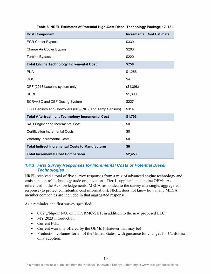
19 This report is available at no cost from the National Renewable Energy Laboratory at www.nrel.gov/publications.
Table 8. NREL Estimates of Potential High-Cost Diesel Technology Package 12–13 L
Cost Component Incremental Cost Estimate
EGR Cooler Bypass $330
Charge Air Cooler Bypass $200
Turbine Bypass $220
Total Engine Technology Incremental Cost $750
PNA $1,256
DOC $4
DPF (2018 baseline system only) ($1,398)
SCRF $1,300
SCR+ASC and DEF Dosing System $227
OBD Sensors and Controllers (NOx, NH3, and Temp Sensors) $314
Total Aftertreatment Technology Incremental Cost $1,703
R&D Engineering Incremental Cost $0
Certification Incremental Costs $0
Warranty Incremental Costs $0
Total Indirect Incremental Costs to Manufacturer $0
Total Incremental Cost Comparison $2,453
1.4.3 First Survey Responses for Incremental Costs of Potential Diesel Technologies
NREL received a total of five survey responses from a mix of advanced engine technology and emission control technology trade organizations, Tier 1 suppliers, and engine OEMs. As referenced in the Acknowledgements, MECA responded to the survey in a single, aggregated response (to protect confidential cost information). NREL does not know how many MECA member companies are included in that aggregated response.
As a reminder, the first survey specified:
• 0.02 g/bhp-hr NOx on FTP, RMC-SET, in addition to the new proposed LLC • MY 2023 introduction • Current FUL • Current warranty offered by the OEMs (whatever that may be) • Production volumes for all of the United States, with guidance for changes for California-
only adoption.

20 This report is available at no cost from the National Renewable Energy Laboratory at www.nrel.gov/publications.
NREL received feedback for U.S. volumes, with very little information regarding impacts for California-only adoption. As NREL was unable to aggregate California-only adoption incremental costs, only incremental costs for U.S. volumes are reported.
After receiving the responses to the first survey request, NREL aggregated the incremental cost data into a range of low, average, and high responses for the potential low-cost diesel technology package, as summarized below for 6–7 L in Table 9 and 12–13 L in Table 10. Note that these low, average, and high incremental cost responses are not to be confused with the proposed low-, average-, and high-cost technology packages. Also, note that the low, average, and high responses for each component/subsystem (row) were calculated so that the total low, average, and high incremental cost may not directly reflect any single survey response.
Table 9. Survey Responses for Potential Low-Cost Diesel Technology Package 6–7 L
6–7 L Low Avg. High
EGR Cooler Bypass $170 $243 $330
Charge Air Cooler Bypass $128 $167 $200
Turbine Bypass $170 $207 $230
Total Engine Technology Incremental Cost $468 $617 $760
LO-SCR $401 $944 $2,200
DOC ($15) $10 $30
DPF ($45) ($17) $0
SCR+ASC and DEF Dosing System $300 $621 $823
OBD Sensors and Controllers (NOx, NH3, and Temp Sensors) $141 $333 $800
Other $50 $175 $300
Total Aftertreatment Technology Incremental Cost $832 $2,066 $4,153
R&D Engineering Incremental Cost $70 $85 $100
Certification Incremental Costs $0 $25 $50
Warranty Incremental Costs $750 $1,875 $3,000
Total Indirect Incremental Costs to Manufacturer $820 $1,985 $3,150
Total Incremental Cost Comparison $2,120 $4,668 $8,063

21 This report is available at no cost from the National Renewable Energy Laboratory at www.nrel.gov/publications.
Table 10. Survey Responses for Potential Low-Cost Diesel Technology Package 12–13 L
12–13 L Low Avg. High
EGR Cooler Bypass $170 $302 $408
Charge Air Cooler Bypass $128 $185 $240
Turbine Bypass $170 $215 $240
Total Engine Technology Incremental Cost $468 $702 $888
LO-SCR $574 $1,120 $2,450
DOC $0 $89 $250
DPF ($98) ($44) $0
SCR+ASC and DEF Dosing System $500 $784 $1,100
OBD Sensors and Controllers (NOx, NH3, and Temp Sensors) $158 $330 $600
Other $50 $150 $300
Total Aftertreatment Technology Incremental Cost $1,184 $2,429 $4,700
R&D Engineering Incremental Cost $110 $354 $503
Certification Incremental Costs $0 $21 $50
Warranty Incremental Costs $1,500 $1,833 $2,500
Total Indirect Incremental Costs to Manufacturer $1,610 $2,208 $3,053
Total Incremental Cost Comparison $3,262 $5,339 $8,641
After receiving the responses to the first survey request, NREL aggregated the incremental cost data into a range of low, average, and high estimates for the potential average-cost diesel technology package, as summarized for 6–7 L in Table 11 and 12–13 L in Table 12.

22 This report is available at no cost from the National Renewable Energy Laboratory at www.nrel.gov/publications.
Table 11. Survey Responses for Potential Average-Cost Diesel Technology Package 6–7 L
6–7 L Low Avg. High
Cylinder Deactivation $480 $790 $1,140
Other $150 $505 $860
Total Engine Technology Incremental Cost $630 $1,295 $2,000
LO-SCR $401 $944 $2,200
DOC ($15) $10 $30
DPF ($45) ($17) $0
SCR+ASC and DEF Dosing System $300 $621 $823
OBD Sensors and Controllers (NOx, NH3, and Temp Sensors) $141 $333 $800
Other $50 $175 $300
Total Aftertreatment Technology Incremental Cost $832 $2,064 $4,153
R&D Engineering Incremental Cost $70 $85 $100
Certification Incremental Costs $0 $25 $50
Warranty Incremental Costs $750 $1,875 $3,000
Total Indirect Incremental Costs to Manufacturer $820 $1,985 $3,150
Total Incremental Cost Comparison $2,282 $5,344 $9,303

23 This report is available at no cost from the National Renewable Energy Laboratory at www.nrel.gov/publications.
Table 12. Survey Responses for Potential Average-Cost Diesel Technology Package 12–13 L
12–13 L Low Avg. High
Cylinder Deactivation $561 $952 $1,550
Other $150 $625 $1,100
Total Engine Technology Cost $711 $1,577 $2,650
LO-SCR $574 $1,120 $2,450
DOC $0 $89 $250
DPF ($98) ($44) $0
SCR+ASC and DEF Dosing System $500 $784 $1,100
OBD Sensors and Controllers (NOx, NH3, and Temp Sensors) $158 $330 $600
Other $50 $150 $300
Total Aftertreatment Technology Incremental Cost $1,184 $2,429 $4,700
R&D Engineering Incremental Cost $110 $354 $503
Certification Incremental Costs $0 $21 $50
Warranty Incremental Costs $1,500 $1,833 $2,500
Total Indirect Incremental Costs to Manufacturer $1,610 $2,209 $3,053
Total Incremental Cost Comparison $3,505 $6,214 $10,403
After receiving the responses to the first survey request, NREL aggregated the incremental cost data into a range of low, average, and high estimates for the potential high-cost diesel technology package, as summarized for 6–7 L in Table 13 and 12–13 L in Table 14.

24 This report is available at no cost from the National Renewable Energy Laboratory at www.nrel.gov/publications.
Table 13. Survey Responses for Potential High-Cost Diesel Technology Package 6–7 L
6–7 L Low Avg. High
EGR Cooler Bypass $170 $243 $330
Charge Air Cooler Bypass $128 $167 $200
Turbine Bypass $170 $207 $230
Total Engine Technology Incremental Cost
$468 $617 $760
PNA $701 $883 $1,000
DOC ($15) ($12) ($9)
DPF (2018 baseline system only)
($759) ($549) ($377)
SCRF $500 $559 $677
SCR+ASC and DEF Dosing System
$584 $722 $793
OBD Sensors and Controllers (NOx, NH3, and Temp Sensors)
$141 $214 $313
Other $50 $50 $50
Total Aftertreatment Technology Incremental Cost
$1,202 $1,868 $2,447
R&D Engineering Incremental Cost
$400 $400 $400
Certification Incremental Costs
$50 $50 $50
Warranty Incremental Costs $750 $750 $750
Total Indirect Incremental Costs to Manufacturer
$1,200 $1,200 $1,200
Total Incremental Cost Comparison
$2,870 $3,685 $4,407

25 This report is available at no cost from the National Renewable Energy Laboratory at www.nrel.gov/publications.
Table 14. Survey Responses for Potential High-Cost Diesel Technology Package 12–13 L
12–13 L Low Avg. High
EGR Cooler Bypass $170 $302 $408
Charge Air Cooler Bypass $128 $185 $240
Turbine Bypass $170 $215 $240
Total Engine Technology Incremental Cost $468 $702 $888
PNA $1,147 $2,270 $3,880
DOC $0 $11 $22
DPF (2018 baseline system only) ($881) ($673) ($560)
SCRF $800 $930 $1,162
SCR+ASC and DEF Dosing System ($209) $387 $723
OBD Sensors and Controllers (NOx, NH3, and Temp Sensors) $158 $254 $330
Other $50 $75 $100
Total Aftertreatment Technology Incremental Cost $1,065 $3,253 $5,657
R&D Engineering Incremental Cost $350 $427 $503
Certification Incremental Costs $13 $32 $50
Warranty Incremental Costs $1,500 $1,650 $1,800
Total Indirect Incremental Costs to Manufacturer $1,863 $2,108 $2,353
Total Incremental Cost Comparison $3,396 $6,063 $8,898
1.4.4 Incremental Costs of Potential Technologies with Extended FUL and Warranty, and California-Only Volumes
After receiving the responses to the first survey request, NREL aggregated the incremental cost data into a range of low, average, and high estimates, as summarized previously. NREL then followed up with an additional survey to identify incremental costs from the MY 2018 baseline, but also to add extended FUL and warranty per Table 1. Lower production volumes representing California only (instead of all of the United States) were also incorporated. The survey assumed implementation for MY 2027 (instead of MY 2023, as in the first survey), as additional time would be necessary to engineer for extended FUL and warranty. Table 15 through Table 20 summarize these additional survey responses.

26 This report is available at no cost from the National Renewable Energy Laboratory at www.nrel.gov/publications.
Table 15. Survey Responses for Potential Low-Cost Diesel Technology Package 6–7 L with Extended FUL, Extended Warranty, and California-Only Volumes
6–7 L Low Avg. High
EGR Cooler Bypass $289 $390 $490
Charge Air Cooler Bypass $191 $225 $259
Turbine Bypass $255 $296 $345
Total Engine Technology Incremental Cost $735 $911 $1,094
LO-SCR $513 $1135 $2,200
DOC $0 $99 $171
DPF $0 $95 $164
SCR+ASC and DEF Dosing System $300 $1161 $1829
OBD Sensors and Controllers (NOx, NH3, and Temp Sensors) $738 $845 $997
Other $300 $300 $300
Total Aftertreatment Technology Incremental Cost $1,851 $3,635 $5,661
R&D Engineering Incremental Cost $70 $70 $70
Certification Incremental Costs $0 $0 $0
Warranty Incremental Costs $10,800 $10,800 $10,800
Total Indirect Incremental Costs to Manufacturer $10,870 $10,870 $10,870
Total Incremental Cost Comparison $13,456 $15,416 $17,625

27 This report is available at no cost from the National Renewable Energy Laboratory at www.nrel.gov/publications.
Table 16. Survey Responses for Potential Low-Cost Diesel Technology Package 12–13 L with Extended FUL, Extended Warranty, and CA Volumes
12–13 L Low Avg. High
EGR Cooler Bypass $289 $390 $490
Charge Air Cooler Bypass $191 $246 $288
Turbine Bypass $255 $296 $345
Total Engine Technology Incremental Cost $735 $932 $1,123
LO-SCR $736 $1,330 $2,450
DOC $0 $144 $330
DPF $0 $83 $191
SCR+ASC and DEF Dosing System $500 $1,240 $1,892
OBD Sensors and Controllers (NOx, NH3, and Temp Sensors) $476 $765 $997
Other $300 $950 $1,600
Total Aftertreatment Technology Incremental Cost $2,012 $4,512 $7,460
R&D Engineering Incremental Cost $110 $357 $603
Certification Incremental Costs $0 $7 $13
Warranty Incremental Costs $7,840 $23,061 $38,282
Total Indirect Incremental Costs to Manufacturer $7,950 $23,424 $38,898
Total Incremental Cost Comparison $10,697 $28,868 $47,481

28 This report is available at no cost from the National Renewable Energy Laboratory at www.nrel.gov/publications.
Table 17. Survey Responses for Potential Average-Cost Diesel Technology Package 6–7 L with Extended FUL, Extended Warranty, and California-Only Volumes
6–7 L Low Avg. High
Cylinder Deactivation $638 $880 $1,140
Other $860 $860 $860
Total Engine Technology Incremental Cost $1,498 $1,740 $2,000
LO-SCR $513 $1,135 $2,200
DOC $0 $99 $171
DPF $0 $95 $164
SCR+ASC and DEF Dosing System $300 $1,161 $1,829
OBD Sensors and Controllers (NOx, NH3, and Temp Sensors) $738 $845 $997
Other $300 $300 $300
Total Aftertreatment Technology Incremental Cost $1,851 $3,635 $5,661
R&D Engineering Incremental Cost $70 $70 $70
Certification Incremental Costs $0 $0 $0
Warranty Incremental Costs $10,800 $10,800 $10,800
Total Indirect Incremental Costs to Manufacturer $10,870 $10,870 $10,870
Total Incremental Cost Comparison $14,219 $16,245 $18,531

29 This report is available at no cost from the National Renewable Energy Laboratory at www.nrel.gov/publications.
Table 18. Survey Responses for Potential Average-Cost Diesel Technology Package 12–13 L with Extended FUL, Extended Warranty, and California-Only Volumes
12–13 L Low Avg. High
Cylinder Deactivation $724 $1,176 $1,860
Other $1,100 $1,100 $1,100
Total Engine Technology Cost $1,824 $2,276 $2,960
LO-SCR $736 $1,330 $2,450
DOC $0 $144 $330
DPF $0 $83 $191
SCR+ASC and DEF Dosing System $500 $1,240 $1,892
OBD Sensors and Controllers (NOx, NH3, and Temp Sensors) $476 $765 $997
Other $300 $950 $1,600
Total Aftertreatment Technology Incremental Cost $2,012 $4,512 $7,460
R&D Engineering Incremental Cost $110 $357 $603
Certification Incremental Costs $0 $7 $13
Warranty Incremental Costs $7,840 $23,061 $38,282
Total Indirect Incremental Costs to Manufacturer $7,950 $23,424 $38,898
Total Incremental Cost Comparison $11,786 $30,212 $49,318

30 This report is available at no cost from the National Renewable Energy Laboratory at www.nrel.gov/publications.
Table 19. Survey Responses for Potential High-Cost Diesel Technology Package 6–7 L with Extended FUL, Extended Warranty, and California-Only Volumes
6–7 L Low Avg. High
EGR Cooler Bypass $289 $340 $391
Charge Air Cooler Bypass $191 $225 $259
Turbine Bypass $255 $296 $345
Total Engine Technology Incremental Cost
$735 $865 $995
PNA $924 $1,097 $1,250
DOC $101 $119 $136
DPF (2018 baseline system only) ($511) ($444) ($377)
SCRF $679 $799 $919
SCR+ASC and DEF Dosing System $1,374 $1,616 $1,858
OBD Sensors and Controllers (NOx, NH3, and Temp Sensors)
$738 $868 $997
Other $0 $0 $0
Total Aftertreatment Technology Incremental Cost
$3,305 $4,044 $4,783
R&D Engineering Incremental Cost $xx $xx $xx
Certification Incremental Costs $xx $xx $xx
Warranty Incremental Costs $xx $xx $xx
Total Indirect Incremental Costs to Manufacturer
$xx $xx $xx
Total Incremental Cost Comparison $xx $xx $xx
Note for Table 19 that insufficient responses were received for this technology package with respect to indirect costs to allow sufficient aggregation. Therefore, indirect and total incremental costs were not calculated.

31 This report is available at no cost from the National Renewable Energy Laboratory at www.nrel.gov/publications.
Table 20. Survey Responses for Potential High-Cost Diesel Technology Package 12–13 L with Extended FUL, Extended Warranty, and California-Only Volumes
12–13 L Low Avg. High
EGR Cooler Bypass $289 $390 $490
Charge Air Cooler Bypass $191 $246 $288
Turbine Bypass $255 $296 $345
Total Engine Technology Incremental Cost $735 $932 $1,123
PNA $1,592 $2,801 $4,656
DOC $0 $153 $263
DPF (2018 baseline system only) ($881) ($698) ($560)
SCRF $960 $1,220 $1,553
SCR+ASC and DEF Dosing System ($209) $1,077 $1,977
OBD Sensors and Controllers (NOx, NH3, and Temp Sensors) $426 $720 $997
Other $1,600 $1,600 $1,600
Total Aftertreatment Technology Incremental Cost $3,488 $6,873 $10,486
R&D Engineering Incremental Cost $603 $603 $603
Certification Incremental Costs $13 $13 $13
Warranty Incremental Costs $38,621 $38,621 $38,621
Total Indirect Incremental Costs to Manufacturer $39,237 $39,237 $39,273
Total Incremental Cost Comparison $43,460 $47,042 $50,846
It should be noted that the total indirect incremental cost estimates by manufacturers, and the total incremental costs in Table 15 to Table 20, are dominated by the warranty incremental costs. In some cases, the high estimate of incremental warranty costs is over $38,000. As discussed in Section 1.4.5, the warranty incremental costs were based on a very small sample size, and may be biased high due to the OEMs’ uncertainty regarding covering warranty for unfamiliar technology needed to meet a 0.02 g/bhp-hr NOx standard at the same time with much longer FULs than current FULs.
1.4.5 Incremental Cost Survey Response Observations The following general observations can be made regarding the incremental costs reported in Table 3 through Table 20.
• The initial NREL estimates for total incremental costs were fairly close to the lower end of survey responses for the first survey (MY 2023, U.S. volume, current FUL).
• Indirect costs are a significant portion of the total cost.
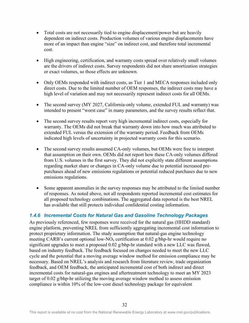
32 This report is available at no cost from the National Renewable Energy Laboratory at www.nrel.gov/publications.
• Total costs are not necessarily tied to engine displacement/power but are heavily dependent on indirect costs. Production volumes of various engine displacements have more of an impact than engine “size” on indirect cost, and therefore total incremental cost.
• High engineering, certification, and warranty costs spread over relatively small volumes are the drivers of indirect costs. Survey respondents did not share amortization strategies or exact volumes, so those effects are unknown.
• Only OEMs responded with indirect costs, as Tier 1 and MECA responses included only direct costs. Due to the limited number of OEM responses, the indirect costs may have a high level of variation and may not necessarily represent indirect costs for all OEMs.
• The second survey (MY 2027, California-only volume, extended FUL and warranty) was intended to present “worst case” in many parameters, and the survey results reflect that.
• The second survey results report very high incremental indirect costs, especially for warranty. The OEMs did not break that warranty down into how much was attributed to extended FUL versus the extension of the warranty period. Feedback from OEMs indicated high levels of uncertainty in projected warranty costs for this scenario.
• The second survey results assumed CA-only volumes, but OEMs were free to interpret that assumption on their own. OEMs did not report how these CA-only volumes differed from U.S. volumes in the first survey. They did not explicitly state different assumptions regarding market share or changes in CA-only volume due to potential increased pre-purchases ahead of new emissions regulations or potential reduced purchases due to new emissions regulations.
• Some apparent anomalies in the survey responses may be attributed to the limited number of responses. As noted above, not all respondents reported incremental cost estimates for all proposed technology combinations. The aggregated data reported is the best NREL has available that still protects individual confidential costing information.
1.4.6 Incremental Costs for Natural Gas and Gasoline Technology Packages As previously referenced, few responses were received for the natural gas (HHDD standard) engine platform, preventing NREL from sufficiently aggregating incremental cost information to protect proprietary information. The study assumption that natural-gas engine technology meeting CARB’s current optional low-NOx certification at 0.02 g/bhp-hr would require no significant upgrades to meet a proposed 0.02 g/bhp-hr standard with a new LLC was flawed, based on industry feedback. The feedback focused on changes needed to meet the new LLC cycle and the potential that a moving average window method for emission compliance may be necessary. Based on NREL’s analysis and research from literature review, trade organization feedback, and OEM feedback, the anticipated incremental cost of both indirect and direct incremental costs for natural-gas engines and aftertreatment technology to meet an MY 2023 target of 0.02 g/bhp-hr utilizing the moving average window method to assess emission compliance is within 10% of the low-cost diesel technology package for equivalent

33 This report is available at no cost from the National Renewable Energy Laboratory at www.nrel.gov/publications.
displacement. A round number estimate total of $3,000 incremental cost was subsequently used for the Task 2: Engine Life-Cycle Costs study.
Similarly, few responses were received for the gasoline HDO engine platform. Some aggregation was possible for direct costs, but only NREL estimates were available for indirect costs. As a result, only total integrated (including direct and indirect) incremental costs ranging from $353 to $468 for MY 2023 were calculated with current FUL.
1.5 Low-, Average-, and High-Cost Estimates Because NREL received a range of values in response to both surveys, the diesel incremental cost analysis results in nine different points of costs, with low-, average-, and high-cost responses to each of the potential low-, average-, and high-cost diesel technology packages.
1.5.1 Low-, Average-, and High-Cost Estimates for MY 2023 with Current FUL and Warranty
These different points of cost defining the range of data received in response to the first survey for MY 2023 and current full useful life as defined in Table 1 are depicted by error bars within the summary graphs in Figure 3 and Figure 4. The incremental cost variance within any one package is larger than the differences between the engine and aftertreatment packages. In addition, the range of costs seem to have a greater impact on the larger displacement platforms, resulting in a large variance within the individual technology packages.

34 This report is available at no cost from the National Renewable Energy Laboratory at www.nrel.gov/publications.
Figure 3. Summary of 6–7-L potential technology packages for MY 2023 with current FUL
$4,666
$5,344
$3,685
$0
$1,000
$2,000
$3,000
$4,000
$5,000
$6,000
$7,000
$8,000
$9,000
$10,000Su
rvey
Cos
t Res
pons
e (2
018
USD
$)
Technology Package Comparison
Survey Responses for Potential Low-Cost Diesel Technology Package 6L/7L
Survey Responses for PotentialAverage-Cost Diesel TechnologyPackage 6L/7L
Survey Responses for Potential High-Cost Diesel Technology Package 6L/7L

35 This report is available at no cost from the National Renewable Energy Laboratory at www.nrel.gov/publications.
Figure 4. Summary of 12–13-L potential technology packages for MY 2023 with current FUL
1.5.2 Low-, Average-, and High-Cost Estimates for MY 2027 with Extended Warranty and Extended Useful Life
The range of incremental costs received in response to the second survey for MY 2027 with extended useful life and warranty as defined in Table 1 are depicted by error bars within the summary graphs in Figure 5 and Figure 6. NREL did not receive enough responses for the third technology package of the potential high-cost diesel technology to aggregate and therefore did not include the estimates received in order to protect the source of the data.
$5,340 $6,214 $6,063
$0
$2,000
$4,000
$6,000
$8,000
$10,000
$12,000Su
rvey
Cos
t Res
pons
e (2
018
USD
$)
Technology Package Comparison
Survey Responses for Potential Low-Cost Diesel TechnologyPackage12L/13L
Survey Responses for PotentialAverage-Cost Diesel TechnologyPackage 12L/13L
Survey Responses for Potential High-Cost Diesel Technology Package12L/13L

36 This report is available at no cost from the National Renewable Energy Laboratory at www.nrel.gov/publications.
Figure 5. Summary of 6–7-L potential technology packages for MY 2027 with extended FUL and warranty
Figure 6. Summary of 12–13-L potential technology packages for MY 2027 with extended FUL and warranty
$15,370 $16,245
$0
$2,000
$4,000
$6,000
$8,000
$10,000
$12,000
$14,000
$16,000
$18,000
$20,000Su
rvey
Cos
t Res
pons
e (2
018
USD
$)
Technology Package Comparison
Survey Responses for Potential Low-Cost Diesel Technology Package 6L/7L
Survey Responses for PotentialAverage-Cost Diesel TechnologyPackage 6L/7L
$28,868 $30,212 $47,042
$0
$10,000
$20,000
$30,000
$40,000
$50,000
$60,000
Surv
ey C
ost R
espo
nse
(201
8 U
SD $
)
Technology Package Comparison
Survey Responses for Potential Low-Cost Diesel Technology Package12L/13L
Survey Responses for PotentialAverage-Cost Diesel TechnologyPackage 12L/13L
Survey Responses for Potential High-Cost Diesel Technology Package12L/13L

37 This report is available at no cost from the National Renewable Energy Laboratory at www.nrel.gov/publications.
1.6 Summary of Incremental Cost Analysis NREL received a total of five survey responses from a mix of advanced engine technology and emission control technology trade organizations, Tier 1 suppliers, and engine OEMs. Data were aggregated with the incremental cost estimates NREL derived from literature review and engineering judgments. The survey responses included incremental cost estimates in a range of values, creating variance for each potential low-, average-, and high-cost technology package. The wide variance in the SCR+ASC and DEF dosing system costs drive most of the variance within the total aftertreatment costs. The cost variance is also much greater in larger displacements due to the high costs of the aftertreatment components and the variance within each of those. Indirect costs are a significant portion of the combined hardware costs of the engine and aftertreatment. Lastly, the incremental costs were not adjusted to reflect a retail markup due to the complexity with which pricing decisions are made.

38 This report is available at no cost from the National Renewable Energy Laboratory at www.nrel.gov/publications.
2 Task 2: Engine Life-Cycle Costs This section details a life-cycle cost analysis completed to understand the true costs to the owner of a vehicle with a 0.02 g/bhp-hr NOx aftertreatment package outside of the direct upfront vehicle cost increase. The life-cycle cost analysis sought to incorporate costs associated with the following elements:
• Initial purchase cost • Fuel consumption changes (changes in fuel economy) • DEF consumption • Maximum useful life of the aftertreatment package (major overhaul intervals) • Other operating and maintenance costs.
To complete the life-cycle cost analysis, two main tasks were completed: assessing the maximum useful life for the aftertreatment packages and computing the life-cycle costs. Section 2.1 reviews the maximum useful life analysis in detail, Section 2.2 reviews the life-cycle cost approach, Section 2.3 outlines the scenarios evaluated in this study, and Section 2.4 summarizes the results of the life-cycle cost analysis.
2.1 Maximum Full Useful Life Analysis The maximum useful life for the aftertreatment system determines the mileage at which costs to the owner may be incurred if the system begins to fail. For all scenarios in the life-cycle cost analysis, the incremental cost associated with the aftertreatment package was assumed to be incurred after the truck mileage exceeded the stated maximum useful life. This assumption is expected to be conservative as not all aftertreatment packages will fail immediately after they exceed their stated maximum useful life. Statistical analysis of failure rates combined with data on aftertreatment technology operating and maintenance costs could give a more accurate depiction of life-cycle costs. However, such data are not currently available.
The extended maximum useful life option was evaluated by considering the tradeoff between increased upfront costs due to improved durability needed for the extended maximum useful life1 and the decrease in owner-related replacement costs at the end of the maximum useful life.
The maximum useful life depends on both the displacement of the vehicle and the fuel type. The extended maximum useful life values were defined based on the CARB proposal in January 2019 and previously shown in Table 1.
2.2 Approach This analysis leverages the high-fidelity vehicle stock model within NREL’s Scenario Evaluation and Regionalization Analysis (SERA) model. The SERA stock model tracks vehicle miles traveled, fuel consumption, and ownership costs throughout each vehicle’s lifetime and is resolved temporally and spatially with high fidelity. The SERA model was complemented by
1 It is important to note that the data received from the cost survey (Section 1.3) combined both an extended useful life and an extended warranty. Thus, the cost data used for the extended useful life scenarios couples both the extended useful life and extended warranty information together.

39 This report is available at no cost from the National Renewable Energy Laboratory at www.nrel.gov/publications.
additional data sets to effectively map the vehicles to the aftertreatment packages evaluated in this study.
The following sections provide a brief overview of the SERA stock model, the data sources used in this study, model validation, scenario design, and the life-cycle cost results.
2.2.1 Scenario Evaluation and Regionalization Analysis (SERA) Model The SERA model’s stock module capability provides a flexible framework for tracking vehicles over their life. The SERA’s stock model has been used for a variety of U.S. Department of Energy and California Energy Commission projects and, in particular, is described in detail in Bush et al. (2019). The general data flow for the SERA stock model is shown in Figure 7, which shows how data for regional sales (total vehicles sold), market shares (disaggregation of vehicle sales by vehicle type), vehicle survival (salvage rate data), annual travel (vehicle-miles traveled), fuel consumption data (fuel economy and fuel types), and emission rate data are combined to track vehicle population, travel, and resulting energy consumption and emissions.
For this analysis, the SERA model was expanded to track vehicle life-cycle costs over the vehicle’s lifetime. The model was updated to account for vehicle costs that could be incurred when purchasing a vehicle or driving the vehicle, as the model already has those data within it.
Figure 7. The general SERA stock model data flow

40 This report is available at no cost from the National Renewable Energy Laboratory at www.nrel.gov/publications.
2.2.2 Data Sources The SERA model provides the analytic framework for a detailed stock model but is complemented by additional data sets to complete the life-cycle analysis required in this study. The data sources used in this analysis are summarized in Table 21.

41 This report is available at no cost from the National Renewable Energy Laboratory at www.nrel.gov/publications.
Table 21. Data Sources Used in Life-Cycle Cost Analysis
Data Source Description How it was used
EMFAC/CA Vision 2.1
The EMFAC emissions model is used by CARB to assess emissions from on-road vehicles (cars, trucks, and buses).
The CA Vision 2.1 model (2017) is a scenario-planning model and provides the detailed stock data required for the SERA model. It should be noted that the CA Vision model is based on the EMFAC 2014 results.
The CA Vision 2.1 model data was used as the base stock model to create within SERA (e.g., vehicle sales, survival, vehicle miles traveled, and fuel economy were matched between SERA and the CA Vision 2.1 model).
Thus, the SERA stock model vehicles, population, total mileage, and fuel consumption match the EMFAC and CA Vision 2.1 models.
IHS Markit (Polk) Department of Motor Vehicles Registration Data
The IHS Markit (formerly known as Polk) Department of Motor Vehicles registration database (2013) provides data across the United States on the quantity and types of trucks registered in each zip code.
The IHS Markit data were used to disaggregate EMFAC vehicles by their engine displacement to compute fleet-wide costs.
For example, the T6 Instate Small truck comprises GVWR classes 4–7, which correspond to multiple engine displacements. The IHS Markit data were used to determine the fraction of T6 Instate Small trucks within each engine displacement class.
Task 1 Cost Data
The Task 1 survey cost data includes the incremental cost for three different aftertreatment packages, two engine displacements, three different fuel types, different maximum useful life estimates, different manufacturing volumes, and different model years.
The Task 1 data were incorporated into the SERA model as upfront costs to the vehicle owner mapped to the appropriate vehicle (model year, engine displacement, fuel type).
The incremental upfront cost was also assumed to be incurred after the maximum useful life of the aftertreatment package was surpassed in most scenarios.
California Energy Commission Fuel Prices
California Energy Commission’s forecast of fuel prices (2017)
Scenario analysis was used to evaluate a 1.25% improvement in fuel economy. The marginal improvement in fuel economy results in fuel cost savings during the vehicle’s life.
Preliminary data from SwRI indicates an improvement of 0%–4%, depending on the engine cycle, with 1.25% as a good central estimate per SwRI feedback. No reductions in fuel economy were evaluated as the vehicles must still meet the existing GHG standards regulated by CARB.
Diesel Exhaust Fluid Price
A constant $6/gal DEF cost was assumed based on NREL’s Co-Optima analysis
Scenario analysis as completed to determine the life-cycle cost of increased DEF consumption.
As seen in Table 21, there are several data sources that combine within the SERA model to evaluate the life-cycle cost of the low-NOx fuel standard. Visually, these data sources are combined as seen in Figure 8.

42 This report is available at no cost from the National Renewable Energy Laboratory at www.nrel.gov/publications.
Figure 8. Data flow and analysis using the SERA model for life-cycle cost analysis
Due to the EMFAC and CA Vision 2.1 model spatial and temporal fidelity, each vehicle is defined by a specific region, vocation, model year, fuel type, and age. These vehicles are then further disaggregated by engine displacement using the IHS Markit (formerly Polk) Department of Motor Vehicles registration data. Thus, the life-cycle costs for each vehicle are a function of all of these parameters, and there is a distribution of life-cycle costs across the California fleet due to different vehicle types and travel profiles. For example, the life-cycle costs for a Class 8 long haul tractor will be very different than a Class 6 parcel delivery truck due to the different aftertreatment package costs (which vary by displacement), in addition to the different marginal fuel cost reductions, because they have very different travel requirements profiles and fuel economies.
The distribution in life-cycle costs will be analyzed across the California fleet vehicle types, engine technologies, displacements, and regions using multiple analytic methods, including scenario analysis and sensitivity analysis.
2.2.3 SERA Model Validation The SERA model was validated against the CA Vision 2.1 model to ensure the starting point for the life-cycle cost analysis was accurate. Figure 9 summarizes the results of the model validation, which show very close agreement between the SERA model and the CA Vision model for predicting stock through 2050. Additionally, validating the model by region, Figure 9 shows there is a less than 1.2% error in predicting the California vehicle population through 2050 for each region.

43 This report is available at no cost from the National Renewable Energy Laboratory at www.nrel.gov/publications.
This model validation indicates that the SERA model matches the CA Vision 2.1 model closely through 2050. For this analysis, the life-cycle cost analysis is focused on model years 2023 and 2027, so this validation signifies that those vehicle sales and survival (lifetimes) will be accurately accounted for in the life-cycle analysis. Additionally, the vehicle travel and fuel consumption data influence the life-cycle costs for each vehicle, and this validation indicates that those costs will be accurately accounted for.
Figure 9. SERA model validation against the CA Vision 2.1 model
2.2.4 Manufacturing Volume Analysis Manufacturing volume influences the upfront cost of aftertreatment systems, as large manufacturing volumes allow the firm to spread capital and fixed operating costs over more units sold, reducing the per-unit cost. As discussed in the Task 1 section of this report, most data collected from OEMs are for a national manufacturing volume. One OEM provided cost estimates for the 12–13-L diesel engine for a California-only manufacturing volume basis. These data were included in the sensitivity analysis to show its potential importance but not in the scenario analysis given the limited data set.
2.3 Parameters Investigated The realized life-cycle cost to the vehicle owner depends on a variety of parameters that need to be evaluated. Some of the key parameters assessed in this study include:
• Aftertreatment design cost basis (Task 1)

44 This report is available at no cost from the National Renewable Energy Laboratory at www.nrel.gov/publications.
• Extended maximum useful life • Manufacturing volume • Engine displacement • Vehicle type, region, model year • Fuel economy impact • DEF consumption impact.
These parameters and their analysis bounds are summarized in Table 22. Each parameter was varied independently of others to understand the life-cycle cost sensitivity to that parameter.
Table 22. Life-Cycle Cost Parameters Investigated in this Study
Parameter Description
Adoption Rate 1) 100% compliance by 2023 (Current useful life, only) 2) 100% by 2027 (Extended full useful life, only)
Max Useful Life 1) (Min) Current useful life 2) (Max) Extended useful life 3–5) 25%/50%/75% of min/max spread
Cost Basis 1–3) Low/Avg/High cost basis from Task 1
Other
Will be needed to investigate life-cycle costs differences due to: 1) Varying aftertreatment packages (displacement) 2) Vehicle types (EMFAC definition) 3) Region (Seven CA Vision 2.1 Model Regions) 4) Model year (2023, 2027) 5) Fuel economy impacts (e.g., no change, 1.25% improvement) 6) DEF consumption changes (e.g., 0%, 2.5%, 5% change) 7) Discount rates (3%, 7%) 8) Manufacturing volume (U.S. vs. California-only)
Due to the large number of parameters, each with its own uncertainty around it, the results look at a scenario analysis (varying multiple parameters at one time) and a sensitivity analysis (varying one parameter at a time).
Adoption rate was originally intended to be a parameter of investigation. However, data were only available for current useful life with 100% compliance by 2023 and extended useful life with 100% compliance by 2027. No data were available to determine learning curves or how costs might change depending on the adoption deadline. For this reason, it was assumed that the current full useful life costs for 2023 adoption would hold for 2027 adoption as well. This allows side-by-side comparison of current and extended full useful life life-cycle costs.
2.3.1 Scenario Analysis Due to the large number of parameters that could influence the life-cycle cost of each vehicle, a scenario analysis approach was taken. Three scenarios were defined to understand the bounds on the life-cycle costs: low-cost scenario, mid-cost scenario, and high-cost scenario. These scenarios were defined to bound the life-cycle cost as well as provide a scenario evaluating a mid-cost life-cycle analysis; however, they do not represent the most likely scenarios that could be realized.

45 This report is available at no cost from the National Renewable Energy Laboratory at www.nrel.gov/publications.
The three scenarios are defined in Table 23 and outline the parameter assumptions used for each scenario. The scenarios were defined to look at the bounds of the life-cycle cost analysis, while the sensitivity analysis was completed to understand the critical parameters driving the life-cycle cost of the aftertreatment system. Because California manufacturing volume data were available from only one OEM for only one engine displacement, all scenarios consider U.S. manufacturing volumes.
Additionally, the upfront cost (Task 1 data) was based only on the average-cost technology package and used the low/average/high error bar bounds. This technology package was selected because the error bar bounds of the average-cost technology package effectively span the full spectrum of potential costs (as seen in Section 1.4). Additionally, the low-cost technology package and high-cost technology package may not actually represent the lowest-cost or highest-cost packages, as found from the survey data in Task 1.
Table 23. Scenario Definitions for Bounding Analysis
Parameter Low-Cost Scenario Mid-Cost Scenario High-Cost Scenario Upfront Cost Low Mid High Manufacturing Scale U.S. U.S. U.S.
Useful Life Current
Full Useful Life Current
Full Useful Life Extended
Full Useful Life Fuel Economy Change 1.25% improvement No change No change DEF Consumption Impact No change 2.5% increase 5% increase
Discount Rate 7% 7% 3%
In addition to the above parameters, the life-cycle cost also depends on the model year of the vehicle (compliance rate), the engine displacement, the fuel type (diesel, gasoline, natural gas), the vehicle’s vocation (defined by EMFAC, which affects the vehicle miles traveled over its lifetime), as well as the region the vehicle is operating in (vehicle miles traveled varies slightly by region within the EMFAC model). Thus, to explore the life-cycle costs across this parameter space, three primary metrics were evaluated for each scenario:
1. Life-cycle costs for each vehicle/displacement/fuel/vocation/region combination
2. A vehicle sales weighted-average life-cycle cost across all vehicle/displacement/fuel/vocation/region combinations
3. A life-cycle cost across the full California fleet.
First, the life-cycle cost was calculated for each vehicle, engine displacement, fuel technology, EMFAC vocation, and region within each of low-cost, mid-cost, and high-cost scenarios. This provides vehicle-specific data and can be used to demonstrate the potential life-cycle costs that could be realized for each vehicle owner.
Second, a sales-weighted average life-cycle cost was determined based on the CA Vision 2.1 predicted sales for the model year 2027. This average metric weights the regions and vocations more heavily if there are more vehicles sold in that aftertreatment definition. For example,

46 This report is available at no cost from the National Renewable Energy Laboratory at www.nrel.gov/publications.
assume there are only two vehicles in California and each has a different life-cycle cost and are sold in different proportions, as seen in Table 24.
Table 24. Example Vehicle Sales Weighted Average
Vehicle/Vocation Example
Life-Cycle Cost Example
Sales (vehicles)
T7 Tractor $1,000 100
T7 Single $2,000 50
One estimate of representative life-cycle costs for vehicles in California may be a simple average of the two life-cycle costs ($1,500). However, a more accurate and representative life-cycle cost would be a vehicle sales weighted average that accounts for the relative proportion of vehicles within each vocation ($1,333).2 This approach was used to estimate a single life-cycle cost across all vehicles in California, which would represent an approximate cost for all vehicle owners in the state.
To complete the sales-weighted average, the EMFAC vehicles must be disaggregated into specific vocation, fuel, and engine displacement categories. IHS Markit (formerly Polk) Department of Motor Vehicles registration data were used to disaggregate the EMFAC vehicles into the appropriate vocation, fuel, and engine displacement categories. A summary of the breakdown can be found in Appendix B, while the full data file is provided as an attachment to the report.
In addition to the vehicle-specific life-cycle costs discussed previously, the life-cycle costs of all vehicles sold across California in 2027 were assessed for each scenario. This metric accounts for the relative proportion of vehicle types sold in California and the total cost California fleet owners would be expected to bear for each scenario. This calculation also accounts for the fact that not all vehicles survive the full expected lifetime (e.g., some Class 8 tractors will last only three years while others will last seven). These survival data are important, as vehicles may be retired before they travel more than the aftertreatment package’s maximum useful life and thus would not incur those future replacement costs.
2.3.2 Sensitivity Analysis To better understand the relative importance of each parameter affecting the life-cycle cost of the aftertreatment package, a sensitivity analysis was completed. A sensitivity analysis varies one single parameter and then shows the impact of that parameter on the life-cycle cost of the vehicle. For this analysis, the mid-cost scenario was used as the starting point for the sensitivity analysis, and the variation in each parameter either increases or decreases the life-cycle cost. By varying each parameter independently, one can determine which parameters are the key cost drivers for the life-cycle cost.
2 Calculated as: $1,000 * (100/(100 + 50)) + $2,000 * (50/(100 + 50)) = $1,333/vehicle

47 This report is available at no cost from the National Renewable Energy Laboratory at www.nrel.gov/publications.
2.4 Results The results are presented in three sections: a case study to demonstrate life-cycle cost methodologies, scenario analysis results, and a sensitivity analysis.
The case study section illustrates the calculation methodologies that are described above and ultimately used in both the scenario and sensitivity analyses. The case study looks at the calculation methods and assumptions through the lens of two specific vehicles of interest to CARB: the T7 Tractor (heavy heavy-duty tractor truck) and the T6 OOS small (medium heavy-duty out-of-state truck with GVWR ≤ 26,000 lb) (CARB 2018b). The case-study graphics aim to systematically depict some of the key calculation assumptions, limitations, and findings in an easier-to-understand format than when aggregated across all the California vehicles, vocations, displacements, regions, and scenario descriptions. Additional, single-vehicle results for EMFAC vehicles of specific interest to CARB can be found in Appendix A.
The Scenario Analysis and Sensitivity Analysis sections then summarize the core findings of the study, as discussed in Section 2.3.
2.4.1 Case Study: T7 Tractor and T6 OOS Small Vehicle Life-Cycle Costs The life-cycle cost analysis methodologies are most easily understood through a specific example. Figure 10 shows the present value annual costs3 for a T7 Tractor (Class 8 line-haul) equipped with a 12–13-L diesel engine for two aftertreatment scenarios: (1) current FUL and (2) extended FUL. Life-cycle costs include the incremental replacement costs after full useful life is achieved (vehicle costs) and potential fuel economy improvements associated with the aftertreatment technology discounted back to present value (fuel costs). For the T7 Tractor 12–13-L engine, the current full useful life is 435,000 miles. If designed for this lifespan, the aftertreatment technology would require two replacements. Extending the aftertreatment’s full useful life to 1,000,000 miles significantly increases the upfront cost of the aftertreatment technology but eliminates the need for replacements through 2050, as seen in Figure 10.
3 The present value annual costs for future years are determined using the discount rate (7% for Figure 10). All values are reported in 2018 dollars, consistent with the Task 1 data, and the first year for discounting is assumed to be in 2027. Using this convention, the incremental vehicle costs (i.e., those due directly to the aftertreatment package) incurred in year 2027 exactly match the Task 1 incremental cost data, while future years are lower due to discounting.

48 This report is available at no cost from the National Renewable Energy Laboratory at www.nrel.gov/publications.
Figure 10. Annual present value cost for a T7 Tractor 12-L diesel engine designed for current full useful life (435,000 miles; top) and extended full useful life (1,000,000 miles; bottom) for MY 2027
in the South Coast Air Basin with a 2.5% increase in DEF consumption, a discount rate of 7%, and national manufacturing volumes
Figure 11 shows annual costs for a T6 OOS small truck with a 6–7-L diesel engine. For the current full useful life design scenario of 110,000 miles, the aftertreatment technology must be replaced three times through 2050. Designing the aftertreatment technology for an extended full useful life of 550,000 miles results in no aftertreatment replacements through 2050.
Figure 11. Annual present value cost for a T6 OOS small 6–7-L diesel engine designed for current
full useful life (110,000 miles; top) and extended full useful life (550,000 miles; bottom) for MY 2027 in the South Coast Air Basin with a 2.5% increase in DEF consumption, a discount rate of 7%, and
national manufacturing volumes

49 This report is available at no cost from the National Renewable Energy Laboratory at www.nrel.gov/publications.
The previous two plots assume that replacement costs are incurred to the owner immediately upon termination of full useful life. In practice, full useful life might be extended by routine maintenance.4 As a result, Figure 10 and Figure 11 likely represent the upper bound on actual life-cycle costs. Statistical analysis of failure rates combined with data on aftertreatment technology operating and maintenance costs could give a more accurate depiction of life-cycle costs. However, such data were not available for these potential future systems.
To explore the full useful life replacement assumption, the life-cycle costs of a vehicle can be compared assuming either no replacements are completed after vehicle mileage exceeds the aftertreatment’s maximum useful life or that replacements are completed. The lower bound on life-cycle costs is set by the condition in which no replacements or maintenance are performed on the aftertreatment package regardless of vehicle mileage. This is unlikely for the current full useful life design but could be realistic for an extended full useful life scenario in which the full useful life of the aftertreatment technology is met near the end of life of the entire truck.
Figure 12 shows total present value cost for the T7 Tractor and T6 OOS small diesel engines as a function of the aftertreatment package’s maximum useful life. The orange markers represent the upper-cost bound that assumes the aftertreatment package will be replaced after the vehicle mileage exceeds the maximum useful life. The blue markers reflect the lower-cost bound of no aftertreatment package replacements over the vehicle lifetime. This analysis assumes linear increments in aftertreatment cost as the designed full useful life increases from current to extended. The actual total present value cost lies somewhere between these two bounds, which are typically less than ~$5,000–$7,000 but depend on the vehicle being evaluated. As the aftertreatment package maximum useful life increases, the spread between the two conditions (orange and blue markers) typically decreases as the number of replacements decreases to zero over the lifetime of the vehicle.
Interestingly, for the T7 Tractor, designing for 75% of extended FUL is slightly more expensive than designing for 100% of extended FUL, as the one replacement that would be necessary in 2047 costs more than the incremental step in upfront cost associated with a 25% longer FUL. However, it is unlikely that the truck owner will replace the entire aftertreatment system that close to the end of life, indicating that the true cost is likely lower than the value estimated here.
4 It should be noted that rather than incurring the replacement cost at the end of the full useful life, one could amortize those costs throughout each year of the vehicle’s operation. This would effectively add incremental routine maintenance for each year and the cost would be mathematically equivalent to the end-of-full-useful-life assumption calculated here. The true incremental lifetime repair cost depends on the expected failure rates for these new aftertreatment packages which were not obtained within this study.

50 This report is available at no cost from the National Renewable Energy Laboratory at www.nrel.gov/publications.
Figure 12. Total present value cost for the T7 Tractor and T6 OOS small vehicles with diesel
engine aftertreatment technology as a function of incremental steps between current FUL and extended FUL for two scenarios: replacements at end of FUL (orange) and no replacements (blue)
Because aftertreatment package repair costs are either paid by the vehicle owner or the vehicle manufacturer through the warranty (if applicable), one may expect the higher upfront cost incurred to the vehicle owner for an aftertreatment package with extended full useful life and extended warranty to be offset by the aftertreatment repair cost savings over the life of the vehicle. CARB staff made this assumption when estimating costs for CARB’s 2018 Step 1 warranty rulemaking, and CARB’s Initial Statement of Reasons (staff report) for this rulemaking (CARB 2018a) assumes that the cost of the warranty packages is equivalent to the lifetime repair savings that the vehicle owner would realize.
The incremental upfront purchase cost that one could estimate based on the survey responses for extended FUL and warranty, and CA-only volumes, as described in Section 1.4.4, would be significantly higher than the repair cost savings that vehicle owners would realize. However, as described more fully in Section 1.4.5, the total incremental costs are dominated by the warranty incremental costs which were based on an extremely small sample size, which may be biased high because of the OEMs’ uncertainty regarding covering warranty for unfamiliar technology and much longer useful lives than today’s useful lives. These warranty costs may be interpreted to represent “worst case” due to these uncertainties.
While NREL does not know the method used by each OEM to determine their incremental warranty cost estimates and it is beyond the scope of this study to evaluate them in detail, a few additional potential reasons for the vehicle owner upfront costs (driven by the high warranty costs) being higher than the lifetime marginal repair savings could include:
• Failure uncertainty – Because the OEMs will not perfectly estimate the probability of failure for their aftertreatment packages, they may charge more than needed initially to ensure they have enough capital to cover any future liabilities. This would be an amount

51 This report is available at no cost from the National Renewable Energy Laboratory at www.nrel.gov/publications.
in excess of what the vehicle owners would actually incur but would be expected to decrease over time as the failure rates on new technologies become known with more certainty.
• Cost of capital – The OEMs have higher costs of capital than individual vehicle owners. Thus, their cost to reserve funding to cover future warranty liabilities would be more than what a vehicle owner would realize in lifetime repair costs on average.
• Soft costs – The OEMs may have embedded additional “soft” costs into the cost estimate for the extended full useful life and extended warranty to account for costs associated with warranty administration (tracking warranty data, contacting vehicle owners, processing payments), legal liability (increased legal staffing in the event of fraud), and potentially others.
• Customer relationships – Some manufacturers may reduce the price of the aftertreatment package with extended warranty for some customers with long-standing relationships or high volumes of purchases. These discounts may need to be offset with the “typical” aftertreatment cost, which may be reflected in the values reported from NREL's survey
The previous plots assumed medium-cost aftertreatment technologies, U.S. manufacturing volumes, up to a 1.25% improvement in fuel economy, a 2.5% increase in DEF consumption, and vehicle sales/operation in the South Coast Air Basin region. The next series of plots illustrates some sensitivity of present value cost to some of these assumptions.
Figure 13 shows present value cost of the T7 Tractor and T6 OOS small diesel trucks for the three aftertreatment cost scenarios presented in Task 1 for current full useful life. This graphic suggests that for a T7 Tractor with a 12–13-L diesel engine with current FUL, the present value cost could be ~42% lower or ~65% higher than the average, depending on which aftertreatment technology cost is realized. For the T6 OOS small truck with a 6–7-L diesel engine, the cost could potentially be 57% lower or 74% higher.
Figure 13. Present value cost for different Class 6 and Class 8 diesel engine aftertreatment
technologies with current full useful life

52 This report is available at no cost from the National Renewable Energy Laboratory at www.nrel.gov/publications.
Figure 14 shows present value cost for different aftertreatment technologies with extended full useful life. For this condition, the T6 OOS small truck with a 6–7-L diesel engine could have a life-cycle cost 12% lower or higher. For the T7 Tractor with a 12–13-L diesel engine, the range in present value cost spans 60% lower or 63% higher, about the average aftertreatment cost technology present value.
Figure 14. Present value cost for different Class 6 and Class 8 diesel engine aftertreatment
technologies with extended full useful life
Figure 15 shows the present value cost for the T7 Tractor with a 12–13-L diesel engine aftertreatment technology manufactured at California and national volumes for current full useful life. No OEM data were available for California manufacturing volumes for extended full useful life. However, this figure suggests that reducing manufacturing volumes to California scales could increase the present value cost by a factor of approximately four to five.

53 This report is available at no cost from the National Renewable Energy Laboratory at www.nrel.gov/publications.
Figure 15. Present value cost for the T7 Tractor and T6 OOS small trucks with diesel engines
designed for current full useful life at both California and national manufacturing volumes
Figure 16 and Figure 17 show present value cost for the T7 Tractor and T6 OOS small trucks with diesel engine aftertreatment technologies as a function of the CA Vision model-defined region for current and extended full useful life, respectively. In both cases, regional life-cycle differences are very small—generally less than ~$100. While vehicle miles traveled is dependent on the region the truck operates in, these differences are small across regions. This leads to the conclusion that regional differences in life-cycle costs are not an important factor in the life-cycle cost assessment.

54 This report is available at no cost from the National Renewable Energy Laboratory at www.nrel.gov/publications.
Figure 16. Present value cost for the T7 Tractor and T7 OOS small trucks with diesel engine
aftertreatment technologies designed for current FUL as a function of region
Figure 17. Present value cost for the T7 Tractor and T7 OOS small trucks with diesel engine aftertreatment technologies designed for extended FUL and warranty as a function of region
2.4.2 Scenario Analysis Results This section presents results from a cost analysis of the three different cost scenarios depicted in Table 23. The scenario analysis results are summarized for the three different metrics discussed in Section 2.3.1:
1. Life-cycle costs for each vehicle/displacement/fuel/vocation/region combination

55 This report is available at no cost from the National Renewable Energy Laboratory at www.nrel.gov/publications.
2. A vehicle sales weighted-average life-cycle cost across all vehicle/displacement/fuel/vocation/region combinations
3. A life-cycle cost across the full California fleet.
2.4.2.1 Vehicle-Specific Life-Cycle Costs The life-cycle cost was calculated for each EMFAC vehicle, engine displacement, fuel technology, EMFAC vocation, and region within each of the low-, mid-, and high-cost scenarios. This provides vehicle-specific data and can be used to demonstrate the potential life-cycle costs that could be realized for each vehicle owner.
For the low-cost scenario (defined in section 2.3.1), the resulting distribution of vehicle life-cycle costs are shown in Figure 18 for each fuel and engine displacement evaluated in this study. Each EMFAC vehicle is plotted within a density plot that shows the relative proportion of vehicle types that have the associated life-cycle cost. It should be noted that this plot does not account for the projected vehicle sales and how those may differ across vehicle types (e.g., the density shown does not reflect the number of vehicles in California that will have that cost, but rather the number of EMFAC vehicle types that have that cost).
Figure 18. Present value life-cycle cost for all EMFAC vehicles in the low-cost scenario,
segmented by fuel type and engine displacement (DSL = diesel, GAS = gasoline)
As seen in Figure 18, some life-cycle costs in the low-cost scenario are negative, indicating the fuel economy benefit outweighs the marginal cost of the aftertreatment package. Additionally, the spread in life-cycle costs is around ~$4,000 for both diesel engine displacements and is primarily due to the different vehicle-miles-traveled profiles across the EMFAC vehicle types. Life-cycle costs for natural gas are not shown, as there was only a single-point estimate of $3,000 for the incremental aftertreatment cost rather than low/high bounds, so natural gas was only evaluated for the mid-cost scenario.
Figure 19 shows the present value life-cycle costs for the mid-cost scenario for all three fuel types. As seen in Figure 19, there could be a significant potential spread in life-cycle costs within a single fuel type and engine displacement category. This is primarily due to the different mileage requirements for certain vehicles combined with the aftertreatment maximum useful life assumption. For the diesel engines, the potential spread in life-cycle costs could be ~$12,000

56 This report is available at no cost from the National Renewable Energy Laboratory at www.nrel.gov/publications.
depending on which EMFAC vehicle type is evaluated. The spread is significantly lower for gasoline and natural-gas engines because there are very few vehicle types defined in EMFAC that use these fuels.
Figure 19. Present value life-cycle cost for all EMFAC vehicles in the mid-cost scenario, segmented by fuel type and engine displacement (DSL = diesel, GAS = gasoline, CNG =
compressed natural gas)
The present value life-cycle costs for the high-cost scenario for diesel are shown in Figure 20. Only diesel is shown because this scenario uses the extended useful life cost data, which are not available for gasoline or natural gas. As seen in Figure 20, the life-cycle costs for a vehicle with a 6-L diesel engine in this scenario ranges from ~$18,000 to nearly $30,000. The life-cycle cost for a vehicle with a 12-L diesel engine ranges from ~$50,000 to $88,000 under this high-cost scenario. As seen previously, these higher costs are due to the high incremental cost of the aftertreatment package with both an extended maximum useful life and warranty combined with the assumption that they are replaced after the vehicle mileage exceeds the maximum useful life. The clear definition of two groups of costs in both the 6-L and 12-L engine displacements seen in Figure 20 shows that if the aftertreatment package does not need to be replaced, the life-cycle cost will be on the lower end of each range. However, if the aftertreatment package is replaced (for vehicles that travel more than the extended useful life), the life-cycle cost increases significantly to the upper end of the range.

57 This report is available at no cost from the National Renewable Energy Laboratory at www.nrel.gov/publications.
Figure 20. Present value life-cycle cost for all EMFAC vehicles in the high-cost scenario, segmented by fuel type and engine displacement (DSL = diesel)
2.4.2.2 Vehicle Sales Weighted Average Costs As seen in Section 2.4.2.1, each EMFAC vehicle has a unique life-cycle cost. To combine these into a single, typical life-cycle cost to evaluate, a vehicle sales weighted average can be completed. Figure 21 shows the vehicle sales weighted-average results for the 6–7-L and 12–13-L engine aftertreatment technologies. The analysis shows a significant spread in potential cost between the three 12–13-L engine cases, ranging from roughly $1,500 all the way up to $71,400.5 Most of this spread is associated with the difference between current and extended full useful life as discussed in Section 2.4.2.1. These sensitivities are discussed in the following section.
Figure 21. EMFAC vehicle sales-weighted average present value cost for 6-L and 12-L diesel
engine technologies under the three cost scenarios described in Table 23
Figure 22 shows the scenario analysis for a 12-L compressed natural-gas engine and a 6-L gasoline engine. The compressed natural-gas costs are based on NREL estimates and do not reflect actual OEM data (only a single-point incremental cost of $3,000 for the aftertreatment
5 These vehicle sales weighted averages are different than the average values shown in the figures in Section 2.4.2.1 because those averages are simple averages across EMFAC vehicle types without regard to how many of those vehicle types are actually sold in California.

58 This report is available at no cost from the National Renewable Energy Laboratory at www.nrel.gov/publications.
package). The gasoline engine data are based on a small number of OEM estimates with limited spread in upfront cost. As a result, the differences between cases are small. Interestingly, for the low-cost scenario of the gasoline engine, the fuel economy benefits effectively cancel out the incremental aftertreatment package costs, resulting in a near-zero life-cycle cost.
Figure 22. Scenario analysis for a 12-liter compressed natural-gas and 6-liter gasoline engine
2.4.2.3 California Fleet Life-Cycle Costs The life-cycle cost across the full California fleet was evaluated to better understand what the total cost to all vehicle owners in California would be. As described in Section 2.3.1, this fleet calculation accounts for vehicle attrition over time because not all vehicles in the fleet will last through 2050.
Figure 23 shows the total California fleet costs for MY 2027 for each scenario evaluated in this study. The fleet costs aggregate all fuel types and engine displacements into a single cost metric. As seen in Figure 23, the total fleet life-cycle cost for the MY 2027 vehicles could range from $92 million to $1.2 billion depending on the scenario. As seen before, the large spread in costs across scenarios is primarily due to the higher incremental costs for the aftertreatment extended useful life and extended warranty, which are used in the high-cost scenario.
Figure 23. Total California fleet life-cycle cost for the MY 2027 vehicles for each scenario analyzed

59 This report is available at no cost from the National Renewable Energy Laboratory at www.nrel.gov/publications.
2.4.3 Sensitivity Analysis Results To better understand how each particular parameter assessed in this study impacts the vehicle’s incremental life-cycle cost, a sensitivity analysis was completed. The vehicle sales weighted average for the mid-cost scenario (see Section 2.4.2.2 for details) was used as the starting (central) point for the sensitivity analysis.
Figure 24 shows the sensitivity analysis results for the diesel 6–7-L and 12–13-L engines. The sensitivity results are relative to the vehicle sales weighted-average costs of $12,700 and $13,200 for the 6–7-L and 12–13-L engines, respectively. For the 12-L engine, the most influential parameter is manufacturing volume, but this is based on a very limited feedback in the cost survey (Section 1.3.2) and thus was not used outside of this sensitivity analysis. Extended full useful life is the next most significant parameter, which also includes the cost associated with the extended warranty. Figure 24 shows the impact of the extended useful life along with 25% increments between the current useful life and extended useful life (linear interpolation of costs from the two data points). Each step helps illustrate how the cost increases as the full useful life increases up to the extended full useful life mileage.
Figure 24. Sensitivity diagram for the diesel 6–7-L and 12–13-L engines relative to the mid-cost
scenario
The influence of the incremental aftertreatment technology cost (Task 1 data) is relatively small compared to the aforementioned factors and has the potential to be nearly offset by fuel economy improvements. Discount rate and DEF consumption have minimal influences on the life-cycle cost. For the 6–7-L diesel engine, the aftertreatment cost (incremental cost data from Task 1) was the most influential sensitivity parameter for which data were available. Manufacturing volume may be more significant, as seen in the 12–13-L engine case, but no data were available for California-only manufacturing volume costs for the 6–7 L.
Because no cost data were available for the effect of manufacturing volume or extended useful life, the sensitivity plots for gasoline and natural gas engines have fewer parameters. Figure 25 shows the sensitivity analysis results for gasoline engines. As seen in Figure 25, the gasoline engine life-cycle cost is impacted most by the fuel economy change and incremental aftertreatment cost parameters. This indicates that if the fuel economy benefit is realized, it will likely fully offset the incremental aftertreatment costs.

60 This report is available at no cost from the National Renewable Energy Laboratory at www.nrel.gov/publications.
Figure 25. Sensitivity diagram for the gasoline 6-L engine relative to the mid-cost scenario
Figure 26 shows the sensitivity analysis results for the natural-gas engine. Fuel economy impacts and discount rate are approximately equal in magnitude but opposite in the direction of their influence.
Figure 26. Sensitivity diagram for the natural-gas 12-L engine relative to the mid-cost scenario
2.5 Life-Cycle Cost Analysis Summary and Conclusions The life-cycle cost analysis seeks to incorporate all direct and indirect incremental costs associated with the different engine aftertreatment technologies over the life of the vehicle. Three scenarios were defined and evaluated to estimate the life-cycle cost across vehicles in California under different conditions.
The scenario results suggest that the life-cycle cost incurred to each vehicle owner depends significantly on the vehicle type and scenario evaluated. Within a given scenario, the spread in life-cycle costs incurred ranges from $4,000 in the low-cost scenario up to nearly $40,000 in the high-cost scenario. Drilling down to the specific EMFAC vehicle definitions (e.g., T7 Tractor), the incremental replacement costs and potential cost savings associated with improved engine fuel economy are two dominant parameters. Because each vehicle has a different mileage profile over its lifetime, the replacement costs and fuel economy savings can vary substantially between vehicles. For example, extending the aftertreatment package’s full useful life from current mileages to proposed mileages has the potential to significantly reduce, if not eliminate, the need for aftertreatment technology replacements through 2050 for some vehicles, but not others. Additionally, this extension results in little, if any, reduction in present value cost for the 6–7-L diesel engines and increases present value cost substantially for the 12–13-L diesel engines.
The scenario results also showed that the total California fleet life-cycle costs for the MY 2027 vehicles could be between $92 million and $1.2 billion depending on the scenario realized. Again, the largest factor differentiating scenarios was whether the current or extended full useful life costs were used.

61 This report is available at no cost from the National Renewable Energy Laboratory at www.nrel.gov/publications.
Next, the vehicle sales weighted-average costs provide an approximate, representative per-vehicle life-cycle cost for each scenario. For the mid-cost scenario, the life-cycle cost could be $12,700 and $13,200 for the diesel 6–7-L and 12–13-L engines, respectively. For the mid-cost scenario, the natural gas life-cycle cost is estimated to be $4,800 while the gasoline engine life-cycle cost is $800.
Lastly, the life-cycle cost results suggest that regional impacts across California are minimal, while manufacturing volume could have a significant impact on present value cost. Very little data were available for California-only manufacturing volumes, but the data available suggest the costs could be 4–5 times more than if a national manufacturing volume was realized.

62 This report is available at no cost from the National Renewable Energy Laboratory at www.nrel.gov/publications.
3 Conclusions The incremental cost analysis was constructed to bracket a range of potential incremental costs associated with achieving 0.02 g/bhp-hr NOx emissions over certification cycles, including a new proposed LLC. Diesel engines were the primary consideration, as they comprise the majority of HD engines. Incremental cost bracketing included three diesel engine and aftertreatment technology packages, two diesel engine displacements, MY 2023 versus 2027 introduction, U.S. versus California-only implementation, and current FUL versus extended FUL and warranty. Direct and indirect incremental costs were broken down to as discrete a level as possible while maintaining data confidentiality. The calculation of incremental costs was limited by the small number of respondents. Engine OEM participation was crucial, as only they could provide estimates for indirect costs, which represented a significant portion of the total cost.
The average incremental cost for the 6–7-L diesel engines for MY 2023 with current FUL ranged from $3,685 to $5,344, but the absolute low and high bounds were between ~$2,000 and over $9,000. Extending FUL and warranty moved the average incremental costs to a range of $15,370 to $16,245, with tighter low and high bounds (constrained in part by the limited number of responses). The average incremental cost for the 12–13-L diesel engines for MY 2023 with current FUL ranged from $5,340 to $6,063, but the absolute low and high bounds were between ~$3,000 and over $10,000. Extending FUL and warranty moved the average incremental costs to a range of $28,868 to $47,042, with much wider low and high bounds (driven in part by the limited number of responses). The natural gas 12-L engine application was unable to be studied in detail, but OEM feedback anticipated that the incremental cost for natural-gas engines and aftertreatment technology is within 10% of the low-cost diesel technology package for equivalent displacement, specifically due to possibly requiring a moving average window method to assess emission compliance. The gasoline engine 6-L application was also unable to be studied in detail, but comparatively low incremental costs were estimated.
Incremental costs are largely driven by indirect costs associated with engineering research and development costs, plus warranty. Those indirect costs, in turn, are driven by production volumes and amortization.
The life-cycle cost analysis incorporates all direct and indirect incremental costs associated with the different engine aftertreatment technologies over the life of the vehicle. The life-cycle costs depend on the vehicle type (mileage), region, fuel, engine displacement, maximum useful life, fuel economy change, diesel exhaust fluid consumption change, and discount rate. The primary drivers of life-cycle cost were the incremental aftertreatment replacement costs and fuel economy benefits.
For the three scenarios evaluated (low-cost, mid-cost, high-cost), the life-cycle costs were evaluated for each EMFAC vehicle type, aggregated to a representative average, and also calculated across the vehicle fleet for the model year 2027 vehicles. The analysis showed that EMFAC vehicles can have significantly different life-cycle costs, and that spread depends on the scenario evaluated: approximately a $4,000 spread across vehicle types in the low-cost scenario, while the high-cost scenario had nearly a $40,000 difference. This large spread was found to be due to the number of aftertreatment package replacements needed throughout the vehicle lifetime. The aggregated, representative average life-cycle costs for the mid-cost scenario were

63 This report is available at no cost from the National Renewable Energy Laboratory at www.nrel.gov/publications.
estimated to be $12,700 for the 6–7-L diesel engine, $13,200 for the 12–13-L diesel engine, $4,800 for the 12-L natural-gas engine, and $800 for the 6-L gasoline engine. The total life-cycle cost to California vehicle owners for the model year 2027 vehicles was estimated to range between $92 million and $1.2 billion depending on the scenario (low-cost or high-cost) realized.
The sensitivity analysis indicated that the manufacturing volume may be the most important parameter impacting the life-cycle cost; however, limited data were received from the external stakeholders surveyed. The next most important parameter was the assumption of extended useful life and extended warranty, as the increase in aftertreatment lifetime may not exceed the vehicle’s travel requirement, which results in larger replacement costs over the vehicle’s life. The aftertreatment cost bound (low/high error bars on the incremental cost data), fuel economy improvement, and discount rate were found to have a moderate impact on the life-cycle cost. Lastly, the region and DEF consumption change were found to have minimal influence on the life-cycle cost.

64 This report is available at no cost from the National Renewable Energy Laboratory at www.nrel.gov/publications.
References Bush, B.; Muratori, M.; Hunter, C.; Zuboy, J.; Melaina, M. 2019. Scenario Evaluation and
Regionalization Analysis (SERA) Model: Demand Side and Refueling Infrastructure Buildout. NREL/TP-5400-70090. https://www.nrel.gov/docs/fy19osti/70090.pdf.
California Air Resources Board (CARB). 2017. On-Road Heavy-Duty Low-NOx Technology Cost Study 16MSC005. May 24, 2017. https://caleprocure.ca.gov/event/3900/0000005722.
CARB. 2018a. Appendix C - Economic Impact Analysis/Assessment. May 8, 2018. https://ww3.arb.ca.gov/regact/2018/hdwarranty18/appc.pdf.
CARB. 2018b. EMFAC2017 Volume III - Technical Documentation, V1.0.2. July 20, 2018. https://ww3.arb.ca.gov/msei/downloads/emfac2017-volume-iii-technical-documentation.pdf.
CARB. 2019. Heavy-Duty Low NOx Program Workgroup Meeting No. 2. May 7, 2019. Ou, L.; Cai, H.; Seong, H.J.; Longman, D.E.; Dunn, J.B.; Storey, J.M.E.; Toops, T.J.; Pihl, J.A.;
Biddy, M.; Thornton, M. 2019. "Co-optimization of Heavy-Duty Fuels and Engines: Cost Benefit Analysis and Implications." Environmental Science & Technology 53: 12904–12913. http://dx.doi.org/10.1021/acs.est.9b03690.
Posada, F.; Chambliss, S.; Blumberg, K. 2016. Costs of Emission Reduction Technologies for Heavy-Duty Diesel Vehicles. The International Council on Clean Transportation, February 2016. https://theicct.org/sites/default/files/publications/ICCT_costs-emission-reduction-tech-HDV_20160229.pdf.
Posada Sanchez, F.; Bandivadekar, A.; German, J. 2012. Estimated Cost of Emission Reduction Technologies for Light-Duty Vehicles. The International Council on Clean Transportation, March 2012. https://theicct.org/sites/default/files/publications/ICCT_LDVcostsreport_2012.pdf.
Sharp, C.A.; Webb, C.C.; Neely, G.D.; Smith, I. 2017. Evaluating Technologies and Methods to Lower Nitrogen Oxide Emissions from Heavy-Duty Vehicles. San Antonio, TX: Southwest Research Institute. April 2017.
Sharp, C.W.; Webb, C.C.; Neely, G.; Carter, M.; Yoon, S.; Henry, C. 2017. "Achieving Ultra Low NOx Emissions Levels with a 2017 Heavy-Duty On-Highway TC Diesel Engine and an Advanced Technology Emissions System - Thermal Management Strategies." SAE Int. J. Engines 10(4), 1697–1712. https://doi.org/10.4271/2017-01-0954.
Sharp, C.W.; Webb, C.C.; Neely, G.; Sarlashkar, J.V.; Rengarajan, S.B.; Yoon, S.; Henry, C.; Zavala, B. 2017. "Achieving Ultra Low NOX Emissions Levels with a 2017 Heavy-Duty On-Highway TC Diesel Engine and an Advanced Technology Emissions System - NOX Management Strategies." SAE Int. J. Engines 10(4): 1736–1748. https://doi.org/10.4271/2017-01-0958.
Sharp, C.W.; Webb, C.C.; Yoon, S.; Carter, M.; Henry, C. 2017. "Achieving Ultra Low NOX Emissions Levels with a 2017 Heavy-Duty On-Highway TC Diesel Engine - Comparison of Advanced Technology Approaches." SAE Int. J. Engines 10(4): 1722–1735. https://doi.org/10.4271/2017-01-0956.

65 This report is available at no cost from the National Renewable Energy Laboratory at www.nrel.gov/publications.
Appendix A. Selected Results for Specific EMFAC Vehicles of Interest to CARB In addition to the life-cycle costs presented in this report, the California Air Resources Board (CARB) indicated a specific interest in the following EMission FACtor (EMFAC) vehicles (CARB 2018b):
Table A1. EMFAC Vehicles of Interest to CARB
EMFAC Vehicle EMFAC Description (GVWR = Gross Vehicle Weight Rating)
T7 Tractor Heavy Heavy-Duty Diesel Tractor Truck
T7 Single Heavy Heavy-Duty Diesel Single Unit Truck
T7 POLA Heavy Heavy-Duty Diesel Drayage Truck near South Coast
T6 OOS Heavy Medium Heavy-Duty Diesel Out-of-State (OOS) Truck with GVWR > 26,000 lb
T6 OOS Small Medium Heavy-Duty Diesel Out-of-State Truck with GVWR ≤ 26,000 lb
Per the CA Vision 2.1 model, the vehicle-miles-traveled profiles for these vehicles with a model year (MY) of 2027 in the South Coast Air Basin (SCAB) region are shown in Figure A1.
Figure A1. Selected EMFAC vehicle miles traveled for MY 2027 in the SCAB region
For these vehicles, the life-cycle costs for each scenario evaluated (low-cost, mid-cost, and high-cost) are shown in the following figures. Figure A2 shows the life-cycle costs for the low-cost scenario, Figure A3 shows the results for the mid-cost scenario, and Figure A4 shows the results for the high-cost scenario. These results are aggregated for each vehicle, which accounts for the costs incurred from the aftertreatment package as well as any potential fuel economy benefit associated with the scenario.

66 This report is available at no cost from the National Renewable Energy Laboratory at www.nrel.gov/publications.
Of note, the individual vehicle life-cycle cost results are very close to the representative life-cycle costs estimated using the vehicle sales weighted average shown in Figure 21 in Section 2.4.2.2.
Figure A2. Present value life-cycle cost for selected EMFAC vehicles (MY 2027 in the SCAB
region) for the low-cost scenario
Figure A3. Present value life-cycle cost for selected EMFAC vehicles (MY 2027 in the SCAB
region) for the mid-cost scenario
Figure A4. Present value life-cycle cost for selected EMFAC vehicles (MY 2027 in the SCAB
region) for the high-cost scenario

67 This report is available at no cost from the National Renewable Energy Laboratory at www.nrel.gov/publications.
Appendix B. EMFAC Vehicle Disaggregation The EMFAC vehicles needed to be broken down into the appropriate fuel and engine displacement categories. The IHS Markit (formerly Polk) Department of Motor Vehicles registration database was used to disaggregate the EMFAC vehicles. The same disaggregation was used for each CA Vision region and the first few results are summarized in Table B1, while the full table is provided in a separate file.
Table B1. EMFAC Vehicle Disaggregation Results
EMFAC 2011 Vehicle Displacement (L)
GVWR Class Fraction (veh/veh)
MH 12 7 0.6008
MH 15 7 0.3992
T6 Ag 6 4 0.3302
T6 Ag 9 4 0.0063
T6 Ag 6 5 0.1554
T6 Ag 9 5 0.0095
T6 Ag 6 6 0.1936
T6 Ag 9 6 0.0995
T6 Ag 6 7 0.0975
T6 Ag 9 7 0.1081
T6 CAIRP heavy 6 7 0.4743
T6 CAIRP heavy 9 7 0.5257
T6 CAIRP small 6 4 0.4156
T6 CAIRP small 9 4 0.0079
T6 CAIRP small 6 5 0.1956
T6 CAIRP small 9 5 0.0119
T6 CAIRP small 6 6 0.2437
T6 CAIRP small 9 6 0.1253
T6 instate construction heavy 6 7 0.4743
T6 instate construction heavy 9 7 0.5257
T6 instate construction small 6 4 0.4156
T6 instate construction small 9 4 0.0079
T6 instate construction small 6 5 0.1956

68 This report is available at no cost from the National Renewable Energy Laboratory at www.nrel.gov/publications.
EMFAC 2011 Vehicle Displacement (L)
GVWR Class Fraction (veh/veh)
T6 instate construction small 9 5 0.0119
T6 instate construction small 6 6 0.2437
T6 instate construction small 9 6 0.1253
T6 instate heavy 6 7 0.4743
T6 instate heavy 9 7 0.5257
T6 instate small 6 4 0.4156
T6 instate small 9 4 0.0079
T6 instate small 6 5 0.1956
T6 instate small 9 5 0.0119
T6 instate small 6 6 0.2437
T6 instate small 9 6 0.1253

© Ricardo plc 2021
August 02, 2021
C022563-003
Cost Impact Study for Potential Next-Tier EPA HDOH Emissions RegulationsFinal report

202 August 2021Project Number: C022563-003© Ricardo plc 2021 Client Confidential – Truck and Engine Manufacturers Association
• Executive summary– Methodology– Summary of results
• Technology cost study: Incremental cost analysis– HHDDE– MHDDE– LHD Gasoline
• Purchase price impact
• Pre-buy analysis
• Technology learning curve
Contents

302 August 2021Project Number: C022563-003© Ricardo plc 2021 Client Confidential – Truck and Engine Manufacturers Association
Ricardo’s cost impact study provides the incremental cost for HD engines to comply with potential next-tier EPA HDOH emission regulations
Executive summary
All incremental costs are relative to MY21 baseline
• Ricardo performed a cost impact study for assessing the impact of potential next-tier EPA HDOH (heavy-duty on-highway) emission regulations for three engine platforms – HHDDE (heavy heavy-duty diesel engines), MHDDE (medium heavy-duty diesel engines), and LHD Gas (light heavy-duty gasoline engines)
• Study investigated costs directly associated with cost drivers like technical solution, useful life, warranty, R&D, OBD, laboratory investments, and in-use compliance
• Ricardo’s proven methodology for technology cost assessment was used for this study− Developed scenarios defining potential next-tier EPA emission regulations− Engine and truck manufacturing OEMs were then requested to share incremental cost information based on identified cost drivers− Responses from OEMs were analyzed and validated using Ricardo’s experience with engine and after-treatment technology assessments, interviews with
industry experts, public reports, and desk research
Incremental cost analysis for potential next-tier EPA HDOH emissions regulations
Platforms
Scenario 1: 90% NOx reduction, Extended UL
and Warranty
Scenario 2: 50% NOx reduction, UL and
Warranty aligned with CARB Omnibus
Scenario 3: 90% NOx reduction, UL and
Warranty aligned with CARB Omnibus
MY 2027 MY 2031 MY 2027 MY 2031 MY 2027 MY 2031
HHDDE $5,882 $18,007 $18,483 $31,153 $21,214 $34,682
MHDDE $4,255 $7,323 $6,648 $9,377 $8,628 $11,494
LHD Gasoline $2,274 $2,475 $1,572 $1,718 $2,521 $2,713
• Based on extensive experience conducting similar studies regarding regulation-driven costs, Ricardo is confident in the methodology and accuracy of the incremental costs we have projected
Summary

402 August 2021Project Number: C022563-003© Ricardo plc 2021 Client Confidential – Truck and Engine Manufacturers Association
Ricardo performed a technology cost impact study based on defined assumptions for the EPA Clean Truck Initiative on HHDDE, MHDDE, and LHD gasoline platforms
Executive summary: Methodology
Methodology
Created 3 scenarios with varying assumptions for NOx reduction stringency, useful life and extended warranty requirements for HHDDE, MHDDE and LHD gasoline platforms
Requested information(RFI’s) related to incremental costs for various cost elements from 9 different engine and vehicle manufacturers – Stellantis, Ford, GM, Cummins, Navistar, Daimler, Volvo and Paccar
Conducted industry expert interviews and desk research for consolidating best practices, cost drivers and opinions related to viability of NOx reduction technologies, costs and costing methodologies
RFI analysis, validation through discussions with OEMs and other research inputs
Results for incremental cost analysis, Purchase price impact and Pre-buy impact
1.
2.
3.
4.
5.
Technical solution (Direct Cost)
Extended useful life
Extended warranty - Emissions related component
R&D
OBD
Laboratory investments
In-use compliance testing
Cost drivers investigated in the study

502 August 2021Project Number: C022563-003© Ricardo plc 2021 Client Confidential – Truck and Engine Manufacturers Association
Nine engine and truck manufacturing OEMs participated in this incremental cost study for NOx reduction regulations
Executive summary: Methodology
OEM participants

602 August 2021Project Number: C022563-003© Ricardo plc 2021 Client Confidential – Truck and Engine Manufacturers Association
• Executive summary– Methodology– Summary of results
• Technology cost study: Incremental cost analysis– HHDDE– MHDDE– LHD Gasoline
• Purchase price impact
• Pre-buy analysis
• Technology learning curve
Contents

702 August 2021Project Number: C022563-003© Ricardo plc 2021 Client Confidential – Truck and Engine Manufacturers Association
Incremental cost analysis for potential EPA next-tier HDOH emissions for HHDDE, MHDDE and LHD Gasoline platforms under 3 different scenarios of assumptions
Executive summary: Summary of results
Scenario 1: 90% NOx reduction, Extended UL and Warranty
HHDDEClass 8> 33k lbs.12-13L
MHDDEClass 6-7> 19,501-33k lbs.7-9L
LHDGasoline> 14,000 lbs.6-8L
Scenario 2: 50% NOx reduction, UL and Warranty aligned with
CARB Omnibus
Scenario 3: 90% NOx reduction, UL and Warranty aligned with
CARB Omnibus
NOx Stringency: 0.02g/bhp-hr.
Useful life: MY27 - No change; MY31 - 11yr/650k mi
Warranty: MY27 - No change; MY31 - 5yr/350k mi
NOx Stringency: 0.1g/bhp-hr.
Useful life: MY27 - 11yr/600k mi; MY31 – 12yr/800k mi
Warranty: MY27 - 7yr/450k mi; MY31 – 10yr/600k mi
NOx Stringency: 0.02g/bhp-hr.
Useful life: MY27 - 11yr/600k mi; MY31 – 12yr/800k mi
Warranty: MY27 - 7yr/450k mi; MY31 – 10yr/600k mi
NOx Stringency: 0.02g/bhp-hr.
Useful life: MY27 - No change; MY31 - 11yr/270k mi
Warranty: MY27 - No change; MY31 - 5yr/150k mi
NOx Stringency: 0.1g/bhp-hr.
Useful life: MY27 - 11yr/270k mi; MY31 - 12yr/350k mi
Warranty: MY27 - 7yr/220k mi; MY31 - 10yr/280k mi
NOx Stringency: 0.02g/bhp-hr.
Useful life: MY27 - 11yr/270k mi; MY31 - 12yr/350k mi
Warranty: MY27 - 7yr/220k mi; MY31 - 10yr/280k mi
NOx Stringency: 0.02g/bhp-hr.
Useful life: MY27 - No change; MY31 - 12yr/155k mi
Warranty: MY27 - No change; MY31 - 5yr/75k mi
NOx Stringency: 0.1g/bhp-hr.
Useful life: MY27 - 12yr/155k mi; MY31 - 15yr/200k mi
Warranty: MY27 - 7yr/110k mi; MY31 - 10yr/160k mi
NOx Stringency: 0.02g/bhp-hr.
Useful life: MY27 - 12yr/155k mi; MY31 - 15yr/200k mi
Warranty: MY27 - 7yr/110k mi; MY31 - 10yr/160k mi
Assumptions for 3 engine platforms across 3 scenarios

802 August 2021Project Number: C022563-003© Ricardo plc 2021 Client Confidential – Truck and Engine Manufacturers Association
Scenario 1: 90% NOx reduction, Extended UL and Warranty
Scenario 2: 50% NOx reduction, UL and Warranty aligned with
CARB Omnibus
Scenario 3: 90% NOx reduction, UL and Warranty aligned with
CARB Omnibus
HD diesel platforms will experience significant cost increase primarily due to extended UL and warranty; LHD gasoline costs predominately driven by AT costs
Executive summary: Summary of results
$31153
$18007
MY 2027 MY2031MY2031 MY 2027 MY2031 MY 2027
$5882
$18483 $21214
$34682
OBD development
Extended useful life
Engine
Vehicle
AftertreatmentORVR
Extended warrantyR&D
Laboratory & equipmentIn-Use testing
MY 2027MY2031MY2031MY 2027 MY 2027 MY2031
$4,255 $7,323 $6,648 $9,377 $8,628 $11,494
MY 2027 MY 2027MY2031 MY2031
$2,475
MY 2027 MY2031
$2,521$2,274 $1,572 $1,718 $2,713
Direct Costs(Technical solution)
Indirect Costs
All incremental costs are relative to MY21 baseline
HHDDE
MHDDE
LHDGasoline

902 August 2021Project Number: C022563-003© Ricardo plc 2021 Client Confidential – Truck and Engine Manufacturers Association
• Executive summary– Methodology– Summary of results
• Technology cost study: Incremental cost analysis– HHDDE– MHDDE– LHD Gasoline
• Purchase price impact
• Pre-buy analysis
• Technology learning curve
Contents

1002 August 2021Project Number: C022563-003© Ricardo plc 2021 Client Confidential – Truck and Engine Manufacturers Association
Assumptions used for defining 3 scenarios for heavy heavy duty diesel engine platform
Technology cost study: Incremental cost analysis for HHDDE
Assumptions for HHDDE
AssumptionsScenario 1: 90% NOx reduction,
Extended UL and WarrantyScenario 2: 50% NOx reduction, UL and Warranty aligned with CARB Omnibus
Scenario 3: 90% NOx reduction, UL and Warranty aligned with CARB Omnibus
MY 2027 MY 2031 MY 2027 MY 2031 MY 2027 MY 2031
Engine and vehicle class 12-13L diesel engines; class 8 vehicles; >33k lbs. vehicle weight
NOx stringency @ 435k mi @ 435k mi
435k -650k mi
@ 435k mi
435k -600k mi
@ 435k mi
435k -800k mi
@ 435k mi
435k -600k mi
@ 435k mi
435k -800k mi
FTP(Federal Test Procedure) (g/bhp-hr.) NOx 0.020 0.020 0.040 0.100 0.130 0.100 0.140 0.020 0.035 0.020 0.040
RMC-SET(Ramped Modal Cycle) (g/bhp-hr.) NOx 0.020 0.020 0.040 0.100 0.130 0.100 0.140 0.020 0.035 0.020 0.040
LLC(Low Load Cycle) (g/bhp-hr.) NOx 0.050 0.050 0.100 0.250 0.320 0.250 0.350 0.050 0.090 0.050 0.100
Idling (g/hr.) NOx 5 5 5 15 15 15 15 5 5 5 5
HDIUT(Heavy-Duty In-Use Test)
Method: 3-Bin Moving average window with cold start; Threshold: 1.5x Standards
Method: 3-Bin Moving average window with cold start; Threshold: 1.5x Standards
Method: 3-Bin Moving average window with cold start; Threshold: 1.5x Standards
Useful life No change from current (10yr/435k mi) 10yr/650k mi 11yr/600k mi 12yr/800k mi 11yr/600k mi 12yr/800k mi
Extended warranty No change from current (5yr/100k mi) 5yr/350k mi 7yr/450k mi 10yr/600k mi 7yr/450k mi 10yr/600k mi

1102 August 2021Project Number: C022563-003© Ricardo plc 2021 Client Confidential – Truck and Engine Manufacturers Association
HHDDE: Incremental costs per vehicle:− Class 8 > 33,000 lbs.− 12-13L platform
Tech costs in 2021 $ Inflation adjusted @ 2% NPV @ 3% discount rate NPV @ 7% discount rate
MY 2027 MY 2031 MY 2027 MY 2031 MY 2027 MY 2031 MY 2027 MY 2031Total incremental cost per vehicle(relative to MY21 baseline costs)
$5,882 $18,007 $6,624 $21,951 $5,547 $16,333 $4,414 $11,159
Direct costs $4,765 $4,765 $5,366 $5,809 $4,494 $4,322 $3,576 $2,953
Engine technology $1,989 $1,989 $2,240 $2,424 $1,876 $1,804 $1,492 $1,232
Aftertreatment technology $2,588 $2,588 $2,915 $3,155 $2,441 $2,348 $1,942 $1,604
Vehicle side changes $188 $188 $212 $229 $177 $171 $141 $117
Indirect costs $1,116 $13,242 $1,257 $16,142 $1,053 $12,011 $838 $8,206
Extended useful life $774 $6,937 $872 $8,457 $730 $6,293 $581 $4,299
Extended warranty of ERC $0 $5,962 $0 $7,268 $0 $5,408 $0 $3,695
Research and development $260 $260 $293 $317 $245 $236 $195 $161
On-board diagnostics $41 $41 $46 $50 $39 $37 $31 $25
Laboratory & equipment $36 $36 $40 $44 $34 $32 $27 $22
In-Use Testing $5 $5 $6 $7 $5 $5 $4 $3
90% NOx reduction, 10yr/650k mi UL, and 5yr/350k mi extended warranty will lead to an incremental cost of $18.1k p.u. for HHDDEs
Technology cost study: Incremental cost analysis for HHDDE
Scenario 1: HHDDE Incremental cost per vehicle
1
1 2 3 4 5 6 7 8 9
2
3
4
5
6
8
9
7

1202 August 2021Project Number: C022563-003© Ricardo plc 2021 Client Confidential – Truck and Engine Manufacturers Association
HHDDE: Incremental costs per vehicle:− Class 8 > 33,000 lbs.− 12-13L platform
Tech costs in 2021 $ Inflation adjusted @ 2% NPV @ 3% discount rate NPV @ 7% discount rate
MY 2027 MY 2031 MY 2027 MY 2031 MY 2027 MY 2031 MY 2027 MY 2031Total incremental cost per vehicle(relative to MY21 baseline costs)
$18,483 $31,153 $20,815 $37,975 $17,433 $28,257 $13,870 $19,304
Direct costs $2,504 $2,504 $2,819 $3,052 $2,361 $2,271 $1,879 $1,551
Engine technology $1,110 $1,110 $1,250 $1,353 $1,047 $1,007 $833 $688
Aftertreatment technology $1,311 $1,311 $1,477 $1,599 $1,237 $1,190 $984 $813
Vehicle side changes $82 $82 $93 $100 $78 $75 $62 $51
Indirect costs $15,980 $28,649 $17,996 $34,923 $15,071 $25,986 $11,991 $17,753
Extended useful life $6,049 $12,682 $6,812 $15,459 $5,705 $11,503 $4,539 $7,859
Extended warranty of ERC $9,739 $15,654 $10,967 $19,082 $9,185 $14,199 $7,308 $9,700
Research and development $112 $224 $126 $273 $106 $203 $84 $139
On-board diagnostics $36 $45 $40 $55 $34 $41 $27 $28
Laboratory & equipment $39 $39 $44 $47 $37 $35 $29 $24
In-Use Testing $5 $5 $6 $7 $5 $5 $4 $3
50% NOx reduction along with CARB Omnibus UL (12yr/800k mi), and warranty (10yr/600k mi) will lead to an incremental cost of $31k p.u. for HHDDEs
Technology cost study: Incremental cost analysis for HHDDE
Scenario 2: HHDDE Incremental cost per vehicle
1
2
3
4
5
6
8
9
7
1 2 3 4 5 6 7 8 9

1302 August 2021Project Number: C022563-003© Ricardo plc 2021 Client Confidential – Truck and Engine Manufacturers Association
HHDDE: Incremental costs per vehicle:− Class 8 > 33,000 lbs.− 12-13L platform
Tech costs in 2021 $ Inflation adjusted @ 2% NPV @ 3% discount rate NPV @ 7% discount rate
MY 2027 MY 2031 MY 2027 MY 2031 MY 2027 MY 2031 MY 2027 MY 2031Total incremental cost per vehicle(relative to MY21 baseline costs)
$21,214 $34,682 $23,890 $42,277 $20,008 $31,458 $15,919 $21,492
Direct costs $4,765 $4,765 $5,366 $5,809 $4,494 $4,322 $3,576 $2,953
Engine technology $1,989 $1,989 $2,240 $2,424 $1,876 $1,804 $1,492 $1,232
Aftertreatment technology $2,588 $2,588 $2,915 $3,155 $2,441 $2,348 $1,942 $1,604
Vehicle side changes $188 $188 $212 $229 $177 $171 $141 $117
Indirect costs $16,449 $29,917 $18,524 $36,469 $15,513 $27,136 $12,343 $18,539
Extended useful life $6,102 $13,011 $6,872 $15,860 $5,755 $11,801 $4,579 $8,062
Extended warranty of ERC $9,989 $16,268 $11,249 $19,830 $9,421 $14,755 $7,496 $10,081
Research and development $262 $529 $296 $645 $247 $480 $197 $328
On-board diagnostics $50 $65 $56 $79 $47 $59 $37 $40
Laboratory & equipment $39 $39 $44 $47 $37 $35 $29 $24
In-Use Testing $6 $6 $7 $8 $6 $6 $5 $4
90% NOx reduction along with CARB Omnibus UL (12yr/800k mi), and warranty (10yr/600k mi) will lead to an incremental cost of $35k p.u. for HHDDEs
Technology cost study: Incremental cost analysis for HHDDE
Scenario 3: HHDDE Incremental cost per vehicle
1
2
3
4
5
6
8
9
7
1 2 3 4 5 6 7 8 9

1402 August 2021Project Number: C022563-003© Ricardo plc 2021 Client Confidential – Truck and Engine Manufacturers Association
Engine technologies required to meet 0.02g/bhp-hr. NOx will lead to $2k in incremental costs
Technology cost study: Incremental cost analysis for HHDDE
Direct cost: Engine technology incremental cost per vehicle
All costs are in 2021 dollars ($) and incremental to MY 2021 baseline costs
Scenario 1 Scenario 2 Scenario 3
MY 2027 MY 2031 MY 2027 MY 2031 MY 2027 MY 2031
Total engine technology incremental cost $1,989 $1,989 $1,110 $1,110 $1,989 $1,989
Cylinder deactivation $1,512 $1,512 $812 $812 $1,512 $1,512
EGR cooler bypass $211 $211 $117 $117 $211 $211
Other required incremental engine technologies $266 $266 $181 $181 $266 $266
− Cylinder deactivation and EGR cooler bypass have large ranges in incremental costs due to differences in engine baselines and hardware requirements for the higher stringency and durability
− Ricardo understands the need for confidentiality and feels that OEMs will adopt individual nuances in engine technology. However, average total incremental costs seen are relatively closely aligned
− Depending on engine-out emissions of their current baseline engines, some OEMs indicated the requirement of additional incremental engine technologies− ‘Other’ technologies can be characterized as ones reducing parasitic engine losses and enabling higher conversion efficiency of exhaust gases
1
1 2 3 4 5 6 7 8 9

1502 August 2021Project Number: C022563-003© Ricardo plc 2021 Client Confidential – Truck and Engine Manufacturers Association
Implementing SwRI’s “Stage 3” aftertreatment on HHDDE platforms will require a $2.6k p.u. increase in aftertreatment costs
Technology cost study: Incremental cost analysis for HHDDE
Direct cost: Aftertreatment technology incremental cost
All costs are in 2021 dollars ($) and incremental to MY 2021 baseline costs
Scenario 1 Scenario 2 Scenario 3
MY 2027 MY 2031 MY 2027 MY 2031 MY 2027 MY 2031
Total after-treatment tech. incremental cost $2,588 $2,588 $1,311 $1,311 $2,588 $2,588
LO-SCR $1,480 $1,480 $772 $772 $1,480 $1,480
ASC + SCRs $529 $529 $297 $297 $529 $529
DOC $0 $0 $0 $0 $0 $0
DPF $0 $0 $0 $0 $0 $0
Sensors and dosing $470 $470 $181 $181 $470 $470
Other electrical components $47 $47 $30 $30 $47 $47
Advanced controls and calibration $62 $62 $32 $32 $62 $62
− Study assumed SwRI’s ‘Stage 3’ demonstrator solution to be sufficient for meeting NOx stringency requirements. Thus, standardizing assumptions for technical solutions in this cost study. OEMs provided incremental cost data for implementing the stage 3 solution over their respective MY 21 baseline engines
− OEMs have commented that the SwRI ‘Stage 3’ demonstrator has not been adequately tested to meet CARB NOx stringency and durability requirements over the useful life. Thus, the actual in-vehicle solution can be very different from the assumed stage 3 demonstrator technology
− Ricardo believes that rigorous engineering development is required to optimize after-treatment conversion efficiency and meeting durability requirements while minimizing incremental weight and cost, and each manufacturer will come to a unique specific solution that is tailored to their vehicles
1 2 3 4 5 6 7 8 9
2

1602 August 2021Project Number: C022563-003© Ricardo plc 2021 Client Confidential – Truck and Engine Manufacturers Association
Vehicle design changes required to package larger AT solutions will require additional $188 p.u. in vehicle costs
Technology cost study: Incremental cost analysis for HHDDE
Direct cost: Vehicle side incremental cost
All costs are in 2021 dollars ($) and incremental to MY 2021 baseline costs
Scenario 1 Scenario 2 Scenario 3
MY 2027 MY 2031 MY 2027 MY 2031 MY 2027 MY 2031
Total vehicle side incremental cost $188 $188 $82 $82 $188 $188
Vehicle changes $188 $188 $82 $82 $188 $188
− Implementing a new after-treatment(AT) solution required modifications to the vehicles. Costs included here include incremental costs for brackets, heat shields, and insulation. These modifications are needed to accommodate the increase in AT size and weight and assist with thermal management
− Ricardo agrees there will be differences between emission reductions from the engine relative to the AT system, and there will be different AT design solutions that necessitate unique vehicle installation requirements
− OEMs have indicated that implementing ‘stage 3’ solution will require a significant redesign of the vehicle cab and chassis. Costs associated with these considerable vehicle redesigns have not been included in the scope of this study
1 2 3 4 5 6 7 8 9
3

1702 August 2021Project Number: C022563-003© Ricardo plc 2021 Client Confidential – Truck and Engine Manufacturers Association
Extension of UL life to 12yr/800k miles for MY31 HHDDEs will lead to an incremental cost of $13k p.u.
Technology cost study: Incremental cost analysis for HHDDE
Indirect cost: Extended useful life incremental cost (1/2)
All costs are in 2021 dollars ($) and incremental to MY 2021 baseline costs
Scenario 1 Scenario 2 Scenario 3
MY 2027 MY 2031 MY 2027 MY 2031 MY 2027 MY 2031
Total extended UL incremental cost $774 $6,937 $6,049 $12,682 $6,102 $13,011
Incremental cost for existing components $0 $532 $491 $1,064 $499 $1,294
R&D for extending UL of existing components $0 $59 $53 $114 $61 $126
R&D for testing and validating UL of existing components $0 $58 $83 $169 $85 $174
Replace/maintain ERC within UL $657 $5,942 $5,293 $11,054 $5,320 $11,104
Replace/maintain non ERCs, essential for functioning of ERCs within UL $117 $327 $117 $256 $117 $267
Other costs $0 $18 $12 $25 $21 $45
− Range of responses for extended useful life reflects some OEM’s confidence in current-practice durability, while others assume incremental hardware and longer validation periods will be required for MY 2031
− Incremental ERC costs to extend useful life ranges between 15% to 25% of current baseline component costs; Most OEMs are anticipating replacements of certain components within the extended useful life period
− Depending on a OEMs amortization schedule and yearly volumes, R&D cost ranged from $2.5M - $25M− Based on experience with similar components, Ricardo believes that 20% is a reasonable estimate for incremental cost increase and 4 years a reasonable
amortization period of R&D costs
4
1 2 3 4 5 6 7 8 9

1802 August 2021Project Number: C022563-003© Ricardo plc 2021 Client Confidential – Truck and Engine Manufacturers Association
− Some OEMs are confident in their product offering and believe the extension of useful life requirements will not lead to any significant increase in cost− Most OEMs have determined it will be necessary to replace components within the extended useful life, and estimated those costs accordingly
− Costs include component costs, dealer labor, and markups− Based on the historical performance of the engine and AT components, the expected replacement frequency of components through full useful life has been
shared− OEMs have cautioned that packaging of the final AT design can lead to significant variation in some of the projected costs, e.g., 1-box vs. 2 box solutions
Extension of UL life to 12yr/800k miles for MY31 HHDDEs will lead to an incremental cost of $13k p.u.
Technology cost study: Incremental cost analysis for HHDDE
Indirect cost: Extended useful life incremental cost (2/2) 1 2 3 4 5 6 7 8 9

1902 August 2021Project Number: C022563-003© Ricardo plc 2021 Client Confidential – Truck and Engine Manufacturers Association
Extension of ERC warranty to 10yr/600k miles will lead to an incremental cost of $16k p.u. for MY31 HHDDEs
Technology cost study: Incremental cost analysis for HHDDE
Indirect cost: Extended warranty for ERC incremental cost
All costs are in 2021 dollars ($) and incremental to MY 2021 baseline costs
Scenario 1 Scenario 2 Scenario 3
MY 2027 MY 2031 MY 2027 MY 2031 MY 2027 MY 2031
Total extended warranty incremental cost $0 $5,962 $9,739 $15,654 $9,989 $16,268
Existing ERC component reliability improvement $0 $554 $2,116 $3,533 $2,186 $3,704
ERC warranty of existing components $0 $2,203 $3,182 $5,549 $3,339 $5,935
ERC warranty costs of new components compared to baseline warranty provision $0 $1,983 $2,812 $3,976 $2,812 $3,976
Emission warranty information reporting $0 $11 $18 $29 $18 $30
Incremental cost for recalls $0 $1,203 $1,489 $2,325 $1,513 $2,382
Other costs $0 $9 $121 $241 $121 $241
− All OEMs are expecting a significant increase in total warranty replacement costs for ERC. These costs include costs associated with replacing existing components and new components through the extended warranty periods, increased costs due to additional recalls, and engineering headcount and resources required to handle additional warranty/recall programs
− For incremental cost determination, most OEMs shared detailed warranty data by components while others shared normalized costs based on historical data− Ricardo believes analysis based on existing warranty data by components provides an accurate method for estimating future incremental warranty costs of existing
components. Warranty associated with new components need to be estimated based on experience with similar surrogate components
1 2 3 4 5 6 7 8 9
5

2002 August 2021Project Number: C022563-003© Ricardo plc 2021 Client Confidential – Truck and Engine Manufacturers Association
R&D costs related to NOx reduction technologies amount to an incremental cost of $530 p.u. for MY31 HHDDEs
Technology cost study: Incremental cost analysis for HHDDE
Indirect cost: R&D incremental cost (incremental to ‘typical’ R&D spend)
All costs are in 2021 dollars ($) and incremental to MY 2021 baseline costs
Scenario 1 Scenario 2 Scenario 3
MY 2027 MY 2031 MY 2027 MY 2031 MY 2027 MY 2031
Total R&D incremental cost $260 $260 $112 $224 $262 $529
Engineering costs associated with commercializing incremental technology $14 $14 $14 $28 $14 $28
Development, verification, durability, vehicle testing, customer field testing, calibration, certification and DF testing
$217 $217 $71 $143 $217 $438
Cost of incorporating new procedure for Low Load Cycle $22 $22 $23 $45 $23 $46
Cost of incorporating new procedures for In-Use Testing $3 $3 $3 $7 $3 $7
Other costs $4 $4 $1 $1 $5 $10
− Majority of R&D is spent on the engineering and validation of durability and performance over an extended period since it requires more prolonged testing− Ricardo believes the best practice is to assume additional engineering headcount and other investments amortized over 4 years to account for increased durability
and efficiency over an extended period
1 2 3 4 5 6 7 8 9
6

2102 August 2021Project Number: C022563-003© Ricardo plc 2021 Client Confidential – Truck and Engine Manufacturers Association
OBD incremental costs are mainly for engineering to ensure strategies for long term compliance and are amortized over 4 years production
Technology cost study: Incremental cost analysis for HHDDE
Indirect cost: On-board diagnostics incremental cost
All costs are in 2021 dollars ($) and incremental to MY 2021 baseline costs
Scenario 1 Scenario 2 Scenario 3
MY 2027 MY 2031 MY 2027 MY 2031 MY 2027 MY 2031
Total OBD incremental cost $41 $41 $36 $45 $50 $65
Evaluating effectiveness of existing strategies and defining new strategies $4 $4 $3 $4 $5 $6
OBD strategy development and calibration for new technologies $21 $21 $17 $21 $24 $32
Cert demonstration tests expanded due to additional OBD monitors $14 $14 $12 $15 $17 $21
Other OBD related costs $2 $2 $3 $4 $4 $6
− Since the cost of OBD is small compared to the components themselves, and the investments required are amortized over many production units, overall costs per unit are modest
− Engineering costs for more stringent requirements with longer durability periods again constitutes majority of OBD incremental costs− Assumptions for investments in engineering range from no incremental spend or included in other categories to more than $10M − Best practice is to estimate additional engineering headcount and test cell usage or CAPEX and amortize over 4 years
1 2 3 4 5 6 7 8 9
7

2202 August 2021Project Number: C022563-003© Ricardo plc 2021 Client Confidential – Truck and Engine Manufacturers Association
Increased use of enhanced lab equipment will add $40 p.u. for monitoring more stringent requirements with greater durability
Technology cost study: Incremental cost analysis for HHDDE
Indirect cost: Laboratory investments incremental cost
All costs are in 2021 dollars ($) and incremental to MY 2021 baseline costs
Scenario 1 Scenario 2 Scenario 3
MY 2027 MY 2031 MY 2027 MY 2031 MY 2027 MY 2031
Total laboratory investment incremental cost $36 $36 $39 $39 $39 $39
Improved measurement capability $16.74 $16.74 $16.74 $16.74 $16.74 $16.74
IUT simulation (CO2-based) $0.00 $0.00 $0.00 $0.00 $0.00 $0.00
LLC programming $0.18 $0.18 $0.03 $0.03 $0.18 $0.18
Motoring dynos $8.50 $8.50 $11.18 $11.18 $11.18 $11.18
Test vehicles and Gen2 PEMS $0.43 $0.43 $0.43 $0.43 $0.43 $0.43
CVS cells $0.12 $0.12 $0.12 $0.12 $0.12 $0.12
Other equipment $9.85 $9.85 $10.30 $10.30 $10.30 $10.30
− Investments in upgraded lab equipment ranged from just under $5M to just over $6.5M− IUT simulation capability upgrades ranged from no investment needed to $3M; Investment for LLC programming ranged from $20,000 to $100,000; Some
OEM’s required no incremental motoring dynos while others invested up to nearly $4M; PEMS equipment costs ranged from nothing to $50k up to $175K while test vehicle costs ranged from nothing to almost $2M; CVS cells costs ranged from no additional investment up to $80k
− Other equipment included additional certification and aging cell upgrades to electrification measurement upgrades with investments from $1.6M to over $6M− Ricardo believes lab equipment should be upgraded as needed and amortized over 4 years as best practice
1 2 3 4 5 6 7 8 9
8

2302 August 2021Project Number: C022563-003© Ricardo plc 2021 Client Confidential – Truck and Engine Manufacturers Association
In-use monitoring costs averaged $6 p.u. with some OEMs assuming more time and equipment, and others no change
Technology cost study: Incremental cost analysis for HHDDE
Indirect cost: In-use compliance incremental cost
All costs are in 2021 dollars ($) and incremental to MY 2021 baseline costs
Scenario 1 Scenario 2 Scenario 3
MY 2027 MY 2031 MY 2027 MY 2031 MY 2027 MY 2031
Total in-use compliance incremental cost $5 $5 $5 $5 $6 $6
Incremental cost of performing regulated in-use test $0.83 $0.83 $0.83 $0.83 $0.89 $0.89
In-use vehicle fleet operation cost $2.38 $2.38 $2.38 $2.38 $3.16 $3.16
Cost of acquiring the test vehicle $0.27 $0.27 $0.27 $0.27 $0.29 $0.29
PEMS and other monitoring system installation and monitoring $1.15 $1.15 $1.15 $1.15 $1.15 $1.15
Compliance monitoring and analysis $0.23 $0.23 $0.23 $0.23 $0.23 $0.23
Other compliance cost $0.47 $0.47 $0.47 $0.47 $0.47 $0.47
− Monitoring greater in-use compliance requirements required no increase from some OEMs up to $2.7M in engineering headcount, test truck and equipment investments from others
1 2 3 4 5 6 7 8 9
9

2402 August 2021Project Number: C022563-003© Ricardo plc 2021 Client Confidential – Truck and Engine Manufacturers Association
• Executive summary– Methodology– Summary of results
• Technology cost study: Incremental cost analysis– HHDDE– MHDDE– LHD Gasoline
• Purchase price impact
• Pre-buy analysis
• Technology learning curve
Contents

2502 August 2021Project Number: C022563-003© Ricardo plc 2021 Client Confidential – Truck and Engine Manufacturers Association
Assumptions used for defining 3 scenarios for medium heavy duty diesel engine platform
Technology cost study: Incremental cost analysis for MHDDE
Assumptions for MHDDE
AssumptionsScenario 1: 90% NOx reduction,
Extended UL and WarrantyScenario 2: 50% NOx reduction, UL and Warranty aligned with CARB Omnibus
Scenario 3: 90% NOx reduction, UL and Warranty aligned with CARB Omnibus
MY 2027 MY 2031 MY 2027 MY 2031 MY 2027 MY 2031
Engine and vehicle class 7-9L diesel engines; class 6-7 vehicles; 19.5-33k lbs. vehicle weight
NOx stringency
• FTP/RMC-SET(Federal Test Procedure/Ramped Modal Cycle): 0.020 g/bhp-hr. NOx
• LLC(Low Load Cycle): 0.050 g/bhp-hr. NOx• Idling: 5 g/hr. NOx• HDIUT(Heavy-Duty In-Use Test):
o Method: 3-Bin Moving average window with cold start
o Threshold: 1.5x Standards
• FTP/RMC-SET(Federal Test Procedure/Ramped Modal Cycle): 0.10 g/bhp-hr. NOx
• LLC(Low Load Cycle): 0.25 g/bhp-hr. NOx• Idling: 15 g/hr. NOx• HDIUT(Heavy-Duty In-Use Test):
o Method: 3-Bin Moving average window with cold start
o Threshold: 1.5x Standards
• FTP/RMC-SET(Federal Test Procedure/Ramped Modal Cycle): 0.020 g/bhp-hr. NOx
• LLC(Low Load Cycle): 0.050 g/bhp-hr. NOx• Idling: 5 g/hr. NOx• HDIUT(Heavy-Duty In-Use Test):
o Method: 3-Bin Moving average window with cold start
o Threshold: 1.5x Standards
Useful life No change from current (10yr/185k mi) 11yr/270k mi 11yr/270k mi 12yr/350k mi 11yr/270k mi 12yr/350k mi
Extended warranty No change from current (5yr/100k mi) 5yr/150k mi 7yr/220k mi 10yr/280k mi 7yr/220k mi 10yr/280k mi

2602 August 2021Project Number: C022563-003© Ricardo plc 2021 Client Confidential – Truck and Engine Manufacturers Association
MHDDE: Incremental costs per vehicle:− Class 6-7 > 19,501-33,000 lbs.− 7-9L platform
Tech costs in 2021 $ Inflation adjusted @ 2% NPV @ 3% discount rate NPV @ 7% discount rate
MY 2027 MY 2031 MY 2027 MY 2031 MY 2027 MY 2031 MY 2027 MY 2031Total incremental cost per vehicle(relative to MY21 baseline costs)
$4,255 $7,323 $4,792 $8,927 $4,013 $6,642 $3,193 $4,538
Direct costs $3,854 $3,854 $4,341 $4,699 $3,635 $3,496 $2,892 $2,389
Engine technology $1,498 $1,498 $1,687 $1,826 $1,413 $1,358 $1,124 $928
Aftertreatment technology $2,082 $2,082 $2,344 $2,537 $1,963 $1,888 $1,562 $1,290
Vehicle side changes $275 $275 $310 $335 $260 $250 $207 $171
Indirect costs $401 $3,469 $451 $4,228 $378 $3,146 $301 $2,149
Extended useful life $171 $1,722 $193 $2,100 $162 $1,562 $128 $1,067
Extended warranty of ERC $0 $1,517 $0 $1,849 $0 $1,376 $0 $940
Research and development $181 $181 $204 $221 $171 $164 $136 $112
On-board diagnostics $21 $21 $23 $25 $19 $19 $15 $13
Laboratory & equipment $24 $24 $27 $29 $23 $22 $18 $15
In-Use Testing $4 $4 $4 $4 $3 $3 $3 $2
90% NOx reduction, 10yr/185k mi UL, and 5yr/100k mi extended warranty will lead to an incremental cost of $7.3k p.u. for MHDDEs
Technology cost study: Incremental cost analysis for MHDDE
Scenario 1: MHDDE Incremental cost per vehicle
Further breakdown of costs not available

2702 August 2021Project Number: C022563-003© Ricardo plc 2021 Client Confidential – Truck and Engine Manufacturers Association
MHDDE: Incremental costs per vehicle:− Class 6-7 > 19,501-33,000 lbs.− 7-9L platform
Tech costs in 2021 $ Inflation adjusted @ 2% NPV @ 3% discount rate NPV @ 7% discount rate
MY 2027 MY 2031 MY 2027 MY 2031 MY 2027 MY 2031 MY 2027 MY 2031Total incremental cost per vehicle(relative to MY21 baseline costs)
$6,648 $9,377 $7,487 $11,430 $6,270 $8,505 $4,989 $5,811
Direct costs $1,975 $1,975 $2,225 $2,408 $1,863 $1,792 $1,482 $1,224
Engine technology $749 $749 $843 $913 $706 $679 $562 $464
Aftertreatment technology $1,041 $1,041 $1,172 $1,269 $982 $944 $781 $645
Vehicle side changes $186 $186 $209 $227 $175 $169 $139 $115
Indirect costs $4,672 $7,401 $5,262 $9,022 $4,407 $6,713 $3,506 $4,586
Extended useful life $1,706 $2,790 $1,921 $3,401 $1,609 $2,531 $1,280 $1,729
Extended warranty of ERC $2,810 $4,326 $3,165 $5,273 $2,651 $3,924 $2,109 $2,681
Research and development $116 $243 $131 $296 $110 $220 $87 $150
On-board diagnostics $11 $14 $12 $17 $10 $12 $8 $9
Laboratory & equipment $26 $26 $29 $31 $24 $23 $19 $16
In-Use Testing $4 $4 $4 $4 $3 $3 $3 $2
50% NOx reduction along with CARB Omnibus UL (12yr/350k mi), and warranty (10yr/280k mi) will lead to an incremental cost of $9.3k p.u. for MHDDEs
Technology cost study: Incremental cost analysis for MHDDE
Scenario 2: MHDDE Incremental cost per vehicle
Further breakdown of costs not available

2802 August 2021Project Number: C022563-003© Ricardo plc 2021 Client Confidential – Truck and Engine Manufacturers Association
MHDDE: Incremental costs per vehicle:− Class 6-7 > 19,501-33,000 lbs.− 7-9L platform
Tech costs in 2021 $ Inflation adjusted @ 2% NPV @ 3% discount rate NPV @ 7% discount rate
MY 2027 MY 2031 MY 2027 MY 2031 MY 2027 MY 2031 MY 2027 MY 2031Total incremental cost per vehicle(relative to MY21 baseline costs)
$8,628 $11,494 $9,716 $14,011 $8,137 $10,426 $6,474 $7,123
Direct costs $3,854 $3,854 $4,341 $4,699 $3,635 $3,496 $2,892 $2,389
Engine technology $1,498 $1,498 $1,687 $1,826 $1,413 $1,358 $1,124 $928
Aftertreatment technology $2,082 $2,082 $2,344 $2,537 $1,963 $1,888 $1,562 $1,290
Vehicle side changes $275 $275 $310 $335 $260 $250 $207 $171
Indirect costs $4,773 $7,639 $5,375 $9,312 $4,502 $6,929 $3,582 $4,734
Extended useful life $1,714 $2,878 $1,930 $3,509 $1,617 $2,611 $1,286 $1,784
Extended warranty of ERC $2,810 $4,326 $3,165 $5,273 $2,651 $3,924 $2,109 $2,681
Research and development $202 $383 $228 $467 $191 $348 $152 $238
On-board diagnostics $17 $22 $19 $27 $16 $20 $13 $14
Laboratory & equipment $26 $26 $29 $31 $24 $23 $19 $16
In-Use Testing $4 $4 $4 $5 $4 $4 $3 $2
90% NOx reduction along with CARB Omnibus UL (12yr/350k mi), and warranty (10yr/280k mi) is estimated to cause an incremental cost of $11.5k p.u. for MHDDEs
Technology cost study: Incremental cost analysis for MHDDE
Scenario 3: MHDDE Incremental cost per vehicle
Further breakdown of costs not available

2902 August 2021Project Number: C022563-003© Ricardo plc 2021 Client Confidential – Truck and Engine Manufacturers Association
• Executive summary– Methodology– Summary of results
• Technology cost study: Incremental cost analysis– HHDDE– MHDDE– LHD Gasoline
• Purchase price impact
• Pre-buy analysis
• Technology learning curve
Contents

3002 August 2021Project Number: C022563-003© Ricardo plc 2021 Client Confidential – Truck and Engine Manufacturers Association
Assumptions used for defining 3 scenarios for LHD gasoline platformTechnology cost study: Incremental cost analysis for LHD Gasoline
Assumptions for LHD Gasoline
AssumptionsScenario 1: 90% NOx reduction,
Extended UL and WarrantyScenario 2: 50% NOx reduction, UL and Warranty aligned with CARB Omnibus
Scenario 3: 90% NOx reduction, UL and Warranty aligned with CARB Omnibus
MY 2027 MY 2031 MY 2027 MY 2031 MY 2027 MY 2031
Engine and vehicle class 6-8L gasoline engines; >14k lbs. vehicle weight
NOx stringency
• FTP/RMC-SET(Federal Test Procedure/Ramped Modal Cycle): 0.020 g/bhp-hr. NOx
• LLC(Low Load Cycle): 0.050 g/bhp-hr. NOx• Idling: 5 g/hr. NOx• HDIUT(Heavy-Duty In-Use Test):
o Method: 3-Bin Moving average window with cold start
o Threshold: 1.5x Standards
• FTP/RMC-SET(Federal Test Procedure/Ramped Modal Cycle): 0.10 g/bhp-hr. NOx
• LLC(Low Load Cycle): 0.25 g/bhp-hr. NOx• Idling: 15 g/hr. NOx• HDIUT(Heavy-Duty In-Use Test):
o Method: 3-Bin Moving average window with cold start
o Threshold: 1.5x Standards
• FTP/RMC-SET(Federal Test Procedure/Ramped Modal Cycle): 0.020 g/bhp-hr. NOx
• LLC(Low Load Cycle): 0.050 g/bhp-hr. NOx• Idling: 5 g/hr. NOx• HDIUT(Heavy-Duty In-Use Test):
o Method: 3-Bin Moving average window with cold start
o Threshold: 1.5x Standards
Useful life No change from current (10yr/110k mi) 12yr/155k mi 12yr/155k mi 15yr/200k mi 12yr/155k mi 15yr/200k mi
Extended warranty No change from current (5yr/50k mi) 5yr/75k mi 7yr/110k mi 10yr/160k mi 7yr/110k mi 10yr/160k mi

3102 August 2021Project Number: C022563-003© Ricardo plc 2021 Client Confidential – Truck and Engine Manufacturers Association
LHD Gas: Incremental costs per vehicle:− > 14,000 lbs.− 6-8L platform
Tech costs in 2021 $ Inflation adjusted @ 2% NPV @ 3% discount rate NPV @ 7% discount rate
MY 2027 MY 2031 MY 2027 MY 2031 MY 2027 MY 2031 MY 2027 MY 2031Total incremental cost per vehicle(relative to MY21 baseline costs)
$2,274 $2,475 $2,561 $3,017 $2,145 $2,245 $1,707 $1,533
Direct costs $1,923 $1,923 $2,166 $2,344 $1,814 $1,744 $1,443 $1,192
Engine technology $488 $488 $549 $595 $460 $443 $366 $302
Aftertreatment technology $1,389 $1,389 $1,565 $1,694 $1,310 $1,260 $1,043 $861
ORVR (Onboard refueling vapor recovery) $42 $42 $47 $51 $39 $38 $31 $26
Vehicle side changes $4 $4 $5 $5 $4 $4 $3 $3
Indirect costs $351 $552 $396 $672 $331 $500 $264 $342
Extended useful life $0 $13 $0 $16 $0 $12 $0 $8
Extended warranty of ERC $0 $183 $0 $224 $0 $166 $0 $114
Research and development $304 $306 $342 $373 $287 $277 $228 $190
On-board diagnostics $9 $10 $10 $12 $8 $9 $7 $6
Laboratory & equipment $5 $5 $5 $6 $5 $4 $4 $3
In-Use Testing $33 $35 $38 $43 $32 $32 $25 $22
90% NOx reduction, 12yr/155k mi useful life, and 5yr/75k mi warranty will lead to an incremental cost of $2.5k p.u. for LHD gas engines
Technology cost study: Incremental cost analysis for LHD Gasoline
Scenario 1: LHD Gas Incremental cost per vehicle
Further breakdown of costs not available

3202 August 2021Project Number: C022563-003© Ricardo plc 2021 Client Confidential – Truck and Engine Manufacturers Association
LHD Gas: Incremental costs per vehicle:− > 14,000 lbs.− 6-8L platform
Tech costs in 2021 $ Inflation adjusted @ 2% NPV @ 3% discount rate NPV @ 7% discount rate
MY 2027 MY 2031 MY 2027 MY 2031 MY 2027 MY 2031 MY 2027 MY 2031Total incremental cost per vehicle(relative to MY21 baseline costs)
$1,572 $1,718 $1,770 $2,094 $1,482 $1,558 $1,179 $1,064
Direct costs $995 $995 $1,120 $1,213 $938 $902 $746 $616
Engine technology $246 $246 $278 $300 $232 $224 $185 $153
Aftertreatment technology $703 $703 $791 $856 $663 $637 $527 $435
ORVR (Onboard refueling vapor recovery) $42 $42 $47 $51 $39 $38 $31 $26
Vehicle side changes $4 $4 $5 $5 $4 $4 $3 $3
Indirect costs $577 $723 $650 $881 $544 $656 $433 $448
Extended useful life $12 $45 $14 $55 $12 $41 $9 $28
Extended warranty of ERC $228 $338 $256 $412 $215 $306 $171 $209
Research and development $292 $294 $329 $358 $275 $266 $219 $182
On-board diagnostics $7 $7 $8 $8 $6 $6 $5 $4
Laboratory & equipment $5 $5 $5 $6 $5 $4 $4 $3
In-Use Testing $33 $35 $38 $43 $32 $32 $25 $22
50% NOx reduction along with CARB Omnibus UL (15yr/200k mi), and warranty (10yr/160k mi) will lead to an incremental cost of $1.7k p.u. for LHD gas engines
Technology cost study: Incremental cost analysis for LHD Gasoline
Scenario 2: LHD Gas Incremental cost per vehicle
Further breakdown of costs not available

3302 August 2021Project Number: C022563-003© Ricardo plc 2021 Client Confidential – Truck and Engine Manufacturers Association
LHD Gas: Incremental costs per vehicle:− > 14,000 lbs.− 6-8L platform
Tech costs in 2021 $ Inflation adjusted @ 2% NPV @ 3% discount rate NPV @ 7% discount rate
MY 2027 MY 2031 MY 2027 MY 2031 MY 2027 MY 2031 MY 2027 MY 2031Total incremental cost per vehicle(relative to MY21 baseline costs)
$2,521 $2,713 $2,839 $3,307 $2,378 $2,461 $1,892 $1,681
Direct costs $1,923 $1,923 $2,166 $2,344 $1,814 $1,744 $1,443 $1,192
Engine technology $488 $488 $549 $595 $460 $443 $366 $302
Aftertreatment technology $1,389 $1,389 $1,565 $1,694 $1,310 $1,260 $1,043 $861
ORVR (Onboard refueling vapor recovery) $42 $42 $47 $51 $39 $38 $31 $26
Vehicle side changes $4 $4 $5 $5 $4 $4 $3 $3
Indirect costs $598 $790 $674 $963 $564 $717 $449 $490
Extended useful life $12 $45 $14 $55 $12 $41 $9 $28
Extended warranty of ERC $237 $393 $267 $479 $223 $356 $178 $243
Research and development $304 $306 $342 $373 $287 $277 $228 $190
On-board diagnostics $7 $7 $8 $8 $6 $6 $5 $4
Laboratory & equipment $5 $5 $5 $6 $5 $4 $4 $3
In-Use Testing $33 $35 $38 $43 $32 $32 $25 $22
90% NOx reduction along with CARB Omnibus UL (15yr/200k mi), and warranty (10yr/160k mi) will lead to an incremental cost of $2.7k p.u. for LHD gas engines
Technology cost study: Incremental cost analysis for LHD Gasoline
Scenario 3: LHD Gas Incremental cost per vehicle
Further breakdown of costs not available

3402 August 2021Project Number: C022563-003© Ricardo plc 2021 Client Confidential – Truck and Engine Manufacturers Association
• Executive summary– Methodology– Summary of results
• Technology cost study: Incremental cost analysis– HHDDE– MHDDE– LHD Gasoline
• Purchase price impact• Pre-buy analysis
• Technology learning curve
Contents
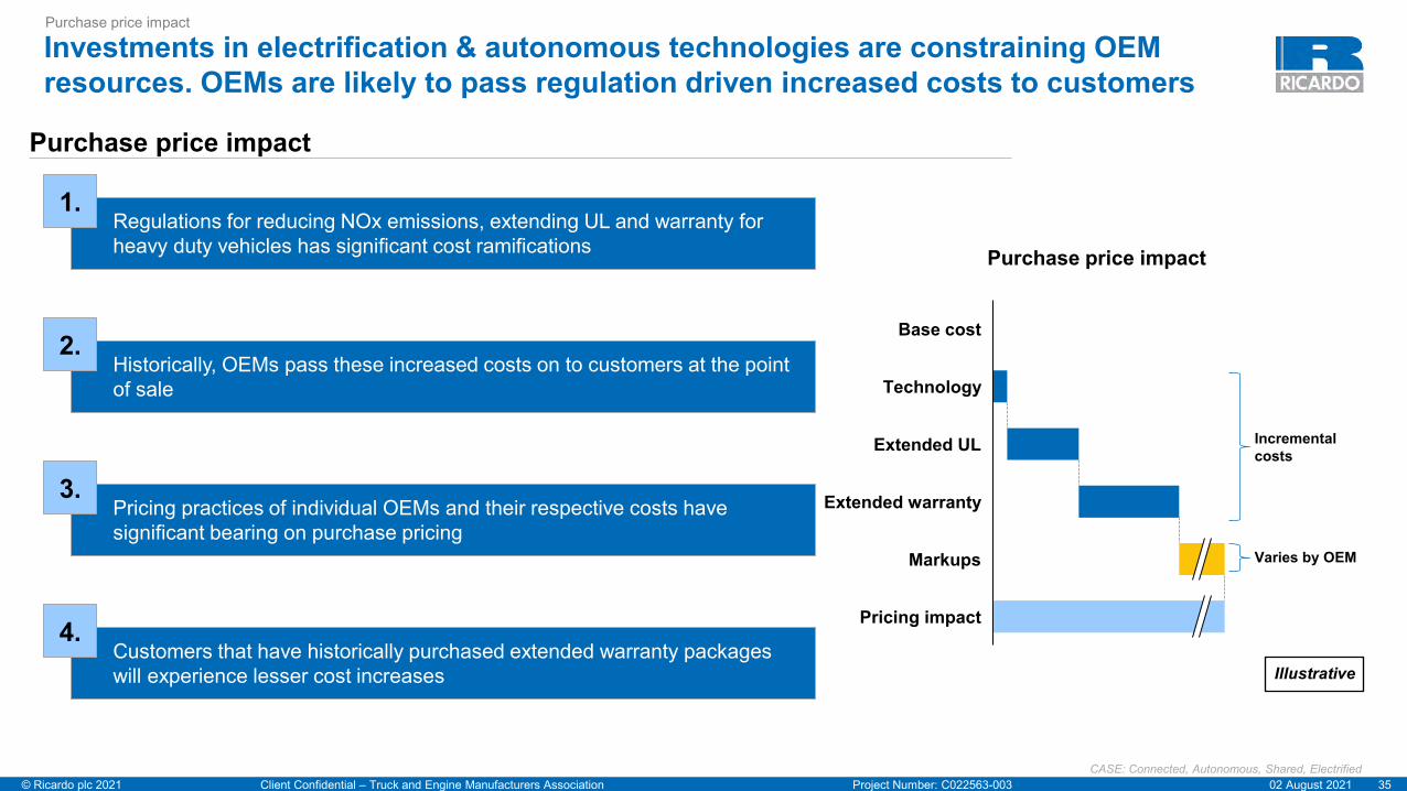
3502 August 2021Project Number: C022563-003© Ricardo plc 2021 Client Confidential – Truck and Engine Manufacturers Association
Investments in electrification & autonomous technologies are constraining OEM resources. OEMs are likely to pass regulation driven increased costs to customers
Purchase price impact
Purchase price impact
Technology
Base cost
Extended UL
Extended warranty
Markups
Pricing impact
Incrementalcosts
Varies by OEM
Purchase price impactRegulations for reducing NOx emissions, extending UL and warranty for heavy duty vehicles has significant cost ramifications
1.
Historically, OEMs pass these increased costs on to customers at the point of sale
2.
Pricing practices of individual OEMs and their respective costs have significant bearing on purchase pricing
3.
Customers that have historically purchased extended warranty packages will experience lesser cost increases
4.Illustrative
CASE: Connected, Autonomous, Shared, Electrified

3602 August 2021Project Number: C022563-003© Ricardo plc 2021 Client Confidential – Truck and Engine Manufacturers Association
• Executive summary– Methodology– Summary of results
• Technology cost study: Incremental cost analysis– HHDDE– MHDDE– LHD Gasoline
• Purchase price impact
• Pre-buy analysis• Technology learning curve
Contents

3702 August 2021Project Number: C022563-003© Ricardo plc 2021 Client Confidential – Truck and Engine Manufacturers Association
Pre-buy/No-buy scenarios historically result from the risk averse trucking industry avoiding new technology and higher costs compelled by regulations
Pre-buy analysis
• Used-vehicle market/prices
• Dealer stock
• Freight rate
• OEM production volume manipulation
Market
• Reliability
• Fuel economy/Cost
• Maintenance cost
• Incremental purchase price
Vehicle
• Average fleet age
• Private vs Public
Fleet
• Availability of capital
• Cost of money
• Lease vs Buy
• Tax incentives
Finance
• Fleet owners use different strategies to manage capital and operational expenses which ultimately impacts pre-buy volumes
− E.g., Lower average fleet age to minimize operating/maintenance cost, refresh fleet with fuel-efficient trucks
• Historical pre-buys estimates;− EPA 2004: Resulted in higher engine costs and lower fuel economy; Regulation
introduction was during start of economic recovery period from 2001 recession; ~30k pre-buy units in 2002 and 2003
− EPA 2007: Resulted in higher engine costs and lower fuel economy; Strong period of trucker profitability; ~130k pre-buy units in 2005 and 2006
− EPA 2010: Significant price increase offset by improved fuel economy; Excess capacity and softer trucker profitability; Start of economic recession; ~10-15k pre-buy units in 2008 and 2009
US Class 8 Tractor Build
Multitude of factors impact scale of pre-buys

3802 August 2021Project Number: C022563-003© Ricardo plc 2021 Client Confidential – Truck and Engine Manufacturers Association
Incremental costs due to increased stringency on NOx emissions, extended warranty & UL is expected to create a pre-buy phenomenon in HHDDE and MHDDE
Pre-buy analysis
Expected pre-buy volume (1/2)
• ACT Research performed pre-buy analysis for understanding the impact of CARB Omnibus Low NOx rulemaking (Omnibus regulations) on heavy duty and medium duty trucks
• Ricardo analysis makes use of the ACT Research pre-buy analysis and scales it appropriately based on incremental costs of technology for different scenarios− Assumes all other factors (micro or macro economic) remain the same
2027 2031 2027 2031 2027 2031 Model Year
2025 2026 2029 2030 2025 2026 2029 2030 2025 2026 2029 2030 Calendar Year
HHDDE 0.45% 6.69% 1.94% 12.62% 1.42% 21.01% 2.03% 13.19% 1.63% 24.11% 2.16% 14.02%
Pre-buy volume as % of marketMHDDE 0.57% 4.46% 0.84% 2.95% 0.89% 6.97% 0.75% 2.63% 1.15% 9.05% 0.79% 2.76%
LHD Gasoline 0.17% 2.58% 0.03% 0.21% 0.12% 1.79% 0.02% 0.15% 0.19% 2.87% 0.03% 0.20%
Scenario 1: 90% NOx reduction, Extended UL and Warranty
Scenario 2: 50% NOx reduction, UL and Warranty aligned with
CARB Omnibus
Scenario 3: 90% NOx reduction, UL and Warranty aligned with
CARB Omnibus
Estimated pre-buy volumes is lower than 1% for MY27 and MY31for all scenarios

3902 August 2021Project Number: C022563-003© Ricardo plc 2021 Client Confidential – Truck and Engine Manufacturers Association
Incremental costs due to increased stringency on NOx emissions, extended warranty & UL is expected to create a pre-buy phenomenon in HHDDE and MHDDE
Pre-buy analysis
Expected pre-buy volume (2/2)
• ACT Research performed pre-buy analysis for understanding the impact of CARB Omnibus Low NOx rulemaking (Omnibus regulations) on heavy duty and medium duty trucks
• Ricardo analysis makes use of the ACT Research pre-buy analysis and scales it appropriately based on incremental costs of technology for different scenarios− Assumes all other factors (micro or macro economic) remain the same
2027 2031 2027 2031 2027 2031 Model Year
2025 2026 2029 2030 2025 2026 2029 2030 2025 2026 2029 2030 Calendar Year
HHDDE 1,001 14,799 4,472 29,067 3,147 46,504 4,673 30,374 3,612 53,375 4,967 32,287
Pre-buy volumeMHDDE 699 5,491 1,081 3,784 1,093 8,579 962 3,366 1,418 11,134 1,010 3,535
LHD Gasoline 8 114 1 10 5 79 1 7 9 126 1 9
Scenario 1: 90% NOx reduction, Extended UL and Warranty
Scenario 2: 50% NOx reduction, UL and Warranty aligned with
CARB Omnibus
Scenario 3: 90% NOx reduction, UL and Warranty aligned with
CARB Omnibus
Estimated pre-buy volumes is lower than 1% for MY27 and MY31for all scenarios

4002 August 2021Project Number: C022563-003© Ricardo plc 2021 Client Confidential – Truck and Engine Manufacturers Association
• Executive summary– Methodology– Summary of results
• Technology cost study: Incremental cost analysis– HHDDE– MHDDE– LHD Gasoline
• Purchase price impact
• Pre-buy analysis
• Technology learning curve
Contents

4102 August 2021Project Number: C022563-003© Ricardo plc 2021 Client Confidential – Truck and Engine Manufacturers Association
Most OEMs do not experience the steep learning cost reductions that US EPA uses in its analysis
Technology learning curve
Technology learning curves – Actual ‘new technology’ cost progression from introduction
0%
20%
40%
60%
80%
100%
Yr.5
Cos
t rel
ativ
e to
orig
inal
Technology introduction year
Yr.2
Yr.1
Yr.4
Yr.6
Yr.3
Yr.8
Yr.7
Yr.9
Yr.10
Yr.11
Yr.12
Yr.13
Yr.14
Yr.15
Yr.16
Yr.17
Yr.18
+16%
+17%
+16%+13%
EPA’s learning curve Direct injectionOEM average learning curveLP EGR
Variable valve timingSCR
Technology learning curve Due to existing confidentiality agreements, only a few OEMs provided data for this section of the study• After an initial two-year period of technology introduction,
EPA’s technology learning curve assumes very steep learning before it becomes more gradual
• Almost none of the OEMs that participated and shared data for this section of the study experienced such steep cost reduction
− Other OEMs provided comments that indicated similar experiences
− OEMs typically experience ~15% less cost-benefit due to learning over time than assumed by EPA
• OEMs experiences with learning are heavily dependent on their purchasing terms with respective supplier
− OEMs typically have long term supply contracts that dictate learning or cost improvements over time
− Some supply contracts have terms for year over year cost reductions, while others have fixed costs through the contracted period
− Cost reduction achieved due to learnings are shared between OEMs and suppliers
• Learning curves associated with different technologies vary with the technology; Assuming same curve for all types of technologies can lead to significant error in cost calculations
Up to 15% in 5yrs 5-10% in next 4yrs 0-5% going forward
Section 1 Section 2 Section 3

Potential Air Quality Benefits of a 90%/75% Reduction in NOx Emissions from New Heavy-Duty On-Highway Vehicles – Technical Details of Analysis and Assumptions
Prepared for the Truck and Engine Manufacturers Association
August 2021

© NERA Economic Consulting i
Project Team Anne E. Smith, Ph.D., Managing Director Bharat Ramkrishnan, Consultant Andrew Hahm, Analyst
About NERA
NERA Economic Consulting (www.nera.com) is a global firm of experts dedicated to applying economic, finance, and quantitative principles to complex business and legal challenges. For over half a century, NERA's economists have been creating strategies, studies, reports, expert testimony, and policy recommendations for government authorities and the world’s leading law firms and corporations. We bring academic rigor, objectivity, and real-world industry experience to bear on issues arising from competition, regulation, public policy, strategy, finance, and litigation.
This report reflects the research, opinions, and conclusions of its authors, and does not necessarily reflect those of NERA Economic Consulting, its affiliated companies, or any other organization.

© NERA Economic Consulting i
Report Qualifications/Assumptions and Limiting Conditions Information furnished by others, upon which all or portions of this report are based, is believed to be reliable, but has not been independently verified, unless otherwise expressly indicated. Public information and industry and statistical data are from sources we deem to be reliable; however, we make no representation as to the accuracy or completeness of such information. The findings contained in this report may contain predictions based on current data and historical trends. Any such predictions are subject to inherent risks and uncertainties. NERA Economic Consulting accepts no responsibility for actual results or future events.
The opinions expressed in this report are valid only for the purpose stated herein and as of the date of this report. No obligation is assumed to revise this report to reflect changes, events or conditions, which occur subsequent to the date hereof.
All decisions in connection with the implementation or use of advice or recommendations contained in this report are the sole responsibility of the client. This report does not represent investment advice nor does it provide an opinion regarding the fairness of any transaction to any and all parties.
© NERA Economic Consulting

© NERA Economic Consulting ii
Contents I. Introduction.......................................................................................................................1
II. Objective of This Analysis................................................................................................1
III. Overview of Methodology ................................................................................................2
IV. Calculation of Reduction in Tons Emitted .....................................................................3
V. Development of Benefit-per-Ton Values and Benefit-per-Truck Estimates ...............5 A. PM2.5 Calculations ................................................................................................................. 6 B. Ozone Calculations.............................................................................................................. 13
VI. Benefit-per-Truck Estimates with Varying Confidence Levels ..................................21
VII. References ........................................................................................................................33
Appendix A: Estimated Total NOx Emissions Reductions Including All Model Years, by State ..................................................................................................................................35
Appendix B: Estimated Benefits per Ton, by State ............................................................39
Appendix C: Benefit-per-Truck Estimates by State, 7% Discount Rate ..........................41
Appendix D: Estimated Average Ozone Response Factors by State ................................45

© NERA Economic Consulting iii
List of Figures Figure 1: NOx Emissions Reduced per Statistical Vehicle (Average per Year per Vehicle) ........................................................................................................................................... 4 Figure 2: Baseline and Scenario Emissions Across All HDOH Truck Categories......................... 5 Figure 3: Map of PM2.5-Only Benefits per Ton by State Using the Low Di et al. (2017) C-R Coefficient (2050)........................................................................................................ 9 Figure 4: Cumulative Distribution of PM2.5-Only Benefits per Ton by State Using the Low Di et al. (2017) C-R Coefficient (2050) ................................................................................. 9 Figure 5: Map of PM2.5-Only Benefits per Ton by State Using the High Di et al. (2017) C-R Coefficient (2050)...................................................................................................... 10 Figure 6: Cumulative Distribution of PM2.5-Only Benefits per Ton by State Using the High Di et al. (2017) C-R Coefficient (2050)............................................................................... 10 Figure 7: Map of PM2.5-Only Benefits per Truck by State Using the Low Di et al. (2017) C-R Coefficient, 3% Discount Rate .................................................................................. 11 Figure 8: Cumulative Distribution of PM2.5-Only Benefits per Truck by State Using the Low Di et al. (2017) C-R coefficient, 3% Discount Rate ....................................................... 11 Figure 9: Map of PM2.5-Only Benefits per Truck by State Using the High Di et al. (2017) C-R Coefficient, 3% Discount Rate .................................................................................. 12 Figure 10: Cumulative Distribution of PM2.5-Only Benefits per Truck by State Using the High Di et al. (2017) C-R Coefficient, 3% Discount Rate ..................................................... 12 Figure 11: Basis for Estimating Ozone Response Factors for Each State .................................... 14 Figure 12: Map of Ozone-Only Benefits per Ton by State Using the Low Zanobetti and Schwartz (2008) C-R Coefficient (2050) ............................................................................... 17 Figure 13: Cumulative Distribution of Ozone-Only Benefits per Ton by State Using the Low Zanobetti and Schwartz (2008) C-R Coefficient (2050) ................................................ 17 Figure 14: Map of Ozone-Only Benefits per Ton by State Using the High Zanobetti and Schwartz (2008) C-R Coefficient (2050) ............................................................................... 18 Figure 15: Cumulative Distribution of Ozone-Only Benefits per Ton by State Using the High Zanobetti and Schwartz (2008) C-R Coefficient (2050) ................................................ 18 Figure 16: Map of Ozone-Only Benefits per Truck by State Using the Low Zanobetti and Schwartz (2008) C-R Coefficient, 3% Discount Rate ........................................................... 19 Figure 17: Cumulative Distribution of Ozone-Only Benefits per Truck by State Using the Low Zanobetti and Schwartz (2008) C-R Coefficient, 3% Discount Rate ............................. 19 Figure 18: Map of Ozone-Only Benefits per Truck by State Using the High Zanobetti and Schwartz (2008) C-R Coefficient, 3% Discount Rate ........................................................... 20 Figure 19: Cumulative Distribution of Ozone-Only Benefits per Truck by State Using the High Zanobetti and Schwartz (2008) C-R Coefficient, 3% Discount Rate ............................ 20 Figure 20: Map of PM2.5-Only Benefits per Truck by State Using the Low Di et al. (2017) C-R Coefficient, 7% Discount Rate .................................................................................. 41

© NERA Economic Consulting iv
Figure 21: Cumulative Distribution of PM2.5-Only Benefits per Truck by State Using the Low Di et al. (2017) C-R Coefficient, 7% Discount Rate ...................................................... 41 Figure 22: Map of PM2.5-Only Benefits per Truck by State Using the High Di et al. (2017) C-R Coefficient, 7% Discount Rate .................................................................................. 42 Figure 23: Cumulative Distribution of PM2.5-Only Benefits per Truck by State Using the High Di et al. (2017) C-R Coefficient, 7% Discount Rate ..................................................... 42 Figure 24: Map of Ozone-Only Benefits per Truck by State Using the Low Zanobetti and Schwartz (2008) C-R Coefficient, 7% Discount Rate ........................................................... 43 Figure 25: Cumulative Distribution of Ozone-Only Benefits per Truck by State Using the Low Zanobetti and Schwartz (2008) C-R Coefficient, 7% Discount Rate ............................. 43 Figure 26: Map of Ozone-Only Benefits per Truck by State Using the High Zanobetti and Schwartz (2008) C-R Coefficient, 7% Discount Rate ........................................................... 44 Figure 27: Cumulative Distribution of Ozone-Only Benefits per Truck by State Using the High Zanobetti and Schwartz (2008) C-R Coefficient, 7% Discount Rate ............................ 44

© NERA Economic Consulting v
List of Tables
Table 1: Avoided Premature Statistical Deaths (%) and National PM2.5 Benefits per Truck (2019$) by Confidence Level Using the Low C-R Coefficient from the Di et al. (2017) Epidemiology Study and Applying 3% and 7% Discount Rates ...................................... 24 Table 2: Avoided Premature Statistical Deaths (%) and National PM2.5 Benefits per Truck (2019$) by Confidence Level Using the High C-R Coefficient from the Di et al. (2017) Epidemiology Study and Applying 3% and 7% Discount Rates ................................. 25 Table 3: Avoided Premature Statistical Deaths (%) and National Ozone Benefits per Truck (2019$) by Confidence Level Using the Low C-R Coefficient from the Zanobetti and Schwartz (2008) Epidemiology Study and Applying 3% and 7% Discount Rates .............................................................................................................................. 26 Table 4: Avoided Premature Statistical Deaths (%) and National Ozone Benefits per Truck (2019$) by Confidence Level Using the High C-R Coefficient from the Zanobetti and Schwartz (2008) Epidemiology Study and Applying 3% and 7% Discount Rates .............................................................................................................................. 27 Table 5: Avoided Premature Statistical Deaths (%) and PM2.5 Benefits per Truck (2019$) for California and Rest of U.S. by Confidence Level Using the Low C-R Coefficient from the Di et al. (2017) Epidemiology Study and Applying 3% and 7% Discount Rates .............................................................................................................................. 29 Table 6: Avoided Premature Statistical Deaths (%) and PM2.5 Benefits per Truck (2019$) for California and Rest of U.S. by Confidence Level Using the High C-R Coefficient from the Di et al. (2017) Epidemiology Study and Applying 3% and 7% Discount Rates .............................................................................................................................. 30 Table 7: Avoided Premature Statistical Deaths (%) and Ozone Benefits per Truck (2019$) for California and Rest of U.S. by Confidence Level Using the Low C-R Coefficient from the Zanobetti and Schwartz (2008) Epidemiology Study and Applying 3% and 7% Discount Rates ........................................................................................... 31 Table 8: Avoided Premature Statistical Deaths (%) and Ozone Benefits per Truck (2019$) for California and Rest of U.S. by Confidence Level Using the High C-R Coefficient from the Zanobetti and Schwartz (2008) Epidemiology Study and Applying 3% and 7% Discount Rates ........................................................................................... 32

© NERA Economic Consulting vi
List of Acronyms
ACE Affordable Clean Energy BCA Benefit-Cost Analysis BenMAP Benefits Mapping and Analysis Program CAMx Comprehensive Air Quality Model with Extensions C-R Concentration-Response EMA Truck and Engine Manufacturer’s Association EPA Environmental Protection Agency FTP Federal Test Procedure GVWR Gross Vehicle Weight Rating HDOH Heavy-Duty On-Highway HHD Heavy Heavy-Duty Vehicle; Class 8a and 8b Trucks (GVWR > 33,000 lbs) LHD2b3 LHD45
Light Heavy-Duty Vehicle; Class 2b and 3 Trucks ((8,500 lbs < GVWR <= 14,000 lbs) Light Heavy-Duty Vehicle; Class 4 and 5 Trucks (14,000 lbs < GVWR <= 19,500 lbs)
LML Lowest Measured Level MHD Medium Heavy-Duty Vehicle; Class 6 and 7 Trucks (19,500 lbs < GVWR <=
33,000 lbs) MOVES3 NAAQS
Motor Vehicle Emission Simulator 3 National Ambient Air Quality Standards
NERA NERA Economic Consulting NOx Nitrogen Oxides OMB Office of Management and Budget PM2.5 Fine Particulate Matter (that have a diameter of less than 2.5 micrometers) RIA Regulatory Impact Analysis

© NERA Economic Consulting 1
I. Introduction
This report provides a description of the data, assumptions and modeling that NERA Economic Consulting (NERA) conducted in its analysis for the Engine and Truck Manufacturers Association (EMA) of the potential per-truck air quality benefits of a possible tightening of the NOx emissions standard for heavy-duty on-highway (HDOH) trucks. This report serves as a technical supplement to a separate NERA report subtitled Conceptual Summary of Methods and Key Results (hereafter called the “Summary Report”) that provides a policy-oriented discussion of the purpose of the analysis and summarizes key results. In addition to documenting the analysis steps in more technical detail, this report provides a more disaggregated view of the key results. We recommend that one first read the Summary Report, as that contains more general background on the context for this analysis and its policy implications than what is found in this technical documentation. II. Objective of This Analysis
As discussed in the accompanying Summary Report for this study, past practice of the U.S. Environmental Protection Agency (EPA or the Agency) in implementing Clean Air Act provisions regarding truck emissions standards suggests that any proposal for a tightening of those standards will need to have estimated benefits that exceed its estimated costs. That is usually demonstrated though a benefit-cost analysis (BCA) that is documented in a regulatory impact analysis (RIA) that the Agency must prepare for every economically significant rulemaking. The approach that EPA typically follows in RIAs to estimate national health benefits of regulations affecting ambient air quality such as fine particulate matter (PM2.5) and ozone includes several steps:
A. Estimating the incremental emission reductions from implementation of the regulation (and their geographical locations);
B. Estimating the ambient ozone and PM2.5 changes across the U.S. as a result of the reduction in emissions;
C. Estimating the population-wide health risk improvements from lower ambient ozone and PM2.5 concentrations; and
D. Estimating the societal value in dollars of the estimated health risk improvements – which are referred to as the potential “benefits” of the regulation.
In RIAs, those benefit calculations are typically carried out for a specific future calendar year (usually when the regulation in question is fully implemented) and are compared to estimates of the annualized costs at that point in time.1 That is a complex and resource-intensive type of analysis that requires specific assumptions about the evolution of markets affected by the regulation (such as the projected future demand for trucking services). Without knowledge of those baseline assumptions, and which specific year will be analyzed, it is not possible to approximate the specific benefits estimates that will be reported in a future RIA. Even if this could be done, the results would provide little insight without a comparable estimate of the total annualized regulatory costs in that particular year – also a complex calculation. However, it is important to develop some rough understanding of the incremental lifecycle cost of a new truck that is likely to pass a RIA’s benefit-cost test before anchoring a rulemaking process around a particular degree of stringency. A scoping analysis is therefore valuable to undertake in the
1 Less frequently, RIAs compute benefits and costs as present values over the duration of the policy implementation period. The
analysis we describe in this report is relevant to that type of benefit-cost comparison as well.

© NERA Economic Consulting 2
preliminary stage of rulemaking, before any specific new standard levels are ready to be proposed. NERA’s analysis, documented here, was developed for use in such a scoping exercise.
In developing a simpler analysis method that could produce such scoping-level insights, NERA noted that preliminary information on a new standard’s potential cost will be available in the form of its impact on the lifecycle cost per new truck. We also note that if the annual benefits of that new standard will be able to pass a BCA in any future year, then the benefits that each individual truck is likely to provide over its operational lifespan also will need to exceed the incremental costs of that truck, or, at least, that this net benefit condition will be achieved on average over all new trucks. Thus, NERA has prepared an initial scoping analysis that estimates of the present value of benefits over the operating life of an average new truck purchased in 2027 (the first year that the anticipated standard is likely to be binding) that meets a hypothetical 90% reduction in the NOx FTP emissions standard. Those per-truck benefits estimates can then be compared to per-truck compliance costs to obtain preliminary insight on whether that particular standard is likely to pass a full BCA.
We emphasize that the estimates we have made in this analysis reflect an effort to anticipate what the Agency would estimate if it applies its own usual assumptions and analysis methodologies. That is, we have used analysis input assumptions that we believe are within the range of those that EPA would likely use. Of course, we do not know what may arise with updated EPA models, data, and input assumptions, but we have sought out the most recent studies and documents on air pollutants that EPA has released. Our estimates are nevertheless subject to revision as more up-to-date information is released. Were we to undertake this type of benefits analysis without regard to what EPA is expected to do, it is likely that we would utilize different methods and assumptions.
III. Overview of Methodology
The process by which we estimate per-truck benefits is summarized in this section. The remaining sections of this report then describe the data, assumptions and models we have used for each step of the process.
First, we calculate the tons of NOx emissions reductions over time from new trucks that meet the tighter NOx standard, if purchased in 2027. (We assume all model year 2027 trucks will fully meet the hypothetical 90% FTP standard reduction, which, based on assumptions provided by EMA, will yield 75% reductions in in-use emissions.) Recognizing that some of the new trucks will operate longer than others, we consider the average tons across all new trucks expected to be purchased in 2027 for each year over a potential life of up to 30 years (i.e., through 2057). That calculation is carried out for each of the eight truck types covered by the assumed standard.2
Next, the per-truck emissions reductions in each future year are translated into a dollar estimate of each year’s health benefits using a simple “reduced-form” method in which the precursor (e.g., NOx) emissions changes are multiplied by an estimated “benefit-per-ton” value. The result of this calculation is a timeline from 2027 through 2057 of annual benefits per truck in each year of the average 2027–vintage truck’s operating life.
That stream of benefits then is discounted to obtain the present value of benefits per truck for each of the eight truck types. Those eight values are combined into a single sales-weighted average benefit-per-truck
2 These eight truck types correspond to regulatory class IDs - 41 (LHD2b3), 42 (LHD45), 46 (MHD), 47 (HHD), 48 (Urban Bus),
49 (Glider Vehicles) per EPA’s emissions inventory model (MOVES3) documentation ( https://nepis.epa.gov/Exe/ZyPDF.cgi?Dockey=P1011TF8.pdf).

© NERA Economic Consulting 3
estimate.3 Consistent with OMB and EPA guidance, we provide benefit-per-truck estimates that are calculated using annual discount rates of 3% and 7%.
Finally, we calculate how these per-truck benefits are affected by changing the allowed extent of extrapolation from original health effects studies, providing a sliding scale of the per-truck benefits estimates with different degrees of qualitative confidence. We refer to this process as “confidence-weighting.”
The resulting scale of estimates with varying degrees of confidence weights represents our scoping-level estimate of the average lifecycle benefits per truck; they can then be compared to estimates of the incremental per-truck compliance cost to determine whether that anticipated standard is likely to pass a benefit-cost test after a more detailed BCA.4
IV. Calculation of Reduction in Tons Emitted
To obtain estimates of the tons of NOx reduced per truck, we relied on EPA’s mobile source emissions model, MOVES3. Those calculations were done by truck type and by state for each state of the conterminous U.S. states (excluding the District of Columbia). We used the MOVES3 data to estimate how long the average truck purchased in 2027 is expected to continue to operate, and to quantify the average operational characteristics of the still-operating trucks as a function of truck age.
Specifically, for each of the eight heavy-duty truck types, we tracked a set of 100 new hypothetical vehicles purchased in 2027 and used the MOVES3 assumptions regarding the percent of vehicles surviving through each of the next 30 years, the average miles the surviving trucks are driven in each year (which is age-dependent), and their associated baseline (current standard) NOx emissions.5 Each year’s reduction in tons of NOx per truck was then calculated as a 75% reduction from the respective year’s baseline NOx emissions (i.e., the sum of baseline NOx emissions from all operational modes), divided by the number of vehicles surviving in that year. This computation was carried out in each year of the truck’s assumed operational life to obtain tons of NOx reduced per truck by year.
Figure 1 illustrates the resulting estimate of reduction in NOx emissions for an average model-year 2027 truck in each year of its operational life.6 Those reductions decline as the trucks age because in each year
3 We weighted the present value estimate of the per-truck benefit obtained for each of the eight truck types by the new vehicle
sales in 2027 for each of the truck types projected in MOVES3. 4 Extensive changes are now expected to occur in the mix of HDOH trucks that will be sold in the future, with a potentially
significant transition away from ignition-based power trains to electric or fuel-cell trucks. Our analysis of the per-truck benefits before any confidence-weighting will not be affected by such a change, but this transition might lower the baseline future PM2.5 and ozone concentrations and thus increase the degree of extrapolation, resulting in some lowering of confidence-weighted estimates. More importantly, however, such a transition might have more effect on the per-truck cost to which our benefits estimates ought to be compared. That is, the total investment costs of developing, designing, and retooling to meet a tighter HDOH diesel NOx standard need to be spread over all of the affected fleet; if the projected size of the future fleet of diesel trucks is much reduced, the estimate of the cost per truck for use in a scoping analysis should be adjusted upwards accordingly.
5 The baseline NOx emissions for each HDOH truck analyzed were calculated for each of the operational modes (running exhaust, start exhaust, extended idle exhaust, and auxiliary power exhaust) which were then summed up to yield the total baseline NOx emissions. The baseline emissions from running exhaust were calculated using running exhaust emission rates (specified in units of grams of NOx/hr) and the number of hours the truck was operating in running exhaust mode. The baseline emissions from the other operational modes – start exhaust, extended idle exhaust, and auxiliary power exhaust – were calculated using their respective emissions rates (specified in units of grams of NOx/vehicle) and the number of vehicles operating in that year.
6 The weights used to compute the average across the different HDOH vehicle types analyzed are the projected new vehicle sales for each of the truck types from MOVES3 in 2027.

© NERA Economic Consulting 4
some of the trucks are removed from service, and trucks that are still in service are used less intensively as they age. The estimated annual reduction in NOx emissions per “statistical” vehicle ranges from a low of 0.004 tons at age 30 to a high of 0.063 tons at age 4.
Figure 1: NOx Emissions Reduced per Statistical Vehicle (Average per Year per Vehicle)
We also used MOVES3 to estimate the aggregate annual reductions in NOx emissions across the lower-48 states that would result from implementation of the tighter NOx standard in every model year from 2027 through 2057. That result could be of use if one were to conduct an analysis of benefits for specific future years rather than on the per-truck basis that is the focus of this scoping analysis.
To compute the total annual tons of reduction over time, we extracted projected baseline NOx emissions from MOVES3 for each of the eight truck-types and all operational modes by state and by year from 2020 through 2050. To calculate the reductions in NOx emissions, we reduced the baseline emissions across all the eight truck types by 75% in each year from 2027 onwards (where 2027 is the year in which the tighter NOx standard is assumed to be implemented).7
The aggregated results are shown in Figure 2, while the results for each individual state are provided in Appendix A. The total baseline emissions across the U.S. for the eight HDOH truck types analyzed are
7 To keep the analysis simple, we did not apply any phase-in period for the standard. However, the effect of the standard (a 50%
reduction in in-use emissions across the entire fleet), does take time to emerge as the standard is not applied to trucks purchased prior to 2027. Those pre-2027 trucks are assumed to remain in the fleet without any changes in their baseline operational or turnover assumptions.

© NERA Economic Consulting 5
projected to reach about 1.02 million tons by 2060, while emissions under the assumed scenario (i.e., with implementation of a 90% tighter NOx FTP standard that provides 75% reduction in in-use emissions) are projected to reach about 0.25 million tons by 2060. Thus, by 2060 the annual reduction in NOx emissions projected from the affected HDOH diesel trucks is projected to be about 0.75 million tons.8
Figure 2: Baseline and Scenario Emissions Across All HDOH Truck Categories
V. Development of Benefit-per-Ton Values and Benefit-per-Truck Estimates
A benefit-per-ton value measures the projected health benefits associated with projected changes in precursor emissions (e.g., NOx). The approach typically employed to compute those estimates involves running specific projected precursor emission changes through a full air quality fate-and-transport model (e.g., CAMx) to project spatial changes in the relevant ambient pollutant concentrations. Those pollutant concentration changes are then provided as input to a demographic health risk analysis model (e.g., BenMAP), along with specific assumptions about the concentration-response (C-R) relationship and social value per health effect incident to produce total monetized benefits. Those total benefits are then
8 This aggregate reduction assumes the current MOVES3 baseline of sales of HDOH diesel trucks. If that baseline does not
reflect the significant transition away from ignition-based power trains to electric and fuel cell power trains that is now widely expected to occur over the same time period, it overstates the total tons of reduction that a new NOx HDOH standard for diesel trucks will actually produce. While it would not affect the per-truck benefits estimates prior to any confidence-weighting adjustments, it could cause overstatement of the estimates on the higher-confidence end of our scale of results, because a lower baseline of emissions would imply greater amounts of extrapolation, as explained in more detail in the Summary Report.

© NERA Economic Consulting 6
divided by the assumed change in tons of the precursor emission to yield a benefit-per-ton estimate stated in dollars.
This is called a “reduced-form” benefits estimate. The Agency and other groups often approximate total benefits of a potential emissions-reduction action by simply multiplying an available (and relevant) benefit-per-ton value by the number of tons of emissions reduction associated with that action. While subject to heightened uncertainty and inaccuracy, this approach avoids the great time and cost of conducting the air quality modeling step. We do not suggest that EPA will or should use this reduced-form approach in its own RIA for a future HDOH rulemaking, but we consider it a reasonable approach for the type of scoping-level approximation of benefits per truck that is the objective of our analysis.
While EPA has already published several such “reduced-form” benefit-per-ton estimates, we chose to derive our own estimates. By computing them ourselves, we can perform a wide range of sensitivity analyses that would not be possible using those published by others. For example, in our analysis, we (a) apply more up-to-date assumptions relating to baseline ambient pollutant concentrations;9 (b) derive and explore the implications of more geographically disaggregated benefit-per-truck estimates; (c) use newer and different C-R assumptions that the Agency might use in its future benefits analyses; and (d) provide a range of benefit-per-truck estimates that vary in the extent to which they rely on extrapolation outside of the range of data supporting the original estimation of the C-R coefficients being applied.
We had to use different data sources to develop our estimates for ozone and PM2.5. The rest of this section therefore describes the methods and the data that we used to compute our benefit-per-ton and associated benefit-per-truck estimates for ozone and PM2.5 separately. It also provides state-specific detail to supplement the more aggregated estimates presented in the accompanying Summary Report. All of the results reported in this section give full weight to risk estimates from exposures as low as zero and make no adjustment for declining confidence associated with extrapolation of the C-R relationship to concentrations at the low end of the range of observations in the original epidemiological study. Our method for assessing the quantitative sensitivity to alternative limits on the degree of such extrapolation is described in Section VI of this report.10
A. PM2.5 Calculations
To develop our “reduced-form” benefit-per-ton estimates for PM2.5, we relied upon air quality modeling used to produce a set of mobile-source benefit-per-ton estimates reported in Wolfe et al. (2018). That study was of particular relevance to our analysis because it provided PM2.5 benefit-per-ton estimates specifically due to NOx emissions from HDOH trucks.11 The paper reported average national and regional (“East” and “West”) benefit-per-ton estimates, using a baseline PM2.5 concentration grid and associated baseline NOx emissions projected to occur in 2025. The benefit-per-ton estimates reported in the paper are calculated using two C-R functions – from Krewski et al. (2009) and Lepeule et al. (2012) – and using BenMAP’s demographic assumptions for the year 2025.
9 For our analysis, we used 2035 baseline ozone and PM2.5 grids from a recent air RIA (EPA, 2019a), which were the BenMAP
inputs with the most up-to-date air quality modeling that we were able to identify in the public domain. The concentrations in these grids also are broadly reflective of the concentrations of ozone and PM2.5 projected to occur in the years during which the tighter standard would be having most of its incremental impact (i.e., in the 2030s and 2040s).
10 The case for this latter type of sensitivity analysis, which we call “confidence weighting,” is explained in more detail in the accompanying Summary Report.
11 The species of PM2.5 associated with NOx precursor emissions is particulate nitrate.

© NERA Economic Consulting 7
EPA provided NERA with the BenMAP grids of 2025 HDOH nitrate contributions and the associated NOx emissions (by state) employed by Wolfe et al. Using those data and the same C-R relationships, NERA ran the BenMAP model to confirm we could replicate the nitrate benefit-per-ton estimates due to HDOH trucks, both at the national and the regional level.
To better understand the degree of potential variation in such values on a geographic basis, NERA then used BenMAP and those same air quality and emissions data to develop benefit-per-ton estimates on a more disaggregated basis, generally state by state (which was the smallest disaggregation available for the emissions data.) However, recognizing that much of the ambient PM2.5 in very small states would be attributable to emissions in surrounding states, several of the smallest Eastern states were aggregated into subregions about the size of the larger states.12
Like Wolfe et al., we estimate a range for the PM2.5 benefits-per-ton using two alternative C-R relationships for mortality risk. Rather than use the same two C-R relationships that Wolfe et al. used, we chose to update those inputs to reflect what one might expect the Agency to use in a future RIA. To decide on the C-R estimates to define the lower and higher ends of our range, we reviewed EPA’s recent Policy Assessment for PM2.5 (EPA, 2020) and also the C-R relationships for PM2.5 that currently exist in the BenMAP health impact functions library Based on the review, we decided to rely on two C-R relationships from a study by Di et al. (2017).13 Also, consistent with EPA practice for long-term PM2.5 benefits calculations, we applied EPA’s standard twenty-year segmented cessation lag (EPA, 2004) to the estimates developed using the Di et al. low and high C-R relationships.14
The year-2050 benefit-per-ton estimates calculated using the low Di et al. C-R relationship are illustrated as a map in Figure 3, and as a population-weighted cumulative distribution in Figure 4 (two pages hence). State-specific estimates range from less than $100 per ton to more than $19,000 per ton (2019$) around a national average of $7,500 per ton.15 This range primarily reflects variations in population densities, and also regional differences in the amount of change in ambient PM2.5 per ton of HDOH NOx emissions. While this is a very wide range around the national average, there are no clear outliers on the range. However, California and several midwestern states account for the highest values. The values in these figures are based on year-2050 demographic assumptions, but the variation from state to state is generally
12 The two multi-state regions are called North East and Mid-Atlantic. The North East region comprises Connecticut,
Massachusetts, New Hampshire, New York, Rhode Island and Vermont. The Mid-Atlantic aggregate region comprises Delaware, Maryland, New Jersey, Pennsylvania, Virginia and West Virginia. The benefit-per ton-estimates for these aggregate regions are calculated by the dividing the aggregate benefits for the region by the aggregate NOx emissions reduction for the region.
13 For the low end of the range, we employed a C-R coefficient for all-cause mortality of 0.0059, based on a relative risk of 1.061 per 10 µg/m3 change in PM2.5 (Two-pollutant analysis, Analysis based on data from nearest monitoring site). For the high end of the range, we employed a C-R coefficient for all-cause mortality of 0.0081, based on a relative risk of 1.084 per 10 µg/m3 change in PM2.5 (Single-pollutant analysis). Both these relative risk estimates are obtained from Table 2 of the Di et al. study (p. 2518). The C-R relationships apply to people ages 65 years or older, and our BenMAP calculations have used this older population when applying the Di et al. coefficients.
14 This structure assumes a 30% reduction in premature mortality in the first year, a 50% reduction over years 2 through 5 and a 20% reduction over years 6 through 20 after the reduction in PM2.5 concentration.
15 In addition to relying on Di et al. C-R estimates rather than either the Krewski et al. or Lepeule et al. C-R functions, these estimates apply year-2050 demographic conditions, whereas Wolfe et al. applies year-2025 demographic assumptions, which produce lower per-ton values. Also, these are stated in 2019 real dollars, whereas Wolfe et al. states its estimates in 2015 real dollars, which also results in lower numerical values. As noted earlier, our analysis methods do replicate the estimates reported Wolfe et al. when we apply the same C-R and demographic assumptions and state the results in same-year real dollars.

© NERA Economic Consulting 8
similar for other demographic years. The numerical values estimated for the 2030, 2040, and 2050 demographic assumptions are provided in Appendix B.
Our year-2050 national average benefit per ton of reduction in HDOH NOx emissions calculated using the high Di et al. (2017) C-R relationship is about $10,000 per ton (2019$). The geographic variation around that average is presented in Figure 5 and Figure 6 on the next page, and is very similar to that using the low Di et al. C-R relationship. Numerical values behind these figures, and for 2030 and 2040 are also provided in Appendix B.
As explained in the prior section, our estimates of the per-truck benefits apply our estimates of benefits per ton in each year from 2027 through 205716 to our estimates of the per-truck tons of reduction each respective year, and take a present value of that stream of annual values. Figure 7 and Figure 8 below present the maps and cumulative distributions, respectively, of PM2.5 benefit-per-truck estimates computed using the low C-R relationship from the Di et al. (2017) epidemiological study and applying a 3% discount rate. Figure 9 and Figure 10 present the same information using instead the high C-R relationship from the Di et al. (2017) epidemiological study (also applying a 3% discount rate). The national average PM2.5 estimates (for a 3% discount rate) are $4,650 per truck based on the low C-R relationship from the Diet al. study and $6,340 per truck based on the high C-R relationship from the Di et al. study. As with the distributions presented in Figure 4 and Figure 6, the states with the highest benefit-per-truck estimates are in the Midwest and California.
The corresponding maps and distributions for the PM2.5 benefit-per-truck estimates computed using a 7% discount rate are presented in Appendix C. For each state, those benefits estimates are about 25% lower than their respective 3% discount rate estimates, leaving the geographical variations much the same as presented in the figures below.
16 For each year’s specific benefit-per-ton value, we interpolated linearly between our 2030 and 2050 per-ton values. We
considered this a reasonable approximation for our scoping analysis. However, we note that use of a more refined interpolation that incorporates year-2040 values appears to increase per-truck benefits estimates by less than 5%.

© NERA Economic Consulting 9
Figure 3: Map of PM2.5-Only Benefits per Ton by State Using the Low Di et al. (2017) C-R Coefficient (2050)
Figure 4: Cumulative Distribution of PM2.5-Only Benefits per Ton by State Using the Low Di et al. (2017) C-R Coefficient (2050)

© NERA Economic Consulting 10
Figure 5: Map of PM2.5-Only Benefits per Ton by State Using the High Di et al. (2017) C-R Coefficient (2050)
Figure 6: Cumulative Distribution of PM2.5-Only Benefits per Ton by State Using the High Di et al. (2017) C-R Coefficient (2050)
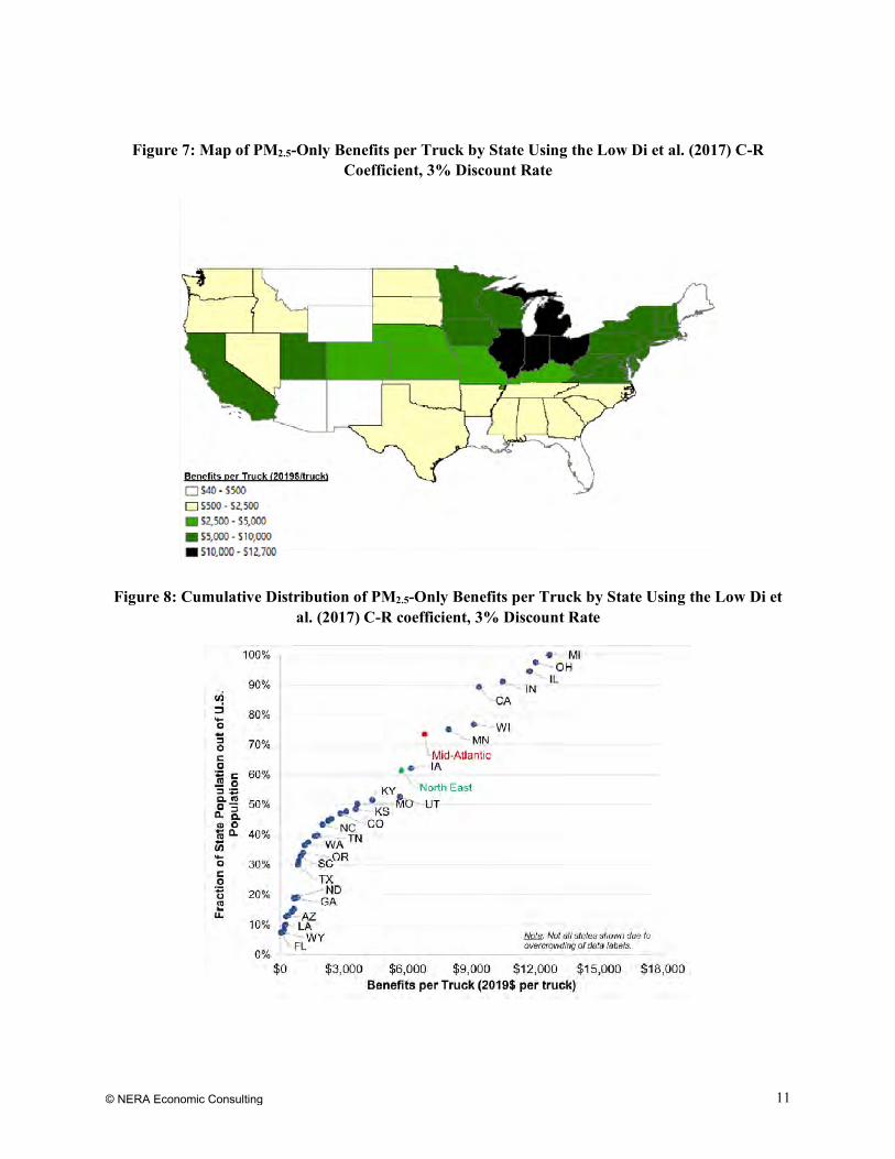
© NERA Economic Consulting 11
Figure 7: Map of PM2.5-Only Benefits per Truck by State Using the Low Di et al. (2017) C-R Coefficient, 3% Discount Rate
Figure 8: Cumulative Distribution of PM2.5-Only Benefits per Truck by State Using the Low Di et al. (2017) C-R coefficient, 3% Discount Rate
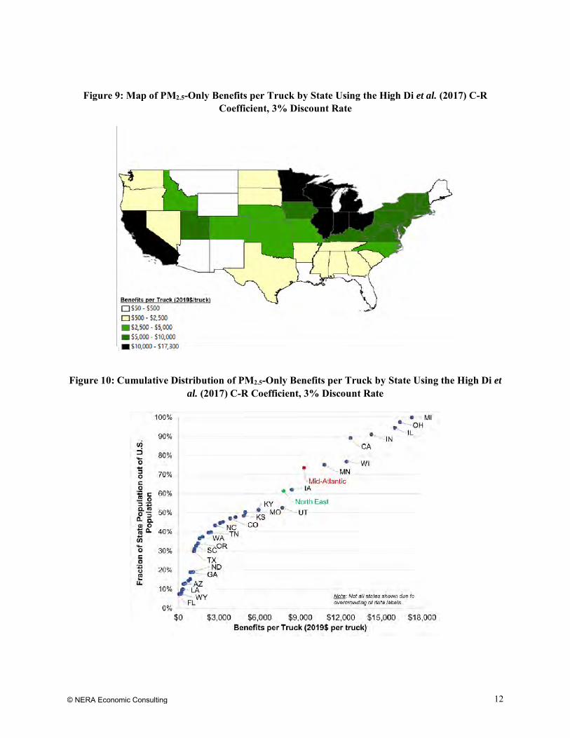
© NERA Economic Consulting 12
Figure 9: Map of PM2.5-Only Benefits per Truck by State Using the High Di et al. (2017) C-R Coefficient, 3% Discount Rate
Figure 10: Cumulative Distribution of PM2.5-Only Benefits per Truck by State Using the High Di et al. (2017) C-R Coefficient, 3% Discount Rate

© NERA Economic Consulting 13
B. Ozone Calculations
Wolfe et al. (2018) does not provide any benefit-per-ton estimates for ozone. Also, there appears to be only one example among EPA’s past RIAs that used the “reduced-form” benefit-per-ton methodology for ozone – the RIA for the Clean Power Plan (EPA, 2015a). Because those estimates were based on NOx
reductions from electricity generating units, which have a very different geographic distribution than vehicle emissions, they are not relevant for use in our HDOH benefits scoping analysis. All the other past RIAs we reviewed that contained estimates of ozone-related health benefits had based those estimates on full-scale US-wide air quality modeling of the specific emissions reductions projected for that regulation. One can develop a rough estimate of the average ozone benefit per ton implied in those remaining RIAs by dividing the RIA’s estimate of total ozone benefits by its estimated tons of NOx emissions reductions. Of those remaining RIAs, the one that is most relevant to an HDOH NOx reduction regulation is the RIA for the Tier 3 Light-Duty Vehicle standards from 2014 (EPA, 2014a). We find that the approximate national average ozone benefit per ton implied in that RIA (stated in 2019$) ranges from about $3,800 per ton when using an all-cause mortality C-R relationship from Bell et al. (2004) to about $17,300 per ton when using an all-cause C-R relationship from Levy et al. (2005). A more relevant but older RIA is that for the prior HDOH NOx emissions rulemaking (EPA, 2000). Its implied national average ozone benefit per ton was $824 (2019$). That estimate was based on a C-R function for hospital admissions rather than mortality. Clearly there is a wide range, but none of those estimates reflects the Agency’s current thinking about ozone-related health risks that could be viewed as a likely basis for ozone benefits calculation in a future RIA. Below we describe how we developed our own reduced-form estimates for ozone benefits, and their implications for per-truck benefits.
EPA’s current draft Policy Assessment for ozone (EPA, 2019c) does not provide epidemiology-based risk calculations for any health effect, and it specifically casts doubt on ozone’s potential mortality risk. This suggests that a future RIA might not attribute any mortality benefits to ozone reductions. In the spirit of providing a range of estimates, however, we decided to employ a low and a high coefficient for respiratory mortality from Zanobetti and Schwartz (2008). This choice reflects the facts that EPA did cite several epidemiological studies addressing respiratory health risks in an appendix of the draft ozone Policy Assessment and that the most recent (2021) health impact functions library in BenMAP also contains several C-R relationships for respiratory health risks; of those cited, Zanobetti and Schwartz provided the clearest option for C-R coefficients specifically for respiratory mortality risk.17
Also challenging to this part of our analysis was a lack of a specific grid of ambient ozone concentrations associated with a specific quantity of tons of NOx emissions, such as was available for PM2.5 from the Wolfe et al. study. We instead had to rely on less nationally comprehensive results from prior air quality modeling sensitivity cases that had been prepared for the 2015 Ozone RIA (EPA, 2015b). For that RIA, EPA conducted several sensitivity runs with CAMx for specific regions of the U.S. that the Agency had projected would need to make NOx reductions to attain an ozone NAAQS down to 65 ppb. Some of those sensitivity runs simulated the ambient ozone impacts of “across-the-board” 50% reductions in anthropogenic NOx emissions, which thus, at least in part, included mobile source emissions reductions. We consider those specific sensitivity runs to be the most relevant for our analysis. They had been run for eight U.S. regions, identified by the colored areas (excluding the two in California) in Figure 11, which is
17 For the low end of the range, we employ a low C-R coefficient for respiratory mortality of 0.00054, based on a relative risk of
1.0054 per 10 ppb change in 8-hr ozone from the 0-day lag model. For the high end of the range, we employ a low C-R coefficient for respiratory mortality of 0.00082, based on a relative risk of 1.0083 per 10 ppb change in 8-hr ozone from the 0-3 day lag model. Both these relative risk estimates are obtained from Table 1 of the Zanobetti and Schwartz study (p. 186).

© NERA Economic Consulting 14
copied from EPA (2015b).18 The outputs of those sensitivity runs that were reported in a technical support document spreadsheet (EPA, 2015c) were ozone design values at each existing monitor across the U.S. for the base case and for each of the sensitivity cases and the NOx emissions changes between the two cases. Following guidance in that document, we used those outputs to calculate “ozone response factors” for each of the sensitivity cases by dividing the projected change in the ozone design value at each monitor across the U.S. by the tons of NOx emissions reduction assumed for that case.
Figure 11: Basis for Estimating Ozone Response Factors for Each State (Source: EPA (2015b), Figure 2-2, with red font text added by NERA, as explained in text.)
Note: For northern states west of WI, “Wisconsin avg (w/o negatives)” means that monitors in WI with a negative response factor were not included in the average estimated for these states. Negative values imply local ozone formation is VOC-limited, which does occur in parts of WI (near the lake), but which we assume does not occur in northern states west of WI.
For each state where emissions were reduced in one of the eight relevant sensitivity runs, we extracted the ozone response factors for all the monitors in that state and adopted the simple average of those values as our analysis’s assumption for that state’s change in ambient ozone due to a ton of NOx emitted by HDOH trucks in that state.
Although EPA’s data provided response factors for all monitors throughout the entire U.S., we did not use response factor data for monitors that were not within the region for which emissions had been cut.19 For areas of the U.S. that were not included in any of EPA’s sensitivity cases (i.e., the white areas in Figure 11), we adopted an average ozone response factor from one of the modeled regions, selecting a region that we judged to have relatively similar ozone forming attributes (e.g., temperature, sunlight, etc.). For
18 None of the sensitivity cases run for the two California regions involved the 50% across-the-board NOx reductions that we
considered relevant for our analysis. 19 We did confirm that response factors for monitors outside of the region of the simulated emissions reductions were generally
very much smaller than those for monitors within the region.

© NERA Economic Consulting 15
example, for Missouri, we used an ozone response factor (i.e., the average ppb change in Missouri per ton of NOx emitted in Missouri) that was the same as EPA’s modeling indicated for Illinois. The red text on Figure 11 identifies the assignments we made for each of those areas that were not included in one of EPA’s sensitivity cases.20 The state-specific values of our resulting set of ozone response factors are provided in Appendix D.
We multiplied our state-specific ozone response factors by the state-specific NOx emission reductions that we also estimated (as described in Section IV, and reported in Appendix A) to obtain rough estimates of projected changes in ozone design values expected to occur in each state with the implementation of the hypothetical tighter HDOH NOx standard. We further assumed that changes in average seasonal ozone concentrations would be equal to the estimated changes in design values that was the basis of our estimates of ozone response factors.21 Using BenMAP, we applied those estimates of absolute changes in ambient ozone to the baseline ozone levels in every 12-km grid cell in each respective state to compute ozone benefit-per-ton estimates. As noted above, we used two C-R relationships for acute respiratory mortality risk during the summer months (June – August) estimated by a multi-city study and reported in Zanobetti and Schwartz (2008).22 Those calculations were carried out for the U.S. and by state for 2030, 2040, and 2050. The benefit-per-ton estimates obtained for the U.S. and by state are provided in Appendix B, with the year-2050 estimates summarized below.
Our estimate of the national average ozone benefit per ton for 2050 computed using the low C-R relationship from the Zanobetti and Schwartz (2008) study is $926 per ton (2019$).23 Figure 12 and Figure 13 present the state-specific results, which show California far higher than any other state: about $5,250 per ton –nearly 6 times the U.S. average. If California is removed from the data, the average for the remaining 47 states is about $430 per ton. Using the high C-R relationship from the Zanobetti and Schwartz (2008) study, we obtain a national average ozone benefit per ton estimate for 2050 of $1,420 per ton (2019$). Figure 14 and Figure 15 present the state-specific results, obtained using the high C-R relationship. The estimate for California is about $8,050 per ton while for the average for the remaining 47 states (excluding California) is about $660 per ton.
Figure 16 and Figure 17 graph the per-truck benefit estimates obtained using the low C-R relationship from the Zanobetti and Schwartz (2008) study when applying a 3% discount rate. The national average ozone benefit-per-truck estimate is $530 per truck (2019$). California’s estimate is $2,920 per truck, while the average for Rest of U.S. is $250 per truck. Figure 17 and Figure 18 graph the per-truck benefit estimates obtained using the high C-R relationship from the Zanobetti and Schwartz (2008) study when
20 Because the sensitivity cases for California were not appropriate for our analysis needs, we made an assignment for California
too, as identified in red font in the figure. 21 We surmise that this assumption causes our analysis to overstate the projected changes in ozone in most locations, as it is quite
likely that absolute changes in average ozone will be smaller than absolute changes in the highest levels of ozone. If so, this also means that our benefit-per-truck estimates for ozone will be overstated. As those estimates have turned out quite small even if they may be overstated due to this assumption, we have not attempted to further refine the assumption or to conduct sensitivity analyses for it.
22 Consistent with EPA’s methods for estimating risk from ozone exposures measured only during ozone-season months, our benefits calculations are for June through August. An adjustment factor of 0.25 was applied to BenMAP’s year-round counts of avoided respiratory mortality. This factor reflects the fraction of the days in the year covered by those months.
23 This is low compared to the ozone benefit-per-ton values implied in the Tier 3 Light-Duty Vehicle Standards RIA (EPA, 2014a). The primary reason for the large reduction is that our benefits calculations are for respiratory mortality only, whereas the 2014 RIA used C-R relationships for all-cause mortality, which the Agency now views as not likely causal. We also suspect (but cannot confirm) that the 2014 RIA applied a seasonal C-R relationship to mortality risk across the entire year. The Agency did not make such an extrapolation in its Health Exposure and Risk Assessment for that ozone NAAQS review (EPA 2014b).

© NERA Economic Consulting 16
applying a 3% discount rate. We obtain the national average ozone benefit-per-truck estimate to be $810 per truck (2019$). The estimate for California is obtained to be $4,480 per truck while the average for the Rest of the U.S. is obtained to be $390 per truck.
The corresponding maps and distributions for the ozone benefit-per-truck estimates computed using a 7% discount rate are presented in Appendix C. For each state, those benefits estimates are about 25% lower than their respective 3% discount rate estimates, with the geographical variations much the same as presented in the figures below.

© NERA Economic Consulting 17
Figure 12: Map of Ozone-Only Benefits per Ton by State Using the Low Zanobetti and Schwartz (2008) C-R Coefficient (2050)
Figure 13: Cumulative Distribution of Ozone-Only Benefits per Ton by State Using the Low Zanobetti and Schwartz (2008) C-R Coefficient (2050)

© NERA Economic Consulting 18
Figure 14: Map of Ozone-Only Benefits per Ton by State Using the High Zanobetti and Schwartz (2008) C-R Coefficient (2050)
Figure 15: Cumulative Distribution of Ozone-Only Benefits per Ton by State Using the High Zanobetti and Schwartz (2008) C-R Coefficient (2050)

© NERA Economic Consulting 19
Figure 16: Map of Ozone-Only Benefits per Truck by State Using the Low Zanobetti and Schwartz (2008) C-R Coefficient, 3% Discount Rate
Figure 17: Cumulative Distribution of Ozone-Only Benefits per Truck by State Using the Low Zanobetti and Schwartz (2008) C-R Coefficient, 3% Discount Rate

© NERA Economic Consulting 20
Figure 18: Map of Ozone-Only Benefits per Truck by State Using the High Zanobetti and Schwartz (2008) C-R Coefficient, 3% Discount Rate
Figure 19: Cumulative Distribution of Ozone-Only Benefits per Truck by State Using the High Zanobetti and Schwartz (2008) C-R Coefficient, 3% Discount Rate

© NERA Economic Consulting 21
VI. Benefit-per-Truck Estimates with Varying Confidence Levels
An important input that drives the benefit-per-ton estimates and thus the benefit-per-truck estimates is the C-R coefficient, which is an assumption about the increase in health risk per unit change in ozone and PM2.5 concentration. That assumption is usually based on a statistically derived association reported in one of many existing epidemiological papers. There are significant scientific uncertainties introduced when using these statistical associations to predict risks under different population and air quality conditions than those analyzed in the papers, since it involves extrapolation outside the range of observed exposures. The accompanying Summary Report of our analysis provides a detailed explanation of this concern with extrapolation in benefits analyses.24 It also discusses an approach to quantify the sensitivity of benefits estimates to various amounts of limitations on the amount of extrapolation allowed in their computation, which we have applied to the benefit-per-truck estimates of our scoping analysis.
We provide alternative estimates of benefits per truck associated with varying levels of extrapolation-related confidence. Estimates at the “more confident” end of the spectrum exclude benefits calculated to occur in areas with projected baseline concentrations below the 25th percentile of the range of observations in the original C-R estimation data. Estimates at the “less confident” end of the spectrum make no exclusions at all, allowing extrapolation of the C-R relationship even where projected baseline concentrations are lower than the lowest measured level (LML) in the original epidemiological study.25 Estimates that fall between these two ends of the spectrum exclude benefits that are in areas with projected baseline concentrations that are below percentile levels lower than the 25th percentile of the pollutant observations in the original study (such as the 1st, 5th, 10th percentiles of the original study’s observed exposure levels). Thus, we create a sliding scale of per-truck benefits estimates with increasing levels of qualitative confidence.26
To apply this method, two sets of data are needed. First, the relevant baseline concentrations associated with the regulation’s benefits, Cb, must be identified. Second, the concentrations associated with each selected population-weighted percentile p in the original epidemiological study must be obtained. These values are denoted Cp, which we apply for p=0, 1st, 5th, 10th, and 25th percentiles. The estimated benefits are placed into bins according to the baseline concentration level, Cb, from which they have been computed. Total benefits associated with each percentile level p are then recomputed by summing up benefits in only those bins with baseline concentrations Cb ≥ Cp. This results in gradually declining benefits-per-ton estimates as the percentile cut-off p rises – implying greater qualitative confidence that the benefits included in the computation are not the result of speculative extrapolation outside of the range of observed exposures.
An appropriate set of baseline exposures would be those projected to be in effect during the time period when the new regulation is taking effect. For our analysis, that would be from 2027 through 2057. The most relevant air quality projections usable in BenMAP that we could identify in the public domain are those prepared for the RIA for finalizing the repeal of the Clean Power Plan (EPA, 2019a), which include projected PM2.5 and ozone levels nationally for the years 2025, 2030, and 2035. We obtained those BenMAP air quality grids from EPA. We chose to use the 2035 projections for our analysis, as most of
24 See Section IV of that Summary Report. 25 The Agency uses the acronym LML to denote the 0th percentile of the distribution of exposures in the original study. 26 The values along this scale bear no relationship to statistical measures of significance or confidence intervals; nor do the ranges
provided within each segment of the scale, which reflect only high and low point estimates of the C-R relationship from different estimation methods.

© NERA Economic Consulting 22
the per-truck benefits occur in the years 2027 through 2040, although about 20% do occur after 2040, when baseline exposures will probably be lower still.
For each of the C-R relationships that we use in our scoping analysis, we obtained the concentrations associated with each percentile (i.e., the Cp values) from the respective original study. We use the population-weighted exposure distribution from Di et al. (2017) to develop the values of Cp for our low and highPM2.5 benefit-per-truck estimates, and we use the distribution of ozone exposures in the Zanobetti and Schwartz (2008) study to develop confidence-weighting adjustments for our low and high ozone benefit-per-truck estimates. The percentiles in the Di et al. study are available in supplemental materials to the original paper but are more precisely listed in a PM2.5 docket entry (EPA, 2019b). We use information on the distribution of city-specific average ozone concentrations reported in Table 2 of the online supplement to Zanobetti and Schwartz (2008) study.
For the two epidemiological studies that we have relied upon, Tables 1 through 4 below identify (in the first row) the ambient concentration levels (Cp values) for each of the above percentile cut-off levels that we have used to explore sensitivities to extrapolation-related confidence weighting. The second row of each table identifies the percentage of the respective study’s total avoided premature statistical deaths that lie within each alternative confidence range. (These sum to 100% across the row.) The last two rows of each table report the benefit-per-truck values associated with each confidence level when applying, respectively, a 3% and 7% discount rate to the present value calculation. The first column in each table reports the national average estimates unadjusted for confidence (which we reported in the previous section), while the values in the columns to the right show the estimates that have increasingly higher confidence, up to the point where only benefits in areas with exposures at or above the 25th percentile of the original epidemiological study are included.
Table 1 and 2 present the PM2.5 benefit-per-truck estimates calculated using low and high C-R coefficients from Di et al. (2017). It shows that about 14% of the benefits are projected to occur in locations that have exposures greater than the 25th percentile of all the exposures in the epidemiological study. As shown in Table 1, the unadjusted estimate of $4,650 per truck (obtained using the low C-R coefficient) that was reported in the prior section of this report declines to $650 per truck at the “more confident” end of the spectrum.27 If we were to use the 10th percentile as a less conservative confidence cut-off, the associated benefit-per-truck estimate would be $2,670 with about 57% of the benefits projected to occur in locations that have exposures greater than the 10th percentile of all the study exposures.28 As shown in Table 2, the unadjusted estimate of $6,340 per truck (obtained using the high C-R coefficient), declines to $890 per truck at the “more confident” end of the spectrum. At the 10th percentile confidence cut-off, the benefit-per-truck estimate is $3,640 per truck. As before, the estimates computed using a 7% discount rate are about 25% lower than the respective 3% discount rate estimates.
Table 3 and 4 present the ozone benefit-per-truck estimates calculated using low and high C-R coefficients from the Zanobetti and Schwartz (2008) study. The pattern observed in the drop-off of the benefit-per-truck estimates is significantly different from that for PM2.5. As shown in Table 3, the unadjusted estimate of $530 per truck (obtained using the low C-R coefficient) remains unchanged through the 5th percentile confidence cut-off because almost none of the U.S. is projected to have ozone
27 The benefit-per-truck estimate of $650 is calculated by multiplying the unadjusted estimate by the fraction of benefits that can
be attributed to locations with exposures greater than the 25th percentile of the study exposures: 14%*$4,650. 28 57% is computed as the sum of the percentages of the total deaths that can be attributed to locations with exposures greater
than the 25th percentile of the study exposures (i.e., the sum of the last two columns, 43%+14%). This sum is then multiplied by the unadjusted estimate (i.e., 57%*$4,650) to obtain the 10th percentile confidence-weighted estimate of $2,670.

© NERA Economic Consulting 23
concentrations below 23.4 ppb in our baseline air quality grid, even though Zanobetti and Schwartz data indicate that about 5% of the cities in their study had lower average ozone levels.29 The confidence-weighted ozone benefit estimate declines to $250 per truck at the highest confidence end of the spectrum with 47% of our estimated ozone benefits projected to occur in locations with exposures above the 25th percentile of all the cities observed in the original Zanobetti and Schwartz study. As shown in Table 4, the unadjusted estimate of $810 per truck (obtained using the low C-R coefficient), declines to $380 per truck at the highest confidence end of the spectrum. As before, the estimates computed using a 7% discount rate are about 25% lower than the respective 3% discount rate estimates.
29 We have no explanation for such a discrepancy at this time, which seems surprising given that our estimates of baseline
exposure are more disaggregated than those of Zanobetti and Schwartz’s observations (12-km grid resolution vs. city-wide averages) and they occur later in time (2035 vs. 1989-2000) when tighter ozone standards will be in place.

© NERA Economic Consulting 24
Table 1: Avoided Premature Statistical Deaths (%) and National PM2.5 Benefits per Truck (2019$) by Confidence Level Using the Low C-R Coefficient from the Di et al. (2017) Epidemiology Study and Applying 3% and 7% Discount Rates
Below LML (<0.02)
LML to 1st Percentile
(≥0.02 & <3)
1st to 5th Percentile
(≥3 & <6.2)
5th to 10th Percentile
(≥6.2 & <7.3)
10th to 25th Percentile
(≥7.3 & <9.1)
25th Percentile & Above
(≥9.1) Avoided Premature Statistical Deaths (%)
National 0% 0% 15% 27% 43% 14% Benefit per Truck (2019$)
3% Discount Rate $4,650 $4,650 $4,650 $3,930 $2,670 $650 7% Discount Rate $3,460 $3,460 $3,460 $2,930 $1,980 $490
LML = Lowest Measured Level, meaning the minimum observed PM2.5 concentration in the original epidemiological study

© NERA Economic Consulting 25
Table 2: Avoided Premature Statistical Deaths (%) and National PM2.5 Benefits per Truck (2019$) by Confidence Level Using the High C-R Coefficient from the Di et al. (2017) Epidemiology Study and Applying 3% and 7% Discount Rates
Below LML (<0.02)
LML to 1st Percentile
(≥0.02 & <3)
1st to 5th Percentile
(≥3 & <6.2)
5th to 10th Percentile
(≥6.2 & <7.3)
10th to 25th Percentile
(≥7.3 & <9.1)
25th Percentile & Above
(≥9.1) Avoided Premature Statistical Deaths (%)
National 0% 0% 15% 27% 43% 14% Benefit per Truck (2019$)
3% Discount Rate $6,340 $6,340 $6,340 $5,360 $3,640 $890 7% Discount Rate $4,710 $4,710 $4,710 $3,980 $2,700 $660
LML = Lowest Measured Level, meaning the minimum observed PM2.5 concentration in the original epidemiological study

© NERA Economic Consulting 26
Table 3: Avoided Premature Statistical Deaths (%) and National Ozone Benefits per Truck (2019$) by Confidence Level Using the Low C-R Coefficient from the Zanobetti and Schwartz (2008) Epidemiology Study and Applying 3% and 7% Discount Rates
Below LML (<15.1)
LML to 1st Percentile
(=15.1)
1st to 5th Percentile
(>15.1 & <23.4)
5th to 10th Percentile
(≥23.4 & <35.6)
10th to 25th Percentile
(≥35.6 & <44.0)
25th Percentile & Above (≥44.0)
Avoided Premature Statistical Deaths (%) National 0% 0% 0% 17% 36% 47%
Benefit per Truck (2019$) 3% Discount Rate $530 $530 $530 $530 $440 $250 7% Discount Rate $390 $390 $390 $390 $320 $180
LML = Lowest Measured Level, meaning the minimum observed ozone concentration in the original epidemiological study

© NERA Economic Consulting 27
Table 4: Avoided Premature Statistical Deaths (%) and National Ozone Benefits per Truck (2019$) by Confidence Level Using the High C-R Coefficient from the Zanobetti and Schwartz (2008) Epidemiology Study and Applying 3% and 7% Discount Rates
Below LML (<15.1)
LML to 1st Percentile
(=15.1)
1st to 5th Percentile
(>15.1 & <23.4)
5th to 10th Percentile
(≥23.4 & <35.6)
10th to 25th Percentile
(≥35.6 & <44.0)
25th Percentile & Above (≥44.0)
Avoided Premature Statistical Deaths (%) National 0% 0% 0% 17% 36% 47%
Benefit per Truck (2019$) 3% Discount Rate $810 $810 $810 $810 $670 $380 7% Discount Rate $590 $590 $590 $590 $490 $280
LML = Lowest Measured Level, meaning the minimum observed ozone concentration in the original epidemiological study
© NERA Economic Consulting
As illustrated previously, significant differences exist between the projected concentrations in California and the Rest of U.S., which points to the existence of different patterns in the decline of the benefit-per-truck estimates moving from the “less confident” to the “more confident” end of the benefits estimates scale.30 Table 5 through 8 present the benefit-per-truck estimates separately for California and Rest of the U.S. in the same format as that presented above for the national estimates. These tables show that California benefit-per-truck estimates decrease at a slower rate than the Rest of the U.S estimates do, which further widens the significant disparities that were noted in the unadjusted estimates in the prior section.
Table 5 and 6 present the PM2.5 benefit-per-truck estimates calculated using low and high C-R coefficients from the Di et al. (2017) study for these two regions. As shown in Table 5, the unadjusted estimate using a 3% discount rate (obtained using the low Di et al. (2017) C-R coefficient) declines from $9,330 to $5,570 per truck for California, while it declines from $4,260 to $180 per truck for the Rest of the U.S. While the estimates for California are about 2 times higher than those for the Rest of the U.S. at the “less confident” end of the spectrum, they are 30 times higher at the “more confident” end. About 60% of the benefits in California are projected to occur in locations with baseline concentrations greater than the 25th percentile of the original study; in contrast, the corresponding fraction for benefits estimates across the Rest of the U.S. is about 4%. As shown in Table 6, the unadjusted estimate using a 3% discount rate (obtained using the high Di et al. (2017) C-R coefficient) declines from $12,700 to $7,580 per truck for California, while it declines from $5,810 to $250 per truck for the Rest of the U.S. The relationship between the California and the Rest of the U.S. estimates are similar to those obtained using the low C-R coefficient.
Table 7 and 8 present the ozone benefit-per-truck estimates calculated using low and high C-R coefficients from the Zanobetti and Schwartz (2008) study for the two regions. The unadjusted estimate using a 3% discount rate (obtained using the low Zanobetti and Schwartz (2008) C-R coefficient) declines from $2,920 to $1,690 per truck for California, while it declines from $250 to $80 per truck for the Rest of the U.S. The confidence unadjusted estimate using a 3% discount rate (obtained using the high Zanobetti and Schwartz (2008) C-R coefficient) declines from $4,480 to $2,600 per truck for California, while it declines from $390 to $130 per truck for the Rest of the U.S. Compared to the PM2.5 estimates, a larger disparity in the estimates for the two regions is observed at the “less confident” end of the spectrum. That is, the California benefit-per-truck estimates are about 12 times higher than those for the Rest of the U.S. before confidence-weighting and are about 21 times higher at the other end of the confidence-weighting spectrum.
Although this finding that California has substantially higher benefits per truck could be used to justify a tighter standard for California trucks than for the rest of the U.S., it would be inappropriate to use the higher California-specific benefits estimates in a benefit-cost analysis of a standard that would be applied to other states.
30 The Rest of U.S. region includes all states across the conterminous U.S. except for California.

© NERA Economic Consulting 29
Table 5: Avoided Premature Statistical Deaths (%) and PM2.5 Benefits per Truck (2019$) for California and Rest of U.S. by Confidence Level Using the Low C-R Coefficient from the Di et al. (2017) Epidemiology Study and Applying 3% and 7% Discount Rates
Below LML (<0.02)
LML to 1st Percentile
(≥0.02 & <3)
1st to 5th Percentile
(≥3 & <6.2)
5th to 10th Percentile
(≥6.2 & <7.3)
10th to 25th Percentile
(≥7.3 & <9.1)
25th Percentile & Above
(≥9.1) Avoided Premature Statistical Deaths (%)
California 0% 0% 5% 11% 25% 60% Rest of U.S. 0% 0% 18% 31% 47% 4%
Benefit per Truck (2019$) 3% Discount Rate
California $9,330 $9,330 $9,330 $8,870 $7,880 $5,570 Rest of U.S. $4,260 $4,260 $4,260 $3,510 $2,190 $180
7% Discount Rate California $6,820 $6,820 $6,820 $6,490 $5,760 $4,070
Rest of U.S. $3,180 $3,180 $3,180 $2,620 $1,640 $130 LML = Lowest Measured Level, meaning the minimum observed PM2.5 concentration in the original epidemiological study

© NERA Economic Consulting 30
Table 6: Avoided Premature Statistical Deaths (%) and PM2.5 Benefits per Truck (2019$) for California and Rest of U.S. by Confidence Level Using the High C-R Coefficient from the Di et al. (2017) Epidemiology Study and Applying 3% and 7% Discount Rates
Below LML (<0.02)
LML to 1st Percentile
(≥0.02 & <3)
1st to 5th Percentile
(≥3 & <6.2)
5th to 10th Percentile
(≥6.2 & <7.3)
10th to 25th Percentile
(≥7.3 & <9.1)
25th Percentile & Above
(≥9.1) Avoided Premature Statistical Deaths (%)
California 0% 0% 5% 11% 25% 60% Rest of U.S. 0% 0% 18% 31% 47% 4%
Benefit per Truck (2019$) 3% Discount Rate
California $12,700 $12,700 $12,700 $12,080 $10,730 $7,580 Rest of U.S. $5,810 $5,810 $5,810 $4,780 $2,990 $250
7% Discount Rate California $9,290 $9,290 $9,290 $8,840 $7,850 $5,550
Rest of U.S. $4,330 $4,330 $4,330 $3,560 $2,230 $180 LML = Lowest Measured Level, meaning the minimum observed PM2.5 concentration in the original epidemiological study

© NERA Economic Consulting 31
Table 7: Avoided Premature Statistical Deaths (%) and Ozone Benefits per Truck (2019$) for California and Rest of U.S. by Confidence Level Using the Low C-R Coefficient from the Zanobetti and Schwartz (2008) Epidemiology Study and Applying 3% and 7% Discount
Rates
Below LML (<15.1)
LML to 1st Percentile
(=15.1)
1st to 5th Percentile
(>15.1 & <23.4)
5th to 10th Percentile
(≥23.4 & <35.6)
10th to 25th Percentile
(≥35.6 & <44.0)
25th Percentile & Above (≥44.0)
Avoided Premature Statistical Deaths (%) California 0% 0% 0% 12% 30% 58%
Rest of U.S. 0% 0% 0% 24% 44% 32% Benefit per Truck (2019$)
3% Discount Rate California $2,920 $2,920 $2,920 $2,920 $2,560 $1,690
Rest of U.S. $250 $250 $250 $250 $190 $80 7% Discount Rate
California $2,140 $2,140 $2,140 $2,140 $1,870 $1,240 Rest of U.S. $190 $190 $190 $190 $150 $60
LML = Lowest Measured Level, meaning the minimum observed ozone concentration in the original epidemiological study

© NERA Economic Consulting 32
Table 8: Avoided Premature Statistical Deaths (%) and Ozone Benefits per Truck (2019$) for California and Rest of U.S. by Confidence Level Using the High C-R Coefficient from the Zanobetti and Schwartz (2008) Epidemiology Study and Applying 3% and 7% Discount
Rates
Below LML (<15.1)
LML to 1st Percentile
(=15.1)
1st to 5th Percentile
(>15.1 & <23.4)
5th to 10th Percentile
(≥23.4 & <35.6)
10th to 25th Percentile
(≥35.6 & <44.0)
25th Percentile & Above (≥44.0)
Avoided Premature Statistical Deaths (%) California 0% 0% 0% 12% 30% 58%
Rest of U.S. 0% 0% 0% 24% 44% 32% Benefit per Truck (2019$)
3% Discount Rate California $4,480 $4,480 $4,480 $4,480 $3,920 $2,600
Rest of U.S. $390 $390 $390 $390 $300 $130 7% Discount Rate
California $3,280 $3,280 $3,280 $3,280 $2,870 $1,900 Rest of U.S. $290 $290 $290 $290 $220 $90
LML = Lowest Measured Level, meaning the minimum observed ozone concentration in the original epidemiological study

© NERA Economic Consulting 33
VII. References
Di, Q; Wang, Y; Zanobetti, A; Wang, Y; Koutrakis, P; Choirat, C; Dominici, F; Schwartz, J. 2017. Air pollution and mortality in the Medicare population. New England Journal of Medicine 376(26):2513-2522.
EPA. 2000. Regulatory impact analysis: Heavy-duty engine and vehicle standards and highway diesel fuel sulfur control requirements, EPA420-R-00-026, December.
EPA. 2004. Advisory Council on Clean Air Compliance Analysis response to agency request on cessation lag, EPA-COUNCIL-LTR-05-001, December.
EPA. 2014a. Control of air pollution from motor vehicles: Tier 3 motor vehicle emission and fuel standards final rule, regulatory impact analysis, EPA-420-R-14-005, March.
EPA. 2014b. Health risk and exposure assessment for ozone, final report, EPA-452/R-14-004a, August.
EPA. 2015a. Regulatory impact analysis for the Clean Power Plan final rule, EPA-452/R-15-003, August.
EPA. 2015b. Regulatory impact analysis of the final revisions to the National Ambient Air Quality Standards for ground-level ozone, EPA-452/R-15-007, September.
EPA. 2015c. “Copy of docket data final RIA v2.” Docket # EPA-HQ-OAR-2013-0169-0056, posted October 7.
EPA. 2021. Population and activity of on-road vehicles in MOVES3, EPA-420-R-21-012, April.
EPA. 2019a. Regulatory impact analysis for the repeal of the Clean Power Plan, and the emission guidelines for greenhouse gas emissions from existing electric utility generating units, EPA-452/R-19-003, June.
EPA. 2019b. “Email from Scott Jenkins, EPA, to Benjamin Sabath and Francesca Dominici. Re: question about PM2.5 estimates in Di et al. (2017) studies and data file attachment. May 8, 2019.” Docket # EPA-HQ-OAR-2015-0072-0022, posted September 11.
EPA. 2019c. Policy assessment for the review of the ozone national ambient air quality standards, external review draft, EPA-452/P-19-002, October.
EPA. 2020. Policy assessment for the review of the national ambient air quality standards for particulate matter, EPA-452/R-20-002, January.
Krewski, D; Jerrett, M; Burnett, RT; Ma, R; Hughes, E; Shi, Y; Turner, MC; Pope, CA, III; Thurston, G; Calle, EE; Thun, MJ; Beckerman, B; Deluca, P; Finkelstein, N; Ito, K; Moore, DK; Newbold, KB; Ramsay, T; Ross, Z; Shin, H; Tempalski, B. 2009. Extended follow-up and spatial analysis of the American Cancer Society study linking particulate air pollution and mortality. Research Report 140. Health Effects Institute. Boston, MA.
Lepeule, J; Laden, F; Dockery, D; Schwartz, J. 2012. Chronic exposure to fine particles and mortality: an extended follow-up of the Harvard Six Cities study from 1974 to 2009. Environ. Health Perspect. 120(7):965.
Wolfe, P; Davidson K; Fulcher, C; Fann, N; Zawacki, M; Baker, K. 2018. Monetized health benefits attributable to mobile source emission reductions across the United States in 2025. Science of the Total Environment 650:2490-2498.

© NERA Economic Consulting 34
Zanobetti, A; Schwartz, J. 2008. Mortality displacement in the association of ozone with mortality: an analysis of 48 cities in the United States. Am J Respir Crit Care Med. 177:184-189.

© NERA Economic Consulting 35
Appendix A: Estimated Total NOx Emissions Reductions Including All Model Years, by State
2027 2028 2029 2030 2031 2032 2033 2034 2035 2036 2037 2038 2039 2040 2041 2042 2043 2044 U.S. 39,268 79,207 119,691 161,341 212,912 262,076 309,543 354,311 395,691 433,610 468,668 500,585 528,674 553,267 574,503 592,753 608,024 623,081
Alabama 781 1,575 2,380 3,208 4,234 5,212 6,156 7,047 7,869 8,623 9,320 9,954 10,512 11,000 11,422 11,784 12,087 12,385
Arizona 1,069 2,156 3,258 4,391 5,796 7,136 8,429 9,649 10,776 11,809 12,763 13,632 14,398 15,067 15,645 16,141 16,555 16,963
Arkansas 495 999 1,509 2,034 2,683 3,301 3,898 4,460 4,979 5,454 5,893 6,293 6,644 6,951 7,216 7,442 7,631 7,818
California 4,017 8,102 12,245 16,506 21,785 26,818 31,679 36,266 40,507 44,396 47,993 51,270 54,156 56,685 58,871 60,753 62,332 63,889
Colorado 703 1,418 2,142 2,887 3,810 4,689 5,538 6,339 7,079 7,757 8,384 8,955 9,457 9,896 10,276 10,602 10,875 11,144
Connecticut 346 698 1,055 1,423 1,879 2,313 2,734 3,130 3,497 3,833 4,145 4,428 4,678 4,897 5,087 5,250 5,388 5,523
Delaware 121 245 370 499 660 813 961 1,101 1,231 1,349 1,459 1,559 1,647 1,725 1,792 1,849 1,898 1,946
Florida 2,089 4,214 6,370 8,588 11,349 13,984 16,531 18,935 21,161 23,203 25,094 26,819 28,339 29,674 30,830 31,828 32,669 33,499
Georgia 1,299 2,620 3,959 5,337 7,047 8,677 10,251 11,736 13,109 14,369 15,533 16,594 17,528 18,346 19,053 19,662 20,172 20,675
Idaho 249 502 758 1,022 1,346 1,656 1,954 2,235 2,495 2,733 2,952 3,151 3,327 3,480 3,612 3,724 3,818 3,911
Illinois 1,323 2,669 4,033 5,437 7,178 8,838 10,442 11,955 13,354 14,637 15,823 16,904 17,855 18,690 19,410 20,031 20,551 21,064
Indiana 935 1,887 2,851 3,843 5,071 6,241 7,370 8,436 9,420 10,322 11,155 11,914 12,581 13,166 13,670 14,103 14,464 14,821
Iowa 518 1,045 1,579 2,128 2,806 3,452 4,075 4,663 5,205 5,701 6,159 6,576 6,942 7,262 7,537 7,773 7,969 8,162
Kansas 458 923 1,395 1,880 2,478 3,048 3,597 4,115 4,593 5,030 5,434 5,801 6,124 6,406 6,649 6,857 7,030 7,200
Kentucky 711 1,435 2,167 2,921 3,847 4,730 5,581 6,383 7,123 7,800 8,426 8,994 9,494 9,930 10,305 10,626 10,893 11,156
Louisiana 634 1,279 1,932 2,604 3,435 4,227 4,991 5,712 6,378 6,988 7,552 8,065 8,517 8,912 9,253 9,546 9,790 10,032
Maine 221 445 672 905 1,194 1,469 1,733 1,983 2,213 2,424 2,618 2,795 2,951 3,086 3,203 3,302 3,385 3,467
Maryland 697 1,407 2,126 2,866 3,784 4,660 5,506 6,304 7,043 7,720 8,346 8,917 9,420 9,861 10,242 10,571 10,847 11,119
Massachusetts 646 1,304 1,970 2,657 3,512 4,328 5,117 5,862 6,552 7,186 7,773 8,308 8,780 9,195 9,554 9,865 10,127 10,385
Michigan 1,349 2,722 4,113 5,544 7,320 9,013 10,649 12,191 13,617 14,924 16,132 17,233 18,201 19,050 19,783 20,413 20,940 21,461
Minnesota 792 1,597 2,413 3,252 4,293 5,285 6,242 7,145 7,979 8,744 9,450 10,092 10,657 11,152 11,578 11,944 12,250 12,552
Mississippi 503 1,014 1,532 2,065 2,723 3,351 3,957 4,527 5,054 5,537 5,982 6,388 6,744 7,055 7,323 7,553 7,744 7,933
Missouri 958 1,932 2,918 3,933 5,178 6,364 7,507 8,585 9,579 10,488 11,328 12,091 12,762 13,347 13,851 14,282 14,640 14,993
Montana 219 442 668 900 1,187 1,461 1,725 1,974 2,203 2,413 2,607 2,783 2,938 3,074 3,190 3,290 3,372 3,454
Nebraska 322 649 980 1,321 1,740 2,140 2,525 2,888 3,223 3,530 3,813 4,070 4,296 4,493 4,663 4,808 4,929 5,047
Nevada 311 628 949 1,279 1,688 2,079 2,456 2,812 3,141 3,442 3,722 3,976 4,200 4,396 4,566 4,712 4,834 4,955
New Hampshire 186 375 566 763 1,007 1,239 1,463 1,674 1,869 2,048 2,213 2,363 2,496 2,611 2,711 2,796 2,868 2,938
New Jersey 865 1,745 2,637 3,557 4,705 5,801 6,862 7,864 8,792 9,644 10,433 11,153 11,789 12,348 12,832 13,250 13,604 13,953
New Mexico 387 779 1,178 1,587 2,092 2,573 3,037 3,475 3,879 4,248 4,590 4,900 5,173 5,411 5,616 5,792 5,938 6,082

© NERA Economic Consulting 36
2027 2028 2029 2030 2031 2032 2033 2034 2035 2036 2037 2038 2039 2040 2041 2042 2043 2044 New York 1,363 2,750 4,155 5,602 7,396 9,107 10,759 12,318 13,760 15,083 16,306 17,420 18,402 19,262 20,006 20,646 21,183 21,713
North Carolina 1,321 2,666 4,028 5,430 7,166 8,821 10,420 11,927 13,320 14,597 15,777 16,852 17,798 18,626 19,341 19,955 20,469 20,976 North Dakota 154 310 469 632 833 1,025 1,209 1,383 1,544 1,691 1,827 1,950 2,058 2,153 2,234 2,303 2,361 2,418
Ohio 1,419 2,863 4,326 5,831 7,692 9,467 11,179 12,794 14,287 15,655 16,919 18,070 19,082 19,969 20,734 21,391 21,940 22,482 Oklahoma 644 1,300 1,964 2,646 3,491 4,295 5,070 5,802 6,477 7,095 7,666 8,186 8,642 9,041 9,385 9,680 9,925 10,167
Oregon 492 991 1,498 2,019 2,665 3,281 3,875 4,435 4,953 5,427 5,866 6,265 6,616 6,924 7,189 7,417 7,607 7,795 Pennsylvania 1,325 2,672 4,037 5,442 7,177 8,832 10,429 11,935 13,326 14,601 15,779 16,851 17,795 18,620 19,333 19,945 20,456 20,960 Rhode Island 97 196 296 398 526 648 766 877 980 1,074 1,161 1,241 1,311 1,373 1,426 1,472 1,510 1,548
South Carolina 786 1,584 2,394 3,227 4,255 5,236 6,182 7,074 7,898 8,652 9,349 9,983 10,541 11,029 11,450 11,810 12,111 12,408
South Dakota 172 347 524 706 930 1,143 1,348 1,541 1,719 1,882 2,032 2,169 2,288 2,393 2,483 2,559 2,622 2,685 Tennessee 954 1,923 2,906 3,918 5,169 6,361 7,512 8,598 9,601 10,521 11,371 12,144 12,825 13,421 13,936 14,377 14,747 15,112
Texas 3,377 6,812 10,295 13,878 18,319 22,554 26,643 30,500 34,066 37,335 40,358 43,111 45,534 47,657 49,490 51,067 52,389 53,693 Utah 393 793 1,198 1,614 2,129 2,620 3,094 3,540 3,953 4,331 4,681 4,999 5,279 5,524 5,736 5,917 6,069 6,219
Vermont 113 228 344 464 611 751 886 1,014 1,131 1,239 1,338 1,428 1,507 1,576 1,635 1,686 1,728 1,769 Virginia 1,140 2,299 3,474 4,682 6,176 7,598 8,972 10,266 11,463 12,558 13,571 14,492 15,303 16,012 16,623 17,148 17,587 18,019
Washington 793 1,600 2,418 3,259 4,299 5,290 6,246 7,148 7,981 8,745 9,451 10,093 10,658 11,153 11,580 11,947 12,253 12,556 West Virginia 274 552 835 1,125 1,483 1,825 2,154 2,464 2,751 3,013 3,256 3,476 3,670 3,839 3,984 4,109 4,213 4,316
Wisconsin 933 1,882 2,844 3,833 5,057 6,222 7,347 8,407 9,386 10,283 11,111 11,864 12,526 13,104 13,603 14,030 14,387 14,738 Wyoming 155 312 471 635 836 1,027 1,211 1,384 1,544 1,690 1,825 1,948 2,055 2,149 2,230 2,298 2,355 2,411
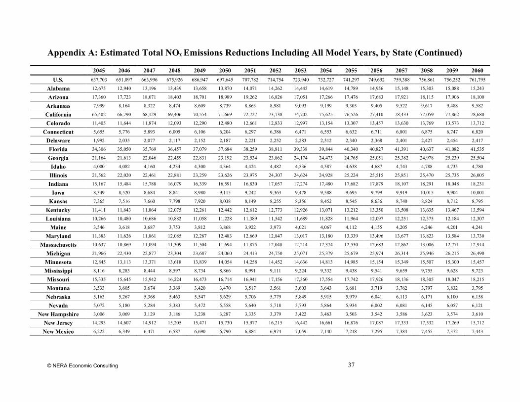
© NERA Economic Consulting 37
Appendix A: Estimated Total NOx Emissions Reductions Including All Model Years, by State (Continued)
2045 2046 2047 2048 2049 2050 2051 2052 2053 2054 2055 2056 2057 2058 2059 2060 U.S. 637,703 651,097 663,996 675,926 686,947 697,645 707,782 714,754 723,940 732,727 741,297 749,692 759,388 756,861 756,252 761,795
Alabama 12,675 12,940 13,196 13,439 13,658 13,870 14,071 14,262 14,445 14,619 14,789 14,956 15,148 15,303 15,088 15,243
Arizona 17,360 17,723 18,071 18,403 18,701 18,989 19,262 16,826 17,051 17,266 17,476 17,683 17,921 18,115 17,906 18,100
Arkansas 7,999 8,164 8,322 8,474 8,609 8,739 8,863 8,981 9,093 9,199 9,303 9,405 9,522 9,617 9,488 9,582
California 65,402 66,790 68,129 69,406 70,554 71,669 72,727 73,738 74,702 75,625 76,526 77,410 78,433 77,059 77,862 78,680
Colorado 11,405 11,644 11,874 12,093 12,290 12,480 12,661 12,833 12,997 13,154 13,307 13,457 13,630 13,769 13,573 13,712
Connecticut 5,655 5,776 5,893 6,005 6,106 6,204 6,297 6,386 6,471 6,553 6,632 6,711 6,801 6,875 6,747 6,820
Delaware 1,992 2,035 2,077 2,117 2,152 2,187 2,221 2,252 2,283 2,312 2,340 2,368 2,401 2,427 2,454 2,417
Florida 34,306 35,050 35,769 36,457 37,079 37,684 38,259 38,811 39,338 39,844 40,340 40,827 41,391 40,637 41,082 41,535
Georgia 21,164 21,613 22,046 22,459 22,831 23,192 23,534 23,862 24,174 24,473 24,765 25,051 25,382 24,978 25,239 25,504
Idaho 4,000 4,082 4,160 4,234 4,300 4,364 4,424 4,482 4,536 4,587 4,638 4,687 4,743 4,788 4,735 4,780
Illinois 21,562 22,020 22,461 22,881 23,259 23,626 23,975 24,307 24,624 24,928 25,224 25,515 25,851 25,470 25,735 26,005
Indiana 15,167 15,484 15,788 16,079 16,339 16,591 16,830 17,057 17,274 17,480 17,682 17,879 18,107 18,291 18,048 18,231
Iowa 8,349 8,520 8,684 8,841 8,980 9,115 9,242 9,363 9,478 9,588 9,695 9,799 9,919 10,015 9,904 10,001
Kansas 7,365 7,516 7,660 7,798 7,920 8,038 8,149 8,255 8,356 8,452 8,545 8,636 8,740 8,824 8,712 8,795
Kentucky 11,411 11,643 11,864 12,075 12,261 12,442 12,612 12,773 12,926 13,071 13,212 13,350 13,508 13,635 13,467 13,594
Louisiana 10,266 10,480 10,686 10,882 11,058 11,228 11,389 11,542 11,689 11,828 11,964 12,097 12,251 12,375 12,184 12,307
Maine 3,546 3,618 3,687 3,753 3,812 3,868 3,922 3,973 4,021 4,067 4,112 4,155 4,205 4,246 4,201 4,241
Maryland 11,383 11,626 11,861 12,085 12,287 12,483 12,669 12,847 13,017 13,180 13,339 13,496 13,677 13,823 13,584 13,730
Massachusetts 10,637 10,869 11,094 11,309 11,504 11,694 11,875 12,048 12,214 12,374 12,530 12,683 12,862 13,006 12,771 12,914
Michigan 21,966 22,430 22,877 23,304 23,687 24,060 24,413 24,750 25,071 25,379 25,679 25,974 26,314 25,946 26,215 26,490
Minnesota 12,845 13,113 13,371 13,618 13,839 14,054 14,258 14,452 14,636 14,813 14,985 15,154 15,349 15,507 15,300 15,457
Mississippi 8,116 8,283 8,444 8,597 8,734 8,866 8,991 9,111 9,224 9,332 9,438 9,541 9,659 9,755 9,628 9,723
Missouri 15,335 15,645 15,942 16,224 16,473 16,714 16,941 17,156 17,360 17,554 17,742 17,926 18,136 18,305 18,047 18,215
Montana 3,533 3,605 3,674 3,369 3,420 3,470 3,517 3,561 3,603 3,643 3,681 3,719 3,762 3,797 3,832 3,795
Nebraska 5,163 5,267 5,368 5,463 5,547 5,629 5,706 5,779 5,849 5,915 5,979 6,041 6,113 6,171 6,100 6,158
Nevada 5,072 5,180 5,284 5,383 5,472 5,558 5,640 5,718 5,793 5,864 5,934 6,002 6,081 6,145 6,057 6,121
New Hampshire 3,006 3,069 3,129 3,186 3,238 3,287 3,335 3,379 3,422 3,463 3,503 3,542 3,586 3,623 3,574 3,610
New Jersey 14,293 14,607 14,912 15,205 15,471 15,730 15,977 16,215 16,442 16,661 16,876 17,087 17,333 17,532 17,269 15,712
New Mexico 6,222 6,349 6,471 6,587 6,690 6,790 6,884 6,974 7,059 7,140 7,218 7,295 7,384 7,455 7,372 7,443

© NERA Economic Consulting 38
2045 2046 2047 2048 2049 2050 2051 2052 2053 2054 2055 2056 2057 2058 2059 2060 New York 22,228 22,701 23,157 23,592 23,984 24,365 24,726 25,071 25,401 25,716 26,024 26,326 26,676 26,247 26,522 26,803
North Carolina 21,469 21,920 22,355 22,769 23,141 23,502 23,845 24,171 24,482 24,780 25,070 25,354 25,683 25,300 25,559 25,823 North Dakota 2,473 2,523 2,571 2,617 2,658 2,697 2,734 2,769 2,803 2,835 2,866 2,896 2,931 2,959 2,987 2,957
Ohio 23,008 23,489 23,952 24,393 24,789 25,172 25,535 25,881 26,210 26,525 26,832 27,132 27,479 27,073 27,346 27,624 Oklahoma 10,402 10,617 10,823 11,019 11,195 11,365 11,525 11,678 11,824 11,962 12,098 12,230 12,382 12,504 12,338 12,460
Oregon 7,977 8,144 8,305 8,458 8,596 8,729 8,855 8,975 9,090 9,200 9,306 9,411 9,532 9,629 9,501 9,598 Pennsylvania 21,449 21,896 22,326 22,735 23,101 23,455 23,791 24,111 24,415 24,705 24,988 25,265 25,584 25,232 25,483 25,740 Rhode Island 1,585 1,619 1,652 1,683 1,712 1,739 1,765 1,790 1,814 1,837 1,860 1,882 1,907 1,928 1,949 1,915
South Carolina 12,696 12,958 13,211 13,451 13,666 13,874 14,071 14,258 14,436 14,606 14,771 14,933 15,119 15,269 15,066 15,215 South Dakota 2,745 2,800 2,852 2,902 2,945 2,988 3,027 3,065 3,100 3,134 3,167 3,198 3,235 3,264 3,294 3,260
Tennessee 15,465 15,789 16,101 16,397 16,663 16,921 17,165 17,398 17,620 17,832 18,038 18,240 18,474 18,662 18,387 18,574 Texas 54,959 56,121 57,242 58,311 59,272 60,206 61,091 61,937 62,743 63,515 64,269 65,008 65,862 64,765 65,437 66,122 Utah 6,364 6,496 6,624 6,746 6,854 6,960 7,059 7,154 7,245 7,331 7,415 7,498 7,593 7,669 7,560 7,636
Vermont 1,810 1,846 1,881 1,914 1,944 1,972 1,999 2,024 2,048 2,071 2,094 2,115 2,140 2,160 2,181 2,158 Virginia 18,438 18,821 19,190 19,541 19,854 20,158 20,446 20,720 20,980 21,229 21,471 21,708 21,982 21,665 21,880 22,100
Washington 12,849 13,117 13,375 13,621 13,841 14,054 14,256 14,448 14,631 14,805 14,976 15,142 15,335 15,490 15,259 15,414 West Virginia 4,415 4,506 4,593 4,676 4,749 4,821 4,889 4,953 5,014 5,072 5,129 5,184 5,248 5,300 5,232 5,284
Wisconsin 15,078 15,390 15,689 15,974 16,229 16,476 16,709 16,932 17,143 17,345 17,541 17,733 17,954 18,133 17,911 18,089 Wyoming 2,465 2,514 2,561 2,605 2,644 2,682 2,717 2,751 2,782 2,812 2,841 2,869 2,901 2,927 2,954 2,925

© NERA Economic Consulting 39
Appendix B: Estimated Benefits per Ton, by State
Zanobetti and Schwartz (2008); Ozone Respiratory Mortality
(2019$/ton) (Low)
Zanobetti and Schwartz (2008); Ozone Respiratory Mortality
(2019$/ton) (High)
Di et al. (2017); PM2.5 All-Cause Mortality (2019$/ton) (Low)
Di et al. (2017); PM2.5 All-Cause Mortality (2019$/ton) (High)
2030 2040 2050 2030 2040 2050 2030 2040 2050 2030 2040 2050 U.S. $666 $816 $926 $1,023 $1,252 $1,420 $6,552 $7,558 $7,842 $8,924 $10,295 $10,681
Alabama $209 $225 $218 $320 $345 $334 $746 $836 $821 $1,016 $1,138 $1,118 Arizona $705 $905 $1,085 $1,082 $1,388 $1,665 $326 $439 $532 $445 $598 $724
Arkansas $93 $101 $99 $143 $155 $152 $1,743 $1,991 $2,013 $2,374 $2,712 $2,742 California $3,662 $4,546 $5,249 $5,620 $6,973 $8,050 $11,572 $14,687 $17,241 $15,762 $20,004 $23,483 Colorado $513 $609 $661 $788 $934 $1,015 $3,543 $4,374 $4,987 $4,826 $5,959 $6,793
Connecticut $111 $128 $128 $170 $197 $196 $7,315 $8,544 $8,581 $9,964 $11,639 $11,689 Delaware $41 $48 $50 $63 $74 $77 $18,053 $21,794 $23,129 $24,591 $29,686 $31,504 Florida $803 $1,020 $1,205 $1,232 $1,565 $1,850 $44 $58 $69 $60 $79 $95 Georgia $361 $433 $472 $554 $665 $724 $805 $1,024 $1,157 $1,096 $1,395 $1,576 Idaho $32 $38 $41 $50 $59 $63 $3,023 $3,793 $4,276 $4,118 $5,167 $5,825 Illinois $101 $112 $112 $154 $173 $172 $15,512 $17,921 $18,514 $21,129 $24,409 $25,218 Indiana $144 $154 $146 $221 $237 $224 $14,172 $15,821 $15,491 $19,303 $21,549 $21,100
Iowa $30 $31 $28 $46 $48 $44 $8,574 $9,102 $8,334 $11,679 $12,398 $11,352 Kansas $28 $29 $26 $43 $44 $41 $4,870 $5,308 $5,036 $6,634 $7,231 $6,859
Kentucky $166 $175 $164 $256 $269 $252 $5,947 $6,501 $6,176 $8,101 $8,855 $8,412 Louisiana $169 $187 $186 $260 $287 $286 $252 $283 $287 $344 $386 $391
Maine $49 $57 $56 $76 $87 $86 $468 $573 $594 $637 $780 $809 Maryland $158 $195 $217 $242 $299 $333 $10,277 $12,838 $14,470 $13,999 $17,488 $19,710
Massachusetts $145 $164 $162 $223 $252 $248 $4,448 $5,077 $5,048 $6,059 $6,915 $6,877 Michigan $233 $257 $252 $358 $394 $387 $16,936 $19,343 $19,381 $23,068 $26,347 $26,399 Minnesota $83 $95 $92 $127 $146 $142 $10,405 $12,486 $12,684 $14,172 $17,008 $17,277 Mississippi $126 $137 $135 $193 $210 $207 $823 $968 $1,025 $1,121 $1,319 $1,396 Missouri $61 $65 $60 $94 $100 $92 $4,994 $5,438 $5,111 $6,802 $7,407 $6,962 Montana $25 $29 $30 $38 $45 $47 $309 $381 $421 $421 $519 $573 Nebraska $17 $18 $16 $26 $27 $25 $4,242 $4,625 $4,397 $5,778 $6,299 $5,989 Nevada $829 $1,129 $1,504 $1,273 $1,733 $2,309 $1,009 $1,366 $1,781 $1,375 $1,861 $2,426
New Hampshire $33 $40 $40 $51 $61 $62 $1,716 $2,137 $2,212 $2,338 $2,912 $3,013

© NERA Economic Consulting 40
Zanobetti and Schwartz (2008); Ozone Respiratory Mortality
(2019$/ton) (Low)
Zanobetti and Schwartz (2008); Ozone Respiratory Mortality
(2019$/ton) (High)
Di et al. (2017); PM2.5 All-Cause Mortality (2019$/ton) (Low)
Di et al. (2017); PM2.5 All-Cause Mortality (2019$/ton) (High)
2030 2040 2050 2030 2040 2050 2030 2040 2050 2030 2040 2050 New Jersey $233 $269 $273 $357 $413 $419 $12,678 $14,931 $15,409 $17,269 $20,338 $20,990 New Mexico $88 $109 $129 $134 $167 $197 $200 $258 $315 $272 $352 $429 New York $388 $436 $443 $595 $670 $680 $9,447 $10,832 $11,238 $12,869 $14,755 $15,308
North Carolina $323 $383 $412 $496 $588 $632 $2,531 $3,128 $3,427 $3,447 $4,260 $4,668 North Dakota $16 $19 $20 $25 $30 $30 $1,048 $1,228 $1,261 $1,427 $1,673 $1,717
Ohio $297 $321 $310 $455 $492 $476 $16,177 $18,207 $18,060 $22,034 $24,799 $24,600 Oklahoma $129 $133 $124 $198 $205 $191 $3,086 $3,320 $3,171 $4,204 $4,523 $4,319
Oregon $72 $82 $89 $111 $126 $136 $1,378 $1,598 $1,722 $1,878 $2,177 $2,345 Pennsylvania $281 $318 $318 $432 $488 $489 $13,961 $16,313 $16,676 $19,016 $22,220 $22,714 Rhode Island $40 $45 $45 $61 $69 $69 $8,404 $9,731 $9,821 $11,448 $13,255 $13,377
South Carolina $172 $211 $241 $264 $324 $371 $1,190 $1,506 $1,732 $1,621 $2,052 $2,360 South Dakota $16 $18 $17 $25 $28 $27 $2,407 $2,651 $2,520 $3,278 $3,611 $3,433
Tennessee $249 $275 $273 $383 $422 $419 $2,177 $2,478 $2,484 $2,965 $3,375 $3,383 Texas $951 $1,159 $1,303 $1,460 $1,779 $1,999 $1,036 $1,318 $1,498 $1,411 $1,795 $2,041 Utah $313 $386 $452 $480 $592 $693 $7,120 $8,730 $9,917 $9,698 $11,891 $13,508
Vermont $17 $20 $20 $26 $30 $30 $1,634 $2,049 $2,230 $2,226 $2,791 $3,038 Virginia $262 $322 $356 $401 $494 $546 $2,409 $3,128 $3,641 $3,282 $4,260 $4,960
Washington $117 $138 $150 $180 $212 $230 $1,430 $1,761 $1,979 $1,947 $2,399 $2,696 West Virginia $97 $100 $94 $149 $153 $144 $3,483 $3,742 $3,622 $4,744 $5,097 $4,933
Wisconsin $82 $93 $89 $126 $142 $137 $12,233 $14,082 $13,799 $16,663 $19,181 $18,796 Wyoming $14 $16 $17 $21 $25 $26 $164 $196 $206 $224 $267 $281

© NERA Economic Consulting 41
Appendix C: Benefit-per-Truck Estimates by State, 7% Discount Rate
Figure 20: Map of PM2.5-Only Benefits per Truck by State Using the Low Di et al. (2017) C-R Coefficient, 7% Discount Rate
Figure 21: Cumulative Distribution of PM2.5-Only Benefits per Truck by State Using the Low Di et al. (2017) C-R Coefficient, 7% Discount Rate

© NERA Economic Consulting 42
Figure 22: Map of PM2.5-Only Benefits per Truck by State Using the High Di et al. (2017) C-R Coefficient, 7% Discount Rate
Figure 23: Cumulative Distribution of PM2.5-Only Benefits per Truck by State Using the High Di et al. (2017) C-R Coefficient, 7% Discount Rate

© NERA Economic Consulting 43
Figure 24: Map of Ozone-Only Benefits per Truck by State Using the Low Zanobetti and Schwartz (2008) C-R Coefficient, 7% Discount Rate
Figure 25: Cumulative Distribution of Ozone-Only Benefits per Truck by State Using the Low Zanobetti and Schwartz (2008) C-R Coefficient, 7% Discount Rate

© NERA Economic Consulting 44
Figure 26: Map of Ozone-Only Benefits per Truck by State Using the High Zanobetti and Schwartz (2008) C-R Coefficient, 7% Discount Rate
Figure 27: Cumulative Distribution of Ozone-Only Benefits per Truck by State Using the High Zanobetti and Schwartz (2008) C-R Coefficient, 7% Discount Rate

© NERA Economic Consulting 45
Appendix D: Estimated Average Ozone Response Factors by State
State Ozone Response Factor (ppb/ton) Alabama 0.000022 Arizona 0.000061
Arkansas 0.000014 California 0.000072 Colorado 0.000061
Connecticut 0.000019 Delaware 0.000017 Florida 0.000022 Georgia 0.000022 Idaho 0.000011 Illinois 0.000005 Indiana 0.000012
Iowa 0.000005 Kansas 0.000005
Kentucky 0.000017 Louisiana 0.000022
Maine 0.000016 Maryland 0.000019
Massachusetts 0.000015 Michigan 0.000014 Minnesota 0.000011 Mississippi 0.000022 Missouri 0.000005 Montana 0.000011 Nebraska 0.000005 Nevada 0.000135
New Hampshire 0.000012 New Jersey 0.000019 New Mexico 0.000021 New York 0.000015
North Carolina 0.000017 North Dakota 0.000011
Ohio 0.000014 Oklahoma 0.000018
Oregon 0.000011 Pennsylvania 0.000012 Rhode Island 0.000019
South Carolina 0.000017 South Dakota 0.000011
Tennessee 0.000019 Texas 0.000025 Utah 0.000098
Vermont 0.000010 Virginia 0.000020

© NERA Economic Consulting 46
State Ozone Response Factor (ppb/ton) Washington 0.000011
West Virginia 0.000019 Wisconsin 0.000009 Wyoming 0.000011

© NERA Economic Consulting 47
NERA Economic Consulting 1255 23rd Street, NW Suite 600 Washington, DC 20037 202-466-3510 [email protected]

STATE OF NEW JERSEY
DEPARTMENT OF ENVIRONMENTAL PROTECTION Advanced Clean Trucks Program and Fleet Reporting Requirements; Proposed Amendments: N.J.A.C. 7-27A-3.10; Proposed New Rules: N.J.A.C. 7:27-31 and 33.
) ) ) ) )
53 N.J.R. 588(a) Notice of Rule Proposal Publication Date: April 19, 2021 Public Hearing Date: May 20, 2021
COMMENTS OF THE TRUCK AND ENGINE MANUFACTURERS ASSOCIATION
June 18, 2021 Timothy A. French Truck & Engine Manufacturers Association 333 West Wacker Drive, Suite 810 Chicago, IL 60606

1
STATE OF NEW JERSEY DEPARTMENT OF ENVIRONMENTAL PROTECTION
Advanced Clean Trucks Program and Fleet Reporting Requirements; Proposed Amendments: N.J.A.C. 7-27A-3.10; Proposed New Rules: N.J.A.C. 7:27-31 and 33.
) ) ) ) )
53 N.J.R. 588(a) Notice of Rule Proposal Publication Date: April 19, 2021 Public Hearing Date: May 20, 2021
Introduction
The Truck and Engine Manufacturers Association (EMA) submits these comments in opposition to the proposal of the New Jersey Department of Environmental Protection (DEP), published in the New Jersey Register on April 19, 2021 (53 N.J.R. 588(a)), to adopt and opt-in to California’s Advanced Clean Trucks (ACT) Program and Fleet Reporting Requirements. As DEP staff know, California’s ACT rule is part of a suite of additional rules that the California Air Resources Board (CARB) has adopted or plans to adopt regulating the emissions from medium-duty (MD) and heavy-duty (HD) on-highway vehicles and engines. Those rules collectively raise a number of concerns regarding the technological feasibility, cost, and practical implementability of California’s future MD and HD regulatory program. That is significant, since we believe that New Jersey is obligated to opt-in to the entirety of California’s MD and HD program, not just the ACT Rule in isolation. The DEP cannot simply pick and choose which particular regulatory elements to adopt. Finally, and most important, the Biden Administration has indicated that it intends to proceed with a national MD and HD regulatory program which, we believe, will obviate the need for New Jersey, or any State, to opt-in to California’s MD/HD program – a program specifically adopted to address California’s truly unique air quality issues.
Because EPA is almost certain to act before New Jersey could fully implement the California MD and HD program, and as explained in greater detail below, we urge the DEP to defer taking any action to adopt the ACT program now. Instead, the DEP should wait to see if the Biden Administration and EPA fulfill their promises to move toward a zero-emission vehicle (ZEV) future. Moreover, and at the very least, the DEP should defer taking action on the ACT Rule until the DEP can make a full assessment of the wide-ranging impacts that will result from the DEP’s having to adopt all of CARB’s other MD/HD rules.
EMA is the trade association that represents, among other entities, the world’s leading manufacturers of MD and HD on-highway vehicles and engines – the types of trucks and truck engines that would be subject to the ACT Program that the DEP has proposed to adopt and implement in New Jersey. EMA regularly represents the interests of its members in helping to develop federal and state programs to regulate the emissions from HD and MD vehicles and engines. Accordingly, the DEP’s pending proposal to opt-in to the ACT Program, which was

2
adopted by CARB and finalized as of March 15, 2021, is directly germane to EMA and its members.
EMA member companies design and manufacture highly-customized vehicles to perform a wide variety of commercial functions, including interstate trucking, regional freight shipping, local parcel pickup and delivery, refuse hauling, and construction – to name a few. EMA member companies are investing billions of dollars to develop MD and HD ZEVs and fully support expanding the market in New Jersey for those ZEV trucks. However, the ACT Program is not a reasonable or cost-effective path to accelerate the deployment of MD and HD ZEVs in New Jersey.
EMA’s comments explain why the DEP should not approve or implement the ACT Proposal in New Jersey, especially at this juncture. In brief, the ACT Program should not be adopted because:
(i) there are better alternative paths for accelerating the deployment of MD and HD ZEVs in New Jersey;
(ii) the ACT Proposal is not a reasonable regulatory program for accelerating the deployment of MD and HD ZEVs in New Jersey, and is more likely to deter the deployment of ZEV trucks;
(iii) the ACT Program, as the DEP proposes to implement it in New Jersey, would not be “identical” to CARB’s ACT Program, and so cannot meet the opt-in criteria under section 177 of the federal Clean Air Act (CAA);
(iv) the DEP has failed to assess the benefits or costs of the ACT Program in a reasonable manner as required under the New Jersey Administrative Procedure Act (APA);
(v) the DEP is not relying on the ACT Program to achieve or demonstrate compliance with the national ambient air quality standards (NAAQS) for ozone in New Jersey, so an opt-in to the ACT Program is not authorized under the section 177 of the CAA – the “opt-in” provision of the CAA; and
(vi) the DEP has additional time to consider these important issues before opting-in to the ACT Program with a model year 2025 effective date, which additional time will allow for the development of a more holistic and integrated program that also considers the measures that EPA will be putting into place.
These comments address each of those issues in turn.
i) New Jersey would be better served by advocating for next-tier nationwide HDOH standards as a “bridge” to ZEVs
EMA and its members fully recognize that ZEVs are integral to the future of the commercial trucking industry. Accordingly, as noted, EMA member companies are investing billions of dollars to develop and bring to market MD and HD ZEVs. Those efforts alone, however, will not achieve success. A broad-based transition of the trucking industry to ZEVs will

3
take a determined and concerted effort by federal and state policymakers, manufacturers, trucking fleets, utilities, and other key stakeholders. During that period of transition, new cost-effective interim NOx and GHG standards for conventionally-fueled trucks will be necessary to achieve additional emission reductions during the bridge-period toward the longer-term development and deployment of commercial ZEVs.
More specifically, next-tier nationwide emission-reduction regulations for conventionally-fueled trucks will be key to establishing a cost-effective bridge to heavy-duty and medium-duty ZEVs. To that end, the DEP along with the other “MOU States” should work with EMA and other stakeholders to advocate for next-tier EPA regulations for HD and MD vehicles and engines that include the following elements:
• Meaningful reductions in the tailpipe NOx standard.
• New test procedures focused on reducing emissions under lightly-loaded operating conditions typical of urban centers.
• Additional NOx control under extended idle conditions.
• Next generation “in-use” compliance-assurance protocols to control emissions over a broader range of real-world operating conditions.
• Program elements to ensure compliance over a longer period of time than currently required.
• Continued reduction of GHG standards and emissions based on an increasing percentage penetration of ZEVs in the MD/HD truck market.
• Flexible emissions credits to incentivize ZEVs.
EMA encourages the DEP to join in EMA’s collaborative work with EPA to assess all of the above program elements as part of a next-tier commercial vehicle rulemaking in 2021 and 2022, with potential nationwide implementation dates starting in 2027.
While several of CARB’s program elements for MD and HD trucks are directionally consistent with those that EMA envisions for EPA’s next-tier nationwide rule, CARB will be implementing those elements with unreasonably short timelines, questionable technical feasibility, unsustainable cost-benefit metrics, and material adverse impacts on new vehicle prices and sales volumes. The overall impacts of CARB’s new regulations are likely to yield extremely negative consequences. In that regard, commercial fleets have not reacted positively in the past to the deployment of major new emissions-control technologies on an accelerated timeline, and, as a result, we fully expect that the very significant “pre-buy/no-buy” scenarios that occurred in 2007 with respect to commercial vehicles will be experienced again in California, as well as in any opt-in States.
A far more effective bridge to widespread commercial MD and HD ZEV sales and deployment is through a cost-effective nationwide EPA-implemented lower-NOx program. Future

4
federally-certified lower-NOx HD/MD engines and vehicles will ensure that businesses and municipalities in each state have access to the full range of powertrain and vehicle solutions they are accustomed to purchasing today. They will not be forced to pay premium prices for potentially less reliable products, to purchase outside their brand preference, or to seek purchase opportunities in neighboring states. And, they can remain profitable without resorting to purchasing used higher-emitting vehicles, or having to maintain their existing fleets longer, both of which adverse outcomes would negate the environmental benefits that result from the purchase and deployment of new vehicles.
The significant nationwide NOx reductions from an EPA lower-NOx program for commercial vehicles and engines would be much more effective than State-specific programs at achieving nearer-term air quality goals, because nationwide standards will cover all of the out-of-state trucks that travel in and through New Jersey. To the extent that there might be other local needs to reduce emissions from NOx “hotspots” within the State (e.g., ports), those local needs could be best addressed through more specific approaches, such as targeted accelerated fleet turnover requirements, alternative fuel specifications, zero-emission vehicle and equipment programs at specific facilities, and other targeted incentive programs, rather than through the adverse statewide economic and environmental impacts that would result from the adoption of CARB’s unilateral ZEV mandates. Accordingly, New Jersey (as well as the other MOU States) should work for the implementation of EPA’s next-tier HD/MD regulations as the best option for achieving their respective air quality goals during the bridge years before significant ZEV-truck market penetration takes hold.
Transitioning the commercial trucking industry to ZEVs demands a strategic and concerted effort by state and federal policymakers, manufacturers, trucking fleets, utilities, and others. More specifically, successfully bridging to a MD and HD ZEV future will require the following steps:
Undertake technical and economic research to:
• Determine the level of incentives needed to overcome the financial barriers to purchasing ZEVs and converting commercial fleets to zero emissions.
• Identify the funding and other potential impediments to building-out the necessary electric charging/hydrogen fueling infrastructure.
• Assess the optimal commercial vehicle market segments most suitable for the near-term deployment of ZEVs; properly prioritize and allocate resources for early deployment in those market segments; and establish reasonable pathways to the broader adoption of commercial ZEVs.
• Determine the optimal long-term ZEV power source for each commercial vehicle market segment and the corresponding infrastructure needs (i.e., electricity and/or hydrogen), including generation and storage.
Establish practical, implementable, and effective policies to:
• Incentivize trucking fleet transitions to ZEVs.
• Accelerate the turnover/retirement of older, high-emitting commercial vehicles.

5
• Target the commercial vehicle applications and markets most suitable for near-term transition to ZEVs.
• Fund construction of the unique charging/fueling infrastructure needed for MD and HD ZEVs, including electricity grid modernization and decarbonization.
• Implement new nearer-term EPA lower-emission standards for conventionally-fueled trucks on a nationwide basis to allow for broad-based additional NOx and GHG reductions and to help manage the longer-term transition (the bridge) to commercial ZEVs.
• Utilize carbon neutral liquid and gaseous fuels for interim GHG reductions.
The DEP should join with other stakeholders, including EMA, to advocate for a national program consistent with the foregoing principles and recommendations. That is the better path to the accelerated successful deployment of MD and HD ZEVs. CARB’s ACT Program will not lead to that desired outcome. It should not be adopted.
ii) CARB’s ACT Rule is not a reasonable means to achieve the accelerated deployment of MD and HD ZEVs in New Jersey
The DEP’s proposal to “opt-in” to CARB’s ACT Program is more likely to hinder, rather than promote, the emerging market for zero-emission commercial vehicles. In brief, the ACT Rule amounts to a naked sales mandate that requires manufacturers to sell a prescribed increasing number of zero-emission MD and HD vehicles, without any corresponding ZEV-purchase requirements. Consequently, instead of buying ZEV trucks, fleet customers in New Jersey may simply choose to purchase other less expensive conventionally-fueled trucks, or to continue maintaining their existing trucks.
In that regard, MD and HD ZEVs have higher initial purchase costs (2 to 3 times higher), higher current overall life-cycle costs and lower utility (i.e., it takes more ZEVs to do the work) than conventionally-fueled vehicles, and the ACT Rule fails to consider the significant financial incentives needed to make MD and HD ZEVs a viable investment for a trucking business. Further, the ACT Rule does not address or provide for the comprehensive and robust charging and refueling infrastructure that will be needed at fleet facilities to operate the mandated ZEVs, the build-out of which will be expensive, complicated, and time-consuming.
As noted above, the core components of an effective MD/HD ZEV program include significant public investments in ZEV infrastructure build-out and in ZEV-purchase incentives. The ACT Rule that the DEP proposes to adopt does not include those necessary program elements, and so will not result in an effective ZEV program for MD and HD ZEVs. To the contrary, the DEP’s proposal likely will have the unintended consequence of slowing the turnover of the MD and HD truck fleet in New Jersey, as fleets shift to purchasing low-mileage used trucks as one potential alternative. The likely results from that accelerated fleet turn-over will be corresponding negative impacts on air quality.
New Jersey’s commercial vehicle market includes many distinct segments that each require unique vehicle configurations, and each application has a different level of suitability for HD and

6
MD ZEVs. We estimate that there are at least 70 different market segments for Class 4 through 8 trucks in New Jersey, with some applications (e.g., residential parcel delivery) representing reasonable targets for electrification, while others (e.g., cement-mixing and plowing snow) are much less suitable. Any analysis of the opportunities for deploying MD and HD ZEVs in New Jersey must consider the diverse market segments and include a robust evaluation of each one. Those segments identified as highly suitable may be considered “beachhead” markets, where zero-emission trucks can be deployed first before expanding to other market segments.
As the DEP staff is well aware, commercial trucks are not just big cars. Unlike the passenger car market where purchasers select from a limited number of vehicle options, commercial fleets provide truck manufacturers with extensive and detailed vehicle specifications so their trucks will meet the particular demands of the fleets’ unique operations in the most efficient and cost-effective manner. When a trucking company purchases a commercial vehicle, it is making a significant capital investment in business equipment that it expects to utilize in a manner that will return a profit. Trucks are amortized over longer time periods than cars, and they are assessed, not with regard to subjective criteria such as style and comfort, but solely on the objective basis of work-performance and cost-efficiency. Thus, truck purchasers’ decisions turn on detailed up-front assessments of the customized truck’s utility for the job at hand, and its purchase price, reliability, durability, operating costs, and resale value. In short, a trucking company will only invest in a new commercial vehicle when it will improve the bottom line of the business.
In light of the foregoing, the zero-emission MD and HD vehicle market in New Jersey will require significant incentive funding until zero-emission trucks are profitable for trucking businesses. Incentives must be sufficient to offset all of the ZEV truck life-cycle costs that will exceed current commercial vehicle costs, including: (i) higher purchase prices, and increased sales taxes; (ii) operational inefficiencies (i.e., it takes more ZEV trucks to perform the work of conventionally-fueled trucks); (iii) lower residual values; (iv) required investments in new maintenance facilities, training, and parts inventories; and (v) significant investments to install and maintain the necessary charging and refueling infrastructure. Additionally, incentives must be available for an extended period of time so fleets can rely on them in implementing their long-term business plans. CARB’s ACT mandates — and the DEP’s proposed opt-in to them — do not include any of those requisite incentives.
As noted, an effective ZEV-truck program also must address the challenges of developing and installing the requisite charging infrastructure to support zero-emission MD and HD battery-electric trucks — something else that the proposed ACT Program completely fails to do. Charging stations must be located at fleet terminals and other depots where trucks are typically parked, and developing that infrastructure will be a complicated, expensive and multi-year undertaking. Moreover, fleets will need to expand the charging infrastructure over time if they plan to deploy additional battery-electric trucks. Since it may take 24 to 48 months from concept to having a fully functional charging station in place, a viable MD/HD ZEV initiative needs to have a primary near-term objective of incentivizing and assisting in the development of an appropriate charging infrastructure to enable the deployment of battery-electric commercial vehicles. Additionally, for fleet applications where fuel-cell electric vehicles may be the better option, hydrogen fueling stations will be needed. Again, the ACT Program does not account for that at all.

7
A reasonable ZEV-truck program needs to include significant incentive funding to offset the higher purchase-related costs and the very significant costs of the ZEV-recharging and refueling infrastructure build-out. The ACT Rule, which does not include such incentives, is inherently unreasonable (and unstable) and cannot stand. As a result, the ACT Rule, with its unilateral ZEV sales mandates and nothing more, is not the regulatory platform on which New Jersey should build its program to accelerate the deployment of MD and HD ZEVs. 1
iii) The DEP’s proposed ACT Program is not “identical” to CARB’s ACT Program and does not meet the opt-in requirements under CAA section 177
There is another reason why the DEP’s proposed opt-in to CARB’s ACT Program should not proceed – the proposed opt-in is not authorized under CAA section 177. The ACT Program as the DEP would adopt and implement it in New Jersey would not be “identical” to the ACT Program that CARB is implementing in California. The DEP admits as much, noting in its proposal that it intends to implement “a nearly identical program in New Jersey.” (Proposal, p.11.) That does not pass muster under the CAA.
CAA section 177 establishes a number of criteria that a State must meet in order to be authorized to adopt and enforce California mobile source standards. See 42 U.S.C. §7507. One of those criteria, discussed more fully below, is that the State must need to include the California standards in its SIP to meet the State’s NAAQS-attainment obligations. New Jersey cannot meet that criterion. Another criterion is that the State’s adoption and opt-in process must result in the State having standards that “are identical to the California standards for which a [preemption] waiver has been granted.” 42 U.S.C. §7505(1). (Emphasis added.) The DEP’s proposal does not satisfy the CAA’s identicality requirement.
The ACT Rule, as adopted in California, requires the manufacturers of MD and HD vehicles to sell an increasing percentage of ZEV trucks starting in 2024, with the mandated ZEV-sales percentages varying for the different weight classes of MD and HD vehicles. The following table summarizes the ZEV sales mandates at issue:
1 EMA previously filed extensive comments with CARB detailing why its ACT Rule is inherently unreasonable. Copies of those comments are attached hereto and incorporated herein.

8
The ACT Rule, as originally adopted in California, applies the foregoing percentage-based sales mandates to the total number of MD and HD vehicles that a manufacturer sells in California to calculate the specific number and types of ZEV trucks, as sorted into the 3 weight-class groups, that a manufacturer needs to sell in a given year. Basically, a manufacturer generates a “deficit” for each conventionally-fueled vehicle it sells in any of the three listed weight-class groups of vehicles. The manufacturer then needs to generate a “credit” to offset that deficit by selling a ZEV truck of the same type, by selling a near-ZEV truck of the same type (which will earn partial credit), or by buying credits from another manufacturer. The credits that a manufacturer earns are weighted (using differing multipliers) based on the vehicle class of the ZEV-truck that the manufacturer sells, with larger heavier trucks earning higher credit-multipliers than smaller lighter trucks. The following table lists the specific credit-multipliers that are applied under the ACT Rule:

9
The ACT Rule’s prescribed ZEV-sales percentages, in essence, are used to calculate the number of deficits that need to be retired each year through a manufacturer’s sale of ZEV trucks and generation of corresponding credits. Those required ZEV-sales numbers are directly tied to the numbers and types of MD and HD vehicles that a manufacturer sells into the California market each year.
Significantly, the DEP is not proposing to utilize the California-sales-based calculations to determine the number of ZEV trucks that would need to be sold in New Jersey under the proposed opt-in to CARB’s ACT Rule. Instead, the DEP intends to apply the above-listed ZEV-percentage sales mandates and weighting factors to the number and types of conventionally-fueled MD and HD vehicles that a manufacturer sells in New Jersey. One very important outcome from substituting New Jersey sales-based data for the California sales-based data is that New Jersey’s ACT Program will not be “identical” to California’s. The number and mix of MD and HD vehicles sold into New Jersey is fundamentally different from the number and mix of MD and HD vehicles sold in California. The result to MD and HD vehicle manufacturers is that the ACT Program as implemented in California, on the one hand, and in New Jersey, on the other, will not be identical.
Consider the following example: In 2028, Manufacturer A sells in California 400 Class 2b-3 Group trucks, 200 Class 4-8 Group trucks, and 400 Class 7-8 tractors. Under the ACT Program’s percentage-based ZEV-sales mandates in 2028, that Manufacturer will need to sell 80 Class 2b-3 ZEV trucks, 60 Class 4-8 ZEV trucks, and 80 Class 7-8 ZEV tractor-trucks. To that Manufacturer, the breakdown for its overall production of MD and HD ZEVs in 2028 for California will need to be 36.5% Class 2b-3 trucks, 27% Class 4-8 trucks, and 36.5% Class 7-8 tractor-trucks (to total 100% of the Manufacturer’s ZEV-truck production). However, if that same Manufacturer A sells in New Jersey that same year (2028) 300 Class 2b-3 Group trucks, 150 Class 4-8 Group trucks, and 50 Class 7-8 tractors, it will need to sell 60 Class 2b-3 ZEV trucks, 45 Class 4-8 ZEV trucks, and 10 Class 7-8 ZEV tractors. Under that scenario, the practical result to that same Manufacturer is that the manufacturing profile for its overall production of ZEV trucks for New Jersey (as distinguished from California) will need to be 52% Class 2b-3 trucks, 39% Class 4-8 trucks, and 9% Class 7-8 tractor-trucks. Thus, to that Manufacturer, and in practice to any manufacturer, the ZEV-truck production mandates under the ACT Program are not identical for California and New Jersey.
Significantly, the disparate and non-identical impacts on manufacturers from imposing the prescribed ZEV-sales mandates on differing mixes of truck sales in the two States will be exacerbated even more – multiplied, in fact – once the ACT Rule’s various ZEV-credit multipliers (weighted differently for the three different weight-class groupings) are applied to manufacturers’ differing mixes of trucks sold each year in the two States. That multiplying effect of the very real differences between the implementation of the ZEV mandates makes it even more apparent that the ACT Program would not apply identically to manufacturers selling trucks in New Jersey and California. The net result is that the DEP is not authorized to adopt the ACT Program under CAA Section 177.
The ACT Program as the DEP has proposed to adopt it is non-identical to California’s in another important aspect as well. More specifically, under CARB’s ACT Rule, MD and HD manufacturers can generate and “bank” early credits by selling ZEV trucks starting this year, in
10
2021, which gives manufacturers a three-year window to generate ZEV credits before they start to accrue deficits in 2024 for their sales of conventionally-fueled vehicles in California.
The DEP is not adopting that provision of CARB’s ACT Rule. In that regard, the DEP states in its proposal that “[t]hough California’s ACT regulation allows credits to be banked as early as 2021, [the DEP’s proposal] provides that early credits may not be banked sooner than the 2024 model year.” (Proposal, pp. 17-18.) “New Jersey will not allow manufacturers to generate credits prior to model year 2024.” (Proposal, p. 19.) Thus, the DEP would provide only a one-year window to generate early ZEV credits, not a three-year window, which means that the DEP’s ACT program will not only be non-identical to CARB’s, but more stringent as well. That is another reason why the DEP’s opt-in proposal is not authorized under the CAA.2
iv) The DEP has failed to assess the likely costs and benefits of the ACT Program in New Jersey as required under the New Jersey APA
New Jersey law requires that any regulatory proposal like the one at issue must include “a description of the expected socio-economic impacts of the rule, a regulatory flexibility analysis, …and a job impact statement which shall include an assessment of the number of jobs to be generated or lost if the proposed rule takes effect.” NJ Rev. Stat. §52:15B-4(a)(2). The required regulatory flexibility analysis needs to include an assessment of the initial capital costs and annual costs that will result from the proposed rule, along with an analysis of how the proposed rule has been designed to minimize any adverse economic impacts. NJ Rev. Stat. §52:14B-19. The DEP has failed to undertake and complete the mandated socio-economic analyses relating to the proposed adoption of the ACT Rule in New Jersey.
Instead of doing any analysis of its own regarding any of the potential socio-economic impacts from the implementation of the ACT Rule in New Jersey, the DEP has relied wholly and exclusively on the Standardized Regulatory Impact Analysis (SRIA) that CARB prepared for the ACT Program as adopted in California. In that regard, the DEP also has relied on all of the California-specific assumptions that went into CARB’s SRIA. This is confirmed by the following multiple statements set forth in the DEP’s proposal:
The Department relied on the methodology provided by CARB to estimate the emission reductions of the rule based on increased sales of medium-duty and heavy-duty ZEVs in New Jersey. These estimates were scaled to fit New Jersey’s demographics and vehicle usage. (Proposal, p. 46.)
* * *
CARB quantified the health risk from exposure to particulate matter (see CARB, Standardized Regulatory Impact Assessment) (CARB SRIA)) . . . and ascribed monetary values associated with each avoided premature death and health
2 CARB’s ACT Rule relies, in part, on an earlier-adopted CARB rule that establishes certification requirements for ZEV powertrains. If the DEP does not also adopt that rule, the ACT Programs in California and New Jersey will be non-identical on that basis as well.

11
incident . . . The Department used CARB’s standard values to monetize the expected health outcomes [in New Jersey]. (Proposal, p. 48.)
* * *
The costs [of the ACT Proposal] can be roughly estimated by adjusting the cost estimates developed by CARB in its Advanced Clean Trucks analysis. See CARB SRIA. CARB’s values were scaled to reflect VMT [vehicle miles traveled] in New Jersey. (Proposal, p. 50.)
* * *
Based on its cost analysis, CARB found “developing ZEVs will decrease costs to the California economy primarily due to lower fuel costs.” CARB SRIA, p. 48. The Department assumes similar savings in New Jersey, even in the absence of California’s Low Carbon Fuel Standard program, which enables vehicle manufacturers to earn credit from producing low carbon vehicles (Proposal, p. 51.)
* * *
The Department estimated the projected emission reductions of greenhouse gases, NOx and PM2.5 from the implementation of the ACT regulation in New Jersey by scaling the benefits calculated by CARB in its rulemaking. Specifically, the Department relied upon the emission benefits described in CARB’s analysis for the ACT, and then scaled the results by multiplying the ratio of New Jersey’s medium-duty and heavy-duty vehicle miles traveled (VMT) by California’s medium- and heavy-duty VMT (Proposal, p. 54.)
* * *
In order to estimate the benefits of implementing the ACT Program in New Jersey through 2040, the Department scaled California’s benefits to New Jersey’s VMT. The scaling factor of New Jersey medium- and heavy-duty VMT divided by California medium- and heavy-duty VMT is 0.150. (Proposal, p.55.)
* * *
As part of its economic analysis, CARB estimated the impact of the ACT Regulation on total employment in California across all industries. [The Department scaled that analysis] adjusting
12
for the size of New Jersey’s employment as of October 2020. (Proposal, p. 61.)
The foregoing quotes from the DEP’s proposal make it clear that the DEP has conducted no independent analysis whatsoever of the socio-economic impacts or employment impacts of implementing the ACT Program in New Jersey. Instead, the sum and substance of the DEP’s analysis was simply to apply a linear VMT-based scaling factor to all of the relevant cost-benefit calculations contained in the SRIA that CARB prepared for its California-tailored ACT regulation. That really amounts to no actual analysis at all. The DEP has simply assumed – without undertaking any critical review or independent verification efforts whatsoever – that the methods and conclusions set forth in CARB’s SRIA are 100% correct and directly transferable to New Jersey. That type of unquestioning wholesale reliance on and deference to the regulatory analysis that another State prepared for its own purposes is inherently deficient as the basis for a valid rulemaking.3
One of the principal shortcomings of the DEP’s short-cut methodology is the underlying assumption that the impact of the ACT Rule in California – the fifth largest economy in the world – can be scaled in a direct and linear fashion to the potential impacts of a similar rule in New Jersey, based solely on relative VMT. That is a manifestly unreasonably assumption, as detailed below.
Among the key differences between California and New Jersey that need to be factored-in when assessing the relative cost-benefit impacts of an ACT Program – differences that are not accounted for through a simple scaling of relative VMTs from MD and HD vehicles – are the following:
the population and mix, by weight and class, of MD and HD vehicles in California is markedly different than in New Jersey;
the driving and traffic patterns of MD and HD vehicles, along with the time-weighted utilization of different vehicle types (as well as the average speeds and loads of those differing vehicles) are not linearly related between California and New Jersey;
the rate at which MD and HD vehicles are replaced is not the same in California and New Jersey (for example, on a percentage basis, twice as many Class 7 trucks are sold in New Jersey than in California; see IHS Markit Data);
CARB has adopted a separate “Truck and Bus Regulation,” which requires the accelerated turnover of pre-2010 MD and HD vehicles in California; New Jersey has no such regulation, which means that the underlying dynamics for new MD and HD vehicle sales in the two States are fundamentally different;
3 There is compelling evidence that CARB’s SRIA is not 100% correct. More specifically, the California Natural Gas Vehicle Coalition (CNGVC) has sued CARB to overturn the ACT Rule on the ground that CARB’s SRIA failed to account for the emissions and other environmental impacts that will result from the construction and development of the comprehensive recharging infrastructure that will be required to implement the ACT Rule’s MD/HD ZEV mandates. See CNGVC v. CARB, Case No. 20CEG02250 (Ca, Sup. Ct., Fresno County).

13
the amount of VMT generated by out-of-state vehicles is not the same in California and New Jersey;
the emission rates from the HD and MD vehicle fleets are not the same in California and New Jersey, since, among other things, the age and usage rates of the vehicles, by weight class, in the respective fleets are not the same;
due to the many differences at issue, California uses a mobile source emissions model – EMFAC2021 – that is entirely different from the emission model approved for use in New Jersey – MOVES3;
the composition, capacity and types of electrical generating units (EGUs) that power the electrical grid in California are different than in New Jersey, which means that switching an increasing percentage of HD and HD vehicles to being powered by the electrical grid will yield different net environmental outcomes – and different risks and impacts from power grid interruptions – in the two States;
it is unreasonable to assume that the per-vehicle marginal costs of the ACT Program will be the same in New Jersey as in California, if New Jersey’s market for MD and HD vehicles is less than one-fifth of the size of California’s;
given the relative size of the California and New Jersey economies, it is not reasonable to assume that New Jersey’s economy can absorb and cover the ZEV infrastructure development costs at issue in the same manner and to the same extent as in California;
given the disparity of financial resources that California and New Jersey can apply to a MD/HD ZEV truck initiative, it can be anticipated that the scope and extent of potentially relevant ZEV incentive programs will differ substantially between the two States;
there is no assurance that the prices for diesel fuel and electricity, as well as the spread between those prices, will remain the same in New Jersey and California out through 2040;
there is no assurance that the mix of battery-electric ZEV trucks and hydrogen fuel-cell ZEV trucks will be the same in California and New Jersey, which will cause substantially different economic impacts; and
given the different levels of ambient air pollutants and the vastly different meteorology, there is no basis for assuming that vehicle emission reductions in California will yield precisely the same air quality benefits, just scaled for VMT, as in New Jersey.
Experts from Ramboll Consulting (Ramboll) have evaluated whether the relevant differences between New Jersey and California – differences relating to, among other things, the MD/HD trucking fleet mix and age, truck utilization rates, traffic patterns, vehicle operating conditions, emission profiles, emission inventories, vehicle turnover rates, out-of-state vehicle impacts, and electrical grid emissions, to name a few –– preclude any reasonable assessment of the potential benefits and costs from adopting a ZEV-truck sales mandate in New Jersey, based

14
solely on applying a VMT-based scaling factor to the calculated benefits and costs from adopting a ZEV-truck sales mandate in California. Ramboll’s analysis shows that such a VMT-based scaling methodology cannot yield a reasonable cost-benefit assessment. A copy of Ramboll’s report is attached.
There are a number of key reasons supporting Ramboll’s assessment. First and foremost, the GHG emission rates from electric generating units (EGUs) in New Jersey will remain higher than in California out to 2040, which encompasses the full phase-in period of the ACT Rule. Thus, switching HD/MD vehicles to being powered by EGUs will result in approximately 30% less GHG reductions in New Jersey than the DEP is assuming based on its rudimentary VMT-scaling approach. Second, New Jersey’s trucking fleet mix (and VMT mix) is comprised, on a percentage basis, of many more short-haul vehicles than are operating in California. Since those vehicles emit less GHGs than the larger long-haul trucks, the presumed GHG benefits in New Jersey will be less for this reason as well. In addition, since short-haul trucks will have less residual value when replaced with ZEV-trucks, the incremental capital costs of the ACT Program will be higher in New Jersey. Third, trucks in California idle (when assessed on an hours basis) two-times more than trucks in New Jersey, meaning that New Jersey will see only one-half of the GHG reductions attributable to the elimination of idle emissions from ZEV trucks.
The DEP’s rudimentary VMT-based scaling analysis fails to account for any of the foregoing relevant factors and differences, and so is fundamentally deficient. As a result, that simplistic analysis cannot and does not satisfy the requirements of New Jersey’s Administrative Procedures Act. Indeed, since the DEP conducted no independent analysis of the actual amount of air pollution reductions (in tons-per-day) that will result from implementing the ACT Program in New Jersey, or of any of the actual associated costs in New Jersey, there is no prospect that the DEP’s rulemaking record in this case could withstand judicial scrutiny. VMT-based scaling of CARB’s SRIA, without more, cannot amount to a sufficient rulemaking record for implementing the ACT Program in New Jersey.
While the DEP’s VMT-scaling methodology is fundamentally deficient (since it involves no actual assessment of any actual costs or potential benefits in New Jersey, as opposed to California), it does highlight the fact that the DEP’s unilateral go-it-alone approach to reducing GHG emissions through the adoption of a ZEV-truck sales mandate just for New Jersey will not and cannot be effective. More specifically, in its proposal, the DEP notes that in order to meet the State’s goals, “New Jersey must reduce its annual GHG emissions by roughly 73 MMT [million metric tons] CO2e [CO-equivalent] by 2050.” (Proposal, p. 6.) The DEP then goes on to acknowledge that, at best, if all goes according to plan, opting-in to the ACT Rule will result in an annual CO2e reduction (by 2040) of just “0.44MMT/year CO2e.” (Proposal, at p.55.)
By the DEP’s own estimates and scaling methodology, all of the costs and market disruptions that will result from a unilateral opt-in to the ACT Rule will generate less than one percent (0.6%) of the required annual reductions in CO2e. And even that minuscule amount is probably overstated given Ramboll’s findings, as highlighted above. Either way, no matter how one might slice the DEP’s expected results, it is clear that the DEP’s proposed opt-in to the ACT Rule is neither reasonable nor cost-effective.

15
It is also worth noting that the DEP’s proposal includes no analysis at all of whether the ACT Program can actually be implemented in New Jersey. In that regard, the DEP has made no showing that sufficient numbers and types of MD and HD ZEV trucks will be available for sale in New Jersey to comply with the proposed ZEV-sales mandate, especially in the absence of any corresponding ZEV-purchase mandates, or any incentives to promote ZEV purchases and the necessary build-out of a robust changing infrastructure. On that basis as well, the DEP’s analysis is inadequate and unreasonable.
In addition, it can be anticipated that once CARB’s mandates take effect in New Jersey, truck dealerships in the State may see their businesses suffer, long-haul fleet operators may choose to move out-of-state, and trucking-related job losses will occur. All of those adverse consequences should be, but have not been, accounted for in the DEP’s analysis of the impacts of the proposal at issue.
In sum, the DEP has utterly failed to support the proposed adoption of the ACT Program with the types of detailed New-Jersey-centric analyses required under the applicable New Jersey statutes. Consequently, the proposed rulemaking –– which will have de minimus impact on GHG emissions in any event –– should not be approved.
v) The DEP likely will not have a basis to adopt and “opt-in” to the ACT Program under section 177 of the Clean Air Act
a. The scope of CAA Section 177
New Jersey is in attainment with the 2008 national ambient air quality standards (NAAQS) for ozone (75 ppb), and will have demonstrated full attainment with the current 70 ppb ozone NAAQS by August of 2024. As the DEP confirmed in its State Implementation Plan (SIP) revision in December of 2017 (at page xiii), “all monitors in the New Jersey portion of the Northern NJ-NY-CT Nonattainment Area are below the 75 ppb standard, and have been since 2014. Therefore, we believe that New Jersey has met its obligations for attainment of the 75 ppb ozone NAAQS.”
Section 177 applies only in those instances where a State that is in nonattainment with a NAAQS (i.e., for ozone) needs to include more stringent California standards as SIP measures to demonstrate NAAQS-attainment.
The specific terms of CAA section 177 (42 U.S.C. §7507) are as follows:
New motor vehicle emission standards in nonattainment areas
Notwithstanding section 7543(a) of this title [the CAA section relating to the preemption of state standards] any State with plan provisions approved under this part [“Part D - Plan Requirements for Nonattainment Areas”] may adopt and enforce for any model year standards relating to the control of emissions from new motor vehicles or new motor vehicle engines and take such other actions as are referred to in section 7543(a) of this title respecting such vehicles if ––

16
(1) Such standards are identical to the California standards for which a [preemption] waiver has been granted for such model year; and
(2) California and such State adopt such standards at least two years before commencement of such model year (as determined by regulations of the Administrator). (Emphasis added.)
The statutory language makes it clear that the option for States to utilize section 177 is limited to those States that have EPA-approved SIPs and that need to include more stringent California standards as SIP provisions in order to bring the States’ nonattainment areas into attainment with the applicable NAAQS, including for ozone. The heading to section 177 – “New motor vehicle emission standards in nonattainment areas” – reinforces that conclusion. In that regard, CAA section 171(2) (42 U.S.C. § 7501(2)) defines a nonattainment area to mean “for any air pollutant, an area which is designated ‘nonattainment’ with respect to that pollutant.” Given that definition, a State that is demonstrating compliance with the NAAQS through an EPA-approved “maintenance plan” would not be eligible for an opt-in under Section 177, since the submission of a maintenance plan applies to a State “which has attained the national primary ambient air quality standard for that pollutant.” (42 U.S.C. § 7505a.)
The Second Circuit Court of Appeals has reinforced that conclusion, noting that “[i]t was in an effort to assist those states struggling to meet federal pollution standards that Congress directed in 1977 that other states could promulgate regulations requiring vehicles sold in their state to be in compliance with California’s emission standards.” Motor Vehicle Manufacturers Ass’n v. New York State of Dept. of Environ. Conservation, 17 F.3rd 521 (2nd Cir. 1994). (Emphasis Added.) “Section 177 was inserted into the Act in 1977 so that states attempting to combat their own pollution problems could adopt California’s more stringent emission controls.” Id.
The relevant legislative history of section 177 also makes it clear that opt-ins to California’s mobile source standards are only available to States that need to utilize California standards to address persistent NAAQS-nonattainment issues. More specifically, as explained in the 1977 House (Report No. 95-294), CAA section 177 was initially referred to as “Section 221” in the proposed 1977 amendments to the CAA. In its explanation of Section 221 (now, Section 177), the House Committee stated that “a State which is subject to the [new] vehicle inspection and maintenance requirements [I/M] of [proposed] section 208 of the [1977 CAA amendments] is authorized to adopt and enforce new motor vehicle emission standards which are identical to California standards for which a waiver is given under section 209(b) of the act.” (H.R. 95-294, p. 431.) Significantly, the application of proposed section 208, which mandated that States adopt I/M programs, was expressly limited to the “29 air quality regions predicted to exceed the national primary ambient air quality standards for carbon monoxide (CO) or for photochemical oxidants.” In other words, the House understood and intended that the option to adopt California standards was limited to those States that would be in nonattainment but for their inclusion of California’s more stringent standards in their SIPs. (Id. at 224.) The House Committee Report went on to note as follows:
[T]he Committee is concerned that preemption [of state standards] (section 209(a) of the Act) now interferes with legitimate police powers of the States, prevents effective protection of public health, and limits

17
economic growth and employment opportunities in non-attainment areas for automotive pollutants. Id. at 244 (emphasis added).
The accompanying Senate Report (S.R. 95-127) for the relevant amendments to the CAA in 1977 contained similar statements regarding the scope and availability of CAA section 177. Of particular note in that regard is the statement of Senator Anderson:
One issue of particular concern to me is the limitation in section 209 of the waiver from the State preemption provision for automobile emission standards only for the State of California . . . . I believe, communities and States with substantial cleanup problems should be allowed the option of protecting the public in their jurisdiction by requiring accelerated cleanup [through California standards]. (S.R. 98-127, p.93.) (Emphasis added.)
Thus, the relevant House and Senate Reports demonstrate that the potential opt-ins envisioned under what would become CAA section 177 were intended to be available only to those States that were still predicted to be in nonattainment with the NAAQS, and so were compelled to adopt more stringent California mobile sources standards as components of their accelerated NAAQS-attainment efforts, specifically as plan provisions in their SIPs. In that regard, the underlying premise for California’s ability to seek a waiver of federal preemption under section 209(b) of the CAA is that the State faces “compelling and extraordinary” air quality challenges. (42 U.S.C. §7543(b)(1)(B).) That same underlying premise necessarily carries over under section 177 for potential opt-in States as well.
It is clear from all of the foregoing that a State’s opt-in to California regulations under Section 177 is authorized only when the California regulations at issue are necessary components of the State’s NAAQS attainment demonstration.
b. New Jersey’s attainment status
New Jersey’s 2017 State Implementation Plan (SIP) for ozone confirms that New Jersey “has met its obligations for attainment of the 84 ppb and 75 ppb ozone NAAQS.” (2017 SIP, p. x.) Indeed, New Jersey’s attainment date for those earlier ozone NAAQS was July 20, 2018. Thus, since “all of New Jersey’s monitors are measuring below the 2008 75 ppb ozone standard” (id.), nonattainment with that standard likely cannot be a justification for attempting to opt-in to CARB’s ACT and Omnibus Low-NOx Rules.
With respect to the current 70 ppb ozone NAAQS, New Jersey’s need to achieve attainment with that lower standard also cannot justify opting-in to CARB’s Regulations. As detailed in New Jersey’s 2018 Air Quality Report (AQR), on a three-year average basis (2015-2018), half of New Jersey’s monitoring sites (8 out of 16) already meet the 70 ppb ozone NAAQS. (See AQR, Table 4-2 and Figure 4-8.) Of the eight sites that do not yet meet the 70 ppb ozone standard, the three-year ozone averages at those sites range from 71 ppb to 75 ppb, and so were already very close to compliance as of 2018. Ozone levels have only gone down since then. In that regard, New Jersey experienced only 5 ozone exceedance days in 2020. (See 2020 Ozone Season Update.)

18
Importantly, New Jersey will need to demonstrate attainment with the 70 ppb ozone NAAQS several years before any opt-in to California’s ACT mandates could take effect. The DEP’s proposed opt-in to the ACT Rule will not take effect until the 2025 model year. Significantly, that timing is after the dates by which New Jersey must demonstrate attainment.
Generally speaking, EPA has designated the northern half of New Jersey as being in “moderate” nonattainment with the 70 ppb standard, while the southern half of the State is in “marginal” nonattainment. For marginal areas, the EPA-mandated attainment date for the 70 ppb standard is August of 2021, just two months from now. For moderate areas, attainment demonstrations through SIP submissions to EPA are required by August of 2022, and the date for attainment of the 70 ppb ozone standard is August of 2024. That date is before the proposed opt-ins would take effect, and after New Jersey will have reached full attainment with the 70 ppb ozone NAAQS.
Accordingly, New Jersey cannot rely on the proposed opt-in to demonstrate attainment with the current ozone NAAQS, and in fact, is obligated to reach attainment before the contemplated opt-in would even take effect, let alone result in significant reductions in ozone-precursor emissions. The net result is that since New Jersey does not need and cannot use CARB’s ACT Rule as a SIP provision to demonstrate ozone attainment, New Jersey is not authorized to opt-in to the ACT Rule under CAA section 177.
vi) The DEP has an additional year to consider better options to accelerate the deployment of MD and HD ZEVs
Since New Jersey is not planning to implement the ACT Rule until the 2025 model year, the two-year lead-time requirement contained in the federal opt-in statute CAA section 177) can still be met if the DEP defers action until some time in 2022. This conclusion stems from the fact that, as it relates to a potential opt-in to the ACT Rule, the term “model year” equates with calendar year. As a result, States such as New Jersey that defer acting on an opt-in initiative until next year, would still have two full “model years” (i.e., calendar years) in advance of an effective date in 2025, and so would still be in compliance with the opt-in lead-time provision of the CAA. The most relevant definition of “model year” is found in the ACT Rule itself. Specifically, the ACT Rule (see CCR Title 13 section 1963 (c)(15)) references a provision of CARB’s “Phase 2” greenhouse gas (GHG) regulations as providing the applicable definition of “model year.” That provision (CCR Title 17 section 95662(a)(16)) defines model year, as follows:
“Model year” means one of the following for compliance with this subarticle. Note that manufacturers may have other model year designations for the same vehicle for compliance with other requirements or purposes:
(A) For tractors and vocational vehicles with a date or manufacture on or after January 1, 2021, the vehicle’s model year is the calendar year corresponding to the date of manufacture; (emphasis added).

19
This directly applicable definition makes it clear that even though the term “model year” may have different applications for compliance with other requirements or purposes, as it relates to the ACT Rule, the term “model year” equates with calendar year. Accordingly, if a potential opt-in State is looking to implement the ACT Rule starting in the 2025 “model year,” that implementation will, by definition, apply to vehicles manufactured in the 2025 calendar year. Given that, so long as any potential opt-in States, including New Jersey, adopt the ACT Rule before the end of the 2022 calendar year, those States will provide the requisite two-years leadtime before the start of the 2025 calendar year.
The applicable and controlling federal definition of “model year” leads to the same conclusion. The relevant EPA definition of “model year” is found in EPA’s Phase 2 greenhouse gas (GHG) regulations. Under the Agency’s Phase 2 regulations, “model year” means:
(i) For tractors and vocational vehicles with a date of manufacture on or after January 1, 2021, the vehicle’s model year is the calendar year corresponding to the date of manufacture (40 C.F.R. §1037.801(i); emphasis added).
This federal regulation matches the directly applicable CARB ACT regulation, and again makes it clear that model years and calendar years are the same for these purposes. This conclusion is further reinforced by the manner in which the ACT Rule phases-in. Under the ACT Rule, a HD vehicle manufacturer’s obligation to produce and sell a certain percentage of zero-emission vehicles (ZEV trucks) in a given model/calendar year is based on the number of conventionally-fueled trucks that a manufacturer sells in that same calendar year. In that regard, sections 1963.1(a) and 1963.1(a) of the ACT Rule provide that:
[A] manufacturer shall annually incur deficits based on the manufacturer’s annual sales volumes of on-road vehicles produced and delivered for sale in California. Deficits are incurred when the on-road vehicle is sold to the ultimate purchaser in California…
[A] manufacturer must retire a number of ZEV or NZEV credits that equals or exceeds their total annual deficits each model year … (emphasis added).
Under these operative provisions of the ACT Rule, and by way of example, vehicles manufactured before the 2025 model year would not factor-in to the calculation of the ACT Rule’s ZEV-truck percentage-sales requirements for the 2025 model year, since those requirements would be based on manufactures’ annual vehicle sales in 2025, not before. In fact, that percentage-sales requirement could not be fully calculated until the end of the 2025 calendar year (again, not before) when a manufacturer’s total annual sales of conventionally-fueled trucks could be calculated.
Thus, it is clear from the operative definitions, and from the manner in which the ACT
Rule phases-in, that model year and calendar year are synonymous as it relates to the implementation of the ACT Rule. Consequently, it is equally clear that the DEP can wait until the

20
2022 calendar year and still provide the two full years of lead-time that the CAA requires before implementing the ACT Rule in the 2025 “model year.”
vii) Conclusion
There is no doubt that ZEVs are the future of the commercial trucking industry, and there is a viable roadmap on an accelerated timeline to develop and bring to market medium- and heavy-duty ZEVs. Policymakers and other stakeholders should collaborate on those targeted and holistic strategies to successfully establish the commercial ZEV market. In the meantime, a complementary nationwide EPA bridge program can serve to reduce NOx and GHG emissions from conventionally-fueled commercial vehicles. EMA and its members have already begun aggressively moving down the road toward a ZEV future. We look forward to working with the DEP and other stakeholders to put in place the necessary elements to ensure we reach that shared goal. That said, and as detailed above, CARB’s ACT Program – which amounts solely to a naked sales mandate – is not a pathway to success, and is not a rule that the DEP is authorized to opt-in to under the CAA. Accordingly, the DEP should not adopt CARB’s ACT Program, but instead should work toward effective holistic national programs. At the very least, the DEP should defer acting on the pending proposal for one year to allow for a more thorough assessment of the multiple issues and concerns relating to CARB’s ACT Program, and to allow for the development of more coordinated multi-pronged ZEV-truck programs, including through the anticipated national initiatives.
Respectfully submitted,
TRUCK & ENGINE MANUFACTURERS ASSOCIATION

STATE OF CALIFORNIAAIR RESOURCES BOARD
Proposed Advanced Clean Truck Regulation; Initial Statement of Reasons
))
Hearing Date:December 12, 2019
COMMENTS OF THETRUCK AND ENGINE MANUFACTURERS ASSOCIATION
December 9, 2019 Timothy A. BlubaughTruck & Engine Manufacturers Association333 West Wacker Drive, Suite 810Chicago, IL 60606
Attachment A

1
STATE OF CALIFORNIAAIR RESOURCES BOARD
Proposed Advanced Clean Truck Regulation; Initial Statement of Reasons
))
Hearing Date:December 12, 2019
Introduction
The Truck and Engine Manufacturers Association (“EMA”) hereby submits its comments in opposition to the Proposed Advanced Clean Trucks (ACT) Regulation, which the California Air Resources Board (CARB) released for public review, along with CARB Staff’s Initial Statement of Reasons (ISOR), on October 22, 2019.
EMA is the trade association that, among other things, represents the interests of the world’s leading manufacturers of heavy-duty and medium-duty on-highway vehicles and engines. Those vehicles are the subject of the pending ACT Regulation. Accordingly, EMA has a direct and substantial interest in this rulemaking.
EMA’s members are investing billions of dollars to develop zero-emission technologies for the heavy-duty market and support expanding the market. But, as detailed below, the Proposed ACT Regulation is not ready for adoption. In essence, CARB’s pending ACT proposal would put the cart before the horse by mandating that manufacturers sell an increasing percentage of zero-emission heavy-duty and medium-duty vehicles (ZEVs), without first ensuring that the requisite ZEV recharging infrastructure and ZEV-purchasing requirements will be in place. Until those two critical legs of what should be a three-legged rulemaking are established, the Proposed ACT Regulation is likely to collapse. Simply stated, commercial vehicle manufacturers will not be able to sell, on an economically viable basis, an increasing number of ZEVs unless a robust ZEV infrastructure is assured and in place, and unless a sufficient number of commercial vehicle fleets in California are required to purchase ZEVs on a similarly increasing-percentage basis. Without those two prongs of what needs to be a three-pronged regulatory paradigm for widespread ZEV deployment, vehicle manufacturers will be faced with unacceptable costs and market risks, and may be compelled to reduce their sales into the California market, or abandon that market altogether. That adverse result becomes even more likely when the costs, burdens and market disruptions of CARB’s anticipated and contemporaneous Omnibus Heavy-Duty On-Highway (HDOH) Low-NOx Regulations are factored in.
In light of the fundamental shortcomings of the Proposed ACT Rulemaking, the Board should not adopt the current proposal. Instead the Board should direct CARB Staff to develop a more strategically focused rule that: (i) couples fleet-and-application-specific ZEV sales mandates with fleet-and-application-specific ZEV purchase mandates; (ii) includes provisions and financial incentives to cover the increased marginal cost of ZEV trucks and to ensure the timely development and installation of the requisite ZEV infrastructure; and (iii) better coordinates, and takes into consideration, the parallel and compounding adverse impacts of both a HDOH ZEV sales mandate and a contemporaneous “omnibus” HDOH ultra-low NOx rule.
Attachment A

2
The Fundamental Challenges at Issue
In evaluating the merits of the Proposed ACT Regulation, it is important to note, as an initial matter, that commercial trucks and the commercial truck market are not analogous to the passenger car market. The size of the respective markets, the nature of the respective motor vehicle products, and the needs of the respective motor vehicle purchasers are fundamentally different.
The passenger car market in California covers more than 30 million vehicles, with annual sales volumes approaching one million. In sharp contrast, the data presented in the ISOR show that annual sales of heavy-duty trucks (Classes 4-8) in California total less than 20,000 units. (ISOR, p. IX-4.) Thus, when the aggregate costs of transforming the medium-duty and heavy-duty truck market into a ZEV-based market are considered, the relatively small size of the relevant commercial vehicle market cannot be overlooked. Unlike the passenger car market, there is a very limited number of trucks to which the very substantial costs of a market-wide ZEV-sales initiative could be allocated. And, compounding that fundamental problem in this instance, those substantial market-wide costs will need to be absorbed and recouped in the same time frame that manufacturers will be forced to absorb and recoup the substantial market-wide costs associated with CARB’s anticipated Omnibus Low-NOx Rule. Thus, the prospects for truck manufacturers to generate any profits on the mandated sale of medium-duty and heavy-duty ZEVs are, at best, remote, especially in the absence of corresponding ZEV-purchase mandates.
Similarly, the nature and utilization of commercial trucks are markedly different from passenger cars. Commercial trucks are built to highly detailed specifications for a very broad range of unique applications, including, to name a few, contractor pickup trucks, parcel delivery vans, pickup and delivery trucks, concrete mixers, dump trucks, bucket trucks, garbage trucks, fire trucks, ambulances, regional freight tractors, and line-haul tractors. Commercial vehicle manufacturers need to be able to meet all of those varying customer needs and produce all of those highly specialized vehicles, while still generating a profit. The product planning, manufacturing process, array of vehicle platforms, production schedules, and product distribution and services functions, again, are nothing like the passenger car industry where the volumes are orders-of-magnitude higher and the range of customer needs and vehicle applications is far narrower. Consequently, while the passenger car market potentially can spread vehicle development costs over literally millions of cars, thereby more readily preserving per-product profit margins, the commercial truck market presents no opportunity to do so. The low product volumes and the high number of different commercial vehicle applications make a unilateral, broad-based and nakedZEV sales mandate inherently impractical.
The needs of commercial vehicle purchasers also are fundamentally different from car-buyers. Commercial trucks are capital assets acquired for specific commercial purposes to help derive profits from specific commercial enterprises. They are amortized over longer time periods than cars, and they are assessed, not with regard to the subjective criteria of style and comfort, but solely on the objective basis of performance capability and cost-efficiency. Thus, truck purchasers’decisions turn on detailed up-front assessments of a truck’s utility for the job at hand, and its purchase price, durability, operating costs, and resale value. To the extent that new vehicle technologies or regulatory controls impact those criteria –– as in the case of a broad-based regulatory mandate for the sale of ZEV trucks –– truck purchasers will alter their purchase patterns and choices, especially in the absence of substantial incentives to cover the increases in the
Attachment A

3
purchase price and operating costs of ZEV trucks.
Putting all of this together, it becomes clear that the pending ACT Proposal, with its market-wide unilateral mandate for the sale of ZEV trucks, will create very significant adverse market disruptions, unless the Proposal is modified in substantial ways. Without those necessary changes to the Proposal, truck manufacturers will be forced to incur very significant per-vehicle costs to design, test, and manufacture a broad array or ZEV trucks, with no assurance that truck-buyers would elect to assume those significantly increased costs through ZEV purchases, and with insufficient volumes to recoup any meaningful return on their overall investments in the development of ZEV technologies.
The fundamental challenges associated with the Proposed ACT Regulation are compounded even further by CARB’s other anticipated and contemporaneous rulemaking for commercial trucks –– CARB’s Omnibus Low-NOx Rulemaking. That rulemaking will apply to manufacturers of traditionally-fueled commercial vehicles, and will entail new low-NOx tailpipe standards, new low-load and in-use testing requirements, extended useful life and warranty provisions, and enhanced vehicle-recall liability. As it stands, commercial vehicle manufacturers would be forced to face the significant technical challenges and costs of that “omnibus” rulemaking (which will take effect in the 2024 model year (MY)) at the exact same time as the ZEV sales mandates would kick in.
The sales volumes and market demands applicable to commercial trucks in California likely cannot accommodate one sweeping regulatory program, much less two at the same time. Consequently, to the extent that CARB continues down its current two-track regulatory path for medium-duty and heavy-duty vehicles, there is a very real chance that manufacturers will be forced out of the California market, not by choice, but by the compounding mandates of CARB.
There is a better path. First, the pending ACT Regulation and the Omnibus Low-NOx Rule should be coordinated to better assess the combined aggregate costs and feasibility issues. Second, with due regard to the production volumes that inherently constrain what can be done, specific commercial-truck fleet types and applications should be identified and prioritized for a more focused and optimized introduction of ZEV trucks. Third, the sales mandates directed at those prioritized fleet applications (“beachhead” markets) should be coupled with corresponding ZEV purchase mandates applicable to the operators of the target fleets of commercial trucks. Fourth, significant incentive funds should be identified and deployed to construct the necessary ZEV infrastructure for the covered fleets and to reimburse fleet operators for the increased marginal costs of purchasing and operating ZEV trucks. And fifth, given what will be the shrinking size of the remaining market for diesel-fueled trucks, the Omnibus Low-NOx Rule should be scaled back substantially to allow for a cost-effective and growing transition to medium-duty and heavy-duty ZEV technologies.
Summary of the Proposed ACT Rule
The Proposed ACT Rule is centered around a mandate that medium-duty and heavy-duty vehicle manufacturers — manufacturers of vehicles with a gross vehicle weight rating (GVWR) greater than 8,500 pounds — produce and sell into California an increasing percentage of ZEVs, calculated on the basis of the manufacturers’ overall sales of medium-duty and heavy-duty vehicles
Attachment A

4
in California. In essence, “affected manufacturers would incur deficits for each vehicle sold into California starting with the 2024 MY that must be met with credits generated from producing and selling ZEVs or NZEVs into California starting in the 2021 MY.” (ISOR, p. III-8.) The ZEV sales mandates would increase annually until the 2030 MY, as follows:
The ZEV credit values that would be used to offset non-ZEV sales would be scaled based on vehicle weight classes to account for the higher emissions associated with larger vehicles, and “to keep credits and deficits approximately equitable from an emissions standpoint.” (ISOR, p. III-9.) The specific proposed weight-class credit modifiers are, as follows:
Limitations would be placed on the use of ZEV credits. In particular, only Class 7 and 8 tractor credits could be used to satisfy the Class 7 and 8 tractor deficits, and all ZEV credits would have a limited lifetime before they would expire. Credits could be generated, banked and traded starting in the 2021 MY, but the means for generating such early credits appear to be largely illusory.
The Proposed ACT Regulation Is NotSupported by Data or Well-Reasoned Analysis
Beyond its fundamental challenges, as noted above, the Proposed ACT Regulation appears, in part, to be an exercise in wishful thinking, and threatens to re-create the decades-long difficulties and market disruptions that CARB encountered through its passenger car ZEV sales mandates.
All stakeholders recognize that there are three core elements to a viable ZEV program for commercial trucks: (i) a well-funded, widespread and assured infrastructure for the prompt and efficient recharging and service of heavy-duty and medium-duty ZEVs; (ii) fleet-and-application-specific purchase mandates (which could and should be incentivized) to ensure that a sufficiently
Attachment A

5
large market exists for ZEV trucks (which will have significantly higher purchase prices, and so might not be acquired by fleet operators in the absence of mandates); and (iii) correspondingly-scaled production mandates to ensure that commercial vehicle manufacturers have ZEVs available in sufficient varieties and numbers to meet the specific market segments and applications covered by the ZEV purchase mandates.
The Proposed ACT Regulation includes only one of those three core elements, and so amounts to an inherently flawed proposal. Any assembly that requires three integrated pieces cannot be built with just one piece. In this instance, vehicle manufacturers will find it difficult if not impossible to incur the very significant costs of developing, testing and manufacturing commercial ZEVs in the absence of an assured ZEV infrastructure and an assured ZEV market. Again, a three-legged stool with only one leg is difficult to sit on. Consequently, until CARB Staff is prepared to propose a thoroughly vetted (and sufficiently funded) three-element ZEV rulemaking for commercial vehicles, the pending rulemaking, which pertains to only one element, should not be adopted.
Beyond its elemental shortcomings and challenges, the Proposed ACT Rule lacks a sufficient basis in data or robust market analysis and projections. Rather, the ISOR includes multiple aspirational statements, with citations to various Executive Orders and legislative targets for addressing climate change. That compendium of good intentions does not amount to a sufficient rulemaking record.
Representative examples of CARB Staff’s hopeful but unsubstantiated assertions in support of the Proposed ACT Regulation are as follows:
Over time, projected price reductions and continued zero-emission technology improvements will allow the ZEV market to expand broadly throughout the trucking sector. (ISOR, p. I-1.)
Longer range ZEVs are expected to become available as technology continues to improve.(ISOR, p. I-10.)
The Proposed ACT Regulation would provide certainty for manufacturers to make investments today to produce increasing numbers of ZEVs, . . . and also would foster a self-sustaining zero-emission truck market through increasing sales of zero-emission trucks and buses in California. (ISOR pp. II-7 and II-8.)
The Proposed ACT Regulation will increase the number of ZEVs deployed, which will in turn increase the amount of electricity supplied by utility providers. (ISOR, p. V-2.)
There are no actual objective data or studies in support of any of the forgoing claims. To the contrary, CARB’s history of imposing aggressive ZEV sales mandates on the passenger car industry, without adopting companion purchase mandates or ZEV infrastructure requirements, demonstrates that unilateral sales mandates for medium-duty and heavy-duty commercial ZEVs in all likelihood will not succeed on the timeline that CARB has assumed.
CARB correctly identified that it is essential for a commercial vehicle buyer to accurately calculate the total cost of ownership (TCO) and predict a return on the capital investment before they will purchase a new vehicle. However, the assumptions that CARB uses to assess TCO of
Attachment A

6
battery-electric medium- and heavy-duty vehicles fail to fully recognize the importance of battery capacity for work trucks and overestimate the benefits of available government incentives. Regarding incentives, a fleet that is considering converting all its trucks to ZEVs over time will need to be able to predict the TCO of ZEVs over many years, likely more than a decade. To ensure a return on the purchase price investment, the fleet must consider (i) up-front purchase price, (ii) operational and maintenance costs, (iii) infrastructure costs, (iv) electricity costs, and (v) resalevalue. Before considering incentives in that calculation, a fleet would need adequate assurances from the government that the incentives will be available over the time it takes to convert the entire fleet to ZEVs. Without that assurance, a fleet likely will not be able to factor in incentives when calculating whether it makes financial sense to begin converting its fleet to ZEVs.
With respect to battery capacity, the TCO analysis for Class 7-8 ZEVs assumes a configuration that has a daily range of only 140 miles. To meet that range the ZEV utilizes a 400 kWh battery pack and would cost $64,312 more than a conventual vehicle. However, in tractor applications, which the ACT rule would specially mandate, even a regional tractor will typically operate more than 300 miles per day. To achieve a 300-mile range, the ZEV would need a 740 kWh battery pack. Assuming $200/kWh cost for the battery pack and 2.1 kWh/mile for the added range, the incremental cost to the buy a ZEV tractor would more than double to over $131,000 above the cost of a conventional tractor. That staggering up-front purchase price increase for a ZEV, to perform the same work as the tractor it replaces, still does not take into account the charging infrastructure costs, electricity costs, battery replacement costs, or loss of residual value.
Even with the overly-optimistic assumptions in CARB’s TCO calculator, a conventional Class 2B-3 pickup trucks still is less expensive to operate than a ZEV pickup in the 2024 through 2030 timeframe. When CARB’s assumptions are corrected to maintain the towing and hauling capacity that are deciding factors in the purchase of a Class 2B-3 pickup truck, the battery size increases 2.5 times. Using the TCO calculator default assumptions with the increased battery size, a Class 3 pickup truck would cost $32,000 more than a conventional truck (a 66% increase).
A deep source of real-world insight into what it takes to deploy zero-emission commercial vehicles exists in programs such as the extensive Low Carbon Transport Heavy-Duty Pilot and Demonstration Projects and the Zero- and Near Zero-Emissions Freight Facilities Project. CARB has invested hundreds of millions of dollars in those projects to test zero-emission commercial vehicles in select market applications, and the data from the projects hold the solutions to the challenges of the development of self-sustaining beachhead ZEV markets. However, but for a few passing comments in the ISOR, CARB Staff choose to ignore the real-world data from those projects and how that rich dataset could be used to create a well-reasoned rule.
Tellingly, the only actual data that CARB staff point to in their ISOR is a zero-emission truck market assessment that EMA prepared. (See ISOR, Appendix E.) But the results andconclusion from that assessment do not support a market-wide sales mandate for ZEV trucks. Rather, the conclusion from that assessment is that there are a limited number (approximately seven) of specific prioritized commercial truck-fleet applications that should be targeted for near-term ZEV deployment through a comprehensive program of purchase and sales mandates, and substantial investments in ZEV infrastructure. Thus, the “updated” market assessment that CARB has appended to the ISOR does not, in fact, make the case for the pending ACT proposal.
Attachment A

7
Significantly, CARB knew as much when it first considered the adoption of mandates for medium-duty and heavy-duty ZEVs. In CARB’s 2016 “Mobile Source Strategy” and its related State Implementation Plan (SIP), CARB targeted “last-mile delivery” fleets as best suited for an initial ZEV truck regulatory program. (See ISOR, p. I-1.) That type of targeted fleet-application program, which EMA has recommended, could be made to work. In contrast, CARB’s subsequent expansion of its ZEV truck program to encompass the entire medium-duty and heavy-duty market through unilateral sales mandates will not work, and may well undermine the developing market for ZEVs due to its significant overreach. To avoid that likely negative outcome, CARB should return to the application and fleet-specific approach that it first envisioned for a commercial vehicle ZEV program.
EMA and its members have over the past two years consistently and constructively pointed out to CARB the flaws in a unilateral ZEV sales mandate for the commercial vehicle sector. In addition to the concerns we have shared, we have read and endorse the recommendations in an August 2019 paper titled Issues Concerning the ARB ZEV Truck Mandate Proposal, byindependent researchers Miller, M. & Burke, A., at the University of California, Davis. (The paper was provided to CARB and copies are available from the authors upon request.) The paper makes detailed findings on issues with CARB’s proposal, including (i) increased ZEV purchase prices and maintenance costs, (ii) significant charging infrastructure investments needed, (iii) uncertainty of Low Carbon Fuel Standard credits over time, (iv) ZEV operational issues for fleets, (v) lack of ZEV availability across the broad vehicle categories included in the mandate, and (vi) strategies fleets will use to avoid purchasing unprofitable ZEVs.
Multiple Obstacles Are Likely to Prevent theEffective Implementation of the Proposed ACT Regulation
To their credit, CARB staff do mention in their ISOR the very real issues that are significant obstacles to the successful implementation of the Proposed ACT Rule. Among those issues are the following:
Large manufacturers have been absent from the ZEV market until recently, and have refrained from investing significant amounts of capital in ZEV trucks because of the uncertainties relating to the longer-term market and due to the substantially estimated higher costs. (ISOR, pp. I-7, I-8 and IX-29.)
ZEV trucks are not suitable for towing heavy loads, and ZEV technologies have inherent characteristics that may be detrimental to certain commercial vehicle applications. (ISOR, pp. I-9 and I-16.)
ZEV trucks have a higher curb weight (e.g., battery packs can weigh 8,000 pounds), less cargo space, and higher near-term cost than conventional commercial vehicles. (ISOR, pp. I-11.) Although this, in and of itself is detrimental to the market, it also incurs other problems. For example, many vehicles are built to GVWRs that don’t exceed 26,000 pounds so the drivers do not require a Commercial Driver’s License, that as a ZEV may need to exceed that GVWR threshold to perform the same work, and thus would require licensed drivers – increasing fleets’ operating costs. Similarly, many vehicles are built with a GVWR that does not exceed 33,000 pounds so they are not subject to the 12 percent
Attachment A

8
Federal Excise Tax that as a ZEV may exceed that threshold – increasing fleets’ acquisition costs.
The ACT Proposal would require extensive development and installation of high-powered charging and hydrogen-refueling stations. That in turn will require site assessments, extensive and time-consuming local and state permitting processes, agreements with utilities, construction of additional electrical infrastructure, and related planning and build-outs, all at very significant expense. (ISOR, pp. I-14 and I-15.)
Currently, differing types of charging stations are being deployed and utilized, and there is no common SAE charging standard, which could lead to stranded infrastructure investments. (ISOR, p. I-17.)
Manufacturers would bear the considerable risks associated with the incremental costs related to the design, production and sale of ZEVs, especially when compared to compliance strategies that depend on modest improvements in conventional truck technologies. Manufacturing ZEV trucks requires large upfront costs that go into research and development, prototyping, assembly-line upgrades and tooling, and other cost categories, including increased component costs. (ISOR, pp. IX-2, IX-29 and IX-31.)
The absence of a ZEV purchase mandate means that manufacturers bear the risk of having to sell ZEVs below cost to meet the requirements of the Proposed ACT Rule. (ISOR, p. IX-31.)
Staff estimates that the batteries of a ZEV would need to be replaced every 300,000 miles and compares that to an 850,00-mile useful life for a heavy-duty diesel engine. (ISOR, IX-23). Using those estimates, a fleet would have to completely replace the batteries of ZEV twice before it would need to rebuild the diesel engine of a conventional truck. Such a comparison highlights that a diesel engine will initially last much longer, and by performing a relatively inexpensive rebuild the fleet can further extend the return on itsinvestment in a diesel engine.
While not identified in the ISOR, ZEV purchase incentive funding that exists today may not be available tomorrow. For example, funds for the fiscal year 2019-2020 Hybrid and Zero-Emission Truck and Bus Voucher Incentive Project (HVIP), that provides the primary source of purchase incentives for ZEV trucks, already are exhausted and future purchase incentives have been put on hold pending identification of a new funding source.
Additionally, not mentioned in the ISOR is the prevalence of wildfires in California, and the attendant extensive Public Safety Power Shutoff (PSPS) events that further enhance the multiple uncertainties that impede the development of a robust ZEV market and infrastructure for commercial vehicles. The utilities proposed long-term solutions to avoid PSPS events is to harden the infrastructure, clear vegetation around hundreds of thousands of miles of transmission and distribution lines, increase inspection frequency, increase energy storage, and deploy microgrids. The costs of those solutions must be passed on to ratepayers, creating further uncertainties for fleets attempting to calculate the life-cycle costs of operating ZEVs.
Attachment A

9
There is no evidence in the record relating to this rulemaking that any of the foregoing obstacles and challenges will be overcome in a manner sufficient to allow for any type of cost-effective implementation of the pending ACT proposal. Consequently, and as already noted, the Board should direct staff to make substantial revisions to the proposal to narrow its scope, provide for corresponding purchase mandates and incentives, include adequate assurances of a robust and widespread ZEV infrastructure, and incorporate a more modest low-NOx program for conventionally-fueled vehicles.
The ACT Proposal Will Not be an EffectiveMeans to Address Nearer-Term Ozone NAAQS Attainment Issues
One asserted justification for the Proposed ACT Regulation is that it will help to achieve California’s criteria pollutant requirements, including the national ambient air quality standard (NAAQS) for ozone. (ISOR, pp. ES-I, ES-5 and Section VI.) That is unlikely.
As stated in the ISOR, the NOx reductions from the Proposed ACT Regulation are projected to be 5 tons per-day (tpd) on a statewide basis as of 2031. (ISOR, p. VI-1.) However, in order to reach attainment with the 2024 ozone NAAQS (of 80 ppb) in the South Coast Air Basin (SoCAB), additional NOx reductions of 108 tpd will be required by 2023. Even greater NOx reductions (on a tpd basis) will be required to achieve the 2031 ozone NAAQS (of 75 ppb) in the SoCAB. The 5 tpd NOx reductions potentially resulting from the ACT Regulations as of 2031 –– statewide reductions that likely scale to only 2 tpd of NOx in the SoCAB –– do not address either the non-attainment issues facing the SoCAB in 2023 or thereafter. To the contrary, as stated in the SCAQMD’s recent Draft Final Contingency Measure Plan, “without considerable emission reductions from sources under federal control, the South Coast Air Basin will not be able to reach attainment in 2023 or the subsequent attainment dates for other air quality standards.” (Id. at p. 38.) Accordingly, the Proposed ACT Regulation is not a relevant control measure for achieving attainment with the ozone NAAQS in the SoCAB on the applicable timeline, and so cannot be justified on that basis.
Moreover, adoption of the proposed ACT Regulation is just as likely to worsen NAAQS-attainment concerns as it is to ameliorate them. As the ISOR notes, “it is possible that manufacturers may shift sales for new California-bound trucks out of state to avoid the requirements of the Proposed ACT Regulation, which would consequently reduce overall projected emission reductions.” (ISOR, p. IX-32.) That possibility becomes much more of a likelihood when CARB’s anticipated “Heavy-Duty Low-NOx Omnibus Regulation” is considered. As noted, the “multi-pronged” requirements under that regulation –– including lower tailpipe NOx
standards, a new low-load test cycle, longer emission durability and warranty requirements, new in-use standards, and other measures –– “will go into effect at the same time the Proposed ACT Regulation will begin to require ZEV sales.” (ISOR, pp. 1-12 and III-14.)
Thus, one likely possibility from the adoption of the Proposed ACT Rule, when coupled with the significant burdens and costs that manufacturers will face under the contemporaneous Low-NOx Omnibus Regulations, is that some number of medium-duty and heavy-duty engine and vehicle manufacturers may choose to exit the California market in advance of the 2024 MY. Irrespective of that reasonably foreseeable outcome, customers likely will pre-buy current technology vehicles and engines, and fleet operators will retain their older trucks for longer time
Attachment A

10
periods than currently anticipated. The net result would be an increase in NOx emissions from the assumed baseline, not a decrease. The Board should give due consideration to this important adverse consequence of the proposed regulations.
The Proposed ACT RegulationFails to Provide Sufficient Leadtime
The Proposed ACT Regulation is scheduled to become a fully-adopted and final rule in late 2020, perhaps even later than that depending on when California’s Office of Administrative Law approves the rulemaking. Thus, the Proposed ACT Regulation, which will take effect in the 2024 MY, will provide less than four-years of leadtime before its implementation.
In order to implement the Proposed ACT Regulation, which would establish new emission standards for new motor vehicles, CARB must seek and obtain from U.S. EPA a waiver of federal preemption under the Clean Air Act. (See 42 U.S.C. § 7543(b).) One of the necessary prerequisites to EPA’s granting a preemption waiver is that the California standards at issue must be consistent with section 202(a) (42 U.S.C. § 7521(a)) of the Clean Air Act. That referenced section, among other things, requires a minimum of four full years of leadtime before new heavy-duty vehicle emission standards can take effect. Accordingly, since the Proposed ACT Regulation does not satisfy that necessary leadtime prerequisite under the Clean Air Act, it would be invalid under federal law.
Specific Comments on theProvisions of the Proposed ACT Regulation
As noted, EMA urges the Board to withdraw and reconsider the Proposed ACT Regulation in a manner than is consistent with the foregoing comments and concerns. However, should the Board elect to approve the Proposed Regulation, EMA has the following specific comments regarding the draft regulatory language:
1. Off Ramps. CARB should add regulatory language that would suspend the manufacturer sales mandates in advance of their 2024 implementation if the commercial vehicle marketplace in California is not ready to effectuate those sales. Stated differently, CARB should add “off-ramps” that would suspend the ZEV sales mandate if adequate fleet-rule purchase mandates and ZEV infrastructure installations are not in place by 2024 (i.e., the other two legs of the three-legged stool). The adequacy of the off-ramps for the sales requirements must take into consideration the volume of ZEVs required by the anticipated future fleet-purchase mandates and any off-ramps in that corresponding purchase-mandaterule. Additionally, the sales requirement off-ramps should be further refined to provideunique provisions for each weight class category (i.e., Class 2B-3, Class 4-5, Class 6-7, Class 8, and Class 7-8 tractors).
EMA recommends including the following specific off-ramps in proposed § 1963.1:
A. Purchase Mandate by 2022. Fleet rules must be in place by 2022 that require ZEV purchases in 2024 in quantities that exceed the number of ZEVs that traditional vehicle manufacturers are mandated to sell plus ZEVs sold by new market entrants and low-volume manufacturers.
Attachment A

11
B. Infrastructure by 2023. Robust charging infrastructure elements for commercial vehicles must be in place by 2023, or scheduled for completion by 2024, to support the number of ZEVs that traditional vehicle manufacturers are mandated to sell, plus ZEVs sold in 2024 by new market entrants and low-volume manufacturers, plus ZEVs already in service. The chargers must be “Level 2 or 3” and located at fleet terminals, and with expansion plans so they can meet the needs of more ZEVs.
2. Tractor Deficits. CARB should remove the restriction in § 1963.3(e) and allow a manufacturer to use truck credits to make up tractor deficits.
3. Deficit Make-Up. CARB should extend the requirement in § 1963.3(b) so a manufacturer must make up a deficit within three model years, like the GHG rule at 40 C.F.R. § 1037.745(e).
4. Credit Life. CARB should extend the credit lifetime in § 1963.2(g)(2) to allow ZEV credits to be used for five model years after the year in which they are generated, like the GHG rule at 40 C.F.R. § 1036.740(d).
5. Credit Retirement Order. CARB should modify § 1963.3(c) to allow manufacturers more flexibility in using credits before they retire.
6. Sales Reporting. CARB should modify § 1963.4(a) to clarify that manufacturers must report by March 31 following the end of each model year.
7. All-Electric Range Determination. CARB should modify § 1963.2(b)(1) by adding language to clarify that manufacturers may determine “all-electric range” in the same manner as GHG certification, including the test procedure.
8. Deficit Calculation. CARB should modify § 1963.1(a)(1)(B) to clarify how deficits are calculated, specifically whether they are calculated per vehicle or across all sales.
9. NZEV Credits. CARB should remove the restriction in § 1963.2(b) that eliminated the generation of NZEV credits after 2030.
Conclusion
Medium-duty and heavy-duty commercial trucks are not simply big cars. They are capital investments used by business entities to help generate profits from specific business operations. Thus, detailed calculations of upfront purchase costs and ongoing operating and fueling costs, including any fuel-infrastructure costs (and the certainty and predictability of those costs), will dictate whether a given commercial vehicle is purchased or not. Commercial vehicle and fleet operators need highly-specified trucks to perform the specific work at issue, and require predictable costs and long-term reliability assurances before converting to a new vehicle technology platform.
In addition, commercial trucks, unlike passenger cars, are highly varied and customized to perform myriad functions in myriad applications, all in an efficient, durable and cost-effective manner. Those multi-various trucks will operate over different types and lengths of routes, under
Attachment A

12
different conditions, carrying different payloads, towing different cargo, and engaging in different patterns of stop-and-go behavior. While some of those highly variable vehicle applications could allow for the targeted introduction of ZEVs (assuming suitable corresponding purchase mandates,infrastructure assurances, and incentives), many applications would not. In some cases, fleets would need to purchase more than one ZEV to replace a single traditionally-fueled truck, due to limited range that a ZEV can operate between charges, the dwell time needed to recharge, and/or lower freight carrying capacity due to the additional weight of the batteries.
The net result is that commercial vehicle fleet operators and small business owners are unlikely to acquire ZEVs in any appreciable numbers until they are proven to be profitable over their useful lives in the particular application(s) of concern to the fleet operator. That includes providing fleet operators with sufficient up-front assurances of ZEVs’ suitability, reliability, durability and cost-effectiveness, as well as the certainty of a readily available and affordable ZEV recharging/refueling infrastructure. Unilateral across-the-board ZEV sales mandates imposed broadly on commercial vehicle manufacturers will not provide the requisite assurances of profitability to vehicle fleet operators, and will not drive a viable ZEV market for commercial trucks.
At the same time, across-the-board ZEV sales mandates, especially when coupled with the additional burdens of CARB’s Omnibus Low-NOx Regulations, could compel some number of commercial vehicle and engine manufacturers to exit the California market. Under the current ACT Proposal, manufacturers would be forced to incur the massive costs of designing, testing and producing some relatively small number of ZEV trucks for a wide range of potential applications without any assurance whatsoever that their ZEV vehicles would be purchased in sufficient numbers to generate any profit, and without any assurance whatsoever that the requisite widespread ZEV infrastructure would be in place. Some manufacturers may elect not assume those costs and risks.
Given the foregoing, one potential outcome of the Proposed ACT Regulations is that commercial vehicle and engine manufacturers may be forced to abandon the California market, and fleet operators will “pre-buy” larger numbers of current-technology, while they retain their older vehicles longer than they otherwise would have. The ultimate impact of that reasonably foreseeable scenario in California is that vehicle emissions will increase, not decrease, compared against the relevant baseline.
To avoid those unintended adverse outcomes, the Board should direct CARB staff to refashion the ACT Rule so that it includes the three necessary components (the three legs) of a viable ZEV program. Those components are: (i) identification of a reasonable number of targeted commercial fleet applications that are best suited to the profitable operation of ZEV trucks; (ii) corresponding sales and purchase mandates for the ZEV trucks used in those targeted commercial fleet applications; and (iii) sufficiently robust regulations and incentives that can assure the development and installation of the ZEV infrastructure needed to support the targeted fleet applications. In addition, the Board should direct CARB staff to coordinate the development of its Omnibus Low-NOx Rule with the ACT Regulation, and to scale-back that Omnibus Rule to account for the compounding burdens facing commercial vehicle manufacturers in California, and in recognition of the shrinking size of the remaining market for diesel-fueled trucks as the
Attachment A

13
prospects for a successful transition to ZEV technologies take root. That type of refashioned and holistic commercial-fleet ZEV program could work, and would be supported by EMA.
Respectfully submitted,
TRUCK & ENGINE MANUFACTURERS ASSOCIATION
116477_5
Attachment A

STATE OF CALIFORNIA AIR RESOURCES BOARD
Proposed Amendments to the Proposed Advanced Clean Trucks Regulations
) )
Hearing Date: June 25, 2020
COMMENTS OF THE TRUCK AND ENGINE MANUFACTURERS ASSOCIATION
May 28, 2020 Timothy A. Blubaugh Truck & Engine Manufacturers Association 333 West Wacker Drive, Suite 810 Chicago, IL 60606
Attachment A

STATE OF CALIFORNIA AIR RESOURCES BOARD
Proposed Amendments to the Proposed Advanced Clean Trucks Regulation
) )
Hearing Date: December 12, 2019
Introduction
The Truck and Engine Manufacturers Association (EMA) hereby submits its comments in opposition to the Proposed Amendments to the Proposed Advanced Clean Trucks (ACT) Regulation that the California Air Resources Board (CARB) released on April 28, 2020, and subsequently revised on May 1, 2020.
EMA represents the world’s leading manufacturers of medium- and heavy-duty on-highway trucks and engines. EMA member companies design and manufacture highly-customized vehicles to perform a wide variety of commercial functions including interstate trucking, regional freight shipping, local parcel pickup and delivery, refuse hauling, and construction – to name a few. The vehicles that EMA members produce are the subject of the pending ACT regulation, and accordingly EMA has a direct and significant interest in this rulemaking.
EMA member companies are developing and promoting zero-emission (ZE) commercial vehicles and therefore strongly support efforts to expand the ZE truck market in California. However, we oppose the proposed amendments to the proposed ACT regulation because they double-down on a flawed regulatory approach. As we pointed out in our comments submitted last year on the initial ACT rule proposal, the structure of the proposed regulation would require manufacturers to sell an increasing percentage of ZE trucks even though the businesses who purchase their products would not be required to buy them. In the interest of advancing their commercial enterprises, those businesses may instead choose to simply purchase other truck technologies or extend their vehicle replacement cycles. In addition to failing to mandate that trucking fleets purchase the ZE trucks that the rule would require manufacturers to sell, the proposed rule does not address establishing the essential charging infrastructure. The proposed amendments do not address those critical shortcomings of the original proposal. Instead, the amendments would simply increase and extend the naked sales mandate on truck manufacturers, and therefore the proposed ACT rule remains a fundamentally flawed regulatory approach.
The proposed ACT rule ignores the fact that for many years ZE trucks will cost more for trucking fleets to purchase and operate than traditional vehicles, and that to operate ZE trucks a fleet must also invest in a charging infrastructure at their facilities to power them. Those incremental costs of ZE commercial vehicles must be offset by government-funded incentives until such time that the overall life-cycle costs of ZE trucks, including the costs associated with the establishing a charging infrastructure, are lower than comparable costs associated with traditional vehicles. Those government incentives must be predictable, sufficient, and sustained so the businesses that operate trucks can calculate a financial benefit from converting to ZE technologies.
Attachment A

The coronavirus pandemic has created turmoil in all sectors of our economy and, considering the California government’s looming budget crises, it is hard to see how those necessary incentives may be adequately funded. Without those incentives, the substantial ZE truck deployments envisioned by the proposed ACT rule remain merely aspirational and without any rational basis.
The increased ZE truck sales percentages mandated by the proposed amendments to the ACT rule also will significantly increase manufacturers’ burden in meeting CARB’s anticipated Omnibus Low-NOX regulations. With ZE sales mandated to increase to 75 percent, the ACT rule would leave very few diesel truck sales in California available to recoup the high costs of developing the emissions-reduction technologies needed to meet the anticipated low-NOX requirements. The compounding and overlapping nature of the ACT and Low-NOX rules are likely to create unacceptable market risks for traditional truck manufacturers that may force them to reduce their sales into the California market, or abandon the market altogether.
The proposed amendments to the ACT regulation simply increase and extend the percentages in the naked ZE truck sales mandate and completely fail to address the fundamental structural deficiencies of the rule’s regulatory approach, and therefore the Board should not adopt them. Instead, the Board should direct staff to develop a more holistic rule that addresses all three critical aspects of the California ZE truck marketplace: (i) available ZE truck products; (ii) fleet purchase, operational, and maintenance needs of ZE trucks; and (iii) development of a robust charging infrastructure at trucking terminals and other fleet facilities. Additionally, the Board should not adopt the ACT rule until sufficient and sustainable government incentives are established so that ZE trucks will not negatively impact the bottom lines of small and large trucking fleets in California. To proceed with the ACT rule as proposed would be an exercise in wishing that the complex challenge of establishing a self-sustaining ZE truck market in California were a simple problem that could be addressed by a simple sales mandate on traditional vehicle manufacturers. Instead of achieving its intended result, the proposed myopic regulatory mandate is likely to compel manufacturers to abandon the California market and, by doing so, harm the small and large trucking businesses in the state that rely on their products and services.
The Proposed Amendments Maintain a Fundamentally Flawed Regulatory Structure and Ignore Important Input Provided by the Board
The proposed amendments retain the flawed framework of the proposed ACT rule and simply mandate that traditional truck manufacturers convert still greater percentages of their California sales to ZE trucks. Like the earlier proposal, the amended proposal fails to address the complex issues of ensuring that trucking fleets will actually purchase and deploy ZE trucks (i.e., which they will only do if ZE trucks will have lower life-cycle costs than other available options) or ensuring that there will be a sufficient infrastructure to charge the ZE trucks. The proposed amendments simply, but substantially, increase and extend the manufacturer sales requirements as shown in the following chart:
Attachment A

At the December 12, 2019, public hearing, the Board considered staff’s initial proposal for
the ACT regulation. During the hearing, the Board received nearly six hours of oral testimony on the proposed rule, in addition to over 120 written submissions. During the hearing EMA proposed an implementable approach for the ACT rule that could successfully achieve greater numbers of ZE trucks deployed than the rule proposed, starting earlier than the proposed rule, and focused in environmental justice communities. We proposed that instead of a naked sales mandate, the ACT rule should holistically establish “beachhead” commercial vehicle markets in the segments that are most suitable for electrification. By first addressing the most suitable market segments, CARB could ensure that (i) manufacturers focus their development resources on products for those specific market segments, (ii) fleets operating in those segments begin converting to ZE trucks, and (iii) infrastructure investments can be channeled to those limited fleet facilities that will be deploying increasing numbers of ZE trucks. Once beachheads are established in initial targeted commercial vehicle market segments, the rule could expand to additional segments.
EMA first proposed to CARB staff that the ACT should target the most suitable commercial vehicle market segments for electrification during a meeting on July 24, 2018. Soon after that, we provided staff an analysis tool for weighing the relative suitability of the different market segments and the number of trucks in each segment that could be converted to ZE. Following that initial proposal in the summer of 2018 and through release of the initial ACT rule proposal in October 2019, we attempted to work with staff on the approach to holistically focus on the most suitable market segments. However, the initial ACT rule proposal included only a manufacturer sales mandate that broadly covers all vehicle classes from Class 2b through 8. During the December 12, 2019, Broad hearing we reiterated our position that a targeted approach for the ACT rule could more successfully grow the ZE truck market in California.
During the December 12, 2019, hearing, Board Members provided direction to staff on how to revise and restructure the proposed ACT rule. The Board Members’ input included direction to align the sales and purchasing mandates, to consider the beachhead strategy, and to
Attachment A

assess the need to develop a charging infrastructure for ZE commercial vehicles. Following are excerpts from some of the Board Members’ direction to staff on those topics:
On aligning the sales and purchase requirements:
• “I think aligning those better really does also help create the market. It sends those signals that this is where we’re heading and people begin to put in place things. But you don’t want to leave the manufacturers hanging with a requirement that they produce things that does not align with the requirement that people have to buy them, because then again, it’s not as likely to achieve the outcomes that we want, which is cleaner air, lower greenhouse gas emissions. But it also places an undue burden on one side of the market.” - Board Member Fletcher
• “I think it’s urgent that we do the fleet man… – the purchase mandates much sooner than what we’re talking – much sooner – having them done much sooner than 2022. I mean, here we are telling these companies to sell all these trucks. Are they’re coming at it and they’re saying, well, are people going to buy them? They’re going to be more expensive. And then we’re not sure there’s going to be incentives. And, you know, we’re uncertain about the charging infrastructure.” – Board Member Sperling
• “And so I worry that as we start these fleet rules that our hearing room is going to be overflowing with people that are legitimately concerned, but we’re not talking about that yet.” – Vice Chair Berg
On the beachhead strategy:
• And that is, we heard a number of people talking about the beachhead concept. And I really think we should be giving some more thought to that, because there are many of these fleets where it does make a lot of sense.” – Board Member Sperling
• “Mr. Mandel [EMA President], I guess we’re going to work with you a lot, because we want to take you up on some of your offer of how to move this around and get some early action items.” – Board Member Riordan
• “I also agree with multiple Board Members about this – being enthusiastic about the sectorial approach, where we can get, as industry says, Mr. Mandel suggested, we could go further in some areas than where the staff is proposing, but maybe be more careful with regard to the heavy-duty tractors that we all want.” … “But I like the sectorial approach, because I think we can help those communities if we’re careful about working with industry to get cleaner trucks in certain sectors faster.” Board Member Balmes
• “I agree with Jed Mandel and the Truck and Engine Manufacturers Association’s position that we could look at this in segments. And there are certain segments along this spectrum of trucks that are probably more ready than others. And we can prioritize – prioritize some of those segments and the investments in those
Attachment A

segments, so that we experience early success. I think that’s important.” – Board Member Mitchell
On the charging infrastructure:
• “So as we move things around, and we accelerate then, there has to be the infrastructure to make it all happen. And it can be costly, and it can be very difficult.” Board Member Riordan
• “And I fear that’s [insufficient passenger car charging stations] going to be even more of a problem as Ms. Riordan said for commercial fleets. I mean, maybe we’re making good progress with infrastructure for commercial fleets. But if it’s anywhere near like we were with passenger vehicles, I think – I’m not so sure. So I want to be convinced that we have the infrastructure there.” Board Member Balmes
• “I think we’ve been entirely too casual about infrastructure. We have substantive funding for vehicle light-duty infrastructure. Our success has been frankly disappointing. And I think as we look to infrastructure, we need to evaluate the barriers that have occurred with regard to our current push for vehicular charging stations which I think have largely accrued or partially accrued to zoning kinds of restrictions. We need to be prepared and have a plan to reach out to those entities in order to enable heavy-duty charging infrastructure.” – Board Member Eisenhut
• “The other part … is the infrastructure. And this is huge. I mean, we can look at the experience we had with light-duty infrastructure and multiply that about ten times, because heavy-duty infrastructure is going to require a lot of involvement with our utilities. It’s going to involve changes to the whole grid operation. It’s going to be expensive.” Board Member Mitchell
• “And so one of the things that I should – that I think should be happening, as we do this, I think it would be good to form some kind of working group.” … “And I suggest that we get that going as soon as possible and that we work – that we start this working group to be working with our staff over the next several months, so that when you come back to us with the rule, we have some good decision makers at this working group that help inform our decisions and the final regulations.” Board Member Mitchell
Unfortunately, none of that direction is reflected in the proposed amendments to the ACT rule. The amendments do not align the sales and purchase mandates, they do not adopt any aspect of the beachhead strategy, and they do not address establishing a charging infrastructure at fleet facilities. Instead, the amendments simply increase and extend the percentages originally proposed for the naked manufacturer sales mandate.
The Notice of Public Availability of Modified Text acknowledges that “the Board directed staff to … give consideration to the Truck and Engine Manufacturers Association proposal.” However, the proposed amendments go in the opposite direction. They maintain the manufacturer
Attachment A

sales mandate and ignore the issues that must be addressed for fleets to purchase and deploy ZE trucks, the investments that must be made in a charging infrastructure at fleet facilities, and the opportunity to establish beachheads in suitable market segments and environmental justice communities. Contrary to considering the EMA proposal, the amendments would simply increase and extend the flawed unilateral sales mandate.
Not only do the proposed amendments reject the beachhead strategy, they pick two of the commercial vehicle applications that are least suitable for electrification and mandate that manufacturers sell even more ZE trucks into those market segments. The rule advances and increases the requirement that manufacturers sell ZE heavy-duty pickup trucks, even though those trucks are purchased almost exclusively for their hauling and towing capacity – performance aspects that will be very challenging to meet with a battery-electric powertrain. Additionally, the proposed amendments more than double the percentages for sales of Class 7 and 8 tractors that are designed to tow loaded semitrailers over long distances – an extremely challenging vehicle configuration and duty cycle for a battery-electric powertrain. Instead of following the Board’s direction and holistically considering the most suitable market segments, or even simply increasing the mandated sales percentages equally in all vehicle weight classes, the proposed rule singles out two of the least suitable segments for the greatest increases.
By ignoring a targeted market segment approach, the proposed amendments to the proposed ACT rule are counter to CARB’s existing strategy for establishing ZE beachheads in other commercial vehicle segments. CARB is deploying a beachhead approach with the Innovative Clean Transit regulation that requires municipalities to begin converting to ZE buses beginning in 2023. Additionally, CARB recently finalized the Zero-Emission Airport Shuttle Regulation that requires fleets to begin converting airport shuttles to ZE buses beginning in 2027. In 2022, CARB plans to establish a regulation to mandate converting port drayage tractors to ZE. With each of those rules, CARB is focusing on a beachhead segment for the deployment of ZE commercial vehicles. However, the proposed ACT rule ignores that precedent – and the Board’s direction – to mandate the sale of ZE trucks across entire vehicle weight classes.
The Proposed ACT Rule is Based on Inaccurate Projections of the Costs Associated with
Deploying Zero-Emission Trucks
During the ACT rulemaking CARB correctly identified that to establish a self-sustaining market in California for ZE commercial vehicles, it will be essential for buyers to be able to accurately compare the total cost of ownership (TCO) of a ZE truck to a traditional vehicle. A commercial vehicle represents a capital investment by a business, and it must return a profit. To ensure that purchasing a new truck is a wise investment, a trucking business must consider (i) up-front purchase price, (ii) operational and maintenance costs, (iii) charging infrastructure costs, (iv) electricity costs, and (v) residual value. The business will only purchase a ZE truck if it can calculate that those life-cycles costs will improve its bottom line. The fleet business may also consider government incentives in that calculation, so long as those incentives will be available over the time it takes to convert the entire fleet of trucks to ZE. Without that assurance, a fleet likely will not be able to factor in incentives when calculating whether it make financial sense to begin converting to ZE trucks.
Attachment A

To support the ACT rule, CARB conducted a TCO analysis that concluded ZE trucks will have favorable life-cycles costs to diesel-fueled trucks by 2024. Unfortunately, that TCO analysis includes many overly-optimistic and assumptions and its conclusions have not been validated. In developing the TCO analysis, CARB chose to ignore an immense amount of data on the real-world operation of hundreds of ZE trucks in the Low Carbon Transport Heavy-Duty Pilot and Demonstration Projects that CARB is funding with hundreds of millions of dollars. Additionally, CARB did not substantiate the TCO analysis by having it reviewed by any fleets that have purchased ZE trucks. Instead, CARB subjectively made many inaccurate assumptions that resulted in a TCO analysis that heavily favors battery-electric trucks. Following are several of those inaccurate assumptions:
• Assumes very long operating life, when many fleets replace trucks after a short period of ownership.
• Assumes low purchase prices that ignore amortization of the costs of product design, development, validation, warranty, and aftermarket support.
• Assumes low battery prices based on battery-electric passenger cars, when truck operating conditions and duty cycles will demand different technologies.
• Underestimates the negative impacts of low battery-electric truck residual values, when residual value is critical to a fleet’s purchasing decision.
• Predicts very long battery replacement cycles, even no replacements over an assumed 26-year life of Class 2b-3 vehicles, when truck operation and charging characteristics will accelerate battery degradation.
• Includes battery-electric truck mileage ranges that will be unacceptable to truck customers – ranges that will be shortened further by the heavy loads and harsh operating conditions associated with commercial vehicles.
• Assumes that battery-electric powertrains will become significantly more efficient over a short period of time.
• Assumes very low fuel efficiency for traditional diesel-fueled vehicles, artificially making battery-electric vehicles compare better,
• Ignores the costs and complications of installing, maintaining, and expanding a charging infrastructure at fleet facilities, which the fleet may rent.
• Assumes significant Low Carbon Fuel Standard (LCFS) benefits to nearly all truck users, when it is completely unproven that operators will receive LCFS credits.
Incorrect TCO Analysis Assumptions for Class 2b-3 Vehicles For Class 2b-3 vehicles, the original TCO calculator showed that even with assumptions that do not align with industry’s and academia’s technical understanding, gasoline and diesel
Attachment A

pickup trucks were cheaper to own and operate than their electrified counterparts. The recently revised state-wide cost/benefit calculator has made even more unrealistic assumptions in order to show a positive business case for battery-electric vehicles. The already parsimonious assumptions on battery and electric motor size have been further reduced. Vehicle lifetime or ownership period has been eliminated, which ignores the fact that the original purchaser will bear the burden of higher purchase costs without realizing the longer-term fuel savings. Similarly, the assumed fuel economy of gasoline powered pickup trucks has been decreased by almost 50 percent, which grossly overstates the fuel savings of a battery-electric pickup truck relative to those vehicles.
While the TCO analysis correctly acknowledges that electric vehicles will need battery replacements, Class 2b-3 are the only vehicles for which no battery replacement is assumed throughout a 26-year lifespan. Despite the lower projected lifetime mileage for Class 2b-3 vehicles, a major component of battery degradation is age related, making it likely that one or more midlife battery replacements would be required. Also, given the uniquely varied and diverse use cases for vehicles in this segment, the assumed annual mileage is both inexplicably lower and has an unusually rapid drop-off in mileage as the vehicle ages.
The TCO analysis incorrectly assumes that only 30 percent of Class 2b-3 vehicles will be
sold to individuals. In fact, approximately 80 percent of Class 2b-3 vehicles are sold to individuals and small businesses. Those individuals and small businesses will rely non-centralized charging stations and therefore would have absolutely no opportunity to benefit from LCFS credits.
Ongoing changes to the TCO analysis may add up to a favorable cost-benefit analysis for
increased numbers of Class 2b-3 battery-electric vehicles, but the underlying assumptions used to get there result in vehicles, especially pickup trucks, that are not commercially viable. A “standard range” battery providing 65 miles of range is unlikely to be suitable for any customers. Similarly, the “long range” battery with a 97-mile range would not be suitable for most customers in this segment. Both individual and commercial users of pickup trucks have variable daily mileage requirements that will not be satisfied with these short ranges. Additionally, with the small battery and motor sizes assumed in the analysis, battery-electric vehicles would be wholly unsuited for towing, which is one of the primary reasons customers purchase class 2b and 3 pickup trucks.
CARB has cited a number of product announcements to support the increase in ZE pickup truck requirements in the proposed amendments to the ACT rule, speculating that at least some of them would be in the Class 2b range. However, even the most capable of those announced pickups only offer payload and towing capability barely equivalent to smallest Class 2b pickup, and would not serve as a substitute for diesel-powered heavy-duty pickup trucks. Customers buy heavy-duty pickup trucks for their capability and will not purchase trucks that do not meet their needs.
CARB Lacks Statutory Authority to Mandate the Certification Warranty, Defect Reporting and Recall Requirements in the
Zero-Emission Powertrains Certification Requirements
The proposed ACT rule still includes the following provision to require that ZE trucks meet CARB’s zero-emission powertrain (ZEP) certification provisions:
Attachment A

Zero-Emission Powertrain Certification for ZEVs. Beginning with the 2024 model year, on-road ZEVs over 14,000 pounds GVWR and incomplete medium-duty ZEVs from 8,501 through 14,000 pounds GVWR produced and delivered for sale in California must meet the requirements of 13 CCR section 1956.8 and 17 CCR section 95663 as amended by the Zero-Emission Powertrain Certification regulation to receive ZEV credit. (See, proposed § 1963.2(h).)
By requiring ZEP certification to meet the requirements of the ACT rule, the rule would
mandate certification, warranty, defect reporting and recall requirements for ZEPs. However, as EMA explained previously, CARB does not have the statutory authority to adopt mandatory ZEP certification requirements, which, as explained below, renders that proposed requirement invalid as a matter of law.
The specific provisions of the proposed ZEP certification requirements would include all
of the following regulatory elements:
(i) Certified heavy-duty families of ZEVs would be required to use a ZEP that is certified in accordance with the “ZEPCert powertrain requirements,” and would be required to submit a detailed “application package” for certification;
(ii) Manufacturers would be required to attest that the vehicle integration components are designed and developed to accommodate the expected output of the ZEP to be used;
(iii) Covered heavy-duty ZEV manufacturers would be required to include a ZEPCert “compliance statement” on their Phase 2 GHG labels;
(iv) Covered heavy-duty ZEV manufacturers would be required to provide vehicle purchasers with a “prescribed guidance statement identifying considerations that would be made when choosing a [heavy-duty electric vehicle],” including range, top speed, maximum grade, and impacts on performance, and also would be required to provide a detailed description of the manufacturer’s diagnosis and repair process;
(v) Covered heavy-duty ZEV manufacturers would be required to make available their diagnostic and repair manuals, as well as any necessary service tools;
(vi) Covered heavy-duty ZEV manufacturers would be required to display or make available various vehicle-related information, including kilowatts used per trip and remaining usable battery-capacity;
(vii) Covered heavy-duty ZEV manufacturers would need to utilize a standardized battery-capacity test (the constant current battery depletion test) to “provide a useful reference point by which different battery-based powertrains could be compared;”
(viii) Covered heavy-duty ZEV manufacturers would be required to describe the monitoring, diagnostics and software strategies that they use;
Attachment A

(ix) Covered heavy-duty ZEV manufacturers would be required to provide ZEP
warranties covering all powertrain components against workmanship and component defects for, at a minimum, 3-years or 50,000 miles of operation;
(x) Covered heavy-duty ZEV manufacturers would be required to submit periodic
“screened” and unscreened” warranty information reports, and to initiate ZEV recalls when the number of screened failures of warranted ZEP components exceeds 4 percent or 25 failures, whichever is greater; and
(xi) Covered heavy-duty ZEV manufacturers would be required to affix a label on each certified ZEP providing, among other things, the manufacturer’s name and a “compliance statement” confirming that the ZEP has been certified to CARB’s requirements.
Significantly, none of the foregoing multiple regulatory requirements relate to engine or
vehicle emissions standards or to engine vehicle emissions performance in-use. Rather, all of the foregoing requirements relate to consumer awareness or protection, all aimed at spurring consumers’ purchases of and satisfaction with ZE trucks. Those types of consumer-protection and market-promotion regulations, however, are beyond the scope of CARB’s certification authority under the relevant California statutes.
Health and Safety Code (“HSC”) section 39018 defines “certification” to mean “a finding
by the state board that a motor vehicle, motor vehicle engine, or motor vehicle pollution control
device has satisfied the criteria adopted by the state board for the control of specified air
contaminants from vehicular sources.” (Emphasis added.) HSC section 39040 defines “motor vehicle pollution control device” to mean “equipment designed for installation on a motor vehicle for the purpose of reducing the air contaminants emitted from the vehicle.” HSC sections 43013(a) and 43101(a) provide that “the state board shall adopt motor vehicle emission standards . . . for the
control of air contaminants and sources of air pollution,” and shall “adopt and implement emission standards for new motor vehicles for the control of emissions from new motor vehicles.” (Emphasis added.) In that regard, HSC section 39027 defines “emission standards” to mean “specified limitations on the discharge of air contaminants into the atmosphere.” Finally, HSC section 43102(a) states that,
No new motor vehicle or new motor vehicle engine shall be certified by the state board, unless the vehicle or engine, as the case may be, meets the emission standards adopted by the state board pursuant to Section 43101 . . . . (Emphasis added.)
From all of the foregoing, it is evident that CARB’s certification authority under the applicable statutes is limited to issuing findings that a new motor vehicle, new motor vehicle engine, or new motor vehicle pollution control device has satisfied CARB’s prescribed limitations on the discharge of specified air contaminants into the atmosphere. As a result, it is equally clear that CARB does not have the authority to certify specific powertrain components that have no capability to discharge any air contaminants into the atmosphere. CARB’s certification authority is inherently tied to the assessment and verification that new motor vehicles and engines –– not
Attachment A

specific zero-emission powertrain components –– are compliant with specified limitations on the discharge of air contaminants. Mandating that manufacturers provide “consistent and reliable information about zero-emission technology” simply does not fit within the scope of CARB’s delegated certification authority as delineated by the relevant HSC statutes. Where a system for vehicle tractive effort is comprised of powertrain components that cannot and do not produce any emissions, those components, by definition and by law, are outside the ambit of CARB’s certification authority for the control of specified air contaminants from motor vehicles and engines.
All of the foregoing statutory provisions support the conclusion that CARB does not have the authority to certify specific heavy-duty powertrains and powertrain components that have no capability to generate or discharge emissions of any air contaminants. Consequently, CARB’s proposal to adopt detailed ZEP-related certification requirements pertaining to battery capacity, labeling, purchasing guidance, on-board information, diagnostics and repairs, are simply beyond the scope of CARB’s legislatively delegated authority, and so are invalid.
The same holds true for CARB’s specific warranty and recall requirements relating to ZEP components. Again, the plain reading of the relevant provisions of the HSC bears this out.
Those relevant statutory provisions are as follows:
HSC §43205.5. Manufacturer’s warranty on vehicles or engines Commencing with the 1990 model-year, the manufacturer of each motor vehicle and motor vehicle engine . . . shall warrant to the ultimate purchaser and each subsequent purchaser that the motor
vehicle or motor vehicle engine meets all of the following requirements:
(a) Is designed, built, and equipped so as to conform with the
applicable emission standards specified in this part for a period of use determined by the state board.
(b) Is free from defects in materials and workmanship which cause the motor vehicle or motor vehicle engine to fail to conform with the applicable requirements specified in this part.
(Emphasis added.)
* * *
HSC §43105. Manufacturer’s violation and failure to correct; recall No new motor vehicle, new motor vehicle engine, or motor vehicle with a new motor vehicle engine required pursuant to this part to meet the emission standards established pursuant to Section 43101 shall be sold to the ultimate purchaser . . . or registered in this state if the
manufacturer has violated emission standards and test procedures
Attachment A

and has failed to take corrective action, which may include recall of vehicles or engines . . . (Emphasis added.)
The foregoing statutes make it clear that CARB’s warranty authority under the HSC is limited to ensuring that manufacturers comply with the tailpipe emission standards and other emissions-related requirements that apply to motor vehicles and motor vehicle engines. CARB’s statutorily-limited warranty authority does not extend to enhancing the “market transparency, consistency and stability” for the various components of ZEPs, or to promoting the “broad market adoption of zero-emission technology in the heavy-duty sector.” The relevant provisions of HSC section 43205.5 do not by any stretch authorize regulations geared to provide “policy support to accelerate” the maturation of the heavy-duty ZEV/ZEP market. Nor do they cover powertrain components at all. Rather, the governing statutory provisions constrain and restrict CARB’s warranty authority to regulations that help to ensure that new motor vehicles and new motor vehicle engines remain in compliance with quantitative emissions standards and related requirements for the period of use that the state board determines. CARB’s proposal for ZEP warranties –– which again is aimed at enhancing customers’ acceptance of and satisfaction with the componentry of heavy-duty ZEPs, not at ensuring robust tailpipe emissions compliance –– exceeds the bounds of CARB’s statutory authority.
Similarly, CARB’s proposal to establish defect reporting and recall requirements centered around the number of failures of ZEP components also is beyond the scope of CARB’s delegated regulatory authority. Under HSC section 43105, CARB-mandated corrective actions, including recalls, are limited to circumstances where it can be demonstrated, through reported failure rates or otherwise, that a manufacturer’s motor vehicles or motor vehicle engines are in violation of “emission standards” or related “test procedures.” Accordingly, the corrective actions, along with the monitoring that might lead to corrective actions, that are permitted under HSC section 43103 do not encompass actions intended to promote the market for “zero-emission” powertrain component parts, such as generators, on-board chargers or battery management systems. Those types of non-emissions-related consumer-satisfaction issues are simply outside the boundaries of CARB’s emissions-related mission and legislative grants of authority, especially as it pertains to warranties, defect reporting, and recall requirements.
CARB’s response to EMA’s detailed explanation why CARB lacks the statutory authority to adopt certification, warranty, defect reporting and recall requirements for zero-emission powertrain (ZEP) components is really no response at all. CARB simply claims that it has broad authority to adopt emission standards and “ancillary requirements” for new motor vehicles and engines. (See Response to Comments, p. 26.) EMA does not dispute that. Rather, what EMA has demonstrated is that CARB has no authority to establish performance and reliability criteria or other ancillary requirements –– including warranty, reporting, and recall requirements –– for the specific components of zero-emission powertrains, such as batteries, generators, and electrical systems, that have no capacity whatsoever to generate any air contaminants in any amount from any new vehicle or engine. CARB’s response does nothing to rebut that clear-cut conclusion.
CARB also concedes in its response that it is, in fact, venturing well beyond its jurisdiction over air contaminants into the realm of consumer protection, a regulatory area that the Legislature has never delegated to CARB. CARB acknowledges that the real object of its attempted ZEP
Attachment A

performance criteria is to “encourage higher utilization of battery-electric and full-cell vehicles,” and to “raise consumer awareness of ZEP technologies.” (Response to Comments, pp. 26-27.) Nothing in the Health and Safety code authorizes CARB to vest itself with such an expansive mandate to act as a consumer advocate for the development of the ZEV/ZEP market.
Consequently, CARB’s ultra vires ZEP regulation remains invalid and unlawful.
CARB Should Restructure the ACT Rule to Maximize the Chances of Success
The proposed ACT rule can and should be restructured into a workable and implementable program that is more likely to establish a self-sustaining market for ZE commercial vehicles in California. To maximize the chances of success, the Board should direct staff to modify the rule to address the following:
• Prioritize the most suitable market segments. ZE trucks are more suitable for certain commercial vehicle market segments than others and therefore the beachhead approach presents a much greater chance of success.
• Link any sales mandates to purchase requirements. To be effective, the two policies must be issued simultaneously, be balanced, and apply to same segment populations in the same time frame.
• Focus on what fleets need to successfully convert to ZE trucks. Before fleets will purchase ZE trucks, they must also be ready to incorporate into their operations the maintenance and operational needs of the new technologies.
• Recognize the critical charging infrastructure needs. Commercial trucking fleets must first invest in and build out adequate charging infrastructure at their facilities to be able to operate ZE trucks. Developing the charging infrastructure is the longest leadtime aspect of converting to ZE trucks, and fleets must have it in place before purchasing ZE trucks. Additionally, the ZE commercial vehicle market will require significant incentives until
ZE trucks provide a positive return on a fleet’s investment. Incentives must be sufficient to address all ZE truck life-cycle costs that exceed traditional vehicles, including (i) higher purchase prices, (ii) operational inefficiencies, (iii) lower residual values, (iv) new maintenance facility and equipment investments, and (v) significant new infrastructure investments. Additionally, incentives must be available for an extended period of time so fleets can rely on them in their long-term business plans to convert to ZE trucks. Without sufficient certainty that adequate incentives will be available years in the future, fleets will not begin the long and complicated process of converting to ZE trucks due to the associated business risks.
To make the ACT rule successful and establish a self-sustaining a ZE commercial vehicle
market, CARB must address the four issues listed above and ensure that the California government will provide sufficient and sustain incentive funding. The incentives must adequately ensure that the small and large businesses that operate commercial vehicles in the state will not be harmed by the rule.
Attachment A

CARB Must Address Several Specific Issues with the Proposed Amendments
Should CARB keep the ACT rule structured as only a naked sales mandate, at a minimum, the Board should direct staff to address the following specific issues with the proposal:
Recognize the Need for a Fleet Rule
At a February 12, 2020, public workshop, CARB staff outlined a plan to bring fleet rules to the Board in 2021 or 2022. Staff predicted that the fleet rules would be effective in 2024 and drive the purchase of more ZE trucks than the sales mandate would require manufacturers to sell. At that workshop staff proposed seven unique concepts from which they would pick the most promising and then begin developing a regulation. While that ambitious approach for the fleet rules may sound promising, it is inherently misaligned with the current sales mandate proposal because they are not addressing the same truck populations in the same time frame. Since robust and effective fleet rules will be critical to establishing a ZE truck market in California, the Board should direct staff to, at the very least, incorporate their intent to establish future fleet rules into the proposed ACT rule. Staff should add to the regulation an exemption for manufacturers from the sales requirements in the event that the fleet rules are not established in time or are not sufficient to mandate the purchase of more ZE trucks than the sales requirements.
Recognize the Need for a Charging Infrastructure
The proposed ACT rule assumes that fleets and utilities will establish the requisite charging stations needed to support the ZE trucks deployed. However, the charging stations for ZE commercial vehicles must be located at fleet terminals and other depots where trucks are typically parked, and developing that charging infrastructure will be complicated, expensive, and time-consuming. Moreover, the charging infrastructure development must consider expanding the number of charging stations in anticipation of the fleet deploying more ZE trucks over time. Additionally, since 80 percent of the Class 2b-3 vehicles are sold to individuals or small businesses, the chargers for those vehicles must be broadly available to retail consumers. Considering that 24 to 48 months may be needed between concept and a fully functional charging station, the ACT rule should include an exemption for manufacturers from the sales requirements in the event that a sufficient charging infrastructure is not in place.
Provide Additional Compliance Provisions for Other States
Section 177 of Clean Air Act allows other states to adopt CARB’s standards. (See, 42 U.S.C. § 7507.) To enhance the chances of the ACT rule to be successful outside of California, the rule should provide truck manufacturers additional compliance flexibilities for those Section 177 states. For example, the Advanced Clean Cars (ACC) rule initially provided a credit travel provision that was later extended through the 2017 model year. The travel provision allowed all zero-emission vehicle (ZEV) types, except transitional ZEVs (TZEVs), that were sold in other states to be counted toward compliance with CARB’s ACC requirements, as if they were sold in California. Similarly, a vehicle sold in California would count toward compliance in a Section 177 state. Under the travel provision, the number of ZEVs that a vehicle manufacturer must sell nationwide will not exceed the number of ZEVs required by CARB’s regulation alone, regardless of how many states adopt CARB’s rule. A travel provision would enhance the chances that other
Attachment A

states could successfully adopt CARB’s ACT rule, and therefore should be included in the rule.
Additionally, the ACC rule currently provides an optional compliance path whereby vehicle manufacturers may elect to pool credits within two large regions outside of California. Unlike the credit travel provision, credit pooling would not alter either the total number of ZE trucks sold inside or outside of California. However, credit pooling would allow more efficient allocation of ZE trucks in states that adopt CARB’s ACT rule and therefore should be included in the rule.
Both the credit travel and pooling provisions are important considerations for the success of the ACT rule in Section 177 states because those states will trail California in the development and implementation of supporting heavy-duty ZE truck policies such as purchase incentives, the development of the charging infrastructure, and the implementation of fleet purchase rules.
Modify the Description of Vehicles Sold in California
The proposed amendments would modify the regulatory language for the population of vehicles from which a manufacturer’s sales mandate percentage is applied to include any vehicle that ends up being put into service in California. However, the proposed amendment would be impossible to implement considering the nature of the multi-stage manufacturing that occurs with all single-unit commercial trucks (i.e., everything but tractors). A single-unit truck is built as an incomplete vehicle by the truck manufacturer (e.g., a chassis-cab), and then another entity installs a body on the truck chassis and completes the vehicle manufacturing. The original truck manufacturer may not even know which of its chassis-cabs will end up in California, and the vehicle may not be put into service until many months after the chassis-cab was built. It would be impracticable for a truck manufacturer to track all of its chassis-cabs through their subsequent sales and manufacturing operations to identify those that may eventually be sold to a user in California. Following is one example of where the language proposed new is used:
Deficit Generation. Starting with the 2024 model year, a manufacturer shall annually incur deficits based on the manufacturer’s annual sales volume of on-road vehicles produced and delivered for sales in California. Deficits are incurred when
the on-road vehicle is sold to the ultimate purchaser in California. (See, proposed § 1963.1(a). Emphasis added.)
To resolve the impracticability of the proposed description of vehicles sold into California,
CARB could do one of two things. CARB could clarify that they plan to regulate the bodybuilders who sell completed commercial vehicles to California customers, thus ensuring that the original truck manufacturer may not later be held liable for those vehicles. Alternatively, CARB could remove the second part of the description that reads: “Deficits are incurred when the on-road vehicle is sold to the ultimate purchaser in California.” Doing so would leave the definition the same as what is in the Advanced Clean Cars and Greenhouse Gas Standards for Medium- and Heavy-Duty Engine and Vehicles (Heavy-Duty GHG) regulations. That simple change would align the ACT rule with other rules and would capture nearly all of a truck manufacturer’s vehicle that are put into service in California. To achieve that end in an implementable manner, CARB should eliminate the impracticable second part of the description and keep the first part. To be
Attachment A

clear, the § 1963.1(a) language should be as follows:
Deficit Generation. Starting with the 2024 model year, a manufacturer shall annually incur deficits based on the manufacturer’s annual sales volume of on-road vehicles produced and delivered for sale in California.
Modify Near Zero Emission Vehicle Requirements
The proposed amendments include the following new requirement for the minimum all-electric range (AER) of a near-zero-emission vehicle (NZEV):
Minimum All-Electric Range. To earn credit, NZEVs must have an all-electric range that equals or exceeds the criteria specified in 17 CCR section 95663(d) until the end of the 2029 model year and an
all-electric range that equals or exceeds 75 miles or greater
starting with the 2030 model year. (See, proposed § 1963.2(b)(2). Emphasis added.)
The proposed 75-mile or greater AER for an NZEV after 2029 is unnecessary. A NZEV couples an electric drivetrain with an internal combustion engine that may be used to generate power to recharge the batteries or propel the vehicle to avoid completely draining the power from the batteries and stranding the vehicle. NZEVs are particularly useful for commercial customers who have occasional uses of a vehicle that may exceed range of its battery capacity. It would be unnecessary to require a 75-mile AER for an NZEV that typically operates over much shorter distances because the customer would be required to pay for and carry extra battery capacity.
Instead of establishing a 75-mile AER, CARB reduce the credits that a manufacturer may generate with an NZEV after 2029. That is, in lieu of requiring a 75-mile AER, CARB should modify § 1963.2(b)(1) to replace the 0.75 not-to exceed value with 0.65 beginning with model year 2030. The 0.65 not-to-exceed factor would reduce the NZEV credits by thirteen percent and thus make them much less valuable. Specifically, § 1963.2(b)(2) should be eliminated and § 1963.2(b)(1) should be revised to read as follows:
NZEV Factor Value. The NZEV factor used to calculate NZEV credits shall be calculated as 0.01 multiplied by the all-electric range, and is not to exceed 0.75 until the end of the 2029 model year and 0.65 starting with the 2030 model year.
Should CARB increase the AER requirement for NZEVs built after 2029, the range should be significantly reduced to allow manufacturers the flexibility to design a product that best suits their customers’ needs. In that case, a 45-mile AER would be more appropriate. Additionally, CARB should clarify the requirements for measuring AER in 17 CCR § 95663(d). We know of no instance where a manufacturer has utilized those complex requirements, and in the interest of regulatory certainty CARB must provide detailed guidance on how to apply them.
CARB has stated that one of the purposes of the ACT rule is to reduce emissions from criteria pollutants and greenhouse gases from on-road medium- and heavy-duty vehicles. Given
Attachment A

their potential to achieve significant near- and long-term emission reductions, EMA recommends that the rule include NZEV credits for vehicles with engines certified to the optional low-NOX standard of 0.02g/hp-hr and that use renewable fuel. Such vehicles not only already achieve near-zero NOX emissions but can also be carbon neutral/negative depending on the fuel source. The definition of NZEV in the proposed rule focuses on certain technologies instead of actual emissions performance or capability. EMA recommends modifying the NZEV definition to include additional technologies that can achieve the optional certification to 0.02g/hp-hr NOX standard and use renewable fuel. CARB should also clarify that the new definition of NZEV used in the ACT rule does not affect the definition of “near-zero” as it is used in other CARB regulations or funding programs.
Modify the Requirement to Make Up a Deficit
The proposed amendments would modify the time period within which manufacturers may make up a deficit as follows:
Requirement to Make Up a Deficit. A manufacturer that retires fewer ZEV or NZEV credits than required to meet its credit obligation in a given model year must make up the deficit by the end
of the next model year by submitting a commensurate number of ZEV credits to satisfy the deficiency. Deficits carried over to the following model year cannot be made up with NZEV credits. (See, proposed § 1963.3(b). Emphasis added.)
The proposed requirement for a manufacturer to make up a deficit by the end of the next model year is unreasonable restrictive. Because commercial vehicles are highly customized to complete unique functions and are sold to entities whose cash flow will vary greatly with changing economic and business conditions, a truck manufacturer’s sales volumes and product mix will very greatly year-over-year. Accordingly, it may be unreasonably challenging for a manufacturer to make up a deficit in one year. That issue was recognized in the Heavy-Duty GHG regulations that provide three model years to remedy a deficit. (See, 40 C.F.R. § 1037.745(e).) To provide manufacturers the flexibility needed in the commercial vehicle marketplace, CARB should modify the requirement to require a manufacturer to make up a deficit within three model years, in alignment with the Heavy-Duty GHG rule.
Modify the Low Tractor Volume Flexibility
The proposed amendments would establish a very limited availability for a manufacturer to use truck credits to make up for a deficit in the tractor category. We understand that CARB is restricting the use of truck credits to make up for tractor deficits to force manufacturers to sell ZE tractors, regardless of what types of vehicles customers are willing to purchase. Such forcing of sales into a particularly unsuitable market is further evidence, on top of our discussion above about the proposed higher tractor sales percentages, that the amendments to the ACT rule represent the antithesis of a beachhead strategy that CARB previously followed and that the Board has recommended. Following is the provision in the proposed amendments that limits a manufacturers ability to transfer credits into the tractor category:
Attachment A

Low Tractor Volume Flexibility. A manufacturer who generates 25 or fewer Class 7-8 tractor deficits in a model year and has tractor deficits remaining after retiring credits per the credit retirement order in sections 1963.3(c)(1) and 1963.3(c)(2) can use a maximum
of 25 Class 2b-3 or Class 4-8 group ZEV credits, starting with the earliest expiring credits, to satisfy their Class 7-8 tractor group deficits. (See, proposed § 1963.3(c)(3). Emphasis added.)
Allowing only 25 truck credits to be used to make up tractor deficits is unreasonably restrictive, particularly since the Weight Class Modifiers in § 1963.1(b) would require a manufacturer to sell more than one ZE truck to make up for the lack of a ZE tractor. The restriction would be especially harmful to a manufacturer who sells a limited number of tractors in California, and likely could not justify the investment in developing a ZE tractor model. To address those concerns, and to provide all manufacturers the ability to balance credits more effectively in response to shifting marketplace conditions, CARB should revise the provision to be as follows:
Low Tractor Volume Flexibility. A manufacturer who has tractor deficits remaining after retiring credits per the credit retirement order in sections 1963.3(c)(1) and 1963.3(c)(2) can use Class 2b-3 or Class 4-8 group ZEV credits, starting with the earliest expiring credits, to satisfy up to 50 of their Class 7-8 tractor group deficits.
Conclusion
EMA member companies are investing heavily in ZE truck technologies and fully support expanding the California market for ZE trucks. However, the proposed ACT rule is built on a flawed regulatory structure and thus it risks poisoning the market. As proposed, the rule would require that manufacturers sell a product that may not further their customers’ business and thus they will not buy. Instead, those trucking fleets may simply purchase other technologies or maintain their existing trucks longer. Hoping that staff will complete fleet rules in record time and successfully implement them with very little leadtime does not justify finalizing a fundamentally flawed rule now. Additionally, hoping that the electricity providers will install an adequate charging infrastructure in time at the fleet facilities where it will be needed does not make up for ignoring that critical aspect in the ACT rulemaking. Avoiding those urgently important aspects of establishing a ZE commercial vehicle marketplace will doom the ACT rule to failure. To avoid that outcome and increase the chances that the ACT will achieve its intended results, the Board must reject the proposed amendments and again direct staff to amend the proposal so that it addresses all three necessary components of a viable ZE truck program: (i) ZE truck products, (ii) robust fleet rules, and (iii) the requisite charging infrastructure.
Following soon after the ACT rule, CARB is anticipated to finalize the Omnibus Low-NOX rule, and the two rules will have significant and overlapping impacts on commercial vehicles sold in California. The rules simultaneously apply to the same group of truck and engine manufacturers, affect the same commercial vehicle products in California, and will significantly impact all those who use trucks and who benefit from them. The enormous technology development costs of the Omnibus Low-NOX rule must be spread over the limited number of medium- and heavy-duty trucks sold in California. At the same time, the ACT rule will impose
Attachment A

enormous research and development costs and require manufacturers to convert up to 75 percent of those trucks to ZE. Thus, among other things, the requirements of the ACT rule will reduce the number of traditional diesel products for which manufacturers can spread, and recoup, the costs of the Omnibus Low-NOX rule. The concurrent nature of the two rules will require manufacturers to complete two major product development programs for the California market in the same time frame and under the unprecedented constraints imposed by the coronavirus pandemic. Those costs ultimately will be borne by commercial truck buyers and will significantly impact the cost of goods movement in California. Further, as a practical matter, the coronavirus crisis also will reduce the leadtime manufactures need to comply with the rules. The crisis will reduce the needed capital and financial assistance commercial truck customers need to fund the higher truck purchase prices and operational costs associated with the ACT rule. Additionally, the crisis will reduce the time and capital available to develop the necessary charging infrastructure, and considering California’s budget situation it will be much harder for the state to fund incentive programs needed to offset the higher purchase and operational costs of ZE trucks.
The enormous economic cost and hardships caused by the coronavirus pandemic, and the diminished ability of truck and engine manufacturers to devote resources needed for future product development, significantly reduces manufacturers’ ability to meet the stringent demands of the Omnibus Low-NOX and ACT rules in the time frames contemplated. Indeed, the crisis even makes it impractical to participate in and to provide data in response to the rulemakings.
It should come as no surprise that truck and engine manufacturers may decide to simply exit the California market due to the costs and feasibility of producing a commercially-viable product under the Omnibus Low-NOX rule. In fact, we have heard from CARB staff that at least one major heavy-duty manufacturer has so informed them. Of course, if one or more manufacturers are compelled to exit the California marketplace, the ACT rule’s ZEV mandate will have no effect on them. Since the sales mandate is calculated as a percentage of diesel sales, their mandate will be X percent of zero.
We look forward to continuing to work with the Board, staff, and other stakeholders to
reduce the unintended negative consequences of the proposed ACT rule and develop a program that will successfully expand the ZE commercial vehicle market in California. If you have any questions, or if there is any additional information we could provide, please do not hesitate to contact Timothy Blubaugh at (312) 929-1972 or [email protected].
Respectfully submitted,
TRUCK & ENGINE MANUFACTURERS ASSOCIATION
118774_6
Attachment A

STATE OF CALIFORNIAAIR RESOURCES BOARD
Second Notice of Public Availability of ) Hearing Date:Additional Documents and Information; ) June 25, 2020Advanced Clean Trucks Regulation )
COMMENTS OF THETRUCK AND ENGINE MANUFACTURERS ASSOCIATION
October 20, 2020 Timothy A. BlubaughTruck & Engine Manufacturers Association333 West Wacker Drive, Suite 810Chicago, IL 60606
Attachment A

1
STATE OF CALIFORNIAAIR RESOURCES BOARD
Second Notice of Public Availability of ) Hearing Date:Additional Documents and Information; ) June 25, 2020Advanced Clean Trucks Regulation )
The Truck and Engine Manufacturers Association (EMA) hereby submits comments on the Second Notice of Public Availability of Additional Documents and Information for the Advanced Clean Trucks (ACT) Regulation that the California Air Resources Board (CARB) released on October 5, 2020.
EMA represents the world’s leading manufacturers of medium- and heavy-duty on-highway trucks and engines. EMA member companies design and manufacture highly-customized low-volume commercial vehicles that perform a wide variety of functions, including long-haul interstate trucking, regional freight shipping, intracity pickup and delivery, parcel delivery, refuse hauling, and construction. EMA member companies are investing billions of dollars to develop and promote medium- and heavy-duty zero-emission vehicles (ZEVs) for those diverse trucking applications and therefore strongly support efforts to expand the California commercial ZEVmarket.
EMA appreciates CARB providing the additional material for the ACT rulemaking record. However, we are concerned that some of the new documents appear to follow the flawed regulatory structure of the ACT regulation. The Multi-State Medium- and Heavy-Duty Zero Emission Vehicle Memorandum of Understanding and the Governor’s Executive Order N-79-20 both appear to promote establishing a commercial ZEV market simply by mandating that manufacturers sell thevehicles. Like the ACT rule, they ignore the fundamental barriers that must be overcome beforetrucking companies will convert to ZEVs. Trucking fleets must earn a profit on the investment they make to purchase a truck, and if a new truck technology is not cost effective they will choose a different technology or decide to maintain their existing trucks longer. The ACT rule does not address the higher life-cycle costs and lower utility of zero-emission trucks, nor does it require development of the unique electric charging or hydrogen fueling infrastructure needed to operate commercial ZEVs. By failing to confront those crucial market challenges, the sales mandate in the ACT rule will not alone be successful in achieving sustainable medium- and heavy-duty ZEV deployments.
During both hearings on the ACT regulation the Board members repeatedly recognized that the ACT rule was incomplete, and that expanding the commercial ZEV market in California would require addressing the fundamental fleet and infrastructure issues. CARB’s anticipated Advanced Clean Fleets (ACF) regulation is intended to address the missing purchase part of the purchase=sale equation that must be solved to make the ACT rule successful. Unfortunately, the ACF regulation has a long way to go before becoming reality. CARB currently is evaluating multiple disparate regulatory concepts for the rule, and each involves significant challenges that
Attachment A

2
CARB must overcome to finalize an effective regulation. At the same time, the ACT rule becomes effective in 2024, anticipates deploying approximately 100,000 ZEVs in California by 2030, and targets 300,000 by 2035. The ACF regulation must ensure that fleets are motivated to purchase all those ZEVs, plus unregulated ZEV sales. Those unregulated sales may come from ZEV manufacturers that do not also produce traditional vehicles and thus are not mandated by the ACT rule to sell anything, and low volume manufacturers that are exempt from the rule. CARB plans to choose a regulatory path for the ACF rule, complete a proposed regulation and achieve Board approval, in time to make the rule effective in 2023. We hope CARB is successful meeting that ambitious rulemaking timeline, and we note that failure to promulgate an effective and implementable ACF regulation will cripple the chances that the ACT rule will be successful.
When approving the ACT rule the Board members also recognized the importance of developing an electric charging and/or hydrogen fueling infrastructure for the commercial ZEVs to be deployed under the rule. The infrastructure must be appropriately sized for medium- and heavy-duty ZEVs, and chargers must be located at fleet terminals where trucks are parked. Since it can take between 24 and 48 months from concept to a fully-functional charging station, and even longer for a hydrogen fueling station, development should begin immediately on the infrastructure for ZEVs sold in 2024, the first year of the ACT rule sales mandate. Similarly, the charging/fueling infrastructure for ZEVs sold in 2025 should be underway next year – and so on for the increasing volumes every subsequent year. Unfortunately, the ACT does not include any requirements for establishing a charging/fueling infrastructure or directly address that crucial market element. Without the infrastructure in place, or at least under construction, it would be financially reckless for a fleet to begin purchasing ZEVs.
Perhaps the greatest challenge in developing the medium- and heavy-duty ZEV market in California will be identifying the funding needed to incentivize fleets to purchase ZEVs and to build out the infrastructure to keep the vehicles in operation. Since a trucking company may only replace ten percent of its fleet with new vehicles in any given year, it could take ten years for the fleet to fully convert to ZEVs. Before undertaking such a long-term technology changeover, a trucking company must be assured of incentive funding throughout that time period that is sufficient to cover the higher life-cycle costs and lower utility of ZEVs. Additionally, the fleet must not only install the first charging stations at its terminals before purchasing ZEVs, it must plan to expand those stations over time and far in advance of receiving each new set of ZEV purchases. Trucking businesses already operate on razor thin profit margins and cannot absorb the financial burden associated with ZEVs, and therefore CARB must provide significant funding forthe commercial ZEV market for the foreseeable future. Such government expenditures will be particularly challenging at a time when State revenue is declining precipitously due to the coronavirus pandemic and the resulting economic crisis. The California Budget Act of 2020 predicts declining revenue in each of the next four years, with revenue in 2023-24 is expected to be twenty percent less than in 2019-20. Without adequate and sustained funding, developing the California medium- and heavy-duty ZEV market as envisioned in the ACT is not sustainable.
The ACT manufacturer sales mandate is on the books, but now CARB must begin some truly hard work. The medium- and heavy-duty ZEV fleet and infrastructure issues must be addressed with appropriate regulatory measures and timely, sufficient, and sustained funding. Otherwise, the lack of follow through will doom the ACT rule to failure.
Attachment A
3
We look forward to continuing to work with CARB and other stakeholders to ensure that the ACT rule can constructively contribute to developing the medium- and heavy-duty ZEV market in California. If you have any questions, or if there is any additional information we could provide, please do not hesitate to contact Timothy Blubaugh at (312) 929-1972, or [email protected].
Respectfully submitted,
TRUCK & ENGINE MANUFACTURERS ASSOCIATION
121099_2
Attachment A

1/11 Ramboll
7250 Redwood Blvd., Suite 105, Novato, CA 94945
+1 415 899 0700
www.ramboll.com
MEMORANDUM
Date: June 11, 2021
To: Timothy French; Truck and Engine Manufacturers Association (EMA)
From: John Grant, Uarporn Nopmongcol, Lit Chan
Subject: Factors that Could Result in Different Impacts with Advanced Clean Truck Rule Adoption in New Jersey Compared to California
The New Jersey Department of Environmental Protection (NJDEP) has released the Notice of Rule
Proposal and State Implementation Plan Revision: Advanced Clean Trucks Program and Fleet
Reporting Requirements1. If adopted, New Jersey would opt-into the California Air Resources Board
(CARB) Advanced Clean Trucks (ACT) rulemaking which requires zero emission vehicle (ZEV) adoption
for heavy-duty (HD) and medium-duty (MD) vehicles.
For the rulemaking technical analysis, NJDEP has assumed that criteria air pollutant and greenhouse
gas (GHG) emission reductions impacts/costs/benefits of the rule scale with CARB ACT rule estimates,
proportional to vehicles miles traveled (VMT) (i.e. CARB ACT rule impacts/costs/benefits scale by the
0.15 ratio of New Jersey (NJ) state-wide to California (CA) state-wide MD and HD vehicle VMT). This
simple scaling methodology does not account for potentially substantial differences in NJ and CA
heavy duty truck fleets that could result in substantially different impact estimates.
At the request of EMA, Ramboll has reviewed the topics below for which New Jersey specific emissions
and/or cost analysis are not well represented by scaling CARB impacts by the 0.15 ratio noted in the
Notice of Rule Proposal and State Implementation Plan Revision: Advanced Clean Trucks Program and
Fleet Reporting Requirements. Topics and a summary of findings are listed below.
• Energy Portfolio / Electric Vehicle Charging: In 2019, New Jersey’s electricity mix
resulted in GHG emission rates (lb/MWh) from the electric sector that were 41% higher
compared to California according to the US Environmental Protection Agency (EPA) Emissions
& Generation Resource Integrated Database (eGRID; EPA, 2021). GHG emission rates in New
Jersey would potentially be higher than in California at least through 2035; therefore,
emissions from electricity used to charge vehicles would be higher. Based on future forecasts
of electricity generation and associated GHG emissions for New Jersey (GWRA 80x50 report;
NJDEP, 2020) and California (E3, 2019; high electrification scenario), electricity GHG emission
rates (lb/MWh) in New Jersey are estimated to be approximately 20% higher in 2030 and 30%
higher in 2040.
• Extended Idle: Truck electrification is expected to reduce all tailpipe emissions, including idle
emissions. Lower per vehicle extended idle activity estimates for combination unit long-haul
trucks in New Jersey could result is lower per vehicle NOx emission reductions in New Jersey
compared to California.
• Vehicle mix: Costs and economic impacts associated with electrification of New Jersey’s fleet
could be higher compared to California’s based on the higher fraction of short-haul trucks
which tend to be older and have less resale value, as well as annual VMT, than long-haul
trucks.
1 https://www.nj.gov/dep/rules/notices/20210419a.html
Attachment B

2/11 Ramboll
7250 Redwood Blvd., Suite 105, Novato, CA 94945
+1 415 899 0700
www.ramboll.com
• Trip Frequency: A lower number of trips per day could lead to less opportunity between trips
for vehicle charging, making implementation of electric trucks more challenging in New Jersey
compared to California.
1. Energy Portfolio Analysis Below we provide a summary of New Jersey’s current and forecast energy portfolio.
According to EPA’s eGRID, calendar year 2019 electricity emission rates in New Jersey (545 pounds
per megawatt hour [lb/MWh] CO2e) were 41% higher than calendar year 2019 electricity emission
rates in California (387 lb/MWh CO2e).
New Jersey’s energy master plan provides an energy forecast to meet increasing electricity demand
due to electrification while reaching its goal of 100% clean energy by 2050. We provide insights on
how this plan compares to California’s renewables portfolio standard program to meet Greenhouse
Gas (GHG) targets over the same time horizon. Given that these are future targets that do not
guarantee implementation, the comparison made in this memorandum should be viewed from a
qualitative perspective only.
As electric vehicles (EVs) shift tailpipe emissions to power plant emissions, their impacts are
determined by the electricity mix. In 2019, total U.S. electricity generation of 4.13 trillion kilo-watt-
hours (kWh) from all energy sources resulted in 1.90 billion tons of carbon dioxide (CO2). This
equaled about 0.92 pounds (lb) of CO2 emissions per kWh. Coal combustion is more carbon intensive
than burning natural gas for electricity2. Electricity generation from biomass, hydro, solar, and wind is
considered carbon neutral. Net CO2 emissions from generation, therefore, vary by region because of
heterogeneity in electricity mix.
Assessing the state’s energy plans can provide insights on GHG impacts due to increasing
electrification (vehicles, engines, buildings). Climate policies are designed to reduce carbon emissions
though various initiatives including carbon taxes, energy efficiencies, renewable portfolio standards,
and other traditional policies leveraged by national and state governments. These policies evaluate
analyses of multiple energy scenarios, including transportation, building, and renewable energy
strategies to determine if GHG reduction targets are achievable. Each state sets its GHG targets and
periodically reassesses and adjusts its roadmap (e.g., energy plan) to assure that the targets can be
met. States that increase reliance on clean energy will likely see overall benefit from electrification.
Nonetheless, such energy plans cannot foresee future developments and therefore should not be
viewed as rigid establishments of future energy portfolios.
1.1 New Jersey Energy Portfolio
Current Year Natural gas and nuclear power together accounted for 94% of New Jersey’s net generation in 2019
(Figure 1). Natural gas-fired generation increased steadily from 2005 to 2015, when it exceeded
nuclear power generation for the first time. The low-cost natural gas nearly eliminated older coal-fired
generation which accounts for 1.5%, down from about 10% in 2010. New Jersey subsidizes three
nuclear power reactors to prevent nuclear plant closures that might result from competition with less
expensive natural gas-fired generation. New Jersey is part of the PJM Interconnection, the regional
transmission organization that coordinates movement of power supplies on the electricity grid in all or
parts of 13 states and the District of Columbia. New Jersey consumes more electricity than it
2
CO2 emission factors in 2019 for coal and natural gas are 2.21 b/kWh and 0.91 b/kWh, respectively.
Attachment B

3/11 Ramboll
7250 Redwood Blvd., Suite 105, Novato, CA 94945
+1 415 899 0700
www.ramboll.com
generates, and in 2018, New Jersey obtained about 8% of its power from generators in other states
through PJM3. New Jersey’s imported electricity typically has had a higher emissions profile.
Electric generation accounts for 20% of GHG emissions in 2019, led by transportation (41%) and
followed by residential (15%) and commercial (11%) fossil fuel use (Figure 2).
Figure 1. New Jersey net electricity generation by source in 2019
Source: NJ.gov
Figure 2. New Jersey GHG sources in 2019
3 U.S. EIA, New Jersey Electricity Profile 2018, Table 10, Supply and disposition of electricity, 1990 through 2018.
Attachment B

4/11 Ramboll
7250 Redwood Blvd., Suite 105, Novato, CA 94945
+1 415 899 0700
www.ramboll.com
Energy Outlook: New Jersey Climate Change Goals
New Jersey released its Energy Master Plan (EMP) in 2019: Pathway to 2050, which targets 100%
clean energy by 2050 (EMP report; NJDEP, 2019). In 2020, in response to the mandate in the Global
Warming Response Act (GWRA), to reduce the state’s GHG emissions by 80% from their 2006
levels (approximately 24.1 MMTCO2e) by 2050, a follow-on report (GWRA 80x50 report; NJDEP,
2020) was released. Both plans call for carbon-neutral electricity generation, electrification of
transportation, increased energy efficiency, improvements in the grid, and building sector
improvements that include expanding net zero carbon homes incentive programs.
The 2019 EMP’s least cost scenario projected that demand for electricity will more than double to
approximately 165 terawatt-hours (TWh) in 2050. In this scenario, 88% of new light-duty vehicle
sales are to be electrified by 2030, rising to 100% by 2035, and 90% of buildings must be electrified
by 2050.
As natural gas power plants are progressively retired (e.g., generation contribution of 30% in 2030;
16% in 2040, 0% in 2050) and existing nuclear is retained, the entirety of the remaining electricity
demand is assumed to be satisfied by renewable power. Particularly, the 2019 EMP assumes a sharp
growth in solar capacity, a steady rise in offshore wind generation, and substantial import on wind-
generation elsewhere in the PJM. In-state generation includes a dispatchable fleet that shifts over time
from natural gas to alternatives such as renewable biogas and hydrogen. Figure 3 presents annual
generation goals for the period 2020-2050 in the second most aggressive pathway presented in the
GWRA 80x50 report (e.g., Pathway 1,2A,2B,2C, biofuel after 2045). As successive waves of
technological change and more reliance on renewables come into effect emissions are expected to
drop through 2050 (Figure 4; yellow line). Out-of-state renewables or additional in-state resources
close the gap and bring emissions to zero by 2050 (Figure 4; bottom line labeled Pathway 1,2, and 3,
Procure out-of-state renewable).
Source: Adapted from GWRA 80x50, Table 3.4
Pathway 1,2A,2B,2C, biofuel after 2045 Figure 3. New Jersey annual generation goals by year (TWh)
Attachment B

5/11 Ramboll
7250 Redwood Blvd., Suite 105, Novato, CA 94945
+1 415 899 0700
www.ramboll.com
Source: GWRA 80x50, Figure 3.12
Figure 4. Estimated emissions in New Jersey electric sector (MMT CO2e)
1.2 California Energy Portfolio
Current Year In 2019, California was the nation’s top producer of electricity from solar, geothermal, and biomass
energy, and the state was second in the nation in conventional hydroelectric power generation (Figure
5). Wind supplied 7% of California's in-state electricity net generation in 2019. Natural gas-fired
power plants provided 42%. Nuclear power provided 8% from only one operating nuclear plant, down
from nearly 20% in 2011 when two nuclear plants were operating. Only 0.1% of California’s net
generation was fueled by coal, and it is all from industrial cogeneration units. California consumes
more electricity than it generates, and in 2018, California obtained about 28% of its power from
generators outside of California including imports from Mexico4. California’s imported electricity
typically have a higher emissions profile.
Electric generation accounts for 15% (9% in-state, 6% imports) of GHG emissions in 2018, led by
transportation (41%) and followed by industrial (24%) and agriculture (8%) (Figure 6).
4 U.S. EIA, State Energy Data System, Table F20, Electricity Consumption Estimates, 2019.
Attachment B

6/11 Ramboll
7250 Redwood Blvd., Suite 105, Novato, CA 94945
+1 415 899 0700
www.ramboll.com
Figure 5. California net electricity generation by source in 2019
Source: California Air Resources Board
Figure 6. California GHG sources in 2018
Energy Outlook: California Climate Change Goals
California's renewable portfolio standard (RPS) was enacted in 2002 and has been revised several
times since then. The 2021 Senate Bill No.100 (SB 100), which is the latest RPS, requires that 33% of
electricity retail sales in California come from eligible renewable resources by 2020, 60% by 2030, and
100% by 2045 (CEC, 2021). SB 100 addresses only retail sales and state agency procurement of
electricity; wholesale or nonretail sales and losses from storage and transmission and distribution lines
are not subject to the law.
The SB 100 report assesses various pathways to achieve the 2045 target. California is moving toward
having 100 percent of new cars and passenger trucks sold in the state be zero-emission by 2035.
California will need to roughly triple its current electricity power capacity by 2045 driven by the
Attachment B

7/11 Ramboll
7250 Redwood Blvd., Suite 105, Novato, CA 94945
+1 415 899 0700
www.ramboll.com
conversion to clean energy resources and growing electricity demand. By 2025, out-of-state coal
generation is projected to be eliminated from the state’s resource mix altogether. As shown in Figure
7, the annual generation in each of the scenarios increases significantly over the modeled years, (e.g.,
SB 100 core scenario). While gas generation decreases between 2027 and 2045, gas capacity is
retained through 2045 to ensure uninterrupted power supply during the transition to 100% clean
energy for reliability needs. Generation of renewable and zero-carbon resources must be at least equal
to retail sales by 2045, however natural gas generation can serve non-retail load or system losses.
Scenario description: 60% RPS = 60% RPS through 2045 (counterfactual); SB 100 Core = 100% RPS by 2045, high electrification
demand; Study = 100% RPS by 2045 including storage and transmission losses. Source: SB 100 Report, Figure 29
Figure 7. California annual generation goals by year (TWh)
1.3 Conclusions
While California has led the nation in clean energy, New Jersey projects swift adoption of clean energy
going forward. New Jersey assumed aggressive wind and solar growth, while California will rely more
on solar as wind generation has ecological and environmental land constraints. Coal reaches
retirement by 2025 in both states. Gas generation will continue to play a role in ensuring grid
reliability, thus will determine GHG emissions from electric sector. Because of ambitious targets of
clean energy in both states, gas generation contribution (%) will progressively decline reaching about
20% in 2035 and less than 10% in 2045 (Figure 8). Similar gas generation mix in the two states by
2035 would result in comparable GHG emission rates (lb/MWh) past 2035 (Table 1).
Attachment B

8/11 Ramboll
7250 Redwood Blvd., Suite 105, Novato, CA 94945
+1 415 899 0700
www.ramboll.com
Note: California values were ‘roughly’ estimated from Figure 8 and included transmission and storage losses. Do not quote.
Figure 8. Forecast of gas generation in the electricity mix (%) for New Jersey and California Table 1. Electricity GHG emission rate (CO2e lb/MWh) for New Jersey and California
State New Jersey* California**
Scenario with Biofuel after 2045 Out-of-state renewable High Electrification
2020 529 529 448
2025 531 410 335***
2030 344 260 223
2035 252 168 166***
2040 269 145 109
2045 219 66 75***
2050 136 0 42
Note: these emission rates were roughly estimated for illustration purpose only. Do not quote.
* GWRA 80x50 report: Generation (MWh) for the biofuel scenario from Table 3.4
(assumed no change in out-of-state scenario), CO2e emissions approximated from Figure 3.12
**E3 (2019): Generation and CO2e emissions from Table 7, High Electrification Scenario which was also assumed in SB 100 Core
***Interpolated between available decadal values
Key takeaways from comparing energy portfolios are as follows:
• Currently, GHG contributions in New Jersey and California from transportation (about 40%)
and electric (15-20%) sectors are comparable.
• GHG impacts are driven by gas generation in the electricity mix as states retire coal and shift
to cleaner energy.
• GHG emission rates in New Jersey likely will be higher than in California at least through
2035; therefore, emissions from electricity used to charge vehicles would be higher. Post-
0%
10%
20%
30%
40%
50%
60%
70%
2020 2025 2030 2035 2040 2045
NJ CA
Attachment B

9/11 Ramboll
7250 Redwood Blvd., Suite 105, Novato, CA 94945
+1 415 899 0700
www.ramboll.com
2035, the GHG emission rates could be more comparable through the adoption of out-of-state
renewables.
• In 2019, New Jersey’s electricity mix resulted in GHG emission rates (lb/MWh) from the
electric sector that were 41% higher compared to California according to EPA’s eGRID.
• Based on future forecasts of electricity generation and associated GHG emissions for New
Jersey (GWRA 80x50 report) and California (E3, 2019; high electrification scenario), electricity
GHG emission rates (lb/MWh) in New Jersey are estimated to be approximately 20% higher in
2030 and 30% higher in 2040.
2. Extended Idle Emissions Extended idle emissions occur when a vehicle engine is turned-on, but the vehicle is not
moving. California’s EMission FACtor (EMFAC) model defines extended idle as any idle period
greater than five minutes, including, for example, idle at rest stops when power is needed
for in-cabin accessories or idle during cargo loading/unloading. EPA’s MOVES model defines
extended idling as only related to hoteling stops of long-haul vehicles when power is needed
for in-cabin accessories and does not include other idle activities such as idle during cargo
loading/unloading. During periods of extended idle operations, power is provided by the
main engine or auxiliary power unit. In cases where power is provided by the main engine,
extended idle operations can result in substantial NOx emissions as a result of operation
when the engine is not sufficiently warm to induce effective catalyst operation.
In the 2016v1 Modeling Platform5 MOVES calendar year 2028 emission inventory, New
Jersey extended idle hours for combination unit long-haul trucks were estimated to be 1.3
hours/day-vehicle6. In California’s EMFAC2017 model, those trucks which most closely
correspond to combination unit long-haul trucks (i.e., T7 and T6 California International
Registration Plan [CAIRP], Neighboring Out-of-state [NOOS], Out-of-state [OOS], and
Tractors) have an average extended idle hours per vehicle of 2.4 hours/day-vehicle based
on a calendar year 2028 EMFAC2017 emission inventory. The California estimate is 1.1
hours/day-vehicle longer than the New Jersey estimates. Some of this additional idle time
could be a result of the different extended idle definitions in MOVES and EMFAC.
Truck electrification is expected to reduce all tailpipe emissions, including idle emissions.
Lower per vehicle extended idle activity estimates for combination unit long-haul trucks in
New Jersey could result in lower per vehicle NOx emission reductions in New Jersey
compared to California.
3. Vehicle Mix New Jersey’s truck fleet includes more activity for short-haul and less activity for long-haul
vehicles compared to California (see Figure 9). A recent MOVES technical support document
noted that “[combination unit] short-haul trucks are often purchased in secondary markets,
such as for drayage applications, after being used primarily for long-haul trips.”7
Replacement of short-haul trucks with zero emission models could incur higher incremental
capital costs compared to long-haul vehicles because the short-haul vehicles are expected
5 https://www.epa.gov/air-emissions-modeling/2016v1-platform
6 Including idling activities in which power is supplied by the main engine or auxiliary power unit.
7 “Population and Activity of Onroad Vehicles in MOVES3”, April 2021, EPA-420-R-21-012, https://nepis.epa.gov/Exe/ZyPDF.cgi?Dockey=P1011TF8.pdf
Attachment B
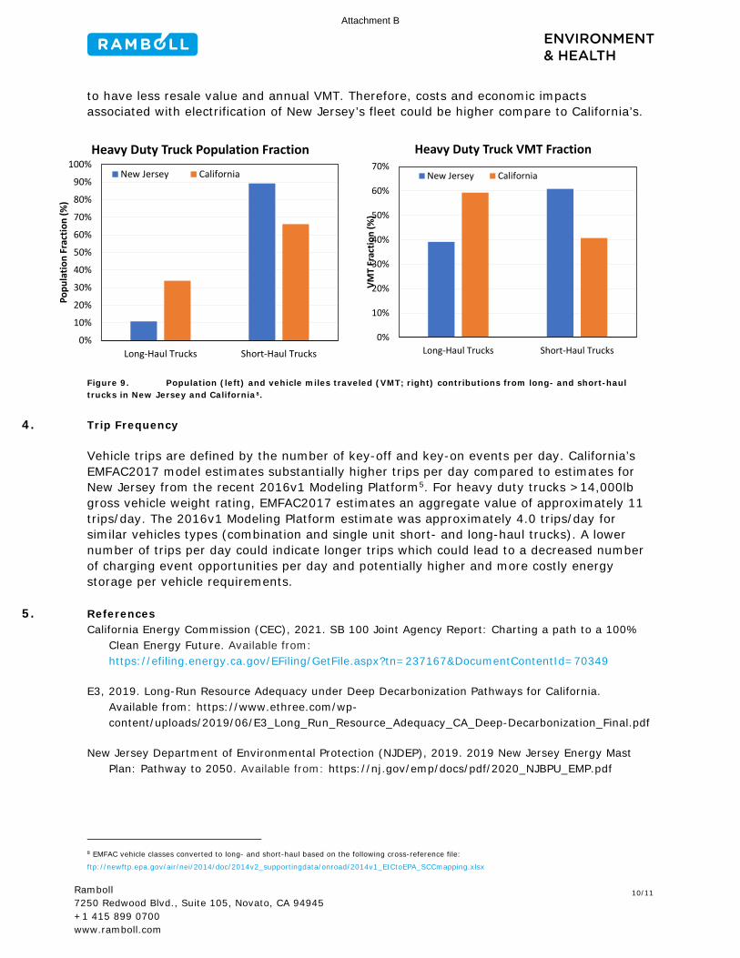
10/11 Ramboll
7250 Redwood Blvd., Suite 105, Novato, CA 94945
+1 415 899 0700
www.ramboll.com
to have less resale value and annual VMT. Therefore, costs and economic impacts
associated with electrification of New Jersey’s fleet could be higher compare to California’s.
Figure 9. Population (left) and vehicle miles traveled (VMT; right) contributions from long- and short-haul trucks in New Jersey and California8.
4. Trip Frequency
Vehicle trips are defined by the number of key-off and key-on events per day. California’s
EMFAC2017 model estimates substantially higher trips per day compared to estimates for
New Jersey from the recent 2016v1 Modeling Platform5. For heavy duty trucks >14,000lb
gross vehicle weight rating, EMFAC2017 estimates an aggregate value of approximately 11
trips/day. The 2016v1 Modeling Platform estimate was approximately 4.0 trips/day for
similar vehicles types (combination and single unit short- and long-haul trucks). A lower
number of trips per day could indicate longer trips which could lead to a decreased number
of charging event opportunities per day and potentially higher and more costly energy
storage per vehicle requirements.
5. References California Energy Commission (CEC), 2021. SB 100 Joint Agency Report: Charting a path to a 100%
Clean Energy Future. Available from:
https://efiling.energy.ca.gov/EFiling/GetFile.aspx?tn=237167&DocumentContentId=70349
E3, 2019. Long-Run Resource Adequacy under Deep Decarbonization Pathways for California.
Available from: https://www.ethree.com/wp-
content/uploads/2019/06/E3_Long_Run_Resource_Adequacy_CA_Deep-Decarbonization_Final.pdf
New Jersey Department of Environmental Protection (NJDEP), 2019. 2019 New Jersey Energy Mast
Plan: Pathway to 2050. Available from: https://nj.gov/emp/docs/pdf/2020_NJBPU_EMP.pdf
8 EMFAC vehicle classes converted to long- and short-haul based on the following cross-reference file:
ftp://newftp.epa.gov/air/nei/2014/doc/2014v2_supportingdata/onroad/2014v1_EICtoEPA_SCCmapping.xlsx
0%
10%
20%
30%
40%
50%
60%
70%
80%
90%
100%
Long-Haul Trucks Short-Haul Trucks
Popu
latio
n Fr
actio
n (%
)
Heavy Duty Truck Population Fraction
New Jersey California
0%
10%
20%
30%
40%
50%
60%
70%
Long-Haul Trucks Short-Haul Trucks
VMT
Frac
tion
(%)
Heavy Duty Truck VMT Fraction
New Jersey California
Attachment B

11/11 Ramboll
7250 Redwood Blvd., Suite 105, Novato, CA 94945
+1 415 899 0700
www.ramboll.com
New Jersey Department of Environmental Protection (NJDEP), 2020. New Jersey’s Global Warming
Response Act 80x50 Report. Available from: https://nj.gov/dep/climatechange/docs/nj-gwra-
80x50-report-2020.pdf
United States Environmental Protection Agency (EPA). 2021. “Emissions & Generation Resource
Integrated Database (eGRID), 2019” Washington, DC: Office of Atmospheric Programs, Clean Air
Markets Division. Available from EPA’s eGRID web site: https://www.epa.gov/egrid.
Attachment B

DRAFT
RESPONSE TO STANDARDIZED
REGULATORY IMPACT ANALYSIS FOR PROPOSED
CARB HEAVY-DUTY EMISSIONS REGULATIONS
P R E PA R E D F O R :
TRUCK & ENGINE MANUFACTURERS ASSOCIATION
333 WEST WACKER DRIVE
CHICAGO, ILL INOIS ▪ 60606
July 29, 2020

2
ACT Research Company (ACTR) appreciates the opportunity to submit the following comments in response to the Standardized Regulatory Impact Assessment (SRIA) associated with the Proposed Heavy-Duty Engine and Vehicle Omnibus Regulation and Associated Amendment that the California Air Resources Board published on June 23, 2020, which was amended on July 10, 2020.
ACTR is a boutique research firm focused on surface transportation dynamics and commercial vehicle demand. ACTR’s customers include leading MD and HD vehicle manufacturers, the commercial vehicle industry’s supply base, investors in transportation and machinery companies, transportation companies, and other groups of stakeholders who need to understand the impact of economic activity on trucking industry profitability, and by extension, demand for medium- and heavy-duty on-highway vehicles.
ACTR’s decision to provide comments on the CARB SRIA relates to a study the company undertook at the behest of the Engine Manufacturers Association (EMA) in early 2020. The resulting study was an upfront cost and total cost of ownership (TCO) analysis relating to the impact of the California Air Resource Board’s (CARB) Omnibus Low-NOx standard proposals and the U.S. Environmental Protection Agency’s (EPA) advanced notice of proposed rulemaking (ANPRM) published in the Federal Register on January 21, 2020, entitled “Control of Air Pollution from New Motor Vehicles: Heavy-Duty Engine Standards.” Given the similarities in the CARB and EPA proposals surrounding NOx and warranty extension, we believe our analysis adds to the discourse surrounding CARB’s proposed Regulation.
ACTR has been and will continue to be a supporter of CARB and EPA efforts to improve air quality. We applaud the 99% and 98% reductions in particulates and NOx, respectively that have occurred over the past quarter-century. And in contrast to the costly final mandates that reduced PM and NOx, the more recent GHG Phase 1 and Phase 2 (to date) regulations have pushed industry stakeholders to deliver tremendous advances in on-highway fuel economy at nominal cost, thereby benefitting both the environment and the buyers of new commercial vehicles.
While we at ACTR recognize the need to continue reducing emissions levels from all sources, we also believe that accuracy in accounting is needed for regulators to make the most optimal decisions possible in plotting the way forward on emissions regulations. It is in that spirit that we believe a better accounting needs to be made in regard to CARB’s current proposal to improve air quality. Based on our modeled conclusions, it is ACTR’s opinion that CARB’s accounting for the cost impact of the proposed regulation is incomplete on several fronts, including:
1) Market sizing 2) R&D accounting 3) Useful life accounting for new technologies and downtime impact 4) Warranty accounting
Over the course of this submission, ACTR will lay out where we believe the accounting as presented in the SRIA fails to capture the true costs of this regulatory proposal. If our analysis is correct, this regulation is likely to cause significant market disruptions as trucking companies actively work to minimize their exposure to new vehicles that will leave them at an operating cost disadvantage to their competition.

3
Market Size and Structure. Although we do not have a fully transparent understanding of the sales projections driven by CARB’s EMFAC model, we disagree with the use of 2013 as the year from which to draw conclusions about the current and future commercial vehicle market size and structure.
• Based on OEM data, we estimate natural gas had a Class 8 market share nationally of 3%-4% in 2013-2014, and has since trended down to 2% in the past two years (see chart). Of course, we recognize that California represents an out-sized proportion of natural gas truck sales, but in the SRIA, CARB assumes HD Otto-cycle engines including natural gas were 43.6% of the heavy heavy-duty (Class 8) market in 2013. We are confident in asserting that this proportion has fallen considerably in the years since, and a more current weighting would increase the diesel units subject to low-NOx standards, which would increase overall costs in the calculation.
• We agree with CARB’s earlier sales volume methodology which took into account the smaller market outlook resulting from the Advanced Clean Truck (ACT) Regulation. But we disagree with the changes made as recommended by the California Department of Finance (page IX-7), to adhere to a legal baseline which will include the mandated zero emissions vehicles under the ACT Regulation. This may have mixed implications for cost outputs, but suggests per-unit costs are understated. The cost study conducted by ACTR used the smaller market size under the ACT Regulation, which lowered overall costs but raised per-unit costs, though the targets in the ACT Regulation have been raised since our study was conducted.
• CARB’s SRIA Does not Consider the Likelihood of Pre-buy/No-buy. We agree with the need to include increased DEF consumption costs and financing costs, as CARB did in the SRIA. However, note that costs to truckers were not included in ACTR’s manufacturing cost analysis, but were included in our Pre-buy/No-buy analysis. In our view, the largest blind spot in CARB’s SRIA is the

4
failure to consider the industry’s instinctive avoidance response to the prospect of costly and risky new regulations. • The higher DEF consumption rate is one of several additional cost factors that should be
considered for the trucking industry, separate from manufacturing costs. These include the taxes on the higher cost of a truck, which is a 12% Federal Excise Tax plus state taxes, and costs to insure the more expensive vehicle, typically 5% of the purchase price per year.
• As a result, for every $1 increase in the purchase price of the vehicle, the equipment costs to the operator are likely to rise by $1.40 - $1.75, depending on one’s assumptions about the operating lifecycle. Hence, we think DEF costs are a very small fraction of the non-manufacturing costs of the Omnibus Low-NOx rulemaking proposal which would be borne by the trucking industry.
o In the cost study ACT Research performed for the EMA, we considered how the preceding costs plus the higher base vehicle prices would impact the trucking industry. Instead of arguing about assumptions, we took a macroeconomic approach.
• We concluded that in this highly fragmented and cyclical industry, which is largely dependent
upon market freight rates, a pre-buy is likely with elevated demand for equipment built before the regulations take place. Trucking is a low-margin industry which abhors risk. Considerable historical precedent shows any significant price increase and technological change will likely drive a pre-buy in this industry. This will add excess capacity to the market and drive down freight rates, with a material adverse effect on earnings for the trucking industry. We have expertise in these freight rate sensitivities through Freight Forecast service, and we estimate the subsequent decline in truckload rates would cost the industry between $6.5 billion and $8.6 billion in the 2027-2028 timeframe. Further, the combination of the effects of the pre-buy and cost of lower freight rates would materially reduce the industry’s ability and willingness to purchase new vehicles after regulations take effect, thereby delaying the benefits of the regulation.
R&D. CARB’s SRIA assigns minimal Research and Development (R&D) costs to the achievement of its proposals, ranging from $78-$85 per unit on Medium Heavy-Duty (MHD) vehicles to $354-$356 per unit on Heavy Heavy-Duty (HHD) vehicles (page IX-10). The underlying sales figures from CARB’s EMFAC model are not clear, and the total R&D costs are not broken out in the aggregate table IX-32.
• The Original Equipment Manufacturer (OEM) study conducted by ACT Research yielded an estimate of $603 million of R&D costs to meet the HHD MY2027 standards proposed for California, only modestly less than the $715 million estimated for full national programs. While the core processes are unchanged regardless of whether it is a partial or national standard, the OEMs intended to reduce the offerings available in California to achieve these modest savings.
• Based on OEM feedback that these costs would be amortized over three- to four-year product cycles, this translates to about $38,000 per unit for the HHD market beginning in MY2027. The

5
CARB SRIA does not explain how it arrives at its significantly lower R&D figure, though we acknowledge there is significant managerial accounting discretion to extend the amortization period and lower the per unit costs. Extending the regulations to a national basis reduces these per-unit costs to just under $2,800 per unit in our model, even keeping with the OEMs’ three- to four-year amortization periods, which highlights the benefit of harmonized national standards over regional ones.
Useful Life. Producing aftertreatment systems to meet tighter standards, increasing the Useful Life (UL) of those systems, and providing a warranty on those systems are three of the distinct challenges presented by the proposed Omnibus Low NOx regulations. CARB’s assertion that increased UL is included in the Technology Costs is disconnected from reality because, for example, Cylinder Deactivation technology is not currently commercially viable and will likely require at least one full replacement to be expected/budgeted in order to meet the UL proposal.
• The OEM survey conducted by ACT Research, which accounted for all major manufacturers, yielded an estimate of $176 million of indirect costs to meet the MY2027 UL provisions in the CARB regulatory proposal for Heavy Heavy-Duty (HHD) vehicles, which added $11,178 of cost per vehicle under our market sizing parameters. It also yielded a similar result for MY2031, and smaller cost figures for medium-duty. These costs are missing from the CARB SRIA.
Warranty. In assigning $930 of incremental repair costs for HHD vehicles in order to extend warranties from 350,000 miles from Step 1 to 600,000 miles, where no warranty data exists, in MY2031, CARB’s warranty analysis (SRIA, page IX-19 to IX-25) materially contradicts the results of both the ACT Research and the NREL cost analyses that was added to the SRIA on July 10, 2020. We also see the $159 estimate for incremental repair costs beginning MY2027 for HHD vehicles as deeply flawed, again considering the unproven nature of the new technologies expected to be employed, particularly cylinder deactivation.
• The feedback from manufacturers used as input for both studies is that the extended warranty provisions would effectively require the manufacturers to account for almost a full aftertreatment system replacement for every vehicle, or about $8,000 per HHD unit. NREL’s average cost scenario for 12-13L engines included a $23,424 per unit incremental warranty cost, but this appears to include the extended useful life provisions as well, which we detailed separately.
• We do not agree with linear extrapolation of warranty costs into the extended warranty periods based on MY2013 data.
o These data represent significantly lower-cost MY2013 emissions systems, not the more costly systems envisioned in the regulation, thus we believe this methodology fails to account for the warranty cost on the added components.
o We believe CARB’s assumption (page IX-22) “that components would continue to fail at the same rate for the duration of the lengthened warranty period” is flawed. Based on feedback from manufacturers during our survey, our experience analyzing the trucking industry, and the Fleet Advantage study charted below, it appears to us to be common knowledge that maintenance costs increase significantly over time. In addition, the Southwest Research Institute (SwRI) Low NOx Stage 3 testing program only tested up to 435,000 miles (page III-7).

6
• The warranty mileage baseline is well above reality, in our view, and ignores the cost incurred by the trucking industry for extended warranties above the regulatory baseline. This methodology understates warranty costs for California and would much more materially understate warranty costs on a national basis where the baseline is below CARB’s Step 1 baseline.
o For MY2027, CARB assumed 40% of HHD trucks are purchased with 500,000-mile warranties, reducing the distance to the 600,000-mile warranty proposal. This ignores the considerable costs some fleets pay for extended warranties and overstates current industry practice. Our research suggests that extended warranties are typically for 400,000 miles, and the take rate is likely less than 40%.
o In reality, the industry standard base warranty is 250,000 miles, and the EPA regulatory baseline is 100,000 miles. Because these are significantly lower than the 350,000-mile CARB Step 1 baseline which will be in effect as of 2022, this is material when considering extending these provisions to the national level. Incremental warranty costs per unit on a national basis from the proposed regulations would thus be significantly higher than the estimates in CARB’s SRIA.
o Based on CARB’s assumption (however questionable) that it can calculate warranty costs linearly, and our view that the incremental warranty costs should be based on the 350,000-mile Step 1 baseline, we should be accruing for an incremental 250,000 miles of warranty coverage, whereas CARB’s analysis includes 190,000 (adding the 40% at 500,000 miles raises the baseline to 410,000 miles). Thus, CARB’s analysis misses about 24% of the regulatory increase in warranty cost.
Technology path. The direct engine and aftertreatment component cost output of $11,347 from the ACTR study, which combined MY2024 and MY2027, was well above the comparable figure from CARB’s SRIA of $6,429 ($1,611 in MY2024 and $4,818 in MY2027). The main source of difference is that the

7
manufacturers did not all choose the same technology path, corresponding to the one laid out in CARB’s proposal, though a portion did. With the consideration that CARB’s proposals are supposed to be technology neutral, with no picking of winners or losers, an estimate that considers more than one technology path is preferable, in our view.
Other. We do not purport to being experts on managing large manufacturing companies, as our expertise is primarily in data analysis and forecasting for the transportation and commercial vehicle industries. However, we question CARB’s assumptions throughout the Standardized Regulatory Impact Analysis (SRIA) cost analysis that the important work of compliance with these emissions regulations is relegated to a single junior engineer earning just $70 per hour. Adding any internal oversight, which seems important from our perspective, would add further incremental compliance costs. In addition, we took particular exception with the doubts CARB cast on the NREL study (page IX-73) by questioning its quality because of a small sample size. CARB knows well the number of major truck OEMs, and while the same could be said of our study, it covered every OEM of consequence. And the results of the ACTR study fell very close to the NREL study, both in stark constrast to the CARB SRIA.
To conclude, ACTR’s analysis suggests that the new purchase price of an HHD vehicle will rise by $69,930 in MY2027 from the current baseline in a California-only scenario, which falls to $25,825 on a national basis. CARB’s SRIA does not add up the estimated costs to present them on a per unit basis in total, which seems very pertinent in our view. Nonetheless, adding up the costs in CARB’s SRIA, we reach roughly $10,000 per unit for MY2027, though this is not clear given the lack of transparency on market sizing (note: we combined the MY2024 proposals into our MY2027 as the MY2024 timeframe was deemed infeasible from a planning and testing perspective). CARB’s numbers do not account for the higher total-cost-of-ownership burden that will be borne by the trucking industry (on ACTR CA-only estimates, $8,392 from 12% FET, $5,070 from 7.25% state taxes, etc.), and eventually, consumers. If we are even “ballpark” correct in our cost assessment, the cost increases at issue have the potential to meaningfully move the trucking industry away from vehicles that meet CARB’s proposed mandates, thereby reducing the regulations’ benefit for several years, especially if the regulations requiring significantly more expensive trucks aligns with the peak of an economic cycle. If that happens, we can expect an even larger prebuy ahead of the mandate, and an extended post-mandate delay, which would invalidate much of CARB’s cost analysis and delay the anticipated benefits.

FINAL DRAFT
COST STUDY: PROPOSED HEAVY-DUTY
ENGINE AND VEHICLE EMISSIONS REGULATIONS
P R E PA R E D F O R :
TRUCK & ENGINE MANUFACTURERS ASSOCIATION
333 WEST WACKER DRIVE
CHICAGO, ILL INOIS ▪ 60606
March 19, 2020
Contents

2
Page(s)
Executive Summary .................................................................................................................................... 3
Summary Tables of Cost Study Outputs ............................................................................................... 3-5
Methodology ........................................................................................................................................... 6-10
• General • Discount rates • Inflation • Market Sizing • State versus Federal Considerations • MY2024 Feasibility Issues
Medium- and Heavy-Duty Cost Details ................................................................................................ 9-13
• Direct & Indirect Manufacturing Costs • MY2027 and MY2031
Pre-buy/No-buy Analysis ..................................................................................................................... 14-19
• Introduction • Pre-buy Model • Freight Rate Impact • Trucking Industry Sizing and Earnings Impact
Sensitivity Analysis Under Pre-buy/No-buy ...................................................................................... 20-23
Conclusions .......................................................................................................................................... 23-24

2
ACT Research Cost Study of the Proposed Omnibus Low-NOx Rulemaking
Executive Summary
Based on a survey of the commercial vehicle and engine manufacturing industry completed in Q1, 2020, this study presents ACT Research’s best estimates of the sum of the direct and indirect costs of meeting the goals of the California Air Resources Board (CARB) Omnibus Low-NOx Rulemaking (Omnibus Regulations), as also referenced in the ANPRM for EPA’s Cleaner Trucks Initiative (CTI). We present estimates for costs of both a nationwide and a California-only program.
This study’s focus is on the costs (including per-vehicle costs) that the truck and engine manufacturing industry likely will incur to comply with the proposed Omnibus Regulations. The study’s primary conclusion is that full compliance with the proposed low-NOx emission standards and other requirements, assuming they track the proposed Omnibus Regulations, will cost the truck and engine manufacturing sector a Net Present Value (NPV) of $9.1 – $13.0 billion.
Assuming the proposed Omnibus Regulations are implemented, manufacturers ultimately will recoup most of those costs through higher vehicle prices. It is the trucking industry that will bear most of the increased costs going forward. Longer-term, the trucking industry eventually will be able to pass the higher costs of compliance on to the shipping community, which in turn will pass them on to consumers. However, given the highly competitive nature of the trucking industry, we also detail the costs of the very likely scenario of a substantive equipment “pre-buy/no-buy” to avoid, at least initially, the higher truck and engine costs associated with the proposed Omnibus Regulations. In ACT’s modeling, the resulting overcapacitization in the freight hauling industry (due to pre-buys of vehicles) likely will yield aggregate pre-buy impacts between $6.5 - $8.6 billion in 2019 dollars, solely as a result of lower freight rates due to overcapacity, and there will be little opportunity to recoup the lost shipping revenues during the periods of overcapacity.
The combined regulatory impact on the manufacturing sector and trucking companies falls between NPVs of $15.6 and $21.6 billion.
Our estimates do not model the increased costs out into perpetuity. Rather, our cost estimates are focused on the two key years when costs are likely to rise significantly: 2027 and 2031. In our analysis, fixed costs were allocated over multi-year product programs. In addition, we have not tried (yet) to estimate the long-run costs to the trucking industry from deploying higher-cost equipment. The costs studied here are solely for the truck and engine manufacturing sector, and just include the pre-buy related effects on trucking. In our judgement, adding the long-run costs on trucking, while likely worth a more thorough analysis, would effectively be double-counting the costs we have estimated for the manufacturers. We include an analysis of the costs for the trucking industry in the Pre-buy/No-buy section, but only to inform our modeling regarding the degree of excess capacity. It should be noted that the increased taxes, insurance costs, financing costs, and emissions fluid costs that trucking companies will face are not included in this aggregate cost estimate of $15.6 to $21.6 billion.

2
Summary Tables. Tables 1-3 summarize the results of our cost study. Our findings related to the costs associated with the MY2027 step of the proposed Omnibus Regulations are itemized in Table 1: Cost Estimates to Meet Proposed MY2027 Vehicle Standards. In MY2027 at the national level, and using the 3% and 7% discount rates to bracket the ranges, we estimate the proposed emissions requirements would cost the industry $1.8 – $2.4 billion for medium-heavy duty vehicles and engines, and $4.5 – $6.1 billion for heavy-heavy duty vehicles and engines, which sums to $6.3 billion at a 7% discount rate, and $8.5 billion at a 3% rate. On a per-unit basis, the cost of compliance ranges from $17,610 to $23,886 for heavy-heavy-duty (HHD) diesel vehicles, and $11,752 to $15,940 for medium-heavy-duty (MHD) diesel vehicles. The total cost figures are smaller for a California-only program, but per-unit costs rise sharply because of the relatively small number of units sold in California.
Table 1: Cost Estimates to Meet Proposed MY2027 Vehicle Standards
Source: ACT Research Co., LLC: Copyright 2020
The cost estimates itemized in Table 2 summarize the results of our cost study for MY2031 compliance. Those costs are primarily related to meeting the extended useful life and emission warranty provisions of the proposed Omnibus Regulations. The cost figures amount to additions to the baseline MY2027 costs (in Table 1), and show the incremental cost estimates for MY2031. For HDD vehicles, our survey indicated an additional $8,352 – $13,194 in costs per truck, depending on the discount rate utilized. For MHD vehicles, the additional costs would range from $3,689 – $5,827 per truck. Combining the HHD and the MHD diesel model outputs, we estimate a discounted cost that ranges between $2.7 – $4.4 billion for the MY2031 proposals on a nationwide basis.

2
Table 2: Additional Cost Estimates to Meet Proposed MY2031 Vehicle Standards
Source: ACT Research Co., LLC: Copyright 2020
Table 3 aggregates the cost estimates for the MY2027 and MY2031 cost models, reflecting our estimates of the combined costs of the proposed Omnibus Regulations. On a nationwide basis, the total combined cost of the Omnibus Regulations for both MHD and HHD vehicles is $9.1 billion to $13.0 billion, depending on whether a 7% or 3% discount rate is utilized. On a per-unit basis, the nationwide cost for HHD vehicles ranges from $25,963 at a 7% discount rate, to $37,079 at the 3% rate. For MHD vehicles, the per-unit costs range from $15,441 to $22,767, respectively. On a California-only basis, the aggregate total costs range from $1.3 – $1.8 billion, which are much smaller than the nationwide costs, but some expense line-items like R&D were relatively fixed. Therefore, on a per-unit basis, the per-unit cost increases range from $57,905 to $80,821 per HHD vehicle, and from $51,365 to $71,878, per MHD vehicle.
Table 3: Cost Estimates to Meet Proposed Combined MY 2027 and MY2031 Vehicle Standards
Source: ACT Research Co., LLC: Copyright 2020

2
Methodology
This cost study was performed using federal guidelines that correspond to EPA’s Guidelines for Economic Analysis and OMB Circular A-4. The baseline assumptions for our analysis are that:
1) Heavy-duty truck manufacturers would continue to work toward meeting the established GHG-2,
2) but would otherwise not explicitly target a. incremental NOx emissions reductions, b. improved low-load SCR performance, or c. longer useful lives for aftertreatment systems.
In light of the pending GHG-2 regulations, we used professional judgement to discount some of the cost inputs that we received from manufacturers, if those inputs did not take into account the improved fuel economy and reductions in fuel consumption, which will help to meet the proposed Omnibus Regulations.
We followed the methods specified by the Environmental Protection Agency (EPA) and the Office of Management and Budget (OMB) to conform to the government’s Social Cost definition, though we have noted where we otherwise would differ with those methods (i.e., inflation and discount rates). We have also presented below an additional set of values that discount the future costs at the private weighted average cost of capital, which for this industry is quite high. Our “Private Cost” estimates below are only alternative results, not EPA/OMB recommended results, and so are not included in the summary tables above.
ACT Research’s cost estimates are based upon industry inputs consisting mainly of confidential business information (CBI), and as a result, specific technology solutions will not be discussed here except to note that those anticipated solutions were not uniform. As explained below, we used conservative analytical judgements where possible. For example, the current regulatory baseline for warranty coverage is 100,000 miles (five years, 3,000 hours). However, our research confirmed that the industry standard for new heavy-duty trucks is a 2-year/250,000-mile warranty that is built into the price. As a result, our study uses 250,000 miles as the baseline, resulting in lower incremental costs than otherwise would have been the case had we used the more common government research practice regarding the existing regulatory baseline.
Discount Rates, Social and Private. Consistent with EPA and OMB guidelines to discount future costs back to their present value at 3% and 7% discount rates in order to determine NPV, we have presented our results discounted at both of those rates. However, considering the significant uncertainty involved in estimating the future costs at issue, we also present the results of our cost estimates discounted using an alternative private cost methodology. The private cost methodology provides for the use of the Weighted Average Cost of Capital (WACC) for the truck and engine manufacturing industry as our discount rate. In calculating the 10% WACC, we used

2
current equity values, as of January 2020, and debt and interest rates from the manufacturers’ most recent annual reports.
Accordingly, in addition to utilizing the 3% and 7% social cost discount rates, we also present an alternative cost estimate (in Table 4) using our more conservative 10% WACC discount rate. While this is more conservative than the social cost methodology, we believe it accounts for some of the uncertainty inherent in this study, including: significant uncertainty about the future state of emissions-control technology, and regarding the most likely compliance pathways that manufacturers may follow. For example, we are estimating that manufacturers will need to budget for two replacements to aftertreatment systems in the life of their trucks in order to comply with the extended useful life and warranty provisions of the Omnibus Regulations. However, between now and MY2027, it is possible that durability could be improved to remove some of those costs. It also is possible that replacement aftertreatment systems will not last as long on older engines, which also is reflected in this cost study.
In light of these and other uncertainties, the alternative 10% WACC-based discount rate could be a reasonable way to estimate more conservatively the unknown variables pertaining to the various potential cost inputs and impacts. The larger alternative discounting mechanism that we have used, in essence, could serve fairly well in lieu of a more formal sensitivity analysis at a point in time when specific technology paths are not yet known.
Inflation methodology. We used inputs in 2019 dollars as it was the year our cost survey was initiated, adjusting for the OEMs who responded in 2018 dollars using the BEA’s GDP Price Deflator. We thought it would be fair to use a lower inflation rate or perhaps even deflationary figure given the historical experience in this industry, but EPA (through EMA) indicated that the GDP Deflator is the standard. Adhering to EPA’s recommended use of the GDP Deflator may inflate the estimated cost of the Omnibus Regulations, leaving room for further study.
Heavy-Heavy Duty Market Sizing. We used 2018 vehicle manufacturer (OEM) market shares as our baseline and assumed those shares as a constant into the future. However, instead of using the 2018 market size and simply rolling it forward, we took into account the fact that 2018 was the fifth-largest year ever for U.S. Class 8 truck production. As it happens, two of the higher production years were 2005 and 2006, with 2006 being the biggest U.S. Class 8 production year ever. Not coincidentally, those two “top-five” years occurred immediately ahead of the expensive EPA07 emissions standards for heavy-duty trucks and engines. We will discuss this “pre-buying” issue later in this report.
To provide a representative baseline, we used a five-year trailing average of U.S. Class 8 truck production (HHD diesel), or 239,000 units, and scaled it up at 1% per-year to account for economic growth, and adjusted for freight productivity. While freight demand grows over time

2
as the population grows, shippers also find ways to improve design and packaging in ways that require fewer truckloads for a given set of goods. As a result, our analysis uses a MY2027 U.S. Class 8 nationwide market size estimate of 257,000 units.
For the California market, based on industry inputs, we used a baseline of just under 7% of nationwide industry sales, and scaled that starting point down by 7.5% in MY2027 to reflect assumed progress toward CARB’s target of 15% zero-emission heavy duty tractors by 2030. We therefore estimate that California will represent just over 6% of nationwide HHD sales in MY2027.
For MY2031, we continued to scale nationwide HHD sales up by a 1% cumulative annual growth rate, bringing the nationwide HHD market to 267,000 units. We also continued with the assumption that California would achieve its 2030 target of 15% zero emissions heavy-duty vehicles, taking California down under 6% of nationwide HHD duty diesel truck sales.
Medium-Heavy Duty Market Sizing. For the MHD market, we used a trailing five-year average of U.S. sales of 142,000 units per-year, scaled up at 1% per-year to account for economic growth and adjusted freight productivity, in line with the above discussion regarding the HHD market. That resulted in a nationwide MHD market size of 152,000 units.
For the California market, we used a baseline of just under 7% of nationwide industry sales, also based on industry inputs, and scaled that down by 20% in MY2027 to reflect progress toward CARB’s target of 50% zero-emission MHD vehicles by 2030. We estimate that California will represent just over 5% of nationwide MHD sales in MY2027.
For MY2031, we continued to scale nationwide MHD sales up at a 1% cumulative annual growth rate, and we made the assumption that California would achieve its target of 50% zero-emission vehicles, taking California down to 3.5% of nationwide MHD diesel truck sales.
State versus Federal Considerations. Based on this cost study, we conclude that the local benefits of California-only regulations do not justify the very significant costs that would impact trucking-related business on a nationwide basis. Due to the relatively small number of trucks sold in California, the research and development costs of advanced aftertreatment on a per-unit basis could be unacceptably high. Our survey of OEMs showed that only about 7% of heavy-duty trucks are sold in California, significantly less than the State’s share of GDP.
Our cost survey also shows that the industry would spend $715 million on research and development for the proposed standards nationally, and $603 million on a California-only standard. The difference between the two totals reflects that fewer models would be offered under a California-only scheme. However, on a per-unit basis, using the market size detailed previously and amortizing the costs over an industry-standard three-year product platform cycle,

2
those R&D costs amount to about $2,800 per-unit at a national level and $38,200 per-unit if the regulations applied only to California.
MY2024 Infeasibility. We are not providing separate estimates for the MY2024-26 elements of the proposed Omnibus Regulations because we did not receive indications that manufacturers can, or will, develop and introduce the technologies that could be used to meet those proposed standards by the 2024MY at reliable product-quality levels. The industry respondents to our survey cited numerous feasibility problems with the MY2024 time horizon. We believe that for some key vehicle categories, the standards proposed under the Omnibus Regulations are technically infeasible within the lead time allowed. Accordingly, we have not fully estimated the costs for the initial phase of the Omnibus Regulations for tractors and vocational vehicles. The lack of sufficient lead times for the development of the required additional technologies would result in significant risks of quality issues later in vehicle life. Simply stated, we could not develop any realistic cost estimates for a near-term regulatory program that manufacturers indicated is essentially unworkable. We believe that the MY2024 proposals would result in a decrease in the in-use reliability and durability of new heavy-duty vehicles, and we cannot accurately quantify the costs that would be associated with such problems. Instead, we merely note that unit costs would likely be greater than the costs we have estimated in this study for a nationwide MY2027 and MY2031 standard.
Heavy-Heavy Duty MY2027 Costs. We estimate in Table 4 that the low-NOx standards proposed for MY2027, including a carry-forward of the MY2024 proposals, would cost HHD truck manufacturers $6.6 billion on a nationwide level, or $25,825 per-unit, in 2019 dollars. For California, our cost estimate of $1.1 billion for the HHD vehicle sector equates to $69,930 per-unit. That level of price increase would in all likelihood significantly reduce the choices of vehicles available in the California market, and could force some smaller volume manufacturers out of the California market. On an inflation-adjusted and discounted basis, using the 3% and 7% discount rates recommended in the EPA and OMB guidelines, the net present value of the HHD costs associated with the Omnibus Regulations on a nationwide basis is $17,600 – $23,900 per HHD vehicle, and $4.5 – $6.1 billion for the HHD industry. For California-only, the net present value ranges from $47,700 – $64,700 per HHD vehicle, and $750 million to $1.02 billion for the HHD industry. Note that in the far-right column of Table 4, we present the cost figures discounted at the 10% WACC, and those costs are considerably lower and could be a better way to account for the uncertainties relating to the possible incorporation of unforeseen technology improvements in the coming years.
Direct Costs. The direct costs included in the foregoing estimates incorporate specific changes to engines, aftertreatment systems and on-board diagnostics. Those costs do not represent any specific technology path, but rather a weighted average of the various manufacturers’ inputs.

2
Those inputs add up to $7,900 per-unit for HHD diesel vehicles nationally, and $11,350 per-unit in California in 2019 dollars. The net present value of those figures is $5,375 – $7,290 nationally, and $7,740 – $10,500 in California, using the 3 and 7% discount rates to bracket the ranges. (See Table 4.)
Indirect Costs. The industry estimated $603 million in R&D costs to meet the MY2027 requirements (including the MY2024 elements) of the Omnibus Regulations in California, and $715 million for a nationwide program. Using inputs from the manufacturers, we amortized the R&D costs over the typical program life in the industry of three to four years.
The other indirect costs were primarily associated with the proposed extended warranty and useful life periods, as well as the related compliance-enforcement programs. The warranty and useful life costs are largely variable, but the compliance programs and R&D requirements are largely fixed. Some manufacturers may plan to find savings by offering fewer vehicle options, but applying those fixed costs to California’s 15,800-unit HHD market still results in major per-unit cost increases relative to the 257,000-unit nationwide market.
Table 4: Cost Estimates to Meet Proposed Combined MY2027 Standards for HHD Vehicles
Source: ACT Research Co., LLC: Copyright 2020

2
Medium-Heavy Duty MY2027. We estimate (in Table 5) that the low-NOx standards contemplated for MY2027, including the MY2024 proposals, would cost $2.6 billion on a nationwide basis, or $17,230 per-unit. On a California-only basis, the program would cost $500 million, which equates to $60,820 per-unit. That level of price increase would in all likelihood significantly reduce the choices available in the California truck market, thereby decreasing competition by forcing some low-volume manufacturers out of the market. The net present value of those figures is $1.8 – $2.4 billion for the MHD industry on a nationwide basis, or $11,750 – $15,940 per-vehicle, using the 3% and 7% discount rates. For California-only, the net present value ranges from $330 – $450 million at the discounted cost rates, which boost the per-unit costs to $41,500 – $56,250. Those MHD costs are largely similar to the cost estimates for HHD diesel vehicles. While smaller in absolute terms, they represent similar proportional price increases relative to new vehicle prices.
Table 5: Cost Estimates to Meet Proposed Combined MY2027 Standards for MHD Vehicles
Source: ACT Research Co., LLC: Copyright 2020
Heavy-Heavy Duty MY2031. We also estimate (in Table 6) that the additional low-NOx requirements for MY2031, using the MY2027 proposals as a baseline, would cost HHD truck manufacturers an additional $4.0 billion on a national level, or $14,830 per-unit, in 2019 dollars. For California, our estimate of $275 million in costs equates to $18,150 per-unit. While there may be modest aftertreatment changes associated with the MY2031 step, there are no additional engine or on-board diagnostics requirements. The costs at issue are almost exclusively related to

2
further extensions to the emissions warranty and useful life periods. On an inflation-adjusted and discounted basis, using the 3% and 7% discount rates recommended by EPA and OMB, the net present value cost ranges from $8,350 – $13,200 per HHD vehicle, for a total of $2.2 – $3.5 billion for the HHD industry at the national level. For California, we estimate the MY2031 proposed requirements would increase the cost of a HHD truck by $10,220 – $16,140. Note again that in the far-right column, we present the cost figures discounted at the 10% WACC. These costs are considerably lower and, again, could better reflect the uncertainties relating to the possible incorporation of unforeseen technology improvements in the coming years.
Table 6: Cost Estimates to Meet Proposed Combined MY2031 Standards for HHD Vehicles
Source: ACT Research Co., LLC: Copyright 2020
Medium-Heavy Duty MY2031. We estimate (in Table 7) that the Omnibus Requirements proposed for MY2031 would cost MHD truck and engine makers an additional $1.0 billion on a national level, or $6,550 per-unit. For California, the projected $100 million cost increase equates to $17,560 per-unit. As noted above in the Market Sizing section, we assume a smaller diesel-powered market size in California in 2031 due to the implementation of CARB’s ZEV rules. The net present value of these costs (using the 3% and 7% discount rates) is $615 – $935 million for the MHD industry on a nationwide basis, or $3,700 – $5,800 per MHD vehicle, and $60 – $90

2
million in California, or $9,900 – $15,600 per vehicle. The costs were largely similar to the estimates calculated for HHD diesel vehicles. While smaller in absolute terms, they represent similar proportional price increases.
Table 7: Cost Estimates to Meet Proposed Combined MY2031 Standards for MHD Vehicles
Source: ACT Research Co., LLC: Copyright 2020

2
Pre-Buy/No-Buy Analysis
Introduction. A “pre-buy” occurs when industry participants initially reject a regulation-driven change in a product, in this case heavy-duty on-highway commercial vehicles, and instead buy as much of that product as possible in the years before the new regulation takes effect. A “no-buy” occurs in the initial years after the new regulation is implemented, when product demand, while not literally zero, falls sharply. The trucking industry is naturally risk-averse and prone to avoid new regulations that may impact the reliability and operating costs of trucks, since operational reliability is so vital to industry participants’ ability to survive in an historically low-margin business.
The base case of our cost study uses a hypothetical market size which takes a trailing five-year average and scales it up by a 1% CAGR. This borrows from the established assumption that freight volume per capita is very stable in the long-run, so freight grows roughly in line with population growth. It also borrows from our view that truck supply and demand always return to equilibrium, notwithstanding intermittent periods of over and under supply relative to freight demand. Based on our cost study, we estimate that HHD truck prices are likely to rise $18k-$24k (14%-18%) in MY2027, and another $8k-$13k (5%-8%) in MY2031. MHD truck prices are likely to rise $12k-$16k in MY2027, and another $4k-$6k in MY2031, with similar percentages, as a result of the proposed Omnibus Regulations.
There is not a great deal of pricing information available in the new MHD and HHD truck markets, though information on freight rates has improved significantly in recent years, so partial equilibrium analysis not very effective for the manufacturing sector, but perhaps better for the trucking industry. And since the costs of the proposed regulations will be passed to the trucking industry, it is those effects which we believe are most important to consider.
Past experience, particularly the pre-buy that occurred in 2005-2006 ahead of EPA07, demonstrates that emissions standards which significantly increase the cost and complexity of HHD tractors are likely to lead to pre-buying of equipment in the years leading up to the regulations, assuming the industry has the financial wherewithal to adjust the timing of capital expenditures. And given the lower tax rates as of 2018, we think the industry is structurally more profitable, or at least it has not been adversely impacted. Therefore, the trucking industry likely will have the ability to pre-buy in advance of the Omnibus Regulations taking effect.
Starting from the experience in 2006-2007, the trend in contract truckload rates, which fell 1.3% in 2007, has risen 3% per-year on average since then. That amounts to a 4%-type opportunity cost for the industry. (See chart below.)

2
With that opportunity cost in mind, we believe the proposed Omnibus Regulations would precipitate the largest-ever pre-buy for medium-heavy and heavy-heavy duty trucks and tractors. The primary repercussions of a pre-buy would be two years of vehicle underproduction in 2027 and 2028 to counterbalance the likely overproduction in 2025 and 2026. While we can make a case that R&D costs are ultimately recouped over time thanks to higher vehicle prices, not all costs are recoverable. There would be significant costs for the OEMs and their employees in terms of the inefficiencies that come with a rapid ramp-up to meet an artificial demand bubble followed by a demand collapse in the period of capacity rebalancing that leads to layoffs and production cuts.
While the vehicle and engine manufacturers will have to handle major market disruptions relating to nonmarket-driven demand impacts, the HHD market has an additional constituency that likely will be severely impacted by the proposed rule-making. The anticipated pre-buy, like the one that occurred ahead of EPA’07 in 2005–2006, is likely to result in significant and unnecessary capacity additions in the HHD trucking industry. A large portion of those truckers operates on a for-hire basis and is dependent upon market rates to move freight. The lower freight rates which will inevitably result from the regulation-driven overcapacity bubble will have a significant adverse financial impact on the nation’s truckers, with an estimated impact of $6.5 – $8.6 billion at net present value.

2
Pre-Buy Model. Using a multi-factor relational model based on a significant history of industry activity before and after the introduction of new emissions regulations, we estimate (in Table 8) the industry will pre-buy 64,800 (4,200 + 60,600) additional HHD tractors and 25,300 (2,600 + 22,700) MHD vocational trucks in 2025 – 2026 ahead of the MY2027 regulations. This adds up to 90,100 total Class 8 vehicles over the two-year pre-buy. Ahead of the MY2031 standards, we estimate another pre-buy of 35,000 (4,200 + 30,700) HHD tractors and 11,600 (2,300 + 9,200) HHD vocational trucks in 2029 – 2030. Vocational trucks are similar to MHD vehicles in that they are typically a component of a job (construction/dump/cement) and are not directly subject to market rates, so the modeled freight rate effects exclude vocational trucks. Overcapacity in MHD vocational trucks will primarily impact manufacturers who will have to lay off workers and lower supplier orders. However, in the HHD tractor market, there likely will be very significant price impacts on freight rates.
Table 8: Prebuy Size Estimates in Units and Percent
The HHD tractor pre-buy model starts with the base tractor price, adds in the 12% Federal Excise Tax (FET) and an average 8% for State and Local taxes. We then raise the sticker price by the cost of meeting the proposed standards, using $23,885 (18% of base), which we settled on because that cost increase was near the center of the range of the $30,300 per-unit value undiscounted at the 2% inflation rate, and the $17,600 per-unit value using a 7% discount rate. We taxed the $23,885 at the FET + state tax rate, added in three years of insurance at a rate of 5% of the truck cost each year, and added financing costs at an interest rate of 5% for half of the value of the
MY2027 $ Change Op.
Costs
MY2027 % Change Op.
Costs
Anticipated Prebuy:
2025
Share of new
Market
Anticipated Prebuy:
2026
Share of new
MarketUS Class 8 Tractor 35,103$ 18.3% 4,219 2.7% 60,622 39.9%US Class 8 Vocational 35,190$ 14.6% 2,620 4.7% 22,667 36.9%US Total Class 8 6,838 3.2% 83,290 39.0%
Source: ACT Research Co.,LLC: Copyright 2020
MY2031 $ Change Op.
Costs
MY2031 % Change Op.
Costs
Anticipated Prebuy:
2029
Share of new
Market
Anticipated Prebuy:
2030
Share of new
MarketUS Class 8 Tractor 12,491$ 6% 4,234 2% 26,717 13%US Class 8 Vocational 14,536$ 6% 2,344 4% 9,236 14%US Total Class 8 6,578 3% 35,953 14%
Source: ACT Research Co.,LLC: Copyright 2020

2
vehicle. This totals about $35,000 of added upfront costs for the HHD vehicle purchaser in MY2027, and another $12,000 in MY2031. (See Table 8.)
Fuel economy considerations all play a role in the model. After considerable discussion, we included the impending fuel economy improvements associated with GHG-2 regulations in MY2027, even though most of those fuel economy improvements will be in effect prior to the Omnibus Regulations. In our cost analysis from the manufacturers’ perspective, we did not include costs or benefits for the GHG-2 regulations, except as we understand the state of the market to be in MY2027. To estimate the social cost to the trucking industry, however, our model’s purpose is to reflect the conditions impacting the industry in MY2027 and MY2031. We considered both the improvements in fuel efficiency and additional use of diesel emissions fluid (DEF), finding that the 4% improvement in fuel efficiency expected in MY2027 from GHG-2 regulations would more than offset a doubling of the DEF dosing rate. Moving from a 2.5% to a 5% DEF dosing rate on a 90,000 mile per-year truckload application would use 233 additional gallons per-year at a cost of about $665, but the 4% fuel efficiency improvement saves $1,300 per-year at 440 gallons in this application. We are not using those estimates as benefits relating to the Omnibus Regulations, but rather to refine our analysis of the potential magnitude of a pre-buy.
Regarding maintenance costs, some of the technology solutions anticipated for the proposed Omnibus Regulations are targeted towards improving the durability of aftertreatment systems, which could have the effect of lowering maintenance expenses in some instances. However, the overall increase in the complexity of the engine and aftertreatment systems likely will require more frequent maintenance for these trucks through their life-cycles, not less. Given the high degree of uncertainty, however, we have not included explicit estimates of maintenance expenses, except to say that there are positives and negatives from a fleet perspective, and as noted earlier in our report, the higher warranty and useful life costs are included in the estimated sticker price increases.
Tractor Pre-Buy. The sum of the multiple costs result in a “willingness to buy” factor, which is the percentage change in total cost of ownership (TCO) of the vehicle before and after the regulation. At a cost of $35,100 in MY2027, the net TCO impact is 18% of the pre-regulation purchase price. Based on historical pre-buys and assuming reasonable industry profit margins leading into the new regulatory mandates, we estimate that the 18% increase will drive an additional 3% of HHD tractor sales in 2025 (4,200 units), and a 40% pre-buy in 2026 (60,600 units). The $12,500 net TCO increase due to the proposed MY2031 standards, which amounts to an additional 6% price/TCO increase, will drive another 2% of tractor sales in 2028 (4,200 units) and an additional 15% pre-buy in 2029 (30,700 units). (See Table 8.)

2
Table 9: Retail Sales and Pre-Buy History and Forecast in the U.S. Class 8 Tractor Market
Freight Rate Impact. Adding these 65,000 “pre-bought” tractors into our population models, where we estimate 1.4 million HHD tractors engaged in truckload and/or less-than-truckload freight hauling, amounts to a 4.5% increase in capacity or supply into the industry. Our freight pricing models indicate that the sensitivity of truckload contract pricing is roughly -64% relative to capacity additions when modeled econometrically with demand and regulatory factors included. In other words, a 1% increase in freight-hauling capacity lowers pricing by .64%, so a 4.5% increase in capacity, as expected in this case, would lower truckload pricing by 2.9%.
Trucking Industry Sizing and Earnings Impact. According to the U.S. Census Bureau’s Quarterly Services Survey, the U.S. trucking industry is on pace for $195 billion in revenue (NAICS code: 4841, General Freight Trucking) in 2019. Using a trailing 5-year industry growth rate of 3% to extrapolate to 2026, the industry should be generating $240 billion of revenue in 2026. A 2.9% pricing impact on a $240 billion segment of the economy would be a cost to aggregate trucking industry earnings of $6.9 billion on an annual basis, and it would likely last 18-24 months. Thus,

2
the total impact on the trucking industry would likely be $10.4 – $13.8 billion of lost earnings in 2026 – 2027. This discounts back to $6.5 - $8.6 billion in 2019 dollars at 7%.
We have focused here on the for-hire market reported on by the Census Bureau. Our estimates do not include effects on the private fleet segment of the trucking industry, which makes up just over half of the tractor fleet, but generally hauls freight for a single company. Private fleets are generally a cost center inside companies that ship goods, with few booking revenue for their services. As a result, we did not include that part of the market in estimating financial impacts.
Vocational Pre-buy. The main focus of our analysis (in Table 8) is on the tractor portion of the heavy-duty Class 8 market, since, over the past decade, tractors have represented 75% of the Class 8 vehicles sold in the US, compared to 25% for the Class 8 market’s vocational segment. Significantly higher miles traveled per-year for tractors mean shorter lengths of ownership due to reliability/downtime issues as miles accrue. On the vocational side of the market, localized vocational applications (P&D, construction, government) mean fewer miles per-year and longer first-buyer ownership. And, as previously discussed, unlike the tractor market, where every vehicle is a profit center, the vocational truck is often a tool used to facilitate a non-transportation related business. Thus, there is significantly more volatility in US tractor demand from year to year compared to the vocational truck portion of the market.
In that regard, like the MHD market, we do not typically view the vocational portion of the HHD market as a candidate for pre-buying. But in terms of vocational equipment pre-buying ahead of EPA07, ACT’s modeling suggests that a prebuy did occur ahead of that regulatory mandate. Vocational buyers and dealers accounted for 30% of the 92,000 units of prebuying that occurred in 2005 and 2006, or 5 percent higher than the segment’s long-run market share. We have concluded that the majority of that prebuy resulted from vocational fleet buyers actively working to avoid the EPA07 emissions mandate.
Using our model, the sharp rise in vehicle costs ahead of the MY2027 mandates in this case indicates that vocational truck buyers will pre-buy approximately 26,000 units in 2025 and 2026. (See Table 8.) At $35,200 in MY2027, the net TCO impact is 15% of the pre-regulation purchase price. That includes a $24,000 price increase, plus taxes, insurance, financing and diesel emissions fluid costs. The net result is that we estimate that the increased costs will drive an additional 5% of vocational tractor sales in 2025 (2,600 units) and a 37% pre-buy in 2026 (22,700 units), which totals to a pre-buy of 25,300 units. For the MY2031 mandate step, the model projects another 4% pre-buy in 2029 (2,300 units) with an additional 14% pre-buy in 2030 (9,200 units) due to a $14,500 net TCO increase for the MY2031 proposed standards, which amounts to an additional 6% price/TCO increase. Combined, the MY2031 vocational Class 8 prebuy sums to 11,600 units.
When combined, the projected US Class 8 prebuy for trucks and tractors rises to 90,100 units ahead of the MY2027 regulatory step, with 6,800 units pulled into 2025 and 83,300 units pulled into 2026. The prebuy represents a 3% increase above modeled 2024 demand and a 39% jump

2
above modeled levels in 2025. For the MY2031 mandate, the model anticipates 6,600 units being pulled into 2029, and an additional pre-buy of 39,900 Class 8 units in 2030. Prebuying as a percentage of the market is 3% in 2028 and 15% in 2029.
Sensitivity Analysis: Costs Using Pre-buy/No-buy Scenario. The tables below (Tables 10-11) provide a sensitivity analysis from the base case costs of the Omnibus Regulations (see Tables 4-7) which assumed a normalized demand environment. Having established that a normalized demand environment is very unlikely, we show below how the cost estimates change when we envision the significantly depressed post-pre-buy market in MY2027 that we think is more likely. In short, the total costs to the manufacturers fall significantly because most of the costs vary with production levels, but the per-unit costs rise because some of those costs are fixed, mainly R&D and compliance program costs.
For HHD vehicles in MY2027 (see Table 10), these industry Total Cost Increase figures are approximately 52% lower than the National costs presented in the base case discussed earlier in this report, and 53% lower on a California basis. (See Tables 4-7.) That is primarily because of a 38% lower vehicle-build forecast.
However, on a per-unit basis, the MY2027 costs are approximately 3% and 31% higher on a National and California-only basis, respectively. Those percentages are consistent across inflation and discount rates.

2
Table 10: Cost Estimates Under No-buy MY2027 Scenario for HHD Vehicles
Source: ACT Research Co., LLC: Copyright 2020
For MY2031 (see Table 11), and calculated off the MY2027 baseline, the per-unit costs rise 4% and 5%, respectively, for the National and California-only programs under the lower no-buy demand scenario. Those respective percentage increases are closer together because the MY2031 costs are largely variable outside of R&D. On an aggregate basis, the lower vehicle-production assumptions would reduce the total costs of the program by 28% for both a National and a California program, due to the 32% lower vehicle-build forecast.

2
Table 11: Cost Estimates Under No-buy MY2031 Scenario for HHD Vehicles
Source: ACT Research Co., LLC: Copyright 2020
Dealer Pre-buy. While we have discussed truckers as the primary drivers of pre-buying, there is another group that is also likely to contribute to pre-buying activity ahead of the MY2027 standard –– truck dealers. Based on the experience ahead of EPA’07, we would expect that U.S. MHD and HHD commercial vehicle dealers would likely increase inventory levels aggressively in advance of the proposed MY2027 regulations. Dealers’ ability to add to stock, however, would largely be determined by the availability of manufacturers’ production capacity. Dealers’ pre-buy decisions would be based on several factors:
First, is the cost of pre- versus post-mandate vehicles. With the sharply higher costs likely for the MY2027 vehicles, having lower priced units in inventory should facilitate dealer sales for several months into the post-mandate period.
Second, given the risks that early post-mandate purchasers might face with respect to the reliability of early post-mandate vehicles, most truckers would prefer to let someone else act as the beta-tester for real-world usage. Dealers carrying pre-mandate

2
inventories could provide their risk-averse customers with a competitive edge early in the post-mandate period.
Looking back to the last major pre-buy in 2006, MHD and HHD vehicle dealers both added to inventories over the course of that year. Based on ACT Research data collection, MHD inventory levels rose from 49,500 units at the end of December 2005, to 70,500 units at the end of 2006. A baseline 6% year to year increase in MHD Classes 5-7 retail sales in the U.S. does not explain the 42% inventory increase across 2006.
Reviewing changes to HHD vehicle inventories ahead of EPA07, from December 2005 to January 2007, U.S. Class 8 inventories rose from 42,200 units to 54,600 units, a 29% increase compared to a 12% increase in U.S. Class 8 retail sales from 2005 to 2006. Arguably the HHD dealer inventory pre-buy should have been larger in 2006, but final demand from trucking companies in the U.S. and Canada pushed the North American Class 8 manufacturing to unprecedented levels. In 2006, total North American Class 8 production rose to 376,000 units, 31,000 units higher than the second-best year ever, 2019.
Thus, we suspect that, as was the case in 2006, it will not be a lack of desire on the part of dealers to add inventory that limits Class 8 inventory-building ahead of the MY2027 regulation. Rather, it will be strong purchasing demand on the part of truck fleet operators that will limit dealers’ ability to acquire and maintain those stocks.
Conclusions. The tables set forth below summarize the results of our cost study.
Table 12: Aggregate Costs, Discounted to NPV at 7%
Our results show that on a nationwide base, using a 7% discount rate, the Omnibus Regulations will yield per-vehicle cost increases for HHD vehicles totaling $26,000 ($17,600 in 2027, and $8,400 in 2031), and per-vehicle cost increases for MHD vehicles totaling $15,400 ($11,800 in 2027, and $3,700 in 2031). The aggregate costs to the industry will be $16.7 billion ($13.9 billion in 2027, and $2.8 billion in 2031). This consists of $9.1 billion of manufacturing costs ($6.3 billion

2
in 2027, and $2.8 billion in 2031) and $7.6 billion of pre-buy/no-buy costs (all focused on 2027) on the trucking industry.
On a California-only basis, our results show, again using a 7% discount rate, that the Omnibus Regulations will yield per-vehicle price increase for HHD vehicles totaling $57,900 ($47,700 in 2027, and $10,200 in 2031), and per-vehicle price increases for MHD vehicles totaling $51,400 ($41,500 in 2027, and $9,900 in 2031). The aggregate cost to the vehicle and engine manufacturing industry will be $1.35 billion ($1.14 billion in 2027, and $0.22 billion in 2031).
All in, the aggregate cost to the vehicle and engine manufacturing industry from the Omnibus Regulations, not including the additional costs to vehicle purchasers and operators would be $9.1 billion, and the lost earnings for the trucking industry would be $7.6 billion, bringing the total cost to $17.1 billion. Those very significant cost impacts call into question whether the Omnibus Regulations could be cost-effective, especially on a nationwide basis.

Potential Air Quality Benefits of a 90%/50% Reduction in NOx Emissions from New Heavy-Duty On-Highway Vehicles – Technical Details of Analysis and Assumptions
Prepared for the Truck and Engine Manufacturers Association
April 2020

© NERA Economic Consulting i
Project Team Anne E. Smith, Ph.D., Managing Director Bharat Ramkrishnan, Consultant Andrew Hahm, Research Associate
About NERA
NERA Economic Consulting (www.nera.com) is a global firm of experts dedicated to applying economic, finance, and quantitative principles to complex business and legal challenges. For over half a century, NERA's economists have been creating strategies, studies, reports, expert testimony, and policy recommendations for government authorities and the world’s leading law firms and corporations. We bring academic rigor, objectivity, and real-world industry experience to bear on issues arising from competition, regulation, public policy, strategy, finance, and litigation.
This report reflects the research, opinions, and conclusions of its authors, and does not necessarily reflect those of NERA Economic Consulting, its affiliated companies, or any other organization.

© NERA Economic Consulting i
Report Qualifications/Assumptions and Limiting Conditions Information furnished by others, upon which all or portions of this report are based, is believed to be reliable, but has not been independently verified, unless otherwise expressly indicated. Public information and industry and statistical data are from sources we deem to be reliable; however, we make no representation as to the accuracy or completeness of such information. The findings contained in this report may contain predictions based on current data and historical trends. Any such predictions are subject to inherent risks and uncertainties. NERA Economic Consulting accepts no responsibility for actual results or future events.
The opinions expressed in this report are valid only for the purpose stated herein and as of the date of this report. No obligation is assumed to revise this report to reflect changes, events or conditions, which occur subsequent to the date hereof.
All decisions in connection with the implementation or use of advice or recommendations contained in this report are the sole responsibility of the client. This report does not represent investment advice nor does it provide an opinion regarding the fairness of any transaction to any and all parties.
© NERA Economic Consulting

© NERA Economic Consulting ii
Contents I. Introduction.......................................................................................................................1
II. Objective of This Analysis................................................................................................1
III. Overview of Methodology ................................................................................................2
IV. Calculation of Reduction in Tons Emitted .....................................................................3
V. Development of Benefit-per-Ton Values and Benefit-per-Truck Estimates ...............5 A. PM2.5 Calculations ................................................................................................................. 6 B. Ozone Calculations.............................................................................................................. 14
VI. Benefit-per-Truck Estimates with Varying Confidence Levels ..................................19
VII. References ........................................................................................................................29
Appendix A: Estimated Total NOx Emissions Reductions Including All Model Years, by State ..................................................................................................................................31
Appendix B: Benefit-per-Ton Estimates by State ...............................................................33
Appendix C: Benefit-per-Truck Estimates by State, 7% Discount Rate ..........................35
Appendix D: Estimated Average Ozone Response Factors by State ................................38

© NERA Economic Consulting iii
List of Figures Figure 1: NOx Emissions Reduced per Statistical Vehicle (Average per Year per Vehicle) ........................................................................................................................................... 4 Figure 2: Baseline and Scenario Emissions Across All HDOH Truck Categories......................... 5 Figure 3: Map of PM2.5-Only Benefits per Ton by State Using the Krewski et al. (2009) C-R Coefficient (2050)........................................................................................................ 8 Figure 4: Cumulative Distribution of PM2.5-Only Benefits per Ton by State Using the Krewski et al. (2009) C-R Coefficient (2050) ................................................................................ 8 Figure 5: Map of PM2.5-Only Benefits per Ton by State Using the Di et al. (2017) C-R Coefficient (2050) ................................................................................................................. 10 Figure 6: Cumulative Distribution of PM2.5-Only Benefits per Ton by State Using the Di et al. (2017) C-R Coefficient (2050)........................................................................................ 10 Figure 7: Map of PM2.5-Only Benefits-per-Truck by State Using the Krewski et al. (2009) C-R Coefficient, 3% Discount Rate .................................................................................. 12 Figure 8: Cumulative Distribution of PM2.5-Only Benefits-per-Truck by State Using the Krewski et al. (2009) C-R coefficient, 3% Discount Rate...................................................... 12 Figure 9: Map of PM2.5-Only Benefits-per-Truck by State Using the Di et al. (2017) C-R Coefficient, 3% Discount Rate .............................................................................................. 13 Figure 10: Cumulative Distribution of PM2.5-Only Benefits-per-Truck by State Using the Di et al. (2017) C-R Coefficient, 3% Discount Rate .............................................................. 13 Figure 11: Basis for Estimating Ozone Response Factors for Each State .................................... 15 Figure 12: Map of Ozone-Only Benefits per Ton by State (2050) ............................................... 17 Figure 13: Cumulative Distribution of Ozone-Only Benefits per Ton by State (2050) ............... 17 Figure 14: Map of Ozone-Only Benefits-per-Truck by State, 3% Discount Rate ........................ 18 Figure 15: Cumulative Distribution of Ozone-Only Benefits-per-Truck by State, 3% Discount Rate ................................................................................................................................ 18 Figure 16: Map of PM2.5-Only Benefits-per-Truck by State Using the Krewski et al. (2009) C-R Coefficient, 7% Discount Rate .................................................................................. 35 Figure 17: Cumulative Distribution of PM2.5-Only Benefits-per-Truck by State Using the Krewski et al. (2009) C-R Coefficient, 7% Discount Rate ..................................................... 35 Figure 18: Map of PM2.5-Only Benefits-per-Truck by State Using the Di et al. (2017) C-R Coefficient, 7% Discount Rate .............................................................................................. 36 Figure 19: Cumulative Distribution of PM2.5-Only Benefits-per-Truck by State Using the Di et al. (2017) C-R Coefficient, 7% Discount Rate .............................................................. 36 Figure 20: Map of Ozone-Only Benefits-per-Truck by State, 7% Discount Rate ........................ 37 Figure 21: Cumulative Distribution of Ozone-Only Benefits-per-Truck by State, 7% Discount Rate ................................................................................................................................ 37

© NERA Economic Consulting iv
List of Tables
Table 1: Avoided Premature Statistical Deaths (%) and National PM2.5 Benefit-per-Truck Estimates (2019$/truck) by Confidence Level Using Krewski et al. (2009) Epidemiology Study and Applying 3% and 7% Discount Rates .................................................. 22 Table 2: Avoided Premature Statistical Deaths (%) and National PM2.5 Benefit-per-Truck Estimates (2019$/truck) by Confidence Level Using Di et al. (2017) Epidemiology Study and Applying 3% and 7% Discount Rates .................................................. 23 Table 3: Avoided Premature Statistical Deaths (%) and National Ozone Benefit-per-Truck Estimates (2019$/truck) by Confidence Level Using Zanobetti and Schwartz (2008) Epidemiology Study and Applying 3% and 7% Discount Rates ...................................... 24 Table 4: Avoided Premature Statistical Deaths (%) and PM2.5 Benefit-per-Truck Estimates (2019$/truck) for California and Rest of U.S. by Confidence Level Using Krewski et al. (2009) Epidemiology Study and Applying 3% and 7% Discount Rates ............... 26 Table 5: Avoided Premature Statistical Deaths (%) and PM2.5 Benefit-per-Truck Estimates (2019$/truck) for California and Rest of U.S. Using Di et al. (2017) Epidemiology Study and Applying 3% and 7% Discount Rates .................................................. 27 Table 6: Avoided Premature Statistical Deaths (%) and Ozone Benefit-per-Truck Estimates (2019$/truck) for California and Rest of U.S. by Confidence Level Using Zanobetti and Schwartz (2008) Epidemiology Study and Applying 3% and 7% Discount Rates .............................................................................................................................. 28

© NERA Economic Consulting v
List of Acronyms ACE Affordable Clean Energy BCA Benefit-Cost Analysis BenMAP Benefits Mapping and Analysis Program CAMx Comprehensive Air Quality Model with Extensions C-R Concentration-Response EMA Truck and Engine Manufacturer’s Association EPA Environmental Protection Agency FTP Federal Test Procedure GVWR Gross Vehicle Weight Rating HDOH Heavy-Duty On-Highway HHD Heavy Heavy-Duty Vehicle; Class 8a and 8b Trucks (GVWR > 33,000 lbs) HHDDV Heavy Heavy-Duty Diesel Vehicle LHD<=14k Light Heavy-Duty Vehicle; Class 2b Trucks with 2 Axles and at least 6 Tires or
Class 3 Trucks (8,500 lbs < GVWR <= 14,000 lbs) LHD45 Light Heavy-Duty Vehicle; Class 4 and 5 Trucks (14,000 lbs < GVWR <=
19,500 lbs) LHDDV Light Heavy-Duty Diesel Vehicle LML Lowest Measured Level MHD Medium Heavy-Duty Vehicle; Class 6 and 7 Trucks (19,500 lbs < GVWR <=
33,000 lbs) MHDDV Medium Heavy-Duty Diesel Vehicle MOVES2014 Motor Vehicle Emission Simulator 2014 NAAQS National Ambient Air Quality Standards NERA NERA Economic Consulting NOx Nitrogen Oxides OMB Office of Management and Budget PM2.5 Fine Particulate Matter (that have a diameter of less than 2.5 micrometers) RIA Regulatory Impact Analysis

© NERA Economic Consulting 1
I. Introduction
This report provides a description of the data, assumptions and modeling that NERA conducted in its analysis for the Engine and Truck Manufacturers Association (EMA) of the potential per-truck air quality benefits of a possible tightening of the NOx emissions standard for heavy-duty on-highway (HDOH) trucks. This report serves as a technical supplement to a separate NERA report subtitled Conceptual Summary of Methods and Key Results (hereafter called the “Summary Report”) that provides a policy-oriented discussion of the purpose of the analysis and summarizes key results. In addition to documenting the analysis steps in more technical detail, this report provides a more disaggregated view of the key results. We recommend that one first read the Summary Report, as that contains more general background on the context for this analysis and its policy implications than what is found in this technical documentation. II. Objective of This Analysis
As discussed in the accompanying Summary Report for this study, past practice of the U.S. Environmental Protection Agency (EPA or the Agency) in implementing Clean Air Act provisions regarding truck emissions standards suggests that any proposal for a tightening of those standards will need to have estimated benefits that exceed its estimated costs. That is usually demonstrated though a benefit-cost analysis (BCA) that is documented in a regulatory impact analysis (RIA) that the Agency must prepare for every major rulemaking. The approach that EPA typically follows in RIAs to estimate national health benefits of regulations affecting ambient air quality such as fine particulate matter (PM2.5) and ozone includes several steps:
A. Estimating the incremental emission reductions from implementation of the regulation (and their geographical locations);
B. Estimating the ambient ozone and PM2.5 changes across the U.S. as a result of the reduction in emissions;
C. Estimating the population-wide health risk improvements from lower ambient ozone and PM2.5 concentrations; and
D. Estimating the societal value in dollars of the estimated health risk improvements – which are referred to as the potential “benefits” of the regulation.
In RIAs, those benefit calculations are typically carried out for a specific future calendar year (usually when the regulation in question is fully implemented) and are compared to estimates of the annualized costs at that point in time.1 That is a complex and resource-intensive type of analysis that requires specific assumptions about the evolution of markets affected by the regulation (such as the projected future demand for trucking services). Without knowledge of those baseline assumptions, and which specific year will be analyzed, it is not possible to approximate the specific benefits estimates that will be reported in a future RIA. Even if this could be done, the results would provide little insight without a comparable estimate of the total annualized regulatory costs in that particular year – also a complex calculation. However, it is important to develop some rough understanding of the incremental lifecycle cost of a new truck that is likely to pass a RIA’s benefit-cost test before anchoring a rulemaking process around a particular degree of stringency. A scoping analysis is therefore valuable to undertake in the
1 Less frequently, RIAs compute benefits and costs as present values over the duration of the policy implementation period. The
analysis we describe in this report is relevant to that type of benefit-cost comparison as well.

© NERA Economic Consulting 2
preliminary stage of rulemaking, before any specific new standard levels are ready to be proposed. NERA’s analysis, documented here, was developed for use in such a scoping exercise.
In developing a simpler analysis method that could produce such scoping-level insights, NERA noted that preliminary information on a new standard’s potential cost will be available in the form of its impact on the lifecycle cost per new truck. We also note that if the annual benefits of that new standard will be able to pass a BCA in any future year, then the benefits that each individual truck is likely to provide over its operational lifespan also will need to exceed the incremental costs of that truck, or, at least, that this net benefit condition will be achieved on average over all new trucks. Thus, NERA has prepared an initial scoping analysis that estimates per-truck air quality benefits, focusing on projected benefits that would be attained by trucks sold in 2027, the first year that the anticipated standard would be binding. Thus, we have developed estimates of the present value of benefits over the operating life of an average new truck purchased in 2027 that meets a hypothetical 90% reduction in the NOx FTP emissions standard. Those per-truck benefits estimates can then be compared to per-truck compliance costs to obtain preliminary insight on whether that particular standard is likely to pass a full BCA.
We emphasize that the estimates we have made in this analysis reflect an effort to anticipate what the Agency would estimate if it applies its own usual assumptions and analysis methodologies. That is, we have used analysis input assumptions that we believe are within the range of those that EPA would likely use. Of course, we do not know what may arise with updated EPA models, data, and input assumptions, but we have sought out the most recent studies and documents on air pollutants that EPA has released. Our estimates are nevertheless subject to revision as more up-to-date information is released. Were we to undertake this type of benefits analysis without regard to what EPA is expected to do, it is likely that we would utilize different methods and assumptions.
III. Overview of Methodology
The process by which we estimate per-truck benefits is summarized in this section. The remaining sections of this report then describe the data, assumptions and models we have used for each step of the process.
First, we calculate the tons of NOx emissions reductions over time from new trucks that meet the tighter NOx standard, if purchased in 2027. (We assume all model year 2027 trucks will fully meet the hypothetical 90% FTP standard reduction, which, based on assumptions provided by EMA, will yield 50% reductions in in-use emissions.) Recognizing that some of the new trucks will operate longer than others, we consider the average tons across all new trucks expected to be purchased in 2027 for each year over a potential life of up to 30 years (i.e., through 2057). That calculation is carried out for each of the eight truck types covered by the assumed standard.2
Next, the per-truck emissions reductions in each future year are translated into a dollar estimate of each year’s health benefits using a simple “reduced-form” method in which the precursor (e.g., NOx) emissions changes are multiplied by an estimated “benefit-per-ton” value. The result of this methodology is a time line from 2027 through 2057 of annual benefits per truck in each year of the average 2027-vintage truck’s operating life.
2 These eight truck types correspond to regulatory class IDs - 41 (LHD <=14k), 42 (LHD45), 46 (MHD), 47 (HHD), 48 (Urban
Bus) and SCCVTypeIDs – 9(LHDDV), 10(MHDDV), 11(HHDDV), 12(Buses) per EPA’s emissions inventory model (MOVES2014) documentation (https://nepis.epa.gov/Exe/ZyPDF.cgi?Dockey=P100O7VJ.pdf)

© NERA Economic Consulting 3
That stream of benefits then is discounted to obtain the present value of benefits per truck for each of the eight truck types. Those eight values are combined into a single sales-weighted average benefit-per-truck estimate.3 Consistent with OMB and EPA guidance, we provide benefit-per-truck estimates that are calculated using annual discount rates of 3% and 7%. Those values represent our scoping-level estimate of the average lifecycle benefits per truck; they can then be compared to estimates of the incremental per-truck compliance cost to determine whether that anticipated standard is likely to pass a benefit-cost test after a more detailed BCA.
Finally, we calculate how these per-truck benefits are affected by changing the allowed extent of extrapolation from original health effects studies, following an approach that the Agency introduced in a 2019 RIA (EPA, 2019a) which we refer to here as “confidence-weighting.”
IV. Calculation of Reduction in Tons Emitted
To obtain estimates of the tons of NOx reduced per truck, we relied on EPA’s mobile source emissions model, MOVES2014. Those calculations were done by truck type and by state for each state of the conterminous U.S. states (excluding the District of Columbia). We used the MOVES2014 data to estimate how long the average truck purchased in 2027 is expected to continue to operate, and to quantify the average operational characteristics of the still-operating trucks as a function of truck age.4
Specifically, for each of the eight heavy-duty truck types, we tracked a set of 100 new hypothetical vehicles purchased in 2027 and used the MOVES2014 assumptions regarding the percent of vehicles surviving through each of the next 30 years, the average miles the surviving trucks are driven in each year (which is age-dependent), and their associated baseline (current standard) NOx emissions.5 Each year’s reduction in tons of NOx per truck was then calculated as a 50% reduction from the respective year’s baseline NOx emissions (i.e., the sum of baseline NOx emissions from all operational modes), divided by the number of vehicles surviving in that year. This computation was carried out in each year of the truck’s assumed operational life to obtain tons of NOx reduced per truck by year.
Figure 1 illustrates the resulting estimate of reduction in NOx emissions for an average model-year 2027 truck in each year of its operational life.6 Those reductions decline as the trucks age because in each year some of the trucks are removed from service, and trucks that are still in service are used less intensively as they age. The estimated reduction in NOx emissions per “statistical” vehicle ranges from a low of 0.004 tons at age 30 to a high of 0.054 tons at age 4.
3 We weighted the present value estimate of the per-truck benefit obtained for each of the eight truck types by the new vehicle
sales in 2027 for each of the truck types projected in MOVES2014. 4 Since the projections for on-road activity and associated baseline NOx emissions in MOVES2014 extend only until 2050, when
the trucks would be 23 years old, we based the survival rates of model-year 2027 trucks to ages of 24 through 30 years on the survival rates to each of those ages assumed in MOVES2014 for model-year 2020 trucks.
5 The baseline NOx emissions for each HDOH truck analyzed were calculated for each of the operational modes (running exhaust, start exhaust, extended idle exhaust, and auxiliary power exhaust) which were then summed up to yield the total baseline NOx emissions. The baseline emissions from running exhaust were calculated using running exhaust emission rates (specified in units of grams of NOx/hr) and the number of hours the truck was operating in running exhaust mode. The baseline emissions from the other operational modes – start exhaust, extended idle exhaust, and auxiliary power exhaust – were calculated using their respective emissions rates (specified in units of grams of NOx/vehicle) and the number of vehicles operating in that year.
6 The weights used to compute the average across the different HDOH vehicle types analyzed are the projected new vehicle sales for each of the truck types from MOVES2014 in 2027.

© NERA Economic Consulting 4
Figure 1: NOx Emissions Reduced per Statistical Vehicle (Average per Year per Vehicle)
We also used MOVES2014 to estimate the aggregate reductions in NOx emissions across the lower-48 states that would result from implementation of the tighter NOx standard to every model year from 2027 through 2050, the final year for which MOVES2014 has NOx emissions projections. That result could be of use if one were to conduct an analysis of benefits for specific future years rather than on a per-truck basis, the focus of our scoping analysis.
To compute the total annual tons of reduction over time, we extracted projected baseline NOx emissions from MOVES2014 for each of the eight truck-types and all operational modes by state and by year from 2020 through 2050. To calculate the reductions in NOx emissions, we reduced the baseline emissions across all the eight truck types by 50% in each year from 2027 onwards (where 2027 is the year in which the tighter NOx standard is assumed to be implemented).7
The aggregated results are shown in Figure 2, while the results for each individual state are provided in Appendix A. The total baseline emissions across the U.S. for the eight HDOH truck types analyzed are projected to reach about 1.1 million tons by 2050, while emissions under the assumed scenario (i.e., with implementation of a 90% tighter NOx FTP standard that provides 50% reduction in in-use emissions) are projected to reach about 0.5 million tons by 2050.
7 To keep the analysis simple, we did not apply any phase-in period for the standard. However, the effect of the standard (a 50%
reduction in in-use emissions across the entire fleet), does take time to emerge as the standard is not applied to trucks purchased prior to 2027. Those pre-2027 trucks are assumed to remain in the fleet without any changes in their baseline operational or turnover assumptions.

© NERA Economic Consulting 5
Figure 2: Baseline and Scenario Emissions Across All HDOH Truck Categories
V. Development of Benefit-per-Ton Values and Benefit-per-Truck Estimates
A benefit-per-ton value measures the projected health benefits associated with projected changes in precursor emissions (e.g., NOx). The approach typically employed to compute those estimates involves running specific projected precursor emission changes through a full air quality fate-and-transport model (e.g., CAMx) to project spatial changes in the relevant ambient pollutant concentrations. Those pollutant concentration changes are then provided as input to a demographic health risk analysis model (e.g., BenMAP), along with specific assumptions about the concentration-response (C-R) relationship and social value per health effect incident to produce total monetized benefits. Those total benefits are then divided by the assumed change in tons of the precursor emission to yield a benefit-per-ton estimate stated in dollars.
This is called a “reduced-form” benefits estimate. The Agency and other groups often approximate total benefits of a potential emissions-reduction action by simply multiplying an available (and relevant) benefit-per-ton value by the number of tons of emissions reduction associated with that action. While subject to heightened uncertainty and inaccuracy, this approach avoids the great time and cost of conducting the air quality modeling step. We do not suggest that EPA will use this reduced-form approach in its own RIA for a future HDOH rulemaking, but we consider it a reasonable approach for the type of scoping-level approximation of benefits per truck that is the objective of our analysis.
While EPA has already published a number of such “reduced-form” benefit-per-ton estimates, we chose to derive our own estimates. By computing them ourselves, we can perform a wide range of sensitivity analyses that would not be possible using those published by others. For example, in our analysis, we (a)

© NERA Economic Consulting 6
apply more up-to-date assumptions relating to baseline ambient pollutant concentrations;8 (b) derive and explore the implications of more geographically disaggregated benefit-per-truck estimates; (c) use newer and different C-R assumptions that the Agency might use in its future benefits analyses; and (d) provide a range of benefit-per-truck estimates that vary in the extent to which they rely on extrapolation outside of the range of data supporting the original estimation of the C-R coefficients being applied.
We had to use different data sources to develop our estimates for ozone and PM2.5. The rest of this section therefore describes the methods and the data that we used to compute our benefit-per-ton and associated benefit-per-truck estimates for ozone and PM2.5 separately. It also provides state-specific detail to supplement the more aggregated estimates presented in the accompanying Summary Report. All of the results reported in this section give full weight to risk estimates from exposures as low as zero and make no adjustment for declining confidence associated with extrapolation of the C-R relationship to concentrations at the low end of the range of observations in the original epidemiological study. Our method for assessing the quantitative sensitivity to alternative limits on the degree of such extrapolation is described in Section VI of this report.9
A. PM2.5 Calculations
To develop our “reduced-form” benefit-per-ton estimates for PM2.5, we relied upon air quality modeling used to produce a set of mobile-source benefit-per-ton estimates reported in Wolfe et al. (2018). That study was of particular relevance to our analysis because it provided PM2.5 benefit-per-ton estimates specifically due to NOx emissions from HDOH trucks.10 The paper reported average national and regional (“East” and “West”) benefit-per-ton estimates, using a baseline PM2.5 concentration grid and associated baseline NOx emissions projected to occur in 2025. The benefit-per-ton estimates reported in the paper are calculated using two C-R functions – from Krewski et al. (2009) and Lepeule et al. (2012) – and using BenMAP’s demographic assumptions for the year 2025.
EPA provided NERA with the BenMAP grids of 2025 HDOH nitrate contributions and the associated NOx emissions (by state) employed by Wolfe et al. Using those data and the same C-R relationships, NERA ran the BenMAP model to confirm we could replicate the nitrate benefit-per-ton estimates due to HDOH trucks, both at the national and the regional level.
To better understand the degree of potential variation in such values on a geographic basis, NERA then used BenMAP and those same air quality and emissions data to develop benefit-per-ton estimates on a more disaggregated basis, generally state by state (which was the smallest disaggregation available for the emissions data.) However, recognizing that much of the ambient PM2.5 in very small states would be attributable to emissions in surrounding states, several of the smallest Eastern states were aggregated into subregions about the size of the larger states.11
8 For our analysis, we used 2035 baseline ozone and PM2.5 grids from a recent air RIA (EPA, 2019a), which were the BenMAP
inputs with the most up-to-date air quality modeling that we were able to identify in the public domain. The concentrations in these grids also are broadly reflective of the concentrations of ozone and PM2.5 projected to occur in the years during which the tighter standard would be having most of its incremental impact (i.e., in the 2030s and 2040s).
9 The case for this latter type of sensitivity analysis, which we call “confidence weighting,” is explained in more detail in the accompanying Summary Report.
10 The species of PM2.5 associated with NOx precursor emissions is particulate nitrate. 11 The two multi-state regions are called North East and Mid-Atlantic. The North East region comprises Connecticut,
Massachusetts, New Hampshire, New York, Rhode Island and Vermont. The Mid-Atlantic aggregate region comprises Delaware, Maryland, New Jersey, Pennsylvania, Virginia and West Virginia. The benefit-per ton-estimates for these aggregate
© NERA Economic Consulting 7
Using the Krewski C-R coefficient that Wolfe et al. used, we found much greater geographic variation in the benefit-per ton-estimates than was apparent from the values for the two aggregate regions in that study. This variation is illustrated for our year-2050 estimates as a map in Figure 3, and as a population-weighted cumulative distribution in Figure 4.12 State-specific estimates range from less than $1,000 per ton to more than $20,000 per ton (2019$) around a national average of $8,000 per ton.13 This range primarily reflects variations in population densities, and also regional differences in the amount of change in ambient PM2.5 per ton of HDOH NOx emissions. The values in these figures are based on year-2050 demographic assumptions, but the variation from state to state is very similar for other demographic years. The numerical values estimated for the 2030, 2040, and 2050 demographic assumptions are provided in Appendix B.
regions are calculated by the dividing the aggregate benefits for the region by the aggregate NOx emissions reduction for the region.
12 We employed a C-R coefficient for all-cause mortality of 0.0058, based on a relative risk of 1.06 per 10 µg/m3 change in PM2.5 reported in that report’s Commentary Table 4 on p. 126.
13 These estimates apply year-2050 demographic conditions, whereas Wolfe et al. applies year-2025 demographic assumptions, which produce lower per-ton values. Also, these are stated in 2019 real dollars, whereas Wolfe et al. states its estimates in 2015 real dollars, which also results in lower numerical values. As noted earlier, our analysis methods do replicate the estimates reported Wolfe et al. when we apply the same demographic assumptions and state the results in same-year real dollars.

© NERA Economic Consulting 8
Figure 3: Map of PM2.5-Only Benefits per Ton by State Using the Krewski et al. (2009) C-R Coefficient (2050)
Figure 4: Cumulative Distribution of PM2.5-Only Benefits per Ton by State Using the Krewski et al. (2009) C-R Coefficient (2050)

© NERA Economic Consulting 9
Like Wolfe et al., we estimate a range for the PM2.5 benefits-per-ton using two alternative C-R relationships for mortality risk. Rather than use the same two C-R relationships that Wolfe et al. used, we chose to update those inputs to reflect what one might expect the Agency to use in a future RIA. To decide on the assumptions that would drive the lower and higher ends of the range, NERA reviewed EPA’s recent Policy Assessment for PM2.5 (EPA, 2020). That document contains all-cause mortality risk estimates that range from one that is much lower than that obtained using the C-R relationship from Krewski et al. (2009) to one that is much higher, based on a new study by Di et al. (2017). Given the widespread use of Krewski et al. in Agency risk analyses up until the current Policy Assessment, and given the fact that it is not as low as the lowest estimate in the Policy Assessment, we chose to be conservative and rely on the C-R relationships from Krewski et al. (2009) at the lower end. We chose to rely on the Di et al. (2017) study at the higher end.14
Consistent with EPA practice for long-term PM2.5 benefits calculations, we applied EPA’s standard twenty-year segmented cessation lag (EPA, 2004) to both the lower and higher end estimates.15 As noted above, our year-2050 national average benefit per ton of HDOH NOx emissions is about $8,000 (2019$); the same estimate calculated using the Di et al. (2017) C-R relationship is about $10,000 per ton (2019$). The geographic variation around that average is presented in Figure 5 and Figure 6 on the next page, and is very similar to that using Krewski et al. Numerical values behind these figures, and for 2030 and 2040 are also provided in Appendix B.
14 We employed a C-R coefficient for all-cause mortality of 0.0087, based on a relative risk of 1.084 per 10 µg/m3 change in
PM2.5 (Single pollutant analysis) from Di et al. (2017), Table 2 (p. 2518). That C-R relationship applies to people ages 65 years or older, and our BenMAP calculations have used this older population when applying the Di et al. coefficient.
15 This structure assumes a 30% reduction in premature mortality in the first year, a 50% reduction over years 2 through 5 and a 20% reduction over years 6 through 20 after the reduction in PM2.5 concentration.

© NERA Economic Consulting 10
Figure 5: Map of PM2.5-Only Benefits per Ton by State Using the Di et al. (2017) C-R Coefficient (2050)
Figure 6: Cumulative Distribution of PM2.5-Only Benefits per Ton by State Using the Di et al. (2017) C-R Coefficient (2050)

© NERA Economic Consulting 11
As explained in the prior section, our estimates of the per-truck benefits apply our estimates of benefits per ton in each year from 2027 through 205716 to our estimates of the per-truck tons of reduction each respective year, and take a present value of that stream of annual values. Figure 7 and Figure 8 below present the maps and cumulative distributions, respectively, of PM2.5 benefit-per-truck estimates computed using the Krewski et al. (2009) epidemiological study and applying a 3% discount rate. Figure 9 and Figure 10 present the same information using instead the Di et al. (2017) epidemiological study (also applying a 3% discount rate). The national average PM2.5 estimates (for a 3% discount rate) are $4,580 per truck based on the Krewski et al. study and $5,540 per truck based on the Di et al. study. As with the distributions presented in Figure 4 and Figure 6, the states with the highest benefit-per-truck estimates are in the Midwest and California.
The corresponding maps and distributions for the PM2.5 benefit-per-truck estimates computed using a 7% discount rate are presented in Appendix C. For each state, those benefits estimates are about 25% lower than their respective 3% discount rate estimates, leaving the geographical variations much the same as presented in the figures below.
16 For each year’s specific benefit-per-ton value, we interpolated linearly between our 2030 and 2050 per-ton values. We
considered this a reasonable approximation for our scoping analysis. However, we note that use of a more refined interpolation that incorporates year-2040 values appears to increase per-truck benefits estimates by less than 5%.

© NERA Economic Consulting 12
Figure 7: Map of PM2.5-Only Benefits-per-Truck by State Using the Krewski et al. (2009) C-R Coefficient, 3% Discount Rate
Figure 8: Cumulative Distribution of PM2.5-Only Benefits-per-Truck by State Using the Krewski et al. (2009) C-R coefficient, 3% Discount Rate

© NERA Economic Consulting 13
Figure 9: Map of PM2.5-Only Benefits-per-Truck by State Using the Di et al. (2017) C-R Coefficient, 3% Discount Rate
Figure 10: Cumulative Distribution of PM2.5-Only Benefits-per-Truck by State Using the Di et al. (2017) C-R Coefficient, 3% Discount Rate

© NERA Economic Consulting 14
B. Ozone Calculations
Wolfe et al. (2018) does not provide any benefit-per-ton estimates for ozone. Also, there appears to be only one example among EPA’s past RIAs that used the “reduced-form” benefit-per-ton methodology for ozone – the RIA for the Clean Power Plan (EPA, 2015a). Because those estimates were based on NOx
reductions from electricity generating units, which have a very different geographic distribution than vehicle emissions, they are not relevant for use in our HDOH benefits scoping analysis. All of the other past RIAs we reviewed that contained estimates of ozone-related health benefits had based those estimates on full-scale US-wide air quality modeling of the specific emissions reductions projected for that regulation. One can develop a rough estimate of the average benefit-per-ton implied in those remaining RIAs by dividing the RIA’s estimate of total benefits by its estimated tons of NOx emissions reductions.
Of those remaining RIAs, the one that is most relevant to an HDOH NOx reduction regulation is the RIA for the Tier 3 Light-Duty Vehicle standards from 2014 (EPA, 2014a). We find that the approximate national-average ozone benefit per ton implied in that RIA (stated in 2019$) ranges from about $3,800 per ton when using an all-cause mortality C-R relationship from Bell et al. (2004) to about $17,300 per ton when using an all-cause C-R relationship from Levy et al. (2005). A more relevant but older RIA is that for the prior HDOH NOx emissions rulemaking (EPA, 2000). Its implied national average ozone benefit per ton was $824 (2019$). That estimate was based on a C-R function for hospital admissions rather than mortality. Clearly there is a wide range, but none of those estimates reflects the Agency’s current thinking about ozone-related health risks that could be viewed as a likely basis for ozone benefits calculation in a future RIA. Below we describe how we developed our own reduced-form estimates for ozone benefits, and their implications for per-truck benefits.
EPA’s current draft Policy Assessment for ozone (EPA, 2019c) does not provide epidemiology-based risk calculations for any health effect, and it specifically casts doubt on ozone’s potential mortality risk. This suggests that a future RIA might not attribute any mortality benefits to ozone reductions. In the spirit of providing an upper and lower value, however, we decided to employ a coefficient for respiratory mortality from Zanobetti and Schwartz (2008) as our higher (i.e., non-zero) estimate. This choice reflects the fact that EPA did cite several epidemiological studies addressing respiratory health risks in an appendix of the draft ozone Policy Assessment; of those cited, Zanobetti and Schwartz provided the clearest option for a C-R coefficient specifically for respiratory mortality risk.17
Also challenging to this part of our analysis was a lack of a specific grid of ambient ozone concentrations associated with a specific quantity of tons of NOx emissions, such as was available for PM2.5 from the Wolfe et al. study. We instead had to rely on less nationally comprehensive results from prior air quality modeling sensitivity cases that had been prepared for the 2015 Ozone RIA (EPA, 2015b). For that RIA, EPA conducted several sensitivity runs with CAMx for specific regions of the U.S. that the Agency had projected would need to make NOx reductions to attain an ozone NAAQS down to 65 ppb. Some of those sensitivity runs simulated the ambient ozone impacts of “across-the-board” 50% reductions in anthropogenic NOx emissions, which thus, at least in part, included mobile source emissions reductions. We consider those specific sensitivity runs to be the most relevant for our analysis. They had been run for eight U.S. regions, identified by the colored areas (excluding the two in California) in Figure 11, which is
17 We employ a C-R coefficient for respiratory mortality of 0.00054, based on a relative risk of 1.0054 per 10 ppb change in 8-hr
ozone from the 0-day lag model reported in Zanobetti and Schwartz (2008), Table 1, p. 186.

© NERA Economic Consulting 15
copied from EPA (2015b).18 The outputs of those sensitivity runs that were reported in a technical support document spreadsheet (EPA, 2015c) were ozone design values at each existing monitor across the U.S. for the base case and for each of the sensitivity cases and the NOx emissions changes between the two cases. Following guidance in that document, we used those outputs to calculate “ozone response factors” for each of the sensitivity cases by dividing the projected change in the ozone design value at each monitor across the U.S. by the tons of NOx emissions reduction assumed for that case.
Figure 11: Basis for Estimating Ozone Response Factors for Each State (Source: EPA (2015b), Figure 2-2, with red font text added by NERA, as explained in text.)
Note: For northern states west of WI, “Wisconsin avg (w/o negatives)” means that monitors in WI with a negative response factor were not included in the average estimated for these states. Negative values imply local ozone formation is VOC-limited, which does occur in parts of WI (near the lake), but which we assume does not occur in northern states west of WI.
For each state where emissions were reduced in one of the eight relevant sensitivity runs, we extracted the ozone response factors for all the monitors in that state and adopted the simple average of those values as our analysis’s assumption for that state’s change in ambient ozone due to a ton of NOx emitted by HDOH trucks in that state.
Although EPA’s data provided response factors for all monitors throughout the entire U.S., we did not use response factor data for monitors that were not within the region for which emissions had been cut.19 For areas of the U.S. that were not included in any of EPA’s sensitivity cases (i.e., the white areas in Figure 11), we adopted an average ozone response factor from one of the modeled regions, selecting a region that we judged to have relatively similar ozone forming attributes (e.g., temperature, sunlight, etc.). For 18 None of the sensitivity cases run for the two California regions involved the 50% across-the-board NOx reductions that we
considered relevant for our analysis. 19 We did confirm that response factors for monitors outside of the region of the simulated emissions reductions were generally
very much smaller than those for monitors within the region.

© NERA Economic Consulting 16
example, for Missouri, we used an ozone response factor (i.e., the average ppb change in Missouri per ton of NOx emitted in Missouri) that was the same as EPA’s modeling indicated for Illinois. The red text on Figure 11 identifies the assignments we made for each of those areas that were not included in one of EPA’s sensitivity cases.20 The state-specific values of our resulting set of ozone response factors are provided in Appendix D.
We multiplied our state-specific ozone response factors by the state-specific NOx emission reductions that we also estimated (as described in Section IV, and reported in Appendix A) to obtain rough estimates of projected changes in ozone design values expected to occur in each state with the implementation of the hypothetical tighter HDOH NOx standard. We further assumed that changes in average seasonal ozone concentrations would be equal to the estimated changes in design values that was the basis of our estimates of ozone response factors.21 Using BenMAP, we applied those estimates of absolute changes in ambient ozone to the baseline ozone levels in every 12-km grid cell in each respective state to compute ozone benefit-per-ton estimates. As noted above, we used a C-R relationship for acute respiratory mortality risk during the summer months (June – August) estimated by a multi-city study and reported in Zanobetti and Schwartz (2008).22 Those calculations were carried out for the U.S. and by state for 2030, 2040, and 2050. The benefit-per-ton estimates obtained for the U.S. and by state are provided in Appendix B, with the year-2050 estimates summarized below.
Our estimate of the national average ozone benefit per ton for 2050 is $795 per ton (2019$).23 Figure 12 and Figure 13 present the state-specific results, which show California far higher than any other state: about $5,250 per ton – more than 6 times the U.S. average. If California is removed from the data, the average for the remaining 47 states is about $400 per ton.
Figure 14 and Figure 15 graph the per-truck benefit estimates when applying a 3% discount rate. The national average ozone benefit-per-truck estimate is $390 per truck (2019$). California’s estimate is $2,570 per truck, while the average for Rest of U.S. is $210 per truck. The corresponding maps and distributions for the ozone benefit-per-truck estimates computed using a 7% discount rate are presented in Appendix C. For each state, those estimates are about 25% lower than the respective 3% discount rate estimates.
20 Because the sensitivity cases for California were not appropriate for our analysis needs, we made an assignment for California
too, as identified in red font in the figure. 21 We surmise that this assumption causes our analysis to overstate the projected changes in ozone in most locations, as it is quite
likely that absolute changes in average ozone will be smaller than absolute changes in the highest levels of ozone. If so, this also means that our benefit-per-truck estimates for ozone will be overstated. As those estimates have turned out quite small even if they may be overstated due to this assumption, we have not attempted to further refine the assumption or to conduct sensitivity analyses for it.
22 Consistent with EPA’s methods for estimating risk from ozone exposures measured only during ozone-season months, our benefits calculations are for June through August. An adjustment factor of 0.25 was applied to BenMAP’s year-round counts of avoided respiratory mortality. This factor reflects the fraction of the days in the year covered by those months.
23 This is low compared to the ozone benefit-per-ton values implied in the Tier 3 Light-Duty Vehicle Standards RIA (EPA, 2014a). The primary reason for the large reduction is that our benefits calculations are for respiratory mortality only, whereas the 2014 RIA used C-R relationships for all-cause mortality, which the Agency now views as not likely causal. We also suspect (but cannot confirm) that the 2014 RIA applied a seasonal C-R relationship to mortality risk across the entire year. The Agency did not make such an extrapolation in its Health Exposure and Risk Assessment for that ozone NAAQS review (EPA 2014b).

© NERA Economic Consulting 17
Figure 12: Map of Ozone-Only Benefits per Ton by State (2050)
Figure 13: Cumulative Distribution of Ozone-Only Benefits per Ton by State (2050)
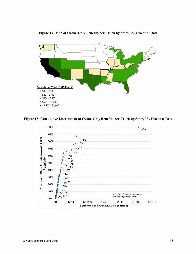
© NERA Economic Consulting 18
Figure 14: Map of Ozone-Only Benefits-per-Truck by State, 3% Discount Rate
Figure 15: Cumulative Distribution of Ozone-Only Benefits-per-Truck by State, 3% Discount Rate
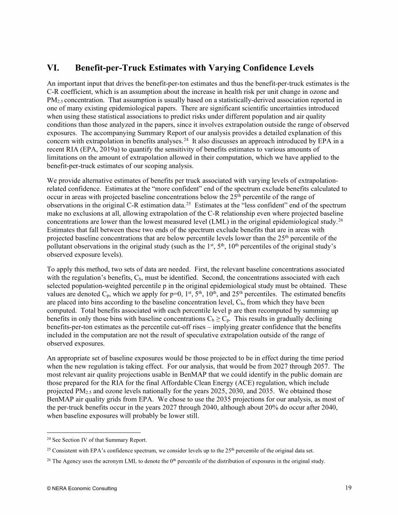
© NERA Economic Consulting 19
VI. Benefit-per-Truck Estimates with Varying Confidence Levels
An important input that drives the benefit-per-ton estimates and thus the benefit-per-truck estimates is the C-R coefficient, which is an assumption about the increase in health risk per unit change in ozone and PM2.5 concentration. That assumption is usually based on a statistically-derived association reported in one of many existing epidemiological papers. There are significant scientific uncertainties introduced when using these statistical associations to predict risks under different population and air quality conditions than those analyzed in the papers, since it involves extrapolation outside the range of observed exposures. The accompanying Summary Report of our analysis provides a detailed explanation of this concern with extrapolation in benefits analyses.24 It also discusses an approach introduced by EPA in a recent RIA (EPA, 2019a) to quantify the sensitivity of benefits estimates to various amounts of limitations on the amount of extrapolation allowed in their computation, which we have applied to the benefit-per-truck estimates of our scoping analysis.
We provide alternative estimates of benefits per truck associated with varying levels of extrapolation-related confidence. Estimates at the “more confident” end of the spectrum exclude benefits calculated to occur in areas with projected baseline concentrations below the 25th percentile of the range of observations in the original C-R estimation data.25 Estimates at the “less confident” end of the spectrum make no exclusions at all, allowing extrapolation of the C-R relationship even where projected baseline concentrations are lower than the lowest measured level (LML) in the original epidemiological study.26 Estimates that fall between these two ends of the spectrum exclude benefits that are in areas with projected baseline concentrations that are below percentile levels lower than the 25th percentile of the pollutant observations in the original study (such as the 1st, 5th, 10th percentiles of the original study’s observed exposure levels).
To apply this method, two sets of data are needed. First, the relevant baseline concentrations associated with the regulation’s benefits, Cb, must be identified. Second, the concentrations associated with each selected population-weighted percentile p in the original epidemiological study must be obtained. These values are denoted Cp, which we apply for p=0, 1st, 5th, 10th, and 25th percentiles. The estimated benefits are placed into bins according to the baseline concentration level, Cb, from which they have been computed. Total benefits associated with each percentile level p are then recomputed by summing up benefits in only those bins with baseline concentrations Cb ≥ Cp. This results in gradually declining benefits-per-ton estimates as the percentile cut-off rises – implying greater confidence that the benefits included in the computation are not the result of speculative extrapolation outside of the range of observed exposures.
An appropriate set of baseline exposures would be those projected to be in effect during the time period when the new regulation is taking effect. For our analysis, that would be from 2027 through 2057. The most relevant air quality projections usable in BenMAP that we could identify in the public domain are those prepared for the RIA for the final Affordable Clean Energy (ACE) regulation, which include projected PM2.5 and ozone levels nationally for the years 2025, 2030, and 2035. We obtained those BenMAP air quality grids from EPA. We chose to use the 2035 projections for our analysis, as most of the per-truck benefits occur in the years 2027 through 2040, although about 20% do occur after 2040, when baseline exposures will probably be lower still.
24 See Section IV of that Summary Report. 25 Consistent with EPA’s confidence spectrum, we consider levels up to the 25th percentile of the original data set. 26 The Agency uses the acronym LML to denote the 0th percentile of the distribution of exposures in the original study.

© NERA Economic Consulting 20
For each of the three C-R relationships that we use in our scoping analysis, we obtained the concentrations associated with each percentile (i.e., the Cp values) from the respective original study. For example, we use the population-weighted exposure distribution from Krewski et al. (2009) to develop the values of Cp for our lower PM2.5 benefit-per-truck estimates, and we use the distribution of PM2.5
exposures in the Di et al. (2017) study to develop confidence-weighting adjustments for our higher PM2.5
benefit-per-truck estimates. The concentration levels at each percentile from the Krewski et al. study are reported in the ACE RIA, but we confirmed them from Table 1 of the original paper. The percentiles in the Di et al. study are available in supplemental materials to the original paper but are more precisely listed in a PM2.5 docket entry (EPA, 2019b). We use information on the distribution of city-specific average ozone concentrations reported in Table 2 of the online supplement to Zanobetti and Schwartz (2008) study.
For each of the three epidemiological studies we have relied upon, Tables 1 through 3 below identify (in the first row) the ambient concentration levels (Cp values) for each of the above percentile cut-off levels that we have used to explore sensitivities to extrapolation-related confidence weighting. The second row of each table identifies the percentage of the respective study’s total avoided premature statistical deaths that lie within each alternative confidence range. (These sum to 100% across the row.) The last two rows of each table report the benefit-per-truck values associated with each confidence level when applying, respectively, a 3% and 7% discount rate to the present value calculation. The first column in each table reports the national average estimates unadjusted for confidence (which we reported in the previous section), while the values in the columns to the right show the estimates that have increasingly higher confidence, up to the point where only benefits in areas with exposures at or above the 25th percentile of the original epidemiological study are included.
Table 1 presents the PM2.5 benefit-per-truck estimates calculated using Krewski et al. (2009). It shows that only about 3% of the benefits are projected to occur in locations that have exposures greater than the 25th percentile of all the exposures in the epidemiological study. Thus, the unadjusted estimate of $4,580 per truck that was reported in the prior section of this report declines to $160 per truck at the “more confident” end of the spectrum.27 If we were to use the 10th percentile as a less conservative confidence cut-off, the associated benefit-per-truck estimate would be $360 with about 8% of the benefits projected to occur in locations that have exposures greater than the 10th percentile of all the study exposures.28 As before, estimates computed using a 7% discount rate are about 25% lower than the respective 3% discount rate.
Table 2 presents the corresponding PM2.5 benefit-per-truck estimates calculated using Di et al. (2017). The uncertainty due to extrapolation is much less pronounced than in Table 1 because the distribution of exposures that were observed in the Di et al. study is lower than that observed in the Krewski et al. study. For example, about 14% of our unadjusted benefits are projected to occur in locations with exposures greater than the 25th percentile of Di et al.’s study, compared to only 3% in the case of Krewski et al. Thus, we can see that the benefit-per-truck estimates decline less when moving from the “less confident” to the “more confident” end of the benefits scale, with the unadjusted estimate (for a 3% discount rate) of $5,540 per truck declining to $780 per truck. At the 10th percentile confidence cut-off, the Di et al. study
27 The benefit-per-truck estimate of $160 is calculated by multiplying the confidence un-adjusted estimate with the fraction of
benefits that can be attributed to locations with exposures greater than the 25th percentile of the study exposures: 3%*$4,580. 28 8% is computed as the sum of the percentages of the total deaths that can be attributed to locations with exposures greater than
the 25th percentile of the study exposures (i.e. the sum of the last two columns): 4.3%+3.4% with the corresponding estimate of $360 computed as: 8%*$4,580.

© NERA Economic Consulting 21
(for the 3% discount rate) is $3,180 per truck, more than eight times greater than the corresponding Krewski et al. estimate.
Table 3 presents the ozone benefit-per-truck estimates calculated using Zanobetti and Schwartz (2008). The pattern observed in the drop-off of the benefit-per-truck estimates is significantly different from that for PM2.5. The unadjusted estimate of $390 per truck remains unchanged through the 5th percentile confidence cut-off because almost none of the U.S. is projected to have ozone concentrations below 23.4 ppb in our baseline air quality grid, even though Zanobetti and Schwartz data indicate that about 5% of the cities in their study had lower average ozone levels.29 The confidence-weighted ozone benefit estimate declines to $180 per truck at the highest confidence end of the spectrum with 46% of our estimated ozone benefits projected to occur in locations with exposures above the 25th percentile of all the cities observed in the original Zanobetti and Schwartz study.
29 We have no explanation for such a discrepancy at this time, which seems surprising given that our estimates of baseline
exposure are more disaggregated than those of Zanobetti and Schwartz’s observations (12-km grid resolution vs. city-wide averages) and they occur later in time (2035 vs. 1989-2000) when tighter ozone standards will be in place.

© NERA Economic Consulting 22
Table 1: Avoided Premature Statistical Deaths (%) and National PM2.5 Benefit-per-Truck Estimates (2019$/truck) by Confidence Level Using Krewski et al. (2009) Epidemiology Study and Applying 3% and 7% Discount Rates
Below LML (<5.8)
LML to 1st Percentile
(≥5.8 & <6.7)
1st to 5th Percentile
(≥6.7 & <8.8)
5th to 10th Percentile
(≥8.8 & <10.2)
10th to 25th
Percentile (≥10.2 & <11.8)
25th Percentile & Above (≥11.8)
Avoided Premature Statistical Deaths (%) National 9% 16% 56% 11% 4% 3%
Benefit-Per-Truck (2019$/truck) 3% Discount Rate $4,580 $4,150 $3,440 $870 $360 $160 7% Discount Rate $3,430 $3,110 $2,570 $650 $270 $120
LML = Lowest Measured Level, meaning the minimum observed PM2.5 concentration in the original epidemiological study

© NERA Economic Consulting 23
Table 2: Avoided Premature Statistical Deaths (%) and National PM2.5 Benefit-per-Truck Estimates (2019$/truck) by Confidence Level Using Di et al. (2017) Epidemiology Study and Applying 3% and 7% Discount Rates
Below LML (<0.02)
LML to 1st Percentile
(≥0.02 & <3)
1st to 5th Percentile
(≥3 & <6.2)
5th to 10th Percentile
(≥6.2 & <7.3)
10th to 25th Percentile
(≥7.3 & <9.1)
25th Percentile & Above
(≥9.1) Avoided Premature Statistical Deaths (%)
National 0% 0% 15% 27% 43% 14% Benefit-Per-Truck (2019$/truck)
3% Discount Rate $5,540 $5,540 $5,540 $4,680 $3,180 $780 7% Discount Rate $4,130 $4,130 $4,130 $3,490 $2,370 $580
LML = Lowest Measured Level, meaning the minimum observed PM2.5 concentration in the original epidemiological study

© NERA Economic Consulting 24
Table 3: Avoided Premature Statistical Deaths (%) and National Ozone Benefit-per-Truck Estimates (2019$/truck) by Confidence Level Using Zanobetti and Schwartz (2008) Epidemiology Study and Applying 3% and 7% Discount Rates
Below LML (<15.1)
LML to 1st Percentile
(=15.1)
1st to 5th Percentile
(>15.1 & <23.4)
5th to 10th Percentile
(≥23.4 & <35.6)
10th to 25th Percentile
(≥35.6 & <44.0)
25th Percentile & Above (≥44.0)
Avoided Premature Statistical Deaths (%) National 0% 0% 0% 17% 37% 46%
Benefit-Per-Truck (2019$/truck) 3% Discount Rate $390 $390 $390 $390 $330 $180 7% Discount Rate $290 $290 $290 $290 $240 $130
LML = Lowest Measured Level, meaning the minimum observed ozone concentration in the original epidemiological study

© NERA Economic Consulting
As illustrated previously, significant differences exist between the projected concentrations in California and the Rest of U.S., which points to the existence of different patterns in the decline of the benefit-per-truck estimates moving from the “less confident” to the “more confident” end of the benefits estimates scale.30 Tables 4 through 6 present the benefit-per-truck separately for California and Rest of the U.S. in the same format as that presented above for the national estimates. These tables show that California benefit-per-truck estimates decrease at a slower rate than the Rest of the U.S estimates do, which further widens the significant disparities that were noted in the unadjusted estimates in the prior section.
Table 4 presents the PM2.5 benefit-per-truck estimates calculated using Krewski et al. (2009) for these two regions. The 3% confidence unadjusted estimate declines from $9,390 to $1,600 per truck for California, while it declines from $4,190 to $20 per truck for the Rest of the U.S. While the estimates for California are about 2 times higher than those for the Rest of the U.S. at the “less confident” end of the spectrum, they are more than 80 times higher at the “more confident” end. About 17% of the benefits in California are projected to occur in locations with baseline concentrations greater than the 25th percentile of the original study; in contrast, the corresponding fraction for benefits estimates across the Rest of the U.S. is less than 1%.
Table 5 presents the corresponding PM2.5 benefit-per-truck estimates calculated using Di et al. (2017). A somewhat lesser rise in disparity with increasing confidence level is observed, but it is still pronounced. The estimates for California are again about 2 times higher than those for the Rest of the U.S. for the “less confident” estimates, but widen to about 30 times higher at the “more confident” end of the benefits estimate spectrum.
Table 6 presents the ozone benefit-per-truck estimates calculated using Zanobetti and Schwartz (2008) for the two regions. In this case – compared to the PM2.5 estimates – a larger disparity in the estimates for the two regions is observed at the “less confident” end of the spectrum, but less at the “more confident” end of the spectrum. That is, the California benefit-per-truck estimates are about 12 times higher than those for the Rest of the U.S. before confidence-weighting, and are about 22 times higher at the other end of the confidence-weighting spectrum.
30 The Rest of U.S. region includes all states across the conterminous U.S. except for California.
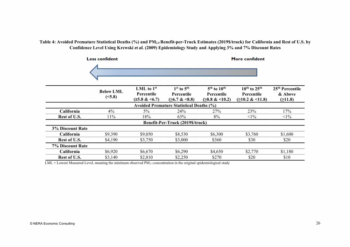
© NERA Economic Consulting 26
Table 4: Avoided Premature Statistical Deaths (%) and PM2.5 Benefit-per-Truck Estimates (2019$/truck) for California and Rest of U.S. by Confidence Level Using Krewski et al. (2009) Epidemiology Study and Applying 3% and 7% Discount Rates
Below LML (<5.8)
LML to 1st Percentile
(≥5.8 & <6.7)
1st to 5th Percentile
(≥6.7 & <8.8)
5th to 10th Percentile
(≥8.8 & <10.2)
10th to 25th Percentile
(≥10.2 & <11.8)
25th Percentile & Above (≥11.8)
Avoided Premature Statistical Deaths (%) California 4% 5% 24% 27% 23% 17%
Rest of U.S. 11% 18% 63% 8% <1% <1% Benefit-Per-Truck (2019$/truck)
3% Discount Rate California $9,390 $9,050 $8,530 $6,300 $3,760 $1,600
Rest of U.S. $4,190 $3,750 $3,000 $360 $30 $20 7% Discount Rate
California $6,920 $6,670 $6,290 $4,650 $2,770 $1,180 Rest of U.S. $3,140 $2,810 $2,250 $270 $20 $10
LML = Lowest Measured Level, meaning the minimum observed PM2.5 concentration in the original epidemiological study

© NERA Economic Consulting 27
Table 5: Avoided Premature Statistical Deaths (%) and PM2.5 Benefit-per-Truck Estimates (2019$/truck) for California and Rest of U.S. Using Di et al. (2017) Epidemiology Study and Applying 3% and 7% Discount Rates
Below LML (<0.02)
LML to 1st Percentile
(≥0.02 & <3)
1st to 5th Percentile
(≥3 & <6.2)
5th to 10th Percentile
(≥6.2 & <7.3)
10th to 25th Percentile
(≥7.3 & <9.1)
25th Percentile & Above
(≥9.1) Avoided Premature Statistical Deaths (%)
California 0% 0% 5% 11% 25% 60% Rest of U.S. 0% 0% 18% 31% 47% 4%
Benefit-Per-Truck (2019$/truck) 3% Discount Rate
California $11,160 $11,160 $11,160 $10,620 $9,430 $6,660 Rest of U.S. $5,080 $5,080 $5,080 $4,180 $2,620 $210
7% Discount Rate California $8,180 $8,180 $8,180 $7,780 $6,910 $4,880
Rest of U.S. $3,790 $3,790 $3,790 $3,120 $1,950 $160 LML = Lowest Measured Level, meaning the minimum observed PM2.5 concentration in the original epidemiological study

© NERA Economic Consulting 28
Table 6: Avoided Premature Statistical Deaths (%) and Ozone Benefit-per-Truck Estimates (2019$/truck) for California and Rest of U.S. by Confidence Level Using Zanobetti and Schwartz (2008) Epidemiology Study and Applying 3% and 7% Discount Rates
Below LML (<15.1)
LML to 1st Percentile
(=15.1)
1st to 5th Percentile
(>15.1 & <23.4)
5th to 10th Percentile
(≥23.4 & <35.6)
10th to 25th Percentile
(≥35.6 & <44.0)
25th Percentile & Above (≥44.0)
Avoided Premature Statistical Deaths (%) California 0% 0% 0% 12% 30% 58%
Rest of U.S. 0% 0% 0% 22% 46% 32% Benefit-Per-Truck (2019$/truck)
3% Discount Rate California $2,570 $2,570 $2,570 $2,570 $2,250 $1,490
Rest of U.S. $210 $210 $210 $210 $160 $70 7% Discount Rate
California $1,890 $1,890 $1,890 $1,890 $1,660 $1,100 Rest of U.S. $150 $150 $150 $150 $120 $50
LML = Lowest Measured Level, meaning the minimum observed ozone concentration in the original epidemiological study

© NERA Economic Consulting 29
VII. References
Di, Q; Dai, L; Wang, Y; Zanobetti, A; Choirat, C; Schwartz, J; Dominici, F. 2017. Association of short-term exposure to air pollution with mortality in older adults. J Am Med Assoc 318(24):2446-2456.
EPA. 2000. Regulatory impact analysis: Heavy-duty engine and vehicle standards and highway diesel fuel sulfur control requirements, EPA420-R-00-026, December.
EPA. 2004. Advisory Council on Clean Air Compliance Analysis response to agency request on cessation lag, EPA-COUNCIL-LTR-05-001, December.
EPA. 2014a. Control of air pollution from motor vehicles: Tier 3 motor vehicle emission and fuel standards final rule, regulatory impact analysis, EPA-420-R-14-005, March.
EPA. 2014b. Health risk and exposure assessment for ozone, final report, EPA-452/R-14-004a, August.
EPA. 2015a. Regulatory impact analysis for the Clean Power Plan final rule, EPA-452/R-15-003, August.
EPA. 2015b. Regulatory impact analysis of the final revisions to the National Ambient Air Quality Standards for ground-level ozone, EPA-452/R-15-007, September.
EPA. 2015c. “Copy of docket data final RIA v2.” Docket # EPA-HQ-OAR-2013-0169-0056, posted October 7.
EPA. 2016. Population and activity of on-road vehicles in MOVES2014, EPA-420-R-16-003, January.
EPA. 2019a. Regulatory impact analysis for the repeal of the Clean Power Plan, and the emission guidelines for greenhouse gas emissions from existing electric utility generating units, EPA-452/R-19-003, June.
EPA. 2019b. “Email from Scott Jenkins, EPA, to Benjamin Sabath and Francesca Dominici. Re: question about PM2.5 estimates in Di et al. (2017) studies and data file attachment. May 8, 2019.” Docket # EPA-HQ-OAR-2015-0072-0022, posted September 11.
EPA. 2019c. Policy assessment for the review of the ozone national ambient air quality standards, external review draft, EPA-452/P-19-002, October.
EPA. 2020. Policy assessment for the review of the national ambient air quality standards for particulate matter, EPA-452/R-20-002, January.
Krewski, D; Jerrett, M; Burnett, RT; Ma, R; Hughes, E; Shi, Y; Turner, MC; Pope, CA, III; Thurston, G; Calle, EE; Thun, MJ; Beckerman, B; Deluca, P; Finkelstein, N; Ito, K; Moore, DK; Newbold, KB; Ramsay, T; Ross, Z; Shin, H; Tempalski, B. 2009. Extended follow-up and spatial analysis of the American Cancer Society study linking particulate air pollution and mortality. Research Report 140. Health Effects Institute. Boston, MA.
Lepeule, J; Laden, F; Dockery, D; Schwartz, J. 2012. Chronic exposure to fine particles and mortality: an extended follow-up of the Harvard Six Cities study from 1974 to 2009. Environ. Health Perspect. 120(7):965.
Wolfe, P; Davidson K; Fulcher,C; Fann, N; Zawacki, M; Baker, K. 2018. Monetized health benefits attributable to mobile source emission reductions across the United States in 2025. Science of the Total Environment 650:2490-2498.

© NERA Economic Consulting 30
Zanobetti, A; Schwartz, J. 2008. Mortality displacement in the association of ozone with mortality: an analysis of 48 cities in the United States. Am J Respir Crit Care Med. 177:184-189.

© NERA Economic Consulting 31
Appendix A: Estimated Total NOx Emissions Reductions Including All Model Years, by State
2027 2028 2029 2030 2031 2032 2033 2034 2035 2036 2037 2038 2039 2040 2041 2042 2043 2044 2045 2046 2047 2048 2049 2050
U.S. 32,336 64,986 97,905 131,009 167,862 202,670 236,023 267,874 297,564 324,976 350,272 373,253 392,157 413,119 430,429 446,171 460,339 473,697 486,102 497,823 508,892 519,411 529,468 539,102
Alabama 684 1,374 2,070 2,769 3,549 4,286 4,992 5,666 6,295 6,875 7,410 7,896 8,337 8,740 9,106 9,439 9,739 10,021 10,284 10,532 10,766 10,988 11,201 11,405
Arizona 760 1,528 2,302 3,081 3,934 4,740 5,512 6,249 6,937 7,572 8,159 8,692 9,176 9,618 10,020 10,386 10,716 11,027 11,316 11,589 11,848 12,093 12,328 12,553
Arkansas 480 965 1,454 1,945 2,478 2,982 3,464 3,925 4,355 4,752 5,119 5,453 5,755 6,033 6,285 6,514 6,721 6,916 7,098 7,270 7,432 7,587 7,735 7,876
California 2,592 5,207 7,842 10,492 13,558 16,453 19,230 21,878 24,342 26,616 28,711 30,612 32,332 33,901 35,327 36,623 37,787 38,883 39,897 40,855 41,758 42,616 43,435 44,219
Colorado 544 1,094 1,649 2,206 2,825 3,409 3,970 4,504 5,003 5,463 5,888 6,274 6,624 6,944 7,235 7,500 7,738 7,962 8,171 8,368 8,554 8,731 8,900 9,062
Connecticut 204 411 618 827 1,076 1,311 1,537 1,752 1,952 2,137 2,306 2,460 2,599 2,726 2,841 2,945 3,039 3,127 3,209 3,285 3,358 3,426 3,492 3,554
Delaware 41 82 123 165 218 269 318 364 407 446 483 515 545 572 596 618 637 656 673 689 704 718 731 744
Florida 1,430 2,874 4,328 5,791 7,464 9,044 10,560 12,005 13,351 14,593 15,738 16,777 17,717 18,575 19,355 20,063 20,700 21,300 21,856 22,380 22,875 23,345 23,794 24,223
Georgia 1,352 2,717 4,094 5,478 6,998 8,433 9,808 11,121 12,347 13,478 14,523 15,473 16,334 17,122 17,839 18,491 19,078 19,632 20,147 20,634 21,094 21,531 21,949 22,350
Idaho 227 456 687 919 1,172 1,410 1,639 1,857 2,061 2,249 2,423 2,581 2,724 2,856 2,975 3,084 3,182 3,274 3,360 3,441 3,518 3,591 3,661 3,728
Illinois 564 1,132 1,704 2,278 2,984 3,651 4,292 4,901 5,467 5,988 6,467 6,901 7,292 7,648 7,971 8,264 8,526 8,773 9,000 9,214 9,416 9,606 9,789 9,963
Indiana 848 1,705 2,569 3,437 4,402 5,314 6,187 7,021 7,798 8,516 9,178 9,780 10,325 10,824 11,277 11,690 12,061 12,410 12,735 13,042 13,332 13,608 13,871 14,124
Iowa 486 977 1,472 1,970 2,509 3,017 3,504 3,970 4,404 4,806 5,177 5,514 5,820 6,101 6,355 6,587 6,797 6,994 7,178 7,351 7,516 7,672 7,821 7,964
Kansas 359 722 1,088 1,456 1,863 2,248 2,616 2,968 3,296 3,599 3,879 4,133 4,364 4,574 4,766 4,940 5,097 5,245 5,383 5,512 5,635 5,752 5,863 5,970
Kentucky 868 1,745 2,630 3,520 4,471 5,369 6,228 7,051 7,818 8,528 9,184 9,780 10,322 10,819 11,270 11,681 12,052 12,402 12,728 13,037 13,329 13,606 13,872 14,127
Louisiana 539 1,083 1,631 2,183 2,790 3,363 3,912 4,436 4,926 5,377 5,794 6,174 6,517 6,832 7,118 7,378 7,612 7,833 8,039 8,233 8,416 8,590 8,757 8,917
Maine 244 491 740 990 1,260 1,515 1,759 1,992 2,209 2,411 2,596 2,765 2,919 3,059 3,187 3,304 3,408 3,507 3,600 3,687 3,769 3,848 3,923 3,995
Maryland 498 1,000 1,506 2,016 2,599 3,149 3,677 4,180 4,649 5,082 5,481 5,843 6,171 6,470 6,742 6,989 7,211 7,420 7,614 7,797 7,970 8,134 8,290 8,440
Massachusetts 504 1,013 1,526 2,042 2,630 3,185 3,717 4,225 4,698 5,135 5,537 5,902 6,233 6,535 6,810 7,059 7,283 7,495 7,691 7,876 8,050 8,216 8,374 8,526
Michigan 1,153 2,318 3,492 4,673 5,980 7,214 8,396 9,526 10,579 11,551 12,449 13,264 14,004 14,680 15,294 15,853 16,357 16,831 17,272 17,689 18,082 18,457 18,814 19,157
Minnesota 563 1,131 1,703 2,279 2,932 3,549 4,141 4,706 5,231 5,717 6,164 6,570 6,938 7,274 7,580 7,857 8,107 8,342 8,560 8,766 8,961 9,145 9,322 9,491
Mississippi 420 845 1,273 1,703 2,183 2,636 3,070 3,485 3,871 4,228 4,557 4,856 5,127 5,375 5,600 5,805 5,989 6,163 6,325 6,477 6,621 6,758 6,889 7,014
Missouri 822 1,651 2,488 3,330 4,253 5,126 5,961 6,759 7,504 8,192 8,827 9,404 9,928 10,407 10,842 11,239 11,596 11,933 12,246 12,542 12,822 13,088 13,342 13,586
Montana 231 465 701 939 1,191 1,430 1,658 1,877 2,081 2,269 2,444 2,602 2,746 2,878 2,998 3,108 3,206 3,299 3,386 3,468 3,546 3,620 3,691 3,759
Nebraska 345 694 1,046 1,401 1,779 2,136 2,478 2,805 3,110 3,392 3,653 3,891 4,106 4,304 4,483 4,647 4,794 4,933 5,063 5,186 5,302 5,412 5,518 5,619
Nevada 270 542 816 1,092 1,400 1,690 1,968 2,234 2,481 2,710 2,920 3,112 3,286 3,444 3,588 3,720 3,838 3,949 4,052 4,150 4,242 4,330 4,413 4,494
New Hampshire 140 282 425 568 730 882 1,028 1,168 1,297 1,417 1,528 1,628 1,719 1,803 1,878 1,947 2,009 2,067 2,121 2,172 2,221 2,266 2,310 2,352
New Jersey 1,648 3,314 4,994 6,685 8,463 10,144 11,752 13,291 14,728 16,058 17,287 18,406 17,500 20,356 21,204 21,976 22,674 23,332 23,947 24,529 25,079 25,603 26,104 26,585
New Mexico 430 865 1,303 1,745 2,218 2,666 3,095 3,504 3,887 4,240 4,567 4,864 5,134 5,381 5,606 5,810 5,995 6,169 6,331 6,484 6,629 6,767 6,899 7,025

© NERA Economic Consulting 32
2027 2028 2029 2030 2031 2032 2033 2034 2035 2036 2037 2038 2039 2040 2041 2042 2043 2044 2045 2046 2047 2048 2049 2050
New York 1,068 2,145 3,231 4,322 5,586 6,779 7,924 9,016 10,031 10,968 11,832 12,615 13,324 13,970 14,558 15,091 15,571 16,022 16,440 16,835 17,207 17,560 17,897 18,220
North Carolina 925 1,858 2,799 3,745 4,829 5,853 6,835 7,771 8,643 9,448 10,190 10,863 11,472 12,028 12,534 12,993 13,406 13,795 14,155 14,495 14,816 15,121 15,412 15,690
North Dakota 160 322 486 650 827 994 1,154 1,307 1,449 1,581 1,703 1,814 1,914 2,007 2,090 2,167 2,236 2,300 2,361 2,418 2,472 2,524 2,573 2,620
Ohio 1,145 2,300 3,465 4,635 5,967 7,225 8,431 9,582 10,654 11,642 12,554 13,382 14,131 14,816 15,437 16,003 16,511 16,990 17,433 17,852 18,248 18,623 18,982 19,326
Oklahoma 555 1,116 1,681 2,250 2,878 3,472 4,040 4,583 5,090 5,557 5,989 6,381 6,737 7,062 7,358 7,627 7,869 8,098 8,310 8,510 8,700 8,880 9,052 9,217
Oregon 411 827 1,246 1,667 2,131 2,570 2,990 3,392 3,766 4,112 4,431 4,721 4,984 5,225 5,444 5,643 5,822 5,991 6,148 6,296 6,437 6,570 6,697 6,820
Pennsylvania 1,210 2,433 3,665 4,905 6,272 7,562 8,799 9,980 11,082 12,099 13,038 13,891 14,665 15,372 16,016 16,601 17,128 17,625 18,087 18,524 18,936 19,328 19,703 20,062
Rhode Island 72 144 217 291 386 475 561 643 719 789 853 910 962 1,010 1,052 1,091 1,126 1,158 1,188 1,216 1,243 1,268 1,291 1,314
South Carolina 699 1,405 2,118 2,834 3,609 4,341 5,042 5,712 6,338 6,916 7,449 7,935 8,375 8,779 9,146 9,479 9,780 10,064 10,329 10,578 10,815 11,039 11,254 11,460
South Dakota 188 377 569 761 965 1,158 1,342 1,519 1,683 1,836 1,977 2,105 2,221 2,328 2,425 2,514 2,593 2,669 2,739 2,805 2,868 2,928 2,985 3,040
Tennessee 899 1,808 2,724 3,645 4,654 5,607 6,519 7,392 8,205 8,957 9,651 10,281 10,853 11,377 11,853 12,286 12,676 13,043 13,386 13,709 14,015 14,305 14,583 14,849
Texas 2,419 4,860 7,322 9,798 12,573 15,193 17,705 20,103 22,338 24,401 26,304 28,033 29,599 31,031 32,332 33,516 34,580 35,584 36,516 37,396 38,226 39,016 39,771 40,493
Utah 268 538 810 1,084 1,392 1,684 1,963 2,229 2,478 2,707 2,918 3,110 3,284 3,443 3,587 3,719 3,837 3,948 4,051 4,149 4,241 4,328 4,412 4,492
Vermont 127 255 384 514 653 785 911 1,032 1,144 1,248 1,344 1,432 1,511 1,584 1,650 1,710 1,765 1,816 1,864 1,909 1,952 1,992 2,031 2,068
Virginia 1,005 2,020 3,044 4,073 5,207 6,279 7,305 8,286 9,201 10,045 10,825 11,533 12,175 12,763 13,297 13,783 14,221 14,634 15,017 15,380 15,722 16,048 16,359 16,658
Washington 700 1,407 2,120 2,837 3,627 4,373 5,088 5,771 6,407 6,995 7,538 8,031 8,479 8,888 9,260 9,598 9,903 10,190 10,458 10,710 10,949 11,175 11,392 11,600
West Virginia 275 552 832 1,113 1,417 1,705 1,980 2,243 2,489 2,716 2,925 3,116 3,289 3,448 3,592 3,723 3,841 3,952 4,056 4,155 4,247 4,336 4,420 4,501
Wisconsin 747 1,501 2,262 3,026 3,867 4,662 5,423 6,150 6,828 7,454 8,032 8,557 9,034 9,470 9,866 10,227 10,552 10,858 11,143 11,412 11,666 11,908 12,139 12,361
Wyoming 216 435 655 877 1,111 1,331 1,542 1,744 1,933 2,107 2,269 2,415 2,549 2,671 2,783 2,884 2,975 3,062 3,143 3,219 3,291 3,360 3,426 3,489

© NERA Economic Consulting 33
Appendix B: Benefit-per-Ton Estimates by State
Zanobetti and Schwartz (2008); Respiratory Mortality (2019$/ton)
Krewski et al. (2009); All-Cause Mortality (2019$/ton)
Di et al. (2017); All-Cause Mortality (2019$/ton)
2030 2040 2050 2030 2040 2050 2030 2040 2050 U.S. $569 $706 $795 $6,980 $7,856 $8,047 $8,310 $9,715 $10,129
Alabama $208 $225 $218 $883 $946 $913 $1,013 $1,135 $1,114 Arizona $701 $904 $1,084 $383 $489 $581 $443 $596 $722
Arkansas $91 $100 $98 $2,063 $2,265 $2,252 $2,366 $2,704 $2,734 California $3,643 $4,543 $5,246 $13,542 $16,372 $18,700 $15,714 $19,943 $23,412 Colorado $511 $608 $661 $4,122 $4,886 $5,432 $4,811 $5,940 $6,772
Connecticut $112 $129 $129 $8,069 $9,116 $9,068 $9,933 $11,603 $11,652 Delaware $67 $73 $74 $20,708 $24,025 $25,156 $24,515 $29,594 $31,407 Florida $799 $1,019 $1,204 $50 $63 $74 $60 $79 $94 Georgia $358 $432 $471 $950 $1,144 $1,267 $1,093 $1,391 $1,571 Idaho $32 $38 $41 $3,409 $4,131 $4,565 $4,105 $5,151 $5,807 Illinois $102 $114 $114 $17,704 $19,670 $19,916 $21,065 $24,336 $25,141 Indiana $143 $154 $146 $16,237 $17,468 $16,855 $19,244 $21,484 $21,036
Iowa $29 $31 $28 $9,528 $9,880 $8,962 $11,643 $12,361 $11,317 Kansas $28 $29 $27 $5,499 $5,840 $5,479 $6,614 $7,208 $6,838
Kentucky $163 $173 $162 $6,987 $7,354 $6,903 $8,076 $8,828 $8,386 Louisiana $168 $186 $186 $301 $326 $323 $343 $384 $390
Maine $49 $57 $56 $508 $603 $619 $635 $778 $807 Maryland $158 $196 $218 $11,743 $14,056 $15,473 $13,956 $17,434 $19,649
Massachusetts $144 $164 $161 $4,947 $5,467 $5,380 $6,040 $6,894 $6,855 Michigan $232 $257 $252 $19,125 $20,979 $20,742 $22,997 $26,266 $26,318 Minnesota $82 $95 $93 $11,454 $13,360 $13,410 $14,129 $16,955 $17,224 Mississippi $125 $137 $135 $990 $1,111 $1,149 $1,117 $1,314 $1,392 Missouri $61 $65 $60 $5,744 $6,064 $5,640 $6,781 $7,384 $6,940 Montana $25 $29 $30 $342 $410 $445 $419 $517 $571 Nebraska $17 $18 $16 $4,766 $5,074 $4,769 $5,760 $6,280 $5,971 Nevada $822 $1,125 $1,500 $1,164 $1,498 $1,900 $1,370 $1,855 $2,419
New Hampshire $33 $40 $41 $1,882 $2,262 $2,326 $2,331 $2,902 $3,003

© NERA Economic Consulting 34
Zanobetti and Schwartz (2008); Respiratory Mortality (2019$/ton)
Krewski et al. (2009); All-Cause Mortality (2019$/ton)
Di et al. (2017); All-Cause Mortality (2019$/ton)
2030 2040 2050 2030 2040 2050 2030 2040 2050 New Jersey $225 $262 $266 $14,316 $16,189 $16,444 $17,215 $20,275 $20,924 New Mexico $85 $106 $125 $231 $286 $338 $271 $351 $428 New York $391 $441 $448 $10,710 $11,844 $12,058 $12,829 $14,709 $15,260
North Carolina $322 $383 $412 $2,920 $3,441 $3,711 $3,437 $4,247 $4,654 North Dakota $15 $18 $18 $1,175 $1,349 $1,368 $1,423 $1,668 $1,712
Ohio $296 $321 $311 $18,322 $19,875 $19,429 $21,967 $24,723 $24,525 Oklahoma $128 $133 $124 $3,683 $3,840 $3,614 $4,191 $4,509 $4,306
Oregon $72 $82 $89 $1,562 $1,755 $1,852 $1,872 $2,171 $2,338 Pennsylvania $282 $321 $321 $15,420 $17,427 $17,587 $18,958 $22,151 $22,644 Rhode Island $40 $44 $44 $9,371 $10,479 $10,456 $11,412 $13,213 $13,336
South Carolina $171 $211 $241 $1,377 $1,660 $1,865 $1,616 $2,046 $2,352 South Dakota $16 $18 $17 $2,689 $2,902 $2,731 $3,268 $3,600 $3,422
Tennessee $248 $275 $273 $2,599 $2,839 $2,805 $2,956 $3,365 $3,373 Texas $946 $1,158 $1,302 $1,224 $1,484 $1,652 $1,407 $1,789 $2,034 Utah $311 $385 $451 $8,326 $9,840 $10,850 $9,668 $11,855 $13,467
Vermont $15 $18 $18 $1,770 $2,158 $2,327 $2,219 $2,782 $3,028 Virginia $260 $321 $355 $2,737 $3,402 $3,875 $3,272 $4,247 $4,944
Washington $116 $138 $150 $1,614 $1,923 $2,119 $1,941 $2,391 $2,688 West Virginia $93 $96 $91 $4,023 $4,169 $3,967 $4,729 $5,081 $4,918
Wisconsin $82 $93 $89 $13,567 $15,146 $14,674 $16,612 $19,123 $18,738 Wyoming $14 $16 $17 $189 $220 $226 $223 $266 $280

© NERA Economic Consulting 35
Appendix C: Benefit-per-Truck Estimates by State, 7% Discount Rate
Figure 16: Map of PM2.5-Only Benefits-per-Truck by State Using the Krewski et al. (2009) C-R Coefficient, 7% Discount Rate
Figure 17: Cumulative Distribution of PM2.5-Only Benefits-per-Truck by State Using the Krewski et al. (2009) C-R Coefficient, 7% Discount Rate

© NERA Economic Consulting 36
Figure 18: Map of PM2.5-Only Benefits-per-Truck by State Using the Di et al. (2017) C-R Coefficient, 7% Discount Rate
Figure 19: Cumulative Distribution of PM2.5-Only Benefits-per-Truck by State Using the Di et al. (2017) C-R Coefficient, 7% Discount Rate

© NERA Economic Consulting 37
Figure 20: Map of Ozone-Only Benefits-per-Truck by State, 7% Discount Rate
Figure 21: Cumulative Distribution of Ozone-Only Benefits-per-Truck by State, 7% Discount Rate

© NERA Economic Consulting 38
Appendix D: Estimated Average Ozone Response Factors by State
State Ozone Response Factor (ppb/ton) Alabama 0.000022 Arizona 0.000061
Arkansas 0.000014 California 0.000072 Colorado 0.000061
Connecticut 0.000019 Delaware 0.000017 Florida 0.000022 Georgia 0.000022 Idaho 0.000011 Illinois 0.000005 Indiana 0.000012
Iowa 0.000005 Kansas 0.000005
Kentucky 0.000017 Louisiana 0.000022
Maine 0.000016 Maryland 0.000019
Massachusetts 0.000015 Michigan 0.000014 Minnesota 0.000011 Mississippi 0.000022 Missouri 0.000005 Montana 0.000011 Nebraska 0.000005 Nevada 0.000135
New Hampshire 0.000012 New Jersey 0.000019 New Mexico 0.000021 New York 0.000015
North Carolina 0.000017 North Dakota 0.000011
Ohio 0.000014 Oklahoma 0.000018
Oregon 0.000011 Pennsylvania 0.000012 Rhode Island 0.000019
South Carolina 0.000017 South Dakota 0.000011
Tennessee 0.000019 Texas 0.000025 Utah 0.000098
Vermont 0.000010 Virginia 0.000020

© NERA Economic Consulting 39
State Ozone Response Factor (ppb/ton) Washington 0.000011
West Virginia 0.000019 Wisconsin 0.000009 Wyoming 0.000011

© NERA Economic Consulting 40
NERA Economic Consulting 1255 23rd Street, NW Suite 600 Washington, DC 20037 +1 202 466 9246

Potential Air Quality Benefits of a 90%/50% Reduction in NOx Emissions from New Heavy-Duty On-Highway Vehicles – Conceptual Summary of Methods and Key Results
Prepared for the Truck and Engine Manufacturers Association
April 2020

© NERA Economic Consulting i
Project Team Anne E. Smith, Ph.D., Managing Director Bharat Ramkrishnan, Consultant Andrew Hahm, Research Associate
About NERA
NERA Economic Consulting (www.nera.com) is a global firm of experts dedicated to applying economic, finance, and quantitative principles to complex business and legal challenges. For over half a century, NERA's economists have been creating strategies, studies, reports, expert testimony, and policy recommendations for government authorities and the world’s leading law firms and corporations. We bring academic rigor, objectivity, and real-world industry experience to bear on issues arising from competition, regulation, public policy, strategy, finance, and litigation.
This report reflects the research, opinions, and conclusions of its authors, and does not necessarily reflect those of NERA Economic Consulting, its affiliated companies, or any other organization.
© NERA Economic Consulting ii
Report Qualifications/Assumptions and Limiting Conditions Information furnished by others, upon which all or portions of this report are based, is believed to be reliable, but has not been independently verified, unless otherwise expressly indicated. Public information and industry and statistical data are from sources we deem to be reliable; however, we make no representation as to the accuracy or completeness of such information. The findings contained in this report may contain predictions based on current data and historical trends. Any such predictions are subject to inherent risks and uncertainties. NERA Economic Consulting accepts no responsibility for actual results or future events.
The opinions expressed in this report are valid only for the purpose stated herein and as of the date of this report. No obligation is assumed to revise this report to reflect changes, events or conditions, which occur subsequent to the date hereof.
All decisions in connection with the implementation or use of advice or recommendations contained in this report are the sole responsibility of the client. This report does not represent investment advice nor does it provide an opinion regarding the fairness of any transaction to any and all parties.
© NERA Economic Consulting

© NERA Economic Consulting iii
Contents I. Introduction.......................................................................................................................1
II. Description of Methodology .............................................................................................2
III. Benefit-per-Truck Estimates Prior to Confidence-Weighting .....................................4
IV. Benefit-per-Truck Estimates with Qualitative Confidence-Weighting .......................5
V. Conclusion .......................................................................................................................14
References ...............................................................................................................................15

© NERA Economic Consulting iv
List of Figures Figure 1: Range of Exposures During 1999-2000 Used in the Krewski et al. (2009) Epidemiology Study to Estimate the C-R Relationship Used for Benefits Calculations in this Analysis ................................................................................................................................ 7 Figure 2: Range of Projected PM2.5 Concentrations in California and Rest of U.S. ....................... 8
List of Tables Table 1: National Ozone and PM2.5-Related Benefit-per-Truck Estimates with No Adjustment for Confidence ............................................................................................................. 4 Table 2: National PM2.5 Benefit-Per-Truck Estimates (2019$/truck) Adjusted by Confidence Level Based on Health Effect Estimates from the Krewski et al. (2009) and Di et al. (2017) Epidemiology Studies, Applying 3% and 7% Discount Rates .................... 10 Table 3: National Ozone Benefit-Per-Truck Estimates (2019$/truck) Adjusted by Confidence Level Based on a Health Effect Estimate from the Zanobetti and Schwartz (2008) Epidemiology Study, Applying 3% and 7% Discount Rates ............................ 10 Table 4: Range of PM2.5 Benefit-Per-Truck Estimates (2019$/truck) for California and Rest of U.S. Adjusted by Confidence Level Based on the Health Effect Estimates from the Krewski et al. (2009) and Di et al. (2017) Epidemiology Studies, Applying 3% and 7% Discount Rates ........................................................................................................... 12 Table 5: Ozone Benefit-Per-Truck Estimates (2019$/truck) for California and Rest of U.S. Adjusted by Confidence Level Based on the Health Effect Estimates from the Zanobetti and Schwartz (2008) Epidemiology Study, Applying 3% and 7% Discount Rates .............................................................................................................................................. 13

© NERA Economic Consulting v
List of Acronyms ACE Affordable Clean Energy BCA Benefit-Cost Analysis BenMAP Benefits Mapping and Analysis Program CAMx Comprehensive Air Quality Model with Extensions C-R Concentration-Response EMA Truck and Engine Manufacturer’s Association EPA Environmental Protection Agency FTP Federal Test Procedure GVWR Gross Vehicle Weight Rating HDOH Heavy-Duty On-Highway HHD Heavy Heavy-Duty Vehicle; Class 8a and 8b Trucks (GVWR > 33,000 lbs) HHDDV Heavy Heavy-Duty Diesel Vehicle LHD<=14k Light Heavy-Duty Vehicle; Class 2b Trucks with 2 Axles and at least 6 Tires or
Class 3 Trucks (8,500 lbs < GVWR <= 14,000 lbs) LHD45 Light Heavy-Duty Vehicle; Class 4 and 5 Trucks (14,000 lbs < GVWR <=
19,500 lbs) LHDDV Light Heavy-Duty Diesel Vehicle LML Lowest Measured Level MHD Medium Heavy-Duty Vehicle; Class 6 and 7 Trucks (19,500 lbs < GVWR <=
33,000 lbs) MHDDV Medium Heavy-Duty Diesel Vehicle MOVES2014 Motor Vehicle Emission Simulator 2014 NAAQS National Ambient Air Quality Standards NERA NERA Economic Consulting NOx Nitrogen Oxides OMB Office of Management and Budget PM2.5 Fine Particulate Matter (that have a diameter of less than 2.5 micrometers) RIA Regulatory Impact Analysis

© NERA Economic Consulting 1
I. Introduction
The U.S. Environmental Protection Agency (EPA) announced a “Cleaner Trucks Initiative” in November 2018 to consider lowering the current federal nitrogen oxide (NOx) standards for heavy-duty on-highway (HDOH) trucks under the provision of the Clean Air Act that authorizes such standards. An Advanced Notice of Proposed Rulemaking soliciting pre-proposal comments primarily on potential truck emissions control technologies was published in the Federal Register on January 21, 2020, and a Proposed Rule is expected to be released later in 2020.
Under the Clean Air Act, federal NOx emissions standards for heavy-duty vehicles must be as stringent as technically feasible given “appropriate consideration of costs.”1 One approach for determining an appropriate cost level (and the one used by EPA in past rulemakings) is to conduct a benefit-cost analysis (BCA) of the tighter NOx standard. Such BCAs are typically presented in the Regulatory Impact Analyses (RIAs) that EPA must prepare for every major rulemaking.2
To obtain insight into the range of potentially justifiable tighter HDOH NOx standards, the Truck and Engine Manufacturers Association (EMA) engaged NERA to prepare estimates of the air quality benefits that EPA is likely to be able to attribute to a tighter NOx standard, focusing specifically on the beneficial impacts attributable to a 90% reduction in the current NOx FTP standard, which EMA estimated could lead to a 50% reduction in the in-use NOx emissions from new HDOH trucks. This report provides a conceptual overview of NERA’s approach and a summary of the main conclusions. More technical details of the data and calculations that NERA utilized are provided in a separate report.
In the case of an air quality regulation, such as that for a lower HDOH emissions standard, the main quantifiable benefits reported in the associated RIA are the societal value of potential improvements in health outcomes from reduced exposures of the U.S. population to the relevant ambient pollutants.3 Typically, RIAs estimate the total benefits projected to occur in one or more specific future years, after several years of implementation and phase-in of the new emission standard. Those annual estimates are compared to estimates of the annualized incremental costs incurred in the same future years to assess the extent to which benefits are projected to exceed costs. Although there is no formal determination on this matter, one would reasonably expect that benefits must exceed costs (i.e., the benefit-to-cost ratio must be greater than 1:1) in order to conclude that the regulation’s costs have been appropriately considered (absent other offsetting or non-quantifiable impacts deemed to be a major concern).
The standard approach that EPA takes in RIAs uses several types of complex models and detailed data inputs, all of which are updated for each new regulatory analysis.4 This is a highly complex process, and also difficult to emulate in advance of EPA’s own analysis without having access to the specific models and data that will be used. One rarely even knows the specific future year(s) that EPA will select as the 1 Clean Air Act Section 202(a)(3)(A). 2 RIAs are required under Executive Orders for every major proposed and final rulemaking of an executive branch agency, such
as EPA. A major rulemaking is defined as a new regulation whose costs would exceed $1 million per year. Among other required contents, RIAs must provide estimates of the potential social benefits and costs of a regulation and their implications for the net benefits of the rule. BCAs can, of course, be prepared to evaluate an appropriate cost level outside of a formal RIA, but the upcoming truck emissions rulemaking can be expected to require a formal RIA.
3 In RIAs, the term “benefit” refers to the monetized societal value that is assigned to a physical estimate of the health risk or environmental damage reduction from a regulation.
4 The models involved just for the benefits portion of the analysis include emissions inventories and emissions projections models such as MOVES2014, 3-dimensional fate and transport models such as CAMx, and health risk analysis models such as BenMAP.

© NERA Economic Consulting 2
focus for its benefit and cost calculations. Therefore, a simpler and quicker approach is needed to develop approximate estimates of the maximum per-truck cost that EPA might expect to be able to justify with a full BCA, in order to provide preliminary guidance on which new emission control technologies, and their associated costs, are reasonable to account for in a proposed rule.
NERA has developed such an initial and more straightforward approach, which is described in high-level terms in this report. Our “scoping” approach has been designed around the fact that it will be quicker to categorize the array of potential control technologies in terms of their total cost per truck than to estimate what those costs will be when projected over the entire future HDOH fleet and annualized for some specific (yet to be known) future year. The scoping approach also takes into account that if annualized incremental costs in any future year will be less than the annual benefits, then the total lifecycle cost per truck will also have to be less than the present value of the benefit that will be produced (on average) by each truck that would be affected by the rule. Thus, NERA has developed a simplified approach that gauges the potential benefits per truck from the assumed tighter NOx standard. Such per-truck benefits estimates can help identify the scope of the maximum per-truck compliance cost that will be likely to pass muster under a full BCA of the proposed tighter NOx standard.
We emphasize that the estimates we summarize in the following sections of this report reflect an effort to anticipate what the Agency would estimate if it applied its own usual assumptions and analysis methodologies. In making our estimates of NOx reduction benefits per truck, we have used analysis input assumptions that we believe are within the range of those that EPA would likely use. Of course, we do not know what may arise with updated EPA models, data, and input assumptions, but we have sought out the most recent studies and documents on air pollutants that EPA has released. Our estimates are nevertheless subject to revision as more up-to-date information is released. The specific assumptions that we have used for the present analyses are the subject of a separate technical report, while this report provides a more qualitative description of the approach and its most central results. Were we to undertake this type of benefits analysis without regard to what EPA is expected to do, it is likely that we would utilize different methods and assumptions.
II. Description of Methodology
The following are the specifics of the new anticipated federal HDOH low-NOx standard that NERA analyzed:
• A 90% reduction in the Federal Test Procedure (FTP) standard from its current level of 0.2 g/hp-hr down to 0.02 g/hp-hr. For NERA’s analysis, EMA provided the assumption that the 90% reduction in the FTP-standard would result in a 50% reduction in baseline in-use emissions for the categories of new HDOH trucks being analyzed.5
• Inclusion of all truck-types defined in EPA’s emissions inventory model as heavy-duty-diesel and on-road. Specifically, those truck-types include long-haul and short-haul combination trucks, long-haul and short-haul single unit trucks, refuse trucks, school buses, transit buses, and intercity buses (a total of 8 types).
• Implementation of the new lower federal NOx standard starting in 2027.
5 This was based on guidance from EMA that the reduction in emissions associated with a 90% FTP standard reduction would be
roughly equivalent to a 50% reduction in in-use emissions.

© NERA Economic Consulting 3
Given the above assumptions regarding the standard to be analyzed, we calculate the benefits per truck associated with a 50% reduction in those trucks’ in-use NOx emissions. The primary purpose of such a low-NOx emission standard would be to achieve reductions in ambient ozone and fine particulate matter (PM2.5) to help states attain or maintain attainment with the NAAQS standards for those two pollutants. Thus, we focus our benefits calculations on the value of projected health risk reductions from the projected reductions in ambient ozone and PM2.5 exposures across the U.S. that would result from reduced HDOH truck NOx emissions across the U.S. due to the implementation of a tighter HDOH NOx standard.6 Based on a long history of such benefits calculations (by EPA and many other entities), approximately 98% of estimated health benefits from reductions in ozone and PM2.5 is due to reductions in mortality risks. Thus, we simplified our benefit-per-truck estimates by estimating only mortality risk benefits, having confidence that this simplification has no meaningful impact on our numerical conclusions.
In order to obtain per-truck benefit estimates, we first calculate the tons of NOx emissions reductions from an average new truck that would be purchased in 2027 meeting the tighter NOx standard, accounting for a potential life of up to 30 years. We do this calculation for each of the 8 truck types covered by the assumed standard. That computation is carried out for each year of a truck’s operational life. We assess the average truck’s continued operation in each future year based on truck survival rates over time.7 The emissions reductions in each future year are then translated into a dollar estimate of each year’s health benefits using a simple “reduced form” method in which the precursor emissions changes are multiplied by a “benefit per ton” value. EPA routinely uses such an approximation when it wishes to avoid a full, complex benefits analysis.8
The result of this methodology is a time line from 2027 through 2057 of annual benefits per truck in each year of the average 2027-vintage truck’s operating life that varies across time (generally declining) as the truck ages. This stream of benefits is discounted to obtain the present value of benefits per truck for each of the 8 truck types. Those 8 values are then combined into a single sales-weighted average benefit-per-truck estimate. It is the latter value that can then be compared to the incremental compliance cost per truck to determine whether the costs of the regulation-driven low-NOx technology is likely to pass a
6 In this context, the emitted NOx is called a “precursor” emission because it contributes to the formation of ambient
concentrations of ozone and PM2.5. 7 NERA’s analysis of the future emission reductions of vintage-2027 trucks extends through 2057, allowing at least some trucks
in each category to last at least 30 years. However, those later-year reductions have minimal impact due to there being only a small fraction of trucks surviving that long (hence very few tons of reduction in the later years), and also because the benefits of any emissions reductions in the later years are heavily discounted. The survival rates in that dataset differ for each of the 8 truck-types, and so too in our analysis. Documentation of how we calculated the tons of reduction by year and the specific data sources is available in a separate, more technical report.
8 A full benefit analysis requires that the specific projected precursor emissions changes be run through an air quality fate and transport model to project geographical changes of the relevant ambient pollutant concentrations. That map of pollutant concentration changes must then be run through a demographic health risk model, with the result being total benefits. The “reduced form” approach provides an approximation by conducting the full linked-model runs for a specific (but generic) number of tons of emissions reduction of a specific type of precursor, then dividing the estimated total benefits for that generic scenario by the tons of reduction. This yields an estimate of benefits stated in dollars-per-ton. This “benefit-per-ton” estimate is then multiplied by the tons of reduction of that precursor predicted for any of a variety of different policies to directly (but very approximately) produce a total benefits estimate without undertaking the complex steps of another full analysis. EPA has already produced and published a number of “benefits per ton” estimates. Although we considered those existing estimates, NERA followed the standard reduced form estimation process described above to derive its own benefits per ton estimates, enabling us to apply more up-to-date assumptions that we believe will be used in a full BCA, to enable us to derive more geographically disaggregated benefits per truck estimates, and to provide a range of estimates that vary in their qualitative confidence. When using the same underlying epidemiological risk relationship, NERA’s per-ton benefits estimates are comparable to those published by EPA. The specific methods and resulting benefits per ton estimates are documented in a separate report.

© NERA Economic Consulting 4
robust benefit-cost test. Consistent with OMB and EPA guidance, we provide benefit-per-truck estimates that are calculated using discount rates of 3% and 7%.
III. Benefit-per-Truck Estimates Prior to Confidence-Weighting
The most important input that drives the benefit-per-ton estimates, and hence the benefit-per-truck estimates, is the assumption about the increase in mortality risk per unit change in ozone and PM2.5
concentration. That is usually based on a statistically-derived association between mortality risk and observed pollutant concentrations or exposures, called a concentration-response (C-R) coefficient. The assumed C-R coefficient is usually obtained from one or more of many existing epidemiological studies and associated peer-reviewed papers. EPA tends to change this mortality risk assumption as new epidemiology papers are published and as each NAAQS review cycle is conducted. We reviewed statements in EPA’s recent Policy Assessments for PM2.5 and ozone (EPA, 2020 and 2019b) to attempt to anticipate which assumptions EPA may adopt in future RIAs. Without commenting on the appropriateness of any such studies, we decided it would be reasonable to provide a range of estimates for the PM2.5 benefits per ton. The lower end of the range is based on a C-R coefficient for all-cause mortality risk from the Krewski et al. (2009) study, and the higher end of the range is based on a C-R coefficient estimate for all-cause mortality risk from the Di et al. (2017) study. For ozone, the recent ozone NAAQS review documents indicate that EPA is giving less causal credence to all-cause mortality risks than in the past, and they provide no quantitative risks based on epidemiological evidence. The ozone Policy Assessment document does, however, identify several epidemiological studies of respiratory health effects for its evidence-based evaluation of potential NAAQS levels, and we focused on those studies for anticipating what the Agency might use if it should include quantified ozone benefits in future RIAs. As a result, we have based our benefit-per-truck estimates for ozone on a risk estimate for respiratory mortality from the Zanobetti and Schwartz (2008) study. One should not, however, dismiss the possibility that the Agency will provide no quantitative estimate of ozone-related mortality benefits in the RIA for a tightened HDOH truck standard in 2020.
There are significant scientific uncertainties introduced when using such statistical associations from epidemiological studies to predict risks for different populations and under different air quality conditions. There are methods for identifying how the uncertainties may be reduced to derive benefits estimates having a higher degree of confidence. That is a complex issue that will be discussed in detail in the next section. However, Table 1 first presents our benefit-per-truck estimates prior to any adjustment for confidence. That is, the following raw per-truck benefits estimates assume that the epidemiological estimates of the increase in mortality risk per unit of ambient pollutant concentration are equally reliable no matter what the level of baseline pollutant exposures might be for the population being assessed in the risk analysis.
Table 1: National Ozone and PM2.5-Related Benefit-per-Truck Estimates with No Adjustment for Confidence
Ozone PM2.5 National Benefits per Truck (3% Discount Rate) $390 $4,580 - $5,540
National Benefits per Truck (7% Discount Rate) $290 $3,430 - $4,130

© NERA Economic Consulting 5
IV. Benefit-per-Truck Estimates with Qualitative Confidence-Weighting
As mentioned above, the mortality risk estimates for PM2.5 and ozone are computed using statistically-derived estimates of associations between ambient pollutant levels in different locations or on different days and their respective mortality rates, often summarized in the form of a “C-R coefficient.” The statistical methods of deriving those C-R coefficient estimates make extensive effort to control for a wide range of other drivers of mortality risk to avoid a spurious inference that a positive statistical association implies a causal relationship between the pollutant and elevated mortality risk. Nevertheless, even if there is a sufficiently “causal” relationship within the range of observed pollutant levels, any use of that unit risk estimate to predict changes in risks in different locations and under different levels of exposure necessarily involves extrapolation outside of the original range of data. Extrapolation always introduces uncertainties that are not included in any of the original study’s statistical measures of confidence. The more extreme is the extrapolation that a risk analysis requires into exposure and population conditions not representative of the original study, the less qualitative confidence one would have in the derived risk estimate.
Such extrapolation can be a particular problem when using studies of air pollutant-health associations from even the relatively recent past to predict risk in a future year because of the rapid declines in pollutant concentrations that have taken place, and which are projected to continue in the future. For example, the average concentrations of PM2.5 experienced by the individuals studied in Krewski et al. (2009) fell by 30% during the period from 1980 to 2000 over which their mortality risk levels were being observed. Furthermore, the EPA dataset we have used in this report to project average PM2.5 levels in 2035 are another 50% lower (before any reductions due to a tightened HDOH NOx standard) than the average exposures occurring at the end of the Krewski et al. study’s period (i.e., in 2000). As a result, a very large fraction of the health benefit estimate reported in Table 1 above requires use of an assumption that the risk association estimated over the historically much-higher range of pollutant exposures in the Krewski et al. study continues to exist when the relevant pollutant levels are far below the originally observed range. That important fact necessarily diminishes the confidence one can have in the estimates of Table 1.
It is possible to adjust the calculated risk estimates to exclude the portions that involve the most extreme amounts of extrapolation from the original study. As the amount of extrapolation in the benefits estimate is reduced, confidence in the resulting estimate is qualitatively improved. This creates a sliding scale of benefits estimates from least confident to most confident. In contrast, the estimates shown in Table 1 above make no exclusions of the calculated risk estimates at all, allowing extrapolation of the risk relationship even where projected baseline concentrations are lower than the lowest measured level (LML) of the original study and hence represent the least confident end of the full spectrum of benefits estimates.9
EPA introduced such a sliding confidence scale for its PM2.5 co-benefits estimates in a recent RIA (EPA, 2019a), which employed a health risk estimate for all-cause mortality from the Krewski et al. (2009) epidemiology study. On that sliding scale, the “more confident” end of the spectrum of mortality risk estimates was calculated by excluding those portions of the underlying risk calculations that applied the original study’s risk association to baseline PM2.5 pollutant exposures below the 25th percentile of the originally-observed range of PM2.5 exposures. The 25th percentile of a data set is generally viewed as the
9 The Agency uses the acronym LML to denote the 0th percentile of the distribution of exposures in the original study.

© NERA Economic Consulting 6
point where sparseness of observations begins to undercut the ability to determine if an average slope detected over the entire set of originally-observed exposure levels remains at the lowest of those levels.10
Comparison of the exposure distributions in Figure 1 and Figure 2 (below) illustrates the degree of extrapolation involved in our benefits analysis.
• Figure 1 shows the range and population-weighted frequency of observed PM2.5 concentrations in the Krewski et al. (2009) epidemiology study (using the concentrations estimated at the end of the follow up period, in 1999-2000). This shows that mean concentrations at the end of that epidemiology study were about 14 µg/m3 and that 75 percent of those observations were higher than about 12 µg/m3 (i.e., higher than the dotted line indicating the 25th percentile). Similarly, 95% of those observations were higher than about 9 µg/m3 (i.e., higher than the dotted line indicating the 5th percentile).
• Figure 2 depicts the population-weighted frequency of PM2.5 concentrations in California and Rest of U.S. (which comprises the conterminous U.S. other than California) that EPA projects will occur in 2035 (which is the period in which a majority of the anticipated HDOH low-NOx benefits will be accruing). The vertical dotted lines indicate the 5th, 10th and 25th percentiles of the original Krewski study’s pollutant observations (i.e., same as in Figure 1). For the Rest of U.S., one can see that the mean PM2.5 concentration is about 7 µg/m3, and almost none of the projected baseline exposures exceed the original study’s 25th percentile of PM2.5 concentrations. Projected PM2.5 levels in California are, as expected, significantly higher, but even so, less than 10% of the California population are exposed to PM2.5 levels higher than the 25th percentile of the original epidemiological study.
10 It is notable that EPA’s numerical implementation of this qualitative rating ends at the 25th percentile, because EPA actually
ascribes even greater confidence to estimates of risk nearer the mean of the observations in the original study. (See, for example, Figure 4-1 on p. 4-26 of the 2019 ACE Rule RIA (EPA, 2019a).

© NERA Economic Consulting 7
Figure 1: Range of Exposures During 1999-2000 Used in the Krewski et al. (2009) Epidemiology Study to Estimate the C-R Relationship Used for Benefits Calculations in this Analysis

© NERA Economic Consulting 8
Figure 2: Range of Projected PM2.5 Concentrations in California and Rest of U.S.

© NERA Economic Consulting 9
Thus, the reliability of predicted risk reductions in our benefits analysis is affected by a significant degree of extrapolation outside of the exposure range of the original epidemiology study that provided an indication (and quantification) of a risk relationship.11 We next provide alternative estimates of our benefit-per-truck calculations that attempt to limit this extrapolation to varying degrees.
In developing our alternative confidence-adjusted estimates, we have used EPA’s method (in EPA, 2019a) to assess how the benefit-per-truck estimates in Table 1 might be adjusted to gain confidence that they do not attribute health effects to exposure levels far outside the range that the underlying epidemiological study considered. In applying this method, we have compared our PM2.5 and ozone exposure data (for the year 2035) to each respective original studies’ distribution of exposures.12
Table 2 (below) shows how our PM2.5-related benefit-per-truck estimates for PM2.5 (in Table 1 above) are adjusted for confidence by this method. Table 2 presents a continuum of confidence-adjusted ozone benefit-per-truck estimates over a range of increasing limitations on the degree of extrapolation allowed in the risk calculations. The first column in each table contains the same estimates reported in Table 1 (i.e., calculated without any limitations on extrapolation in the risk calculation) and the values in the columns to the right show estimates that have increasingly higher confidence (due to progressively reduced reliance on extrapolation), up to the point where only benefits in areas with exposures at or above the 25th percentile of the original epidemiological study are included. Clearly, requiring more confidence in the benefit-per-truck estimates causes the estimates to decline since we exclude benefits that are in areas with projected baseline concentrations that are below various percentile levels of the pollutant observations in the original study (up to the 25th percentile). For instance, the benefit-per-truck estimate of $4,580 for the lower bound in PM2.5 exposures (using the 3% discount rate) declines to only $160 at the “more confident” higher end of the exposure spectrum (i.e., the lower estimate in last column of Table 2). This is a dramatic reduction and suggests that the unadjusted risk estimates for current and future air quality based on the Krewski et al. (2009) study (the epidemiological basis for the lower PM2.5-related benefit-per-truck estimates) are subject to an exceptional amount of potential error due to the necessary extrapolation outside of that study’s range of observed exposures and study populations. The uncertainty due to extrapolation is much less pronounced when using the Di et al. (2017) study (the basis for the higher PM2.5-related benefit-per-truck estimates), which used model-based estimates of ambient PM2.5 to enable inclusion of individuals in lower-PM areas that were not monitored.13
11 The distribution of PM2.5 observations depicted in Figure 1 are those that were used to estimate the specific C-R being used for
benefits calculations in this analysis. However, Krewski et al. also estimated C-R coefficients using observed exposures from the earlier years of the 20-year cohort study. The distribution of concentrations observed at the start of that study sits about 50% to the right of the one in Figure 1, and it produces risk estimates about 33% lower. The correct C-R estimate to use is highly uncertain because it requires an assumption on which exposure window best explains the observed association – a scientific unknown that has not been answered by the available statistics. It is worth noting, however, that use of the earlier exposure window from the Krewski et al. study would reduce benefits estimates based on that study by about one-third and would result in even greater sensitivity to confidence adjustments than is presented in the next portion of this report.
12 That is, while we use the distribution in Figure 1 to develop confidence-weighted adjustments for our lower estimates of PM2.5 benefits-per-truck because they are based on a risk association reported in Krewski et al. (2009), we use information on the distribution of PM2.5 exposures in the Di et al. (2017) study to develop confidence-weighted adjustments for our higher estimates. We use information on the distribution of city-specific average ozone concentrations in the Zanobetti and Schwartz (2008) study for adjusting our ozone benefits-per-truck estimates.
13 The use of modeled rather than monitored PM2.5 data raises its own risk estimation uncertainties in place of a reduction in the out-of-sample extrapolation error that we address here. We make no attempt to adjust for those other uncertainties in this analysis, as we are only attempting to emulate methods that the Agency has itself used in its prior RIAs. (We note that a large portion of the modeled exposure in Di et al. are actually lower than any of the exposures in the Agency’s modeling of current U.S. PM2.5 levels, which indicates a methodological inconsistency that merits future attention.)

© NERA Economic Consulting 10
Table 2: National PM2.5 Benefit-Per-Truck Estimates (2019$/truck) Adjusted by Confidence Level Based on Health Effect Estimates from the Krewski et al. (2009) and Di et al. (2017) Epidemiology Studies, Applying 3% and 7% Discount Rates
No Adjustment LML and
Above 1st Percentile and Above
5th Percentile and Above
10th Percentile and Above
25th Percentile and Above
3% Discount Rate $4,580-$5,540 $4,150-$5,540 $3,440-$5,540 $870-$4,680 $360-$3,180 $160-$780 7% Discount Rate $3,430-$4,130 $3,110-$4,130 $2,570-$4,130 $650-$3,490 $270-$2,370 $120-$580
LML = Lowest Measured Level, meaning the minimum observed PM2.5 concentration in the original epidemiological study
Table 3: National Ozone Benefit-Per-Truck Estimates (2019$/truck) Adjusted by Confidence Level Based on a Health Effect Estimate from the Zanobetti and Schwartz (2008) Epidemiology Study, Applying 3% and 7% Discount Rates
No Adjustment LML and Above
1st Percentile and Above
5th Percentile and Above
10th Percentile and Above
25th Percentile and Above
3% Discount Rate $390 $390 $390 $390 $330 $180 7% Discount Rate $290 $290 $290 $290 $240 $130
LML = Lowest Measured Level, meaning the minimum observed ozone concentration in the original epidemiological study

© NERA Economic Consulting
There is no way to select a single “best” cut-off point for limiting extrapolation uncertainties. In its last PM2.5 NAAQS decision (i.e., the 2013 rulemaking), the Administrator discussed how insufficient confidence in the continued existence of health risk associations would arise somewhere between the 10th to 25th percentiles of a study’s range of observations. She chose to set the standard near the lowest of the 25th percentiles of available studies. Based on that precedent, one could consider choosing to limit the benefit-per-truck estimates to those occurring in locations with exposures at or above the 25th percentile. In that case, our analysis indicates that the national average total benefits-per-truck might be between $340 and $960 if using a 3% discount rate.14 It would be somewhat lower if using a 7% discount rate. If one were instead to use the 10th percentile as the confidence cut-off, our analysis indicates that the national average total benefits-per-truck might be between $690 and $3,510 if using a 3% discount rate, and somewhat lower still if using a 7% discount rate.15
The main conclusion is that, even accounting for much more recent PM2.5 studies, a national average estimate of the combined PM2.5 and ozone benefits-per-truck that includes adjustments for extrapolation uncertainties consistent with prior Administrator judgments would not likely exceed $4,000 per truck.
The above statement is based on a national average estimate of benefits, which is the typical way that EPA conducts its BCAs. Note, however, that Figure 2 shows significant differences in the projected PM2.5 concentration distributions that exist between California and Rest of U.S. This suggests that there could be significantly different patterns in the confidence that this method would assign to the benefit-per-truck estimates for those two regions. It also suggests that even the raw (unadjusted) benefit-per-truck might be significantly higher for trucks operating in California than for those outside of California.
To understand this better, we have recomputed our benefits-per-truck for California and for the Rest of the U.S. separately. The results, including respective effects of confidence-adjustments, are provided in Table 4 (for PM2.5) and Table 5 (for ozone). Those tables highlight the wide disparity in the benefit-per-truck estimates that exist for the two regions, with total per-truck benefits possibly as high as $11,680 in California even with a substantial confidence adjustment (i.e., using the 10th percentile cut-off and a 3% discount rate), while the equivalent per-truck benefits for the Rest of U.S. would likely not exceed $3,000.16
14 This range includes both ozone and PM2.5 benefits and is the sum of the values in the last column of Tables 2 and 3. 15 This is computed by summing the values in the penultimate columns of Table 2 and Table 3. 16 These estimates sum the respective values in the penultimate columns of Table 4 and Table 5.

© NERA Economic Consulting 12
Table 4: Range of PM2.5 Benefit-Per-Truck Estimates (2019$/truck) for California and Rest of U.S. Adjusted by Confidence Level Based on the Health Effect Estimates from the Krewski et al. (2009) and Di et al. (2017) Epidemiology Studies, Applying 3% and 7% Discount Rates
No Adjustment LML and
Above 1st Percentile and Above
5th Percentile and Above
10th Percentile and Above
25th Percentile and Above
3% Discount Rate California $9,390-$11,160 $9,050-$11,160 $8,530-$11,160 $6,300-$10,620 $3,760-$9,430 $1,600-$6,660
Rest of U.S. $4,190-$5,080 $3,750-$5,080 $3,000-$5,080 $360-$4,180 $30-$2,620 $20-$210 National $4,580-$5,540 $4,150-$5,540 $3,440-$5,540 $870-$4,680 $360-$3,180 $160-$780
7% Discount Rate California $6,920-$8,180 $6,670-$8,180 $6,290-$8,180 $4,650-$7,780 $2,770-$6,910 $1,180-$4,880
Rest of U.S. $3,140-$3,790 $2,810-$3,790 $2,250-$3,790 $270-$3,120 $20-$1,950 $10-$160 National $3,430-$4,130 $3,110-$4,130 $2,570-$4,130 $650-$3,490 $270-$2,370 $120-$580
LML = Lowest Measured Level, meaning the minimum observed PM2.5 concentration in the original epidemiological study

© NERA Economic Consulting 13
Table 5: Ozone Benefit-Per-Truck Estimates (2019$/truck) for California and Rest of U.S. Adjusted by Confidence Level Based on the Health Effect Estimates from the Zanobetti and Schwartz (2008) Epidemiology Study, Applying 3% and 7% Discount Rates
No Adjustment LML and Above
1st Percentile and Above
5th Percentile and Above
10th Percentile and Above
25th Percentile and Above
3% Discount Rate California $2,570 $2,570 $2,570 $2,570 $2,250 $1,490
Rest of U.S. $210 $210 $210 $210 $160 $70 National $390 $390 $390 $390 $330 $180
7% Discount Rate California $1,890 $1,890 $1,890 $1,890 $1,660 $1,100
Rest of U.S. $150 $150 $150 $150 $120 $50 National $290 $290 $290 $290 $240 $130
LML = Lowest Measured Level, meaning the minimum observed ozone concentration in the original epidemiological study

© NERA Economic Consulting 14
V. Conclusion
If a BCA is to be used to assess the level of cost that might be warranted to implement a tighter HDOH NOx standard, it is reasonable, as an initial scoping exercise, to attempt to assess the maximum lifecycle cost per truck that might be justifiable, before a specific HDOH standard is proposed and a more complex, resource-intensive full BCA is prepared. Having such ex ante insights can help guide regulators towards regulatory proposals that will readily pass the more rigorous BCA test. To that end, NERA has developed rough estimates of the potential lifecycle per-truck benefits that one might expect to result from such a complete BCA, and has addressed issues of confidence that might be associated with such estimates. Our analysis has limitations but has been based on data and studies that are currently available, and has taken into consideration the current status of Agency discussions regarding the health risks driving PM2.5 and ozone NAAQS decisions. In this report, we have explained our approach at a conceptual rather than technical level. The many assumptions that we have used, and the studies and data that we applied to set those assumptions, are documented in a separate technical report.
The goal of our analysis has been to develop approximate estimates of the per-truck lifecycle benefits associated with a 90% reduction in the FTP NOx standard for HDOH trucks, and a corresponding 50% reduction in in-use NOx emissions. We emphasize that the estimates we report here reflect an effort to anticipate what the Agency itself would estimate if it applied its own usual assumptions and analysis methodologies in a formal RIA, expected to be released later in 2020. We also note that our estimates have been based on data and modeling that the Agency has released in the past. Those will probably be replaced by updated information developed as part of the upcoming HDOH RIA. As there is no publicly available information on the nature of such updates, our present estimates are imprecise and subject to revision as such updated information becomes available. As noted above, were we to undertake this type of benefits analysis without regard to what we anticipate EPA is likely to do, it is likely that we would utilize different methods and assumptions.
We find that, prior to any confidence weighting, the Agency might determine that a 90% reduction in the FTP NOx standard for HDOH (with a corresponding 50% reduction in-use NOx emissions) would result in national average benefits-per-truck for 2027 model year trucks in the range of (roughly) $5,000 to $6,000 (for PM2.5 and ozone combined). When confidence-adjusted for the multiple uncertainties associated with statistical extrapolations from the underlying epidemiological evidence of health risks, the Agency might project national average total per-truck benefits less than $4,000. This suggests that a NOx-control technology to achieve the estimated HDOH NOx reductions would need to cost less than about $4,000 per truck to pass a robust benefit-cost test.
In conducting this scoping analysis, we also noted that ozone benefits-per-ton were much higher for California than the rest of the U.S. We have thus also provided per-truck benefits estimates for California and separately for the Rest of the U.S.17 In this disaggregated analysis, we estimate that EPA’s future analyses might estimate per-truck benefits for trucks operating in California as high as $13,730 at the least-confident level, and as high as about $11,680 for a relatively moderate degree of increased confidence (at the 10th percentile exposure cut-off). At the same time, of course, the equivalent benefit-per-truck estimates for Rest of U.S. would be reduced to about $5,300 (least confidence) and to about $2,800 (greater confidence).
In all of the above numerical summaries, we rely on the 3% discount rate and the higher end of our PM2.5 benefits ranges, which are the combination of assumptions that produces the highest benefits estimates.
17 The latter estimate is for the average over the 47 other conterminous U.S. states.

© NERA Economic Consulting 15
Use of a 7% discount rate generally reduces the per-truck benefits by about 25%. Use of the lower PM2.5 benefits study (the Krewski et al. study) has an even larger effect, though the amount of reduction varies with the confidence level and region of the estimate, as can be discerned from the detailed information provided in Tables 4 and 5. We also note that our analysis has assumed, based on input from EMA, that a 90% reduction in the FTP standard would reduce in-use HDOH NOx emissions by 50%. NERA offers no opinion on what the correct in-use reduction percentage reduction should be, but it is straightforward to make adjustments. For example, if one expects in-use emissions to be reduced by the full 90% of the FTP standard’s reduction, the benefit-per-truck estimates could increase by about 80%.
Finally, it should be noted that the benefits estimates we report are conservative or, stated differently, weighted to the high side. That conservative approach stems from the fact that in conducting our analyses we have assumed that: there is no exposure threshold to PM2.5 or ozone below which mortality effects are no longer evident; it is still appropriate to include benefits associated with ozone-related mortality impacts; the slope of the relative risk function for mortality is linear all the way down to zero exposure; it is appropriate to account for and credit potential health effects benefits at exposure levels below the NAAQS for PM2.5 and ozone; the statistical associations observed in the relevant epidemiological studies between exposure to air pollution and mortality effects are sufficient to infer causality, notwithstanding unresolved issues relating to manipulative or interventional causation; and it is appropriate to assess quantified benefits values at the 10th percentile of the exposure levels at issue in the underlying epidemiological studies, as opposed to utilizing a cut-point at the 25th percentile of exposures. Applying different assumptions regarding any of the foregoing points would lead to a reduction in the calculated benefits estimates.
References
85 Fed. Reg. 3306, “Control of air pollution from new motor vehicles: heavy-duty engine standards,” Advanced Notice of Proposed Rulemaking, January 21, 2020.
Di, Q; Dai, L; Wang, Y; Zanobetti, A; Choirat, C; Schwartz, J; Dominici, F. 2017. Association of short-term exposure to air pollution with mortality in older adults. J Am Med Assoc.et 318(24):2446-2456.
EPA. 2020. Policy assessment for the review of the national ambient air quality standards for particulate matter, EPA-452/R-20-002, January.
EPA. 2019a. Regulatory impact analysis for the repeal of the Clean Power Plan, and the emission guidelines for greenhouse gas emissions from existing electric utility generating units, EPA-452/R-19-003, June.
EPA. 2019b. Policy assessment for the review of the ozone national ambient air quality standards, external review draft, EPA-452/P-19-002, October.
Krewski, D; Jerrett, M; Burnett, RT; Ma, R; Hughes, E; Shi, Y; Turner, MC; Pope, CA, III; Thurston, G; Calle, EE; Thun, MJ; Beckerman, B; Deluca, P; Finkelstein, N; Ito, K; Moore, DK; Newbold, KB; Ramsay, T; Ross, Z; Shin, H; Tempalski, B. 2009. Extended follow-up and spatial analysis of the American Cancer Society study linking particulate air pollution and mortality. Research Report 140. Health Effects Institute. Boston, MA.
Zanobetti, A; Schwartz, J. 2008. Mortality displacement in the association of ozone with mortality: an analysis of 48 cities in the United States. Am J Respir Crit Care Med. 177:184-189.

© NERA Economic Consulting 16
NERA Economic Consulting 1255 23rd Street, NW Suite 600 Washington, DC 20037 +1 202 466 9246

NREL is a national laboratory of the U.S. Department of Energy Office of Energy Efficiency & Renewable Energy Operated by the Alliance for Sustainable Energy, LLC This report is available at no cost from the National Renewable Energy Laboratory (NREL) at www.nrel.gov/publications.
Contract No. DE-AC36-08GO28308
Technical Report NREL/TP-5400-76571 May 2020
On-Road Heavy-Duty Low-NOx Technology Cost Study Lauren A. Lynch, Chad A. Hunter, Bradley T. Zigler, Matthew J. Thornton, and Evan P. Reznicek
National Renewable Energy Laboratory

NREL is a national laboratory of the U.S. Department of Energy Office of Energy Efficiency & Renewable Energy Operated by the Alliance for Sustainable Energy, LLC This report is available at no cost from the National Renewable Energy Laboratory (NREL) at www.nrel.gov/publications.
Contract No. DE-AC36-08GO28308
National Renewable Energy Laboratory 15013 Denver West Parkway Golden, CO 80401 303-275-3000 • www.nrel.gov
Technical Report NREL/TP-5400-76571 May 2020
On-Road Heavy-Duty Low-NOx Technology Cost Study Lauren A. Lynch, Chad A. Hunter, Bradley T. Zigler, Matthew J. Thornton, and Evan P. Reznicek
National Renewable Energy Laboratory
Suggested Citation Lynch, Lauren, A. Chad A. Hunter, Bradley T. Zigler, Matthew J. Thornton, and Evan P. Reznicek. 2020. On-Road Heavy-Duty Low-NOx Technology Cost Study. Golden, CO: National Renewable Energy Laboratory. NREL/TP-5400-76571. https://www.nrel.gov/docs/fy20osti/76571.pdf.

NOTICE
This work was authored by the National Renewable Energy Laboratory, operated by Alliance for Sustainable Energy, LLC, for the U.S. Department of Energy (DOE) under Contract No. DE-AC36-08GO28308. Funding provided by the California Air Resources Board under Funds-In Agreement number 16MSC005/FIA-17-1855. The views expressed herein do not necessarily represent the views of the DOE, the U.S. Government, or the California Air Resources Board.
This report is available at no cost from the National Renewable Energy Laboratory (NREL) at www.nrel.gov/publications.
U.S. Department of Energy (DOE) reports produced after 1991 and a growing number of pre-1991 documents are available free via www.OSTI.gov.
Cover Photos by Dennis Schroeder: (clockwise, left to right) NREL 51934, NREL 45897, NREL 42160, NREL 45891, NREL 48097, NREL 46526.
NREL prints on paper that contains recycled content.

iii This report is available at no cost from the National Renewable Energy Laboratory at www.nrel.gov/publications.
Disclaimer The statements and conclusions in this report are those of the contractor and not necessarily those of the California Air Resources Board. The mention of commercial products, their source, or their use in connection with material reported herein is not to be construed as actual or implied endorsement of such products.

iv This report is available at no cost from the National Renewable Energy Laboratory at www.nrel.gov/publications.
Acknowledgments The authors would like to thank Rasto Brezny from the Manufacturers of Emission Controls Association (MECA), Chris Sharp from Southwest Research Institute (SwRI), George Mitchell and James Sanchez of the U.S. Environmental Protection Agency (EPA), and all of the participating Tier 1 suppliers and engine original equipment manufacturers for their collaboration and information provided in support of this study. This study would not have been possible without the strong support and engagement of those industry partners who participated in supplying incremental cost information. The authors would also like to thank Brian Bush for his development and support of the Scenario Evaluation and Regionalization Analysis model, Margaret Mann for her contributions and input, and Whitney Yeldell for her diligence and attention to detail while editing this report.
This report was written in fulfillment of the California Air Resources Board/U.S. Department of Energy National Renewable Energy Laboratory agreement 16MSC005/FIA-17-1855 under the sponsorship of the California Air Resources Board. Work was completed as of March 2020.
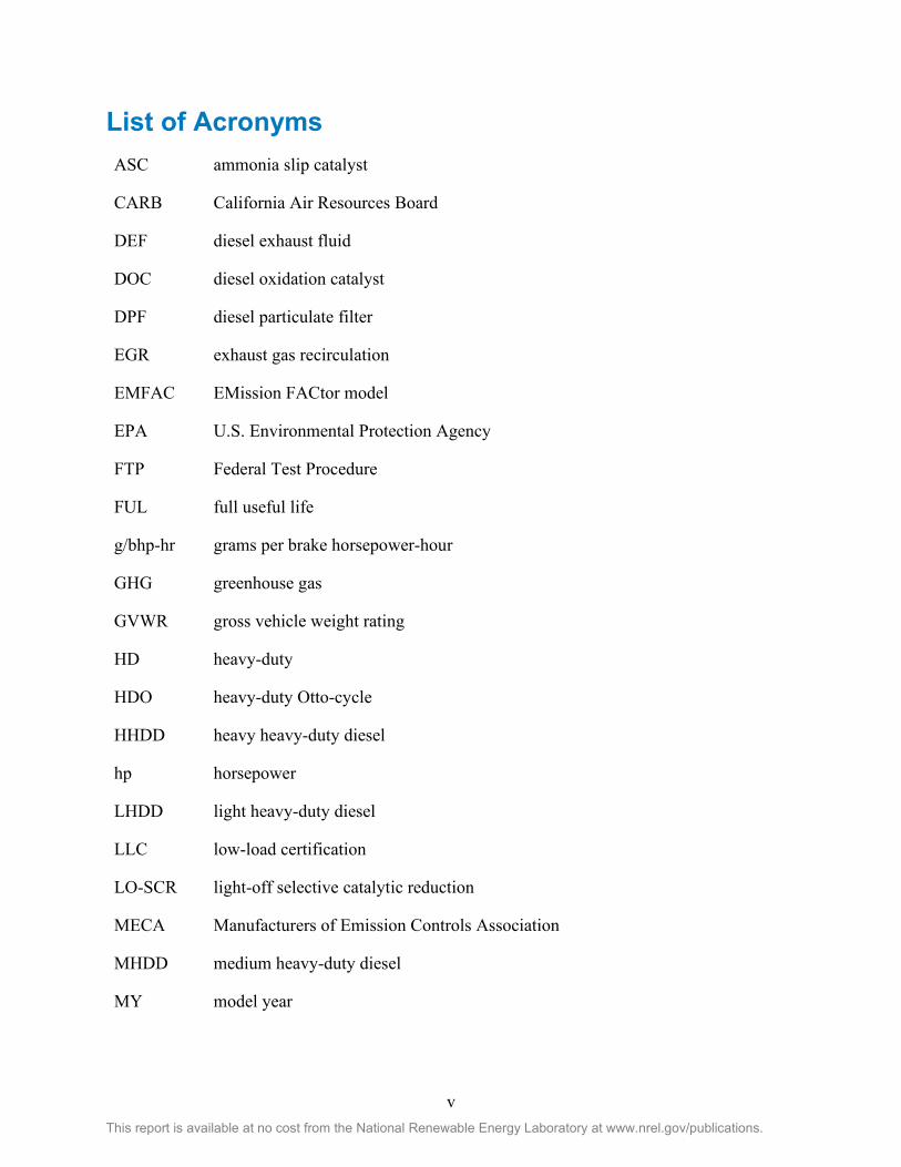
v This report is available at no cost from the National Renewable Energy Laboratory at www.nrel.gov/publications.
List of Acronyms ASC ammonia slip catalyst
CARB California Air Resources Board
DEF diesel exhaust fluid
DOC diesel oxidation catalyst
DPF diesel particulate filter
EGR exhaust gas recirculation
EMFAC EMission FACtor model
EPA U.S. Environmental Protection Agency
FTP Federal Test Procedure
FUL full useful life
g/bhp-hr grams per brake horsepower-hour
GHG greenhouse gas
GVWR gross vehicle weight rating
HD heavy-duty
HDO heavy-duty Otto-cycle
HHDD heavy heavy-duty diesel
hp horsepower
LHDD light heavy-duty diesel
LLC low-load certification
LO-SCR light-off selective catalytic reduction
MECA Manufacturers of Emission Controls Association
MHDD medium heavy-duty diesel
MY model year

vi This report is available at no cost from the National Renewable Energy Laboratory at www.nrel.gov/publications.
NH3 ammonia
NOx oxides of nitrogen
NREL National Renewable Energy Laboratory
OBD on-board diagnostics
OEM original equipment manufacturer
OOS out of state
PM particulate matter
PNA passive NOx absorber
R&D research and development
SCAB South Coast Air Basin
SCR selective catalytic reduction
SCRF selective catalytic reduction on filter
SERA Scenario Evaluation and Regionalization Analysis
SET-RMC Supplemental Emission Test with Ramped Mode Cycles
SI spark ignition
SwRI Southwest Research Institute
TWC three-way catalyst

vii This report is available at no cost from the National Renewable Energy Laboratory at www.nrel.gov/publications.
Executive Summary The National Renewable Energy Laboratory (NREL) conducted a cost analysis for emission control technologies under contract to the California Air Resources Board (CARB). CARB sought incremental cost analysis for emission control technologies for on-road heavy-duty (HD) engines used in vehicles greater than 14,000 pounds (lb) gross vehicle weight rating (GVWR) to achieve oxides of nitrogen (NOx) emissions rates significantly lower than those required by current emissions standards (CARB 2017). This low-NOx emission technology cost analysis comprised two main tasks:
• Task 1: An incremental cost analysis for engine and exhaust aftertreatment systems • Task 2: An engine and exhaust aftertreatment life-cycle cost analysis incorporating
incremental upfront costs and operating costs. The incremental cost analysis included a review of current and under-development engine and exhaust aftertreatment technologies that could achieve 0.02 grams per brake horsepower-hour (g/bhp-hr) NOx on certification test cycles, including a proposed updated certification test cycle that includes additional low-load operating conditions. Diesel, natural gas, and gasoline HD engine applications were studied. Three diesel technology package combinations of engine and exhaust aftertreatment options were selected based on research in progress at Southwest Research Institute (SwRI), also funded by CARB. The three diesel technology packages were intended to bracket potential cost ranges across two engine displacement levels: ~6–7 liters (L) and ~12–13 L. Representative technology packages for HD natural gas (12 L) and gasoline (6 L) engines were also defined, each with a single displacement level providing a tie point to similar diesel options.
Diesel engines were the primary consideration, as they comprise the majority of HD engines. In addition to studying three diesel technology packages across two engine displacement levels, incremental cost bracketing also included model year (MY) 2023 versus 2027 introduction, U.S. versus California-only implementation, and current full useful life (FUL) versus extended FUL and warranty. Direct and indirect incremental costs were broken down to as discrete a level as possible while maintaining data confidentiality. The calculation of incremental costs was limited by a small number of respondents.
The surveyed original equipment manufacturers (OEMs), Tier 1 suppliers, and trade organizations such as the Manufacturers of Emission Controls Association (MECA) responded with incremental cost, not validation that 0.02 g/bhp-hr emissions levels or specific technology packages are feasible. Engine OEM participation was crucial, as only they could provide estimates for indirect costs that represented a significant portion of the total cost. Incremental costs are largely driven by indirect costs associated with engineering research and development costs and warranty costs. The indirect costs are highly dependent on production volumes over which to amortize research and development costs. Indirect costs due to warranty are high, reflecting high uncertainty with new technology and the introduction timeframes. The incremental costs were not adjusted to reflect a retail markup due to the complexity with which pricing decisions are made.
The average incremental cost for the 6–7-L diesel engines for MY 2023 with current FUL ranged from $3,685 to $5,344, but the absolute low and high bounds were between ~$2,000 and over

viii This report is available at no cost from the National Renewable Energy Laboratory at www.nrel.gov/publications.
$9,000. Extending FUL and warranty moved the average incremental costs to a range of $15,370 to $16,245, with tighter low and high bounds (constrained in part by the limited number of responses). The average incremental cost for the 12–13-L diesel engines for MY 2023 with current FUL ranged from $5,340 to $6,063, but the absolute low and high bounds were between ~$3,000 and over $10,000. Extending FUL and warranty moved the average incremental costs to a range of $28,868 to $47,042, with much wider low and high bounds (driven in part by the limited number of responses). The natural gas 12-L engine application was unable to be studied in detail, but OEM feedback indicated the anticipated incremental cost for natural gas engines and aftertreatment technology is within 10% of the low-cost diesel technology package incremental cost for equivalent displacement, possibly due to requiring a moving average window method to assess emission compliance. The gasoline engine 6-L application was also unable to be studied in detail due to lack of OEM feedback, but comparatively low incremental costs were estimated.
A life-cycle cost analysis was completed to understand the full costs to the owner of the vehicles with a 0.02 g/bhp-hr NOx technology package outside of the direct upfront vehicle cost increase. The life-cycle cost analysis sought to incorporate costs associated with the following elements: initial incremental purchase cost, fuel consumption changes (changes in fuel economy), diesel exhaust fluid (DEF) consumption changes, and the maximum FUL of the aftertreatment package (major overhaul intervals). Thus, the life-cycle costs depend on the vehicle type (mileage), region, fuel, engine displacement, maximum useful life, fuel economy change, DEF consumption change, and discount rate.
Three scenarios were defined to evaluate the bounds of the life-cycle costs across all parameters evaluated. For the three scenarios evaluated (Low-Cost, Mid-Cost, High-Cost), the life-cycle costs were evaluated for each EMission FACtor (EMFAC) model vehicle type (CARB 2018b), aggregated to a representative average and calculated across the vehicle fleet for the MY 2027 vehicles. The analysis showed that EMFAC vehicles can have significantly different life-cycle costs and that the spread depends on the scenario evaluated: approximately a $4,000 spread across vehicle types in the Low-Cost scenario, while the High-Cost scenario had nearly a $40,000 difference. This large spread was found to be due to the number of aftertreatment package replacements needed throughout the vehicle lifetime. The aggregated, representative average life-cycle costs for the Mid-Cost scenario were estimated to be $12,700 for the 6-L diesel engine, $13,200 for the 12-L diesel engine, $4,800 for the 12-L natural gas engine, and $800 for the 6-L gasoline engine. The total life-cycle costs to California vehicle owners for the MY 2027 vehicles were estimated to range between $92 million and $1.2 billion, depending on the scenario (Low-Cost or High-Cost) realized.
The sensitivity analysis indicated that the manufacturing volume may be the most important parameter impacting the life-cycle cost; however, limited data were received from the external stakeholders surveyed. The next most important parameter was the assumption of extended FUL and extended warranty, as the increase in aftertreatment lifetime may not exceed the vehicle’s travel requirement, which results in larger replacement costs over the vehicle’s life. However, one may expect that the higher upfront purchase incurred by the vehicle owner should effectively be offset by the repair savings over the lifetime of the vehicle. Next, the aftertreatment cost bound (low/high error bars on the incremental cost data), fuel economy improvement, and

ix This report is available at no cost from the National Renewable Energy Laboratory at www.nrel.gov/publications.
discount rate were found to have a moderate impact on the life-cycle cost. Lastly, the region and DEF consumption change were found to have minimal influence on the life-cycle cost.
The results of this cost analysis reflect the specific technology and aftertreatment FUL assumptions on which the study was based. In particular, the incremental cost of moving from a 0.2g/bhp-hr to 0.02 g/bhp-hr standard is expected to be non-linear due to diminishing returns on technology performance. Extrapolating the results beyond this specific study and outside of these specific assumptions is not recommended and should only be done with careful attention to the scope and limits of this study.

x This report is available at no cost from the National Renewable Energy Laboratory at www.nrel.gov/publications.
Table of Contents Executive Summary .......................................................................................................................... vii Abstract .............................................................................................................................................1 Project Background and Objective ......................................................................................................2 Project Summary ...............................................................................................................................4 1 Task 1: Engine Incremental Cost Analysis ....................................................................................6
1.1 Representative Engine Platform Approach ..........................................................................6 1.2 Identifying Potential Diesel Technologies to Achieve 0.02 g/bhp-hr NOx ..............................9 1.3 Identifying Potential Gasoline and Natural Gas Technologies to Achieve 0.02 g/bhp-hr NOx .. ........................................................................................................................................ 11 1.4 NREL Survey of Potential Technologies to Achieve 0.02 g/bhp-hr NOx ................................ 12
1.4.1 Definition of Baseline Costs of Current Technologies With 2018 EPA Certification ............. 12 1.4.2 NREL Initial Incremental Cost Estimates ............................................................................... 13 1.4.3 First Survey Responses for Incremental Costs of Potential Diesel Technologies .................. 19 1.4.4 Incremental Costs of Potential Technologies with Extended FUL and Warranty, and California-Only Volumes ......................................................................................................................... 25 1.4.5 Incremental Cost Survey Response Observations ................................................................. 31 1.4.6 Incremental Costs for Natural Gas and Gasoline Technology Packages ............................... 32
1.5 Low-, Average-, and High-Cost Estimates .......................................................................... 33 1.5.1 Low-, Average-, and High-Cost Estimates for MY 2023 with Current FUL and Warranty ..... 33 1.5.2 Low-, Average-, and High-Cost Estimates for MY 2027 with Extended Warranty and Extended Useful Life ............................................................................................................................... 35
1.6 Summary of Incremental Cost Analysis ............................................................................. 37 2 Task 2: Engine Life-Cycle Costs .................................................................................................. 38
2.1 Maximum Full Useful Life Analysis .................................................................................... 38 2.2 Approach ......................................................................................................................... 38
2.2.1 Scenario Evaluation and Regionalization Analysis (SERA) Model ......................................... 39 2.2.2 Data Sources .......................................................................................................................... 40 2.2.3 SERA Model Validation .......................................................................................................... 42 2.2.4 Manufacturing Volume Analysis ........................................................................................... 43
2.3 Parameters Investigated .................................................................................................. 43 2.3.1 Scenario Analysis ................................................................................................................... 44 2.3.2 Sensitivity Analysis ................................................................................................................ 46
2.4 Results ............................................................................................................................. 47 2.4.1 Case Study: T7 Tractor and T6 OOS Small Vehicle Life-Cycle Costs ...................................... 47 2.4.2 Scenario Analysis Results ...................................................................................................... 54 2.4.3 Sensitivity Analysis Results .................................................................................................... 59
2.5 Life-Cycle Cost Analysis Summary and Conclusions ........................................................... 60 3 Conclusions ............................................................................................................................. 62 References ....................................................................................................................................... 64 Appendix A. Selected Results for Specific EMFAC Vehicles of Interest to CARB .............................. 65 Appendix B. EMFAC Vehicle Disaggregation ................................................................................. 67

xi This report is available at no cost from the National Renewable Energy Laboratory at www.nrel.gov/publications.
List of Figures Figure 1. Schematic of proposed low- and average-cost diesel aftertreatment technology ........................ 10 Figure 2. Schematic of proposed high-cost diesel aftertreatment technology ............................................ 11 Figure 3. Summary of 6–7-L potential technology packages for MY 2023 with current FUL .................. 34 Figure 4. Summary of 12–13-L potential technology packages for MY 2023 with current FUL .............. 35 Figure 5. Summary of 6–7-L potential technology packages for MY 2027 with extended FUL and
warranty ................................................................................................................................. 36 Figure 6. Summary of 12–13-L potential technology packages for MY 2027 with extended FUL and
warranty ................................................................................................................................. 36 Figure 7. The general SERA stock model data flow ................................................................................... 39 Figure 8. Data flow and analysis using the SERA model for life-cycle cost analysis ................................ 42 Figure 9. SERA model validation against the CA Vision 2.1 model .......................................................... 43 Figure 10. Annual present value cost for a T7 Tractor 12-L diesel engine designed for current full useful
life (435,000 miles; top) and extended full useful life (1,000,000 miles; bottom) for MY 2027 in the South Coast Air Basin with a 2.5% increase in DEF consumption, a discount rate of 7%, and national manufacturing volumes .......................................................................... 48
Figure 11. Annual present value cost for a T6 OOS small 6–7-L diesel engine designed for current full useful life (110,000 miles; top) and extended full useful life (550,000 miles; bottom) for MY 2027 in the South Coast Air Basin with a 2.5% increase in DEF consumption, a discount rate of 7%, and national manufacturing volumes .......................................................................... 48
Figure 12. Total present value cost for the T7 Tractor and T6 OOS small vehicles with diesel engine aftertreatment technology as a function of incremental steps between current FUL and extended FUL for two scenarios: replacements at end of FUL (orange) and no replacements (blue) ...................................................................................................................................... 50
Figure 13. Present value cost for different Class 6 and Class 8 diesel engine aftertreatment technologies with current full useful life ..................................................................................................... 51
Figure 14. Present value cost for different Class 6 and Class 8 diesel engine aftertreatment technologies with extended full useful life.................................................................................................. 52
Figure 15. Present value cost for the T7 Tractor and T6 OOS small trucks with diesel engines designed for current full useful life at both California and national manufacturing volumes ............... 53
Figure 16. Present value cost for the T7 Tractor and T7 OOS small trucks with diesel engine aftertreatment technologies designed for current FUL as a function of region ...................... 54
Figure 17. Present value cost for the T7 Tractor and T7 OOS small trucks with diesel engine aftertreatment technologies designed for extended FUL and warranty as a function of region ................................................................................................................................................ 54
Figure 18. Present value life-cycle cost for all EMFAC vehicles in the low-cost scenario, segmented by fuel type and engine displacement (DSL = diesel, GAS = gasoline) ..................................... 55
Figure 19. Present value life-cycle cost for all EMFAC vehicles in the mid-cost scenario, segmented by fuel type and engine displacement (DSL = diesel, GAS = gasoline, CNG = compressed natural gas) ............................................................................................................................. 56
Figure 20. Present value life-cycle cost for all EMFAC vehicles in the high-cost scenario, segmented by fuel type and engine displacement (DSL = diesel) ................................................................ 57
Figure 21. EMFAC vehicle sales-weighted average present value cost for 6-L and 12-L diesel engine technologies under the three cost scenarios described in Table 23 ........................................ 57
Figure 22. Scenario analysis for a 12-liter compressed natural-gas and 6-liter gasoline engine ................ 58 Figure 23. Total California fleet life-cycle cost for the MY 2027 vehicles for each scenario analyzed ..... 58 Figure 24. Sensitivity diagram for the diesel 6–7-L and 12–13-L engines relative to the mid-cost scenario
................................................................................................................................................ 59 Figure 25. Sensitivity diagram for the gasoline 6-L engine relative to the mid-cost scenario .................... 60 Figure 26. Sensitivity diagram for the natural-gas 12-L engine relative to the mid-cost scenario ............. 60

xii This report is available at no cost from the National Renewable Energy Laboratory at www.nrel.gov/publications.
List of Tables Table 1. Current and Proposed Extended Full Useful Life and Warranty for Engine Life-Cycle Cost
Analysis .................................................................................................................................... 5 Table 2. Engine Platform Analysis for Incremental Cost Analysis .............................................................. 7 Table 3. NREL Estimates of Potential Low-Cost Diesel Technology Package 6–7 L ............................... 14 Table 4. NREL Estimates of Potential Low-Cost Diesel Technology Package 12–13 L ........................... 15 Table 5. NREL Estimate of Potential Average-Cost Diesel Technology Package 6–7 L........................... 16 Table 6. NREL Estimates of Potential Average-Cost Diesel Technology Package 12–13 L ..................... 17 Table 7. NREL Estimates of Potential High-Cost Diesel Technology Package 6–7 L .............................. 18 Table 8. NREL Estimates of Potential High-Cost Diesel Technology Package 12–13 L .......................... 19 Table 9. Survey Responses for Potential Low-Cost Diesel Technology Package 6–7 L ............................ 20 Table 10. Survey Responses for Potential Low-Cost Diesel Technology Package 12–13 L ...................... 21 Table 11. Survey Responses for Potential Average-Cost Diesel Technology Package 6–7 L ................... 22 Table 12. Survey Responses for Potential Average-Cost Diesel Technology Package 12–13 L ............... 23 Table 13. Survey Responses for Potential High-Cost Diesel Technology Package 6–7 L ......................... 24 Table 14. Survey Responses for Potential High-Cost Diesel Technology Package 12–13 L ..................... 25 Table 15. Survey Responses for Potential Low-Cost Diesel Technology Package 6–7 L with Extended
FUL, Extended Warranty, and California-Only Volumes ..................................................... 26 Table 16. Survey Responses for Potential Low-Cost Diesel Technology Package 12–13 L with Extended
FUL, Extended Warranty, and CA Volumes ......................................................................... 27 Table 17. Survey Responses for Potential Average-Cost Diesel Technology Package 6–7 L with Extended
FUL, Extended Warranty, and California-Only Volumes ..................................................... 28 Table 18. Survey Responses for Potential Average-Cost Diesel Technology Package 12–13 L with
Extended FUL, Extended Warranty, and California-Only Volumes ..................................... 29 Table 19. Survey Responses for Potential High-Cost Diesel Technology Package 6–7 L with Extended
FUL, Extended Warranty, and California-Only Volumes ..................................................... 30 Table 20. Survey Responses for Potential High-Cost Diesel Technology Package 12–13 L with Extended
FUL, Extended Warranty, and California-Only Volumes ..................................................... 31 Table 21. Data Sources Used in Life-Cycle Cost Analysis ........................................................................ 41 Table 22. Life-Cycle Cost Parameters Investigated in this Study .............................................................. 44 Table 23. Scenario Definitions for Bounding Analysis .............................................................................. 45 Table 24. Example Vehicle Sales Weighted Average ................................................................................ 46

1 This report is available at no cost from the National Renewable Energy Laboratory at www.nrel.gov/publications.
Abstract The National Renewable Energy Laboratory (NREL) conducted a cost analysis for emission control technologies under contract to the California Air Resources Board (CARB). CARB sought incremental cost analysis for emission control technologies for on-road heavy-duty (HD) engines used in vehicles greater than 14,000 pounds (lb) gross vehicle weight rating (GVWR) to achieve oxides of nitrogen (NOx) emissions rates significantly lower than those required by current emissions standards. Specifically, incremental costs (without any retail price markup) were estimated for representative diesel, natural gas, and gasoline engine and emission aftertreatment systems that were selected to represent potential technology packages that could achieve 0.02 grams per brake horsepower-hour (g/bhp-hr) NOx on certification test cycles, including a proposed updated certification test cycle that includes additional low-load operating conditions. NREL surveyed stakeholders including industry association groups, Tier 1 suppliers, and engine original equipment manufacturers (OEMs) to estimate incremental direct and indirect costs. Incremental costs were considered for current engine full useful life (FUL) definitions, as well as with proposed increased FUL and warranty periods. The incremental costs were subsequently incorporated in life-cycle cost analyses examining the incremental engine and aftertreatment costs along with life-cycle costs over the various engine FUL scenarios. Life-cycle costs analysis included the incremental upfront cost, fuel consumption changes (changes in fuel economy), diesel exhaust fluid (DEF) consumption changes, and the maximum FUL of the aftertreatment package (major overhaul intervals).

2 This report is available at no cost from the National Renewable Energy Laboratory at www.nrel.gov/publications.
Project Background and Objective Current emission standards for heavy-duty diesel engines, established by the United States Environmental Protection Agency (EPA) for 2010, specify a limit of 0.20 grams per brake horsepower-hour (g/bhp-hr) NOx. This standard represents a 90% reduction from the previous benchmark of 2.0 g/bhp-hr and applies to both heavy-duty diesel engines and heavy-duty Otto-cycle engines used in vehicles greater than 14,000-lb GVWR.
Diesel-engine manufacturers utilize a variety of technologies in order to meet these standards, primarily among them being selective catalytic reduction (SCR). Natural-gas engine manufacturers use SCR for lean-burn engines and three-way catalysts (TWCs) for stoichiometric engines. Both of these methods reduce NOx emissions by removing them from the engine-out exhaust prior to exiting the tailpipe. These manufacturers have used lessons learned from other applications such as stationary-source and light-duty vehicles to meet current NOx emission requirements, and as these technologies mature there are opportunities to reduce emissions even further.
The California Air Resources Board (CARB), together with the Southwest Research Institute (SwRI), is currently funding several research programs to investigate the feasibility of achieving NOx emissions less than the 2010 limit of 0.20 g/bhp-hr. The first (“Stage 1”) project is a $1.6 million research contract between CARB and SwRI to evaluate improved engine emission control calibration, enhanced aftertreatment technologies and configurations, improved aftertreatment thermal management, urea dosing strategies, and engine management practices for two heavy-duty engines: one natural-gas engine with a TWC and one diesel engine with a diesel particulate filter (DPF) and SCR. The target emission rate for this project, which was finalized in December 2016, is 0.02 g/bhp-hr NOx.
CARB is also contracting a $1.05 million “Stage 2” project with SwRI to further optimize the diesel engine aftertreatment system for low engine-load duty cycles typical of city driving. Stage 2 objectives are to develop a supplemental low-load certification test cycle that will, along with the Federal Test Procedure (FTP), ensure NOx control under nearly all driving conditions and evaluate metrics for in-use testing under low-load operations. The “Stage 3” project, currently in the planning stage, will complement the Stage 1 and Stage 2 efforts with testing on an additional engine that is representative of likely future engine configurations.
Alongside current emission standards, CARB and EPA both require that heavy-duty engines meet these standards throughout their entire useful life. The useful life period is defined according to a vehicle’s GVWR, and for heavy-duty engines ranges from 110,000–435,000 miles. The useful life period for Otto-cycle and light heavy-duty diesel engines (14,001–19,500-lb GVWR) is 110,000 miles/10 years; for medium heavy-duty diesel engines (19,501–33,000-lb GVWR) 185,000 miles/10 years; and for heavy heavy-duty diesel engines (greater than 33,000-lb GVWR) 435,000 miles/10 years, or 22,000 hours.
Well-maintained on-road diesel engines can operate significantly beyond their currently defined useful life periods (e.g., many heavy-duty diesel engines currently operate upwards of 800,000 miles to over a million miles), and CARB is taking this reality into consideration as it evaluates the consequences of lowering its NOx emission targets. Engine durability becomes a critical

3 This report is available at no cost from the National Renewable Energy Laboratory at www.nrel.gov/publications.
factor with longer useful life definitions, particularly in preventing “upstream” engine component failures that can damage “downstream” emission control system components and cause excess emissions of criteria pollutants such as particulate matter (PM) and NOx. Therefore, manufacturers will need to improve the durability of their engines and emission control systems by developing higher-quality parts and assembly methods and replacement of components and/or subsystems.
CARB is expected to propose new standards to be implemented by 2024, which will set even lower NOx emission standards and add new certification test cycles to ensure emission control at low-load operations. Adding this new test cycle to the certification requirement is expected to drive further improvements to aftertreatment hardware and engine control and calibration.
With these new emission standards of approximately 0.02 g/bhp-hr NOx in mind, it is important to examine the direct and indirect costs of implementing new technologies, both the incremental costs to original equipment manufacturers and the costs of using the technology packages throughout the engines’ useful life. These costs can be divided by category, including the specific technologies for achieving the NOx standard, the costs to increase durability (extended useful life), and the costs of the on-board diagnostics (OBD) hardware and calibration works impacted by the changes. This cost analysis will use specific emission control and engine technologies identified by SwRI in Stages 1 and 2, along with testing that is representative of likely future engine configurations.

4 This report is available at no cost from the National Renewable Energy Laboratory at www.nrel.gov/publications.
Project Summary This project was defined by two tasks—Task 1: Engine Incremental Cost Analysis and Task 2: Engine Life-Cycle Costs. For Task 1, NREL reviewed current technologies and technology packages that are being examined as part of the SwRI projects, Stages 2 and 3, as provided by CARB. NREL identified and reviewed likely emission control and engine technologies to meet 0.02 g/bhp-hr NOx requirements with CARB staff based on Stage 2 and 3 efforts from SwRI testing of potential future engine configurations. These technologies were then defined as the potential technologies and the starting point of developing a low-NOx technology incremental cost analysis from 2018 baseline costs.
NREL then evaluated these potential technologies and technology packages for engine plus aftertreatment incremental cost analysis via a series of surveys sent to Tier 1 suppliers, trade organizations, and engine OEMs. The surveys defined the potential technologies broken into engine components, emission control components, subsystems, and indirect costs. The combination of incremental costs (over the 2018 baseline) associated with developing and integrating the specified lower NOx emission control technologies into the engines, the costs of increasing the durability of these engines and their emission control systems, and the costs of directly impacted OBD hardware and calibration works of these specified technology packages were then examined to understand the total incremental cost implications to Tier 1 suppliers and engine OEMs of the potential technologies.
The evaluation of costs was dependent on cooperation from Tier 1 suppliers, trade organizations and engine OEMs, as well as the availability of direct and indirect cost information for engine and emission control technologies. NREL utilized existing relationships with industry partners in order to perform a thorough cost assessment but could not guarantee full cooperation or sharing of confidential cost information from Tier 1 suppliers, trade organizations, and engine OEMs.
After accounting for the initial incremental cost implications to Tier 1 suppliers (both collectively through the Manufacturers of Emission Controls Association [MECA] and individually) and engine OEMs, NREL conducted a life-cycle cost analysis as Task 2 to examine the costs of using the specified technology packages during the engines’ certification full useful life (FUL). NREL utilized a range of FUL values for each heavy-duty vehicle category, Classes 4 through 8. The current FUL mileage—for heavy-duty engines of 110,000 miles up to 435,000 miles, depending on a vehicle's GVWR; 110,000 miles/10 years for heavy-duty Otto-cycle (HDO) and light heavy-duty diesel (LHDD) engines (14,001–19,500-lb GVWR); 185,000 miles/10 years for medium heavy-duty diesel (MHDD) engines (19,501–33,000-lb GVWR); and 435,000 miles/10 years or 22,000 hours for heavy heavy-duty diesel (HHDD) engines (greater than 33,000-lb GVWR)—was defined as the low-end value of the range for each specific vehicle class. For the high-end value of the range, NREL utilized input from CARB for proposed extended FUL targets as the upper-bound levels for each specific vehicle class: 250,000 miles/15 years for HDO engines (14,001–19,500-lb GVWR), 550,000 miles/15 years for LHDD engines (14,001–19,500-lb GVWR) and MHDD engines (14,001–19,500-lb GVWR), and 1,000,000 miles/15 years for HHDD engines (greater than 33,000-lb GVWR). Additionally, per CARB’s guidance, the high-end value with extended FUL also includes the provision that warranty periods will increase to 80% of the extended FUL, both in mileage and time, except for heavy-

5 This report is available at no cost from the National Renewable Energy Laboratory at www.nrel.gov/publications.
duty Otto-cycle, which was specified as 220,000 miles/12 years. The current FUL defining the lower bound and the extended FUL defining the upper bound are summarized in Table 1.
Table 1. Current and Proposed Extended Full Useful Life and Warranty for Engine Life-Cycle Cost Analysis
LHDD MHDD HHDD Natural Gas – Otto
Heavy-Duty – Otto
GVWR (lb) 14,001–19,500 19,501–33,000 >33,000 >33,000 14,000
Current full useful life
110,000 miles/10 years
185,000 miles/10 years
435,000 miles/10 years,
22,000 hours
435,000 miles/10 years,
22,000 hours
110,000 miles/15 years
Proposed extended full useful life
550,000 miles/15 years
550,000 miles/15 years
1,000,000 miles/15
years
1,000,000 miles/15
years
250,000 miles/15 years
Proposed warranty period with extended full useful life
440,000 miles/12 years
440,000 miles/12 years
800,000 miles/12
years
800,000 miles/12
years
220,000 miles/12 years
After accounting for the initial incremental costs of the technologies, as determined in Task 1, the life-cycle cost assessment of Task 2 then took into account the aftertreatment technologies' effects on fuel consumption, DEF consumption, major overhaul intervals (full useful life estimates), manufacturing volume, and financial discount rates. The life-cycle cost modeled for each vehicle is specific to the EMission FACtor (EMFAC) model’s vehicle definition of vehicle miles traveled, which depends on the specific region, vocation, model year, fuel type, and age.
For the life-cycle cost analysis in Task 2, the aftertreatment full useful life mileage was used to set the equipment overhaul schedule. For all scenarios in the life-cycle cost analysis, the incremental cost associated with the aftertreatment package was assumed to be incurred after the truck mileage exceeded the stated maximum FUL. This assumption is expected to be conservative, as not all aftertreatment packages will fail immediately after they exceed their stated maximum FUL and statistical analysis of failure rates combined with data on aftertreatment technology operating and maintenance costs were not available. To understand the impact of this assumption on the life-cycle cost, a sensitivity analysis was completed assuming the aftertreatment package would not need to be replaced over the vehicle’s lifetime, as that provides the lower bound on the life-cycle cost.
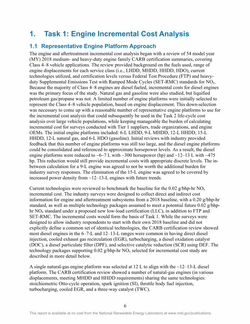
6 This report is available at no cost from the National Renewable Energy Laboratory at www.nrel.gov/publications.
1. Task 1: Engine Incremental Cost Analysis 1.1 Representative Engine Platform Approach The engine and aftertreatment incremental cost analysis began with a review of 54 model year (MY) 2018 medium- and heavy-duty engine family CARB certification summaries, covering Class 4–8 vehicle applications. The review provided background on the fuels used, range of engine displacements for each service class (i.e., LHDD, MHDD, HHDD, HDO), current technologies utilized, and certification levels versus Federal Test Procedure (FTP) and heavy-duty Supplemental Emissions Test with Ramped Mode Cycles (SET-RMC) standards for NOx. Because the majority of Class 4–8 engines are diesel fueled, incremental costs for diesel engines was the primary focus of the study. Natural gas and gasoline were also studied, but liquified petroleum gas/propane was not. A limited number of engine platforms were initially selected to represent the Class 4–8 vehicle population, based on engine displacement. This down-selection was necessary to come up with a reasonable number of representative engine platforms to use for the incremental cost analysis that could subsequently be used in the Task 2 life-cycle cost analysis over large vehicle populations, while keeping manageable the burden of calculating incremental cost for surveys conducted with Tier 1 suppliers, trade organizations, and engine OEMs. The initial engine platforms included: 6-L LHDD, 9-L MHDD, 12-L HHDD, 15-L HHDD, 12-L natural gas, and 6-L HDO (gasoline). Initial reviews with industry provided feedback that this number of engine platforms was still too large, and the diesel engine platforms could be consolidated and referenced to approximate horsepower levels. As a result, the diesel engine platforms were reduced to ~6–7 L with ~300 horsepower (hp) and ~12–13 L with ~475 hp. This reduction would still provide incremental costs with appropriate discrete levels. The in-between calculation for a 9-L engine was agreed to not be worth the additional burden for industry survey responses. The elimination of the 15-L engine was agreed to be covered by increased power density from ~12–13-L engines with future trends.
Current technologies were reviewed to benchmark the baseline for the 0.02 g/bhp-hr NOx incremental cost. The industry surveys were designed to collect direct and indirect cost information for engine and aftertreatment subsystems from a 2018 baseline, with a 0.20 g/bhp-hr standard, as well as multiple technology packages assumed to meet a potential future 0.02 g/bhp-hr NOx standard under a proposed new low-load certification (LLC), in addition to FTP and SET-RMC. The incremental costs would form the basis of Task 1. While the surveys were designed to allow industry respondents to start with their own 2018 baseline and did not explicitly define a common set of identical technologies, the CARB certification review showed most diesel engines in the 6–7-L and 12–13-L ranges were common in having direct diesel injection, cooled exhaust gas recirculation (EGR), turbocharging, a diesel oxidation catalyst (DOC), a diesel particulate filter (DPF), and selective catalytic reduction (SCR) using DEF. The technology packages supporting 0.02 g/bhp-hr NOx selected for incremental cost study are described in more detail below.
A single natural-gas engine platform was selected at 12 L to align with the ~12–13-L diesel platform. The CARB certification review showed a number of natural-gas engines (in various displacements, meeting MHDD and HHDD requirements) sharing the same technologies: stoichiometric Otto-cycle operation, spark ignition (SI), throttle body fuel injection, turbocharging, cooled EGR, and a three-way catalyst (TWC).

7 This report is available at no cost from the National Renewable Energy Laboratory at www.nrel.gov/publications.
A single gasoline-fueled HDO platform was selected at 6 L to align with the ~6–7-L diesel platform. The CARB certification review showed HDO gasoline is approaching 0.02 g/bhp-hr NOx on the current certification cycles using stoichiometric, SI, naturally aspirated, EGR technologies with a TWC technology package.
Utilizing the results and recommendations from Stage 2 and 3 efforts from SwRI testing of potential future diesel-engine configurations, NREL identified three diesel technology packages to evaluate the total incremental cost implications for an MY 2023 release nationwide. These identified diesel technology packages were intended to represent potential low-, average-, and high-cost options to meet a 0.02 g/bhp-hr NOx standard and were meant to provide a broader assessment of potential incremental costs than a single option. As previously referenced, no natural-gas technology package was surveyed for incremental costs related to 0.02 g/bhp-hr NOx, and the HDO gasoline technology package only included TWC and calibration upgrades. The resulting engine platforms defined for the incremental cost study are summarized in Table 2.
Table 2. Engine Platform Analysis for Incremental Cost Analysis
LHDD HHDD Natural Gas – HHDD standard
Gasoline – HDO
Engines ~6–7 L
~300 hp
~12–13 L
~475 hp
12 L 6 L
Current full useful life
110,000 miles/10 years
435,000 miles/10 years,
22,000 hours
435,000 miles/10 years,
22,000 hours
110,000 miles/10 years
Low-Cost Tech. $$$ $$$ Not applicable Not applicable
Avg.-Cost Tech. $$$ $$$ Not applicable $$$
High-Cost Tech. $$$ $$$ Not applicable Not applicable
NREL then directly surveyed heavy-duty engine OEMs, Tier 1 suppliers, emission control technology manufacturers, and industry trade organizations to obtain the most accurate and current cost information for the identified likely technology packages to meet 0.02 g/bhp-hr NOx requirements and the cost implications for using these specific technologies. The cost survey included a definition of the potential technologies as engine components, emission control components, subsystems and strategies, and indirect costs broken into categories of research and development (R&D) costs, certification costs, and warranty costs. The combination of costs associated with developing and integrating the specified lower NOx emission control technologies into the engines, the costs of increasing the durability of these engines and their emission control systems, and the costs of impacted OBD hardware and calibration of these specified technology package were then examined to understand the total incremental cost implications to Tier 1 suppliers and engine OEMs of the potential technologies in two different surveys. Any incremental costs associated with future OBD requirements unrelated to meeting 0.02 g/bhp-hr NOx were excluded from this study. Similarly, incremental costs related to future greenhouse gas (GHG) or fuel efficiency requirements and not specifically to meeting 0.02 g/bhp-hr NOx were also excluded.

8 This report is available at no cost from the National Renewable Energy Laboratory at www.nrel.gov/publications.
The first survey assumed that the 0.02 g/bhp-hr NOx regulation beginning MY 2023 included current FTP and SET-RMC steady-state test cycles, as well as a proposed new LLC for medium- and heavy-duty engine system certification. While not finalized and currently the topic of ongoing research, the new LLC engine cycle was assumed to last approximately 90 minutes, including a combination of motoring, sustained low load, and high-power transients. This first survey considered FUL hours/miles to remain the same as the current regulation. The survey was designed to allow industry respondents to start with their own 2018 baseline and did not explicitly define a common set of identical technologies. As a reference point, NREL provided internally generated estimates (from research, literature review, and engineering judgement) for the 2018 current technology costs (Posada, Chambliss, and Blumberg 2016; Posada Sanchez, Bandivadekar, and German 2012; Ou et al. 2019). Direct costs for both a 2018 baseline and 0.02 g/bhp-hr technology packages were surveyed on discrete engine and aftertreatment subsystem levels, along with indirect costs. The level of discrete subsystems was kept as small as possible to provide insight for where the costs accumulate while also being kept large enough to prevent identification of proprietary or confidential cost information from an individual respondent. Furthermore, only incremental costs are reported in this report and preliminary reviews with CARB to prevent identifying proprietary or confidential 2018 baseline costs. The survey requested future costs be calculated in 2018 dollars. The first survey asked for production volumes to be identified and to provide guidance on cost impacts for 0.02 g/bhp-hr incremental costs if regulation were to include all of the United States or California only.
The second survey was a follow-up survey sent to those Tier 1 suppliers, trade organization, and engine OEMs that responded to the first survey. The technology packages remained the same as the first survey, but instead assumed 0.02 g/bhp-hr NOx regulation beginning MY 2027 and again included current FTP and SET-RMC steady-state test cycles, as well as a new LLC. This second survey also considered extended useful life hours/miles as proposed by CARB in Table 1. The second survey asked for costing information to consider 0.02 g/bhp-hr regulation if only California were included, representing lower production volumes than a scenario where all of the U.S. were included.
NREL then aggregated all of the data from the cost survey responses and the initial estimates derived by NREL from research, literature review, and engineering judgement. The incremental costs were not adjusted to reflect a retail markup due to the complexity with which pricing decisions are made. In responding to NREL’s surveys, trade organizations, Tier 1 suppliers, and OEMs did provide feedback that they did not agree or conclude that these technologies would be feasible for meeting the 0.02 g/bhp-hr NOx requirements by MY 2023. Their valuable input was strictly a costing exercise and not a technology feasibility assessment. The diesel incremental cost information resulted in a range of costs due to the format of the provided data from the responses received. This range consisted of a low, average, and high estimate for engine technology costs, aftertreatment technology costs, OBD-related direct costs, and indirect costs. The survey results for the diesel engine and aftertreatment technology packages were then defined as three total incremental costs of low, average, and high estimates based on the identified potential technology packages to achieve 0.02 g/bhp-hr NOx requirements.
Fewer responses were received for the natural gas (HHDD standard) engine platform, preventing NREL from sufficiently aggregating incremental cost information to protect proprietary information. Therefore, NREL reported the total integrated incremental cost as an order of

9 This report is available at no cost from the National Renewable Energy Laboratory at www.nrel.gov/publications.
magnitude in comparison to the diesel engine with similar displacement results; the subsystem-level engine, aftertreatment, and OBD system direct costs as well as the indirect costs were not broken out or reported.
Similarly, few responses were received for the gasoline HDO engine platform. Some aggregation was possible for direct costs, but only NREL estimates were available for indirect costs. As a result, only total integrated incremental costs are reported.
1.2 Identifying Potential Diesel Technologies to Achieve 0.02 g/bhp-hr NOx
CARB is currently funding several research programs with SwRI to investigate the feasibility of achieving 0.02 g/bhp-hr NOx emissions with a diesel engine and is in the Stage 3 process of testing specific emission control and diesel engine technologies. Based on SwRI’s research and results from Stages 1 and 2 (Sharp et al., “Thermal Management,” 2017; Sharp et al., “Comparison of Advanced,” 2017; Sharp et al., “NOx Management,” 2017), NREL identified different engine and emission control technologies that showed potential capabilities of achieving 0.02 g/bhp-hr NOx emissions during current FTP and SET-RMC steady-state test cycles, as well as a proposed new LLC cycle by MY 2023. These diesel engine and emission control technologies were grouped into three different diesel technology packages to represent a range of potential low-, average-, and high-costing diesel technology package solutions.
The potential low-cost diesel technology package consisted of an EPA 2017 certification-compliant engine with a variable-geometry turbo charger, no turbo compounding, and a combined engine thermal management strategy of EGR cooler bypass, charge air cooler bypass, and a turbine bypass. In addition to the engine system, the emission control technologies included two points of DEF dosing and DEF mixers, one light-off SCR (LO-SCR), one DOC, one DPF, two SCRs, and one ammonia slip catalyst (ASC). The aftertreatment system also contained a NOx sensor upstream of the first DEF dosing system and mixer, a temperature sensor upstream of the LO-SCR, a second temperature sensor downstream of the LO-SCR, a second NOx sensor downstream LO-SCR and upstream of the DOC, a third temperature sensor downstream of the LO-SCR and upstream of the DOC, a fourth temperature sensor downstream of the DOC and upstream of the DPF, a fifth temperature sensor downstream of the DPF and upstream of the first second DEF dosing system and mixer, an ammonia (NH3) sensor downstream the first SCR and upstream the second SCR, a sixth temperature sensor downstream of the ASC, and a third NOx sensor downstream of the ASC. An example of the aftertreatment technology system with sensors is illustrated in Figure 1.

10 This report is available at no cost from the National Renewable Energy Laboratory at www.nrel.gov/publications.
Figure 1. Schematic of proposed low- and average-cost diesel aftertreatment technology
Figure from SwRI
The potential average-cost diesel technology package consisted of an EPA 2017 certification-compliant engine with a variable-geometry turbo charger, no turbo compounding, and an engine thermal management strategy and technology for cylinder deactivation. In addition to the engine system, the emission control technologies again included the same aftertreatment system as the low-cost diesel technology package with two points of DEF dosing and DEF mixers, one LO-SCR, one DOC, one DPF, two SCRs, and one ASC, as shown in Figure 1. The aftertreatment system also contained a NOx sensor upstream of the first DEF dosing system and mixer, a temperature sensor upstream of the LO-SCR, a second temperature sensor downstream of the LO-SCR, a second NOx sensor downstream LO-SCR and upstream of the DOC, a third temperature sensor downstream of the LO-SCR and upstream of the DOC, a fourth temperature sensor downstream of the DOC and upstream of the DPF, a fifth temperature sensor downstream of the DPF and upstream of the first second DEF dosing system and mixer, an NH3 sensor downstream of the first SCR and upstream of the second SCR, a sixth temperature sensor downstream of the ASC, and a third NOx sensor downstream of the ASC.
The proposed high-cost diesel technology package consisted of an EPA 2017 certification-compliant engine with a variable-geometry turbo charger, no turbo compounding, and a combined engine thermal management strategy of EGR cooler bypass, charge air cooler bypass, and a turbine bypass. In addition to the engine system, the emission control technologies included a passive NOx absorber (PNA), one DOC, one DEF doser and DEF mixer, one selective catalytic reduction on filter (SCRF), one SCR, and one ASC. The aftertreatment system also contained a NOx sensor upstream of the PNA, a second NOx sensor downstream of the PNA, an NH3 sensor downstream of the SCRF and upstream of the SCR, and a third NOx sensor downstream of the ASC. An example of the aftertreatment technology is illustrated in Figure 2.

11 This report is available at no cost from the National Renewable Energy Laboratory at www.nrel.gov/publications.
Figure 2. Schematic of proposed high-cost diesel aftertreatment technology Figure from SwRI
Note that the proposed technology packages that were initially designed to represent low-, average-, and high-cost combinations. It was assumed that the PNA, as a very new technology, would drive incremental costs to be higher than other packages. Likewise, cylinder deactivation was assumed to have a higher incremental cost than cooler bypasses for charge air, EGR, and turbine given the same aftertreatment package. However, once incremental cost information became available, the relative incremental costs did not necessarily turn out in that order. Nevertheless, to maintain consistency in the study, the proposed technology packages continued to be referred by their initial naming convention.
1.3 Identifying Potential Gasoline and Natural Gas Technologies to Achieve 0.02 g/bhp-hr NOx
The single natural-gas 12-L engine platform was selected to align with the ~12–13-L diesel platform. The CARB certification review showed a number of natural-gas engines (in various displacements, meeting MHDD and HHDD requirements) sharing the same technologies: stoichiometric Otto-cycle operation, SI, throttle body fuel injection, turbocharging, cooled EGR, and a TWC. Notably, most of the natural-gas engines already meet CARB’s optional low-NOx standard at 0.02 g/bhp-hr under the current certification cycles. Because the proposed LLC certification was assessed to be less challenging for a stoichiometric SI engine than a diesel engine, it was assumed that the current 2018 “baseline” technology package would already meet the new 0.02 g/bhp-hr NOx requirement. Incremental cost for 0.02 g/bhp-hr NOx was therefore not calculated, but cost increases related to extending FUL were considered. As noted later in this report, industry feedback identified this assumption as incorrect.
The single gasoline-fueled HDO platform was selected at 6 L to align with the ~6–7-L diesel platform. The CARB certification review showed HDO gasoline is approaching 0.02 g/bhp-hr NOx on the current certification cycles, and similar technology (stoichiometric, SI, naturally aspirated, EGR technologies with a TWC) with liquified petroleum gas fuel has recently been certified at 0.05 g/bhp-hr and 0.02 g/bhp-hr under CARB’s optional low-NOx standards. The base engine was assumed to need no significant upgrades for the 0.02 g/bhp-hr standard with proposed LLC certification cost study, but TWC direct cost upgrades and indirect costs for engineering, certification, and warranty were surveyed, as well as extended FUL impacts. Vehicle packaging impacts were noted to also potentially be required to enable close coupling of the TWCs.

12 This report is available at no cost from the National Renewable Energy Laboratory at www.nrel.gov/publications.
1.4 NREL Survey of Potential Technologies to Achieve 0.02 g/bhp-hr NOx
NREL created a cost survey with a baseline price of an MY 2018 system representing an EPA 2018 certification-compliant engine and aftertreatment system in 2018 dollars and asked trade organizations, Tier 1 suppliers, and engine OEMs to provide incremental cost estimates in comparison to the above-defined technologies with the potential to achieve 0.02 g/bhp-hr NOx requirements. The cost survey was reviewed with CARB and EPA staff and approved by CARB before submitting for requested responses. The survey consisted of two technology packages for diesel engine and aftertreatment systems, one technology package for natural-gas engines and aftertreatment, and one technology package for gasoline engines and aftertreatment systems. To simplify the survey for stakeholder input and avoid asking for input on three separate combinations of engine and aftertreatment technology packages, the two unique diesel engine technology packages (charge air, EGR, and turbine cooler bypass vs. cylinder deactivation) were surveyed with the two unique aftertreatment technology packages (Figure 1 and Figure 2). From these incremental cost inputs, NREL could construct the proposed low-, average-, and high-cost combined engine and aftertreatment technology packages.
The first survey assumed that the 0.02 g/bhp-hr NOx regulation beginning MY 2023 included current FTP and SET-RMC steady-state test cycles, as well as a new LLC cycle. While not finalized and currently the topic of ongoing research, the LLC was assumed as a new engine certification cycle lasting approximately 90 minutes and included a combination of motoring, sustained low load, and high-power transients. This first survey also considered FUL hours/miles to remain the same as the current regulation. NREL also prefaced the likely follow-up survey seeking additional guidance on how increasing FUL hour/mile requirements may further affect the provided costs.
The second survey was a follow-up survey sent to the same Tier 1 suppliers, trade organizations, and engine OEMs that responded to the first survey. The technology packages remained the same and instead assumed 0.02 g/bhp-hr NOx regulation beginning MY 2027 and again included current FTP and SET-RMC steady-state test cycles, as well as a proposed new LLC cycle. Again, while not finalized and currently the topic of ongoing research, the LLC was assumed as a new engine certification cycle lasting approximately 90 minutes and included a combination of motoring, sustained low load, and high-power transients. This second survey considered extended FUL hours/miles as proposed by CARB’s Stage 2 definitions defined in Table 1. Additionally, per CARB’s guidance, the extended FUL also included the assumption that warranty periods will increase to 80% of the extended FUL, both in mileage and time, except for heavy-duty Otto cycle, which was specified as 220,000 miles/12 years.
1.4.1 Definition of Baseline Costs of Current Technologies With 2018 EPA Certification
As a starting point for the incremental cost definition of potential technologies to meet 0.02 g/bhp-hr NOx requirements, NREL estimated the direct manufacturing costs and indirect costs for an EPA 2018-certified engine and aftertreatment system production costs of current technology to meet 0.20 g/bhp-hr NOx in 2018 dollars for the U.S. market based on literature reviews and engineering judgement (Posada, Chambliss, and Blumberg, 2016; Posada Sanchez, Bandivadekar, and German 2012; Ou 2019). These estimates were defined for two diesel
13 This report is available at no cost from the National Renewable Energy Laboratory at www.nrel.gov/publications.
platforms, 6–7 L and 12–13 L, based on the majority of current market offerings. NREL then estimated the incremental cost of MY 2023 technologies to meet a 0.02 g/bhp-hr NOx requirement based on literature review, engineering judgement, and feedback from SwRI to provide a baseline estimate of the incremental costs for the two potential diesel technology packages for each of the two engine platforms. The NREL estimates for EPA 2018-certified (0.20 g/bhp-hr NOx) engine and aftertreatment direct and indirect costs, as well as NREL estimates for incremental direct and indirect costs for MY 2023 0.02 g/bhp-hr NOx were generated as starting points for stakeholders to consider in the survey. NREL requested survey responses to utilize the baseline estimates, if accurate, or to correct NREL's incremental cost estimates as necessary. Only incremental costs are revealed in this report.
The baseline technology packages for the diesel engine and aftertreatment technology consisted of an EPA 2018-certified engine, a DOC, a DPF, a DEF dosing system and mixer (with a single doser), am SCR with ASC, one NOx sensor, three NH3 sensors, and four temperature sensors. These components were the same for the two platforms of 6–7 L and 12–13 L. The baseline costs and resulting incremental costs were scaled accordingly. The baseline technology package for the gasoline HDO engine platform consisted of stoichiometric, SI, naturally aspirated, EGR technologies with a TWC. The baseline technology package for the natural-gas system consisted of stoichiometric Otto-cycle operation, SI, throttle body fuel injection, turbocharging, cooled EGR, and a TWC.
1.4.2 NREL Initial Incremental Cost Estimates NREL’s initial estimated incremental costs of the potential diesel technology package likely to be the lowest incremental cost to meet 0.02 g/bhp-hr NOx for the 6–7-L platform are depicted in Table 3. This technology package consisted of an EPA 2017 certification-compliant engine with a variable-geometry turbo charger, no turbo compounding, and a combined engine thermal management strategy of EGR cooler bypass, charge air cooler bypass, and a turbine bypass. In addition to the engine system, the emission control technologies included two points of DEF dosing and DEF mixers, one LO-SCR, one DOC, one DPF, two SCRs, and one ASC. In the following tables, note that negative incremental costs mean the cost for that component/subsystem reduce from the 2018 baseline.

14 This report is available at no cost from the National Renewable Energy Laboratory at www.nrel.gov/publications.
Table 3. NREL Estimates of Potential Low-Cost Diesel Technology Package 6–7 L
Cost Component Incremental Cost Estimate
EGR Cooler Bypass $330
Charge Air Cooler Bypass $200
Turbine Bypass $220
Total Engine Technology Incremental Cost $750
LO-SCR $530
DOC ($15)
DPF ($45)
SCR+ASC and DEF Dosing System $751
OBD Sensors and Controllers (NOx, NH3, and Temp Sensors) ($66)
Total Aftertreatment Technology Incremental Cost $1,155
R&D Engineering Incremental Cost $100
Certification Incremental Costs $0
Warranty Incremental Costs $0
Total Indirect Incremental Costs to Manufacturer $100
Total Incremental Cost Comparison $2,005
NREL’s initial estimated incremental costs of the potential diesel technology package, likely to be the lowest incremental cost to meet 0.02 g/bhp-hr NOx for the 12–13-L platform, are depicted in Table 4.

15 This report is available at no cost from the National Renewable Energy Laboratory at www.nrel.gov/publications.
Table 4. NREL Estimates of Potential Low-Cost Diesel Technology Package 12–13 L
Cost Component Incremental Cost Estimate
EGR Cooler Bypass $330
Charge Air Cooler Bypass $200
Turbine Bypass $220
Total Engine Technology Incremental Cost
$750
LO-SCR $750
DOC $504
DPF ($98)
SCR+ASC and DEF Dosing System
$1,277
OBD Sensors and Controllers (NOx, NH3, and Temp Sensors)
($66)
Total Aftertreatment Technology Incremental Cost
$2,367
R&D Engineering Incremental Cost
$100
Certification Incremental Costs $0
Warranty Incremental Costs $0
Total Indirect Incremental Costs to Manufacturer
$100
Total Incremental Cost Comparison
$3,217
NREL’s initial estimated incremental costs of the potential diesel technology package, likely to be an average of incremental cost to meet 0.02 g/bhp-hr NOx for the 6–7-L platform, are depicted in Table 5. The potential average-cost diesel technology package consisted of an EPA 2017 certification-compliant engine with a variable-geometry turbo charger, no turbo compounding, and an engine thermal management strategy and technology for cylinder deactivation. In addition to the engine system, the emission control technologies again included the same aftertreatment system as the low-cost diesel technology package with two points of DEF dosing and DEF mixers, one LO-SCR, one DOC, one DPF, two SCRs, and one ASC.

16 This report is available at no cost from the National Renewable Energy Laboratory at www.nrel.gov/publications.
Table 5. NREL Estimate of Potential Average-Cost Diesel Technology Package 6–7 L
Cost Component Incremental Cost Estimate
Cylinder Deactivation $1,050
Total Engine Technology Incremental Cost $1,050
LO-SCR $530
DOC ($15)
DPF ($45)
SCR+ASC and DEF Dosing System $751
OBD Sensors and Controllers (NOx, NH3, and Temp Sensors) ($66)
Total Aftertreatment Technology Incremental Cost $1,155
R&D Engineering Incremental Cost $100
Certification Incremental Costs $0
Warranty Incremental Costs $0
Total Indirect Incremental Costs to Manufacturer $100
Total Incremental Cost Comparison $2,305
NREL’s initial estimated incremental costs of the potential diesel technology package, likely to be the average incremental cost to meet 0.02 g/bhp-hr NOx for the 12–13-L platform, are depicted in Table 6.

17 This report is available at no cost from the National Renewable Energy Laboratory at www.nrel.gov/publications.
Table 6. NREL Estimates of Potential Average-Cost Diesel Technology Package 12–13 L
Cost Component Incremental Cost Estimate
Cylinder Deactivation $1,050
Total Engine Technology Incremental Cost $1,050
LO-SCR $750
DOC $504
DPF $98
SCR+ASC and DEF Dosing System $1,277
OBD Sensors and Controllers (NOx, NH3, and Temp Sensors) ($66)
Total Aftertreatment Technology Incremental Cost $2,563
R&D Engineering Incremental Cost $100
Certification Incremental Costs $0
Warranty Incremental Costs $0
Total Indirect Incremental Costs to Manufacturer $100
Total Incremental Cost Comparison $3,713
NREL’s initial estimated incremental costs of the potential diesel technology package, likely to be the highest incremental cost to meet 0.02 g/bhp-hr NOx for the 6–7-L platform, are depicted in Table 7. The potential high-cost diesel technology package consisted of an EPA 2017 certification-compliant engine with a variable-geometry turbo charger, no turbo compounding, and a combined engine thermal management strategy of EGR cooler bypass, charge air cooler bypass, and a turbine bypass. In addition to the engine system, the emission control technologies included a PNA, one DOC, one DEF doser and DEF mixer, one SCRF, one SCR, and one ASC.

18 This report is available at no cost from the National Renewable Energy Laboratory at www.nrel.gov/publications.
Table 7. NREL Estimates of Potential High-Cost Diesel Technology Package 6–7 L
Cost Component Incremental Cost Estimate
EGR Cooler Bypass $330
Charge Air Cooler Bypass $200
Turbine Bypass $220
Total Engine Technology Incremental Cost $750
PNA $730
DOC ($15)
DPF (2018 baseline system only) ($759)
SCRF $714
SCR+ASC and DEF Dosing System $74
OBD Sensors and Controllers (NOx, NH3, and Temp Sensors) $314
Total Aftertreatment Technology Incremental Cost $1,058
R&D Engineering Incremental Cost $0
Certification Incremental Costs $0
Warranty Incremental Costs $0
Total Indirect Incremental Costs to Manufacturer $0
Total Incremental Cost Comparison $1,808
NREL’s initial estimated incremental costs of the potential diesel technology package, likely to be the highest incremental cost to meet 0.02 g/bhp-hr NOx for the 12–13-L platform, are depicted in Table 8.

19 This report is available at no cost from the National Renewable Energy Laboratory at www.nrel.gov/publications.
Table 8. NREL Estimates of Potential High-Cost Diesel Technology Package 12–13 L
Cost Component Incremental Cost Estimate
EGR Cooler Bypass $330
Charge Air Cooler Bypass $200
Turbine Bypass $220
Total Engine Technology Incremental Cost $750
PNA $1,256
DOC $4
DPF (2018 baseline system only) ($1,398)
SCRF $1,300
SCR+ASC and DEF Dosing System $227
OBD Sensors and Controllers (NOx, NH3, and Temp Sensors) $314
Total Aftertreatment Technology Incremental Cost $1,703
R&D Engineering Incremental Cost $0
Certification Incremental Costs $0
Warranty Incremental Costs $0
Total Indirect Incremental Costs to Manufacturer $0
Total Incremental Cost Comparison $2,453
1.4.3 First Survey Responses for Incremental Costs of Potential Diesel Technologies
NREL received a total of five survey responses from a mix of advanced engine technology and emission control technology trade organizations, Tier 1 suppliers, and engine OEMs. As referenced in the Acknowledgements, MECA responded to the survey in a single, aggregated response (to protect confidential cost information). NREL does not know how many MECA member companies are included in that aggregated response.
As a reminder, the first survey specified:
• 0.02 g/bhp-hr NOx on FTP, RMC-SET, in addition to the new proposed LLC • MY 2023 introduction • Current FUL • Current warranty offered by the OEMs (whatever that may be) • Production volumes for all of the United States, with guidance for changes for California-
only adoption.

20 This report is available at no cost from the National Renewable Energy Laboratory at www.nrel.gov/publications.
NREL received feedback for U.S. volumes, with very little information regarding impacts for California-only adoption. As NREL was unable to aggregate California-only adoption incremental costs, only incremental costs for U.S. volumes are reported.
After receiving the responses to the first survey request, NREL aggregated the incremental cost data into a range of low, average, and high responses for the potential low-cost diesel technology package, as summarized below for 6–7 L in Table 9 and 12–13 L in Table 10. Note that these low, average, and high incremental cost responses are not to be confused with the proposed low-, average-, and high-cost technology packages. Also, note that the low, average, and high responses for each component/subsystem (row) were calculated so that the total low, average, and high incremental cost may not directly reflect any single survey response.
Table 9. Survey Responses for Potential Low-Cost Diesel Technology Package 6–7 L
6–7 L Low Avg. High
EGR Cooler Bypass $170 $243 $330
Charge Air Cooler Bypass $128 $167 $200
Turbine Bypass $170 $207 $230
Total Engine Technology Incremental Cost $468 $617 $760
LO-SCR $401 $944 $2,200
DOC ($15) $10 $30
DPF ($45) ($17) $0
SCR+ASC and DEF Dosing System $300 $621 $823
OBD Sensors and Controllers (NOx, NH3, and Temp Sensors) $141 $333 $800
Other $50 $175 $300
Total Aftertreatment Technology Incremental Cost $832 $2,066 $4,153
R&D Engineering Incremental Cost $70 $85 $100
Certification Incremental Costs $0 $25 $50
Warranty Incremental Costs $750 $1,875 $3,000
Total Indirect Incremental Costs to Manufacturer $820 $1,985 $3,150
Total Incremental Cost Comparison $2,120 $4,668 $8,063

21 This report is available at no cost from the National Renewable Energy Laboratory at www.nrel.gov/publications.
Table 10. Survey Responses for Potential Low-Cost Diesel Technology Package 12–13 L
12–13 L Low Avg. High
EGR Cooler Bypass $170 $302 $408
Charge Air Cooler Bypass $128 $185 $240
Turbine Bypass $170 $215 $240
Total Engine Technology Incremental Cost $468 $702 $888
LO-SCR $574 $1,120 $2,450
DOC $0 $89 $250
DPF ($98) ($44) $0
SCR+ASC and DEF Dosing System $500 $784 $1,100
OBD Sensors and Controllers (NOx, NH3, and Temp Sensors) $158 $330 $600
Other $50 $150 $300
Total Aftertreatment Technology Incremental Cost $1,184 $2,429 $4,700
R&D Engineering Incremental Cost $110 $354 $503
Certification Incremental Costs $0 $21 $50
Warranty Incremental Costs $1,500 $1,833 $2,500
Total Indirect Incremental Costs to Manufacturer $1,610 $2,208 $3,053
Total Incremental Cost Comparison $3,262 $5,339 $8,641
After receiving the responses to the first survey request, NREL aggregated the incremental cost data into a range of low, average, and high estimates for the potential average-cost diesel technology package, as summarized for 6–7 L in Table 11 and 12–13 L in Table 12.

22 This report is available at no cost from the National Renewable Energy Laboratory at www.nrel.gov/publications.
Table 11. Survey Responses for Potential Average-Cost Diesel Technology Package 6–7 L
6–7 L Low Avg. High
Cylinder Deactivation $480 $790 $1,140
Other $150 $505 $860
Total Engine Technology Incremental Cost $630 $1,295 $2,000
LO-SCR $401 $944 $2,200
DOC ($15) $10 $30
DPF ($45) ($17) $0
SCR+ASC and DEF Dosing System $300 $621 $823
OBD Sensors and Controllers (NOx, NH3, and Temp Sensors) $141 $333 $800
Other $50 $175 $300
Total Aftertreatment Technology Incremental Cost $832 $2,064 $4,153
R&D Engineering Incremental Cost $70 $85 $100
Certification Incremental Costs $0 $25 $50
Warranty Incremental Costs $750 $1,875 $3,000
Total Indirect Incremental Costs to Manufacturer $820 $1,985 $3,150
Total Incremental Cost Comparison $2,282 $5,344 $9,303

23 This report is available at no cost from the National Renewable Energy Laboratory at www.nrel.gov/publications.
Table 12. Survey Responses for Potential Average-Cost Diesel Technology Package 12–13 L
12–13 L Low Avg. High
Cylinder Deactivation $561 $952 $1,550
Other $150 $625 $1,100
Total Engine Technology Cost $711 $1,577 $2,650
LO-SCR $574 $1,120 $2,450
DOC $0 $89 $250
DPF ($98) ($44) $0
SCR+ASC and DEF Dosing System $500 $784 $1,100
OBD Sensors and Controllers (NOx, NH3, and Temp Sensors) $158 $330 $600
Other $50 $150 $300
Total Aftertreatment Technology Incremental Cost $1,184 $2,429 $4,700
R&D Engineering Incremental Cost $110 $354 $503
Certification Incremental Costs $0 $21 $50
Warranty Incremental Costs $1,500 $1,833 $2,500
Total Indirect Incremental Costs to Manufacturer $1,610 $2,209 $3,053
Total Incremental Cost Comparison $3,505 $6,214 $10,403
After receiving the responses to the first survey request, NREL aggregated the incremental cost data into a range of low, average, and high estimates for the potential high-cost diesel technology package, as summarized for 6–7 L in Table 13 and 12–13 L in Table 14.

24 This report is available at no cost from the National Renewable Energy Laboratory at www.nrel.gov/publications.
Table 13. Survey Responses for Potential High-Cost Diesel Technology Package 6–7 L
6–7 L Low Avg. High
EGR Cooler Bypass $170 $243 $330
Charge Air Cooler Bypass $128 $167 $200
Turbine Bypass $170 $207 $230
Total Engine Technology Incremental Cost
$468 $617 $760
PNA $701 $883 $1,000
DOC ($15) ($12) ($9)
DPF (2018 baseline system only)
($759) ($549) ($377)
SCRF $500 $559 $677
SCR+ASC and DEF Dosing System
$584 $722 $793
OBD Sensors and Controllers (NOx, NH3, and Temp Sensors)
$141 $214 $313
Other $50 $50 $50
Total Aftertreatment Technology Incremental Cost
$1,202 $1,868 $2,447
R&D Engineering Incremental Cost
$400 $400 $400
Certification Incremental Costs
$50 $50 $50
Warranty Incremental Costs $750 $750 $750
Total Indirect Incremental Costs to Manufacturer
$1,200 $1,200 $1,200
Total Incremental Cost Comparison
$2,870 $3,685 $4,407

25 This report is available at no cost from the National Renewable Energy Laboratory at www.nrel.gov/publications.
Table 14. Survey Responses for Potential High-Cost Diesel Technology Package 12–13 L
12–13 L Low Avg. High
EGR Cooler Bypass $170 $302 $408
Charge Air Cooler Bypass $128 $185 $240
Turbine Bypass $170 $215 $240
Total Engine Technology Incremental Cost $468 $702 $888
PNA $1,147 $2,270 $3,880
DOC $0 $11 $22
DPF (2018 baseline system only) ($881) ($673) ($560)
SCRF $800 $930 $1,162
SCR+ASC and DEF Dosing System ($209) $387 $723
OBD Sensors and Controllers (NOx, NH3, and Temp Sensors) $158 $254 $330
Other $50 $75 $100
Total Aftertreatment Technology Incremental Cost $1,065 $3,253 $5,657
R&D Engineering Incremental Cost $350 $427 $503
Certification Incremental Costs $13 $32 $50
Warranty Incremental Costs $1,500 $1,650 $1,800
Total Indirect Incremental Costs to Manufacturer $1,863 $2,108 $2,353
Total Incremental Cost Comparison $3,396 $6,063 $8,898
1.4.4 Incremental Costs of Potential Technologies with Extended FUL and Warranty, and California-Only Volumes
After receiving the responses to the first survey request, NREL aggregated the incremental cost data into a range of low, average, and high estimates, as summarized previously. NREL then followed up with an additional survey to identify incremental costs from the MY 2018 baseline, but also to add extended FUL and warranty per Table 1. Lower production volumes representing California only (instead of all of the United States) were also incorporated. The survey assumed implementation for MY 2027 (instead of MY 2023, as in the first survey), as additional time would be necessary to engineer for extended FUL and warranty. Table 15 through Table 20 summarize these additional survey responses.

26 This report is available at no cost from the National Renewable Energy Laboratory at www.nrel.gov/publications.
Table 15. Survey Responses for Potential Low-Cost Diesel Technology Package 6–7 L with Extended FUL, Extended Warranty, and California-Only Volumes
6–7 L Low Avg. High
EGR Cooler Bypass $289 $390 $490
Charge Air Cooler Bypass $191 $225 $259
Turbine Bypass $255 $296 $345
Total Engine Technology Incremental Cost $735 $911 $1,094
LO-SCR $513 $1135 $2,200
DOC $0 $99 $171
DPF $0 $95 $164
SCR+ASC and DEF Dosing System $300 $1161 $1829
OBD Sensors and Controllers (NOx, NH3, and Temp Sensors) $738 $845 $997
Other $300 $300 $300
Total Aftertreatment Technology Incremental Cost $1,851 $3,635 $5,661
R&D Engineering Incremental Cost $70 $70 $70
Certification Incremental Costs $0 $0 $0
Warranty Incremental Costs $10,800 $10,800 $10,800
Total Indirect Incremental Costs to Manufacturer $10,870 $10,870 $10,870
Total Incremental Cost Comparison $13,456 $15,416 $17,625

27 This report is available at no cost from the National Renewable Energy Laboratory at www.nrel.gov/publications.
Table 16. Survey Responses for Potential Low-Cost Diesel Technology Package 12–13 L with Extended FUL, Extended Warranty, and CA Volumes
12–13 L Low Avg. High
EGR Cooler Bypass $289 $390 $490
Charge Air Cooler Bypass $191 $246 $288
Turbine Bypass $255 $296 $345
Total Engine Technology Incremental Cost $735 $932 $1,123
LO-SCR $736 $1,330 $2,450
DOC $0 $144 $330
DPF $0 $83 $191
SCR+ASC and DEF Dosing System $500 $1,240 $1,892
OBD Sensors and Controllers (NOx, NH3, and Temp Sensors) $476 $765 $997
Other $300 $950 $1,600
Total Aftertreatment Technology Incremental Cost $2,012 $4,512 $7,460
R&D Engineering Incremental Cost $110 $357 $603
Certification Incremental Costs $0 $7 $13
Warranty Incremental Costs $7,840 $23,061 $38,282
Total Indirect Incremental Costs to Manufacturer $7,950 $23,424 $38,898
Total Incremental Cost Comparison $10,697 $28,868 $47,481
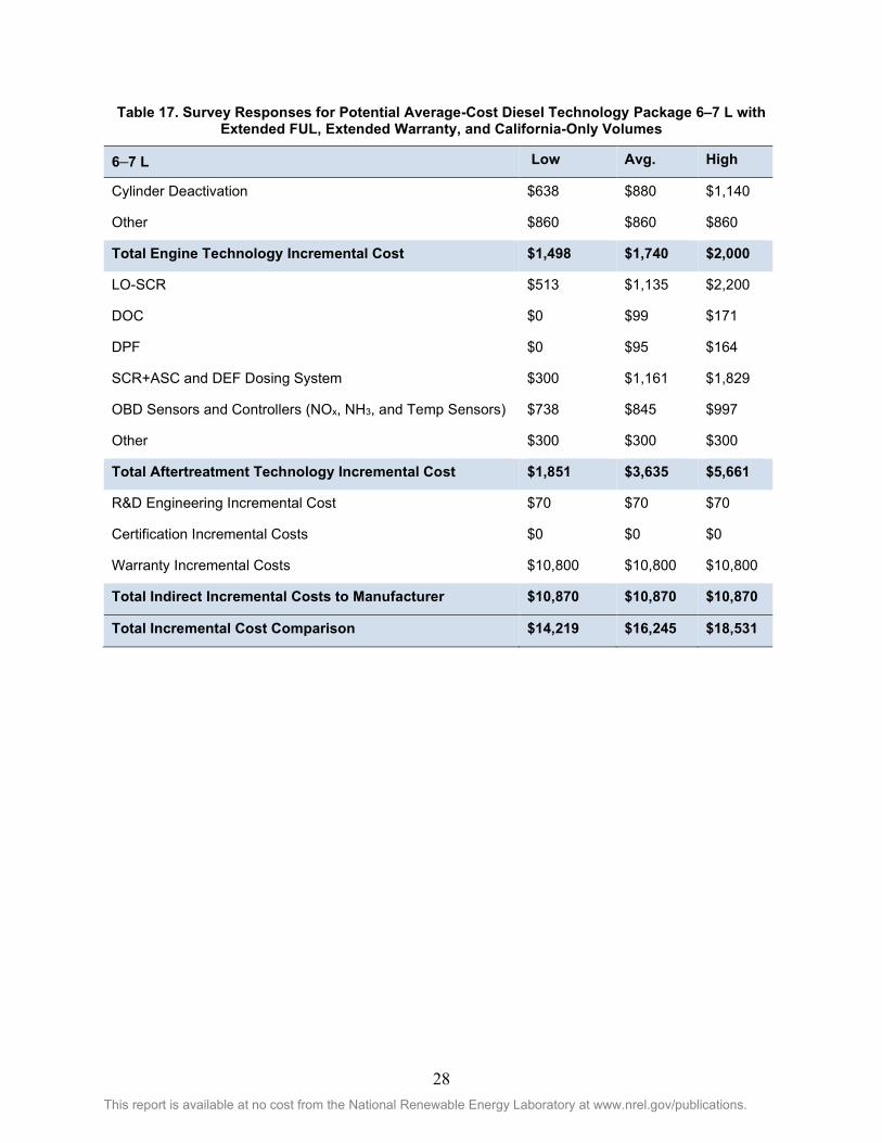
28 This report is available at no cost from the National Renewable Energy Laboratory at www.nrel.gov/publications.
Table 17. Survey Responses for Potential Average-Cost Diesel Technology Package 6–7 L with Extended FUL, Extended Warranty, and California-Only Volumes
6–7 L Low Avg. High
Cylinder Deactivation $638 $880 $1,140
Other $860 $860 $860
Total Engine Technology Incremental Cost $1,498 $1,740 $2,000
LO-SCR $513 $1,135 $2,200
DOC $0 $99 $171
DPF $0 $95 $164
SCR+ASC and DEF Dosing System $300 $1,161 $1,829
OBD Sensors and Controllers (NOx, NH3, and Temp Sensors) $738 $845 $997
Other $300 $300 $300
Total Aftertreatment Technology Incremental Cost $1,851 $3,635 $5,661
R&D Engineering Incremental Cost $70 $70 $70
Certification Incremental Costs $0 $0 $0
Warranty Incremental Costs $10,800 $10,800 $10,800
Total Indirect Incremental Costs to Manufacturer $10,870 $10,870 $10,870
Total Incremental Cost Comparison $14,219 $16,245 $18,531

29 This report is available at no cost from the National Renewable Energy Laboratory at www.nrel.gov/publications.
Table 18. Survey Responses for Potential Average-Cost Diesel Technology Package 12–13 L with Extended FUL, Extended Warranty, and California-Only Volumes
12–13 L Low Avg. High
Cylinder Deactivation $724 $1,176 $1,860
Other $1,100 $1,100 $1,100
Total Engine Technology Cost $1,824 $2,276 $2,960
LO-SCR $736 $1,330 $2,450
DOC $0 $144 $330
DPF $0 $83 $191
SCR+ASC and DEF Dosing System $500 $1,240 $1,892
OBD Sensors and Controllers (NOx, NH3, and Temp Sensors) $476 $765 $997
Other $300 $950 $1,600
Total Aftertreatment Technology Incremental Cost $2,012 $4,512 $7,460
R&D Engineering Incremental Cost $110 $357 $603
Certification Incremental Costs $0 $7 $13
Warranty Incremental Costs $7,840 $23,061 $38,282
Total Indirect Incremental Costs to Manufacturer $7,950 $23,424 $38,898
Total Incremental Cost Comparison $11,786 $30,212 $49,318

30 This report is available at no cost from the National Renewable Energy Laboratory at www.nrel.gov/publications.
Table 19. Survey Responses for Potential High-Cost Diesel Technology Package 6–7 L with Extended FUL, Extended Warranty, and California-Only Volumes
6–7 L Low Avg. High
EGR Cooler Bypass $289 $340 $391
Charge Air Cooler Bypass $191 $225 $259
Turbine Bypass $255 $296 $345
Total Engine Technology Incremental Cost
$735 $865 $995
PNA $924 $1,097 $1,250
DOC $101 $119 $136
DPF (2018 baseline system only) ($511) ($444) ($377)
SCRF $679 $799 $919
SCR+ASC and DEF Dosing System $1,374 $1,616 $1,858
OBD Sensors and Controllers (NOx, NH3, and Temp Sensors)
$738 $868 $997
Other $0 $0 $0
Total Aftertreatment Technology Incremental Cost
$3,305 $4,044 $4,783
R&D Engineering Incremental Cost $xx $xx $xx
Certification Incremental Costs $xx $xx $xx
Warranty Incremental Costs $xx $xx $xx
Total Indirect Incremental Costs to Manufacturer
$xx $xx $xx
Total Incremental Cost Comparison $xx $xx $xx
Note for Table 19 that insufficient responses were received for this technology package with respect to indirect costs to allow sufficient aggregation. Therefore, indirect and total incremental costs were not calculated.

31 This report is available at no cost from the National Renewable Energy Laboratory at www.nrel.gov/publications.
Table 20. Survey Responses for Potential High-Cost Diesel Technology Package 12–13 L with Extended FUL, Extended Warranty, and California-Only Volumes
12–13 L Low Avg. High
EGR Cooler Bypass $289 $390 $490
Charge Air Cooler Bypass $191 $246 $288
Turbine Bypass $255 $296 $345
Total Engine Technology Incremental Cost $735 $932 $1,123
PNA $1,592 $2,801 $4,656
DOC $0 $153 $263
DPF (2018 baseline system only) ($881) ($698) ($560)
SCRF $960 $1,220 $1,553
SCR+ASC and DEF Dosing System ($209) $1,077 $1,977
OBD Sensors and Controllers (NOx, NH3, and Temp Sensors) $426 $720 $997
Other $1,600 $1,600 $1,600
Total Aftertreatment Technology Incremental Cost $3,488 $6,873 $10,486
R&D Engineering Incremental Cost $603 $603 $603
Certification Incremental Costs $13 $13 $13
Warranty Incremental Costs $38,621 $38,621 $38,621
Total Indirect Incremental Costs to Manufacturer $39,237 $39,237 $39,273
Total Incremental Cost Comparison $43,460 $47,042 $50,846
It should be noted that the total indirect incremental cost estimates by manufacturers, and the total incremental costs in Table 15 to Table 20, are dominated by the warranty incremental costs. In some cases, the high estimate of incremental warranty costs is over $38,000. As discussed in Section 1.4.5, the warranty incremental costs were based on a very small sample size, and may be biased high due to the OEMs’ uncertainty regarding covering warranty for unfamiliar technology needed to meet a 0.02 g/bhp-hr NOx standard at the same time with much longer FULs than current FULs.
1.4.5 Incremental Cost Survey Response Observations The following general observations can be made regarding the incremental costs reported in Table 3 through Table 20.
• The initial NREL estimates for total incremental costs were fairly close to the lower end of survey responses for the first survey (MY 2023, U.S. volume, current FUL).
• Indirect costs are a significant portion of the total cost.

32 This report is available at no cost from the National Renewable Energy Laboratory at www.nrel.gov/publications.
• Total costs are not necessarily tied to engine displacement/power but are heavily dependent on indirect costs. Production volumes of various engine displacements have more of an impact than engine “size” on indirect cost, and therefore total incremental cost.
• High engineering, certification, and warranty costs spread over relatively small volumes are the drivers of indirect costs. Survey respondents did not share amortization strategies or exact volumes, so those effects are unknown.
• Only OEMs responded with indirect costs, as Tier 1 and MECA responses included only direct costs. Due to the limited number of OEM responses, the indirect costs may have a high level of variation and may not necessarily represent indirect costs for all OEMs.
• The second survey (MY 2027, California-only volume, extended FUL and warranty) was intended to present “worst case” in many parameters, and the survey results reflect that.
• The second survey results report very high incremental indirect costs, especially for warranty. The OEMs did not break that warranty down into how much was attributed to extended FUL versus the extension of the warranty period. Feedback from OEMs indicated high levels of uncertainty in projected warranty costs for this scenario.
• The second survey results assumed CA-only volumes, but OEMs were free to interpret that assumption on their own. OEMs did not report how these CA-only volumes differed from U.S. volumes in the first survey. They did not explicitly state different assumptions regarding market share or changes in CA-only volume due to potential increased pre-purchases ahead of new emissions regulations or potential reduced purchases due to new emissions regulations.
• Some apparent anomalies in the survey responses may be attributed to the limited number of responses. As noted above, not all respondents reported incremental cost estimates for all proposed technology combinations. The aggregated data reported is the best NREL has available that still protects individual confidential costing information.
1.4.6 Incremental Costs for Natural Gas and Gasoline Technology Packages As previously referenced, few responses were received for the natural gas (HHDD standard) engine platform, preventing NREL from sufficiently aggregating incremental cost information to protect proprietary information. The study assumption that natural-gas engine technology meeting CARB’s current optional low-NOx certification at 0.02 g/bhp-hr would require no significant upgrades to meet a proposed 0.02 g/bhp-hr standard with a new LLC was flawed, based on industry feedback. The feedback focused on changes needed to meet the new LLC cycle and the potential that a moving average window method for emission compliance may be necessary. Based on NREL’s analysis and research from literature review, trade organization feedback, and OEM feedback, the anticipated incremental cost of both indirect and direct incremental costs for natural-gas engines and aftertreatment technology to meet an MY 2023 target of 0.02 g/bhp-hr utilizing the moving average window method to assess emission compliance is within 10% of the low-cost diesel technology package for equivalent

33 This report is available at no cost from the National Renewable Energy Laboratory at www.nrel.gov/publications.
displacement. A round number estimate total of $3,000 incremental cost was subsequently used for the Task 2: Engine Life-Cycle Costs study.
Similarly, few responses were received for the gasoline HDO engine platform. Some aggregation was possible for direct costs, but only NREL estimates were available for indirect costs. As a result, only total integrated (including direct and indirect) incremental costs ranging from $353 to $468 for MY 2023 were calculated with current FUL.
1.5 Low-, Average-, and High-Cost Estimates Because NREL received a range of values in response to both surveys, the diesel incremental cost analysis results in nine different points of costs, with low-, average-, and high-cost responses to each of the potential low-, average-, and high-cost diesel technology packages.
1.5.1 Low-, Average-, and High-Cost Estimates for MY 2023 with Current FUL and Warranty
These different points of cost defining the range of data received in response to the first survey for MY 2023 and current full useful life as defined in Table 1 are depicted by error bars within the summary graphs in Figure 3 and Figure 4. The incremental cost variance within any one package is larger than the differences between the engine and aftertreatment packages. In addition, the range of costs seem to have a greater impact on the larger displacement platforms, resulting in a large variance within the individual technology packages.

34 This report is available at no cost from the National Renewable Energy Laboratory at www.nrel.gov/publications.
Figure 3. Summary of 6–7-L potential technology packages for MY 2023 with current FUL
$4,666
$5,344
$3,685
$0
$1,000
$2,000
$3,000
$4,000
$5,000
$6,000
$7,000
$8,000
$9,000
$10,000Su
rvey
Cos
t Res
pons
e (2
018
USD
$)
Technology Package Comparison
Survey Responses for Potential Low-Cost Diesel Technology Package 6L/7L
Survey Responses for PotentialAverage-Cost Diesel TechnologyPackage 6L/7L
Survey Responses for Potential High-Cost Diesel Technology Package 6L/7L

35 This report is available at no cost from the National Renewable Energy Laboratory at www.nrel.gov/publications.
Figure 4. Summary of 12–13-L potential technology packages for MY 2023 with current FUL
1.5.2 Low-, Average-, and High-Cost Estimates for MY 2027 with Extended Warranty and Extended Useful Life
The range of incremental costs received in response to the second survey for MY 2027 with extended useful life and warranty as defined in Table 1 are depicted by error bars within the summary graphs in Figure 5 and Figure 6. NREL did not receive enough responses for the third technology package of the potential high-cost diesel technology to aggregate and therefore did not include the estimates received in order to protect the source of the data.
$5,340 $6,214 $6,063
$0
$2,000
$4,000
$6,000
$8,000
$10,000
$12,000Su
rvey
Cos
t Res
pons
e (2
018
USD
$)
Technology Package Comparison
Survey Responses for Potential Low-Cost Diesel TechnologyPackage12L/13L
Survey Responses for PotentialAverage-Cost Diesel TechnologyPackage 12L/13L
Survey Responses for Potential High-Cost Diesel Technology Package12L/13L

36 This report is available at no cost from the National Renewable Energy Laboratory at www.nrel.gov/publications.
Figure 5. Summary of 6–7-L potential technology packages for MY 2027 with extended FUL and warranty
Figure 6. Summary of 12–13-L potential technology packages for MY 2027 with extended FUL and warranty
$15,370 $16,245
$0
$2,000
$4,000
$6,000
$8,000
$10,000
$12,000
$14,000
$16,000
$18,000
$20,000Su
rvey
Cos
t Res
pons
e (2
018
USD
$)
Technology Package Comparison
Survey Responses for Potential Low-Cost Diesel Technology Package 6L/7L
Survey Responses for PotentialAverage-Cost Diesel TechnologyPackage 6L/7L
$28,868 $30,212 $47,042
$0
$10,000
$20,000
$30,000
$40,000
$50,000
$60,000
Surv
ey C
ost R
espo
nse
(201
8 U
SD $
)
Technology Package Comparison
Survey Responses for Potential Low-Cost Diesel Technology Package12L/13L
Survey Responses for PotentialAverage-Cost Diesel TechnologyPackage 12L/13L
Survey Responses for Potential High-Cost Diesel Technology Package12L/13L

37 This report is available at no cost from the National Renewable Energy Laboratory at www.nrel.gov/publications.
1.6 Summary of Incremental Cost Analysis NREL received a total of five survey responses from a mix of advanced engine technology and emission control technology trade organizations, Tier 1 suppliers, and engine OEMs. Data were aggregated with the incremental cost estimates NREL derived from literature review and engineering judgments. The survey responses included incremental cost estimates in a range of values, creating variance for each potential low-, average-, and high-cost technology package. The wide variance in the SCR+ASC and DEF dosing system costs drive most of the variance within the total aftertreatment costs. The cost variance is also much greater in larger displacements due to the high costs of the aftertreatment components and the variance within each of those. Indirect costs are a significant portion of the combined hardware costs of the engine and aftertreatment. Lastly, the incremental costs were not adjusted to reflect a retail markup due to the complexity with which pricing decisions are made.
38 This report is available at no cost from the National Renewable Energy Laboratory at www.nrel.gov/publications.
2 Task 2: Engine Life-Cycle Costs This section details a life-cycle cost analysis completed to understand the true costs to the owner of a vehicle with a 0.02 g/bhp-hr NOx aftertreatment package outside of the direct upfront vehicle cost increase. The life-cycle cost analysis sought to incorporate costs associated with the following elements:
• Initial purchase cost • Fuel consumption changes (changes in fuel economy) • DEF consumption • Maximum useful life of the aftertreatment package (major overhaul intervals) • Other operating and maintenance costs.
To complete the life-cycle cost analysis, two main tasks were completed: assessing the maximum useful life for the aftertreatment packages and computing the life-cycle costs. Section 2.1 reviews the maximum useful life analysis in detail, Section 2.2 reviews the life-cycle cost approach, Section 2.3 outlines the scenarios evaluated in this study, and Section 2.4 summarizes the results of the life-cycle cost analysis.
2.1 Maximum Full Useful Life Analysis The maximum useful life for the aftertreatment system determines the mileage at which costs to the owner may be incurred if the system begins to fail. For all scenarios in the life-cycle cost analysis, the incremental cost associated with the aftertreatment package was assumed to be incurred after the truck mileage exceeded the stated maximum useful life. This assumption is expected to be conservative as not all aftertreatment packages will fail immediately after they exceed their stated maximum useful life. Statistical analysis of failure rates combined with data on aftertreatment technology operating and maintenance costs could give a more accurate depiction of life-cycle costs. However, such data are not currently available.
The extended maximum useful life option was evaluated by considering the tradeoff between increased upfront costs due to improved durability needed for the extended maximum useful life1 and the decrease in owner-related replacement costs at the end of the maximum useful life.
The maximum useful life depends on both the displacement of the vehicle and the fuel type. The extended maximum useful life values were defined based on the CARB proposal in January 2019 and previously shown in Table 1.
2.2 Approach This analysis leverages the high-fidelity vehicle stock model within NREL’s Scenario Evaluation and Regionalization Analysis (SERA) model. The SERA stock model tracks vehicle miles traveled, fuel consumption, and ownership costs throughout each vehicle’s lifetime and is resolved temporally and spatially with high fidelity. The SERA model was complemented by
1 It is important to note that the data received from the cost survey (Section 1.3) combined both an extended useful life and an extended warranty. Thus, the cost data used for the extended useful life scenarios couples both the extended useful life and extended warranty information together.

39 This report is available at no cost from the National Renewable Energy Laboratory at www.nrel.gov/publications.
additional data sets to effectively map the vehicles to the aftertreatment packages evaluated in this study.
The following sections provide a brief overview of the SERA stock model, the data sources used in this study, model validation, scenario design, and the life-cycle cost results.
2.2.1 Scenario Evaluation and Regionalization Analysis (SERA) Model The SERA model’s stock module capability provides a flexible framework for tracking vehicles over their life. The SERA’s stock model has been used for a variety of U.S. Department of Energy and California Energy Commission projects and, in particular, is described in detail in Bush et al. (2019). The general data flow for the SERA stock model is shown in Figure 7, which shows how data for regional sales (total vehicles sold), market shares (disaggregation of vehicle sales by vehicle type), vehicle survival (salvage rate data), annual travel (vehicle-miles traveled), fuel consumption data (fuel economy and fuel types), and emission rate data are combined to track vehicle population, travel, and resulting energy consumption and emissions.
For this analysis, the SERA model was expanded to track vehicle life-cycle costs over the vehicle’s lifetime. The model was updated to account for vehicle costs that could be incurred when purchasing a vehicle or driving the vehicle, as the model already has those data within it.
Figure 7. The general SERA stock model data flow

40 This report is available at no cost from the National Renewable Energy Laboratory at www.nrel.gov/publications.
2.2.2 Data Sources The SERA model provides the analytic framework for a detailed stock model but is complemented by additional data sets to complete the life-cycle analysis required in this study. The data sources used in this analysis are summarized in Table 21.

41 This report is available at no cost from the National Renewable Energy Laboratory at www.nrel.gov/publications.
Table 21. Data Sources Used in Life-Cycle Cost Analysis
Data Source Description How it was used
EMFAC/CA Vision 2.1
The EMFAC emissions model is used by CARB to assess emissions from on-road vehicles (cars, trucks, and buses).
The CA Vision 2.1 model (2017) is a scenario-planning model and provides the detailed stock data required for the SERA model. It should be noted that the CA Vision model is based on the EMFAC 2014 results.
The CA Vision 2.1 model data was used as the base stock model to create within SERA (e.g., vehicle sales, survival, vehicle miles traveled, and fuel economy were matched between SERA and the CA Vision 2.1 model).
Thus, the SERA stock model vehicles, population, total mileage, and fuel consumption match the EMFAC and CA Vision 2.1 models.
IHS Markit (Polk) Department of Motor Vehicles Registration Data
The IHS Markit (formerly known as Polk) Department of Motor Vehicles registration database (2013) provides data across the United States on the quantity and types of trucks registered in each zip code.
The IHS Markit data were used to disaggregate EMFAC vehicles by their engine displacement to compute fleet-wide costs.
For example, the T6 Instate Small truck comprises GVWR classes 4–7, which correspond to multiple engine displacements. The IHS Markit data were used to determine the fraction of T6 Instate Small trucks within each engine displacement class.
Task 1 Cost Data
The Task 1 survey cost data includes the incremental cost for three different aftertreatment packages, two engine displacements, three different fuel types, different maximum useful life estimates, different manufacturing volumes, and different model years.
The Task 1 data were incorporated into the SERA model as upfront costs to the vehicle owner mapped to the appropriate vehicle (model year, engine displacement, fuel type).
The incremental upfront cost was also assumed to be incurred after the maximum useful life of the aftertreatment package was surpassed in most scenarios.
California Energy Commission Fuel Prices
California Energy Commission’s forecast of fuel prices (2017)
Scenario analysis was used to evaluate a 1.25% improvement in fuel economy. The marginal improvement in fuel economy results in fuel cost savings during the vehicle’s life.
Preliminary data from SwRI indicates an improvement of 0%–4%, depending on the engine cycle, with 1.25% as a good central estimate per SwRI feedback. No reductions in fuel economy were evaluated as the vehicles must still meet the existing GHG standards regulated by CARB.
Diesel Exhaust Fluid Price
A constant $6/gal DEF cost was assumed based on NREL’s Co-Optima analysis
Scenario analysis as completed to determine the life-cycle cost of increased DEF consumption.
As seen in Table 21, there are several data sources that combine within the SERA model to evaluate the life-cycle cost of the low-NOx fuel standard. Visually, these data sources are combined as seen in Figure 8.

42 This report is available at no cost from the National Renewable Energy Laboratory at www.nrel.gov/publications.
Figure 8. Data flow and analysis using the SERA model for life-cycle cost analysis
Due to the EMFAC and CA Vision 2.1 model spatial and temporal fidelity, each vehicle is defined by a specific region, vocation, model year, fuel type, and age. These vehicles are then further disaggregated by engine displacement using the IHS Markit (formerly Polk) Department of Motor Vehicles registration data. Thus, the life-cycle costs for each vehicle are a function of all of these parameters, and there is a distribution of life-cycle costs across the California fleet due to different vehicle types and travel profiles. For example, the life-cycle costs for a Class 8 long haul tractor will be very different than a Class 6 parcel delivery truck due to the different aftertreatment package costs (which vary by displacement), in addition to the different marginal fuel cost reductions, because they have very different travel requirements profiles and fuel economies.
The distribution in life-cycle costs will be analyzed across the California fleet vehicle types, engine technologies, displacements, and regions using multiple analytic methods, including scenario analysis and sensitivity analysis.
2.2.3 SERA Model Validation The SERA model was validated against the CA Vision 2.1 model to ensure the starting point for the life-cycle cost analysis was accurate. Figure 9 summarizes the results of the model validation, which show very close agreement between the SERA model and the CA Vision model for predicting stock through 2050. Additionally, validating the model by region, Figure 9 shows there is a less than 1.2% error in predicting the California vehicle population through 2050 for each region.

43 This report is available at no cost from the National Renewable Energy Laboratory at www.nrel.gov/publications.
This model validation indicates that the SERA model matches the CA Vision 2.1 model closely through 2050. For this analysis, the life-cycle cost analysis is focused on model years 2023 and 2027, so this validation signifies that those vehicle sales and survival (lifetimes) will be accurately accounted for in the life-cycle analysis. Additionally, the vehicle travel and fuel consumption data influence the life-cycle costs for each vehicle, and this validation indicates that those costs will be accurately accounted for.
Figure 9. SERA model validation against the CA Vision 2.1 model
2.2.4 Manufacturing Volume Analysis Manufacturing volume influences the upfront cost of aftertreatment systems, as large manufacturing volumes allow the firm to spread capital and fixed operating costs over more units sold, reducing the per-unit cost. As discussed in the Task 1 section of this report, most data collected from OEMs are for a national manufacturing volume. One OEM provided cost estimates for the 12–13-L diesel engine for a California-only manufacturing volume basis. These data were included in the sensitivity analysis to show its potential importance but not in the scenario analysis given the limited data set.
2.3 Parameters Investigated The realized life-cycle cost to the vehicle owner depends on a variety of parameters that need to be evaluated. Some of the key parameters assessed in this study include:
• Aftertreatment design cost basis (Task 1)

44 This report is available at no cost from the National Renewable Energy Laboratory at www.nrel.gov/publications.
• Extended maximum useful life • Manufacturing volume • Engine displacement • Vehicle type, region, model year • Fuel economy impact • DEF consumption impact.
These parameters and their analysis bounds are summarized in Table 22. Each parameter was varied independently of others to understand the life-cycle cost sensitivity to that parameter.
Table 22. Life-Cycle Cost Parameters Investigated in this Study
Parameter Description
Adoption Rate 1) 100% compliance by 2023 (Current useful life, only) 2) 100% by 2027 (Extended full useful life, only)
Max Useful Life 1) (Min) Current useful life 2) (Max) Extended useful life 3–5) 25%/50%/75% of min/max spread
Cost Basis 1–3) Low/Avg/High cost basis from Task 1
Other
Will be needed to investigate life-cycle costs differences due to: 1) Varying aftertreatment packages (displacement) 2) Vehicle types (EMFAC definition) 3) Region (Seven CA Vision 2.1 Model Regions) 4) Model year (2023, 2027) 5) Fuel economy impacts (e.g., no change, 1.25% improvement) 6) DEF consumption changes (e.g., 0%, 2.5%, 5% change) 7) Discount rates (3%, 7%) 8) Manufacturing volume (U.S. vs. California-only)
Due to the large number of parameters, each with its own uncertainty around it, the results look at a scenario analysis (varying multiple parameters at one time) and a sensitivity analysis (varying one parameter at a time).
Adoption rate was originally intended to be a parameter of investigation. However, data were only available for current useful life with 100% compliance by 2023 and extended useful life with 100% compliance by 2027. No data were available to determine learning curves or how costs might change depending on the adoption deadline. For this reason, it was assumed that the current full useful life costs for 2023 adoption would hold for 2027 adoption as well. This allows side-by-side comparison of current and extended full useful life life-cycle costs.
2.3.1 Scenario Analysis Due to the large number of parameters that could influence the life-cycle cost of each vehicle, a scenario analysis approach was taken. Three scenarios were defined to understand the bounds on the life-cycle costs: low-cost scenario, mid-cost scenario, and high-cost scenario. These scenarios were defined to bound the life-cycle cost as well as provide a scenario evaluating a mid-cost life-cycle analysis; however, they do not represent the most likely scenarios that could be realized.

45 This report is available at no cost from the National Renewable Energy Laboratory at www.nrel.gov/publications.
The three scenarios are defined in Table 23 and outline the parameter assumptions used for each scenario. The scenarios were defined to look at the bounds of the life-cycle cost analysis, while the sensitivity analysis was completed to understand the critical parameters driving the life-cycle cost of the aftertreatment system. Because California manufacturing volume data were available from only one OEM for only one engine displacement, all scenarios consider U.S. manufacturing volumes.
Additionally, the upfront cost (Task 1 data) was based only on the average-cost technology package and used the low/average/high error bar bounds. This technology package was selected because the error bar bounds of the average-cost technology package effectively span the full spectrum of potential costs (as seen in Section 1.4). Additionally, the low-cost technology package and high-cost technology package may not actually represent the lowest-cost or highest-cost packages, as found from the survey data in Task 1.
Table 23. Scenario Definitions for Bounding Analysis
Parameter Low-Cost Scenario Mid-Cost Scenario High-Cost Scenario Upfront Cost Low Mid High Manufacturing Scale U.S. U.S. U.S.
Useful Life Current
Full Useful Life Current
Full Useful Life Extended
Full Useful Life Fuel Economy Change 1.25% improvement No change No change DEF Consumption Impact No change 2.5% increase 5% increase
Discount Rate 7% 7% 3%
In addition to the above parameters, the life-cycle cost also depends on the model year of the vehicle (compliance rate), the engine displacement, the fuel type (diesel, gasoline, natural gas), the vehicle’s vocation (defined by EMFAC, which affects the vehicle miles traveled over its lifetime), as well as the region the vehicle is operating in (vehicle miles traveled varies slightly by region within the EMFAC model). Thus, to explore the life-cycle costs across this parameter space, three primary metrics were evaluated for each scenario:
1. Life-cycle costs for each vehicle/displacement/fuel/vocation/region combination
2. A vehicle sales weighted-average life-cycle cost across all vehicle/displacement/fuel/vocation/region combinations
3. A life-cycle cost across the full California fleet.
First, the life-cycle cost was calculated for each vehicle, engine displacement, fuel technology, EMFAC vocation, and region within each of low-cost, mid-cost, and high-cost scenarios. This provides vehicle-specific data and can be used to demonstrate the potential life-cycle costs that could be realized for each vehicle owner.
Second, a sales-weighted average life-cycle cost was determined based on the CA Vision 2.1 predicted sales for the model year 2027. This average metric weights the regions and vocations more heavily if there are more vehicles sold in that aftertreatment definition. For example,

46 This report is available at no cost from the National Renewable Energy Laboratory at www.nrel.gov/publications.
assume there are only two vehicles in California and each has a different life-cycle cost and are sold in different proportions, as seen in Table 24.
Table 24. Example Vehicle Sales Weighted Average
Vehicle/Vocation Example
Life-Cycle Cost Example
Sales (vehicles)
T7 Tractor $1,000 100
T7 Single $2,000 50
One estimate of representative life-cycle costs for vehicles in California may be a simple average of the two life-cycle costs ($1,500). However, a more accurate and representative life-cycle cost would be a vehicle sales weighted average that accounts for the relative proportion of vehicles within each vocation ($1,333).2 This approach was used to estimate a single life-cycle cost across all vehicles in California, which would represent an approximate cost for all vehicle owners in the state.
To complete the sales-weighted average, the EMFAC vehicles must be disaggregated into specific vocation, fuel, and engine displacement categories. IHS Markit (formerly Polk) Department of Motor Vehicles registration data were used to disaggregate the EMFAC vehicles into the appropriate vocation, fuel, and engine displacement categories. A summary of the breakdown can be found in Appendix B, while the full data file is provided as an attachment to the report.
In addition to the vehicle-specific life-cycle costs discussed previously, the life-cycle costs of all vehicles sold across California in 2027 were assessed for each scenario. This metric accounts for the relative proportion of vehicle types sold in California and the total cost California fleet owners would be expected to bear for each scenario. This calculation also accounts for the fact that not all vehicles survive the full expected lifetime (e.g., some Class 8 tractors will last only three years while others will last seven). These survival data are important, as vehicles may be retired before they travel more than the aftertreatment package’s maximum useful life and thus would not incur those future replacement costs.
2.3.2 Sensitivity Analysis To better understand the relative importance of each parameter affecting the life-cycle cost of the aftertreatment package, a sensitivity analysis was completed. A sensitivity analysis varies one single parameter and then shows the impact of that parameter on the life-cycle cost of the vehicle. For this analysis, the mid-cost scenario was used as the starting point for the sensitivity analysis, and the variation in each parameter either increases or decreases the life-cycle cost. By varying each parameter independently, one can determine which parameters are the key cost drivers for the life-cycle cost.
2 Calculated as: $1,000 * (100/(100 + 50)) + $2,000 * (50/(100 + 50)) = $1,333/vehicle

47 This report is available at no cost from the National Renewable Energy Laboratory at www.nrel.gov/publications.
2.4 Results The results are presented in three sections: a case study to demonstrate life-cycle cost methodologies, scenario analysis results, and a sensitivity analysis.
The case study section illustrates the calculation methodologies that are described above and ultimately used in both the scenario and sensitivity analyses. The case study looks at the calculation methods and assumptions through the lens of two specific vehicles of interest to CARB: the T7 Tractor (heavy heavy-duty tractor truck) and the T6 OOS small (medium heavy-duty out-of-state truck with GVWR ≤ 26,000 lb) (CARB 2018b). The case-study graphics aim to systematically depict some of the key calculation assumptions, limitations, and findings in an easier-to-understand format than when aggregated across all the California vehicles, vocations, displacements, regions, and scenario descriptions. Additional, single-vehicle results for EMFAC vehicles of specific interest to CARB can be found in Appendix A.
The Scenario Analysis and Sensitivity Analysis sections then summarize the core findings of the study, as discussed in Section 2.3.
2.4.1 Case Study: T7 Tractor and T6 OOS Small Vehicle Life-Cycle Costs The life-cycle cost analysis methodologies are most easily understood through a specific example. Figure 10 shows the present value annual costs3 for a T7 Tractor (Class 8 line-haul) equipped with a 12–13-L diesel engine for two aftertreatment scenarios: (1) current FUL and (2) extended FUL. Life-cycle costs include the incremental replacement costs after full useful life is achieved (vehicle costs) and potential fuel economy improvements associated with the aftertreatment technology discounted back to present value (fuel costs). For the T7 Tractor 12–13-L engine, the current full useful life is 435,000 miles. If designed for this lifespan, the aftertreatment technology would require two replacements. Extending the aftertreatment’s full useful life to 1,000,000 miles significantly increases the upfront cost of the aftertreatment technology but eliminates the need for replacements through 2050, as seen in Figure 10.
3 The present value annual costs for future years are determined using the discount rate (7% for Figure 10). All values are reported in 2018 dollars, consistent with the Task 1 data, and the first year for discounting is assumed to be in 2027. Using this convention, the incremental vehicle costs (i.e., those due directly to the aftertreatment package) incurred in year 2027 exactly match the Task 1 incremental cost data, while future years are lower due to discounting.
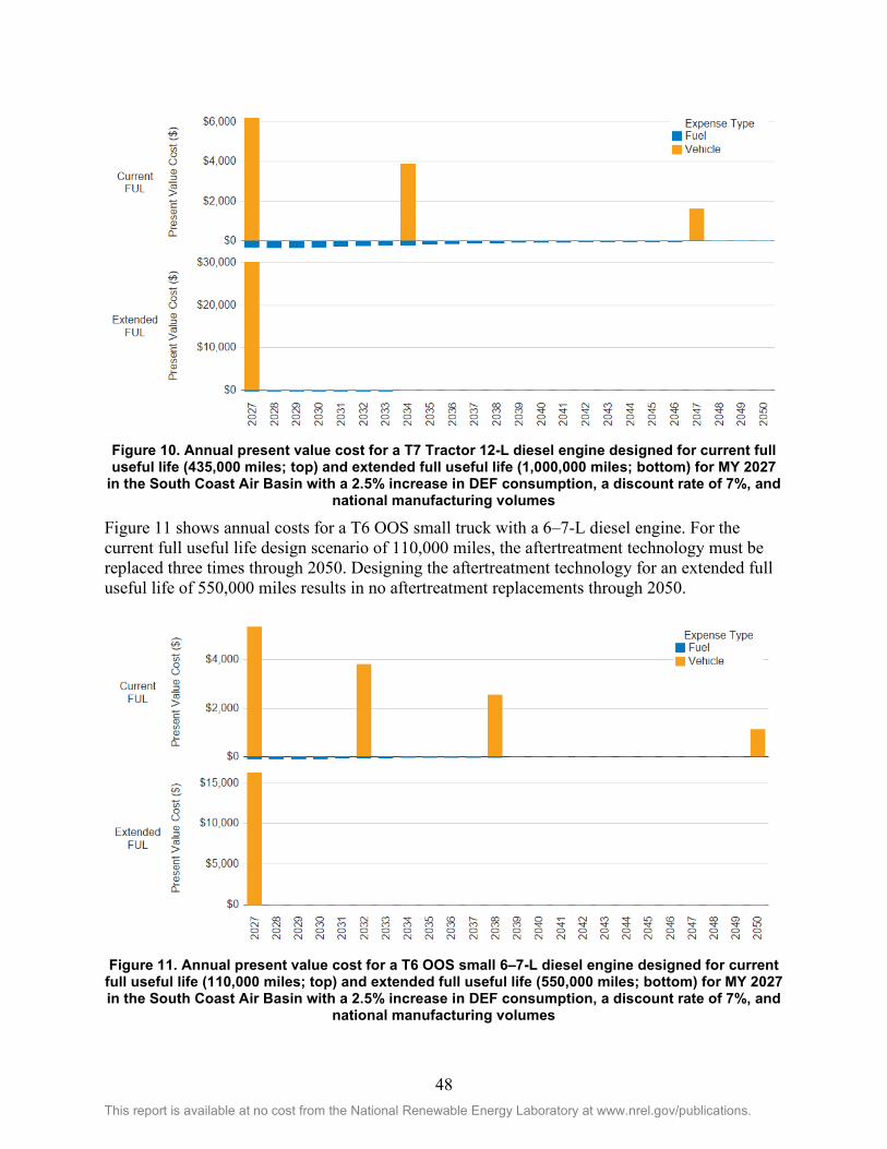
48 This report is available at no cost from the National Renewable Energy Laboratory at www.nrel.gov/publications.
Figure 10. Annual present value cost for a T7 Tractor 12-L diesel engine designed for current full useful life (435,000 miles; top) and extended full useful life (1,000,000 miles; bottom) for MY 2027
in the South Coast Air Basin with a 2.5% increase in DEF consumption, a discount rate of 7%, and national manufacturing volumes
Figure 11 shows annual costs for a T6 OOS small truck with a 6–7-L diesel engine. For the current full useful life design scenario of 110,000 miles, the aftertreatment technology must be replaced three times through 2050. Designing the aftertreatment technology for an extended full useful life of 550,000 miles results in no aftertreatment replacements through 2050.
Figure 11. Annual present value cost for a T6 OOS small 6–7-L diesel engine designed for current
full useful life (110,000 miles; top) and extended full useful life (550,000 miles; bottom) for MY 2027 in the South Coast Air Basin with a 2.5% increase in DEF consumption, a discount rate of 7%, and
national manufacturing volumes

49 This report is available at no cost from the National Renewable Energy Laboratory at www.nrel.gov/publications.
The previous two plots assume that replacement costs are incurred to the owner immediately upon termination of full useful life. In practice, full useful life might be extended by routine maintenance.4 As a result, Figure 10 and Figure 11 likely represent the upper bound on actual life-cycle costs. Statistical analysis of failure rates combined with data on aftertreatment technology operating and maintenance costs could give a more accurate depiction of life-cycle costs. However, such data were not available for these potential future systems.
To explore the full useful life replacement assumption, the life-cycle costs of a vehicle can be compared assuming either no replacements are completed after vehicle mileage exceeds the aftertreatment’s maximum useful life or that replacements are completed. The lower bound on life-cycle costs is set by the condition in which no replacements or maintenance are performed on the aftertreatment package regardless of vehicle mileage. This is unlikely for the current full useful life design but could be realistic for an extended full useful life scenario in which the full useful life of the aftertreatment technology is met near the end of life of the entire truck.
Figure 12 shows total present value cost for the T7 Tractor and T6 OOS small diesel engines as a function of the aftertreatment package’s maximum useful life. The orange markers represent the upper-cost bound that assumes the aftertreatment package will be replaced after the vehicle mileage exceeds the maximum useful life. The blue markers reflect the lower-cost bound of no aftertreatment package replacements over the vehicle lifetime. This analysis assumes linear increments in aftertreatment cost as the designed full useful life increases from current to extended. The actual total present value cost lies somewhere between these two bounds, which are typically less than ~$5,000–$7,000 but depend on the vehicle being evaluated. As the aftertreatment package maximum useful life increases, the spread between the two conditions (orange and blue markers) typically decreases as the number of replacements decreases to zero over the lifetime of the vehicle.
Interestingly, for the T7 Tractor, designing for 75% of extended FUL is slightly more expensive than designing for 100% of extended FUL, as the one replacement that would be necessary in 2047 costs more than the incremental step in upfront cost associated with a 25% longer FUL. However, it is unlikely that the truck owner will replace the entire aftertreatment system that close to the end of life, indicating that the true cost is likely lower than the value estimated here.
4 It should be noted that rather than incurring the replacement cost at the end of the full useful life, one could amortize those costs throughout each year of the vehicle’s operation. This would effectively add incremental routine maintenance for each year and the cost would be mathematically equivalent to the end-of-full-useful-life assumption calculated here. The true incremental lifetime repair cost depends on the expected failure rates for these new aftertreatment packages which were not obtained within this study.

50 This report is available at no cost from the National Renewable Energy Laboratory at www.nrel.gov/publications.
Figure 12. Total present value cost for the T7 Tractor and T6 OOS small vehicles with diesel
engine aftertreatment technology as a function of incremental steps between current FUL and extended FUL for two scenarios: replacements at end of FUL (orange) and no replacements (blue)
Because aftertreatment package repair costs are either paid by the vehicle owner or the vehicle manufacturer through the warranty (if applicable), one may expect the higher upfront cost incurred to the vehicle owner for an aftertreatment package with extended full useful life and extended warranty to be offset by the aftertreatment repair cost savings over the life of the vehicle. CARB staff made this assumption when estimating costs for CARB’s 2018 Step 1 warranty rulemaking, and CARB’s Initial Statement of Reasons (staff report) for this rulemaking (CARB 2018a) assumes that the cost of the warranty packages is equivalent to the lifetime repair savings that the vehicle owner would realize.
The incremental upfront purchase cost that one could estimate based on the survey responses for extended FUL and warranty, and CA-only volumes, as described in Section 1.4.4, would be significantly higher than the repair cost savings that vehicle owners would realize. However, as described more fully in Section 1.4.5, the total incremental costs are dominated by the warranty incremental costs which were based on an extremely small sample size, which may be biased high because of the OEMs’ uncertainty regarding covering warranty for unfamiliar technology and much longer useful lives than today’s useful lives. These warranty costs may be interpreted to represent “worst case” due to these uncertainties.
While NREL does not know the method used by each OEM to determine their incremental warranty cost estimates and it is beyond the scope of this study to evaluate them in detail, a few additional potential reasons for the vehicle owner upfront costs (driven by the high warranty costs) being higher than the lifetime marginal repair savings could include:
• Failure uncertainty – Because the OEMs will not perfectly estimate the probability of failure for their aftertreatment packages, they may charge more than needed initially to ensure they have enough capital to cover any future liabilities. This would be an amount

51 This report is available at no cost from the National Renewable Energy Laboratory at www.nrel.gov/publications.
in excess of what the vehicle owners would actually incur but would be expected to decrease over time as the failure rates on new technologies become known with more certainty.
• Cost of capital – The OEMs have higher costs of capital than individual vehicle owners. Thus, their cost to reserve funding to cover future warranty liabilities would be more than what a vehicle owner would realize in lifetime repair costs on average.
• Soft costs – The OEMs may have embedded additional “soft” costs into the cost estimate for the extended full useful life and extended warranty to account for costs associated with warranty administration (tracking warranty data, contacting vehicle owners, processing payments), legal liability (increased legal staffing in the event of fraud), and potentially others.
• Customer relationships – Some manufacturers may reduce the price of the aftertreatment package with extended warranty for some customers with long-standing relationships or high volumes of purchases. These discounts may need to be offset with the “typical” aftertreatment cost, which may be reflected in the values reported from NREL's survey
The previous plots assumed medium-cost aftertreatment technologies, U.S. manufacturing volumes, up to a 1.25% improvement in fuel economy, a 2.5% increase in DEF consumption, and vehicle sales/operation in the South Coast Air Basin region. The next series of plots illustrates some sensitivity of present value cost to some of these assumptions.
Figure 13 shows present value cost of the T7 Tractor and T6 OOS small diesel trucks for the three aftertreatment cost scenarios presented in Task 1 for current full useful life. This graphic suggests that for a T7 Tractor with a 12–13-L diesel engine with current FUL, the present value cost could be ~42% lower or ~65% higher than the average, depending on which aftertreatment technology cost is realized. For the T6 OOS small truck with a 6–7-L diesel engine, the cost could potentially be 57% lower or 74% higher.
Figure 13. Present value cost for different Class 6 and Class 8 diesel engine aftertreatment
technologies with current full useful life

52 This report is available at no cost from the National Renewable Energy Laboratory at www.nrel.gov/publications.
Figure 14 shows present value cost for different aftertreatment technologies with extended full useful life. For this condition, the T6 OOS small truck with a 6–7-L diesel engine could have a life-cycle cost 12% lower or higher. For the T7 Tractor with a 12–13-L diesel engine, the range in present value cost spans 60% lower or 63% higher, about the average aftertreatment cost technology present value.
Figure 14. Present value cost for different Class 6 and Class 8 diesel engine aftertreatment
technologies with extended full useful life
Figure 15 shows the present value cost for the T7 Tractor with a 12–13-L diesel engine aftertreatment technology manufactured at California and national volumes for current full useful life. No OEM data were available for California manufacturing volumes for extended full useful life. However, this figure suggests that reducing manufacturing volumes to California scales could increase the present value cost by a factor of approximately four to five.

53 This report is available at no cost from the National Renewable Energy Laboratory at www.nrel.gov/publications.
Figure 15. Present value cost for the T7 Tractor and T6 OOS small trucks with diesel engines
designed for current full useful life at both California and national manufacturing volumes
Figure 16 and Figure 17 show present value cost for the T7 Tractor and T6 OOS small trucks with diesel engine aftertreatment technologies as a function of the CA Vision model-defined region for current and extended full useful life, respectively. In both cases, regional life-cycle differences are very small—generally less than ~$100. While vehicle miles traveled is dependent on the region the truck operates in, these differences are small across regions. This leads to the conclusion that regional differences in life-cycle costs are not an important factor in the life-cycle cost assessment.

54 This report is available at no cost from the National Renewable Energy Laboratory at www.nrel.gov/publications.
Figure 16. Present value cost for the T7 Tractor and T7 OOS small trucks with diesel engine
aftertreatment technologies designed for current FUL as a function of region
Figure 17. Present value cost for the T7 Tractor and T7 OOS small trucks with diesel engine aftertreatment technologies designed for extended FUL and warranty as a function of region
2.4.2 Scenario Analysis Results This section presents results from a cost analysis of the three different cost scenarios depicted in Table 23. The scenario analysis results are summarized for the three different metrics discussed in Section 2.3.1:
1. Life-cycle costs for each vehicle/displacement/fuel/vocation/region combination

55 This report is available at no cost from the National Renewable Energy Laboratory at www.nrel.gov/publications.
2. A vehicle sales weighted-average life-cycle cost across all vehicle/displacement/fuel/vocation/region combinations
3. A life-cycle cost across the full California fleet.
2.4.2.1 Vehicle-Specific Life-Cycle Costs The life-cycle cost was calculated for each EMFAC vehicle, engine displacement, fuel technology, EMFAC vocation, and region within each of the low-, mid-, and high-cost scenarios. This provides vehicle-specific data and can be used to demonstrate the potential life-cycle costs that could be realized for each vehicle owner.
For the low-cost scenario (defined in section 2.3.1), the resulting distribution of vehicle life-cycle costs are shown in Figure 18 for each fuel and engine displacement evaluated in this study. Each EMFAC vehicle is plotted within a density plot that shows the relative proportion of vehicle types that have the associated life-cycle cost. It should be noted that this plot does not account for the projected vehicle sales and how those may differ across vehicle types (e.g., the density shown does not reflect the number of vehicles in California that will have that cost, but rather the number of EMFAC vehicle types that have that cost).
Figure 18. Present value life-cycle cost for all EMFAC vehicles in the low-cost scenario,
segmented by fuel type and engine displacement (DSL = diesel, GAS = gasoline)
As seen in Figure 18, some life-cycle costs in the low-cost scenario are negative, indicating the fuel economy benefit outweighs the marginal cost of the aftertreatment package. Additionally, the spread in life-cycle costs is around ~$4,000 for both diesel engine displacements and is primarily due to the different vehicle-miles-traveled profiles across the EMFAC vehicle types. Life-cycle costs for natural gas are not shown, as there was only a single-point estimate of $3,000 for the incremental aftertreatment cost rather than low/high bounds, so natural gas was only evaluated for the mid-cost scenario.
Figure 19 shows the present value life-cycle costs for the mid-cost scenario for all three fuel types. As seen in Figure 19, there could be a significant potential spread in life-cycle costs within a single fuel type and engine displacement category. This is primarily due to the different mileage requirements for certain vehicles combined with the aftertreatment maximum useful life assumption. For the diesel engines, the potential spread in life-cycle costs could be ~$12,000

56 This report is available at no cost from the National Renewable Energy Laboratory at www.nrel.gov/publications.
depending on which EMFAC vehicle type is evaluated. The spread is significantly lower for gasoline and natural-gas engines because there are very few vehicle types defined in EMFAC that use these fuels.
Figure 19. Present value life-cycle cost for all EMFAC vehicles in the mid-cost scenario, segmented by fuel type and engine displacement (DSL = diesel, GAS = gasoline, CNG =
compressed natural gas)
The present value life-cycle costs for the high-cost scenario for diesel are shown in Figure 20. Only diesel is shown because this scenario uses the extended useful life cost data, which are not available for gasoline or natural gas. As seen in Figure 20, the life-cycle costs for a vehicle with a 6-L diesel engine in this scenario ranges from ~$18,000 to nearly $30,000. The life-cycle cost for a vehicle with a 12-L diesel engine ranges from ~$50,000 to $88,000 under this high-cost scenario. As seen previously, these higher costs are due to the high incremental cost of the aftertreatment package with both an extended maximum useful life and warranty combined with the assumption that they are replaced after the vehicle mileage exceeds the maximum useful life. The clear definition of two groups of costs in both the 6-L and 12-L engine displacements seen in Figure 20 shows that if the aftertreatment package does not need to be replaced, the life-cycle cost will be on the lower end of each range. However, if the aftertreatment package is replaced (for vehicles that travel more than the extended useful life), the life-cycle cost increases significantly to the upper end of the range.

57 This report is available at no cost from the National Renewable Energy Laboratory at www.nrel.gov/publications.
Figure 20. Present value life-cycle cost for all EMFAC vehicles in the high-cost scenario, segmented by fuel type and engine displacement (DSL = diesel)
2.4.2.2 Vehicle Sales Weighted Average Costs As seen in Section 2.4.2.1, each EMFAC vehicle has a unique life-cycle cost. To combine these into a single, typical life-cycle cost to evaluate, a vehicle sales weighted average can be completed. Figure 21 shows the vehicle sales weighted-average results for the 6–7-L and 12–13-L engine aftertreatment technologies. The analysis shows a significant spread in potential cost between the three 12–13-L engine cases, ranging from roughly $1,500 all the way up to $71,400.5 Most of this spread is associated with the difference between current and extended full useful life as discussed in Section 2.4.2.1. These sensitivities are discussed in the following section.
Figure 21. EMFAC vehicle sales-weighted average present value cost for 6-L and 12-L diesel
engine technologies under the three cost scenarios described in Table 23
Figure 22 shows the scenario analysis for a 12-L compressed natural-gas engine and a 6-L gasoline engine. The compressed natural-gas costs are based on NREL estimates and do not reflect actual OEM data (only a single-point incremental cost of $3,000 for the aftertreatment
5 These vehicle sales weighted averages are different than the average values shown in the figures in Section 2.4.2.1 because those averages are simple averages across EMFAC vehicle types without regard to how many of those vehicle types are actually sold in California.

58 This report is available at no cost from the National Renewable Energy Laboratory at www.nrel.gov/publications.
package). The gasoline engine data are based on a small number of OEM estimates with limited spread in upfront cost. As a result, the differences between cases are small. Interestingly, for the low-cost scenario of the gasoline engine, the fuel economy benefits effectively cancel out the incremental aftertreatment package costs, resulting in a near-zero life-cycle cost.
Figure 22. Scenario analysis for a 12-liter compressed natural-gas and 6-liter gasoline engine
2.4.2.3 California Fleet Life-Cycle Costs The life-cycle cost across the full California fleet was evaluated to better understand what the total cost to all vehicle owners in California would be. As described in Section 2.3.1, this fleet calculation accounts for vehicle attrition over time because not all vehicles in the fleet will last through 2050.
Figure 23 shows the total California fleet costs for MY 2027 for each scenario evaluated in this study. The fleet costs aggregate all fuel types and engine displacements into a single cost metric. As seen in Figure 23, the total fleet life-cycle cost for the MY 2027 vehicles could range from $92 million to $1.2 billion depending on the scenario. As seen before, the large spread in costs across scenarios is primarily due to the higher incremental costs for the aftertreatment extended useful life and extended warranty, which are used in the high-cost scenario.
Figure 23. Total California fleet life-cycle cost for the MY 2027 vehicles for each scenario analyzed

59 This report is available at no cost from the National Renewable Energy Laboratory at www.nrel.gov/publications.
2.4.3 Sensitivity Analysis Results To better understand how each particular parameter assessed in this study impacts the vehicle’s incremental life-cycle cost, a sensitivity analysis was completed. The vehicle sales weighted average for the mid-cost scenario (see Section 2.4.2.2 for details) was used as the starting (central) point for the sensitivity analysis.
Figure 24 shows the sensitivity analysis results for the diesel 6–7-L and 12–13-L engines. The sensitivity results are relative to the vehicle sales weighted-average costs of $12,700 and $13,200 for the 6–7-L and 12–13-L engines, respectively. For the 12-L engine, the most influential parameter is manufacturing volume, but this is based on a very limited feedback in the cost survey (Section 1.3.2) and thus was not used outside of this sensitivity analysis. Extended full useful life is the next most significant parameter, which also includes the cost associated with the extended warranty. Figure 24 shows the impact of the extended useful life along with 25% increments between the current useful life and extended useful life (linear interpolation of costs from the two data points). Each step helps illustrate how the cost increases as the full useful life increases up to the extended full useful life mileage.
Figure 24. Sensitivity diagram for the diesel 6–7-L and 12–13-L engines relative to the mid-cost
scenario
The influence of the incremental aftertreatment technology cost (Task 1 data) is relatively small compared to the aforementioned factors and has the potential to be nearly offset by fuel economy improvements. Discount rate and DEF consumption have minimal influences on the life-cycle cost. For the 6–7-L diesel engine, the aftertreatment cost (incremental cost data from Task 1) was the most influential sensitivity parameter for which data were available. Manufacturing volume may be more significant, as seen in the 12–13-L engine case, but no data were available for California-only manufacturing volume costs for the 6–7 L.
Because no cost data were available for the effect of manufacturing volume or extended useful life, the sensitivity plots for gasoline and natural gas engines have fewer parameters. Figure 25 shows the sensitivity analysis results for gasoline engines. As seen in Figure 25, the gasoline engine life-cycle cost is impacted most by the fuel economy change and incremental aftertreatment cost parameters. This indicates that if the fuel economy benefit is realized, it will likely fully offset the incremental aftertreatment costs.

60 This report is available at no cost from the National Renewable Energy Laboratory at www.nrel.gov/publications.
Figure 25. Sensitivity diagram for the gasoline 6-L engine relative to the mid-cost scenario
Figure 26 shows the sensitivity analysis results for the natural-gas engine. Fuel economy impacts and discount rate are approximately equal in magnitude but opposite in the direction of their influence.
Figure 26. Sensitivity diagram for the natural-gas 12-L engine relative to the mid-cost scenario
2.5 Life-Cycle Cost Analysis Summary and Conclusions The life-cycle cost analysis seeks to incorporate all direct and indirect incremental costs associated with the different engine aftertreatment technologies over the life of the vehicle. Three scenarios were defined and evaluated to estimate the life-cycle cost across vehicles in California under different conditions.
The scenario results suggest that the life-cycle cost incurred to each vehicle owner depends significantly on the vehicle type and scenario evaluated. Within a given scenario, the spread in life-cycle costs incurred ranges from $4,000 in the low-cost scenario up to nearly $40,000 in the high-cost scenario. Drilling down to the specific EMFAC vehicle definitions (e.g., T7 Tractor), the incremental replacement costs and potential cost savings associated with improved engine fuel economy are two dominant parameters. Because each vehicle has a different mileage profile over its lifetime, the replacement costs and fuel economy savings can vary substantially between vehicles. For example, extending the aftertreatment package’s full useful life from current mileages to proposed mileages has the potential to significantly reduce, if not eliminate, the need for aftertreatment technology replacements through 2050 for some vehicles, but not others. Additionally, this extension results in little, if any, reduction in present value cost for the 6–7-L diesel engines and increases present value cost substantially for the 12–13-L diesel engines.
The scenario results also showed that the total California fleet life-cycle costs for the MY 2027 vehicles could be between $92 million and $1.2 billion depending on the scenario realized. Again, the largest factor differentiating scenarios was whether the current or extended full useful life costs were used.
61 This report is available at no cost from the National Renewable Energy Laboratory at www.nrel.gov/publications.
Next, the vehicle sales weighted-average costs provide an approximate, representative per-vehicle life-cycle cost for each scenario. For the mid-cost scenario, the life-cycle cost could be $12,700 and $13,200 for the diesel 6–7-L and 12–13-L engines, respectively. For the mid-cost scenario, the natural gas life-cycle cost is estimated to be $4,800 while the gasoline engine life-cycle cost is $800.
Lastly, the life-cycle cost results suggest that regional impacts across California are minimal, while manufacturing volume could have a significant impact on present value cost. Very little data were available for California-only manufacturing volumes, but the data available suggest the costs could be 4–5 times more than if a national manufacturing volume was realized.

62 This report is available at no cost from the National Renewable Energy Laboratory at www.nrel.gov/publications.
3 Conclusions The incremental cost analysis was constructed to bracket a range of potential incremental costs associated with achieving 0.02 g/bhp-hr NOx emissions over certification cycles, including a new proposed LLC. Diesel engines were the primary consideration, as they comprise the majority of HD engines. Incremental cost bracketing included three diesel engine and aftertreatment technology packages, two diesel engine displacements, MY 2023 versus 2027 introduction, U.S. versus California-only implementation, and current FUL versus extended FUL and warranty. Direct and indirect incremental costs were broken down to as discrete a level as possible while maintaining data confidentiality. The calculation of incremental costs was limited by the small number of respondents. Engine OEM participation was crucial, as only they could provide estimates for indirect costs, which represented a significant portion of the total cost.
The average incremental cost for the 6–7-L diesel engines for MY 2023 with current FUL ranged from $3,685 to $5,344, but the absolute low and high bounds were between ~$2,000 and over $9,000. Extending FUL and warranty moved the average incremental costs to a range of $15,370 to $16,245, with tighter low and high bounds (constrained in part by the limited number of responses). The average incremental cost for the 12–13-L diesel engines for MY 2023 with current FUL ranged from $5,340 to $6,063, but the absolute low and high bounds were between ~$3,000 and over $10,000. Extending FUL and warranty moved the average incremental costs to a range of $28,868 to $47,042, with much wider low and high bounds (driven in part by the limited number of responses). The natural gas 12-L engine application was unable to be studied in detail, but OEM feedback anticipated that the incremental cost for natural-gas engines and aftertreatment technology is within 10% of the low-cost diesel technology package for equivalent displacement, specifically due to possibly requiring a moving average window method to assess emission compliance. The gasoline engine 6-L application was also unable to be studied in detail, but comparatively low incremental costs were estimated.
Incremental costs are largely driven by indirect costs associated with engineering research and development costs, plus warranty. Those indirect costs, in turn, are driven by production volumes and amortization.
The life-cycle cost analysis incorporates all direct and indirect incremental costs associated with the different engine aftertreatment technologies over the life of the vehicle. The life-cycle costs depend on the vehicle type (mileage), region, fuel, engine displacement, maximum useful life, fuel economy change, diesel exhaust fluid consumption change, and discount rate. The primary drivers of life-cycle cost were the incremental aftertreatment replacement costs and fuel economy benefits.
For the three scenarios evaluated (low-cost, mid-cost, high-cost), the life-cycle costs were evaluated for each EMFAC vehicle type, aggregated to a representative average, and also calculated across the vehicle fleet for the model year 2027 vehicles. The analysis showed that EMFAC vehicles can have significantly different life-cycle costs, and that spread depends on the scenario evaluated: approximately a $4,000 spread across vehicle types in the low-cost scenario, while the high-cost scenario had nearly a $40,000 difference. This large spread was found to be due to the number of aftertreatment package replacements needed throughout the vehicle lifetime. The aggregated, representative average life-cycle costs for the mid-cost scenario were

63 This report is available at no cost from the National Renewable Energy Laboratory at www.nrel.gov/publications.
estimated to be $12,700 for the 6–7-L diesel engine, $13,200 for the 12–13-L diesel engine, $4,800 for the 12-L natural-gas engine, and $800 for the 6-L gasoline engine. The total life-cycle cost to California vehicle owners for the model year 2027 vehicles was estimated to range between $92 million and $1.2 billion depending on the scenario (low-cost or high-cost) realized.
The sensitivity analysis indicated that the manufacturing volume may be the most important parameter impacting the life-cycle cost; however, limited data were received from the external stakeholders surveyed. The next most important parameter was the assumption of extended useful life and extended warranty, as the increase in aftertreatment lifetime may not exceed the vehicle’s travel requirement, which results in larger replacement costs over the vehicle’s life. The aftertreatment cost bound (low/high error bars on the incremental cost data), fuel economy improvement, and discount rate were found to have a moderate impact on the life-cycle cost. Lastly, the region and DEF consumption change were found to have minimal influence on the life-cycle cost.

64 This report is available at no cost from the National Renewable Energy Laboratory at www.nrel.gov/publications.
References Bush, B.; Muratori, M.; Hunter, C.; Zuboy, J.; Melaina, M. 2019. Scenario Evaluation and
Regionalization Analysis (SERA) Model: Demand Side and Refueling Infrastructure Buildout. NREL/TP-5400-70090. https://www.nrel.gov/docs/fy19osti/70090.pdf.
California Air Resources Board (CARB). 2017. On-Road Heavy-Duty Low-NOx Technology Cost Study 16MSC005. May 24, 2017. https://caleprocure.ca.gov/event/3900/0000005722.
CARB. 2018a. Appendix C - Economic Impact Analysis/Assessment. May 8, 2018. https://ww3.arb.ca.gov/regact/2018/hdwarranty18/appc.pdf.
CARB. 2018b. EMFAC2017 Volume III - Technical Documentation, V1.0.2. July 20, 2018. https://ww3.arb.ca.gov/msei/downloads/emfac2017-volume-iii-technical-documentation.pdf.
CARB. 2019. Heavy-Duty Low NOx Program Workgroup Meeting No. 2. May 7, 2019. Ou, L.; Cai, H.; Seong, H.J.; Longman, D.E.; Dunn, J.B.; Storey, J.M.E.; Toops, T.J.; Pihl, J.A.;
Biddy, M.; Thornton, M. 2019. "Co-optimization of Heavy-Duty Fuels and Engines: Cost Benefit Analysis and Implications." Environmental Science & Technology 53: 12904–12913. http://dx.doi.org/10.1021/acs.est.9b03690.
Posada, F.; Chambliss, S.; Blumberg, K. 2016. Costs of Emission Reduction Technologies for Heavy-Duty Diesel Vehicles. The International Council on Clean Transportation, February 2016. https://theicct.org/sites/default/files/publications/ICCT_costs-emission-reduction-tech-HDV_20160229.pdf.
Posada Sanchez, F.; Bandivadekar, A.; German, J. 2012. Estimated Cost of Emission Reduction Technologies for Light-Duty Vehicles. The International Council on Clean Transportation, March 2012. https://theicct.org/sites/default/files/publications/ICCT_LDVcostsreport_2012.pdf.
Sharp, C.A.; Webb, C.C.; Neely, G.D.; Smith, I. 2017. Evaluating Technologies and Methods to Lower Nitrogen Oxide Emissions from Heavy-Duty Vehicles. San Antonio, TX: Southwest Research Institute. April 2017.
Sharp, C.W.; Webb, C.C.; Neely, G.; Carter, M.; Yoon, S.; Henry, C. 2017. "Achieving Ultra Low NOx Emissions Levels with a 2017 Heavy-Duty On-Highway TC Diesel Engine and an Advanced Technology Emissions System - Thermal Management Strategies." SAE Int. J. Engines 10(4), 1697–1712. https://doi.org/10.4271/2017-01-0954.
Sharp, C.W.; Webb, C.C.; Neely, G.; Sarlashkar, J.V.; Rengarajan, S.B.; Yoon, S.; Henry, C.; Zavala, B. 2017. "Achieving Ultra Low NOX Emissions Levels with a 2017 Heavy-Duty On-Highway TC Diesel Engine and an Advanced Technology Emissions System - NOX Management Strategies." SAE Int. J. Engines 10(4): 1736–1748. https://doi.org/10.4271/2017-01-0958.
Sharp, C.W.; Webb, C.C.; Yoon, S.; Carter, M.; Henry, C. 2017. "Achieving Ultra Low NOX Emissions Levels with a 2017 Heavy-Duty On-Highway TC Diesel Engine - Comparison of Advanced Technology Approaches." SAE Int. J. Engines 10(4): 1722–1735. https://doi.org/10.4271/2017-01-0956.

65 This report is available at no cost from the National Renewable Energy Laboratory at www.nrel.gov/publications.
Appendix A. Selected Results for Specific EMFAC Vehicles of Interest to CARB In addition to the life-cycle costs presented in this report, the California Air Resources Board (CARB) indicated a specific interest in the following EMission FACtor (EMFAC) vehicles (CARB 2018b):
Table A1. EMFAC Vehicles of Interest to CARB
EMFAC Vehicle EMFAC Description (GVWR = Gross Vehicle Weight Rating)
T7 Tractor Heavy Heavy-Duty Diesel Tractor Truck
T7 Single Heavy Heavy-Duty Diesel Single Unit Truck
T7 POLA Heavy Heavy-Duty Diesel Drayage Truck near South Coast
T6 OOS Heavy Medium Heavy-Duty Diesel Out-of-State (OOS) Truck with GVWR > 26,000 lb
T6 OOS Small Medium Heavy-Duty Diesel Out-of-State Truck with GVWR ≤ 26,000 lb
Per the CA Vision 2.1 model, the vehicle-miles-traveled profiles for these vehicles with a model year (MY) of 2027 in the South Coast Air Basin (SCAB) region are shown in Figure A1.
Figure A1. Selected EMFAC vehicle miles traveled for MY 2027 in the SCAB region
For these vehicles, the life-cycle costs for each scenario evaluated (low-cost, mid-cost, and high-cost) are shown in the following figures. Figure A2 shows the life-cycle costs for the low-cost scenario, Figure A3 shows the results for the mid-cost scenario, and Figure A4 shows the results for the high-cost scenario. These results are aggregated for each vehicle, which accounts for the costs incurred from the aftertreatment package as well as any potential fuel economy benefit associated with the scenario.

66 This report is available at no cost from the National Renewable Energy Laboratory at www.nrel.gov/publications.
Of note, the individual vehicle life-cycle cost results are very close to the representative life-cycle costs estimated using the vehicle sales weighted average shown in Figure 21 in Section 2.4.2.2.
Figure A2. Present value life-cycle cost for selected EMFAC vehicles (MY 2027 in the SCAB
region) for the low-cost scenario
Figure A3. Present value life-cycle cost for selected EMFAC vehicles (MY 2027 in the SCAB
region) for the mid-cost scenario
Figure A4. Present value life-cycle cost for selected EMFAC vehicles (MY 2027 in the SCAB
region) for the high-cost scenario

67 This report is available at no cost from the National Renewable Energy Laboratory at www.nrel.gov/publications.
Appendix B. EMFAC Vehicle Disaggregation The EMFAC vehicles needed to be broken down into the appropriate fuel and engine displacement categories. The IHS Markit (formerly Polk) Department of Motor Vehicles registration database was used to disaggregate the EMFAC vehicles. The same disaggregation was used for each CA Vision region and the first few results are summarized in Table B1, while the full table is provided in a separate file.
Table B1. EMFAC Vehicle Disaggregation Results
EMFAC 2011 Vehicle Displacement (L)
GVWR Class Fraction (veh/veh)
MH 12 7 0.6008
MH 15 7 0.3992
T6 Ag 6 4 0.3302
T6 Ag 9 4 0.0063
T6 Ag 6 5 0.1554
T6 Ag 9 5 0.0095
T6 Ag 6 6 0.1936
T6 Ag 9 6 0.0995
T6 Ag 6 7 0.0975
T6 Ag 9 7 0.1081
T6 CAIRP heavy 6 7 0.4743
T6 CAIRP heavy 9 7 0.5257
T6 CAIRP small 6 4 0.4156
T6 CAIRP small 9 4 0.0079
T6 CAIRP small 6 5 0.1956
T6 CAIRP small 9 5 0.0119
T6 CAIRP small 6 6 0.2437
T6 CAIRP small 9 6 0.1253
T6 instate construction heavy 6 7 0.4743
T6 instate construction heavy 9 7 0.5257
T6 instate construction small 6 4 0.4156
T6 instate construction small 9 4 0.0079
T6 instate construction small 6 5 0.1956

68 This report is available at no cost from the National Renewable Energy Laboratory at www.nrel.gov/publications.
EMFAC 2011 Vehicle Displacement (L)
GVWR Class Fraction (veh/veh)
T6 instate construction small 9 5 0.0119
T6 instate construction small 6 6 0.2437
T6 instate construction small 9 6 0.1253
T6 instate heavy 6 7 0.4743
T6 instate heavy 9 7 0.5257
T6 instate small 6 4 0.4156
T6 instate small 9 4 0.0079
T6 instate small 6 5 0.1956
T6 instate small 9 5 0.0119
T6 instate small 6 6 0.2437
T6 instate small 9 6 0.1253
www.nikolamotor.com Page 1 of 3
August 16, 2021 Ms. Rachel Sakata Oregon Department of Environmental Quality 700 NE Multnomah Street, Suite 600 Portland, OR 97232-4100
RE: Nikola Comments – Rulemaking – Proposed adoption of California’s Advanced Clean
Trucks rule
Dear Environmental Quality Staff:
Nikola Corporation (“Nikola”) appreciates this opportunity to submit comments in support of Oregon’s
adoption of California’s Advanced Clean Trucks (“ACT”) regulation. Greenhouse Gas (“GHG”) emissions
from transportation account for about 28% of total GHG emissions in the United States, with commercial
trucks contributing an astounding 23% of the total carbon emissions emitted from the transportation sector,
followed by passenger vehicles1. In Oregon, transportation - by air, water, rail, or road - is the largest
contributor of GHG emissions, at 40%. Of the emissions generated, about 27% are from heavy-duty
vehicles. As a designer and manufacturer of zero-emission battery-electric and hydrogen fuel cell electric
vehicles (“FCEV”), electric vehicle drivetrains, vehicle components, energy storage systems, and hydrogen
station infrastructure, Nikola is driven to revolutionize the economic and environmental impact of commerce
as we know it today. We encourage the Oregon Department of Environmental Quality to include both BEV
and FCEV zero-emission (“ZE”) technologies as it considers future implementation of clean truck policies.
Overview
The aggressive standards set by the ACT rule will go a long way toward advancing Oregon’s objectives to
reduce GHG emissions, improve air quality (especially in disadvantaged communities), and transition the
medium- and heavy-duty transportation space to green well-paying jobs. This rule is a critical precondition
for a well-functioning medium- and heavy-duty zero-emission vehicle (“MHD ZEV”) market. Nikola strongly
supports adoption of the ACT rule by Oregon and the other signatories to the MHD ZEV Memorandum of
Understanding signed in July 2020. Adopting the ACT rule signals to manufacturers (“OEMs”) like Nikola
that their respective MHD ZEV technologies will receive priority in Oregon to combat GHG emissions and
the state’s air quality objectives. This is perhaps the single most integral action that a state can take to
galvanize the development and maturation of a MHD ZEV market, however, as discussed below, the
current rule is unlikely to reach its desired scale of impact without the necessary support of complementary
“ecosystem” policies.
1 https://www.epa.gov/greenvehicles/fast-facts-transportation-greenhouse-gas-emissions
www.nikolamotor.com Page 2 of 3
Additional Policies and Investments
It is critically important that Oregon enact manufacturer sales targets for MHD ZEVs. This will advance
Oregon’s market leadership and will also send a decisive signal that ZE trucks and buses will become
mainstream by 2030 and dominant before 2040. Furthermore, the ACT rule is most likely to succeed if it is
included as one part of a suite of policies including: fleet purchase requirements to spur market adoption of
ZEVs currently under development, strong and sustained point-of-sale purchase incentives to drive market
transformation, and commitment by other state agencies to implement supportive infrastructure policy.
• Nikola strongly encourages the following actions to be taken in concert with the ACT rule for it to be
successful:
o Adopt fleet purchase requirements that mirror the sales targets in the ACT rule, upon final
publication of the Advanced Clean Fleets rule by the California Air Resource Board
(“CARB”). Immediately after finalizing the ACT rule, CARB staff began developing a
complementary fleet rule called Advanced Clean Fleets.2
o Create a ramp up to the rule via sustained and sufficient investments in incentives for the
up-front costs of zero-emission trucks and the infrastructure required to support these
trucks; and
o Ensure competitive electricity rates for hydrogen production and dispensing and MHD ZEV
charging by developing electricity rates that minimize demand charges and enable the use
of on-site renewable energy.
o Develop a wholesale electricity market, and enable wholesale market participation for
electrolytic hydrogen producers, which will provide the means for both low cost hydrogen
production as well as the deployment of additional renewable energy generation to support
the increased electricity demand relating to ZEVs.
o Permit siting of hydrogen pipelines along existing rights of way for natural gas pipelines,
and support transmission interconnections and rights of way for electrolytic hydrogen
production facilities.
o Ensure that revenues from the Clean Fuels Program can be directed towards the
deployment of hydrogen fueling and EV charging infrastructure to allow for infrastructure
that can support hundreds of trucks per day at public fueling stations. This can be further
supported by by eliminating per station cost caps or targeting cost caps to a $/truck served
or $/energy potentially dispensed metric.
o Support infrastructure upgrades along roads and freeway exits to enable freight vehicle
movement to new hydrogen fueling stations.
o Encourage demonstration pilots with utilities and fleets in Oregon for BEV charging and
hydrogen FCEV use to inform development of advantageous rates, demonstrate emissions
reductions, and encourage fleet adoption.
2 https://ww2.arb.ca.gov/our-work/programs/advanced-clean-fleets

www.nikolamotor.com Page 3 of 3
Incentives
• Incentive programs could jumpstart market transformation by giving fleets the funding required to
become early adopters of ZEVs and help manufacturers reach production scale. However, ZEV
adoption must extend well past early adopters for Oregon to reach a 30% MHD ZEV sales target
by 2030. This requires not only sustained incentive availability beyond currently available funding in
these programs, but also a transition to more flexible and innovative models that can effectively
channel incentive dollars into resale MHD markets, where many small and minority-owned fleets
procure new trucks.
• Many of the baseline assumptions in CARB’s ACT rulemaking—regarding total cost of ownership
and price parity over time—relied on the assumption of ongoing incentives and low fueling costs
supported by California’s Low Carbon Fuel Standard program, which reduces the effective
operating cost for MHD ZEVs and commercial EV rates adopted by the California Public Utilities
Commission.
• The impact of the Clean Fuels Program and EV rates is critical, especially during early stages of
market adoption. Just as CARB determined that sustained incentives are required to support the
business case for MHD ZEVs in California, Oregon should assume similar incentive support will be
needed for its own MHD ZEV market. Importantly, such sustained incentive support can and
should step-down with time to keep pace with technological improvement as OEMs increase
production volumes and costs reduce in parallel with technology cost curves.
• The development of federal incentives, such as a national “point of sale” purchase incentive,
inclusion of hydrogen within the EPA’s Renewable Fuel Standard program, and infrastructure-
related tax credits could be a game-changer for the ZEV industry and remove the pressure on
states as being the sole source for driving down the price of vehicles and proving market
readiness.
We appreciate Oregon’s leadership to adopt policies like the ACT which will complement the Clean Fuels
Program and recently passed legislation, including House Bill 2021 (Marsh) - 100% Clean Energy for All.
These actions will accelerate the deployment and market adoption of zero-emission heavy-duty trucks and
infrastructure and help the state reach its GHG reduction goals by the middle of the century. Nikola looks
forward to working with the Department of Environmental Quality and other stakeholders in Oregon to
inform this process and support the state’s zero-emission transportation objectives.
Sincerely,
Alana Langdon
Senior Manager, External Affairs and Public Policy
Nikola Corporation

Keith Wilson President & CEO TITAN Freight Systems, Inc. July 26, 2021 Rulemaking Advisory Committee Members Advanced Clean Trucks Oregon Department of Environmental Quality RE: Advanced Clean Truck comparison between California and Oregon Dear Fellow RAC Members, Thank you for this opportunity to share the information below. California Air Resource Board (CARB) has been working on their Advanced Clean Trucks (ACT) policy for five years. They have fully funded research and development and have worked closely with manufacturers to determine the best course of action. The accompanying photo was taken two years ago and is the first Freightliner zero emission vehicle being tested in Chino, California, by CARB South Coast Air Quality Management District. TITAN Freight Systems, my company, has worked extensively with CARB, Freightliner Electric Mobility Group (EMG) and many other heavy duty electric truck manufacturers this past few years. We are excited to take delivery of our first electric truck when they become available. Before ACT, in 1990, California implemented the Zero Emissions Vehicle program1, this advanced clean car initiative required large vehicle manufacturers to sell at least 10% zero emissions vehicles (ZEV) by 2003. Today, 31 years later, they have not achieved this goal. The policy did not align with developments in technology and failed. In part, CARB has used this experience to create the ACT policy to ensure success. They have aligned and invested in the three legs required to ensure their ACT policy succeeds: Product, Incentives, Infrastructure. Product: There currently are few, if any, medium or heavy-duty ZEV production vehicles available in the United States. Freightliner and Volvo, two of the leaders in ZEV development, expect to begin production in late 2022, early 2023. Freightliner’s initial production volume is expected to be five (5) units per day. Tesla, a leader in ZEV, has delayed their heavy-duty truck production2 by more than three years and still has no firm delivery date. CARB has worked closely with manufacturers and has developed their ZEV sales percentage schedule to ensure manufacturers production numbers will meet the policy demands. TriMet, an early adopter of zero emissions buses, from January until June of this year has experienced a 45% up time with these buses. They are in the shop more than they are in revenue operation. This example should give pause in the
1 California: ZEV, transportpolicy.net 2 Tesla delays electric Semi for third time, Commercial Carrier Journal, July 26, 2021

rush to create a policy relying on a product that is not yet available, relies on new technology and operates at a significantly higher cost. Incentives: California provides a Hybrid and Zero-Emission Truck and Bus Voucher Incentive Program (HVIP)3 of $120,000 per heavy duty (Class 8) truck. Oregon provides zero. In addition, California has several other mature programs in place of or in addition to the HVIP program including Carl Moyer Memorial Air Quality Standards Attainment Program4 and a robust Greenhouse Gas (GHG) program with steady Cap & Trade funding. Oregon is considering rulemaking of a GHG Cap & Reduce program with Community Climate Incentives (CCI’s) but unsure at this time if CCI’s will be available as incentives like California’s HVIP. TITAN has pre-ordered six Freightliner ZEV medium and heavy-duty trucks with expected delivery in Q1 of 2023. Without incentives for product purchase and infrastructure, a heavy-duty truck will cost $13,118 more per year than its diesel engine equivalent (see attached Total Cost of Ownership [TCO] analysis with exact prices and quotes). The TCO includes energy credits received from Oregon’s Clean Fuels program. Infrastructure: California Senate Bill 350 (SB350)5, “The CPUC, along with the CARB and Energy Commission, will support transportation electrification by directing electrical corporations to file applications for programs and investments to accelerate widespread transportation electrification.” Oregon has no such programs currently. TITAN’s infrastructure cost to add charging capabilities for six trucks will cost $354,921 (see attached TCO analysis). To oversimplify, without infrastructure support, it is like buying a diesel truck and having to buy a fueling station for each one you purchase. In June, I met with senior CARB legislative personnel and the team that wrote the ACT policy. Among many questions, I asked them about leakage, registering vehicles in other states (e.g., Penske has one of the largest fleets in California and a base state of Indiana), and how will the ACT policy account for these out of state registered vehicles? Currently, they have no way of addressing leakage. Please ensure any policy is fair, transparent and applies to all vehicles operating in our state, regardless of base state. My concern is that Oregon has not set in place the base policy, incentives or infrastructure needed to ensure this policy will succeed. This policy may further contribute to Oregon carrier’s operating at a competitive disadvantage versus their peers in other states. Based on the American Transportation Research Institute (see attached ATRI document) annual state highway user tax for a carrier operating in Oregon is the highest in the nation at $30,410 per truck per year. For comparison, carriers operating in the other 49 states are taxed at between $12,318 and $23,030. Furthermore, Oregon is 26% above our 2020 GHG goal of 51 mtco2e. Today, our emissions are 64.6 mtco2e and growing. If we act without substantive work to ensure a successful policy, we risk continued deterioration in credibility but more importantly we lose time to address the climate crisis. It doesn’t have to be that way. TITAN no longer uses petroleum diesel in our Oregon operations. We use renewable diesel (not biodiesel) as our primary energy source. We rely on petroleum diesel only when a truck is not able to get to a location that provides renewable diesel. For 93% of our energy needs, we are fossil fuel free.
3 https://californiahvip.org/funding/ 4 https://ww2.arb.ca.gov/our-work/programs/carl-moyer-memorial-air-quality-standards-attainment-program 5 https://www.energy.ca.gov/rules-and-regulations/energy-suppliers-reporting/clean-energy-and-pollution-reduction-act-sb-350

Renewable diesel, which is relatively new, has the exact same chemical composition as petroleum diesel, its low-carbon twin. They are interchangeable and perform as “drop in” substitutes. Renewable diesel emits 69 percent less GHG than petroleum diesel and less GHG than an electric vehicle.
Renewable diesel is available in Oregon today. It is sold at the same price as petroleum diesel and for diesel engine owners, delivers tangible savings in increased performance and reduced per-mile maintenance costs. Renewable diesel emits 30% less soot / black carbon, which immediately provides environmental benefits and long-term health savings associated with cleaner fuels and safer air in our communities. California’s strength is their Cap & Trade program which provides significant incentives for ZEV’s. Oregon’s strength is our mature and second strongest in the nation Clean Fuels Program. As California implements their Advanced Clean Trucks rule, they will steadily use less petroleum and renewable diesel. California consumes over 600 million gallons a year of renewable diesel, the same amount of petroleum diesel Oregon uses in a year. We do not have to wait to take climate action. Our Clean Fuels Program has made renewable diesel readily available and low cost. Let’s use it. Sincerely yours, Keith Wilson
Diesel ApplicationEnergy Options Energy Type
ASTM(American Society for
Testing and Standards)
Carbon Intensity[g CO2e / MJ]
CI Reductionvs.
Petroleum Diesel Petroleum Diesel (B5) Fossil D975 97.64 ---
Natural Gas (Compressed) Fossil WK40094 79.98 18%
Natural Gas (Biogas) Renewable WK40094 50.00 49%
Biodiesel (B99) Renewable D6751 35.40 64%
Electricity (hydro, natural gas, coal, wind) Oregon Mix 32.15 67%
Renewable Diesel (R99) Renewable D975 30.02 69%

HEAVY DUTY CLASS 8 VEHICLE - ELECTRIC VS DIESEL - TOTAL COST OF OWNERSHIP (TCO) ANALYSIS
VARIABLE COST PER MILE (CPM) ANALYSIS
Energy Electric Diesel CommentskW Gallon
Cost Per Unit $0.139 $2.560 PGE 060421 Quote / TITAN actual diesel price for 060421Miles Per Gallon 6.7 TITAN class 8 single axle day cab (SADC) tractor MPH
kW Per Mile 1.9eCascadia - Efficiency considerations: Temp, load, regen, terrain - Brett Pope - Volvo Electric Truck Director - 10% to 20% braking regenerative charge)
Charging Efficiency 85% DTNA Advanced Electric Truck - 15% transmission loss during truck chargingkW Per Mile 2.24Cost Per Mile $0.311 $0.382
Clean Fuels Program - CreditsCredit Per Unit $0.199 PGE 060421 Quote - Assuming $2000 buy-in for Renewable CFCkW Per Mile 1.9Credit Per Mile $0.377 Clean Fuels Program - Oregon Department of Evironmental Quality
Energy Total CPM -$0.066 $0.382
Maintenance
Diesel Cost Per Mile $0.085$.0618 to $.1048 CPM, "Understanding the whole maintenance picture", FleetOwner, August 7, 2019
EV Lower CPM 50%Maintenance Total CPM $0.043 $0.085
TOTAL VARIABLE CPM -$0.024 $0.467
EQUIPMENT COST PER MILE (CPM) ANALYSIS
EquipmentUnit Cost eCascadia Cascadia Class 8 Single Axle Day (SADC) Cab tractorMSRP $326,102 $120,000Grants, incentives, % MSRP 0%Total Unit Cost $326,102 $120,000
Charging UnitUnit Cost - Infrastructure $32,081 ($192,487 ÷ 6 units ordered) PGE 060421 Quote $192,487 "Make-Ready" infrastructure
Unit Cost - Charging Dispensers $27,906($167,434 ÷ 6 units ordered) McCoy Freightliner 060421 Quote $162,434 + $5,000 for electrician hook up to PGE infrastructure
Grants, incentives, % MSRP 0%Total $59,987
Total Unit & Charging Cost $386,089 $120,000
FinancingTerm Months 84 84 Key Bank "Key for Green" federal assistance with financingDiscount Rate, Interest Cost 5% 5% Key Bank "Key for Green" federal assistance with financingFactor - Principal & interest payment 1.19 1.19Payment Per Month $5,470 $1,700
Operating MilesMiles Per Day 150 150 Standard pickup and delivery route milesOperating Days Per Month 21 21Miles Per Month 3150 3150
TOTAL EQUIPMENT CPM $1.736 $0.540
TOTAL COST of OWNERSHIP (TCO) PER MILE $1.713 $1.007
DUTY CYCLE - TCO - 10 YEARS Industry average duty is 13 years. Early years of new technology estimated to be lessFinancing Period Months 84 84 7 year financing cycleTCO $453,217.70 $266,391.90Remaining Useful Life Months 36 36 3 years remaining of 10 year duty cycleTCO -$2,669.15 $52,967.96Duty Cycle TCO $450,548.55 $319,359.85
DELTA10 Year Additional Cost -$131,188.70Per Year Additional Cost -$13,118.87
Factors OmittedBattery replacement @ Year 8 North American Council for Freight Efficiency estimateSalvage / Residual Value @ Year 10 5%Collision Insurance - EV higher with 2x replacement cost vs diesel
Incentives / Credit / Financing OutlookKey Bank "Key for Green", credit risk reduction for emerging green technologySen. Wyden, Senate Finance Committee - 30% tax credit proposed - In work group currently