WORKING PAPERS 2020 - Banco de Portugal

13WORKING

PAPERS 2020

BANCO DE PORTUGAL

E U R O S Y S T E M

Nuno Lourenço | António Rua

THE DEI: TRACKING ECONOMIC ACTIVITY DAILY DURING

THE LOCKDOWN

Lisboa, 2020 • www.bportugal.pt

JULY 2020 The analyses, opinions and findings of these papers representthe views of the authors, they are not necessarily those of the

Banco de Portugal or the Eurosystem

Please address correspondence toBanco de Portugal, Economics and Research Department

Av. Almirante Reis, 71, 1150-012 Lisboa, PortugalTel.: +351 213 130 000, email: [email protected]

THE DEI: TRACKING ECONOMIC ACTIVITY DAILY DURING

THE LOCKDOWNNuno Lourenço | António Rua

WORKING PAPERS 2020

13

Working Papers | Lisboa 2020 • Banco de Portugal Av. Almirante Reis, 71 | 1150-012 Lisboa • www.bportugal.pt •

Edition Economics and Research Department • ISBN (online) 978-989-678-741-7 • ISSN (online) 2182-0422

The DEI: tracking economic activity daily during thelockdown

Nuno LourençoBanco de Portugal

Nova SBE

António RuaBanco de Portugal

Nova SBE

July 2020

AbstractThe SARS-CoV-2 outbreak has spread worldwide causing unprecedented disruptions in theeconomies. These unparalleled changes in economic conditions made clear the urgent need todepart from traditional statistics to inform policy responses. Hence, the interest in trackingeconomic activity in a timely manner has led economic agents to rely on high-frequency dataas traditional statistics are released with a lag and available at a lower frequency. Naturally,taking on board such a novel data involves addressing some of the complexities of high-frequency data (e.g. marked seasonal patterns or calendar effects). Herein, we propose a dailyeconomic indicator (DEI), which can be used to assess the behavior of economic activityduring the lockdown period in Portugal. The indicator points to a sudden and sharp drop ofeconomic activity around mid-March 2020, when the highest level of alert due to the COVID-19 pandemic was declared in March 12. It declined further after the declaration of the State ofEmergency in the entire Portuguese territory in March 18, reflecting the lockdown of severaleconomic activities. The DEI also points to an unprecedented decline of economic activity inthe first half of April, with some very mild signs of recovery at the end of the month.

JEL: C22, C38, E32.Keywords: Daily economic index, high-frequency, measurement of economic activity, factormodel.

Acknowledgements: The opinions expressed in this article are those of the authors and do notnecessarily coincide with those of Banco de Portugal or the Eurosystem. Any errors and omissionsare the sole responsibility of the authors. The authors would like to thank all data providers for theirprompt responses and outstanding efforts in collecting and sharing the daily data.E-mail: [email protected]; [email protected]

2

1. Introduction

Monitoring economic developments in real-time is often grounded in the assessmentof a large panel of variables available at a monthly or quarterly frequency. Theseindicators are also made available with a release lag, thus not proving to be suitableto track sudden changes of economic activity. The use of high-frequency data,i.e., data recorded at infra-monthly intervals, dates back to the 1920s. In fact,statisticians and econometricians at the time relied on weekly data to supportpolicy analysis. Fisher (1923) pionereed this work, by proposing a weekly indexnumber of wholesale prices, based on price quotations of 200 commodities. Earlyefforts to model the statistical properties of high-frequency data were remarkable.In this regard, Crum (1927) studied the series of weekly bank debits outside NewYork City from 1919 to 1926 and developed a seasonal adjustment based on themedian-link-relative method suggested by Persons (1919).

Nowadays, with the rapid dissemination of statistical data that are beingprocessed weekly, daily or even hourly, the information set available to economicagents has been made progressively larger. Nevertheless, there is still room toimprove on data collection while making it available to economic policy agents asmost of the data is typically owned by private firms. Furthermore, relying on high-frequency data poses challenges to empirical work (e.g., multiple seasonal patternsand non-integer periodicities, calendar effects, high volatility and a marked irregularcomponent, existence of outliers). Therefore, taking on board such a high-frequencydata into the analysis of short-term economic prospects is not straightforward whichexplains why its use has been rather limited.

The SARS-CoV-2 outbreak has made clear the urgent need to depart fromtraditional statistics and rely instead on high-frequency non-conventional datasources. One of the reasons behind this shift relates to the rapid change of economicconditions. The unprecedented nature of the shock makes it difficult to assess theimpact of the COVID-19 pandemic on the real economy. In this regard, a lot ofeffort is being devoted to measure economic activity at a high-frequency so as tohelp designing sound economic policies. Recently, Lewis et al. (2020) proposed aweekly economic index (WEI) to track the rapid economic developments associatedwith the response to the novel coronavirus in the United States. It correspondsto the single factor estimated from ten weekly series. Similarly, the Bundesbank(2020) developed a weekly activity indicator (WAI) for the German economy basedon a dataset comprising seven high-frequency indicators. Herein, in contrast withprevious literature, we focus on developing a composite daily economic indicator.

The uselfulness of several non-conventional data sources to track economicdevelopments has been documented in the literature. This can be particularlyrelevant in the face of sudden disruptions of economic activity that pose challengesto the more traditional statistics. A very promising data source refers to that ofcard-based payments, as these provide an encompassing view of transactions inthe economy. The applications on the use of payments data to track economicactivity are quite extensive and include, inter alia, Carlsen and Storgaard (2010)

3 The DEI: tracking economic activity daily during the lockdown

for Denmark, Barnett et al. (2016) for the United States, Duarte et al. (2017) forPortugal, Galbraith and Tkacz (2018) for Canada and Aprigliano et al. (2019) forItaly. In addition, transportation activites have also been used to gauge prospectson economic activity. In fact, as pointed out by Lahiri et al. (2004), transportationactivities are very sensitive to the business cycle. However, their use to trackbusiness cycle fluctuations has been rather limited. One of the reasons behindthis refers to a non-negligible release lag of these statistics, a situation thathas been circumvented with the rise of systems with electronic toll collectionsthat allow these statistics to be more promptly available (see also Lahiri andYao (2012)). Moreover, Askitas and Zimmermann (2018) consider transportationactivity performed by heavy transport vehicles across Germany to track thegeneral state of the economy, while Fenz and Schneider (2009) use this type ofdata to predict Austrian exports. Interesting insights can also be derived fromelectricity consumption data due to its broad coverage and wide availability. In thisrespect, Arora and Lieskovsky (2014) show evidence of the usefulness of electricityconsumption to trace GDP developments, which is also corroborated by the workof Aprigliano et al. (2019).

Herein, we develop a Daily Economic Indicator (DEI) to track economic activityin Portugal on a high-frequency basis. After an extensive data collection and apreliminary analysis, we end up with five daily series, namely card-based payments,road traffic of heavy commercial vehicles, cargo and mail landed, electricityconsumption and natural gas consumption. These series present the strongest co-movement with GDP developments among the series assessed and allow to coverseveral important dimensions of economic activity as discussed above. Based onthose series, a latent factor is estimated drawing on a factor model. However, priorto that step, a pre-treatment of the variables has to be performed to cope with dataissues such as seasonality and calendar effects. For that purpose, we resort to STL(Seasonal-Trend decomposition based on Loess) and RegARIMA methods. We findmarked seasonal intra-weekly patterns in the series that have to be accounted foras well as the presence of significant calendar effects.

The proposed composite indicator presents statistically significant informationcontent about current GDP developments. In particular, the evolution of economicactivity during the lockdown is analysed. We find that the DEI started to decreasesubstantially in mid-March, at the time the Portuguese government declared thehighest level of alert due to the COVID-19 pandemic followed a few days afterby the declaration of the State of Emergency in the entire Portuguese territory.Such analysis reinforces the usefulness of high-frequency indicators such as theDEI. Naturally, the use of high-frequency indicators is not limited to the analysisof particular events such as the lockdown, but can also be used for monitoringreal activity in a timely manner and, thus, anticipating the path of low frequencyvariables.

The remainder of the paper proceeds as follows. In section 2, we present theeconometric framework pursued. Section 3 describes the data. The daily economicindicator is put forward and discussed in section 4. Section 5 concludes.

4

2. Econometric framework

Despite the potential usefulness of considering high-frequency indicators, the useof such series involves tackling several issues. In fact, daily raw data typicallypresents strong seasonal patterns.1 However, daily or weekly series are availablefor much shorter time spans than monthly or quarterly data. This implies that,for example, annual seasonality can be poorly estimated using such high-frequencydata. To overcome this issue, one can consider year-on-year growth rates (as in, forinstance, Lewis et al. (2020) for weekly data). Such data transformation is easilyinterpretable and allows to accommodate slowly moving annual seasonality.

However, although we are comparing a given date vis-à-vis the same date inthe previous year, the weekday might differ. In fact, in many economic series,the behavior differs across the seven days of the week. Such distinction can beparticularly marked between, for example, the weekend and working days. Toaccount for intra-weekly seasonality we resort to STL (see also Bergmeir et al.(2016) and Hyndman and Athanasopoulos (2014)).2

Furthermore, there are specific events that occur every year which one shouldalso take into account. In this respect, national holidays are often linked to a datebut there are moving holidays such as Easter which do not always fall on thesame date. Hence, after coping with intra-weekly seasonality, the impact of thosecalendar effects is purged resorting to seasonal RegARIMA models.

After the pre-treatment of the data, one can proceed with factor modelestimation to obtain the daily economic indicator. In the remainder of the section,we run through the above-mentioned building blocks in detail.

2.1. STL

The STL is a non-parametric method proposed by Cleveland et al. (1990). Itallows to decompose a seasonal time series (Yt) into trend (Tt), seasonal (St)and remainder (Rt) components, i.e,

Yt = Tt + St +Rt, t = {1, ...,N} . (1)

STL is a very versatile and robust method for decomposing time series and ithas several advantages over other decomposition methods. It can handle any typeof seasonality, meaning that it is not restricted to monthly and quarterly data.The seasonal component is allowed to change over time, with the rate of changecontrolled by the parameter seasonal width. The smoothness of the trend-cycleis also user-defined. It can be specified to be robust to outliers, so that sporadic

1For an overview of different seasonal adjustment procedures for daily and weekly data see, forexample, Ladiray et al. (2018).

2Note that if one is interested in addressing multiple periodicities, one can use STL sequentially(see Cleveland et al. (1990) and Ollech (2018)).


unusual observations will not affect the estimates of the trend-cycle and seasonalcomponents. Although the above model corresponds to an additive decomposition,a multiplicative decomposition can be obtained by first taking logs of the data.

The STL operates by iterating through smoothing of the seasonal and trendcomponents where all smoothing is done resorting to Loess.3 For the seasonalsmoothing, observations are separated into cycle-subseries. These subseries areseparately smoothed and then recombined. The trend smoothing is done afterremoving the previously estimated seasonal component. This is iterated untilconvergence. The STL also has an outer loop which, after each inner loop,computes robustness weights that are passed on to the inner loop, in order tocope with outliers.

2.1.1. Loess. Loess was initially proposed by Cleveland (1979) and developedfurther by Cleveland and Devlin (1988). Loess combines the simplicity of linearleast squares regression with the flexibility of nonlinear regression. This is achievedby fitting, at each point in the data set, a low-degree polynomial to a localizedsubset of the data. The polynomial is estimated using weighted least squares, givingmore weight to the data points nearer the point of estimation and less weight tothe data points that are further away. The value of the regression function fora specific data point is obtained by evaluating the local polynomial at that datapoint. This is done for each of the N data points.

The usual weight function used for Loess is the tri-cube weight function

W (d) =

{ (1− d3

)30 ≤ d < 1

0 d ≥ 1(2)

where d is the distance of a given data point from the point of estimation, scaledto lie in the range from 0 to 1. Therefore, the weight for a specific point ti inany localized subset of data is obtained by evaluating the weight function at thedistance between that point and the point of estimation t, after scaling the distanceso that the maximum absolute distance over all of the points in the subset of datais exactly one. That is,

wi(t) = W

(|ti − t||tq − t|

). (3)

This means that observations close to t have the largest weights while decreasingas the distance increases, becoming zero at the qth farthest point. Note that theparameter q determines the number of neighbouring observations included in thelocal regression and therefore controls the smoothing degree. The choice regardingthe degree of smoothing can be informed by diagnostic methods (see Clevelandand Terpenning (1982) and Cleveland et al. (1990)).

3Loess or Lowess stands for "LOcally WEighted Scatterplot Smoother".

6

2.1.2. Inner Loop. The inner loop is basically an iteration between seasonalsmoothing (smoothing of the cycle-subseries) and trend smoothing. The inner loopiteratively updates the trend and seasonal components. This is done by subtractingthe current estimate of the trend from the raw series. The time series is thenpartitioned into cycle-subseries. The cycle-subseries are Loess smoothed and thenpassed through a low-pass filter. The seasonal components are the smoothed cycle-subseries minus the result from the low-pass filter. The seasonal components aresubtracted from the raw data. The result is Loess smoothed, which becomes thetrend. What is left is the remainder. More formally, the kth iteration of the innerloop is composed by the following steps:

1. Detrending: The first step is to detrend the series, calculating Yt − T (k)t .

2. Cycle-subseries smoothing: The detrended time series is broken into cycle-subseries. For example, daily data with a weekly seasonality would yield sevencycle-subseries: all Sundays will be one time series, all Mondays a second, etc.Each cycle-subseries is smoothed by Loess with a span of q. The smoothedvalues yield a temporary seasonal time series C(k+1)

t .3. Low-pass filtering of smoothed cycle-subseries: To prevent low-frequency power

from entering the seasonal component, a low pass filter is applied on C(k+1)t

yielding L(k+1)t . The filter is composed of moving average and Loess filters.

4. Detrending of smoothed cycle-subseries: S(k+1)t = C

(k+1)t − L(k+1)

t . This isthe (k + 1)th estimate of seasonal component.

5. Deseasonalizing: The original series is deseasonalized by subtracting theseasonal component computed in the previous step, that is, Yt − S(k+1)

t .6. Trend smoothing: Smoothing by Loess the deseasonalized time series results

in T (k+1)t , the (k + 1)th estimate of the trend component.

2.1.3. Outer Loop. If outlying values are apparent in the time series, one may wishto run the outer loop to down-weight these values. In the outer loop, robustnessweights are assigned to each data point depending on the size of the remainder.This allows for reducing or eliminating the effects of outliers.

After running the inner loop, given the estimates for the trend and seasonalcomponents, the remainder can be obtained simply by

Rt = Yt − Tt − St. (4)

Let

h = 6×median (|Rt|) . (5)

Then the robustness weight at time t is calculated as

ρt = B (|Rt| /h) (6)

where B is the bisquare weight function


B(u) =

{ (1− u2

)20 ≤ u < 1

0 u ≥ 1(7)

For the Loess regressions in the steps 2 and 6 of the inner loop, the neighborhoodweight is multiplied by the robustness weight, which allows to dampen the influenceof outliers.

2.2. RegARIMA

To determine the impact of moving holidays on the time series, we consider aRegARIMA model (see, for example, Findley et al. (1998)):

ϕp (L) ΦP (Ls) (1− L)d (1− Ls)D

Yt − r∑j=1

βjZjt

= θq (L) ΘQ (Ls) εt (8)

where L is the lag operator, p, q, d, s, P , D, Q are non-negative integers (s ≥ 2)and Zjt, j = {1, ..., r} are the set of independent variables. The parameters p,q, P , Q determine the order of the lag polynomials and d and D control for thenon-seasonal and seasonal differencing, respectively. In the case of the daily series,s= 365.4 The parameter βj captures the impact of regressor Zjt on Yt. To capturethe impact of moving holidays, regressors for these holidays are included in the setof independent variables. As the event may affect beyond the date of the eventitself, a number of days preceding and/or following the event can also be consideredin the set of regressors.5

2.3. Factor model

After the above pre-treatment of the data, one can proceed into the estimation ofthe factor model. LetXt be aM -dimensional column vector of time series, observedfor t = {1, ...,N}, that is, Xt = [Y1t · · ·Ymt · · ·YMt]

′. The variables in Xt arerepresented as the sum of two orthogonal components: the common component,driven by a small number of unobserved common factors that accounts for mostof the co-movement among the variables; and the idiosyncratic component, drivenby variable-specific shocks.

The data generating process forXt admits a static factor representation writtenas:

Xt = ΛFt + ξt (9)

4In this case, the leap day, February 29, has to be dropped.5See, for example, Ladiray (2018) about impact models to estimate the before or after effect

on the activity.

8

where Ft = (f1t, ..., frt)′ is a (r× 1) vector of latent factors, Λ is a (M × r) matrix

of unknown factor loadings and ξt denotes aM -dimensional vector of idiosyncraticterms. This representation is without loss of generality as it can be shown that thedynamic factor model representation has an equivalent static factor formulation(see, for instance, Stock and Watson (2005)).

The space spanned by the latent factors can be estimated through the principalcomponents estimator which has been shown to be consistent under relativelygeneral assumptions (see Stock and Watson (1998, 2002b), Bai and Ng (2002)and Amengual and Watson (2007)).6 The proposed DEI corresponds to the latentfactor f1t driving the co-movements of the variables in Xt (see also Lewis et al.(2020)).

3. Data

The lack of priors on which economic time series prove to be more relevant fortracking economic activity at a high-frequency basis motivated an unparalleleddata collection effort. A comprehensive dataset comprising around two dozens ofdaily economic time series with a minimal sample period for in-sample analysis wasbuilt at the first place. The series were chosen to encompass several domains ofthe economy, thus signalling developments across different sectors.

We collected data on traffic from Instituto da Mobilidade e dos Transportes(IMT).7 In addition to total traffic, we also gathered disaggregated data ontraffic of heavy commercial vehicles and light passenger vehicles. These trafficstatistics provide a measure of daily traffic intensity as they record the number ofvehicles passing through tolls, adjusted for the number of miles travelled. As manygoods across Portugal are transported by road and Spain is the country’s maintrading partner, these statistics may signal prospects on both the production andinternational trade. We considered daily traffic data since the beginning of 2012.

Also on transport activity, we gathered data on the movement of passengersat national airports, the number of aircrafts landed as well as freight movements(cargo and mail shipments) which are compiled by ANA Aeroportos de Portugal andthe Portuguese Civil Aviation Authority (ANAC) and kindly provided by StatisticsPortugal for the period since 2009.

Energy consumption developments are also of utmost relevance to assess thestage of economic activity in the industrial and domestic sectors. Therefore, wecollected data on electricity consumption across different distribution grids (e.g.very high-voltage, high-voltage, medium-voltage) which was provided by EDP

6The typical assumptions allow for some heteroskedasticity and limited dependence of theidiosyncratic components in both the time and cross-section dimensions, as well as for moderatecorrelation between the latter and the factors.

7IMT currently manages 15 motorway concessions in Portugal from north to south,corresponding to the universe of existing concessions.


Distribuição. As these series are only available since the beginning of 2011, this setof information was complemented with aggregate electricity consumption (adjustedfor temperature effects) released by Redes Energéticas Nacionais (REN). We alsocollected data on natural gas consumption in the conventional market for the periodsince the start of 2013, which has also been provided by REN.

An additional source of data aiming at tracking the consumer behavior andtransactions in general refers to card-based payments and ATM cash withdrawals,carried out both with cards issued in Portugal and abroad. These series are compiledand have been provided by Banco de Portugal.8 Although these series are availablefor a longer time span, we will restrict henceforth the analysis to the period fromJanuary 1, 2009 to April 30, 2020.

4. Results

4.1. Preliminary analysis

Given the composition of the initial dataset and to avoid over-representation ofany particular economic activity dimension, we pursue a parsimonious approachregarding the number of variables considered. In this respect, one should mentionthe acclaimed work by Stock and Watson (1989) who proposed a compositeeconomic indicator for the United States based on a factor model using just fourseries (in the same vein, Azevedo et al. (2006) developed a composite indicator forthe euro area activity also resorting to a small number of series). More recently,focusing on weekly data, Lewis et al. (2020) consider ten high-frequency indicatorswhereas Bundesbank (2020) take on board seven weekly series.9

Having in mind the objective of obtaining a broadly based measure, weconsider those variables that display more information content about the evolutionof economic activity.10 We end up with five daily series: road traffic of heavycommercial vehicles; electricity consumption; natural gas consumption; cargo andmail landed; card-based payments. As in Lewis et al. (2020) we disregard financialdata as the aim is not to track financial conditions, but the real activity instead.

8For this type of data, there are two discontinuities. Until October 31, 2015 there is no splitbetween operations with cards issued in Portugal and abroad. From November 1, 2015 onwardsdata is available for cards issued in Portugal whereas data regarding cards issued abroad is availableonly since January 1, 2018.

9In the former case, the high-frequency indicators include measures of same-store retail sales,steel production, fuel sales, railroad traffic, electricity consumption, an index of consumer sentiment,initial and continued claims for unemployment insurance, an index of temporary and contractemployment and tax collections from paycheck withholdings. In the latter case, the series includeelectricity consumption, truck toll mileage, Google searches related to unemployment and short-timework, worldwide number of flights, air pollution and cash withdrawals.

10In particular, the co-movement between the year-on-year quarterly growth rate of each dailyseries and GDP growth has been assessed to pre-select the variables.

10

4.2. Intra-weekly seasonality

As described in section 2, we firstly estimate the weekly seasonality using the robustSTL. In particular, we take logs of the series and set the value of the smoothingparameter to 151, as in Ollech (2018).11 This means that around 3 years of dataare used in Loess regressions. Such a value is high enough to avoid including annualperiodic movements into the intra-weekly seasonal factors while leaving some roomfor variation of the seasonal factors.12

Following Ollech (2018), we compute the smoothed periodogram for both thedifferenced original series and the differenced seasonally adjusted series (see Figure1). One can see that the spectral peaks associated with intra-weekly seasonality(at frequency 2π/7 and its harmonics, denoted by the dashed lines in Figure 1)have been filtered out.

In Figure 2, we display the estimated seasonal factors for all indicators. For eachvariable, we plot the cycle-subseries of the weekly seasonal component. Each cycle-subseries is plotted separately against time. In particular, first the Sunday valuesare plotted, then the Monday values are displayed, and so forth. The midmean foreach weekday corresponds to the horizontal line.

The immediate finding is that there is a strong weekly seasonal pattern in allseries. As expected, in the case of the road traffic of heavy commercial vehicles,there is a striking difference between working days and the weekend. In particular,traffic on Sundays is 90 per cent lower than on an average day, while on Saturdays itis almost 60 per cent lower. One can also conclude that such magnitudes have fallensomewhat during the period under analysis. Concerning electricity consumption,usage on Sundays is 15 per cent lower while on Saturdays it is near 10 per cent lowerthan the average day. One should also mention that electricity consumption onMondays seems to be a bit below the observed for the remaining working days, mostprobably reflecting the gradual resume of production activity after the weekend.The natural gas consumption presents a relatively similar seasonal pattern to theobserved for electricity consumption. Both series are reflecting, to a large extent,the intra-weekly seasonality of industrial activity. In particular, gas consumption onSundays is around 20 per cent lower while on Saturdays it is close to 15 per centlower than the average day. Regarding cargo and mail landed, Sundays record avalue 45 per cent below the average day but this figure has been decreasing overtime. On Saturdays, cargo and mail landed are also below average and the gaphas been widening. Mondays and Tuesdays correspond basically to an average day,while the remaining weekdays are characterized by cargo and mail landed above

11In this respect, Cleveland et al. (1990) argue that it should be an odd number and at least 7,but beyond that there is no unique choice.

12One should bear in mind that STL, as well as other well-established seasonal adjustmentprocedures such as X-12-ARIMA, TRAMO-SEATS and unobserved component models, despitetheir advantages, are not free of caveats when applied to daily data and may not be completelyeffective on removing intra-weekly seasonality (see, for example, Ladiray et al. (2018)).


average. In what concerns card-based payments, purchases are 25 per cent lower onSundays and 10 per cent higher on Fridays and Saturdays. The remaining weekdaysbehave close to an average day.

0 0.5 1 1.5 2 2.5 3-70

-60

-50

-40

-30

-20

-10

0

10

20

Original seriesSeasonally adjusted series

(a) Road traffic of heavy commercial vehicles

0 0.5 1 1.5 2 2.5 3-100

-80

-60

-40

-20

0

20


(b) Electricity consumption

0 0.5 1 1.5 2 2.5 3-80

-70

-60

-50

-40

-30

-20

-10

0

10


(c) Natural gas consumption

0 0.5 1 1.5 2 2.5 3-70

-60

-50

-40

-30

-20

-10

0

10

20


(d) Cargo and mail landed

0 0.5 1 1.5 2 2.5 3-70

-60

-50

-40

-30

-20

-10

0

10


(e) Card-based payments

Figure 1: Smoothed periodogram.

12

Weekday

Cyc

le−

Sub

serie

s

Sun. Mon. Tue. Wed. Thu. Fri. Sat.

−1.

0−

0.8

−0.

6−

0.4

−0.

20.

00.

20.

4


Weekday

Cyc

le−

Sub

serie

s


−0.

15−

0.10

−0.

050.

000.

05


Weekday

Cyc

le−

Sub

serie

s


−0.

20−

0.10

0.00

0.05


Weekday

Cyc

le−

Sub

serie

s


−0.

6−

0.4

−0.

20.

00.

2


Weekday

Cyc

le−

Sub

serie

s


−0.

2−

0.1

0.0

0.1


Figure 2: Cycle-subseries of the weekly seasonal component.

4.3. Calendar effects

After removing the intra-weekly seasonality, one proceeds with the estimation ofthe effects of Carnival and Easter (which involves two national holidays, the GoodFriday and the Easter Sunday). Besides considering regressors for each of thosedays, to capture potential effects in the activity during the days before or after thoseevents, we also consider regressors for these periods. In particular, we consider awindow width of one week, that is, we consider three days before and after each


event. In the case of Carnival, this means considering the period from Saturday toFriday (as Carnival occurs on a Tuesday) whereas for Easter the period ranges fromTuesday to Wednesday next week. Regarding the specification of the RegARIMAmodel, the polynomial lag orders are determined by minimizing the BIC criterion.

The estimated effects are reported in Figure 3 along with the 95 per centconfidence intervals. Regarding the road traffic of heavy commercial vehicles, thereis a substantially decline of traffic on Carnival, by around 70 per cent, and areduction of 10 per cent on the previous day. In the remaining days, the impactis not statistically different from zero. In what concerns Easter, the major effect ison Good Friday with a negative impact of 90 per cent and around 30 per cent inthe subsequent three days. A very similar pattern is found for both electricity andnatural gas consumption, but with smaller magnitudes. In the case of Carnival day,the negative impact on electricity and natural gas consumption is estimated to bearound 15 per cent. For Good Friday, the effect is close to 15 per cent for electricityand near 25 per cent for natural gas consumption. For cargo and mail landed, theCarnival effect is close to 15 per cent and there is also a statistically significanteffect on the following day of around 20 per cent. It is also found a significantimpact throughout the Easter period, with the major effect being recorded onGood Friday (almost 60 per cent). Regarding card-based payments, there are nosignificant effects during the Carnival period. For Easter, it is observed a positiveimpact on the days immediately before Good Friday, a negative effect betweenGood Friday and Monday with the largest impact recorded on Sunday (close to 50per cent).

14

Sat

.

Sun

.

Mon

.

Car

niva

l

Wed

.

Thu

.

Fri.

-1

-0.8

-0.6

-0.4

-0.2

0

0.2

Tue

.

Wed

.

Thu

.

Goo

d F

riday

Sat

.

Eas

ter

Mon

.

Tue

.

Wed

.-1

-0.8

-0.6

-0.4

-0.2

0

0.2


Sat

.

Sun

.

Mon

.

Car

niva

l

Wed

.

Thu

.

Fri.

-0.2

-0.15

-0.1

-0.05

0

0.05

Tue

.

Wed

.

Thu

.

Goo

d F

riday

Sat

.

Eas

ter

Mon

.

Tue

.

Wed

.-0.2

-0.15

-0.1

-0.05

0

0.05


Sat

.

Sun

.

Mon

.

Car

niva

l

Wed

.

Thu

.

Fri.

-0.3

-0.25

-0.2

-0.15

-0.1

-0.05

0

0.05

0.1

0.15

Tue

.

Wed

.

Thu

.

Goo

d F

riday

Sat

.

Eas

ter

Mon

.

Tue

.

Wed

.-0.3

-0.25

-0.2

-0.15

-0.1

-0.05

0

0.05

0.1

0.15


Sat

.

Sun

.

Mon

.

Car

niva

l

Wed

.

Thu

.

Fri.

-0.7

-0.6

-0.5

-0.4

-0.3

-0.2

-0.1

0

0.1

0.2

0.3

Tue

.

Wed

.

Thu

.

Goo

d F

riday

Sat

.

Eas

ter

Mon

.

Tue

.

Wed

.-0.7

-0.6

-0.5

-0.4

-0.3

-0.2

-0.1

0

0.1

0.2

0.3


Sat

.

Sun

.

Mon

.

Car

niva

l

Wed

.

Thu

.

Fri.

-0.6

-0.5

-0.4

-0.3

-0.2

-0.1

0

0.1

0.2

0.3

0.4

Tue

.

Wed

.

Thu

.

Goo

d F

riday

Sat

.

Eas

ter

Mon

.

Tue

.

Wed

.-0.6

-0.5

-0.4

-0.3

-0.2

-0.1

0

0.1

0.2

0.3

0.4


Figure 3: Carnival and Easter effects on the daily series.


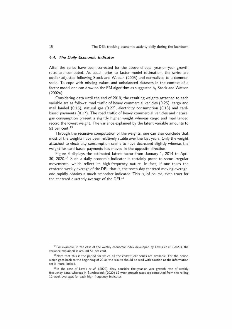
4.4. The Daily Economic Indicator

After the series have been corrected for the above effects, year-on-year growthrates are computed. As usual, prior to factor model estimation, the series areoutlier-adjusted following Stock and Watson (2005) and normalized to a commonscale. To cope with missing values and unbalanced datasets in the context of afactor model one can draw on the EM algorithm as suggested by Stock and Watson(2002a).

Considering data until the end of 2019, the resulting weights attached to eachvariable are as follows: road traffic of heavy commercial vehicles (0.25), cargo andmail landed (0.15), natural gas (0.27), electricity consumption (0.18) and card-based payments (0.17). The road traffic of heavy commercial vehicles and naturalgas consumption present a slightly higher weight whereas cargo and mail landedrecord the lowest weight. The variance explained by the latent variable amounts to53 per cent.13

Through the recursive computation of the weights, one can also conclude thatmost of the weights have been relatively stable over the last years. Only the weightattached to electricity consumption seems to have decreased slightly whereas theweight for card-based payments has moved in the opposite direction.

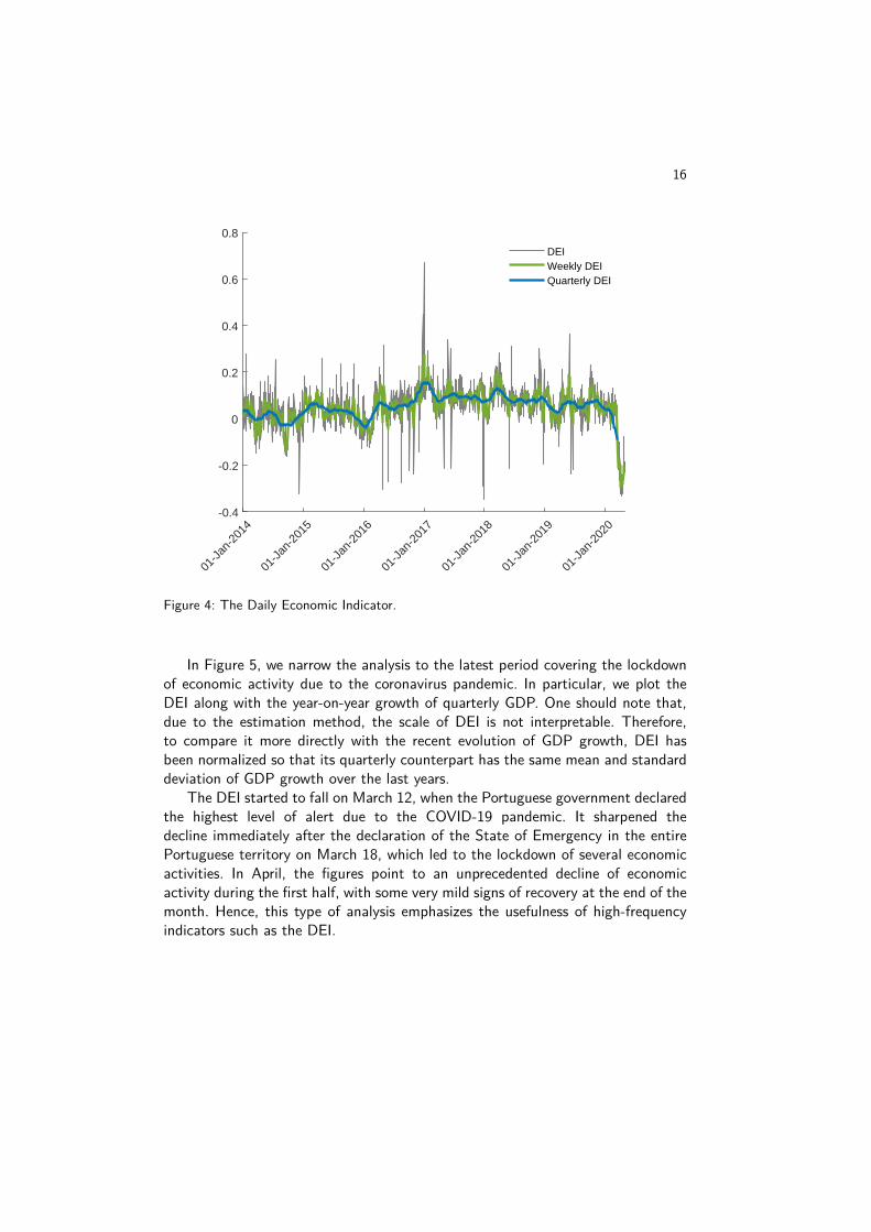
Figure 4 displays the estimated latent factor from January 1, 2014 to April30, 2020.14 Such a daily economic indicator is certainly prone to some irregularmovements, which reflect its high-frequency nature. In fact, if one takes thecentered weekly average of the DEI, that is, the seven-day centered moving average,one rapidly obtains a much smoother indicator. This is, of course, even truer forthe centered quarterly average of the DEI.15

13For example, in the case of the weekly economic index developed by Lewis et al. (2020), thevariance explained is around 54 per cent.

14Note that this is the period for which all the constituent series are available. For the periodwhich goes back to the beginning of 2010, the results should be read with caution as the informationset is more limited.

15In the case of Lewis et al. (2020), they consider the year-on-year growth rate of weeklyfrequency data, whereas in Bundesbank (2020) 12-week growth rates are computed from the rolling12-week averages for each high-frequency indicator.

16

01-J

an-2

014

01-J

an-2

015

01-J

an-2

016

01-J

an-2

017

01-J

an-2

018

01-J

an-2

019

01-J

an-2

020

-0.4

-0.2

0

0.2

0.4

0.6

0.8

DEIWeekly DEIQuarterly DEI

Figure 4: The Daily Economic Indicator.

In Figure 5, we narrow the analysis to the latest period covering the lockdownof economic activity due to the coronavirus pandemic. In particular, we plot theDEI along with the year-on-year growth of quarterly GDP. One should note that,due to the estimation method, the scale of DEI is not interpretable. Therefore,to compare it more directly with the recent evolution of GDP growth, DEI hasbeen normalized so that its quarterly counterpart has the same mean and standarddeviation of GDP growth over the last years.

The DEI started to fall on March 12, when the Portuguese government declaredthe highest level of alert due to the COVID-19 pandemic. It sharpened thedecline immediately after the declaration of the State of Emergency in the entirePortuguese territory on March 18, which led to the lockdown of several economicactivities. In April, the figures point to an unprecedented decline of economicactivity during the first half, with some very mild signs of recovery at the end of themonth. Hence, this type of analysis emphasizes the usefulness of high-frequencyindicators such as the DEI.


01-O

ct-20

19

01-N

ov-2

019

01-D

ec-2

019

01-J

an-2

020

01-F

eb-2

020

01-M

ar-2

020

01-A

pr-2

020

-20

-15

-10

-5

0

5

10

15P

er c

ent

DEIWeekly DEIGDP (y-o-y growth rate)

Figure 5: Economic activity during the lockdown period.

Finally, as in Lewis et al. (2020) we also assess the information content of theDEI to track current GDP developments. We start by regressing GDP growth onthe quarterly average of the DEI, i.e.,

yt = β0 + β1xt +S∑

s=1

γsyt−s + ut (10)

with the number of autoregressive lags selected according to BIC criterion. Theestimation results are presented in Table 1.

The results reveal that the quarterly average of the DEI conveys significantinformation about current GDP growth, even after controlling for its pastbehaviour.16

We also investigate the usefulness of the high-frequency availability of the DEIin a regression context. For that purpose, we consider a Mixed-Data Sampling(MIDAS) approach. The MIDAS approach, which has been put forward by Ghyselset al. (2004), allows series yt sampled at lower-frequencies (such as quarterlyGDP), to be regressed on a variable x(m)

t sampled at frequency m, say daily (see,

16We also assessed the impact of excluding one series at a time from the DEI to evaluate thedeterioration of the performance of the composite indicator with a more limited set of data. Wefind that the informational content of the composite indicator tends to decrease, although notsubstantially, with the largest drop recorded when electricity consumption is excluded.

18

Quarterly data regression Mixed frequency regression

Beta polynomial Almon polynomial

Low-frequency regressorsConstant 0.356*** 0.413*** 0.397***

(0.116) (0.122) (0.113)yt−1 0.550*** 0.400*** 0.410

(0.079) (0.100) (0.094)Quarterly DEI 10.684***

(1.845)Parameters associated with DEIβ1 15.192***

(2.479)θ1 2.375* 0.005

(1.232) (0.060)θ2 1.450* 0.004**

(0.768) (0.002)

R-squared 0.938 0.949 0.950Adjusted R-squared 0.935 0.940 0.942

Table 1. GDP regression results.Notes: *,**,*** denote statistical significance at the 10, 5 and 1 per cent significance levels, respectively.The standard errors are reported within brackets.

for example, Andreou et al. (2013), for a comprehensive overview). Consider thefollowing MIDAS model:

yt = β0 + β1B(L1/m; θ)x(m)t + ut (11)

where B(L1/m; θ) =∑K

k=0B(k; θ)Lk/m and L1/m is a lag operator such thatLk/mx

(m)t = x

(m)t−1/m, and the lag coefficient in B(k; θ) of the corresponding lag

operator Lk/m is parameterised as a function of a small-dimensional vector ofparameters θ. Thus, B(k; θ) is a weighting scheme used for aggregation. As thenumber of lags of x(m)

t can increase quite substantially, in particular when thefrequency of the variables is very different, say quarterly and daily, the use ofa convenient parametric function of B(L1/m; θ) allows to cope with parameterproliferation. In particular, we consider the Beta polynomial which is characterisedby two parameters, θ1and θ2, and the traditional Almon polynomial (of degreetwo). The model has also been augmented with lags of the dependent variable.From Table 1, one can conclude that both mixed-frequency models present a quitehigh explanatory power and slightly higher than in the previous case.


5. Concluding remarks

During rapidly evolving economic conditions, traditional statistics fail to providetimely signals on the state of the economy. The outbreak of the novel coronavirusat the end of 2019 and its lightning-fast spread across continents led economiststo depart from traditional statistics and rely on high-frequency data instead. Infact, alternative data sources have become an increasingly important tool to trackeconomic activity in the aftermath of the COVID-19 pandemic, due to the lack ofrelevant up-to-date data. This effort in collecting timely data has been particularlynotable in central banks and other major institutions. Such a line of research cangreatly benefit from the engagement of private firms, which typically own this typeof data.

In this paper, we carried out an extensive data collection of non-traditionalstatistics from several sources at a daily frequency to assess which time seriesprove to be more relevant for tracking economic activity. However, when dealingwith high-frequency data, there are relevant issues that have to be addressed,including marked seasonal patterns and calendar effects, which are expected toinfluence the dynamics of the time series. In this respect, we estimated the intra-weekly seasonal pattern by means of the STL method, while calendar effects havebeen addressed through RegARIMA models.

After a preliminary analysis and bearing in mind a widespread coverage ofeconomic activity, we selected five daily series. These series cover electronicpayments, transportation activity and energy consumption. The latent factorunderlying the evolution of those series constitutes the proposed daily economicindicator. The analysis of the recent behaviour of DEI during the lockdown periodin Portugal reveals a sudden and sharp drop of economic activity from mid-March2020 onwards. In particular, when the Portuguese government declared the highestlevel of alert due to the COVID-19 pandemic on March 12, the DEI started itsdownward path. It declined further after the declaration of the State of Emergencyin the entire Portuguese territory on March 18, which led to the lockdown ofseveral economic activities. Moreover, the DEI points to an unprecedented declineof economic activity in April during the first half, with some very timid signs ofrecovery at the end of the month.

Lastly, we also assess the information content of the DEI to track current GDPdevelopments. The results reveal that the quarterly average of the DEI conveyssignificant information about current GDP growth, even after controlling for its pastbehaviour. These findings are corroborated in a Mixed-Data Sampling regressionapproach, hence highlighting the usefulness of the DEI in tracking economicactivity.

20

References

Amengual, D. and M. Watson (2007). “Consistent estimation of the number ofdynamic factors in a large N and T panel.” Journal of Business & EconomicStatistics, 25(1), 91–96.

Andreou, E., E. Ghysels, and A. Kourtellos (2013). “Should macroeconomicforecasters use daily financial data and how?” Journal of Business & EconomicStatistics, 31(2), 240–251.

Aprigliano, V., G. Ardizzi, and L. Monteforte (2019). “Using Payment System Datato Forecast Economic Activity.” International Journal of Central Banking, 15(4),55–80.

Arora, V. and J. Lieskovsky (2014). “Electricity Use as an Indicator ofU.S. Economic Activity.” Working paper series, U.S. Energy InformationAdministration.

Askitas, N. and K. Zimmermann (2018). “Nowcasting Business Cycles Using TollData.” Journal of Forecasting, 34, 299–306.

Azevedo, J., S. Koopman, and A. Rua (2006). “Tracking the business cycle of theEuro area: a multivariate model-based band-pass filter.” Journal of Business &Economic Statistics, 24(3), 278–290.

Bai, J. and S. Ng (2002). “Determining the number of factors in approximate factormodels.” Econometrica, 70(1), 191–221.

Barnett, W., M. Chauvet, D. Leiva-Leon, and L. Su (2016). “Nowcasting NominalGDP with the Credit-Card Augmented Divisia Monetary Aggregates.” Workingpapers series in theoretical and applied economics no. 201605, University ofKansas.

Bergmeir, C., R. J. Hyndman, and J. M. Benítez (2016). “Bagging exponentialsmoothing methods using STL decomposition and Box–Cox transformation.”International Journal of Forecasting, 32(2), 303–312.

Bundesbank (2020). “A weekly activity index for the German economy.” Monthlyreport may 2020, vol. 2,. no. 5, 68-72.

Carlsen, M. and P. E. Storgaard (2010). “Dankort Payments as a Timely Indicatorof Retail Sales in Denmark.” Technical report.

Cleveland, R. B., W. S. Cleveland, J. E. McRae, and I. J. Terpenning (1990). “STL:A seasonal-trend decomposition procedure based on loess.” Journal of OfficialStatistics, 6(1), 3–33.

Cleveland, W. S. (1979). “Robust Locally Weighted Regression and SmoothingScatterplots.” Journal of the American Statistical Association, 74, 829–836.

Cleveland, W. S. and S. J. Devlin (1988). “Locally Weighted Regression: AnApproach to Regression Analysis by Local Fitting.” Journal of the AmericanStatistical Association, 83, 596–610.

Cleveland, W. S. and I. J. Terpenning (1982). “Graphical Methods for SeasonalAdjustment.” Journal of the American Statistical Association, 77, 52–62.

Crum, W. L. (1927). “Weekly Fluctuations in Outside Bank Debits.” The Reviewof Economics and Statistics, 9(1), 30–36.


Duarte, C., P. M. Rodrigues, and A. Rua (2017). “A Mixed Frequency Approachto the Forecasting of Private Consumption with ATM/POS Data.” InternationalJournal of Forecasting, 33(1), 61–75.

Fenz, G. and M. Schneider (2009). “A Leading Indicator of Austrian Exports Basedon Truck Mileage.” Monetary policy & the economy q1/09: 44-52.

Findley, D. F., B. C. Monsell, W. R. Bell, M. C. Otto, and B. Chen (1998). “NewCapabilities and Methods of the X-12-ARIMA Seasonal-Adjustment Program.”Journal of Business & Economic Statistics, 16(2), 127–152.

Fisher, I. (1923). “A Weekly Index Number of Wholesale Prices.” Journal of theAmerican Statistical Association, 18(143), 835–840.

Galbraith, J. W. and G. Tkacz (2018). “Nowcasting with Payments System Data.”International Journal of Forecasting, 34(2), 366–76.

Ghysels, E., P. Santa-Clara, and R. Valkanov (2004). “The MIDAS touch: Mixeddata sampling regressions.” Discussion paper, UNC and UCLA.

Hyndman, R. J. and G. Athanasopoulos (2014). Forecasting: principles and practice.OTexts: Melbourne, Australia.

Ladiray, D. (2018). Calendar Effects. Chapter 5 in G. L. Mazzi, D. Ladiray and D.Rieser (eds) Handbook on Seasonal Adjustment, European Commission.

Ladiray, D., G. L. Mazzi, J. Palate, and T. Proietti (2018). Calendar Effects.Chapter 29 in G. L. Mazzi, D. Ladiray and D. Rieser (eds) Handbook on SeasonalAdjustment, European Commission.

Lahiri, K. and W. Yao (2012). “Should transportation output be included as partof the coincident indicators system?” OECD Journal: Journal of Business CycleMeasurement and Analysis, 2012(1), 1–24.

Lahiri, K., W. Yao, and P. Young (2004). “Transportation and the Economy:Linkages at Business-Cycle Frequencies.” Transportation Research Record, 1864,103–111.

Lewis, D., K. Mertens, and J. Stock (2020). “U.S. Economic Activity during theEarly Weeks of the SARS-CoV-2 Outbreak.” Staff report no. 920, april 2020,Federal Reserve Bank of New York.

Ollech, D. (2018). “Seasonal adjustment of daily time series.” Discussion paper no41/2018, Deutsche Bundesbank.

Persons, W. M. (1919). “Indices of business conditions.” The Review of Economicsand Statistics, 1, 5–107.

Stock, J. and M. Watson (1989). New Indexes of Coincident and Leading EconomicIndicators. in NBER Macroeconomics Annual 1989, 4: 351-409, National Bureauof Economic Research.

Stock, J. and M. Watson (1998). “Diffusion indexes.” Working paper no. 6702,National Bureau of Economic Research.

Stock, J. and M. Watson (2002a). “Macroeconomic forecasting using diffusionindices.” Journal of Business & Economic Statistics, 20, 147–162.

Stock, J. and M. Watson (2002b). “Forecasting using principal components froma large number of predictors.” Journal of the American Statistical Association,97, 1167–1179.

22

Stock, J. and M. Watson (2005). “Implications of dynamic factor models for VARanalysis.” Working paper no. 11467, National Bureau of Economic Research.

Working Papers

20171|17 The diffusion of knowledge via managers’

mobility

Giordano Mion | Luca David Opromolla | Alessandro Sforza

2|17 Upward nominal wage rigidity

Paulo Guimarães | Fernando Martins | Pedro Portugal

3|17 Zooming the ins and outs of the U.S. unemployment

Pedro Portugal | António Rua

4|17 Labor market imperfections and the firm’s wage setting policy

Sónia Félix | Pedro Portugal

5|17 International banking and cross-border effects of regulation: lessons from Portugal

DianaBonfim|SóniaCosta

6|17 Disentangling the channels from birthdate to educational attainment

Luís Martins | Manuel Coutinho Pereira

7|17 Who’s who in global value chains? A weight-ed network approach

João Amador | Sónia Cabral | Rossana Mastrandrea | Franco Ruzzenenti

8|17 Lending relationships and the real economy: evidence in the context of the euro area sovereign debt crisis

Luciana Barbosa

9|17 Impact of uncertainty measures on the Portuguese economy

Cristina Manteu | Sara Serra

10|17 Modelling currency demand in a small open economy within a monetary union

António Rua

11|17 Boom, slump, sudden stops, recovery, and policy options. Portugal and the Euro

Olivier Blanchard | Pedro Portugal

12|17 Inefficiency distribution of the European Banking System

João Oliveira

13|17 Banks’ liquidity management and systemic risk

Luca G. Deidda | Ettore Panetti

14|17 Entrepreneurial risk and diversification through trade

Federico Esposito

15|17 The portuguese post-2008 period: a narra-tive from an estimated DSGE model

Paulo Júlio | José R. Maria

16|17 A theory of government bailouts in a het-erogeneous banking system

Filomena Garcia | Ettore Panetti

17|17 Goods and factor market integration: a quan-titative assessment of the EU enlargement

FLorenzo Caliendo | Luca David Opromolla | Fernando Parro | Alessandro Sforza

20181|18 Calibration and the estimation of macro-

economic models

Nikolay Iskrev

2|18 Are asset price data informative about news shocks? A DSGE perspective

Nikolay Iskrev

3|18 Sub-optimality of the friedman rule with distorting taxes

Bernardino Adão | André C. Silva

4|18 The effect of firm cash holdings on monetary policy

Bernardino Adão | André C. Silva

5|18 The returns to schooling unveiled

Ana Rute Cardoso | Paulo Guimarães | Pedro Portugal | Hugo Reis

6|18 Real effects of financial distress: the role of heterogeneity

Francisco Buera | Sudipto Karmakar

7|18 Did recent reforms facilitate EU labour mar-ket adjustment? Firm level evidence

Mario Izquierdo | Theodora Kosma | Ana Lamo | Fernando Martins | Simon Savsek

8|18 Flexible wage components as a source of wage adaptability to shocks: evidence from European firms, 2010–2013

Jan Babecký | Clémence Berson | Ludmila Fadejeva | Ana Lamo | Petra Marotzke | Fernando Martins | Pawel Strzelecki

9|18 The effects of official and unofficial informa-tion on tax compliance

Filomena Garcia | Luca David Opromolla Andrea Vezulli | Rafael Marques

10|18 International trade in services: evidence for portuguese firms

João Amador | Sónia Cabral | Birgitte Ringstad

11|18 Fear the walking dead: zombie firms, spillovers and exit barriers

Ana Fontoura Gouveia | Christian Osterhold

12|18 Collateral Damage? Labour Market Effects of Competing with China – at Home and Abroad

Sónia Cabral | Pedro S. Martins | João Pereira dos Santos | Mariana Tavares

13|18 An integrated financial amplifier: The role of defaulted loans and occasionally binding constraints in output fluctuations

Paulo Júlio | José R. Maria

14|18 Structural Changes in the Duration of Bull Markets and Business Cycle Dynamics

João Cruz | João Nicolau | Paulo M.M. Rodrigues

15|18 Cross-border spillovers of monetary policy: what changes during a financial crisis?

Luciana Barbosa | Diana Bonfim | Sónia Costa | Mary Everett

16|18 When losses turn into loans: the cost of undercapitalized banks

Laura Blattner | Luísa Farinha | Francisca Rebelo

17|18 Testing the fractionally integrated hypothesis using M estimation: With an application to stock market volatility

Matei Demetrescu | Paulo M. M. Rodrigues | Antonio Rubia

20191|19 The transmission of unconventional mon-

etary policy to bank credit supply: evidence from the TLTRO

António Afonso | Joana Sousa-Leite

2|19 How responsive are wages to demand within the firm? Evidence from idiosyncratic export demand shocks

Andrew Garin | Filipe Silvério

3|19 Vocational high school graduate wage gap: the role of cognitive skills and firms

Joop Hartog | Pedro Raposo | Hugo Reis

4|19 What is the Impact of Increased Business Competition?

Sónia Félix | Chiara Maggi

5|19 Modelling the Demand for Euro Banknotes

António Rua

6|19 Testing for Episodic Predictability in Stock Returns

Matei Demetrescu | Iliyan Georgiev Paulo M. M. Rodrigues | A. M. Robert Taylor

7|19 The new ESCB methodology for the calcula-tion of cyclically adjusted budget balances: an application to the Portuguese case

Cláudia Braz | Maria Manuel Campos Sharmin Sazedj

8|19 Into the heterogeneities in the Portuguese labour market: an empirical assessment

Fernando Martins | Domingos Seward

9|19 A reexamination of inflation persistence dynamics in OECD countries: A new approach

Gabriel Zsurkis | João Nicolau | Paulo M. M. Rodrigues

10|19 Euro area fiscal policy changes: stylised features of the past two decades

Cláudia Braz | Nicolas Carnots

11|19 The Neutrality of Nominal Rates: How Long is the Long Run?

João Valle e Azevedo | João Ritto | Pedro Teles

12|19 Testing for breaks in the cointegrating re-lationship: on the stability of government bond markets’ equilibrium

Paulo M. M. Rodrigues | Philipp Sibbertsen Michelle Voges

13|19 Monthly Forecasting of GDP with Mixed Frequency MultivariateSingular Spectrum Analysis

Hossein Hassani | António Rua | Emmanuel Sirimal Silva | Dimitrios Thomakos

14|19 ECB, BoE and Fed Monetary-Policy announcements: price and volume effects on European securities markets

Eurico Ferreira | Ana Paula Serra

15|19 The financial channels of labor rigidities: evidence from Portugal

Edoardo M. Acabbi | Ettore Panetti | Alessandro Sforza

16|19 Sovereign exposures in the Portuguese banking system: determinants and dynamics

Maria Manuel Campos | Ana Rita Mateus | Álvaro Pina

17|19 Time vs. Risk Preferences, Bank Liquidity Provision and Financial Fragility

Ettore Panetti

WORKING PAPERS 2020 - Banco de Portugal

Documents

Transcript of WORKING PAPERS 2020 - Banco de Portugal