Wolaita Sodo University
70
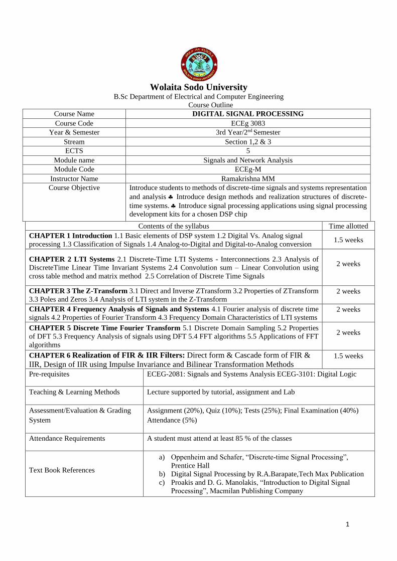
1 Wolaita Sodo University B.Sc Department of Electrical and Computer Engineering Course Outline Course Name DIGITAL SIGNAL PROCESSING Course Code ECEg 3083 Year & Semester 3rd Year/2 nd Semester Stream Section 1,2 & 3 ECTS 5 Module name Signals and Network Analysis Module Code ECEg-M Instructor Name Ramakrishna MM Course Objective Introduce students to methods of discrete-time signals and systems representation and analysis Introduce design methods and realization structures of discrete- time systems. Introduce signal processing applications using signal processing development kits for a chosen DSP chip Contents of the syllabus Time allotted CHAPTER 1 Introduction 1.1 Basic elements of DSP system 1.2 Digital Vs. Analog signal processing 1.3 Classification of Signals 1.4 Analog-to-Digital and Digital-to-Analog conversion 1.5 weeks CHAPTER 2 LTI Systems 2.1 Discrete-Time LTI Systems - Interconnections 2.3 Analysis of DiscreteTime Linear Time Invariant Systems 2.4 Convolution sum – Linear Convolution using cross table method and matrix method 2.5 Correlation of Discrete Time Signals 2 weeks CHAPTER 3 The Z-Transform 3.1 Direct and Inverse ZTransform 3.2 Properties of ZTransform 3.3 Poles and Zeros 3.4 Analysis of LTI system in the Z-Transform 2 weeks CHAPTER 4 Frequency Analysis of Signals and Systems 4.1 Fourier analysis of discrete time signals 4.2 Properties of Fourier Transform 4.3 Frequency Domain Characteristics of LTI systems 2 weeks CHAPTER 5 Discrete Time Fourier Transform 5.1 Discrete Domain Sampling 5.2 Properties of DFT 5.3 Frequency Analysis of signals using DFT 5.4 FFT algorithms 5.5 Applications of FFT algorithms 2 weeks CHAPTER 6 Realization of FIR & IIR Filters: Direct form & Cascade form of FIR & IIR, Design of IIR using Impulse Invariance and Bilinear Transformation Methods 1.5 weeks Pre-requisites ECEG-2081: Signals and Systems Analysis ECEG-3101: Digital Logic Teaching & Learning Methods Lecture supported by tutorial, assignment and Lab Assessment/Evaluation & Grading System Assignment (20%), Quiz (10%); Tests (25%); Final Examination (40%) Attendance (5%) Attendance Requirements A student must attend at least 85 % of the classes Text Book References a) Oppenheim and Schafer, “Discrete-time Signal Processing”, Prentice Hall b) Digital Signal Processing by R.A.Barapate,Tech Max Publication c) Proakis and D. G. Manolakis, “Introduction to Digital Signal Processing”, Macmilan Publishing Company
-
Upload
khangminh22 -
Category
Documents
-
view
5 -
download
0
Transcript of Wolaita Sodo University
1
Wolaita Sodo University B.Sc Department of Electrical and Computer Engineering
Course Outline Course Name DIGITAL SIGNAL PROCESSING
Course Code ECEg 3083
Year & Semester 3rd Year/2nd Semester
Stream Section 1,2 & 3
ECTS 5
Module name Signals and Network Analysis
Module Code ECEg-M
Instructor Name Ramakrishna MM
Course Objective Introduce students to methods of discrete-time signals and systems representation
and analysis Introduce design methods and realization structures of discrete-
time systems. Introduce signal processing applications using signal processing
development kits for a chosen DSP chip
Contents of the syllabus Time allotted
CHAPTER 1 Introduction 1.1 Basic elements of DSP system 1.2 Digital Vs. Analog signal
processing 1.3 Classification of Signals 1.4 Analog-to-Digital and Digital-to-Analog conversion 1.5 weeks
CHAPTER 2 LTI Systems 2.1 Discrete-Time LTI Systems - Interconnections 2.3 Analysis of
DiscreteTime Linear Time Invariant Systems 2.4 Convolution sum – Linear Convolution using
cross table method and matrix method 2.5 Correlation of Discrete Time Signals
2 weeks
CHAPTER 3 The Z-Transform 3.1 Direct and Inverse ZTransform 3.2 Properties of ZTransform
3.3 Poles and Zeros 3.4 Analysis of LTI system in the Z-Transform 2 weeks
CHAPTER 4 Frequency Analysis of Signals and Systems 4.1 Fourier analysis of discrete time
signals 4.2 Properties of Fourier Transform 4.3 Frequency Domain Characteristics of LTI systems 2 weeks
CHAPTER 5 Discrete Time Fourier Transform 5.1 Discrete Domain Sampling 5.2 Properties
of DFT 5.3 Frequency Analysis of signals using DFT 5.4 FFT algorithms 5.5 Applications of FFT
algorithms
2 weeks
CHAPTER 6 Realization of FIR & IIR Filters: Direct form & Cascade form of FIR &
IIR, Design of IIR using Impulse Invariance and Bilinear Transformation Methods
1.5 weeks
Pre-requisites ECEG-2081: Signals and Systems Analysis ECEG-3101: Digital Logic
Teaching & Learning Methods Lecture supported by tutorial, assignment and Lab
Assessment/Evaluation & Grading
System
Assignment (20%), Quiz (10%); Tests (25%); Final Examination (40%)
Attendance (5%)
Attendance Requirements A student must attend at least 85 % of the classes
Text Book References
a) Oppenheim and Schafer, “Discrete-time Signal Processing”,
Prentice Hall
b) Digital Signal Processing by R.A.Barapate,Tech Max Publication
c) Proakis and D. G. Manolakis, “Introduction to Digital Signal
Processing”, Macmilan Publishing Company
2
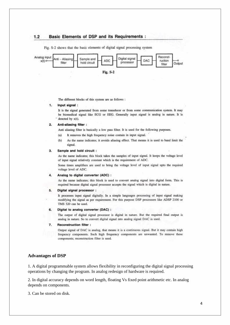
CHAPTER ONE
INTRODUCTION TO DSP
Digital Signal Processing (DSP) refers to processing of signals by digital systems like Personal
computers and systems designed using digital integrated circuits, microprocessors and microcontrollers
Signal:
A signal is defined as a function of one or more variables which conveys information on the
nature of a physical phenomenon. The value of the function can be a real valued scalar
quantity, a complex valued quantity, or perhaps a vector.
System:
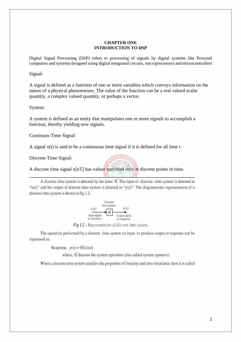
A system is defined as an entity that manipulates one or more signals to accomplish a
function, thereby yielding new signals.
Continuos-Time Signal:
A signal x(t) is said to be a continuous time signal if it is defined for all time t.
Discrete-Time Signal:
A discrete time signal x[nT] has values specified only at discrete points in time.
3
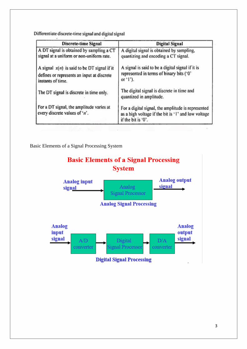
Basic Elements of a Signal Processing System
4
Advantages of DSP
1. A digital programmable system allows flexibility in reconfiguring the digital signal processing
operations by changing the program. In analog redesign of hardware is required.
2. In digital accuracy depends on word length, floating Vs fixed point arithmetic etc. In analog
depends on components.
3. Can be stored on disk.
5
4. It is very difficult to perform precise mathematical operations on signals in analog form but these
operations can be routinely implemented on a digital computer using software.
5. Cheaper to implement.
6. Small size.
7. Several filters need several boards in analog, whereas in digital same DSP processor is used for
many filters.
Disadvantages of DSP
1. When analog signal is changing very fast, it is difficult to convert digital form.(beyond 100KHz
range)
2. w=1/2 Sampling rate.
3. Finite word length problems.
4. When the signal is weak, within a few tenths of millivolts, we cannot amplify the signal after it is
digitized.
5. DSP hardware is more expensive than general purpose microprocessors & micro controllers.
Applications of DSP
1. Filtering.
2. Speech synthesis in which white noise (all frequency components present to the same level) is
filtered on a selective frequency basis in order to get an audio signal.
3. Speech compression and expansion for use in radio voice communication.
4. Speech recognition.
5. Signal analysis.
6. Image processing: filtering, edge effects, enhancement.
7. PCM used in telephone communication.
8. High speed MODEM data communication using pulse modulation systems such as FSK, QAM etc.
MODEM transmits high speed (1200-19200 bits per second) over a band limited (3-4 KHz) analog
telephone wire line.
9. Wave form generation.
6
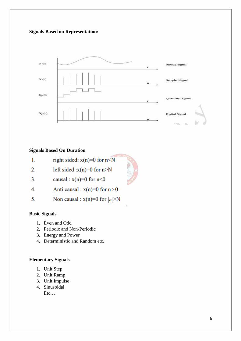
Signals Based on Representation:
Signals Based On Duration
Basic Signals
1. Even and Odd
2. Periodic and Non-Periodic
3. Energy and Power
4. Deterministic and Random etc.
Elementary Signals
1. Unit Step
2. Unit Ramp
3. Unit Impulse
4. Sinusoidal
Etc…
7
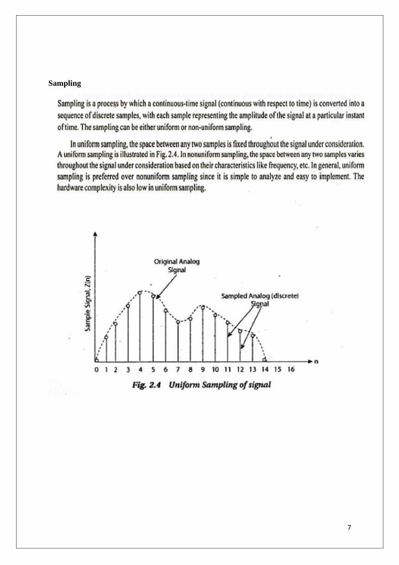
Sampling
8
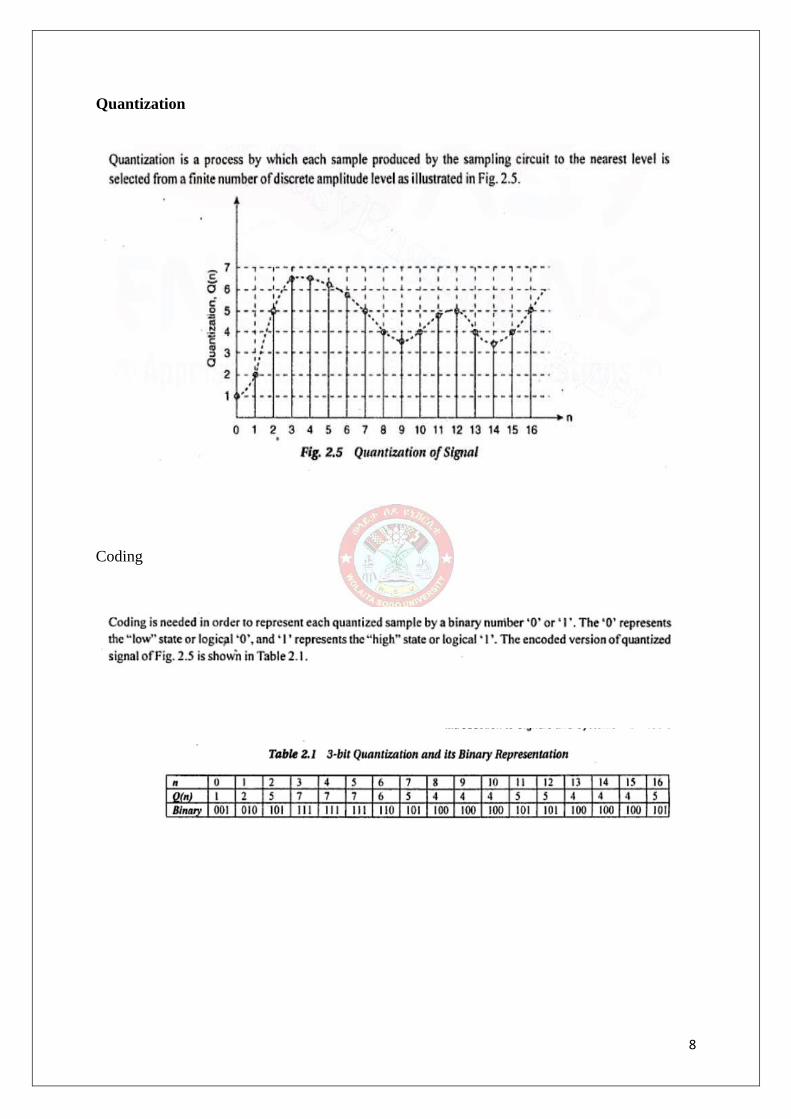
Quantization
Coding
9
10 Instructor – Ramakrishna MM
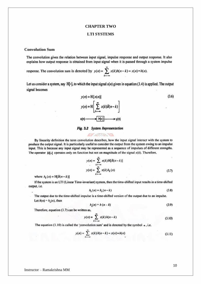
CHAPTER TWO
LTI SYSTEMS
Convolution Sum
11 Instructor – Ramakrishna MM
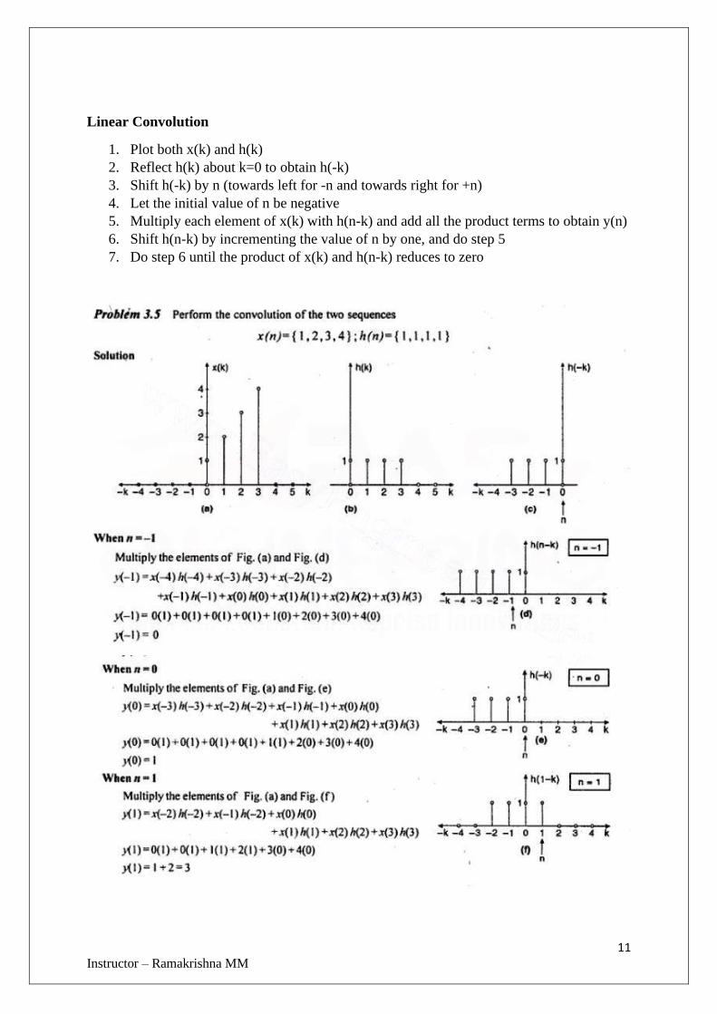
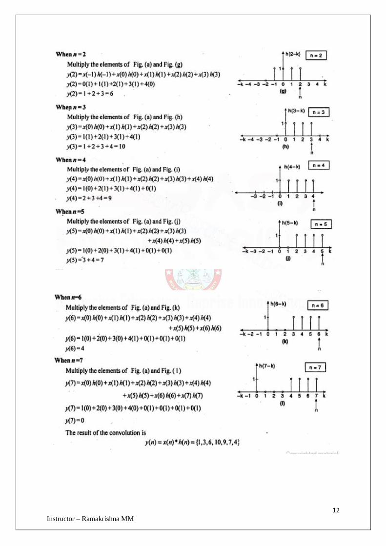
Linear Convolution
1. Plot both x(k) and h(k)
2. Reflect h(k) about k=0 to obtain h(-k)
3. Shift h(-k) by n (towards left for -n and towards right for +n)
4. Let the initial value of n be negative
5. Multiply each element of x(k) with h(n-k) and add all the product terms to obtain y(n)
6. Shift h(n-k) by incrementing the value of n by one, and do step 5
7. Do step 6 until the product of x(k) and h(n-k) reduces to zero
12 Instructor – Ramakrishna MM
13 Instructor – Ramakrishna MM
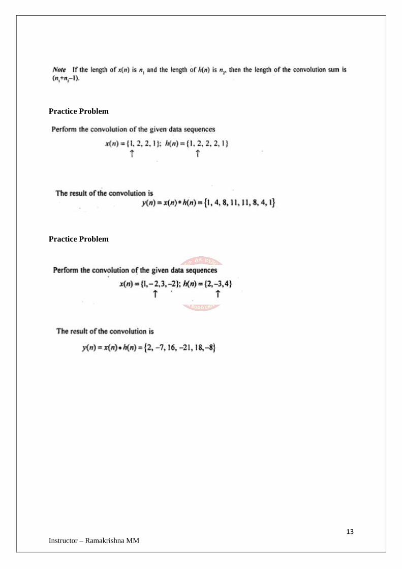
Practice Problem
Practice Problem
14 Instructor – Ramakrishna MM
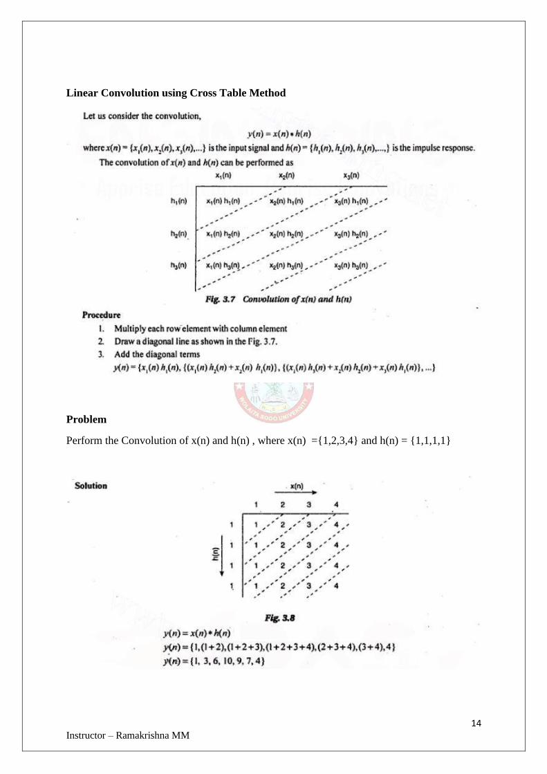
Linear Convolution using Cross Table Method
Problem
Perform the Convolution of x(n) and h(n) , where x(n) ={1,2,3,4} and h(n) = {1,1,1,1}
15 Instructor – Ramakrishna MM
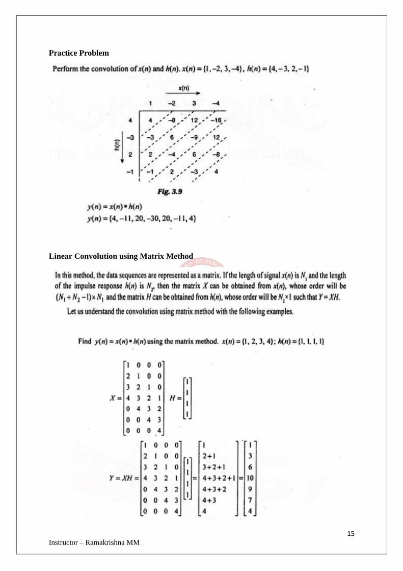
Practice Problem
Linear Convolution using Matrix Method
16 Instructor – Ramakrishna MM
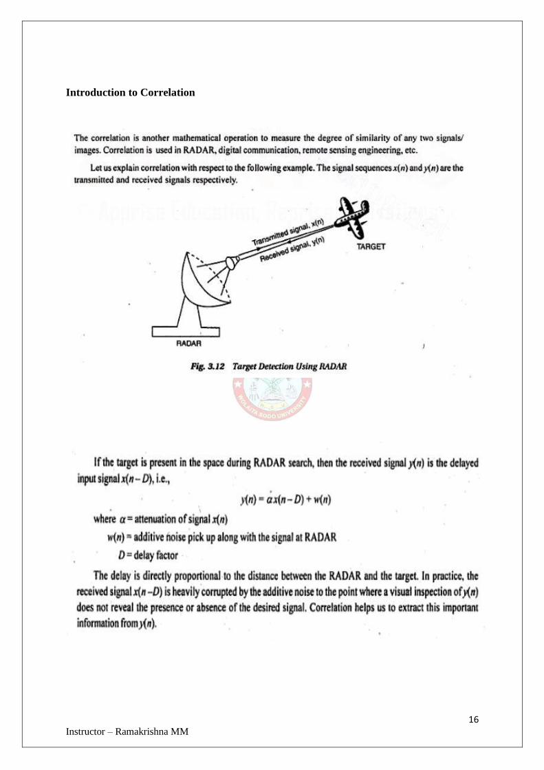
Introduction to Correlation
17 Instructor – Ramakrishna MM
Cross Correlation
Problem
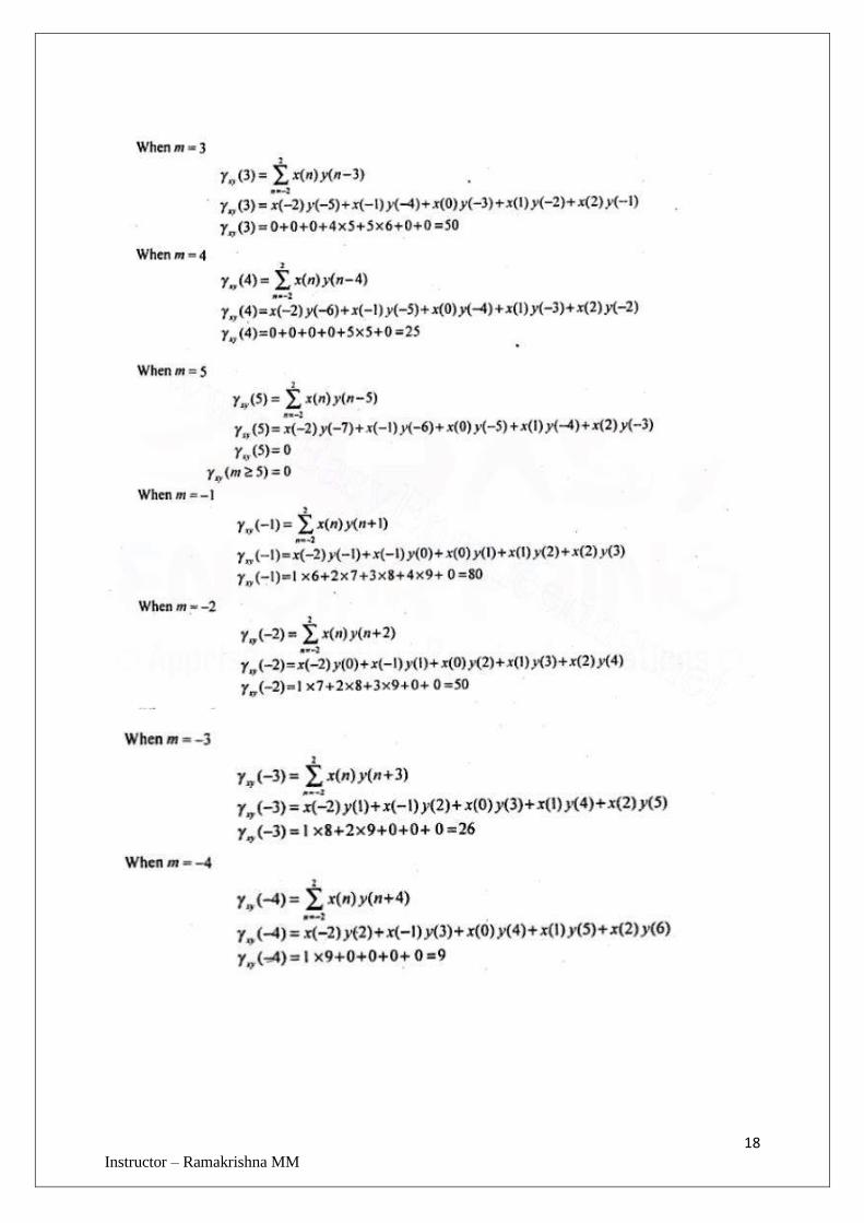
18 Instructor – Ramakrishna MM
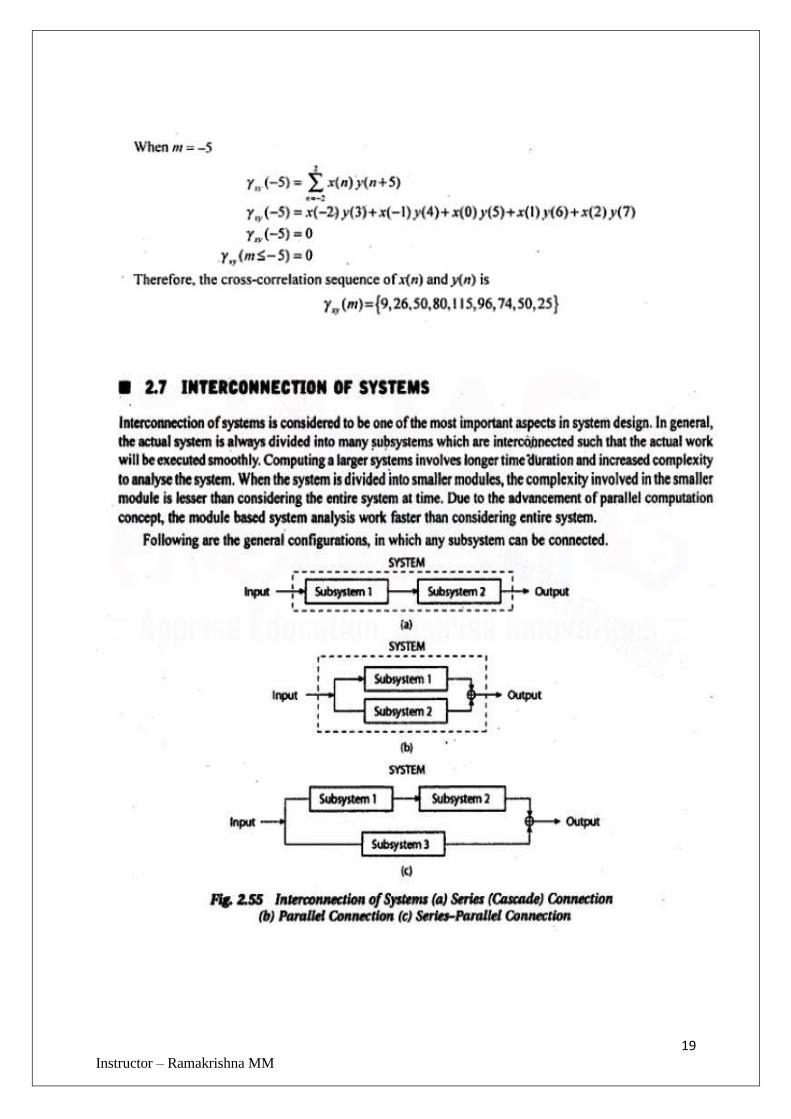
19 Instructor – Ramakrishna MM
20
CHAPTER THREE
Z TRANSFORM
The Z-transform is a powerful method for solving difference equations and, in general, to
represent discrete systems. Although applications of Z-transforms are relatively new, the
essential features of this mathematical technique date back to the early 1730s when DeMoivre
introduced the concept of a generating function that is identical with that for the Z-transform.
Recently, the development and extensive applications of the Z-transform are much enhanced
as a result of the use of digital computers.
In mathematics and signal processing, the Z-transform converts a discrete-time signal, which
is a sequence of real or complex numbers, into a complex frequency-domain representation.
It can be considered as a discrete-time equivalent of the Laplace transform
The Defination of Z Transform
The Z-transform can be defined as either a one-sided or two-sided transform.
Bilateral Z-transform
The bilateral or two-sided Z-transform of a discrete-time signal is the formal power
series defined as
X(z) = z{x(n)} = ∑ 𝑥(𝑛) 𝑧−𝑛∞𝑛=−∞
where is an integer and z is, in general, a complex number:
One sided or Single sided Z Transform
X(z) = z{x(n)} = ∑ 𝑥(𝑛) 𝑧−𝑛∞𝑛=0
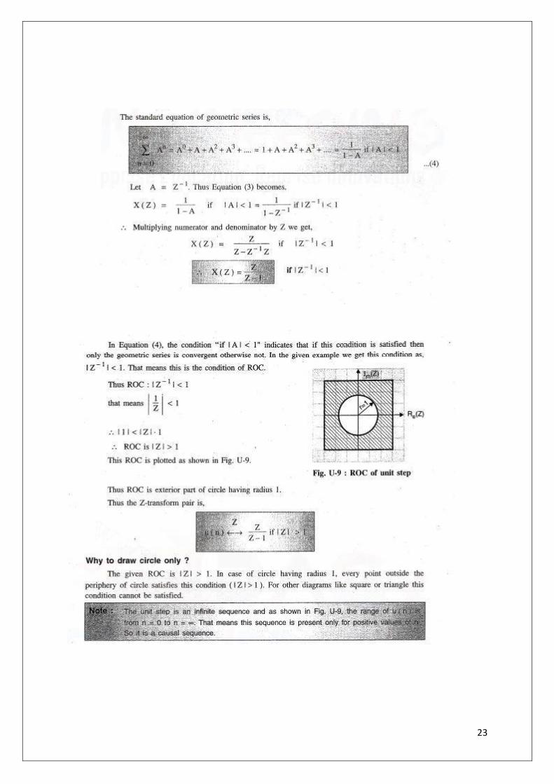
Region of Convergence
The Region of Convergence (ROC) of x(z) is all set of values of z for which x(z) attains a finite
value.
21
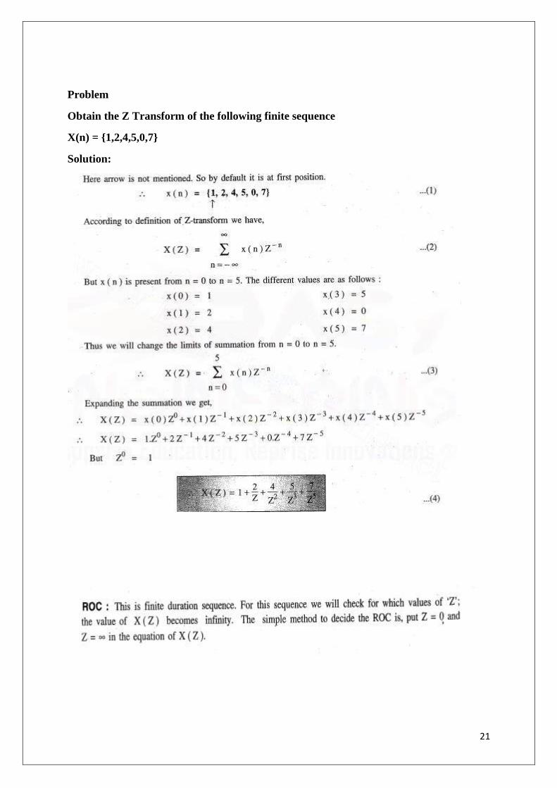
Problem
Obtain the Z Transform of the following finite sequence
X(n) = {1,2,4,5,0,7}
Solution:
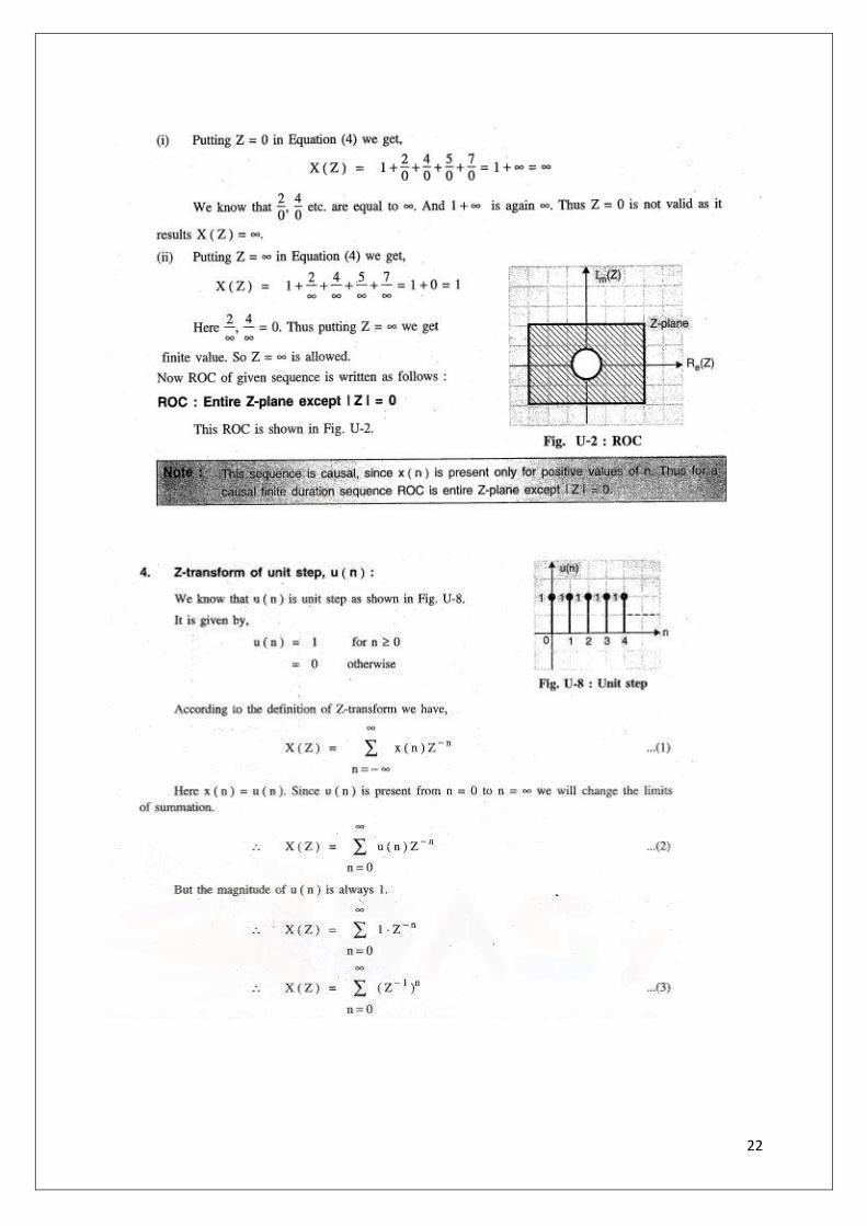
22
23

24
Problem
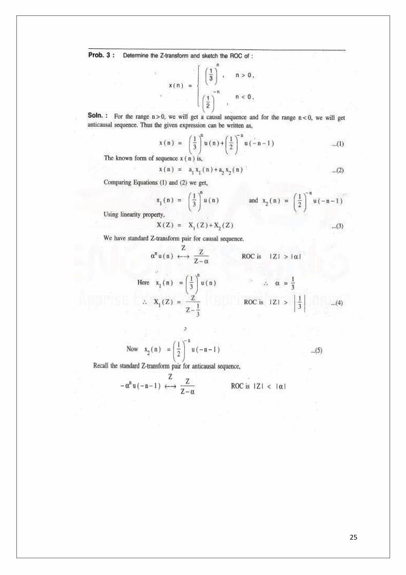
Determine the Z Transform and ROC of the signal
X(n) = [ 3(4n) – 5(3n)] u(n)
25
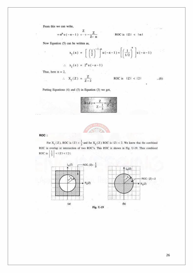
26
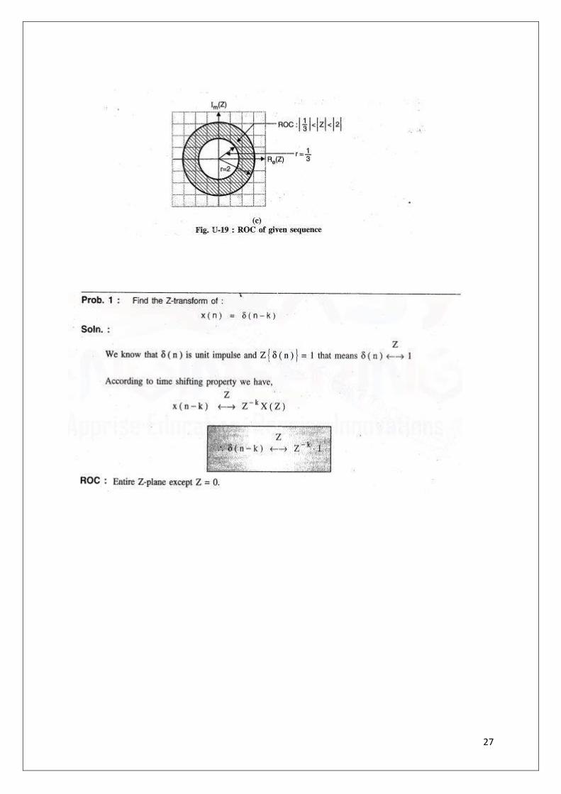
27
28
29
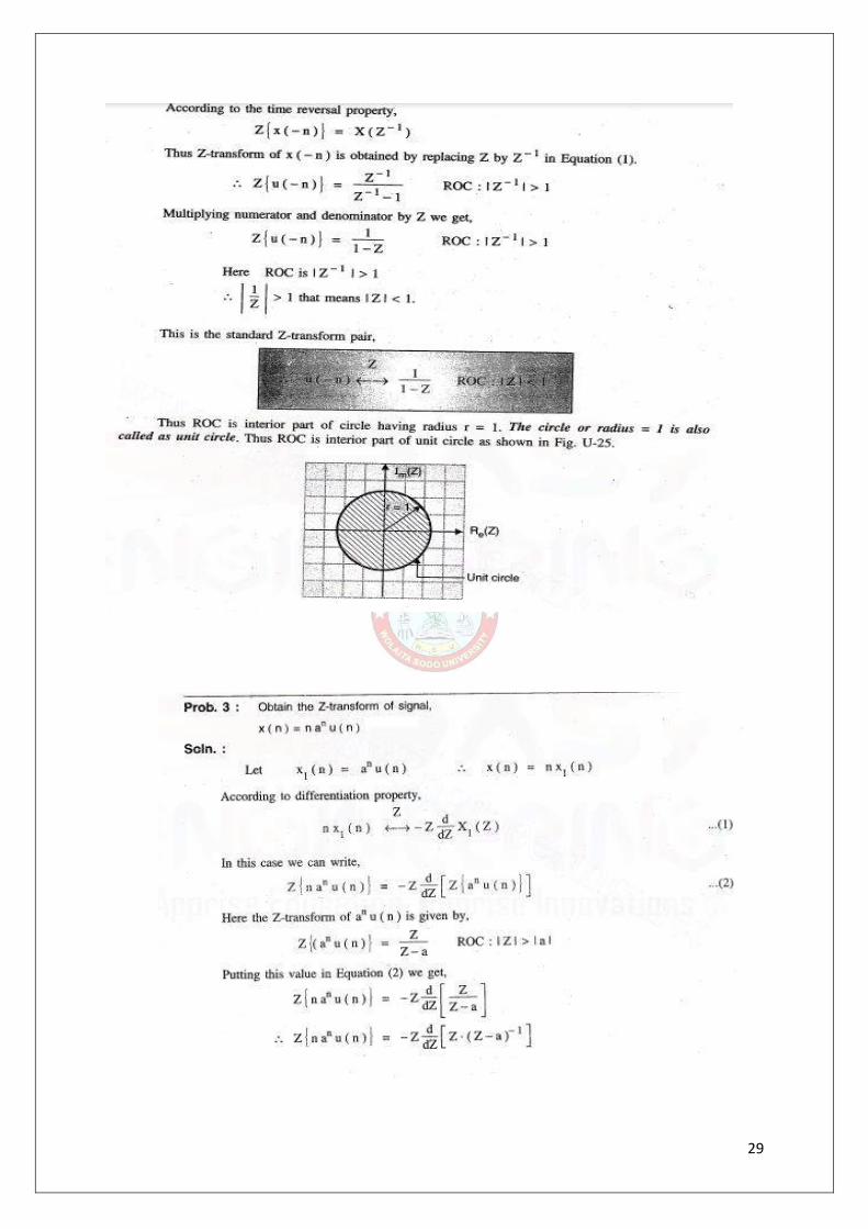
30
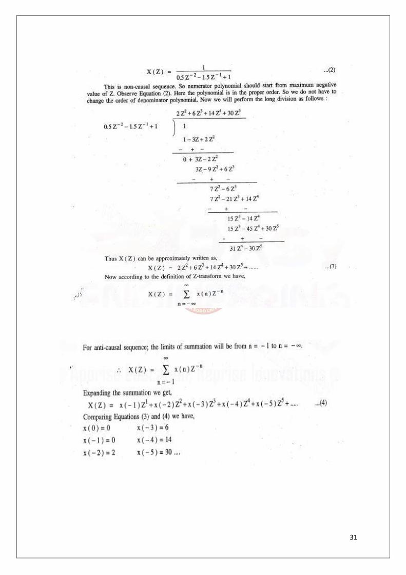
31
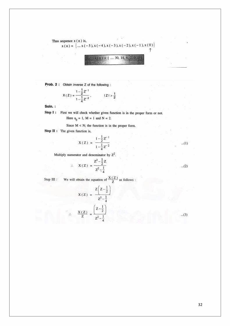
32
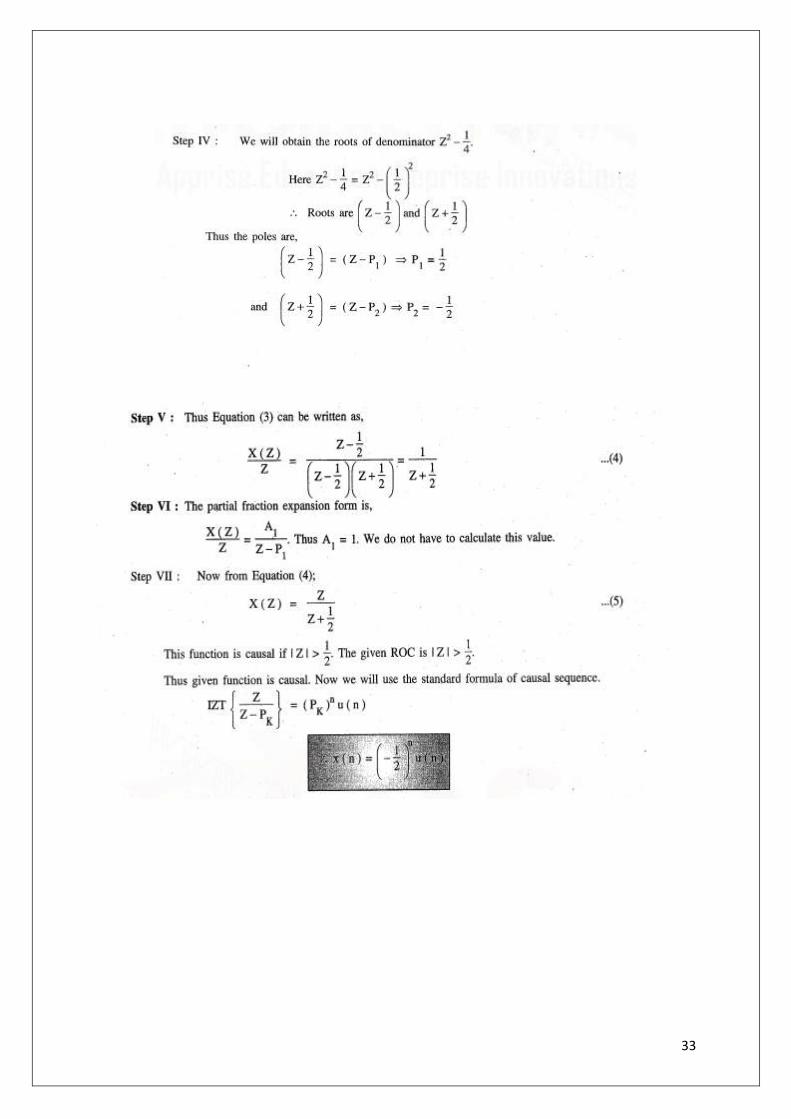
33
34
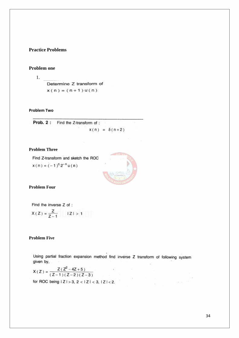
Practice Problems
Problem one
1.
Problem Two
Problem Three
Problem Four
Problem Five
35 Instructor – Ramakrishna MM
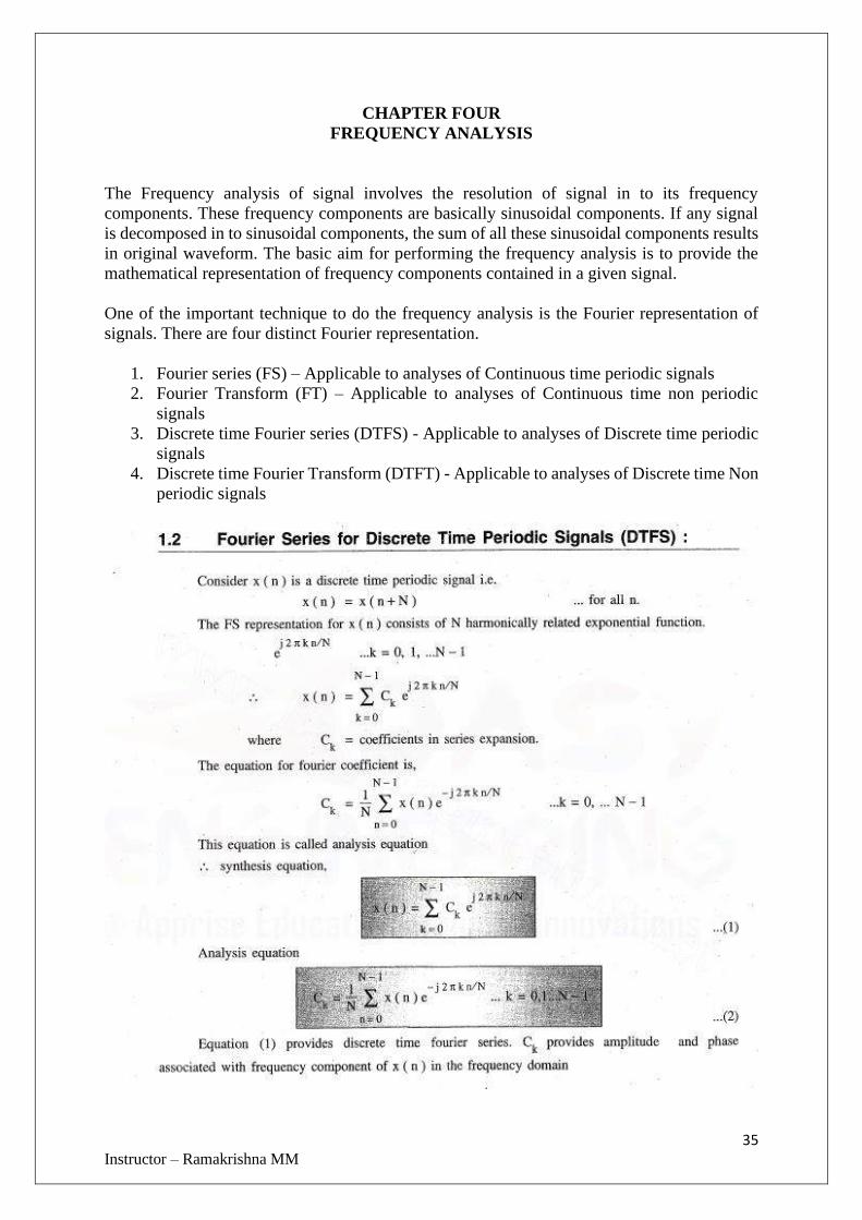
CHAPTER FOUR
FREQUENCY ANALYSIS
The Frequency analysis of signal involves the resolution of signal in to its frequency
components. These frequency components are basically sinusoidal components. If any signal
is decomposed in to sinusoidal components, the sum of all these sinusoidal components results
in original waveform. The basic aim for performing the frequency analysis is to provide the
mathematical representation of frequency components contained in a given signal.
One of the important technique to do the frequency analysis is the Fourier representation of
signals. There are four distinct Fourier representation.
1. Fourier series (FS) – Applicable to analyses of Continuous time periodic signals
2. Fourier Transform (FT) – Applicable to analyses of Continuous time non periodic
signals
3. Discrete time Fourier series (DTFS) - Applicable to analyses of Discrete time periodic
signals
4. Discrete time Fourier Transform (DTFT) - Applicable to analyses of Discrete time Non
periodic signals
36 Instructor – Ramakrishna MM
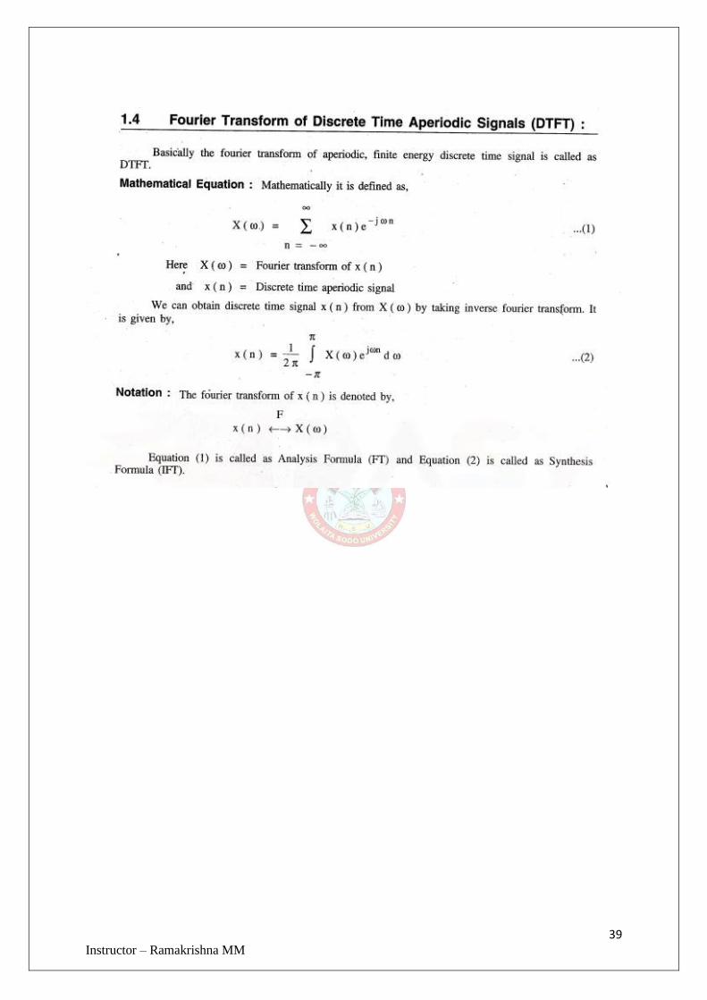
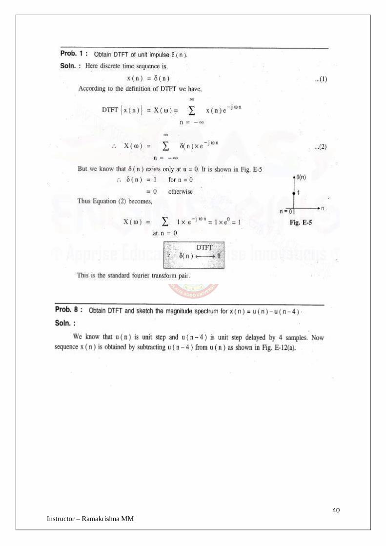
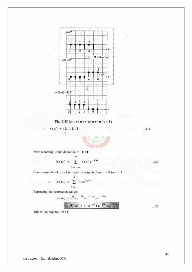
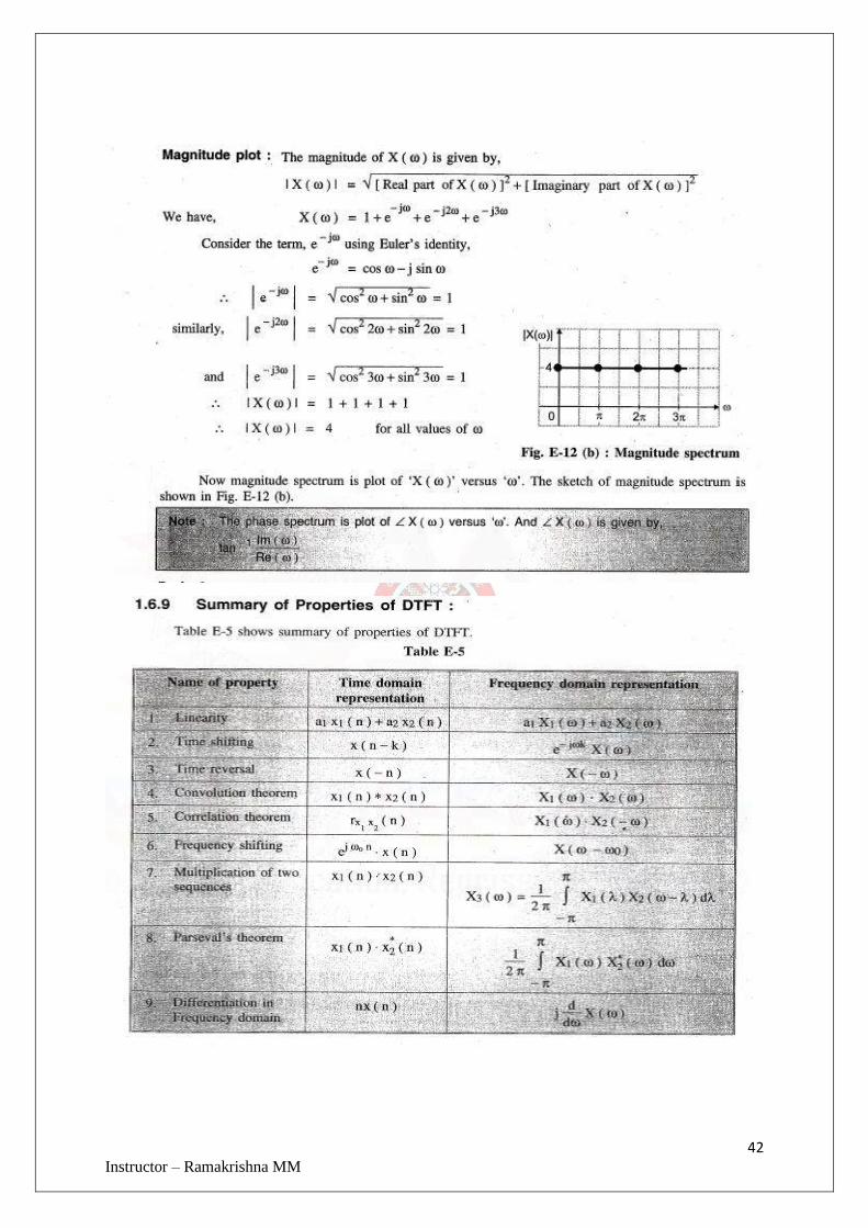
37 Instructor – Ramakrishna MM
38 Instructor – Ramakrishna MM
39 Instructor – Ramakrishna MM
40 Instructor – Ramakrishna MM
41 Instructor – Ramakrishna MM
42 Instructor – Ramakrishna MM
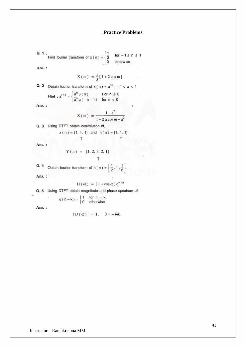
43 Instructor – Ramakrishna MM
Practice Problems
44 Instructor - Ramakrishna MM
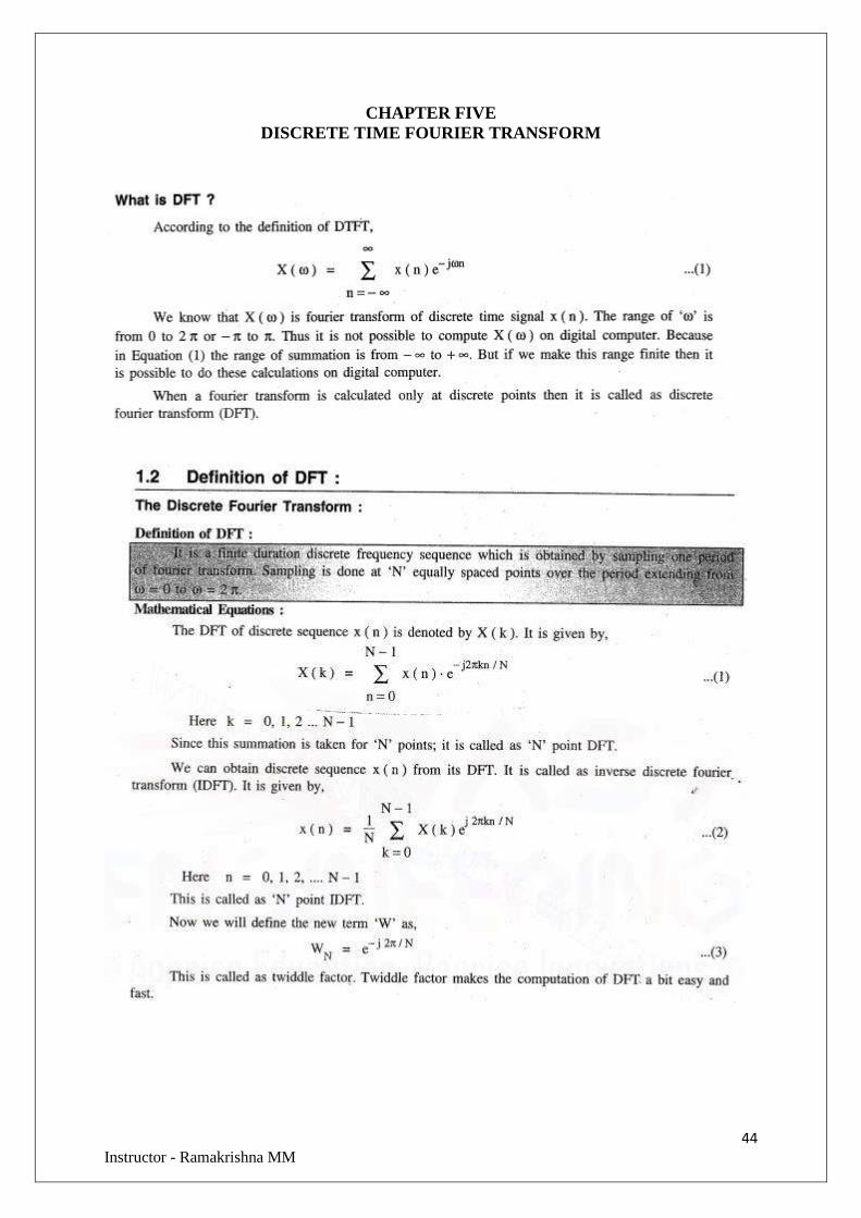
CHAPTER FIVE
DISCRETE TIME FOURIER TRANSFORM
45 Instructor - Ramakrishna MM
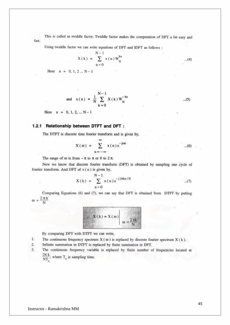
46 Instructor - Ramakrishna MM
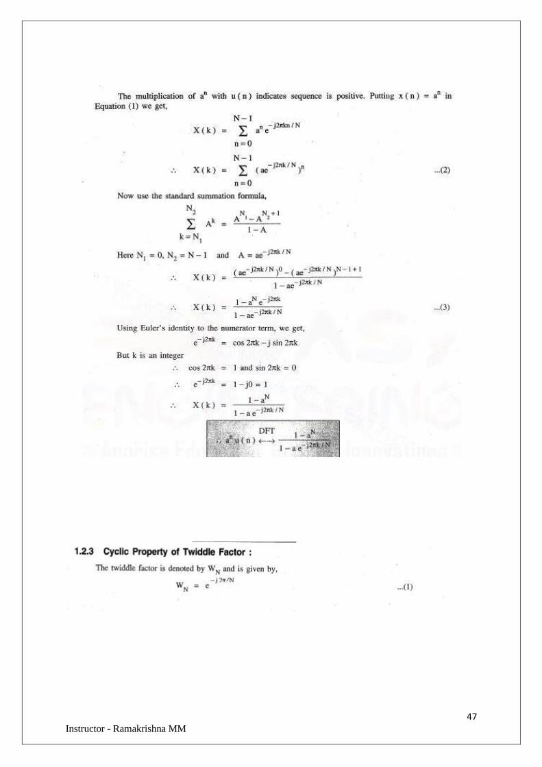
47 Instructor - Ramakrishna MM
48 Instructor - Ramakrishna MM
49 Instructor - Ramakrishna MM
50 Instructor - Ramakrishna MM
51 Instructor - Ramakrishna MM
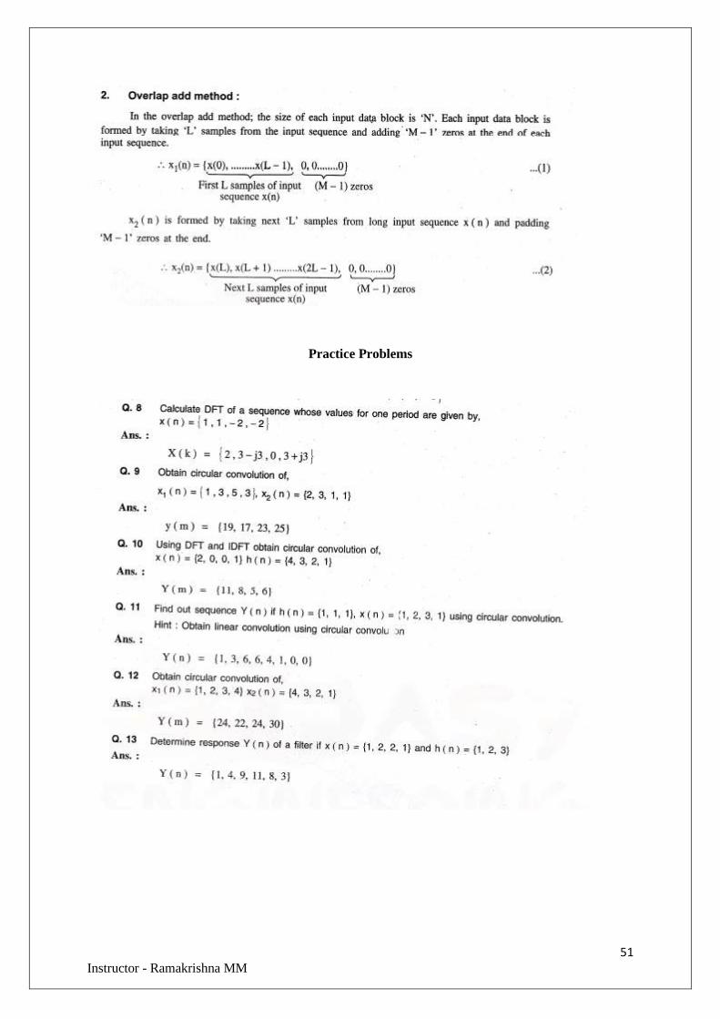
Practice Problems
52 Instructor - Ramakrishna MM
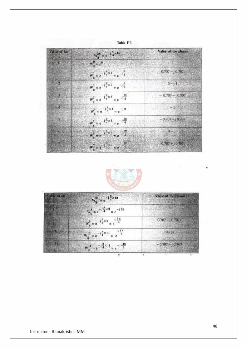
FAST FOURIER TRANSFORM
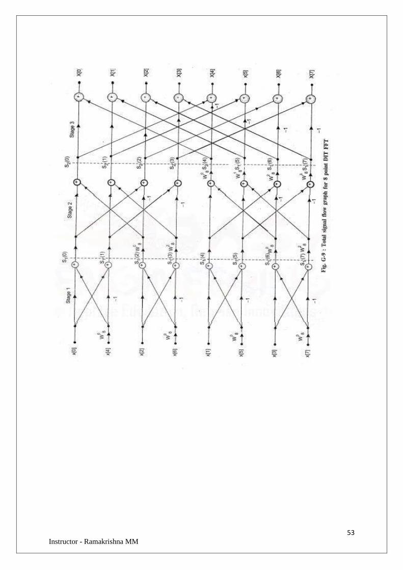
53 Instructor - Ramakrishna MM
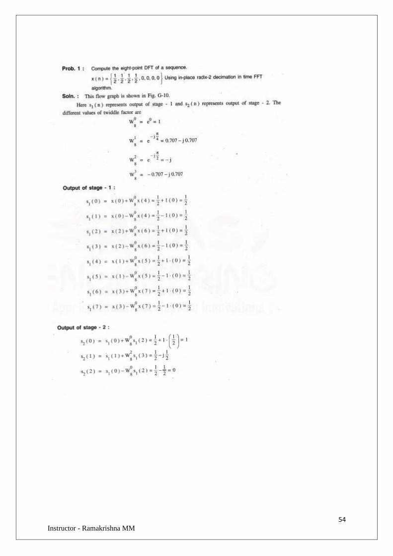
54 Instructor - Ramakrishna MM
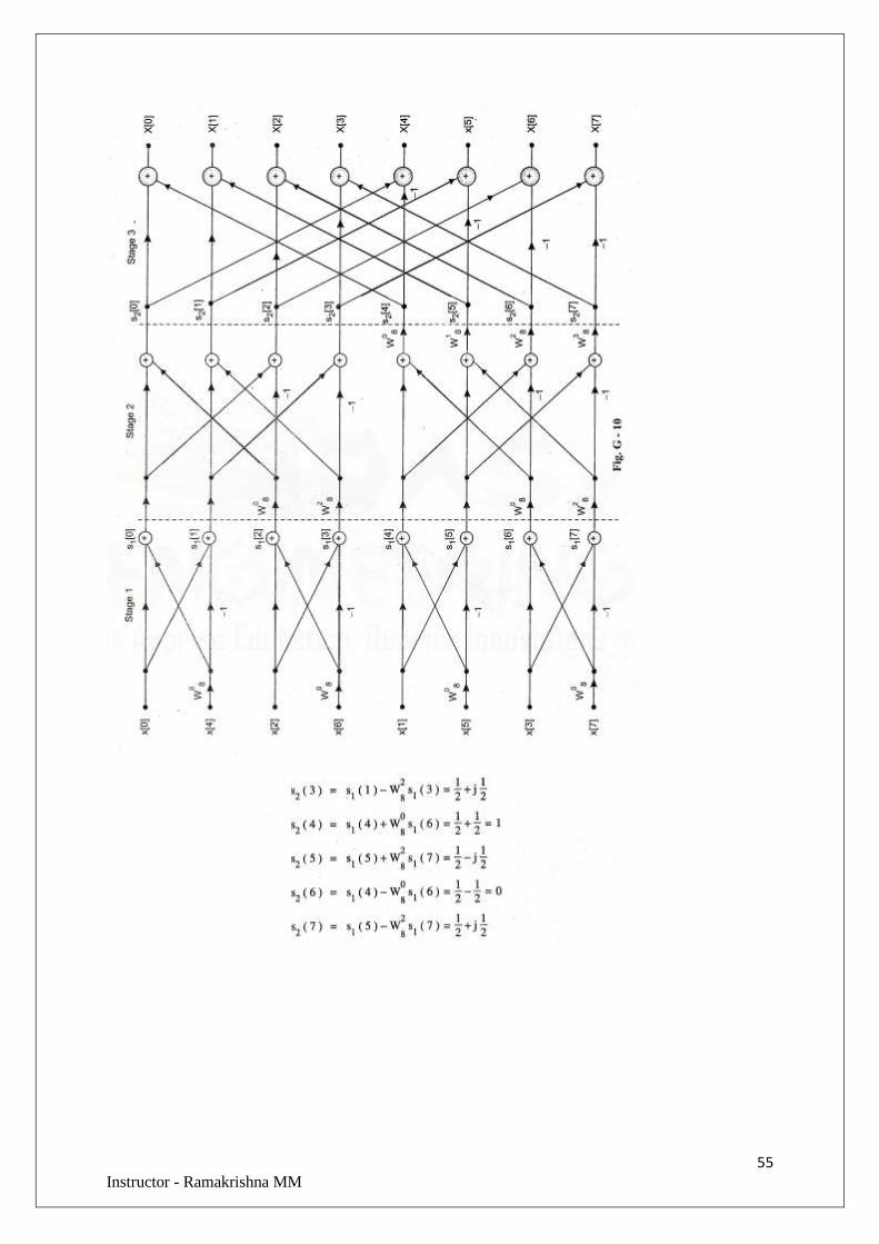
55 Instructor - Ramakrishna MM
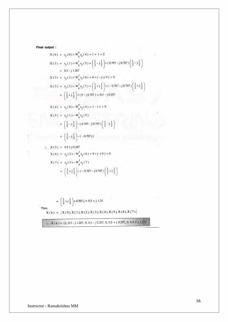
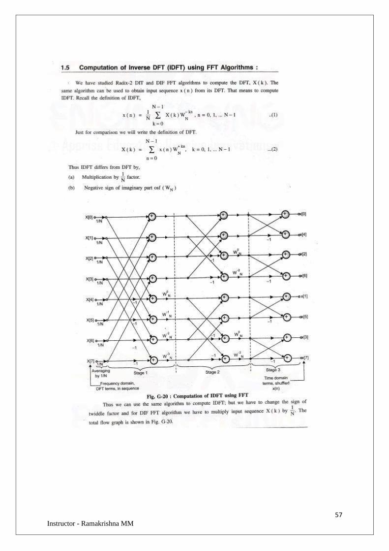
56 Instructor - Ramakrishna MM
57 Instructor - Ramakrishna MM
58 Instructor - Ramakrishna MM
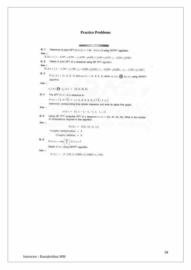
Practice Problems
59 Instructor – Ramakrishna MM
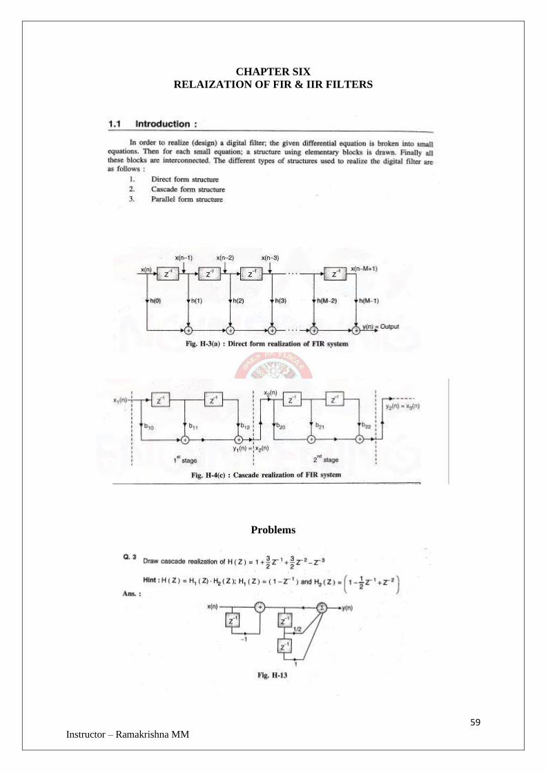
CHAPTER SIX
RELAIZATION OF FIR & IIR FILTERS
Problems
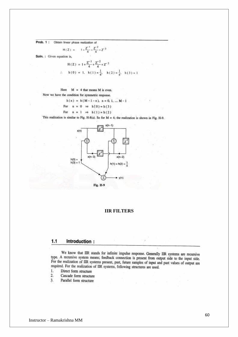
60 Instructor – Ramakrishna MM
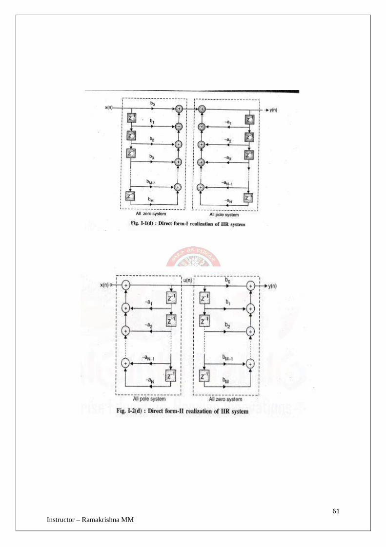
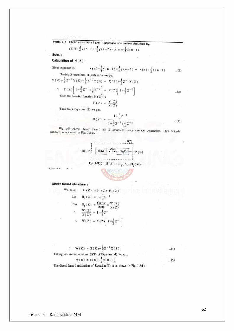
IIR FILTERS
61 Instructor – Ramakrishna MM
62 Instructor – Ramakrishna MM
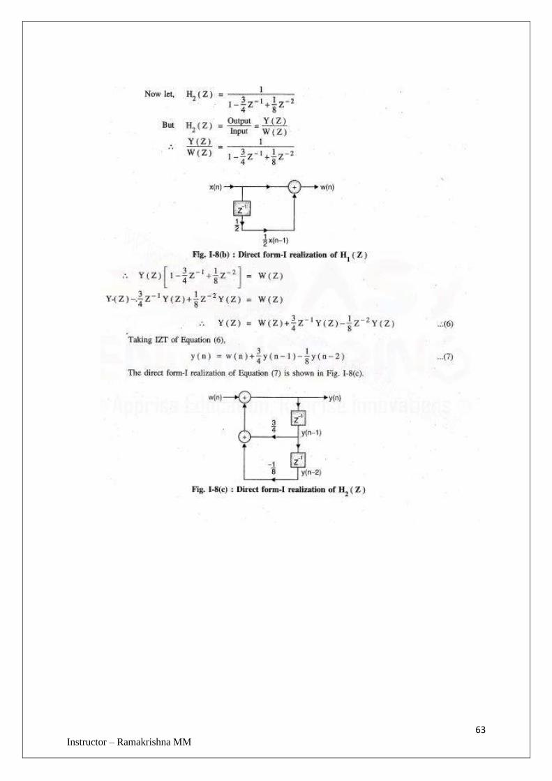
63 Instructor – Ramakrishna MM
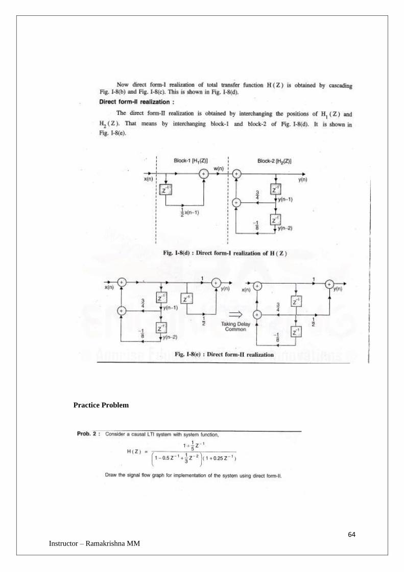
64 Instructor – Ramakrishna MM
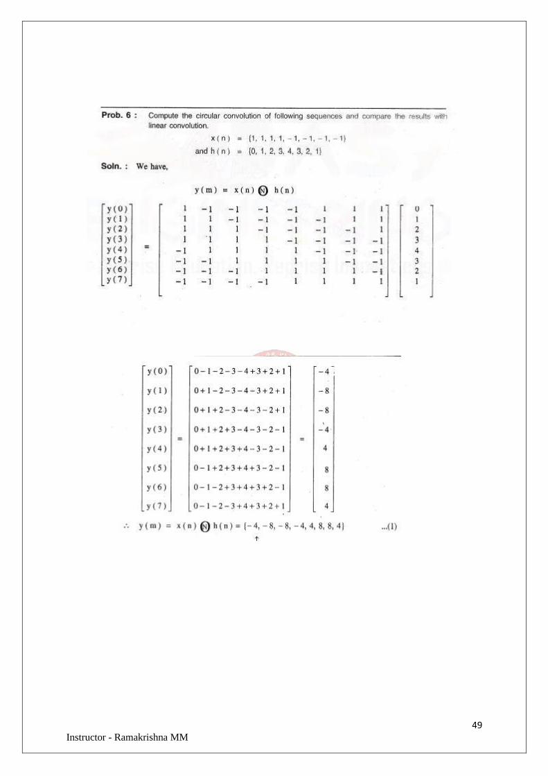
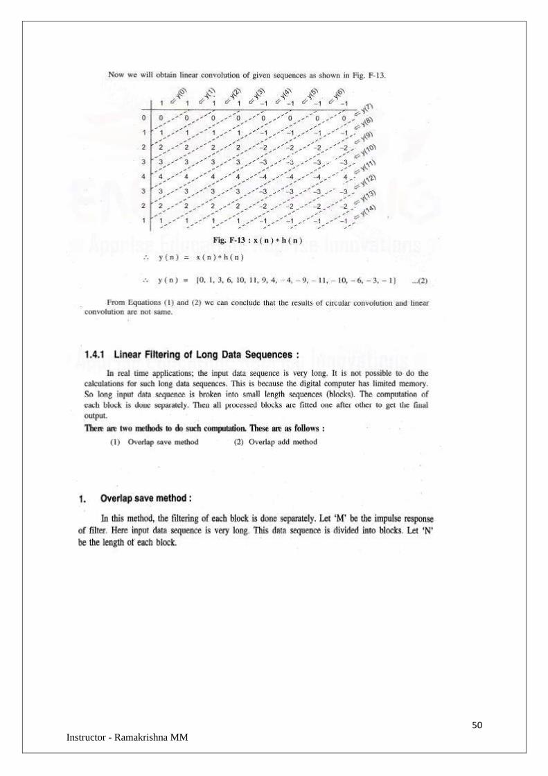
Practice Problem
65 Instructor – Ramakrishna MM
Practice Problem
Practice Problem
66 Instructor – Ramakrishna MM
FILTER DEISGN
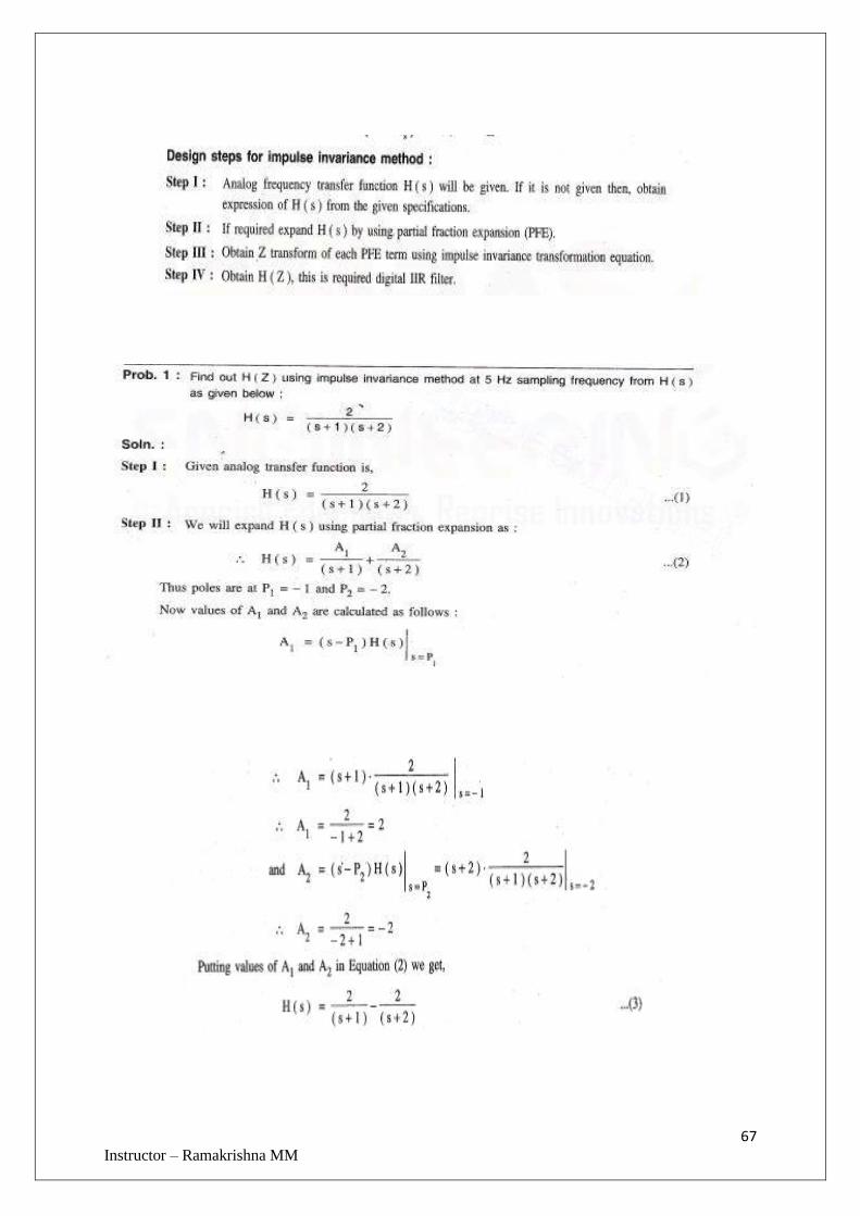
67 Instructor – Ramakrishna MM
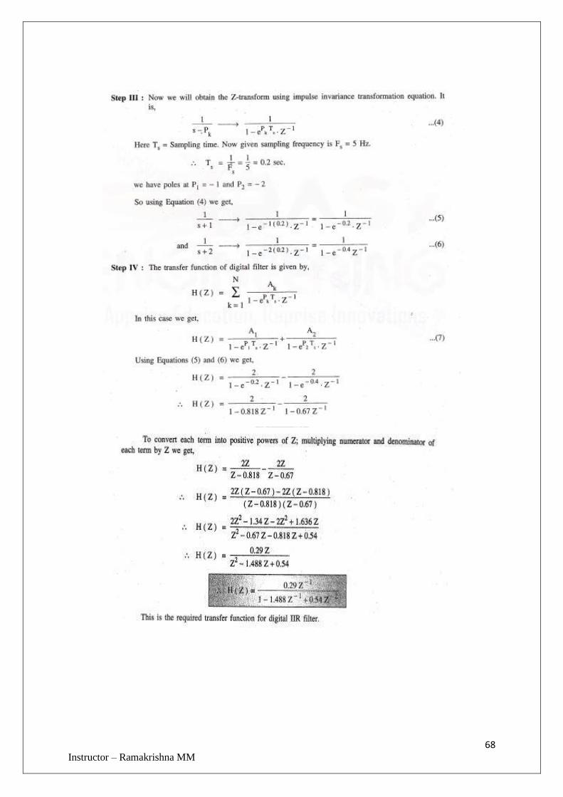
68 Instructor – Ramakrishna MM
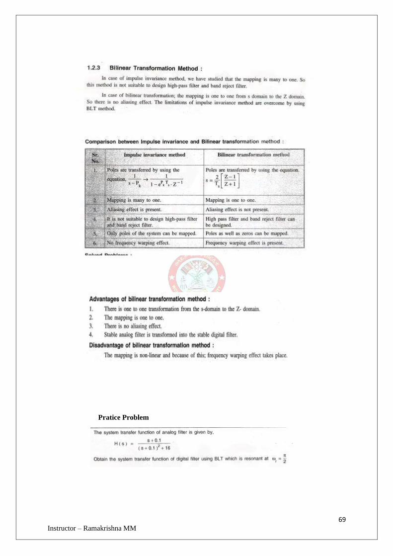
69 Instructor – Ramakrishna MM
Pratice Problem
70 Instructor – Ramakrishna MM
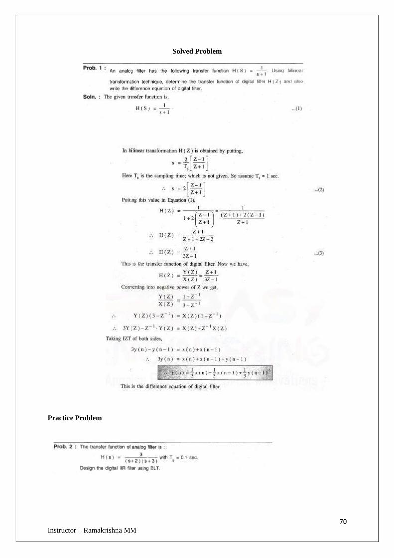
Solved Problem
Practice Problem