William S. Breffle Edward R. Morey Robert D. Rowe Donald M ...
279
RECREATIONAL FISHING DAMAGES FROM FISH CONSUMPTION ADVISORIES IN THE WATERS OF GREEN BAY William S. Breffle Edward R. Morey Robert D. Rowe Donald M. Waldman Sonya M. Wytinck Stratus Consulting Inc. 1881 9th Street, Suite 201 Boulder, Colorado 80302 (303) 381-8000 Prepared for: U.S. Fish and Wildlife Service U.S. Department of Interior U.S. Department of Justice November 1, 1999
-
Upload
khangminh22 -
Category
Documents
-
view
1 -
download
0
Transcript of William S. Breffle Edward R. Morey Robert D. Rowe Donald M ...

RECREATIONAL FISHING DAMAGES FROM FISH CONSUMPTION ADVISORIES
IN THE WATERS OF GREEN BAY
William S. BreffleEdward R. MoreyRobert D. Rowe
Donald M. WaldmanSonya M. Wytinck
Stratus Consulting Inc.1881 9th Street, Suite 201Boulder, Colorado 80302
(303) 381-8000
Prepared for:U.S. Fish and Wildlife ServiceU.S. Department of InteriorU.S. Department of Justice
November 1, 1999

William F. HartwigU.S. Fish and Wildlife Service, Regional Director and Authorized Official

CONTENTS
Figures . . . . . . . . . . . . . . . . . . . . . . . . . . . . . . . . . . . . . . . . . . . . . . . . . . . . . . . . . . . . . . . . . . . vTables . . . . . . . . . . . . . . . . . . . . . . . . . . . . . . . . . . . . . . . . . . . . . . . . . . . . . . . . . . . . . . . . . . . viiAcronyms . . . . . . . . . . . . . . . . . . . . . . . . . . . . . . . . . . . . . . . . . . . . . . . . . . . . . . . . . . . . . . . . xi
Chapter 1 Introduction
1.1 Introduction . . . . . . . . . . . . . . . . . . . . . . . . . . . . . . . . . . . . . . . . . . . . . . . . . . 1-11.2 Scope of the Recreational Fishing Assessment . . . . . . . . . . . . . . . . . . . . . . . . 1-31.3 The Damage Assessment Approach . . . . . . . . . . . . . . . . . . . . . . . . . . . . . . . . 1-61.4 Primary Data Collection . . . . . . . . . . . . . . . . . . . . . . . . . . . . . . . . . . . . . . . . . 1-71.5 Summary of Analysis and Results . . . . . . . . . . . . . . . . . . . . . . . . . . . . . . . . . 1-10
Chapter 2 Background
2.1 Recreational Fishing in the Waters of Green Bay . . . . . . . . . . . . . . . . . . . . . . . 2-12.2 Overview of FCAs in the Assessment Area . . . . . . . . . . . . . . . . . . . . . . . . . . . 2-92.3 Impacts from FCAs . . . . . . . . . . . . . . . . . . . . . . . . . . . . . . . . . . . . . . . . . . . 2-182.4 Economic Values . . . . . . . . . . . . . . . . . . . . . . . . . . . . . . . . . . . . . . . . . . . . . 2-21
Chapter 3 Primary Data Collection
3.1 Introduction . . . . . . . . . . . . . . . . . . . . . . . . . . . . . . . . . . . . . . . . . . . . . . . . . . 3-13.2 Sampling Plan . . . . . . . . . . . . . . . . . . . . . . . . . . . . . . . . . . . . . . . . . . . . . . . . . 3-2
3.2.1 Selection of Target Population . . . . . . . . . . . . . . . . . . . . . . . . . . . . . . 3-23.2.2 Sample Collection at County Courthouses . . . . . . . . . . . . . . . . . . . . . . 3-6
3.3 Telephone Survey . . . . . . . . . . . . . . . . . . . . . . . . . . . . . . . . . . . . . . . . . . . . . . 3-83.3.1 Telephone Survey Instrument . . . . . . . . . . . . . . . . . . . . . . . . . . . . . . . 3-83.3.2 Telephone Survey Implementation . . . . . . . . . . . . . . . . . . . . . . . . . . 3-10
3.4 Mail Survey . . . . . . . . . . . . . . . . . . . . . . . . . . . . . . . . . . . . . . . . . . . . . . . . . 3-143.4.1 Mail Survey Instrument . . . . . . . . . . . . . . . . . . . . . . . . . . . . . . . . . . . 3-143.4.2 Mail Survey Implementation . . . . . . . . . . . . . . . . . . . . . . . . . . . . . . . 3-18
3.5 Sample Evaluation . . . . . . . . . . . . . . . . . . . . . . . . . . . . . . . . . . . . . . . . . . . . 3-203.5.1 Sample Bias . . . . . . . . . . . . . . . . . . . . . . . . . . . . . . . . . . . . . . . . . . . 3-203.5.2 Nonresponse Bias . . . . . . . . . . . . . . . . . . . . . . . . . . . . . . . . . . . . . . . 3-253.5.3 Recall Bias . . . . . . . . . . . . . . . . . . . . . . . . . . . . . . . . . . . . . . . . . . . . 3-29

ii
3.5.4 Adjusting the Sample Estimates to the Population Estimates . . . . . . . 3-303.5.5 Target Population Coverage of All Open-Water Fishing in the
Wisconsin Waters of Green Bay . . . . . . . . . . . . . . . . . . . . . . . . . . . . 3-33
Chapter 4 Green Bay Angler Profile
4.1 Introduction . . . . . . . . . . . . . . . . . . . . . . . . . . . . . . . . . . . . . . . . . . . . . . . . . . 4-14.2 Green Bay Fishing Activity and Expenditures . . . . . . . . . . . . . . . . . . . . . . . . . 4-24.3 Overall Attitudes about the Green Bay Recreational Fishery . . . . . . . . . . . . . 4-114.4 Awareness of FCAs . . . . . . . . . . . . . . . . . . . . . . . . . . . . . . . . . . . . . . . . . . . 4-144.5 Impacts of FCAs . . . . . . . . . . . . . . . . . . . . . . . . . . . . . . . . . . . . . . . . . . . . . 4-15
Chapter 5 The Green Bay Choice Questions
5.1 Introduction . . . . . . . . . . . . . . . . . . . . . . . . . . . . . . . . . . . . . . . . . . . . . . . . . . 5-15.2 Choice Questions Are Well Established for Estimating Tradeoffs . . . . . . . . . . 5-35.3 Valuation and the Use of Choice Questions . . . . . . . . . . . . . . . . . . . . . . . . . . 5-55.4 The Green Bay Choice Pairs . . . . . . . . . . . . . . . . . . . . . . . . . . . . . . . . . . . . . . 5-6
5.4.1 Choice Set Characteristics . . . . . . . . . . . . . . . . . . . . . . . . . . . . . . . . . . 5-95.4.2 Selection of Choice Sets . . . . . . . . . . . . . . . . . . . . . . . . . . . . . . . . . . 5-14
5.5 Evaluation of Choices across Alternatives . . . . . . . . . . . . . . . . . . . . . . . . . . . 5-155.6 The Expected Days Followup Question to Each Choice Pair . . . . . . . . . . . . . 5-21
Chapter 6 A Combined Revealed Preference and Stated Preference Model ofGreen Bay Fishing
6.1 Introduction . . . . . . . . . . . . . . . . . . . . . . . . . . . . . . . . . . . . . . . . . . . . . . . . . . 6-16.2 Factors Affecting Utility from Fishing Green Bay . . . . . . . . . . . . . . . . . . . . . . 6-26.3 Factors Affecting Utility from Fishing Elsewhere . . . . . . . . . . . . . . . . . . . . . . 6-46.4 Estimation of the Model . . . . . . . . . . . . . . . . . . . . . . . . . . . . . . . . . . . . . . . . . 6-5
Chapter 7 The Estimated Model
7.1 Introduction . . . . . . . . . . . . . . . . . . . . . . . . . . . . . . . . . . . . . . . . . . . . . . . . . . 7-17.2 Signs and Significance of the Parameter Estimates . . . . . . . . . . . . . . . . . . . . . 7-17.3 Measures of Model Fit . . . . . . . . . . . . . . . . . . . . . . . . . . . . . . . . . . . . . . . . . . 7-27.4 Changes in Green Bay Fishing from Changes in FCAs . . . . . . . . . . . . . . . . . . . 7-3
Chapter 8 Lower-Bound Estimates of 1998 Damages
8.1 Introduction . . . . . . . . . . . . . . . . . . . . . . . . . . . . . . . . . . . . . . . . . . . . . . . . . . 8-18.2 WTP per Year, per Fishing Day, and per Green Bay Fishing Day . . . . . . . . . . 8-1

iii
8.3 Two Lower-Bound Estimates of Total 1998 Damages for Open-WaterFishing in the Wisconsin Waters of Green Bay . . . . . . . . . . . . . . . . . . . . . . . . 8-5
8.4 Benefits Transfer to Estimate the Damages Associated with the Green Bay Ice Fishery and the Michigan Green Bay Fishery . . . . . . . . . . . . . . . . . . . . . . . 8-7
Chapter 9 Testing the Sensitivity of the WTP Estimates to Modifications to the Model
9.1 Introduction . . . . . . . . . . . . . . . . . . . . . . . . . . . . . . . . . . . . . . . . . . . . . . . . . . 9-19.2 A-B Models . . . . . . . . . . . . . . . . . . . . . . . . . . . . . . . . . . . . . . . . . . . . . . . . . . 9-2
9.2.1 A-B Models with Homogenous Preferences . . . . . . . . . . . . . . . . . . . . 9-39.2.2 A-B Models with Classic Heterogeneity . . . . . . . . . . . . . . . . . . . . . . . 9-39.2.3 A-B Models with Random Heterogeneity . . . . . . . . . . . . . . . . . . . . . . 9-4
9.3 Heterogeneity in Models Allowing Substitution . . . . . . . . . . . . . . . . . . . . . . . 9-5
Chapter 10 Total Recreational Fishing Damages and Conclusions
10.1 Introduction . . . . . . . . . . . . . . . . . . . . . . . . . . . . . . . . . . . . . . . . . . . . . . . . . 10-110.2 Total Recreational Fishing Damages through Time . . . . . . . . . . . . . . . . . . . . 10-1
10.2.1 Damages for Past Losses . . . . . . . . . . . . . . . . . . . . . . . . . . . . . . . . . . 10-110.2.2 Damages for Future Service Flow Losses . . . . . . . . . . . . . . . . . . . . . 10-710.2.3 Total Recreational Fishing Damages . . . . . . . . . . . . . . . . . . . . . . . . . 10-9
10.3 Conclusions . . . . . . . . . . . . . . . . . . . . . . . . . . . . . . . . . . . . . . . . . . . . . . . . . 10-9
Chapter 11 References . . . . . . . . . . . . . . . . . . . . . . . . . . . . . . . . . . . . . . . . . . . . . . . . . . 11-1
Appendices
A Modeling Consumer Preferences for Green Bay Fishing Days and Fishing DaysUsing Stated and Revealed Preference Data
B EstimationC Estimated Compensating Variations and Expected Compensating VariationsD Model VariationsE Survey InstrumentsF Supporting Data

FIGURES
1-1 Wisconsin and Michigan Waters of Green Bay . . . . . . . . . . . . . . . . . . . . . . . . . . . . . . 1-41-2 Example Choice Question . . . . . . . . . . . . . . . . . . . . . . . . . . . . . . . . . . . . . . . . . . . . . 1-9
3-1 The Eight Targeted Counties . . . . . . . . . . . . . . . . . . . . . . . . . . . . . . . . . . . . . . . . . . . 3-33-2 Lake Michigan District of Wisconsin . . . . . . . . . . . . . . . . . . . . . . . . . . . . . . . . . . . . . 3-4
4-1 Distribution of Reported Number of Open-Water Fishing Days on Wisconsin Watersof Green Bay in 1998, for All Mail Survey Respondents . . . . . . . . . . . . . . . . . . . . . . . 4-4
4-2 How Often Anglers Target a Specific Species on Green Bay . . . . . . . . . . . . . . . . . . . 4-74-3 Percent of Green Bay Fishing Days Spent on a Boat . . . . . . . . . . . . . . . . . . . . . . . . . . 4-94-4 Quality of Green Bay Relative to Other Places Respondent Fishes . . . . . . . . . . . . . . 4-11
5-1 Example Choice Question . . . . . . . . . . . . . . . . . . . . . . . . . . . . . . . . . . . . . . . . . . . . . 5-8
TABLES
1-1 1998 per Day and per Angler Damages for Open-Water Fishing in the WisconsinWaters of Green Bay . . . . . . . . . . . . . . . . . . . . . . . . . . . . . . . . . . . . . . . . . . . . . . . . 1-11
1-2 Total Values for Recreational Fishing Service Losses for the Waters of Green BayResulting from Fish Consumption Advisories for PCBs . . . . . . . . . . . . . . . . . . . . . . 1-12
2-1 Hours of Fishing Effort on the Michigan and Wisconsin Waters ofGreen Bay: 1990-1998 . . . . . . . . . . . . . . . . . . . . . . . . . . . . . . . . . . . . . . . . . . . . . . . . 2-3
2-2 Open-Water Fishing Hours on the Fox River from Its Mouth to the Dam atDePere: 1990-1998 . . . . . . . . . . . . . . . . . . . . . . . . . . . . . . . . . . . . . . . . . . . . . . . . . . 2-4
2-3 Ice-Fishing Hours on the Wisconsin Waters of Green Bay: 1990-1998 . . . . . . . . . . . . 2-42-4 Percent of Total Catch by Species for the Wisconsin Waters of Green Bay
and Lake Michigan: 1990-1998 . . . . . . . . . . . . . . . . . . . . . . . . . . . . . . . . . . . . . . . . . 2-52-5 Percent of Open-Water Catch on Wisconsin Waters of Green Bay by
Species: 1986-1998 . . . . . . . . . . . . . . . . . . . . . . . . . . . . . . . . . . . . . . . . . . . . . . . . . . 2-62-6 Percent of Targeted Open-Water Angling Hours on Wisconsin Waters
of Green Bay by Species: 1986-1998 . . . . . . . . . . . . . . . . . . . . . . . . . . . . . . . . . . . . . 2-72-7 Percent of Catch on Michigan Waters of Green Bay by Species: 1985-1998 . . . . . . . . 2-82-8 Fish Consumption Advisories for the Wisconsin Waters of Green Bay: 1976-1999 . . 2-112-9 Fish Consumption Advisories for the Lower Fox River between Green Bay
and the Dam at DePere . . . . . . . . . . . . . . . . . . . . . . . . . . . . . . . . . . . . . . . . . . . . . . 2-142-10 1998 Wisconsin FCAs for Green Bay and Fox River, and Michigan FCAs
for Lower Green Bay, Upper Green Bay, and Little Bay de Noc . . . . . . . . . . . . . . . . 2-152-11 State of Michigan Fish Consumption Advisories for Green Bay South
of Cedar River: 1988-1997 . . . . . . . . . . . . . . . . . . . . . . . . . . . . . . . . . . . . . . . . . . . . 2-172-12 State of Michigan Fish Consumption Advisories for Little Bay de Noc: 1989-1997 . 2-182-13 Studies of Behavioral Responses by Anglers to Fish Consumption Advisories . . . . . 2-192-14 Selected Valuation Studies for Changes on Catch Rates . . . . . . . . . . . . . . . . . . . . . . 2-232-15 Selected Valuation Studies for the Reduction of Toxins at Fishing Sites . . . . . . . . . . 2-24
3-1 Percent of Boat Anglers from Lake Michigan District Counties Choosing theFox River or Green Bay as Their Most Frequently Visited Site . . . . . . . . . . . . . . . . . . 3-5
3-2 1997-1998 Angling License Samples Obtained . . . . . . . . . . . . . . . . . . . . . . . . . . . . . . 3-73-3 Timeline for Sampling of Licenses by County . . . . . . . . . . . . . . . . . . . . . . . . . . . . . . . 3-73-4 1997-1998 Angling License Sample Obtained . . . . . . . . . . . . . . . . . . . . . . . . . . . . . . . 3-93-5 Proportion of Starting Sample with Available Phone Number . . . . . . . . . . . . . . . . . . 3-113-6 Disposition of Telephone Survey Sample . . . . . . . . . . . . . . . . . . . . . . . . . . . . . . . . . 3-123-7 Disposition of Sample by County Where License Purchased . . . . . . . . . . . . . . . . . . . 3-13

viii
3-8 Telephone Survey Respondent Green Bay Fishing Activity in 1998 . . . . . . . . . . . . . 3-133-9 Recreation Survey Pretesting Steps . . . . . . . . . . . . . . . . . . . . . . . . . . . . . . . . . . . . . 3-153-10 Disposition of Mail Survey Sample . . . . . . . . . . . . . . . . . . . . . . . . . . . . . . . . . . . . . . 3-203-11 Mean Fishing Days to All Sites in 1998 by Green Bay Experience . . . . . . . . . . . . . . 3-223-12 Socioeconomic Profile by Green Bay Experience . . . . . . . . . . . . . . . . . . . . . . . . . . . 3-233-13 Importance Rating of 10 Actions to Improve Wisconsin Fishing . . . . . . . . . . . . . . . . 3-243-14 Fishing Days in 1998: Mail Respondents versus Nonrespondents . . . . . . . . . . . . . . . 3-273-15 Importance Rating of 10 Actions to Improve Wisconsin Fishing: Mail Survey
Respondents versus Nonrespondents . . . . . . . . . . . . . . . . . . . . . . . . . . . . . . . . . . . . 3-283-16 Adjustment from the Mail Sample Estimated Open-Water Fishing Days
to the Population Estimated Open-Water Fishing Days in 1998 for Anglers Activein Open-Water Fishing on the Wisconsin Waters of Green Bay . . . . . . . . . . . . . . . . . 3-31
3-17 1998 Green Bay Angler Incidence Rate by County Where License Purchased . . . . . . 3-343-18 Number and Percent of Sampled 1998 Green Bay Angler Fishing Days by
Resident State/County . . . . . . . . . . . . . . . . . . . . . . . . . . . . . . . . . . . . . . . . . . . . . . . 3-353-19 Mean Days Fishing Green Bay in 1998 by Resident State . . . . . . . . . . . . . . . . . . . . . 3-36
4-1 Number of Days Fishing in 1998 by Mail Survey Respondents . . . . . . . . . . . . . . . . . . 4-34-2 Total Number of Reported Fishing Days on Wisconsin Waters of Green Bay in
1998, by Residence, for Mail Survey Respondents . . . . . . . . . . . . . . . . . . . . . . . . . . . 4-54-3 Number of Reported Fishing Days on the Fox River between the Mouth and
DePere Dam as Compared to All Wisconsin Waters of Green Bay in1998, for Mail Survey Respondents . . . . . . . . . . . . . . . . . . . . . . . . . . . . . . . . . . . . . . 4-6
4-4 Perceived Average Time to Catch a Fish in Green Bay . . . . . . . . . . . . . . . . . . . . . . . . 4-84-5 Typical Expenditures on Green Bay Fishing Days . . . . . . . . . . . . . . . . . . . . . . . . . . . 4-104-6 Angler Rating of Importance of Actions in Terms of How the Actions Would
Enhance Recreational Fishing on the Waters of Green Bay . . . . . . . . . . . . . . . . . . . . 4-124-7 Statements about Catch Rates . . . . . . . . . . . . . . . . . . . . . . . . . . . . . . . . . . . . . . . . . 4-134-8 Statements about Boat Launch Fees in Relation to Catch Rates and PCB
Contamination . . . . . . . . . . . . . . . . . . . . . . . . . . . . . . . . . . . . . . . . . . . . . . . . . . . . . 4-134-9 How Bothered Anglers Would Be by Different Levels of FCAs for the Fish They
Target in Green Bay . . . . . . . . . . . . . . . . . . . . . . . . . . . . . . . . . . . . . . . . . . . . . . . . . 4-154-13 Respondent Perception of Current FCAs on Green Bay . . . . . . . . . . . . . . . . . . . . . . 4-164-14 Behavioral Changes in Response to FCAs for Green Bay . . . . . . . . . . . . . . . . . . . . . 4-17
5-1 Average Time to Catch a Fish in Green Bay . . . . . . . . . . . . . . . . . . . . . . . . . . . . . . . 5-105-2 Perceived Average Time to Catch a Fish in Green Bay . . . . . . . . . . . . . . . . . . . . . . . 5-105-3 Green Bay FCA Levels for an Average Size Fish . . . . . . . . . . . . . . . . . . . . . . . . . . . 5-125-4 1998 Wisconsin FCAs for Green Bay and Fox River for Selected Species . . . . . . . . 5-135-5 Pearson Correlation Coefficients between Green Bay Characteristics across
the Choice Pairs . . . . . . . . . . . . . . . . . . . . . . . . . . . . . . . . . . . . . . . . . . . . . . . . . . . . 5-155-6 Importance of Green Bay Characteristics to Choice Pair Decisions . . . . . . . . . . . . . . 5-16

ix
5-7 Mean Importance of Green Bay Characteristics to Choice Pair Decisionsby Target . . . . . . . . . . . . . . . . . . . . . . . . . . . . . . . . . . . . . . . . . . . . . . . . . . . . . . . . . 5-17
5-8 Mean Importance of Green Bay Characteristics to Choice Pair Decisions by Avidityin 1998 . . . . . . . . . . . . . . . . . . . . . . . . . . . . . . . . . . . . . . . . . . . . . . . . . . . . . . . . . . . 5-18
5-9 Mean Characteristics Levels for the Preferred Alternatives by Whetherthe Characteristics Were Important to Choice . . . . . . . . . . . . . . . . . . . . . . . . . . . . . 5-19
5-10 Mean Characteristics Levels for the Preferred Alternatives by Target Species . . . . . . 5-205-11 Comparison of Expected Days to Visit Preferred Green Bay Alternative
to Reported Days . . . . . . . . . . . . . . . . . . . . . . . . . . . . . . . . . . . . . . . . . . . . . . . . . . . 5-235-12 Mean Characteristics Levels for the Preferred Alternatives by Whether
Respondent Expects to Spend Fewer, the Same as, or More than Current Days . . . . 5-24
8-1 WTP per Green Bay Fishing Day and per Fishing Day . . . . . . . . . . . . . . . . . . . . . . . . 8-48-2 Comparison of Wisconsin and Michigan Counties near Green Bay . . . . . . . . . . . . . . . 8-9
9-1 Comparison of Mean WTP Estimates across Models . . . . . . . . . . . . . . . . . . . . . . . . . 9-2
10-1 Total Values for Recreational Fishing Service Losses for the Waters of Green BayResulting from Fish Consumption Advisories for PCBs . . . . . . . . . . . . . . . . . . . . . . 10-2
10-2 Key Omissions and Biases in the Estimated Values for RecreationalFishing Losses . . . . . . . . . . . . . . . . . . . . . . . . . . . . . . . . . . . . . . . . . . . . . . . . . . . . 10-11

ACRONYMS
CATI computer-assisted telephone interviewingCERCLA Comprehensive Environmental Response, Compensation, and Liability ActCES constant elasticity of substitutionFCAs fish consumption advisoriesFS Feasibility StudyLL linear logitLMD Lake Michigan DistrictMDNR Michigan Department of Natural ResourcesNRDA Natural Resource Damage AssessmentPCBs polychlorinated biphenylsRI Remedial InvestigationRP revealed preferenceRUM random utility modelSARA Superfund Amendment and Reauthorization ActSP stated preferenceU.S. DOI U.S. Department of the InteriorU.S. EPA U.S. Environmental Protection AgencyWDNR Wisconsin Department of Natural ResourcesWTP willingness to pay

1. PCBs are a hazardous substance under 40 CFR § 301.4 pursuant to Section 102(a) of the ComprehensiveEnvironmental Response, Compensation, and Liability Act (CERCLA) and Section 311 of the Federal WaterPollution Control Act.
CHAPTER 1INTRODUCTION
1.1 INTRODUCTION
This report assesses compensable values of recreational fishing service flow losses to the public(referred to herein as recreational fishing damages) as a result of releases of polychlorinatedbiphenyls (PCBs) into the waters of Green Bay. This report was prepared as part of the LowerFox River/Green Bay Natural Resource Damage Assessment (NRDA) in accordance with theregulations at 43 CFR §11.81-11.84, the “Assessment Plan: Lower Fox River/Green Bay NRDA”noticed at 61 FR 43,558 (August 12, 1996), and the “Lower Fox River/Green Bay NRDA: InitialRestoration and Compensation Determination Plan” (IRCDP) noticed at 63 FR 50,254(September 21, 1998). As explained in Chapter 5 of the IRCDP, this report uses existing literatureand data, as well as data from a new survey of recreational anglers, to identify and quantifyimpacts of the PCB contamination on recreational fishing through time.
This report computes total recreational fishing damages, including damages both for losses thathave already been incurred and for losses that are projected to continue until the FCAs are lifted.The calculation of damages for losses that have already occurred will be incorporated by theU.S. Fish and Wildlife Service (Service) into its determination of the compensable values portionof the NRDA. The estimate of damages for projected future losses is based on remedial scenariosproposed in the draft remedial investigation/feasibility study (WDNR, 1999), and will be revisedand incorporated into the Service’s compensable values determination after theU.S. Environmental Protection Agency (U.S. EPA) has issued a record of decision and theTrustees have selected a preferred restoration alternative.
Background
PCBs are hazardous substances that were released into the Lower Fox River of Wisconsin bylocal paper company facilities as part of the manufacturing, deinking, and repulping of carbonlesscopy paper that contained PCBs (Sullivan et al., 1983; WDNR, 1998a; Stratus Consulting,1999b), primarily between the late 1950s and mid-1970s.1 Through time, PCBs have been andcontinue to be redistributed into the sediments and natural resources of the Lower Fox River andthe Bay of Green Bay. Through the food chain process, PCBs bioaccumulate in fish and wildlife.As a result of elevated PCB concentrations in fish, in 1976 the Wisconsin Department of Health

INTRODUCTION < 1-2
and Human Services first issued fish consumption advisories (FCAs) for sport-caught fish in theWisconsin waters of Green Bay, and in 1977 Michigan first issued FCAs for the Michigan watersof Green Bay (Stratus Consulting, 1999a).
These FCAs for the waters of Green Bay continue today, although the specifics of the FCAs havevaried through time and vary by location, fish species, and for some species by fish size (seeChapter 2 for an additional discussion). In 1999, sport-caught fish throughout the waters of GreenBay were subject to FCAs. Even with significant removal of PCB contaminated sediment in theLower Fox River, FCAs are expected to continue for decades; and with no additional sedimentremoval, the FCAs may continue for 100 years or more (Velleux and Endicott, 1994; WDNR,1997b). PCBs may also cause injury to fish populations, thereby reducing recreational fish catch(61 FR 43558; ThermoRetec Consulting, 1999b), but these injuries have not been quantified.
There is abundant literature demonstrating that the existence of FCAs cause recreational fishingservice flow losses to anglers in that anglers change where and how often they fish, change whatthey fish for and what they keep, change how they prepare and cook the fish they catch, andexperience reduced enjoyment of the fishing experience (see Chapter 2). The literature alsodemonstrates that the value of these service flow losses (damages) to anglers can be substantial.The potential significance of these losses in the waters of Green Bay is amplified because there arehundreds of thousands of recreational fishing days each year at the site (Chapter 2).
While there is ample literature to confirm that FCAs and any reduction in fish populationsdiminish the level of recreational fishing services provided by the resource, the literature does notprovide site-specific and case-specific information that is sufficient for this assessment. Therefore,we conducted a new recreational fishing study specific to the site and the case.
Report Organization
The remainder of this introduction provides an overview of the recreational fishing study andsummarizes key results from the report. Chapter 2 provides background data on the assessmentarea and FCAs at the assessment area, and illustrates literature that confirms that anglers respondto, and value, the impacts of FCAs and value changes in catch rates. Chapter 3 summarizes thedata collection methods, including sampling methods and the survey instruments; and Chapter 4provides a profile of the surveyed anglers. Chapter 5 provides the choice questions used to valuechanges in FCAs, Chapter 6 presents the economic model and estimation to value changes inFCAs, and Chapter 7 summarizes the model parameter estimates. Chapter 8 provides lower-bound 1998 damage estimates, and Chapter 9 includes sensitivity analyses to alternative modelspecifications. Chapter 10 provides total damage estimates and conclusions. The appendicesprovide detailed models and results, a copy of the survey materials, and supporting data tables.

INTRODUCTION < 1-3
1.2 SCOPE OF THE RECREATIONAL FISHING ASSESSMENT
Assessment Area
The assessment area for this determination of recreational fishing damages is the waters of GreenBay, which are located in northeastern Wisconsin and in the Upper Peninsula of Michigan(Figure 1-1). The waters of Green Bay include the Bay of Green Bay, all bays within Green Bay(e.g., Little and Big Bay de Noc, Sturgeon Bay), and all rivers feeding into Green Bay up to thefirst dam or obstruction, including the Lower Fox River from the Dam at De Pere to the Bay ofGreen Bay. The entire waters of Green Bay are included because PCBs, and fish and wildlife thatuptake PCBs, are mobile within the waters of Green Bay and because there are PCB fishconsumption advisories for the entirety of Green Bay, including its tributaries. Thus, the PCBsreleased into the Lower Fox River result in service losses, and therefore damages, throughout thewaters of Green Bay. While PCBs from the Lower Fox River are transported to the waters,sediments, and natural resources of Lake Michigan, this assessment does not address anyrecreational fishing service flow losses from the release of PCBs into Lake Michigan outside ofthe waters of Green Bay.
The waters of Green Bay are split into the Wisconsin waters of Green Bay and the Michiganwaters of Green Bay (Figure 1-1). The dividing line on the western shore is the state line at theMenominee River, and on the eastern shore it is just above Rock Island.
Throughout this report several terms are used interchangeably to refer to activities in and naturalresources and waters of Green Bay (e.g., waters of Green Bay, Green Bay fishery, Green Bayfishing). In the general discussions in Chapters 1, 2, and 10, these terms refer to all of the watersof Green Bay, unless specifically identified otherwise (e.g., Lower Fox River, the Bay of GreenBay, Michigan waters of Green Bay). Chapters 3 through 7, 9, and the appendices focus onassessing damages in the Wisconsin waters of Green Bay and, for presentation ease, refer to thesewaters without always identifying Wisconsin.
Types and Measures of Service Flow Losses
This report estimates the value of recreational service flow losses (e.g., damages) resulting fromthe imposition of FCAs in response to PCB contamination in the assessment area. While fishpopulations may be injured by PCBs, resulting in recreational fishing flow losses through reducedcatch rates, these injuries have not been quantified and are not included in the valuation ofrecreational service losses. However, the damage assessment methods and results are designed tosupport the valuation of recreational fishing service flow losses from reduced catch rates if suchinjuries are quantified at a later date, and to compute the value of service flow benefits fromincreased catch rates if increasing catch rates is part of a restoration package.

INTRODUCTION < 1-4
#S
#S
ú
ú
ú
M i c h i g a n
L a k e
#
Green Bay
Marinette
SturgeonBay
G r
e e
n
B a
y
Men
omin
ee
Duc
k C
r.
Low
er F
ox R
Wal
ton
Ced
ar R
.
Ocont o
Pen
sau kee R .
Litt le Suamico R.
Big Suamico
Peshtigo R.
Wisconsin Big Bayde Noc
Little Bayde Noc
Michigan
5 0 5 10 15 Miles
NWaters of Green Bay
Michigan watersWisconsin waters
ú First dam
Figure 1-1Wisconsin and Michigan Waters of Green Bay

INTRODUCTION < 1-5
Recreational fishing service flow losses from FCAs can be classified into the following fourcategories:
1. Reduced enjoyment from current Green Bay fishing days. Anglers active at theassessment site may experience reduced enjoyment from their days at the site because ofconcerns about health safety and displeasure with catching contaminated fish. Theseconcerns can result in changes in fishing locations within the waters of Green Bay,changes in target species type and size, and changes in behavior regarding keeping,preparing, and consuming fish.
2. Losses by Green Bay anglers from fishing at substitute sites. Because of FCAs, anglerswho fish the waters of Green Bay may substitute some of their fishing days from thewaters of Green Bay to other fishing sites that, in the absence of FCAs in the waters ofGreen Bay, would be less preferred sites.
3. Losses by Green Bay anglers who take fewer total fishing days. Because of FCAs,anglers who fish the waters of Green Bay may take fewer total fishing days than theywould otherwise prefer. For example, an angler may still take the same number of days toother sites, but take fewer days to the waters of Green Bay to avoid the FCAs.
4. Losses by other anglers and nonanglers. Because of FCAs, some anglers may completelyforego fishing the waters of Green Bay, in one year or many years. Other individuals whowould fish the waters of Green Bay if it did not have FCAs may completely forego fishing.
The approach employed in this report measures the value of service losses within categories 1 and2, but not for categories 3 and 4. As a result, the calculations understate recreational fishingdamages. The magnitude of this omission is unknown, although results presented in Chapter 3indicate that losses in category 4 are not inconsequential, as the total potential number of anglerswho would be active in Green Bay fishing in the absence of FCAs may be as much as 30% largerthan occurs with the current FCAs.
Consistent with the Department of Interior regulations for conducting NRDAs, this reportmeasures the value of service flow losses through measuring recreational anglers’ willingness topay (WTP) for changes in FCA levels [43 CFR §11.83 (c)].
Time Period
Consistent with the CERCLA regulations, compensable damages are computed for interimservices lost to the public resulting from PCB contamination from 1981, beginning with the 1981fishing season after the enactment of the Superfund Amendment of Reauthorization Act (SARA)in late 1980, until the service flows are restored to baseline [43 CFR § 11.80 (b)]. For purposes ofthis determination, which concerns the value of losses to recreational anglers, the service flows

INTRODUCTION < 1-6
are considered to be returned to baseline when there are no longer FCAs. We compute interimdamages to include (1) damages for past service flow losses starting at January 1, 1981 through1999, and (2) damages for future service flow losses beginning in 2000 until FCAs are removed.Future damages are computed under alternative remediation and restoration scenarios. Pastdamages are computed both from 1981 and 1976, when FCAs were first issued in response toPCB contamination.
1.3 THE DAMAGE ASSESSMENT APPROACH
This assessment is designed to measure damages accurately and cost-effectively using theapproach summarized below.
A Mix of Primary Data Collection and Benefits Transfer
The assessment focuses on primary data collection and analysis to estimate open-waterrecreational fishing damages for a target population of anglers who purchase Wisconsin fishinglicenses in eight Wisconsin counties near Green Bay and who are active in Green Bay fishing.Data collection focuses on the Wisconsin waters of Green Bay because PCB loadings and theresultant FCAs are more severe for the Wisconsin waters of Green Bay than for the Michiganwaters of Green Bay, and because the recreational fishing activity in the Wisconsin waters ofGreen Bay is much larger than in the Michigan waters of Green Bay (Chapter 2). Therefore,recreational fishing losses are expected to be greater in the Wisconsin waters of Green Bay than inthe Michigan waters of Green Bay. We focus on a target population of anglers who purchaselicenses in eight counties near the Bay of Green Bay because these anglers account for the vastmajority of anglers and fishing days in the Wisconsin waters of Green Bay (see below andChapter 2). Data collection focuses on open-water fishing (e.g., non-ice fishing) because itaccounts for almost 90% of all fishing on the waters of Green Bay.
Based on the damages per open-water fishing day in the Wisconsin waters of Green Bay, weemploy benefits transfer methods [43 CFR § 11.83 (c)(2)(vi)] to compute damages for fishingdays in the Michigan waters of Green Bay, and for ice-fishing days in the Wisconsin waters ofGreen Bay. This provides a high-quality benefits transfer because it applies to the same waterbody, and to the same or similar fish species and fishing activities.
Focus on Green Bay Fishing by Green Bay Anglers
The primary data collection is from a sample of the target population of anglers who currently fishthe Wisconsin waters of Green Bay and focuses on the valuation of changes in fishing conditionsin the Wisconsin waters of Green Bay. Through this approach, we estimate the extent and valueof service flow losses with a large sample of anglers who are specifically knowledgeable of theresources and injuries of interest, and the survey is designed so that the valuation questions are

INTRODUCTION < 1-7
relevant to respondents. Respondent familiarity and relevant questions specific to the site andconditions of interest, combined with the real world nature of the questions, enhances responseaccuracy and the applicability of the results to the valuation of service flow losses and thedetermination of compensable values.
Focus on FCAs, Catch Rates, and Costs
The survey focuses on FCAs and catch rates for four species that account for about 90% of theGreen Bay fishing activity, and on fishing costs. Interviews with anglers indicate they are mostconcerned with changes in these site characteristics, and much less concerned with changes inmost other site characteristics such as improving recreational facilities. By focusing on the keytarget species and key site characteristics, site conditions can be efficiently presented, resulting ina cost-effective assessment that has limited cognitive burden on survey respondents.
Combining Revealed Preference and Stated Preference Data
The assessment is designed to collect and combine data on actual fishing activities under currentconditions (e.g., days fishing in the Wisconsin waters of Green Bay and elsewhere), referred to asrevealed preference data, with stated preference data on how anglers would be willing to trade-offchanges in fishing characteristics, including catch rates, FCAs, and costs, and on how many daysanglers would fish Green Bay under alternative conditions for the waters of Green Bay. Thiscombination of data allows the benefits of both types of data to be realized.
Stated preference data are collected using choice questions, which are related to conjoint analysis.The revealed preference and stated preference data, along with site-specific and individual-specificdata, are combined in random utility models of recreation demand to estimate damages. Theseeconomic methods are recognized in the NRDA regulations at 43 CFR § 11.83 and at 15 CFRPart 990 Preamble Appendix G, and are well established in the literature (see Chapter 6).
1.4 PRIMARY DATA COLLECTION
A primary assessment of damages is performed through new survey research to measure the valueof recreational fishing service flow losses for the Wisconsin waters of Green Bay. A three-stepprocedure was used to collect data from a random sample of individuals in the target populationof anglers who purchased licenses in eight counties near Green Bay and who are active in fishingthe Wisconsin waters of Green Bay. First, a random sample of anglers was drawn from lists of1997 license holders in the county courthouses in the eight counties near the Bay of Green Bay:Brown, Door, Kewaunee, Manitowoc, Marinette, Oconto, Outagamie, and Winnebago. Thispopulation includes residents of these counties, as well as residents of other Wisconsin counties,and nonresidents who purchased their Wisconsin fishing licenses in these eight counties.

INTRODUCTION < 1-8
Second, a telephone survey was completed in late 1998 and early 1999. From the courthousesample, the telephone numbers were obtained and a telephone contact was attempted with4,596 anglers; 3,190 anglers completed the telephone survey for a 69% response rate. Thetelephone survey collects data from all anglers on the number of total days fished in 1998, howmany days were in the waters of Green Bay, and on attitudes about actions to improve fishing.Anglers who had participated in open-water fishing in the Wisconsin waters of Green Bay in 1998were recruited for a followup mail survey: 92% of the recruited open-water Green Bay anglersagreed to participate. Data from the telephone survey allow comparisons of anglers who were andwere not active in fishing the Wisconsin waters of Green Bay, as well as a comparison of thoseanglers who completed the mail survey versus anglers who did not complete the mail survey.
Third, a mail survey was used to collect data for estimating damages associated with PCBcontamination and the resultant FCAs. The core of this mail survey is a series of eight choicequestions used to assess damages for reductions in enjoyment for current open-water fishing daysin the Wisconsin waters of Green Bay (Figure 1-2). In each question, respondents are providedtwo alternatives (A and B), each with different levels of fishing characteristics for the waters ofGreen Bay, and asked to choose whether Alternative A or Alternative B is preferred. Fishingcharacteristics include catch rates and FCA levels for yellow perch, trout and salmon, walleye, andsmallmouth bass; and an angler’s share of a daily fee. By varying the levels of the characteristics(e.g., catch rates, FCA levels, and the amount of fees) across alternatives and questions, thesurvey provides input data for computing the amount of money the anglers would be willing topay (or the increases in fish catch rates the anglers would be willing to give up) to reduce oreliminate FCAs, as well as the amount of money the anglers would be willing to pay for increasedcatch rates (see Chapter 6 for a detailed discussion).
As part of each choice question, a followup question asks how often the respondent would fishthe Wisconsin waters of Green Bay under the alternative they select. This followup questionallows for the estimation of damages associated with substituting days from the waters of GreenBay to other fishing sites because of FCAs.
The mail survey also updates the angler’s fishing activity profile for 1998 by asking how manydays fishing occurred since the telephone survey; collects attitude, opinion, and socioeconomicdata; and collects other data to evaluate the choice question responses. Of the 820 anglers mailedthe survey, 647 (79%) completed and returned the survey.
Based on an evaluation of the sampling plan and available data, adjustments to the sampleestimate of average days fished per angler are made to obtain a target population estimateaccounting for potential recall, sampling, and nonresponse (Section 3.5.4) biases. Further, thesample can be expected to account for on the order of 90% of recreational fishing days on theWisconsin waters of Green Bay and to be reasonably representative of the mix of resident andnonresident anglers (Section 3.5.5).

INTRODUCTION < 1-9
Figure 1-2Example Choice Question
If you were going to fish the waters of Green Bay, would you prefer to fish the waters ofGreen Bay under Alternative A or Alternative B? Check one box in the last row
Alternative A–
Alternative B–
Yellow Perch
Average catch rate for a typical angler.......................
40 minutes per perch 30 minutes per perch
Fish consumption advisory....... No more than one meal per week No more than one meal per week
Trout and Salmon
Average catch rate for a typical angler.......................
2 hours per trout/salmon 2 hours per trout/salmon
Fish consumption advisory....... Do not eat No more than one meal per month
Walleye
Average catch rate for a typical angler.......................
8 hours per walleye 4 hours per walleye
Fish consumption advisory....... Do not eat No more than one meal per month
Smallmouth bass
Average catch rate for a typical angler.......................
2 hours per bass 2 hours per bass
Fish consumption advisory....... No more than one meal permonth
Unlimited consumption
Your share of the daily launch fee............................. Free $3
Check the box for thealternative youprefer..........................................
“ “

INTRODUCTION < 1-10
1.5 SUMMARY OF ANALYSIS AND RESULTS
Awareness and Impacts
Eighty-five percent of the anglers active in the Wisconsin waters of Green Bay had heard or haveread about the FCAs. Generally, the anglers’ perceptions of the specific advisory levels (i.e., howoften one could eat fish of each species) are generally consistent with the published FCAs,although perceptions tend to understate the actual FCA severity for smallmouth bass.
The majority of the anglers rate the advisories as somewhat to very bothersome to their GreenBay fishing. Seventy-seven percent of the anglers identify behavioral responses to the FCAs in theWisconsin waters of Green Bay, with 30% of active anglers reporting they spend fewer daysfishing the Wisconsin waters of Green Bay because of the FCAs. Over half the anglers havechanged the species or size of fish they keep to eat, and over half have changed the way the fishthey keep are cleaned, prepared, or cooked.
Per Day and Per Angler Damages
Applying random utility models to the primary survey data, an estimate of damages per fishingday per angler is developed for the population of anglers who purchased a fishing license in theeight targeted counties and who are active in open-water fishing in the Wisconsin waters of GreenBay. Two measures are computed and reported in Table 1-1 for the elimination of existing FCAs.
1. The value of eliminating the current Green Bay FCAs per fishing day spent in theWisconsin waters of Green Bay in 1998, which measures the value of reduced enjoymentof existing fishing days in these waters. Our primary estimate for this measure is $9.75 perGreen Bay open-water fishing day.
2. The value of eliminating the current Green Bay FCAs per fishing day spent at all fishingsites in 1998. This measure includes the value of reduced enjoyment of existing fishingdays in the waters of Green Bay (as above) plus the value of services lost when anglers arecompelled to substitute to fishing days from Green Bay to other sites (sites that in theabsence of FCAs in Green Bay would be less preferred) because of the FCAs at Green Bay. Our primary estimate for this measure is $4.17 per open-water fishing day, and isapplied to all open-water fishing days, not just those to Green Bay.
In Table 1-1, the estimated per fishing day values are multiplied by the estimated average numberof fishing days per angler in the target population to compare the two value measures on a perangler basis. As shown in Table 1-1, the values for the more comprehensive second damagemeasure are about 7% larger than for the first measure. In short, the largest values from theelimination of Green Bay FCAs arise from reduced enjoyment of current trips, with modestincreases arising from substituting visits to other sites.

INTRODUCTION < 1-11
Table 1-11998 per Day and per Angler Damages for Open-Water Fishing
in the Wisconsin Waters of Green Bay(for anglers active in open-water fishing on the Wisconsin waters of Green Bay)
Measure Damages per Fishing Day
Applicable Days(average/angler)
Average AnnualDamages per Angler
1. $9.75 per Green BayWTPG
fishing day5.25 days in the Wisconsinwaters of Green Bay
$51.18
2. $4.17 per fishing day 13.19 total fishing days $55.00WTPF
The per day estimates are computed with our primary economic model. Sensitivity analyses formodel assumptions have found the per fishing day value estimate to be very robust (see Chapter 9and Appendix D). Further, the values per day in the Wisconsin waters of Green Bay do not differgreatly by location of origin of the angler. Thus, modest variations in the composition of theanglers will have little impact on per fishing day value estimates. This stability validates thebenefits transfer portion of the assessment.
Damages per day are also computed per fishing day for changes from less stringent FCAs to noFCAs. These values (reported in Chapter 8) are used to evaluate damages through time and toconduct the benefits transfer to ice fishing in Wisconsin waters of Green Bay and to all fishing inMichigan waters of Green Bay.
Total Recreational Fishing Damages
Annual recreational fishing damages in 1998 and the present value of all interim recreationalfishing losses from the beginning of 1981 until restoration is complete are summarized inTable 1-2. The values reported in Table 1-2 for Wisconsin open-water fishing are based ondamage measure 2 in Table 1-1, and the values reported for Wisconsin ice fishing and Michiganfishing are based on the less comprehensive damage measure 1 in Table 1-1 because we do nothave estimates of total fishing days at all sites (as opposed to just at Green Bay sites) for anglersactive in these fishing activities.
To compute damages in each past and future year, estimated fishing days for the year aremultiplied by an estimate of damages per fishing day for the FCAs that existed in past years or forfuture years. For example, in 1998, the estimated 641,060 open-water fishing days (to all fishingsites) is multiplied by $4.17 per open-water fishing day for a total open-water fishing damage

INTRODUCTION < 1-12
Table 1-2Total Values for Recreational Fishing Service Losses for the Waters of Green Bay
Resulting from Fish Consumption Advisories for PCBs($ millions, $1998, present value to 2000)a,b
Damage Category
(A)Wisconsin
Waters of Green Bay
(B)MichiganWaters ofGreen Bay
(C)All Waters of
Green Bay(A + B)
Open-WaterFishing
Open-Waterplus Ice All Fishing All Fishing
PrimaryStudy
Primary +Transfer
BenefitsTransfer
Primary +Transfer
1998 Value of 1998 Losses $2.673 $3.127 $0.438 $3.566
1. Present Value of Past Losses: a. 1981-1999b. 1976-1980
$37.8$5.4
$44.3$6.3
$20.2$5.8
$64.5$12.1
2. Present Value of Future Lossesc
a. Intensive Remediationd
b. Intermediate Remediatione
c. No Additional Remediationf
$30.7$43.2$62.3
$36.2$51.0$72.9
$5.3$7.5
$10.2
$41.5$58.5$83.2
3. Present Value of Total Damagesfrom 1981 to Baseline (1a+2)a. Intensive Remediationb. Intermediate Remediationc. No Additional Remediation
$68.5$81.0
$100.2
$80.5$95.3
$117.3
$25.5$27.7$30.4
$106.0$123.0$147.7
a. Rounded to the nearest $1,000 for 1998 annual values and to the nearest $100,000 for present valueestimates. Totals may not equal sum of elements due to rounding.b. Values for Wisconsin open-water fishing include reduced quality of current days plus substitution of daysto other sites. Values for Wisconsin ice fishing and Michigan fishing include only reduced quality of currentdays. See text for additional discussion.c. Present values computed adjusting for changes in FCAs through time, assuming an average fishing activityat 1998 levels, and a 3% discount rate.d. 20 years of damages = 10 years sediment removal plus 10 years of declining FCAs.e. 40 years of damages = 10 years sediment removal plus 30 years of declining FCAs.f. FCAs decline to zero over 100 years due to natural recovery.

INTRODUCTION < 1-13
estimate of $2.673 million (rounded to the closest $1,000). For Wisconsin ice fishing in 1998, weemploy the benefits transfer and select the 1998 open-water fishing value of $9.75 (measure 1 inTable 1-1) times an estimated 46,541 ice-fishing days in the Wisconsin waters of Green Bay for atotal of $454,000. For ice fishing we use the same $9.75 per day damage as for open-waterfishing days in Green Bay because the ice fishing is in the same waters, for the same species, andthe ice anglers predominately are also open-water anglers. The combination of open-water fishingand ice fishing is the total estimate of damages from 1998 recreational fishing service losses in theWisconsin waters of Green Bay of $3,127,000.
We also apply the benefits transfer values for fishing in the Michigan waters of Green Bay. Avalue of $2.92 per fishing day in the Michigan waters of Green Bay is selected, reflecting thelower FCA levels in these waters for 1998 as compared to the Wisconsin waters of Green Bay.The per day damage is multiplied by 150,500 fishing days for a Michigan total of $439,000. The1998 total for all waters of Green Bay is $3,566,000.
The present value of all interim damages from 1981 until restoration is complete is also providedin Table 1-2 (rounded to the closest $100,000). Damages for past service flow losses arecomputed from 1981 and are continued through 1999. Fishing activity through time is based onWDNR and MDNR estimates for the waters of Green Bay. Damages per Green Bay fishing dayare scaled through time to reflect changes in FCAs through time. Generally, the damages per dayfrom FCAs in Wisconsin are the same or less in the past because the FCA levels were the same orless (as a result, anglers may have experienced the same or less loss of enjoyment but experiencedincreased health risks in the past, which is not included in the damage estimates). In Michigan,however, the FCAs were more restrictive in some past years. Also note that fishing days in thepast were often larger than in 1998. Total damages for past service flow losses are estimated to beabout $64.5 million, with about 69% of these damages in the Wisconsin waters of Green Bay.
FCAs were first issued in response to PCB contamination in the waters of Green Bay in 1976.Including damages for the period from 1976 to 1980 adds about $6.3 million for all Wisconsinfishing, $5.8 million for all Michigan fishing, and $12.1 million in total, which increases the totalpast damages by about 19%.
Damages for future recreational fishing service flow losses are computed starting in 2000. Theduration and levels of the FCAs depend on the level of remediation efforts to address PCBcontaminated sediments, which have not been selected. Therefore, pending final selection ofremediation efforts, we have identified three potential remediation scenarios to illustrate how themagnitude of damage estimates for projected future recreational service losses may vary with theselected remediation. The estimation of damages for future service losses will be revised andincorporated into the Service’s compensable values determination after the U.S. EPA has issued aRecord of Decision and the Trustees have selected a preferred restoration alternative.

INTRODUCTION < 1-14
The three remediation scenarios reflect the range of options considered in the draft RemedialInvestigation/Feasibility Study (RI/FS) (ThermoRetec Consulting, 1999a,b), as well as theOctober 27, 1997 Fox River Global Meeting Goal Statement (FRGS-97) by the Fox River GlobalMeeting Participants (1997).
1. Intensive remediation. All FCAs are removed in 20 years. This is modeled as a 10-yearPCB removal period, during which time the FCA-caused service losses and accompanyingdamages per fishing day are assumed to decline linearly at a natural recovery rate (seeScenario 3), followed by a 10-year accelerated recovery period during which time theFCA-caused service losses and accompanying damages per fishing day are assumed todecline linearly to zero. This scenario closely reflects the FRGS-97 goal, and is similar tothe RI/FS scenario of PCB removal to a 250 µg/kg minimum concentration levelthroughout the Lower Fox River (however, the draft RI/FS suggests the potential forremoval of FCAs in less than 10 years after the above removal is complete, which wouldreduce damages).
2. Intermediate remediation. All FCAs are removed in 40 years. This is modeled as a10-year PCB removal period, during which time the FCA-caused service losses andaccompanying damages per fishing day are assumed to decline linearly at a naturalrecovery rate (see Scenario 3), followed by a 30-year accelerated recovery period, duringwhich time the FCA-caused service losses and accompanying damages per fishing days areassumed to decline linearly to zero. This scenario is similar to the RI/FS scenario of PCBremoval to a 250 µg/kg average concentration level throughout the Lower Fox River.
3. No additional remediation (no action remedy). No significant additional PCB removaloccurs and the elimination of FCAs occurs due to natural recovery. We model the naturalrecovery rate to be a linear decline in FCA-caused service losses and damages per fishingday to zero at the end of 100 years. This is a conservative assumption as the draft RI/FSsuggests that with no additional remediation, the Wisconsin FCAs may continue with littlechange for 100 years or more. Using an assumption of no change for 100 years wouldincrease past damages by over 40% and total damages by over 20%.
For all future years we assume that fishing effort remains constant at 1998 levels for all fishingconsidered, and those levels are based on estimates in this study, as described in Section 8.4. Theassumption of current fishing activity levels into the future may or may not be a conservativeassumption as fishing effort in the waters of Green Bay was at a decade lowest level in 1997 and1998. Fishing effort may or may not remain depressed, most likely depending on the future catchrates, changes in FCAs and other water quality measures, and changes in the population ofnortheast Wisconsin. This assumption can be revisited and revised after the U.S. EPA selection ofa Record of Decision and the Trustees have selected a preferred restoration alternative.

INTRODUCTION < 1-15
The damages per fishing day due to FCAs decline as identified in each scenario. Theseassumptions are the same for each category of damages considered (open-water and ice fishing inWisconsin, and all fishing in Michigan). Again, after the U.S. EPA’s selection of a Record ofDecision and the Trustees’ selection of a preferred restoration alternative, the time path of FCAscan be revisited and damages computed based on the projected time path of FCAs and the valuesfor different FCA levels in Table 8-1.
Damages for future recreational fishing service losses range from $41.5 million (under Scenario 1with intensive remediation) to $83.2 million (under Scenario 3 with no additional remediation).The Wisconsin share of the damages for future service losses is about 87%, reflecting the moresignificant fishing activity and more restrictive advisories in the Wisconsin waters of Green Bay.
Total damages for past and future service losses range from $106 million under Scenario 1 (withintensive remediation) to $148 million under Scenario 3 (with no additional remediation). TheWisconsin share is about 76% to 79%, depending on the remediation scenario, reflecting thegreater number of fishing days and more severe FCAs in these waters.
A 3% discount rate is used to escalate past damages and to discount future damages to the year2000. A 3% discount rate is consistent with the average real 3-month Treasury bill rates over thelast 15 years (Bureau of Economic Analysis, 1998; Federal Reserve, 1998) and is consistent withU.S. DOI recommendations (U.S. DOI, 1995) for NRDAs under CFR §11.84(e).
The present value of past and future service flow losses varies with the discount rate. Forexample, increasing the discount rate to 6% increases the value of past service flow losses butdecreases the value of future service flow losses. The value of the total of past and future serviceflow losses would increase by about 15% under Scenario 1, increase by about 7% underScenario 2, and decrease by about 6% under Scenario 3. Decreasing the discount rate to 2%would decrease the value of past and future service flow losses in Scenario 1 by about 3%,increase the value in Scenario 2 by less than 1%, and increase the value in Scenario 3 byabout 9%.
These damage estimates are conservative. The computations exclude damages to anglers andnonanglers who do not fish Green Bay at all because of the FCAs, damages from reducing totalfishing days by Green Bay anglers, damages due to injuries to Oneida tribal waters, and damagesthat could result from potential fish population injuries. The computations are based on aconservative selection of per fishing day damage values and conservative estimates of ice-fishingactivity. Chapter 10 provides a detailed presentation of the computation of damages through timeand of key factors leading to conservative damage estimates.

1. The open-water creel survey on the bay generally runs from March 15 to October 31, and on the tributariesgenerally runs from March 1 to May 15 and from September 1 to December 31. All Wisconsin survey data in thischapter were received from Brad Eggold, WDNR Senior Fisheries Biologist, Plymouth Field Station.
CHAPTER 2BACKGROUND
This chapter provides background data on fishing activity in the assessment area (Section 2.1), anoverview of FCAs for the assessment area (Section 2.2), and a summary of literature about howanglers respond to FCAs (Section 2.3) and how much anglers value changes in FCAs and catchrates (Section 2.4).
2.1 RECREATIONAL FISHING IN THE WATERS OF GREEN BAY
The waters of Green Bay are located in northeastern Wisconsin and in the Upper Peninsula ofMichigan. The Bay of Green Bay is the largest bay on Lake Michigan and is approximately190 miles in length extending from the City of Green Bay at the southern tip to the Bays de Nocat the north. Additionally, the waters of Green Bay include all the tributaries leading into the Bayof Green Bay up to their first dam or barrier. Thus, the waters of Green Bay are extensive andsupport a substantial recreational fishery.
Because of its size, the weather, and the fish available (discussed below), fishing the waters ofGreen Bay (especially in the Bay of Green Bay) is substantially different from fishing in mostinland waters. Further, because the Bay of Green Bay is smaller than and sheltered from LakeMichigan, it also offers a fishing experience that is generally different from fishing in LakeMichigan: fishing the waters of Green Bay is unique.
The Wisconsin Department of Natural Resources (WDNR) conducts a yearly creel survey foropen-water fishing in the Wisconsin waters of Green Bay. These data include catch by species,1
overall effort, and effort by targeted species. The primary purpose of this creel survey is to collectinformation such as the number of fish caught, the weight and length of the fish, and if the fishwas tagged. Information is also collected on what type of fishing (pier, ramp, shore, stream, orice) occurs; and estimates on how many hours were spent fishing and targeting specific species.The creel survey is supplemented by a mail survey of moored boat owners and a charter boatsurvey, which provide estimates of fishing hours for these fishing modes. Combined, the creelsurvey plus the moored and charter boat surveys estimate total fishing effort in hours fished.

BACKGROUND < 2-2
2. All Michigan Creel data in this chapter were received from Gerald Rakoczy, MDNR Fisheries ResearchBiologist.
3. Throughout this report, we refer to trout and salmon as a group, which includes coho, chinook, and atlanticsalmon, as well as rainbow, brown, brook, and lake trout.
The fishing effort data from the WDNR surveys for 1990 through 1998 are shown in Table 2-1,along with fishing effort data from the Michigan Department of Natural Resources (MDNR) creelsurvey. The Wisconsin data are for the March to December season; the MDNR data are for2
overall fishing efforts in the Michigan waters of Green Bay for the entire year. The number ofhours fishing on both the Wisconsin and Michigan waters of Green Bay has been decreasing in thelast few years, but both remain large and important fisheries. The Michigan Green Bay fishery forthe entire year averages about 60% the size of the Wisconsin Green Bay open-water fishery fromMarch to December.
The Fox River portion of the Wisconsin waters of Green Bay passes through the City of GreenBay, the region’s major city. The WDNR surveys estimate that fishing effort on the Lower FoxRiver has accounted for about 3% of the open-water fishing in the Wisconsin waters of GreenBay over the last nine years (Table 2-2).
Ice fishing is a significant part of the Wisconsin Green Bay fishery. Table 2-3 shows the ratio ofice-fishing to open-water fishing in the Wisconsin waters of Green Bay from the WDNR surveys,which varies year-to-year depending on the length of the ice-fishing season.
The waters of Green Bay provide a unique mix of target species for recreational fishing. Table 2-4compares the different fish species as a proportion of total catch for the Wisconsin waters ofGreen Bay and for Lake Michigan from the 1998 Wisconsin creel survey. Trout and salmonfishing dominates the remainder of the Wisconsin waters of the Lake Michigan fishery, whereas3
anglers most frequently catch yellow perch on Green Bay and infrequently target and catch perchin Lake Michigan. Walleye and smallmouth bass are important and growing fisheries in GreenBay, while walleye accounted for only 0.1% of the 1998 Lake Michigan catch, and smallmouthbass accounted for 3.1%. Note that these catch statistics do not include the approximately 15% offishing activity that is from charter boats and moored boats (creel data are not collected for thesefishing modes). Therefore, these statistics are viewed as indicative of the percentage of catch andof changes in catch through time.
Historically the yellow perch fishery made up an even greater portion of the catch on Green Bay,but declining fish stocks have both decreased the overall catch in the bay and led to changes in thespecies that are targeted. Tables 2-5 and 2-6 compare catch and effort breakdowns by species forthe 1986 to 1998 angling years. In 1998, only 16% of the hours spent on Green Bay were in theperch fishery, the result of a steady drop in effort starting in 1992. Perch also decreased in itsshare of the overall total number of fish caught in Green Bay from 94% in 1992 to 73% in

BACKGROUND < 2-3
Table 2-1Hours of Fishing Effort on the Michigan and Wisconsin Waters of Green Bay: 1990-1998
1990 1991 1992 1993 1994 1995 1996 1997 1998 1990-1998aAverage
b
Hours of all fishing efforton the Michigan waters ofGreen Bay (all year) 736,599 948,456 692,284 734,400 609,360 666,976 627,900 452,044 532,829 693,601
Hours of open-water fishingeffort on the Wisconsinwaters of Green Bay(March to December) 1,245,291 1,324,911 1,188,588 1,112,877 1,191,252 1,078,522 972,938 886,873 905,762 1,100,779
Michigan effort as apercentage of Wisconsinopen-water fishing effort 59% 72% 58% 66% 51% 62% 65% 51% 59% 61%
a. In 1997 there was no winter (January-March) creel survey conducted in Michigan Green Bay and therefore, the harvest and effort estimates for 1997 arenot comparable to prior years that included the winter data. Insufficient data were collected at South Haven and Saugatuck during some months and thereforethe estimates may not be reliable or comparable to prior years.b. Excluding 1997 for the Michigan data.
Source: WDNR creel, and moored and charter boat surveys, 1990-1998. Data provided by Brad Eggold, Senior Fisheries Biologist, Plymouth Station.MDNR, 1985-1998. Data provided by Gerald Rakoczy, MDNR Fisheries Research Biologist.

BACKGROUND < 2-4
Table 2-2Open-Water Fishing Hours on the Fox River from Its Mouth to the Dam at DePere:
1990-1998
Angling 1990-Hours 1990 1991 1992 1993 1994 1995 1996 1997 1998 1998
Average
Fox River a23,965 21,870 22,131 34,645 27,412 28,186 50,921 46,291 37,404 32,536
All waters ofGreen Bayb 1,245,291 1,324,911 1,188,588 1,112,877 1,191,252 1,078,522 972,938 886,873 905,762 1,100,779Fox River asa percent ofGreen Bay 1.9% 1.7% 1.9% 3.1% 2.3% 2.6% 5.2% 5.2% 4.1% 3.1%a. These data are available only for the ramp, pier, shore, and stream fisheries, omitting the moored and charterfisheries. Charter fishing is limited to the Marinette and Door county regions of Green Bay and therefore is not part ofthe Fox River effort, but to the extent that the anglers who moor their boats fish on the Fox River, the Fox River as apercent of Green Bay will be underestimated.b. These data are for ramp, pier, shore, stream, moored, and charter fisheries.
Source: WDNR creel surveys 1990-1998. Data provided by Brad Eggold, Senior Fisheries Biologist, Plymouth Station.
Table 2-3Ice-Fishing Hours on the Wisconsin Waters of Green Bay: 1990-1998
1990 1991 1992 1993 1994 1995 1996 1997 1998 1990-1998Average
Ice fishing 878,269 834,219 448,610 370,664 278,258 316,660 234,617 169,973 29,108 395,598
Open water 1,245,291 1,324,911 1,188,588 1,112,877 1,191,252 1,078,522 972,938 886,873 905,762 1,100,779
All fishing 2,123,560 2,159,130 1,637,198 1,483,541 1,469,510 1,395,182 1,207,555 1,056,846 934,870 1,496,377Ice fishingas a percentof allfishing 41% 39% 27% 25% 19% 23% 19% 16% 3% 24%Ice fishingas a percentof open-waterfishing 71% 63% 38% 33% 23% 29% 24% 19% 3% 34%Source: WDNR creel, charter boat, and moored boat surveys, 1990-1998. Data provided by Brad Eggold, Senior Fisheries
Biologist, Plymouth Station.

BACKGROUND < 2-5
4. From conversations with Gerald Rakoczy, these species account for at least 95% of the catch in the Michiganwaters of Green Bay.
Table 2-4Percent of Total Catch by Species for the Wisconsin Waters of Green Bay and
Lake Michigan: 1990-1998a
Green Bay (excluding Green Bay)Lake Michigan
Yellow perch 73.3% 18.5%Trout/salmon 6.0% 78.1%Walleye 10.3% 0.1%Smallmouth bass 4.7% 3.1%All other species 5.8% 0.2%a. Measured by number of fish. These data are available only for the ramp, pier, shore, and stream fishing hours.The moored and charter fishing is omitted. Percentages are rounded and may not total 100%.
Source: WDNR creel surveys 1990-1998. Data provided by Brad Eggold, Senior Fisheries Biologist, PlymouthStation.
1998. This drop was not as large as the decrease in effort as perch have much higher catch ratesthan other species, and while the proportion of effort has increased for other species their catchrates and overall effort have also declined. Again, note that the WDNR statistics provided did notinclude catch data for the approximately 15% of fishing activity that is from charter boats andmoored boats. Estimates of time spent per fish caught, by species, are reported in Section 5.2under the discussion of “catch times.”
Table 2-7 shows the percentage of catch by species for the Michigan waters of Green Bay. In itscreel survey the MDNR reports catch only for the four species that dominate the fishery: chinooksalmon, brown trout, yellow perch, and walleye. Perch are by far the most frequently caught4
species in the Michigan waters of Green Bay, but have been declining in both their levels of catchand proportion of overall catch. This trend parallels what has happened in the Wisconsin waters ofGreen Bay. The MDNR does not collect data on the effort spent targeting specific species, so thatcomparison cannot be made.

BACKGROUND < 2-6
Table 2-5Percent of Open-Water Catch on Wisconsin Waters of Green Bay by Species: 1986-1998a
1986 1987 1988 1989 1990 1991 1992 1993 1994 1995 1996 1997 1998 1986-1998Mean
Yellow perch 94% 95% 96% 97% 95% 95% 94% 89% 91% 89% 78% 65% 73% 93%
Trout/salmon 3% 3% 2% 2% 3% 2% 2% 3% 2% 4% 4% 7% 6% 3%
Walleye 2% 1% 2% 0.3% 0.3% 0.3% 1% 3% 3% 2% 3% 11% 10% 2%
Smallmouth bass 0.5% 0.5% 0.6% 0.7% 1% 2% 4% 4% 3% 4% 8% 7% 5% 2%
All other species 0.4% 0.2% 0.1% 0.1% 0.4% 0.4% 0.2% 1% 1% 2% 6% 10% 6% 1%
a. These data are available only for the ramp, pier, shore, and stream fisheries. The moored and charter fishing is omitted. Percentages are rounded and maynot total 100%.
Source: WDNR creel surveys 1986-1998. Data provided by Brad Eggold, Senior Fisheries Biologist, Plymouth Station.

BACKGROUND < 2-7
Table 2-6Percent of Targeted Open-Water Angling Hours on Wisconsin Waters of Green Bay by Species: 1986-1998a
1986 1987 1988 1989 1990 1991 1992 1993 1994 1995 1996 1997 1998 1986-1998Mean
Yellow perch 55% 63% 55% 58% 64% 66% 61% 48% 49% 49% 35% 19% 16% 49%
Trout/salmon 31% 25% 28% 25% 15% 15% 18% 20% 18% 18% 17% 27% 33% 22%
Walleye 11% 10% 11% 5% 5% 5% 8% 11% 13% 12% 21% 26% 22% 12%
Smallmouth bass 1% 2% 5% 10% 11% 7% 8% 12% 12% 13% 17% 21% 20% 11%
All other species 2% 1% 2% 2% 6% 6% 5% 8% 9% 9% 11% 6% 9% 6%
a. These data are available only for the ramp, pier, shore, and stream fishing hours. The moored and charter fishing is omitted. Percentages are rounded and may nottotal 100%.
Source: WDNR creel surveys 1986-1998. Data provided by Brad Eggold, Senior Fisheries Biologist, Plymouth Station.

BACKGROUND < 2-8
Table 2-7Percent of Catch on Michigan Waters of Green Bay by Species: 1985-1998
% of Catch 1985 1986 1987 1988 1989 1990 1991 1992 1993 1994 1995 1996 1997 1998 1985-1998aMean
Yellow perch 95% 94% 91% 90% 85% 89% 92% 94% 69% 75% 62% 82% 48% 80% 82%
Trout/salmon 1% 1% 4% 3% 3% 0% 0% 0% 14% 7% 7% 3% 20% 6% 5%
Walleye 4% 5% 5% 7% 12% 10% 8% 6% 17% 18% 32% 16% 33% 15% 13%
a. In 1997 there was no winter (January-March) creel survey conducted in Michigan Green Bay and therefore, the harvest and effort estimates for 1997 are notcomparable to prior years that included the winter data. Insufficient data were collected at South Haven and Saugatuck during some months and therefore theestimates may not be reliable or comparable to prior years. Percentages are rounded and may not total 100%.
Source: MDNR, 1985-1998. Data provided by Gerald Rakoczy, MDNR Fisheries Research Biologist.

BACKGROUND < 2-9
5. Further, because of PCB contamination, the large-scale commercial carp fishery in Green Bay was suspended tointerstate commerce in 1975 and closed entirely in 1984 (Kleinert, 1976; Allen et al., 1987).
2.2 OVERVIEW OF FCAS IN THE ASSESSMENT AREA
PCBs are synthetic substances that were used by the NCR Corporation until 1971 when they werereplaced by other emulsion constituents. PCBs continued to be released into the Fox River andaccumulated in its sediments for several years until the majority of NCR broke and post-consumerNCR paper had been recycled, some of which migrated downstream and into Green Bay. Fishabsorb these PCBs though sediments suspended in the water and through the food they eat. PCBsaccumulate in the fat of a fish and are extremely persistent and easily passed through the foodchain. As a result, larger, older, or predatory fish, and bottom fish, accumulate higher levels ofPCBs in their bodies (Stratus Consulting, 1998).
As a result of PCBs, FCAs for recreational fishing have been in place since 1976 for theWisconsin waters of Green Bay and Lake Michigan. In this section we summarize the history of5
FCAs in the waters of Green Bay; for a more extensive discussion, see Stratus Consulting (1998).
Wisconsin
Wisconsin’s FCAs for 1997 to 1999 (WDNR, 1997a, 1998b, 1999) explain the health risks fromPCB contamination of fish as follows:
High consumption of PCB-contaminated fish has been linked to slowerdevelopment and learning disabilities in infants and children born to women whoregularly have eaten highly contaminated fish for many years before becomingpregnant. Once eaten, PCBs are stored in body fat for many years. This is true foranimals, such as game fish, and humans. Because PCBs are stored in the body forso long, each time you ingest PCBs the total amount of PCB in your bodyincreases. Following the consumption guidelines in this publication can minimizeyour lifetime build-up of PCBs regardless of your age, sex or physical status.
Further anglers are told:
Although this advisory is based on reproductive risks rather than cancer, somecontaminants do cause cancer in animals. Your risk of cancer from eating contaminatedfish cannot be predicted with certainty . . . If you follow this advisory over your lifetime,you will minimize your exposure and reduce whatever cancer risk is associated with thosecontaminants.

BACKGROUND < 2-10
The Wisconsin FCAs for fish contaminated with PCBs and pesticides are accompanied by adviceregarding the preparation of these fish. The preparation advice includes removal of skin and fat,cooking by baking or broiling, and discarding any drippings.
Over time, advice offered in the Wisconsin FCAs has become increasingly specific (Tables 2-8and 2-9). The initial FCAs were relatively general. Early advisories typically focused on speciesand simply advised anglers to limit consumption of fish mentioned. As more information about thecontamination of sportfish species became available, FCAs were increasingly refined to focus onlocation, species, and size. Through time the overall level of severity of the advisories haveremained generally similar for some species and become more restrictive for other species.
From 1985 through 1996, the Wisconsin FCAs reflected two levels of consumption restrictions.At the more restrictive level, the Wisconsin FCAs advised that some fish, primarily larger fish, aswell as fish from locations with higher PCB levels, should not be eaten at all. At the lessrestrictive level, the Wisconsin FCAs advised that women of childbearing years and childrenshould not eat the fish, and all others should restrict consumption of these fish to one meal aweek. Beginning in 1997, the Wisconsin FCAs reflected five levels of consumption advice:(1) unlimited consumption, (2) eat no more than one meal a week, (3) eat no more than one meala month, (4) eat no more than one meal every two months, and (5) do not eat. While the level ofadvisory varies for each fish species, overall future changes in FCAs can be expected to generallymove in the same direction for all species (e.g., all advisories will remain the same or become lessrestrictive with changes in PCB contamination and changes in advisory standards).
The 1998 Wisconsin advisories are listed in Table 2-10 (they have remained the same for GreenBay in 1999). Table 2-10 also lists the 1998 Michigan advisories that are discussed below. It isrelevant to note that effectively all sport-caught fish in the Wisconsin waters of Green Bay have aPCB advisory. The Lower Fox River advisory levels are more restrictive than those for theremaining waters of Green Bay, reflecting higher concentrations of PCBs in the sediments, watercolumn, and fish.
Michigan
Similar FCAs apply to the Michigan waters of Green Bay. The Michigan FCAs separate the GreenBay waters into three sections: the waters south of Cedar River, the waters in Little Bay de Noc,and the waters between Cedar River and Little Bay de Noc (in this middle region the FCA forLake Michigan north of Franklin applies; this area includes Big Bay de Noc). The 1988-1997Michigan advisories for Green Bay south of the Cedar River are shown in Table 2-11 and thosefor Little Bay de Noc are shown in Table 2-12; they have generally been less restrictive than thoseissued for PCBs in the Wisconsin waters of Green Bay and more restrictive than the Michiganadvisories for Lake Michigan north of Franklin.

BACKGROUND < 2-11
Table 2-8Fish Consumption Advisories for the Wisconsin Waters of Green Bay: 1976-1999
Species ‘76 ‘77 ‘78 ‘79 ‘80 ‘81 ‘82 ‘83 ‘84 ‘84+ ‘85 ‘85+ ‘86 ‘87 ‘88 ‘89 ‘90 ‘91 ‘92 ‘93 ‘94 ‘95* ‘96* ‘97 ‘98 ‘99Yellow Perch All " " "À À À À À À À À À À À À À ÀTrout > 20" Ö Ö ¼ ¼ ¼ ¼ ¼ ¼ ¼a a a a a a a
Lake Trout All M
Lake Trout < 20" À ÀLake Trout <25 ØLake Trout 20-25" ¼ ¼Lake Trout > 25" M M M
Brown Trout All Ø M M M
Brown Trout < 12" À À À À À À À À À ÀBrown Trout > 12" M M M M M M M M M M
Brown Trout < 14" ˜
Brown Trout 14"-21" —
Brown Trout > 21" M
Brown Trout < 17" ˜ ˜
Brown Trout 17-28" — —
Brown Trout > 28" M M
Rainbow Trout All ˜ ˜ ˜Ø Ø À ÀRainbow < 22" À À À À À À À À À ÀRainbow > 22" M M M M M M M M M M
Brook Trout All Ø ØBrook Trout < 15" À À À À À À À À À ÀBrook Trout > 15" M M M M M M M M M M
Salmon > 20" Ö Ö ¼ ¼ ¼ ¼ ¼ ¼a a a a a a
Chinook Salmon All Ø

BACKGROUND < 2-12
Table 2-8 (cont.)Fish Consumption Advisories for the Wisconsin Waters of Green Bay: 1976-1999
Species ‘76 ‘77 ‘78 ‘79 ‘80 ‘81 ‘82 ‘83 ‘84 ‘84+ ‘85 ‘85+ ‘86 ‘87 ‘88 ‘89 ‘90 ‘91 ‘92 ‘93 ‘94 ‘95*‘96* ‘97 ‘98 ‘99Chinook Salmon < 25" Ø À À À À À À À À À ÀChinook Salmon > 25" M ¼ ¼ M M M M M M M M M MChinook Salmon < 29" "Chinook Salmon > 29" ˜Chinook Salmon < 30" ˜ ˜Chinook Salmon > 30" — —Coho Salmon All Ø À ÀCoho Salmon < 28" MCoho Salmon >28" ØSmallmouth Bass All Ø M ¼ ¼ À À À À À À À À À À ˜ ˜ ˜c
Walleye All Ø ØWalleye < 20" ¼ ¼ À À À À À À À À À ÀWalleye > 20" M M M M M M M M M M M MWalleye < 17" ˜ ˜ ˜ Walleye 17"-26" — — —Walleye > 26" M M MBullheads All ¼ ¼ ¼ ¼ ¼ ¼ ¼ À Ø À À À À À À À À À À À Àa,b a,c a,c a,d a,d a,d a,d
Whitefish All ¼ ¼ ¼ ¼ ¼ ¼ — — —a,b a,c a,c a,d a,d a,d
Carp All Ö Ö ¼ ¼ ¼ ¼ ¼ ¼ ¼ M M M M M M M M M M M M M M M M Ma a a a a a a
Catfish All ¼ ¼ ¼ M M — — —a,b a,c a,c
White Sucker All Ø M M M M À À À À À À À À ˜ ˜ ˜White Bass All M M M M M M M M M M M M M M MSplake < 16" ¼ ¼ ¼ ¼ ¼ ¼ ¼ ¼ ¼ ¼ ˜ ˜ ˜Splake > 16" M M M M M M M M M MSplake 16"-20" — — —Splake > 20" M M MNorthern Pike All Ø Ø ¼ ¼Northern Pike < 28" À À À À À À À À À À

BACKGROUND < 2-13
Table 2-8 (cont.)Fish Consumption Advisories for the Wisconsin Waters of Green Bay: 1976-1999
Species ‘76 ‘77 ‘78 ‘79 ‘80 ‘81 ‘82 ‘83 ‘84 ‘84+ ‘85 ‘85+ ‘86 ‘87 ‘88 ‘89 ‘90 ‘91 ‘92 ‘93 ‘94 ‘95*‘96* ‘97 ‘98 ‘99Northern Pike > 28" M M M M M M M M M MNorthern Pike < 22" " " "Northern Pike > 22" ˜ ˜ ˜Sturgeon All M M M M M M MWhite Perch All M — —
¼ = Limit consumption for general population, no consumption by children aged 6 or under, or by women who are pregnant, nursing, or expect to bearchildren.Ø = No consumption by infants, children, or by women who are pregnant, nursing, or expect to bear children.Ö = Limit consumption to 1 meal per week for general population, limit consumption to 1 average size serving per week for pregnant women and children.À = Remove all fat and skin before cooking, follow cooking and cleaning tips for reducing PCB levels." = Limit consumption to one meal every week.˜ = Limit consumption to one meal every month.— = Limit consumption to one meal every two months.M = No consumption.+ = This advisory was published in a health guide separate from the fishing regulations pamphlet.* = Advisories were not reprinted in 1995 and 1996. The 1994 advisory remained in force during these years.a. Consumption limit for general population is 1 meal (½ pound) per week.b. Advisory limited to southern Green Bay (south of a line between Pensaukee and Little Sturgeon).c. Advisory limited to southern Green Bay (south of Peshtigo).d. Advisory limited to southern Green Bay (south of a line from Pensaukee to Little Sturgeon Bay).
Sources: Stratus Consulting, 1998; WDNR, 1998b, 1999.

BACKGROUND < 2-14
Table 2-9Fish Consumption Advisories for the Lower Fox River between Green Bay and the Dam at DePere
Species ‘76 ‘77 ‘78 ‘79 ‘80 ‘81 ‘82 ‘83 ‘84 ‘84+ ‘85 ‘85+ ‘86 ‘87 ‘88 ‘89 ‘90 ‘91 ‘92 ‘93 ‘94 ‘95 ‘96 ‘97 ‘98 ‘99Yellow Perch All ˜ ˜ ˜Walleye All M M MWalleye < 15" À À À À À À ÀWalleye 15-18" ¼ ¼ ¼ ¼ ¼ ¼ ¼Walleye > 18" M M M M M M MWalleye < 16" ˜ ˜ ˜Walleye 16"-22" — — —Walleye > 22" M M MSmallmouth Bass All — — —White Sucker All M M ¼ ¼ ¼ ¼ ¼ ¼ ¼ ¼ — — —Northern Pike All ¼ ¼ ¼ ¼ ¼ ¼ ¼ ¼ ¼Northern Pike < 25" ˜ ˜ ˜Northern Pike > 25" — — —Black Crappie < 9" ˜ ˜ ˜Black Crappie > 9" — — —Bluegill All ˜ ˜ ˜Rock Bass All ˜ ˜ ˜White Perch All —White Bass All M M M M M M M M M M M M MCarp All M M M M M M M M M M M M MCatfish All M M M M M M M M M M M MDrum All M M M M M M M M M¼ = Limit consumption for general population, no consumption by children aged 6 or under, or by women who are pregnant, nursing, or expect to bear children.À = Remove all fat and skin before cooking, follow cooking and cleaning tips for reducing PCB levels." = Limit consumption to one meal every week. — = Limit consumption to one meal every two months.˜ = Limit consumption to one meal every month. M = No consumption.
+ = This advisory was published in a health guide separate from the fishing regulations pamphlet.
Sources: Stratus Consulting, 1998; WDNR, 1998b, 1999.

BACKGROUND < 2-15
Table 2-101998 Wisconsin FCAs for Green Bay and Fox River, and Michigan FCAs for Lowera b
Green Bay, Upper Green Bay, and Little Bay de Nocc d e
Unlimited a Week a Month 2 Months Do Not EatOne Meal One Meal Every
One Meal
Bluegill WI Fox River all sizes
Brown trout WI Green Bay < 17" 17-28" > 28"
MI Lower Green Bay GP<18" WC<14" WC14-18" GP WC>18"
MI Upper Green Bay GP<22" WC<22" GP WC>22"
Burbot MI Little Bay de Noc GP WC<26" WC>26"
MI Lower Green Bay GP = WC<26" WC>26"unlimited
Carp WI Fox River all sizes
WI Green Bay all sizes
MI Lower Green Bay GP WC
MI Upper Green Bay GP WC
Channel catfish WI Fox River all sizes
WI Green Bay all sizes
MI Lower Green Bay GP WC
MI Upper Green Bay GP WC
Chinook salmon WI Green Bay < 30" > 30"
MI Lower Green Bay GP WC
MI Upper Green Bay GP WC
Lake trout MI Lower Green Bay GP<22" GP>22" WC<26" WC>26"
MI Upper Green Bay GP<22" GP>22" WC<26" WC>26"
Longnose MI Little Bay de Noc GP<14" GP>14" WC<14" WC14-18" WC>18"sucker
Northern pike WI Fox River < 25" > 25"
WI Green Bay < 22" > 22"
MI Lower Green Bay WC<22" WC>22"
Rainbow trout WI Green Bay all sizes
MI Lower Green Bay GP WC
MI Upper Green Bay GP WC<18" WC>18"

BACKGROUND < 2-16
Table 2-10 (cont.)1998 Wisconsin FCAs for Green Bay and Fox River, Michigan FCAs for Lower Greena b
Bay, Upper Green Bay, and Little Bay de Nocc d e
Unlimited a Week a Month Months Do Not EatOne Meal One Meal Every 2
One Meal
Smallmouth bass WI Fox River all sizes
WI Green Bay all sizes
MI Little Bay de Noc GP WC
Walleye WI Fox River < 16" 16-22" > 22"
WI Green Bay < 17" 17-26" > 26"
MI Lower Green Bay GP<18" GP18-26" WC<18" WC18-26" GP >26"WC >26"
MI Upper Green Bay GP<22" GP>22" WC18-26" WC>26"WC<18"
White bass WI Fox River all sizes
WI Green Bay all sizes
MI Lower Green Bay GP WC
Whitefish WI Green Bay all sizes
MI Lower Green Bay GP WC
MI Upper Green Bay GP WC<18" WC18-26" WC>26"
White sucker WI Fox River all sizes
Green Bay all sizes
MI Lower Green Bay GP WC
Yellow perch WI Fox River all sizes
WI Green Bay all sizes
MI Lower Green Bay GP WC
MI Upper Green Bay GP WC
GP = general population, WC = women and children.a. Including tributaries up to the first dam or barrier.b. From mouth up to the dam at DePere.c. Michigan waters of Green Bay south of the Cedar River.d. Michigan waters of Green Bay north of the Cedar River (excluding Little Bay de Noc), same advisories asLake Michigan north of Franklin.e. Apply to smallmouth bass, burbot, and longnose sucker.
Source: MDNR, 1998.
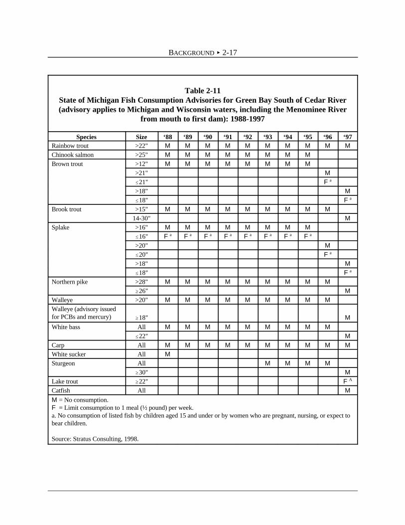
BACKGROUND < 2-17
Table 2-11State of Michigan Fish Consumption Advisories for Green Bay South of Cedar River(advisory applies to Michigan and Wisconsin waters, including the Menominee River
from mouth to first dam): 1988-1997
Species Size ‘88 ‘89 ‘90 ‘91 ‘92 ‘93 ‘94 ‘95 ‘96 ‘97Rainbow trout >22" M M M M M M M M M M
Chinook salmon >25" M M M M M M M M
Brown trout >12" M M M M M M M M
>21" M
#21" Fa
>18" M
#18" Fa
Brook trout >15" M M M M M M M M M
14-30" M
Splake >16" M M M M M M M M
#16" F F F F F F F Fa a a a a a a a
>20" M
#20" Fa
>18" M
#18" Fa
Northern pike >28" M M M M M M M M M
$26" M
Walleye >20" M M M M M M M M M
Walleye (advisory issuedfor PCBs and mercury) $18" M
White bass All M M M M M M M M M
#22" M
Carp All M M M M M M M M M M
White sucker All M
Sturgeon All M M M M
$30" M
Lake trout $22" FA
Catfish All M
M = No consumption.F = Limit consumption to 1 meal (½ pound) per week.a. No consumption of listed fish by children aged 15 and under or by women who are pregnant, nursing, or expect tobear children.
Source: Stratus Consulting, 1998.

BACKGROUND < 2-18
Table 2-12State of Michigan Fish Consumption Advisories for Little Bay de Noc (Lake Michigan):
1989-1997
Species Size ‘89 ‘90 ‘91 ‘92 ‘93 ‘94 ‘95 ‘96 ‘97
Longnose suckers >16" F F F F F F Fa a a a a a a
$14" Fa
Walleye >22" F F F F F F Fb,c b,c b b b,c b,c b,c
F = Limit consumption to 1 meal (½ pound) per week.a. No consumption of listed fish by children aged 15 and under or by women who are pregnant, nursing, or expect tobear children.b. No more than one meal a month of listed fish by children aged 15 and under or by women who are pregnant,nursing, or expect to bear children.c. Advisory listed for mercury only.
Source: Stratus Consulting, 1998.
Michigan FCAs changed significantly in structure and content in 1998. Different advisories arenow given for (1) women who are pregnant, nursing, or expect to bear children and for children,and (2) for the general population; and more restriction levels have been added. The 1998 levelsfor Michigan are shown in Table 2-11, along with the 1998 Wisconsin advisories for Green Bayfor comparison. Generally the advisories issued in 1998 in Michigan are less restrictive thanformer Michigan advisories and current Wisconsin advisories as they have the same or similaradvisories for women and children, but less restrictive advisories for the remainder of thepopulation.
2.3 IMPACTS FROM FCAS
One intent of FCAs is to educate and warn anglers of potential health risks and to encouragechanges in behavior, if and as necessary, to reduce potential health risks. The literature on anglers’behavioral response to FCAs repeatedly shows that anglers change their behavior in response toFCAs. Table 2-13 provides a sample of this literature. These behavioral responses range fromreductions in trip taking to changes in how fish are prepared and cooked. These behavioralchanges represent recreational fishing services that have been lost (damages) to anglers. Evenanglers who do not change their behavior may experience a reduction in enjoyment of their fishingexperience and thus experience a loss of services (damages).

BACKGROUND < 2-19
Table 2-13Studies of Behavioral Responses by Anglers to Fish Consumption Advisories
Author Study Type of Advisory Considered Reported Behavioral Response
Locationand Date of
Hutchinson, Lower Fox Lower Fox River 64% Had made a change, of these:1999 River, 71% Travel to other locations to fish
Wisconsin, -Varies by species, levels include 65.9% Do not eat the fish they catch1997 no consumption and limited 17.7% Change frequency of fish consumption
consumption 9.8% Target and catch different species7.3% Change the size of fish they keep2.4% Clean or prepare fish in different ways
West et al., Michigan, Michigan Great Lakes and inland 76% Change cleaning methods1989 1988 waters 73% Change cooking methods
-Varies by species, levels include 66% Eat different speciesno consumption and limitedconsumption
6% Eat less fish from the site
West et al., Michigan, Michigan Great Lakes and inland 75% Change cleaning methods1993 1991-1992 waters 86% Change cooking methods (Great Lakes
-Varies by species, levels include 80% Eat different species (Great Lakes anglers)no consumption and limited 46% Eat less fish from the site (overall)consumption 27% Change cooking methods (overall)
anglers)
Fiore et al., Lake Fish caught in Lake Michigan and 57% Report changing fishing habits and/or fish1989 Michigan, Green Bay consumption habits
Wisconsin,1985 -Varies by species, levels include
limited consumption and noconsumption
Silverman, Lake All waters of Michigan, including 10% Take fewer trips1990 St. Clair, Great Lakes and inland waters 31% Change fishing locations
Detroit River, 21% Change targeted speciesLake Erie, -Varies by species, levels include 56% Change cleaning methods1990 no consumption and limited 41% Change the size of fish consumed
consumption 28% Change cooking methods56% Eat less fish from the site31% Eat different species
Knuth et al., New York Fish caught in Lake Ontario 83% Use risk-reducing cleaning methods1996 portion of 42% Use risk-reducing cooking methods
Lake Ontario, -Varies by species, levels include 32% Said they would eat more fish in the1993 no consumption and limited absence of advisories
consumption

BACKGROUND < 2-20
Table 2-13 (cont.)Studies of Behavioral Responses by Anglers to Fish Consumption Advisories
Author Date of Study Type of Advisory Considered Reported Behavioral ResponseLocation and
Knuth et al., Ohio River, Fish caught in the Ohio River 37% Take fewer trips1993 Illinois, 26% Change fishing locations
Indiana, Ohio, -Advisories vary throughout the 26% Change targeted speciesKentucky, different states and species, levels 22% Change cleaning methodsPennsylvania, include no consumption and limited 17% Change the size of fish consumedWest Virginia, consumption 13% Change cooking methods1992 42% Eat less fish from the site
13% No longer eat fish from the site
Connelly et al., New York, All waters of New York 18% Take fewer trips1992 1992 45% Change cleaning methods
-Varies by species, levels include 25% Change the size of fish consumedno consumption and limited 21% Change cooking methodsconsumption 70% Eat less fish from the site
27% Eat different species17% No longer eat fish from the site
Connelly et al., New York, New York inland waters and Lake 17% Take fewer trips1990 1987-1988 Ontario 31% Change fishing locations
-Varies by species, levels include 51% Eat less fish from the siteno consumption and limited 17% Eat different speciesconsumption 11% No longer eat fish from the site
46% Change cleaning/cooking methods
Vena, 1992 Lake Ontario, Fish caught on Lake Ontario 16% Take fewer tripsNew York, 30% Change fishing locations1990-1991 -Varies by species, levels include 20% Change targeted species
limited consumption and no 31% Change cleaning methodsconsumption 53% Eat less fish from the site
16% No longer eat fish from the site
The study results listed in Table 2-13 show that the responses to FCAs vary by location, FCAseverity, and species. The literature cited suggests that the presence of FCAs has resulted inchanges in the number and/or quality of recreational fishing days taken. These studies show arange of 10% to 71% of the anglers taking fewer trips to the contaminated sites. These trips maybe substituted to other sites that would be considered inferior if the site were not contaminated orsubstituted from fishing to other, less preferred activities. Anglers may be incurring higher travelcosts and/or inferior conditions because of the substitution.
Anglers who remain in the fishery are also impacted. The studies cited in Table 2-13 also foundthat 6% to 70% of anglers eat fewer fish from the site, 27% to 80% changed the species that they

BACKGROUND < 2-21
eat, 11% to 66% no longer eat any fish from the site, 2% to 83% changed the way they clean thefish, and 13% to 86% changed the way they cook the fish.
Evidence that anglers have substituted fishing days to other fishing sites is also found in aWisconsin study, which did not ask about behavioral responses to FCAs (Bishop et al., 1994).Anglers who fished inland waters were asked about the relative importance of various factors thatplayed a part in choosing not to fish in the Great Lakes. “PCB and other contamination in thefish” was identified as a “somewhat important” or “very important” factor by 55% of therespondents. No other single factor was cited by a higher proportion of respondents.
The presence of FCAs may also keep potential anglers from fishing at all. For some individuals,Green Bay may be the only site that they would like to fish because of the convenience of itslocation or other unique attributes. These individuals may return to fishing in the absence ofcontamination and the resultant FCAs, and therefore have experienced service flow losses.
The Hutchinson (1999) study cited in Table 2-13 looked at the impacts of PCB contamination onsubsistence fishing in the Lower Fox River. Personal interviews were conducted with 70 Hmongor Laotion anglers, 25 Anglo-American anglers, and 7 other minority anglers. This study foundthat anglers from Hmong/Laotion and other minority groups were more likely than Anglo anglersto eat fish from the Lower Fox River (80%, 72%, and 12%, respectively). About 62% of the non-Anglo anglers ate fish from the Lower Fox River once a month or more. At the time of the studyall fish had a minimum restriction of “eat no more than once a month” in the Wisconsin FCAs forthe Lower Fox River. When asked about how they reacted to FCAs, 79% of Anglo anglers, 64%of Hmong/Laotion anglers, and 17% of other minorities said they had changed their fishingactivity in response to the FCAs.
The identified studies indicate that FCAs impact anglers and their fishing enjoyment. Several ofthe studies include Green Bay in their study area, but most of the studies that include Green Baydo so as part of a larger area. The Hutchinson (1999) study focuses specifically on the Lower FoxRiver and the mouth of the Bay around the City of Green Bay, but also focuses on a subset ofanglers rather than all recreational anglers.
2.4 ECONOMIC VALUES
In 1996 anglers spent over $900 million on recreational fishing in Wisconsin (U.S. DOI, 1998).Anglers clearly value their fishing experiences, but figures about total expenditures do not tell uswhat they value about specific sites or fishing days. Models of recreational fishing demand areused to determine the values that anglers place on the different characteristics of fishing sites. Inthis section we summarize results of the recreation demand literature to value changes in catchrates and for the removal of FCAs. We find the existing literature provides a useful perspective on

BACKGROUND < 2-22
expected values for the waters of Green Bay, but the literature is not adequate to be relied onsolely for this damage assessment.
Values for Changes in Catch Rates
Demand for a fishing day is an increasing function of catch rates. All else being equal, an anglerwould rather catch more fish. Because catch rates are such an important part of the anglingexperience, many studies have been done that value catch increases and reductions. Table 2-14lists a sample of studies that value changes in catch rates in Lake Michigan and Green Bay. Thesestudies indicate that values for changes in catch rates are not inconsequential, but there is largevariation in the values these studies produce as there is variation in the location of the studies, thepopulation included, and the species studied. Milliman et al. (1992) surveyed Green Bay anglers ina contingent valuation study that valued additional catch and size of sportfish, but did so when thefishery was at its recent best, and the marginal value of another fish would be low compared tocurrent conditions. The values for the Great Lakes trout/salmon fishery from Lyke’s (1993) studywere derived from a population of Great Lakes trout/salmon anglers, as well as anglers who didnot fish the Great Lakes and would be less concerned with its catch rates. Chen et al. (1999) andSamples and Bishop (1985) both valued increases in trout/salmon species outside of ourassessment site.
Chen et al. (1999) modeled fishing choices of Michigan anglers for trips targeting Great Lakestrout and salmon. Each site is a Michigan county, and there are 41 counties that support thefishery. Data on 325 trips from 90 individuals are from their 1994 survey. Value estimates forchanging the catch rates in Muskegon County by different amounts are reported in Table 2-14.For doubling the catch rate, the value per user day estimates range from $3.42 to $14.23,depending on the model. For tripling the catch rate, values range from $12.62 to $56.03.
No single previous study values the specific assessment area and specifically addresses anglers’values for changes in catch rates for the species of most interest in this fishery. Thus, the currentstudy provides the basis for measuring accurately values for changes in catch rates for the keyspecies of interest, for addressing potential damages from PCB-induced reductions in catch rates,and for addressing restoration benefits of increased catch rates.
Values for FCAs
While there is relatively extensive literature on the valuation of changes in catch rates, there arefewer studies that value changes in the levels of toxins and the resulting FCAs. Some of thesestudies are summarized in Table 2-15. The values anglers place on cleaner waters and fish aresubstantial, but vary across site, type of contamination, levels of contamination, shares of tripsaffected by the FCAs, substitute sites available, and other factors.

BACKGROUND < 2-23
Table 2-14Selected Valuation Studies for Changes on Catch Rates
Authors and Year Modeled Population Model Item Valued (1998 dollars)
StudyLocation Value Estimatesa
Samples and Lake 592 residents of Multiple site travel 10% increase in trout and salmon $0.67 per tripBishop, Michigan, 11 Wisconsin counties cost model catch rates1985 1979 adjacent to Lake $15.15 per additional
Michigan trout/salmon
Milliman et al., Green Bay, 250 sport anglers who Dichotomous choice Hicksian surplus for yellow perch $38.38 per trip1992 1983 had been contacted on- contingent valuation
site model (catch per trip was at historically $0.29 per additional fishhigh level at time of survey, 1983) $0.44 per additional inch in
length of fish
Lyke, Wisconsin 274 Great Lakes trout Nested logit travel Avoid a 50% reduction Lake $0.07 per trip1993 Great Lakes, and salmon anglers cost model Michigan lake trout catch
1990239 inland anglers Avoid a 33% reduction Lake $0.12 per trip
Michigan salmon catch
Value of trip to Lake Michigan $21.80 per trip
Chen et al., Michigan 325 trips from Multinomial logit and Increase in trout and salmon catch $3.42 to $14.23 per day for1999 waters of 90 Michigan resident probit repeated rates doubling the catch rate,
Great Lakes, anglers random utility models $12.62 to $56.03 per day for1994 tripling the catch rate
a. Per trip (per day) values apply to trips to the impacted fishing site.

BACKGROUND < 2-24
Table 2-15Selected Valuation Studies for the Reduction of Toxins at Fishing Sites
Authors Study Location Sample Information Model Resource Change (1998 dollars)Value Estimates
a
Herriges et al., Wisconsin 240 Great Lakes trout Kuhn Tucker models 20% reduction in $66.41 to $81.99 per1999 waters of Great and salmon anglers, and contaminant levels in fish angler per season
Lakes 247 non-Great Lakes $9.08 to $11.22 per Greatanglers (data from Lakes fishing dayLyke, 1993)
Chen and Michigan Great 338 one-day salmon Simulated maximum likelihood is Remove area of concern $1.19 to $5.61 per tripCosslett, Lakes sites fishing trips used to estimate a random parameter designation at all Michigan1998 probit model Great Lakes sites (total of
14 )
Lyke, Wisconsin 274 Great Lakes trout Contingent valuation Eliminate all contaminants $47.08 (LL) to $165.541993 Great Lakes and salmon anglers, and -Linear logit (LL) that threaten human health (CES) per angler per year
239 inland anglers -Constant elasticity of substitution in Wisconsin Great Lakes $3.88 (LL) to $13.61(CES) (CES) per Great Lakes
fishing day
Montgomery and New York 266 anglers and 3,013 Repeated discrete choice RUM Remove toxic contamination $1.98 per tripNeedelman, nonanglers at 23 of 2,586 lakes $0.59 per angler day1997 $83.14 per angler season

BACKGROUND < 2-25
Table 2-15 (cont.)Selected Valuation Studies for the Reduction in of Toxins at Fishing Sites
Authors Location Information Model Resource Change (1998 dollars)Study Sample Value Estimates
a
Hauber and Maine lakes 143 Maine anglers Nested logit RUM Clean up all Maine rivers $1.46 to $1.70 per tripParsons, and rivers having FCAs1998 2,425 freshwater
fishing day trips
Jakus et al., Reservoirs in 368 anglers Repeated discrete choice RUM (for Remove FCAs from 6 of 14 $3.15 per trip1997 middle and fishing Tennessee annual), eastern Tennessee reservoirs $52.13 per angler per season
eastern reservoirs multinomial logit site-choice — —Tennessee model (for per-trip) Remove FCAs from 2 of 14 $2.03 per trip
middle Tennessee reservoirs $24.15 per angler per season
Jakus et al., Reservoirs in 222 anglers Multinomial logit site choice Remove FCAs from 6 of 14 $7.40 per trip1998 Tennessee fishing Tennessee model total Tennessee reservoirs (assumes all anglers know about
reservoirs FCA)-Valuation considers whether $1.51 per tripangler knows about advisories (across all anglers, but assuming
those who do not know have zeroloss)
Parsons et al., Reservoirs in 143 anglers Various RUMs Remove FCAs from 2 of 14 $1.95 to $2.05 per trip1999 middle fishing in middle middle Tennessee reservoirs
Tennessee Tennesseereservoirs
a. Per trip (and per day) values in this column apply to all trips taken in the modeled region, not just the trips to the contaminated sites. A lower-boundestimate of annual value could be computed by multiplying the per-trip values by the number of trips to all sites modeled, not just the contaminated sites. Thevalues per trip to contaminated sites only would be greater than the per-trip values reported in this table.
BACKGROUND < 2-26
6. Other types of models are also estimated, but those models are not utility theoretic and often give implausibleresults that are not consistent with expectations. However, all estimated models indicate that toxins reduce theamount and quality of fishing services.
Herriges et al. (1999) developed utility-theoretic Kuhn-Tucker recreation demand models andestimated them using Lake Michigan and Green Bay angling data from 487 anglers collected by Lyke (1993). The models are used to value a 20% reduction in toxins at four aggregate6
Wisconsin sites, which include Green Bay. The models indicate toxins in Lake Michigansignificantly reduce the well-being of Wisconsin anglers. Site-specific values are not presented,but the range of values for a 20% reduction in toxins at all four sites is $66.41 to $81.99 perangler per year ($1998). For comparison to the other studies, we divide the annual values inHerriges et al. by the sample average number of Great Lakes fishing days (7.31) to obtain valuesper Great Lakes fishing day of $9.08 to $11.22. Similarly for Lyke, using her sample average of12.16 Great Lakes fishing days, the values per Great Lakes fishing days range from $3.88 to$13.61.
Montgomery and Needelman (1997) estimated a repeated discrete choice model of trips to2,586 possible fishing sites, 23 of which had toxic contamination. These 23 sites include smallerlakes, as well as portions of larger lakes such as Lake Ontario and Lake Champlain. Thepopulation used in this study included 266 New York residents who had fished, and 3,013 whohad not fished, between mid-April and October 1989. With 2,586 possible fishing sites, but only23 contaminated, few angler trips were affected; the impact should be less significant than that ofGreen Bay FCAs on Green Bay anglers. However, even with a small proportion of sites affected(about 1%) and a population sample that was made mostly of nonanglers, Montgomery andNeedelman estimated the value of eliminating toxic contamination at all the toxic sites would be$1.98 per trip ($1998), estimated using only data from anglers. Note that these values applied toall fishing trips taken to all sites, not just trips to the affected sites.
Three studies listed in Table 2-15 (Jakus et al., 1997, 1998; Parsons et al., 1999) estimated thevalue of reducing toxic contamination to the degree that FCAs could be removed fromcontaminated reservoirs in Tennessee. These studies concentrated on different geographic regionsand included both toxic and nontoxic sites. The models developed were all random utility models,and the population was limited to anglers who used the sites. It should be emphasized that theper-trip values from all of these studies were for trips to all sites modeled, including nontoxicsites. These values did not apply only to the trips taken to the toxic sites.
The values estimated for removing FCAs from two toxic sites within a 14-site region were about$2 per trip. As two sites constituted 14% of 14 sites, a rough first approximation of the per-tripvalue of cleanup for only the affected sites was approximately $14 ($2/0.14). The values forremoving FCAs from 6 toxic sites within a 14-site region were $3.15 per trip from a multinomiallogit site-choice model, $1.51 in the same type of model but with the assumption that anglers whodid not know about FCAs had zero loss, and $7.40 in the same model with the assumption that all

BACKGROUND < 2-27
anglers knew about FCAs. The 6-site subset represented 43% of the total number of sites, so arough first approximation of the losses per trip to the contaminated sites ranged from about $3 to$17 [($1.51 to $7.40)/$0.43]. This study showed significant values for removing FCAs but lookedat a fishery that was markedly different from Green Bay. The system of reservoirs offered smallerwaters with similar nontoxic substitutes to the few reservoirs that were contaminated.
Chen and Cosslett (1998) used data collected on 338 single-day fishing trips targeting trout orsalmon. The choice set included 41 possible sites in the Michigan waters of the Great Lakes. Theyestimated three models of fishing demand: a varying parameter multinomial probit model, anindependent multinomial logit model, and an independent multinomial probit model. They valuedthe cleanup of toxic contamination at 14 sites in the Great Lakes waters of Michigan sufficient toremove the designation of Area of Concern by the International Joint Commission. The values forthis cleanup ranged from $1.19 to $5.61 per trip. Again these values are not directly applicable toGreen Bay because it was a multisite study limited to trout and salmon anglers in Michigan, andvalues applied to all trips taken in the 41-site region. These 41 affected sites accounted for 34% ofthe sites, implying an approximate value per trip to an affected site of about $3.50 to $16.50[($1.19 to $5.61)/0.34].
None of these studies provided site-specific estimates for the assessment area, or adequatelyshowed how the value of recreational fishing services vary with the levels of FCAs of relevance tothis damage assessment. Most were for multiple sites with similar substitutes and/or limited fishspecies. These studies all indicated the significance of damages from contamination, but did notprovide specific values sufficiently useful to transfer to the damage assessment of Green Bay.

CHAPTER 3PRIMARY DATA COLLECTION
3.1 INTRODUCTION
The principal objective of our assessment is to cost-effectively develop estimates of the value ofservices lost (damages) as a result of FCAs in the waters of Green Bay. For cost-effectiveness welimited our target population, and therefore our sample, for the primary damage assessment toanglers who purchased Wisconsin fishing licenses in eight Wisconsin counties near Green Bay andwho were active in open-water fishing in the Wisconsin waters of Green Bay in 1998. InChapter 8 we conduct a benefits transfer [43 CFR § 11.83(c)(2)(vi)] to estimate ice-fishingdamages in the Wisconsin waters of Green Bay, and to estimate damages for all lost recreationalfishing in the Michigan waters of Green Bay. The assessment does not address the value ofrecreational fishing services lost for anglers who do not fish Green Bay because of FCAs.
By sampling anglers who actively fish Green Bay, we measure damages for those individualsfamiliar with the site and for whom PCBs and the resultant FCAs are most relevant, which aids inthe accuracy of the assessment. We focus on anglers active in the Wisconsin waters of Green Baywhere the majority of damages can be expected to occur because the days of recreational fishingin these waters is about double that in the Michigan waters (Chapter 2), and because the PCBconcentrations and severity of FCAs are higher in the Wisconsin waters of Green Bay(Chapter 2). We focus on anglers who purchase licenses in eight nearby counties because they canbe expected to account for the majority of fishing activities in the Wisconsin waters of Green Bay(Section 3.2). We focus on open-water fishing because it accounts for 85% or more of all fishingon the waters of Green Bay.
A three-step procedure is used to collect data from a sample of anglers in the target population.First, a random sample of anglers was drawn from 1997 license holders in the county courthousesin the eight targeted counties. Second, using the license holder list, a telephone survey wasconducted to identify and recruit Green Bay anglers for a followup mail survey and to collect datafrom a cross-section of anglers. Third, a mail survey was conducted with anglers active in open-water fishing in the waters of Green Bay. The mail survey asked more questions and morecomplicated questions that would not be desirable to ask by telephone.
In this chapter we address the selection of the target population for the primary assessment andthe sampling procedures (Section 3.2), discuss the telephone and mail survey instruments andtheir implementation (Sections 3.3 and 3.4), and evaluate the sampling plan (Section 3.5).

PRIMARY DATA COLLECTION < 3-2
1. WDNR open-water creel surveys 1990-1998. Data provided by Brad Eggold, Senior Fisheries Biologist,Plymouth Field Station.
Throughout this chapter, Green Bay refers to the Wisconsin waters of Green Bay, unlessspecifically identified otherwise.
3.2 SAMPLING PLAN
3.2.1 Selection of Target Population
The target population for the primary assessment is all resident and nonresident anglers who areactive in fishing in the Wisconsin waters of Green Bay in 1998 and who purchased theirWisconsin fishing license in one of eight Wisconsin counties near to the waters of Green Bay. Theeight counties include five with shorelines on the waters of Green Bay: Marinette, Oconto,Brown, Kewaunee, and Door; and three nearby counties with relatively large numbers of potentialGreen Bay anglers: Manitowoc, Outagamie, and Winnebago (Figure 3-1). We limited our targetpopulation and sampling to these eight counties because anglers purchasing licenses in these eightcounties can be expected to account for most of the fishing activity in the Wisconsin waters ofGreen Bay, and thus the sample will provide a cost-effective means of data collection. Severalpieces of evidence support these conclusions.
The 1991 National Survey of Fishing, Hunting, and Wildlife-Associated Recreation (U.S. DOI,1992) indicates that fishing in general tends to be a fairly localized activity. The average one-waydistance by in-state residents for a fishing trip is about 34 miles. For Great Lakes fishing, theaverage one-way distance traveled by in-state residents is about 60 miles. Thus, we expect that alarge fraction of fishing trips to the waters of Green Bay and the Lower Fox River originate in thecounties around the waters of Green Bay.
A WDNR study of recreational boating patterns in Wisconsin suggests that a large percentage ofthe fishing effort on Green Bay originates in the counties near Green Bay (Penaloza, 1991, 1992).This is important because boating accounts for as much as 80% of fishing activity on theWisconsin waters of Green Bay.1 The Penaloza study explores the origination and destinationpatterns for boating trips in the state of Wisconsin. For Wisconsin locations, the study finds thatthe median one-way distance traveled by boaters is 10 miles, while the average one-way distanceis 42 miles, again indicating that most boat fishing trips originate from nearby counties.
Penaloza identifies a “Lake Michigan” district, which includes 14 counties adjacent to, or near,Green Bay (Figure 3-2). This district includes the eight counties we include in our sample, plusFlorence, Menominee, Shawano, Waupaca, Waushara, and Calumet counties. More than 80% ofthe respondents residing in the Lake Michigan District (LMD) specify the LMD as a destination

PRIMARY DATA COLLECTION < 3-3
Figure 3-1The Eight Targeted Counties

PRIMARY DATA COLLECTION < 3-4
Marinette
Oconto
Outagamie
Winnebago Manitowoc
BrownKewaunee
Door
LakeMichigan
MICHIGAN
Menominee
Shawano
Calumet
Waupaca
Waushara
Florence
Lake MichiganDistrict
8 Targeted Counties
Green Bay
Figure 3-2Lake Michigan District of Wisconsin
for boating trips involving fishing. This study also finds that about 77% of the individualschoosing the LMD as a destination are residents of the LMD. Since the frequency ofuse typically decreases as the distance to a site increases, we would expect substantially more than77% of boating days in the district can be attributed to residents of the district.
The Penaloza survey asked boat anglers to identify their most frequently visited boat fishing site.For residents of the LMD, the percent indicating Green Bay or the Fox River are listed inTable 3-1. Note that the percentage citing Green Bay or the Fox River generally decreases as thecounty of residence is farther from these waters. The LMD counties that are not included in our

PRIMARY DATA COLLECTION < 3-5
Table 3-1Percent of Boat Anglers from Lake Michigan District Counties Choosing the Fox River
or Green Bay as Their Most Frequently Visited Site
County of ResidenceIncluded in Current
Study CountiesGreen Bay/Fox River as
Most Frequently Visited SiteBrown Yes 29%Calumet No 0%Door Yes 83%Florence No 0%Kewaunee Yes 17%Manitowoc Yes 25%Marinette Yes 8%Menominee No 0%Oconto Yes 8%Outagamie Yes 3%Shawano No 0%Waupaca No 0%Waushara No 0%Winnebago Yes 0%Source: Based on data from WDNR boating study (Penaloza, 1991, 1992).
target population had no anglers citing the Fox River and Green Bay as their most frequentlyvisited boating site.
Our eight targeted counties contain 83% of the population of the LMD (Wisconsin LegislativeReference Bureau, 1997). Most of the LMD counties not included in the sampling are the farthestfrom Green Bay, and it is likely that about 95% of the Green Bay fishing days by residents of theLMD are by residents of the eight targeted counties (see Section 3.5.5). By narrowing our sampleto the eight targeted counties we significantly reduce the cost of assembling a sample, whichrequires visits to each county’s courthouse because electronic records of fishing licenses do notexist.
By focusing on where anglers purchase their fishing licenses, rather than where they reside, thetarget population will include anglers who are residents of other Wisconsin counties and who arenonresidents. For instance, nonresidents who fish the Wisconsin waters of Green Bay are mostlikely to purchase their Wisconsin fishing licenses in Wisconsin counties near Green Bay. Thesame may be true for Wisconsin residents from other counties who primarily fish at Green Bay orother northeast Wisconsin destinations. Thus, the sample will represent a very large share of

PRIMARY DATA COLLECTION < 3-6
2. 1998-1998 licenses are valid for April 1997 through March 1998. A complete set of 1998 licenses is notavailable at courthouses, or any other location, until mid-1999.
3. In Kewaunee County licenses are filed by vendor and not by type. In this case, as each data entry person wentthrough the vendor stack, he or she used a list to keep track of a separate count for each license type, and enteredthe data for each license type into a separate worksheet.
anglers who are active in fishing the Wisconsin waters of Green Bay by including residents ofthose counties, who account for most fishing days in these waters, as well as including residentsof other Wisconsin counties and nonresidents who purchase their licenses in these eight counties.
3.2.2 Sample Collection at County Courthouses
Our sample was selected from the population of anglers who purchased 1997-1998 fishinglicenses in the eight targeted counties as a cost-effective means to identify and sample anglers inthe target population.2 Potential sample bias due to differences between a sample of 1997-1998license holders and the target population of 1998 anglers who purchase licenses in these countiesis addressed in Section 3.5.1.
We targeted an initial random sample of almost 11,500 anglers in the eight targeted counties toresult ultimately in no less than 500 completed mail surveys. This sample size allowed for aconservative estimate of the incidence rate of Green Bay anglers, bad addresses, mail andtelephone completion rates, and a substantial contingency for other unknowns.
The sample size targets were created by using the 1996-1997 license sales data from the WDNR(licenses valid from April 1, 1997 to March 31, 1998) to determine the proportions of fishinglicenses sold per county for the eight targeted counties (Table 3-2).
Anglers’ names and addresses were obtained from copies of 1997-1998 fishing season licensessold in the eight targeted counties near Green Bay. Vendors keep carbon copies of each licensesold until the end of the license season and then turn them over to the county clerk. As ofJuly 1998, the most recent, accessible sample of Wisconsin fishing licenses were those turned inafter the 1997 season (which ended in March 1998). To get this sample, each of the eight countyclerks was visited over the three-week period from July 20 to August 11, 1998. The dates ofthese visits and the number of data entry assistants used by county are shown in Table 3-3.
The fishing licenses were randomly sampled so that each angler had a nearly equal probability ofbeing sampled. Licenses were segregated by fishing license type.3 One type of license wasassigned to each data entry person who entered the data into an Excel workbook, keeping aseparate worksheet for each type of license. For licenses issued to individuals, every 15th license

PRIMARY DATA COLLECTION < 3-7
Table 3-21997-1998 Angling License Samples Obtained
CountyTotal Fishing Licenses
Sold, 1996a
Proportion of 1996Licenses Sold by Each
Countyb
Number of LicensesNeeded per County for
Samplec
Brown 35,110 20% 2,340Door 21,561 12% 1,437Kewaunee 10,972 6% 731Manitowoc 15,701 9% 1,046Marinette 18,951 11% 1,263Oconto 12,436 7% 829Outagamie 26,753 16% 1,783Winnebago 31,064 18% 2,070Total 172,548 100% 11,499a. Includes sales of all types of fishing licenses.b. Percents may not total 100% due to rounding.c. Number needed to get a total of about 11,500 licenses, while maintaining the county proportions of totallicense sales.
Source for fishing licenses sold: Based on WDNR Bureau of Customer Service and Licensing, Report ofFishing Licenses Sold by County, B130-30.
Table 3-3Timeline for Sampling of Licenses by County
County City CourthouseTarget
Sample Size Date
(1998)Data EntryAssistants
Brown Green Bay 2,340 August 5/6 3Door Sturgeon Bay 1,437 August 3 2Kewaunee Kewaunee 731 July 30 2Manitowoc Manitowoc 1,046 July 29 2Marinette Marinette 1,263 August 7 3Oconto Oconto 829 July 24 2Outagamie Appleton 1,783 July 20/21 2Winnebago Oshkosh 2,070 August 10/11 3All targeted counties 11,499

PRIMARY DATA COLLECTION < 3-8
was input (starting with the 14th license); and for licenses issued to married couples or families,every 7th license was input (starting with the 7th license), alternating between recording thehusband’s or wife’s name. In any case where the selected license record was illegible (15 cases),the next legible license was recorded. The count was then resumed from the original illegiblelicense.
For nonresident licenses, if the selected license record had a nondomestic address (two cases), thenext license record with an American address was recorded. The count was then resumed fromthe original nondomestic address.
For each county, once all license types had been counted through, another count was made of thetotal number of licenses selected, and this total was compared to the target sample for the county.If the number of licenses selected was more than a few licenses short of the targeted sample,additional licenses were selected from each license type. A new skip interval was calculated forthe license types issued to individuals and for the license types issued to married couples orfamilies. The number of licenses obtained by county and license type are shown in Table 3-4.
3.3 TELEPHONE SURVEY
3.3.1 Telephone Survey Instrument
The telephone survey was used to identify the proportion of anglers who fish the waters of GreenBay, to obtain data on total fishing days and Green Bay fishing days, and to identify and recruitanglers who were active in 1998 in fishing the Wisconsin waters of Green Bay to participate in thefollowup mail survey. The telephone survey also collected information for all anglers in thetelephone sample, regardless of whether they fished Green Bay in 1998. This allows a comparisonof activity levels and attitudes for anglers who are active in Green Bay fishing versus anglers whoare not, and allows a comparison of those Green Bay anglers who complete the followup mailsurvey to those who complete the telephone survey but do not complete the followup mail survey.The telephone survey collected the following information.
< Fishing activity level. Data were collected on the total days of ice-fishing and open-waterfishing in 1998 up to the time of the telephone survey and how many of these days were inthe waters of Green Bay. Because the survey was implemented in late 1998, over 95% ofdays fished in 1998 by these anglers are reflected in these data. These days are separatedinto days fished in the Lower Fox River and elsewhere in the waters of Green Bay(including tributaries up to the first dam or obstruction).
< Attitudes about Green Bay fishing. Anglers who did not fish Green Bay in 1998 wereasked why they did not fish; and, if they would consider fishing Green Bay in the future,what things would have to change to consider fishing in the future. The questions about

PRIMARY DATA COLLECTION < 3-9
Table 3-41997-1998 Angling License Sample Obtained
License TypeCounty
Brown Door Kewaunee Manitowoc Marinette Oconto Outagamie Winnebago TotalResident annual 1,310 321 178 459 650 396 917 1,169 5,400Husband and wife 671 147 62 220 276 237 637 520 2,770Sportsman 236 45 34 102 102 56 214 188 977Two day 49 452 356 146 20 5 2 0 1,030Nonresident annual 25 115 24 16 80 33 12 12 317
Nonresident 15 day 13 65 12 10 26 18 6 27 192
Nonresident 4 day 41 181 39 52 127 55 27 205 731Nonresident family annual 2 60 15 7 30 18 5 7 144Nonresident family 15 day 0 65 7 8 25 14 5 13 152Patron 0 0 1 14 0 0 0 0 15Total sample obtained 2,347 1,451 728 1,034 1,336 832 1,825 2,141 11,694Target 2,340 1,437 731 1,046 1,263 829 1,783 2,070 11,499Total sample obtained aspercent of target 100.3% 101.0% 99.6% 98.9% 105.8% 100.4% 102.4% 103.4% 101.7%

PRIMARY DATA COLLECTION < 3-10
why they did not fish Green Bay and what would have to change are open-ended — potential responses are not provided to the respondent. These questions provide anindication of the share of anglers who are not active in Green Bay fishing who attributenot fishing in Green Bay to PCBs and fish consumption advisories — a damage categorythat is not otherwise quantified in this assessment. These anglers experience a damage inthat the PCBs and resultant FCAs cause them to forgo fishing at a site they wouldotherwise choose to visit.
< Attitudes about fish contamination and fishery management options. Questions wereasked about catching fish that are free of contamination and about the importance of10 actions that could be taken to improve fishing in Wisconsin: six for the waters of GreenBay and four for other waters. These actions include increasing catch rates for sport fishand for panfish, cleaning up contaminants, increasing boat ramps and other facilities,improving water quality, and reducing the cost of a fishing trip. These questions identifythe relative importance of improvements in different fishing characteristics for all anglersand for Green Bay anglers. The responses to these questions also provide a key point ofcomparison between those anglers completing the followup mail survey versus all otheranglers completing the telephone survey.
< Socioeconomic characteristics. Questions include years of fishing experience, boatownership, vacation home ownership with distance from Green Bay, age, employmentstatus, racial group, household composition, and gender. These data assist in the statisticalevaluation of group respondents.
< Mail survey solicitation. For anglers who actively fished Green Bay in 1998, thetelephone survey concludes with a solicitation to participate in the followup mail survey;and confirms the correct name and address to which materials would be sent, and atelephone number for any future contact.
3.3.2 Telephone Survey Implementation
The telephone survey was conducted by Hagler Bailly’s facility in Madison, Wisconsin. This26-station centrally monitored interviewing facility uses CASES, a computer-assisted telephoneinterviewing (CATI) software developed and supported by the University of California, Berkeley.The telephone survey occurred between November 17, 1998 and January 15, 1999.
To ensure the efficient use of resources, the initial sample of license holders collected at countycourthouses was split into two segments, with the first segment of 6,799 records (about 60% of
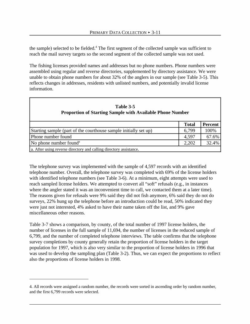
PRIMARY DATA COLLECTION < 3-11
4. All records were assigned a random number, the records were sorted in ascending order by random number,and the first 6,799 records were selected.
the sample) selected to be fielded.4 The first segment of the collected sample was sufficient toreach the mail survey targets so the second segment of the collected sample was not used.
The fishing licenses provided names and addresses but no phone numbers. Phone numbers wereassembled using regular and reverse directories, supplemented by directory assistance. We wereunable to obtain phone numbers for about 32% of the anglers in our sample (see Table 3-5). Thisreflects changes in addresses, residents with unlisted numbers, and potentially invalid licenseinformation.
Table 3-5Proportion of Starting Sample with Available Phone Number
Total PercentStarting sample (part of the courthouse sample initially set up) 6,799 100%Phone number found 4,597 67.6%No phone number founda 2,202 32.4%a. After using reverse directory and calling directory assistance.
The telephone survey was implemented with the sample of 4,597 records with an identifiedtelephone number. Overall, the telephone survey was completed with 69% of the license holderswith identified telephone numbers (see Table 3-6). At a minimum, eight attempts were used toreach sampled license holders. We attempted to convert all “soft” refusals (e.g., in instanceswhere the angler stated it was an inconvenient time to call, we contacted them at a later time).The reasons given for refusals were 9% said they did not fish anymore, 6% said they do not dosurveys, 22% hung up the telephone before an introduction could be read, 50% indicated theywere just not interested, 4% asked to have their name taken off the list, and 9% gavemiscellaneous other reasons.
Table 3-7 shows a comparison, by county, of the total number of 1997 license holders, thenumber of licenses in the full sample of 11,694, the number of licenses in the reduced sample of6,799, and the number of completed telephone interviews. The table confirms that the telephonesurvey completions by county generally retain the proportion of license holders in the targetpopulation for 1997, which is also very similar to the proportion of license holders in 1996 thatwas used to develop the sampling plan (Table 3-2). Thus, we can expect the proportions to reflectalso the proportions of license holders in 1998.
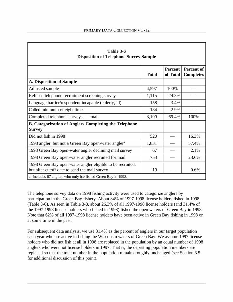
PRIMARY DATA COLLECTION < 3-12
Table 3-6Disposition of Telephone Survey Sample
TotalPercentof Total
Percent ofCompletes
A. Disposition of Sample
Adjusted sample 4,597 100% —
Refused telephone recruitment screening survey 1,115 24.3% —
Language barrier/respondent incapable (elderly, ill) 158 3.4% —
Called minimum of eight times 134 2.9% —
Completed telephone surveys — total 3,190 69.4% 100%
B. Categorization of Anglers Completing the TelephoneSurvey
Did not fish in 1998 520 — 16.3%
1998 angler, but not a Green Bay open-water anglera 1,831 — 57.4%
1998 Green Bay open-water angler declining mail survey 67 — 2.1%
1998 Green Bay open-water angler recruited for mail 753 — 23.6%
1998 Green Bay open-water angler eligible to be recruited,but after cutoff date to send the mail survey 19 — 0.6%
a. Includes 67 anglers who only ice fished Green Bay in 1998.
The telephone survey data on 1998 fishing activity were used to categorize anglers byparticipation in the Green Bay fishery. About 84% of 1997-1998 license holders fished in 1998(Table 3-6). As seen in Table 3-8, about 26.3% of all 1997-1998 license holders (and 31.4% ofthe 1997-1998 license holders who fished in 1998) fished the open waters of Green Bay in 1998.Note that 62% of all 1997-1998 license holders have been active in Green Bay fishing in 1998 orat some time in the past.
For subsequent data analysis, we use 31.4% as the percent of anglers in our target populationeach year who are active in fishing the Wisconsin waters of Green Bay. We assume 1997 licenseholders who did not fish at all in 1998 are replaced in the population by an equal number of 1998anglers who were not license holders in 1997. That is, the departing population members arereplaced so that the total number in the population remains roughly unchanged (see Section 3.5for additional discussion of this point).

PRIMARY DATA COLLECTION < 3-13
Table 3-7Disposition of Sample by County Where License Purchased
CountyWhere 1997
LicensePurchased
1997 License SalesReported by
WDNRInitial Sample ofLicense Holders
Reduced Sampleof LicenseHolders
Telephone SurveysCompleted
NumberPercentof Total Number
Percentof Total Number
Percentof Total Number
Percentof Total
Brown 28,800 19.6% 2,347 20.1% 1,407 20.7% 658 20.6%
Manitowoc 13,316 9.1% 1,034 8.8% 609 9.0% 317 9.9%
Marinette 16,920 11.5% 1,336 11.4% 736 10.8% 354 11.1%
Oconto 10,120 6.9% 832 7.1% 502 7.4% 247 7.7%
Outagamie 22,455 15.3% 1,825 15.6% 1,011 14.9% 514 16.1%
Winnebago 25,275 17.2% 2,141 18.3% 1,270 18.7% 554 17.4%
Door 19,457 13.3% 1,451 12.4% 841 12.4% 343 10.8%
Kewaunee 10,233 7.0% 728 6.2% 423 6.2% 203 6.4%
All Targeted 146,576 100% 11,694 100% 6,799 100% 3,190 100%Source for fishing licenses sold: Based on WDNR Bureau of Service and Licensing, Report of Fishing LicensesSold by County, B130-30.
Table 3-8Telephone Survey Respondent Green Bay Fishing Activity in 1998
1997-1998 LicenseHolders
1997-1998 LicenseHolders Who
Fished in 1998Number Percent Number Percent
Fished Green Bay in 1998- Fished Green Bay open water in 1998- Fished Green Bay in 1998, but only ice fishing
90683967
28.4% 26.3% 2.1%
90683967
33.9% 31.4% 2.5%
Fished Green Bay sometime in the past, but not in 1998 1,084 34.0% 862 32.3%
Never fished Green Bay 1,197 37.5% 899 33.7%
Undetermined 3 0.1% 3 0.1%
Total 3,190 100.0% 2,670 100.0%

PRIMARY DATA COLLECTION < 3-14
The telephone survey identified 839 Green Bay open-water anglers in 1998, of which 820 wererecruited for the followup mail survey, with 753 (92%) agreeing to participate in the survey(Table 3-6). Nineteen Green Bay open-water anglers were identified too late to be recruited forthe mail survey.
3.4 MAIL SURVEY
3.4.1 Mail Survey Instrument
The core of the mail survey is a series of eight choice questions concerning preferred alternativesfor fishing conditions in the waters of Green Bay (see Section 1.4 and Figure 1-2), and a followupquestion to each choice question about how often the respondent would fish the waters of GreenBay under the preferred alternative. These questions provide the stated preference informationused to value changes in Green Bay fishing conditions. The details of the choice questions andfollowup questions are discussed in Chapter 5, and the modeling of and results for the choicequestions are discussed in Chapters 6 through 9. The mail survey questions before and after thechoice question section support the development and evaluation of the choice questions, and arediscussed in the remainder of this section.
The design of the mail (and telephone) survey instrument reflected a neutral presentation. Thesponsor(s) of the survey and the intended use of the results for damage assessment were notidentified. Cover letters for the mail survey identified that the survey would assist in “importantmanagement decisions to be made concerning fishing in and around Green Bay,” and that “theresults of this study will be made available to government and industry representatives.”
In pretests, when respondents were asked who they thought the survey was being conducted forand why, the most frequent answers were they did not know or that it involved the State ofWisconsin to help evaluate what to do in Green Bay. Respondents often stressed to us theimportance of their input given their concerns with FCAs, catch rates, costs, and otherconsiderations in the waters of Green Bay. Respondents infrequently raised the potential link tothe Superfund or NRDA cases. Given these considerations and the high response rates, weconclude the respondents treated their responses as having important input to managementdecisions that would affect them and did not consider the work to be for litigation.
Information in the survey was verified as factual, and the facts and survey presentation wererepeatedly tested and peer reviewed for presentation and content. The final survey instrumentsreflected an 18-month process that involved five focus groups and four pretests involving about200 anglers, most of whom were active in fishing the waters of Green Bay (Table 3-9).
The remainder of this section summarizes the content of the mail survey instrument (seeAppendix E for a copy of this survey instrument, and Section 5.4 for additional discussion).

PRIMARY DATA COLLECTION < 3-15
Table 3-9Recreation Survey Pretesting Steps
Date Site ActivityNumber of
Participants Type of Respondents Focus Investigators
4/22/97 Marinette,Wisconsin
Focusgroup
12 Anglers who fished Green Bay orLake Michigan in the past 3 years
Investigate awareness ofpollution and PCB issues,health concerns about eatingfish, and behavioral responsesto perceived pollution in GreenBay and Lake Michigan
Mike Welsh
4/23/97 Marinette,Wisconsin
Focusgroup
12 Anglers who did not fish Green Bayor Lake Michigan in the past 3 years
6/23/97 Green Bay,Wisconsin
Focusgroup
12 Anglers who fished Green Bay orLake Michigan in the past 3 years
Test survey materials, assesspotential attributes andattribute levels for potentialchoice question, explore role ofPCBs in anglers’ perception ofthe Green Bay fishery
Mike Welsh
6/23/97 Green Bay,Wisconsin
Focusgroup
6 Anglers who did not fish Green Bayor Lake Michigan in the past 3 years
6/24/97 Green Bay,Wisconsin
Focusgroup
12 Anglers who fished Green Bay orLake Michigan in the past 3 years
12/10/97 Green Bay,Wisconsin
In-depthinterview
52 Anglers who fished Green Bay in thepast 3 years or who would fish GreenBay in the absence of pollution-related issues
Test choice question surveymaterials, clarity of questions,and length of survey
Mike Welsh,Edward Morey,Jeff Lazo,Sonya Wytinck
12/11/97 Oshkosh,Wisconsin
In-depthinterview
50
8/16 to08/30/98
BrownCountyresidents
Mail/Phone
26 Anglers who fished Green Bay in thepast 12 months
Final pretest of survey Mike Welsh,Sonya Wytinck
9/9/98 Green Bay,Wisconsin
In depthinterview
18 Anglers who fished Green Bay in thepast 12 months
Mike Welsh,Sonya Wytinck

PRIMARY DATA COLLECTION < 3-16
The Study Area
The mail survey begins by clearly delineating the study area as the “Waters of Green Bay,” whichinclude the Bay of Green Bay, Sturgeon Bay, and the rivers and streams that feed into Green Bayup to their first dam, if any. This is reinforced through the cover page title, “What Do You ThinkAbout Fishing the Waters of Green Bay? 1998 Angler Survey;” a color map and definition of thestudy area inside the front page; and Questions 1 and 2, which ask about how the quality offishing in these waters compared to other locations the anglers fish at.
Fishing Activity
Questions 3 through 6, 39, and 40 complete the respondent’s record of Green Bay fishing days in1998, including the number of additional days fishing the waters of Green Bay since the telephonesurvey (Q3), and the number of additional days anticipated in 1998 (for surveys mailed before theend of the year, Q39, Q40). Other fishing activity questions include how often they targetdifferent species (Q4), what percent of their open-water fishing days are from a boat (Q5), and (ifthey fish from a boat) how many people are in their typical boat fishing group (Q6). Thesequestions are used to characterize the anglers by type of anglers (e.g., shore anglers for perch,boat anglers for sport-caught fish) and to evaluate further the validity of the data collection. Forexample, anglers who often target perch would be expected to place more importance on perchcatch rates and FCAs than would anglers who seldom target perch.
Fishing Characteristics
The survey focuses on catch rates and FCAs for four species (yellow perch, trout/salmon,walleye, and smallmouth bass), and on costs to visit a Green Bay fishing site. Each of these fishingcharacteristics is given a consistent presentation to reduce any potential importance bias bystressing a specific characteristic (e.g., FCA levels). Questions 7 through 13 introduce the fishingcharacteristics to be addressed in the choice questions and thus begin the cognitive process ofevaluating how important different levels of these characteristics are to anglers’ fishingexperiences. These questions also introduce a minimum set of common information, and introducethe concepts of relative importance and tradeoffs between alternative characteristics before theactual choice questions. See Section 5.4 for an additional discussion on the selection of these sitecharacteristics (and omission of other site characteristics), and the selection of the levels of thecharacteristics.
Question 7 asks the respondent to rate the importance of various actions that can be taken toenhance the Green Bay fishery (similar to telephone survey Question 13), including adding boatlaunch facilities, shoreline parks, and nature trails; improving water clarity; increasing catch rates;removing PCBs and fish consumption advisories; and other items of concern to the respondent.This question addresses all the characteristics to be traded off in the choice questions and providesa consistency check between the telephone survey and mail survey concerning the relative

PRIMARY DATA COLLECTION < 3-17
importance of actions to enhance the Green Bay fishery. Further, items in Question 7 that are notaddressed in the choice questions (boat launches, shoreline parks, and trails) are an indirectreminder that there are other alternative (substitute) improvements than those addressed in detaillater on.
Question 8 introduces the concept of catch time in terms of how long one fishes on average perfish caught; differentiates catch time from the bag limit; and asks about the importance ofincreasing fish populations and thus catch rates.
Questions 9 through 11 concern PCBs and FCAs. Question 9 introduces PCBs and the resultingFCAs, and asks whether the respondent was aware of the FCAs. Question 10 further definesFCAs to establish a consistent understanding, and identifies a subset of the potential health risksassociated with eating PCB-contaminated fish. The health impacts identified (for women,increased risks of bearing children who have learning disabilities or develop more slowly; and forthe total population, increased cancer risks) are consistent with the WDNR FCAs and publishedinformation (see Young, 1999 for a brief summary). Question 10 prepares the respondent toevaluate the relative importance of changes in FCAs versus catch rates and fishing costs by askinghow bothersome, if at all, it is to fish with advisories of different severity levels.
Question 11 addresses if and how anglers react to the fish consumption advisories in terms ofreducing days fished, changing the location of fishing, changing the type and size of fish targetedand kept, and changing methods of fish preparation and cooking. These response categories aresimilar to the types of impacts typically associated with FCAs (see Chapter 2), and reflect theintent of FCAs — to change behavior, as required, to reduce potential adverse exposure to PCBs.
Question 12 asks for a breakdown of expenses the respondent personally incurs on a typical dayof fishing the waters of Green Bay. This question serves as a reminder of the costs the respondentincurs and is asked before the questions addressing tradeoffs between costs, catch rates, and FCAlevels.
Question 13 addresses the relative importance of higher boat launch fees, catch times, and PCBcontamination. For respondents who do not fish from a boat, this question introduces the conceptthat they should “think of the daily boat launch fee as a fee you would have to pay to fish thewaters of Green Bay” so that the cost variable in the choice questions has a meaning to allrespondents. This presentation was tested in the pretests and found to be accepted in a mannerconsistent with the ultimate choice questions (e.g., trading off costs versus FCA levels and catchrates).
Questions 15 through 34 are the fishing choice and followup questions, which are discussed inChapter 5. Item 14 is not a question but an information section prior to the fishing choicequestions.

PRIMARY DATA COLLECTION < 3-18
Followup and Socioeconomic Questions
Questions 35 through 38 are followup questions to evaluate the responses to the choice questionsand other survey questions. Question 35 asks how important each characteristic in the choicequestions was to the choices (e.g., perch catch rate, perch FCA, trout catch rate, . . ., daily boatlaunch, or access fee). Question 35 is used to establish links from:
< attitudes and fishing behaviors to those characteristics anglers state they are mostconcerned about when making choices among alternatives in the choice questions(e.g., anglers who target perch can be expected to care more about perch catch rates andperch FCAs)
< characteristics anglers state they are concerned about and intended to rank high in theirchoices (Question 35) and the actual characteristic levels in alternatives selected in thechoice questions (e.g., respondents who rank perch catch rates as one of the mostimportant characteristics make choices that show a preference for perch catch rates).
When evaluated across the entire sample and all choice questions (see Section 5.4), these linkssubstantiate that the responses to choice questions are meaningful because they reflect both actualbehavior and attitudes, as well as reflecting intended responses to the choice questions.
Question 36 asks about perceived average catch rates, Question 37 asks about perceived FCAlevels, and Question 38 asks about perceived average daily boat launch fees — all for the watersof Green Bay. These questions aid in understanding perceptions about fishing conditions in thewaters of Green Bay. Note, however, that perceptions may reasonably differ from measuredconditions, and may vary across individuals, because of different experiences and expertise;because the FCAs and catch rates have varied through time and vary throughout the Bay of GreenBay (in Wisconsin and Michigan), and between Green Bay and the Lower Fox River (the FCAseven vary by the size of fish for some species); and because of measurement error.
The mail survey concludes with education and household income questions, which were not askedin the telephone survey.
3.4.2 Mail Survey Implementation
The mail survey was also carried out by the Hagler Bailly Survey Center. Ten versions of the mailsurvey were prepared. These versions differed only in terms of the choice alternatives presented inQuestions 19, 21, 23, 25, 27, 29, 31, and 33. Sampled anglers were randomly assigned a versionnumber (1-10) before being called for the telephone screener survey to assure random assignment.The mail survey consisted of the following procedures.

PRIMARY DATA COLLECTION < 3-19
1. Initial mail survey package. All 1998 Green Bay anglers who agreed to participate in themail survey were mailed a survey booklet within one week of their completion of thetelephone screener survey. This mailing consisted of a cover letter from Hagler Bailly, amail survey booklet, an incentive (two $1 bills), and a postage-paid return envelope. Thismailing was done from October 26, 1998 to January 11, 1999.
2. Thank you/reminder postcard. All anglers were mailed a postcard within one week of theinitial survey mailing. This postcard thanked those who had responded and reminded thosewho had not responded to please do so.
3. Followup survey mailing. Approximately two weeks after the thank you/reminderpostcard, all nonrespondents were sent a followup survey mailing. This mailing consistedof a cover letter from Hagler Bailly, another copy of the mail survey booklet, and apostage-paid return envelope. (This letter was revised after December 31, 1998, toremove references to the holiday season.)
4. Second followup survey mailing. Approximately two weeks after the first followupsurvey mailing, all nonrespondents were sent another followup survey mailing. Thismailing consisted of a cover letter from Hagler Bailly, another copy of the mail surveybooklet, and a postage-paid return envelope.
5. Special third followup survey mailing. Nonrespondents who had completed a telephonesurvey before November 20, 1998, were sent a third survey mailing. This mailingconsisted of a cover letter from Hagler Bailly, another copy of the mail survey booklet,and a postage-paid return envelope. This was mailed in January, after the holiday season,and was sent four to six weeks after the second followup survey had been mailed.
6. Initial mail survey package to anglers who refused second phase. The 68 Green Bayanglers who, in the telephone survey, declined to participate in the second phase of theresearch were also mailed a survey package, although this initial mailing was not sent untilJanuary 8, 1999 (at least one month after their initial refusal). These respondents werethanked for their participation in the initial phase of research, and were asked toreconsider helping out with the second phase. Since the study was near completion, theseanglers only received the first three mailings described above. Fifty percent of theserespondents completed and returned the survey.
Table 3-10 shows the response rates to the mail survey. In the telephone survey, 839 anglers wereidentified as having fished the open waters of Green Bay in 1998. Eight-hundred-twenty of theseidentified anglers were sent a mail survey; 19 were not eligible as they were identified too late inthe process to be included in the followup mail survey sample). By the cut off date ofFebruary 1, 1999, 647 had returned the mail survey. Overall, completed mail surveys werereceived from about 79% of the 820 Green Bay open-water anglers to whom the mail survey was

PRIMARY DATA COLLECTION < 3-20
Table 3-10Disposition of Mail Survey Sample
Number of Surveys Percent of Surveys
Number mailed 820 100%
Undeliverable 6 0.7%
Refused 4 0.5%
Not returned before cut-off date 163 19.9%
Completed 647 78.9%
sent and from about 77% of the 839 Green Bay open-water anglers identified in the telephonesurvey.
3.5 SAMPLE EVALUATION
This section evaluates the collected sample data in terms of potential sample bias comparing thesample versus the target population for the primary assessment (Section 3.5.1), potentialnonresponse bias resulting from less than full participation of the sampled anglers (Section 3.5.2),and potential recall bias on how many days were spent fishing in 1998 (Section 3.5.3). To accountfor these potential biases, in Section 3.5.4 we apply corrections to the sample estimates for open-water fishing days to determine population estimates of open-water fishing days. No adjustmentsare made to the estimates of damages per open-water fishing days due to FCAs. In Section 3.5.5we use the sample results to evaluate what share of all fishing days in the Wisconsin waters ofGreen Bay are likely to be by the target population.
3.5.1 Sample Bias
Sample bias refers to biases that may result from differences between the sample selected and thetarget population. The target population for the primary valuation is anglers who purchasedlicenses in the eight targeted counties and who actively fished Green Bay in 1998. Through thecourthouse sampling procedures we have a random sample of 1997 anglers purchasing licenses inthese counties without any significant sampling bias. Sample biases may arise from (1) differencesbetween the 1997 license-holder population used to develop the sample and the 1998 populationof anglers active in fishing the waters of Green Bay, and (2) differences between those individualsfor whom a telephone number could and could not be identified.

PRIMARY DATA COLLECTION < 3-21
1997 License Holders versus 1998 Anglers
Turning to the first issue, the sampling technique captured anglers who purchased licenses in 1997and fished in 1998, but did not capture any anglers who fished in 1998 but did not purchaselicenses in 1997, i.e., “new” anglers. This omission creates four questions: (1) How many of these“new” anglers are there?, (2) What percentage of them fished in Green Bay?, (3) How often didthey fish in Green Bay and at all fishing sites?, and (4) How do these “new” anglers value servicelosses from FCAs compared to repeat anglers?
We address the first question by assuming that the number of “new” anglers in the population isthe same as the number of “dropout” anglers who bought licenses in 1997 but did not fish at all in1998 (otherwise the angling population size would continuously decrease; in fact, the fishinghours slightly increased from 1997 to 1998, as reported in Table 2-3). According to the telephonesurvey, 16.3% of all 1997 license holders did not fish at all in 1998 (Table 3-6). We assume thatan equal number of “new” anglers replaces these “dropout” anglers in 1998.
The second question is the percentage of these “new” anglers who fished in Green Bay in 1998.We have no reason to expect that “new” anglers will prefer or reject Green Bay as a fishinglocation in greater or lesser proportions than did the telephone survey respondents who fished in1998. Therefore, we assume that the same percentage of these “new” anglers fished in Green Bayas was reported by the survey respondents, i.e., 31.4% (Table 3-8).
The third question is how often these “new” anglers go fishing (at Green Bay and at all sites),compared to the anglers participating in the telephone survey. Anglers who fish every year may bemore avid (i.e., fish more days per year) than anglers who only fish in some years. For example,Table 3-11 identifies that the number of fishing days is about 36% lower for anglers who did notfish Green Bay in 1998 but have in the past (e.g., they may be “intermittent” Green Bay anglers),and Table 3-12 suggests that females may be more likely to be “intermittent” anglers. Femalelicense holders fish about 40% less than do male license holders (Appendix F, Table F-1).
Thus, it may introduce a bias to assume that the “new” anglers not captured by the survey fish thesame amount as the survey respondents (who bought licenses in 1997 and were still fishing in1998). To be conservative and account for this potential bias, we assume that the “new” anglersare less avid than the survey respondents and that they fished only 50% as often (half as manydays per year). This assumption is conservative and may result in an underestimate of damagesbecause the 50% assumption produces a larger reduction that other evidence suggests (Table 3-11and Appendix F, Table F-1), and because the assumption that “new” anglers are less avid thanlong-time (or repeat) anglers may be false. For example, many of these “new” anglers may be newto the sport because they are recent immigrants to the area who are just as avid as long-timeresidents.
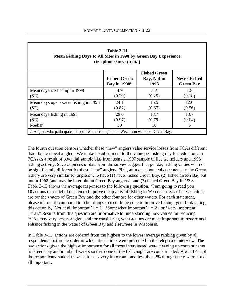
PRIMARY DATA COLLECTION < 3-22
Table 3-11Mean Fishing Days to All Sites in 1998 by Green Bay Experience
(telephone survey data)
Fished GreenBay in 1998a
Fished GreenBay, Not in
1998Never Fished
Green BayMean days ice fishing in 1998(SE)
4.9(0.29)
3.2(0.25)
1.8(0.18)
Mean days open-water fishing in 1998(SE)
24.1(0.82)
15.5(0.67)
12.0(0.56)
Mean days fishing in 1998(SE)Median
29.0(0.97)
20
18.7(0.79)
10
13.7(0.64)
6a. Anglers who participated in open-water fishing on the Wisconsin waters of Green Bay.
The fourth question censors whether these “new” anglers value service losses from FCAs differentthan do the repeat anglers. We make no adjustment to the value per fishing day for reductions inFCAs as a result of potential sample bias from using a 1997 sample of license holders and 1998fishing activity. Several pieces of data from the survey suggest that per day fishing values will notbe significantly different for these “new” anglers. First, attitudes about enhancements to the Greenfishery are very similar for anglers who have (1) never fished Green Bay, (2) fished Green Bay butnot in 1998 (and may be intermittent Green Bay anglers), and (3) fished Green Bay in 1998.Table 3-13 shows the average responses to the following question, “I am going to read you10 actions that might be taken to improve the quality of fishing in Wisconsin. Six of these actionsare for the waters of Green Bay and the other four are for other waters. For each statement,please tell me if, compared to other things that could be done to improve fishing, you think takingthis action is, ‘Not at all important’ [ = 1], ‘Somewhat important’ [ = 2], or ‘Very important’[ = 3].” Results from this question are informative to understanding how values for reducingFCAs may vary across anglers and for considering what actions are most important to restore andenhance fishing in the waters of Green Bay and elsewhere in Wisconsin.
In Table 3-13, actions are ordered from the highest to the lowest average ranking given by allrespondents, not in the order in which the actions were presented in the telephone interview. Thetwo actions given the highest importance for all those interviewed were cleaning up contaminantsin Green Bay and in inland waters so that none of the fish caught are contaminated. About 84% ofthe respondents ranked these actions as very important, and less than 2% thought they were not atall important.

PRIMARY DATA COLLECTION < 3-23
Table 3-12Socioeconomic Profile by Green Bay Experience
(telephone survey)
FishedGreen Bay
in 1998
FishedGreen Bay,Not in 1998
NeverFished
Green BayAll
Respondents
Percent male 81.9% 77.2% 65.8% 74.2%
Mean age (SE)(Question 18)
41.5(0.40)
43.6(0.35)
41.7(0.35)
42.3(0.21)
Percent Caucasian(Question 20)
91.6% 91.8% 90.3% 91.2%
Percent Native American(Question 20)
5.0% 5.2% 5.1% 5.0%
Percent with job for which theyreceive a wage or salary
84.3% 82.9% 82.3% 83%
Percent — work full-time 77.5% 74.4% 72.3% 74.6%
Percent — work part-time 6.7% 7.8% 9.4% 8.1%
Percent — homemaker 2.0% 1.9% 4.7% 3.0%
Percent — retired 7.1% 8.5% 6.6% 7.4%
Percent — self employed 4.4% 5.0% 3.7% 4.3%
Mean N of people in household(SE) (Question 21)
3.2(0.05)
3.0(0.04)
3.2(0.04)
3.1(0.02)
The action ranked next in importance was improving the clarity of water in Green Bay, which wasslightly more important to those who had never fished Green Bay (about 70% of those who hadnever fished Green Bay thought it was very important compared to 61% of those who had fishedin the waters of Green Bay in 1998). The remaining actions were very important to some anglersbut not the majority of anglers. Only 29% of anglers felt increasing panfish catch rates was veryimportant (34% of 1998 Green Bay anglers), and 22% felt that increasing public boat launches oninland waters was very important. Note also that anglers, including Green Bay anglers, felt thatadditional inland boat ramps were slightly more important than additional Green Bay boat ramps.
Next, evidence here suggests that the anglers that fish less often do not necessarily havesignificantly lower values per fishing day, if lower values at all, for eliminating FCAs in GreenBay. For example, while female license holders tend to fish about 30% to 40% less often than domale license holders (Table F-1), they have per day values for reducing FCAs that are 40% larger

PRIMARY DATA COLLECTION < 3-24
Table 3-13Importance Rating of 10 Actions to Improve Wisconsin Fishing
(telephone survey Question 13, where 1 = not at all important, 2 = somewhat important,and 3 = very important; mean and SE reported)
FishedGreen Bay
in 1998
FishedGreen Bay,Not in 1998
NeverFished
Green BayAll
Respondents
Clean up contaminants so thatnone of the fish caught in GreenBay are contaminated
2.83(0.01)
2.81(0.01)
2.87(0.01)
2.84(0.01)
Clean up contaminants so thatnone of the fish caught in theinland waters of Wisconsin arecontaminated
2.82(0.01)
2.79(0.01)
2.87(0.01)
2.83(0.01)
Improve the water clarity inGreen Bay
2.51(0.02)
2.57(0.02)
2.66(0.02)
2.59(0.01)
Increase average catch of panfishlike yellow perch on Green Bay
1.95(0.03)
1.97(0.03)
1.88(0.02)
1.93(0.01)
Provide additional public boatlaunches on inland waters
1.96(0.02)
1.90(0.02)
1.89(0.02)
1.91(0.01)
Increase average catch of sportfish like trout, salmon, bass, andwalleye on Green Bay
1.88(0.02)
1.86(0.02)
1.89(0.02)
1.88(0.01)
Provide additional public boatlaunches on Green Bay
1.89(0.02)
1.82(0.02)
1.82(0.02)
1.84(0.01)
Make existing boat ramps aroundGreen Bay free
1.80(0.03)
1.78(0.02)
1.82(0.02)
1.80(0.01)
Reduce the cost of fishing licenses 1.69(0.03)
1.71(0.02)
1.76(0.02)
1.72(0.01)
Reduce the cost of launching aboat on inland lakes
1.70(0.02)
1.68(0.02)
1.75(0.02)
1.72(0.01)

PRIMARY DATA COLLECTION < 3-25
(Chapter 9). Anglers who reside farther away from Green Bay tend to fish Green Bay less thananglers who live closer to Green Bay, but are estimated to have similar values per fishing day forthe removal of FCAs as those anglers who live closer to Green Bay (see Chapter 9).
Missing Telephone Numbers
The second source of potential sampling bias is that phone numbers could not be identified forabout one-third of the anglers identified in the courthouse sample. Some anglers have unlistedphone numbers (approximately 21% of households in the sample area do not have listed phonenumbers, which corresponds to about two-thirds of the sample for which phone numbers were notfound). Other anglers may have moved out of the area and are replaced by other anglers movinginto the area, with no clear bias. Other anglers may have provided inaccurate or invalid addresses,with unknown bias.
A study evaluating the design of the national hunting and fishing survey found that the amount offishing days by households without telephones was higher than for households with telephones(Westat, 1989, page 6-4). Therefore, the omission of anglers without telephones may result inunderstated estimates of days per angler.
Research by Piekarski (1989) indicates that households with nonlisted telephone numbers aremore likely to be multifamily housing units and renter-occupied than are listed households. Inaddition, nonlisted households are also more likely to be urban, especially in metropolitanstatistical areas with large central cities. Younger persons (both female and male), as well assingle, divorced, and separated householders (with and without children), are more likely to beunlisted than other types of households. Retired householders are over-represented, whileemployed householders are under-represented, in a sample of listed households. Finally, we areunaware of any consistent evidence that household income differs significantly between listed andnonlisted households.
Given the mixed evidence relevant to anglers for whom no phone number could be found, andthat the values per fishing day and the number of fishing days (which are multiplied to obtaindamages) may be offset for some unlisted anglers (e.g., see discussion of female anglers above),we conclude that no adjustments to the estimates of days per angler, and of the value per fishingday from reductions in FCAs, are warranted because of unlisted phone numbers.
3.5.2 Nonresponse Bias
Nonresponse bias refers to biases resulting from the differences between the respondents and thenonrespondents in the sample of anglers who purchase licenses in the eight sample frame countiesand who are active in Green Bay fishing. For the reasons presented below, we conclude thatnonresponse bias, if any, would have a very small impact on per day value estimates, but may

PRIMARY DATA COLLECTION < 3-26
5. This included 50% of those who were not recruited to receive a mail survey when called for the telephonesurvey, but who were still sent the mail survey.
6. Item nonresponse is very low at 4% or less for most all questions. The exceptions are 4-11% for the individualspecies in the target species question (Question 4), 7% for income, and up to 20% for comment questions forwhich responses were optional.
affect the estimates of fishing days per angler, for which we make an adjustment, as describedbelow.
Telephone Survey
The telephone survey high response rate of 69.4% can be expected to reduce potentialnonresponse bias. External data for anglers who purchase their licenses in the eight sample framecounties and who are active in fishing the waters of Green Bay are not readily available againstwhich to compare our telephone sample. The two observable variables we have for our telephonenonrespondents are the county where they purchased their Wisconsin fishing license, and the typeof license purchased. The survey participation rates in the telephone survey are very similarregardless of the type of license purchased or the county in which the fishing license waspurchased (see Appendix F, Tables F-2 and F-3). While we have no evidence to indicate clearlythat nonrespondents to the telephone survey fish any more or less than respondents, it may be thecase that anglers who fish less often may find the topic less salient to them and, compared toanglers that fish more often, may be less likely to participate in the telephone survey, which startsby identifying “we are conducting a study of people’s opinions about fishing.”
To be conservative in the damage assessment, while we have no evidence of this potential bias,we assume it exists in the estimate of open-water fishing days and make an adjustment for it. Weassume 31.4% of these nonrespondents are Green Bay anglers (as in the sample of active anglersas a whole), but that they fish Green Bay 50% as often as do the anglers who completed thetelephone survey (see Section 3.5.4). As noted above, the values for reducing FCAs are similar to(and in some cases larger) than for anglers who fish more often, and therefore we make noadjustment for potential nonresponse in the telephone survey to the per angler estimates of fishingdays or damages per fishing day resulting from FCAs.
Mail Survey
The mail survey had a high response rate, with 79% of those mailed the survey (and 77% of allidentified 1998 Green Bay anglers in the telephone survey) returning the survey.5,6 Evaluatingthese results, we find no basis for a potential response bias and make no adjustments.
There was little difference in fishing avidity between those recent Green Bay anglers whocompleted and returned the mail survey and those who did not. In fact, Table 3-14 shows that
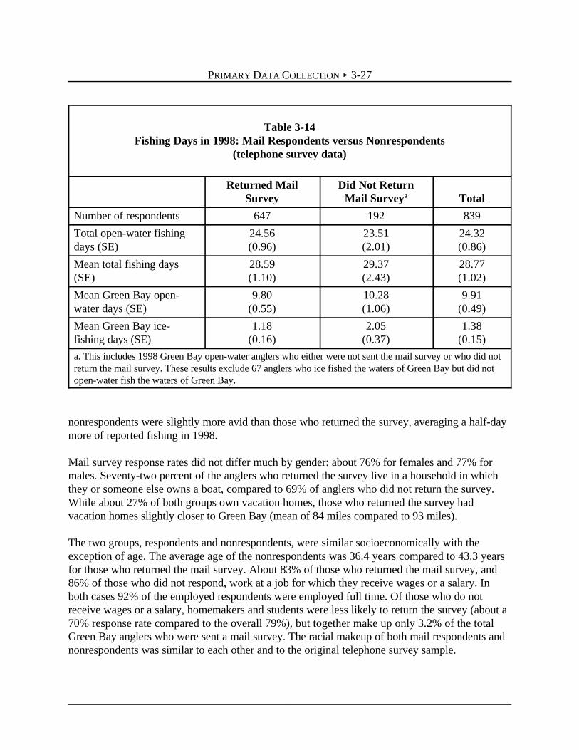
PRIMARY DATA COLLECTION < 3-27
Table 3-14Fishing Days in 1998: Mail Respondents versus Nonrespondents
(telephone survey data)
Returned MailSurvey
Did Not ReturnMail Surveya Total
Number of respondents 647 192 839
Total open-water fishingdays (SE)
24.56(0.96)
23.51(2.01)
24.32(0.86)
Mean total fishing days(SE)
28.59(1.10)
29.37(2.43)
28.77(1.02)
Mean Green Bay open-water days (SE)
9.80(0.55)
10.28(1.06)
9.91(0.49)
Mean Green Bay ice-fishing days (SE)
1.18(0.16)
2.05(0.37)
1.38(0.15)
a. This includes 1998 Green Bay open-water anglers who either were not sent the mail survey or who did notreturn the mail survey. These results exclude 67 anglers who ice fished the waters of Green Bay but did notopen-water fish the waters of Green Bay.
nonrespondents were slightly more avid than those who returned the survey, averaging a half-daymore of reported fishing in 1998.
Mail survey response rates did not differ much by gender: about 76% for females and 77% formales. Seventy-two percent of the anglers who returned the survey live in a household in whichthey or someone else owns a boat, compared to 69% of anglers who did not return the survey.While about 27% of both groups own vacation homes, those who returned the survey hadvacation homes slightly closer to Green Bay (mean of 84 miles compared to 93 miles).
The two groups, respondents and nonrespondents, were similar socioeconomically with theexception of age. The average age of the nonrespondents was 36.4 years compared to 43.3 yearsfor those who returned the mail survey. About 83% of those who returned the mail survey, and86% of those who did not respond, work at a job for which they receive wages or a salary. Inboth cases 92% of the employed respondents were employed full time. Of those who do notreceive wages or a salary, homemakers and students were less likely to return the survey (about a70% response rate compared to the overall 79%), but together make up only 3.2% of the totalGreen Bay anglers who were sent a mail survey. The racial makeup of both mail respondents andnonrespondents was similar to each other and to the original telephone survey sample.

PRIMARY DATA COLLECTION < 3-28
As shown in Table 3-15 respondents and nonrespondents hold very similar opinions about the10 actions to improve Wisconsin fishing, with the nonrespondents placing a slightly higherimportance on cleaning up contaminants and improving water clarity in Green Bay. When askedhow important it is to them that the fish they catch are free of contaminants, 89% of thenonrespondents said very important compared to 79% of the respondents. This suggests thatnonrespondents to the mail survey may value removing PCBs and the resultant FCAs more highlythan do respondents.
Table 3-15Importance Rating of 10 Actions to Improve Wisconsin Fishing:
Mail Survey Respondents versus Nonrespondents(telephone survey Question 13; mean and SE reported)
Returned MailSurvey
(N = 647)
Did Not ReturnMail Surveya
(N = 192)Clean up contaminants so that none of the fish caughtin Green Bay are contaminated
2.82(0.02)
2.87(0.03)
Clean up contaminants so that none of the fish caughtin the inland waters of Wisconsin are contaminated
2.81(0.02)
2.87(0.03)
Improve the water clarity in Green Bay 2.47(0.03)
2.65(0.04)
Increase average catch of panfish like yellow perch onGreen Bay
1.96(0.03)
1.99(0.06)
Provide additional public boat launch facilities on inlandwaters
1.96(0.03)
1.92(0.05)
Increase average catch of sport fish like trout, salmon,bass, and walleye on Green Bay
1.88(0.03)
1.89(0.06)
Provide additional public launch facilities on Green Bay 1.89(0.03)
1.86(0.05)
Make existing boat ramps around Green Bay free 1.80(0.03)
1.78(0.05)
Reduce the cost of fishing licenses 1.67(0.03)
1.70(0.05)
Reduce the cost of launching a boat on inland lakes 1.71(0.03)
1.68(0.05)
a. This includes all 173 Green Bay open-water anglers who did not return the mail survey and 19 Green Bayopen-water anglers who were not mailed the survey because they were identified too late in the process.

PRIMARY DATA COLLECTION < 3-29
7. The Wisconsin sample is particularly relevant as it focused on northeast Wisconsin in a triangular regionbetween Green Bay, Madison, and Milwaukee.
In summary, Green Bay open-water anglers who returned the mail survey were on average older,a little less avid about fishing, and only slightly less concerned about contamination than thosewho did not return the survey. Thus, we conclude that potential response bias, if any, is likely tobe very small and could slightly bias downward the damage estimates.
3.5.3 Recall Bias
Due to the timing of our survey in late 1998, we collected data on the annual number of daysfishing in 1998 up to the time of the telephone survey and updated the estimates in the mailsurvey, which added about 2% to the estimates. The process of collecting fishing activity data onan annual recall basis, rather than in sampling waves throughout the year, may be subject to recallbias, and may result in increased estimates of fishing activity. Recall bias in recreation studies issometimes referred to as “telescoping,” where respondents assign events from the past timeperiods into more recent time periods (Pollock et al., 1995). Recall bias for recreational fishingwas examined by Westat (1989; see also Chu et al., 1992) as part of the methods development forthe National Survey of Fishing, Hunting, and Wildlife-Associated Recreation (National Survey).Westat, with recreation data collected in Wisconsin and Texas, compared estimates of fishingactivity using repeated two-week recall versus annual recall (as well as semiannual and quarterlyrecall).7 The two-week recall sample was selected by Westat as providing estimates with limitedor no recall bias. The ratio of annual fishing days from the repeated two-week recall samplecompared to the annual recall sample was 62.2% (adjusted for drop-outs of avid anglers; seeWestat pages 6-16 to 6-19).
To account for potential recall bias when computing aggregate damages for the target population,we multiply our best estimates from the mail survey of 9.95 Green Bay fishing days and24.98 total fishing days per Green Bay angler (see Table 4-1 and discussion in Section 4.2) by62.2% to adjust for potential recall bias. As discussed in Section 3.5.4, these adjusted fishing dayestimates are combined with other sampling adjustments to reduce further the mean sampleestimates to be applied to all anglers in the target population.
The Westat study also found a small recall bias in annual recall of fishing participation rates(e.g., they did or did not fish). The Westat study was conducted with the general population,while our study already identified individuals who held fishing licenses in 1997 and who are muchmore likely to have fished in 1998 than the general population. Thus, any potential participationrecall bias in our study is minimized or eliminated, and no correction is made for this potentialbias.

PRIMARY DATA COLLECTION < 3-30
3.5.4 Adjusting the Sample Estimates to the Population Estimates
Based on the above discussion of potential sampling, nonresponse, and recall biases, the samplemean estimates of fishing days are adjusted to be applied to the target population to computeaggregate damages. These adjustments and the resulting population mean estimates are illustratedin Table 3-16. In Table 3-16, the 4,596 anglers in the telephone sample are grouped according todisposition in the telephone survey, and for each group the number of Green Bay anglers and thenumber of Green Bay open-water fishing days per angler are computed reflecting adjustments forpotential recall, sampling, and nonresponse biases, as follows.
1. For the 647 anglers who completed the mail survey (Table 3-16, line 1), their sample meanestimate of 9.95 Green Bay fishing days (Table 4-1) is multiplied by 62.2% to result in arecall-adjusted population mean Green Bay open-water fishing days of 6.19(9.95 × 62.2%). This is the final estimate for these 647 anglers (last column of Table 3-6).
2. For the 192 Green Bay open-water anglers who completed only the telephone survey(line 2), we assume the same recall-adjusted estimate of 6.19 Green Bay open-waterfishing days as for those who also completed the mail survey (e.g., 100% of the mailsurvey recall adjusted estimate is used). As with the telephone survey, these anglers hadactually fished slightly more than respondents who completed the mail survey.
3. For the 1,831 anglers who completed the survey and who were active anglers, but whowere not active in fishing Green Bay (line 3), none are Green Bay anglers and there are noGreen Bay fishing days.
4. For the 520 1997 license holders who did not fish in 1998 and for the 100 license holderswho refused the interview saying they no longer fish (line 4), we assume they are replacedin the population by 1998 license holders who did not have licenses in 1997 (“new”anglers). We assume 31.4% of these “new” anglers are Green Bay anglers, the same as forthe 2,370 anglers active in open-water fishing who completed the telephone survey(resulting in 163 + 31 = 194 “new” Green Bay anglers). We assume these “new” anglersfished 50% as many days (adjusted for recall) as the 647 in the mail sample of 1997 licenseholders who also fished in 1998 for an estimated 3.11 (6.19 × 0.5) open-water fishing daysin Green Bay.
5. For the 291 individuals who did not answer the telephone, or for whom language barriersprevented communication, and for the 245 individuals who hung up their telephone beforethe introduction was read (line 5), we assume 31.4% are Green Bay anglers (as in thepopulation who completed the telephone interview). We assume they fish Green Bay thesame number of days as the license holders who completed the mail survey (adjusted forrecall) because there is no evidence to suggest these anglers are different from anglers whocompleted the telephone or mail surveys.

PRIMARY DATA COLLECTION < 3-31
Table 3-16Adjustment from the Mail Sample Estimated Open-Water Fishing Days
to the Population Estimated Open-Water Fishing Days in 1998 for Anglers Activein Open-Water Fishing on the Wisconsin Waters of Green Bay
Telephone Sample Disposition
Numberof Anglers
inTelephone
Survey
PercentageWho Are
Green BayActive
NumberGreenBay
Anglers
Green BayDays
as % of RecallAdjust.
Sample Mean
FinalEstimatedGreen BayDays perAngler
1. Green Bay anglers who completedtelephone and mail survey
647 100% 647 — 6.19a
2. Green Bay anglers who completedtelephone survey only 192 100% 192 100%b 6.19
3. Non-Green Bay anglers whocompleted telephone survey
1,831 0% 0 — —
4. Did not open-water fish in 1998> Completed telephone survey> Refused telephone survey
520100
31.4%31.4%
16331
50%50%
3.113.11
5. No contact completed> No answer or language barrier> Hung up before introduction
291245
31.4%31.4%
9177
100%100%
6.196.19
6. Others/refused telephone survey> Not interested> Take name off list/other
558212
31.4%31.4%
17567
50%50%
3.113.11
7. Population estimates of Green Bayopen-water fishing days in 1998 (% of mail survey estimate of 9.98)
4,596 31.4% 1,444 — 5.25
(52.8%)
8. Population estimate of total open-water fishing days in 1998
13.19c
a. Sample mean of 9.95 (Table 4-1) × 62.2% for recall adjustment (Section 3.5.3) = 6.19 recall adjusted open-water Green Bay fishing days.b. Note that, through the telephone survey, Green Bay open-water anglers who were nonrespondents to the mailsurvey had fished slightly more than respondents completing the mail survey (Table 3-14).c. Equals sample mean of 24.98 (Table 4-1) × 52.8% combined recall, sample, and nonresponse adjustment factor= 13.19.

PRIMARY DATA COLLECTION < 3-32
8. The Lake Michigan day estimates are not exactly comparable as Green Bay angling is a subset of LakeMichigan angling. Some Lake Michigan anglers may fish in Lake Michigan inside and outside of Green Bay,and some Green Bay anglers may never fish in Lake Michigan outside of Green Bay.
9. The WDNR does not report the estimated number of open-water fishing days in the waters of Green Bay. Anapproximation can be developed by dividing the number of open-water fishing hours in the Wisconsin open-water creel survey for 1998 (905,762 from Table 2-1) by the creel estimate of four hours fishing per day, whichresults in 226,440 days. Dividing that number of fishing days by 48,600 Green Bay anglers in the targetpopulation (Chapter 8), who account for the vast majority of these fishing days, results in 4.7 Green Bay open-water days per angler in March through December. Recall the open-water creel survey omits certain time periods(see Footnote 1 in Chapter 1).
6. For the 770 (558 + 212) anglers who were contacted by telephone and did not hang upbefore the introduction, but then refused the telephone survey (line 6), we assume 31.4%were Green Bay open-water anglers who fish half as often as the license holders whocompleted the mail survey.
Under the above assumptions, in Table 3-16, the total estimated number of Green Bay open-wateranglers in the original telephone sample is 1,444, and the weighted average Green Bay open-waterdays is 5.25, which equals 52.8% of the initial sample best estimate of 9.95 (line 7). About 80% ofthis difference is because of adjustments for recall bias and about 20% is because of adjustmentsfor sampling and nonresponse bias. We apply this same 52.8% correction factor to the24.98 sample estimate of total open-water fishing days (Table 4-1) to develop a populationestimate of 13.19 total open-water fishing days in 1998 (line 8). Applying the 52.8% correctionfactor to the total (open-water plus ice) fishing days estimates in Table 4-1 results in adjustedtotal fishing days per sampled angler of 5.87 on Green Bay and 15.34 at all sites.
By way of comparison, the adjusted target population estimates of 5.87 Green Bay total fishingdays per Green Bay angler is nearly equal to the 1996 National Survey estimate for LakeMichigan anglers of 5.8 ± 2.0 days of Lake Michigan fishing, and the 15.34 total fishing daysestimate is less than the National Survey estimate of 20.2 ± 8.4 total fishing days per LakeMichigan angler. The National Survey estimates are based on a sample of only 36 anglers.8 Thetotal fishing day estimate of 15.34 is slightly more than the approximately 14 day estimate fromthe Westat survey for Wisconsin residents from the same region, which was based on a sample ofover 1,700 anglers (although the estimates are over a decade old and include non-Green Bayanglers, who fish less often than do Green Bay anglers — see Table 3-11). Further, theseestimates are generally consistent with the WDNR creel estimates of angler activity in the watersof Green Bay for 1998.9

PRIMARY DATA COLLECTION < 3-33
10. We further assume that LMD anglers purchase their licenses in their county of residence. Because someresidents of omitted counties (and all residents of Menominee County) who fish Green Bay may purchase theirlicenses in one of the eight targeted counties, it may be that over 83% of LMD anglers are covered in our targetpopulation.
3.5.5 Target Population Coverage of All Open-Water Fishing in the Wisconsin Watersof Green Bay
While the target population for the primary assessment is those Green Bay open-water anglerswho purchase their Wisconsin fishing licenses in one of eight targeted counties near the waters ofGreen Bay, data from the WDNR and from our survey indicate that the target population mayaccount for on the order of 90% of all Green Bay open-water fishing days, and our samplegenerally reflects the distribution of Green Bay open-water fishing days by origin of residence ofthe anglers. This can be ascertained by examining our sample in three groups: anglers from theLake Michigan District (see Figure 3-2), anglers from out-of-state, and anglers from the rest ofWisconsin outside of the LMD. For each group, we use data and assumptions to evaluate theapproximate share of the group’s Green Bay open-water fishing days that is likely to berepresented in our target population and approximately what share of the total number of GreenBay open-water fishing days the group is likely to account for.
The computations in the remainder of this Section 3.5.5 are based on a combination of literaturedata and our survey data and are intended only to indicate the potential magnitude of how thetarget population covers the entire population of Green Bay anglers, rather than to be preciseestimates, either for the total or individual components of this analysis.
Lake Michigan District
The population of the targeted counties is about 83% of the LMD population (WisconsinLegislative Reference Bureau, 1997). If we assume that the incidence of fishing is the samethroughout the LMD, then 83% of all LMD license holders are in the eight targeted counties.10
We expect the incidence of Green Bay anglers to be less in the omitted counties than the includedcounties because the omitted counties are farther from the site. Table 3-17 shows the incidence ofGreen Bay fishing by county for our sample. Anglers who purchased licenses in a county adjacentto Green Bay (Brown, Door, Kewaunee, Marinette, and Oconto) were about twice as likely tofish Green Bay as those who purchased their licenses in one of the nonadjacent targeted counties.This reflects that resident anglers in nearby counties are more likely to fish Green Bay than areresident anglers from more distant counties (consistent with the evidence presented above that themedian travel distance for boat fishing is 10 miles), and some anglers from outside the region whofish in Green Bay purchase licenses near the site. Because the omitted counties are even fartherfrom the site than the three nonadjacent counties in our sample, we can expect an even lower

PRIMARY DATA COLLECTION < 3-34
11. 83%/[83%+ (17% × 0.5 × 0.55)] = 94.7%, where 83% and 17% are the population percentages for theincluded and omitted LMD counties, and 0.5 and 0.55 are the adjustments for reduced incidence and reducedGreen Bay fishing days in omitted LMD counties.
Table 3-171998 Green Bay Angler Incidence Rate by County Where License Purchased
County Where 1997-1998License Purchased
Number of ScreenersCompleted
Number of Green BayAnglers Identified
Green Bay AnglerIncidence Rate
Brown County 658 246 37.4%
Door County 343 139 40.5%
Kewaunee County 203 54 26.6%
Manitowoc County 317 63 19.9%
Marinette County 354 113 31.9%
Oconto County 247 60 24.3%
Outagamie County 514 86 16.7%
Winnebago County 554 78 14.1%
All targeted Counties 3,190 839 26.3%
- Adjacent to Green Bay 1,805 612 33.9%
- Not adjacent to GreenBay 1,385 227 16.4%
incidence of Green Bay anglers in these counties. For the omitted LMD counties, we assume theincidence of Green Bay open-water anglers to be 50% as much as for included counties.
Next, we expect the number of open-water fishing days per Green Bay angler to decrease withdistance from the site. In a later analysis (Table 4-2) we find that anglers who reside in the threenonadjacent counties report 60% as many Green Bay open-water fishing days per angler as doanglers who reside in the five adjacent counties, and further that anglers from elsewhere inWisconsin report 55% as many Green Bay open-water fishing days per angler as do anglers whoreside in the five adjacent counties. For the omitted LMD counties, we assume the rate of GreenBay fishing days by Green Bay open-water anglers is 55% as large as for included LMD counties.
Combining the above data and assumptions, our target population can be expected to account forabout 95% of the Green Bay open-water fishing days by anglers from the Lake MichiganDistrict.11

PRIMARY DATA COLLECTION < 3-35
Recall that Penaloza (1992) reported about 77% of boat trips in the LMD district originated byanglers in the LMD (these percentages may be even higher in 1998 given that the reduced catchrates from the early 1990s to 1998 may deter anglers who are farther away more than they deteranglers from nearby counties). In our data we find that the percent of boat versus nonboat daysdoes not vary much with distance from the site, so we assume about 77% of all Green Bay fishingdays are from anglers residing in the LMD. Thus, the residents from the eight counties in thetarget population will account for about 73% of all Green Bay fishing days (77% × 95%). Oursample may omit about 4% of the total Green Bay open-water fishing days by excluding fiveLMD counties from our target population (77% LMD total minus 73% of this total that isexpected from the targeted counties).
Table 3-18 identifies our sample number of anglers and reported Green Bay days by residence.About 76% of our sampled anglers, and about 83% of the reported days, are from residents of theeight targeted counties. Thus, our sample has a slightly higher percentage of days by anglersresiding in the targeted counties than the above data supports may be likely to occur for all GreenBay fishing days.
Table 3-18Number and Percent of Sampled 1998 Green Bay Angler Fishing Days
by Resident State/County(telephone and mail survey data)
State/County ofResidence
Numberof Anglers
Green BayOpen-WaterFishing Days
Green BayIce-Fishing
DaysGreen Bay
Fishing DaysWisconsin 531 82% 5,672 88% 736 96% 6,408 89%
In targeted counties 494 76% 5,381 83% 721 94% 6,102 85% Not in targeted 37 6% 291 5% 15 2% 306 4%
Michigan 13 2% 266 4% 23 3% 289 4%Other state 103 16% 502 8% 7 1% 509 7%All 647 100% 6,440 100% 766 100% 7,206 100%
Out-of-State Anglers
Table 3-18 reports that anglers from out-of-state account for about 18% of the respondents and12% of the Green Bay fishing days in the sample. This reflects that out-of-state anglers tend tofish Green Bay fewer days than do resident anglers (Table 3-19). The exception is anglers fromMichigan who fish more days in Green Bay, which is reasonable as almost all of these 13 anglerslive in a county (and in or near the city of Menominee) that is adjacent to Wisconsin and to boththe Bay of Green Bay and the Menominee River (which is part of the waters of Green Bay).

PRIMARY DATA COLLECTION < 3-36
Table 3-19Mean Days Fishing Green Bay in 1998 by Resident State
(telephone survey data)a
State ofResidence N
Mean Days IceFishing in 1998 (SE)
Mean Days Open-Water Fishing in
1998 (SE)Mean Days Fishing
in 1998 (SE)Wisconsin 752 1.9
(0.18)9.8
(0.53)11.7
(0.60)Michigan 16 3.1
(1.34)18.9
(6.38)22.0
(6.34)Other states 138 0.2
(0.11)4.9
(0.39)5.2
(0.40)All 906 1.7
(0.15)9.2
(0.46)10.9
(0.52)a. Per-angler days increase slightly in the final mail sample reflecting end-of-year fishing days. See Chapter 4.
Our sample is likely to include most nonresident anglers who fish the waters of Green Bay. This isbecause nonresident anglers are most likely to purchase their licenses in a county near their fishingdestination. In fact, we find that 90% of our sample of out-of-state anglers purchased theirlicenses in one of the five adjacent counties, and only 10% purchased a license in one of the threenonadjacent counties. Further we find that 99% of reported open-water fishing days in Wisconsinby out-of-state anglers in our telephone sample are on the waters of Green Bay. While a few out-of-state anglers who fish Green Bay may purchase their Wisconsin fishing licenses outside of ourtargeted counties, is appears likely that most all will purchase their licenses in the targetedcounties: we assume 95% of Green Bay fishing days by out-of-state anglers are reflected in oursample. Thus, our sample omits less than 1% of all Green Bay open-water fishing days (5% of theapproximately 12% of total Green Bay open-water fishing days by out-of-state anglers).
Anglers from the Rest of Wisconsin
Anglers from the rest of Wisconsin who fish the waters of Green Bay are likely to purchase theirlicenses near their residences, or near where they plan to fish. Anglers from the rest of Wisconsinaccount for 6% of our sample anglers and 5% of our sample of Green Bay open-water fishingdays (Table 3-18). Our target population omits Green Bay fishing days by those Green Bayanglers who purchase their licenses outside of the targeted counties. The size of this omission isunknown. However, for simplicity, if we assumed 100% coverage of Green Bay fishing days fromLMD anglers by residents of our eight targeted counties and 100% coverage of out-of-stateanglers, the difference of 6% between the sample share of fishing days by anglers residing in ourtargeted counties (83%) and the projected share of fishing days by anglers residing in LMD

PRIMARY DATA COLLECTION < 3-37
counties (77% or more) would approximately represent the omission of Green Bay open-waterfishing days by Wisconsin anglers who reside outside of the eight targeted counties.
Target Population Coverage of All Green Bay Fishing Days
Based on the above computations, selection of our target population is likely to account for about90% of all Green Bay open-water fishing days. The sample does not account for Green Bay open-water fishing days by LMD residents outside of the eight targeted counties (about 4%), by out-of-state anglers who purchase their licenses outside of the eight targeted counties (less than 1%), andby residents from other counties in Wisconsin who purchase their licenses outside of the eighttargeted counties (about 6%).

CHAPTER 4GREEN BAY ANGLER PROFILE
4.1 INTRODUCTION
This chapter provides data on fishing activity and attitudes for our sample of anglers who activelyfished the Wisconsin waters of Green Bay in 1998. These results focus on the 647 anglers whocompleted both the telephone and mail surveys, and who report over 7,000 Green Bay fishingdays and over 18,000 total fishing days in 1998. In this chapter, Green Bay fishing refers tofishing the Wisconsin waters of Green Bay, including all tributaries up to the first dam orobstruction, unless specifically identified otherwise.
The vast majority of anglers active in Green Bay fishing are aware of and show a generalknowledge about the PCB FCAs. Anglers express that cleaning up PCBs so that the FCAs can beremoved is one of the most important improvements, if not the single most importantimprovement, that can be made in the Green Bay recreational fishery. Boat launches, improvedfacilities, and reduced costs are desirable, but much less important than uncontaminated fish andincreased catch rates (in that order).
The impacts of PCB contamination and the resultant FCAs are substantial. The majority ofcurrent Green Bay anglers indicate that as a result of PCB contamination and FCAs, they havealtered their Green Bay fishing behavior. Additionally, over 10% of the sampled anglers that didnot fish Green Bay in 1998 express that PCB contamination was a key factor explaining why theydid not fish Green Bay in 1998.
These results indicate that the PCB contamination and the FCAs can be expected to result insignificant damages to Green Bay anglers and to other anglers who do not currently fishGreen Bay.
Section 4.2 provides angler reported data on the number of Green Bay fishing days per GreenBay angler, as well as expenditure data and additional angler characteristics. Section 4.3 providesattitudinal data about the Green Bay fishery as a whole. Section 4.4 discusses anglers’ awarenessof FCAs, and the impacts of FCAs on recreational fishing behavior and enjoyment are presentedin Section 4.5.

GREEN BAY ANGLER PROFILE < 4-2
1. These estimates are based on the entire year of fishing, whereas the telephone survey estimates are based ona larger sample of 839 Green Bay anglers (Table 3-14 “Total” column); they omit up to six weeks of potentialfishing for some anglers. The mail survey estimates of 9.95 Green Bay open-water fishing days and 24.98 totalopen-water fishing days, are, respectively, 0.4% and 2.7% larger than the corresponding telephone surveyestimates.
4.2 GREEN BAY FISHING ACTIVITY AND EXPENDITURES
Data on the number of days Green Bay anglers fished in 1998 were collected in two parts.First, in the telephone survey anglers were asked how many days they had spent fishing fromJanuary 1, 1998, until the time of the telephone interview. Second, in the mail survey they wereasked how many days they had fished in 1998 since the day of the telephone interview. The datafrom these two sources were combined for the total reported days fished in 1998. Unless statedotherwise, the results in this chapter are as reported by respondents and are not adjusted forpotential recall, sample, and nonresponse bias (see Section 3.5.4).
The number of reported 1998 fishing days is reported in Table 4-1. These numbers are slightlyhigher than the reported days in Chapter 3, which were only for fishing activity fromJanuary 1, 1998, to the day the telephone survey was completed (between late October andDecember 1998). As noted in Chapter 3, the total fishing days and Green Bay fishing daysestimated in the telephone survey were similar for mail survey respondents and nonrespondents.The number of open-water fishing days by anglers active in Green Bay fishing, as reported inTable 4-1, is used as the basis for the open-water fishing damage computations.1 In Section 3.5.4,we develop an adjustment factor of 52.8% for potential recall, sampling, and nonresponse biases,and the adjusted numbers, which are reported in the last column of Table 4-1, are used inChapters 8 and 10 to compute annual damages in 1998 and the present value of damages from1999 into the future.
These avidity levels are similar to estimates from Bishop et al.’s (1994) study where they foundthat Lake Michigan anglers averaged 32 fishing days a year with 9 of those days on the GreatLakes. Once adjusted for potential recall, sample, and nonresponse biases, the estimates arecomparable to or less than estimates from the 1996 National Survey of Fishing, Hunting andWildlife Associated Recreation (U.S. DOI, 1998) for anglers active in the Wisconsin waters ofLake Michigan (see Section 3.5.4).
Estimates for Green Bay angling days demonstrate a highly skewed distribution. As seen inFigure 4-1, most individuals fish the open waters of Green Bay only a few times in the season,but many fish almost weekly, and some fish several times a week.
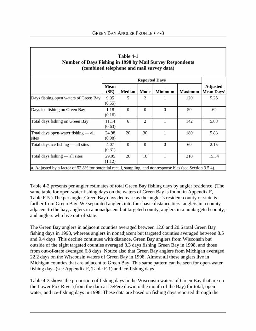
GREEN BAY ANGLER PROFILE < 4-3
Table 4-1Number of Days Fishing in 1998 by Mail Survey Respondents
(combined telephone and mail survey data)
Reported Days
AdjustedMean Daysa
Mean(SE) Median Mode Minimum Maximum
Days fishing open waters of Green Bay 9.95(0.55)
5 2 1 120 5.25
Days ice fishing on Green Bay 1.18(0.16)
0 0 0 50 .62
Total days fishing on Green Bay 11.14(0.63)
6 2 1 142 5.88
Total days open-water fishing — allsites
24.98(0.98)
20 30 1 180 5.88
Total days ice fishing — all sites 4.07(0.31)
0 0 0 60 2.15
Total days fishing — all sites 29.05(1.12)
20 10 1 210 15.34
a. Adjusted by a factor of 52.8% for potential recall, sampling, and nonresponse bias (see Section 3.5.4).
Table 4-2 presents per angler estimates of total Green Bay fishing days by angler residence. (Thesame table for open-water fishing days on the waters of Green Bay is found in Appendix F,Table F-5.) The per angler Green Bay days decrease as the angler’s resident county or state isfarther from Green Bay. We separated anglers into four basic distance tiers: anglers in a countyadjacent to the bay, anglers in a nonadjacent but targeted county, anglers in a nontargeted county,and anglers who live out-of-state.
The Green Bay anglers in adjacent counties averaged between 12.0 and 20.6 total Green Bayfishing days in 1998, whereas anglers in nonadjacent but targeted counties averaged between 8.5and 9.4 days. This decline continues with distance. Green Bay anglers from Wisconsin butoutside of the eight targeted counties averaged 8.3 days fishing Green Bay in 1998, and thosefrom out-of-state averaged 6.8 days. Notice also that Green Bay anglers from Michigan averaged22.2 days on the Wisconsin waters of Green Bay in 1998. Almost all these anglers live inMichigan counties that are adjacent to Green Bay. This same pattern can be seen for open-waterfishing days (see Appendix F, Table F-1) and ice-fishing days.
Table 4-3 shows the proportion of fishing days in the Wisconsin waters of Green Bay that are onthe Lower Fox River (from the dam at DePere down to the mouth of the Bay) for total, open-water, and ice-fishing days in 1998. These data are based on fishing days reported through the

GREEN BAY ANGLER PROFILE < 4-4
2. It would be difficult to explain this difference with sampling variability in either survey. Other plausibleexplanations could include differences in how WDNR and our respondents assign days between the Bay ofGreen Bay and the Lower Fox River, or potential undersampling of the Lower Fox River in the WDNR creelsurvey.
186
10394
45 49
2312
37
4
22
72
0
20
40
60
80
100
120
140
160
180
200
1 or 2 3 or 4 5 or 6 7 or 8 9 or 10 11 or 12 13 or 14 15 or 16 17 or 18 19 or 20 >20
Number of Days Fishing Open Waters of Green Bay in 1998
Num
ber
of A
ngle
rs
Figure 4-1Distribution of Reported Number of Open-Water Fishing Days on Wisconsin Waters of Green
Bay in 1998, for All Mail Survey Respondents (combined telephone and mail survey data)
telephone survey by the 647 respondents who completed both the telephone and mail survey andomit about 2% of total fishing days reported between the telephone and mail survey. About13.4% of all fishing days are on the Lower Fox River, with the proportion higher for open-waterfishing days than for ice-fishing days. This percentage is higher than the 5% reported for theWDNR creel survey for 1998 (Table 2-2). The reason for this divergence in results is uncertaingiven the otherwise overall consistency between our results and the WDNR results.2 Similarresults for all 906 Green Bay anglers completing the telephone survey are found in Appendix F(Table F-6).
In the mail survey, anglers were asked how often they target specific species when fishing onGreen Bay. Figure 4-2 shows the distribution of targeting effort. The percent of anglers who

GREEN BAY ANGLER PROFILE < 4-5
Table 4-2Total Number of Reported Fishing Days on Wisconsin Waters of Green Bay in 1998, by
Residence, for Mail Survey Respondents (combined telephone and mail survey data)
Residence
Numberof
Anglers
Total Days Days per Angler
Total
% ofTotal Green Bay
Fishing DaysMean(SE) Median Mode Min. Max.
Other states Total 117 800 11% 6.8
(1.03)4 2 1 95
Michigan 13 289 4% 22.2(7.62)
15 1 1 95
Wisconsin, but noteight targeted counties
37 306 4% 8.3(1.55)
5 2 1 38
Eight targetedcounties
Total493 6,100 85% 12.4
(0.77)6 2 1 142
Brown County 195 2,340 32% 12.0(1.24)
6 2 1 142
Door County 46 947 13% 20.6(3.7)
11 4 1 100
Kewaunee County 20 345 5% 17.3(5.60)
7.5 1 1 90
Manitowoc County 49 462 6% 9.4(1.64)
7 10 1 76
Marinette County 59 773 11% 13.1(1.64)
9 2 1 60
Oconto County 37 462 6% 12.5(2.45)
6 3 1 57
Outagamie County 53 450 6% 8.5(1.46)
3 1 1 50
Winnebago County 34 321 4% 9.4(3.09)
4.5 1 1 105
All mail surveyrespondents
647 7,206 100% 11.1(0.63)
6 2 1 142

GREEN BAY ANGLER PROFILE < 4-6
3. The nonresponse rate for the different species in this question is much higher than other questions in thesurvey. This is likely because some respondents who never target a particular species left the answer for thatspecies blank. Only 2 of the 647 respondents left all the species blank. The percentages listed are for allanglers, assuming those who left the response blank for a species do not fish for that species. Omitting missingresponses increases the percentages to 44% for perch, 37% for smallmouth bass, 34% for walleye, 26% fortrout/salmon, and 46% for whatever is biting. The carp percentage is unchanged.
Table 4-3Number of Reported Fishing Days on the Fox River between the Mouth and DePere Dam
as Compared to All Wisconsin Waters of Green Bay in 1998, for Mail Survey Respondents(N = 647)a (telephone survey data)
Sample Days per Angler
Total
% of TotalGreen Bay
Fishing DaysMean(SE) Median Mode Min. Max.
Green Bay total daysAll sites 7,107 100% 11.0
(0.62)6 2 1 142
On Fox River 951 13.4% 1.5(0.28)
0 0 0 130
Green Bay open-water daysAll sites 6,342 89.2% 9.8
(0.55)5 2 1 120
On Fox River 865 12.2% 1.3(0.25)
0 0 0 110
Green Bay ice-fishing daysAll sites 765 10.8% 1.2
(0.16)0 0 0 50
On Fox River 86 1.2% 0.1(0.05)
0 0 0 20
a. Sample includes anglers who fish the open-water Wisconsin waters of Green Bay. Anglers who only icefished these waters are excluded.
“often” or “almost always” target each the four key species is 42% for perch, 34% for bass, 32%for walleye, 24% for trout/salmon, 7% for carp/catfish/whitebass, and 41% for “whatever isbiting.”3 Note that the percentages of anglers citing “often” or “always” totals to 180%. Adjustedto the 180% total the perch share, for example, is 23% (42%/180%), which is comparable withthe percent of activity identified as targeting perch by the WDNR creel survey (Table 2-6). Notealso that a large share of anglers are opportunistic and target whatever is biting (41%). Thus,

GREEN BAY ANGLER PROFILE < 4-7
4 .8%
1 3 .1%
1 7 .9%
2 2 .0%
2 2 .4%
1 9 .8%
8 .0%
3 0 .6%
1 9 .8%
1 7 .9%
1 3 .5%
1 0 .2%
6 .3%
1 6 .1%
1 7 .6%
2 8 .3%
1 9 .8%
1 1 .9%
8 .4%
1 8 .9%
1 4 .8%
2 4 .1%
2 0 .7%
1 3 .1%
1 1 .4%
5 9 .0%
1 4 .7%
8 .4%
4 .2%2 .3%
1 0 .7%
1 7 .5%
1 0 .1%
2 1 .0%
1 5 .3%
2 5 .5%
0 %
1 0 %
2 0 %
3 0 %
4 0 %
5 0 %
6 0 %
7 0 %
8 0 %
9 0 %
1 0 0 %
Per
cent
of
Ang
lers
P e r c h T r o u t /S a lm o n
W a lle y e B a ss C a rp e tc . W h a tever i sb itin g
S p e c ies
A l m o s t a l w a y s
O ften
S o m etim e s
S e l d o m
N e v e r
M issin g
Figure 4-2How Often Anglers Target a Specific Species on Green Bay
(mail survey Question 4)
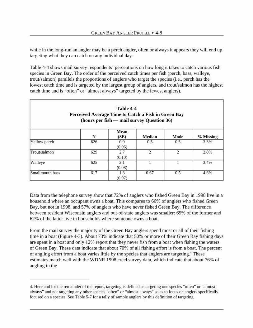
GREEN BAY ANGLER PROFILE < 4-8
4. Here and for the remainder of the report, targeting is defined as targeting one species “often” or “almostalways” and not targeting any other species “often” or “almost always” so as to focus on anglers specificallyfocused on a species. See Table 5-7 for a tally of sample anglers by this definition of targeting.
while in the long-run an angler may be a perch angler, often or always it appears they will end uptargeting what they can catch on any individual day.
Table 4-4 shows mail survey respondents’ perceptions on how long it takes to catch various fishspecies in Green Bay. The order of the perceived catch times per fish (perch, bass, walleye,trout/salmon) parallels the proportions of anglers who target the species (i.e., perch has thelowest catch time and is targeted by the largest group of anglers, and trout/salmon has the highestcatch time and is “often” or “almost always” targeted by the fewest anglers).
Table 4-4Perceived Average Time to Catch a Fish in Green Bay
(hours per fish — mail survey Question 36)
NMean(SE) Median Mode % Missing
Yellow perch 626 0.9(0.06)
0.5 0.5 3.3%
Trout/salmon 629 2.7(0.10)
2 2 2.8%
Walleye 625 2.1(0.08)
1 1 3.4%
Smallmouth bass 617 1.3(0.07)
0.67 0.5 4.6%
Data from the telephone survey show that 72% of anglers who fished Green Bay in 1998 live in ahousehold where an occupant owns a boat. This compares to 66% of anglers who fished GreenBay, but not in 1998, and 57% of anglers who have never fished Green Bay. The differencebetween resident Wisconsin anglers and out-of-state anglers was smaller: 65% of the former and62% of the latter live in households where someone owns a boat.
From the mail survey the majority of the Green Bay anglers spend most or all of their fishingtime in a boat (Figure 4-3). About 73% indicate that 50% or more of their Green Bay fishing daysare spent in a boat and only 12% report that they never fish from a boat when fishing the watersof Green Bay. These data indicate that about 70% of all fishing effort is from a boat. The percentof angling effort from a boat varies little by the species that anglers are targeting.4 Theseestimates match well with the WDNR 1998 creel survey data, which indicate that about 76% ofangling in the

GREEN BAY ANGLER PROFILE < 4-9
11.9%
5.4%3.6% 3.9%
1.4%
4.5%1.9%
4.3%6.7%
16.1%
39.3%
1.2%
0%
5%
10%
15%
20%
25%
30%
35%
40%
45%
0% 10% 20% 30% 40% 50% 60% 70% 80% 90% 100% Missing
Proportion of Fishing Days Spent on a Boat
Pro
port
ion
of A
ngle
rs
Figure 4-3Percent of Green Bay Fishing Days Spent on a Boat
(mail survey Question 5)
waters of Green Bay are from a boat (defined as hours under the categories of ramp, moored, andcharter).
Anglers who fish by boat report an average of 2.5 people (including themselves) in the boat for atypical trip. The minimum was 1 person and the maximum was 5 people. The average number ofpeople in a boat varies somewhat among those who target different specific species: 2.6 for perchtargeters, 2.8 for trout/salmon targeters, 2.1 for walleye targeters, 2.2 for bass targeters, and2.4 for those with no specific target.
In Question 12, anglers report expenses for a “typical” day of fishing on the waters of Green Bay.Anglers report spending an average of about $74 per day, with a median of $31 and a mode of$20. The breakdown of these costs is presented in Table 4-5. The 1996 National Survey(U.S. DOI, 1998) reports a yearly expenditure of $328 per angler ($1998) on Great Lakes fishing,with an average of 5 days per angler, resulting in an average of about $65 per day ($1998).Bishop et al. (1994) report per capita expenditure per day of $130 ($1998) for Wisconsin GreatLakes fishing.

GREEN BAY ANGLER PROFILE < 4-10
Table 4-5Typical Expenditures on Green Bay Fishing Days
(mail survey Question 12 mean estimate $/day)
Mean SE Median Mode Min. Max. MissingGas for vehicle/boat 21.23 6.97 10 10 0 4000 0.9%Boat launching fee 2.60 0.11 3 0 0 20 0.9% Motel/hotel 9.12 1.41 0 0 0 500 0.9%Fishing gear 15.66 4.48 5 5 0 2000 1.1%Bait 5.73 0.79 5 5 0 500 1.1%Food and beverages 12.30 1.74 6 10 0 998 0.9%Guide or charter fees 5.40 1.36 0 0 0 400 0.9%Other 5.36 3.94 0 0 0 2500 1.1%Totala 74.32 14.84 31 20 0 8705 0.8%a. This does not equal the sum of the means of the expenditure items. This is the mean of the totalexpenditures that was calculated by each respondent.
In the mail survey (Q38), anglers were asked, “What do you think is the average daily boatlaunch fee for the waters of Green Bay?” The mean of the angler estimates is $4.41, the medianis $4.00, and the mode is $3.00. The median reported in Questions 12 and 38 are the same, butthe mean is lower in Question 12. Question 12 respondents were asked what they actually pay,and over one-fourth of the anglers do not use a boat on their “typical” day of fishing on thewaters of Green Bay (Figure 4-3), and others may launch their boats from their own or free boatlaunches.
Current Green Bay anglers (those active in Green Bay fishing in 1998) are more likely than otheranglers to have a vacation home near Green Bay: 28% of current green Bay anglers own vacationhomes, which are on average 90 miles (SE = 12.3) from Green Bay; 29% of anglers who havefished Green Bay in the past, but not in 1998, own vacation homes with an average distance of107 miles (SE = 8.7); and 25% of anglers who have never fished Green Bay own vacation homeswith an average distance of 164 miles from Green Bay. A difference in the location of vacationhomes is also seen between anglers who reside in and outside of Wisconsin. About 27% of bothgroups own vacation homes, but the vacation homes of Wisconsin residents are on average93 miles (SE = 5.9) from Green Bay, and the vacation homes of nonresidents are on average266 miles (SE = 30.6) from Green Bay. Compared to all anglers, recent Green Bay anglers aremore likely to be male, retired or self-employed, and less likely to be homemakers, but beyondthis characteristics are similar to other anglers.

GREEN BAY ANGLER PROFILE < 4-11
2.6%
10.4%
18.2%
27.8%
20.1%
10.8%
3.3%5.1%
1.7%
0.0%
5.0%
10.0%
15.0%
20.0%
25.0%
30.0%
1. Muchworse than
otherplaces
2 3 4. Aboutthe same
5 6 7. Muchbetter
than otherplaces
8. Don’tKnow
9. Missing
Green Bay Relative to Other Places
Per
cent
of
Res
pond
ents
Figure 4-4Quality of Green Bay Relative to Other Places Respondent Fishes
4.3 OVERALL ATTITUDES ABOUT THE GREEN BAY RECREATIONAL FISHERY
Overall Attitudes
Anglers were split as to whether they felt the quality of fishing on Green Bay was currently better(34%), worse (29%), or the same (28%) relative to other places they fish (Figure 4-4). Most feelthe Green Bay fishery is as good as or better than other places, which explains why they haveremained in the fishery. That the 29% who feel the quality of fishing is worse than other siteshave remained active in the fishery is evidence that Green Bay is a unique site to these anglers.
Respondents were asked to write a comment to explain their rating of Green Bay relative to otherplaces they fished. For those who feel Green Bay is worse than other sites, catch attributes,negative conditions at the site (such as weather, the size of, distance to, or facilities on GreenBay) and contamination or pollution problems (including PCBs and not being able to eat the fish)are mentioned most frequently as reasons to prefer other sites (see Appendix F, Table F-4, andaccompanying discussion).
In mail survey Question 7, when asked about how important different actions are in terms ofenhancing recreational fishing on Green Bay, 70% of anglers indicate that cleaning up PCBs soFCAs could be reduced or eliminated is the most important action resulting in a mean score of4.4 on a 5 point scale (1 = least important to 5 = most important) (see Table 4-6). The action

GREEN BAY ANGLER PROFILE < 4-12
ranked
Table 4-6Angler Rating of Importance of Actions in Terms of How the Actions Would Enhance
Recreational Fishing on the Waters of Green Bay(mail survey Question 7 where 1 = Least Important to 5 = Most Important)
Action
Rating
1.Least
Important
2. 3. 4. 5.Most
Important MissingMean(SE)
Median
Adding more boat launchfacilities
31.5% 24.1% 24.1% 10.2% 8.7% 1.4% 2.4(0.05)
2
Adding more shoreline parks,nature centers, and trails
26.9% 20.6% 23.3% 15.3% 12.2% 1.7% 2.6(0.05)
3
Increasing water clarity 8.7% 8.8% 20.9% 25.8% 34.2% 1.7% 3.7(0.05)
4
Increasing catch rates 14.8% 14.8% 23.2% 22.6% 22.9% 1.7% 3.2(0.05)
3
Cleaning up PCBs so fishconsumption advisories canbe reduced or eliminated
3.7% 3.3% 9.4% 12.8% 70.0% 0.8% 4.4(0.04)
5
second in importance is improving water clarity in Green Bay, which is on average given a 3.7with 34% saying it is a most important action by rating it a 5. Increasing catch rates is rankedthird in importance, with an average of 3.2 on the 5 point scale and 23% saying it is a mostimportant action. Adding shoreline parks is ranked as a most important action for only 12.2% ofrespondents, and adding more boat launch facilities is ranked as a most important action for only8.7% of respondents. This ranking is consistent with the responses to the telephone survey(discussed in Chapter 3) where all the respondents (Green Bay anglers or otherwise) rankcleaning up contaminants as the most important action, followed by improving water clarity, andthen increasing catch rates and providing more boat launches.
For most anglers, improving catch rates is rated as less important than removing PCBcontamination from Green Bay. However, catch rates still are important to anglers and theirfishing experience. Table 4-7 shows how strongly respondents feel about two catch rate issues.Sixty-five percent of respondents agree that efforts should be made to increase Green Bay catchrates, and 80% of the respondents agree that efforts should be made to ensure that fishpopulations and catch rates do not decline.

GREEN BAY ANGLER PROFILE < 4-13
Question 13 directly addresses the relative importance of increased catch rates and reduced PCBsin terms of paying higher fees to support these improvements (Table 4-8). Opinion is mixedabout
Table 4-7Statements about Catch Rates
(mail survey Question 8)
We Should Increase CatchRates by Increasing Green
Bay Fish Populations
We Should Not Let Green BayFish Populations Decline
because that Would CauseCatch Rates to Decline
1. Strongly Disagree 4.5% 3.9%2. Disagree 5.9% 2.8%3. Neither Agree nor Disagree 24.4% 12.7%4. Agree 27.1% 21.8%5. Strongly Agree 37.7% 58.3%
Missing 0.5% 0.6%Mean Rating (SE) 3.9 (0.04) 4.3 (0.04)
Table 4-8Statements about Boat Launch Fees in Relation to Catch Rates and PCB Contamination
(mail survey Question 13)
I Would Be Willing to PayHigher Boat Launch Fees IfCatch Rates Were Higher on
the Waters of Green Bay
I Would Be Willing to PayHigher Boat Launch Fees If
the Fish Had No PCBContamination
1. Strongly Disagree 25.0% 18.2%2. Disagree 11.9% 8.2%3. Neither Agree nor Disagree 31.4% 24.1%4. Agree 18.1% 20.9%5. Strongly Agree 13.5% 28.4%
Missing 0.2% 0.2%Mean Rating (SE) 2.8 (0.05) 3.3 (0.06)

GREEN BAY ANGLER PROFILE < 4-14
paying more to increase catch rates, with similar shares of individuals agreeing, disagreeing, andneither agreeing nor disagreeing. The results are different for PCBs, with about 50% agreeingthey would be willing to pay more in fees if the fish had no PCB contamination. This isconsistent with other survey responses, which all indicate a higher importance and value placedon cleaning up contamination than on improving catch rates.
These mail survey results are consistent with the earlier telephone survey results, where 82% ofboth Wisconsin and out-of-state anglers feel being able to catch fish free of contaminants is veryimportant (telephone Question 12), and both groups rank cleaning up contaminants inGreen Bay, cleaning up contaminants from inland waters, and improving the clarity of water inGreen Bay as highest in importance among actions to improve the quality of fishing in Wisconsin(telephone Question 13).
4.4 AWARENESS OF FCAS
The Green Bay anglers who returned the mail survey are both aware and concerned about FCAsfor the waters of Green Bay. Eighty-five percent said they had heard or read about the FCAsbefore receiving this mail survey. This response is consistent with our focus groups and pretestinterviews, in which respondents consistently displayed a high level of awareness of andknowledge about fish contamination.
When respondents were asked how much it would bother them to have various levels of FCAsfor the fish they target in Green Bay, 24% were “not at all bothered” by an “Eat no more than onemeal a week” restriction, and 8.4% were not at all bothered by a “Do not eat” restriction.Conversely, 28.3% found the “Eat no more than one meal a week” restriction very bothersome,and 77% found the “Do not eat” restriction to be very bothersome (Table 4-9). Note that the mostfrequent response (mode) for all FCA levels is “very bothersome.”
Angler perceptions of advisory levels are generally consistent with the 1998 published advisories,but do reflect variations across individuals. It is important to note that the advisories vary throughtime, and vary between the Bay of Green Bay, the Lower Fox River (more severe), and in theMichigan waters of Green Bay (less severe). Table 4-10 shows the levels of advisories thatrespondents thought were closest to the FCAs. The bold, italicized entries show the actual rangefor the 1998 Wisconsin advisory levels for Green Bay and the Lower Fox River. The finalcolumn shows the percent of respondents whose responses are consistent with the 1998 levels forGreen Bay and/or the Fox River. Most perch, trout/salmon, and walleye anglers chose one of thecurrent levels for the species they targeted, but many bass anglers underestimated the smallmouthbass restriction.

GREEN BAY ANGLER PROFILE < 4-15
Table 4-9How Bothered Anglers Would Be by Different Levels of FCAs
for the Fish They Target in Green Bay(mail survey Question 10 where 1 = not at all bothersome to 5 = very bothersome)
Rating
Level of FCAs
Eat No More thanOne Meal a Week
Eat No More than OneMeal a Month Do Not Eat
1. Not at all bothersome 24.0% 11.3% 8.4%
2. 13.3% 6.2% 1.7%
3. 18.6% 18.1% 4.0%
4. 13.1% 19.3% 4.6%
5. Very bothersome 28.3% 42.0% 77.1%
Missing 2.8% 3.1% 4.2%
Mean rating of how bothersome(SE)
3.1(0.06)
3.8(0.05)
4.5(0.05)
Median rating of how bothersome 3 4 5
Anglers who live in the eight targeted counties are more likely to report an advisory level that isconsistent with the 1998 Wisconsin advisory than those who do not live in the eight targetedcounties (whether they live in other Wisconsin counties or out-of-state). Michigan anglers (about2% of our sample) are more likely to underestimate the Wisconsin advisory, which is consistentwith the fact that Michigan advisories are generally less severe than Wisconsin’s advisories (seeChapter 2 for a comparison). Other anglers in the region may also be influenced by the Michiganadvisories.
4.5 IMPACTS OF FCAS
As identified in Chapter 2, PCBs and the resulting FCAs can be expected to impact anglerbehavior and enjoyment. In our telephone survey we asked anglers who had not fished Green Bayin 1998 why they had not fished Green Bay in 1998 or why they had never fished Green Bay, ifthey would consider fishing Green Bay if conditions were different and if so, what things wouldhave to change before they would consider fishing Green Bay (telephone survey Questions 10and 11). About 7.4% of anglers in our telephone sample express that PCBs and FCAs are a keyfactor in explaining why they did not fish Green Bay in 1998. If these anglers were to become

GREEN BAY ANGLER PROFILE < 4-16
Table 4-10Respondent Perception of Current FCAs on Green Baya
(mail survey Question 37)
UnlimitedOne Meal
a Week
OneMeal aMonth
One MealEvery 2Months
Do NotEat Missing
Consistentwith 1998Wisconsin
FCA Range
Yellow perch
All anglers 28.1% 52.6% 12.5% 1.6% 3.1% 2.2% 65.1%
Perch anglersb 25.6% 61.6% 9.6% 0.8% 0.8% 1.6% 71.2%
Live in 8 county region 28.0% 54.0% 12.4% 1.4% 3.0% 1.2% 66.4%
Trout/Salmon
All anglers 3.1% 27.2% 48.2% 10.5% 9.0% 2.0% 67.7%
Trout/salmon anglers 3.2% 33.3% 44.4% 11.1% 4.8% 3.2% 60.3%
Live in 8 county region 2.4% 25.2% 50.7% 10.6% 9.3% 1.8% 70.6%
Walleye
All anglers 6.8% 38.8% 35.4% 10.5% 6.3% 2.2% 52.2%
Walleye anglers 9.6% 30.8% 42.3% 9.6% 7.7% 0.0% 59.6%
Live in 8 county region 5.1% 36.9% 39.4% 11.0% 6.7% 1.0% 57.1%
Smallmouth bass
All anglers 11.9% 39.0% 30.9% 7.0% 8.4% 2.9% 37.9%
Bass anglers 25.4% 39.0% 22.0% 3.4% 8.5% 1.7% 25.4%
Live in 8 county region 9.9% 38.1% 34.3% 6.9% 8.7% 2.0% 41.2%
a. The bold, italicized percentage numbers indicate the 1998 Wisconsin advisory levels. There is more thanone box shaded for each species as the advisory changes relative to fish size and location.b. This refers to anglers who target perch, those who said they “often” or “almost always” target perch onGreen Bay, but do not “often” or “almost always” target any other species. The same approach applies to“trout/salmon anglers,” “walleye anglers,” and “smallmouth bass anglers.”

GREEN BAY ANGLER PROFILE < 4-17
5. About 5.3% of the telephone sample reported stopping Green Bay fishing because of the advisories, and2.1% reported they would consider fishing Green Bay if the contaminants and FCAs were removed. Thepotential increase in Green Bay anglers is 23.6% [(5.3% + 2.1%) / 31.4%].
active in Green Bay fishing, the number of anglers active in Green Bay fishing from ourpopulation would increase by about 24%.5
Mail survey Question 11 asked “In response to the existing fish consumption advisories for thewaters of Green Bay, do you do any of the following?,” and then was followed by a list ofpotential behavioral responses as identified in Table 4-11. Overall, 77% of respondents identifymaking one or more of the changes. A significant percent of anglers (30%) change how oftenthey fish in Green Bay and where they fish in Green Bay. Keeping with the FCArecommendation, 40-50% change the target species, change the size of the fish they keep, orchange how fish are cleaned or prepared.
Table 4-11Behavioral Changes in Response to FCAs for Green Bay
(mail survey Question 11)
In response to existing FCAs for the waters of Green Bay, do you do anyof the following? . . .
Percent WhoMade thisChange Missing
Spend fewer days fishing the waters of Green Bay 30.0% 2.0%
Change the places I fish on the waters of Green Bay 30.6% 1.9%
Change the species I fish for on the waters of Green Bay 22.9% 1.9%
Change the species of fish I keep to eat from the waters of Green Bay 45.0% 1.9%
Change the size of fish I keep to eat from the waters of Green Bay 47.1% 2.6%
Change the way Green Bay fish are cleaned or prepared 45.4% 2.6%
Change the way Green Bay fish are cooked at my house 24.7% 2.8%
Made one or more of these changes 77.4% 1.6%

1. Cost and quality are also defined as characteristics of a commodity or an activity like fishing. Qualitycharacteristics are commonly referred to as attributes, but cost is not an attribute. Later when we discuss choicepairs (Section 5.4), for simplicity of presentation, we refer to characteristics of different Green Bay alternativesto include both attributes and cost.
CHAPTER 5THE GREEN BAY CHOICE QUESTIONS
5.1 INTRODUCTION
Choice questions, sometimes called stated-choice questions or attribute-based choice questions,along with data on observed fishing behavior, are used to estimate anglers’ willingness to pay(WTP) to reduce or remove Green Bay FCAs. A choice question presents an individual with anumber of alternatives, each described in terms of the levels of their common set ofcharacteristics, and asks the individual to state his preferred alternative.1
Consider presenting a current Green Bay angler with the following simple choice pair: Green Baywith a $5 launch fee and an average catch rate of one fish per hour, versus Green Bay with an$8 launch fee and an average catch rate of one fish every 30 minutes. If an angler chooses thesecond alternative (higher cost and catch rate), his WTP per Green Bay fishing day for thedoubled catch rate is at least $3. If the angler chooses the first alternative, the WTP is less than$3. Many different choice pairs can be generated by varying the launch fee and catch rates. Forexample, if there are three launch fees and four catch rates, there are 12 possible alternatives and66 possible pairs. If site characteristics include cost, catch rate, and FCA level, choice pairs candetermine how an angler(s) would trade off less stringent FCAs at the site for higher cost, bettercatch rates for higher cost, or better catch rates for more stringent FCAs.
We ask this type of Green Bay choice question, then ask a followup question of how often theangler would fish Green Bay if it were as described in his chosen alternative. This followupquestion gives the angler the opportunity to indicate whether he considers the chosen Green Bayalternative better or worse than current conditions. For example, an angler could choose analternative and then report he would fish Green Bay less, or even zero times, if the conditionswere as in the chosen alternative. Section 5.6 further describes the followup question.
Choice questions are a stated preference (SP) technique for estimating preferences because therespondent is asked to state something about his preferences. In contrast, revealed preference(RP) techniques observe an individual’s actual choices in the market or other arenas, andinferences are made about the individual’s preferences based on those observed choices; SP data

THE GREEN BAY CHOICE QUESTIONS < 5-2
2. The same basic list of advantages can be found in Adamowicz et al. (1998).
3. See, for example, McFadden (1986), Ben-Akiva and Morikawa (1990), Morikawa et al. (1990), Cameron(1992), Louviere (1992), Hensher and Bradley (1993), Adamowicz et al. (1994, 1997), Ben-Akiva et al. (1994),Swait et al. (1994), Morikawa et al. (1991), Louviere (1996), Kling (1997), and Mathews et al. (1997).
have advantages over RP data. Morikawa et al. (1990) states, “for example, since SP data arecollected in a fully controlled “experimental” environment, such data has the following advantagesin contrast with RP data that are generated in natural experiments: 1) they can elicit preferencesfor nonexisting alternatives; 2) the choice set is prespecified; 3) multicollinearity among attributescan be avoided; and 4) range of attribute values can be extended.”2 Further, because SP dataallow the researcher to control more variables and because there are more unknowns influencingthe decisions in RP data, the SP data often contain less noise and measurement error (Louviere,1996).
Revealed preference (RP) data have a potential advantage in that these data reflect actualdecisions made and the consequences of those decisions. If the consequences are significant,respondents have incentives to make choices consistent with their preferences (assuming theyhave adequate knowledge about the choices). With choice questions in SP data, if the respondentdoes not feel his responses have meaningful consequences, the incentives to carefully respondconsistently with one’s preference are reduced, which may result in data of reduced accuracy. Toaddress this potential issue with SP data, we designed the survey materials to communicate theimportance of the respondents’ answers, and we implemented the assessment with anglers whoare active in fishing the waters of Green Bay. These anglers are familiar with the site and issues atthe site, and can be expected to understand and care that resource managers are evaluatingoptions for the site (see Chapter 3 for an additional discussion).
This chapter is organized as follows: Section 5.2 provides an introduction to choice questions andtheir use in the valuation of environmental amenities, Section 5.3 discusses the selection of the SPchoice questions for our application, and Section 5.4 describes the specific Green Bay choice pairsin our application. Section 5.5 provides a general discussion of the responses to the choice pairsand how they indicate a WTP for an improvement in quality, and Section 5.6 discusses thefollowup question to each choice pair about how many days they would expect to spend at theirpreferred alternative.
While this chapter discusses SP questions and data, it is important to remember that to estimatedamages we combine the SP data with data on observed fishing days under current conditions, sowe use a combination of SP and RP data. This practice is widely supported.3 SP and RP dataprovide different information about anglers’ preferences, so combining them into an integratedmodel leads to better estimates of those preferences. The integrated model is presented inChapter 7. In this chapter, Green Bay refers to the Wisconsin waters of Green Bay, unlessspecifically identified otherwise.

THE GREEN BAY CHOICE QUESTIONS < 5-3
4. Cattin and Wittink (1982) and Wittink and Cattin (1989) survey the commercial use of conjoint analysis,which is widespread. For survey articles and reviews of conjoint, see Louviere (1988, 1992), Green andSrinivasan (1990), and Batsell and Louviere (1991). Transportation planners use choice questions to determinehow commuters would respond to a new mode of transportation or a change in an existing mode. Hensher (1994)provides an overview of choice questions as they have been applied in transportation.
5. Louviere (1994) provides an overview of choice questions as they have been applied in marketing.
5.2 CHOICE QUESTIONS ARE WELL ESTABLISHED
FOR ESTIMATING TRADEOFFS
Choice question methods have an established basis in the professional literature and are consistentwith NRDA regulations. Choice questions evolved from conjoint analysis, a method usedextensively in marketing and transportation research.4 Conjoint analysis requires respondents torank or rate multiple alternatives where each alternative is characterized by multiplecharacteristics (e.g., Johnson et al., 1995; Roe et al., 1996). Choice questions require respondentsto choose the most preferred alternative (a partial ranking) from multiple alternative goods (i.e., achoice set), where the alternatives within a choice set are differentiated by their characteristics.
There are many desirable aspects of choice questions, not the least of which is the nature of thechoice being made. To choose the most preferred alternative from some set of alternatives is avery common decision experience, especially when one of the characteristics of the alternatives isa price. One needs only to walk the aisles of a grocery store to experience this type of decisionenvironment. Morikawa et al. (1990) note that choice questions often contain useful informationon trade-offs among characteristics. Quoting from Mathews et al. (1997), “SP models providevaluable information for restoration decisions by identifying the characteristics that matter toanglers and the relative importance of different characteristics that might be included in a fishingrestoration program.” Johnson et al. (1995) note that, “The process of evaluating a series ofpairwise comparisons of attribute profiles encourages respondents to explore their preferences forvarious attribute combinations.” Choice questions encourage respondents to concentrate on thetrade-offs between characteristics rather than to take a position for or against an initiative orpolicy. Adamowicz et al. (1996) note that the repeated nature of choice questions makes itdifficult to behave strategically.
Choice questions allow for the construction of goods characterized by characteristics levels that(currently) do not exist. This feature is particularly useful in marketing studies when the purposeis to estimate preferences for proposed goods.5 For example, Beggs et al. (1981) assess thepotential demand for electric cars. Similarly, researchers estimating the value of environmentalgoods are often valuing a good or condition that does not currently exist, e.g., Green Bay absentPCB contamination and FCAs.

THE GREEN BAY CHOICE QUESTIONS < 5-4
6. For more details, see for example, Louviere (1988), Green and Srinivasan (1990), Agarwal and Green(1991), Gan and Luzar (1993), Bradley and Daly (1994), Mazzotta and Opaluch (1995), and Swait andAdamowicz (1996).
Like all elicitation techniques, the responses to choice questions may contain biases or randomerrors. Choosing can be difficult if the individual is almost indifferent between two alternatives. Ifeach respondent is asked to answer a number of choice questions there can be both learning andfatigue. Respondents can become frustrated if they dislike all of the available alternatives, and theymay have no incentive for sufficient introspection to determine their preferred alternative. Anumber of studies have investigated these issues.6 Paraphrasing Morikawa et al. (1990, p. 4),other possible reasons for bias or noise include: 1) the respondent chooses solely on the basis ofwhat he or she considers to be the most important attribute, 2) choices are biased toward thestatus quo, 3) the respondent uses the questionnaire as an opinion statement for his own benefit,4) the respondent ignores his constraints, and 5) the respondent ignores an attribute if its levellacks credibility. While these are all matters of concern, such decision protocols can also bias oradd random noise to actual choices (RP data). Nevertheless, the general consensus is that if SPchoice questions are carefully designed and implemented they can elicit important and relevantinformation about preferences, information that often cannot be deduced solely on the basis ofobserved behavior.
Choice questions, rankings, and ratings are increasingly used to estimate the value ofenvironmental goods. For example, Magat et al. (1988) and Viscusi et al. (1991) estimate thevalue of reducing health risks; Adamowicz et al. (1994, 1997), and Morey et al. (1999a) estimaterecreational site choice models for fishing, mountain biking, and moose hunting, respectively;Adamowicz et al. (1996) estimate the value of enhancing the population of a threatened species;Layton and Brown (1998) estimate the value of mitigating forest loss resulting from globalclimate change; and Morey et al. (1999b) estimate WTP for monument preservation inWashington, DC. In each of these studies, a price (e.g., tax, or a measure of travel costs) isincluded as one of the characteristics of each alternative so that preferences for the othercharacteristics can be measured in terms of dollars. Other examples of choice questions to valueenvironmental commodities include Swait et al. (1998), who compare prevention versuscompensation programs for oil spills, and Mathews et al. (1997) and Ruby et al. (1998) who askanglers to choose between two saltwater fishing sites as a function of their characteristics.Mathews et al. is an NRDA application.
Alternatively, a number of environmental studies have used ratings, in which survey respondentsrate the degree to which they prefer one alternative over another. For example, Opaluch et al.(1993) and Kline and Wichelns (1996) develop a utility index for the characteristics associatedwith potential noxious facility sites and farm land preservation, respectively. Johnson andDesvousges (1997) estimate WTP for various electricity generation scenarios using a rating scalein which respondents indicate their strength of preference for one of two alternatives within eachchoice set. Other environmental examples include Rae (1983), Lareau and Rae (1998), Krupnick

THE GREEN BAY CHOICE QUESTIONS < 5-5
7. See, for example, Louviere and Woodward (1983), Louviere (1988), and Elrod et al. (1992).
and Cropper (1992), Gan and Luzar (1993), and Mackenzie (1993). Adamowicz et al. (1997)provides an overview of choice and ranking experiments as they are applied to environmentalvaluation. It is argued that choice questions better predict actual choices than do rating questionsbecause choice questions mimic the real choices individuals are continuously required to make,whereas individuals rank and rate much less often.7
Choice and rating questions characterize the alternatives in term of a small number ofcharacteristics. For example, Opaluch et al. (1993) characterize noxious facilities in terms ofseven characteristics; Adamowicz et al. (1997) use six characteristics to describe recreationalhunting sites; Johnson and Desvousges (1997) use nine characteristics to describe electricity-generation scenarios; Mathews et al. (1997) use seven characteristics to describe fishing sites;Morey et al. (1999a) use six characteristics to describe mountain bike sites; and Morey et al.(1999b) use two characteristics to characterize monument preservation programs.
Choice-based damage computation methods as applied here are consistent with U.S. DOI NRDAregulations [43 C.F.R. § 11.83(c)(3)] because they measure WTP. The choice-based method usedhere combines elements of random utility models used in recreation assessments and contingentvaluation methods for determining use values, which are identified as acceptable methods in theU.S. DOI regulations [43 C.F.R. §11.83(c)]. Choice-based methods are explicitly identified (asconjoint methods) in the NOAA NRDA regulations for use in valuing and scaling injuries andrestoration (15 C.F.R. Part 990, preamble Appendix B, part G). Mathews et al. (1995) note thatconjoint analysis is one of the most promising techniques for making the determination of in-kindcompensation.
5.3 VALUATION AND THE USE OF CHOICE QUESTIONS
Choice questions were used to supplement the data on current fishing days because Green Bay isunique. No sites exist that are similar to Green Bay in terms of catch rates, size, and other factors,but that differ from Green Bay in terms of the level of PCB contamination and associated FCAs.Lake Michigan has similar FCAs for PCBs, but it is a much larger water body that generallyrequires larger boats to fish and that has varying fish species from the waters of Green Bay. Theinland lakes are much smaller and do not suffer from PCB contamination; many have FCAs, butnot for PCBs. If there were a number of sites similar to Green Bay but with varying catch ratesand varying FCA levels, there might be less of a need for choice questions. Instead, one might beable to estimate an angler’s WTP for higher Green Bay catch rates or lower Green Bay FCA usingonly observed trip patterns for existing sites. However, this is not the case, so choice questionsare a well-substantiated antidote to a lack of variation in the characteristics of the alternativesavailable.
THE GREEN BAY CHOICE QUESTIONS < 5-6
8. For example, in focus groups anglers were asked: “What was the most important factor in your decisionswhen you first decided to fish Green Bay? What two or three factors contribute most to your enjoyment offishing trips to Green Bay? What two or three factors detract most from your enjoyment of fishing trips on thewaters of Green Bay? If you could change anything about fishing on the waters of Green Bay, what would youchange?” Only one angler mentioned launch facilities and no anglers mentioned other facilities. Pretest anglersalso rated enhanced facilities for fishing in the waters of Green Bay and as in the final survey (see Tables 3-11,3-15, and 4-9) recreational facilities always were rated much lower than catch times and FCAs.
We have Green Bay anglers focus on preferred Green Bay alternatives and characteristics ofGreen Bay fishing. These anglers are most familiar with the site and issues and can be expected togive informed judgments, and thus accurate valuations relevant to the specific issue of PCBadvisories in the waters of Green Bay.
Finally, as discussed further in the next section, the inclusion of cost and multiple Green Bayattributes allow for a comparison between FCAs and catch rates to assess their tradeoffs as wellas dollar valuation. This feature makes the study broader than just an FCA valuation study, andallows for other useful valuation anchors. For example, the valuation of changes in catch rates isprevalent in the literature (see Chapter 2).
5.4 THE GREEN BAY CHOICE PAIRS
Each Green Bay alternative was described to respondents in terms of nine characteristics: a launchfee; the average amount of time necessary to catch a fish (catch time) for each of the four species(yellow perch, trout/salmon, walleye, and smallmouth bass); and an FCA level for each of the fourspecies.
We include catch times (the reciprocal of catch rates) and costs in our characteristics set becausea large body of recreational fishing literature has shown consistently that these are importantcharacteristics of site choice. Further, catch times are included to support any subsequentcomputation of damages from reduced catch times and to compute benefits from increased catchrates if such a program is part of a restoration package. We include FCAs as a key feature of thedamages caused by the PCB contamination and because recent literature demonstrates theimportance of FCAs to recreational fishing (see Chapter 2). Our focus groups, pretests, and finalsurvey all confirm the importance of these characteristics. The selection of levels for each of thesecharacteristics is described below (see “Choice Set Characteristics”).
Supporting recreational facilities, such as more boat launches, picnic tables, and walking trails, arenot included as characteristics in the choice questions because anglers in the focus groups andpretests indicate little concern about existing conditions and changes in these site characteristicscompared to catch rates and FCAs.8 We concluded that addressing recreational facilities would

THE GREEN BAY CHOICE QUESTIONS < 5-7
9. In contrast, one could develop choice pairs where there are two or more sites available and ask which site theindividual would visit. Examples include Magat et al. (1988), Viscusi et al. (1991), Adamowicz et al. (1994,1997), Mathews et al. (1997), Ruby et al. (1998), and Morey et al. (1999a). Choice studies such as this one thatask the individual to choose over different “states” include Johnson et al. (1995), Adamowicz et al. (1996),Roe et al. (1996), Johnson and Desvousges (1997), Morey et al. (1997, 1999b), Stevens et al. (1997), Laytonand Brown (1998), and Swait et al. (1998).
10. Many studies use only choice questions to estimate preferences. In these cases, one must be sure that thechoice questions provide everything one needs to know about preferences, including how behavior would changeif site characteristics change. In this assessment, the choice questions are only one component of the data.Chapter 7 presents the integrated model. In Chapter 9, we consider models based solely on the data from thechoice pairs.
not improve the damage assessment, but would complicate survey design and the cognitiveburden for respondents.
Figure 5-1 is an example choice pair presented to every angler preceding the choice questions.Note that in this choice pair, Green Bay Alternative B has a less stringent advisory fortrout/salmon, walleye, and smallmouth bass, and the catch rate is better for perch and walleye(i.e., the time it takes to catch these species is less). However Alternative B has a launch fee of$3, whereas Alternative A is free. Appendix E contains Version 1 of the survey, including theexample pair and eight other pairs. Other versions are identical except that the specificcombinations of characteristics in the choice questions presented vary by version (see Section 5.5and Tables E-1 through E-10).
Note that the Green Bay choice pairs do not ask the individuals where they would fish if they hadthe choice between different sites, but whether they would prefer to fish Green Bay underconditions A or B; that is, the choice-pair questions ask anglers to choose which Green Bay theywould prefer, not how often they would go.9 Given this, the answers to the choice pairs measurevalues for changes in site characteristics for existing days at the site, but cannot be used todetermine how often an angler would fish Green Bay under different conditions and the relatedvalues for changes in site visits. However, when the choice-pair data are combined with the dataon how often anglers fish Green Bay under current conditions and the anglers’ answers toquestions on how often they would fish Green Bay under different conditions, one can betterestimate both how anglers would trade off Green Bay characteristics and how often they wouldfish Green Bay under different conditions, which is what is done in this report.10 The choice-pairdata tell us how an angler would trade off different Green Bay characteristics on a Green Bayfishing day. Therefore, the choice pairs can be used to estimate how much anglers would prefer aGreen Bay fishing day with no FCAs to fishing Green Bay under current conditions.

THE GREEN BAY CHOICE QUESTIONS < 5-8
Figure 5-1Example Choice Question
If you were going to fish the waters of Green Bay, would you prefer to fish the waters ofGreen Bay under Alternative A or Alternative B? Check one box in the last row
Alternative A–
Alternative B–
Yellow Perch
Average catch ratefor a typicalangler.......................
40 minutes per perch 30 minutes per perch
Fish consumption advisory....... No more than one meal per week No more than one meal per week
Trout and Salmon
Average catch ratefor a typicalangler.......................
2 hours per trout/salmon 2 hours per trout/salmon
Fish consumption advisory....... Do not eat No more than one meal per month
Walleye
Average catch ratefor a typicalangler.......................
8 hours per walleye 4 hours per walleye
Fish consumption advisory....... Do not eat No more than one meal per month
Smallmouth bass
Average catch ratefor a typicalangler.......................
2 hours per bass 2 hours per bass
Fish consumption advisory....... No more than one meal permonth
Unlimited consumption
Your share of the daily launch fee.............................
Free $3
Check the box for thealternative youprefer..........................................
“ “
THE GREEN BAY CHOICE QUESTIONS < 5-9
11. An alternative way to define catch success is how many fish one can expect, on average, to catch in a givenamount of time (e.g., two perch per hour or eight perch per day). In focus group discussions, we found that thisdefinition was occasionally confused with the “bag limit” by anglers accustomed to catching the limit. The baglimit is a legal limit on the number of fish an angler is allowed to keep per day. Alternatively, when weexpressed catch rates in terms of the amount of time it would take, on average, to catch each fish, no confusionwith bag limits was detected. Defining catch rates in terms of days rather than hours or minutes would have alsointroduced ambiguity because the number of hours in a “day” of fishing varies across anglers.
12. Total hours targeting a species is computed as total angler hours multiplied by the percent of angler hourstargeting the species.
5.4.1 Choice Set Characteristics
Catch Times
The catch characteristic for each species is defined as the amount of time it would take, onaverage, to catch a fish, expressed in either minutes or hours (e.g., a perch every 30 minutes, abass every two hours). Increasing the catch time indicates worsening conditions (e.g., with atrout/salmon catch time of two hours one would expect to catch twice as many fish in a givenperiod than one would expect with catch time of four hours).11 We will refer to a bettering orworsening of the catch rate as a decrease or increase in the catch time, respectively. For eachGreen Bay alternative, the perch catch time took one of five levels: every 10, 20, 30, 40, or60 minutes. For the other species, catch time took one of six levels: a fish every hour, every twohours, four hours, six hours, eight hours, or every twelve hours. In Green Bay, perch take lesstime to catch than other sport fish. These ranges were chosen on the basis of historical WDNRcatch data and feedback from anglers during pretesting, and were chosen to include catchcharacteristics that are both better and worse than Green Bay conditions in recent years prior tothe 1998 survey.
Catch data (catch and fishing time) for the Green Bay fishery in Wisconsin were collected by theWDNR. Table 5-1 reports the total hours spent targeting a species divided by the total catch forthat species to obtain the average time to catch each species.12 The long-run averages(1986-1998) are 31 minutes per perch, 7.8 hours per trout/salmon, 6.9 hours per walleye and5.0 hours per bass. Average catch time has increased dramatically in recent years.
It is important to note that the WDNR creel survey does not collect catch data for moored boatdays or charter boat days, which constituted about 15% of total fishing effort in the waters ofGreen Bay according to the WDNR estimates of fishing hours. Comparing the data for boat tripsfrom a ramp to nonboat trips (pier, shore, and stream fishing modes) reveals that generally it takesless time to catch a fish from a boat than from nonboat modes. Therefore, as a result of theomission of moored and charter boat mode days, the catch times in Table 5-1 may overstateactual catch times.

THE GREEN BAY CHOICE QUESTIONS < 5-10
Table 5-1Average Time to Catch a Fish in Green Bay
(hours per fish)
1998Average
1986-1998Average
1996-1998
Yellow perch 0.75 0.52 0.74
Trout/salmon 19.4 7.8 12.1
Walleye 7.4 6.9 7.6
Smallmouth bass 15.0 5.0 8.9Source: WDNR creel data. Does not include catch statistics for moored boats or charter boats. As a result, thereported catch times may overstate actual catch times.
Mail survey respondents were asked what they felt were the current average catch times (for allanglers, not just themselves) on the Green Bay waters. The means of the responses are shown inTable 5-2, which indicate that anglers have perceptions about average catch times that areconsistent with the WDNR data for perch, but are substantially shorter than the WDNR data forother species. This might be because the respondents overestimate what other anglers catch, areoptimistic, are better anglers than most, or because their perceptions correspond to long-runaverages. It may also be because catch varies by location or other factors, including measurementerror in the creel data due to the omission of boats moored and charter boat fishing days.
Table 5-2Perceived Average Time to Catch a Fish in Green Bay
(hours per fish — mail survey Question 36)
N Mean (SE) Median Mode % MissingYellow perch 626 0.9 (0.06) 0.5 0.5 3.3%
Trout/salmon 629 2.7 (0.10) 2 2 2.8%
Walleye 625 2.1 (0.08) 1 1 3.4%
Smallmouth bass 617 1.3 (0.07) 0.67 0.5 4.6%

THE GREEN BAY CHOICE QUESTIONS < 5-11
Fish Consumption Advisories
Consider now the FCA characteristics by species. Generally, for reductions in PCB levels, theFCAs for all species will decrease or remain the same (depending on the change in PCB levels).Generally, it is not the case that with changes in PCB levels, FCAs would become more stringentfor some species and less stringent for other species.
The reality of how FCAs will change with changes in PCBs is reflected in the design of the FCAcharacteristics. We define nine FCA levels covering the FCA for each of our four species ofinterest (Table 5-3). Level 1 indicates PCB levels are sufficiently low such that all species may beeaten in unlimited quantities; there is no health risk from consumption. Level 9 is the mostrestrictive: trout/salmon, walleye, and bass should not be eaten, and a perch meal should beconsumed once a month at most. In general, the stringency of FCAs for particular speciesincreases or stays the same moving from lower to higher levels, with two exceptions: going fromLevel 5 to Level 4, the walleye FCA becomes less stringent while the perch FCA becomes morestringent, and going from Level 6 to Level 5, the trout/salmon FCA becomes less stringent whilethe walleye FCA becomes more stringent. These two exceptions allow for examination of whetherrespondents are sensitive to the variations within the mix of FCAs across levels; the results showthat anglers are.
Note that in the presentation of the pairs (see the example in Figure 5-1), the FCAs in each of thealternatives are reported by species, but because they are based on nine aggregate levels they donot vary in unrealistic ways by species across the alternatives. This design and presentation of theFCA characteristics account for the fact that the FCAs are correlated across species through theirunderlying cause, PCB contamination, but take into account the fact that FCAs vary by species,and that different anglers might be interested in different species.
The actual FCAs for the waters of Green Bay vary by species, fish size, and location. Table 5-4shows the 1998 WDNR advisories for the Fox River from its mouth at Green Bay up to DePereDam, and for the Wisconsin waters of Green Bay (which include all other tributaries up to theirfirst dam) for the species addressed in the survey (see Table 2-10 for a summary of FCAs for allspecies). Note that the nine FCA levels in Table 5-3 vary by species but not by size. The leastrestrictive advisories in 1998, by species, are once a week for perch, and once a month for trout/salmon, bass, and walleye. This corresponds to Level 4 in Table 5-3, which is a conservativerepresentation of the current FCA conditions in the Wisconsin waters of Green Bay for each ofthe four species.
Note that in the WDNR advisory for Green Bay, there is a distinction between once a month andonce every two months; this restriction was not used in the choice pairs. Eliminating this categoryreduces the complexity of the levels and choice tasks. Assuming the current FCA advisory is oncea month, if it is once every two months, will also lead to lower damage estimates. In the focus

THE GREEN BAY CHOICE QUESTIONS < 5-12
Table 5-3Green Bay FCA Levels for an Average Size Fish
(mail survey — see Appendix E)
Species Fish Meals Advised
FCA Level 1 Yellow perchTrout/salmonWalleyeSmallmouth bass
“Unlimited”“Unlimited”“Unlimited”“Unlimited”
FCA Level 2 Yellow perchTrout/salmonWalleyeSmallmouth bass
“Unlimited”“Eat no more than 1 meal a week”“Eat no more than 1 meal a week”“Unlimited”
FCA Level 3 Yellow perchTrout/salmonWalleyeSmallmouth bass
“Unlimited”“Eat no more than 1 meal a month”“Eat no more than 1 meal a month”“Eat no more than 1 meal a week”
FCA Level 4 Yellow perchTrout/salmonWalleyeSmallmouth bass
“Eat no more than 1 meal a week”“Eat no more than 1 meal a month”“Eat no more than 1 meal a month”“Eat no more than 1 meal a month”
FCA Level 5 Yellow perchTrout/salmonWalleyeSmallmouth bass
“Unlimited”“Eat no more than 1 meal a month”“Do not eat”“Eat no more than 1 meal a month”
FCA Level 6 Yellow perchTrout/salmonWalleyeSmallmouth bass
“Unlimited”“Do not eat”“Eat no more than 1 meal a month”“Eat no more than 1 meal a month”
FCA Level 7 Yellow perchTrout/salmonWalleyeSmallmouth bass
“Unlimited”“Do not eat”“Do not eat”“Eat no more than 1 meal a month”
FCA Level 8 Yellow perchTrout/salmonWalleyeSmallmouth bass
“Eat no more than 1 meal a week”“Do not eat”“Do not eat”“Eat no more than 1 meal a month”
FCA Level 9 Yellow perchTrout/salmonWalleyeSmallmouth bass
“Eat no more than 1 meal a month”“Do not eat”“Do not eat”“Do not eat”

THE GREEN BAY CHOICE QUESTIONS < 5-13
Table 5-41998 Wisconsin FCAs for Green Bay and Fox River for Selected Species
UnlimitedOnce aWeek
Once aMonth
Once Every2 Months Do Not Eat
Yellow perch Fox River all sizes
Green Bay all sizes
Rainbow trout Green Bay all sizes
Chinook salmon Green Bay < 30" > 30"
Brown trout Green Bay < 17" 17-28" > 28"
Walleye Fox River < 16" 16-22" > 22"
Green Bay < 17" 17-26" > 26"
Smallmouth bass Fox River all sizes
Green Bay all sizesSource: WDNR creel data.
groups, respondents were largely indifferent between once every two months and once a month.Perceived FCAs and actual FCAs are generally consistent, as discussed in Chapter 4.
Note that the difference between Level 4 and Level 3 is the elimination of the FCA for yellowperch (in both the Lower Fox River and the Bay of Green Bay). The difference between Level 3and Level 2 is a reduction in severity in each of the trout/salmon, walleye, and smallmouth bassFCAs, with the smallmouth bass FCA going to unlimited. The difference between Level 2 andLevel 1 is the reduction of trout/salmon and walleye FCAs from once a week to unlimited.
Daily Fee
One of the characteristics used to describe each Green Bay alternative is the “share of the dailylaunch fee.” For angling trips that did not involve a boat, respondents were told twice they should“think of the daily boat launch fee as a fee you would have to pay to fish the waters of GreenBay,” so the cost variable in the choice question has a meaning to all respondents. Thispresentation strategy was tested in the pretests and found to be accepted in a manner consistentwith the design of the choice questions. For each Green Bay alternative, the launch fee took oneof nine levels: free, $2, $3, $5, $7, $9, $10, $12, or $15, which includes fees that are lower thanand higher than the current average fee. Inclusion of this “cost” characteristic gives therespondent the opportunity to indicate his WTP for better conditions on Green Bay; without itmonetary estimates of damages would not be possible.

THE GREEN BAY CHOICE QUESTIONS < 5-14
Green Bay has many boat access points, some run by private marinas or private land owners,some city run, some county run, and some state run. In the summer of 1997, we collected launchfee data for 37 launches. Fifty-one percent of these sites charged $3.00 to launch a boat; theaverage was $2.84, and the range was $0.00 to $7.00. In the mail survey (Q38), anglers wereasked, “Approximately what do you think is the average daily boat launch fee for the waters ofGreen Bay?” The mean of the angler estimates is $4.41, the median is $4.00, and the mode is$3.00. The anglers’ perceptions of costs were very consistent with the data collected on actualboat fees, again reflecting anglers’ familiarity with fishing in the waters of Green Bay. The costrange in the choice questions is broader than actually observed to allow for higher costs tradeoffswith less stringent FCAs and higher catch rates. The cost range was determined from the focusgroups and pretests, and spans the partial range of cost differentials anglers indicated wereacceptable for changes in FCAs and catch rates (i.e., some anglers would pay more than $15 forimprovements at the site, and thus our range results in conservative value estimates).
5.4.2 Selection of Choice Sets
Given the number of characteristics and the levels they can take, there are 1,620 possible GreenBay alternatives and an extremely large number of possible pairs. Eighty of these pairs werechosen so that there would be sufficient independent variation in the levels of the six differentcharacteristics. Independent variation is required to identify the separate influence of each of thecharacteristics.
The experimental design for the choice study was accomplished using the conjoint designsoftware of Bretton Clark (1990). This software uses a set of characteristics and the levels ofthese characteristics as inputs to produce a set of “products,” which in our case is a set of GreenBay alternatives. Each Green Bay alternative in the final set of 80 pairs represents a specificcombination of the levels for the FCA, and catch and cost characteristics. The set produced by theconjoint design software represents the smallest possible set of alternatives sufficient to estimate amain effects model; it contains 160 Green Bay alternatives. In other words, the design programproduces the smallest possible set of alternatives with sufficient variation in any one characteristic,independent of all the others, to allow estimation of the effect of changes in that characteristic onthe probability of selection. The 160 members of the set were randomly divided into 80 pairs,which in turn were randomly allocated among 10 versions of the survey instrument. The simplecorrelations between the characteristics in the 160 alternatives are reported in Table 5-5. None ofthe correlations is significantly different from zero, indicating independent variation among thecharacteristics which aids the estimation of separate values for each characteristic. The specificchoice pairs for each survey version are included with the survey materials in Appendix E.

THE GREEN BAY CHOICE QUESTIONS < 5-15
Table 5-5Pearson Correlation Coefficients between Green Bay Characteristics
across the Choice Pairs
Yellow PerchCatch
Trout/SalmonCatch
WalleyeCatch
SmallmouthBass Catch FCA Fee
Yellow perch catch 1.0000 -0.0335 0.0122 0.0062 -0.0104 0.0302Trout/salmon catch -0.0335 1.0000 -0.0472 0.0160 0.0228 0.0033Walleye catch 0.0122 -0.0472 1.0000 -0.0089 -0.0245 0.0541Smallmouth basscatch 0.0062 0.0160 -0.0089 1.0000 -0.0542 0.0392FCA -0.0104 0.0228 -0.0245 -0.0542 1.0000 0.0281Fee 0.0302 0.0033 0.0541 0.0392 0.0281 1.0000
5.5 EVALUATION OF CHOICES ACROSS ALTERNATIVES
In this section anglers’ choices of the preferred alternatives from the choice pairs are summarizedand evaluated. Overall, their choices are very consistent with the characteristics they rate asimportant in other survey questions and with their reported preferences such as species targetpreference.
Only 138 (2.7%) of the choice pairs were left unanswered. This is consistent with our findingfrom the focus groups and pretests that most anglers found the survey interesting and the choicetasks reasonable. Remember that we surveyed only current Green Bay anglers.
In 40.5% of sample pairs, anglers chose the more costly alternative, which indicates that GreenBay anglers are willing to pay for better Green Bay conditions. An estimate of this WTP isdetermined by inputting all of the choice data into a statistical model, along with the data onactual number of Green Bay days under current conditions. The model is outlined in Chapter 6,and the WTP estimates for eliminating Green Bay FCAs are reported in Chapter 8.
In pairs where the only varying characteristic is a higher cost for a less stringent FCA level, onecould estimate from that pair how many anglers have a WTP for the specified FCA reduction atleast as large as the cost difference. However, there are few such pairs, as most comparisonsinvolve changes in three or more characteristics. To estimate the specific magnitude of WTP forchanges in characteristic levels, one must use the data in its entirety.
For most anglers, their chosen alternatives indicate consistent preferences across the choices,i.e., the criteria on which they base the pairwise choices appear to stem from stable preferences.The pairwise choices are also consistent with anglers’ answers to other questions in the survey. In

THE GREEN BAY CHOICE QUESTIONS < 5-16
practice we do not expect every choice for all anglers to be perfectly consistent, which the methodand statistical evaluation are designed to accommodate through the random element in anglerchoices. In reviewing each angler’s response for consistency, only a few anglers in our samplemade choices that may indicate that their choices were based on something other than theirpreferences, such as always choosing the first or second alternative in each of the eight choices.For example, only eight anglers (1.2%) always chose the first or second alternative, and it ispossible those alternatives were always their preferred ones.
After the angler answered the eight choice pairs, Question 35 inquired about the importance ofeach of the Green Bay characteristics in making pairwise choices. The average importance level ofeach characteristic is reported in Table 5-6, where 1 is “not at all important” and 5 is “veryimportant.” FCAs for perch and walleye and perch catch rates are the three characteristicsconsidered to be the most important in choosing among the pairs. Most respondents indicated thatperch FCA levels and catch rates were quite important in making their choice decisions, as werewalleye FCAs and catch rates. This is to be expected as perch is a frequently targeted andfrequently caught species on Green Bay, and fishing activity in Green Bay for walleye has beenrapidly growing.
Table 5-6Importance of Green Bay Characteristics to Choice Pair Decisions
(mail survey Question 35 1 = “not at all important” and 5 = “very important”)
Characteristic N Mean (SE) Median Mode % Missing
Yellow perch catch rate 638 3.6 (0.05) 4 5 1.4%
Yellow perch FCA level 639 3.7 (0.05) 4 5 1.2%
Trout/salmon catch rate 638 2.8 (0.05) 3 3 1.4%
Trout/salmon FCA level 640 3.1 (0.06) 3 3 1.1%
Walleye catch rate 639 3.5 (0.05) 4 3 1.2%
Walleye FCA level 634 3.7 (0.05) 4 5 2.0%
Smallmouth bass catch rate 633 3.1 (0.05) 3 3 2.2%
Smallmouth bass FCA level 633 3.0 (0.06) 3 1 2.2%
Fee 636 3.1 (0.05) 3 3 1.7%

THE GREEN BAY CHOICE QUESTIONS < 5-17
13. In this section we define target angler as one who “often” or “almost always” targets a species, but does not“often” or “almost always” target any other species. We use this definition to identify anglers who are focusedon one individual species.
Table 5-7 shows how the respondents who exclusively target one specific species rated theimportance of the different Green Bay characteristics in their choice decisions.13 For example,125 anglers, or 23% of the same “often” or “almost always” target perch but not other species.Most anglers (348 or 54%) are not exclusive anglers, which is consistent with a large share (41%)of anglers “often” or “almost always” targeting “whatever is biting” (Figure 4-2). The exclusiveanglers indicate that they typically target a particular species rate catch time and the FCA for thatspecies as more important than catch times and FCAs for other species. This shows consistencybetween angler preferences and their intentions for selecting alternatives in the choice questions.These intentions are reflected in the actual choices made (see Chapter 8).
Table 5-7Mean Importance of Green Bay Characteristics to Choice Pair Decisions by Targeta
(mail survey Questions 35 and 4)
Characteristic
TargetsYellowPerch
TargetsTrout/Salmon
TargetsWalleye
TargetsSmallmouth
Bass
No Targetor Multiple
TargetsNumber of observations 125 63 52 59 348
Yellow perch catch rate 4.3 (0.09) 2.6 (0.18) 3.1 (0.17) 3.0 (0.17) 3.7 (0.07)
Yellow perch FCA level 4.3 (0.09) 3.2 (0.21) 3.5 (0.20) 3.4 (0.20) 3.7 (0.07)
Trout/salmon catch rate 2.4 (0.10) 4.2 (0.14 ) 2.3 (0.16) 2.3 (0.15) 2.8 (0.07)
Trout/salmon FCA level 2.9 (0.12) 4.2 (0.14) 2.8 (0.21) 2.8 (0.21) 3.1 (0.08)
Walleye catch rate 3.1 (0.10) 2.9 (0.16) 4.4 (0.12) 3.1 (0.15) 3.7 (0.06)
Walleye FCA level 3.5 (0.12) 3.6 (0.18) 4.1 (0.17) 3.4 (0.19) 3.8 (0.07)
Smallmouth bass catch rate 2.6 (0.11) 2.4 (0.15) 2.5 (0.17) 4.2 (0.13) 3.4 (0.07)
Smallmouth bass FCA level 2.8 (0.13) 2.9 (0.21) 2.6 (0.22) 3.2 (0.21) 3.1 (0.08)
Fee 3.3 (0.12) 3.2 (0.19) 3.0 (0.20) 3.1 (0.16) 3.0 (0.07)a. Each target group targets the respective species “often” or “almost always” and does not target any otherspecies “often” or “almost always.” Standard errors appear in parentheses. Bold text highlights answers byanglers targeting the identified species.
How important the different characteristics are to the choice pair decisions does not vary greatlyby characteristics of the angler other than target species preference, but some small differencescan be detected. Women rate the FCAs more important and catch time less important than do

THE GREEN BAY CHOICE QUESTIONS < 5-18
men. A typical result in the risk literature is that women are more risk averse than men (see, forexample, Slovic, 1987). This is not surprising since consumption of PCB-contaminated fish bypregnant women can affect a child’s development. Anglers with higher education levels generallyhave lower mean importance ratings, as do anglers with higher income levels. Anglers who fished15 or more days on the open waters of Green Bay in 1998 have the same or slightly higherimportance ratings for all characteristics than those who fished less than 5 days, as reported inTable 5-8.
Table 5-8Mean Importance of Green Bay Characteristics to Choice Pair Decisions
by Avidity in 1998a
(mail survey Question 35 1 = “not at all important” and 5 = “very important”)
Characteristic
Low Avidity(<5 Green Bay days per year)
N = 289
High Avidity($$15 Green Bay days per year)
N = 135
Yellow perch catch rate 3.5 (0.08) 3.8 (0.12)
Yellow perch FCA level 3.7 (0.08) 3.7 (0.12)
Trout/salmon catch rate 2.7 (0.08) 2.9 (0.12)
Trout/salmon FCA level 3.0 (0.09) 3.2 (0.13)
Walleye catch rate 3.4 (0.07) 3.7 (0.10)
Walleye FCA level 3.7 (0.08) 3.8 (0.11)
Smallmouth bass catch rate 3.0 (0.08) 3.3 (0.12)
Smallmouth bass FCA level 2.9 (0.09) 3.0 (0.14)
Fee 3.0 (0.08) 3.3 (0.12)
a. Standard errors appear in parentheses.
While importance increases with avidity, it does not increase as much as for whether the anglertargets a particular species; this result suggests that values per day may not vary much by angleravidity, which is confirmed by model results in Chapter 9 and Appendix D. Note also thatdifferences in mean importance ratings of FCAs across avidity groups are generally less than forother characteristics, implying similar values across the groups.
In general, anglers’ intentions in Question 35 are consistent with their actual pairwise choices;anglers who report catch as very important tend to choose alternatives with higher catch ratesthan those who rate catch as unimportant, and anglers who report FCAs as important tend tochoose alternatives with less stringent FCA levels. Table 5-9 reports the means and modes of the

THE GREEN BAY CHOICE QUESTIONS < 5-19
Table 5-9Mean Characteristics Levels for the Preferred Alternativesby Whether the Characteristics Were Important to Choicea
(mail survey Question 35)
CharacteristicAll
Respondents
CharacteristicImportant
(rating = 4, 5)
CharacteristicNot Important(rating = 1, 2)
Yellow perch catch time(minutes per fish)
mean (SE)mode
29 (0.25)10
27 (0.34)10
31 (0.54)30
Trout/salmon catch time(hours per fish)
mean (SE)mode
5.2 (0.05)1
4.9 (0.09)1
5.4 (0.08)1
Walleye catch time(hours per fish)
mean (SE)mode
5.2 (0.05)1
5.0 (0.07)1
5.6 (0.13)8
Smallmouth bass catch time(hours per fish)
mean (SE)mode
5.3 (0.05)1
5.0 (0.08)2
5.6 (0.10)12
Yellow perch FCA level(meals per month)
mean (SE)mode
24 (0.15)30
25 (0.18)30
23 (0.37)30
Trout/salmon FCA level(meals per month)
mean (SE)mode
6.6 (0.16)1
6.9 (0.24)1
5.8 (0.24)0
Walleye FCA level(meals per month)
mean (SE)mode
6.6 (0.16)1
6.8 (0.21)1
5.7 (0.36)0
Smallmouth bass FCA level(meals per month)
mean (SE)mode
11.0 (0.19)1
11.7 (0.30)1
10.4 (0.29)1
Fee(dollars)
mean (SE)mode
6.2 (0.06)2
5.8 (0.10)2
6.6 (0.11)2
a. Increasing catch time means it takes longer to catch a fish. Increasing meals per month reflects a lessrestrictive FCA.
characteristics of the chosen alternatives for all anglers, for those anglers who rated thecharacteristics as important (rated 4 or 5), and for those anglers that rated the characteristics asunimportant (rated 1 or 2). For example, in the Green Bay alternatives chosen by anglers whoreported salmon catch as important, the average trout/salmon catch time is 4.9 hours, whereas forthose anglers who reported salmon catch as not important, the average is 5.4 hours. Expectedresults are also obtained for species’ FCA characteristics. The average recommended maximumnumber of meals for the preferred Green Bay alternatives (based on the average of the FCAcharacteristics for these choices) is reported in Table 5-9 by species. The maximum is assumed to

THE GREEN BAY CHOICE QUESTIONS < 5-20
be 30 (roughly a meal a day), so 30 meals correspond to no FCA, and zero meals correspond tothe most restrictive “do not eat” level. Anglers who place more importance on the FCA for aspecies are more inclined to choose alternatives with less stringent FCAs for that species, allowingmore meals per month. For all four species, the average number of meals allowed is higher foranglers placing importance on the FCA characteristic. For example, in Table 5-9, in thealternatives chosen by anglers who reported walleye FCA levels as important, the average of therecommend maximum meals is 6.8 per month, whereas for those who reported walleye FCAlevels as unimportant, the average maximum meals per month is less than 5.7.
Table 5-10 shows the same findings when anglers are separated by target species. This tablereports the mean characteristics levels for catch rates of the chosen alternatives for anglers whotarget a specific species (see Footnote 12). In this table we do not report the average FCA levelsas FCAs generally change in a consistent manner for all species, so there is little opportunity foran angler to choose alternatives with FCA levels that are low for a target species but high forother species.
Table 5-10Mean Characteristics Levels for the Preferred Alternatives by Target Speciesa
(mail survey Question 4)
Characteristic
TargetsYellowPerch
TargetsTrout/Salmon
TargetsWalleye
TargetsSmallmouth
Bass
No Targetor Multiple
Targets
Yellow perch catch time(minutes per fish) 27 (0.56) 32 (0.84) 29 (0.87) 30 (0.84) 29 (0.35)
Trout/salmon catch time(hours per fish) 5.3 (0.12) 4.6 (0.15) 5.5 (0.18) 5.3 (0.17) 5.3 (0.07)
Walleye catch time(hours per fish) 5.6 (0.12) 5.4 (0.16) 4.5 (0.17) 5.3 (0.18) 5.1 (0.07)
Smallmouth bass catch time(hours per fish) 5.4 (0.12) 5.3 (0.17) 5.6 (0.19) 4.5 (0.16) 5.3 (0.07)
a. Each target group targets the respective species “often” or “almost always” and does not target any otherspecies “often” or “almost always.” Standard errors appear in parentheses. Bold text highlights answers byanglers targeting the identified species.

THE GREEN BAY CHOICE QUESTIONS < 5-21
5.6 THE EXPECTED DAYS FOLLOWUP QUESTION TO EACH CHOICE PAIR
After each choice pair, the following followup question about the expected number of days theangler would visit the preferred site was asked:
How often would you fish the waters of Green Bay if it had the conditions described bythe alternative you just chose (A or B)? Your answer could depend on a number offactors:
< How many days you typically fish in a year and how many of those days are spentfishing the waters of Green Bay.
< How much you enjoy fishing the waters of Green Bay compared to other placesyou might fish.
< How far you live from Green Bay compared to other places you might fish.
< The cost of fishing the waters of Green Bay compared to other places you mightfish.
< Whether you think the conditions for the waters of Green Bay in the alternativeyou just chose are better, worse, or about the same as current conditions.
< The more you fish the waters of Green Bay the less time you will have for fishingelsewhere.
Excluding ice fishing, how many days, on average, would you fish the waters of GreenBay in a typical year if the conditions on the waters of Green Bay were those described inthe alternative you chose ? Fill in the blank.
days fishing the waters of Green Bay in a typical year.
The answers to these expected days followup questions, along with the number of days the anglerfished Green Bay in 1998, will be used to estimate how the number of fishing days in Green Baywould change if there were a change in its characteristics. One would expect that, for someanglers, an improvement in conditions would lead to an increase in fishing days and that the long-run response to an improvement would be greater than the short-run response, because it takestime for anglers to break habits and initiate change. The answers to the expected days questionslikely reflect what anglers would do in the short-run, and therefore are likely to underestimate thelong-run response to an improvement.

THE GREEN BAY CHOICE QUESTIONS < 5-22
14. If the angler does not like the alternatives, he also has the option of not choosing from that pair (thishappened in less than 3% of the pairs). In addition, 172 (3.3%) of the expected days followup questions wereunanswered. Ten anglers (1.5%) left all eight of these followup questions blank, and 53 respondents (8.2%) leftone or more of them blank. Blanks on the followup questions were assumed to contain no information about theindividual’s preferences; they were not interpreted as responses of zero days.
15. With questions involving a choice of moose hunting site, Adamowicz et al. (1997) included as a thirdalternative, “Neither site A nor site B. I will NOT go moose hunting.” Along with two water-based recreationalsites Adamowicz et al. (1994) included as a third alternative, “Any other nonwater related recreational activityor stay at home.” With choice pairs over mountain bike sites, Morey et al. (1999a) included no “opt-out”alternative other than the option of not answering a choice pair. Through focus groups and the survey, they foundrespondents able and willing to answer most of the pairs. Ruby et al. (1998) investigated the inclusion and formof “opt-out” alternatives, and found that the form of the “opt-out” can matter.
The expected days question for each pair gives the angler the ability to express possibledispleasure with the chosen alternative by reporting that he would reduce or stop fishing GreenBay entirely if it had the conditions of the chosen alternative, for example, if the respondent feelsthe chosen alternative is inferior to Green Bay under current conditions. That is, the respondenthas the ability to “just say no.”14 Alternatively, if the respondent feels the chosen alternative issuperior to Green Bay under current conditions, he has the option of saying he will fish more. Theangler also can report that he would continue to fish Green Bay his current number of days.
When presented with a pair where both alternatives are unappealing, and with no way to expressdispleasure with these options, some individuals either may not respond out of protest or may notrespond due to an inability to identify the preferred alternative. To avoid such possibilities someauthors have advocated a third “opt-out” alternative, such as “would not fish” or “would fishelsewhere.”15 Our expected days question plays the role of such a third alternative, while avoidingone of its disadvantages: giving the respondent an easy way to avoid difficult choices. Choosingwill be difficult when the angler is almost indifferent between the two sets of Green Baycharacteristics. However, if the individual makes these choices he reveals the rate at which he iswilling to trade off site characteristics. There is no fundamental reason individuals cannot choosebetween alternatives they dislike, or between options both better than the status quo, and suchchoices provide valuable information about preferences.
In 69.9% of the answered expected days questions, anglers report a number of Green Bay fishingdays greater than their current 1998 numbers. If 1998 is assumed to be a typical year and a basefor comparison, these responses indicate that anglers feel the preferred alternative in the pair isbetter than the status quo. In 8.0% of the answered questions, anglers report their current numberof Green Bay fishing days. In 22.1%, anglers report an expected number of Green Bay fishingdays less than their current numbers, indicating anglers feel the alternatives in the pair are inferiorto current conditions. Eighty-five of the anglers (13%) provide an answer of days at trips toGreen Bay in response to at least one of their Green Bay alternative choices; that is, they say theywould not fish if the conditions were as described in that pair. Zero fishing days was reported for

THE GREEN BAY CHOICE QUESTIONS < 5-23
just over 4% of the followup questions. Summary statistics from the expected days questions arecompared to reported 1998 Green Bay days in Table 5-11.
Table 5-11Comparison of Expected Days to Visit Preferred Green Bay Alternative to Reported Days
Expected Days to VisitPreferred Alternative Reported 1998 Days
Mean Green Bay fishing days(standard error)
17.81(0.33)
9.95(0.55)
Median Green Bay fishing days 10 5
Mode for Green Bay fishing days 10 2
Minimum Green Bay fishing days 0 1
Maximum Green Bay fishing days 300 120
That anglers prefer the chosen Green Bay alternatives, on average, to current Green Bayconditions is not surprising (since the angler gets to choose the preferred site), and is consistentwith the study goal of estimating anglers’ WTP for an improvement, rather than a deterioration atthe site. This preference also indicates a WTP for better conditions because the average launch feein the chosen alternatives is higher than the current average, indicating anglers prefer the chosenalternative to the status quo, even though it costs more. At the same time, for 22% of thefollowup questions, respondents reported fewer Green Bay fishing days, which is consistent withthe random procedure generating some choice pairs where both choices could be perceived asinferior to current conditions (see discussion of Table 5-12 below).
The characteristics levels in the chosen alternatives are consistent with the chosen alternativebeing, on average, preferred to current conditions. Over the chosen Green Bay alternatives, theaverage of the FCAs is Level 4, which is the least stringent representation of current FCA levels.The FCA level chosen most frequently is “unlimited consumption” for perch, as shown inTable 5-9. Over the chosen alternatives, the averages of the catch rates are better than those thatWDNR reported for Green Bay in 1998, but worse than anglers’ perceptions of the catch rates. Incontrast, the modes are better than both the 1998 WDNR catch rates and the averages of theanglers’ perceptions. Remember that not all anglers are concerned with all catch rates: a perchangler may be willing to choose an alternative with the worst walleye catch rate to get the bestperch catch rate or perch FCA level.
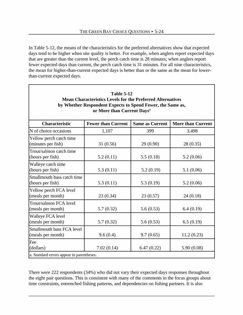
THE GREEN BAY CHOICE QUESTIONS < 5-24
In Table 5-12, the means of the characteristics for the preferred alternatives show that expecteddays tend to be higher when site quality is better. For example, when anglers report expected daysthat are greater than the current level, the perch catch time is 28 minutes; when anglers reportfewer expected days than current, the perch catch time is 31 minutes. For all nine characteristics,the mean for higher-than-current expected days is better than or the same as the mean for lower-than-current expected days.
Table 5-12Mean Characteristics Levels for the Preferred Alternatives
by Whether Respondent Expects to Spend Fewer, the Same as,or More than Current Daysa
Characteristic Fewer than Current Same as Current More than Current
N of choice occasions 1,107 399 3,498
Yellow perch catch time(minutes per fish) 31 (0.56) 29 (0.90) 28 (0.35)
Trout/salmon catch time(hours per fish) 5.2 (0.11) 5.5 (0.18) 5.2 (0.06)
Walleye catch time(hours per fish) 5.3 (0.11) 5.2 (0.19) 5.1 (0.06)
Smallmouth bass catch time(hours per fish) 5.3 (0.11) 5.3 (0.19) 5.2 (0.06)
Yellow perch FCA level(meals per month) 23 (0.34) 23 (0.57) 24 (0.18)
Trout/salmon FCA level(meals per month) 5.7 (0.32) 5.6 (0.53) 6.4 (0.19)
Walleye FCA level(meals per month) 5.7 (0.32) 5.6 (0.53) 6.5 (0.19)
Smallmouth bass FCA level(meals per month) 9.6 (0.4) 9.7 (0.65) 11.2 (0.23)
Fee(dollars) 7.02 (0.14) 6.47 (0.22) 5.90 (0.08)
a. Standard errors appear in parentheses.
There were 222 respondents (34%) who did not vary their expected days responses throughoutthe eight pair questions. This is consistent with many of the comments in the focus groups abouttime constraints, entrenched fishing patterns, and dependencies on fishing partners. It is also

THE GREEN BAY CHOICE QUESTIONS < 5-25
consistent with the responses to Question 11 of the mail survey, where 68% of the anglersindicated they had not reduced the number of days spent fishing Green Bay in response to FCAs.
That an angler does not change his or her number of fishing days in response to the change inenvironmental characteristics does not indicate that he or she would not benefit from animprovement in FCAs or catch rates. If conditions are improved, constraints can keep the anglerfrom increasing fishing days, but each day fished will be enjoyed more. If conditions worsen, theangler still might prefer fishing Green Bay to doing something else, he just prefers it less. Whenthe quality of a product is improved or its price is decreased, many consumers do not buy more ofit, but they do get greater benefits from the amount they purchase. Also, if a product’s qualitydecreases or price increases, many consumers will not purchase less in the short run; e.g., onedoes not immediately reduce gas consumption when its price has risen, even though the price hikemakes the individual worse off.
Sixty-six percent of the anglers did vary their answers to the expected days questions over theeight pairs, indicating that for the majority of anglers, the number of days they fish Green Bay willvary as a function of changes in the characteristics of Green Bay, even in the short run. For suchanglers, if Green Bay conditions are improved, they are likely to fish Green Bay more days andvalue each of those days more than they currently value Green Bay fishing days.

CHAPTER 6A COMBINED REVEALED PREFERENCE
AND STATED PREFERENCE MODEL OF GREEN BAY FISHING
6.1 INTRODUCTION
In this chapter we present our main model used to estimate per fishing day values for changes inFCAs and catch times. The technical details of the model are presented in Appendices A and B.The model presented here is considered our main model because it is consistent with traditionalrecreational demand models and is a straightforward specification that can be expected to providerobust estimates; it uses all of the RP and SP data available. In Chapter 9 we explore thesensitivity of the damage estimates to preselected model variations. These variations, some ofwhich add considerable elaboration, provide results consistent with (and generally not statisticallysignificantly different from) the main model results, supporting the robustness of the main model.
This chapter describes the model developed to explain each angler’s observed and stated GreenBay fishing choices as a function of a number of Green Bay characteristics. The parameters onthese characteristics represent the relative importance of the Green Bay characteristics indetermining the benefits an angler will get from fishing Green Bay. For example, the parameter onlaunch fee indicates the decrease in benefits from a day of fishing Green Bay if the launch fee isincreased $1, and the parameter on average catch time for perch indicates the decrease in benefitsfrom a day of fishing Green Bay if the catch time for perch increases one hour.
In our main model, all of the SP and RP data are combined for the estimation of the model. Threetypes of preference data are available: 1) anglers’ preferred alternatives from the eight Green Baychoice pairs, 2) the expected number of Green Bay fishing days to be spent at the preferred GreenBay alternatives from the eight followup questions to the choice pairs, and 3) the number offishing days in total to all sites and the number of days each angler fishes Green Bay under currentconditions. The first two data types are SP data and the last data type is RP data. The estimates ofthe model parameters (reported in Chapter 7) are those parameter values that best explain all ofthe anglers’ choices. As noted in Chapter 5, combining RP and SP data is widely supportedbecause of the relative strengths of these two types of data. While both types of data provideinformation about behavior and tradeoffs, the relative strength of RP data is in predicting trip-taking behavior, and the relative strength of SP data is in determining the rates at which the angleris willing to trade off site characteristics.
This model assumes the angler, when he fishes, chooses the fishing site that gives him the largestnet benefit. That is, he will choose Green Bay alternative A over B if he prefers A to B, and then

A SP/RP MODEL OF GREEN BAY FISHING < 6-2
1. We restrictively assume all increased days to Green Bay are substituted from other fishing sites (and vice-versa for decreased fishing days at Green Bay). Actual increases in Green Bay fishing days may also come fromincreases in total fishing days, not just from substituting days from other sites. The assumption of no increase intotal fishing days is more straightforward to model and requires fewer survey questions (e.g., we do not ask iftotal days change and by how much). The substitution assumption is implemented in the model by holding totalfishing days constant, even though increases in fishing days may in fact occur when Green Bay is improved.Further, we restrict any expected increases in Green Bay days in the followup questions to be no more than thetotal fishing days at other sites under current conditions.
he will choose Green Bay with conditions A over some other site if he expects the net benefitfrom fishing Green Bay under these conditions is greater than the net benefit from fishingelsewhere. If not, he will fish elsewhere. The model is designed to be a partial model in that itdoes not explain the angler’s total number of fishing days, only the allocation of those fishing daysbetween Green Bay and other sites. That is, the model is not designed to predict how an angler’stotal number of fishing days might increase if Green Bay conditions are significantly improved. Itwill, however, predict the extent to which an angler’s current number of fishing days would bereallocated to Green Bay if Green Bay were improved.1
The model assumes that fishing is separable from nonfishing activities in that it assumes that howan angler chooses between Green Bay and other sites and how an angler chooses between GreenBay under different conditions does not depend on the costs or attributes of other activities. Thatis, how an angler would choose between Green Bay under different conditions does not dependon the characteristics of other fishing sites, and how an angler would choose between Green Bayand another site does not depend on the characteristics of nonfishing activities. While not alwaysliterally true, these are standard modeling assumptions. When examining choices over Green Bayalternatives under different conditions, the characteristics of other sites remain constant.
Because the model is not designed to predict how total fishing days would increase if Green Bayis improved, damage estimates derived from the model will be conservative. The component ofbenefits associated with the possibility that the angler might fish more, in total, if Green Bay isimproved, rather than just fishing Green Bay some increased proportion of some constant numberof days, is omitted. It is our intent to be conservative here.
In this chapter, the basics of the model are presented. The extensive technical and mathematicaldetails of model development are presented in Appendices A and B.
6.2 FACTORS AFFECTING UTILITY FROM FISHING GREEN BAY
The utility (satisfaction) an angler receives from a day of fishing Green Bay is modeled to be afunction of costs (which include the opportunity cost of travel and on-site time, plus monetaryexpenses including travel costs and any launch fee); the catch times for four different speciesgroups targeted in Green Bay: trout/salmon, perch, walleye, and bass; and the level of FCAs

A SP/RP MODEL OF GREEN BAY FISHING < 6-3
2. Note that the full budget constraint is , where Yi is the angler’s per-choice occasionβ y i GiY TC FEE( )− −income and TCGi is angler i’s trip cost for Green Bay (excluding the launch fee). Since income and trip costs toGreen Bay remain constant, they do not influence the probability of choosing one Green Bay alternative over theother, and they are omitted for convenience of presentation.
U FEE ACT ACT ACT ACT
FCA FCA FCA N
i y cp p ct t cw w cb b
FCA FCA FCA Gi
= − + + + +
+ + + + + =
β β β β β
β β β ε
( )
... , ,...,2 2 3 3 9 9 1 i
(which can be one of nine levels, including no FCAs). The utility angler i gets from fishing GreenBay is assumed to be:
(1)
where FEE is the launch fee; ACT is the average time to catch a fish, indexed by the four species:p = perch, t = trout/salmon, w = walleye, and b = bass; FCA is a dummy variable indexed by eachof the nine FCA levels ($FCA1 is fixed at zero for identification), and is a stochastic term forεGicapturing random effects on utility from fishing Green Bay.2 The FCA variables are dummyvariables, which take on a value of one for one of FCA Levels 2-9, and a value of zero for allothers. Note again that ACT is the reciprocal of the associated catch rate. Money not spent fishingis assumed to be spent on a numeraire, a generic bundle with a price of $1.
Parameter indicates the increase in utility if the cost of the fishing day decreases one dollar andβ y
is typically referred to as the marginal utility of money. It is assumed to be a constant. Thisparameter is expected to have a positive sign, which also implies that the angler prefers a lowerlaunch fee. Downward sloping demand (i.e., demand is a decreasing function of price) is astandard tenet of consumer economic theory and a universally observed phenomenon.
The catch parameters, represent the change in utility from an increase in theβ β β βcp ct cw cb, and , , ,time it takes to catch the four species. These parameters are expected to be negative (because thevariable is catch time rather than catch rate); anglers like to catch fish, so they prefer to catch afish in a shorter amount of time, or more fish in the same amount of time.
As also noted in Chapter 3, the answers to the attitudinal questions definitely indicate that anglersplace importance on catching fish. For example, when anglers were asked to rate from one to fivethe importance of increasing catch rates in Green Bay, 68.5% responded with a three or higher.When asked to explain their ratings of Green Bay relative to other sites in the survey(Question 1), 29.1% voluntarily offered catch-related comments as their first explanation, againshowing the importance of catch rate.
The represent the change in utility from the different FCA levels. Because eight dummiesβFCA ' srepresenting nine possible FCA levels are used, the model allows a nonlinear relationship betweenseverity of the FCA and the angler’s utility. This feature, for example, allows the impact on utilityof a change from FCA Level 4 to 3 to be different from the impact of a change from Level 9 to 8.

A SP/RP MODEL OF GREEN BAY FISHING < 6-4
3. In Chapter 9 individual-specific characteristics are incorporated into Uo .
UOi Oi= +β ε0
Because FCAs make anglers worse off, all of these parameters are expected to have a negativesign and to be nondecreasing in absolute value as the stringency of the advisory increases.
Attitudinal questions from the mail survey corroborate the negative effects of FCAs on anglers.When asked to rate the importance of different enhancement activities, such as cleaning up PCBsso that FCAs could be removed, increasing the catch rates, or adding parks or boat launches(Question 7), anglers identify PCB cleanup as more important than any other option. Further,when asked how bothered they are about different FCA levels on a one-to-five scale, the meansfor all FCA levels are greater than three, and increase with the severity of FCAs.
If in a pair-wise Green Bay choice the utility from alternative B is greater than the utility fromalternative A, the angler chooses B. In this model, it is assumed that preferences arehomogeneous; that is, all anglers have the same marginal utilities for changes in the sitecharacteristics for Green Bay. This assumption is relaxed in Chapter 9, and while in some cases itis found that different anglers have significantly different preferences, the effect on mean values ofallowing preferences to be heterogeneous across anglers is usually found to be very minor.
6.3 FACTORS AFFECTING UTILITY FROM FISHING ELSEWHERE
As stated earlier, the model also predicts the expected allocation of total 1998 fishing daysbetween the Green Bay alternative (with the preferred characteristics) versus all other sites, whichis represented as one generic other site. This other generic site may vary across anglers andsimplifying assumptions must be made because data on trip costs and other characteristics for theother site are unobserved (but are assumed to remain constant over time). The utility from fishingthe other site, , is assumed to be some constant that is the same for everyone (and estimatedUOi
as a parameter in the model), plus a stochastic random component for the other site, which variesacross anglers:3
(2)
For each fishing day, an angler compares the utility from the preferred Green Bay alternative fromthe choice pair to the utility from the other non-Green Bay fishing site. If the utility from fishingGreen Bay with the preferred set of characteristics is greater than the utility from fishingelsewhere, the angler will choose Green Bay for that fishing day, and vice versa. The estimatedmodel parameters (see Chapter 7) are those estimates that best explain the expected allocations ofthe total 1998 fishing days to the preferred Green Bay alternatives from the choice pairs, eachangler’s current allocation of fishing days between Green Bay and other sites, and anglers’ choicesin the eight Green Bay pairs.

A SP/RP MODEL OF GREEN BAY FISHING < 6-5
6.4 ESTIMATION OF THE MODEL
In the empirical model, parameters are estimated using a mathematical search algorithm thatmakes the observed anglers’ choices most likely. In other words, the estimated parametersmaximize the likelihood of observing the anglers’ chosen alternatives from the choice pairs, theirallocations of current fishing days to the chosen alternatives, and finally, the reported currentnumber of fishing days to Green Bay. The parameter estimates are called maximum likelihoodestimates because they are estimates of the population parameters that maximize the likelihood ofdrawing the sample of the observed choices.
The likelihood function that is maximized is derived and presented in detail in Appendix A. Inshort, it is a complex joint probability over all of the individuals in the data set. For a singleindividual it is computed as the product of the probabilities of the chosen Green Bay alternativesover the eight choice-occasion pairs; multiplied by the product of the probabilities of the expectedallocation of 1998 total days to the preferred Green Bay alternatives over the choice-occasionpairs, conditional on the chosen Green Bay alternatives; multiplied by the probability of thecurrent allocation of 1998 total days to Green Bay under actual conditions. Maximizing thelikelihood function is equivalent to maximizing the joint probability of observing the collectiveangler behavior and choices.

CHAPTER 7THE ESTIMATED MODEL
7.1 INTRODUCTION
This chapter presents an overview of the estimation of the full model. As discussed earlier, themain model uses the SP Green Bay choice pair data, the SP data on the number of days the anglerexpects to fish the preferred Green Bay site, and the RP data on the actual number of days spentfishing Green Bay to estimate simultaneously the anglers’ choices from the choice pairs and theallocation of total fishing days between Green Bay and other sites. The utility from fishing GreenBay and the utility from fishing another fishing site are defined in Chapter 6. The estimatedparameters of those utility functions are discussed qualitatively here, and the specific parameterestimates are reported in Appendix B.
These parameters are used to estimate the anglers’ values for changes in the characteristics ofGreen Bay, and to construct value estimates for recreational fishing services lost due to thepresence of FCAs in Green Bay. Major conclusions that can be drawn from this chapter andAppendix B are that model parameters are estimated with a high level of accuracy and makesense, and that the model does a good job in explaining angler choices and behavior. Technicalresults and measures of model goodness-of-fit (i.e., how well the model explains the data) arepresented in detail in Appendix B. The estimates here apply to our target population of 1998anglers active in fishing the Wisconsin waters of Green Bay and who purchased a fishing license inone of eight nearby counties.
7.2 SIGNS AND SIGNIFICANCE OF THE PARAMETER ESTIMATES
An important result from this estimation is that all of the estimated parameters have the correctsigns (Table B-2 in Appendix B). The estimated parameters on the catch times and the FCAvariables are negative, and the estimated parameter on the launch fee is positive (recall that the feeenters the utility function with a negative sign). These parameter signs indicate anglers are worseoff as catch times increase, as FCAs increase, and as costs increase. Further, parameters on theFCA dummy variables tend to increase in absolute value as the FCA level becomes more severe.For example, the parameter for the most severe level, Level 9, is -1.15, whereas the parameter forLevel 2 is -0.09. FCA parameter estimates also show that as the severity of FCAs increases, sodoes the damage, but not necessarily in a linear fashion.

THE ESTIMATED MODEL < 7-2
1. To determine which alternative the model predicts would be chosen from a pair, the estimated parametervalues are put into Equation 1 in Chapter 6, along with the Green Bay characteristics from the two alternatives.Whichever alternative gives the highest value for estimated expected utility is the alternative the model predictswill be chosen.
The parameters are estimated by maximum likelihood, so they have desirable statistical properties.In addition, the parameter estimates have small confidence intervals; that is, there is confidencethat the estimates of the parameters would not vary much across random samples. Usingconventional statistical tests, the parameters are all highly statistically “significant,” which meansthat they differ from zero with a high degree of confidence.
7.3 MEASURES OF MODEL FIT
Several statistical procedures were implemented to assess how well the model explains the data.Overall, the results from these procedures show that the model does a very good job in explainingangler choices and the number of days anglers spend fishing Green Bay under current conditions.
An intuitively appealing test of fit in the A-B choice-pair portion of the model is to examine theproportion of angler choices from the choice pairs that are accurately predicted by the model. Themodel correctly predicts 73% of the 5,038 choice occasions in the data.1 A pseudo-R2 for thechoice pairs is 0.43. It is akin to a measure of fit for a simple linear regression model where thevalue ranges from zero to one and indicates the percentage of variation in the data that isexplained by the model. A pseudo-R2 of 0.43 is quite high for cross-sectional data.
The estimated model also does well in identifying alternatives that are appealing or unappealing toanglers. For example, when the predicted probability of selecting alternative A is less than 0.1,alternative A is chosen in only 5% of the pairs; anglers only rarely choose alternatives that themodel indicates are unlikely to be chosen. Conversely, when the predicted probability is greaterthan 0.9, alternative A is chosen in almost all of the pairs, 96%. The estimated model identifies theGreen Bay alternatives anglers actually do prefer as likely candidates to be chosen.
Another measure of model accuracy is a comparison of the mean number of days that anglerswould expect to visit the preferred Green Bay alternatives (reported in the followup questions tothe choice pairs), with the model’s prediction of the mean number of days. The means are almostidentical (12.0197 versus 12.0927), although there is significant variation on an individual basis(see Appendix B). The model is also sufficiently flexible to predict perfectly the mean currentnumber Green Bay days from the RP data: 10 predicted and actual.

THE ESTIMATED MODEL < 7-3
2. A conservative interpretation of current FCAs in Green Bay is Level 4, as discussed in Section 5.4 (seeTable 5-3 for the FCA level definitions).
7.4 CHANGES IN GREEN BAY FISHING FROM CHANGES IN FCAS
The model is not only useful in predicting choices based on the pairs and predicting days undercurrent conditions, it can also predict how changes in FCAs or other Green Bay characteristicssuch as catch time will affect the proportion of fishing days spent at Green Bay versus other sites,and therefore the total number of Green Bay days, holding total fishing days constant.
The model’s estimate of the probability that Green Bay will be chosen under current FCA Level 4conditions (versus another site) is 0.40 for anglers who currently fish in Green Bay and purchasedlicenses in the eight counties.2 With the elimination of FCAs in Green Bay, that percentage wouldincrease to almost 0.46, and the number of Green Bay days would increase by 14.5%. As PCBsare gradually removed from Green Bay and FCAs become less stringent in phases, other scenariosmay become relevant. For example, the probability of visiting Green Bay would increase to 0.43 ifFCAs were at Level 3, and increase to 0.45 at Level 2. Results from catch-time scenarios arepresented in Table B-6. An important finding is that catch time for all four species in Green Baywould have to be reduced by almost half for visitation to increase as much as it would if FCAswere completely removed.

CHAPTER 8LOWER-BOUND ESTIMATES OF 1998 DAMAGES
8.1 INTRODUCTION
This chapter presents lower bound estimates of per fishing day and 1998 aggregate damagesresulting from FCAs in the waters of Green Bay. Damages are measured in terms of what anangler would be willing to pay for the absence of FCAs.
In Section 8.2 we introduce two per-day WTP measures: WTP per fishing day and WTP perGreen Bay fishing day; we relate them to annual damages per angler and provide estimates ofthese fishing measures (see also Appendix C). Section 8.3 calculates the 1998 annual damages foropen-water fishing in the Wisconsin waters of Green Bay for our target population using the twoper fishing day damage measures and estimates of 1998 fishing days for our target population.Section 8.4 applies benefits transfer methods to select per fishing day values for ice fishing in theWisconsin waters of Green Bay by our target population and for fishing days in the Michiganwaters of Green Bay, and computes 1998 annual damages for these fishing activities.
The damage estimates provided in this chapter are lower bound estimates. The per day estimatesare for current Green Bay anglers and reflect reduced enjoyment when visiting Green Bay and thesubstitution of fishing days from Green Bay to other fishing sites, but do not account for the factthat these anglers may increase their total number of fishing days (to all sites and to Green Bay) inthe absence of FCAs. The aggregate estimates omit Green Bay anglers who purchase theirWisconsin fishing licenses outside of the eight targeted counties, and omit damages to individualswho do not fish at Green Bay at all because of the FCAs.
8.2 WTP PER YEAR, PER FISHING DAY, AND PER GREEN BAY FISHING DAY
Concepts
In this section we define two per day fishing WTP measures, one that applies to Green Bay fishingdays and one that applies to all fishing days (including days at Green Bay and all other sites), andtwo comparable lower-bound estimates of yearly damages for an angler’s WTPY.
per Green Bay fishing day, , is how much an angler would pay per Green Bay fishingWTP WTPG
day for the absence of injuries. multiplied by the angler’s current number of open-waterWTPG
Green Bay fishing days (with injuries), , is a lower-bound estimate of that angler’s annualDG

LOWER-BOUND ESTIMATES OF 1998 DAMAGES < 8-2
1. In Appendix D, we consider preference heterogeneity.
willingness-to-pay, , for the absence of injuries. It does not account for the possibility thatWTPY
absent injuries, the angler might want to fish Green Bay more. Denote this lower-bound estimateof an angler’s yearly damages, , where .WTPYG WTP WTP D WTPY G G YG = × ≤
per fishing day, , is how much an angler would pay per fishing day, not just perWTP WTPF
Green Bay fishing day, for the absence of injuries to Green Bay. multiplied by the angler’sWTPF
current total number of open-water fishing days (with injuries), , is also a lower-boundDF
estimate of , but includes more of the damages than does . Denote this secondWTPY WTPYG
lower-bound estimate of yearly damages, , where andWTPYF WTP WTP D WTPY F F YF = × ≤.WTP WTP WTPY Y YG F≤ ≤
When Green Bay is improved there are two ways an angler can increase his number of Green Bayfishing days: he can hold total fishing days constant but increase the proportion of those days toGreen Bay, or he can both increase total fishing days and increase the proportion of those days toGreen Bay. Unlike , incorporates the possibility that with the absence of injuries theWTPYG WTPYF
proportion of fishing days the angler takes to Green Bay might increase, so. is still a lower-bound estimate of because it does not account forWTP WTPY YF G≥ WTPYF WTPY
the possibility that the angler might fish more in total if Green Bay were not injured.
Looking ahead, , even though ; this is because applies toWTP WTPF G≤ WTP WTPY YF G≥ WTPF
all fishing days, whereas applies to only Green Bay fishing days. An angler will pay noWTPG
more per fishing day to have the FCAs at Green Bay removed than he would pay per Green Bayfishing day, because all fishing days are not necessarily to Green Bay.
Estimates
is how much the utility from a Green Bay fishing day would increase if there were noWTPG
FCAs, converted into dollars by dividing this increase in utility by the marginal utility of money. Inthe primary model, preferences are assumed not to vary across anglers, so is the same forWTPG
all anglers.1
Based on the parameter estimates reported in Appendix B (and discussed in Appendix B andChapter 7), WTP values are reported in Table 8-1 for changes in FCA levels and changes in catchrates. (the estimated value of ) for reducing FCAs from FCA Level 4 to FCAWTPG$ WTPG
Level1 (no FCAs) is $9.75; that is, $9.75 for every Green Bay fishing day. For comparison, $9.75 is 13% of the average reported cost of a Green Bay fishing day. The 95% confidence interval onthe $9.75 estimate is $8.06 to $11.73.
FCA Level 4 represents FCAs by species that are equal to or less stringent than current levels (seethe “Fish Consumption Advisory” subsection of Section 5.4.1 in Chapter 5), so $9.75 is a

LOWER-BOUND ESTIMATES OF 1998 DAMAGES < 8-3
2. is an increasing function of catch rates. The $4.17 estimate is based on 1998 Green Bay catch rates.WTPF
Historically, catch rates were better for all species. If instead the 13-year average catch rates from 1986 to 1998are used, increases by 16%. is not a function of catch rates. Thus, should be relied on forWTPF$ WTPG WTPF
the assessment of how catch rates affect FCA values. Therefore, using the 1998 damage estimate as a basis forpast damages will understate past damages.
conservative estimate of the for eliminating the need for FCAs. for reducing FCAsWTPG WTPG$
from Level 3 to Level 1 (no FCAs) is $4.86. For reducing FCAs from FCA Level 2 to no FCAs, itis $1.81. These latter estimates can be used to estimate damages after partial cleanup.
The value for FCA Level 6 is smaller than for both FCA Levels 4 and 5. Compared to FCALevel 4, FCA Level 6 has a less severe restriction on perch but a more stringent restriction ontrout/salmon (see Table 5-3). Here, the perch restriction is likely to apply to more anglers, but theincreased trout/salmon restriction of “do not eat” can be expected to be very bothersome, andthus these two changes roughly cancel. Compared to FCA Level 5, FCA Level 6 has a less severerestriction on walleye, but a more stringent restriction on trout/salmon. Because more anglerscited that they “often” or “always” target walleye than trout/salmon (Section 4.2 and Figure 4-2),it is not surprising that the values are larger for FCA Level 5 than for FCA Level 6.
One could offset the current damages from the FCAs with improved catch rather than money. Themodel estimates indicate that to do this, catch rates for all four species would have to increase by61%. Note that increasing all catch rates by 61% would not compensate for past damages.
is how much the utility from an average fishing day would increase if there were no GreenWTPF
Bay FCAs, converted into dollars by dividing the increase in utility by the marginal utility ofmoney. Based on the parameter estimates reported in Appendix B (and discussed in Appendix Band Chapter 7), for reducing FCAs from Level 4 to Level 1 (no FCAs) is $4.17; that is,WTPF$
$4.17 for every fishing day.2 Remember that $4.17 applies to all fishing days, not just Green Bayfishing days, so it is less than , which is $9.75. The 95% confidence interval on the $4.17WTPG$
estimate is $3.41 to $5.00. As noted in Chapter 2, there are a number of studies that haveestimated WTP per fishing day for reductions in FCAs and contaminants at different sites and fordifferent species (see Table 2-13). The value of $4.17 falls within the range in the literature.Values of for different resource changes are also reported in Table 8-1.WTPF$
for reducing FCAs from FCA Level 3 to no FCAs is $2.15, and for reducing FCAs fromWTPF$
FCA Level 2 to no FCAs is $0.82. Per fishing day values for 10% and 100% increases in catchrates from current levels are reported in Table 8-1. Note that these values apply to all anglerstaking trips to the Wisconsin waters of Green Bay, not just to the anglers targeting these species.

LOWER-BOUND ESTIMATES OF 1998 DAMAGES < 8-4
Table 8-1WTP per Green Bay Fishing Day and per Fishing Daya,b
Resource Change WTP G$ WTP F$
FCA Value FCA Level 9 ÷ FCA Level 1 FCA Level 8 ÷ FCA Level 1 FCA Level 7 ÷ FCA Level 1 FCA Level 6 ÷ FCA Level 1 FCA Level 5 ÷ FCA Level 1 FCA Level 4 ÷÷ FCA Level 1c
FCA Level 3 ÷ FCA Level 1 FCA Level 2 ÷ FCA Level 1 FCA Level 4 ÷ FCA Level 1 (13-year average catch)d
$21.71 [$19.00 - $24.81]$19.78 [$17.42 - $22.14]$14.32 [$12.35 - $16.41]$9.91 [$8.14 - $11.81]$11.22 [$9.71 - 13.26]$9.75 [$8.06 - $11.73]$4.86 [$3.40 - $6.32]$1.81 [$0.46 - $3.18]
$9.75 [$8.15 - $11.39]
$8.52 [$7.48 - $9.50]$7.87 [$6.96 - $8.83]$5.92 [$5.15 - $6.84]$4.23 [$3.54 - $5.02]$4.75 [$4.01 - $5.57]$4.17 [$3.41 - $5.00]$2.15 [$1.57 - $2.79]$0.82 [$0.19 - $1.51]
$4.83 [$3.99 - $5.84]
Catch Valuese
Yellow perch – 10% increase – 100% increase Trout/salmon – 10% increase – 100% increase Walleye – 10% increase – 100% increase Smallmouth bass – 10% increase – 100% increase All species at once – 10% increase – 100% increase
$0.74 [$0.62 - $0.87]$3.72 [$3.13 - $4.27]
$0.77 [$0.53 - $0.99]$3.84 [$2.71 - $5.03]
$0.40 [$0.33 - $0.47]$1.98 [$1.64 - $2.34]
$0.65 [$0.52 - $0.80]$3.24 [$2.63 - $4.01]
$2.56 [$2.23 - $2.92]$12.79 [$11.33 - $14.50]
$0.30 [$0.25 - $0.35]$1.52 [$1.29 - $1.75]
$0.31 [$0.23 - $0.40]$1.57 [$1.13 - $2.04]
$0.16 [$0.13 - $0.19]$0.80 [$0.65 - $0.95]
$0.26 [$0.20 - $0.32]$1.32 [$1.06 - $1.65]
$1.04 [$0.91 - $1.18]$5.58 [$4,95 - $6.29]
a. Catch times are set at 1998 levels: perch – 0.75, trout/salmon – 19.4, walleye – 7.4, bass – 15.0.b. Simulated 95% confidence intervals approximated using Krinsky-Robb procedure with 500 draws inbrackets.c. Bold entry represents the 1998 advisory levels.d. Average catch times from 1986 to 1998: perch – 0.52, trout/salmon – 7.8, walleye – 6.9, bass – 5.0.e. Catch rate is inverse of catch time. Computed with FCA level set at 4.
LOWER-BOUND ESTIMATES OF 1998 DAMAGES < 8-5
3. If a linear relationship were assumed instead, values for small changes in catch rates would be smaller, andvalues for large changes in catch rates would be larger.
These values follow the pattern for the FCA values, with slightly more than double theWTPG
values for . The values for increases in catch reflect the model assumption of decreasingWTPF
marginal utility of increasing catch (because catch time in the utility function is the reciprocal ofthe catch rate).3 The values for a 100% increase in catch rates are about five times the values for a10% increase in catch rates. The values in Table 8-1 are comparable to the values for the mostsimilar resource changes as reported in the literature [Table 2-14, see Samples and Bishop (1985),Milliman et al. (1992), and Chen et al. (1999)].
Next we compare the two lower-bound annual damage measures on a per angler basis, for whichwe use the scenario of a reduction in FCAs from Level 4 (current) to Level 1 (no FCAs). Theannual value for Green Bay fishing days is = $9.75 per Green Bay fishing day × 5.25WTPY G
Green Bay fishing days = $51.19 per Green Bay open-water angler. The annual value for allfishing days is = $4.17 per fishing day × 13.19 fishing days = $55.00. As noted above,WTPYF
while , the annual damages per angler are reversed with about 7% largerWTP WTPG F$ $> WTPYF
than .WTPYG
8.3 TWO LOWER-BOUND ESTIMATES OF TOTAL 1998 DAMAGES FOR OPEN-WATER FISHING IN THE WISCONSIN WATERS OF GREEN BAY
Annual total damages equal the estimate of total fishing days (either to Green Bay or to all sites)times the corresponding per fishing day damage estimate. These are lower-bound estimatesbecause the damage per day values are lower-bound estimates. First we provide estimates of totalfishing days, then we provide estimates of total damages. As noted above, the estimates in thissection pertain only to open-water fishing by anglers who are active in Green Bay fishing and whopurchased their Wisconsin fishing licenses in eight counties near to Green Bay.
Estimated Open-Water Fishing Days
An estimate of total 1998 Green Bay open-water fishing days by those who purchased licenses inone the eight counties is computed by multiplying the number of these anglers by the estimatedmean number of open-water Green Bay fishing days, which is 5.25; its confidence interval is 4.67to 5.82. The estimate of total 1998 open-water fishing days by these Green Bay anglers isobtained by multiplying the number of these anglers by their estimated mean number of fishingdays, 13.19; its 95% confidence interval is 12.18 to 14.20.
The number of anglers who purchased licenses in the eight counties and actively fished Green Bayin 1998 was estimated using county data from WDNR on the number of licenses sold in 1997.Each resident fishing license, sportsman license, nonresident fishing license, nonresident 15-day

LOWER-BOUND ESTIMATES OF 1998 DAMAGES < 8-6
4. It would not be cost-effective to purchase one of these licenses unless two individuals intended to fish.
5. Confidence intervals for aggregate annual damages are approximated assuming the percentage of licensedanglers active at Green Bay, the mean number of days, and estimated WTP are uncorrelated random variables.The separate confidence intervals for all of these variables are reported throughout this chapter. The number oflicense holders is not assumed to be random, and the product of these variables gives aggregate damages. Theconfidence intervals for aggregate damages (and aggregate days later in the chapter) are approximated usingasymptotic variances.
fishing license, and patron license is counted as one angler. Each resident husband-and-wifefishing license, nonresident family fishing license, and nonresident family 15-day fishing license isconservatively counted as two anglers.4 Finally, each two-day sports license and nonresident4-day fishing license is conservatively counted as half an angler (i.e., it is assumed each anglerpurchasing these licenses purchases two on average) because it would not be cost-effective for anindividual to buy more than two of these types of licenses (on the other hand, assuming theypurchase fewer than two two-day licenses would result in more anglers and higher damages).Given these definitions, in 1997 154,783 anglers purchased their licenses in one of the eightcounties (Appendix F, Table F-8). The number of anglers in 1998 is assumed to be the samebecause 1998 license data are currently unavailable.
Some of these anglers do not fish Green Bay. Based on the telephone screener, the percentage oflicense holders in the targeted counties that fished Green Bay in 1998 is 31.4% with a 95%confidence interval of 29.6% to 33.2%. Applying 31.4% to the total number of anglers, weestimate that in 1998 approximately 48,602 anglers purchased their license in one of the eightcounties and fished Green Bay, which has a 95% confidence interval of 45,877 to 51,327.
Multiplying 48,602 anglers by the estimated mean Green Bay open-water fishing days of 5.25, weestimate that in 1998 there were approximately 255,160 Green Bay open-water fishing days byanglers who purchased their licenses in one of the eight counties. The 95% confidence interval is224,000 to 287,000. Multiplying 48,602 anglers by the estimated mean total open-water fishingdays of 13.19, we estimate approximately 641,060 total open-water fishing days by anglers whopurchased their license in one of the eight counties and who fished Green Bay. The confidenceinterval on this estimate is 580,000 to 702,000.
Annual Open-Water Fishing Damages in Wisconsin Waters of Green Bay
multiplied by the current number of open-water Green Bay fishing days in 1998 by GreenWTPG$
Bay anglers who purchased their licenses in one of the eight counties is a lower-bound estimate onaggregate damages for this group. We estimate in 1998, this group of anglers fished the openwaters of Green Bay 255,160 days, so a lower-bound estimate of 1998 damages to this group is$2.49 million ($9.75 × 255,160). The confidence interval on this estimate is $1.93 million to$3.05 million.5

LOWER-BOUND ESTIMATES OF 1998 DAMAGES < 8-7
6. For an overview of the benefits transfer technique see Brookshire and Neill (1992), Boyle and Bergstrom(1992) and Desvouges et al. (1992), all in a special section of Water Resources Research devoted to benefitstransfer.
multiplied by the total number of fishing days in 1998 by Green Bay anglers whoWTPF$
purchased their licenses in one of the eight counties is another lower-bound estimate on aggregatedamages for this group. We estimate that in 1998 this group of anglers fished a total of641,060 days on open water, so a second lower-bound estimate of 1998 damages to this group is$2.67 million ($4.17 × 641,060). The confidence interval is $2.13 million to $3.22 million. It islarger than the other lower-bound estimate because it accounts for the possibility that anglersmight spend a larger proportion of their fishing days at Green Bay if it were not injured.
8.4 BENEFITS TRANSFER TO ESTIMATE THE DAMAGES ASSOCIATED WITH
THE GREEN BAY ICE FISHERY AND THE MICHIGAN GREEN BAY
FISHERY
The benefits transfer approach involves estimating damages for an assessment area by usingvalues derived from the application of primary economic methods in other studies, rather thancollecting primary valuation data for the assessment area. In this section, we will apply the unitvalue method, a benefits transfer approach identified in the U.S. DOI regulations [43 CFR § 11.83(c)(2)(vi)], to value damages from PCBs and resultant FCAs to ice-fishing days in the Wisconsinwaters of Green Bay, and all fishing days in the Michigan waters of Green Bay.
There are two sites involved in a benefits transfer: the targeted site (to which values will betransferred) and the study site (where a primary study of damages has been completed). To assessthe suitability of the benefits transfer approach we must compare the targeted site to the study siteand consider three questions: are the sites similar, are the populations similar, and are the changesbeing valued similar?6 Our primary study site is the Wisconsin waters of Green Bay, ourpopulation is Green Bay anglers who purchased their licenses in one of the eight counties, and thechange being valued is a reduction in PCBs and resultant removal of FCA restrictions.
Ice Fishing on the Wisconsin Waters of Green Bay
The first transfer of values is to ice-fishing days on the Wisconsin waters of Green Bay. The site isvery similar to the study site as it is the exact same location, but at a different time of year. Yellowperch dominates Green Bay ice fishing as it does the open-water fishing, accounting for 90% ofthe ice-fishing catch in 1998 (WDNR creel). Other species caught are walleye, burbot, andnorthern pike.

LOWER-BOUND ESTIMATES OF 1998 DAMAGES < 8-8
7. We use the ratio from the telephone survey because the Green Bay ice-only anglers are not included in thefollowup mail survey. Note also that by using a ratio, the recall, nonresponse, and sampling bias adjustments arecarried forward to the ice-fishing damage calculation.
The ice-fishing anglers are very similar to the open-water anglers. From our telephone survey wefound that 73% of the anglers who ice fished on Green Bay in 1998 also fished the open waters ofGreen Bay in 1998. Green Bay open-water anglers who also ice fish in the waters of Green Bayare slightly more avid about ice fishing than anglers who only ice fish (averaging 6.4 Green Bayice-fishing days, SE=0.56, compared to 5.4 Green Bay ice-fishing days, SE=0.72). Therefore,Green Bay open-water anglers in the target population account for about 76% of the ice-fishingdays.
The change being valued is the same for the primary study and the targeted area, as FCAs for icefishing on the Wisconsin waters of Green Bay are the same as those for open-water fishing on theWisconsin waters of Green Bay.
As such we can apply the estimated WTP per Green Bay fishing day for open-water days, $9.75,to the number of Green Bay ice-fishing days. From our telephone survey we found that Green Bayice-fishing days were equivalent to 18.24% of Green Bay open-water fishing days for all anglerswho had open-water or ice fished on Green Bay in 1998.7 Our estimate of Green Bay fishing daysfor 1998 is 255,160. Multiplying this by 18.24% we get an estimate of 46,541 Green Bay ice-fishing days.
Thus, a lower-bound estimate of the 1998 damages associated with the injuries the WisconsinGreen Bay ice fishery for our target population from PCBs and the resultant FCAs is$0.454 million ($9.75 times 46,541 Green Bay ice-fishing days).
All Fishing in the Michigan Waters of Green Bay
The second transfer of values is to the Michigan Waters of Green Bay. This site is very similar tothe study site as they are both portions of Green Bay. They share a similar mix of species, withyellow perch, walleye, and trout/salmon making up at least 95% of the Michigan Green Bayfishery (see Section 2.1 for more detail).
The individuals using the fishery are also similar. As discussed in Chapter 3 we expect the fishingin Green Bay to be a fairly localized activity, and that most Michigan Green Bay angling would bedone by anglers in nearby counties. Therefore most of the anglers live in a similar region.Comparing the Wisconsin and Michigan counties that surround Green Bay we find similarsocioeconomic characteristics, with Michigan having a somewhat higher unemployment and lowerper capita income (see Table 8-2).

LOWER-BOUND ESTIMATES OF 1998 DAMAGES < 8-9
Table 8-2Comparison of Wisconsin and Michigan Counties near Green Bay
Population(7/1/1998)
Percentover 65Years(1995)
Percentover 25Years(1990)
PercentHigh SchoolGrads over25 (1990)
PercentCollege
Grads over25 (1990)
PercentUnemployed
(1994)
Per CapitaPersonalIncome(1993)
6 Michigancounties near Green Baya 170,746 15% 64% 78% 14% 8% $16,5398 Wisconsincounties near Green Bayb 727,752 13% 63% 78% 16% 5% $19,509a. Alger, Delta, Dickinson, Marquette, Menominee, and Schoolcraft.b. The eight targeted counties.
Source: U.S. Census Bureau website http://www.census.gove/statab/USA96/.
The Michigan change being valued is different from Wisconsin because FCAs are less restrictivein the Michigan waters of Green Bay. Current levels of FCAs in the Michigan waters of GreenBay are closest to our Level 2 for the general population, and our Level 4 for women who arepregnant, nursing, or expect to bear children, and for children (hereafter, when we refer to FCAsfor women, we refer specifically to this subset of women).
FCA Level 2 allows unlimited consumption of yellow perch and smallmouth bass and restrictstrout/salmon and walleye to no more than one meal a week. The Michigan advisory for thegeneral population (see Table 2-10) allows unlimited consumption for yellow perch andsmallmouth bass, and has a range of restrictions for trout/salmon and walleye from unlimited forchinook salmon and smaller sizes of brown trout and walleye, to do not eat for larger sizes ofbrown trout and walleye.
FCA Level 4 allows one meal a week for yellow perch, and one meal a month for all otherspecies. The Michigan advisory for women and children allows one meal a week for perch, onemeal a month for smallmouth bass, and a range of one meal a week to do not eat for trout/salmonand walleye, dependent on the part of Green Bay and size of fish (one meal a week applies onlyfor walleye and rainbow trout less than 18"). Based on the average size of fish caught in LakeMichigan (Appendix F, Table F-7) the “eat no more than one meal a week” advisory could applyto as much as one-half of the fish caught and kept.
From our primary study, the estimated per Green Bay fishing day for a reduction from FCAWTPLevel 2 to no FCAs is $1.81, and from FCA Level 4 to no FCAs is $9.75.

LOWER-BOUND ESTIMATES OF 1998 DAMAGES < 8-10
The women and children advisories could be a concern to male or female anglers with householdmembers for whom the advisories apply. From our survey we find that about 45% of anglers areof an age most likely associated with having and raising small children: 18 to 40 years old. In fact,about 28% of our sample of anglers are age 18 to 40 and have at least one household memberwho is less than 16 years old, and thus may be concerned with the advisories aimed at women andchildren. To be conservative, we assume that 14% of the fishing days (half of the 28% of anglers)are by anglers for whom the women and children advisory would be a concern. This reflects thatin some of these households the children may be older and no additional children are expected,and that fish may be consumed in different amounts by different household members. Therefore,we select an average WTP per Green Bay fishing days for the absence of PCBs on the MichiganWaters of Green Bay of $2.92 (14% times $9.75 plus 86% times $1.81).
Comparing the WDNR and MDNR creel surveys we found that all fishing on the Michigan watersof Green Bay was equivalent to 58.83% of the March to December fishing on the Wisconsinwaters of Green Bay in 1998 (see Table 2-1). Therefore we estimate that there were 150,103 dayson the Michigan waters of Green Bay (58.83% times 255,160 Wisconsin Green Bay days).
Thus, a lower-bound estimate of the 1998 damages associated with the Michigan waters of GreenBay from PCBs and the resultant FCAs is $0.438 million ($2.92 times 150,103 Michigan GreenBay fishing days).

CHAPTER 9TESTING THE SENSITIVITY OF THE WTP ESTIMATES
TO MODIFICATIONS TO THE MODEL
9.1 INTRODUCTION
This chapter examines the sensitivity of the value estimates to preselected variations in thespecification of the main economic model. Technical details of these model variations arepresented in Appendix D. One of the most important conclusions of this sensitivity analysis isthat the mean values for changes in FCAs are generally robust (insensitive and statisticallyinsignificantly different from the main model), except in models that introduce randomheterogeneity of preferences, which result in higher values for reduced FCAs, and thus higherdamages from the existence of the current FCAs.
Table 9-1 summarizes the values for the main model (from Chapter 7) and the model variations.In the first set of model variations, discussed in Section 9.1, we use just the data from the A-Bchoice questions, omitting data from the followup questions on the expected number of GreenBay fishing days to the preferred alternatives or RP data on the actual number of days undercurrent conditions. These variations can be used only to estimate . Variations on the mainWTPG
model with homogeneous preferences include the basic model (excluding the followup questionor data on actual days) and two variations examining learning and fatigue (one allowing noiseparameters to vary over the choice pairs, and one allowing all parameters to vary). Next, usingthe A-B choice data, heterogeneity of preferences is incorporated. Classic heterogeneity allowsthe effect of changes in site characteristics on utility to vary with characteristics of the individualsuch as distance from the site, gender, target species, and income (through the marginal utility ofmoney). Random heterogeneity allows preferences to vary across anglers without having toexplain the source of the variation, and allows choice occasions for a given angler to becorrelated.
Additional models, discussed in Section 9.2, use the A-B choice data plus the followup expecteddays question and some or all of the RP data on reported number of fishing days. These modelsuse two alternative strategies to incorporate preference heterogeneity. Both models provide both
and estimates.WTPG WTPF
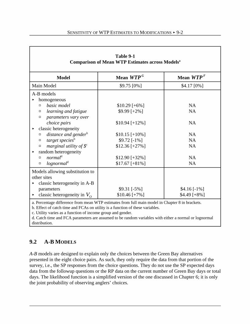
SENSITIVITY OF WTP ESTIMATES TO MODIFICATIONS < 9-2
Table 9-1Comparison of Mean WTP Estimates across Modelsa
Model Mean Mean WTP G WTP F
Main Model $9.75 [0%] $4.17 [0%]
A-B models< homogeneous
R basic modelR learning and fatigueR parameters vary over
choice pairs< classic heterogeneity
R distance and genderb
R target speciesb
R marginal utility of $c
< random heterogeneityR normald
R lognormald
$10.29 [+6%]$9.99 [+2%]
$10.94 [+12%]
$10.15 [+10%]$9.72 [-1%]
$12.36 [+27%]
$12.90 [+32%]$17.67 [+81%]
NANA
NA
NANANA
NANA
Models allowing substitution toother sites< classic heterogeneity in A-B
parameters< classic heterogeneity in VO
$9.31 [-5%]$10.46 [+7%]
$4.16 [-1%]$4.49 [+8%]
a. Percentage difference from mean WTP estimates from full main model in Chapter 8 in brackets.b. Effect of catch time and FCAs on utility is a function of these variables.c. Utility varies as a function of income group and gender.d. Catch time and FCA parameters are assumed to be random variables with either a normal or lognormaldistribution.
9.2 A-B MODELS
A-B models are designed to explain only the choices between the Green Bay alternativespresented in the eight choice pairs. As such, they only require the data from that portion of thesurvey, i.e., the SP responses from the choice questions. They do not use the SP expected daysdata from the followup questions or the RP data on the current number of Green Bay days or totaldays. The likelihood function is a simplified version of the one discussed in Chapter 6; it is onlythe joint probability of observing anglers’ choices.
SENSITIVITY OF WTP ESTIMATES TO MODIFICATIONS < 9-3
The parameters in the A-B models have the same interpretation as those from the A-B portion ofthe main model, as defined in Chapter 6. The A-B models have fewer parameters to estimatebecause the A-B parameters are the only parameters in the models. Estimates of these parametersare still consistent (i.e., a simple definition of consistency is that the parameter estimate equals itstrue value if the sample is sufficiently large), just as they are in the main model, but are estimatedless precisely than when all of the data are used. That is, the additional information on choicesnot used in the A-B models is used in the main model to improve the accuracy of its estimates,which means that the standard deviations on the parameter estimates get smaller as more data areused in the estimates. Because the A-B models do not model the allocation of current daysbetween Green Bay and other sites, only mean can be estimated, not the mean .WTPG WTPF
9.2.1 A-B Models with Homogenous Preferences
The parameter estimates from an A-B model with homogeneous preferences are very similar tothe A-B estimates from the main model. As a result, mean is also very similar to $9.75:WTPG
$10.29. This model also examines learning and fatigue effects and positioning bias effects.Through responding to the choice pairs, the respondent may gain better knowledge andunderstanding of the survey process, and this learning effect may express itself through adecrease in the random noise in the decision-making process. Conversely, if there is a largenumber of survey choice pairs, a fatigue effect may set in as the respondent tires during the dataelicitation process. This effect may be manifested as an increase in random noise for choice pairstoward the end of the process. Results suggest weak but statistically insignificant learning andfatigue effects. The mean from the A-B model with learning and fatigue increases toWTPG
$9.99, only 2% higher than the estimate from the model with all variances restricted to be equal,$9.75. To further investigate the potential for learning and fatigue, the data were divided intothree sets: early choice pairs (1 and 2), middle choice pairs (3 through 6), and late choice pairs (7and 8). The results indicate that parameters do vary across choice occasions when they are notrestricted to be the same, but not in a systematic way, which suggests the absence of learning andfatigue effects. The mean from the second model examining learning and fatigue isWTPG
$10.94.
Finally, we cannot reject the null hypothesis of no positioning bias; that is, there is no evidencethat respondents systematically select A or B independent of the characteristics. A homogenouspreferences A-B model was estimated to investigate whether respondents are drawn to alternativeA in the choice pairs simply because it is the first option presented; a dummy variable forAlternative A was not significant.

SENSITIVITY OF WTP ESTIMATES TO MODIFICATIONS < 9-4
9.2.2 A-B Models with Classic Heterogeneity
In other variations of the A-B model, heterogeneity is allowed. The classic heterogeneity methodis to let the effects on utility from changes in site characteristics vary as a function of individualcharacteristics. This method has been employed for many years, and a summary discussion canbe found in Pollack and Wales (1992). Interactions between Green Bay characteristics and anglercharacteristics allow preferences for the site characteristics to vary across people as a function ofdistance (the closest distance from the angler’s home or vacation cabin to Green Bay) andgender; other demographic characteristics were not as important in preliminary analyses. Theutility function with these interactions is a modification of Equation 1 in Chapter 6 and can befound in Equation 2 in Appendix D. Simply put, the change in utility from a change in a sitecharacteristic is a linear function of distance and gender. In all, or most all model variations(Table 9-1), mean for a reduction in FCAs decreases with distance or if the angler is aWTPG
male, i.e., women and those living closer to Green Bay have stronger preferences for FCAremoval. As noted earlier, a possible explanation is linked to the pregnancy risk associated withPCBs for women. Conversely, men care relatively more about catch rates. Although classicheterogeneity incorporated this way led to a significant improvement in the explanatory power ofthe model, the mean estimate of ($10.15) is affected very little. Details on WTP for eachWTPG
demographic group are reported in Appendix D.
Other classic heterogeneity specifications were pursued as well. For example, the effects onutility from changes in FCAs and catch were allowed to vary as a function of the angler’s targetspecies. Catch for a species was significantly more important to anglers targeting that species,and perch and walleye anglers care more about FCAs than other anglers. Angler preferences overGreen Bay alternatives were not found to vary as a function of the number of current Green Baydays. Finally, the marginal utility of money was allowed to vary as a function of income stratumand gender, and males and the wealthy were found to have a significantly lower marginal utilityof money (and therefore higher WTP). Mean WTP did not differ significantly from the estimatesfrom the main model in any of these specifications. In the last model where marginal utility ofmoney varies, mean WTP was about 27% higher, but its confidence interval was also quite large.
9.2.3 A-B Models with Random Heterogeneity
Another completely different method to accommodate heterogeneity of preferences was also usedfor comparison. With this method, FCA and catch time demand parameters are assumed to berandom variables, where the distribution across the population is assumed to be known, and theparameters of that distribution are estimated. Basically, this method assumes that preferencesdiffer over the population of anglers, but in a way unobservable to the researcher. Randomparameters allow for heterogeneity without having to determine its source. Further, the methodexplicitly recognizes that for an angler, choices across the pairs can be correlated. For example,an angler who has a stronger than average preference for catching fish is likely to have largercatch-time parameters not only in one or some of the pairs, but in all of the pairs. Hausman and

SENSITIVITY OF WTP ESTIMATES TO MODIFICATIONS < 9-5
Wise (1978) were the first to explicitly model the assumption of uncorrelated random terms, andthe method is currently being used widely to value a wide variety of commodities (see, forexample, Layton and Brown, 1998; Train, 1998; and Breffle and Morey, 1999).
Both normal and lognormal distributions are assumed for the random parameters. Randomizationof the catch and FCA parameters significantly improves model fit, and the estimated parametersof the parameter distributions match well with other literature (see Appendix D, Section D.1.4).Mean is higher from the random parameters model: $12.90 under the normal distributionWTPG
and $17.67 under the lognormal distribution.
9.3 HETEROGENEITY IN MODELS ALLOWING SUBSTITUTION
Two additional models were estimated allowing for heterogeneous preferences. In the first case,preferences for catch and FCAs were allowed to vary as a function of distance and gender, in thesame fashion as the A-B model discussed above. This model uses the SP data from the choicepairs, the responses to the followup questions to the choice pairs on expected days of visitation,and the RP data on total days to all sites. Most parameters estimates and model results wereroughly similar to the model with no heterogeneity, with the one exception being that FCA andcatch effects tend to increase in magnitude with distance. Mean is $9.31. Because theWTPG
model allows substitution to other fishing sites, mean can also be estimated, which isWTPF
$4.16. In this model, the amount of noise in the stochastic random term for the generic “other”alternative can be compared to that for the Green Bay choice pairs. A greater level of randomnessis expected for the “other” site because explicit characteristics of the site are not included in themodel, and that result is shown in the estimates.
The second case allows for heterogeneity in the utility from the index of other alternative sites.This model uses all of the SP and RP data. Utility for the other index is assumed to vary withdistance to Green Bay and gender, and the utility function is in Equation 13 in Appendix D,Section D.3. Men and those at a greater distance derive more utility from fishing another site.The effect of distance is reasonable, since trip costs to Green Bay increase with distance. Themean is $10.46, and the mean is $4.49.WTPG WTPF
A random parameters specification for the full model was not pursued for several reasons. First,mean WTP is robust over the model specifications, and second, the higher values from therandom A-B models suggest that values from the full nonrandom model are conservative.

CHAPTER 10TOTAL RECREATIONAL FISHING DAMAGES AND CONCLUSIONS
10.1 INTRODUCTION
This chapter provides the computation of the total value of recreational fishing service flow losses(damages) through time from 1981 until the FCAs are removed, and summarizes key conclusionsof the assessment. Section 10.2 discusses the detailed computation of total recreational fishingdamages through time. Section 10.3 provides conclusions, including a summary of study designfeatures that indicate the estimated damages are likely to understate the value of recreationalfishing service flow losses.
10.2 TOTAL RECREATIONAL FISHING DAMAGES THROUGH TIME
The present value of all interim losses from 1981 until the FCAs are removed is summarized inTable 10-1. These damages, as well as damages for recreation fishing service flow losses from1976 through 1980, are discussed below. Table 10-1 also includes 1998 annual damages fromChapter 8, which are not discussed again here. To compute damages for service flow losses ineach past and future year, estimated fishing activity for the year is multiplied by an estimate ofdamages per fishing day for the FCAs in that year.
Damages are computed in 1998 dollars and converted to the present value of damages in 2000. A3% discount rate is used to escalate past damages and to discount future damages to the year2000. A 3% discount rate is consistent with the average real three-month Treasury bill rates overthe last 15 years (Bureau of Economic Analysis, 1998; Federal Reserve, 1998) and is consistentwith U.S. DOI implementation guidance (U.S. DOI, 1995) for NRDAs under 43 CFR §11.84(e).
10.2.1 Damages for Past Losses
Damages for past losses are computed from 1981, commencing after the enactment of SARA, andcontinuing through 1999 (damages for past losses from 1976 through 1980 are discussed at theend of this section). In the past, the FCAs have varied considerably in both the Wisconsin andMichigan waters of Green Bay. For example, sometimes the FCAs were the same for all anglers,and sometimes the FCAs were different for women who were pregnant, nursing, or who expectedto bear children, and for children, than for the rest of the angling population. Further, the FCAsoften varied by the size of a species of fish, with the sizes varying through time, and the FCAs

TOTAL RECREATIONAL FISHING DAMAGES AND CONCLUSIONS < 10-2
Table 10-1Total Values for Recreational Fishing Service Losses for the Waters of Green Bay
Resulting from Fish Consumption Advisories for PCBs($ millions, $1998, present value to 2000)a,b
Damage Category
(A)Wisconsin
Waters of Green Bay
(B)MichiganWaters ofGreen Bay
(C)All Waters
ofGreen Bay
(A + B)
Open-WaterFishing
Open-Waterplus Ice All Fishing All Fishing
PrimaryStudy
Primary +Transfer
BenefitsTransfer
Primary +Transfer
1998 Value of 1998 Losses $2.673 $3.127 $0.438 $3.566
1. Present Value of Past Losses: a. 1981-1999b. 1976-1980
$37.8$5.4
$44.3$6.3
$20.2$5.8
$64.5$12.1
2. Present Value of Future Lossesc
a. Intensive Remediationd
b. Intermediate Remediatione
c. No Additional Remediationf
$30.7$43.2$62.3
$36.2$51.0$72.9
$5.3$7.5
$10.2
$41.5$58.5$83.2
3. Present Value of Total Damages from1981 to Baseline (1a+2)a. Intensive Remediationb. Intermediate Remediationc. No Additional Remediation
$68.5$81.0$100.2
$80.5$95.3$117.3
$25.5$27.7$30.4
$106.0$123.0$147.7
a. Rounded to the nearest $1,000 for 1998 annual values and to the nearest $100,000 for present valueestimates. Totals may not equal sum of elements due to rounding.b. Values for Wisconsin open-water fishing include reduced quality of current days plus substitution of daysto other sites. Values for Wisconsin ice fishing and Michigan fishing include only reduced quality of currentdays. See text for additional discussion.c. Present values computed adjusting for changes in FCAs through time, assuming an average fishing activityat 1998 levels, and a 3% discount rate.d. 20 years of damages = 10 years sediment removal plus 10 years of declining FCAs.e. 40 years of damages = 10 years sediment removal plus 30 years of declining FCAs.f. FCAs decline to zero over 100 years due to natural recovery.

TOTAL RECREATIONAL FISHING DAMAGES AND CONCLUSIONS < 10-3
varied across years in terms of which species were included. Generally, our nine FCA levels(Table 5-3) do not match the past FCAs, but can be used to understand how per fishing daydamages vary with the severity of FCAs. Recognizing the uncertainties in valuing past FCAs, weselect per fishing day damage estimates for each year that are expected to be equal to or less thanactual values based on comparing the actual past year FCAs to our nine FCA levels (i.e., they areconservative estimates).
Wisconsin Open-Water Fishing
Damages for past losses for anglers active in open-water fishing in Green Bay are computed usingthe value method, which includes values for changes in the quality of open-water fishingWTPF
days in Green Bay, as well as values related to substituting open-water fishing days across sites.Damages for past losses are computed as follows.
1. In 1998, open-water fishing damages are computed as discussed in Section 8.4, andescalated to a 2000 present value.
2. 1999 open-water fishing damages are set equal to 1998 damages and escalated to 2000values. This assumes that fishing activity in 1999 is the same as in 1998 (because thesedata are not yet available) and reflects that the FCAs are largely unchanged.
3. For all other years, we first estimate the open-water fishing days on Green Bay, thenmultiply these days by a factor to obtain the total open-water fishing days at all sites byanglers who open-water fish in Green Bay. The estimates of open-water fishing activity onGreen Bay for 1986 through 1997 are based on the WDNR creel survey estimates becausethese are the only available estimates (see Table 2-2 for data back to 1990). The creelsurvey estimates of hours are divided by the creel survey estimate of approximately fourhours per fishing day to obtain the number of open-water fishing days. These data areavailable back to 1986. We use the average of the WDNR 1986 through 1997 fishinglevels as the levels for each year from 1981 to 1985 (even though this long-term average isabout 25% less than existed in each of the several years immediately after 1985). Next, thetotal number of open-water fishing days for each year is estimated to equal the Green Bayopen-water fishing days for the year multiplied by 2.512, where 2.512 is the 1998 ratio oftotal open-water fishing days on Green Bay for anglers who are active in open-waterfishing in Green Bay (13.19/5.25).
4. The Wisconsin FCAs for the waters of Green Bay have changed through time (e.g., seeTables 2-8 and 2-9). In summary, the selected per fishing day values for the FCAs rangefrom $0.81 to $2.15 for the period 1981 through 1996, and the value is $4.17 for theperiod from 1997 to 1999. The values are less in 1981 through 1996 than in 1997 through1999, reflecting the increased completeness (more species included) and severity of themore recent advisories. The detailed selection of values follows.

TOTAL RECREATIONAL FISHING DAMAGES AND CONCLUSIONS < 10-4
A. The 1997 and 1999 advisories are very similar to the 1998 advisories, and weselect the Level 4 of $4.17 for all three years.WTPF
B. For 1987 through 1996, the Wisconsin advisories were less restrictive. While theadvisories show some variations over time, between the Bay and Lower Fox River,and for some specific species within the trout/salmon group, in general they can besummarized as follows. For yellow perch, smallmouth bass, smaller walleye, andsmaller trout/salmon, the FCAs advised the removal of fat and suggested methodsof cooking, but did not advise limits on consumption. For larger walleye andtrout/salmon, the FCAs advised no consumption. For smaller walleye andtrout/salmon, the advisories were similar to our Level 1 of unlimited consumption( = $0.00) or our Level 2 ( = $0.81), reflecting some restrictions onWTPF WTPF
walleye and trout/salmon. For larger walleye and trout/salmon, the advisories aremost similar to our Level 7 ( = $5.92), except that Level 7 includesWTPF
restrictions for smallmouth bass.
This split advisory by size of trout/salmon and walleye implies that advisoryLevel 0 or 1 damages apply on days an angler catches, or expects to catch, asmaller trout/salmon or walleye; and advisory Level 7 damages are relevant ondays an angler catches, or expects to catch, a larger trout/salmon or walleye.Based on WDNR evidence for 1988 through 1998 on the average size of catch(Table F-7), it appears that, generally, the average size of trout/salmon and walleyemeasured in the creel surveys is of a size similar to or larger than the advisory cut-off sizes (although this varies by year and species). Thus, advisory Level 7 mayapply to roughly 50% of fishing days (sometimes more, sometimes less). To beconservative, and to reflect the inclusion of smallmouth bass in our advisoryLevel 7, we assume Level 1 damages ($0.00) apply to two-thirds of fishing daysand advisory Level 7 damages ($5.92) apply to one-third of fishing days, for aweighted average of $1.97.
C. For 1985 and 1986, the Wisconsin advisories recommend the removal of fat forperch and smaller trout/salmon, limited consumption for smaller walleye andsmaller bass, and no consumption for larger trout/salmon, walleye, and bass. Theseguidelines are a mix of Levels 1, 2, and 9. We select the Level 3 value of $2.15 toconservatively reflect this more complicated mix.
D. For 1984, the advisories differ for women (focusing on women who are pregnant,nursing, or expect to bear children) and children versus the general population. Forwomen and children, the guidelines are most similar to our Level 7 by stressing theremoval of fat for perch and “do not eat” for other species. The general populationguidelines advise not to eat larger trout/salmon. We select Level 7 toconservatively reflect the advisories for women and children and Level 2 to reflectthe advisories for the general population, for a weighted value of $1.53 (14% times

TOTAL RECREATIONAL FISHING DAMAGES AND CONCLUSIONS < 10-5
1. Based on the telephone survey data, the ratio of ice-fishing days by all Green Bay anglers, including thosewho did not open-water fish, to open-water days is 18.24%.
$5.92 plus 86% times $0.81; see Section 8.4 “All Fishing in Michigan Waters ofGreen Bay” for a discussion on weights for values for advisories for women andchildren versus advisories for the rest of the angler population).
E. For 1980 through 1983, the FCAs focus on trout/salmon only and recommend nomore than one meal a week for the general population, and do not eat for childrenand for women (who are pregnant, nursing, or expect to bear children). Theseadvisories are similar to but less comprehensive than the 1984 advisories.Therefore, we conservatively select the Level 2 value of $0.81. Level 2 is the sameas the general population advisories, except that Level 2 includes a once a weekadvisory for walleye. However, Level 2 significantly understates the advisories ontrout/salmon for women and children.
Wisconsin Ice Fishing
Because we do not have estimates of total ice-fishing days at all ice-fishing sites for anglers whoice fish the Wisconsin waters of Green Bay, we conservatively apply values to estimates ofWTPG
ice-fishing days in the Wisconsin waters of Green Bay.
1. 1998 ice-fishing damages are computed as discussed in Section 8.4 ( = $9.75 timesWTPG
the number of ice-fishing days, which is set equal to 18.24% of open-water fishing days)and escalated to a 2000 present value.1!gcfnote!
2. 1999 ice-fishing damages are set equal to 1998 damages and escalated to a 2000 presentvalue. This assumes that ice-fishing activity in 1999 is the same as in 1998, and reflectsthat the FCAs are largely unchanged.
3. For all past years, ice-fishing days on Green Bay are estimated as 18.24% of the estimatedopen-water fishing days on Green Bay. Note that this is potentially very conservative asWDNR data (Table 2-3) suggest that historically this percentage is closer to 34%.
4. For all past years, the FCA value selected is the value corresponding to the WTPG WTPF
value selected for Wisconsin open-water fishing days. The corresponding valuesWTPG
are $9.75 for 1997 through 1999, $5.94 for 1987 through 1996 and for 1981 through1983, and $6.09 for 1984 through 1986.

TOTAL RECREATIONAL FISHING DAMAGES AND CONCLUSIONS < 10-6
Michigan Fishing
Damages computed for FCAs in the Michigan waters of Green Bay include both open-water andice-fishing days. Because we do not have estimates of total fishing days at all sites for anglers whofish the Michigan waters of Green Bay, we conservatively use the values, which areWTPG
multiplied by estimates of fishing days in the Michigan waters of Green Bay. Damages for pastlosses are computed as follows.
1. 1998 fishing damages are computed as discussed in Section 8.4 [ = $2.92 timesWTPG
150,103 fishing days on the Michigan waters of Green Bay (which in 1998 equals 58.83%of Wisconsin open-water fishing days on the waters of Green Bay)] and escalated to a2000 present value.
2. 1999 open-water fishing damages are set equal to 1998 damages and escalated to a 2000present value. This assumes that fishing activity in 1999 is the same as in 1998, andreflects that the FCAs are largely unchanged.
3. The estimates of fishing activity on the Michigan waters of Green Bay for 1981 through1997 are based on the ratio of WDNR creel survey estimates to Michigan creel surveyestimates for each year (e.g., see Table 2-1 for data back to 1990). The ratio before 1990,for which data were not available, is set equal to the average ratio for 1990-1998 of61.42%.
4. The Michigan FCAs for the waters of Green Bay have varied considerably through time(e.g., see Tables 2-10, 2-11, and 2-12). The upper and lower Green Bay advisories havetended to be similar, although the upper Green Bay advisories have, for some species insome years, been less stringent, often in terms of the size of fish that triggers an advisorylevel. For example, in 1998, for walleye larger than 18", the advisory in lower Green Bayis “eat no more than one meal a month” and in upper Green Bay the advisory is “eat nomore than one meal a week.” We summarize the Michigan advisories focusing on lowerGreen Bay. Because the advisories for upper Green Bay are less stringent for some speciesin some years, the values selected are likely to be less conservative than for FCAs in theWisconsin waters of Green Bay.
In summary, the selected per day values for past years range from $3.56 to $4.86, whichare larger than the $2.92 selected for 1998. Compared to 1998, past FCAs were generallymore restrictive for women and children by recommending no consumption of any listedspecies, whereas in 1998 the women and children advisories varied by the size of the fish.The selection of values follows.
A. The 1988 through 1997 FCAs generally advise no consumption of largertrout/salmon and walleye, generally for all members of the population. We weight

TOTAL RECREATIONAL FISHING DAMAGES AND CONCLUSIONS < 10-7
Level 7 by one-third to reflect the advisory for larger fish for a value of $4.77($14.32/3). Note this is similar to the Level 3 of $4.86.WTPG
B. The advisories before 1988 focused on trout/salmon only and were separate for thegeneral population and for women (generally for women who are pregnant,nursing, or expect to bear children) and children, with the age of children forwhom the advisory is applied varying through time. The general populationadvisories in 1986 and 1987 suggested no consumption of larger trout/salmon, andconsumption of smaller trout/salmon no more than once a week (with the sizesvarying by trout/salmon species); in 1980 through 1985, the advisories suggestedconsumption of any trout/salmon no more than once a week. From 1980 to 1987,the advisories for women and children generally recommended no consumption oftrout/salmon. We apply the Level 7 value to women and children, andconservatively apply the Level 2 value for the general population for a weightedaverage of $3.56 (14% times $14.32 plus 86% times $1.81).
Total Damages for Past Service Flow Losses
Total past damages from 1981 to 1999 are $64.5 million, with Wisconsin open-water fishingaccounting for about 59% of the total, all Wisconsin fishing accounting for 69% of the total, andall Michigan fishing accounting for 31% of the total.
FCAs were first issued in response to PCB contamination in the waters of Green Bay in 1976. Toinclude damages for the period from 1976 to 1980, we assume the computed annual 1981damages are the same for each year from 1976 to 1980, and escalate the damages to a 2000present value. These 1976 through 1980 past damages amount to $6.3 million for all Wisconsinfishing, $5.8 million for all Michigan fishing, and $12.1 million in total. The annual estimatedannual damages for 1976 through 1981 in Wisconsin are less than for 1981 through 1999 becauseof the very limited Wisconsin advisories in 1976 through 1980. Including damages from 1976 to1980 would increase past damages by about 19%, compared to damages for 1981 through 1999.
10.2.2 Damages for Future Service Flow Losses
Damages for future service flow losses are computed starting in 2000. The duration and levels ofthe FCAs depend on the level of remediation efforts to address PCB contaminated sediments,which have not been selected. Therefore, pending final selection of remediation efforts, we haveidentified three potential remediation scenarios to illustrate how the magnitude of damageestimates for projected future recreational service losses may vary with the selected remediation.The estimation of damages for future service losses will be revised and incorporated into theService’s compensable values determination after the U.S. EPA has issued a Record of Decisionand the Trustees have selected a preferred restoration alternative.

TOTAL RECREATIONAL FISHING DAMAGES AND CONCLUSIONS < 10-8
The three remediation scenarios reflect the range of options considered in the draft RemedialInvestigation/Feasibility Study (RI/FS) (ThermoRetec Consulting, 1999a, b), as well as theOctober 27, 1997 “Fox River Global Meeting” Goal Statement (FRGS-97) by the Fox RiverGlobal Meeting Participants (1997).
1. Intensive remediation. All FCAs are removed in 20 years. This is modeled as a 10-yearPCB removal period, during which time the FCA-caused service losses and accompanyingdamages per fishing day are assumed to decline linearly at a natural recovery rate (seeScenario 3), followed by a 10-year accelerated recovery period during which time theFCA-caused service losses and accompanying damages per fishing day are assumed todecline linearly to zero. This scenario closely reflects the FRGS-97 goal, and is similar tothe RI/FS scenario of PCB removal to a 250 µg/kg minimum concentration levelthroughout the Lower Fox River (however, the draft RI/FS suggests the potential forremoval of FCAs in less than 10 years after the above removal is complete, which wouldreduce damages).
2. Intermediate remediation. All FCAs are removed in 40 years. This is modeled as a10-year PCB removal period, during which time the FCA-caused service losses andaccompanying damages per fishing day are assumed to decline linearly at a naturalrecovery rate (see Scenario 3), followed by a 30-year accelerated recovery period duringwhich time the FCA-caused service losses and accompanying damages per fishing day areassumed to decline linearly to zero. This scenario is similar to the RI/FS scenario of PCBremoval to a 250 µg/kg average concentration level throughout the Lower Fox River.
3. No additional remediation (no action remedy). No significant additional PCB removaloccurs and the elimination of FCAs occurs due to natural recovery. We model the naturalrecovery rate to be a linear decline in FCA-caused service flow losses and damages perfishing day to zero at the end of 100 years. This is a conservative assumption as the draftRI/FS suggests that with no additional remediation, the Wisconsin FCAs may continuewith little change for 100 years or more.
For all future years we assume that fishing effort remains constant at 1998 levels for all fishingconsidered, and the levels are based on estimates in this study, as described in Section 8.4. Theassumption of current fishing activity levels into the future may or may not be a conservativeassumption as fishing effort in the waters of Green Bay was at a decade lowest level in 1997 and1998. Fishing effort may or may not remain depressed, most likely depending on the future catchrates, changes in FCAs and other water quality measures, and changes in the population ofnortheast Wisconsin. This assumption can be revisited and revised after the U.S. EPA selection ofa Record of Decision and the Trustees have selected a preferred restoration alternative.
As identified in the scenarios, we assume that damages per fishing day due to FCAs decrease overtime in a linear fashion. In the no action Scenario 3, damages per day decrease to zero at a natural

TOTAL RECREATIONAL FISHING DAMAGES AND CONCLUSIONS < 10-9
recovery rate assumed to occur over a 100 year period. In Scenarios 1 and 2, damages per daydecrease at the assumed natural recovery rate for the first 10 years during remediation, thendecrease at an accelerated, but still linear, rate over the next 10 years (Scenario 1) or 30 years(Scenario 2). This process is the same for each category of damages considered (open water andice fishing in Wisconsin, and all fishing in Michigan). Again, after the U.S. EPA’s selection of arecord of decision and the trustees’ selection of a preferred restoration alternative, the time pathof FCAs can be revisited and damages computed based on the projected time path of FCAs andthe values for different FCA levels in Table 8-1.
Estimated damages for future service flow losses range from $41.5 million (under Scenario 1 withintensive remediation) to $83.2 million (under Scenario 3 with no additional remediation). TheWisconsin share of the damages for future service losses is about 87% reflecting the moresignificant fishing activity and more restrictive advisories in the Wisconsin waters of Green Bay.
10.2.3 Total Recreational Fishing Damages
Total damages for past and future recreational fishing service losses range from $106.0 millionunder Scenario 1 (intensive remediation) to $147.7 million under Scenario 3 (no additionalremediation). The Wisconsin share ranges from 76% to 79% depending on the scenario. Damagesfor future recreational fishing service flow losses constitute from 39% of the total if intensiveremediation is implemented, up to 56% of the total if no additional remediation is undertaken.
The present value of past and future service flow losses varies with the discount rate. Forexample, increasing the discount rate to 6% increases the value of past service flow losses butdecreases the value of future service flow losses. The value of the total of past and future serviceflow losses would increase by about 15% under Scenario 1, increase by about 7% underScenario 2, and decrease by about 6% under Scenario 3. Decreasing the discount rate to 2%decreases the value of past and future service flow losses in Scenario 1 by about 3%, increases thevalue in Scenario 2 by less than 1%, and increases the value in Scenario 3 by about 9%.
10.3 CONCLUSIONS
The value of recreational fishing service losses in the Wisconsin and Michigan waters of GreenBay from PCB releases into the Lower Fox River have been and continue to be substantial,affecting as many as 350,000 fishing days per year in these waters in recent years (and more inpast years), and causing anglers to substitute to other fishing sites or to participate less in fishing.The value of losses in the Wisconsin waters of Green Bay is larger than in the Michigan waters ofGreen Bay, reflecting the increased recreational fishing days and higher PCB concentrations in theWisconsin waters.

TOTAL RECREATIONAL FISHING DAMAGES AND CONCLUSIONS < 10-10
2. The study estimate is 255,200 with a 95% confidence interval of 224,000 to 287,000. The WDNR does notreport days, but they can be approximated by dividing the 905,762 hours by 4 hours/day estimated in the creelsurvey to equal 226,440 days. The confidence interval on the 905,762 hours is ± 70,000 hours, and thus theconfidence interval of the approximation of days exceeds 209,000 to 244,000 (given the unknown variance onthe hours/day estimate).
The value of recreational fishing losses (damages) estimated here is consistent with the literatureon recreational fishing impacts and damages from FCAs. About three-quarters of those anglerswho continue to fish the Wisconsin waters of Green Bay report behavioral responses to the FCAs,and other anglers report no longer fishing the waters of Green Bay due to FCAs — all of whichare comparable to other studies about FCAs on the Great Lakes. The damages per angler per yearfrom the FCAs (about $55 for anglers active in Green Bay fishing) are comparable to or even lessthan values found in the literature (especially when accounting for differences in the scenarios forthis study compared to those in the literature). The values for changes in catch rates are alsocomparable to the literature.
The measured damages per fishing day are robust to multiple variations in model specification. Infact, most of the preselected alternative model specifications provided larger damage estimates.
The estimated damages are expected to be a conservative measure of the total value of lostrecreational fishing services; e.g., the damages are understated. The principal factors causing theestimated values to be conservative are presented below and are summarized in Table 10-2. Theidentified potential percentage impacts on the estimates are indicative, rather than precise, basedon available evidence and expert opinion. These factors are not accounted for in the estimateddamages, either to be conservative or because of uncertainty about how much adjustment tomake.
1. Uncertainty in estimates of fishing days in the Wisconsin waters of Green Bay.Damages from 1981 through 1997 are computed based on the WDNR estimates of fishinghours in the Wisconsin waters of Green Bay, which are the only estimates available.Future damages are based on estimates from this study. The 1998 estimates in the currentstudy are for anglers who purchased licenses in eight targeted counties and may accountfor over 90% of fishing days in the Wisconsin waters of Green Bay (Section 3.5.5), butare about 13% larger than in the WDNR data for 1998 (although it is important to notethat the two 1998 estimates are not statistically significantly different).2!gcfnote! Some ofthis difference may be attributed to sampling procedures in the WDNR open-water creelsurvey (e.g., the tributaries are sampled March 1 through May 15 and September 1through December 31, and omit sampling from May 15 through September 1, which mayalso explain why the WDNR estimate of the percent of effort on the Lower Fox River for1998 is lower than found in this study; and the open-water creel study in the bay coversthe period March 15 through October 31, omitting early and late season fishing days).

TOTAL RECREATIONAL FISHING DAMAGES AND CONCLUSIONS < 10-11
Table 10-2Key Omissions and Biases in the Estimated Values
for Recreational Fishing Lossesa,b
ItemPotential Impact on
Item EstimatesPotential Impact
on Total Damages
1. Estimates of fishing days in the Wisconsin watersof Green Bay
0% to -10% for Wisconsindamages for past losses or
0% to +13% forWisconsin damages for
future losses
-4% to +7%
2. Omission of anglers who do not fish Green Baybut would if PCBs and FCAs did not exist
About -5% for all measures
3. Omission of nonanglers who would fish if PCBsand FCAs did not exist.
Unknown
4. Omission of losses from reductions in total fishingdays
Unknown
5. Use of , rather than , for ice fishingWTPG WTPF
and Michigan fishingAbout -7% for Wisconsin
ice fishing and forMichigan fishing
About -2% to -3%
6. Omitted losses to Oneida tribal waters Unknown, but likely to be smaller than themeasured damages
7. Limited subsistence fishing losses Unknown, but likely to be small relative tomeasured damages
8. Understated FCA assumptions -10% for future years, unknown for past years
9. Understated past losses due to overstated pastcatch times
About -16% for damagesfor past losses
About -7% to -10%
10. Conservative estimate of Wisconsin ice-fishingdays
About -80% forWisconsin ice fishing
About -9%
11. Conservative assumption for national recovery Up to -6% (Scenario 1)to -40% (Scenario 3) fordamages for future losses
Up to -2% (Scenario 1)to -20% (Scenario 3)
12. Omitted health and other potential damages Unknown
a. The identified percent of impact on the estimates are indicative measures, rather than precise measures, of thepotential impacts based on available evidence and professional judgment.b. Negative percentages indicate potentially understated damages; positive percentages indicate potentiallyoverstated damages.
TOTAL RECREATIONAL FISHING DAMAGES AND CONCLUSIONS < 10-12
3. For example, in the absence of FCAs assume 25% to 50% anglers become active in Green Bay fishing, andthey fish half as often as the average. Then, a 24% potential increase in anglers times (0.25-0.50) actualparticipation rate times 0.5 activity rate = 3% to 6%.
If the estimates in the current study are preferred to the WDNR estimates, then pastdamages may be understated, potentially by about 10%, and total damages may beunderstated by about 4% to 6% (depending on the remediation scenario). If the WDNRestimates are preferred over using fishing days estimates from this study, future damagesmay be overstated, potentially on the order of 13%, and total damages overstated byabout 5% to 7% (depending on the remediation scenario).
2. Omitted service losses to anglers who do not fish Green Bay, but would if PCBcontamination and FCAs did not exist. About 7.4% of Wisconsin license holders in thetelephone survey reported that FCAs were a key reason why they do not fish Green Bay in1998. If these anglers fished Green Bay, the potential increase in Green Bay anglers wouldbe about 24% (Section 2.4). Even if only a share of these anglers became Green Bayanglers and they fished green Bay less often than other anglers, the potential omission maybe on the order of 5% of the quantified damages.3!gcfnote! This omission is likely to applyequally to fishing in Michigan waters of Green Bay.
3. Omitted service losses to nonanglers who do not fish at all, but would fish if PCBcontamination and FCAs did not exist. Some individuals, particularly those who livenearby and who would likely fish in the waters of Green Bay in any one year, do not fishat all because of the FCAs. Information on the significance of this omission is not availablebut because of the size of the nonangling population in any year, it could add severalpercent to the damages.
4. Omitted service losses for reduced total fishing days by Green Bay anglers. Our lowerbound damage estimates include reduced enjoyment of current days plus losses associatedwith substituting Green Bay fishing days to other fishing sites that, in the absence of FCAsin the waters of Green Bay, would be less preferred. Damages are omitted for thepotential reductions in total fishing because of the FCAs. The magnitude of this omissionis unknown. By way of comparison, the estimate of damages associated with substitutingfishing days to other sites is about 7% larger compared to estimates that do not allowsubstitution.
5. Use of lower value measure for benefits transfer to ice fishing and fishing in Michiganwaters of Green Bays. These benefits transfers use the lower value measure, ,WTPG
(Section 8.4), which can be expected to produce damage estimates about 5-10% lowerthan when using the more comprehensive value measure because the WTPF WTPG
measure does not allow anglers to increase Green Bay days by substituting from otherfishing sites (this difference was about 7% for open-water fishing and we assume a similar

TOTAL RECREATIONAL FISHING DAMAGES AND CONCLUSIONS < 10-13
4. For perch, the assumed “once a week” level understates the advisory level for the Lower Fox River. Fortrout/salmon, the assumed “once a month” level understates the restrictions for larger salmon and large browntrout. For walleye, the assumed “once a month” only holds for smaller walleye, and understates the restrictionfor medium and larger walleye (large walleye should not be eaten at all). For smallmouth bass, the assumed“once a month” level understates the advisory for the Lower Fox River.
5. For example, in Table 8-1 comparing Levels 6 and 7, only the walleye advisory becomes more restrictive(from “eat no more than one meal per month” to “do not eat” (as applies to large walleye) and values increase byabout 40%. Comparing Levels 8 and 9, perch and smallmouth bass advisories increase from assumed to theactual levels applicable to the Lower Fox River and damages increase by about 8 to 10%.
difference is likely for ice fishing and fishing in Michigan waters). Given that ice fishing inWisconsin waters of Green Bay plus all fishing in Michigan waters of Green Bay accountfor about 33% of total damages, this may result in a reduction in total damages on theorder of 2% to 3%.
6. Omitted damages to Oneida tribal waters. Recreational fishing by Oneida Nation tribalmembers on Oneida tribal waters within the Wisconsin waters of Green Bay (portions ofDuck Creek and other tributaries) does not require Wisconsin fishing licenses. Thesedamages have not been fully measured, if measured at all. The magnitude of this omissionis unknown. While these omitted service losses and damages are likely to be significant tothe Oneida Nation because of the cultural significance of the fishing, they are likely to besmaller than the quantified recreational fishing damages in this report given the relativesize of impacted fishable waters on reservation lands compared to the total Wisconsinwaters of Green Bay and given the relative size of the angler populations in the generalpopulation and in the Oneida Nation.
7. Limited or omitted subsistence fishing service flow losses. While some subsistenceanglers may have participated in this study, because of language barriers it is likely thatsubsistence fishing damages are not well represented in this assessment. Hutchison (1999)addresses the existence and significance of subsistence fishing impacts, but does notquantify damages. While these service flow losses are important to consider, mitigate, andcompensate, their omission is likely to be relatively small (in dollars of damage) comparedto the quantified recreational fishing damages.
8. Understated FCA assumptions. Throughout the damage assessment, we conservativelyselected the FCA levels in the waters of Green Bay. For example, for the damages from1998 service flow losses, the per fishing day damage in Wisconsin waters of Green Bay of$9.75 is based on FCA Level 4 in our analysis (Table 5-3), which understates the FCAlevels for every one of the four focus species.4!gcfnote! This omission could understateWisconsin damages by at least 10% and potentially significantly more.5!gcfnote! Thisunderstatement is carried forward into the computation of damages for future year losses.

TOTAL RECREATIONAL FISHING DAMAGES AND CONCLUSIONS < 10-14
6. As an angler catches more fish, the advisories can be expected to be more bothersome as the angler may notbe able to eat the increased catch of fish as often as he would like. If the angler catches less fish, some advisoriesbecome less restrictive because the angler may not catch enough fish to eat meals of fish very often.
7. Even if the WDNR past estimates were used for each past year, and the average from the past used in thefuture, rather than using our survey estimates for ice-fishing hours, the 1998 and 1999 damages would decreaseslightly, but total damages for past ice fishing would still increase by over 80%, and total damages wouldincrease by nearly 9%.
For damages for past losses we make similar conservative assumptions about theapplicable FCA levels to select damages per fishing day from our available estimates inTable 8-1, but the degree of understatement in past damages is more difficult to assess andremains unknown.
9. Understated damages for past losses due to overstated past catch times. The value ofservice losses due to FCAs increases as catch times (how long it takes to catch a fish)decrease.6!gcfnote! Our per fishing day values are based on 1998 catch time, which weremuch higher than the average catch times in the past. If the 13-year average catch timeswere used, damages for past losses would be as much as 16% larger (Section 8.2). Sincedamages for past losses account for on the order of 44% to 60% of the total damagesunder the alternative remediation scenarios, this omission could result in total damagesunderstated by as much as 7% to 10%.
10. Conservative ice-fishing computation. The ratio of ice-fishing days to open-water fishingdays in the Wisconsin waters of Green Bay is held constant at 18.24% (measured in oursurvey data), even thought the past average is closer to 34%. Thus, actual ice-fishingdamages may average up to 86% more than measured ice-fishing damages, and thus totaldamages may be conservative by about 9%.7!gcfnote!
11. Conservative natural recovery for damages for future service flow losses. The futurescenarios assume natural recovery over a 100-year period. The draft RI/FS suggests thatwith no additional remediation there may be little or no change in the FCAs. If theassumption of no change in FCAs over a 100-year period were used in the computations,damages for future service flow losses would increase by about 6% to 8% for Scenarios 1and 2, and by more than 40% for Scenario 3. Total damages would increase by about 3%to 4% for Scenarios 1 and 2, and by more than 20% for Scenario 3.
12. Omitted health damages. The estimated damages do not include the value of healthimpacts from eating contaminated fish. This may be particularly relevant where past FCAswere less restrictive than in 1998. This is because past PCB levels in the sediments (andthus in fish) were comparable to current PCB levels, and past FCAs, under currentscientific standards may have understated the health risks, leading to over consumption ofPCB-contaminated fish.

TOTAL RECREATIONAL FISHING DAMAGES AND CONCLUSIONS < 10-15
13. Omission of other potential damages. Additional potential injuries, for which damageshave not been quantified, include impacts of PCBs on fishery populations in the waters ofGreen Bay, which may reduce recreational fishing catch; and PCBs from the Lower FoxRiver entering Lake Michigan and contributing to loadings causing FCAs and/or healthrisks from consuming fish, and potential fishery injuries.

CHAPTER 11REFERENCES
Abramowitz, M. and I. Stegun. 1964. Handbook of Mathematical Functions, with Formulas,Graphs and Math Tables. National Bureau of Standards, Applied Math Series 55,U.S. Government Printing Office.
Adamowicz, W.L., J. Louviere, and J. Swait. 1998. Introduction to Attribute-Based StatedChoice Methods. Final Report, Resource Valuation Branch, Damage Assessment Center, NationalOceanic and Atmospheric Administration. Submitted by Advanis.
Adamowicz, W., J. Louviere, and M. Williams. 1994. Combining Revealed and Stated PreferenceMethods for Valuing Environmental Amenities. Journal of Environmental Economics andManagement 26:271-292.
Adamowicz, W., P. Boxall, M. Williams, and J. Louviere. 1996. Stated Preference Approachesfor Measuring Passive Use Values: Choice Experiments versus Contingent Valuation, Workingpaper.
Adamowicz, W.L., J. Swait, P. Boxall, J. Louviere, and M. Williams. 1997. Perceptions versusObjective Measures of Environmental Quality in Combined Revealed and Stated PreferenceModels of Environmental Valuation. Journal of Environmental Economics and Management32:65-84.
Agarwal, M.K. and P.E. Green. 1991. Adaptive Conjoint Analysis versus Self-Explicated Models:Some Empirical Results. International Journal of Marketing 8:141-146.
Allen, P., J. Sullivan, L. Persson, and other members of the Technical Advisory Committee. 1987.Toxic Substances Management Technical Advisory Committee Report: Lower Green BayRemedial Action Plan. Wisconsin Department of Natural Resources. PUBL-WR-166-87. 133 pp.
Amemiya, T. 1994. Introduction to Statistics and Econometrics. Cambridge: Harvard UniversityPress.
Batsell, R.R. and J.J. Louviere. 1991. Experimental Analysis of Choice. Marketing Letters2:199-214.
Beggs, S., S. Cardell, and J. Hausman. 1981. Assessing the Potential Demand for Electric Cars.Journal of Econometrics 16:1-19.

REFERENCES < 11-2
Ben-Akiva, M. and T. Morikawa. 1990. Estimation of Travel Demand Models from MultipleData Sources. In Transportation and Traffic Theory, M. Koshi (ed.). New York: Elsevier.pp. 461-76.
Ben-Akiva, M., M. Bradley, T. Morikawa, J. Benjamin, T. Novak, H. Oppewal, and V. Rao.1994. Combining Revealed and Stated Preference Data. Marketing Letters 5(4):335-350.
Bishop, R., A. Lyke, P. Champ, D. Bush, and J.R. Swinton. 1994. The Wisconsin Great LakesSport Fisheries for Trout and Salmon: A Socioeconomic Profile. University of Wisconsin SeaGrant Institute. September.
Boyle, K.J. and J.C. Bergstrom. 1992. Benefit Transfer Studies: Myths, Pragmatism and Idealism.Water Resources Research 23(3)(March):657-664.
Bradley, M. and A. Daly. 1994. Use of the Logit Scaling Approach to Test for Rank Order andFatigue Effects in Stated Preference Data. Transportation 21:167-184.
Breffle, W. and E.R. Morey. 1999. Investigating Heterogeneity of Preferences in a RepeatedLogit Recreation Demand Model of Atlantic Salmon Fishing. Stratus Consulting and University ofColorado working paper, Boulder.
Bretton Clark. 1990. Conjoint Designer Version 3. 89 Headquarters Plaza, North Tower,14th Floor, Morristown, NJ 07960; (201) 993-3135 (phone), (201) 993-1757 (fax).
Brookshire, D.S. and H.R. Neill. 1992. Benefits Transfers: Conceptual and Empirical Issues.Water Resources Research 23(3)(March):651-656.
Brownstone, D. and K. Train. 1999. Forecasting New Product Penetration with FlexibleSubstitution Patterns. Journal of Econometrics 89(1):109-129.
Bureau of Economic Analysis. 1998. Website: http://www.bea.doc.gov/bea/dn1.htm (seeSummary, 1929-97, from the Survey of Current Business), released August 1998.
Burtless, G. and J. Hausman. 1978. The Effect of Taxation on Labor Supply: Evaluating the GaryIncome Maintenance Experiment. Journal of Political Economy 86:1101-1130.
Butler, J. and R. Moffitt. 1982. A Computationally Efficient Quadrature Procedure for theOne-Factor Multinomial Probit Model. Econometrica 50:761-64.
Cameron, T.A. 1992. Combining Contingent Valuation and Travel Cost Data for the Valuation ofNonmarket Goods. Land Economics 68(3):302-317.

REFERENCES < 11-3
Cattin, P. and D.R. Wittink. 1982. Commercial Use of Conjoint Analysis: A Survey. Journal ofMarketing 46:44-53.
Chen, H.Z. and S.R. Cosslett. 1998. Environmental Quality Preference and Benefit Estimation inMultinomial Probit Models: A Simulation Approach. American Journal of AgriculturalEconomics 80:512-520.
Chen, H.Z., F. Lupi, and J.P. Hoehn. 1999. An Empirical Assessment of Multinomial Probit andLogit Models for Recreational Demand. In Valuing Recreation and the Environment,J.A. Herriges and C.L. Kling (eds.). Northampton, MA: Elgar. pp. 65-120.
Chu, A., D. Eisenhower, M. Hay, D. Morganstein, J. Neter, and J. Waksberg. 1992. Measuringthe Recall Bias in Self-Reported Fishing and Hunting Activities. Journal of Official Statistics8:19-39.
Clawson, M. 1959. Methods of Measuring the Demand for and Value of Outdoor Recreation.Reprint No.10. Resources for the Future. Washington, DC.
Connelly, N.A., T.L. Brown, and B.A. Knuth. 1990. New York Statewide Angler Survey 1988.Prepared by the New York State Department of Environmental Conservation, Division of Fishand Wildlife, Albany. April.
Connelly, N.A., B.A. Knuth, and C.A. Bisogni. 1992. Effects of the Health Advisory andAdvisory Changes on Fishing Habits and Fish Consumption in New York Sport Fisheries. Reportfor New York Sea Grant Institute Project No. R/FHD-2-PD.
Desvousges, W.H., M.C. Naughton, and G.R. Parsons. 1992. Benefit Transfer: ConceptualProblems in Estimating Water Quality Benefits Using Existing Studies. Water ResourcesResearch 23(3)(March):675-683.
Elrod, T., J.J. Louviere, and K.S. Davey. 1992. An Empirical Comparison of Ratings-Based andChoice-Based Conjoint Models. Journal of Marketing Research 30:368-377.
Federal Reserve. 1998. The Federal Reserve. Website:http//www.bog.frb.fed.us/releases/H15/data.thm (see Treasury Bills 3-month constant maturities).Updated April 1999.
Fox River Global Meeting Participants. 1997. Fox River Global Meeting Goal Statement. Meetingat U.S. EPA Region 5 Offices, Chicago, IL. October 27.
Fiore, B.J., H.A. Anderson, L.P. Hanrahan, L.J. Olson, and W.C. Sonzogni. 1989. Sport FishConsumption and Body Burden Levels of Chlorinated Hydrocarbons: A Study of WisconsinAnglers. Archives of Environmental Health 4(2):82-88.

REFERENCES < 11-4
Gan, C. and E.J. Luzar. 1993. A Conjoint Analysis of Waterfowl Hunting in Louisiana. Journal ofAgricultural and Applied Economics 25(2):36-45.
Green, P.E. and V. Srinivasan. 1990. Conjoint Analysis in Marketing: New Developments withImplications for Research and Practice. Journal of Marketing October:3-19.
Groves, R.M. and M.P. Couper. 1998. Nonresponse in Household Interview Surveys. New York:John Wiley and Sons.
Hagler Bailly. 1998. Lower Fox River/ Green Bay NRDA: Initial Restoration and CompensationDetermination Plan Prepared for USFWS Region 3, Fort Snelling, MN. September 14.
Hanemann, W.M. 1984. Welfare Analysis with Discrete Choice Models. Discussion paper.
Hauber, A.B. and G.R. Parsons. 1998. The Effect of Nesting Structure Specification on WelfareEstimation in a Random Utility Model of Recreation Demand: An Application to the Demand forRecreation Fishing. Working Paper No. 98-11. University of Delaware, College of Business andEconomics, Department of Economics, Newark.
Hausman, J.A. and D.A. Wise. 1978. A Conditional Probit Model for Qualitative Choice: DiscreteDecisions Recognizing Interdependence and Heterogeneous Preferences. Econometrica46(2):403-427.
Hensher D.A. 1994. Stated Preference Analysis of Travel Choices: The State of Practice.Transportation 21:107-133.
Hensher, D.A. and M. Bradley. 1993. Using Stated Choice Data to Enrich Revealed PreferenceDiscrete Choice Models. Marketing Letters 4:139-152.
Herriges, J.A., C.L. Kling, and D.J. Phaneuf. 1999. Corner Solution Models of RecreationDemand: A Comparison of Competing Frameworks. In Valuing Recreation and the Environment,J.A. Herriges and C.L. Kling (eds.). Northampton, MA: Elgar. pp. 163-197.
Hewitt, J. and M. Hanneman. 1995. A Discrete/Continuous Choice Approach to ResidentialWater Demand under Block Rate Pricing. Land Economics 71:173-192.
Hildreth, C. and C. Houck. 1968. Some Estimators for a Linear Model with Random Coefficients.Journal of the American Statistical Association 63:584-95.
Hsiao, C. 1975. Some Estimation Methods for a Random Coefficient Model. Econometrica43:305-25.

REFERENCES < 11-5
Hutchison, R. 1999. Impacts of PCB Contamination on Subsistence Fishing in the Lower FoxRiver Prepared for Stratus Consulting and USFWS. January.
Jakus, P.M., D. Dadakas, and J.M. Fly. 1998. Fish Consumption Advisories: IncorporatingAngler-Specific Knowledge, Habits, and Catch Rates in a Site Choice Model. American Journalof Agricultural Economics 80(5):1019-1024.
Jakus, P.M., M. Downing, M.S. Bevelhimer, and J.M. Fly. 1997. Do Sportfish ConsumptionAdvisories Affect Reservoir Anglers’ Site Choice? Agricultural and Resource Economic ReviewOctober:196-204.
Johnson, F.R. and W.H. Desvousges. 1997. Estimating Stated Preferences with Rated-Pair Data:Environmental, Health, and Employment Effects of Energy Programs. Journal of EnvironmentalEconomics and Management 34:79-99.
Johnson, N., S. Kotz, and N. Balakrishnan. 1997. Discrete Multivariate Distributions. NewYork: Wiley and Sons.
Johnson, F.R., W.H. Desvousges, E.E. Fries, and L.L. Wood. 1995. Conjoint Analysis ofIndividual and Aggregate Environmental Preferences. Triangle Economic Research TechnicalWorking Paper No. T-9502.
Kleinert, S.J. 1976. The PCB Problem in Wisconsin. Report Prepared by Wisconsin Departmentof Natural Resources for the Joint Hearing of the Assembly Environmental Quality Committeewith the Senate and Assembly Natural Resources Committees on NR 212 Administrative Rulesfor PCB Effluent Standards.
Kline, J. and D. Wichelns. 1996. Measuring Public Preferences for the Environmental AmenitiesProvided by Farmland. European Review of Agricultural Economics 23:421-436.
Kling, C.L. 1997. An Evaluation of the Gains from Combining Travel Cost and ContingentValuation Data to Value Nonmarket Goods. Land Economics 73:428-437.
Knuth, B. 1996. Who Heeds Fish Consumption Advisories? The Information Exchange 5:1-5.
Knuth, B.A., N.A. Connelly, and M.A. Shapiro. 1993. Angler Attitudes and Behavior Associatedwith Ohio River Health Advisories. Human Dimensions Research Unit, Department of NaturalResources, New York State College of Agriculture and Life Sciences, A Statutory College of theState University, Fernow Hall, Cornell University, Ithaca.
Krupnick A. and M.L. Cropper. 1992. The Effects of Information on Health Risks Valuations.Journal of Risk and Uncertainty 5:29-48.

REFERENCES < 11-6
Lareau, T.J. and D.A. Rae. 1998. Valuing WTP for Diesel Odor Reductions: An Application ofContingent Ranking Technique. Southern Economics Journal 55(3):728-742.
Layton, D. and G. Brown. 1998. Heterogeneous Preferences Regarding Global Climate Change.Presented at NOAA Applications of Stated Preference Methods to Resource CompensationWorkshop, Washington, DC.
Louviere, J.J. 1988. Conjoint Analysis Modeling of Stated Preferences. Journal of TransportEconomics and Policy 10:93-119.
Louviere, J.J. 1992. Experimental Choice Analysis: Introduction and Overview. Journal ofBusiness Research 24:89-95.
Louviere, J.J. 1994. Conjoint Analysis. In Advances in Marketing Research, R. Bagozzi (ed.).Cambridge, MA: Blackwell Publishers.
Louviere, J.J. 1996. Combining Revealed and Stated Preference Data: The Rescaling Revolution.Prepared for the AERE Workshop: Tahoe City, CA. June 2-4.
Louviere, J.J. and G. Woodward. 1983. Design and Analysis of Simulated Consumer Choice orAllocation Experiments: An Approach Based on Aggregated Data. Journal of MarketingResearch 20:350-367.
Lyke, A.J. 1993. Discrete Choice Models to Value Changes in Environmental Quality: A GreatLakes Case Study. Thesis presented to the University of Wisconsin-Madison.
MacDonald, H.F. and K.J. Boyle. 1997. The Effect of a Statewide Consumption Advisory onOpen Water Fishing in Maine. North American Journal of Fisheries Management 17(3):687-695.
Mackenzie, J. 1993. A Comparison of Contingent Preference Models. American Journal ofAgricultural Economics 75:593-603.
Maddala, G.S. 1983. Limited-Dependent and Qualitative Variables in Econometrics. Cambridge:Cambridge University Press.
Magat, W.A., W.K. Viscusi, and J. Huber. 1988. Paired Comparison and Contingent ValuationApproaches to Morbidity Risk Valuation. Journal of Environmental Economics and Management15:395-411.
Mathews, K.E., W.H. Desvousges, F.R. Johnson, and M.C. Ruby. 1997. Using Economic Modelsto Inform Restoration Decisions: The Lavaca Bay, Texas Experience. TER technical reportprepared for presentation at the Conference on Restoration of Lost Human Uses of theEnvironment, Washington, DC. May 7-8.

REFERENCES < 11-7
Mathews, K.E., F.R. Johnson, R.W. Dunford, and W.H. Desvousges. 1995. The Potential Role ofConjoint Analysis in Natural Resource Damage Assessments. TER General Working PaperNo. G-9503.
Mazzotta, M.J. and J.J. Opaluch. 1995. Decisionmaking When Choices Are Complex: A Test ofHeiner’s Hypothesis. Land Economics 71(4):500-515.
McFadden, D. 1986. The Choice Theory Approach to Market Research. Marketing Science5(4):275-297.
MDNR. 1998. Michigan Fish Advisory: Important Facts to Know If You Eat Michigan Fish.MDNR and Michigan Department of Community Health.
Milliman, S.R., B.L. Johnson, R.C. Bishop, and K.J. Boyle. 1992. The Bioeconomics of ResourceRehabilitation: A Commercial Sport Analysis for a Great Lakes Fishery. Land Economics68(2):191-210.
Moffitt, R. 1986. The Econometrics of Piecewise-Linear Budget Constraints: A Survey andExposition of the Maximum Likelihood Method. Journal of Economics and Business Statistics4:109-113.
Montgomery, M. and M. Needelman. 1997. The Welfare Effects of Toxic Contamination inFreshwater Fish. Land Economics 73(2):211-223.
Morey, E.R. 1994. What Is Consumer’s Surplus Per Day of Use? When Is It a ConstantIndependent of the Number of Days of Use? and What Does It Tell Us about Consumer’sSurplus. Journal of Environmental Economics and Management 26( 3):257-270.
Morey, E.R. 1999. TWO RUMS UNCLOAKED: A Nested Logit Model of Site Choice, and aNested Logit Model of Participation and Site Choice. Chapter 4 in Valuing Recreation and theEnvironment Using Recreation Demand Models, C.L. Kling and J.A. Herriges, eds.Northampton, MA: Edward Elgar Publishing Ltd.
Morey, E.R., T. Buchanan, and D.M. Waldman. 1999a. Happy (hypothetical) Trails to You: TheImpact of Trail Characteristics and Access Fees on a Mountain Biker’s Trail Selection andConsumer’s Surplus. Working paper, University of Colorado, Boulder.
Morey, E.R., K.G. Rossmann, L. Chestnut, and S. Ragland. 1997. Valuing Acid DepositionInjuries to Cultural Resources. Prepared by Stratus Consulting for National Acid PrecipitationAssessment Program.
Morey, E.R., K.G. Rossmann, L. Chestnut, and S. Ragland. 1999b. Estimating E[WTP] forReducing Acid Deposition Injuries to Cultural Resources: Using Choice Experiments in a Group

REFERENCES < 11-8
Setting to Estimate Passive-Use Values. Forthcoming as Chapter 10 in Valuing CulturalHeritage: Applying Environmental Valuation Techniques to Historic Buildings, Monuments andArtifacts, S. Narvud and R.C. Ready (eds.). Edward Elgar Publishing Ltd, expected in early 2000.
Morikawa T., M. Ben-Akiva, and D. McFadden. 1990. Incorporating Psychometric Data inEconometric Travel Demand Models. Prepared for the Banff Invitational Symposium onConsumer Decision Making and Choice Behavior.
Morikawa T., M. Ben-Akiva, and K. Yamada. 1991. Forecasting Intercity Rail Ridership UsingRevealed Preference and Stated Preference Data. Transportation Research Record 1328:30-35.
Opaluch, J.J., S.K. Swallow, T. Weaver, C.W. Wessells, and D. Wichelns. 1993. EvaluatingImpacts from Noxious Facilities: Including Public Preferences in Current Siting Mechanisms.Journal of Environmental Economics and Management 24:41-59.
Parsons, G.R., P.M. Jakus, and T. Thomasi. 1999. A Comparison of Welfare Estimates from FourModels for Linking Seasonal Recreational Trips to Multinomial Logit Models of Site Choice.University of Delaware working paper (April).
Penaloza, L.J. 1991. Boating Pressure on Wisconsin’s Lakes and Rivers: Results of the 1989-90Wisconsin Recreational Boating Study, Phase 1. Technical Bulletin No. 174. WisconsinDepartment of Natural Resources, Madison.
Penaloza, L.J. 1992. Boating Attitudes and Experiences: Results of the 1989-90 WisconsinRecreational Boating Study, Phase 2. Technical Bulletin No. 180. Wisconsin Department ofNatural Resources, Madison.
Phaneuf, D., C.L. Kling, and J.A Herriges. 1998. Valuing Water Quality Improvements UsingRevealed Preference Methods When Corner Solutions Are Present. American Journal ofAgricultural Economics 80(5):1025-1031.
Piekarski, L. 1989. Choosing between Directory Listed and Random Digit Sampling in Light ofNew Demographic Findings. Paper presented at the annual American Association of PublicOpinion Research Conference. May 19.
Pollack, R.A. and T.J. Wales. 1992. Demand System Specification and Estimation. New York:Oxford University Press.
Pollock, K.H., M.P. Jones, and T.L. Brown. 1995. Angler Survey Methods and TheirApplications in Fisheries Management. American Fisheries Society Special Publications 25.

REFERENCES < 11-9
Rae, D.A. 1983. The Value to Visitors of Improving Visibility as Mesa Verde and Great SmokeyNational Parks. In Managing Air Quality and Scenic Resources at National Parks andWilderness Areas, R.D. Rowe and L.G. Chestnut (eds.). Boulder, CO: Westview Press.
Revelt, D. and K. Train. 1998. Mixed Logit with Repeated Choices: Households’ Choices ofAppliance Efficiency Level. Review of Economics and Statistics 80(4):647-657.
Roe, B., K.J. Boyle, and M.F. Teisl. 1996. Using Conjoint Analysis to Derive Estimates ofCompensating Variation. Journal of Environmental Economics and Management 31:145-150.
Ruby, M.C., F.R. Johnson, and K.E. Mathews. 1998. Just Say ‘No’: Assessing Opt-Out Optionsin a Discrete-Choice Stated-Preferences Survey of Anglers. TER working paper T-9801.
Samples, K.C. and R.C. Bishop. 1985. Estimating the Value of Variations in Anglers’ SuccessRates: An Application of the Multiple-Site Travel Cost Method. Marine Resources Research2(1):55-74.
Silverman, W.M. 1990. Michigan’s Sport Fish Consumption Advisory: A Study in RiskCommunication. A thesis submitted in partial fulfillment of the requirements for the degree ofMaster of Science (Natural Resources), University of Michigan.
Slovic, P. 1987. Perception of Risk. Science 236:281-285.
Stevens, T.H., C. Barrett, and C.E. Willis. 1997. Conjoint Analysis of Groundwater ProtectionPrograms. Agricultural and Resource Economics Review (October):229-236.
Stratus Consulting. 1998. Fish Consumption Advisories in the Lower Fox River and Green BayAssessment Area Final Report. November 24.
Stratus Consulting Inc. 1999a. Injuries to Fishery Resources, Lower Fox River/Green BayNatural Resource Damage Assessment. Prepared for U.S. Fish and Wildlife Service,U.S. Department of the Interior, U.S. Department of Justice. November 8.
Stratus Consulting Inc. 1999b. PCB Pathway Determination for the Lower Fox River/Green BayNatural Resource Damage Assessment. Prepared for U.S. Fish and Wildlife Service,U.S. Department of Justice. August 30.
Sullivan, J., J. Delfino, C. Buelow, and T. Sheffy. 1983. Polychlorinated Biphenyls in the Fish andSediment of the Lower Fox River, Wisconsin. Bulletin of Environmental Contamination andToxicology 30:58-64.

REFERENCES < 11-10
Swait, J. and W. Adamowicz. 1996. The Effect of Choice Environment and Task Demand onConsumer Behavior: Discriminating between Contribution and Confusion. Rural Economy StaffPaper 96-09. University of Alberta, Department of Rural Economy, Edmonton, Canada.
Swait, J., W. Adamowicz, and J. Louviere. 1998. Attribute-Based Stated Choice Methods forResource Compensation: An Application to Oil Spill Damage Assessment. Prepared forpresentation at the Natural Resources Trustee Workshop on Applications of Stated PreferenceMethods to Resource Compensation, Washington, DC. June 1-2.
Swait, J., J. Louviere, and M. Williams. 1994. A Sequential Approach to Exploiting theCombined Strengths of SP and RP Data: Application to Freight Shipper Choice. Transportation21:135-152.
Swamy, P. 1970. Efficient Inference in a Random Coefficient Regression Model. Econometrica38:311-323.
ThermoRetec Consulting. 1999a. Draft Feasibility Study: Lower Fox River, WI. ProjectNo. 3-3584-540. Prepared for Wisconsin Department of Natural Resources. February.
ThermoRetec Consulting. 1999b. Draft Remedial Investigation: Lower Fox River, WI. Preparedfor Wisconsin Department of Natural Resources. February.
Train, K.E. 1998. Recreation Demand Models with Taste Differences over People. LandEconomics 74(2):230-239.
U.S. DOI. 1992. U.S. Department of the Interior, Fish and Wildlife Service and U.S. Departmentof Commerce, Bureau of the Census. 1991 National Survey of Fishing, Hunting, andWildlife-Associated Recreation — Wisconsin. U.S. Government Printing Office,Washington, DC.
U.S. DOI. 1995. The Appropriate Discount Rate of Social Policy Analysis: Discussion andEstimation. United States Department of Interior. Issue paper 11/22/95.
U.S. DOI. 1998. U.S. Department of the Interior, Fish and Wildlife Service and U.S. Departmentof Commerce, Bureau of the Census. 1996 National Survey of Fishing, Hunting, andWildlife-Associated Recreation — Wisconsin. U.S. Government Printing Office,Washington, DC.
Velleux, M. and D. Endicott. 1994. Development of a Mass Balance Model for Estimating PCBExport from the Lower Fox River to Green Bay. Journal of Great Lakes Research84(2):416-434.

REFERENCES < 11-11
Vena, J.E. 1992. Risk, Perception, Reproductive Health Risk and Consumption of ContaminatedFish in a Cohort of New York State Anglers. New York State Angler Study Year One ProgressReport.
Viscusi, W.K., W.A. Magat, and J. Huber. 1991. Pricing Environmental Health Risks: SurveyAssessments of Risk-Risk and Risk-Dollar Trade-Offs for Chronic Bronchitis. Journal ofEnvironmental Economics and Management 21:32-51.
Waldman, D.M. 1985. Computation in Duration Models with Heterogeneity. Journal ofEconometrics 28:27-34.
WDNR. 1997a. Important Health Information for People Eating Fish from Wisconsin Waters.Wisconsin Division of Health and Wisconsin Department of Natural ResourcesPUB No FH824-97.
WDNR. 1997b. Polychlorinated Biphenyl (PCB) Contaminated Sediment in the Lower Fox River:Modeling Analysis of Selective Sediment Remediation. Wisconsin Department of NaturalResources Bureau of Watershed Management PUBL-WT-482-97.
WDNR. 1998a. Fox River and Green Bay PCB Fate and Transport Model Evaluation TechnicalMemorandum 2d: Compilation and Estimation of Historical Discharges of Total Suspended Solidsand PCB from Fox River Point Sources, Draft. June 3.
WDNR. 1998b. Important Health Information for People Eating Fish from Wisconsin Waters.Wisconsin Division of Health and Wisconsin Department of Natural ResourcesPUB No FH824-98.
WDNR. 1999. Important Health Information for People Eating Fish from Wisconsin Waters.Wisconsin Division of Health and Wisconsin Department of Natural ResourcesPUB No FH824-99.
West, P.C., J.M. Fly, R. Marans, and F. Larkin. 1989. Michigan Sport Anglers Fish ConsumptionSurvey. Natural Resource Sociology Research Lab, Technical Report #1, University of Michigan.
West, P.C., J.M. Fly, R. Marans, F. Larkin, and D. Rosenblatt. 1993. 1991-92 Michigan SportAngler Fish Consumption Study. University of Michigan, Natural Resource Sociology ResearchLab Technical Report No. 6.
Westat. 1989. Investigation of Possible Recall/Reference Period Bias in National Surveys ofFishing, Hunting and Wildlife-Associated Recreation. Westat, Inc. Prepared for theU.S. Department of Interior, Fish and Wildlife Service, Washington, DC, under ContractNo. 14-16-009-87-008. Rockville, MD. December.

REFERENCES < 11-12
Westfall, P. and S. Young. 1989. p Value Adjustments for Multiple Tests in Multivariate BinomialModels. Journal of the American Statistical Association 84:780-786.
Wisconsin Legislative Reference Bureau. 1997. State of Wisconsin 1997-1998 Blue Book. JointCommittee on Legislative Organization, Wisconsin Legislature.
Wittink, D.R. and P. Cattin. 1989. Commercial Use of Conjoint Analysis: An Update. Journal ofMarketing 53:91-96.
Young, M. 1999. Health Reports Make Strong Case for PCB Hazards. Fox River Current.May/June Vol. 2 No. 2. (A publication of the Lower Fox River Intergovernmental Partnership.)

APPENDIX AMODELING CONSUMER PREFERENCES FOR GREEN BAY
FISHING DAYS AND FISHING DAYS USING
STATED AND REVEALED PREFERENCE DATA
A.1 INTRODUCTION
The purpose of this research is to estimate the parameters in two conditional indirect utilityfunctions: one for a Green Bay fishing day, and one for fishing elsewhere. There are two types ofdata available: stated preference (SP) data and revealed preference (RP) data. The RP data consistof the total number of fishing days for each individual in the sample and the number of those daysto Green Bay under current conditions. The SP data consist of the answers to choice questions.Each sampled individual indicated his or her choice between a pair of Green Bay alternatives(Green Bay under different conditions), and then indicated the number of times in n choiceoccasions (fishing days) the preferred Green Bay alternative would be chosen, in a choice set thatincludes it and all non-Green Bay fishing sites. For each sampled individual, these two questionsare repeated J times, where the characteristics of the Green Bay alternatives in the pairs are variedover the J pairs.
Section A.2 develops the choice probabilities for the two Green Bay alternatives using only thepart of the SP data that indicate which Green Bay alternative is chosen. Section A.3 uses all of theSP data and the RP data on the total number of fishing days under current conditions to modelhow often the preferred Green Bay alternative would be chosen versus some other non-Green Baysite. Section A.4 incorporates the RP data on the total number of fishing days to Green Bay undercurrent conditions, and Section A.5 presents the likelihood function for the model. Section A.6provides details on the derivation of the probability of choosing the preferred Green Bayalternative over fishing elsewhere, conditional on the utility from the preferred Green Bayalternative being greater than the utility from the Green Bay alternative not chosen.
A.2 CHOICE PROBABILITIES FOR SP GREEN BAY PAIRS
Let utility for the Green Bay alternatives be given by:
(1)U x i m j J kij
k
i ij
k
ij
k
ijij ij ij= ′ + = = ∈β ε , , ..., ; ,..., ; [ 1 2],1 1,

MODELING CONSUMER PREFERENCES < A-2
1. Later, different types of individuals are allowed to have different marginal utilities of money.
2. For RP data, the usual discrete-choice model specification is that the disturbances are known to the individual,and the behavioral assumption is utility maximization. This assumption is also sometimes made for SP data,although the rationale is less clear. Burtless and Hausman (1978) and Moffitt (1986) interpret disturbancesunknown to the decision-maker in models with piecewise-linear budget constraints. In those models (and thewater demand model of Hewitt and Hanneman, 1995) there is also “heterogeneity” error, which is observed bythe decision-maker but unobservable to the investigator. Under the assumption that disturbances are known tothe individual a priori, they would perform the conceptual experiment of generating pairs of disturbances andnievaluating utility for the two scenarios under the assumption of utility maximization. However, this wouldproduce the identical likelihood.
3. In this notation, if the individual chooses alternative , then the alternative that was not chosenKij = 1 2[ ]oris .3 2 1− =Kij [ ]or
where is the utility of the k-th alternative of pair j to individual i. That is, i indexes the mijkijU
respondents, j indexes the J pairs, and kij indicates which of the two alternatives within each pair ischosen. The L × 1 vector contains the characteristics of the alternatives, and hence theij
kijxelements of the unknown L × 1 vector can be interpreted as marginal utilities. The first elementβof is the difference between choice-occasion income for individual i and the cost of alternativeij
kijxkij, and the model is restricted to one with a constant marginal utility of money, which is the firstelement of .1 This specification implies no income effects; that is, the probability of choosing anyβalternative is independent of income. The term is the nonstochastic part of utility, while′βi ij
kijxrepresents a stochastic component. The following assumptions are made:ij
kijε
Assumption 1. for all i (heterogeneity in the marginal utilities will be considered later); andβ βi =
Assumption 2. are independent (across i) and identically distributed mean zero normal randomijkijε
variables, uncorrelated with , with constant unknown variance .ijkijx σ ε
2
For SP data, it is assumed that the individual does not know his stochastic component beforeactually deciding on the particular alternative. That is, is assumed to be the sum of factorsij
kijεunknown to both the individual and the investigator.2 Let be the Bernoulli randomKij ∈ [ , ]1 2variable that is the choice for individual i on occasion j. The individual is assumed to choosealternative kij with the probability:3
(2)P K k P P U Uij ij ijk
ijk
ijkij ij ij( ) ( ),= = = > −3
where kij is the observed value of Kij . That is, we may think of the individual’s choice as adrawing from a Bernoulli distribution with the probability given by Equation 2.
MODELING CONSUMER PREFERENCES < A-3
4. The parameter ni is set equal to the number of days individual i fished in 1998.
From Equations 1 and 2 and assumption 1, the probability of choosing alternative kij is:
(3)[ ][ ]
ijk
ijk
ijk
ijk
ijk
ijk
ijk
ijk
ijk
ijk
ijk
ij ij ij ij ij
ij ij ij ij
ij ij
P P x x
P x x
x x
= ′ + > ′ +
= − < − ′ −
= − ′ −
− −
− −
−
( )
( )
( ) 2
3 3
3 3
3
β ε β ε
ε ε β
β σ εΦ /
where is the standard deviation of under assumption 2 and is the univariate2σ ε ijk
ijkij ij3− −ε ε ( )Φ ⋅
standard normal cumulative distribution function. Note that Equation 3 would be the probabilityin the usual probit model for dichotomous choice under the assumption the individual knows therandom component and maximizes utility. This probability will enter into the likelihood function inSection A.5. The parameter vector is identified only up to the scale factor , and is notβ 2σ ε σ ε
identified, since only the sign and not the scale of the dependent variable (the utility difference) isobserved. Nevertheless, we have chosen to list the parameters of the likelihood function
separately. Notice also the J observations for each respondent have simply been stacked( , )β σ ε
to produce a data set with Jm observations.
A.3 FREQUENCY OF SELECTING THE PREFERRED GREEN BAY ALTERNATIVE
VERSUS ANOTHER SITE
Now suppose in addition to the data on kij, the individual answers a question giving the number oftimes Green Bay alternative kij would be chosen compared to some other (non-Green Bay)alternative, in their next ni choice occasions (fishing days). Utility for the “other” alternative,Uij
0
(fishing elsewhere), is given by Equation 4:
(4)ij ij ijU x0 0 0= ′ +β ε ,
where are disturbances and are the characteristics of the other site. The followingεij0 xij
0
assumption characterizes the disturbances:
Assumption 3: The are independent (across i) and identically distributed normal randomεij0
variables, with zero expectation, and .( )E ij ij
k ijε ε σ ε0
0=
In this model, the value of a random variable Nij is known, where Nij is the number of times GreenBay site kij is chosen over the non-Green Bay site in the next ni occasions.4 The nonstochasticparts of the utilities for the two alternatives in this choice set are and . The individual′β ij
kijx ′β ijx0
knows these, but does not know the random component associated with either alternative becausehe must decide in advance how he feels at the time of the choice. If < , for example,′β ijx0 ′β ij
kijx

MODELING CONSUMER PREFERENCES < A-4
5. This is in contrast to assuming the individual repeatedly applies a maximum expected utility decision rule,which would imply a corner solution at either zero or ni. When we consider revealed preference choices below,we assume that the individual knows his stochastic component and maximizes utility.
6. We are effectively assuming: A model that explicitly recognizes theP N n N P N ni i iJ ij ijj
J
( ) ( )1 11
= = ==
∏,..., .
fact that the same individual makes all choices exists (it is called the multivariate binomial distribution; seenij
Johnson et al., 1997). It appears to be unwieldy, except possibly for the case J = 2. For most if not allformulations of this multivariate distribution the marginals are univariate binomial, so the method of estimatingthe ’s suggested here is justified. There has been some interest in testing the equality of the across j (seepij
0 pij0
Westfall and Young, 1989), but that is not the main focus here.
he knows, on average, he would be better off choosing Green Bay site kij over fishing elsewhere,but he cannot be certain. For some trips, may be sufficiently larger than so that > .εij
0ijkijε Uij
0ijkijU
Over a future set of choice occasions, then, it is assumed that he calculates his answer to thenumber question probabilistically. That is, he calculates the conditional probability that he willprefer alternative kij over fishing elsewhere (see Equation 6 below) and then reports the closestinteger to ni times that probability.5 This is the expected number of trips under the assumptionmade below that the Nij are distributed binomially, and this average number of trips is elicited inthe survey.
Since the Nij are counts ranging from zero to ni, given the behavioral assumption discussed abovea plausible stochastic model for the Nij is that they are distributed binomially, N B n pij i ij~ ,( ),0
with probability mass function (conditional on the choice of kij):
(5)P N n K kn
np pij ij ij ij
i
ijij
n
ij
n nij i ij( ) ( ) ( )0 0= = =
− −| ,1
where nij are the observed values of Nij.6 Equation 5 will enter into the likelihood function in
Section A.5.
The parameter in Equation 5 is the probability of choosing Green Bay alternative kij over thepij0
“other” site, conditional on choosing alternative kij over alternative 3 - kij:
(6)
ij ijk
ij ijk
ijk
ij ijk
ij ijk
ijk
ijk
ijk
ijk
ij ijk
ijk
ijk
ijk
ijk
p P U U U U
P x x x x
x x x x
x x
ij ij ij
ij ij ij ij ij ij
ij ij ij
ij ij
0 0 3
0 3 3
3
( )
( )
[ ) ( ) 2 ]
[ ( ) 2 ]
= > >
= − < − ′ − − < − ′ −
=− ′ − − ′ −
− ′ −
−
− −
−−
−
|
[ ( )| ]
( / , / ;
/
ε ε β ε ε β
β σ β σ ρ
β σε ε
ε
0
20
0
3
Φ
Φ
where σ ε ε σ σ σε ε ε02
0 02− = − = + −Var ( )0 2 2ij ij
kij

MODELING CONSUMER PREFERENCES < A-5
7. Note that in Equation 6, appears twice. On one occasion it is normalized by , and on the other byβ 2σ ε
. Also note that under the alternative assumption that disturbances are known to the individual a priori, heσ ε0−would perform the conceptual experiment of generating ni pairs of disturbances, evaluating utility under the twoscenarios, and counting the number of Green Bay trips under the assumption of utility maximization. Thisprocess would also imply Equations 5-7.
and where is the correlation between and ,ρ ε εij ij
kij0 − ε εijk
ijkij ij3− −
(7)ρσ
σ σε
ε ε
=−
2
2 22 0
and and are the standard univariate and bivariate normal distribution functions,Φ Φ2
respectively.7 (For details of the derivation of Equation 6, see Section A.6.)
A.4 INCORPORATING THE RP DATA ON ACTUAL GREEN BAY FISHING DAYS
In addition to the SP data and the ni, we have for each i the number of fishing days to Green Bay,(taken, of course, under current conditions). This RP data may be used with the other data inni
G
the estimation of the model parameters. Utility for the d-th actual Green Bay fishing day isgiven by:
(8)U xidG
iG
idG= ′ +β ε
where is a vector of characteristics of Green Bay under actual conditions, and is a randomxiG εid
G
component with variance .σG2
In deciding how many days to fish Green Bay, the individual compares utility at Green Bay toutility at other sites, given by Equation 4. For RP data we assume the individual knows hisrandom component at the time each fishing day’s choice is made, so that the probability of goingto Green Bay on day d is:
(9)
P P U U
P x x
P x x
x x
iG
idG
ij
iG
idG
ij ij
ij idG
iG
ij
iG
ij G
= >
= ′ + > ′ +
= − < ′ − ′
= ′ − ′ −
( )
( )
( )
[( ) ]
0 0
0
0
0
0
0
β ε β ε
ε ε β β
β β σΦ /
where:(10)σ ε ε σ σ σ0
20 02− = − = + −G ij ij
GG GVar ( )0 2 2

MODELING CONSUMER PREFERENCES < A-6
Since is a function of , the information contained in is useful in estimation, and isPiG β ni
G
incorporated into the likelihood.
To summarize, the random variable takes a variety of identifying notations. Table A-1εsummarizes the cases.
Table A-1Summary of Disturbances
Disturbance Site Data Type
Green Bay, proposed SPεijkij
Other than Green Bay SP/RPεij0
Green Bay, actual RPεijG
Disturbances for revealed versus stated preference data may or may not have different variances,which would mean the informational content (toward the estimation of ) would differ. Since weβallow correlation among disturbances and can only estimate the variance of the disturbancedifferences, we cannot assess the relative information content of the different kinds of data.
A.5 THE LIKELIHOOD FUNCTION
The maximum likelihood parameter estimates are consistent. They are also asymptotically efficientunder the additional assumption that and are uncorrelated across j. The likelihood functionεij
0 εijkij
is a function of the probabilities of the preferred alternatives from the Green Bay pairs(Section A.2), the conditional probabilities for how often the preferred Green Bay alternativeswould be selected versus a non-Green Bay site using RP data on the number of total fishing days(Section A.3), and the probabilities for actually visiting Green Bay using RP data on the numberof Green Bay days (Section A.4). The likelihood function is:
(11)
L n k n i m j J x x n
n
nP P P N n K k P K k
ij ij iG
ij ij i G
i
iG i
G niG n n
ij ij ij ij ij ijj
J
i
m
iG
i iG
( , , , ,..., , ,..., | , , ; , , , )
|
= = =
− = = =
−
==∏∏
1 1
( ) (1 ) ( ) ( )
1 20
11
β σ σ σε

MODELING CONSUMER PREFERENCES < A-7
8. Although all parameters are listed separately, it is evident that normalizations are necessary.
9. It is a conditional probability, rather than a conditional expectation, so the Mill’s ratio results from theselection literature (e.g., Maddala, 1983, p. 367) cannot be used.
Note that in this likelihood appears in several expressions: in normalized by , inβ PiG σ 0−G
normalized by , and in and normalized by . TheP N n K kij ij ij ij( | )= = σ ε0− Pi P K kij ij( )= 2σ ε
ratios of any two of these three parameters are identified in estimation.8
A.6 DERIVATION OF EQUATION 6
Consider the probability of choosing Green Bay site kij over a non-Green Bay site, conditional onthe choice of Green Bay site kij over Green Bay site 3 - kij. To ease the notation, supposealternative 1 is chosen rather than alternative 2, and the individual and choice occasion subscriptsare ignored. Under assumptions 2 and 3, the random vector has a multinormal( , , )ε ε ε1 2 0 distribution with zero mean vector and covariance matrix:
(12)
σ σσ σ
σ σ σ
ε εο
ε εο
εο εο
2
2
02
0
0
This implies:
(13)ωω
ωε εε ε
=
−−
1
2
def
0 1
2 1(0 )~ ,N Ω
where:
(14)Ω =
−σ σ
σ σε ε
ε ε
02 2
2 22
The probability in Equation 6 is a conditional probability of a bivariate normal random variable,where the conditioning event does not have zero probability (which is the more usual case).9 Let
and . From Amemiya (1994, pp. 35-36), denoting thea x xij ijkij
10( )= − ′ −β a x xij
kijkij ij
23( )= − ′ −−β
joint, marginal, and conditional density functions of and its elements as f, we have:ω

MODELING CONSUMER PREFERENCES < A-8
(15)f a
f d
P a
a
( )
( )
( )1 2 2
1 2 2
2 2
2
ω ωω ω ω
ω|
,
< =<
−∞∫
so that:
(16)P a a f a d
f d d
f d d
aa
a
a
( ) ( )
( )
( )1 1 2 2 1 2 2
1 2 2 1
1 2 2 1
21
2
1
ω ω ω ω ωω ω ω ω
ω ω ω ω< < = < = −∞−∞
−∞−∞
∞−∞
∫∫
∫∫∫| |
,
,1
This is the ratio of a bivariate normal cumulative distribution function evaluated at and toα1 α2
a univariate normal cumulative distribution function evaluated at :α2
(17)( )
( )P a aa a
a( )
2
21 1 2 2
2 1 2
2
ω ωσ σ ρ
σ
ε ε
ε
< < =−
|/ , / ;
/,
Φ
Φ
0
which is Equation 6.
APPENDIX BESTIMATION
B.1 INTRODUCTION
This appendix contains the details of estimation for the full model. The full model uses the binarychoice stated preference data, the count data on days to the chosen alternative, and the revealedpreference data on the number of Green Bay days. Section B.2 discusses the specification of theconditional indirect utility functions for the Green Bay choices. In Section B.3 we add theelements of the model necessary to incorporate the revealed preference data and the quantitativestated preference data comparing the Green Bay choice to the individual’s alternative sites.Section B.4 includes all the pertinent information concerning the maximization of the likelihood,as well as the results from that exercise (parameter estimates, asymptotic t-statistics, etc.).Section B.5 provides a discussion of hypothesis tests and measures of goodness-of-fit. Thisappendix concludes with a discussion of the exercises the model can be put through, and theresults of some of those exercises.
B.2 THE MODEL AND BINARY CHOICE STATED PREFERENCE DATA
To use the binary choice SP data, a particular form for utility of a fishing day at Green Bay(Equation 1 in Appendix A) must be specified, which means in particular the choice of variables inthe linear-in-parameters deterministic portion of Equation 1 in Appendix A. To this end it isassumed that utility is linear in the variables representing catch times for the four species, a set ofdummy variables that represent the level of FCAs, and the launch fee, if any. The model is:
(1)U c FCA y TC feeijk
l lk
l p s w bFCAq q
ky i i
kijk
q
ij ij ij ij ij= + + − − += =∑ ∑β β β ε, , ,
( ) ,2
9
for i = 1,..., m; j = 1,..., 8, kij = 1 or 2, and where yi and TCi are choice occasion income and travelcost for individual i, and average catch times (cl , l = p,...,b) are measured as the time (in hours) ittakes on average to catch one fish of a particular species (perch, salmon/trout, walleye, bass). Forexample, the perch catch time is thought to be approximately 0.75 hours. Therefore, it is expectedthat the coefficients of the catch times will be negative. The nine FCA levels are represented by aset of eight dummy variables, each representing a certain configuration of fish consumptionadvisories for the four target species. The FCA levels corresponding to the dummy variablesgenerally increase in severity, so that FCA3 = 1 means more (and/or more severe) restrictions thanFCA2 = 1, for example. A value of zero for all of the dummy variables (FCA2 through FCA9)

ESTIMATION < B-2
means essentially no restrictions (eat as many of all species as desired), and FCA9 = 1 is a warningnot to eat more than one perch meal per month or any of the remaining three species at all. Theexception is in moving from FCA4 to FCA5 and from FCA5 to FCA6 with the consumption ofsome species becoming more restricted and others less restricted (see Section 5.4). Since yi andTCi do not vary by kij, these variables disappear from the relevant utility difference (see, forexample, Equation 3 in Appendix A). In the pairs, the launch fees range from $0-$15. Table B-1summarizes the data for the 10 versions of the survey, each with eight, paired Green Bayscenarios (160 total scenarios).
Table B-1Data Summary
Variable PerchSalmon/Trout Walleye Bass FCA Level Launch Fee
Mean .52 5.55 5.51 5.48 4.5 $7.50
Range .11 - 1.00 1.0 - 12.0 1.0 - 12.0 1.0 - 12.0 1 - 9 $0 - $15
B.3 ADDING QUANTITATIVE STATED PREFERENCE AND REVEALED
PREFERENCE DATA
Since there are no data on the characteristics of the alternative fishing sites for the respondents,utility for the non-Green Bay alternative site (Equation 4 in Appendix A) is assumed to beconstant across individuals and choice occasions, with an additive random disturbance:
(2)U ij O ij0 0= +γ ε .
This means that variables such as catch time, travel cost, and any fish advisories at other sites (butnot income, as it will still drop out) are grouped into the error term. Although a component oftravel cost such as distance to the site cannot contribute to a utility difference when the site isGreen Bay for both choices, as it is in the binary choice SP data, it could affect the utilitydifferences between other sites and Green Bay. We assume here that the variation in distance toanglers’ other sites is not great across anglers. We further assume that any variation is likely to berandomly distributed across anglers (anglers living close to and far from Green Bay havealternative sites both near and far), so that the lack of these data adds noise (in the form ofincreased variance of the disturbance term in Equation 2), but does not bias parameter estimates.
Other forms of Equation 2 that included person-specific explanatory variables were tested, andthese specifications did not materially change results — see Appendix D.
ESTIMATION < B-3
Utility for going to Green Bay under current conditions is given by Equation 3:
(3)U c FCA y TC fee i midG
l ll p s w b
FCAq q y i i idG
q
= + + − − + == =∑ ∑β β β ε, , ,
( ) , ,..., ,2
9
1
where the values for explanatory variables are perch catch = 0.75, salmon catch = 19.4, walleyecatch = 7.4, bass catch = 15.0, FCA Level = 4 (FCA4 = 1, FCAm = 0 œ m … 4), and fee = $3.
B.4 OPTIMIZATION AND PARAMETER ESTIMATES
Gauss application model “Maxlik” was used to maximize the likelihood (Equation 11 inAppendix A). To obtain good starting values, we followed a routine: First, the binary probitmodel treating the 8m observations (where m is the number of respondents) as independent wasfit, with the same catch time and FCA specification discussed above (the stated preferencemodel), and with normalized to . These estimates were used as starting values, along withεσ 2 1
2zero for the constant and one for the variance ( ) when the information on number of days to0
2σother sites was added, and the probit/binomial model was fit (a model with the other siteincluded). These estimates in turn became starting values, along with various positive constantsfor the variance of error differences. Convergence was achieved for a variety of starting values,and always at the same point. Estimation was done on a personal computer with a Pentium IIIchip operating at 450 megahertz, and took approximately four minutes to converge.
Table B-2 provides the estimated values of the parameters and their estimated asymptotict-statistics.
All parameters have the expected signs and all are statistically significant by conventionalstandards. The perch catch time has by far the largest parameter of the four species catch times.The pattern of estimated coefficients on the FCA variables is somewhat striking: as the FCA levelincreases they increase (in absolute value) nearly uniformly, and where they do not, it is asexpected (see Section B.2). The same is true for their precision, as measured by their asymptotict-statistics.

ESTIMATION < B-4
Table B-2Parameter Estimates from Main Model
Parameter Estimate Asy. t-ratio
β y0.0535 20.57
β p- 0.5307 - 14.99
βt- 0.0212 - 7.58
βw- 0.0287 - 11.95
βb- 0.0231 - 11.44
βFCA2- 0.0972 - 3.07
βFCA3- 0.2599 - 7.653
βFCA4- 0.5215 - 12.92
βFCA5- 0.6017 - 15.80
βFCA6- 0.5303 - 13.08
βFCA7- 0.7660 - 18.91
βFCA8- 1.0581 - 23.40
βFCA9- 1.1616 - 24.79
γ 0- 1.1420 - 34.40
0−εσ 5.5540 33.15a
0−Gσ 3.5257 17.32a
n 647
Log - L - 19.25833
a. t-statistics apply to the logged parameter estimates.
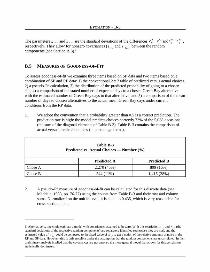
ESTIMATION < B-5
1. Alternatively, one could estimate a model with covariances assumed to be zero. With this restriction, and (theσ 0 σ Gstandard deviations of the respective random components) are separately identified (otherwise they are not), and theestimated value of could be compared to the fixed value of to get a notion of the relative amounts of noise in theσ G σ εRP and SP data. However, this is only possible under the assumption that the random components are uncorrelated. In fact,preliminary analysis implied that the covariances are not zero, so the more general model that allows for this correlationstatistically dominates.
The parameters and are the standard deviations of the differences and ,0−εσ 0−Gσ ε εij ij
kij0 − ε εij ijG0 −
respectively. They allow for nonzero covariances ( and ) between the randomσ ε 0 σ G0
components (see Section A.3).1
B.5 MEASURES OF GOODNESS-OF-FIT
To assess goodness-of-fit we examine three items based on SP data and two items based on acombination of SP and RP data: 1) the conventional 2 x 2 table of predicted versus actual choices,2) a pseudo-R2 calculation, 3) the distribution of the predicted probability of going to a chosensite, 4) a comparison of the stated number of expected days to a chosen Green Bay alternativewith the estimated number of Green Bay days to that alternative, and 5) a comparison of the meannumber of days to chosen alternatives to the actual mean Green Bay days under currentconditions from the RP data.
1. We adopt the convention that a probability greater than 0.5 is a correct prediction. Theprediction rate is high: the model predicts choices correctly 73% of the 5,038 occasions(the sum of the diagonal elements of Table B-3). Table B-3 contains the comparison ofactual versus predicted choices (in percentage terms).
Table B-3Predicted vs. Actual Choices — Number (%)
Predicted A Predicted B
Chose A 2,270 (45%) 809 (16%)
Chose B 544 (11%) 1,415 (28%)
2. A pseudo-R2 measure of goodness-of-fit can be calculated for this discrete data (seeMaddala, 1983, pp. 76-77) using the counts from Table B-3 and their row and columnsums. Normalized on the unit interval, it is equal to 0.435, which is very reasonable forcross-sectional data.

ESTIMATION < B-6
3. The mean predicted probability of the preferred alternative from the stated preferenceexperiment is 0.63, with a standard deviation of 0.22. This is calculated over647 individuals x 8 experiments = 5,176 - 138 missing = 5,038 observations.
In Table B-4, the percentage of pairs that alternative A is actually selected is presented fordifferent ranges of the predicted probability of selecting alternative A. These values showthat an alternative is infrequently chosen when its probability of being chosen is small, andfrequently chosen when its probability is high. For example, when the predicted probabilityof selecting alternative A is less than 0.1, A is chosen in only 5% of the pairs; but when thepredicted probability is greater than 0.9, A is chosen in almost all of the pairs, 96%.
Table B-4Predicted Probabilities for Alternative A
and the Percent of Pairs A Is Selected
Predicted Probability of Alternative APercent of Pairs in Each Range from
which Alternative A Selected
0-0.1 5.49%
0.1-0.2 18.29%
0.2-0.3 24.74%
0.3-0.4 34.99%
0.4-0.5 45.83%
0.5-0.6 55.47%
0.6-0.7 65.33%
0.7-0.8 74.57%
0.8-0.9 84.16%
0.9-1.0 96.15%
4. Respondents indicate the number of days they would spend at Green Bay if conditions atGreen Bay were the same as their chosen alternative. The parameter estimates from themodel can be used to predict the conditional probability of choosing Green Bay under thehypothetical conditions over the individual’s other (real) choices. This is Equation 6 inAppendix A. Multiplying this probability by the actual number of open-water days for therespondent produces an estimate of the number of Green Bay days under hypotheticalconditions. The means (standard deviations) of the indicated number of Green Bay days(truncated to be no larger than the total days at all sites for each angler) and estimatednumber of days are 12.0927 (14.8531) and 12.0917 (12.2885), respectively. The closeness

ESTIMATION < B-7
of these numbers means that the model estimates are in accord with the SP frequency data.While the means are very close, there is substantial variation. Table B-5 is a histogram ofthe differences across the chosen alternatives. For example, the difference betweenreported and estimated Green Bay days is between ± 4.5 for almost half of the alternatives(48.7%).
Table B-5Difference between Reported
and Estimated Green Bay Days
Difference Frequency (%)
< -20 267 (5.2%)
-20 to -15 156 (3.0%)
-15 to -10 290 (5.8%)
-10 to -4.5 507 (10.0%)
-4.5 to -3.5 97 (1.9%)
-3.5 to -2.5 126 (2.5%)
-2.5 to -1.5 157 (3.1%)
-1.5 to -0.5 179 (3.6%)
-0.5 to 0.5 507 (9.8%)
0.5 to 1.5 442 (8.8%)
1.5 to 2.5 454 (9.0%)
2.5 to 3.5 348 (6.9%)
3.5 to 4.5 157 (3.1%)
4.5 to 10 851 (16.9%)
10 to 15 360 (7.1%)
15 to 20 145 (2.9%)
> 20 133 (2.6%)
5. The estimated mean number of expected days to the chosen Green Bay alternatives(12.09) is larger than the reported number of days (9.95). Because current conditions are,on average, inferior to the average conditions over the chosen alternatives, this resultshows that model estimates are consistent with actual behavior.

ESTIMATION < B-8
The probability of going to Green Bay under current conditions is estimated by the model at 0.40,which when multiplied by the total number of days is exactly equal to the actual number of GreenBay days: 9.95. This is required by the choice of statistical model for number of days (binomial).The standard deviation of the number of days in the data is 14.10, compared to 9.91 for thedistribution of the predictions.
B.6 USING THE MODEL
The model can be used to estimate how the probability of fishing Green Bay will change (andhence how the number of days fishing Green Bay will change, holding constant total fishing days)from either a change in catch times or FCA levels. This is done with Equation 9 in Appendix A,repeated here:
(4)P x xiG
iG
ij G= ′ − −Φ [( ( ) / ],β σ00
employing estimates for and . For example, suppose there is an hour increase in the time itβ σ 0−G
takes to catch a perch. The argument of the normal CDF in Equation 4 would then decrease by0.5307/12.43 = 0.04270, causing a 40% chance of going to Green Bay to decrease to about 38%.Reducing the FCA level from four to one causes the 40% probability of going to Green Bay toincrease to about 46% (and the mean number of days to increase 14.5%). Table B-6 providessome behavioral responses to site changes.
Table B-6Behavioral Response to Changes in Site Characteristics
Change in SiteCharacteristic
Change in Probabilityof Going to Green Bay
Change in Mean Numberof Green Bay Days
FCA4 ÷ FCA1 40% ÷ 46% 14.5%
FCA3 ÷ FCA1 43%÷ 46% 6.8%
FCA2 ÷ FCA1 45% ÷ 46% 2.4%
Double perch catch rate 40% ÷ 42% 5.5%
Quadruple perch catch rate 40% ÷ 43% 8.3%
Multiply perch catch by 10 40% ÷ 44% 10.0%
Double all catch rates 40% ÷ 47% 19.1%

ESTIMATION < B-9
For example, holding constant other site characteristics, the probability of going to Green Baywould increase by 6% if FCAs were eliminated. However, at an existing FCA Level of four,doubling the catch rate for perch would only cause a 2% increase in the probability of going toGreen Bay.
The model can also be used to estimate compensating variation resulting from changes in catchrates, fees, or FCA levels (Appendix C).

APPENDIX CESTIMATED COMPENSATING VARIATIONS
AND EXPECTED COMPENSATING VARIATIONS
C.1 INTRODUCTION
This appendix derives two lower-bound estimates of the aggregate compensating variation fordifferent improvements in the characteristics of Green Bay. An estimate is “lower-bound” if it isan estimate of only a subset of the damages. One of these lower-bound estimates is smaller thanthe other because it is an estimate of a smaller subset of the damages.
The improvements considered will be for reductions in FCAs and increases in catch rates.Specifically, we estimate individual i’s compensating variation for an improvement in thecharacteristics of Green Bay for a Green Bay fishing day. In addition, we estimate individual i’sexpected compensating variation for an improvement in the characteristics of Green Bay for afishing day. Note that fishing days in the latter case include all open-water fishing days, includingthose to Green Bay and those to other sites.
Denote individual i’s expected compensating variation for a season for a change in thecharacteristics of Green Bay, . Individual i’s for the elimination of Green Bay( )E CVi ( )E CVi
FCAs is the expected value of the yearly damages to individual i from the FCAs. Aggregatingthese over all individuals, one obtains the expected value of total damages per year from GreenBay PCBs and the resulting FCAs. We do not estimate this; rather we report a lower-boundestimate of these total damages. It is a lower-bound estimate for two reasons: it does not includeall of the potential components of each impacted individual’s damages, and it does not include allpotentially impacted individuals.
Denote individual i’s expected compensating variation for a fishing day for a change in thecharacteristics of Green Bay, , and denote individual i’s compensating variation for a( )E CVi
F
Green Bay fishing day for a change in the characteristics of Green Bay, . The estimatedCViG
and , along with estimates of the current number of fishing days and Green BayCViG ( )E CVi
F
fishing days by a subset of those who currently fish Green Bay, will be used to obtain two lower-bound estimates of WTP for the elimination of FCAs for this target population.
For an improvement in Green Bay , is how much the angler would pay per season (year) forCVi
the improvement, whereas is how much the angler would pay per Green Bay fishing day forCViG
the improvement, and is how much the angler would pay per fishing day. Note that for anCViF
improvement in Green Bay, , and for a deterioration in Green Bay,0 ≤ ≤CV CViF
iG

ESTIMATED AND EXPECTED COMPENSATING VARIATIONS < C-2
1. Given the model, and are constants independent of the individual’s number of fishing days andCV F CV G
Green Bay fishing days. This follows from the assumption that the utility from a fishing day (Green Bay fishingday) is not a function of the number of fishing days (Green Bay fishing days) — see Equations 1 and 3 inAppendix B. In this case, any quality increase can be represented by an equivalent price decrease, andEquation 1 (in this appendix) holds if the marginal utility of money is positive, which it is. That is, Equation 1holds because the angler will not decrease fishing days if Green Bay improves in quality.
. An angler will pay no more per fishing day to have the FCAs at Green BayCV CViG
iF≤ ≤ 0
reduced than he would pay per Green Bay fishing day because all fishing days are not necessarilyto Green Bay.
Explaining further, is individuals i’s compensating variation per Green Bay fishing day for anCViG
improvement in the conditions of Green Bay. There is no question as to where the angler will fishon a Green Bay fishing day: it is Green Bay. In contrast, is individuals i’s compensatingCVi
F
variation per fishing day for an improvement in the conditions of Green Bay given that theindividual can choose to fish either Green Bay or elsewhere.
For an improvement in Green Bay conditions:1
, (1)CV D CV D CViG
i iF
i i
G F
× ≤ × ≤0 0
where is the number of days in a season individual i fishes Green Bay under current (injured)DiG0
conditions, and is the number of days individual i fishes (all sites) under current conditionsDiF 0
(Morey, 1994).
would be individual i’s seasonal compensating variation if he were constrained to( )CV DiG
i
G
0
×fish Green Bay the same number of days with the improvement as he did in the injured state.
because he has the ability to take greater advantage of the improvement byCV CViG
i i
G
D0
× ≤increasing the number of days he fishes Green Bay. would be individual i’s( )CVi
Fi
F
D0
×compensating variation if he were constrained to fish the same total number of days with theimprovement as he did in the injured state. because he has the ability to takeCV D CVi
Fi i
F
0
× ≤advantage of the improvement by increasing the number of days he fishes.
because an individual who is constrained to fish Green Bay theCV D CV DiG
i
G
iF
i
F
0 0
× ≤ ×same number of days both before and after Green Bay is improved is more constrained in hisability to take advantage of the improvement than an individual constrained to fish the samenumber of total days both before and after Green Bay is improved. The latter constraint allows theindividual to increase his days to Green Bay by reducing the days to other sites if this makes himbetter off, whereas the former constraint does not.

ESTIMATED AND EXPECTED COMPENSATING VARIATIONS < C-3
2. Estimated is a random variable.CViF
3. For details, see Morey (1999), p. 103.
4. Note that any scaling of in estimation will cancel out of Equation 2.β
5. In Appendix D, we consider preference heterogeneity.
C.2 ESTIMATED COMPENSATING VARIATION PER GREEN BAY FISHING DAY
Typically when estimating compensating variations, the expected value of the compensatingvariation is estimated rather than the compensating variation itself, because the compensatingvariation depends on unobservable stochastic terms, so it is a random variable. However, if thereis only one alternative in each state of the world, the compensating variation is not a randomvariable. Since is per Green Bay fishing day and since the only alternative is Green Bay,CVi
G
is not a random variable and can be estimated as .2 This is because theCViG CV CVi
GiG= E( )
random component(s) cancel out of the CV formula when the individual chooses the samealternative in each state.3 In discrete choice models without income effects, the compensatingvariation can be written as the difference between the maximum utility in the two states multipliedby the inverse of the constant marginal utility of money (see Hanemann, 1984; and Morey, 1999):
(2)
( ) ( ) ( )[ ]( )
CV U U x x
x x
iG
yiG
iG
yiG
idG
iG
idG
yiG
iG
= − = + − +
= −
1 1
1
1 0 1 1
1 1
β ββ ε β ε
ββ β
' '
' '
where is the utility from a Green Bay fishing day in the improved state, and is the utilityUiG1
UiG0
in the current state; that is, denotes Green Bay under improved conditions and denotesG1 G0
Green Bay under current conditions.4
In addition, , so:x x iiG G= ∀
(3)CV CV iiG G= ∀
That is, everyone one has the same , which we can calculate.5 The estimate is reported inCV G
Chapter 8.

ESTIMATED AND EXPECTED COMPENSATING VARIATIONS < C-4
C.3 A LOWER-BOUND ESTIMATE OF DAMAGES
Equations 1 and 3 imply:
(4)CV D N CVG G× ≤ ×0
where is the number of individuals in the target population and is the number of GreenN DG0
Bay fishing days by the target population under current conditions, so is a lower-( )CV DG G×0
bound estimate of the recreational fishing damages to the target population. The 1998 estimate isreported in Chapter 8.
C.4 EXPECTED COMPENSATING VARIATION PER FISHING DAY
Since is per fishing day and on each fishing day the angler has the choice of two sites: GreenCViF
Bay or elsewhere, is a function of unobservable stochastic components, and so cannot beCViF
estimated. Instead we estimate its expectation:
(5)( ) [ ]E E ECV U U U UiF
yiG
iO
iG
iO= −
1 1 0
β(max( , )) (max( , ))
where is the utility from fishing at another site. Given that and are bivariate normal:U io Ui
G U io
(6)( )E max( , ) ( ' ) ('
) ('
)U U xx x
iG
iO
iG i
G
G GG
iG
G G
= + − − + −− −
−− −
γ β γβσ
γσ
σ φβσ
γσ0 0
0
0
00
0
0
0
Φ
where is the univariate standard normal cumulative distribution function, is the standardΦ( )⋅ φ ( )⋅normal density function (Maddala, 1983, p. 370), andσ ε ε σ σ σ0 0 02− = − = + −G ij ij
GG G
2 0 2 2Var[ ](see Appendix A).
Substituting Equation 6 into 5, and simplifying it one obtains:
(7)
E( )
[( ' ) ('
) ('
)
( ' ) ('
) ('
)]
CV
xx x
xx x
iF
yiG i
G
GG
iG
G
iG i
G
GG
iG
G
= −−
+−
− −−
−−
−−
−
−−
−
1 1
1 1
0
0 0
00
00
0
0
00
00
0
0
ββ γ
β γσ
σ φβ γ
σ
β γβ γ
σσ φ
β γσ
Φ
Φ

ESTIMATED AND EXPECTED COMPENSATING VARIATIONS < C-5
Since, in this model, , . The estimate of isx xiG G= ∀ i ( )E E iCV CVi
F F= ∀( ) E ( )CV F
reported in Chapter 8.
C.5 A SECOND LOWER-BOUND ESTIMATE OF DAMAGES
Returning to Equation 1, consider the inequality .CV D CViF
i i
F
0
× ≤
Taking the expectation of both sides and noting that is exogenous:DiF 0
. (8)E ) E0
( ( )CV D CViF
i i
F
× ≤
Since ,this simplifies to . Summing overE( E( iCV CViF F) )= ∀ E ) E
0
( ( )CV D CVFi i
F
× ≤individuals, one obtains:
, (9)E ) E 0
( ( )CV D CVF Fi
i
N
× ≤=∑
1
where is the number of Green Bay fishing days by the target population under currentDF 0
conditions, so is a second lower-bound estimate of the recreational fishing[ ]E ) 0
(CV DF F×damages to the target population. It is less constrained than the first estimate, so it is expected tobe larger than the first lower-bound damage estimate. Anglers value improvements in Green Baymore highly when they can fish it more. The 1998 estimate is reported in Chapter 8.

1. For the random parameters models, estimated mean E(CVG) is reported.
2. If instead of using the 1998-level catch rates (recall that the catch rate is the reciprocal of the average time tocatch a fish), the 13-year averages from 1986 to 1998 were used, predicted days and consumer surplus perfishing day would increase by about 16%. Therefore, using the 1998 levels results in conservative estimates ofdays and damages.
APPENDIX DMODEL VARIATIONS
This appendix presents model variations and reports estimation results. In Section D.1 modelsexplaining choices from the alternative pairs using only the SP data are derived. These modelsassume both homogeneous and heterogeneous preferences. In Section D.2, heterogeneouspreferences are introduced into the full model covered in Appendix B. A general finding in all ofthese variations is that using only SP choice data or allowing for preferences to vary acrossindividuals has little effect on estimated mean damages from FCAs — in most models meandamages do not vary significantly from each other. The notable exceptions are the randomparameters specifications and a specification that allows the marginal utility of money to vary withindividual characteristics, both giving higher damage estimates.
Estimated mean compensating variations for many of the models discussed in detail below aresummarized in Table D-1 for a change in FCA level from Level 4 to Level 1 (no FCAs). Theestimated mean CVG is reported for all models,1 and the estimated mean E(CVF) is reported for themodels allowing substitution in and out of Green Bay to other sites. Recall that the estimatedmean CVG for the full model with no heterogeneity is $9.75, and the estimated mean E(CVF) is$4.17. Along with mean consumer surplus, 95% confidence intervals for the means are reported.These ranges were simulated using 500 parameter draws from the estimated variance-covariancematrix.
Mean predicted Green Bay days under current and baseline conditions are also presented inTable D-1 for all of the models allowing substitution from other sites. They are computed bymultiplying the model predicted probability of fishing Green Bay under current conditions byobserved 1998 open-water fishing days at all sites in 1998, so total days are held constant.2 Allmodels closely predict the current mean: over the sample, the mean is 10.0, and predictions rangefrom 10.0 to 10.9. The models are roughly consistent in predicting how mean days will increasewith cleanup. Predictions in increased days range from 0.4 to 1.2 days; that is, the increases inpercentage terms are from 4% to 15%.

MODEL VARIATIONS < D-2
Tab
le D
-1Su
mm
ary
of E
stim
ated
Mea
n C
ompe
nsat
ing
Var
iati
ons
from
Gre
en B
ay M
odel
s: F
CA
Lev
el 4
to
No
FC
As
Mea
n C
V p
er G
reen
Bay
Fis
hing
Day
aM
ean
E(C
V)
Fis
hing
Day
sa,d
Pre
dict
ed G
reen
Bay
Day
s
Allb
Nea
rcF
arc
Allb
Nea
rcF
arc
Cur
rent
dB
asel
ined
Full
mod
el No
hete
roge
neity
Cla
ssic
het
erog
enei
tyin
VO o
nlye
$9.7
5 ($
0.0)
[$8.
06-$
11.7
3]$1
0.46
($0
.0)
[$8.
79-$
12.3
5]
NA
NA
NA
NA
$4.1
7 ($
0.0)
[$3.
41-$
5.00
]$4
.49
($0.
72)
[$3.
96-$
5.75
]
NA
$4.6
3
NA
$3.5
9
10.0
10.1
11.4
11.4
A-B
-oth
er Cla
ssic
het
erog
enei
tyin
VO o
nlye
Cla
ssic
het
erog
enei
tyin
A-B
par
amet
ers
only
f
$9.5
7 ($
0.0)
[$7.
57-$
11.7
5]$9
.31
($1.
47)
[$7.
73-$
11.6
8]
NA
$9.2
0
NA
$10.
68
$4.3
5 ($
0.58
)[$
3.48
-$5.
26]
$4.1
6 ($
1.55
)[$
3.46
-$5.
27]
$4.4
5
$4.2
9
$3.6
8
$3.4
0
10.9
10.4
11.8
11.6
A-B
No
hete
roge
neity
Cla
ssic
het
erog
enei
tyf
Ran
dom
het
erog
enei
ty(n
orm
al)g
Ran
dom
het
erog
enei
ty(l
ogno
rmal
)h
$10.
29 (
$0.0
)[$
8.10
-$13
.22]
$10.
15 (
$1.7
2)[$
7.99
-$12
.51]
$12.
90 (
$0.0
)[$
8.70
-$15
.75]
$17.
67 (
$0.0
)[$
12.6
3-$2
4.72
]
NA
$10.
23
NA
NA
NA
$9.1
7
NA
NA
NA
NA
NA
NA
NA
NA
NA
NA
NA
NA
NA
NA
NA
NA
NA
NA
NA
NA
NA
NA
a. W
eigh
ted
aver
age
(wei
ghtin
g is
by
actu
al d
ays
at a
ll si
tes
or G
reen
Bay
day
s) in
all
mod
els
with
cla
ssic
het
erog
enei
ty.
b. S
tand
ard
devi
atio
n ac
ross
sam
ple
in p
aren
thes
es. 9
5% n
umer
ical
ly-s
imul
ated
con
fide
nce
inte
rval
in b
rack
ets.
c. “
Nea
r” m
eans
sho
rtes
t dri
ving
dis
tanc
e is
with
in th
e ei
ght t
arge
ted
coun
ties:
73
mi.
“Far
” is
for
hou
seho
lds
fart
her
than
73
mi.
d. T
he a
vera
ge ti
me
to c
atch
a f
ish
is s
et a
t the
199
8 le
vel f
or a
ll sp
ecie
s.e.
Util
ity f
or o
ther
(V
O)
is a
line
ar f
unct
ion
of d
ista
nce
and
gend
er. N
o cl
assi
c he
tero
gene
ity in
A-B
par
amet
ers.
f. F
CA
and
cat
ch p
aram
eter
s ar
e lin
ear
func
tions
of
dist
ance
and
gen
der.
g. F
CA
and
cat
ch p
aram
eter
s ar
e no
rmal
ly d
istr
ibut
ed. R
esul
ts r
epor
ted
for
Her
mite
qua
drat
ure
usin
g 9
eval
uatio
n po
ints
. Exp
ecte
d C
V is
repo
rted
.h.
FC
A a
nd c
atch
par
amet
ers
are
logn
orm
ally
dis
trib
uted
. Res
ults
rep
orte
d fo
r si
mul
atio
n us
ing
500
draw
s. E
xpec
ted
CV
is r
epor
ted.

MODEL VARIATIONS < D-3
D.1 A-B MODELS USING ONLY THE SP DATA FROM THE
A-B CHOICE QUESTIONS
In this section models are presented that explain only the choices from the pairs of Green Bayalternatives with different site characteristics, conditional on fishing Green Bay. Only the SP dataon site selection from the choice pairs (A versus B) are used; none of the SP or RP data onplanned or actual numbers of Green Bay days are used. These models are called A-B models, andwhile their parameter estimates are consistent, the omission of the additional data on days reducesefficiency of the estimates. Further, because the A-B model does not allow substitution out ofGreen Bay fishing to other sites, only the CV per Green Bay fishing day, CVG, can be estimated, aswas explained in Appendix C.
D.1.1 A-B Model with Homogeneous Preferences
Initially, consider an A-B model with preferences that do not vary across individuals. Assume thatthe indirect utility function for the choice pairs is identical to that of the full model developed inAppendix B (see Equation 1 in Appendix B). The likelihood function is simply the portion of thelikelihood in Appendix A that explains choice of alternative from the SP pairs:
(1)L k i m j J x x Pij ij ij ijk
j
J
i
mij( 1 1 )1 2, ,..., , ,... | , , ,= = =
==∏∏β σ ε
11
To estimate this model, was fixed at . As a result, the expression disappears fromσ ε 1 2/ 2σ ε
the likelihood. Parameter estimates and the asymptotic t-statistics are presented in Table D-2. Theestimated model predicts approximately 73% of the pairs correctly, and all of the parameters arestatistically significant with the expected sign. Also, the parameter estimates are similar to the A-Bestimates from the full model (Appendix B). The calculation of CVG for all A-B models with noincome effects is explained in Appendix C.
For a change in FCAs from current Level 4 to no FCAs results in an estimated mean CVG of$10.29, which does not vary across anglers. This value is only 6% higher than the value from thefull model of $9.75. However, the reduction in efficiency in the A-B estimate is reflected in thesimulated 95% confidence interval of the mean CVG: $8.10 to $13.22 for the A-B model, ascompared to $8.13 to $11.81. The confidence interval for the A-B model is wider on thehigh end.

MODEL VARIATIONS < D-4
Table D-2Parameter Estimates from Nonrandom A-B Models
Parameter\Model
Homogeneity Heterogeneity
Estimated Parameters (asymptotic t-statistics)
Homogeneous parameters$y
$p
$t
$w
$b
$FCA2
$FCA3
$FCA4
$FCA5
$FCA6
$FCA7
$FCA8
$FCA9
Heterogeneous parameters$pg
$tg
$wg
$bg
$FCAg
$pd
$td
$wd
$bd
$FCAd
0.0459 (16.891)-0.5211 (-16.673)-0.0281 (-8.732)-0.0363 (-11.703)-0.0310 (-9.998)-0.1770 (-3.672)-0.2437 (-4.942)-0.4724 (-9.652)-0.6698 (-13.703)-0.4533 (-8.958)-0.7890 (-17.484)-1.0772 (-22.733)-1.1872 (-21.733)
0.0466 (15.381)-0.4707 (-4.904)-0.0285 (-3.472)-0.0192 (-2.447)-0.0310 (-3.787)-0.2351 (-3.517)-0.3210 (-4.935)-0.6388 (-9.219)-0.8897 (-12.240)-0.6030 (-8.975)-1.0494 (-12.729)-1.4622 (-13.316)-1.5970 (-13.866)
-0.1398 (-1.321)0.0031 (0.351)
-0.0214 (-2.491)-0.0008 (-0.086)-0.2868 (-4.706)8.667e-4 (3.574)
-3.455e-5 (-1.594)2.424e-6 (0.109)1.091e-5 (0.598)-2.981e-4 (1.944)
MODEL VARIATIONS < D-5
D.1.2 Investigating Learning/Fatigue and Positioning Bias
The A-B model with no heterogeneity was then modified to examine whether learning or fatigueeffects exist, and whether there is positioning bias toward the A (i.e., the first) alternative. As therespondent gains knowledge and understanding of the survey process, the learning effect mayexpress itself through a decrease in the stochastic variance for initial choice pairs as comparedσ ε
2
to later ones. Recollect there was a practice pair that was not included in estimation. Similarly, ifthere are a large number of survey choice pairs, a fatigue effect may set in as the respondent tiresof the data elicitation process. This effect may be manifested as an increase in noise for choicepairs toward the end of the process.
Two A-B methods were employed to investigate the presence of learning and fatigue. First, amodel was estimated in which was fixed at for the middle four choice pairs (j 0 [3, 4,σ ε 1 2/5, 6]), but was separately estimated as an unrestricted parameter for the first two choice pairsσ ε
(j 0 [1, 2]) and the last two (j 0 [7, 8]). Results suggest weak but statistically insignificant learningand fatigue effects. As compared to 0.707 ( = ), estimated equals 0.936, and1 2/ σ εj j, [ , ],∈ 1 2estimated equals 1.052. Based on a likelihood ratio test, the null hypothesis thatσ εj j, [ , ],∈ 7 8variances are equal across the choice occasions cannot be rejected. CVG for this model is $9.99,which is only 2% higher than the estimate from the model with all variances restricted to be thesame.
The second method fixes at for all of the choice occasions, but allows to vary in anσ ε 1 2/ βunrestricted fashion over the three choice-occasion groups. This method is less restrictive than theprevious method. If parameter proportionality holds, where only varies across choiceβoccasions by a factor of proportionality, learning and fatigue would be evident if the elements of
were all bigger for j 0 [3, 4, 5, 6] than for the first two or last two choices. Because is fixedβ σ ε
in estimation at the same value for all three groups, and because only the ratio of and isβ σ ε
identified in estimation, more noise would show up as smaller values for . The results from theβthree independently estimated models show that parameter proportionality does not hold, because
does not vary systematically across the choice occasions. A likelihood ratio test indicates thatβ βis not proportional across choice occasions at conventional significance levels. However, there issome moderate evidence of fatigue, although no evidence of learning. The estimated CVG, aweighted average across the choice-occasion groups, is $10.94, which is 12% higher than theestimate from the model restricting to be the same across choice occasions. As a result, weβmaintain that $9.75 is a conservative estimate of damages per day. The CVG estimates separatelyfor the groups are $8.65 for the early choice occasions, $15.02 for the middle choice occasions,and $5.06 for the later choice occasions. Note that relative to the $9.75 estimate from the mainmodel, these are all imprecise estimates.
Finally, an A-B model with no heterogeneity was estimated that included a dummy variable forwhether the alternative selected was the first presented, alternative A. This variable was astatistically insignificant determinant of choice, so the null hypothesis of no positioning bias couldnot be rejected.

MODEL VARIATIONS < D-6
3. For example, the mean CVG for a change from FCA Level 4 to no FCAs for individuals living five miles awayis $13.68 for women and $9.75 for men. Note that the mean compensating variations for all classicheterogeneous models reported in this appendix are weighted means, where the weights used were either theindividual’s proportion of the sample number of days to Green Bay in 1998 for CVG or the proportion of thesample number of days to all sites in 1998 for E(CVF). These weights were used because we estimate CV perGreen Bay fishing day or per fishing day, not per angler.
D.1.3 A-B Models with Heterogeneous Preferences: Interaction
In this section, A-B model parameters are allowed to interact with observed individualsocioeconomic characteristics, the “classic” method of admitting heterogeneous preferences.Consequently, CVi
G also varies as a function of characteristics. While marginal utilities for changesin site characteristics and consumer surplus vary in plausible ways as a function of individualattributes, we also find that estimated mean CVG for the sample is quite comparable to that fromthe full model or to the A-B model with no heterogeneity. Incorporating heterogeneity at theA-B level appears to have little effect on mean damages (see Table D-1).
Preliminary analyses and simple statistics for the sample suggested that the A-B choices vary withgender and distance from Green Bay. Other socioeconomic characteristics were not as importantin the preliminary analysis. Therefore, the effects of catch and FCAs were modeled as functions ofthose two variables. The set of FCA marginal utilities is assumed to vary proportionately as afunction of individual characteristics. For example, FCA effects for men are all decreased by thepercentage $FCAg (see Equation 2 below) compared to women. The likelihood function is the sameas in Section D.1.1, with the only exception that now includes interactions with individualVij
kij
characteristics. Specifically:
(2)
V FEE ACT GEND DIST
FCAq GEND DIST ,
ijk
y jk ljk ll
i ld i
jk FCAq FCAg FCAq i FCAd FCAq iq
ij = − + + +
+ + +
=
=
∑
∑
β β β β
β β β β β
( ) [ ( ) ( )]
[ ( ) ( )]
1
4
2
9
lg
where l indexes the fish species for catch (l = 1, ..., 4), ACTl is the average time to catch species l,q indexes the FCA levels (q = 2, ..., 9; $FCA1 is fixed at zero for identification), FEEjk is the launchfee for alternative k in pair j, GENDi equals one if angler i is a male, and DISTi is the closestdistance to Green Bay from either angler i’s vacation cabin or home.
This model was found to be statistically superior to the homogeneous A-B model on the basis of alikelihood ratio test, although the proportion of choices predicted correctly did not changeappreciably. Parameter estimates are reported in Table D-2. The effects of FCAs and catch forsome species were found to vary significantly as a function of gender and distance from GreenBay. Women were found to have larger FCA effects (in absolute value) and therefore largerdamages.3 They care more about FCAs than men. Conversely, men were found to have a larger

MODEL VARIATIONS < D-7
4. Note that target is correlated with distance (a much higher percentage of yellow perch anglers live close toGreen Bay, and a much higher percentage of salmonid anglers live farther away). An angler is defined here as atarget angler for a species if he fishes for that species “often” or “almost always,” and does not fish for any otherspecies “often” or “almost always.”
5. Along these lines, omitting extremely avid anglers with a large number of days from the data set prior toestimation was also not found to have a notable or significant effect on parameter or per-day consumer surplusestimates.
marginal utility for catching walleye. Marginal utilities for perch catch and FCAs decrease withdistance, while the marginal utility for trout and salmon catch increases with distance at a marginalsignificance level (the t-statistic is -1.59). For those traveling to Green Bay from within the eighttargeted counties (within 73 miles), the mean CVG is $10.23, while for those farther away it is$9.17. Over the entire sample, the mean is $10.15, with a standard deviation of $1.72. Thesimulated 95% confidence interval for mean CVG is $7.99 to $12.51. Note that this mean is only4% higher than the mean from the full model.
Other interaction specifications were run as well, and while some of these generalizations werestatistically significant, uniformly they do not lead to statistically or substantively differentestimates of mean consumer surplus. For example, the effects of FCAs and catch on utility werealso allowed to vary as a function of the angler’s target species. The effects on utility of catchchanges for all four of the target species are all greater for the respective target anglers, and perchand walleye anglers care more about FCAs than other target anglers or anglers who have notarget.4 The effect on damages was small, however. Effects on utility from FCAs and catch werenot found to vary significantly as a function of the actual number of Green Bay days.5 Finally,marginal utility of money was allowed to vary across gender and income groups; males and thewealthy have a significantly lower marginal utility of money. This specification led to a higherestimate of the weighted mean CVG, $12.36 (27% higher than $9.75). However, the simulatedconfidence interval on mean CVG was quite large, [-$19.34 to $35.98], because some draws of theprice parameter for affluent males using the estimated covariance matrix are very small and evenhave the wrong sign. Therefore, it is not possible to conclude that $12.36 is significantly higherthan $9.75.
D.1.4 A-B Model with Heterogeneous Preferences: Random Parameters
Two primary issues have motivated the use of random parameters in modeling consumer choice.First, random parameters provide a way to induce correlation in the stochastic components ofutility within pairs of alternatives and across an individual’s choice occasions. Hausman and Wise(1978) were the first to model explicitly correlated disturbances. Second, random parametersallow for preference heterogeneity across individuals without having to model heterogeneityexplicitly as a function of individual covariates. Note that the estimates from our main model,

MODEL VARIATIONS < D-8
6. This is the usual formulation for the random coefficients model. See Hildreth and Houck (1968), Swamy(1970), and Hsiao (1975).
which does not explicitly model correlation across pairs, are consistent in the presence of suchcorrelation.
Random parameters have been used to model choice-experiment data for a wide array ofcommodities and environmental amenities, including alternative-fuel vehicles (Brownstone andTrain, 1999); appliance efficiency (Revelt and Train, 1998); forest loss along the Colorado FrontRange resulting from global climate change (Layton and Brown, 1998); and the level ofpreservation of marble monuments in Washington, DC (Morey and Rossmann, 1999). Threerecreational site-choice examples using simulation with revealed preference data are a partialdemand system of fishing site choice in Montana (Train, 1998), and complete demand systems ofparticipation and site choice for Atlantic salmon fishing (Breffle and Morey, 1999) and fishing inthe Wisconsin Great Lakes region (Phaneuf et al., 1998).
Model Specification
The random parameters A-B model for Green Bay fishing explicitly estimates the correlationbetween disturbances within pairs and across choice occasions, in the spirit of Hausman and Wise(1978). Assumption 2 from Appendix A is maintained, but assumption 1 is now replaced by:
(3)β β υ υi i i N= + , . ~ ,i i.d. (0 )Σ
where Li is an L × 1 random vector that represents heterogeneity of preferences acrossindividuals.6 An individual’s marginal utility of an alternative’s characteristic differs from theaverage by an additive, mean-zero random variable assumed uncorrelated with the modeldisturbance. All J pairs are evaluated by the individual with these marginal utilities. Then:
(4)U x x xijk
i ijk
ijk
ijk
i ijk
ijkij ij ij ij ij ij= ′ + = ′ + ′ +β ε β υ ε( ),
where the new model disturbance is in parentheses. It is straightforward to find the correlationbetween these disturbances (and hence the utilities) within a pair and across pairings for eachindividual. Within a pair we have:
(5)E[( )( )] ( ) ( )1 1 2 1 2′ + ′ + = ′υ ε υ εi ij ij i ij ij ij ijx x x x2 Σ ,
and from pair j to pair l we have:
(6)E[( )( )] ( ) ( ).′ + ′ + = ′υ ε υ εi ijk
ijk
i ilk
ilk
ijk
ilkx x x xij ij il il ij ilΣ

MODEL VARIATIONS < D-9
7. See Butler and Moffitt (1982) and Waldman (1985).
With correlation allowed, it is now more convenient for the unit of observation to be theindividual (i), not the individual-pair (i, j) as in the nonrandom model. The probability ofobserving the vector of J pair-wise choices is a J-dimensional multinormal probability:
(7)P P K k K k P U U U Ui i i iJ ij ik
ik
iJk
iJki i iJ iJ= = = = > >− −( ) ( ).1 1 1
3 31,..., ,...,11
Substituting the random utility model and the specification for the $i (Equation 3) into Equation 7yields, after some rearranging:
(8)
P P K k K k
P x x x x
x x x x
i i i iJ ij
i ik
ik
i ik
ik
ik
ik
i ik
ik
i ik
ik
ik
ik
i i i i i i
i i i i i i
= = = =
′ + − ′ + < − ′ −
′ + − ′ + < − ′ −
′
− − −
− − −
( )
[( ) ( ) ( ),
( ) ( ) ( ),
(
3 31 1
3
3 3 3
1 1
1 1 1 1
2 2 2 2 2 2
1 1 1 1 1 1
1 1 1 1 1 1
,...,
υ ε υ ε β
υ ε υ ε β
υ
M
i iJk
iJk
i iJk
iJk
iJk
iJkx x x xiJ iJ iJ iJ iJ iJ3 3 3) ( ) ( )].− − + −+ − ′ < − ′ −ε υ ε β
Although evaluation of this integral is more complicated than the equivalent expression in thenonrandom model, the “equicorrelated” nature of the problem means that Pi can be calculated asthe integral of a joint conditional probability over the density of Li by standard reasoning.7 The Jevents are correlated, but the source of the correlation is the individual-specific parameter errorvector Li. This common factor design allows for the computational simplification mentionedabove. The J events in the probability in Equation 8, conditional on Li, are independent, so thejoint conditional probability may be written as the product of the J conditional probabilities. Thenthe resulting product is integrated with respect to Li to remove the conditioning:
(9)
P P x x x x
x x x x d
P x
i ik
ik
ik
ik
i ik
ik
iJk
iJk
iJk
iJk
i iJk
iJk
i i i
j
J
ij
k
ij
k
ij
i i i i i i
iJ iJ iJ iJ iJ iJ
ij ij
= − < − ′ − − ′ −
− < − ′ − − ′ −
= − < − ′
−
−∞
∞− −
− − −
=−∞
∞ −
∫
∏∫
[ ( ) ( )
( ) ( )| ] ( )
[ (
3 3 3
3 3 3
1
3
ε ε β υ
ε ε β υ υ φ υ υ
ε ε β
1 1 1 1 1 11 1 1 1 1 1 ,
M
3 3
1
3
] ( )
[2
) )] ( )
− −
=−∞
∞ −
− − ′ −
= −+
′ −∏∫
k
ij
k
i ij
k
ij
k
i i i
j
Ji
ij
k
ij
k
i i
ij ij ij ij
ij ij
x x x d
x x d
) ( )|
( (
υ υ φ υ υ
β υσ
φ υ υε
Φ
where N is the L-variate multinormal density function with mean vector 0 and covariancematrix 3:

MODEL VARIATIONS < D-10
8. Under normality and the additional assumption of a diagonal 3, the multinormal joint density of Li, N(Li),factors into the product over k of N(Lik), although no further simplification appears to be possible because eachelement of Li appears in each probability. This means that there is no computational advantage in the additionalassumption of a diagonal covariance matrix.
(10)[ ]φ υ π υ υ( ) | | exp ./i
Li i= ′−
− −2 2 1
21Σ Σ
The order of magnitude of the integral in Equation 9 is determined by the assumptions made forVar(Li) = 3. Specifically, it is equal to the number of distinct nonzero diagonal elements, which isthe number of parameters assumed to be random.8
For the model of Equation 3, $i = $ + Li, the likelihood of observing ki1, . . ., kiJ is:
(11)L k i m j J x x Pij ij ij ii
m
( 1 1 )1 2
1, ,..., , ,..., | , ; , ,= = =
=∏β σ ε Σ
where the Pi are from Equation 9.
Methods of Estimation
For the purpose of estimation by maximum likelihood, Equation 11 can be evaluated in either oftwo ways. First, since the kernal of N(@) is of the form exp(-[@]2), the combination of Equations 9and 10 with a change of variables ( for the case of one random parameter) can bev = υ συ/ 2written in the form:
(12) e g d−∞
∞ −
∫ν
ν ν2
( ) .
This integral can be approximated using Hermite polynomial quadrature, which is fast enough tobe a practical computational method (Butler and Moffit, 1982; Waldman, 1985). Quadrature canbe made as accurate as necessary. If the order of magnitude of the integral is small, which is thecase in the current application [in Hausman and Wise (1978), three parameters are random], theestimation problem is computationally tractable by quadrature. Second, if quadrature is notfeasible because the order of magnitude is too large, a simulation method could be used (seeLayton and Brown, 1998; Train, 1998; Breffle and Morey, 1999). Using simulation, the integral isapproximated in two steps: first, the joint probability is computed many times using a largenumber of random draws from the distribution of L, and then the average is computed. Details onHermite quadrature are relegated to Section D.3.

MODEL VARIATIONS < D-11
Estimated Random Parameters A-B Model
The four parameters on the catch rates and the eight parameters on the FCA dummy variables areall random, and assumed to be normally distributed with zero covariance. There is no classicheterogeneity in the model. In addition, it is assumed the standard deviations of the catchparameters vary in proportion to their means, and the same is separately true for the FCAparameters. That is, the ratio of the mean parameter to the standard deviation is the same for eachof the four catch rates, and for each of the eight FCA levels. Therefore, only two standarddeviations are estimated. Assuming that the standard deviation varies in proportion to the mean isa common way of dealing with heteroskedasticity, and allows the model to be more generalwithout making it intractable. This technique is similar to one used by Brownstone and Train(1999) in a random parameters logit model, where the standard deviation was assumed to beequal to the mean. The marginal utility of money is not assumed to be random due to undesirableeffects on the distribution of the E(CV)s because the price parameter is in the denominator of theCV formula (Layton and Brown, 1998; Phaneuf et al., 1998).
Specifically, the conditional indirect utility function for alternative j in angler i’s k-th choice is:
(13)V FEE ACT FCAqijk
y jk c ci l ljkl
FCA FCAi FCAqq
jkij = − + + + +
= =∑ ∑β β ν β β ν β( ) ( ) ( ) ( ) ( )
1
4
2
9
where $c and $FCA are the mean base catch and FCA parameters, respectively; $l is thedeterministic multiplicative factor shifting the mean (and the standard deviation of the randomcomponent) of each catch parameters for the four species; $FCAq is the multiplicative factor forFCA level q; and $y is the marginal utility of money. The base standard deviations of the catch andFCA parameters are Fc and FFCA, and $p (for perch) and $FCA2 are fixed at one to achieveidentification of the model.
This model was estimated using both quadrature and simulation, and parameter estimates arereported in Table D-3. Likelihood ratio tests show that the randomization of the catch and FCAparameters significantly improves model fit relative to the homogenous nonrandom A-B model.Results from various model runs show that 500 draws in simulation and 9 evaluation points (seeSection D.3) using quadrature are sufficient for parameter estimates to be stable. That is, at theselevels of draws and points, parameter estimates are the same within 2%, and parameters do notchange significantly with more draws or evaluation points. Therefore, there is virtually nosimulation noise. An interesting finding is that simulation took over three times as much computertime as quadrature for the 2% threshold.
The ratios of the standard deviation to the mean are 0.66 and 0.92, which match well with theratios for random parameters in other studies valuing environmental improvements. The rangeover 20 parameters in 3 studies is 0.40 to 14.29, with a mean of 2.28 and a median of 1.43(Layton and Brown, 1998; Phaneuf et al., 1998; and Train, 1998). The estimated parameters of

MODEL VARIATIONS < D-12
Table D-3Parametersa and Consumer Surplus Estimates for Random Parameters A-B Model
Method Hermite Quadrature Simulation
Evaluation points/random draws 9 500
Mean parameters$y
$c
$FCA
$p
$t
$w
$b
$FCA2
$FCA3
$FCA4
$FCA5
$FCA6
$FCA7
$FCA8
$FCA9
0.0555 (15.267)-0.645 (-11.607)-0.327 (-4.916)
1.0 (fixed)0.0480 (6.384)0.0647 (7.985)0.0544 (7.295)
1.0 (fixed)1.618 (6.224)2.189 (6.519)2.963 (6.151)2.463 (5.944)3.531 (5.857)4.813 (5.607)5.300 (5.526)
0.0556 (15.282)-0.648 (-11.607)-0.324 (-4.513)
1.0 (fixed)0.0478 (6.348)0.0650 (7.989)0.0544 (7.306)
1.0 (fixed)1.643 (5.774)2.215 (5.938)3.000 (5.608)2.503 (5.437)3.578 (5.326)4.881 (5.098)5.384 (5.035)
Standard deviationsb
Fc
FFCA
0.428 (-5.270)0.302 (-5.638)
0.431 (-5.322)0.296 (-5.238)
E(CV)sNo FCAs v. FCA4 $12.90 $12.89
a. Asymptotic t-statistics are reported in parentheses.b. t-statistics are for the natural logarithms of the standard deviations. The parameters were exponentiated inestimation to restrict them to be positive.

MODEL VARIATIONS < D-13
9. Because the standard deviations of all random catch parameters are restricted to vary proportionately withtheir means, and the same is true for FCA parameters, these percentages apply to all catch and FCA parameters,respectively.
10. Note that with random parameters, is a random variable which depends on .CViG υi
11. In a multi-site random model, E(CV) would need to be numerically approximated just as the joint probability.
12. If a parameter is not random, its value equals the mean for all individuals.
the normal distributions also imply that 6.6% of the population have catch parameters of theopposite sign (i.e., they value catch reductions) and 14.0% have FCA parameters of the oppositesign.9 This result is an artifact of the distributional assumption.
E(CVG) was estimated for a change to no FCAs from FCA Level 4.10 The computation of E(CVG)for a random parameters model with no income effects and only one alternative in each state ofthe world, such as this model, is straightforward. It can be computed as the difference betweenutility in the two states divided by the marginal utility of money. Because utility is linear in $, theformula for E(CVi
G) when some parameters are random (but not the price parameter) and there isonly one alternative in each state is the same as for the nonrandom model:11
(14)
[ ]
[ ]
E( ) ( ) ( )
( ) ,
CV x x d
x x
iG
yi i i i i
yi i
= ′ −
= ′ −
−∞
∞
∫1
1
1 0
1 0
ββ φ ν ν
ββ
where $ is the vector of the means of the parameters.12
Note that because the choice of alternatives is not modeled as a function of individualcharacteristics, E(CVi
G) = E(CV) œ i. The estimated E(CVG)s for the two approximation methodsare also reported in Table D-3 with the parameter estimates. Estimated E(CVG) is $12.90 usingthe model estimated by quadrature, which is higher than $9.75 from the nonrandom model withRP data. The mean parameters for FCAs are about 20% larger than the estimates from thenonrandom model, generating higher damages. It is reasonable to expect that making parametersrandom may significantly raise or lower E(CV).
The normal specification of L is only one possibility from many choices. A second randomparameters A-B model was estimated under the assumption that the random parameters arelognormally distributed: and . This distributionalln N(( ) ~ , )β β σci c c ln N(( ) ~ , )β β σFCAi FCA FCAassumption restricts the marginal utilities for increases in the time it takes to catch fish and theseverity of FCAs to be negative to everybody. Because Hermite quadrature only applies when thedistribution is normal, the simulation method was used with 500 draws. The estimateddistributions of and are -1 × N(-0.598, 0.670) and -1 × N(-1.560, 1.286),ln( )βC ln( )βFCA

MODEL VARIATIONS < D-14
13. Note that mean E(CVG) would have to be simulated if the price parameter is random because the formula isnonlinear in the price parameter. Train (1998) allows the price parameter to be random and lognormallydistributed. Layton and Brown (1998), however, warn of undesirable effects on the distribution of the E(CV)s asa result (because the price parameter is in the denominator of the CV formula), and hold the price parameterfixed. Phaneuf et al. (1998) also hold the marginal utility of money fixed. A small draw of the price parameterfrom its distribution will cause the E(CV) associated with that draw to balloon, which overall will have anupward effect on simulated mean E(CV).
14. When the RP data on 1998 Green Bay days were included, the model did not converge. This is notsurprising, and nonconvergence does not detract from the quality of estimates from the main model withhomogeneous preferences or any of the convergent models with heterogeneity. Introducing a large number ofadditional variables into a model often results in multicollinearity. As a result, parameters cannot be estimatedwith precision. The covariance matrix computed as the inverse of the Hessian matrix of numericalapproximations of second order partial derivatives of the log-likelihood will not in fact invert if the Hessian isnearly singular (i.e., the likelihood function is virtually flat in some dimensions).
15. Results for another A-B-other model, which allows classic heterogeneity in Vo, are also reported inTable B-1. The parameter and consumer surplus estimates from A-B-other models are similar to the main model.These estimates are consistent but less efficient than the main model because they do not include the RP data onGreen Bay days.
respectively. The estimated E(CVG) is $17.67, which is considerably larger than $9.67. The largervalue is not surprising since the mean of a lognormally-distributed random parameter is anβi
increasing function not only of the mean but also the standard deviation :β σ. The mean $FCAi is -0.480 when the distribution is assumed to beE exp( ) ( ( / ))β β σi = + 2 2
lognormal, as compared to -0.327 under the normal assumption. We do not estimate a model inwhich the price parameter is random.13
D.2 VARIATIONS ON MODELS ALLOWING SUBSTITUTION TO OTHER SITES
Classic heterogeneity is incorporated into models allowing substitution in and out of Green Bay intwo ways. In the first of these models, the same specification for was used as presented inVij
kij
Equation 2, where the marginal utilities from FCAs and catch are assumed to be functions ofgender and distance. This model was estimated using the SP data from the choice pairs, theexpected number of days the chosen alternative would be visited from the followup questions tothe pairs, and the RP data on total number of days.14 This model is referred to as an A-B-othermodel in Table D-1.15 In the second of the two models, the A-B parameters are assumed to behomogeneous, but the utility for other, VOi, is assumed to be a function of gender and distance:
(15)V GEND DISTOi i i= + +β γ γ0 1 2 .

MODEL VARIATIONS < D-15
16. For example, consider a male angler and a female angler who each live 5 miles from Green Bay. A man iswilling to pay $8.74 per Green Bay fishing day for removal of FCAs and $3.62 for a doubling of the perch catchrate. A woman is willing to pay $12.14 per Green Bay fishing day for the removal of FCAs, but only $0.49 for adoubling of the perch catch rate.
17. As with the A-B model with classic heterogeneity, the estimated mean is a weighted average using theproportion of sample days as weights.
18. In contrast, a random term in VO adds nothing, because is equivalent to .U VOi o i i= + +υ ε U VOi o i= + η
In this second specification, the RP data on actual Green Bay days is included. Both of thesegeneralizations significantly increase explanatory power. We were unable to get convergence on amodel using all the data with classic heterogeneity in both and .Vij
kij VOi
Parameters from the A-B-other model with classic heterogeneity are reported in Table D-4 andshow similarities and differences when compared to the A-B model with classic heterogeneity.Again, we find that women have a higher WTP for eliminating FCAs in Green Bay. Men havesignificantly higher values for increasing catch rates for all species than do women.16 An importantdifference in the results is that both FCA and catch effects are larger (in absolute value) foranglers at a greater distance. Also, the parameters from the A-B-other model with heterogeneityhave much higher t-statistics than the parameters from the A-B model with heterogeneity.However, the estimated mean CVG of $9.31 is similar to the full model without heterogeneity; it isless than 5% lower.
Also, the amount of noise in the stochastic term for the other index can be compared to that fromthe Green Bay choice pairs, because they are assumed to be uncorrelated, and is separatelyσ 0
2
estimated. A greater level of randomness is expected for the other site because explicitcharacteristics of the site are not included in the model. The estimate of is over 10, which isσ 0
2
greater than ½, the value of .σ ε2
Results from the full model with heterogeneity in VO show that men and those at a greaterdistance are less likely to fish Green Bay. The parameters are in Table D-4. The A-B parametersfrom this model are close to those from the homogeneous A-B model and main model, as is meanCVG of $10.47, which is 7% higher than for the homogeneous full model.17
Because these models allow substitution in and out of Green Bay, mean E(CVF) can also becompared across the models. For the first heterogeneous A-B-other specification, estimated meanE(CVF) is $4.16, which is only one cent lower than $4.17 from the homogeneous full model. Forthe second heterogeneous specification, mean E(CVF) is $4.13, which is 7% lower.
In theory, a random parameters specification for A-B parameters in the full model could bespecified and estimated, although that is not done.18 Because of the complexity and form of thelikelihood function for the full model, simulation rather than quadrature as a means of estimation

MODEL VARIATIONS < D-16
Table D-4Parameter Estimates from Heterogeneous Nonrandom Models
that Allow Substitution out of Green Bay
Parameter\ModelHeterogeneity in A-Ba Heterogeneity in VO
b
Estimated Parameters (asymptotic t-statistics)Homogeneous parameters$y
$p
$t
$w
$b
$FCA2
$FCA3
$FCA4
$FCA5
$FCA6
$FCA7
$FCA8
$FCA9
$0
F0 or F0 - ,
F0 - G
Heterogeneous parameters$pg
$tg
$wg
$bg
$FCAg
$pd
$td
$wd
$bd
$FCAd
(1
(2
0.0446 (10.022)-0.0545 (-10.527)
0.0206 (6.035)0.0386 (5.997)0.0050 (1.227)
-0.0481 (-14.277)-0.2709 (-80.475)-0.5409 (-160.440)-0.6005 (-177.310)-0.5369 (-159.446)-0.7633 (-225.195)-1.0245 (-300.755)-1.2345 (-365.401)-0.7483 (-221.829)3.199 (690.739)c
NAa
-0.3721 (-107.489)-0.0322 (-5.042)
-0.0539 (-14.550)-0.0187 (-5.844)
-0.2806 (-83.105)-8.067e-4(-39.345)-9.212e-5 (-4.946)-1.958e-4 (-7.864)-6.061e-5 (-4.299)3.842e-4 (16.472)
0.0521 (19.313)-0.5345 (-13.150)-0.0244 (-9.296)
-0.0294 (-10.294)-0.0255 (-8.297)-0.0846 (-3.425)-0.2508 (-5.843)
-0.5448 (-14.170)-0.5853 (-18.225)-0.5182 (-12.387)-0.7453 (-25.813)-1.0403 (-28.068)-1.1384 (-24.772)-2.2961 (-24.500)5.2441 (34.206)c
4.1280 (25.304)c
1.0450 (13.669)4.581e-3 (16.572)
a. These results are for an A-B-other model that allows substitution out of Green Bay, but the RP data on the actualnumber of days at Green Bay is not included. Therefore, F0 - G is not a parameter in this model. In addition, ,0 and ,ij areassumed to be uncorrelated, so F0 rather than F0 - , is estimated. See text for discussion.b. These results are for a full model that does include RP data on the actual number of Green Bay days.c. F parameters were exponentiated in estimation to restrict them to be positive. t-statistics apply to the loggedparameter estimates.
MODEL VARIATIONS < D-17
would be necessary. Estimating a full model with random parameters seems unnecessary because:1) mean consumer surplus is robust across the different nonrandom specifications; and 2) thehigher consumer surplus values from the random A-B models suggest that damages estimated bythe nonrandom full model are conservative.
D.3 DETAILS ON HERMITE POLYNOMIAL QUADRATURE
Hermite polynomial quadrature is a method of approximating integrals of functions on ( )−∞ ∞,with integrands that take the form presented in Equation 12. It is based on standard Gaussianmethods. Consider first only one random parameter, in which case the approximation toEquation 12 is:
(16)e g d g Rm m mm
M−
=−∞
∞= +∑∫ ν ν ν ω ν
2
( ) ( ) .1
Here, <m is the mth zero of the Hermite polynomial Hm(<), m is the number of evaluation points,and Tm is the mth weight, given by:
(17)ωπ
νm
m
m m
m
m H=
−
−
2 1
12
!
[ ( )].2
The remainder is:
. (18)Rm
mgm m
m= < < ∞!
!,
πξ ξ
2 (2 )( ) 0(2 )
Abramowitz and Stegun (1964) present <m and Tm for various m in tabular form.
Let and indicate the elements of this vector with superscripts. That is, is∆x x xij ijk
ijkij ij= −−3 ∆xij
k
the kth element of . Suppose without loss of generality that the single varying parameter is the∆xijk
first. Then g(<) is:
(19)[ ]g x xij ijj
J
( ) ( ) ( )/ν π σ β σ νε υ= − ′ −− −
=∏1 2 2 1 2 1
1
2 2Φ ∆ ∆/
Notice the necessary change of variable to accommodate the fact that the normal kernal is e−
υσυ
2
22
and not .e−υ 2

MODEL VARIATIONS < D-18
For the case of two (or more) varying parameters the elements in the random vector <i inEquations 9 and 10 are treated separately (and denoted here by subscript), and the numericalintegration is done from the inside out. Without loss of generality, suppose the two varyingparameters are the first and the second. Then Equation 11 becomes:
(20)P x x x d
d
ij
J
ij i ij i ij i i
i i
= − ′ − − −
•
−
−
=−∞
∞
−∞
∞
∏∫∫ Φ ∆ ∆ ∆[( ) ( )]exp( )
exp( ) ,
/2 2 21 2
11
12
222
2
12
1
1 2σ β σ ν σ ν ν ν
ν ν
ε υ υ
where is the standard deviation of random parameter k. The integral inside the brackets isσυk
similar to the single varying parameter case, and can be evaluated in that manner. Call thisquantity h(<1). It is a function of $, and <1, but not a function of <2 (recall F, is notσ υ1
, σ υ2,
identified in this model). Equation 9 may be written:
(21)P h di i i i= −−∞
∞
∫ ( ) ( ) 1ν ν ν1 12exp
which again can be evaluated as a single quadrature. The number of function evaluations increasesexponentially. That is, if five function evaluations are used when there is a single varyingparameter, then 25 are used for two, 125 for three, etc. The approximation of the double integralis:
(22)P w w gi m m m mm
M
m
M
≈
−
==∑∑π ν ν1
2 111
1 2 2 1
2
2
1
1
( , )

APPENDIX ESURVEY MATERIALS
This appendix includes survey materials, including:
< Telephone survey instrument.
< Mail survey instrument. Note: only Version 1 is included. All versions are the same exceptthat the choice pairs vary across versions.
< Table of choice pairs by survey version.
< Mail survey first letter, postcard, and second letter.
< Phone survey implementation instructions.

r" , I
My nome i, Ifill inl and I 0Il\ cal ling from II.gle, eOllly In 'he Univ"",i')' R==h PMk in MIld Lwn, WI. We are oondu<'ing • >looy of r«'ple's opinion, ,\>00, fishil\i . M,y I .p<ok "'"h
---- -'
You or< pm of. ,moll group of O1lilers woo hove be<n «i<n' iftcollp"I"",ed for ,hi, "ooy. Your opin ion. will "P""'"' 0,1><, .o~'r> lik" )"U. bu, woo w"re 00' >elwed for Ihi, >looy,
TI", i, 00' • mork<ling or <al" call AI",. I ,,',n, to '''Uf< yO" 'hat yow- name "ill o"vcr be OSSOClaled ""Ih your ""S"'WI io any way, and '!\al .11 )'OU' ,OSpOll"> will \>0: k<pI coofLdcn'iol , n", .urvey ",",lIy tokes .boo, 5 min""'" Hal" I "".<he<! . oou",hol<l" I><IJ""i?
I. Sin<e JonUN)' I oflh" Y"M, on oow many do)" did YO" ,pend part 0' .11 of 0 •• day ito f,o/1 ,og' ,A''''t 'Q imu-"iew"" , in Ihis q",,,jon ,,~ an j""",,<a i" ,,/I day .. o/fi,hi"K "garal ... o/localion/
(IF ZERO, FILL Q3_4 WITH OANDGOTOQJ)
2 W,,,,..,y ofU .... tIa)" ito r"binK ,he "~'e" of G,een Bay> When I .. y the ""'m of G~n no)' I am ;""loo' Oi ,he bay or Gm:n B.y, Snugoon Bay,.ii.!:!!I the river> and """.m, ,ha, feed ioto Grecn fuy up '0 lhell fin ' dO/ll. For ''''''ple, i, woold include 'he Fo< Ri," .. be,,,-.." lj,..n fuy ond the dam ., DePere
, , (FlLL Q3_4 WITHOANDGOTOQJ]
3 On how mOllY day. did J'<!" .pend pat! Or . 11 of the d,y icc fi>hing Ih< "." ... of D,een Flay>
4 On how man)' o.y' did yO" .pend port or,lI of ' he d.y ice fish io& ,I>< 1'0> Ri"<1 \>0:''''''''0 G_" B.y 000 ,he dLUll . , DeP"",?
IFQ41,EQJ, (JOTOQS,- £LSEGOTO Q4_CHK)

P.~< 1
<Q4_t,;IlK> OIl, <i<fioitioo of the " .. ,en of Green Bay ,oc ludes <he Fox Ri,..,r b«w<e" Greo" Bay and <he dam .1 noP<re. y 0" s'''~ Ihat yo" SpcTl' Ifill Q41 d.y. icc r"hLni the Fox Ri,..,r betw",,, Gr.en B.y and lhe dam .. DePere, btl, on ly Ifill Q31 day. icc frshil\i the watcrs o[Gre," B.y which would ;",1...0< , .. F,,< Ri"<r be,wcon Gr«n B.y ond the dam at DePere,
Did )'OU ",dud, <he number of d. y. k< [,..,iog the 1'0. R",,, betwo<" Oro<" B.y artd the dam at DcPcrc .. part of the <by, ice [r..,iog ),""o 11.y"
, ,-, GOTOQJ]
<Q!fIlK_YES> 1 om sorr)', I om uocle" aOou\ how many da)" you Lee Ii.hcd Green Boy .. a whole ""d how m..,y of'he .. d.y, "'''"'' '1"'"' i<e fi.hm~ on ,he Fo< Ri,..,r he,wcon Green B.y Olld 'h< ~ ot DePe". 00TOQJ)
~, Since January I oflhi, )'ear on !\ow m3lty day. did you Spend all Of part of <he d.y fishirtg other than ;0< fi,k;ng. fl"ot.lO i"'."'ie"~" , in 'hi' q","ion we"", m"'rested '" . 11 day. of ic. fishing "gatdl .... oflo<><io")
I)a,.. ro'h io~ (no' 1'0 ro,h,og)
fFZERO, FILL Q7 de 8 WfJHOAND GOTO CHECK!]
6, Were an,. of the", ""n_i cc f"II;I\i da)'S fi'hil\i the "",'m ofGrttn Bay" lI.'hen I say tIt. w.ters of(;t«n I).y ! om i""ludil\i the boy of Green Boy, S'urs""n B'y. lIIlII 111< riw", and ",.,.n" 'bat feed ;n'o GT«lI Boy up '0 the" fint dam. For <x..-npl<, i, would i""IUIl< lhe Fo< R" ',,, ""''''«0 Gree" Iko)' and til< dorn .. DePere,
, ,-, (FILL Q7 & 8 WITHQANI) GOlOClffCKI
7. OIl how mony of these non_l<O fishirtg d. y. did ),ou ,pend )'WI 0' .11 of 'h< day fishil\i ,he wO'e" of Grec" Ikoy?
_ D.)'. r,'hing (no' ic. fishing) "'.,,,.. of Go'«n BO)'
8, On OOW mllJlY of the", non_,ee fi>hing day. d;.l you 'pend P"~ or .11 of the do)' flShlnl! ,0< Fo, Rive, he,w«n Green B.y and til< dam ., De Pe'.?
(IFQ8LE Q7 corocm;CKI, USE GOTOQ8_CIIKI
<Q8 CHK> Our d,flnitlOn of ,h. watet'< of(;",," Ba)' ;",,100.:. 'he Fox River he,wecn Grc<n Boy and Ill< dam at DePOT<. You <aid lllat )'OU <pent Ifill Q8] day' f"hln& the Fox Rl'c, he'"'ccn Gr«" Bay and Ill< "om at DeP.re. but only Ifi ll Q7] d.y, r"h '"i ,ho " .. ,<" of G,o<" Boy "hi'h wo"ld mdude ob< Fo, Ri, .. " belw""n Oreen Ray..".; ,he dam., DeP",<,
Did )'0" ;,,<100.: ,he numhcr of day. fi'h ing til< Fox Riv<r Il<tw«" (j",." Bay ""'; 10. dam . , D.P.,. as pan oflll< d.)', f"hin~ Grun B. l'
, (GOTOQ71
<Q&_CHK_YES> 1 om wrry. I am u"cle'" aix>ul how mOJl)' do)" ),ou fi>h<d Gr<en Bay os • wbol., .00 Ito", mllJlY ofthele (10)'. w.,. 'pen, fi'h illl: "" ob< Fo, Ri,'e, be,ween fi,..,n flay and '0< dam at DePe .. , COIOQ7j
<CHECKI> IFQ3 - QANDQ7 . OCOTO ,WT II£C£I'o7,- ELSE GOTO QJll
<NOT RECENT> 9, 11>,'e )'ou ",,, f"he<! "n ,ho waren ofGrc<n 13.1'
, GOTOQilal

10, \\'hy ba\,<n', )"00 fi,ttW ,It<: " .... ,,,,f Green Ba)' "occ Januory I? ( Do 001 ",od ml<gor;<s, lisl<n 10 '<'<1"''''' ,,"" eM. ",ing ,I,;; following mUg"'i", If "nSUF< of how to code. ,m" ,·"balim "<><1" -01"',", Th< I"QI:'Dm will ace'pl up 10 6 mno"" Aft" each '<SPO"" , l"oiM M'ilh "A"y olh" "",a",' '']
o 1'0 mo .. ru, ntion<d I Contomin,n" in tb< fi.h l PCB, in fi,h J F;,b .... "., ,.f. '0 ,ot
4 Pott.'iO" ~ F;,h doo', ,.st. ~""(! b Lo" i"" .. " 7 No , im. fo. fi.h;"~ ""J''"o", 8 Th". , ... btU" rtao .. '" fi,h 9 011 ... _-> _________ _
11.. Would you corwder fiUting 1M wa'e" of(ireen B.)' If CORd"lO" ' ""~'" "liferent?
, Ye. ,. fGOTOQilB] GOTOQI1J
, 1 b, IVh., "'loll' would have to change bef"" you W(luld C(lo,ide, r"~l "i the " .. ,<" of G,e.:n
fuy? ( Do oot rc.>d <",<fori ... )jot." to ""portS< >n<I C<XI< ""ng the foUowin~ <."'~on<'. If ."'''''' of bow to code. mter ,,,,,batim uRde, "ollt<:''', Tl>e pWiT"'m "i ll """pi up to 6 reawno. Aftor caeh ""pon ... probe "i,h ""'0), otl><' ",awn,,?""]
" , , , • , • , • ,
On G .... n Bo)'
12. A"~le" ba,', diff.,"", f .. l;oll' .bou, hO,,"' ;mpOr1"'" ;t i< to be .bk c,teh fl ," ,hat ". f, .. of con,,,,,, i,,,,,,,,, Would )'OU say ;\ ;, "N", ., alllmportont", "Somewhat Importa,-,," "r "Very Important" '0 )'OU ,~., rosh you ""toh "'" free of oon,.minon",
r\O,"j ,II hnport""' l Some"'h" ;mport. "1 3 V.ry ;mro",ot

,,... 0 ..... Ilay ....... s. .. .,- """'~"'.'
13. I om reinllO I'eallIO you 10 OoI:I.ioo>f!hal miP' be taken 10 imJ'lrO"" !he quali,)' off .. ~inJ in Wi_Min. Six ofthex .. ,ions an: for !he: "~ofG~ Bay ond !he: orb<. fout ... for 011>« ,,~,= fo< _h ............ plt.ue .ell Ill< ,f. "'m~ 10 otbcr thin,. that """Id be <10<>0 to ,mproo..., fishiT\i. )'O<Ilhinl talin, thi, o<'iorI is "Noc 01 .1I 1mpo<lall'"' "So"""h.o, ImJ'<'lU"'" or "V<I)" Impc>rWl'"
[R .. d .ach ac'ion, di"ille in", 'w<> blocks. Gr«n lI.y oc'"", and "",,·Green !loy, 1W><lom1)" .. Ioc' bk>< k '" ..,. n ... ....t J)"stem.ati<ol l)"~"'Y lWtiT\i ilem ,,,thin bIo<I;.J
l'ot., . U Som ... h., " • .,' ' "DOrI'G' l!!ptrlIDI ImDOrlon.
8lotk , ,,.... ... si. _ """ could be tal: ... to imJ'lrO'" !he qualiljl of flSlliT\i Oft Ih< " ...... of<it<o:<lll.y
111< ...... II>< ., .. ",,«.,cl! of '9011 fi,h lik. ',ou' • .. I""",. ~, and """ I<y< on the "" .... of Gte<n H.y."" ..... "" .....
I"" ..... the .,.e<>ae c:ot~h of pon fIsh like ) .. Uow peKh on the " -.. of<it<o:<l Bay .... .. .... .... . ............ 1
Clun up <anUmlnanlS '" !hot --= of fiob ~inthe"~ofG=nBay _ cuurninat<d .... _ ..... _ ...... _ ..... _.......... I
Impro"'1hc: dOli,y oflhe ..... t ... in G"",n il>), I
Pm"ide aclditional publ" launl:h r .. ili.i .. on G=n Hay ............ .. , .... "" ........... .
, ,
, , , , , , ,

Not., ,II Som,w."
BtO,k 2 )I,,,, are r.,.., '"'tjon, ,hal eouid h< tokcn to impro" 'he qual ity of f"h ;og 00 ,Oe ,nland waten of Wi<oon,j n
C lean up coman,;"""" SO ,hal ""nc of the fi ,h cought in the in land ",at.,., ofWiwln' ln or<
COn'Onllnot<XI.
Pro"lde odditiona l pubhc boat I. unch faciliti. ,
,
on lnbOO "~tc"", ..... ,,, .... 1
R«Io<c 'he om' of I,"ochint • boat on inlond lakes 1
(lFQ9 _ 1. GOTOQ16j
15 , In ",o..t year did you fitS, fi ,h ,he "~'ers of Green B.y"
16. Do )'00, '" 00e. rome',"c in rOUT bmaeoo ld. 0"" a 00.(1
lYe. I No
17. Do yo.. have a .. """,ion 00"'" or c.bin>
, , , ,
,
, ,
1 y " . ->- About how m."y miles ;, ,I from YOU' voc>,ion home oH.bin to ,Oe bay of Green Ba), '
__ M,I« '0 ~'Y Ore", " lhl o L ... ,h'n I m;l.

_ __ A~'
Which categ,),y be" d's<ribe, y0"' <mploymrnr m,",? (REA D LIST)
I Full tim' 2 P ... , tim.
, N •.•• .;. Which "'OKOf' be" de>cribe, )'ou> (Rf:AD I.IST)
, Stullen! , 1l,1i ... ~ , lIom,m,lt" , Un'mpl"y<~ , (lIh .. , S.lf '''rloy<~
1" •• ;", Am.rican , Mi," ; Mri,," Aru<rkan , m.r.ni< , C.u", i. n , O,h" (PkG" spuW ,
21, IrtC l l!d,"~ youndf. bow maHY people "" ;de ;n 'our bou><bold'
_ _ _ Numb .. of p<opJt in ho" "h"ld
22 I""l od,"~ YOIlf:>CIf. how maJ\y oftbe« at< 16 Or moT< j'e"", old?
__ ~N"",b" o[p<ople in hou""Old 000'" Ih< .~, of 16

2], INTERVIEWER: RECORD OENDtR
M.I. l fem. l,
[if ql _O and q' - O, ghfish mQ ("'" fi,h<!d in 1998) go'o term;""," [if q I 81 Q and qj - O ~nd qJ mU, gbfi,h-I (ic. fi,hed o"'y, nol GB) 8010 ICrmiMIC! (if ql 81 0 alld qj _O ~nd qJ X' 0, gbfi,h- ; (iel f"h<!d OIf/y, GB) gOlo wm,,,,,"1 (if ql g< 0 alld qj gl Q alld q7- 0, ghfi,h- J (,","-k. fuh<!d, "'" GB) ",crull! (if ql g< 0 alld q5 gl 0 and q7 gl 0, ghfi,(h- J (""n-ic. fish"', GBI ",cruil!
One purpooc of thi, "00), i, to ooll<ct inform., iD" to h<lp m." bel«, (\«" ioo, obout m."-.:in~ fish ifli in Wisconsin, We would li k, to oonlac, yoo by m.il to 10..., ""'" .bo"' you, Opi","" ' about fishin~ in Wlscon,in,
W ... k<!<J you ro, thi, >tooy u,ifli ,=ds of ind "'idual, who purcl=<d fishing lio<",,, ;" 1997, C.., I oonfi1l1l yoor name.md addr<", to make '"'" we r..,'e tl-l< 00"",' add"" to ",nd to. ",.t<ti.I ,~ If R IS HESIT.tI>T, GOTO HESiTANT
NAME' @"""", STREET ADDRESS: @add'e» CITY: @~uy STATE, @State liP. @zip PHONE NUMBER:@;phono
We ""II be .. ndifli )'OU 'ho >lll"C)' 'I,thin tl-l< next """k or two, We can't . ff<mJ to pOly you for )'our "me to complete the '\m'''Y. but we "i ll i.dud< 0 toKen of 0", .ppm;,.tion alon~ ",ilh tbe
"''''''y. B«.u>< 'I~ ",II be combining tbe an,wets )'0" g.'" "' <OO'y with y<>ur anNus from the '"""'y, " " importon' that )'OU, .nd ~ot ","'«I"t elso ;n )'OU' hou .. hold fill out th< moH ,",,'.y_ Some of thc que"ion, in the ,urvey will .. , how m,oy day' you h"", beon fishing '''IC' thi. <.11. It wou ld b< "'f)' helpful to u, if)'ou 00"1d ' eep II""k of tl-l< number of da)" 'OU go fISh ing berwecn 1\OW ond ,he tim. )'ou g<1 ow ,ut\'<y,
GOTO TERMINATE

<HESITANT> Yoo Ito,." oc<" .de,,(ificall y <e lected to "", ;' ;pal< i" (h " '''''h. B)' ~<lpin>;"' ou' w,(h 'hi' moil ,urvcy you "illl>c T<pT<","(in~ th, opinion. of o(Oer "'Sk" I,ke )'ou",.lf. bu, "ho " ',,, '""( ,00""" [0' 'hi' "cody, Wc COIl·( .fford (0 f"Y you for your1 ;me '0 romple'" 'he ,.ur)'ey. ""( we ,,';11 ".<IWe • '0)"" of OU' 'ppre<;io"o" .Ion~ ""h ,he 'Ufvey Would ),ou be "i lling '0 help u, ou,?
(1fA'(). GOTOTHMINA·n;
CM I confirm ),our name and add,." '0 ma" SU'" ,,'< hov, tl>o: COrIO<;' a&jre;, to ",nd tlIe m .... i.l,o
NAME:@nam< STREET ADDRESS, €odd",,, CITY, lifcity STATE, @lta'e ZIP: @zip PHONE NUMBER: lifphone
lJocaus:e we ",,;11 be ""mbi";">: (he "",wen you i"'e "' too.y WIth yow on,""'''' from ,he '""'<Y. ;, is impo>rlllO( ,It.o, )'00. ""d no' ,0""0,,, <I" on YOOf hoosebold fill out the 1l1.,,1 '1m"<)".
S-ome oflhe q"",,;on,;" 11>0: '"r.'.y ,,'111 os~ bow mOllY day, you It.o". been fLShl1l~, I, would be ,'ery helpful to u, if you ooul ~ ~ .. p ,.-..ek oflh<: number of d.y. )'00 ~o fishilli bctw«n oowand Ih<: time you ~et OU, >u"'oy.
>TERMINATE<
Th>Itl:, fOf your htlp. ThO! ".Illh<: q",,"ioru; we Ito,." for 'ou

What Do You Think About Fishing the Waters of
Green Bay?
Walleye
1998 Angler Survey
Chinook Salmon
Yellow Perch
Sma llmouth Bass
Research Cotdlctod by H33Ier Sailly Please mum $Uro"eY 00:
1Jnoftll»y Fishing Survey Hagler Bainy. Uciva.ilY Research r:.rt
455 Sci"oce Dri ve Madison, WI Hi II·I(ISS

The Waters of Green Bay
F<Y Itll' ""'yY. It.. .......... 01 O"",n Say- 1",,_ Ih: boy 01 Gr= Bay. SI<II&<"" Ray. and Ih: "'= and .uumo """ f«<\ inoo G«otn Bay "" '" tbcir fiR' dAm. If ........... "" (\>m,
.1""1'''' trib" ... ),. Ih: hili ""J'l~ of , ... tril:>uta<)' "«NI'idercd 10 be pon ollh: ,,~1b'I; 01 Orten Bay. Tri,,"wy h"¢r> .... ~'n 011 'hi' nul'> ,."lIer lri,,"''''Y "'<an" Of<'_.
"
, "
" Michigan I
f ·
"
Lake
Michigan
Wa ll" of G"",n Bay

II
iii
II
ronions "f'hi. ,un"" a rt ' 00"1 Y"U' n'hing .<.h' iti« on tho w.tt", of Gr .. n Soy. For 'hi' '''''-' J". H .. "".."", of G, .. n B'j-" in<iud. ,h. ba)' of Gr .. n Bay, Stu..: ... " ila)', and the rin ... nd .. ' .... ms 'h., rted ;"W G .... n ROJ' up '0 Ih,I, first d . ", ( ... .... p).
On • ",,~I. f rom 1 107 wh, ... I mtallS "~luch Wo"." and 7 m .. D> " ~Iu<h BtH .. ", ho ....
do you ..... 1he quoli.)" of r,'h ing on 'h' , ... 1, ,,, of G .... n Ila)' cornp .... d to "'her pi."" )'OU rosh' ei,c/, ""' no""" , M",h Wor>C Moch Bottor
(t\>n Other Aoo"' thon Other
" ~ ,be S..,. ,~, Don) Know , , , , , , , , , , • , ,
PI .... pro.1d •• romm<nl th., will ht lp u, ""d",;'.nd Jour ""ing in Qu<>lion I. Frll in'", blonk
11.,'. ) '0)\0 I><en r. ... I"R si...,. ,h. day .. < called lOU .boo! Ibi. "udy? ( ) C" clr on, n"mb<,
2 Ye. II@f' (If "r .. "j Sin"" the da y w< ""lied you. on how m.ny additional d ",., did lOU ,,,,nd.1I or pan of lb. day fishing ...
(he w.'e" of G""," Ba)" Fill '" 'h, "ymlvr of dQYs
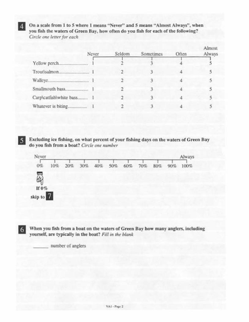
..
II
III
On ....... ',-010 I 10 S _h ... I _ .... ,~ ....... aDd S ......... "AI,_' AI~.).~ ... -bm
you n", ''''' "'0"'" ofG<e<n lIa) . h(v.o- on ... <10 l"" roo ,.". nth oflh. ' ..... 'n&! Cir</. _1<tkT /tK.....,.
-Ke",. '~m $o<no,"'" 0<," ~'" , , , , Yeklow por<h .. , , , • Troutl>Uno n .. , , , W.IIol'" .......... --- --- -- -----, - , , • ,-~ , , , , C><1"adisbl. .. t.u """'-_n._ , , , • ..... 1 •••• , ..... bot .. , •• _ , , , ,
"""udln, 1« nSh;"~. on ,,-h., perctnt of ,oo r n'hin~ do,. on "'. ""on of Gr .. n Ihy do 'OU IbII from a bo.C 0«/. C<I' """"'r
, '5
, - , ".
, .,. , "'"
, - , - , ... , .,. ~." , ,,..
WhO. IOU IbII r""" a _IOn \ ..... ",IOn ofGlftn Bay ...... madf .""" .... Indudin~ )OUnri •• ..., 'IJliaolly In I/O. _ 1 fill;" ... bIooIt
___ ... mbcr of ""l:l<n
, , , , , , ,

III
On • ..,01, from I to 5 ~h,1'< I n"'.n> ··u..,t Importont"' o"d 5 .. "' . .. , "Most Imponont··. ho"' .wuld you , ... the follo,..int .ctio,,< In term< of ho'" .h.y .. ould .,,1000'1« you, ,« .... ion,1 fi.hin~ on Iho W'''", 01 ;"",,, Ih)"1 Cord , 0"' ""mb<-, jo' each "clioo
AddLn~ more bolo, launch locilitie, .
Addinr more sho relu.e par. ,. nalure con<"" .• 1Id t .. w.. .., ... , ..
Incrc",,"'g ","e, o11nt)' ..
Increasing " .toh rat< ..
Cleanin¥ up PCB, .. r"h con' ""'pti"n . dvisone, """ t>c r<duced or olimtnated.
Ot"", ... :;. PIe.>.« 'ped f)"
""' ImpomOllI , , , ,
, ,
,
, , , , ,
,
Mo<t Im[lO" 'nL , , , ,
, , , , , ,
, , ,
Fo, tIIi. ,",," )" w. d.fine On ,,· • .-oge COlch .... "" how ofle", 0" .. ·.'-OK., '1,'plcol angl<r " 'ould <otol, tho typo "I r"h he or 1Ioe i, .argeting. For "."ple. on .. ·.rag. c>lch rale ",ight to< ~ h"u", ptr fWo or 30 minu ... pt. fi,h. 01 OOJu .... tilt actua! cotch .. t<
will .'.ry fro", day to da~' and .c'-- "ngl",.
Th •• , .... ~. catch ral< is""' rM ,ome as the bag limi •. Th, bog I;"~t I, lh. numb<r of r,sh an '''~1<r <;an le~a!ly k .. p tach d.y.
On 0 11 .. 1< of 1 '0 5. ,,·h ... 1 ",ton' "Slnmgl)' Ol<agr«" and 5 "",a ... "S1rt,"gl~ ... g...., ••. ho,,- do you f .. 1 . buul e..,h of the 1",lowln, .. . t.,11<" .. 1 Ci,eI, 00' "u"",, , ft" ' o"h
"a" .. m'
We shouJO inc",= c",eh "'OS by incr<",ing Green Boy fISh pop"la,io .. "." ..
Strongly Di3>.~roc ,
w. ,hould oo,l<t Oree" Bay Cosh popul .. io .. Oecline t>ecau,", tha, ""mid t.u,", e.,eh '"'''' 10 decline" .".
, ,
No"Oc, Aj;T<e 00' S,ro"~ly
D""g,ct , A~re< , , , , ,

III ~" ,,,,", "·.,."orc....," B.)' . ... 1 ... "«1 .... h'" i CauS< he. ',h probl ..... in human>. Gr .. n Ba y
C", ,;" ';;;: 'nll<n "". """ ,.fel), .>1 " ... Is of G~" II.), fish.
PCB, "r, , ub".n.,.,. thal " 'tT< uS<d b,' indu.'ry "nlil tho mid l!>'/O· .. I'ell. ",I,a>«! into .h. <nl'i",,,,, .. ,,, . o<o",ulale I" ,.,HI"""" at th, boltom of 1> . .. and ,I, .. ms. PClh ~"in'" fl,h IhnU~h Ih, rood <h.i,,_
B'Ioro ) '00 ....,.;,'«1 11l1 • • UT .... y, had ,'ou h,.r<! or rtad '00"1 fI'h C<ln,""'pllon .d ,';'ori .. for Ih. " .... '" of Gfffn II.,! e",/. 0"' ""mb"
s" 2 Yos
3 ;.;o( 'u'"
1m FCA. vary by fi,h 'pod .. and fish d ... FCA' for PCR, co" 1"0110..., I" .. "
IJolimi, .. 1 ronsu"'pli." Eat 00 rno", th .n on< ", .. I. ,,'« k Eot "" 100 ... 'han one ", .. I. monlh Eo,,,,, ""' .... Ih.o un< ", .. 1,\" ,)' ho'o ...,nth. [)o no' ,.t
F",'h'g ".." . n,h .ban is fK'Gmm<nd«l in .h. FCA for PUh:
fM ,,'0""0, in' ....... tho ri.~ of b<.ring child ... " "ho hu. I.aming di ... hiIlU .. or d«oIop ,,"' .... klwly.
PCB. do nol a IT..,t tI .. ,,,,,," or < .... 11 or rosh, or 'he .~pe . .... ''''.> "u",ber, or .. .. of fI'h.
On • s<alt froon I 10 5 "'h . ... 1 ", .. 1\5 "Not at ,\11 1I01ll,,,,,n,," and 5 "'''1\5 " V"Y 110111 • .,.,,,,,,"' .n,,,', r 'he following question. For tho fi,h ~'ou ,,'.uld lik. to fi>h for in Ih. w."" of G...,n B.)" how much wo"'~ it both" )'ou. if at all. if PCBs .... 1.«1 in tho follo"'ing fi.h coRSuOlption ad,i .. ,; .. ' (,,,c/. on, "yrnkr for ,"en """ i' Q,)'
No'" All '<0 B",hcT>OIDe Bottlerrome , , , ,
Eat no ""',. ,han 0"" ",,,0]. " 'Ctk ...... , , , , .. .. ... ..... , , , ,
D<:> no, eo" , , , , ,

In ... _ '0 'he ul"ln~ 0>11 <OruIuollp,lon •• hioorit$ rOc 'he ~-01< .. or C ..... n IIa) '. do )'0<1 do on)' ofthe f,"lo"in~? Cirel. n., .um/><. foe ,at~ " ",,,,,,. ,
<- , . IfN"'I f'''~' day< fi""~t .he ..... m ofOreen S.y ................. . CMn«. , .. pI~u. I fi,k on ,he "'>lor> or G""n Boy .. _". c""n~ ,1>0 ' 1'.0" I fi,h foe on ,he w.,o .. of G"",n O.y_
ohan£C ,II< 'puu, r1 fi'~ I k"p IQ .~, fron> IhI: .... l<fS of Oreen BiIy ..... _ c~ IhI: "':L r1fWo I I;",p" ,~, from.he " ...... ofOr= BOY._. c ..... ro lhe ""y Green B.y full arc c/ . .... d",. ,.....po'fil
clwle< ,he "-oy G",," D.y fISh "" cooktd " my 1100,", •• ,.
------ -------- --.. -
• , , ,
On .,'.raco. _ "''''''' do )..,.. p ... "".111 'p<fId r ..... ,ypl<al do)' of n"'ln~ on the ,,-. 1<1 .. or G .... n Boy!
J/ 1"" dOlI " I)'pitoll)' .... nd ""''''lon on 11,,,, pi .... pu' $(l III"" ,p~' opt- III .tli ......... ,,..., _ttaIIJ ........ . 11,"" ........ y -. ,rips orion, •• u..n 0 ... day. 1<11 .. ''''' • • '-<n&' D)I1 por d.)-.
Cia> /or ""hick.,.;l.". boaI ..... _ . ............ _ ...... _ ....... S Boa, launc"-'t 100:_ .. _ .. _ ..... _ ...... _._._ ........ _ ....... S MO'd'hl)1Cl ___ .. ___ .. _ .................... __ ___ .................. ______ S
Food :and beoerat<S-._ .............. _ ............................. S G_ .". clwtn """- _ .. ~ ... ______ .. _........ .. ... ___ ______ $
Oth« ···>Pbsr opocO'y
--- --- _ ........ ..... ,--Ad<! up , ... lotal
• , , , , , , ,
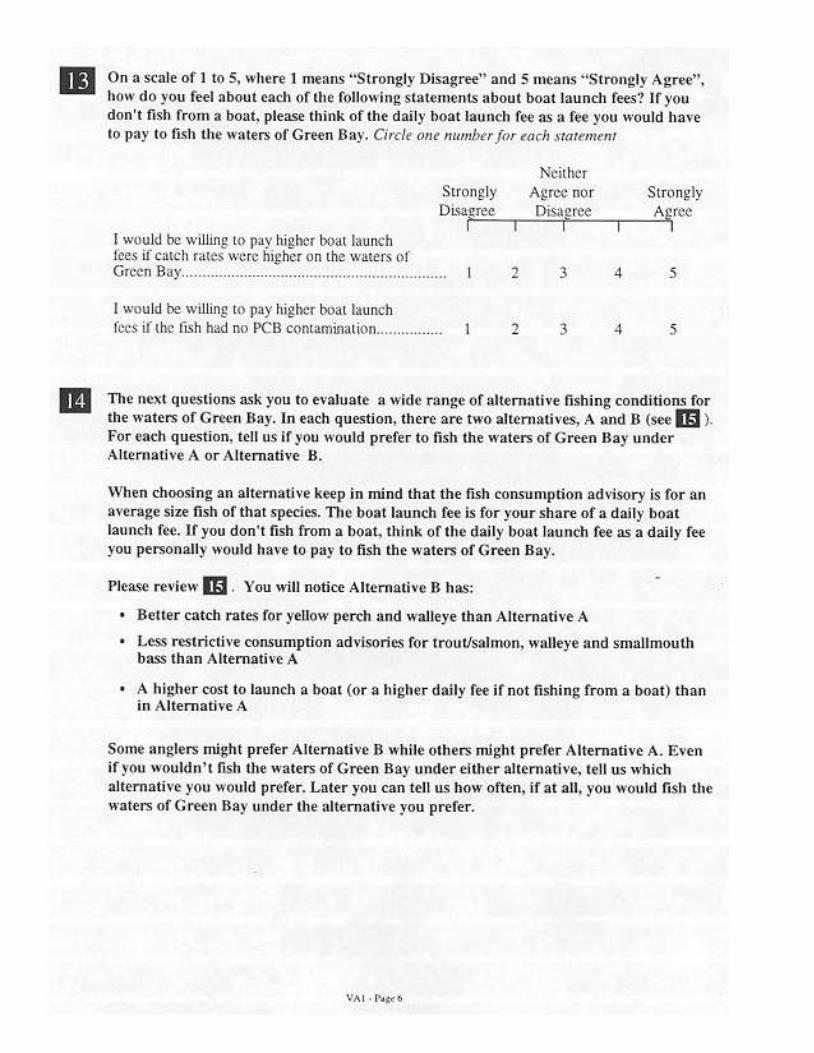
m
m
On 3 scoJ, of I t"~, wh .... 1 ..... 1lS "Stron~ly U;"'grff".nd 5 "",.n, " Stron~lr "'g,"''', ho~' do )'00 r .. , OOOU' ,ach of Ih. foll,,"iug , ,0te,,><"1> aoou, 00a' launch f~~ Jr )'"'" don ', fl'h from ...... ,. pl .... think oftht d. iI)' bo., 'ounch r .. as. re<),oo would h.,.. 10 p.y to fi,h tho ""3t.,, of Gr .. " Boy. C"c/. ",u n"mI" , fi" mrh ,.""<",,nr
Stro"~ly Dl"~re< ,
J "" uld be willing [0 p>y h~lIcr 00" lau""h foe, if c'lCh ' .. e, "'Or< Iu~ocr on , fie wat,,, of Greo" B,y. .. . __ . , .. " n . ,_ ... , "" •• ••• , t
J w"uld be willing to fl'Y hi~bcr boa< Ia"nth fees if to., fISh had 00 PCB ""momm"i,," .. ,.,
, ,
Noitllcr Airce DOr D"'~ r .. ,
, ,
Stfon~l )'
A. ree , , ,
no< n,,, qu""'iom; a.Q; you to .. ·.'0 .... "Ide ",n~. of .It.mal;" r"hing conditio!\! for ,h. wa« ... orc .... " Ihr. In .. ch ques,;on. lh" •• ", 'W" .I .. ,.,'oth-os, A and B (_Oil J. For •• eh qu.";"n. 1<11 .... I! Y"" would p",r" to fish Ih. " ....... oIG .... " Bay u"dcr Al l<m. ,;". A or AI"m.~,.. H.
Wh on <hoosing an altern .. ;", ~ .. p in mind th., tho fWi colUu"'ption ad"i",!)· is for an . ,',rag. nu 0>11 of that .p<ri«_ no< bo •• launch f .. i, for yoo. ,ha l'< of a dall)' ooa' launch foe. UyO" don', fi,h fro", a boa ••• hink ofth. d. ily bo.".unch f .. as. daily f .. )'00 p< ..... nally woold ho," to p.y to fi>ll th' wa"", of (il'«n 11 . )'_
1'1 • • ", rt,iew m, \ '00 wili llOti", """m.ti,. 1\ lo a"
• lIe"« ca'rn rat .. for y.llow perth and ~·.' I.)'. ,h . n Altem >li .. '"
· u.. .... tri"i,·. rolUUmption ad,;""" .. for 'rouVsa"""". wall.)·. and 'mallmou,h b." .ban AI" m ath ', A
• '" hiRher """ to launch . _, (or a high .. doHy f .. if not fi'hin~ from . 00>1) til." in AIt.math·, '"
So", •• n~I.r> might pref .. AIl,m.tI.o 1\ ,,·"iI. oth.", might prtf .. AII<mati" A. E,'. n if Y"" "-""'d,,', fI'" tho " .• 1<", of G_n II . )' "nde' .lth" .ltom. ,;"'. 1<11 u, which all<rna'i.·o )'00 ,,'ould prtf .. , L.", ),ou can 1<11 u. how 0/1<", if at all, )'0'" woold fi.h ,h. " 'al<,,, of (;""'" II.)' """ .. Ih •• It.rnalh·, you pl'<f .. ,

IIiI If )l'" W .... ~oi n~ to fi,h .h. "'~t .... uf G""n Ba)', "'Quid ~·ou pref" '" fi>l. Ih. " · ... B of GTffn Bay under Altem.li .. A or AI«m a';". B' Ch«l 0"' box i" "" tail m"'
A'~"~O c.lth ,a" for a ')'1)>:,1 angb.
FOsh corlS, "'p!io" .. h i",'Y
nom and S>lmon
A'~r>to <>"h rato for . ,ypic;oJ >Jl~Ie,-
FOsh OorlS""'Pl;o" od,i<.ory
Wallo)'!'
A""" gooooch rate for a typical an~k'. , .. ... ... "
FlIh co",umption .a,iw'l',_
Smallmou,h bus
Average c .. eh 'Ole
[or . ,)'pic.hllgIeL
Alternative A Al1cmativc B
'I'
40 minU Le< pcr perch ~I """",C, pcr J>Crch
No mOl< ,flail one meal per ",ook ~o more 'h'" one meal pcr "..,."
2 OourS peT IrOU"""""" o
1)(1 rot cat
Do no' .a,
2 hours per trout/salmon
No more 'Oan 0"" meal per Ill<Inlh
4 hour< per ",,,'leye
No more 1tw1 one me.l peT ""'nth
F\<I1 <"",umplion ad,'iwry. ... No 1OOr< than one me" p'"
~".
200"" per b=
Unlimited corL<umplion
You, iliare oft .. do;)), lau",t. f ••..
ChKk lhe box for ,h. alt.m.II," yoo p,..f<T ..
,,"
o o iii! PI<_ com"","' on how you <h"", 1>.,,",..,. Allern a'h'. A and AI,.mali,.. II in m,
Fill m Ih, bI"."

m 110 ... oft." " 'OUld you fi,h I~' ~-"ters Of Gr«" Hoy If 1\ ~.~ Ih. rondi1ioR> d""rii><d by the .ltema1;", )'00 jn« d1_ (A oe HJ' You, " OW," could d'p'''d on a n"ml><r of rawm"
•
•
•
•
•
•
11 0 .. ' maO,' d.," )'OU '),pkollr n,h in. J't"' ."d hu" man)' of'h ... daY' . .... ptn, fi>hin~ ,h. "'.",, of G""," 110)'_
11 0w much )'OU .njoy fishing 110 . w.I.", of erN" Ba)' rornp.T"«l 10 01hu piON< )'OU mj~ht fish
no. ""', of r .. hing ,h ... ~, .. > of G"",n Bar romporod to other plac .. )'on might fooll
Wh"h., fOu ,hjn~ th . <""dilion' for the ,,'.,.'" of G .... n Bay in ,h • • Itemoth. !on j .... , eh.,.. .... ""Iter, "'ors<, nr '00u1 the .. '"., "" 'u''''''' oondiHo" ..
no. ""' ... )'011 fi , h lh. " ,.1<", of G""," Bay ,h. 1<5> ,jm< )'011 ... iII h ... for fi 'hing .t.< .. ·h .... .
u<1uding j« fi,hi ng. how m.n), dol's, on .v . .... ~., wool<l )'(>11 H.h the ",.ttn; of G~" Bay in • I)'pica, )"" if ,h. conditions on Ih . ... ,,,,, of G,...n Bay"· ... ,10.,.. de><,it.«I in ,b. al1tmali>', J'w <host in Oil , fili In In, bionk
____ da)~ ''''' i"~ ,tic w'w" o(G"", " Bay ,n, ,)'p;;al )~ ..
III PI.",,,, <om" .. ", 0" ho,,' you an,,,'.re<I m . fill in ,M blank

l1li If )-.,., .~ .. ~n~ 10 roo ,~. ""tl"l of Gfftn fla)-. .. · .... 1eI , .... pro"', ' 0 l1$li II .. ......... or Crt<n R.y ~nder A'_'I.-e " .... AI' om aH,-. B! CMd "". bo. ,~ til< Ill .. ,,,,.'
w .... ye
yoo, .\I'I...-e of" .. a;oi/y lounch fee
CM<~ ,~. 1><>. , .... th. ol,t m a"vt y .... pref.,
Alternati ve A
."
30 m""''''l 1"" pon;h
Unlimit<d <OD$UmpI"'"
12 hooan 1"" troullsalmon
Eo! "" moo: , ..... I ..... 1 ... <:d;
2 00." per ",. Ile)"
E,a, "" RIO" ,lwo I ..... 1. we<k
Unlim''''~''''
"
o
Alternative B
."
In rrunu loS pe' fN' fCh
~ 00 ....,.. ,h;on I ....,.10 • ..,.t
6110"" PI" \J'OUt/oahDn
Eat "" """,,!han I mUla_~
4 oo U'I I"" .. 'alkl"
Ea' "" mort ,han I me>! , mon,h
12110 ... pcr bus
~ no moo: , ..... I meaI.-"
""
o lID t:"luding ic< r""'nJ. 1>(>00 ''''"Y doy .. on "'u 'co . .. w lel ) .... h!oll 'M n .... of G_n 1I0y
In a ''-~ .... if lll. COfIdi,1on$ f)fI 1M n' .... oH ; ...... Ray ...... "'_ d<S<rib«! In ~ .l1em • • i .. you ell"" In m? Fill j~ 1M bJank
____ d.ys rLihU\li tOo w,,,,,, MGrte n B.y

m If )'ou " -. ,, ~oin; t" n, h the " '., . ... "r G ..... Boy. " '"uld )'''u p ... rec to fish the ",.",.,,! Gr .. " Boy ond .. Altomath ,. A or Altern"',', II? Ch,el on, box i. rh. Iw "'".
Trou, . rId Solmon
Smdlrn" u' h .,..,
YO"' we< of the d.dy lour>::h fee
Ch ock the box for the . itemOli,', )'00 pr<f"
Alternative A ... I!I min"IOS por porch
Eat no mm. [ho" I meal . "",nIh
1 ""u" [>Of 1r( •• "I",iJrJoo
Do..,t ."
Do rot eat
I ho ur 1"" IUss
Do 00' <.,
'"
o
Alternat ive B ... I "'Uf pcr porch
EO! "" mm e than I n.,al . ",ok
.j IloUTS per lroutl<>lmo n
Do no' 0 >[
I bour pcr walJe)"
Do not w
2 oourS pcr N5s
[;0, "" more trw, I "",oJ . month
o HI Excluding ice n'h j,% h",,-m'"r d.~·., on . ...... g •• would y"" n,h the ,"'.'<IS of G<"etn B.y
in • typic.' ye .. li the oon~ili()ns on the ".,,," of G....,n B.), ,,-. '" thos< d = ri l><d In th e . nenl.H,-,),," ch_ in m -r Fill in ,h. Nonl
,-., .... ,.

III lf~'ou " .... go;"g 10 Ii'" the water> ofCr«" Bay. "-""Id l O" pref,r'o f,'h Ih, " '., .... of G",." n.), uTlde, Allem"h', A or Alt.m.lh', B? Ch«1: on, W~ in 1M 10.<1 roo'
Yellow Porch
Trou, .nd Solmon
You, s/late ol ' he ';' "1 launch r",
Ch«~ U •• 00< fo' U •• al"rn.ti", yO" pm«
Altemalive A
'" 40 mUMOS r>O' perth
!) "limi<e~ """SO"" r>< >On
I ""U, pcr 1.0"" .. [0>0"
Do no ... ,
Eo! no more th.1n I meal . mon,h
8 ""Uf< per 1>=
Eat flO more ,han I meo!. "",n,h
o
Allernative B
'" IU l!1lJluoe, pcr I"'rch
Unlimited cOI\!UmptIDn
8 hour< per troutl<almon
E'->l no _ to ,han I me.1> month
~ ""ur< per "'alIeye
Eat 1'1(1 more lllan 1 "",.1. month
6 hours pcr b.wl
Eat 00 roo", than I me'" week
o m E>duding j"" rlYling, how m, ny d. )., on ...... g • • would Y>ll fish tho "-.1<,, of G....,,, lI.y
in • typica' lU, i f ,h. conditio,," on til. ",.ton of G~" Bay "· ... 'h"", des<rib<d '01 'h • • Item., i,-o you eh .... in m ' fill in Ih. blank

I!IiI If),"" ~ .... to;,'g to fi Sh , h .... ~(."' )fG....,n Roy . ... ""Id )'0" prrl.r to n,1o th' ~ .• 1< " of G,,,n b al" unde, AI«m.,i,-. A . , AIt,rn>!;". II' O",k ,,~, i>cx m ,I" Ian row
Trout.rId Salmon
Yo ur stw. o[ , t.;; daily wHIch ' ..
Ch e<k the no. (.rlb, oll<m . ';" ' l"" prtfor
Alternative A
'" 1 hom pe r re"h
Unbmil<d """'""'1"00"
2 ",,"r> pe r "ooVsalroo"
UnHmilOO """,, mpI;',"
4 hoUfS per w.IJeye
Unlimitod """,""'ptio"
g hours per ~
Unlimited <onsu"'pt"'n
'"'
o
Alternative B
J.() m"IU'<S peT pc rd
Unlllm"" cunsumpti<:.n
6 hou" peT lrouV<.almon
Do 001 . at
I ""UT per ", .. lloye
Do oot cat
I hou r per II.>«
Eot 00 more ,han I 1reO.l . month
o I!II [ ,dudint I~ r,sh i n~. ho,,- many d.)'s. on ...... g •. ",.uld )'OU n,h U,~ wal. ", or G _ " !lay
in • typitll year U 1\,. roodil;.'" on lho .... I.T> Ore",, " !lay w .... tho>< dts<ri_ in Ih . anem. th-, yoo <h_ln m? fill m Ih' bicl"t
____ d.% rl"'iIl~ tho w"," of Green Ray

ED If,'ou ~.,.. ~oi,,~ lG fish ,ho M"'." of G~n Hay, ~'oHld you pl"<f<r to n,1o ,h. "',"'" of Go«n B .~, "nil .. Altematl .. A oe Altom.U ... 6 1 Ch.c~ "''' box in Ih' 10" ro~'
Yellow I'm,h
W.lle)"
Smallmou th ba»
You, shore of tl>e d>ily launch fee
Chtck tho bo. lo<th' .. I"n,.';". )'00 p ... fec
Alternative A ... 21) mu,",,,,, per p""h
Unlimited <"","mplio "
lJo no' eot
12 """IS 1"" walle""
Do no, c>l
4 hours PC' bas<
E<\, "" more than 1 meal. moOlh
Free
o
Al!crnmivc B ... 40 monulOS I't' pe"" Unlimited ro",umPlion
8 ""ur< pcr \10"""""0" Eat"" mort LO>." I me. l . month
6 hours PC' ,,'.11<:),<
Do not .,1
2 hour< per_,
Eat 00 mo re tlwl I meal. mont"
"
o £>;cludjn~ j« n'hj"~. ho,,- m. n)' do)'" 0" ",'er2g<, "'auld you fi1ll tho ",.1<n of G .... n Bar in • [Hi"l ,'ut If Ihe condi tio,," on lh • ..->t." of G.....,n B.y ~ ..... 1bost described ;n 11 .. a ltom.li,'. , '00 <hoot i" m 0 fill in 'h' blani
da)" ;i.~inf ltlc w"m. of Grecn 8.y

Iil!I If ,'U" w." going to fISh ,h ..... "''' of C""''' n.)'. "wid f OU pr.f" ,. n,h the .... , ... of G"",n no)" undor ""t.n,aH,', '" or /l1l<moth'. H? Ch,cI on, /H)X in th, I",., 'QW
Trout anO Salmon
Smallmouth ~
YO"' shore of lhe doil)' 4 uoch fee
Chock th.btl> ror the .lIentalh . J"" petft<
Altcmm;v"" A
" l:O m",ulOS pcr polch
U nlimilcd <o",omp,;o"
I h<I"r pcr lro utlsalroo n
Eat 00 more ,oan I roc'" mont"
6 ""urS "'" t>ass
Ell 00 more ,!\an I "",.,. mon,h
o
Alternative R
" 411 ",,,,, ,"' pe' r><f<h
81\ no rooco ,11;0" I meol, momh
12 """r< pcr or"ulisalmon
Do 001 "at
8 hourS pcr ... illIe)"
Do 00' . ..
12 hours pcr bass
Do no, e ..
o lID £xcluding i« r"hing, how m.ny d ay .. on a,'eng'> would you r,'h th e .... t .... of Gr .. n Bay
in a typicol yur if ,h. conditions on the " ,.1<n ofe .... " (1O)' ....... Iho« d...,rit>od In tho .nem,1; .. Y"" ch_ in Em ' f;1/ m 'n' bl"nK
d. l" tishUit the "''' "'' of Green Ba y

III If y ........... r";"R k> Ii ... ,h. ,",. t.", or c, ...... Ro.·, ..... Id you p...r ... 10Il0l' II, ...... l<n of C ..... B.y under A" ...... U~ ..... "I"matl.-. 8 ' OI« t "'" bo, .. II" "'" roM-
Altcm ~li \'c A
'I'
I ""ur 1'<" fl"fth
U IIiImIIed """"'''''''",''
8 hoWl pet ,roW......,. Ea! "" ...".,!han I .... >I . .. "teI<
12 00"" 1"" ,..ollol"
E .. 00 more ,han I ..... 1 • ,,·etk
I hour pet Iws
UnlimKd co .. umptJon
$10
I Alternative B
'I'
III n'U1uLCS pet p"rch
UnlwI>,,'" COR<umpl"'"
6 _. per ,"""'<>!mo" UnbnuIcd co"'''''''''n
1 MU" por ",-alkl"
Un "mi,ocI «'''''''''PO ion
'"
Ch .. ~ tho _ for tho 01""",,; •• you pm •• o o III £>;dudl", I« r .... ln~, """. ""' .. , dOY" _ n .... rr, >rould 1"" II ... ,h ... ,,,.'" or Glftn Ray
In • 'ypial y ... Iftl>< _ditto,"".,.. U,. ,,·.t .... of G .... " 1I0y .. -.... ,nOll< d<OCril><d in ,I>< olltm .. i>'. you <bOIl< in m T Fill In I~' blank
_ _ __ d.ys r""io~ ,"" ",,,,,,ofO,..,,, Bay

II If J"" w, ... ~oing to rlSh ,h. " · ... "'"rG,..,." B.,." ,,lUI~ ,-"" prer" to n,h ,1'1< ,,-,.' .... 01 (; ""''' R.y "n~.' Alten,.,ht A 0' ,,1I.m.li," H' Ch,cI on, !)Q~ in th. 10>1 ,,,.'
Yollow Pe"h
Trout.1l(! S.""",O
Sm. limo",h ""'"
You, >lure oft .... daily "lOrd fee
Ch ... .k 'hobo.r", th • • Il.rnalive )'..., pr<'"
Alltmat;ve A ., 10 m'n"'''' ~' p"reh
Eo,,., "\(Ite ' h'n I n",.I . "..,ok
I hou, per """I/,,, Imon
Do n01 • • '
4 hc,"" per w,lleye
Do fI(I l ."
4 hoofS pe' bass
cOl no more lilan I .",.1. "\(In,h
"
o
A lternative B ., 30 minu'" fl< r per< h
Eo. no mort lOan I meal . ",eo~
4 tIou" per ''0011 .. Il00 .
Ea, t1(I more 'han I me.1 a mon,h
~ ","" per ",.IIe)'O
Eo( 00 mot< Ih.in I meal a "",n,h
r,., no more (!\an I me.l. month
o m [ x<luding j"" fi.hing, ho,,-manr d.,. •• on ., ..... g<, "'oold )'00 fI'" Ih. "'.'0,. "r Gffi<n R'J'
In • IHi.", J"" ifth. rondilion' on tht w~I.", <If C,..,." Ilar we'" Ihost dos<nbed j" the .Il.moti,-, )'00 <h05< in m' fill i. In. blonk

m
1m
m
On. ",,10 '...,n' 1 to S ~· h • ..., 1;, "),"01., A.1I' i H".nr- and 5;, 0."''1' h,,~rt."t'·. ~·h.n )'0" ~ ..... m'''"~ )'00' <ho;, .. in m ,hrough • ho"' import' "1 ""1'< '.,h of lh , fOllowing? Circl, On' ""mbn for <dell
The ."".£< catoh rate fOT y,lIo~' pncn .. ... , ,." .. ,
The fl>lt consumpt K)" '~'T'Ory fo r J,lIow p<Yrlo
The ,,·.ra~. """n ra<e fOT "o"v,ol"","" .. ,, __ The r,," co",u",p,j(m O(l,isory for "c"lisalmon __
The "-''''ge <a"o ta .. fo , b~II,)',
'10[ .t AlJ
Importlnt I I , , , , , , ,
, , , , , The """l' <.100 , ... Ior ,ma/l"",.tIr 00"" .. " .. "..... t 2 The fish oo","mp'"'" '~ ''''''ry for s"",ilmo",h 00»,. ... t 2
You, ,t\are oft". boo, I~unch!" lor dOil)- ocem iu if"'" fi,I""g from a boo'I ..... ... __ _ , n " .. . .... .. , 2
Very , , Im"'l".m ; ; , ; ; , ; ; , ; ; , ; ; , ; ; , , ; , ; ; , ; ; ,
ror •• <~ of the fOl lo"'ing kind. or fi,h. what do you "'ink .'" tho mn"<"' ,,·<ra~. ",,1m rat .. (ror a ll .ngltn. nol ju<t for yom,,,If) on tho ,,'ote,.. of C...,.n B. ,.· Grci, i«", c~,wP"nding ro a"'Tal' <alch "Ut elM.,., '" c~',,"' <""dillO">'
A fjsI! e\,!!D' , .. , .. , m.
'" '" ~ ~ , , , • , " milluto, ml!lut£l millu!e.< men",« 00"' -"" oou" 0001, ""urs ""UIS , , , , , , , , , ,
Yellow porch._ A , , , , , G " , , T,Out IsaImon, A , , , , , G " , W>llc;~_ A , , 0 , , G "
, Smallmou!h lw.> . ... _ .. , .. A , C , , , G "
, , FOr . ",,10 or ,~. rono~ing kind, off"h, "him a,hl"'T' ,< ... , do )'0" !hlnk is cl"",,' 10 11,. cuIT'n1 fish comump,jon ~d'i"'ry ror an . ,' .... g. site fish or 11, , 1 spe<ies un t~ • ..-... ,.. or Gr ... n B. y? COrel. Q"< I",,, j or tach /)pt ofji,h
Yellow porch ..
T ,out/salmon_
W.ue)"". ,, __ , ,,,,,Ilmouth b= . ..
Unlimited consumo LNn ,
A
A
A
... .. ... , .. , A
f:.at no more th>." 1 moll ~["Z' , , , ,
,
Ea< no roo" Eo1 "" roote 'Wl I "....1 Ih>.n 1 me.' ~rnpnth £'~rv:l [!!!ntllJ , i22 nm , at ,
C 0 , C 0 , C 0 , , G ,
OVER

m
Ill!
IIiI
Al'f'<CU!ma,tly. "ha, do , -"" ,hlnk I, tho ."<TOg. doily _, C-" II.y~ FiIl .. w_ I ........ Itt r.... 1M ""'" of
S. """'!< d>iI)"launcluq lOt on c..en Ba)'
NOIlnd udi.: ic< r..lh in~, h. " , II~.,~ .,.. )'00 ,<> to C,<hin; (on Ih . ... " .. of G ..... 0 2)' and ...... h .... ) t><',.. .. n ,",wand DK<",bfc 3 1, 1m ! Cird, "," ""mi><,
I J d<fln'ltly .",, ', rtSh 2 Ip,cboN),,,-,,,,',lUh J I probdNy .. ill fo>ll ~ 4 I tk/im,,1y .. ill fish ~
No. includ,,! n f"""'.l . on ...,.. mati. cays do "'" thmk you ,"'III fO i<IIinf bo' ..... I.,,,. IWIil 0..:.,....,.,. 11. 19'Ili' Fill .. rluMMt
_.,.... days of r ...... ,
U tho In """"" In at ' M u .... , time thI. "In' ... , 1\0 ... liktlj' ... Y"" I. to Ice r."" nc (on 11>0 .. . , ... orC ....... 110)' l.'!lI ...... 'h .... ) bei"'",, ".".. ond DKtmlltr 31. lm~ C'TCU "'" no"""'. I I d'fini"/), """ 'J go .... r""",, 2 J probdbly '"",, ', ,0 ice r ...... ' 1 I pn>bab/y ,.i/l 10 i:e flSlunllGli" 4 I difm"'/Y ,,;/1 '" .... r"""" IGi"
On how ...... y <l>ys do yp~ lIuol:: you will J<I ... (..run, t>e< .... ee. IIOW arid Dec:._ 31. J993' fill inrlulMnk
....,jl1onaJ days of ice (..mo,
II \\'ha,;, Ill. hi""" , ...... or It,-., of 0<11001 )"" h •• ·• """,pIt1td! 0",/. "'" """"""
I DId "", oomple .. hi,h rcllool 2 Ih,h 5Cboo. dlplonu Or "'Iu;."'.' J SQmc oOlkge. two year C¢DoIlC oklree (AS) 01 te<~"ic.1 schOol 4 Four year ""Dol" rf. dUlK (BA, BS) 5 So .... l ,.d .. 'c..."II; btu diodll()l rectI'''' , ... ""' .. Ik,...e 6 G,.d .... .up<:< (MA. MS. MBA. Phn.ID. MD . • "'.J
1 Lasllw1~IO.ooo 2 SIO.ooo '" $19.'199 J $20.000 (0 S:!9,m ~ $30,000 '" S39,m S $40.000 w \.49,1'99
6 $50.000 '0 $S9,m 1 $60.000(0$19,'199 g UO.OOOooS99.m 9 $100,000 10$149.9911 10 $150,00001 ""'to
v .........

Table E-1Version 1 Choice Pairs
Pair 1 Pair 5
Alternative A Alternative B Alternative A Alternative B
Yellow perch catch rate 30 minutes 20 minutes 20 minutes 40 minutes
Trout / Salmon catch rate 12 hours 6 hours 4 hours 8 hours
Walleye catch rate 2 hours 4 hours 12 hours 6 hours
Smallmouth bass catch rate 4 hours 12 hours 4 hours 2 hours
FCA level FCA 2 FCA 4 FCA 7 FCA 5
Your share of daily launch fee $7 $10 Free $2
Pair 2 Pair 6
Alternative A Alternative B Alternative A Alternative B
Yellow perch catch rate 10 minutes 1 hour 20 minutes 40 minutes
Trout / Salmon catch rate 2 hours 4 hours 1 hour 12 hours
Walleye catch rate 6 hours 1 hour 2 hours 8 hours
Smallmouth bass catch rate 1 hour 2 hours 6 hours 12 hours
FCA level FCA 9 FCA 8 FCA 5 FCA 9
Your share of daily launch fee $12 $3 $5 $3
Pair 3 Pair 7
Alternative A Alternative B Alternative A Alternative B
Yellow perch catch rate 40 minutes 10 minutes 1 hour 10 minutes
Trout / Salmon catch rate 1 hour 8 hours 8 hours 6 hours
Walleye catch rate 12 hours 8 hours 12 hours 2 hours
Smallmouth bass catch rate 8 hours 6 hours 1 hour 2 hours
FCA level FCA 6 FCA 3 FCA 2 FCA 1
Your share of daily launch fee $15 $9 $10 $15
Pair 4 Pair 8
Alternative A Alternative B Alternative A Alternative B
Yellow perch catch rate 1 hour 30 minutes 10 minutes 30 minutes
Trout / Salmon catch rate 2 hours 6 hours 1 hour 4 hours
Walleye catch rate 4 hours 1 hour 4 hours 6 hours
Smallmouth bass catch rate 8 hours 1 hour 4 hours 8 hours
FCA level FCA 1 FCA 7 FCA 8 FCA 4
Your share of daily launch fee Free $5 $2 $9

Table E-2Version 2 Choice Pairs
Pair 1 Pair 5
Alternative A Alternative B Alternative A Alternative B
Yellow perch catch rate 40 minutes 1 hour 1 hour 10 minutes
Trout / Salmon catch rate 2 hours 12 hours 1 hour 12 hours
Walleye catch rate 1 hour 8 hours 12 hours 1 hour
Smallmouth bass catch rate 12 hours 6 hours 12 hours 8 hours
FCA level FCA 3 FCA 6 FCA 9 FCA 7
Your share of daily launch fee $7 $12 $9 $10
Pair 2 Pair 6
Alternative A Alternative B Alternative A Alternative B
Yellow perch catch rate 20 minutes 30 minutes 20 minutes 40 minutes
Trout / Salmon catch rate 12 hours 2 hours 2 hours 4 hours
Walleye catch rate 1 hour 12 hours 6 hours 2 hours
Smallmouth bass catch rate 1 hour 6 hours 4 hours 6 hours
FCA level FCA 1 FCA 5 FCA 6 FCA 1
Your share of daily launch fee $2 $3 $15 $10
Pair 3 Pair 7
Alternative A Alternative B Alternative A Alternative B
Yellow perch catch rate 1 hour 30 minutes 10 minutes 30 minutes
Trout / Salmon catch rate 6 hours 8 hours 6 hours 8 hours
Walleye catch rate 6 hours 2 hours 8 hours 4 hours
Smallmouth bass catch rate 4 hours 12 hours 1 hour 2 hours
FCA level FCA 3 FCA 8 FCA 5 FCA 9
Your share of daily launch fee $5 Free Free $15
Pair 4 Pair 8
Alternative A Alternative B Alternative A Alternative B
Yellow perch catch rate 20 minutes 40 minutes 10 minutes 40 minutes
Trout / Salmon catch rate 1 hour 4 hours 4 hours 8 hours
Walleye catch rate 8 hours 4 hours 12 hours 1 hour
Smallmouth bass catch rate 2 hours 8 hours 12 hours 4 hours
FCA level FCA 4 FCA 2 FCA 6 FCA 4
Your share of daily launch fee $7 $12 $5 $12

Table E-3Version 3 Choice Pairs
Pair 1 Pair 5
Alternative A Alternative B Alternative A Alternative B
Yellow perch catch rate 1 hour 30 minutes 30 minutes 20 minutes
Trout / Salmon catch rate 2 hours 1 hour 4 hours 2 hours
Walleye catch rate 2 hours 4 hours 6 hours 12 hours
Smallmouth bass catch rate 8 hours 1 hour 4 hours 2 hours
FCA level FCA 7 FCA 3 FCA 1 FCA 3
Your share of daily launch fee $2 $3 $10 $12
Pair 2 Pair 6
Alternative A Alternative B Alternative A Alternative B
Yellow perch catch rate 30 minutes 20 minutes 1 hour 10 minutes
Trout / Salmon catch rate 12 hours 6 hours 6 hours 8 hours
Walleye catch rate 8 hours 6 hours 12 hours 6 hours
Smallmouth bass catch rate 2 hours 6 hours 6 hours 12 hours
FCA level FCA 2 FCA 8 FCA 4 FCA 7
Your share of daily launch fee $9 $7 $2 $3
Pair 3 Pair 7
Alternative A Alternative B Alternative A Alternative B
Yellow perch catch rate 40 minutes 20 minutes 40 minutes 10 minutes
Trout / Salmon catch rate 6 hours 8 hours 4 hours 12 hours
Walleye catch rate 2 hours 8 hours 8 hours 4 hours
Smallmouth bass catch rate 1 hour 8 hours 1 hour 2 hours
FCA level FCA 6 FCA 8 FCA 9 FCA 4
Your share of daily launch fee $9 $5 $7 $5
Pair 4 Pair 8
Alternative A Alternative B Alternative A Alternative B
Yellow perch catch rate 10 minutes 1 hour 30 minutes 20 minutes
Trout / Salmon catch rate 1 hour 12 hours 1 hour 2 hours
Walleye catch rate 1 hour 4 hours 2 hours 1 hour
Smallmouth bass catch rate 6 hours 12 hours 8 hours 4 hours
FCA level FCA 2 FCA 5 FCA 5 FCA 9
Your share of daily launch fee Free $15 $12 $9
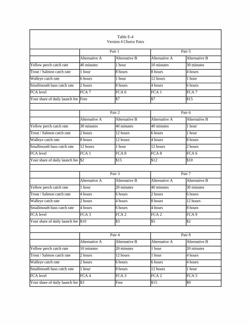
Table E-4Version 4 Choice Pairs
Pair 1 Pair 5
Alternative A Alternative B Alternative A Alternative B
Yellow perch catch rate 40 minutes 1 hour 10 minutes 30 minutes
Trout / Salmon catch rate 1 hour 8 hours 8 hours 4 hours
Walleye catch rate 6 hours 1 hour 12 hours 1 hour
Smallmouth bass catch rate 2 hours 8 hours 4 hours 6 hours
FCA level FCA 7 FCA 6 FCA 1 FCA 7
Your share of daily launch fee Free $7 $7 $15
Pair 2 Pair 6
Alternative A Alternative B Alternative A Alternative B
Yellow perch catch rate 30 minutes 40 minutes 40 minutes 1 hour
Trout / Salmon catch rate 2 hours 12 hours 6 hours 1 hour
Walleye catch rate 8 hours 12 hours 4 hours 8 hours
Smallmouth bass catch rate 12 hours 1 hour 12 hours 2 hours
FCA level FCA 1 FCA 8 FCA 8 FCA 6
Your share of daily launch fee $2 $15 $12 $10
Pair 3 Pair 7
Alternative A Alternative B Alternative A Alternative B
Yellow perch catch rate 1 hour 20 minutes 40 minutes 30 minutes
Trout / Salmon catch rate 4 hours 6 hours 2 hours 6 hours
Walleye catch rate 2 hours 4 hours 8 hours 12 hours
Smallmouth bass catch rate 4 hours 6 hours 4 hours 8 hours
FCA level FCA 3 FCA 2 FCA 2 FCA 9
Your share of daily launch fee $10 $3 $5 $2
Pair 4 Pair 8
Alternative A Alternative B Alternative A Alternative B
Yellow perch catch rate 10 minutes 20 minutes 1 hour 20 minutes
Trout / Salmon catch rate 2 hours 12 hours 1 hour 4 hours
Walleye catch rate 2 hours 6 hours 6 hours 4 hours
Smallmouth bass catch rate 1 hour 8 hours 12 hours 1 hour
FCA level FCA 4 FCA 3 FCA 2 FCA 5
Your share of daily launch fee $3 Free $15 $9

Table E-5Version 5 Choice Pairs
Pair 1 Pair 5
Alternative A Alternative B Alternative A Alternative B
Yellow perch catch rate 20 minutes 10 minutes 10 minutes 20 minutes
Trout / Salmon catch rate 8 hours 12 hours 2 hours 4 hours
Walleye catch rate 1 hour 2 hours 12 hours 2 hours
Smallmouth bass catch rate 2 hours 6 hours 2 hours 12 hours
FCA level FCA 1 FCA 9 FCA 8 FCA 2
Your share of daily launch fee $12 Free $10 $2
Pair 2 Pair 6
Alternative A Alternative B Alternative A Alternative B
Yellow perch catch rate 40 minutes 10 minutes 1 hour 10 minutes
Trout / Salmon catch rate 2 hours 4 hours 8 hours 12 hours
Walleye catch rate 4 hours 8 hours 8 hours 4 hours
Smallmouth bass catch rate 6 hours 12 hours 1 hour 4 hours
FCA level FCA 7 FCA 3 FCA 4 FCA 6
Your share of daily launch fee $7 $2 Free $9
Pair 3 Pair 7
Alternative A Alternative B Alternative A Alternative B
Yellow perch catch rate 1 hour 30 minutes 30 minutes 1 hour
Trout / Salmon catch rate 6 hours 12 hours 6 hours 1 hour
Walleye catch rate 1 hour 6 hours 1 hour 6 hours
Smallmouth bass catch rate 4 hours 1 hour 8 hours 6 hours
FCA level FCA 5 FCA 8 FCA 3 FCA 1
Your share of daily launch fee $3 $10 $15 $5
Pair 4 Pair 8
Alternative A Alternative B Alternative A Alternative B
Yellow perch catch rate 30 minutes 40 minutes 20 minutes 40 minutes
Trout / Salmon catch rate 8 hours 1 hour 1 hour 12 hours
Walleye catch rate 2 hours 12 hours 8 hours 6 hours
Smallmouth bass catch rate 2 hours 8 hours 4 hours 2 hours
FCA level FCA 6 FCA 4 FCA 7 FCA 5
Your share of daily launch fee $5 $9 $3 $7

Table E-6Version 6 Choice Pairs
Pair 1 Pair 5
Alternative A Alternative B Alternative A Alternative B
Yellow perch catch rate 1 hour 30 minutes 30 minutes 40 minutes
Trout / Salmon catch rate 4 hours 2 hours 1 hour 6 hours
Walleye catch rate 4 hours 1 hour 1 hour 6 hours
Smallmouth bass catch rate 1 hour 12 hours 1 hour 4 hours
FCA level FCA 9 FCA 6 FCA 2 FCA 4
Your share of daily launch fee $12 Free $7 $3
Pair 2 Pair 6
Alternative A Alternative B Alternative A Alternative B
Yellow perch catch rate 10 minutes 20 minutes 10 minutes 40 minutes
Trout / Salmon catch rate 6 hours 8 hours 8 hours 4 hours
Walleye catch rate 12 hours 2 hours 6 hours 1 hour
Smallmouth bass catch rate 6 hours 8 hours 8 hours 2 hours
FCA level FCA 7 FCA 9 FCA 2 FCA 9
Your share of daily launch fee $12 $10 $3 $5
Pair 3 Pair 7
Alternative A Alternative B Alternative A Alternative B
Yellow perch catch rate 40 minutes 10 minutes 30 minutes 1 hour
Trout / Salmon catch rate 8 hours 4 hours 1 hour 12 hours
Walleye catch rate 4 hours 8 hours 8 hours 2 hours
Smallmouth bass catch rate 6 hours 8 hours 4 hours 12 hours
FCA level FCA 3 FCA 5 FCA 8 FCA 7
Your share of daily launch fee $2 $15 $12 $7
Pair 4 Pair 8
Alternative A Alternative B Alternative A Alternative B
Yellow perch catch rate 20 minutes 1 hour 30 minutes 20 minutes
Trout / Salmon catch rate 12 hours 2 hours 6 hours 2 hours
Walleye catch rate 12 hours 2 hours 4 hours 12 hours
Smallmouth bass catch rate 12 hours 2 hours 6 hours 1 hour
FCA level FCA 1 FCA 8 FCA 6 FCA 3
Your share of daily launch fee $5 $9 $10 $15

Table E-7Version 7 Choice Pairs
Pair 1 Pair 5
Alternative A Alternative B Alternative A Alternative B
Yellow perch catch rate 1 hour 40 minutes 1 hour 40 minutes
Trout / Salmon catch rate 12 hours 6 hours 2 hours 6 hours
Walleye catch rate 1 hour 8 hours 4 hours 2 hours
Smallmouth bass catch rate 6 hours 8 hours 8 hours 1 hour
FCA level FCA 4 FCA 1 FCA 2 FCA 1
Your share of daily launch fee $2 $9 $5 Free
Pair 2 Pair 6
Alternative A Alternative B Alternative A Alternative B
Yellow perch catch rate 10 minutes 20 minutes 30 minutes 1 hour
Trout / Salmon catch rate 1 hour 4 hours 4 hours 8 hours
Walleye catch rate 6 hours 12 hours 6 hours 8 hours
Smallmouth bass catch rate 1 hour 2 hours 6 hours 4 hours
FCA level FCA 6 FCA 5 FCA 8 FCA 9
Your share of daily launch fee $2 Free $7 $12
Pair 3 Pair 7
Alternative A Alternative B Alternative A Alternative B
Yellow perch catch rate 20 minutes 10 minutes 20 minutes 10 minutes
Trout / Salmon catch rate 8 hours 2 hours 12 hours 1 hour
Walleye catch rate 4 hours 2 hours 2 hours 4 hours
Smallmouth bass catch rate 12 hours 4 hours 8 hours 2 hours
FCA level FCA 7 FCA 4 FCA 6 FCA 1
Your share of daily launch fee $9 $15 $3 $7
Pair 4 Pair 8
Alternative A Alternative B Alternative A Alternative B
Yellow perch catch rate 30 minutes 40 minutes 40 minutes 30 minutes
Trout / Salmon catch rate 12 hours 1 hour 8 hours 2 hours
Walleye catch rate 12 hours 1 hour 12 hours 6 hours
Smallmouth bass catch rate 2 hours 12 hours 6 hours 12 hours
FCA level FCA 3 FCA 5 FCA 2 FCA 4
Your share of daily launch fee $3 $10 $15 $12

Table E-8Version 8 Choice Pairs
Pair 1 Pair 5
Alternative A Alternative B Alternative A Alternative B
Yellow perch catch rate 1 hour 10 minutes 20 minutes 30 minutes
Trout / Salmon catch rate 4 hours 6 hours 6 hours 8 hours
Walleye catch rate 8 hours 1 hour 8 hours 12 hours
Smallmouth bass catch rate 1 hour 4 hours 2 hours 4 hours
FCA level FCA 7 FCA 8 FCA 2 FCA 5
Your share of daily launch fee $5 $9 $15 $5
Pair 2 Pair 6
Alternative A Alternative B Alternative A Alternative B
Yellow perch catch rate 20 minutes 30 minutes 1 hour 40 minutes
Trout / Salmon catch rate 2 hours 1 hour 4 hours 2 hours
Walleye catch rate 8 hours 4 hours 1 hour 6 hours
Smallmouth bass catch rate 6 hours 4 hours 12 hours 6 hours
FCA level FCA 5 FCA 9 FCA 1 FCA 9
Your share of daily launch fee $10 Free $3 $9
Pair 3 Pair 7
Alternative A Alternative B Alternative A Alternative B
Yellow perch catch rate 10 minutes 1 hour 20 minutes 10 minutes
Trout / Salmon catch rate 4 hours 6 hours 1 hour 12 hours
Walleye catch rate 12 hours 6 hours 2 hours 4 hours
Smallmouth bass catch rate 8 hours 2 hours 1 hour 8 hours
FCA level FCA 4 FCA 3 FCA 8 FCA 7
Your share of daily launch fee $7 $2 Free $10
Pair 4 Pair 8
Alternative A Alternative B Alternative A Alternative B
Yellow perch catch rate 40 minutes 20 minutes 40 minutes 10 minutes
Trout / Salmon catch rate 12 hours 8 hours 12 hours 6 hours
Walleye catch rate 2 hours 1 hour 12 hours 8 hours
Smallmouth bass catch rate 12 hours 1 hour 4 hours 12 hours
FCA level FCA 3 FCA 6 FCA 2 FCA 9
Your share of daily launch fee $12 $2 $2 $7

Table E-9Version 9 Choice Pairs
Pair 1 Pair 5
Alternative A Alternative B Alternative A Alternative B
Yellow perch catch rate 1 hour 30 minutes 30 minutes 10 minutes
Trout / Salmon catch rate 1 hour 8 hours 6 hours 12 hours
Walleye catch rate 2 hours 4 hours 12 hours 2 hours
Smallmouth bass catch rate 6 hours 1 hour 12 hours 6 hours
FCA level FCA 3 FCA 4 FCA 2 FCA 9
Your share of daily launch fee $9 $15 $9 $5
Pair 2 Pair 6
Alternative A Alternative B Alternative A Alternative B
Yellow perch catch rate 20 minutes 40 minutes 20 minutes 1 hour
Trout / Salmon catch rate 4 hours 2 hours 12 hours 2 hours
Walleye catch rate 6 hours 1 hour 1 hour 4 hours
Smallmouth bass catch rate 2 hours 8 hours 6 hours 1 hour
FCA level FCA 6 FCA 8 FCA 4 FCA 5
Your share of daily launch fee $12 $5 $12 $7
Pair 3 Pair 7
Alternative A Alternative B Alternative A Alternative B
Yellow perch catch rate 30 minutes 1 hour 40 minutes 30 minutes
Trout / Salmon catch rate 2 hours 8 hours 8 hours 4 hours
Walleye catch rate 8 hours 6 hours 2 hours 8 hours
Smallmouth bass catch rate 2 hours 8 hours 2 hours 8 hours
FCA level FCA 7 FCA 5 FCA 7 FCA 8
Your share of daily launch fee $3 Free $10 $2
Pair 4 Pair 8
Alternative A Alternative B Alternative A Alternative B
Yellow perch catch rate 10 minutes 40 minutes 1 hour 20 minutes
Trout / Salmon catch rate 1 hour 4 hours 6 hours 1 hour
Walleye catch rate 1 hour 4 hours 12 hours 6 hours
Smallmouth bass catch rate 1 hour 4 hours 4 hours 12 hours
FCA level FCA 1 FCA 6 FCA 3 FCA 1
Your share of daily launch fee $10 Free $3 $15

Table E-10Version 10 Choice Pairs
Pair 1 Pair 5
Alternative A Alternative B Alternative A Alternative B
Yellow perch catch rate 20 minutes 10 minutes 30 minutes 1 hour
Trout / Salmon catch rate 6 hours 2 hours 2 hours 12 hours
Walleye catch rate 2 hours 1 hour 12 hours 1 hour
Smallmouth bass catch rate 8 hours 2 hours 6 hours 2 hours
FCA level FCA 9 FCA 2 FCA 6 FCA 9
Your share of daily launch fee $7 Free $12 $15
Pair 2 Pair 6
Alternative A Alternative B Alternative A Alternative B
Yellow perch catch rate 30 minutes 40 minutes 20 minutes 1 hour
Trout / Salmon catch rate 12 hours 8 hours 4 hours 6 hours
Walleye catch rate 6 hours 8 hours 6 hours 4 hours
Smallmouth bass catch rate 1 hour 6 hours 1 hour 8 hours
FCA level FCA 7 FCA 1 FCA 2 FCA 1
Your share of daily launch fee $9 $3 $3 $12
Pair 3 Pair 7
Alternative A Alternative B Alternative A Alternative B
Yellow perch catch rate 10 minutes 1 hour 30 minutes 20 minutes
Trout / Salmon catch rate 4 hours 1 hour 4 hours 12 hours
Walleye catch rate 4 hours 12 hours 2 hours 8 hours
Smallmouth bass catch rate 12 hours 4 hours 2 hours 4 hours
FCA level FCA 3 FCA 8 FCA 4 FCA 3
Your share of daily launch fee $5 $15 $2 $10
Pair 4 Pair 8
Alternative A Alternative B Alternative A Alternative B
Yellow perch catch rate 10 minutes 40 minutes 40 minutes 10 minutes
Trout / Salmon catch rate 8 hours 1 hour 6 hours 8 hours
Walleye catch rate 2 hours 8 hours 12 hours 1 hour
Smallmouth bass catch rate 4 hours 12 hours 1 hour 12 hours
FCA level FCA 5 FCA 4 FCA 7 FCA 5
Your share of daily launch fee $2 $10 $5 $9

;;: H ! H w~ FIP' J"p, ~'f" 0 ~ :E ~~ I!~ oo~!i ~ 4: s'l!~!:i" ~ . .§. 3:1, H " ... ~' =,,' J!!! !nl" ', . "It • d • • ,,' ',-" !'oH " ,~ , ! , . :I , j'" "" ~i;;t ~ ~_! !,.i -~~ "' - ::, ~f ~ ~f Q,I i " 5~ .2.;'~ '<~!I'"~11 i, !I!-5 ~ ~f, ~ ~. j ca , • ~I 1;; IU'! it: l~ ~ [.! [Ill ~ , , . 1 ~,. I'll' 1'-'" a'". .' ;r ~ ;pl~ ,il:::' ~ ' g'a.Il:'l : ~,g,~ ;> ~ ~!t~i ~ l to
I.;; ~ ~ ".. ;1". ~",;r5n .s~oal! 8--!:f- : J til i 1f ~:i 4~Etl ;;· !?"n. 3~ !. §:f 1 :: J . t ~~'< ~.' U ::s i. i!~i· ~:' ~s gl: '< .. ~ e, l!.!l. !" fl!. ·· 1I e: . .!i:! Ii" l!. !! If l ';!,
I ' "', ;·'lh • <. ,$1 lIlt [ ,~ii;2.a h","iii l· !f~:~~! ~I' • _ ~f t. "'alP' "'5-~ ~g f ~
II [ f j! i 11:'J !,il .~ .,d
~ 3 §~~ ~~ ~i ~g~ s~ ~ t" .. ;r Ii ". n ; l': !,~ .. f~.';;~;'o;: [~ , Ii: • II ~g 0: !i6- ,,",;;": i
1 . • ~<' , ,~.I h , d! '" I ' " 0 t ,,! !l '" , '1
[ ! ~ll ~~i' l!' iij~li ~~~ a' -I ,,'i ld;:! IL~,l ~!.l< • ! i"' "'1' I .. ··' .~ I . • !. • nf lo~.'-l. ,~!~" r"l'l i I. , _ ,,_ ,-g, to"' '" , "' l ; ' ~ s' lO "" fif~~ ~t-(;, q .n "~ , ~ ~ · H ~. ~ . ! H " ' !! !! ,
2, ;;'~ ~ Ii ~ ,:: ~ . . Ii ~ ,

" feoo ., • ..., __ .., .• ...,.nod. _<) ...... ,,,- c,' . >4_ r ........................ Go-So, lI' ........ _t "~.d .... ..........t ... _ .'Y ..... -= '1., ..... __ , .. " " .... ..,. . I · .... ___ ... __ lIrc.m;I' ............ ,.,._ .. _ ..... dIoopU.' .... o/'I"E .... __ 0, "'._ ..... ,., ... , <;_&, .. ' ...... "'_ .... , .~;I1 .... _ .. _ ...... ~""""'h >- boo< ...... _ .. l0<100i,,, pon;.;poO< in'" "od)'
Thoo/. ,.,. (0< _ ""I'
_ R ... t-, I lq le, B.a", S"",<>" M .......
01. ' 'or B.;Uy M • .: .. ",", WI $)1' ·05!

~ Hagler Bai lly _ .... <---... ;".~- .... '" k-. "'''' ~ " ',_m1\, ...
In,"" rov<'f kUcr 10 ........ "" ..... 1 K<:ond ph ....
1NnIc )'<>U for Ialti"i 10 lIS 1M< ltsI ynr .bout )1>'1' fiy,i"i "<pori...,,, •. Yow conuromt< h<lped .. ",.delL "'>II ..... _ofr. ...... lhoto<cu<>"" ............. orQ..,." Bay. A. ponofthis "Wy ....... omdiDj; "'" • >bon ..... 2 ourwy ..... "ill h<lp ..... :dc. I'nl how -'= foxl .bouI dofTcrml ~ opt __ "'"' ooukI olkct fl>hinc "" tho ,,_ ofGlt'a> Boy.
\\'. "'" bopin& IkM J'<IU un !Ole the lime 10 (,11 "'" this ""-q". you .... pon of ........ Igtoop of ""aI ...... 1'10 11»" bo:aJ o<;mifo<ally .. I<cIN 10 pooti<if'U< in (~i • .......,.. R<,.rn~ of .. h<u..r )'0\1 flsl>«l ,he " .. t .... ofG .... " Bay oflen or only one< in 1995. il i, jmpo<lAlllln.( "'" be.v your "!'inion,. Yoot "''''¢IS will tcpreS<n! ,he "~ of",""y "' .. , .. III .... oimi lor 20 youn><lf and w ill allow cnn,i<l<,atioh of )'<>Or "",inion. in d.ddin& whioh 0,.." I)"y m"""icmc.t <>plio,," 10
pur ... ,
II ~ imponam ..... this survey ... (,11«1 OW by roo. Th< :RrVey""''''''' _It_ )0 mi"",co,o oompl<l< .............. _ ......... im<S k». AnsworJ 10 this "",,'01 ... ..... r.d!LJtiaI; y<Mr nom< will _ ... be ............ Informal;"" from !he ...... -ey will ""Iy'" ,".101"" in mtisIicaIkrms. ~ I .... idenlifalion nwnbef on the _k of ..... """"Y ,., ..... Ilqlor o..illy, the: flml hira! to"""'"" .... """C)'. """ ",",bine: "'" Inf ....... ;"., f""" )'OUr mail .... ..,. .. ilh ..... infonnotion )1>U JII"Wld<d "'-er ..... 1<1q>/>on<.
A """mary of ..... ", .. I", of !hi . """1 will be mod, "".iJ.t>k t" a""""",,,,n, on<l ir.du,1ry "fW'"CTU"'w" , If you W<lu ld l i~ •• """"'Ar)' of ,he ""ul", .impl ~ I"'" yOIIf nam., odd", .. , or.d '<Oi'y of""uJ", T<q""'tcd' on !h< *" "f,he "'urn .n,.<lOp<, W. '"r«' to 110" ... ,.IIS in <l>o: 'l'riT\i of 1999,
If you ho~ 01>' qU<Slions'- tholludy, ........... Id lik '" _ '""" you. YOll ...... Il In<
(0110<1 .. G.6CI-212_2&oo. Thant you,
Sin«tdy,
p.., Rathbun 11'111<, EJ.aj lIy Survt)' M"""I]t,

~ Hagler Bailly - .... ~""-'J"'"~_''''' .""_.,,, ... M",,,,,, w""""", " "'_, ...
, .. _n,·_ .~,_m_
K _ _ " _ . ....... --.
A ftw "...,tJ 010 ... ., sene ~ ... . """~. uk;"I abou1 ) ...... r.shinl ...... ie",",,- W. "'" pa...... many.,.1<1$ ha\ .. .............:t Ihri • ......-.y. buI "" ";11 _Id 1;h 10 boar from y<>Il. If you l'O<CfI~y mailed our """'Y _ II> .... pIcaoc ocupI our -. ond dilftjUd !hi.lmer.
w~ reali. this i •• bu>y tim< of"" )_ rOf many propI<, and " .. 1V<001y opp«<iMc: y .... lOkin& tho lime '" boEp In out. Si,..,. " .. _ only obi< to 'WY<), ....... 1 """,ber of "'&las. )'_ relJ<>n>< i, v<ry imporum R<g>rd l ... of whe<h<T )'OU ""'. FIshed ,be .'''Of' ofOreen Boy on,. 0< only 01\«. it i. Importalll lila. "" .... YOY' Qvinion" Yow onJ"',,, "'ill ftp.< .. n,''''',i,,,, of many 0Ih<T on.:lers ,imiilll 10 YOIllSClf and .. ill oilow ooo,id<",uon of your opiniQn, in deddinll whi,h G-. iJay maRai\<mcn, "",,>om 10 P""'"
In Ihe rvem ..... )'OUf SIrVey "'" bet. misplo<<4. a ~ su:wy ond • JIOI'u3" s:Wd ... If· oddras<d "'"dov< "'" _Ioscd for )'0lIl toO,~.
" ..... mary of"'" , .... 11. oftbi. _ ...ty .. ;U b< """" ovoilobk 10 CO ............. and industry ",'_'ilMi,'CO. If you .....wI like. """"'"'l' of .... results, 'implY P'" )'OUt _. odd ...... ond " CCIp)' of ~I''''«i~- on !he boook or!be ",Iurn <IIvclo!><- We expect \0 ba,u<",IU in the
'l'rilli ofl999.
1r1M .. i ... y\~,"~ " " ' OIl do '0 II<lp you romplelO thi. ' """'y. pl .... retl f_ .0 <all "" ""Ii«' .. (..6Ot·2J2·2SOO.
s:,,,,, .. ty.
Po,. Rathbu. Il-.:I., lIailly Su,vey MonoS<r
... , 1'''· .. <=·· ....... " "' ,'~

~ Hagler Bailly ... "" .. "" , ............ 'nc ........ "" ........ . Mk
." kio«< "'"" M •• """ VI<,,,,,,,,,, "'''_''''
1999 foll",,'. up moil 'UI".Y eo,'<[ 10<1"
T,t-._ m .'"", . "" OOO) '''·z"",
II rew w«ks .~o. we sen' yOll • surve), »king .bout )'0"' fi.hifli: expenC[lCe" We arc plcosed tho< m.ny ""~i<,,, hov. returned thei, ''''''<y, but " ... s,;u ,,<>old " ke 10 bear from you. If )'OU l'<'C<"tly m.ile<l "'" '""'OY back to U', pie"", oe<ept oor thank, and d; .... ~.,.. (h;, 1<1I"r,
W. g .... Uy ' pPT<m'e your takiJli !he time 10 help US QU' Since ""'. "~r< 'm l)' obi< to '",,'0)' •
"".11 "umber of 00&1.", your ""pons< ,. "ery important Roganll< ... of" h<!her )'OU h.ve fi,he" the ",.t<", of Gre<:" Boy often or only once, it i. importaftt that w ... at wyr opinion,_ You, .."."', ,.. "ill ,..,,"''''", ,he v'""~ of many Olhcf ..,glen . imilar to youtS<lf and ",ill allow ooMid,,,,,i,,,, of yO"' 0»;" '""' '" d«\d,"~ which Grecn Bay ffi3II'g, men, optio", '" put$ ...
In !he .... ,nt Hut )'our ,uNe), ... b<:en m,sploced, 0 rcpJoccmmt .urver ."d • po.tAge p.ald. ,,'f_ odd"" .. d <n""'ope .... <n<losed for yO"' <on"<n;<n«,
A ,ummary of tbe ,uul" of!h;, SlCldy " 'ill be made: ""Ioble to ~o"<mrn<nt and iOOu<lry rcp",,,,ntat;vcs. If you wo"ld I;k. a SUmm"'Y "fttre ",,"Its. SImply put your 1l3Il1<, add ... n, and "copy of""ul" uque<1ed" OIl tho ba<ok "fthe rctum en,dope. We cxp«t to h.>,'e re.ult, ;" the 'PIlnKof l 999.
Ifl~ " In),thilli "'< CM do to h<lp )'OU rompl'" t~ , . '""'0)', ple= kel me to coli me coll<", otI-6(l8-22·2S00,
Slfl<<rdy,
Pom Rathbun Hilil<r Bailly Survey Manager

~ Hagler Bailly """'"' ' .;0, """"" ......... """""'" ...... '" "" ." """', "''''' .......... ""~- ""..,""
S<eon<' follow,up mol l . ur"ey ",ver 1,.,«,
m ,600, ",.,,,,, , ,,- 1""'1 ",.,.,..
llm sorry to l>o1her )"00 . s.in_ bur " " jmwilll"l1" bel[ from VO\l, Good dcci>loflHbmrt m.n.o¥' n~ GT<cn Boy OO/l .mix be m.d< if ,,-e know ,""w peOple hke ) '0" "ill be . ffwoo. I w.s .ble 10 '""'0)' only . S/ruIll number of >rIgl.". llIi. me.." 11>;" )"<>Ur ""pon"', WIll represent no< only you bu, . Iso 1he "'<"~ of mher OIl,i." like Y""_ It .100 ",e,", 'hat to K<' , iood UM.,..tan~;"~ ofth< TO" \:< of QP'moos .boot the ;"''''. I must hear [",m M ml ny Wpk " oo"ibk
R<~dk" of whether roo ",,"e fished til<: ... ,t,,, of G,c<n Blly ofl<n or onl)' 00«, il i, lmpor1OJl' tho, "'~ hear your "1';0;"",. You can be .. , or«Ilhat your r«po""" 10 this '"""'Y w;1I be kopO ",nroocntia!, our name will "'''',r be ",,,aIO<l '" ""YOIl<. Infol1ll.llt;on [rom tbe surrey ""II be repOT1ro only," ,to,ini,,1 torm • . 1'h< id<"M,c;ohOn nwnbor On til< back o[!be •• rye)' i. US«! O"l y (Of ,,..,kill\: P1lIJ'O""" so Vi. ' OIl ",'oid te-<;<)""",ti" ¥ lho", peOple woo "" 'e . lre3dy oomplo<O<Ithe ' "TV'Y,
B« .... yoor "" pOn", " SO impOrt""' , I om etlC lo,;ng .""the, ooPY of the ,u""y on<l • pO'tage. paid, .. If...od,=<I "",dope fOT your oonv<n ;,nc., If for """'. r<:awn )'0" Oln't compicte the ,urv'y, ploase ",rile m,' note on your surv'Y booJ"" aM r<:t um it IVhen )'<>II h,we completed ,he ' UT\" y, 'imply '''urn i, in the po>tage.p.oid .nvel.",.,
If you ""'" any q<><S1Io", .boo! till, study. we "''OIl ld Ilk. to he..- f""" you, Pic"'" feol free to coil m. 0011«' a, 0·608·232.2800,
nank YbU fo r )'0"' holp !
Sincerely.
Pam Rothbun Hafler B .. II)' SUr>''Y Managor

:gj Hagler Bailly ......... ~ .... - -................ __ w ........ ''''M".
Spcci>lllunl lollo.o."" ",..;) "' ...... r <;<Wrl Ion<,
''''- '''-r." _ m·,.,.
1ft Dtnmbtr ........ you. ~ bookie< oskinc _ yow opiniono on rlshi,. Ibc .. ..- of 0...... Boy. w. reaI;.,.!hot .... hoi'''"' ," 2 'r IOU. busy limo of~ ond yo..- SpOre tim< IIIiahl ha,.. boca limito:L Now!hal "'" holidays on: <>V<T, .... ore hoopirIc thai you "., .. ill h<lp .. -As I mentioned \><1_. 1 ...... bl< to ........ y only. SIIUlI n"mbtr of .. 11.' .. 0 it i. "et)'
impottant lila! J hear from .lIlh<: ""ill ... !hat I mailed. , ....... y to. Good dc<isions.born OW\aiini G .... " Bay 0"" W be made if",. k""w how people l i~. )'OIl wil l be .ff<ctod
R< ... dl ... of .. 'h<tl>ot )'0" ha ... r,Wd !he _ .... "far.." U.y oft .. Of OIIly onco, it i . impo<\l<l1 that "-' Out)'O'" opi ......... Vour .. """"'. will be ,.,... 10 repreoml .... rcsponseI of 0lher..,.Jtrs who ... <irni12r lO)'OUr y"", COlI be ......... thai yow .... ,~ I " to Ibis 0WV<y will be I:cpc confodmtW; your ....... will _ be 1<¥,,1ed to anyone. lnfonnation from !he: ...",q .... 11 be ...... t<donly;" .. ..;" ... , ........
!)cc .... your rnponso is.., imponan~ I om <n<losini -.. oopy or .... _ ond . JlO5lai<paid., ..,'f-addrased <m,<1ope r..- your OO''''a>icnce. If for lOIn< re&SOII you can', ""m.,lele the: """,oy. pkq< .. rit< me, oote on your ~ bookie! and ""urn it. When yoo llave completed .... ' ''''''y. , imply return it in .... p<l11lie-l"'id ., ... do"".
lf1"" ""'''''Y qlXOl""" .bout lIIi ... ..:Iy ..... would lik. to h<u from you. I'~ ... recl 1m: to call .... coil .. , .. G-608·232·21OO.
Porn Rolh ...... lllikr Blilly Sur·iCY Monas"
0''': 1 • • C4' ..... _~c-
" - ~ HPF~ F ~ JI':' : C'I-"'1l'°i .. ,. if ::8["';; >
'" ~g ~'!!"1~ i :5 hi~ :;; ~ .. ~a.E- <"l
'1'1 iffft ~fl ~ ~'I~ti ~ II g ~r~.· c f[f ~ f"- ~ :i'. '" ~ ~ ".,. ~ '"
;'~i ".~~_ ~'_'" ~i!._~ !Ie. [l ~ <& 5,5 ~ ~ ~l!i!'i 0
o~~ ~ <n "g j! - ~'" "g1;'" .. <':
< i a~'~illi~ ~ 1~-!rrl:1 e.J ~ j~li ~~;!~ i '"
i I. _ .• o or ~ _, 0
ri'l; S-$ O~g-'"
''''ft 9 - ,t,h ~ ° Ip · ~ " '< s- E
T ! -, --a~~§~ '"
If. I "~I h ~ ~f ;;HI F ~'" 1",,1 q ~f~ . ~ ~·~t !9 . wPi~ Cl"':':! :;;; ..
'r' 'i!li";!i'l :j21.Jli iJ !~:~: i _n-~2,i' 1;; € ;t
1 ~. ~ § Ir~" - -o ~",,,,
:O:i~r~l~ ~,<if''i,,;o· f '°5- &~~~ ..., .. ~;r~a ':Jl J~" ,.
HlH f,JI.CI i~l !llr ~I :!!= 9'd~~a 6H ~ _ g .... ~ e- ;ll ; '" rJ!l 0 '0'11' ,'0' f~-' ~~ ~ .~,,>
1'"_ " .... ", .$! ",-;, -",, '"
~~In " ,~ r -pt-· , ,;1-
f:g~P ;!!:!'
a!!. ,h,,... ]!: ~ a ~I ;! ~;f,:~~. ::i~"'~ _'g .. ... !!:! 8.~~~>~ !~;;'
. ,Ii ~II~i~1 !'~!111[ ~. ilil ;~ -''' !l -n ,-liS ".. ~i!' 1 ~,,! i! 1'] -'l" :i '"
h~Hi' [1;,111 , 'lit !I __ $~;;C ,..-..,
.J-oiI -< ~ fl t ' - . ,
!l.fi:.: ~1'I:1 ~
'1' • '" fl" n 4' -! t r· j,
i'_ --a f < •
~ ,;iii "i'h:! j [~[ . _.
, -0 itS",.·"
rip - . . ~
~""~ ..... ,,,
"Ii !'" ,It I" .t~ g: ~ -. ~
s'f""d s·
rf,i II tt' !I "1 i ~I. .. .. ~ " 'OO
" " t'l j" , ~11'·~r i.~1t I IiI ~n .. ~;~ --
,d· .-«~ ~ fl. _ ~ f,,!;i ~~-
• • - • .

J. Cock, fo[ Refurn! QUql iQn..itc!rul m !be ,",,'oy t'" .. , rdused .." U)ded with :>n 'r' PI"", probe ' hcse que"ioo, at Ie,,, Onco by ,elh"i 'll< ",spande"' how impart.." ,he queS!ion i, and r<mindilli: them !h .. tl;e" ""pan .. , w111 toe kep' strictly confiden,i.l, All 1Oform. "on 'hey p""'ido ,.,-ill be "o",bin<d "'i'h the "span"" of othcr hou«oold" and tbeir name ,.,-,11 "'" be "'''''' ''1':<1 ,,'i'~ ,n. final d.",.
4, Cocks for Doo " Koo"'_l<o", , io ,n. "''''0)' 'hat 'he ""pa""""' doc. oot know nmllO be coded os • 'd'. 1'1 " .. probe !he .. que<1;OO, at leo", oncc to fL!ld OU! if 'll< ""paooon' ".Ily doc, oot know or jU<1 n«d, to thlllk .oou, 'ho 'n,,,'er.
'Othu·SPECIfY·· A, qoc<1ion 10, 1 L 19, ond 20 tll< respon", codo' .re "0' exMU";V,. lit lhc", que"',o", therc oro code. de,il:n",ed os ·Otbcr-SPECIFY' If> ",ponde"' ~;Y<' • 10'PO= oot cO"er<d by the pre-<;ooed re.pon"". ,he i"te"'i.",,,[ .oould enter tbe 'other' cooo ond 'yp: ou, ,b<: re'po"de"'s ven,a,im ""pan«
PROC[DURES
We ore colhn~ hOllschold. in 'h" "u<\y ro ,b<: .. l l in~ OO"tS for thi, project will be Mond.), 'hrough Frid.y, 4:00 p.m. un,,19:00 p.m, S.,urd.y.nd Sunday. 12 Noon wttil5:00 p.rn Each intmiH:"'Cr shoold work" 1<." one " ... ker'ld 'hift. I""'h in",..,ie,.,.,,, .oould oomplcto '110 .. 1 2 >c=nlO~ '""'ey' P:' oou,. An."~rio~ m""hi .. mes<as<s ",ill be re.>d vuW,im os ,b<:y ._or on ,be oompu'er "'_0.
If the ",pooo.n, ... ..,y que<1i"", .bout the ,un'''Y ' hcy m.y ,peal: with Pam Rathbun. Sir>« Pam g.".rally ,,"'ill ""t be a' the otT"", durin~ oollmg hours. you should II)' to ""h<d"i< • tim<: with !be ,ospo"",,"" fot Pom to call lh<m bac~ (fill 00' a sheet with tit< ,",'ure oftbe qu<"ion and lhe be" "one '0 ,ail ba<k io 'll< ",,"'bo<:>~ pro"ici<ci).
RESULTS
Tho primary use of ,b<: d ... from tb<: ,hi, s<LKly "ill be to ,.,imate <tati"i,,1 model, explalOlOg ho", IIJli:lo" ""por'ld '0' "ide ,""ge or po .. ibl, ~,"i o~ ooocii"on,.
QUFAQION·BY·QUESTIOIoi I NSTRUCnOIoiS
I· 4 1n thi, «<,ion wc fmd 00' if tb<: ",'porxknt h .. h«n io. r .. ~i"i ';"0< 'll< beii"nilli: of ,be yeM (Jonu")' I. 1998). If ,b<: ""pondent h<IS h«n icc f"~mK ,,~ (,r'Id 0"' On bow many da)" tbe Ic<pondon" icc f"bed and who", ,It< ""ponden' ioo jished, For thi' ,u,,'''Y w, "'" part LCulorl)" ;nt="ed '" fishing ",'iv"y on tho "w.te" ofGn:en 3>y". Whe" we sa)' lh< w."" of Green 3>)' ,,~ lOch"je the bay of Gn:cn B.y, SIUIK""n Hay. iiII!l ,he MV<f! ond stle<tm' tha, feed mOO G'e<n B.y "p to tbeir fiut dam. We ba,'o i""ILKled a m.p for )'ou 10 «e ",flat we n":>n by tho ",.'oro of Green B.y, TIt;, i, • <t", ,,1 def,n i, ion ond you mu<1 mak< sure ,h.t you read lhc d<finit\Qn "<Tbatim in Q2. Note that tbe Fox R;ver be,ween G[e<n Bay and the dam " DePo", i, • ,"1>-1<, of tbe wat"" ofGmn Uw We "p<ct only a "".11 proponion oftbe ,orgel anglers will ~n aoi"~ i« ("hiog.

1 • 8 In Ih; .. «'ioo "'. f,od "'" if ,I!<: ,"pOndon' OM bo:cn Ii.hing in 'h, opm ,.. .. ". (oot ic< fishing) . ioco lh< begiooing of ,1'1< yeo, (I""Ullry I. 1998), Ifthe "'p<>n<.ien' .os been fishing (no' ice fi.hing) we find 00' on 1>ow many do)" 'he "")'I<>QJen" fished and ",her<: <lie I<spond<n' fished. For ,hi. ,urvey w, or< l"";'ul., ly int.",,,,,,, in [,sh1OK ><'ivi'y on the "v.~«" of Gl<cn B.y" When we ... y ,he wate,.. ofO",eo B.y ,,~ lIIdu<.!<: <lie My ofGr«n B,)". S'urgOOll B,y. AIlII ,he ,h'e ... and ,",,,.,m ,iu, feed in,o G""," B.y "p '0 ,hei, [,"" d"", Wc h,w ioch"kd • map for )'OU '0 .. 0 ",iut we "'"." b)' the "',, .... of G,oen Boy, Th" i • • ,ri,i",,1 defini'ion and yoo must nwe '"I< thol yw ",0<1 II>c: ""fin;I;':" "<rballm 10 06, Nole that <lie Fox Rive, hel"'ccn Grecn nay and tl'l< dam ., DePer. ;, • ,"i>-kt of lh< ""« ... of Green Boy
Ifth<: re'ponde nl "" fi,hed II>< "".te" ofGm:. Ilay ,i"ot J •• ""ry 1. 1998. II>c: progrom "ill lake yoo 10 Q12. If tl>< "')'I<>QJe'" hos not iisb,d 11'1< .... te ... ofG,...," Boy ,i"", J.mary I. 1998, the program "ill take yoo to the <NOT Rt:CEN1> ~lloo. 09. QlOand QI L
9 In Ihi, qll<1t;"n we food oot if the n:.pOndont ,,·tr fished the ,,~t<r'S ofG",en Hay, If 00\ lh< pro~"'m ",II tab: you 10QI L
10 H'n: we lin<! why the ,"pOndonl h.." 'I f tshed th<: "',«" ofG"",n fuy .in"" the fi", of the y,ar. n " qo<stiorr "d"'~n«Ilo be op<n~. listen 10 ''''PO"'''' and oodc lhe".. ,fthey f,' 1 '"'0 """ of I'" co"go~<o pn:" j)<:<lfied cote\:one,. 1f)"OO On: 001 'ure enter lhe ""pon .. "erbatim utKie, the "Oll>ef' "legory. B. 'On: '" prompl ,1'1<: r"pood<n' "ith "lIn), other ",,,,,,,n,"'" The PNlI"''''' "ill ollow "P to 6 ",MOn'.
II Here we fioo if the re,potKient would fisb '"' "~Ie" of Gr«" Bay if condition' """'" diff,rent. Thi. question i, de';i'''''' 10 be open .. "~ed, Listen to ",'pon",' 000 oodc them if1,",), f.1I in", or" of'''' cat.goti., pn:" j)<:<lfied <"'~<>ri<o. lf yoo ore no' 'w-.: enter the ""po." ,,"'batim "n<i<T II>c: "Oll>c:," ,"Ie~my. Be '"'" to prompt the re.pood<nt wi,h "A")'thing ,1",?"11>< PNlI''''' ",II olio,,' up to 6 ,eOSOnS,
I J Detem,i ... Oow ""pooo'"' f«l, .bool '"'no"' man.gement aclio"" that oould .ffect fish,ng in Wi",oo,;. 11>< onitr in " 'h"h lh<>< ,lem. lIT< pre><n,ed ,,,II change bet,,"",," ... pot>donl$,
14 • 2) The .. que"i"", , impl)' coll«' bock£!OOod c.oratlemtle. of the n:.pondent> Roc< (Q20) i. som."i.,., • "",it,,,. question. PI<"" ,cmlod the '<>p<>n<.i<nt .bout OOIlfidenti.li,y and lell 'o,m tnat " " importanl for "' 10 ,,<1, r<pr<"':Jl1,' i,'e ,"""pi, of different 'ypo. of1>ou"1>oM,,
R«rui, T"" \' .... ;.:." of to. mail ,"" .. y or. "'10K pr<pared. The fint " for ,1>0 .. ",1>0 h,,'e fi,l>c:d ,h. open ",a" ... of Green Bo)' 'loco 111198. The ><0000 i, for lhooe wl>o ha,', li,he<,! ;n Op<n ,,~t= .in« 111198""1 did nol fi," Gr<cn B,)' Thu,. the >ample f", lho moi l follo",.up '",,-oy ofGr«n B,y ""Sic", " ill oorui" of e"ery ",sler "'ho has fi,hed lhe ol"n "'."" of G"",n Boy "tlCe 11iI\Ulll")' 1. 19\18 who ogre<, to re« i'" ,he m.iloo~, The >amplo for the moil follo,,'.up .ur,,-cy ofnon Gre<n B.), .. gl.,.. ,,',II 00""" of 2 OUt of e"ory J p<T5On, w1>o fIShed in opcn "','.rs but 00' in Green B.y (NOTE: ,he computer will ,",o,",tioo1l)" toll yO" ,f)"oo or< to "",ruit """pi, or 001,)

Q: II"ho i. H.gl" I!.il!)·~
THE CREE.' UA , . • "lStHSG S".,'I:V PROJECT .W""ER: 1·5I!O·~~9
,h"HRS TO Cmt"o," Qn:STtOSS
A. HOik, U .. lly i . a profe .. ional '""'oy """,",oh [tf'" hin:d '0 . .. ,,' wi,h thtl study.
0: lIo ... dl~ ) '0" ~<t my nom.? A: Yom ""n. " ... ",,"",, li,.lIy >electoo from • Ii" ofp«Jple WM i>"rth..w ["hong h,<"""
in 1997.
Q: Wh.t do )'O U mu" ·"i,n';fl"lIy" .. I«t<d? A: Your nan", " ... ",1«<00 .'''onI,"~ <0. sampl in~ pion, Th;. 1.tffiplinS plan "' .. d<, iSoeJ '.
prod""" • "'P""''''"tat;ve 1.tffipl< of ,ooL"idu. b purdwing fISh ing license. in North EoJt Wi"",,", in.
Q: Who i , '1X'",orlng 'hi' "u~y~ A: Thi . "ooy i. being done '0 provide ,,",.ul" '0 ~o"<mmc:n' lIlld indu"l)" rep"""n'"'ti," " To
. "oid ony bi .... . !he 'poIl""'" are not ~'><4
Q: Wh)' i, thi. stud,' b,in~ don.? A: The", ate mOIl)' ,mponar" m"""fement dec i,ion, ,( ••• ;em;"~ fishi"i in .00 around Grecn
B.y, Th ,. '.,,"<y " I><ing conducted to understand "Sl< ... I'<. f<",,,,<. 'Q Ix IxI1<r ,bl< to m''''g< fishi~.
Q: n .. , 'hl, h .. , •• n)" h;ng '0 ~o " 'ith 'he EPAlSor.rfond bu,'n,,, on 'h. t·o, Ili",,? A: The '''u l" "il l I>< usefol '0 tl>< >tate and f<deraJ ~ove"'",e"t. ,nd to ,ndu,,!),. fo, many
"""' ... ". m'flli<mon, activitic. , I Wfll oot ioform<d of ".Y ""'''' ,,,,,,ifi' PUfJlOS< for the "O(Iy.
Q: ]o Y9" ,<ally"',"' '0 hur from "',? I don" r.. h ".ry often. A: Many ... il<a only fi!h ooc< or jU>1 • fe", ,in""~ • yeo,. T ( o ... in inpu' rcprc"'nting.1I
~I<". " " impor1>ll' '0 hav< • sampl' 'ha, i",luu .. <>pimon' of .. glen 10 k" )'ou.
Q: 10 thi, <onf"l,n,ial? A, Y<>. troWt definite ly' 1\11 ,he info",-.a';"" "'0 r<loose " in 'erm. of'l>< percen' of '<spooo.""
tho, provided «rtain "',we" '0 «"";" ~ueit;""" In ,hi. form 00 iooi"id ... 1 «spond.", "n I>< iden,ifLed, Coofid,"';ai;'y i. torr;bly ,mporun, '0 !he .,,("'"'' of our ,,,,rI<. OS ~~ do m'")' ,u,,'ey •. Th",- ,,~ .. , 1'<1)" , .. d"1 to »I'"t«, on ,nd"'idual'. ononymi.y.
If r"'PQnd,n' i. no' "ti,f"~ ,,' I<h th .. , .n,~ "" or "..nt> more infQrtn ""on, pl .... "'y "Thttt i •• 11 !he infQrmati()fl1 hOI" .boot th" "W)'. If you need mOf< infortn3.ion t , .. amIIti< to h,,"c you """a1: wi,h 0'" of my ,uP<"v;sors,"
If mpon d,n' off, ... <Orn""n" ,h.t ." "ot dirmlj' .. I.t,d to an)" of 'h' qO'''ion, In 'h • • ««ner, pie ... say " 1 ",ilt mo; •• notc of!h" 0" 'he .urve)" form. 1\11 ',,,u l,, ~'illix mad< "".il.bl, ' 0 .11 ;nte""':~ ",,~ i .. : ·

APPENDIX FSUPPORTING DATA
Table F-1Avidity for Anglers Who Fished Green Bay in 1998 by Gender
(telephone survey data)
Telephone ScreenerRespondents Mail Survey Respondents
Male Female Male Female
Number in sample 742 164 528 119
Mean total days (SE)- Open water
25.7(0.93)
16.5(1.58)
26.52(1.11)
15.9(1.58)
Mean Green Bay days (SE) - Open water
9.7(0.52)
7.0(0.89)
10.5(0.64)
6.9(0.82)
Mean total days (SE)- Ice and open water
31.1(10.7)
19.3(2.08)
31.0(1.26)
17.7(1.84)
Mean Green Bay days (SE) - Ice and open water
11.5(0.6)
8.0(0.98)
11.7(0.73)
7.7(0.91)
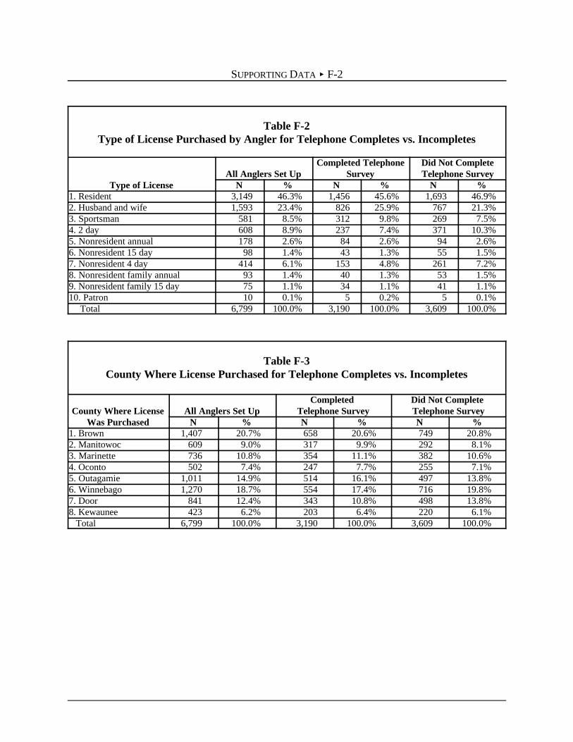
SUPPORTING DATA < F-2
Table F-2Type of License Purchased by Angler for Telephone Completes vs. Incompletes
Type of LicenseAll Anglers Set Up
Completed TelephoneSurvey
Did Not CompleteTelephone Survey
N % N % N %1. Resident 3,149 46.3% 1,456 45.6% 1,693 46.9%2. Husband and wife 1,593 23.4% 826 25.9% 767 21.3%3. Sportsman 581 8.5% 312 9.8% 269 7.5%4. 2 day 608 8.9% 237 7.4% 371 10.3%5. Nonresident annual 178 2.6% 84 2.6% 94 2.6%6. Nonresident 15 day 98 1.4% 43 1.3% 55 1.5%7. Nonresident 4 day 414 6.1% 153 4.8% 261 7.2%8. Nonresident family annual 93 1.4% 40 1.3% 53 1.5%9. Nonresident family 15 day 75 1.1% 34 1.1% 41 1.1%10. Patron 10 0.1% 5 0.2% 5 0.1%
Total 6,799 100.0% 3,190 100.0% 3,609 100.0%
Table F-3County Where License Purchased for Telephone Completes vs. Incompletes
County Where LicenseWas Purchased
All Anglers Set UpCompleted
Telephone SurveyDid Not Complete Telephone Survey
N % N % N %1. Brown 1,407 20.7% 658 20.6% 749 20.8%2. Manitowoc 609 9.0% 317 9.9% 292 8.1%3. Marinette 736 10.8% 354 11.1% 382 10.6%4. Oconto 502 7.4% 247 7.7% 255 7.1%5. Outagamie 1,011 14.9% 514 16.1% 497 13.8%6. Winnebago 1,270 18.7% 554 17.4% 716 19.8%7. Door 841 12.4% 343 10.8% 498 13.8%8. Kewaunee 423 6.2% 203 6.4% 220 6.1%
Total 6,799 100.0% 3,190 100.0% 3,609 100.0%

SUPPORTING DATA < F-3
Table F-4 Comments about Green Bay
(mail survey Question 2)
Reasons for Rating
Rating of Green Bay Relative to Other Places
Worse Same BetterDon’tKnow
Number of respondents 202 180 221 33
Site or use of site — negative(weather, location, facilities . . .)a 23.8% 8.3% 11.8% 0.0%
Site or use of site — positive(weather, location, facilities . . .)a 1.5% 2.8% 12.2% 0.0%
Catch — negative(poor rate, variety, size, limit . . .)a 50.5% 15.0% 14.0% 0.0%
Catch — positive(good rate, variety, size, limit . . .)a 4.5% 6.7% 49.3% 0.0%
General comment — negative(e.g., I don’t like Green Bay/otherplace . . .)a 14.4% 5.0% 3.2% 0.0%
General comment — positive(e.g., I like Green Bay/other place . . .)a 1.0% 1.1% 20.4% 0.0%
Don’t own a boat 0.0% 0.6% 0.9% 0.0%
Have limited information aboutGreen Bay or other sites 13.9% 10.6% 4.5% 72.7%
Can’t eat the fish/PCBs 16.8% 1.1% 4.5% 0.0%
Can eat the fish 0.5% 1.4% 0.0% 0.0%
Other pollution or contamination issues 7.4% 0.0% 1.4% 0.0%
Water is clean/clarity improving 3.0% 1.7% 5.4% 0.0%
a. Though respondents usually made comments about Green Bay relative to another site, some also madecomments about other sites relative to Green Bay. Thus, respondents who think Green Bay is worse andrespondents who think Green Bay is better, could both be coded as making a negative comment about fishingsites. In the former case the negative comment is about Green Bay and in the latter it is about another site. Mostof the negative comments from respondents who rated Green Bay as “worse” pertained to Green Bay; the oppositeis true for those rating Green Bay as “better.”

SUPPORTING DATA < F-4
Table F-5Number of Reported Open-Water Fishing Days on Wisconsin Water of Green Bay in 1998,
by Residence, for Mail Survey Respondents (combined telephone and mail survey data)
Residence
Numberof
Anglers
Total Trips Days per Angler
Total
% of TotalGreen Bay
Open-WaterDays
Mean(SE) Median Mode Min. Max.
Other statesTotal
117 770 12% 6.6(1.0)
4 1 1 95
Michigan 13 266 4% 20.5(7.63)
10 1 1 95
Wisconsin, but noteight targetedcounties
37 291 5% 7.9(1.4)
4 2 1 30
Eight targetedcounties
493 5,379 84% 10.9(0.67)
5 2 1 120
BrownCounty
195 2,124 33% 10.9(1.14)
5 2 1 120
DoorCounty
46 792 12% 17.2(2.93)
10 4 1 90
KewauneeCounty
20 308 5% 15.4(5.36)
6.5 1 1 90
ManitowocCounty
49 382 6% 7.8(1.36)
5 10 1 62
MarinetteCounty
59 702 11% 11.9(1.54)
6 5 1 60
OcontoCounty
37 400 6% 10.8(2.06)
6 3 1 45
OutagamieCounty
53 388 6% 7.3(1.31)
3 1 1 50
WinnebagoCounty
34 283 4% 8.3(2.28)
4 1 1 75
All mail surveyrespondents
647 6,440 100% 10.0(0.55)
5 2 1 120

SUPPORTING DATA < F-5
Table F-6Number of Reported Fishing Days on the Fox River between the Mouth and DePere Dam
as Compared to All Wisconsin Waters of Green Bay in 1998, for Telephone SurveyRespondents Who Fished Green Bay in 1998 (N = 906)a
(telephone survey data)
Total Days Days per Angler
Total% of Total GreenBay Fishing Days
Mean(SE) Median Mode Min. Max.
Green Bay total daysAll sites 9,832 100% 10.9
(0.52)5 2 1 142
On Fox River 1,579 16.1% 1.7(0.26)
0 0 0 130
Green Bay open-water days
All sites 8,316 84.6% 9.2(0.46)
5 2 0 120
On Fox River 1,365 13.9% 1.5(0.23)
0 0 0 110
Green Bay ice-fishingdays
All sites 1,516 15.4% 1.7(0.15)
0 0 0 50
On Fox River 214 2.2% 0.2(0.05)
0 0 0 20
a. All anglers who fished the Wisconsin waters of Green Bay, including those who only open-water fished, onlyice fished, or did both open-water and ice fishing.

SUPPORTING DATA < F-6
Table F-7Size of Fish Caught in the Wisconsin Waters of Lake Michigan Waters
SpeciesMean Length (inches):
1988-1998aTypical Rangeb
(inches)
Coho salmon 21.52 11-26
Chinook salmon 27.34 20-35
Rainbow trout 26.13 20-30
Brown trout 20.87 16-24
Brook troutc 13.94 10-16
Lake trout 27.43 17-27
Walleye Not reported 13-25
a. Source: WDNR, 1999 Wisconsin’s 1998 Open Water Sportfishing Effort and Catch from Lake Michigan andGreen Bay. http://www/dnr/state/wi/us/org/water/fhp/fish/lakemich.b. Source: Wisconsin Sea Grant Fish of the Great Lakes.http://h2o.seagrantwisc.edu/communications/publications/Fish.Michpage.html.c. 1988 through 1995 only. 1993 is the last year more than 100 brook trout were caught on Green Bay. Therewere no brook trout registered as caught after 1996 through 1998.

SUPPORTING DATA < F-7
Table F-8Anglers Purchasing Licenses in Eight Targeted Counties in 1997 by License Category
License Category Number of Licenses Number of Anglersa
1. Resident fishing 76,536 76,536
2. Nonresident fishing 5,575 5,575
3. Nonresident 15-day fishing 2,461 2,461
4. Sportsman 14,182 14,182
5. Patron 2,049 2,049
6. Resident husband and wife fishing 18,405 36,810
7. Nonresident family fishing 1,155 2,310
8. Nonresident family 15-day fishing 940 1,880
9. Two-day sports 15,716 7,858
10. Nonresident 4-day fishing 10,244 5,122
Total 147,263 154,783
a. Categories 1 through 5 licenses counted as one angler; categories 6 through 8 licenses counted as two anglers;categories 9 and 10 counted as half an angler.
Source for fishing licenses sold: Based on WDNR Bureau of Customer Service and Licensing, Report of FishingLicenses Sold by County, B130-30.