Why Does Risk Matter More in Recessions than in Expansions?

Discussion Paper no. 2021-11

Martin M. Andreasen, Giovanni Caggiano, Efrem Castelnuovo and Giovanni Pellegrino

Abstract:

This paper uses a nonlinear vector autoregression and a non-recursive identification strategy to showthat an equal-sized uncertainty shock generates a larger contraction in real activity when growth is low(as in recessions) than when growth is high (as in expansions). An estimated New Keynesian model withrecursive preferences and approximated to third order around its risky steady state replicates thesestate-dependent responses. The key mechanism behind this result is that firms display a strongerupward nominal pricing bias in recessions than in expansions, because recessions imply higher inflationvolatility and higher marginal utility of consumption than expansions.

Keywords: New Keynesian Model, Nonlinear SVAR, Non-recursive identification, State-dependentuncertainty shock, Risky steady state.

JEL Classification: E32

Martin M. Andreasen: Aarhus University, CREATES, and the Danish Finance Institute. (email:mandreasen@econ.au.dk); Giovanni Caggiano: Monash University and University of Padova. (email:giovanni.caggiano@monash.edu); Efrem Castelnuovo: University of Padova. (email:efrem.castelnuovo@unipd.it); Giovanni Pellegrino: Aarhus University (email: gpellegrino@econ.au.dk).

Why Does Risk Matter More in Recessionsthan in Expansions?

Martin M. Andreaseny Giovanni Caggianoz

Efrem Castelnuovox Giovanni Pellegrino

August 2021

Abstract

This paper uses a nonlinear vector autoregression and a non-recursive identi-cation strategy to show that an equal-sized uncertainty shock generates a largercontraction in real activity when growth is low (as in recessions) than when growthis high (as in expansions). An estimated New Keynesian model with recursive pref-erences and approximated to third order around its risky steady state replicatesthese state-dependent responses. The key mechanism behind this result is thatrms display a stronger upward nominal pricing bias in recessions than in expan-sions, because recessions imply higher ination volatility and higher marginal utilityof consumption than expansions.

Keywords: New Keynesian Model, Nonlinear SVAR, Non-recursive identica-tion, State-dependent uncertainty shock, Risky steady state.

We thank Guido Ascari, Nicholas Bloom, Ryan Chahrour, Chris Edmond, Andrea Ferrero, PabloGuerron-Quintana, Tom Holden, Michel Juillard, Martin Kleim, Sydney Ludvigson, Elmar Mertens,Juan Rubio-Ramirez, Henning Weber and participants to many seminar and conference audiences fortheir comments. Andreasen and Pellegrino acknowledge funding from the Independent Research FundDenmark, project number 7024-00020B. Caggiano and Castelnuovo acknowledge nancial support bythe Australian Research Council (respectively, DP190102802 and DP160102281). .

yAarhus University, CREATES, and the Danish Finance Institute. Email: mandreasen@econ.au.dk.zMonash University and University of Padova. Email: giovanni.caggiano@monash.edu.xUniversity of Padova. Email: efrem.castelnuovo@unipd.it.Aarhus University. Email: gpellegrino@econ.au.dk.

1 Introduction

The Great Recession and the recent COVID-19 pandemic have gone hand-in-hand with

spectacular spikes in virtually all measures of US uncertainty (Bloom (2014), Barrero and

Bloom (2020)). Following the seminal papers by Bloom (2009) and Fernández-Villaverde

et al. (2011), numerous studies have investigated the importance of uncertainty shocks for

the business cycle. This paper makes three contributions to this literature. First, using

a nonlinear vector autoregressive (VAR) with a non-recursive identication strategy, we

show that an equal-sized uncertainty shock generates a larger contraction in real activ-

ity when growth is low (as in recessions) than when growth is high (as in expansions).

Second, we demonstrate that a dynamic stochastic general equilibrium (DSGE) model

approximated to third order around its risky steady state is able to capture such state-

dependent responses to an uncertainty shock. In contrast, any state-dependent e¤ects of

this shock are absent when using the deterministic steady state for the third-order ap-

proximation, as commonly done in the literature. Third, relying on this methodological

contribution, we use an estimated New Keynesian model to examine the economic mech-

anisms behind our new VAR evidence. The results reveal that the traditional aggregate

supply (AS) relation implies an upward nominal pricing bias for rms, as emphasized in

Fernández-Villaverde et al. (2015), but that this bias is state-dependent and essential to

understand the asymmetric responses to an uncertainty shock. As a result, our analysis

delivers an empirically credible micro-founded model that can be used to study the role

of monetary policy for addressing the state-dependent e¤ects of uncertainty shocks across

the business cycle.

Let us elaborate on our contributions. First, we estimate a nonlinear VAR using

quarterly US data to assess whether an uncertainty shock has real e¤ects that depend

on the stance of the business cycle. To allow for potentially state-dependent e¤ects to a

shock, we extend the standard VAR by adding quadratic terms that involve the growth

rate of real GDP and a proxy for nancial uncertainty, which are both endogenous in

the VAR. Uncertainty shocks are identied using a non-recursive strategy that combines

event, correlation, and sign restrictions following the recent work of Antolín-Díaz and

Rubio-Ramírez (2018) and Ludvigson et al. (2019). Our main empirical result is that

an uncertainty shock of the same size generates a larger response of real activity during

recessions than in expansions. This nding is in line with previous contributions on the

nonlinear e¤ects of uncertainty shocks (see, for instance, Caggiano et al. (2014), Alessan-

dri and Mumtaz (2019), Cacciatore and Ravenna (2020)). Importantly, our empirical

nding is based on a non-recursive identication strategy, and is therefore not subject

to the critique in Ludvigson et al. (2019) of the standard recursive identication scheme

1

often used to identify exogenous variations in uncertainty.

Our second contribution is methodological and relates to the ability of nonlinear

DSGE models to generate state-dependent e¤ects of uncertainty shocks. These models

are widely used in the literature to study the economic mechanisms behind the real

e¤ects of uncertainty shocks when solved by a third-order approximation around the

deterministic steady state, as in Fernández-Villaverde et al. (2011), Born and Pfeifer

(2014), Fernández-Villaverde et al. (2015), and Basu and Bundick (2017), among many

others. This is a fruitful way to proceed to understand the e¤ects of uncertainty shocks

on average. However, it does not allow the researcher to investigate the potentially state-

dependent e¤ects of uncertainty shocks, because only the level of a given variable and

terms that are linear in the states are risk-corrected in this approximation (Cacciatore

and Ravenna (2020)). One way to address this shortcoming is to apply a fourth-order

approximation around the deterministic steady state, because it also corrects terms that

are quadratic in the states and hence allows for state-dependent e¤ects of uncertainty

shocks, as exploited in Cacciatore and Ravenna (2020) and Diercks et al. (2020). But

going beyond a third-order approximation substantially increases the execution time and

the memory requirement when solving DSGE models, which may limit the applicability of

this solution when the desire is to formally estimate these models. We therefore propose

a computationally less demanding alternative by simply moving the approximation point

for the third-order approximation to the risky steady state.1 This long-term equilibrium

point is characterized by allowing agents to respond to uncertainty, whereas any e¤ects

of uncertainty is absent in the deterministic steady state. The appealing feature of this

modication is that all linear and nonlinear terms in the approximation are adjusted for

risk, enabling us to capture potentially di¤erent e¤ects of uncertainty shocks in expansions

and recessions. To ensure stability, we also provide a pruned version of this approximation

and its closed-form solution for unconditional rst and second moments as well as impulse

response functions by using the results in Andreasen et al. (2018). Hence, our contribution

makes it feasible to estimate nonlinear DSGE models with state-dependent e¤ects of

uncertainty shocks using techniques that are commonly applied in the literature.

Building on this methodological contribution, in the third part of the paper we work

with a version of the New Keynesian model proposed by Basu and Bundick (2017) and

rened in Basu and Bundick (2018) to understand why risk matters more in recessions

than in expansions. Key features of this model are recursive preferences as in Epstein and

Zin (1989), an uncertainty shock in the disturbance to the households utility function,

and nominal price stickiness as in Rotemberg (1982). We extend the model by consump-

tion habits, the exible formulation of recursive preferences in Andreasen and Jørgensen

1Solutions around the risky steady state are discussed in Coeurdacier et al. (2011) for a rst-orderapproximation and in de Groot (2013) for approximations up to second order. However, the methodsadopted in these papers to compute approximations around the risky steady state di¤er from the approachapplied in the present paper.

2

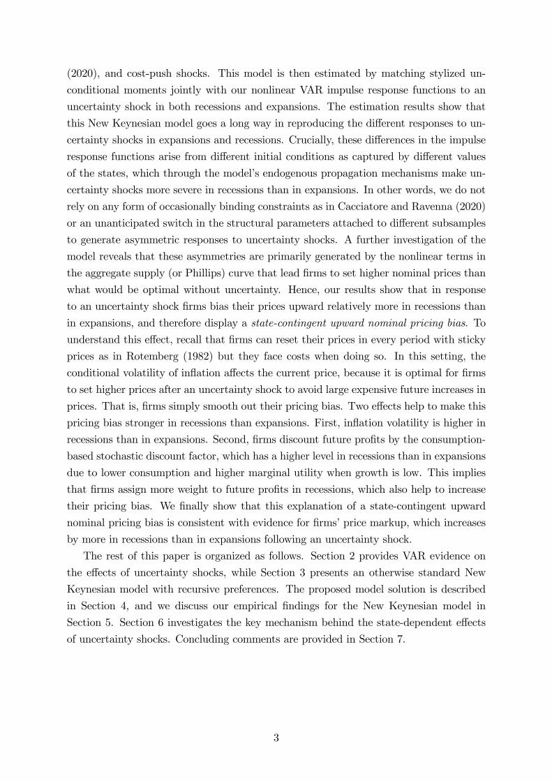
(2020), and cost-push shocks. This model is then estimated by matching stylized un-

conditional moments jointly with our nonlinear VAR impulse response functions to an

uncertainty shock in both recessions and expansions. The estimation results show that

this New Keynesian model goes a long way in reproducing the di¤erent responses to un-

certainty shocks in expansions and recessions. Crucially, these di¤erences in the impulse

response functions arise from di¤erent initial conditions as captured by di¤erent values

of the states, which through the models endogenous propagation mechanisms make un-

certainty shocks more severe in recessions than in expansions. In other words, we do not

rely on any form of occasionally binding constraints as in Cacciatore and Ravenna (2020)

or an unanticipated switch in the structural parameters attached to di¤erent subsamples

to generate asymmetric responses to uncertainty shocks. A further investigation of the

model reveals that these asymmetries are primarily generated by the nonlinear terms in

the aggregate supply (or Phillips) curve that lead rms to set higher nominal prices than

what would be optimal without uncertainty. Hence, our results show that in response

to an uncertainty shock rms bias their prices upward relatively more in recessions than

in expansions, and therefore display a state-contingent upward nominal pricing bias. To

understand this e¤ect, recall that rms can reset their prices in every period with sticky

prices as in Rotemberg (1982) but they face costs when doing so. In this setting, the

conditional volatility of ination a¤ects the current price, because it is optimal for rms

to set higher prices after an uncertainty shock to avoid large expensive future increases in

prices. That is, rms simply smooth out their pricing bias. Two e¤ects help to make this

pricing bias stronger in recessions than expansions. First, ination volatility is higher in

recessions than in expansions. Second, rms discount future prots by the consumption-

based stochastic discount factor, which has a higher level in recessions than in expansions

due to lower consumption and higher marginal utility when growth is low. This implies

that rms assign more weight to future prots in recessions, which also help to increase

their pricing bias. We nally show that this explanation of a state-contingent upward

nominal pricing bias is consistent with evidence for rmsprice markup, which increases

by more in recessions than in expansions following an uncertainty shock.

The rest of this paper is organized as follows. Section 2 provides VAR evidence on

the e¤ects of uncertainty shocks, while Section 3 presents an otherwise standard New

Keynesian model with recursive preferences. The proposed model solution is described

in Section 4, and we discuss our empirical ndings for the New Keynesian model in

Section 5. Section 6 investigates the key mechanism behind the state-dependent e¤ects

of uncertainty shocks. Concluding comments are provided in Section 7.

3

2 VAR Evidence

This section presents our reduced-form evidence for state-dependent e¤ects of an un-

certainty shock. We introduce a nonlinear VAR in Section 2.1, discuss identication in

Section 2.2, and present the impulse responses in Section 2.3. Various robustness checks

are discussed in Section 2.4, while Section 2.5 presents a simulation study that validates

the applied estimation method.

2.1 An Interacted VAR

We consider the vector of macro variablesYt = [log V XOt; logGDPt; logCt; log It, logHt,

logPt; Rt]0of dimension n 1, where V XOt is the implied volatility index in the stock

market (the S&P 100), GDPt is output, Ct is consumption, It is investment, Ht is hours

worked, Pt is the price level, and Rt is the policy rate.2 The vector Yt evolves as specied

by the following interacted VAR (IVAR)

Yt = +LXj=1

AjYtj +LXj=1

cj log V XOtj logGDPtj + t, (1)

where and cj have dimension n 1, Aj has dimension n n, and the n 1 vector ofresiduals t IID (0;). Unlike linear VARs, our IVAR includes the quadratic termslog V XOtj logGDPtj to capture potentially state-contingent e¤ects of higher uncer-tainty for various levels of the growth rate in GDP, i.e., logGDPt log(GDPt=GDPt1).We estimate this IVAR with four lags by OLS using quarterly US data from 1962Q3 to

2017Q4.3 Given that the VXO is unavailable before 1986, we follow Bloom (2009) and

combine the VXO by the monthly volatility of daily returns in the S&P 500 before 1986.

Our sample includes the zero lower bound for the monetary policy rate from 2008Q4

to 2015Q4. Hence, we replace the federal funds rate in this period by the shadow rate

of Wu and Xia (2016) to account for unconventional monetary policy. The estimation

results clearly favor our IVAR specication against a linear VAR, as we reject the joint

null hypothesis of cj = 0 for j = f1; 2; 3; 4g with a likelihood ratio test statistics of 62:0,implying a p-value of 0:0002 in the 228-distribution. Table 1 reports stylized uncondi-

tional moments for the growth rates of the four variables in the VAR and IVAR that are

related to economic activity. Both models match the empirical means and standard de-

viations, and hence show no sign of overtting. We also see that the IVAR is marginally

2The denition of these variables follows the one used by Basu and Bundick (2017) for their VAR.3Alternatives to the IVAR include the nonlinear factor model in Guerron-Quintana et al. (2021) and

the quadratic autoregression in Aruoba et al. (2017) that both are motivated from a second-order prunedperturbation approximation. We prefer the IVAR because it is computationally easier to estimate thanthe factor model in Guerron-Quintana et al. (2021), which requires the use of a particle lter. To ourknowledge, the quadratic autoregression in Aruoba et al. (2017) is currently only developed for univariatetime series.

4

better at generating negative skewness and excess kurtosis than the linear VAR. Thus,

the presence of nonlinear terms allow the IVAR to better capture higher order moments

of the empirical distribution than implied by the linear VAR.

Table 1: VARs: Unconditional Moments for Economic ActivityThis table reports unconditional moments for the growth rate in output, consumption, investment, and

hours worked using US data from 1962Q3 to 2017Q4. The corresponding moments in the linear VAR

and the IVAR are obtained from 500 simulated time series of the same lenght as in the empirical sample.

Data Linear VAR IVAR

Mean Std. Skew. Kurt. Mean Std. Skew. Kurt. Mean Std. Skew. Kurt.

Growth rates:

Output 0.39 0.81 -0.36 4.75 0.38 0.81 -0.004 3.23 0.38 0.81 -0.02 3.30

Consumption 0.40 0.46 -0.27 4.01 0.39 0.45 -0.09 3.20 0.39 0.45 -0.13 3.20

Investment 0.69 2.06 -1.15 6.70 0.63 2.07 -0.13 3.52 0.64 2.00 -0.26 3.73

Hours worked 0.04 0.66 -0.92 5.18 0.04 0.66 -0.02 3.10 0.04 0.63 -0.26 3.50

2.2 Uncertainty Shocks: Identication Strategy

Following Bloom (2009), many contributions in the literature have identied uncertainty

shocks by imposing zero-restrictions either on the impact of macroeconomic shocks on

uncertainty or on the impact of uncertainty shocks on the business cycle. However,

this recursive identication strategy has recently been questioned by Ludvigson et al.

(2019), who nd a non-zero contemporaneous correlation between uncertainty and the

business cycle. We therefore follow Ludvigson et al. (2019) and use a combination of

event restrictions and constraints from external variables, which we supplement with

sign restrictions to obtain a robust non-recursive identication of uncertainty shocks. To

present this alternative, let et denote the structural shocks with zero mean and covariance

matrix In. The mapping between the reduced-form residuals t and the structural shocks

et in the IVAR is t = Bet, whereB = PQ is of dimension nn, P is a lower-triangular

Cholesky factor of with non-negative diagonal elements, and Q is any orthonormal

rotation matrix (i.e., QQ0 = In) that implies positive diagonal elements of B. Let Bdenote the set that contains the innitely many solutions of B that satisfy the n(n+1)=2

restrictions implied by the covariance matrix, i.e., = BB0. Given that not all of these

mathematically acceptable solutions are interesting from an economic standpoint, we

impose restrictions to get the subset of economically admissible solutions.4

4The set B is constructed using the algorithm in Rubio-Ramírez et al. (2010). First, we initialize B tobe the unique lower-triangular Cholesky factor P . Then, we rotate B by drawing K = 500; 000 randomorthogonal matrices Q. Each rotation is performed by drawing an n n matrix M from a N (0; In)density. Then, Q is taken to be the orthonormal matrix in the QR decomposition of M . Let et(B) =

5

The rst set of restrictions we impose relate to specic events or narratives following

the work of Antolín-Díaz and Rubio-Ramírez (2018) and Ludvigson et al. (2019). In

particular, we consider the dates located by Bloom (2009) that coincide with spikes in

the nancial uncertainty proxy of Ludvigson et al. (2019).5 In addition, we also include

the events emphasized in Ludvigson et al. (2019) as well as 2000Q2 (collapse of the dot-

com bubble) and 2010Q2 (Euro area debt crisis and fears about a global slowdown) with

clear spikes in the nancial uncertainty proxy of Ludvigson et al. (2019). At each of

the dates, we require that realized uncertainty shocks eunc;t exceed their 50th percentile

p (eunc;t; 50) across all unconstrained solutions in B, except on 1987Q4 (Black Monday)and 2008Q4 (collapse of Lehman Brothers) where the uncertainty shock should exceed its

75th percentile as in Ludvigson et al. (2019). The selected dates with spikes in nancial

uncertainty are plotted in Figure 1.

Figure 1: Spikes in Financial UncertaintyThe red line denotes nancial volatility according to the VXO since 1986, and the realized volatility inthe S&P 500 before 1986 as in Bloom (2009). The blue line is the measure of nancial uncertainty inLudvigson et al. (2019) for a forecast horizon of one month. Vertical black lines denote the events thatare used to identify uncertainty shocks as reported in Table 2.

1965 1970 1975 1980 1985 1990 1995 2000 2005 2010 2015

­1

0

1

2

3

4

5

6

Bloom's LMN Bloom's updateBloom's excluded LMN extra

VXO (standardized)LMN f inancial uncertainty h=1 (standardized)

Our second set of restrictions impose two external constraints on eunc;t following the

work of Ludvigson et al. (2019). The rst requirement is that the correlation between eunc;tand the stock market return Rmt must be lower than the median value of this correlation

B1t t be the shocks implied by B 2 B for a given t. Then, K di¤erent matrices B imply K di¤erent

unconstrained shocks et(B) = B1t, t = 1; :::; T .

5When examining the recent peaks in the VXO, we identify one in 2016Q1, which we also include.Several uncertainty-triggering events occurred right before or during this quarter, e.g., the rst increaseof the federal funds rate that ended the zero lower bound phase after seven years; fears about Chinaseconomic fragility; the policy rate in Japan became negative; and the announcement in February 2016by the British Prime Minister David Cameron of the Brexit referedum in June that year.

6

across all unconstrained solutions in B. In our case, this implies that the correlationbetweenRmt and eunc;t must be less than or equal to0:15, which is a stronger requirementthan imposed in Ludvigson et al. (2019). The motivation for this assumption is the well-

known leverage e¤ect, which implies that a negative shock to the stock market (that

reduces Rmt ) make rms more leveraged and hence more risky. The second constraint

requires that the correlation between eunc;t and the growth rate in the real gold price

gt must be higher than the median value of this correlation across all unconstrained

solutions in B. In our case, this means that the correlation between gt and eunc;t mustbe bigger than or equal to 0.03, which also is slightly more restrictive than in Ludvigson

et al. (2019). The theoretical justication for this constraint is that gold operates as a

safe asset among investors, and its price should therefore be positively correlated with

uncertainty shocks due to higher demand.

To further sharpen the identication, we require a non-positive response of GDP,

investment, consumption, and hours on impact following a positive uncertainty shock,

which is consistent with a large number of theoretical and empirical investigations of un-

certainty shocks (see, e.g., Bloom (2014) for a survey). As shown in the Online Appendix,

these sign restrictions only help to narrow the identied set but have hardly any e¤ect on

the median target of the identied set, which we will focus on in our subsequent analysis.

For completeness, all the identication restrictions are summarized in Table 2.

2.3 Impulse Response Functions

We quantify the business cycle e¤ects of uncertainty shocks by computing generalized

impulse response functions (GIRFs) that account for the nonlinearities introduced by the

term log V XOtj logGDPtj in the IVAR (Koop et al. (1996)). The GIRFs for Yt

at horizon h to an uncertainty shock of size unc in period t is dened as

GIRFY(h; unc;$t1) E [Yt+hjunc;$t1] E [Yt+hj$t1] . (2)

These impulse responses depend on the state of the economy, which is captured by the

initial conditions $t1 fYt1; :::;YtLg. We are interested in exploring the e¤ects ofan uncertainty shock across the business cycle, and we therefore compute GIRFs when

the initial condition for real GDP growth is below its 10th percentile (i.e., deep recessions)

and above its 90th percentile (i.e., strong expansions). The results are reported in the

left column in Figure 2, which shows the responses for the the median target (MT) model

BMT , which is the solution in B that delivers the GIRFs with the smallest distance tothe median of the impulse responses in the identied set (see Fry and Pagan (2011)). For

a positive one-standard deviation uncertainty shock (unc = 1), we nd the familiar drop

in real activity for several quarters after the shock in both recessions and expansions.

However, the key focus of the present paper is the nding that this drop in activity

7

Table 2: Identifying Restrictions for Uncertainty ShocksThis table summarizes the identifying assumptions for uncertainty shocks in the IVAR. For event restric-tions, the notation > p(eUnc;t; 50th) indicates that the uncertainty shock at a given date should exceedthe 50th percentile of its distribution. The sources for each of these event constraints are from Bloom(2009) and Ludvigson et al. (2019) (LMN). Excluded dates from Bloom (2009) are 1963Q4 (Assassinationof JFK), 1997Q4 (Asian crisis), and 2003Q1 (Iraq invasion).

Conditions on eunc;t SourceEvent Restrictions1966Q3: Vietnam buildup > p(eunc;t; 50th) Bloom1970Q2: Cambodia and Kent state > p(eunc;t; 50th) Bloom1973Q4: OPEC I, Arab-Israeli War > p(eunc;t; 50th) Bloom1974Q3: Franklin National > p(eunc;t; 50th) Bloom1978Q4: OPEC II > p(eunc;t; 50th) Bloom1979Q4: Volcker experiment > p(eunc;t; 50th) LMN1980Q1: Afghanistan, Iran hostages > p(eunc;t; 50th) Bloom1982Q4: Monetary policy turning point > p(eunc;t; 50th) Bloom1987Q4: Black Monday > p(eunc;t; 75th) Bloom & LMN1990Q4: Gulf War I > p(eunc;t; 50th) Bloom1998Q3: Russian, LTCM default > p(eunc;t; 50th) Bloom2000Q2: Collapse of the tech bubble > p(eunc;t; 50th) LMN extra2001Q3: 9/11 terrorist attacks > p(eunc;t; 50th) Bloom2002Q3: Worldcom, Enron > p(eunc;t; 50th) Bloom2008Q4: Great recession > p(eunc;t; 75th) Bloom & LMN2010Q2: European debt crisis > peunc;t; 50th) LMN extra2011Q3: Debt ceiling crisis > p(eunc;t; 50th) LMN2016Q1: FFR lifto¤ and China > p(eunc;t; 50th) Bloom (update)

External RestrictionsStock market return, rmt 6 p(corr(eunc;t; rmt ); 50th) LMNReal log di¤erence price of gold, gt > p(corr(eunc;t;gt); 50th) LMN

Sign Restrictions on ImpactGDP < 0Investment < 0Consumption < 0Hours < 0

is larger and more persistent in deep recessions (the red dotted lines) than in strong

expansions (the blue lines) although the size of the uncertainty shock is the same. For

instance, in recessions the peak responses of output, investment, and hours are -0.28%,

-0.87%, and -0.45%, respectively, whereas the corresponding responses in expansions are

only -0.19%, -0.35%, and -0.23%. Turning to the nominal side, the responses for prices

are slightly positive in expansions and slightly negative in recessions. For the monetary

policy rate, we nd a clear negative e¤ect of an uncertainty shock, with e¤ects that are

stronger in recessions than in expansions.

8

Figure 2: Nonlinear VAR: Impulse Responses to an Uncertainty ShockThe charts to the left show the median target responses in the IVAR in deep recessions and strongexpansions following a positive one-standard deviation uncertainty shock. The charts to the right showthe di¤erence between these responses in (deep recessions minus strong expansions) in addition to the 68and 90 percent condence interval, which are estimated by a residual-based bootstrap (with 1,000 draws)when conditioning on the median target responses. All responses are shown in percentage deviations,except for the policy rate where changes in percentage points are reported.

5 10 15 200

0.1

0.2Impulse Responses (MT)

5 10 15 20­0.3

­0.2

­0.1

0

5 10 15 20­0.15

­0.1

­0.05

0

5 10 15 20­1

­0.5

0

0.5

5 10 15 20

­0.4

­0.2

0

5 10 15 20­0.2

00.20.40.60.8

5 10 15 20­0.4

­0.2

0

5 10 15 20

­0.02

0

0.02

Difference

5 10 15 20­0.2

0

0.2

5 10 15 20­0.2

0

0.2

5 10 15 20

­1

­0.5

0

5 10 15 20­0.4

­0.2

0

0.2

5 10 15 20­1

­0.5

0

5 10 15 20­0.4

­0.2

0

0.2

The charts to the right in Figure 2 report the distance between the MT responses

in recessions relative to the MT responses in expansions, where the shaded gray and

9

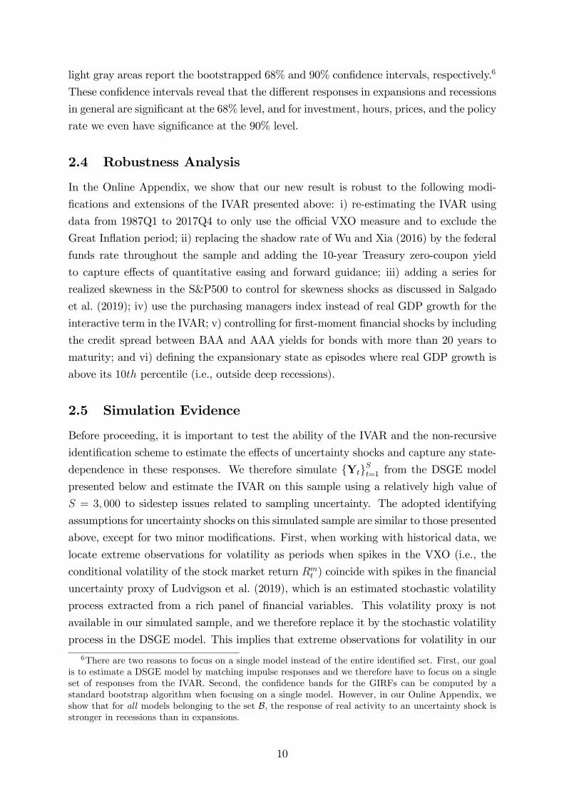
light gray areas report the bootstrapped 68% and 90% condence intervals, respectively.6

These condence intervals reveal that the di¤erent responses in expansions and recessions

in general are signicant at the 68% level, and for investment, hours, prices, and the policy

rate we even have signicance at the 90% level.

2.4 Robustness Analysis

In the Online Appendix, we show that our new result is robust to the following modi-

cations and extensions of the IVAR presented above: i) re-estimating the IVAR using

data from 1987Q1 to 2017Q4 to only use the o¢ cial VXO measure and to exclude the

Great Ination period; ii) replacing the shadow rate of Wu and Xia (2016) by the federal

funds rate throughout the sample and adding the 10-year Treasury zero-coupon yield

to capture e¤ects of quantitative easing and forward guidance; iii) adding a series for

realized skewness in the S&P500 to control for skewness shocks as discussed in Salgado

et al. (2019); iv) use the purchasing managers index instead of real GDP growth for the

interactive term in the IVAR; v) controlling for rst-moment nancial shocks by including

the credit spread between BAA and AAA yields for bonds with more than 20 years to

maturity; and vi) dening the expansionary state as episodes where real GDP growth is

above its 10th percentile (i.e., outside deep recessions).

2.5 Simulation Evidence

Before proceeding, it is important to test the ability of the IVAR and the non-recursive

identication scheme to estimate the e¤ects of uncertainty shocks and capture any state-

dependence in these responses. We therefore simulate fYtgSt=1 from the DSGE model

presented below and estimate the IVAR on this sample using a relatively high value of

S = 3; 000 to sidestep issues related to sampling uncertainty. The adopted identifying

assumptions for uncertainty shocks on this simulated sample are similar to those presented

above, except for two minor modications. First, when working with historical data, we

locate extreme observations for volatility as periods when spikes in the VXO (i.e., the

conditional volatility of the stock market return Rmt ) coincide with spikes in the nancial

uncertainty proxy of Ludvigson et al. (2019), which is an estimated stochastic volatility

process extracted from a rich panel of nancial variables. This volatility proxy is not

available in our simulated sample, and we therefore replace it by the stochastic volatility

process in the DSGE model. This implies that extreme observations for volatility in our

6There are two reasons to focus on a single model instead of the entire identied set. First, our goalis to estimate a DSGE model by matching impulse responses and we therefore have to focus on a singleset of responses from the IVAR. Second, the condence bands for the GIRFs can be computed by astandard bootstrap algorithm when focusing on a single model. However, in our Online Appendix, weshow that for all models belonging to the set B, the response of real activity to an uncertainty shock isstronger in recessions than in expansions.

10

simulated sample are episodes when the conditional volatility of Rm and the stochastic

volatility shocks both are high and exceed their 50th percentile across all unconstrained

solutions in B. Second, the DSGE model presented below does not include a gold price,and we are therefore unable to include the correlation restriction between the real gold

price and uncertainty shocks in the simulation study.

Figure 3: Simulation Exercise for the IVAR: IRFs to an Uncertainty ShockThis gure shows the generalized impulse response functions (GIRFs) in the IVAR to a positive one-standard deviation shock to uncertainty in strong expansions (to the left) and deep recessions (to theright) on a simulated sample of 3; 000 draws from the New Keynesian DSGE model using the estimatesin column (1) of Table 4. The solid (dashed) lines report the median target impulse responses in strongexpansions (deep recessions) when computed as suggested by Fry and Pagan (2011), while the identiedsets in the IVAR are denoted by the shaded areas. The marked solid lines denote the true responses inthe DSGE model. All responses are shown in percentage deviations, except for the policy rate wherechanges in percentage points are reported.

2 4 6 8 10 12 14 16 18 200

0.2

0.4

Strong Expansions (EXP)

2 4 6 8 10 12 14 16 18 20

­0.4

­0.2

0

2 4 6 8 10 12 14 16 18 20

­0.2

­0.1

0

2 4 6 8 10 12 14 16 18 20

­1

­0.5

0

2 4 6 8 10 12 14 16 18 20­0.3

­0.2

­0.1

0

2 4 6 8 10 12 14 16 18 20

­0.2­0.1

00.1

2 4 6 8 10 12 14 16 18 20

­0.15­0.1

­0.050

2 4 6 8 10 12 14 16 18 200

0.2

0.4

Deep Recessions (REC)

2 4 6 8 10 12 14 16 18 20

­0.4

­0.2

0

2 4 6 8 10 12 14 16 18 20

­0.2

­0.1

0

2 4 6 8 10 12 14 16 18 20

­1

­0.5

0

2 4 6 8 10 12 14 16 18 20­0.3

­0.2

­0.1

0

2 4 6 8 10 12 14 16 18 20

­0.2­0.1

00.1

2 4 6 8 10 12 14 16 18 20

­0.15­0.1

­0.050

The results from this simulation exercise are summarized in Figure 3. Very encourag-

ingly, we nd that the identied set for uncertainty shocks in the IVAR (denoted by the

shaded areas) nearly always contains the true responses in the DSGE model.7 A careful

7The exception is for the responses in uncertainty (i.e. VXO), which exceed the true responses in therst couple of periods after the uncertainty shock. Unreported results show that this upward bias is closely

11

inspection of Figure 3 also shows that the IVAR is able to generate state-dependent ef-

fects in the responses, and that they match those in the DSGE model. This is especially

the case for investment and hours, where we see large di¤erences between recessions and

expansions.8

We draw two conclusions from this simulation exercise. First, the non-recursive iden-

tifying scheme in the IVAR is su¢ ciently exible to capture the responses of uncertainty

shocks in our DSGE model. Second, any state-dependence in the responses to uncer-

tainty shocks are well captured by the IVAR in (1). Thus, an important econometric

implication of this simulation exercise is that the GIRFs from the IVAR can be used for

a direct inference approach when estimating our DSGE model.

3 A New Keynesian Model

This section presents a New Keynesian DSGE model to explain why uncertainty shocks

have larger e¤ects in recessions than in expansions. Our starting point is the model by

Basu and Bundick (2017) and its renement in Basu and Bundick (2018). We extend

this model along three dimensions. First, external consumption habits are included to

capture a hump-shaded response in consumption to an uncertainty shock. Second, the

exible formulation of recursive preferences in Andreasen and Jørgensen (2020) is adopted

to keep risk aversion at a low and plausible level. Finally, standard cost-push shocks

are introduced to match the comovement between consumption and output across the

business cycle. Given that the basic structure of this New Keynesian model is widely

known, we only present its crucial parts and defer a full presentation with derivations to

the Online Appendix.

3.1 Households

We consider an innitely lived representative household with recursive preferences as

in Epstein and Zin (1989) and Weil (1990). Using the formulation in Rudebusch and

Swanson (2012), the value function Vt is given by

Vt =

(ut + (Et

V 1t+1

)

11 when ut > 0 for all t

ut (Et(Vt+1)1

)

11 when ut < 0 for all t

; (3)

related to the adopted simulation procedure for the VXO which is 100q4max

VtRmt+1

; 0:000026

as suggested by the codes related to Basu and Bundick (2018). By imposing this lower bound forthe conditional variance of stock returns Vt

Rmt+1

, we get an upward bias in the IVAR residuals for

log V XOt and subsequently also an upward bias in the impulse response functions for log V XOt.8See also the Online Appendix, where we also plot the median target responses.

12

where ut is the utility function and Et [] is the conditional expectation in period t. Theparameter 2 R n f1g captures householdsappetite for the resolution of uncertainty,implying preferences for early (late) resolution of uncertainty if > 0 ( < 0) for ut > 0,

and vice versa when ut < 0. Andreasen and Jørgensen (2020) further argue that the size

of this timing attitude is proportional to , meaning that numerically larger values of

imply stronger preferences for early (late) resolution of uncertainty.

The expression for householdsutility at time t is

ut a1t

1

1 (Ct bCt1) (1Nt;)1

1+ u0

; (4)

which depends on habit-adjusted consumption Ct bCt1 and leisure 1 Nt.9 As in

Basu and Bundick (2017), at is a preference shock that evolves according to the process

at+1 = aat + a;ta;t+1 where a;t+1 NID (0; 1). The process for stochastic volatilitya;t is specied as a;t+1 = (1)+a;t+;t+1, where the innovations in uncertainty;t+1 NID (0; 1) and uncorrelated with a;t+1 at all leads and lags. The constant u0captures utility from government spending and goods produced and consumed within the

household. As shown by Andreasen and Jørgensen (2020), the main reason for including

u0 is to separately control the level of the utility function and hence disentangle the

timing attitude from relative risk aversion (RRA), which otherwise are tightly linked

in the standard formulation of recursive preferences in Epstein and Zin (1989) and Weil

(1990). To see this, note that (3) and (4) imply

RRA =

1 b

" + (1 ) ((Css bCss) (1Nss)1)1

((Css bCss) (1Nss)1)1 + (1 )u0

#;

at the deterministic steady state (ss) when accounting for the endogenous labor sup-

ply (see Swanson (2018)). Hence, a high timing attitude does not necessarily imply

a high RRA, which is in contrast to the standard case with u0 = 0 where RRA =1b ( + (1 )).The household receives labor income Wt for each unit of labor Nt supplied to the

intermediate rms. These rms are owned by the household that therefore holds their

equity shares St, which have the price PEt and pay dividends DEt . The household also

holds one-period real bonds with the gross return RRt as issued by the rms, and it holds

nominal bonds issued by the government with the gross return Rt.

9Following Basu and Bundick (2018), we include a1t instead of at in (4) to avoid having an asymptotein the policy function at = 1, as noted by de Groot et al. (2018).

13

3.2 Firms

The nal output Yt is produced by a representative nal good producer using the pro-

duction function Yt =R 1

0Yt (i)

(;t1)=;t di;t=(;t1)

, where ;t captures a time-

varying substitution elasticity between the intermediate goods Yt(i). It is assumed that

log (;t+1=) = log(;t=) + ;t+1, where ;t+1 NID (0; 1). Cost minimiza-

tion implies that Yt(i) =hPt(i)Pt

i;tYt, where Pt

R 10Pt (i)

1;t di 11;t denotes the

aggregate price level and Pt (i) is the price of the ith good.

Intermediate rms produce Yt(i) using the Cobb-Douglas production function with

xed costs, i.e., Yt(i) = (Kt1(i)Ut(i))p (ZtNt(i))

1p , where Kt1(i) is the capital

stock, Ut(i) is the utilization rate, and Zt captures productivity shocks as logZt+1 =

Z logZt + ZZ;t+1 with Z;t+1 NID (0; 1). The capital stock evolves as Kt(i) =1 (Ut(i)) K

2(It(i)=Kt1(i) )2

Kt(i) + It(i), where K introduces adjustment

costs and It(i) is investment. The depreciation costs are given by (Ut(i)) = +1(Ut(i)Uss) +

22(Ut(i) Uss)2. Intermediate rms operate in a market with monopolistic com-

petition and face quadratic adjustment costs as in Rotemberg (1982). The expression for

real dividends therefore reads

Dt(i)

Pt=

Pt(i)

Pt

1;tYt

Wt

PtNt(i) It(i)

P2

Pt(i)

ssPt1(i) 12Yt

where Wt is the wage and ss denotes ination in the deterministic steady state. Each

intermediate rm nances a fraction of its capital stock by issuing one-period riskless

bonds, i.e., Bt(i) = Kt1(i). As a result, the real dividend payments to equity holders

are DEt (i) =Pt = Dt (i) =Pt (Kt1 (i)Kt (i) =R

Rt ):

3.3 Monetary Policy and Stock Market Volatility

The central bank adjusts the nominal interest rate Rt to stabilize ination around its

target ss and output growth according to the rule

ln(Rt=Rss) = log (t=ss) + Y log(Yt=Yt1); (5)

where t Pt=Pt1 denotes gross ination.10

As in Basu and Bundick (2017), the gross stock market return is dened as Rmt =DEt + P

Et

=PEt1. The model-implied measure for stock market volatility is then given

by V XOt = 100q4 Vt

Rmt+1

, where Vt

Rmt+1

is the quarterly conditional variance of

Rmt+1.

10Unreported results show no evidence of interest rate smoothing in (5) when using the estimatorpresented in Section 5.1.

14

3.4 Equilibrium

We focus on the symmetric equilibrium, where all intermediate rms choose the same

price Pt(i) = Pt, employ the same amount of labor Nt(i) = Nt, and choose the same level

of capital Kt(i) = Kt and utilization rate Ut(i) = Ut. Consequently, all rms have the

same cash ows and are nanced with the same mix of bonds and equity. The markup

of the price in relation to marginal cost is t = 1=t, where t denotes the marginal cost

of producing one additional unit by the intermediate rm.

4 Model Solution

This section derives a third-order approximation to DSGEmodels around the risky steady

state and study some of its implications. Section 4.1 describes a general class of DSGE

models that includes the New Keynesian model presented above. The third-order Taylor

approximation around the risky steady state is derived in Section 4.2, and we discuss a

pruned version of this approximation in Section 4.3. The accuracy and execution time of

various approximations are studied in Section 4.4.

4.1 General Model

We consider the class of models where the equilibrium conditions are given by

Et [f (yt+1;yt;xt+1;xt)] = 0: (6)

The states appear in xt with dimension nx 1, while the control variables of dimensionny 1 are collected in yt, with n nx + ny. We also let xt

hx01;t x02;t

i0, where x1;t

refers to the endogenous states and x2;t to the exogenous states, which evolve as

x2;t+1 = h2 (x2;t) + ~t+1; (7)

where t+1 IID (0; In), and n is the number of elements in the vector of shocks t+1.11

The assumption that the innovations enter linearly in (7) is without loss of generality,

because the state vector may be extended to account for nonlinearities between xt and

t+1, as needed when including stochastic volatility in the exogenous states (see Andreasen

(2012) for further details). The exact solution to this class of models is given by

yt = g (xt) (8)

11All eigenvalues of @h2 (x2;t) =@x2;t must have modulus less than one, implying that trends may onlybe included if the model after re-scaling has an equivalent representation without trending variables.The procedure of re-scaling a DSGE model with trends is carefully described in King et al. (2002).

15

xt+1 = h (xt) + t+1 (9)

where h0 ~0

i0has dimension nx n. The functions g () and h () are generally

unknown and must be approximated.

4.2 A Third-Order Approximation at the Risky Steady State

Let xt = x denote the risky steady state. This long-term equilibrium point is character-

ized by the absence of structural shocks (i.e., t+1 = 0) but agents nevertheless respond

to their probability distribution. This makes the risky steady state di¤erent from the

widely used deterministic steady state, where agents do not respond to the probability

distribution of the structural shocks.

The considered third-order approximation around x is given by

yt = g (x) + gx (x) (xt x) + 12gxx (x) (xt x)2 + 1

6gxxx (x) (xt x)3

xt+1 = h (x) + hx (x) (xt x) + 12hxx (x) (xt x)2 + 1

6hxxx (x) (xt x)3 + t+1;

(10)

where (xt x)2 (xt x) (xt x) and (xt x)3 (xt x)2 (xt x). The rst-order derivative of g (xt) with respect to xt is denoted gx (x) when evaluated at x. A

similar notation is used for h (xt) and for higher-order derivatives.12 The procedure we

use to compute the required derivatives of g () and h () is similar to the one applied inCollard and Juillard (2001a) for a simple endowment model and in Collard and Juillard

(2001b) for a DSGE model solved by a second-order approximation. Hence, we substitute

(8) and (9) into (6) to get

Et [F (xt; t+1)] Etfgh (xt) + t+1

;g (xt) ;h (xt) + t+1;xt

= 0: (11)

We then compute a third-order Taylor approximation of F (xt; t+1) at xt = x and t+1 =

0. Evaluating the expectations with respect to terms that involve t+1 and using the

method of undetermined coe¢ cients, we obtain the following conditions (derived in our

Online Appendix):

[F (x;0)]i +1

2[F (x;0)]

i12

[V [t+1]]12 +1

6[F (x;0)]

i123

m3

123

= 0 (12)

[Fx (x;0)]i1+3

6[Fx (x;0)]

i123

[V [t+1]]12 = 0 (13)

[Fxx (x;0)]i12

= 0 (14)

[Fxxx (x;0)]i123

= 0; (15)

12Note that x is a xed-point in h (), i.e. h (x) = x, and that the ergodic mean E [xt] generally di¤ersfrom the risky steady state x because E [xt+1 x] = E

h12hxx (x) (xt x)

2+ 1

6hxxx (x) (xt x)3i6=

0.

16

where the tensor notation is used with i = f1; 2; :::; ng, 1; 2; 3 = f1; 2; :::; ng, and1; 2; 3 = f1; 2; :::; nxg. Also, V [t+1] is the covariance matrix of t+1 (which equalsIn), and m

3 with dimensions n n n contains all third order moments of t+1. The

derivatives of F (xt; t+1) are denoted with subscripts and evaluated at the risky steady

state, e.g., Fx (x;0) = @F (xt; t+1) =@x0tjxt=x;t+1=0.

To understand the implications of (12) to (15), let us rst consider the case without

uncertainty by letting V [t+1] = 0 and m3 (t+1) = 0 to obtain the certainty equiva-

lence solution. The n 1 equations in (12) then simplies to [F (x;0)]i = 0, implying

that x = xss and y = yss. We also have that (13) reduces to [Fx (xss;0)]i1= 0, which

gives the well-known quadratic system for computing the rst-order derivatives gx (xss)

and hx (xss), as shown in Schmitt-Grohe and Uribe (2004). Moreover, (14) reduces to

[Fxx (xss;0)]i12

= 0 and (15) to [Fxxx (xss;0)]i123

= 0, which are the linear sys-

tems exploited by the standard perturbation method to compute the second-order terms

gxx (xss) and hxx (xss) and the third-order terms gxxx (xss) and hxxx (xss), respectively

(see Schmitt-Grohe and Uribe (2004) and Andreasen (2012)). Thus, without uncertainty,

the conditions in (12) to (15) are identical to those used by the standard perturbation

method to obtain the certainty equivalent part of this approximation.

In the presence of uncertainty, condition (12) still determines x and y, but in this case

x 6= xss and y 6= yss. Given (x; y), condition (13) allows us to determine the rst-orderderivatives of g () and h () by solving a quadratic system that includes the variance term36[Fx (x;0)]

i123

[V [t+1]]12. This adjustment has two important implications. First, itimplies that the rst-order derivatives gx (x) and hx (x) contain an uncertainty correction

for variance risk. Second, the Blanchard-Kahn conditions for getting unique and stable

rst-order derivatives have to hold for a risk-adjusted version of the model. Hence, uncer-

tainty may contribute to violate or satisfy the Blanchard-Kahn conditions, unlike in the

standard perturbation method where these conditions are evaluated at the deterministic

steady state. Importantly, the uncertainty correction 36[Fx (x;0)]

i123

[V [t+1]]12 is ofthird order and therefore not present in the second-order approximation around the risky

steady state as studied in Collard and Juillard (2001b).

The condition in (14) for the second-order terms gxx (x) and hxx (x) is similar to the

one used in the standard perturbation method, except that all derivatives of F (), g (),and h () are evaluated at the risky steady state. This implies that gxx (x) and hxx (x)contain a correction for uncertainty, which is essential for our analysis, because it enables

us to obtain impulse response functions for uncertainty shocks that are state-dependent.

Finally, the condition in (15) allows us to determine gxxx (x) and hxxx (x) by solving a

linear system, where all derivatives of F (), g (), and h () are evaluated at the riskysteady state. As a result, gxxx (x) and hxxx (x) are also adjusted for uncertainty for the

same reasons as mentioned for gxx (x) and hxx (x).13 For the New Keynesian model we

13Very loosely, one can think of gx (x) gx (xss)+0:5gx (xss) and hx (x) hx (xss)+0:5hx (xss),

17

consider, nearly all of the uncertainty correction in the higher-order derivatives comes

from the risk adjustment in gx (x) and hx (x), meaning that a third-order approximation

is needed for our model to get visible state-dependence in the impulse response functions

for an uncertainty shock.14

Unfortunately, the moment conditions in (12) to (15) do not imply a recursive struc-

ture for computing the required terms in (10). This is because F (x;0), Fx (x;0),

and F (x;0) depend on (x; y) and the derivatives of g () and h (). We therefore usean iterative procedure, where F (x;0), Fx (x;0), and F (x;0) are computed using

derivatives of g () and h () from the standard perturbation method in the rst iter-

ation and afterwards from the previous iteration to recursively solve (12) to (15). Our

Online Appendix summarizes this algorithm, which basically iterates on the solution rou-

tine for the standard perturbation approximation until convergence (typically with ve

iterations).15

4.3 A Pruned State-Space Representation

The system for a standard third-order perturbation approximation obviously reduces

to the system in (10) when all derivatives of the g- and h-functions with respect to the

perturbation parameter are equal to zero. This means that the pruning scheme introduced

in Andreasen et al. (2018) can also be applied to (10) with all derivatives of the g- and h-

functions with respect to xt evaluated at x instead of xss. The Blanchard-Kahn condition

related to (13) ensures that hx (x) is stable and hence that this pruned approximation is

stable. Thus, the closed-form solution for unconditional moments and GIRFs derived in

Andreasen et al. (2018) can also be applied to our third order approximation at the risky

steady state. This greatly facilitates its use in a formal estimation routine that matches

unconditional rst and second moments, impulse response functions, or a combination of

the two, as considered below in Section 5.

where is the perturbation parameter as dened in Schmitt-Grohe and Uribe (2004). In the standardperturbation method, only gx (xss) and hx (xss) are used to compute the higher-order derivatives. Incontrast, the procedure we use implies that gx (xss)+0:5gx (xss) and hx (xss)+0:5hx (xss) are usedto compute the higher-order derivatives, which therefore include an adjustment for uncertainty.14As shown in the Online Appendix, the expressions for F (x;0), Fx (x;0), and F (x;0) are

identical to those provided for F, Fx, and F, respectively, in Schmitt-Grohe and Uribe (2004)and Andreasen (2012), when setting all derivatives of g () and h () with respect to the perturbationparameter equal to zero. The conditions in (12) to (15) are therefore easy to implement from existingresults and computer packages on the standard perturbation method. In our case, we modify the highlye¢ cient Matlab codes of Binning (2013).15The proposed solution in (10) is, strictly speaking, not a perturbation approximation, because it

does not perturb a known solution. Instead, it corresponds to a projection approximation that onlyexploits local properties of the model solution, and it is therefore best characterized as a local projectionapproximation.

18

4.4 Accuracy and Execution Time

We evaluate the accuracy of Taylor approximations around the deterministic and risky

steady state by computing unit-free Euler-equation errors for the considered New Key-

nesian model along a simulated sample of 10; 000 observations for the states. The two

estimated versions of the New Keynesian model presented below in Table 4 are considered

for this exercise, where the states are simulated using a standard third-order perturbation

approximation, i.e., by a Taylor approximation around the deterministic steady state.

Table 3: Accuracy and Execution Time

Panel A in this table reports the mean absolute unit-free Euler-equation errors (MAEs) and the rootmean squared unit-free Euler-equation errors (RMSEs) in a second-, third-, and fourth-order Taylorapproximation around the deterministic steady state, and in a second- and third-order Taylor approxi-mation around the risky steady state. All model equations are included when computing the MAEs andthe RMSEs, except for the link-equations related to lagged controls and the equations for the exogenousshocks, where the errors always are zero. The Euler-equations errors are reported in percent and com-puted using a simulated sample path of 10,000 observations for the states. For each estimated versionof the model, the simulated sample path is computed using a third-order Taylor approximation aroundthe deterministic steady state. Conditional expectations in the Euler-equations are evaluated by Gauss-Hermite quadratures using ve points per shock, giving a total of 54 = 625 points. The considered modelparameters are those reported in Table 4. Panel B shows the execution time in seconds for obtainingthe approximated model solutions and for simulating 10,000 observations using each of the consideredapproximations. The computations are done on a standard laptop with an Intel(R) Core(TM) i7-7600CPU processor with 2.80GHz.

Taylor approximations Taylor approximationsat deterministic steady state at risky steady state2nd 3rd 4th 2nd 3rd

Panel A: Accuracy (in pct.)Benchmark MAEs 1.19 1.10 0.65 1.06 0.79

RMSEs 3.26 3.03 2.27 3.10 2.44

Standard EZ MAEs 1.41 1.22 0.79 1.16 0.87RMSEs 3.98 3.44 5.61 3.45 3.44

Panel B: Execution time (in sec.)Benchmark Model solution 0.03 0.60 12.0 0.45 3.50

Simulation of 0.13 1.04 22.4 0.13 1.04of 10,000 observations

For the benchmark model, panel A in Table 3 shows that the standard perturbation

method performs fairly well, as the mean absolute Euler errors (MAEs) across all en-

dogenous equations in the model are only 1:19% at second order, 1:10% at third order,

and 0:65% at fourth order. We nd a similar monotone improvement in accuracy by in-

creasing the approximation order when computing the root mean squared Euler-equation

errors (RMSEs), that penalize large errors more heavily than the MAEs. For approxi-

mations around the risky steady state, the second-order approximation of Collard and

Juillard (2001b) provides a small improvement when compared to the standard pertur-

bation method at second order, as the MAEs falls from 1:19% to 1:06% and the RMSEs

19

from 3:26% to 3:10%. We see more notable reductions in the Euler errors by using the

proposed third-order approximation around the risky steady state, as the MAEs falls from

1:10% to 0:79% and the RMSEs from 3:03% to 2:44% when compared to a third-order

approximation around xss. Thus, the accuracy of our approximation clearly outperforms

the standard perturbation method at third order and is close to providing the same level

of accuracy as the fourth-order Taylor approximation around xss with a MAE of 0:65 and

a RMSE of 2:27.

Table 3 shows that we broadly nd the same results for the estimated version of the

New Keynesian model with standard Epstein-Zin preferences, i.e., u0 = 0. The only

exception is that the RMSEs for the fourth-order Taylor approximation around xss is

5:61% and hence higher than both third-order approximations with RMSEs of 3:44%.

The execution time for the various approximations are provided in panel B of Table3. The standard third-order perturbation approximation is obtained in just 0:60 seconds,

while it takes 12 seconds to compute a fourth-order approximation using the codes of

Levintal (2017). The required time for computing our third-order approximation around

the risky steady state depends mainly on the number of iterations needed to obtain

convergence, but the execution time is typically around 4 seconds. Thus, we get an

approximated model solution with state-dependent impulse response functions following

an uncertainty shock that is about three times faster than the existing alternative of using

a fourth-order approximation. In addition, it is also more costly to use a fourth-order than

a third-order approximation when simulating the model. This is illustrated at the bottom

of Table 3, where it takes one second to simulate 10; 000 observations from a third-order

approximation but about 22 seconds when using a fourth-order approximation.

To summarize, the proposed third-order Taylor approximation around the risky steady

state delivers a high level of accuracy that is comparable to a fourth-order perturbation

approximation but is computationally much more e¢ cient than this fourth order alter-

native. This is particularly convenient when it comes to estimating DSGE models like

ours, where uncertainty shocks are allowed to have state-dependent e¤ects.16

5 Empirical Results for the New Keynesian Model

This section presents our empirical ndings for the New Keynesian model. We introduce

the adopted estimation methodology in Section 5.1, and discuss the estimated parameters

in Section 5.2 and the model t in Section 5.3.16de Groot (2016) highlights another shortcoming of the third-order Taylor approximation at the

deterministic steady state, as none of its terms account for the conditional standard deviation of volatilityshocks, i.e. . Unreported results show that our third-order Taylor approximation around the riskysteady state corrects for and hence also addresses this limitation of the standard solution method.

20

5.1 Estimation Methodology

To describe our estimation approach, let the vector contain the structural parameters of

the New Keynesian model. As in Basu and Bundick (2017), we estimate using two sets

of moments. The rst set includes the MT responses from the IVAR for the rst 20 periods

following an uncertainty shock in expansions b EXP and in recessions b REC as presented inSection 2. The second source of information is a vector of unconditional sample momentsbmT , which ensures that the model also matches stylized unconditional properties of the

US economy in addition to the conditional moments following an uncertainty shock.

These unconditional moments are constructed using the same data as applied to estimate

the IVAR. That is, we use ination, the shadow rate of Wu and Xia (2016), output,

investment, consumption, and hours (with the four latter series detrended as in Hamilton

(2018)). The included moments are the mean of ination and the policy rate, as well as

the covariances and auto-covariances related to the standard deviations and correlations

listed in Table 5. Hence, the adopted estimator is given by

= argmin 2

b EXP EXP ( )0V1EXP

b EXP EXP ( )+b REC REC ( )0V1REC

b REC REC ( )+ ( bmT m ( ))

0W1 ( bmT m ( )) ;

(16)

where VEXP ,VREC , and W are diagonal matrices containing bootstrapped standard

errors for the related moments and denotes the feasible domain of . The moments

in the New Keynesian model are denoted by EXP ( ), REC ( ), and m ( ), which we

compute using the third-order pruned approximation around the risky steady state. The

impulse responses to an uncertainty shock are here obtained using a procedure similar

to the one applied in the IVAR. That is, for each , we simulate 10; 000 observations for

output in the New Keynesian model to nd the set of states where output is below its 10%

percentile (denoted XREC) and above its 90% percentile (denoted XEXP ). The impulse

response functions are then computed as the average of the GIRFs across these selected

states, i.e., m ( ; h) =1250

P250i=1GIRFY(h; unc;x

(i)) for x(i) 2 Xm, where m ( ) f m ( ; h)g

20h=1 and m = fEXP;RECg using 250 selected states. The expression for

GIRFY(h; unc;x(i)) is here evaluated in closed form using the observation in Section 4.3,

which greatly reduces the computational costs in relation to the estimation.17 Finally, we

set to ensure that the model implies a reasonable t to the unconditional moments, and

hence replicates both the impulse responses from the IVAR and the selected unconditional

macro moments.17Given that a simulated sample is needed to nd the two sets Xrec and Xexp, we settle by only

computing unconditional means in m ( ) in closed form, while all unconditional second moments inm ( ) are obtained from the simulated sample to avoid the more computational evolved expression forthese moments provided in Andreasen et al. (2018).

21

While most of the structural parameters in the model are estimated, we calibrate a few

parameters that would be hard to pin down by our estimation procedure. Following Basu

and Bundick (2017), we calibrate = 0:9 for rm leverage, p = 1=3 in the production

function, = 0:025 for steady state capital depreciations, 2 = 0:0003 in the function for

depreciation costs (with 1 = 1= 1+ ), and the xed cost to remove pure prot forintermediate rms using the procedure in Basu and Bundick (2017). For households, the

values of Nss and are set to match a steady state Frisch labour supply of two.

5.2 Estimated Structural Parameters

The estimation results for our preferred version of the model are reported in the rst

column of Table 4, where RRA is constrained to a plausible level of ten. We nd a

standard value for the subjective discount factor ( = 0:994), and evidence in favor of

habit formation in consumption (b = 0:26). The preference parameter is somewhat

high at 39:06, but this reects the low calibrated value of = 0:017, and we therefore

nd a fairly standard exponent for consumption of (1 ) = 0:64 in (4). Theseestimates imply that Vt < 0, meaning that negative values of reect preferences for

early resolution of risk. We nd = 138, which is very similar to the estimate reportedin Andreasen and Jørgensen (2020) when RRA = 10. Our estimate of is also extremely

precise, with a bootstrapped standard error of 3:89. To aid the interpretation of the

estimated price adjustment parameter P = 163, Table 4 reports the corresponding

Calvo parameter Calvo that implies the same slope of the aggregate supply relation as

P . We nd Calvo = 0:84, which corresponds to an average price duration of about 6

quarters. The substitution elasticity between intermediate goods is 6:45, which gives

an average price markup of about 18%. Finally, the central bank assigns more weight to

stabilizing ination than output growth with = 1:04 and Y = 0:39.

22

Table 4: Estimated Structural Parameters

This table reports the estimated structural parameters in the New Keynesian model using (16) with = 105, where bootstrapped standard errors are shown in parenthesis. These standard errors areobtained by simulated 196 samples of the same length as in the data from the IVAR model by drawingwith replacement from the estimated residuals t, From these samples, the required sample momentsfor the estimator in (16) are generated, where the median target impulse responses, i.e. BMT , are usedto identify uncertainty shocks. The results in column (1) are for the benchmark model where RRA= 10, which implies u0 = 1:01. The results in column (2) are for the standard formulation of recursivepreferences with u0 = 0, where the estimates imply an RRA of 124. The estimates of P are reportedas the corresponding Calvo parameter Calvo, i.e. the probability of not adjusting prices, that gives thesame slope of the aggregate supply relation.

(1) (2)Description Benchmark Standard specication of

model recursive preferences (u0 = 0) Subjective discount factor 0:994

(0:002)0:994(0:002)

b Habit formation 0:26(0:04)

0:27(0:04)

Preference parameter 39:06(0:30)

38:93(0:29)

Timing attitude 137:75(3:08)

144:37(3:58)

K Investment adjustment costs 5:50(0:90)

5:46(0:90)

Calvo Price stickiness 0:84(0:06)

0:84(0:05)

Substitution elasticity of goods 6:45(1:59)

6:27(1:63)

Weight on ination gap 1:04(0:02)

1:04(0:02)

Y Weight on output growth 0:39(0:05)

0:39(0:05)

ss Steady state ination rate 1:015(0:001)

1:015(0:001)

Stochastic processes Persistence of uncertainty shock 0:69

(0:08)0:69(0:08)

Volatility of uncertainty shock 1:04(0:03)

1:05(0:006)

a Persistence of demand shock 0:96(0:01)

0:96(0:01)

a Volatility of demand shock 103 0:20(0:04)

0:22(0:04)

z Persistence of technology shock 0:63(0:06)

0:62(0:08)

z Volatility of technology shock 0:005(0:0006)

0:006(0:0009)

Persistent of markup shock 0:68(0:06)

0:66(0:06)

Volatility of markup shock 0:20(0:007)

0:20(0:006)

The second column in Table 4 shows the corresponding estimates when applying the

standard formulation of recursive preferences with u0 = 0. We nd that the estimates

are very similar (but not identical) to those reported for our preferred specication.

23

The key di¤erence relates to RRA, which is 124 when u0 = 0 and hence comparable to

other estimates in the macro literature as in Binsbergen et al. (2012) and Rudebusch

and Swanson (2012) but much larger than implied by micro evidence (see, for instance,

Barsky et al. (1997)).

5.3 Model Fit

Figure 4 shows the ability of the New Keynesian model to reproduce the median tar-

get responses in the IVAR following an uncertainty shock of the same size in recessions

and expansions. We nd that the model successfully matches the drop in output, con-

sumption, and the substantially larger reduction in investment, which is more severe in

recessions than in expansions. This ability of the model to generate state-dependent ef-

fects of an uncertainty shock is seen clearly from Figure 5, which compares the responses

in the New Keynesian model across expansions and recessions. The model produces also

a larger contraction of hours in recessions than in expansions, though it does not quan-

titatively replicate the contraction estimated with the IVAR.18 The e¤ects on the price

level are well matched in recessions, whereas the responses in expansions are at the lower

end of the 90% condence band. The negative response in the policy rate on impact is

perfectly captured by the model, but it generally predicts a less accommodating path for

the policy rate following uncertainty shocks than implied by the IVAR.

18It is well known that without modeling labor market frictions, the response of hours in this type ofmodel tends to be weaker than in the data. See Basu and Bundick (2017) and Fernández-Villaverde andGuerron-Quintana (2020) for discussions on this point.

24

Figure 4: New Keynesian Model: IRFs to an Uncertainty ShockThis gure shows the impulse response functions following a positive one-standard deviation shock touncertainty in the IVAR at the median target responses and their 90 percentage condence bands. Thecorresponding responses in the the New Keynesian model are computed for ;t = 1 using the estimatesin column (1) of Table 4. The responses are shown for strong expansions (charts to the left) and deeprecessions (charts to the right). All responses are shown in percentage deviations, except for the policyrate where changes in percentage points are reported.

2 4 6 8 10 12 14 16 18 20

00.05

0.10.15

Strong Expansions (EXP)

2 4 6 8 10 12 14 16 18 20­0.4

­0.2

0

0.2

2 4 6 8 10 12 14 16 18 20­0.3­0.2­0.1

00.1

2 4 6 8 10 12 14 16 18 20

­1­0.5

00.5

2 4 6 8 10 12 14 16 18 20­0.6

­0.4

­0.2

0

2 4 6 8 10 12 14 16 18 20­0.5

0

0.5

2 4 6 8 10 12 14 16 18 20

­0.4

­0.2

0

0.2

Data 90%: EXP Data: EXP Model: EXP Data 90%: REC Data: REC Model: REC

2 4 6 8 10 12 14 16 18 20

00.050.1

0.15

Deep Recessions (REC)

2 4 6 8 10 12 14 16 18 20­0.4

­0.2

0

0.2

2 4 6 8 10 12 14 16 18 20­0.3­0.2­0.1

00.1

2 4 6 8 10 12 14 16 18 20

­1­0.5

00.5

2 4 6 8 10 12 14 16 18 20­0.6

­0.4

­0.2

0

2 4 6 8 10 12 14 16 18 20­0.5

0

0.5

2 4 6 8 10 12 14 16 18 20

­0.4

­0.2

0

0.2

Table 5 reports the means and a scaled version of the second moments that also enter

in the estimation. We nd that the model closely matches the average level of ination

and the policy rate, while the mean of detrended output, consumption, investment and

hours are (by construction) zero and therefore not included. The model is also successful

in matching all standard deviations and autocorrelations, and it also captures the cross-

correlations of consumption, investment, hours, ination, and the policy rate with respect

to detrended output.

Accordingly, this model goes a long way in reproducing the di¤erent impulse responses

25

Figure 5: New Keynesian Model: A State-Dependent Uncertainty ShockThis gure shows the impulse response functions following a positive one-standard deviation uncertaintyshock (i.e. ;t = 1) in the New Keynesian model using the estimates in column (1) of Table 4. Theresponses are shown for strong expansions and deep recessions. All responses are shown in percentagedeviations, except for the policy rate where changes in percentage points are reported.

5 10 15 200

0.05

0.1

0.15

Model: Strong Expansions Model: Deep Recessions

5 10 15 20­0.3

­0.2

­0.1

0

5 10 15 20­0.2

­0.15

­0.1

­0.05

0

5 10 15 20­0.8

­0.6

­0.4

­0.2

0

5 10 15 20­0.2

­0.15

­0.1

­0.05

0

5 10 15 20

­0.1

­0.05

0

5 10 15 20­0.15

­0.1

­0.05

0

0.05

of real activity to an uncertainty shock in expansions and recessions, while providing a

fairly accurate description of a variety of other macroeconomic moments. Crucially, the

di¤erences in these impulse responses between the two states of the business cycle are

not explained by changes in the structural parameters or by larger uncertainty shocks in

recessions than in expansions. Instead, these asymmetric responses are due to di¤erent

initial conditions, as captured by the states xt, which through the models endogenous

propagation mechanisms make an uncertainty shock more severe in recessions than in

expansions.

26

Table 5: New Keynesian Model: Fit to Unconditional Moments

This table reports the means along with the standard deviations and correlations that are related to thecovariances and auto-covariances included in the estimator in (16). The data moments are computedusing quarterly US data from 1962Q3 to 2017Q4, while the corresponding model-implied moments arecomputed in closed form for the means and using a simulated sample of 10; 000 observations for the secondmoments. Moments for output, consumption, investment, and hours are in deviation from steady state,as indicated by the "hat" notation, while the moments for ination and the policy rate are annualized.The detrending of the moments in US data are done using the procedure in Hamilton (2018).

(1) (2) (3)Moments Data Benchmark Standard specication of

Model recursive preferences (u0 = 0)Meanslog t 0.034 0.034 0.033logRt 0.051 0.055 0.056

Standard deviationsYt 0.034 0.036 0.036Ct 0.022 0.022 0.022It 0.101 0.098 0.099Nt 0.032 0.030 0.030log t 0.022 0.025 0.026logRt 0.041 0.025 0.026

Cross-correlationscorr(Yt; Ct) 0.86 0.68 0.65corr(Yt; It) 0.86 0.93 0.93corr(Yt; Nt) 0.90 0.96 0.96corr(Yt; log t) -0.38 -0.04 -0.05corr(Yt; logRt) -0.04 0.03 0.02

Auto-correlationscorr(Yt; Yt1) 0.92 0.97 0.97corr(Ct; Ct1) 0.90 0.97 0.96corr(It; It1) 0.91 0.97 0.97corr(Nt; Nt1) 0.91 0.96 0.96corr(log t; log t1) 0.99 0.92 0.92corr(logRt; logRt1) 0.97 0.96 0.96

6 Inspecting the Mechanisms

This section identies the mechanisms in the New Keynesian model that generate larger

e¤ects of an uncertainty shock in recessions than in expansions. We rst show in Section

6.1 that the state-dependent e¤ects of an uncertainty shock are primarily generated by

the upward nominal pricing-bias channel. The economic interpretation of this channel is

27

presented in Section 6.2, while Section 6.3 provides some external validation that supports

the importance of this channel.

6.1 Channels for an Uncertainty Shock

As emphasized by Bianchi et al. (2019), each of the intertemporal Euler-equations in

the model reects expectations to uncertain realizations of state and control variables in

the future and hence introduce di¤erent channels for an uncertainty shock to a¤ect the

economy. This implies that our model has the following channels for uncertainty shocks:

i) the precautionary savings channel as captured by the consumption Euler-equation; ii)

the nominal upward pricing bias channel as captured by the New Keynesian Phillips curve

(NKPC) related to rmsoptimality condition for the nominal price; iii) the ination risk

premium channel related to the Fisherian equation; and iv) the investment adjustment

channel, that arises due to investment adjustment costs.19

We evaluate the relative importance of each channel by solving the model as described

in Section 4, except that each Euler-equation is linearized one at the time to eliminate its

implied channel for uncertainty shocks. For each of these modied solutions, we calculate

the di¤erences in the impulse responses between recessions and expansions, and compare

them to the baseline case where all channels are active. Our ndings are summarized in

Figure 6. The results show that omitting the nominal pricing bias channel (the green

line with stars) removes nearly all of the asymmetry in the responses between recessions

and expansions, whereas none of the other channels have similar profound e¤ects. This

shows that the upward nominal pricing bias channel is the crucial channel to generate

larger responses of output, consumption, investment, and hours to uncertainty shocks in

recessions than in expansions.20

19The Euler-equation for stock returns may also imply an equity risk premium channel for uncertaintyshocks. However, this channel is not present in our New Keynesian model because it omits feedbacke¤ects from the stock market to the real economy.20In the Online Appendix we draw the same conclusion by considering the reverse exercise, where only

the upward nominal pricing bias channel is active in the model. The Online Appendix also shows thatthe upward nominal pricing bias channel does not a¤ect the overall magnitude of the impulse responsesto an uncertainty shock but only the state-dependence of these responses.

28

6.2 A State-Dependent Upward Nominal Pricing Bias Channel

This upward nominal pricing bias channel arises because rmsprot function is asymmet-

ric around the optimum in absence of uncertainty.21 Hence, in the presence of uncertainty

and sticky prices, it is benecial for rms to set a relatively high nominal price. That

is, rms respond to higher uncertainty by biasing their prices upwards. Our results show

that rms bias their prices upward relatively more in recessions than in expansions and

hence display a state-dependent upward nominal pricing bias. This e¤ect is also evident

from Figure 5, as prices in the baseline responses increase by more in recessions than in

expansions following the rst quarters after the uncertainty shock, whereas this di¤erence

disappears in Figure 6 when omitting the upward nominal pricing bias channel. To un-

derstand the state-dependent nature of this pricing bias, we rst study the rms pricing

problem in a stylized two-period partial equilibrium setting, where the various e¤ects are

very transparent. The following subsection then shows that these insights carry over to

the full general equilibrium model studied above.

6.2.1 A Two-Period Setting

Consider the following setting for the ith rm, which generalizes the static example in

Fernández-Villaverde et al. (2015) and Born and Pfeifer (2020) to two periods and with

quadratic price adjustment costs. The rm lives for two periods, and is initially at the

deterministic steady state where ss = 1 and Pss = 1. No shocks a¤ect real quantities,

meaning that marginal costsMCt (i) and aggregate output Yt are constant at ( 1) =and 1, respectively. The objective of the rm is to set the current price Pt (i) and the

future price Pt+1 (i) when accounting for uncertainty about the aggregate price level in

the next period, i.e., Pt+1, whereas the current price level is known at Pt = 1. The

expression for real prot is otherwise identical to the one provided in the full model,

except that future prots are discounted by . Hence, the rm solves the problem

MaxPt(i);Pt+1(i)

Pj=f0;1g

Etj"Pt+j(i)

Pt+j 1

Pt+j(i)

Pt+j

P2

Pt+j(i)

Pt1+j(i) 12#

:

(17)

Suppose that the rm expects an aggregate price level in period t+1 of either Pt+1 =

Pt+ or Pt+1 = Pt with equal probability. Without price adjustment costs (P = 0),it is easy to see that (17) reduces to two static optimization problems, where the current

optimal price is Pt (i) = 1 (because Pt is known), and the optimal price in the next

period Pt+1 (i) displays the familiar upward pricing bias due to uncertainty about Pt+1(see Fernández-Villaverde et al. (2015) and Born and Pfeifer (2020)). To illustrate the

21As claried by Fernández-Villaverde et al. (2015) and Born and Pfeifer (2020), the asymmetry ofthe prot function is due to the combination of the isoelastic Dixit-Stiglitz demand function and theassumption that demand always has to be satised.

29

Figure6:New

KeynesianModel:Transmission

Channelsforan

UncertaintyShock

Forapostiveone-standarddeviationuncertaintyshock,thisgureshowsthedi¤erenceintheresponsesbetweenrecessionsandexpansions.Thebaselinecase

iswhenallchannelsforuncertaintyshocksarepresentinthemodel.Agivenchannelisremovedfrom

thisbaselinebysolvingthemodelusingathird-order

approximationattheriskysteadystatewiththemodicationthattheEuler-equationforaparticularchannelisonlylinearized.Allresponsesarecomputed

usingtheestimatesincolumn(1)ofTable4fortheNewKeynesianmodel.

510

1520

­0.1

­0.0

8

­0.0

6

­0.0

4

­0.0

20

Base

line

No P

reca

utio

nary

Sav

ings

No N

omin

al P

ricin

g Bi

asNo

Infla

tion

Risk

Pre

miu

mNo

Inve

stmen

t Adj

ustm

ent

510

1520

­0.0

4

­0.0

3

­0.0

2

­0.0

10

0.01

510

1520

­0.4

­0.3

­0.2

­0.10

0.1

510

1520

­0.0

8

­0.0

6

­0.0

4

­0.0

20

510

1520

­0.0

50

0.05

510

1520

­0.1

5

­0.1

­0.0

50

0.050.

1

30

e¤ects of accounting for price stickiness, we let = 6, P = 163, and = 0:994 as

implied by our estimates in Table 4. The rst chart in Figure 7 shows the prot function

for di¤erent values of the current price Pt (i) around the optimum of Pt+1 (i). The novel

observation is that this prot function is asymmetric around one as P > 0, despite

the aggregate price level Pt is known. In contrast, without price stickiness P = 0, the

prot function is perfectly symmetric around one with a known price level, as shown

in the Online Appendix. The second chart in Figure 7 plots the entire prot function

and reveals that both Pt (i) and Pt+1 (i) display upwards pricing biases. Thus, although

there is no uncertainty about the current price level Pt, the presence of price stickiness

makes it optimal for the rm to bias its current price upwards to smooth out its price

adjustment costs. In other words, uncertainty about the aggregate price level in the next

period is su¢ cient to generate an upward pricing bias in the current price Pt (i). This

is an important observation because it corresponds to the situation in the full general

equilibrium model, as rms realize that uncertainty will be higher in the next period but

already in the current period decide to bias their prices upwards.

Figure 7: The Firms Prot FunctionThis gure plots the rms prot function as stated in (17), where Pt = 1 and the aggregate price level inthe next period is uncertain and given by either Pt+1 = Pt + or Pt+1 = Pt with equal probability.The applied values are = 6, P = 163, and = 0:994.

Figure 7 also shows that these pricing biases are increasing in the amount of uncer-

tainty about Pt+1 - and hence future ination t+1 Pt+1=Pt - as captured by higher

values of . This nding is closely related to the result in Born and Pfeifer (2020), who

show that higher uncertainty about the aggregate price level generates a higher upward

31

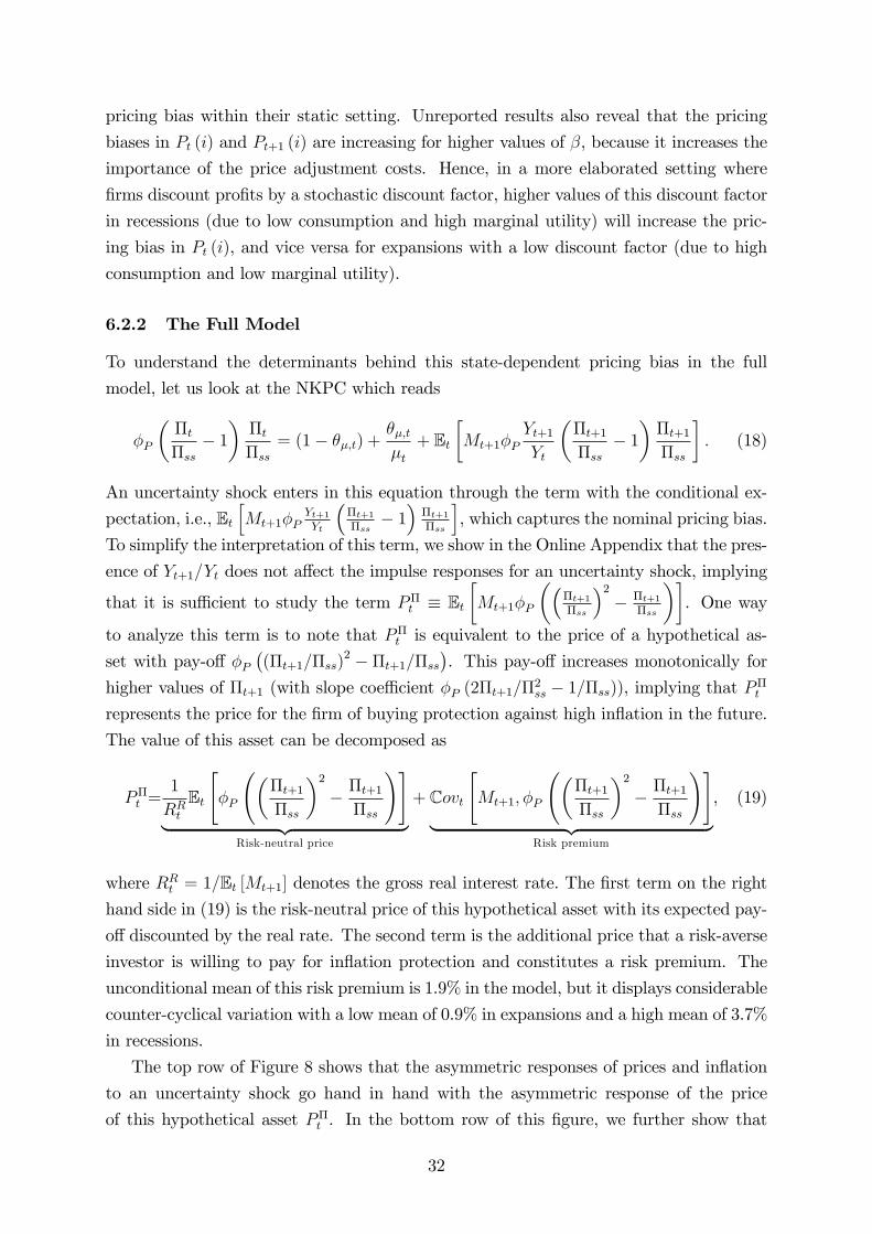
pricing bias within their static setting. Unreported results also reveal that the pricing

biases in Pt (i) and Pt+1 (i) are increasing for higher values of , because it increases the

importance of the price adjustment costs. Hence, in a more elaborated setting where

rms discount prots by a stochastic discount factor, higher values of this discount factor

in recessions (due to low consumption and high marginal utility) will increase the pric-

ing bias in Pt (i), and vice versa for expansions with a low discount factor (due to high

consumption and low marginal utility).

6.2.2 The Full Model

To understand the determinants behind this state-dependent pricing bias in the full

model, let us look at the NKPC which reads

P

tss

1tss

= (1 ;t) +;tt+ Et

Mt+1P

Yt+1Yt

t+1ss

1t+1ss

: (18)

An uncertainty shock enters in this equation through the term with the conditional ex-

pectation, i.e., EthMt+1P

Yt+1Yt

t+1ss

1t+1ss

i, which captures the nominal pricing bias.

To simplify the interpretation of this term, we show in the Online Appendix that the pres-

ence of Yt+1=Yt does not a¤ect the impulse responses for an uncertainty shock, implying

that it is su¢ cient to study the term Pt EtMt+1P

t+1ss

2 t+1

ss

. One way

to analyze this term is to note that Pt is equivalent to the price of a hypothetical as-

set with pay-o¤ P(t+1=ss)

2 t+1=ss. This pay-o¤ increases monotonically for

higher values of t+1 (with slope coe¢ cient P (2t+1=2ss 1=ss)), implying that Pt

represents the price for the rm of buying protection against high ination in the future.

The value of this asset can be decomposed as

Pt =1

RRtEt

"P

t+1ss

2 t+1ss

!#| z

Risk-neutral price

+ Covt

"Mt+1; P

t+1ss

2 t+1ss

!#| z

Risk premium

, (19)

where RRt = 1=Et [Mt+1] denotes the gross real interest rate. The rst term on the right

hand side in (19) is the risk-neutral price of this hypothetical asset with its expected pay-

o¤ discounted by the real rate. The second term is the additional price that a risk-averse

investor is willing to pay for ination protection and constitutes a risk premium. The

unconditional mean of this risk premium is 1.9% in the model, but it displays considerable

counter-cyclical variation with a low mean of 0.9% in expansions and a high mean of 3.7%

in recessions.

The top row of Figure 8 shows that the asymmetric responses of prices and ination

to an uncertainty shock go hand in hand with the asymmetric response of the price

of this hypothetical asset Pt . In the bottom row of this gure, we further show that

32

Figure 8: New Keynesian Model: Determinants of the Upward Pricing BiasThis gure shows the impulse response functions following a positive one-standard deviation uncer-tainty shock (i.e. ;t = 1) in the New Keynesian model using the estimates in column (1) of Ta-ble 4. The responses are shown for strong expansions and deep recessions. The risk premium in

Pt is given by CovtMt+1; P

t+1ss

2 t+1

ss

, the ination volatility risk premium is dened as

CovtMt+1; P

t+1ss

2, and ination volatility is measured by Vt [t+1]. The responses of prices and

ination are shown in percentage deviations, whereas the other response are scaled by 100 and shown inabsolute deviations.

1 2 3 40

0.005

0.01

0.015

0.02

0.025

0.03

Model: Strong Expansions Model: Deep Recessions

1 2 3 4

­0.01

0

0.01

0.02

1 2 3 4

­1

0

1

2

3

4

1 2 3 40

0.5

1

1.5

2

2.5

3

3.5

1 2 3 40

1

2

3

4

5

6

7

1 2 3 40

0.2

0.4

0.6

0.8

1

10 ­4

these asymmetric responses in Pt are generated by the risk premium. The dominating

term in this risk premium is the squared term for ination, i.e., CovtMt+1; P

t+1ss

2,

which can be interpreted as an ination volatility risk premium. To understand why

this conditional covariance displays larger responses in recessions than in expansions, we

exploit two insights from the simplied two-period setting discussed above.

First, the ination volatility risk premium is closely related to the amount of ination

volatility, which increases the pricing bias as shown in Section 6.2.1. One way to mea-

sure the degree of ination volatility is to compute the conditional variance of ination

Vt [t+1]. We nd that the mean of Vt [t+1] in recessions is 19% higher than the mean

in expansions, showing that recessions in the New Keynesian model are characterized by

much more ination volatility than expansions.22 The process for stochastic volatility

22This is consistent with empirical evidence, both when measuring ination volatility by the interquar-

33

a;t contributes in two important ways to generate this asymmetry. First, recessions have

a higher value of a;t than expansions, implying that an equal-size preference shock a;t+1is expected to have a larger impact on ination in recessions than in expansions. Second,

the bottom right chart in Figure 8 shows that an uncertainty shock increases ination

volatility by more in recessions than in expansions.

Second, another key driver of the ination volatility risk premium is the dynamics

of the stochastic discount factor Mt+1. In the New Keynesian model, we nd that the

realized values of Mt+1 have a higher level in recessions than in expansions due to lower

consumption and higher marginal utility than in expansions. As shown in Section 6.2.1,

a higher value of the discount factor increases the weight in the prot function to the

intertemporal smoothing of the pricing bias, and as a result helps to generate a larger

upward pricing bias in recessions than in expansions.

Thus, the economic intuition behind the state-contingent upward nominal pricing bias

is as follows. With price stickiness as in Rotemberg (1982), rms can reset their prices in

every period but face costs when doing so. In this multiperiod setting, ination volatility

a¤ects the current price, because it is optimal for rms to set higher prices after an

uncertainty shock to avoid large expensive future increases in prices. Two e¤ects help to

make this pricing bias stronger in recessions than expansions. First, ination volatility

is higher in recessions than in expansions. Second, rms discount future prots by the

stochastic discount factor, which has a higher level in recessions than in expansions. This

implies that rms assign more weight to future prots, which also helps to increase their

pricing bias by more in recessions than in expansions.

6.3 External Validation of the Key Mechanism

The reduction in real activity following uncertainty shocks implies that wages and the

rental rate of capital also fall in the New Keynesian model (not shown). With higher

prices, we therefore see a higher price markup, which Fernández-Villaverde et al. (2015)

and Basu and Bundick (2017) show is the key driver behind the real e¤ects of uncertainty

shocks in the model, although Born and Pfeifer (2020) challenge this e¤ect. Our nding

that the upward nominal pricing bias is state-contingent helps to clarify how this channel

works across the business cycle. This is illustrated in Figure 9, which shows that the

price markup increases by more in recessions than in expansions (top chart to the left),

and that this di¤erence disappears when we omit the state-contingent nominal pricing

bias (top chart to the right).

Thus, a simple way to validate the key mechanism in the New Keynesian model for

generating asymmetric responses to an uncertainty shock is to explore if the price markup

tile range of the one quarter ahead forecast of ination in the Survey of Professional Forecasts or by aGARCH(1,1) model applied to the residuals of an autoregression with four lags for CPI ination.

34

in the US displays asymmetric e¤ects across the business cycle. We implement this

external validation of the model by extending the IVAR with the price markup, which

we measure by the inverse of the labor share in the business sector as in Fernández-

Villaverde et al. (2015). Similar to our baseline analysis in Section 2, we allow the

responses of the price markup and the other variables in the IVAR to change across the

business cycle. The middle row in Figure 9 reports the median target responses for the

price markup in expansions and recessions alone with their 90 percent condence bands.

The responses in recessions are much larger than in expansions, in particular after the

rst four quarters. This is seen clearly from the bottom left chart in Figure 9, which

shows that the median target response in recessions is substantially above the response

in expansions. The bottom right chart shows that the di¤erences in these median target

responses are signicant at the 90% level. Thus, the dynamic responses of the price

markup in the US appear to be consistent with the predictions from the New Keynesian

model, which leaves further support for the presence of a state-contingent upward nominal

pricing bias.23

7 Conclusion

This paper employs a nonlinear VAR and a non-recursive identication strategy using a

combination of narrative, correlation, and sign restrictions to show that the real e¤ects

of an uncertainty shock are stronger when growth is low (as in recessions) than when

growth is high (as in expansions). An estimated medium-scale New Keynesian model

approximated to third order around the risky steady state goes a long way in reproducing

these state-dependent impulse responses to an uncertainty shock. The key mechanism is

that rms display a stronger nominal upward pricing bias in recessions than in expansions,

as rms face more ination uncertainty and have a higher value of the discount factor in

these states of the business cycle. This leads rms to post higher prices through higher

markups in recessions when compared to expansions, which then worsens the real e¤ects

of an uncertainty shock in recessions. This prediction is supported by a nonlinear VAR

that produces a larger response in an empirical measure of the price markup in recessions

than in expansions following an uncertainty shock.

23In the Online Appendix, we further show that the only channel that eliminates the state-dependentresponses of the price markup to an uncertainty shock is the nominal upward pricing bias channel.

35

Figure9:PriceMarkup

Thisgureshowsthegeneralizedimpulseresponsefunctionsforthepricemarkupinpercenttoaone-standarddeviationuncertaintyshock.Thetoprowshows

theresponsesinthebaselineNew

Keynesianmodel(totheleft)andwhenomittingthenominalpricingbias(totheright)usingtheestimatesincolumn(1)of

Table4.Thechartsinthemiddlerowshowthemediantarget(MT)reponsesintheextendedIVARduringstrongexpansions(totheleft)anddeeprecessions(to

theright)alongwiththe90%condencebands.Atthebottomrow,thedi¤erencesinthemediantargetresponsesintheIVARarereported(totheleft),while

thedi¤erenceintheseresponsesbetweendeeprecessionsandstrongexpansionsareshowntotherightalongwiththebootstrapped68%and90%condence

bands.

24

68

1012

1416

1820

0

0.050.

1

0.15

New

Key

nesi

an m

odel

: Bas

elin

e

REC

EXP

24

68

1012

1416

1820

0

0.050.

1

0.15

New

Key

nesi

an m

odel

: No

nom

inal

pric

ing

bias

REC

EXP

24

68

1012

1416

1820

­0.10

0.1

0.2

0.3

IVAR

: Stro

ng E

xpan

sion

s (E

XP)

90%

con

f. ba

nd: E

XP

24

68

1012

1416

1820

­0.10

0.1

0.2

0.3

IVAR

: Dee

p Re

cess

ions

(REC

)

90%

con

f. ba

nd: R

EC

24

68

1012

1416

1820

­0.10

0.1

0.2

IVAR

: The

MT

resp

onse

sIV

AR: D

iffer

ence

in M

T re

spon

ses

05

1015

200

0.1

0.2

0.3

36

References

Alessandri, P. and Mumtaz, H. (2019), Financial regimes and uncertainty shocks, Jour-

nal of Monetary Economics 101, 3146.

Andreasen, M. M. (2012), On the e¤ects of rare disasters and uncertainty shocks for risk

premia in non-linear dsge models, Review of Economic Dynamics 15(3), 295316.

Andreasen, M. M., Fernández-Villaverde, J. and Rubio-Ramírez, J. F. (2018), The

pruned state-space system for non-linear dsge models: Theory and empirical ap-

plications, Review of Economic Studies 85(1), 149.

Andreasen, M. M. and Jørgensen, K. (2020), The importance of timing attitudes in

consumption-based asset pricing models, Journal of Monetary Economics 111, 95117.

Antolín-Díaz, J. and Rubio-Ramírez, J. F. (2018), Narrative sign restrictions, American

Economic Review 108(10), 28022829.

Aruoba, S., Bocola, L. and Schorfheide, F. (2017), Assessing DSGE Model Nonlineari-

ties, Journal of Economic Dynamics & Control 83, 3454.

Barrero, J. M. and Bloom, N. (2020), Economic uncertainty and recovery, JacksonHole Economic Policy Symposium Paper, August.

Barsky, R., Juster, F., Kimball, M. and Shapiro, M. (1997), Preference parameters and

behavioral heterogeneity: An experimental approach in the health and retirement

study, Quarterly Journal of Economics 112(2)((2)), 537579.

Basu, S. and Bundick, B. (2017), Uncertainty shocks in a model of e¤ective demand,

Econometrica 85(3), 937958.

Basu, S. and Bundick, B. (2018), Uncertainty shocks in a model of e¤ective demand:

Reply, Econometrica 86(4), 15271531.

Bianchi, F., Kung, H. and Tirskikh, M. (2019), The origins and e¤ects of macroeconomic

uncertainty, Duke University and London Business School, available athttps://sites.google.com/view/francescobianchi/home.

Binning, A. (2013), Solving second and third-order approximations to dsge models: A

recursive sylvester equation solution, Norges Bank Working Paper No. 18.

Binsbergen, J. H. V., Fernández-Villaverde, J., Koijen, R. S. and Rubio-Ramírez, J.

(2012), The term structure of interest rates in a dsge model with recursive prefer-

ences, Journal of Monetary Economics 59(7), 634½U648.

37

Bloom, N. (2009), The impact of uncertainty shocks, Econometrica 77(3), 623685.

Bloom, N. (2014), Fluctuations in uncertainty, Journal of Economic Perspectives

28(2), 153176.

Born, B. and Pfeifer, J. (2014), Risk matters: The real e¤ects of volatility shocks:

Comment, American Economic Review 104(12), 42314239.

Born, B. and Pfeifer, J. (2020), Uncertainty-driven business cycles: assessing the markup

channel, Quantitative Economics forthcoming.

Cacciatore, M. and Ravenna, F. (2020), Uncertainty, wages, and the business cycle,

Economic Journal forthcoming.

Caggiano, G., Castelnuovo, E. and Groshenny, N. (2014), Uncertainty shocks and unem-

ployment dynamics: An analysis of post-wwii u.s. recessions, Journal of Monetary

Economics 67, 7892.

Coeurdacier, N., Rey, H. and Winant, P. (2011), The Risky Steady State, American

Economic Review: Papers & Proceedings 101(3), 398½U401.

Collard, F. and Juillard, M. (2001a), Accuracy of stochastic perturbation methods: The

case of asset pricing models, Journal of Economic Dynamics and Control 25(6-7), 979999.

Collard, F. and Juillard, M. (2001b), A higher-order taylor expansion approach to simula-

tion of stochastic forward-looking models with an application to a nonlinear phillips

curve model, Computational Economics 17(2-3), 125139.

de Groot, O. (2013), Computing The Risky Steady State of DSGE Models, Economic

Letter 120(3), 566569.

de Groot, O. (2016), What order? perturbation methods for stochastic volatililty as-

set pricing and business cycle models, Centre for Dynamic MacroeconomicAnalysis Working Paper No. 201606.

de Groot, O., Richter, A. W. and Throckmorton, N. A. (2018), Uncertainty shocks in a

model of e¤ective demand: Comment, Econometrica 86(4), 15131526.

Diercks, A. M., Hsu, A. and Tamoni, A. (2020), When it rains it pours: Cascading

uncertainty shocks, available at https://andreatamoni.meltinbit.com/.

Epstein, L. and Zin, S. (1989), Substitution, risk aversion, and the temporal behavior of

consumption and asset returns: A theoretical framework, Econometrica 57(4), 937969.

38

Fernández-Villaverde, J. and Guerron-Quintana, P. (2020), Uncertainty shocks and busi-

ness cycle research, Review of Economic Dynamics forthcoming.

Fernández-Villaverde, J., Guerrón-Quintana, P., Kuester, K. and Rubio-Ramírez, J. F.

(2015), Fiscal volatility shocks and economic activity, American Economic Review

105(11), 33523384.

Fernández-Villaverde, J., Guerrón-Quintana, P., Rubio-Ramírez, J. F. and Uribe, M.

(2011), Risk matters: The real e¤ects of volatility shocks, American Economic

Review 101, 25302561.

Fry, R. and Pagan, A. (2011), Sign restrictions in structural vector autoregressions: A

critical review, Journal of Economic Literature 49(4), 938960.

Guerron-Quintana, P. A., Khazanov, A. and Zhong, M. (2021), Nonlinear Dynamic

Factor Models, Working Paper pp. 134.

Hamilton, J. D. (2018), Why you should never use the hodrick-prescott lter, Review of

Economics and Statistics 100, 831843.

King, R. G., Plosser, C. I. and Rebelo, S. T. (2002), Production, growth and business

cycles: Technical appendix, Computational Economics 20, 87116.

Koop, G., Pesaran, M. and Potter, S. (1996), Impulse response analysis in nonlinear

multivariate models, Journal of Econometrics 74(1), 119147.

Levintal, O. (2017), Fifth-order perturbation solution to dsge models, Journal of Eco-

nomic Dynamics and Control 80, 116.

Ludvigson, S. C., Ma, S. and Ng, S. (2019), Uncertainty and business cycles: Exogenous

impulse or endogenous response?, American Economic Journal: Macroeconomics

forthcoming.

Rotemberg, J. J. (1982), Monopolistic price adjustment and aggregate output, Review

of Economic Studies 49, 517531.

Rubio-Ramírez, J. F., Waggoner, D. F. and Zha, T. (2010), Structural vector autore-

gressions: Theory of identication and algorithms for inference, Review of Economic

Studies 77, 665696.

Rudebusch, G. D. and Swanson, E. T. (2012), The bond premium in a dsge model

with long-run real and nominal risks, American Economic Journal: Macroeconomics

4(1), 105143.

39

Salgado, S., Guvenen, F. and Bloom, N. (2019), Skewed Business Cycles, NBER Work-

ing Paper (No. 26565).

Schmitt-Grohe, S. and Uribe, M. (2004), Solving dynamic general equilibrium models

using a second-order approximation to the policy function, Journal of Economic

Dynamics and Control 28, 755775.

Swanson, E. T. (2018), Risk aversion, risk premia, and the labor margin with generalized

recursive preferences, Review of Economic Dynamics 28, 290321.

Weil, P. (1990), Nonexpected utility in macroeconomics, Quarterly Journal of Eco-

nomics 105(1), 2942.

Wu, J. C. and Xia, F. D. (2016), Measuring the macroeconomic impact of monetary pol-

icy at the zero lower bound, Journal of Money, Credit, and Banking 48(2-3), 253291.

40

Online Appendix (not for publication):Why Does Risk Matter More in Recessions than in

Expansions?

Martin M. Andreasen∗ Giovanni Caggiano†

Efrem Castelnuovo‡ Giovanni Pellegrino§

1 The Interacted VAR

1.1 Computing the Generalized Impulse Response Functions

The algorithm for computing the generalized impulse response functions (GIRFs) follows the steps suggested by Koop,Pesaran & Potter (1996), and it is designed to simulate the effects of an orthogonal structural shock as in Kilian andVigfusson (2011). The idea is to compute the empirical counterpart of the theoretical GIRFY(h, δ,ωt−1) of the vectorof endogenous variables Yt, h periods ahead, for a given initial condition ωt−1 = Yt−1, ...,Yt−L. Below, we use thenotation that L is the number of lags in the IVAR, and δunc is size of the structural shock hitting at time t. FollowingKoop et al. (1996), such GIRF can be expressed as

GIRFY(h, δunc,ωt−1) = E[Yt+h |δunc,ωt−1] − E[Yt+h |ωt−1] , (1)

where E[·] is the expectation operator, and h = 0, 1, ...,H indicates the horizons at which the GIRF are computed. Wecompute the GIRFs as follows:

1. We pick a matrix B among the set of retained matrices that satisfy our identifying restrictions, as stated in the mainpaper;

2. Conditioning on a ωt−1 and the IVAR, we randomly extract (with repetition) residualsηst+h

500

s=1

19

h=0from d(0, Ω),

where Ω is the estimated covariance matrix and d(·) is the empirical distribution of the residuals. We use these residualsto simulate 500 realizations of

Yst+h|ωt−1

500

s=1for h = 0, 1, ..., 19;

3. Given the residualsηst+h

500

s=1

19

h=0from step 2, we transform them to the structural shocks by using the relation est =

B−1ηst . At the position in est which corresponds to the uncertainty shock, denoted esunc,t, we add the quantity δunc.

Then we transform the structural shocks back to the IVAR residuals using Bes

t = ηst , which we use to computeYst+h|δ,ωt−1

500

s=1;

4. We then estimate the GIRFs conditional on ωt−1 as GIRFBY(h, δunc,ωt−1) = 1500

∑500s=1

(Yst+h|δunc,ωt−1 −Ys

t+h|ωt−1

)for h = 0, 1, ..., 19;

∗Aarhus University, CREATES, and the Danish Finance Institute. Email: mandreasen@econ.au.dk.†Monash University and the University of Padova. Email: giovanni.caggiano@monash.edu.‡The University of Melbourne and the University of Padova. Email: efrem.castelnuovo@gmail.com.§Aarhus University. Email: gpellegrino@econ.au.dk.

1

5. We repeat steps 2-4 for all the initial conditions ωt−1 that belong to two subsets. An initial condition ωt−1 =Yt−1, ...,Yt−L is classified to belong to “deep contractions”if ∆ lnGDPt−1 is in the bottom decile of the quarter-on-quarter GDP growth rate for the empirical distribution and to "strong expansions" if ∆ lnGDPt−1 is in the topdecile of the quarter-on-quarter GDP growth for the rate empirical distribution;

6. We take the average of the GIRFs obtained in step 5 over the initial states that belong to either deep contractions orstrong expansions, i.e., GIRFBY(h, δunc,Ω

contr .t−1 ) and GIRFBY(h, δunc,Ω

exp.t−1 ), respectively;

7. We repeat steps 2-6 for each matrix B that satisfies our identifying restrictions to obtain the identified set.

To plot a summary state-dependent GIRF out of the identified set, we use the Median Target (MT) response proposedby Fry & Pagan (2011) on our IVAR. That is, we select GIRFs that correspond to the single B which minimizes the distanceto the responses implied by the median of the identified set in recessions and expansions. This matrix is denoted BMT .As mentioned in our paper, we compute confidence bands for the MT GIRFs by running a residual-based bootstrap. Thatis, we use a residual-based bootstrap of the IVAR to simulate R = 1, 000 samples of the same lenght as in our empiricalsample.1 Then, for each simulated sample, we estimate the IVAR and compute the GIRFs for an uncertainty shock asoutlined above. When implementing this procedure, the initial conditions and the covariance matrix for the IVAR residualsnow depend on the particular dataset r, i.e., ωrt−1 and Ωr

t . This means that in the procedure rather than using the BMT ,we use the rotation QMT which corresponds to the MT response, i.e., we use Br,MT = PsQMT with Ps being the uniquelower-triangular Cholesky factor associated to Ωr

t , i.e., Ωrt = PrPr′.

In the main paper we only show median target responses and a test for their difference that (only) accounts for estimation(or sampling) uncertainty by using this residual-based bootstrap. Figure 1 instead shows our identified set for the state-dependent responses and their difference for the whole identified set, which (only) accounts for model uncertainty, i.e., theuncertainty related to all the responses in the identified set. As the results show, all models belonging to the identified setsuggest a stronger response of real activity to an uncertainty shock in recessions. This means that model uncertainty is notan important source of uncertainty as regards the difference of our state-dependent median target responses.

1The bootstrap used is similar to the one used by Christiano, Eichenbaum, and Evans (1999) (see their footnote 23). The code discards theexplosive artificial draws to be sure that exactly 1,000 draws are used. In our simulations, this happens a negligible fraction of times.

2

Figure 1: Excess Effects of Uncertainty Shock in Recessions: Model UncertaintyThis figure in the first two columns shows the identified set for the generalized impulse response functions (GIRFs) to a positive one-standarddeviation shock to uncertainty in strong expansions (first column) and deep recessions (second column) as estimated by the IVAR on historical USdata from 1962Q3 to 2017Q4. The set for strong expansions are constructed as follows: i) for an accepted draw of B, the dates are located wherethe economy is in a strong expansion, ii) at these dates, the GIRFs are computed using (1) and the average GIRF across these dates are reported.A similar procedure is used for deep recessions. Each GIRF is computed using Monte Carlo integration with 500 draws. The solid (dashed)lines report the median target impulse responses in strong expansions (deep recessions) when computed as suggested by Fry & Pagan (2011).The number of retained draws for identifying uncertainty shocks is 187 out a total of 500,000 draws. The third column shows the differencesbetween the median target (MT) responses between deep recessions and strong expansions when only accounting for model uncertainty. Greybands represent the identified set for the difference of responses. All responses are shown in percentage deviations, except for the policy ratewhere changes in percentage points are reported.

5 10 15 20

0

0.05

0.1

0.15

Strong Expansions (EXP)

5 10 15 20­0.4

­0.2

0

0.2

5 10 15 20­0.3

­0.2

­0.1

0

0.1

5 10 15 20

­1

0

1

5 10 15 20­0.6

­0.4

­0.2

0

5 10 15 20­0.4­0.2

00.20.40.6

5 10 15 20­0.4

­0.2

0

0.2

5 10 15 20

0

0.05

0.1

0.15

Deep Recessions (REC)

5 10 15 20­0.4

­0.2

0

0.2

5 10 15 20­0.3

­0.2

­0.1

0

0.1

5 10 15 20

­1

0

1

5 10 15 20­0.6

­0.4

­0.2

0

5 10 15 20­0.4­0.2

00.20.40.6

5 10 15 20­0.4

­0.2

0

0.2

5 10 15 20

­0.01

0

0.01

REC­EXP

5 10 15 20­0.1

­0.05

0

0.05

5 10 15 20­0.06

­0.04

­0.02

0

5 10 15 20

­0.6

­0.4

­0.2

0

5 10 15 20

­0.2

­0.1

0

5 10 15 20

­0.4

­0.2

0

5 10 15 20

­0.2

­0.1

0

3

1.2 Validation of the Empirical Identification Under the DGP of the Model

We have adopted a mix of Narrative Sign Restrictions (NSR) and standard Sign Restrictions (SR) to identify uncertaintyshocks from our estimated IVAR. This section checks whether this approach can be validated under the DGP of the DSGEmodel we adopt.The DSGE model we use features an endogenous measure of financial uncertainty, a model-consistent VXO, which

responds to four shocks, i.e., a first-moment technology shock, a first-moment cost-push shock, a first-moment preferenceshock, and a second-moment preference shock, which is the uncertainty shock.We conduct a Monte Carlo exercise with artificial data simulated using our DSGE model to assess our empirical

identification strategy. The model is solved with our proposed third-order approximation around the risky steady state,which allows all shocks, including the uncertainty shock, to have state-dependent effects. We conduct a population analysisand simulate a sample of 3,000 observations with the model using the benchmark estimate of the structural parameters asprovided in the paper.2 We then estimate an IVAR and produce impulse responses to uncertainty shocks by adopting ouridentification strategies, i.e., the baseline mix of NSR and SR. Consistently with what is done to identify the dates in ourbaseline analysis, we select the dates with the biggest spikes in the VXO and combine them with the biggest spikes in thevolatility process.3 ,4 Similarly to our baseline analysis, we require the realizations of our identified uncertainty shocks to belarger than the median value of the empirical density of the uncertainty shocks in the selected dates.5 As in the baseline,we also require a negative on-impact response of real GDP, investment, consumption, and hours to an uncertainty shock.In the paper, we verify the ability of these restrictions in the IVAR to replicate the impulse responses in the DSGE modelby the IVAR MT responses. Figures 2 and 3 below supplement this analysis by showing the identified set for the responsesin the IVAR and the state-dependent MT responses from the IVAR.

2Note that our DSGE model with four shocks does not imply stochastic singularity in the IVAR with seven variables because the DSGE modelis solved with nonlinear terms.

3Although the word "Narrative" loses its meaning for an exercise based on data simulated from a model, the proposed exercise wants toresemble the identification strategy we used in our baseline analysis where uncertainty shocks are identified using information from the VXObiggest spikes coupled with an estimate of the economy-wide stochastic volatility process (given by the LMN financial volatility indicator). Theassumption at the basis of this exercise is that the econometrician perfectly knows the economy-wide stochastic volatility process at the basis offinancial volatility, rather than knowing its estimate.

4We select the dates that at the same time correspond to the biggest 1.5% among the VXO spikes and the biggest 1.5% among the stochasticvolatility process spikes. This threshold seems appropriate as it guarantees that enough responses are retained and that selected dates areinformative enough to identify the uncertainty shocks. We retained 46 draws out of 500,000 rotations.

5Similarly to our baseline analysis, we impose that the correlation between the series of identified uncertainty shocks and (model-implied)stock market returns be smaller than the median value of the empirical density of the correlation coeffi cients for all draws.

4

Figure 2: Simulation Exercise for the IVAR: IRFs to Uncertainty ShocksThis figure shows the identified set for the generalized impulse response functions (GIRFs) in the IVAR to a positive one-standard deviation shockto uncertainty in strong expansions (to the left) and deep recessions (to the right) on a simulated sample of 3, 000 draws from the New KeynesianDSGE model using the estimates in column (1) of Table 3 as given in the paper. The set for strong expansions are constructed as follows: i) foran accepted draw of B, the dates are located where the economy is in a strong expansion, ii) at these dates, the GIRFs are computed using (1)and the average GIRF across these dates are reported. A similar procedure is used for deep recessions. Each GIRF is computed using MonteCarlo integration with 500 draws. The solid (dashed) lines report the median target impulse responses in strong expansions (deep recessions)when computed as suggested by Fry & Pagan (2011). The marked solid lines denote the true responses in the DSGE model. All responses areshown in percentage deviations, except for the policy rate where changes in percentage points are reported.

2 4 6 8 10 12 14 16 18 200

0.2

0.4

Strong Expansions (EXP)

2 4 6 8 10 12 14 16 18 20

­0.4

­0.2

0

2 4 6 8 10 12 14 16 18 20

­0.2

­0.1

0

2 4 6 8 10 12 14 16 18 20

­1

­0.5

0

2 4 6 8 10 12 14 16 18 20­0.3

­0.2

­0.1

0

2 4 6 8 10 12 14 16 18 20

­0.2­0.1

00.1

2 4 6 8 10 12 14 16 18 20

­0.15­0.1

­0.050

2 4 6 8 10 12 14 16 18 200

0.2

0.4

Deep Recessions (REC)

2 4 6 8 10 12 14 16 18 20

­0.4

­0.2

0

2 4 6 8 10 12 14 16 18 20

­0.2

­0.1

0

2 4 6 8 10 12 14 16 18 20

­1

­0.5

0

2 4 6 8 10 12 14 16 18 20­0.3

­0.2

­0.1

0

2 4 6 8 10 12 14 16 18 20

­0.2­0.1

00.1

2 4 6 8 10 12 14 16 18 20

­0.15­0.1

­0.050

5

Figure 3: Simulation Exercise for the IVAR: MT responsesThis figure shows the identified set for the generalized impulse response functions (GIRFs) in the IVAR to a positive one-standard deviationshock to uncertainty in strong expansions and deep recessions on a simulated sample of 3, 000 draws from the New Keynesian DSGE model usingthe estimates in column (1) of Table 3 of the paper. The set for strong expansions are constructed as follows: i) for an accepted draw of B, thedates are located where the economy is in a strong expansion, ii) at these dates, the GIRFs are computed using (1) and the average GIRF acrossthese dates are reported. A similar procedure is used for deep recessions. Each GIRF is computed using Monte Carlo integration with 500 draws.The solid (dashed) lines report the median target impulse responses in strong expansions (deep recessions) when computed as suggested by Fry& Pagan (2011). All responses are shown in percentage deviations, except for the policy rate where changes in percentage points are reported.

5 10 15 200

0.1

0.2

0.3

0.4

VXO

5 10 15 20­0.4

­0.3

­0.2

­0.1

0Output

5 10 15 20

­0.2

­0.15

­0.1

­0.05

0Consumption

5 10 15 20­1

­0.5

0Investment

5 10 15 20

­0.2

­0.15

­0.1

­0.05

0Hours

5 10 15 20­0.1

­0.05

0

0.05

0.1Prices

5 10 15 20

­0.06

­0.04

­0.02

0

Policy rate

6

1.3 Robustness checks for the nonlinear SVAR model

No sign restrictions. Among the baseline set of restrictions for our IVAR we also include traditional sign restrictions,and specifically we impose a non-positive impact response of GDP, investment, consumption, and hours to a (positive)uncertainty shock. These sign restrictions, which we impose to sharpen the identification of the set of admissible rotations,are supported by a large number of theoretical and empirical analyses on the business cycle effects of uncertainty shocks(for a survey, see Bloom (2014)). Figure 4 shows the IVAR results when omitting the additional sign restrictions (SR).Figure 1 reveals that these sign restrictions help to narrow the identified set, but hardly affect the estimated median targetmodel, which is the focus of our paper.Control for skewness shocks. Several recent studies investigate the role of skewness shocks as a driver of business

cycle fluctuations (see, e.g., Salgado, Guvenen & Bloom (2019)). In particular, skewness shocks may be behind the findingsof the emerging growth-at-risk literature (see, e.g., Adrian, Boyarchenko & Giannone (2019)). These considerations raisethe concern that our baseline identification strategy may confound second and third-moment shocks. As follows we performan exercise that aims to control for financial skewness shocks when identifying financial uncertainty shocks.We first construct a measure of realized financial skewness as the monthly skewness of daily SP500 returns.6 We

transform our monthly measure of skewness to make it comparable to the CBOE SKEW index. Let St be the month-tskewness, then we define a new index Skewt = 100 − 10 · St. Hence if Skew < (>)100 the distribution of stock marketreturns is right (left) skewed.7 We take the quarterly average of such financial skewness index, which we log-transform. Thisvariable is then added to the endogenous variables of our IVAR (a similar approach is applied in Salgado et al. (2019)). Toensure that skewness shocks do not disrupt the identified uncertainty shocks, we adopt the following identification strategy.First, we do not impose any timing restrictions on the skewness-uncertainty contemporaneous relationship, as it is notneeded when using narrative sign restrictions. Second, in addition to our baseline set of restrictions, we follow Furlanetto,Ravazzolo & Sarferaz (2019) and impose that a financial uncertainty (skewness) shock generates an on-impact responseof the financial uncertainty-skewness ratio that is bigger (smaller) than one.8 Third, we also impose that the skewnessshock and the uncertainty shock have a positive on-impact effect on the uncertainty and skewness proxies, respectively, toensure that the ratios that we constrain are positive. The results for this robustness check are provided in Figure 5, whichshows that our baseline results are robust to controlling for skewness shocks. One way to clearly see this is from the secondcolumn in Figure 5, where the difference in the MT-responses are well within the confidence bands for the difference in theMT-responses in the baseline IVAR that does not control for skewness shocks.Control for first-moment financial shocks. Our baseline IVAR model does not feature any measure of financial

stress such as credit spreads. This choice is consistent with the Basu & Bundick (2017) model, where first-moment financialshocks do not have any role due to the frictionless financial markets hypothesis. However, controlling for credit spreads andfirst-moment financial shocks is important for at least three reasons. First, credit spreads have large predictive power for theUnited States’real activity (see Gilchrist & Zakrajšek (2012)), so they may represent a relevant omitted variable. Second,as advocated by recent studies, financial frictions and credit spreads are important for the transmission of uncertaintyshocks (Gilchrist, Sim & Zakrajšek (2014); Alfaro, Bloom & Lin (2019); Arellano, Bai & Kehoe (2019)). Third, as financialstress and financial uncertainty go hand-in-hand, the use of a credit spread indicator may help to improve the identificationof financial uncertainty shocks, avoiding confounding second-moment financial shocks with first-moment financial shocks.Our narrative sign restrictions approach has the advantage of not imposing any timing restrictions on the credit spread-uncertainty contemporaneous relationship.To disentangle uncertainty shocks from first-moment financial shocks, first, we augment our baseline IVAR vector of

endogenous variables with a measure of credit spread meant to capture stress in financial markets, i.e., the differencebetween the BAA yield and the AAA one. Second, as with the previous check for skewness shocks, we add some ratioconstraints to our baseline set of restrictions following the approach proposed by Furlanetto et al. (2019). They identifyfinancial and uncertainty shocks using a sign restrictions approach which features, among others, restrictions on ratios ofthe impulse responses of proxies for first and second-moment financial indicators. Following their approach, we impose thata financial uncertainty (credit spread) shock generates an on-impact response of the financial uncertainty-credit spread ratio

6We use the series SP500 Composite price index, daily data, downloaded from Datastream (Code S&PCOMP(PI)). The series starts in 1964.7The CBOE implied skewness (SKEW) index starts only in 1990. We do not splice our monthly series with the SKEW index because,

differently than with realized volatility and the VXO index of implied volatility, their behavior in the common sample is quite different (theircorrelation coeffi cient is only 0.05).

8To implement this identification strategy, we standardized the financial skewness index to impose the same standard deviation of ouruncertainty proxy.

7

that is bigger (smaller) than one.9 As earlier, we also impose that the credit spread shock and the uncertainty shock havea positive on-impact effect on the uncertainty and the credit spread proxies, respectively, to ensure that the ratios that weconstrain are positive. Figure 6 reports the findings from this robustness check. The impulse responses are state-dependentand their difference is very similar to the baseline difference. Hence, the figure suggests that our baseline results are robustto controlling for first-moment financial shocks.Sample from 1987. In our baseline analysis we follow Bloom (2009) and Ludvigson, Ma & Ng (2019) and use a long

sample that starts in the ’60s, in particular in 1962Q3 like in Bloom (2009). For the IVAR, a long sample featuring severalrecessions is advisable because it sharpens our inference for the state-dependent responses. As a robustness check for ourmain finding, in Figure 7 we report that the results from an IVAR estimated on a sample starting in 1987Q1, i.e. when theVXO implied-volatility index is available. In performing this exercise we lose 8 out of our 18 event restrictions in Table 1of the paper. This notwithstanding, Figure 7 shows that we still find large differences in the impulse response functionsacross expansions and recessions. From the second column in this figure, we actually find that these differences for severalvariables are outside the confidence bands for the corresponding responses in the baseline IVAR on the long sample andhence larger than the responses reported in the main paper.10

Alternative control for unconventional monetary policy. In the baseline analysis, we account for unconventionalmonetary policy during the zero lower bound period from 2008Q4 to 2015Q4 by using the Wu and Xia’s (2016) shadowrate instead of the federal funds rate in this period. But the estimate in Wu and Xia is admittedly only one estimateof the shadow rate (see, e.g., Bauer & Rudebusch (2016) and Krippner (2020), who find that estimated shadow ratesare quite sensitive to several modeling assumptions). Hence, we conduct an alternative exercise where we use the federalfunds rate along with the 10-year treasury zero-coupon yield in our IVAR as another way to account for unconventionalmonetary policy. The rational for including the 10-year interest rate is that it may capture effects of quantitative easingand forward guidance even when the short rate is at the lower bound. Figure 8 shows that the impulse responses for thisalternative version of our IVAR are virtually identical to our baseline estimate, showing that the specific way we accountfor unconventional monetary policy is not essential for our main finding.PMI as an alternative conditioning variable. Our baseline IVAR features an interaction term of uncertainty —

i.e., the variable we shock —with the quarterly GDP growth rate —i.e., the conditioning variable we use to define the statesof deep recessions and strong expansions. To document the robustness of our main findings along the definition of ourtwo states, we now consider the PMI (Purchasing Managers Index) as an alternative conditioning variable, which we alsoadd to our vector of endogenous variables. Consistently with our baseline analysis, we define expansions as episodes whenthe PMI is above its 90% percentile, whereas deep recessions are defined as episodes when the PMI is less than or equalto 44.5, consistent with the findings in Berge & Jordà (2011). The results in Figure 9 document that we still find largedifferences in the responses to uncertainty shocks when we use this alternative conditioning variable to identify recessionsand expansions.Wider expansions state. In our baseline analysis, we use the initial conditions corresponding to the bottom and top

deciles of the GDP growth rate distribution to define the states of deep contractions and strong expansions, respectively.Defining two extreme states allow us to not confound them and hence miss relevant nonlinearities (see, e.g., Caggiano,Castelnuovo, Colombo & Nodari (2015)). However, arguably strong expansions do not include the typical expansionary (ornon-contractionary) phases of the business cycle of the US economy. To document whether our results are robust along thisdimension, here we contrast our baseline findings for strong expansions to an alternative expansionary state, defined as notbeing a deep recession. The results in the right panels of Figure 10 show that the differences in state-dependent responsesget only slightly smaller than the baseline case but are still statistically indistinguible from them (as the difference is withinthe baseline difference band).

9We standardized the credit spread index to impose the same standard deviation of our uncertainty proxy.10For this shorter sample, it is suffi cient to only use 2 lags in the IVAR as oppose to the 4 lags we use in the long sample.

8

Figure 4: IVAR impulse responses to uncertainty shocks: No sign restrictionsThis figure shows the identified set for the generalized impulse response functions (GIRFs) to a positive one-standard deviation shock touncertainty in strong expansions (to the left) and deep recessions (to the right) as estimated by the IVAR on historical US data from 1962Q3 to2017Q4 when omittingthe traditional sign restrictions. The set for strong expansions are constructed as follows: i) for an accepted draw of B,the dates are located where the economy is in a strong expansion, ii) at these dates, the GIRFs are computed using (1) and the average GIRFacross these dates are reported. A similar procedure is used for deep recessions. Each GIRF is computed using Monte Carlo integration with 500draws. The solid (dashed) lines report the median target impulse responses in strong expansions (deep recessions) when computed as suggestedby Fry & Pagan (2011). All responses are shown in percentage deviations, except for the policy rate where changes in percentage points arereported.

2 4 6 8 10 12 14 16 18 20

0

0.05

0.1

0.15

Strong Expansions (EXP)

2 4 6 8 10 12 14 16 18 20

­0.4

­0.2

0

0.2

2 4 6 8 10 12 14 16 18 20

­0.3­0.2­0.1

00.1

2 4 6 8 10 12 14 16 18 20

­1

0

1

2 4 6 8 10 12 14 16 18 20­0.6

­0.4

­0.2

0

2 4 6 8 10 12 14 16 18 20­0.4­0.2

00.20.40.6

2 4 6 8 10 12 14 16 18 20­0.4

­0.2

0

0.2

2 4 6 8 10 12 14 16 18 20

0

0.05

0.1

0.15

Deep Recessions (REC)

2 4 6 8 10 12 14 16 18 20

­0.4

­0.2

0

0.2

2 4 6 8 10 12 14 16 18 20

­0.3­0.2­0.1

00.1

2 4 6 8 10 12 14 16 18 20

­1

0

1

2 4 6 8 10 12 14 16 18 20­0.6

­0.4

­0.2

0

2 4 6 8 10 12 14 16 18 20­0.4­0.2

00.20.40.6

2 4 6 8 10 12 14 16 18 20­0.4

­0.2

0

0.2

9

Figure 5: IVAR impulse responses to uncertainty shocks: Control for skewness shocksThis figure shows the identified set for the generalized impulse response functions (GIRFs) to a positive one-standard deviation shock touncertainty in strong expansions (to the left) and deep recessions (to the right) as estimated by the IVAR on historical US data from 1964Q1 to2017Q4 for the case we control for skewness shocks. The set for strong expansions are constructed as follows: i) for an accepted draw of B, thedates are located where the economy is in a strong expansion, ii) at these dates, the GIRFs are computed using (1) and the average GIRF acrossthese dates are reported. A similar procedure is used for deep recessions. Each GIRF is computed using Monte Carlo integration with 500 draws.The solid (dashed) lines report the median target impulse responses in strong expansions (deep recessions) when computed as suggested by Fry& Pagan (2011). All responses are shown in percentage deviations, except for the policy rate where changes in percentage points are reported.

5 10 15 20

0

0.1

0.2

5 10 15 20­0.3

­0.2

­0.1

0

5 10 15 20­0.2

­0.1

0

5 10 15 20­1

­0.5

0

5 10 15 20

­0.4

­0.2

0

5 10 15 20­0.2

00.20.40.60.8

5 10 15 20

­0.2

­0.1

0

5 10 15 20

­0.02

0

0.02

5 10 15 20­0.2

0

0.2

5 10 15 20­0.2

0

0.2

5 10 15 20

­1

­0.5

0

5 10 15 20­0.4

­0.2

0

0.2

5 10 15 20­1

­0.5

0

5 10 15 20­0.4

­0.2

0

0.2

10

Figure 6: IVAR impulse responses to uncertainty shocks: Control for credit spread shocksThis figure shows the identified set for the generalized impulse response functions (GIRFs) to a positive one-standard deviation shock touncertainty in strong expansions (to the left) and deep recessions (to the right) as estimated by the IVAR on historical US data from 1964Q1 to2017Q4 for the case we control for credit spread shocks. The set for strong expansions are constructed as follows: i) for an accepted draw of B,the dates are located where the economy is in a strong expansion, ii) at these dates, the GIRFs are computed using (1) and the average GIRFacross these dates are reported. A similar procedure is used for deep recessions. Each GIRF is computed using Monte Carlo integration with 500draws. The solid (dashed) lines report the median target impulse responses in strong expansions (deep recessions) when computed as suggestedby Fry & Pagan (2011). All responses are shown in percentage deviations, except for the policy rate where changes in percentage points arereported.

5 10 15 20

0

0.1

0.2

5 10 15 20­0.4

­0.2

0

5 10 15 20­0.2

­0.1

0

5 10 15 20

­1

­0.5

0

5 10 15 20­0.6

­0.4

­0.2

0

5 10 15 20­0.2

00.20.40.60.8

5 10 15 20­0.4

­0.2

0

5 10 15 20

­0.02

0

0.02

5 10 15 20­0.2

0

0.2

5 10 15 20­0.2

0

0.2

5 10 15 20

­1

­0.5

0

5 10 15 20­0.4

­0.2

0

0.2

5 10 15 20­1

­0.5

0

5 10 15 20­0.4

­0.2

0

0.2

11

Figure 7: IVAR impulse responses to uncertainty shocks: Sample from 1987This figure shows the identified set for the generalized impulse response functions (GIRFs) to a positive one-standard deviation shock touncertainty in strong expansions (to the left) and deep recessions (to the right) as estimated by the IVAR on historical US data from 1987Q1to 2017Q4. The set for strong expansions are constructed as follows: i) for an accepted draw of B, the dates are located where the economy isin a strong expansion, ii) at these dates, the GIRFs are computed using (1) and the average GIRF across these dates are reported. A similarprocedure is used for deep recessions. Each GIRF is computed using Monte Carlo integration with 500 draws. The solid (dashed) lines reportthe median target impulse responses in strong expansions (deep recessions) when computed as suggested by Fry & Pagan (2011). All responsesare shown in percentage deviations, except for the policy rate where changes in percentage points are reported.

5 10 15 200

0.1

0.2Impulse Responses (MT)

5 10 15 20­0.4

­0.2

0

5 10 15 20­0.4

­0.2

0

5 10 15 20­1.5

­1

­0.5

0

5 10 15 20­0.6

­0.4

­0.2

0

5 10 15 20­0.2

00.20.40.60.8

5 10 15 20

­0.2

­0.1

0

5 10 15 20

­0.02

0

0.02

Difference

5 10 15 20­0.2

0

0.2

5 10 15 20­0.2

0

0.2

5 10 15 20

­1

­0.5

0

5 10 15 20­0.4

­0.2

0

0.2

5 10 15 20­1

­0.5

0

5 10 15 20­0.4

­0.2

0

0.2

12

Figure 8: IVAR impulse responses to uncertainty shocks: Alternative control for unconventional monetarypolicyThis figure shows the identified set for the generalized impulse response functions (GIRFs) to a positive one-standard deviation shock to uncertaintyin strong expansions (to the left) and deep recessions (to the right) as estimated by the IVAR on historical US data from 1962Q3 to 2017Q4 forthe case we control for unconventional monetary policy via the 10-year treasury bill rate. The set for strong expansions are constructed as follows:i) for an accepted draw of B, the dates are located where the economy is in a strong expansion, ii) at these dates, the GIRFs are computed using(1) and the average GIRF across these dates are reported. A similar procedure is used for deep recessions. Each GIRF is computed using MonteCarlo integration with 500 draws. The solid (dashed) lines report the median target impulse responses in strong expansions (deep recessions)when computed as suggested by Fry & Pagan (2011). All responses are shown in percentage deviations, except for the policy rate where changesin percentage points are reported.

5 10 15 200

0.1

0.2

5 10 15 20­0.3

­0.2

­0.1

0

5 10 15 20­0.2

­0.1

0

5 10 15 20­1

­0.5

0

5 10 15 20­0.6

­0.4

­0.2

0

5 10 15 20­0.2

00.20.40.60.8

5 10 15 20

­0.2

0

0.2

5 10 15 20

­0.02

0

0.02

5 10 15 20­0.2

0

0.2

5 10 15 20­0.2

0

0.2

5 10 15 20

­1

­0.5

0

5 10 15 20­0.4

­0.2

0

0.2

5 10 15 20­1

­0.5

0

5 10 15 20­0.4

­0.2

0

0.2

13

Figure 9: IVAR impulse responses to uncertainty shock: PMI as an alternative conditioning variableThis figure shows the identified set for the generalized impulse response functions (GIRFs) to a positive one-standard deviation shock touncertainty in strong expansions (to the left) and deep recessions (to the right) as estimated by the IVAR on historical US data from 1962Q3 to2016Q4 for the case we use the PMI index as an alternative conditioning variable. The set for strong expansions are constructed as follows: i)for an accepted draw of B, the dates are located where the economy is in a strong expansion, ii) at these dates, the GIRFs are computed using(1) and the average GIRF across these dates are reported. A similar procedure is used for deep recessions. Each GIRF is computed using MonteCarlo integration with 500 draws. The solid (dashed) lines report the median target impulse responses in strong expansions (deep recessions)when computed as suggested by Fry & Pagan (2011). All responses are shown in percentage deviations, except for the policy rate where changesin percentage points are reported.

5 10 15 20

0

0.05

0.1

0.15

5 10 15 20­0.4

­0.2

0

5 10 15 20­0.15

­0.1

­0.05

0

5 10 15 20­1

­0.5

0

0.5

5 10 15 20­0.4

­0.2

0

5 10 15 20­0.2

00.20.40.60.8

5 10 15 20­0.2

0

0.2

5 10 15 20

­0.02

0

0.02

5 10 15 20­0.2

0

0.2

5 10 15 20­0.2

0

0.2

5 10 15 20

­1

­0.5

0

5 10 15 20­0.4

­0.2

0

0.2

5 10 15 20­1

­0.5

0

5 10 15 20­0.4

­0.2

0

0.2

14

Figure 10: IVAR impulse responses to uncertainty shock: Wider expansions stateThis figure shows the identified set for the generalized impulse response functions (GIRFs) to a positive one-standard deviation shock touncertainty in strong expansions (to the left) and deep recessions (to the right) as estimated by the IVAR on historical US data from 1962Q3 to2017Q4 for the case we use an alternative definition for the expansions state that collects all initial conditions not in the deep contractions state.The set of responses for the expansions state is constructed as follows: i) for an accepted draw of B, the dates are located where the economy isin an expansion, ii) at these dates, the GIRFs are computed using (1) and the average GIRF across these dates are reported. A similar procedureis used for deep recessions. Each GIRF is computed using Monte Carlo integration with 500 draws. The solid (dashed) lines report the mediantarget impulse responses in strong expansions (deep recessions) when computed as suggested by Fry & Pagan (2011). All responses are shown inpercentage deviations, except for the policy rate where changes in percentage points are reported.

5 10 15 200

0.1

0.2Impulse Responses (MT)

5 10 15 20­0.3

­0.2

­0.1

0

5 10 15 20­0.15

­0.1

­0.05

0

5 10 15 20­1

­0.5

0

5 10 15 20

­0.4

­0.2

0

5 10 15 20­0.2

00.20.40.60.8

5 10 15 20­0.3

­0.2

­0.1

0

5 10 15 20

­0.02

0

0.02

Difference

5 10 15 20­0.2

0

0.2

5 10 15 20­0.2

0

0.2

5 10 15 20

­1

­0.5

0

5 10 15 20­0.4

­0.2

0

0.2

5 10 15 20­1

­0.5

0

5 10 15 20­0.4

­0.2

0

0.2

15

2 The DSGE model

The DSGE model we adopt is based on Basu & Bundick (2017) and its modification in Basu & Bundick (2018). The modelis summarized below.

2.1 Households

A representative household maximizes lifetime utility given by recursive preferences over consumption Ct and leisure 1−Nt.The utility of consumption and leisure are subject to preference shocks, denoted at. The household receives labor incomeWt for each unit of labor Nt supplied to the intermediate goods producing firms. The household owns these firms andhold equity shares St in these firms. Each equity shares have a real price of PEt and pay dividends DE

t per share St. Thehousehold also holds one-period real and nominal bonds issued by the government, giving a gross return of and RRt and Rt,respectively.The household maximizes lifetime utility by choosing Ct+s, Nt+s, Bt+s+1, and St+s+1 for all s = 0, 1, 2, ... by solving

the problem

Vt = max

[a1−σt

(1

1− σ((Ct − bCt−1)

η(1−Nt,)1−η)1−σ + u

(1)0

)+ u

(2)0 + β(Et

[V 1−αSwant+1

])

1

1−αSwan

],

subject to its real intertemporal budget constraint each period

Ct + PEt St+1 +1

RRtBt+1 ≤WtNt +

(DEt + PEt

)St +

BtΠt

where Πt is gross inflation. Note that we in this Online Appendix accommodate two constants, i.e. u(1)0 and u(2)

0 , with theimplicit understanding that only one of these constants are "active" in the model. The reason for introducing two constantsis to see the effects of having preference shocks hitting the constant (with u(1)

0 ) and not hitting the constant (with u(2)0 ).

Standard derivations imply

∂Vt∂Ct

= ηa1−σt

((Ct − bCt−1)η

(1−Nt)1−η)1−σ

Ct − bCt−1

∂Vt+1

∂Ct+1= ηa1−σ

t+1

((Ct+1 − bCt)η (1−Nt+1)1−η)1−σ

Ct+1 − bCt∂Vt∂Ct+1

= β(EtV 1−αt+1 )

11−α−1Et

[V −αt+1

∂Vt+1

∂Ct+1

]where λt denotes the Lagrange multiplier on the household budget constraint. Thus, the household’s stochastic discountfactor Mt+1 between periods t and t+ 1 is

Mt+1 =∂Vt/∂Ct+1

∂Vt/∂Ct

= β

(at+1

at

)1−σ(Ct − bCt−1)

(Ct+1 − bCt)

((Ct+1 − bCt)η (1−Nt+1)1−η

(Ct − bCt−1)η

(1−Nt)1−η

)1−σ (Vt+1

Et[V 1−αSwant+1 ]

1

1−αSwan

)−αSwan

The first-order conditions for the household are then easily shown to be

(1− η)

η

Ct − bCt−1

1−Nt= Wt,

PEt = Et[Mt+1

(DEt+1 + PEt+1

)],

1 = RRt Et[λt+1

λt

]1 = RtEt

[λt+1

λt

1

Πt+1

], ,

16

which represent the household intratemporal optimality condition with respect to consumption and leisure, the Eulerequations for equity shares, and one-period risk-less firm bonds, respectively.

2.2 Intermediate Goods Producing Firms

The ith intermediate goods producing firm rents labor Nt(i) from the household to produce the intermediate good Yt(i),where i ∈ [0, 1]. Each intermediate good is produced in a monopolistically competitive market, where the producerfaces quadratic costs à la Rotemberg (1982) (determined by φP ) of changing the nominal price Pt(i) each period. Theintermediate firm owns its capital stock Kt(i) and faces convex adjustment costs (controlled by φK) when changing thequantity of installed capital. The firm also chooses its investment It(i) and the rate of utilization Ut(i) of its capital stock.Each firm issues equity shares St(i) and one-period risk-less bonds Bt(i). Firm i chooses Nt(i), It(i), Ut(i), and Pt(i) tomaximize firm cash flows Dt(i)/Pt(i) given aggregate demand Yt, the elasticity of substitution among intermediate goodsθµ,t, and the price Pt of the finished good. Note that we deviate from Basu & Bundick (2017) by allowing the elasticityof substitution among intermediate goods to be time-varying to capture the present of cost-push shocks. All intermediatefirms have the same constant-returns-to-scale Cobb—Douglas production function, subject to a fixed cost of production Φand the level of productivity Zt.Each intermediate firm maximizes the discounted cash flow using the household’s real stochastic discount factor Mt,t+s,

i.e.

max Et∞∑s=0

Mt,t+sDt+s(i),

subject to the production function [Pt(i)

Pt

]−θµ,tYt = [Kt−1(i)Ut(i)]

α[ZtNt(i)]

1−α − Φ,

and the capital accumulation equation

Kt(i) =

(1− δ(Ut(i))−

φK2

(It(i)

Kt−1(i)− δ0

)2)Kt−1(i) + It(i).

The expression for dividends is given by

Dt(i) =

[Pt(i)

Pt

]1−θµ,tYt −WtNt(i)− It(i)−

φP2

(Pt(i)

ΠssPt−1(i)− 1

)2

Yt,

where Πss denotes gross inflation in the steady state. The depreciations depend on utilization in the following way

δ(Ut(i)) = δ0 + δ1(Ut(i)− U) +δ2

2(Ut(i)− U)2,

where U is the utilization rate in the steady state.Each intermediate firm finances a percentage ν of its capital stock each period with one-period risk-less bonds. Thus,

the quantity of issued bonds equals Bt(i) = νKt−1(i). The total real cash flow of the firm is divided between payments tobond holders and equity holders as follows

DEt = Dt − ν(Kt−1 −

1

RRtKt).

The optimization problem for the firm readsMaxNt(i),Ut(i),Kt(i),Pt(i),It(i) ∀t>0

L=Et∞∑s=0

Mt+s

[[Pt+s(i)Pt+s

]1−θµ,t+sYt+s −Wt+sNt+s(i)− It+s(i)− φP

2

(Pt+s(i)

ΠssPt−1+s(i)− 1)2

Yt+s

]+Et

∞∑s=0

Mt+sΞt+s

([Kt−1+s(i)Ut+s(i)]

α[Zt+sNt+s(i)]

1−α − Φ−[Pt+s(i)Pt+s

]−θµYt+s

)

17

+Et∞∑s=0

Mt+sqt+s

[(1− δ(Ut+s(i))− φK

2

(It+s(i)

Kt−1+s(i)− δ)2)Kt+s(i) + It+s(i)−Kt+s(i)

]where the lagrange multipliers Ξt and qt denote, respectively, the marginal cost of producing one additional unit of

intermediate good i and the price of a marginal unit of installed capital.

We get the following first order conditions1) For Nt(i)

∂L∂Nt(i)

= −Wt + Ξt (1− α) [Kt−1(i)Ut(i)]α

[ZtNt(i)]−αZt = 0

m

Wt = Ξt (1− α) [Kt−1(i)Ut(i)]α [ZtNt(i)]

1−α

Nt(i)

mWtNt(i) = Ξt (1− α) [Kt−1(i)Ut(i)]

α[ZtNt(i)]

1−α

Alternatively, we also note that this equation can be expressed as

WtNt(i) = Ξt (1− α)Outputt

where [Kt−1(i)Ut(i)]α

[ZtNt(i)]1−α = Outputt, implying that

1 = Ξt (1− α)OutputtWtNt(i)

m1

Ξt= (1− α)

1

WtNt(i)

Outputt︸ ︷︷ ︸soutput,t

where soutput,t is the labor share of output (See 1059 in Rotemberg and Woodford, 1999).2) For Ut(i):

∂L∂Ut(i)

= Ξtα [Kt−1(i)Ut(i)]α−1

Kt−1(i)[ZtNt(i)]1−α − qtδ′(Ut(i))Kt−1(i) = 0

mqtδ′(Ut(i))Kt−1(i)Ut(i) = Ξtα [Kt−1(i)Ut(i)]

α[ZtNt(i)]

1−α

3) For Pt(i):

∂L∂Pt(i)

= (1− θµ,t)[Pt(i)

Pt

]−θµ,t YtPt− φP

(Pt(i)

ΠssPt−1(i)− 1

)1

ΠssPt−1(i)Yt + Ξtθµ,t

[Pt(i)

Pt

]−θµ,t−11

PtYt

−φPEt

Mt+1

(Pt+1(i)

ΠssPt(i)− 1

)−ΠssPt+1(i)

(ΠssPt(i))2 Yt+1

= 0

m

φP

(Pt(i)

ΠssPt−1(i)− 1

)1

ΠssPt−1(i)Yt = (1− θµ,t)

[Pt(i)

Pt

]−θµ,t YtPt

+ Ξtθµ,t

[Pt(i)

Pt

]−θµ,t−11

PtYt

+φPEt

[Mt+1

(Pt+1(i)

ΠssPt(i)− 1

)Pt+1(i)

Πss (Pt(i))2Yt+1

]

18

m

φP

(Pt(i)

ΠssPt−1(i)− 1

)Pt

ΠssPt−1(i)= (1− θµ,t)

[Pt(i)

Pt

]−θµ,t+ θµ,tΞt

[Pt(i)

Pt

]−θµ,t−1

+φPEt[Mt+1

Yt+1

Yt

(Pt+1(i)

ΠssPt(i)− 1

)Pt+1(i)

ΠssPt(i)

PtPt(i)

]4) For Kt+1(i) :Before we derive this expression, it is convenient to define RKt as the marginal product per unit of capital services

Kt−1(i)Ut(i), which is paid to the owners of the capital stock, i.e.:

RKt ≡ Ξt∂F (Kt−1(i)Ut(i), ZtNt(i))

∂ (Kt−1(i)Ut(i))= Ξtα [Kt−1(i)Ut(i)]

α−1[ZtNt(i)]

1−α

mRKt Kt−1(i)Ut(i) = Ξtα [Kt−1(i)Ut(i)]

α[ZtNt(i)]

1−α

This will allow us to simplify the expression below. Now let us consider the first-order condition for capital:∂L

∂Kt(i)= −qt + Et

[Mt+1Ξt+1α [Kt(i)Ut+1(i)]

α−1Ut+1(i)[Zt+1Nt+1(i)]1−α

]+Et

[Mt+1qt+1

(1− δ(Ut+1(i))− φK

2

(It+1(i)Kt(i)

− δ0

)2)− φK

(It+1(i)Kt(i)

− δ0

)−It+1(i)

[Kt(i)]2 Kt(i)

]= 0

m

qt = Et

M t+1 Ξt+1α [Kt(i)Ut+1(i)]α−1

[Zt+1Nt+1(i)]1−α︸ ︷︷ ︸RKt+1

Ut+1(i)

+Et

[Mt+1qt+1

(1− δ(Ut+1(i))− φK

2

(It+1(i)Kt(i)

− δ0

)2)− φK

(It+1(i)Kt(i)

− δ)−It+1(i)

[Kt(i)]2 Kt(i)

]m

qt = EtMt+1

[RKt Ut+1(i) + qt+1

(1− δ(Ut+1(i))− φK

2

(It+1(i)

Kt(i)− δ0

)2)

+ φK

(It+1(i)

Kt(i)− δ)It+1(i)

Kt(i)

]5) For It(i)

∂L∂It(i)

= −1 + qt(1− φK(

It(i)

Kt−1(i)− δ0

)1

Kt−1(i)Kt−1(i)) = 0

⇓1 = qt

(1− φK

(It(i)

Kt−1(i)− δ0

))

2.3 The Final Good Producing Firm

A representative final good producer combines the intermediate goods to construct the final output good Yt. The profitmaximizing problem for the final good producing firm results in the following first-order condition, which is the demandschedule for intermediate firms (which has been already used above):

Yt(i) =

[Pt(i)

Pt

]−θµ,tYt.

The market for the final good is perfectly competitive, and thus, the final good producing firm earns zero profits inequilibrium.

19

2.4 Equilibrium

In the symmetric equilibrium, all intermediate goods firms choose the same price Pt(i) = Pt, employ the same amount oflabor Nt(i) = Nt, and choose the same level of capital and utilization rate Kt(i) = Kt and Ut(i) = Ut. Thus, all firmshave the same cash flows and are financed with the mix of bonds and equity. The markup of price over marginal cost isµt = 1/Ξt, and gross inflation is Πt = Pt/Pt−1.Note that the households budget constraint implies to (as stocks are St = St+1 = 1)

Ct + PEt St+1 +1

RRtBt+1 = WtNt + (DE

t + PEt )St +Bt

⇓Ct +

1

RRtBt+1 =

Wt

PtNt +DE

t +Bt

mCt +

1

RRtνKt = WtNt +DE

t + νKt−1.

2.5 Monetary Policy

The central bank adjusts the nominal gross one-period interest rate Rt in accordance with the following rule:

log(Rt/R) = ρr log(Rt−1/R) + (1− ρr)(ρπ log (Πt/Π) + ρy log(Yt/Yt−1)

)+(1− ρr)ζV Reqt (V Reqt − auxt) .

where V Reqt = Vt[REt+1

]is the quarterly conditional variance of the return on equity and

auxt = (1− γ)∑∞i=0 γ

iV Reqt−i= (1− γ)V Reqt + γEt [auxt+1]

where γ = 0.9999 to let auxt approximate the unconditional mean of V Reqt . Note that we let ρr = ζV Reqt = 0 in the paper.

2.6 Shock processes

We assume the following processes for the exogenous shocks:

ln at+1 = ρa ln at + σa,tεa,t+1

σa,t+1 = (1− ρσ)σa + ρσσa,t + σσεσ,t+1

lnZt = ρZ lnZt−1 + σZεZ,t+1

ln (θµ,t+1/θµ) = ρθµ log(θµ,t/θµ) + σθµεθ,t+1,

where εa,t+1, εσ,t+1, εZ,t+1, and εθ,t+1 are standard Gaussian, independent across time, and mutually independent.

2.7 The VXO index

The VXO index in the U.S. is a market estimate of the expected volatility in the Standard and Poor’s 100 index obtainedfrom option prices. A model-implied VXO index can be computed as the expected conditional volatility of the return onfirm equity, i.e. as

REt+1 =DEt+1 + PEt+1

PEt

V XOt = 100√

4× Vt[REt+1

],

20

where Vt[REt+1

]is the quarterly conditional variance of the return on equity REt+1. We annualize the quarterly conditional

variance and then transform this variance into a standard deviation in percentage points.

2.8 Risk Aversion at the Steady State

We follow Swanson (2012) and Swanson (2018) and compute two measures of relative risk aversion in our model. Withrecursive Epstein-Zin preferences controlled by α, there are two measures of relative risk aversion. The first measure RRAc

applies when there is no upper bound for labor and therefore total household wealth At equals the present discountedvalue of consumption. The other measure RRAcl applies when the upper bound for the household’s time endowment iswell-specified, meaning that total household wealth At equals the present discounted value of leisure plus consumption.Throughout this section we use the notational convention in Swanson (2012) where a variable in the steady state is

denoted without a subscript. For instance c is the steady state value of ct. Moreover, u = u (c, n).The general formulas with external habit formation are (see Swanson (2012), page 24, eq 53 and eq 54)

RRAcl =−u11 + λu12

u1

c+ w (1− n)

1 + wλ+ αSwan

(c+ w (1− n))u1

u

RRAc = c

(−u11 + λu12

u1

1

1 + wλ+ αSwan

u1

u

)where

w = −u2

u1

λ =wu11 + u12

u22 + wu12

Note thatRRAcl = −u11+λu12

u1

c+w(1−n)1+wλ + αSwan (c+w(1−n))u1

u

= c+w(1−n)c c

[−u11+λu12

u1

11+wλ + αSwan u1

u

]m

RRAcl =(

1 +w

c(1− n)

)RRAc

Here, we use the notation that

• u = the utility function

• u1 = the partial derivative of u with respect to consumption

• u2 = the partial derivative of u with respect to hours worked

• w = the steady state wage level

• c = the steady state consumption level

• n = hours worked

Note that the way Swanson (2012) defines λ is different from the way we define λt in our model (i.e. the lagrangemultiplier on households’budget restriction). Recall that our utility function reads (ignoring preference shocks)

u =θV

1− σ((ct − bct−1)

η(1− nt)1−η) 1−σ

θV + u0

=θV

1− σ (ct − bct−1)η 1−σθV (1− nt)(1−η) 1−σ

θV + u0

21

Hence, in the steady state we have

u1 = η (ct − bct−1)η 1−σθV−1

(1− nt)(1−η) 1−σθV

u11 = η(η 1−σθV− 1)

(ct − bct−1)η 1−σθV−2

(1− nt)(1−η) 1−σθV

u2 = − (1− η) (ct − bct−1)η 1−σθV (1− nt)(1−η) 1−σ

θV−1

u22 = (1− η)(

(1− η) 1−σθV− 1)

(ct − bct−1)η 1−σθV (1− nt)(1−η) 1−σ

θV−2

u12 = −η (1− η) 1−σθV

(ct − bct−1)η 1−σθV−1

(1− nt)(1−η) 1−σθV−1

Thus

wt = −u2

u1= −−(1−η)(ct−bct−1)

η 1−σθV (1−nt)

(1−η) 1−σθV

−1

η(ct−bct−1)η 1−σθV

−1(1−nt)

(1−η) 1−σθV

= (1−η)(1−nt)−1

η(ct−bct−1)−1

= 1−ηη

ct−bct−1

1−nt

Andλt = wu11+u12

u22+wu12

=1−ηη

ct−bct−11−nt

η(η 1−σθV−1)

(ct−bct−1)η 1−σθV

−2(1−nt)

(1−η) 1−σθV −η(1−η) 1−σ

θV(ct−bct−1)

η 1−σθV

−1(1−nt)

(1−η) 1−σθV

−1

(1−η)(

(1−η) 1−σθV−1)

(ct−bct−1)η 1−σθV (1−nt)

(1−η) 1−σθV

−2− 1−η

η

ct−bct−11−nt

η(1−η) 1−σθV

(ct−bct−1)η 1−σθV

−1(1−nt)

(1−η) 1−σθV

−1

=1−ηη η

(η 1−σθV−1)

(ct−bct−1)η 1−σθV

−1(1−nt)

(1−η) 1−σθV

−1−η(1−η) 1−σ

θV(ct−bct−1)

η 1−σθV

−1(1−nt)

(1−η) 1−σθV

−1

(1−η)(

(1−η) 1−σθV−1)

(ct−bct−1)η 1−σθV (1−nt)

(1−η) 1−σθV

−2− 1−η

η η(1−η) 1−σθV

(ct−bct−1)η 1−σθV (1−nt)

(1−η) 1−σθV

−2

=

[(ct−bct−1)

η 1−σθV

−1(1−nt)

(1−η) 1−σθV

−1](

(1−η)(η 1−σθV−1)−η(1−η) 1−σ

θV

)[(ct−bct−1)

η 1−σθV (1−nt)

(1−η) 1−σθV

−2](

(1−η)(

(1−η) 1−σθV−1)− 1−η

η η(1−η) 1−σθV

)

=

[(ct−bct−1)

η 1−σθV

−1(1−nt)

(1−η) 1−σθV

−1](

(1−η)η 1−σθV−(1−η)−η(1−η) 1−σ

θV

)[(ct−bct−1)

η 1−σθV (1−nt)

(1−η) 1−σθV

−2](

(1−η)2 1−σθV−(1−η)−(1−η)2 1−σ

θV

)

=

[(ct−bct−1)

η 1−σθV

−1(1−nt)

(1−η) 1−σθV

−1](−(1−η))[

(ct−bct−1)η 1−σθV (1−nt)

(1−η) 1−σθV

−2](−(1−η))

= (ct−bct−1)−1

(1−nt)−1

= 1−ntct−bct−1

Thuswtλt = 1−η

ηct−bct−1

1−nt1−nt

ct−bct−1= 1−η

η

Hence, the first measure of relative risk-aversion is:

RRAc = c(−u11+λu12

u1

11+wλ + αSwan u1

u

)22

= c(−η(η 1−σθV−1)

(c−bc)η 1−σθV

−2(1−n)

(1−η) 1−σθV − 1−n

c−bcη(1−η) 1−σθV

(c−bc)η 1−σθV

−1(1−n)

(1−η) 1−σθV

−1

η(c−bc)η 1−σθV

−1(1−n)

(1−η) 1−σθV

11+ 1−η

η

+αSwan η(c−bc)η 1−σθV

−1(1−n)

(1−η) 1−σθV

θV1−σ ((c−bc)η(1−n)1−η)

1−σθV +u

(1)0 +u

(2)0

)

= c

(−(η 1−σθV−1)

(c−bc)−1− 1−nc−bc (1−η) 1−σ

θV(1−n)−1

11

1+ 1−ηη

+ αSwan η(c−bc)η 1−σθV

−1(1−n)

(1−η) 1−σθV

θV1−σ ((c−bc)η(1−n)1−η)

1−σθV +u

(1)0 +u

(2)0

)

= c

(−(η 1−σθV−1)

(c−bc)−1− 1c−bc (1−η) 1−σ

θV

11

1+ 1−ηη

+ αSwan η(c−bc)η 1−σθV

−1(1−n)

(1−η) 1−σθV

θV1−σ ((c−bc)η(1−n)1−η)

1−σθV +u

(1)0 +u

(2)0

)

=1

1−b

(1−η 1−σ

θV

)−(1−η) 1−σ

θV

1+ 1−η

η

+ αSwan cη(c−bc)η 1−σθV

−1(1−n)

(1−η) 1−σθV

θV1−σ ((c−bc)η(1−n)1−η)

1−σθV +u

(1)0 +u

(2)0

= 11−b

η(

1−η 1−σθV− 1−σθV

+η 1−σθV

)η+1−η + αSwan cη(c−bc)

η 1−σθV

−1(1−n)

(1−η) 1−σθV

θV1−σ ((c−bc)η(1−n)1−η)

1−σθV +u

(1)0 +u

(2)0

=η(

1− 1−σθV

)1−b + αSwan cη(c−bc)

η 1−σθV

−1(1−n)

(1−η) 1−σθV

θV1−σ ((c−bc)η(1−n)1−η)

1−σθV +u

(1)0 +u

(2)0

=η(

1− 1−σθV

)1−b + αSwan

cc−bcη(c−bc)

η 1−σθV (1−n)

(1−η) 1−σθV

θV1−σ ((c−bc)η(1−n)1−η)

1−σθV +u

(1)0 +u

(2)0

=η(

1− 1−σθV

)1−b + αSwanη

1−b(c−bc)

η 1−σθV (1−n)

(1−η) 1−σθV

θV1−σ ((c−bc)η(1−n)1−η)

1−σθV +u

(1)0 +u

(2)0

Thus, for a given value of RRAc we can back out the constant, i.e.

RRAc −η(

1− 1−σθV

)1−b = αSwanη

1−b(c−bc)

η 1−σθV (1−n)

(1−η) 1−σθV

θV1−σ ((c−bc)η(1−n)1−η)

1−σθV +u

(1)0 +u

(2)0

m

RRAc−η

(1− 1−σ

θV

)1−b

αSwanη1−b

((c−bc)

η 1−σθV (1−n)

(1−η) 1−σθV

) = 1

θV1−σ ((c−bc)η(1−n)1−η)

1−σθV +u

(1)0 +u

(2)0

m

θV1−σ

((c− bc)η (1− n)1−η) 1−σ

θV + u(1)0 + u

(2)0 =

αSwanη1−b

((c−bc)

η 1−σθV (1−n)

(1−η) 1−σθV

)RRAc−

η

(1− 1−σ

θV

)1−b

m

u(1)0 + u

(2)0 =

αSwanη1−b

((c−bc)

η 1−σθV (1−n)

(1−η) 1−σθV

)RRAc−

η

(1− 1−σ

θV

)1−b

− θV1−σ

((c− bc)η (1− n)1−η) 1−σ

θV

2.9 Solution for the deterministic steady state

To facilitate the derivations, we follow introduce the two constants const1 and const2 scaling the production function andthe value function, respectively. Below we let µt = 1

Ξt. Hence, the model reads (without stating the exogenous processes)

23

1 Yt + Φ = const1([Kt−1Ut]α

[ZtNt]1−α

2 Ct + 1RRtνKt = WtNt +DE

t + νKt−1

3 (1−η)η

Ct−bCt−1

1−Nt = Wt

4 Vt = const2 ·a

1−σθVt

[θV

1−σ((Ct − bCt−1)

η(1−Nt)1−η) 1−σ

θV + u(1)0

]+ u

(2)0

+ β(EVt)

1

1−αSwan

5 EVt = Et[V 1−αSwant+1

]6 WtNt = (1− α) (Yt + Φ) 1

µt7 RKt Kt−1Ut = α (Yt + Φ) 1

µt8 qt (δ1 + δ2(Ut − 1))Kt−1Ut = α (Yt + Φ) 1

µt

9 Kt =

(1−

(δ0 + δ1(Ut − 1) + δ2

2 (Ut − 1)2)− φK

2

(It

Kt−1− δ0

)2)Kt−1 + It

10 1 = RRt Et [Mt+1]

11 1 = RtEt[Mt+1

1Πt+1

]12 PEt = Et

[Mt+1(DE

t+1 + PEt+1)]

13 log(Rt) = ρr log(Rt−1) + (1− ρr)(log(Rss) + ζπ log( ΠtΠss ) + ζ∆y log( Yt

Yt−1) + ζy log( YtYss ))

+(1− ρr)ζV Reqt (V Reqt − auxt)

14 DEt = Yt −WtNt − It − φP

2

(ΠtΠss− 1)2

Yt − ν(Kt−1 − 1RRtKt)

15 qt = Et[Mt+1[RKt+1Ut+1

+qt+1

(1−

(δ0 + δ1(Ut+1 − 1) + δ2

2 (Ut+1 − 1)2)− φK

2

(It+1

Kt− δ0

)2)

+ φK

(It+1

Kt− δ0

)It+1

Kt]]

16 1qt

= 1− φK(

ItKt−1

− δ0

)17 φP

(ΠtΠss− 1)

ΠtΠss

= (1− θµ,t) +θµ,tµt

+ φPEt[Mt+1

Yt+1

Yt

(Πt+1

Πss− 1)

Πt+1

Πss

]18 EReqt = Et

[DEt+1+PEt+1

PEt

]19 EReq2t = Et

[(DEt+1+PEt+1

PEt

)2]

20 V Reqt = EReq2t − (EReqt )2

21 auxt = (1− γ)V Reqt + γEt [auxt+1]

Recall that

Mt+1 = β

(at+1

at

)1−σ(Ct − bCt−1)

(Ct+1 − bCt)

((Ct+1 − bCt)η (1−Nt+1)1−η

(Ct − bCt−1)η

(1−Nt)1−η

)1−σ (Vt+1

Et[V 1−αSwant+1 ]

1

1−αSwan

)−αSwan

and therefore Mss = β. We use const1 and const2 to ensure that Yss = 1 and Vss = 1. We also have that Uss = 1, andclearly ass = Zss = 1.

From EQ 10:1 = RRt Et [Mt+1]

⇓RRss =

1

β.

From EQ 11:

1 = RtEt[Mt+1

1

Πt+1

]⇓

Rt =Πss

β.

24

From EQ 17:

φP

(Πt

Πss− 1

)Πt

Πss= (1− θµ,t) +

θµ,tµt

+ φPEt[Mt+1

Yt+1

Yt

(Πt+1

Πss− 1

)Πt+1

Πss

]⇓

θµ − 1 =θµµss

mµss =

θµθµ − 1

.

EQ 9:

Kt =

(1−

(δ0 + δ1(Ut − 1) +

δ2

2(Ut − 1)2

)− φK

2

(It

Kt−1− δ0

)2)Kt−1 + It

⇓

Kss =

(1− δ0 −

φK2

(It

Kt−1− δ0

)2)Kss + Iss

m

1 = 1− δ0 −φK2

(IssKss− δ0

)2

+IssKss

m

0 = −φK2

(IssKss− δ0

)2

+

(IssKss− δ0

)m

0 =

[1− φK

2

(IssKss− δ0

)](IssKss− δ0

)We consider the solution

IssKss

= δ0,

while the other solution is as 2φK

+ δ0 = IssKss

.

From EQ 161

qt= 1− φK

(It

Kt−1− δ0

)⇓

qss = 1.

From EQ 15:

qt = Et[Mt+1[RKt+1Ut+1

+qt+1

(1−

(δ0 + δ1(Ut+1 − 1) +

δ2

2(Ut+1 − 1)2

)− φK

2

(It+1

Kt− δ0

)2)

+ φK

(It+1

Kt− δ0

)It+1

Kt]]

⇓1 = β[RKss + (1− δ0)]

RKss =1

β− (1− δ0)

25

To determine Φ, we first need an expression for pure profits in firms. Here, we note that

Dt(i) =

[Pt(i)

Pt

]1−θµ,tYt −WtNt(i)− It(i)−

φP2

(Pt(i)

ΠssPt−1(i)− 1

)2

Yt

which in the symmetric equilbrium reduces to

Dt = Yt −WtNt − It −φP2

(Πt

Πss− 1

)2

Yt.

Hence, in the steady state we getDss = Yss −WssNss − Iss

Now from EQ 6, WssNss = (1− α) (Yss + Φ) 1µss

. Insertin gives

Dss = Yss − (1− α) (Yss + Φ)1

µss− Iss

= Yss − (1− α) (Yss + Φ)1

µss− δ0Kss

as IssKss

= δ0, so Iss = δ0Kss. Now note that because β is close to one, we have RKss = 1β − (1− δ0) ≈ δ0. Importantly, this

approximation does not affect the perturbation approximation because the expression for pure profits does not enter on itsown as an equilibrium condition. Thus, we get

Dss ≈ Yss − (1− α) (Yss + Φ)1

µss−RKKss

From EQ 7RKt Kt−1Ut = α (Yt + Φ) 1

µt⇓RKssKss = α (Yss + Φ) 1

µss

Thus we getDss ≈ Yss − (1− α) (Yss + Φ) 1

µss− α (Yss + Φ) 1

µss

= Yss − (Yss + Φ) 1µss

mDssµss = Yssµss − Yss − ΦmDssµss = Yss (µss − 1)− ΦThus, given µss > 0, for Dss = 0 we require that

Φ = Yss (µss − 1) .

From EQ 7:

RKt Kt−1Ut = α (Yt + Φ)1

µt

⇓

Kss =α (Yss + Φ) 1

µss

RKss.

ThenIss = δ0Kss

26

From EQ 2:

Ct +1

RRtνKt = WtNt +DE

t + νKt−1

⇓

Css = WssNss +DEss + νKss −

1

RRssνKss

= WssNss +

[Yss −WssNss − Iss −

φP2

(Πss

Πss− 1

)2

Yss − ν(Kss −1

RRssKss)

]+ νKss −

1

RRssνKss

= Yss − Iss

where we use EQ 14 to get an expression for DEss.

From EQ 8:

qss (δ1 + δ2(Uss − 1))KssUss = α (Yss + Φ)1

µss

⇓δ1Kss = α (Yss + Φ)

1

µss

m

δ1 =α (Yss + Φ) 1

µss

Kss

m

δ1 =α (Yss + Φ) 1

µssα(Yss+Φ) 1

µss

RKss

= RKss

=1

β− (1− δ0)

The next subsection explains how we set Nss and η. Given these values, we get from EQ 6

Wss = (1− α) (Yss + Φ)1

µssNss

The constant scaling the production function is then given by (ses EQ 1)

const1 =Yss + Φ

Kαss[ZssNss]

1−α

Also the constant scaling the utility function can be found (see EQ 4)

Vss = const2 ·[

θV1− σ

((Css − bCss)η (1−Nss)1−η) 1−σ

θV + u(1)0

]+ u

(2)0

+ βVss

m

Vss = const2 ·

[θV

1−σ((Css − bCss)η (1−Nss)1−η) 1−σ

θV + u(1)0

]+ u

(2)0

1− β

27

m

const2 =Vss (1− β)[

θV1−σ ((Css − bCss)η (1−Nss)1−η)

1−σθV + u

(1)0

]+ u

(2)0

From EQ 2 we get

Css +1

RRssνKss = WssNss +DE

ss + νKss

mDEss = Css +

1

RRssνKss −WssNss − νKss

and from EQ 12PEss = Mss(D

Ess + PEss)

m

PEss =βDE

ss

1− β .

Finally, from EQ 18

EReqss =DEss + PEssPEss

=DEss

PEss+ 1

=1− ββ

+ 1

=1

β,

and from EQ 19

EReq2t =1

β2 .

2.9.1 Determining Nss and η

The value of Nss and η are determined jointly based on a desired to set the Frisch labor supply elasticity to 2. In general,we have that the Frisch elasticity of labor supply is defined as

Frischt ≡∂Nt∂Wt

Wt

Nt

∣∣∣∣λt

,

where λt is the lagrange multiplier associated to the household’s budget constraint. We start by using the first-orderconditions for consumption and labour, which imply

ηa1−σt

((Ct − bCt−1)η

(1−Nt)1−η)1−σ

Ct − bCt−1= λt

a1−σt (η − 1)

((Ct − bCt−1)

η(1−Nt)1−η)1−σ

1−Nt= λtWt

From the first-order condition for consumption we have

ηa1−σt (Ct − bCt−1)

η(1−σ)−1(1−Nt)(1−η)(1−σ) = λt

28

m(Ct − bCt−1)

η(1−σ)−1=

λt

ηa1−σt

(1−Nt)−(1−η)(1−σ)

m

Ct = bCt−1 +

[λt

ηa1−σt

(1−Nt)−(1−η)(1−σ)

] 1η(1−σ)−1

= bCt−1 +

[λt

ηa1−σt

(1−Nt)(η−1)(1−σ)

] 1η(1−σ)−1

Inserting this expression for consumption in the first-order condition for labour we have

a1−σt (η − 1)

([λt

ηa1−σt

(1−Nt)(η−1)(1−σ)] ηη(1−σ)−1

(1−Nt)1−η)1−σ

1−Nt= λtWt

m

a1−σt (η − 1)

([λt

ηa1−σt

] ηη(1−σ)−1

(1−Nt)(η−1)(1−σ) ηη(1−σ)−1

+1−η)(1−σ)

= λtWt (1−Nt)

m

a1−σt (η − 1)

[λt

ηa1−σt

] η(1−σ)η(1−σ)−1

(1−Nt)((η−1)(1−σ) ηη(1−σ)−1

+1−η)(1−σ)−1 = λtWt

But note that the long exponent reduces to:((η − 1) (1− σ) η

η(1−σ)−1 + 1− η)

(1− σ)− 1

=(η(η−1)(1−σ)η(1−σ)−1 + 1− η

)(1− σ)− 1

=(η(η−1)(1−σ)η(1−σ)−1 + (1−η)(η(1−σ)−1)

η(1−σ)−1

)(1− σ)− η(1−σ)−1

η(1−σ)−1

=

(η(η−1)(1−σ)2

η(1−σ)−1 +(1−η)(η(1−σ)2−(1−σ))

η(1−σ)−1

)− η(1−σ)−1

η(1−σ)−1

= −(1−η)(1−σ)η(1−σ)−1 − η(1−σ)−1

η(1−σ)−1

= −((1−σ)−η(1−σ))η(1−σ)−1 − η(1−σ)−1

η(1−σ)−1

= −(1−σ)+η(1−σ)η(1−σ)−1 − η(1−σ)−1

η(1−σ)−1

= −1+ση(1−σ)−1 −

−1η(1−σ)−1

= ση(1−σ)−1

Thus, we have

a1−σt (η − 1)

[λt

ηa1−σt

] η(1−σ)η(1−σ)−1

(1−Nt)σ

η(1−σ)−1 = λtWt

29

From this equation, we can isolotate for Nt to get

(1−Nt)σ

η(1−σ)−1 =λtWt

a1−σt (η − 1)

[λt

ηa1−σt

] −η(1−σ)η(1−σ)−1

m

1−Nt =

λtWt

a1−σt (η − 1)

[λt

ηa1−σt

] −η(1−σ)η(1−σ)−1

η(1−σ)−1

σ

m

Nt = 1−

λtWt

a1−σt (η − 1)

[λt

ηa1−σt

] −η(1−σ)η(1−σ)−1

η(1−σ)−1

σ

.

Now for a given value of λt we obtain the partial derivative

∂Nt∂Wt

= −η (1− σ)− 1

σ

λtWt

a1−σt (η − 1)

[λt

ηa1−σt

] −η(1−σ)η(1−σ)−1

η(1−σ)−1

σ −1

λt

a1−σt (η − 1)

[λt

ηa1−σt

] −η(1−σ)η(1−σ)−1

.

Now, notice that the definition of the Frisch elasticity can be re-written as

Frischt =∂Nt∂Wt

∣∣∣∣λt

Wt

1−Nt1−NtNt

so that:

Frischt = −η(1−σ)−1σ

[λtWt

a1−σt (η−1)

[λt

ηa1−σt

] −η(1−σ)η(1−σ)−1

] η(1−σ)−1σ −1

× λta1−σt (η−1)

[λt

ηa1−σt

] −η(1−σ)η(1−σ)−1 Wt λtWt

a1−σt (η−1)

[λt

ηa1−σt

] −η(1−σ)η(1−σ)−1

η(1−σ)−1

σ

1−NtNt

= −η(1−σ)−1σ

[λtWt

a1−σt (η−1)

[λt

ηa1−σt

] −η(1−σ)η(1−σ)−1

]−1

Wtλta1−σt (η−1)

[λt

ηa1−σt

] −η(1−σ)η(1−σ)−1 1

11−NtNt

= −η(1−σ)−1σ

1−NtNt

= (1− η (1− σ)) 1σ

1−NtNt

Thus, at the steady state, we get

Frischss = (1− η (1− σ))1

σ

1−NssNss

From EQ 3 we have in steady state(1− η)

η

Css (1− b)1−Nss

= Wss

m(1− η)Css (1− b) = Wss (1−Nss) η

mCss (1− b) = (Wss (1−Nss) + Css (1− b)) η

30

m

η =Css (1− b)

Wss (1−Nss) + Css (1− b)

=

[Wss (1−Nss)Css (1− b) + 1

]−1

Also from EQ 6 we have

Wss = (1− α) (Yss + Φ)1

µssNss

which when inserted gives

η =

[(1− α) (Yss + Φ) (1−Nss)

Css (1− b)µssNss+ 1

]−1

Finally, substituting this expression in to the one for the Frisch elasticity gives

Frischss = (1− η (1− σ))1

σ

1−NssNss

mσNss

1−NssFrischss =

(1−

[(1− α) (Yss + Φ) (1−Nss)

Css (1− b)µssNss+ 1

]−1

(1− σ)

).

For at given value of Frischss, this expressions allow us to solve nonlinearly for Nss. Given this value, we then find thevalue of η that is consistent with Frischss and Nss, i.e.

η =Css (1− b)

Wss (1−Nss) + Css (1− b)

3 Approximation around the Risky Steady State

This section derives the first-, second-, and third-order approximated solutions to a general class of DSGE models. Ournotation follows the one in Schmitt-Grohé & Uribe (2004) but our procedure is different as we aim to do the approximationaround an estimate of the risk steady state and not around the deterministic steady state as in Schmitt-Grohé & Uribe(2004). The risky steady state is defined as the point where agents respond to uncertainty, but at this particular point nouncertainty is present. The adopted procedure follows the one suggested in Collard & Juillard (2001a) for models solvedup to second order.11

3.1 The Class of DSGE Models

We consider the class of DSGE models where the set of equilibrium conditions can be written as

Et [f (yt+1,yt,xt+1,xt)] = 0. (2)

Here, Et is the conditional expectation given information available at time t. The vector xt is the set of state variables(pre-determined variables) and has dimension nx×1. The vector yt contains the set of control variables (non pre-determinedvariables) and has dimension ny × 1. We also let n ≡ nx + ny.

The state vector is partitioned as xt ≡[

x′1,t x′2,t]′, where x1,t with dimension nx1 ×1 contains the set of endogenous

state variables and x2,t with dimension nx2×1 contains the set of exogenous state variables. Note also that nx1

+nx2= nx.

For the exogenous state variables we assume that

x2,t+1 = h (x2,t) + ηεt+1, (3)

11See also Collard & Juillard (2001b) for an application of this method beyond second order in a small endowment model.

31

where εt+1 has dimension ne × 1, and thus, η has dimension nx2× ne.

The general solution to this class of DSGE model is given by

yt = g (xt) (4)

xt+1 = h (xt) + ηεt+1 (5)

η =

[0η

](6)

where the functions g (·) and h (·) are unknown. We will approximate these functions up to third order. This is done aroundan estimate of the risky steady state, which we denote by x for the states and by y for the controls. For this purpose, letus express (2) as

Et [F (xt, εt+1)] ≡ Et [f (yt+1,yt,xt+1,xt)] = 0

mEt [F (xt, εt+1)] ≡ Et

[f(g(h (xt) + ηεt+1

),g (xt) ,h (xt) + ηεt+1,xt

)]= 0. (7)

Note that we generally do not havef ≡ f (y, y, x, x) = 0 (8)

due to the presence of uncertainty. Importantly, we need to ensure that x is a fixed-point in (5).

The approach is to consider a Taylor-series expansion of F (xt, εt+1), and take conditional expectations to this expansion.Then the method of undetermined coeffi cients is used to find the required loadings of g (·) and h (·), as well as the pointat which any derivatives are taken. For the indices we adopt the convention that the subscript is related to the order ofdifferentiation. I.e. a "1" is for the first time we take derivatives and so on. Thus,

α1, α2, α3 = 1, 2, ...nx

γ1, γ2, γ3 = 1, 2, ...nx

β1, β2, β3 = 1, 2, ...ny

φ1, φ2, φ3 = 1, 2, ..., nε

while i = 1, 2..., n will be used to index the n equations in the model. We will also use the condense notation:

gt+1 ≡ g (xt+1)

gt ≡ g (xt)

ht ≡ h (xt)

where the superscript denotes the time index for the state variable at which the functions g (·) and h (·) are to be evaluated.Thus, we can write (7) condensely as

Et [F (xt, εt+1)] ≡ Et[f(gt+1,gt,ht + ηεt+1,xt

)]= 0, (9)

where both xt and εt+1 are variables in the function F (xt, εt+1).

32

3.2 The First-Order Approximation

We consider a solution of the formg (xt) = g (x) + gx (x) (xt − x)

mg (xt) = y + gx (x) (xt − x)

myt − y = gx (x) (xt − x) . (10)

andh (xt) = h (x) + hx (x) (xt − x) + ηεt+1

mxt+1 − x = hx (x) (xt − x) + ηεt+1. (11)

Note that x clearly is a fixed-point for (11) because E [εt+1] = 0, i.e. xt+1 = xt = x, and therefore yt+1 = yt = y.

3.2.1 The Solution

We start by a general first-order approximation to (9):

[F (x,0)]i+ Et

[[Fx (x,0)]

iα1

[xt − x]α1 + [Fε (x,0)]

iφ1

[εt+1]φ1

]= 0

m[F (x,0)]

i+ [Fx (x,0)]

iα1

[xt − x]α1 = 0 (12)

because Et [εt+1] = 0. We then compute [Fxt (x,0)]iα1and [Fε (x,0)]

iφ1in turn, i.e.

[Fxt (x,0)]iα1

=[fyt+1

]iβ1

[gt+1x

]β1

γ1

[htx]γ1

α1+ [fyt ]

iβ1

[gtx]β1

α1+[fxt+1

]iγ1

[htx]γ1

α1+ [fxt ]

iα1

and[Fε (x,0)]

iφ1

=[fyt+1

]iβ1

[gt+1x

]β1

γ1[η]

γ1

φ1+[fxt+1

]iγ1

[η]γ1

φ1,

where all derivatives of f , g (·), and h (·) are evaluated at xt= x and εt+1 = 0. Note that (12) must hold for all values ofxt. Hence, we must require that

F (x,0) = 0,

meaning that x = xss and y = yss as in the standard perturbation approximation. We must also require that [Fxt (x,0)]iα1

=0, implying that we obtain gx and hx by solving the standard quadratic problem[

fyt+1

]iβ1

[gx]β1γ1

[hx]γ1α1

+ [fyt ]iβ1

[gx]β1α1

+[fxt+1

]iγ1

[hx]γ1α1

+ [fxt ]iα1

= 0,

where all derivatives of f , g (·), and h (·) are evaluated at xt= x and εt+1 = 0. Hence, we get the same expression for gxand hx as in the standard perturbation approximation. Thus, at first order, this alternative approximation is identical tothe standard perturbation approximation.

3.3 The Second-Order Approximation

We consider a solution of the form

[g (xt)]β1 = g (x) + [gx (x)]

β1α1

[(xt − x)]α1 +

1

2[gxx (x)]

β1α1α2

[(xt − x)]α1 [(xt − x)]

α2

m[yt − y]

β1 = [gx (x)]β1α1

[(xt − x)]α1 +

1

2[gxx (x)]

β1α1α2

[(xt − x)]α1 [(xt − x)]

α2 (13)

33

where y = g (x) and

[h (xt)]γ1 = h (x) + [hx (x)]

γ1α1

[(xt − x)]α1 +

1

2[hxx (x)]

γ1α1α2

[(xt − x)]α1 [(xt − x)]

α2 + ηεt+1

m[xt+1 − x]

γ1 = [hx (x)]γ1α1

[(xt − x)]α1 +

1

2[hxx (x)]

γ1α1α2

[(xt − x)]α1 [(xt − x)]

α2 + ηεt+1 (14)

where x = h (x). Note that x clearly is a fixed-point for (14) because E [εt+1] = 0, i.e. xt+1 = xt = x, and thereforeyt+1 = yt = y.

3.3.1 The Solution

We start by a general second-order approximation to (9)

[F (x,0)]i+ Et

[[Fx (x,0)]

iα1

[xt − x]α1 + [Fε (x,0)]

iφ1

[εt+1]φ1

]+Et

[12 [Fxx (x,0)]

iα1α2

[xt − x]α1 [xt − x]

α2 + 12 [Fεε (x,0)]

iφ1φ2

[εt+1]φ1 [εt+1]

φ2 + [Fxε (x,0)]iα1φ2

[xt − x]α1 [εt+1]

φ2

]=

0m

[F (x,0)

i]+[Fx (x,0)]

iα1

[xt − x]α1 + 1

2 [Fxx (x,0)]iα1α2

[xt − x]α1 [xt − x]

α2 + 12 [Fεε (x,0)]

iφ1φ2

Et

[[εt+1]

φ1 [εt+1]φ2

]= 0

because Et [εt+1] = 0.m[F (x,0)

i]

+ [Fx (x,0)]iα1

[xt − x]α1 + 1

2 [Fxx (x,0)]iα1α2

[xt − x]α1 [xt − x]

α2 + 12 [Fεε (x,0)]

iφ1φ2

[I]φ1

φ2= 0

because V art [εt+1] = I. This equation must hold for all values of xt. So we must require that

[F (x,0)]i+

1

2[Fεε (x,0)]

iφ1φ2

[I]φ1

φ2= 0 (15)

[Fx (x,0)]iα1

= 0 (16)

[Fxx (x,0)]iα1α2

= 0 (17)

where the two last conditions are well-known from the standard perturbation approximation. In relation to the firstcondition, recall that

[Fε]iφ1

=[fyt+1

]iβ1

[gt+1x

]β1

γ1[η]

γ1

φ1+[fxt+1

]iγ1

[η]γ1

φ1.

Therefore

[Fεε]iφ1φ2

=([

fyt+1yt+1

]iβ1β2

[gt+1x

]β2

γ2[η]

γ2

φ2+[fyt+1xt+1

]iβ1γ2

[η]γ2

φ2

) [gt+1x

]β1

γ1[η]

γ1

φ1

+[fyt+1

]iβ1

[gt+1xx

]β1

γ1γ2[η]

γ1

φ1[η]

γ2

φ2

+([

fxt+1yt+1

]iγ1β2

[gt+1x

]β2

γ2[η]

γ2

φ2+[fxt+1xt+1

]iγ1γ2

[η]γ2

φ2

)[η]

γ1

φ1

m

[Fεε]iφ1φ2

=[fyt+1yt+1

]iβ1β2

[gt+1x

]β2

γ2[η]

γ2

φ2

[gt+1x

]β1

γ1[η]

γ1

φ1

+[fyt+1xt+1

]iβ1γ2

[η]γ2

φ2

[gt+1x

]β1

γ1[η]

γ1

φ1

+[fyt+1

]iβ1

[gt+1xx

]β1

γ1γ2[η]

γ1

φ1[η]

γ2

φ2

+[fxt+1yt+1

]iγ1β2

[gt+1x

]β2

γ2[η]

γ2

φ2[η]

γ1

φ1

+[fxt+1xt+1

]iγ1γ2

[η]γ2

φ2[η]

γ1

φ1,

34

m

[Fεε]iφ1φ2

=[fyt+1yt+1

]iβ1β2

[gt+1x

]β2

γ2[η]

γ2

φ2

[gt+1x

]β1

γ1[η]

γ1

φ1

+[fyt+1

]iβ1

[gt+1xx

]β1

γ1γ2[η]

γ1

φ1[η]

γ2

φ2

+2[fxt+1yt+1

]iγ1β2

[gt+1x

]β2

γ2[η]

γ2

φ2[η]

γ1

φ1

+[fxt+1xt+1

]iγ1γ2

[η]γ2

φ2[η]

γ1

φ1,

which is identical to the expression obtained in Andreasen (2012) for Fσσ (xss, σ) when setting all derivatives with respectto the perturbation parameter σ equal to zero.The suggestive procedure for solving the equations in (15) to (17) is as follows

1. Compute (gx (xss) ,gxx (xss)) and (hx (xss, 0) ,hxx (xss)) by standard perturbation at the deterministic steady statexss Let x(0) = xss and y(0) = yss, and let i = 1.

2. Given(gx(x(i−1)

),gxx

(x(i−1)

))and

(hx(x(i−1)

),hxx

(x(i−1)

)), solve (15) to get x(i) and y(i).

3. Given x(i) and y(i), compute gx(x(i)),hx

(x(i))) from (16) and

(gxx

(x(i)),hxx

(x(i)))from (17).

4. If x(i) ≈ x(i−1) then stop, otherwise let i = i+ 1 and go to step 2.

Hence, we use the n× 1 equations in (15) to determine (x, y) by solving a nonlinear fixed-point problem, conditioningon the derivatives of g (·) and h (·). Given a value of (x, y), we then solve for gx (x) and hx (x) using the n× nx equationsin (16), which is a standard quadratic problem known from solving in a standard linearized approximation around thedeterministic steady state. The n×n2

x equations in (17) are identical to those derived for the second order derivatives solelywith respect to state vector in Schmitt-Grohé & Uribe (2004), except that all derivatives are evaluated at (x, y) and not atthe steady state. Hence, (22) allow us to obtain gxx (x) and hxx (x) by solving a linear system.

3.4 The Third-Order Approximation

We consider a solution of the form

[g (xt)]β1 = g (x) + [gx (x)]

β1α1

[(xt − x)]α1 +

1

2[gxx (x)]

β1α1α2

[(xt − x)]α1 [(xt − x)]

α2

+1

6[gxxx (x)]

β1α1α2α3

[(xt − x)]α1 [(xt − x)]

α2 [(xt − x)]α3

m

[yt − y]β1 = [gx (x)]

β1α1

[(xt − x)]α1 +

1

2[gxx (x)]

β1α1α2

[(xt − x)]α1 [(xt − x)]

α2 (18)

+1

6[gxxx (x)]

β1α1α2α3

[(xt − x)]α1 [(xt − x)]

α2 [(xt − x)]α3

where y = g (x) and

[xt+1]γ1 = h (x) + [hx (x)]

γ1α1

[(xt − x)]α1 +

1

2[hxx (x)]

γ1α1α2

[(xt − x)]α1 [(xt − x)]

α2

+1

6[hxxx (x)]

γ1α1α2α3

[(xt − x)]α1 [(xt − x)]

α2 [(xt − x)]α3 + ηεt+1

m

[xt+1 − x]γ1 = [hx (x)]

γ1α1

[(xt − x)]α1 +

1

2[hxx (x)]

γ1α1α2

[(xt − x)]α1 [(xt − x)]

α2 (19)

+1

6[hxxx (x)]

γ1α1α2α3

[(xt − x)]α1 [(xt − x)]

α2 [(xt − x)]α3 + ηεt+1

35

where x = h (x). Note that x clearly is a fixed-point for (19) because E [εt+1] = 0, i.e. xt+1 = xt = x, and thereforeyt+1 = yt = y.

3.4.1 The Solution

We start by a general third-order approximation to (9)

[F (x,0)]i+ Et

[[Fx (x,0)]

iα1

[xt − x]α1 + [Fε (x,0)]

iφ1

[εt+1]φ1

]+Et

[12 [Fxx (x,0)]

iα1α2

[xt − x]α1 [xt − x]

α2 + 12 [Fεε (x,0)]

iφ1φ2

[εt+1]φ1 [εt+1]

φ2 + [Fxε (x,0)]iα1φ2

[xt − x]α1 [εt+1]

φ2

]+Et

[16 [Fxxx (x,0)]

iα1α2α3

[xt − x]α1 [xt − x]

α2 [xt − x]α3 + 3

6 [Fεεx (x,0)]iφ1φ2α3

[εt+1]φ1 [εt+1]

φ2 [xt − x]α3

]+Et

[36 [Fxεx (x,0)]

iα1φ2α3

[xt − x]α1 [εt+1]

φ2 [xt − x]α3 + 1

6 [Fεεε (x,0)]iφ1φ2φ3

[εt+1]φ1 [εt+1]

φ2 [εt+1]φ3

]= 0

m

[F (x,0)]i+ [Fx (x,0)]

iα1

[xt − x]α1

+ 12 [Fxx (x,0)]

iα1α2

[xt − x]α1 [xt − x]

α2 + 12 [Fεε (x,0)]

iφ1φ2

[I]φ1

φ2

+ 16 [Fxxx (x,0)]

iα1α2α3

[xt − x]α1 [xt − x]

α2 [xt − x]α3 + 3

6 [Fεεx (x,0)]iφ1φ2α3

[I]φ1

φ2[xt − x]

α3

+ 16 [Fεεε (x,0)]

iφ1φ2φ3

[m3]φ1

φ2φ3= 0

because Et [εt+1] = 0 and V art [εt+1] = I. Here, we have introduced the notation

[m3]φ1

φ2φ3=

m3 (εt+1 (φ1, 1)) if φ1 = φ2 = φ3

0 else,

where m3 (εt+1 (φ1, 1)) denotes the third moment of εt+1 (φ1, 1) for φ1 = 1, 2, ..., nε. Notice that m3 has dimensionsnε×nε×nε and that we do not accommodate co-skewness. This equation must hold for all values of xt. So we must requirethat

[F (x,0)]i+

1

2[Fεε (x,0)]

iφ1φ2

[I]φ1

φ2+

1

6[Fεεε (x,0)]

iφ1φ2φ3

[m3]φ1

φ2φ3= 0 (20)

[Fx (x,0)]iα1

+3

6[Fεεx (x,0)]

iφ1φ2α3

[I]φ1

φ2= 0 (21)

[Fxx (x,0)]iα1α2

= 0 (22)

[Fxxx (x,0)]iα1α2α3

= 0 (23)

where i = 1, 2, ..., n, φ1, φ2, φ3 = 1, 2, ..., nε, and α1, α2, α3 = 1, 2, ..., nx. The suggestive procedure for solving theequations in (20) to (23) is as follows

1. Compute (gx (xss) ,gxx (xss) ,gxxx (xss)) and (hx (xss) ,hxx (xss) ,hxxx (xss)) by standard perturbation at the de-terministic steady state xss Let x(0) = xss and y(0) = yss, and let i = 1.

2. Given(gx(x(i−1)

),gxx

(x(i−1)

),gxxx

(x(i−1)

))and

(hx(x(i−1)

),hxx

(x(i−1)

),hxxx

(x(i−1)

)), solve (20) to get x(i)

and y(i).

3. Given x(i) and y(i), compute (gx(x(i)), hx

(x(i))) from (21), then (gxx

(x(i)), hxx

(x(i))) from (22), and finally

(gxxx(x(i)), hxxx

(x(i))) from (23).

4. If x(i) ≈ x(i−1) then stop, otherwise let i = i+ 1 and go to step 2.

Hence, we use the n× 1 equations in (20) to determine (x, y) by solving a nonlinear fixed-point problem, conditioningon the derivatives of g (·) and h (·). Given a value of (x, y), we then solve for gx (x) and hx (x) using the n× nx equationsin (21). As we show below, this is done by solving a quadratic problem that is very similar to the quadratic problem solvingin a standard linearized approximation around the deterministic steady state except that (21) includes the adjustment

36

36 [Fεεx (x,0)]

iφ1φ2α3

[I]φ1

φ2for variance risk. The n× n2

x equations in (22) are identical to those derived for the second orderderivatives solely with respect to state vector in Schmitt-Grohé & Uribe (2004), except that all derivatives are evaluated at(x, y) and not at the steady state. Hence, (22) allow us to obtain gxx (x) and hxx (x) by solving a linear system. Finally,the n× n3

x equations in (23) are identical to those derived for the third order derivatives solely with respect to state vectorin Andreasen (2012) and enable us to obtain gxxx (x) and hxxx (x) by solving a linear system.Next, we derive [Fεεx]

iφ1φ2α3

in Section 3.4.2 and [Fεεε]iφ1φ2φ3

in Section 3.4.3, before outlining how to solve the systemin (21) in Section 3.4.4.

3.4.2 Computing [Fεεx]iφ1φ2α3

Recall that[Fεε]

iφ1φ2

=[fyt+1yt+1

]iβ1β2

[gt+1x

]β2

γ2[η]

γ2

φ2

[gt+1x

]β1

γ1[η]

γ1

φ1

+[fyt+1xt+1

]iβ1γ2

[η]γ2

φ2

[gt+1x

]β1

γ1[η]

γ1

φ1

+[fyt+1

]iβ1

[gt+1xx

]β1

γ1γ2[η]

γ1

φ1[η]

γ2

φ2

+[fxt+1yt+1

]iγ1β2

[gt+1x

]β2

γ2[η]

γ2

φ2[η]

γ1

φ1

+[fxt+1xt+1

]iγ1γ2

[η]γ2

φ2[η]

γ1

φ1

=∑5j=1Q

ij

whereQi1 ≡

[fyt+1yt+1

]iβ1β2

[gt+1x

]β2

γ2[η]

γ2

φ2

[gt+1x

]β1

γ1[η]

γ1

φ1

Qi2 ≡[fyt+1xt+1

]iβ1γ2

[η]γ2

φ2

[gt+1x

]β1

γ1[η]

γ1

φ1

Qi3 ≡[fyt+1

]iβ1

[gt+1xx

]β1

γ1γ2[η]

γ1

φ1[η]

γ2

φ2

Qi4 ≡[fxt+1yt+1

]iγ1β2

[gt+1x

]β2

γ2[η]

γ2

φ2[η]

γ1

φ1

Qi5 ≡[fxt+1xt+1

]iγ1γ2

[η]γ2

φ2[η]

γ1

φ1

Thus, we have[Q1,x]

iα3

= ([fyt+1yt+1yt+1

]iβ1β2β3

[gt+1x

]β3

γ3[htx]

γ3

α3+[fyt+1yt+1yt

]iβ1β2β3

[gtx]β3

α3

+[fyt+1yt+1xt+1

]iβ1β2γ3

[htx]γ3

α3+[fyt+1yt+1xt

]iβ1β2α3

)

×[gt+1x

]β2

γ2[η]

γ2

φ2

[gt+1x

]β1

γ1[η]

γ1

φ1

+[fyt+1yt+1

]iβ1β2

[gt+1xx

]β2

γ2γ3[htx]

γ3

α3[η]

γ2

φ2

[gt+1x

]β1

γ1[η]

γ1

φ1

+[fyt+1yt+1

]iβ1β2

[gt+1x

]β2

γ2[η]

γ2

φ2

[gt+1xx

]β1

γ1γ3[htx]

γ3

α3[η]

γ1

φ1

[Q2,x]iα3

= ([fyt+1xt+1yt+1

]iβ1γ2β3

[gt+1x

]β3

γ3[htx]

γ3

α3+[fyt+1xt+1yt

]iβ1γ2β3

[gtx]β3

α3

+[fyt+1xt+1xt+1

]iβ1γ2γ3

[htx]γ3

α3+[fyt+1xt+1xt

]iβ1γ2α3

)

× [η]γ2

φ2

[gt+1x

]β1

γ1[η]

γ1

φ1

+[fyt+1xt+1

]iβ1γ2

[η]γ2

φ2

[gt+1xx

]β1

γ1γ3[htx]

γ3

α3[η]

γ1

φ1

[Q3,x]iα3

=([

fyt+1yt+1

]iβ1β3

[gt+1x

]β3

γ3[htx]

γ3

α3+[fyt+1yt

]iβ1β3

[gtx]β3

α3+[fyt+1xt+1

]iβ1γ3

[htx]γ3

α3+[fyt+1xt

]iβ1α3

)×[gt+1xx

]β1

γ1γ2[η]

γ1

φ1[η]

γ2

φ2

+[fyt+1

]iβ1

[gt+1xxx

]β1

γ1γ2γ3[htx]

γ3

α3[η]

γ2

φ2[η]

γ1

φ1

37

[Q4,x]iα3

= ([fxt+1yt+1yt+1

]iγ1β2β3

[gt+1x

]β3

γ3[htx]

γ3

α3+[fxt+1yt+1yt

]iγ1β2β3

[gtx]β3

α3

+[fxt+1yt+1xt+1

]iγ1β2γ3

[htx]γ3

α3+[fxt+1yt+1xt

]iγ1β2α3

)

×[gt+1x

]β2

γ2[η]

γ2

φ2[η]

γ1

φ1

+[fxt+1yt+1

]iγ1β2

[gt+1xx

]β2

γ2γ3[htx]

γ3

α3[η]

γ2

φ2[η]

γ1

φ1

[Q5,x]iα3

= ([fxt+1xt+1yt+1

]iγ1γ2β3

[gt+1x

]β3

γ3[htx]

γ3

α3+[fxt+1xt+1yt

]iγ1γ2β3

[gtx]β3

α3

+[fxt+1xt+1xt+1

]iγ1γ2γ3

[htx]γ3

α3+[fxt+1xt+1xt

]iγ1γ2α3

)

× [η]γ2

φ2[η]

γ1

φ1

Thus, we get[Fεεx]

iφ1φ2α3

[I]φ1

φ2=

1) ([fyt+1yt+1yt+1

]iβ1β2β3

[gt+1x

]β3

γ3[htx]

γ3

α3+[fyt+1yt+1yt

]iβ1β2β3

[gtx]β3

α3

+[fyt+1yt+1xt+1

]iβ1β2γ3

[htx]γ3

α3+[fyt+1yt+1xt

]iβ1β2α3

)

×[gt+1x

]β2

γ2[η]

γ2

φ2

[gt+1x

]β1

γ1[η]

γ1

φ1[I]φ1

φ2

+[fyt+1yt+1

]iβ1β2

[gt+1xx

]β2

γ2γ3[htx]

γ3

α3[η]

γ2

φ2

[gt+1x

]β1

γ1[η]

γ1

φ1[I]φ1

φ2

+[fyt+1yt+1

]iβ1β2

[gt+1x

]β2

γ2[η]

γ2

φ2

[gt+1xx

]β1

γ1γ3[htx]

γ3

α3[η]

γ1

φ1[I]φ1

φ2

4)+([fyt+1xt+1yt+1

]iβ1γ2β3

[gt+1x

]β3

γ3[htx]

γ3

α3+[fyt+1xt+1yt

]iβ1γ2β3

[gtx]β3

α3

+[fyt+1xt+1xt+1

]iβ1γ2γ3

[htx]γ3

α3+[fyt+1xt+1xt

]iβ1γ2α3

)

× [η]γ2

φ2

[gt+1x

]β1

γ1[η]

γ1

φ1[I]φ1

φ2

+[fyt+1xt+1

]iβ1γ2

[η]γ2

φ2

[gt+1xx

]β1

γ1γ3[htx]

γ3

α3[η]

γ1

φ1[I]φ1

φ2

5)+([

fyt+1yt+1

]iβ1β3

[gt+1x

]β3

γ3[htx]

γ3

α3+[fyt+1yt

]iβ1β3

[gtx]β3

α3+[fyt+1xt+1

]iβ1γ3

[htx]γ3

α3+[fyt+1xt

]iβ1α3

)×[gt+1xx

]β1

γ1γ2[η]

γ2

φ2[η]

γ1

φ1[I]φ1

φ2

+[fyt+1

]iβ1

[gt+1xxx

]β1

γ1γ2γ3[htx]

γ3

α3[η]

γ2

φ2[η]

γ1

φ1[I]φ1

φ2

19) +([fxt+1yt+1yt+1

]iγ1β2β3

[gt+1x

]β3

γ3[htx]

γ3

α3+[fxt+1yt+1yt

]iγ1β2β3

[gtx]β3

α3

+[fxt+1yt+1xt+1

]iγ1β2γ3

[htx]γ3

α3+[fxt+1yt+1xt

]iγ1β2α3

)

×[gt+1x

]β2

γ2[η]

γ2

φ2[η]

γ1

φ1[I]φ1

φ2

+[fxt+1yt+1

]iγ1β2

[gt+1xx

]β2

γ2γ3[htx]

γ3

α3[η]

γ2

φ2[η]

γ1

φ1[I]φ1

φ2

22) +([fxt+1xt+1yt+1

]iγ1γ2β3

[gt+1x

]β3

γ3[htx]

γ3

α3+[fxt+1xt+1yt

]iγ1γ2β3

[gtx]β3

α3

+[fxt+1xt+1xt+1

]iγ1γ2γ3

[htx]γ3

α3+[fxt+1xt+1xt

]iγ1γ2α3

)

× [η]γ2

φ2[η]

γ1

φ1[I]φ1

φ2

= 0which is identical to the expression obtained in Andreasen (2012) for Fσσx (xss, σ) when setting all derivatives with

respect to the perturbation parameter σ equal to zero.

38

3.4.3 Computing [Fεεε]iφ1φ2α3

Recall that[Fεε]

iφ1φ2

=[fyt+1yt+1

]iβ1β2

[gt+1x

]β2

γ2[η]

γ2

φ2

[gt+1x

]β1

γ1[η]

γ1

φ1

+[fyt+1xt+1

]iβ1γ2

[η]γ2

φ2

[gt+1x

]β1

γ1[η]

γ1

φ1

+[fyt+1

]iβ1

[gt+1xx

]β1

γ1γ2[η]

γ1

φ1[η]

γ2

φ2

+[fxt+1yt+1

]iγ1β2

[gt+1x

]β2

γ2[η]

γ2

φ2[η]

γ1

φ1

+[fxt+1xt+1

]iγ1γ2

[η]γ2

φ2[η]

γ1

φ1

=∑5j=1Q

ij

whereQi1 ≡

[fyt+1yt+1

]iβ1β2

[gt+1x

]β2

γ2[η]

γ2

φ2

[gt+1x

]β1

γ1[η]

γ1

φ1

Qi2 ≡[fyt+1xt+1

]iβ1γ2

[η]γ2

φ2

[gt+1x

]β1

γ1[η]

γ1

φ1

Qi3 ≡[fyt+1

]iβ1

[gt+1xx

]β1

γ1γ2[η]

γ1

φ1[η]

γ2

φ2

Qi4 ≡[fxt+1yt+1

]iγ1β2

[gt+1x

]β2

γ2[η]

γ2

φ2[η]

γ1

φ1

Qi5 ≡[fxt+1xt+1

]iγ1γ2

[η]γ2

φ2[η]

γ1

φ1

Thus, we have

[Q1,ε]iφ3

=([

fyt+1yt+1yt+1

]iβ1β2β3

[gt+1x

]β3

γ3[η]

γ3

φ3+[fyt+1yt+1xt+1

]iβ1β2γ3

[η]γ3

φ3

) [gt+1x

]β2

γ2[η]

γ2

φ2

[gt+1x

]β1

γ1[η]

γ1

φ1

+[fyt+1yt+1

]iβ1β2

[gt+1xx

]β2

γ2γ3[η]

γ3

φ3[η]

γ2

φ2

[gt+1x

]β1

γ1[η]

γ1

φ1

+[fyt+1yt+1

]iβ1β2

[gt+1x

]β2

γ2[η]

γ2

φ2

[gt+1xx

]β1

γ1γ3[η]

γ3

φ3[η]

γ1

φ1

[Q2,ε]iφ3

=([

fyt+1xt+1yt+1

]iβ1γ2β3

[gt+1x

]β3

γ3[η]

γ3

φ3+[fyt+1xt+1xt+1

]iβ1γ2γ3

[η]γ3

φ3

)[η]

γ2

φ2

[gt+1x

]β1

γ1[η]

γ1

φ1

+[fyt+1xt+1

]iβ1γ2

[η]γ2

φ2

[gt+1xx

]β1

γ1γ3[η]

γ3

φ3[η]

γ1

φ1

[Q3,ε]iφ3

=([

fyt+1yt+1

]iβ1β3

[gt+1x

]β3

γ3[η]

γ3

φ3+[fyt+1xt+1

]iβ1γ3

[η]γ3

φ3

) [gt+1xx

]β1

γ1γ2[η]

γ1

φ1[η]

γ2

φ2

+[fyt+1

]iβ1

[gt+1xxx

]β1

γ1γ2γ3[η]

γ1

φ1[η]

γ2

φ2[η]

γ3

φ3

[Q4,ε]iφ3

=([

fxt+1yt+1yt+1

]iγ1β2β3

[gt+1x

]β3

γ3[η]

γ3

φ3+[fxt+1yt+1xt+1

]iγ1β2γ3

[η]γ3

φ3

) [gt+1x

]β2

γ2[η]

γ2

φ2[η]

γ1

φ1

+[fxt+1yt+1

]iγ1β2

[gt+1xx

]β2

γ2γ3[η]

γ3

φ3[η]

γ2

φ2[η]

γ1

φ1

[Q5,ε]iφ3

=([

fxt+1xt+1yt+1

]iγ1γ2β3

[gt+1x

]β3

γ3[η]

γ3

φ3+[fxt+1xt+1xt+1

]iγ1γ2γ3

[η]γ3

φ3

)[η]

γ2

φ2[η]

γ1

φ1

Collecting the terms we have[Fεεε]

iφ1φ2φ3

=([fyt+1yt+1yt+1

]iβ1β2β3

[gt+1x

]β3

γ3[η]

γ3

φ3+[fyt+1yt+1xt+1

]iβ1β2γ3

[η]γ3

φ3

) [gt+1x

]β2

γ2[η]

γ2

φ2

[gt+1x

]β1

γ1[η]

γ1

φ1

+[fyt+1yt+1

]iβ1β2

[gt+1xx

]β2

γ2γ3[η]

γ3

φ3[η]

γ2

φ2

[gt+1x

]β1

γ1[η]

γ1

φ1

+[fyt+1yt+1

]iβ1β2

[gt+1x

]β2

γ2[η]

γ2

φ2

[gt+1xx

]β1

γ1γ3[η]

γ3

φ3[η]

γ1

φ1

+([

fyt+1xt+1yt+1

]iβ1γ2β3

[gt+1x

]β3

γ3[η]

γ3

φ3+[fyt+1xt+1xt+1

]iβ1γ2γ3

[η]γ3

φ3

)[η]

γ2

φ2

[gt+1x

]β1

γ1[η]

γ1

φ1

39

+[fyt+1xt+1

]iβ1γ2

[η]γ2

φ2

[gt+1xx

]β1

γ1γ3[η]

γ3

φ3[η]

γ1

φ1

+([

fyt+1yt+1

]iβ1β3

[gt+1x

]β3

γ3[η]

γ3

φ3+[fyt+1xt+1

]iβ1γ3

[η]γ3

φ3

) [gt+1xx

]β1

γ1γ2[η]

γ1

φ1[η]

γ2

φ2

+[fyt+1

]iβ1

[gt+1xxx

]β1

γ1γ2γ3[η]

γ1

φ1[η]

γ2

φ2[η]

γ3

φ3

+([

fxt+1yt+1yt+1

]iγ1β2β3

[gt+1x

]β3

γ3[η]

γ3

φ3+[fxt+1yt+1xt+1

]iγ1β2γ3

[η]γ3

φ3

) [gt+1x

]β2

γ2[η]

γ2

φ2[η]

γ1

φ1

+[fxt+1yt+1

]iγ1β2

[gt+1xx

]β2

γ2γ3[η]

γ3

φ3[η]

γ2

φ2[η]

γ1

φ1

+([

fxt+1xt+1yt+1

]iγ1γ2β3

[gt+1x

]β3

γ3[η]

γ3

φ3+[fxt+1xt+1xt+1

]iγ1γ2γ3

[η]γ3

φ3

)[η]

γ2

φ2[η]

γ1

φ1

m

[Fεεε]iφ1φ2φ3

=[fyt+1yt+1yt+1

]iβ1β2β3

[gt+1x

]β3

γ3[η]

γ3

φ3

[gt+1x

]β2

γ2[η]

γ2

φ2

[gt+1x

]β1

γ1[η]

γ1

φ1

+[fyt+1yt+1xt+1

]iβ1β2γ3

[η]γ3

φ3

[gt+1x

]β2

γ2[η]

γ2

φ2

[gt+1x

]β1

γ1[η]

γ1

φ1

+[fyt+1yt+1

]iβ1β2

[gt+1xx

]β2

γ2γ3[η]

γ3

φ3[η]

γ2

φ2

[gt+1x

]β1

γ1[η]

γ1

φ1

+[fyt+1yt+1

]iβ1β2

[gt+1x

]β2

γ2[η]

γ2

φ2

[gt+1xx

]β1

γ1γ3[η]

γ3

φ3[η]

γ1

φ1

+[fyt+1xt+1yt+1

]iβ1γ2β3

[gt+1x

]β3

γ3[η]

γ3

φ3[η]

γ2

φ2

[gt+1x

]β1

γ1[η]

γ1

φ1

+[fyt+1xt+1xt+1

]iβ1γ2γ3

[η]γ3

φ3[η]

γ2

φ2

[gt+1x

]β1

γ1[η]

γ1

φ1

+[fyt+1xt+1

]iβ1γ2

[η]γ2

φ2

[gt+1xx

]β1

γ1γ3[η]

γ3

φ3[η]

γ1

φ1

+[fyt+1yt+1

]iβ1β3

[gt+1x

]β3

γ3[η]

γ3

φ3

[gt+1xx

]β1

γ1γ2[η]

γ1

φ1[η]

γ2

φ2

+[fyt+1xt+1

]iβ1γ3

[η]γ3

φ3

[gt+1xx

]β1

γ1γ2[η]

γ1

φ1[η]

γ2

φ2

+[fyt+1

]iβ1

[gt+1xxx

]β1

γ1γ2γ3[η]

γ1

φ1[η]

γ2

φ2[η]

γ3

φ3

+[fxt+1yt+1yt+1

]iγ1β2β3

[gt+1x

]β3

γ3[η]

γ3

φ3

[gt+1x

]β2

γ2[η]

γ2

φ2[η]

γ1

φ1

+[fxt+1yt+1xt+1

]iγ1β2γ3

[η]γ3

φ3

[gt+1x

]β2

γ2[η]

γ2

φ2[η]

γ1

φ1

+[fxt+1yt+1

]iγ1β2

[gt+1xx

]β2

γ2γ3[η]

γ3

φ3[η]

γ2

φ2[η]

γ1

φ1

+[fxt+1xt+1yt+1

]iγ1γ2β3

[gt+1x

]β3

γ3[η]

γ3

φ3[η]

γ2

φ2[η]

γ1

φ1

+[fxt+1xt+1xt+1

]iγ1γ2γ3

[η]γ3

φ3[η]

γ2

φ2[η]

γ1

φ1

m

[Fεεε]iφ1φ2φ3

=[fyt+1yt+1yt+1

]iβ1β2β3

[gt+1x

]β3

γ3[η]

γ3

φ3

[gt+1x

]β2

γ2[η]

γ2

φ2

[gt+1x

]β1

γ1[η]

γ1

φ1

+3[fyt+1yt+1xt+1

]iβ1β2γ3

[η]γ3

φ3

[gt+1x

]β2

γ2[η]

γ2

φ2

[gt+1x

]β1

γ1[η]

γ1

φ1

+3[fyt+1yt+1

]iβ1β2

[gt+1xx

]β2

γ2γ3[η]

γ3

φ3[η]

γ2

φ2

[gt+1x

]β1

γ1[η]

γ1

φ1

+0

+0

40

+3[fyt+1xt+1xt+1

]iβ1γ2γ3

[η]γ3

φ3[η]

γ2

φ2

[gt+1x

]β1

γ1[η]

γ1

φ1

+3[fyt+1xt+1

]iβ1γ2

[η]γ2

φ2

[gt+1xx

]β1

γ1γ3[η]

γ3

φ3[η]

γ1

φ1

+0+0+[fyt+1

]iβ1

[gt+1xxx

]β1

γ1γ2γ3[η]

γ1

φ1[η]

γ2

φ2[η]

γ3

φ3

+0+0+0

+0+[fxt+1xt+1xt+1

]iγ1γ2γ3

[η]γ3

φ3[η]

γ2

φ2[η]

γ1

φ1

m

[Fεεε]iφ1φ2φ3

=[fyt+1yt+1yt+1

]iβ1β2β3

[gt+1x

]β3

γ3[η]

γ3

φ3

[gt+1x

]β2

γ2[η]

γ2

φ2

[gt+1x

]β1

γ1[η]

γ1

φ1

+3[fyt+1yt+1xt+1

]iβ1β2γ3

[η]γ3

φ3

[gt+1x

]β2

γ2[η]

γ2

φ2

[gt+1x

]β1

γ1[η]

γ1

φ1

+3[fyt+1yt+1

]iβ1β2

[gt+1xx

]β2

γ2γ3[η]

γ3

φ3[η]

γ2

φ2

[gt+1x

]β1

γ1[η]

γ1

φ1

+3[fyt+1xt+1xt+1

]iβ1γ2γ3

[η]γ3

φ3[η]

γ2

φ2

[gt+1x

]β1

γ1[η]

γ1

φ1

+3[fyt+1xt+1

]iβ1γ2

[η]γ2

φ2

[gt+1xx

]β1

γ1γ3[η]

γ3

φ3[η]

γ1

φ1

+[fyt+1

]iβ1

[gt+1xxx

]β1

γ1γ2γ3[η]

γ1

φ1[η]

γ2

φ2[η]

γ3

φ3

+[fxt+1xt+1xt+1

]iγ1γ2γ3

[η]γ3

φ3[η]

γ2

φ2[η]

γ1

φ1

which is identical to the expression obtained in Andreasen (2012) for Fσσσ (xss, σ) by setting all derivatives with respectto the perturbation parameter σ equal to zero.

3.4.4 Solving the System in (21)

The only new issue to address when going from second to third order is how to solve (21). Now recall that

[Fxt (x,0)]iα1

=[fyt+1

]iβ1

[gt+1x

]β1

γ1

[htx]γ1

α1+ [fyt ]

iβ1

[gtx]β1

α1+[fxt+1

]iγ1

[htx]γ1

α1+ [fxt ]

iα1,

where all derivatives of f , g (·), and h (·) are evaluated at xt= x and εt+1 = 0. Hence, we have

[Fx (x,0)]iα1

+3

6[Fεεx (x,0)]

iφ1φ2α3

[I]φ1

φ2= 0

m [fyt+1

]iβ1

[gx]β1γ1

[hx]γ1α1

+ [fyt ]iβ1

[gx]β1α1

+[fxt+1

]iγ1

[htx]γ1

α1+ [fxt ]

iα1

+3

6[Fεεx (x,0)]

iφ1φ2α3

[I]φ1

φ2= 0.

Note that [Fx]iα1

+ 36 [Fεεx]

iφ1φ2α3

[I]φ1

φ2= 0 implies(

[Fx (x,0)]α1+

3

6[I]φ1

φ2[Fεεx (x,0)]φ1φ2α3

)[xt − x]

α1 = 0

m (fyt+1gxhx + fytgx + fxt+1hx + fxt +

3

6[Fεεx (x,0)]φ1φ2

[I]φ1

φ2

)(xt − x) = 0

41

m (−fyt+1

gxhx − fxt+1hx)

(xt − x) =

(fytgx + fxt +

3

6[I]φ1

φ2[Fεεx (x,0)]φ1φ2

)(xt − x)

m

[−fxt+1 −fyt+1

] [ hx (xt − x)gxhx (xt − x)

]=

[fxt + 3

6 [I]φ1

φ2[Fεεx]φ1φ2

fyt

] [(xt − x)

gx (xt − x)

].

Hence, for a linearized system we get

[−fxt+1

−fyt+1

] [ Et [xt+1 − x]Et [yt+1 − y]

]=

[fxt + 3

6 [I]φ1

φ2[Fεεx (x,0)]φ1φ2

fyt

] [ xt − xyt − y

],

where all derivatives of f are evaluated at xt= x. Accordingly, this risk-adjusted quadratic system of equations can besolved as in Klein (2000) using the Matlab code gx_hx.m.

3.5 Summary of the Algorithm at Third order

To present the algorithm let Dg (xt)≡ (g (xt) ,gxx (xt) ,gxxx (xt)) and Dh (xt)≡(h (xt),hxx (xt),hxxx (xt)). The suggestive procedure for solving (20) to (23) is:

1. Compute Dg (xss) and Dh (xss) by the standard perturbation method. Let x(0) = xss and y(0) = yss, and let i = 1.

2. Compute Fεε(x(i−1),0

), Fεεx

(x(i−1),0

), and Fεεε

(x(i−1),0

)using Dg

(x(i−1)

)and Dh

(x(i−1)

). Then solve for (20)

to get x(i) and y(i).

3. Use x(i), y(i), Dg(x(i−1)

), and Dh

(x(i−1)

)to compute Fεεx

(x(i),0

).

4. Given x(i), y(i), and Fεεx(x(i),0

), compute (gx

(x(i)), hx

(x(i))) from (21), (gxx

(x(i)), hxx

(x(i))) from (22), and

(gxxx(x(i)), hxxx

(x(i))) from (23).

5. If x(i) ≈ x(i−1) then stop, otherwise let i = i+ 1 and go to step 2.

In terms of the expressions for all derivatives of F, we directly have that Fx, Fxx, and Fxxx correspond to those stated inSchmitt-Grohé & Uribe (2004) and Andreasen (2012) for the standard perturbation method. We have also shown that theexpressions for Fεε (x,0), Fεεx (x,0), and Fεεε (x,0) are identical to those provided for Fσσ, Fσσx, and Fσσσ, respectively,in Schmitt-Grohé & Uribe (2004) and Andreasen (2012), when setting all derivatives of g (·) and h (·) with respect to theperturbation parameter σ equal to zero. Thus, this algorithm for solving (20) to (23) is easy to implement from existingresults and computer packages on the standard perturbation method. In our case, we modify the highly effi cient Matlabcodes of Binning (2013). The only new issue to address is how to solve (21), which reads[

fyt+1

]iβ1

[gx]β1γ1

[hx]γ1α1

+ [fyt ]iβ1

[gx]β1α1

+[fxt+1

]iγ1

[hx]γ1α1

+[fadjxt

]iα1

= 0.

where[fadjxt

]iα1≡ [fxt ]

iα1

+ 36 [Fεεx (x,0)]

iφ1φ2α3

[I]φ1

φ2all derivatives of f , g (·), and h (·) are evaluated at xt= x and εt+1 = 0.

Thus, when conditioning on a given value of Fεεx (x,0), this system can be solved using existing routines for a linearrational expectation model (see for instance Klein (2000)).

42

3.6 An Effi cient Solution of (20)

This subsection shows how to derive an effi cient solution of (20) for the considered New Keynesian model. Recall that themodel reads (without stating the exogenous processes):

1 Yt + Φ = const1([Kt−1Ut]α

[ZtNt]1−α

2 Ct + 1RRtνKt = WtNt +DE

t + νKt−1

3 (1−η)η

Ct−bCt−1

1−Nt = Wt

4 Vt = const2 ·a

1−σθVt

[θV

1−σ((Ct − bCt−1)

η(1−Nt)1−η) 1−σ

θV + u(1)0

]+ u

(2)0

+ β(EVt)

1

1−αSwan

5 EVt = Et[V 1−αSwant+1

]6 WtNt = (1− α) (Yt + Φ) 1

µt7 RKt Kt−1Ut = α (Yt + Φ) 1

µt8 qt (δ1 + δ2(Ut − 1))Kt−1Ut = α (Yt + Φ) 1

µt

9 Kt =

(1−

(δ0 + δ1(Ut − 1) + δ2

2 (Ut − 1)2)− φK

2

(It

Kt−1− δ)2)Kt−1 + It

10 1 = RRt Et [Mt+1]

11 1 = RtEt[Mt+1

1Πt+1

]12 PEt = Et

[Mt+1(DE

t+1 + PEt+1)]

13 log(Rt) = ρr log(Rt−1) + (1− ρr)(log(Rss) + ζπ log( ΠtΠss ) + ζ∆y log( Yt

Yt−1) + ζy log( YtYss ))

+(1− ρr)ζV Reqt (V Reqt − auxt)

14 DEt = Yt −WtNt − It − φP

2

(ΠtΠss− 1)2

Yt − ν(Kt−1 − 1RRtKt)

15 qt = Et[Mt+1[RKt+1Ut+1

+qt+1

(1−

(δ0 + δ1(Ut+1 − 1) + δ2

2 (Ut+1 − 1)2)− φK

2

(It+1

Kt− δ0

)2)

+ φK

(It+1

Kt− δ0

)It+1

Kt]]

16 1qt

= 1− φK(

ItKt−1

− δ0

)17 φP

(ΠtΠss− 1)

ΠtΠss

= (1− θµ,t) +θµ,tµt

+ φPEt[Mt+1

Yt+1

Yt

(Πt+1

Πss− 1)

Πt+1

Πss

]18 EReqt = Et

[DEt+1+PEt+1

PEt

]19 EReq2t = Et

[(DEt+1+PEt+1

PEt

)2]

20 V Reqt = EReq2t − (EReqt )2

21 auxt = (1− γ)V Reqt + γEt [auxt+1]Note also that

Mt+1 = β

(at+1

at

) 1−σθV (Ct+1 − bCt)η

1−σθV−1

(1−Nt+1)(1−η) 1−σ

θV

(Ct − bCt−1)η 1−σθV−1

(1−Nt)(1−η) 1−σθV Vt+1(

Et[V 1−αSwant+1

]) 1

1−αSwan

−αSwan

In all equations with forward looking variables, we allow for an expectation error E, or risk adjustment, which is givenby 1

2 [Fεε (x,0)]iφ1φ2

[I]φ1

φ2+ 1

6 [Fεεε (x,0)]iφ1φ2φ3

[m3]φ1

φ2φ3. Note also that we summarize the equations exactly as stated in

our unit-free implementation of the model in Matlab. That is:

43

f1 −1− ΦYt

+ const1([Kt−1Ut]α

[ZtNt]1−α/Yt = 0

f2 −1 +(− 1RRtνKt +WtNt +DE

t + νKt−1

)/Ct = 0

f3 −1 + 1Wt

(1−η)η

Ct−bCt−1

1−Nt = 0

f4 −1 +

[const2 ·

a

1−σθVt

[θV

1−σ((Ct − bCt−1)

η(1−Nt)1−η) 1−σ

θV + u(1)0

]+ u

(2)0

+ β(EVt)

1

1−αSwan

]/Vt = 0

f5 −1 + Et[V 1−αSwant+1

]/EVt + E5 = 0

f6 −1 +(1−α)(Yt+Φ) 1

µt

WtNt= 0

f7 −1 +α(Yt+Φ) 1

µt

RKt Kt−1Ut= 0

f8 −1 +α(Yt+Φ) 1

µt

qt(δ1+δ2(Ut−1))Kt−1Ut= 0

f9 −KtIt +

(1−(δ0+δ1(Ut−1)+

δ22 (Ut−1)2)−φK2

(It

Kt−1−δ)2)Kt−1

It+ 1 = 0

f10 −1 +RRt Et [Mt+1] + E10 = 0

f11 −1 +RtEt[Mt+1

1Πt+1

]+ E11 = 0

f12 −1 +Et[Mt+1(DEt+1+PEt+1)]

PEt+ E12 = 0

f13 log(Rt) = ρr log(Rt−1) + (1− ρr)(log(Rss) + ζπ log( ΠtΠss ) + ζ∆y log( Yt

Yt−1) + ζy log( YtYss ))

+(1− ρr)ζV Reqt (V Reqt − auxt)

f14 −1 +Yt−WtNt−It−

φP2 ( Πt

Πss−1)

2Yt−ν(Kt−1− 1

RRtKt)

DEt= 0

f15 −1 + Et[Mt+1

qt[RKt+1Ut+1 + qt+1

(1−

(δ0 + δ1(Ut+1 − 1) + δ2

2 (Ut+1 − 1)2)− φK

2

(It+1

Kt− δ0

)2)

+φK

(It+1

Kt− δ0

)It+1

Kt]] + E15 = 0

f16 − 1qt

+ 1− φK(

ItKt−1

− δ0

)= 0

f17 −φP(

ΠtΠss− 1)

ΠtΠss

+ (1− θµ,t) +θµ,tµt

+ φPEt[Mt+1

Yt+1

Yt

(Πt+1

Πss− 1)

Πt+1

Πss

]+ E17 = 0

f18 −1 + Et[DEt+1+PEt+1

EReqt PEt

]+ E18 = 0

f19 −1 + Et[(

DEt+1+PEt+1

PEt

)21

EReq2t

]+ E19 = 0

f20 −V Reqt + EReq2t − (EReqt )2

= 0f21 −auxt + (1− γ)V Reqt + γauxt+1 + E21 = 0f22 at = (1− ρa)ass + ρaat−1 + σat−1ε

at

f23 zt = (1− ρz)zss + ρzzt−1 + σωzt−1σzεz,tf24 σt = (1− ρσ)σss + ρσσt−1 + σσεσ,t

We want to derive a precedure to easily find the solution for the risky steady state - denoted by a bar. We assume thatζy = 0. We obtain this solution by solving the system in closed form up to a guess of Cbar, Nbar, Ubar, EVbar, and V R

eqbar.

Thus for a given value of Cbar, Nbar, Ubar, EVbar, and V Reqbar, we can solve the system. From equations 22 to 24 we clearly

have

abar = ass

zbar = zss

σbar = σss

Equation 4 gives

Vbar = const2 ·a

1−σθV

bar

[θV

1− σ((Cbar − bCbar)η (1−Nbar)1−η) 1−σ

θV + u(1)0

]+ u

(2)0

+ β(EVbar)

1

1−αSwan

44

Thus, we have

Mt+1 = β(Cbar − bCbar)η

1−σθV−1

(1−Nbar)(1−η) 1−σθV

(Cbar − bCbar)η1−σθV−1

(1−Nbar)(1−η) 1−σθV

(Vbar

(EVbar)1

1−α

)−αSwan

= β

(Vbar

(EVbar)1

1−α

)−αSwan

Equation 10 implies−1 +RRt Et [Mt+1] + E10 = 0

⇓RRbar =

1− E10

Mbar

From Equation 21 we have−auxbar + (1− γ)V Reqbar + γauxbar + E21 = 0

m(1− γ)V Reqbar + E21 = auxbar (1− γ)

mauxbar = V Reqbar +

E21

1− γAlso, Equation 11 implies

RtEt[Mt+1

1

Πt+1

]= 1− E11

⇓Πbar =

RbarMbar

1− E11

and inserting into Equation 13 (recall ζy = 0)

log(Rbar) = ρr log(Rbar) + (1− ρr)(logRss + ζπ log(Πbar

Πss))

+(1− ρr)ζV Reqt (V Reqbar − auxbar)

mlog(Rbar) = logRss + ζπ log(

Πbar

Πss) + ζV Reqt (V Reqbar − auxbar)

m

log(Rbar) = logRss + ζπ log

(1

Πss

RbarMbar

1− E11

)+ ζV Reqt (V Reqbar − auxbar)

m

logRbar = logRss + ζπ log

(1

Πss

Mbar

1− E11

)+ ζπ logRbar + ζV Reqt (V Reqbar − auxbar)

m

Rbar = exp

1

1− ζπ

[logRss + ζπ log

(1

Πss

Mbar

1− E11

)]+ ζV Reqt (V Reqbar − auxbar)

Thus

Πbar =RbarMbar

1− E11

45

Equation 17 gives

−φP(

Πt

Πss− 1

)Πt

Πss+ (1− θµ,t) +

θµ,tµt

+ φPEt[Mt+1

Yt+1

Yt

(Πt+1

Πss− 1

)Πt+1

Πss

]+ E17 = 0

⇓θµµbar

= φP

(Πbar

Πss− 1

)Πbar

Πss− (1− θµ)− φP

[Mbar

(Πbar

Πss− 1

)Πbar

Πss

]− E17

mµbar =

θµ

φP

(ΠbarΠss− 1)

ΠbarΠss− (1− θµ)− φP

[Mbar

(ΠbarΠss− 1)

ΠbarΠss

]− E17

From Equation 3, we get

Wbar =(1− η)

η

Cbar − bCbar1−Nbar

.

Equation 6 implies

1 =(1− α) (Yt + Φ) 1

µt

WtNt.

⇓Ybar =

WbarNbarµbar(1− α)

− Φ

Also, Equation 1 gives

−1− Φ

Yt+ const1([Kt−1Ut]

α[ZtNt]

1−α/Yt = 0

⇓Ybar + Φ = const1([KbarUbar]

α[ZbarNbar]

1−α

m[KbarUbar]

α=

Ybar + Φ

const1× [ZbarNbar]1−α

m

Kbar =

[Ybar + Φ

const1× [ZbarNbar]1−α

] 1α 1

Ubar.

For Equation 7, we have

RKbar =α (Ybar + Φ) 1

µbar

KbarUbar.

Using Equation 14, we get

DEt = Yt −WtNt − It −

φP2

(Πt

Πss− 1

)2

Yt − ν(Kt−1 −1

RRtKt)

⇓

DEbar = Ybar −WbarNbar − Ibar −

φP2

(Πbar

Πss− 1

)2

Ybar − ν(Kbar −1

RRbarKbar),

and Equation 2 gives

Ct = WtNt +DEt + νKt−1 −

1

RRtνKt

46

⇓

Cbar = WbarNbar +DEbar + νKbar −

1

RRbarνKbar

= WbarNbar + Ybar −WbarNbar − Ibar −φP2

(Πbar

Πss− 1

)2

Ybar − ν(Kbar −1

RRbarKbar)

+νKbar −1

RRbarνKbar

= Ybar − Ibar −φP2

(Πbar

Πss− 1

)2

Ybar

m

Ibar = Ybar − Cbar −φP2

(Πbar

Πss− 1

)2

Ybar.

Therefore we also have

DEbar = Ybar −WbarNbar − Ibar −

φP2

(Πbar

Πss− 1

)2

Ybar − ν(Kbar −1

RRbarKbar).

From Equation 12 we get

−1 +Et[Mt+1(DE

t+1 + PEt+1)]

PEt+ E12 = 0

⇓Mbar(D

Ebar + PEbar) = (1− E12)PEbar

mMbarD

Ebar = (1− E12 −Mbar)P

Ebar

m

PEbar =MbarD

Ebar

1− E12 −Mbar.

Equation 16 implies1

qt= 1− φK

(It

Kt−1− δ0

)⇓

qbar =1

1− φK(IbarKbar

− δ0

) .From Equation 18, we get

−1 + Et[DEt+1 + PEt+1

EReqt PEt

]+ E18 = 0

⇓DEbar + PEbarEReqbarP

Ebar

= 1− E18

m

EReqbar =DEbar + PEbar

(1− E18)PEbar.

Finally, Equation 19 implies

−1 + Et

[(DEt+1 + PEt+1

PEt

)21

EReq2t

]+ E19 = 0

47

⇓

EReq2bar =

(DEbar + PEbarPEbar

)21

1− E19.

Thus, this leaves us with f5, f8, f9, f15, and f20 to determine Cbar, Nbar, Ubar, EVbar, and V Reqbar. Note that if ρy 6= 0,

then we can add Rbar and f13 to this last step, meaning that six variables would have to be determined by a nonlinear rootsolver.

4 Extra results for the Section "Inspecting the Mechanism"

4.1 Counterfactual exercises on the uncertainty channels

In the paper, we evaluate the relative importance of each uncertainty channel of our DSGE model in generating state-dependent effects to an uncertainty shock. Each of the intertemporal Euler-equations in the model reflects expectationsover future uncertain realizations of state and control variables in the model, and hence introduce different channels foruncertainty to affect the economy. This implies that our model presented in Section 2 has the following five channels foruncertainty shocks, which we associate with the respective intertemporal Euler-equations:

1. the precautionary savings channel as captured by the households’optimality condition for one-period risk-less firmbonds and reflecting the consumption Euler-equation:

1 = RRt Et [Mt+1] ,

where Mt+1 denotes the household’s stochastic discount factor as defined above;12

2. the equity risk premium channel, which emerges from the Euler-equation for stock returns (i.e., households’optimalitycondition for equity shares):

PEt = Et[Mt+1(DE

t+1 + PEt+1)];

3. the nominal upward pricing bias channel as captured by firms’optimality condition for the nominal price (i.e. thenonlinear aggregate supply relation):

φP

(Πt

Π− 1

)Πt

Π= (1− θµ,t) +

θµ,tµt

+ φPEt[Mt+1

Yt+1

Yt

(Πt+1

Πss− 1

)Πt+1

Πss

];

4. the inflation risk premium channel related to the Fisherian equation:

1 = RtEt[Mt+1

(1

Πt+1

)];

5. the investment adjustment channel, which arises due to investment adjustment costs, connected to the firms’optimalitycondition for physical capital:

qt = Et

Mt+1

RKt+1Ut+1 + qt+1

(

1− δ(Ut+1)− φK2

(It+1

Kt− δ)2)

+φK

(It+1

Kt− δ)It+1

Kt

.

We conduct counterfactual exercises that solve the model with our proposed solution method, except that we linearizeeach Euler equation one at the time so to sterilize the effects of uncertainty shocks propagated through that specific channel.The results, presented in the paper, suggest that the nominal pricing bias channel is the crucial channel to generate largerresponses of output, consumption, investment, and hours to an uncertainty shock in recessions than in expansions.

12For the definition of the variables the reader is referred to Section 2 of this Online Appendix.

48

Here we support our conclusion with a "reverse" counterfactual exercise, where only the nominal pricing bias channel isactive in the model. Specifically, we linearize every model equation, including the intertemporal Euler equations above, butthe equation connected to the nominal pricing bias channel, i.e., the nonlinear aggregate supply relation, and the nonlinearequation where the stochastic volatility shock hits, i.e., at+1 = ρaat + σa,tεa,t+1.13 For the modified solution, we calculatethe differences in the impulse responses between recessions and expansions, and compare them with the baseline scenariowhere all channels are active. Results are shown in Figure 11. Most of the state-dependence in response to uncertaintyshocks arises because of the nonlinear terms connected to the New Keynesian Phillips curve. Further, the bigger on-impactincrease in prices during recessions than expansions is virtually all explained by these nonlinear terms. Hence, we draw thesame conclusion as in the paper: the nominal pricing bias channel is the crucial channel to generate larger responses of realvariables to an uncertainty shock in recessions than in expansions.Finally, is the nominal pricing bias channel also important unconditionally, i.e., in affecting the overall magnitude of

the impulse responses to uncertainty shocks, on top of being important for generating state-dependent dynamics? Figure12 compares the baseline state-dependent impulse responses to the counterfactual state-dependent responses for the casewhere all uncertainty channels are active except for the nominal pricing bias channel. The results show that the upwardpricing bias channel does not affect the overall magnitude of the impulse responses to uncertainty shocks but only itsstate-dependency.

13The last equation must be nonlinear to properly capture the real effects of uncertainty shocks. But the nonlinear terms connected to thisequation do not generate any state-dependent dynamics to an uncertainty shock. Hence, by construction, any state-dependence found in thisexercise is only generated by the nominal pricing bias channel.

49

Figure 11: New Keynesian Model: State-dependent role of the nominal pricing bias channelFor a positive one-standard deviation uncertainty shock, this figure shows the difference in the responses between recessions and expansions.The baseline case is when all channels for uncertainty shocks are present in the model. The counterfactual case is obtained by solving the modelusing a third-order approximation at the risky steady state with the modification that all the model equations are linearized but the nonlinearaggregate supply relation and the nonlinear equation where the stochastic volatility shock hits, i.e., at+1 = ρaat + σa,tεa,t+1. All responses arecomputed using the estimates for the New Keynesian model in column (1) of Table 3 of the paper.

5 10 15 20­0.06

­0.04

­0.02

0

5 10 15 20­0.03

­0.02

­0.01

0

5 10 15 20­0.25

­0.2

­0.15

­0.1

­0.05

0

5 10 15 20­0.05

­0.04

­0.03

­0.02

­0.01

0

5 10 15 20­0.03

­0.02

­0.01

0

0.01

5 10 15 20­0.03

­0.02

­0.01

0

50

Figure 12: New Keynesian Model: Unconditional role of the nominal pricing bias channelThis figure shows the impulse response functions following a positive one-standard deviation uncertainty shock (i.e. εσ,t = 1) in the NewKeynesian model using the estimates in column (1) of Table 3 of the paper. The baseline case is when all channels for uncertainty shocks arepresent in the model. The nominal pricing bias channel is removed from this baseline by solving the model using a third-order approximation atthe risky steady state with the modification that the nonlinear aggregate supply relation is only linearized. All responses are shown in percentagedeviations, except for the policy rate where changes in percentage points are reported.

5 10 15 200

0.05

0.1

0.15

5 10 15 20­0.3

­0.2

­0.1

0

5 10 15 20­0.2

­0.15

­0.1

­0.05

0

5 10 15 20­0.8

­0.6

­0.4

­0.2

0

5 10 15 20­0.2

­0.15

­0.1

­0.05

0

5 10 15 20

­0.1

­0.05

0

5 10 15 20­0.15

­0.1

­0.05

0

0.05

1 2 3 4 5­0.01

0

0.01

0.02

51

4.2 Exercise on the nonlinear expectation term of the Phillips curve

The nonlinear aggregate supply relation connected to the nominal pricing bias in our model is given by:

φP

(Πt

Π− 1

)Πt

Π= (1− θµ,t) +

θµ,tµt

+ φPEtMt+1

Yt+1

Yt

(Πt+1

Π− 1

)Πt+1

Π

, (24)

where Πt+1 = Pt+1/Pt. Focusing on the expectation term, i.e.,:

TermEt ≡ EtMt+1

Yt+1

Yt

(Πt+1

Π− 1

)Πt+1

Π

,

we have that, everything else equal, the more this expectation term will react to an uncertainty shock, the more firms willprudently bias their price decision upward after the shock.We now assess which of the (nonlinear) terms of the expectation term is important for generating the state-dependent

firms’upward price bias decision. Specifically, we perform an exercise where we replace the expectation term in the Phillipscurve of the model with the following one:

TermEt = γ2 · EtMt+1

(Yt+1

Yt

)γ1(

Πt+1

Π− 1

)Πt+1

Π

+

+ (1− γ2) · EtMt+1

(Yt+1

Yt

)γ1(

Πt+1

Π− 1

),

which, when γ1 = 1 and γ2 = 1, reduces to the baseline Phillips curve. Instead, when γ1 = 0 we exclude the growth rateof output (Yt+1

Yt) from the expectation term, and when γ2 = 0 we do not consider the quadratic term in expected inflation,

i.e., we only consider(

Πt+1

Π − 1).

Figure 13 shows the results for the difference between state-conditional responses for four cases: baseline model (i.e.,γ1 = 1 and γ2 = 1), no nonlinear terms in the Phillips curve (same case as in Figure 6 in the paper), no output growthterm (i.e., γ1 = 0 and γ2 = 1), and no quadratic terms in expected inflation (i.e., γ1 = 1 and γ2 = 0). Two results can bedrawn from the figure. First, the growth rate of output in the expectation term of the Phillips curve is not a determinantof the state-dependent responses, i.e., if we deviate from the baseline model by adopting γ1 = 0 the results do not changewith respect to baseline case. Second, the quadratic terms in expected inflation are the important driver behind the biggerincrease in prices and larger contraction in economic activity that we observe in recessions compared to expansions followinguncertainty shocks. Indeed, if we instead deviate from the baseline by adopting γ2 = 0, then the bigger upward price biasin recession vanishes. In particular, the difference between state-dependent responses (and the same responses, not shownhere) become very similar to the one obtained for the case when the Phillips curve is linearized, i.e., for the case when thenominal price bias is not active. Hence, the quadratic terms of expected inflation Πt+1 are the key terms in the Phillipscurve to generate the state-dependent upward price bias.14

4.3 Upward pricing bias under Rotemberg price setting

In the paper we conclude that the higher the level of inflation volatility, the higher the upward price bias in today’s pricedue to precautionary pricing behavior. But, why is inflation volatility Vart (Πt+1) important for determining today’s priceeven under the Rotemberg price setting, i.e., in a setting in which firms can reset their prices in every period? In thissubsection we show that it is because of the influence of today’s price on future adjustment costs. Intuitively, higherinflation volatility translates into a higher future price level due to the asymmetry in the firm’s profit function as explainedby Fernández-Villaverde, Guerrón-Quintana, Kuester & Rubio-Ramírez (2015) and Born & Pfeifer (2020). But, the convexadjustment costs for changing prices imply that the firm, rather than just upward bias tomorrow’s price, prefers to upwardbias today’s price to to upward bias tomorrow’s price by less (and hence pay overall less discounted adjustment costs).

14We also performed an exercise to assess the role of the nonlinear terms of current inflation, at the left-hand side of the Phillips curve, buttheir neglection does not reduce the state-dependent response of prices. This confirms that the nonlinear terms connected with expected inflationare the important ones for generating the state-dependent upward price bias.

52

Figure 13: New Keynesian Model: Role of the nonlinear terms of the Phillips curveFor a positive one-standard deviation uncertainty shock, this figure shows the difference in the responses between recessions and expansions. Thebaseline case is when all channels for uncertainty shocks are present in the model. The nominal pricing bias channel is removed from this baselineby solving the model using a third-order approximation at the risky steady state with the modification that the nonlinear aggregate supplyrelation is only linearized. The other cases considered in the figure are explained in the detail in the main text. All responses are computed usingthe estimates in column (1) of Table 3 of the paper for the New Keynesian model.

5 10 15 20­0.06

­0.05

­0.04

­0.03

­0.02

­0.01

0

5 10 15 20­0.03

­0.02

­0.01

0

0.01

5 10 15 20­0.25

­0.2

­0.15

­0.1

­0.05

0

0.05

5 10 15 20­0.05

­0.04

­0.03

­0.02

­0.01

0

0.01

5 10 15 20­0.03

­0.02

­0.01

0

0.01

5 10 15 20­0.03

­0.02

­0.01

0

0.01

This intuition is confirmed by a simple inspection of the derivation of the aggregate Phillips curve under Rotembergpricing (equation 24). The aggregate Phillips curve is the firm’s optimality condition for today’s price evaluated in equi-librium (its derivation is available in Section 2.2 of this Appendix). The only reason why tomorrow’s price appears in thefirm’s optimality condition for today’s price is because of the influence of today’s price on tomorrow’s adjustment costs.15

By contrast, in the absence of Rotemberg adjustment costs, the Phillips curve will not contain tomorrow’s price in theoptimality condition (and it would make sense, as the firm —differently than Calvo pricing —can reset its price in everyperiod). We next illustrate this point in a stylized example.16

15Recall that the dynamic optimization problem of firm indexed by i is the following:

MaxNt(i),U(i),Kt+1(i),Pt(i) ∀t>0

Et∞∑s=0

Mt+s

[[Pt+s(i)

Pt+s

]1−θµ,t+sYt+s −Wt+sNt+s(i)− It+s(i)−

φP2

(Pt+s(i)

ΠPt−1+s(i)− 1

)2Yt+s

]

s.t.[Pt(i)

Pt

]−θµYt = [Kt(i)Ut(i)]

α [ZtNt(i)]1−α − Φ

& Kt+1(i) =

(1− δ(Ut(i))−

φK2

(It(i)

Kt(i)− δ)2)

Kt(i) + It(i),

The first-order condition for Pt(i) is at the basis of the Phillips curve. It can be seen that Rotemberg adjustment costs also make yesterday’sprice important for determining today’s price. This introduces state-dependence in the price decision.16Oh (2020) provides simulations for Rotemberg vs. Calvo pricing that show that the upward pricing bias is more potent under Calvo pricing.

On the basis of steady state aggregate considerations, he also finds that under Rotemberg pricing (of the form we are using) there is no upwardpricing bias. We show that outside of steady state (when adjustment costs are present) also Rotemberg pricing implies an aggregate upward

53

Consider the following problem of the representative firm, which generalizes the problem considered in Fernández-Villaverde et al. (2015) and Born & Pfeifer (2020) to the case of two periods and to the presence of adjustment costs.Consider a firm living for two periods, today (t) and tomorrow (t + 1), subject to Rotemberg adjustment costs. Supposealso, without loss of generality, that the firm is initially in steady state with inflation Π = 1 when an ex-ante mean-preserving spread (uncertainty) shock regarding tomorrow aggregate price level realizes (today’s aggregate price level isassumed certain, i.e. Pt = 1). Suppose that the firm sets prices at the beginning of each period, i.e., the firm will have toset tomorrow’s price before tomorrow’s uncertainty is resolved. For simplicity, assume two equally-likely states of the worldin t+ 1, so that the firm expects an aggregate price of either Pt+1 = Pt + σ or Pt+1 = Pt − σ with 50% probability each,where σ denotes the standard deviation of the realizations of tomorrow’s price level, or σ =

√Vart (Pt+1). We have that

Et(Pt+1) = Pt. Real firm’s profits of period t are given by πt =(Pt(i)Pt−MC(i)

)(Pt(i)Pt

)−θµY − φP

2

(Pt(i)Pt−1(i) − 1

)2

Y , where

MC(i) denotes the firm’s real marginal costs and Y denotes real aggregate output. We further assume that there is neithergrowth nor other shocks affecting real quantities, meaning that MCt(i) = MCt+1(i) = MC(i) and Yt = Yt+1 = Y . Hence,we only focus on uncertainty over the price level because it is the only variable with respect to which the profit function isasymmetric, and hence it is the only variable for which future uncertainty matters. For simplicity, we also assume that thefirm discounts future profits with the discount rate β. Hence, to determine today’s price Pt(i) and tomorrows price Pt+1(i),the firm solves the following intertemporal problem:

MaxPt(i),Pt+1(i)

(Pt(i)

Pt

)1−θµY −MC(i)

(Pt(i)

Pt

)−θµY − φP

2

(Pt(i)

Pt−1(i)− 1

)2

Y +

+β

0.5

[(Pt+1(i)Pt+σ

)1−θµY −MC(i)

(Pt+1(i)Pt+σ

)−θµY

]+

0.5

[(Pt+1(i)Pt−σ

)1−θµY −MC(i)

(Pt+1(i)Pt−σ

)−θµY

]+

−φP2(Pt+1(i)Pt(i)

− 1)2

Y

,

where the variables follows the same notation of Section 2 above.The firm’s optimality condition for Pt(i) can be shown to be the following:

φP

(Pt(i)

Pt−1(i)− 1

)Pt

Pt−1(i)= (1− θµ)

[Pt(i)

Pt

]−θµ+MC(i) · θµ

[Pt(i)

Pt

]−θµ−1

+βφP

(Pt+1(i)

Pt(i)− 1

)Pt+1(i)

Pt(i)

PtPt(i)

, (25)

which evaluated in equilibrium is just a simplified version of our Phillips curve (recall, indeed, that we have 1/µt = MCt ):

φP

(PtPt−1

− 1

)PtPt−1

= (1− θµ) +MC · θµ + βφP

(Pt+1

Pt− 1

)Pt+1

Pt

.

The firm’s optimality condition for Pt+1(i) is

β0.5

[(1− θµ)

(Pt+1(i)

Pt + σ

)−θµ Y

Pt + σ+MC(i)θµ

(Pt+1(i)

Pt + σ

)−θµ−1Y

Pt + σ

]

+β0.5

[(1− θµ)

(Pt+1(i)

Pt − σ

)−θµ Y

Pt − σ+MC(i)θµ

(Pt+1(i)

Pt − σ

)−θµ−1Y

Pt − σ

]

−φP(Pt+1(i)

Pt(i)− 1

)Y

Pt(i)

= 0

pricing bias in presence of higher inflation volatility. A simple second-order approximation of the NKPC (available upon request) is enough toshow that this is indeed one of the implications of the model we are adopting.

54

m

φP (Pt+1(i)− Pt(i))

= β0.5

[(1− θµ)

(Pt+1(i)

Pt + σ

)−θµ 1

Pt + σ+MC(i)θµ

(Pt+1(i)

Pt + σ

)−θµ−11

Pt + σ

]

+β0.5

[(1− θµ)

(Pt+1(i)

Pt − σ

)−θµ 1

Pt − σ+MC(i)θµ

(Pt+1(i)

Pt − σ

)−θµ−11

Pt − σ

]

m

Pt+1(i) = Pt(i) +β

φp0.5

[(1− θµ)

(Pt+1(i)

Pt + σ

)−θµ 1

Pt + σ+MC(i)θµ

(Pt+1(i)

Pt + σ

)−θµ−11

Pt + σ

]

The previous equation confirms that this stylized two-period firm’s problem has aggregate implications very similar tothe firm’s price-setting problem in our DSGE model. It also confirms that tomorrow’s optimal price matters when decidingtoday’s price. In solving the previous firm’s problem we use the following parameters: β = 0.98, θµ = 11 (implying a 10%markup), φP = 163.3 (our estimate), Et(Pt+1) = Pt = P = 1, and, for simplicity, Y = 1.17

Figure 14 upper panels plot firm’s expected profit function and optimal today’s price — i.e., the function maximum— given optimal tomorrow’s price for both the cases of certainty (σ = 0) and uncertainty (σ = 0.1 or σ = 0.15) overtomorrow’s aggregate price, and for the cases of Rotemberg adjustment costs (φP = 163.3, left panels) or no adjustmentcosts (φP = 0, right panels). Several conclusions can be drawn. First, the lifetime profit function is asymmetric in Pt(i)

Ponly when Rotemberg adjustment costs are present. Second, this asymmetry implies an upward price bias in today’soptimal price only when Rotemberg adjustment costs are present. Third, the lifetime profit function is asymmetric inPt+1(i)P with or without adjustment costs. This can be seen from the lower panels of Figure 14, which represent the lifetime

expected profit function over today’s and tomorrow’s prices. Tomorrow’s price is upward biased as the price is set before

uncertainty is resolved and because the generic period profit function,(P (i)P

)1−θµY −MC(i)

(P (i)P

)−θµY , is asymmetric

in P (i)P (Fernández-Villaverde et al. (2015) and Born & Pfeifer (2020)). Fourth, Rotemberg adjustment costs introduce a

trade-off in the price-setting firm’s decision. Indeed, as it is evident from the lower panels of Figure 14, under Rotembergpricing the firm prefers to upward bias today’s price so that to upward bias by less tomorrow’s price with respect to asituation without the convex adjustment costs. In other words, in a multiperiod context, after an (ex-ante) uncertaintyshock firms find it optimal to set higher prices today (than in absence of uncertainty) not to be forced to raise their pricestoo much in the future, i.e., they smooth their upward price bias over time. Fifth, as the upper panels document, the biggerthe variance over future prices, σ2, the bigger the upward price bias in today’s price. This confirms that expected inflationvariance is important for today’s price setting. Provided that expected inflation variance is higher in recessions than inexpansions in our model, this explains why our model predicts a bigger upward price bias in response to an uncertaintyshock during recessions.

17Since the firm is initially in steady state with inflation Π = 1, we also have that period t−1 firm’s price is equal to the steady state aggregateprice, i.e., Pt−1(i) = Pt−1 = Pt = 1.

55

Figure 14: Asymmetric profit function: Upward pricing bias under ex-ante uncertainty and Rotembergprice settingThis figure shows the solution of the firm’s problem outlined in the Section 4.3 for the parameters values indicated in the same Section. Theupper panels plot firm’s expected profit function and optimal today’s price — i.e., the function maximum —given optimal tomorrow’s price forboth the cases of certainty (σ = 0) and uncertainty (σ = 0.1 or σ = 0.15), and for the cases of Rotemberg adjustment costs (φP = 163.3, leftpanels) or no adjustment costs (φP = 0, right panels). Vertical lines represent optimal prices. The lower panels represent the lifetime expectedprofit function over today’s and tomorrow’s prices. Optimal today’s and tomorrow’s prices by the intersection of straight lines and are indicatedwith stars/asterisks.

56

4.4 Counterfactual exercises on the drivers of the state-dependent response of the markup

We here present an additional result for Section 6.3 of the paper. We show that the only channel that eliminates the state-dependent response of the markup to an uncertainty shock is the nominal upward pricing bias channel. Results are shownin Figure 15. The upper chart in Figure 15 shows the baseline state-dependent response of the markup to an uncertaintyshock. The lower chart shows the baseline difference in the impulse responses between recessions and expansions and puts itin comparison with the corresponding differences for the case we omit one at a time the uncertainty channels in the model.These results further support the importance of the nominal upward pricing bias channel in generating the stronger realeffects of uncertainty shocks in recessions than expansions.

Figure 15: New Keynesian Model: Role of the uncertainty channels for the state-dependent markupresponseFor a postive one-standard deviation uncertainty shock, this figure shows in the upper panel the baseline state-dependent responses and in thelower panel the difference in the responses between recessions and expansions. The baseline case is when all channels for uncertainty shocks arepresent in the model. A given channel is removed from this baseline by solving the model using a third-order approximation at the risky steadystate with the modification that the Euler-equation for a particular channel is only linearized. All responses are computed using the estimatesin column (1) of Table 3 of the paper for the New Keynesian model.

2 4 6 8 10 12 14 16 18 200

0.05

0.1

0.15

Mar

kup

(%)

Baseline: State­dependent response

RECEXP

2 4 6 8 10 12 14 16 18 200

0.05

0.1

0.15

Mar

kup

(%)

Difference: Baseline vs. counterfactuals

Baseline No Precautionary Sav ings No Nominal Pricing Bias No Inf lation Risk Premium No Inv estment Adjustment

57

References

Adrian, T., Boyarchenko, N. & Giannone, D. (2019), ‘Vulnerable growth’, American Economic Review 109(4), 1263—89.

Alfaro, I., Bloom, N. & Lin, X. (2019), ‘The finance uncertainty multiplier’, available athttps://nbloom.people.stanford.edu/research.

Andreasen, M. M. (2012), ‘On the Effects of Rare Disasters and Uncertainty Shocks for Risk Premia in Non-Linear DSGEModels’, Review of Economic Dynamics 15(3), 295—316.

Arellano, C., Bai, Y. & Kehoe, P. J. (2019), ‘Financial markets and fluctuation in volatility’, Journal of Political Economyforthcoming.

Basu, S. & Bundick, B. (2017), ‘Uncertainty shocks in a model of effective demand’, Econometrica 85(3), 937—958.

Basu, S. & Bundick, B. (2018), ‘Uncertainty shocks in a model of effective demand: Reply’, Econometrica 86(4), 1527—1531.

Bauer, M. D. & Rudebusch, G. D. (2016), ‘Monetary Policy Expectations at the Zero Lower Bound’, Journal of Money,Credit and Banking 48(7), 1440—1465.

Berge, T. J. & Jordà, Ò. (2011), ‘Evaluating the Classification of Economic Activity into Recessions and Expansions’,American Economic Journal: Macroeconomics 3, 246—277.

Binning, A. (2013), ‘Solving Second and Third-Order Approximations to DSGE Models: A Recursive Sylvester EquationSolution’, Norges Bank, Working Paper 18 .

Bloom, N. (2009), ‘The impact of uncertainty shocks’, Econometrica 77(3), 623—685.

Bloom, N. (2014), ‘Fluctuations in uncertainty’, Journal of Economic Perspectives 28(2), 153—176.

Born, B. & Pfeifer, J. (2020), ‘Uncertainty-driven business cycles: assessing the markup channel’, Quantitative Economicsforthcoming.

Caggiano, G., Castelnuovo, E., Colombo, V. & Nodari, G. (2015), ‘Estimating fiscal multipliers: News from a nonlinearworld’, Economic Journal 125(584), 746—776.

Christiano, L. J., Eichenbaum, M. & Evans, C. (1999), ‘Monetary policy shocks: What have we learned and to what end?’,In: J.B. Taylor and M. Woodford (eds.): Handbook of Macroeconomics, Elsevier Science, 65—148.

Collard, F. & Juillard, M. (2001a), ‘A Higher-Order Taylor Expansion Approach to Simulation of Stochastic Forward-Looking Models with an Application to a Nonlinear Phillips Curve Model’, Computational Economics 17(2-3), 125—139.

Collard, F. & Juillard, M. (2001b), ‘Accuracy of Stochastic Perturbation Methods: The Case of Asset Pricing Models’,Journal of Economic Dynamic and Control 25(6-7), 979—999.

Fernández-Villaverde, J., Guerrón-Quintana, P., Kuester, K. & Rubio-Ramírez, J. F. (2015), ‘Fiscal volatility shocks andeconomic activity’, American Economic Review 105(11), 3352—3384.

Fry, R. & Pagan, A. (2011), ‘Sign restrictions in structural vector autoregressions: A critical review’, Journal of EconomicLiterature 49(4), 938—960.

Furlanetto, F., Ravazzolo, F. & Sarferaz, S. (2019), ‘Identification of financial factors in economic fluctuations’, EconomicJournal 129, 311—337.

Gilchrist, S., Sim, J. W. & Zakrajšek, E. (2014), ‘Uncertainty, financial frictions, and investment dynamics’, BostonUniversity and Federal Reserve Board of Governors, mimeo.

58

Gilchrist, S. & Zakrajšek, E. (2012), ‘Credit spreads and business cycle fluctuations’, American Economic Review102(4), 1692—1720.

Kilian, L. & Vigfusson, R. (2011), ‘Are the responses of the u.s. economy asymmetric in energy price increases and de-creases?’, Quantitative Economics 2, 419—453.

Klein, P. (2000), ‘Using the generalized schur form to solve a multivariate linear rational expectations model’, Journal ofEconomic Dynamic and Control 24, 1405—1423.

Koop, G., Pesaran, M. & Potter, S. (1996), ‘Impulse response analysis in nonlinear multivariate models’, Journal ofEconometrics 74(1), 119—147.

Krippner, L. (2020), ‘A Note of Caution on Shadow Rate Estimates’, Journal of Money, Credit and Banking 52(4), 951—962.

Ludvigson, S. C., Ma, S. & Ng, S. (2019), ‘Uncertainty and business cycles: Exogenous impulse or endogenous response?’,American Economic Journal: Macroeconomics forthcoming.

Oh, J. (2020), ‘The propagation of uncertainty shocks: Rotemberg versus Calvo’, International Economic Review61(3), 1097—1113.

Rotemberg, J. J. (1982), ‘Monopolistic price adjustment and aggregate output’, Review of Economic Studies 49, 517—531.

Salgado, S., Guvenen, F. & Bloom, N. (2019), ‘Skewed Business Cycles’, NBER Working Paper (No. 26565).

Schmitt-Grohé, S. & Uribe, M. (2004), ‘Solving Dynamic General Equilibrium Models Using a Second-Order Approximationto the Policy Function’, Journal of Economic Dynamics and Control 28(4), 755—775.

Swanson, E. (2012), ‘Risk aversion and the labor margin in dynamic equilibrium models’, Working Paper version .

Swanson, E. T. (2018), ‘Risk Aversion, Risk Premia, and the Labor Margin with Generalized Recursive Preferences’, Reviewof Economic Dynamics 28, 290—321.

Wu, J. C. & Xia, F. D. (2016), ‘Measuring the macroeconomic impact of monetary policy at the zero lower bound’, Journalof Money, Credit, and Banking 48(2-3), 253—291.

59