WHO GAINS WHEN WORKERS TRAIN?TRAINING AND CORPORATE PRODUCTIVITY IN A

PANEL OF BRITISH INDUSTRIES

Lorraine DeardenHoward Reed

John Van Reenen

THE INSTITUTE FOR FISCAL STUDIESWP 00/04

1

Who Gains when Workers Train? Training and Corporate Productivity in a panel of

British industries

Lorraine Dearden*, Howard Reed** and John Van Reenen***

March 2000

Abstract

There is a vast empirical literature of the effects of training on wages that are taken asan indirect measure of productivity. This paper is part of a smaller literature on theeffects of training on direct measures of industrial productivity. We analyse a panel ofBritish industries between 1983 and 1996. Training information (and other individualproductivity indicators such as education and experience) is derived from a question thathas been asked consistently over time in the Labour Force Survey. This is combinedwith complementary industry-level data sources on value added, wages, labour andcapital. We use a variety of panel data techniques (including system GMM) to argue thattraining significantly boosts productivity. The existing literature has underestimated thefull effects of training for two reasons. First, it has tended to treat training as exogenouswhereas in reality firms may choose to re-allocate workers to training when demand (andtherefore productivity) is low. Secondly, our estimates of the effects of training on wagesare about half the size of the effects on industrial productivity. It is misleading to ignorethe pay-off firms take in higher profits from training. The effects are economically large.For example, raising the proportion of workers trained in an industry by 5 percentagepoints (say from the average of 10% to 15%) is associated with a 4 per cent increase invalue added per worker and a 1.6 per cent increase in wages.

Keywords: Productivity, training, wages, panel data

JEL Classifications: J31; C23; D24

AcknowledgementsFinancial support from the Economic and Social Research Council, award no. R000222382 and theLeverhulme Trust, is gratefully acknowledged. The authors would like to thank Amanda Gosling, Lisa Lynch,Rachel Griffith, Nicholas Bloom and participants in the IFS seminar for helpful comments and suggestions.We are grateful to the Office for National Statistics for supplying the Census of Production data and to theOECD for supplying the ISDB data. Material from the Labour Force is Crown Copyright; have been madeavailable by the Office for National Statistics through the ESRC Data Archive and has been used bypermission. Neither the ONS nor the Data Archive bear any responsibility for the analysis or interpretation ofthe data reported here. The views expressed in this report are solely those of the authors and not those ofthe IFS, which has no corporate views.

*Institute for Fiscal Studies** Institute for Fiscal Studies and University College London***CEPR, Institute for Fiscal Studies and University College London

2

1. Introduction

For some time in the UK, there has been a widely-held view that there needs to

be an expansion of vocational and work-related training in order to increase the

skill level of the workforce and to ensure stronger long-term economic

performance.1 Running parallel to this there has been a perception that British

industry has been suffering from a ‘productivity gap’2, with lower output per

worker than her main industrialised competitors. Given that low productivity is

often seen as a malady affecting UK performance and training as one of the

cures for the problem, the main aim of this study is to assess whether training

has an impact on various measures of corporate productivity.

This is not a new question in itself. As we show in Section 2, there is a small (but

growing) empirical literature on the link between training and industrial

performance. There is a rather larger literature in the closely related field of the

impact of training on the wages of individual employees.

This study breaks new ground in several ways. First, very few papers have

access to longitudinal information on training and productivity. This is important if

one wishes to control for unobserved fixed effects and potential endogeneity of

training (and other variables) in production functions. Britain is fortunate in that

the national Labour Force Survey has asked a consistent question on training

since 1984 that we use to construct an industry level panel dataset. As far as we

know, Only Black and Lynch (1999) have used panel data with repeated training

1 See, for example, Green and Steedman (1997) for an appraisal from the academic perspective;

and the first report of the National Skills Task Force (1998) for a perspective on the UK’s skill

position commissioned by a government department.2 This view is articulated by HM Treasury (1998). See Griffith and Simpson (1998) for an

exploration of the ‘productivity gap’ claim.

3

questions over time, and even this exists only for a survey they administered

themselves for two years. As Lynch (1998, p.406) emphasises for the U.S. “We

have no aggregate measurement of the stock of post-school training in the

economy that parallels the information we have on the average educational

attainment of workers”3. Secondly, although there are several studies of the

impact of training on wages in the UK there is no econometric work which

examines directly the link between training and productivity.

A third novel feature of this paper is that we explicitly compare the production

function estimates with wage equations. It is important to examine if training

differentially benefits firms and employers. Only the simplest models of perfectly

competitive labour markets with general training imply that wage equations alone

will be adequate in gauging the productivity effects of training. In models of

specific human capital were the costs and benefits of training are split between

firms and workers, examining earnings alone will underestimate the full return to

training. In modern models of training under imperfect information (e.g. Acemoglu

and Pischke, 1999) or under bargaining (e.g. Booth et al, 1999) the returns to

training are not fully appropriated by employees.

We conduct our analysis of the effects of training on corporate productivity at an

industry level, rather than at the level of the firm or individual. Aggregation has

pros and cons that we discuss. On the positive side, if there are important

spillovers to training within an industry (e.g. through a faster rate of innovation)

then a firm level analysis will potentially miss out these linkages and

underestimate the return to human capital4. On the negative side, there may be

aggregation biases at the sectoral level which could lead to negative or positive

3 The CPS asked training questions for on-the job training in supplements for only two years

(1983 and 1991). The NLSY has consistent training questions only between 1979-86 and is, of

course, only for young people.4 For example, O’Mahony (1998) finds that the coefficient on labour skills in a production function

is more than twice that assumed by traditional growth accounting from relative wages.

4

biases. We follow Grunfeld and Griliches (1960) in claiming that the pros

outweigh the cons5.

The format of the paper is as follows. Section 2 presents a guide to the previous

literature on the effects of training on productivity and earnings. Section 3

describes the data and Section 4 outlines a simple empirical model of

productivity and training. The results are in section 5 and we offer concluding

comments in section 6. The main result is that we find a statistically and

economically significant effect of training on industrial productivity. A 5

percentage point increase in training is associated with a four percent increase in

productivity and a 1.6 per cent increase in hourly wages. The productivity effect

of training is over twice as large as the wage effect, implying that existing

estimates have underestimated the benefits of training by focusing on wages.

Failure to accounting for the endogeneity of training also leads to an

underestimation of the true economic returns. We argue that this may be

because firms re-allocate workers to training activities when demand and

productivity are low.

2. Previous Literature6

Employers may fully or partially fund the training of workers in the hope of

gaining a profitable return on this investment. In practice, however, it is very

difficult to measure this return and most studies have looked at wages. Most

studies looking at the private return to work-related training find that training

results in workers receiving higher real wages7. Good examples of previous UK

5 Of course, combining firm level and industry level data on training would be the best strategy.

Unfortunately there is no company dataset with any serious time dimension that currently allows

one to perform this exercise.6 We are not addressing here the large literature on the impact of formal qualifications on wages

or labour productivity. See Card (1999) for a survey of the former or Sianesi and Van Reenen

(1999) for a survey of the latter.7 Studies of government-related training schemes tend to produce much lower returns.

5

work are Greenhalgh and Stewart (1987) looking at the 1975/76 National

Training Survey, Booth (1991) who uses the 1987 British Social Attitudes Survey

and Booth (1993) who looks at the 1987 British National Survey of 1980

Graduates and Diplomas. An important point about all these papers is that they

all use cross-sectional data sources rather than longitudinal data (although in

many cases the data have a retrospective element). A recent study by Blundell

et. al. (1996) using panel data from the British National Child Development

Survey (NCDS) to look at the returns to different types of work-related training

controlling for a host of individual and background characteristics. The authors

find that work-related training has a significant impact on the earnings prospects

of individuals, adding some 5 per cent to their real earnings over the ten years

between 1981 and 1991.8.

In a more comparative vein, Tan et. al. (1992) use data from the US, UK and

Australia and found that in all three countries company based training (As

opposed to training outside the firm) provided the largest returns followed by off-

the-job training. They also found that the size of the returns to training in the US

were substantially larger than those in Britain and Australia9. Lynch (1992) uses

data from the US NLSY to estimate the returns to training. She finds that

receiving on-the-job, off-the-job and apprenticeship training results in higher

wages for young people. She finds, however, that on-the-job training only has a

8 Note that estimates of the effects of a year in a job which included some training on wage

growth are not comparable to effects of an additional year of schooling at the average level of

education, since job training is not a full-time (full-year) activity (Mincer, 1994). Lillard and Tan

(1992) note that there is not one kind of training, but various kinds for different purposes. Some

kinds of training are relevant in the context of technological change, and some are not. Some

actively complement formal schooling, and some do not.9 For instance they found that company training was associated with an initial increase in wages

of around 18 per cent in the US compared with around 8 per cent in Australia and 7 per cent in

Britain.

6

significant impact on wages if it was provided by the person's current employer

and concludes that on-the-job training is quite firm specific.

Other recent studies include Lillard and Tan (1992) on US panel data,

Blanchflower and Lynch (1992) using UK and US panel data, Winkelmann (1994)

using German data and Bartel (1995) looking within a large US manufacturing

company. All of these studies find statistically significant positive returns to

training.

Although these studies are informative, they only tell half the story. The

relationship between wage increases and productivity gains can vary according

to the structure of the labour and product markets and according to who actually

pays the costs of training. In a simple neoclassical view of the labour market

where the market is perfectly competitive wages will be equal to the value of

marginal product. Thus the wage can be taken as a direct measure of

productivity. However even in this case there can be a divergence between

observed earnings and productivity if the employee receives an element of non-

financial remuneration or, especially, if the employer is providing training but the

employee is paying part or all of the costs of training. An employee may implicitly

pay the costs of a training scheme to the employer in the form of lower wages

whilst being trained, which then rise after training is completed. If this is the case,

then we might see a greater increase in observed wages than in productivity due

to training costs driving a wedge between (net) earnings and productivity.10

If the labour market is characterised by imperfect competition then the strict link

between wages and productivity can be broken. Employees can find themselves

being paid less (or more) than their marginal revenue product, and there may be

scope for bargaining and rent-sharing. However, it is still the case that,

10 Another possibility however is that employees’ wages are lower during training because they

are not contributing to firm productivity whilst actually being trained. This could be the case even

if firms were actually paying for training.

7

conditional on a given degree of rent-sharing between firms and workers,

increases in wages have to be paid out of productivity gains and therefore we

can assert the general principle that these real wage increases should provide a

lower bound on the likely size of productivity increases.11 In practice, however,

the productivity gains are likely to be higher than this. For instance, when training

has a large firm-specific component (i.e. training providing firm-specific

knowledge and skills which has little or no value when an employee leaves the

firm that provided the training) and, more generally, when labour mobility is

effectively restricted, there may be productivity gains from training that are not

passed on to the employee in terms of wages but are only reflected in direct

measures of productivity12.

Even if the link between earnings and productivity holds over the duration of an

employee’s stay with a given firm, but not in a given period, there may be a

substantial discrepancies between earnings and productivity measured at a given

period in time. This could be the case for instance if firms offered deferred

compensation packages, where the employee’s remuneration is ‘backloaded’

towards later years as a means of ensuring loyalty and/or effort early in the

employee’s tenure.13 Backloading could lead to increases in wages which

outstripped increases in productivity.

11 An exception to this would occur if training actually strengthened employees’ bargaining

position in some way and hence increased employees’ ability to appropriate rents (perhaps due

to increasing the accumulation of specific human capital).12 Following Becker (1975), economic theory distinguishes training according to its portability

between firms. The two polar forms are specific training and general training, the latter generating

extremely versatile skills, equally usable or marketable in any other firm that might employ the

worker concerned. A standard result based on the general–specific distinction concerns training

finance. General training will not be financed by the firm due to the risk of its training investment

being poached away by other firms; hence it is workers receiving general training who will bear

the cost of it, either directly or in the form of reduced wages during the training period. As for firm-

specific training, the firm may be willing to fund part of its costs, while reaping part of its benefits.13 for a theoretical exposition see, for example, Lazear (1979).

8

There is far less work on the impact of training on directly measured productivity.

Some interesting evidence on the links between the skill composition of the work-

force of a firm and labour productivity is provided by the National Institute of

Economic and Social Research. In their work they take a number of UK

manufacturing firms and match them with Continental firms producing similar

products. This allowed them to carry out direct productivity comparisons of these

matched samples of manufacturing plants14. All the case studies found evidence

of a productivity gap between the UK and European plants that was partly

attributable to poor skills. Not all of these skills were due to the training system,

however, and although suggestive, it is unclear how general this qualitative

evidence is.

On the econometric side several micro studies have found impacts of training on

subjective measures of performance. In the US, Bartel (1995) found a significant

relationship between formal on-the-job training and the subjective performance

ratings of professional employees by using the 1986-1990 personnel records of a

large US manufacturing company. Also on US data, Barron et al. (1989) find that

a 10% increase in training is associated with a 3% increase in the growth of a

subjective productivity scale, while Russel et al. (1985) find similar results for a

sample of retail stores.

Using more objective measures of performance, Holzer et al (1993) found that

firms receiving training grants in Michigan state had significantly faster growth in

labour productivity than those who applied but did not get grants. Bartel (1994)

used another survey of U.S. employers and also uncovered faster productivity

growth for firms instituting training programmes.

14 A range of different industries was covered: engineering (metalworking) — Dali, Hitchens and

Wagner (1985) and Mason and van Ark (1994); wood furniture — Steedman and Wagner (1987);

clothing manufacture — Steedman and Wagner (1989); food manufacture — Mason, van Ark and

Wagner (1994); and a service sector: hotels — Prais, Jarvis and Wagner (1989).

9

Using Dutch firm level data, de Koning (1994) found that external training has a

significant positive effect on productivity, while internal training an insignificant

effect. The effect of training is small - a doubling of the training effort increases

productivity by about 10%. Somewhat larger effects are found by Boon and ven

der Eijken (1997) who use training expenditures to construct a stock measure15.

A significantly positive (but small) impact of training is also found for a sample of

large Spanish firms by Alba-Ramirez (1994). Barrett and O’Connell (1998) also

uncover significant effects of “general” (but not specific) training for a surveyed

sample of Irish firms.

One general problem with these studies is that they tend to be rather specific

samples. Black and Lynch have managed to construct a more representative

sample of U.S. establishments matched to the LRD (Longitudinal Research

Database, an administrative data source). In the cross section (Black and Lynch,

1995) they identified some effects of the type of training on productivity, but they

could find no effects at all when they controlled for plant specific effects (Black

and Lynch, 1996). Ichinowski et al (1997) argue that training per se is likely to be

less important than the overall combination of complementary human resource

practices. They demonstrate this in their panel of steel finishing mills. Black and

Lynch (1996) and Bartel (1995) do not find strong evidence of such interactions

in their data.

Despite many important contributions, the overall impression is that the micro

literature has had difficulties in establishing a strong link between training and

productivity. Black and Lynch point to several sources of measurement difficulties

such as the low signal to noise ratio in the training indicator when using the

15 They get a value added to human capital stock elasticity of 0.38. They do not control for

education or occupation, however, which will be highly correlated with training.

10

‘within’ dimension of short panels. This suggests using panel data with a longer

time dimension to smooth out some of the measurement error.

Another problem is that training is potentially endogenous. Firms have choices

over when workers can train. Part of this is controlled for by examining the same

firms over time. But transitory shocks may also have an impact on training

decisions and none of the studies properly control for this. In particular, there is a

lot of evidence that training programmes are introduced when firms are faced by

negative demand shocks. Since production is slack there is an incentive to re-

allocated workers to training activities. Black and Lynch (1997) argue that

employers decide to adopt a new workplace practice, like a training programme,

in times of trouble, and Bartel (1991) finds that those firms that were operating

below average productivity were more likely to implement formal training than

those firms with average or above average productivity. In a similar vein, Nickell

and Nicolitsas (1996) offer some British evidence on how ‘bad times’ encourage

firms to introduced HRM practices that cost time, but save money. The upshot of

this is that we are likely to underestimate the effect of training unless we treat it

as a choice variable16.

Our contribution in this paper is to advance the literature in at least three ways.

First, we build a panel with a long time series dimension across the bulk of the

UK economy based on representative data. The will deal with the issue of non-

random selection and potentially with measurement error from short panels.

Second, we explicitly allow for endogeneity and fixed effects using GMM

techniques. Third, we combine information from the production function literature

with the wage equation literature?

16 Of course there are arguments suggesting that endogeneity will lead to an upward bias. If good

times generate free cash flow and firms are financially constrained in their training investments,

then we will tend to overestimate the effect of training unless it is treated as endogenous.

11

3.Data

3.1 Data Construction

This paper uses data from several different complementary datasets. The reason

for this is that no one British dataset contains the required data on training and

measures of corporate performance that are needed for the analysis.

The main dataset is the Labour Force Survey (LFS). LFS is a large-scale

household interview based survey of individuals in the UK which has been

carried out on varying bases since 197317. Around 60,000 households have been

interviewed per survey since 1984. The LFS data are useful for our purposes as

they contain detailed information on:

• the extent and types of training undertaken by employees in the survey;

• personal characteristics of interviewees (e.g. age, sex, region);

• the skills of individuals (educational qualifications and occupation);

• some basic workplace characteristics (e.g. employer size, industry);

• job characteristics of employees (e.g. job tenure, hours of work).

We work with this information aggregated into proportions and/or averages by

(broadly) three digit SIC80 industry18. Our sample includes all employed men and

women aged between 16 and 64 inclusive (i.e. employees plus the self-

employed) for whom there was information on the industry under which their

employment was classified.

17 Between 1975 and 1983 the survey was conducted every two years; from 1984 until 1991 it

was conducted annually. Since 1992 the Labour Force survey has been conducted every three

months in a five-quarter rolling panel format.18 See Appendix A for more information on how the data are aggregated into the 1980 Standard

Industrial Classification (SIC80) categories.

12

The main training question asked to employees in the Labour Force Survey

between 1983 and 1996 was, “over the 4 weeks ending Sunday … have you

taken part in any education or training connected with your job, or a job that you

might be able to do in the future … ?” Figure 3.1 below shows the average

proportions of employees undertaking training in each year of the LFS sample.

Figure 3.1 shows a reasonably steady increase in the proportion of employees in

the LFS receiving training in the 1980s19. From 1990 onwards, the proportion of

employees receiving training stabilises at around 14% and stays at or around this

level for the rest of the sample period.

We did some simple decomposition analyses to investigate whether the increase

in aggregate training was due to the growth in size of industries which are (and

always have been) relatively more training intensive. It turns out that this is only a

minor factor: over 95% of the increase in aggregate training is due to an increase

within a large number of different sectors20. This is consistent with the findings of

other papers which have found that the aggregate growth of education or

occupational skills is essentially a within industry phenomenon (e.g. Machin and

Van Reenen, 1998).

19 It should be noted that the figure of around 5% for 1983 is almost certainly an underestimate

because in 1983 the 4 week training question was only asked of employees under 50, whereas in

all subsequent years it was asked of employees over 50 and under 65 as well. However, even if

the training measure is calculated as the proportion of employees aged under 50 receiving

training in every year, the figure for 1983 is still lower than for 1984.20 The change of training propensity over a given period. can be decomposed into a within-

industry and a between-industry component: ii

iii

i STTST ∑∑ ∆+∆=∆ where T = proportion

of workers undertaking training, S = share of industry i in total employment, a bar denotes a mean

over time and the delta is the difference over the same two time periods.

13

Figure 3.1. Overall Training Incidence, Labour Force Survey, 1983-96p

rop

ort

ion

re

ceiv

ing

tra

inin

g la

st 4

we

eks

, L

FS

year1985 1990 1995

0

.05

.1

.15

.2

.25

LFS also has further information on the type of training received (although not all

of these are asked in each year). For example, Figure 3.2 shows the incidence of

training on-the-job and off-the-job. In the LFS, “on-the-job” training is defined as

learning by example and practice whilst actually doing the job, whilst “off-the-job”

training refers to training which is conducted as a formal training course (such as

a classroom or training section).21

The time series of these training variables is presented for the period 1984 to

1996 only, as the definition of the variable in 1983 was somewhat incompatible.

21 It is important to note that the on-the-job/off-the-job distinction is to do with the formality or

informality of training rather than the location. A training course could be conducted at an

employer’s premises and still be ‘off-the-job training’ on the LFS definition. In some years, the

LFS data do provide information on the location of the training course, but there is not enough of

a consistent time series on training location to allow us to make use of this variable.

14

Figure 3.2. The incidence of on-the-job and off-the job training, 1984-96pr

opor

tion

unde

rtak

ing

trai

ning

year

training on the job training off the job

1985 1990 1995

0

.05

.1

Interestingly, the overall increase in recorded levels of training between 1984 and

1996 seems to be almost completely accounted for by an increase in off-the-job

training. The incidence of on-the-job training over the time period has been more

or less constant.

Other indicators of training (not asked in every year) include the duration of

training, whether it was employer funded, whether it was completed or still

ongoing. In the results section we examined whether there were differential

productivity effects for all these different types of training.

It is useful to address the subject of data quality with regard to the training

question. Although the question which has been asked to employees in the LFS

is consistently phrased over time, the measure takes no account of the intensity

15

or length of the training course (except insofar as a longer training course is more

likely to fall within the 4-week period prior to the survey). Furthermore, there is

some evidence both from our own investigative data analysis and from other

sources that the average length of a training course has been falling since the

late 1980s22. Unfortunately our attempts to identify differential effects of training

courses according to the length of the most recent training course undertaken

were hampered by the fact that this question is not defined consistently over time

and there is a lot of non-response to the duration question. However, some

comfort is provided by the fact that when we estimate training effects separately

for each year of the LFS sample, the magnitude of the training effect does not

differ significantly over time; one might expect a decrease in the productivity

effect of the training measure for the later years if the average quality of training

courses has declined (see Section 5.1 for the details of this procedure).

The second major dataset we use is the Annual Census of Production (ACOP).

This gives production statistics on capital, labour and output for industries in the

manufacturing, energy and water sectors (collectively known as the production

sector of the economy). It is based on the ARD (Annual Respondents Database)

which is a survey of all production establishments (plants) in the UK with 100 or

more employees, plus a subset of establishments with less than 100

employees.23 We use the COP data on value added, gross output, investment,

employment and wages for industries in the manufacturing sector and the energy

and water industries.

Capital stocks were calculated using the perpetual inventory method drawing on

NIESR’s estimates on initial capital stocks (see O’Mahony and Oulton, 1990). All

the nominal measures were deflated with three digit industry price indices from

22 For a detailed analysis see Felstead et al (1997).23 for more details see Griffith (1999).

16

ONS. For the services industries we drew on the ISDB (intersectoral Database)

compiled by the OECD.

There was a change in SIC classification in 1992 which forced us to aggregate

some of the industries and prevented us from using some of the industries after

the change. Additionally, we insisted on having at least 25 individuals in each cell

in each year. After matching the aggregated individual data from LFS we were

left with 94 industry groupings over (a maximum of) 14 years. Full details of this

process are in the Appendices A and B.

3.2 Data Description

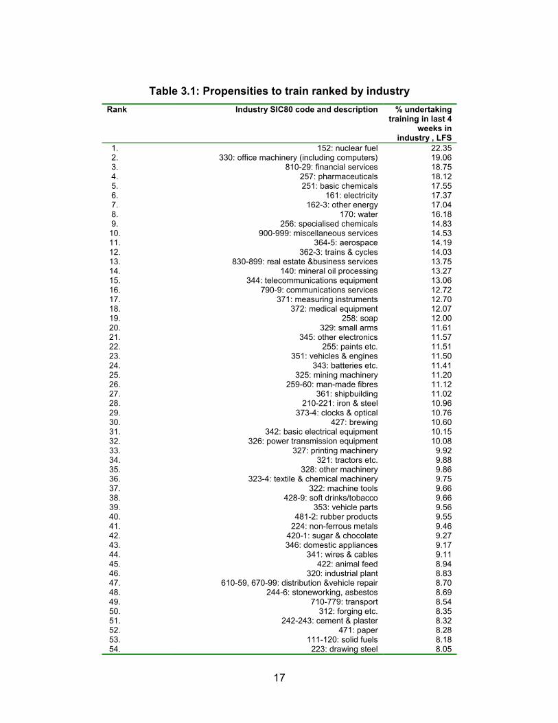
Armed with this dataset we present various descriptive statistics by industry. First

we ranked all industries by their propensity to train. From Table 3.1 we see that

the highest-training industries are generally high tech - pharmaceuticals,

aerospace, chemicals and computers. Another important group are the energy

industries including electricity and especially nuclear fuel, which is the top-ranked

training. This is to be expected, given that, given that these industries include a

lot of specialised equipment and stringent safety requirements.

17

Table 3.1: Propensities to train ranked by industryRank Industry SIC80 code and description % undertaking

training in last 4weeks in

industry , LFS 1. 152: nuclear fuel 22.35 2. 330: office machinery (including computers) 19.06 3. 810-29: financial services 18.75 4. 257: pharmaceuticals 18.12 5. 251: basic chemicals 17.55 6. 161: electricity 17.37 7. 162-3: other energy 17.04 8. 170: water 16.18 9. 256: specialised chemicals 14.83 10. 900-999: miscellaneous services 14.53 11. 364-5: aerospace 14.19 12. 362-3: trains & cycles 14.03 13. 830-899: real estate &business services 13.75 14. 140: mineral oil processing 13.27 15. 344: telecommunications equipment 13.06 16. 790-9: communications services 12.72 17. 371: measuring instruments 12.70 18. 372: medical equipment 12.07 19. 258: soap 12.00 20. 329: small arms 11.61 21. 345: other electronics 11.57 22. 255: paints etc. 11.51 23. 351: vehicles & engines 11.50 24. 343: batteries etc. 11.41 25. 325: mining machinery 11.20 26. 259-60: man-made fibres 11.12 27. 361: shipbuilding 11.02 28. 210-221: iron & steel 10.96 29. 373-4: clocks & optical 10.76 30. 427: brewing 10.60 31. 342: basic electrical equipment 10.15 32. 326: power transmission equipment 10.08 33. 327: printing machinery 9.92 34. 321: tractors etc. 9.88 35. 328: other machinery 9.86 36. 323-4: textile & chemical machinery 9.75 37. 322: machine tools 9.66 38. 428-9: soft drinks/tobacco 9.66 39. 353: vehicle parts 9.56 40. 481-2: rubber products 9.55 41. 224: non-ferrous metals 9.46 42. 420-1: sugar & chocolate 9.27 43. 346: domestic appliances 9.17 44. 341: wires & cables 9.11 45. 422: animal feed 8.94 46. 320: industrial plant 8.83 47. 610-59, 670-99: distribution &vehicle repair 8.70 48. 244-6: stoneworking, asbestos 8.69 49. 710-779: transport 8.54 50. 312: forging etc. 8.35 51. 242-243: cement & plaster 8.32 52. 471: paper 8.28 53. 111-120: solid fuels 8.18 54. 223: drawing steel 8.05

18

Rank Industry SIC80 code and description % undertakingtraining in last 4

weeks inindustry , LFS

55. 247: glass 8.00 56. 241: clay products 7.86 57. 483: plastics 7.83 58. 492-3: musical instruments & photography 7.81 59. 424-6: spirits & wine 7.73 60. 472: paper conversion 7.68 61. 463: carpentry/joinery 7.54 62. 475: printing/publishing 7.53 63. 500-599: construction 7.52 64. 660-9: restaurants/hotels 7.49 65. 222: steel tubes 7.34 66. 314: metal doors/windows 7.09 67. 494: toys 6.94 68. 347: lighting 6.91 69. 352: vehicle bodies 6.85 70. 418-9: bread & starch 6.76 71. 316: hand tools 6.61 72. 248: ceramic goods 6.58 73. 415-6: fish & grain 6.31 74. 311: foundries 6.31 75. 464-6: wooden items 6.14 76. 441-2: leather 6.07 77. 491: jewelry/coins 5.96 78. 467: wooden furniture 5.95 79. 0-99: agriculture 5.78 80. 231-9: other mineral extraction 5.52 81. 411-2: animal products 5.34 82. 432-5: natural fibres 5.22 83. 495: miscellaneous manufacturing 5.19 84. 414: fruit & vegetables 5.11 85. 455-6: textiles & fur 4.82 86. 313: nuts & bolts 4.76 87. 438: carpets 4.59 88. 431: woolen goods 4.43 89. 453: clothing 4.27 90. 461-2: wood processing equipment 3.99 91. 436: hosiery 3.90 92. 439: miscellaneous textiles 3.83 93. 451: footwear 3.76 94. 437: textile finishing 2.72

NotesThese are derived from the LFS matched to our 94 industry groupings 1984-

1996.

19

Financial services and banking (where IT equipment is intensively used) are also

highly ranked. At the low end of the table come several industries associated with

low-paid, low-skilled labour such as textiles, footwear and clothing, all with less

than 5% of employees being trained.

To begin the analysis we simply plot the scatterplot of labour productivity (log real

value added per worker) against training propensity in Figure 3.3. There is a

strong positive correlation. Figure 3.4 repeats the exercise for log hourly wages.

The correlation is somewhat weaker (a result which is repeated in the

econometric analysis) but still clearly positive. These are the essential patterns in

the data that we will be testing more rigorously in Section 5.

The outliers in both graphs tend to be in the service sector. Further analysis

revealed that the series for value added and capital stocks tended to be rather

unreliable in the service sector and (to a lesser extent) in the non-manufacturing

parts of the production sector. For example in banking and financial services real

value added per person declined every year between 1983 and 1996 according

to the ISDB! Measuring productivity and prices is an inherently difficult problem in

these sectors. Although we only have 91 observations in these sectors they are

large and since we weight by the size of the industry, they have a large influence

on the results. Given the poor quality of the data we decided, somewhat

reluctantly, to focus the econometric part of the analysis on the production side of

the economy (some results for non-production are given in section 5).

20

Figure 3.1 Labour Productivity and Training in British IndustriesLa

bour

Pro

duct

ivity

proportion training last 4 wks

log(Value Added per head)

0 .1 .2 .3 .4

1

2

3

4

5

Figure 3.2 Wages and Training in British Industries

Log(

Hou

rly W

age)

proportion training last 4 wks

lrhw

0 .1 .2 .3 .4

0

1

2

3

21

Notes to Figures 3.1 and 3.21. Each point is an industry-year observation

2. The OLS regression line has a slope of 4.91 for productivity and 2.95 for wages

3. Labour productivity is log(Value added per employee) from Census of Production

4. Wages are log hourly wages from the Census of Production (wages) and the LFS (hours)

5. Training is the proportion of workers involved in training from the LFS

For descriptive purposes we split industries into ‘high-training’ and ‘low-training’

based on whether they are above or below the median training propensity

(8.7%). Industries ranked 1 through 47 fall into the ‘high-training’ category. Table

3.2 gives the mean characteristics of the high and low training industries. High

training industries are characterised by being more productive and paying high

wages as we expected. Furthermore, they are more capital intensive, conduct

more research and development, employ more workers of higher skills

(managers/professionals and those with more qualifications) and longer tenure.

They also employ more men and have fewer small firms.

We also analysed the time series trends of these variables split by high and low

training industries. The relative differences appeared to be very persistent over

time, although there was some tendency for the older individuals to increase their

training more than the younger individuals.

Since most of these characteristics are associated with higher productivity the

scatterplots of Figures 3.1 and 3.2 could merely represent the fact that high

training industries happen to employ workers who are more productive. We need

to turn to an explicit econometric model to investigate whether there is a causal

effect of training per se on productivity.

22

Table 3.2Means of Variables by High and Low Training Industries

Variable Mean (low trainingindustries)

Mean (high trainingindustries)

proportion of male employees 62.4% 80.9%proportion aged: 16-24 22.7% 15.5% : 25-34 24.5% 25.4% : 35-44 22.2% 24.0% : 45-54 19.1% 22.1% : 55-64 11.1% 12.8%proportion in occupation: :professional/managerial 14.7% 27.1% :clerical 8.5% 10.9% :security/personal 1.9% 1.6% :sales 3.4% 2.5% :other occupations 71.5% 58.0%highest qualification: :degree 2.6% 7.3% :sub-degree level 3.7% 9.2% :A level / equivalent 15.5% 22.5% :O level/ equivalent 15.6% 14.3% :other/none/missing 62.7% 46.7%tenure in current job: :less than 6 months 10.9% 7.1% :6 months – 1 year 8.4% 5.8% :1 year – 2 years 11.1% 8.0% :2 years – 5 years 21.6% 17.8% :5 years – 10 years 18.8% 19.7% :10 years – 20 years 18.0% 24.3% :more than 20 years 9.0% 16.5%proportion in small firm 21.2% 12.6%average log capital-labour ratio 2.22 3.02average log real value added perworker

2.76 3.19

average log gross output per worker 3.80 4.27average log hourly wages 1.56 1.84average hours worked 39.1 40.2average R&D spend as proportion ofoutput

0.52 2.99

Notes to Table 3.2`High Training’ industries are those that trained on average more than 8.7% of

employees (the sample median).

23

4. A Model of training and productivity

Following Bartel (1995), consider a simple Cobb-Douglas production function -

this should be thought of as a first order approximation to a more complicated

functional form (we discuss alternatives below).

βα KALQ = (1)

Where Q is value added, L is effective labour, K is capital and A is a Hicks neutral

efficiency parameter. Effective labour will depend on many aspects of the

organisation of the firm. If we assume that training improves the amount of

effective labour then write effective labour as

TU NNL γ+= (2)

where NU are untrained workers and NT are trained workers (we expect γ>1).

Substituting equation (2) into (1) gives:

βαγ KNNAQ TU )( +=

which can be re-expressed as

βααγ KNTRAINAQ ))1(1( −+= (3)

where TRAIN = NT/N , the proportion of trained workers in an industry. If

(γ−1)TRAIN is small we can use the approximation ln(1+x) = x and re-write the

production function in logarithmic form as

KNTRAINAQ loglog)1(loglog βαγα ++−+= (4)

24

If the industry exhibits constant returns to scale then equation (4) can be re-

written in terms of labour productivity as

)/log()1)(1(log)/log( NKTRAINANQ βγβ +−−+= (5)

If the trained are no more productive than the untrained (γ =1) then the coefficient

on TRAIN will be zero. Of course, there are a large number of other influences on

productivity captured in A. In the empirical work below we consider a large vector

of other variables. In particular we will allow for other dimensions of worker

heterogeneity by including standard proxies for human capital (education,

occupation, age and tenure). Furthermore, we allow for differential hours, worker

turnover rates, innovation (as proxied by R&D intensity), gender, regional

composition and the proportion of small firms. Finally we will examine the returns

to different types of training (e.g. off the job and on the job).

Despite the presence of these additional observables to control for factors

affecting productivity there remain several econometric problems. Firstly, there

are likely to be unobservable factors that are correlated with our regressors that

we have not measured. For example, some industries may have a higher rate of

technological progress which requires a larger amount of training. It is the

unobserved technical change which boosts productivity and not training per se.

Unless we control for these fixed effects we may overstate the importance of

training for productivity. There are a variety of methods to control for this

problem. Since we have a long panel (1983-1996) we deal with it by including a

full set of industry dummies (fixed effects). The within groups bias should not be

large with a time series of this dimension but we are careful to check by

examining the fully balanced data and examining other estimation strategies (see

below).

25

A second major problem is that of endogeneity. Transitory shocks could raise

productivity and induce changes in training activity (and of course in the other

inputs, labour and capital). For example, faced with a downturn in demand in its

industry, a firm may reallocate idle labour to training activities (`the pit stop

theory’). This would mean that we underestimate the productivity effects of

training because human capital acquisition will be high when demand and

production is low24.

To deal with this problem one needs to use sets of instrumental variables that are

correlated with training, but not with the productivity shock. One strategy is to

seek an external instrument correlated with the receipt of training but

uncorrelated with productivity. The strategy taken here is to draw on recent

advances in GMM techniques to deal with these problems (e.g. Blundell and

Bond, 1998) utilising the fact that we have longitudinal data. We use a system

estimator that exploits information in the levels and difference equations. An

additional advantage of this procedure is that, as with any valid instrumental

variables strategy, it should correct for bias arising for measurement error in the

dependent variable and regressors.

For ease of exposition consider a simplified univariate stochastic representation

of equation (5)

ititit uxy += θ (6)

where i = industry, t = time and uit = fi + mit + vit

We initially assume fi is a firm effect, mit and vit are serially uncorrelated errors.

24 A similar issue arises in the evaluation of government training schemes when individuals who

have had a transitory drop in their earnings are more likely to be allocated to a training

programme. This `Ashenfelter dip’ will tend to lead to an underestimation of the benefits of

training on income.

26

OLS will be inconsistent if the fixed effects are correlated with the x variables.

Including the fixed effects and the time dummies and estimating by within groups

will be a consistent estimator of θ only if the regressors are strictly exogenous,

i.e. 0 ,0)( ≠=+ suxE itsit . For weakly exogenous regressors (such as a lagged

dependent variable) where E(xituit) = 0, but 0 ,0)( >≠+ suxE itsit , Nickell (1981)

has shown that the size of this bias will decrease in T, the length of the panel.

It is quite likely that even weak exogeneity may be invalid. Firms will adjust their

inputs (such as labour and possibly training) in response to current shocks.Furthermore, there might be serial correlation in the vit process. For example,

continue to assume that mit is uncorrelated but allow vit to be AR(1), i.e.

ititit evv += −1ρ (7)

The combination of (6) and (7) implies a general dynamic model of the form

itiitititit wxxyy ++++= −− ηπππ 13211 (8)

with common factor (COMFAC) restrictions 213 πππ −= . Note that

1−−+= itititit mmew ρ and ii f)1( ρη −= . In these circumstances we consider

weaker moment conditions. Standard assumptions on the initial conditions(E(xi1eit) = E(xitmit) = 0) gives the moment condition

E(xit-s∆wit) = 0, s > 1 (9)

27

This allows the construction of suitably lagged levels of the variables (includingthe yit’s) to be used as instruments after the equations have been first differenced

(see Arellano and Bond, 1991).

As has been frequently pointed out, the resulting first differenced GMM estimator

has poor finite sample properties when the lagged levels of the series are only

weakly correlated with the subsequent first differences (Blundell and Bond,

1998). This has been a particular problem in the context of production functions

due to the high persistence of the capital stock series (e.g. Griliches and

Mairesse, 1998).

Under further assumptions on the initial conditions, the weak instruments

problem (cf. Staiger and Stock, 1997) can be mitigated. If we are willing to

assume E(∆xiηi) = 0 and E(∆yiηi) = 0 then we obtain additional moment conditions

1 ,0))(( >=+∆ − swxE itisit η (10)

Stationarity of the variables is a sufficient (but not necessary) condition for

moment conditions in equation (10) to hold. This allows for suitably lagged first

differences of the variables to be used as instruments for the equations in levels.

The combination of the moment conditions for the levels equations in equation

(10) to the more standard moment conditions in equation (9) can be used to form

a GMM `system’ estimator. This has been found to perform well in Monte Carlo

simulations and in the context of the estimation of production functions (Blundell

and Bond, 1999). This IV procedure should also be a way of controlling for

transitory measurement error (the fixed effects control for permanent

measurement error). Random measurement error has been found to be a

problem in the returns to human capital literature, typically generating attenuation

bias (see Card, 1999)

28

Note that the estimation strategy will depend on the absence of serial correlationin the eit ‘s in equation (7). We report serial correlation tests in addition to the

Sargan-Hansen test of the overidentifying restrictions in all the GMM results

below.

Finally, consider two more issue which are harder to deal with: aggregation and

training stocks vs. training flows. Estimation at the three digit industry level has

advantages but also disadvantages relative to micro-level estimation. The

production function in equation (1) at the firm level describes the private impact

of training on productivity. However, many authors, especially in the endogenous

growth literature (e.g. Aghion and Howitt, 1998), have argued that there will be

externalities to human capital acquisition. For example, workers with higher

human capital are more likely to generate new ideas and innovations which may

spill over to other firms25. If spillovers are industry specific this implies that there

should be another term added to equation (5) representing mean industry level

training. In this case the coefficient on training in an industry level production

function should exceed that in a firm level production function26. Secondly,

grouping by industry may smooth over some of the measurement error in the

micro data and therefore reduce attenuation bias.

On the negative side, there may be aggregation biases in industry level data. A

priori it is impossible to sign these biases and we expect that the fixed effects will

control for much of the problem. For example, we are taking logs of means and

not the means of logs in aggregating equation (1). So long as the higher order

moments of the distributions are constant over time in an industry then they will

25 Although there are many papers which examine externalities of R&D (e.g. see the survey by

Griliches, 1991) and a few which look at human capital (Acemoglu and Angrist, 2000, Grifftith,

Redding and Van Reenen, 2000 and Moretti, 1999) there are none that focus on training

spillovers.26 For the same argument in the R&D context see Griliches (1992)

29

be captured by a fixed effect27. If the coefficients are not constant across firms in

equation (1), but are actually random, this will also generate higher order terms

at the industry level. In the empirical results we also experiment with including

higher order moments to make sure our results are robust to potential

aggregation biases.

Turning to the problem of training stocks and flows, note that the model in

equation (1) assumes that we know the stocks of trained workers in an industry.

What we actually have in the data is an estimate of the proportion of workers in

an industry who received training in a given 4-week period (the flow). Since

individuals are sampled randomly over time in the LFS this should be an

unbiased estimate of the proportion of time spent in training over the year28.

If we define the stock of people who have useful training skills in the industry at

time t as NTt and the flow as MT

t then if the stock evolves according to the

standard perpetual inventory formula it can be expressed as

NTt = MT

t + (1-δ) NTt-1 (11)

where δ is the rate at which the stock of effectively trained workers at time t

decay in their productive usefulness by t+1. This training depreciation rate

represents several things. Firstly, individuals will move away from the industry, so

their training can no longer contribute to the industry’s human capital stock.

Secondly, the usefulness of training will decline over time as old knowledge

becomes obsolete and people forget (e.g knowledge of the DOS operating

system). Thirdly, to the extent that training is firm-specific, turnover between firms

27 If they evolve at the same rate across industries they will be picked up by the time dummies.28 If there are many multiple training spells in the month we will underestimate the proportion who

are being trained. If Spring (the LFS quarter we use) is a particularly heavy training season then

we will overestimate the proportion being trained in a year. These biases are likely to be small

and offsetting.

30

in the same industry may reduce industry productivity. Although we obtain some

measures of turnover using the LFS, the second element of depreciation is

essentially unknown. Because of this our baseline results simply uses the

proportion of workers trained in an industry (TRAIN in equation (3)). This will be

equal to the stock when δ=1. Nevertheless, we also estimate the training stock

(under different assumptions on δ) and check our results for robustness using

this alternative measure.

5. Results

5.1 Baseline Results of the Production Functions

In Table 5.1 we present the first basic results for industry-level regressions using

log real value added per head as the dependent variable. The first two columns

present some OLS results for the production sector. The second column includes

skill variables whereas the first column does not. Training has a significant

impact on productivity in the first column, even after conditioning for a large

number of controls. It seems clear, however, that its impact is overstated since

the association is reduced dramatically (and is only significant at the 10% level)

after we control for skills (qualifications and occupation). As we saw that skilled

industries are far more likely to train this is unsurprising. Column (2)

demonstrates that skill-intensive sectors have also higher productivity on both

the occupational and educational dimension29.

Turning to the other variables, the coefficient on the capital labour ratio is highly

significant and takes a reasonable point estimate (the share of the wage bill in

29 We experimented with using more educational groups, but found additional ones (e.g.

degree/no degree) were insignificant once we conditioned on the other variables in the

regression.

31

value added is about 0.7). Productivity significantly increases in hours per

employee and decreases with the degree of worker turnover. Lagged R&D

intensity is also positively associated with higher productivity. Industries with a

larger proportion of very young workers (16-24), female employees, and/or small

firms are associated with lower productivity in column (2).

As discussed in section 4 it is important to consider fixed effects. In column (3)

we simply include a full set of sectoral dummies. The capital intensity coefficient

is lower, but remains significant, as do the turnover, age and occupational skills

variables. The gender and educational variables are driven to insignificance30.

Surprisingly, R&D intensity is more significant in the within dimension. Most

importantly for our purposes, the training variable remains significant with a

higher point estimate.

Current training may be an inappropriate variable for a variety of reasons. For

example, workers may actually be less productive during the time that they are

being trained (the employee herself is devoted to training activities and this may

also disrupt the production activities of co-workers if they have to help in the

training). Consequently column (4) substitutes lagged training for current training.

Although the point estimate has fallen marginally, it remains significant at

conventional levels

30 There is some collinearity between occupation and education as measures of skill, of course.

Dropping occupations from the equation strengthens the educational variable.

32

Table 5.1. Productivity Regressions: Production Sector

(1) (2) (3) (4)ln(value addedper worker)

OLS – no skillvariables

OLS – skillvariables

Within Groups– currenttraining

Within Groups– laggedtraining

Industryproportion:Traint % 1.581 0.363 0.692

(0.216) (0.237) (0.167)Traint-1 % 0.621

(0.165)Turnovert-1 % -0.794 -0.526 -0.432 -0.452

(0.276) (0.269) (0.206) (0.207)Industry average:log(K/N) 0.278 0.266 0.213 0.216

(0.012) (0.012) (0.036) (0.036)log(hours/N) 0.397 0.470 0.282 0.242

(0.236) (0.226) (0.180) (0.180)log(R&D) 0.692 0.148 1.269 1.279Industryproportion:

(0.351) (0.335) (0.506) (0.507)

Male 0.231 0.279 -0.117 -0.127(0.094) (0.096) (0.124) (0.125)

Age 16-24 -1.497 -0.739 -0.390 -0.326(0.241) (0.237) (0.169) (0.168)

Age 25-34 -0.342 -0.262 -0.311 -0.287(0.241) (0.227) (0.154) (0.154)

Age 45-54 0.007 0.216 -0.102 -0.097(0.245) (0.231) (0.155) (0.156)

Age 55-64 -0.232 0.146 0.146 0.153(0.284) (0.270) (0.192) (0.192)

Occupation: 0.762 0.283 0.313Profess./managerial (0.138) (0.129) (0.129)Occupation: 0.798 -0.079 -0.069Clerical (0.207) (0.182) (0.182)Occupation: 0.527 -0.519 -0.538Security/personal (0.494) (0.353) (0.354)Occupation: 1.872 -0.078 -0.103Sales employees (0.292) (0.288) (0.289)No Qualifications -0.267 0.105 0.029

(0.127) (0.113) (0.112) % in small firm 0.002 -0.161 0.002 -0.006

(0.108) (0.110) (0.121) (0.121)NT 970 970 970 970Years 1984-1996 1984-1996 1984-1996 1984-1996R-Square 0.813 0.838 0.945 0.945

Notes:All regressions include a full set of regional dummies (10), time dummies (12) and tenure dummies(6);observations weighted by number of individuals in an LFS industry cell.

33

Table 5.2 reports results for the manufacturing sector only. All the results of the

previous table go through even though the sample is smaller. The training effects

are slightly more precisely determined in this sample than the previous sample

which is probably because value added and capital are measured more

accurately here than in the extraction industries.

If the non-production sector observations are included (agriculture, construction

and services) the coefficient on training rises to 0.727 with a standard error of

0.206. We were concerned about the quality of the data in these sectors as we

were only able to obtain consistent numbers for value added and capital for 9

industrial groupings for a limited number of years31. Even in these aggregated

industries the trends in productivity appeared counter-intuitive. Given the size of

these sectors, including them in the main estimates (which are weighted by

sector size) degrades the quality of the results. Performing the production

functions solely on the non-production industries gave a large coefficient on

training (0.919) with a larger standard error (1.757). Because of these concerns

over data quality we focus on the manufacturing sample for the detailed

econometric results32.

31 up to 1989 for miscellaneous services, until 1990 for construction, until 1991 for agriculture and

up to 1993 in all other cases.32 All the main qualitative results go through on the production sector as a whole. For example the

coefficient (standard error) on training in column (1) of Table 5.4 in the production sector is

0.473(0.196) compared to 0.469(0.167) in manufacturing. The equivalent numbers in column (2)

are 1.319(0.564) in the production sector compared to 1.348(0.527) in manufacturing.

34

Table 5.2. Productivity Regressions: Manufacturing Sector

(1) (2) (3) (4)ln(value addedper worker)

OLS – no skillvariables

OLS – skillvariables

Within Groups– currenttraining

Within Groups– laggedtraining

Industryproportion:Traint % 1.626 0.507 0.520

(0.213) (0.227) (0.164)Traint-1 % 0.509

(0.162)Turnovert-1 % -1.645 -1.496 -1.164 -1.194

(0.308) (0.288) (0.227) (0.226)Industry average:log(K/N)t 0.327 0.309 0.085 0.085

(0.016) (0.015) (0.038) (0.038)log(hours/N) t -0.194 -0.144 0.085 0.062

(0.240) (0.224) (0.178) (0.178)log(R&D/Y)t-1 0.283 -0.134 0.639 0.645Industryproportion:

(0.327) (0.304) (0.472) (0.472)

Malet 0.181 0.245 -0.037 -0.048(0.090) (0.089) (0.117) (0.118)

Age 16-24t -1.182 -0.359 -0.112 -0.059(0.233) (0.225) (0.162) (0.160)

Age 25-34t 0.200 0.233 0.073 0.101(0.236) (0.218) (0.150) (0.150)

Age 45-54t -0.277 -0.065 0.108 0.116(0.232) (0.215) (0.148) (0.148)

Age 55-64t -0.520 -0.106 0.369 0.378(0.278) (0.260) (0.185) (0.185)

Occupation t: 0.841 0.240 0.259Profess./managerial (0.129) (0.124) (0.123)Occupation: 1.469 0.013 0.025Clerical (0.201) (0.172) (0.172)Occupation: 0.063 -0.492 -0.471Security/personal (0.452) (0.335) (0.334)Occupation: 1.279 -0.051 -0.061Sales employees (0.272) (0.270) (0.270)No Qualifications -0.086 0.098 0.039

(0.120) (0.105) (0.104) % in small firm t 0.312 0.145 0.003 -0.002

(0.107) (0.103) (0.112) (0.112)NT 898 898 898 898Years 1984-1996 1984-1996 1984-1996 1984-1996R-Square 0.789 0.825 0.937 0.937

Notes:All regressions include a full set of regional dummies (10), time dummies (12) and tenure dummies(6);observations weighted by number of individuals in an LFS industry cell.

35

We conducted a large number of robustness tests on the models in these tables.

Table 5.3 reports some results. Keeping only industries which had fourteen

continuous years of data (balanced panel) in row 2. means losing 40% of the

observations with an insignificant change in the coefficient. The third row

includes average wages as a measure of unobserved worker quality. Although

wages take a positive and (weakly) significant coefficient the training effect

remains robust. Since training is correlated with unionisation, we could be picking

up “collective voice” effects. Union membership is only available in LFS since

1989. Despite the loss in sample in row 4, the training effect is quite robust.

Union density is negatively, but insignificantly, associated with productivity. In

the fifth row we allow the training effect to be different in each of the 85

industries. The mean of these heterogeneous coefficients is close to the pooled

results. There was some evidence that the training effects were larger in

industries that had more human capital and were more high tech. We test more

rigorously in the GMM results below. The sixth row conditions on having larger

numbers in each cell, this seems to increase the training effect, suggesting some

attenuation bias. The final row replaces the dependent variable with output which

produces a smaller effect, probably because we are not controlling for other

variables such as energy and intermediate inputs.

36

Table 5.3. Results of Within Groups robustness Tests

Robustness test NT Training coefficient, productionsector(s.e.)

1. Original training coefficient in production sector, Table5.1 column (3)

970 0.692(0.167)

2. Using the balanced panel only to check for biasassociated with finite T (Nickell, 1981):

572 0.508(0.234)

3. Conditioning on wage in productivity regression tocontrol for unobserved worker quality

970 Training: 0.659(0.167)

Wage coeff.: 0.100(0.051)

4. Include union density (only available 1989-96) 547 training: 0.565(0.261)union: -0.042(0.161)

5. Allow all industries to have different trainingcoefficients

970 mean of heterogeneouscoefficients: 0.533

6. Conditioning on having at least 150 LFS individualsper cell

409 .986(0.330)

7. Using gross output per head instead of value addedper head

970 0.335(0.143)

Notes to TableThese all use the specification in the third column of Table 5.1

There are several other econometric reasons why the results in Table 5.1 and

5.2 may be misleading. Although endogeneity problems are mitigated by the use

of lagged training in column (4) there may still be problems (e.g. if there is

residual serial correlation). Furthermore, the dynamic structure of the production

function may be more complex than the simple static model with uncorrelated

shocks so far examined (e.g. equation (10)).

Table 5.4 presents some results using the GMM- System estimator described in

section 4. Each regression includes all the covariates in Table 5.2 , although we

only report results for the key variables (full results available on request). The

first column simply performs the standard static specification but instruments

capital intensity and hours. We use instruments in levels from t-2 in the first

difference equation and instruments dated t-1 in differences in the levels

equation (see base of table for exact timing). We initially assume current training

is exogenous as before.

37

Treating hours and capital intensity as endogenous leads to increases in their

implied impacts compared to the within groups results. Capital takes on a larger

and more sensible point estimate. The training effect remains quite similar to the

Within Groups estimates. The second column relaxes the exogeneity assumption

on training using the same timing of instruments as the other variables.

Remarkably, the training coefficient triples in size. This clearly rejects the

hypothesis that the within group estimates over-estimate the productivity effect of

training. One reason why there may be an underestimate is if firms train when

demand (and therefore productivity which is pro-cyclical) is low.

To probe these results further we include a lagged dependent variable in the

model in column (3). Although it is highly significant the other coefficients are

largely unchanged. In column (4) we also include lags of the capital and hours

variables. Column (5) implements fully the model of equation (8) and includes the

first lag of all the right hand side variables in the regression (but continues to

assume they are weakly exogenous). Finally column (6) allows all the right hand

side variables (with the exception of the time and regional dummies) to be

endogenous. This is the most demanding specification of the table33.

Throughout these experiments there is a positive and significant impact of

training on productivity. The exact magnitude of the effect varies somewhat in

different specifications, but always remains above the estimates which treated

training as exogenous.

33 Instrumenting the regional dummies with lags does not alter the results. The problem with this

column is that we have are using so many instruments that the Sargan test has practically no

power to reject the null.

38

Table 5.4. Productivity Regressions: Manufacturing Sector, GMM results

(1) (2) (3) (4) (5) (6)ln(Value added perworker)

Static, trainingexogenous

Static, trainingendogenous

Dynamic, trainingendogenous

Dynamic, trainingendogenous

ExtendedDynamicPF

Dynamic full PFspecification

Industry average:ln(Q/N)t-1 0.075 0.466 0.453 0.554Industry proportion: (0.029) (0.066) (0.069) (0.056)Traint % 0.469 1.348 1.503 0.856 1.132 0.795

(0.167) (0.527) (0.458) (0.406) (0.383) (0.308)Traint-1 % -0.001 0.207 0.224

(0.210) (0.237) (0.227)Turnovert-1 % -0.776 -0.685 -0.831 -0.306 -0.327 -0.598

(0.232) (0.236) (0.233) (0.217) (0.194) (0.420)Turnovert-2 % 0.134 -0.492

(0.193) (0.297)Industry average:log(K/N)t 0.247 0.300 0.227 0.258 0.275 0.235

(0.063) (0.055) (0.043) (0.089) (0.083) (0.083)log(K/N)t-1 -0.138 -0.131 -0.040

(0.080) (0.075) (0.079)log(hours/N)t 0.518 0.489 0.458 0.371 0.390 0.420

(0.158) (0.145) (0.141) (0.153) (0.152) (0.120)log(hours/N)t-1 -0.326 -0.427 -0.443

(0.073) (0.197) (0.103)log(R&D/Y)t-1 0.311 0.020 -0.108 0.130 1.260 1.207

(0.334) (0.344) (0.337) (0.253) (0.507) (1.119)log(R&D/Y)t-2 -1.372

(0.523)-1.449(1.222)

Serial Correlation(LM1)

-3.389 -4.154 -4.126 -5.813 -5.496 -5.618

Serial Correlation(LM2)

-1.706 -1.492 -0.955 -0.783 -0.932 -0.633

Sargan (df) 83.98(46) 108.75 (102) 159.86(136) 132.74(133) 136.04(133) 169.19(219)p-value 0.091 0.305 0.087 0.490 0.411 0.995Instruments ln(Hrs/N)t-2,t-3 and

ln(K/N)t-2,t-3 indifferencedequations;∆ln(Hrs/N)t-1 and∆ln(K/N)t-1 in thelevels equations.

ln(TRAIN)t-2,t-3

ln(Hrs/N)t-2,t-3ln(K/N)t-2,t-3 indifferencedequations;∆ln(TRAIN)t-1,

∆ln(Hrs/N)t-1 ,

∆log(K/N)t-1 in thelevels equations.

Ln(TRAIN)t-2,t-3

Log(Q/N)t-2,,t-3,

log(Hrs/N)t-2,t-3log(K/N)t-2,t-3 indifferencedequations;∆log(TRAIN)t-1,

∆log(Q/N)t-1,

∆log(Hrs/N)t-1

∆log(K/N)t-1 in thelevels equations.

Ln(TRAIN)t-2,t-3

Log(Q/N)t-2,,t-3,

log(Hrs/N)t-2,t-3log(K/N)t-2,t-3 indifferencedequations;∆log(TRAIN)t-1,

∆log(Q/N)t-1,

∆log(Hrs/N)t-1

∆log(K/N)t-1 in thelevels equations.

Ln(TRAIN)t-2,t-3

Log(Q/N)t-2,,t-3,

log(Hrs/N)t-2,t-3log(K/N)t-2,t-3 indifferencedequations;∆log(TRAIN)t-1,

∆log(Q/N)t-1,

∆log(Hrs/N)t-1

∆log(K/N)t-1 in thelevels equations.

all variablestreated asendogenous(except time andregionaldummies)

NT 818 818 818 818 818 818Years 1985-1996 1985-1996 1985-1996 1985-1996 1985-1996 1985-1996

Notes to Table 5.4

Estimation by GMM-SYS in Arellano and Bond (1998) DPD-98 package written in GAUSS; all regressions include thecurrent values of all the variables in Tables 5.1 and 5.2 (i.e. occupations, qualifications, age, tenure, gender, region,firm size; time dummies) and in columns (5) and (6) the first lags of all these variables are also included; capitalintensity, hours and lagged productivity are always treated as endogenous; the other variables are treated as exogenousexcept in column (6) where all variables are instrumented; asymptotically robust (one-step) standard errors inparentheses; LM1(2) is a Lagrange Multiplier test of first (second) order serial correlation distributed N[1,0] under thenull (see Arellano and Bond, 1991); Sargan is a Chi-squared test of the overidentifying restrictions; observationsweighted by number of individuals in an LFS industry cell.

39

The diagnostics are satisfactory. There is evidence of negative first order

correlation (in the differenced residuals) which is consistent with our

assumptions. There is some evidence of second order correlation (at the 10%

level) in the first column, but this reflects misspecification as it disappears in the

more general specifications in the other columns. Longer memory autocorrelation

would invalidate the use of our instruments34. Another test of instrument validity

is the Sargan statistic which also easily passes in the preferred specifications.

We subjected the results in Table 5.4 to a battery of robustness tests (see next

section for some of the more interesting ones). For example, using the final

column of Table 5.4 we tried the following experiments. Firstly, to test for non-

constant returns employment and its lag were included (instrumented in the usual

way). The employment terms were individually and jointly insignificant, with a p-

value of 0.21. Secondly, to examine aggregation biases we included higher order

powers of the right hand side variables. These were uninformative. For example

including squared terms (and first lag) of training, capital intensity and hours gave

a chi-squared(6) of 10.5 (p-value = 0.101). Thirdly, the training question was

asked slightly differently in 1983 (it applied only to workers under 50). Dropping

1983 (which is only ever used for instruments in any case) and re-estimating

1986-1996 lead to a coefficient on training of 0.858 with standard error of 0.321.

Fourthly, additional dynamics were not needed in the specifications. For

example, lags at t-2 of training, capital intensity, value added and hours were

jointly insignificant (p-value 0.621). Fifthly, we checked whether allowed the

training effect had changed over time in any secular way (especially across the

change of industrial classifications in 1992). The coefficient seemed reasonably

stable over time, although there was some suggestion that the impact of training

34 In fact, we identify a significant training effect even when we drop the most recent instruments

and use (t-3) and before in the differenced equations and (t-2) in the levels equations. P-value of

two training variables is 0.011.

40

was lower in the 1990-1993 recession35. Sixth, we included the mean wage on

the right hand side to control for worker quality. The variable was insignificant (a

coefficient of 0.004 with a standard error of 0.111) and the training effect was

unchanged.

Finally, we tried many interactions consistent with a more general production

function. None of these were significant at the 5% level36, but there was a

suggestion of complementarity between human capital and training. Including the

interaction of training with professional/managerial workers was significant at the

10% level. The coefficient on training was estimated to be 0.046 in industries

where only 10% of employees were in the most skilled occupational class,

compared to 0.39 when the proportion of the skilled was 20% (the sample mean).

5.2 Further investigations of the impact of training on productivity

We investigated how different types of training could lead to different productivity

pay-offs. Using the on-the-job/off-the-job distinction in the training variable did

suggest that off the job training had a larger impact on productivity. When the

proportion of workers who had off the job training (and its lag) were included as

extra variables (in addition to TRAIN), they were jointly significant at 10% (p-

value of joint test 0.063). This may be because it represents more formal training

which is more likely to have a lasting impact on productivity. It is useful to note

that the increase in overall training is largely due to off-the-job training rather than

on-the-job training. As this is the case, it seems reasonable to assume that a lot

of the increase in training is genuinely productivity-enhancing.

35 The joint significance of the interaction of training and a dummy variable for the 1992-1996

period (and its first lag) was 0.783. For 1993-1996 the equivalent was p-value 0.593. For 1991-

1996 the p-value was 0.516. Allowing the 1990-93 period dummy to interact with training gave a

p-value of 0.072.36 For example, the interaction of R&D with training was positive and the interaction of small firms

with training was negative.

41

Other measures of the type of training were not informative. We did not find any

additional effect of employer-provided or training length.

We were concerned about misspecification of the training measure as a flow

rather than a stock. Consequently we re-estimated all the equations in Table 5.4

using the stock measure of training (predicted proportion of workers who have

been trained at some point in the past)37. In Table 5.5 the point estimates are

similar to those of the previous table, but estimated more precisely. The dynamic

equations of columns (4) through (6) appear more satisfactory than in the

previous table with current training taking a positive coefficient and lagged

training a negative coefficient. In fact, the common factor (COMFAC) restrictions

are not rejected in column (6). Imposing these restrictions by minimum distance

gives much more precise estimates (in bold).

37 We use the median inter-industry employee turnover rate, assume a growth of the training

stock of 2% a year and a training depreciation rate of 15%. The results are robust to using a

depreciation rate of 10% or 20%, including within-industry turnover and setting the growth rate to

zero. We also considered looking at the inflows of trained workers from other industries to

improve the stock measure, but the LFS sample of industry switchers was too small to construct

the full three digit flow matrix.

42

Table 5.5: Productivity Regressions: Manufacturing Sector, GMM results,Training Stock

(1) (2) (3) (4) (5) (6)ln(Value added perworker)

Static, trainingexogenous

Static, trainingendogenous

Dynamic, trainingendogenous

Dynamic, trainingendogenous

ExtendedDynamicPF

Dynamic full PFspecification

Industry average:ln(Q/N)t-1 0.056 0.463 0.432 0.537Industry proportion: (0.035) 0.066 (0.071) (0.057)Traint % (stock) 0.354 0.870 0.576 0.913 1.132 0.701

(0.143) (0.287) (0.250) (0.305) (0.298) (0.243)Traint-1 % (stock) -0.733 -0.675 -0.547

(0.256) (0.263) (0.223)Training stock (imposeCOMFAC)

0.515(0.192)

log(K/N)t 0.217 0.239 0.209 0.120 0.145 0.112(0.062) (0.052) (0.044) (0.087) (0.083) (0.082)

log(K/N)t-1 -0.011 -0.005 0.064(0.079) (0.080) (0.076)

log(K/N) (imposeCOMFAC)

0.224(0.045)

rho (autocorrelationcoefficient)

0.498(0.174)

COMFAC TEST (df)p-value

41.62(33)0.144

Serial Correlation(LM2)

-1.851 -1.733 -1.133 -0.973 -1.053 -0.900

Sarganp-value

0.106 0.348 0.024 0.296 0.162 0.860

Instruments ln(Hrs/N)t-2,t-3 andln(K/N)t-2,t-3 indifferencedequations;∆ln(Hrs/N)t-1 and∆ln(K/N)t-1 in thelevels equations.

ln(TRAIN)t-2,t-3

ln(Hrs/N)t-2,t-3

ln(K/N)t-2,t-3 indifferencedequations;∆ln(TRAIN)t-1,

∆ln(Hrs/N)t-1 ,

∆log(K/N)t-1 in thelevels equations.

ln(TRAIN)t-2,t-3

log(Q/N)t-2,t-3

log(Hrs/N)t-2,t-3log(K/N)t-2,t-3 indifferencedequations;∆log(TRAIN)t-1,

∆log(Q/N)t-1,

∆log(Hrs/N)t-1

∆log(K/N)t-1 in thelevels equations.

ln(TRAIN)t-2,t-3

log(Q/N)t-2,t-3

log(Hrs/N)t-2,t-3log(K/N)t-2,t-3 indifferencedequations;∆log(TRAIN)t-1,

∆log(Q/N)t-1,

∆log(Hrs/N)t-1

∆log(K/N)t-1 in thelevels equations.

ln(TRAIN)t-2,t-3

log(Q/N)t-2,t-3

log(Hrs/N)t-2,t-3log(K/N)t-2,t-3 indifferencedequations;∆log(TRAIN)t-1,

∆log(Q/N)t-1,

∆log(Hrs/N)t-1

∆log(K/N)t-1 in thelevels equations.

all variablestreated asendogenous(except time andregionaldummies)

NT 818 818 818 818 818 818Years 1985-1996 1985-1996 1985-1996 1985-1996 1985-1996 1985-1996

Notes to Table 5.5

Estimation by GMM-SYS in Arellano and Bond (1998) DPD-98 package written in GAUSS; all regressions include thecurrent values of all the variables in Tables 5.1 and 5.2 (i.e. occupations, qualifications, age, tenure, gender, region,firm size; time dummies) and in columns (5) and (6) the first lags of all these variables are also included; capitalintensity, hours and lagged productivity are always treated as endogenous; the other variables are treated as exogenousexcept in column (6) where all variables are instrumented; asymptotically robust (one-step) standard errors inparentheses; LM1(2) is a Lagrange Multiplier test of first (second) order serial correlation distributed N[1,0] under thenull (see Arellano and Bond, 1991); Sargan is a Chi-squared test of the overidentifying restrictions; observationsweighted by number of individuals in an LFS industry cell.; in column (6) the numbers in bold are the coefficients andstandard errors after imposing the COMFAC restrictions by minimum distance; COMFAC is a chi-squared test.

43

5.3 Wage regressions

Since there is a large existing empirical literature on the effects of training on

wages we have focused on productivity in this paper. But it is still of great interest

to also examine the wage impact of training. In order to make the effects of

training comparable we have kept an identical specification in the hourly wage

equation keeping the same control variables on the right hand side as in the

production function.

Table 5.6 has the production sector results and Table 5.7 the manufacturing

sector results. There is a statistically significant effect of training in column (1) of

both tables. Most of the variables are conventionally signed. Industries who use

workers with greater skills, have more men, higher capital intensity and larger

establishments pay higher wages. Younger and older workers are paid less than

prime age workers. More surprisingly, longer hours are associated with lower

hourly pay.

The strong correlation of training with wages is severely reduced when one

controls for skills. In fact, the correlation actually becomes negative (although

insignificant) in column (2). The within group estimates restore some of the

effect, implying a positive and significant impact of training on wages in both the

production sector as a whole and the manufacturing sector alone.

44

Table 5.6. Hourly Wage Regressions: Production Sector

(1) (2) (3) (4)ln(hourly wage) OLS – no skill

variablesOLS – skill

variablesWithin Groups

– currenttraining

Within Groups– laggedtraining

Industryproportion:Traint % 0.500 -0.163 0.327

(0.138) (0.157) (0.112)Traint-1 % 0.459

(0.111)Turnovert-1 % -0.098 0.046 0.158 0.148

(0.177) (0.178) (0.139) (0.138)Industry average:log(K/N)t 0.036 0.033 0.092 0.092

(0.008) (0.008) (0.024) (0.024)log(hours/N) t -0.739 -0.665 -0.599 -0.621

(0.151) (0.150) (0.121) (0.120)log(R&D/Y) t 0.041 -0.247 -0.859 -0.840Industryproportion:

(0.225) (0.222) (0.341) (0.339)

Male 0.712 0.672 -0.128 -0.143(0.060) (0.063) (0.084) (0.083)

Age 16-24 t -0.929 -0.618 -0.153 -0.128(0.154) (0.157) (0.114) (0.112)

Age 25-34 t -0.160 -0.144 -0.168 -0.150(0.154) (0.151) (0.104) (0.103)

Age 45-54 t -0.184 -0.075 -0.152 -0.149(0.157) (0.153) (0.105) (0.104)

Age 55-64 t -0.497 -0.312 -0.240 -0.223(0.182) (0.179) (0.129) (0.129)

Occupation t: 0.250 0.176 0.186Profess./managerial (0.092) (0.087) (0.087)Occupation: 0.208 -0.140 -0.143Clerical (0.137) (0.123) (0.122)Occupation: 0.372 0.308 0.278Security/personal (0.328) (0.238) (0.237)Occupation: 0.599 -0.348 -0.365Sales employees (0.193) (0.194) (0.193)No Qualifications -0.323 0.083 0.045

(0.084) (0.076) (0.075) % in small firm t -0.369 -0.435 -0.059 -0.061

(0.072) (0.073) (0.081) (0.081)NT 970 970 970 970Years 1984-1996 1984-1996 1984-1996 1985-1996R-Square 0.751 0.769 0.919 0.920

Notes:All regressions include a full set of regional dummies (10), time dummies (12) and tenure dummies(6);observations weighted by number of individuals in an LFS industry cell.

45

Table 5.7. Hourly Wage Regressions: Manufacturing Sector

(1) (2) (3) (4)ln(hourly wage) OLS – no skill

variablesOLS – skill

variablesWithin Groups

– currenttraining

Within Groups– laggedtraining

Industryproportion:Traint % 0.745 -0.196 0.130

(0.122) (0.129) (0.097)Traint-1 % 0.230

(0.096)Turnovert-1 % -1.467 -1.298 -0.328 -0.335

(0.177) (0.164) (0.140) (0.136)Industry average:log(K/N) t 0.105 0.108 0.022 0.021

(0.009) (0.009) (0.022) (0.022)log(hours/N) t -1.405 -1.307 -0.841 -0.850

(0.137) (0.127) (0.105) (0.105)log(R&D)t-1 -0.612 -0.885 -1.740 -1.728Industryproportion:

(0.187) (0.173) (0.279) (0.278)

Male t 0.621 0.555 -0.050 -0.060(0.051) (0.051) (0.069) (0.069)

Age 16-24 t -0.759 -0.371 -0.143 -0.130(0.133) (0.128) (0.095) (0.095)

Age 25-34 t -0.083 -0.123 -0.015 -0.004(0.135) (0.124) (0.089) (0.088)

Age 45-54 t -0.199 -0.074 -0.083 -0.081(0.133) (0.122) (0.087) (0.087)

Age 55-64 t -0.287 -0.041 -0.130 -0.121(0.159) (0.148) (0.109) (0.109)

Occupation t: 0.267 0.095 0.098Profess./managerial (0.073) (0.073) (0.073)Occupation: 0.794 0.009 0.007Clerical (0.114) (0.102) (0.101)Occupation: 0.098 0.217 0.212Security/personal (0.257) (0.198) (0.197)Occupation: 0.116 -0.183 -0.190Sales employees (0.155) (0.159) (0.159)No Qualifications -0.355 0.095 0.079

(0.068) (0.062) (0.061) % in small firm t -0.089 -0.170 -0.036 -0.037

(0.061) (0.059) (0.066) (0.066)NT 898 898 898 898Years 1984-1996 1984-1996 1984-1996 1984-1996R-Square 0.816 0.849 0.941 0.942

Notes:All regressions include a full set of regional dummies (10), time dummies (12) and tenure dummies(6);observations weighted by number of individuals in an LFS industry cell.

46

Table 5.8 contains the GMM results which mirror the specifications of the

production function. As with productivity, allowing the training variable to be

endogenous increases the implied effect (column (2) vs. column (1)). The training

effect is insignificant at conventional levels. Column (3) includes a lagged

dependent variable which is highly significant. Column (4) allows an extra lag on

turnover, R&D, capital intensity and hours. Column (5) allows lags on all the

variables and column (6) implements the most general dynamic specification

treating all variables as endogenous. As with the production function, treating

training as exogenous leads to downwardly biased estimates. In the preferred

specification of column (6) training has a statistically significant effect on wages

that is quantitatively larger than column (1).

One striking result is that whichever table we consider, the implied impact of

training on wages in lower than its effect on productivity. For example, in the

most general specification of column (6) the productivity effect of training is Table

is about 0.8 and the wage effect 0.3. Differential effects on wages and

productivity would be predicted in a basic human capital model where employers

paid for some of the costs of firm specific training. The only other study to

examine this found that the benefits of training are split about 50-50 between

firms and workers (Barron et al (1989) on firm level data for the US ).

47

Table 5.8. Hourly Wage Regressions: Manufacturing Sector, GMM results

(1) (2) (3) (4) (5) (6)ln(wage) Static, training

exogenousStatic, training

endogenousDynamic, training

endogenousDynamic, training

endogenousExtended

Dynamics,training

endogenous

ExtendedDynamics,

All variablestreated as

endogenousIndustry average:ln(wage)t-1 0.235 0.686 0.646 0.615Industry proportion: (0.061) (0.067) (0.060) (0.049)Traint % 0.088 0.179 0.421 0.497 0.374 0.326

(0.105) (0.365) (0.307) (0.238) (0.222) (0.157)Traint-1 % -0.213 -0.192 0.049

(0.124) (0.130) (0.110)Turnovert-1 % -0.514 -0.504 -0.152 -0.195 -0.046 0.146

(0.162) (0.155) (0.196) (0.122) (0.098) (0.215)Turnovert-2 % -0.117 0.182

(0.099) (0.153)Industry average:log(K/N)t 0.120 0.123 0.102 0.148 0.115 0.059

(0.050) (0.039) (0.031) (0.045) (0.046) (0.039)log(K/N)t-1 -0.107 -0.078 -0.023

(0.039) (0.041) (0.039)log(hours/N)t -0.602 -0.612 -0.535 -0.563 -0.541 -0.451

(0.125) (0.102) (0.091) (0.083) (0.082) (0.059)log(hours/N)t-1 0.351 0.583 0.375

(0.036) (0.096) (0.057)log(R&D)t-1 -0.362 -0.391 -0.221 -0.066 0.610 1.035

(0.205) (0.229) (0.197) (0.130) (0.256) (0.631)log(R&D)t-2 -0.690 -1.441

(0.265) (0.605)Serial Correlation(LM1)

-3.317 -3.278 -5.621 -5.431 -5.731 -5.860

Serial Correlation(LM2)

-2.244 -2.328 -2.161 -1.245 -1.927 -2.406

Sargan p-value 0.136 0.312 0.002 0.025 0.067 0.772

Instruments ln(Hrs/N)t-2 andln(K/N)t-2 indifferencedequations;∆ln(Hrs/N)t-1 and∆ln(K/N)t-1 in thelevels equations.

ln(TRAIN)t-2,t-3ln(Hrs/N)t-2,ln(K/N)t-2 indifferencedequations;∆ln(TRAIN)t-1,

∆ln(Hrs/N)t-1 ,

∆log(K/N)t-1 in thelevels equations.

ln(TRAIN)t-2,t-3log(W)t-2,

log(Hrs/N)t-2,log(K/N)t-2 indifferencedequations;∆log(TRAIN)t-1,

∆log(W)t-1,

∆log(Hrs/N)t-1

∆log(K/N)t-1 in thelevels equations.

ln(TRAIN)t-2,t-3log(W)t-2,

log(Hrs/N)t-2,log(K/N)t-2 indifferencedequations;∆log(TRAIN)t-1,

∆log(W)t-1,

∆log(Hrs/N)t-1

∆log(K/N)t-1 in thelevels equations.

ln(TRAIN)t-2,t-3log(W)t-2,

log(Hrs/N)t-2,log(K/N)t-2 indifferencedequations;∆log(TRAIN)t-1,

∆log(W)t-1,

∆log(Hrs/N)t-1

∆log(K/N)t-1 in thelevels equations.

all variablestreated asendogenous(except timedummies andregionaldummies)

NT 818 818 818 818 818 818Years 1985-1996 1985-1996 1985-1996 1985-1996 1985-1996 1985-1996

Notes to Table

Estimation by GMM-SYS in Arellano and Bond (1998) DPD-98 package written in GAUSS; All regressions includethe current values of all the variables in Tables 5.6 and 5.7 (occupations, qualifications, age, tenure, gender, region,firm size; time dummies) and in columns (5) and (6) the first lag of these variables is also included; capital intensity,hours, lagged productivity treated as endogenous in all columns; robust standard errors in parentheses; LM1(2) is aLagrange Multiplier test of first (second) order serial correlation distributed N[1,0] under the null (see Arellano andBond, 1991); Sargan is a Chi-squared test of the overidentifying restrictions; observations weighted by number ofindividuals in an LFS industry cell.

48

Taken as a whole, the GMM models of wages show a much less precise effect of

training than the production functions. There are also some signs of diagnostic

problems. In particular, the second order serial correlation test rejects the null in

most of the columns. We experimented with using only longer lags (t-3) as

instruments, but all the estimates became extremely imprecise suggesting that

the longer lags may have little power. This problem may be due to the rather ad

hoc nature of the wage equation. We have more confidence in the statistical

properties of the productivity results than the wage results for this reason.

5.4 Quantifying the effects of Training

Our key qualitative conclusions are: (1) the effects of training on productivity are

much larger than the effects of productivity on wages and (2) that treating training

as exogenous leads to an underestimation of the `true effect’. But how big is the

`true’ effect?

Interpreting the magnitude of the coefficients is a hazardous business. At first

sight the size of the implied training effects appears implausibly large. From

Tables 5.4 and 5.8 we take the coefficient on training in the productivity

regressions to be about 0.8 and the coefficient on training in the wage

regressions to be about 0.3. This would imply huge effects if we moved from

having zero training to 100% training in a sector. This is not a very informative

thought experiment, however, as it is way out of line with the empirical variation

in the data.

49

Notes to Figure 5.1These simulations are all based on the effects on value added per head of raising the proportion of workers

in an industry by 5 percentage points (e.g. from 10% to 15%). They use coefficients taken from different

models - i.e. the effect is (exp(θ)-1)*100%. Model A : OLS regression with no controls; Model B: Table 5.2

column (1) includes all controls except skills and fixed effects; Model C: Table 5.2 column (2) same as

Model B but includes skills; Model D: Table 5.4 column (6) treats training (and other variables) as

endogenous.

Recall that the mean proportion of workers being trained in an industry is about

10%. If an industry managed to increase the proportion of workers from the mean

to 15% this would be associated with a 4% ( = exp(0.05*0.8)-1) increase in

productivity and a 1.5% (= exp(0.05*0.3)-1) increase in wages. Note that it took

the UK economy 13 years to generate an increase in the proportion workers

trained on this scale (from 9% in 1984 to 14% in 1996).

Figure 5.1 illustrates the magnitude of the effects for our different models for a 5

percentage point increase in training proportions. The raw correlation of

Figure 5.1: Predicted effect of 5 percentage point increase in training

05

101520253035

A. Nocontrols

B. somecontrols

C. inc.skills

D. endog.training

Model Specification

% in

crea

se in

labo

ur

prod

uctiv

ity

50

productivity on training is huge (Model A). We can account for an overwhelming

proportion of this correlation, however, by our control variables. The 31% effect in

model A falls to 8.5% in model B and 2.6% in model C. Dealing with endogeneity

through GMM (model D) increases the effect to 4.1%.

How do our results compare with other papers in the training literature? In fact,

they are not out of line with many other papers. Take two representative

examples from the British training and wages literature38. First, Blundell et al

(1996) estimates the wage return to a training spell on the current job of

between a week and one month as 4.6% (their Table 5.10, p.59). Since the mean

duration of the current job in their data is 7.8 years (Table A.1), this implies that a

small proportion of work-time in training (around 1% of total months worked on

the job39) is associated with a 4.6% increase in wages. Second, Booth (1991)

finds that an incidence of training in the last 2 years leads to a wage premium of

9.9% for full-time men and 16.3% for full-time women who had experienced the

mean number of training days. Since women in her data had an average of

fifteen days of training over a two year period (Table 1), the results imply that

over a typical year (240 days) spending 3.1% (=7.5/240) of the time training is

associated with a 16.3% increase in wages. For men, spending 2.4% of the time

in training is associated with a 9.9% increase in wages.

In our data the typical training course lasts for about 2 weeks. Our average

industry with a 10% rate of training (TRAIN = 0.1) could therefore be thought to

have about 5% of the total annual hours supplied by “trained workers”.

Increasing these hours by one percentage point requires a two percentage point

increase in TRAIN. According to our estimates a two percentage point increase

in TRAIN is associated with a 0.6% ( = exp(0.02*0.3)-1) increase in wages and a

38 See the earlier discussion of these papers in section 2.39 Generously assume that the training course lasts for a month, then 1/(7.8*12)=1.06%

51

1.6% (=exp(0.02*0.8)-1) increase in labour productivity. This is smaller than the

Blundell et al (1996) and Booth (1991) studies.

This is not to say that the other micro studies are correct. They may have upward

biases by failing to control for some of the employer characteristics that we can

include (e.g. capital intensity). We are merely arguing that our results are not

wildly out of line with other econometric results of wages and training, since

many other researchers have also estimated some large wage returns to training.

Another comparison would be with the schooling and earnings literature. The

consensus is that a year of schooling increases expected wages by about 10%

(e.g. Card, 1999). Some recent evidence using IV estimation has tended to find

higher effects. In our data a year of training has much larger implied effects than

a year of schooling. There are two reasons why the effects of a year of training

may be genuinely larger. First, our industry level estimates include some of the

externalities from human capital formation. Some recent papers (e.g. Moretti,

1999) suggest that these may be substantial. Secondly, employee training is

more focused on raising productivity than is education. Schooling is more likely to

be portable across industries and has a greater consumption component. For

example, we find it quite conceivable that a three year history degree raises

potential remuneration in the labour market by no more than an intensive 6

month work-related course in computer programming.

Consequently, although our estimated effects of training are large we do not think

they are implausible. Having said this, there are several caveats surrounding the

precise quantitative interpretation of training. A policy of increasing training may

not produce such large effects on productivity for several reasons. First, since

training is assigned to those workers best able to benefit from it, putting a

randomly chosen worker on a training course will not have such large effects. We

are essentially estimating the effects of `treatment on the treated’ rather than on

the average. Secondly, the finding of large effects does not justify a policy

52

intervention by itself. The costs of training may also be large, and the exact

market failures need to be specified. Thirdly, there may be some other

unobserved variables than we have not fully controlled for that are correlated with

training and productivity. The average unobserved quality of a industry’s

technology or skills, for example. Training could be merely a signal of a cluster of

other human resource innovations occurring in the industry40. We have tried to

control for this in various ways (e.g. by including a large number of controls, fixed

effects and instrumenting training), but we still may be overestimating the effect.

Even in this pessimistic case, however, it is difficult to see why these biases

should be larger for productivity than for wages. Thus, our key qualitative

conclusion - that one must look at the firm side as well as the worker side when

analysing training, will continue to hold.

6. Conclusions

In this paper we have examined the issue of the impact of private sector training

on productivity. Rather than simply use wages as a measure of productivity we

have contributed to an emerging literature which examines the impact of training

directly on industrial productivity. We have assembled a dataset which

aggregates individual level data on training and establishment data on

productivity and investment into an industry panel covering 1983-1996. We

control for unobserved heterogeneity and the potential endogeneity of training

using a variety of methods including GMM system estimation.

40 Ichinowski et al (1997) argue that training is only one of a series of complementary practices

within a human resource system. By itself, they argue, it is unlikely to have a substantial effect on

productivity.

53

Using this new data, we identify a statistically and economically significant effect

of training on value added per head in the UK. An increase of five percentage

points in the proportion of employees trained is associated with a 4 percent

increase in productivity.

We argue that the methodologies in the existing literature may underestimate the

importance of training for at least three reasons. First, we found that treating

training as exogenous causes an underestimate of the returns to training

(measured either by the production function or wage equation approach). The

lower estimates from firm/plant level analyses on training could be due to the fact

that firms invest in training when demand is low and the opportunity cost of

moving idle resources into training is also low. Or it could be that instrumenting

successfully corrects for substantial measurement error in the training variable.

Secondly, the focus on wages as the relevant measure of productivity ignores the

benefits the firm may capture through higher profits. Throughout our results we

found that the overall effect of training on productivity was around twice as large

as the effects on wages. This result could occur even under standard specific

human capital theory. But it could also arise for a number of other reasons due to

imperfections in the labour market. Clearly further research is needed to

distinguish between these possible scenarios.

Finally, our industry level analysis may capture externalities from training that are

missed out in the micro-level studies. One avenues of future research would

include probing the returns to training by combining enterprise data with industry-

level data to investigate the externalities story.

The main criticism of our results, we feel, is technological change may be more

rapid in some industries than others generating higher productivity and training.

Other studies also have this problem. We have tried to control for this by

including measures of technology and instrumenting training. Nevertheless, an

important area for future research would be probe more deeply the causes of

54

training. In particular there are a large number of policy experiments across

regions and industries that could be the exogenous drivers of training incidents.

These could potentially be used as external instruments to complement the

`internal’ instruments we have used in this paper.

This paper suggests that the importance attached by policy-makers to training is

not misplaced. Economists may have actually underestimated the importance of

training for modern economies due to the existing empirical strategies. It is time

to start casting the net wider than wages in seeking the impact of training on

corporate and national economic performance.

55

References

ACEMOGLU, D. and ANGRIST, J. (2000) `How large are the social returns toeducation? Evidence from compulsory schooling laws’, MIT mimeo.

ACEMOGLU, D. and PISHKE, S. (1999), The Structure of Wages andInvestment in General Training’, Journal of Political Economy, 107, 539-572.

AGHION, P. and HOWITT, P. (1998), Endogenous Growth Theory, Cambridge,Mass.: MIT Press.

ALBA-RAMIREZ, A. (1994), “Formal Training, Temporary Contracts, Productivityand Wages in Spain”, Oxford Bulletin of Economics and Statistics, 56, 2,151-170.

ARELLANO, M. and BOND, S. (1991), “Some tests of specification for paneldata: Monte Carlo evidence and an application to employment equations”Review of Economic Studies, 58, 277-297

ARELLANO, M. and BOND, S. (1998) “Dynamic Panel Data Estimation usingDPD for GAUSS”, mimeo Institute for Fiscal Studies

BARRETT, A. and O’CONNELL, P. (1998) `Does Training Generally Work? TheReturns to in-company training’ Centre for Economic Policy DiscussionPaper No. 1879

BARRON, J. M., BLACK, D. A. and LOEWENSTEIN, M. A. (1989), “JobMatching and On-the-Job Training”, Journal of Labour Economics, 7, 1, 1-19.

BARTEL, A. P. (1994), “Productivity Gains from the Implementation of EmployeeTraining Programmes”, Industrial Relations, 33, 411-425

BARTEL, A. P. (1995), “Training, Wage Growth, and Job Performance: Evidencefrom a Company Database”, Journal of Labour Economics, 13, 3, 401-425.

BECKER, G. S. (1975), Human Capital (2nd edn), New York: Columbia UniversityPress.

BISHOP, J. H. (1994), “The Impact of Previous Training on Productivity andWages”, ch.6 in Lynch, L. (ed.), Training and the Private Sector -International Comparisons, Chicago: University of Chicago Press.

BLACK, S. E. and LYNCH, L.M. (1996), “Human-Capital Investments andProductivity”, American Economic Review, 86, 2, 263-267.

BLACK, S. E. and LYNCH, L.M. (1997), “How to Compete: The Impact ofWorkplace Practices and Information Technology on Productivity”,National Bureau of Economic Research, Working Paper No.6120.

56

BLANCHFLOWER, D. and LYNCH, L. M. (1992), "Training at work: acomparison of US and British youths", London School of Economics,Centre for Economic Performance, Discussion Paper no. 78.

BLUNDELL, R. and BOND, S (1998) “Initial Conditions and Moment Restrictionsin dynamic Panel Data Models” Journal of Econometrics, 87, 115-143

BLUNDELL, R. and BOND, S (1999) “GMM Estimation with Persistent PanelData: An Application to production functions” Institute for Fiscal StudiesWorking Paper No. W99/4

BLUNDELL, R., DEARDEN, L. and MEGHIR, C. (1996), The Determinants ofWork Related Training in Britain, London: Institute of Fiscal Studies.

BLUNDELL, R., DEARDEN, L., MEGHIR, C. and SIANESI, B. (1998), TheReturns from Education and Training to the Individual, the Firm and theEconomy: A Review of the Theoretical and Empirical Literature, TechnicalReport to the DfEE Skills Task Force, London: Institute for Fiscal Studies.

BOOTH, A. (1991), “Job-related formal training: who receives it and what is itworth?”, Oxford Bulletin of Economics and Statistics, 53, pp.281-94.

BOOTH, A. (1993), “Private sector training and graduate earnings”, Review ofEconomics and Statistics, 75, pp. 164-70.

BOOTH,A., FRANCESCONI,M. and ZOEGA, G. (1999) `Training, Rent Sharingand Unions’, mimeo University of Essex

BOON,M. and VAN DER EIJKEN,B. “Employee Training and productivity inDutch manufacturing firms” Statistics Netherlands, mimeo

BROWN, C. (1982), “Estimating the Determinants of Employee Performance”,The Journal of Human Resources, 17, 178-194.

BROWN, C., REICH, M. and STERN, D. (1993), “Becoming a high-performanceOrganisation: The Role of Security, Employee Involvement and Training”,The International Journal of Human Resource Management, 4, 247-275.

CARD, D. (1999), “The Causal Effect of Education on Earnings”, in Ashenfelter,O. and Card, D. (eds.), Handbook of Labour Economics, Elsevier,Amsterdam.

CHAPMAN, P. G. (1993), The Economics of Training, Hemel Hempstead:Harvester Wheatsheaf.

DALI, A., HITCHENS, D. and WAGNER, K. (1985), “Productivity, Machinery andSkills in a Sample of British and German Manufacturing Plants: Results ofa Pilot Study”, National Institute Economic Review, 111, February.

DE KONING, J. (1994), “Evaluating Training at the Company Level”, ch.7 inMcNabb, R. and Whitfield, K. (eds.), The Market for Training, Aldershot:Avebury.

57

DYER, L. and REEVES, T. (1995), "Human resource strategies and firmperformance: what do we know and where do we need to go?",International Journal of Human Resource Management 6 (3): 656-670.

FELSTEAD, A., GREEN, F. and MAYHEW, K. (1997), Getting the Measure ofTraining, Leeds, Centre for Industrial Policy and Performance.

GREEN, F. (1996), “Skill, Training, Organisational Commitment andUnemployment: The Economics of a Labour Management Strategy”,Centre for Economic Performance, Discussion Paper No.313, LondonSchool of Economics and Political Science.

GREEN, F. and STEEDMAN, H. (1997), Into the Twenty First Century: AnAssessment of British Skill Profiles and Prospects, LSE Centre forEconomic Performance, Special Report.

GRIFFITH, R. (1999), “Using the ARD Establishment Level Data to Look atForeign Ownership and Productivity in the United Kingdom”, EconomicJournal 109: F416-F442.

GRIFFITH, R. and SIMPSON, H. (1998), Productivity and the Role ofGovernment, IFS Commentary No. 73.

GRIFFITH, R., REDDING and VAN REENEN, J. (2000) `Mapping the Two Facesof R&D: Productivity growth in a panel of OECD industries’ Institute forFiscal Studies Working Paper No. W00/02

GRILICHES (1992) `The Search for R&D Spillovers’ Scandinavian Journal ofEconomics 94, S29-S47

GRILICHES, Z. and MAIRESSE, J. (1997) “Production functions: the Search forIdentification” in S. Strom (ed.) Essays in Honour of Rayner Frisch,Econometric Society Monograph Series, Cambridge University Press.

GRUNFELD, D. and GRILICHES, Z. (1960) `Is Aggregation necessarily bad?’The Review of Economics and Statistics, XLII, 1, 1-13

HM TREASURY (1998), Pre-Budget Report, Cm. 4076, London: StationeryOffice.

HOLZER,H., BLOCK, R., CHEATHAM,M., and KNOTT, J. (1993) “Are trainingsubsidies for firms effective? The Michigan Experience” Industrial andLabor Relations Review, 46, 625-636

HUSELIF, M. A. (1995), "The impact of human resource management practiceson turnover, productivity, and corporate financial performance", Academyof Management Journal, Vol. 38, No. 3, pp. 635-672.

HUSELIF, M. A. and BECKER, B. E. (1996), "High performance work systemsand firm performance: cross sectional versus panel results", IndustrialRelations, vol. 35, pp. 400-422.

58

ICHNIOWSKI (1990), "Human resources management systems and theperformance of US manufacturing businesses", NBER Working Paper3449.

ICHNIOWSKI, SHAW, K. and PRENNUSHI, G. (1997), "The effects of human

resource management practices on productivity", American Economic Review,

87, June, 291-313LAZEAR , E. (1979), “Why is there mandatory retirement?”, Journal of Political

Economy, 87, December, pp. 1261-84.LILLARD, L. A. and TAN, H. W. (1992), “Private Sector Training: Who Gets It and

What Are Its Effects?”, Research in Labour Economics, 13, JAI Press, 1-62.

LYNCH, L. M. (1992) "Private sector training and the earnings of youngworkers", American Economic Review, vol. 82, pp. 299-312.

LYNCH, L. M. (1998) “A Needs analysis of training data: What do we want, Whatcan we have, Can we ever get it?” Chapter 12 in Haltiwanger, J., Manser,M. and Topel, R. (eds) Labor Statistics Measurement Issues, ChicagoUniversity Press

MACHIN,S. and VAN REENEN, J. (1998) “Technology and changes in the skillstructure: Evidence from seven OECD countries” Quarterly Journal ofEconomics CXI, 443, 195-226

MACDUFFIE, J. P. and KOCHAN, T. A. (1995), "Do US firms invest less inhuman resources? Training in the world auto industry", Industrial Relations34 (2): 147-168.

MASON, G. and FINEGOLD, D. (1995), “Productivity, Machinery and Skills in theUnited States and Western Europe”, National Institute of Economic andSocial Research, Discussion Paper No.89.

MASON, G. and VAN ARK, B. (1994), “Vocational Training and productivityPerformance: An Anglo-Dutch Comparison”, ch.14 in Mc Nabb, R. andWhitfield, K. (eds.), The Market for Training, Aldershot: Avebury.

MASON, G., VAN ARK, B. and WAGNER, K. (1994), “Productivity, ProductQuality and workforce Skills: Food Processing in four EuropeanCountries”, National Institute Economic Review, February.

McINTOSH, S. (1999), ‘A cross-country comparison of the determinants ofvocational training using the European Labour Force Survey’, mimeo,Centre for Economic Performance, London School of Economics.

MINCER, J. (1994), “Investment in US Education and Training”, National Bureauof Economic Research, Working Paper No.4844.

MORETTI, E. (1999) `Estimating the return to education: Evidence from repeatedcross-sectional and longitudinal data’ Centre for Labor Economic WorkingPaper No. 22, University of California at Berkeley

59

NATIONAL SKILLS TASK FORCE (1998), Towards a National Skills Agenda,Sudbury, Department for Education and Employment.

NICKELL, S. J. (1981), “Biases in dynamic models with fixed effects”,Econometrica 47: pp.1399-1416.

NICKELL, S.J. and NICOLITSAS, D. (1996) `Does doing badly encouragemanagement innovation?’ Centre for Economic Performance mimeo

O'MAHONY, M. and OULTON, N. (1990), "Industry-level estimates of the capitalstock in UK manufacturing, 1948-85", National Institute Discussion Paper,No. 172.

O'MAHONY, M. (1998) “Anglo-German Productivity differences: the role of broadcapital” Bulletin of Economic Research, 50, 19-36

PRAIS, S. J. (1995), Productivity, Education and Training - An InternationalPerspective, the National Institute of Economic and Social Research,Cambridge University Press.

PRAIS, S. J., JARVIS, V. and WAGNER, K. (1989), “Productivity and vocationalSkills in Services in Britain and Germany: Hotels”, National InstituteEconomic Review, No. 130, November, pp. 52-74.

REDDING, S. (1996), ‘The low skill, low-quality trap: strategic complementaritiesbetween human capital and R&D’, Economic Journal, 106, pp. 458-70.

SIANESI, B. and VAN REENEN, J. (1999) `The Returns to Education: A Reviewof the Macro-Economic Literature’ Report to DfEE, Institute for FiscalStudies

STAIGER, D. and STOCK, J. (1997) “Instrumental Variable Regression withweak instruments” Econometrica, 65, 557-587

STEEDMAN, H. and WAGNER, K. (1987), “A Second Look at Productivity,Machinery and Skills in Britain and Germany”, National Institute EconomicReview.

STEEDMAN, H. and WAGNER, K. (1989), “Productivity, Machinery and Skills:Clothing Manufacturing in Britain and Germany”, National InstituteEconomic Review.

STEVENS, M. (1994), “A theoretical model of on-the-job training with imperfectcompetition’, Oxford Economic Papers, 46, pp. 537-62.

TAN, H. C., CHAPMAN, B., PETERSON, C. and BOOTH, A. (1992), "Youthtraining in the US, Britain and Australia", in Research in Labor Economics,vol. 13, pp. 63-99, JAI Press.

TREGASKIS, O. (1995), Training, HR Strategy and the National Context: AnExamination of French and UK Organisations, Organising Employment forHigh Performance, employment Research Unit Annual Conference.

WINKELMANN, R. (1994), “Training, Earnings and Mobility in Germany”, Centrefor Economic Policy Research, Discussion Paper, No.982.

60

Data Appendix A

This paper uses data from several different complementary datasets. The reason

for this is that no one British dataset contains the required data on training and

measures of corporate performance as well as other features of the production

function (such as the capital stock) which are needed for the analysis. Thus we

use several datasets which we combine in a manner explained below. The data

sets used are the following:

i. The Labour Force SurveyThe Labour Force Survey (LFS) is a large-scale household interview based

survey of individuals in the UK which has been carried out on varying bases

since 1973. Between 1975 and 1983 the survey was conducted every two years;

from 1984 until 1991 it was conducted annually. Since 1992 the Labour Force

survey has been conducted every three months in a five-quarter rolling panel

format. Around 60,000 households have been interviewed per survey since 1984.

The LFS data are useful for our purposes as they contain detailed information on:

• the extent and types of training undertaken by employees in the survey;

• personal characteristics of interviewees (e.g. age, sex, region of residence);

• the educational qualifications held by interviewees;

• workplace characteristics of employees (e.g. employer size);

• job characteristics of employees (e.g. job tenure, hours of work).

We work with this information aggregated into proportions and/or averages by

industry (i.e. the proportion of individuals employed in a given industry with

degree-level qualifications, the proportion of male employees, the average hours

worked by employees in a given industry, etc.). Our sample includes all

employed men and women aged between 16 and 64 inclusive (i.e. employees

61

plus the self-employed) for whom there was information on the industry under

which their employment was classified.

ii. The Census of ProductionThe Census of Production (COP) gives production statistics on capital, labour

and output for industries in the manufacturing, and energy and water sectors

(collectively known as the production sector of the economy). It is based on the

ARD (Annual Respondents Database) which is a survey of all production

establishments (plants) in the UK with 100 or more employees, plus a subset of

firms with less than 100 employees.41 We use the COP data on value added,

gross output, investment, employment and wages for industries in the

manufacturing sector and the energy and water industries.

iii. The International Sectoral Data BaseThe OECD publishes annual data from 1960 onwards for a selection of countries,

including the UK, on production statistics across manufacturing and services in

its International Sectoral Data Base (ISDB). We use the ISDB data on value

added, investment, capital stocks, employment and wages for industries in the

sectors which are not covered by the Census of Production – construction,

agriculture and service industries. Although the ISDB data also cover

manufacturing and energy and water, we prefer to use the COP data where it is

available for a given industry as the COP has a much finer level of

disaggregation (as explained later in this section).

iv. NIESR data on capital stocks for manufacturing industriesIt is important to have a measure of the capital stock in each industry at a given

point in time in order to control for the effects of capital on industrial performance

in our final regressions. Once we have a measure for one time period, we can

41 for more details see Griffith (1999).

62

calculate the capital stock for an industry in other time periods provided we have

investment data for the other time periods in our data set, as follows:

ttkt IKK +−=+ )1(1 δ (3.1)

where Kt is the capital stock at time t, It is investment at time t and δ is the rate of

depreciation of the existing capital stock42. ISDB contains capital stock estimates

but only at a very aggregated level (see below). Much more disaggregated

estimates of the capital stock in 1979 for manufacturing industries have been

produced by the National Institute for Economic and Social Research (O’Mahony

and Oulton, 1990) and we use these as our starting estimates for manufacturing.

It is then possible to estimate the capital stock for each point in time using the

investment data from COP.

v. Price Index dataTo deflate the nominal data on output, investment and labour from the Census of

Production and ISDB into real time series for each industry, we use input and

output price index data taken from the ONS Annual Abstract of Statistics for

various years.

Combining Datasets

In order to use the data as a fully integrated dataset which would enable us to

conduct regression analysis, it was necessary to address several issues. Below,

each of these are discussed.

42 We assume an 8% per annum depreciation rate for capital as a whole. For some years the

COP investment data distinguishes between investment in buildings, plant and machinery, and

vehicles, and for these years we are able to use different depreciation rates for each type of

capital.

63

Industries in the UK are classified according to the Standard Industrial

Classification (SIC). The SIC was revised most recently in 1992, but for most of

the period covered by our data set (1983-96), the previous (1980) classification

was in use. We refer to these as SIC92 and SIC80 respectively. SIC80 classifies

industries into 10 divisions (0 to 9), and this level of aggregation is known as the

1-digit aggregation. SIC80 can be broken down more finely into 49 classes;

each division breaks down into sub-classes (for example, division 0 breaks down

into 01, 02 and 03), and this is the 2-digit level of aggregation. More

disaggregated breakdowns are available – 199 groups (3-digit level) and finally,

several hundred units (4-digit level). Table 3.1 shows the level of aggregation

provided by the different data sources that we use.

Table A.1. Levels of industrial aggregation in data sources used

Data source Level of SIC aggregation

Labour Force Survey 1983-1993: 4-digit SIC801994-: 4-digit SIC92

Census of Production 1980-1992: 3-digit SIC801992-: 3-digit SIC92

International Sectoral Data Base SIC92 – 17 divisions(maps to between 1 and 2 digit SIC80)

NIESR capital stock data 1979: 3-digit SIC80

Whilst ideally we would probably wish to work at the 3-digit level of aggregation,

there are two problems which prevent us from doing this in some cases:

a) The ISDB dataThe ISDB only provides divisional information under the SIC92 classification. For

industries not in manufacturing or energy and water we are forced to work at or

just below the 1-digit level of aggregation. In practice, the SIC92 divisional

64

categories map onto 2 subdivisions for SIC80 divisions 6 (wholesale and retail

distribution, hotels and restaurants), 7 (transport and communications) and 8

(banking, real estate and financial services). Adding these six subdivisions to

divisions 0 (agriculture), 5 (construction) and 9 (miscellaneous services) means

that we are left with only 9 industrial categories outside the sectors covered by

the COP data.

b) Small cell sizes arising from 3-digit aggregation of the LFSThe Labour Force Survey is a much smaller sample of industrial information than

is the Census of Production. In order to derive reliable statistics on different

employee variables within each industry it was decided that the LFS data should

be aggregated in such a way that the number of employees in a given industry in

any year should be no less than 25. Whilst using a 3-digit level of aggregation in

the manufacturing and energy and water sectors gave us 119 industries, it was

found that 30 of these fell below the limit of 25 employees in one or more years.

Where this happened, the solution was to combine the data for the industry in

question with the data for an industry with an adjacent SIC code to create a new

grouping. This exercise left us with LFS data for 90 industrial groupings in the

production sector of the economy.

Conversion from SIC92 to SIC80

For 1993 and onwards in the Census of Production, 1994 and onwards in the

Labour Force Survey and for the whole period of the ISDB, the industrial data is

classified according to SIC92 rather than SIC80. To produce a consistently

defined panel over the whole sample period it is necessary to convert the data

from SIC92 into SIC80. This was done using a conversion table supplied from

the Office for National Statistics which gave the equivalent SIC80 classification

for each possible SIC92 classification. A problem arises when one 3-digit SIC92

classification maps onto more than one 3-digit SIC80 classification: in this case

what is the most accurate way to reclassify the data? The solution used here

65

exploited the dual classification of establishments (under SIC92 and SIC80) in

the 1992 ARD database to assign ‘portions’ of SIC92 industries to SIC80

industries based on their employment weights in the ARD. For the details of this

process see Appendix B.

Sample Selections and Missing Data

The processes followed above would have left us with data on 99 industrial

groupings over 14 years for a total of 1386 data points. Unfortunately we do not

achieve this number as we are forced to make the following additional sample

restrictions shown in Table 3.2. This leaves us with 1144 data points. However,

as the regressions in Section 5 use some data which is lagged one year we have

to use the 1983 data to provide lags, reducing the number of regression

observations to 968.

Table A.2. Sample restrictionsPotential sample size 1386Restriction Reduction in sample

size

In agriculture, construction and service sectors,reliable data not available after 1993 (andearlier in some sectors)

-35

In production sector: extensive missing COPand/or capital stock data in 5 industries*

-70

Poor matching between SIC80 and SIC92classifications results in loss of data from 1993or 1994 onwards

-135

Missing data for two industries in 1983 (fromLFS)

-2

Total 1144

Number of data points used in regressions insection 5 (1984-96, regressions include lags) 968

* It was possible to interpolate values for capital stock, wage bill and gross value added measures if a singleyear of data was missing within the sample period. This was done in 16 instances. However, in some casesreliable COP data was simply not available for one or more of the value added, investment or wage billmeasures and in this case we dropped the industry from the sample. Details of this procedure are availablefrom the authors on request.

66

Appendix B: Conversion between SIC92 and SIC80

The results in these paper use a panel of industries defined according to the

ONS’s 1980 Standard Industrial Classification (SIC80). However, in 1992 a new

classification was introduced, known as SIC92. Between 1983 and 1993 in the

LFS, and 1983 and 1992 in the Census of Production, industrial information is

available under the SIC80 classification. However, for 1994 and onwards in the

LFS, and 1993 and onwards in the COP, only information classified under SIC92

is available. Thus it was necessary to convert data for the later years of the

sample from SIC92 to SIC80. This is difficult as the matching between the SIC92

and SIC80 classifications is often not one-to-one; one SIC92 coding can convert

to many SIC80 codings, and vice-versa. Two methods were used for this

conversion according to which sectors the data was being converted to:

a) conversion into SIC80 (1 digit) 1-4 (the ‘production sector’ of theeconomy)

For this we used the 1992 ARD data which classified individual production

establishments in Britain under both the SIC92 and SIC80 schemas at the 4-digit

level of disaggregation. The advantage of this survey is that it allows us to

disaggregate employment in a given SIC92 coding into its composite SIC80

codings, and also to look at how employment in each of these ‘cells’ compares.

The employment statistics in ARD are grossed up to sum to overall employment

in the production sector of the economy, which we will denote by Np. Industries in

the production sector can be classified under the schemas SIC80

( 8080 ,...,2,1 Ii = ) or SIC92 ( 9292 ,...,2,1 Ii = ), which are both exhaustive. Denoting

the estimate from ARD of the number of people employed in an industrial sub-

classification which would be classified as i80 under SIC80 and as i92 under

SIC92 by 9280iin , the following expression holds:

67

9280 92

80 ii i

ip nnN ∑∑= (B.1)

Now, denoting the overall average of one of the variables we use in the (post-

1993) LFS data (e.g. proportion of workers receiving training) in the sectors

which correspond to production sectors in SIC80 by pL , and the average of this

LFS variable in classification i92 of the SIC92 data by 92iL , it is possible to take

LFS data aggregated by SIC92 and reallocate it according to SIC80 by the

formula

∑=92

92928080

ˆi

iiii LwL , (B.2)

where 80

ˆiL is our estimate of the average of the LFS variable in classification i80 of

the SIC80 data, and the weights 92

92809280

i

iiii N

nw = (derived from ARD). Hence we

use the employment weights in ARD to re-allocate the LFS variables under

SIC92 classifications to given SIC80 classifications. Similarly, for variables such

as gross value added and the capital stock which are available in the post-1992

Census of Production under SIC92 classifications, the ARD weights are used in a

similar manner to re-classify these variables into SIC80. This exercise is

necessarily inexact because without dual classification of employees and

establishments by SIC80 and SIC92 in the LFS and COP respectively, there is

no way of knowing which employees or production in a given SIC92 would

correspond precisely to a given SIC80 (unless the SIC92 maps uniquely to one

SIC80 classification). We have to work with data aggregated at SIC92 level and

reclassify into data aggregated at SIC80 level. The induced measurement error

in the LFS average variables and the COP variables causes some discrepancies

in the measured data for 1993 and onwards as some variables show very large

upward or downward jumps for some industries. It was for this reason that we

were forced to drop some of the data for later years in the sample as shown in

Table 3.2. Details are available from the authors on request. Nonetheless, the

68

post-1992 matching strategy was a success overall as the majority of industry-

level data derived using the matching matrix was usable.

b) conversion into SIC80 (1 digit) 0 (agriculture, forestry and fishing)and 5-9 (construction and services)

These industries are not covered by ARD and so no matching matrix was

available. The data we had on output, capital, investment and wages from ISDB

for these industries was classified under ISIC (International Standard Industrial

Classification) which maps directly to just below 1-digit SIC92 classifications. It

can also be mapped roughly to SIC80 classifications as illustrated in the table

below.

Table B.1. ISIC, SIC92 and SIC80 mappings – agriculture, construction andservices

ISIC classification SIC92 (1 letter)direct mapping

SIC80 (2 digit)approximatemapping

AGR (agriculture, forestry, fishing) 00-09 00-09CST (construction) 45 50-59RWH (wholesale & retail trade, repair of motorvehicles & household goods)

50-52 61-65, 67

HOT (hotels & restaurants) 55 66TAS (transport & storage) 60-63 71-77COM (communication) 64 79FNS (financial intermediation) 65-69 81-82RES (real estate & business services) 70-74 83-85SOC (other services) 75-99 90-99

It should be stressed that the mapping to SIC80 here is only approximate. This

may partly account for the relatively poor results which were obtained in the

regressions which used the service sector data (see section 5).