Where the Cathedrals and Bazaars Are: An Index of Open Source Software Activity and Potential

DRAFT

Where the Cathedrals and Bazaars Are:

An Index of Open Source Software Activity and Potential

[Shortened Title]

Open Source Software Activity and Potential Index

Douglas S. NoonanAssociate Professor

School of Public PolicyGeorgia Institute of Technology

Paul M.A. BakerDirector of Research

Center for Advanced Communications PolicyGeorgia Institute of Technology

Art SeaveyNew Kind

Nathan W. Moon Research Scientist

Center for Advanced Communications PolicyGeorgia Institute of Technology

March 2010

1

Abstract

This paper presents a framework to measure activity and potential for open source software

development and use at a country level. The framework draws on interviews with experts in the

open source software industry and numerous existing studies in the literature to identify relevant

indicators. Several indices of diverse variable lists and weighting and aggregation methods were

developed and tested for robustness. The results provide a first step toward more systematically

understanding the current state of open source software internationally.

Keywords: open source software, index construction, technology policy, technology diffusion

2

1.0 Intro

2.0 Background 2.1 Lit review 2.2 Expert interviews 2.3 Index Design 3.0 Index construction 3.1 Open Source Index Models 3.11 Three different indices (A, P, ratio) 3.12 Aggregations and variables (and subscripts)

3.2 Variables and data sources 3.21 Data limitations 3.22 Variable coverage (L, S) 3.23 Variable types (B, R) 3.24 Additional variables 3.25 Missing values

3.3 Aggregations 3.31 Transformations (f3) and rescaling 3.32 Aggregating indicators (f2) to obtain dimensions 3.33 Aggregating dimensions (f1) to obtain indices 3.34 Weighted average indices

4.0 Results 4.1 Descriptive stats about the indices 4.2 Tables with top 20 & bottom 20 for selected indices 4.3 Maps

5.0 Sensitivity analysis 5.1 Table of correlations across indices 5.2 Table of correlations by dimension

6.0 Conclusion

7.0 Appendix

7.1 Variable list 7.2 Complete index values 7.3 References

3

1.0 Introduction

Open source software (OSS), also known as Free/Libre/Open Source Software (FLOSS),

presents an important case of innovation in software production and distribution. The

voluminous literature on OSS includes Steven Weber’s (2005) The Success of Open Source and

Joseph Feller et al.’s (2007) Perspectives on Free and Open Source Software in addition to

various other works (e.g., Hahn 2002, Weber 2005, Dibona et al. 2005, Bitzer and Schroder

2006, Ghosh 2006). Raymond’s (1999) seminal work on OSS portrays a dichotomy between

proprietary software and OSS as a cathedral and a bazaar, respectively. The analogy plays on the

systematic and revered construction of a cathedral (for proprietary) versus a buzzing bazaar full

of decentralized activity (for open source). This paper advances scholarship on the distribution of

the bazaar on a global scale by adding empirical detail to the ever-growing literature on both the

theory of OSS and its firms and developers. The analysis provides more information about the

development, adoption, and diffusion of OSS technology and methods. This initial inquiry into

its prevalence should inform the ever-increasing debate and scholarly interest in OSS.

The decision to implement technologies and technological processes is a function of a

range of social, economic, and political variables. The involvement of governmental

policymakers and regulators, both at the national and sub-national levels, is a critical factor in the

deployment and adoption of technologies, both explicitly (in terms of specifications, technical

standards, requirements for adoption, etc.) as well as implicitly (the apparent favoring of a

technology by government officials as a “pull” factor). This present inquiry maps out the terrain

of OSS activity and measures factors that drive OSS potential. Developing a standardized

4

heuristic (in this case, an index) for assessing a country’s adoption of OSS can inform future

inquiries into both the causes and consequences of where a country falls on a “cathedral-to-

bazaar” continuum.

To develop an index of OSS, a conceptual model is introduced that draws a distinction

between OSS activity levels and the potential for OSS development. The conceptual model

draws on interviews with experts in the OSS industry and numerous studies in the literature to

identify relevant indicators. Section 2 describes this literature and expert opinion underpinning

the index framework. Section 3 outlines the data collected. Section 4 discusses the construction

of indices for robust measurement of OSS activity and potential at a national level. Section 5

reports the results for the OSS indices and sensitivity tests. The final section discusses the

broader implications.

2.0 Background

2.1 Literature

While a variety of different approaches exist for the design of an instrument such as an

open source index, generally improved validity flows from a systematic examination of

supporting literature. In order to devise an index, relevant insights and themes were culled from

the existing literature and interviews with software industry experts who specialize in OSS. The

results of this literature review are summarized next.

In addition to technological issues, social, cultural, and policy issues also impact OSS

diffusion and adoption (Gosain 2003, Lin 2006, Vaisman 2007, Lewis 2008). The social and

policy sciences might be said to have arrived relatively late to the “OSS party.” This may be due,

in large part, to the paucity of relevant data on the OSS. Ghosh (2007) explains why little

5

empirical evidence exists for explaining why or how the open source model works. Hard data on

the monetary value of OSS collaborative development is almost non-existent. This limits

economic evaluations, and non-economic activity such as the creation and development of free

software is hard to measure in any quantifiable sense. Ghosh contends, therefore, that the lack of

objective, “census-type” sources means that many indicators, quantitative and qualitative, may

require the use of surveys, which can be costly and unwieldy. Again, with respect to the

development of a robust global open source index, the availability of accurate data sources for a

wide range of countries is a critical factor in this emerging research area. A number of social

scientists have observed the critical data constraint facing this research area (Van Wendel de

Joode et al. 2006).

The calls for more social science and policy research into OSS have been numerous.

Weber (2000) identifies three key issues for social scientists to investigate: (1) motivation of

individuals who develop open source; (2) coordination of activities in the supposed absence of a

hierarchical structure, and (3) growing complexity in open source projects and its management.

While the purpose of this analysis is to better portray the landscape of OSS activity globally,

these issues—in particular the research on motivation (e.g., David and Shapiro 2008,

Krishnamurthy 2006, Lerner and Tirole 2005b)—indirectly inform the design of the indices and

the selection of indicator variables.

Several themes consistently emerge from the literature. First, technology adoption at the

national (country) level is often emphasized. Second, analyses of public-sector OSS adoption

usually focus on relevant policy issues. Third, literature on the private sector rarely goes to level

of the individual firm. Beyond these issues of adoption, the literature routinely recognizes

6

developer roles in adoption and use. Finally, and almost universally, economic issues pertaining

to open source software capture the attention of researchers, but study is still impeded by a lack

of quantitative evidence.

Adoption at national (country) level: Scholars have examined the adoption of open

source by national governments, particularly through the passage of laws and regulations. By

2001, Peru, Brazil, Argentina, France, and Mexico all had measures pending that would mandate

the use of open source software on government computers (Lewis 2008). Other national and sub-

national efforts were made in countries such as Germany, Spain, Italy, and Vietnam to establish

official alternatives to the use of closed, proprietary software by government (Lewis 2008).

When considering open source adoption at the national level, one key issue is governmental,

educational, and “third-sectoral” interests in pursuing this option.

Public Sector Adoption and Public Policy Issues: Whereas some governments have

begun to procure open source software, others, such as Japan, Korea, and China, have actually

channeled public funds to large-scale open source development projects (Chae and McHanney

2006). The distinction here, as made by Lee (2006), is that a nation that “considers” OSS

signifies its desire to establish a level playing field within the public sector’s information

technology procurement policies. Such a policy is not necessarily “pro-OSS” because it neither

constitutes a government preference for OSS, nor mandates the government to choose it.

However, when policy makers decide to “prefer” OSS over proprietary software, the decision is

likely to be criticized by proprietary software developers as procurement discrimination. Other

issues germane for policy makers include OSS’s impact on e-government initiatives. Berry and

Moss (2006) discuss circumstances in which the discourse and practice of non-proprietary

7

software contribute to e-government’s openness and democratization. OSS can protect and

extend transparency and accountability in e-governments, as well as offer opportunities for

citizens, non-governmental organizations, public administrators, and private firms to socially

shape OSS’s direction. Finally, policy issues such as standards settings and open licensing, both

of which structure the deployment of open source software, are inherently political processes that

also impact technological choices (Simon 2005, Seiferth 1999).

Private Sector Adoption and Use: Within national contexts, the private sector,

specifically any firm reliant on information technology, still remains an important stakeholder

group when considering the opportunities and barriers to the adoption of open source. Notably,

Bonaccorsi and Rossi (2006) call attention to the factors informing private sector decisions about

whether to embrace or reject open source. Considerations include economic (price and license

constraints), social (conforming to values of OSS community), and technological (exploiting

feedback and contributions from developers, promoting standardization, security issues)

motivations.

Role of Developers in Adoption and Use Decisions: The motivations of open source

developers in the literature have generally been explained in the literature through a taxonomy

that considers two components of motivation—intrinsic (e.g., fun, flow, learning, community)

and extrinsic (e.g., financial rewards, improving future job prospects, signaling proficiency to

others) (Lerner and Tirole 2005a). Krishnamurthy (2006) identifies four important mitigating and

moderating factors in the conversation surrounding developer motivation: (1) financial

incentives, (2) nature of task, (3) group size, and (4) group structure. Such issues are important

because the motivations of open source developers shape socially the adoption of these systems

8

by firms and governmental agencies. Lin (2006) argues that open source development entails a

global knowledge network, which consists of: (1) a heterogeneous community of individuals and

organizations who do not necessarily have professional backgrounds in computer science, but

who have at least developed the competency to understand programming and work within a

public domain, and (2) corporations, which results in a hybrid form of software development and

distribution.

Economic Issues Pertaining to Open Source Software: Much of the literature on OSS

adoption involves the work of economists, many of whom are intrigued by OSS’s distinctive

mode of technological development, innovation, and distribution, especially its non-proprietary

and community-based nature. Lerner and Tirole (2005a) suggest four major issues of interest to

scholars studying open source software: (1) technological characteristics conducive to smooth

open source development, (2) optimal licensing of open source, (3) the coexistence of open

source and proprietary software, and (4) the potential for the open source model to be carried

over to other industries. Forge’s (2006) analysis of the packaged software industry extends

Lerner and Tirole’s third point in the context of European economic development, where

encouraging OSS may provide a strategic counterbalance against concerns that a few, select

proprietary software firms exert excessive market power.

2.2 Expert Interviews

A series of in-depth interviews with OSS experts and professionals were conducted in

order to inform the design of an index measuring OSS activity. This critical source of insight was

gathered from a variety of informant sources via semi-structured interviews conducted jointly by

the authors. The interviews were performed in person and, for international informants, via

9

telephone, and each lasted between 30 and 90 minutes. Over a dozen informants were selected

from a variety of leadership roles (directors of developer relations, regional markets, legal

affairs, policy) within a major international open-source software firm. Building on their

cooperation, the interview team then contacted a dozen foreign IT professionals with expertise in

the OSS arena, with regional representation including Brazil, Chile, Costa Rica, Mexico, France,

Germany, Spain, India, China, the Middle East, Australia and the South Pacific. The interviews

discussed such matters as what constitutes OSS activity, on what scales OSS activity can and

should be measured, and what facilitates or hinders OSS development and adoption. There was

considerable variation in the answers received, even from people within the same organization.

Follow-up questions helped to reconcile the variety of responses and start to build a “modal”

conception of OSS activity, what composes its critical dimensions, and how to make an index

most useful to the professionals and experts in the arena. Quite interestingly, there was strong

sentiment among stakeholders for making the index (of open source activity) itself “open

source.” Keeping the construction of the index transparent, using only public and accessible data

sources, and allowing for subsequent modification by the user community were seen as vital

elements to any OSS index. The authors agree with this rationale on the grounds that the Index

described here will be open to further study and improvement.

2.3 Index Design: Conceptual Issues

The design of an open source index poses several interesting challenges. First is the

tension between actual, observed OSS activity and latent, potential OSS activity. Both OSS

activity and OSS potential have received attention in the scholarly literature, especially whenever

questions arise about the future of OSS, the success of OSS relative to proprietary software, or

10

areas where OSS (or institutions or policies) is seen to lag in comparison to other countries or

regions. The distinction between active OSS development and adoption versus the potential for

such also arose during the expert interviews. Hence, the authors have addressed this dichotomy

by developing two different indices, one capturing “activity” (conceptually similar to adoption)

and the other capturing “potential” (roughly related to propensity or capacity) in OSS. The open

source activity index (A) and the open source potential index (P) are constructed in parallel

fashion. The following section describes the basic construction including operational concepts,

selection and categorization of variables, and design considerations for modularity and

aggregation.

The open source indices are each composed of dimensions, indicators, and variables.

Figure 1 depicts this generic structure. The three dimensions of both the Activity Index and the

Potential Index are composed of government, firm, and community categories. Each dimension

is then operationalized by indicators, which are generated by a transformation or aggregation of

the actual underlying variables (data). Each variable in the inventory of data sets is therefore

linked to the dimensions via indicators. Of course, an alternative index could employ more,

fewer, or different dimensions. These three dimensions1 emerged consistently from the expert

interviews, and most published research on the social and policy aspects of OSS connects closely

to at least one of these dimensions. A lengthy candidate variable list is based on the theoretical

issues from the literature, consideration of insights and observations from expert informants, and

data availability. To develop a global index (rather than just for OECD nations, for instance),

11

1 The government dimension included issues of policy and procurement, legal standards, property rights and IP law, civil liberties and democracy and corruption in governance, R&D funding, treaty participation, and other policies. The firms dimension involved commercial enterprises, generally speaking, as well as the broader economy, the ICT infrastructure and workforce, prosperity, and de novo economic and infrastructural growth. The community dimension includes primarily educational attributes like the human capital of the population, computer literacy and training (in CS or in OSS specifically), and the cultural affinity for OSS participation.

with a prerequisite that data be publicly accessible, the data availability criteria proved

particularly limiting.

Figure 1: Generic index construction

INDEX = f1(Dimension1, ..., Dimensioni, …., DimensionI)

Dimensioni = f2(Indicator1, ..., Indicator j, … , IndicatorJ) ∀ i=1,…,I

Indicatorj = f3(Variablej) ∀ j=1,…,J

A second design consideration relates to both transparency and modularity in the

construction of the index. Each candidate variable for inclusion in an index must be identified for

a reason; therefore, it is linked to either the Activity or the Potential index. It is also categorized

based on one of the three dimensions: government (G), firms (F), or community (C). Each

variable is further categorized as being either a direct variable (related to or impacting OSS

specifically) or an indirect, contextual variable (e.g., GDP, employment by sector, civil liberties).

More direct variables are often preferred because of their closer relationship to OSS, although

they are scarcer and limited in the number of countries they cover. Both academic researchers

and expert informants recognize these data limitations and regularly employ or recommend

indirect variables to describe OSS activity and potential until better data is available. The indices

here do likewise in a transparent fashion. Finally, each variable is also categorized as either a

ratio or interval measure, for reasons explained below.

A third major design concern relates to the aggregation and “weighting” of variables. In

terms of Figure 1, choosing the f1 and f2 functions are critical to the index performance. Without

some externally validated model to impose structure and weights on the combination of the

12

indicator variables, the design choices by the authors may seem arbitrary. This is a risk facing all

such indices, such as the Human Development Index used by the United Nations, the Civil

Liberties Index of Freedom House, or the Body Mass Index. In recognition of this important

concern, the approach here takes several steps to address possible arbitrariness in construction.

First, the index construction is based on an extensive review of the relevant literature and on in-

depth interviews with numerous stakeholders. The literature review and interviews were

conducted to reveal the relative importance and interrelationships of various themes identified

above. Second, several alternative models for the open source index are developed here—each

with substantively different designs—allowing for tests of correspondence in index values across

alternative models (a type of convergent validity check). If the alternative models yield largely

similar results from the index, this lends confidence that the index is not merely an artifact of

some arbitrary design choices. The alternative models might best be thought of as experimental

approaches to designing a practical open source index. Third, the index construction is fully

transparent and replicable by others, inviting everyone to test for sensitivity and make

improvements.

Lastly, the index construction is influenced by lessons learned in the extensive literature

on environmental sustainability indicators. Like the sustainability indices, of which there are

over 15 competing and contested variants, the open source indices require constructing novel

indices of complex phenomena where relative weights of indicators might be contested. In

particular, care is paid to mitigate the sensitivity of index values to arbitrary weighting and

aggregation choices made by the researchers, along the lines of Ebert and Welsch (2004). If an

index’s rankings shuffle greatly because of different indicator weights, variable transformation

13

(e.g., log or raw income), or other aggregation rules, then the index itself becomes suspect

without a credible theory dictating the “appropriate” weight, transformation, or aggregation rule

in the OSS index. Ebert and Welsch (2004) show how using a geometric mean (unlike arithmetic

means) of ratio variables (rather than interval variables) in the index preserves the rank ordering,

regardless of the transformations or weights chosen.2 This robustness to arbitrary weighting and

transformations is a particularly attractive property of the index, and thus geometric means of

ratio variables will be preferred as the f2 function (see Figure 1) whenever possible.

3.0 Index Construction

3.1 Open Source Index Models

The following section details the actual construction of the models for the Activity and

Potential Indices. We also construct a third index to measure a different OSS-related concept,

the ratio of activity to potential (Ratio = A/P), where the resulting value could be interpreted as a

measure of “realized potential.” Nations with very large Ratio values will tend to exhibit more

OSS activity relative to what their contextual or environmental factors would predict. (A Ratio is

available for each pair of A and P computed.) After some experimentation, several alternative

models to construct those indices are proposed here. To indicate the differences in how the index

is constructed, each index is denoted with two subscripts. The first subscript indicates the

aggregation rules used (technically, which f1 and f2 functions are employed). The second

subscript indicates which set of variables is used. Each model captures different aspects of the

underlying phenomena and consequently has different advantages and limitations. We first

discuss data limitations, variable coverage of countries, variable type designations, and

14

2 Ratio variables are those that have natural zero values, such as “population” or “number of Firefox installs.” Interval variables, on the other hand, do not have natural zeros, such as “degrees Fahrenheit” or “a dummy variable for whether Linux supports the native language.”

aggregation methods.

3.2 Variables and data sources

3.21 Data limitations

The OSS indices constructed here employ numerous datasets that are publicly available

(with one exception). In a perfect world the indices would draw on a wide variety of datasets

populated with systematically, consistently, and comprehensively measured data. Because of the

nature of existing international data, however, most variables cover only a limited number of

countries and years. In practice, there is a trade-off between the number of countries directly

modeled and the range of variables included that span that in turn cover all the countries.

Conversely, the larger the number of variables included in the Index the smaller the number of

countries for which complete and up-to-date data exist. There are of course several ways in

which to deal with this. Future efforts to develop these indices should improve the inclusiveness

both cross-sectionally (number of countries) and longitudinally (over time) in the dataset. This is

particularly important for the variables directly related to OSS.

3.22 Variable coverage (L, S)

To show this trade-off, this paper reports indices for a “long” and a “short” list of

countries. Variables are classified according to whether they cover a “short” (roughly N < 100) or

a “long” (N > 120) list of countries. “Short” (S) variables tend to be of higher quality or more

directly related to important indicators, whereas “long” (L) variables are more general and only

indirectly relate. The index construction recognizes this balance and separately creates “short”

and “long” versions of each index—where the latter sacrifices some variable quality in order to

obtain greater coverage of countries. In one sense, the comparison is between a higher-quality

15

index measuring OSS activity/potential among relatively “elite” countries and a lower-quality

index measuring OSS activity/potential among a more inclusive group.

3.23 Variable types (B, R)

Following Figure 1, indices A and P are computed here using the same general structure:

combining multiple dimensions, several indicators for each dimensions, and variables measuring

those indicators. Table 1 first shows the various indicators for each dimension. Table 1 also lists

the names of the variables chosen for each indicator in the A and P indices. (Note that the top

variable of each pair in a cell is the “long” variable). Variables are further classified according to

their nature as interval- or ratio-scale measures and whether they are the best available variable

for a particular indicator. The best available proxy for each indicator is listed under that column

in Table 1. More direct measures are preferred to indirect measures of the indicator, when

available. The best long or short variable may differ for some indicators. Similarly, the best

available ratio-scale proxy variable is listed under that column in Table 1. Ratio-scale variables

possess useful properties for preserving rank-ordering, as discussed. Logically, the best variable

differs from the ratio-scale variable only when the best variable is an interval-scale measure. In

general, each set of indicators is drawn from variables that are either best (B) or ratio-scale (R)

and either short (S) or long (L) depending on how many missing values it has. Thus, there are

several variations of each index A or P, denoted with subscripts either BL, BS, RL, or RS to

indicate the set of variables used in its construction. Many of the variables are shared across

multiple models in this application. Definitions and sources for the variables listed in Table 13

16

3 Notice the grey-shaded cells, where only 6 out of 46 cells do not have a suitable and available variable at this time. Filling in these blanks is a task for future research. For now, these gaps are minor and need not preclude the construction and testing of these preliminary indices. Only two out of the 23 total indicators have no variables available, and neither affect the potential index.

can be found in Table A1 in the Appendix.

Table 1: Indicators and Variables SelectedIndex Dimension Indicator Best Ratio

Activity

G

procurement OSSpolNatmanGovExppGDP

GovExppGDPGovExppGDP

Activity

Gpolicy OSSpolNatRD

OSSfundingOSSpolNatRDOSSfunding

Activity

G

use

ActivityF

RHCEs & other developers

RHCEpcRHCEpc

RHCEpcRHCEpc

ActivityF

firms’ installs/users LinuxUserspcLinuxUserspc

LinuxUserspcLinuxUserspc

ActivityF

firms developing/ supporting OSS

Activity

C

household installs/users, Wiki participants

GoogleAppGoogleApp

GoogleAppGoogleApp

Activity

COSS courses, adoption by educators SchoolNet

.SchoolNet

Activity

Cdiscussion in media rOSSnews

rOSSnewsrOSSnewsrOSSnews

Activity

C

language supported LinuxLangLinuxLang

Potential

G

software policy nPiracyOOXML

nPiracynPiracy

Potential

G

corruption and liberties

nCivLibnCivLib

TurnoutTurnout

Potential

G e-government eGoveGov

eGoveGov

Potential

G

IP law nTRIPSnIPRI

Potential F

IT industry size/competition

ICTtop250pGDPICTtop250pGDP

ICTtop250pGDPICTtop250pGDP

Potential F

IT growth newCellGroTelcomInvestpc

newCellGroTelcomInvestpc

Potential FR&D SciArticlespc

RnDemploypcSciArticlespcRnDemploypcPotential F

internet access nNetPricenNetPrice

nNetPricenNetPrice

Potential F

de novo growth inewGrowthinewGrowth

inewGrowthinewGrowth

17

C

culture TVpcTVpc

TVpcTVpc

C

education CollegeGradEngpgrad

CollegeGradEngpgrad

C CS majors PCspcPCspc

PCspcPCspc

C

internet users InternetUserspcInternetUserspc

InternetUserspcInternetUserspc

3.24 Additional variables

Although Table 1 lists the primary variables (those used in all the indices), they are drawn

from a much larger pool of candidate variables—each of which is classified similarly (i.e., as

long, short, best, ratio, interval) and associated with an indicator. Additional variables, beyond

those in Table 1, appear in Table A1. Indices constructed with a weighted average make use of

additional variables indirectly measuring OSS aspects of a country, as described below. For

instance, the “Firefox users” variable relates directly and “PCs per capita” variable relates

indirectly to the household installs indicator (an activity indicator in the Community dimension).

3.25 Missing values

Missing values are prevalent in the datasets used here and, unfortunately, require difficult

choices and compromises in order to produce an index. Rather than collect primary data, this

analysis occasionally imputes missing data. Because many variables were missing values for

most of the countries, imputation is resorted to only in the rare instances when it was both very

useful (e.g., imputing a single value meant that the country would not be dropped from the

index) and when close proxies were available. Generally, rather than mask this tradeoff through

statistical imputation techniques, the trade-off between data coverage (i.e., more countries in the

index) and data quality (i.e., more and better variables in the index) is handled transparently in

18

this analysis by reporting both L and S indices.

A major concern in imputation is that the likelihood of a missing value for a particular

country might be correlated with that (missing) value. Using other countries' values to impute the

missing value might bias the estimated value if there is something special about the country with

the missing observation that makes the countries with complete data non-representative. This is

especially likely to pose a problem for international data where, for instance, a variable might be

available only for OECD countries and, obviously, countries belonging to the OECD differ from

non-OECD countries in numerous ways. Imputation is employed here only in instances when a

particular county has a missing value in the current (i.e., most recent) year for which that

variable is collected and there are earlier observations for that variable in that country. In these

cases, a linear imputation is employed in order to estimate what the “current” value for that

country would be (using only its prior years' values).

3.3 Aggregations

3.21 Transformations (f3) and rescaling

Most variables are transformed via the f3 function in order to create the indicators. This

initial transformation is critical because the index combines heterogeneous variables with widely

varying units of measurement. Combining count variables (e.g., number of applications to

Google’s “Summer of Code” program) with indicator variables (e.g., country has an OSS

procurement policy) and with other types of variables requires transforming or rescaling the

original input variables into more commensurable indicators. Similarly, scale effects arising from

the variation in sheer size of countries can demand that some variables (e.g., number of Red Hat

Certified Engineers) be measured proportional to country size. Without that rescaling, these

19

variables would essentially proxy for country size rather than intensity of OSS activity or

potential. Thus, all variables are normalized (i.e., transformed to a Z-score) before entering the

index. Any other rescaling is described in the variable definition in Table A1.

3.22 Aggregating indicators (f2) to obtain dimensions

After rescaling and normalization (and the few imputations) are completed, the next step

is to settle on the f2 functions that aggregate the multiple indicators into single dimension values.

These functions could include an arithmetic mean (a), a geometric mean (g), a maximum value

(x), and a minimum value (i). Aggregating across different indicators within a particular

dimension is also sensitive to instances where a country is missing values for one or more of

those indicators. For the minimum, maximum, and arithmetic mean aggregations, missing values

for the constituent indicators are ignored and the operation is applied to the remaining indicators

(unless fewer than two indicators values existed, in which case the dimension value is also

missing).

A fourth type of aggregation function is also considered: the geometric mean. The

geometric mean aggregation bears some distinction as being the most robust, in theory, to

arbitrary scaling effects for ratio-scale variables (see Ebert and Welsch, 2004, and others). The

advantage of geometric mean indices arises when ratio-scale variables are used, thus a g index

will always imply R (ratio) variables. A trade-off arises here because several components of the

indices such as measures of “liberty” or “language” are typically only found in interval-scale.

For aggregation by geometric mean, the dimension value is assigned a “missing” value if all or

all but one constituent indicators have missing values. This geometric aggregation rule limits its

sensitivity to holes in the data (although, as a tradeoff, fewer countries can be included in this

20

index).

3.23 Aggregating dimensions (f1) to obtain indices

The last step in initially constructing the indices involves deciding on the aggregation

function f1 to compile the three dimensions into a single, final index value. Common choices for

aggregating the dimensions include arithmetic means (a), minimum values (i), and maximum

values (x). Because the dimensions themselves are aggregates of indicators, this ‘aggregation of

aggregations’ permits a large number of combinations of the f1 and f2 functions. Five basic

combinations are reported here: aa (mean-mean, or arithmetic mean of arithmetic means), ag

(mean-geometric mean, or arithmetic mean of geometric means), ia (mini-mean, or minimum of

arithmetic means), and xi (maxi-min, or maximum of minimums).4 The first two are our

preferred constructions, because they are easiest to interpret (aa) and have nice robustness

properties (ag). The third is the “weakest” dimension, where dimensions are themselves

averages. The fourth is the “best” dimension, where dimensions are measured by their weakest

contributor. Of course, other aggregations are possible as well (e.g., ii or “mini-min”, xi or

“maxi-min”). The many different combinations of aggregation rules (f1 and f2 functions) possible

allow us to conduct sensitivity tests for the index.5 These sensitivity checks are discussed in

Section 5.

The preferred constructions (aa, ag), reported in Section 4, highlight three attributes of

21

4 Just as the indicator aggregations (f2) were sensitive to missing values, so are the index aggregations (f1) of dimensions. The indicator aggregation rules described here allow the dimension value to be computed even if one or more indicator values are missing. The index aggregation rules used here, however, do not. If a country is missing a value for one or more of its dimensions, an index value is not computed for that country.

5For each of three dimensions (government, firms, community), we consider five different aggregation rules for f2, two different sets of indicators depending on data coverage (L or S), and two different sets of indicators based on type (B or R). This generates, essentially, some 60 different possible sub-indices for A and 60 more for P, which are subjected to a sensitivity analysis. The results reported here are among the least sensitive to these choices and the extent of this sensitivity is reported in discussion section.

the OSS index: robustness, ease of interpretation, and comprehensiveness. The robust index (ag)

is an arithmetic mean of geometric means. Using the S (short country span) variables further

enhances its robustness, while sacrificing some sample coverage. The more easily interpreted

index (aa) is an arithmetic mean of arithmetic means, which is also the most comprehensive if

the L (long country span) variable set is used. The index construction described here applies to

both the activity (A) and the potential (P) indices.

3.24 Weighted average indices

The aa and ag aggregations give equal weights to the three dimensions (government,

business, and community). Of course, the weight can be readily adjusted to suit other index

users’ preferences or purposes. Although an equal weighting followed from our extensive review

of the literature in conjunction with input from various industry sources, a weighted average is

worth pursuing to check for sensitivity. Unfortunately, any weighting scheme risks the

appearance of arbitrariness. To mitigate this, we introduce an endogenous weighting approach

where the weights are based on existing relations in the data. In this approach, all proposed

variables are classified as either directly related to OSS (e.g., Firefox downloads, government

OSS policies, number of Red Hat Certified Engineers) or indirect, contextual variables (e.g.,

GDP, employment by sector, civil liberty index). For the A index, dimension (G, F, C) values are

then computed using the best direct measures of A available and an arithmetic mean (or

minimum) aggregation f2. Next, each dimension value is regressed on the many indirect variables

associated with A.6 The fitted values from each dimension's regression are then aggregated as a

22

6 To construct the weighted averages, direct measures in each of the three dimensions are regressed on the set of indirect variables – making for three equations simultaneously estimated using least squares. A seemingly unrelated regression (SUR) framework is employed thereby allowing the error terms in each equation to be correlated, which seems plausible a priori because a country's unobservable OSS aspects may be correlated across dimensions. The SUR approach proves unnecessary with this data, as the independence of the equations cannot be rejected and separate regressions can suffice.

weighted average (f1), where the weights are the R2 values from the regressions. Thus, the index

value is a weighted average score across the different dimensions. The weights depend on how

well the variables directly measuring OSS are explained by the indirect measures. The country's

dimension values depend on its contextual values.

Using fitted values to compose the dimension values has the dual advantages of enabling

greater coverage (a country that has a missing value for the direct variable can still have a

predicted value) and of purging the dimension values of larger residuals or anomalous values in

direct measures. Allowing the weights to derive from the auxiliary regressions replaces an

arbitrary weighting imposed by the researchers with one that directly reflects to the extent to

which variation in the direct OSS measure is explained by the data at hand. Dimensions that are

better explained or predicted are thus given greater weight. On the other hand, this model

reduces the ability of the analyst to apply expert knowledge or to experiment with their own

weighting preferences. This procedure can be performed with direct variables that have more (S)

or fewer (L) missing observations. All of this is done separately for activity and for potential

variables and is denoted with wa for weighted average. There are 26 indicators7 used to construct

Awa and 27 indicators8 for Pwa. Table A1 in the Appendix also contains their definitions.

Finally, the Ratio index is derived directly from a pair of A and P indices’ ranks. As such,

23

7 These include: rOSShits, GDPpcPPP, PCpc, XPpGDPm, iServerspc, InternetHostspc, OSSpolNat, OSSpolMun, OSSpolNatRD, OSSpolMunRD, dOSSpolNat, dOSSpolMun, dOSSpolNatRD, dOSSpolMunRD, OSSpolNatadv, OSSpolNatman, OSSpolNatpre, OSSpolMunadv, OSSpolMunman, OSSpolMunpre, dOSSpolNatadv, dOSSpolNatman, dOSSpolNatpre, dOSSpolMunadv, dOSSpolMunman, and dOSSpolMunpre. Because the Index C construction uses a linear fit of these variables and individual coefficients are not of particular interest, linear rescaling is inconsequential and so the variables enter the regressions in their raw form.

8 These include: Age2529pc, Age2024pc, TVpc, urbanpc, Age1524pc, Literacy, HSenroll, HSvoc, newspc, InternetUserspc, Phonespc, Radiopc, Cellspc, PhoneUSA, PhoneLoc, Phonelinespc, Phonelinespworker, PhoneWaittime, Phonepc, nNetPrice, GDPpc, TradepGDP, ICTpExport, SciArticlespc, POiGov, POinternet, and nWTO. Because the Index C construction uses a linear fit of these variables and individual coefficients are not of particular interest, linear rescaling is inconsequential and so the variables enter the regressions in their raw form.

it reflects the variations in constructions of A and P. It must be emphasized, however, that the

Ratio index is a distinct index that measures something different than either activity or potential.

Scaling a country’s OSS activity by its OSS potential allows users to readily see which countries

are “overachieving” and which are “underachieving” relative to their potential. In gross terms,

this suggests where OSS growth potential is greatest. Decomposing the index, perhaps by re-

weighting the dimensions constituting A and P, can suggest explanations for why some countries

are over- or under-performing in OSS.

4.0 Results

4.1 Descriptive statistics for the indices

With so many possible indices to construct given the available data, only some of them

can be described here for the sake of brevity. Table 2 reports descriptive statistics for four

versions of the activity index (Aaa,BL, Aaa,BS, Aag,RS, and Awa), four corresponding potential indices

(Paa,BL, Paa,BS, Pag,RS, and Pwa), and two ratios (Ratioag,RS , Ratioaa,BL). While Table 2 offers little in

the way of intuition due to the varying scales across the indices, a few things should be evident at

first glance. First and foremost, the number of countries (N) for which the index is available

varies greatly across indices, as expected. Second, the variance in the index value differs widely

across indices, suggesting that some index constructions involve more tightly clustered values

than others. Given that the index values themselves have little cardinal meaning, we confine our

interest to ordinal or rank values. Finally, not visible in Table 2 is that the weights across

dimensions in Awa and Pwa are not generally wildly different.9

Table 2: Descriptive Statistics for Select Indices

24

9 For example, the weights for the G, F, and C dimensions in Awa are 0.979, 0.896, and 0.818, respectively. The corresponding weights for Pwa are 0.833, 0.839, and 0.951.

Variable Obs (N) Mean Std. Dev. Min MaxAag,RS 47 0.69 0.66 0.00 2.02 Pag,RS 105 7.29 6.07 0.98 44.23 Aaa,BS 47 0.36 0.52 -0.87 1.60 Paa,BS 60 0.26 0.44 -0.73 1.27 Aaa,BL 132 0.11 0.58 -0.59 1.78 Paa,BL 138 -0.01 0.60 -1.05 1.52 Awa 121 0.00 0.51 -0.68 1.66 Pwa 74 0.02 0.56 -0.88 1.46 RatioagRS 42 0.09 0.10 0.00 0.43Ratioaa,BL 107 1.59 9.82 -9.78 81.30

Table 3 shows select pairwise rank correlations among the indices reported in Table 2.

Each cell reports the Spearman correlation (and the number of observations used to compute it)

between two corresponding indices. In other words, only correlations between activity indices or

between potential indices are shown. The correlations reported in Table 3 are all statistically

significant, positive, and in many cases generally quite large. The alternative index designs do

appear to be measuring roughly the same thing. While some concern about the robustness of the

activity measures is warranted due to the lower pairwise correlations with Aag,RS, this result arises

largely because of the particular ratio-scale variables used in the Aag,RS index.10 Aside from the

weaker relationship between the R and B variable sets for the activity index, the correlations

range between 0.70 and 0.95 and are all significant at the 1% level. For the arithmetic mean

indices, the long and short versions are correlated at 0.73 and 0.93 for the activity and the

potential indices, respectively. This suggests that the cost, in terms of variable quality, for

switching to variables that have a greater coverage of countries is relatively small, especially for

the potential index. The rank orderings are also similar between the arithmetic mean and the

25

10 As shown in Table 5 in section 5, the rank correlations between the Aag and other versions of A are significant and greater than 0.5 when the other versions use the ratio-scale variables or when computing Aag,RL with the “long” set of ratio-scale variables.

weighted average versions. Whether it is 40 or 100 countries, the simple arithmetic mean

generates a rank ordering that is highly correlated with the weighted-average approach. Table 3

suggests that the cost, in terms of less intuition and perhaps less valid proxy variables, for using

the geometric means of ratio-scale variables to enhance robustness may be more substantial,

however. Correlations in the first two columns of Table 3 are weaker, as would be expected given

its nonlinearity and the restricted set of indicators.

Table 3: Rank-correlations, selected indices

geometric mean (Xag,RS)

geometric mean (Xag,RS)

weighted mean(Xwa)

weighted mean(Xwa)

arithmetic mean (Xaa,BL)

arithmetic mean (Xaa,BL)

X= A P A P A P

Xaa,BS 0.4245*47

0.6966*56

0.7056*46

0.9362*40

0.7314*47

0.9312*60

Xaa,BL 0.4926*47

0.7676*103

0.8958*103

0.9524*71

Xwa0.4606*46

0.7716*63

Table 4 shows the countries with the 20 highest values in several representative indices. It

should be emphasized that the pool of countries included differs across indices, which

complicates direct comparisons between the columns in Table 4. The first two columns derive

from the geometric mean versions Aag,RS and Pag,RS reported in Table 2. Thus, these rankings are

based on the index design preferred for its robustness. The next two columns do likewise for the

arithmetic mean versions Aaa,BL, and Paa,BL. These rankings are based on the index design

preferred for its ease of interpretation and comprehensiveness.

Table 4: Top 20 Countries in Xag,RS, Xaa,BL

(rank) country(rank) country(rank) country(rank) country

Aag,RS Aaa,BL Pag,RS Paa,BL

26

1) Sweden Spain Iceland Sweden2) Ireland France Vanuatu USA3) France Belgium Latvia Norway4) United Kingdom Iceland Croatia Denmark5) Finland Brazil Czech United Kingdom6) Pakistan Norway South Korea Canada7) South Africa United Kingdom Lithuania Netherlands8) Paraguay Qatar Poland Finland9) Bulgaria Denmark Singapore Switzerland10) Vietnam Finland Slovenia Australia11) Israel Taiwan Panama New Zealand12) China Peru Cyprus South Korea13) Norway Australia Germany Japan14) Spain Sweden Hungary Israel15) Philippines China Estonia Austria16) Italy Italy Greece France17) Brazil Netherlands Ukraine Germany18) Venezuela USA Sweden Belgium19) Netherlands Japan USA Iceland20) Denmark Estonia Japan Estonia

4.2 Maps

Figure 2 depicts maps of three different index values across the panels. Panel A and Panel

B show the most comprehensive indices Aaa,BL and Paa,BL, respectively, while Panel C shows

Ratiowa,BL (ratio of Activity to Potential). Higher index values are shaded darker, while countries

with missing data are not colored in the world map. The maps indicate some broad patterns.

Africa and the Middle East (and, to a lesser extent, eastern Europe, central America, and

southeast Asia) lag behind in the OSS activity. South America shows a mix of activity, while

South Africa stands out as the leading African nation. Solid performances are visible in high-

profile OSS countries such as Brazil and Peru in South America and China, Japan, and Taiwan in

Asia. The potential index maps shows a different pattern, one more broadly reflective of

27

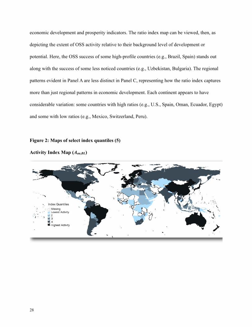
economic development and prosperity indicators. The ratio index map can be viewed, then, as

depicting the extent of OSS activity relative to their background level of development or

potential. Here, the OSS success of some high-profile countries (e.g., Brazil, Spain) stands out

along with the success of some less noticed countries (e.g., Uzbekistan, Bulgaria). The regional

patterns evident in Panel A are less distinct in Panel C, representing how the ratio index captures

more than just regional patterns in economic development. Each continent appears to have

considerable variation: some countries with high ratios (e.g., U.S., Spain, Oman, Ecuador, Egypt)

and some with low ratios (e.g., Mexico, Switzerland, Peru).

Figure 2: Maps of select index quantiles (5)

Activity Index Map (Aaa,BL)

28

Potential Index Map (Paa,BL)

Ratio A/P (Ratiowa,BL) Index Map

5.0 Sensitivity Analysis

With many candidate indices (and sub-indices), tests for robustness to different aggregation

rules, sample sizes, and measure types are critical. The primary concern here is with correlations

in rank-orderings (rather than raw values) derived from each index. Ideally, the OSS indices that

measured similar things would not vary dramatically across different aggregation rules or types

29

of measures. To the extent that the index is sensitive to these design choices, the usefulness of the

index should be questioned.

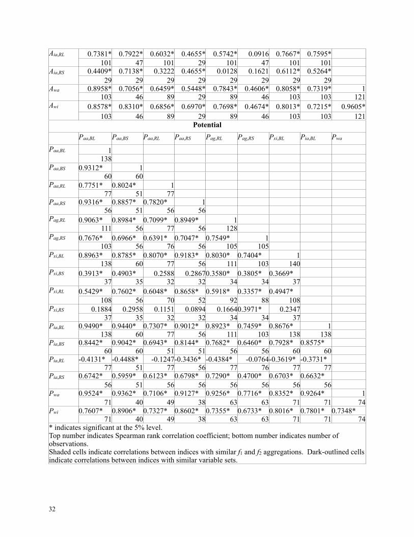
Table 5 summarizes some of the observed Spearman rank-order correlations between

alternative indices. Some variation is to be expected given that the different indices aim to

measure different things (e.g., activity vs. potential vs. their ratio) and they employ different

variables. Overall, a good deal of stability is found across aggregation rules. For the activity

indices, all rank correlations are positive and nearly all are significant at the 5% level (usually at

the 0.1% level). Rank correlations across different aggregation rules (while using the same

indicators) are quite strong. Across 101 countries, the A ranks are significantly correlated

between the arithmetic mean aggregation and the geometric mean (0.75), the maxi-min (0.69),

and the mini-mean (0.64). Rank orderings do vary if the A depends on averages of indicators or

on the “weakest link” of those indicators, but the rankings are still closely correlated. For similar

index constructions, the correlations are even stronger. Indices with the same aggregation rules

but different indicators (e.g., Aaa,BL and Aaa,BS), are highly correlated; significant Spearman

correlation coefficients exceed 0.5 in all but one case. For example, the rank correlation between

long and short indices is 0.73 when using the best indicators and a simple arithmetic mean, and it

is 0.90 when using ratio-scale variables and a geometric mean. Perhaps the strongest evidence

that the A index is robust to aggregation rules (and even to alternate indicator variables) can be

found in the high rank-correlation coefficient (0.82) between the preferred arithmetic mean and

geometric mean indices for the “long” indicators (Aaa,BL, and Aag,RL). Somewhat troubling is the

weaker rank correlation for the corresponding “short” indicators. The short indices, which use

better indicators but at the cost of a reduced sample, have weaker correlations across aggregation

30

rules (Aaa,RS and Aag,RS are correlated at 0.40). Similar results, often even stronger, hold even if

the correlations reported in Table 5 are computed using casewise deletion (so that the same set of

countries is used throughout). Moreover, as the lower half of Table 5 indicates, these general

observations about the strength of correlations hold when looking at the potential indices (P).11

Finally, Table 5 shows that the P indices are closely rank-correlated with Pwa. The indices are

largely robust to alternative weights for averaging.

Table 5: Select index rank correlationsActivityActivityActivityActivityActivityActivityActivityActivityActivityActivity

Aaa,BL Aaa,BS Aaa,RL Aaa,RS Aag,RL Aag,RS Axi,BL Aia,BL Awa

Aaa,BL 1Aaa,BL 132

Aaa,BS 0.7314* 1Aaa,BS47 47

Aaa,RL 0.7238* 0.7544* 1Aaa,RL101 47 101

Aaa,RS 0.5611* 0.8414* 0.8897* 1Aaa,RS29 29 29 29

Aag,RL 0.8189* 0.4272* 0.6380* 0.3862* 1Aag,RL

101 47 101 29 101Aag,RS 0.4926* 0.4245* 0.4185* 0.3961* 0.8957* 1Aag,RS

47 47 47 29 47 47Axi,BL 0.8757* 0.7100* 0.6977* 0.3488 0.6991* 0.1962 1Axi,BL

132 47 101 29 101 47 132Axi,BS 0.6074* 0.8111* 0.5649* 0.6471* 0.2364 0.2008 0.8106*Axi,BS

47 47 47 29 47 47 47Axi,RL 0.8366* 0.4301* 0.6965* 0.3433 0.8833* 0.8447* 0.7429*Axi,RL

101 47 101 29 101 47 101Axi,RS 0.5907* 0.5668* 0.4712* 0.3839* 0.7740* 0.9483* 0.3205Axi,RS

29 29 29 29 29 29 29Aia,BL 0.8411* 0.5932* 0.6455* 0.6312* 0.6674* 0.4017* 0.7103* 1Aia,BL

132 47 101 29 101 47 132 132Aia,BS 0.4556* 0.6619* 0.6244* 0.5966* 0.4372* 0.4307* 0.5663* 0.7553*Aia,BS

47 47 47 29 47 47 47 47

31

11 In many cases, the correlations are even stronger (e.g., Paa,BL has a greater rank-correlation with Paa,BS and Pag,RL) but remain generally consistent with the activity variables. One exception is with the Pia,RL index, which is generally negatively correlated with other index measures. This surprising result largely follows from a negative correlation between the F dimension in the ratio-scale and the C dimension with the best variables for this subset of countries. This peculiar result poses only a minor concern because the odd-behaving ratio-scale version of P with a mini-mean aggregation is useful primarily for comparison to Pag,RL, especially given that the superior Pia,BL index is present.

Aia,RL 0.7381* 0.7922* 0.6032* 0.4655* 0.5742* 0.0916 0.7667* 0.7595*Aia,RL

101 47 101 29 101 47 101 101Aia,RS 0.4409* 0.7138* 0.3222 0.4655* 0.0128 0.1621 0.6112* 0.5264*Aia,RS

29 29 29 29 29 29 29 29Awa 0.8958* 0.7056* 0.6459* 0.5448* 0.7843* 0.4606* 0.8058* 0.7319* 1Awa

103 46 89 29 89 46 103 103 121Awi 0.8578* 0.8310* 0.6856* 0.6970* 0.7698* 0.4674* 0.8013* 0.7215* 0.9605*Awi

103 46 89 29 89 46 103 103 121PotentialPotentialPotentialPotentialPotentialPotentialPotentialPotentialPotentialPotential

Paa,BL Paa,BS Paa,RL Paa,RS Pag,RL Pag,RS Pxi,BL Pia,BL Pwa

Paa,BL 1Paa,BL 138

Paa,BS 0.9312* 1Paa,BS

60 60Paa,RL 0.7751* 0.8024* 1Paa,RL

77 51 77Paa,RS 0.9316* 0.8857* 0.7820* 1Paa,RS

56 51 56 56Pag,RL 0.9063* 0.8984* 0.7099* 0.8949* 1Pag,RL

111 56 77 56 128Pag,RS 0.7676* 0.6966* 0.6391* 0.7047* 0.7549* 1Pag,RS

103 56 76 56 105 105Pxi,BL 0.8963* 0.8785* 0.8070* 0.9183* 0.8030* 0.7404* 1Pxi,BL

138 60 77 56 111 103 140Pxi,BS 0.3913* 0.4903* 0.2588 0.28670.3580* 0.3805* 0.3669*Pxi,BS

37 35 32 32 34 34 37Pxi,RL 0.5429* 0.7602* 0.6048* 0.8658* 0.5918* 0.3357* 0.4947*Pxi,RL

108 56 70 52 92 88 108Pxi,RS 0.1884 0.2958 0.1151 0.0894 0.16640.3971* 0.2347Pxi,RS

37 35 32 32 34 34 37Pia,BL 0.9490* 0.9440* 0.7307* 0.9012* 0.8923* 0.7459* 0.8676* 1Pia,BL

138 60 77 56 111 103 138 138Pia,BS 0.8442* 0.9042* 0.6943* 0.8144* 0.7682* 0.6460* 0.7928* 0.8575*Pia,BS

60 60 51 51 56 56 60 60Pia,RL -0.4131* -0.4488* -0.1247-0.3436* -0.4384* -0.0764-0.3619* -0.3731*Pia,RL

77 51 77 56 77 76 77 77Pia,RS 0.6742* 0.5959* 0.6123* 0.6798* 0.7290* 0.4700* 0.6703* 0.6632*Pia,RS

56 51 56 56 56 56 56 56Pwa 0.9524* 0.9362* 0.7106* 0.9127* 0.9256* 0.7716* 0.8352* 0.9264* 1Pwa

71 40 49 38 63 63 71 71 74Pwi 0.7607* 0.8906* 0.7327* 0.8602* 0.7355* 0.6733* 0.8016* 0.7801* 0.7348*Pwi

71 40 49 38 63 63 71 71 74* indicates significant at the 5% level.Top number indicates Spearman rank correlation coefficient; bottom number indicates number of observations.Shaded cells indicate correlations between indices with similar f1 and f2 aggregations. Dark-outlined cells indicate correlations between indices with similar variable sets.

* indicates significant at the 5% level.Top number indicates Spearman rank correlation coefficient; bottom number indicates number of observations.Shaded cells indicate correlations between indices with similar f1 and f2 aggregations. Dark-outlined cells indicate correlations between indices with similar variable sets.









32

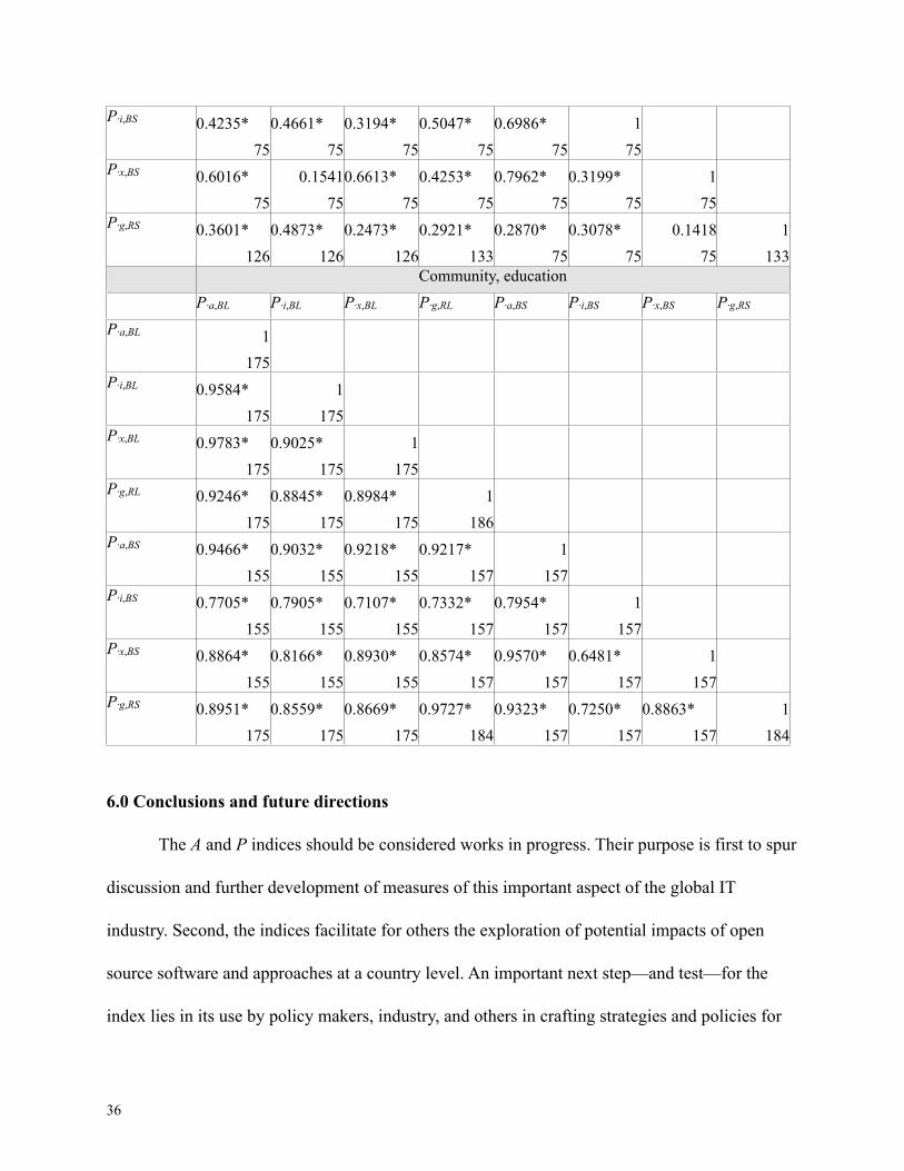
Because the open source index is composed of three different sub-indices or dimensions, the

robustness of the dimensions to alternative approaches also merits some scrutiny. As in Table 5,

Table 6 shows the rank correlations between various constructions of the government (G), firms

(F), and community (C) dimensions of the OSS indices. The dimension values are highly rank-

correlated with one another even when produced with different aggregations or variable sets.

This is especially true for the dimensions in the activity index, where the pairwise rank

correlations between dimensions that use different aggregation rules or different variable lists are

typically well over 0.7 and often over 0.95. The G and F dimensions for the potential index

exhibit somewhat less consistency, where the P·i,BS and P·g,RS dimensions are weakly or

uncorrelated with other aggregations using similar indicators. Although this presents some reason

for caution, it bears emphasis that Table 6 shows rank correlations for 48 different dimension

measures, and a few weak correlations are to be expected.

Table 6: Select dimension rank correlationsActivity GovernmentGovernmentGovernmentGovernmentGovernmentGovernmentGovernmentGovernment

A·a,BL A·i,BL A·x,BL A·g,RL A·a,BS A·i,BS A·x,BS A·g,RS A·a,BL 1A·a,BL

193A·i,BL 0.8915* 1A·i,BL

193 193A·x,BL 0.9989* 0.8832* 1A·x,BL

193 193 193A·g,RL 0.9071* 0.9856* 0.9021* 1A·g,RL

122 122 122 122A·a,BS 0.4440* 0.5336* 0.4456* 0.6752* 1A·a,BS

48 48 48 48 48A·i,BS 0.5367* 0.6463* 0.4926* 0.7587* 0.7757* 1A·i,BS

48 48 48 48 48 48A·x,BS 0.27550.3549* 0.3093* 0.5139* 0.9421* 0.5627* 1

33

A·x,BS

48 48 48 48 48 48 48A·g,RS 0.6680* 0.7719* 0.6745* 0.8620* 0.7738* 0.6933* 0.6470* 1A·g,RS

48 48 48 48 48 48 48 48IndustryIndustryIndustryIndustryIndustryIndustryIndustryIndustry


132A·i,BL 0.9142* 1A·i,BL

132 132A·x,BL 0.9900* 0.8712* 1A·x,BL

132 132 132A·g,RL 0.9756* 0.9651* 0.9547* 1A·g,RL

132 132 132 132A·a,BS 1.0000* 0.9142* 0.9900* 0.9756* 1A·a,BS

132 132 132 132 132A·i,BS 0.9142* 1.0000* 0.8712* 0.9651* 0.9142* 1A·i,BS

132 132 132 132 132 132A·x,BS 0.9900* 0.8712* 1.0000* 0.9547* 0.9900* 0.8712* 1A·x,BS

132 132 132 132 132 132 132A·g,RS 0.9756* 0.9651* 0.9547* 1.0000* 0.9756* 0.9651* 0.9547* 1A·g,RS

132 132 132 132 132 132 132 132Community, educationCommunity, educationCommunity, educationCommunity, educationCommunity, educationCommunity, educationCommunity, educationCommunity, education


190A·i,BL 0.9607* 1A·i,BL

190 190A·x,BL 0.8402* 0.7385* 1A·x,BL

190 190 190A·g,RL 0.3268* 0.3307* 0.2987* 1A·g,RL

190 190 190 190A·a,BS 0.9472* 0.9048* 0.8291* 0.2870* 1A·a,BS

190 190 190 190 190A·i,BS 0.8874* 0.9085* 0.7152* 0.2589* 0.9517* 1A·i,BS

190 190 190 190 190 190A·x,BS 0.8378* 0.7387* 0.9627* 0.2916* 0.8380* 0.7181* 1

34

A·x,BS

190 190 190 190 190 190 190A·g,RS 0.3323* 0.3410* 0.3067* 0.9978* 0.2905* 0.2653* 0.2998* 1A·g,RS

190 190 190 190 190 190 190 190

Potential GovernmentGovernmentGovernmentGovernmentGovernmentGovernmentGovernmentGovernmentP·a,BL P·i,BL P·x,BL P·g,RL P·a,BS P·i,BS P·x,BS P·g,RS

P·a,BL 1P·a,BL

179P·i,BL 0.7388* 1P·i,BL

179 193P·x,BL 0.8361* 0.3456* 1P·x,BL

179 179 179P·g,RL 0.8229* 0.6995* 0.6678* 1P·g,RL

130 130 130 130P·a,BS 0.5849* 0.6032* 0.3033* 0.5204* 1P·a,BS

94 95 94 78 95P·i,BS -0.1135 0.2312 -0.1724 -0.10430.7047* 1P·i,BS

47 48 47 43 43 48P·x,BS 0.6136* 0.4162* 0.4428* 0.6029* 0.5572* -0.129 1P·x,BS

94 95 94 78 95 43 95P·g,RS 0.8229* 0.6995* 0.6678* 1.0000* 0.5204* -0.10430.6029* 1P·g,RS

130 130 130 130 78 43 78 130IndustryIndustryIndustryIndustryIndustryIndustryIndustryIndustry

P·a,BL P·i,BL P·x,BL P·g,RL P·a,BS P·i,BS P·x,BS P·g,RS P·a,BL 1P·a,BL

140P·i,BL 0.6903* 1P·i,BL

140 140P·x,BL 0.9314* 0.5026* 1P·x,BL

140 140 140P·g,RL 0.5995* 0.3892* 0.5655* 1P·g,RL

140 140 140 185P·a,BS 0.6605* 0.3933* 0.5784* 0.5630* 1P·a,BS

75 75 75 75 75

35

P·i,BS 0.4235* 0.4661* 0.3194* 0.5047* 0.6986* 1P·i,BS

75 75 75 75 75 75P·x,BS 0.6016* 0.15410.6613* 0.4253* 0.7962* 0.3199* 1P·x,BS

75 75 75 75 75 75 75P·g,RS 0.3601* 0.4873* 0.2473* 0.2921* 0.2870* 0.3078* 0.1418 1P·g,RS

126 126 126 133 75 75 75 133Community, educationCommunity, educationCommunity, educationCommunity, educationCommunity, educationCommunity, educationCommunity, educationCommunity, education

P·a,BL P·i,BL P·x,BL P·g,RL P·a,BS P·i,BS P·x,BS P·g,RS P·a,BL 1P·a,BL

175P·i,BL 0.9584* 1P·i,BL

175 175P·x,BL 0.9783* 0.9025* 1P·x,BL

175 175 175P·g,RL 0.9246* 0.8845* 0.8984* 1P·g,RL

175 175 175 186P·a,BS 0.9466* 0.9032* 0.9218* 0.9217* 1P·a,BS

155 155 155 157 157P·i,BS 0.7705* 0.7905* 0.7107* 0.7332* 0.7954* 1P·i,BS

155 155 155 157 157 157P·x,BS 0.8864* 0.8166* 0.8930* 0.8574* 0.9570* 0.6481* 1P·x,BS

155 155 155 157 157 157 157P·g,RS 0.8951* 0.8559* 0.8669* 0.9727* 0.9323* 0.7250* 0.8863* 1P·g,RS

175 175 175 184 157 157 157 184

6.0 Conclusions and future directions

The A and P indices should be considered works in progress. Their purpose is first to spur

discussion and further development of measures of this important aspect of the global IT

industry. Second, the indices facilitate for others the exploration of potential impacts of open

source software and approaches at a country level. An important next step—and test—for the

index lies in its use by policy makers, industry, and others in crafting strategies and policies for

36

the advancement of open source interests and ICT development more broadly.

Until now, much of the OSS domain is dominated by anecdotal and informal knowledge,

especially about the state of OSS on a global scale. The A and P indices represent an important

first step in advancing discussions about global OSS development by providing systematic and

robust empirical evidence on a global scale. To do so, we confronted head-on the difficulties in

constructing useful indices for such a tricky concept as OSS activity or potential. Our efforts

attempt to reflect the openness and transparency of the OSS enterprise, thus our methods are

described in detail here and the base data are readily available for download by the broader “user

community” for this research. While we believe that the indices presented here provide a good

“snapshot” of a country’s open source potential and activity, it is worth noting that better data

collection—beyond the scope of the current project—could improve the index in subsequent

iterations. We welcome continued improvements to and adaptations of these indices.

Turning to policy considerations, government commissions and agencies have proposed,

and in some cases implemented, a variety of measures to encourage open source developers. For

example, in the United States, the President's Information Technology Advisory Committee

(2000) recommended direct federal subsidies for open source projects to advance high-end

computing, and a report from the European Commission (2001) also discussed support for open

developers and standards. Many European governments have policies to encourage the use and

purchase of open source software for government use. As is well known, governments can

sponsor the development of localized open source projects. Economists have sought to

understand the consequences of a vibrant open source sector for social welfare. Perhaps not

surprisingly, definitive or sweeping answers have been difficult to come by. But if a tentative

37

conclusion can be made, most analyses have concluded, based on limited data, that government

support for open source projects is likely to have an ambiguous effect on social welfare.

We hope that these indices are not the end product of research in this area, but rather the

beginning of an empirical research agenda at the intersection of OSS and public policy. Future

research could make use of these indices to test a variety of hypotheses about the causes and

effects of OSS and related policies. Anecdotal evidence, case studies, and intuitions pervade the

OSS discourse. Thus far, much of the literature has very limited generalizability because of the

prevalence of case-study approaches. The OSS indices presented here can help bring light where

there is much heat. For example, the frequent claims about OSS's liberating nature and positive

implications for social welfare (made often by governments themselves) lack a strong empirical

basis. Future research can use these OSS indices to systematically assess the societal impacts of

effects of OSS. The indices can enable testing of hypotheses about whether OSS drives

innovation, economic development, transparency in governance, or other social aims. These

indices can also play pivotal roles in studies of the rise of OSS activity. Identifying the

determinants of OSS activity, and the factors that influence which countries achieve more of

their OSS potential, merits additional investigation.

If “footloose” developers can participate in OSS projects across boundaries, what role

does the state and geography more generally have in guiding the evolution of OSS? The OSS

indices can inform studies of the effectiveness of particular OSS policies and initiatives on

developing OSS, of strategic interdependence between states in setting their OSS policy (akin to

trade policy), of the influences of different political and cultural landscapes on the popularity of

OSS, and of the impact of education programs on OSS. Knowing where the cathedrals and

38

bazaars are will hopefully launch a new set of inquiries into the determinants of that distribution

and the implications of greater OSS activity and potential.

7.0 Appendix

7.1 Variable List

Variables in Index A and Index P Indicator SourceOSSpolNatman Count of policies at the national level

that mandate open source softwareCenter for Strategic and International Studies “Government Open Source Policies” 2008

GovExppGDP Government expenditures as percent gross domestic product

World Development Indicators 2003

OSSpolNatRD Count of policies at the national level that provide R&D for open source software

Center for Strategic and International Studies “Government Open Source Policies” 2008

OSSfundng Ratio of national and local R&D policies to all national and local policies

derived from Center for Strategic and International Studies 2008

RHCEpc number of Red Hat Certified Engineers Red Hat, Inc. 2008LinuxUserspc Number of GNU/Linux users

registered per capitaLinux Counter 2008

GoogleApppc Number of applications submitted to Google Summer of Code per capita

Google Summer of Code 2005

SchoolNet Percent schools connected to Internet CIA World Fact Book 2004rOSSnews Number of hits for “open source

software” on Google News archives within country during 2008

Google News 2008

LinuxLang 1 if native language support for GNU/Linux, 0 if otherwise

Distro Watch

nPiracy Number of pirated software units divided by total number of units put into use, negative transform

Business Software Alliance 2006

OOXML -1 if country voted for OOXML passage, 0 if No, empty if abstained or not invited

Open Malaysia Blog, ISO 2008

nCivLib Freedom in the World Index of Civil Liberties scored 1 through 7, higher being worse, negative transform

Freedom House 2006

Turnout Percent voters of voting age population (1945 to 1998)

International IDEA

eGov e-Government Survey Score United Nations 2008nTRIPS -1 if participant of TRIPS (Trade

Related Aspects of Intellectual Property)

World Trade Organization 2008

nIPRI Intellectual Property RIghts Index, higher score indicates more rights, negative transform

Property Rights Alliance 2008

ICTtop250pGDP Number of ICT firms in the Top 250 per gross domestic product

OECD 2005

39

ICTexpendpGDP ICT expenditures as percent gross domestic product

CIA World Fact Book 2004

newCellGro Growth of number of cell phones from 1995 to 2001, percent growth over baseline year


TelecomInvestpc Private investment in telecoms (current US$) per capita

International Telecommunications Union 2001

SciArticlespc Number of published scientific and technical journal articles per capita


RnDemploypc Scientists and engineers per capita World Development Indicators 2000nNetPrice Price basket for Internet service per

month, negative transformCIA World Fact Book 2003

inewGrowth Growth of Foreign Direct Investment from 2001 to 2006, percent growth over baseline year

United Nations Conference on Trade and Development

TVpc Number of television sets per capita World Development Indicators 2000Techphob Percent students who consider

themselves technophobicComputers in Human Behavior 1995

College Percent of college aged population enrolled


GradEngpgrad Graduates in engineering, manufacturing and construction (% of total graduates, tertiary)


PCspc Number of personal computers per capita

International Telecommunications Union 2004

InternetUserspc Number of Internet users per capita International Telecommunications Union 2004

Awa VariablesrOSShits Hits for "open source software" on Google by region=countryGoogle 2008GDPpcPPP Gross domestic product per capita

adjusted purchasing power parity2002

PCpc Personal computers per capita International Telecommunications Union 2004

XPpGDPPm Cost of Windows XP in "gross domestic product months”

First Monday – Ghosh

iServerspc Internet servers per capita CIA World Fact Book 2005InternetHostspc Computers connected to Internet per

capitaComputers in Human Behavior 2007

OSSpolNat and (d) Two variables were created as a count of all National and Municipal level policies. These variables were further subdivided to create counts of policies that indicated just Mandates, Preferences, Advisorys, or R&D. This resulted in 10 variables. For each count variable, a dummy variable was created indicating 0 if no policy, 1 if one or more. Therefore, 20 policy variables total were available.


OSSpolMun and (d)Two variables were created as a count of all National and Municipal level policies. These variables were further subdivided to create counts of policies that indicated just Mandates, Preferences, Advisorys, or R&D. This resulted in 10 variables. For each count variable, a dummy variable was created indicating 0 if no policy, 1 if one or more. Therefore, 20 policy variables total were available.

Center for Strategic and International Studies “Government Open Source Policies” 2008OSSpolNatRD and (d)

Two variables were created as a count of all National and Municipal level policies. These variables were further subdivided to create counts of policies that indicated just Mandates, Preferences, Advisorys, or R&D. This resulted in 10 variables. For each count variable, a dummy variable was created indicating 0 if no policy, 1 if one or more. Therefore, 20 policy variables total were available.


OSSpolMunRD and (d)



OSSpolNatadv and (d)



OSSpolNatman and (d)



OSSpolNatpre and (d)



OSSpolMunadv and (d)



OSSpolMunman and (d)



OSSpolMunpre and (d)



Pwa VariablesAge2529% Persons age 25 to 29 as percent

populationCIA World Fact Book 2005

40

Age2024% Persons age 20 to 24 as percent population


Age1524% Persons age 15 to 24 as percent population


TVpc Television sets per capita World Development Indicators 2001urban% Percent population residing in urban

area2002

Literacy% Percent population 15 and older who are literate

HSenroll% Percent eligible population enrolled in high school


HSvoc Enrollment in upper secondary technical/vocational programs

OECD 2005

newspc Number of daily newspapers per capita 2000InternetUserspc Number of Internet users per capita International Telecommunications

Union 2004Phonespc Telephone landlines per capita World Development Indicators 2001Radiopc Radio sets per capita World Development Indicators 2001Cellspc Cellular phones per capita World Development Indicators 2001PhoneUSA Average cost of telephone call to US

(US$ per three minutes)World Development Indicators 2001

PhoneLoc Telephone average cost of local call (US$ per three minutes)


Phonelinespc Telephone mainlines in largest city (per 1,000 people)


Phonelinespworker Telephone mainlines per employee World Development Indicators 2001PhoneWaittime Telephone mainlines, waiting time

(years)World Development Indicators 2000

Phonepc Fixed line and mobile phone subscribers (per 1,000 people)


nNetPrice Price basket for Internet service per month, negative transform


GDPpc Gross domestic product per capita World Development Indicators 2003TradepGDP Trade as percent of gross domestic

productWorld Development Indicators 2003

ICTpExport Communications, computer, etc. (% of service exports, BoP)


SciArticlespc Number of scientific or technical journal articles published per capita


POiGov PO offers electronic services, percent of 12 potential services

Original data collection

POInternet Post Office provides public Internet access points (1=yes, 0=no)… year=2005 or most recent if missing

Original data collection

nWTO -1 if member of World Trade Organization

World Trade Organization 2007

7.2 Complete Index Values

41

Table A2: Select index ranks for all countries

Country Aaa,BL Aaa,BS Aag,RL Aag,RS Paa,BLPaa,BS Pag,RLPag,RS Ratioaa,BL

Ratioag,RL

Ratioaa,BS Ratioag,RS

Awa Pwa

Afghanistan . . . . . . . . . . . . . .Albania . . . . 41 . 9 54 . . . . 93 6Algeria 99 . 92 . 86 . 97 94 38 81 . . 88 .Andorra . . . . . . 14 . . . . . . .Angola . . . . 132 . . . . . . . 99 65Antigua and Barbuda . . . . . . 4 . . . . . . .Argentina 39 42 36 32 49 . 7 21 8 40 . 29 32 30Armenia 101 . . . . . . . . . . . 98 .Australia 13 10 22 25 10 13 15 29 36 23 13 22 12 9Austria 34 16 51 37 15 14 21 43 65 48 18 33 29 13Azerbaijan 129 . 47 . 99 . . . 21 . . . . 45Bahamas 62 . 33 . . . 17 . . 33 . . . .Bahrain 58 . 60 . . . . . . . . . 58 .Bangladesh 84 . 87 . 105 58 114 85 64 77 . . 110 70Barbados 88 . . . . . 48 . . . . . 52 .Belarus 72 . 84 . 28 . . . 87 . . . . 15Belgium 3 13 10 23 18 16 25 42 11 14 10 17 1 8Belize . . . . 72 . 57 . . . . . 56 .Benin . . . . 109 . 121 87 . . . . 108 71Bhutan . . . . . . . . . . . . . .Bolivia 83 . 45 . 78 43 40 59 29 42 . . 94 49Bosnia and Herzegovina 66 . . . . . . . . . . . . .Botswana 128 . 86 . 43 . 104 75 102 75 . . 78 56Brazil 5 32 4 17 55 46 68 45 2 1 30 15 10 .Brunei Darussalam 65 . . . . . . . . . . . . .Bulgaria 22 23 16 9 47 29 53 56 5 11 5 5 15 26Burkina Faso . . . . 124 . 126 82 . . . . 118 .Burundi . . . . 129 . . . . . . . . 72Cambodia 123 . . . 127 . 102 . 48 . . . 75 .Cameroon 107 . 48 . 126 . 113 80 66 43 . . 101 64Canada 33 24 53 39 6 8 13 27 76 52 22 35 24 .Cape Verde . . . . . . 91 . . . . . . .Central African Republic . . . . 138 . . . . . . . . .

Chad . . . . 136 . . . . . . . . .Chile 28 . 40 . 48 33 62 50 6 35 . . 20 28China, People's Republic of 15 22 6 12 66 48 . . 106 . 32 . 28 .

Columbia 36 . . . 60 27 83 63 103 . . . 25 33Comoros . . . . . . . . . . . . . .Congo, Democratic Republic of the 105 . 101 . 130 60 . . 72 . . . . .

Costa Rica 59 44 46 30 52 32 58 58 95 41 31 27 53 32Croatia 53 26 58 42 46 . 55 4 85 51 . 40 61 23Cuba 68 . . . 98 . . . 70 . . . . .Cyprus 50 31 57 41 37 . 44 12 82 50 . 39 48 .Czech Republic 47 . 56 . 40 25 60 5 73 46 . . 41 .Côte d'Ivoire (Ivory Coast) 108 . 99 . 115 . . . 62 . . . 100 .

Denmark 9 9 17 20 4 7 8 31 30 21 16 19 4 .

42

Djibouti 112 . . . . . 124 . . . . . . .Dominica . . . . . . 81 . . . . . 49 .Dominican Republic 97 . 79 . 73 . 36 74 15 73 . . . .Ecuador 80 . . . 65 54 86 70 10 . . . 87 51Egypt 77 . 82 . 64 49 101 88 13 66 . . 89 43El Salvador 90 . 81 . 85 45 56 30 42 72 . . 83 .Equatorial Guinea . . . . . . . . . . . . . .Eritrea 131 . . . . . . . . . . . . .Estonia 20 . 30 . 20 . 26 15 27 28 . . 42 11Ethiopia 100 . 100 . . . . . . . . . 121 68Fiji 118 . 70 . 101 . 90 47 28 59 . . 70 .Finland 10 2 18 5 8 6 18 24 26 20 4 9 5 4France 2 7 1 3 16 12 23 34 14 2 7 6 17 .Gabon . . . . 117 . . . . . . . 82 .Gambia 111 . . . 112 . 119 99 61 . . . . 69Georgia . . . . 57 . 74 90 . . . . . .Germany 21 15 20 28 17 15 1 13 33 24 14 25 27 12Ghana 93 . . . 94 . 118 84 53 . . . 72 52Greece 61 . 65 . 38 37 46 16 86 60 . . 59 25Grenada . . . . 54 . 75 . . . . . 51 .Guatemala 91 . . . 95 . 106 89 56 . . . 86 53Guinea . . . . 133 . . . . . . . . .Guinea-Bissau . . . . 135 . . . . . . . . .Guyana . . . . 84 . 80 81 . . . . . .Haiti 103 . 98 . 137 . 115 102 78 85 . . . .Honduras 104 . . . 96 52 99 86 46 . . . 95 61Hong Kong . . . . . . . . . . . . . .Hungary 45 . 34 . 29 23 41 14 67 30 . . 50 19Iceland 4 1 35 31 19 . 22 1 12 36 . 31 3 .India 29 29 27 24 79 59 96 71 98 4 27 11 35 60Indonesia 70 41 85 46 81 44 84 78 50 71 1 41 90 .Iran, Islamic Republic of . . . . 62 57 77 83 . . . . 31 38

Iraq 71 . . . . . . . . . . . . .Ireland 23 5 19 2 21 19 31 37 37 16 2 3 13 .Israel 38 14 9 11 14 . 28 22 75 12 . 14 30 17Italy 16 17 13 16 26 18 27 44 19 15 12 13 16 10Jamaica . . . . 75 35 73 68 . . . . 77 .Japan 19 . . . 13 4 20 20 43 . . . 22 3Jordan 60 . 66 . 77 42 92 46 74 54 . . 84 42Kazakhstan 125 . 80 . 67 . 34 36 4 74 . . . .Kenya 117 . 44 . 104 50 . . 34 . . . 107 63Kiribati . . . . . . . . . . . . . .Kuwait 81 . 69 . 51 . 45 67 101 61 . . 62 .Kyrgyzstan . . . . . . . . . . . . . .Laos (Lao People's Democratic Repub.. 132 . . . 100 . . . 22 . . . 111 .

Latvia 114 . 68 . 27 . 33 3 93 63 . . 54 16Lebanon 85 . 74 . . . 61 . . 68 . . 76 .Lesotho . . . . 89 . 94 64 . . . . . 55Liberia . . . . . . . . . . . . . .Libya (Libyan Arab Jamahiriya) 89 . . . . . . . . . . . . .

Liechtenstein . . . . . . 3 . . . . . . .

43

Lithuania 76 . 29 . 35 . 43 7 90 26 . . 46 29Luxembourg 44 . 55 . 25 . 35 . 77 49 . . 21 .Macedonia, Former Yugoslav Republic.. 64 . . . . . . . . . . . . 35

Madagascar . . . . 119 . 105 98 . . . . 114 .Malawi . . . . 116 . . . . . . . 120 .Malaysia 43 37 23 26 39 21 49 26 40 13 24 23 67 20Maldives 74 . 67 . . . 89 . . 55 . . . .Mali . . . . 114 . 128 . . . . . 116 .Malta 49 . 38 . . . 37 . . 38 . . 45 .Marshall Islands . . . . . . . . . . . . . .Mauritania . . . . 118 . . . . . . . 106 .Mauritius 116 . 64 . 53 . 59 60 105 57 . . 64 31Mexico 54 . 42 . 56 38 67 51 100 34 . . 63 36Micronesia, Federated States of . . . . . . . . . . . . . .

Moldova 127 . 83 . 33 . . . 97 . . . 105 34Monaco 37 . . . . . . . . . . . . .Mongolia . . . . . . 70 41 . . . . 104 46Montenegro . . . . . . . . . . . . . .Morocco 102 . 93 . 93 55 100 79 45 82 . . 92 44Mozambique 124 . . . 113 . . . 41 . . . . .Myanmar . . . . . . . . . . . . . .Namibia 120 . 78 . 92 . 93 95 20 67 . . 81 .Nauru . . . . . . . . . . . . . .Nepal 119 . 75 . 110 . 111 96 39 62 . . 117 .Netherlands 17 8 11 19 7 11 10 33 47 19 11 18 11 .New Zealand 25 . 32 . 11 20 16 32 60 32 . . 19 .Nicaragua . . . . 103 . 98 . . . . . . .Niger . . . . 134 . 127 105 . . . . 119 73Nigeria 115 . . . 120 . 109 91 54 . . . 112 .North Korea (Korea, Democratic Peop.. 79 . . . . . . . . . . . . .

Norway 6 4 15 13 3 5 6 28 25 22 8 16 2 2Oman 92 . 72 . 68 . . . 9 . . . . .Pakistan 42 25 12 6 106 . 78 76 91 3 . 1 36 59Palau . . . . . . . . . . . . . .Panama 86 . 73 . 71 39 82 11 16 65 . . 66 48Papua New Guinea 113 . 95 . 107 . 110 100 57 80 . . 96 .Paraguay 55 34 26 8 87 . 88 61 81 5 . 2 33 47Peru 12 45 43 34 69 41 71 65 107 39 34 30 7 .Philippines 69 46 25 15 76 40 79 73 32 8 33 4 40 .Poland 40 21 54 40 30 24 42 8 44 47 6 37 44 22Portugal 35 27 61 44 32 28 39 49 35 56 19 38 34 21Qatar 8 . . . . . . . . . . . . .Romania 63 . 63 . 45 26 47 23 89 58 . . 71 .Russian Federation 48 . 31 . 34 30 52 48 80 27 . . 79 24Rwanda . . . . 131 . . . . . . . . .Saint Kitts and Nevis . . . . . . 72 . . . . . . .Saint Lucia . . . . . . 51 . . . . . . .Saint Vincent and the Grenadines . . . . . . 85 . . . . . . .

Samoa 121 . . . . . . . . . . . 68 .San Marino . . . . . . . . . . . . . .

44

Sao Tome and Principe . . . . . . 63 . . . . . . .Saudi Arabia 82 . . . 70 . . . 18 . . . 74 50Senegal 95 . 90 . 97 . 117 52 52 78 . . 102 62Serbia 75 . . . . . . . . . . . . .Seychelles . . . . 36 . 64 . . . . . . .Sierra Leone . . . . 123 . 125 104 . . . . . .Singapore 24 18 52 38 24 . 2 9 31 53 . 36 23 .Slovakia 51 30 59 43 31 . . . 83 . . . 43 18Slovenia 30 12 49 35 23 . 30 10 55 44 . 34 38 .Solomon Islands . . . . . . 116 77 . . . . . .Somolia 109 . . . . . . . . . . . . .South Africa 32 28 7 7 61 56 . . 104 . 28 . 37 40South Korea (Korea, Republic of) 31 36 14 21 12 1 19 6 69 18 23 24 39 5

Spain 1 19 3 14 22 17 29 40 7 6 15 12 6 14Sri Lanka 73 40 41 33 91 . 95 62 59 31 . 28 57 .Sudan 94 . 88 . 122 . 122 103 71 76 . . . 74Suriname . . . . 88 . 54 . . . . . . .Swaziland . . . . 108 . . . . . . . . .Sweden 14 3 5 1 1 2 5 18 51 17 17 8 8 1Switzerland 27 20 50 36 9 10 24 38 63 45 20 32 26 7Syria 96 . 91 . . . . . . . . . 91 .Taiwan (Republic of China) 11 . . . . . . . . . . . . .

Tajikistan 130 47 94 47 . . . . . . . . . .Tanzania 126 . . . . . . . . . . . 73 .Thailand 46 43 24 27 74 47 76 57 96 9 3 20 55 39Timor-Leste . . . . . . . . . . . . . .Togo . . . . 125 . 107 97 . . . . 113 67Tonga . . . . . . . . . . . . . .Trinidad and Tobago 87 . 71 . 59 34 38 25 3 64 . . 65 41Tunisia 56 . 37 . 90 53 87 66 79 29 . . 85 54Turkey 67 . 77 . 63 36 69 39 17 69 . . 80 .Turkmenistan . . . . . . . . . . . . . .Tuvalu . . . . . . . . . . . . . .Uganda 122 . 96 . 128 . 112 53 49 83 . . 115 66Ukraine 78 39 76 45 42 22 66 17 94 70 29 42 60 .United Arab Emirates 52 . 62 . 44 . . . 84 . . . . .United Kingdom (of England, Scotlan.. 7 6 2 4 5 9 12 35 24 7 9 7 9 .

United States of America 18 11 28 22 2 3 11 19 58 25 21 21 14 .

Uruguay 57 38 39 29 50 31 50 69 88 37 26 26 69 27Uzbekistan 106 . . . 58 . 32 72 1 . . . . .Vanuatu . . . . 83 . 108 2 . . . . . .Vatican City . . . . . . . . . . . . . .Venezuela 26 35 21 18 82 51 65 55 99 10 25 10 18 37Vietnam 41 33 8 10 102 . . . 92 . . . 47 .Yemen 110 . 97 . 80 . 120 93 23 84 . . 103 57Zambia . . . . 111 . 123 101 . . . . 109 58Zimbabwe 98 . 89 . 121 . 103 92 68 79 . . 97 .

7.3 References

45

Bitzer, Jürgen and Philip J.H. Schröder (eds), The Economics of Open Source Software Development. Elsevier. (2006).

Berry, David and Giles Moss, “Free and Open Source Software: Opening and Democratizing E-Government’s Black Box,” Information Polity: The International Journal of Government and Democracy in the Information Age 11, no. 1 (2006): 21-34.

Bonaccorsi, Andrea and Cristina Rossi. “Comparing Motivations of Individual Programmers andFirms to Take Part in the Open Source Movement: From Community to Business,” Knowledge, Technology & Policy 18, no. 4 (Winter 2006): 40-64.

David, Paul A. and Joseph S. Shapiro. “Community-Based Production of Open Source Software: What Do We Know about the Developers Who Participate?” 20, no. 4 (2008): 364-398.

DiBona, Chris, Mark Stone, and Danese Cooper (eds), Open Sources 2.0: The Continuing Evolution. O'Reilly Media. (October 21, 2005).

Ebert, Udo and Heinz Welsch, “Meaningful Environmental Indices: A Social Choice Approach,” Journal of Environmental Economics and Management, 47, no. 2 (2004): 270-283.

Feller, Joseph, Brian Fitzgerald, Scott A. Hissam, and Karim R. Lakhani (eds), Perspectives on Free and Open Source Software. MIT Press (2007).

Forge, Simon, “The Rain Forest and the Rock Garden: The Economic Impacts of Open Source Software,” Info: The Journal of Policy, Regulation and Strategy for Telecommunications, Information, and Media 8, no. 3 (2006): 12-31.

Ghosh, Rishab Aiyer, CODE: Collaborative Ownership and the Digital Economy. MIT Press. (2006).

Ghosh, Rishab Aiyer, “Understanding Free Software Developers: Findings from the Floss Study,” in Joseph Feller, Brian Fitzgerald, Scott A. Hissam, and Karim R. Lakhani, eds. Perspectives on Free and Open Source Software. Cambridge: MIT Press (2007): 23-45.

Gosain, Sanjay, “Looking Through a Window on Open Source Culture: Lessons for Community Infrastructure Design,” Systemes d’Information et Management 8, no. 1 (2003): 11-42.

Hahn, R.W. (ed), Government Policy toward Open Source Software. AEI-Brookings Joint Center for Regulatory Studies: Washington DC. (2002).

Krishnamurthy, Sandeep, “On the Intrinsic and Extrinsic Motivation of Free/Libre/Open Source

46

(FLOSS) Developers,” Knowledge, Technology & Policy 18, no. 4 (Winter 2006): 17-39.

Lee, Jyh-An, “Government Policy toward Open Source Software: The Puzzles of Neutrality and Competition,” Knowledge, Technology & Policy 18, no. 4 (Winter 2006): 113-141.

Lerner, Josh, and Jean Tirole, “The Scope of Open Source Licensing,” Journal of Law Economics & Organization 21, no. 1 (April 2005a): 20-56.

Lerner, Josh, and Jean Tirole, “The Economics of Technology Sharing: Open Source and Beyond,” Journal of Economic Perspectives 19, no. 2 (Spring 2005b): 99-120.

Lewis, James. “Government Open Source Policies.” Working Paper. Center for Strategic and International Studies. (July 2008).

Lin, Yuwei, “Hybrid Innovation: The Dynamics of Collaboration between the FLOSS Community and Corporations,” Knowledge, Technology & Policy 18, no. 4 (Winter 2006): 86-100.

Moon, Nathan, and Baker, Paul, “Adoption and Use of Open Source Software: Preliminary Literature Review,” Center for Advanced Communications Policy, Georgia Institute of Technology. Working Paper. (2009).

Raymond, Eric, The Cathedral & the Bazaar: Musings on Linux and Open Source by an Accidental Revolutionary. O’Reilly Media. (1999).

Simon, K. D., “The Value of Open Standards and Open-Source Software in GovernmentEnvironments,” IBM Systems Journal 44, no. 2 (2005): 227-238

Seiferth, C. Justin, “Open Source and These United States,” Knowledge, Technology & Policy 12, no. 3 (Fall 1999): 50-79.

Vaisman, Daria, “Coding a Revolution,” Foreign Policy 159 (March/April 2007): 93.

Van Wendel de Joode, Ruben, Yuwei Lin, and Shay David, “Rethinking Free, Libre, and Open Source Software,” Knowledge, Technology & Policy 18, no. 4 (Winter 2006): 5-16.

Weber, Steven, The Political Economy of Open Source Software, BRIE Working Paper 140. (June 2000.)

Weber, Steven, The Success of Open Source, Harvard University Press. (2005).

47

Where the Cathedrals and Bazaars Are: An Index of Open Source Software Activity and Potential

Documents

Transcript of Where the Cathedrals and Bazaars Are: An Index of Open Source Software Activity and Potential