When Machine Vision Meets Histology: A ComparativeEvaluation of Model Architecture for Classification of

Histology Sections

Cheng Zhong1, Ju Han1, Alexander Borowsky3, Yunfu Wang1,4, BahramParvin2,Hang Chang1,⋆

1Lawrence Berkeley National Laboratory, Berkeley, CA, USA2Department of Electrical and Biomedical Engineering, University of Nevada, Reno, NV, USA

3Center for Comparative Medicine, University of California, Davis, CA, USA4Department of Neurology, Taihe Hospital, Hubei University of Medicine, Shiyan, Hubei, China

⋆ Corresponding Author: hchang@lbl.gov

Abstract

Classification of histology sections in large cohorts, in terms of distinct regions ofmicroanatomy (e.g., stromal) and histopathology (e.g., tumor, necrosis), enablesthe quantification of tumor composition, and the construction of predictive mod-els of genomics and clinical outcome. To tackle the large technical variations andbiological heterogeneities, which are intrinsic in large cohorts, emerging systemsutilize either prior knowledge from pathologists or unsupervised feature learningfor invariant representation of the underlying properties in the data. However,to a large degree, the architecture for tissue histology classification remains un-explored and requires urgent systematical investigation. This paper is the firstattempt to provide insights into three fundamental questions in tissue histologyclassification: I. Is unsupervised feature learning preferable to human engineeredfeatures? II. Does cellular saliency help? III. Does the sparse feature encodercontribute to recognition? We show that (a) in I, both Cellular MorphometricFeature and features from unsupervised feature learning lead to superior perfor-mance when compared to SIFT and [Color, Texture]; (b) in II, cellular saliencyincorporation impairs the performance for systems built upon pixel-/patch-levelfeatures; and (c) in III, the effect of the sparse feature encoder is correlated withthe robustness of features, and the performance can be consistently improved bythe multi-stage extension of systems built upon both Cellular Morphmetric Fea-ture and features from unsupervised feature learning. These insights are validatedwith two cohorts of Glioblastoma Multiforme (GBM) and Kidney Clear Cell Car-

Preprint submitted to Elsevier September 13, 2016

cinoma (KIRC).

Keywords: Computational Histopathology, Classification, Unsupervised FeatureLearning, Sparse Feature Encoder

1. Introduction1

Although molecular characterization of tumors through gene expression anal-2

ysis has become a standardized technique, bulk tumor gene expression data pro-3

vide only an average genome-wide measurement for a biopsy and fail to reveal4

inherent cellular composition and heterogeneity of a tumor. On the other hand,5

histology sections provide wealth of information about the tissue architecture that6

contains multiple cell types at different states of cell cycles. These sections are7

often stained with hematoxylin and eosin (H&E) stains, which label DNA (e.g.,8

nuclei) and protein contents, respectively, in various shades of color. Furthermore,9

morphometric abberations in tumor architecture often lead to disease progression,10

and it is therefore desirable to quantify tumor architecture as well as the corre-11

sponding morphometric abberations in large cohorts for the construction of pre-12

dictive models of end points, e.g., clinical outcome, which have the potential for13

improved diagnosis and therapy.14

Despite the efforts by some researchers on reducing inter- and intra-pathologist15

variations Dalton et al. (2000) during manual analysis, this approach is not a scal-16

able solution, and therefore impedes the effective representation and recognition17

from large cohorts for scientific discoveries. With its value resting on capturing18

detailed morphometric signatures and organization, automatic quantitative analy-19

sis of a large collection of histological data is highly desirable, and is unfortunately20

impaired by a number of barriers mostly originating from the technical variations21

(e.g., fixation, staining) and biological heterogeneities (e.g., cell type, cell state)22

always presented in the data. Specifically, a histological tissue section refers to an23

image of a thin slice of tissue applied to a microscopic slide and scanned from a24

light microscope, and the technical variations and biological heterogeneities lead25

to significant color variations both within and across tissue sections. For example,26

within the same tissue section, nuclear signal (color) varies from light blue to dark27

blue due to the variations of their chromatin content; and nuclear intensity in one28

tissue section may be very close to the background intensity (e.g., cytoplasmic,29

macromolecular components) in another tissue section.30

It is also worth to mention that alternative staining (e.g., fluorescence) and mi-31

croscopy methods (multi-spectral imaging) have been proposed and studied in or-32

2

der to overcome the fundamental limitations/challenges in tissue histology Stack33

et al. (2014); Levenson et al. (2015); Rimm (2014); Huang et al. (2013); Ghaznavi34

et al. (2013); however, H&E stained tissue sections are still the gold standard for35

the assessment of tissue neoplasm. Furthermore, the efficient and effective rep-36

resentation and interpretation of H&E tissue histology sections in large cohorts37

(e.g., The Cancer Genome Atlas dataset) have the potential to provide predictive38

models of genomics and clinical outcome, and are therefore urgently required.39

Although many techniques have been designed and developed for tissue histol-40

ogy classification (see Section 2), the architecture for tissue histology classifica-41

tion remains largely unexplored and requires urgent systematical investigation. To42

fulfil this goal, our paper provides insights to three fundamental questions in tissue43

histology classification: I. Is unsupervised feature learning preferable to human44

engineered features? II. Does cellular prior knowledge help? III. Does the sparse45

feature encoder contribute to recognition? The novelty of our work resides in three46

folds: (i) architecture design: we have systematically experimented the system ar-47

chitecture with various combinations of feature types, feature extraction strategies48

and intermediate layers based on sparsity/locality-constrained feature encoders,49

which ensures the extensive evaluation and detailed insights on impact of the key50

components during the architecture construction; (ii) experimental design: our51

experimental evaluation has been performed through cross-validation on two in-52

dependent datasets with distinct tumor types, where both datasets have been cu-53

rated by our pathologist to provide examples of distinct regions of microanatomy54

(e.g., stromal) and histopathology (e.g., tumor, necrosis) with sufficient amount55

of technical variations and biological heterogeneities, so that the architecture can56

be faithfully tested and validated against important topics in histopathology (see57

Section 4 for details). More importantly, such an experimental design (combina-58

tion of cross-validation and validation on independent datasests), to the maximum59

extent, ensures the consistency and unbiasedness of our findings; and (iii) out-60

come: the major outcome of our work are well-justified insights in the architec-61

ture design/construction. Specifically, we suggest that the sparse feature encoders62

based on Cellular Morphometric Feature and features from unsupervised feature63

learning provide the best configurations for tissue histology classification. Fur-64

thermore, these insights also led to the construction of a highly scalable and ef-65

fective system (CMF-PredictiveSFE-KSPM, see Section 4 for details) for tissue66

histology classification. Finally, we believe that our work will not only benefit the67

research in computational histopathology, but will also benefit the community of68

medical image analysis at large by shedding lights on the systematical study of69

other important topics.70

3

Organization of this paper is as follows: Section 2 reviews related works. Sec-71

tion 3 describes various components for the system architecture during evaluation.72

Section 4 elaborates the details of our experimental setup, followed by a detailed73

discussion on the experimental results. Lastly, section 5 concludes the paper.74

2. Related Work75

Current work on histology section analysis is typically forumulated and per-76

formed at multiple scales for various end points, and several outstanding reviews77

can be found in Demir and Yener (2009); Gurcan et al. (2009). From our perspec-78

tive, the trends are: (i) nuclear segmentation and organization for tumor grading79

and/or the prediction of tumor recurrence Basavanhally et al. (2009); Doyle et al.80

(2011).(ii) patch level analysis (e.g., small regions) Bhagavatula et al. (2010);81

Kong et al. (2010), using color and texture features, for tumor representation. and82

(iii) detection and representation of the auto-immune response as a prognostic tool83

for cancer Fatakdawala et al. (2010).84

While our focus is on the classification of histology sections in large cohorts,85

in terms of distinct regions of microanatomy (e.g., stromal) and histopathology86

(e.g., tumor, necrosis), the major challenge resides in the large amounts of tech-87

nical variations and biological heterogeneities in the data Kothari et al. (2012),88

which typically leads to techniques that are tumor type specific or even laboratory89

specific. The major efforts addressing this issue fall into two distinct categories:90

(i) fine-tuning human engineered features Bhagavatula et al. (2010); Kong et al.91

(2010); Kothari et al. (2012); Chang et al. (2013a); and (ii) applying automatic fea-92

ture learning Huang et al. (2011); Chang et al. (2013c) for robust representation.93

Specifically, the authors in Bhagavatula et al. (2010) designed multi-scale image94

features to mimic the visual cues that experts utilized for the automatic identifi-95

cation and delineation of germ-layer components in H&E stained tissue histology96

sections of teratomas derived from human and nonhuman primate embryonic stem97

cells; the authors in Kong et al. (2010) integrated multiple texture features (e.g.,98

wavelet features) into a texture-based content retrieval framework for the identi-99

fication of tissue regions that inform diagnosis; the work in Kothari et al. (2012)100

utilized various features (e.g., color, texture and shape) for the study of visual101

morphometric patterns across tissue histology sections; and the work in Chang102

et al. (2013a) constructed the cellular morphometric context based on various103

cellular morphometric features for effective representation and classification of104

distinct regions of microanatomy and histopathology. Although many successful105

systems have been designed and developed, based on human engineered features,106

4

for various tasks in computational histopathology, the generality/applicability of107

such systems to different tasks or to different cohorts can sometimes be limited,108

as a result, systems based on unsupervised feature learning have been built with109

demonstrated advantages especially for the study of large cohorts, among which,110

both the authors in Huang et al. (2011) and Chang et al. (2013c) utilized sparse111

coding techniques for unsupervised charactorization of tissue morphometric pat-112

terns.113

Furthermore, tissue histology classification can be considered as a specific114

application of image categorization in the context of computer vision research,115

where spatial pyramid matching(SPM) Lazebnik et al. (2006) has clearly be-116

come the major component of the state-of-art systems Everingham et al. (2012)117

for its effectiveness in practice. Meanwhile, sparsity/locality-constrained feature118

encoders, through dictionary learning, have also been widely studied, and the im-119

provement in classification performance has been confirmed in various applica-120

tions Yang et al. (2009); Wang et al. (2010); Chang et al. (2013a).121

The evolution of our research on the classification of histology sections con-122

tains several stages: (i) kernel-based classification built-upon human engineered123

feature (e.g., SIFT features) Han et al. (2011); (ii) independent subspace analy-124

sis for unsupervised discovery of morphometric signatures without the constraint125

of being able to reconstruct the original signal Le et al. (2012); (iii) single layer126

predictive sparse decomposition for unsupervised discovery of morphometric sig-127

natures with the constraint of being able to reconstruct the original signal Nayak128

et al. (2013); (iv) combination of either prior knowledge Chang et al. (2013a) or129

predictive sparse decomposition Chang et al. (2013c) with spatial pyramid match-130

ing; and (v) more recently, stacking multiple predictive sparse coding modules131

into deep hierarchy Chang et al. (2013d). And this paper builds on our longstand-132

ing expertise and experiences to provide (i) extensive evaluation on the model133

architecture for the classification of histology sections; and (ii) insights on several134

fundamental questions for the classification of histology sections, which, hope-135

fully, will shed lights on the analysis of histology sections in large cohorts towards136

the ultimate goal of improved therapy and treatment.137

3. Model Architecture138

To ensure the extensive evaluation and detailed insights on impact of the139

key components during the architecture construction, we have systematically ex-140

perimented the model architecture with various combinations of feature types,141

feature extraction strategies and intermediate layers based on sparsity/locality-142

5

Table 1: Annotation of abbreviations in the paper, where FE stands for feature extraction; SFEstands for sparse feature encoding; and SPM stands for spatial pyramid matching. Here, we alsoprovide the dimension information about (i) original features (outcome of FE); (ii) sparse codes(outcome of SFE); (iii) final representation (outcome of final spatial pooling, i.e., SPM); and (iv)final prediction (outcome of architectures as a one-dimensional class label.)

Category Abbreviation Description Dimension

FE

CMF Cellular Morphometric Feature 15DSIFT Dense SIFT 128SSIFT Salient SIFT 128DCT Dense [Color,Texture] 203SCT Salient [Color,Texture] 203

DPSD Dense PSD 1024SPSD Salient PSD 1024

SFE

SC Sparse Coding 1024GSC Graph Regularized Sparse Coding 1024LLC Locality-Constraint Linear Coding 1024

LCDL Locality-Constraint Dictionary Learning 1024

SPM KSPM Kernal SPM (256, 512, 1024)LSPM Linear SPM (256, 512, 1024)

Architecture FE-KSPM Architectures without the sparse feature encoder 1FE-SFE-LSPM Architectures with the sparse feature encoder 1

constrained feature encoders. And this section describes how we built the tissue143

classification architecture for evaluation. Table 1 and Table 2 summarize the aber-144

rations and important terms, respectively, and detailed descriptions are listed in145

the sections as follows,146

3.1. Feature Extraction Modules (FE)147

The major barrier in tissue histology classification, in large cohorts, stems148

from the large technical variations and biological heterogeneities, which requires149

the feature representation to capture the intrinsic properties in the data. In this150

work, we have evaluated three different features from two different categories151

(i.e., human-engineered feature and unsupervised feature learning). Details are as152

follows,153

Cellular Morphometric Feature - CMF: The cellular morphometric features154

are human-engineered biological meaningful cellular-level features, which are ex-155

tracted based on segmented nuclear regions over the input image. It has been re-156

cently shown that tissue classification systems based on CMF are insensitive to157

6

Table 2: Annotation of important terms used in this paper.

Term Description

Human Engineered Features Refers to features that are pre-determined by human experts,with manually fixed filters/kernels/templates during extraction.

Cellular Prior Knowledge Refers to the morphometric information, in terms of shape, intensity, etc.,that are extracted from each individual cell/nucleus

Cellular Saliency Refers to perceptually salient regionscorresponding to cells/nulei in tissue histology sections.

Multi-Stage System Specifically refers to the architectures with multiplestacked feature extraction/abstratcion layers.

Single-Stage System Specifically refers to the architectures with a singlefeature extraction layer.

segmentation strategies Chang et al. (2013a). In this work, we employ the seg-158

mentation strategy proposed in Chang et al. (2013b), and simply use the same set159

of features as described in Table 3. It is worth to mention that although generic cel-160

lular features, e.g., Zernike monments Apostolopoulos et al. (2011); Asadi et al.161

(2006), have been successfully applied in various biomedical applications, we162

choose to use CMF due to (i) its demonstrated power in tissue histology classifi-163

cation Chang et al. (2013a); and (ii) the limited impact by including those generic164

cellular features on both evaluation and understanding of the benefits introduced165

by the sparse feature encoders.166

Dense SIFT - DSIFT: The dense SIFT features are human-engineered fea-167

tures, which are extracted from regularly-spaced patches over the input image,168

with the fixed patch-size (16× 16 pixels) and step-size (8 pixels).169

Salient SIFT - SSIFT: The salient SIFT features are human-engineered fea-170

tures, which are extracted from patches centered at segmented nuclear centers Chang171

et al. (2013b) over the input image, with a fixed patch-size (16× 16 pixels).172

Dense [Color,Texture] - DCT: The dense [Color,Texture] features are human173

engineered features, and formed as a concatenation of texture and mean color174

with the fixed patch-size (20 × 20 pixels) and step-size (20 pixels), where color175

features are extracted in the RGB color space, and texture features (in terms of176

mean and variation of filter responses) are extracted via steerable filters Young177

and Lesperance (2001) with 8 directions (θ ∈ 0, π8, π4, 3π

8, 1π

2, 5π

8, 3π

4, 7π

8) and 5178

scales (σ ∈ 1, 2, 3, 4, 5) on the grayscale image.179

Salient [Color,Texture] - SCT: The salient [Color,Texture] features are human-180

engineered features, which are extracted on patches centered at segmented nuclear181

centers Chang et al. (2013b) over the input image, with a fixed patch-size (20×20182

7

Table 3: Cellular morphometric features, where the curvature values were computed with σ = 2.0,and the nuclear background region is defined to be the region outside the nuclear region, but insidethe bounding box of nuclear boundary.

Feature DescriptionNuclear Size #pixels of a segmented nucleus

Nuclear Voronoi Size #pixels of the voronoi region, where the segmented nucleus residesAspect Ratio Aspect ratio of the segmented nucleusMajor Axis Length of Major axis of the segmented nucleusMinor Axis Length of Minor axis of the segmented nucleus

Rotation Angle between major axis and x axis of the segmented nucleusBending Energy Mean squared curvature values along nuclear contourSTD Curvature Standard deviation of absolute curvature values along nuclear contour

Abs Max Curvature Maximum absolute curvature values along nuclear contourMean Nuclear Intensity Mean intensity in nuclear region measured in gray scaleSTD Nuclear Intensity Standard deviation of intensity in nuclear region measured in gray scale

Mean Background Intensity Mean intensity of nuclear background measured in gray scaleSTD Background Intensity Standard deviation of intensity of nuclear background measured in gray scale

Mean Nuclear Gradient Mean gradient within nuclear region measured in gray scaleSTD Nuclear Gradient Standard deviation of gradient within nuclear region measured in gray scale

pixels).183

Dense PSD - DPSD: The unsupervised features are learned by predictive184

sparse decomposition (PSD) on randomly sampled image patches following the185

protocol in Chang et al. (2013c), and the dense PSD features are extracted from186

regularly-spaced patches over the input image, with the fixed patch-size (20× 20187

pixels), step-size (20 pixels) and number of basis functions (1024). Briefly, given188

X = [x1, ...,xN ] ∈ Rm×N as a set of vectorized image patches, we formulated189

the PSD optimization problem as:190

minB,Z,W

∥X−BZ∥2F + λ∥Z∥1 + ∥Z−WX∥2F

s.t. ∥bi∥22 = 1,∀i = 1, . . . , h (1)

where B = [b1, ...,bh] ∈ Rm×h is a set of the basis functions; Z = [z1, ..., zN ] ∈191

Rh×N is the sparse feature matrix; W ∈ Rh×m is the auto-encoder; λ is thee192

regularization constant. The goal of jointly minimizing Eq. (1) with respect to the193

triple ⟨B,Z,W⟩ is to enforce the inference of the regressor WX to be resemble194

to the optimal sparse codes Z that can reconstruct X over B Kavukcuoglu et al.195

(2008). In our implementation, the number of basis functions (B) is fixed to be196

1024, λ was fixed to be 0.3, empirically, for the best performance.197

Salient PSD - SPSD: The salient PSD features are extracted on patches cen-198

tered at segmented nuclear centers Chang et al. (2013b) over the input image, with199

8

Table 4: Properties of various features in evaluation. Note, all human-engineered features arepre-determined and dataset independent; while features from unsupervised feature learning aretask/dataset-dependent, and are able to capture task/dataset-specific information, such as poten-tially meaningful morphometric patterns in tissue histology.

FE Design Target Biological InformationCMF Human-Engineered Cell (dataset independent) Cellular morphometric informationSIFT Human-Engineered Generic (dataset independent) NACT Human-Engineered Color and texture patterns (dataset independent) NAPSD Learned Generic (dataset dependent) Dataset dependent

the fixed patch-size (20× 20 pixels) and fixed number of basis functions (1024).200

The properties of aforementioned features are summarized in Table 4. Note201

that salient features are not included, given the fact that they only differ from their202

corresponding dense versions with extra saliency information. It is clear that,203

different from SIFT and CT, which are generic features designed for general pur-204

poses, both CMF and PSD can encode biological meaningful information, where205

the former works in a pre-determined manner while the latter has the potential206

to capture biological meaningful patterns in an unsupervised fashion. Therefore,207

within the context of tissue histology classification, CMF and PSD have the po-208

tential to work better due to these intrinsic properties, as shown in our evaluation.209

3.2. Sparse Feature Encoding Modules (SFE)210

It has been shown recently Yang et al. (2009); Wang et al. (2010) that the211

impose of the feature encoder through dictionary learning, with sparsity or local-212

ity constraint, significantly improves the efficacy of existing image classification213

systems. The rationale is that the sparse feature encoder functions as an ad-214

ditional feature extraction/abstraction operation, and thus adds an extra layer215

(stage) to the feature extraction component of the system. Therefore, it extends216

the original system with multiple feature extraction/abstraction stages, which is217

able to capture intrinsic patterns at the higher-level, as suggested in Jarrett et al.218

(2009). To study the impact of the sparse feature encoder on tissue histology219

classification, we adopt three different sparsity/locality-constrained feature en-220

coders for evaluation. Briefly, let Y = [y1, ...,yM ] ∈ Ra×M be a set of features,221

C = [c1, ..., cM ] ∈ Rb×M be the set of sparse codes, and B = [b1, ...,bb] ∈ Ra×b222

be a set of basis functions for feature encoding, the feature encoders are summa-223

rized as follows,224

9

Sparse Coding - (SC):225

minB,C

M∑i=1

||yi −Bci||2 + λ||ci||1; s.t. ||bi|| ≤ 1,∀i (2)

where ||bi|| is a unit ℓ2-norm constraint for avoiding trivial solutions, and ||ci||1226

is the ℓ1-norm enforcing the sparsity of ci. In our implementation, the number of227

basis functions (B) is fixed to be 1024, λ is fixed to be 0.15, empirically, for the228

best performance.229

Graph Regularized Sparse Coding - (GSC) Zheng et al. (2011)230

minB,C

M∑i=1

||yi −Bci||2 + λ||ci||1 + αTr(CLCT); s.t. ||bi|| ≤ 1, ∀i (3)

where ||bi|| is a unit ℓ2-norm constraint for avoiding trivial solutions, and ||ci||1231

is the ℓ1-norm enforcing the sparsity of ci, Tr(·) is the trace of matrix ·, L is the232

Laplacian matrix, and the third term encodes the Laplacian regularizer Belkin and233

Niyogi (2003). Please refer to Zheng et al. (2011) for details of the formulation.234

In our implementation, the number of basis functions (B) is fixed to be 1024, the235

regularization parameters, λ and α are fixed to be 1 and 5, respectively, for the236

best performance.237

Locality-Constraint Linear Coding - (LLC) Wang et al. (2010):238

minB,C

M∑i=1

||yi −Bci||2 + λ||di ⊙ ci||1; s.t. 1⊤ci = 1,∀i (4)

where ⊙ denotes the element-wise multiplication, and di ∈ Rb encodes the simi-239

larity of each basis vector to the input descriptor yi, Specifically,240

di = exp(dist(yi,B)

σ

)(5)

where dist(yi,B) = [dist(yi,b1), ..., dist(yi,bb)], dist(yi,bj) is the Euclidean241

distance between yi and bj , σ is used to control the weight decay speed for the242

locality adaptor. In our implementation, the number of basis functions (B) is243

fixed to be 1024, the regularization parameters λ and σ are fixed to be 500 and244

100, respectively, to achieve the best performance.245

Locality-Constraint Dictionary Learning - (LCDL) Zhou and Barner (2013):246

The LCDL optimization problem is formulated as:247

10

minB,C

∥Y −BC∥2F + λN∑i=1

K∑j=1

[c2ji ∥yi − bj∥22

]+ µ ∥C∥2F (6)

s.t.

1Tci = 1 ∀i (∗)cji = 0 if bj /∈ Ωτ (yi) ∀i, j (∗∗)

where Ωτ (yi) is defined as the τ -neighborhood containing τ nearest neighbors of248

yi, and λ, µ are positive regularization constants. µ ∥C∥2F is included for numer-249

ical stability of the least–squares solution. The sum-to-one constraint (∗) follows250

from the symmetry requirement, while the locality constraint (∗∗) ensures that yi251

is reconstructed by atoms belonging to its τ -neighborhood, allowing ci to char-252

acterize the intrinsic local geometry. In our implementation, the number of basis253

functions (B) is fixed to be 1024, the regularization parameters λ and µ are fixed254

to be 0.3 and 0.001, respectively, and the neighborhood size τ is fixed to be 5,255

empirically, to achieve the best performance.256

The major differences of aforementioned sparse feature encoders reside in two257

folds:258

1. Objective:259

(a) SC: Learning sets of over-complete bases for efficient data represen-260

tation, originally applied to modeling the human visual cortex;261

(b) GSC : learning the sparse representations that explicitly take into ac-262

count the local manifold structure of the data;263

(c) LLC: generating descriptors for image classification by using efficient264

locality-enforcing term;265

(d) LCDL learning a set of landmark points to preserve the local geometry266

of the nonlinear manifold;267

2. Locality Enforcing Strategy:268

(a) SC: None;269

(b) GSC: using graph Laplacian to enforce the smoothness of sparse rep-270

resentations along the geodesics of the data manifold;271

(c) LLC: using a locality adaptor which penalizes far-way samples with272

larger weights. During optimization, the basis functions are normal-273

ized after each iteration, which could cause the learned basis func-274

tions deviate from the original manifold and therefore lose locality-275

preservation property;276

11

(d) LCDL deriving an upper-bound for reconstructing an intrinsic nonlin-277

ear manifold without imposing any constraint of the energy of basis278

functions;279

It is clear that SC is the most general approach for data representation purpose. Al-280

though various locality-constrained sparse coding techniques have demonstrated281

success in many applications Zheng et al. (2011); Wang et al. (2010); Zhou and282

Barner (2013), their distance metric in Euclidean Space has imposed implicit hy-283

pothesis on the manifold of the target feature space, which might potentially im-284

pair the performance, as reflected in our evaluation.285

3.3. Spatial Pyramid Matching Modules (SPM)286

As an extension of the traditional Bag of Features (BoF) model, SPM has287

become a major component of state-of-art systems for image classification and288

object recognition Everingham et al. (2012). Specifically, SPM consists of two289

steps: (i) vector quantization for the construction of dictionary from input; and290

(ii) histogram (i.e., histogram of dictionary elements derived in previous step)291

concatenation from image subregions for spatial pooling. Most recently, the ef-292

fectiveness of SPM for the task of tissue histology classification has also been293

demonstrated in Chang et al. (2013a,c). Therefore, we include two variations of294

SPM as a component of the architecture for tissue histology classification, which295

are described as follows,296

Kernel SPM (KSPM Lazebnik et al. (2006)): The nonlinear kernel SPM297

that uses spatial-pyramid histograms of features. In our implementation, we fix298

the level of pyramid to be 3.299

Linear SPM (LSPM Yang et al. (2009)): The linear SPM that uses the linear300

kernel on spatial-pyramid pooling of sparse codes. In our implementation, we fix301

the level of pyramid to be 3, and choose the max pooling function on the absolute302

sparse codes, as suggested in Yang et al. (2009); Chang et al. (2013a).303

The choice of spatial pyramid matching module is made to optimize the per-304

formance/efficiency of the entire classification architecture. Experimentally, we305

find that (i) FE-KSPM outperforms FE-LSPM; and (ii) FE-SFE-LSPM and FE-306

SFE-KSPM have similar performance, while the former is more computationally307

efficient than the latter. Therefore, we adopt FE-SFE-LSPM and FE-KSPM dur-308

ing the evaluation.309

As suggested in Jarrett et al. (2009), the vector quantization component of310

SPM can be seen as an extreme case of sparse coding, and the local histogram con-311

struction/concatenation component of SPM can be considered as a special form312

12

of spatial pooling. As a result, SPM is conceptually similar to the combination313

of sparse coding with spatial pooling, and therefore is able to serve as an extra314

layer (stage) for feature extraction. Consequently, FE-KSPM can be considered315

as a single-stage system, and FE-SFE-LSPM can be considered as a multi-stage316

system with two feature extraction/abstraction layers.317

3.4. Classification318

For architecture: FE-SFE-LSPM, we employed the linear SVM for classifi-319

cation, the same as in Wang et al. (2010); Yang et al. (2009). For architecture:320

FE-KSPM, the homogeneous kernel map Vedaldi and Zisserman (2012) was first321

applied, followed by linear SVM for classification.322

4. Experimental Evaluation of Model Architecture323

4.1. Experimental Setup324

Our extensive evaluation is performed based on the cross-validation strategy325

with 10 iterations, where both training and testing images are randomly selected326

per iteration, and the final results are reported as the mean and standard error of327

the correct classification rates with various dictionary sizes (256,512,1024) on the328

following two distinct datasets, curated from (i) Glioblastoma Multiforme (GBM)329

and (ii) Kidney Renal Clear Cell Carcinoma (KIRC) from The Cancer Genome330

Atlas (TCGA), which are publicly available from the NIH (National Institute of331

Health) repository. The curation is performed by our pathologist in order to pro-332

vide examples of distinct regions of microanatomy (e.g., stromal) and histopathol-333

ogy (e.g., tumor, necrosis) with sufficient amount of biological heterogeneities and334

technical variations, so that the classification model architecture can be faithfully335

tested and validated against important studies. Furthermore, the combination of336

extensive cross-validation and independent validation on datasets with distinct tu-337

mor types, to the maximum extent, ensures the consistency and unbiasedness of338

our findings. The detailed description of our datasets as well as the corresponding339

task forumulation are described as follows,340

GBM Dataset: In brain tumors, necrosis, proliferation of vasculature, and341

infiltration of lymphocytes are important prognostic factors. And, some of these342

analyses, such as the quantification of necrosis, have to be defined and performed343

as classification tasks in histology sections. Furthermore, necrosis is a dynamic344

process and different stages of necrosis exist (e.g., from cells initiating a necrosis345

process to complete loss of chromatin content). Therefore, the capability of iden-346

tification/classification of these end points, e.g., necrosis-related regions, in brain347

13

Figure 1: GBM Examples. First column: Tumor; Second column: Transition to necrosis; Thirdcolumn: Necrosis. Note that the phenotypic heterogeneity is highly diverse in each column.

tumor histology sections, is highly demanded. In this study, we aim to validate the348

model architecture for the three-category classification (i.e., Tumor, Necrosis, and349

Transition to Necrosis) on the GBM dataset, where the images are curated from350

the whole slide images (WSI) scanned with a 20X objective (0.502 micron/pixel).351

Representative examples of each class can be found in Figure 1, which reveal352

a significant amount of intra-class phenotypic heterogeneity. Such a highly het-353

erogenous dataset provides an ideal test case for the quantitative evaluation of the354

composition of model architecture and its impact, in terms of performance and355

robustness, on the classification of histology sections. Specifically, the number356

of images per category are 628, 428 and 324, respectively, and most images are357

1000 × 1000 pixels. For this task, we train, with various model architectures,358

on 160 images per category and tested on the rest, with three different dictionary359

sizes: 256, 512 and 1024.360

KIRC Dataset: Recent studies on quantitative histology analysis Lan et al.361

(2015); Rogojanu et al. (2015); Huijbers et al. (2013); de Kruijf et al. (2011) re-362

veal that the tumor-stroma ratio is a prognostic factor in many different tumor363

14

types, and it is therefore interesting and desirable to know how such an index364

plays its role in KIRC, which can be fulfilled with two steps as follows, (i) iden-365

tification/classification of tumor/stromal regions in tissue histology sections for366

the construction of tumor-stroma ratio; and (ii) correlative analysis of the derived367

tumor-stroma ratio with clinical outcome. Therefore, in this study, we aim to368

validate the model architecture for the three-category classification (i.e., Tumor,369

Normal, and Stromal) on the KIRC dataset, where the images are curated from370

the whole slide images (WSI) scanned with a 40X objective (0.252 micron/pixel).371

Representative examples of each class can be found in Figure 2, which (i) contain372

two different types of tumor corresponding to clear cell carcinoma, with the loss373

of cytoplasm (first row), and granular tumor (second row), respectively; and (ii)374

reveal large technical variations (i.e., in terms of staining protocol), especially in375

the normal category. The combination of the large amount of biological hetero-376

geneity and technical variations in this curated dataset provides an ideal test case377

for the quantitative evaluation of the composition of model architecture and its378

impact, in terms of performance and robustness, on the classification of histology379

sections. Specifically, the number of images per category are 568, 796 and 784,380

respectively, and most images are 1000×1000 pixels. For this task, we train, with381

various model architectures, on 280 images per category and tested on the rest,382

with three different dictionary sizes: 256, 512 and 1024.383

4.2. Is unsupervised feature learning preferable to human engineered features?384

Feature extraction is the very first step for the construction of classification/recogonition385

system, and is one of the most important factors that affect the performance. To386

answer this question, we evaluated four well-selected features based on two vastly387

different tumor types as described previously. The evaluation was carried out with388

the FE-KSPM architecture for its simplicity, and the performance was illustrated389

in Figure 3 for the GBM and KIRC datasets. It is clear that the systems based on390

CMF (CMF-KSPM) and PSD (PSD-KSPM) have the top performances, which are391

due to i) the critical role of cellular morphometric context during the pathological392

diagnosis, as suggested in Chang et al. (2013a); and ii) the capability of unsuper-393

vised feature learning in capturing intrinsic morphometric patterns in histology394

sections.395

4.3. Does Cellular Saliency Help?396

CMF differs from DSIFT, DCT and DPSD in that (1) CMF characterizes bi-397

ological meaningful properties at cellular-level, while DSIFT, DCT and DPSD398

are purely pixel/patch-level features without any specific biological meaning; (2)399

15

Figure 2: KIRC examples. First column: Tumor; Second column: Normal; Third column: Stro-mal. Note that (a) in the first column, there are two different types of tumor corresponding to clearcell carcinoma, with the loss of cytoplasm (first row), and granular tumor (second row), respec-tively; and (b) in the second column, staining protocol is highly varied. The cohort contains asignificant amount of tumor heterogeneity that is coupled with technical variation.

CMF is extracted per nuclear region which is cellular-saliency-aware, while DSIFT,400

DCT and DPSD are extracted per regularly-spaced image patch without using401

cellular information as prior. An illustration of aforementioned feature extrac-402

tion strategies can be found in Figure 4. Recent study Wu et al. (2013) indicates403

that saliency-awareness may be helpful for the task of image classification, thus it404

will be interesting to figure out whether SIFT, [Color,Texture] and PSD features405

can be improved by the incorporation of cellular-saliency as prior. Therefore,406

we design salient SIFT (SSFIT), salient [Color,Texture] and salient PSD (SPSD)407

features, which are only extracted at nuclear centroid locations. Comparison of408

classification performance between dense features and salient features, with the409

FE-KSPM architecture, is illustrated in Figure 5 for GBM and KIRC datasets,410

which show that, for SIFT, [Color,Texture] and PSD features, cellular-saliency-411

awareness plays a negative role for the task of tissue histology classification. One412

16

256 512 1024Dictionary Size

70

75

80

85

90

Per

form

ance

(%

)Feature evaluation on GBM dataset

CMF-KSPMDPSD-KSPMDSIFT-KSPMDCT-KSPM

256 512 1024Dictionary Size

80

85

90

95

Per

form

ance

(%

)

Feature evaluation on KIRC dataset

CMF-KSPMDPSD-KSPMDSIFT-KSPMDCT-KSPM

Figure 3: Evaluation of different features with FE-KSPM architecture on both GBM (left) andKIRC (right) datasets. Here, the performance is reported as the mean and standard error of thecorrect classification rate, as detailed in Section 4.

possible explanation is that, different from CMF, which encodes specific biologi-413

cal meanings and summarizes tissue image with intrinsic biological-context-based414

representation, SIFT, [Color,Texture] and PSD lead to appearance-based image415

representation, and thus require dense sampling all over the place in order to faith-416

fully assemble the view of the image.417

4.4. Does the Sparse Feature Encoder Help?418

The evaluation of systems with the sparse feature encoder is carried out with419

the configuration FE-SFE-LSPM, where LSPM is used instead of KSPM for im-420

proved efficiency. Classification performance is illustrated in Figure 6 and Fig-421

ure 7 for the GBM and KIRC datasets, respectively; and the results show that,422

compared to FE-KSPM,423

1. For FE=CMF and SFE∈SC,GSC,LLC,LCDL, FE-SFE-LSPM consis-424

tently improves the classification performance for both GBM and KIRC425

datasets;426

2. For FE∈SIFT,[Color,Texture] and SFE∈SC,GSC,LLC,LCDL, FE-SFE-427

LSPM improves the performance for KIRC dataset; while impairs the per-428

formance for GBM dataset;429

17

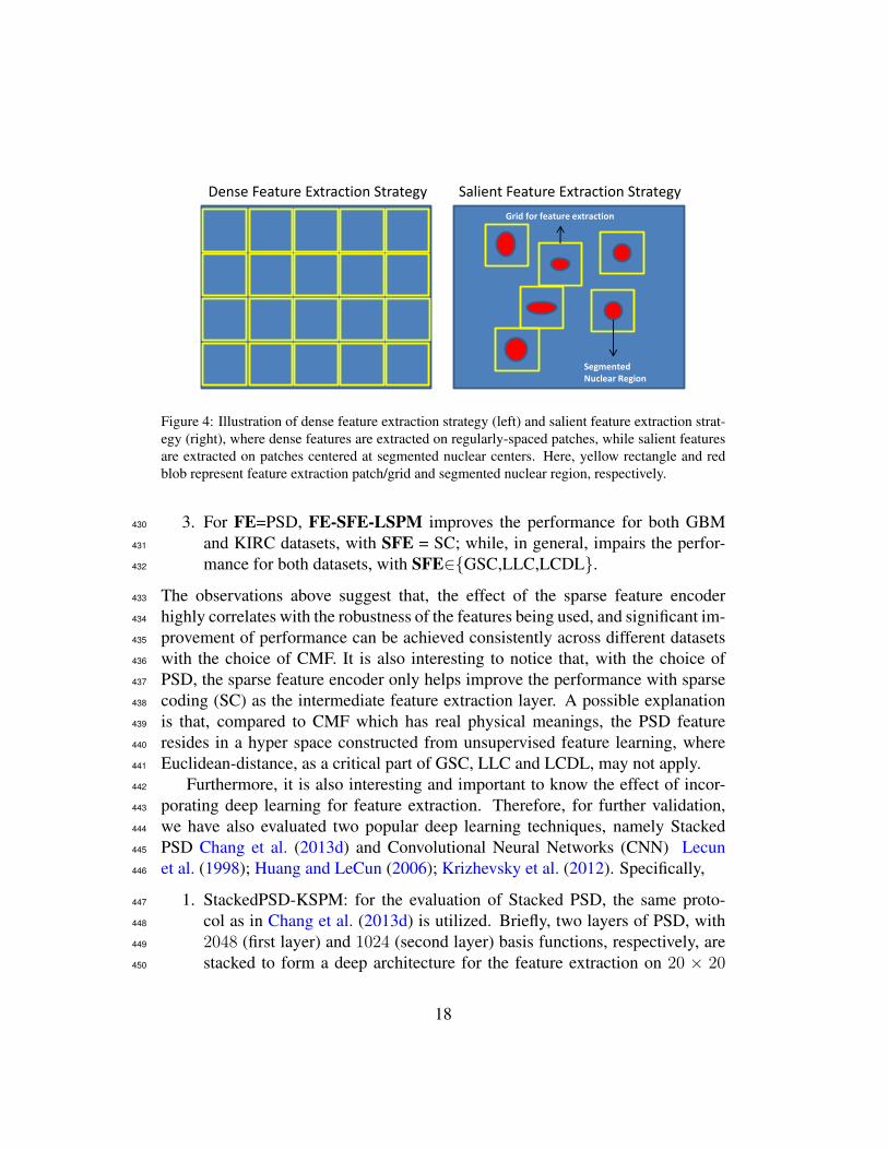
Dense Feature Extraction Strategy Salient Feature Extraction Strategy

Segmented

Nuclear Region

Grid for feature extraction

Figure 4: Illustration of dense feature extraction strategy (left) and salient feature extraction strat-egy (right), where dense features are extracted on regularly-spaced patches, while salient featuresare extracted on patches centered at segmented nuclear centers. Here, yellow rectangle and redblob represent feature extraction patch/grid and segmented nuclear region, respectively.

3. For FE=PSD, FE-SFE-LSPM improves the performance for both GBM430

and KIRC datasets, with SFE = SC; while, in general, impairs the perfor-431

mance for both datasets, with SFE∈GSC,LLC,LCDL.432

The observations above suggest that, the effect of the sparse feature encoder433

highly correlates with the robustness of the features being used, and significant im-434

provement of performance can be achieved consistently across different datasets435

with the choice of CMF. It is also interesting to notice that, with the choice of436

PSD, the sparse feature encoder only helps improve the performance with sparse437

coding (SC) as the intermediate feature extraction layer. A possible explanation438

is that, compared to CMF which has real physical meanings, the PSD feature439

resides in a hyper space constructed from unsupervised feature learning, where440

Euclidean-distance, as a critical part of GSC, LLC and LCDL, may not apply.441

Furthermore, it is also interesting and important to know the effect of incor-442

porating deep learning for feature extraction. Therefore, for further validation,443

we have also evaluated two popular deep learning techniques, namely Stacked444

PSD Chang et al. (2013d) and Convolutional Neural Networks (CNN) Lecun445

et al. (1998); Huang and LeCun (2006); Krizhevsky et al. (2012). Specifically,446

1. StackedPSD-KSPM: for the evaluation of Stacked PSD, the same proto-447

col as in Chang et al. (2013d) is utilized. Briefly, two layers of PSD, with448

2048 (first layer) and 1024 (second layer) basis functions, respectively, are449

stacked to form a deep architecture for the feature extraction on 20 × 20450

18

256 512 1024Dictionary Size

20

30

40

50

60

70

80

90P

erfo

rman

ce (

%)

Dense vs salient features on GBM dataset

DPSD-KSPMSPSD-KSPMDSIFT-SC-LSPMSSIFT-SC-LSPMDSIFT-KSPMSSIFT-KSPMDCT-KSPMSCT-KSPM

256 512 1024Dictionary Size

55

60

65

70

75

80

85

90

95

100

Per

form

ance

(%

)

Dense vs salient features on KIRC dataset

DPSD-KSPMSPSD-KSPMDSIFT-SC-LSPMSSIFT-SC-LSPMDSIFT-KSPMSSIFT-KSPMDCT-KSPMSCT-KSPM

Figure 5: Evaluation of dense feature extraction and salient feature extraction strategies with theFE-KSPM architecture on both GBM (left) and KIRC (right) datasets, where solid line and dashedline represent systems built upon dense feature and salient feature, respectively. Here, the perfor-mance is reported as the mean and standard error of the correct classification rate, as detailed inSection 4.

image-patches with a step-size fixed to be 20, empirically, for best perfor-451

mance. After the patch-based extraction, the same protocol as shown in452

FE-KSPM is utilized for classification.453

2. AlexNet-KSPM: for the evaluation of CNN, we adopt one of the most pow-454

erful deep neural network architecture: AlexNet Krizhevsky et al. (2012)455

with the Caffe Jia et al. (2014) implementation. Given (i) the extremely456

large scale (60 million parameters) of the AlexNet architecture; (ii) the sig-457

nificantly smaller data-scale of GBM and KIRC, compared to ImageNet Deng458

et al. (2009) with one thousand categories and millions of images, where459

AlexNet is originally trained; and (iii) the significant decline of performance460

due to over-fitting that we experience with the end-to-end tuning of AlexNet461

on our dataset as a result of (i) and (ii), we simply adopt the pre-trained462

AlexNet for feature extraction on 224× 224 image-patches with a step-size463

fixed to be 45, empirically, for best performance. After the patch-based464

19

256 512 1024

Dictionary Size

82

84

86

88

90

92

94P

erfo

rman

ce (

%)

CMF-based architectures on GBM dataset

CMF-LCDL-LSPMCMF-LLC-LSPMCMF-SC-LSPMCMF-GSC-LSPMCMF-KSPM(baseline)

256 512 1024

Dictionary Size

82

84

86

88

90

92

94

Per

form

ance

(%

)

DPSD-based architectures on GBM dataset

DPSD-LCDL-LSPMDPSD-LLC-LSPMDPSD-SC-LSPMDPSD-GSC-LSPMDPSD-KSPM(baseline)

256 512 1024

Dictionary Size

70

75

80

85

Per

form

ance

(%

)

DSIFT-based architectures on GBM dataset

DSIFT-LCDL-LSPMDSIFT-LLC-LSPMDSIFT-SC-LSPMDSIFT-GSC-LSPMDSIFT-KSPM(baseline)

256 512 1024

Dictionary Size

60

65

70

75

80

Per

form

ance

(%

)

DCT-based architectures on GBM dataset

DCT-LCDL-LSPMDCT-LLC-LSPMDCT-SC-LSPMDCT-GSC-LSPMDCT-KSPM(baseline)

Figure 6: Evaluation of the architectures with sparse feature encoders (FE-SFE-LSPM) on GBMdataset. Here, the performance is reported as the mean and standard error of the correct classifica-tion rate, as detailed in Section 4.

extraction, the same protocol as shown in FE-KSPM is utilized for classifi-465

cation. It is worth to mention that such an approach falls into the categories466

of both deep learning and transfer learning.467

Experimental results, illustrated in Figure 8, suggest that,468

1. Both sparse feature encoders and feature extraction strategies based on deep469

learning techniques consistently improve the performance of tissue histol-470

ogy classification;471

2. The extremely large-scale convolutional deep neural networks (e.g., AlexNet),472

pre-trained on extremely large-scale dataset (e.g., ImageNet), can be di-473

rectly applicable to the task of tissue histology classification due to the ca-474

pability of deep neural networks in capturing transferable base knowledge475

across domains Yosinski et al. (2014). Although the fine-tuning of AlexNet476

20

256 512 1024

Dictionary Size

90

92

94

96

98

Per

form

ance

(%

)CMF-based architectures on KIRC dataset

CMF-LCDL-LSPMCMF-LLC-LSPMCMF-SC-LSPMCMF-GSC-LSPMCMF-KSPM(baseline)

256 512 1024

Dictionary Size

90

92

94

96

98

Per

form

ance

(%

)

DPSD-based architectures on KIRC dataset

DPSD-LCDL-LSPMDPSD-LLC-LSPMDPSD-SC-LSPMDPSD-GSC-LSPMDPSD-KSPM(baseline)

256 512 1024

Dictionary Size

88

90

92

94

96

98

Per

form

ance

(%

)

DSIFT-based architectures on KIRC dataset

DSIFT-LCDL-LSPMDSIFT-LLC-LSPMDSIFT-SC-LSPMDSIFT-GSC-LSPMDSIFT-KSPM(baseline)

256 512 1024

Dictionary Size

82

84

86

88

90

92

Per

form

ance

(%

)

DCT-based architectures on KIRC dataset

DCT-LCDL-LSPMDCT-LLC-LSPMDCT-SC-LSPMDCT-GSC-LSPMDCT-KSPM(baseline)

Figure 7: Evaluation of the architectures with sparse feature encoders (FE-SFE-LSPM) on KIRCdataset. Here, the performance is reported as the mean and standard error of the correct classifica-tion rate, as detailed in Section 4.

towards our datasets shows significant performance drop due to the problem477

of over-fitting, the direct deployment of pre-trained deep neural networks478

still provides a promising solution for tasks with limited data and labels,479

which is very common in the field of medical image analysis.480

481

4.5. Revisit on Spatial Pooling482

To further study the impact of pooling strategy, we also provide extensive483

experimental evaluation on one of the most popular pooling strategies (i.e., max484

pooling) in place of spatial pyramid matching within FE-SFE-LSPM framework,485

which is defined as follows,486

max : fj = max|c1j|, |c2j|, ..., |cMj| (7)

21

256 512 1024

Dictionary Size

96

96.5

97

97.5

98

98.5

99

99.5

Per

form

ance

(%

)

Evaluation of deep-learning-based architectures on KIRC dataset

StackedPSD-KSPMAlexNet-KSPMCMF-LLC-LSPMCMF-KSPM(baseline)

256 512 1024

Dictionary Size

90

90.5

91

91.5

92

92.5

93

93.5

94

94.5

Per

form

ance

(%

)

Evaluation of deep-learning-based architectures on GBM dataset

StackedPSD-KSPMAlexNet-KSPMCMF-LCDL-LSPMCMF-KSPM(baseline)

Figure 8: Evaluation of the effect of incorporating deep learning for feature extraction on bothGBM and KIRC datasets. Note that, given the various combinations of FE-SFE-LSPM, CMF-LCDL-LSPM and CMF-LLC-LSPM are chosen for GBM and KIRC datasets, respectively, fortheir best performance. Here, the performance is reported as the mean and standard error of thecorrect classification rate, as detailed in Section 4.

where C = [c1, ..., cM ] ∈ Rb×M is the set of sparse codes extracted from an im-487

age, cij is the matrix element at i-th row and j-th column of C, and f = [f1, ..., fb]488

is the pooled image representation. The choice of max pooling procedure has489

been justified by both biophysical evidence in the visual cortex Serre et al. (2005)490

and researches in image categorization Yang et al. (2009), and the derived archi-491

tecture is described as FE-SFE-Max. In our experimental evaluation, we focus on492

the top-two-ranked features (i.e., DPSD and CMF), where the corresponding com-493

parisons of classification performance are illustrated in Figure 9. It is clear that494

systems with SPM pooling consistently outperforms systems with max pooling495

with various combinations of feature types and sparse feature encoders. A possi-496

ble explanation is that the vector quantization step in SPM can be considered as an497

extreme case of sparse coding (i.e., with a single non-zero element in each sparse498

code); and the local histogram concatenation step in SPM can be considered as499

a special form of spatial pooling. As a result, SPM is conceptually similar to an500

extra layer of sparse feature encoding and spatial pooling, as suggested in Jarrett501

et al. (2009), and therefore leads to an improved performance, compared to the502

architecture with max pooling.503

22

4.6. Revisit on Computational Cost504

In addition to classification performance, another critical factor, in clinical505

practice, is the computational efficiency. Therefore, in this section, we provided a506

detailed evaluation on computational cost of various systems. Given the fact that507

(i) training can always be carried out off-line; (ii) the classification of the systems508

in evaluation are all based on linear SVM, our evaluation on computational effi-509

ciency focuses on on-line feature extraction (including sparse feature encoding),510

which is the most time-consuming part during the testing phase. As shown in511

Table 5,512

1. SIFT features are the most computational efficient features among all the513

ones in comparison. However, the systems built on SIFT features greatly514

suffer from the technical variations and biological heterogeneities in both515

datasets, and therefore are not good choices for the classification of tissue516

histology sections;517

2. Given the fact that the nuclear segmentation is a prerequisite for salient518

feature extraction (e.g., SPSD, SSIFT and SCT), systems built upon salient519

features may not be necessarily more efficient than systems built upon dense520

features. Furthermore, since the salient features typically impair the tissue521

histology classification performance, they are therefore not recommended;522

3. The gain in performance of sparse feature encoders in our evaluation is at523

the cost of computational efficiency. And the scalability of derived systems524

can be improved by (i) the development of more computational-efficient525

algorithms, which was demonstrated in Table 6; and (ii) the deployment526

of advanced computational techniques, such as cluster computing or GPU527

acceleration for clinical deployment, which was demonstrated in Table 5 for528

AlexNet.529

4. Most interestingly, the sparse feature encoder, based on CMF-SFE, is much530

more efficient even compared to many shallow architectures based on PSD531

or CT features; and, it is only 5% slower compared to its corresponding532

shallow version, based on CMF. The computational efficiency are due to (i)533

the high sparsity of nuclei compared to dense image patches (e.g., 350 nu-534

clei/image v.s. 2000 patches/image); and (ii) the extremely low dimension-535

ality of cellular morphometric features compared to other features (e.g., 15536

nuclear morphometric features v.s. 128 SIFT features, 203 CT features and537

1024 PSD features). Furthermore, in computational histopathology, both538

nuclear-level information (based on nuclear segmentation) and patch-level539

23

information (based on tissue histology classification) are very critical com-540

ponents, which means the nuclear segmentation results can be shared across541

different tasks for the further improvement of the efficiency of multi-scale542

integrated analyses.543

To further improve the scalability of systems built-upon CMF-SFE, as a demon-544

stration of algorithmic-scaling-up of sparse feature encoders, we constructed a545

predictive sparse feature encoder (PredictiveSFE) in place of SFE as follows, to546

approximate the morphometric sparse codes, specifically, provided by Equation 2,547

minB,C,G,W

∥Y −BC∥2F + λ∥C∥1 + ∥C−Gσ(WY)∥2F

s.t. ∥bi∥22 = 1, ∀i = 1, . . . , h (8)

where Y = [y1, ...,yN ] ∈ Rm×N is a set of cellular morphometric descriptors;548

B = [b1, ...,bh] ∈ Rm×h is a set of the basis functions; C = [c1, ..., cN ] ∈549

Rh×N is the sparse feature matrix; W ∈ Rh×m is the auto-encoder; σ(·) is the550

element-wise sigmoid function; G = diag(g1, . . . , gh) ∈ Rh×h is the scaling551

matrix with diag being an operator aligning vector, [g1, . . . , gh], along the diag-552

onal; and λ is the regularization constant. Joint minimization of Eq. (8) w.r.t553

the quadruple ⟨B,C,G,W⟩, enforces the inference of the nonlinear regressor554

Gσ(WY) to be similar to the optimal sparse codes, C, which can reconstruct555

Y over B Kavukcuoglu et al. (2008). As shown in Algorithm 1, optimization556

of Eq. (8) is iterative, and it terminates when either the objective function is be-557

low a preset threshold or the maximum number of iterations has been reached.558

In our implementation, the number of basis functions (B) was fixed to be 128,559

and the SPAMS optimization toolbox Mairal et al. (2010) is adopted for efficient560

implementation of OMP to compute the sparse code, C, with sparsity prior set to561

30. The end result is a highly efficient (see Table 6) and effective (see Figure 10)562

system, CMF-PredictiveSFE-KSPM, for tissue histology classification.563

5. Conclusions564

This paper provides insights to the following three fundamental questions for565

the task of tissue histology classification:566

I. Is unsupervised feature learning preferable to human engineered features? The567

answer is that, CMF and PSD work the best, compared to SIFT and [Color,Texture]568

features, on two vastly different tumor types. The reasons are that (i) CMF en-569

codes biological meaningful prior knowledge, which is widely adopted in the570

24

Table 5: Average computational cost (measured in second) for feature extraction (including sparsefeature encoding) on images with size 1000 × 1000 pixels. The evaluation is carried out withIntel(R) Xeon(R) CPU X5365 @ 3.00GHz, and GeForce GTX 580.

Feature Extraction Component(s) Average Computational Cost (in second)Nuclear Segmentation 40

CMF-SFE 42 = Nuclear-Segmentation-Cost(40) + SFE-Cost(2)DPSD-SFE 115 = DPSD-Cost(95) + SFE-Cost(20)SPSD-SFE 70 = SPSD-Cost(60) + SFE-Cost(10)DSIFT-SFE 16 = DSIFT-Cost(10) + SFE-Cost(6)SSIFT-SFE 47 = SSIFT-Cost(45) + SFE-Cost(2)DCT-SFE 90 = DCT-Cost(80) + SFE-Cost(10)SCT-SFE 108 = SCT-Cost(105) + SFE-Cost(3)

CMF 40 = Nuclear-Segmentation-Cost(40)DPSD 95SPSD 60 = Nuclear-Segmentation-Cost(40) + PSD-Cost(20)DSIFT 10SSIFT 45 = Nuclear-Segmentation-Cost(40)+SIFT-Cost(5)DCT 80SCT 105 = Nuclear-Segmentation-Cost(40) + SCT-Cost(65)

StackedPSD 100AlexNet 1200/180 (CPU-Only/GPU-Acceleration)

Table 6: PredictiveSFE achieved 40X speed-up, compared to SFE, in sparse cellular morpho-metric feature extraction. The evaluation was carried out with Intel(R) Xeon(R) CPU X5365 @3.00GHz

Sparse Cellular Morphometric Feature Extraction Average Computational Cost (in second)PredictiveSFE 0.05

SFE 2

25

Algorithm 1 Construction of the Predictive Sparse Feature Encoder (Predic-tiveSFE)Input: Training set Y = [y1, ...,yN ] ∈ Rm×N

Output: Predictive Sparse Feature Encoder W ∈ Rh×m

1: Initialize: Randomly initialize B, W, and G2: repeat3: Fixing B, W and G, minimize Eq. (8) w.r.t C, where C can be ei-

ther solved as a ℓ1-minimization problem Lee et al. (2007) or equiva-lently solved by greedy algorithms, e.g., Orthogonal Matching Pursuit(OMP) Tropp and Gilbert (2007).

4: Fixing B, W and C, solve for G, which is a simple least-square problemwith analytic solution.

5: Fixing C and G, update B and W, respectively, using the stochastic gradi-ent descent algorithm.

6: until Convergence (maximum iterations reached or objective function ≤threshold)

practice of pathological diagnosis; and (ii) PSD is able to capture intrinsic mor-571

phometric patterns in histology sections. As a result, both of them produce robust572

representation of the underlying properties preserved in the data.573

II. Does cellular saliency help? The surprising answer is that cellular saliency574

does not help improve the performance for systems built upon pixel-/patch-level575

features. Experiments on both GBM and KIRC datasets confirm the performance-576

drop with salient feature extraction strategies, and one possible explanation is that577

both pixel-level and patch-level features are appearance-based representations,578

which require dense sampling all over the place in order to faithfully assemble579

the view of the image.580

III. Does the sparse feature encoder contribute of recognition? The sparse feature581

encoder significantly and consistently improves the classification performance for582

systems built upon CMF; and meanwhile, it conditionally improves the perfor-583

mance for systems built upon PSD (PSD-SC-LSPM), with the choice of sparse584

coding (SC) as the intermediate feature extraction layer. It is believed that the con-585

sistency of performance highly correlates with the robustness of the feature being586

used, and the improvement of performance is due to the capability of the sparse587

feature encoder in capturing complex patterns at the higher-level. Furthermore,588

this paper provides a clear evidence that deep neural networks (i.e., AlexNet), pre-589

trained on large scale natural image datasets (i.e., ImageNet), is directly applicable590

26

to the task of tissue histology classification, which is due to the capability of deep591

neural networks in capturing transferable base knowledge across domains Yosin-592

ski et al. (2014). Although the fine-tuning of AlexNet towards our datasets shows593

significant performance drop due to the problem of over-fitting, the direct deploy-594

ment of pre-trained deep neural networks still provides a promising solution for595

tasks with limited data and labels, which is very common in the field of medical596

image analysis.597

Besides the insights in the aforementioned fundamental questions, this paper598

also shows that the superior performance of the sparse feature encoder is at the599

cost of computational efficiency. However, the scalability of the sparse feature600

encoder can be improved by (i) the development of more computational-efficient601

algorithms; and (ii) the deployment of advanced computational techniques, such602

as cluster computing or GPU acceleration. As a demonstration, this paper pro-603

vides an accelerated version of CMF-SFE, namely CMF-PredictiveSFE, which604

falls into the category of algorithmic-scaling-up and achieves 40X speed-up dur-605

ing sparse feature encoding. The end result is a highly scalable and effective606

system, CMF-PredictiveSFE-KSPM, for tissue histology classification.607

Furthermore, all our insights are independently validated on two large cohorts,608

Glioblastoma Multiforme (GBM) and Kidney Clear Cell Carcinoma (KIRC), which,609

to the maximum extent, ensures the consistency and unbiasedness of our findings.610

To the best of our knowledge, this is the first attempt that systematically provides611

insights to the fundamental questions aforementioned in tissue histology classi-612

fication; and there are reasons to hope that the configuration: FE-SFE-LSPM613

(FE∈CMF,PSD) as well as its accelerated version: FE-PredictiveSFE-KSPM614

(FE∈CMF,PSD), can be widely applicable to different tumor types.615

Acknowledgement616

This work was supported by NIH R01 CA184476 carried out at Lawrence617

Berkeley National Laboratory.618

References619

Apostolopoulos, G., Tsinopoulos, S., Dermatas, E., 2011. Recognition and identi-620

fication of red blood cell size using zernike moments and multicolor scattering621

images. In: 2011 10th International Workshop on Biomedical Engineering. pp.622

1–4.623

27

Asadi, M., Vahedi, A., Amindavar, H., 2006. Leukemia cell recognition with624

zernike moments of holographic images. In: NORSIG 2006. pp. 214–217.625

Basavanhally, A., Xu, J., Madabhushu, A., Ganesan, S., 2009. Computer-aided626

prognosis of ER+ breast cancer histopathology and correlating survival out-627

come with oncotype DX assay. In: ISBI. pp. 851–854.628

Belkin, M., Niyogi, P., 2003. Laplacian eigenmaps for dimensionality reduction629

and data representation. Neural Computation 15 (6), 1373–1396.630

Bhagavatula, R., Fickus, M., Kelly, W., Guo, C., Ozolek, J., Castro, C., Kovacevic,631

J., 2010. Automatic identification and delineation of germ layer components in632

h&e stained images of teratomas derived from human and nonhuman primate633

embryonic stem cells. In: ISBI. pp. 1041–1044.634

Chang, H., Borowsky, A., Spellman, P., Parvin, B., 2013a. Classification of tu-635

mor histology via morphometric context. In: Proceedings of the Conference on636

Computer Vision and Pattern Recognition. pp. 2203–2210.637

Chang, H., Han, J., Borowsky, A., Loss, L. A., Gray, J. W., Spellman, P. T.,638

Parvin, B., 2013b. Invariant delineation of nuclear architecture in glioblastoma639

multiforme for clinical and molecular association. IEEE Trans. Med. Imaging640

32 (4), 670–682.641

Chang, H., Nayak, N., Spellman, P., Parvin, B., 2013c. Characterization of tissue642

histopathology via predictive sparse decomposition and spatial pyramid match-643

ing. Medical image computing and computed-assisted intervention–MICCAI.644

Chang, H., Zhou, Y., Spellman, P. T., Parvin, B., 2013d. Stacked predictive sparse645

coding for classification of distinct regions in tumor histopathology. In: Pro-646

ceedings of the IEEE International Conference on Computer Vision. pp. 502–647

507.648

Dalton, L., Pinder, S., Elston, C., Ellis, I., Page, D., Dupont, W., Blamey, R., 2000.649

Histolgical gradings of breast cancer: linkage of patient outcome with level of650

pathologist agreements. Modern Pathology 13 (7), 730–735.651

de Kruijf, E. M., van Nes, J. G., van de Velde, C. J. H., Putter, H., Smit, V. T. H.652

B. M., Liefers, G. J., Kuppen, P. J. K., Tollenaar, R. A. E. M., Mesker, W. E.,653

2011. Tumorstroma ratio in the primary tumor is a prognostic factor in early654

28

breast cancer patients, especially in triple-negative carcinoma patients. Breast655

Cancer Research and Treatment 125 (3), 687696.656

Demir, C., Yener, B., 2009. Automated cancer diagnosis based on histopatholog-657

ical images: A systematic survey. Technical Report, Rensselaer Polytechnic658

Institute, Department of Computer Science.659

Deng, J., Dong, W., Socher, R., Li, L.-J., Li, K., Fei-Fei, L., 2009. ImageNet: A660

Large-Scale Hierarchical Image Database. In: CVPR09. pp. 248–255.661

Doyle, S., Feldman, M., Tomaszewski, J., Shih, N., Madabhushu, A., 2011. Cas-662

caded multi-class pairwise classifier (CASCAMPA) for normal, cancerous, and663

cancer confounder classes in prostate histology. In: ISBI. pp. 715–718.664

Everingham, M., Van Gool, L., Williams, C. K. I., Winn, J., Zisserman, A., 2012.665

The PASCAL Visual Object Classes Challenge 2012 (VOC2012) Results.666

Fatakdawala, H., Xu, J., Basavanhally, A., Bhanot, G., Ganesan, S., Feldman,667

F., Tomaszewski, J., Madabhushi, A., 2010. Expectation-maximization-driven668

geodesic active contours with overlap resolution (EMaGACOR): Application to669

lymphocyte segmentation on breast cancer histopathology. IEEE Transactions670

on Biomedical Engineering 57 (7), 1676–1690.671

Ghaznavi, F., Evans, A., Madabhushi, A., Feldman, M. D., 2013. Digital imaging672

in pathology: Whole-slide imaging and beyond. Annual Review of Pathology673

Mechanisms of Disease 8 (1), 331–359.674

Gurcan, M., Boucheron, L., Can, A., Madabhushi, A., Rajpoot, N., Bulent,675

Y., 2009. Histopathological image analysis: a review. IEEE Transactions on676

Biomedical Engineering 2, 147–171.677

Han, J., Chang, H., Loss, L., Zhang, K., Baehner, F., Gray, J., Spellman, P., Parvin,678

B., 2011. Comparison of sparse coding and kernel methods for histopathologi-679

cal classification of glioblastoma multiforme. In: ISBI. pp. 711–714.680

Huang, C., Veillard, A., Lomeine, N., Racoceanu, D., Roux, L., 2011. Time ef-681

ficient sparse analysis of histopathological whole slide images. Computerized682

medical imaging and graphics 35 (7-8), 579–591.683

Huang, F. J., LeCun, Y., 2006. Large-scale learning with svm and convolutional684

for generic object categorization. In: Proceedings of the 2006 IEEE Computer685

29

Society Conference on Computer Vision and Pattern Recognition - Volume 1.686

CVPR ’06. IEEE Computer Society, Washington, DC, USA, pp. 284–291.687

Huang, W., Hennrick, K., Drew, S., 2013. A colorful future of quantitative pathol-688

ogy: validation of vectra technology using chromogenic multiplexed immuno-689

histochemistry and prostate tissue microarrays. Human Pathology 44, 29–38.690

Huijbers, A., Tollenaar1, R., v Pelt1, G., Zeestraten1, E., Dutton, S., McConkey,691

C., Domingo, E., Smit, V., Midgley, R., Warren, B., Johnstone, E. C., Kerr, D.,692

Mesker, W., 2013. The proportion of tumor-stroma as a strong prognosticator693

for stage ii and iii colon cancer patients: validation in the victor trial. Annals of694

Oncology 24 (1), 179185.695

Jarrett, K., Kavukcuoglu, K., Ranzato, M., LeCun, Y., 2009. What is the best696

multi-stage architecture for object recognition? In: Proc. International Confer-697

ence on Computer Vision (ICCV’09). IEEE, pp. 2146–2153.698

Jia, Y., Shelhamer, E., Donahue, J., Karayev, S., Long, J., Girshick, R., Guadar-699

rama, S., Darrell, T., 2014. Caffe: Convolutional architecture for fast feature700

embedding. arXiv preprint arXiv:1408.5093.701

Kavukcuoglu, K., Ranzato, M., LeCun, Y., 2008. Fast inference in sparse coding702

algorithms with applications to object recognition. Tech. Rep. CBLL-TR-2008-703

12-01, Computational and Biological Learning Lab, Courant Institute, NYU.704

Kong, J., Cooper, L., Sharma, A., Kurk, T., Brat, D., Saltz, J., 2010. Texture based705

image recognition in microscopy images of diffuse gliomas with multi-class706

gentle boosting mechanism. In: ICASSAP. pp. 457–460.707

Kothari, S., Phan, J., Osunkoya, A., Wang, M., 2012. Biological interpretation708

of morphological patterns in histopathological whole slide images. In: ACM709

Conference on Bioinformatics, Computational Biology and Biomedicine. pp.710

218–225.711

Krizhevsky, A., Sutskever, I., Hinton, G. E., 2012. Imagenet classification with712

deep convolutional neural networks. In: Advances in Neural Information Pro-713

cessing Systems 25: 26th Annual Conference on Neural Information Process-714

ing Systems 2012. Proceedings of a meeting held December 3-6, 2012, Lake715

Tahoe, Nevada, United States. pp. 1106–1114.716

30

Lan, C., Heindl, A., Huang, X., Xi, S., Banerjee, S., Liu, J., Yuan, Y., 2015. Quan-717

titative histology analysis of the ovarian tumour microenvironment. Scientific718

Reports 5 (16317).719

Lazebnik, S., Schmid, C., Ponce, J., 2006. Beyond bags of features: Spatial pyra-720

mid matching for recognizing natural scene categories. In: Proceedings of the721

Conference on Computer Vision and Pattern Recognition. pp. 2169–2178.722

Le, Q., Han, J., Gray, J., Spellman, P., Borowsky, A., Parvin, B., 2012. Learning723

invariant features from tumor signature. In: ISBI. pp. 302–305.724

Lecun, Y., Bottou, L., Bengio, Y., Haffner, P., 1998. Gradient-based learning ap-725

plied to document recognition. In: Proceedings of the IEEE. pp. 2278–2324.726

Lee, H., Battle, A., Raina, R., Ng, A. Y., 2007. Efficient sparse coding algorithms.727

In: In NIPS. NIPS, pp. 801–808.728

Levenson, R. M., Borowsky, A. D., Angelo, M., 2015. Immunohistochemistry and729

mass spectrometry for highly multiplexed cellular molecular imaging. Labora-730

tory Investigation 95, 397–405.731

Mairal, J., Bach, F., Ponce, J., Sapiro, G., Mar. 2010. Online learning for matrix732

factorization and sparse coding. J. Mach. Learn. Res. 11, 19–60.733

Nayak, N., Chang, H., Borowsky, A., Spellman, P., Parvin, B., 2013. Classifi-734

cation of tumor histopathology via sparse feature learning. In: Proc. ISBI. pp.735

410–413.736

Rimm, D. L., 2014. Next-gen immunohistochemistry. Nature Methods 11, 381–737

383.738

Rogojanu, R., Thalhammer, T., Thiem, U., Heindl, A., Mesteri, I., Seewald, A.,739

Jger, W., Smochina, C., Ellinger, I., Bises, G., 2015. Quantitative image anal-740

ysis of epithelial and stromal area in histological sections of colorectal cancer:741

An emerging diagnostic tool. BioMed Research International 2015 (569071),742

179185.743

Serre, T., Wolf, L., Poggio, T., 2005. Object recognition with features inspired744

by visual cortex. In: Proceedings of the Conference on Computer Vision and745

Pattern Recognition. Vol. 2. pp. 994–1000.746

31

Stack, E. C., Wang, C., Roman, K. A., Hoyt, C. C., 2014. Multiplexed immuno-747

histochemistry, imaging, and quantitation: A review, with an assessment of748

tyramide signal amplification, multispectral imaging and multiplex analysis.749

Methods 70 (1), 46–58.750

Tropp, J., Gilbert, A., 2007. Signal recovery from random measurements via or-751

thogonal matching pursuit. Information Theory, IEEE Transactions on 53 (12),752

4655–4666.753

Vedaldi, A., Zisserman, A., 2012. Efficient additive kernels via explicit feature754

maps. IEEE Transactions on Pattern Analysis and Machine Intelligence 34 (3),755

480–492.756

Wang, J., Yang, J., Yu, K., Lv, F., Huang, T., Gong, Y., 2010. Locality-constrained757

linear coding for image classification. In: Proceedings of the Conference on758

Computer Vision and Pattern Recognition. pp. 3360–3367.759

Wu, R., Yu, Y., Wang, W., 2013. Scale: Supervised and cascaded laplacian eigen-760

maps for visual object recognition based on nearest neighbors. In: CVPR. pp.761

867–874.762

Yang, J., Yu, K., Gong, Y., Huang, T., 2009. Linear spatial pyramid matching763

using sparse coding for image classification. In: Proceedings of the Conference764

on Computer Vision and Pattern Recognition. pp. 1794–1801.765

Yosinski, J., Clune, J., Bengio, Y., Lipson, H., 2014. How transferable are features766

in deep neural networks? In: Advances in Neural Information Processing Sys-767

tems 27: Annual Conference on Neural Information Processing Systems 2014,768

December 8-13 2014, Montreal, Quebec, Canada. pp. 3320–3328.769

Young, R. A., Lesperance, R. M., 2001. The gaussian derivative model for spatial-770

temporal vision. I. Cortical Model. Spatial Vision 2001, 3–4.771

Zheng, M., Bu, J., Chen, C., Wang, C., Zhang, L., Qiu, G., Cai, D., 2011. Graph772

regularized sparse coding for image representation. IEEE Transactions on Im-773

age Processing 20 (5), 1327–1336.774

Zhou, Y., Barner, K. E., 2013. Locality constrained dictionary learning for non-775

linear dimensionality reduction. IEEE Signal Process. Lett. 20 (4), 335–338.776

32

256 512 1024

Dictionary Size

75

80

85

90

Per

form

ance

(%

)

CMF-based architectures on GBM dataset

CMF-LCDL-LSPMCMF-LLC-LSPMCMF-SC-LSPMCMF-GSC-LSPMCMF-LCDL-MaxCMF-LLC-MaxCMF-SC-MaxCMF-GSC-Max

256 512 1024

Dictionary Size

75

80

85

90

Per

form

ance

(%

)

DPSD-based architectures on GBM dataset

DPSD-LCDL-LSPMDPSD-LLC-LSPMDPSD-SC-LSPMDPSD-GSC-LSPMDPSD-LCDL-MaxDPSD-LLC-MaxDPSD-SC-MaxDPSD-GSC-Max

256 512 1024

Dictionary Size

84

86

88

90

92

94

96

98

Per

form

ance

(%

)

CMF-based architectures on KIRC dataset

CMF-LCDL-LSPMCMF-LLC-LSPMCMF-SC-LSPMCMF-GSC-LSPMCMF-LCDL-MaxCMF-LLC-MaxCMF-SC-MaxCMF-GSC-Max

256 512 1024

Dictionary Size

84

86

88

90

92

94

96

98

Per

form

ance

(%

)

DPSD-based architectures on KIRC dataset

DPSD-LCDL-LSPMDPSD-LLC-LSPMDPSD-SC-LSPMDPSD-GSC-LSPMDPSD-LCDL-MaxDPSD-LLC-MaxDPSD-SC-MaxDPSD-GSC-Max

Figure 9: Evaluation of the impact of different spatial pooling strategies with the FE-SFE-LSPMframework on both GBM and KIRC datasets. Note that, given many of the popular spatial poolingstrategies, max pooling is chosen due to the extensive justification by both biophysical evidencein the visual cortex and researches in image categorization tasks. The derived architecture is de-scribed as FE-SFE-Max, and only the top-two-ranked features (i.e., DPSD and CMF) are involvedduring evaluation. Here, the performance is reported as the mean and standard error of the correctclassification rate, as detailed in Section 4.

33

256 512 1024

Dictionary Size

89

90

91

92

93

94

Per

form

ance

(%

)

CMF-based architectures on GBM dataset

CMF-LCDL-LSPMCMF-LLC-LSPMCMF-SC-LSPMCMF-GSC-LSPMCMF-PredictiveSFE-KSPM

256 512 1024

Dictionary Size

96.5

97

97.5

98

98.5

99

99.5

Per

form

ance

(%

)

CMF-based architectures on KIRC dataset

CMF-LCDL-LSPMCMF-LLC-LSPMCMF-SC-LSPMCMF-GSC-LSPMCMF-PredictiveSFE-KSPM

Figure 10: Systems built-upon CMF-PredictiveSFE provide very competitive performance com-pared to systems built-upon CMF-SFE. Here, the performance is reported as the mean and stan-dard error of the correct classification rate, as detailed in Section 4.

34