What's in a Name? Intelligent Classification and Identification ...

1

Queen Mary University of London

What's in a Name? Intelligent

Classification and Identification

of Online Media Content

Eugene Dementiev

2016

Submitted in partial fulfilment of the requirements of the Degree of Doctor of Philosophy

2

Declarations

I, Dementiev Eugene, confirm that the research included within this thesis is my

own work or that where it has been carried out in collaboration with, or supported

by others, that this is duly acknowledged below and my contribution indicated.

I attest that I have exercised reasonable care to ensure that the work is original, and

does not to the best of my knowledge break any UK law, infringe any third party’s

copyright or other Intellectual Property Right, or contain any confidential material.

I accept that the College has the right to use plagiarism detection software to check

the electronic version of the thesis.

I confirm that this thesis has not been previously submitted for the award of a

degree by this or any other university.

The copyright of this thesis rests with the author and no quotation from it or

information derived from it may be published without the prior written consent of

the author.

Eugene Dementiev

Submission date: 04.04.2016

Last updated: 24.05.2016

3

Acknowledgements

I would like to thank my supervisor Professor Norman Fenton for his support,

guidance and understanding; and for giving me the opportunity to learn so many

things from him. I could never wish for a better supervisor.

Prof Martin Neil, Dr William Marsh, Tanmoy Kumar, Evangelia Kyrimi, and other

research group colleagues provided invaluable insight, comments and ideas, for

which I am deeply grateful.

The feedback provided by my examiners Andrew Moore and Jeroen Keppens was

extremely helpful and aided me in improving the final edition of this thesis.

A separate gratitude is to MovieLabs for supplying data for the research and useful

knowledge, and to Agena for graciously providing their BN modelling software

and calculation API.

I also extend my thanks to the EPSRC for funding and to Queen Mary University

of London for making this project possible. This work was also supported in part

by European Research Council Advanced Grant ERC-2013-AdG339182-

BAYES_KNOWLEDGE (April 2015-Dec 2015).

A special gratitude to my wife Aliya who gave her best to help me through the

final stages of this project, and to my family who were very supportive throughout

the project.

4

Abstract

The sheer amount of content on the Internet poses a number of challenges for

content providers and users alike. The providers want to classify and identify user

downloads for market research, advertising and legal purposes. From the user’s

perspective it is increasingly difficult to find interesting content online, hence

content personalisation and media recommendation is expected by the public. An

especially important (and also technically challenging) case is when a

downloadable item has no supporting description or meta-data, as in the case of

(normally illegal) torrent downloads, which comprise 10 to 30 percent of the global

traffic depending on the region. In this case, apart from its size, we have to rely

entirely on the filename – which is often deliberately obfuscated – to identify or

classify what the file really is.

The Hollywood movie industry is sufficiently motivated by this problem that it

has invested significant research – through its company MovieLabs – to help

understand more precisely what material is being illegally downloaded in order

both to combat piracy and exploit the extraordinary opportunities for future sales

and marketing. This thesis was inspired, and partly supported, by MovieLabs who

recognised the limitations of their current purely data-driven algorithmic

approach.

The research hypothesis is that, by extending state-of-the-art information retrieval

(IR) algorithms and by developing an underlying causal Bayesian Network (BN)

incorporating expert judgment and data, it is possible to improve on the accuracy

of MovieLabs’s benchmark algorithm for identifying and classifying torrent

names. In addition to identification and standard classification (such as whether

the file is Movie, Soundtrack, Book, etc.) we consider the crucial orthogonal

classifications of pornography and malware. The work in the thesis provides a

number of novel extensions to the generic problem of classifying and personalising

5

internet content based on minimal data and on validating the results in the absence

of a genuine ‘oracle’.

The system developed in the thesis (called Toran) is extensively validated using a

sample of torrents classified by a panel of 3 human experts and the MovieLabs

system, divided into knowledge and validation sets of 2,500 and 479 records

respectively. In the absence of an automated classification oracle, we established

manually the true classification for the test set of 121 records in order to be able to

compare Toran, the human panel (HP) and the MovieLabs system (MVL). The

results show that Toran performs better than MVL for the key medium categories

that contain most items, such as music, software, movies, TVs and other videos.

Toran also has the ability to assess the risk of fakes and malware prior to

download, and is on par or even surpasses human experts in this capability.

6

Table of Contents

Declarations ...................................................................................................................... 2

Acknowledgements ......................................................................................................... 3

Abstract .............................................................................................................................. 4

List of Abbreviations ..................................................................................................... 12

Glossary ........................................................................................................................... 15

Notation ........................................................................................................................... 16

List of Figures ................................................................................................................. 17

List of Tables ................................................................................................................... 20

List of Algorithms .......................................................................................................... 24

Chapter 1 Introduction ............................................................................................ 25

1.1. Motivation ............................................................................................................. 25

1.2. Research Hypothesis and Objectives ................................................................ 33

1.3. Structure of the Thesis ......................................................................................... 34

Chapter 2 Background and Data ............................................................................ 36

2.1. The Benchmark and Prototype Systems ........................................................... 36

2.2. File Data ................................................................................................................. 39

2.3. Class Taxonomy ................................................................................................... 41

2.4. Title and Names Databases ................................................................................ 43

2.5. Data Samples ........................................................................................................ 46

2.6. Classification and Evaluation Methods ............................................................ 57

Brief Introduction to Document Classification ................................... 59

7

Naïve Bayesian Classifiers ..................................................................... 61

Terms of Accuracy .................................................................................. 63

Probabilistic Prediction Metrics ............................................................ 66

Applying Accuracy Metrics in the Project .......................................... 71

2.7. String Comparison ............................................................................................... 75

2.8. Summary ............................................................................................................... 80

Chapter 3 Torrent Name Bayesian Network Model .......................................... 81

3.1. Bayes’ Theorem .................................................................................................... 82

3.2. Bayesian Networks Overview and Key Concepts .......................................... 84

Bayesian Network Definition ................................................................ 84

Simple BN Examples .............................................................................. 85

Bayesian Network Inference Algorithms, Tools and Applications . 89

Hard, Soft and Virtual Evidence ........................................................... 92

Modelling Continuous Variables .......................................................... 93

3.3. Building Bayesian Networks .............................................................................. 94

Knowledge Engineering versus Machine Learning ........................... 95

Conditional Dependency ....................................................................... 97

Defining BN Structure .......................................................................... 100

Prior and Likelihood Definition .......................................................... 102

Applying Idioms in the Project ........................................................... 105

3.4. Model Overview ................................................................................................ 113

3.5. Real Medium....................................................................................................... 114

3.6. Fakes and Malware ............................................................................................ 116

8

3.7. Advertised Medium .......................................................................................... 120

3.8. File Size ................................................................................................................ 124

3.9. Signatures ............................................................................................................ 126

Regular Signature Node NPTs ............................................................ 128

Special Signature Node NPTs ............................................................. 135

3.10. Porn Detection .................................................................................................... 137

3.11. Title Detection..................................................................................................... 141

3.12. Risky Titles .......................................................................................................... 144

3.13. Extensibility ........................................................................................................ 147

3.14. Summary ............................................................................................................. 149

Chapter 4 Capturing Evidence ............................................................................. 150

4.1. Signature Definition........................................................................................... 151

Pattern Types ......................................................................................... 154

Associations and Strength ................................................................... 157

Special Signatures ................................................................................. 162

4.2. Porn Studios and Actors ................................................................................... 164

4.3. Signature Detection and Filtering Algorithm ................................................ 165

4.4. Title Matching ..................................................................................................... 170

Title Alignment ..................................................................................... 171

n-gram Pre-filtering .............................................................................. 175

Procedure ............................................................................................... 179

4.5. Extensibility ........................................................................................................ 185

4.6. Summary ............................................................................................................. 186

9

Chapter 5 Formal Framework for System Evaluation ..................................... 187

5.1. Compatibility of Agent Output ....................................................................... 188

5.2. Verdict Mapping and Probability Vector Translation .................................. 190

5.3. Comparing MVL and Toran on DS2500 and DS480 ..................................... 193

5.4. Scoring Metric Requirements ........................................................................... 194

5.5. Tiered Scoring Rule............................................................................................ 195

5.6. Random Predictions .......................................................................................... 199

5.7. Summary ............................................................................................................. 201

Chapter 6 Empirical Evaluation and Analysis .................................................. 202

6.1. Assessment of Probabilistic Predictions ......................................................... 204

Knowledge and Validation Sets .......................................................... 204

DS120: Test Set ....................................................................................... 206

6.2. Confusing Predictions ....................................................................................... 207

6.3. Evaluation in Terms of Accuracy .................................................................... 211

Accuracy Metrics ................................................................................... 212

Receiver Operating Characteristic (ROC).......................................... 213

6.4. BitSnoop Experiment ......................................................................................... 216

6.5. Porn Detection .................................................................................................... 219

6.6. Fakes and Malware ............................................................................................ 220

6.7. Summary ............................................................................................................. 221

Chapter 7 Summary and Conclusions ................................................................ 223

7.1. Methodology ....................................................................................................... 224

7.2. Research Objectives ........................................................................................... 226

10

7.3. Future Work ........................................................................................................ 228

Improving Toran ................................................................................... 228

Further Contribution to Validation .................................................... 230

7.4. Conclusions ......................................................................................................... 231

Appendices .................................................................................................................... 234

Appendix A XML Data Structure ......................................................................... 234

Appendix B Results in XML Format ................................................................... 237

Appendix C Databases of Titles, Actors and Studios ...................................... 237

C.1. Titles Database ................................................................................................... 237

C.2. Porn Actor Database ......................................................................................... 237

C.3. Porn Studio Database ....................................................................................... 237

Appendix D Data Sets ............................................................................................ 238

D.1. DS2500................................................................................................................. 238

D.2. DS480................................................................................................................... 238

D.3. DS120................................................................................................................... 238

D.4. Fakes and Malware Data Set ........................................................................... 238

D.5. BitSnoop Data Set .............................................................................................. 238

Appendix E Junction Tree BN Propagation Algorithm .................................. 239

Appendix F BN Definition ................................................................................... 243

Appendix G Example Model Output for Different Signature

Combinations .............................................................................................................. 247

Appendix H Signature and Keyword Configurations ..................................... 249

H.1. MovieLabs Keyword Configuration .............................................................. 249

H.2. Toran Signature Configuration ....................................................................... 249

11

Appendix I Pattern Parts of the TV Signature ................................................. 250

Appendix J Torrent Name Filtering Examples................................................. 251

References ...................................................................................................................... 252

12

List of Abbreviations

AE Absolute error

API Application Program Interface

AS Absolute Error

AST Absolute Error Tiered

BLAST Basic Local Alignment Search Tool

BLOSUM Blocks Substitution Matrix

BN Bayesian Network

BS Brier Score

BST Brier Score Tiered

CB Content-Based

CF Collaborative Filtering

CSV Categorisation Status Value

DAG Directed Acyclic Graph

DS120 Data Set 120

DS2500 Data Set 2500

DS480 Data Set 480

DSBS BitSnoop Data Set

DSFM Fakes and Malware Data Set

FN False Negatives

FP False Positives

FPR False Positive Rate

GB Gigabyte

13

HP Human Panel

IDF Inverse Document Frequency

IFPI International Federation of the Phonographic Industry

IMDb Internet Movie Database

IMDbPY IMDb Python

IR Information Retrieval

KB Kilobyte

KE Knowledge Engineering

LS Logarithmic scoring

MAE Mean Absolute Error

MAE Mean Average Error

MAET Mean Absolute Error Tiered

MB Megabyte

MCC Matthews Correlation Coefficient

ML Machine Learning

MPAA Motion Picture Association of America

MVL MovieLabs (the benchmark system)

NPT Node Probability Table

OO Object-Oriented

OOBN Object-Oriented Bayesian Network

OST Original Sound Track

P2P Peer-to-peer

PCC Pearson Product-Moment Correlation Coefficient

PDF Probability Density Function

14

QS Quadratic scoring rule

RIAA Recording Industry Association of America

ROC Receiver Operating Characteristic

SS Spherical scoring rule

SW Smith-Waterman

TC Text Classification

TF Term Frequency

TN True Negatives

Toran Torrent Analyser

TP True Positive

TPR True Positive Rate

XML Extensible Markup Language

15

Glossary

DS120 Data Set of 121 items classified by human experts and the benchmark

system and completely verified (test set)

DS2500 Data Set of 2,500 items classified by human experts and the

benchmark system (knowledge set)

DS480 Data Set of 479 items classified by human experts and the benchmark

system (validation set)

DSBS Data set of 45,209 items captured from BitSnoop torrent tracker to

evaluate prediction accuracy on independent data

DSMF Data set of 100 items for evaluating accuracy of fakes and malware

prediction

IMDbPY Python package to retrieve and manage the data of the IMDb movie

database about movies, people, characters and companies

MVL MovieLabs torrent classification benchmark system

Toran The prototype classifier system we created to test our method

16

Notation

Lucida Sans Typewriter font is used in the body of text to refer to (parts of)

torrent names, name string evidence, regular expressions; and is the primary font

in algorithm boxes.

𝐶𝑎𝑚𝑏𝑟𝑖𝑎 𝑀𝑎𝑡ℎ font is used to refer to variables, formulas and expressions.

Bayesian Network node names are normally given in italics (e.g. Title Found).

Bayesian Network node states are normally given in double inverted commas (e.g.

“Video”, “Audio”, “Other”).

Bayesian Network fragments that are unified into a single node on a diagram are

shown with a rectangular dashed border.

Bayesian Network graphs show nodes that are observed in pink and nodes that

are the focus of prediction in green (appearing as and respectively).

17

List of Figures

Figure 1: Example of a Torrent Name...................................................................................................... 32

Figure 2: Composition of Data Sets according to Human Classifiers ................................................. 48

Figure 3: DS2500 and DS480 Composition according to Average and Majority Voting .................. 49

Figure 4: Verified Composition of DS120 ................................................................................................ 52

Figure 5: Example of a Partially Classified Item in BitSnoop Data Set ............................................... 56

Figure 6: Example of a Misclassified Item in BitSnoop Data Set .......................................................... 56

Figure 7: Composition of DSBS According to BitSnoop........................................................................ 57

Figure 8: Naïve Bayes Illustration ............................................................................................................ 61

Figure 9: Possible Votes that Produce Distributions in Table 11 ......................................................... 72

Figure 10: Torrent Name and Movie Title Aligned ............................................................................... 76

Figure 11: Basic BN for Fakes Detection .................................................................................................. 85

Figure 12: Basic BN for Fakes Detection Example after Evidence Propagation ................................. 86

Figure 13: Revised Example Model for Fakes Detection ....................................................................... 86

Figure 14: Possible Outcomes of the Fakes Detection Model: a) Show the marginal values before

propagation, b-e) Show the values after propagation with the given observations ......................... 88

Figure 15: Extended Example Model for Fakes Detection .................................................................... 88

Figure 16: Basic BN for Input, Real Medium, Fake and Malware ....................................................... 98

Figure 17: Converging Connection .......................................................................................................... 98

Figure 18: Diverging Connection ............................................................................................................. 99

Figure 19: Serial Connection ..................................................................................................................... 99

Figure 20: Example of using Ranked Nodes to Assess Classifier Accuracy ..................................... 104

Figure 21: Cause-Consequence Idiom ................................................................................................... 105

Figure 22: Cause-Consequence Idiom Example ................................................................................... 106

Figure 23: Definitional-Synthesis Idiom (Fenton & Neil 2012d) ........................................................ 106

Figure 24: Definitional Idiom Example of a Deterministic Formula ................................................. 107

18

Figure 25: Synthesis Example for String Properties before Divorcing .............................................. 107

Figure 26: Synthesis Example for String Properties after Divorcing ................................................. 108

Figure 27: Measurement Idiom (Fenton & Neil 2012d) ....................................................................... 108

Figure 28: Fakes Detection as Example of Accuracy Measurement Idiom Instantiation ............... 109

Figure 29: Extended Fakes Detection Model Demo ............................................................................. 110

Figure 30: Induction Idiom Example ..................................................................................................... 111

Figure 31: Effects of Contextual Differences on Learnt Distribution ................................................ 112

Figure 32: Basic Overview of the Current Model ................................................................................. 113

Figure 33: Example of a Fake Torrent .................................................................................................... 117

Figure 34: Model Fragment – Real Medium, Input, Fake, Malware .................................................. 119

Figure 35: Current Model Fragment – Real Medium, Fake, Advertised Medium .......................... 121

Figure 36: Relationship between Fake, Real Medium and Advertised Medium .................................... 123

Figure 37: Example of File Size Distributions ....................................................................................... 125

Figure 38: Current Model Fragment – Advertised Medium and Several Signature Nodes .......... 127

Figure 39: Video Editing Software Torrent with Weak Movie Signature ......................................... 129

Figure 40: Video: TV Signature Detected NPT Graphs (Driven by Original Data and Generated) .. 130

Figure 41: Language Detected NPT Graph .............................................................................................. 136

Figure 42: BN Fragment – Option for Modelling Porn and Malware ............................................... 137

Figure 43: Current Model Fragment – Porn Detection ........................................................................ 137

Figure 44: Porn Signature Found NPT Graphs ....................................................................................... 139

Figure 45: Example of a Torrent Name with Multi-Category Title Match ....................................... 143

Figure 46: Title Detection Example – Current Model Fragment ........................................................ 144

Figure 47: Normal Use of the Risky Title Detection Mechanism for New Torrent Items .............. 146

Figure 48: Non-Fake Can Match as Risky Title .................................................................................... 147

Figure 49: Evidence Entering into the Classifier BN Model ............................................................... 150

Figure 50: Torrent Name Example with Disposable Data .................................................................. 154

19

Figure 51: Medium Category Associations of Signature live ......................................................... 157

Figure 52: Porn IP Signature Pattern...................................................................................................... 164

Figure 53: Example of Torrent without File Type Evidence ............................................................... 171

Figure 54: Obfuscated Torrent Name Alignment ................................................................................ 172

Figure 55: Impact of Coefficient c on the BST for Examples #2 and #4 from Figure 9 and Table 11 ............ 198

Figure 56: Medium Confusion Matrices for DS2500 and DS480 ........................................................ 208

Figure 57: Medium Confusion Matrices for DS120 .............................................................................. 210

Figure 58: ROC Curves for Medium in DS2500, DS480 and DS120 by All Agents ......................... 214

Figure 59: Confusion Matrices for BitSnoop Data Set ......................................................................... 217

Figure 60: ROC Graph and AUC for BitSnoop Data Set ..................................................................... 218

Figure 61: Interpretation of Evidence in CSI.Miami.S10.WEB-DLRIP Torrent .......................... 225

Figure 62: Complete Example for CSI.Miami.S10.WEB-DLRIP Torrent..................................... 226

Figure A.1: Processed Torrent XML Record Example #1 .................................................................... 234



Figure E.1: Example of Graph Moralisation ......................................................................................... 239

Figure E.2: Graph Triangulation Example ............................................................................................ 240

Figure E.3: Clusters and Separators ....................................................................................................... 241

Figure E.4: Junction Tree Example ......................................................................................................... 241

Figure E.5: Illustration of Evidence Collection and Distribution Sequence ..................................... 242

Figure F.1: File Size Distribution in Medium Categories by Experts on 2500 Sample .................... 244

Figure F.2: File Size NPT Plots in Current Model ................................................................................ 246

Figure G.1: Example – Movie (Audio and Video Signatures) ............................................................ 247

Figure G.2: Example – Television or Radio Recording (Size and Date) ............................................ 247

Figure G.3: Example – Movie and No OST Signatures ....................................................................... 248

Figure G.4: Example – Movie and OST Signatures, with File Size .................................................... 248

Figure G.5: Example – Movie and OST Signatures, but No File Size ................................................ 248

20

List of Tables

Table 1: Data Meaning of Torrent Name Example from Figure 1 ....................................................... 32

Table 2: Torrent Name Examples ............................................................................................................. 40

Table 3: MovieLabs Classification Taxonomy ........................................................................................ 41

Table 4: Our Classification Taxonomy (* Original Sound Track) ........................................................ 42

Table 5: Original and Filtered Count of Titles per Category in the Title Database ........................... 45

Table 6: Population Estimate based on DS2500 with Margins ............................................................. 50

Table 7: Fakes and Malware Distribution in DSFM ............................................................................... 54

Table 8: Categories in the BitSnoop Data Set and Mapping to Toran Taxonomy ............................. 55

Table 9: Term Weights Illustration for Example in Table 1 .................................................................. 62

Table 10: Terms of Accuracy ..................................................................................................................... 64

Table 11: Example Predictions for Item that is “Video: Movie” .......................................................... 72

Table 12: Accuracy Metrics Calculated for Examples from Table 11 .................................................. 74

Table 13: Example of a Movie Title and Torrent Name for Alignment .............................................. 76

Table 14: 3-Gram Example of ‘Matrix’ ..................................................................................................... 77

Table 15: Alignment Example under Different Rules ............................................................................ 78

Table 16: Example of Alignment and Score Matrix ............................................................................... 79

Table 17: Illustration of Fakes Detection Test ......................................................................................... 83

Table 18: NPT for Torrent is Fake in the Basic Model ............................................................................. 85

Table 19: NPT for Evidence of Fake Detected in the Basic Model ............................................................ 86

Table 20: NPT for Evidence for Fake Detected Example with 2 Parents ................................................. 87

Table 21: NPT for Evidence of Fake Detected in Accuracy Idiom Example ......................................... 109

Table 22: NPT for Detection Accuracy in Accuracy Idiom Example ................................................... 109

Table 23: Original Medium Category Proportions Estimated by MovieLabs .................................. 114

Table 24: Proportions of Sub-Categories Provided by Humans and Amended by MovieLabs .... 115

Table 25: NPT for Real Medium in Current Model ............................................................................... 116

21

Table 26: Fakes & Malware Preliminary Study Summary .................................................................. 118

Table 27: NPT Fragment for Fake in Current Model ............................................................................ 119

Table 28: NPT Fragment for Malware in Current Model ..................................................................... 120

Table 29: NPT Fragment for Advertised Medium in Current Model (Not Fake) ............................... 121

Table 30: NPT Fragment for Advertised Medium in Current Model when Fake is True (non-

normalised probabilities)......................................................................................................................... 122

Table 31: File Size Ranges ........................................................................................................................ 124

Table 32: Movie Torrent Example with Audio Signature ................................................................... 127

Table 33: Associations between Medium Categories .......................................................................... 131

Table 34: Mapping for 𝑇 and 𝑀 from Table 33 ..................................................................................... 132

Table 35: Generating Signature NPT Column Example ...................................................................... 134

Table 36: NPT Fragment for Date Detected ............................................................................................ 135

Table 37: NPT Fragment for Year Detected ............................................................................................ 136

Table 38: NPT Fragment for Subtitles Detected ...................................................................................... 136

Table 39: NPT for Porn ............................................................................................................................. 138

Table 40: Example – Torrents with Porn Signatures but Actually Not Porn .................................... 138

Table 41: 𝑇 and 𝑀 Parameters for Porn Signature Found NPT ............................................................ 140

Table 42: NPT for Porn Studio Found in Current Model ...................................................................... 140

Table 43: NPT for Porn Actor Found in Current Model ........................................................................ 141

Table 44: NPT for Found in DB in Current Model (non-normalised probabilities) ......................... 143

Table 45: NPT for Found Risky Title in Current Model ........................................................................ 145

Table 46: Basic Signature Example ......................................................................................................... 152

Table 47: Example – Torrent Names with HDTV and HDTVRip Signatures ..................................... 153

Table 48: A Few Examples Torrent Names Matching the torrents Signature ............................. 155

Table 49: A Few Examples Torrent Names Matching the Special TV Signature ............................. 163

Table 50: Example Torrents for Signature Detection and Filtering Illustration ............................... 169

Table 51: Signatures Detected in Torrents from Table 50 ................................................................... 169

22

Table 52: Cumulative Signature Strength from Table 51 .................................................................... 170

Table 53: Torrent Names from Table 50 after Filtering ....................................................................... 170

Table 54: Matching Titles with a Gap and without .............................................................................. 172

Table 55: Title Alignment Substitution Table ....................................................................................... 173

Table 56: Title Alignment Configuration .............................................................................................. 173

Table 57: Actual and Normalised Alignment Scores for Table 54 ..................................................... 175

Table 58: Generating 3-grams ................................................................................................................. 176

Table 59: n-gram Scores for the Example in Table 58 .......................................................................... 176

Table 60: Bonuses and Penalties for Title Matching ............................................................................ 183

Table 61: Virtual Evidence for Found in DB Example .......................................................................... 184

Table 62: Medium Prior Distributions for Humans and MVL ........................................................... 191

Table 63: Porn Prior Distributions for Humans and MVL .................................................................. 191

Table 64: Example of Translating Full to Partial Category Distributions ......................................... 192

Table 65: Examples when an Expert is Wrong, MVL Partially is Right and Toran is Correct ....... 193

Table 66: Deriving a Single Estimate of the ‘True’ State from Expert Verdicts ................................ 194

Table 67: Equation Components and Other Parameters for BST Example, 𝑐 = 10 ......................... 196

Table 68: Calculating BST (𝑐 = 5) and AE (𝑐 = 30) for Examples in Figure 9 and Table 11 ............. 197

Table 69: Illustration of Tiered Score Metric Being Non-Discriminative of Super-Category Size 197

Table 70: Possible Brier Score for ‘Unknown’ Predictions Depending on the True Item State ..... 200

Table 71: Prediction and Evaluation Parameters ................................................................................. 204

Table 72: Average Error of MVL and Toran T on DS2500 and DS480 with 95% Confidence Interval ........ 205

Table 73: Title Matching Improves Results for Movies, TVs and Games in DS2500 and DS480 ... 206

Table 74: Average Error of HP, MVL and Toran T on DS120 ............................................................. 206

Table 75: Title Matching Improves Results for Movies, TVs and Games in DS120 ......................... 207

Table 76: Data for Average Accuracy on DS2500 and DS120 ............................................................. 212

Table 77: Average Accuracy on DS2500 and DS120 ............................................................................ 212

23

Table 78: AUC for Porn and Medium for All Agents on all Data Sets .............................................. 215

Table 79: Average Error Metrics per Agent in BitSnoop Data Set ..................................................... 216

Table 80: Data for Porn Detection Accuracy ......................................................................................... 219

Table 81: Porn Detection Accuracy and Error ...................................................................................... 219

Table 82: Data for Fake and Malware Detection Accuracy ................................................................. 220

Table 83: Fake and Malware Detection Accuracy and Error .............................................................. 220

Table 84: Evidence Strength for Prikolisty.UNRATED.2009.HDRip.MP3.700MB.avi Torrent........ 225

Table F.1: File Size Distribution in Medium Categories by Experts on 2500 Sample ...................... 243

Table F.2: NPT for File Size in Current Model ...................................................................................... 245

Table I.1: Complex TV Pattern Parts ...................................................................................................... 250

Table J.1: Torrent Name Filtering Examples ......................................................................................... 251

24

List of Algorithms

Algorithm 1: Generate Column for Signature Found NPT ................................................................... 132

Algorithm 2: NPT Normalisation ........................................................................................................... 133

Algorithm 3: Gather Signature Frequencies ......................................................................................... 158

Algorithm 4: Weigh Category Counts (Continuation of Algorithm 3) ............................................. 159

Algorithm 5: Normalise and Filter Associations (Continuation of Algorithm 4) ............................ 160

Algorithm 6: Updating Signature Associations (Continuation of Algorithm 5)............................. 161

Algorithm 7: Detect Signatures and Filter Torrent Name ................................................................... 167

Algorithm 8: Record Signature Observations ....................................................................................... 168

Algorithm 9: Detect and Filter Porn Studios and Actors .................................................................... 168

Algorithm 10: Score Match ...................................................................................................................... 174

Algorithm 11: Score Gap ......................................................................................................................... 174

Algorithm 12: Calculate Overlapping 3-grams .................................................................................... 177

Algorithm 13: Calculate 𝑆𝑛𝑜𝑟𝑚𝐺 ........................................................................................................... 178

Algorithm 14: Find Best Record Matches for an Item (Part 1)............................................................ 180

Algorithm 15: Find Best Record Matches for an Item (Part 2)............................................................ 181

Algorithm 16: Match Item and Record (Part 1) .................................................................................... 181



25

Chapter 1

Introduction

This chapter covers the motivation and gives the necessary introduction to the

application domain, defines the research hypothesis and research objectives and

explains the structure of this document.

1.1. Motivation

The relentless growth of the Internet and its resources (Qmee 2013; Internet World

Stats 2014; Cisco 2015a) continues to pose novel challenges. Content and service

providers strive to monitor the data consumption in order to serve personalised

advertising and perform market research, while Internet users often benefit from

receiving automated recommendations based on their preferences and tastes.

Indeed, personalisation of online content is now so pervasive that users are

conditioned to expect such recommendations wherever they go online. Among the

examples of such personalisation are:

targeted ads provided by big advertisement networks that monitor general

activity of a person online and serve ads based on this activity;

search engine results that are often also tailored to reflect the user interests,

so that the same request will produce different results to different people;

item recommendations by online shops that are based on previous

purchases or product page visits;

local news and weather forecasts showed by news portals based on visitor’s

location;

online video streaming services recommending titles to watch based on the

history of past items and ratings the user had left; etc.

26

Cisco estimated the global Internet traffic at 59.9 Exabytes per month in 2014 and

that 80-90% of all Internet traffic was primarily video transfer, and that 67% of all

traffic was caused specifically by digital TV, video on demand and streaming

(Cisco 2015a). According to YouTube, 300 hours of video are uploaded to YouTube

every minute (Youtube Press 2015), and in 2012 the number of videos watched per

day reached 4 billion (YouTube 2012).

Netflix stated in their Q1 2015 shareholders report (Hastings & Wells 2015) that

users streamed a total of 10 billion hours of content through their services in the

first quarter of 2015. They do not, however, provide a break down in terms of

movies, TV series or other types of video; and nor do they supply an actual number

of items watched. Given an average length of a movie around 2 hours and an

average length of a TV episode of 40 minutes, this is equivalent to over 55 million

movies or over 165 million TV episodes watched per day.

An especially important class of downloadable content – and one which is a major

focus of this thesis – is referred to as BitTorrent (Cohen 2011; BitTorrent 2015a), or

just torrent. A combined estimate provided by Cisco (Cisco 2015b) and Sandvine

(Sandvine 2014) indicates that BitTorrent traffic accounts for between 5% to 35% of

household and mobile traffic, depending on the region.

A BitTorrent file is a shorthand for a file created by Internet users for sharing

images, videos, software and other content legally or illegally; and the mechanism

for this is provided by a peer-to-peer (P2P) networking architecture where

individual nodes, such as users’ computers, communicate with each other without

a complete reliance on a central server, as opposed to a client-server architecture

(Schollmeier 2001).

In many cases the torrents have no conventional metadata or naming standard, so

it is very difficult to adequately analyse and classify such items reliably and

autonomously.

27

Torrent files are mostly posted on the Internet by individuals, as opposed to

companies, and this makes them very difficult to account for in any terms other

than traffic volume. Classically, these files are available on multitudes of websites,

called trackers. Zhang et al reported in 2011 that the total number of trackers they

discovered was approaching 39,000 although only 728 were operating actively

(Zhang et al. 2011). The total number of torrent files collected was over 8.5 million,

out of which almost 3 million were actively shared by users. With an exception of

a handful of extremely large projects, an average number of torrents served by a

tracker was around 10,000.

In 2011 a report by Envisional commissioned by NBCUniversal, a large media and

entertainment company, claimed that two thirds of BitTorrent traffic were

infringing content (Envisional 2011). In 2014 a report by Tru Optik claimed that the

global monetary value of content downloaded from torrent networks amounted to

more than £520 billion in 2014 (Tru Optik 2014). This figure, however, assumes that

everything that was downloaded and presumably watched would otherwise be

purchased via official distribution channels. Such an assumption may be indicative

of bias in Tru Optik’s claims, and ignores the fact that some people may have

financial, geographical or language-related barriers to accessing material legally.

With regards to the type of content, Tru Optik claim in the same report that in a

typical day people download over 12 million TV episodes and complete seasons,

14 million movies and movie collections, 4 million songs and albums, 7 million

games, 4 million software programmes and 7 million pornographic videos; as well

as over 9.64 million pieces of content produced by TV networks CBS, ABC, Fox,

CW, HBO, FX, NBC, AMC, Showtime and. They do not, however, specify how the

classification or identification was made, and nor does Envisional in their 2011

report.

It is crucial to note that companies such as Tru Optik and Envisional may have a

strong vested interest in overestimating the volume and value of downloaded

28

copyrighted content. There is an obvious demand for being able to identify and

classify such downloads automatically in a transparent and coherent way, such

that unbiased statistical data can be obtained. In fact, this thesis was partly

motivated by exactly such a demand by MovieLabs (properly introduced in

Section 2.1), a private research lab funded by several major Hollywood studios and

heavily involved with developing new methods to analyse torrent traffic.

An important drawback of such reports as the ones produced by Tru Optik and

Envisional is the assumption that all BitTorrent content, or even all downloaded

content, is illegal, which is a fallacy dismissed by the International Federation of

the Phonographic Industry (IFPI), which is an organisation RIAA often turns to for

statistics. In their 2015 report IFPI suggest that in 2014 revenue from digital sales,

i.e. legal downloads, reached the same figures as revenue from physical sales (IFPI

2015), which demonstrates well the importance of providing better quality

statistics about the content being downloaded from the Internet.

Regardless of validity of the claims like the ones by Tru Optik and Envisional, large

potential loss of revenue is often a major cause for legal battles between rights

holders (and their agencies), such as Recording Industry Association of America

(RIAA) or Motion Picture Association of America (MPAA), and popular BitTorrent

trackers, who operate websites primarily used for providing downloads of such

content. A prominent example was the Swedish court case #B 13301-06 (Stockholm

District Court 2009; Stockholms Tingsrätt 2009) against the creators of The Pirate

Bay, which was a very popular torrent tracker and served in excess of 10 times

more downloads than the second biggest tracker in 2011 (Zhang et al. 2011).

29

An analogy to help understand the legal BitTorrent concept was provided in a

ruling of the Federal Court of Australia:

‘…the file being shared in the swarm is the treasure, the BitTorrent client is

the ship, the .torrent file is the treasure map, The Pirate Bay provides

treasure maps free of charge and the tracker is the wise old man that needs

to be consulted to understand the treasure map.’

In addition to this analogy, it has to be noted that the treasure never actually leaves

the place where it was found, and rather self-replicates into the pocket of the one

who found it, thus leaving no one deprived of the access to the treasure, but

nonetheless raising an issue of opportunity cost to publishers who argue they lost

profits because a free alternative was available (Siwek 2006; Dejean 2009).

Although the nature of P2P technology is such that it is often used for illegal file

sharing, it is not solely used for piracy. Legal applications of P2P include free

software and game distribution, e.g. distributing famous open-source software

such as OpenOffice and Ubuntu (OpenOffice 2015; Ubuntu 2015) and others; client

distribution for commercial software relying on client-server architecture, such as

online game clients, which may also include BitTorrent and other P2P elements

e.g. (Enigmax 2008; Meritt 2010; Wikia 2015; CCP Games 2015); crypto-currencies

(Nakamoto 2008); file storage sync services (BitTorrent 2015c); internal corporate

data transfer (Paul 2012) etc. P2P technology is also used for censorship

circumvention as part of virtual private network architectures (Wolinsky et al.

2010).

Some artists and bands release promotional packages on BitTorrent to get the

public involved (BitTorrent 2015b). There are over 10 million items available as

torrent downloads at the Internet Archive who collect items that are legally

available for free to the public (Internet Archive 2016), and an additional catalogue

of resources hosting free and legal torrent downloads is maintained (Gizmo’s

30

Freeware 2015). There is also an argument that online piracy is motivated to a great

degree by the lack of a legal and convenient alternatives online (Masnick 2015),

and that the impact of piracy is overestimated (Milot 2014) or may even be a

positive factor for the industry (Smith & Telang 2009).

An additional benefit to automatic torrent classification and identification may

come in the domain of cyber-security and involve early malware detection. Big

movie studios or companies operating on behalf of Hollywood studios, such as

MediaDefender (Wikipedia 2016), attempt to combat piracy by employing a range

of tactics aimed at disrupting file sharing networks. One prominent method is to

flood the network with multiple fakes aimed at particular titles that are deemed

high interest, for example, titles of recently released Hollywood blockbuster

movies, which are highly anticipated. By maintaining a high number of fake

downloads the anti-piracy entities reduce the chances of a common user

downloading an actual movie. Once the user downloads a fake, they will normally

remove it from their machine, thus limiting the fake’s potency, which is why this

tactic is only employed for a particular title for a short period of time while the

movie is considered to be the most relevant. This minimises losses by tackling the

free downloads at the time most critical for cinema ticket sales.

Fakes are also often posted by other malicious actors such as hackers. Most fakes

are either trailers or broken videos. A considerable proportion of such items,

however, also either contain an infected executable file or a link to a malicious web

page employing social engineering methods to coerce an unsuspecting user into

enabling an attacker to infect their machine with malware or bot-net inclusion.

While most of these items are disguised as movies, this is also relevant to a lesser

extent to other medium categories, such as music, in which case an advertisement

video may be flooded into the file sharing network masquerading as a live concert

recording (Angwin et al. 2006).

31

Claimed Benefits

Corporations can benefit from exploiting the market research, including but not

limited to:

evaluating brand and title popularity unaffected by monetary aspects of

the market;

estimating potential losses due to piracy with a greater degree of

accuracy;

matching real world events, such as movie releases or announcements,

to the download activity;

identifying market niches where legal alternatives are lacking e.g.

providing an official dubbing or subtitles in languages where no formal

alternative exists for certain movies or TV series, despite the title’s

popularity;

attempting to relate user buying patterns with their download

preferences.

The individual users, however, may also find a benefit from automatic tools being

able to:

estimate the risk that a file is a fake and does not contain what the file

name advertises;

predict the risk of the file containing malware based purely on its

properties (name, size, source etc.) before any download is attempted;

provide tailored recommendations of downloads or products based on

the download profile of the user.

Uncertainty lies at the heart of classification, even when undertaken by humans

who sometimes find it difficult to classify an item fully into a single category, and

may be more comfortable to use a number of weighted categories to describe that

item. The issue is especially problematic for media content available online,

32

because it is ultimately impossible to conclusively determine its true identity until

the file is completely downloaded and analysed in full. So it is natural to express

an uncertain belief in the likely category instead of trying to use a hard

classification. Bayes’ theorem (see Section 3.1 for a detailed introduction) is

especially suitable for expressing a probability of an ultimately unobserved

hypothesis (e.g. true state of the item), given some factual evidence. The potential

of this theorem is fully realised in Bayesian network (BN) modelling (see Section

3.2), which allows construction of a network of related variables or events and

makes it possible to model their relationships. Crucially, we can incorporate our

prior beliefs and expertise into the model and achieve accurate results when data

are scarce or even unavailable.

Data scarcity is especially pertinent for the torrent identification and classification

problem since, in most cases, the only ‘data’ available to us on an individual torrent

are those which can be extracted from the torrent name.

{www.scenetime.com}Law.and.Order.SVU.S13E10.480p.WEB-DL.x264-mSD.exe

Figure 1: Example of a Torrent Name

Figure 1 presents an example of such torrent name, and Table 1 provides a

breakdown of the name into meaningful pieces of data.

Data Meaning

www.scenetime.com Tracker website

Law.and.Order.SVU TV series ‘Law & Order: Special Victims Unit’

S13E10 Season 13 episode 10

480p Video resolution

WEB-DL Video capture source type

x264 Video encoding

-mSD Distributor signature

exe File type extension – software

Table 1: Data Meaning of Torrent Name Example from Figure 1

All inference has to be based on the file name along with some prior knowledge,

which is why we believe that it must be addressed from a Bayesian probabilistic

perspective. For example, we can also give a prediction with a particular degree of

33

certainty whether a file is pornographic (‘porn’ onwards), fake or malware; and

supply extra information about the evidence retrieved from the file name, which

can explain why a particular prediction was made. Combining all this information

into a well-structured format is the ultimate way to enable further analysis as

indicated above, benefitting both the end users and the service providers. By

solving the problem of torrent classification and identification we would also be

able to define a coherent method and provide a range of tools for solving similar

problems. A basic example of a similar problem is on-line recommendation that

holds item classification to be a pre-requisite. A more advanced example is

identifying a shopping category by analysing a search request string typed by an

online shopper.

In contrast to the work on network traffic classification, such as in (Moore & Zuev

2005; Charalampos et al. 2010; Bashir et al. 2013), where the network behaviour or

actual network packet-related data are analysed directly, this thesis is only

concerned with analysing file name and size which describe a torrent item.

1.2. Research Hypothesis and Objectives

The main research hypothesis of this thesis is that it is possible to achieve

quantifiable improvements to the accuracy and utility of the current state-of-the-

art of automated classification and identification of downloadable media content

based on minimal data. The focus is on deriving an underlying probabilistic model

that incorporates expert judgement along with data, which also enables us to

perform further rich analysis on the post-processed data. The hypothesis is

underpinned by the following objectives:

1. To develop an automated classification system, based on a probabilistic

model that can deliver accurate and rich probabilistic classification of files

without the need to maintain any media database and using minimal input

such as file name and size.

34

2. To show that, when the system in 1) employs (as, for example, the

MovieLabs system does) to a database of item titles, it is possible to provide

improved probabilistic classification and identification, including

estimation of probability of fakes and malware.

3. To develop a general and rigorous metric-based framework for assessing

the accuracy of systems that perform media classification and identification

– even in the absence of an oracle for determining the ‘true’ state of content

– so that the performance of the proposed new system can be formally

compared against alternatives such as the MovieLabs system and human

judges when presented with the same input data.

4. To perform extensive empirical validation of the system based on the

framework established in 3).

1.3. Structure of the Thesis

Chapter 2 introduces the MovieLabs benchmark system and our alternative

prototype system. It explains the data we used, and how we obtained, analysed

and processed them. It defines the classification hierarchy and covers the data

samples we collected. A literature review and an overview of the methods and

technologies used in the thesis are also provided.

Chapter 3 covers other underlying topics which form the theoretical basis for the

thesis, namely, Bayesian networks and modelling, and describes the novel BN we

use to model the uncertainty of classification predictions.

Chapter 4 explains how we define and capture the evidence used as input for our

BN model. The two most important pieces of evidence to consider are observations

related to file size and medium type signatures detected in a file name or any

possible title matches in that file name.

35

In Chapter 5 we define the framework for comparing classification results

produced by different agents, and propose an evaluation metric that extends

classical metrics and enables adequate analysis of classification performance on a

multi-level hierarchy of categories with varying number of classes in each

category.

In Chapter 6 we compare and contrast the results achieved by humans, the

benchmark and our prototype systems.

We conclude the thesis in Chapter 7 and summarise the contribution from the

previous chapters and discuss possible future work and direction of the research.

36

Chapter 2

Background and Data

This chapter provides a detailed analysis of data used and collected throughout

this research project, introduces the MovieLabs benchmark system and our

alternative prototype system, in addition to reviewing state-of-the-art of the topics,

relevant to data processing, namely, information retrieval, classification and

classifier evaluation.

The chapter is structured as follows: Section 2.1 briefly introduces the benchmark

system and our prototype. Section 2.2 explains the primary input data e.g. torrent

information. Section 2.3 defines the category hierarchy used for classification.

Section 2.4 outlines the import procedures for auxiliary input data e.g. titles.

Section 2.5 covers the data samples. Section 2.6 covers the relevant theory in fields

of classification and classifier evaluation. Section 2.7 introduces string alignment

which is relevant for title identification.

The material in Sections 2.1 to 2.5 is, to the best of our knowledge, a novel

contribution and is focused on our approach to the problem domain.

2.1. The Benchmark and Prototype Systems

a) Benchmark

Among the organisations especially interested in solving the torrent identification

and classification problem are the big Hollywood movie studios since they not

only provide the most significant investment in the original movie content, but are

most at risk from Internet piracy. MovieLabs is a private research lab that is funded

by six major US Hollywood studios to accelerate the development of technologies

essential to the distribution and use of consumer media (MovieLabs 2016).

37

MovieLabs conduct continuous in-depth research of the material posted on torrent

networks. They develop and maintain a proprietary system, which we shall

subsequently call MVL that allows them to capture, organise and analyse a very

large collection of torrent files posted on multiple online platforms throughout the

Internet. The primary target of the MovieLabs system is to detect torrents that

contain movies published by the main Hollywood studios, but they also try to

capture items of other categories.

We believe that the MVL system represents a viable benchmark, against which a

new automated approach can be tested. MovieLabs recognised that, given the

complexity of torrent names and obfuscation involved, it is increasingly difficult

for automated systems like theirs to achieve good results with a deterministic

approach (MovieLabs 2012).

While the details of the MVL classification engine are proprietary, it is known that

it is a rule-based approach that does not address uncertainty while analysing the

data, and is only capable of making hard classification or identification decisions

with no regard to the uncertainty of the outcome (MovieLabs 2014). Hence, the

classification decisions are non-probabilistic and are based mostly on running

regular expression matching against a list of titles that they are seeking to detect,

and then looking at a limited number of keywords associated with a particular

category. The MVL system also attempts to retrieve meta-data from other online

platforms that store torrent classifications, and hence relies to a degree on other

black-box systems.

In order to compare our method to MVL, we picked a limited number of items

from the MovieLabs’ database of torrents and separated it into several data sets,

covered in more detail in Section 2.5.

38

We extend the keyword system, originally used by MovieLabs, in Chapter 4 to

build a more flexible architecture that allows coherent encoding of expertise from

multiple sources, agents or experts.

b) Prototype

We developed a prototype classifier system called Toran (Torrent Analyser), which

is written in Java and uses the AgenaRisk API (Agena 2016a) to perform Bayesian

computations. Toran takes in torrent name and file size as parameters and returns

a number of probabilistic predictions where each variable’s state is assigned a

predicted probability.

The Toran output is a report in XML format (Extensible Markup Language),

described in (W3C 2008). The XML schema of the report can be found in Appendix

A and a few examples of torrents processed into this format can be found in

Appendix Figures A.1, A.2 and A.3. Appendix B provides an example of a

complete Toran’s XML report.

The report contains multiple torrent records, and each record specifies:

original properties:

o torrent hash code identifier

o torrent name string

o file size

observations extracted from the filename:

o sub-strings associated with medium categories

o title matches

filtered file name (after all known removable signatures are filtered out)

39

variable predictions (as a map of states and corresponding probability

values):

o porn

o risk of fake

o risk of malware

o medium category

Subsequent chapters explain in detail the Bayesian model and Toran configuration.

The information included into the report makes it possible to explain how Toran

arrived at its predictions and allows further analysis.

2.2. File Data

MovieLabs provided us with a large database of torrent files they collected over

several years, as well as a feed that prints newly detected and processed items in

real time. The following primary pieces of data were reliably available:

a) Hash Code is a pseudo-unique torrent identifier, which takes into account

both the torrent name and its content. A particular torrent always resolves

to the same hash code. We use the hash code as item identifier when

processing torrents.

b) Torrent Name, also called file name, is always defined by the user who is

posting the torrent, and does not necessarily follow any naming notation

(see Table 2 for examples). Even though in most cases such names are

descriptive of the content, torrents exist with names either giving false

information (e.g. malware masked as a popular movie, see Table 2 #2), or

just being unreadable or corrupt (e.g. ��). In other cases information

contained in the string is too little or ambiguous to perform any analysis

(e.g. 000143288_250), or it could be in a foreign language (e.g. 사랑과

도주의 나날.zip).

40

# File Name String

1 How.I.Met.Your.Mother.S07E24E25.HDTV.XviD-NYDIC

2 Cpasbien_The_Interview_(2014)_FANSUB_XviD_downloader.exe

3 Carcedo - Un espanol frente al holocausto [8473] (r1.1).epub

4 Kim Kardashian Playboy Pics

5 [ www.torrent.com ] - Million.Dollar.Listing.S07E07.x264-YesTV

6 Plebs.S02E03.PDTV.x264-RiVER

7 House Of Anubis S02e71-90

8 PAW.Patrol.S01.HDTVRip.x264.960x(semen_52-TNC)

9 Revenge - Temporada 4 [HDTV][Cap.402][V.O.Sub. Español]

Table 2: Torrent Name Examples

c) File Size: bytes, kilobytes (KB), megabytes (MB) or gigabytes (GB); as most

files fall into the range between 1 MB and 1 GB we convert size to MB for

uniformity. When little information is available the file size can provide at

least some possibilities for classification because it is the piece of evidence

that we always have available.

d) A number of other attributes provided by the MovieLabs database are not

used by the current method, but could be incorporated in the model as

explained in Future Work Section 7.3.

41

2.3. Class Taxonomy

The class taxonomy used by MovieLabs can be seen in Table 3.

Category Level 1 Category Level 2 Category Level 3

Video

Movie Trailer

TV Anime

Adult

Audio Music Soundtrack

Podcast

Software

Application PC

Mobile

Game

Console

PC

Mobile

Update

Image

Text Magazine

Book Comic

Unknown

Table 3: MovieLabs Classification Taxonomy

To achieve the objectives set out in Chapter 1, it was crucial to develop a refined

version of the class taxonomy because of a number of obvious weaknesses in the

original in Table 3. For example:

There is non-orthogonality in how “Adult” is a sub-category of video,

although almost any form of media may feature adult content.

There are no provisions in MVL to attempt to detect fakes or malware.

Due to the deterministic nature of MVL it is unable to express uncertainty

and hence has to fall back on the catch-all “Unknown” class when it does

not have enough information.

To address these issues, while retaining the core MovieLabs classification

requirements, we adopted the revised taxonomy in Table 4, which also illustrates

how classes from MovieLabs can be translated into the new hierarchy.

42

Super-

Category

Sub-

Category

MovieLabs

Category Equivalent

Audio

Audio: Music Audio: Music

Audio: OST* Audio: Music: Soundtrack

Audio: Other Audio: Podcast

Image Image

Mixed N/A

Software Software: Game Software: Game

Software: Other Software: Application

Text

Text: Book Text: Book

Text: Magazine Text: Magazine

Text: Other N/A

Video

Video: Movie Video: Movie

Video: Other Video: Movie: Trailer

Video: Adult

Video: TV Video: TV

Table 4: Our Classification Taxonomy (* Original Sound Track)

The key points to note are:

There is no “Unknown” category since the major objective of our Bayesian

probabilistic approach is that every item’s uncertainty is characterised by

probability values associated with each category.

We simplified the classification by reducing it to two levels of abstraction

for practical reasons explained in more detail in Section 3.5.

“Audio: Soundtrack” is a separate class from “Audio: Music” that is needed

because it is common for a torrent that is the soundtrack of a movie to have

the same (or very similar) title as a torrent that is the movie, making the

classification especially challenging.

We added the “Mixed” category for rare cases when a torrent contains a

mixture of different types of files (e.g. a movie with soundtrack and

additional materials; or a collection of movies, games, comics etc. that

belong to the same franchise) and it is impossible even for a human expert

to reliably decide on a single category classification.

43

From a consultation with MovieLabs we concluded that items they

classified as “Video: Adult” are normally short porn videos, which fall

under “Video: Other” category in our classification.

In relation to the hierarchy in Table 4, elsewhere in the thesis the terms ‘partial’ or

‘full’ classifications refer to cases where only super-category or the actual sub-

category were identified respectively. So, for example, for a movie item, its partial

classification is “Video” and its full classification is “Video: Movie”.

2.4. Title and Names Databases

In order to attempt identification of files as movies, TVs or games we require an

extensive list of titles against which to match the file names. The plain text data

files provided by the Internet Movie Database (IMDb 2016) suit our purpose well

enough as a proof of concept. We used the IMDbPY framework (IMDbPY 2015) to

import the data into a MySQL database (MySQL 2015). The composition of the

original IMDb data is quite complex, so we only cover the parts relevant for this

thesis.

The most significant information for us was:

the title itself;

its production year, which is very important as it normally appears in file

names and also helps distinguish between same titles released at different

times;

the category of the item translated into our taxonomy;

whether the title is an episode and of which TV series or show.

Movie titles in the database also contain some porn movies, which is useful for

porn detection, but the list is very limited. Table 5 outlines an estimated

distribution of content titles found in the original IMDb data, which is polluted to

44

a degree by the imperfect import method that produced a number of duplicates

and some broken relations between items.

In addition to a large list of TV shows, episodes and movies, the data set included

a limited number of gaming titles and even some alternative names to capture

cases such as when the same movie was released under different titles around the

world including official translations into other languages. It is important to note,

however, that this list is not comprehensive, and contains a lot of noise produced

by the IMDbPY import procedure.

We attempted to improve the database by removing duplicates and very

ambiguous titles as the IMDb seems to store some impractical data e.g. titles ‘2’

(IMDb 2015b), ‘01’ (IMDb 2015a), ‘Air’ (IMDb 2015c) etc., which are entries for

abandoned projects, works in progress, place holders or other unreleased items

that may be subject to change in future. We also filtered out some erroneous data

imported from IMDb plain text files by IMDbPY. The basic filtering rule in both

these cases was a missing production year, which accounts for 14.42% of the total

number from Table 5. We decided to import only those titles from IMDb which

had been previously rated by their visitors.

Additionally, the following Boolean criteria were applied to each title item:

not an episode;

not a short video (but can be a series comprised of short episodes);

has production year.

The rationale is to limit the data to significant items only and reduce the chance of

a false positive identification, which inevitably increases with a bigger vocabulary

of longer titles. We also decided to ignore TV episode names because they were

observed extremely rarely in torrent names (1 out of 2500 in one of the data sets),

yet required a lot of processing time to match, and contributed to many false

positives.

45

Title Category Original Count Filtered Count

TV Episode 1,812,676 0

Movie 1,018,507 344,176

Game 14,125 6,169

TV Series and Shows 110,796 43,033

Alternative titles 389,549 233,529

Total 3,345,653 626,907

Table 5: Original and Filtered Count of Titles per Category in the Title Database

While importing the titles, apart from mapping them into our taxonomy, we

introduced a property ‘stripped’ that represents the title string with sequences of

any non-alphanumeric Unicode characters replaced by a space. This new attribute

is used later to compare a title item to a torrent name. After importing titles and

their alternative naming we found a large number of duplicate entries in the

‘stripped’ column. This was caused by three different cases:

1. multiple same titles released in the same year;

2. original titles clashing with alternative naming from other titles;

3. multiple same alternative naming for one or more titles; so we had to prune

these as well.

Final title data can be found in Appendix Section C.1. Chapter 4 explains in detail

how we use the titles to improve classification. There are many limitations to the

ways we exploit title data and they are highlighted in the Future Work Section 7.3

along with some suggestions for improvement.

To enable porn detection we captured some of the names of porn actresses from

Adult Film Database (Adult Film Database 2015) since they appear very often in

porn file names. Extracting suitable names requires filtering to prevent a large

number of false positive identifications due to some actors’ names being either too

short or too common. We restricted the list to actresses only, because names of

male actors rarely appear in file names. We set the career starting year filter to 1980

because older actors appeared in a tiny number of file names. We then limited this

46

list (see Appendix Section C.2) to unique names only and filtered out names where

either the name or the surname were shorter than 3 characters long, or the whole

name was shorter than 9 characters long. While this approach provided a starting

ground for improved porn detection, a more appropriate data set is in the long

term improvement plans. We expanded this information by a short list of porn

studios (see Appendix Section C.3), which can also be sometimes detected in the

torrent name.

2.5. Data Samples

As indicated earlier, torrent names are formed voluntarily and freely by their

individual publishers and therefore do not abide by any specific naming rules,

formats or convention. This leads to names that can be inaccurate or plainly

misleading. Some names are obfuscated either by mistake, or intentionally, to

disable automatic detection of illegal or malicious content. Hence, often the torrent

file name may provide little insight into its true contents. The only way to truly

identify and classify a torrent is to download it and run it all the way through – an

impossible task for anything other than a small sample. There have been very small

samples analysed manually for legal and research purposes (MovieLabs 2012), but

most research is based on analysis of aggregated statistics as indicated in (Smith &

Telang 2012).

Amazon Mechanical Turk (Amazon Mechanical Turk 2015) is an online

crowdsourcing platform that enables, for example, researchers to contract human

participants to perform experiments, such as torrent identification and

classification given a particular taxonomy. An attempt was made to develop a

‘ground truth’ sample of 2500 items classified and identified by human

participants of the Amazon Mechanical Turk in (Tonkin et al. 2013). This study

demonstrated that the performance of untrained participants was poor and unfit

to qualify as a reliable sample for baseline comparison.

47

In an attempt to address this issue we hired and trained three individuals (called

later HP for ‘human panel’) to provide us with classifications and identifications

for our own sample set. The original set of items collected (DS2500) formed our

own basis for domain knowledge, which was incorporated into Toran together

with MovieLabs’ expertise and title database. However, when we attempted to

verify the true contents of the items in this set, it became apparent that it was

impossible due to the majority of items being non-downloadable.

We proceeded to collect another set of items from recently captured torrents and

gathered 600 items out of which 121 items were successfully verified.

Consequently, we divided this collection into DS120 (the set of 121 verified items)

and DS480 (the remaining 479 items) such that the latter would be the validation

set and the former would serve as the ultimate test set with truly known

classifications and identities of items.

The human classifiers were of European origin, two males and a female, in their

twenties. Two of them have higher education and they all speak English and

Russian fluently, which is important since these languages are the top two used in

torrent naming. All humans classified items independently from each other, at

their own pace during multiple sessions. Although the same copy of the data set

was issued to the classifiers, they did not always process items in the order given.

It is possible that their accuracy was declining within each session due to fatigue,

but they were free to design their own schedule for processing items.

The classifiers were instructed to choose the category that they felt could best be

associated with each item. If in doubt, they were supposed to either select the most

likely category, or choose ‘unknown’ if truly unsure. In addition to selecting

medium category they also classified items as ‘porn’ or ‘not porn’ with a possibility

to fall back to ‘unknown’ in the uncertain cases.

48

Figure 2: Composition of Data Sets according to Human Classifiers

The category distributions given by human classifiers, including the proportion of

‘unknown’ verdicts, for DS2500, DS480 and DS120 is shown in Figure 2.

Some items were classified by humans into different categories, be it in error or

resulting from a different understanding of the class taxonomy. In order to choose

a single human classification we employed a majority vote strategy, such that a

category is selected for an item if it has at least 2 out of 3 votes. This classification

can then be used to compare against a prediction made by an automated classifier.

If, however, a classification could not be established by majority vote or it was

‘unknown’, the item would not be used to estimate performance of automated

classifiers.

0

0.05

0.1

0.15

0.2

0.25

0.3

Pro

po

rtio

n

DS2500 DS480 DS120

49

Figure 3: DS2500 and DS480 Composition according to Average and Majority Voting

Figure 3 compares class distribution in DS2500 and DS480 according to average

voting versus majority voting. Note that this strategy is irrelevant for DS120

because it contains verified items and predictions made by automated agents are

evaluated against the real state of items, rather than against the human

approximation of the true state.

a) DS2500: Knowledge Set

We could not use items from (Tonkin et al. 2013) data set as they did not include

item hash identifiers, so we collected a sample of the same size from the MovieLabs

database. The collection method relies on requesting a limited number of items

from the database by supplying a portion of a hash code as prefix. It is unclear

whether the MVL attempts to return a representative sub-sample as a response to

such query. Tonkin et al. compared a few such sets and concluded that they share

a similar category (as classified by MVL) spread and torrent discovery date spread.

Using Bayesian inference (assuming uniform priors for the different categories),

we have calculated the posterior population distributions for each category, based

on observed frequency (by majority vote) of categories in DS2500.

Table 6 shows the mean and 95 percentile ranges for these posterior distributions

(in classical statistical terms these correspond essentially to the 95% confidence

intervals, although strictly – and more usefully - what they tell is that there is a

Audio:Music

Audio: OST Audio:Other

Image Mixed Software:Game

Software:Other

Text: Book Text:Magazine

Text: Other Video:Movie

Video:Other

Video: TV

Pro

po

rtio

n

Average Vote Majority Vote

Pro

po

rtio

n

DS2500 DS480

50

90% chance that the true value lies between the stated range, e.g. 14.56 to 17.02 for

the true percentage of items in the category “Audio: Music”).

Population Estimate

Margin Percentile

Category DS2500

Count

Estimated

Mean % Value Lower (5%) Upper (95%)

Audio: Music 321 15.78 14.56 17.02

Audio: OST 9 0.50 0.26 0.79

Audio: Other 10 0.54 0.30 0.84

Image 55 2.74 2.17 3.36

Mixed 0 0.05 0.00 0.15

Software: Game 87 4.31 3.61 5.06

Software: Other 193 9.50 8.50 10.54

Text: Book 85 4.21 3.51 4.95

Text: Magazine 23 1.17 0.81 1.59

Text: Other 4 0.25 0.10 0.45

Video: Movie 562 27.60 26.16 29.06

Video: Other 295 14.50 13.31 15.71

Video: TV 385 18.91 17.62 20.23

Table 6: Population Estimate based on DS2500 with Margins

We may draw a general impression of the population based on composition of

DS2500, subject to the margins of error in Table 6.

While some of the categories are poorly represented in the sample (and hence

require larger proportional confidence intervals), it is important to note that this

research concerns a knowledge-based approach to classification, and is focused

primarily on such categories as video and software. With regards to DS2500 we

were aiming to learn what kind of items are posted as torrents, and incorporate a

generalised version of this knowledge into the bigger classification framework.

Apart from acquiring domain knowledge from DS2500 we also used it for tuning

the Toran prototype and compared its performance against the MVL system. Once

we achieved a considerable improvement over MVL, we went on to test Toran on

other data sets. When evaluating predictions on DS2500 we have to assume the

51

human classifications as the actual state of the items, because the ultimate true state

is unknown to us.

Full results of Toran and MVL versus human approximation of the item

classifications are given in Sections 6.1 and 6.3 and the complete data set is

available in Appendix Section D.1.

b) DS480: Validation Set

DS480 is not a part of DS2500 and consists of 479 items collected from a live stream

of recently discovered torrents, but is similar in that its items are not verified and

we only have human classifications to take as the approximation of the true item

state. We did not incorporate any knowledge from this set into the Toran

configuration to ensure that it provided us with a clear idea of the method’s

performance.

MVL and Toran are compared on this set against human classifications in Chapter

6 and the complete data set is available in Appendix Section D.2.

c) DS120: Test Set

DS120 contains 121 items collected, similarly to DS480, from a live stream of

recently discovered torrents. However, in contrast to DS480, in this set we were

able to verify contents of all files. It is different from DS2500 and DS480 in that it

allows us to evaluate performance of human classifiers as well as automated

classifier agents.

We recognise that the size of DS120 is lower than preferable to provide a very

reliable assessment of accuracy. However, obtaining a fully verified set even of this

size was a major challenge, since to verify the contents of a torrent requires us to

fully download and inspect/play it in its entirety. Moreover, there are a number

of practical challenges that limited our ability to download and verify items. For

example:

52

Many torrents fail to start downloading or become unavailable

prematurely, even if discovered recently.

Torrents often maintain a low or unreliable download speed while taking

up space in the download queue.

When torrents are downloaded, precautions must be made to avoid

malware while verifying content.

The sheer volume of traffic makes real verification a remarkably difficult task. For

example, the data contained in torrents from DS120, DS480 and DS2500 alone

amount to 4.6 terabytes, which is over 250 hours of continuous download on a full-

speed average Internet connection (Ofcom Communications 2013).

Also, due to the nature of file sharing systems, the full speed download is not

guaranteed; many torrents quickly become unavailable and in many cases full

verification is impossible.

Figure 4 shows the actual medium class distribution in DS120.

Figure 4: Verified Composition of DS120

0.00

0.05

0.10

0.15

0.20

0.25

Pro

po

rtio

n

53

We compare humans, MVL and Toran predictions to the verified classifications,

estimate their accuracy on actual data and provide a confidence interval in Chapter

6. The complete data set is available in appendix Section D.3.

d) Fakes and Malware Data Set (DSFM): Test Set

One of our core research objectives was to design a coherent framework which can

improve detection of high risk files such as fakes and malware. We consider a torrent

to be a fake if it was created to mislead the public rather than share its supposed

original content. For example, the torrent from Figure 1 contains the name of a TV

series and some information about the video quality and encoding, so it clearly

attempts to communicate that the torrent contains a video file. Yet, if the torrent

actually contains a malicious executable file, which in this particular case is given

away by the ‘.exe’ file extension, it is then a fake. Note that the same name can be

used by a fake and a legitimate torrent, for example, ‘Gone Girl (2014) HDRIP AVI’

may be a broken video in the former case and the actual movie in the latter.

Torrents with encrypted names that aim to avoid automatic detection are not

considered fake in this context. Another interesting case are items named like ‘San

Andreas AVI’. Such a torrent may contain the movie ‘San Andreas’ (2015), or a

holiday video made by somebody who spent a weekend in San Andreas and

wanted to share it with their friends. In both cases it would not be a fake, because

it does not claim to be (or not be) the movie, specifically.

Some torrents also contain malware e.g. malicious executable code of undeclared

purpose. Most commonly, malware is correlated with fakes but, in theory, any

piece of software can be infected with malware that piggybacks on the actual

advertised functionality of the application.

We attempted to establish whether humans, who are specifically instructed to be

alert and suspicious, are able to identify fakes. We then compared their results to

Toran’s performance.

54

We also gained some insight into how humans perform this task. The reasoning

provided by human participants suggests that, apart from intuition, humans

evaluate the risk of a fake by checking whether:

they see any unrecognised keywords in the file name

the file size is lower than expected

the movie was released at the moment of classification, and whether it was

released in a digital format specifically

We downloaded and verified 100 items that looked like movie torrents from a live

feed of items recently discovered by the MovieLabs torrent tracker. None of these

items appear in any of our other data sets.

We presented the human participants with a choice of three options per item:

Fake – item is not the movie it claims to be

Malware – not only the item is a fake, but it also is (contains) malware

None – the item is actually the movie it claims to be

Class Count

Fake and Malware 23

Fake not Malware 23

None 54

Total 100

Table 7: Fakes and Malware Distribution in DSFM

Table 7 shows class distribution in DSFM. While again we would have preferred a

larger test set, it provides grounds for establishing the feasibility of our method.

The complete data set, including the verdicts given by individual human

participants, is available in appendix Section D.4. Comparison between human

and Toran’s performance are given in Chapter 6.

55

e) Bitsnoop Data Set (DSBS): Test Set

A classification system that is supposed to be autonomous should be tested in a

live environment outside of the lab conditions under which it was developed. For

such a test we gathered, over the course of several weeks, torrents from a live feed

of a popular tracker (BitSnoop 2015) that claims to index more than 24 million

torrents from more than 350 other. BitSnoop seems to focus on items that are music,

games, software applications, books, movies and TV programmes. This means that

many categories that are available to Toran for selection are actually absent from

the set of true categories, leading to potentially higher error rate and increased

number of false positives. It also means that our prior expectations about the

distribution of medium across the item collection is only partially suitable for this

data set.

Bitsnoop Category Toran Medium

Audio Audio

Audio » Lossless Audio: Music

Audio » Music Audio: Music

Games Software: Game

Games » Mac Software: Game

Games » PC Software: Game

Games » Playstation Software: Game

Games » PSP Software: Game

Games » X-Box Software: Game

Other N/A

Other » Comics Text: Book

Other » Ebooks Text: Book

Other » Pictures Image

Software Software: Other

Software » Mac Software: Other

Software » Mobile Software: Other

Software » PC Software: Other

Software » Unix Software: Other

Video Video

Video » Anime Video: TV

Video » Movies Video: Movie

Video » Music Video: Other

Video » TV Video: TV

Table 8: Categories in the BitSnoop Data Set and Mapping to Toran Taxonomy

56

Table 8 demonstrates the categories found in the BitSnoop data set and how we

map them into our own taxonomy.

We do not know exactly how BitSnoop populate their database and what is the

classification procedure (if any), but we do know that it is quite different from the

one followed by MovieLabs. Our attempts to contact BitSnoop for clarification

were ignored, so we consider this experiment at face value. Crucially, some items

at BitSnoop are misclassified or only partially classified.

VA - Finding Neverland (The Album) [2015] [OST] [CDRiP] [MP3-VBR] [GloDLS]

Figure 5: Example of a Partially Classified Item in BitSnoop Data Set

For example, the torrent in Figure 5 of size 100MB is listed at BitSnoop as “Audio”;

however, we can clearly see that it is, in fact, “Audio: Soundtrack” for the movie

‘Finding Neverland’ (2004).

Дядя Деда / Uncle Grandpa [35 серий из ?] (2013) SATRip от New-Team | D

Figure 6: Example of a Misclassified Item in BitSnoop Data Set

Another example of a misclassified item is presented in Figure 6, which is 5,680MB

and is listed as “Video: Movie”, while it actually is a “Video: TV”.

In order to provide a coherent comparison, we attempted to obtain MVL

classifications for items collected from BitSnoop. However, since MVL does not

index all of BitSnoop items, we had to limit the data set only to include torrents

that had a full classification provided by BitSnoop while at the same time indexed

by MVL.

57

Figure 7: Composition of DSBS According to BitSnoop

The final size of DSBS is 45,209 items. Figure 7 shows the class distribution in DSBS

according to full categories translated from classifications provided by BitSnoop.

The complete data set is available in Appendix Section D.5. The results and

comparison between Toran and MVL performance are given in Section 6.4.

2.6. Classification and Evaluation Methods

This thesis is ultimately concerned with classification of generic ill-formed media

items in order to process them into an organised data structure. Automated

classification was pioneered as text classification, also called text categorisation

(TC), which is an important area of research dating back more than half a century

(Maron 1961; Borko & Bernick 1963). The most common uses for TC currently

include automatic indexing or tagging, multimedia categorisation, author

identification, language identification, text filtering (e.g. document relevance or

spam filters), word sense disambiguation etc. TC essentially relies on breaking up

a document into words, phrases or fragments (normally called terms) and working

out the document category based on the term it contains. A torrent name is a text

string (i.e. ‘document’) and consists of keywords and titles (i.e. ‘terms’), which is

why we consider TC relevant to our work.

0

0.05

0.1

0.15

0.2

0.25

0.3

0.35

0.4

0.45

Pro

po

rtio

n

58

A classical approach to classification employs knowledge engineering (Studer et

al. 1998) practices such that a domain expert defines a set of membership rules for

each category or class, and the items that satisfy the criteria are assigned to the

relevant category automatically. While allowing for accurate definition and

adjustment of conditions to achieve very good results (Hayes et al. 1990), such

systems have a major drawback in the form of knowledge acquisition bottleneck,

meaning that every amendment to the classification scheme requires intervention

of a domain expert to define or fix the membership rules.

In the past 20 years the newly emerged field of machine learning (Mitchell 1996)

became increasingly focused on automated TC (Sebastiani 2002). The main idea

behind this approach is to use sets of pre-classified documents called training sets,

to allow a machine learning (ML) algorithm to devise a strategy for categorising

the documents in such a way that they logically fall into defined categories, and

then extrapolate this strategy and apply it for future classification.

Ultimately, a categorisation decision can be either Boolean (also ‘hard’) or ranked.

The former specifies whether an item is assigned to a category or not, while the

latter computes the rank of each possible assignment. Boolean classification is

widely used in automated systems, while ranked systems are extremely useful for

providing viable decision support in terms of categorisation options to a human

operator who makes the final classification decision.

One of the benefits of ML over KE in classification is the ability to devise

classification rules automatically with little or no knowledge specifically encoded

into the process, based simply on correlations within the training set. However,

this also is a drawback because it provides no coherent way of recognising the

difference between correlation and causation, and requires a sufficiently large set

of verified training data.

59

Brief Introduction to Document Classification

A typical classification algorithm has to transform a document into a compact

representation of its content before it can interpret it. A popular way to model a

document is to process it into a vector of term weights (Salton et al. 1975).

Depending on the algorithm, a term can be defined as either a word or a phrase.

Furthermore, a phrase can be motivated either syntactically (Lewis 1992) (i.e.

according to the language grammar), or statistically (Caropreso et al. 2001) (i.e. as

a set or a sequence of words which form patterns statistically significant in the

document). There are many ways to calculate the weights of each term, as long as

they accurately denote the significance of the term within the document.

The term frequency / inverse document frequency (TF-IDF) (Salton 1989) is a classical

measure used for specifying word weights. According to this technique, each

document 𝑑𝑗 is defined by a vector of TF-IDF weights for the top K most significant

keywords in the item. For document classification, K was found to be optimal

around 100 (Pazzani et al. 1996; Balabanović 1997). Each such weight for keyword

𝑘𝑖 is defined as a product of term frequency of 𝑘𝑖 in 𝑑𝑗 and inverse document frequency

for 𝑘𝑖:

𝑤𝑖 = 𝑇𝐹𝑖,𝑗 × 𝐼𝐷𝐹𝑖 (1)

𝑇𝐹𝑖,𝑗 is the measure of relevance of the keyword in the document, while 𝐼𝐷𝐹𝑖 is

inversely proportional to relevance of the keyword to the whole document

collection. When documents are compared, words frequently found in the

collection as a whole are considered to be less important than the rarer terms.

Normalisation is then performed to remove bias towards longer documents.

Before calculating the term weights, in most cases function words are removed (e.g.

conjunctions, prepositions, articles etc). Then stemming (Lovins 1968; Porter 1980)

is applied, which reduces all words to their morphological roots e.g. reducing

60

‘arguing’, ‘argue’, ‘argus’, ‘argued’ and ‘argues’ to the stem ‘argu’, which itself is

not a vocabulary word. Sometimes, however, it is more sensible to leave the text

unchanged before performing classification, for example, to establish authorship

of a disputed document. In such case a particular importance may lie with the

frequency of words e.g. ‘because’ or ‘though’ used by the author.

The term categorisation status value (CSV) is used in ranked inductive classifiers and

is defined as a number between 0 and 1. It represents a degree to which a document

belongs to a category, and which is returned by the CSV function. The CSV

function can be defined in a number of ways, but among the most popular is the

naïve Bayes approach. In case of Boolean categorisation, the CSV function can

return a true or false value. Alternatively, it may be derived from a ranked function

by using a threshold to automatically make a decision whether the rank implies

true or false, which is similar to how a human expert might reason. The threshold

can be defined either analytically or statistically. The former includes probability

membership estimations and decision-theoretic measures (e.g. utility, or the

benefit). The latter involves testing different values of the threshold on a validation

set in order to optimise it. This approach is called thresholding and includes two

additional variants: proportional thresholding which is based on the assumption that

the number of documents assigned to a category from the training set is

proportional to that of the test set; and fixed thresholding which adjusts the

threshold in a way that every document is assigned to a fixed number of categories.

61

Naïve Bayesian Classifiers

While Bayes’ theorem and Bayesian networks are covered in Chapter 3, this sub-

section briefly introduces the context for its use with regards to this thesis.

Capturing the essential uncertainty about an item belonging to a particular

category is possible in the framework of probabilistic classification, such as with a

Bayesian classifier.

In this case the CSV function can be defined as:

𝐶𝑆𝑉(𝑑) = 𝑃(𝑐|𝑑) (2)

where it returns a probability 𝑃(𝑐|𝑑) that an arbitrary item 𝑑, which is represented

by a vector of weights 𝑑 belongs to a particular category 𝑐. Probability 𝑃(𝑐|𝑑) also

depends on related probabilities 𝑃(𝑐), which is the probability that an arbitrarily

selected item belongs to the category 𝑐; 𝑃(𝑑), which is the probability that an

arbitrarily selected item is described by the vector of weights 𝑑; and 𝑃(𝑑|𝑐), which

is the probability that an arbitrary item from category 𝑐 is described by the vector

𝑑, according to:

𝑃(𝑐|𝑑) = 𝑃(𝑐) 𝑃(𝑑|𝑐)

𝑃(𝑑) (3)

Calculating 𝑃(𝑑|𝑐), however, is problematic due to the large number of possible

terms and their weights.

Figure 8: Naïve Bayes Illustration

d

w1 w2 ... wn

62

One of the ways of resolving this problem is by using the principle of naïve Bayes

(Duda & Hart 1973; Lewis 1998), which is illustrated in Figure 8 where an item 𝑑

is described by a vector 𝑑 = {𝑤1, 𝑤2, … , 𝑤𝑛} where 𝑤1 through 𝑤𝑛 are term weights

and 𝑛 is the total number of terms in the document vector. In fact, most Bayesian

classifiers or recommender systems are ultimately based on the idea of a naïve

Bayesian learning approach that assumes event independence i.e. that attributes

(e.g. terms) appear in a document completely independently. Although this is

logically wrong, such classifiers were proven to be very effective (Langley et al.

1992; Sahami 1996; Friedman 1997; Friedman et al. 1997), especially for text-based

classification. Once the independence is assumed, it becomes possible to link terms

to categories directly:

𝑃(𝑑|𝑐) = ∏𝑃(𝑤𝑖|𝑐)

𝑛

𝑖=1

(4)

where probability 𝑃(𝑑|𝑐) is the product of probabilities of individual weights

observed within the category 𝑐.

Considering the example torrent from Figure 1 and its ‘terms’ given in Table 1, we

may encode the item according to the semantic type of its terms. For simplicity, we

may express this as {TV title, season and episode, video information, executable

extension}. Each of these terms would have a particular probability of appearing

for a given category, such as, for example, ‘TV title’ and ‘season and episode’ are

very likely for items in the “Video: TV” category and unlikely for other categories,

while ‘executable extension’ is likely for “Software” and unlikely for others.

Term Weight for

“Video: TV”

Weight for

“Software”

TV title 0.90 0.001

Season and episode 0.85 0.001

Video information 0.90 0.001

Executable extension 0.0001 0.9

Table 9: Term Weights Illustration for Example in Table 1

63

We calculate 𝑃(𝑑|𝑐) for each category according to Equation 4 and compare them:

𝑃(𝑑|𝑐 = "𝑉𝑖𝑑𝑒𝑜: 𝑇𝑉") = 0.9 × 0.85 × 0.9 × 0.0001 ≈ 2.52 × 10−5

𝑃(𝑑|𝑐 = "𝑆𝑜𝑓𝑡𝑤𝑎𝑟𝑒") = 0.001 × 0.001 × 0.001 × 0.9 ≈ 9.00 × 10−7

(5)

where “Video: TV” ends up being the more likely category.

As we will explain in Chapter 3 the Toran system is an extension of a Bayesian

classifier, but with a richer causal structure and without many of the unrealistic

term independence assumptions (the necessary model is a Bayesian network). The

necessary Bayesian inference calculations required are much more complex than

those of a naïve Bayesian classifier, but can be performed using Bayesian network

tools.

Terms of Accuracy

Multiple methods exist to measure the quality of classification results that can be

assessed either analytically or experimentally. The analytical evaluation normally

implies a proof that a system is complete and correct, which may be difficult to

define and prove. In the case of multiple and subjective categories, it is argued in

(Sebastiani 2002) that the problem cannot be properly formalised. Hence,

evaluation is usually performed experimentally, often with an accent on

effectiveness of the system (i.e. the degree of correctness of the classifier) rather

than its efficiency.

Binary (e.g. Boolean) classification results are often measured in terms of true

positives (TP), true negatives (TN), false positives (FP) and false negatives (FN). Table

10 illustrates these terms of accuracy given possible combinations of predicted and

actual states.

64

Actual State

False True

Predicted State False TN FN

True FP TP

Table 10: Terms of Accuracy

Among the most popular metrics are precision 𝜋 and recall 𝜌 (also known as

sensitivity), which are classical measures in IR, and can be naturally applied to

classification.

In general, precision 𝜋 of a system (also called positive predictive value) on a given

set of items is equal to the proportion of correct instances of classification out of

the whole set of positive decisions performed:

𝜋 =𝑇𝑃

𝑇𝑃 + 𝐹𝑃, 0 ≤ 𝜋 ≤ 1 (6)

Recall 𝜌, also called sensitivity, is the number of correct positive classifications out

of the number of actual positives:

𝜌 =𝑇𝑃

𝑇𝑃 + 𝐹𝑁, 0 ≤ 𝜌 ≤ 1 (7)

Two different variations for calculating recall and precision are possible:

macroaveraging where individual category values are calculated and then an overall

category average is taken; or microaveraging where all classifications from all

categories are averaged.

Specificity 𝛾 is a measure of how well a system is able to detect negative results,

which is similar to recall/sensitivity, which is concerned with how well a system is

able to detect positive results.

𝛾 =𝑇𝑁

𝑇𝑁 + 𝐹𝑃, 0 ≤ 𝛾 ≤ 1 (8)

65

The above metrics are combined by the f-measure (also 𝐹1 score), which is the

harmonic mean of precision and recall and is more tolerant to outliers than other

means:

𝐹1 = 2 ×𝜋 × 𝜌

𝜋 + 𝜌, 0 ≤ 𝐹1 ≤ 1 (9)

The 𝐹𝛽 variant provides an ability to weight precision or recall higher than the other

by adjusting the value of 𝛽:

𝐹𝛽 = (1 + 𝛽2) ×

𝜋 × 𝜌

𝛽2 × 𝜋 + 𝜌, 0 ≤ 𝐹𝛽 ≤ 1 (10)

In essence, recall is 𝛽 times more important than precision.

The above measures were criticised in (Powers 2011) for not using the false negatives

and hence being susceptible to manipulation by biased predictions. Matthews

correlation coefficient (MCC) (Matthews 1975) is a metric which utilises all results

of the classification and is generally considered to be more balanced and suitable

even if classes vary highly in size.

𝑀𝐶𝐶 =𝑇𝑃 × 𝑇𝑁 − 𝐹𝑃 × 𝐹𝑁

√(𝑇𝑃 + 𝐹𝑃)(𝑇𝑃 + 𝐹𝑁)(𝑇𝑁 + 𝐹𝑃)(𝑇𝑁 + 𝐹𝑁),−1 ≤ 𝑀𝐶𝐶 ≤ 1 (11)

MCC returns a value from -1 to 1, where 1 means perfectly correct classification, 0

is neither better nor worse than random and -1 is complete disagreement with the

true state.

An additional evaluation criteria is accuracy 𝛼, which measures how well a binary

classifier categorises all items, implying that not pairing 𝑑 to 𝑐 requires a specific

choice not to; and is defined as:

𝛼 =𝑇𝑃 + 𝑇𝑁

𝑇𝑃 + 𝐹𝑃 + 𝑇𝑁 + 𝐹𝑁, 0 ≤ 𝛼 ≤ 1 (12)

66

Probabilistic Prediction Metrics

Probabilistic predictions are made in the form of a prediction vector, which is

composed of probabilities assigned to each of the possible classes, such that all of

them add up to 1. We introduce here several scoring rules, which we apply to our

method in Chapter 5.

We define the actual state of an item as:

𝑆𝑅 = {𝑆𝑐1𝑅 , … , 𝑆𝑐𝑘

𝑅 }, 𝑐 ∈ 𝐶𝑘 = |𝐶|

(13)

where 𝑆𝑅 is a set of weights assigned to each state 𝑐 of the item’s actual

classification, 𝐶 is the set of all possible states, and 𝑘 is the size of 𝐶. To illustrate,

let there be 4 possible states: “Video”, “Audio”, “Software” and “Text”. An item

that is, in fact, a “Video”, would be encoded as a vector by assigning a value of 1

to “Video” and values of 0 to all other categories:

𝑆𝑅1 = {

𝑃(𝑆 = 𝑉𝑖𝑑𝑒𝑜) = 1.0𝑃(𝑆 = 𝐴𝑢𝑑𝑖𝑜) = 0.0𝑃(𝑆 = 𝑆𝑜𝑓𝑡𝑤𝑎𝑟𝑒) = 0.0

𝑃(𝑆 = 𝑇𝑒𝑥𝑡) = 0.0

(14)

A prediction vector 𝑆𝑃 is the same as 𝑆𝑅, and 𝑆𝑐𝑃 denotes the predicted weight of

category 𝑐 in the item’s classification. To illustrate how accuracy is compared let

𝑆𝑃1, 𝑆𝑃2 and 𝑆𝑃3 be different predictions expressed by vectors:

𝑆𝑃1 = {

𝑃(𝑆 = 𝑉𝑖𝑑𝑒𝑜) = 0.75𝑃(𝑆 = 𝐴𝑢𝑑𝑖𝑜) = 0.05

𝑃(𝑆 = 𝑆𝑜𝑓𝑡𝑤𝑎𝑟𝑒) = 0.10

𝑃(𝑆 = 𝑇𝑒𝑥𝑡) = 0.10

𝑆𝑃2 = {

𝑃(𝑆 = 𝑉𝑖𝑑𝑒𝑜) = 0.25𝑃(𝑆 = 𝐴𝑢𝑑𝑖𝑜) = 0.25


𝑃(𝑆 = 𝑇𝑒𝑥𝑡) = 0.25

𝑆𝑃3 = {

𝑃(𝑆 = 𝑉𝑖𝑑𝑒𝑜) = 0.25𝑃(𝑆 = 𝐴𝑢𝑑𝑖𝑜) = 0.65


𝑃(𝑆 = 𝑇𝑒𝑥𝑡) = 0.05

(15)

67

Brier score (BS) was introduced in (Brier 1950) and is one of the most popular

metrics. It is equal to the sum of squared differences between predicted and actual

probability values for each class or state:

𝐵𝑆(𝑆𝑅 , 𝑆𝑃) = ∑(𝑆𝑐𝑃 − 𝑆𝑐

𝑅)2

𝑐 ∈ 𝐶

, 0 ≤ 𝐵𝑆 ≤ 2 (16)

Where 𝐵𝑆(𝑆𝑅, 𝑆𝑃) is the Brier score, calculated for a pair of probability vectors, 𝐶 is

the set of possible classes, 𝑐 is a particular class such that 𝑐 ∈ 𝐶, 𝑆𝑐𝑅 is the true state

proportion of the item within category 𝑐 (e.g. 𝑆𝑣𝑖𝑑𝑒𝑜𝑅 = 1 and 𝑆𝑎𝑢𝑑𝑖𝑜

𝑅 = 0) and 𝑆𝑐𝑃 is

the predicted proportion of the item within 𝑐. Higher values of BS correspond to

worse predictions, because it is an error metric, while 𝐵𝑆 = 0 is indicative of a

perfect prediction.

𝐵𝑆(𝑆𝑅 , 𝑆𝑃1) = 𝑠𝑢𝑚

{

(0.75 − 1)2

(0.05 − 0)2

(0.10 − 0)2

(0.10 − 0)2}

≈ 0.02


{

(0.25 − 1)2

(0.25 − 0)2

(0.25 − 0)2

(0.25 − 0)2}

= 0.75


{

(0.25 − 1)2

(0.65 − 0)2

(0.05 − 0)2

(0.05 − 0)2}

= 0.99

(17)

Equation 17 illustrates how BS is calculated for different prediction vectors from

example above. Note that average Brier score over the whole data set is equal to

mean squared error, and when there are only 2 possible classes, i.e. classification is

binary, BS is also equal to error rate.

Absolute error (AE) (Armstrong 2001; Hyndman & Koehler 2006) considers only

the absolute difference between the prediction and the actual state. When the true

state is a single category, AE is equal to the difference between 1 and the predicted

68

probability of the item to belong to the correct category, hence 0 denotes a perfect

match while 1 means a complete mismatch.

𝐴𝐸(𝑆𝑅 , 𝑆𝑃) = 1 − 𝑃(𝑆𝑐𝐴𝑃 = 𝑆𝑐𝐴

𝑅 ), 0 ≤ 𝐴𝐸 ≤ 1 (18)

where 𝑐𝐴 denotes the actual category of the item. Equation 19 shows AE calculated

for all three predictions from the example above. Note that AE does not

discriminate between wrong predictions that spread the probability over multiple

classes, and strong erroneous predictions of a single class.

𝐴𝐸(𝑆𝑅 , 𝑆𝑃1) = 1 − 0.75 = 0.25

𝐴𝐸(𝑆𝑅 , 𝑆𝑃2) = 1 − 0.25 = 0.75

𝐴𝐸(𝑆𝑅 , 𝑆𝑃3) = 1 − 0.25 = 0.75

(19)

Average AE over a set of multiple items is called mean average (percentage) error

(MAE). Over the set of examples in Equation 19 MAE is 0.58.

Quadratic scoring rule (QS) (Brier 1950) is defined as the sum of squares of each

predicted class subtracted from twice the correct portion of prediction 𝑆𝑐𝐴𝑃 :

𝑄𝑆(𝑆𝑅, 𝑆𝑃) = 2 × 𝑆𝑐𝐴𝑃 − ∑(𝑆𝑐

𝑃)2

𝑐 ∈ 𝐶

, − 1 ≤ 𝑄𝑆 ≤ 1 (20)

We can apply this metric to the examples above and arrive at the set of results:

𝑄𝑆(𝑆𝑅, 𝑆𝑃1) = 2 × 0.75 − (0.752 + 0.052 + 0.12 + 0.12) ≈ 1.5 − 0.58 ≈ 0.92

𝑄𝑆(𝑆𝑅, 𝑆𝑃2) = 2 × 0.25 − (0.252 + 0.252 + 0.252 + 0.252) = 0.5 − 0.25 = 0.25

𝑄𝑆(𝑆𝑅, 𝑆𝑃3) = 2 × 0.25 − (0.252 + 0.652 + 0.052 + 0.052) = 0.5 − 0.49 = 0.01

(21)

Unlike BS or AE, a higher QS value is indicative of a better prediction.

69

Spherical scoring rule (SS) (Roby 1964) is defined as the correct portion of

prediction 𝑆𝑐𝐴𝑃 over the magnitude of the prediction vector ‖𝑆𝑃‖:

𝑆𝑆(𝑆𝑅 , 𝑆𝑃) =𝑆𝑐𝐴𝑃

‖𝑆𝑃‖=

𝑆𝑐𝐴𝑃

√∑ (𝑆𝑐𝑃)2𝑐 ∈ 𝐶

, 0 ≤ 𝑆𝑆 ≤ 1 (22)

Applied to examples above,

𝑆𝑆(𝑆𝑅 , 𝑆𝑃1) =0.75

√0.585≈ 0.98

𝑆𝑆(𝑆𝑅 , 𝑆𝑃2) =0.25

√0.25= 0.50

𝑆𝑆(𝑆𝑅 , 𝑆𝑃3) =0.25

√0.49≈ 0.36

(23)

Similarly to QS, a higher SS means better prediction. Note how BS, QS and SS are

sensitive to the confidence of the wrong predictions, issuing a higher penalty to

prediction vectors with erroneous predictions of bigger magnitude.

Logarithmic scoring (LS) (Toda 1963; Shuford et al. 1966) rule is defined as a

logarithm of the correct portion of the prediction 𝑆𝑐𝐴𝑃 to an arbitrary base 𝑛:

𝐿𝑆(𝑆𝑅 , 𝑆𝑃) = 𝑙𝑜𝑔𝑛(𝑆𝑐𝐴𝑃 ),

−∞ ≤ 𝐿𝑆 ≤ 0𝑛 > 0

(24)

Applied to examples above,

𝐿𝑆(𝑆𝑅, 𝑆𝑃1) = log(0.75) ≈ −0.13

𝐿𝑆(𝑆𝑅, 𝑆𝑃2) = log(0.25) ≈ −0.60

𝐿𝑆(𝑆𝑅, 𝑆𝑃3) = log(0.25) ≈ −0.60

(25)

Higher LS also expresses better prediction, however there are several differences

from the metrics above:

The worst prediction will get a score of −∞ which means that it may be

impossible to calculate average LS for a sample

70

LS only accounts for the correct portion of the prediction, completely

discarding any information about how the incorrect portion of the

prediction was distributed among classes

LS is able to return a score even when the actual state is a mixture of classes

(e.g. a musical video may be classed as 50% music and 50% video), in which

case it is extended according as follows:

𝐿𝑆(𝑆𝑅 , 𝑆𝑃) =∑𝑃(𝑆𝑐𝑅) 𝑙𝑜𝑔 (𝑃(𝑆𝑐

𝑅 = 𝑆𝑐𝑃))

𝑐∈𝐶

(26)

Pearson product-moment correlation coefficient (PCC) (Bravais 1846; Pearson

1896) can be used in cases when the true state of the item is also spread across

multiple classes. PCC is defined as a cross product of two vectors �̅�1 and �̅�2 divided

by a product of their magnitudes:

𝑃𝐶𝐶(�̅�1, �̅�2) =�̅�1 × �̅�2

‖�̅�1‖ × ‖�̅�2‖, −1 ≤ 𝑃𝐶𝐶 ≤ 1 (27)

Where 𝑃𝐶𝐶 = 0 denotes complete absence of correlation, 𝑃𝐶𝐶 = 1 is complete

positive correlation and 𝑃𝐶𝐶 = −1 is total negative correlation. It is possible to

express a prediction and the true state as vectors, so this formula is also applicable

to estimating prediction accuracy. Similarly to LS, PCC can handle situations

where the true state itself is a mixture of categories.

Imagine a musical video represented by the following true state distribution:

𝑆𝑅 =

{

𝑃(𝑆 = 𝑉𝑖𝑑𝑒𝑜) = 2 3⁄

𝑃(𝑆 = 𝐴𝑢𝑑𝑖𝑜) = 1 3⁄

𝑃(𝑆 = 𝑆𝑜𝑓𝑡𝑤𝑎𝑟𝑒) = 0

𝑃(𝑆 = 𝑇𝑒𝑥𝑡) = 0

(28)

An effectively uncertain true state makes Brier, quadratic and spherical scores

inappropriate. On the other hand, translating both true state and predicted state

into corresponding vectors 𝑆𝑅{2 3⁄ , 1 3⁄ , 0, 0} and 𝑆𝑃{0.75, 0.05, 0.1, 0.1} allows using

71

cosine similarity metric CS which is equal in this case to the Pearson correlation

coefficient:

𝐶𝑆(𝑆𝑅, 𝑆𝑃) =𝑆𝑅 × 𝑆𝑃

‖𝑆𝑅‖ × ‖𝑆𝑃‖≈ 0.91 (29)

The metric CS is defined in the range from -1 to 1, where a complete mismatch

results in -1, value of 0 denotes random chance and 1 means a complete match.

Applying Accuracy Metrics in the Project

In this section we assess the suitability of the accuracy metrics described above to

assess predictions made by a probabilistic system such as Toran. Many commonly

used accuracy metrics have their drawbacks, such as high sensitivity to outliers,

ability to return undefined or infinite values, inability to properly handle non-

binary outcomes that are not equally different from one another, etc.; and are

summarised in (Hyndman & Koehler 2006; Constantinou & Fenton 2012).

We compare performance of these metrics on a few synthetic prediction examples,

each defined as a probability vector in Table 11.

72

Examples

Category 1 2 3 4 5 6 7 8 9

Audio: Music 0.00 0.00 0.00 0.03 0.05 0.00 0.08 0.33 0.00

Audio: OST 0.00 0.00 0.00 0.03 0.05 0.00 0.08 0.00 0.00

Audio: Other 0.00 0.00 0.00 0.03 0.05 0.00 0.08 0.00 0.00

Image 0.00 0.00 0.00 0.03 0.05 0.00 0.08 0.00 0.00

Mixed 0.00 0.00 0.00 0.03 0.05 0.00 0.08 0.00 0.00

Software: Game 0.00 0.00 0.00 0.03 0.05 0.00 0.08 0.00 0.00

Software: Other 0.00 0.00 0.33 0.03 0.05 0.00 0.08 0.33 1.00

Text: Book 0.00 0.00 0.00 0.03 0.05 0.00 0.08 0.33 0.00

Text: Magazine 0.00 0.00 0.00 0.03 0.05 0.00 0.08 0.00 0.00

Text: Other 0.00 0.00 0.00 0.03 0.05 0.00 0.08 0.00 0.00

Video: Movie 1.00 0.67 0.67 0.36 0.38 0.33 0.08 0.00 0.00

Video: Other 0.00 0.33 0.00 0.36 0.05 0.33 0.08 0.00 0.00

Video: TV 0.00 0.00 0.00 0.03 0.05 0.33 0.08 0.00 0.00

Table 11: Example Predictions for Item that is “Video: Movie”

These predictions could be derived, for example, from a combination of 3 votes

according to Figure 9. We expect that accuracy metrics rank these predictions in

the order they are presented in the Table 11 (except for #8 and #9 for reasons

discussed below).

1 Video: Movie 2 Video: Movie 3 Video: Movie

Video: Movie Video: Movie Video: Movie

Video: Movie Video: Other Software: Other

4 Video: Movie 5 Video: Movie 6 Video

Video: Other Unknown Video

Unknown Unknown Video

7 Unknown 8 Audio: Music 9 Software: Other

Unknown Software: Other Software: Other

Unknown Text: Book Software: Other

Figure 9: Possible Votes that Produce Distributions in Table 11

Example #1 is a simple case of a unanimously correct classification. In #2 and #3

there are 2 out of 3 correct votes, but the crucial difference is that the third vote in

former case is a related sub-category, while in the latter case it is an unrelated

73

category. Compared to example #3, in the example #4 one of the votes is

‘Unknown’, while one correct vote is replaced by a vote for a related video

category. Example #5 features two ‘Unknown’ votes and one correct vote, making

the collective prediction more uncertain. We prefer to rank example #6 lower than

#5 because it does not contain a certain vote for a correct category at all and rather

has three weak votes for the video super-category in general. It is possible however

that #4, #5, #6 and #7 receive similar scores depending on how “Unknown” is

interpreted. For example, if an agent uses a prior distribution for “Unknown”

cases, and in that distribution chance of “Video: Other” is 0.33, then #4 is virtually

the same as #5. This is why we reason about the examples in this section assuming

“Unknown” represents ignorance and an equal distribution across categories.

However, when performance of actual agents is confirmed further in the thesis,

they are allowed to use their prior category distributions for the “Unknown”

interpretation. In this case the requirement is that each of the examples #3-7

receives either the same or worse score than the previous example.

Example #7 is completely uncertain, while #8 is a range of wrong answers.

Prediction #9 is a strong wrong prediction in a particular sub-category, which is

marginally worse than #8 because the latter at least shows some uncertainty about

the category, while #9 is completely confident and wrong. It may be argued that

there could be no difference between #8 and #9 or that it is not necessary to

distinguish these examples for assessing the ability to make correct predictions.

However, the distinction may still be important for analysing the nature of

incorrect predictions.

We apply metrics, such as absolute error AE, quadratic score QS, Brier score BS,

logarithmic score LS and spherical score SS, to the examples from Table 11, and the

calculated scores can be found in Table 12.

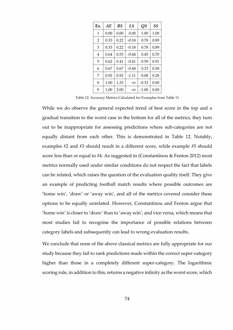
74

Ex. AE BS LS QS SS

1 0.00 0.00 0.00 1.00 1.00

2 0.33 0.22 -0.18 0.78 0.89

3 0.33 0.22 -0.18 0.78 0.89

4 0.64 0.55 -0.44 0.45 0.70

5 0.62 0.41 -0.41 0.59 0.91

6 0.67 0.67 -0.48 0.33 0.58

7 0.92 0.92 -1.11 0.08 0.28

8 1.00 1.33 -∞ -0.33 0.00

9 1.00 2.00 -∞ -1.00 0.00

Table 12: Accuracy Metrics Calculated for Examples from Table 11

While we do observe the general expected trend of best score in the top and a

gradual transition to the worst case in the bottom for all of the metrics, they turn

out to be inappropriate for assessing predictions where sub-categories are not

equally distant from each other. This is demonstrated in Table 12. Notably,

examples #2 and #3 should result in a different score, while example #5 should

score less than or equal to #4. As suggested in (Constantinou & Fenton 2012) most

metrics normally used under similar conditions do not respect the fact that labels

can be related, which raises the question of the evaluation quality itself. They give

an example of predicting football match results where possible outcomes are

‘home win’, ‘draw’ or ‘away win’, and all of the metrics covered consider these

options to be equally unrelated. However, Constantinou and Fenton argue that

‘home win’ is closer to ‘draw’ than to ‘away win’, and vice versa, which means that

most studies fail to recognise the importance of possible relations between

category labels and subsequently can lead to wrong evaluation results.

We conclude that none of the above classical metrics are fully appropriate for our

study because they fail to rank predictions made within the correct super-category

higher than those in a completely different super-category. The logarithmic

scoring rule, in addition to this, returns a negative infinity as the worst score, which

75

hampers its suitability for average performance assessment. We discuss a possible

solution to address this issue in chapter Section 5.5.

2.7. String Comparison

One of the aims of this research is to develop a framework which combines a

Bayesian approach to classification with an external knowledge source in a way

that the former can perform autonomously and adequately while the latter

requires manual maintenance but improves the final results delivered by the

method. Apart from classifying media items by analysing various file type

signatures in the file name, a major challenge lies in the attempt to individually

identify media files as particular movie titles and detect whether there are risks

associated with these titles at the given time. To accomplish this task, we use a

collection of movie, TV series and video game titles as specified in Section 2.4.

There are several reasons for attempting to detect a title in the name string:

a) There may be no information about medium present in the file name, in

which case it may be sensible to assume the item is a movie, given its file

size and the fact a title was detected.

b) Some titles (e.g. movies prior to their digital release) can be associated with

higher risks of fakes or malware, and the fact of detecting such a title must

impact the medium type of the prediction.

c) Porn detection can also be improved for files which have no regular porn

markers such as signatures, actors or studios, by detecting a title of a porn

movie.

Detecting a title in a noisy file name string is, in essence, a problem of finding the

longest common sub-sequences, while at the same time allowing some degree of

mismatch between the sequences that should be matched as similar. The sheer

number of titles in the database makes identification a non-trivial task, and the fact

76

that it has to be performed for multiple files as quickly as possible, only adds to

the complexity.

The field of bio-informatics provides a range of approaches to this problem. It is a

very common activity to align two genome sequences in order to establish if there

are similarities that may hint at functional, evolutionary or structural relationships

between them.

The essential purpose of the alignment is to capture regions which are either the

same or similar (e.g. where particular characters may be swapped without losing

the overall meaning of the sequence).

Movie The Bourne Legacy (2012)

Torrent Jason Bourne 04 - La peur dans la peau - L’héritage [ATG 2012] 720p.mp4

Table 13: Example of a Movie Title and Torrent Name for Alignment

Consider the torrent name and the movie title from Table 13 aligned in Figure 10.

The pairs of the same characters are marked with an asterisk below them; and

whenever a mismatch occurs, a gap is inserted in one of the sequences, which is

denoted by a dash. A sequence alignment function is also able to produce a

particular score that denotes the degree of similarity. It is configurable in terms of

how subsequent matches or mismatches should be treated, or which characters are

interchangeable and to what degree.

The------ Bourne -----L---eg----acy-- (--------------------------2012)----------

----Jason Bourne 04 - La pe-ur da--ns -la peau - L’héritage [ATG 2012-] 720p.mp4

****** * * * ****

Figure 10: Torrent Name and Movie Title Aligned

One of the first widely adopted methods for sequence alignment is the

Needleman–Wunsch algorithm (Needleman & Wunsch 1970), which is an example

of dynamic programming, whereby a complex problem is broken up into smaller

sub-problems and solved gradually. It computes a matrix 𝐹𝑚,𝑛, where 𝑚 and 𝑛 are

the lengths of the sequences, and calculates a score of all possible global alignments

(i.e. total resulting sequence), and then finds the most optimal alignment. A

77

variation of the Needleman–Wunsch method is the Smith–Waterman (SW)

algorithm (Smith & Waterman 1981), which is more concerned with local

alignments (i.e. alignment of sub-sequences) by comparing segments of all

possible alignments and optimising the resulting similarity measure. The SW

variation is more relevant to this thesis as it specifically addresses partial

alignments, which may provide additional evidence for the classification model.

BLAST (Altschul et al. 1990) is one of the most widely used tools for sequence

alignment in bioinformatics (Casey 2005), and features a heuristic algorithm based

on matching sequences of n-grams, an n-gram being a sequence of 𝑛 characters.

Using such a technique provides an opportunity for a much shorter processing

time with a subsequent detailed alignment where applicable.

Table 14 provides an example of breaking up a movie title ‘Matrix’ into 3-grams:

Original MATRIX

3-Grams MAT ATR TRI RIX

Table 14: 3-Gram Example of ‘Matrix’

Matching strings as n-grams is faster than sequence alignment and provides a

quick method of establishing whether it is even worth it to attempt sequence

alignment.

Most sequence alignment algorithms share a very important feature, allowing us

to define a substitution matrix e.g. BLOSUM (Henikoff & Henikoff 1992), which

specifies a degree of similarity between each pair of amino acids. For example, it

may specify that matching amino acids C and A should result in a higher score than

C and P. Ultimately, a substitution matrix allows for identifying similar sub-

sequences even after they were affected by mutations (e.g. where not all characters

match exactly).

Additional tuning is possible via implementing a particular scoring policy, which

can dramatically impact the resulting alignment. A gap occurs when the algorithm

78

decides that it is more expensive score-wise to match two incompatible characters

than to shift one of the sequences to the right or left by inserting a gap. Gap starters

and gap extenders can be treated differently and some gapping policies may

favour long gaps over a lot of small gaps by making a gap starter expensive and a

gap extender cheap. Table 15 illustrates how different gapping and scoring rules

can impact the final alignment. The scoring rules used in our approach are

explained further in Section 4.4.

Movie Title The Matrix (1999)

Torrent Name (TheNeo) Mediatrix (Into the matrix) [2011]

Alignment

Rule Set 1

-The---- M---atrix (1999---------------)-------

(TheNeo) Mediatrix (----Into the matrix) [2011]

*** * ******* *

Alignment

Rule Set 2

-------------------------The Matrix- (---1999)--

(TheNeo) Mediatrix (Into the matrix) -[201----1]

********** *

Table 15: Alignment Example under Different Rules

We briefly cover the Smith-Waterman algorithm as it is relatively simple to

implement and provides a sufficient insight into the string alignment theory. In a

classical implementation a matrix 𝑀𝑛+1,𝑚+1is constructed where 𝑚 and 𝑛 are the

lengths of the two strings being aligned. Alignment of ‘Mediatrix’ and ‘Matrix’

results in a 10 by 7 matrix.

The matrix is filled according to the scoring rules, which in this example are:

match same characters: 2

match different characters: -1

gap: 0

This means that positioning the same characters opposite each other bears a score

of 2, different characters opposite each other result in a score of negative 1 and

simply shifting either string one position is a zero score. The top-left cell is always

a 0, and all other cell scores are calculated using the formula:

79

𝑀𝑖,𝑗 = 𝑚𝑎𝑥

{

0 𝑀𝑖−1,𝑗−1 + 𝑚𝑎𝑡𝑐ℎ(𝑖, 𝑗)

𝑀𝑖,𝑗−1 + 𝑔𝑎𝑝(𝑗)

𝑀𝑖−1,𝑗 + 𝑔𝑎𝑝(𝑖)

(30)

Top and left rows will be hence filled with zeroes, representing an entry point

before any characters were matched. The remaining matrix is then eventually filled

with scores as in Table 16.

Mediatrix

M---atrix

- M E D I A T R I X

- 0 0 0 0 0 0 0 0 0 0

M 0 2 2 2 2 2 2 2 2 2

A 0 2 2 2 2 4 4 4 4 4

T 0 2 2 2 2 4 6 6 6 6

R 0 2 2 2 2 4 6 8 8 8

I 0 2 2 2 4 4 6 8 10 10

X 0 2 2 2 4 4 6 8 10 12

Table 16: Example of Alignment and Score Matrix

Whenever we move diagonally, this means that characters were matched, and

horizontal or vertical movement is a result of inserting a gap. Once all the scores

are calculated, the algorithm backtracks the alignment from the last cell which had

the best score. It then moves backwards building up the final alignment strings by

selecting a cell that bears the least score loss compared to the current cell,

preferring the diagonal movement if multiple cells have the same score record. In

many cases two strings can be aligned in multiple ways with the same final score.

80

2.8. Summary

In this chapter we introduced a commercial benchmark system MVL developed by

MovieLabs that provided results for comparison to our prototype classifier Toran.

We explained the input data, which is a list of basic torrent information, such as

unique identifier, download’s name and file size. It is supplemented with a

database of movie, TV series and game titles, as well as a limited set of names of

porn actors and studios.

We explained the classification taxonomy originally used by MVL and highlighted

its drawbacks, and introduced the Toran classifier system which we used to test

the application of our methodology.

As part of our study we used human participants to help us construct data samples

and manually classify and identify several thousand torrent files. A small subset

of these items was also fully downloaded and its content verified. Other data sets

were also developed to evaluate prediction of fakes and malware, and to provide

confident results about medium classification on an independent test set. These

data, together with benchmark classifications, were separated into four data sets

which are explained in this section and can be found in Appendix D.

81

Chapter 3

Torrent Name Bayesian Network Model

This chapter directly addresses Research objective 1 (from Section 1.2) by

providing a novel BN model that lies at the heart of the torrent identification and

classification system Toran. It was developed using a combination of data and

expert domain knowledge, rather than a straight ML approach for reasons

explained further in this chapter.

The chapter first provides relevant theory about Bayes’ theorem and Bayesian

modelling in Sections 3.1, 3.2 and 3.3. It then gives a brief overview of the whole

model in Section 3.4 and explains every part in more detail in Sections 3.5 to 3.12,

also providing judgement for the conditional probability definitions of any

relevant nodes, and how various concepts within the model evolved over time.

While some evidence observed in the model is trivial, such as ‘file size’, other

evidence is captured through a complex process, which is explained in Chapter 4.

Elsewhere in this chapter relevant references are provided pointing to evidence

capturing procedures. Section 3.13 outlines our ideas for possible extensions of our

model and the procedure to be followed.

The material in Sections 3.4 to 3.13 and application specific examples in Sections

3.1 to 3.3 are, to the best of our knowledge, a novel contribution.

82

3.1. Bayes’ Theorem

Bayes’ Theorem (Bayes & Price 1763; McGrayne 2011; Fenton & Neil 2012b; Barber

2012) is named after Thomas Bayes who, in 1763 showed how initial beliefs can be

updated by new evidence. It describes the relation of prior probability before

evidence and the posterior probability once some evidence is observed. Formally,

it describes the probability of some unknown event 𝐻 given evidence 𝐸:

𝑃(𝐻|𝐸) =𝑃(𝐸|𝐻) 𝑃(𝐻)

𝑃(𝐸) (31)

where 𝑃(𝐻) is the prior probability of 𝐻, 𝑃(𝐸|𝐻) is the likelihood and 𝑃(𝐻|𝐸) is the

posterior probability of 𝐻. When 𝑃(𝐸) = 0, 𝑃(𝐻|𝐸) is not defined. When 𝐻 is a set

of 𝑛 mutually exclusive and exhaustive events, we can express the probability of

the evidence by the law of total probability (Zwillinger & Kokoska 2000) as:

𝑃(𝐸) =∑𝑃(𝐸|𝐻𝑖) 𝑃(𝐻𝑖)

𝑛

𝑖=0

(32)

A practical example that is relevant to the problem domain, considers fake items.

We know that highly anticipated titles or those that have been released recently

are most at risk of being faked on the file sharing networks. Some of these fakes

could be broken videos, while others could contain malware. Therefore, it is

important to assess the risk that a downloadable item is in the risk group, a fake

and subsequently – concealed malware.

Imagine that, based on information such as a database of recently released movies

and/or expert judgment, there is a test to determine whether a torrent is a fake or

not by analysing its name. Suppose the test is accurate enough to conclude an item

to be a fake in 99% of cases when it is an actual fake, and in 5% of cases when it is

not a fake. So the true positive rate for the test is 99% and the false positive rate is

83

5%. Suppose, we can estimate that for the torrents posted more than 2 months ago,

around 5 in 1000 are fakes. Then for this class of torrents we have:

𝑃(𝐹𝑎𝑘𝑒) = 0.005𝑃(𝐷𝑒𝑡𝑒𝑐𝑡𝑒𝑑|𝐹𝑎𝑘𝑒) = 0.99 𝑃(𝐷𝑒𝑡𝑒𝑐𝑡𝑒𝑑|¬𝐹𝑎𝑘𝑒) = 0.05

(33)

According to the rule of total probability (Zwillinger & Kokoska 2000):

𝑃(𝐷𝑒𝑡𝑒𝑐𝑡𝑒𝑑) = 𝑃(𝐷𝑒𝑡𝑒𝑐𝑡𝑒𝑑|𝐹𝑎𝑘𝑒)𝑃(𝐹𝑎𝑘𝑒) + 𝑃(𝐷𝑒𝑡𝑒𝑐𝑡𝑒𝑑|¬𝐹𝑎𝑘𝑒)𝑃(¬𝐹𝑎𝑘𝑒) =

0.99 × 0.005 + 0.05 × 0.995 = 0.0547 (34)

We are interested in the chance that the item really is a fake given that the match

was positive:

𝑃(𝐹𝑎𝑘𝑒|𝐷𝑒𝑡𝑒𝑐𝑡𝑒𝑑) =𝑃(𝐷𝑒𝑡𝑒𝑐𝑡𝑒𝑑|𝐹𝑎𝑘𝑒) 𝑃(𝐹𝑎𝑘𝑒)

𝑃(𝐷𝑒𝑡𝑒𝑐𝑡𝑒𝑑)=

0.99 × 0.005

0.0547≈ 0.091

(35)

This means that even if our test determines the torrent to be a fake, the chances are

that it is a false positive, because the initial probability of finding such an item is

very low. This means that the test for fake items must be made more accurate, or

accompanied by another test.

Not Fake Fake

Not Detected 94525 5

Detected 4975 495

Total 99500 500

Table 17: Illustration of Fakes Detection Test

Table 17 illustrates this example applied to a random selection of 100,000 items. In

the rest of this chapter we demonstrate how we apply Bayes’ theorem in building

a probabilistic model to address the problem of item classification in the problem

domain context.

84

3.2. Bayesian Networks Overview and Key Concepts

This section provides an overview of Bayesian networks (BNs) covering those

aspects necessary for the thesis and is structured as follows: Sub-section 3.2.1

provides an essential definition of BNs. Sub-section 3.2.2 gives relevant BN

examples. Sub-section 3.2.3 outlines the key properties of BNs, relevant tools,

applications and briefly covers the Bayesian inference methods. Sub-section 3.2.4

explains the difference between hard, soft and virtual evidence. Sub-section 3.2.5

outlines how continuous nodes are modelled in AgenaRisk.

Bayesian Network Definition

A Bayesian Network (BN) is a graphical probabilistic model (Pearl 1988; Edwards

2000; Nielsen & Jensen 2009; Koski & Noble 2009), consisting of variables or events,

formally called nodes, connected with arrows, formally called edges and

representing causal or influential relationships between the nodes. The collection

of nodes and edges is called a graph or topology. For a pair of events 𝐴 and 𝐵 in a

relationship 𝐴 → 𝐵, 𝐴 is called parent and 𝐵 is called child. Nodes that do not have

a parent are called root nodes. A BN is a type of directed acyclic graph (DAG), which

implies that no node can be an ancestor to itself, and that all edges are directed

(Christofides 1975; Thulasiraman & Swamy 1992).

There are many possible types of nodes such as Boolean, labelled, ranked, and

continuous or integer intervals. Depending on the node type, random variables

represented by the nodes, are either discrete or continuous. In the former case the

range of values must be an exhaustive collection of mutually exclusive states (e.g.

“True” and “False”; or “Low”, “Medium” and “High”). In the latter case we can

define ranges, but the actual variable can take any value allowed by the node type.

For example, for a continuous integer type node, we may define ranges (-∞, -11],

[-10, 10], [11, +∞), allowing the variable to take any integer value. However, the

85

number of states of the variable is then 3, which makes it possible to process

continuous nodes in the same manner as discrete nodes.

Each node has an underlying node probability table (NPT), also called conditional

probability table for child nodes. For a node A without parents the NPT is simply

the prior probability of each state of A. For a node 𝐵 with parents the NPT specifies

for each state of B, the probability of that state given all combinations of the states

of the parents of B.

Simple BN Examples

Consider the example of fakes detection illustrated in Table 17 and a very simple

corresponding BN in Figure 11. It is very important to note that the causation is

expressed in this case by the arrow going from Torrent is Fake to Evidence of Fake

Detected, because the result depends on the input, and not the other way around.

However, correct inference in BNs is also possible when edges do not follow

causation direction.

Figure 11: Basic BN for Fakes Detection

Considering the set of newly added records, the prior for a file name to contain a

risky title was set at 30 in 100, which has to be first normalised so that it adds up

to 1. Leaf nodes like Torrent is Fake have a very simple NPT such as in Table 18.

Torrent is Fake False 0.7

True 0.3

Table 18: NPT for Torrent is Fake in the Basic Model

Evidence of Fake Detected is a child node, so we have to specify probability values

based on detection accuracy, which is assumed to be 99% for cases where there

really is a risky title and 95% otherwise, as shown in Table 19.

Torrent

is Fake

Evidence of

Fake Detected

86

Torrent is Fake False True

Evidence of Fake Detected False 0.95 0.01

True 0.05 0.99

Table 19: NPT for Evidence of Fake Detected in the Basic Model

Once an observation is entered into the Evidence of Fake Detected, it back-propagates

to Torrent is Fake as in Equation 35 as the model calculates the posterior probability

of Torrent is Fake (see Figure 12).

Figure 12: Basic BN for Fakes Detection Example after Evidence Propagation

Now, in practice, the test to determine whether a torrent is fake based on its name

will depend on a number of factors. One such factor is the Database Coverage (where

we assume the test involves looking up a database of ‘risky titles’). In this case we

revise the BN model shown in Figure 11 by adding an extra parent to Evidence of

Fake Detected as shown in Figure 13.

Figure 13: Revised Example Model for Fakes Detection

If a node has multiple parents its NPT table becomes increasingly complex because

the number of cells in the table is equal to the product of the number of options

each parent variable can take. Suppose the variable Database Coverage has just two

states “high” and “low”, which may correspond to the proportion of movie titles

in the database out of all titles filmed. Clearly the accuracy of our test is going to

be influenced by whether or not we have a sufficient number of titles in our

database.

Torrent

is Fake

Evidence of

Fake Detected

Database

Coverage

87

DB Coverage Low High

Torrent is Fake False True False True

Evidence for Fake Detected False 0.99 0.7 0.95 0.01

True 0.01 0.3 0.05 0.99

Table 20: NPT for Evidence for Fake Detected Example with 2 Parents

Table 20 illustrates a possible revised NPT for Evidence of Fake Detected in the more

complex version of the model. If the database coverage is “Low”, evidence can

only be correctly detected in 30% of cases when it actually is in the name string, as

opposed to 99% detection rate with a “High” coverage database. We also assume

a “Low” database coverage may rarely lead to false positives while a “High”

coverage may cause a higher number of false positives due to file names matching

something in the database.

Figure 14a shows the model in its prior marginal state before any observations are

entered. Note that observing the evidence for a fake yields a high confidence in the

prediction that the item is fake (Figure 14b, c), regardless of the database state.

However, when we do not observe any evidence of a fake, there is an important

difference. In Figure 14d our prior belief in 30% chance of a fake is only weakly

affected, because database coverage is low. In this scenario failing to observe any

evidence of fakes is likely due to having insufficient data rather than because the

item was not a fake.

On the other hand, when database coverage is high as in Figure 14e an item that is

a fake is very strongly expected to be properly detected, hence failing to observe

evidence for a fake leads us to believe that the item is not one.

88

Figure 14: Possible Outcomes of the Fakes Detection Model: a) Show the marginal values before

propagation, b-e) Show the values after propagation with the given observations

From consulting with domain experts and studying the problem domain, we

determined a possible improvement to the model in Figure 13. This extension may

be motivated by inclusion of a relation between the type of an item and its

prevalence to be a fake. For example, we know that most fakes are disguised as

movies, and we can express this by adding two new nodes Item is Movie and Item

Looks Like Movie, as in Figure 15.

Figure 15: Extended Example Model for Fakes Detection

Torrent

is Fake

Evidence of

Fake Detected

Database

Coverage

Item is MovieItem Looks

Like Movie

89

This extension allows us to specify that an actual movie is very unlikely to be a

fake, while items that are fakes or movies are very likely to appear as movies too.

Items that appear as movies and are fakes at the same time, are likely to contain

evidence for fakes, such as a title of a highly anticipated movie.

Bayesian Network Inference Algorithms, Tools and Applications

While the Bayesian inference calculations in the above 3-node model for fakes

detection example can be computed manually, the necessary calculations quickly

become intractable as more nodes and edges are added. For example, inference in

the extended model in Figure 15 is already extremely complex to undertake

manually. Indeed, the general problem of exact inference for an arbitrary BN is

known to be NP-hard (Cooper 1990). However, in the late 1980s efficient

propagation algorithms were developed for a broad variety of BNs (Pearl 1988;

Henrion 1988; Lauritzen & Spiegelhalter 1988). These algorithms have

subsequently been implemented in widely available software tools. To run the

necessary computations for the BN model and associated classification and

identification method developed in this thesis, we use the application program

interface (API) of one such tool AgenaRisk (Agena 2016c). AgenaRisk employs the

junction tree propagation algorithm (Jensen & Nielsen 2007), which we describe in

Appendix E.

With the advent of widely available BN tools, there has been an explosion of

interest in BNs since the mid-1990s with BN-based decision support applications

developed in a wide range of fields (Fenton & Neil 2012b; Pourret et al. 2008).

These include: making high-stakes critical real-time decisions at the NASA Mission

Control Center (Horvitz & Barry 1995); device fault diagnostic and troubleshooting

(Breese & Heckerman 1996; Skaaning et al. 2003); pharmacokinetic analysis

(Gelman et al. 1996); medicine (Díez et al. 1997) (Burnside et al. 2006; Fenton & Neil

90

2010); analysis in genetics (Friedman et al. 2000; Jansen et al. 2003; Jiang et al. 2011);

vehicle reliability for the military (Neil et al. 2001); terrorist attack detection

(Laskey & Levitt 2002); Air Traffic Control environment (Neil et al. 2003); railway

accident causation (Marsh & Bearfield 2004); football predictions (Constantinou et

al. 2012); software reliability (Fenton & Bieman 2014); reliability of complex

systems (Marquez et al. 2010), law (Fenton 2011; Keppens 2011; Fenton et al. 2013).

Compared to classical statistics, BNs provide the following benefits (also note that

c and e cannot be achieved with rule-based decision support systems):

a) Modelling causality allows a BN to be explained to a domain expert who is

not necessarily a statistician. When data is not available, it is still possible to

model causal relations between significant variables by eliciting

probabilities and likelihoods from the domain experts. This is crucial

because in many classical statistical methods such as regression analysis

(Seber & Lee 2003), observational data is analysed for direct correlation

clues, and may lead to wrong assumptions about causation (Armstrong

2012; Cook & Weisberg 1982; Freedman 1991). Moreover, such methods do

not allow inclusion of any kind of logical reasoning that must apply

regardless of data, e.g. an argument that while predicting software defects,

performing no testing would yield no defects (Fenton et al. 2007). Likewise,

regression models are incapable of adequately incorporating very rare

events that a domain expert may consider possible in future.

b) Combining different types of evidence makes it possible to encode objective

data and subjective beliefs into the model (Heckerman 2008) and allows

setting the type of data and NPT individually for each variable.

c) What-if analysis is possible because causal BNs allow differentiation between

observations and interventions. As defined in (Pearl 2009), an intervention

on a variable A simply sets the variable to a desired state and cuts off edges

leading from its parents to disable back-propagation, which enables us to

91

avoid a correlation due to unmeasured common causes and highlights

direction of causality.

d) Back-propagation of evidence from effect to cause provides crucial backward

reasoning that enables powerful predictions. Once an observation is entered

in an effect node, it updates probability distribution of its cause, as per

Figure 12.

e) Explaining away, as in the fakes detection example in Figure 14 above, where

the probability of the torrent being a fake is discounted when other reasons

for detecting evidence of fake are observed. For example, when some

evidence is found and the database coverage is low, the final confidence is

higher that the item is a fake. However, if the database coverage was high,

it is considered to be the more likely reason for detecting the evidence (i.e.

false positive) and the posterior probability of fake is reduced.

f) Visible auditable reasoning means that it is possible to work out why exactly

the model arrived at a particular prediction, which may be a great

debugging opportunity.

g) Computing predictions despite missing evidence is crucial for many real world

applications, because we cannot rely on always having sufficient data, nor

do we actually have that much data in reality. With no observations entered,

a BN would return predictions that represent our prior belief, and with

more evidence added, the more accurate the final predictions will become.

While Bayes’ theorem provides a rational and correct way to characterise

uncertainty of an unknown hypothesis as new evidence is observed, there is no

universal acceptance of the need for Bayes or even the need to capture uncertainty

at all. There are also two common specific objections to using Bayes:

1. Need to specify prior probabilities: There is a special concern when this

requires subjective judgment. This arises from a philosophical debate going

on in the field of probability analysis (Kendall 1949; Casella & Berger 1987;

92

Gelman 2008; Senn 2011) for decades, concerning the definition of

probability itself and involving the comparison of frequentist and Bayesian

schools of thought. The frequentist approach considers drawing

probabilities from directly observing data, while the Bayesian considers

probability to be a function of logic and revolves around updating initial

subjective prior with subsequent objective evidence. It can be argued that

with sufficient data one can arrive at an objective probability of a variable

by simply observing the frequency of that variable in a big enough sample.

However, this fails to address cases where little or no historical data is

available while expert judgment may be in abundance. The Bayesian

approach joins data and knowledge allowing better decision-making when

data is scarce (McGrayne 2012).

2. Complexity of the Bayesian calculations: This is, of course, especially

relevant when there are multiple dependent variables. Fortunately it is

alleviated by using Bayesian networks and automated tools that implement

the necessary inference algorithms.

Hard, Soft and Virtual Evidence

Whenever evidence is entered into a node, it is usually ‘hard evidence’ that is

considered, which means that one node state is assigned a probability of 1 and the

other states of 0. However, in real world applications we sometimes can only

obtain uncertain evidence in cases when we are not entirely sure about the

observation. For example, we could be 90% certain that a Boolean node is true, but

this means that we cannot use hard evidence to express this. In fact, the model

should propagate and return marginal values for the states of “true” and “false”

as 0.9 and 0.1 respectively. Such implementation is called soft evidence. However

this is technically difficult to implement (Fenton et al. 2012), so commercial tools

93

normally implement virtual evidence (Pearl 1988) which uses a likelihood ratio

defined as:

𝑃(𝑂𝑏(𝑎1)|𝑎1) ∶ … ∶ 𝑃(𝑂𝑏(𝑎𝑛)|𝑎𝑛) (36)

where 𝑛 is the number of states of the variable 𝐴, 𝑃(𝑂𝑏(𝑎𝑖)|𝑎𝑖) is interpreted as the

probability of observing state 𝑎𝑖 when 𝐴 is indeed in this state. Then the posterior

probability 𝑃(𝐴 = 𝑎𝑚|𝑉𝑒) is defined as:

𝑃(𝐴 = 𝑎𝑚|𝑉𝑒) =𝑃(𝑎𝑚) × 𝑃(𝑂𝑏(𝑎𝑚)|𝑎𝑚)

∑ 𝑃(𝑎𝑖) × 𝑃(𝑂𝑏(𝑎𝑖)|𝑎𝑖)𝑖 (37)

where 𝑉𝑒 denotes ‘virtual evidence’. To illustrate, a Boolean variable with prior

probability for true being 0.2 and virtual probability for true being 0.9 would result

in a posterior probability:

0.9 × 0.2

0.9 × 0.2 + 0.1 × 0.8≈ 0.69 (38)

We use virtual evidence in the model for title identification in cases of multiple

title category matches per torrent name, as explained further in Section 3.11.

Modelling Continuous Variables

Unlike other propagation algorithms which assume that numerical variables have

a fixed set of pre-defined discrete states, the AgenaRisk inference algorithm

implements dynamic discretisation as described in (Neil et al. 2007). The

implementation is based on the ideas originally proposed in (Kozlov & Koller

1997) and is a more flexible alternative to approaches involving conditional

Gaussian (Lauritzen & Jensen 2001; Lauritzen 1992), or mixtures of truncated

exponentials (Cobb & Shenoy 2006; Rumí et al. 2006).

Specifically, in AgenaRisk it is possible to use all of the following distributions:

Beta, Chi Squared, Exponential, Extreme Value, Gamma, Gaussian, Logistic, Log

Normal, Student, Triangle, Truncated Normal, Uniform or Weibull. The dynamic

discretization algorithm approximates the probability density function (PDF) 𝑓𝑥 of

94

any of these distributions. It finds an optimal discretization set and optimal values

for the discretised PDF 𝑓𝑥′ via a series of iterations within an acceptable degree of

precision. Unlike other Bayesian modelling software (Lunn et al. 2000; Stan

Development Team 2014; Murphy 2014; Bayes Server 2015; Hugin 2015),

AgenaRisk therefore provides an efficient and flexible way of modelling

continuous nodes without having to manually specify discrete intervals or limit

oneself to Gaussian distributions only.

We used continuous nodes in a supplementary BN to learn parameters of the size

distributions for the main BN. Moreover, in revisions of the model following the

original submission of this thesis, we use continuous nodes both for the size node

and for the nodes that measure the level of evidence detected for each item

category (e.g. category keywords and patterns, or file size).

3.3. Building Bayesian Networks

While Section 3.2 makes clear the benefits of a well-crafted BN once it is built, there

are great challenges in actually building a sensible and useful BN for a given

problem domain. This section describes the various methods used in this thesis to

develop the BN model for file identification and classification and is structured as

follows: Sub-section 3.3.1 compares two distinct approaches – knowledge

engineering and machine learning – to building BNs. Sub-section 3.3.2 covers the

topic of conditional dependency of variables. Sub-section 3.3.3 outlines some

approaches to creating BN structure and lists the major steps in this process. Sub-

section 3.3.4 provides an overview of popular approaches to learning prior

probabilities for the model, including elicitation from domain experts. Sub-section

3.3.5 explains in detail theory behind reusable patterns called idioms, introduced

first in Section 3.3.3 and how they are relevant to this project.

95

Knowledge Engineering versus Machine Learning

A good model lies at the heart of proper probability analysis, and it is important

to capture the structure of the model and define prior and conditional

probabilities. A natural approach is knowledge engineering (KE), which aims to

exploit the experience, judgement and knowledge of the domain experts and elicit

from them the BN structure, any possible causal relationships between variables,

and probabilities.

Although BNs are originally motivated by the knowledge and insight of domain

experts, there is a separate branch of Bayesian modelling, which employs machine

learning (ML) methods (Neapolitan 2003; Murphy 2012; Barber 2012) and is

concerned with both model structure and the prior and conditional probabilities

being learned from the data itself, such that the resulting model describes the data

sample. Because ML implementations naturally recover a model that best

describes the data, it is important to consider the possibility of the analysed sample

being insufficiently large.

In practice, however, it is often sensible to integrate knowledge-based and data-

driven approaches. A number of theory refinement methods are discussed in

(Buntine 1991), some of which revolve around the idea of starting with a network

structure elicited from an expert and refining it with subsequent automated

learning. Belief and causal networks are contrasted in (Heckerman et al. 1994) by

enforcing different requirements on automated learning methods, which shows

how domain knowledge impacts the learning process even in the early stages of

model type definition. A method for specifying constraints into a model learning

process is proposed in (Altendorf et al. 2005; Zhou et al. 2014; Zhou et al. 2015).

Such constraints represent the proportional relation between variables. A

framework allowing an expert to define hard constraints on the structure and soft

constraints on the priors is proposed in (de Campos & Qiang 2008). A method

96

based on dependency analysis aimed at learning structure from incomplete data-

sets by making assumptions about missing data to fill the gaps, is proposed in (Fiot

et al. 2008). It is suggested in (Cano et al. 2011) to learn the structure of the BN

automatically, but confirm certain low-confidence parts of the structure with an

expert. Work in (Flores et al. 2011) presents an overview of several methods

allowing an expert to specify the full structure; identify causal direct links; causal

dependency; relation (i.e. edge) directions; identify related variables with

unknown relation direction; temporal tiers, where variables are grouped within

timeline; or correlations. The method proposed in (Khan et al. 2011) is based on an

expert executing an evidence gathering test at each step of the learning procedure.

The example provided in (Fenton 2012) illustrates a common situation whereby it

is impossible, even when there is an extremely large data sample for a small

number of variables, to use a machine learning or frequentist approach to learn a

simple relationship easily known to an expert. An example in (Fenton 2014)

illustrates how a model refined by expert judgement can provide more semantic

insight and lead to better decision making. Another example in (Fenton 2015a)

illustrates how a data-based approach may have to arrive at a wrong model, due

to a critical semantic meaning not explicitly present in the data set. Yet an expert

can identify semantics missing from the data and help create a correct model. An

illustration of how data-driven approaches may fail to identify crucial

interventions that may impact the data critically, is presented in (Fenton 2015b). It

is clear that employing, at least to some degree, expert judgement is preferable to

a pure machine learning approach, to be able to cope with inadequacies of data.

This thesis is concerned with analysing data where a sufficiently large validated

sample with known actual item categories may not be available for implementing

ML approaches appropriately; hence the rest of this section refers to KE methods.

97

Conditional Dependency

When linking nodes together, it is important to consider that from the

mathematical standpoint 𝐴 → 𝐵 structure is just as valid as 𝐵 → 𝐴. However, from

the practical perspective it may be better to select the parent based on whether it

is easier to define the unconditional rather than conditional prior probability for it,

or if maintaining the causal relation allows for a more transparent model. For

example, consider a variable Collection 𝐶 that represents the source, from which

we process torrent files, with possible values ‘new’ and ‘old’, and a variable Fake

𝐹. As noted in Sections 2.2 and 3.1, newly posted torrents are much more likely to

be fakes and this increases the risk of malware.

Depending on the structure of the model, there can be two sets of priors to define:

1. For 𝐶 → 𝐹: 𝑃(𝐶), 𝑃(𝐹|𝐶)

2. For 𝐹 → 𝐶: 𝑃(𝐹), 𝑃(𝐶|𝐹)

It is simple to define the model in terms of known parameter Collection influencing

the unknown parameter Fake because we can define the former based on the data

being analysed. For example, we may know in advance which torrent collection

the experiment will be running on, and whether the item in consideration is ‘new’

or ‘old’. In such a case the prior probability of 𝐶 does not matter because the

variable is always observed, and can be set with an ignorant prior of 0.5 for each

option. We can then use our expectation of a larger proportion of fakes among the

‘new’ items to define conditional priors of 𝐹 given 𝐶. On the other hand, defining

the prior unconditional probability of item being a fake is much more difficult than

working out expected proportions based on other factors such as the recency of an

item, or its medium which allows defining what kinds of media are more likely to

be faked.

We can extend this model by including the real medium of the item. This allows

specifying that fake downloads are mostly videos (e.g. broken videos) or software

98

(e.g. malware). Finally, to give a prediction of the risk of malware, the model is

extended with another node that specifies that malware is mostly found in fakes

that are in reality software. We end up with the model in Figure 16.

Figure 16: Basic BN for Input, Real Medium, Fake and Malware

In BNs there are 3 types of dependency connections (d-connections) identified in

(Fenton & Neil 2012c), which are all found in Figure 16: converging, diverging and

serial. Evidence flow between nodes depends on hard evidence being entered at

the nodes between them as illustrated by Figures 17, 18 and 19.

a) Converging (Figure 17)

Node 𝐹 has multiple parents 𝐶 and 𝑀. If there is hard evidence entered at 𝐹

or any its children, then 𝐶 and 𝑀 are dependency-connected (d-connected),

meaning that any evidence entered at 𝐶 will update posterior of 𝑀 and vice

versa. Otherwise they are dependency-separated (d-separated), meaning that

there is no evidence flow between them.

Figure 17: Converging Connection

Collection (C)Real

Medium (M)

Fake (F) Malware (W)

C F Mc

Observation: Set

C F Mc c,f

Observation: Set Observation: Set

99

b) Diverging (Figure 18)

Node 𝑀 is a parent of multiple nodes 𝐹 and 𝑊. If there is hard evidence

entered at 𝑀, then 𝐹 and 𝑉 are d-separated. Otherwise they are d-connected.

Figure 18: Diverging Connection

c) Serial (Figure 19)

Nodes 𝐶, 𝐹 and 𝑊 are connected in a sequence such that 𝐹 is conditionally

dependent on 𝐶, and 𝑊 is conditionally dependent on 𝐹.

If hard evidence is entered at 𝐹, then 𝐶 and 𝑊 are d-separated, and d-

connected otherwise.

Figure 19: Serial Connection

The solid arrows on Figures 17, 18 and 19 represent the actual edges, while the

dashed arrows illustrate information flow from instantiated nodes. Instantiation of

a node refers to a hard observation being entered into that node. Note how

information can flow in the direction opposite to the direction of the edge. Middle

nodes with a pink background block evidence propagation between side nodes

and make them d-separated. Middle nodes with green background allow d-

connection and evidence flow.

F M Wm

Observation: Set

F M Ww

Observation: Set

w

Observation: Set

w

C F Wc

Observation: Set

C F Wc

Observation: Set

f

Observation: Set

c

100

Defining BN Structure

According to standard software engineering practices, a system should be built

from modules or components, usually employing object-oriented (OO) methods

(Goldberg & Robson 1983; Rumbaugh et al. 1991; Meyer 1998). A number of

repeated concepts is identified, which are implemented and reused on a regular

basis, and are called design patterns (Gamma et al. 1995; Jackson 1995). These

patterns represent templates of recognised solutions to common problems. For

example, most software systems have at least one object that is unique in its type,

and accessed by many other components of the system. The Singleton design

pattern structurally describes how this case may be implemented in a coherent

way.

Extending this idea to BN construction, Laskey and Mahoney defined a method of

organising parts of BNs into semantically meaningful units, which they called

fragments (Laskey & Mahoney 1997). In this definition, all fragments can be

constructed separately from each other, and each is a set of nodes related by edges

and makes logical sense on its own. They build on this in (Laskey & Mahoney 2000)

by proposing a system engineering approach where simple prototypes are created

in iterations following a spiral lifecycle model, which are evaluated and amended.

Following this approach allows the knowledge engineer to better understand the

domain and the expert to acquire understanding of principles of Bayesian

modelling.

Koller and Pfeffer argued that just like programming languages and databases

benefit from an object-oriented approach, the BN building process could be

improved greatly in the same fashion (Koller & Pfeffer 1997). They conceptualised

object-oriented Bayesian Networks (OOBNs) where an object is a BN fragment

which is viewed as a stochastic function with attributes that can be observed as

inputs and predicted attributes as outputs, with some of the attributes being

101

private and not visible or accessible from outside of the object. Furthermore, an

output node of one object can be an input node for another, which enables multiple

levels of abstraction. The objects are encapsulated in a sense that only internal

evidence can influence their outputs.

Building on the OOBN work, Neil et al. define a number of idioms (Neil et al. 2000),

which are refined in (Fenton & Neil 2012d), and are analogous to design patterns

in OO programming and generalise a set of very particular types of BN structure

fragments which are viewed as building blocks for a BN. They also formalise the

process of mapping a subset of nodes and edges to a particular idiom, allowing an

engineer who is building the model to refer to this simple idiom selection rule

when translating structure elicited from a domain expert to a BN. We use this

approach extensively and a detailed explanation of both the idioms and how these

idioms were used to develop the BN in the thesis is provided in Section 3.3.5.

Other related approaches to building BNs are:

Similarity networks proposed by Heckerman (Heckerman 1990) which he

used for disease diagnostic, but is not restricted to this domain. This method

identifies the single hypothesis node called distinguished node (e.g. the

disease) and produces a series of small disjoint knowledge maps of various

variables related to the distinguished node. These are then merged into a

large knowledge map. This method assumes that the smaller knowledge

maps cover instances of the distinguished node that are exhaustive and

mutually exclusive; that the distinguished node is not a child; and that the

domain has only non-zero probabilities.

Causal maps are defined in (Eden et al. 1992) as a directed graph which

expresses judgement that certain actions or events will cause specific

outcomes. Nadkarni and Shenoy propose an approach that elicits a Bayesian

causal map (Nadkarni & Shenoy 2001) from experts via an interview and

transforming it into a Bayesian Network (Nadkarni & Shenoy 2004).

102

In essence, building a BN can be summarised into the following steps:

1) Identify significant variables relevant to the problem, preferably using pre-

defined relevant idioms, which also capture the node dependencies (i.e.

edges).

2) For those variables that are not part of a pre-defined idiom construct,

connect the variables with edges, preferably directed along causal links.

3) Identify correct type of all variables and what their values could be, and

whether they are continuous or not.

4) Define prior probabilities for non-children nodes.

5) Define conditional probabilities for children nodes.

The steps 1 and 2 were covered above, and the next sub-section covers the steps 3

to 5.

Prior and Likelihood Definition

It is a common argument that humans work best with qualitative rather than

quantitative assessment (Pearl 1988; Spiegelhalter et al. 1993) and that domain

experts and humans in general are prone to have difficulties or express biases

when dealing with probabilities (Tversky & Kahneman 1974; Gigerenzer et al.

1998; Donnelly 2005; O’Hagan et al. 2006), and that addressing these issues is

increasingly expensive and is generally infeasible (Renooij 2001). Because of such

prevailing views, eliciting parameters from experts (Savage 1971) is focused on

acquiring general notion of variables, relations between the variables, and degree

and direction of impact.

Parameter elicitation is often done via interviews with experts (Nadkarni &

Shenoy 2004) or questionnaires. Experts are normally asked to rate prior

probabilities on a scale e.g. from 1 to 10, “very low” to “very high”, a combination

of numeric scale and text labels (van der Gaag et al. 2002), or using probability

lotteries (Harrison et al. 2014).

103

While it is possible to perform sensitivity analysis to refine the elicited parameters

by exploring sensitivity to edge removal (Renooij 2010), or more traditionally by

inspecting how a target variable reflects changes to other parameters in its

posterior probability, it is computationally expensive, especially when multiple

parameters are adjusted simultaneously (Laskey 1995; Coupé et al. 2000).

With increasing complexity of models, the task of probability elicitation becomes

more daunting. One technique called divorcing (Neil et al. 2000; Nielsen & Jensen

2009) is to reduce the number of parents a node has by introducing synthetic

intermediate nodes, which in turn significantly reduces the size of the node’s NPT

and hence requires fewer probabilities to be entered. It is increasingly more

common to apply approaches that allow us to avoid specifying probability values

directly. Conditional probabilities can often be defined with a Noisy-OR model if

an expert indicates that any cause can independently lead to a particular effect. A

Noisy-AND model can be used if a combination of causes is required to achieve

the effect (Henrion 1989; Pradhan et al. 1994; Zagorecki & Druzdzel 2004).

Another option is to consider using qualitative probabilistic networks (Wellman 1990)

which are an abstraction of quantitative BNs, and use qualitative instead of

numeric relationships with emphasis on synergy and degree of impact. When

coupled with sensitivity analysis this method is claimed to be successful in arriving

at meaningful likelihood values (Biedermann & Taroni 2006).

A special type of variable called ranked node was introduced in (Fenton & Neil 2007)

that largely solves the problem of defining probability distributions for many

commonly occurring nodes that have a scale-type list of ordered states e.g. “Very

Low”, “Low”, “Medium”, “High”, “Very High”. Such ranked nodes are modelled

by a doubly truncated normal distribution (i.e. TNormal). Typically the ordinal

scale has 3, 5 or 7 states, but the method described in (Fenton & Neil 2007), which

is implemented in AgenaRisk, allows for any number of states since a ranked node

has an underlying numerical range of 0-1; the 𝑛 states are mapped to 𝑛 equal

104

intervals within this range. Instead of manually defining all entries of the

underlying probability table of the ranked node, it is possible to capture most

common parent child relationships by a TNormal distribution whose mean is some

kind of weighted type function of the parents. (Fenton & Neil 2007) demonstrated

that four such weighted functions covered most common relationships (namely:

weighted mean, weighted max, weighted min and a weighted min-max that

combines min and max). Each of these is implemented in AgenaRisk.

In essence, only the relevant weighted function, together with the parent

weights,needs to be elicited from the expert. The variance of the TNormal acts as

a ‘credibility’ index and is directly proportional to the magnitude of the correlation

between variables. Tests performed by Fenton & Neil and by Laitila & Virtanen

(Laitila & Virtanen 2016) indicate that using this approach is much more reliable

than eliciting every probability value for the NPTs manually and provides

enormous effort savings.

Figure 20: Example of using Ranked Nodes to Assess Classifier Accuracy

Figure 20 provides an illustration of a typical application of ranked nodes. In this

case the child node “Classifier Accuracy” refers to the accuracy of a human

classifier, which is impacted by their experience, training and the effort they put

into the classification task. We may define all nodes as ranked, with 3 states each

“Low”, “Medium” and “High”. We note that effort is an especially important

factor, because no matter how good the expert is, a lack of effort will result in a job

done poorly. Therefore we may define the weights for experience, training and

105

effort as 3, 3 and 10 respectively, and define accuracy as a weighted minimum of

these parameters. In the figure we consider two polar scenarios. The first (blue)

observes low experience and training, but high effort, which results in likely low

accuracy of the expert. In the second scenario (green) the expert has high

experience and training, but puts in a low effort, which also results in a low overall

accuracy, which is in line with our assumptions. We could use any other weighted

function, such as a weighted mean, but this particular option would not be suitable

for this illustration, as it would allow high effort to overpower low experience and

training and cause the model to incorrectly predict high accuracy.

Applying Idioms in the Project

Each idiom (as specified in Section 3.3.3) has its own semantic meaning, and

dictates the edge directions. It needs to be noted that, although it is recommended

that edges maintain causal directions (Koller & Friedman 2009; Fenton & Neil

2012a), it is not a hard requirement, as explained in Section 3.3.2. The following

idioms were identified:

1) Cause-consequence idiom (Fenton & Neil 2012d) models a causal process in

terms of the relationship between its cause (i.e. process input) and its consequence

(i.e. process output).

Figure 21: Cause-Consequence Idiom

Figure 21 shows the generic example in a), its basic instantiation in b) and an

extended generic example with controls and mitigants in c), which is instantiated

in Figure 22. The direction of the arrows in a) and b) indicates the causality

Cause

Consequence

Virus in System

Failure during

Operation

a) Basic Format b) Simple Instance

Cause Event Consequence

Control Mitigant

c) Extension: Risk Cause-Consequence Idiom

106

direction. The model describes the basic relation where one variable is a direct

cause for another and models uncertainty about the cause when the consequence

is observable.

Figure 22: Cause-Consequence Idiom Example

Figure 22 gives an example instantiation of a risk cause-consequence idiom,

showing how consequences can be influenced by controls, which are not direct

causes but rather work in combination with them; and mitigants, which are

combined with consequences to impact severity of the outcome.

2) Definitional / synthesis idiom allows for combination of information from

multiple nodes into a single node via a non-causal relationship as seen in Figure

23. The synthetic node is determined by the values of its parent nodes according

to a particular combination rule.

Figure 23: Definitional-Synthesis Idiom (Fenton & Neil 2012d)

We give two examples to illustrate this concept.

a) Definitional Relationship

Consider the task of identifying a torrent as a particular movie title. To do this,

we need to compare the torrent’s name to a candidate movie title. One of the ways

would be to break up both strings of characters into a number of pieces of the

Download Torrent

with Risky Title

(Cause)

Run

Downloaded File

(Event)

Video File Asked

to Install “Codec”

(Control)

Computer Infected

with Malware

(Consequence)

Antivirus Installed

(Mitigant)

Factor 2

Synthetic

Factor

Factor 1 Factor n...

107

same length (e.g. sub-sequences 3 characters long) and count the total number of

matching sub-sequences, to establish a very rough estimate of similarity between

the torrent’s name and the title. The maximum number of such overlaps can be

calculated if we simply know lengths of the two compared strings.

Figure 24: Definitional Idiom Example of a Deterministic Formula

Figure 24 illustrates how we can encode the Maximum Overlap node to serve as a

function that takes as parameters Title Length and Torrent Name Length and

calculates the result deterministically. Section 2.6 provides relevant background

into string comparison for title identification.

b) Synthesis to Reduce Combinatorial Explosion (‘Divorcing’)

Within the context of risky title detection, we may design a basic model which

takes account of not only database coverage but also quality of the torrent name

string. The factors that we might be willing to consider are file name length,

whether there is a mix of characters from different languages, and the chance that

there was an intentional obfuscation of the name or unintentional misprints.

Figure 25: Synthesis Example for String Properties before Divorcing

Figure 25 demonstrates a model that combines multiple factors into a single node,

resulting in a very big NPT. Separately defining each probability value in this

NPT is impractical or extremely difficult. Table 20 demonstrated how NPTs

increase in complexity with every new added parent, therefore it is important to

keep the number of parents to a minimum if the NPT is to be constructed

Maximum

OverlapTitle Length

Torrent Name

Length

Multiple

Languages in

Torrent Name

Title DetectedTitle in File

Name

Database

Coverage

Torrent Name

Length

Obfuscation or

Misprints

108

manually. Suppose Torrent Name Length has 3 states (e.g. “Short”, “Medium” and

“Long”) and the other nodes are binary. In this case the total number of cells in

Title Detected NPT is 96.

Figure 26: Synthesis Example for String Properties after Divorcing

Figure 26 demonstrates that by creating a synthetic node Torrent Name String

Clarity which combines relevant nodes and has 3 states, we can reduce the

number of cells from 96 to 24.

3) Measurement idiom captures uncertainty arising from the way in which a

variable is measured. It relies on 3 components: the actual value or attribute, the

assessed value or attribute and the assessment method’s accuracy, as shown in

Figure 27.

Figure 27: Measurement Idiom (Fenton & Neil 2012d)

In fact, a simple instance of the measurement idiom was already presented in

Figure 13, where the attribute we are seeking to ‘measure’ is whether or not an

item is a fake. As is common in all instances of the measurement idiom, the ‘actual

value’ is normally not directly observable; instead the ‘assessed value’ (which is

the test result in the example) is the approximation of it. The higher the assessment

accuracy (i.e. the higher the database coverage is in the example) the more closely

we expect the assessed value to reflect the actual value. If the assessment accuracy

Multiple

Languages in

Torrent Name

Title DetectedTitle in File

Name

Database

Coverage

Torrent Name

Length

Obfuscation or

Misprints

Torrent Name

String Clarity

Assessed

Value or

Attribute

Assessment

Accuracy

Actual

Value or

Attribute

109

is known to be low then generally the assessed value of the attribute tells us little

about the actual value.

We may further improve the example model by including another important factor

– Torrent Name String Clarity – such that the revised model is as in Figure 28.

Figure 28: Fakes Detection as Example of Accuracy Measurement Idiom Instantiation

Note that dotted arrows represent the synthesis idiom instance, as multiple nodes

are combined into a single synthetic accuracy node. Solid arrows are the ones

making up the measurement idiom instantiation.

Torrent is Fake False True

Detection Accuracy Low High Low High

Evidence of Fake Detected False 0.7 0.95 0.6 0.01

True 0.3 0.05 0.4 0.99

Table 21: NPT for Evidence of Fake Detected in Accuracy Idiom Example

Let the NPT for Torrent is Fake be defined as in Table 18, and the NPTs for Evidence

of Fake Detected and Detection Accuracy be defined according to Tables 21 and 22

respectively. Torrent String Clarity and Database Coverage are defined to be uniform.

Database Coverage Low High

Torrent String Clarity Bad Good Bad Good

Detection Accuracy Low 0.99 0.4 0.6 0.01

High 0.01 0.6 0.4 0.99

Table 22: NPT for Detection Accuracy in Accuracy Idiom Example

The general motivation behind these example NPTs is that either bad name string

clarity or low database coverage may cause low accuracy, but string clarity has a

Torrent

is Fake

Evidence of

Fake Detected

Detection

Accuracy

Database

Coverage

Torrent String

Clarity

110

higher impact. When accuracy is low, we effectively have low confidence in the

results of the detection test, either positive or negative.

Figure 29: Extended Fakes Detection Model Demo

111

This is illustrated by scenarios b and c in Figure 29, where our prior belief about

the item being a fake was almost unaffected by detected evidence due to low

accuracy.

On the other hand, increasing the system’s accuracy makes for a dramatic impact

of detecting evidence on our posterior belief, as demonstrated by Figure 29d and

to a larger extent by Figure 29e.

4) Induction idiom is used when a number of observations of the same event

type are available, to make a prediction about an unknown event of this type, given

contextual differences. A very simplistic example is parameter learning such as

trying to learn movie length distribution based on a number of observed movie

lengths in a user’s collection.

Figure 30: Induction Idiom Example

In the BN illustrated by Figure 30, we model movie length as a Normal distribution

with unknown parameters Mean and Variance. The priors for both Mean and

Variance are defined as uniform continuous distributions expressing our initial

ignorance of movie length. By creating a node for each observed movie with NPT

112

defined as Normal(mean, variance), we learn the mean and variance parameters and

hence the movie length distribution.

The ‘contextual differences’ in this case (illustrated by Figure 31) would be whether

we were trying to predict the length of an unobserved movie in a different user’s

collection, knowing that the different user tends to be less patient, and therefore

likely to watch movies of shorter length. We may add a contextual parent to the

predicted node, and define the latter to consist of two partitions. One would apply

if user is not impatient (the original prediction as in Figure 30), and the other would

use a weight of e.g. 0.8 for the learnt mean to calculate the predicted movie length,

as seen in Figure 31.

Figure 31: Effects of Contextual Differences on Learnt Distribution

Defining the idioms is an important step towards formalising the process of

building BNs, and closing the gap between well-established software engineering

procedures and BN-building practices.

113

3.4. Model Overview

Figure 32: Basic Overview of the Current Model

Over multiple iterations of the model throughout the lifespan of the project we

arrived at the general structure shown in Figure 32. Note that multiple nodes are

combined behind nodes with rectangular dashed border for diagram simplicity

(the rectangular nodes can be thought of as BN objects). The core concept is that

the torrent type, also called ‘medium’, dictates other properties of the file.

However, as we may not directly observe the actual medium or other properties;

we have to predict them based on the declared file size and evidence encoded in

the torrent name string by its poster. It is important to distinguish actual and

advertised properties because some torrents have a description that is deceptive

and does not correspond to their actual contents.

One of the primary objectives of this thesis was to develop a coherent framework

to produce reliable predictions about the content of torrent downloads. We

Signature

Found

Advertised

Medium

Real

Medium

Fake Malware

Risky Title

Found

Input

Title Found

File SizePorn Studio or

Actor Found

Porn

Porn Signature

Found

114

identified the following attributes that are normally not directly observable and

that we therefore seek to predict (coloured green in Figure 32):

Primary medium of the download e.g. music, movie, game etc.

Whether the item is porn

Whether the item is a fake

Whether the item contains malware

These predictions are based on evidence, entered as observations, for nodes that

are directly observable (coloured pink in Figure 32). These include:

File size

Medium signatures

Porn signatures

Porn actor and studio names

Movie, TV series and game titles

‘Risk group’ titles

Each of the above is explained in their own sections in this chapter.

3.5. Real Medium

In the early conceptualisation stage MovieLabs supplied us with their estimation

of possible medium distribution of super categories, as shown in Table 23.

Medium

Category Proportion

Audio 16

Image 6

Software 8

Text 10

Video 60

Table 23: Original Medium Category Proportions Estimated by MovieLabs

We adopted our two-level taxonomy at a later stage and then needed to extend

MovieLabs priors to the relevant subcategories.

115

We used human classifiers’ votes on DS2500 to get rough proportions of sub-

categories within their super categories (𝐻 column in Table 24). In some cases the

human classifiers were not always sure or disagreed about an item’s classification.

Although they were instructed to select the category they felt was most probable,

in some cases they chose only a super category or the “unknown” option.

According to feedback from MovieLabs on these proportion figures, we adjusted

some of them (𝐻𝐴 column in Table 24). For example, we redistributed weight from

movies and music towards other video and audio sub-categories, accordingly.

Books, on the other hand, gained weight.

Super Category Sub-Category 𝑯 𝑯𝑨

Audio

Audio: Music 0.92 0.83

Audio: OST 0.03 0.05

Audio: Other 0.06 0.12

Image Image 1.00 1.00

Software Software: Game 0.30 0.30

Software: Other 0.70 0.70

Text

Text: Book 0.75 0.90

Text: Magazine 0.20 0.08

Text: Other 0.05 0.02

Video

Video: Movie 0.45 0.34

Video: Other 0.25 0.30

Video: TV 0.30 0.36

Table 24: Proportions of Sub-Categories Provided by Humans and Amended by MovieLabs

At a much later point we inserted the “Mixed” category into the taxonomy. The

resulting figures were rounded to 3 significant figures to accommodate

probabilities as low as 0.001 for “Mixed”. The resulting distribution can be found

in Table 25.

116

Real

Medium

Audio: Music 0.132

Audio: OST 0.008

Audio: Other 0.016

Image 0.058

Mixed 0.001

Software: Game 0.025

Software: Other 0.058

Text: Book 0.090

Text: Magazine 0.008

Text: Other 0.001

Video: Movie 0.206

Video: Other 0.182

Video: TV 0.215

Table 25: NPT for Real Medium in Current Model

The NPT table for Real Medium is very simple because it is a root node. Ultimately,

it expresses our prior belief in the distribution of various categories of medium

among the downloadable torrent files.

3.6. Fakes and Malware

A study in (Cuevas et al. 2010) reveals that 30% of supplied and 25% of

downloaded content could be classified as fake items in 2010. Note that we focus

primarily on fakes mimicking movies that are either anticipated or running in

movie theatres. The actual content of the fakes may be either broken videos or

malware. These observations are in line with information provided to us by

MovieLabs and with our own analysis of the DSFM and DS120 samples. We also,

however, consider the possibility for games, software and TVs to be faked. We can

draw a chain of relations between the events ‘movie title match in file name’, ‘title

of interest’, ‘fake’ and ‘malware’ where various risks must be assessed. It can also

happen that a file name contains a movie title, but ends with an executable

software extension such as ‘exe’, which also highlights a high risk of malware.

117

As discussed in Chapter 2, we define a fake as a torrent that is created not for the

purpose of sharing the desired original content, but to mislead the public. For

example, it could be named as an upcoming movie and contain a broken video, or

a bait video with instructions to download a ‘codec’ from a suspicious web

address, which actually turns out to be malware.

3_Idiots__Full_Movie__DVDRiPHQ__Hindi_Torrent_____Download_.exe

Figure 33: Example of a Fake Torrent

The item in Figure 33 illustrates a simple fake torrent, which has a movie title

(‘3 Idiots’) in the name string and claims to contain a movie ripped from a DVD.

However, it also has some evidence in the name string that indicates that it actually

might contain an executable rather than a video file. In theory, it could be software

that would download the actual movie, but most likely it is malware, trying to fool

an unwary user into launching this potentially malicious runnable file. In our

study of newly posted torrent files we observed multiple items similar to this

example, and all of them were malware.

In addition to the research in (Cuevas et al. 2010), which attempts to study the

intentions of those who post torrent content online, we conducted a small study of

our own. It was supposed to confirm or refine the prior expectation of fakes and

malware among downloadable torrent files, and confirm or disprove the original

statement that MovieLabs shared with us that a third of items that look like porn

are, in fact, malware. In this experiment we downloaded 211 items from a single

stream of newly posted torrents that looked like they contain porn, or upcoming

or recently released movies. We then verified the contents of the items, which are

summarised in Table 26, where 𝑈 denotes upcoming titles, 𝑇 refers to movies

running in theatres, and 𝑅 refers to movies that were released within 3 months

from the date of the study, and not running in theatres any more.

118

Looks Like

Porn 𝑼 𝑻 𝑹

Total 106 4 63 38

Fake 3 4 33 2

Malware 1 2 20 2

Advertisement 11 1 15 1

None of the above 92 0 24 22

Table 26: Fakes & Malware Preliminary Study Summary

The groups ‘Fake’, ‘Malware’ and ‘Advertisement’ are not mutually exclusive in

this table. We noticed that many torrents contained text files and web links that

promoted torrent tracker websites or contained other advertising. Note that

upcoming titles and those currently running in theatres are the most at risk of

being fake. Additionally, out of all 42 fake items, 25 were malware, and the rest

were broken or irrelevant videos. This small study provides us with a basis for

drawing general relationships between porn, fakes, malware and titles that are

most at risk.

The BN fragment of the current model illustrated by Figure 34 demonstrates the

core mechanism for detecting fakes and malware. Input is a simple switch node

that allows to choose a different prior for fakes depending on the collection of items

being analysed. In our case two modes were relevant – ‘newly posted files’ and

‘old files’ – with the relevant observation set automatically depending on the mode

selected by a human operator prior to running a classification task on a batch of

items. This BN fragment presents a simple instantiation of the cause-consequence

idiom from Section 3.3.5.

119

Figure 34: Model Fragment – Real Medium, Input, Fake, Malware

We define the NPT for Fake in Table 27, based on expert feedback from MovieLabs

and our own study summarised in Table 26. Note that by default we use a very

small number for True e.g. 0.0001, and only columns with non-default values are

shown.

Input New Files Old Files

Real

Medium M

ixed

So

ftwa

re: Oth

er

Vid

eo: M

ov

ie

Vid

eo: O

ther

Vid

eo: T

V

Mixed

So

ftwa

re: Gam

e

So

ftwa

re: Oth

er

Vid

eo: M

ov

ie

Vid

eo: O

ther

Vid

eo: T

V

Fake False 0.9 0.4 0.999 0.7 0.999 0.999 0.999 0.99 0.999 0.99 0.999

True 0.1 0.6 0.001 0.3 0.001 0.001 0.001 0.01 0.001 0.01 0.001

Table 27: NPT Fragment for Fake in Current Model

Table 27 captures the knowledge that old files generally pose a much lower risk of

fakes, yet we still identify that it is mostly items in “Software: Other” and “Video:

Other” categories that may be deceiving. Other categories such as “Software:

Game”, “Video: Movie”, “Video: TV” and “Mixed” are assumed to also have a

small chance of being a fake. On the other hand, for new files there is a much higher

chance of fakes originating in “Software: Other” and “Video: Other” categories,

e.g. because a torrent bearing a name of a relevant popular movie actually contains

a broken video or malware.

Many users are very likely to remove an item they discover to be fake from their

machine, which makes most fake items rather short-lived and means that there

Fake

Input Malware

Real

Medium

120

may be torrents containing fakes that did not circulate in the network long enough

to be even picked up by the MovieLabs system.

Fake False True

Real

Medium Mixed Software:

Game Software:

Other Mixed Software:

Game Software:

Other

Malware False 0.9999 0.9999 0.9999 0.4 0.1 0.05

True 0.0001 0.0001 0.0001 0.6 0.9 0.95

Table 28: NPT Fragment for Malware in Current Model

The NPT for Malware is defined as in Table 28 and is based on expert feedback

from MovieLabs and our own study summarised in Table 26. Note that by default

we use a zero probability for True, and only columns with non-default values are

shown. This effectively means that we assume that malware can only be software,

and those torrents that contain other types of files mixed with software. We

decided to use this assumption to avoid unnecessary complexity of the model,

even though there is technically a non-zero (but very low) probability that other

types of media may be infected. Normally we assume that software, when it is not

a fake, still has a very low probability of containing malware, for example due to

sharing infected software that is otherwise legitimate. However, if the software is

a fake, then chances of malware become very high, but not a complete certainty,

because sometimes it may just be a faulty or harmless computer program.

3.7. Advertised Medium

Advertised Medium is the key to interpretation of the evidence we can gather. The

essence of this concept is that declared file size and the posted name may not

describe the actual content of the torrent. Normally, we assume that a non-fake

item is most likely to be described in a meaningful way that reflects its actual

contents (i.e. advertised medium is the same as real medium), while a fake will

attempt to look like something else (i.e. advertised medium is different from real

medium).

121

Figure 35: Current Model Fragment – Real Medium, Fake, Advertised Medium

Figure 35 demonstrates the relevant fragment from the model. The relationship

between Real Medium and Fake defines which categories can or are expected to be

fakes, and the node Advertised Medium specifies how the appearance of items can

be affected if they were fakes according to the NPT fragment in Table 30. An item

that is not fake has its medium simply translated from ‘real’ to ‘advertised’ as

illustrated by the NPT fragment in Table 29. Note that only a subset of the

categories are displayed.

Fake False

Real Medium Audio:

Music

Software:

Other

Text:

Magazine

Video:

Movie

Advertised

Medium

Audio: Music 1 0 0 0

Software: Other 0 1 0 0

Text: Magazine 0 0 1 0

Video: Movie 0 0 0 1

Table 29: NPT Fragment for Advertised Medium in Current Model (Not Fake)

The purpose of the NPT fragment in Table 30 is to map the real medium of a fake

to its advertised medium, allowing us to express the relationship between each

pair of real and advertised categories. Note that the values shown are prior to

normalisation and each value in every column is then proportionally scaled, such

that all values in a column add up to 1 (this is done automatically in AgenaRisk).

Assume that omitted cells contain a value of 1. The numbers in this table are based

on consultations with MovieLabs experts.

Real

Medium

FakeAdvertised

Medium

122

Fake True

Real Medium Audio:

Music Mixed

Software:

Other

Video:

Movie

Video:

Other

Advertised

Medium

Audio: Music 1000 1 1 1 1

Mixed 1 700 1 1 1

Software: Game 1 50 350 1 1

Software: Other 1 50 450 1 1

Video: Movie 1 100 400 1000 600

Video: Other 1 1 50 10 100

Video: TV 1 1 50 1 50

Table 30: NPT Fragment for Advertised Medium in Current Model when Fake is True (non-normalised probabilities)

The motivation behind the figures in Table 30 is that “Mixed” category items, when

being fake, might be advertised as software, or they can be a real movie file

accompanied with an executable malware file. The column for “Software: Other”

suggests that fakes coming from this category will mostly be presented as

applications, games or movies. It is a rare case that movies themselves may be

fakes, but sometimes users post a porn movie and name it as a recent blockbuster.

We also observe cases where a movie would be posted with a cryptic name,

suggesting that there is a private catalogue that maps these cryptic names to the

actual movie titles, available to users of a particular sharing service. A possible

reason for this is to avoid detection by anti-piracy agents.

From Figure 36a we note that there are very few fake items compared to the total

population size. When an item is not fake, the posterior medium distribution is

maintained across all categories except for a small fluctuation in “Video: Movie”

and “Software: Other”, because these two categories are most affected by fakes.

123

Figure 36: Relationship between Fake, Real Medium and Advertised Medium

When Fake is set to “True”, Advertised Medium shows categories that the fakes

mimic, while Real Medium shows real categories of the fakes. Note that a small

proportion of fakes may still originate from “Video: Movie” and “Video: TV”

probably due to mistakes or intentional obfuscation in the name.

The most significant and practical implication of this section for the current model

is the ability to handle cases when an item looks like a “Video: Movie”, but we find

124

some evidence that it may be a fake, and therefore change our posterior belief

about real medium to be “Video: Other” or “Software: Other” instead.

3.8. File Size

File size is a very significant piece of evidence, since it is indicative of the torrent’s

content even without much meaningful evidence in the name string. However, a

deep analysis of the relationship between file size and medium categories was

required before we could use this data. The NPT for File Size is ultimately based

on DS2500. See Figure F.1 and Table F.1 for the original data supplied by experts.

We define 33 discrete ranges that increase in interval size according to their order

of magnitude as shown in Table 31. For example, a file of size 907MB will fall into

the range “900 to 1,000” while a file of size 4,500MB will fall into the range “4,000

to 5,000”.

File

Size (MB)

Range

Size (MB)

0 to 100 10

100 to 1,000 100

1,000 to 10,000 1,000

10,000 to 50,000 10,000

Over 50,000 ∞

Table 31: File Size Ranges

The primary reasoning for such a discretisation of ranges is that there is more

diversity in the lower end of the spectrum – more than 50% of files in the sample

fall below 500MB and more than 70% of files fall below 1,000MB.

Ideally File Size should be defined as a continuous-type node within the modelling

software with a multi-modal distribution for each parent’s state. However, due to

difficulties in learning the necessary distributions and their parameters we decided

to discretise this node and plot smoothened distributions manually. The multi-

modal nature of file size distributions lies with potential granularity of some

125

categories according to their orthogonal properties. For example, we observe that

movies cluster around 2GB for regular movies and 8GB for high definition movies.

We constructed the NPT for the File Size node, motivated by the original data (see

Figure 37; frequency per range is y-axis, ranges are x-axis), avoiding data artefacts

like zeros and sudden spikes. In some cases our derived distributions do not follow

the data completely due to not having observed sufficient numbers of items of

every category. For 5 of 13 categories with total count less than 1% of all items in

DS2500, we manually defined distributions based on expert-confirmed

assumptions.

For example, “Audio: OST” (original soundtrack) comprised less than 0.5% of the

studied sample, which significantly lowers the reliability of such data. In case of

“Audio: OST”, we made an assumption that it is more likely for somebody to share

a complete soundtrack for an item such as a movie, for which a reasonable size

may be under 200MB. As indicated in the Future Work Section 7.3, a separate study

of the file size alone would benefit the overall model.

Frequency in DS2500 Derived Distribution

So

ftw

are:

Oth

er

Au

dio

: OS

T

Figure 37: Example of File Size Distributions

0

20

40

60

80

100

10 60 200 700 3000 8000

0

0.05

0.1

0.15

0.2

10 60 200 700 3000 8000

0

1

2

3

4

10 30 50 70 90 200 400

0

0.05

0.1

0.15

10 50 90 400 800

126

Essentially, evidence connected to Real Medium would have a higher impact on the

final predictions than the evidence connected to Advertised Medium due to relation

to Fake, which was explained in Section 3.6. Therefore we decided to connect the

File Size node to Advertised Medium in the absence of a complete expert

understanding of how file size was related to different types of media at all size

ranges. It is important to note that many fakes also mimic file size. For example, a

broken video bearing a name of a popular movie could play for only several

seconds, but still have the size that a decent movie video file is expected to have,

which indicates that file size is yet another attribute of the torrent appearance and

should not be directly connected to Real Medium. The final NPT and accompanying

graphs for each medium category are available in Appendix Table F.2 and

Appendix Figure F.2 respectively.

3.9. Signatures

The original expertise provided to us by MovieLabs revolved around the idea of

keywords, which could be detected as substrings in a file name and subsequently

associated with a medium category. We re-defined this approach in terms of

signatures, which are the primary piece of evidence found in the torrent name

strings, and consider whether the name string contains:

Specific medium category evidence

Mention of a language

Subtitles info

Date

Year

For the purpose of the BN model in the project, a signature is evidence found in

the torrent name that is associated with a particular medium category and has a

strength value for this association. Section 4.1 explains the process of extracting

evidence to be used for the BN model as observations, and how signatures are

127

defined in terms of text strings, patterns and strength of category associations.

There are several special types of evidence such as date, subtitles, year and

language that are similar to the regular category signatures. Each medium sub-

category has its own node, e.g. as illustrated by the BN fragment in Figure 38. This

allows us to specify that there is a chance to detect a signature for a particular

advertised medium category when the item actually belongs some real medium

category.

Figure 38: Current Model Fragment – Advertised Medium and Several Signature Nodes

Consider, for example, the torrent name from Table 32. While it has a number of

general video and movie-specific attributes, it also contains information about the

audio channel. This means that we can expect to observe some audio signatures in

a file name that ultimately describes a video file (see Appendix Figure G.1 for a BN

illustration).

Before.Sunset.2004.DVDRip.x264.aac.mkv

Before Sunset Movie title

2004 Movie release year

DVDRip Video source

x264 Video encoding

mkv File extension

aac Audio compression

Table 32: Movie Torrent Example with Audio Signature

Another type of behaviour modelled is that the same bit of information may refer

to files of different type. For example, a date in a file name may indicate that it is

either a radio recording (i.e. “audio”), or a record of a TV programme (i.e. “video”)

as demonstrated by Appendix Figure G.2.

Advertised

Medium

Date

Signature

Found

Audio:

Music Signature

Found

Video:

Movie Signature

Found

Software:

Game Signature

Found

Subtitles

Signature

Found

128

Some signatures may have to be able to overpower other evidence. For example, a

file name may have a number of strong clues that the item is a movie (e.g. as in

Appendix Figure G.3), but a simple inclusion of ‘OST’ in the name may almost

definitively indicate that it is, in fact, only soundtrack (e.g. as in Appendix Figure

G.4) and not the actual movie. Of course, file size would also be different for both

these examples and has to be taken into account. However, even without file size

evidence, the posterior belief will shift towards soundtrack after observing

relevant evidence as shown in Appendix Figure G.5. Note that detecting both

soundtrack and movie signatures may also refer to a mixed torrent that contains

both the movie and the soundtrack, so a decision rule approach here is not a

completely suitable option.

Regular Signature Node NPTs

In the early iterations of the model we used Boolean nodes to model evidence for

a particular category. However, the necessity to specify the amount (or strength)

of evidence for a particular category soon became apparent. The current model

uses a positive numeric value for the strength of detected signatures. Apart from

state 0 which simply means that nothing was found, there are 19 more states up to

2 in increments of 0.1, and the last state is from 2 to infinity. Effectively, the value

of 2 is a cap we placed to make the NPTs for signature nodes more practical. In

reality very few items will reach the cap for more multiple categories at once. For

example, an item with over 2 signature strength for “Video: Movie” is very

unlikely to also reach over 2 for another category.

The underlying probability distribution for every signature node must be

inherently bimodal because the normal expectation should be ultimately high to

find no evidence, e.g. prior probability for the 0 state is close to 1. However, the

discovery of evidence should follow a logical progression. For example, the more

129

accurate the description of a movie torrent, the higher the signature score for

“Video: Movie”.

The manner of discretisation of the regular signature nodes means that they each

have a 21 by 13 NPT. Our approach for defining conditional probabilities for

signature nodes is based on the notion of related medium categories. For example,

“Video: TV” category is related to “Video: Movie” closer, as opposed to “Text:

Book”, because there are some signatures shared between movie and TV torrents,

such as HDTVRIP, which refers to the video being ripped from HDTV source. It is

also of interest that the same signature may not be relevant for all sub-categories

within one category, e.g. x264 is not used for “Video: Other” but possible for

“Video: Movie” or “Video: TV”.

Sony.Vegas.Movie.Studio.Platinum.Edition.v.8.0d.build.139.2008.PC

Figure 39: Video Editing Software Torrent with Weak Movie Signature

Note that evidence associations between categories are not necessarily reversible,

for example, weak movie evidence may contribute toward “Software: Other”, but

not the other way around. This case may be illustrated by a torrent containing

video processing software such as the example in Figure 39.

The crucial point about associations between categories lies in the ability to capture

the following behaviour:

An item that belongs to a category 𝐴 is expected to have strong evidence

associated with 𝐴 in the name string.

Presence of weak evidence associated with category 𝐴 may contribute to our

belief that the item actually belongs to a different category 𝐵.

A simple example to illustrate this was presented in Table 32. Such a torrent

contains strong cumulative evidence for “Video: Movie” and weak evidence for

“Audio”, which in this case must contribute to our belief that the actual sub-

130

category is “Video: Movie”. In essence, a movie torrent is more likely to have very

strong movie evidence and may have some weak audio evidence.

Figure 40: Video: TV Signature Detected NPT Graphs (Driven by Original Data and Generated)

Figure 40 demonstrates the original data motivating the NPT for Video: TV

Signature Detected node as well as our projected interpretation of this data. The

x-axis is the signature strength of advertised medium categories found in a torrent

of a particular real medium category (e.g. “Video: TV” in this graph). The y-axis of

the leftmost graph is the frequencies with which each signature strength value was

observed in the data for “Video: TV”, while y-axis in the rightmost graph is the

expected probability of observing signature strengths. The actual numbers on the

y-axis are not important as we are mostly concerned with trends and proportions

here.

Note that we deliberately reduce sensitivity to finding no evidence by setting the

first row in each NPT column to a very large number, which enforces little

posterior effect when the node is instantiated to 0 evidence. Therefore, the first

data point in the graph on the right is omitted. Parameters for the distributions

were informed in part by expert knowledge provided by MovieLabs, and

supplemented by analysis of the DS2500 data sample.

0.1 0.3 0.5 0.7 0.9 1.1 1.3 1.5 1.7 1.9

Generated NPT Graph

Audio: Music Video: Movie Video: TV Other Categories

0.1 0.3 0.5 0.7 0.9 1.1 1.3 1.5 1.7 1.9P

(Sig

nat

ure

Str

en

gth

)Advertised Cat. Sig. Strength for Real Medium Cat.

Generated NPT Graph

0.1 0.3 0.5 0.7 0.9 1.1 1.3 1.5 1.7 1.9

Fre

qu

en

cy o

f O

bse

rve

d S

ign

atu

re S

tre

ngt

h

Advertised Cat. Sig. Strength for Real Medium Cat.

Data Driven Graph

131

Every medium category corresponds to a column in the NPT and, except for the

first row, features a distribution with a geometric progression based on parameters

𝑇 (i.e. starting point) and 𝑀 (i.e. multiplier), which are determined according to

Tables 33 and 34. We identified several levels of category relationships as seen in

Table 33. Refer to the short sub-category names in Table 4.

Association from Category 𝑐

Au

dio

: Mu

sic

Au

dio

: OS

T

Au

dio

: Oth

er

Imag

e

So

ftwa

re: Gam

e

So

ftwa

re: Oth

er

Text: B

oo

k

Text: M

agazin

e

Text: O

ther

Vid

eo: M

ov

ie

Vid

eo: O

ther

Vid

eo: T

V

Sig

nat

ure

Fo

un

d f

or

Cat

ego

ry 𝐶𝐸

Audio: Music 1 W S W

Audio: OST S 1

Audio: Other S 1

Image 1 S

Software: Game 1 S S

Software: Other W W 1 S

Text: Book W S 1 W

Text: Magazine S 1

Text: Other S 1

Video: Movie W W 1 S S

Video: Other S 1 W

Video: TV W S 1

Table 33: Associations between Medium Categories

Table 33 outlines how much evidence associated with a category 𝐶𝐸 will contribute

to believing that the item actually belongs to a category 𝑐, and assumes the

following legend:

1: category 𝑐 is the same as 𝐶𝐸

S: weak evidence associated with 𝐶𝐸 strongly contributes to 𝑐

W: weak evidence associated with 𝐶𝐸 weakly contributes to 𝑐

132

Table 34 provides definitions of 𝑇 and 𝑀 which are passed as parameters to

Algorithm 1 below.

Association 𝑻 𝑴

1 1.0 1.10

S 6.0 0.65

W 3.0 0.65

(default) 2.0 0.65

Table 34: Mapping for 𝑇 and 𝑀 from Table 33

Each column of a signature node NPT is defined according to the Algorithm 1,

which takes parameters 𝑇 and 𝑀, the list of column rows 𝑅 and uses an arbitrarily

large constant e.g. 3,000 as the value for the first row before normalisation.

// Parameters: starting value 𝑇, multiplier 𝑀, rows 𝑅

// Initialise cell value 𝐸

𝐸 = 𝑇

for each 𝑟 ∈ 𝑅 do {

// Set the row cell Er

𝐸𝑟 = 𝐸

𝐸 = 𝐸 ×𝑀

}

// Set the zero row cell to a sufficiently big number

// to represent prior belief in zero evidence

𝐸0 = 3000

// Normalise column by invoking Algorithm 2

NORMALISE(𝑅)

Algorithm 1: Generate Column for Signature Found NPT

The normalisation procedure simply weights all values in the column according to

Algorithm 2, such that they add up to 1 and are effectively probabilities. Algorithm

2 takes as a parameter the list of column rows 𝑅. We assume here that the sum of

values in the whole column is not equal to 0.

133

// Parameters: rows 𝑅

// Initialise column sum 𝑆

𝑆 = 0


// Row cell Er

𝑆 = 𝑆 + 𝐸𝑟

}


// Row cell Er

𝐸𝑟 = 𝐸𝑟 𝑆⁄

}

Algorithm 2: NPT Normalisation

The following example considers generating values for the NPT in Video: TV

Signature Found node, column “Audio: Music”. According to Tables 33 and 34, 𝐶𝐸

is “Video: TV”, 𝑐 is “Audio: Music”, parameters 𝑇 and 𝑀 are 3.0 and 0.65

respectively. A relevant scenario is when we find weak TV evidence e.g. ‘Part 1’,

and the desired outcome here is for this evidence to contribute to the belief that the

item actually is “Audio: Music” on the assumption that a real TV would have a

much stronger TV evidence.

134

Column

Generated by

Algorithm 1

Final Column

Normalised with

Algorithm 2

3000 (initially 3.0) 0.998147

1.95 0.000649

1.2675 0.000422

0.823875 0.000274

0.535519 0.000178

0.348087 0.000116

0.226257 7.53E-05

0.147067 4.89E-05

0.095593 3.18E-05

0.062136 2.07E-05

0.040388 1.34E-05

0.026252 8.73E-06

0.017064 5.68E-06

0.011092 3.69E-06

0.00721 2.4E-06

0.004686 1.56E-06

0.003046 1.01E-06

0.00198 6.59E-07

0.001287 4.28E-07

0.000837 2.78E-07

Table 35: Generating Signature NPT Column Example

Table 35 shows how Algorithm 1 starts with setting the zero row to 𝑇 then fills the

column down multiplying the previous value by 𝑀, and then sets the zero row to

an arbitrarily high number e.g. 3000. Then Algorithm 2 normalises the column

such that all values become probabilities and add up to 1. The large number in zero

row is used to make sure that not finding any evidence does not have a big impact

on the posterior belief. We decided to use this approach in order to avoid situations

where a signature, that Toran is not aware of, fails to be picked up and thus impacts

the posterior belief in a wrong way.

135

Special Signature Node NPTs

While most signatures are based on generic patterns related to media types,

extensions, commonly used keywords etc., there are particular signatures that

could be combined into several groups:

Date

Year

Subtitles

Language

When considering NPTs of these nodes below, note that only significant columns

are displayed, and all others can be assumed to have 0.999 in “false” or “none” as

applicable, which is also true for Tables 37 and 38.

Date Detected is a very basic node and it captures whether a numeric date is

contained in the torrent name. Its NPT is defined in Table 36. Most commonly we

find dates to be used for videos in general and short videos in particular, as well

as for music, images and software.

Advertised

Medium

Audio:

Music Image

Software:

Other

Video:

Movie

Video:

Other

Video:

TV

Date False 0.997 0.997 0.997 0.997 0.99 0.995

True 0.003 0.003 0.003 0.003 0.01 0.005

Table 36: NPT Fragment for Date Detected

Year Detected is also a basic node and captures whether the torrent name contains

a year starting with 19 or 20, and its NPT is defined in Table 37. We can often find

a mention of year in names of music and movie files, and less frequently in other

videos, software and books.

136

Advertised

Medium

Audio:

Music

Software:

Other

Text:

Book

Video:

Movie

Video:

Other

Video:

TV

Year False 0.98 0.99 0.99 0.98 0.99 0.99

True 0.02 0.01 0.01 0.02 0.01 0.01

Table 37: NPT Fragment for Year Detected

Subtitles Detected is another binary evidence node and refers to whether the torrent

name contains subtitles information. We find that the absolute majority of such

items are movies or TV series, as illustrated by Table 38.

Advertised

Medium

Video:

Movie

Video:

TV

Subtitles False 0.993 0.994

True 0.007 0.006

Table 38: NPT Fragment for Subtitles Detected

Language is very often present in the names of video torrents, and to a lesser extent

in software. The NPT for Language Detected was generated according to the

procedure in Algorithm 1 with “Video: Movie”, “Video: TV” and “Video: Other”

as increasing columns with 𝑇 = 1.0 and 𝑀 = 1.1, “Software: Other” decreasing

with 𝑇 = 6.0 and 𝑀 = 0.65 and all other categories decreasing with 𝑇 = 2.0 and

𝑀 = 0.65, as is demonstrated by Figure 41.

Figure 41: Language Detected NPT Graph

0.1 0.3 0.5 0.7 0.9 1.1 1.3 1.5 1.7 1.9Pro

bab

ility

of

Ob

serv

ing

this

str

engt

h

Cumulative Category Strength

Software: Other Other Categories Video Categories

137

Note that the zero row is omitted and contains numbers close to 1 to express our

prior belief of not detecting language in any torrents.

3.10. Porn Detection

A large number of torrents contain porn content (around 16% according to DS2500)

and this can be captured with signatures that are specifically related to porn, and

by checking whether the file name string contains some of the names of porn actors

or studios. MovieLabs initially informed us that around a third of content that

claimed to be porn, turned out to be malware. This assertion suggested that a BN

to model this behaviour should look like that shown in Figure 42.

Figure 42: BN Fragment – Option for Modelling Porn and Malware

However, our own study of the data could not confirm this claim. Out of over a

hundred items that looked like porn only one turned out to be malware (see Table

26), so we concluded that there was not a special relationship between porn and

malware and that a possibility for malware could be modelled via fakes. We

concentrated on trying to more accurately detect porn content by modelling it

according to the BN fragment in Figure 43.

Figure 43: Current Model Fragment – Porn Detection

Real

Medium

MalwareItem Looks

Like Porn

Porn Evidence

Exists

Porn Evidence

Found

Real

Medium

PornPorn Studio

Found

Porn Actor

Found

Advertised

Medium

Porn Signature

Found

138

It is important that we can specify which types of media can actually contain porn

and this is accommodated by the Porn node being a child of Real Medium, and the

NPT is defined as in Table 39.

Real

Medium

Au

dio

: Mu

sic

Au

dio

: OS

T

Au

dio

: Oth

er

Imag

e

Mixed

So

ftwa

re: Gam

e

So

ftwa

re: Oth

er

Text: B

oo

k

Text: M

agazin

e

Text: O

ther

Vid

eo: M

ov

ie

Vid

eo: O

ther

Vid

eo: T

V

Porn False 1.0 1.0 1.0 0.5 0.9 0.99 0.99 0.95 0.9 1.0 0.8 0.4 0.99

True 0.0 0.0 0.0 0.5 0.1 0.01 0.01 0.05 0.1 0.0 0.2 0.6 0.01

Table 39: NPT for Porn

The logic behind Porn NPT is that some media formats simply should not be

considered porn, such as audio, while others have varying probability of

containing adult material. Most porn is observed in a form of short videos and, to

a lesser extent, full length movies that are often simply compilations of short

unrelated videos.

The current model draws evidence from the following clues found in the torrent

name, as illustrated by Figure 43:

Porn signatures

Names of porn actors

Porn studios

Titles for movies that are listed as adult

Actual Category Torrent Name

Audio: Music 200069 - Sexy Trance – 07

Audio: Music VA-Sex4yourears.Com_Presents-the_Ultimate_Sextape-2010-DjLeak

Video: Movie Sex.Tape.[1080p].2014

Video: Other Sexy Striptease (Vocal Trance).mp4

Video: Movie The Girl Next Door.mkv

Table 40: Example – Torrents with Porn Signatures but Actually Not Porn

139

The node Porn Signature Found works similarly to other signature nodes covered

in Section 3.9. However, one important difference is that we specify explicitly that

porn keywords can be found for items that are not porn. See a number of examples

in Table 40. Note that “Audio: Music” is not even a visual type of medium, yet it

may be accompanied by porn keywords.

Figure 44: Porn Signature Found NPT Graphs

The NPT columns for Porn Signature Found are generated by the procedure

explained in Algorithm 1, with the configuration in Table 41. When porn is false,

“Audio: Music” is the increasing column and when porn is true, “Video: Other”

and “Image” are the increasing columns. The resulting NPT (except the zero row)

is illustrated by Figure 44. The x-axis is the porn signature strength of advertised

medium categories found in a torrent of a particular real medium category when

the torrent is actually porn or not. The y-axis is the expected probability of

observing signature strengths. The actual numbers on the y-axis are not important

as we are mostly concerned with trends and proportions here.

We assume that images generally do not get such an abundance of porn keywords

as do videos, but images are the second most common source of porn. Note that

0.1 0.3 0.5 0.7 0.9 1.1 1.3 1.5 1.7 1.9

Not Porn

Audio: Music Image Video: Movie Video: Other Other Categories

0.1 0.3 0.5 0.7 0.9 1.1 1.3 1.5 1.7 1.9

P(S

ign

atu

re S

tre

ngt

h)

Porn Sig. Strength for Real Medium Cat.

Not Porn

0.1 0.3 0.5 0.7 0.9 1.1 1.3 1.5 1.7 1.9

P(S

ign

atu

re S

tre

ngt

h)

Porn Sig. Strength for Real Medium Cat.

Porn

140

the graph on the right omits “Audio: Music” as it is now included in “Other

Categories”.

Category 𝑻 𝑴

No

t P

orn

Audio: Music 0.8 1.10


Other Categories 2.0 0.65

Po

rn

Video: Other 1.0 1.10

Image 1.0 1.05


Other Categories 2.0 0.65

Table 41: 𝑇 and 𝑀 Parameters for Porn Signature Found NPT

The BN also supports the notion that in some cases items that may look like porn

actually are not porn. For example, titles such as ‘Sexy Vol Trance’ may often be

found in names of torrents that contain music. Note how “Audio: Music” is

defined in Table 41 in such a way that it allows for strong porn evidence. This

means that when only porn-related words are detected, the model still needs to

take other factors like video or image evidence and file size into account.

In order to improve porn detection we expanded a short list of porn studios

provided by MovieLabs and gathered more than 3,500 porn actors’ names. The

detection mechanism here is binary and therefore the NPTs are rather simple, as

illustrated by Tables 42 and 43.

Porn False True

Porn Studio

Found

False 0.9999 0.99

True 0.0001 0.01

Table 42: NPT for Porn Studio Found in Current Model

The list of studios in our database is composed of rare combinations of words and

characters, and was collected specifically to minimise false positives. However, it

is a small list and we do not expect to often detect an entry from it.

141

Porn False True

Porn Actor

Found

False 0.999 0.88

True 0.001 0.12

Table 43: NPT for Porn Actor Found in Current Model

Similarly, we only picked actors’ names for which we were confident false

positives could be avoided, at the cost of the list being not nearly exhaustive.

However, when there is a match, it should act as strong evidence in favour of porn.

More details about detecting names and studios can be found in Section 4.3.

The final piece of evidence relevant for porn detection is being able to match the

torrent name to a title of a known adult movie. Title detection is more generally

covered in Section 3.11.

3.11. Title Detection

Based on manually processing 2500 items, we estimate that 99% of movies, games

and TV series torrents contain the item’s title in the torrent name. However, out of

these 99% items only 22% contain a title in its original release form while others

contain an official alternative (e.g. translated), obfuscated or unofficial title or

shorthand. We collected a number of official titles from IMDb as we explain in

Section 2.4. Some items are pre-classified by IMDb as adult content. We use this

distinction to improve porn detection by separating movies into two types of titles:

’movie not porn‘ and ’movie porn’.

An identification system can only get as good as its knowledge of the titles that it

needs to identify, therefore database coverage is a very important factor in our

estimation of identification expectations. It is important to note that a lot of content

on the Internet is inherently something that would not appear on a formal database

of titles. For example, somebody may film their cat performing a trick, and the

video may become very popular; then someone would make a compilation of

142

similar videos and post them as a torrent. Such a torrent would not appear as a

title in a database.

There is an additional difficulty in maintaining any kind of relevant database. For

example, we could not use IMDb’s data directly because a very large proportion

of it was irrelevant and made title matching significantly longer and less accurate.

New items must also be regularly added to the database, which means even higher

maintenance costs. This is one of the reasons we decided to use title matching as a

secondary source of evidence.

Please refer to the model overview BN in Figure 32 for the structure relevant to

title identification. The node Found in DB specifies that it is very unlikely for an

item to be a fake and porn at the same time, however, real fakes are likely to mimic

movies specifically. When an item is not a fake, we expect to capture few titles by

putting a strong prior for “None”.

When an item is not fake or porn, we expect to detect some titles in their relevant

categories. The porn category is expected to come mainly as movies with fewer

TVs and even fewer games. We also expect that some of the porn torrents may be

identified as non-porn movies, and vice-versa. Primarily this is due to porn and

non-porn movies being sometimes named the same way. For example, there are

several thriller, drama and even horror movies named ‘The Girl Next Door’, as

well as dozens of porn movies and shorts.

The NPT for Found in DB is defined as in Table 44. Note that the values shown are

prior to normalisation and each value in every column is then proportionally

scaled, such that all values in a column add up to 1. Assume that omitted columns

contain a value of 1 in all rows except the top row, which contains an arbitrarily

large number e.g. 3000.

143

Fake False True

Porn False True False True

Advertised

Medium Software:

Game

Video:

Movie

Video:

TV

Software:

Game

Video:

Movie

Video:

TV

Software:

Other

Video:

Other …

Fo

un

d i

n D

B

None 3000 3000 3000 3000 3000 3000 3000 3000 3000

Game 500 1 1 2 1 1 1 1 1

Movie Not

Porn 1 500 1 1 50 1 2000 2000 1

Movie Porn 1 50 1 1 500 1 1 1 1

TV 1 1 500 1 1 50 1 1 1

Table 44: NPT for Found in DB in Current Model (non-normalised probabilities)

The probability values of this NPT were primarily informed by the performance

of Toran on the DS2500 sample. Note that we may also sometimes erroneously

detect a title (e.g. a movie title found for an item that is a game). We also expect to

often get a positive match to a correct title when the item is a TV or a movie.

However, our database of game titles is underpopulated, so only around a third of

game items may return a positive game title match.

[SKIDROW]Battleship.2012.HQ.REPACK

Figure 45: Example of a Torrent Name with Multi-Category Title Match

The evidence for this node may be uncertain in cases where the detection

mechanism returns multiple title matches of the same score in different categories.

In these cases the observation is entered as virtual evidence as defined in Section

3.2.4. For example, the torrent name in Figure 45 would positively match to a

movie ‘Battleship’ released in 2012, and its accompanying video game that has the

same title and release year. In this case the evidence is entered as 0.5 for both

“Movie Not Porn” and “Game” states (see Figure 46c, note that it is actually virtual

evidence rather than soft). In contrast, should we only detect a match in a single

category, we would enter hard evidence on one of those states (Figure 46b).

144

a) Prior marginal values

before propagation

b) Revised probabilities when

found game title

c) Revised probabilities when

found both game and a movie title

Figure 46: Title Detection Example – Current Model Fragment

For further details on the procedure for filtering the name string and capturing a

title see Sections 4.3 and 4.4.

3.12. Risky Titles

As indicated in Section 1.1, upcoming, recently released or otherwise relevant

movie titles are often aggressively protected by their owners, especially when they

are Hollywood studios. Such movies are also often a target for hackers who post

disguised malware. Before a movie is leaked or digitally released to the public in

any other way (e.g. on DVD, Blu-ray, official web download etc.), its title should

be listed in the ‘risk group’. While we observe very few cases of downloads with

illegal recordings made inside a cinema theatre, we do notice that after a movie is

digitally released, it is always guaranteed to be available on the Internet, and may

soon be moved from the ‘risk group’ to the general title database.

The node Risky Title Found describes the chances of an item being successfully

matched to one of such titles depending on whether it is a fake, and on how it looks

like.

145

Fake False True

Advertised

Medium Mixed

Software:

Game

Video:

Movie Mixed

Software:

Game

Video:

Movie

Video:

TV

Risky Title Found False 0.99 0.99 0.95 0.7 0.99 0.01 0.99

True 0.01 0.01 0.05 0.3 0.01 0.99 0.01

Table 45: NPT for Found Risky Title in Current Model

The NPT for Found in DB is defined as in Table 45. Note that only significant

columns of the NPT are shown, and for all other columns assume 0.9999 for the

“False” row. This NPT is based on the expert knowledge supplied to us by the

MovieLabs, our own study of newly posted torrents (see Table 26) and

performance of our title matching mechanism. We suggest from the records we

processed manually that among items that look like movies that currently are or

recently were running in theatres, around 45% and 25% were fakes and malware,

respectively.

It is important that even when an item is not a fake and is a movie or, to a lesser

extent, game or mixed collection, it can match a title in the risk group (i.e. produce

a false positive), because items may have different content based on the same title.

For example, it is quite common for popular movies to be followed up by a video

game based on the movie and sharing the same title. For example, at the time of its

release in 2012 the movie ‘Battleship’ (2012) would have been considered a risky

title, and it would very likely be detected in a torrent with the game ‘Battleship’

(2012), hence resulting in a false positive. Alternatively, there could be an old

movie that has the same title as a more recent remake. A mixed collection could

claim to include both.

Figure 47 shows two scenarios applicable to risky title detection. Note that for this

figure there is strong evidence for the item to look like a movie, but this is omitted

from the figure.

146

a) Item looks like a movie but does not

contain a risky title

b) Item looks like a movie and contains a

risky title

Figure 47: Normal Use of the Risky Title Detection Mechanism for New Torrent Items

Once a ‘risky’ title is detected in a file name (see Figure 47a), this should lead us to

believe that the file is a fake with a high degree of confidence. In this case, it most

likely is either a trailer, a short snapshot of the movie running repetitively or

featuring the production studio’s logo, or simply a broken video. There is also a

reasonable probability that the video file would request the viewer to download a

‘codec’ by following a link to a web page planted with malware. Most items,

however, will not be positively matched to the ‘risk group’, and our belief would

be that they are likely to be what they look like, such as in Figure 47b.

Figure 48 shows that the model is able to correctly classify an item when it is not a

fake even when there is evidence that it is. In this example the risky title is detected,

but other evidence suggests that the item is music, so the posterior probability of

a fake is driven down.

147

Figure 48: Non-Fake Can Match as Risky Title

When the item is fake, however, the belief is that it most likely will target a movie

for reasons explained above.

One of the drawbacks of this approach is that it is heavily dependent on the list of

‘risky’ titles being up to date, which implies high maintenance costs.

Unfortunately, it may be otherwise impossible to establish whether an item is a

fake in many cases, relying only on the torrent’s name and size.

3.13. Extensibility

A model is not set in stone and must be able to adapt to changes in the environment

it reflects. While it may be difficult to prepare the model for all kinds of future

challenges and types of evidence yet to be observed, there are two most probable

scenarios of our model being extended:

1. Changing Medium Signature Associations

A rather simple case is when new data is discovered about relationships between

evidence of a particular medium and other medium categories. For example, if a

strong link between “Text: Magazine” and “Video: TV” is established, then we re-

generate the column for “Video: TV” in the Text: Magazine Signature Found

according to the strength of the relationship and the procedure outlined in

148

Algorithm 1. In any other case the solution is ultimately the same and simply

requires the distribution in the relevant column to be re-generated with the right

parameters.

2. Revising Taxonomy

Most of the nodes in the BN are child nodes of Real Medium or Advertised Medium

which means that a change to taxonomy will require most NPTs in the model to

be updated. While the existing hierarchy allows all possible items to be classified,

alternative variations or granularity levels are possible. New NPTs will have to be

derived from the relationship between the old and new hierarchies. Here are a few

examples:

a) Change “Audio: Soundtrack” to “Audio: Music: Soundtrack”

In this case we only need to amend “Audio: Music” to “Audio: Music: Other” to

specify that it does not include soundtrack, and no other changes are required.

b) Add a category “Video: Other: Trailer”

This change requires “Video: Other” to be updated to “Video: Other except

Trailers” and to have its probability reduced to accommodate a new probability

appearing for the trailers in Real Medium. Similarly, conditional probabilities for

“Video: Other: Trailer” in the nodes Fake, Advertised Medium, Found Date, Found

in Database, Found in Risk Group take some value from “Video: Other except

Trailers” depending on the relation to medium being specifically a trailer. For

example, it is relevant for the node Fake, because trailers are one of the mediums

of fakes together with “Video: Other except Trailers” and “Software: Other”. The

node Porn is largely unaffected and trailers must be given very low probability.

In Malware a zero probability can be assumed for trailers. For medium signature

nodes the column is defined depending on the expected relationship to the

category. For example, it is reasonable to expect a stronger relationship in “Video:

Movie” Signature Found and a weaker relationship in other video evidence nodes.

For other signature nodes the same column is used as for the “Video: Other except

149

Trailers”. A new signature node is required to model trailer-specific evidence like

a keyword ‘trailer’, for which movies should get a stronger relationship and other

video categories a weaker one.

3.14. Summary

The primary background highlighted by this chapter comes from Bayesian

Network modelling for the purpose of classification, and string alignment to aid

title identification. This chapter covered in detail the topics of Bayesian calculus

and discussion about modelling and interpreting uncertainty which is inherent to

our everyday lives; and approaches to constructing BNs and parameter elicitation.

In this chapter we also covered in detail the structure and logic of our classification

model. The primary attributes of a downloadable item the model predicts are: real

medium, porn content, risk of fakes and malware. One of the key concepts of the

model is the distinction between what an item looks like and what it really is. Most

of the evidence we may gather is directly related to the appearance of the item and

not necessarily its true nature, hence most of the observation nodes are linked to

Real Medium via Advertised Medium. We capture evidence by looking for media

type signatures, title matches, porn keywords, studios and actors.

This chapter also provides reasoning behind conditional prior probabilities in the

BN’s NPTs and provides insight into how the model evolved over the course of

the project. It explains the concept of signature nodes which are able to indicate

the medium category most likely to contain the detected evidence. We recognise

that some medium categories are more closely related than the others and use these

relationships to build the conditional probability distributions for the signature

found nodes’ NPTs.

Lastly, we cover possible ways of extending the model by providing a number of

scenarios for future work and improvement.

150

Chapter 4

Capturing Evidence

In this chapter we address Research objective 1 (from Section 1.2) by providing the

means to automatically gather evidence to be used as inputs for the BN model

described in Chapter 3. This chapter describes the processing of strings (e.g. file

names) in order to extract observations for the Bayesian network model. The

chapter defines relevant rules and explains how an expert system was built

encoding the original MovieLabs expertise combined with our study of DS2500

and newly posted torrent items.

Separating the configuration of evidence signatures and their category association

strengths provides an extension to the model that is flexible and can be updated

easier without having to change BN structure or priors.

Figure 49: Evidence Entering into the Classifier BN Model

The chapter is therefore primarily concerned with collecting evidence for the BN

model from torrent names. Figure 49 describes Toran extracting evidence (solid

ended arrows) and entering it into the model (empty ended arrows). Given a

torrent name, we first run it through our database of signatures.

Most signatures are associated with a node in the BN and observations are entered

into the model based on the evidence extracted from the name string. We also

apply a number of regular expressions to the name string in order to clear as much

File Name

String

BN

Model

Signature &

Noise Filter

Porn Actor &

Studio Check

1

3

Category Title

Matcher4 5

2

File Size

Risky Title

Matcher

Signature

Configuration

151

noise (such as brackets, extra spaces, other separator characters etc.) as possible.

The remainder of the name string is considered a candidate title and is then

matched to our database of titles. The result of this procedure is used as an

observation for the model. Finally, we check whether the name string contains a

‘risky’ title, which is a process similar to the regular title matching, but is only

concerned with a small list of titles, which has to be regularly updated.

The remainder of this chapter is structured as follows: Section 4.1 covers in detail

how we define links between evidence and medium categories or other nodes in

the network. Section 4.2 explains how we use the names of porn studios and actors

and how these records are matched against a file name. Section 4.3 details the

procedure and the algorithm of extracting observations and filtering the file

names. Section 4.4 is concerned with the title matching procedure, and explains

the challenges and practical issues we faced. Section 4.5 outlines the possibility for

expanding the list of discoverable signatures or incorporating new data.

4.1. Signature Definition

MovieLabs use a set of over 600 items (see Appendix Section H.1) as keywords to

match against names. However, these are not exactly keywords as they also

include names of porn actresses, popular software packages, movie studios and

some other titles. We studied the DS2500 sample in order to expand and refine this

set of keywords, and then ultimately decided to transform the concept of keywords

into the concept of regular expressions, which we now refer to as signatures. Full

configuration of signatures is available in Appendix Section H.2. Using regular

expressions rather than exact keywords allows adopting a form of stemming (as

specified in Section 2.6.1) and make each signature apply to a number of possible

forms within the file name string.

152

Each signature record has the following attributes:

Order of application

Type

Regular expression

Associated categories with strength of each such association

A simple example is presented in Table 46. The meaning of this signature is that it

either suggests that the file is a movie or TV series or episode with dubbing, or it

refers to a genre of electronic music. Category weights suggest that this signature

is more relevant to videos rather than music, and are informed by expert

judgement and our own study of the DS2500 sample. Type 501 means that this

signature must be removed from the file name string if it is surrounded by

separators, which is covered in more detail in Section 4.1.1.

Attribute Value

Order 11

Type 501

Regular Expression dub(bed)?

Associations

Video: TV (0.25)

Video: Movie (0.25)

Audio: Music (0.10)

Table 46: Basic Signature Example

Detection of signatures is paired with filtering the torrent name string, which

makes the order of application of regular expressions important. For example,

considering items such as in Table 47, we want to match and remove HDTVRip

before HDTV, because the former is a larger keyword and removing the latter first

could result in a residual Rip which could then lead to a wrong interpretation of

the evidence. These two keywords have different semantic meanings – the former

generally refers to videos ripped from an HD stream and is not limited to TV

episodes, while the latter refers to TV episodes much more often than to other

types of video.

153

Category Torrent Name

Video: TV House.S07E17.PROPER.HDTV.XviD.2HD

Video: Other One_Rat_Short (2006).HDTVRip.720p.mp4

Table 47: Example – Torrent Names with HDTV and HDTVRip Signatures

Another example is DVD which more commonly appears in plain form for video

processing software packages than for video files themselves. However, there are

a number of signatures based on this keyword that strongly relate to various

videos, such as HDDVDRip, DVDPAL, DVDScreener, DVD5 etc. Note that these

signatures have varying strength of relations to different video sub-categories.

All signatures are loosely separated into 17 ordered groups and are matched case-

insensitively except for one special case, which is covered in Section 4.1.3.

1) TV patterns to match a wide variety of ‘season X episode Y’ type

combinations, including some combinations from other languages; see

Section 4.1.3 for further details;

2) Date and year;

3) A number of porn-associated release groups and domains;

4) File extensions;

5) Release groups and domains not associated with porn;

6) Other domains;

7) A particular IP address pattern that is associated with porn (see Section 4.1.3

for details);

8) Strong language patterns;

9) Weak language patterns and subtitles;

10) Various signatures related to medium categories;

11) Various signatures related to medium categories that must be applied

after (10);

12) Porn signatures;

154

13) A special porn signature referring to a popular way of encoding porn movie

names (e.g. KTDS-529, see Section 4.1.3 for details);

14) Various signatures and release groups related to medium categories that

must be applied after (13);

15) Numeric sequences that are not dates or years;

16) Countries, which appear mostly in names of video files;

17) Several patterns to clear up filtering leftovers, primarily non-alphanumeric

characters, but also patterns to remove substrings that were not associated

with any model observations and are unlikely to be a part of a title (e.g. the

highlighted content in Figure 50) and most commonly referred to torrent

releasers.

[LE-Production]_Sanzoku_no_Musume_Ronja_[1280x720_x264]_[oster1&Meri]

Figure 50: Torrent Name Example with Disposable Data

The remainder of this section is structured as follows: Sub-section 4.1.1 covers in

more detail the different signature types. Sub-section 4.1.2 explains how we define

associations between medium categories and signatures and their strength. Sub-

section 4.3 provides an overview and explanation of the procedure of detecting

signatures in a torrent name. Sub-section 4.1.3 covers in more detail several non-

trivial signatures.

Pattern Types

It was indicated earlier that signatures not only capture observations for the BN,

but also clear up the torrent name string such that, ideally, only an item’s title and

release year are left. Hence all signatures refer to either removable or non-

removable content. The general idea is to remove all signatures that reasonably

should not be a part of a title. Of course, there is always a possibility that somebody

makes a movie called e.g. ‘Best of torrent mp3s’, but we believe it is a reasonable

compromise to model more common items instead.

155

Apart from removability, signature types refer to common conditions on the

signature surroundings within the torrent string. For example, signature type 701

adds optional domain prefix (e.g. www) and suffix (e.g. org, net, com etc.) and then

removes any part of the name string which matches the resulting regular

expression. For instance, using torrents as such a signature will match the gold-

highlighted substring in all torrents in Table 48. An obvious improvement is to

allow the expression to absorb neighbouring sequences of alphanumeric

characters (e.g. by adding [\p{N}\p{L}]* on both sides of the string ‘torrents’),

which expands the matches to blue-highlighted substrings.

Torrent Name Example

talking.slovoed.deluxe.7.1_[torrents.ru]

Pyar Ka Punchnama (2011) 1CD DVDRip Xvid MSubs(www.mastitorrents.com)

[DVD-9-AYN]POONGATRILEUNSWASATHAI-www.tamiltorrents.net-arun14184

Windows Loader v1.9.7 [h33t] [rahultorrents]

DelDengi042010 [Bigtorrents.org].pdf

Table 48: A Few Examples Torrent Names Matching the torrents Signature

A separator is a sequence of non-alphanumeric characters, except $ and @ that

matches the pattern [^\p{L}\p{N}\$@]. We decided to use this definition

because of the high degree of variability in punctuation used by torrent posters to

separate words in the name string.

We group patterns together in order to improve the effect of filtering and reduce

processing time. The following properties are taken into consideration when

grouping:

Whether a pattern can be safely removed from the string, or it can be a part

of another pattern or used as a word in a title (e.g. ‘movie’ is often used in

titles so should not be removed). Such removable pattern can be used as

evidence or simply match noise.

156

Whether there are any conditions on the context (e.g. surrounding

characters) to match a pattern.

If a pattern is removable, whether any surrounding characters could also be

removed. This property simplifies configuration and maintenance of

signatures since it is effectively factorisation of common removable context.

We arrived at this configuration after a lot of experimenting with DS2500. The

signatures are grouped into following types:

a) Matches if surrounded by non-alphanumeric characters, and removed. This

type is mostly reserved to file extensions such as audio extension mp3.

b) Matches if found as a substring, and removed. It is suitable for patterns

which are not expected to be a part of something else or deemed safe to be

simply cut out e.g. image or video dimensions 1920[хx×]1080p?.

c) Like b) but not removed and is useful for patterns that have a meaning and

can also appear as parts of a title, and is mostly used with porn keywords.

d) Matches if surrounded by separators, and removed. It is suitable for

patterns that are complete exact words e.g. full.?movie.

e) Like d) but not removable and is appropriate for separate words that have

category associations but may also appear in a title, e.g. babysitters?.

f) Matches if found between open and closed brackets, and removed. It is used

for clean-up patterns to remove unnecessary punctuation remaining after

filtering, and to remove a small number of specific releaser patterns that are

related to common release groups, e.g. malestom.

g) Matches if found between open and closed brackets, and removed together

with all content up to the nearest open and closed bracket to the left and

right respectively. It is suitable for removing releaser patterns e.g.

mix(ed)?.by.

h) Matches if found as a substring, and is removed together with an optional

domain prefix (e.g. www) and suffix (e.g. org, net or com etc.). It is used to

157

match potential domain addresses of seeders and release groups, and also

to remove all unknown domains from the name string.

i) Matches if found as a substring, and is removed together with optional

surrounding sequences of alpha-numeric characters. It is used to clean up

parts of the name string that contain patterns that are unlikely to be a part

of a title e.g. downloader.

These signature types allow for a flexible configuration of signatures and

simplification of the pattern definition within signatures as we can simply specify

what prefix and suffix should be attached to a signature pattern.

Associations and Strength

We analysed the DS2500 sample to make sure important relations between

categories were not missed. We ran each item from the sample through the

signature association and strength detection procedure explained in Algorithm 3

to make our priors partially informed by data.

Figure 51: Medium Category Associations of Signature live

Figure 51 shows a frequency distribution of the live signature per medium

category in DS2500, as well as prior manual definitions and the final combined

0 0.2 0.4 0.6 0.8

Video: TV

Video: Other

Video: Movie

Audio: Music

Association Strength

Manual From Data Combined

158

values. Note that the observations from data may help refine manually defined

values and make the final associations more relevant.

Algorithms 3, 4, 5 and 6 are motivated by theory from Section 2.6.1 and are

collectively a procedure for analysing a data sample of pre-classified torrents and

extracting signature to category associations and their strengths directly from data.

Then a new configuration of signatures is suggested, based on a balanced fusion

of existing set up and the attributes learnt from data.

// Variables: torrent and signature databases 𝐷𝑇 and 𝐷𝑆, temporary signature

map 𝐷�̂�, signature count map 𝐶𝑆, category count map 𝐶𝐶

// Gather frequencies per signature per category

for each 𝑡 ∈ 𝐷𝑇 do {

𝑡. 𝑓𝑖𝑙𝑡𝑒𝑟𝑒𝑑 = 𝑡. 𝑛𝑎𝑚𝑒

for each 𝑠 ∈ 𝐷𝑆 do {

if 𝑡. 𝑓𝑖𝑙𝑡𝑒𝑟𝑒𝑑 matches 𝑠. 𝑝𝑎𝑡𝑡𝑒𝑟𝑛 {

if 𝑠. 𝑟𝑒𝑚𝑜𝑣𝑎𝑏𝑙𝑒 {

𝑡. 𝑓𝑖𝑙𝑡𝑒𝑟𝑒𝑑 = 𝑡. 𝑓𝑖𝑙𝑡𝑒𝑟𝑒𝑑.remove(𝑠. 𝑝𝑎𝑡𝑡𝑒𝑟𝑛)

}

𝐶𝑆 [𝑠] += 1

𝐶𝐶 [𝑡. 𝑐𝑎𝑡𝑒𝑔𝑜𝑟𝑦] += 1

𝐷�̂� [𝑠, 𝑡. 𝑐𝑎𝑡𝑒𝑔𝑜𝑟𝑦] += 1

}

}

}

Algorithm 3: Gather Signature Frequencies

Algorithm 3 assumes that all items in 𝐷𝑇 are properly labelled, and is mainly

suitable for medium category associations and porn. However, it may also be

adapted to provide more insight into associations for special signatures like date,

subtitles, language and year.

159

// Variables: category average count 𝐴𝐶, temporary signature map 𝐷�̂�

for each 𝑐 ∈ 𝐶𝐶 do {

𝐴𝐶 += 𝑐. 𝑐𝑜𝑢𝑛𝑡

}

// Calculate average count per category

𝐴𝐶 = 𝐴𝐶 𝐶𝐶 . 𝑠𝑖𝑧𝑒⁄

// Weigh each temporary signature association by frequency of appearance

for each (𝑠, 𝑐) ∈ 𝐷�̂� {

if 𝐷�̂� [𝑠, 𝑐] < 𝐴𝐶 {

// Signature was rarely seen for category 𝑐, weigh it by 𝐴𝐶

𝐷�̂� [𝑠, 𝑐] = 𝐷�̂� [𝑠, 𝑐] 𝐴𝐶⁄

}

else {

// Signature was seen for category 𝑐 more than average,

// weigh by category 𝑐 count

𝐷�̂� [𝑠, 𝑐] = 𝐷�̂� [𝑠, 𝑐] 𝐶𝐶 [𝑐]⁄

}

}

Algorithm 4: Weigh Category Counts (Continuation of Algorithm 3)

Algorithm 4 is a procedure to weigh the significance of each association within a

particular signature. If a category was generally rarely observed in the sample, it

should not be taken as reliable. Instead, it is given a lesser weight by dividing it by

general category average count. If, however, a category was seen relatively often,

we may then conclude that association with a signature may be meaningful.

Algorithm 5 is the next step and describes normalising association values within

each signature to add up to the signature max weight 𝑊𝑚𝑎𝑥 = 3, which is a

reasonable value for a very strong single association, and may be fairly distributed

among several associations of a signature. Essentially normalisation is the same as

in Algorithm 2, but the final values are multiplied by 𝑊𝑚𝑎𝑥. After normalisation

weak results below threshold 𝜏𝑊 = 0.1 are filtered out.

160

// Variables: temporary signature map 𝐷�̂�, signature max weight 𝑊𝑚𝑎𝑥,

// threshold 𝜏𝑊

for each 𝑠 ∈ 𝐷�̂� {

// Invoke Algorithm 2

NORMALISE(𝑠. 𝑎𝑠𝑠𝑜𝑐𝑖𝑎𝑡𝑖𝑜𝑛𝑠)

for /* association */ 𝑎 ∈ 𝑠 {

𝑎. 𝑠𝑡𝑟𝑒𝑛𝑔𝑡ℎ ∗= 𝑊𝑚𝑎𝑥

if 𝑎. 𝑠𝑡𝑟𝑒𝑛𝑔𝑡ℎ < 𝜏𝑊 {

𝑠.remove(𝑎)

}

}

}

Algorithm 5: Normalise and Filter Associations (Continuation of Algorithm 4)

Finally, a new set of signature associations is suggested by combining 𝐷𝑆 and 𝐷�̂�

by weighing them appropriately. Each signature is weighted separately by

assessing how often the signature was detected in the sample. A rare occurrence

in the sample is weighted heavily towards the old configuration while a frequent

sighting of a signature in the sample gives it more credibility. However, we

decided to limit the maximum weight, which can be applied to an update from the

sample, to 0.3 on the basis that an existing set up should be gradually updated with

new data rather than be significantly impacted straight away.

As defined in Algorithm 6, the weight for an update is calculated based on

individual signature appearance frequency in the sample compared to that of an

average signature. Rare signatures are capped at 0.1 weight and more frequent

signatures are assigned a weight between 0.1 and 0.3. This weighting policy

expresses our belief in reliability or significance of the sample that is used for

updating association strengths. If the confidence in the sample is higher than 0.3,

it is possible to use the same sample multiple times to update associations, such

that each subsequent application of the update procedure would make the final

associations closer to those derived from the sample. Alternatively, a different

weighting policy could be used.

161

Algorithm 6 assumes that the signatures that did not appear in the sample at all

are not included in the calculation of the average signature appearance count 𝐴𝑆

on the premise that such signatures should simply be unaffected by this

configuration update. In fact, the sample may be specifically themed towards a

particular set of signatures which would put other signatures at a disadvantage,

which should not be allowed.

Once the final strength value for an association was calculated, it is only kept if it

is above threshold 𝜏𝐴 = 0.15, which is supposed to keep signatures specialised

rather than provide a general blanket distribution for all categories.

// Variables: signature database 𝐷𝑆, temporary signature map 𝐷�̂�,

// signature count map 𝐶𝑆, average non-zero signature count 𝐴𝑆,

// update weight 𝑊𝑈, original weight 𝑊𝑂, threshold for associations 𝜏𝐴,

// total number of signature occurrences |𝐶𝑆|

for each 𝑠 ∈ 𝐷�̂� {

if 𝐶𝑆 [𝑠] < 𝐴𝑆 {

// Rarely observed signature, weight up to 0.1

𝑊𝑈 = 0.1 ∗ 𝐶𝑆 [𝑠] / 𝐴𝑆

}

else {

// Frequently observed signature, weight between 0.1 and 0.3

𝑊𝑈 = 0.1 + 0.2 ∗ 𝐶𝑆 [𝑠] / |𝐶𝑆|

}

𝑊𝑂 = 1 −𝑊𝑈

for /* association */ 𝑎 ∈ 𝑠 {

𝑎. 𝑠𝑡𝑟𝑒𝑛𝑔𝑡ℎ = 𝑎. 𝑠𝑡𝑟𝑒𝑛𝑔𝑡ℎ ∗ 𝑊𝑈 + 𝐷𝑆 [𝑠, 𝑎. 𝑐𝑎𝑡𝑒𝑔𝑜𝑟𝑦]. 𝑠𝑡𝑟𝑒𝑛𝑔𝑡ℎ ∗𝑊𝑂

if 𝑎. 𝑠𝑡𝑟𝑒𝑛𝑔𝑡ℎ < 𝜏𝐴 {

𝑠.remove(𝑎)

}

}

}

return 𝐷�̂�

Algorithm 6: Updating Signature Associations (Continuation of Algorithm 5)

Inspecting the data in this manner helped us define the final strength figures.

However, we could not simply take associations and strengths from the data. To

confidently use such an approach alone we would need a much larger sample,

162

with each medium sub-category appearing a sufficient number of times. Therefore,

to a large extent, the strengths and associations of signatures rely on expert

judgement, informed by data and general understanding of the field.

We studied final classification results on the DS2500 set iteratively, sensibly

tweaking effects of applicable signatures for items that were classified poorly until

we were satisfied with the method’s performance. We used three separate sample

sets as a safeguard from overfitting to original DS2500 data.

Special Signatures

Some signatures are very large and elaborate. We do not necessarily aim to

optimise the signature detection mechanism for performance, but we do have to

keep the database of signatures easy to maintain while it is in development and

hence some items may not appear properly structured. This section covers several

important signatures which may not be included in the overall list in the

appendices due to their size or composition and may be difficult to understand

without an explanation unlike most of the signatures.

a) Complex TV signature

Most TV series or episodes torrent names’ try to identify a particular season or

episode within the series, or even a more complex combination of them. Often

these may be given in foreign languages or in certain format. Table 49 illustrates

several such examples with the signature highlighted in gold.

163

Torrent Name Example

Witchblade.season2.episode6.avi

The_Infinite_Vacation_03_(of_05)_(2011).cbz

[AniDub]_Ultimate_Girls_TV_[08_of_12]_[ru_jp]_[704x396_XviD_mp3].avi

Zemlya.Lyubvi.(051-075.serii.iz.150).1999.XviD.TVRip

Futurama.(6.sezon.01.serija.iz.26).2010.XviD.DVDRip.(HDRip).avi

Versiya.(3.sezon.6.seriya.iz.8).2012.XviD.SATRip.avi

[한글]스파르타쿠스 벤젠스 시즌2 7화 저용량

Эпизод 9 - Рефлексы Часть I .mp4

Table 49: A Few Examples Torrent Names Matching the Special TV Signature

The signature is composed of several ‘scenarios’, each of which is in turn

composed of a combination of common parts (see Appendix Table I.1). Each

part is a simple set of possible options combined as a union.

Part 1 (P1) generally matches the state of a season such as ‘full’, ‘whole’, ‘all’

etc.;

Part 2 (P2) provides a mix of expressions for ‘season’ and ‘episode’ in a

number of forms and languages;

Part 3 (P3) matches membership articles such as ‘of’, ‘from’ etc.;

Part 4 (P4) describes the episode’s number, e.g. numbers of words like ‘one’.

There are several options for these parts to be combined together:

P4, P2, P4, P2, P3, P4,

P2, P4, P2, P4,

P4, P2, P3, P4,

P2, P4, P3, P4,

P1, P2, P4,

P4, P3, P4,

P1, P2,

P2, P4

164

The separator between a pair of parts is assumed to be a sequence of non-

alphanumeric characters of length 0 to 3. This helps us ensure that common

separators do not get into the way of detection. An example interpretation of

“P4, P2, P4, P2, P3, P4” could be ‘3 season 5 episode of 12’.

b) IP address porn

A rare but practically definitive porn signature follows the pattern of an IP

address starting with either 3 or 6 and having only two digits in the first group,

which can sometimes be followed by a number in brackets. It is defined in

Figure 52 and is matched and removed directly from the name string without

restrictions.

[36]\d{1,2}(\p{Ps}[0-9]\p{Pe})?\.\d{1,3}\.\d{1,3}\.\d{1,3}

Figure 52: Porn IP Signature Pattern

c) Special porn signature

We noticed that a portion of porn videos contain a specific pattern of:

3 capital letters followed by a possible dash and then 2-4 numbers;

Or 2-4 capital letters followed by 3 numbers.

However, it also often appears for non-porn items such as music, so we decided

to define this signature as: weak porn, strong “Video: Other”, weak “Video:

Movie” and medium “Audio: Music”. This is the only case where a match is

forced to be case-sensitive.

4.2. Porn Studios and Actors

Porn studios and actors are stored as two separate lists (see Appendix C) in pre-

processed format as regular expressions. For porn studios spaces in the name are

replaced with .? which allows them to be matched if separated by other characters

or found in the name string without separators at all. For actor names a similar

logic is applied, however we not only check for a Name.?Surname pattern, but

165

also Surname.?Name. While this provides us with a great opportunity to detect

porn, this part of the detection mechanism clearly depends on the quality of

studios and actors database and could be further expanded. If matched, both porn

studios are removed from the torrent name string, though actors’ names are kept

since there could be porn movies containing porn actor’s name in the title.

4.3. Signature Detection and Filtering Algorithm

The detection and filtering procedure closely follows the ordering groups given in

Section 4.1 with a few additions, and is formally defined as Algorithm 7. The list

below informally summarises the complete filtering procedure. Note that, as

shown in Table 48, some signatures may be detected by patterns of other

signatures. Therefore, matching order may be important for some patterns, which

is especially relevant in case of bigger patterns associated with strong evidence.

For example, the TV pattern is quite complex and involves words in multiple

languages as well as digits. It is also a very strong piece of evidence and to

guarantee its detection, it is matched first. Date and year patterns may easily be

absorbed by some of the other signatures and are therefore matched early. Some

groups have similar priority or are unlikely to overlap, but are grouped together

to simplify configuration maintenance (e.g. groups 3-5, 6-7 and 9-14). The noise

group is extremely aggressive in matching and has to be applied last, or it would

remove a lot of potentially useful evidence.

1) Match and remove TV patterns

2) Numerical patterns

a) Match and remove full dates

b) Match 4-digit 19xx and 20xx years

3) Match and/or remove porn studio and actors’ names

4) Match and remove porn release groups or domains

166

5) Match and remove all file extensions, surrounded by non-alphanumeric

characters

6) Match and remove known domains or release groups (for example,

SKIDROW refers to a community of game crackers and any file containing

this keyword is almost certainly a game)

7) Remove other domains (e.g. www.byte.to is a reference to a torrent

tracker which is used to share all kinds of files and is not associated with

any particular category)

8) Match and remove porn IP pattern

9) Match full language keywords, and remove if surrounded by brackets e.g.

[English], because otherwise may be a part of a title

10) Match and remove short language patterns surrounded by separators

11) Match and remove, depending on type, universal keywords or patterns

12) Match and remove, depending on type, specialised keywords or patterns

13) Match and remove, depending on type, porn keywords or patterns

14) Match and remove the special porn pattern

15) Match and remove, depending on type, brands or release groups

16) Match and remove non-year numeric sequences surrounded by brackets

17) Match countries

18) Clean up noise

a) Trim non alphanumeric characters from start and end until opening

or closing bracket respectively

b) Remove the single ending word, if preceded by a bracket

c) Remove the ‘distributor’ pattern (e.g. by Group or [-EKZ] which

are the nickname of the person or group who shared the file and are

not yet associated with any particular category)

d) Remove brackets that do not have alphanumeric values between

them

167

e) Remove secondary ‘distributor’ pattern (i.e. contents of first and last

brackets)

f) Remove ending ‘distributor’ pattern (i.e. sequence starting with a

dash followed by (a space and) numbers or letters, trailing with

separators, until the end)

g) Replace separator sequences by a space

Algorithm 7 is the main procedure and relies on Algorithms 8 and 9. It takes torrent

name 𝑁 and BN model 𝑀 as parameters, and returns filtered torrent name.

// Parameters: torrent name 𝑁, BN model 𝑀

// Variables: signature database 𝐷𝑆, observations map 𝑂

for each 𝑠 ∈ 𝐷𝑆 do {

if 𝑁 matches 𝑠. 𝑝𝑎𝑡𝑡𝑒𝑟𝑛 {

if 𝑠. 𝑟𝑒𝑚𝑜𝑣𝑎𝑏𝑙𝑒 {

𝑁 = 𝑁.remove(𝑠. 𝑝𝑎𝑡𝑡𝑒𝑟𝑛)

}


RECORD_OBSERVATION(𝑠,𝑂)

}

if 𝑠. 𝑜𝑟𝑑𝑒𝑟 == 3 {


𝑁 = FILTER_PORN_STUDIO_ACTOR(𝑁,𝑂)

}

}

// Transfer gathered evidence to model

for each 𝑜 ∈ 𝑂 do {

𝑀𝑜.𝑛𝑜𝑑𝑒 = 𝑜. 𝑣𝑎𝑙𝑢𝑒

}

Return 𝑁

Algorithm 7: Detect Signatures and Filter Torrent Name

Algorithm 8 assumes that an association from a signature to a medium category

corresponds uniquely to a node in the BN, and takes a signature 𝑠 and the map of

observations 𝑂 as parameters.

168

// Parameters: signature 𝑠, map of observations 𝑂

for each /* association */ 𝑎 ∈ 𝑠𝐴 do {

if 𝑎. 𝑛𝑜𝑑𝑒. 𝑡𝑦𝑝𝑒 is Boolean {

// Boolean evidence found, set to true

𝑂𝑛𝑜𝑑𝑒.𝑛𝑎𝑚𝑒 = 𝑡𝑟𝑢𝑒

}

else {

// Node is numeric, accumulate evidence

𝑂𝑛𝑜𝑑𝑒.𝑛𝑎𝑚𝑒 += 𝑎. 𝑠𝑡𝑟𝑒𝑛𝑔𝑡ℎ

}

}

Algorithm 8: Record Signature Observations

Algorithm 9 takes the torrent name 𝑁, a signature 𝑠 and the map of observations 𝑂

as parameters, and returns filtered torrent name.

// Parameters: torrent name 𝑁, map of observations 𝑂

// Variables: porn actor and studio databases 𝐷𝑃𝐴 and 𝐷𝑃𝑆,

// observations map 𝑂

for each /* studio record */ 𝑟 ∈ 𝐷𝑃𝑆 do {

if 𝑁 matches 𝑟. 𝑝𝑎𝑡𝑡𝑒𝑟𝑛 {

// Set observation and filter name

𝑂𝑟.𝑛𝑜𝑑𝑒_𝑛𝑎𝑚𝑒 = 𝑡𝑟𝑢𝑒

𝑁 = 𝑁.remove(𝑟. 𝑝𝑎𝑡𝑡𝑒𝑟𝑛)

}

}

for each /* actor record */ 𝑟 ∈ 𝐷𝑃𝐴 do {

if 𝑁 matches 𝑟. 𝑝𝑎𝑡𝑡𝑒𝑟𝑛1 or 𝑁 matches 𝑟. 𝑝𝑎𝑡𝑡𝑒𝑟𝑛2 {

// Set observation

𝑂𝑟.𝑛𝑜𝑑𝑒_𝑛𝑎𝑚𝑒 = 𝑡𝑟𝑢𝑒

}

}

return 𝑁

Algorithm 9: Detect and Filter Porn Studios and Actors

To illustrate the procedure given above let us consider two torrent record names

with signature matches highlighted in gold in Table 50.

169

# Original Torrent Name

1 Ghost.Rider：Spirit.of.Vengeance.2012.2D.BluRay.1080p.AVC.DTS-HD.MA5.1-CHDBits

2 Phineas.i.Ferb.(1.sezon.25-26.serii.iz.32).2008.XviD.SATRip.-Puzkarapuz

Table 50: Example Torrents for Signature Detection and Filtering Illustration

Table 51 provides an overview of all meaningful signatures detected in the torrent

names from Table 50. Refer to the short sub-category names in Table 4. Note that

clear-up patterns are omitted.

Torrent #1 Torrent #2 Signature

Match

Associated

Node Strength Signature Match

Associated

Node Strength

AVC

Video: Movie 0.75 1.sezon.25-26.serii.iz.32 Video: TV 2.95

Video: Other 0.3 2008 Year 1

Video: TV 0.45

XviD

Video: Movie 0.8

MA5.1

Software: Other 0.2 Video: Other 0.45

Video: Movie 0.45 Video: TV 0.55

Software: Game 0.2

SATRip

Video: Movie 0.4

Video: TV 0.4 Video: Other 0.4

1080p

Video: Movie 0.85 Video: TV 0.95

Video: Other 0.6

Video: TV 0.6

2D

Video: Movie 0.7

Video: Other 0.7

Video: TV 0.7

BluRay

Video: Movie 1

Video: Other 0.3

Video: TV 0.3

DTS

Audio: Other 0.2

Video: Movie 0.5

Audio: OST 0.2

Audio: Music 0.4

HD

Image 0.15

Video: Movie 0.45

Video: Other 0.35

Software: Game 0.15

Video: TV 0.35

2012 Year 1

Table 51: Signatures Detected in Torrents from Table 50

As per Algorithm 7 above, for each torrent record we calculate cumulative strength

for each numeric evidence node, illustrated by Table 52. Note that the category

with the highest cumulative strength actually matches the expected category of the

torrent, i.e. movie for Torrent #1 and TV for Torrent #2. Entering such observations

into the BN model naturally reinforces the correct prediction.

170

Torrent #1 Torrent #2

Category Cumulative

Strength Category

Cumulative

Strength

Audio: Music 0.40 Video: Movie 1.20

Audio: OST 0.20 Video: Other 0.85

Audio: Other 0.20 Video: TV 4.45

Image 0.15

Software: Game 0.35

Software: Other 0.20

Video: Movie 4.70

Video: Other 2.25

Video: TV 2.80

Table 52: Cumulative Signature Strength from Table 51

Finally, after the filtering was performed, the resulting strings contain only the

movie and TV series titles, including release years as illustrated by Table 53. More

examples of original and filtered torrent names can be found in Appendix J.

# Torrent Name After Filtering

1 Ghost Rider：Spirit of Vengeance 2012

2 Phineas i Ferb 2008

Table 53: Torrent Names from Table 50 after Filtering

The next step is to perform title matching, explained in the next section.

4.4. Title Matching

The central idea of title matching is the possibility to improve medium

classification if the title of the downloadable file content was correctly identified,

by making the assumption that file content is of the same type as the identified

title. For example, when we detect a movie title in the torrent name, this increases

our belief that the file is a “Video: Movie”, unless there is sufficient evidence to

believe otherwise (e.g. signatures of audio, soundtrack and small file size). An

additional benefit is the ability to sensibly predict the medium even if no traces of

actual file type are found in the torrent name, and only the title is present, e.g. as

in torrent from Figure 53.

171

The Hobbit: The Battle of the Five Armies (2014)

Figure 53: Example of Torrent without File Type Evidence

In the file names the most common titles to be found are movies, TV series, games

and music. As explained in Section 2.4, we use a list of movie, TV series and game

titles imported from IMDb. It is absolutely crucial that the database of titles used

for identification is well built and maintained, because file names inherently

contain text that can lead to false matches against a title, which is especially true

for very long titles or file names.

The rest of this section is structured as follows: Section 4.4.1 explains in detail how

torrent names and titles are aligned. Section 4.4.2 covers the n-gram pre-filtering

procedure that we use to greatly reduce processing time. Section 4.4.3 describes

the complete process of matching a title and how all parts and procedures are

linked together.

Title Alignment

We use string alignment to match titles to torrent names because this provides us

with a number of tweaks i.e. scoring rules, which we can use for optimisation. It

also provides us with an opportunity to capture imperfectly matching pairs of file

name and title strings as though they were identical. We base our algorithm on the

SW algorithm and other theory described in Section 2.6. In essence, this algorithm

puts two strings next to each other and tries to align them by inserting gaps such

that the best alignment score is achieved. The primary differences that we

introduce are:

a) Matching is case insensitive, and implemented by turning both compared

strings to upper case.

b) Matched sub-sequences are scored proportionally to their length, such that

the longer the unbroken matched sub-sequence, the higher the score; and

that several matched sub-sequences will score lower than a single matched

172

sub-sequence of the same length. See example in Table 54 where the first

title has only 1 matching sub-sequence of length 12 highlighted in yellow

and the second title has two matching sub-sequences of 4 and 8 length

highlighted yellow and green respectively.

Filtered Torrent Name Bad Apple 2004

Title 1 Bad Apple 2012

Score 1 367

Title 2 Bad Pineapple 2012

Score 2 146

Table 54: Matching Titles with a Gap and without

c) Gapping policy specifies a more expensive gap opener, but allows up to 2

gaps at a lower cost. A gap opener in this case is the beginning of a gap

longer than 2 characters. Extending a gap further than that also has a cost.

Essentially, this makes a number of smaller gaps more attractive than one

single gap of the same total length, yet the intent is to account for possible

variation in separators (which is partially addressed by prior pattern

filtering).

d) We build on the idea of a substitution matrix to allow numbers to be treated

as letters, to handle cases of intentional obfuscation like in Figure 54, where

numbers from a torrent are matched to letters in a title, and are indicated by

a “+” underneath.

50U7H P4RK B45S T0 M0U7H

SOUTH PARK BASS TO MOUTH

+ + + ++ + + +

Figure 54: Obfuscated Torrent Name Alignment

Otherwise a very taxing score is given to matching differing characters to

avoid this completely. Note that such substitutions are allowed one-way

only. See Table 55 for complete substitution table.

173

Character in

Torrent Name 0 1 3 4 5 6 7 9

Allowed

Substitutions O

L

I E A S G

H

T G

Table 55: Title Alignment Substitution Table

According to Equation 30, for each possible character alignment, we calculate a

score for a match which, in this case, means aligning two characters together, or

for inserting a gap. Table 56 summarises the title alignment scoring policy.

Adjusting these variables makes it possible to tune the alignment algorithm to

other components of our method. For example, the current set up is very strict

because we are aware of a rather poor state of the title database, and hence we limit

the matches only to confident cases as much as possible.

Variable Value

Match score 6

Substitution match score 5

Mismatch score -30

Gap score -3

Gap expensive score -20

Expensive gap 3

Table 56: Title Alignment Configuration

The motivation for a large negative mismatch score is to discourage the algorithm

matching different digits or characters beyond those allowed in the substitution

matrix. The gapping policy is configured in a way that it is more affordable to

insert a gap than to mismatch symbols, yet a long gap is more expensive than a

symbol mismatch. A low penalty for mismatching would cause the algorithm to

align wrong words, while a low penalty for gaps could lead to a situation where

the majority of file name or title would be matched to gaps instead of symbols.

The essential idea is that we want to allow some noise in the matched string, but

want to keep the algorithm strict enough and be able to see a significant difference

174

between a clean match and a noisy match. We experimented with the values in

Table 56 by calibrating them on the validation set DS480.

Algorithm 10 defines the procedure for calculating a score for matching a pair of

characters and takes characters 𝐶1 and 𝐶2, and the number of consecutive matches

𝑐 prior to this comparison, as parameters and returns a score. Note that a pattern

of a single symbol match followed by a single gap repetitively, is discouraged by

starting to award a positive score only from the second consecutively matched

character.

// Parameters: characters 𝐶1 and 𝐶2,

// prior consecutive matches 𝑐

if 𝐶1 == 𝐶2 {

return 𝑠𝑐𝑜𝑟𝑒_𝑚𝑎𝑡𝑐ℎ ∙ 𝑐

}

if 𝐶1 substitutes 𝐶2 {

return 𝑠𝑐𝑜𝑟𝑒_𝑠𝑢𝑏𝑠𝑡𝑖𝑡𝑢𝑡𝑖𝑜𝑛_𝑚𝑎𝑡𝑐ℎ ∙ 𝑐

}

return 𝑠𝑐𝑜𝑟𝑒_𝑚𝑖𝑠𝑚𝑎𝑡𝑐ℎ

Algorithm 10: Score Match

Likewise, Algorithm 11 defines the procedure for calculating a gap score by taking

the prior number of consecutive gaps 𝑔.

// Parameter: prior consecutive gaps 𝑔

if 𝑔 == 𝑒𝑥𝑝𝑒𝑛𝑠𝑖𝑣𝑒_𝑔𝑎𝑝 {

return 𝑠𝑐𝑜𝑟𝑒_𝑔𝑎𝑝_𝑒𝑥𝑝𝑒𝑛𝑠𝑖𝑣𝑒

}

return 𝑠𝑐𝑜𝑟𝑒_𝑔𝑎𝑝

Algorithm 11: Score Gap

Actual alignment score 𝑆𝑎𝑐𝑡𝑢𝑎𝑙𝐴 is calculated according to SW algorithm and our

scoring policy given above. We calculate the maximum alignment score 𝑆𝑚𝑎𝑥𝐴 ,

175

which would be achieved if the filtered torrent was the same as the title; and

normalised alignment score 𝑆𝑛𝑜𝑟𝑚𝐴 according to Equation 39.

𝑆𝑚𝑎𝑥𝐴 =∑(𝑙 × 𝑠𝑐𝑜𝑟𝑒_𝑚𝑎𝑡𝑐ℎ)

𝐿−1

𝑙=0

𝑆𝑛𝑜𝑟𝑚𝐴 =

𝑆𝑎𝑐𝑡𝑢𝑎𝑙𝐴

𝑆𝑚𝑎𝑥𝐴

(39)

Where 𝐿 is the length of the shortest string of the two aligned. Table 57 illustrates

actual and normalised alignment scores for the example from Table 54 above.

Title 1 Title 2

𝑺𝒎𝒂𝒙𝑨 546 546

𝑺𝒂𝒄𝒕𝒖𝒂𝒍𝑨 367 146

𝑺𝒏𝒐𝒓𝒎𝑨 0.672 0.267

Table 57: Actual and Normalised Alignment Scores for Table 54

For each torrent we find the best match in each of the categories contained in the

title database, namely movies, TV series and games. Section 4.4.3 provides further

details for title match selection.

n-gram Pre-filtering

String alignment is often a computationally expensive process (Li & Homer 2010),

and it does not really need to be performed for each of the 3.2 million titles we hold

on record. Doing so takes 66 seconds on average to filter and identify a torrent

record. We draw on the idea of improving retrieval performance (for example,

similar to the BLAST algorithm from Section 2.6) by using n-grams to first establish

the titles that are even worth attempting to align to.

Before any title alignment is performed, we first determine suitable titles for the

filtered torrent name by calculating the proportion of matching 3-grams between

the filtered name and the title. For this operation both strings are stripped of any

176

non-alphanumeric characters. Consider an example in Table 58 which illustrates

n-gram generation.

Filtered Name THE MISFITS

Name 3-grams THE HEM EMI MIS ISF SFI FIT ITS

Title 1 String THE MISFIT

Title 1 3-grams THE HEM EMI MIS ISF SFI FIT

Title 2 String THE FLUXUS MISFITS

Title 2 3-grams THE HEF EFL FLU LUX UXU XUS USM SMI MIS ISF SFI FIT ITS

Table 58: Generating 3-grams

We calculate the maximum n-gram score 𝑆𝑚𝑎𝑥𝐺 according to Equation 40.

𝑆𝑚𝑎𝑥𝐺 = 𝐿 + 1 − 𝑁 (40)

Where 𝐿 is the length of the shortest compared string, and 𝑁 is the length of

n-grams, which we set to 3. We then calculate the total number of overlapping

3-grams 𝑆𝑎𝑐𝑡𝑢𝑎𝑙𝐺 according to Algorithm 12, which takes as parameters: the shorter

string (i.e. needle) 𝐸, list of 3-grams of the needle 𝐺𝐸 and the longer string (i.e.

haystack) 𝐻. The normalised n-gram score 𝑆𝑛𝑜𝑟𝑚𝐺 is calculated according to

Equation 41.

𝑆𝑛𝑜𝑟𝑚𝐺 = min (1,

𝑆𝑎𝑐𝑡𝑢𝑎𝑙𝐺

𝑆𝑚𝑎𝑥𝐺 ) (41)

Table 59 illustrates n-gram scores for the example in Table 58.

Title 1 Title 2

𝑺𝒎𝒂𝒙𝑮 7 8

𝑺𝒂𝒄𝒕𝒖𝒂𝒍𝑮 7 6

𝑺𝒏𝒐𝒓𝒎𝑮 1 0.75

Table 59: n-gram Scores for the Example in Table 58

177

Because the maximum score is based on the shortest of the two strings, the second

title will be considered similar enough for further analysis on the premise that

extra content from the title could have been omitted in the torrent name.

// Parameters: needle 𝐸, 3-grams 𝐺𝐸, haystak 𝐻

// Variables: n-gram score 𝑆𝑎𝑐𝑡𝑢𝑎𝑙𝐺

, max n-gram score 𝑆𝑚𝑎𝑥𝐺

,

// n-gram length 𝑁

if 𝐸. 𝑙𝑒𝑛𝑔𝑡ℎ < 𝑁 and 𝐻 contains 𝐸 {

return 1

}

if 𝐸 == 𝑁 {

return 𝑆𝑚𝑎𝑥𝐺

}

𝑆𝑎𝑐𝑡𝑢𝑎𝑙𝐺 = 0

for 𝑔 ∈ 𝐺𝐸 do {

if H contains g {

𝑆𝑎𝑐𝑡𝑢𝑎𝑙𝐺 = 𝑆𝑎𝑐𝑡𝑢𝑎𝑙

𝐺 + 1

}

}

return 𝑆𝑎𝑐𝑡𝑢𝑎𝑙𝐺

Algorithm 12: Calculate Overlapping 3-grams

178

The normalised n-gram score 𝑆𝑛𝑜𝑟𝑚𝐺 is calculated according to Algorithm 13. It

takes torrent 𝑡 and title 𝑖 as parameters and returns a score 𝑆𝑛𝑜𝑟𝑚𝐺 .

// Parameters: torrent 𝑡, title 𝑖

// Variables: n-gram length 𝑁, needle 𝐸, set of n-grams 𝐺𝐸, haystack 𝐻

𝐿 = shortest(𝑡. 𝑓𝑖𝑙𝑡𝑒𝑟𝑒𝑑, 𝑖. 𝑠𝑡𝑟𝑖𝑝𝑝𝑒𝑑)

𝑆𝑚𝑎𝑥𝐺 = 𝐿 + 1 − 𝑁

if 𝑡. 𝑓𝑖𝑙𝑡𝑒𝑟𝑒𝑑. 𝑙𝑒𝑛𝑔𝑡ℎ < 𝑖. 𝑠𝑡𝑟𝑖𝑝𝑝𝑒𝑑. 𝑙𝑒𝑛𝑔𝑡ℎ {

𝐸 = 𝑡. 𝑓𝑖𝑙𝑡𝑒𝑟𝑒𝑑

// Generate ngrams like in Table 58

𝐺𝐸 = ngrams(𝑡. 𝑓𝑖𝑙𝑡𝑒𝑟𝑒𝑑, 3)

𝐻 = 𝑖. 𝑠𝑡𝑟𝑖𝑝𝑝𝑒𝑑

}

else {

𝐸 = 𝑖. 𝑠𝑡𝑟𝑖𝑝𝑝𝑒𝑑

// Generate ngrams like in Table 58

𝐺𝐸 = ngrams(𝑖. 𝑠𝑡𝑟𝑖𝑝𝑝𝑒𝑑, 3)

𝐻 = 𝑡. 𝑓𝑖𝑙𝑡𝑒𝑟𝑒𝑑

}


𝑆𝑎𝑐𝑡𝑢𝑎𝑙𝐺

= OVERLAPS(𝐸, 𝐺𝐸, 𝐻)

𝑆𝑛𝑜𝑟𝑚𝐺 = 𝑆𝑎𝑐𝑡𝑢𝑎𝑙

𝐺 𝑆𝑚𝑎𝑥𝐺⁄

return 𝑆𝑛𝑜𝑟𝑚𝐺

Algorithm 13: Calculate 𝑆𝑛𝑜𝑟𝑚𝐺

Note that for Algorithm 13 we strip both strings of any spaces to discount for cases

where a torrent name has deliberately no separators between words. Title

alignment procedure handles the same cases with scoring rules.

We use a threshold 𝜏𝐺 = 0.5 to filter out an absolute majority of titles before any

alignment is attempted. For the torrent with filtered file name ‘The Misfits’ this

procedure quickly eliminates 99.95% titles from the database. This allows us to

bring the average processing time to 4 seconds per torrent, down from 66 seconds,

which is more than 16 times faster and makes running experiments much easier.

These algorithms are essentially of polynomial time complexity (Pocklington 1911;

Cobham 1964).

179

Procedure

This section provides further insight into the combined procedure of performing

title identification. Algorithm 14 defines a high level procedure of matching an

item 𝑡 to a database and assumes that all items and database records are

represented by strings (e.g. torrent name and a title from database) and may share

a secondary property, which follows a particular pattern and positively affects the

final match score if shared. Records in the database are assumed to be grouped by

category. A record may also be marked as ‘alternative’, which would reduce any

score that it can produce. A ‘match’ here is an object created for particular item-

record pair and describes their matching score; and whether they share the

secondary property, referred to as ‘shared property’. If two matches have the same

score, the one with the shared property is prioritised. Maximum of 1 record can be

returned per category (e.g. movie, TV or game). For a match to be considered, it

must also have a score above threshold 𝜏𝐼. We tested 𝜏𝐼 in the range from 0.75 to 1

and the best results were attained with 𝜏𝐼 = 0.95.

180

// Parameter: item 𝑡 // Variables: database 𝐷𝐼, set of previously approved matches 𝑀, score threshold 𝜏𝐼 // First filter out known patterns according to Algorithm 7

𝑡. 𝑓𝑖𝑙𝑡𝑒𝑟𝑒𝑑 = FILTER(𝑡. 𝑜𝑟𝑖𝑔𝑖𝑛𝑎𝑙_𝑠𝑡𝑟𝑖𝑛𝑔)

for each 𝑖 in 𝐷𝐼 {

// Match object 𝑚 created for item 𝑡 and record 𝑖 according to Algorithm 16

𝑚 = MATCH(𝑡,𝑖)

if 𝑀 is empty {

𝑀.add(𝑚)

continue

}

if 𝑚. 𝑠𝑐𝑜𝑟𝑒 < 𝜏𝐼 or 𝑚. 𝑠𝑐𝑜𝑟𝑒 < 𝑀[0]. 𝑠𝑐𝑜𝑟𝑒{

// Discard new match if below threshold or worse than previous results

continue

}

if 𝑚. 𝑠𝑐𝑜𝑟𝑒 > 𝑀[0].score {

// If new match has better score, overwrite previous results

clear 𝑀

𝑀.add(𝑚)

continue

}

// New match is same-score as previous results

for each �̂� in 𝑀 {

if 𝑚. 𝑐𝑎𝑡𝑒𝑔𝑜𝑟𝑦 == �̂�. 𝑐𝑎𝑡𝑒𝑔𝑜𝑟𝑦 {

// Replace old match of same score and same category,

// if new match has a shared property

if 𝑚. 𝑠ℎ𝑎𝑟𝑒𝑑_𝑝𝑟𝑜𝑝𝑒𝑟𝑡𝑦 and not �̂�. 𝑠ℎ𝑎𝑟𝑒𝑑_𝑝𝑟𝑜𝑝𝑒𝑟𝑡𝑦 {

𝑀.remove(�̂�)

𝑀.add(𝑚)

// Continute to next item

continue 2

}

}

}

// 𝑀 does not contain a match object in the same category as new match, add it

𝑀.add(𝑚)

}

Algorithm 14: Find Best Record Matches for an Item (Part 1)

Algorithm 15 is the part 2 of Algorithm 14 and performs the final round of filtering

of the results. At this point set 𝑀 may contain either no matches at all, or up to 3

matches of different categories. If any of these matches have a shared property (i.e.

year match), then other matches must be removed.

181

// Variable: set of approved matches 𝑀, temporary set 𝑀𝑌

for each �̂� in 𝑀 {

// Copy matches with a shared property to 𝑀𝑌

if �̂�. 𝑠ℎ𝑎𝑟𝑒𝑑_𝑝𝑟𝑜𝑝𝑒𝑟𝑡𝑦 {

𝑀𝑌.add(�̂�)

}

}

if 𝑀𝑌 not empty {

return 𝑀𝑌

}

return 𝑀

Algorithm 15: Find Best Record Matches for an Item (Part 2)

The procedure for actually matching an item to a database record may be separated

into 3 major parts:

1) Set up and handling trivial cases (see Algorithm 16)

2) Choosing n-gram score or alignment score

3) Application of penalties and bonuses

// Parameter: item 𝑡, record 𝑖

// Variables: this match 𝑚

𝑚. 𝑠ℎ𝑎𝑟𝑒𝑑_𝑝𝑟𝑜𝑝𝑒𝑟𝑡𝑦 = ( 𝑡. 𝑓𝑖𝑙𝑡𝑒𝑟𝑒𝑑 contains 𝑖. 𝑠𝑒𝑐𝑜𝑛𝑑𝑎𝑟𝑦_𝑝𝑟𝑜𝑝𝑒𝑟𝑡𝑦 )

// Account for short records by concatenating the secondary property

if 𝑖. 𝑠𝑡𝑟𝑖𝑝𝑝𝑒𝑑. 𝑙𝑒𝑛𝑔𝑡ℎ < 3 {

𝑖. 𝑠𝑡𝑟𝑖𝑝𝑝𝑒𝑑.append(𝑖. 𝑠𝑒𝑐𝑜𝑛𝑑𝑎𝑟𝑦_𝑝𝑟𝑜𝑝𝑒𝑟𝑡𝑦)

}

else if 𝑚. 𝑠ℎ𝑎𝑟𝑒𝑑_𝑝𝑟𝑜𝑝𝑒𝑟𝑡𝑦 {

𝑡. 𝑓𝑖𝑙𝑡𝑒𝑟𝑒𝑑.remove(𝑖. 𝑠𝑒𝑐𝑜𝑛𝑑𝑎𝑟𝑦_𝑝𝑟𝑜𝑝𝑒𝑟𝑡𝑦)

}

if 𝑡. 𝑓𝑖𝑙𝑡𝑒𝑟𝑒𝑑 == 𝑖. 𝑠𝑡𝑟𝑖𝑝𝑝𝑒𝑑 {

𝑚. 𝑠𝑐𝑜𝑟𝑒 = 1

return 𝑚

}

Algorithm 16: Match Item and Record (Part 1)

In application to torrent names and a title database, 𝑖. 𝑠𝑒𝑐𝑜𝑛𝑑𝑎𝑟𝑦_𝑝𝑟𝑜𝑝𝑒𝑟𝑡𝑦 refers

to title’s release year.

182

The procedure in Algorithm 17 is aimed at establishing the raw match score either

via n-gram assessment only, or via string alignment.


// Variables: this match 𝑚, score threshold 𝐻𝑖, score 𝑆, maximum score 𝑆𝑚𝑎𝑥


𝑆𝑛𝑜𝑟𝑚𝐺

= NGRAM_SCORE(𝑡, 𝑖)

if 𝑆𝑛𝑜𝑟𝑚𝐺 < 𝐻𝑖 {

// 𝑆𝑛𝑜𝑟𝑚𝐺

below threshold, no need to do string alignment

𝑆 = 𝑆𝑛𝑜𝑟𝑚𝐺

𝑆𝑚𝑎𝑥 = 𝑆𝑚𝑎𝑥𝐺

}

else {

// Calculate according to Equation 39

𝑆 = 𝑆𝑛𝑜𝑟𝑚𝐴

𝑆𝑚𝑎𝑥 = 𝑆𝑚𝑎𝑥𝐴

}

if 𝑆 == 0 {

𝑚. 𝑠𝑐𝑜𝑟𝑒 = 𝑆

return 𝑚

}


Note that before string alignment is performed, we replace Roman numbers in

both strings with Arabic numbers to tackle cases when e.g. ‘Part III’ has to be

aligned to ‘Part 3’ with exactly the same score.

Algorithm 18 applies relevant bonuses and penalties to the score. For example,

movies and games have a particular release year which normally accompanies the

title. This is not the case for TV series because they may span years and initial

release year is rarely mentioned. Therefore, in case the matched title is a game or a

movie there is a bonus for a year match, or a penalty for a year missing from the

torrent name, or a penalty for a mismatch between a year in the title and a year in

the torrent name. Another interesting case is when the torrent is matched to a title

which is an alternative (i.e. ‘aka’) title. In this case a slight penalty is applied to

differentiate such a match from a match to a full independent form of a title. These

183

bonuses and penalties are applied as multipliers to the match score, which is then

divided by the previously calculated maximum score and is capped at 1.


// Variables: this match 𝑚, shared property bonus 𝐵𝑌,

// array of record categories 𝐶𝐵 eligible for receiveing 𝐵𝑌,

// penalties for missing secondary property 𝑃𝑀 and secondary property mismatch 𝑃𝑋,

// penalty for alternative records 𝑃𝐾,

// regular expression for detecting secondary properties 𝑅𝑌

if 𝑖. 𝑎𝑙𝑡𝑒𝑟𝑛𝑎𝑡𝑖𝑣𝑒 {

𝑆 ∗= 𝑃𝐾

}

if 𝑖. 𝑐𝑎𝑡𝑒𝑔𝑜𝑟𝑦 in 𝐶𝐵 {

if 𝑚. 𝑠ℎ𝑎𝑟𝑒𝑑_𝑝𝑟𝑜𝑝𝑒𝑟𝑡𝑦 {

𝑆 ∗= 𝐵𝑌

}

else if 𝑡. 𝑜𝑟𝑖𝑔𝑖𝑛𝑎𝑙_𝑠𝑡𝑟𝑖𝑛𝑔 matches 𝑅𝑌 {

// Secondary property mismatch

𝑆 ∗= 𝑃𝑋

}

else {

// Secondary property missing

𝑆 ∗= 𝑃𝑀

}

}

𝑚. 𝑠𝑐𝑜𝑟𝑒 = min(𝑆,1)

return 𝑚


Current bonus and penalty multipliers can be found in Table 60.

Variable Value

𝐵𝑌 1.15

𝑃𝑀 0.95

𝑃𝑋 0.9

𝑃𝐾 0.95

Table 60: Bonuses and Penalties for Title Matching

As explained in Section 3.11, title identification is used as evidence for the BN node

Found in DB. In case only a single match is remaining at the end of identification

process, the observation is set as hard evidence for the appropriate category. If

184

multiple matches were returned, then each category of returned matches will

receive soft evidence according to the value of their relevant score. So, for example,

if a single match was returned for a movie title with score 0.99, the node Found in

DB is set to “Movie” = true; and if on the other hand there was also a match for a

game with score 0.99 then virtual evidence entered into the Found in DB node

resembles a vector as in Table 61.

Virtual

State

Evidence

Found

in DB

None 0.0

Game 0.5

Movie Not Porn 0.5

Movie Porn 0.0

TV 0.0

Table 61: Virtual Evidence for Found in DB Example (normalised)

The implication of using soft evidence here is that it will bear less weight when the

model calculates than hard evidence.

The same procedure applies to detecting ‘risky’ titles, albeit simpler because only

non-porn movies are included on that list.

185

4.5. Extensibility

There are three areas where there is potential for extending and improving the

evidence capturing procedure:

1. Updating Signature Category Association Strengths

One of the crucial aspects of any working system is the ability to adapt to new

conditions. A basic way of improving our approach is by having a few experts

classify more downloads to reinforce signature associations to categories, and the

strength of these associations.

If the new sample adheres to a different class hierarchy and the sample's

significance justifies adopting that taxonomy, then the process described in Section

3.13 2) could be followed. In case the taxonomy is compatible with the one in Table

4, we can use the procedure in Algorithms 3, 4, 5 and 6 to fuse the weights and

associations from a data sample with the existing signature configuration.

2. Adding New Signatures

New signatures can be added to our configuration to incorporate new knowledge.

Once a signature is defined together with all its associations, we can use the same

procedure as in Section 4.5 1) to see if there is any useful information in the data to

support this signature set up.

3. Amending the Database of Titles

The database of titles is likely to be the first part of the method configuration to be

updated. The current title database set up has several problems explained in the

Future Work Section 7.3. It is, however, a straightforward process to update or

completely replace the title database as long as items conform to the general

format. Adding, removing or amending a title requires no additional changes and

any new items classified after the update will take this new information into

account.

186

4.6. Summary

This chapter covers in detail all automatic processes involved in assessing items

and in performing actual classification and identification. The process may be

summarised as initial detection of medium signatures and file name filtering, then

a set of roughly similar titles is quickly identified using n-gram comparison,

followed by a much more thorough process of title alignment to get a precise match

score.

Lastly, we cover possible ways of extending Toran or updating its configuration

by providing a number of scenarios for future work and improvement.

187

Chapter 5

Formal Framework for System Evaluation

This chapter addresses Research objective 3 (from Section 1.2) by introducing a

novel and robust framework to reconcile varying class taxonomies employed by

different systems, and probabilistic predictions and non-probabilistic hard

verdicts generated by automatic systems and human experts. We propose an

extension to well-established error metrics that makes them compatible with a

multi-label hierarchical class taxonomy. We show how the framework is used to

pre-format and then compare the results achieved by our prototype Toran to the

results of the benchmark MovieLabs system (MVL) and human expert panel (HP).

It is crucial to be able to estimate accuracy and effectiveness of an approach once

it is formalised and tested. Evaluation of classification algorithms is an area of

research of its own (see Section 2.6 for more background), but most accuracy

metrics revolve around the concept of real state (i.e. classification) of an item

compared to its estimated state (i.e. the outcome of the classifier). We believe that

in the absence of a sufficiently large sample of verified items, an assessment of the

real item state can be drawn from a human expert, or a majority vote of multiple

human experts, which is more desirable. This approximation of the true state can

then be compared to the results of the algorithm that is being evaluated.

This chapter is structured as follows: Section 5.1 describes a framework

consolidating different class taxonomies and output of various classifying agents.

Section 5.2 is concerned with mapping non-probabilistic verdicts of experts and

MVL to a probabilistic vector and translations between super-category and sub-

category prediction vectors. Section 5.3 defines several examples of human panel

classifying an item and resulting probability vectors. Section 5.4 identifies

requirements that a scoring metric must satisfy in order to be suitable for

188

comparing results of probabilistic and non-probabilistic agents. Section 5.5 defines

the tiered scoring rule which we use for evaluation. Section 5.6 highlights the

importance of a random prediction definition.

5.1. Compatibility of Agent Output

In this thesis we are concerned with validating the results of our classification

method. We gathered several samples of data and built several sets of predictions

made by different agents – human experts, MVL and Toran. Output provided by

these agents is very different in format. While humans and MVL select a single

sub-category or super-category and may return an ‘Unknown’ result, Toran

always returns a probabilistic distribution across all sub-categories. Yet we need

to compare results provided by these agents in order to evaluate the quality of our

predictions.

Using an appropriate evaluation metric or a scoring rule is absolutely crucial,

because ultimately, it is this metric that defines whether a classification approach

is valid and accurate. An unsuitable metric can lead to completely wrong

conclusions. In essence, the work presented in this thesis would be incomplete

without proper means of assessing quality of predictions made by Toran by

comparing them to predictions made by other agents.

In this section we list a number of challenges arising from classification results

comparison and evaluation in similar settings involving agents that provide

output in different formats, and present a framework for tackling these challenges.

We can summarise the issues in the following list:

1) Mapping

Human agents as well as MVL can return a classification which is a sub-

category (i.e. full classification), a super-category (i.e. partial classification) or

“Unknown” while the true state of an item from a set of verified items DS120

189

is the item’s full classification. Toran always returns a vector of probabilities for

each sub-category, with all values adding up to 1. This brings forward the

problem of mapping full, partial and “Unknown” predictions to a probabilistic

vector of either super-categories or sub-categories.

2) Related states

Our classification categories are grouped into a multi-level hierarchy, which

makes most classical accuracy metrics not fully appropriate to evaluate

classification performance, as explained in Section 2.6.5. For example, an item

that belongs to “Video: Movie” must score better being classified as “Video:

TV” than being classified as “Audio: Music”, because sub-categories of a single

super-category are obviously closer to each other than to members of other

super-categories. We may address this problem by developing an appropriate

scoring rule that extends the well-established metrics and allows handling the

issue of multi-level classification hierarchy.

3) Estimated or unknown true state

The true state of an item is only known for a very limited subset of records

where the real classification and identity are verified (i.e. DS120 sample). We

developed knowledge and validation sets DS2500 and DS480 respectively by

having human experts suggest an estimate of the true state. Three experts may

provide varying estimates, which are sometimes completely different. We must

be cautious when comparing prediction results between verified data and

unverified non-unanimous expert estimates. While the former allows

application of a range of existing accuracy metrics, the latter requires us to

define the exact procedure to be followed, before any metric can be applied.

An additional issue is that humans themselves may incorrectly classify a

proportion of records, which means a truly correct prediction will score badly

190

against a wrong expert estimate, and this has to be taken into account when

interpreting results.

5.2. Verdict Mapping and Probability Vector Translation

The most important part of the evaluation process is to compare how different

agents classify items with known actual state. We decided to format hard human

panel votes and MovieLabs decisions as probability distributions, which would be

compatible with results returned by Toran or any other probabilistic system. In our

taxonomy there are 6 super-categories and 13 total sub-categories (see Section 2.3).

It is important to be able to convert a vector of full category predictions to a vector

of partial category predictions and vice versa. This section explains the relevant

processes.

a) Mapping a single category verdict to a probability vector

Essentially, every hard verdict given by a human expert or MVL can be

represented as a vector of probabilities 𝑆𝑃 with the single selected label having a

probability of 1 and all other labels having a probability of 0.

b) Human and MVL prior distributions

In DS2500 MVL classified 1033 items with only a super-category and 244 as

“Unknown”. Between the three human classifiers these figures were 563 and 572

respectively. In order to translate such votes into a sub-category distribution we

use a concept of prior distribution. We produced the distributions in Table 62

based on the number of full category votes given by MVL or humans in DS2500.

The same logic was applied to prior distributions for porn in Table 63.

191

DS2500 Counts Derived Prior Distributions

Category Humans MVL “Unknown” Partial

Human MVL Human MVL

Audio: Music 971 35 0.15 0.03 0.94 1.00

Audio: OST 29 0 0.00 0.00 0.00 0.00

Audio: Other 59 0 0.01 0.00 0.06 0.00

Image 187 55 0.03 0.04 1.00 1.00

Mixed 0 0 0.00 0.00 1.00 1.00

Software: Game 271 51 0.04 0.04 0.31 0.57

Software: Other 604 42 0.09 0.03 0.69 0.43

Text: Book 279 17 0.04 0.01 0.80 1.00

Text: Magazine 69 0 0.01 0.00 0.20 0.00

Text: Other 24 0 0.00 0.00 0.00 0.00

Video: Movie 1,732 564 0.27 0.46 0.45 0.55

Video: Other 966 129 0.15 0.11 0.25 0.13

Video: TV 1,174 330 0.18 0.27 0.30 0.32

Partial 563 1,033

Unknown 572 244

Table 62: Medium Prior Distributions for Humans and MVL

During the accuracy evaluation process, when we consider an ‘unknown’ or

partial verdict given by humans or MVL, we use these distributions. In the former

case the distribution can be used as a prediction directly, while in the latter the

distribution is restricted to the single selected super-category and individual sub-

category weights are scaled to sum up to 1.

Agent Counts Derived Priors

Porn Humans MVL Humans MVL

False 5,548 1,944 0.86 0.94

True 874 126 0.14 0.06

Unknown 1,078 430

Table 63: Porn Prior Distributions for Humans and MVL

For example, if MVL classifies an item as “Video”, the relevant prediction

probability vector has all sub-categories set to 0, except for video sub-categories,

which are set according to Table 62 partial distribution for video.

In case we need to calculate prediction accuracy for humans against an actual

item’s classification, we convert individual human votes using the same logic, then

192

sum up their relevant distributions into one and normalise it such that all values

add up to 1.

c) Translating a full category to partial category distribution

We can translate a sub-category distribution into a super-category distribution by

setting the weight of each super-category to the sum of the weights of its sub-

categories, which is formally defined by Equation 42.

𝑆𝐶𝑗 = ∑ 𝑃(𝑆 = 𝐶𝑘)

𝐶𝑘∈𝐶𝑗

(42)

Table 64 illustrates how we map a full category prediction vector into a super-

category prediction vector.

Full

Distribution

Partial

Distribution

Audio: Music 0.1

Audio: OST 0.2

Audio: Other 0.3

Image 0.0

Mixed 0.1

Software: Game 0.0

Software: Other 0.1

Text: Book 0.0

Text: Magazine 0.0

Text: Other 0.0

Video: Movie 0.0

Video: Other 0.2

Video: TV 0.0

Audio 0.6

Image 0.0

Mixed 0.1

Software 0.1

Text 0.0

Video 0.2

Table 64: Example of Translating Full to Partial Category Distributions

This procedure could be used to compare classifier agents in terms of super-

category prediction should there be a need to.

193

5.3. Comparing MVL and Toran on DS2500 and DS480

Our approach absorbs the knowledge from DS2500 and is validated on DS480.

However, these data sets contain items only classified by human experts while the

actual categories of the items are unverified. Humans sometimes make mistakes

or disagree with each other, which makes the ‘true’ state of these items itself

uncertain.

We considered evaluating accuracy for every separate human verdict per torrent

item and then taking an average error score. So, for an item with 3 votes we could

calculate a score 3 times. This poses a problem for cases where 2 experts classify

an item correctly and 1 expert makes a mistake. Effectively, when Toran predicts

correctly it is penalised by the wrong human vote. This is illustrated by Table 65,

where a single human made a mistake, Toran made a correct prediction and MVL

only named the correct super-category. An item like the ones in this table would

increase Toran’s total error on the data set by around 0.67.

Torrent Name

Human Verdict Toran Verdict Toran Error MVL Verdict MVL Error

Example 1 (2010) Кислород [320kbps]

Video: Movie Audio: Music 1.99 Audio 1.49

Example 2 Dum Maaro Dum - 2011 - Mp3-320-Kbps - Yoge786[www.ahashare.com]

Video: Movie Audio: Music 1.99 Audio 1.49

Example 3 [ohys] FateKaleid Liner Prisma Illya - 01 (NICO 720x400 x264 AAC).mp4

Video: Other Video: TV 1.99 Video 1.49

Table 65: Examples when an Expert is Wrong, MVL Partially is Right and Toran is Correct

We ultimately decided to compare Toran and MVL results to the voice of the

majority in the human panel. We pick the estimate of the ‘true’ state of an item

according to a classification shared by at least 2 experts. This can either be a full or

partial classification. Table 66 illustrates a few examples of working out the

category of the item against which MVL and Toran will be evaluated. In DS2500

194

277 items have a majority super-category only and 194 items are undecided, while

for DS480 these figures are 28 and 45 respectively.

Verdict

Ex. 1 2 3 Derived ‘True’ State

1 Video Video Unknown Video

2 Video: TV Unknown Unknown N/A

3 Video: Other Video Video: Other Video: Other

4 Software: Game Unknown Video: TV N/A

5 Video: Other Video: Movie Video: TV Video

6 Audio: Music Unknown Audio Audio

Table 66: Deriving a Single Estimate of the ‘True’ State from Expert Verdicts

Once the single category is determined, we are free to apply any scoring metric in

the same way it can be applied for DS120 where the actual item state is verified.

5.4. Scoring Metric Requirements

The classification task is essentially two-tiered with first super-category and then

its particular sub-category being identified. We need to make sure that the metric

we use for evaluation takes account of a correct classification in the super-category

even when the sub-category is wrongly identified, e.g. for an item which is a

“Video: Movie”, the best score should be when it is classified as such. However,

being classified as “Video: Other” should be scored better than “Software: Other”,

or any other equally irrelevant sub-category.

It is also crucial that the metric does not discriminate by super-category size when

calculating score for a correct sub-category match. For example, super-categories

“Image”, “Software” and “Video” contain 1, 2 and 3 sub-categories respectively.

Items correctly classified while belonging to any of these categories must be scored

exactly the same. In other words, classifying an image correctly should not score

better or worse than classifying a movie correctly.

195

A metric 𝑀 must:

a) be defined to return a non-infinite score for average performance

calculation;

b) be able to handle partial classifications;

c) behave equally for correct classifications for items in categories of different

size;

d) return best score for an exact match of predicted state and the real state; and

the worst score when the prediction matches neither the item’s super-

category nor the item’s sub-category.

5.5. Tiered Scoring Rule

In Equation 43 we propose a tiered metric 𝑀𝑇 which can extend different classical

scoring rules. For this metric we need a probability vector for each of super-

category and sub-category predictions. Once one of these is provided by an agent,

the second can be derived according to procedures described in Section 5.2. An

‘Unknown’ verdict can also be used to generate both vectors.

𝑀𝑇 =𝑀1 × |𝐶1| + 𝑀2 × 𝑐

|𝐶1| + 𝑐 (43)

Where 𝑀1 is the score calculated for a prediction vector of super-categories, |𝐶1| is

the count of all sub-categories within the real super category of the item, 𝑀2 is the

score calculated for the prediction vector of sub-categories. Variable 𝑐 is the

coefficient of sensitivity to a full-category score. It allows specifying the

significance of the super-category match. In other words, it provides an ability to

specify how strongly sub-categories within the same super-category are related.

Consider an implementation of this tiered metric 𝐵𝑆𝑇 based on the Brier score:

𝐵𝑆𝑇 =𝐵𝑆1 × |𝐶1| + 𝐵𝑆2 × 𝑐

|𝐶1| + 𝑐 (44)

196

Where 𝐵𝑆1 and 𝐵𝑆2 are the super-category and sub-category Brier scores

respectively.

To illustrate, consider example 2 from Figure 9 and Table 11. The human votes

were “Video: Movie” 2 times and “Video: Other” 1 time for an item which really

is “Video: Movie”. We use sensitivity coefficient of 10 for reasons explained later

in this section. Table 67 defines each of the components of the 𝐵𝑆𝑇 equation and

other parameters for this instance.

Component Component Description Instantiation

𝑆𝑆𝑢𝑝𝑒𝑟𝑅 Real super-category of the item 𝑉𝑖𝑑𝑒𝑜

𝑆𝑆𝑢𝑝𝑒𝑟𝑃 Predicted super-category

vector

{

𝑃(𝑆 = 𝐴𝑢𝑑𝑖𝑜) = 0.0

𝑃(𝑆 = 𝐼𝑚𝑎𝑔𝑒) = 0.0

𝑃(𝑆 = 𝑀𝑖𝑥𝑒𝑑) = 0.0


𝑃(𝑆 = 𝑇𝑒𝑥𝑡) = 0.0

𝑷(𝑺 = 𝑽𝒊𝒅𝒆𝒐) = 𝟏. 𝟎

𝑆𝑆𝑢𝑏𝑅 Real sub-category of the item 𝑉𝑖𝑑𝑒𝑜: 𝑀𝑜𝑣𝑖𝑒

𝑆𝑆𝑢𝑏𝑃 Predicted sub-category vector

{

𝑃(𝑆 = 𝐴𝑢𝑑𝑖𝑜:𝑀𝑢𝑠𝑖𝑐) = 0.00𝑃(𝑆 = 𝐴𝑢𝑑𝑖𝑜:𝑂𝑆𝑇) = 0.00

𝑃(𝑆 = 𝐴𝑢𝑑𝑖𝑜:𝑂𝑡ℎ𝑒𝑟) = 0.00

𝑃(𝑆 = 𝐼𝑚𝑎𝑔𝑒) = 0.00

𝑃(𝑆 = 𝑀𝑖𝑥𝑒𝑑) = 0.00

𝑃(𝑆 = 𝑆𝑜𝑓𝑡𝑤𝑎𝑟𝑒: 𝐺𝑎𝑚𝑒) = 0.00

𝑃(𝑆 = 𝑆𝑜𝑓𝑡𝑤𝑎𝑟𝑒: 𝑂𝑡ℎ𝑒𝑟) = 0.00

𝑃(𝑆 = 𝑇𝑒𝑥𝑡: 𝐵𝑜𝑜𝑘) = 0.00

𝑃(𝑆 = 𝑇𝑒𝑥𝑡:𝑀𝑎𝑔𝑎𝑧𝑖𝑛𝑒) = 0.00

𝑃(𝑆 = 𝑇𝑒𝑥𝑡: 𝑂𝑡ℎ𝑒𝑟) = 0.00

𝑷(𝑺 = 𝑽𝒊𝒅𝒆𝒐:𝑴𝒐𝒗𝒊𝒆) = 𝟎. 𝟔𝟕

𝑷(𝑺 = 𝑽𝒊𝒅𝒆𝒐:𝑶𝒕𝒉𝒆𝒓) = 𝟎. 𝟑𝟑𝑃(𝑆 = 𝑉𝑖𝑑𝑒𝑜: 𝑇𝑉) = 0.00

|𝐶1| Number of sub-categories in

the real super-category 3

𝑐 Sensitivity coefficient 10

𝐵𝑆1 Brier score for 𝑆𝑆𝑢𝑝𝑒𝑟𝑃 5 × (0 − 0)2 + (1 − 1)2 = 0

𝐵𝑆2 Brier score for 𝑆𝑆𝑢𝑏𝑃 (1 − 0.67)2 + (0 − 0.33)2 = 0.22(2)

𝐵𝑆𝑇 Final tiered Brier score 0 × 3 + 0.22(2) × 10

3 + 10≈ 0.17

Table 67: Equation Components and Other Parameters for BST Example, 𝑐 = 10

197

This approach works with other metrics such as 𝐴𝐸, so we extend it as 𝐴𝐸. Table

68 provides a summary of resulting 𝐵𝑆𝑇 and 𝐴𝐸𝑇 for each of the examples from

Figure 9 and Table 11. We also show the relevant score for super and sub-

categories for reference. Examples #6 and #8 are treated quite differently by these

rules, which is due to the Brier Score penalising a confident wrong prediction while

favouring a spread of multiple wrong predictions. Note that the forms 𝐵𝑆1 and

𝐵𝑆2 refer to the score for super-category and sub-category matches respectively.

Ex. 𝑨𝑬𝟏 𝑨𝑬𝟐 𝑨𝑬𝑻 𝑩𝑺𝟏 𝑩𝑺𝟐 𝑩𝑺𝑻

1 0.00 0.00 0.00 0.00 0.00 0.00

2 0.00 0.33 0.30 0.00 0.22 0.14

3 0.33 0.33 0.33 0.22 0.22 0.22

4 0.26 0.64 0.61 0.08 0.55 0.37

5 0.51 0.62 0.61 0.33 0.41 0.38

6 0.00 0.67 0.61 0.00 0.67 0.42

7 0.77 0.92 0.91 0.73 0.92 0.85

8 1.00 1.00 1.00 1.33 1.33 1.33

9 1.00 1.00 1.00 2.00 2.00 2.00

Table 68: Calculating BST (𝑐 = 5) and AE (𝑐 = 30) for Examples in Figure 9 and Table 11

We demonstrate in Table 69 the tiered scoring rule return the same score for a

correct classification regardless of the actual super-category size.

Actual State ACS Prediction 𝑨𝑬𝑻 𝑩𝑺𝑻

Image 1 Image 0.00 0.00

Software: Game 2 Software: Game 0.00 0.00

Video: Movie 3 Video: Movie 0.00 0.00

Table 69: Illustration of Tiered Score Metric Being Non-Discriminative of Super-Category Size

We believe that the tiered metric allows to better approach accuracy estimation in

situations items are classified into a hierarchy of multiple labels. The tiered metric

satisfies the criteria listed above:

a) it can extend a metric that is defined within an acceptable range such as

Brier score or mean absolute error;

b) it respects related classes and correctly improves the score by a portion of a

match attributed to a related category (as seen in Table 68);

198

c) it does not discriminate correct classifications by super-category size (as

shown in Table 69);

d) exact match returns the best score possible while a complete mismatch

returns the worst score.

The metric is compatible with the classical scoring rules by decomposing a score

produced by such a metric into multiple levels and applying a weight, so the final

output is in the same range as output of the classical metric used on the same

instance of item classification.

In addition to the characteristics above, this approach is also flexible in allowing

us to specify how strongly members of the same super-category are related. The

coefficient 𝑐 is defined in the range from 0 to positive infinity. Applied to 𝐵𝑆𝑇, a

higher value of 𝑐 results in a score which is closer to 𝐵𝑆2 while a lower value makes

the score closer to 𝐵𝑆1 with the value of 0 making the score equal to 𝐵𝑆1.

Figure 55: Impact of Coefficient c on the BST for Examples #2 and #4 from Figure 9 and Table 11

It needs to be noted that 𝑐 loses effectiveness quite sharply around the value of 60.

Figure 55 illustrates two arbitrary examples 𝐵𝑆𝑇1 (𝐵𝑆1 = 0 and 𝐵𝑆2 = 0.22), and

𝐵𝑆𝑇2 (𝐵𝑆1 ≈ 0.09 and 𝐵𝑆2 ≈ 0.55). Lower values of 𝑐 make the score tend to 𝐵𝑆1

while higher values of 𝑐 make the score tend to 𝐵𝑆2.

0

0.1

0.2

0.3

0.4

0.5

0.6

0 10 20 30 40 50 60 70 80 90 100 110 120 130 140 150

Sco

re

Sensitivity Coefficient

BST1 BST2

199

Formally,

{

𝑐 ≥ 0𝑐 = 0, 𝐵𝑆𝑇 = 𝐵𝑆1𝑐 → 0, 𝐵𝑆𝑇 → 𝐵𝑆1𝑐 → ∞,𝐵𝑆𝑇 → 𝐵𝑆2

(45)

For results evaluation we calibrated the value of 𝑐 for 𝐵𝑆𝑇 and 𝐴𝐸𝑇 based on the

example predictions from Figure 9 and Table 11, such that they follow associated

requirements. For 𝐵𝑆𝑇 we decided to use 𝑐 = 5, because a suitable value of c ranges

from 3.9 to 5.3, and we believe that a considerably bigger weight must be given to

a full category match over a partial match. For 𝐴𝐸𝑇 only 𝑐 = 30 falls within the

constraints associated with Figure 9 and Table 11.

5.6. Random Predictions

When evaluating predictions, it is important to consider the score the metric gives

to a ‘random’ guess. If a system does not perform better than selecting classes at

random then it is inadequate. Considering the Brier score, we may calculate the

‘random’ score when all categories are equally distanced from each other (e.g. a

basic ‘Unknown’ distribution), according to Equation 46.

𝐵𝑆𝑅𝑎𝑛𝑑 = 1 −1

|𝐶| (46)

Where |𝐶| is the number of categories. For example, for an item with 13 possible

categories and a random prediction of 1/13 per category, 𝐵𝑆𝑅𝑎𝑛𝑑 ≈ 0.92. However,

when we consider an ‘Unknown’, the estimation of an average ‘random’ score

becomes more complex.

200

Category Predicted

Probability

Item 1

Actual

State

Item 2

Actual

State

Item 3

Actual

State

Audio: Music 0.06 1

Audio: OST 0.06

Audio: Other 0.06

Image 0.17 1

Mixed 0.17

Software: Game 0.08

Software: Other 0.08 1

Text: Book 0.06

Text: Magazine 0.06

Text: Other 0.06

Video: Movie 0.06

Video: Other 0.06

Video: TV 0.06

0.99 0.76 0.93 Brier Score

Table 70: Possible Brier Score for ‘Unknown’ Predictions Depending on the True Item State

Table 70 demonstrates that Brier Score for a prediction with a priored ‘Unknown’

distribution results in very different scores depending on the real state of the item,

which should not be the case.

A further complication is using a tiered Brier score as defined in Equation 44,

which aims to reward predictions within the same super-category even if the sub-

category does not match. We empirically define a random 𝐵𝑆𝑇 by scoring a large

number of randomly generated combinations of prediction vectors and true item

states. To be exact, the following steps are repeated 10,000,000 times and an

average is calculated:

1) Pick random super-category 𝐶

2) Pick random sub-category 𝑐 ∈ 𝐶

3) Fill a prediction vector 𝑆 with random numbers and normalise

4) Calculate 𝐵𝑆𝑇(𝑐, 𝑆)

The resulting average 𝐵𝑆𝑇 for random predictions is 0.923, which is the same as

for a random prediction according to a regular Brier score. We can use this number

201

as a very basic benchmark for a method viability. If the final score of a classifying

agent is close to this figure, then the predictions are little better than random.

5.7. Summary

In this chapter we introduced a coherent framework for comparing results of

different types provided by different classifying agents and systems. We identified

a set of requirements that a metric should sensibly satisfy to work in a multi-class

hierarchical setting and suggested an extension to classical metrics that addresses

this issue and explained in detail justification for this extension and its parameters.

202

Chapter 6

Empirical Evaluation and Analysis

This chapter provides an in-depth analysis and comparison of results achieved by

our system Toran, the MovieLabs benchmark system MVL and the human panel

(HP). It addresses Research objective 2 in Section 6.1 by showing that title

matching improves classification results and estimation of probability of fakes and

malware. It addresses Research objective 4 by providing assessment of the results

in comparison between classifying agents on multiple data sets. DS2500 and DS480

provide the basis for preliminary testing on non-verified data, pre-classified only

by humans. DS120 is the general-purpose testing set, while DSFM is specifically

concerned with the ability to capture fakes and malware. DSBS is a sequential set

of newly posted torrent records from BitSnoop online feed – to test our

methodology in vivo. These data sets including results of all agents are available

in Appendix D.

This chapter considers performance of the four agents:

the human panel HP;

the MovieLabs benchmark system MVL;

our system Toran (with title matching turned off);

our system Toran T (with title matching turned on).

Throughout the chapter we accept a confidence interval of 95% and margin of error

is identified following classification error figures in the form 𝑒 ± 𝑚, where 𝑒 is the

value of a classification error metric and 𝑚 is the statistical margin of error, which

is calculated according to:

203

𝑚 = 𝑧 ∙ 𝑆𝐸

𝑆𝐸 =𝑠

√𝑛

𝑠 = √∑ (𝑒 − 𝑒𝑖)2𝑛𝑖=1

𝑛 − 1

(47)

where 𝑧 is the critical value associated with the chosen confidence interval (1.96 for

95%), 𝑆𝐸 is the standard error of the mean, 𝑛 is the number of items averaged, 𝑠 is

the sample standard deviation, 𝑒 is the mean classification error and 𝑒𝑖 is an

individual item’s classification error.

We use a combination of Brier score and absolute error as defined in Section 2.6.4,

to evaluate the quality of our probabilistic predictions in Section 6.1. These metrics

were selected because they address different aspects of classification analysis: the

Brier score puts a higher emphasis on the spread of the wrong portion of a

prediction, while absolute error is more concerned with the confidence of correct

portion of the prediction. We complement evaluation by extending these metrics

to their tiered versions as defined in Section 5.5, which addresses the issue of

related classes in the taxonomy, and produce improved scores when a prediction

is only partially correct, compared to a completely wrong prediction.

We then consider how agents misclassify items and show how categories are

mistaken for other categories in Section 6.2.

We also consider an interpretation of the results where the top predicted category

is selected as a hard verdict. In Section 6.3 we compare these hard choices directly

to expert and MVL verdicts in terms of accuracy as defined in Section 2.6.3.

We then compare Toran and MVL performance in Section 6.3.2 on an independent

sample collected from a popular torrent tracker (BitSnoop 2015) by combining all

scoring techniques used in previous sections.

204

While most of this chapter is concerned with medium classification, Sections 6.5

and 6.6 evaluate the ability of Toran, MVL and humans to detect porn, fakes and

malware.

6.1. Assessment of Probabilistic Predictions

This section is focused on evaluating performance in terms of the error metrics

Brier score and mean absolute error, and their extended tiered versions.

Parameters used for calculating predictions and evaluation scores are defined in

Table 71.

Parameter Value

BST coefficient 𝑐 5

MAET coefficient 𝑐 30

n-gram pre-filtering

score threshold 𝜏𝐺 0.5

Title match threshold 𝜏𝐼 0.95

Table 71: Prediction and Evaluation Parameters

This section first provides an overview of Toran’s performance during preliminary

testing on DS2500 and DS480 in comparison to MVL in Sub-section 6.1.1, while the

actual testing on DS120 is covered in Sub-section 6.1.2.

Knowledge and Validation Sets

Our methodology is informed to a great degree by the data we studied in DS2500.

However, it is important to note that humans sometimes make mistakes and

therefore a classifier ideally trained to mimic human experts will be prone to the

same type of errors, so we did not specifically aim to achieve zero error for these

sets.

As these data sets contain items that are not verified, we perform evaluation on the

assumption that categories decided by the human majority are the actual

classifications of items. This assumption is a compromise to allow us to obtain a

205

general idea of Toran and MVL performance before testing them on other data

sets. Items, for which this human approximation of the actual state is undefined,

are skipped from error calculation.

Error

Set Agent BS BST MAE MAET

DS2500 MVL 0.56 ±0.03 0.45 ±0.03 0.37 ±0.02 0.35 ±0.02

Toran T 0.44 ±0.03 0.36 ±0.02 0.34 ±0.02 0.33 ±0.02

DS480 MVL 0.63 ±0.07 0.49 ±0.06 0.43 ±0.04 0.40 ±0.04

Toran T 0.51 ±0.06 0.40 ±0.05 0.40 ±0.04 0.38 ±0.04

Table 72: Average Error of MVL and Toran T on DS2500 and DS480 with 95% Confidence Interval

Table 72 considers average medium classification error, so the lower number

indicates the better prediction. Note that over a set of items 𝐴𝐸 and 𝐴𝐸𝑇 become

𝑀𝐴𝐸 and 𝑀𝐴𝐸𝑇. DS2500 provides more reliable results due to increased sample

size compared to DS480. One of the key observations here is that MVL benefits

more from using a tiered metric (for example, the error drops from 0.56 to 0.45 𝐵𝑆

in DS2500 while for Toran it only drops from 0.44 to 0.36). This is because MVL

often (over 35% of times) returns only a partial classification or an “Unknown”,

which spreads the weight of the prediction over multiple categories. The tiered

metric rewards predictions that fall into the same super-category as the actual

class, therefore a partial prediction, given that it picks the correct super-category,

naturally benefits from this way of scoring. Effectively, the difference between

regular and tiered metrics demonstrates how likely an agent is to pick a wrong

sub-category within the correct super-category.

Another observation from Table 72 is that Toran seems to score better with 𝑩𝑺

rather than 𝑴𝑨𝑬 (e.g. 𝑀𝐴𝐸𝑇 for DS480 is much more similar between Toran and

MVL than 𝐵𝑆𝑇). A possible reason for this is that, even when classifying correctly,

Toran will often not assign a whole 100% chance to the correct category. For

example, a probability of 0.9 towards “Video: Movie” is a very strong probability

206

and we may interpret it as Toran classifying an item as a movie, however 𝑀𝐴𝐸 will

consider this as 0.1 error.

Error

Set Agent BST MAET

DS2500 Toran 0.26 ±0.03 0.28 ±0.02

Toran T 0.23 ±0.03 0.23 ±0.02

DS480 Toran 0.30 ±0.06 0.32 ±0.05

Toran T 0.25 ±0.06 0.27 ±0.05

Table 73: Title Matching Improves Results for Movies, TVs and Games in DS2500 and DS480

Table 73 shows the effect of enabling title matching in DS2500 and DS480 with 95%

confidence level. This table uses the same item sets as Table 72, but restricted only

to items identified by humans as games, movies and TVs, which are the categories

where title data is available. We note that there is a small improvement in

classifying items when an external title database is used, which demonstrates the

potential of title matching. We believe that a better quality database of titles may

yield a further improvement, which is noted in the Future Work Section 7.3.

DS120: Test Set

Classification of items in DS120 is the test which allows us to compare automated

systems against human experts and establish the general accuracy of human

experts themselves. Comparing results to the actual state of the items instead of

expert impression of it is the most conclusive way of calculating accuracy of a

classification agent.

Error

BS BST MAE MAET

Agent

HP 0.30 ±0.08 0.24 ±0.06 0.38 ±0.05 0.37 ±0.05

MVL 0.64 ±0.13 0.49 ±0.11 0.43 ±0.08 0.41 ±0.07

Toran T 0.46 ±0.10 0.38 ±0.08 0.40 ±0.06 0.38 ±0.06

Table 74: Average Error of HP, MVL and Toran T on DS120

207

One of the drawbacks of DS120 is the small sample size, which drastically hampers

confidence in attained accuracy figures. The results shown in Table 74 indicate

that Toran is a viable classification engine and performs only slightly worse than

humans according to 𝑀𝐴𝐸𝑇 (e.g. humans and Toran show 0.37 ±0.05 and 0.38 ±0.06

error respectively). Interestingly, the Brier score indicates that Toran and

especially MVL sometimes strongly misclassify items within the correct super-

category on a few occasions (e.g. 𝐵𝑆 0.64 for MVL dropping to 0.49 𝐵𝑆𝑇 and 0.46

to 0.38 for Toran). This may happen, for example, when the item name contains

sufficient super-category but little sub-category specific evidence.

One of the surprising findings revealed by this experiment was an unexpectedly

large error of the collective human classifiers (e.g. 0.37 ±0.05 according to 𝑀𝐴𝐸𝑇).

This is crucial as it shows that it is infeasible to train a classifier solely on human-

processed data, as it would inherit the non-ideal performance of humans.

Error

BST MAET

Agent Toran 0.32 ±0.11 0.34 ±0.09

Toran T 0.28 ±0.10 0.32 ±0.08

Table 75: Title Matching Improves Results for Movies, TVs and Games in DS120

Table 75 shows that there is potential for improving classification results by title

matching, but error difference is very small and sample size does not allow us to

make strong conclusions.

6.2. Confusing Predictions

A confusion matrix (Congalton & Mead 1983) visualises classification results and

makes it easy to identify categories that attract false positives. Note that we only

include items for which a full category is known in DS120 or assumed by human

expert majority in DS480 and DS2500. Therefore, 73 and 471 items are not included

in the confusion matrices from DS480 and DS2500 respectively. Each row

208

represents an average prediction that is assigned to an item that actually belongs

to the row’s category, therefore values in each row add up to 1. An ideal classifier

would have no false positives, and therefore its confusion matrix would show a

simple filled diagonal.

DS2500 DS480

Predicted Category

Au

dio

: Mu

sic

Au

dio

: OS

T

Au

dio

: Oth

er

Imag

e

Mix

ed

So

ftware: G

ame

So

ftware: O

ther

Tex

t: Bo

ok

Tex

t: Mag

azine

Tex

t: Oth

er

Vid

eo: M

ov

ie

Vid

eo: O

ther

Vid

eo: T

V

Au

dio

: Mu

sic

Au

dio

: OS

T

Au

dio

: Oth

er

Imag

e

Mix

ed

So

ftware: G

ame

So

ftware: O

ther

Tex

t: Bo

ok

Tex

t: Mag

azine

Tex

t: Oth

er

Vid

eo: M

ov

ie

Vid

eo: O

ther

Vid

eo: T

V

Act

ual

Cat

ego

ry

Audio: Music

MV

L

Audio: OST

Audio: Other

Image

Mixed

Software: Game

Software: Other

Text: Book

Text: Magazine

Text: Other

Video: Movie

Video: Other

Video: TV

Audio: Music

To

ran T

Audio: OST

Audio: Other

Image

Mixed

Software: Game

Software: Other

Text: Book

Text: Magazine

Text: Other

Video: Movie

Video: Other

Video: TV

Figure 56: Medium Confusion Matrices for DS2500 and DS480

Figure 56 compares category confusion of Toran and MVL on DS2500 and DS480

sets. Both systems have a few things in common. Notably, many non-video items

are predicted to be videos, as well as many text items in DS2500 are misclassified

(i.e. wrongly predicted) to be specifically books, just like many audios are

misclassified as specifically music. This is likely to happen due to prior

expectations of both systems. For example, most items are videos, so when there

is a lack of evidence found in the name string, both Toran and MVL might consider

209

it to be a video. When there is evidence of a text item but not any specific text

category, both systems are likely to guess the item is a book. More subtle

differences include Toran misclassifying audio items as videos and text items as

software more often than MVL.

Figure 57 extends the above analysis by providing confusion matrices for DS120

set for humans, MVL and Toran, which allows us to look into human

misclassification habits. Humans classify most items correctly, however they

misclassify many items of different categories as videos. This may be due to a

strong prior humans have for an arbitrary item to be a video. They also seem to

misclassify “Audio: Other”, perhaps due to poor naming of such items and

confusion of audio books with text books and radio shows with TV shows.

A proportion of “Image” is confused with “Video: Other”, perhaps, due to

mistaking a collection of porn pictures for a porn video. “Image” is also sometimes

confused to “Software: Other” in cases of 3D modelling or image processing

software.

“Text: Book” can sometimes be misclassified as “Audio: Music” in cases of lyrics

collections, or with “Image” in case of comic books. “Text: Magazine” is generally

difficult for classification as the file name may simply contain a title of the

magazine or a part of it.

“Video: Movie” is sometimes confused with “Video: Other”, especially in cases of

porn movies which may not necessarily be listed on databases like IMDb, yet are

released as full-length movies. “Video: TV”, on the other hand, may be confused

with “Video: Other” in cases of TV periodic show being misclassify as a one-off

programme.

Confusion matrices in Figure 57 show that humans are less likely to misclassify

items compared to MVL or Toran. Visually, the diagonal produced by humans is

more intensive and Toran’s diagonal is visually more complete than MVL’s due to

210

being more likely to correctly classify soundtrack, software applications and

magazines, so Toran is less likely to misclassify items than MVL.

Predicted Category

Au

dio

: Mu

sic

Au

dio

: OS

T

Au

dio

: Oth

er

Imag

e

Mix

ed

So

ftware: G

ame

So

ftware: O

ther

Tex

t: Bo

ok

Tex

t: Mag

azine

Tex

t: Oth

er

Vid

eo: M

ov

ie

Vid

eo: O

ther

Vid

eo: T

V

Act

ual

Cat

ego

ry

Audio: Music

HP

Audio: OST

Audio: Other

Image

Mixed

Software: Game

Software: Other

Text: Book

Text: Magazine

Text: Other

Video: Movie

Video: Other

Video: TV

Audio: Music

MV

L

Audio: OST

Audio: Other

Image

Mixed

Software: Game

Software: Other

Text: Book

Text: Magazine

Text: Other

Video: Movie

Video: Other

Video: TV

Audio: Music

To

ran T

Audio: OST

Audio: Other

Image

Mixed

Software: Game

Software: Other

Text: Book

Text: Magazine

Text: Other

Video: Movie

Video: Other

Video: TV

Figure 57: Medium Confusion Matrices for DS120

It has to be noted though that this analysis may not allow us to draw very strong

conclusions due to the small size of DS120, but still provides valuable insight into

capabilities of the three classifying agents.

211

6.3. Evaluation in Terms of Accuracy

In this section we consider the relative accuracy of the different agents when they

are forced to provide an explicit decision about an item. A simple approach to

select a hard prediction is to pick the top predicted category out of the whole

prediction vector. We can calculate values of true positives (TP), true negatives (TN),

false positives (FP) and false negatives (FN) and derive from them the associated

values 𝜌, 𝜋, α, F1, and 𝑀𝐶𝐶 as described in Section 2.6.3.

Each category has its own TP, FP, TN and FN counters. The following procedure

is applied to determine these values for a single item:

1) All categories that are not the true state of the item 𝑆𝑅 nor are the highest

predicted category 𝑆𝑃, have their TN incremented.

2) If the true state of the item 𝑆𝑅 matches 𝑆𝑃, category 𝑆𝑅 has is TP value

incremented.

3) If 𝑆𝑅 does not match 𝑆𝑃, then 𝑆𝑅 has FN and 𝑆𝑃 has FP values incremented.

4) If 𝑆𝑃 is a set of equally predicted top categories, then they all have FP

incremented, except for 𝑆𝑅 ∈ 𝑆𝑃 when 𝑆𝑅 has TP incremented instead.

If 𝑆𝑅 ∉ 𝑆𝑃 then 𝑆𝑅 has FN incremented.

We effectively reduce the multiclass classification problem down to a binary

classification for each individual category. However, we also combine the results

by summing up TP, FP, TN and FN values per each agent to calculate average

performance metric on the complete data set.

212

Accuracy Metrics

Due to the multi-class nature of medium category being predicted, FP is always

equal to FN in this section. A single correct classification results in 1 TP and 12 TN,

while a misclassification is 1 FP, 1 FN and 11 TN. This can be illustrated by Table

76. This in turn means that recall 𝜌 is equal to precision 𝝅 and also equal to F1 score.

Set Agent TP FP TN FN

DS2500 MVL 1,254 775 23,573 775

Toran T 1,425 604 23,744 604

DS120

HP 97 24 1,428 24

MVL 68 53 1,399 53

Toran T 80 41 1,411 41

Table 76: Data for Average Accuracy on DS2500 and DS120

We can reason about the results in a basic way by looking at the absolute number

of correctly predicted actual categories (TP) and those that were failed to be

correctly predicted (FN), which is equal to recall (see Table 77).

Accuracy Metrics

Set Agent 𝝆 𝝅 𝜶 𝑭𝟏 𝑴𝑪𝑪

DS2500 MVL 0.62 0.62 0.94 0.62 0.59

Toran T 0.70 0.70 0.95 0.70 0.68

DS120

HP 0.80 0.80 0.97 0.80 0.79

MVL 0.56 0.56 0.93 0.56 0.53

Toran T 0.66 0.66 0.95 0.66 0.63

Table 77: Average Accuracy on DS2500 and DS120

Interestingly, accuracy 𝛼 seems to be quite strong according to these metrics, but

this is due to an extremely large number of TNs. In these conditions it may be

sensible to judge performance by 𝑀𝐶𝐶, which is specifically balanced to deal with

classes of considerably different sizes. Toran seems to perform better than MVL

but worse than humans according to accuracy metrics. However, one of the

primary objectives of MVL was to quantify the uncertainty associated with

213

classification, so it is unsurprising that it performs relatively poorly when forced

to provide a ‘certain’ classification.

Receiver Operating Characteristic (ROC)

A popular method of assessing performance of a classifier is via the Receiver

Operating Characteristic (ROC) curve graphs (Fawcett 2006), which are created by

plotting the True Positive Rate (TPR) against the False Positive Rate (FPR), which

are defined in Equation 48.

𝑇𝑃𝑅 =𝑇𝑃

𝑇𝑃 + 𝐹𝑁

𝐹𝑃𝑅 =𝐹𝑃

𝐹𝑃 + 𝑇𝑁

(48)

For each curve on the ROC graph, TPR and FPR are calculated given a specific

threshold 𝜏 of confidence of the classifier’s decision. For example, with 𝜏 = 0.7 only

a class with predicted probability of 0.7 or stronger would be accepted as a positive

classification, while with 𝜏 = 0.1 there can be many labels accepted as positives.

We calculate points for values of 𝜏 from 0 to 1 in increments of 0.001. The bottom-

left corner of the graph corresponds to 𝜏 = 1, which means that only predictions of

100% confidence are taken as positives, hence low number of TP and FP. The top-

right corner corresponds to 𝜏 = 0 where any prediction is taken as a positive;

therefore all possible classes are either TP or FP.

214

Figure 58: ROC Curves for Medium in DS2500, DS480 and DS120 by All Agents

Figure 58 demonstrates ROC curves for medium in DS2500 and DS120. The

‘Random’ line dividing the graph in half represents an agent classifying items at

random. The further a ROC curve is from this line the better are the predictive

qualities. In this figure, for example, the best predictor is the humans on the DS120

sample. In general, the results reflected by the ROC graphs correspond with other

metrics – humans perform the best, closely followed by Toran and then MVL.

The sharpness of the MVL curve is due to low granularity of possible levels of

confidence, where each verdict is one of the following: unknown, partial and full

medium. When translated into a probability vector as per Section 5.2, it results in

a limited possible number.

An additional use of ROC graphs is that we may find a point for each agent that is

furthest from the ‘Random’ line. The threshold value associated with this point

would be optimal. In our application, the optimal threshold happens to be the

same as if we always picked the top predicted category as the hard choice.

However, it is possible to devise more complex rules for selecting the top category,

based on some utility value, for example.

00.10.20.30.40.50.60.70.80.9

1

0 0.1 0.2 0.3 0.4 0.5 0.6 0.7 0.8 0.9 1T

rue

Po

siti

ve

Rat

e

False Positive Rate

DS120

MVL Toran T Random HP

0

0.1

0.2

0.3

0.4

0.5

0.6

0.7

0.8

0.9

1

0 0.1 0.2 0.3 0.4 0.5 0.6 0.7 0.8 0.9 1

Tru

e P

osi

tiv

e R

ate

False Positive Rate

DS2500

0

0.1

0.2

0.3

0.4

0.5

0.6

0.7

0.8

0.9

1

0 0.1 0.2 0.3 0.4 0.5 0.6 0.7 0.8 0.9 1

Tru

e P

osi

tiv

e R

ate

False Positive Rate

DS120

215

The area under the ROC curve (AUROC or AUC) is a popular assessment metric

(Flach et al. 2011), which is an aggregated measure of classification performance

and combines all possible decision thresholds. It estimates the probability that the

classifier will rank a random positive item higher than a random negative item –

for example, the chance that a random porn video is classified as porn with a

higher confidence than a random non-porn video. Essentially, AUC equal to 1

means perfect classification and 0.5 means no better than random. AUC less than

0.5 means worse than random, but for binary classification may allow the

classifier’s decisions to be inversed and thus achieve better prediction quality.

Though AUC is normally calculated by integration, in our case we may use the

trapezoidal rule as per Equation 49 to approximate such definite integral.

𝐴𝑈𝐶 =ℎ

2∑(𝑓(𝑥𝑖+1) + 𝑓(𝑥𝑖))

𝑁

𝑖=1

(49)

where 𝑁 is the number of points and ℎ is the increments of 𝑥. Variable 𝑥 refers to

FPR and 𝑓(𝑥) refers to TPR.

Agent

HP MVL Toran T

Data Set DS120 0.97 ±0.09 0.88 ±0.09 0.95 ±0.09

DS2500 - 0.89 ±0.03 0.94 ±0.03

Table 78: AUC for Porn and Medium for All Agents on all Data Sets

Table 78 shows AUC calculated for medium predictions on DS2500 and DS120 for

all agents and margin of error shown is based on sample sizes, uniform sample

proportion and confidence interval of 95%. In medium classification Toran

provides results better than MVL and only slightly worse than humans. We

believe that, in combination with other metrics, AUC can serve as an additional

indicator of results quality.

216

6.4. BitSnoop Experiment

The BitSnoop data set is very important to us for two reasons. Firstly, it is

sufficiently large to be able to make strong conclusions from it, and secondly it

draws items from a source, independent from MovieLabs, and its data was not

involved in building Toran in the first place.

Table 79 provides average error for Toran and MVL on DSBS. Note that margin of

error is considerably smaller than for other sets. Both classifiers have a much

smaller error than for other sets, which is due to DSBS being composed of mostly

movies and TVs, with a much smaller proportion of music, books and software.

Items belonging to these categories normally have sufficient evidence in the name

string, and are therefore easier for Toran and MVL to classify than items of other

categories that lack such an abundance of category-specific evidence.

Error

BS BST MAE MAET

Agent

MVL 0.384 ±0.006 0.337 ±0.005 0.298 ±0.004 0.285 ±0.004

Toran 0.269 ±0.005 0.209 ±0.004 0.231 ±0.003 0.218 ±0.003

Toran T 0.268 ±0.005 0.208 ±0.004 0.217 ±0.003 0.205 ±0.003

Table 79: Average Error Metrics per Agent in BitSnoop Data Set

We can see from the difference between 𝐵𝑆 and 𝐵𝑆𝑇 that agents misclassify some

items within the correct super-categories, giving a strong probability to the wrong

sub-category. However, judging by a smaller difference between 𝑀𝐴𝐸 and 𝑀𝐴𝐸𝑇,

we may conclude that it does not happen too often (otherwise the error would

likely be higher). A possible reason for this is that most items are named in a way

that there is sufficient evidence to make a strong prediction rather than a spread of

weaker probabilities. In general, Toran performs better than MVL by at least 7%

according to 𝑴𝑨𝑬𝑻 difference between lowest MVL and highest Toran T error.

We can also see clearly that title matching further improves Toran results (0.218

±0.003 𝑀𝐴𝐸𝑇 without and 0.205 ±0.003 with title matching). Note that the effect of

217

title matching is virtually insignificant according to 𝐵𝑆𝑇, because most items in

the data set contain a lot of secondary medium information in the torrent names,

which is sufficient to correctly classify an item with a strong probability (e.g. 0.9).

However, such a prediction may return a very small 𝐵𝑆𝑇 error when other

categories are distributed more or less evenly, while 𝑀𝐴𝐸𝑇 would return a value

close to 0.1. Yet, enabling title matching may result in a much stronger prediction

(i.e. closer to 1), thus dramatically reducing 𝑀𝐴𝐸𝑇.

MVL Toran T

Predicted Category

Au

dio

: Mu

sic

Imag

e

So

ftware: G

ame

So

ftware: O

ther

Tex

t: Bo

ok

Vid

eo: M

ov

ie

Vid

eo: O

ther

Vid

eo: T

V

Au

dio

: Mu

sic

Imag

e

So

ftware: G

ame

So

ftware: O

ther

Tex

t: Bo

ok

Vid

eo: M

ov

ie

Vid

eo: O

ther

Vid

eo: T

V

Act

ual

Cat

ego

ry

Audio: Music

Image

Software: Game

Software: Other

Text: Book

Video: Movie

Video: Other

Video: TV

Figure 59: Confusion Matrices for BitSnoop Data Set

Figure 59 show confusion matrices for BitSnoop data set. Note that only relevant

categories are displayed. Both MVL and Toran seem to be good at classifying

music, movies and TVs. Toran misclassifies some images as TVs and many games

as applications. However, unlike MVL, Toran misclassifies fewer “Video: Other”

as movies or TVs. MVL misclassifies a lot of items as movies and, to a smaller

extent, TVs, which is likely due to its prior. Both Toran and MVL misclassify some

games, movies and other videos as TVs. In general, Toran’s confusion matrix is

visually closer to a diagonal than the one produced by MVL, but it is evident that

there is ample room for improvement.

218

Agent AUC

MVL 0.940 ±0.005

Toran T 0.975 ±0.005

Figure 60: ROC Graph and AUC for BitSnoop Data Set

According to the ROC graph from Figure 60, Toran clearly shows better

performance than MVL. According to AUC, Toran’s performance is better by at

least 2.5%.

The results achieved on an independent data set for which Toran was not attuned

to, demonstrate that the methodology provides a feasible coherent framework and

can work outside of the laboratory environment.

The BitSnoop study conclusively demonstrates that our classification framework

can successfully rival contemporary industrial standards and may be used on data

that it was not specifically designed to work with.

0

0.1

0.2

0.3

0.4

0.5

0.6

0.7

0.8

0.9

1

0 0.1 0.2 0.3 0.4 0.5 0.6 0.7 0.8 0.9 1

Tru

e P

osi

tiv

e R

ate

False Positive Rate

MVL Toran Random

219

6.5. Porn Detection

Porn detection is a binary problem, so it is best suited to be evaluated in terms of

accuracy. However, 𝑀𝐴𝐸 is also a viable option.

Set Agent TP FP TN FN

DS2500 MVL 112 6 1,885 169

Toran T 205 13 1,878 76

DS120

HP 34 1 84 2

MVL 11 0 85 25

Toran T 22 2 83 14

Table 80: Data for Porn Detection Accuracy

Table 80 shows the raw observations about porn detection assuming the top

predicted category as a hard verdict. We notice that Toran picks up around twice

as many porn items as MVL. Both agents are very accurate about the items picked,

but fail to detect a lot of items.

Accuracy Error

Set Agent 𝝆 𝝅 𝜶 𝑭𝟏 𝑴𝑪𝑪 𝑴𝑨𝑬

DS2500 MVL 0.57 0.84 0.75 0.68 0.51 0.38 ±0.08

Toran T 0.30 0.64 0.60 0.41 0.19 0.29 ±0.08

DS120

HP 0.94 0.97 0.98 0.96 0.94 0.13 ±0.03

MVL 0.31 1.00 0.79 0.47 0.49 0.21 ±0.07

Toran T 0.61 0.92 0.87 0.73 0.67 0.19 ±0.07

Table 81: Porn Detection Accuracy and Error

Table 81 shows accuracy metrics and mean absolute error for porn detection in

DS2500 and DS120. Note that a normal version of 𝑀𝐴𝐸 is used because there are

no category levels involved. It is coherent with Table 80 in Toran having a lot

higher recall than MVL (1.8 times in DS2500 and almost 2 times in DS120). 𝑀𝐴𝐸

is relatively high compared to accuracy values in DS120, which suggests that some

correct predictions were not very confident. Based on the metrics above (e.g. 𝐹1,

or 𝑀𝐶𝐶), humans are very good in identifying porn items, followed by Toran,

220

which is better than MVL (almost twice better TP and FN, 𝐹1 and 𝑀𝐶𝐶 being

higher by more than 0.2). While the size of DS120 limits the strength of conclusions,

we may still be confident that Toran is a viable porn detection system, albeit with

room for improvement.

6.6. Fakes and Malware

Detecting fakes and malware is also a binary problem, so we evaluate it in terms

of accuracy and 𝑀𝐴𝐸.

Agent TP FP TN FN

Fakes HP 14 8 46 32

Toran T 26 5 49 20

Malware HP 7 1 76 16

Toran T 6 2 83 14

Table 82: Data for Fake and Malware Detection Accuracy

Table 82 shows the raw observations about fake and malware detection assuming

the top predicted category as a hard verdict. Humans and Toran seem to have a

similar rate of false positives, but Toran identifies almost twice as many fakes

as humans and about the same number of malware items. A large proportion of

items remain undetected by both agents (more than two thirds for humans and

about half fakes and two thirds malware for Toran), so there is a considerable room

for improvement. We believe that a well maintained list of titles, as well as the risk

group, may further improve results demonstrated in this section.

Accuracy Error

Agent 𝝆 𝝅 𝜶 𝑭𝟏 𝑴𝑪𝑪 𝑴𝑨𝑬

Fakes HP 0.30 0.64 0.60 0.41 0.19 0.38 ±0.08

Toran T 0.57 0.84 0.75 0.68 0.51 0.29 ±0.08

Malware HP 0.26 1.00 0.83 0.41 0.46 0.17 ±0.07

Toran T 0.30 0.88 0.83 0.45 0.45 0.18 ±0.07

Table 83: Fake and Malware Detection Accuracy and Error

221

Table 83 shows accuracy metrics and mean absolute error for DSFM set. We note

that recall is poor for both agents, although precision is better, especially for

malware. Although the size of this set does not allow us to draw very strong

conclusions, the potential is clear for Toran to operate on par with or even better

than humans in fake and malware detection.

6.7. Summary

This chapter concluded the classification and evaluation parts of the thesis and

presented a detailed evaluation of classification and identification results. We

showed that Toran generally matches and sometimes outperforms MVL in

medium classification and porn identification and is closer in results to humans

than to MVL. Unlike MVL, Toran is capable of predicting fakes and malware in

addition to its primary functionality.

We applied a range of assessment techniques and metrics to the results to ensure

that our conclusions are not biased towards a particular accuracy measurement

method. We measured error by Brier score and mean absolute error, including our

proposed extension to these error metrics that allow capturing the proportion of a

prediction assigned to a wrong sub-category within a correct super-category. We

used confusion matrices to show in detail how different agents misclassify

categories. We also evaluated accuracy in terms of recall, precision, accuracy, 𝐹1

score, and Matthews correlation coefficient, based on the number of true and false

positives and negatives, having the top predicted category of a classifying agent

taken as a hard verdict. We used ROC graphs to compare performance of different

classifying agents given different thresholds of verdict confidence acceptance and

gave relevant AUC values. We provided margin of error for applicable metrics for

confidence level of 95%.

Smaller test sets are unsuitable to making strong conclusions but they provide us

with a proof of viability of the Toran prototype system and demonstrate that it has

222

a solid potential. The bigger BitSnoop data set allows making strong conclusions

and we observe that Toran, in fully autonomous mode, is able to outperform the

benchmark MVL system in medium classification (see Table 79 and Figure 60).

Note that MVL combines analysis of file name and size with title information,

meta-data at the torrent publication source and is also able to scan the torrent

content’s manifest, which may provide a deeper understanding of the file’s

content. These capabilities require regular maintenance yet a fully unsupervised

Bayesian Toran system was able to compete with MVL.

In summary, we used DS2500 and DS480 for preliminary testing and to prove the

method’s viability. DSFM was used to demonstrate that Toran can compete with

human classifiers in identifying fakes and malware. BitSnoop data set provided us

with an opportunity to definitively conclude that Toran can perform on par or

better than a commercial benchmark system, with a very small margin of error

(below 0.005).

223

Chapter 7

Summary and Conclusions

In this thesis we addressed the problem of identifying and classifying generic

Internet media content in the absence of informative data such as meta-tags. In

Chapter 1 we explained the important need for such identification and

classification in the context of BitTorrent files that contribute a large proportion of

global Internet traffic, yet are mostly analysed in terms of general volume. The

sharing and downloads of BitTorrent files has major financial, legal and security

implications, and there is an urgent need for different organisations and users to

learn about the content of the files, but typically only the file name and size are

available. Being able to process ill-formed user-generated file names is the key to

enabling richer analysis of torrent data.

In this context, and also taking account of a virtual absence of sufficient verified

data samples for training, validation and testing in a classical frequentist approach,

we argued that a Bayesian framework of identification and classification should be

used, because it allows us to incorporate expert judgment with limited data in

order to characterise the inherent uncertainty of such classification.

Section 7.1 provides an example of the complete methodology applied to a torrent

item, including how we would logically reason about evidence in the name string,

how the evidence is translated into BN observations and the final results calculated

by the model. In Section 7.2 we review the progress made in terms of research

objectives and give a summary of various sections and chapters addressing these

objectives. Section 7.3 lays out the prospects for future work, focusing not only on

improving the framework in general and Toran implementation in particular, but

also on possible ways of improving evaluation of multi-category hierarchical

classification solutions. In Section 7.4 we reflect on the work described in this thesis

224

and gives a few examples of instantiating our general framework in other

application domains.

7.1. Methodology

We approached the problem by developing a comprehensive Bayesian Network

model (see Chapter 3) that relies on:

Torrent size

Detection of a movie, game or TV series title in the file name

Detection of medium-specific and other evidence in the file name

We collected and studied a large sample of torrent files that, together with domain

experts, informed the model structure and parameters including prior

probabilities. We used several other samples for validation and testing (see

Section 2.5). While building the model we conducted several studies into the

online content in order to refine our prior beliefs and domain knowledge.

We applied a range of information retrieval and string processing techniques to

extract evidence from file names, involving sequence alignment, n-gram and

regular expression matching (see Chapter 4). We defined a flexible framework that

allows updating and modification of the current configuration, such that new

knowledge may be incorporated easily (see Sections 3.13 and 4.5).

To illustrate how our methodology is applied to classify a torrent item, and what

reasoning goes into the process consider the example shown in Figure 61.

225

Figure 61: Interpretation of Evidence in CSI.Miami.S10.WEB-DLRIP Torrent

This illustrates a torrent with name CSI.Miami.S10.WEB-DLRIP of size

5,800MB and demonstrates a human thought-process of identifying and

classifying this torrent. Our method attempts to mimic such reasoning.

The main task is to extract as much evidence from the torrent and use it as

observations in the classifier BN model defined in Chapter 3 . We begin by entering

the file size into the model. The size 5,800MB is a size most expected for “Video:

Movie” or to a lesser degree for “Software: Game” (as explained in Section 3.8 for

conditional priors of file size). Other evidence we enter into the BN will refine our

posterior belief about this. We run the torrent name through our list of signatures

which are associated with one or more medium category (as was explained in

Section 4.3). Each detected signature has semantical meaning and we enter

cumulative strength of signatures detected for each medium category into the

relevant BN node (as explained in Section 3.9).

Association Strength to

Category

Sub-String Captured by Signatures Video: Movie Video: TV

S10 2.95

WEB-DLRIP 0.15 0.7

Total 0.15 3.65

Table 84: Evidence Strength for Prikolisty.UNRATED.2009.HDRip.MP3.700MB.avi Torrent

Table 84 shows sub-strings captured by signatures and associated category

strengths. Substring WEB-DLRIP refers to a video ripped from an online streaming

CSI.Miami.S10.WEB-DLRIP

CSI: Miami (2002–2012)

5,800mb

Whole TV SeasonTV

Video

+

226

service. S10 denotes the 10th season in the series. Both these signatures are

removable, so we filter them out of the file name. The cumulative strengths are

entered as observations into the nodes “Video: Movie” Signature Found and “Video:

TV” Signature Found respectively.

The remaining file name string is CSI.Miami and it does not correspond to any

signature, therefore we suppose that it may be a part of a title. Using the method

described in Section 4.4.3 we gain a single match to a title “CSI: Miami (2002)”,

which is a TV series with a score of 1. We enter a hard observation “TV” into the

node Found in DB (which is described Section 3.11).

Figure 62: Complete Example for CSI.Miami.S10.WEB-DLRIP Torrent

Figure 62 illustrates the BN with observations entered and shows the result of

evidence propagation through the model. Nodes with no new evidence are

omitted. The combination of evidence suggests the item is almost certainly a TV

series, not fake and not malware.

7.2. Research Objectives

Our main research hypothesis was that such an approach could provide improved

accuracy over the current state-of-the-art systems such as that developed by

MovieLabs – the organisation funded by the major Hollywood studios.

227

Throughout the project we defined and developed a framework that to build a

Bayesian classification system that uses available domain knowledge and data. We

explained our approach in detail such that it may be reproduced in the same or an

alternative domain.

We performed extensive evaluation of our prototype system Toran, the MovieLabs

benchmark system MVL and a panel of human classifiers in Chapter 6. While our

smaller data sets only allow us to establish viability of our approach in medium

and porn classification, the bigger BitSnoop sample definitively shows that Toran

successfully rivals MVL, even in fully autonomous mode. There is also a potential

for Toran to perform on par or better compared to humans when detecting fakes

and malware. Based on these findings, we can claim that the research hypothesis

has been established.

In addition the research hypothesis, the four research objectives from Section 1.2

were fulfilled as follows:

Research objective 1 is addressed in Chapter 3 by demonstrating how a BN

model was constructed for classification and identification, and in Chapter

4 by explaining how evidence is extracted from file names to be used as

observations in the model.

Research objective 2 is addressed in Sections 6.1 and 6.6 by showing that

title matching improves classification results and allows automatically

detecting fakes and malware on par or better than human experts.

Research objective 3 is addressed in Chapter 5 by creating a compatibility

framework for results of different classification agents, and defining an

extension to well-established error metrics that makes them compatible

with a multi-label hierarchical class taxonomy.

Research objective 4 is addressed in Chapter 6 by providing assessment of

the results in comparison between classifying agents on multiple data sets

using a variety of metrics and evaluation techniques.

228

7.3. Future Work

This section considers two broad directions that can be pursued as a result of this

research. One relates to improvements of the current implementation of our Toran

prototype, and the other puts a focus on validation of classifier systems in this (or

similar) application domains.

Improving Toran

We identify a number of potential extensions to the Toran prototype that may

improve the classification results.

Medium classification may be improved by:

Expanding the list of signatures associated with particular medium

categories.

More accurate and reliable way of modelling file size, for example, by fitting

data from a sufficiently large sample to distribution functions or applying

parameter learning techniques.

More granularity could be added to the taxonomy by separating out new

categories and introducing another level of hierarchy.

Evidence detection may be improved by applying a range of machine learning

techniques to identify keywords or patterns and link them to categories, prior to

refining them with expert knowledge.

The BN model may be expanded to include additional attributes, which are

currently used as evidence but not attempted to be predicted, such as:

format (e.g. HD, low resolution, theatre recording)

content (e.g. animation, live action, anime, sport, news, documentary)

country

languages

subtitles

229

Torrent meta-data may be exploited by obtaining and reading the torrent manifest

and analysing download dynamics.

Additional meta-data may be obtained by performing search engine or large

database queries, or attempting to search torrent trackers and obtain their

classifications for torrents. It could be possible to look up a hash code of a torrent

and try to extract any informative metadata found.

Title, fake and malware identification may be dramatically improved by:

Improving the quality of the title database and exploring the possibility of

including a small number of high impact titles.

Adding translations into languages commonly found in torrents, such as

Russian, Japanese, Korean and Chinese, including their English

transliteration.

Adding music, books, software and game titles and brands.

Peers is an indicator of how many clients are downloading or uploading the content

of a torrent and could be used as an indicator of current popularity of the torrent.

The rate at which the torrent’s popularity falls or grows could reveal if the torrent

is a fake or a legitimate item. A fake torrent is characteristic of a very short

popularity span when it grows very fast in the beginning. However, as users finish

downloading and realise it was a fake, they remove the torrent and its content from

their machine, and its popularity starts falling rapidly. Unfortunately, this piece of

evidence is not always available and requires monitoring to be exploited

effectively.

A Bayesian approach may be used instead of sequence alignment to estimate title

match scores.

More accurate classification of porn could be achieved by expanding the list of

porn actresses and studios, as well as importing more porn movie titles and adding

more porn-related signatures.

230

Further Contribution to Validation

One of the key problems with validation of a system like Toran is the lack of a

sufficiently large data set of verified items. We believe that it may be beneficial to

the research field if a large data set is established (including items of rare classes),

verified and made available for other researchers. This would also contribute to

research in machine learning by enabling training on verified data, as opposed to

human processed data.

Another issue we noted in this thesis is the problem of evaluating predictions in a

multi-label hierarchical set up. While the tiered scoring metric we proposed allows

us, in principle, to address this issue, the topic may still need further research into

the effects of prior distributions, used to interpret partial and “unknown” verdicts,

on the usability of the tiered metric. For example, we use a scale of possible

predictions to calibrate the tiered coefficient such that the metric scores these

examples as expected. However, the desired ranking order of these example

predictions is fundamental, as it impacts whether a metric is capable to be

calibrated in such a way. It needs to be better established how a partial prediction

relates to an “unknown” verdict, especially when the latter has a prior distribution

strongly favouring a particular category. Depending on such a prior definition, an

“unknown” verdict may attain a better score than a deliberate prediction.

231

7.4. Conclusions

This project attempted to devise a general methodology to approach a problem of

classification in a setting where popular machine learning or frequentist

approaches may not be appropriate. The resulting framework draws on a number

of techniques borrowed from various research areas, such as Bayesian networks,

classification and sequence alignment.

The domain we chose to demonstrate the application of methodology in practice

may not be the obvious one. Some could argue that a classifier could just be trained

on a set of human-processed items without the need to create an expert knowledge

system. In our study we found out that even a panel of three trained human experts

is far from ideal when it comes to classifying items like torrent files, and one must

keep in mind that these human classifiers also had the power of Internet search

engines at their hands. This important finding means that a system trained to

perform like humans will make the same mistakes as humans. Unfortunately, it is

very expensive to establish a sufficiently large sample of verified items. It took us

several weeks and many man-hours to capture and verify a small sample of just

120 items. Downloading multiple torrents for verification from an established

torrent tracker is not a big problem, but it is quite a challenge to do the same for a

bunch of torrents not indexed by any established tracker with a lot of sharing users.

We do believe, however, that it would be highly beneficial to capture a larger

sample of verified items, to allow for strong conclusions when testing a classifier

system. One of the drawbacks of a small sample is that margin of error is quite

large and may be an issue when two classifiers need to be compared and both seem

to perform on a somewhat similar level.

We are happy, however, that several samples created as part of this project will

now be available to other researchers, including those who are seeking to improve

232

classification methods or those who may want to study reasons for worse than

expected human performance.

Through our existing contacts and the sophistication of the Toran system

developed we hope that the methodology finds its way into a widely available

implementation that may help the public by adding transparency to estimating

composition of content downloaded around the world. This would help address

the issue of regularly overestimated financial losses due to privacy.

We are also confident that the general framework described in the thesis will allow

other researchers to develop classification systems in applicable domains. We

highlight three such application domains already being considered for this work:

1. A new project that is focused on attribution of artworks and can reuse much

of the framework presented in the thesis (except for string processing). The

BN model is strongly related to the one we described in Chapter 3 and

various analyses of imagery are easily incorporated into the concept of

evidence associated with nodes in the BN.

2. A system that analyses a user’s query to an online retailer and figures out

the desired shopping category; and a closely related system that classifies

generic online shop item pages into a particular taxonomy. The latter may

be especially relevant for services that aim to aggregate online shopping

experience from different retailers.

3. A very different example, proposed by a colleague who works in cyber

security, was that this framework may be helpful in creating a system that

classifies and monitors risk of sensitive data leaving corporate premises.

The range of components involved in the final system produced by our suggested

framework means that, depending on the application domain, some components

may be more relevant than others. For example, Toran uses signature associations

to filter the torrent name and then sequence alignment to match titles, and the

233

evidence produced by this process is useful but not critical to the classification

system, so in its current state it has a lot of unrealised potential. For a different

application, such as the above cyber security example, sequence alignment may be

used to detect parts of sensitive data obfuscated by surrounding noise. For such a

system, evidence signatures may be of lesser importance compared to an efficient

and effective sequence alignment component, so it may be sensible to concentrate

on refining it at the cost of underused signature definitions.

It may be possible to extend the BN we made to predict many other features, such

as video/image quality, languages, genres etc. It would then be viable to apply the

methodology to developing a real-time recommender system that could take into

account items the user downloaded in the past, and highlighting suggested items

on the webpages the user visits.

We believe that the project was a success in the sense that we defined a general

framework and demonstrated how, following its steps, we create a sensible

classification system that is capable of rivalling contemporary industrial

applications.

234

Appendices

Appendix A XML Data Structure

The XML schema is available as part ‘Appendix A – Report Schema.xsd’ of the

illustrative materials attached to this thesis. Alternatively, it is available online

(Dementiev 2015).

<torrent hash="6004b255e164d81a8b3b98990301b758d2f0fe1f">

<attributes>

<size>700</size>

<name>Entrapment.mkv</name>

</attributes>

<observations>

<signature value="mkv">

<association name="Video: Movie" value="0.55"/>

<association name="Video: TV" value="0.6"/>

</signature>

<associations_summary>



</associations_summary>

<title score="0.95" year="2009" name="Entrapment" category="Video: Movie" risky="0" porn="1"/>

</observations>

<attributes_derived>

<name_filtered>ENTRAPMENT</name_filtered>

</attributes_derived>

<predictions>

<porn>0.684000</porn>

<fake>0.000000</fake>

<malware>0.000000</malware>

<medium_full>

<label name="Audio: Music" value="1.8508898210711777E-4"/>

<label name="Audio: OST" value="2.839702574419789E-6"/>

<label name="Audio: Other" value="9.687494184618117E-7"/>

<label name="Image" value="3.4726501780824037E-6"/>

<label name="Mixed" value="2.337589876333368E-6"/>

<label name="Software: Game" value="8.069046998571139E-6"/>

<label name="Software: Other" value="2.234982639492955E-5"/>

<label name="Text: Book" value="1.4067740039536147E-6"/>

<label name="Text: Magazine" value="2.003991312449216E-6"/>

<label name="Text: Other" value="1.0480264656109739E-8"/>

<label name="Video: Movie" value="0.9973332285881042"/>

<label name="Video: Other" value="4.506212717387825E-4"/>

<label name="Video: TV" value="0.0019875874277204275"/>

</medium_full>

</predictions>

</torrent>

Figure A.1: Processed Torrent XML Record Example #1

235

<torrent hash="60029033ab7dafb7aed1fbf1593e929d63107bd7">

<attributes>

<size>617</size>

<name>How.I.Met.Your.Mother.S04E20.rus.eng.HDTV.720p.[Kuraj-Bambey.Ru].mkv</name>

</attributes>

<observations>

<signature value="S04E20">


</signature>

<signature value="mkv">



</signature>

<signature value="eng">

<association name="Language" value="0.75"/>

</signature>

<signature value="rus">


</signature>

<signature value="720p">


<association name="Video: Other" value="0.5"/>


</signature>

<signature value="HDTV">



</signature>







<title score="1.0" year="2005" name="How I Met Your Mother" category="Video: TV" risky="0" porn="0"/>

</observations>


<name_filtered>HOW I MET YOUR MOTHER</name_filtered>


<predictions>

<porn>0.001100</porn>

<fake>0.000000</fake>


<medium_full>











<label name="Video: Movie" value="2.3076798242982477E-4"/>


<label name="Video: TV" value="0.9997665286064148"/>

</medium_full>

</predictions>

</torrent>


236

<torrent hash="d7eee31291dbf956b4821b1652185d5faa84c869">

<attributes>

<size>2232</size>

<name>X-Men Days of Future Past 2014 720p WEB-Rip x264 AAC - KiNGDOM [S@BBIR].mp4</name>

</attributes>

<observations>

<signature value="2014">

<association name="Year" value="1.0"/>

</signature>

<signature value="AAC">



</signature>

<signature value="mp4">




</signature>

<signature value="x264">



</signature>

<signature value="720p">




</signature>

<signature value="@">

<association name="Porn" value="0.55"/>

</signature>

<signature value="Rip">



<association name="Software: Game" value="0.1"/>


</signature>


<association name="Porn" value="0.55"/>




<association name="Software: Game" value="0.1"/>


<title score="1.0" year="2014" name="X-Men: Days of Future Past" category="Video: Movie" risky="0"

porn="0"/>

</observations>


<name_filtered>X MEN DAYS OF FUTURE PAST 2014 WEB</name_filtered>


<predictions>

<porn>0.021600</porn>

<fake>0.000100</fake>


<medium_full>











<label name="Video: Movie" value="0.9994342923164368"/>


<label name="Video: TV" value="2.1038689010310918E-4"/>

</medium_full>

</predictions>

</torrent>


237

Appendix B Results in XML Format

Note that the results in XML format are available as part ‘Appendix B –

Results.xml’ of the illustrative materials attached to this thesis. Alternatively, they

are available online (Dementiev 2015).

Appendix C Databases of Titles, Actors and Studios

Note that the following databases are available, including column headers, in tab-

separated value format as part of the illustrative materials attached to this thesis.

Alternatively, they are available online (Dementiev 2015).

C.1. Titles Database

This data set is available as illustrative material ‘Appendix C.1 - Titles

Database.tsv’.

C.2. Porn Actor Database

This data set is available as illustrative material ‘Appendix C.2 - Porn Actor

Database.tsv’.

C.3. Porn Studio Database

This data set is available as illustrative material ‘Appendix C.3 - Porn Studio

Database.tsv’.

238

Appendix D Data Sets

Note that the following data sets are available, including column headers, in tab-

separated value format as part of the illustrative materials attached to this thesis.

Alternatively, they are available online (Dementiev 2015).

D.1. DS2500

This data set is available as illustrative material ‘Appendix D.1 - DS2500.tsv’.

D.2. DS480


D.3. DS120


D.4. Fakes and Malware Data Set

This data set is available as illustrative material ‘Appendix D.4 - Fakes and

Malware Data Set.tsv’.

D.5. BitSnoop Data Set

This data set is available as illustrative material ‘Appendix D.5 – BitSnoop Data

Set.tsv’.

239

Appendix E Junction Tree BN Propagation Algorithm

The major steps of the algorithm are:

1) Moralise the BN into an undirected graph by adding an edge between every

pair of nodes, which have a common child, and removing directions from edges.

Figure E.1: Example of Graph Moralisation

Figure E.1 (i) shows an example Bayesian network. Nodes A and E have a common

child B, and nodes F and G have a common child H. To moralise the graph, these

2 pairs of nodes are connected with an edge, and are then called ‘married’. Figure

E.1 (ii) shows the new edges in red, and also demonstrates how edge direction was

removed.

2) Triangulate the moral graph to identify clusters. To do this, the following

procedure should be repeated:

a) Calculate weight for every node. The weight is equal to the number of edges

that have to be added, such that the node forms a complete sub-graph in any

combination with a pair of its neighbours.

b) Pick the node that has the minimal weight, and add all the edges required.

When the DAG is a BN, we use the product of the number of states in the node

i) Directed acyclic graph (DAG)

A B

D EC

F G

H

ii) Corresponding moral graph

A B

D EC

F G

H

240

and its neighbours as the secondary weight, which is required when there are

multiple nodes with the same minimum weight. For our example we assume all

nodes have an equal number of states, hence any minimum-weight node is

acceptable.

c) Record the node and its neighbours as a cluster.

d) Remove the node from the graph.

It is important to note that this step is not deterministic and there could be

multiple junction trees created from the same DAG. For this example, the

following procedure is used to create one of the possible sets of clusters:

Figure E.2: Graph Triangulation Example

Figure E.2 demonstrates how we identified clusters ABE, FGH, EFG, DEF, ACD,

ADE, DE and E.

3) Construct the junction tree from the clusters, identified earlier by following

the process:

a) Discard any clusters, which are contained in another cluster (e.g. DE and E).

b) Identify 𝑛 − 1 separators between the remaining 𝑛 clusters such. A

separator is a common subset between a pair of clusters.

c) Build the junction tree by connecting clusters via separators, selecting first

the biggest separators, then the ones with minimum weight, which is the product

A

D EC

F G

A

D EC

F

A B

D EC

F G

H

i) B and H have weight of 0Remove B (cluster ABE)

A

D EC

F G

H

ii) H has weight of 0Remove H (cluster FGH)

iii) G has weight of 1Remove G (cluster EFG)

iv) F has weight of 0Remove F (cluster DEF)

A

D E

v) All nodes have weight of 1Remove C (cluster ACD)

vi) All nodes have weight of 0Remove A (cluster ADE)

A

D EC D E

vii) D and E have weight of 0Remove D (cluster DE)

E

viii) E has weight of 0Remove E (cluster E)

241

of all states in all nodes within the separator. In our example, all separators are 2

nodes big and all nodes have the same number of states, so the order is not

important.

Figure E.3: Clusters and Separators

Note that the Figure E.3 identified that ADE is linked to 3 separators, so it will be

a junction in the tree:

Figure E.4: Junction Tree Example

Figure E.4 presents the final junction tree for a BN from Figure E.1 (i). AgenaRisk

uses the sum-product algorithm proposed in (Pearl 1982) for evidence propagation,

which employs the idea of message passing. The abstract sequence is:

a) Designate one cluster node as root. Each node that has only 1 connection is

called a leaf.

b) Evidence is collected, starting from the leaf nodes, toward the root node.

c) Once the evidence from the whole tree is gathered at the root node, it is then

distributed in the opposite direction until all leaf nodes receive an update. As a

result, all nodes in the BN are updated to the exact marginal probabilities. See

Figure E.5 for illustration of this sequence.

ABE AE ADE ACD AD ADE ADE DE DEF

DEF EF EFG EFG FG FGH

ABE

AE

ADEACD AD DE DEF EF EFG FG FGH

242

Figure E.5: Illustration of Evidence Collection and Distribution Sequence

Messages being passed along the graph are updated with new evidence at every

node they pass through, and a message cannot be sent until all prerequisites were

received. For the purpose of this algorithm, the junction tree above is a factor graph

(Kschischang et al. 2001). Generally, a message passed from a variable 𝑥 to a factor

𝑦 is denoted as a function 𝜇𝑥→𝑦, and is defined as a product of messages from all

other factor nodes to this variable:

∀ 𝑆𝑖 ∈ 𝑥: 𝜇𝑥 → 𝑦(𝑆𝑖) = ∏ 𝜇𝑦′→𝑥𝑦′∈ 𝑁(𝑥) \ 𝑦

(𝑆𝑖) (50)

Where 𝑆𝑖 is a particular state of the variable 𝑥 and 𝑁(𝑥) is a set of all factor nodes

neighbouring 𝑥. In leaf nodes the message is initialised as marginal distributions.

The algorithm recognises the type of message passed from a factor 𝑦 to a variable

𝑥 separately, and it is denoted as a function 𝜇𝑦→𝑥 and is defined as a product of all

messages accumulated by the factor, marginalised over all other variables in the

graph:

∀ 𝑆𝑖 ∈ 𝑥: 𝜇𝑦 → 𝑥(𝑆𝑖) = ∑ 𝑓(𝑥′′)

𝑥′′∈ 𝑋 \ 𝑥

∏ 𝜇𝑥′→𝑦𝑥′∈ 𝑁(𝑦) \ 𝑥

(𝑆𝑖) (51)

Where 𝑆𝑖 is a particular state of the variable 𝑥, 𝑋 is the set of all variables in the

graph 𝑓(𝑥′′) is the marginal distribution of variable 𝑥′′ and 𝑁(𝑦) is a set of all

variable nodes neighbouring 𝑦.

The sum-product algorithm is best suited to computing exact marginal

distributions on DAGs, but can also be approximated for general graphs (Pearl

1988).

ABE

AE

ADEACD AD DE DEF EF EFG FG FGH

1

2

345

6

7

8 9 10

1 Evidence Collection

6 Evidence Distribution

ADE Root node

243

Appendix F BN Definition

The Toran’s underlying classification model is available as illustrative material

‘Appendix A - Toran.cmp’ attached to this thesis, or online (Dementiev 2015). It

can be viewed and run with the free AgenaRisk software (Agena 2016b). Tables

and figures below are related to the NPT definition of the File Size node.

< MB

Au

dio

:

Mu

sic

Au

dio

:

OS

T

Au

dio

:

Oth

er

Imag

e

So

ftwa

re:

Gam

e

So

ftwa

re:

Oth

er

Text:

Bo

ok

Text:

Mag

azine

Text:

Oth

er

Vid

eo:

Mo

vie

Vid

eo:

TV

Vid

eo:

Oth

er

10 15 3 0 12 4 78 47 1 4 0 0 6

20 3 0 2 13 3 22 12 6 0 0 0 6

30 8 0 2 3 1 7 4 4 0 0 0 5

40 7 0 1 4 2 7 5 0 0 0 0 4

50 7 1 2 5 0 6 0 5 0 1 1 7

60 7 1 3 6 2 4 1 1 0 0 0 10

70 13 2 3 4 2 5 2 1 0 0 2 4

80 14 2 0 1 1 2 0 2 0 1 1 7

90 18 1 2 1 0 0 0 4 0 0 2 3

100 11 0 2 2 1 3 2 4 0 0 4 2

200 75 3 8 15 6 11 2 1 0 1 50 43

300 38 0 4 4 11 7 1 0 0 0 43 24

400 30 2 0 1 4 7 0 0 0 12 77 24

500 17 0 2 2 2 4 0 0 0 5 21 25

600 8 0 1 1 2 6 1 1 0 8 27 17

700 6 0 2 1 5 3 1 0 0 71 11 19

800 5 0 1 2 3 0 0 0 0 128 25 34

900 4 0 0 2 1 1 0 0 0 13 8 13

1000 3 0 0 0 3 2 1 0 0 11 4 15

2000 14 1 2 2 15 5 1 0 0 155 45 72

3000 4 0 1 2 5 4 0 0 0 41 13 21

4000 4 0 0 0 7 4 1 0 1 12 11 13

5000 2 0 0 0 7 4 1 2 0 31 11 7

6000 1 0 0 0 2 0 0 0 0 6 12 6

7000 0 0 0 0 3 3 0 0 0 8 5 6

8000 2 0 0 0 3 1 1 0 0 8 4 3

9000 0 0 0 0 1 0 0 0 0 6 5 1

10000 0 0 0 1 0 0 0 0 0 2 5 1

20000 4 0 0 0 6 0 0 0 0 2 15 3

30000 0 0 0 0 1 2 0 0 0 5 2 0

40000 1 0 0 0 0 0 0 0 0 0 5 1

50000 0 0 0 0 0 0 0 0 0 1 1 0

Table F.1: File Size Distribution in Medium Categories by Experts on 2500 Sample

244

Audio: Music

Audio: OST

Audio: Other

Image

Text: Book

Text: Magazine

Text: Other

Software: Game

Video: Movie

Video: Other

Video: TV

Software: Other

Figure F.1: File Size Distribution in Medium Categories by Experts on 2500 Sample

0

20

40

60

80

10

30

50

70

90

20

0

40

0

60

0

80

0

10

00

30

00

0

20

40

60

80

10

30

50

70

90

20

0

40

0

60

0

80

0

10

00

30

00

0

2

4

6

8

10

10

30

50

70

90

20

0

40

0

60

0

80

0

10

00

30

00 0

5

10

15

20

10 30 50 70 90 200 400 600

0

10

20

30

40

50

10 30 50 70 90 200 400

0

2

4

6

8

10 30 50 70 90 200 400

0

1

2

3

4

5

10

30

50

70

90

20

0

40

0

60

0

80

0

10

00

30

00

50

00

0

5

10

15

20

10

40

70

10

0

40

0

70

0

10

00

40

00

70

00

10

00

0

40

00

0

0

50

100

150

200

0

20

40

60

80

10

40

70

10

0

40

0

70

0

10

00

40

00

70

00

10

00

0

0

20

40

60

80

100

10

0

30

0

50

0

70

0

90

0

20

00

40

00

60

00

80

00

10

00

0

30

00

0 0

20

40

60

80

100

10

40

70

10

0

40

0

70

0

10

00

40

00

70

00

245

MB Audio:

Music

Audio:

OST

Audio:

Other Image Mixed

Software:

Game

Software:

Other

Text:

Book

Text:

Magazine

Text:

Other

Video:

Movie

Video:

Other

Video:

TV 0 - 10 2.23E-02 5.86E-02 7.93E-02 1.42E-01 3.35E-05 2.35E-02 1.77E-01 3.28E-01 2.79E-02 3.60E-01 3.91E-10 1.62E-09 7.34E-10

10 - 20 2.53E-02 6.15E-02 8.01E-02 1.13E-01 8.82E-05 1.64E-02 1.45E-01 2.21E-01 4.19E-02 2.30E-01 1.95E-09 2.11E-03 6.32E-04

20 - 30 2.98E-02 6.46E-02 8.09E-02 9.43E-02 2.18E-04 1.15E-02 1.19E-01 1.48E-01 5.58E-02 1.48E-01 9.77E-09 3.51E-03 1.05E-03

30 - 40 3.42E-02 6.79E-02 8.17E-02 7.55E-02 5.07E-04 4.06E-03 9.75E-02 9.98E-02 6.98E-02 9.43E-02 4.88E-08 5.85E-03 1.76E-03

40 - 50 4.02E-02 7.13E-02 8.26E-02 6.60E-02 1.11E-03 5.80E-03 8.00E-02 6.71E-02 8.20E-02 6.04E-02 2.44E-07 9.75E-03 2.93E-03

50 - 60 4.76E-02 7.48E-02 8.34E-02 6.13E-02 2.27E-03 8.29E-03 6.56E-02 4.51E-02 8.12E-02 3.87E-02 1.22E-06 1.63E-02 4.88E-03

60 - 70 5.65E-02 7.85E-02 8.42E-02 6.13E-02 4.38E-03 1.18E-02 5.38E-02 3.03E-02 8.12E-02 2.48E-02 6.10E-06 2.71E-02 8.13E-03

70 - 80 6.70E-02 8.20E-02 8.51E-02 6.60E-02 7.94E-03 1.69E-02 4.41E-02 2.04E-02 8.12E-02 1.58E-02 3.05E-05 4.51E-02 1.36E-02

80 - 90 8.48E-02 8.61E-02 8.60E-02 7.08E-02 1.35E-02 2.42E-02 3.62E-02 1.37E-02 8.04E-02 1.01E-02 1.53E-04 7.52E-02 2.26E-02

90 - 100 1.12E-01 9.23E-02 8.68E-02 8.02E-02 2.16E-02 3.45E-02 2.97E-02 9.19E-03 7.95E-02 6.48E-03 7.63E-04 1.25E-01 3.76E-02

100 - 200 1.18E-01 9.48E-02 8.57E-02 8.49E-02 3.24E-02 4.93E-02 2.43E-02 6.17E-03 7.91E-02 4.17E-03 3.82E-03 9.24E-02 6.27E-02

200 - 300 1.12E-01 6.07E-02 4.28E-02 4.25E-02 4.57E-02 7.05E-02 2.07E-02 3.94E-03 7.85E-02 2.66E-03 9.54E-03 7.92E-02 1.05E-01

300 - 400 6.70E-02 3.88E-02 2.10E-02 2.12E-02 6.05E-02 5.48E-02 1.76E-02 2.56E-03 7.79E-02 1.73E-03 2.38E-02 5.28E-02 1.17E-01

400 - 500 4.91E-02 2.48E-02 1.03E-02 1.06E-02 7.53E-02 3.91E-02 1.49E-02 1.64E-03 4.19E-02 1.08E-03 4.77E-02 3.96E-02 1.05E-01

500 - 600 3.72E-02 1.58E-02 5.04E-03 5.31E-03 8.80E-02 1.96E-02 1.27E-02 1.05E-03 2.09E-02 7.20E-04 9.54E-02 2.97E-02 5.97E-02

600 - 700 2.68E-02 1.02E-02 2.49E-03 2.65E-03 9.67E-02 1.57E-02 1.08E-02 6.56E-04 1.05E-02 4.32E-04 9.94E-02 2.97E-02 2.24E-02

700 - 800 1.93E-02 6.44E-03 1.25E-03 1.33E-03 9.97E-02 1.96E-02 9.18E-03 3.94E-04 5.23E-03 2.88E-04 9.54E-02 3.96E-02 1.49E-02

800 - 900 1.49E-02 4.10E-03 5.97E-04 6.63E-04 9.67E-02 2.74E-02 7.81E-03 2.63E-04 2.62E-03 2.16E-04 5.56E-02 8.25E-02 2.24E-02

900 - 1k 1.04E-02 2.54E-03 2.71E-04 3.32E-04 8.80E-02 6.26E-02 6.63E-03 1.97E-04 1.31E-03 1.44E-04 4.77E-02 1.22E-01 5.53E-02

1k - 2k 7.44E-03 1.56E-03 1.36E-04 1.66E-04 7.53E-02 9.40E-02 5.64E-03 1.12E-04 6.54E-04 7.20E-05 5.56E-02 6.10E-02 6.12E-02













50k+ 1.49E-04 1.95E-05 5.42E-06 2.02E-08 3.35E-05 7.83E-04 3.32E-05 6.56E-07 7.98E-08 7.20E-06 1.56E-05 7.45E-06 4.17E-03

Table F.2: NPT for File Size in Current Model

246

Audio: Music

Audio: OST

Audio: Other

Image

Text: Book

Text: Magazine

Text: Other

Software: Game

Video: Movie

Video: Other

Video: TV

Software: Other

Figure F.2: File Size NPT Plots in Current Model

0

0.05

0.1

0.15

10

40

70

10

0

40

0

70

0

10

00

40

00

70

00

10

00

0

40

00

0 0

0.05

0.1

0.15

10

30

50

70

90

20

0

40

0

60

0

80

0

10

00

0

0.02

0.04

0.06

0.08

0.1

10

30

50

70

90

20

0

40

0

60

0

80

0

10

00

30

00 0

0.05

0.1

0.15

10 30 50 70 90 200 400 600

0

0.1

0.2

0.3

0.4

10 30 50 70 90 200 400

0

0.02

0.04

0.06

0.08

0.1

0

40

80

30

0

70

0

20

00

60

00

10

00

0

50

00

0

0

0.1

0.2

0.3

0.4

10 30 50 70 90 200 400 600

0

0.02

0.04

0.06

0.08

0.1

10

40

70

10

0

40

0

70

0

10

00

40

00

70

00

10

00

0

40

00

0

0

0.05

0.1

0.15

40

0

60

0

80

0

10

00

30

00

50

00

70

00

90

00

20

00

0

40

00

0

0

0.05

0.1

0.15

10

40

70

10

0

40

0

70

0

10

00

40

00

70

00

10

00

0

0

0.05

0.1

0.15

0

0.05

0.1

0.15

0.2

10

40

70

10

0

40

0

70

0

10

00

40

00

70

00

247

Appendix G Example Model Output for Different

Signature Combinations

Note that only the relevant fragment from the example is displayed. All other

nodes which are supposed to have an observation entered can be assumed

instantiated to “none”, “0”, “false” etc. as applicable.

Figure G.1: Example – Movie (Audio and Video Signatures)

Figure G.2: Example – Television or Radio Recording (Size and Date)

248

Figure G.3: Example – Movie and No OST Signatures

Figure G.4: Example – Movie and OST Signatures, with File Size

Figure G.5: Example – Movie and OST Signatures, but No File Size

249

Appendix H Signature and Keyword Configurations

Note that the following configurations are available, including column headers, in

tab-separated value format as part of the illustrative materials attached to this

thesis. Alternatively, they are available online (Dementiev 2015).

H.1. MovieLabs Keyword Configuration

This data set is available as illustrative material ‘Appendix H.1 - MovieLabs

Keyword Configuration.tsv’.

H.2. Toran Signature Configuration

This data set is available as illustrative material ‘Appendix H.2 - Toran Signature

Configuration.tsv’.

250

Appendix I Pattern Parts of the TV Signature

Part Options

1

(?!(19|20)[0-9]{2})[0-9]+(-[0-9]+)?

full

all

[а-я]+[йе] вс е вес ь whole

complet(e|a)?

2

saisons?

sasong

season[se]?

seizoe?n

cezon[iy]?

seri[ae]s?(?!l)

seri(ia|ja|ya|i|j|y)

se[sz]on[iy]?

с ез оны? episodes?

с ери[яий] v[yu]p[uy]sk(i|ov)?

temp(orad(a|es))?

bölüm

시즌

화

chapters?

час т [ьи] [э е]п[иi]з од([ыи]|ов)? выпу с ки?

3 iz

из from

4

(?!(19|20)[0-9]{2})[0-9]+(-[0-9]+)?

one

two

three

four

five

(I{1,3}|IV|V|VI{1,3}|IX|X)

Table I.1: Complex TV Pattern Parts

251

Appendix J Torrent Name Filtering Examples Original Name Filtered Name

Shutter Island [2010 leaked screening]DvDrip -wmv [new movie] SHUTTER ISLAND

Bangor.Flying.Circus-Bangor.Flying.Circus.1969.FLAC.CUE.Lossless BANGOR FLYING CIRCUS BANGOR FLYING CIRCUS 1969

Kopy.V.Glubokom.Zapase.2010.DVD-9 KOPY V GLUBOKOM ZAPASE 2010

How.I.Met.Your.Mother.S04E20.rus.eng.HDTV.720p.[Kuraj-Bambey.Ru].mkv HOW I MET YOUR MOTHER

Nas - Hip Hop Is Dead (Retail) (2006) (Malcko The Infamous) NAS HIP HOP IS DEAD

[www.byte.to].Icarus.Uncut.German.2010.DVDRip.XviD-ViDEOWELT ICARUS 2010

Hart.of.Dixie.2x11.mp4 HART OF DIXIE

Shawn.Michaels.MacMillan.River.Adventures.S01E09.HDTV.XviD-ECT.avi SHAWN MICHAELS MACMILLAN RIVER ADVENTURES

--==WINDOWS 7 X86 SP1 v.1.2012 ©SPA 2012(9.01.12)==-- WINDOWS 7 2012

In the loop[DVDrip][AC3 5.1 Spanish][www.lokotorrents.com] IN THE LOOP

[05,07] (7,3) The Misfits (1961) FR.avi THE MISFITS

Auslogics.BoostSpeed.v5.0.5.240.Cracked-Kindly AUSLOGICS BOOSTSPEED

Das_automatische_Gehirn_11.12.16_21-45_arte_45_TVOON_DE.mpg.mp4.otrkey DAS AUTOMATISCHE GEHIRN ARTE 45

Man.From.Shaolin.2012.DVDRip.XviD-PTpOWeR MAN FROM SHAOLIN 2012

Zero.2.2010.DVDRip.avi ZERO 2 2010

The_Infinite_Vacation_03_(of_05)_(2011).cbz THE INFINITE VACATION

Loft.Collection.1993-1996.MP3.320kbps.Paradise.Kinozal.TV LOFT COLLECTION 1993 1996 PARADISE

Jack Reacher 2012 DutchReleaseTeam DVDRip[Xvid]AC3 5.1[FR] - YIFY JACK REACHER 2012 RELEASETEAM

The.Hobbit.2012.DVDScr.XVID.AC3.HQ.Hive-CM8 THE HOBBIT 2012

The Lonely Island - Incredibad [2009] FLAC THE LONELY ISLAND

Saw VII (2010 Movie) DvdRip Xvid {1337x} X.avi SAW VII

Ангел зла.2009.Blu-Ray.Remux.(1080p).mkv АНГЕЛ ЗЛА 2009

The Sims 3 Pets [Multi21] Crack + Keygen - sLayer2013.rar THE SIMS 3 PETS

Epic (2013).DVDRip.XVID.AC3.HQ.Hive-CM8 EPIC

Wedding.Crashers[2005]DvDrip[Eng][Uncorked]-aXXo WEDDING CRASHERS

Taken 2.2012.720p.BluRay.x264-playxd TAKEN 2 2012

Criminal.Minds.Suspect.Behavior.S01.FRENCH.LD.DVDRip.XviD-JMT CRIMINAL MINDS SUSPECT BEHAVIOR

Table J.1: Torrent Name Filtering Examples

252

References

Adult Film Database, 2015. Actor Advanced Search. Available at:

http://www.adultfilmdatabase.com/browse.cfm?type=actor [Accessed March

5, 2015].

Agena, 2016a. AgenaRisk Enterprise. Available at:

http://www.agenarisk.com/products/enterprise.shtml [Accessed May 17,

2016].

Agena, 2016b. AgenaRisk Free Version. Available at:

http://www.agenarisk.com/products/free_download.shtml [Accessed May

17, 2016].

Agena, 2016c. AgenaRisk: Bayesian Network and Simulation Software for Risk

Analysis and Decision Support. Available at: http://www.agenarisk.com/

[Accessed May 17, 2016].

Altendorf, E.E., Restificar, A.C. & Dietterich, T.G., 2005. Learning from Sparse

Data by Exploiting Monotonicity Constraints. In Proceedings of the Twenty-

First Conference on Uncertainty in Artificial Intelligence. Edinburgh, Scotland:

AUAI Press, pp. 18–26.

Altschul, S. et al., 1990. Basic Local Alignment Search Tool. Journal of Molecular

Biology, 215(3), pp.403–410.

Amazon Mechanical Turk, 2015. Welcome. Available at:

https://www.mturk.com/mturk/welcome [Accessed March 5, 2015].

Angwin, J., Mcbride, S. & Smith, E., 2006. Record Labels Turn Piracy Into a

Marketing Opportunity. The Wall Street Journal. Available at:

http://www.wsj.com/articles/SB116113611429796022 [Accessed May 14,

2015].

Armstrong, J.S., 2012. Illusions in Regression Analysis. International Journal of

Forecasting, 28(3), pp.689–694.

Armstrong, S., 2001. Evaluating Forecasting Methods. In Principles of Forecasting: a

Handbook for Researchers and Practitioners. pp. 443–472.

253

Balabanović, M., 1997. An Adaptive Web Page Recommendation Service. In

Proceedings of the first international conference on Autonomous agents - AGENTS

’97. New York, New York, USA: ACM Press, pp. 378–385.

Barber, D., 2012. Bayesian Reasoning and Machine Learning, Cambridge University

Press.

Bashir, A. et al., 2013. Classifying P2P Activity in Netflow Records: A Case Study

on BitTorrent. In Communications (ICC), 2013 IEEE International Conference on.

Budapest, Hungary, pp. 3018–3023.

Bayes & Price, 1763. An Essay towards Solving a Problem in the Doctrine of

Chances. By the Late Rev. Mr. Bayes, F. R. S. Communicated by Mr. Price, in

a Letter to John Canton, A. M. F. R. S. Philosophical Transactions, 53, pp.370–

418.

Bayes Server, 2015. Bayes Server - Bayesian Network Software. Available at:

http://www.bayesserver.com/ [Accessed March 21, 2015].

Biedermann, A. & Taroni, F., 2006. Bayesian Networks and Probabilistic

Reasoning about Scientific Evidence when there is a Lack of Data. Forensic

Science International, 157(2-3), pp.163–167.

BitSnoop, 2015. BitSnoop New Torrents - Everything. BitSnoop.com. Available at:

http://bitsnoop.com/new_all.html?fmt=rss [Accessed July 23, 2015].

BitTorrent, 2015a. BitTorrent. Available at: http://www.bittorrent.com/ [Accessed

March 11, 2015].

BitTorrent, 2015b. BitTorrent Bundle. BitTorrent Website. Available at:

https://bundles.bittorrent.com/ [Accessed June 8, 2015].

BitTorrent, 2015c. BitTorrent Sync. BitTorrent Inc. Sync Website. Available at:

https://www.getsync.com/ [Accessed June 8, 2015].

Borko, H. & Bernick, M., 1963. Automatic Document Classification. Journal of the

ACM, 10(2), pp.151–161.

Bravais, A., 1846. Analyse Mathematique sur les Probabilites des Erreurs de

Situation d’un Point. Memoires par divers Savans, 9, pp.255–332.

Breese, J.S. & Heckerman, D., 1996. Decision-Theoretic Troubleshooting: A

Framework for Repair and Experiment. In Proceedings of the Twelfth

254

International Conference on Uncertainty in Artificial Intelligence. Morgan

Kaufmann Publishers Inc., pp. 124–432.

Brier, G.W., 1950. Verification of Forecasts Expressed in Terms of Probability.

Monthly Weather Review, 78, pp.1–3.

Buntine, W., 1991. Theory Refinement on Bayesian Networks. In Proceedings of the

Seventh conference on Uncertainty in Artificial Intelligence (UAI’91). Los

Angeles, California, USA: Morgan Kaufmann Publishers Inc., pp. 52–60.

Burnside, E.S. et al., 2006. Bayesian Network to Predict Breast Cancer Risk of

Mammographic Microcalcifications and Reduce Number of Benign Biopsy

Results: Initial Experience. Radiology, 240(3), pp.666–673.

De Campos, C.P. & Qiang, J., 2008. Improving Bayesian Network Parameter

Learning Using Constraints. In Pattern Recognition, 2008. ICPR 2008. 19th

International Conference on. Tampa, FL: IEEE, pp. 1–4.

Cano, A., Masegosa, A.R. & Moral, S., 2011. A Method for Integrating Expert

Knowledge When Learning Bayesian Networks From Data. Systems, Man,

and Cybernetics, Part B: Cybernetics, IEEE Transactions on, 41(5), pp.1382–1394.

Caropreso, M.F., Matwin, S. & Sebastiani, F., 2001. A Learner-Independent

Evaluation of the Usefulness of Statistical Phrases for Automated Text

Categorization. Text Databases and Document Management: Theory and Practice,

pp.78–102.

Casella, G. & Berger, R.L., 1987. Reconciling Bayesian and Frequentist Evidence

in the One-Sided Testing Problem. Journal of the American Statistical

Association, 82(397), pp.106–111.

Casey, R.M., 2005. BLAST Sequences Aid in Genomics and Proteomics.

BeyeNETWORK. Available at: http://www.b-eye-network.com/view/1730.

CCP Games, 2015. Downloading EVE. EVElopedia. Available at:

https://wiki.eveonline.com/en/wiki/Downloading_EVE [Accessed June 8,

2015].

Charalampos, R. et al., 2010. Probabilistic Graphical Models for Semi-Supervised

Traffic Classification. In Proceedings of the 6th International Wireless

Communications and Mobile Computing Conference. Caen, France: ACM, pp.

752–757.

255

Christofides, N., 1975. Graph Theory: An Algorithmic Approach, Orlando, FL, USA:

Academic Press, Inc.

Cisco, 2015a. The Zettabyte Era - Trends and Analysis. Cisco VNI. Available at:

http://www.cisco.com/c/en/us/solutions/collateral/service-provider/visual-

networking-index-vni/VNI_Hyperconnectivity_WP.html [Accessed May 31,

2015].

Cisco, 2015b. VNI Forecast Highlights. Cisco VNI. Available at:

http://www.cisco.com/web/solutions/sp/vni/vni_forecast_highlights/index.ht

ml [Accessed January 6, 2015].

Cobb, B.R. & Shenoy, P.P., 2006. Inference in Hybrid Bayesian Networks with

Mixtures of Truncated Exponentials. International Journal of Approximate

Reasoning, 41(3), pp.257–286.

Cobham, A., 1964. The Intrinsic Computational Difficulty of Functions. In Y. Bar-

Hillel, ed. Proc. of the 1964 International Congress for Logic, Methodology, and the

Philosophy of Science. Amsterdam: North Holland, pp. 24–30.

Cohen, B., 2011. The BitTorrent Protocol Specification. BitTorrent.org. Available at:

http://www.bittorrent.org/beps/bep_0003.html [Accessed May 17, 2016].

Congalton, R. & Mead, R.A., 1983. A Quantitative Method to Test for Consistency

and Correctness in Photointerpretation. Photogrammetric Engineering &

Remote Sensing, 49(1), pp.69–74.

Constantinou, A. & Fenton, N., 2012. Solving the Problem of Inadequate Scoring

Rules for Assessing Probabilistic Football Forecast Models. Journal of

Quantitative Analysis in Sports, 8(1), pp.1–14.

Constantinou, A.C., Fenton, N. & Neil, M., 2012. pi-football: A Bayesian Network

Model for Forecasting Association Football Match Outcomes. Knowledge-

Based Systems, 36, pp.322–339.

Cook, R.D. & Weisberg, S., 1982. Criticism and Influence Analysis in Regression.

Sociological Methodology, 13, pp.313–361.

Cooper, G.F., 1990. The Computational Complexity of Probabilistic Inference

Using Bayesian Belief Networks. Artificial Intelligence, 42(2-3), pp.393–405.

Coupé, V.M.H., Van Der Gaag, L.C. & Habbema, J., 2000. Sensitivity Analysis: An

Aid for Belief-Network Quantification. The Knowledge Engineering Review,

15(3), pp.215–232.

256

Cuevas, R. et al., 2010. Is Content Publishing in BitTorrent Altruistic or Profit-

driven? In Co-NEXT ’10, Proceedings of the 6th International COnference.

Philadelphia, Pennsylvania: ACM, pp. 1–12.

Dejean, S., 2009. What Can We Learn from Empirical Studies about Piracy?

CESifo Economic Studies.

Dementiev, E., 2015. Illustrative Material. What’s in a Name? Intelligent

Classification and Identification of Online Media Content. Available at:

http://thesis.som-service.com/illustrative_material/ [Accessed October 5,

2015].

Díez, F.J. et al., 1997. DIAVAL, a Bayesian Expert System for Echocardiography.

Artificial Intelligence in Medicine, 10(1), pp.59–79.

Donnelly, P., 2005. Appealing Statistics. Significance, 2(1), pp.46–48.

Duda, R.O. & Hart, P.E., 1973. Pattern Classification and Scene Analysis, Wiley.

Eden, C., Ackermann, F. & Cropper, S., 1992. The Analysis of Cause Maps.

Journal of Management Studies, 29(3), pp.309–204.

Edwards, D., 2000. Directed Acyclic Graphs. In Introduction to Graphical Modelling.

Springer, pp. 191–203.

Enigmax, 2008. EA Choose BitTorrent for Warhammer Online Distribution.

TorrentFreak. Available at: https://torrentfreak.com/ea-choose-bittorrent-for-

warhammer-online-distribution-080813/ [Accessed June 8, 2015].

Envisional, 2011. An Estimate of Infringing Use of the Internet,

Fawcett, T., 2006. An Introduction to ROC Analysis. Pattern Recognition Letters,

27(8), pp.861–874.

Fenton, N., 2014. A Bayesian Network for a Simple Example of Drug Economics

Decision Making. Available at:

https://www.eecs.qmul.ac.uk/~norman/papers/Drug Ecconomics.pdf

[Accessed March 25, 2015].

Fenton, N., 2012. A Short Story Illustrating Why Pure Machine Learning

(Without Expert Input) May be Doomed to Fail and Totally Unnecessary.

Available at:

http://www.eecs.qmul.ac.uk/~norman/papers/ml_simple_example.pdf


257

Fenton, N., 2015a. Another Machine Learning Fable. Available at:

https://www.eecs.qmul.ac.uk/~norman/papers/Another_machine_learning_f

able.pdf [Accessed March 25, 2015].

Fenton, N., 2015b. Moving from Big Data and Machine Learning to Smart Data

and Causal Modelling: a Simple Example from Consumer Research and

Marketing. Available at:

https://www.eecs.qmul.ac.uk/~norman/papers/The_problems_with_big_data

.pdf [Accessed March 25, 2015].

Fenton, N. et al., 2007. Predicting Software Defects in Varying Development

Lifecycles Using Bayesian Nets. Information & Software Technology, 49(1),

pp.32–43.

Fenton, N., 2011. Science and Law: Improve Statistics in Court. Nature, 479(7371),

pp.36–37.

Fenton, N. & Bieman, J., 2014. Software Metrics: A Rigorous and Practical Approach

3rd ed., CRC Press.

Fenton, N. & Neil, M., 2012a. Causal Inference and Choosing the Correct Edge

Direction. In Risk Assessment and Decision Analysis with Bayesian Networks.

CRC Press, pp. 172–174.

Fenton, N. & Neil, M., 2010. Comparing Risks of Alternative Medical Diagnosis

Using Bayesian Arguments. Journal of Biomedical Informatics, 43(4), pp.485–

495.

Fenton, N. & Neil, M., 2012b. Risk Assessment and Decision Analysis with Bayesian

Networks, CRC Press.

Fenton, N. & Neil, M., 2012c. Structural Properties of BNs. In Risk Assessment and

Decision Analysis with Bayesian Networks. CRC Press, pp. 144–151.

Fenton, N. & Neil, M., 2012d. The Idioms. In Risk Assessment and Decision Analysis

with Bayesian Networks. CRC Press, pp. 174–190.

Fenton, N. & Neil, M., 2007. Using Ranked Nodes to Model Qualitative

Judgements in Bayesian Networks. Knowledge and Data Engineering, IEEE

Transactions on, 19(10), pp.1420–1432.

Fenton, N., Neil, M. & Lagnado, D.A., 2013. A General Structure for Legal

Arguments About Evidence Using Bayesian Networks. Cognitive Science,

37(1), pp.61–102.

258

Fenton, N., Neil, M. & Lagnado, D.A., 2012. Modelling Mutually Exclusive

Causes in Bayesian Networks. Cognitive Science, 37(1), pp.61–102.

Fiot, C. et al., 2008. Learning Bayesian Network Structure from Incomplete Data

without Any Assumption. In J. R. Haritsa, R. Kotagiri, & V. Pudi, eds.

Database Systems for Advanced Applications. Springer Berlin Heidelberg, pp.

408–423.

Flach, P.A., Hernandez-Orallo, J. & Ferri, C., 2011. A Coherent Interpretation of

AUC as a Measure of Aggregated Classification Performance. In Proceedings

of the 28th International Conference on Machine Learning (ICML-11). pp. 657–

664.

Flores, M.J. et al., 2011. Incorporating Expert Knowledge when Learning

Bayesian Network Structure: A Medical Case Study. Artificial Intelligence in

Medicine, 53(3), pp.181–204.

Freedman, D.A., 1991. Statistical Models and Shoe Leather. Sociological

Methodology, 21, pp.291–313.

Friedman, J.H., 1997. On Bias , Variance , 0 / 1 — Loss , and the Curse-of-

Dimensionality. Data Mining and Knowledge Discovery, 1(1), pp.55–77.

Friedman, N. et al., 2000. Using Bayesian Networks to Analyze Expression Data.

Journal of Computational Biology, 7(3-4), pp.601–620.

Friedman, N., Geiger, D. & Goldszmidt, M., 1997. Bayesian Network Classifiers

G. Provan, P. Langley, & P. Smyth, eds. Machine Learning, 29(1), pp.131–163.

Van der Gaag, L.C. et al., 2002. Probabilities for a Probabilistic Network: a Case

Study in Oesophageal Cancer. Artificial Intelligence in Medicine, 25(2), pp.123–

148.

Gamma, E. et al., 1995. Design Patterns: Elements of Reusable Object-oriented

Software, Addison-Wesley Longman Publishing Co., Inc.

Gelman, A., 2008. Objections to Bayesian Statistics. Bayesian Analysis, 3(3),

pp.445–449.

Gelman, A., Bois, F. & Jiang, J., 1996. Physiological Pharmacokinetic Analysis

Using Population Modeling and Informative Prior Distributions. Journal of

the American Statistical Association, 91(436), pp.1400–1412.

259

Gigerenzer, G., Hoffrage, U. & Ebert, A., 1998. AIDS Counselling for Low-Risk

Clients. AIDS Care, 10(2), pp.197–211.

Gizmo’s Freeware, 2015. 30 Sites For Legal (and Free) Torrents.

TechSupportAlert.com. Available at:

http://www.techsupportalert.com/content/finding-legal-and-free-

torrents.htm [Accessed May 17, 2016].

Goldberg, A. & Robson, D., 1983. Smalltalk-80: The Language, Addison-Wesley

Longman Publishing Co., Inc.

Harrison, G.W., Martínez-Correa, J. & Swarthout, J.T., 2014. Eliciting Subjective

Probabilities with Binary Lotteries. Journal of Economic Behavior &

Organization, 101, pp.128–140.

Hastings, R. & Wells, D., 2015. Quarterly Earnings: Q1 15 Letter to Shareholders,

Hayes, P.J. et al., 1990. TCS: a Shell for Content-Based Text Categorization. In

CAIA-90, 6th IEEE Conference on Artificial Intelligence Applications. Santa

Barbara, CA, pp. 320–326.

Heckerman, D., 2008. A Tutorial on Learning with Bayesian Networks. In D. E.

Holmes & L. C. Jain, eds. Innovations in Bayesian Networks. Springer Berlin

Heidelberg, pp. 33–82.

Heckerman, D., 1990. Probabilistic Similarity Networks. Networks, 20(5), pp.607–

636.

Heckerman, D., Geiger, D. & Chickering, D.M., 1994. Learning Bayesian

Networks: The Combination of Knowledge and Statistical Data. In

Proceedings of the Tenth International Conference on Uncertainty in Artificial

Intelligence. Seattle, WA: Morgan Kaufmann Publishers Inc., pp. 293–301.

Henikoff, S. & Henikoff, J.G., 1992. Amino Acid Substitution Matrices from

Protein Blocks. Proceedings of the National Academy of Sciences of the USA,

89(22), pp.10915–10919.

Henrion, M., 1988. Propagating Uncertainty in Bayesian Networks by

Probabilistic Logic Sampling. In J. F. Lemmer & L. N. Kanal, eds. Uncertainty

in Artificial Intelligence 2. North Holland, pp. 149–163.

Henrion, M., 1989. Some Practical Issues in Constructing Belief Networks. In L.

N. Kanal, T. S. Levitt, & J. F. Lemmer, eds. Uncertainty in Artificial Intelligence.

North-Holland, pp. 161–173.

260

Horvitz, E. & Barry, M., 1995. Display of Information for Time-critical Decision

Making. In Proceedings of the Eleventh Conference on Uncertainty in Artificial

Intelligence. Montréal, Qué, Canada: Morgan Kaufmann Publishers Inc., pp.

296–305.

Hugin, 2015. Hugin. Available at: http://hugin.com/ [Accessed March 21, 2015].

Hyndman, R. & Koehler, A., 2006. Another Look at Measures of Forecast

Accuracy. International Journal of Forecasting, 22(4), pp.679–688.

IFPI, 2015. IFPI Digital Music Report 2015,

IMDb, 2015a. 01. Internet Movie Database. Available at:

http://www.imdb.com/title/tt1975798/ [Accessed March 11, 2015].

IMDb, 2015b. 2. Internet Movie Database. Available at:


IMDb, 2015c. Air. Internet Movie Database. Available at:


IMDb, 2016. Alternative Interfaces. Internet Movie Database. Available at:

http://www.imdb.com/interfaces/ [Accessed May 17, 2016].

IMDbPY, 2015. IMDbPY. Sourceforge. Available at: http://imdbpy.sourceforge.net/


Internet Archive, 2016. Archive Torrents. Internet Archive Website. Available at:

https://archive.org/details/bittorrent [Accessed May 17, 2016].

Internet World Stats, 2014. Internet Growth Statistics. Internet World Stats.

Available at: http://www.internetworldstats.com/emarketing.htm [Accessed

March 11, 2015].

Jackson, M.A., 1995. Software Requirements & Specifications: A Lexicon of Practice,

Principles and Prejudices, ACM Press/Addison-Wesley.

Jansen, R. et al., 2003. A Bayesian Networks Approach for Predicting Protein-

Protein Interactions from Genomic Data. Science, 302(5644), pp.449–453.

Jensen, F.V. & Nielsen, T.D., 2007. Propagation in Junction Trees. In Bayesian

Networks and Decision Graphs. Springer, pp. 124–130.

261

Jiang, X. et al., 2011. Learning Genetic Epistasis Using Bayesian Network Scoring

Criteria. BMC Bioinformatics, 12(1), p.89.

Kendall, M.G., 1949. On the Reconciliation of Theories of Probability. Biometrika,

36(1-2), pp.101–116.

Keppens, J., 2011. On Extracting Arguments from Bayesian Network

Representations of Evidential Reasoning. In ICAIL’11 Proceedings of the 13th

International Conference on Artificial Intelligence and Law. Pittsburgh, PA:

ACM, pp. 141–150.

Khan, O.Z., Poupart, P. & Agosta, J.M., 2011. Automated Refinement of Bayes

Networks’ Parameters Based on Test Ordering Constraints. In J. Shawe-

Taylor et al., eds. Advances in Neural Information Processing Systems 24. Curran

Associates, Inc., pp. 2591–2599.

Koller, D. & Friedman, N., 2009. Box 3.C - Skill: Knowledge Engineering. In

Probabilistic Graphical Models: Principles and Techniques. MIT Press, pp. 64–68.

Koller, D. & Pfeffer, A., 1997. Object-Oriented Bayesian Networks. In Proceedings

of the Thirteenth Conference on Uncertainty in Artificial Intelligence. Providence,

Rhode Island: Morgan Kaufmann Publishers Inc., pp. 302–313.

Koski, T. & Noble, J., 2009. Bayesian Networks: An Introduction 1st ed., John Wiley

& Sons.

Kozlov, A. V. & Koller, D., 1997. Nonuniform Dynamic Discretization in Hybrid

Networks. In Proceedings of the Thirteenth Conference on Uncertainty in Artificial

Intelligence. Providence, Rhode Island: Morgan Kaufmann Publishers Inc.,

pp. 314–325.

Kschischang, F.R., Frey, B.J. & Loeliger, H.A., 2001. Factor Graphs and the Sum-

Product Algorithm. Information Theory, IEEE Transactions on, 47(2), pp.498–

519.

Laitila, P. & Virtanen, K., 2016. Improving Construction of Conditional

Probability Tables for Ranked Nodes in Bayesian Networks. IEEE

Transactions on Knowledge and Data Engineering, PP(99), pp.1–14.

Langley, P., Iba, W. & Thompson, K., 1992. An Analysis of Bayesian Classifiers. In

W. Swartout, ed. Proceedings of the Tenth National Conference on Artificial

Intelligence. AAAI’92. AAAI Press, pp. 223–228.

262

Laskey, K.B., 1995. Sensitivity Analysis for Probability Assessments in Bayesian

Networks. Systems, Man and Cybernetics, IEEE Transactions on, 25(6), pp.901–

909.

Laskey, K.B. & Levitt, T.S., 2002. Multisource Fusion for Opportunistic Detection

and Probabilistic Assessment of Homeland Terrorist Threats. In AeroSense

2002. Orlando, Florida, USA: International Society for Optics and Photonics,

pp. 80–89.

Laskey, K.B. & Mahoney, S.., 2000. Network Engineering for Agile Belief

Network Models. Knowledge and Data Engineering, IEEE Transactions on, 12(4),

pp.487–498.

Laskey, K.B. & Mahoney, S.M., 1997. Network Fragments: Representing

Knowledge for Constructing Probabilistic Models. In Proceedings of the

Thirteenth conference on Uncertainty in artificial intelligence. San Francisco:

Morgan Kaufmann Publishers Inc., pp. 334–341.

Lauritzen, S.L., 1992. Propagation of Probabilities, Means, and Variances in

Mixed Graphical Association Models. Journal of the American Statistical

Association, 87(420), pp.1098–1108.

Lauritzen, S.L. & Jensen, F., 2001. Stable Local Computation with Conditional

Gaussian Distributions. Statistics and Computing, 11(2), pp.191–203.

Lauritzen, S.L. & Spiegelhalter, D.J., 1988. Local Computations with Probabilities

on Graphical Structures and Their Application to Expert Systems. Journal of

the Royal Statistical Society. Series B (Methodological), 50(2), pp.157–224.

Lewis, D.D., 1992. An Evaluation of Phrasal and Clustered Representations on a

Text Categorization Task. In Proceedings of SIGIR-92, 15th ACM International

Conference on Research and Development in Information Retrieval. Copenhagen,

Denmark: ACM, pp. 37–50.

Lewis, D.D., 1998. Naive (Bayes) at Forty: The Independence Assumption in

Information Retrieval. In C. Nédellec & C. Rouveirol, eds. 10th European

Conference on Machine Learning. Chemnitz, Germany: Springer Berlin

Heidelberg, pp. 4–15.

Li, H. & Homer, N., 2010. A Survey of Sequence Alignment Algorithms for Next-

Generation Sequencing. Briefings in Bioinformatics, 11(5), pp.473–483.

Lovins, J.B., 1968. Development of a Stemming Algorithm. Mechanical Translation

and Computational Linguistics, 11, pp.22–31.

263

Lunn, D.J. et al., 2000. WinBUGS - A Bayesian Modelling Framework: Concepts,

Structure, and Extensibility. Statistics and Computing, 10(4), pp.325–337.

Maron, M.E., 1961. Automatic Indexing: An Experimental Inquiry. Journal of the

ACM, 8(3), pp.404–417.

Marquez, D., Neil, M. & Fenton, N., 2010. Improved Reliability Modeling Using

Bayesian Networks and Dynamic Discretization. Reliability Engineering &

System Safety, 95(4), pp.412–425.

Marsh, W. & Bearfield, G., 2004. Using Bayesian Networks to Model Accident

Causation in the UK Railway Industry. In Probabilistic Safety Assessment and

Management (PSAM7). Springer, pp. 3597–3602.

Masnick, M., 2015. MPAA’s Lies About Films Being Available Online Easily

Debunked In Seconds. Techdirt.

Matthews, B.W., 1975. Comparison of the Predicted and Observed Secondary

Structure of T4 Phage Lysozyme. Biochimica et Biophysica Acta (BBA) - Protein

Structure, 405(2), pp.442–451.

McGrayne, S.B., 2011. The Theory That Would Not Die, Yale University Press.

McGrayne, S.B., 2012. The Theory That Would Not Die: How Bayes’ Rule Cracked the

Enigma Code, Hunted Down Russian Submarines, and Emerged Triumphant from

Two Centuries of Controversy Reprint Ed., Yale University Press.

Meritt, 2010. Complete Game Client Torrent Available! Rift Game Tech Support

Forums. Available at: http://forums.riftgame.com/technical-discussions/tech-

support/89277-complete-game-client-torrent-available.html [Accessed June

8, 2015].

Meyer, B., 1998. Object-Oriented Software Construction, Prentice Hall New York.

Milot, M.R., 2014. Testing the Lost Sale Concept in the Context of Unauthorized

BitTorrent Downloads of CAM Copies of Theatrical Releases. APAS

Laboratory.

Mitchell, T., 1996. Machine Learning, McGraw Hill.

Moore, A.W. & Zuev, D., 2005. Internet Traffic Classification Using Bayesian

Analysis Techniques. SIGMETRICS Perform. Eval. Rev., 33(1), pp.50–60.

MovieLabs, 2012. in a private meeting.

264

MovieLabs, 2016. Motion Pictures Laboratories, Inc. MovieLabs Website. Available

at: http://www.movielabs.com/ [Accessed May 17, 2016].

MovieLabs, 2014. MovieLabs Source Code.

Murphy, K., 2012. Graphical Model Structure Learning. In Machine Learning: A

Probabilistic Perspective. MIT Press, pp. 909–949.

Murphy, K., 2014. Software Packages for Graphical Models. Available at:

http://www.cs.ubc.ca/~murphyk/Software/bnsoft.html [Accessed March 21,

2015].

MySQL, 2015. MySQL: The world’s most popular open source database.

Available at: http://www.mysql.com/ [Accessed March 11, 2015].

Nadkarni, S. & Shenoy, P.P., 2001. A Bayesian Network Approach to Making

Inferences in Causal Maps. European Journal of Operational Research, 128,

pp.479–798.

Nadkarni, S. & Shenoy, P.P., 2004. A Causal Mapping Approach to Constructing

Bayesian Networks. Decision Support Systems, 38(2), pp.259–281.

Nakamoto, S., 2008. Bitcoin: A Peer-to-Peer Electronic Cash System. Consulted,

1(2012).

Neapolitan, R.E., 2003. Learning Bayesian Networks, Prentice Hall.

Needleman, S.B. & Wunsch, C.D., 1970. A General Method Applicable to the

Search for Similarities in the Amino Acid Sequence of Two Proteins. Journal

of Molecular Biology, 48(3), pp.443–453.

Neil, M. et al., 2001. Using Bayesian Belief Networks to Predict the Reliability of

Military Vehicles. Computing Control Engineering Journal, 12(1), pp.11–20.

Neil, M., Fenton, N. & Marquez, D., 2007. Using Bayesian Networks and

Simulation for Data Fusion and Risk Analysis. In D. Skanata & D. M. Byrd,

eds. NATO Science for Peace and Security Series: Information and Communication

Security. Amsterdam: IOS Press, pp. 204–216.

Neil, M., Fenton, N. & Nielson, L., 2000. Building Large-Scale Bayesian Networks.

The Knowledge Engineering Review, 15(3), pp.257–284.

265

Neil, M., Malcolm, B. & Shaw, R., 2003. Modelling an Air Traffic Control

Environment Using Bayesian Belief Networks. In International System Safety

Conference. Ottawa, Ontario Canada.

Nielsen, T.D. & Jensen, F.V., 2009. Bayesian Networks and Decision Graphs, Springer

Science & Business Media.

O’Hagan, A. et al., 2006. Uncertain judgements: Eliciting experts’ probabilities, John

Wiley & Sons.

Ofcom Communications, 2013. Average UK Broadband Speed Continues to Rise.

News Releases 2013. Available at:

http://media.ofcom.org.uk/news/2013/average-uk-broadband-speed-

continues-to-rise/ [Accessed July 14, 2015].

OpenOffice, 2015. OpenOffice.org P2P Downloads. OpenOffice Website. Available

at: http://www.openoffice.org/distribution/p2p/magnet.html [Accessed June

8, 2015].

Paul, R., 2012. Exclusive: A Behind-the-Scenes Look at Facebook Release

Engineering. Ars Technica. Available at:

http://arstechnica.com/business/2012/04/exclusive-a-behind-the-scenes-look-

at-facebook-release-engineering/ [Accessed June 8, 2015].

Pazzani, M., Muramatsu, J. & Billsus, D., 1996. Syskill & Webert: Identifying

Interesting Web Sites. In 13th National Conference on Artificial Intelligence.

Portland, pp. 69–77.

Pearl, J., 1988. Probabilistic Reasoning in Intelligent Systems: Networks of Plausible

Inference, Morgan Kaufmann Publishers Inc.

Pearl, J., 1982. Reverend Bayes on Inference Engines: A Distributed Hierarchical

Approach. In Proceedings of the Second National Conference on Artificial

Intelligence (AAAI-82). Pittsburgh, PA: AAAI Press, pp. 133–136.

Pearl, J., 2009. The Logic of Structure-Based Counterfactuals. In Causality: Models,

Reasoning and Inference. Cambridge University Press, pp. 201–259.

Pearson, K., 1896. Mathematical Contributions to the Theory of Evolution. III.

Regression, Heredity and Panmixia. Philosophical Transactions of the Royal

Society of London, 187, pp.253–318.

266

Pocklington, H.C., 1911. The Determination of the Exponent to which a Number

Belongs, the Practical Solution of Certain Congruences, and the Law of

Quadratic Reciprocity. Math. Proc. Cambr. Phil. Soc., 16, pp.1–5.

Porter, M.F., 1980. An Algorithm for Suffix Stripping. Program: Electronic Library

and Information Systems, 14(3), pp.130–137.

Pourret, O., Naïm, P. & Marcot, B., 2008. Bayesian Networks: A Practical Guide to

Applications (Statistics in Practice), Wiley-Blackwell.

Powers, D.M.W., 2011. Evaluation: From Precision, Recall and F-Measure To

ROC, Informedness, Markedness & Correlation. Journal of Machine Learning

Technologies, 2(1), pp.37–63.

Pradhan, M. et al., 1994. Knowledge Engineering for Large Belief Networks. In R.

L. de Mantaras & D. Poole, eds. Uncertainty in Artificial Intelligence 1994:

Proceedings of the 10th Conference. Seattle, WA: Morgan Kaufmann Publishers

Inc., pp. 484–491.

Qmee, 2013. What happens online in 60 seconds? [Infographic]. Qmee. Available

at: http://blog.qmee.com/qmee-online-in-60-seconds/ [Accessed March 11,

2015].

Renooij, S., 2010. Bayesian Network Sensitivity to Arc-Removal. In Proceedings of

the Fifth European Workshop on Probabilistic Graphical Models (PGM-2010). pp.

233–241.

Renooij, S., 2001. Probability Elicitation for Belief Networks: Issues to Consider.

The Knowledge Engineering Review, 16(3), pp.255–269.

Roby, T.B., 1964. Belief States: A Preliminary Empirical Study,

Rumbaugh, J. et al., 1991. Object-Oriented Modeling and Design 3rd ed., Prentice-

Hall Englewood Cliffs.

Rumí, R., Salmerón, A. & Moral, S., 2006. Estimating Mixtures of Truncated

Exponentials in Hybrid Bayesian Networks. Test, 15(2), pp.397–421.

Sahami, M., 1996. Learning Limited Dependence Bayesian Classifiers. In KDD96

Proceedings of the Second International Conference on Knowledge Discovery and

Data Mining. AAAI Press, pp. 335–338.

Salton, G., 1989. Automatic Text Processing: The Transformation, Analysis, and

Retrieval of Information by Computer, Addison-Wesley.

267

Salton, G., Wong, A. & Yang, C., 1975. A Vector Space Model for Automatic

Indexing. Communications of the ACM, 18(11), pp.613–620.

Sandvine, 2014. Global Internet Phenomena Report. Sandvine: Trends.

Savage, L.J., 1971. Elicitation of Personal Probabilities and Expectations. Journal of

the American Statistical Association, 66(336), pp.783–801.

Schollmeier, R., 2001. A Definition of Peer-to-Peer Networking for the

Classification of Peer-to-Peer Architectures and Applications. In Peer-to-Peer

Computing, 2001. Proceedings. First International Conference on. Linköping,

Sweden, pp. 101–102.

Sebastiani, F., 2002. Machine Learning in Automated Text Categorization. ACM

Computing Surveys (CSUR), 34(1), pp.1–47.

Seber, G.A.F. & Lee, A.J., 2003. Linear Regression: Estimation and Distribution

Theory. In Linear Regression Analysis. Wiley-Interscience, pp. 35–97.

Senn, S., 2011. You May Believe You Are a Bayesian But You Are Probably

Wrong. Rationality, Markets and Morals, 2(42), pp.48–66.

Shuford, E.H., Albert, A. & Massengill, H.E., 1966. Admissible Probability

Measurement Procedures. Psychometrika, 31(2), pp.125–145.

Siwek, S.E., 2006. The True Cost of Motion Picture Piracy to the U.S. Economy,

Skaaning, C. et al., 2003. Automated Diagnosis of Printer Systems Using Bayesian

Networks. U.S. Patent 6 535 865.

Smith, M.D. & Telang, R., 2012. Assessing the Academic Literature Regarding the

Impact of Media Piracy on Sales. SSRN.

Smith, M.D. & Telang, R., 2009. Piracy or Promotion? The Impact of Broadband

Internet Penetration on DVD Sales. SSRN.

Smith, T.F. & Waterman, M.S., 1981. Identification of Common Molecular

Subsequences. Journal of Molecular Biology, 147, pp.195–197.

Spiegelhalter, D.J. et al., 1993. Bayesian Analysis in Expert Systems. Statistical

Science, 8(3), pp.219–247.

Stan Development Team, 2014. Stan: A C++ Library for Probability and Sampling,

Version 2.5.0. Available at: http://mc-stan.org [Accessed March 21, 2015].

268

Stockholm District Court, 2009. Case no B 13301-06. www.ifpi.org. Available at:

http://www.ifpi.org/content/library/Pirate-Bay-verdict-English-

translation.pdf [Accessed August 26, 2015].

Stockholms Tingsrätt, 2009. Dom 2009-04-17 i mål nr B 13301-06. Available at:

http://www.sr.se/Diverse/AppData/Isidor/files/83/6277.pdf [Accessed

August 26, 2015].

Studer, R., Benjamins, V.R. & Fensel, D., 1998. Data & Knowledge Engineering.

Data & Knowledge Engineering, Elsevier, 25(1-2), pp.161–197.

Thulasiraman, K. & Swamy, M.N.S., 1992. Acyclic Directed Graphs. In Graphs:

Theory and Algorithms. John Wiley and Son, pp. 118–119.

Toda, M., 1963. Measurement of Subjective Probability Distributions,

Tonkin, E., Chen, A. & Waters, M., 2013. MovieLabs Interim Report, University of

Bath, UK.

Tru Optik, 2014. Digital Media Unmonetized Demand and Peer-to-Peer File Sharing

Report, Stamford, CT.

Tversky, A. & Kahneman, D., 1974. Judgment under Uncertainty: Heuristics and

Biases. Science, 185(4157), pp.1124–1131.

Ubuntu, 2015. Alternative Downloads. Ubuntu Website. Available at:

http://www.ubuntu.com/download/alternative-downloads [Accessed June 8,

2015].

W3C, 2008. Extensible Markup Language (XML) 1.0 (Fifth Edition). W3C

Recommendation. Available at: http://www.w3.org/TR/REC-xml/ [Accessed

August 17, 2015].

Wellman, M.P., 1990. Fundamental Concepts of Qualitative Probabilistic

Networks. Artificial Intelligence, 44(3), pp.257–303.

Wikia, 2015. Blizzard Downloader. WoWWiki. Available at:

http://wowwiki.wikia.com/Blizzard_Downloader [Accessed June 8, 2015].

Wikipedia, 2016. MediaDefender. Wikipedia, The Free Encyclopedia. Available at:

https://en.wikipedia.org/wiki/MediaDefender [Accessed May 17, 2016].

Wolinsky, D.I. et al., 2010. On the Design of Autonomic, Decentralized VPNs. In

Collaborative Computing: Networking, Applications and Worksharing

269

(CollaborateCom), 2010 6th International Conference on. Chicago, USA: IEEE, pp.

1–10.

YouTube, 2012. Holy Nyans! 60 Hours per Minute and 4 Billion Views a Day on

YouTube. YouTube Official Blog. Available at: http://youtube-

global.blogspot.co.uk/2012/01/holy-nyans-60-hours-per-minute-and-4.html

[Accessed November 16, 2015].

Youtube Press, 2015. Statistics. Youtube Press Statistics. Available at:

http://youtube.com/yt/press/statistics.html [Accessed May 31, 2015].

Zagorecki, A. & Druzdzel, M.J., 2004. An Empirical Study of Probability

Elicitation Under Noisy-OR Assumption. In FLAIRS Conference. AAAI Press,

pp. 880–886.

Zhang, C. et al., 2011. Unraveling the BitTorrent Ecosystem. Parallel and

Distributed Systems, IEEE Transactions on, 22(7), pp.1164–1177.

Zhou, Y. et al., 2015. Probabilistic Graphical Models Parameter Learning with

Transferred Prior and Constraints. In 31st Conference on Uncertainty in

Artificial Intelligence (UAI 2015). pp. 972–981.

Zhou, Y., Fenton, N. & Neil, M., 2014. Bayesian Network Approach to

Multinomial Parameter Learning using Data and Expert Judgments.

International Journal of YApproximate Reasoning, 55(5), pp.1252–1268.

Zwillinger, D. & Kokoska, S., 2000. CRC Standard Probability and Statistics Tables

and Formulae, CRC Press.

What's in a Name? Intelligent Classification and Identification ...

Documents

Transcript of What's in a Name? Intelligent Classification and Identification ...