Weighted Heterogeneous Ensemble for the Classi cation of ...

Weighted Heterogeneous Ensemble for theClassi�cation of Intrusion Detection Using antColony Optimization for Continuous Search SpacesAbdulla Aburomman ( [email protected] )

UKM: Universiti Kebangsaan Malaysia https://orcid.org/0000-0001-8420-7604Dheeb Albashish

Al-Balqa' Applied University

Research Article

Keywords: Heterogeneous ensemble, Weighted Majority Voting, Nearest Neighbor, Arti�cial NeuralNetworks, Naive Bayes, Ant Colony Optimization for continuous search spaces

Posted Date: March 11th, 2022

DOI: https://doi.org/10.21203/rs.3.rs-805019/v1

License: This work is licensed under a Creative Commons Attribution 4.0 International License. Read Full License

https://doi.org/10.21203/rs.3.rs-805019/v1

mailto:[email protected]

https://orcid.org/0000-0001-8420-7604

https://doi.org/10.21203/rs.3.rs-805019/v1

https://creativecommons.org/licenses/by/4.0/

Noname manuscript No.(will be inserted by the editor)

Weighted heterogeneous ensemble for the classification

of intrusion detection using ant colony optimization for

continuous search spaces

Abdulla Amin Aburomman · Dheeb Albashish

Received: date / Accepted: date

Abstract This paper proposes a heterogeneous

ensemble classifier configuration for a multiclass

intrusion detection problem. The ensemble is com-

posed of k-Nearest Neighbors (kNN), Artificial Neu-

ral Networks (ANN), and Naıve Bayes (NB) classi-

fiers. The decisions of these classifiers are combined

withWeighted Majority Voting (WMV), where op-

timal weights are generated by Ant Colony Opti-

mization for continuous search spaces (ACOR). As

a comparison basis, we have also implemented the

ensemble configuration with the unweighted ma-

jority voting or Winner Takes All (WTA) strat-

egy. To ensure the maximum variety of classifiers,

we have implemented three versions of each clas-

sification algorithm by varying each classifier’s pa-

rameters making a total of nine diverse experts for

the ensemble. For our empirical study, we used the

F. AuthorDepartment of Electrical, Electronic & Systems Engi-neering, Faculty of Engineering & Built Environment,National University of Malaysia, 43600 UKM Bangi, Se-langor, Malaysia. E-mail: [email protected]

S. AuthorComputer Science Department, Prince Abdullah binGhazi Faculty of Information and Communication Tech-nology, Al-Balqa Applied University, Salt, Jordan.E-mail: [email protected]

full NSL-KDD dataset to classify network traffic

into one of five different classes. Our results indi-

cate that the ensemble configuration using ACOR-

optimized weights are capable of resolving the con-

flicts between multiple classifiers and improving

the overall classification accuracy of the ensemble.

Keywords Heterogeneous ensemble · Weighted

Majority Voting · Nearest Neighbor · Artificial

Neural Networks · Naıve Bayes · Ant Colony

Optimization for continuous search spaces

1 Introduction

Intrusion detection is a network security mecha-

nism for detecting unauthorized access to com-

munication networks. Intrusion detection systems

(IDS) are crucial to maintaining safe, secure and

uncompromised networks by identifying atypical

and suspicious activities. In other words, intrusion

detection is a pattern recognition problem where

the objective is to classify inbound network traffic

as either normal or anomalous. Ensemble methods

combine a number of individual classifiers to create

2 Abdulla Amin Aburomman, Dheeb Albashish

a composite classifier with the goal of outperform-

ing any of the singular classifiers. There are two

types of ensemble methods, homogeneous (where

different datasets are used to train one classifier)

and heterogeneous (where one dataset is used to

train many classifiers) (1).

The heterogeneous ensemble approach has the

benefit of increased reliability of classification. By

weighing and combining the predictions of several

diverse classifiers, we are able to reach the final

decision with greater confidence. The diversity of

the classifiers in the heterogeneous ensemble is of

great importance, since classifiers that make the

same classification errors are redundant and re-

duce the overall accuracy of the ensemble classi-

fier. There are several ways to achieve classifier

diversity, including the use of different training

datasets to train base classifiers; choosing a va-

riety of base classifiers; and applying varied pa-

rameters to the base classifiers.(1). Similarly, there

are several ways to define an ensemble of classi-

fiers, including voting, bagging, boosting, stack-

ing, cascading and delegation. One of the simplest

and most popular methods to implement is voting.

In the voting method, the decision of the ensem-

ble is dominated by the decisions of the majority.

The simplest voting technique is uniform voting,

also known as Winner Takes All (WTA) strategy,

where every classifier is assigned equal importance.

However, with the introduction of diversity among

classifiers, we will expect various degrees of success

of the classifiers. The weighted voting technique is

used to assign weighted coefficients to each classi-

fier, representing its confidence scores.

In our earlier work (2), we introduced an en-

semble design based on binary classification meth-

ods. The resulting ensemble decision was a set of

posterior probabilities for each of five classes in

the dataset: ”Normal”, ”Probe”, ”DoS”, ”U2R”

and ”R2L”. However, simply selecting the class

with highest posterior probability as a final de-

cision leads to poor generalization ability of the

ensemble. This is partially due to the inherent un-

balance among the number of training and test-

ing examples for each class. However, we recognize

that the utilization of two-class experts leads to

some unclassifiable regions in an ensemble decision

space.

In this paper, we introduce a novel approach

based on multiclass classification algorithms with

the aim to further improve the generalization of

generated ensemble. The transition from binary to

multiclass classification is not a straight-forward

process and the chief contribution of this paper

is the development of a voting scheme which will

simultaneously maximize the accuracy of the fi-

nal classification decision while retaining the class-

wise posterior probabilities for each class and for

each classifier. We achieve this by combining the

Recall Combiner (REC) method proposed by Kuncheva

and Rodriguez in (3) with the adaptability of meta-

heuristic optimization. The set of several classi-

fiers, based on k Nearest Neighbor (kNN), Ar-

tificial Neural Network (ANN) and Naıve Bayes

(NB), are combined in a Weighted Majority Voting

(WMV) strategy, with weights generated by Ant

Title Suppressed Due to Excessive Length 3

Colony Optimization for continuous search spaces

(ACOR). As a reference point, we also examine the

effectiveness of the same set of experts combined

with Winner Takes All (WTA) strategy.

The remainder of this paper is organized as

follows. Section 2 summarizes the related work.

Section 3 introduces our methodology. Section 4

presents our experimental results and discussions.

Finally, the Section 5 presents the concluding re-

marks and the direction of future work. For conve-

nience, used notation and symbols have been sum-

marized in

2 Related work

In this section, we summarize the most relevant

studies related to the construction of heterogeneous

ensembles. In particular, we are interested in re-

search studies concerned with weighted voting en-

sembles and methods for generating weight coeffi-

cients. In order to avoid the redundancy, we ded-

icate this section only to several most prominent

techniques found in reviewed papers.

In (4), the authors implement and research a new

approach for detecting malware. The proposed ap-

proach uses an interconnected collection of fea-

tures obtained by large-scale statistical and dy-

namic malware analysis and uses ensemble learn-

ing and big data technologies to detect malware

in a distributed environment. The method con-

structs a number of lower level classification mod-

els. A series of robust algorithms is then deployed

for each of the simple classifiers to assign rank

and weight.Weights shall then be used in majority

voting and the option of an optimum category of

stacking classifiers. The solution proposed is im-

plemented at the top of Apache Spark, which, due

to its ease of use and improved performance, is al-

ready a standard for the distributed computation

of big data. The tests show that the proposed ap-

proach enhances the efficiency of large-scale gen-

eralization of malware detection.

In (5) authors implemented KMeans and GMM

Clustering for the reduction of the data set and the

protection of traffic diversity. The aggregated data

serves as input into the Random Forest Classifier

(RFC). For class detection of attacks, the classifi-

cation RF was also performed. As an introduction

to the basic learners of ensemble methods, the find-

ings from KMeans RF classification, GMM classi-

fication and RF graded classifications were taken.

Authors researched and compared two ensemble

approaches, namely AdaBoost ensemble based on

weighted votes and ensemble based on stacking.

The analysis was performed on two datasets, namely

NSL-KDD and UNSW-NB15. AdaBoost Ensem-

ble accuracies were obtained with a weighted vot-

ing basis of 90.46% and 83.32%, respectively, for

KDDTest+ and KDDTest-21. The accuracy of the

UNSW-NB15 test data with AdaBoost basedWeighted

Voting ensemble was also achieved at 91.31%. For

KDDTest+ and KDDTest-21 respectively, 85.24%

and 78.20% were achieved with Stacking-based en-

semble accuracies. In the end, the stacking-based

ensemble for the UNSW-NB15 test dataset achieved

precision of 89.57 percent. In general, through en-

semble methods, authors were able to achieve bet-

ter detection rates and accuracies with reduced


false alarm rates. Testing of latency time in the dis-

tributed Spark system on different machines was

carried out by adjusting the number of executing

cores.

An online classification system for intrusion de-

tection data based on the use of an assembly clas-

sification model was proposed in (6) which defines

the assembly function as non-trainable assembly

functions and discovers it data guided via Genetic

Program (GP) methods. The system architecture

that integrates various types of functionality, in-

cluding drift detection mechanisms, simple model

inductions / replacements, and the efficient GP

measurement of the combiner is supported by their

approach.A series of experiments on artificial and

real data sets enable to compare the approaches

with several competitors and research the effects

and strategies on the detection of drifts and the re-

placement of base classifiers by different windown

dimensions. The outcome of these experiments in-

dicated that the architecture proposed can deal ef-

fectively with non-stationary data streams and is

therefore a useful solution for intrusion detection

scenarios for real-life applications.

Based on homogeneous ensembles, and based

on binary classification where weighted averages

combine the predictions of each classifier (7) intro-

duced a new ensemble method called Vote-boosting,

it’s kind of bagging and AdaBoost interpolation.

The authors carried out a comparison of vote-boosting

ensembles and other related methods: bagging, Ad-

aBoost and random forest. The voting-boosting

ensembles display the best overall results.

In their work (8), authors proposed a new mul-

timodal RRSB ensemble algorithm that generates

specific yet diverse classifiers in order to improve

the ranking of ensemble. Experimental results from

multiple UCI data sets show that, in most cases,

the proposed method can improve classification ef-

ficiency. Compared to other approaches, the RRSB

is stable, with different k values. In addition, RRSB

testing time is less than GA-based and PSO-based

methods and is equivalent to FASBIR. Finally, the

experimental results of the KDD Cup 99 data set

show that RRSB is successful for a large and un-

balanced data set.

In (9), a novel approach to combining one-class

classifiers is proposed for resolving multi-class prob-

lems on the basis of dynamic ensemble selection.

The key contribution of this paper was a DES-

based decomposition proposal to delete non-competent

classifiers before the aggregating of their outputs.

Their proposal was examined on the basis of rigor-

ous computational experiments, exploring the po-

tential of the proposed DES system for improv-

ing the efficacy of multi class decomposition using

single-class classifiers, and investigating the way in

which different types of single-class classifiers com-

ply with the DES methodology. They explored the

function and impact of the hyper-parameters of the

proposed method and concluded that the values

proposed were stable and led to a robust classifi-

cation system. Finally , we compared baseline clas-

sifiers with k-nn as well as binary decomposition

using OVO and OVA approaches. We concluded

that the proposed one-class DES system provides


an appealing solution to problems with the large

number of classes and embedded data levels.

Kausar et al. (10) argue that the confidence in

the final decision can be greatly increased by com-

bining weighted opinions of several experts into a

weighted voting ensemble. Under the assumption

that classifier output represents a posterior prob-

ability of given example being an instance of some

class, authors propose to generate a single weight

coefficient for each classifier in the ensemble. Parti-

cle Swarm Optimization (PSO)(11) is used to gen-

erate weights and the final decision is reached with

weighted voting. The meta-heuristic approach is,

therefore, used to find near optimal set of weights

for which the classification error of the ensemble

is minimized. Authors deploy a set of base classi-

fiers with binary output, where the posterior prob-

ability equals 1 for class predicted by the base

classifier and 0 for any other class. The idea pre-

sented in (10) is very similar to the approach we

adopted. However, instead of rating the overall

performance of classifier with a single weight, we

introduce a method where classifier’s proficiency

with each class in the dataset is rated individually.

This approach enables us to combine different sub-

spaces of decision regions from multiple base clas-

sifiers. The other major difference is the extension

of meta-heuristic weight optimization approach to

a multiclass classification domain.

In (12), authors study three methods for creat-

ing heterogeneous ensemble: majority voting, Bayesian

averaging and belief measure. Four base classifiers:

Artificial Neural Networks (ANN), Support Vec-

tor Machines (SVM), k Nearest Neighbor (kNN)

and Decision Trees (DT) are trained with the same

training set. With an introduction of belief mea-

surement, authors estimate the probability that

value predicted by the classifier is the actual class

label of given observation. These probabilities could

be easily computed based on validation results,

and a final decision is determined by the classifier

with highest belief value. In essence, this approach

closely resembles approach we adopted in this pa-

per. However, we replace belief measurement with

a set of meta-optimized weight coefficients. The

other important difference is that we recognize the

possibility that particular classifier can be profi-

cient when classifying samples from a certain class

and completely unreliable for some other class, at

the same time. To rectify this problem, we propose

to construct a set of weight coefficients for each

classifier and for each class and effectively decom-

pose each classifier’s decision function to a set of c

decision sub-functions, for a c class problem.

As an alternative approach to voting, Folino

et. al. (13) proposed an ensemble based on a fu-

sion of multiple classifiers with Genetic Program-

ming (GP)(14). The basic principle behind this ap-

proach was to utilize the GP Tool to generate a

fusion function which will combine classifiers into

an ensemble. The validation subset was used to

evolve a fusion function which will maximize the

classification accuracy of the resulting ensemble.

In order to generate the ensemble classifier, opti-

mized fusion function is used with the classifica-

tion results for test subset. The main advantage

of this approach is the elimination of additional

training phase for the ensemble. However, the ap-


proach based on weighted voting can also retain

this advantage. With ACOR-WMV approach, we

propose similar utilization of validation set, but

with one key difference: instead of evolving the fu-

sion function, we can generate the set of optimal

weight coefficients for voting procedure. Although

both approaches are based on same assumptions,

the voting based fusion offers an additional advan-

tage of relatively low computational cost.

In general, methods for combing heterogeneous

classifiers can be dived into two groups: classifier

selection - where the best classifier is selected for

each subspace defined by decision function; and

classifier fusion or aggregation - where classifiers’

decisions are merged with some fusion function.

Related literature reveals several attempts to com-

bine both approaches (some of which are reviewed

in this section), with varying degrees of success.

The main contribution of this paper is utilization

of meta-heuristic optimization algorithms to find

the set of weights which will:

– emphasize the decision of the classifier, but only

in those sub-regions of decision space where

classifier shows proficiency (strictly under the

assumption that this proficiency can be deter-

mined with validation) and

– use weighted voting to aggregate the decision

of several classifiers into a final decision.

In order to accomplish set goals, we propose a

weight generation model which will perform both

tasks simultaneously.

3 Methodology

The proposed classification methodology is based

on a heterogeneous ensemble, which will label pat-

terns in user activities as either normal user be-

havior, or as a network intrusion - in which case

we are interested in identifying the type of network

intrusion, as well. The ensemble combines nine ex-

perts, based on kNN, ANN and NB algorithms.

The Weighted Majority Voting (WMV) based on

Recall Combiner (REC) and weight coefficients ob-

tained with Ant Colony Optimization for contin-

uous search spaces (ACOR) is used to aggregate

the decisions of nine experts into a final decision.

In addition, we will also combine the experts’ de-

cisions into an unweighted ensemble, with Winner

Takes All (WTA) strategy.

Methodology framework can be decomposed into

five steps:

1. Training and validation of experts,

2. Classification of test set with trained experts,

3. Optimization of weights with ACOR, based on

validation results,

4. Combining test results of experts with ACOR-

WMV ensemble,

5. Combining test results of experts with WTA

ensemble.

This experimental framework is depicted in Fig.

1.


Fig. 1 Experimental framework

3.1 Experts

In general, the classification task can be defined

as a process of finding a classification hypothesis

h (also called the decision rule or approximation

function), which will approximate the target func-

tion f . We can formally define the target function

as a function that maps input vector x ∈ X to

a discrete value in output domain y ∈ Y . This

is expressed as y = f(x). Therefore, the decision

function h will also map the input vector x to the

output domain Y . Consequently, there are two pos-

sible outcomes:

– The input vector is x is mapped accurately, i.e.

h(x) = y, in which case the classification is

successful,

– The input vector x is not mapped correctly, i.e.

h(x) 6= y, in which case we will have a misclas-

sification.

For simplicity sake, we will use h to denote a

classifier or an expert, and value h(x) ∈ Y to de-

note the decision of that expert. It should also be

noted that output domain for a c class classifica-

tion is defined as Y = {1, . . . , c}, where each of the

c integers represents a class.

Classification models based on supervised learn-

ing rely on training phase to generate a classifica-

tion hypothesis h. The classifier h is constructed

by finding the decision function which will success-

fully classify most of the pairs in the training set

S{(x1, y1), . . . , (xn, yn)}. The set S consists of n

training vectors xi and matching targets yi. Each

input point or observation xi is a p-dimensional

row vector, defined in feature space X ∈ Rp. The

corresponding target yi will be a class label defined

in output domain Y .

The simplest way to measure the reliability of

classifier h is to compute its misclassification rate

ε(h), i.e. the fraction of training set pairs which

were not classified correctly. We can express this

concept with Eq. 1

ε(h) =1

n

n∑

i=1

1(h(xi) 6=yi) (1)

Where 1(h(xi) 6=yi) is an indicator function, defined

as 1(h(xi) 6=yi) = 1 if h(xi) 6= yi, and 1(h(xi) 6=yi) = 0

otherwise.

Through the training phase, the misclassifica-

tion rate is, directly or indirectly, minimized. There-

fore, even for low values of misclassification rate

ε(h), the classifier h may not generalize well for a

new set of previously unseen examples. In order to

evaluate the generalization ability of the classifier,

we introduce a validation set SM with m new pairs

(xM,i, yM,i), for i = 1, . . . ,m.

Through past decades, the research in the field

of Machine Learning has produced many classifica-

tion algorithms capable of multiclass classification.


Sections 3.1.1, 3.1.2 and 3.1.3 we will outline sev-

eral of the most prominent classifiers.

3.1.1 k Nearest Neighbor

The kNN based algorithms for data classification

are widely known for their relative simplicity and

effectiveness. The basic algorithm rests on the as-

sumption that all input row vectors can be repre-

sented as points in p-dimensional space Rp (15). By

evaluating the distances between known points in

the training set xi, for i = 1, . . . , n, and some new

point xN , we can find the k points in training set

which are nearest to the new point. Accordingly,

we will also have a set of k class labels which match

the k nearest points in feature space. The decision

of kNN classifier h(xN ) is based on a majority vot-

ing procedure, where the class with most support

(among classes of k nearest neighbors) is selected

as the final decision.

We can represent the kNN decision making for

a two-dimensional feature space in Fig. 2. Instances

of three classes are marked with blue, green and

red circles. The distances between new example

(marked with white circle) and its k = 5 nearest

neighbors are denoted with d1, . . . , d5. The final

decision is based on the class with the most sup-

port, in this case, the class marked with red color.

Fig. 2 kNN classification

In general, there are many methods to deter-

mine the distance between two points in feature

space. The use of different distance functions will

increase the diversity among kNN based classifiers.

Since the diversity is important for a good ensem-

ble, we will define three kNN classifiers, denoted

as h1, h2 and h3, with Euclidean, Jaccard, and

Spearman distance function, respectively.

Let us denote the distance between some train-

ing set point xi and some new point xN , with d.

Then we can define the Euclidean distance with

Eq. 2, the Jaccard distance with Eq. 3 and the

Spearman distance with Eq. 4.

d = (xN − xi)(xN − xi)T (2)

d =N[

(x(j)N 6= x

(j)i ) ∩ (x

(j)N 6= 0) ∪ (x

(j)i 6= 0)

]

N[

(x(j)N 6= 0) ∪ (x

(j)i 6= 0)

]

(3)


Where: N[

(x(j)N 6= x

(j)i ) ∩ (x

(j)N 6= 0) ∪ (x

(j)i 6= 0)

]

is a number of non-zero features that differ, and

N[

(x(j)N 6= 0) ∪ (x

(j)i 6= 0)

]

is total number of non-

zero features. Index j = 1, . . . , p is used to repre-

sent each feature of input vector.

d = 1−(

R(xN )− R(xN ))

·(

R(xi)− R(xi))T

√

(

R(xN )− R(xN ))

·(

R(xN )− R(xN ))T

√

(

R(xi)− R(xi))

·(

R(xi)− R(xi))T

(4)

Where: R(xN ) and R(xi) are Spearman ranks of

given data points, and R(xN ) and R(xi) are coor-

dinate wise rank vectors.

3.1.2 Artificial Neural Networks

Artificial neural networks (ANN) are very effective

at learning real-valued, discrete-valued, or vector-

valued functions and have been favorably applied

to learning complex real-world sensor data (15).

Given a set of training data points and target la-

bels S, ANN constructs a classification hypothesis

h so that the number of misclassified instances is

minimized. The ANN classifier is a complex map-

ping function made of a number of relatively sim-

ple mathematical functions called neurons (16).

In order to solve the multiclass classification

problem, we deployed a three layer ANN classifier,

where each layer consists of a certain number of

neurons. The size of first layer, also called the in-

put layer, is determined by the dimension of the

input point xi. Consequently, the input layer will

be comprised of p neurons, where each feature of

input vector xN is an input layer neuron. The size

of the second (hidden) layer is a user defined pa-

rameter H. Input to each neuron in hidden layer

L1, . . . , LH is a sum of neurons from first layer,

modified by input layer weights β. The third or

output layer is defined with output domain Y , i.e.

output layer will have c neurons, one for each class.

Input to each neuron in output layer is a sum of

neurons from hidden layer, modified by the hidden

layer weights γ. The neuron from the output layer

Rr, for r = 1, . . . , c, with the greatest value will

define predicted class h(xN ) for a new input point

xN . In general, this concept can be represented

with Fig. 3.

Fig. 3 ANN classification

We define the final decision h(xN ) of ANN clas-

sifier with Eq. 5.


h(xN ) =c

argmaxr=1

Rr (5)

The weight coefficients βs and γr are generated

during the training phase, where selected train-

ing algorithm is used to minimize the classification

error ε(h) for a given training set S. The selec-

tion of different training algorithms can promote

the diversity among ANN classifiers. Accordingly,

we define three ANN classifiers, denoted as: h4,

h5 and h6, based on Scaled Conjugate Gradient

back-propagation (SCG), One Step Secant (OSS)

and Fletcher-Powell Conjugate Gradient (CGF),

respectively.

3.1.3 Naıve Bayes

Generally, Naıve Bayes classifiers are algorithms

based on Bayes’ theorem, where assumption of con-

ditional independence between features is made.

From practical standpoint, this assumption is fre-

quently violated and term ”naıve” is used because

this violation is intentionally overlooked. Never-

theless, the practical application of NB classifier

have often shown favorable results.

From probabilistic aspect, the classification prob-

lem can be defined as an estimation of posterior

probability P (h(x)|S), with which we examine the

likelihood of some classification hypothesis h mak-

ing the prediction h(x) - based on the evidence

found in training set S = {(x1, y1), . . . , (xn, yn)}.

Bayes theorem states that this probability will, in

general, depend on three values:

P (h(x)) the prior probability of class prediction

h(x) occurring. This probability is estimated

independently of evidence found is training set

S, and it may be viewed as a frequency of h(x)

class label.

P (S) the prior probability of set S. This value is

a constant for any hypothesis h and it bears no

reflection on the validity of given hypothesis.

P (S|h(x)) the posterior probability of having some

set S, under assumption that hypothesis h holds

true for every instance (xi, yi) in training set.

Based on defined values, the Bayes theorem is

given in Eq. 6.

P (h(x)|S) = P (h(x) · P (S|h(x)))P (S)

(6)

Since the prior probability P (xN ) is constant

value and it does not reflects on the classification

hypothesis h, we can define the decision making

process of NB classifier with Eq. 7.

h(xN ) =c

argmaxr=1

P(

Pr ·p∏

j=1

P (x(j)N |Pr

)

(7)

Where we used Pr to denote the probability that

h(xN ) = r, for r = 1, . . . , c.

Depending on the type of classification prob-

lem, different probability distributions may be used

with NB algorithm. With aim to promote the di-

versity among classifiers, we implemented three

different kernel distribution functions. Kernel dis-

tribution is appropriate when continuous distribu-

tion is required and it may be used in cases where


the distribution of predictor can be skewed or mul-

timodal (i.e. have multiple peaks).

Accordingly, the diversity of NB classifiers is

promoted with implementation of three kernel dis-

tribution functions:

1. Normal (or Gaussian) kernel K(x), defined by

Eq. 8,

2. Epanechnikov kernel K(x), defined by Eq. 9,

3. Triangle kernel K(x), defined by Eq. 10,

K(x) =1√2π

e−0.5x2

(8)

K(x) =3

4(1− x2)1(|x|≤1) (9)

K(x) = (1− |x|)1(|x|≤1) (10)

Where we use 1(|x|≤1) to denote the indicator func-

tion, such that 1(|x|≤1) = 1 if (|x| ≤ 1), and 1(|x|≤1) =

0, otherwise.

In addition to kernel distribution function, we

also define the scale or kernel width factor κ which

will modify the feature values. Finally, the proba-

bility estimation for NB classifier is defined by Eq.

11.

P (x(1)N , x

(2)N , . . . , x

(p)N |Pr) =

1

nκ

n∑

i=1

K

(

xN − xi

κ

)

(11)

3.2 Ensemble

Given a set of l experts hj , where j = 1, . . . , l, we

generate an ensemble E as a weighted combination

of predictions from each expert hj(xN ). Several

considerations must be made before the ensemble

is formally defined:

1. There is no formal training procedure for an

ensemble, i.e. the ensemble classifier is not di-

rectly related to the training sample S.

2. The weights for voting procedure are optimized

with regard to validation results. In addition,

optimized weights will be used with all future

(test) samples.

3. The output of each expert hj is a single discrete

value defined in output domain Y . This will

enable us to handle results from fundamentally

different experts (kNN, ANN and NB) in same

way.

For proposed ensemble, the weight optimiza-

tion task can be regarded as a ”black box” mech-

anism, i.e. the optimization algorithm is not an

integral part of ensemble. This modal approach to

ensemble design will allow us to use any optimiza-

tion algorithm capable of solving multimodal prob-

lems in continuous search space. Formally, the set

of optimal weights W is a result of optimization,

i.e. W = O(M), where O is the selected optimiza-

tion algorithm and M is a set of validation results.

For a validation set SM with m pairs {xM,i, yM,i},

the validation results M are generally presented

by Eq. 12.


M =

h1(xM,1) · · · hj(xM,1) · · · hl(xM,1)

......

......

...

h1(xM,i) · · · hj(xM,i) · · · hl(xM,i)

......

......

...

h1(xM,m) · · · hj(xM,m) · · · hl(xM,m)

(12)

Given the diversity of the classifiers, it is a safe

to assume that not all of the classifiers in the en-

semble will be equally reliable at labeling given

observations. The idea of introducing weight coef-

ficients to quantify the confidence in an opinion of

a classifier is a widely accepted approach. In this

paper we implement a weighting scheme based on

class recall. This bears some resemblance to the

Recall Cominer (REC) proposed in (3). However,

there are two key differences:

– As considered earlier, the classification output

hj(xN ) is a single integer defined in output do-

main Y . Therefore, we will not have a set of

posterior probabilities for a new sample xN for

all classes in dataset. Instead, we propose to re-

tain this information by substituting the role of

posterior probabilities with weight matrix W .

– The REC ensemble is based on a direct mea-

surement of class recall (accuracy of each ex-

pert with each class) - based on validation re-

sults. In our work, we propose a different way

to measure the class recall, i.e. we utilize the

meta-heuristic optimization to generate the set

of optimal weight coefficients.

Both aspects of the problem, the utilization of

posterior probabilities and measurement of class

recall, are solved simultaneously with implemen-

tation of weight matrix W . To fully utilize the

potential of each expert, we generate c different

weights for each expert in the ensemble. Depending

on the output of the classifier hj(xN,i), for some

new observation xN,i, we use a different weight co-

efficient. For an ensemble of j classifiers, where the

output of each classifier is represented by an inte-

ger r = 1, . . . , c, we can define a set of weights with

a weight matrix W , generally defined by Eq. 13.

W =

w1,1 · · · w1,j · · · w1,l

......

......

...

wr,1 · · · wr,j · · · wr,l

......

......

...

wc,1 · · · wc,j · · · wc,l

(13)

For simplicity sake, let us denote the ensem-

ble created with weight matrix W and validation

results for i-th observation Mi, as EW (Mi), for

i = 1, . . . ,m. Then we will consider a validation

sample to be correctly classified by ensemble if

EW (Mi) = yM,i, where yM,i is i-th target in vali-

dation set. If we look back to the weight optimiza-

tion problem, it is clear that generated weights

should maximize the classification accuracy of the

resulting ensemble. Accordingly, we define objec-

tive, or fitness function z(W ), as classification ac-

curacy of the ensemble classifier EW constructed

with weight matrix W . This is represented with

Eq. 14.


z(W ) =1

m

m∑

i=1

1(EW (Mi)=yM,i) (14)

Where 1(EW (Mi)=yM,i) is an indicator function, de-

fined as 1(EW (Mi)=yM,i) = 1 if EW (Mi) = yM,i,

and 1(EW (Mi)=yM,i) = 0 otherwise.

At this point we will insert the assumption that

there exists an optimization algorithm O which

will maximize the objective function z(W ) given

the validation results M and validation targets

{yM,1, . . . , yM,m}. The implementation details of

such algorithm will be considered in Section 3.3.

Each element of the weight matrix W , wr,j is

to be used with classifier hj if and only if that

classifier predicts a label hj(xN ) = r. The selected

weights wr,j are added for each class in an ensem-

ble, and label with the highest score is adopted as

the prediction of the ensemble E(xN,i). In other

words, the weight matrix W , represents a set of

posterior probabilities that classifier hj has made

correct classification for each class c in dataset.

With aggregation of these probabilities we are able

to find the most likely class label of the example.

Weighted Majority Voting ensemble, constructed

in described way, is defined with Eq. 15.

E(xN,i) =c

argmaxr=1

l∑

j=1

wr,j · 1(hj(xN,i)=r) (15)

Where 1(hj(xN,i)=r) is an indicator function, such

that: 1(hj(xN,i)=r) = 1 if (hj(xN,i) = r) and 1(hj(xN,i)=r) =

0, otherwise.

For a c = 5 class problem, with l = 9 experts,

the example of voting procedure for proposed en-

semble is illustrated in Fig. 4. In this example, the

class label ”1” will have the most votes, however,

this will not necessarily mean that this class will

also have the highest support.

Fig. 4 Weighted voting procedure

The proposed WMV ensemble is defined by al-

gorithm 1, for a test set SN with s examples. It

should be noted, that with the omission of weight

coefficient wr,1 from Eq. 15, this ensemble becomes

the ”unweighted” majority voting, or the Winner

Takes All (WTA) ensemble. Therefore, both WMV

and WTA ensembles, can be implemented with fol-

lowing algorithm.

Algorithm 1 Ensemble algorithm1: procedure Ensemble

2: get experts’ validation results M ;

3: get weight matrix W = O(M);

4: for sample i = 1, . . . , s do

5: for expert j = 1, . . . , l do

6: get experts’ test results hj(xN,i);

7: for sample i = 1, . . . , s do

8: get weight coefficient wr,j from weight ma-

trix;

9: get ensemble result E(xN,i), by evaluating

Eq. 15;

10: return ensemble results

{E(xN,1), . . . , E(xN,s)};


3.3 Ant Colony Optimization for continuous

search spaces

The ant colony optimization method (ACO) was

originally developed as a meta-heuristic approach

for combinatorial optimization (17). However, it

is possible to extend ACO to solve problems in

the continuous domain, without any major con-

ceptual change to its structure. The transition be-

tween combinatorial to continuous optimization is

achieved with the replacement of discrete proba-

bility function, used to simulate the pheromone

model, with a probability density function (PDF).

The PDF is obtained by sampling the set of solu-

tions called solution archive T . This modification

of ACO is also called ACOR, where the R suffix

denotes the real domain R.

In this paper, we implement ACOR algorithm

to generate the matrix of optimal weight coeffi-

cients W ∗. The fitness of each solution Wi, for i =

1, . . . , b, is evaluated by Eq. 14, and it represents

the classification accuracy of ACOR-WMV ensem-

ble generated with Wi, based on the validation re-

sults M and validation targets {yM,1, . . . , yM,m}.

The potential solution Wi is a c× l matrix, as rep-

resented in Eq. 12. The ACOR algorithm starts

by generating the set of b solutions randomly. The

fitness function is evaluated for each solution and

the solutions are sorted from highest to lowest fit-

ness in a solution archive T . The solution archive

T = {W1, . . . ,Wb}, contains all initial solutions,

with best solution in the first position and the

worst solution is in the last position in the archive.

The ACOR algorithm searches iteratively through

feasible space for fixed number of iterations, t =

1, . . . , tmax. Accordingly, we use notation T (t) to

denote the solution archive in iteration t.

The set of new solutions, analogous to ants, is

generated in each iteration. The new solutions Wj ,

for j = 1, . . . , a are sampled with a Gaussian kernel

K(Wj), from the archive T (t), as represented by

Eq. 16.

K(Wj) =∑b

i=1λi

1

σi

√2π

e

(wj−µi)2

2σ2i (16)

Where: λi is a weight with the ranking of i-th so-

lution, σi is a standard deviation of i-th solution

and µi is a mean value of i-th solution.

The weight λi, for i = 1, . . . , s, is calculated by

Eq. 17.

λi =1

q · b√2π

e(rank(i)−1)2

2q2b2 (17)

where q is user-defined parameter that represents

the locality of the search.

Each ant selects one of the existing solutions

from the archive, by sampling its corresponding

weight. The selected solution is then modified by

Eq. 16 with the mean µi = Wi and standard devi-

ation σi defined by Eq. 18.

σi = ξ∑b

r=1

Wr −Wi

b− 1, b > 1 (18)

Where ξ is another user set parameter, called the

speed of convergence.

The generated solutions are then appended to

the archive T (t). The fitness is evaluated again and


the archive is sorted according to calculated values.

The size of the archive is maintained constant, by

removing the last a solutions in each iteration. The

process is repeated until the maximal number of

iterations tmax is reached. The optimal solution is

first solution in the archive T at the last iteration,

i.e. W ∗ = T(tmax)1 . The implementation of ACOR

method is presented with algorithm 2.

Algorithm 2 ACOR algorithm1: procedure ACOR

2: for solution i = {1, . . . , b} do

3: initialize solution Wi ∼ U(−1, 1)c·l;

4: get fitness of a solution z(Wi), from Eq. 14;

5: sort solution archive T , according to fitness;

6: for iteration t = {1, . . . , tmax} do

7: for new solutions j = {1, . . . , a} do

8: get weights λ, from Eq. 17;

9: select Gaussian kernel based on λ;

10: get standard deviation σ, from Eq. 18;

11: get new solution Wj with σ, from Eq. 16;

12: get fitness of a solution z(Wj), Eq. 14;

13: sort solution archive T (t), according to fit-

ness;

14: remove the last a solutions from archive;

15: return optimal solution W∗ = T(tmax)1 ;

4 Experimental procedure

This experiment was conducted on a desktop com-

puter with Intel core I7 3.40 GHz processor 16GB

RAM running 64bit Windows 10 Professional Edi-

tion. All codes used in the experiments were imple-

mented in Matlab 2015a. The experimental proce-

dure analyses 11 classification models, 9 of which

are single stage classifiers and 2 ensemble classi-

fiers. The summary of implemented approaches is

presented in Table 1

The parameters for ACOR optimization of weight

coefficients are presented in Table 2.

Table 2 ACOR parameters

Description Parameter Value

Maximal number of iterations tmax 100

Number of agents a 50

Size of solution archives b 100

Locality of the search q 0.2

Speed of convergence ξ 0.9

The basic metric for examining the performance

of each classifier is its confusion matrix and values

derived from confusion matrix. We will use 4 at-

tributes from confusion matrix to compute evalu-

ate the effectiveness of the classifier:

TP number of true positives, or the number in-

stances that were correctly classified as a class

r, i.e. hj(xN,i) = yN,i, for yN,i = r.

TN number of true negatives, or the number of in-

stances that were correctly classified with some

class other than r, i.e. hj(xN,i) = yN,i, for

yN,i 6= r.

FP number of false positives, or the number in-

stances of that were incorrectly classified as

class r, i.e. h(xN,i) 6= yN,i, for yN,i = r.,

FN number of false negatives, or the number of

instances that were incorrectly classified with

some class other than r, i.e. hj(xN,i) 6= yN,i,

for yN,i = r.

These 4 values are computed for each class r =

1, . . . , c in dataset and several classification prop-

erties are calculated as presented in Table 3.


Table 1 Base classifiers parameters

Classifier Classification algorithm Characteristics Parameters

h1 kNN Euclidean distance function k = 3

h2 kNN Jaccard distance function k = 2

h3 kNN Spearman distance function k = 1

h4 ANN SCG training algorithm H = 520

h5 ANN OSS training algorithm H = 500

h6 ANN CGF training algorithm H = 480

h7 NB Normal (Gaussian) kernel κ = 1.4

h8 NB Epanechnikov kernel κ = 2

h9 NB Triangular kernel κ = 1.6

E1 ACOR-WMV ACOR optimized weights Table 2

E2 WTA Unweighted voting None

Table 3 Classification properties

Classification property Formula

True positive rate (sensitivity) TPR = TP

TP+FN

True negative rate (specificity) TNR = TN

TN+FP

False positive rate (fall-out) FPR = FP

FP+TN

False negative rate (miss rate) FNR = FN

FN+TP

Precision PPV = TP

TP+FP

F1 score F1 = 2TP

2TP+FP+FN

In addition, we will also consider the overall

accuracy ACC, for both test and validation sets.

The comparison of computational efficiency will be

based on the total running time of each classifier

τ .

4.1 Dataset

The experimental procedure is based on a simula-

tion of network communication, with the recorded

instances of network traffic and the matching class

labels provided by NSL-KDD dataset. The NSL-

KDD is a dataset proposed by Tavallaee et al.

(18). It is created from the original KDD Cup 99

dataset by removing redundancies while keeping

all of its 41 features. The data class attribute can

take on one of five values: Normal traffic, Probe

attack, User to Root (U2R) attack, Remote to Lo-

cal (R2L) attack and Denial of Service (DoS) at-

tack. This dataset has a large number of training

and test instances which makes it more practical

to work with. In addition, NSL-KDD was made

more challenging, by removing easily classifiable

samples from KDD cup 99 dataset. The following

two dataset files used in this experiment are down-

loaded from (19):

1. Training data: (KDDTrain+.TXT), this is full

NSL-KDD training data set.

2. Testing data: (KDDTest+.TXT), this is full

NSL-KDD test data set.

Data selection process involves splitting data

into three groups:

Training subset The set of input data points and

matching targets, which will be used for train-

ing of base classifiers.

Validation subset A smaller data set of input points

and matching target labels that is created from

(KDDTest+.TXT) file and removed from there


to insure its independency. It is used to gener-

ate weight coefficients for ensemble classifiers.

Test subset The set of input points and match-

ing target labels that are disjoint from both

the training and the validation data sets used

exclusively to evaluate the performance of the

trained and tuned classifiers.

Numbers of training pairs in these sets are pre-

sented in Table 4.

4.2 Results and discussion

The weight optimization with ACOR is performed

iteratively, for a population of potential solutions.

With each new population algorithm searches for

new solutions with greater fitness values. Conse-

quently, the best fitness and the average fitness of

the population are steadily converging toward the

maximum. The convergence of ACOR algorithm

for weight optimization problem is presented in

Fig. 5.

Fig. 5 ACOR Convergence

Performance of all implemented classifiers is

summarised in Table 5. The overall accuracy presents

the percentage of correctly classified examples in

test and validation subsets. We will establish the

effectiveness of proposed classifiers based on accu-

racy measurement paired with the total running

time of the algorithm.

Table 5 Classification results

Classifier Test ACC Validation ACC Run time

h1 (kNN) 77.26 % 70.82 % 1.60 min

h2 (kNN) 42.37 % 45.25 % 3.10 min

h3 (kNN) 78.85 % 73.10 % 1.50 min

h4 (ANN) 78.88 % 60.42 % 23.93 min

h5 (ANN) 77.47 % 72.04 % 71.63 min

h6 (ANN) 79.03 % 72.40 % 72.25 min

h7 (NB) 76.32 % 71.91 % 59.14 min

h8 (NB) 75.64 % 70.84 % 54.67 min

h9 (NB) 76.15 % 71.84 % 54.23 min

E1 (ACOR-WMV) 83.43 % 76.33 % 0.94 min

E2 (WTA) 76.57 % 70.99 % 0.01 min

Fig. 6 presents a graphical summary of test

and validation accuracies for all implemented clas-

sifiers.

Fig. 6 Classification results

Closer analysis of performance of ensemble clas-

sifiers is presented with Tables 6 and 7, for ACOR-

WMV and WTA classifier, respectively. Six calcu-

lated parameters are compared for each class in

the NSL-KDD dataset.


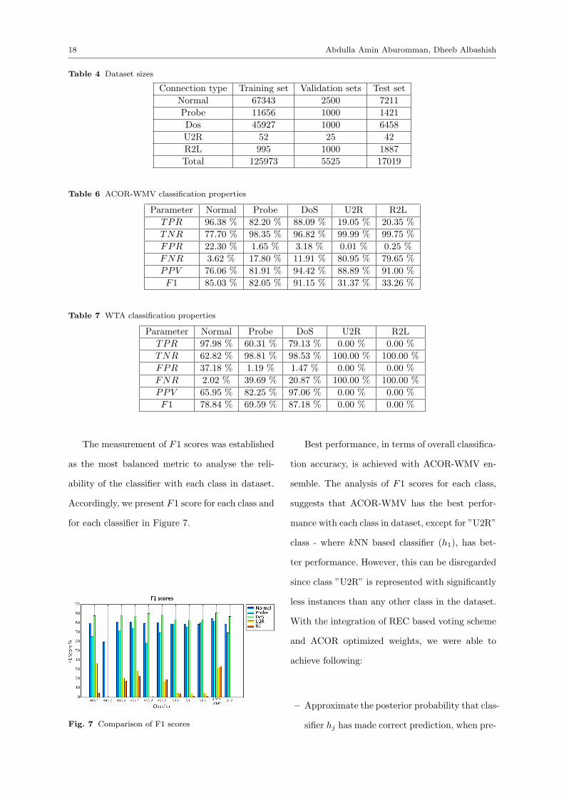
Table 4 Dataset sizes

Connection type Training set Validation sets Test set

Normal 67343 2500 7211

Probe 11656 1000 1421

Dos 45927 1000 6458

U2R 52 25 42

R2L 995 1000 1887

Total 125973 5525 17019

Table 6 ACOR-WMV classification properties

Parameter Normal Probe DoS U2R R2L

TPR 96.38 % 82.20 % 88.09 % 19.05 % 20.35 %

TNR 77.70 % 98.35 % 96.82 % 99.99 % 99.75 %

FPR 22.30 % 1.65 % 3.18 % 0.01 % 0.25 %

FNR 3.62 % 17.80 % 11.91 % 80.95 % 79.65 %

PPV 76.06 % 81.91 % 94.42 % 88.89 % 91.00 %

F1 85.03 % 82.05 % 91.15 % 31.37 % 33.26 %

Table 7 WTA classification properties

Parameter Normal Probe DoS U2R R2L

TPR 97.98 % 60.31 % 79.13 % 0.00 % 0.00 %

TNR 62.82 % 98.81 % 98.53 % 100.00 % 100.00 %

FPR 37.18 % 1.19 % 1.47 % 0.00 % 0.00 %

FNR 2.02 % 39.69 % 20.87 % 100.00 % 100.00 %

PPV 65.95 % 82.25 % 97.06 % 0.00 % 0.00 %

F1 78.84 % 69.59 % 87.18 % 0.00 % 0.00 %

The measurement of F1 scores was established

as the most balanced metric to analyse the reli-

ability of the classifier with each class in dataset.

Accordingly, we present F1 score for each class and

for each classifier in Figure 7.

Fig. 7 Comparison of F1 scores

Best performance, in terms of overall classifica-

tion accuracy, is achieved with ACOR-WMV en-

semble. The analysis of F1 scores for each class,

suggests that ACOR-WMV has the best perfor-

mance with each class in dataset, except for ”U2R”

class - where kNN based classifier (h1), has bet-

ter performance. However, this can be disregarded

since class ”U2R” is represented with significantly

less instances than any other class in the dataset.

With the integration of REC based voting scheme

and ACOR optimized weights, we were able to

achieve following:

– Approximate the posterior probability that clas-

sifier hj has made correct prediction, when pre-


dicting the class r, for j = 1, . . . , l and r =

1, . . . , c.

– Use approximated probabilities as weights in

majority voting procedure to generate an en-

semble classifier.

– Reinforce the decisions of experts only for those

classes where that expert shows proficiency. We

also, simultaneously, diminish the influence of

that experts for classes with which it performs

poorly.

Other ensemble approach, based onWTA strat-

egy, shows exceptionally poor performance. The

unweighted voting procedure is strongly biased to-

ward the classes with more instances in training

dataset. Based on the measurement of running time

of both ensembles and with the consideration of

obtained accuracy, we can establish that ACOR-

WMV approach is by far superior to the WTA

based ensemble.

5 Conclusion and future work

This paper presents a framework for generating an

ensemble of 9 experts for classification of network

traffic for Intrusion Detection System. Each expert

is trained and validated with subsets drawn from

the NSL-KDD set. We present a novel method of

generating weights for Weighted Majority Voting

(WMV) procedure, where we use ACOR optimized

linear coefficients to approximate the class recalls

for each expert in ensemble. The class recall com-

biner (REC) scheme, powered by ACOR weights

presents a viable solution to ensemble classifica-

tion, as shown by the experimental procedure. The

ensemble approach offers an additional advantage

of not being directly trained. In addition we have

also implemented an unweighted version of ensem-

ble, based on Winner Takes All (WTA) strategy.

Test results indicate that the best performance

is achieved with ACOR-WMV ensemble. Although

much faster, the ensemble based on WTA strategy

was not able to combine the decision of its experts

in an effective way. The second best overall accu-

racy was achieved with a classifier based on Artifi-

cial Neural Networks (ANN). However, the ACOR-

WMV shows significantly better results, with an

improvement of 4.4 % in overall classification ac-

curacy. In conclusion, the relatively low compu-

tational cost and high classification accuracy put

forward the WMV based ensemble as the viable

solution to NSL-KDD classification problem.

The logical extension of presented research is

two-folded:

– The implementation of different expert classi-

fiers for the ensemble,

– The implementation of different algorithms for

weight optimizations.

The expansion of expert sub-systems for an

ensemble should further improve the diversity of

the ensemble, and lower the chance of two experts

making the same classification errors. With addi-

tion of other popular single-stage classification al-

gorithms (e.g. Support Vector Machines, Decision

trees, etc.) we may expect an increase in perfor-

mance of the multiple classifier system based on

WMV procedure. Similarly, we may expect some

improvement if we were to substitute the ACOR


algorithm with some other meta-heuristic optimiza-

tion algorithm (e.g. Particle Swarm Optimization,

Genetic Algorithm, Artificial Immune System, etc.).

The modular design of proposed ensemble, will

make these task simpler, with only minimal mod-

ifications to the existing ensemble algorithm.

Compliance with Ethical Standards

The authors have no relevant financial or non-financial

interests to disclose.

The authors have no conflicts of interest to declare that

are relevant to the content of this article.

All authors certify that they have no affiliations with

or involvement in any organization or entity with any

financial interest or non-financial interest in the subject

matter or materials discussed in this manuscript.

The authors have no financial or proprietary interests

in any material discussed in this article.

All authors certify that they have no research involving

human participants and/or animals.

References

1. T. T. Nguyen, A. V. Luong, M. T. Dang, A. W.-

C. Liew, J. McCall, Ensemble selection based on

classifier prediction confidence, Pattern Recognition

100 (2020) 107104.

2. A. A. Aburomman, M. B. I. Reaz, A novel svm-knn-

pso ensemble method for intrusion detection sys-

tem, Applied Soft Computing 38 (2016) 360–372.

3. L. I. Kuncheva, J. J. Rodrıguez, A weighted voting

framework for classifiers ensembles, Knowledge and

Information Systems 38 (2) (2014) 259–275.

4. D. Gupta, R. Rani, Improving malware detection

using big data and ensemble learning, Computers

& Electrical Engineering 86 (2020) 106729.

5. G. Kaur, A comparison of two hybrid ensemble tech-

niques for network anomaly detection in spark dis-

tributed environment, Journal of Information Secu-

rity and Applications 55 (2020) 102601.

6. G. Folino, F. S. Pisani, L. Pontieri, A gp-based en-

semble classification framework for time-changing

streams of intrusion detection data, Soft Comput-

ing (2020) 1–20.

7. M. Sabzevari, G. Martınez-Munoz, A. Suarez, Vote-

boosting ensembles, Pattern Recognition 83 (2018)

119–133.

8. Y. Zhang, G. Cao, B. Wang, X. Li, A novel ensemble

method for k-nearest neighbor, Pattern Recognition

85 (2019) 13–25.

9. B. Krawczyk, M. Galar, M. Wozniak, H. Bustince,

F. Herrera, Dynamic ensemble selection for multi-

class classification with one-class classifiers, Pattern

Recognition 83 (2018) 34–51.

10. A. Kausar, M. Ishtiaq, M. A. Jaffar, A. M. Mirza,

Optimization of ensemble based decision using pso,

in: Proceedings of the World Congress on Engineer-

ing, WCE, Vol. 10, 2010, pp. 671–676.

11. A. Kumar, A. Jaiswal, Particle swarm optimized en-

semble learning for enhanced predictive sentiment

accuracy of tweets, in: Proceedings of ICETIT 2019,

Springer, 2020, pp. 633–646.

12. A. Borji, Combining heterogeneous classifiers for

network intrusion detection, in: Annual Asian Com-

puting Science Conference, Springer, 2007, pp. 254–

260.

13. G. Folino, F. S. Pisani, P. Sabatino, A distributed

intrusion detection framework based on evolved spe-

cialized ensembles of classifiers, in: European Con-

ference on the Applications of Evolutionary Com-

putation, Springer, 2016, pp. 315–331.

14. N. Acosta-Mendoza, A. Morales-Reyes, H. J. Es-

calante, A. Gago-Alonso, Learning to assemble clas-

sifiers via genetic programming, International Jour-

nal of Pattern Recognition and Artificial Intelli-

gence 28 (07) (2014) 1460005.

15. R. S. Michalski, J. G. Carbonell, T. M. Mitchell,

Machine learning: An artificial intelligence ap-

proach, Springer Science & Business Media, 2013.


16. C. M. Bishop, Neural networks for pattern recogni-

tion, Oxford university press, 1995.

17. K. Socha, M. Dorigo, Ant colony optimization for

continuous domains, European journal of opera-

tional research 185 (3) (2008) 1155–1173.

18. M. Tavallaee, E. Bagheri, W. Lu, A.-A. Ghorbani, A

detailed analysis of the kdd cup 99 data set, in: Pro-

ceedings of the Second IEEE Symposium on Com-

putational Intelligence for Security and Defence Ap-

plications 2009, IEEE, 2009, pp. 1–6.

19. https://www.unb.ca/cic/datasets/nsl.html.

Weighted Heterogeneous Ensemble for the Classi cation of ...

Documents

Transcript of Weighted Heterogeneous Ensemble for the Classi cation of ...