Weather Impacts on Maize, Soybean, and Alfalfa Productionin the Great Lakes Region, 1895–1996

Jeffrey A. Andresen,* Gopal Alagarswamy, C. Alan Rotz, Joe T. Ritchie, and Andrew W. LeBaron

ABSTRACT spring freezes (Carter, 1995; Kunkel and Hollinger,1995), and excessive precipitation and flooding duringWeather and climate have had major influences on crop productionthe growing season (Kunkel et al., 1994).in the Upper Great Lakes states of Michigan, Minnesota, and Wiscon-

Analyses of the impact of weather and climate onsin during the past century. However, isolation of the impact ofweather is made difficult by the confounding effects of technological agriculture for extended time periods have been fre-improvements in agriculture, which have resulted in significant grain quently constrained by the lack of quality long-termyield increases. The objective of this study was to identify climatologi- climatological data series and the limited number ofcal impacts involved with the production of three crops commonly experimental treatment combinations available fromgrown in the region—alfalfa (Medicago sativa L.), maize (Zea mays field experiments. In addition, it is difficult to isolateL.), and soybean [Glycine max (L.) Merr.]—without the influence of the impact of weather due to the confounding effectstechnology, and trends of relevant agroclimatological variables during

of technological improvements in agriculture (e.g., im-the period 1895–1996. The models DAFOSYM, CERES-Maize, andproved varieties, increased rates of fertilization), whichSOYGRO models were used to simulate crop growth, development,have resulted in significant yield increases during theand yield of the three crops, respectively. Regionally, low precipitationpast century (Thompson, 1986). An alternative strategyand moisture stress were chief limitations to simulated crop yields.is the use of crop simulation models that are based onSimulated maize and soybean yield series were found to increase with

time an average of 11.4 kg ha�1 yr�1 and 4.9 kg ha�1 yr�1, respectively, the underlying physiological processes governing plantacross the study sites during the study period. These increases were growth and development. Such models, if properly cali-associated with average study period increases in total seasonal precip- brated and tested, allow a user to easily investigate theitation of 0.4 mm yr�1 and decreased total seasonal potential evapo- effects of individual input variables by holding all otherstranspiration of 0.2 mm yr�1. No consistent trends were found for constant and provide a more convenient, less expensivealfalfa. The simulated yield results support previous research identi- tool than long-term field research in the evaluation offying a period of benign climate, which favored crop production in crop response to environmental and management fac-the region from 1954 to 1973, and was preceded and followed by

tors (Angus, 1991). Crop simulation models can also beperiods of relatively greater yield variability.used to investigate multiple factors and their interac-tions at various hierarchical levels, including farm, re-gional, and national scales.Agriculture ranks among the most important eco-

Using crop simulation models, this research was con-nomic activities of the Upper Great Lakes statesducted to study the impact of weather and climate onof Michigan, Minnesota, and Wisconsin, accounting fortypical crops grown in the Great Lakes region for anmore than $15 billion in annual cash receipts (USDA-extended, 102-yr time period without the influence ofNASS, 1997). Weather remains among the most impor-technological improvements. Three crops commonlytant uncontrollable elements involved in regional cropgrown in the region were chosen for the study—alfalfa,production. The role of growing season precipitationmaize, and soybean—which were simulated with theand associated availability of soil moisture is of particu-Dairy Forage System DAFOSYM (Rotz et al., 1989),lar importance, and has been the subject of much previ-CERES-Maize, and SOYGRO crop models, respec-ous research. In general, rainfed crops in the regiontively. The latter two models are part of the Decisionrespond negatively to below normal precipitation totalsSupport (DSSAT) model software system (Tsuji et al.,and the lack of plant-available water during the growing1994). Nearly all nonclimatic input variables in the simu-season (Thompson, 1986; Brown and Rosenberg, 1997;lations were held constant so as to isolate the effects ofMorey et al., 1980; Larson and Clegg, 1999), especiallyweather, which was described collectively by air tem-during moisture-sensitive phenological stages (Nesmithperature, precipitation, solar irradiance, and model-and Ritchie, 1992; Sionit and Cramer, 1977; Andresenderived variables such as evapotranspiration and sea-et al., 1989; Brown and Tanner, 1983). Other majorsonal change in soil water content.meteorological constraints to crop production identified

Specific objectives were: (i) the creation of time seriesby past studies include heat stress due to high air tem-of crop yield and agroclimatological variables associatedperatures (Carlson, 1990), lack of warmth and limitedwith yield to serve as benchmark series for comparisonlength of the growing season (Lauer et al., 1999), latewith any future changes in climate; and (ii) determina-tion of any trends in the time series developed in (i)

J.A. Andresen and A.W. LeBaron, Dep. of Geography, Natural Sci- during the study period. Particular attention was givenence Bldg., Michigan State Univ., East Lansing, MI 48824-1115; G.to the time period between the mid-1950s and mid-Alagarswamy and J.T. Ritchie, Dep. of Crop and Soil Sciences, Michi-1970s, which has been identified by previous researchersgan State Univ., East Lansing, MI 48824; and C.A. Rotz, Bldg. 3702,

Curtin Road, Pasture Systems & Watershed Management Res., Uni- as a period of lesser climatic variability, and to areasversity Park, PA 16802. Received 2 Aug. 2000. *Corresponding author within the region where agricultural activities histori-(andresen@msu.edu).

Abbreviations: DOY, day of year; DUL, drained upper limit.Published in Agron. J. 93:1059–1070 (2001).

1059

1060 AGRONOMY JOURNAL, VOL. 93, SEPTEMBER–OCTOBER 2001

(Genesee), Madison, WI (Dane), Rochester, MN (Olmsted),cally have been limited by climatological and soil con-Sioux Falls, SD (Minnehaha), and South Bend, IN (St. Joseph)straints, but which could become more favorable forwere used for both maize and soybean simulation tests.agriculture in the future given a warmer climate.

Because of significant upward trends in the measured yieldsduring the 1961–1990 period due to improvements in technol-MATERIALS AND METHODSogy and other factors (e.g., Thompson, 1969; Garcia et al.,

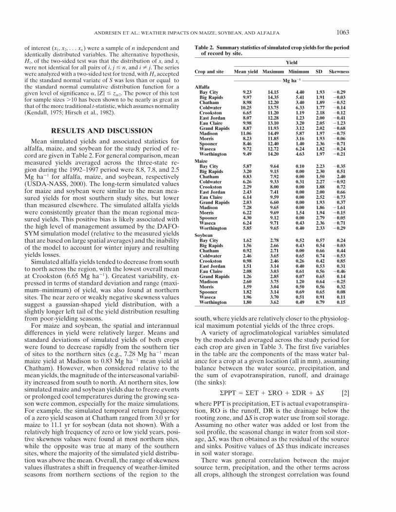
The crop simulation models selected for use in this study 1987), the simulated and measured yield series were not di-were chosen at least partially on the basis of previous tests rectly comparable, because the simulated series were derivedfor reasonable and satisfactory performance in a number of assuming constant levels of technology. As a result, the mea-locations and under varying circumstances (e.g., Hodges et sured county-level yield time series data were first statisticallyal., 1987; Kiniry et al., 1997; Martin et al., 1996; Colson et al., detrended with linear or nonlinear (simple polynomial equa-1995; Piper et al., 1996). As a preliminary test for the study, tions) regressions using the TableCurve 3D software packagesimulated yields obtained from the selected models using an (SPSS, 1997). Measured residual series were then calculatedindependent five-station set of daily measured weather data as the difference of measured and detrended yields each year.were compared with measured county-level yields for the pe- For the simulated yield series, the residuals were defined asriod 1961–1990 (USDA-NASS, 2000). Stations (counties) used the simulated yield minus the mean simulated yield over thefor the alfalfa test simulations were Green Bay, WI (Brown), validation period (1961–1990). Example time series of simu-Madison, WI (Dane), Rochester, MN (Olmsted), South Bend, lated vs. measured yields residuals for alfalfa, maize, and soy-

bean at St. Cloud, MN, South Bend, IN, and Rochester, MN,IN (St. Joseph), and St. Cloud, MN (Stearns), while Flint, MI

Fig. 1. Simulated vs. measured yield residuals of (a) alfalfa at St. Cloud, MN; (b) maize at South Bend, IN; and (c) soybean at Rochester, MN,1961–1990. Residuals were determined on the basis of period means (simulated) or time-detrended (measured) series.

ANDRESEN ET AL.: WEATHER IMPACTS ON MAIZE, SOYBEAN, AND ALFALFA 1061

are given in Fig. 1. For the 15 crop/site combinations, general during the period of 1895–1996. Thirteen locations across theregion (five in Michigan, five in Minnesota, and three in Wis-overall agreement was found in comparisons of the measured

and simulated residuals. Mean absolute differences between consin) were selected for analysis on the basis of availableclimatological data series quality, record length, and homoge-simulated and measured residuals ranged from 0.41 to 0.72,

0.48 to 0.65, and 0.16 to 0.26 Mg ha�1 for alfalfa, maize, and neity for the period 1895–1996. The sites were also chosen onthe basis of representative geographical coverage of the re-soybean crops, respectively, which were not significantly dif-

ferent in test period means of paired t-tests (P � 0.05) across gion, including all major land resource areas (MLRA), whichdescribe common soils, vegetation, and other natural resourceall three crops and all five sites. In only 1 of the 15 crop–site

combinations (alfalfa at Sioux Falls) was there a significant characteristics (USDA-SCS, 1981). Site locations and MLRAswithin the region are given in Fig. 2. Three of the study loca-difference in the yield residual variance using an F-test (P �

0.05). In general, the model-simulated yield variances were tions were specifically chosen from northern, historically non-agricultural areas, to investigate the contrast in agronomiclarger than measured, which is expected since the measured

series are spatial averages of smaller scale yields within a potential found from south to north across the region.Daily series of precipitation and maximum and minimumcounty and the model simulations, by definition, are single

point, plot-level estimates. air temperatures for each study site were obtained from theNOAA Summary of the Day (NOAA-NCDC, 1895–1996).In a separate test of model validity, a t-test was used to

determine whether or not the slope coefficients of linear re- The individual lengths of the data series ranged from 68 to102 yr and all but four of the series began in the 1895–1900gression between measured vs. simulated residuals at each

crop–site combination was significantly different from 0 (i.e., period. Missing air temperature and precipitation data withinthe period of record were estimated by spatial interpolation�1 � 0 or �1 � 0). In all crop–site combinations, the null

hypothesis (�1 � 0) was rejected (P � 0.05), indicating a of data from neighboring stations and were provided by theMidwest Regional Climate Center in Champaign, IL (K. Kun-linear relationship between the simulated and measured yield

residuals. Overall, the models appeared to account for the kel, personal communication, 1998). Daily solar irradiancedata for the entire study period were synthetically generatedmajority of observed negative and positive deviations from

mean yields, and were therefore judged to be acceptable for on the basis of the measured precipitation and air temperaturedata with the Weather Generator (WGEN) methodology ofuse in this study.

Historical simulations for all three crops were performed Richardson and Wright (1984). Soils data used in the simula-

Fig. 2. Study site locations and Major Land Resource Areas (from USDA-SCS, 1981) within the Upper Great Lakes region.

1062 AGRONOMY JOURNAL, VOL. 93, SEPTEMBER–OCTOBER 2001

Table 1. Site locations, climatological record lengths, and soil profile information used in the study.

Site Lat. Long. Climatological record length Soil series Textural class Profile depth PEW† in profile

yr cm mmBay City, MI 43� 37� 83� 52� 101 Tappan Loam 192 240Big Rapids, MI 43� 42� 85� 29� 101 Remus Sandy loam 158 196Chatham, MI 46� 20� 86� 55� 96 Emmet Sandy loam 150 179Coldwater, MI 41� 57� 85� 00� 100 Locke Sandy loam 173 217Crookston, MN 47� 48� 96� 37� 102 Fargo Silty clay 120 158East Jordan, MI 45� 09� 85� 08� 68 Onaway Sandy loam 107 134Eau Claire, WI 44� 52� 91� 29� 101 Seaton Silt loam 116 164Grand Rapids, MN 47� 14� 93� 30� 82 Hamerly Loam 120 149Madison, WI 43� 08� 89� 20� 101 Dodge Silt loam 213 273Morris, MN 45� 35� 95� 53� 102 Webster Silty clay loam 116 189Spooner, WI 45� 49� 91� 53� 102 Santiago Silt loam 120 149Waseca, MN 44� 04� 93� 31� 82 Webster Silty clay loam 122 153Worthington, MN 43� 39� 95� 35� 102 Webster Silty clay loam 122 153

† PEW, plant extractable water.

tions were based on profile data typical of agricultural soils (DOY) 122] for maize and DOY 137 for soybean. For allalfalfa simulations, a first-year crop stand was assumed. Maizein the vicinity of each location in the study and were obtained

from laboratory pedon data available at the National Soil and soybean were harvested each season at physiological ma-turity (or following abnormal termination of growth due toSurvey Center (USDA-NRCS-NSSC, 1999). Daily estimates

of potential evapotranspiration, actual evapotranspiration, soil freezing air temperatures). Alfalfa was harvested with fourseasonal cuts taken at the seven southernmost stations andwater evaporation, and plant-available water were obtained

from the crop simulation model output. These water balance- three seasonal cuts taken at the remaining six northern stationsdepending on weather conditions. For the three cut harvestrelated variable estimates are based on the original work of

Ritchie (1972) and Priestley and Taylor (1972), and are depen- system, the first cut was set for DOY 166, followed by secondand third cuts on DOY 198 and 233, respectively. For the fourdent on daily air temperatures, solar irradiance, leaf area of

the crop, and existing soil moisture content (Rotz et al., 1989; cut system, the first cut was set at DOY 152, followed bysecond, third, and fourth cuts on DOY 191, 232, and 292, re-Jones and Kiniry, 1986; Wilkerson et al., 1985). A summary

of station locations, climatic periods of record, and basic soil spectively.Model simulations for all three crops were run indepen-profile information is given in Table 1.

Mean air temperature and total precipitation averaged for dently in chronological order for each location and scenario.There were no carryover effects from one growing season tothe period of record for the April–October months provide

an approximate range of growing season climatological condi- a subsequent season. Soil water in the models initialized eachseason at the drained upper limit (DUL) or field capacity ontions across the region. Mean air temperatures generally de-

crease from south to north across the area, from a maximum 1 March for DAFOSYM and on 1 April for CERES-Maizeand SOYGRO. Daily output from each of the models, includ-of 17.7�C at Morris to a minimum of 14.7�C at Chatham. The

pattern of seasonal precipitation totals is more complex, with ing estimates of potential evapotranspiration, actual evapo-transpiration, surface runoff, drainage out of the root zone,greatest values in central sections of the region (e.g., Eau

Claire, 613 mm; Waseca, 593 mm), decreasing toward both and soil water content, were saved and archived on a dailybasis, with growing season statistics calculated in a secondarythe east (Bay City, 476 mm) and west (Crookston, 416 mm).

The spatial patterns of both variables are in relative agreement processing step. For statistical summation and averaging pur-poses, the growing season for maize and soybean was definedwith published climatological normals for the summer season

(Reinke et al., 1993). as the date of planting through physiological maturity or termi-nation of growth due to freezing or persistently cold tempera-To isolate the effects of weather and climate on crop perfor-

mance, soil fertility levels in all simulations were assumed tures. For alfalfa, the growing season was defined as the periodfrom 1 March through 31 October. Decreases in alfalfa yieldsto be nonlimiting for crop growth and development. Other

agronomic input data necessary for the crop simulations (e.g., due to winter injury, a potentially important climatologicallimiting factor (Sharratt et al., 1986), were not explicitly ac-crop cultivar characteristics, plant populations) were chosen to

reflect typical current (i.e., late 1990s) technology and growing counted for by the version of DAFOSYM used in the study.conditions. Plant populations were set at 6 and 20 plants m�2

for maize and soybean crops. The alfalfa model does not have Trend Statisticsa plant population input. Crop cultivar characteristics were

To determine the nature of changes in the variables studied,selected to reflect the climatological conditions across theestimates of both trend magnitude and significance were calcu-region. For maize, a short-season cultivar adapted for use inlated. Trend magnitude was obtained with the method of Senthe Great Lakes region was used. The base 8�C thermal time(1968). A nonparametric statistic was selected due to the lackrequired for the juvenile phenological stages of the maizeof normality for some of the variables analyzed, especiallyhybrid (P1 variable) was 200, while the thermal time fromthose involving precipitation. The trend magnitude statisticsilking to maturity (P2 variable) was 685. For soybean, a ge-(B), a nonparametric analogue of the least squares derivedneric Group 2 maturity group was used in southern sectionsslope parameter estimate, is defined as:of the region, while generic Group 1 and Group 0 maturity

groups were used in central and northern sections, respec- B � med {Dij} [1]tively. Cultivar characteristics are not a user-specified input

where Dij � (xj � xi )/( j � i) for all possible pairs (xi, xj ), 1 �in the DAFOSYM alfalfa simulation.i � j � n, and n the number of observations in the series.Planting dates of both maize and soybean crops were deter-The nonparametric Mann-Kendall or Kendall’s tau statisticmined automatically by the models each season on the first(Kendall, 1975) was used to determine the significance of theday meeting user-specified weather and soil conditions (simu-

lated 5 cm soil temperature �10�C) after 1 May [day of year trends. The null hypothesis, Ho, was that the data in the series

ANDRESEN ET AL.: WEATHER IMPACTS ON MAIZE, SOYBEAN, AND ALFALFA 1063

Table 2. Summary statistics of simulated crop yields for the periodof interest (x1, x2, . . . xn ) were a sample of n independent andof record by site.identically distributed variables. The alternative hypothesis,

H1, of the two-sided test was that the distribution of xi and xj Yieldwere not identical for all pairs of i, j � n, and i � j. The series

Crop and site Mean yield Maximum Minimum SD Skewnesswere analyzed with a two-sided test for trend, with Ho acceptedMg ha�1if the standard normal variate of S was less than or equal to

Alfalfathe standard normal cumulative distribution function for aBay City 9.23 14.15 4.40 1.93 �0.29given level of significance �, |Z| � z�/2. The power of this testBig Rapids 9.97 14.35 5.41 1.91 �0.03for sample sizes 10 has been shown to be nearly as great as Chatham 8.98 12.20 3.40 1.89 �0.52

that of the more traditional t-statistic, which assumes normality Coldwater 10.25 13.75 6.33 1.77 �0.14Crookston 6.65 11.20 1.19 2.18 �0.12(Kendall, 1975; Hirsch et al., 1982).East Jordan 8.07 12.28 1.23 2.00 �0.41Eau Claire 9.98 13.10 3.20 2.05 �1.23Grand Rapids 8.87 11.93 3.12 2.02 �0.68RESULTS AND DISCUSSION Madison 11.06 14.49 5.87 1.97 �0.75Morris 8.23 11.85 3.16 1.93 �0.06Mean simulated yields and associated statistics for Spooner 8.46 12.40 1.40 2.36 �0.71Waseca 9.72 12.72 6.24 1.82 �0.24alfalfa, maize, and soybean for the study period of re-Worthington 9.49 14.20 4.63 1.97 �0.21cord are given in Table 2. For general comparison, mean

Maizemeasured yields averaged across the three-state re-Bay City 5.87 9.64 0.10 2.23 �0.35

gion during the 1992–1997 period were 8.8, 7.8, and 2.5 Big Rapids 3.20 9.15 0.00 2.30 0.51Chatham 0.83 7.92 0.00 1.50 2.40Mg ha�1 for alfalfa, maize, and soybean, respectivelyColdwater 6.26 9.33 0.31 2.27 �0.92(USDA-NASS, 2000). The long-term simulated values Crookston 2.29 8.00 0.00 1.88 0.72

for maize and soybean were similar to the mean mea- East Jordan 2.43 7.41 0.00 2.00 0.66Eau Claire 6.14 9.59 0.00 2.52 �0.73sured yields for most southern study sites, but lowerGrand Rapids 2.03 6.60 0.00 1.93 0.37than measured elsewhere. The simulated alfalfa yields Madison 7.28 9.65 0.00 1.86 �1.61Morris 6.22 9.69 1.54 1.94 �0.15were consistently greater than the mean regional mea-Spooner 4.30 9.12 0.00 2.79 �0.05sured yields. This positive bias is likely associated withWaseca 6.24 9.71 0.43 2.36 �0.71

the high level of management assumed by the DAFO- Worthington 5.85 9.65 0.40 2.33 �0.29SYM simulation model (relative to the measured yields Soybean

Bay City 1.62 2.78 0.52 0.57 0.24that are based on large spatial averages) and the inabilityBig Rapids 1.56 2.66 0.43 0.54 �0.03of the model to account for winter injury and resulting Chatham 0.92 2.71 0.00 0.66 0.44

yields losses. Coldwater 2.46 3.65 0.65 0.74 �0.53Crookston 0.98 2.46 0.26 0.42 0.85Simulated alfalfa yields tended to decrease from southEast Jordan 1.51 3.14 0.40 0.53 0.31to north across the region, with the lowest overall mean Eau Claire 2.08 3.03 0.61 0.56 �0.46Grand Rapids 1.26 2.85 0.07 0.65 0.14at Crookston (6.65 Mg ha�1 ). Greatest variability, ex-Madison 2.60 3.75 1.20 0.64 �0.25pressed in terms of standard deviation and range (maxi-Morris 1.59 3.04 0.50 0.56 0.32

mum–minimum) of yield, was also found at northern Spooner 1.82 3.14 0.69 0.65 0.08Waseca 1.96 3.70 0.51 0.91 0.11sites. The near zero or weakly negative skewness valuesWorthington 1.80 3.62 0.49 0.79 0.15suggest a gaussian-shaped yield distribution, with a

slightly longer left tail of the yield distribution resultingfrom poor-yielding seasons. south, where yields are relatively closer to the physiolog-

ical maximum potential yields of the three crops.For maize and soybean, the spatial and interannualdifferences in yield were relatively larger. Means and A variety of agroclimatological variables simulated

by the models and averaged across the study period forstandard deviations of simulated yields of both cropswere found to decrease rapidly from the southern tier each crop are given in Table 3. The first five variables

in the table are the components of the mass water bal-of sites to the northern sites (e.g., 7.28 Mg ha�1 meanmaize yield at Madison to 0.83 Mg ha�1 mean yield at ance for a crop at a given location (all in mm), assuming

balance between the water source, precipitation, andChatham). However, when considered relative to themean yields, the magnitude of the interseasonal variabil- the sum of evapotranspiration, runoff, and drainage

(the sinks):ity increased from south to north. At northern sites, lowsimulated maize and soybean yields due to freeze events

RPPT � RET RRO RDR �S [2]or prolonged cool temperatures during the growing sea-son were common, especially for the maize simulations. where PPT is precipitation, ET is actual evapotranspira-

tion, RO is the runoff, DR is the drainage below theFor example, the simulated temporal return frequencyof a zero yield season at Chatham ranged from 3.0 yr for rooting zone, and �S is crop water use from soil storage.

Assuming no other water was added or lost from themaize to 11.1 yr for soybean (data not shown). With arelatively high frequency of zero or low yield years, posi- soil profile, the seasonal change in water from soil stor-

age, �S, was then obtained as the residual of the sourcetive skewness values were found at most northern sites,while the opposite was true at many of the southern and sinks. Positive values of �S thus indicate increases

in soil water storage.sites, where the majority of the simulated yield distribu-tion was above the mean. Overall, the range of skewness There was general correlation between the major

source term, precipitation, and the other terms acrossvalues illustrates a shift in frequency of weather-limitedseasons from northern sections of the region to the all crops, although the strongest correlation was found

1064 AGRONOMY JOURNAL, VOL. 93, SEPTEMBER–OCTOBER 2001

Table 3. Mean simulated crop water balance and other agroclimatological variables† for the period of record by site.

Crop and site �Precip. �ET �Runoff �Drainage �S �PET �ET/PET Yield

mm Mg ha�1

AlfalfaBay City 476.4 489.6 46.3 31.8 �91.2 867.9 116.8 9.23Big Rapids 508.7 519.9 64.1 28.1 �103.3 852.9 122.5 9.97Chatham 521.8 468.5 19.8 66.4 �33.6 778.1 128.2 8.98Coldwater 563.1 524.1 57.4 46.7 �65.1 866.2 125.7 9.97Crookston 416.5 388.9 29.9 18.7 �21.1 860.8 103.9 6.66East Jordan 498.8 492.0 38.7 26.6 �57.0 849.5 118.6 8.07Eau Claire 612.3 565.2 43.9 47.9 �44.7 862.1 139.4 9.98Grand Rapids 509.0 465.5 38.0 45.5 �36.9 801.8 120.2 8.87Madison 553.2 547.9 15.2 60.5 �70.3 852.6 136.1 11.06Morris 486.1 470.8 67.8 34.5 �87.0 874.8 107.1 8.23Spooner 551.2 486.6 33.5 45.5 �14.3 833.7 129.6 8.46Waseca 592.6 520.3 92.5 60.9 �81.1 881.3 119.7 9.73Worthington 556.1 501.3 80.9 43.3 �78.2 877.3 116.9 9.49

MaizeBay City 320.6 410.3 47.7 7.4 �144.8 644.2 87.1 5.87Big Rapids 332.9 367.6 56.7 16.6 �108.0 642.9 79.9 3.20Chatham 297.5 299.2 21.1 31.5 �54.3 488.7 68.3 0.83Coldwater 367.4 429.3 51.9 20.6 �134.5 628.5 90.6 6.26Crookston 283.8 362.5 57.8 6.0 �142.5 584.3 74.4 2.29East Jordan 318.9 344.8 34.3 16.9 �77.1 603.2 76.8 2.43Eau Claire 423.8 444.9 64.3 30.2 �115.6 630.2 94.0 6.14Grand Rapids 331.7 372.8 48.0 20.9 �110.0 542.5 80.7 2.03Madison 384.2 454.7 25.3 36.5 �132.2 630.1 97.4 7.28Morris 354.7 457.6 35.6 21.9 �160.3 654.0 94.9 6.22Spooner 372.6 389.0 50.7 26.6 �93.7 565.3 82.9 4.30Waseca 415.2 447.4 81.6 14.1 �127.9 636.2 91.9 6.24Worthington 389.7 440.2 68.2 15.3 �134.0 639.0 90.4 5.85

SoybeanBay City 271.5 334.8 41.9 7.0 �112.3 568.4 71.3 1.62Big Rapids 301.5 331.8 56.5 13.9 �100.7 580.8 74.0 1.56Chatham 326.9 311.5 23.2 35.3 �43.1 513.3 76.9 0.92Coldwater 359.2 410.6 53.8 19.8 �125.0 606.4 89.5 2.46Crookston 269.2 307.8 55.2 6.5 �100.4 565.0 66.3 0.98East Jordan 307.4 326.7 33.3 16.8 �69.4 577.5 73.0 1.51Eau Claire 372.7 381.3 57.9 31.8 �98.3 571.9 78.2 2.08Grand Rapids 327.4 345.7 48.7 22.9 �89.9 518.0 81.3 1.26Madison 381.2 422.0 26.5 41.3 �108.6 608.4 94.4 2.60Morris 319.7 365.8 32.9 27.5 �106.4 603.8 73.8 1.59Spooner 378.2 377.2 52.8 31.4 �83.2 579.6 81.2 1.82Waseca 419.6 426.7 85.9 16.2 �109.1 631.6 93.0 1.96Worthington 389.6 416.7 72.8 17.0 �116.8 630.9 89.7 1.80

† ET, evapotranspiration; �S, change in soil water storage; PET, potential evapotranspiration.

Fig. 3. Scatterplot of simulated daily ET/PET summed from planting to maturity vs. soybean yields, Coldwater, 1897–1996.

ANDRESEN ET AL.: WEATHER IMPACTS ON MAIZE, SOYBEAN, AND ALFALFA 1065

with the �ET term. The �PPT and �ET were largest season. Both variables tended to decrease from south-western sites in the region toward the northeast forfor the alfalfa crop, followed by maize and soybean.

This is primarily a result of the longer growing season all crops.A strong correlation between precipitation, waterfor alfalfa (198 d for alfalfa vs. a general range of

110–130 d for maize). The seasonal runoff (�RO) term stress, and interannual crop yields that has been identi-fied by many previous researchers, was also found in thiswas very similar across the crops, with small differences

due to differing soil characteristics. Total mean seasonal study. In Fig. 3, a scatterplot of simulated �ET/PET vs.simulated yields for soybean for the 1897–1996 perioddrainage (�DR) for maize and soybean was similar, but

less than that of alfalfa with the longer growing season. of record at Coldwater demonstrates this association.However, the strength of the correlation between yieldThe change in soil water storage term, �S, tended to

be largest for maize and least for alfalfa, which in turn and �ET/PET (and other precipitation-related variables)for all crops was found to decrease from south to northwas related to rates of ET during the growing season.

For example, simulated daily ET rates during the month across the region. This is in agreement with the resultsof Kunkel and Hollinger (1991), who utilized CERES-of July at Madison averaged 5.0 mm for maize vs. 4.8

and 3.2 mm for soybean and alfalfa, respectively (data Maize and SOYGRO models to simulate regional-scalecrop growth and yield in the Midwestern USA.not shown). Soil water storage was an important fraction

of ET on a seasonal basis, contributing 12, 29, and 26% Of the nonwater-related agroclimatological variablesinvestigated for association with simulated crop yields,of the total seasonal ET for alfalfa, maize, and soy-

bean, respectively. highest correlations were found with growing season airtemperatures and thermal time. The regional changesBesides the water balance components and crop

yields, other variables included in Table 3 are potential between maize yield and these variables is illustratedin Fig. 4, in which the coefficient of determination (r 2 )evapotranspiration summed during the growing season,

�PET, and the summed daily ratio of actual to potential values resulting from regressions of yield and �ET/PET(top number) and yield and seasonally summed thermalevapotranspiration, �ET/PET, which serves as a proxy

for accumulated moisture stress during the growing sea- time, base 8�C (bottom number) are plotted at eachstudy site. The r 2 values for �ET/PET and yield de-son and has been previously shown to be highly posi-

tively correlated with crop yields (Andresen et al., 1989). creased from �0.56 to 0.68 along the southern tier ofsites to 0.27 to 0.43 along the northern tier of stations,Both seasonal �ET and �PET values simulated by the

models were within the range of those observed in previ- whereas r 2 values for the growing degree days vs. yieldregressions increased from 0.06 to 0.27 to 0.28 to 0.59ous field studies (e.g., Brown and Tanner, 1983; Hat-

tendorf et al., 1988; Rhoads and Bennet, 1990; Reicosky in the same direction.As a further illustration of differing patterns withinand Hetherly, 1990). Similar to the water balance vari-

ables, largest �ET and �PET values were found to be the region, a comparison of several simulated variablesaveraged for the five highest yielding years in the periodlargest for the alfalfa crop due to its relatively longer

Fig. 4. Coefficients of determination (r 2 ) for seasonally accumulated ET/PET vs. yield (top number) and seasonally accumulated thermal time(base 8�C) vs. yield (bottom number) for maize at each site for the period of record.

1066 AGRONOMY JOURNAL, VOL. 93, SEPTEMBER–OCTOBER 2001

Fig. 5. Comparison of agroclimatological variables for maize averaged for years with highest five yields at Chatham, Eau Claire, and Madisonvs. the same variables averaged for period of record.

Historical Trendsof record (POR) vs. the same variables averaged for allyears in the POR is given in Fig. 5 for maize at Chatham, Several trends were identified in the historical clima-Eau Claire, and Madison. The greatest yields in this tological data and from agroclimatological output vari-north–south transect across the region are all associated ables derived from the model simulations. Trend statis-with relatively higher precipitation and other water- tics for several variables summarized by crop and siterelated variables. For example, �PPT and �ET/PET at are given in Table 4, while representative time seriesMadison are 33 and 21% greater for the highest yielding for selected variables obtained in maize simulations forgroup than for the POR means. In contrast, mean grow- Worthington are given in Fig. 6. Across the study period,ing season air temperature for the high-yielding mean the sign of the trend statistic was positive for no lessvaries from 5% less than the POR means at Madison than 11 of the 13 site–crop combinations for seasonalto 3 and 8% greater than POR means at Eau Claire precipitation, suggesting increases during the study pe-and Chatham, respectively. These results suggest a shift riod. However, the increases were statistically signifi-of the primary climatological constraint for annual crops cant at only one or two locations, depending on crop.from moisture stress in southern sections of the region Further inspection of the precipitation time series datato the amount of accumulated heat, and, by association, indicated a steady or slightly decreasing trend of precipi-

tation with time from the beginning of the study periodthe length of growing season across northern sections.

ANDRESEN ET AL.: WEATHER IMPACTS ON MAIZE, SOYBEAN, AND ALFALFA 1067

Table 4. Trend statistics (yr�1 ) for simulated agroclimatological variables† for the period of record by site and crop.

Yield �PPT �ES �EP �PET PEWt �S WUE �ET/PET

kg ha�1 mm kg ha�1 mm�1

AlfalfaBay City �2.445 0.379 0.000 �0.140 �0.197 0.249* 0.557* 0.000 0.020Big Rapids �4.353 0.500 �0.031 �0.286 �0.176 �0.100 0.364 0.001 0.030Chatham 3.337 0.519 0.000 0.277 0.200 �0.138 0.064 0.000 0.027Coldwater 0.004 0.075 �0.012 �0.233 �0.630* 0.027 0.306 0.010 0.055Crookston �7.149 �0.224 0.027 �0.420 �0.128 �0.037 0.304 0.004 �0.054East Jordan �11.119 0.364 0.000 �0.346 �0.452* �0.267 0.582 �0.008 0.026Eau Claire �7.141 �0.222 0.050 �0.469 �0.405** �0.179 0.399 0.001 0.001Gr. Rapids 25.033* 1.645** 0.094** 1.077* 0.063 0.085 �0.023 0.020* 0.207*Madison �5.527 0.234 0.000 �0.070 0.000 �0.047 0.063 �0.010 �0.009Morris 5.778 0.075 �0.045 0.000 �0.417* 0.167 0.029 0.009 0.036Spooner �7.691 0.511 0.084* �0.148 �0.284* �0.025 0.205 �0.015 0.057Waseca 16.672 1.510* �0.027 0.500 �0.735*** 0.231* 0.127 0.014 0.211*Worthington 1.859 0.056 0.113* 0.100 �0.592*** 0.048 �0.025 0.000 0.114

MaizeBay City 4.000 0.058 0.040 0.027 �0.098 �0.060 0.056 0.011 0.041Big Rapids �2.216 0.313 �0.025 �0.068 �0.008 0.000 0.208* �0.004 �0.001Chatham 1.000*** 1.322** 0.264 0.716*** 0.955*** �0.143 �0.906** 0.003*** 0.308***Coldwater 8.076 0.295 0.162 �0.005 �0.002 0.149 0.186 0.015 0.137*Crookston 6.900 �0.222 �0.153 0.013 �0.186 0.022 0.047 0.025 �0.001East Jordan �3.088 0.125 �0.134 0.134 �0.567* 0.053 0.110 �0.010 0.046Eau Claire 14.214 0.354 0.051 0.251 0.032 0.091 0.117 0.019 0.146*Gr. Rapids 33.192*** 2.632*** 0.717* 0.825*** 0.961*** 0.196 �0.134 0.080*** 0.453***Madison 2.000 0.444 �0.081 0.074 �0.019 0.129 0.287 0.005 0.032Morris 15.128* 0.000 �0.103 0.205* �0.140 0.059 0.067 0.031** 0.077Spooner 21.770* 0.838 0.251 0.283 0.091 0.235 0.268 0.032 0.168*Waseca 28.790** 1.500** 0.244 0.614*** 0.210 0.409* 0.101 0.037* 0.294**Worthington 18.718* 0.065 0.189 0.167 �0.384*** 0.214* 0.080 0.031* 0.174**

SoybeanBay City 0.853 0.020 0.077 �0.081 �0.187** 0.052 0.134 0.002 0.010Big Rapids 1.263 0.500 �0.015 �0.029 �0.117 �0.026 0.225* 0.005 0.051Chatham 9.188* 0.722 0.222* 0.256* 0.126 0.235* 0.032 0.024** 0.190***Coldwater 1.783 0.066 0.022 0.007 �0.326*** 0.167 0.236* 0.007 0.079*Crookston 0.821 �0.053 �0.043 0.004 �0.165* 0.068 0.289 0.002 �0.003East Jordan 2.744 0.245 �0.038 0.058 �0.453*** 0.188 0.185 0.008 0.105Eau Claire 4.543* 0.227 0.130 0.107 �0.133* 0.000 0.233* 0.009* 0.084*Gr. Rapids 9.652* 1.881*** 0.484* 0.206* 0.090 0.250* 0.308* 0.020* 0.224***Madison 4.944* 0.465 �0.195* 0.385*** 0.047 0.185* 0.079 0.010* 0.080*Morris 2.000 0.117 �0.001 �0.041 �0.147** 0.099 0.130 0.005 0.046Spooner 5.406* 0.443 0.181 0.036 �0.250*** 0.131 0.252* 0.012* 0.058Waseca 15.069* 1.286* �0.096 0.539** �0.373** 0.479* 0.294 0.032*** 0.193**Worthington 6.390* �0.235 0.023 0.160 �0.564*** 0.167 0.164 0.014* 0.126**

* Significant at the 0.05 level.** Significant at the 0.01 level.*** Significant at the 0.001 level.† PPT, precipitation; ES, soil evaporation; EP, transpiration; PET, potential evapotranspiration; PEWt, plant extractable water at first cut, silk, and first

pod stages for alfalfa, maize, and soybean crops, respectively; �S, change in soil water storage; WUE, water use efficiency defined as the ratio of yieldand total ET (kg ha�1 mm�1 ).

followed by statistically significant increases in precipi- northern study locations, where increases in growingseason length were also noted.tation from approximately the late 1930s through the

end of the study period at the majority of the sites Alfalfa yield trends over the period of record weremuch less well-defined than for the spring-planted an-(data not shown). These increases are in agreement with

larger regional scale trends (Karl et al., 1994) and are nual crops, with negative test statistic values at sevenlocations (one of which was significant) and positiveat least partially due to greater frequency of wet days

and wet days that follow wet days (Andresen, unpub- values at six locations during the period of record.Closer inspection of the individual yield series at eachlished data, 1999). Similarly, increases in simulated soil

moisture available to the plant at midseason, a key vari- site indicated that yields at 10 of the sites have increasedduring the past 40 to 60 yr, but similar to precipitation,able in determining ultimate yield potential, were also

found for maize (2 of 13 locations with significant in- the increases were partially or totally offset by decreasesin yields during the first few decades of the study pe-creases) and soybean (4 of 13 locations with significant

increases). In contrast, significant decreases in simulated riod, resulting in the mixed period of record trends (datanot shown).potential ET were found at 7, 4, and 9 of the 13 locations

for alfalfa, maize, and soybean crops, respectively. As Among the most important of the trends agronomi-cally are decreases in potential ET, which were statisti-a result of the trends toward wetter, less stressful condi-

tions, there were significant increases in both maize cally significant at 7, 4, and 9 of the 13 sites for alfalfa,maize, and soybean crops, respectively. Since potential(positive trends at 6 out of 13 locations) and soybean

(positive trends at 7 of 13 locations) yields across much ET estimates from the models are based primarily onthe Priestley-Taylor (1972) methodology, which is inof the region. Overall, greatest increases in simulated

yields for all crops with time were found at western and turn largely dependent on net radiation, this decrease

1068 AGRONOMY JOURNAL, VOL. 93, SEPTEMBER–OCTOBER 2001

Fig. 6. Time series of several variables for maize simulations at Worthington, 1895–1996. The bold line denotes a 9-yr moving average. PETdenotes potential evapotranspiration, ET evapotranspiration, �S change in soil water storage, and WUE water use efficiency (yield).

is most likely associated with corresponding increasing synthetic solar irradiance series across the growing sea-son were found at all 13 stations (significant at 9), withtrends in precipitation and decreases in solar irradiance

(not shown). Unfortunately, historical solar irradiance a mean annual decrease of 0.009 MJ m�2 d�1 during thestudy period. Given a mean daily growing season totaldata in this region are not available, and model input

for this study were stochastically generated on the basis across the region of approximately 22 MJ m�2 d�1, thisdecrease represents a magnitude of 4.1% for a 100-yrof wet and dry day sequences (Richardson and Wright,

1984), which makes direct association of the interrelated period, which is similar in magnitude to increases in re-gional cloudiness during concurrent time periods (Hen-trends with changes in solar irradiance more difficult.

It is nonetheless notable that decreasing trends of the derson-Sellers, 1989; Angell, 1990).

ANDRESEN ET AL.: WEATHER IMPACTS ON MAIZE, SOYBEAN, AND ALFALFA 1069

Table 5. Mean and standard deviations of crop yield for alfalfa, son (1986) and Garcia et al. (1987), who both foundmaize, and soybean at Coldwater, Madison, and Waseca for increases in weather variability relative to observed crop1934–1953, 1954–1973, and 1974–1993 time periods. yields in neighboring production areas of the Corn Belt

Crop region during recent decades.Alfalfa Maize Soybean

Site and CONCLUSIONStime period Mean SD Mean SD Mean SD

In this study, CERES-Maize, SOYGRO, and DAFO-Mg ha�1

SYM crop simulation models were used to identify im-Waseca1934–1953 9.83 1.84 6.04 2.20 1.79 0.92 pacts of weather and climate on corn, soybean, and1954–1973 9.76 1.61 6.90 2.18 2.06 0.85 alfalfa production at 13 sites in the Great Lakes region1974–1993 10.05 1.98 6.57 2.26 2.24 0.91

using long-term climatological series. The confoundingMadisoninfluence of technological improvement with time was1934–1953 10.89 2.09 7.13 1.69 2.47 0.70

1954–1973 10.69 2.02 7.51 1.24 2.64 0.64 removed from the analysis by holding all input variables1974–1993 10.79 1.99 7.73 1.05 2.88 0.90 in the model simulations constant, except for weather.

Coldwater Use of the simulation models also allowed analysis of1934–1953 10.18 2.26 5.56 2.93 2.25 0.82agroclimatological variables strongly associated with1954–1973 9.93 1.58 6.66 1.71 2.67 0.59

1974–1993 10.39 1.80 7.10 2.03 2.69 0.64 crop yield but not commonly available for long timeperiods.

Across the region, and in agreement with previousYield Variability and Evidence for the Period studies, water and its availability were of greatest rela-

of Benign Climate tive importance in describing year-to-year yield variabil-ity during the study period. The majority of annual cropOne feature of the climatic record identified by previ-ET in long-term hydrological balance averages wasous researchers is the so-called period of benign climatefound to originate as growing season precipitation, whilebetween the mid 1950s and 1970s, in which relatively12, 29, and 26% of total ET was supplied by soil waterfavorable weather led to consistently high agriculturalstorage (from nongrowing season precipitation) for al-productivity across the Corn Belt region of the centralfalfa, maize, and soybean, respectively. The amount ofUSA (Baker et al., 1993; Carlson, 1990; Thompson,thermal time and growing season length was also found1986). This period was typified by cooler and wetterto be of importance, especially for annual crops in north-than normal growing season weather across the regionern fringes of the region. While variability of simulatedand overall lesser climatic variability than in precedingcrop yields was generally found to be lower during theand following decades.1954–1973 period vs. preceding and following 20-yr peri-In an effort to find evidence of this period in theods, significant positive trends in simulated yields weresimulated yield series of the project, means and standardfound for many crop–site combinations during the 102-deviations of yield were calculated for three 20-yr seg-yr study period, which were in turn associated with cor-ments of the series—1934–1953, 1954–1973, and 1974–responding trends toward wetter, less stressful growing1993—representing time periods before, during, andseason weather.after the benign period. Period statistics for maize yields

Collectively, the results demonstrate the potential ag-at Waseca, Madison, and Coldwater, three sites locatedricultural impact of small, but discernable changes inin the southern, most heavily agricultural portion of theclimate and suggest that at least some of the observedregion, are given in Table 5. Although not statisticallyregional yield increases that have occurred in recentsignificant, simulated mean yields were greatest for thedecades have been the result of more favorable weather1974–1993 period in seven of the nine site–crop combi-conditions. The majority of future climate projectionsnations, with the relatively greater yields of the mostin the region currently call for conditions that arerecent decades being offset by an unchanging frequencywarmer and wetter than the present climate (Wigley,of poor yield seasons (e.g., the 1988 growing season).1999), which, given the historical climatological con-Standard deviations of yield were lowest during thestraints identified in this study, might favor agricultural1954–1973 period for soybean at all three sites and atcrops. At a minimum, the series of simulated agroclima-one site (Waseca) for maize and at two sites for alfalfatological variables developed and the techniques used(also not statistically significant). Thus, this subset ofin this study might serve as a baseline reference in effortsthe simulated series does at least partially support ato estimate or assess the potential regional agronomicperiod of relatively lesser climatic and yield variability.impacts of any future changes in climate.Reasons for the lack of more complete agreement with

the previous work may include differences in the spatial ACKNOWLEDGMENTSscale considered in the present and previous studies

This work was supported in part by USEPA Grant(plot-level vs. state-level or larger scale), difficulty inCR827236-01-0 and Michigan Agricultural Experiment Sta-total separation of the influence of improving technol-tion Project no. MICL03373.ogy and its interactions with climate in the yield series

of the previous studies, and other factors that influence REFERENCESyields that are not accounted for in the models, such as Andresen, J.A., R.F. Dale, J.J. Fletcher, and P.V. Preckel. 1989. Pre-the influence of weeds, insects, and plant diseases. These diction of county-level corn yields using an energy-crop growth

index. J. Clim. 2:48–56.results are in agreement with previous work of Thomp-

1070 AGRONOMY JOURNAL, VOL. 93, SEPTEMBER–OCTOBER 2001

Angell, J.K. 1990. Variation in United States cloudiness and sunshine Morey, R.V., J.R. Gilley, F.G. Bergsrud, and L.R. Dirkzwager. 1980.Yield response of corn related to soil moisture. Trans. ASAEduration between 1950 and the drought year of 1988. J. Clim.

3:296–309. 23:92–98.National Oceanic and Atmospheric Administration, National ClimaticAngus, J.F. 1991. The evolution of methods for quatifying risk in

water limited environments. p. 39–53. In R.C. Muchow and J.A. Data Center. 1895–1996. Climatological data. NOAA/NCDC,Asheville, NC.Ballamy (ed.) Proc. from Int. Symp. on Climatic Risk in Crop

Production: Models and Management for the Semiarid Tropics and Nesmith, D.S., and J.T. Ritchie. 1992. Effects of soil water deficitsduring tassel emergence on development and yield component ofSubtropics, Brisbane, Australia. 2–6 July 1990. CAB Int. Publ.,

Wallingford, UK. maize (Zea mays L.). Field Crops Res. 28:251–256.Piper, E.L., K.J. Boote, J.W. Jones, and S.S. Grimm. 1996. ComparisonBaker, D.G., D.L. Ruschy, and R.H. Skaggs. 1993. Agriculture and

the recent benign climate in Minnesota. Bull. Am. Meteorol. Soc. of two phenology models for predicting flowering and maturitydate of soybean. Crop Sci. 36:1606–1614.74:1035–1040.

Brown, P.W., and C.B. Tanner. 1983. Alfalfa stem and leaf growth Priestley, C.H.B., and R.J. Taylor. 1972. On the assessment of surfaceheat flux and evaporation using large-scale parameters. Monthlyduring water stress. Agron. J. 75:799–805.

Brown, R.A., and N.J. Rosenberg. 1997. Sensitivity of crop yield Weather Review 100:81–92.Reicosky, D.C., and L.G. Heatherly. 1990. Soybean. p. 639–674. Inand water use to change in a range of climatic factors and CO2

concentrations: A simulation study applying EPIC to the central B.A. Stewart and D.R. Nielsen (ed.) Irrigation of agricultural crops.ASA Monogr. 30. ASA, CSSA, and SSSA, Madison, WI.USA. Agric. For. Meteorol. 83:171–203.

Carlson, R.E. 1990. Heat stress, plant-available soil moisture, and Reinke, B.C., J.R. Angel, K.E. Kunkel, and S.E. Hollinger. 1993.User guide: Midwestern agricultural climate atlas. Version 1.0.corn yields in Iowa: A short- and long-term view. J. Prod. Agric.

3:293–297. Midwestern Climate Center Res. Rep. 93-01. Illinois State WaterSurvey, Champaign, IL.Carter, P.R. 1995. Late spring frost and postfrost clipping effect on

corn growth and yield. J. Prod. Agric. 8:203–209. Rhoads, F.M., and J.M. Bennett. 1990. Corn. p. 569–596. In B.A.Stewart and D.R. Nielsen (ed.) Irrigation of agricultural crops.Colson, J., D. Wallace, A. Bouniols, J.B. Denis, and J.W. Jones.

1995. Mean squared error of yield prediction by SOYGRO. Agron. ASA Monogr. 30. ASA CSSA, and SSSA, Madison, WI.Richardson, C.W., and D.A. Wright. 1984. WGEN: A model for gener-J. 87:397–402.

Garcia, P., S.E. Offutt, M. Pinar, and S.A. Changnon. 1987. Corn ating daily weather variables. USDA-ARS publ. ARS-8. USDA-ARS, Washington, DC.yield behavior: Effects of technological advances and weather con-

ditions. J. Clim. Appl. Meteorol. 26:1092–1102. Ritchie, J.T. 1972. Model for predicting evaporation from a row cropwith incomplete cover. Water Resour. Res. 8:1204–1213.Hattendorf, M.J., M.S. Redelfs, B. Amos, L.R. Stone, and R.E. Gwin.

1988. Comparative water use characteristics of six row crops. Rotz, C.A., J.R. Black, D.R. Mertens, and D.R. Buckmaster. 1989.DAFOSYM: A model of the dairy forage system. J. Prod. Agric.Agron. J. 80:80–85.

Henderson-Sellers, A. 1989. North American total cloud amount vari- 2:83–91.Sen, P.K. 1968. Estimates of the regression coefficient based on Ken-ations this century. Global Planetary Change 1:175–194.

Hirsch, R.M., J.R. Slack, and R.A. Smith. 1982. Techniques of trend dall’s tau. J. Am. Stat. Assoc. 63:1379–1389.Sharratt, B.S., D.G. Baker, and C.C. Schaeffer. 1986. Climatic effectanalysis for monthly water data. Water Resour. Res. 18:107–121.

Hodges, T., D. Botner, C. Sakamoto, and J. Haug. 1987. Using the on alfalfa dry matter production: I. Spring harvest. Agric. For.Meteorol. 37:123–131.CERES-Maize model to estimate production for the U.S. Corn

Belt. Agric. For. Meteorol. 78:293–303. Sionit, N., and P.J. Cramer. 1977. Effect of water stress during differentstages of growth of soybeans. Agron. J. 69:274–278.Jones, C.A., and J.R. Kiniry. 1986. CERES-Maize: A simulation model

of maize growth and development. Texas A&M Univ. Press, Col- SPSS. 1997. TableCurve 3.0 Automated Surface Fitting and EquationRecovery software user’s manual. Version 3.0. SPSS, Chicago, IL.lege Station, TX.

Karl, T.R., D.R. Easterling, R.W. Knight, and P.Y. Hughes. 1994: Thompson, L.M. 1969. Weather and technology in the production ofcorn in the U.S. Corn Belt. Agron. J. 61:453–456.U.S. national and regional temperature anomalies. p. 686–736. In

T.A. Boden et al. (ed.) Trends ’93: A compendium of data on Thompson, L.M. 1986. Climatic change, weather variability, and cornproduction. Agron. J. 78:649–653.global change. ORNL/CDIAC-65. Carbon Dioxide Information

Analysis Center, Oak Ridge National Lab., Oak Ridge, TN. Tsuji, G.Y., G. Uehara, and S. Balas (ed.) 1994. DSSAT v3. Cropsimulation software. Univ. of Hawaii, Honolulu, HI.Kendall, M.G. 1975. Rank correlation methods. 5th ed. Charles Griffin

and Company Ltd. Publ., London, UK. U.S. Department of Agriculture–National Agricultural Statistics Ser-vice. 1997. 1997 Census of Agriculture [Online]. Available at: http://Kiniry, J.R., J.R. Williams, R.L. Vanderlip, J.D. Atwood, D.C. Rei-

cosky, J. Mulliken, W.J. Cox, H.J. Mascagni, S.E. Hollinger, and www.usda.gov/nass/ (verified 15 May 2001). USDA-NASS, Wash-ington, DC.W.J. Weibold. 1997. Evaluation of two maize models for nine U.S.

locations. Agron. J. 89:421–426. U.S. Department of Agriculture–National Agricultural Statistics Ser-vice. 2000. Published estimates data base (PEDB) [Online]. Avail-Kunkel, K.E., S.A. Changnon, and J.R. Angel. 1994. Climatic aspects

of the 1993 Upper Mississippi Valley basin flood. Bull. Am. Mete- able at: http://www.nass.usda.gov:81/ipedb/ (verified 15 May 2001).USDA-NASS, Washington, DC.orol. Soc. 75:811–822.

Kunkel, K.E., and S.E. Hollinger. 1991. Operational crop yield assess- U.S. Department of Agriculture–Natural Resources ConservationCenter–National Soil Survey Center. 1999. National Soil Surveyments using CERES-Maize and SOYGRO. 20th AMS Conf. on

Agricultural and Forest Meteorology, Salt Lake City, UT. 10–13 laboratory online database access [Online]. Available at: http://vmhost.cdp.state.ne.us/�nslsoil/soil.html (verified 15 May 2001).Sept. 1991. Am. Meteorological Soc., Boston, MA.

Kunkel, K.E., and S.E. Hollinger. 1995. Late spring freezes in the USDA, NRCS, and NSSC, Lincoln, NE.U.S. Department of Agriculture–Soil Conservation Service. 1981.central U.S.: Climatological aspects. J. Prod. Agric. 8:190–198.

Larson, E.J., and M.D. Clegg. 1999. Using corn maturity to maintain Land resource regions and major land resource areas of the UnitedStates. Agric. Handb. 296. USDA-SCS, Washington, DC.grain yield in the presence of late-season drought. J. Prod. Agric.

12:400–405. Wigley, T.M.L. 1999. The science of climate change: Global and U.S.perspectives. Pew Center on Global Climate Change Spec. Rep.Lauer, J.G., P.R. Carter, T.M. Wood, G. Diezel, D.W. Wiersma, R.E.

Rand, and M.J. Mlynarek. 1999. Corn yield response to planting The Pew Trust, New York.Wilkerson, G.G., J.W. Jones, K.J. Boote, and J.W. Mishoe. 1985.date in the northern Corn Belt. Agron. J. 91:834–839.

Martin, E.C., J.T. Ritchie, and B.D. Baer. 1996. Assessing investment SOYGRO V5.0: Soybean crop growth and yield model. Tech. Doc.Univ. of Florida, Gainesville, FL.risk of irrigation in humid climates. J. Prod. Agric. 9:228–233.