21-393 Operations Research II Group Project

WALMART SUPPLY CHAINMANAGEMENT

December 16, 2018

Chaoran JinDavid LiuJessica LiuAnny Yang

1. Abstract

In this paper, we will study the optimal ordering strategy for Walmart e-commerce tominimize the total cost of ordering and storing their products. The key factors we aimto optimize is the Days on Hand and level of inventory per order.

2. Introduction

(a) Background, keywords and definitions

As one of America’s largest multinational retail corporation, Walmart sells around35 million products on its online store. It is obvious that not all products get or-dered by customers at the same frequency. For example, furniture is orderedonline way less than toys and games are, Walmart tries to keep as many of prod-ucts sold online in stock as possible to improve customer experience. This leadsto the problem that we would like to discuss in our study.

Before we dive into the problem, we would like to introduce the following termsthat we will use in this paper:

i. Days on Hand (DOH): describes the number of days on average a productstay in inventory until it is sold.

ii. Cube on Hand (COH): describes the space on average a product needs instorage before it is sold.

iii. Stock Keeping Unit (SKU): is a billable product often displayed in a way thathelps track the item for inventory.

Note that DOH and COH are closely tied together. SKUs that have smaller DOHdo not necessarily have a cheap inventory cost since they may have large COHthat increases inventory cost.

Overall, we are interested in how to optimize DOH to reduce total inventory cost.For our study, we would like to focus on products that have > 67 DOH. We wouldlike focus on these SKUs to investigate on whether it is possible to reduce theDOH of these products. Since it is still a broad question, we will narrow downthe problem more in the following section.

In this study, We will investigate how to optimize the DOH in order to minimizethe overall costs of these SKUs.

(b) The problem we face and its significance

The total inventory cost of a product is determined by many factors, major onesbeing the COH and DOH of the product.We would not go into details on how

1

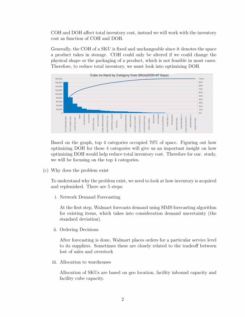
COH and DOH affect total inventory cost, instead we will work with the inventorycost as function of COH and DOH.

Generally, the COH of a SKU is fixed and unchangeable since it denotes the spacea product takes in storage. COH could only be altered if we could change thephysical shape or the packaging of a product, which is not feasible in most cases.Therefore, to reduce total inventory, we must look into optimizing DOH.

Based on the graph, top 4 categories occupied 70% of space. Figuring out howoptimizing DOH for these 4 categories will give us an important insight on howoptimizing DOH would help reduce total inventory cost. Therefore for our. study,we will be focusing on the top 4 categories.

(c) Why does the problem exist

To understand why the problem exist, we need to look at how inventory is acquiredand replenished. There are 5 steps:

i. Network Demand Forecasting

At the first step, Walmart forecasts demand using SIMS forecasting algorithmfor existing items, which takes into consideration demand uncertainty (thestandard deviation).

ii. Ordering Decisions

After forecasting is done, Walmart places orders for a particular service levelto its suppliers. Sometimes these are closely related to the tradeoff betweenlost of sales and overstock

iii. Allocation to warehouses

Allocation of SKUs are based on geo location, facility inbound capacity andfacility cube capacity.

2

iv. Logistics

Logistics takes into account all others contributors such as whether lead timecould be shortened, what is the delivery speed, and what is transportationcost.

v. Inventory handling

Finally, everything leads to the problem we care the most about: inventoryhandling.

Now that we’ve understood the problem, its existence and its significance, we can moveon to the next section where we model the problem.

3. Modelling

(a) Overview

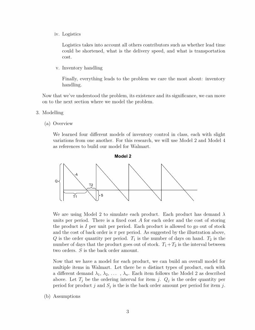
We learned four different models of inventory control in class, each with slightvariations from one another. For this research, we will use Model 2 and Model 4as references to build our model for Walmart.

We are using Model 2 to simulate each product. Each product has demand λunits per period. There is a fixed cost A for each order and the cost of storingthe product is I per unit per period. Each product is allowed to go out of stockand the cost of back order is π per period. As suggested by the illustration above,Q is the order quantity per period. T1 is the number of days on hand. T2 is thenumber of days that the product goes out of stock. T1 +T2 is the interval betweentwo orders. S is the back order amount.

Now that we have a model for each product, we can build an overall model formultiple items in Walmart. Let there be n distinct types of product, each witha different demand λ1, λ2, . . . , λn. Each item follows the Model 2 as describedabove. Let Tj be the ordering interval for item j. Qj is the order quantity perperiod for product j and Sj is the is the back order amount per period for item j.

(b) Assumptions

3

i. We assume that the demand λ for each product is constant during each period.

ii. We assume that every item shares the same T1 and T2. By assuming the sameordering interval T for every product, we can minimize the inventory cost aswell as eliminate extra order cost.

iii. We assume that the order cost A is fixed for all orders regardless of the sizeof the order or the type of products. Hence it averages out to A/n for eachindividual SKU.

iv. We assume that the back order cost π is fixed for all orders regardless of thesize of the order or the type of products.

v. We assume that the inventory cost I is the same for all products.

(c) Correlation between terms

T = T1 + T2

Qj = λjT

Qj − Sj = λjT1

Sj = λjT2

(d) Problem and Optimization

Let K be the average cost per period

K =n∑j=1

Kj

where Kj denotes the average cost per period for product j and

Kj = A

nT+ I

T1

T

Qj − Sj2 + π

T2

T

Sj2

Since the inventory cost I is the same for every product, we can simply analyzethe total cost for one category.

Note that T1T

= Qj−Sj

Qjand T2

T= Sj

Qj

So we can rewrite Kj in terms of λj, Qj and Sj, and we have

Kj = AλjnQj

+ I(Qj − Sj)2

2Qj

+ πS2j

2Qj

Set∂Kj

∂Qj

= ∂Kj

∂Sj= 0

4

and solve the equation

∂Kj

∂Qj

= −AλjnQ2

j

+ I(Qj − Sj)Qj

− I(Qj − Sj)2

2Q2j

−πS2

j

2Q2j

= 0

∂Kj

∂Sj= −2(Qj − Sj)

Qj

I + πSjQj

= 0

From equation 2, we have Sj = QjI

π+I

Plug into equation 1, we have

∂Kj

∂Qj

= −AλjnQ2

j

+I(Qj − QjI

π+I )Qj

−I(Qj − QjI

π+I )2

2Q2j

−π(QjI

π+I )2

2Q2j

= −AλjnQ2

j

+ I − I2

π + I−I(Q2

j − 2Q2jI

π+I + Q2jI

2

(π+I)2 )2Q2

j

− πI2

2(π + I)2

= −AλjnQ2

j

+ I − I2

π + I− I

2 + I2

π + I− I3

2(π + I)2 − πI2

2(π + I)2

= −AλjnQ2

j

+ I

2 − I2

2(π + I) = 0

We have that for any category, the optimal Qj =√

2Aλj(π+I)nIπ

the optimal Sj =√

2AλjI

nπ(π+I)

the optimal T2 = Sj

λj=

√2AI

nλjπ(π+I)

the optimal T = Qj

λj=

√2A(π+I)nλjIπ

Thus, the optimal T1 = T − T2 =√

2A(π+I)nλjIπ

−√

2AInλjπ(π+I) , which is what we want

to find, Days on Hand.

(e) Data set

We are mainly going to be using two CSV files we collected from the WalmartOracle Database using SQL. For this research, we limit our model to only thewarehouse in Davenport, FL (MCO). The first CSV file records all the ordersplaced by Walmart and the product and category of that product, and the secondfile is similar but with back orders. For each of the two files, the file includes thename of the product, the category the product belongs to, the date the order was

5

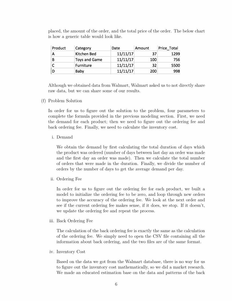
placed, the amount of the order, and the total price of the order. The below chartis how a generic table would look like.

Although we obtained data from Walmart, Walmart asked us to not directly shareraw data, but we can share some of our results.

(f) Problem Solution

In order for us to figure out the solution to the problem, four parameters tocomplete the formula provided in the previous modeling section. First, we needthe demand for each product; then we need to figure out the ordering fee andback ordering fee. Finally, we need to calculate the inventory cost.

i. Demand

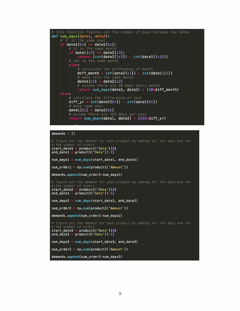
We obtain the demand by first calculating the total duration of days whichthe product was ordered (number of days between last day an order was madeand the first day an order was made). Then we calculate the total numberof orders that were made in the duration. Finally, we divide the number oforders by the number of days to get the average demand per day.

ii. Ordering Fee

In order for us to figure out the ordering fee for each product, we built amodel to initialize the ordering fee to be zero, and loop through new ordersto improve the accuracy of the ordering fee. We look at the next order andsee if the current ordering fee makes sense, if it does, we stop. If it doesn’t,we update the ordering fee and repeat the process.

iii. Back Ordering Fee

The calculation of the back ordering fee is exactly the same as the calculationof the ordering fee. We simply need to open the CSV file containing all theinformation about back ordering, and the two files are of the same format.

iv. Inventory Cost

Based on the data we got from the Walmart database, there is no way for usto figure out the inventory cost mathematically, so we did a market research.We made an educated estimation base on the data and patterns of the back

6

ordering. Also, we discussed with people in the industry and the flow managerfrom the Walmart Davenport warehouse to make a more accurate estimationabout the inventory cost.

(Details on how to figure out the demand, ordering fee, and back ordering fee canbe found in the programming section of the appendix)

In order to simplify the model, we ran our data analysis on only four productsfrom four categories. We chose the top four categories with the longest Days onHand (DOH) so that the reduction of operation cost would be significant. Also,we chose the one generic product from each categories for the data analysis. Thefour categories are Kitchen Bed, Toys and Game, Furniture, and Baby product.

After conducting a data analysis on the CSV files by running some Python pro-grams, we figured out the fixed order cost A is 51089 dollars, the back order costPi is 7289 dollars. The demands for each of the four product from the four cate-gories are [17.39, 104.13, 6.22, 257.7] respectively (per day). The inventory costI is 12 dollars per product per day, and because there are only four products,so n = 4. With these information, we have all the parameters for our model.After adapting the model, we found that the order quantity per period would be[192.55, 471.2, 115, 741] for each product respectively. The back ordering amountwould be [0, 87, 0, 311] with each product respectively. The 0 means that itis not necessary to back order those product which makes sense, because of thenature of the category. Kitchen Bed and Furniture are all products that take abig amount of space, and not that fluid. From this we can also derive T2, thenumber of days the product goes out of stock. T2 = [N/A, 1, N/A, 1.3], andT, the number of days between orders, [12, 4.6, 21.5, 3.1]. This data also makessense, because we order product with a more fluid nature more often, and biggerproduct less often. Finally, we can calculate T1, the number of days the productis on hand. T1 = [12, 3.6, 21.5, 1.8], this is also the optimized number so we canachieve the minimum operating cost.

4. Other Analysis (concerns not addressed above)

There are a couple assumptions we made in this analysis, that are slightly differentfrom the real life scenario. First, in the analysis, we derived a fixed ordering cost, backordering cost, and inventory cost. However, due to the constraint of the model, wecouldn’t have them varied for each product. Also, based on our analysis, the demandestimation is linear. In the future, we can do some different analysis to capture thepatterns of demands more accurately. Because of the above two reasons, the analysiscan be more accurate in the future.

5. Further Applications and Variations

Some variations and analysis we can do in the future includes, figuring out thecorrelation between the size of the item and the cost of fulfillment (more sizable product

7

should have a bigger fulfillment cost), looking into the ordering decision and decidebetween the trade of of loss of sales and overstocking (maybe it is more cost efficient tolose some customers to avoid the high overstocking expenses), and peak season analysis.For example, during holidays like Thanksgiving and Christmas, because of the discountand deals, the pressure of fulfillment would increase by a huge amount. In the future,maybe we can do a separate data analysis project to see how peak seasons wouldaffect the cost of fulfillment and if there are different models more suitable for peakseasons. Finally, this model is very powerful. The same model works on some otherindustries other than warehouse as well. For example, we can adapt our model to studyrestaurants, transportation services, real estates and many other more industries. Allthese industries have some very similar characteristics, like demand/supply, orderingcost, inventory costs which all fit the model.

6. Summary

By optimizing in stock quantity, back ordering quantity, inventory days on handand some other factors, we are successfully able to reduce fulfillment cost and increaseprofit base on our data analysis with Walmart’s Davenport, Florida e-commerce ful-fillment center. We mainly used inventory model 2 and model 4 which we learned inclass, and ran some Python data analysis model on the data to figure out the optimalquantity and days on hand for fulfillment. Through this study, we learned a lot moreabout the models (2 and 4), parsing large data, and the fact that the cost of fulfillmentdepends a lot on the nature of the product.

7. Appendix

8

9

10