WALL BUILD-UP IN SPRAY DRYERS - University of ...
377
WALL BUILD-UP IN SPRAY DRYERS by Guy James Hassall A thesis submitted to The University of Birmingham for the degree of Engineering Doctorate (EngD) School of Chemical Engineering University of Birmingham July 2011
-
Upload
khangminh22 -
Category
Documents
-
view
1 -
download
0
Transcript of WALL BUILD-UP IN SPRAY DRYERS - University of ...

WALL BUILD-UP IN SPRAY DRYERS
by
Guy James Hassall
A thesis submitted to
The University of Birmingham
for the degree of
Engineering Doctorate (EngD)
School of Chemical Engineering
University of Birmingham
July 2011

University of Birmingham Research Archive
e-theses repository This unpublished thesis/dissertation is copyright of the author and/or third parties. The intellectual property rights of the author or third parties in respect of this work are as defined by The Copyright Designs and Patents Act 1988 or as modified by any successor legislation. Any use made of information contained in this thesis/dissertation must be in accordance with that legislation and must be properly acknowledged. Further distribution or reproduction in any format is prohibited without the permission of the copyright holder.

Abstract
Most granular laundry detergents are manufactured through spray drying. One drawback of
this process is wall build-up, which negatively effects process operation, safety and product
quality.
Macro and micro-scale observations showed the amount and micro-structure of deposits
changed significantly across the dryer. These changes were linked to changes in particle
properties during drying. Measurements of deposition ranged from 1 - 10 kgm-2, or 2 - 10%
of the total slurry sprayed, depending on location, operating conditions and slurry/powder
properties. Wall deposition appeared to be time dependent.
Wall deposition was broken down into two critical steps; collision frequency, describing how
many and how often particles hit the wall and, collision success rate which describes
particle’s behaviour upon contact with the wall. Collision frequency was investigated using
Particle Imagine Velocimetry (PIV) to measure both fluid and particle dynamics. Finding both
to be time dependent, and to vary with position and operating conditions.
To investigate collision success rate, particle physical and mechanical properties were
studied, revealing mutual dependence of all properties on both formulation and particle
size. Impacting these particles at a range of velocities and angles found that the fraction of
particles that broke ranged from 0 - 100% and restitution coefficients from 0.1 - 0.8.

This thesis is dedicated to my parents

“All’s well that ends well”
- William Shakespeare (1605)

Acknowledgements
First of all I would like to thank my supervisors, each of whom, in their own way have helped,
encouraged and enabled me to produce this thesis. Mark Simmons who has supervised me
academically, ensuring that my collection of work and ideas finally became a submittable
thesis. Carlos Amador who challenged me to think and sometimes even act like an engineer.
I would like to thank Andrew Bayly for setting up the project and inputting his expertise.
I also want to acknowledge people beyond my supervisors who helped. Richard Greenwood
deserves great credit for dealing with both me and the administrative side of the EngD. At
P&G Zayeed Alam who managed my work within the company. I also have to give special
mention to HongSing Tan for the advice, wisdom and sometimes therapy he gave me. I’d like
to thank Nicola Tilt for her help with statistics. It is only right that I take this opportunity to
thank the students who I had the fortune of working with in some capacity and whose work
contributed towards this thesis, my thanks go out to Lena, Wan and Andrew. I also
acknowledge the support of P&G and EPSRC. I would like to thank Martin Hyde of TSI for his
technical input and support on the PIV work.
I’d like to thank family and friends, especially my parents for their support during my many
years of education. All of the people in Newcastle who I have had the pleasure of calling
friends over the last 5 years, you are too numerous to name, but thanks to all of you, the
Iranians, French, Scots, Malaysians, Irish and Spaniards, not to forget the Geordies. You all
made my time in Newcastle something I will struggle to either forget or get over easily.
Special thanks to Becks for her help and support, especially at the beginning and end of this
EngD.

Table of Contents
List of Figures ..................................................................................................................... i
List of Tables .................................................................................................................. viii
Nomenclature .................................................................................................................. ix
Chapter 1 – Introduction.................................................................................................... 1
1.1 Introduction ................................................................................................................. 1
1.2 Business Case and Benefits .......................................................................................... 4
1.3 Project Objectives ........................................................................................................ 5
1.4 Outline of Thesis .......................................................................................................... 6
1.5 Publications Arising from this Work ............................................................................ 8
Chapter 2 – Literature Review............................................................................................ 9
2.1 Introduction ................................................................................................................. 9
2.2 Granular Laundry Detergents ...................................................................................... 9
2.3 Detergent Manufacture: Spray Drying ...................................................................... 13
2.3.1 Spray Drying ........................................................................................................ 13
2.3.2 Detergent Spray Drying and Processing ............................................................. 15
2.3.3 Slurry Preparation and Pumping ........................................................................ 18
2.3.4 Atomisation ........................................................................................................ 18
2.3.5 Spray-Air Contact ................................................................................................ 19
2.3.6 Drying .................................................................................................................. 21
2.3.7 Product Separation and Transportation ............................................................. 24
2.3.8 Post-Drying Component Addition ...................................................................... 24
2.3.9 Packing ................................................................................................................ 24
2.4 Modelling and Simulation of Spray Dryers ................................................................ 25
2.4.1 Heat and Mass Balances ..................................................................................... 26

2.4.2 Rate Based Models ............................................................................................. 27
2.4.3 Computational Fluid Dynamics (CFD) Models .................................................... 28
2.5 Fluid Dynamics in Spray Dryers .................................................................................. 31
2.5.1 Flow Diagnostic Techniques ............................................................................... 32
2.5.2 Particle Image Velocimetry ................................................................................ 35
2.5.2.1 Background ..................................................................................................... 35
2.5.2.2 Seeding of Flow ............................................................................................... 36
2.5.2.3 Laser ................................................................................................................ 37
2.5.2.4 Camera ............................................................................................................ 38
2.5.2.5 Synchroniser ................................................................................................... 38
2.5.2.6 Image Analysis – Cross Correlation ................................................................. 39
2.5.2.7 Limitations ...................................................................................................... 40
2.5.3 Fluid Dynamic Parameters .................................................................................. 41
2.5.4 Flow Patterns in Spray Dryers ............................................................................ 44
2.5.4.1 Experimental Studies into Fluid Dynamics in Spray Dryers ............................ 45
2.5.4.2 Rankine Vortex ................................................................................................ 45
2.5.4.3 Transient Flows ............................................................................................... 46
2.5.5 Modelling and Simulations Studies into Fluid Dynamics in Spray Dryers .......... 48
2.6 Particle Dynamics in Spray Dryers ............................................................................. 49
2.6.1 Techniques for Measuring Particle Size, Loading and Trajectories In-Situ ........ 50
2.6.1.1 Imaging Techniques ........................................................................................ 50
2.6.1.2 Light-Scattering Techniques............................................................................ 51
2.6.2 Particle Residence Time Studies ......................................................................... 51
2.6.3 Particle Size Studies ............................................................................................ 52
2.6.4 Particle Velocity and Trajectory Studies ............................................................. 53

2.6.5 Simulation Studies of Particle Dynamics ............................................................ 53
2.7 Wall Deposition in Spray Dryers ................................................................................ 54
2.7.1 Disadvantages of Wall Deposition ...................................................................... 55
2.7.2 Methods Reducing Wall Deposition ................................................................... 56
2.7.3 Methods of Removing Wall Deposits ................................................................. 57
2.7.4 Theoretical Explanations of Wall Deposition ..................................................... 57
2.7.5 Experimental Investigations into Wall Deposition ............................................. 58
2.7.6 Modelling and Simulation of Wall Deposition.................................................... 60
2.8 Particle Characterisation ............................................................................................ 61
2.8.1 Particle Size ......................................................................................................... 61
2.8.2 Particle Morphology ........................................................................................... 63
2.8.3 Particle Density ................................................................................................... 64
2.8.4 Hydroscopic Behaviour ....................................................................................... 66
2.8.4.1 Bound and Free Moisture ............................................................................... 66
2.8.4.2 Equilibrium Relative Humidity ........................................................................ 67
2.8.5 Mechanical Properties ........................................................................................ 67
2.9 Particle Impact Behaviour .......................................................................................... 70
2.9.1 Restitution .......................................................................................................... 71
2.9.1.1 Restitution Coefficient .................................................................................... 71
2.9.1.2 Experimental Investigations into Restitution Coefficients ............................. 72
2.9.1.3 Theoretical Investigations into Restitution Coefficients ................................ 73
2.9.2 Breakage and Attrition ....................................................................................... 74
2.9.2.1 Factors Affecting Breakage ............................................................................. 74
2.9.2.2 Mechanisms of Breakage and Failure ............................................................. 75
2.9.2.3 Breakage Tests and Experimental Studies ...................................................... 76

2.9.2.4 Theoretical Investigations and Models of Breakage ...................................... 78
2.9.3 Deposition ........................................................................................................... 78
2.9.3.1 Stickiness, Adhesion and Cohesion ................................................................. 79
2.9.3.2 Interparticle Forces ......................................................................................... 79
2.9.3.3 Measurement of Interparticle Forces and Surface Properties ....................... 80
2.10 Literature Review Summary ...................................................................................... 82
Chapter 3 – Materials and Methods ................................................................................. 84
3.1 Introduction ............................................................................................................... 84
3.2 Pilot Plant Spray Dryer ............................................................................................... 84
3.3 Detergent Formulations ............................................................................................. 88
3.3.1 Detergent Formulas Manufacture and Preparation .......................................... 89
3.3.2 Detergent Formulation Used for PIV Experiments ............................................. 89
3.3.3 Detergent Formulations used for Particle Characterisation and Impacts
Experiments ....................................................................................................................... 90
3.4 Wall Deposition .......................................................................................................... 91
3.4.1 Whole Operation Deposition Measurement ...................................................... 92
3.4.2 Time Dependent Deposition Measurement ....................................................... 94
3.5 Particle Image Velocimetry ........................................................................................ 95
3.5.1 Particle Image Velocimetry Installation on Spray Dryer .................................... 95
3.5.2 PIV Equipment and Settings ............................................................................... 97
3.5.3 Spray Dryer Operation ........................................................................................ 97
3.5.4 Airflow Experiments and Analysis ...................................................................... 99
3.5.5 Spraying Experiments and Analysis .................................................................. 100
3.6 Impact Experiments ................................................................................................. 101
3.6.1 Impact Rig, design, Set-up and Operation ........................................................ 101

3.6.2 Particle Imaging and Analysis ........................................................................... 103
3.6.3 Statistical Analysis ............................................................................................ 104
3.7 Particle Characterisation .......................................................................................... 105
3.7.1 Particle Size, Shape and Structure .................................................................... 105
3.7.1.1 Scanning Electron Microscopy (SEM) ........................................................... 105
3.7.2 Particle Density ................................................................................................. 105
3.7.2.1 Envelope Density – GeoPyc .......................................................................... 105
3.7.2.2 Skeletal Density - AccuPyc ............................................................................ 107
3.7.3 Hydroscopic Behaviour ..................................................................................... 107
3.7.3.1 Moisture Content .......................................................................................... 107
3.7.3.2 Equilibrium Relative Humidity ...................................................................... 108
3.7.4 Mechanical Properties ...................................................................................... 108
3.7.4.1 Confined Compression .................................................................................. 109
3.7.4.2 Unconfined Compression ............................................................................. 112
3.8 Computational Fluid Dynamics Simulations ............................................................ 113
Chapter 4 – Wall Deposition in Detergent Spray Dryers .................................................. 116
4.1 Introduction ............................................................................................................. 116
4.2 Experimental ............................................................................................................ 120
4.3 Qualitative Observation of Wall Deposition ............................................................ 121
4.3.1 Macro-scale Observations of Wall Deposition ................................................. 121
4.3.2 Micro-scale Observations of Wall Deposition .................................................. 126
4.4 Measurement of Wall Deposition............................................................................ 130
4.4.1 The Effect of wall Deposition on Powder Yield ................................................ 133
4.4.2 Wall Deposition as a Function of Location within the Dryer ............................ 133
4.4.3 The Effect of Dryer Operating Conditions on Wall Deposition ........................ 137

4.4.4 The Effect of Slurry and Powder Properties on Wall Deposition ..................... 140
4.5 Time-Dependent Studies of Wall Deposition .......................................................... 145
4.6 Wall Deposition Conclusions ................................................................................... 152
Chapter 5 – Fluid Dynamics in a Detergent Spray Dryer .................................................. 155
5.1 Introduction ............................................................................................................. 155
5.2 Experimental ............................................................................................................ 155
5.3 Time Average Velocity Studies................................................................................. 158
5.3.1 Velocity Magnitude .......................................................................................... 161
5.3.2 Radial Velocity .................................................................................................. 164
5.3.3 Tangential Velocity ........................................................................................... 166
5.3.4 Comparison with Previous Work ...................................................................... 167
5.4 Time Averaged Turbulent Parameters ..................................................................... 171
5.4.1 Turbulence Intensity ......................................................................................... 171
5.5 Time Dependent Velocity Studies ............................................................................ 173
5.5.1 Velocity Signals and Histograms ....................................................................... 173
5.5.2 Periodicity ......................................................................................................... 175
5.6 Conclusions .............................................................................................................. 177
Chapter 6 – Particle Dynamics in a Detergent Spray Dryer .............................................. 180
6.1 Introduction ............................................................................................................. 180
6.2 Experimental ............................................................................................................ 180
6.3 Results: Time-Averaged Particle Dynamics ............................................................. 182
6.3.1 Particle Size ....................................................................................................... 182
6.3.1.1 Mean ‘Projected Area’ Particle Size .............................................................. 182
6.3.1.2 Particle Size Distribution ............................................................................... 189
6.3.2 Particle Number Concentration, C ................................................................... 192

6.3.3 Particle Volume Fraction .................................................................................. 196
6.3.4 Particle Flow Fields ........................................................................................... 199
6.4 Results: Time Dependent Particle Dynamics ........................................................... 207
6.4.1 Time Dependent Particle Size, Number Concentration and Volume Fraction 207
6.4.2 Time Dependent Particle Flow Fields ............................................................... 210
6.5 Conclusions .............................................................................................................. 214
Chapter 7 – Particle Characterisation and Impact Behaviour .......................................... 216
7.1 Introduction ............................................................................................................. 216
7.2 Experimental ............................................................................................................ 216
7.2.1 Particle Characterisation Experiments ............................................................. 216
7.2.2 Particle Impacts Experiments ........................................................................... 218
7.3 Particle Characterisation Results ............................................................................. 219
7.3.1 Effect of Formulation on Particle Shape and Structure ................................... 219
7.3.2 Hydroscopic Behaviour ..................................................................................... 223
7.3.2.1 Moisture Content .......................................................................................... 223
7.3.2.2 Equilibrium Relative Humidity ...................................................................... 225
7.3.3 Particle Density ................................................................................................. 226
7.3.3.1 Envelope Density .......................................................................................... 226
7.3.3.2 Apparent Density .......................................................................................... 228
7.3.4 Mechanical Properties ...................................................................................... 230
7.3.4.1 Confined Yield Stress .................................................................................... 230
7.3.4.2 Confined Join Stress ...................................................................................... 232
7.3.4.3 Unconfined Young’s Modulus ....................................................................... 234
7.3.4.4 Unconfined Yield Stress ................................................................................ 235
7.3.5 Particle Characterisation Conclusions .............................................................. 237

7.4 Particle Impact Behaviour Results ........................................................................... 239
7.4.1 Particle Breakage .............................................................................................. 239
7.4.1.1 Breakage Mechanisms .................................................................................. 239
7.4.1.2 Breakage Fractions ........................................................................................ 242
7.4.1.3 Number of Fragments Generated ................................................................ 248
7.4.2 Rebound Behaviour .......................................................................................... 254
7.4.2.1 Restitution Coefficient .................................................................................. 254
7.4.2.2 Rebound Angle .............................................................................................. 263
7.5 Conclusions .............................................................................................................. 273
Chapter 8 – Conclusions ................................................................................................. 275
8.1 Summary of Research .............................................................................................. 275
8.2 Wall Deposition ........................................................................................................ 275
8.3 Fluid Dynamics ......................................................................................................... 276
8.4 Particle Dynamics ..................................................................................................... 277
8.5 Particle Characterisation and Impact Behaviour ..................................................... 278
8.6 Implications of this research for the sponsoring company (Procter & Gamble) ..... 279
8.7 Future Work ............................................................................................................. 280
Chapter 9 – References .................................................................................................. 282
Appendix A – PIV MATLAB Codes ................................................................................... 291
A.1 Fluid Dynamics Codes (Chapter Five) ...................................................................... 291
A.1.1 Vector file loading and 3D matrix construction ............................................... 291
A.1.2 Calculation and plotting of velocity and turbulence parameters .................... 294
A.1.3 Calculation and plotting of transience and periodicity parameters ................ 299
A.2 Particle Dynamics Codes (Chapter Six) .................................................................... 309
A.2.1 Image Manipulation ......................................................................................... 309

A.2.2 Image Analysis .................................................................................................. 311
A.2.3 Particle PIV data handling and Plotting ............................................................ 318
Appendix B – Wall Deposition Example Calculations ...................................................... 322
Appendix C – Fluid Dynamics in a Detergent Spray Dryer (Further Data) ......................... 324
C.1 Normalised Time Averaged Flow Fields .................................................................. 324
C.2 Turbulent Parameters ............................................................................................. 327
C.2.1 Turbulent Kinetic Energy .................................................................................. 327
C.2.2 Reynolds Stresses ............................................................................................. 329
Appendix D – Particle Dynamics Analaysis Methods ....................................................... 331
D.1 PIV Images Captured ............................................................................................. 331
D.2 Image Analysis – Choice of Threshold .................................................................... 336
D.3 Calculation of Size, Conentration and Loading Parameters .................................. 342
D.4 Particle PIV Cross-Correlation ................................................................................ 346
D.5 Sources of Potential Error in Analysis Methods ...................................................... 347
Appendix E – Particle Characterisation and Impacts Statistical Analysis .......................... 349
E.1 Correlation of all Variables ..................................................................................... 349
E.2 Modelling of Response Variables ............................................................................ 351
E.2.1 Breakage Fraction .................................................................................................. 351
E.2.2 Restitution Coefficent ............................................................................................ 352
E.2.3 Rebound Angle from Impact .................................................................................. 352

i
List of Figures
Figure 1.1: Simplified Detergent Spray Drying Process taken from Bayly (2004) ...................... 3
Figure 2.1: Spray Dryer Configurations taken from Masters (1991) ........................................ 14
Figure 2.2: Detergent spray dryer geometry ............................................................................ 15
Figure 2.3: Detergent Manufacturing Process Overview ......................................................... 17
Figure 2.4: Mechanisms of droplet drying (simplified). Adapted from Masters (1991). ......... 22
Figure 2.5: Typical PIV Experimental Set-up taken from Raffel et al. (2007) ........................... 36
Figure 2.6: FFT Cross Correlation Analysis taken from Raffel et al. (2007) .............................. 40
Figure 2.7: Particle Equivalent Circle Diameter ........................................................................ 62
Figure 2.8: Illustrations of various types of particle volume taken from Webb (2001) ........... 65
Figure 2.9: Typical strain-stress curve, where region 1) – elastic deformation, 2) – plastic
deformation .............................................................................................................................. 68
Figure 2.10: Methods of characterising powder mechanical properties (a) confined
compression; (b) unconfined compression of several particles; (c) unconfined compression of
one particle ............................................................................................................................... 70
Figure 2.11: Stickiness Characterisation Techniques for Powders taken from Boonyai et al.
(2004) ........................................................................................................................................ 81
Figure 2.12: Sticky-point curve for an idealised material taken from Kudra (2003) ................ 82
Figure 3.1: P&G Integrated Pilot Plant ..................................................................................... 85
Figure 3.2: Counter-current Spray Dryer (air movement left and particle movement right) .. 86
Figure 3.3: P&G Integrated Pilot Plant Experimental Layout (to scale) showing vertical
measurement positions for wall deposition (left) and PIV (right) ........................................... 88
Figure 3.4: Spray Dryer Inspection Hatch Deposition Measurement (before and after
operation) ................................................................................................................................. 93
Figure 3.5: Spray Dryer Inspection Hatch Deposition Plates (before and after operation) ..... 94
Figure 3.6: PIV experimental set-up installed on spray dryer .................................................. 96

ii
Figure 3.7: Particle Impact Experimental Set-up .................................................................... 102
Figure 3.8: Volume determination by displacement of dry solid medium (DryFlo), (Webb
(2001)) .................................................................................................................................... 106
Figure 3.9: Simplified diagram of the AccuPyc (Webb (2001)) .............................................. 107
Figure 3.10: Overview of Instron Confined Compaction (Mort (2002)) ................................. 110
Figure 3.11: Overview of Instron Confined Compaction (Mort (2002)) ................................. 111
Figure 3.12: SEM Images of unconfined compression tablet before testing ......................... 112
Figure 3.13: CFD Meshing of IPP Spray Dryer ......................................................................... 115
Figure 4.1: Scale Diagram of IPP showing experimental positions ........................................ 120
Figure 4.2: Typical wall deposition as viewed from position E: (a) looking down the dryer and
(b) close-up of dryer wall ........................................................................................................ 122
Figure 4.3: Typical wall deposition as viewed from position D .............................................. 123
Figure 4.4: Typical wall deposition as viewed from position C .............................................. 124
Figure 4.5: Typical wall deposition as viewed from position A .............................................. 125
Figure 4.6: SEM Images of Deposits from position E ............................................................. 128
Figure 4.7: SEM Images of Top-layer Deposits from position D ............................................. 128
Figure 4.8: SEM Images of Lower-layer Deposits from position D ......................................... 128
Figure 4.9: SEM Images of Top-layer Deposits from position C ............................................. 129
Figure 4.10: SEM Images of Deposits from position A ........................................................... 129
Figure 4.11: Wall Deposition as a function of Axial Position within the Dryer ...................... 134
Figure 4.12: Normalised Wall Deposition as a function of Axial Position within the Dryer ... 136
Figure 4.13: Wall Deposition as a function of Slurry Flow ..................................................... 137
Figure 4.14: Wall Deposition as a function of Air Flow Rate .................................................. 138
Figure 4.15: Wall Deposition as a function of Product Belt Temperature ............................. 139
Figure 4.16: Wall Deposition as a function of Slurry Moisture Content ................................ 141
Figure 4.17: Wall Deposition as a function of Slurry Surfactant Content .............................. 142

iii
Figure 4.18: Wall Deposition as a function of Powder Product Moisture ............................. 143
Figure 4.19: Wall Deposition as a function of Powder Product Mean Particle Size .............. 144
Figure 4.20: Accumulative Wall Deposition ........................................................................... 146
Figure 4.21: Initial (1 minute) Wall Deposition Repeats ........................................................ 147
Figure 4.22: Disruption to dryer air flow rate whilst using collection plates ......................... 149
Figure 4.23: Time Dependent Wall Deposition Observed with PIV ....................................... 151
Figure 5.1: Locations of image areas relative to spray dryer (a) position L and (b) position H
................................................................................................................................................ 156
Figure 5.2: CFD Simulation Results of Flow Fields in Dryer Without (a) and With (b) PIV set-
up ............................................................................................................................................ 157
Figure 5.3: Plots of (a) mean velocity magnitude and (b) RMS velocity versus the number of
PIV images analysed ............................................................................................................... 159
Figure 5.4: Flow Field Plots of Velocity Magnitude Absolute Values (ms-1) (a) position L high
flow rate.................................................................................................................................. 160
Figure 5.5: Flow Field Plots of Velocity Magnitude Absolute Values (ms-1): (a) position L high
flow rate, (b) position H low flow rate, (c) position H medium flow rate and (d) position H
high flow rate. ......................................................................................................................... 161
Figure 5.6: Profile Velocity Magnitude plots .......................................................................... 162
Figure 5.7: Profile Radial Velocity Plots .................................................................................. 164
Figure 5.8: Flow Field Plots of Absolute Values of Radial Velocity (ms-1): (a) position L high
flow rate, (b) position H low flow rate, (c) position H medium flow rate and (d) position H
high flow rate. ......................................................................................................................... 165
Figure 5.9: Flow Field Plots of Absolute Values of Tangential Velocity: (a) position L high flow
rate, (b) position H low flow rate, (c) position H medium flow rate and (d) position H high
flow rate. ................................................................................................................................ 166
Figure 5.10: Profile Tangential Velocity Plots ......................................................................... 167
Figure 5.11: Comparison of Tangential Velocity Profile Plots with Published Work ............. 169

iv
Figure 5.12: Turbulence Intensity Plots (% mean velocity magnitude) : (a) position L high
flow rate, (b) position H low flow rate, (c) position H medium flow rate and (d) position H
high flow rate. ......................................................................................................................... 171
Figure 5.13: Velocity Magnitude Signal Plots and Velocity Histograms: (a) position L high
flow rate, (b) position H low flow rate, (c) position H medium flow rate and (d) position H
high flow rate. ......................................................................................................................... 174
Figure 5.14: Periodogram plots for centre of all experimental conditions: (a) position L high
flow rate, (b) position H low flow rate, (c) position H medium flow rate and (d) position H
high flow rate. ......................................................................................................................... 176
Figure 6.1: Locations of image areas relative to spray dryer (a) position L and (b) position H
................................................................................................................................................ 181
Figure 6.2: Mean projected area diameter, dA as a Function of Radial Position ................... 183
Figure 6.3: Mean Particle Size Contour Plots: (A) Position L and (B) Position H ................... 188
Figure 6.4: Particle size distributions position L (a) 1.0 relative slurry and 6000 kghr-1 air; (b)
1.200 relative slurry and 6000 kghr-1 air and (C) 1.2 relative slurry and 8000 kghr-1 air. ...... 190
Figure 6.5: Particle size distributions position H (a) 1.0 relative slurry and 6000 kghr-1 air; (b)
1.200 relative slurry and 6000 kghr-1 air and (C) 1.2 relative slurry and 8000 kghr-1 air. ...... 191
Figure 6.6: Particle Concentration, C, as a Function of Radial Position ................................. 193
Figure 6.7: Particle Concentration Contour Plots: (A) Position L and (B) Position H ............. 195
Figure 6.8: Particle Volume Fraction as a Function of Radial Position ................................... 196
Figure 6.9: Particle Volume Fraction Contour Plots: (A) Position L and (B) Position H .......... 198
Figure 6.10: Time Average Particle Flow Fields (ms-1): (A) Position L and (B) Position H ...... 203
Figure 6.11: Velocity Vectors Generated per Interrogation Spot for Particle Flow Fields: (A)
Position L and (B) Position ...................................................................................................... 205
Figure 6.12: Velocity Magnitude Standard Deviation for Particle Flow Fields (ms-1): (A)
Position L and (B) Position H................................................................................................... 206
Figure 6.13: Time Dependent Particle Size (A), Concentration (B) and Volume Fraction (C):
Position L ................................................................................................................................ 208
Figure 6.14: Time Dependent Particle Size (A), Concentration (B) and Volume Fraction (C):
Position H ................................................................................................................................ 209

v
Figure 6.15: Time Dependent Particle Velocity Fields (ms-1): Position L ................................ 212
Figure 6.16: Time Dependent Particle Velocity Fields (ms-1): Position H ............................... 213
Figure 7.1: SEM images of HH formulation for each sieve cut ............................................... 220
Figure 7.2: SEM images of HL formulation for each sieve cut................................................ 220
Figure 7.3: SEM images of LH formulation for each sieve cut................................................ 221
Figure 7.4: SEM images of LL formulation for each sieve cut ................................................ 221
Figure 7.5: Powder moisture contents for each formulation as a function of particle sieve cut
................................................................................................................................................ 224
Figure 7.6: Powder Equilibrium Relative Humidities .............................................................. 225
Figure 7.7: Particle Envelope Densities .................................................................................. 227
Figure 7.8: Particle apparent densities ................................................................................... 229
Figure 7.9: Confined yield stresses for the four formulations as a function of particle sieve cut
................................................................................................................................................ 231
Figure 7.10: Confined compression join stresses as a function of particle size for the four
formulations ........................................................................................................................... 233
Figure 7.11: Unconfined Compression Young’s Modulus ...................................................... 234
Figure 7.12: Unconfined Compression Yield Stresses ............................................................ 236
Figure 7.13: Chipping of a 1180-1800 μm HL particle at 5 ms-1 ............................................. 240
Figure 7.14: Chipping of a 1180-1800 μm HL particle at 10 ms-1 ........................................... 241
Figure 7.15: A HL particle of 1180-1800 μm splitting at 10 ms-1 ........................................... 241
Figure 7.16: A HL particle of 1180-1800 μm splitting at 10 ms-1 ............................................ 241
Figure 7.17: A HL particle of 1180-1800 μm smashing at 15 ms-1 ......................................... 242
Figure 7.18: A HL particle of 1180-1800 μm smashing at 10 ms-1 ......................................... 242
Figure 7.19: Breakage Fraction: HH Formulation ................................................................... 245
Figure 7.20: Breakage Fraction: HL Formulation .................................................................... 246
Figure 7.21: Breakage Fraction: LH Formulation .................................................................... 247

vi
Figure 7.22: Breakage Fraction: LL Formulation ..................................................................... 248
Figure 7.23: Number of Fragments: HH Formulation ............................................................ 250
Figure 7.24: Number of Fragments: HL Formulation ............................................................. 251
Figure 7.25: Number of Fragments: LH Formulation ............................................................. 252
Figure 7.26: Number of Fragments: LL Formulation .............................................................. 253
Figure 7.27: Restitution Coefficient: HH Formulation ............................................................ 256
Figure 7.28: Restitution Coefficient: HL Formulation ............................................................. 257
Figure 7.29: Restitution Coefficient: LH Formulation ............................................................. 258
Figure 7.30: Restitution Coefficient: LL Formulation ............................................................. 259
Figure 7.31: Normal Restitution Coefficient: HH Formulation ............................................... 260
Figure 7.32: Normal Restitution Coefficient: HL Formulation ................................................ 261
Figure 7.33: Normal Restitution Coefficient: LH Formulation ................................................ 262
Figure 7.34: Normal Restitution Coefficient: LL Formulation ................................................ 263
Figure 7.35: Angle between Impact and Rebound Vectors: HH Formulation ........................ 265
Figure 7.36: Angle between Impact and Rebound Vectors: HL Formulation ......................... 266
Figure 7.37: Angle between Impact and Rebound Vectors: LH Formulation ......................... 267
Figure 7.38: Angle between Impact and Rebound Vectors: LL Formulation ......................... 268
Figure 7.39: Angle between Surface and Rebound Vector: HH Formulation ........................ 269
Figure 7.40: Angle between Surface and Rebound Vector: HL Formulation ......................... 270
Figure 7.41: Angle between Surface and Rebound Vector: LH Formulation ......................... 271
Figure 7.42: Angle between Surface and Rebound Vector: LL Formulation .......................... 272
Figure B.1: Sections used in estimation of spray dryer internal wall area ............................. 323
Figure C.1: Flow Field Plots of Velocity Magnitude Normalised Values: (a) low-position with
high-flowrate, (b) high-position with low-flowrate, (c) high-position with medium-flowrate
and (d) high-position with high-flowrate. .............................................................................. 325

vii
Figure C.2: Flow Field Plots of Normalised Values of Radial Velocity: (a) low-position with
high-flowrate, (b) high-position with low-flowrate, (c) high-position with medium-flowrate
and (d) high-position with high-flowrate. .............................................................................. 326
Figure C.3: Flow Field Plots of Normalised Values of Tangential Velocity: (a) low-position with
high-flowrate, (b) high-position with low-flowrate, (c) high-position with medium-flowrate
and (d) high-position with high-flowrate. .............................................................................. 327
Figure C.4: Turbulent Kinetic Energy Plots: (a) low-position with high-flowrate, (b) high-
position with low-flowrate, (c) high-position with medium-flowrate and (d) high-position
with high-flowrate. ................................................................................................................. 328
Figure C.5: Reynolds Stress Plots: (a) low-position with high-flowrate, (b) high-position with
low-flowrate, (c) high-position with medium-flowrate and (d) high-position with high-
flowrate. ................................................................................................................................. 329
Figure C.6: Normalised Reynolds Stress Plots: (a) low-position with high-flowrate, (b) high-
position with low-flowrate, (c) high-position with medium-flowrate and (d) high-position
with high-flowrate. ................................................................................................................. 330
Figure D.1: Example of PIV Images captured (a) position L; (b) position H) .......................... 331
Figure D.2: Histograms of greyscale values for the images shown in Figure 6.1: (a) position L;
(b) position H. ......................................................................................................................... 333
Figure D.3: Particle Volume Fraction as a Function of Radial Position Calculated with
graythresh algorithm .............................................................................................................. 337
Figure D.4: Number of particles detected as a function of threshold value: (a) position H; (b)
position L ................................................................................................................................ 339
Figure D.5: (a) Example of particle selection to obtain threshold value; (b) corresponding
grayscale values. ..................................................................................................................... 341
Figure D.6: Area of lasersheet covered by image................................................................... 344
Figure D.7: The divergence of a Gaussian beam around the waist ........................................ 345
Figure E.1: Correlation values of particle impacts variables .................................................. 350
Figure E.2: Breakage fraction response models for key parameters ..................................... 351
Figure E.3: Restitution Coefficent response models for key parameters .............................. 352
Figure E.4: Rebound angle from impact response models for key parameters .................... 352

viii
List of Tables
Table 2.1: A summary of detergent powder requirements adapted from de Groot et al.
(1995). ....................................................................................................................................... 10
Table 2.2:Detergent powder component groups, functions and examples of chemical
compounds adapted from de Groot et al. (1995). ................................................................... 12
Table 2.3: Spray Dryer Model Levels of Complexity ................................................................. 30
Table 2.4: Summary of flow diagnostic techniques ................................................................. 33
Table 2.5: Summary of Factors Affecting Particle Breakage .................................................... 75
Table 3.1: Detergent Formulation for PIV Experiments ........................................................... 90
Table 3.2: Detergent Formulations for Impact Experiments ................................................... 91
Table 3.3: Air flowrates used for PIV trials ............................................................................... 98
Table 3.4: Operating parameters used for measurements above nozzle ................................ 99
Table 3.5: Operating parameters used for measurements below nozzle ................................ 99
Table 4.1: Summary of Effect of Spray Drying Variables and Parameters on Wall Deposition
................................................................................................................................................ 118
Table 4.2: Details of Formulations , Operating Conditions, Powder Properties and yields for
Trials where Wall Deposition was Measured ......................................................................... 132
Table 4.3: Initial Deposition Rates .......................................................................................... 147
Table 5.1: Experimental Conditions ....................................................................................... 156
Table 6.1: Operating parameters used for studying particle dynamics ................................. 181
Table 7.1: Physical and Mechanical Particle Properties Measured ....................................... 217
Table 7.2: Formulations Overview.......................................................................................... 218
Table B.1: Detergent Formulations for Impact Experiments ................................................. 322
Table D.1: Thresholding levels for all datasets ....................................................................... 342

ix
Nomenclature
Symbols
Aw water activity
C particle number concentration
d diameter
e restitution coefficient
I turbulence intensity – dimensionless
LIA interrogation area length - m
n number of velocity values
m mass
k turbulence kinetic energy - kJ.kg-1
r radial position
R Reynolds stresses
R spatial cross-correlation function of the transmitted light intensity
S swirl number
ū mean velocity - ms-1
u’ fluctuating components of velocity - ms-1
ũ root mean square of fluctuating components of velocity - ms-1
U instantaneous velocity - ms-1
v volume
x x position in Cartesian coordinates
y y position in Cartesian coordinates
θ the angle between the x dimension and tangent to curvature of wall - radians
viscosity

x
density
relaxation time
σ stress
Subscripts
h horizontal plane
i impact
n normalised
p particle
r radial in cylindrical coordinates
r rebound
x tangential Cartesian coordinates
y radial in Cartesian coordinates
z axial in both Cartesian and cylindrical coordinates
Θ tangential in cylindrical coordinates

Chapter One: Introduction
1
1.0 Chapter 1 – Introduction
1.1 Introduction
The focus of this thesis is wall deposition in spray dryers formed during the manufacture of
granular laundry detergents. This project was undertaken as an Engineering Doctorate
(EngD) in Formulation Engineering at the School of Chemical Engineering at the University of
Birmingham, with Procter and Gamble (P&G) as the industrial partner.
Laundry detergents are used all over the globe to aid the cleaning of garments during
washing. Detergent products are supplied in a variety of physical forms (Bajpai and Tyagi
(2007)) such as powders, liquids and bar soaps. Additionally unit dose forms such as solid
tablets (compressed powder of a different formulation to loose powder) and liquitabs (liquid
detergent encased in a membrane that dissolves upon water contact) have been introduced
in recent years. The type of detergent and how the consumer uses the product depends
mainly on their geographical location (de Groot et al. (1995)). In industrialised geographies
the majority of consumers use automatic washing machines (where the main cleaning action
is carried out mechanically), however the type of machine and detergent compatibility varies
between country and region. In developing nations the majority of consumers still wash
their laundry by hand.
Consumers have different requirements from laundry detergents, depending on their
location and wash method. In general, consumers want a product to perform well and
deliver good cleaning whilst protecting their garments. Consumers also expect the product
to look and smell appealing. The challenge of detergent manufacturers is to delight the

Chapter One: Introduction
2
consumer by meeting, and where possible, exceeding, these expectations so that the
consumers become regular users of their products. In the 21st century society is demanding
increased levels of environmental consideration from products and from the companies that
make them, adding further pressure on manufacturers to consistently improve their
environmental impact and sustainability credentials of their products (Huntington (2004)).
This research is concerned with granular laundry detergents. There are two main process
routes for manufacturing granular detergents, agglomeration and spray drying.
Agglomeration involves mixing small particles together with a liquid binder to form bigger
granules with more desirable properties such as flowability. Spray drying is the process of
atomising a feed slurry into small droplets which are then contacted with hot air to dry them
and form a powder product. This project is focussed solely on detergents produced through
spray drying.
Spray drying is defined by Masters (1991) as “the transformation of feed from a fluid state
into a dried particulate form by spraying the feed into a hot drying medium”. The process of
using spray drying to manufacture detergents was developed in the 1930s and 1940s (Dyer
et al. (2004)). Masters (1991) describes 4 main stages in the generic spray drying process:
1. Atomisation – the break-up of the feed slurry to form small droplets.
2. Spray air contact – the movement of the atomised droplets through the drying air,
resulting in heat transfer from the air to the droplet.
3. Drying of droplets/sprays – the process of mass transfer of drying as the water
migrates from the droplets.

Chapter One: Introduction
3
4. Separation and recovery of dried product – capture and handling of the powder
product after drying.
In addition to these four generic stages, detergent manufacture includes two other major
steps, slurry preparation and pumping before atomisation and powder mixing, handling and
packing after the powder is dried. Figure 1.1 shows a simplified layout of the detergent spray
drying process taken from Bayly (2004).
CRUTCHER
TOWER
RAW MATERIALS(SOLID AND LIQUID)
Nozzle
Exhaust Air
Blown
Powder
Hot Air
Inlet
Figure 1.1: Simplified Detergent Spray Drying Process taken from Bayly (2004)
Spray drying has several advantages for manufacturing detergents over its rival processes
such as agglomeration, these can be summarised as:
1. Ability to form a free flowing powder directly from a liquid (slurry) feedstock (Oakley
(2004)).

Chapter One: Introduction
4
2. High throughput and continuous operation of the process (Masters (1991)).
3. Control of particle/powder properties such as size distribution, porosity and bulk
density. All of which are desired by the consumer (de Groot et al. (1995)).
4. Proven technology widely used with large amounts of operational experience
(Chaloud et al. (1957)).
Spray drying also has several drawbacks, including wall deposition which has a negative
effect on both product quality and process operation. This phenomenon is the focus of this
research and the reasons behind this choice are discussed in detail in the next section.
1.2 Business Case and Benefits
Wall deposition, or wall build-up is the collection of layers of material onto the walls of
process equipment in powder handling operations. It is formed when product particles
adhere to the surface (Cleaver (2008)). The amount of wall build-up observed varies
depending on location, process operating conditions, material formulation and duration of
operation. As mentioned before, this is one of the major drawbacks in spray drying as a
manufacturing route for products such as detergents.
Wall build-up is observed in virtually all spray drying processes according to Bayly (2005) and
Masters (1991). Detergent spray drying is no different, with build-up observed at all stages
of the process where powder is present. Build-up is observed within the drying chamber,
exhaust system and post-dryer handling systems where powder is mixed, stored and packed.
The focus of this research is on build-up in the drying chamber which has the most
significant effect on process operation and product quality as described by Bayly (2005).

Chapter One: Introduction
5
Wall build-up in the drying chamber can have a significant effect on process operating
conditions, operational safety, process reliability and maintenance/cleaning requirements.
Perhaps more importantly it also has an effect on product quality. Product colour, particle
size distribution, particle morphology and chemical activity can all be affected. Each of these
is interlinked and is described in more detail in Chapter Two as the background to this work
is laid out.
The work presented in this thesis is part of a larger program of work within Procter and
Gamble to develop better understanding and therefore modelling capability of spray drying
processes for detergent manufacture. Understanding and modelling of spray drying enables
the process to be operated more efficiently in terms of materials and energy usage,
production capacity to be optimised, product quality improved and delivered more
consistently and quicker scale-up and process development which requires less experimental
work and fewer pilot plant trials. All of these factors improve the economics of granular
detergent manufacture and process development.
1.3 Project Objectives
The overall aim of this project is to develop an understanding of wall build-up in spray
dryers. In order to focus the research, this goal can be broken down into a logical sequence
of steps, the first being to understand the nature of wall deposition and then breaking the
mechanism that leads to wall deposition into two steps, particles coming into contact with
the walls (collision frequency) and then what happens when particles hit the wall (impact
behaviour). These steps are broken down into the following questions:

Chapter One: Introduction
6
1. Where in the spray drying process does wall deposition occur? Thus, which areas of
the spray drying process experience the highest levels of deposition?
2. How does product formulation and plant operating conditions affect wall deposition?
3. What airflow patterns are formed within the dryer? How do these influence the
movement of particles through the dryer?
4. How do particles move through the spray dryer? How do particles impact on the
dryer walls? What are the properties of particles striking the dryer walls?
5. Can the impacts of particles on the dryer walls be reproduced in the laboratory and
how do particle characteristics affect these impacts?
1.4 Outline of Thesis
Chapter Two – Literature Review
This chapter introduces granular detergent products, their formulation and manufacture
through spray drying. Published research of relevance in the area of spray drying and
detergents is examined and critically reviewed such that the context of this work is laid out.
Details of theories and principles used and applied during this work are also given.
Chapter Three – Materials and Methods
The experimental methods, equipment and materials used in this work are described in
chapter three. The justification for each technique and the set-up used for each set of
experiments is also provided.
Chapter Four – Wall Deposition in Detergent Spray Dryers
The spray drying process is examined to identify areas where deposition occurs and methods
developed to measure this deposition during plant operation with different formulations

Chapter One: Introduction
7
and conditions. Chapter four tackles the first two questions posed earlier in this chapter
“Where in the spray drying process does wall deposition occur? Which areas experience the
highest levels of deposition?” and “How does formulation and plant operating conditions
affect wall deposition?”
Chapter Five – Fluid Dynamics inside a Detergent Spray Dryer
The air flow patterns inside spray dryers are widely acknowledged to heavily influence
particle movement through the dryer, and therefore both product quality and process
operation. Chapter five covers experiments to study air flow patterns inside a counter
current detergent spray dryer to answer the questions “What airflow patterns are formed
within the dryer? How do these patterns influence the movement of particles through the
dryer?”
Chapter Six – Particle Dynamics inside a Detergent Spray Dryer
Experiments to visualise particles drying inside of the spray dryer are reported here. The size
distribution, concentration, volume fraction and velocities of particles are presented as a
function of both location within the dryer and dryer operating conditions. This enabled the
following questions to be answered “How particles move through the spray dryer? How do
particles impact on the dryer walls? What are the properties of particles striking the dryer
walls?”
Chapter Seven – The Properties and Impact Behaviour of Spray Dried Detergent Granules
The physical and mechanical properties of detergent particles are known to significantly
affect the impact behaviour and therefore deposition of detergent particles. The first part of
this chapter covers experiments and measurements to characterise these properties for
various detergent formulations. The impact behaviour of detergent granules determines if

Chapter One: Introduction
8
particles will stick to process equipment walls to form wall build-up. The second part of this
chapter covers experiments to investigate the particle impact behaviour to tackle the
questions, “Can these impacts be reproduced in the laboratory? How do particle
characteristics affect these impacts?”
Chapter Eight – Conclusions
The final chapter of the thesis brings together the previous chapters to draw overall
conclusions on the research. These are collated into a detailed summary of wall deposition
and the variables which affect it. Recommendations for further work and future projects are
discussed along with their relevance to the current detergent industry.
1.5 Publications Arising from this Work
Hassall, G.J., Amador, C., Bayly, A.E. and Simmons, M.J.H, The Impact Behaviour of Spray
Dried Detergent Granules, 16th International Drying Symposium (IDS 2008), November 2008,
Hyderabad (India). Oral presentation and conference paper.
Hassall, G.J., Amador, C., Bayly, A.E. and Simmons, M.J.H, The Impact Behaviour of Spray
Dried Detergent Granules, (In preparation)
Hassall, G.J., Amador, C., Bayly, A.E. and Simmons, M.J.H, Particle and Fluid Dynamics inside
a Counter-current Detergent Spray Dryer , (In preparation)

Chapter Two: Literature Review
9
2.0 Chapter 2 – Literature Review
2.1 Introduction
This Chapter introduces granular laundry detergents, their formulation and manufacture
through spray drying, together with details of theories and experimental methods used and
applied during this work; these include areas of particle technology, particle characterisation
and fluid dynamics. Published research of relevance in the area of spray drying and
detergents is examined and critically reviewed such that the context of this work is laid out.
The literature reviewed here comes from both external sources, such as open published
scientific literature from journals and conferences and from internal sources at P&G.
2.2 Granular Laundry Detergents
Soaps have been used to clean both people and objects since ancient times. Traditional
soaps were manufactured by boiling fats and oils with an alkali. Soaps manufactured this
way were used well into the 20th century. Synthetic detergents were first developed in
Germany as a response to the lack of fats and oils available during the First World War
(Bajpai and Tyagi (2007)). However, these initial synthetic detergents did not deliver the
cleaning power of natural soaps. It took until the 1930s and 1940s for the technology of
synthetic detergents to develop sufficiently to match and surpass the cleaning performance
of natural soaps. This development allowed Procter and Gamble to launch the first modern
“built” synthetic detergent powder “Tide” in the USA during 1946, (Dyer et al. (2004)). This
launch represented a major development not only in cleaning performance, but also in the
manufacturing process as new spray drying towers were built to manufacture the synthetic
formulation, which differed greatly from early soap based formulas. The launch of “Tide”

Chapter Two: Literature Review
10
was a huge success as it became the market leader soon after launch (Dyer et al. (2004)),
consuming the market share of soap based products, leading to the eventual replacement of
soaps with synthetic detergents.
Detergent powders are used to wash clothes and therefore their purpose is to remove soils
from clothing during the wash cycle. After washing the garments should be left soil and stain
free with a pleasant fragrance. Consumers expect detergents to consistently deliver and
improve on these criteria. Detergent manufacturers strive to impress consumers, retaining
their custom whilst winning over new consumers to their brand. This means constantly
improving their products in terms of powder appearance and fragrance, cleaning
performance and soil removal as well as the fragrance and appearance of laundry after
washing. These requirements are tensioned against needs to reduce costs to maintain profit
margins, especially during times of increasing raw materials costs. A summary of the
requirements for detergent powders from both consumer and manufacturing viewpoints are
given in Table 2.1.
Table 2.1: A summary of detergent powder requirements adapted from de Groot et al. (1995).
Detergent Powder User Requirements Detergent Powder Product
(Manufacturers’) Requirements
Good overall performance Correct balance of components
High solubility Components of good quality
Appealing shape, colour and perfume Free flowing and homogenous powders
No side effects on skin or fabrics Correct perfuming

Chapter Two: Literature Review
11
In order to perform and deliver the required cleaning, detergent powders contain many
components, all of which have different roles during the wash cycle. The main component
groups of a typical detergent powder, according to de Groot et al. (1995), are summarised in
Table 2.2 below, where the italics denote ingredients included in the slurry for spray drying
(§2.3).
Yangxin et al. (2008) list six groups of components which laundry detergents generally
comprise of, surfactants, builders, enzymes, bleaching agents, fillers and minor additives
(such as dispersing agents, fabric softening clay, dye transfer inhibitors and brighteners).
They highlight surfactants and builders as the two most important of these component
groups, as they play a key role in cleaning. Current and future developments in detergents
will be focused on these component groups to both improve performance and reduce
environmental impact of laundry detergent products.
Fifteen different groups of components are listed and described by Bajpai and Tyagi (2007)
as they break the groups listed by de Groot et al. (1995) and Yangxin et al. (2008) into more
specific divisions.
The chemical ingredients of detergent powders vary significantly between brands,
geographies and manufacturers. These changes are driven by consumers’ expectations and
trends in how they use the product, availability and cost of raw materials in that specific
geography and both local and international environmental legislation. There are many
different chemical compounds and materials used in each group of detergent components.
Examples of commonly used chemical ingredients for each active group of components are
given in Table 2.2.

Chapter Two: Literature Review
12
Table 2.2:Detergent powder component groups, functions and examples of chemical compounds adapted from de Groot et al. (1995).
Active Group Function Chemical Compounds
Surfactants Surface active agents to remove fatty/oily
soils and wet surfaces
Anionic Linear-Alkylbenezene-Sulphonate (LAS)
Non-ionic Alcohol-ethoxylate (AE)
Alkylphenol ethoxylate (APE)
Builders Enhance the action of surfactants Zeolite
Sodium Tripolyphosphate (STPP)
Sodium Carbonate
Sodium Silicate
Bleaches (and Activators) Remove Stains Sodium Perborate
Sodium Percarbonate
Fillers (and Processing Aids) Aid processing and physical structure Sodium Sulphate
Water
Enzymes Remove blood and protein stains Alcalase
Protease
Specific Additives (and Minors) Improve performance aside from cleaning Polymers (polycarboxylate)
Brighteners (fluorescers)
Perfumes Fragrance

Chapter Two: Literature Review
13
2.3 Detergent Manufacture: Spray Drying
Spray drying is the main process route for manufacturing granular laundry detergents, in
terms of both volume and sales, with volumes still growing annually, making research into
this process hugely important in the detergent industry (Huntington (2004) and Bayly et al.
(2008)). This section covers both generic spray drying and the spray drying process specific
to detergent powder manufacture and an overview of both is given.
2.3.1 Spray Drying
Spray drying is the transformation of a feed from a fluid state into a dried particulate form
by spraying the feed into a hot drying medium. It is a unique drying process, since it involves
both particle formation and drying (Masters (1991)). This process is an attractive choice of
unit operation for drying processes because of its ability of spray dryers to transform a liquid
feed into dry spherical particles at high throughputs (Oakley (2004)).
Spray drying has a wide range of applications and many different process layouts and
techniques are used to achieve the desired product properties for each specific application.
The main way of classifying dryers is through their layout which can be co-current or
counter-current, as shown in Figure 1.1, taken from Masters (1991). In a co-current dryer
both the spray and air move in the same direction, with both usually entering at the top of
the drying chamber and leaving through the bottom. Counter-current systems operate with
the air and spray moving in opposite directions where the feed is sprayed downwards
through a current of rising air. This is the system that is used for manufacturing detergent
powders so this review will focus on counter-current systems. However, several phenomena

Chapter Two: Literature Review
14
of spray drying have been investigated much more deeply in co-current rather than counter-
current units and hence work in co-current dryers is reported for these phenomena.
Figure 2.1: Spray Dryer Configurations taken from Masters (1991)
Masters (1991) lists four main stages of the generic spray drying process:
1. Atomisation
2. Spray air contact
3. Drying of droplets/sprays
4. Separation and recovery of dried product
These four process stages only cover the actually spray drying step. To cover the entire
detergent manufacturing process, slurry preparation and pumping, post-drying component
addition and packing can be added to form a list of seven process stages.

Chapter Two: Literature Review
15
2.3.2 Detergent Spray Drying and Processing
Detergent powders are manufactured using counter-current spray-drying systems. A
simplified cross-section of a typical detergent spray dryer is shown in Figure 2.2.
Tower Exhaust
Tower Shell
Tower Diameter
Cone DiameterHip
Nozzle Ring
Nozzle Arm
Hot Air Inlet
Bustle RingPlenumRing
Top Level
Middle Level
Bottom Level
Bottom Outlet
Tower Cone
Figure 2.2: Detergent spray dryer geometry
The two main parts of the tower are the shell (cylindrical section) and the cone. The cone is
the lower part of the tower which slopes inwards to form the base outlet, the shell is the
tubular section above the cone. The detergent slurry enters the tower through the nozzles
that are located in the shell, often spread across three levels. The hot air inlets are located at

Chapter Two: Literature Review
16
the top of the tower cone just above the hip. The diagram below shows both bustle and
plenum rings on the hot air inlet system.
The slurry is prepared by mixing all of the required ingredients in a constantly agitated
heated vessel, referred to as the crutcher. Once mixed the slurry is moved onto another
heated and agitated vessel, known as the drop tank, which acts a buffer between the batch
process of crutching and continuous process of spraying. The slurry is then pumped and
atomised through nozzles in the spray tower.
The atomised droplets are dried by evaporating their water content off by exposing them to
the hot air flow inside the tower. The droplets enter the tower through nozzles located
towards the top of the dryer shell and travel downwards through the rising hot air flow until
they reach the bottom of the tower. They are collected on a moving belt, cooled and then
mixed with any additional components that are heat sensitive and therefore cannot be
added into the crutcher mix. The powder mixture is then packed into either boxes or bags
before being stored and distributed.
An overview of the detergent manufacturing process is shown in figure 2.2. The stages of
the process are covered in turn in the following sections.

Chapter Two: Literature Review
17
Exhaust Air containing Fines
to cyclones
Slurry
Blown (dried) Powder
Crutcher
Drop Tank
Low-Pressure Pump
High-Pressure Pump
Finished product to be packed
Spray Dryer
Air Lift
Blown Powder Belt
Gravity Separator and Sieves
Component Addition Mix Drum
Slurry ComponentsSolids: Liquids:
Builders SurfactantsFillers Minors
Polymers
Post Dryer ComponentsLiquids: Solids:
Surfactants BuildersPerfumes Fillers
EnzymesBleaches
Exhaust Air containing Fines
to cyclones
Slurry
Hot Air
Hot Air
Flow Key
Solid Component Addition
Liquid Component Addition
Slurry Spray
Blown (dried) Powder
Hot Air
Cold Air
Process Stages
1 Slurry Preparation and Pumping
2 Atomisation
3 Spray Air Contact
4 Drying
5 Separation and Recovery of Dried Product
6 Post Drying Component Addition
7 Packing
1
2
5
6
7
4
3
Slurry
Figure 2.3: Detergent Manufacturing Process Overview

Chapter Two: Literature Review
18
2.3.3 Slurry Preparation and Pumping
The preparation of the detergent slurry occurs in the crutcher - a heated, continuously
stirred vessel. Both liquid and solid components of the spray-drying slurry are mixed
together into an aqueous solution. It is important that the crutcher mix is developed into a
consistent, homogenous, stable mixture with appropriate rheological properties, to allow it
to be pumped continuously and for suitable atomisation to be achieved. Additional water
can be added, if required in order to achieve the correct rheological properties, although
process economics mean that it is desirable to keep the water content within the crutcher
mix to a minimum in order to reduce the amount of water that has to be evaporated in the
drying process. Crutching is a batch process and another stirred vessel, referred to as the
drop tank is used to form a buffer between the crutcher and the continuous spraying
process. The slurry is then pumped up to a pressure for atomisation (50-100 bar), via a two
stage pumping system.
2.3.4 Atomisation
The purpose of atomisation is to physically break the feed/slurry into a large number of
droplets, generating the distinct elements that become the powder product. This also
generates a high surface to mass ratio, improving heat and mass transfer and therefore
drying.
Breaking the feed/slurry into small droplets requires energy input to overcome the viscosity
and surface tension of the feed material. There are several different mechanisms of

Chapter Two: Literature Review
19
atomisation available for spray drying, each of these utilises a different mechanism to
provide energy and break the feed into droplets, three main types are listed below:
Pressure energy utilised through pressure nozzles
Kinetic energy generated through two-fluid nozzles
Centrifugal energy utilised through rotating disks (wheel atomisers)
Atomisation of detergent slurry is achieved using pressure nozzles (50-100 bar). By passing
the slurry through the nozzle, pressure energy is converted to kinetic energy resulting in a
high speed film that readily disintegrates as the film is unstable. The feed is made to rotate
within the nozzle, which means that a cone shaped spray is developed.
Pressure nozzles expose detergent slurry to extreme shear rates and therefore rheological
behaviour the slurry is critical in detergent atomisation, as it controls how viscosity changes
with shear rate and therefore governs the breakup of the slurry into droplets. The
challenges of understanding atomisation of complex fluids such as detergent slurries was
discussed by Hecht (2005) and Hecht and Bayly (2009), who linked controlling droplet (and
therefore particle) size to nozzle type, the pressure used and slurry properties.
2.3.5 Spray-Air Contact
Contact between the atomised droplets (spray) and the heated air is responsible for drying
of the droplets and their transformation into particles. This contact is determined by the
flow patterns of the air. In virtually all spray dryers, the drying air is given a swirling motion
which increases the residence time of the drying droplets/particles and increases the relative

Chapter Two: Literature Review
20
velocities between particles and air (Muller et al. (2001)). This increases the heat transfer
coefficient and thus ensures better heat exchange and drying (Hecht and King (2000)),
resulting in more energy efficient dryers. The swirl also aids flow stability. Tall form counter
current detergent dryers offer significantly longer residence times than their co-current
counterparts (Masters (1991)).
Air flow patterns in spray dryers and their effect on product quality and dryer operation
have been given particular attention by researchers and this work as well as the
fundamental fluid dynamics that affect these is covered later in the literature review (§2.5).
Air flow patterns dictate the movement of particles through the dryer, controlling collisions
between particles and particles, leading to agglomeration, and collision between particles
and wall leading to wall deposition, the dynamics of particles inside spray dryers is also
covered later in this literature review (§2.6).
During drying large amounts of heat energy are required to transfer from the air to
droplets/particles in order to remove moisture. This energy is provided by heating the inlet
air: temperatures of between 200°C and 400°C are typical for detergents depending on
product formulation, dryer design and throughput. There are several different methods of
heating employed in spray drying, but heating air through combustion of oil or gas is the
preferred method for detergents as it is capable of generating large amounts of heat and
contact between flue gases and the product is not an issue.

Chapter Two: Literature Review
21
2.3.6 Drying
Drying of droplets is the key stage of spray drying as droplets are transformed into particles
and consequently the powder product is created. Understanding this process is critical to
successful operation of spray drying and production of a suitable product (Hecht (2004)). Of
particular relevance to this project are understanding the changes that goes on during the
drying process as droplets turn into particles as they travel though the spray dryer and come
into contact with the walls at various stages of the drying process.
Many papers have been published on the subject of droplet drying. This literature can
generally be split into two groups: modelling and understanding of the phases of droplet
drying and the production and modelling of drying curves. The relevance of work to
detergents varies greatly due to the nature of the drying material studied, whether they
contain dissolved or undissolved solids etc. This section of the literature review will cover
the publications and literature most relevant to detergent spray drying.
The evaporation of water from the atomised droplets involves simultaneous heat and mass
transfer. When the droplets are dispersed in the drying air, heat is transferred from the air
to the droplets. This heat energy is then converted to latent heat when the water
evaporates. The drying of droplets is almost always broken down into stages in literature.
These stages are based on two related items, the rate of drying and moisture content of the
droplet/particle and its physical state at that specific point in the drying process.
One of the earliest studies into drying of droplets containing solids was carried out by
Charlesworth and Marshall (1960). They investigated the drying rates of drops containing

Chapter Two: Literature Review
22
dissolved solids, dividing the drying process into three stages and developing a detailed
understanding of the particle morphologies created through different drying mechanisms.
Nesic and Vodnik (1991) developed this work further, describing five stages of drying and
using differential equations to describe the rate of droplet drying.
Figure 2.4 below gives a simplified summary of the mechanisms of droplet drying and the
particle morphologies formed. The most relevant of these mechanisms to detergents is the
formation of a hollow sphere. This was considered by Sano and Keey (1982) who studied the
drying of a droplet containing colloidal material into a hollow sphere.
Figure 2.4: Mechanisms of droplet drying (simplified). Adapted from Masters (1991).
In terms of the rate during the various stages of drying, Masters (1991) states that the rate
at which moisture is removed from a droplet peaks during the initial period drying and then

Chapter Two: Literature Review
23
slows down as drying progresses. This can be explained through consideration of the
physical state of droplet as it becomes a particle and mass and heat transfer become
increasing limited by the internal resistance of the drying particle as the internal solid
structure is formed. The influence of these characteristics on drying rates was investigated
both experimentally and through modelling by Hecht and King (2000) and Hecht and King
(2000).
The general understanding of the three stages of the drying process for detergent slurries is
summarised by Hecht (2004):
1. Surface Drying: Any moisture on or close to the surface of the droplet is evaporated
first. This results in the outer part of the particle drying whilst the centre still contains
moisture.
2. Diffusion Drying: Water diffuses from the internal part of the particle and evaporates.
Initially this process is fast enough that the particle maintains a constant
temperature. However as this process slows down the particle temperature starts to
rise and that leads to the third stage of drying.
3. Steam Puffing: is the result of a situation where the outer part of a particle is dry and
solid enclosing a core which has a large moisture content. The core of the particle
heats up (as the rate of diffusion slows, see above) and this results in the entrapped
water evaporating. This evaporation produces an expansion which rips the outer
solid shell apart. This affect is known as puffing and results in a lower product
density and also more porous particles.

Chapter Two: Literature Review
24
2.3.7 Product Separation and Transportation
The dried product leaves the spray-drying chamber through the outlet in the bottom of the
cone and is collected on the tower belt. The tower belt carries the base powder to the airlift,
which carries the powder back up to the top of the process facility. The main purpose of the
airlift is to cool the powder, thus reducing its stickiness and ensuring that it does not cake
during later stages of the process (de Groot et al. (1995)). As a consequence of this
stickiness, wall deposition of powder is often observed in the air lift. The air lift also provides
an opportunity for any additional drying of the blown powder to occur.
2.3.8 Post-Drying Component Addition
Once the product has been carried up by the airlift it is processed through several stages
where the additional components are added. These post-drying add components include
solid components added here to increase capacity by reducing the fraction of the final
product that is spray dried, thus improving process economics. Additionally components
such as perfumes, bleaches and enzymes too sensitive to survive the excessive temperatures
of the spray drying process are therefore added after drying (de Groot et al. (1995)).
2.3.9 Packing
Once all the components have been added the product is passed into large bins ready to be
packaged and delivered to the consumer. The most common types of detergent packaging
are cardboard cartons and plastic bags. Both types of packaging are designed to increase
product shelf life through minimising moisture transfer with the surrounding environment as
covered by Godridge (2009).

Chapter Two: Literature Review
25
2.4 Modelling and Simulation of Spray Dryers
As with virtually all operations in the processing industries the design and operation of spray
dryers can be improved through modelling and simulation. These improvements, often
referred to as optimisation, can bring wide ranging benefits to e.g. product quality, dryer
throughput, energy usage, maintenance requirements and operational safety.
One of the aims of this project is to contribute towards the development of a mathematical
model of wall build within the spray drying tower, therefore it is essential to understand
previous work that has been carried on the modelling of spray drying process.
Modelling of spray dryers is particularly important due to the difficulty in applying traditional
chemical engineering scale-up techniques from pilot plant to full scale towers. This is
covered by Oakley (1994) who states
“in the case of spray dryers simple scale-up rules are hard to find because of the complex
interaction of the process variables: the complex gas flow patterns usually found, the
atomisation process, and the mixing of spray and gas”.
Oakley (1994) also explains how because of the lack of understanding of complex gas flows
meant that spray dryers used to be designed using non-theoretical correlations based on
experience with existing installations and pilot plants. Computational Fluid Dynamics (CFD)
has increasingly allowed these complex gas flows to be modelled and therefore predicted,
allowing spray dryers to be designed based on principle based models as opposed to
experience.

Chapter Two: Literature Review
26
Reviews of mathematical modelling techniques for spray drying before the widespread
availability of CFD include Zbicinski et al. (1988) and Langrish (2009) who both split models
into three categories depending on the complexity of the mathematics used. Currently there
are varying levels of mathematical complexity used for modelling spray dryers, these were
reviewed by Oakley (2004), who classified them as:
1. Heat and mass balances
2. Equilibrium based models
3. Rate based models
4. Computational fluid dynamics (CFD) models
Equilibrium based models are only applicable to co-current spray dryers and therefore will
not be discussed further in this review. Each of the remaining levels is described in the
following section, with the relevant literature on each type of model reviewed and
compared. A summary is given in Table 2.3. More depth on modelling of specific aspects of
spray dryers is given in the relevant sections following in this literature review.
2.4.1 Heat and Mass Balances
The simplest form of modelling involves heat and mass balances over the volume of the
dryer. The inputs required by the model are specification of inlet streams, exit streams,
moisture contents and simple thermal properties (enthalpy of components). These balances
are used to predict items such as drying load, exhaust conditions and process capacity,
depending on the model inputs specified.

Chapter Two: Literature Review
27
These models are usually applied as a preliminary step in process or product design to check
feasibility before resources are dedicated to detailed design and modelling. An example of
this preliminary step is described by Velic et al. (2003), who used spreadsheet based heat
and mass balances to study the potential for reuse of process heat to improve spray dryer
efficiency.
2.4.2 Rate Based Models
If particles in a spray dryer are not close to equilibrium then a model which takes account of
the drying rate of the particles and their residence time is required for realistic prediction of
exit solids moisture content. Oakley (2004) describes how rate based models can be used to
calculate the drying rate of a droplet and its final moisture content, but avoid the need to
calculate detailed gas flow patterns and particle trajectories which would necessitate costly
CFD simulations.
These methods encompass models of droplet-particle drying rates and estimates of droplet-
particle residence times, both of which can be determined either through calculation or
experimentation. An example of application of rate based model principles is given by Parti
and Palancz (1974) who built a model for designing dryers and drying processes using drying
rate equations. A dynamic model for controlling food spray dryer was developed by Perez-
Correa and Farias (1995). More recently Montazer-Rahmati and Ghafele-Bashi (2007)
constructed a rate based differential model of a counter-current spray dryer and validated it
against industrial data.

Chapter Two: Literature Review
28
2.4.3 Computational Fluid Dynamics (CFD) Models
The most complex technique for modelling spray drying processes is to use Computational
Fluid Dynamics (CFD). CFD simulations are now frequently used to model spray dryers and
vary in levels of complexity depending on the number of phenomena they include.
CFD is a technique which uses numerical methods to solve the equations which govern the
flow of fluids: the Navier-Stokes equations, which define any single-phase fluid flow. CFD is
described in detail by Chung (2002) and most packages use finite volume methods to solve
the equations. The procedure for any CFD simulation is to firstly define the geometry of the
problem and then the volume occupied by the fluid is divided into discrete cells, this is
referred to as meshing. The boundary conditions of the problem are defined, specifying the
fluid behaviour and properties at the boundary of the problem and the initial conditions on
time-dependent simulations. The equations required for the modelling being conducted are
then solved in each cell of the mesh and the results collated before being displayed.
The suitability of CFD to applications for spray drying are discussed by workers including,
Oakley (1994). Recent reviews of the application of CFD simulations to modelling of spray
dryers include Langrish and Fletcher (2003) and Fletcher et al. (2006).
Early work on applying CFD to spray dryers only captured the air flow patterns present as
described by Langrish and Fletcher (2003) (§2.5.5). A major step forward in using CFD was to
include discrete droplets and particles in the simulation, so that their movement through the
dryer could be predicted. This coupling with inclusion of drying models allowed particle

Chapter Two: Literature Review
29
properties to be predicted, early workers using this approach include, Oakley and Bahu
(1992), Livesley et al. (1992), Oakley (1994) and Kieviet and Kerkhof (1996).
More advanced models that have included air flow patterns, droplets/particles, drying
and/or particle-wall interaction include, Southwell et al. (1999), Straatsma et al. (1999),
Harvie et al. (2001), Harvie et al. (2002), Huang et al. (2003), Huang et al. (2004) and Fletcher
and Langrish (2009). CFD studies including particles from both external and internal sources
are discussed in depth in the particle dynamics section of this literature review (§2.6). More
detail on how submodels of particle-wall interaction are built into CFD are given later
(§2.7.6).

Chapter Two: Literature Review
30
Table 2.3: Spray Dryer Model Levels of Complexity
Level Model Type Normal Inputs Normal Outputs Software Run Time Application
1 Heat and Mass
Balance
Inlet Streams
Exit moisture content
Exhaust gas conditions
Heat requirements
Spreadsheet
(MS Excel)
Seconds Scoping
Preliminary design
2 Equilibrium-
based
Inlet Streams
Desorption Isotherm
As (1) plus:
Exit moisture at
equilibrium
Spreadsheet
(MS Excel)
Seconds Scoping
Preliminary design
Process simulation
3 Rate-based
with Simplified
particle
Motion
As (2) plus:
Chamber Volume
Chamber coefficient
Droplet-Particle sizes
Drying kinetics
Exit moisture vs. time
Variations in
performance
Spreadsheet
(MS Excel)
Technical
Programming
Package
(MatLab)
Seconds Overall process simulation
Process optimisation
4 Rate-based
with full
simulation of
fluid and
particle
motion (CFD)
As (3) plus:
Detailed chamber geometry
Detailed gas inlet conditions
Detailed spray inlet
conditions
As (3) plus:
Gas flow field
Gas temperature field
Particle trajectories
Particle temperature -
history
CFD Package
(Fluent)
Hours
Days
weeks
Detailed designs
Investigation of
aerodynamics
Investigation of product
quality
Capacity increase studies

Chapter Two: Literature Review
31
2.5 Fluid Dynamics in Spray Dryers
Key to understanding any spray-drying process is to understand the air flow patterns within
the dryer as it is widely established the movement, loading and residence times of particles
in the drying chamber is dictated by the air flow patterns present (Fletcher et al. (2006)).
This in turn controls the critical transformations occurring to particles, such as drying,
agglomeration and wall-deposition (Bayly (2008)). These determine dryer operation and
product quality.
This part of the literature review covers all aspects of fluid dynamics in spray dryers, starting
with an introduction to the theoretical principles of fluid dynamics used in this work. A
review of flow diagnostic techniques available is given to highlight the reasons behind the
choice of Particle Image Velocimetry (PIV) in this work. Finally published literature on
investigations, both experimentally and simulatory, into fluid dynamics in spray dryers is
reviewed, such that it will provide an context for and allow comparison with results on fluid
dynamics in spray dryers presented later in this thesis.
Previous experimental and simulation studies have been conducted into air flow patterns
inside of spray dryers, however, the majority of this work has been conducted on co-current
spray dryers and counter-current dryers have received little attention. Therefore
opportunities exist to further develop knowledge and understanding of counter-current
spray-drying. However, workers on counter-current systems must be aware of the limits in
applying co-current research and findings to their own dryers

Chapter Two: Literature Review
32
2.5.1 Flow Diagnostic Techniques
Many different techniques are available for measuring fluid velocities and studying flow
patterns. The aim of this section is to give a brief overview of commonly available flow
diagnostics techniques which are suitable for studying air flow patterns in spray dryers.
Particle Image Velocimetry (PIV), the main flow diagnostic technique chosen and applied
during this research, is described in detail. Reviews of flow diagnostic techniques include
Durst (1990), who reviewed optical techniques employed in momentum and heat transfer
studies, Bryanston-Cross et al. (2000) described the limitations and strengths of optical flow
visualisation techniques and Mavros (2001) who reviewed flow visualisation methods for
application in stirred vessels. Both Adrian (1991) and Kurada et al. (1993) reviewed particle-
imaging techniques for quantitative fluid flow measurements and visualisation.
For the purpose of this review the techniques have been divided into two categories, single
point measurements and ensemble measurements. A summary of the techniques covered
here is given in Table 2.4, which includes the basis of the technique and comparison of their
temporal and spatial resolution. Single point techniques include pitot tube and hot wire
anemometry, which are both intrusive to the flow. Laser Doppler anemometry has the
benefit of being able to be installed without intruding into the flow field. Ensemble
techniques are generally based on optical or nucleonic techniques which again are non-
intrusive.

Chapter Two: Literature Review
33
Table 2.4: Summary of flow diagnostic techniques
Technique Basis of Measurement Components of Set-up Temporal Resolution Spatial Resolution Si
ngl
e P
oin
t Te
chn
iqu
es
Pitot Tube Measurement of the dynamic pressure
of the flow to calculate fluid velocity
Two concentric tubes,
measuring dynamic and
static pressure
Continuous Hole in end of tube
Hot-wire
Anemometry
Detection of the cooling effect of the
fluid flow is related to fluid velocity
Single hot wire in flow and
electronics
Up to 50 kHz Length of wire
Ultrasonic
Anemometry
Time of flight measurements to detect
effect of fluid movement on speed of
sound
Transducers to send and
receive ultrasound
Up to 100 Hz Distance between
transducers
Laser Doppler
Anemometry
(LDA)
Detection of seeding particles through
interference on laser light
Seeded flow, laser beams,
optics and computer
Up to 100 Hz 1 or 2 mm2
Ense
mb
le T
ech
niq
ues
Simple imaging Influence of flow on objects or seeding
visualises flow and is capture in images
or series of images
Objects or seeding in the
flow and camera
Up to 10 kHz
(depends on camera)
Large areas up to m2
Chemical Tracers Chemical detection of tracers Flow with tracer and
chemical detector
Sampling rate of
detector
Whole flow systems
Particle Image
Velocimetry (PIV)
Optical detection of seeding particles Seeded flow, Lasersheet,
camera and computer
Up to 2 kHz Up to 200 mm2

Chapter Two: Literature Review
34
Positron Emission
Particle Tracking
(PEPT)
A dynamically similar (to the particles
or fluid medium) radioactive particle is
tracked as its decay leads to two back-
to-back photons so that its position can
be inferred.
Radioactive tracer
particle(s) and positron
camera positioned to
track decay within flow.
Up to 250 Hz 0.5mm inside an
area of 60 x 60 x 60
cm3
Computer-automated radioactive particle tracking (CARPT)
A dynamically similar (to the particles
or fluid medium) radioactive particle
that emits constant energy gamma
radiation. An array of strategically
positioned detectors detect the gamma
radiation and then software is used to
calculate/infer the particles position.
Radioactive tracer
particle(s), gamma ray
detectors and computer
running tracking software.
Up to 50 Hz 0.5mm inside an
area of 60 x 60 x 60
cm3

Chapter Two: Literature Review
35
2.5.2 Particle Image Velocimetry
Particle Image Velocimetry has been employed during this work. The technique can be
thought of as an advanced version of imaging of seeded flows, where digital images of
seeded flow are used to produce a velocity flow field automatically through computer
analysis.
2.5.2.1 Background
The term Particle Image Velocimetry was first used over twenty five years ago and its
development over the last four decades is reviewed by Adrian (2005). Further reviews of this
technique include, Adrian (1991), Grant (1997), Stanislas and Monnier (1997) and
Saareninne et al. (2001).
A generic PIV set-up is shown in Figure 2.5 and consists of four main components:
1.0 Seeded fluid flow
2.0 Lasersheet
3.0 Camera
4.0 Synchroniser

Chapter Two: Literature Review
36
Figure 2.5: Typical PIV Experimental Set-up taken from Raffel et al. (2007)
The principle of operation of PIV is that two images of a seeded flow are taken in quick
succession. Cross-correlation is then conducted by splitting the image up into interrogation
windows where the greyscale of the two images is overlapped until the strongest match is
found, the displacement required for this match is divided by the time between the two
images to generate the velocity vector in that window.
2.5.2.2 Seeding of Flow
To enable the measurement of a fluid velocity the flow being studied with PIV must be
seeded with particles which reflect light from the laser to the camera and thus enable fluid
motion to be detected. Melling (1997) explored and reviewed seeding options for PIV
summarising that the key principle of PIV is that this seeding faithfully follows the fluid

Chapter Two: Literature Review
37
movement, thus allowing accurate measurements of its velocity. This is achieved by ensuring
the particles are neutrally buoyant and sufficiently small. Seeding particles which effectively
follow the flow will have a short relaxation time, given by:
18
2 p
ps d ( 2.1 )
Melling (1997) also emphasised the importance that seeding particles are evenly distributed
within the flow and have a narrow size range, to avoid errors in image analysis (cross-
correlation). Additionally seeding particles should be chemically-inert, non-volatile, non-
abrasive and preferably non-toxic. Typical examples of seeding particles for liquid
measurements include polypropylene, hollow glass spheres and alumina. For gaseous flows
oil droplets and smoke are commonly used.
2.5.2.3 Laser
Lasers are the main form of light source used for PIV, because of their ability to emit
monochromatic light with high energy density, which can be bundled into thin lightsheets,
(Raffel et al. (2007)). Lasers are available in many forms, as either continuous or pulsed light
sources. Lasers used for PIV are reviewed by, Raffel et al. (2007) and Stanislas and Monnier
(1997). PIV requires a pulsed laser, capable of high repetition rates, with solid state Nd:YAG
(Neodym, yttrium-aluminium-garnet) lasers being commonly used for PIV applications due
their suitability and cost advantages over other suitable laser types. The wavelength of light
produced by Nd:YAG lasers is typical either 1064 nm (infra-red) or 532 nm (green).

Chapter Two: Literature Review
38
2.5.2.4 Camera
One of the main drivers of PIV development since the 1970s and 1980s has been the
advancement in digital camera technology, allowing high resolution digital images to be used
in PIV applications. This has enabled fast computer processing of images to determine flow
field velocities (Raffel et al. (2007)).
Digital cameras rely on Charge-Coupled Devices (CCD) which are electrical sensors, which
convert light (photons) into an electrical charge (electrons). This electrical charge is then
passed on as a digital signal to either a frame grabber or memory within the camera. An
individual CCD element is referred to as a pixel and CCD devices use arrays of these to build-
up an image, Raffel et al. (2007). Typical resolutions of PIV cameras range between 512 x 512
pixels and 2048 x 2048 pixels, larger resolutions are appearing continuously, with the
continuous development of digital camera technology.
Cross-correlation used in PIV relies on capturing sequential images with a very short time
between them. In order to achieve this a “frame-straddling” technique is used, where two
laser pulses are captured as either separate sequential frames (single-frame, single-
exposure) or on one frame (single-frame, multiple-exposure) separated by a time period
controlled by the synchroniser.
2.5.2.5 Synchroniser
To capture suitable images of the flow field studied, the laser pulse and camera must be
triggered with both the correct sequence and timing for the flow field being studied. A
computer-controlled synchroniser performs the task of triggering both the camera and laser,

Chapter Two: Literature Review
39
such that they operate as an integrated automated system. During image acquisition the
synchroniser locks into the frame of the camera and controls the laser pulses to match up
with the frames as required. More details of synchroniser operation as part of PIV is given by
Raffel et al. (2007).
2.5.2.6 Image Analysis – Cross Correlation
The principle of operation for PIV is to measure the movement of seeding particles, and thus
the fluid velocity. In images containing large amounts of similar seeding particles, tracking of
individual particles quickly becomes impossible and therefore statistical methods have been
developed to predict the most probable displacement of a group of particles rather than
tracking individual particles.
In order to calculate the most probable displacement of a group of particles, the image is
divided in a number of squares, called interrogation areas (IA). Typical interrogation areas
are 8x8 pixels, 16x16 pixels, 32x32 pixels or 64x64 pixels. The statistical method most
commonly chosen for PIV is referred to as cross-correlation, which is conducted for each
interrogation window between the first and second frames, the equation for this is shown
below:
dxdyyyxxIyxIyxR ),(),(),( 00 ( 2.2 )
Where R is the spatial cross-correlation function of the transmitted light intensity, I and I’ in
the first and second frame respectively. To simplify and speed-up the cross-correlation, the
Fast Fourier Transform (FFT) technique is used to solve the above equation. The cross-
correlation function represents the probability distribution of all possible displacements of

Chapter Two: Literature Review
40
the particles in the sample area. This process is illustrated in Figure 2.6 where the peak on
the left hand plot represents the most probable displacement, which is then used to
generate the velocity vector for that interrogation window.
Figure 2.6: FFT Cross Correlation Analysis taken from Raffel et al. (2007)
To ensure the velocity vector produced is realistic and not a statistical inaccuracy, criteria
such as peak to peak ratio and signal to noise ratios are used on cross-correlation and then
criteria such as maximum velocity or comparison with neighbouring vectors, are usual set on
whether a velocity vector is carried forward or not.
2.5.2.7 Limitations
PIV resolves velocity fields on a finite scale, determined by the interrogation area sizes
(§2.5.2.6). This means that PIV may not have the resolution to pick up the smallest scales of
turbulence in the flow and thus PIV effectively acts as a low pass filter, smoothing out the
smallest eddies, as discussed by Sheng et al. (2000). This limitation is not exclusive to PIV as

Chapter Two: Literature Review
41
even single point techniques such as LDA will operate over a finite area which may be bigger
than the smallest scale eddies.
Temporal resolution issues were also considered a limitation during the early development
of PIV, with techniques such as LDA offering much larger sampling frequencies. However,
recent advances in PIV have largely eliminated issues with temporal resolution and high-
speed PIV systems are now capable of sampling at rates above 2 kHz (Adrian (2005)).
2.5.3 Fluid Dynamic Parameters
In a three dimensional flow system, using Cartesian co-ordinates, the mean velocity
magnitude, ū, at any point can be computed from the three mean velocity components in
each dimension, ux, uy and uz:
222
zyx uuuu ( 2.3 )
In a two dimensional system the mean velocity magnitude in the horizontal plane, ūh, can be
calculated from ūx and ūy:
22yxh uuu (2.4 )
In a cylindrical vessel such as a spray dryer it is more appropriate to describe the velocity
components in cylindrical coordinates, i.e. in terms of tangential, radial and axial directions.
The velocity magnitude and axial velocity remain the same, but the tangential velocity, uΘ,
and radial velocities, ūr, can be calculated from ūx and ūy, respectively.

Chapter Two: Literature Review
42
sin.cos. yx uuu ( 2.5 )
sin.cos. xyr uuu ( 2.6 )
θ is the angle between the x dimension and the tangent to the curvature of the dryer wall, at
that position.
Flows inside spray dryers are considered to be turbulent. Turbulent flow can be described as
subject to random fluctuations in all directions at any point in the system. For a flow which is
steady on average, the instantaneous velocity, U, at any point can be decomposed into the
time averaged velocity, ū, and the fluctuating component (deviation from the mean), u’,
(Reynolds decomposition):
uuU ( 2.7 )
As the deviation from the mean velocity, u’, has both positive and negative values it is
usually characterised using the Root Mean Square (RMS) velocity, ũ:
22'~ uUuu ( 2.8 )
The turbulence intensity (turbulence level) is the ratio of the RMS velocity to the mean
velocity. This was calculated the following equations:
h
hh
u
uI
~ ( 2.9 )

Chapter Two: Literature Review
43
Turbulent Kinetic Energy (TKE) is the mean kinetic energy per unit mass of fluid associated
with eddies in turbulent flow and for time-averaged flows. It can be expressed (per unit
mass) as:
2~
2
1uk ( 2.10 )
Where ū is calculated using equ 8.
Using PIV only yields two velocities, but 3D kinetic energy can be estimated, as done by
Sheng et al (2000), through assuming that the axial velocity is the mean of radial and
tangential velocities (isotropic assumption). Applying this assumption to equ (2.8) and
substituting this into equ (2.10) gives equ (2.11):
22 ~~
4
3ruuk ( 2.11 )
The Reynolds stress tensor is defined as
''
jiij uuR (2.12)
They can be physically interpreted as the stress applied to the mean flow by the fluctuating
velocity component. The turbulent kinetic energy is determined from the diagonal
components of this tensor. Since 2D PIV measures both tangential and radial components it
is also possible to calculate the non-diagonal component described as equ (2.13) below:
))(( rrr uUuUR (2. 13 )

Chapter Two: Literature Review
44
Thus 2-D PIV can resolve three out of the six terms in the tensor (assuming Rij = Rji). In this
work the Reynolds stress components have been normalised against the tangential inlet
velocity using:
2U
RR
ij
ijn ( 2.14 )
2.5.4 Flow Patterns in Spray Dryers
So far this section has covered theoretical aspects of fluid dynamics and flow diagnostic
techniques applied in this work. Here, the characteristics and the phenomena observed
within air flows inside spray dryers are introduced. Work on all types of dryers is reported.
However, this review is focused on building up a picture of the characteristics of air flows
and the phenomena encountered inside tall-form counter-current detergent spray dryers.
This will provide a context for and allow comparison with results on fluid dynamics in spray
dryers presented later in this thesis. To aid this context and comparison, theoretical aspects
of the characteristics of flows observed are also included.
Air flows in spray dryers are usually imparted with a swirling motion, forming a vortex within
the drying chamber. This is usually achieved by angling the air inlets. The advantages of
imparting swirl to air flows in spray dryers is discussed by Southwell and Langrish (2001) (co-
current), and Muller et al. (2001) (counter-current). The key advantages of using a swirling
flow are:
Improvement in flow stability in terms of uniformity across the dryer
Spray-air contact is improved through the spreading effect of swirl on the spray cone

Chapter Two: Literature Review
45
Relative velocities between particles and air are increased, increasing heat and mass
transfer coefficients and therefore improving drying efficiency
2.5.4.1 Experimental Studies into Fluid Dynamics in Spray Dryers
Workers performing experimental measurements of air flow patterns have used a wide
range of techniques. Stafford et al. (1997) used Particle Image Velocimetry (PIV) to
investigate both air and spray flow patterns inside a co-current spray dryer. Bayly et al.
(2004) measured air velocities in a counter-current spray dryer using LDV to build-up air-flow
profiles showing how both axial and tangential velocities change with radial position across
the dryer (§ 2.5.4.2).
Langrish et al. (1992) and Southwell and Langrish (2000) both used smoke to allow flow
visualisation in co-current pilot plant spray dryers, observing turbulent flows. The residence
time in detergent spray dryers has been investigated through use of chemical tracers by
Taylor (1994), Place et al. (1959), Paris et al. (1971), Keey and Pham (1976) and AdeJohn and
Jeffreys (1978) who used both a tracer to investigate air residence times and smoke for flow
visualisation.
2.5.4.2 Rankine Vortex
The characteristics of the vortex formed within the flow, is dependent upon the dryer
design. For tall form counter-current spray dryers Bayly et al. (2004) describe how a Rankine
type vortex is formed in the drying chamber. The type of vortex formed changes with axial
position, starting as a forced vortex close to the air inlets and changing towards a Rankine
type vortex moving up the dryer away from the air inlets. This development in the vortex

Chapter Two: Literature Review
46
structure formed leads to a change in the shape of the tangential velocity profile across the
dryer, with the peak tangential velocity moving towards the centre of the tower with
increasing axial position. This is also reported by Nijdam (2004) and Sharma (1990).
The Rankine vortex model consists of a free vortex containing a forced vortex core.
Tangential velocities increase with distance inward from the dryer wall, until a point at which
the velocity starts to decrease, reaching a minimum at the centre of the dryer.
Mathematically this can be described as the tangential velocity at a radial point, r is given by:
)(
)(
Rrr
RU
RrR
rU
U
(2. 15 )
Where R is the radius of the vortex core and Uθ is the maximum velocity at the peak.
2.5.4.3 Transient Flows
Several workers have examined the phenomena of time-dependency and instability of air
flows in spray dryers. Oscillations and instabilities in the vortex within a spray dryer have
specifically been linked to increased deposition of material on the dryer walls by LeBarbier et
al. (2001) and Southwell and Langrish (2001), who give a detailed explanation of how the
formation of precessing vortex cores leading to periodic oscillations in velocity profile across
the drying chamber for co-current dryers.
Both experimental and simulatory investigations have been conducted into this
phenomenon. Langrish et al. (1993) measured air velocities in a co-current dryer and
conducted FFT analysis on the velocity signal to obtain a period of between 1 and 3 seconds,

Chapter Two: Literature Review
47
comparing well with simulation predictions of 1 second. Muller et al. (2001) used ultrasonic
anemometry to study time-dependent behaviour in a tall-form counter-current detergent
spray-dryer, finding periods in oscillation of velocities between 1 and 5 seconds. Southwell
and Langrish (2001) used LDV and flow visualisation to investigate the effect of increasing
swirl angle (swirl number) on flow stability in a co-current dryer, they found that no amount
of swirl would deliver steady flow and that 25° (swirl number 0.45) gave the most suitable
flow stability combined with good air-spray mixing without increased wall deposition.
LeBarbier et al. (2001) conducted flow visualisation experiments and observed a time-
dependent precession of the vortex which depended on the inlet angle. They ran transient
simulations and found agreement between these and the experiment data for time-
dependent behaviour. Guo et al. (2003) used transient CFD simulations of the sudden
expansion followed by contraction as found on the inlet to a co-current spray dryer and
found time-dependent behaviour in the flows simulated. Langrish et al. (2004) ran transient
simulations of flow with varying swirl, highlighting the need to run transience simulation of
spray dryers to capture the important time-dependent flow phenomena.
Most recently Fletcher and Langrish (2009) and Gabites et al. (2010) both used CFD
simulations to study transience in flow inside spray dryers, highlighting the need for yet
further development of CFD simulations to increase accuracy of predictions of time
dependent flows.

Chapter Two: Literature Review
48
2.5.5 Modelling and Simulations Studies into Fluid Dynamics in Spray Dryers
Investigations into air flow patterns using modelling and simulation techniques such as
Computational Fluid Dynamics (CFD) have been widely conducted. Harvie et al. (2001) and
Harvie et al. (2002) used CFD to investigate air-flow patterns in a tall-form co-current milk
spray-dryer, linking air flow-patterns to wall deposition, they concluded that the relationship
between initial particle momentum and gas flow field determines dryer performance. More
recently Fletcher and Langrish (2009) considered the effect of two different turbulence
models in time dependent simulations of spray dryers, concluding that although both
methods gave similar time averaged results, only scale-adaptive simulations captured large
scale eddies.
Several CFD simulations of air flow patterns in spray dryers have been compared and
validated against experiments to measure air flow patterns, these include Kieviet et al.
(1997) and Livesley et al. (1992) who found good agreement between CFD simulations and
experimentally measured velocity values. Southwell et al. (1999) compared CFD simulations
with previous work on using turbulence in spray dryers, finding reasonable agreement. More
recently Gabites et al. (2010) used flow visualisation to observe movements in the vortex
inside a milk powder dyrer and thus validate their time dependent simulations.
One important aspect of CFD simulations of spray dryers is experimental validation to ensure
that air and particle dynamics are being correctly predicted by the model. With simpler
models validation is easily conducted by comparing the results to the exit streams observed
and product obtained, however for CFD validation is more complex. Oakley (2004) covers
this when stating,

Chapter Two: Literature Review
49
“experimental validation of the gas flow patterns and particle trajectories predicted by these
models was an important aspect of getting their widespread acceptance.”
He adds “non-invasive measurement of gas and particle motion within an enclosed spray
chamber are by no means straightforward and have normally been achieved by either laser
or hotwire anemometry. Most published data is on lab-scale spray dryers, data on industrial
scale spray dryers are limited because of the practical difficulties and propriety nature of
such measurements.”
Workers who have sought to validate their CFD simulations of spray dryers include, Kieviet et
al. (1997) and Livesley et al. (1992) who found good agreement between CFD simulations
and experimentally measured velocity values. More recently validation of CFD was carried
out by Southwell and Langrish (2001), Harvie et al. (2002) and Huang et al. (2004), who all
again found agreement between measurements and CFD predictions. Bayly et al. (2004)
found good agreement between CFD simulations and LDV measurements in tall-form
counter-current spray dryers, making their work particularly relevant to this thesis. Most
recently Gabites et al. (2010) used flow visualisation to validate the time dependent aspects
of their simulations.
2.6 Particle Dynamics in Spray Dryers
The air flow patterns in a spray drier control movement, loading and residence times of
particles in the drying chamber and therefore the critical transformations occurring to
particles, such as drying, agglomeration and wall-deposition. These determine dryer
operation and product quality. This section considers particle dynamics in spray dryers and
reviews the techniques available to study particle trajectories and velocities, sizes and

Chapter Two: Literature Review
50
concentrations., Previous studies into particle movement, loading, sizes and residence times
are discussed and finally simulation of particle dynamics is discussed and reviewed.
Literature on studies of particles inside spray dryers is relatively sparse in comparison to that
on air flow patterns within spray dryers, limitations of modelling techniques for particle
dynamics have also restricted the number of simulation investigations published. Therefore
a clear gap exists in understanding the size, concentration and movement of particles within
spray dryers.
2.6.1 Techniques for Measuring Particle Size, Loading and Trajectories In-Situ
Techniques for measuring particle size are frequently split into three categories, physical,
imaging and light scattering, as done by both Tayali and Bates (1990) and Black et al. (1996).
Only imaging and light scattering techniques are applicable for in-situ measurement of
particle sizes and several of these techniques allow particle loading and velocities to be
measured along with particle size, these techniques are briefly reviewed here.
2.6.1.1 Imaging Techniques
Photography – capturing images of particles within the process will allow image analysis to
calculate size and loading parameters. Particle tracking to obtain velocities and trajectories is
also a possibility, depending on both spatial and temporal resolution of the images captured.
Particle Image Velocimetry – following on from photography, PIV can be used to obtain
images and therefore the same parameters with the addition of using cross-correlation to
obtain particle velocity flow fields. PIV has been explained previously (§2.5.2). Stafford et al.

Chapter Two: Literature Review
51
(1997), used this technique to study the movement of both air and drying droplets in a co-
current spray dryer.
2.6.1.2 Light-Scattering Techniques
Laser Doppler Anemometry/Phase Doppler Anemometry – can be applied to flows
containing particles rather than seeding, where similarly the velocity and size of particles can
be obtained via interference patterns.
2.6.2 Particle Residence Time Studies
Several experimental studies have been conducted into the residence time of particles inside
spray dryers. Despite this being a critical parameter in controlling particle drying and
therefore product quality Taylor (1994) described literature on this subject as “sparse”. Since
then several studies have been conducted to understand and quantify particle Residence
Time Distributions (RTD).
Powder RTDs in two different size counter-current spray dryers were measured using an
inorganic salt tracer by Taylor (1994) who found that residence time in the larger tower was
greater and that air flow patterns affected powder RTD in both sizes of dryers. This
technique was employed again by Taylor (1998) to study the difference in particle residence
times in co and counter current spray dryers, with the later found to have the largest mean
residence time. The co-current dryer was found to have the greater variance in its RTD and
this was linked to increased turbulence in the co-current dryer and resulting changes in drag
forces on particles, as were differences in particle morphology observed. Both of these

Chapter Two: Literature Review
52
studies were used to aid construction of mixing models to understand flow patterns and
mixing in spray dryers.
The importance of understanding particle RTD in scaling up spray drying processes was
emphasised by Zbicinski et al. (2002). Their studies in a counter-current spray dryer, found
variation in RTD for particles of different sizes. They also concluded that particle RTD will
always be less than for the drying medium (usually air) and that there is no simple link
between the two. This was also concluded by Kieviet and Kerkhof (1995), who worked with a
co-current dryer.
2.6.3 Particle Size Studies
Studies of particle sizes in-situ, during drying inside spray drying processes have been
relatively scarce. One such study was conducted by Zbicinski et al. (2004) who investigated
particle size as a function of location (radial and axial positions) inside a counter-current
spray dryer using LDA. They concluded that agglomeration led to an increase in mean
particle size with increasing distance from nozzle and that changes in inlet air temperature
and flowrate also affected this agglomeration, with higher temperatures below the nozzle
leading to increased agglomeration. Mean particle size was found to increase with radial
distance from the centre of the dryer, meaning bigger particles tend to move towards the
dryer walls.

Chapter Two: Literature Review
53
2.6.4 Particle Velocity and Trajectory Studies
Again, literature on particle velocities and trajectories measured in-situ during spray drying is
scarce. Publications on this area are an assortment of different types of experiments on
different areas of spray drying.
Zbicinski et al. (2004) measured particle velocities at various axial positions in a counter-
current spray dryer, observing particle movement in both directions and at velocities up to
2.5 ms-1, with both air flowrate and temperature influencing particle velocities.
2.6.5 Simulation Studies of Particle Dynamics
As discussed previously (§2.4.3), more recent CFD simulation of spray dryers have included
droplets/particles dispersed in the gas phase. However, the capability of these simulations,
in terms of the number of particle simulated, is currently limited by computational power
available. CFD simulations of spray dryers that include particles usually use the Euler-
Lagrangian method to track discrete particles as they move through the fluid flow within the
drying chamber.
More advanced models that have included air flow patterns, droplets/particles, drying
and/or particle-wall interaction include, Southwell et al. (1999), Straatsma et al. (1999),
Harvie et al. (2001), Harvie et al. (2002), Huang et al. (2003), Huang et al. (2004) and Fletcher
and Langrish (2009).
Sub-models describing the collision of a particle with other particles and the dryer walls are
used to allow particle deposition to be included in these simulations. The complexity of

Chapter Two: Literature Review
54
these submodels has increased in recent years and are covered by Crowe et al. (1998) and
Crowe (2006).
Studies of incorporating particles into CFD simulations within P&G include, modelling
atomisation, Ng and Amador (2008), evaluating plant layout based on particle movement,
Ng and Amador (2008) and modelling of particle-wall interaction, Ng (2009).
2.7 Wall Deposition in Spray Dryers
The main focus of this research is wall deposition in spray dryers and this section of the
literature review examines published work on wall deposition, including studies into its
effect on the process, theoretical descriptions of the phenomena and both experimental and
modelling studies to understand the mechanisms behind its occurrence.
During virtually all spray-drying operations product is found to build-up on the drying
chamber walls. This build up can have a significant effect on the process operation and
product quality. Wall deposition is frequently cited as one of the main drawbacks of spray
drying as a manufacturing process (Masters (1991), Fletcher et al. (2006) and Woo et al.
(2010)).
Wall deposition/build-up has been an issue in spray drying detergents since the technology
was first developed in the first half of the 20th century. In fact the first synthetic detergent,
“Tide”, had to be reformulated to make it processable as its original formula was prone to
build-up on the dryer walls (Dyer et al. (2004)).

Chapter Two: Literature Review
55
2.7.1 Disadvantages of Wall Deposition
Masters (1991) explains that retention of product at the chamber wall over lengthy time
intervals is undesirable, because of the increased cleaning requirement and the potential
effect on product quality. This was expanded on by Bayly (2005), who describes the
following negative aspects of wall deposition specific to manufacturing detergents.
Process Operating Conditions. The presence of large amount of material on the dryer
walls will negatively affect the operation of the spray drying process through changing air
flow patterns, heat transfer and therefore temperature profiles and also affecting
instrumentation used to monitor the process.
Operational Safety. Wall deposits can be exposed to elevated temperatures if located
close to the air inlets, this can result in over heating of this material and possible
combustion causing fires and explosions in dryers. (Ozmen and Langrish (2003), Langrish
et al. (2007) and Chen et al. (2005)).
Maintenance and Cleaning Requirements. Material stuck to the wall needs to be
removed periodically through cleaning of the drying chamber. From an economic point
of view, this means lost production time through increased downtime for cleaning as
well as increased costs through labour and equipment required for cleaning (Masters,
(1991)).
Product Quality. Wall deposition affects product quality mainly through contamination
of product with material that has been deposited in the wall for a long period of time.
This material will have been exposed to the high temperatures within the dryer for

Chapter Two: Literature Review
56
longer periods of time than the bulk of the powder, possibly causing further chemical
reactions and degradation. These can result in oxidation, de-colouring and possible
combustion. Re-entrained wall deposits may have agglomerated and therefore particle
size and morphology can be altered (Bayly (2005)).
Process Reliability. All of the above factors will affect process reliability in terms of being
able to operate the process safely and efficiently, whilst making product of the required
standard. In addition wall deposition can have a significant effect on the yield of the
process, therefore dictating how much useful powder product can be obtained. Maury et
al. (2004) studied the effect of process variables on the yield of powder product and
found that using higher air temperatures increased yield, by reducing wall deposition
through increased drying of droplets before they contacted the dryer walls.
2.7.2 Methods Reducing Wall Deposition
Several methods have been examined for reducing the amount of deposition during dryer
operation. Masters (1991) describes the use of air jets and air brooms close to the dryer
walls to stop particle sticking and therefore reduce deposition. However, the effectiveness of
these methods has been questioned by Woo et al. (2009) amongst others. Langrish and
Zbicinski (1994) examined the effect of the varying swirl of the air flow patterns and the
spray cone angle of wall deposition in a co-current dryer, finding that maximising both swirl
and spray cone angle minimises deposition. Conversely Ozmen and Langrish (2003) found
that increasing swirl increased wall deposition in a similar co-current dryer. Another avenue
of investigation has been to manipulate dryer wall surface energies, Woo et al. (2009) found
that reducing wall surface energy by replacing stainless steel with Teflon reduced wall

Chapter Two: Literature Review
57
deposition. They also investigated the deposit strength by using an air spray tester to
remove deposits, finding that wall surface energy only affects the tendency of deposits to
remain attached in certain conditions.
2.7.3 Methods of Removing Wall Deposits
As stated previously, material deposited on the walls of any spray dryer will have to be
removed through periodic cleaning. The frequency and type of cleaning used depends on the
product being manufactured, dryer designed and throughput. For example bulk chemical
items do not have the hygiene restrictions of food and pharmaceutical products that may
require Cleaning in Place (CIP) systems to maintain a sterile and chemically uncontaminated
system. A variety of different methods exist for removing wall deposits and cleaning spray
dryers, the most common being either washing with water and mechanical removal of the
deposits either manually or with automated systems.
2.7.4 Theoretical Explanations of Wall Deposition
Langrish and Fletcher (2003) describe the process of wall-build up in spray dryers:
“Particles build up on the walls of spray dryers due to adhesion of particles to initially clean
walls. Subsequent layers of particles become attached to this initial layer (cohesion). On the
other hand, particles maybe removed from the wall deposits by the shear stress created
from the gas flowing past the wall. Eventually a dynamic equilibrium is established between
newly attached particles and detaching layers.”
Masters (1991) synthesises the following generic list of causes of wall deposits in spray
drying:

Chapter Two: Literature Review
58
1. Semi-wet deposits caused by the coarse droplets of the spray travelling to the wall in
a time sufficient for such droplets to acquire dry surfaces.
2. Sticky deposits caused by the nature of the product at the temperature of the dryer.
3. Surface dusting of wall by dry powder.
4. Deposits caused by product build-up at positions of any distortion on the inner drying
chamber surface
5. Deposits caused by product build-up at positions of excessive heat loss from the
inner drying chamber surface (i.e. cold bridges in connection with the design of the
structure, or at doors, pressure relief vents etc.).
Descriptions of mechanisms behind formation of deposits in certain areas of dairy spray
dryers are offered by Chen et al. (1993), Chen et al. (1994), Ozmen and Langrish (2003) and
Kota and Langrish (2006).
Hanus and Langrish (2007) theoretically examine the phenomena of re-entrainment of wall
deposits, based on published literature and theory, concluding that this process is strongly
dependent upon particle size and gas velocity.
2.7.5 Experimental Investigations into Wall Deposition
A number of studies have been conducted to experimentally investigate wall deposition in
spray dryers. These have focused on either dairy or food applications using co-current dryers
and vary in complexity from simply measuring deposition rates to investigating the effect of

Chapter Two: Literature Review
59
process variables and material properties on deposition. The following is a brief review of
publications reporting experiment work into wall deposition.
Chen et al. (1993) measured the amount of deposition in a co-current dairy spray dryer by
scraping samples of deposits from areas of the walls and ceiling, also measuring the particle
size distribution in these samples. They found that particle size and amount of deposition
was lower towards the top of the dryer, and that deposition was related to temperature
distribution within the dryer. This work was followed up by Chen et al. (1994), who studied
the deposition of milk powder using a laboratory rig that mimicked the ceiling of a co-
current dairy spray dryer. They found that the effect of particle size and water activity on
deposition rate was related to the cohesiveness of the powder. The rate of deposition was
found to decrease at the later stages of the deposition and electrostatics appeared to have
no effect of the deposition rate.
Langrish and Zbicinski (1994) measured the amount of material deposited over an entire
four hour operation of a pilot plant by collecting the material deposited on the internal wall.
These rates were used to study the effect of swirl and spray cone angle on deposition as well
for validation of a CFD containing a wall deposition submodel.
Ozmen and Langrish (2003) used stainless steel plates installed on and designed to mimic
the walls of pilot plant spray dryer to measure the rate of deposition. The airflow patterns
(swirl of the inlet air) and particle stickiness were altered so that the effect of these on
deposition could be studied. They found that decreasing the swirl of the air flow gave the
least deposition and that increasing particle temperature relative to the sticky-point curve

Chapter Two: Literature Review
60
increased deposition. A similar approach to measuring wall deposition rates was used by
Kota and Langrish (2006) to study the effect of the flow rate and solid content of liquid feed,
finding deposition to increase as a function of liquid feed solids content. They also studied
the material deposited on the walls, concluding re-entrainment of these was unlikely as they
were found to be fused together to form a solid material. This technique for measuring
deposition rate was also applied by Langrish et al. (2007) to compare the rate of deposition
of maltodextrin and skim milk, showing that skim milk suffers the larger deposition rates.
Woo et al. (2008) examined wall deposits formed during spray drying of a sucrose-
maltodextrin solution, finding that the moisture content, particle size and morphology of
deposits was a function of location within the dryer and also drying conditions.
2.7.6 Modelling and Simulation of Wall Deposition
Publication of work on modelling of wall deposition in spray dryers has been infrequent.
Those references that do exist are mainly focused around developing algorithms
(submodels) to describe particle-wall collisions, which can be built into CFD simulations of
dairy and food spray dryers.
Initially these submodels used a stick on contact criteria, i.e. any particle that came into
contact with the wall during the simulation would become stuck. This approach was used by
Langrish and Zbicinski (1994) and Huang et al. (2004) amongst others. Although, this method
was a pioneering step to model wall deposition, it suffered from inaccuracy as it does not

Chapter Two: Literature Review
61
take particle properties into account, meaning there is no change in particle impact
behaviour (likelihood of sticking) to account for the drying of particles.
Later workers have taken steps to include particle properties, such as deformability and
stickiness, into particle-wall collision submodels to increase accuracy and account for
changes in particles during drying (Woo et al. (2010)). The need to understand changes in
particle properties during drying has created a need for experimental tests to understand
these. Literature published on this subject is covered later (§2.9.3).
Harvie et al. (2002) used the concept of a sticky point curve to describe whether particles
stuck to the wall or not, above this temperature sticking occurred and below particles
remained in the air flow. The rheological viscoelastic characteristics of particles (which
change as the particle dries) are employed to model the stick or not stick criteria in a model
produced by Woo et al. (2010).
2.8 Particle Characterisation
This research is concerned with the process of spray drying detergent powders and
therefore being able to understand and account for the characteristics of particulate
materials is an essential element of this work. This section of the literature review
introduces theoretical concepts on particle characterisation and work on measuring /
characterisation these, with a focus on granular detergents and spray dried powders.
2.8.1 Particle Size
The characterisation of particle size is critical to any analysis involving particulate processing.
Describing particle size is easily done for spherical particles using either their radii or

Chapter Two: Literature Review
62
diameter. However, this is not so easily done for irregularly shaped particles and has been
widely discussed in literature. Rhodes (1997) gives an indication of how difficult the problem
of describing the physical characteristics of irregular-shaped particles by stating
“the description of the shapes of irregular-shaped particles is a branch of science itself”
and
“it will be clear to the reader that no single physical dimension can adequately describe the
size of an irregularly shaped particle”.
Despite this there are a widely used range of diameters used to describe irregular particles,
these are described by Rhodes (1997). The diameter used in this work, the equivalent
diameter of a circle with same area as the projected area of the particle resting in a stable
position, as shown in Figure 2.7.
Circle with area equal to projected area of particle
Equivalent circle diameter
Figure 2.7: Particle Equivalent Circle Diameter
Most problems involving particles usually have a population of particles, the size for a
population of particles can be described using a particle size distribution. For the purpose of
this work, both size distributions and volume mean particle sizes were calculated in terms of
mass distribution, thus:

Chapter Two: Literature Review
63
3
4
43d
dD (2.15)
2.8.2 Particle Morphology
Particle morphology describes the physical characteristics of particles, such as shape,
texture, structure and porosity amongst others. These characteristics of particles will dictate
the processability of a powder, in terms of the tendency of it suffer attrition, deposition and
caking, and also the final product characteristics of the product such as flowability,
appearance and density (Walton and Mumford (1999)).
Studies into generic spray dried particle morphology are discussed in Walton and Mumford
(1999), Walton and Mumford (1999) and Walton (2000), where both spray drying and single
droplet drying were applied to a range of materials to understand the influence of process
and material parameters on the morphology of particles formed. The main features of
particles observed in this work were hollowness, agglomeration and both spherical and
irregular shapes. Particles were split into three classifications depending on their structure
and morphology:
Agglomerate – A particle composed of individual grains of material bound together
Skin-Forming – A particle composed of a continuous non-liquid phase which is polymeric or
sub-micron crystalline in nature.
Crystalline Structure – A particle composed of large individual crystal nuclei bound together
by a continuous microcrystalline phase

Chapter Two: Literature Review
64
These classifications are simplified cases involving basic materials, for complex detergent
slurries all three can be considered to occur at once. The morphology and microstructure of
detergent granules is a complex topic and depends on formulation, the drying process and
also the microstructure of the slurry being dried (Stewart (2008) and Bayly (2006)). The
relationship between these factors and granule morphology is not trivial (Stewart (2008)).
The microstructure of slurry depends heavily on its formulation, with slurries typically
thought to contain three phases, inorganic (undissolved builders etc), organic (surfactants
and polymers) and aqueous (water containing dissolved inorganics). Of particular
importance is the phase chemistry of surfactant components (Stewart (2008)), this
microstructure affects the rheology and therefore atomisation of the slurry, which in turn
affects particle formation and drying (Bayly (2006)). In addition aspects of the slurry
microstructure can be carried forward into the dried granules. Spray dried detergent
granules tend to be porous, agglomerated, non-spherical particles with a wide range of sizes
and shapes (Bayly (2006) and Stewart (2008)). These characteristics can also be linked with
the various stages of drying (§ 2.3.6), particularly steam puffing which leads the formation of
hollow and porous, non-spherical particles.
2.8.3 Particle Density
The density of a material is defined as its mass divided by its volume. For solid materials this
is easily defined and quantified as both their mass and volume can be easily measured. But
for porous materials, the volume becomes harder to define and therefore the density is not
as easily quantified. Various different definitions of density for particulate and porous
materials such as detergent powders exist and are shown in Figure 2.8.

Chapter Two: Literature Review
65
Figure 2.8: Illustrations of various types of particle volume taken from Webb (2001)
Three types of density are widely used to characterise detergent powder density, with the
later two used in this work:
Bulk Density – is the density of an assembly of particles and includes interparticle voids as
well as all internal and external pores.
voidsopenporessclosedporesolid
solidbulk
VVVV
m
( 2.16 )
Envelope or Hydrodynamic Density – excludes the interparticle voids to draw an envelope
density of the particle as illustrated in Figure 2.8.
.
openporessclosedporesolid
solidenvelope
VVV
m
( 2.17 )

Chapter Two: Literature Review
66
Skeletal or Apparent Density – excludes open pores and interparticle voids to calculate the
skeletal density of particles and is usually measured using helium pycnometry.
sclosedporesolid
solidapparent
VV
m
( 2.18 )
2.8.4 Hydroscopic Behaviour
Detergent powders are formed by drying an aqueous slurry to form a hydroscopic material.
This means that their moisture content is constantly changing during the manufacturing
process. It is widely accepted that the moisture content of detergent powder will have a
significant effect on its physical and mechanical properties (Bayly (2006)). A detergent
powder that contains the wrong amount of moisture may be difficult to produce and
package, unstable whilst in storage and will ultimately reach the consumer in a poor
condition. These factors mean that moisture content of detergent powders can greatly
affect the economics of their production and sale (Bayly (2009)).
2.8.4.1 Bound and Free Moisture
The moisture contained within a detergent powder slurry can be split into two separate
phases, free moisture and bound moisture (Bayly (2009)). These are defined as:
Free-moisture – any water that is not chemically bound is referred to as free moisture. This
moisture comes from either raw materials or is added to aid processing. Within the granule
this moisture will be contained within the organic phase of the granule and in open and
close pores.

Chapter Two: Literature Review
67
Bound Moisture – any water that is chemically bound is referred to as bound moisture. For
example any hydrated water that is chemically contained in substances such as Sodium
Carbonate hydrates.
2.8.4.2 Equilibrium Relative Humidity
Equilibrium Relative Humidity (eRH) is defined as the maximum value of relative humidity
(expressed as a percentage between 0% and 100%) that a hygroscopic material can be
placed in for there to be no resulting exchange of moisture between the sample and the
environment. This is sometimes quoted as water activity (Aw), which is expressed as a
number between 0 and 1, such that 100% eRH is equal to 1 Aw. The importance of
Equilibrium Relative Humidity is that it used as an indicator of “free” moisture within a
sample and thus this measurement is frequently used to characterise the moisture content
of detergent powder samples.
2.8.5 Mechanical Properties
All materials will deform under the application of stresses, this deformation is governed by
the nature and magnitude of the stresses applied and the properties of the material being
deformed. The properties that govern deformation of materials under stress are frequently
referred to as mechanical properties. In particle technology mechanical properties of both
individual particles and bulk powders are of great importance as they will determine their
behaviour as they are subject to stresses and strains during processing. Of particular
relevance to this work is the role of mechanical properties in governing the deformation of
particles upon impact with process equipment walls, a key parameter in caking and
deposition (Cleaver (2008)).

Chapter Two: Literature Review
68
Mechanical properties of materials can be described using a stress-strain curve which shows
the extent of deformation (strain) under a range of stresses. An idealised stress-strain curve
for a solid material is shown in Figure 2.9. Where stress is a measure () of the average
amount of force exerted per unit area and strain is a measure (), defined as the ratio of
deformation with respect to the original length.
1 2
Figure 2.9: Typical strain-stress curve, where region 1) – elastic deformation, 2) – plastic deformation
Observation of these curves for solid materials usually identifies two types of deformation:
Elastic deformation – is temporary, as the material returns to its original shape when the
stress is removed. Elastic deformations are caused by the deformations of chemical bonds
thus such deformations are reversible i.e. the energy consumed to deform that material is
returned when it reverts back it to its original shape. The elastic regime is characterized by a
linear relationship between stress and strain, denoted linear elasticity and known as Hooke’s
law (region 1 on Figure 2.9). The gradient of this region is referred to as Young’s (or the
elastic) modulus, which is used to describe elastic deformation of a material.

Chapter Two: Literature Review
69
Plastic deformation – causes non-reversible changes in a material such that it does not
return to its original shape and retains its final shape when the stress is removed. These
permanent deformations are a result of a breakdown in material structure as internal
friction consumes the energy used to deform the material. Plastic deformation begins at a
point referred to as the yield stress, below which only elastic deformation occurs and above
which plastic deformation occurs. Plastic deformation of material is dependent on load rate
but independent of time, i.e. under a constant load the material will not change shape.
Both Young’s modulus and yield stress are of importance in powder technology and a variety
of methods have been developed for obtaining stress-strain curves of particulate materials.
The most common methods are centred around compression of material whilst recording
both the stress and strain. Other methods include nano-indentation, which is described by Li
and Bhushan (2002). Compression methods can be divided into confined and unconfined
compression:
Confined compression – A bed of powder is compressed in a die and therefore has limited
volume in which to deform. This measurement takes into account both particle structure
and material properties (Figure 2.10 (a)). This method and the theory behind its application
have been reviewed by Kawakita and Ludde (1970) and Nordstorm et al. (2008).
Unconfined compression – Either an individual particle (Figure 2.10 (c)) or a tablet (Figure
2.10 (b)) of the material is compressed between two plates and is free to deform
horizontally as far as possible. The difficultly in handling and compressing single granules
which are small and irregular in nature needs to be considered with the single particle

Chapter Two: Literature Review
70
compression. Publications on these techniques include Pitchumani et al. (2004), Iveson and
Page (2005) and Samimi et al. (2005).
(a) (b) (c)
Figure 2.10: Methods of characterising powder mechanical properties (a) confined compression; (b)
unconfined compression of several particles; (c) unconfined compression of one particle
Examples of studies in particle mechanical properties include, Adams et al. (1994) who used
confined uniaxial compression to test the strength of agglomerates, Berggren et al. (2004)
who again used confined compression to study spray dried particles, Samimi et al. (2005)
who compared both single unconfined and confined bulk compression to DEM simulations,
concluding that bulk compression should be used with caution to indicate the properties of
single particles. Yap et al. (2007) used both single and bulk compression to evaluate the
mechanical properties of pharmaceutical excipients.
2.9 Particle Impact Behaviour
Wall deposition during the spray drying process is caused by particles impacting and sticking
to the process equipment walls, therefore understanding the impact behaviour of particles is
critical to this work and is covered in this section of the literature review.

Chapter Two: Literature Review
71
2.9.1 Restitution
When two bodies are brought into contact they may remain in contact, but if the bodies
separate again after contact they are described as rebounding, or bouncing off of one and
another. Restitution is the description of how the bodies rebound and move apart.
2.9.1.1 Restitution Coefficient
During inelastic collisions some of the kinetic energy is transformed into other forms of
energy such as heat, sound and deformation of the material. The coefficient of restitution is
a measure of the elasticity of a collision between two bodies, and is specifically defined as
the ratio of the velocity of a body after impact to its velocity before impact.
Assuming that the body remains intact, then the coefficient of restitution, e, can be
calculated as the ratio of velocities before and after impact thus:
i
r
v
ve ( 2.19 )
A perfectly elastic collision between two bodies will result in all velocities being unchanged
and therefore the restitution coefficient has a value of exactly one. For a completely inelastic
collision where the two bodies remain in contact the restitution coefficient will have a value
of zero.
The coefficient of restitution is affected by both the conditions of the impact and the
properties of the bodies coming into contact. For impacts of particular materials with
surfaces and other granules the coefficient of restitution is frequently referred to as a
“property” of the material.

Chapter Two: Literature Review
72
2.9.1.2 Experimental Investigations into Restitution Coefficients
Many experimental studies have been conducted into the restitution of particulate
materials. Experiments to study restitution usually employ high-speed photography to film
the impact of particles on a surface and thus obtain the impact rebound velocities. These
studies can be split into two groups, experiments to understand the fundamentals of
impacts and restitution using idealised materials and experiments to study the effect of
particle properties on impacts and restitution. This later group tend to be focused on
agglomerates with the aim of better understanding and modelling granulation processes in
industries such as pharmaceuticals and consumer goods.
Investigations into the fundamentals of restitution of idealised materials include, Gorham
and Kharaz (2000) who measured the rebound characteristics (velocity, angle and rotation)
of 5mm aluminium oxide spheres impacting on different surfaces (soda-lime glass and
aluminium alloy) so that they achieved both fully elastic responses along with plastic
deformation. One relevant result of this work was to show that impact angle affects both the
normal and tangential restitution coefficients. Kharaz et al. (2001) conducted similar
experiments to expand this work finding close agreement between their results and previous
published numerical work. Dong and Moys (2006) study the effect of initial spin on oblique
impacts of steel balls, finding that the value of the restitution coefficient increases with
forward spin in the direct of impact and decreases with backward spin.
Studies of agglomerated granules include those of Iveson and Litster (1998) who made and
impacted liquid-bound granules finding that these highly plastic particles had a restitution
coefficient less than 1.0%. Fu et al. (2004) studied the impacts of wet granules measuring

Chapter Two: Literature Review
73
their coefficient of restitution along with the maximum contact area. They found changing
the parameters of the granulation process and materials used to manufacture their granules
(liquid to solid ratio, primary particle size, binder viscosity and granulation time), changed
the restitution coefficient, with a minimum of 97% of kinetic energy dissipated through
viscous flow. Fu et al. (2004) also studied the impact behaviour of wet granules, examining
the effect of variation in the manufacturing process on mechanical properties and therefore
restitution coefficient, finding that more tightly controlled manufacture led to less variation
in granule properties and therefore restitution coefficients. The restitution coefficient was
found to be a function of granule structure by Mangwandi et al. (2007), who impacted three
different types of granules described as binderless (autoadhesion), wet (liquid bridges) and
melt (solid bridges). Clear differences between the values of restitution coefficient were
observed for the different types of granules. This was explained by the presences of different
bonding mechanisms, which dictate the energy dissipation mechanism upon impact.
An additional aspect of non-ideal particle restitution is the effect of shape. The impact of
irregularly shaped particles has been studied by Li et al. (2004) using a two camera set-up to
capture motion in all directions. The low value of restitution coefficients obtained for ore
particles was attributed to small scale fragmentation of particles, owing to their irregular
shape.
2.9.1.3 Theoretical Investigations into Restitution Coefficients
A theoretical analysis of the restitution coefficient of elastic-plastic spheres was conducted
by Thornton and Ning (1998) to model the stick and bounce behaviour of these spheres with
and without adhesion forces present. By considering the contact mechanics and adhesion

Chapter Two: Literature Review
74
forces present the coefficient of restitution is expressed in terms of a critical sticking
velocity, above which the particle deforms plastically and sticks and below which the impact
is considered to be elastic. Weir and Tallon (2005) examined the theoretical regimes
underlying the collision and recoil of elasto-plastic particles in low-velocity normal impacts.
They found the coefficient of restitution to be a function of the ratio of the relative impact
velocity to the system compression wave speed, and the ratio of the yield stress to Young’s
Modulus.
2.9.2 Breakage and Attrition
Particle breakage describes the size reduction of particulate solids. This is of importance
during the manufacture and processing of spray dried detergent granules as reduction in
particle size will affect powder processability (flowability and wall deposition) as well as
product quality. This subject has been widely covered in literature. This review aims to cover
the most relevant work and ensure that the theory and terms used in this work are well
defined for the reader.
Attrition is defined as unintentional breakage of particles and conversely comminution is
deliberate size reduction. Attrition was discussed by Bemrose and Bridgwater (1987) and
comminution by Peukert and Vogel (2001).
2.9.2.1 Factors Affecting Breakage
Factors that breakage of particulate solids can by be grouped into material properties,
environmental conditions and process conditions, as summarised in Table 2.5 (Bemrose and

Chapter Two: Literature Review
75
Bridgwater (1987) (attrition), Peukert and Vogel (2001) (comminution) and Reynolds et al.
(2005) (during granulation)).
Table 2.5: Summary of Factors Affecting Particle Breakage
Material Properties Contact Conditions Environmental
Conditions Single Bulk
Density Frequency Temperature
Young’s Modulus Contact Area Consolidation Stress Humidity
Hardness Contact Force Shear Stress Fluid Pressure
Fracture Toughness Impact Angle
(Oblique/Normal)
Shear Strain Fluid Viscosity
Yield Stress Time Strain Rate
Shape Size Friction Bed Height
Surface Roughness Velocity Size Distribution
Porosity
Number and Size of
Flaws
2.9.2.2 Mechanisms of Breakage and Failure
Owing to the large amounts of literature published there are a wide range of terms used to
describe the mechanisms of particle breakage. The following is a summary of definitions of
these terms.

Chapter Two: Literature Review
76
Wear – damage to the surface of the particle, which can be caused by abrasion (friction with
a surface) or erosion (by impact on a surface). These mechanisms have been reviewed by
Hutchinsons (1993) and Ennis and Sunshine (1993).
Chipping – sub-surface cracks form during the application of stress to the particle, resulting
in removal of small pieces (significantly smaller than particle) from the particle surface
(Ghadiri (1997)).
Fragmentation – larger cracks develop within the particle application of stress to the
particle, meaning that the particle breaks into two or more fragments (Ghadiri (1997)).
Fatigue – repeated application of stresses, usually small stresses, which develop cracks
leading to particle failure (Goder et al. (2002)).
2.9.2.3 Breakage Tests and Experimental Studies
Test methods into breakage are reviewed by Bemrose and Bridgwater (1987), Reynolds et al.
(2005) and Ahmadian (2008). Test methods can be split into two categories, single particle
tests that apply forces/stresses to particles through either compression (similar to
mechanical properties measurement (§2.8.5)) or through impact onto a surface, and bulk
tests that apply forces/stresses to a population of particles through either, compression,
impact or shearing. Applications of the various test methods have been widely reported in
literature and given here is a summary of relevant work to this thesis, namely single particle
impacts.
Published work has reported experiments to study breakage behaviour in order to
understand the effect of particle properties (material/chemical composition, morphology

Chapter Two: Literature Review
77
and mechanical properties) and impact parameters (velocity and angle). The effect of
particle impact velocity has been examined by most workers, including, Salman et al. (1995),
Boerefijn et al. (1998), Boerefijn et al. (1998; Salman et al. (2002),Samimi et al. (2003),
Samimi et al. (2004) and Reynolds et al. (2005). The unanimous conclusion of all workers is
that increasing impact velocity increases the amount of particles broken, as there is more
kinetic energy available to deform the particle to the point of failure. The mechanism of
breakage also changes with increased impact velocity, with increased fragmentation instead
of chipping, reported by several workers, including Salman et al. (2004), who specifically
studied the failure modes of spheres at a range of velocities.
Workers examining the effect of impact angle on particle breakage include, Salman et al.
(1995), Salman et al. (2002) and Samimi et al. (2003) who specifically targeted understanding
the effect of angle on breakage of two types of synthetic detergent granules. In general,
decreasing impact angle away from normal was found to decrease both the amount of
particles broken and the extent of fragmentation. Samimi et al. (2003) elaborate on this,
indentifying that at low velocities, where the chipping regime of breakage dominated, that
the normal component of the impact velocity determined the extent of breakage,
independent of impact angle. At higher impact velocities, the tangential component played a
major role in the fragmentation of the granules, as the breakage increased significantly with
decreasing impact angle under constant normal component of impact velocity. Samimi et al.
(2004) studied the effect of angle on breakage mechanism finding that reducing angle from
away from normal decreased failure of particles and led to asymmetrical breakage.

Chapter Two: Literature Review
78
The majority of studies into breakage have featured some kind of examination of how
breakage varies between different size particles, including, Salman et al. (2002), Samimi et
al. (2003), Pitchumani et al. (2003), Salman et al. (2004), Samimi et al. (2004) and Reynolds
et al. (2005). In general it is concluded that larger particles are more likely to suffer breakage
and a greater extent of failure.
Studies into the effect of granule morphology of particular relevance to this work include,
Samimi et al. (2003) and Samimi et al. (2004) who studied the breakage of two types of
synthetic detergent granules with the same formulation, but produced by two different
manufacturing processes (granulation and spray drying). Their main findings were that the
different morphologies created by different manufacturing processes affect breakage, with
the spray dried granule showing more breakage.
2.9.2.4 Theoretical Investigations and Models of Breakage
Theoretical investigations into particle breakage include, Ghadiri and Zhang (2002), Schonert
(2004) and Herbst and Potapov (2004). Two main types of models of particle breakage have
been published, empirical models constructed based on experimental data from studies
similar to those described in the previous section (§2.9.1.3), or theoretical as described
above. Empirical models include the work of Ghadiri and Zhang (2002) and more complex
models include the DEM work of Herbst and Potapov (2004).
2.9.3 Deposition
Deposition describes the process of particles becoming attached to a surface. This is a result
of attractive forces between particles and the surface, and for further layers of deposition on

Chapter Two: Literature Review
79
top of the initial layer inter-particle attractive forces. This process is similar to caking, as
described by Cleaver (2008) ”the undesired aggregation of particles resulting in the
transformation of a free flowing powder into a coherent solid mass”.
2.9.3.1 Stickiness, Adhesion and Cohesion
Stickiness is an ambiguous term widely used to describe the state of materials that have a
tendency to stick, or become adhered to other materials. Specific to particulate materials,
Pasley and Haloulos (1995) state “Stickiness is used to define a state in which mass of
powder resists movement and is no longer free flowing”. They go on to define the term as
two properties, cohesion and adhesion:
Cohesion – is the measure of inter particle attractive forces
Adhesion – is a measure of particle-wall interaction.
2.9.3.2 Interparticle Forces
The attraction between particles and surfaces and between particles and other particles are
caused by a range of forces acting between the bodies. These have been reviewed by Rumpf
(1990), Seville et al. (1997) and Cleaver (2008) in terms of their influence on particulate
materials. The following is a short summary of the main attractive forces that need to be
considered when dealing with particulate materials.
van der Waals Forces – these forces occur between molecules in the two bodies and are
electrostatic in nature. The electrostatic forces are caused by dipoles in the molecules
present. The magnitude of van der Waals forces between two bodies can be predicted by

Chapter Two: Literature Review
80
either the Hamaker theory or Lifshitz theory, which are described in detail by Seville et al.
(1997).
Electrostatics – if particles become electrically charged in relation to each other and/or
surfaces they will experience attractive forces. There are a variety of mechanisms by which
particles can become charged in relation to their surroundings and these are again described
by Seville et al. (1997).
Liquid Bridges – liquid present between particles and particles and surfaces will provide
attractive forces through capillary actions, provided the liquid wets both surfaces. This
phemonena is described by Cleaver (2008) and Seville et al. (1997).
Solid Bridges – contact of solid bridges between particles and particles and surfaces can be
caused by solidifying of liquid bridges as they dry, or by processes such as sintering.
Mechanical Inter-Locking – with non-spherical particles and/or rough surfaces, outlying
features can become physically inter locked and lead to particles becoming attached.
2.9.3.3 Measurement of Interparticle Forces and Surface Properties
Plentiful work has been published to describe the flowability and deposition of particulate
materials as a result of interparticle forces. Methods to measure interparticle forces have
been reviewed by Pasley and Haloulos (1995) and Boonyai et al. (2004), with the summary
diagram below taken from the later.

Chapter Two: Literature Review
81
Figure 2.11: Stickiness Characterisation Techniques for Powders taken from Boonyai et al. (2004)
Research conducted with the aim of understanding powder stickiness during drying
processes has been focused on construction of a stickiness curve and identification of a so
called sticky-point or sticky region on this plot. A stickiness curve is usually a plot of
temperature against moisture content for a particulate material, onto which areas of
different flowability or stickiness properties are marked, an example is shown in Figure 2.12.
The definition and identification of sticky regions was described by Kudra (2003).

Chapter Two: Literature Review
82
Figure 2.12: Sticky-point curve for an idealised material taken from Kudra (2003)
Workers developing stickiness curves for spray dried products include, Adhikari et al. (2003)
and Adhikari et al. (2005) who worked with sugar rich food stuffs, developing both a physical
stickiness tester and glass transisiton approach. The cohesion and stickiness of dairy
powders for focus on wall deposition during spray drying of milk has been studied by Rennie
et al. (1999), Kim et al. (2005) and Nijdam and Langrish (2006), with a particular focus on the
effect of surface composition (fat migration).
2.10 Literature Review Summary
Granular laundry detergents are complex mixtures of chemicals that are predominantly
manufactured through spray drying. The process of spray drying detergents is mature, yet
there exists several opportunities to improve its operation in terms of efficiency, safety and
product quality, one of these is wall deposition.
Understanding of this phenomenon in spray drying is limited, along with understanding of
fluid and particle dynamics in spray dryers. Published work from both internal and external

Chapter Two: Literature Review
83
sources varies greatly on all of these aspects of spray drying. Therefore an opportunity to
expand understanding of all three these exists, and is covered in the first three results
chapters of this thesis.
Wall deposition in spray dryers is known to be the result of particles striking the wall so
process equipment, a wide range of literature is available on particle technology, including
characterisation particle properties and relating these to particle impact behaviour.
However, little work has been conducted on either using spray dried detergents and
therefore the last two chapters of this thesis aim to apply particle technology to greater
understand spray dried detergent particles and their impact behaviour, thus further
exploring wall deposition in spray dryers.

Chapter Three: Materials and Methods
84
3.0 Chapter 3 – Materials and Methods
3.1 Introduction
The aim of this chapter is to introduce the experimental methods, equipment and materials
used in this research. The justification for the selection of each technique and the set-up
used for each set of experiments is described in detail. Firstly, the pilot plant spray dryer
used for all experimentation and manufacture of powders used in this work is covered. This
is followed by detail on the formulations used during experiments, both used for
experiments in the dryer and subsequent analysis. The techniques and experimental set-ups
used for experimentation on the dryer are then described, starting with the observation and
measurement of wall deposition, then moving on to the use of Particle Image Velocimetry
(PIV) to study air and particle dynamics. Experiments on detergent powders are described in
final parts of this Chapter, firstly the impact experiments, and secondly the characterisation
of the physical and mechanical properties of the powders.
3.2 Pilot Plant Spray Dryer
The Integrated Pilot Plant (IPP) spray dryer is a pilot plant counter current detergent spray
dryer (§2.3), designed to be “directly scalable” with full-scale manufacturing plants. The
principles of this scalability are described later in this section. It is used within P&G to test
the processability of new formulations and also to manufacture small amounts of
formulations for consumer testing. Both of these tasks are undertaken before full-scale
manufacture of formulations. This brings several benefits to the company, in particular it
reduces the scale, and therefore cost of experimentation with new formulations, reduces
downtime in production plants and allows small scale consumer trials to happen without

Chapter Three: Materials and Methods
85
interruption of production plant schedules. This facility is thus the most important step in
process and product development within Procter and Gamble’s dry laundry business.
Figure 3.1: P&G Integrated Pilot Plant
The IPP, similar to all large-scale detergent spray dryers, operates in a counter-current
manner. The drying air enters the drying chamber through angled inlets on the tower hip as
shown in Figure 3.2. This results in the air travelling upwards through the tower in a swirling
motion. The slurry is atomised using a pressure nozzle located approximately half way up the
tower. The droplets of slurry are contacted with the hot air, resulting in drying. Owing to the

Chapter Three: Materials and Methods
86
swirling motion of the air the droplets/particles move the drying in a circular motion
(maximising residence and therefore drying time) until they reach the tower cone where
they leave the dryer as powder product. The exhaust drying air is drawn out the top of the
tower. This air stream contains fine particles and is cleaned by either cyclones or filters
before being released to atmosphere.
Fines
Slurry
Inlet
Air Inlet
Powder Product
Smaller
Particles
Larger
Particles
Nozzle Spray
Cone
Exhaust Air
Slurry
Inlet
Air Inlet
Powder Product
Figure 3.2: Counter-current Spray Dryer (air movement left and particle movement right)
As mentioned above, the IPP is designed to be “directly scalable” with full-scale
manufacturing plants and therefore as many design features as possible have been kept
identical to the full-scale plants. Spray dryers are known to suffer from poor scalability:
Oakley (1994), Langrish and Fletcher (2003) and Huntington (2004), amongst others describe
this (§2.4). The design of the IPP was a radical change from previous pilot plants,
(Niederkorn (2000)), in that its layout is based on a horizontal section of a full-scale plant
(tall and thin), rather than being a scaled down version in all dimensions (short and relatively

Chapter Three: Materials and Methods
87
wide). The critical parameter for ensuring “scalability” of spray drying is the residence time
of droplets/particles within the drying chamber (Oakley (1994)), as this dictates the drying of
the droplet and therefore the properties of the particles produced (Huntington (2004)). The
IPP layout (tall and thin) was designed to ensure that this key parameter was constant
between full-scale and pilot-scale dryers. However, despite the constant residence time, the
scalability of the IPP is not exact, because of the variation in mechanisms, such as drying and
agglomeration which affect product properties, between it and full-scale plants. Therefore
the scalability relies on previous experience and modelling tools to translate results obtained
from the IPP to full-scale plants. The IPP is therefore termed “directly-scalable” rather than
“absolutely scalable”.
A scale diagram of the IPP spray dryer is shown in Figure 3.3. This diagram includes the
positions of experimental equipment used in experiments during this work, which are
referred to later in this thesis, each position is labelled with a letter.

Chapter Three: Materials and Methods
88
Slurry Inlet
Air Inlets 0.0 m
PIV (L)7.50 m
PIV (H) 13.5 m
Wall Deposition (E) 12.00 m
Wall Deposition (D) 9.00 m
Wall Deposition (C) 6.00 m
Wall Deposition (A) -3.00 m
1.7 m
18.00 m
Wall Deposition (B) 3.00 m
Figure 3.3: P&G Integrated Pilot Plant Experimental Layout (to scale) showing vertical measurement
positions for wall deposition (left) and PIV (right)
3.3 Detergent Formulations
Several different detergent formulations were used in this research. This section explains the
methods of manufacture and preparation of powders used along with details of the
components and their levels in each formulation.

Chapter Three: Materials and Methods
89
3.3.1 Detergent Formulas Manufacture and Preparation
All powders used during this work were manufactured using the IPP. Once manufactured the
powders were stored before preparation and use.
To allow the effect of particle size to be studied in experimentation, samples of powder were
separated into five different particle size ranges, namely, 150-250, 250-425, 425-710, 710-
1180 and 1180-1800 micrometres. This was achieved using a series of wire sieve trays of
mesh sizes 1800 μm, 1180 μm, 710 μm, 425 μm, 250 μm and 150 μm. The sieve trays used
were 8 inches (200 mm) in diameter. Approximately 100 g of powder was placed on the top
sieve and the stack was mechanically shaken for 5 minutes on the Ro-Tap supplied by Gilson
Co. The powder was then collected from each sieve tray and the process repeated until
enough of each size cut had been obtained.
3.3.2 Detergent Formulation Used for PIV Experiments
A single formulation was manufactured throughout all plant trials on which PIV experiments
were conducted, as shown in Table 3.1.

Chapter Three: Materials and Methods
90
Table 3.1: Detergent Formulation for PIV Experiments
Component Function Component Fraction by mass (wt)
Surfactant LAS (linear Alkylbenzene-Sulphonate) 11.0%
Polymer Polycarboxylate 2.0%
Builders Phosphate 10.0%
Sodium Silicate 5.0%
Sodium Sulphate 65.0%
Others (minor components and processing aids) 7.0%
Using one formulation allowed the elimination of any changes in plant operation and
product properties owing to changes in formulation. This was a simplified formulation that
had been used before in previous studies of tower operation. Its processability and the
operating conditions required for successful drying were known, reducing the time taken to
achieve steady state operation whilst producing powder with the desired properties, thus
maximising useful experimental time.
3.3.3 Detergent Formulations used for Particle Characterisation and Impacts
Experiments
Four different formulations were used for the particle impacts experiments and subsequent
characterisation work discussed in Chapter 7. These formulations were chosen to allow the
effect of chemical composition on both the physical and mechanical properties and the
impact behaviour of spray dried detergent particles to be studied. These formulations are
summarised in Table 3.2.

Chapter Three: Materials and Methods
91
Table 3.2: Detergent Formulations for Impact Experiments
Component
Function
Component Fraction by mass (wt)
High SiO2
High LAS
High SiO2
Low LAS
Low SiO2
High LAS
Low SiO2
Low LAS
Surfactant LAS (linear Alkylbenzene-
Sulphonate)
23.0% 5.0% 30.0% 5.0%
Polymer Polycarboxylate 2.0% 2.0% 2.0% 2.0%
Builders Phosphate 20.0% 20.0% 20.0% 20.0%
Sodium Silicate 14.4% 20.0% 0.0% 0.0%
Sodium Sulphate 30.4% 42.8% 37.8% 62.8%
Others (minor components including
processing aids)
10.2% 10.2% 10.2% 10.2%
The amount of a surfactant, LAS (linear Alkylbenzene-Sulphonate) was altered along with the
amount of a builder, Sodium Silicate (SiO2) and Sodium Sulphate was used to balance the
formulation to 100% of the required mass. These two materials were chosen as they are key
to the development of future detergent formulations (Yangxin et al. (2008)), and are
believed to have a significant effect on the mechanical properties of spray dried detergent
particles. A particle with a high level of LAS will be paste-like, sticky, soft and therefore easily
deformable. Sodium silicate increases the strength of particles, such that particles high in
silicate will be strong yet brittle (Bayly (2006)).
3.4 Wall Deposition
An important part of this research was to develop methods for quantifying the amount of
material deposited on the spray dryer walls during operation. During this work two main

Chapter Three: Materials and Methods
92
methods were used, firstly deposition was measured at the end of an entire period of dryer
operation, secondly deposition was measured for increments of time during dryer operation
(time dependent measurement). Both rely on collecting and weighing the material deposited
on a known area, giving a mass of material deposited per unit area, similar to experiments
described by Langrish and Zbicinski (1994) and Woo et al. (2008). Measurements were made
at several different axial positions (heights, in relation to air inlets) on the spray dryer at -3 m
(A), 3 m (B), 6 m (C), 9 m (D) and 12 m (E) as shown on Figure 3.3, so that the amount of
deposition could be studied as a function of position within the dryer (it has to be noted that
position B was not available for all of the work conducted and is therefore absent from some
data sets). Various formulations and operating conditions were used to allow the effect of
formulation and drying operating conditions on wall deposition to be examined.
3.4.1 Whole Operation Deposition Measurement
A simple but effective method to measure the amount of wall deposition over a whole
period of operation of the pilot plant spray dryer was to collect the material deposited on
the inside of the numerous inspection hatches. This allowed calculation of the deposition per
unit area for an entire period of operation.

Chapter Three: Materials and Methods
93
Figure 3.4: Spray Dryer Inspection Hatch Deposition Measurement (before and after operation)
An example of the material deposited on an inspection hatch during operation is shown in
Figure 3.4. Each hatch was 260 mm by 240 mm, giving an internal surface area for deposition
of 0.0624 m2. This method was open to potential error through loss of deposits from around
the edge of the hatch, when opening and also from any powder which was not collected for
weighing. Efforts were made to minimise these potential errors by ensuring all deposited
material was collected.
The deposit per unit area measured for hatches in various positions on the dryer was
extrapolated over the entire internal wall of the dryer (by splitting it into sections where the
value of the hatch in that area was applied, see appendix B for an example of this
calculation) to allow the total amount of material deposited on the walls to be estimated. In
turn this figure was used to calculate an estimate of the fraction of slurry sprayed that
became deposited on the dryer walls, a yield calculation for product lost through wall
deposition. Specific details of the experiments utilising this technique and the calculations on
the data obtained are given in Chapter 4 (§ 4.4).

Chapter Three: Materials and Methods
94
3.4.2 Time Dependent Deposition Measurement
To enable measurement of the amount of material deposited for increments of time during
operation of the spray dryer, a removable plate was installed on the inside of the inspection
hatch at 6 metres above the air inlets (position C) (Figure 3.5). The plates was held in place
by guides which over lapped the edge of the plate, leaving an surface area of 260 mm by 200
mm (0.052 m2) exposed for deposition.
Figure 3.5: Spray Dryer Inspection Hatch Deposition Plates (before and after operation)
This allowed the amount of material deposited over a certain time period to be measured by
removing and weighing the plates, then positioning back inside the tower for the next time
increment, before repeating the process to build-up data on the amount of material
deposited as a function of time, i.e. a deposition rate for time increments during operation.
The use of plates made sure that material was being deposited on a layer of already
deposited material, rather than on a clear steel surface as would be the case if the
inspection hatch scraping method (§3.4.1) had been employed for these measurements.
Specific details of the experiments utilising this technique and the calculations on the data
obtained are given in Chapter 4 (§ 4.5).

Chapter Three: Materials and Methods
95
3.5 Particle Image Velocimetry
In this section the experimental set-up and procedure for all the PIV work conducted in the
IPP spray dryer is described. The PIV equipment used, how this equipment was installed and
operated on the pilot plant is presented. Finally a description of how the data obtained was
analysed to produce the results presented in Chapters 5 and 6 is given.
3.5.1 Particle Image Velocimetry Installation on Spray Dryer
The key challenge with using PIV in a large scale piece of equipment, such as the IPP spray
dryer, is to achieve the correct arrangement between the camera and laser sheet so that
movement of particles in the horizontal plane can be imaged. In this section, how the PIV
equipment was installed on the spray dryer is explained. Experiments were conducted in two
locations, position L which is below the spray nozzle (7.5 m above the air inlets) and in
position H, which is above the spray nozzle (13.5 m above the air inlets), as is shown on
Figure 3.3. These two locations were chosen so that air and particle motion could be
observed in the two different flow regimes within the dryer, namely, low particle
concentration above the nozzle and high particle concentration below the nozzle, (Bayly
(2008)).

Chapter Three: Materials and Methods
96
Laser
Source Laser Sheet
CameraMirror
Image
captured
Laser
Source
Particle
movement
1.70 m
0.25 m
0.30 m
0.10 m
0.1
5 m
0.15 m
Figure 3.6: PIV experimental set-up installed on spray dryer
An overview of the experimental set-up installed each location is given in Figure 3.6. The
lasersheet was projected horizontally across the drying chamber and the camera was
focussed on this through a mirror arrangement as shown at the top of Figure 3.6. The
bottom of Figure 3.6 shows a top-down view of the lasersheet and the motion of
air/particles it captures in the horizontal plane. The area of this plane captured within the
image captured by the camera is highlighted by the square illustrated on the right hand side
of Figure 3.6.

Chapter Three: Materials and Methods
97
3.5.2 PIV Equipment and Settings
Two different PIV systems were used in this work. Both were supplied from the EPSRC
Instrument pool by TSI Inc. A low speed system was used for air flow experiments, and a
high speed system was used for the experiments with particles present. The system used for
each dataset is indicated later.
The low speed system consisted of a dual head Nd:YAG Solo laser (New Wave Research,
Fremont, California) and a 4 mega pixel CCD camera (TSI PowerView Plus 4MP PIV Camera,
TSI Inc.) with a resolution of 2048 x 2048 pixels2, where each pixel represented
approximately 4.9 x 10⁻⁹ m2 (length of 7.0 x 10⁻⁵ m). The camera and the laser were both
controlled by a TSI LaserPulse 610035 Synchroniser (TSI Incorporated, Shoreview, New
Mexico) and a Dell Precision workstation running TSI Insight 3G software.
The high-speed PIV system consisted of a dual head Nd:YAG Pegasus laser (New Wave
Research, Fremont, California) and a 1 mega pixel CCD camera (TSI PowerView HS-3000
Camera Model 630064, TSI Inc.) with a resolution of 1024 x 1024 pixels2, where each pixel
represented approximately 2.0 x 10⁻⁸ m2 (length of 1.4 x 10⁻⁴ m). The camera and the laser
were both controlled by a TSI LaserPulse 610035 Synchroniser (TSI Incorporated, Shoreview,
New Mexico) and a Dell Precision workstation running TSI Insight 3G software.
3.5.3 Spray Dryer Operation
Two types of plant operation were undertaken during this work:
Cold air was passed through the dryer with no detergent present, for observation of
air flow patterns.

Chapter Three: Materials and Methods
98
Operation of the dryer, where detergent is sprayed into a hot air stream to allow the
movement of particles within the air to be observed.
For the cold air only trials three different airflow rates were used, these are shown below in
Table 3.3. The air flow rate was controlled by adjusting the air inlet and outlet fan speeds
until the required flow rate was reached. The air used was at ambient temperature (10-20
°C). The other process variable that was controlled during these trials was the pressure
within the drying chamber. Like many spray dryers, detergent dryers are operated under
vacuum (a pressure below atmospheric), this prevents unwanted escape of product through
any holes/gaps in the dryer. For the purpose of this work the tower underpressure was kept
constant at 124.5 Pa (0.5 inches of water).
Table 3.3: Air flowrates used for PIV trials
Flow Condition Air flowrate (kghr-1) Inlet Tangential Velocity (ms-1)
Low 6500 3.3
Medium 8000 4.1
High 10000 5.1
In the trials where detergent was sprayed three operational parameters of the dryer were
adjusted, namely the air inlet and slurry flow rates and the air inlet temperature. This
allowed the effect of different combinations of air and slurry flow rates to be studied, whilst
ensuring that the moisture content (drying) of the powder remained unchanged. The
conditions used for these PIV experiments are shown in Table 3.4 and Table 3.5. A simple
mass balance model (§2.4.1) was used to calculate these operating conditions, although they

Chapter Three: Materials and Methods
99
were changed occasionally by the plant operators to ensure the correct product moisture
content was achieved.
Table 3.4: Operating parameters used for measurements above nozzle
Relative Slurry Flowrate Air Flowrate (kghr-1) Air Inlet Temperature (°C)
1.0 6000 240
1.2 6000 260
1.2 8000 220
Table 3.5: Operating parameters used for measurements below nozzle
Relative Slurry Flowrate Air Flowrate (kghr-1) Air Inlet Temperature (°C)
1.0 6000 240
1.2 6000 260
1.2 8000 220
3.5.4 Airflow Experiments and Analysis
To allow the measurement of air velocities and the observation of air flow patterns the
ambient airflow was seeded with olive oil droplets. Droplets in the order of 1 µm were used
and have a sufficiently small relaxation time (3 x 10⁻⁶ seconds, calculated as the Stokes drag
relaxation time as described by Raffel et al. (2007) that they can be considered to faithfully
follow the air flow. An aerosol of oil droplets was provided by a TSI 9307-6 seeding device.
This device uses pressurised air to atomise oil into fine droplets, forming an aerosol, an
impactor plate is situated inside the vessel to collect larger droplets and ensure a narrow
size range of oil droplets is supplied. The stream of air and oil droplets entered the drying

Chapter Three: Materials and Methods
100
chamber through a specially constructed flange and lance fitting. The location of this lance in
the drying chamber was optimised through trial and error to find the position that gave the
most consistent seeding of the air flow in the area being studied.
Fast Fourier Transform (FFT) cross correlation was used with a Gaussian peak engine, to
interrogate the images, which were divided into Interrogation Areas (IA) of length LIA. 1000
image pairs were captured for each experiment. The images were processed using a
recursive Nyquist grid. For the first pass the interrogation areas were 64 x 64 pixels2 with 32
x 32 pixels2 being used for the second pass. The vectors generated were then filtered using a
local vector validation, which rejected any vector with velocity value greater than 5 times
the local mean (3 x 3 grid). After this filtering, the vector field condition was used to
recursively fill any holes in the vector field with a local mean (3 x 3 grid). The resulting vector
files were loading into and processed using MATLAB 7.1 software (Mathworks Inc.), with
fluid dynamic parameters (described in §2.5.3) calculated by subroutines (examples of which
are displayed in appendix A) before being displayed.
3.5.5 Spraying Experiments and Analysis
Particle velocities and trajectories were calculated using the high-resolution particle image
velocimetry analysis algorithm of the TSI Insight PIV 3G software. This application is designed
to allow the particles that are used for cross-correlation to be specified based on size and
greyscale. To ensure only particles that were contained in the lasersheet were used in this
analysis, images were thresholded using the MATLAB 7.1 software (Mathworks Inc.). The
threshold limit used was selected through observation of the greyscale values of in and out
of focus particles within each set of images, details of this process are given in Appendix D.

Chapter Three: Materials and Methods
101
The thresholded data were saved as TIFF files before they were loaded into the Insight 3G
software for cross-correlation.
As for the air flow, the algorithm utilises Fast Fourier Transform (FFT) cross correlation to
interrogate the images, which were divided into Interrogation Areas (IA) of 64 x 64 pixels2.
The resulting vector files were loading into and processed in MATLAB 7.1 (Mathworks Inc.)
before being displayed. Image analysis algorithms written in MATLAB 7.1 (Mathworks Inc.)
were used to calculate particle size and concentration parameters from thresholded images,
details of these calculations are given in Appendix D (example codes are displayed in
Appendix A).
Two sets of 1000 image pairs (2000 in total) taken at a rate of 500 Hz (4 seconds of footage)
were analysed for each experimental point.
3.6 Impact Experiments
In order to investigate the impact behaviour of individual detergent granules an impact rig
was used to fire particles into a target. High speed video footage of the impact target was
taken so that the impact behaviour of the particles could be observed. This section describes
the rig design and its operation and analysis of the images obtained.
3.6.1 Impact Rig, design, Set-up and Operation
This design of impact rig has been used extensively previously: Samimi et al. (2003) and
Samimi et al. (2004) studied the impact breakage of detergent materials, although a slightly

Chapter Three: Materials and Methods
102
different set-up of the rig was used so that impact debris could be collected and analysed. A
schematic of the experimental set-up is shown in Figure 3.7.
High-Speed Digital Camera
Image Analysis
Laptop
Impact Target
Particle Feeder
Air Eductor
Air Pressure
Control
Compressed
Air Supply
Barrel
High-Speed Digital Camera
Image Analysis
Laptop
Impact Target
Particle Feeder
Air Eductor
Air Pressure
Control
Compressed
Air Supply
Barrel
Figure 3.7: Particle Impact Experimental Set-up
The impact rig consisted of an air-eductor which used a compressed air supply to accelerate
particles through the barrel of the rig. The barrel was 0.02 m in diameter and 1 metre in
length. The air eductor was designed to generate a small vacuum at the inlet to barrel
(accelerating tube) so that particles were entrained due to the Venturi effect. Particle
velocities were controlled through adjustment of the inlet pressure of the compressed air
supply to the eductor. The compressed air supply pressure was controlled by an inlet valve
with associated pressure gauge. A porous sintered plate was located above the eductor to
help ensure the airflow inside the barrel was straight.

Chapter Three: Materials and Methods
103
Particles were fed into the rig using a vibratory particle feeder, the rate of particles fed into
the rig was controlled by adjusting the oscillations of the particle feed tray. The particle
feeder was set so that a constant steady stream of particles was fed into the rig, resulting in
regular particle impacts on the target. Due to the nature of the rig these impacts were
spread across a 0.01m2 area of the target and therefore not all particles striking the target
are in the field of view or in focus of the high-speed camera.
A series of stainless steel impact targets were positioned at the bottom of the barrel, so that
particles accelerated down the rig are directed onto it. These targets were at a range of
angles from horizontal, 30°, 45°, 60° and 90°.
3.6.2 Particle Imaging and Analysis
The impact of particles was filmed using a RedLake MotionPro X4 high-speed digital camera.
Images were captured at a rate of 10,000 frames per second with a resolution of 256 × 256
pixels using an exposure time of 15 µs. The exposure time of 15 µs was found to minimise
blurring of particles (at this exposure, a particle travelling at 20 ms-1 will move 0.3 mm),
whilst still allowing a sufficient amount of light to be captured to ensure good quality
images. Lighting was provided by two carefully positioned 400 W spotlights.
Multiple particle impacts were captured in one sequence of images; typically 2000 to 5000
frames were taken, (time periods of between one fifth and half a second) enough to capture
around 50 to 100 particle impacts, depending upon the particle size and feed rate.
A calibration shot (focusing on a scale a set-distance from the lens) was taken at the start of
each filming session. This meant the camera was focused on a point at a set distance from

Chapter Three: Materials and Methods
104
the lens (e.g. the depth of field is used to ensure camera is in focus). The camera was then
positioned so that the lens was the same distance from the centre of the impact target as it
had been from the calibration scale. The calibration scale was used to calculate the actual
distance each pixel on the screen represented by simply taking the number of pixels used to
display a set distance on an image of the scale. Each pixel typical represented a distance of
0.05 mm.
Twenty particles were analysed for each experimental condition (constant particle sieve cut,
formulation, moisture content, impact velocity and angle) and only particles that were
clearly in focus were chosen for analysis. Neglecting particles that were not in focus ensured
that all observed breakage could be seen as well as minimising error whilst calculating
particle velocities. Particle velocities were obtained by noting the original position of a
particle in terms of its x and y axis pixel values, then moving several frames forward and
taking the x and y pixel values for the particle’s final position. This allowed the distance
moved in a set time period to be calculated. If breakage of each individual particle was
observed it was recorded along with the number of fragments generated. If no breakage was
observed the rebound velocity was calculated in the same way as described for impact
velocity. The ratio of rebound to impact velocity was calculated to give the restitution
coefficient of the particle.
3.6.3 Statistical Analysis
JMP Statistical Discovery Software version 8.02 (SAS Institute, Cary, NC) was used to analyse
the relationship between all of the variables studied in the impact experiments. Initially this
work involved correlation of the entire dataset to produce values for correlation between

Chapter Three: Materials and Methods
105
variables, allowing judgement on their interaction. Based on the high correlations seen
between some of the variables and impact behaviour responses, surface response models
were fitted using the JMP software.
3.7 Particle Characterisation
3.7.1 Particle Size, Shape and Structure
3.7.1.1 Scanning Electron Microscopy (SEM)
Electron microscopy was used to characterise the structure and morphology of samples of
detergent powders used in this research. Scanning Electron Microscopy (SEM) has several
advantages over optical microscopy, including increased magnification and better
topographical information about a materials surface.
All SEM images presented in this thesis were obtained using a Hitachi Tabletop Microscope,
quasi-SEM TM-1000 at P&G’s Newcastle Technical Centre. This can view samples at
magnifications from 20 and 10000 x. It operates with a fixed accelerating Voltage of 15 kV
under a vacuum of approximately 0.1 Pa.
3.7.2 Particle Density
3.7.2.1 Envelope Density – GeoPyc
The concept of envelope density is explained previously (§2.9.3). The envelope density of
samples in this work was determined using the GeoPyc device supplied by Micrometerics.
The GeoPyc determines the envelope density of a sample through a displacement method,
which measures the volume of a sample of known mass. This technique relies on DryFlo, a

Chapter Three: Materials and Methods
106
highly flowable material made-up off a narrow distribution of microspheres. This is used in
place of oil or mercury which have been traditionally employed, and has the benefit of not
entering pore space or wetting the sample (Webb (2001)).
The GeoPyc consisted of a piston and cylinder arrangement as shown in Figure 3.8. A force is
applied to the piston and it moves inside the cylinder and compresses the material present.
The amount of force can be adjusted to control the amount of compaction that occurs. A
force of 55 N was used throughout this work. The cylinder rotates during the compaction
process to ensure the material inside is continuously mixed and does not segment.
The measurement is conducted over two stages, firstly the volume of the DryFlo alone is
inserted into the cylinder and a preliminary compaction undertaken to establish a zero-
volume baseline (Figure 3.8a). The pre-weighed sample is then inserted into the cylinder
with the DryFlo. To ensure that all of the sample is surrounded by DryFlo, the cylinder is
gently agitated to mix the sample and DryFlo. The compaction procedure is then repeated to
give the volume of the sample (Figure 3.8b), this volume is used to calculate the density of
the sample. Five repeats were conducted for both the baseline and sample compaction steps
so that an average value could be calculated for increased accuracy (Webb (2001)).
(a) (b)
Figure 3.8: Volume determination by displacement of dry solid medium (DryFlo), (Webb (2001))

Chapter Three: Materials and Methods
107
3.7.2.2 Skeletal Density - AccuPyc
The concept of skeletal density has been explained previously (§2.9.3). The AccuPyc is a
helium gas pycnometer. A sample of known mass is sealed inside the sample chamber of
known volume (Figure 3.9a), helium is admitted, and then expanded into a reference
chamber also of known volume (Figure 3.9b). The difference in pressure from prior to
expansion and afterwards is measured and used to calculate the sample volume. Dividing
this volume into the sample mass gives the gas displacement density. Helium is the
preferred gas medium as it readily diffuses into small pores, (Webb (2001)).
(a) (b)
Figure 3.9: Simplified diagram of the AccuPyc (Webb (2001))
3.7.3 Hydroscopic Behaviour
3.7.3.1 Moisture Content
The absolute (§2.9.4) moisture content of samples was measured using an infra-red mass
loss method. The standard procedure within P&G is to expose the sample to a temperature
of 160°C for a period of 5 minutes and measure the change in mass of the sample as its
water evaporates. The standard P&G procedure was used so that the moisture content of
powders made and used in this work could be related directly to those made and used in
other work within the company. This method has been developed through vast experience

Chapter Three: Materials and Methods
108
within the company, the temperature of 160 °C is used because it is above that required to
evaporate both free and chemical bound moisture within the sample (Bayly (2009)). The
time period of 5 minutes is long enough to ensure the entire sample has been heated to 160
°C and therefore that the moisture content has completely evaporated. Two different
models of infrared moisture measurement balances were used, both supplied by Mettler
Toledo, the HB43-S and the H7.
3.7.3.2 Equilibrium Relative Humidity
Equilibrium Relative Humidities were measured using AW-DIO Water Activity Station probes
in conjunction with a Hygrolab 3 bench-top display unit. Both were supplied by Rotonic. To
measure the eRH of a powder sample it was placed inside a reusable plastic sample
container, which was in turn inserted into a thermally insulated block to prevent
temperature changes in the sample during measurement. The sample was covered by the
water activity probe which was then activated and left until it reached equilibrium. Once at
equilibrium the eRH value was recorded from the bench-top unit.
3.7.4 Mechanical Properties
The importance of mechanical properties to the work presented in this thesis were discussed
previously, (§2.8 and 2.9), along with the two principal methods of measuring mechanical
parameters, namely confined and unconfined compression tests. Both of these were
conducted using an Instron 4469 mechanical tester, which records the force required to
apply a certain strain to a sample material. The force recorded can be converted into a
stress, allowing a stress versus strain curve to be obtained (§2.8.5). There are many complex
methods of operation and experimental set-ups available on the Instron, here only

Chapter Three: Materials and Methods
109
compression testing was conducted. One key consideration for both confined and
unconfined compression work described in this thesis is the rate-dependent behaviour of
granular detergent materials. This is expressed as strain rate-dependent since this is the
parameter through which this instrument controls compression tests. To account for his
behaviour and allow direct comparison between different measurements, a constant strain
rate of 1.0 mm.min-1 was used for all work, as recommended by Mort (2002).
3.7.4.1 Confined Compression
Uniaxial confined compression tests on powder samples have been investigated by Kawakita
and Ludde (1970), Mort et al. (1994) and Adams et al. (1994) amongst others. Within P&G
this type of test has been developed into a standard method for product characterisation,
called “Compaction curve analysis” (Mort (2002) and Mort (2004)). The key parameters
obtained from compaction curve analysis are the yield stress and join stress of the powder
sample. Values of each are calculated from the compaction curve obtained through
compression of the powder sample in a die using the Instron. An overview of this
experimental set-up is shown in Figure 3.10. The die used in this work was 25.4 mm (1 inch)
in diameter.

Chapter Three: Materials and Methods
110
Figure 3.10: Overview of Instron Confined Compaction (Mort (2002))
The force-displacement data obtained from this uniaxial compression is then plotted in a
manner referred to as compaction curve analysis and shown in Figure 3.11 (Mort (2002)).
The force applied is converted into a pressure (stress) and plotted along the x-axis. The
displacement measured is adjusted by subtracting the elastic deformation (both sample and
equipment compliance, which is estimated using a mathematical model as described by
Mort et al. (1994)) at each point to leave the plastic deformation of the sample. This is then
converted into relative density (measured density / true density based on the mass of
sample entered into the analysis software) and then plotted on the y-axis. The values of this
parameter are represented by the bold line on the plot in Figure 3.11. Another parameter
plotted on the compaction curve is the “compaction rate”, a semi-log relationship between
density (Mort et al. (1994)).

Chapter Three: Materials and Methods
111
Figure 3.11: Overview of Instron Confined Compaction (Mort (2002))
The compaction curve of granular materials is generally interpreted as having three distinct
regions (Mort et al. (1994)). These are labelled 1, 2 and 3 on the plot in Figure 3.11. Region 1
is controlled by packing arrangement, as the granules move past each other as bulk density
is reduced by the pressure applied. This process is succeeded by plastic deformation of
granules in region 2 to fill any remaining interstitial voids in the packing structure. The final
stage is the final removal of inter-granular porosity as particles disintegrate and lose their
individual structures. The transition between regions 1 and 2 is associated with the onset of
plastic deformation in the granular material and is termed the apparent yield stress (σayp).
The stress at the transition between regions 2 and 3 is termed the join stress (σjoin) and
indicates the removal of particles individual structure as they break and their surfaces join
together, eliminating interstitial voidage. Values for both of these parameters are extracted

Chapter Three: Materials and Methods
112
through automatic calculations within the analysis software used within P&G as described by
Mort (2004).
3.7.4.2 Unconfined Compression
Unconfined compression of tablets of detergent powder is a technique that has been
developed to allow the mechanical properties of detergent materials to be studied
independently of the effect of particle structure. The tablets compressed were made
through similar confined compression in a punch and die arrangement as described for the
compaction curve analysis. A force of 45 kN was used to compress the powder to form
tablets, this large pressure was used to ensure all porosity was removed from the sample
and a solid material formed. In order to check this, SEM images of the tablets were taken
and are shown in Figure 3.12, where the tablet’s surface can be seen to be solid and
continuous on two scales. This is also similar to the appearance of confined compression
powder after the compression.
Figure 3.12: SEM Images of unconfined compression tablet before testing

Chapter Three: Materials and Methods
113
The tablets were then placed between the two anvils and compressed at a strain rate of
1.0 mm.min-1 until a force of 45 kN was applied. The stress versus strain curve obtained from
this compression was then used to calculate values for the Young’s modulus and yield stress.
The Young’s modulus of the tablet was calculated as the gradient of the linear deformation
region. The yield stress was obtained as the stress relating to the lowest value of the second
derivative of stress-strain curve obtained, the point which indicates the end of the linear
deformation region.
3.8 Computational Fluid Dynamics Simulations
Computational Fluid Dynamics (CFD) simulations used for aiding understanding of
experimental results in Chapters 5 and 6 were performed using the commercially available
FLUENT (version 12.0.16) package. This work was conducted by BoonHo Ng who is based in
P&G’s Beijing Technical Centre.
The geometry of the spray dryer was represented by a three-dimensional mesh, generated
from a three dimensional solid model created from engineering drawings of the dryer using
the pre-processor GAMBIT 2.4.6. Due to the complexity of the geometry, the meshes were
generated through TGrid meshing scheme with Tet/Hybrid elements. The total cell number
for the mesh is 4,983,118 cells, with cell refinement for the whole section of ~1.15 m above
and below the mirror box, as shown in Figure 3.6. The total mesh size is 4,278,125 cells. An
overview of this mesh is shown in Figure 3.13.
The mesh generated was then used in FLUENT to simulate the air flow within the dryer. A
pressure-based solver with implicit linearisation was used to solve the mathematical model

Chapter Three: Materials and Methods
114
in two steps. In the first step, the momentum equations were solved for acquiring velocity
profiles. In this study, the second order discretisation model was used for momentum
equations. In the second step, an equation for the pressure correction was derived from the
continuity equation and the linearised momentum equations. This pressure correction
equation was then solved to obtain the necessary corrections to the pressure and velocity
fields and the face mass fluxes such that continuity was satisfied. Due to the unsteady-state
nature of process, the simulations were done as transient processes with first order implicit
temporal formulation, with time step of 0.01 s. The boundary was treated as a non-slip wall
in the simulations. A Reynolds stress turbulence model was used to capture the swirls in the
spray drying tower. 16 parallel processors were used to run the simulations. Each simulation
was run for more than 50 s of process time in order to obtain for reliable results.
The dryer operating conditions used in experiments were replicated in the CFD simulations.
The operating temperature was set at 20 °C where the air density was assumed as 1.205
kgm-3 and the air flowrate used in experiments was used to set the dryer loading in CFD. To
allow simulation results to be compared directly with experimental data, a plane in the
location of the lasersheet (0.25 m below mirror box) was created in the CFD simulation,
results were plotted for the area of this plane that was covered by PIV images in the
experiments.

Chapter Three: Materials and Methods
115
Figure 3.13: CFD Meshing of IPP Spray Dryer

Chapter Four: Wall Deposition
116
4.0 Chapter 4 – Wall Deposition in Detergent Spray Dryers
4.1 Introduction
The principal aim of this research is to develop a detailed understanding of the mechanisms
of wall deposition in detergent spray dryers. In this Chapter, this knowledge is developed
through experimental studies: qualitative observation of wall deposition from entire periods
of dryer operation are presented together with quantitative measurements made for a
number of dryer operations with a variety of formulations, dried under different operating
conditions. Since wall deposition is known to be a dynamic process, this was investigated
with the aim of understanding the governing physics behind the process.
In order to relate this work to previous findings from published studies, a summary of
previous work is given in Table 4.1 below. This is referred to throughout the Chapter as a
basis for comparison. The process of wall deposition can be broken down into two steps:
firstly, the particle must come into contact with the wall and secondly, the particle must stick
(adhere) to the wall. The effects of each of these stages on wall deposition are governed by
the collision frequency (i.e. how many particles hit the wall) and the collision success rate
(i.e. how many particles stick when they hit the wall). The collision frequency of particles is
governed by their movement and collision success by their physical and mechanical
properties. Table 4.1 summarises existing knowledge on how spray drying variables and
parameters affect wall deposition, in terms of collision frequency and collision success rate.
Currently, the influence of dryer operating conditions and formulation upon particle
movement and properties inside the dryer, and their consequent effect on wall deposition

Chapter Four: Wall Deposition
117
are not fully understood, (§2.7). Hence, precise conclusions on how wall deposition is
influenced by these interrelating variables cannot be drawn, but their influence on wall
deposition can be seen in this Chapter.

Chapter Four: Wall Deposition
118
Table 4.1: Summary of Effect of Spray Drying Variables and Parameters on Wall Deposition
Variable Effect on Particle Dynamics: Collision Frequency
Effect on Particle Properties: Collision success rate
Axial position (above nozzle)
Particle concentration is lower than below nozzle, as only a fraction of particles are entrained in the air flow to reach this area (Masters (1991), Kota and Langrish (2006), Bayly (2008) and Woo et al. (2008)).
Collision frequency reduced owing to fewer particles within this part of dryer
Particle size and moisture content are lower than below nozzle, as entrainment favours smaller particles which dry more rapidly. Dryer particles are less likely to deform and stick to wall on impact (Woo et al. (2008), Bayly (2009) and Woo et al. (2010)).
Collision success rate reduced as particles are dryer
Axial position (below nozzle)
Particle concentration is greater below the nozzle as all particles travel through this area (Masters (1991), Kota and Langrish (2006), Bayly (2008) and Woo et al. (2008)).
Collision frequency increased owing to more particles within this part of dryer
Particle moisture content peaks close to the nozzle, making particles most likely to stick. Moisture content decreases down the dryer, reducing likelihood of particles sticking (Woo et al. (2008), Bayly (2009) and Woo et al. (2010)).
Collision success rate peaks close to nozzle and decreases with distance below the nozzle
Axial position (dryer cone)
Air flows around air inlets reduce particle-wall collisions in this area. Particles must leave the entrainment in the air and move over the cone walls to leave the dryer (Masters (1991), Kota and Langrish (2006), Bayly (2008) and Woo et al. (2008)).
Collision frequency decreases near to air inlets and increases on cone walls.
Particle moisture content is low after drying and therefore particles are less likely to deform and stick (Woo et al. (2008), Bayly (2009) and Woo et al. (2010)).
Collision success rate reduced as particles are dry
Slurry flow rate
Particle concentration increases with increasing flow rate as more slurry is present within dryer (Masters (1991) and Bayly (2008)).
Collision frequency increased owing to more particles within this part of dryer
Drying decreases, increasing particle moisture content and likelihood of sticking, unless air flow rate or air temperature is increased to counteract increased drying load. (Huntington (2004) and Hecht and Bayly (2009))
Collision success rate will increase unless extra drying load is counteracted

Chapter Four: Wall Deposition
119
Air flow rate Increases in air flow rate alter air flow patterns resulting in a stronger vortex forcing particles towards the walls, resulting in more particle-wall collisions (Southwell and Langrish (2001), Harvie et al. (2002), Bayly et al. (2004) and Woo et al. (2008)).
Collision frequency increased owing to more particles travelling towards the wall.
Changes in air flow rate and therefore air flow patterns will alter particle residence times and temperature profiles particles experience, altering particle properties and therefore they ability to deform and stick to the wall (Woo et al. (2008), Bayly (2009) and Woo et al. (2010)).
Changes in collision success rate are unclear
Product belt temperature
n/a Increasing product belt temperature means that particles leaving the dryer are hotter, having experienced more drying and therefore will have a lower moisture content (Woo et al. (2008), Bayly (2009) and Woo et al. (2010)).
Collision success rate decreases as particles are dryer
Slurry moisture content
n/a Particles contain more moisture (at least initially) and will therefore be more likely to deform and stick ((Woo et al. (2008), Bayly (2009) and Woo et al. (2010)).
Collision success rate increases as particles are wetter
Slurry surfactant
content
n/a Particles contain more surfactant will be more likely to deform and stick to the wall (Huntington (2004), Bayly (2006) and Stewart (2008)). Collision success rate increases are particle are stickier
Powder production moisture
n/a Particles contain more moisture and will therefore be more likely to deform and stick ((Woo et al. (2008), Bayly (2009) and Woo et al. (2010)).
Collision success rate increases as particles are wetter
Powder product
particle size
n/a Particle size is controlled by several factors, including atomisation and agglomeration. The mechanisms which result in particles stick to each other in agglomeration are the same as particles sticking to the wall. (Hanus and Langrish (2007) and Woo et al. (2008)).
Collision success rate will increase

Chapter Four: Wall Deposition
120
4.2 Experimental
All the experiments were conducted on the pilot plant spray dryer (§3.2) for a variety of
trials involving changing both formulation and dryer operating conditions. The position and
type of spray nozzle (§2.3) used was the same for all trials. A scale diagram of the spray dryer
is shown in Figure 4.1, where the experimental positions used during this work are shown.
Wherever data is presented, a simplified description of the formulation and operating
conditions used are given. Utilising standard pilot plant trials allowed wall deposition from a
range of current and future formulations to be observed, enabling this work to be of
particular relevance to the business.
Slurry Inlet
Air Inlets 0.0 m
Wall Deposition (E) 12.00 m
Wall Deposition (D) 9.00 m
Wall Deposition (C) 6.00 m
Wall Deposition (A) -3.00 m
1.7 m
18
.00
m
Wall Deposition (B) 3.00 m
Figure 4.1: Scale Diagram of IPP showing experimental positions

Chapter Four: Wall Deposition
121
4.3 Qualitative Observation of Wall Deposition
The first step in understanding wall deposition in detergent spray dryers was to observe
material deposited on the walls after a period of operation. This was repeated for a large
number of operations involving different formulations, operating conditions and spray
nozzle positions. These observations were made on two different scales:
Macro-scale – covering the nature of the deposits on a dryer wide basis to highlight the
phenomenon as observed in spray drying operations.
Micro-scale – examining the microstructure of wall deposits from various dryer operations
and locations within the dryer to understand the mechanisms of deposition, to aid
explanation the observations on the macro-scale.
4.3.1 Macro-scale Observations of Wall Deposition
Figure 4.2 (a) shows wall deposition, looking down the dryer from position E (Figure 4.1),
which is 3 metres above the spray nozzle used in this work (the other nozzles not used in this
work can be seen further down the dryer). The walls at this position can be seen to be
covered in a relatively thin and even layer of deposited material. A close-up image of this
deposition is shown in Figure 4.2 (b) and reveals patches in the wall build-up, showing the
deposition in this position to be variable across areas of the dryer walls.

Chapter Four: Wall Deposition
122
(a)
(b)
Figure 4.2: Typical wall deposition as viewed from position E: (a) looking down the dryer and (b) close-up of
dryer wall

Chapter Four: Wall Deposition
123
Figure 4.3 shows wall deposition as viewed from position D (approximately 0.3 metres below
the spray nozzle). The layers of deposits on the walls here can be seen to be much thicker
and more uneven than were observed above the nozzle. The thickness and unevenness of
deposits increases further in Figure 4.4 which shows the area around position C.
Figure 4.3: Typical wall deposition as viewed from position D
The increased amounts of deposition in the area below the nozzle would be expected based
Table 4.1, as particle concentration increases and particle moisture content is at its highest.
This maximises particle-wall collision frequency and the likelihood of particles being able to
deform and stick. In addition, particles close to the nozzle will also be carrying momentum
from the nozzle, and will not be fully entrained in the air flow. This results in the particles
travelling towards the dryer walls, increasing the number of particles striking the walls and
therefore sticking, than in other areas of the dryer (Bayly (2008)). These collisions could also

Chapter Four: Wall Deposition
124
potentially be at velocities and/or angles, which favour deposition of particles in comparison
to impacts in other areas of the dryer (Bayly (2008)). The collision success rate of particles
on the dryer walls will be higher close to the nozzle. As particles here are at the start of their
journey through the dryer and have experienced minimal drying, hence they are more
‘slurry-like’ and ‘sticky’ than solid and therefore potentially more likely to stick when brought
into contact with the wall.
Figure 4.4: Typical wall deposition as viewed from position C
Less deposited material is visible in Figure 4.4, and comparison of this with Figure 4.3 shows
how deposition decreases with distance from the nozzle, as particles dry and become less
likely to stick to the wall, lowing collision success rate, as described in Table 4.1.

Chapter Four: Wall Deposition
125
Figure 4.5: Typical wall deposition as viewed from position A
The view of deposition around the air inlets and lower section of the drying chamber is
shown in Figure 4.5. Less material appears to be deposited in the lower part of the drying
chamber and very little around the air inlets. This is likely to be caused by the increased air
velocities which have the effect of blowing particles away from the wall, reducing particle
collision frequency, and increased air temperatures which reduce collision success rate
through extra drying (Table 4.1). The material deposited appears to be patchy and there
seems to be evidence of slurry running down the dryer walls and drying to form deposits.
This may be an issue from start-up of the dryer where atomisation and air flows have not yet
reached steady state, thus allowing wet slurry to run down the walls. An alternative possible
source of these streaks is wall deposits washed down by water used to clean the dryer
between runs. Another feature revealed in Figure 4.5 is discolouration of some deposited

Chapter Four: Wall Deposition
126
material that has been exposed to high temperatures for the period of dryer operation. This
highlights an important consequence of wall build-up, as charring (oxidation and resulting
colour changes) of wall deposits (§2.7.1) is a key quality issue as it can contaminate large
amounts of powder with miscoloured (black or brown) particles, thus rendering this product
unsuitable for supply to consumers.
4.3.2 Micro-scale Observations of Wall Deposition
To further understand the trends and features of wall deposition observed on the macro-
scale, micro-scale investigations of wall deposits were made using SEM (§3.7.1.1). For all
SEM images displayed here, the black scale bar represents 1 mm over its entire length, with
each sub-division being 100 µm.
Figure 4.6 shows SEM images of deposits collected from position E. These deposits can be
seen to be made up of small particles stuck to each other to form a porous deposit where
the individual constituent particles can still be clearly defined. These particle diameters are
in the range of 10 - 200 µm. This structure of small particles could be the feature which
results in the smooth appearance of the deposits in this area of the dryer (Figure 4.2).
Figure 4.7 and Figure 4.8 show SEM images of wall deposits collected from position D.
Material deposited on the dryer walls in this area can be split into two categories. Firstly
there is a soft fluffy layer of recently deposited material, which can range from a thickness of
several millimetres to several centimetres depending on dryer operation. This was removed
first, ensuring that the lower layers were not disturbed. Below this top layer is a hard,
cement-like layer of material that has been deposited on the wall for a longer period of time,

Chapter Four: Wall Deposition
127
again this can range in thickness from several millimetres to several centimetres. Figure 4.7
shows two examples of top layer deposits from position D, these images clearly show
individual particles that have deposited on lower levels of wall build-up. There appears to be
a variety of particle sizes deposited, typically between 100 and 300 µm in diameter, larger
than seen higher up the dryer. None of the particles within these deposits appear to have
experienced any suffered large deformation on impact.
Figure 4.8 shows hard lower level make-up, collected from below the softer top layer
deposits in position D. It can be seen that this material is not formed from individual
particles adhered to each other, it is a more uniform material that has clearly undergone a
change in structure from when the individual particles were deposited on the wall. This
process of build-up aging may possibly be the result of sintering of the particles deposited on
the wall as they are exposed to heat over the duration of plant operation. Another possible
explanation for this change is that the material making up lower level deposits is in fact
material left over from previous trials that has been wetted, but not removed from the wall
during washing and cleaning of the dryer. This consideration is important, as even though all
efforts were made to clean the dryer walls between trials, it may indicate that trials do not
always start with a clean or even layer of deposits on the walls (owing to shortfalls of
cleaning techniques). The formation of the two types of deposits shown in Figure 4.7 and
Figure 4.8 may therefore explain the increased thickness and unevenness observed
previously in Figure 4.3.

Chapter Four: Wall Deposition
128
Figure 4.6: SEM Images of Deposits from position E
Figure 4.7: SEM Images of Top-layer Deposits from position D
Figure 4.8: SEM Images of Lower-layer Deposits from position D

Chapter Four: Wall Deposition
129
Figure 4.9: SEM Images of Top-layer Deposits from position C
Figure 4.10: SEM Images of Deposits from position A
In contrast to Figure 4.7, Figure 4.9 shows top layer deposits from position C. Particles
making up these deposits appear more deformed, suggesting they are softer when they hit
the wall because they have experienced less drying, as would be expected in the area closest
to the spray cone of the nozzle.
Figure 4.10 shows close up images of deposits collected from position A in the dryer cone.
These deposits appear similar to those lower layer level deposits shown in Figure 4.8. The
mechanism for this structure forming in the cone is unclear, but as shown in Figure 4.5 it is

Chapter Four: Wall Deposition
130
possible that during either start up of the dryer or washing out, a mixture of slurry, wetted
powder and/or wash water runs down the walls and this may dry and harden over time to
give the continuous type of deposit seen mainly in Figure 4.10. The re-entrainment of large
pieces of wall deposits during dryer operation may also contribute to this material observed
in the cone. These large pieces of material would fall through the dryer quickly, under the
influence of gravity, rather than being entrained in the air flow, meaning they reach the cone
walls with little drying, thus providing a wet material to stick to the cone walls and seed the
deposition of dry particles. Evidence of this may be found in the way that individual particles
appear to be stuck onto a layer of more solid material.
4.4 Measurement of Wall Deposition
Quantitative investigations of wall deposition are presented in this section. Measurements
of the total amount of deposition over a complete period of operation of the dryer were
made for a variety of trials as shown in Table 4.2. This was achieved by collecting the
material deposited on the inside of inspection hatches located at different axial positions on
the dryer (§3.4.2). The collected material was then weighed to give a mass deposited on
each hatch, this value was then translated to an equivalent mass of slurry using the
difference in moisture content between the collected deposit and the slurry being sprayed.
This mass value for each hatch was then converted into a deposition per unit area, allowing
the deposition of material to be studied as a function of position within the dryer.
In order to calculate deposition over the entire area of dryer, it was then split into sections
and the deposition per unit area values obtained were extrapolated over these areas to
estimate the total amount of material deposited over these sections. By summing the

Chapter Four: Wall Deposition
131
material deposited in these sections, the total amount of material deposited over the entire
dryer was obtained and compared to the total amount of slurry sprayed during the entire
period of dryer operation, enabling calculation of a yield value. An example of this
calculation is given in Appendix B. This is expressed in terms of the fraction of slurry lost to
wall deposition. The effects of dryer operating conditions and slurry and powder product
properties on this yield value were then examined, relating the findings to the summary of
published knowledge on this shown in Table 4.1.

Chapter Four: Wall Deposition
132
Table 4.2: Details of Formulations , Operating Conditions, Powder Properties and yields for Trials where Wall Deposition was Measured
Trial
Formulation Operating Conditions Powder Properties Yield
Relativ
Slurry
Moisture
Total
Surfactant
(%mass)
Relative
Slurry
Flow Rate
Air Flow
Rate
(kghr-1)
Air Inlet
Temp
(°C)
Product
Belt
Temp
(°C)
Spray
Duration
(min)
Relative
Powder
Moisture
Powder mean
particle size
(by mass)
(µm)
Slurry
Lost as
Deposits
(%mass)
1 1.04 14.4 1.00 8500 300 105 108 1.18 600 8.7
2 1.04 14.4 1.00 8500 300 105 137 1.18 550 6.9
3 0.98 14.3 1.02 8250 300 100 147 1.43 600 5.7
4 0.96 14.6 0.97 8500 310 105 153 1.14 650 6.5
5 1.04 14.4 1.00 8500 300 105 101 1.18 550 5.3
6 1.06 13.5 0.92 9000 300 100 186 0.75 510 5.0
7 0.91 12.9 1.01 7000 310 110 260 0.71 490 3.0
8 1.03 13.2 0.96 7500 300 110 187 0.79 520 3.6
9 0.94 9.5 1.14 7500 290 115 230 0.64 450 2.5

Chapter Four: Wall Deposition
133
4.4.1 The Effect of wall Deposition on Powder Yield
The final column of Table 4.2 shows the yield which ranges between 2.5 and 8.9% by mass of
the total sprayed over the 9 trials. This is clearly a significant amount of product lost to wall
deposition. The following sections examine these values as a function of location within the
dryer, plant operating parameters and slurry/powder properties.
4.4.2 Wall Deposition as a Function of Location within the Dryer
Wall deposition was observed to vary with position within the dryer in terms of both
quantity and structure (§ 4.3). To investigate this observation further, the amount of
material deposited at various axial positions within the dryer during an entire operation
were studied and expressed as mass per unit area. The results of this are shown in Figure
4.11 where the deposition per unit area is plotted as a function of axial position.
Measurements were made in 5 locations (positions A, B, C, D and E, although position B was
not available for some trials, due to engineering work on the plant), as plotted on Figure
4.11; the points are joined with lines to highlight the changes between the different
locations. An illustration of the dryer layout with matching axial scale to the graph is
displayed next to the plot in Figure 4.11

Chapter Four: Wall Deposition
134
-3
0
3
6
9
12
15
0.02.04.06.08.010.0
Axi
al P
osi
tio
n R
ela
tive
to
Air
In
lets
(m
)
Deposition (kg.m-2)
Trial 1
Trial 2
Trial 3
Trial 4
Trial 5
Trial 6
Trial 7
Trial 8
Trial 9
Exhaust Air and Fines
Spray Nozzle
Air Inlets
Powder Product
A
B
C
D
E
Figure 4.11: Wall Deposition as a function of Axial Position within the Dryer
The Figure shows that the amount of material deposited in various positions within the dryer
varies greatly, as would be expected and is in agreement with literature on deposition within
all types of spray dryers (Table 4.1) (§2.7). The maximum amount of deposition is observed
in two areas, depending on which trial is being examined. The area just below the nozzle,
Position C, is expected to show the most deposition (Table 4.1) (§2.7), as the proximity to
the nozzle affects both the movement and nature of particles, leading to greater collision
frequency and collision success rate, resulting in greater deposition. The dryer cone,
position A, is an area where which large amounts of deposition would not be expected, but

Chapter Four: Wall Deposition
135
may be explained through consideration of how particles move through this area of the
dryer (Table 4.1). Particles which have travelled down the dryer will reach a point around the
air inlets where they fall onto the walls of the dryer cone, sliding down before exiting the
dryer, this leads to a high collision frequency, which could result in more deposition. An
additional point is that as shown in Figure 4.5, there is a possibility of slurry running down
the dryer walls during start-up, forming deposits in the dryer cone which dry and harden
over the period of operation.
Above the nozzle the amount of deposition is seen to decrease with increasing axial distance
from the air inlets, this would be expected as particles will be drier and less likely to stick in
these locations. The effect of dry particles not sticking is best shown by the low values of
deposition in position B (3 m above the air inlets) where the collision frequency of particles
will be similar to other areas of the dryer shell, but, in this area particles will be at their
driest, and therefore will be least likely to stick and will have the lowest collision success
rate.
Figure 4.12 shows the normalised amount of material deposited as a function of axial height
inside the dryer, that is the amount of material deposited divided by the dryer-wide average
value for the amount of deposition, calculated by divided the total amount of material
deposited over the entire dryer by the total wall area of the dryer. Variation in the maximum
and relative amounts of material deposited in all locations can be seen in both Figure 4.11
and Figure 4.12 for all of the trials performed. This variation is caused by changes in many
parameters between different trials, demonstrating the effect of both dryer operating
conditions and slurry/powder properties on wall deposition. These parameters will affect

Chapter Four: Wall Deposition
136
atomisation and therefore the particle size distribution, concentration and trajectories of
particles moving through the dryer, affecting in turn, drying and agglomeration. All of these
contribute towards changes in the collision frequency and collision success rate of particle
impacting on the dryer walls and therefore wall deposition, as shown by differences
between Figure 4.11 and Figure 4.12. The influence of each of these contributing factors is
described in the following sections.
Exhaust Air and Fines
Spray Nozzle
Air Inlets
Powder Product
A
B
C
D
E
-3
0
3
6
9
12
15
0.01.02.03.04.05.0
Axi
al P
osi
tio
n R
ela
tive
to
Air
In
lets
(m
)
Normalised Deposition
Trial 1
Trial 2
Trial 3
Trial 4
Trial 5
Trial 6
Trial 7
Trial 8
Trial 9
Figure 4.12: Normalised Wall Deposition as a function of Axial Position within the Dryer

Chapter Four: Wall Deposition
137
4.4.3 The Effect of Dryer Operating Conditions on Wall Deposition
The fraction of slurry lost to deposition is plotted as a function of three key operating
parameters, slurry flow rate, air flow rate and powder product belt temperature (the
temperature of particles leaving the dryer as they are collected on the product belt). Other
operating parameters did not vary enough between the trials used to allow a clear
representation of their effect on wall deposition to be established and therefore are not
examined.
Relative Slurry Flowrate
0.90 0.95 1.00 1.05 1.10 1.15 1.20
Slu
rry L
ost
(%m
ass)
0
2
4
6
8
10
Trial 1
Trial 2
Trial 3
Trial 4
Trial 5
Trial 6
Trial 7
Trial 8
Trial 9
Figure 4.13: Wall Deposition as a function of Slurry Flow
Figure 4.13 shows the effect of variation in the slurry flow rate used in each dryer trial has on
the fraction of slurry sprayed which is lost through wall deposition. There appears to be no
clear trend in this plot, however, there is an indication that slurry loss decreases (wall

Chapter Four: Wall Deposition
138
deposition) with decreasing slurry flow rate, particularly with trial 9 as an outliner. This trend
is unexpected based on the contents of Table 4.1, as increased slurry flow rate would result
in higher particle concentrations within the dryer, meaning more particles are available to
hit the dryer walls (increased collision frequency). However this effect may be counteracted
by changes in atomisation caused by increasing slurry flow rate, which would be expected to
alter particle size and reduce particle drying (Table 4.1), although these effects may be
cancelled out through increase in drying air flow rate and/or temperature.
Air Flow Rate (Kg.hr-1
)
6000 6500 7000 7500 8000 8500 9000 9500
Slu
rry L
ost
(%m
ass)
0
2
4
6
8
10
Trial 1
Trial 2
Trial 3
Trial 4
Trial 5
Trial 6
Trial 7
Trial 8
Trial 9
Figure 4.14: Wall Deposition as a function of Air Flow Rate
The change in the amount of slurry lost through wall deposition with increasing air flow rate
is shown in Figure 4.14. Increases in the air flow rate through the dryer appear to result in
greater amounts of wall deposition, in agreement with previous work (Table 4.1). Changes in

Chapter Four: Wall Deposition
139
air flow rates through the dryer will alter the air flow patterns inside the dryer, a phenomena
that has been linked with wall deposition in the literature (Southwell and Langrish (2000),
Harvie et al. (2002) and Ozmen and Langrish (2003)) (§2.7). These changes in air flow
patterns will affect particle movement, changing collision frequency and velocity between
particles and the wall. Furthermore changes in particle movement will affect particle
trajectories through the dryer, altering residence times and the temperature profiles
particles experience, changing particle drying, thus adjusting collision success rate for
particles hitting the dryer walls (Bayly (2008)). There appaears to be two groups of results in
Figure 4.14, with trials 7, 8 and 9 showing lower depositon rates than the rest, this may be
linked to the general trend of these bing the trials with the lower slurry moisture and
surfactant contents.
Product Belt Temperature (oC)
90 95 100 105 110 115 120
Slu
rry L
ost
(%m
ass)
0
2
4
6
8
10
Trial 1
Trial 2
Trial 3
Trial 4
Trial 5
Trial 6
Trial 7
Trial 8
Trial 9
Figure 4.15: Wall Deposition as a function of Product Belt Temperature

Chapter Four: Wall Deposition
140
The amount of slurry lost through wall deposition can be seen to increase with decreasing
product belt temperature in Figure 4.15, in agreement with Table 4.1. The product belt
temperature is a measure of the temperature of powder leaving the dryer, and a decrease in
this parameter indicates that particles are reaching lower temperatures inside the dryer and
therefore possibly experience less drying, making them more likely to stick to the dryer
walls, thus increasing the amount of slurry lost through wall deposition. Again trials 7, 8 and
9 appear to be offset from the main bulk of the results and demostrait the highest product
belt temperatures.
4.4.4 The Effect of Slurry and Powder Properties on Wall Deposition
Slurry and powder properties change with both formulation and dryer operating conditions,
these in turn will change the amount of wall deposition occurring (§2.7). This means that
every trial examined here will have droplets/particles of differing properties and
morphologies travelling through the dryer. Unfortunately these changes in particle
properties with drying and formulation are currently poorly understood (Bayly (2008)),
meaning that although their effect can be examined, the exact mechanism by which they
influence wall deposition cannot be directly evaluated.
To examine the effect of these properties on wall deposition, several slurry and powder
product properties (slurry moisture content, slurry surfactant content, final powder product
moisture content and mean particle size) have been plotted as a function of the amount of
slurry lost through wall deposition.

Chapter Four: Wall Deposition
141
Relative Slurry Moisture Content
0.90 0.92 0.94 0.96 0.98 1.00 1.02 1.04 1.06 1.08
Slu
rry L
ost
(%m
ass)
0
2
4
6
8
10
Trial 1
Trial 2
Trial 3
Trial 4
Trial 5
Trial 6
Trial 7
Trial 8
Trial 9
Figure 4.16: Wall Deposition as a function of Slurry Moisture Content
Figure 4.16 shows how changes in the moisture content of slurry being sprayed affects the
amount of slurry lost through wall deposition. The trend here appears to be unclear,
however, there is an indication that the amount of slurry lost to wall deposition increases
with increases slurry moisture content. This would be expected, based on Table 4.1.

Chapter Four: Wall Deposition
142
Slurry Surfactant Content (%mass)
9 10 11 12 13 14 15
Slu
rry L
ost
(%m
ass)
0
2
4
6
8
10
Trial 1
Trial 2
Trial 3
Trial 4
Trial 5
Trial 6
Trial 7
Trial 8
Trial 9
Figure 4.17: Wall Deposition as a function of Slurry Surfactant Content
Detergent formulations contain varying amount of surfactants depending on their end-use
and where in the world they are sold (Bayly et al. (2008)). Figure 4.17 shows how the
amount of slurry lost increases with increasing amount of surfactant in the formulation.,
with one extreme case in trial 9 which contains a little surfactant. The trends observed
would be expected (Table 4.1) as increasing surfactant content is known to change the
microstructure and rheology of detergent slurry (Bayly (2006) and Stewart (2008)), such that
is becomes more viscous and therefore more likely to stick (§2.7). In addition the presence
of more surfactant may lead to more liquid organic phase being present in the granule (Bayly
(2006)), resulting in a more sticky surface that can form liquid bridges and become attached
the dryer wall and material deposited on it (§2.7).

Chapter Four: Wall Deposition
143
Relative Powder Product Moisture
0.0 0.2 0.4 0.6 0.8 1.0 1.2 1.4 1.6
Slu
rry L
ost
(%m
ass)
0
2
4
6
8
10
Trial 1
Trial 2
Trial 3
Trial 4
Trial 5
Trial 6
Trial 7
Trial 8
Trial 9
Figure 4.18: Wall Deposition as a function of Powder Product Moisture
A key parameter for controlling the spray drying process and product quality is the moisture
content of powder product leaving the dryer. Figure 4.18 shows how the amount of slurry
lost through wall deposition increases with increasing powder product moisture content, as
would be expected from Table 4.1. This increase in wall deposition can be simply explained
by considered that the more moisture particles contain the more likely they are to stick to
the dryer walls, in a similar fashion to that explained for the powder product belt
temperature. There are two clear groups of results in Figure 4.18, trials 6, 7, 8 and 9 are
grouped together with the lower product moisture contents and demostraiting the lowest
depositon, these trials also have the lowest product mean particle sizes and use slurries with
the lower moisture and slurry contents. This demostraits the interrelation of these

Chapter Four: Wall Deposition
144
parameters and their effects on deposition. Conversely the other trials have larger product
moisture contents, mean particles sizes and slurries which contain more moisture and
surfactant and show more depositon, again demostraiting the interrelation and effect of
these parameters on deposition.
Powder Product Mean Particle Size (by mass) (m)
400 450 500 550 600 650 700
Slu
rry L
ost
(%m
ass)
0
2
4
6
8
10
Trial 1
Trial 2
Trial 3
Trial 4
Trial 5
Trial 6
Trial 7
Trial 8
Trial 9
Figure 4.19: Wall Deposition as a function of Powder Product Mean Particle Size
Particle size is another key parameter for controlling product quality when spray drying
detergents. Changes in particle size distribution and mean particle size of the powder
product are driven by agglomeration inside the spray dryer. A process which can be
considered to rely on the same driving forces as wall deposition (particles sticking to each
other in the air flow as oppose to on the dryer walls). Therefore, as described in Table 4.1, it
would be expected that the mean particle size increases with increasing wall deposition, as
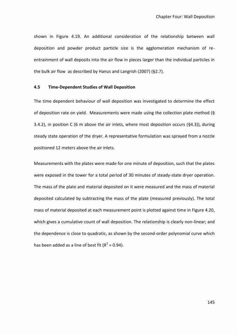
Chapter Four: Wall Deposition
145
shown in Figure 4.19. An additional consideration of the relationship between wall
deposition and powder product particle size is the agglomeration mechanism of re-
entrainment of wall deposits into the air flow in pieces larger than the individual particles in
the bulk air flow as described by Hanus and Langrish (2007) (§2.7).
4.5 Time-Dependent Studies of Wall Deposition
The time dependent behaviour of wall deposition was investigated to determine the effect
of deposition rate on yield. Measurements were made using the collection plate method (§
3.4.2), in position C (6 m above the air inlets, where most deposition occurs (§4.3)), during
steady state operation of the dryer. A representative formulation was sprayed from a nozzle
positioned 12 meters above the air inlets.
Measurements with the plates were made for one minute of deposition, such that the plates
were exposed in the tower for a total period of 30 minutes of steady-state dryer operation.
The mass of the plate and material deposited on it were measured and the mass of material
deposited calculated by subtracting the mass of the plate (measured previously). The total
mass of material deposited at each measurement point is plotted against time in Figure 4.20,
which gives a cumulative count of wall deposition. The relationship is clearly non-linear; and
the dependence is close to quadratic, as shown by the second-order polynomial curve which
has been added as a line of best fit (R2 = 0.94).

Chapter Four: Wall Deposition
146
0.00
0.50
1.00
1.50
2.00
2.50
0 5 10 15 20 25 30
Mas
s D
epso
ited
Per
Un
it A
rea
(kgm
-2)
Time (minutes)
Figure 4.20: Accumulative Wall Deposition
Examining the data points plotted in Figure 4.20 reveals wide variation in deposition rate
between measurement points, with values switching between positive and negative. This
could possibly be a feature of the measurement technique if material was lost during
removal and weighing of the plate, although all efforts were made to keep this to a
minimum. Therefore, we can conclude that this feature at least in part is owing to constant
changes in the material and amount of it deposited as this is a dynamic process.
Other potential sources of errors in this work include small systemic errors such as
inaccuracy of the balance and errors with timing of the period the plate was exposed in
dryer.

Chapter Four: Wall Deposition
147
Another point of interest in Figure 4.20 is that the largest deposition rate is observed for the
first period of measurement (time zero to one minute). This is unexpected (§2.7), with most
literature reporting that particles becoming deposited on bare steel is the limiting step in
deposition (§2.7). To ensure this was a reliable observation and not a freak data point, three
repeats of this initial period of deposition were conducted. The results of these repeats are
shown in Table 3.4 and the actual deposition shown in Figure 4.21. These show that the
amount of material deposited and the inferred rate of deposition is fairly constant between
the initial study and the three repeats, demonstrating this as a reliable trend.
Table 4.3: Initial Deposition Rates
Measurement Amount Deposited
(kg)
Deposition
(kgm-2)
Rate of Deposition
(kgm-2s-1)
30 minute study 0.038 0.73 0.012
Repeat 1 0.036 0.69 0.012
Repeat 2 0.035 0.67 0.011
Repeat 3 0.035 0.67 0.011
Figure 4.21: Initial (1 minute) Wall Deposition Repeats
When compared with published studies on wall deposition in co-current spray dryers the
deposition rates found here are quite large (§2.7). In addition only limited literature

Chapter Four: Wall Deposition
148
considers the idea of wall deposition reaching an equilibrium state (§2.7). This could
potentially be because of the nature of detergent particles and the deposits they form
(bigger particles, forming larger, heavier, but more porous deposits) meaning they are more
likely to experience re-entrainment back into the air flow than other spray dried materials.
This means that wall deposition in detergent spray dryers is more likely to lead to a dynamic
equilibrium between entrainment and deposition than for other spray dried materials.
These initial results were produced during one dedicated pilot plant trial to validate the
technique used here. This trial allowed measurements to be made which gave the results
presented in this section, however, this trial also highlighted problems with the
measurement technique. The main issue with making these measurements is that it requires
opening inspection hatches on the dryer during operation. This results in large amounts of
ambient air flowing through the hatch into the dryer (which is operated under vacuum to
ensure no product escapes). This flow of air into the dryer has a significant effect on its
operation, affecting the drying air flow rate through the drying chamber (Figure 4.22),
disturbing air flow patterns and in turn affecting particle velocities as well as changing the
temperature profile experienced by the particles.

Chapter Four: Wall Deposition
149
0
1000
2000
3000
4000
5000
6000
7000
8000
00:00 05:00 10:00 15:00 20:00 25:00 30:00 35:00 40:00 45:00 50:00 55:00
Air
Flo
w R
ate
(kg.
hr-
1)
Time (minutes)
Figure 4.22: Disruption to dryer air flow rate whilst using collection plates
All of these factors affect the drying of particles as well as their movement, influencing
product properties such as moisture content as well as affecting wall deposition itself.
Therefore, although this technique allowed us to demonstrate the time dependence of wall
deposition, it cannot be considered reliable as opening and closing the inspection hatches
has a significant effect on dryer operation. This means that steady state operation cannot
be achieved whilst using this technique over prolonged periods of time and wall deposition
under normal operating conditions cannot be investigated using this technique. This leaves
an important area of opportunity of research into wall deposition inside spray dryers using
non-intrusive techniques, such as ultrasonics (§8.7).

Chapter Four: Wall Deposition
150
To complement the time dependent findings reported above, visual observations of wall
deposition were made using the PIV set-up utilised in Chapter 6 (§ 3.5). These observations
allowed qualitative investigation of both deposition and re-entrainment of material on the
dryer walls.
An example of these observations is given in Figure 4.23 where the deposition of material on
the dryer wall can be observed for a period of 100 seconds in 20 second increments. The
material deposited on the wall is shown by the white area at the top of the images, the
white spots in the lower part of the image show particles that are entrained in the air flow
travelling past the wall. The scale-bar shown here represents 50 mm over its entire length.
Examining changes in the deposit shown, between frames in Figure 4.23 highlights the
dynamic nature of wall deposition. The size of the deposit grows over the period of
observation and the whole can be seen to increase from frame to frame. However, certain
areas of the deposition can be seen to shrink between frames, showing how some parts of
the deposit break off and are re-entrained in the air flow.

Chapter Four: Wall Deposition
151
0 seconds 20 seconds 40 seconds
60 seconds60 seconds 80 seconds 100 seconds
50 mm
Figure 4.23: Time Dependent Wall Deposition Observed with PIV

Chapter Four: Wall Deposition
152
4.6 Wall Deposition Conclusions
Wall deposition in a detergent spray dryer has been investigated such that the context of the
problem covered in this thesis can be appreciated by the reader. Initially quantitative
observations of deposition on both the macro and micro scales were made using
photography and electron microscopy. The macro scale observations reveal variation in
deposition with location within the dryer in terms of amount and appearance of deposits.
The thickest and most uneven deposits were seen closet the spray nozzle, with deposits
becoming thinner and smoother moving up the dryer away from the nozzle. In the lower
part of the dryer smaller amounts of uneven, and sometime discoloured deposits are seen,
with the exception of the dryer cone where large amounts of hard deposits are seen,
possible as an artefact of slurry or wash water running down the dryer walls during either
start-up or cleaning. Micro scale investigations of deposits from various locations within the
dryer reveal variation in their micro-structures, potentially explaining the trends seen on the
macro-scale observations.
Qualitative studies of wall deposition have been conducted on both the macro and micro
scales. Macro-scale investigation showed how deposition changed with position inside the
dryer, with the thickest and most uneven make-up close to the nozzle and the thinner and
smoother deposits of smaller diameter particles higher up the dryer. Deposits around the air
inlets and cone were shown to be uneven and discoloured in areas exposed to high
temperatures of inlet air. Examination of the microstructure of these deposits have shown
variation between deposits as function of location in the dryer, which may explain the

Chapter Four: Wall Deposition
153
appearance of deposition observed on the macro-scale, with a clear link between the
wetness of particles striking the walls and the roughness of deposits observed.
Quantitative data on the amount of wall deposits formed during spray drying detergents
during a number of operations has been obtained. The amount of deposition was found to
vary between different locations in the dryer (expressed as axial position relative to air
inlets), with the most deposition seen just below the spray nozzle, in agreement with (§ 4.3)
and (§2.7). Large amounts of deposition were also observed in the dryer cone, for some
trials. The amount of deposition in all locations was seen to vary between different dryer
operations (trials), to limit the effect of this variation, a yield expression in terms of the
fraction of the total slurry sprayed that was lost through wall deposition was used.
This yield value was found to vary with dryer operating conditions, with increasing slurry
flow rates found to reduce deposition, whilst increasing air flow rates were found to
increase deposition, both of these operating parameters will alter collision frequency and
success rate. Increasing powder product belt temperature was also found to decrease
deposition, this is thought to be caused by changes in drying, and therefore particles
properties which influence collision success rate. The influence of slurry and powder product
properties on the amount of slurry lost though deposition was also examined. Increasing
surfactant content was found to increase deposition, as was increased slurry and final
product moisture content, an effect suspected to be caused by moisture and organic
components making particles more viscous and therefore more likely to stick and form
deposits, thus increasing collision success rate.

Chapter Four: Wall Deposition
154
Wall deposition has been shown to be time dependent, with a decrease in deposition rate
over a period of 30 minutes. This is believed to be caused by a narrowing of the gap between
the rate of deposition of material and the rate at which material is re-entrained into the air
flow. An interesting feature of the deposition rates measured, was that the initial period of
deposition resulted in the largest deposition rate, which is unexpected and goes against
reports in literature (§2.7). To ensure this observation was reliable, this initial period of
deposition was repeated three times, giving very similar deposition rates, demonstrating this
phenomenon is an actual feature of spray drying detergents.
Observations of wall deposition were made using Particle Image Velocimetry and these
reveal the mechanisms of both deposition and re-entrainment at work within the spray
dryer. Adding strength to the conclusion that wall deposition reaches equilibrium between
deposition and re-entrainment, resulting in its growth first slowing and then stopping over
time of dryer operation.
During this chapter, wall deposition has been simplified into a phenomena which is governed
by two steps, namely collision frequency and collision success rate. The remainder of this
thesis examines these two critical steps in wall deposition in spray drying detergents. Firstly,
fluid dynamics and particle dynamics inside the dryer, which control collision frequency, are
examined in Chapters 5 and 6. Secondly collisions success rate is investigated through work
on understanding the physical and mechanical properties of detergent granules, their impact
behaviour and linking the two in Chapter 7.

Chapter Five: Fluid Dynamics
155
5.0 Chapter 5 – Fluid Dynamics in a Detergent Spray Dryer
5.1 Introduction
Airflow patterns inside spray dryers are known to be of critical importance in determining
product quality and process operation (§2.5). This Chapter details experimental studies of air
flow patterns close to the wall of a counter-current detergent spray dryer. This area has
been studied due to its importance as the area in which most particles travel through the
spray dryer (as they move outwards due to centripetal force of the swirling air flow).
Therefore the air flow patterns in this area determine how particles interact with both each
other and the dryer wall, with the potential consequence of creation of wall build-up or
production of oversized agglomerated particles.
Particle Image Velocimetry (PIV) was used to measure air velocities inside the dryer (§3.5).
The measurements were analysed to investigate turbulent and time-dependent
characteristics of these flows. A comparison is conducted between results from this work
and published work on similar dryers (§ 2.5.4.1).
5.2 Experimental
PIV measurements were made with air only present inside the spray dyer, i.e. no detergent
particles were present. The experiments were conducted in two locations, as shown in
Figure 3.3: the higher position (H) is above and the lower (L) is below the usual location of
the spray nozzle. This allowed the change in airflow pattern due to distance from the air
inlets to be studied. The exact positions, of the areas for which flow fields have been
produced are also shown in Figure 5.1.

Chapter Five: Fluid Dynamics
156
1.700 m
0.161 m
0.161 m
1.700 m
0.165 m
0.165 ma b
Figure 5.1: Locations of image areas relative to spray dryer (a) position L and (b) position H
To examine the influence of air flowrate, three different flowrates were used for
experiments made in position H. This gave four experimental conditions in total, shown
below in Table 5.1. Like many spray dryers, detergent dryers are operated under vacuum,
this prevents unwanted escape of product through any holes/gaps in the dryer. For the
purpose of this work the dryer under-pressure was kept constant at 0.25 kPa.
Table 5.1: Experimental Conditions
Condition Position Air flow rate (kghr-1)
Air inlet tangential velocity (ms-1)
a Lower (L) 10000 (high) 5.1
b Higher (H) 6500 (low) 3.3
c Higher (H) 8000 (medium) 4.1
d Higher (H) 10000 (high) 5.1
Inserting an object into any flow will alter the movement of the fluid (and therefore the flow
patterns observed) as the fluid moves around the object. Installation of the mirror box into
the spray dryer (§3.5.1) is no different. To enable the effect of the box on the flow around it

Chapter Five: Fluid Dynamics
157
to be studied, CFD simulations of the spray dryer were conducted with and without the
mirror box present. These simulations were conducted by BoonHo Ng at P&G’s Beijing
Technical Centre (§3.8) and the results are shown in Figure 5.2. For each of the scenarios
simulated, both contour plots of velocity magnitude and vector plots of the flow field were
generated. The area occupied by the mirror box is shown in orange.
Area Studied
Area Studied
Area Studied
a
b
Figure 5.2: CFD Simulation Results of Flow Fields in Dryer Without (a) and With (b) PIV set-up
Comparison of Figure 5.2 a and b clearly show that the present of the mirror box affects the
flow within the spray dryer, with a wake effect of the box clearly visible on the contour and
vector plots. However, the effect on the flow seems to be most pronounced in areas above

Chapter Five: Fluid Dynamics
158
from the imaged area and therefore it can be concluded that although the mirror box affects
the flow, the effect should not be pronounced in the area where PIV measurements were
made.
The methods used to calculate all parameters displayed as results in this Chapter are given in
the literature review (§ 2.5.3).
5.3 Time Average Velocity Studies
To ensure that the results presented here are representative of the flow, it is important to
check that a sufficiently large sample size of PIV image pairs has been captured. To prove
that this is the case, plots of Root Mean Square (RMS) (§ 2.5.3) and mean velocity magnitude
value against the number of PIV image pairs analysed are shown in Figure 5.3 (for the
position L, at the highest air flow rate). The mean values converge after 150-200 image pairs
and the RMS converges after 200-300 image pairs, showing that the turbulent flow can be
taken as steady-on-average and that the sample size of 1000 image pairs is more than
sufficient.
In order to demostrait the repeatability of these results, three flow fields produced from
different data sets at the same experimental conditions are shown in Figure 5.4. These flow
fields show tight agreement with very little difference in either velocity values or flow
direction, demostraiting strong repeatability in these experiments.

Chapter Five: Fluid Dynamics
159
0 100 200 300 400 500 600 700 800 900 10000
0.5
1
1.5
2
2.5
3Below Nozzle - High Flowrate: Continious Mean of Velocity Magnitude in Spot X-32 Y-32
PIV Image Pairs Analysed
Me
an
Ve
locity M
ag
nitu
de
(m
s-1
)
0 100 200 300 400 500 600 700 800 900 10000
0.05
0.1
0.15
0.2
0.25
0.3
0.35
0.4Below Nozzle - High Flowrate: Continious Standard Deviation of Velocity Magnitude in Spot X-32 Y-32
PIV Image Pairs Analysed
RM
S V
elo
city M
ag
nitu
de
(m
s-1
)
a
b
Figure 5.3: Plots of (a) mean velocity magnitude and (b) RMS velocity versus the number of PIV images
analysed

Chapter Five: Fluid Dynamics
160
x position (mm)
y p
ositio
n (
mm
)
Below Nozzle - High Flowrate: Velocity Magnitude
0 20 40 60 80 100 120 140 1600
20
40
60
80
100
120
140
160
0
0.5
1
1.5
2
2.5
x position (mm)
y p
ositio
n (
mm
)
Below Nozzle - High Flowrate: Velocity Magnitude
0 20 40 60 80 100 120 140 1600
20
40
60
80
100
120
140
160
0
0.5
1
1.5
2
2.5
x position (mm)
y p
ositio
n (
mm
)
Below Nozzle - High Flowrate: Velocity Magnitude
0 20 40 60 80 100 120 140 1600
20
40
60
80
100
120
140
160
0
0.5
1
1.5
2
2.5
Figure 5.4: Flow Field Plots of Velocity Magnitude Absolute Values (ms-1
) (a) position L high flow rate
In the following analysis of the PIV results, the velocity data is displayed as both flow fields
and profile plots for velocity magnitude, radial velocity and tangential velocity. The flow
fields are shown in plan view, with wall situated in the blank space at the top of the plot and
the air flow moving from left to right. Normalised versions of these flow fields are shown in
Appendix C.

Chapter Five: Fluid Dynamics
161
5.3.1 Velocity Magnitude
Figure 5.5 shows flow fields of velocity magnitude values for each of the experimental
conditions studied.
x position (mm)
y p
ositio
n (
mm
)
Above Nozzle - Low Flowrate: Velocity Magnitude
0 20 40 60 80 100 120 140 1600
20
40
60
80
100
120
140
160
0
0.5
1
1.5
2
2.5
x position (mm)
y p
ositio
n (
mm
)
Below Nozzle - High Flowrate: Velocity Magnitude
0 20 40 60 80 100 120 140 1600
20
40
60
80
100
120
140
160
0
0.5
1
1.5
2
2.5
x position (mm)
y p
ositio
n (
mm
)
Above Nozzle - Medium Flowrate: Velocity Magnitude
0 20 40 60 80 100 120 140 1600
20
40
60
80
100
120
140
160
0
0.5
1
1.5
2
2.5
x position (mm)
y p
ositio
n (
mm
)
Above Nozzle - High Flowrate: Velocity Magnitude
0 20 40 60 80 100 120 140 1600
20
40
60
80
100
120
140
160
0
0.5
1
1.5
2
2.5
aa b
c d
Figure 5.5: Flow Field Plots of Velocity Magnitude Absolute Values (ms-1
): (a) position L high flow rate, (b)
position H low flow rate, (c) position H medium flow rate and (d) position H high flow rate.
Values of velocity magnitude along the centre of these flow fields are plotted as a function
of radial position for all four experimental conditions in Figure 5.6.

Chapter Five: Fluid Dynamics
162
r/R Position
0.900.920.940.960.981.00
Velo
city M
agnitude (
ms-1
)
0.0
0.5
1.0
1.5
2.0
2.5
Position L High Flowrate
Position H Low Flowrate
Position H Medium Flowrate
Position H High Flowrate
Figure 5.6: Profile Velocity Magnitude plots
The largest velocities are seen for the lower position with high flow rate condition (Figure 5.5
(a) and blue squares Figure 5.6) and the smallest velocities are seen in the higher position
with low flow rate (Figure 5.5 (b) and green triangles Figure 5.6). Velocities were found to
vary between 0.5 and 2.5 ms-1 in the lower position, depending on radial position and
between 0.8 and 1.8 ms-1 in the higher position, depending on flow rate and radial position.
The observation that velocity was at its highest value in position L at high flow rate and its
lowest value in position H at low flow rate can be explained by examining two key factors
which affect air velocities inside a counter current spray dryer, namely tower location
(height, axial position) and air flow rate (§ 2.5.4).
The effect of axial position (distance from air inlets) can be studied by comparing the two
high flow rate experimental conditions, in the lower position, (Figure 5.5 (a) and blue

Chapter Five: Fluid Dynamics
163
squares in Figure 5.6) and the higher position, (Figure 5.5 (d) and red triangles in Figure 5.6).
This shows that the air velocity (in the horizontal plane) decreases with axial position. This is
an example of swirl decay, (§2.5.4), a decrease in the tangential component of fluid velocity
in a swirling motion with distance from the initial source of swirl. This would be expected, as
described specifically for counter current spray dryers by Bayly et al. (2004) and Muller et al.
(2001), who state that the swirl of the flow decreases as it rises up the tower, as velocity in
the horizontal plane (tangential and radial velocities) decreases with increasing velocity in
the vertical plane (axial velocity). Direct comparison between these results and the results of
previous workers on this phenomenon are given later on in this section.
Comparing the three flow fields displayed for different flow rates of air in the higher
experimental position (Figure 5.5b) to (Figure 5.5c) to (Figure 5.5d) shows that the absolute
values of air velocity magnitude increase with increasing flow rate, as would be expected in
any system where more fluid is passing through the same volume.
Air velocities can be seen to vary across the flow field in both directions, radial and
tangential. The largest values of velocity magnitude are seen in the bottom right hand corner
of every flow field, and conversely the lowest velocities are seen in the top left hand corner
for all flow fields displayed. This is an unanticipated finding as the velocity in the flow fields
would be expected to be tangentially symmetrical. This offset in velocity towards the bottom
right (and top left) corner may be an effect on the air flow patterns of the mirror boxinserted
into the drying chamber (§ 5.2). It would have been anticipated that the velocity would vary
with radial distance only. Most literature on airflow patterns in counter current spray dryers
reports that air velocity (both velocity magnitude and tangential velocity) increases with

Chapter Five: Fluid Dynamics
164
radial distance from the wall at positions close to the wall, as described by the Rankine
vortex model (§2.5.4.2). This trend is shown in all flow fields displayed.
5.3.2 Radial Velocity
Figure 5.8 shows plots of values of radial velocity as a flow field for each of the experimental
conditions studied, profiles of the radial velocity values along the centre line of these flow
fields are shown in Figure 5.7.
r/R Position
0.900.920.940.960.981.00
Radia
l V
elo
city (
ms-1
)
-0.4
-0.3
-0.2
-0.1
0.0
0.1
0.2
Position L High Flowrate
Position H Low Flowrate
Position H Medium Flowrate
Position H High Flowrate
Figure 5.7: Profile Radial Velocity Plots

Chapter Five: Fluid Dynamics
165
x position (mm)
y p
ositio
n (
mm
)
Below Nozzle - High Flowrate: Radial Velocity
0 20 40 60 80 100 120 140 1600
20
40
60
80
100
120
140
160
-1
-0.5
0
0.5
x position (mm)
y p
ositio
n (
mm
)
Above Nozzle - Low Flowrate: Radial Velocity
0 20 40 60 80 100 120 140 1600
20
40
60
80
100
120
140
160
-0.6
-0.4
-0.2
0
0.2
0.4
x position (mm)
y p
ositio
n (
mm
)
Above Nozzle - Medium Flowrate: Radial Velocity
0 20 40 60 80 100 120 140 1600
20
40
60
80
100
120
140
160
-0.6
-0.4
-0.2
0
0.2
0.4
x position (mm)
y p
ositio
n (
mm
)
Above Nozzle - High Flowrate: Radial Velocity
0 20 40 60 80 100 120 140 1600
20
40
60
80
100
120
140
160
-0.6
-0.4
-0.2
0
0.2
0.4
aa b
c dx position (mm)
y p
ositi
on
(m
m)
Above Nozzle - Low Flowrate: Radial Velocity
0 20 40 60 80 100 120 140 1600
20
40
60
80
100
120
140
160
-0.6
-0.4
-0.2
0
0.2
0.4
Figure 5.8: Flow Field Plots of Absolute Values of Radial Velocity (ms-1
): (a) position L high flow rate, (b)
position H low flow rate, (c) position H medium flow rate and (d) position H high flow rate.
The largest velocities are seen in position L with high flowrate condition (Figure 5.8 (a) and
blue squares in Figure 5.7) and the smallest velocities are seen in position H at low flowrate
(Figure 5.8 (b) and green triangles in Figure 5.7). Velocities were found to vary between -1.0
and 0.5 ms-1 in position L and between -0.6 and 0.3 ms-1 in position H depending on flowrate.
The change in sign of these velocities indicates a change in direction across the flow field,
positive velocity values represent movement towards the wall (upwards on the plot) and
conversely negative values represent movement away from the wall (downwards on the

Chapter Five: Fluid Dynamics
166
plot), which may be an effect of the box as shown in the CFD simulation discussed previously
(§ 5.2).
5.3.3 Tangential Velocity
Figure 5.9 shows plots of values of tangential velocity as a flow field for each of the
experimental conditions studied. Profiles of tangential velocity values along the centre line
of these flow fields are shown in Figure 5.10.
x position (mm)
y p
ositio
n (
mm
)
Below Nozzle - High Flowrate: Tangential Velocity
0 20 40 60 80 100 120 140 1600
20
40
60
80
100
120
140
160
0
0.5
1
1.5
2
2.5
x position (mm)
y p
ositio
n (
mm
)
Above Nozzle - High Flowrate: Tangential Velocity
0 20 40 60 80 100 120 140 1600
20
40
60
80
100
120
140
160
0
0.5
1
1.5
2
2.5
x position (mm)
y p
ositio
n (
mm
)
Above Nozzle - Medium Flowrate: Tangential Velocity
0 20 40 60 80 100 120 140 1600
20
40
60
80
100
120
140
160
0
0.5
1
1.5
2
2.5
x position (mm)
y p
ositio
n (
mm
)
Above Nozzle - Low Flowrate: Tangential Velocity
0 20 40 60 80 100 120 140 1600
20
40
60
80
100
120
140
160
0
0.5
1
1.5
2
2.5aa b
c d
Figure 5.9: Flow Field Plots of Absolute Values of Tangential Velocity: (a) position L high flow rate, (b)
position H low flow rate, (c) position H medium flow rate and (d) position H high flow rate.

Chapter Five: Fluid Dynamics
167
r/R Position
0.900.920.940.960.981.00
Ta
ng
en
tia
l V
elo
city (
ms-1
)
0.0
0.5
1.0
1.5
2.0
2.5
Position L High Flowrate
Position H Low Flowrate
Position H Medium Flowrate
Position H High Flowrate
Figure 5.10: Profile Tangential Velocity Plots
The largest velocities are seen in position L high flowrate condition (Figure 5.9 (a) and blue
squares in Figure 5.10) and the smallest velocities are seen in position H at low flowrate
(Figure 5.9 (b) and green triangles in Figure 5.10). Velocities were found to vary between 0.2
and 2.5 ms-1 in position L and between 0.2 and 1.8 ms-1 in position H depending on flowrate.
5.3.4 Comparison with Previous Work
Several studies have been published into air flows within comparable detergent spray
dryers, these studies involve both experimental measurements and application of
Computational Fluid Dynamics (CFD), (§2.5.4). This section presents both qualitative and
quantitative comparisons between the experimental work presented here and published
studies. This comparison starts by examining the trends and key features seen in these

Chapter Five: Fluid Dynamics
168
measurements and relating them to those seen in both measurements and simulations of
similar systems.
Several key trends are seen in the flow fields produced from PIV measurements as a function
of position within the dryer and air flow rate. These can be summarised as an increase in air
velocities in all locations with increasing air flow rate, an obvious trend in consideration of
conservation of mass and momentum (§2.5.3) and not surprisingly this is reported in all
literature on air flows in comparable spray dryers. Although absolute values of velocities and
velocity components are sometime offset in both experiments and simulations, trends in
changes in air velocities due to changes in air flow rates are always in agreement with the
work presented here.
Changes in air velocity with position inside the dryer are a more complex phenomenon and
therefore present more opportunity for disagreement between different studies and also
between measurements and CFD results. Through assuming the dryer is tangentially
symmetrical, these changes in position can be split into two types, changes in radial
positions at a specified axial position and conversely changes in axial position at given radial
positions. These are usually expressed as profiles of velocity or velocity components (radial,
tangential and axial) as a function of radial position, at various axial positions.
Measurements made in this work do not cover the full diameter of the dryer so comparison
with full radial velocity profiles is not possible, however, comparison of values from this
work, Bayly et al. (2004) and Nijdam (2004) are shown in Figure 5.11. Here tangential
velocity profiles are presented as a function of radial position and axial position, allowing the
trends discussed above to be compared between this work and published work. The

Chapter Five: Fluid Dynamics
169
tangential velocities displayed are normalised against the inlet tangential velocities for each
experiment in order to allow comparison between work performed for different dryers at
different flow rates. The axial position is expressed as a fraction of the height of the dryer,
again to enable comparison to be made.
Radial Position (r/R)
0.0 0.2 0.4 0.6 0.8 1.0
Norm
alis
ed T
angential V
elo
city
0.0
0.2
0.4
0.6
0.8
1.0
Bayly et al. (2004) at h/H = 0.3
Bayly et al. (2004) at h/H = 0.9
Nijdam (2004) at h/H = 0.2
Nijdam (2004) at h/H = 0.6
PIV at h/H = 0.3
PIV at h/H = 0.7
Figure 5.11: Comparison of Tangential Velocity Profile Plots with Published Work
The key trends seen and described for the PIV work presented here can be seen in the
published literature complied on Figure 5.11. Changes between the values and shape of
profiles of tangential velocities between the different studies can be explained by the small
difference in dryer geometries and experimental techniques and conditions used. The PIV
data obtained fall on a range of radial positions for which there are few published velocity
data, meaning that definitive conclusions on agreement cannot be made. However, any
changes in velocity values and velocity profile shapes between this work and published

Chapter Five: Fluid Dynamics
170
studies can be explained by changes in dryer geometry, experimental conditions and
techniques including the presence of the mirror box in the drying chamber. One aspect of
these velocity profiles is the rapid increase in tangential velocity with distance from the wall
for the area closest to the wall. This indicates that any boundary layer between the wall and
bulk of the flow is very small and that air is moving at considerable velocities close to the
wall.
All of tangential velocity profiles plotted here display the characteristics of Rankine vortexes,
as report in literature (§2.5.4.2). The changes in the shape of these velocity profiles, as the
peak tangential velocity moves towards the centre of the tower with increasing axial
position, is described by the phenomena of swirl decay (§2.5.4). This was reported by Bayly
et al. (2004), Nijdam (2004) and Sharma (1990) (§2.5.4.1). This means that air flow patterns
are a function of axial position within the dryer, meaning that particle velocities and
trajectories change with axial position, with potential consequences in terms of particle-wall
interaction and its effect on wall deposition.

Chapter Five: Fluid Dynamics
171
5.4 Time Averaged Turbulent Parameters
5.4.1 Turbulence Intensity
Figure 5.12 shows flow field plots of turbulence intensity, as a percentage of mean velocity
magnitude values, (§2.5.3) for all four experimental conditions. Additional turbulent
parameters are shown in Appendix C.
x position (mm)
y p
ositio
n (
mm
)
Above Nozzle - Medium Flowrate: Turbulence Intensity Velocity Magnitude
0 20 40 60 80 100 120 140 1600
20
40
60
80
100
120
140
160
0
1
2
3
4
5
6
7
8
9
10
x position (mm)
y p
ositio
n (
mm
)
Above Nozzle - Low Flowrate: Turbulence Intensity Velocity Magnitude
0 20 40 60 80 100 120 140 1600
20
40
60
80
100
120
140
160
0
1
2
3
4
5
6
7
8
9
10
x position (mm)
y p
ositio
n (
mm
)
Above Nozzle - High Flowrate: Turbulence Intensity Velocity Magnitude
0 20 40 60 80 100 120 140 1600
20
40
60
80
100
120
140
160
0
1
2
3
4
5
6
7
8
9
10
x position (mm)
y p
ositio
n (
mm
)
Below Nozzle - High Flowrate: Turbulence Intensity Velocity Magnitude
0 20 40 60 80 100 120 140 1600
20
40
60
80
100
120
140
160
0
1
2
3
4
5
6
7
8
9
10
a b
c d
Figure 5.12: Turbulence Intensity Plots (% mean velocity magnitude) : (a) position L high flow rate, (b)
position H low flow rate, (c) position H medium flow rate and (d) position H high flow rate.

Chapter Five: Fluid Dynamics
172
Values of turbulence intensity for velocity magnitude vary between 2.0 and 10.0% of the
mean velocity magnitude value, depending on experimental position and air flow rate. Large
values are seen closest to the wall (top of plot) for all experimental conditions, as with the
velocity results, it is unclear if these are an artefact of the measurement technique
(described below) or if they are caused by the presence of the boundary layer at the dryer
wall.
The largest values are seen in position L, ranging from 4.0 to 10%. Smaller values (excluding
edge values) of turbulence intensity are observed in position H, these increase from 2.0 -
4.0% at the low flow rate, through to 2.0 – 5.0% for medium flow and finally 2.5 – 7.0% for
high flow rate. Overall turbulence intensity is seen to increase towards the air inlets at the
bottom of the spray dryer and with increasing flow rate.
An interesting feature present in all four plots is the area of high values of turbulence
intensity, shown as dark red areas at the top of each plot, in the area which is closest to the
dryer wall. Two possible explanations for the appearance of this feature are available; firstly
this is a representation of an area of high turbulence in the boundary layer close to the dryer
wall. The second explanation is that this is a feature of the measurement technique applied
and this area displays artificial values of turbulence as a result of issues with the PIV images
captured and cross-correlation using them, most likely caused by reflection of laser light
from the dryer wall. This feature makes it difficult to draw any definite conclusions on the
levels of turbulence intensity in this area.

Chapter Five: Fluid Dynamics
173
5.5 Time Dependent Velocity Studies
Air flow patterns inside spray dryers are known to be time dependent and this is discussed
widely in literature by amongst others, LeBarbier et al. (2001), Southwell and Langrish
(2001), Muller et al. (2001), Langrish (2009) and Gabites et al. (2010) (§2.5.4.3). This section
examines data obtained from PIV experiments with the aim of detecting time dependence in
the air flows studied.
5.5.1 Velocity Signals and Histograms
Velocity signal plots and histograms of velocity values are shown for values of velocity
magnitude normalised against the mean value of velocity magnitude, in Figure 5.13. These
plots are made for the PIV integration spot (§2.5.2.6) exactly in the centre of the area
investigated (the area of PIV images was broken into a grid of 64 by 64 interrogation
windows, the spot at 32, 32, i.e. in the centre was chosen for this work).
Both signal and histogram plots show how velocity magnitude changes for each of the four
experimental conditions studied. Both of these plots represent 1000 data points captured at
a rate of 1 Hz. Observing signal plots for velocity magnitude for all four experimental
conditions show that the largest amplitude is always seen for position L with high flowrate
condition (Figure 5.13a), indicating the increased turbulence within the flow at this condition
(as seen for turbulence intensity in Figure 5.12) The corresponding histograms show a wider
distribution of velocities than seen for the other three experimental conditions, again
highlighting the increased turbulence observed for position L with high flowrate (Figure
5.13a).

Chapter Five: Fluid Dynamics
174
0 0.2 0.4 0.6 0.8 1 1.2 1.4 1.6 1.8 20
100
200
300
400
500
600
700
800Above Nozzle - High Flowrate: Velocity Magnitude Histogram Spot X-32 Y-32
Normalised Velocity (ms-1)
Fre
quency
0 100 200 300 400 500 600 700 800 900 10000
0.2
0.4
0.6
0.8
1
1.2
1.4
1.6
1.8
2Above Nozzle - High Flowrate: Velocity Magnitude Spot X-32 Y-32 over Time
time (seconds)
Norm
alis
ed V
elo
city (
ms-1
)
a
0 100 200 300 400 500 600 700 800 900 10000
0.2
0.4
0.6
0.8
1
1.2
1.4
1.6
1.8
2Below Nozzle - High Flowrate: Velocity Magnitude Spot X-32 Y-32 over Time
time (seconds)
Norm
alis
ed V
elo
city
0 0.2 0.4 0.6 0.8 1 1.2 1.4 1.6 1.8 20
100
200
300
400
500
600
700
800Below Nozzle - High Flowrate: Velocity Magnitude Histogram Spot X-32 Y-32
Normalised Velocity
Fre
quency
0 100 200 300 400 500 600 700 800 900 10000
0.2
0.4
0.6
0.8
1
1.2
1.4
1.6
1.8
2Above Nozzle - Low Flowrate: Velocity Magnitude Spot X-32 Y-32 over Time
time (seconds)
Norm
alis
ed V
elo
city
0 0.2 0.4 0.6 0.8 1 1.2 1.4 1.6 1.8 20
100
200
300
400
500
600
700
800Above Nozzle - Low Flowrate: Velocity Magnitude Histogram Spot X-32 Y-32
Normalised Velocity
Fre
quency
0 100 200 300 400 500 600 700 800 900 10000
0.2
0.4
0.6
0.8
1
1.2
1.4
1.6
1.8
2Above Nozzle - Medium Flowrate: Velocity Magnitude Spot X-32 Y-32 over Time
time (seconds)
Norm
alis
ed V
elo
city
0 0.2 0.4 0.6 0.8 1 1.2 1.4 1.6 1.8 20
100
200
300
400
500
600
700
800Above Nozzle - Medium Flowrate: Velocity Magnitude Histogram Spot X-32 Y-32
Normalised Velocity
Fre
quency
b
c
d
Figure 5.13: Velocity Magnitude Signal Plots and Velocity Histograms: (a) position L high flow rate, (b)
position H low flow rate, (c) position H medium flow rate and (d) position H high flow rate.
For in position H experimental conditions (b to c to d), the amplitude of the velocity signal
increases, as do the width of distributions on the corresponding velocity histograms. This
may indicate increasing levels of turbulence in the flow as velocity increases, possibly owing

Chapter Five: Fluid Dynamics
175
to increasing Reynolds number of the flow, or may be caused by changes in time dependent
features of the flow with increasing flow rate.
Attempts to observe periodic fluctuations in velocity, caused by oscillation of the vortex due
to time-dependent flow characteristics inside the dryer, were made through observation of
these signal plots. This did not show any visible evidence of periodicity, therefore further
analysis was conducted as described in the next section.
5.5.2 Periodicity
The potential for the presence of time-dependent flow patterns inside spray dryers was
introduced previously (§2.5.4.3). Here attempts were made to investigate this phenomenon
by processing velocity signal plots, displayed in Figure 5.13, applying Fast Fourier Transform
(FFT) analysis using MATLAB 7.1 software (Mathworks Inc.). To enable identification of any
frequencies that may have an associated periodic oscillation in velocity, periodograms were
produced for the spot at the exact centre of the area investigated for all experimental
conditions. These are displayed in Figure 5.14.

Chapter Five: Fluid Dynamics
176
0 0.05 0.1 0.15 0.2 0.25 0.3 0.35 0.4 0.45 0.50
20
40
60
80
100
120
140
160
180
200Above Nozzle - High Flowrate: Periodogram of Velocity Magnitude in Spot X-32 Y-32
Po
we
r
Frequency(cycles/second)
0 0.05 0.1 0.15 0.2 0.25 0.3 0.35 0.4 0.45 0.50
20
40
60
80
100
120
140Above Nozzle - Medium Flowrate: Periodogram of Velocity Magnitude in Spot X-32 Y-52
Po
we
r
Frequency(cycles/second)
0 0.05 0.1 0.15 0.2 0.25 0.3 0.35 0.4 0.45 0.50
50
100
150Above Nozzle - Low Flowrate: Periodogram of Velocity Magnitude in Spot X-32 Y-32
Po
we
r
Frequency(cycles/second)
0 0.05 0.1 0.15 0.2 0.25 0.3 0.35 0.4 0.45 0.50
100
200
300
400
500
600
700Below Nozzle - High Flowrate: Periodogram of Velocity Magnitude in Spot X-32 Y-32
Po
we
r
Frequency(cycles/second)
a b
c d
Figure 5.14: Periodogram plots for centre of all experimental conditions: (a) position L high flow rate, (b)
position H low flow rate, (c) position H medium flow rate and (d) position H high flow rate.
The clarity of the periodograms shown here varies and the power values for any peaks are
much lower than shown for previous studies e.g. Muller et al. (2001) (§2.5.4.3). However, a
weak indication of periodicity is visible in the time frame expected from previous studies,
particularly in the plot for position L and high flow rate which shows a distinctive peak at a
frequency of approximately 0.23 (cycles/seconds). This gives a period of approximately 4
seconds, which is comparable to the period found by Muller et al. (2001).
The lack of clarity from these periodicity studies may be the result of one or a combination
of several properties of the velocity measurements made here, namely:
The position of these measurements is very close to the wall and it is possible that
this area is not exposed to such significant changes in velocity, owing to vortex

Chapter Five: Fluid Dynamics
177
oscillation, as a position much closer to the centre of the drying chamber, as used by
Muller et al. (2001).
Additional turbulence may be generated in the area of measurement by the presence
of material deposited on the dryer walls and/or the mirror box, adding extra noise to
the velocity signal analysed.
The use of PIV as a measurement technique may limit the chances of detecting
periodicity in terms of the spatial resolution (spot-size area) and the temporal
resolution (measurement frequency) being unsuitable to pick-up periodicity in the
vortex.
In conclusion these attempts to study periodicity in the air-flow within the spray dryer have
given an indication of time-dependent behaviour. The period of these oscillations in vortex
have been indicated to be in the range of 4 seconds, which is in agreement with previous
studies (§2.5.4.3). This has paved the way for future investigations examining the effect of
radial position within the drying chamber on periodicity, these studies could potentially
utilise different techniques to avoid the possible effects of using PIV.
5.6 Conclusions
Air flow patterns have been studied inside an industrial scale counter-current detergent
spray-dryer. Experiments were conducted in the horizontal plane in an area adjacent to the
dryer wall. Two different axial positions on the dryer were used, so that the effect of
distance from the air inlets could be studied. Three different air flow rates were used in the
higher position to study the effect of flow rates on flow patterns.

Chapter Five: Fluid Dynamics
178
Time averaged velocity flow fields have been obtained experimentally for velocity magnitude
and the radial and tangential velocity components. These show that the velocity values
obtained for tangential velocity are very similar to the velocity magnitude values calculated
for all experiment conditions, demonstrating that tangential velocity dominates movement
in the horizontal plane. Values of velocity magnitude observed were between 0.5 and 2.5
ms-1 in position L and 0.5 and 1.8 ms-1 in position H depending on flow rate. Tangential
velocity values were almost identical to these. Radial velocities were found to change
direction across the area investigated, with flows towards the wall (positive values) in the
area closest to the oncoming flow (right side) and flow away from the wall (negative values)
in the area furthest from the oncoming flow (left side). The values of radial velocity range
from -1.0 and 0.5 ms-1 in position L and -0.06 and 0.30 ms-1 in position H, depending on
flowrate. The change in radial flow direction may be an effect of the presence of the mirror
box in the flow.
A comparison has been made between time averaged tangential velocity profiles produced
from this work and published studies on similar detergent spray dryers. Common
characteristics and features in tangential velocity profiles show the key trends seen for the
PIV work presented here. This reinforces the conclusions drawn on flow patterns in spray
dryers during this chapter.
Calculations using the experimental velocity data found that, flow in the lower position was
found to exhibit the largest amounts of turbulence with turbulence intensity values of 5 to
10% of the mean velocity magnitude. In addition these trends in turbulence are also seen in
signal and histogram plots of velocity magnitude, for the centre interrogation spot for each

Chapter Five: Fluid Dynamics
179
experimental condition. Attempts to identify periodicity within these velocity signal plots
gave an indication of periods in the area of 4 seconds, however, clear periodgrams were not
produced.

Chapter Six: Particle Dynamics
180
6.0 Chapter 6 – Particle Dynamics in a Detergent Spray Dryer
6.1 Introduction
In Chapter 5, air flow patterns within a counter-current detergent spray dryer were
investigated using PIV. In this Chapter, PIV measurements made on detergent particles
within the process are reported which are used to determine the particle dynamics. The PIV
images were used to obtain particle size, concentration and loading data using bespoke
image analysis methods. Cross-correlation of the images was also conducted to obtain
particle velocities. All of these parameters were examined as a function of dryer operating
conditions and position within the drying chamber.
This chapter begins with a description of the experimental set-up and techniques applied to
obtain the images. The development of image analysis techniques to obtain parameters
from these images is described in Appendix D, such that the reader can understand and
appreciate the principles and assumptions applied to obtain the data. Results displayed here
are firstly for time averaged data, then secondly for time dependent results, before
conclusions are drawn.
6.2 Experimental
Experiments were conducted in two locations, a high position (position H) above the spray
nozzle and a low position (position L) below the spray nozzle; as illustrated in Figure 3.3 (§
3.5). The exact position of the areas for which flow fields have been produced are shown in
Figure 5.1.

Chapter Six: Particle Dynamics
181
1.700 m
0.161 m
0.161 m
1.700 m
0.165 m
0.165 ma b
Figure 6.1: Locations of image areas relative to spray dryer (a) position L and (b) position H
Three different combinations of slurry and air flow rates were applied at each position,
giving six experimental conditions, shown in Table 6.1.
Table 6.1: Operating parameters used for studying particle dynamics
Relative Slurry Flowrate Air Flowrate (kghr-1) Air Inlet Temperature (°C)
Position H
1.0 6000 240
1.2 6000 260
1.2 8000 220
Position L
1.0 6000 240
1.2 6000 260
1.2 8000 220
For all experimental conditions, images were captured for 4 seconds at a rate of 500 Hz,
giving 2000 image pairs per condition. These images were then saved as TIFF files for later
image analysis. The image analysis methods developed and used during this work are
described in Appendix D.

Chapter Six: Particle Dynamics
182
6.3 Results: Time-Averaged Particle Dynamics
Time-averaged results for particle size, loading and concentration inside the spray during
operation are discussed in this section. Each of these parameters is displayed as a function of
dryer operating conditions (Table 3.4) and radial distance from the dryer wall for both
positions L and H. Contour plots for each parameter over the area studied are also shown.
Particle velocity flow fields are also shown for each experimental condition, allowing the
effect of position within the dryer and operating conditions on particle velocities to be
examined.
6.3.1 Particle Size
6.3.1.1 Mean ‘Projected Area’ Particle Size
The mean particle sizes presented are based on the calculated equivalent diameters of
spheres with the same projected area as the irregularly shaped particles in binary images.
This calculation was done using the “regionprops” algorithm in MATLAB which uses the
quantity, /4 PA Ad , is used in calculation of the volumetric shape factor, k, proposed by
Heywood (1962) (Clift et al. (1978)), as 3/ AdVk .
Values of dA are displayed as a function of dryer operating conditions (experimental
conditions) and radial distance from the dryer wall experimental positions L and H in Figure
1.1. The error bars shown here represent an error of one pixel width, at the respective
resolutions. The values vary as a function of slurry flow rate and position (H or L) with the
largest values of 800 – 1000 µm being observed for position L. This was expected as most
particles travel down through the dryer from the nozzle (Bayly (2008)). Smaller values of dA

Chapter Six: Particle Dynamics
183
were seen at position H as only the minority of smaller particles are sufficiently entrained in
the airflow to be carried above the nozzle.
r/R Position
0.840.860.880.900.920.940.960.981.00
Me
an
"P
roje
cte
d A
rea
" P
art
icle
Siz
e (
m)
0
200
400
600
800
1000
1200
1400
1.0 Relative Slurry 6000 (kghr-1) Air Lower
1.2 Relative Slurry 6000 (kghr-1) Air Lower
1.2 Relative Slurry 8000 (kghr-1) Air Lower
1.0 Relative Slurry 6000 (kghr-1) Air Higher
1.2 Relative Slurry 6000 (kghr-1) Air Higher
1.2 Relative Slurry 8000 (kghr-1) Air Higher
Figure 6.2: Mean projected area diameter, dA as a Function of Radial Position
Regardless of flow rate or height of measurement, the values of dA decrease with radial
distance from dryer wall both above and below the nozzle, this is may be explained by the
effect of the swirling flow inducing centripetal forces on the particles, in effect “throwing”
them out towards the wall. This is a process which is preferential to larger particles, as
smaller particles are more easily deviated as they have less inertia and are therefore more
likely to follow the swirl of the air. Whereas the trajectory of the larger particles is

Chapter Six: Particle Dynamics
184
influenced by the swirl to a lesser extent (due to larger momentum/inertia), meaning that
they move more directly through the dryer than moving round closer to the wall.
To explain the above particle sizes and mass results, the process by which the detergent
slurry is atomised and then dried to create the final powder product inside a spray dryer
needs to be examined. The first step in this process is atomisation, which turns the
detergent slurry into discrete droplets, which will eventually form the particles of detergent
powder. Therefore the droplet size produced is a critical parameter in determining the
particle size within the process and product. Atomisation is achieved through use of a
pressure nozzle (§2.3.4), and the size distribution of droplets obtained is highly dependent
on the type of nozzle and pressure/flow rate of the slurry. In general the droplet size
obtained from atomisation is known to decrease with increasing nozzle pressure, which is a
direct function of the slurry flow rate, due to increased shear rates in the nozzle (§2.3.4).
This would suggest that a smaller droplet size should be obtained at higher slurry flow rates
in the experiments. However, the data shown in Figure 6.8 show the opposite trend, with an
increase in dA with increased slurry flow rate (at constant air flow rate).
This suggests that other phenomena within the dryer are affecting particle size. Both drying
and agglomeration have a significant effect (Hecht (2004)) and are heavily influenced by
dryer operating conditions. As described in the literature review (§2.3.6) drying occurs due
to simultaneous heat and mass transfer, this process involves initial shrinkage as water is
lost through drying and is followed by steam puffing (§2.3.6), which leads to expansion in
particle size as a porous structure is developed in the drying particle. Since the trajectories

Chapter Six: Particle Dynamics
185
of individual particles are different, it is not possible to determine a priori the extent of
puffing as a function of position in the dryer.
Agglomeration is known to drive particle size distribution in spray drying operations (§2.3)
and requires firstly that particles come into contact with each other, and secondly that these
collisions result in the particles sticking to each other, referred to as collision frequency and
collision success rate respectively. Collision frequency is a function of the concentration
(number and loading) of particles inside the dryer and the velocity and turbulence of the air
flow through which the particles are travelling. The collision success rate is affected by
moisture content, structure, mechanical and physical properties of particles.
In addition to agglomeration of particles colliding in the flow, particles deposited on the
walls will be brought into contact with impacting particles from the bulk. The process of wall
deposition is known to be affected by both dryer operating conditions and the duration of
operation, as the layers deposited build-up over time (§2.7). This process is dynamic and
material is re-entrained into the air flow as well as deposited onto the wall. The material re-
entrained will most likely break off in large agglomerated lumps. The rate of re-entrainment
and the size of the particles re-joining the air flow will depend on many factors, such as the
nature of the particles deposited, dryer operating conditions and the duration for which the
dryer has been operated, but in particularly it will depend on the air velocity and turbulence
passing over it, as described by Hanus and Langrish (2007) (§2.7.4). This mechanism is only
applicable to areas which experience wall deposition, and therefore is most likely to occur
below the nozzle, where wall deposition is observed.

Chapter Six: Particle Dynamics
186
The data shown in Figure 6.4 and Figure 6.5 suggest that both agglomeration mechanisms
are indeed the driver for the observed particle sizes. In particular they drive the creation of
particles which are much bigger than those created by atomisation and puffing of single
particles during drying. The size distributions in the Position L contain particles which are up
to ten times the diameter of typical atomised droplets (Bayly (2008)). As the air flow rate
rises, the collision frequency between the particles would be expected to rise due to the
increased air velocities, and thus turbulence, inside the dryer. Comparing the data taken at
1.2 relative slurry flowrate and 8000 kghr-1 air flow rate (black squares) with the data at 1.2
relative slurry flowrate and 6000 kghr-1 (green squares), there is a noticeable rise in particle
size. Reducing the relative slurry flowrate to 1.0 at the lower air flowrate used has a smaller
effect and the particle sizes are the same within experimental error. In position H, these
trends appear to be less clear, as would be expected, as the particle size distribution above
the nozzle depends on entrainment of particles in the air flow rather than agglomeration
Figure 6.3 shows contour plots of dA over the measured field of view. Whilst at position H,
the diameter observed is a strong function of y position and a weak function of x, this is not
the case for position L where the distribution is clearly two dimensional.
In order to explain this, two main hypotheses have been put forward as possible reasons for
the asymmetrical results in the tangential direction below the nozzle:
1. Distorted airflow patterns possibly caused by the mirror box (inserted into the drying
chamber) (§ 5.3).

Chapter Six: Particle Dynamics
187
2. Re-entrainment of material deposited on the side of the mirror box passing through
the field of view.
Distorted airflow patterns. The offset in velocity towards the bottom right (and top left)
corner shown in Figure 5.5 (§5.3) may be an effect of the mirror box on the air flow patterns.
Air flow patterns in the dryer are known to move in all three dimensions, it is difficult to
understand the full extent of these distortions on the flow patterns since PIV cannot be used
without the mirror box. However, it is easy to envisage a situation where the distortion in
air flow could have the effect of carrying more particles into the region of the image where
the radial air flow is towards the wall (left hand side), conversely, where the radial
component air flow is moving away from the wall, particles may be carried out or moved
away from the image.
Re-entrainment of material. Material was observed to build-up on the mirror box, through
the same mechanism as wall-deposition. Therefore it would be expected that material would
be re-entrained into the air flow from the mirror box; if this was to move downwards under
the influence of gravity it could well pass through the affected area of the image. This could
result in a significant amount of large particles passing through a specific area of the image,
as observed. In addition the fact this asymmetry is only observed in position L, where wall
deposition occurs, is an indicator this is the reason behind the discussed asymmetry.
The likelihood of the situation is that this observation is a combination of both factors which
cannot be fully understood with the data available.

Chapter Six: Particle Dynamics
188
x position (mm)
y p
ositio
n (
mm
)
1200kghr-1 Slurry 8000kghr-1 Air Above Nozzle: Mean Particle Diameter
0 20 40 60 80 100 120 1400
20
40
60
80
100
120
140
0
100
200
300
400
500
600
700
800
900
1000
x position (mm)
y p
ositio
n (
mm
)
1200kghr-1 Slurry 6000kghr-1 Air Above Nozzle: Mean Particle Diameter
0 20 40 60 80 100 120 1400
20
40
60
80
100
120
140
0
100
200
300
400
500
600
700
800
900
1000
x position (mm)
y p
ositio
n (
mm
)
1000kghr-1 Slurry 6000kghr-1 Air Above Nozzle: Mean Particle Diameter
0 20 40 60 80 100 120 1400
20
40
60
80
100
120
140
0
100
200
300
400
500
600
700
800
900
1000
x position (mm)
y p
ositio
n (
mm
)
1000kghr-1 Slurry 6000kghr-1 Air Below Nozzle: Mean Particle Diameter
0 20 40 60 80 1000
20
40
60
80
100
0
100
200
300
400
500
600
700
800
900
1000
x position (mm)
y p
ositio
n (
mm
)
1000kghr-1 Slurry 6000kghr-1 Air Below Nozzle: Mean Particle Diameter
0 20 40 60 80 1000
20
40
60
80
100
0
100
200
300
400
500
600
700
800
900
1000
x position (mm)
y p
ositio
n (
mm
)
1200kghr-1 Slurry 8000kghr-1 Air Below Nozzle: Mean Particle Diameter
0 20 40 60 80 1000
20
40
60
80
100
0
100
200
300
400
500
600
700
800
900
1000
x position (mm)
y p
ositi
on
(m
m)
1200kghr-1 Slurry 8000kghr-1 Air Above Nozzle: Mean Particle Diameter
0 20 40 60 80 1000
20
40
60
80
100
0
100
200
300
400
500
600
700
800
900
1000
A
B
Figure 6.3: Mean Particle Size Contour Plots: (A) Position L and (B) Position H

Chapter Six: Particle Dynamics
189
6.3.1.2 Particle Size Distribution
Particle size distributions for each experimental condition in experimental position L are
shown in Figure 6.4, and those for experimental position H in Figure 6.5. These size
distributions are taken over the whole field of view and averaged over 4 seconds (2000
images) and presented as both mass fraction and number distributions. The D10, D50 and D90
values (i.e. the percentage less than size), by mass, assuming spherical particles with
projected area diameter as diameter of the sphere), are marked on each mass distribution
plot. Comparison of the mass and number distribution plots for all experimental conditions
show that by number, the smallest particle size possible is clearly the most common. The
number of particles present decreases rapidly with increasing particle size for all
experimental conditions. Direct comparison of between positions H and L for all
experimental conditions show unsurprisingly that larger particle sizes occur more frequently
at position L and the distribution of particle size here is much wider. The nature of
distribution appears to change between experimental conditions in both locations,
demonstrating that slurry and air flow rates influence particle size distribution.
The range of particle sizes in the lower position is much wider than would be expected
looking at typical spray dried detergent powder product size distributions, where the
maximum particle size is usually in the order of 1000-2000 µm (Huntington (2004), this may
indicate that both particle growth through agglomeration and size reduction through
attrition/abrasion and breakage occur during the spray drying process.

Chapter Six: Particle Dynamics
190
Projected Area Diameter, dA (m)
0 1000 2000 3000 4000 5000
Ma
ss F
ractio
n
0.0
0.1
0.2
0.3
D90
D10 D50
Projected Area Diameter, dA (m)
0 1000 2000 3000 4000 5000
Ma
ss F
ractio
n
0.0
0.1
0.2
0.3
D90
D10
D50
Projected Area Diameter, dA (m)
0 1000 2000 3000 4000 5000
Mass F
raction
0.0
0.1
0.2
0.3
D90
D10D50
C
B
A
Projected Area Diameter, dA (m)
0 1000 2000 3000 4000 5000
Nu
mb
er
Fra
ctio
n
0.0
0.2
0.4
0.6
0.8
Projected Area Diameter, dA (m)
0 1000 2000 3000 4000 5000
Nu
mb
er
Fra
ctio
n
0.0
0.2
0.4
0.6
0.8
Projected Area Diameter, dA (m)
0 1000 2000 3000 4000 5000
Nu
mb
er
Fra
ctio
n
0.0
0.2
0.4
0.6
0.8
Figure 6.4: Particle size distributions position L (a) 1.0 relative slurry and 6000 kghr-1
air; (b) 1.200 relative
slurry and 6000 kghr-1
air and (C) 1.2 relative slurry and 8000 kghr-1
air.

Chapter Six: Particle Dynamics
191
Projected Area Diameter, dA (m)
0 1000 2000 3000 4000 5000
Mass F
raction
0.0
0.1
0.2
0.3
D90
D50
D10
Projected Area Diameter, dA (m)
0 1000 2000 3000 4000 5000
Mass F
raction
0.0
0.1
0.2
0.3
D90
D50
D10
Projected Area Diameter, dA (m)
0 1000 2000 3000 4000 5000
Ma
ss F
ractio
n
0.0
0.1
0.2
0.3
D90
D50
D10
C
B
A
Projected Area Diameter, dA (m)
0 1000 2000 3000 4000 5000
Nu
mb
er
Fra
ctio
n
0.0
0.2
0.4
0.6
0.8
Projected Area Diameter, dA (m)
0 1000 2000 3000 4000 5000
Nu
mb
er
Fra
ctio
n
0.0
0.2
0.4
0.6
0.8
Projected Area Diameter, dA (m)
0 1000 2000 3000 4000 5000
Nu
mb
er
Fra
ctio
n
0.0
0.2
0.4
0.6
0.8
Figure 6.5: Particle size distributions position H (a) 1.0 relative slurry and 6000 kghr-1
air; (b) 1.200 relative
slurry and 6000 kghr-1
air and (C) 1.2 relative slurry and 8000 kghr-1
air.

Chapter Six: Particle Dynamics
192
The results shown in Figure 6.4 and Figure 6.5 can also be explained in the context of particle
agglomeration. These distributions all appear binominal or multinomial, suggesting that the
mechanism that leads to particles forming is not a gradual growth of particles through
agglomeration of particles entrained in flow, as would be captured by the “snap-shot” of
images, but rather a sudden, discontinuous process of pieces of wall deposited material
being re-entrained in the flow.
The amount of material deposited on the dryer walls, and therefore re-entrained in the air
flow will increase over the period of dryer operation, and we would expect agglomeration
through this mechanism to change accordingly. Therefore the times at which each
experiment was done need to be considered. As this mechanism is only possible where wall
deposition is observed, it is only applicable to position L, where the experiments were run as
follows, 1.0 releative slurry flow rate, 6000 kghr-1 air was run on one day, then on the next
day, 1.2 releative slurry flow rate, 6000 kghr-1 was run first, and then followed by 1.2
releative slurry flowrate, 8000 kghr-1. The particle size distributions (Figure 6.4) show that
the effect of duration of dryer operation may contribute to the amount of large particles
observed in the distributions, as 1.0 releative slurry flow rate, 6000 kghr-1 and 1.2 releative
slurry flow rate, 6000 kghr-1 appear similar, where as 1.2 releative slurry flow rate, 8000
kghr-1, which was conducted after the longest period of operation, shows a wider
distribution of larger particle sizes.
6.3.2 Particle Number Concentration, C
The number of particles per unit volume, C (calculated based on the volume of the
lasersheet, §D.3) displayed as a function of radial position from the dryer wall is shown in

Chapter Six: Particle Dynamics
193
Figure 6.6 and can be seen to vary as a function of slurry and air flow rate and location in the
dryer.
r/R Position
0.840.860.880.900.920.940.960.981.00
Pa
rtic
le C
on
ce
ntr
atio
n,
C (
m-3
)
0.0
5.0e+6
1.0e+7
1.5e+7
2.0e+7
2.5e+7
3.0e+7
3.5e+7
1.0 Relative Slurry 6000 (kghr-1) Air Lower
1.2 Relative Slurry 6000 (kghr-1) Air Lower
1.2 Relative Slurry 8000 (kghr-1) Air Lower
1.0 Relative Slurry 6000 (kghr-1) Air Higher
1.2 Relative Slurry 6000 (kghr-1) Air Higher
1.2 Relative Slurry 8000 (kghr-1) Air Higher
Figure 6.6: Particle Concentration, C, as a Function of Radial Position
The largest values of C are, unsurprisingly, observed for the higher slurry flow rates at
Position L. The concentration of particles for lower slurry flow rate in the lower position is
comparable to the concentrations seen in the higher position. The number of particles
present is of course a function of slurry flow rate and particle size (§ 6.3.1), i.e. for the lower
position the particles are bigger, so there is more slurry contained in a similar number of
particles than in the higher position. The concentration of particles decreases with
increasing radial distance from the dryer wall, highlighting again the effect of the swirling air
flow on particle movement as its centripetal forces “throw” particles out towards the dryer
walls.

Chapter Six: Particle Dynamics
194
Figure 6.7 shows contour plots of particle concentration over area studied at each
experimental condition in each position. Similarly to Figure 6.9, asymmetrical patterns are
seen in position L, as particle concentration changes in both the radial and tangential
directions. The hypothesis for this described above also applies here.

Chapter Six: Particle Dynamics
195
x position (mm)
y p
ositio
n (
mm
)
1200kghr-1 Slurry 8000kghr-1 Air Above Nozzle: Mean Particle Concentration
0 20 40 60 80 100 120 1400
20
40
60
80
100
120
140
0
0.5
1
1.5
2
2.5
3
3.5
4
4.5
5x 10
7
x position (mm)
y p
ositio
n (
mm
)
1200kghr-1 Slurry 6000kghr-1 Air Above Nozzle: Mean Particle Concentration
0 20 40 60 80 100 120 1400
20
40
60
80
100
120
140
0
0.5
1
1.5
2
2.5
3
3.5
4
4.5
5x 10
7
x position (mm)
y p
ositio
n (
mm
)
1000kghr-1 Slurry 6000kghr-1 Air Above Nozzle: Mean Particle Concentration
0 20 40 60 80 100 120 1400
20
40
60
80
100
120
140
0
0.5
1
1.5
2
2.5
3
3.5
4
4.5
5x 10
7
x position (mm)
y p
ositio
n (
mm
)
1000kghr-1 Slurry 6000kghr-1 Air Above Nozzle: Mean Particle Concentration
0 20 40 60 80 1000
20
40
60
80
100
0
0.5
1
1.5
2
2.5
3
3.5
4
4.5
5x 10
7
x position (mm)
y p
ositio
n (
mm
)
1000kghr-1 Slurry 6000kghr-1 Air Below Nozzle: Mean Particle Concentration
0 20 40 60 80 1000
20
40
60
80
100
0
0.5
1
1.5
2
2.5
3
3.5
4
4.5
5x 10
7
x position (mm)
y p
ositio
n (
mm
)
1200kghr-1 Slurry 6000kghr-1 Air Below Nozzle: Mean Particle Concentration
0 20 40 60 80 1000
20
40
60
80
100
0
0.5
1
1.5
2
2.5
3
3.5
4
4.5
5x 10
7
x position (mm)
y p
ositio
n (
mm
)
1200kghr-1 Slurry 8000kghr-1 Air Below Nozzle: Mean Particle Concentration
0 20 40 60 80 1000
20
40
60
80
100
0
0.5
1
1.5
2
2.5
3
3.5
4
4.5
5x 10
7
A
B
Figure 6.7: Particle Concentration Contour Plots: (A) Position L and (B) Position H

Chapter Six: Particle Dynamics
196
6.3.3 Particle Volume Fraction
Particle volume fractions were calculated by taking the projected area diameter of each
particle, dA to be a spherical equivalent diameter on the basis of volume, dV, hence
63
VdV . These data were then summed for that area of the image and divided by the
volume of the area of the image. This data is shown as a function of radial position from the
dryer wall in Figure 6.8.
r/R Position
0.840.860.880.900.920.940.960.981.00
Pa
rtic
le V
olu
me
Fra
ctio
n
0.0000
0.0002
0.0004
0.0006
0.0008
1.0 Relative Slurry 6000 (kghr-1) Air Lower
1.2 Relative Slurry 6000 (kghr-1) Air Lower
1.2 Relative Slurry 8000 (kghr-1) Air Lower
1.0 Relative Slurry 6000 (kghr-1) Air Higher
1.2 Relative Slurry 6000 (kghr-1) Air Higher
1.2 Relative Slurry 8000 (kghr-1) Air Higher
Figure 6.8: Particle Volume Fraction as a Function of Radial Position
Particle volume fraction can be seen to vary as a function of slurry and air flow rate and
location in the dryer. The largest particle volume fractions are seen in position L, as would be
expected with the majority of particle heading downwards from the nozzle. In this lower

Chapter Six: Particle Dynamics
197
position both slurry and air flow rates appear to affect particle volume fraction, which
appears to decrease linearly with distance from the dryer wall.
Lower particle volume fractions are observed in position H (above the nozzle), with less
effect of slurry and air flow rates seen apart from in the area closest to the dryer wall, where
slurry rate seems to significantly increase particle volume fraction. The decrease in particle
volume fraction with distance from the dryer wall seems to be less dramatic than that seen
in position L, with a rapid decrease close to the wall before the rate of change slows with
increasing distance from the wall.
Contour plots of particle volume fraction over the areas studied are shown in Figure 6.9,
which demonstrate all of the trends discussed above and observed in Figure 6.8. As with the
previous two particle dynamics parameters, asymmetrical distribution of values in position L
can be observed and again the hypothesis for this described above applies here too.

Chapter Six: Particle Dynamics
198
x position (mm)
y p
ositio
n (
mm
)
1200kghr-1 Slurry 8000kghr-1 Air Above Nozzle: Mean Particle Volume Fraction
0 20 40 60 80 100 120 1400
20
40
60
80
100
120
140
0
0.1
0.2
0.3
0.4
0.5
0.6
0.7
0.8
0.9
1x 10
-3
x position (mm)
y p
ositio
n (
mm
)
1200kghr-1 Slurry 6000kghr-1 Air Above Nozzle: Mean Particle Volume Fraction
0 20 40 60 80 100 120 1400
20
40
60
80
100
120
140
0
0.1
0.2
0.3
0.4
0.5
0.6
0.7
0.8
0.9
1x 10
-3
x position (mm)
y p
ositio
n (
mm
)
1000kghr-1 Slurry 6000kghr-1 Air Above Nozzle: Mean Particle Volume Fraction
0 20 40 60 80 100 120 1400
20
40
60
80
100
120
140
0
0.1
0.2
0.3
0.4
0.5
0.6
0.7
0.8
0.9
1x 10
-3
x position (mm)
y p
ositio
n (
mm
)
1200kghr-1 Slurry 8000kghr-1 Air Above Nozzle: Mean Particle Volume Fraction
0 20 40 60 80 1000
20
40
60
80
100
0
0.1
0.2
0.3
0.4
0.5
0.6
0.7
0.8
0.9
1x 10
-3
x position (mm)
y p
ositio
n (
mm
)
1000kghr-1 Slurry 6000kghr-1 Air Below Nozzle: Mean Particle Volume Fraction
0 20 40 60 80 1000
20
40
60
80
100
0
0.1
0.2
0.3
0.4
0.5
0.6
0.7
0.8
0.9
1x 10
-3
x position (mm)
y p
ositio
n (
mm
)
1200kghr-1 Slurry 6000kghr-1 Air Below Nozzle: Mean Particle Volume Fraction
0 20 40 60 80 1000
20
40
60
80
100
0
0.1
0.2
0.3
0.4
0.5
0.6
0.7
0.8
0.9
1x 10
-3
x position (mm)
y p
ositio
n (
mm
)
1200kghr-1 Slurry 8000kghr-1 Air Below Nozzle: Mean Particle Volume Fraction
0 20 40 60 80 1000
20
40
60
80
100
0
0.1
0.2
0.3
0.4
0.5
0.6
0.7
0.8
0.9
1x 10
-3
A
B
Figure 6.9: Particle Volume Fraction Contour Plots: (A) Position L and (B) Position H

Chapter Six: Particle Dynamics
199
6.3.4 Particle Flow Fields
PIV cross-correlation (§D.3) was used to obtain time-averaged particle velocity fields, which
are shown in Figure 6.10. Particle velocities in Position H are much larger than those in
Position L. This suggests that two different flow regimes exist within the dryer, depending
on position relative to the spray nozzle. Simplistically these two regimes can be described as
a flow containing a higher loading of larger particles, which move more slowly in the
horizontal plane (as measured here) below the nozzle, and a sparser flow of smaller particles
moving faster in the horizontal plane above the nozzle. A further feature distinguishing the
two regimes is the direction of flow observed: above the nozzle all particle velocities seem to
be tangential, moving parallel to the dryer wall, below the nozzle in position L, the direction
of particle velocities appear to be less well defined. Although tangential velocity still seems
to dominate here, all three experimental conditions show more deviation from the strictly
tangential flow above the nozzle, this could be an indication of more turbulent air flow
patterns in this position or an effect of extra turbulence caused by proximity to the nozzle.
In position L velocities are seen to vary between 0.0 and 0.2 ms-1, the effect of slurry and air
flow rates appears to be small, with the 1.0 releative slurry flow rate and the 6000 kghr-1 air
flow rate experimental condition showing slightly larger velocities than the other two
experimental conditions. On the whole, all velocities in the horizontal plane, in this region
appear to be much lower than those of air flow alone, as shown in Figure 5.5 (§5.3).
Although particles would be expected to have lower velocities than air, the fact the
velocities differ by an order of magnitude is unexpected and may be explained by
considering the motion of particles in the axial direction. The reason behind this discrepancy

Chapter Six: Particle Dynamics
200
may lie in both the nature of the particles and the proximity of the experimental position to
the nozzle. Particles which have just left the nozzle will have experienced little drying relative
to those which have been inside the dryer for a longer period, and will be contain lots of
water in a solid structure, making them much denser than dried and puffed particles.
Therefore they are more likely to fall under the influence of gravity before becoming
entrained in the swirling air flow. In addition to the nature of the particles, the movement of
particles in this area of the dryer may be heavily influenced by momentum they obtain from
atomisation through the nozzle, this momentum is likely to result in the velocity in the axial
direction, and could therefore explain the lack of velocity observed in the horizontal plane.
These observations may be a feature of the location used for the experiment, and if images
were captured further away from the nozzle, particles may demonstrate higher velocities in
the horizontal plane as particles becoming increasingly entrained in the air flow. This effect
appears to be particularly pronounced for the low air flow rate, high slurry flow rate in
position L where the particle velocities appear to be the smallest and in the most variety of
scattered directions. This could be explained if a point is reached where the amount of air
flowing through the dryer isn’t sufficient to entrain the amount of slurry atomisied into
particles. This could also explain the large standard deviation in particle velocities (Figure
6.12) observed for this condition.
Another possible explanation for the observation of smaller than expected velocities in the
horizontal plane could be an artefact of the measurement and analysis technique applied
here, PIV only captures average particle velocities and therefore could filter out individual
particle velocities and result in a small average velocity (especially if particles in the same

Chapter Six: Particle Dynamics
201
interrogation spot are moving in opposite directions). Issues with special and temporal
resolutions could limit the ability of the technique used here to detect changes in direction
over time and also filter out the smallest levels of variation in particle direction.
Velocities in both locations can be seen to be constant as a function of radial distance from
the wall, with the exception of the area close to the dryer wall (top of plots) which may
indicate the presence of a boundary layer in the airflow, which slows particles down. This
could also be an artefact of the measurement technique as is seen on a smaller scale around
all edges of the plot.
Velocities in position H were found to vary between 0.2 and 0.4 ms-1, depending on dryer
operating conditions, showing that in the sparser regime above the nozzle, the effect of air
flow and also of slurry flow rate, and therefore particle loading inside the dryer, influence
how particles move.
In order to further understand the results presented here, the statistics of the data produced
have been examined. Figure 6.11 shows the number of velocity vectors generated during
cross correlation, i.e. the number of data points used to calculate the time averaged velocity
in each interrogation spot. The number of vectors is plotted as the colour fill on the contour,
where blue represents zero, i.e. no velocity vectors were successfully generated through
cross-correlation and where red represents 2000, i.e. a velocity vector was suitably
generated for that spot with every pair of images processed. The velocity vectors of the
particle flow field are plotted over this to allow comparison between the number of vectors
generated and the velocity calculated in each spot. Examining the number of velocity vectors

Chapter Six: Particle Dynamics
202
generated in each integration spot (Figure 6.11) reveals that there is a close link between the
number of vectors generated and particle number concentration (Figure 6.7).

Chapter Six: Particle Dynamics
203
x position (mm)
y p
ositio
n (
mm
)
Above Nozzle - Low Slurry Flowrate and Low Air Flowrate : Velocity Magnitude
0 20 40 60 80 100 120 1400
20
40
60
80
100
120
140
0
0.05
0.1
0.15
0.2
0.25
0.3
0.35
0.4
0.45
0.5
x position (mm)
y p
ositio
n (
mm
)
Below Nozzle - Low Slurry Flowrate and Low Air Flowrate : Velocity Magnitude
0 20 40 60 80 1000
20
40
60
80
100
0
0.05
0.1
0.15
0.2
0.25
0.3
0.35
0.4
0.45
0.5
x position (mm)
y p
ositio
n (
mm
)
Below Nozzle - Low Slurry Flowrate and Low Air Flowrate : Velocity Magnitude
0 20 40 60 80 1000
20
40
60
80
100
0
0.05
0.1
0.15
0.2
0.25
0.3
0.35
0.4
0.45
0.5
x position (mm)
y p
ositio
n (
mm
)
Below Nozzle - High Slurry Flowrate and Low Air Flowrate : Velocity Magnitude
0 20 40 60 80 1000
20
40
60
80
100
0
0.05
0.1
0.15
0.2
0.25
0.3
0.35
0.4
0.45
0.5
x position (mm)
y p
ositio
n (
mm
)
Below Nozzle - High Slurry Flowrate and High Air Flowrate : Velocity Magnitude
0 20 40 60 80 1000
20
40
60
80
100
0
0.05
0.1
0.15
0.2
0.25
0.3
0.35
0.4
0.45
0.5
x position (mm)
y p
ositio
n (
mm
)
Above Nozzle - High Slurry Flowrate and Low Air Flowrate : Velocity Magnitude
0 20 40 60 80 100 120 1400
20
40
60
80
100
120
140
0
0.05
0.1
0.15
0.2
0.25
0.3
0.35
0.4
0.45
0.5
x position (mm)
y p
ositio
n (
mm
)
Above Nozzle - High Slurry Flowrate and High Air Flowrate : Velocity Magnitude
0 20 40 60 80 100 120 1400
20
40
60
80
100
120
140
0
0.05
0.1
0.15
0.2
0.25
0.3
0.35
0.4
0.45
0.5
A
B
Figure 6.10: Time Average Particle Flow Fields (ms-1
): (A) Position L and (B) Position H

Chapter Six: Particle Dynamics
204
This pattern is highlighted in position L where both particle number concentration and the
number of velocity vectors generated are at a maximum close to the wall and in an
asymmetric fashion towards the left hand side of the image and in position H where the
number of vectors and particle number concentration are at a maximum close to the wall.
The link between the number of vectors generated and the velocity calculated for each spot
appears to be unclear, with one dataset showing a clear link between maximum velocities
and the highest number of vectors generated (position L (below the nozzle) the 1.0 releative
slurry flow rate and 6000 kghr-1 air), and all other data sets display velocities which appear
independent of the number of vectors generated. The apparent independence of velocities
from the number of vectors generated allows confidence in the data generated as it
demonstrates the velocities calculated here are not a function of the technique and analysis
applied. Although results produced in areas with more vectors generated are more likely to
be reliable than those produced in areas with fewer vectors generated, as would be
expected. This leads to the conclusion that, as a general point, velocity data plotted in areas
closer to the wall are more reliable than those further away from the wall.
To further understand the results presented here, the standard deviation of the time
averaged particle velocities are plotted with the actual velocity vectors over them in Figure
6.12. The standard deviations presented here are in ms-1 and show values similar to the
velocity magnitude in Figure 6.10, indicating that there is large variation in particle velocities
over the period of measurement, particularly for position L (below the nozzle) the 1.2
releative slurry flow rate and 6000 kghr-1 air conditions.

Chapter Six: Particle Dynamics
205
x position (mm)
y p
ositio
n (
mm
)
Above Nozzle - High Slurry Flowrate and High Air Flowrate: Vectors per Spot
0 20 40 60 80 100 120 1400
20
40
60
80
100
120
140
0
200
400
600
800
1000
1200
1400
1600
1800
2000
x position (mm)
y p
ositio
n (
mm
)
Above Nozzle - High Slurry Flowrate and Low Air Flowrate: Vectors per Spot
0 20 40 60 80 100 120 1400
20
40
60
80
100
120
140
0
200
400
600
800
1000
1200
1400
1600
1800
2000
x position (mm)
y p
ositio
n (
mm
)
Above Nozzle - Low Slurry Flowrate and Low Air Flowrate: Vectors per Spot
0 20 40 60 80 100 120 1400
20
40
60
80
100
120
140
0
200
400
600
800
1000
1200
1400
1600
1800
2000
x position (mm)
y p
ositio
n (
mm
)
Below Nozzle - Low Slurry Flowrate and Low Air Flowrate: Vectors per Spot
0 20 40 60 80 1000
20
40
60
80
100
0
200
400
600
800
1000
1200
1400
1600
1800
2000
x position (mm)
y p
ositio
n (
mm
)
Below Nozzle - Low Slurry Flowrate and Low Air Flowrate: Vectors per Spot
0 20 40 60 80 1000
20
40
60
80
100
0
200
400
600
800
1000
1200
1400
1600
1800
2000
x position (mm)
y p
ositio
n (
mm
)
Below Nozzle - High Slurry Flowrate and Low Air Flowrate: Vectors per Spot
0 20 40 60 80 1000
20
40
60
80
100
0
200
400
600
800
1000
1200
1400
1600
1800
2000
x position (mm)
y p
ositio
n (
mm
)
Below Nozzle - High Slurry Flowrate and High Air Flowrate: Vectors per Spot
0 20 40 60 80 1000
20
40
60
80
100
0
200
400
600
800
1000
1200
1400
1600
1800
2000
A
B
Figure 6.11: Velocity Vectors Generated per Interrogation Spot for Particle Flow Fields: (A) Position L and (B) Position

Chapter Six: Particle Dynamics
206
x position (mm)
y p
ositio
n (
mm
)
Above Nozzle - High Slurry Flowrate and High Air Flowrate: Standard Dev
0 20 40 60 80 100 120 1400
20
40
60
80
100
120
140
0
0.05
0.1
0.15
0.2
0.25
x position (mm)
y p
ositio
n (
mm
)
Above Nozzle - High Slurry Flowrate and Low Air Flowrate: Standard Dev
0 20 40 60 80 100 120 1400
20
40
60
80
100
120
140
0
0.05
0.1
0.15
0.2
0.25
x position (mm)
y p
ositio
n (
mm
)
Above Nozzle - Low Slurry Flowrate and Low Air Flowrate: Standard Dev
0 20 40 60 80 100 120 1400
20
40
60
80
100
120
140
0
0.05
0.1
0.15
0.2
0.25
x position (mm)
y p
ositio
n (
mm
)
Below Nozzle - High Slurry Flowrate and Low Air Flowrate: Standard Dev
0 20 40 60 80 1000
20
40
60
80
100
0
0.05
0.1
0.15
0.2
0.25
x position (mm)
y p
ositio
n (
mm
)
Below Nozzle - Low Slurry Flowrate and Low Air Flowrate: Standard Dev
0 20 40 60 80 1000
20
40
60
80
100
0
0.05
0.1
0.15
0.2
0.25
x position (mm)
y p
ositio
n (
mm
)
Below Nozzle - Low Slurry Flowrate and Low Air Flowrate: Standard Dev
0 20 40 60 80 1000
20
40
60
80
100
0
0.05
0.1
0.15
0.2
0.25
x position (mm)
y p
ositio
n (
mm
)
Below Nozzle - High Slurry Flowrate and High Air Flowrate: Standard Dev
0 20 40 60 80 1000
20
40
60
80
100
0
0.05
0.1
0.15
0.2
0.25
A
B
Figure 6.12: Velocity Magnitude Standard Deviation for Particle Flow Fields (ms-1
): (A) Position L and (B) Position H

Chapter Six: Particle Dynamics
207
6.4 Results: Time Dependent Particle Dynamics
Air flows inside spray dryers are widely reported to be time-dependent (§2.5.4.3). As air flow
patterns are known to largely determine particle movement inside spray dryers, it can
therefore be assumed that particle dynamics inside spray dryers undergo changes on similar
time scales. The dynamics of the flows are investigated by plotting mean particle size,
particle number concentration and particle volume fraction as a function of time. Particle
velocity flow fields are also plotted as a function of time.
6.4.1 Time Dependent Particle Size, Number Concentration and Volume Fraction
Mean particle diameter (blue), number concentration (red) and particle volume fraction
(green) are plotted as a function of time for a period of 4 seconds for the 1.0 releative slurry
flowrate, 6000 kghr-1 air experimental conditions for both experimental positions in Figure
6.13 and Figure 6.14. These plots reveal the time dependent behaviour of all particle
parameters in the two different flow regimes inside the dryer. As would be expected, the
values of mean particle diameter and particle volume fraction are much larger in position L
and display much more variation. The number concentration of particles is more comparable
between the two experimental positions, although the lower position shows slightly larger
values and more frequent variation.

Chapter Six: Particle Dynamics
208
0.0
E+0
05
.0E+
06
1.0
E+0
71
.5E+
07
2.0
E+0
72
.5E+
07
0 0.5 1 1.5 2 2.5 3 3.5 4
Par
ticl
e C
on
cen
trat
ion
(m-3
)
Time (seconds)
Particle Concentration: Lower Experimental Position 1000 kghr-1 Slurry 6000 kghr-1 Air
0
200
400
600
800
1000
1200
1400
1600
0 0.5 1 1.5 2 2.5 3 3.5 4
Me
an P
arti
cle
Dia
me
ter
(µm
)
Time (seconds)
Mean Particle Diameter: Lower Experimental Position 1000 kghr-1 Slurry 6000 kghr-1 Air
0
0.0002
0.0004
0.0006
0.0008
0.001
0.0012
0.0014
0.0016
0.0018
0.002
0 0.5 1 1.5 2 2.5 3 3.5 4
Par
ticl
e V
olu
me
Fra
ctio
n
Time (seconds)
Particle Volume Fraction: Lower Experimental Position 1000 kghr-1 Slurry 6000 kghr-1 Air
A
B
C
Figure 6.13: Time Dependent Particle Size (A), Concentration (B) and Volume Fraction (C): Position L

Chapter Six: Particle Dynamics
209
0.0
E+0
05
.0E+
06
1.0
E+0
71
.5E+
07
2.0
E+0
72
.5E+
07
0 0.5 1 1.5 2 2.5 3 3.5 4
Par
ticl
e C
on
cen
trat
ion
(m-3
)
Time (seconds)
Particle Concentration: Higher Experimental Position 1000 kghr-1 Slurry 6000 kghr-1 Air
0
200
400
600
800
1000
1200
1400
1600
0 0.5 1 1.5 2 2.5 3 3.5 4
Me
an P
arti
cle
Dia
me
ter
(µm
)
Time (seconds)
Mean Particle Diameter: Higher Experimental Position 1000 kghr-1 Slurry 6000 kghr-1 Air
0
0.0002
0.0004
0.0006
0.0008
0.001
0.0012
0.0014
0.0016
0.0018
0.002
0 0.5 1 1.5 2 2.5 3 3.5 4
Par
ticl
e V
olu
me
Fra
ctio
n
Time (seconds)
Particle Volume Fraction: Higher Experimental Position 1000 kghr-1 Slurry 6000 kghr-1 Air
A
B
C
Figure 6.14: Time Dependent Particle Size (A), Concentration (B) and Volume Fraction (C): Position H

Chapter Six: Particle Dynamics
210
6.4.2 Time Dependent Particle Flow Fields
In order to examine particle velocity flow fields as a function of time, a series of flow fields
have been produced for small increments of the time period observed in these experiments.
The data sets presented in this chapter are for measurements over a period of 4 seconds,
which was divided into 10 periods of 0.4 seconds. The sampling rate was 500 Hz, giving 200
image pairs per increment. This kind of analysis greatly reduces number of vectors used to
calculate each velocity and therefore brings in some statistical error, but allows time
dependent behaviour over time scales of less than a second to be visualised.
Figure 6.15 shows velocity flow fields for increments of 0.4 seconds which allows the
variation in velocity magnitude and direction to be observed throughout the 4 second
measurement period. The largest values of velocity magnitude seen here appear for small
areas of the image for one or two increments of the data and are much larger than the time
averaged velocity (Figure 6.10). This variation in velocity magnitude and direction indicates a
flow which is constantly changing, and can therefore assumed to be linked to turbulent air
flow, and possibly transient behaviour, which would be expected to vary over a time scale of
several seconds (§5.5.2). The flow fields shown for position H in Figure 6.16 reveal smaller
variations in velocity direction with time, and a gradual increase in values of velocity
magnitude over the final 5 increments (2 seconds) in the right hand side of the plot. This
gradual increase indicates variation of particle velocities on a longer time scale than seen for
position L. The lack of variation in particle velocity direction shows a flow which changes a
lot less than position L and this could either be a function of particle dynamics or of the less
turbulent air flow observed in position H (§5.4). These differences again indicate the

Chapter Six: Particle Dynamics
211
presence of two particle flow regimes within detergent spray dryers, depending on axial
position in relation to the nozzle.

Chapter Six: Particle Dynamics
212
x position (mm)
y p
ositio
n (
mm
)
Below Nozzle - Low Slurry Flowrate and Low Air Flowrate : Velocity Magnitude
0 20 40 60 80 1000
20
40
60
80
100
0
0.05
0.1
0.15
0.2
0.25
0.3
0.35
0.4
0.45
0.5
x position (mm)
y p
ositio
n (
mm
)
Below Nozzle - Low Slurry Flowrate and Low Air Flowrate : Velocity Magnitude
0 20 40 60 80 1000
20
40
60
80
100
0
0.05
0.1
0.15
0.2
0.25
0.3
0.35
0.4
0.45
0.5
x position (mm)y p
ositio
n (
mm
)
Below Nozzle - Low Slurry Flowrate and Low Air Flowrate : Velocity Magnitude
0 20 40 60 80 1000
20
40
60
80
100
0
0.05
0.1
0.15
0.2
0.25
0.3
0.35
0.4
0.45
0.5
x position (mm)
y p
ositio
n (
mm
)
Below Nozzle - Low Slurry Flowrate and Low Air Flowrate : Velocity Magnitude
0 20 40 60 80 1000
20
40
60
80
100
0
0.05
0.1
0.15
0.2
0.25
0.3
0.35
0.4
0.45
0.5
x position (mm)
y p
ositio
n (
mm
)
Below Nozzle - Low Slurry Flowrate and Low Air Flowrate : Velocity Magnitude
0 20 40 60 80 1000
20
40
60
80
100
0
0.05
0.1
0.15
0.2
0.25
0.3
0.35
0.4
0.45
0.5
x position (mm)
y p
ositio
n (
mm
)
Below Nozzle - Low Slurry Flowrate and Low Air Flowrate : Velocity Magnitude
0 20 40 60 80 1000
20
40
60
80
100
0
0.05
0.1
0.15
0.2
0.25
0.3
0.35
0.4
0.45
0.5
x position (mm)
y p
ositio
n (
mm
)
Below Nozzle - Low Slurry Flowrate and Low Air Flowrate : Velocity Magnitude
0 20 40 60 80 1000
20
40
60
80
100
0
0.05
0.1
0.15
0.2
0.25
0.3
0.35
0.4
0.45
0.5
0.0 – 0.4 seconds 0.4 – 0.8 seconds 0.8 – 1.2 seconds
1.2 – 1.6 seconds 1.6 – 2.0 seconds 2.0 – 2.4 seconds
2.4 – 2.8 seconds 3.2 – 3.6 seconds2.8 – 3.2 seconds
3.6 – 40 seconds
Figure 6.15: Time Dependent Particle Velocity Fields (ms-1
): Position L

Chapter Six: Particle Dynamics
213
x position (mm)
y p
ositio
n (
mm
)
Above Nozzle - Low Slurry Flowrate and Low Air Flowrate : Velocity Magnitude
0 20 40 60 80 100 120 1400
20
40
60
80
100
120
140
0
0.05
0.1
0.15
0.2
0.25
0.3
0.35
0.4
0.45
0.5
x position (mm)
y p
ositio
n (
mm
)
Above Nozzle - Low Slurry Flowrate and Low Air Flowrate : Velocity Magnitude
0 20 40 60 80 100 120 1400
20
40
60
80
100
120
140
0
0.05
0.1
0.15
0.2
0.25
0.3
0.35
0.4
0.45
0.5
x position (mm)
y p
ositio
n (
mm
)
Above Nozzle - Low Slurry Flowrate and Low Air Flowrate : Velocity Magnitude
0 20 40 60 80 100 120 1400
20
40
60
80
100
120
140
0
0.05
0.1
0.15
0.2
0.25
0.3
0.35
0.4
0.45
0.5
x position (mm)
y p
ositio
n (
mm
)
Above Nozzle - Low Slurry Flowrate and Low Air Flowrate : Velocity Magnitude
0 20 40 60 80 100 120 1400
20
40
60
80
100
120
140
0
0.05
0.1
0.15
0.2
0.25
0.3
0.35
0.4
0.45
0.5
x position (mm)y p
ositio
n (
mm
)
Above Nozzle - Low Slurry Flowrate and Low Air Flowrate : Velocity Magnitude
0 20 40 60 80 100 120 1400
20
40
60
80
100
120
140
0
0.05
0.1
0.15
0.2
0.25
0.3
0.35
0.4
0.45
0.5
x position (mm)
y p
ositio
n (
mm
)
Above Nozzle - Low Slurry Flowrate and Low Air Flowrate : Velocity Magnitude
0 20 40 60 80 100 120 1400
20
40
60
80
100
120
140
0
0.05
0.1
0.15
0.2
0.25
0.3
0.35
0.4
0.45
0.5
x position (mm)
y p
ositio
n (
mm
)
Above Nozzle - Low Slurry Flowrate and Low Air Flowrate : Velocity Magnitude
0 20 40 60 80 100 120 1400
20
40
60
80
100
120
140
0
0.05
0.1
0.15
0.2
0.25
0.3
0.35
0.4
0.45
0.5
x position (mm)
y p
ositio
n (
mm
)
Above Nozzle - Low Slurry Flowrate and Low Air Flowrate : Velocity Magnitude
0 20 40 60 80 100 120 1400
20
40
60
80
100
120
140
0
0.05
0.1
0.15
0.2
0.25
0.3
0.35
0.4
0.45
0.5
x position (mm)y p
ositio
n (
mm
)
Above Nozzle - Low Slurry Flowrate and Low Air Flowrate : Velocity Magnitude
0 20 40 60 80 100 120 1400
20
40
60
80
100
120
140
0
0.05
0.1
0.15
0.2
0.25
0.3
0.35
0.4
0.45
0.5
x position (mm)
y p
ositio
n (
mm
)
Above Nozzle - Low Slurry Flowrate and Low Air Flowrate : Velocity Magnitude
0 20 40 60 80 100 120 1400
20
40
60
80
100
120
140
0
0.05
0.1
0.15
0.2
0.25
0.3
0.35
0.4
0.45
0.5
x position (mm)
y p
ositio
n (
mm
)
Below Nozzle - Low Slurry Flowrate and Low Air Flowrate : Velocity Magnitude
0 20 40 60 80 1000
20
40
60
80
100
0
0.05
0.1
0.15
0.2
0.25
0.3
0.35
0.4
0.45
0.5
0.0 – 0.4 seconds 0.4 – 0.8 seconds 0.8 – 1.2 seconds
1.2 – 1.6 seconds 1.6 – 2.0 seconds 2.0 – 2.4 seconds
2.4 – 2.8 seconds 3.2 – 3.6 seconds2.8 – 3.2 seconds
3.6 – 40 seconds
Figure 6.16: Time Dependent Particle Velocity Fields (ms-1
): Position H

Chapter Six: Particle Dynamics
214
6.5 Conclusions
Particle dynamics inside the spray dryer were studied through the use of PIV to capture
images. A method for thresholding images was developed (Appendix D), such that binary
images could be obtained containing only particles contained with the laser sheet. Image
analysis and PIV cross-correlation were used to obtain data on particle size, concentration
and volume fraction as a function of position within the dryer (both axial and radial) and of
slurry and air flow rates, on both a time averaged and time-dependent basis.
Particle size, concentration, volume fraction and velocity magnitude and directions all vary
with dryer operating conditions and position within the dryer. Two different flow regimes
exist inside the dryer, below the nozzle the flow contains a higher loading of larger particles,
which move more slowly in the horizontal plane (as measured here), in a wide range of
directions, below the nozzle, whilst above the nozzle there is a sparser flow of smaller
particles moving faster in the horizontal plane, consistently parallel to the wall.
The effect of slurry flow rate on particle size, concentration and volume fraction has been
linked to changes in atomisation, agglomeration and the distribution of particles inside the
dryer. These effects are more pronounced in position L, below the nozzle, where the
majority of particles travel. In the higher position, above the nozzle, only particles
sufficiently entrained in the air flow to be carried upwards in the dryer are observed,
meaning the effect of atomisation and agglomeration are less prominent. One feature of
these results is an unexpected asymmetric distribution of particle size, concentration and
volume fraction in the tangential direction observed in experiments in position L. Two

Chapter Six: Particle Dynamics
215
possible reasons are; disruption in air flows caused by the mirror box and re-entrainment of
deposited material on the mirror box.
Flow fields of particle velocities show variation in both velocity magnitude and direction with
slurry and air flow rates and position within the dryer. The largest velocities are seen in
position H, where increases in slurry and air flow rates result in larger velocity magnitude
values, with velocity direction remaining constant, parallel to the wall. In position L velocity
magnitude values are lower and change less much less with slurry and air flow rates, the
direction of particle velocities appear to be more variable in this position.
In both flow regimes, above and below the nozzle, particle size, concentration and volume
fraction have all been shown to vary with time. Flow fields produced from particle velocities
have also been shown to vary with time, with velocity magnitude varying more above the
nozzle and velocity direction varying more below the nozzle.
One key conclusion into time dependence is to highlight the need to select the correct
temporal resolution for all experiments involving particle dynamics in. This has to be
considered when reviewing the results presented in this chapter, and could explain some of
the variation seen in results.

Chapter Seven: Particle Characterisation and Impacts
216
7.0 Chapter 7 – Particle Characterisation and Impact Behaviour
7.1 Introduction
The impact behaviour leading to particle breakage, restitution or more critically, in the
context of this work, deposition of particles, is greatly affected by their physical and
mechanical properties. The purpose of this Chapter is to present the results of experiments
conducted to characterise the physical and mechanical properties of detergent
granules/powders and also their impact behaviour. Variation in physical and mechanical
properties was achieved by using four different detergent formulations. The first part of the
Chapter presents characterisation of the physical and mechanical properties of these
formulations. This allows their effect to be interpreted in the second part of the Chapter
where the impact behaviour of the four formulations is examined. The effect of both particle
(particle size and formulation, i.e. changing physical and mechanical properties) and impact
properties (impact velocity and impact angle) on particle breakage and restitution, were
studied.
7.2 Experimental
7.2.1 Particle Characterisation Experiments
Values of the properties listed in Table 7.1 were obtained through a wide range of
techniques, some from standard measurements and others from methods developed during
this project (§3.7). For the techniques which were either developed during this work, or are
exclusive to the company, a detailed description of the principles behind them is given.
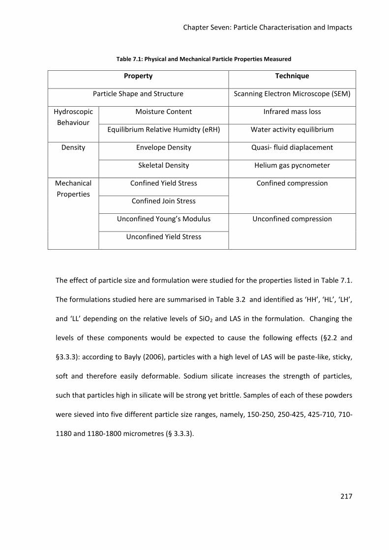
Chapter Seven: Particle Characterisation and Impacts
217
Table 7.1: Physical and Mechanical Particle Properties Measured
Property Technique
Particle Shape and Structure Scanning Electron Microscope (SEM)
Hydroscopic
Behaviour
Moisture Content Infrared mass loss
Equilibrium Relative Humidty (eRH) Water activity equilibrium
Density Envelope Density Quasi- fluid diaplacement
Skeletal Density Helium gas pycnometer
Mechanical
Properties
Confined Yield Stress Confined compression
Confined Join Stress
Unconfined Young’s Modulus Unconfined compression
Unconfined Yield Stress
The effect of particle size and formulation were studied for the properties listed in Table 7.1.
The formulations studied here are summarised in Table 3.2 and identified as ‘HH’, ‘HL’, ‘LH’,
and ‘LL’ depending on the relative levels of SiO2 and LAS in the formulation. Changing the
levels of these components would be expected to cause the following effects (§2.2 and
§3.3.3): according to Bayly (2006), particles with a high level of LAS will be paste-like, sticky,
soft and therefore easily deformable. Sodium silicate increases the strength of particles,
such that particles high in silicate will be strong yet brittle. Samples of each of these powders
were sieved into five different particle size ranges, namely, 150-250, 250-425, 425-710, 710-
1180 and 1180-1800 micrometres (§ 3.3.3).

Chapter Seven: Particle Characterisation and Impacts
218
Table 7.2: Formulations Overview
Component
Function
Component Fraction by mass (wt)
High SiO2
High LAS
(HH)
High SiO2
Low LAS
(HL)
Low SiO2
High LAS
(LH)
Low SiO2
Low LAS
(LL)
Surfactant LAS (linear Alkylbenzene-
Sulphonate)
23.0% 5.0% 30.0% 5.0%
Polymer polycarboxylate 2.0% 2.0% 2.0% 2.0%
Builders Phosphate 20.0% 20.0% 20.0% 20.0%
Sodium Silicate 14.4% 20.0% 0.0% 0.0%
Sodium Sulphate 30.4% 42.8% 37.8% 62.8%
Others (minor components) 3.2% 3.2% 3.2% 3.2%
Additional Water (processing aid) 7.0% 7.0% 7.0% 7.0%
7.2.2 Particle Impacts Experiments
Particles were fired into a steel target to mimic their impact on the dryer walls using a
Ghadiri design (Ahmadian (2008) and Samimi et al. (2003)) particle impact rig (§3.6.1). The
impact velocity of particles was controlled by adjusting the air pressure used to accelerate
particles in the impact rig (§3.6.1). Four different impact targets (90°, 60°, 45° and 30°) were
used to allow the impact angle of particles to be changed. High speed video footage of the
target was taken so that the impact behaviour of the particles could be observed. The
images captured were analysed to obtain particle velocities and breakage details so that
impact behaviour could be expressed quantitatively.

Chapter Seven: Particle Characterisation and Impacts
219
To enable the effect of formulation (and the resulting physical and mechanical properties of
granules) on impact behaviour to be studied, the four different formulations summarised in
Table 3.2 were used and as before, samples of each of these powders were sieved into five
different particle size ranges, namely, 150-250, 250-425, 425-710, 710-1180 and 1180-1800
micrometres (§3.3.3), so that the effect of particle size could be also be studied. Statisitcal
analysis of these results was conducted using JMP software (§3.6.3). Both correlation and
response modelling was undertaken to aid understanding of the results from these
experiments. The results from this analysis are presented in Appendix E.
7.3 Particle Characterisation Results
The results from experiments to characterise the physical and mechanical properties of the
four formulations are shown in this section.
7.3.1 Effect of Formulation on Particle Shape and Structure
The sieved samples were examined using the Hitachi TM-1000 table top electron microscope
(§3.7.1.1). Images of each sieve cut for each formulation are displayed in Figure 7.1 (HH),
Figure 7.2 (HL), Figure 7.3 (LH) and Figure 4.2 (LL). All of these images were taken with a
magnification of x 80. The images were selected from extensive range to ensure they were
representative.

Chapter Seven: Particle Characterisation and Impacts
220
150-250 microns 250-425 microns 425-710 microns
710-1180 microns 1180-1800 microns
Figure 7.1: SEM images of HH formulation for each sieve cut
150-250 microns 250-425 microns 425-710 microns
710-1180 microns 1180-1800 microns
Figure 7.2: SEM images of HL formulation for each sieve cut

Chapter Seven: Particle Characterisation and Impacts
221
150-250 microns 250-425 microns 425-710 microns
710-1180 microns 1180-1800 microns
Figure 7.3: SEM images of LH formulation for each sieve cut
150-250 microns 250-425 microns 425-710 microns
710-1180 microns 1180-1800 microns
Figure 7.4: SEM images of LL formulation for each sieve cut

Chapter Seven: Particle Characterisation and Impacts
222
These figures illustrate common themes for all of the formulations and particle sizes.
Notably most particles show signs of damage from abrasion and attrition, this could occur
during either processing and/or sieving. The following observations can be made on how
particle size is linked to particle structure:
For particles in the 150-250 μm size range the vast majority are single entities, either
single puffed droplet or debris from large broken particle.
Some agglomerates are present along with single entities in the 250-425 μm range.
All particles above 425 μm feature some kind of agglomeration. As particles get
bigger they become agglomerates with increasing numbers of primary particles.
These observations can be attributed to the range of droplet sizes created during
atomisation, which is usually around 200 to 400 μm according to Bayly et al. (2008) and
therefore any particle larger than this can be assumed to be formed from agglomerated
smaller particles.
Variation in appearance and structure between particles of different formulations is also
noted. Particles from the LL formulation tend to have the most porous surfaces (Figure 4.2)
and seem to suffer the most damage from abrasion/attrition. The formulas containing the
higher levels of silicate (HH, HL) tend to have the smoothest surface appearance (Figure 7.1
and Figure 7.2) and suffer least damage, they also seem to have the roundest shape. This
change in appearance in surface texture and shape maybe a function of changes in
atomisation, caused by variation in slurry viscosity as discussed by Stewart (2008) (§2.3.4),
and the drying mechanism described by Hecht (2004) (§2.3.6) taking place for each
formulation.

Chapter Seven: Particle Characterisation and Impacts
223
7.3.2 Hydroscopic Behaviour
In this section, the moisture content and equilibrium relative humidity values of the powders
used in this research are examined.
7.3.2.1 Moisture Content
The moisture content of a detergent powder refers to the sum of both the bound and free
moisture contained within the particles. This was measured using an infrared mass loss
method (§3.7.3.1). The results obtained from these measurements are plotted as a function
of particle size for four formulations in Figure 7.5. These data points represent the average
of five repeats. Moisture contents were found to vary between 3 and 12 % by mass,
depending on both formulation and particle size. All of the formulations were manufactured
from slurry with the same moisture content and dried under the same conditions, therefore
the variation seen is caused by changes in the drying behaviour of different formulations.
This might be caused by changes in the split between bound and free moisture in the
formulation and also variation in droplet/particle size changes between formulations, caused
by both atomisation and agglomeration.

Chapter Seven: Particle Characterisation and Impacts
224
Particle Size (m)
150-250 250-425 425-710 710-1180 1180-1800
Po
wd
er
Pro
duct
Mo
istu
re C
on
ten
t (%
ma
ss)
0.0
2.0
4.0
6.0
8.0
10.0
12.0
High SiO2 High LAS
Low SiO2 Low LAS
Low SiO2 High LAS
High SiO2 Low LAS
Figure 7.5: Powder moisture contents for each formulation as a function of particle sieve cut
Figure 7.5 shows a clear effect of particle size on moisture content for all formulations, and
shows a general increase with increasing size. The degree of increase is not consistent for
each formulation, again a possible indicator of different drying behaviour. An overall
increase in moisture content with particle size is expected as big particles will dry more
slowly than smaller ones as described by Hecht (2004), due to heat and mass transfer
limitations within the particle structure and also in the boundary layer around the particle,
as widely reported in literature (§2.3.6). An additional consideration is the possibility of
variation in chemical composition between different sizes, which in turn would lead to
differing balance of free and bound moisture according to Bayly (2006).

Chapter Seven: Particle Characterisation and Impacts
225
7.3.2.2 Equilibrium Relative Humidity
Free moisture is known to be key in determining detergent powder properties as this water
is free to move into the organic phase of the granule, altering the phase of the surfactant in
the granule and thus changing its mechanical properties, and covered by Bayly (2006) and
Stewart (2008). The values of eRH for all four formulas are displayed in Figure 7.6, as a
function of particle size.
Particle Size (m)
150-250 250-425 425-710 710-1180 1180-1800
Equili
brium
Rela
tive H
um
idity (
%)
25
30
35
40
45
50
55
High SiO2 High LAS
Low SiO2 Low LAS
Low SiO2 High LAS
High SiO2 Low LAS
Figure 7.6: Powder Equilibrium Relative Humidities
Clear variation in eRH values for all of the formulations can be seen, with the LL formulation
having the largest values of between 42% and 48%. The lowest values are seen for the HL
formulation, at around 30%, for all particle sizes. This variation gives a clear indication of
different amounts of free moisture contained within each, as a result of different levels of

Chapter Seven: Particle Characterisation and Impacts
226
key components. This in turn affects the balance between free and bound moisture in the
slurry and powder product.
The trend in eRH with changes in particle size appears to be small for some formulations,
namely the two formulations containing large amounts of sodium silicate; HH and HL. The LL
formulation shows an unclear trend, where the middle particle size exhibits the largest value
of eRH, for all samples measured at around 48%. The LH formulation demonstrates the
clearest trend, with values eRH increasing with particle size, from approximately 34% to 38%
over the range of particle sizes, as would be expected as larger particles dry less due to heat
and mass transfer limitations as they travel through the spray dryer covered by Hecht
(2004).
7.3.3 Particle Density
This section of the chapter covers results for the envelope and apparent (skeletal) density as
a function of formulation and particle size.
7.3.3.1 Envelope Density
The principle of envelope density is discussed in section (§2.8.3) and Figure 7.7 shows values
of this for the four formulations used in this work as a function of particle size. Envelope
density varies between values of 500 and 1400 kgm-3 as a function of particle size and
formulation. The LL formula displays the largest values for envelope density for all particle
sizes, varying from 0.7 to 1.4 kgm-3, whilst the high silicate formulation displays the smallest
values for all but the largest particle size, varying from 0.5 to 0.9 kgm-3. The changes in
envelope density, with particle size (for each individual formulation), show the effect of

Chapter Seven: Particle Characterisation and Impacts
227
particle structure on density (§ 7.3.1), with items such as porosity and agglomeration
influencing envelope density, as well as the density of the detergent material itself. Smaller
particles could also actually be undissolved solids from the slurry which pass through the
entire spray drying process unchanged; possibly solid lumps of sulphate and such as would
have much higher densities than normal granules and therefore the presence of just a few
could influence the envelope density of a sample as suggested by Bayly (2006).
Particle Size (m)
150-250 250-425 425-710 710-1180 1180-1800
Envelo
pe D
ensity (
kg.m
-3)
400
600
800
1000
1200
1400
High SiO2 High LAS
Low SiO2 Low LAS
Low SiO2 High LAS
High SiO2 Low LAS
Figure 7.7: Particle Envelope Densities
Another issue to be considered on how particle size influences envelope density is the
accuracy of the technique employed with respect to particle size. The method used employs
a quasi-fluid fine powder, ‘dry-flo’, which is packed around the particles in the sample during
the compression, thus allowing the envelope volume to be measured. The size distribution
of the dry-flo powder heavily influences its ability to pack tightly around the sample

Chapter Seven: Particle Characterisation and Impacts
228
granules, with the packing value decreasing as the particle size in the sample approaches
that of the dry-flo. This may partially explain the trend of increasing envelope density at
small particle sizes, as this is the region in which sample particles and dry-flo particles
approach the same size, thus reducing packing and in accurately measuring the envelope
volume of the sample. The lower size limit of particles that can be measured using this
technique is not stated by the manufacturer or any workers on this device, so definite
conclusions on this cannot be drawn.
The variation in envelope densities observed for the smallest particles sizes shows
interesting trends in terms of the effect of formulation, and specifically the level of sodium
silicate builder. The two formulations which contain no sodium silicate appear to have
almost identical envelope densities for the smaller particle sizes, as do the two formulas
which contain sodium silicate, with the zero silicate powders having the largest envelope
densities. This behaviour seems less well defined at larger particle sizes, where the LL
formula shows much higher values than the other three formulas. These changes with
formulation may be partly explained by changes in porosity and also by variation in the
skeletal density of each formulation described in the next section.
7.3.3.2 Apparent Density
Figure 7.8 shows values of apparent density (§2.8.3) for the four formulations as a function
of particle size.

Chapter Seven: Particle Characterisation and Impacts
229
Particle Size (m)
150-250 250-425 425-710 710-1180 1180-1800
Ap
pare
nt
De
nsity (
kg.m
-3)
0
500
1000
1500
2000
2500
3000
High SiO2 High LAS
Low SiO2 Low LAS
High SiO2 Low LAS
Low SiO2 High LAS
Figure 7.8: Particle apparent densities
Values of apparent density can be seen to vary between 1.7 and 2.4 kg.m-3. The effect of
formulation on apparent density appears to be greater than that of particle size.
As with the envelope density data, the LL formulation shows the largest apparent density
values for all particle sizes, between 2.3 and 2.4 kgm-3. The next highest values are for the HL
formulation, varying between 2.3 and 1.9 kgm-3. Increasing particle size appears to slightly
decrease the skeletal density for all formulations. This change is a function of increasing
moisture content with particle size or an increase in the amount of closed pores in larger
particles.
Comparison of envelope and skeletal densities reveal that the inclusion of open pores within
the sample reduces its density by between two and three times. This indicates that between
half and two-thirds of the volume of a detergent particle can be accounted for by

Chapter Seven: Particle Characterisation and Impacts
230
considering open pores. The effect of formulation and particle parameters on these two
density parameters shows no clear links, therefore it can be determined that formulation
and particle size influence envelope density of detergent granules through changes in
microstructure (porosity) rather than actually density of the solid detergent material in the
granule.
7.3.4 Mechanical Properties
The mechanical properties of the particles are key to understanding the impact behaviour of
particles, in terms of their deformation and therefore energy dissipation on impact and also
the contact area created between the particle and the impacted surface. This in turn
controls restitution and deposition, which determines the collision success rate of particles
on the dryer walls, and is therefore of great importance to this work. Presented here are the
results for characterisation of the mechanical properties of the detergent powders, with two
main techniques being employed: confined compression, and unconfined compression
(§2.8.5). The former gives the mechanical properties of the formulation independent of
particle structure, whilst the latter gives mechanical properties of the formulation including
particle structure which enables the effects of material properties and particle structure to
be decoupled.
7.3.4.1 Confined Yield Stress
The confined yield stress is defined as an interpretation of the point at which the granules in
a powder sample, being compressed within a die begin to plastically deform. This a useful
value when investigating the impact behaviour of particles, as it is the point at which plastic
deformation begins and therefore energy dissipation through deformation, which will

Chapter Seven: Particle Characterisation and Impacts
231
control restitution and ultimately deposition, through the size of the contact area made
through deformation. Therefore the changes in confined yield stress with formulation and
particle size will allow understanding of how impact behaviour changes with these variables.
Values for confined yield stress of all formulas as a function of particle size are plotted in
Figure 7.9.
Particle Size (m)
150-250 250-425 425-710 710-1180 1180-1800
Confined Y
ield
Str
ess (
Pa)
0
1e+5
2e+5
3e+5
4e+5
5e+5
High SiO2 High LAS
High SiO2 Low LAS
Low SiO2 High LAS
Low SiO2 Low LAS
Figure 7.9: Confined yield stresses for the four formulations as a function of particle sieve cut
Values of confined yield stress can be seen to vary with both formulation and particle size.
The highest yield stresses across all particle sizes can be seen for the HH formulation, this is
despite this formula having the largest moisture content of the four, which would be
expected to reduce yield stress, as stated by Bayly (2006). This leads to the conclusion that
addition of silicate and LAS strengthens granules enabling them to resist plastic deformation;
examining the microstructure of these granules, as shown in Figure 7.1 to 7.4 shows that

Chapter Seven: Particle Characterisation and Impacts
232
they appear to have solid structures in comparison with the other formulas, with the
exception of the HL formula.
The trends for the effect of formulation for the other three formulas become less clear. The
LH formula has the largest yield stress for the smallest particle size, whilst the LL formula has
the second largest values for the two middle particle sizes. The HL formulation has the
second highest values for the biggest two particle sizes.
The effect of particle size on yield stress appears to be different for each formulation,
however, the formulations containing large amounts of LAS surfactant (HH and LH) show
similar trends. For these formulations, the largest values of yield stress are seen for the
smallest particle sizes, and then yield stress decreases with increasing particle size, almost
reaching a plateau for final three particle sizes, this may be an effect of particle structure, as
the morphology of granules is known to change between the 250-425 µm and 425-710 µm
size group (§7.3.1). The effect of particle size for the formulations containing low levels of
LAS surfactant appear to go the other way, with the smallest particles having the lowest
yield stress values, and then an increase with particle size, although the trends are less clear.
All of this indicates that particle morphology and structure, which varies with particle size (§
7.3.1), has a significant effect on yield stress of samples of detergent powders, this effect
appears to also depend on formulation, which also controls particle morphology (§ 7.3.1)
7.3.4.2 Confined Join Stress
The confined join stress is defined as an interpretation of the point at which the granules in a
powder sample (compressed within a die) begin to physically lose their structure under the
stress being applied. This is useful for investigating the impact behaviour of particles, as it is

Chapter Seven: Particle Characterisation and Impacts
233
an indication of the point at which particle will break. Therefore the changes in confined
yield stress with formulation and particle size will allow understanding of how particle
breakage changes with these variables. Values are plotted in Figure 7.10.
Particle Size (m)
150-250 250-425 425-710 710-1180 1180-1800
Confined J
oin
Str
ess (
Pa)
0
1e+6
2e+6
3e+6
4e+6
5e+6
6e+6
High SiO2 High LAS
Low SiO2 High LAS
High SiO2 Low LAS
Low SiO2 Low LAS
Figure 7.10: Confined compression join stresses as a function of particle size for the four formulations
The join stress of granules can be seen to vary between 6×10⁶ and 8×10⁵ Pa. Examining
Figure 7.10 reveals a general trend of decreasing join stress with particle size, with the
exception of the HL formulation. The largest values for join stress are displayed by the LH
formula at small particle sizes (6×10⁶ Pa), indicating these granules offer the most resistance
to applied stresses before they lose their individual structures.
All formulas appear to reach a plateau of constant join stress values for larger particle sizes,
this may be a feature of the agglomerated nature of particles above 425 (µm) (§ 7.3.1). This
is assuming that the agglomerated granules are most likely to break through splitting into

Chapter Seven: Particle Characterisation and Impacts
234
their constituent particles, thus the same stress is required to do this regardless of the
number of constituent particles in the original agglomerate.
7.3.4.3 Unconfined Young’s Modulus
The unconfined Young’s modulus is the measure of the amount of elastic deformation a
tablet of detergent material will undergo at an applied level of stress. This value is important
in the impact behaviour of particles as it controls the amount of deformation a particle
suffers up to the yield stress, this parameter was used to explain adhesion (deposition) of
particles by Johnson et al. (1971), in their famous JKR theory. Therefore Young’s modulus
can be used to aid understanding of collision success rate of particles on the dryer walls. The
values of Young’s modulus displayed in Figure 7.11 are expressed in units of Pascal, as the
strain in this work was described as a fraction of the tablets original thickness.
Particle Size (m)
150-250 250-425 425-710 710-1180 1180-1800
Unconfined Y
oung's
Modulu
s (
Pa)
0
1e+8
2e+8
3e+8
4e+8
5e+8
6e+8
7e+8
High SiO2 High LAS
Low SiO2 Low LAS
Low SiO2 High LAS
High SiO2 Low LAS
Figure 7.11: Unconfined Compression Young’s Modulus

Chapter Seven: Particle Characterisation and Impacts
235
Clear trends in Young’s Modulus with formulation can be seen in Figure 7.11, with the LL
formula, shows the largest values at all particle sizes, ranging between 5.2×10⁸ and 6.2×10⁸
Pa. The lowest values are exhibited for the HL formula, with the exception of the largest
particle size where the HH formula shows the smallest values. The effect of particle size on
Young’s modulus varies between formulations, however, the trends seen in the two
formulas containing large amounts of LAS appear to be similar, a steady decline with
increasing particle size, as do the two formulas containing small amounts of LAS, which show
the smallest values for the mid-sized particles.
7.3.4.4 Unconfined Yield Stress
The unconfined yield stress is defined as an interpretation of the point at which the tablet of
detergent material in a powder sample being compressed begins to plastically deform.
Having an understanding of how the yield stress of the solid detergent material compares to
that of particles of the same material allows the effect of particle structure to be accounted
for, thus helping understand the importance of the microstructure of detergent granules in
their impact behaviour. Values for unconfined yield stress of all four formulas as a function
of particle size are plotted in Figure 7.12.

Chapter Seven: Particle Characterisation and Impacts
236
Particle Size (m)
150-250 250-425 425-710 710-1180 1180-1800
Unconfined Y
eild
Str
ess (
Pa)
0.0
1.0e+7
2.0e+7
3.0e+7
4.0e+7
5.0e+7
6.0e+7
7.0e+7
8.0e+7
High SiO2 High LAS
Low SiO2 Low LAS
Low SiO2 High LAS
High SiO2 Low LAS
Figure 7.12: Unconfined Compression Yield Stresses
Clear effects of formulation on unconfined yield stress can be seen in Figure 7.12 (with the
one exception of the LH formula at the largest particle size). The largest values of unconfined
yield stress, varying between 5×10⁷ and 7×10⁷ Pa are shown by the HL formula across all
particle sizes. The smallest values of yield stress are shown by the LH formula, which has
yield stresses approximately one order of magnitude lower than those of the HL formula.
The fact that the two formulas which contain low levels of LAS have significantly larger
values of yield stress than the formulas containing large amounts of LAS indicate that
addition of this component has a key role in controlling yield stress of detergent material,
this is also evident when considering the small difference in the LAS content between the HH
formula and the LH formula. This trend would be expected based on the conclusions of
Yangxin et al. (2008). Unexpectedly the effect of moisture content on yield stress, explained

Chapter Seven: Particle Characterisation and Impacts
237
by Bayly (2009), does not appear in this data, this is possibly because it is over shadowed by
large changes in component levels between the formulas used.
Particle size seems to influence the yield stress values of the HL formula much more than
any of the other formulas, particularly the LL formula where the yield stress is almost
constant across all particle sizes.
Comparison of the values of unconfined yield stress with those of confined compression,
show that the later have yield stress values of one or two orders of magnitudes lower than
the former, showing that including particle structure reduces the yield stress of detergent
granules. The effect of formulation and particle size also varies greatly between the two sets
of yield stress data. All of these changes highlight the importance of granule microstructure
on mechanical properties.
7.3.5 Particle Characterisation Conclusions
The physical and mechanical properties of particles are key to determining their impact
behaviour, in terms of restitution, breakage, deposition, or a combination of these, and
therefore determine the collision success rate of particles impact on the dryer walls. Physical
and mechanical parameters of a range of formulations of detergent powders have been
studied as a function of particle size. This has revealed a mutual dependence of all properties
on both formulation and particle size. It is clear that most, if not all physical and mechanical
properties are interlinked.
The microstructure, morphology and structure and appearance of granules was found to
vary with both particle size and formulation. These changes in microstructure have been

Chapter Seven: Particle Characterisation and Impacts
238
linked to the formation of granule characteristics through agglomeration and drying
mechanisms in the spray drying process.
The hydroscopic behaviour of the detergent formulations studied have been characterised in
terms of total moisture content and equilibrium relative humidity. Both of these parameters
were found to vary with particle size and formulation, with the largest particles having the
largest total moisture contents. The density of the powders was studied through
measurement of both the envelope and skeletal density of samples, again both were found
to vary with formulation and particle size.
Confined and unconfined compression tests were used to examine the mechanical
properties of the detergent powders, with and without the effects of particle structure. The
mechanical properties of powders were found to vary greatly with formulation but less so
with particle size. The influence of particle structure was found to reduce the yield stress
values obtained by one or two orders of magnitude. This change also highlighted the effect
of formulation and particle sizes on the yield stress of detergent granules, through their
influence on the microstructure developed during spray drying.
This section has shown the effect of formulation and particle size on microstructure, physical
and mechanical properties of detergent powders. These parameters are known to be
important in controlling particle impact behaviour and therefore particle collision success
rate. The impact behaviour of these detergent powders are examined in the next section.

Chapter Seven: Particle Characterisation and Impacts
239
7.4 Particle Impact Behaviour Results
7.4.1 Particle Breakage
Breakage of detergent particles during spray drying and processing will have a significant
effect of product quality (§2.2) and therefore understanding this aspect of impact behaviour
is of considerable interest. Both particle and impact properties studied are reported to affect
particle breakage (§2.9.2), therefore it is expected that all will affected the results presented
in this section.
The fraction of particles that broke under each experimental condition was recorded, along
with the number of fragments generated by each particle that broke. This data is presented
in terms of the fraction of particles that broke at each experimental condition and the
average number for fragments from breakage at each condition. Before this quantitative
data, examples of the three types of breakage mechanisms observed are shown and
discussed qualitatively.
7.4.1.1 Breakage Mechanisms
Examples of the three types of particle failure mechanisms (§2.9.2) observed are shown in
the following figures. These allow the reader to gain an appreciation of the types of
breakage of detergent granules observed upon impact with a steel surface. Additionally,
these observations help to give an indication of the link between the granules
microstructure and its breakage, as examined by Mullier et al. (1987) and Samimi et al.
(2003).

Chapter Seven: Particle Characterisation and Impacts
240
The microstructure of detergent granules was previously examined (§ 7.3.1). It was found to
change greatly with particle size, smaller particles tend to be single entities with larger
particles (typically above 425 µm) being agglomerates. This needs to be kept in mind when
trying to understand breakage mechanisms of detergent granules. Therefore the hypothesis
behind the breakage of larger particles and possibly some smaller particles is that the
particle is an agglomerated structure and the kinetic energy dissipated at the point of impact
breaks the bonds holding these particles together.
Figure 7.13 and Figure 7.14 show HL formulation particles being chipped (attrition and
abrasion) at 5 and 10 ms-1 respectively. The main characteristic of attrition and abrasion is
that some small amount of material is released whilst the main body of the particle remains
intact. The weakest bonds in these cases appear to be positioned such that individual or
agglomerates of small numbers of constituent particles, resulting in the main bulk of the
particle staying together with a number of smaller pieces removed from it as shown in Figure
7.13 and Figure 7.14.
0.0000 seconds 0.0004 seconds 0.0008 seconds 0.0012 seconds 0.0016 seconds
Figure 7.13: Chipping of a 1180-1800 μm HL particle at 5 ms-1

Chapter Seven: Particle Characterisation and Impacts
241
0.0000 seconds 0.0002 seconds 0.0004 seconds 0.0006 seconds 0.0008 seconds
Figure 7.14: Chipping of a 1180-1800 μm HL particle at 10 ms-1
Figure 7.15 and Figure 7.16 show particles splitting, involving the particle breaking into
smaller particles of reasonably equal size. In this kind of breakage, the weakest bonds in the
granule are those between large parts of the granule, meaning the granule breaks apart to
leave large fragments. Figure 7.15 shows one particle splitting into two particles with some
smaller fragments also being created. Figure 7.16 shows a particle splitting into 3 equally
sized pieces along with some smaller fragments.
0.0000 seconds 0.0001 seconds 0.0002 seconds 0.0003 seconds 0.0004 seconds
Figure 7.15: A HL particle of 1180-1800 μm splitting at 10 ms-1
0.0000 seconds 0.0002 seconds 0.0004 seconds 0.0006 seconds 0.0008 seconds
Figure 7.16: A HL particle of 1180-1800 μm splitting at 10 ms-1
The complete destruction of the particle’s original structure, through either breaking of large
number of bonds between constituent particles and even breaking constituent particles,

Chapter Seven: Particle Characterisation and Impacts
242
during smashing is shown in Figure 7.17 and Figure 7.18. Smashing is characterised by the
large amount of fragments created and the way in which these fragments are scattered in all
directions.
0.0002 seconds 0.0004 seconds 0.0006 seconds 0.0008 seconds 0.0000 seconds Figure 7.17: A HL particle of 1180-1800 μm smashing at 15 ms
-1
0.0000 seconds 0.0002 seconds 0.0004 seconds 0.0006 seconds 0.0008 seconds
Figure 7.18: A HL particle of 1180-1800 μm smashing at 10 ms-1
These examples of breakage mechanisms highlight the importance of detergent granule
microstructure in breakage and therefore how parameters such a formulation and drying
conditions will affect the processability of detergent powders in terms of size reduction
through breakage.
7.4.1.2 Breakage Fractions
Figures 7.19-7.22 show the effect of formulation, particle size, impact kinetic energy and
impact angle on the fraction of particles that suffer breakage. The most striking trend in
these plots is that the fraction of particles suffering breakage increases with impact kinetic
energy and particle size for all four formulations, at all impact angles. These trends are also
shown in the statistical analysis in Appendix E, and would be expected as increasing kinetic

Chapter Seven: Particle Characterisation and Impacts
243
energy (linked to particle size) means more energy is available to deform and then
eventually break both bonds between constituent particles and the structure of individual
constituent particles within the particle. Higher kinetic energy increases the loading (force)
on the particle as it impacts. This will increase the impact stress and therefore deformation.
If the force is great enough the deformation will continue through the elastic regime into the
plastic regime and possibly to the point of failure, for both bonds between constituent
particles and the structure of individual constituent particles. The models shown in Appendix
E highlight how these trends are most pronounced at lower to mid values of these
parameters and their effect decreases at higher values, particularly for particle size.
Larger detergent particles are constructed from agglomerated smaller particles (§ 7.3.1).
These changes in particle morphology appear to be closely linked with the breakage
behaviour of detergent powders studied in this work. Evidence for this can be seen as the
breakage fraction for particles increases with the number of consistent particles making up
particles in each size range. Moreover, there is a fairly consistent change in breakage
fraction with impact velocity, across all angles and formulations, as particle size increases.
This is a clear indication of the role of particle morphology, in terms of agglomerated versus
single particle granules (§ 7.3.1), in particle breakage.
The effect on angle on breakage fraction is that increasing angles towards the normal
increases breakage fraction, potentially due to the increasing normal impact velocity
component. This effect appears to be most significant for the smallest impact angles, as
shown by the models in (§E.2.3). However, this effect appears to be smaller in this work than
in comparison to the findings of workers such as Samimi et al. (2003) found that impact

Chapter Seven: Particle Characterisation and Impacts
244
angle heavily influenced breakage, this discrepancy might be linked to the structure of spray
dried detergents.
The effect of formulation and resulting particle properties on breakage fraction appears to
be complex. The response modelling (§E.2) shows that SiO2 content has a significant effect
on breakage, with mid levels of this parameter producing the smallest breakage fraction. The
effect of LAS levels on breakage fraction was found to not be significant. In terms of resulting
particle properties, both types of particle density measured in this work have a strong
positive correclation, showing that increasing density leads to more breakage, this could be
caused by the increased kinetic energy carried by heavier particles upon impact. Moisture
content also has a positive correlation, however, eRH does not, suggesting the effect of free
moisture is not as important as described by Bayly (2009). The mechanical poroperties
measured show a range of correlations, with all being negative apart from the unconfined
yield stress, decreasing meachanical strength would be expected to increase breakage and
this may explain the moisture content correlation. The unconfined yield stress may be an
outlier and its effect may be cancelled out by the effect of granular structure on mechanical
behaviour upon impact.

Chapter Seven: Particle Characterisation and Impacts
245
90 Degrees
Impact Kinetic Energy (J)
1e-8 1e-7 1e-6 1e-5 1e-4 1e-3
Fra
ctio
n o
f P
art
icle
s (
%)
0
20
40
60
80
100
150-250 microns
250-425 microns
425-710 microns
710-1180 microns
1180-1800 microns
60 Degrees
Impact Kinetic Energy (J)
1e-8 1e-7 1e-6 1e-5 1e-4 1e-3
Fra
ctio
n o
f P
art
icle
s (
%)
0
20
40
60
80
100
45 Degrees
Impact Kinetic Energy (J)
1e-8 1e-7 1e-6 1e-5 1e-4 1e-3
Fra
ction
of P
art
icle
s (
%)
0
20
40
60
80
100
30 Degrees
Impact Kinetic Energy (J)
1e-8 1e-7 1e-6 1e-5 1e-4 1e-3
Fra
ction
of P
art
icle
s (
%)
0
20
40
60
80
100
Figure 7.19: Breakage Fraction: HH Formulation

Chapter Seven: Particle Characterisation and Impacts
246
90 Degrees
Impact Kinetic Energy (J)
1e-8 1e-7 1e-6 1e-5 1e-4 1e-3
Fra
ction
of P
art
icle
s B
roken
(%
)
0
20
40
60
80
100
150-250 microns
250-425 microns
425-710 microns
710-1180 microns
1180-1800 microns
60 Degrees
Impact Kinetic Energy (J)
1e-8 1e-7 1e-6 1e-5 1e-4 1e-3
Fra
ction
of P
art
icle
s B
roken
(%
)
0
20
40
60
80
100
45 Degrees
Impact Kinetic Energy (J)
1e-8 1e-7 1e-6 1e-5 1e-4 1e-3
Fra
ction
of P
art
icle
s B
roken
(%
)
0
20
40
60
80
100
30 Degrees
Impact Kinetic Energy (J)
1e-8 1e-7 1e-6 1e-5 1e-4 1e-3
Fra
ction
of P
art
icle
s B
roken
(%
)
0
20
40
60
80
100
Figure 7.20: Breakage Fraction: HL Formulation

Chapter Seven: Particle Characterisation and Impacts
247
90 Degrees
Impact Kinetic Energy (J)
1e-8 1e-7 1e-6 1e-5 1e-4 1e-3
Fra
ction
of P
art
icle
s B
roken
(%
)
0
20
40
60
80
100
60 Degrees
Impact Kinetic Energy (J)
1e-8 1e-7 1e-6 1e-5 1e-4 1e-3
Fra
ction
of P
art
icle
s B
roken
(%
)
0
20
40
60
80
100
45 Degrees
Impact Kinetic Energy (J)
1e-8 1e-7 1e-6 1e-5 1e-4 1e-3
Fra
ction
of P
art
icle
s B
roken
(%
)
0
20
40
60
80
100
30 Degrees
Impact Kinetic Energy (J)
1e-8 1e-7 1e-6 1e-5 1e-4 1e-3
Fra
ction
of P
art
icle
s B
roken
(%
)
0
10
20
30
40
50
60
70
150-250 microns
250-425 microns
425-710 microns
710-1180 microns
1180-1800 microns
Figure 7.21: Breakage Fraction: LH Formulation

Chapter Seven: Particle Characterisation and Impacts
248
90 Degrees
Impact Kinetic Energy (J)
1e-8 1e-7 1e-6 1e-5 1e-4 1e-3
Fra
ctio
n o
f P
art
icle
s (
%)
0
20
40
60
80
100
150-250 microns
250-425 microns
425-710 microns
710-1180 microns
1180-1800 microns
60 Degrees
Impact Kinetic Energy (J)
1e-8 1e-7 1e-6 1e-5 1e-4 1e-3
Fra
ctio
n o
f P
art
icle
s (
%)
0
20
40
60
80
100
45 Degrees
Impact Kinetic Energy (J)
1e-8 1e-7 1e-6 1e-5 1e-4 1e-3
Fra
ction
of pa
rtic
les (
%)
0
20
40
60
80
100
30 Degrees
Impact Kinetic Energy (J)
1e-8 1e-7 1e-6 1e-5 1e-4 1e-3
Fra
ction
of P
art
icle
s (
%)
0
10
20
30
40
50
60
70
Figure 7.22: Breakage Fraction: LL Formulation
7.4.1.3 Number of Fragments Generated
The number of fragments generated from each particle that suffered breakage are examined
here as a function of impact velocity, impact angle, formulation and particle size. Figures

Chapter Seven: Particle Characterisation and Impacts
249
7.23-7.26 show average number of fragments generated, at each impact angle as a function
of impact velocity, formulation and particle size. The number of fragments formed from each
break increases with both impact velocity and particle size, as would be expected from the
breakage fraction results. There appears to be an approximately linear relationship between
the number of fragments formed and impact velocity, for the majority of particle sizes across
the four formulations and four impact angles.
The relationship between the number of fragments generated and particle size shows a clear
trend across all formulations and impact angles, that increasing particle size increases the
average number of fragments generated from each particle breaking. This would be
expected based upon the literature (§2.9.2.3) and the findings on particle structure (§7.3.1).
The smallest particles clearly break into the fewest fragments (often no more than 2).
The statistical analysis of these results showed very similar correlations to breakage
fractions, as would be expected (§2.9.2.3). Therefore, particle density and mechanical
properties are the key particle properties in determining the number of fragments
generated aside from particle size.

Chapter Seven: Particle Characterisation and Impacts
250
90 Degrees
Impact Velocity (ms-1)
0 5 10 15 20 25 30
Nu
mb
er
of
Fra
gm
en
ts
0
2
4
6
8
10
60 Degrees
Impact Velocity (ms-1)
0 5 10 15 20 25 30
Nu
mb
er
of
Fra
gm
en
ts
0
2
4
6
8
10
150-250 microns
250-425 microns
425-710 microns
710-1180 microns
1180-1800 microns45 Degrees
Impact Velocity (ms-1)
0 5 10 15 20 25 30
Nu
mb
er
of
Fra
gm
en
ts
0
2
4
6
8
10
30 Degrees
Impact Velocity (ms-1)
0 5 10 15 20 25 30
Nu
mb
er
of
Fra
gm
en
ts
0
2
4
6
8
10
Figure 7.23: Number of Fragments: HH Formulation

Chapter Seven: Particle Characterisation and Impacts
251
90 Degrees
Impact Velocity (ms-1)
0 5 10 15 20 25 30
Nu
mb
er
of
Fra
gm
en
ts
0
2
4
6
8
10
150-250 microns
250-425 microns
425-710 microns
710-1180 microns
1180-1800 microns
60 Degrees
Impact Velocity (ms-1)
0 5 10 15 20 25 30
Nu
mb
er
of
Fra
gm
en
ts
0
2
4
6
8
10
45 Degrees
Impact Velocity (ms-1)
0 5 10 15 20 25 30
Nu
mb
er
of
Fra
gm
en
ts
0
2
4
6
8
10
30 Degrees
Impact Velocity (ms-1)
0 5 10 15 20 25 30
Nu
mb
er
of
Fra
gm
en
ts
0
2
4
6
8
10
Figure 7.24: Number of Fragments: HL Formulation

Chapter Seven: Particle Characterisation and Impacts
252
90 Degrees
Impact Velocity (ms-1)
0 5 10 15 20 25 30
Fra
ctio
n o
f P
art
icle
s B
roke
n (
%)
0
20
40
60
80
100
60 Degrees
Impact Velocity (ms-1)
0 5 10 15 20 25 30
Fra
ctio
n o
f P
art
icle
s B
roke
n (
%)
0
20
40
60
80
100
45 Degrees
Impact Velocity (ms-1)
0 5 10 15 20 25 30
Fra
ctio
n o
f P
art
icle
s B
roke
n (
%)
0
20
40
60
80
100
30 Degrees
Impact Velocity (ms-1)
0 5 10 15 20 25 30
Fra
ctio
n o
f P
art
icle
s B
roke
n (
%)
0
20
40
60
80
100
150-250 microns
250-425 microns
425-710 microns
710-1180 microns
1180-1800 microns
Figure 7.25: Number of Fragments: LH Formulation

Chapter Seven: Particle Characterisation and Impacts
253
90 Degrees
Impact Velocity (ms-1)
0 5 10 15 20 25 30
Nu
mb
er
of
Fra
gm
en
ts
0
2
4
6
8
10
60 Degrees
Impact Velocity (ms-1)
0 5 10 15 20 25 30
Nu
mb
er
of
Fra
gm
en
ts
0
2
4
6
8
10
150-250 microns
250-425 microns
425-710 microns
710-1180 microns
1180-1800 microns45 Degrees
Impact Velocity (ms-1)
0 5 10 15 20 25 30
Nu
mb
er
of
Fra
gm
en
ts
0
2
4
6
8
10
30 Degrees
Impact Velocity (ms-1)
0 5 10 15 20 25 30
Nu
mb
er
of
Fra
gm
en
ts
0
2
4
6
8
10
Figure 7.26: Number of Fragments: LL Formulation

Chapter Seven: Particle Characterisation and Impacts
254
7.4.2 Rebound Behaviour
The rebound behaviour of particles that did not break upon impact was examined in terms
of restitution coefficient and rebound angle. Owing to the fact that several impact angles
were studied, the restitution coefficient was expressed in both its standard form and also as
a normal restitution coefficient, that is the ratio of the normal velocity component for
rebound to the normal component of the impact velocity. In addition the rebound angle of
particles was described in two ways, as an angle from the impact vector (where deviation in
either direction was taken as positive) and as an angle from the surface (taken clockwise).
7.4.2.1 Restitution Coefficient
The rebound velocity of any particles not suffering breakage was calculated in the same way
as is described for the impact velocities (§3.6.2), this meant the ratio of impact and rebound
velocities for each individual particle could be calculated to give the restitution coefficient
for all unbroken particles. Figures 7.27-7.29 show plots of the restitution coefficient and
Figures 7.31-7.34 show the normal restitution coefficient measured for 5 particle sizes at
varying impact velocities and angles for all four formulations.
From these plots impact angle appears to have the greatest affect on values of restitution
coefficient, as it increases with increasing obliqueness of the impact angle, as shown by the
strong negative correlation (§E.1) and the response models (§E.2). For normal restitution
coefficient the effect of angle is also shown, although not as strongly, potentially showing
the effect of impact angle on contact mechanics and energy dissipation during impact. The
effect of impact angle is also seen in the negative correlation between normal impact
velocity and restitution coefficient, there appears to be little correlation between impact

Chapter Seven: Particle Characterisation and Impacts
255
velocity and restitution coefficient, showing that the normal velocity component is driver for
changes in restitution with impact velocity. Particle size, LAS and SiO2 content were all
included in the response models (§E.2), but show only a small influence on restitution
coefficient compared to impact angle. Literature, including Thornton and Ning (1998) and Fu
et al. (2004), suggests that two properties that change with formulation, namely hardness
and Young’s modulus would be expected to have an effect on restitution coefficient.
However, the effect of youngs modulus on these results can be seen to not that great in the
the response models (§E.2). This may be because the Young’s modulus of compressed
powder tablets was measured rather than that of actual particles. The hardness of the
material was not measured during this work and therefore can not be linked to the
restitution results here.

Chapter Seven: Particle Characterisation and Impacts
256
90 Degrees
Impact Velocity (ms-1)
0 5 10 15 20 25 30
Restitu
tion C
oeff
icent
0.0
0.2
0.4
0.6
0.8
1.0
60 Degrees
Impact Velocity (ms-1)
0 5 10 15 20 25 30
Restitu
tion C
oeff
icent
0.0
0.2
0.4
0.6
0.8
1.0
150-250 microns
250-425 microns
425-710 microns
710-1180 microns
1180-1800 microns 45 Degrees
Impact Velocity (ms-1)
0 5 10 15 20 25 30
Restitu
tion C
oeff
icent
0.0
0.2
0.4
0.6
0.8
1.0
30 Degrees
Impact Velocity (ms-1)
0 5 10 15 20 25 30
Restitu
tion C
oeff
icent
0.0
0.2
0.4
0.6
0.8
1.0
Figure 7.27: Restitution Coefficient: HH Formulation

Chapter Seven: Particle Characterisation and Impacts
257
90 Degrees
Impact Velocity (ms-1)
0 5 10 15 20 25 30
Restitu
tion C
oeff
icent
0.0
0.2
0.4
0.6
0.8
1.0
150-250 microns
250-425 microns
425-710 microns
710-1180 microns
1180-1800 microns
60 Degrees
Impact Velocity (ms-1)
0 5 10 15 20 25 30
Restu
tition C
oeff
icent
0.0
0.2
0.4
0.6
0.8
1.0
45 Degrees
Impact Velocity (ms-1)
0 5 10 15 20 25 30
Restitu
tion C
oeff
icent
0.0
0.2
0.4
0.6
0.8
1.0
30 Degrees
Impact Velocity (ms-1)
0 5 10 15 20 25 30
Restitu
tion C
oeff
icent
0.0
0.2
0.4
0.6
0.8
1.0
Figure 7.28: Restitution Coefficient: HL Formulation

Chapter Seven: Particle Characterisation and Impacts
258
90 Degrees
Impact Velocity (ms-1)
0 5 10 15 20 25 30
Restitu
tion C
oeff
icie
nt
0.0
0.2
0.4
0.6
0.8
1.0
60 Degrees
Impact Velocity (ms-1)
0 5 10 15 20 25 30
Restitu
tion C
oeff
icie
nt
0.0
0.2
0.4
0.6
0.8
1.0
150-250 microns
250-425 microns
425-710 microns
710-1180 microns
1180-1800 microns45 Degrees
Impact Velocity (ms-1)
0 5 10 15 20 25 30
Restitu
tion C
oeff
icie
nt
0.0
0.2
0.4
0.6
0.8
1.0
30 Degrees
Impact Velocity (ms-1)
0 5 10 15 20 25 30
Restitu
tion C
oeff
icie
nt
0.0
0.2
0.4
0.6
0.8
1.0
Figure 7.29: Restitution Coefficient: LH Formulation

Chapter Seven: Particle Characterisation and Impacts
259
90 Degrees
Impact Velocity (ms-1)
0 5 10 15 20 25 30
Restitu
tion C
oeff
icent
0.0
0.2
0.4
0.6
0.8
1.0
60 Degrees
Impact Velocity (ms-1)
0 5 10 15 20 25 30
Restitu
tion C
oeff
icent
0.0
0.2
0.4
0.6
0.8
1.0
150-250 microns
250-425 microns
425-710 microns
710-1180 microns
1180-1800 microns 45 Degrees
Impact Velocity (ms-1)
0 5 10 15 20 25 30
Restitu
tion C
oeff
icent
0.0
0.2
0.4
0.6
0.8
1.0
30 Degrees
Impact Velocity (ms-1)
0 5 10 15 20 25 30
Restitu
tion C
oeff
icent
0.0
0.2
0.4
0.6
0.8
1.0
Figure 7.30: Restitution Coefficient: LL Formulation

Chapter Seven: Particle Characterisation and Impacts
260
90 Degrees
Impact Velocity (ms-1)
0 5 10 15 20 25 30
Norm
al R
estitu
tion C
oeff
icent
0.0
0.1
0.2
0.3
0.4
0.5
60 Degrees
Impact Velocity (ms-1)
0 5 10 15 20 25 30
Norm
al R
estitu
tion C
oeff
icent
0.0
0.1
0.2
0.3
0.4
0.5
150-250 microns
250-425 microns
425-710 microns
710-1180 microns
1180-1800 microns 45 Degrees
Impact Velocity (ms-1)
0 5 10 15 20 25 30
Norm
al R
estitu
tion C
oeff
icent
0.0
0.1
0.2
0.3
0.4
0.5
30 Degrees
Impact Velocity (ms-1)
0 5 10 15 20 25 30
Norm
al R
estitu
tion C
oeff
icent
0.0
0.1
0.2
0.3
0.4
0.5
Figure 7.31: Normal Restitution Coefficient: HH Formulation

Chapter Seven: Particle Characterisation and Impacts
261
90 Degrees
Impact Velocity (ms-1)
0 5 10 15 20 25 30
Norm
al R
estitu
tion C
oeff
icent
0.0
0.1
0.2
0.3
0.4
0.5
150-250 microns
250-425 microns
425-710 microns
710-1180 microns
1180-1800 microns
60 Degrees
Impact Velocity (ms-1)
0 5 10 15 20 25 30
Norm
al R
estitu
tion C
oeff
icent
0.0
0.1
0.2
0.3
0.4
0.5
45 Degrees
Impact Velocity (ms-1)
0 5 10 15 20 25 30
Norm
al R
estitu
tion C
oeff
icent
0.0
0.1
0.2
0.3
0.4
0.5
30 Degrees
Impact Velocity (ms-1)
0 5 10 15 20 25 30
Norm
al R
estitu
tion C
oeff
icent
0.0
0.1
0.2
0.3
0.4
0.5
Figure 7.32: Normal Restitution Coefficient: HL Formulation

Chapter Seven: Particle Characterisation and Impacts
262
30 Degrees
Impact Velocity (ms-1)
0 5 10 15 20 25 30
No
rma
l R
estitu
tio
n C
oe
ffic
ien
t
0.0
0.1
0.2
0.3
0.4
0.5
45 Degrees
Impact Velocity (ms-1)
0 5 10 15 20 25 30
No
rma
l R
estitu
tio
n C
oe
ffic
ien
t
0.0
0.1
0.2
0.3
0.4
0.5
60 Degrees
Impact Velocity (ms-1)
0 5 10 15 20 25 30
No
rma
l R
estitu
tio
n C
oe
ffic
ien
t
0.0
0.1
0.2
0.3
0.4
0.5
150-250 microns
250-425 microns
425-710 microns
710-1180 microns
1180-1800 microns
90 Degrees
Impact Velocity (ms-1)
0 5 10 15 20 25 30
No
rma
l R
estitu
tio
n C
oe
ffic
ien
t
0.0
0.1
0.2
0.3
0.4
0.5
Figure 7.33: Normal Restitution Coefficient: LH Formulation

Chapter Seven: Particle Characterisation and Impacts
263
90 Degrees
Impact Velocity (ms-1)
0 5 10 15 20 25 30
Norm
al R
estitu
tion C
oeff
icent
0.0
0.1
0.2
0.3
0.4
0.5
60 Degrees
Impact Velocity (ms-1)
0 5 10 15 20 25 30
Norm
al R
estitu
tion C
oeff
icent
0.0
0.1
0.2
0.3
0.4
0.5
150-250 microns
250-425 microns
425-710 microns
710-1180 microns
1180-1800 microns 45 Degrees
Impact Velocity (ms-1)
0 5 10 15 20 25 30
Norm
al R
estitu
tion C
oeff
icent
0.0
0.1
0.2
0.3
0.4
0.5
30 Degrees
Impact Velocity (ms-1)
0 5 10 15 20 25 30
Norm
al R
estitu
tion C
oeff
icent
0.0
0.1
0.2
0.3
0.4
0.5
Figure 7.34: Normal Restitution Coefficient: LL Formulation
7.4.2.2 Rebound Angle
Figures 7.35-7.38 show the angle between the impact and rebound vectors of particles
changes with formulation, particle size, impact velocity and impact angle. Figures 7.39-7.42

Chapter Seven: Particle Characterisation and Impacts
264
show how the angle between the surface and rebound vector change with the same
parameters.
The angle between the impact and rebound vectors seems to be largely determined by the
impact angle, with the increasing obliqueness of the impact increasing this angle, this is
shown in the statistical analysis (§E.1 and E.2). The angle between the rebound vector and
the surface also increases with increasing obliqueness of the impact angle. The only other
parameter to play any kind of significant role is normal impact component, which appears to
decrease rebound angle as it increases. As with restitution particle properties were found to
have little effect, particle size, LAS and SiO2 content were all included in the response models
(§E.2), but show a little influence on rebound angle.

Chapter Seven: Particle Characterisation and Impacts
265
90 Degrees
Impact Velocity (ms-1)
0 5 10 15 20 25 30
Angle
(de
g)
be
twee
n I
mpa
ct
an
d R
eb
ou
nd
0
20
40
60
80
100
120
140
160
180
150-250 microns
250-425 microns
425-710 microns
710-1180 microns
1180-1800 microns
60 Degrees
Impact Velocity (ms-1)
0 5 10 15 20 25 30
Angle
(de
g)
be
twee
n I
mpa
ct
an
d R
eb
ou
nd
0
20
40
60
80
100
120
140
160
180
45 Degrees
Impact Velocity (ms-1)
0 5 10 15 20 25 30
Angle
(de
g)
be
twee
n I
mpa
ct
an
d R
eb
ou
nd
0
20
40
60
80
100
120
140
160
180
30 Degrees
Impact Velocity (ms-1)
0 5 10 15 20 25 30
Angle
(de
g)
be
twee
n I
mpa
ct
an
d R
eb
ou
nd
0
20
40
60
80
100
120
140
160
180
Figure 7.35: Angle between Impact and Rebound Vectors: HH Formulation

Chapter Seven: Particle Characterisation and Impacts
266
90 Degrees
Impact Velocity (ms-1)
0 5 10 15 20 25 30
An
gle
(d
eg)
be
twe
en
Im
pa
ct
an
d R
eb
ou
nd
0
20
40
60
80
100
120
140
160
180
150-250 microns
250-425 microns
425-710 microns
710-1180 microns
1180-1800 microns
60 Degrees
Impact Velocity (ms-1)
0 5 10 15 20 25 30
An
gle
(d
eg)
be
twe
en
Im
pa
ct
an
d R
eb
ou
nd
0
20
40
60
80
100
120
140
160
180
45 Degrees
Impact Velocity (ms-1)
0 5 10 15 20 25 30
An
gle
(d
eg)
be
twe
en
Im
pa
ct
an
d R
eb
ou
nd
0
20
40
60
80
100
120
140
160
180
30 Degrees
Impact Velocity (ms-1)
0 5 10 15 20 25 30
An
gle
(d
eg)
be
twe
en
Im
pa
ct
an
d R
eb
ou
nd
0
20
40
60
80
100
120
140
160
180
Figure 7.36: Angle between Impact and Rebound Vectors: HL Formulation

Chapter Seven: Particle Characterisation and Impacts
267
90 Degrees
Impact Velocity (ms-1)
0 5 10 15 20 25 30
Angle
(de
g)
be
twee
n I
mpa
ct
an
d R
eb
ou
nd
0
20
40
60
80
100
120
140
160
180
150-250 microns
250-425 microns
425-710 microns
710-1180 microns
1180-1800 microns
60 Degrees
Impact Velocity (ms-1)
0 5 10 15 20 25 30
Angle
(de
g)
be
twee
n I
mpa
ct
an
d R
eb
ou
nd
0
20
40
60
80
100
120
140
160
180
45 Degrees
Impact Velocity (ms-1)
0 5 10 15 20 25 30
Angle
(de
g)
be
twee
n I
mpa
ct
an
d R
eb
ou
nd
0
20
40
60
80
100
120
140
160
180
30 Degrees
Impact Velocity (ms-1)
0 5 10 15 20 25 30
Angle
(de
g)
be
twee
n I
mpa
ct
an
d R
eb
ou
nd
0
20
40
60
80
100
120
140
160
180
Figure 7.37: Angle between Impact and Rebound Vectors: LH Formulation

Chapter Seven: Particle Characterisation and Impacts
268
90 Degrees
Impact Velocity (ms-1)
0 5 10 15 20 25 30
Angle
(de
g)
be
twee
n I
mpa
ct
an
d R
eb
ou
nd
0
20
40
60
80
100
120
140
160
180
150-250 microns
250-425 microns
425-710 microns
710-1180 microns
1180-1800 microns
60 Degrees
Impact Velocity (ms-1)
0 5 10 15 20 25 30
Angle
(de
g)
be
twee
n I
mpa
ct
an
d R
eb
ou
nd
0
20
40
60
80
100
120
140
160
180
45 Degrees
Impact Velocity (ms-1)
0 5 10 15 20 25 30
Angle
(de
g)
be
twee
n I
mpa
ct
an
d R
eb
ou
nd
0
20
40
60
80
100
120
140
160
180
30 Degrees
Impact Velocity (ms-1)
0 5 10 15 20 25 30
Angle
(de
g)
be
twee
n I
mpa
ct
an
d R
eb
ou
nd
0
20
40
60
80
100
120
140
160
180
Figure 7.38: Angle between Impact and Rebound Vectors: LL Formulation

Chapter Seven: Particle Characterisation and Impacts
269
90 Degrees
Impact Velocity (ms-1)
0 5 10 15 20 25 30
Angle
(de
g)
be
twee
n R
eb
ou
nd
an
d S
urf
ace
0
20
40
60
80
100
120
140
160
180
150-250 microns
250-425 microns
425-710 microns
710-1180 microns
1180-1800 microns
60 Degrees
Impact Velocity (ms-1)
0 5 10 15 20 25 30
Angle
(de
g)
be
twee
n R
eb
ou
nd
an
d S
urf
ace
0
20
40
60
80
100
120
140
160
180
45 Degrees
Impact Velocity (ms-1)
0 5 10 15 20 25 30
Angle
(de
g)
be
twee
n R
eb
ou
nd
an
d S
urf
ace
0
20
40
60
80
100
120
140
160
180
30 Degrees
Impact Velocity (ms-1)
0 5 10 15 20 25 30
Angle
(de
g)
be
twee
n R
eb
ou
nd
an
d S
urf
ace
0
20
40
60
80
100
120
140
160
180
Figure 7.39: Angle between Surface and Rebound Vector: HH Formulation

Chapter Seven: Particle Characterisation and Impacts
270
90 Degrees
Impact Velocity (ms-1)
0 5 10 15 20 25 30
Angle
(de
g)
be
twee
n R
eb
ou
nd
an
d S
urf
ace
0
20
40
60
80
100
120
140
160
180
150-250 microns
250-425 microns
425-710 microns
710-1180 microns
1180-1800 microns
60 Degrees
Impact Velocity (ms-1)
0 5 10 15 20 25 30
Angle
(de
g)
be
twee
n R
eb
ou
nd
an
d S
urf
ace
0
20
40
60
80
100
120
140
160
180
45 Degrees
Impact Velocity (ms-1)
0 5 10 15 20 25 30
Angle
(de
g)
be
twee
n R
eb
ou
nd
an
d S
urf
ace
0
20
40
60
80
100
120
140
160
180
30 Degrees
Impact Velocity (ms-1)
0 5 10 15 20 25 30
Angle
(de
g)
be
twee
n R
eb
ou
nd
an
d S
urf
ace
0
20
40
60
80
100
120
140
160
180
Figure 7.40: Angle between Surface and Rebound Vector: HL Formulation

Chapter Seven: Particle Characterisation and Impacts
271
90 Degrees
Impact Velocity (ms-1)
0 5 10 15 20 25 30
Angle
(de
g)
be
twee
n R
eb
ou
nd
an
d S
urf
ace
0
20
40
60
80
100
120
140
160
180
150-250 microns
250-425 microns
425-710 microns
710-1180 microns
1180-1800 microns
60 Degrees
Impact Velocity (ms-1)
0 5 10 15 20 25 30
Angle
(de
g)
be
twee
n R
eb
ou
nd
an
d S
urf
ace
0
20
40
60
80
100
120
140
160
180
45 Degrees
Impact Velocity (ms-1)
0 5 10 15 20 25 30
Angle
(de
g)
be
twee
n R
eb
ou
nd
an
d S
urf
ace
0
20
40
60
80
100
120
140
160
180
30 Degrees
Impact Velocity (ms-1)
0 5 10 15 20 25 30
Angle
(de
g)
be
twee
n R
eb
ou
nd
an
d S
urf
ace
0
20
40
60
80
100
120
140
160
180
Figure 7.41: Angle between Surface and Rebound Vector: LH Formulation

Chapter Seven: Particle Characterisation and Impacts
272
90 Degrees
Impact Velocity (ms-1)
0 5 10 15 20 25 30
An
gle
(d
eg)
be
twe
en
Re
bo
un
d a
nd
Su
rfa
ce
0
20
40
60
80
100
120
140
160
180
150-250 microns
250-425 microns
425-710 microns
710-1180 microns
1180-1800 microns
60 Degrees
Impact Velocity (ms-1)
0 5 10 15 20 25 30
An
gle
(d
eg)
be
twe
en
Re
bo
un
d a
nd
Su
rfa
ce
0
20
40
60
80
100
120
140
160
180
45 Degrees
Impact Velocity (ms-1)
0 5 10 15 20 25 30
An
gle
(d
eg)
be
twe
en
Re
bo
un
d a
nd
Su
rfa
ce
0
20
40
60
80
100
120
140
160
180
30 Degrees
Impact Velocity (ms-1)
0 5 10 15 20 25 30
An
gle
(d
eg)
be
twe
en
Re
bo
un
d a
nd
Su
rfa
ce
0
20
40
60
80
100
120
140
160
180
Figure 7.42: Angle between Surface and Rebound Vector: LL Formulation

Chapter Seven: Particle Characterisation and Impacts
273
7.5 Conclusions
The physical and mechanical properties of particles are key to determining their impact
behaviour, in terms of restitution, breakage, deposition, or a combination of these, and
therefore determine the collision success rate of particles impact on the dryer walls. Physical
and mechanical parameters of a range of formulations of detergent powders were studied
as a function of particle size. This has revealed a mutual dependence of all properties on
both formulation and particle size. It is clear that most, if not all physical and mechanical
properties are interlinked.
The microstructure, morphology and structure and appearance of granules was found to
vary with both particle size and formulation, with all particles above 425 µm being formed of
two or more agglomerated particles and those below this size being a mixture of single dried
droplets, fragments of broken particles and smaller agglomerates. The total moisture
content and equilibrium Relative humidity, both were found to vary with particle size and
formulation, with the largest particles having the largest total moisture contents. Similarly
the density of the powders were found to vary with formulation and particle size.
The mechanical properties of powders were found to vary greatly with formulation but less
so with particle size. The influence of particle structure was found to reduce the yield stress
values obtained by one or two orders of magnitude. This change also highlighted the effect
of formulation and particle sizes on the yield stress of detergent granules, through their
influence on the microstructure developed during spray drying.
The fraction of particles suffering breakage was seen to vary from zero to 100%. Increasing
particle size and impact velocity was found to increase the fraction of particles suffering

Chapter Seven: Particle Characterisation and Impacts
274
breakage for all formulations. The number of fragments formed when a particle broke also
increased with both particle size and impact velocity. The relationship between the number
of fragments from each breakage and impact velocity was considered to be roughly linear
for each particle size. The SiO2 content was found to have a significant effect on particle
breakage, with mid levels of this parameter producing the smallest amount of breakage.
Restitution coefficient was influenced greatly by impact angle, with normal velocity
component being the only other significant influence. The effect of formulation and resulting
particle properties appears to be minial for the restitution coefficient. Rebound angle was
also found to be influenced by impact angle and normal velocity component only.
This work has investigated the physical and mechanical properties and their effect on the
impact behaviour of spray dried detergent powders generating data on how breakage and
restitution coefficients are affected by impact velocity, impact angle particle size and
formulation. However no visible deformation of particles was observed and no particles
were found to stick to the target.

Chapter Eight: Conclusions
275
8.0 Chapter 8 – Conclusions
8.1 Summary of Research
The thesis aim was to develop a detailed understanding of wall deposition during the spray
drying of detergent powders and the influence of both process and product parameters
upon it. The phenomena was broken down into two stages, firstly the movement of particles
striking the wall and secondly what occurs during the impact with the wall. Particle and fluid
dynamics were utilised in the first stage, whilst the second stage was investigated by
examining the physical and mechanical characteristics of detergent particles and their effect
on impact behaviour.
8.2 Wall Deposition
Macro scale observations revealed a variation in deposition with location within the dryer in
terms of amount and appearance of deposits. The thickest and most uneven deposits were
seen closest to the spray nozzle, with deposits becoming thinner and smoother moving away
from the nozzle. Micro scale investigations of deposits revealed a variation in their micro-
structures, potentially explaining the trends seen on the macro-scale observations.
Quantitative studies of wall deposits showed that amounts of between 1.0 and 10.0 kgm-2
were deposited. This was translated into a yield value, with the amount of slurry lost to wall
deposition calculated by extrapolating deposition rates for different parts of the dryer to
form a total amount of deposition over the whole dryer. This yield value was estimated to
vary between 2.0 and 10.0% of the slurry sprayed.

Chapter Eight: Conclusions
276
Wall deposition was also shown to be time dependent, with a decrease in deposition rate
over a period of 30 minutes, from a peak initial rate of around 0.01 kgm-2s-1. This is believed
to be caused by a narrowing of the gap between the rate of deposition of material and the
rate at which material is re-entrained into the air flow. Particle Image Velocimetry
observations revealed the mechanisms of both deposition and re-entrainment at work.
8.3 Fluid Dynamics
Air flow patterns were studied at two different axial positions and three different air flow
rates. Time averaged velocity flow fields obtained for velocity magnitude and the radial and
tangential velocity components, show that the velocity values obtained for tangential
velocity are very similar to the velocity magnitude values calculated for all experiment
conditions, demonstrating that tangential velocity dominates movement in the horizontal
plane. Values of velocity magnitude observed were between 0.5 and 2.5 ms-1 in the lower
position and 0.5 and 1.8 ms-1 in the higher position. Tangential velocity values were almost
identical to these. Radial velocities were found to change direction across the area
investigated, with flows towards the wall (positive values) in the area closest to the
oncoming flow (right side) and flow away from the wall (negative values) in the area furthest
from the oncoming flow (left side). The values of radial velocity range from between -1.0 and
0.5 ms-1 in the lower position and -0.06 and 0.30 ms-1 in the higher position. The change in
radial flow direction may be an effect of the presence of the mirror box in the flow. The
resulting velocity profiles compared well to literature results.
Flow in the lower position was found to exhibit the largest amounts of turbulence with
turbulence intensity values of 4 to 10% of the mean velocity magnitude, compared to

Chapter Eight: Conclusions
277
between 2 and 7% in the higher position. Attempts to identify periodicity within these
velocity signal plots gave an indication of periods in the area of 4 seconds, however, clear
periodgrams were not produced.
8.4 Particle Dynamics
Particle dynamics were studied through the use of PIV to capture images. A method for
thresholding images was developed, such that binary images could be obtained containing
only particles contained with the lasersheet, allowing image analysis and PIV cross-
correlation to obtain data on particle characteristics and dynamics.
Particle size (mean projected area diameter) was found to vary between 200 and 900 µm,
particle concentration between 1.5 x 10⁶ and 3.5 x 10⁷ particles.m3, volume fraction
between 2 x 10⁵ and 7 x 10⁴ and mean velocity magnitude between 0.05 and 0.5 ms-1. The
observation of how these parameters change with axial position relative to the spray nozzle
led to the conclusion that two different flow regimes exist inside the dryer. Below the nozzle
the flow contains a higher loading of larger particles, which move more slowly in the
horizontal plane, in a wide range of directions. Above the nozzle a sparser flow of smaller
particles moving faster in the horizontal plane, consistently parallel to the wall, was
observed. An unexpected asymmetric distribution of particle size, concentration and volume
fraction in the tangential direction was observed in experiments below the nozzle. Two
reasons were hypothesised, disruption in air flows caused by the mirror box and re-
entrainment of deposited material on the mirror box.
Flow fields of particle velocities showed variation in both velocity magnitude and direction
with slurry and air flow rates and position within the dryer. The largest velocities seen were

Chapter Eight: Conclusions
278
above the nozzle, where increases in slurry and air flow rates resulted in larger velocity
magnitude values, with velocity direction remaining constant, parallel to the wall. Below the
nozzle, velocity magnitude values were smaller and changed less much less with slurry and
air flow rates, the direction of particle velocities appeared to be more variable in this
position.
In both flow regimes, above and below the nozzle, particle size, concentration and volume
fraction were all shown to vary with time. Flow fields produced from particle velocities were
also shown to vary with time, with velocity magnitude varying more above the nozzle and
velocity direction varying more below the nozzle. One key conclusion is the importance of
selecting the correct temporal resolution for all experiments involving particle dynamics in
detergent spray dryers.
8.5 Particle Characterisation and Impact Behaviour
Physical and mechanical parameters of a range of formulations were studied, which revealed
a mutual dependence of all properties on both formulation and particle size. It is clear that
most, if not all physical and mechanical properties are interlinked. The same formulations
and particle sizes were impacted at a range of velocities and angles, results revealed that the
fraction of particles suffering breakage ranged from 0 to 100%, with impact kinetic energy
and particle size the largest effects and SiO2 content and impact angle having significant
influence. Restitution coefficients ranged from 0.1 to 0.8, mainly influenced by impact angle,
but with signicant effects caused by impact velocity, particle size and formulation.

Chapter Eight: Conclusions
279
8.6 Implications of this research for the sponsoring company (Procter & Gamble)
This thesis represents the first study into wall deposition in the spray drying of detergents
and as such has implications and potential applications for P&G during manufacture of
current products and when developing new products.
The development of techniques has enabled the company to systematically study the effect
of formulation (slurry/powder properties) and dryer operator conditions on wall deposition.
The observation of discoloured deposits around the air inlets aids understanding of charring,
aiding the reduction of this issue. The finding that wall deposition is time-dependent has
implications in terms of production scheduling as the majority of deposition appears to
happen in the initial period of operation, meaning that prolonged periods of operation will
lose a lower proportion of slurry sprayed to deposition than short periods of operation
between cleaning out of the dryer. Another point of note is the possibility of washout water
being a cause or seed for deposition within the dryer.
The study of fluid and particle dynamics has demonstrated the complex and time dependent
nature of each of these as well as their interaction. These factors stress the complexity of
modelling techniques, such as CFD, required to conduct accurate simulations of detergent
spray dryers. The observation that airflow patterns are heavily influenced by the air flow rate
through the dryer is of importance in the selection of operating conditions for spray dryers.
It is common for air flow rates and air temperatures to be changed to accommodate
different amounts of drying required with different slurry flow rates, however it is clear that
changing air flow rates affects particle movement, changing residence times and wall
collision frequency which affects particle formation and thus product morphology and

Chapter Eight: Conclusions
280
properties. In addition the change of air flow patterns with axial position in highlights the
need for more detailed thought on the location of spray nozzles. The observation of
deposition and re-entrainment highlights the complex nature of particle-wall interaction and
how this influences product morphology and properties, meaning simulations of spray
drying cannot neglect this if they are accurately predict product properties.
Investigation of particle physical and mechanical properties has shown how these change
with particle size and formulation and that they are largely interdependent. The impact
behaviour of powder product influences processability of powder, affecting product quality
and process reliability. The effect of particle size on these highlights the need to understand
atomisation and the mechanics such as wall deposition (and re-entrainment) which affect
particle size, and thus particle properties, allowing optimisation of particle size to improve
product quality and process reliability. The values of particle properties and impact
behaviour parameters will enable the application of modelling techniques such as DEM in
the development of simulations of post-dryer powder handling systems to again improve
product quality and process reliability.
8.7 Future Work
Development of a non-intrusive method for measuring wall deposition is a crucial next step
in understanding this phenomenon. Ultrasonics is the most likely technique to achieve this
as described by Hassall (2008). Further observations of wall deposition via PIV or another
imaging system would allow the mechanisms of deposition and re-entrainment to be further
understood.

Chapter Eight: Conclusions
281
This work has developed an understanding of particle-wall interaction and how this is
influenced by air flow patterns and dryer operating conditions, however this needs to be
expanded to cover the whole area of the dryer. An improvement would be to utilise a non-
intrusive technique, such as LDV, thus ruling out the possibility of the measurement affecting
the fluid and/or particle dynamics being observed. The temporal and spatial resolution used
for these measurements needs to be carefully selected in order to capture the time
dependence of both fluid and particle dynamics within the dryer. Improved understanding of
fluid and particle dynamics would aid development of more accurate CFD simulations.
The missing piece of work on understanding wall deposition in spray dryers is to understand
how the physical and mechanical properties of detergent particles change as they dry whilst
travelling through the dryer. Generating droplets of detergent slurry without using a
pressure nozzle is difficult, and therefore so is obtaining small amounts of droplets or semi
dry particles to characterise and impact in a controlled environment. To overcome this
difficulty several different approaches can be suggested:
Thermal analysis, using DMA and DSC, of dry granules with varying moisture contents
to understand their mechanical properties and changes which go on during drying as
proposed and initiated by Veryaeva et al. (2009) and Hassall et al. (2008).
Studying the impact behaviour of semi-dry particles extracted directly from the dryer.
Drying of slurry “cakes” in controlled conditions to allow its properties to be
characterised independently of having to atomise it to form particles.

Chapter Nine: References
282
9.0 Chapter 9 – References
Adams, M. J., M. A. Mullier and J. P. K. Seville (1994). "Agglomerate Strength Measurement using a Uniaxial Confined Compression Test." Powder Technology 78: 5-13.
AdeJohn, A. O. and G. V. Jeffreys (1978). "Flow Visualisation and Residence Time Studies in a Spray Dryer." Trans IChemE 56: 36-42.
Adhikari, B., T. Howes, B. Bhandari and V. Truong (2003). "In Situ Characterisation of Stickiness of Sugar-Rich Foods Using a Linear Actuator Driven Stickiness Testing Device." Journal of Food Engineering 58(11-22): 11.
Adhikari, B., T. Howes, D. Lecomte and B. Bhandari (2005). "A Glass Transistion Temperature Approach for the Prediction of the Surface Stickiness of a Drying Dropplet During Spray Drying." Powder Technology 149: 168-179.
Adrian, R. J. (1991). "Particle-Imaging Techniques for Experimental Fluid Mechanics." Annual Review of Fluid Mechanics 23: 261-304.
Adrian, R. J. (2005). "Twenty years of Particle Image Velocimetry." Experiments in Fluids 39: 10.
Adrian, R. J. (2005). "Twenty Years of Particle Image Velocimetry." Experiments in Fluids 39: 159-169.
Ahmadian, H. (2008). Analysis of Enzyme Dust Formation in Detergent Manufacturing Plant. School of Process, Enviromental and Materials Engineering. Leeds, The University of Leeds. PhD.
Amador, C. (2009). Discussion on particle residence times. G. Hassall. Newcastle-Upon-Tyne. Bajpai, D. and V. K. Tyagi (2007). "Laundry Detergents: An Overview." Journal of Oleo Science
56(7): 327-341. Bayly, A. E. (2004). Introduction to detergent spray drying within P&G. P&G Internal Training.
A. E. Bayly. Newcastle Upon Tyne, Procter and Gamble. Bayly, A. E. (2005). EngD Project Proposal: Wall Build-up in Spray Dryers, Procter and
Gamble. Bayly, A. E. (2006). Discussion on the effect of formulation on detergent particle properties.
G. J. Hassall. Newcastle-Upon-Tyne. Bayly, A. E. (2008). Discussion on particle movement through spray dryers. G. Hassall.
Newcastle-Upon-Tyne. Bayly, A. E. (2009). Water - The most important ingredent in dry laundry. Beijing, Procter and
Gamble. Bayly, A. E., P. Jukes, M. Groombridge and C. McNally (2004). Airflow Patterns in a Counter-
Current Spray Drying Tower - Simulation and Measurement. International Drying Symposium 2004. Sao Paulo. B: 775-781.
Bayly, A. E., D. J. Smith, N. S. Roberts, D. W. York and S. Capeci (2008). Handbook of Detergents: Part F - Production. London, CRC Press.
Bemrose, C. R. and J. Bridgwater (1987). "A Review of Attrition and Attrition Test Methods." Powder Technology 49: 97-126.
Berggren, J., G. Frenning and G. Alderborn (2004). "Compression Behaviour and Tablet-Forming Ability of Spray Dried Amorphous Composite Particles." European Journal of Pharmaceutical Sciences 22: 191-200.

Chapter Nine: References
283
Black, D. L., M. Q. McQuay and M. P. Bonin (1996). "Laser-Based Technqiues for Particle Size Measurement: A Review of Sizing Methods and Their Industrial Applications." Progress in Energy and Combustion Science 22: 267-306.
Boerefijn, R., Z. Ning and M. Ghadiri (1998). "Disintegration of Weak Lactose Agglomerates for Inhalation Applications." International Journal of Pharmaceutics 172: 199-209.
Boonyai, P., B. Bhandari and T. Howes (2004). "Stickiness Measurement Techniques for Food Powders: A Review." Powder Technology 145: 34-46.
Bryanston-Cross, P., M. Burnett, B. Timmerman, W. K. Lee and P. Dunkley (2000). "Intelligent Diagnostic Optics for Flow Visualisation." Optics and Laser Technology 32: 641-654.
Chaloud, J. H., J. B. Martin and J. S. Baker (1957). "Fundamentals of Spray Drying Deteregents." Chemical Engineering Progress 53(12): 593-596.
Charlesworth, D. H. and W. R. Marshall (1960). "Evaporation from Drops Containing Containing Dissolved Solids." American Institute of Chemical Engineers Journal 6(1): 9-23.
Chen, X. D., R. Lake and S. Jebson (1993). "Study of Milk Powder Deposition on a Large Industrial Dryer." Trans IChemE 71(C): 180-186.
Chen, X. D., L. Rutherford and R. J. LLoyd (1994). "Preliminary Results of Milk Powder Deposition at Room Temperature on a Stainless Steel Surface Mimicking the Ceiling of a Spray Dryer." Trans IChemE 72(C): 170-175.
Chung, K. H. K., M. J. H. Simmons and M. Barigou (2009). "Local gas and liquid phase velocity measurement in a miniature stirred vessel using PIV combined with a new image processing algorithm." Experimental Thermal and Fluid Science 33(4): 743-753.
Chung, T. J. (2002). Compuational Fluid Dynamics. Cambridge, Cambridge University Press. Cleaver, J. (2008). Powder Caking: A Review for IFPRI, International Fine Particles Research
Institute Clift, R., J. R. Grace and M. E. Weber (1978). Bubbles, Drops and Particles. New York,
Academic Press. Crowe, C. T. (2006). Multiphase Flow Handbook. London, CRC. Crowe, C. T., M. Sommerfeld and Y. Tsuji (1998). Multiphase Flows with Droplets and
Particles. London, CRC Press. de Groot, W. H., I. Adami and G. F. Moretti (1995). The Manufacture of Modern Detergent
Powders. Dong, H. and M. H. Moys (2006). "Experimental Stduy of Oblique Impacts with Initial Spin."
Powder Technology 161: 22-31. Durst, F. (1990). "Optical Techniques for Fluid Flow and Heat Transfer." Experimental
Thermal and Fluid Science 3: 33-51. Dyer, D., F. Dalzell and R. Olegario (2004). Rising Tide. Boston, Massachusetts, Harvard
Business School Press. Ennis, B. J. and G. Sunshine (1993). "On Wear as a Mechanism of Granule Attrition."
Tribology International 26(5): 319-327. Fletcher, D. F., B. Guo, D. J. E. Harvie, T. A. G. Langrish, J. J. Nijdam and J. Williams (2006).
"What is Important in the Simulation of Spray Dryer Performance and how do Current CFD Models Perform?" Applied Mathematical Modelling 30: 1281-1292.
Fletcher, D. F. and T. A. G. Langrish (2009). "Scale-Adaptive Simu;ation (SAS) Modelling of Pilot-Scale Spray Dryer." Chemical Engineering Research and Design 87: 1371-1378.

Chapter Nine: References
284
Fu, J., M. J. adams, G. K. Reynolds, A. D. Salman and M. J. Hounslow (2004). "Impact Deformation and Rebound of Wet Granules." Powder Technology 140: 248-257.
Fu, J., G. K. Reynolds, M. J. adams, A. D. salman and M. J. Hounslow (2004). "An Experimental Study of the variability in the Properties and Quality of Wet Granules." Powder Technology 140: 209-216.
Gabites, J. R., J. Abrahamson and J. A. Winchester (2010). "Air Flow Patterns in an Industrial Milk Powder Spray Dryer." Chemical Engineering Research and Design.
Ghadiri, M. (1997). Particle Impact and Attrition. Powder Technology Handbook. K. Gotoh, H. Masada and K. Higshitani. New York, Marcel Dekker: 183-191.
Ghadiri, M. and Z. Zhang (2002). "Impact Attrition of Particulate Solids. Part 1: A Theorectical Model of Chipping." Chemical Engineering Science 57: 3659-3669.
Goder, D., H. Kalman and A. Ullmann (2002). "Fatigue characteristics of granular materials." Powder Technology 122: 19-25.
Godridge, R. K. (2009). Predictive Storage Stability of Granular Laundry Detergents. Center for Formulation Engineering. Birmingham, The University of Birmingham.
Gorham, D. A. and A. H. Kharaz (2000). "The Measurement of Particle Rebound Characteristics." Powder Technology 112: 193-202.
Grant, I. (1997). "Particle Image Velocimetry: A Review." Proceedings Institution of Mechanical Engineers 211(C): 55-76.
Guo, B., T. A. G. Langrish and D. F. Fletcher (2003). "Simulation of Gas Flow Instability in a Spray Dryer." Trans IChemE 81(A): 631-638.
Hanus, M. J. and T. A. G. Langrish (2007). "Resuspension of Wall Deposits in Spray Dryers." Journal of Zhejiang University Science A 8(11): 1762-1774.
Harvie, D. J. E., T. A. G. Langrish and D. F. Fletcher (2001). "Numerical Simulations of Gas Flow Patterns within a Tall-form Spray Dryer." Trans IChemE 79(A): 12.
Harvie, D. J. E., T. A. G. Langrish and D. F. Fletcher (2002). "A Computational Fluid Dynamics Study of a Tall-Form Spray Dryer." Trans IChemE 80(C): 12.
Hassall, G. (2008). Preliminary Experiments in the use of Ultrasound and Acoustics to Measure Wall Deposition in Spray Dryers. Newcastle-Upon-Tyne, Procter and Gamble.
Hassall, G., C. Amador and A. E. Bayly (2008). Understanding the effect of temperature and moisture content on the deformability of blown powder through analysis of its organic components. Newcastle-Upon-Tyne, Procter and Gamble.
Hecht, J. P. (2004). Mathematical Model of a Drying Drop of Laundry Detergent Slurry Including Puffing Cincinnati, USA, Procter and Gamble.
Hecht, J. P. (2005). Key Challanges in Atomisation in Consumer Product Manufacturing. Instittue of Liquid Atomisation and Spray Systems. Irvine, California, USA.
Hecht, J. P. and A. E. Bayly (2009). Atomisation for Spra Drying: Unanswered Questions and Industrial Needs. 11th Triennial International Annual Conference on Liquid Atomisation and Spray Systems. Vail, Colorado, USA.
Hecht, J. P. and C. J. King (2000). "Spray Drying: Influence of Developing Drop Morphology on Drying Rates and Retention of Volatile Substances. 1. Single Drop Experiments." Industrial and Engineering Chemistry Research 39: 1756-1765.

Chapter Nine: References
285
Hecht, J. P. and C. J. King (2000). "Spray Drying: Influence of Developing Drop Morphology on Drying Rates and Retention of Volatile Substances. 2. Modelling." Industrial and Engineering Chemistry Research 39: 1766-1774.
Herbst, J. A. and A. V. Potapov (2004). "Making a Discrete Grain Breakage Model Practical for Comminution Equpiment Performnce and Simulation." Powder Technology 143-144: 144-150.
Huang, L., K. Kumar and A. S. Mujumdar (2003). "Use of Computational Fluid Dynamics to Evaluate Alternative Spray Dryer Chamber Configuurations." Drying Technology 21(3): 385-412.
Huang, L., K. Kumar and A. S. Mujumdar (2004). "Simulation of a Spray Dryer Fitted with a Rotary Disk Atmoiser using a Three-Dimensional Computational Fluid Dynamics Model." Drying Technology 22(6): 1489-1515.
Huntington, D. (2004). "The Influence of the Spray Drying Process on Product Porperties." Drying Technology 22(6): 1261-1287.
Hutchinsons, I. M. (1993). "Mechanisms of Wear in Powder Technology: A Review." Powder Technology 76: 3-13.
Iveson, S. M. and J. D. Litster (1998). "Liquid-bound Granule Impact Deformation and Coefficent of Restitution." Powder Technology 99: 234-242.
Iveson, S. M. and N. W. Page (2005). "Dynamic Strength of Liquid-Bound Granular Materials: The Effect of Particle Size and Shape." Powder Technology 152: 79-89.
Johnson, K. L., K. Kendall and A. D. Roberts (1971). "Surface Energy and the Contact of Elastic Solids." Proceeding of the Royal Society of London 324: 301-313.
Kawakita, K. and K. H. Ludde (1970). "Some Considerations on Powder Compression Equations." Powder Technology 4: 61-68.
Keey, R. B. and Q. T. Pham (1976). "Residence-Time Distribution of Air in a Tall-Form Spray Chamber." Chemical Engineering Science 32: 1219-1226.
Kharaz, A. H., D. A. Gorham and A. D. Salman (2001). "An Experiemntal Study of the Elastic Rebound of Spheres." Powder Technology 120(281-291): 281.
Kieviet, F. G. and P. J. A. M. Kerkhof (1995). "Measurements of Particle Residence Time Distributions in a Co-Current Spray Dryer." Drying Technology 13(5): 1241-1248.
Kieviet, F. G. and P. J. A. M. Kerkhof (1996). Using Compuataional Fluid Dynamics to Model Product Quality in Spray Drying: Air Flow, Temperature and Humidity Patterns. International Drying Symposium 1996. Krakow, Poland: 259-265.
Kieviet, F. G., J. VanRaaij, P. P. E. A. DeMoor and P. J. A. M. Kerkhof (1997). "Measurement and Modelling of the Air Flow Pattern in a Pilot-Plant Spray Dryer." Trans IChemE 75(A): 321-328.
Kim, E. H. J., X. D. Chen and D. Pearce (2005). "Melting Characteristics of Fat Present on the Surface of Industrial Spray-Dried Dairy products." Colloids and Surfaces B: Biointerfaces 42: 1-8.
Kota, K. and T. A. G. Langrish (2006). "Fluxes and Patterns of Wall Deposits for Skim Milk in a Pilot-Scale Spray Dryer." Drying Technology 24(8): 993-1001.
Kudra, T. (2003). "Sticky Region in Drying—Definition and Identification." Drying Technology 21(8): 1457-1469.
Kurada, S., G. W. Rankin and K. Sridhar (1993). "Particle-Imaging Techniques for quantitative Flow Visualisation: a Review." Optics and Laser Technology 25(4): 219-233.

Chapter Nine: References
286
Langrish, T. A. G. (2009). "Multi-Scale Mathematical Modelling of Spray Dryer." Journal of Food Engineering 93: 10.
Langrish, T. A. G., W. C. Chan and K. Kota (2007). "Comparison of Maltodextrin and Skim Milk Wall Deposition rates in a Pilot-Scale Spray Dryer." Powder Technology 179(1-2): 84-89.
Langrish, T. A. G. and D. F. Fletcher (2003). "Prospects for the Modelling and Design of Spray Dryers in the 21st Century." Drying Technology 21(2): 197-215.
Langrish, T. A. G., R. B. Keey and C. A. Hutchinson (1992). "Flow Visualisation in a Spray Dryer Fitted with a Vaned-wheel Atmoiser: Photography and Prediciton." Trans IChemE 70(A): 385-394.
Langrish, T. A. G., D. E. Oakley, R. B. Keey, R. E. Bahu and C. A. Hutchinson (1993). "Time-Dependent Flow Patterns in Spray Dryers." Trans IChemE 71(A): 355-360.
Langrish, T. A. G., J. Williams and D. F. Fletcher (2004). "Simulation of the Effects of Inlet Swirl on Gas Flow Patterns in a Pilot-Scale Spray Dryer." Trans IChemE 82(A7): 821-833.
Langrish, T. A. G. and I. Zbicinski (1994). "The Effects of Air Inlet Geometry and Spray Cone Angle on the Wall Deposition Rate in Spray Dryers." Trans IChemE 72(A): 420-430.
LeBarbier, C., T. K. Kockel, D. F. Fletcher and T. A. G. Langrish (2001). "Experimental Measurement and Numerical Simulation of the Effect of Swirl on Flow Stability in Spray Dryers." Chemical Engineering Research and Design 79(A3): 260-268.
Li, T., J. Zhang and W. Ge (2004). "Simple Measurement of Restitution Coefficient of Irregular Particles." China Particuology 2(6): 274-275.
Li, X. and B. Bhushan (2002). "A Review of Nanoindentation Continuous Stiffness Measurement Technique and its Applications." Materials Characterization 48(1): 11-36.
Livesley, D. M., D. E. Oakley, R. F. Gillespie, B. Elhaus, C. K. Ranpuria, T. Taylor, W. Wood and M. L. Yeoman (1992). Development and Validation of a Computational Model for Spray-Gas Mixing in Spray Dryers. International Drying Symposium 1994. A. S. Mujumdar. Montreal, Canada. 3: 407-416.
Mangwandi, C., Y. S. Cheong, M. J. Adams, M. J. Hounslow and A. D. Salman (2007). "The Coefficent of Restitution of Different Representative Types of Granules." chemical Engineering Science 62(437-450): 437.
Masters, K. (1991). Spray Drying Handbook. London, Longman. Maury, M., K. Murphy, S. Kumar, L. Shi and G. Lee (2004). "Effects of Process Variables on
the Powder Yield of Spray-Dried Trehalose on a Laboratory Spray-Dryer." European Journal of Pharmaceutics and Biopharmaceutics 59: 565-573.
Mavros, P. (2001). "Flow Visualisation in Stirred Tanks: A Review of Experimental Techniques." Trans IChemE 79(A): 113-125.
Melling, A. (1997). "Tracer Particles and Seeding for Particle Image Velocimetry." Measurement Science and Technology 12(8): 1406-1416.
Montazer-Rahmati, M. M. and S. H. Ghafele-Bashi (2007). "Improved Differential Modelling and Performance Simulation of Slurry Spray Dryers as Verified by Industrial Data." Drying Technology 25: 1451-1462.
Mort, P. (2002). Analysis and Application of Powder Compaction Diagrams. Cincinnati, Procter and Gamble.

Chapter Nine: References
287
Mort, P. (2004). Automated Generation and Analysis of Powder Compaction Diagrams. Cincinnati, Procter and Gamble.
Mort, P., R. Sabia, D. Niesz and R. Riman (1994). "Automated Generation and Analysis of Powder Compaction Diagrams." Powder Technology 79: 111-119.
Muller, J., A. E. Bayly and D. Huntington (2001). Flow Patterns in Spray Dryers. Procter and Gamble Internal Report. A. E. Bayly, Procter and Gamble.
Nesic, S. and J. Vodnik (1991). "Kinetics of Droplet Evaporation." Chemical Engineering Science 46(2): 527-537.
Ng, B. H. (2009). A CFD Tool to Investigate Wall make-up. Newcastle-Upon-Tyne, Procter and Gamble.
Ng, B. H. and C. Amador (2008). Evaluation of New Tubular Guard Designs in London Tower. Newcastle-Upon-Tyne, Procter and Gamble.
Ng, B. H. and C. Amador (2008). Modelling Slurry Injection in a Spray Drying Tower - Validation and Modification. Newcastle-Upon-Tyne, Procter and Gamble.
Niederkorn, T. (2000). Global Scalable Tower: Pilot Plant Development and Design. T. Niederkorn. Newcastle-Upon-Tyne, Procter and Gamble.
Nijdam, J. J. (2004). Experimental Investigation of Air Flows in IPP Spray Dryer. Newcastle-Upon-Tyne, Procter and Gamble.
Nijdam, J. J. and T. A. G. Langrish (2006). "The Effect of Surface Composition of the Functional Properties of Milk Powders." Journal of Food Engineering 77(919-925): 919-925.
Nordstorm, J., K. Welch, G. Frenning and G. Alderborn (2008). "On the Physical Interpretation of the Kawakita and Adams Parameters Derived from Confined Compression of Granular Solids." Powder Technology 182: 424-435.
Oakley, D. E. (1994). "Scale-up of Spray Dryers with the Aid of Computational Fluid Dynamics." Drying Technology 12(1&2): 217-233.
Oakley, D. E. (2004). "Spray Dryer Modelling in Theory and Practice." Drying Technology 22(6): 1371-3937.
Oakley, D. E. and R. E. Bahu (1992). Computational Modelling of Spray Dryers. European Symposium on Computer Aided Process Engineering - 2. Toulouse (France).
Ozmen, L. and T. A. G. Langrish (2003). "An experimental Investigation of the Wall Deposition of Milk Powder in a Pilot-Scale Spray Dryer." Drying Technology 21(7): 1253-1272.
Paris, J. R., N. P. Ross, S. P. Dastur and R. L. Morris (1971). "Modelling of the Air Flow Pattern in a Countercurrent Spray Drying Tower." Industrial and Engineering Chemistry Process Design and Development 10(2): 157-164.
Parti, M. and B. Palancz (1974). "Mathematical Model for Spray Drying." chemical Engineering Science 29: 355-362.
Pasley, H. and P. Haloulos (1995). "Stickiness - A Comparison of Test Methods and Characterisation Parameters." Drying Technology 13(5/7): 165-172.
Perez-Correa, J. R. and F. Farias (1995). "Modelling and Control of a Spray Dryer: a Simulation Study." Food Control 6(4): 219-227.
Peukert, W. and L. Vogel (2001). "Comminution of Polymers - An Example of Product Engineering." Chemical Engineering and Technology 9: 945-950.

Chapter Nine: References
288
Pitchumani, R., G. M. H. Meesters and B. Scarlett (2003). "Breakage Behaviour of Enzyme Granules in a Repeated Impact Test." Powder Technology 130: 421-427.
Pitchumani, R., O. Zhupanska, G. M. H. Meesters and B. Scarlett (2004). "Measurement and Characterisation of Particle Strength using a New Robotic Compression Tester." Powder Technology 143-144: 56-64.
Place, G., K. Ridgway and P. V. Danckwerts (1959). "Investigation of Air-Flow in a Spray Dryer by Tracer and Model Techniques." Trans IChemE 37: 268-276.
Raffel, M., C. E. Willert, S. T. Wereley and J. Kompenhans (2007). Particle Image Velocimetry - A Practical Guide. New York, Springer.
Rennie, P. R., X. D. Chen, C. Hargreaves and A. R. Mackereth (1999). "A Study of the Cohesion of Dairy Powders." Journal of Food Engineering 39: 277-284.
Reynolds, G. K., J. S. Fu, Y. S. Cheong, M. J. Hounslow and A. D. Salman (2005). "Breakage in Granulation: A Review." Chemical Engineering Science 60: 3969-3992.
Rhodes, M. (1997). Introduction to Particle Technology Chichester, Wiley. Rumpf, H. (1990). Particle Technology. London, Chapman and Hall. Saareninne, P., M. Piirto and H. Eloranta (2001). "Experiences of Turbulence Measurement
With PIV." Measurement Science and Technology 12(11): 1904-1910. Salman, A. D., C. A. Biggs, J. Fu, I. Angyal, M. Szabo and M. J. Hounslow (2002). "An
Experimental Investigation of Particle Fragmentation using Single Particle Impact Studies." Powder Technology 128: 36-46.
Salman, A. D., D. A. Gorham and A. Verba (1995). "A Study of Solid Particle Failure under Normal and Oblique Impact." Wear 186-187: 92-98.
Salman, A. D., G. K. Reynolds, J. S. Fu, Y. S. Cheong, C. A. Biggs, M. J. Adams, D. A. Gorham, J. Lukenics and M. J. Hounslow (2004). "Descriptive Classification of the Impact Failure Modes of Spherical Particles." Powder Technology 143-144: 19-30.
Samimi, A., M. Ghadiri, R. Boerefijn, A. Groot and R. Kohlus (2003). "Effect of Structural Characteristics on Impact Breakage of Agglomerates." Powder Technology 130: 428-435.
Samimi, A., A. Hassanpour and M. Ghadiri (2005). "Single and Bulk Compressions of Soft Granules: Experimental Study and DEM Evaluation." Chemical Engineering Science 60: 3993-4004.
Samimi, A., R. Moreno and M. Ghadiri (2004). "Analysis of Impact Damage of Agglomerates: Effect of Impact Angle." Powder Technology 143-144: 97-109.
Sano, Y. and R. B. Keey (1982). "The Drying of Spherical Particle Containing Colloidal Material into a Hollow Sphere." Chemical Engineering Science 37(6): 881-889.
Schonert, K. (2004). "Breakage of Spheres and Circular Discs." Powder Technology 143-144: 2-18.
Seville, J. P. K., U. Tuzun and R. Clift (1997). Processing of Particulate Solids. London, Chapman and Hall.
Sharma, S. (1990). Spray Dryer Simulation and Air Flow Pattern Studies. Chemical Engineering. Birmingham, University of Aston. Ph.D.
Sheng, J., H. Meng and R. O. Fox (2000). "A Large Eddy PIV Method for Turbulence Dissipation Rate Estimation." Chemical Engineering Science 55: 4423-4434.
Southwell, D. B. and T. A. G. Langrish (2000). "Observations of Flow Patterns in a Spray Dryer." Drying Technology 18(3): 661-685.

Chapter Nine: References
289
Southwell, D. B. and T. A. G. Langrish (2001). "The Effect of Swirl on Flow Stability in Spray Dryers." Chemical Engineering Research and Design 79(A3): 222-234.
Southwell, D. B., T. A. G. Langrish and D. F. Fletcher (1999). "Process Intensification in Spray Dryers by Turbulence Enhancement." Trans IChemE 77(A): 189-205.
Stafford, R. A., O. Fauroux and D. H. Glass (1997). "Flow Visualisation and Instanteous Velocity Measurements of Spray Dryer Gas and Spray Flows Using Particle Image Velocimetry." Drying Technology 15(6-8): 1661-1671.
Stanislas, M. and J. C. Monnier (1997). "Practical Aspects of Image Recording in Particle Image Velocimetry." Measurement Science and Technology 8: 1417-1426.
Stewart, J. A. (2008). Engineering the Properties of Spray-Dried Deteregent Granules. Engineering in the Faculty of Engineering and Physical Sciences. Manchester, University of Manchester. Doctor of Engineering.
Straatsma, J., G. Van Houwelingen, A. E. Steenbergen and P. De Jong (1999). "Spray Drying Food Products: 1. Simulation Model." Journal of Food Engineering 42: 67-72.
Tayali, N. E. and C. J. Bates (1990). "Particle Sizing Techniques in Multiphase Flows: A Review." Flow Measurement and Instrumentation 1: 77-105.
Taylor, T. (1994). Powder and Air Residence Time Distributions in Countercurrent Spray Driers. International Drying Symposium 1994. Gold Coast, Australia: 463-470.
Taylor, T. (1998). Particle Residence Time Distribution in Con and Counter Current Spray Drying Towers. 11th International Drying Symposium (IDS '98). Halkidiki, Greece. A: 533-540.
Thornton, C. and Z. Ning (1998). "A Theoretical Model for the Stick/Bounce Behaviour of Adhesive, Elastic-Plastic Spheres." Powder Technology 99: 154-162.
Velic, D., M. Bilic, S. Tomas and M. Planinic (2003). "Simulation, Calculation and Possibilities of Energy Saving in Spray Drying Process." Applied Thermal Engineering 23: 2119-2131.
Veryaeva, L., G. Hassall and C. Amador (2009). Investigating the mechanical properties of phosphate, nil-phosphate and nil-silicate formulations using confined and unconfined compression. newcastle-Upon-Tyne, Procter and Gamble.
Walton, D. E. (2000). "The Morphology of Spray-Dried Particles: A Qualitative View." Drying Technology 18(9): 1943-1986.
Walton, D. E. and C. J. Mumford (1999). "The Morphology of Spray Dried Particles: The Effect of Process Variables upon the Morphology of Spray-Dried Particles." Trans IChemE 77(A): 442-460.
Walton, D. E. and C. J. Mumford (1999). "Spray Dried Products - Characterisation of Particle Morphology." Trans IChemE 77(A): 21-38.
Webb, P. A. (2001). Volume and Density Determinations for Particle Technologists, Micromeritics Instrument Corp.
Weir, G. and S. Tallon (2005). "The Coefficent of Restitution for Normal Incident, Low Velocity Particle Impacts." Chemical Engineering Science 60: 3637-3647.
Woo, M. W., W. R. W. Daud, A. S. Mujumdar, S. M. Tasirin and M. Z. M. Talib (2010). "Role of Rheological Characterisitics in Amorphous Food Particle-Wall Collisions in Spray Drying." Powder Technology 198: 251-257.

Chapter Nine: References
290
Woo, M. W., W. R. W. Daud, S. M. Tasirin and M. Z. M. Talib (2008). "Amorphous Particle Deposition and Product Quality under different Conditions in a Spray Dryer." Particuology 6: 265-270.
Woo, M. W., W. R. W. Daud, S. M. Tasirin and M. Z. M. Talib (2009). "Controlling Food Powder Deposition in Spray-Dryers: Wall Surface Energy Manipulation as an Alternative." Journal of Food Engineering 94: 192-198.
Woo, M. W., W. R. Wan Daud, A. S. Mujumdar, M. Z. M. Talib, W. Z. Hua and S. M. Tasirin (2008). "Comparative Study of Droplet Drying Models for CFD Modelling." Chemical Engineering Research and Design 86: 1038-1048.
Yangxin, Y. U., J. Zhao and A. E. Bayly (2008). "Development of Surfactants and Builder in Detergent Formulations." Chinese Journal of Chemical Engineering 16(4): 517-528.
Yap, S. F., M. J. Adams, J. P. K. Seville and Z. Zhang (2007). "Single and Bulk Compression of Pharamceutical Excipients: Evaluation of Mechnical Properties." Powder Technology 185(1): 1-10.
Zbicinski, I., S. Grabowski, C. Strumillo, L. Kiraly and W. Krzanowski (1988). "Mathematical Modelling of Spray Drying." Computers and Chemical Engineering 12(2/3): 209-214.
Zbicinski, I., M. Piatkowski and C. Strumillo (2004). Experimental Analysis of the Mechanism of Counter-Current Spray Drying Process. 14th International Drying Symposium (IDS 2004). Sao Paulo, Brazil. A: 161-168.
Zbicinski, I., C. Strumillo and A. Delag (2002). "Drying Kinetics and Particle Residence Time in Spray Drying." Drying Technology 20(9): 1751-1768.

Appendix A: MATLAB Codes
291
A. Appendix A – PIV MATLAB Codes
This appendix displays the MATLAB codes written to calculate the results shown in Chapter 5
and Chapter 6, from the raw PIV data obtained from experiments.
A.1 Fluid Dynamics Codes (Chapter Five)
Chapter Five presents results from PIV studies of seeded air flows within the spray dryer.
This section of the appendix displays the MATLAB codes that were written to calculate the
results shown in Chapter Five from the vector files produced by the PIV software.
A.1.1 Vector file loading and 3D matrix construction
The first step in these calculations was to load up individual vector files (one per
measurement point, i.e. 1000 vector files for each experimental point), which form the
output from PIV cross-correlation with TSI PIV software. The vector files contain a list of 5
columns with X and Y coordinates, giving the location of the spot of information, with U (X)
and V (Y) velocity values along with a value indicating the type of velocity vector generated
for that spot (first peak correlation, filled vector, failed vector etc). This list was arranged by
the location of the spot working across the studied area in rows starting at the top of the
image. These vector files were loaded into MATLAB to create a matrix for each, and a check
was made to remove unsuitable any vector values. The checked matrix of vector files was
then stacked, such that the output of this code is 3D matrix of X and Y coordinates, U and V
velocities and vector type, with time as the Z axis.

Appendix A: MATLAB Codes
292
%% RoySoft 2009
%% Written by G. Hassall
%% Based on codes by K. Chung and G. Neal
%% Input to specify the number of vector files to be loaded
nfiles = input ('Last Frame? (e.g. 499) >> ')
%% Move to directory containing vector files
cd ('C:\Users\Guy\Desktop\March Airflow Vectors\21
meters\10000kg');
%% Load first vector (where name of file is specified)
fname3 = ['10000 kghr000000.T000.D000.P001.H001.L.vec'];
s=csvread([fname3],1,0);
%% Conversion of Cartesian coordinates to polar coordinates
[m,n] = size(s);
r = zeros(m,11);
r(:,1) = s(:,1)-80.7;
r(:,2) = s(:,2)+700.4;
[r(:,3),r(:,4)] = cart2pol(r(:,1),r(:,2));
r(:,5) = (r(:,3)-1.5707);
r(:,6) = ((s(:,3)).*(cos(r(:,5))))-((s(:,4)).*(sin(r(:,5))));
r(:,7) = ((s(:,4)).*(cos(r(:,5))))+((s(:,3)).*(sin(r(:,5))));
%% Rearrangement of polar coordinate data back into 5 column
matrix
t = zeros(size(s));
t(:,1) = s(:,1);
t(:,2) = s(:,2);
t(:,3) = r(:,6);
t(:,4) = r(:,7);
t(:,5) = s(:,5);
G=t;
%% Load remaining vector files as a loop (where number of
files is specified by input above)
for i = (1 : nfiles);
if i < 10
fname3 = ['10000
kghr','00000',int2str(i),'.T000.D000.P001.H001.L.vec'];
elseif 100 > i & i > 9
fname3 = ['10000
kghr','0000',int2str(i),'.T000.D000.P001.H001.L.vec'];
elseif 1000 > i & i > 99
fname3 = ['10000
kghr','000',int2str(i),'.T000.D000.P001.H001.L.vec'];
else

Appendix A: MATLAB Codes
293
fname3 = ['10000
kghr','00',int2str(i),'.T000.D000.P001.H001.L.vec'];
end
if exist (fname3)>0;
s=csvread([fname3],1,0);
%% Conversion of Cartesian coordinates to polar coordinates
[m,n] = size(s);
r = zeros(m,11);
r(:,1) = s(:,1)-80.7;
r(:,2) = s(:,2)+700.4;
[r(:,3),r(:,4)] = cart2pol(r(:,1),r(:,2));
r(:,5) =(r(:,3)-1.5707);
r(:,6) = ((s(:,3)).*(cos(r(:,5))))-((s(:,4)).*(sin(r(:,5))));
r(:,7) = ((s(:,4)).*(cos(r(:,5))))+((s(:,3)).*(sin(r(:,5))));
%% Rearrangement of polar coordinate data back into 5 column
matrix
t = zeros(size(s));
t(:,1) = s(:,1);
t(:,2) = s(:,2);
t(:,3) = r(:,6);
t(:,4) = r(:,7);
t(:,5) = s(:,5);
G2=t;
%%%Stacking data onto the first data file, constructing a 3D
matrix%%%
G=cat(3,G,G2);
end
end
clear G2;
%% Removal of false vector velocity values (5th column less
than 1)
[D,L]=find(G(:,5,:)<1);
for l=1:length(D);
G(D(l),3:4,L(l))=NaN;
l=l+1;
end
%% Changing of all filled vector 5th column values to 1
[D,L]=find(G(:,5,:)>1);
for l=1:length(D);
G(D(l),5,L(l))=1;
l=l+1;
end
%% Save 3D Matrix

Appendix A: MATLAB Codes
294
savefile = '3dmatrixcylindercoord.mat';
save(savefile, 'G')
%% Return to directory containing MATLAB Codes
cd ('C:\Users\Guy\Desktop\PIV MATLAB Codes');
A.1.2 Calculation and plotting of velocity and turbulence parameters
Velocity and turbulent parameters were calculated from the 3D matrix. The data in the
matrix was first rearranged into a square shape where the velocity values for each
interrogation window were arranged such that they re-created the layout of the image
captured. Once rearranged these values were either averaged, or used for calculations of the
parameters required in the form a matrix which represents the area of the image captured,
allowing contour plots of the parameters calculated over this area to be produced.
%% RoySoft 2009
%% Written by G. Hassall
%% Based on codes by K. Chung and G. Neal
%% Move to directory containing 3D matrix
cd ('C:\Users\Guy\Desktop\March Airflow Vectors\21
meters\10000kg');
%% Load 3D matrix
load 3dmatrixcylindercoord.mat
%% Input to specify the number of spots in the image
f = input('number of spots?')
%% Input to specify velocity value for nomralising against
s = input('air inlet tangential velocity (m/s)?')
%% Reshaping the matrix into 3D materix in square shape
sizeG=size(G);
sizeG=sizeG(3);
for i = 1:1:sizeG;
U=G(:,3,i);
UU=reshape(U,f,[]);
Umatrix(:,:,i)=UU;
V=G(:,4,i);

Appendix A: MATLAB Codes
295
VV=reshape(V,f,[]);
Vmatrix(:,:,i)=VV;
Vec=G(:,5,i);
VVec=reshape(Vec,f,[]);
Vecmatrix(:,:,i)=VVec;
clear U UU V VV Vec VVec;
end;
%% Creating matrices for velocity and turbulent parameters
Umean = nan(f,f);
Vmean = nan(f,f);
RMSU = nan(f,f);
RMSV = nan(f,f);
RSUV = nan(f,f);
RSSUV = nan(f,f);
RSSSUV = nan(f,f);
RSSSSUV = nan(f,f);
TKE = nan(f,f);
URes = nan(f,f);
RMSURes = nan(f,f);
RMSSURes = nan(f,f);
TurbInU = nan(f,f);
TurbInV = nan(f,f);
Turbinures = nan(f,f);
TurbinURes = nan(f,f);
STDU = nan(1000,1);
STDV = nan(1000,1);
RMSUU = nan(f,f);
RMSVV = nan(f,f);
STDUV = nan(1000,1);
UURes = nan(1000,1);
%% Loops to load velocity data for each spot and calulate
parameters
for i=1:f;
for j = 1:f;
U = squeeze(squeeze(Umatrix(i,j,:)));
V = squeeze(squeeze(Vmatrix(i,j,:)));
UX = squeeze(squeeze(Umatrix(i,j,:)));
VX = squeeze(squeeze(Vmatrix(i,j,:)));
NU = find(~isnan(U));
NV = find(~isnan(V));
U = U(NU);
V = V(NU);
AU=size(U);
AV=size(V);
Kount(i,j)=AU(1);
if AU(1) > 1
Umean(i,j)=mean(U);

Appendix A: MATLAB Codes
296
Vmean(i,j)=mean(V);
URes (i,j) =
((((Umean(i,j).^2))+((Vmean(i,j)).^2)).^0.5);
for h=1:Kount(i,j);
UZ = U(h,1);
VZ = V(h,1);
STDU(h,1) = ((UZ-(Umean(i,j))).^2);
STDV(h,1) = ((VZ-(Vmean(i,j))).^2);
STDUV(h,1) = ((UZ-(Umean(i,j)))*(VZ-(Vmean(i,j))));
UURes = (((UZ.^2)+(VZ.^2)).^0.5);
STDURes(h,1) = ((UURes - (URes(i,j))).^2);
end
RMSU(i,j)=(std(U,1))^2;
RMSV(i,j)=(std(V,1))^2;
RMSUU(i,j) = (sum(STDU)/1000);
RMSVV(i,j) = (sum(STDV)/1000);
TKE(i,j)= 3/4*(RMSU(i,j)+RMSV(i,j))^(1/2);
RMSURes(i,j) =
((((RMSU(i,j).^2))+((RMSV(i,j)).^2)).^0.5);
RMSSURes(i,j)= (sum(STDURes)/1000);
Udash = U-Umean(i,j);
Vdash = V-Vmean(i,j);
RSUVL=Udash.*Vdash;
RSUV(i,j)=mean(RSUVL);
RSSUV(i,j) = (((sum(STDUV))/1000));
RSSSUV(i,j) = ((((sum(STDUV))/1000))/s);
RSSSSUV(i,j) = (((sum(STDUV))/1000));
TurbInU (i,j) = (RMSU(i,j)/Umean(i,j));
TurbInV (i,j) = (RMSV(i,j)/abs(Vmean(i,j)));
Turbinures (i,j) = ((RMSURes(i,j)/URes(i,j))*100);
TurbinURes (i,j) = ((RMSSURes(i,j)/URes(i,j))*100);
end
end
end
%% Plot tangential velocity
Umeanplot = rot90(Umean);
a=figure;
axes('FontSize',14)
X = linspace(0,161.4,63);
Y = linspace(0,161.4,63);
contourf(X,Y,Umeanplot,50,'linestyle','none');
set(gca,'DataAspectRatio',[1 1 1])
caxis([0.0 2.5]);
colorbar('FontSize',14)
title ('Above Nozzle - High Flowrate: Tangential
Velocity','FontSize',14)
xlabel('x position (mm)','FontSize',14)
ylabel('y position (mm)','FontSize',14)

Appendix A: MATLAB Codes
297
%% Plot radial velocity
Vmeanplot = rot90(Vmean);
b=figure;
axes('FontSize',14)
X = linspace(0,161.4,63);
Y = linspace(0,161.4,63);
contourf(X,Y,Vmeanplot,50,'linestyle','none');
set(gca,'DataAspectRatio',[1 1 1])
caxis([-1.0 0.5]);
colorbar('FontSize',14)
title ('Above Nozzle - High Flowrate: Radial
Velocity','FontSize',14)
xlabel('x position (mm)','FontSize',14)
ylabel('y position (mm)','FontSize',14)
%% Plot velocity magniutude
UResplot = rot90(URes);
c=figure;
axes('FontSize',14)
X = linspace(0,161.4,63);
Y = linspace(0,161.4,63);
contourf(X,Y,UResplot,50,'linestyle','none');
set(gca,'DataAspectRatio',[1 1 1])
caxis([0.0 2.5]);
colorbar('FontSize',14)
title ('Above Nozzle - High Flowrate: Velocity
Magnitude','FontSize',14)
xlabel('x position (mm)','FontSize',14)
ylabel('y position (mm)','FontSize',14)
%% Plot velocity magnitude with velcity vectors
UResplot = rot90(URes);
c=figure;
axes('FontSize',14)
X = linspace(0,161.4,63);
Y = linspace(0,161.4,63);
contourf(X,Y,UResplot,50,'linestyle','none');
set(gca,'DataAspectRatio',[1 1 1])
caxis([0.0 2.5]);
colorbar('FontSize',14)
title ('Above Nozzle - High Flowrate: Velocity
Magnitude','FontSize',14)
xlabel('x position (mm)','FontSize',14)
ylabel('y position (mm)','FontSize',14)
hold on
scale = 0.75;
quiver(X,Y,Umeanplot, Vmeanplot, scale,'k','LineWidth',0.5);
hold off

Appendix A: MATLAB Codes
298
%% Plot TKE
TKEplot = rot90(TKE);
d=figure;
axes('FontSize',14)
X = linspace(0,161.4,63);
Y = linspace(0,161.4,63);
contourf(X,Y,TKEplot,50,'linestyle','none');
set(gca,'DataAspectRatio',[1 1 1])
caxis([0.0 0.5]);
colorbar('FontSize',14)
title ('Above Nozzle - High Flowrate: Turbulent Kinetic Energy
','FontSize',14)
xlabel('x position (mm)','FontSize',14)
ylabel('y position (mm)','FontSize',14)
%% Plot Reynolds stresses
RSSSSUVplot = rot90(RSSSSUV);
e=figure;
axes('FontSize',14)
X = linspace(0,161.4,63);
Y = linspace(0,161.4,63);
contourf(X,Y,RSSSSUVplot,500,'linestyle','none');
set(gca,'DataAspectRatio',[1 1 1])
caxis([0.0 0.03]);
colorbar('FontSize',14)
title ('Above Nozzle - High Flowrate: Reynolds
Stresses','FontSize',14)
xlabel('x position (mm)','FontSize',14)
ylabel('y position (mm)','FontSize',14)
%% Plot normalised Reynolds stresses
RSSSUVplot = rot90(RSSSUV);
e=figure;
axes('FontSize',14)
X = linspace(0,161.4,63);
Y = linspace(0,161.4,63);
contourf(X,Y,RSSSUVplot,500,'linestyle','none');
set(gca,'DataAspectRatio',[1 1 1])
caxis([0.0 0.01]);
colorbar('FontSize',14)
title ('Above Nozzle - High Flowrate: Normalised Reynolds
Stresses','FontSize',14)
xlabel('x position (mm)','FontSize',14)
ylabel('y position (mm)','FontSize',14)
%% Plot turbulence intensity
guy4 = rot90(TurbinURes);
g=figure;

Appendix A: MATLAB Codes
299
axes('FontSize',14)
X = linspace(0,161.4,63);
Y = linspace(0,161.4,63);
contourf(X,Y,guy4,1000,'linestyle','none');
set(gca,'DataAspectRatio',[1 1 1])
caxis([0 8]);
colorbar('FontSize',14)
title ('Above Nozzle - High Flowrate: Turbulence Intensity
Velocity Magnitude','FontSize',14)
xlabel('x position (mm)','FontSize',14)
ylabel('y position (mm)','FontSize',14)
%% Return to directory containing MATLAB Codes
cd('C:\Users\Guy\Desktop\PIV MATLAB Codes');
A.1.3 Calculation and plotting of transience and periodicity parameters
Time dependent and transient parameters were calculated by loading the 3D matrix. The
velocity data for a specific interrogation spot was then copied from the 3D matrix and
manipulated to allow velocity to be plotted as a function of time (signal plots) using the first
code shown below. This velocity data was also saved and then loaded up by the second code
shown below so that transient parameters could be calculation and Fast Fourier Transform
analysis conducted and the results plotted.
%% RoySoft 2009
%% Written by G. Hassall
%% Based on codes by K. Chung and G. Neal
%Directory/folder for vector files
cd ('C:\Users\Guy\Desktop\March Airflow Vectors\15 meters\8000
kg');
%%%Load 3D matrix%%%
%%%%%%%%%%%%%%%%%%%%%%%%%%%%%%%%%%%%%%%%%%%%%%%%%%%%%%%%%%%%%%
%%%%%%%%
load 3dmatrixcylindercoord.mat
% Obtaining correct rwo number to look up correct spot from 3D
matrix
f = input('number of spots?') %enter number of spots image is
split into
r = input('spot position x?')

Appendix A: MATLAB Codes
300
t = input('spot position y?')
q=((t-1)*f)+r; %row number to look up corresponding spot on
image
% Tangential Velocities for Spot
A=G(q,3,:); %"cuts" out velocity values for U of particular
spot
m=size (G, 3); %number of velocity values to be used
B = squeeze(A); %turns 1x1 3D matrix in A to column of
velocity values
spota=zeros(m,3); %generate matrix to have time and velocity
in 2 columns
spota(:,1)=(1:m); %but time values in, 1 second per row,
1,2,3,4.....
spota(:,2)=B(:,1); %copy in velocity values next to time
values
savefile = ['Tangential Velocity Spot X-',int2str(r),' Y-
',int2str(t),'.mat'];
save(savefile, 'spota');
x=spota(:,1); %single column with time vales
y=spota(:,2); %single column with velocity values
figure
axes('FontSize',14)
h = plot (x,y,'r'); %plots velocity vs time
ylim([-1.0 4.0]);
title (['Below Nozzle - High Flowrate: Tangential Velocity in
Spot X-',int2str(r),' Y-',int2str(t),' over
Time'],'FontSize',14)
xlabel ('time (seconds)','FontSize',14)
ylabel ('Velocity (ms-1)','FontSize',14)
saveas(h,['Tangential-Velocity Vs time (line) Spot X-
',int2str(r),' Y-',int2str(t),]) %saves velocity vs time plot
figure
axes('FontSize',14)
h = plot (x,y,'r.'); %plots velocity vs time
ylim([-1.0 4.0]);
title (['Below Nozzle - High Flowrate: Tangential Velocity in
Spot X-',int2str(r),' Y-',int2str(t),' over
Time'],'FontSize',14)
xlabel ('time (seconds)','FontSize',14)
ylabel ('Velocity (ms-1)','FontSize',14)
saveas(h,['Tangential-Velocity Vs time (points) Spot X-
',int2str(r),' Y-',int2str(t),]) %saves velocity vs time plot
[n,xout] = hist(B,10); %"bins" values to give groups for
histogram plot
z=figure

Appendix A: MATLAB Codes
301
axes('FontSize',14)
bar(xout,n,'r'); %plots frequency against velocity "bin"
values
ylim([0 800]);
xlim([-1.0 4.0]);
title (['Below Nozzle - High Flowrate: Tangential Velocity
Histogram in Spot X-',int2str(r),' Y-
',int2str(t),],'FontSize',14)
xlabel ('Velocity (ms-1)','FontSize',14)
ylabel ('Frequency','FontSize',14)
saveas(z,['Tangential-Velocity-Histogram Spot X-',int2str(r),'
Y-',int2str(t),]) %saves velocity histogram
% V Velocities for Spot
A=G(q,4,:); %"cuts" out velocity values for V of particular
spot
m=size (G, 3); %number of velocity values to be used
B = squeeze(A); %turns 1x1 3D matrix in A to column of
velocity values
spota=zeros(m,2); %generate matrix to have time and velocity
in 2 columns
spota(:,1)=(1:m); %but time values in, 1 second per row,
1,2,3,4.....
spota(:,2)=B(:,1); %copy in velocity values next to time
values
savefile = ['Radial-Velocity Spot X-',int2str(r),' Y-
',int2str(t),'.mat'];
save(savefile, 'spota');
x=spota(:,1); %single column with time vales
y=spota(:,2); %single column with velocity values
figure
axes('FontSize',14)
h = plot (x,y,'g'); %plots velocity vs time
ylim([-2.5 2.5]);
title (['Below Nozzle - High Flowrate: Radial Velocity in Spot
X-',int2str(r),' Y-',int2str(t),' over Time'],'FontSize',14)
xlabel ('time (seconds)','FontSize',14)
ylabel ('Velocity (ms-1)','FontSize',14)
saveas(h,['Radial Velocity Vs time (line) Spot X-
',int2str(r),' Y-',int2str(t),]) %saves velocity vs time plot
figure
axes('FontSize',14)
h = plot (x,y,'g.'); %plots velocity vs time
ylim([-2.5 2.5]);
title (['Radial Velocity in Spot X-',int2str(r),' Y-
',int2str(t),' over Time'],'FontSize',14)
xlabel ('time (seconds)','FontSize',14)

Appendix A: MATLAB Codes
302
ylabel ('Velocity (ms-1)','FontSize',14)
saveas(h,['Radial Velocity Vs time (points) Spot X-
',int2str(r),' Y-',int2str(t),]) %saves velocity vs time plot
[n,xout] = hist(B,10); %"bins" values to give groups for
histogram plot
z=figure
axes('FontSize',14)
bar(xout,n,'g'); %plots frequency against velocity "bin"
values
ylim([0 800]);
xlim([-2.5 2.5]);
title (['Below Nozzle - High Flowrate: Radial Velocity
Histogram in Spot X-',int2str(r),' Y-
',int2str(t),],'FontSize',14)
xlabel ('Velocity (ms-1)','FontSize',14)
ylabel ('Frequency','FontSize',14)
saveas(z,['Radial Velocity-Histogram Spot X-',int2str(r),' Y-
',int2str(t),]) %saves velocity histogram
% Resultant velocity for spot
A=G(q,3,:); %"cuts" out velocity values for U of particular
spot
m=size (G, 3); %number of velocity values to be used
B = squeeze(A); %turns 1x1 3D matrix in A to column of
velocity values
spota=zeros(m,2); %generate matrix to have time and velocity
in 2 columns
spota(:,1)=(1:m); %but time values in, 1 second per row,
1,2,3,4.....
spota(:,2)=B(:,1); %copy in velocity values next to time
values
D=G(q,4,:); %"cuts" out velocity values for V of particular
spot
E = squeeze(D); %turns 1x1 3D matrix in A to column of
velocity values
spota(:,3)=D(:,1); %copy in velocity values next to time
values
ures=zeros(size(spota,1),2);
ures(:,1)=spota(:,1);%copies the time values in ures matrix
ures(:,2)=((((spota(:,2).^2))+((spota(:,3).^2))).^0.5);
savefile = ['Resultant Velocity Spot X-',int2str(r),' Y-
',int2str(t),'.mat'];
save(savefile, 'ures');
x=ures(:,1); %single column with time vales
y=ures(:,2)./2.05; %single column with velocity values
figure

Appendix A: MATLAB Codes
303
axes('FontSize',16)
h = plot (x,y,'b'); %plots velocity vs time
ylim([0.0 2.0]);
title (['Below Nozzle - High Flowrate: Velocity Magnitude Spot
X-',int2str(r),' Y-',int2str(t),' over Time'],'FontSize',14)
xlabel ('time (seconds)','FontSize',16)
ylabel ('Normalised Velocity','FontSize',16)
saveas(h,['Resultant Velocity Vs time (line) Spot X-
',int2str(r),' Y-',int2str(t),]) %saves velocity vs time plot
figure
axes('FontSize',14)
h = plot (x,y,'b.'); %plots velocity vs time
ylim([-1.0 4.0]);
title (['Below Nozzle - High Flowrate: Velocity Magnitude Spot
X-',int2str(r),' Y-',int2str(t),' over Time'],'FontSize',14)
xlabel ('time (seconds)','FontSize',14)
ylabel ('Velocity (ms-1)','FontSize',14)
saveas(h,['Resultant Velocity Vs time (points) Spot X-
',int2str(r),' Y-',int2str(t),]) %saves velocity vs time plot
[n,xout] = hist(y,10,'b'); %"bins" values to give groups for
histogram plot
z=figure
axes('FontSize',16)
bar(xout,n); %plots frequency against velocity "bin" values
ylim([0 800]);
xlim([0.0 2.0]);
title (['Below Nozzle - High Flowrate: Velocity Magnitude
Histogram Spot X-',int2str(r),' Y-
',int2str(t),],'FontSize',14)
xlabel ('Normalised Velocity','FontSize',16)
ylabel ('Frequency','FontSize',16)
saveas(z,['Resultant Velocity-Histogram Spot X-',int2str(r),'
Y-',int2str(t),]) %saves velocity histogram
cd ('C:\Users\Guy\Desktop\PIV MATLAB Codes');
%% RoySoft 2009
%% Written by G. Hassall
%Directory/folder for vector files
cd ('C:\Users\Guy\Desktop\March Airflow Vectors\15 meters\8000
kg');
%%%Load 3D matrix%%%

Appendix A: MATLAB Codes
304
%%%%%%%%%%%%%%%%%%%%%%%%%%%%%%%%%%%%%%%%%%%%%%%%%%%%%%%%%%%%%%
%%%%%%%%
% Obtaining correct rwo number to look up correct spot from 3D
matrix
r = input('spot position x?')
t = input('spot position y?')
load (['Resultant Velocity Spot X-',int2str(r),' Y-
',int2str(t),'.mat']);
p=size (ures,1); %time period of measurement ie number of
velocity measurements (usually 1000 secs)
ubar=zeros (p,14); %matrix for storing results
ubar(:,1:2)=ures(:,1:2); %makes 1st and 2nd columns in ubar
time and velocity
%%Continious mean calculation and plot
for i= (1:p);
ubar(i,3)= mean(ubar(1:i,2));
end
%% continious standard deviation
for i= (1:p);
ubar(i,10)= std(ubar(1:i,2));
end
x=ubar(:,1); %single column with time vales
y=ubar(:,3); %single column with velocity values
figure
axes('FontSize',14);
h = plot (x,y,'k'); %plots velocity vs time
title (['Below Nozzle - High Flowrate: Continious Mean of
Velocity Magnitude in Spot X-',int2str(r),' Y-
',int2str(t)],'FontSize',14)
xlabel ('time (seconds)')
ylabel ('Mean Velocity Magnitude (ms-1)')
saveas(h,['Mean Velocity Magnitude Spot X-',int2str(r),' Y-
',int2str(t),]) %saves plot
x=ubar(:,1); %single column with time vales
y=ubar(:,3); %single column with velocity values
figure
axes('FontSize',14);
h = plot (x,y,'k'), axis([0 1000 0 3]); %plots velocity vs
time

Appendix A: MATLAB Codes
305
title (['Below Nozzle - High Flowrate: Continious Mean of
Velocity Magnitude in Spot X-',int2str(r),' Y-
',int2str(t)],'FontSize',14)
xlabel ('PIV Image Pairs Analysed')
ylabel ('Mean Velocity Magnitude (ms-1)')
saveas(h,['Mean Velocity Magnitude Spot scaled X-
',int2str(r),' Y-',int2str(t),]) %saves plot
x=ubar(:,1); %single column with time vales
y=ubar(:,10); %single column with velocity values
figure
axes('FontSize',14)
h = plot (x,y,'k'), axis([0 1000 0 0.4]); %plots velocity vs
time
title (['Below Nozzle - High Flowrate: Continious Standard
Deviation of Velocity Magnitude in Spot X-',int2str(r),' Y-
',int2str(t)],'FontSize',14)
xlabel ('PIV Image Pairs Analysed')
ylabel ('RMS Velocity Magnitude (ms-1)')
saveas(h,['std Velocity Magnitude Spot scaled X-',int2str(r),'
Y-',int2str(t),]) %saves plot
%%Mean every 5 points calculation and plot
z = (p/5)
for i = (1:z);
c = (i+(4*i));
ubar(c,12) = mean(ubar((((c-4):c)),2));
ubar(c,11) = c;
end
x=ubar(:,11); %single column with time vales
y=ubar(:,12); %single column with velocity values
figure
axes('FontSize',14)
h = plot (x,y,'.'); %plots velocity vs time
title (['Below Nozzle - High Flowrate: Mean Velocity Magnitude
for every 5 seconds in Spot X-',int2str(r),' Y-
',int2str(t)],'FontSize',14)
xlabel ('time (seconds)')
ylabel ('Mean Velocity Magnitude (ms-1)')
saveas(h,['Mean Velocity Magnitude for every 5 points Spot X-
',int2str(r),' Y-',int2str(t),]) %saves plot
%%Mean every 10 points calculation and plot
z = (p/10)
for i = (1:z);
c = (i+(9*i));
ubar(c,14) = mean(ubar((((c-9):c)),2));
ubar(c,13) = c;

Appendix A: MATLAB Codes
306
end
x=ubar(:,13); %single column with time vales
y=ubar(:,14); %single column with velocity values
figure
axes('FontSize',14)
h = plot (x,y,'.'); %plots velocity vs time
title (['Below Nozzle - High Flowrate: Mean Velocity Magnitude
for every 10 seconds in Spot X-',int2str(r),' Y-
',int2str(t)],'FontSize',14)
xlabel ('time (seconds)')
ylabel ('Mean Velocity Magnitude (ms-1)')
saveas(h,['Mean Velocity Magnitude for every 10 points Spot X-
',int2str(r),' Y-',int2str(t),]) %saves plot
%%Mean every 20 points calculation and plot
z = (p/20)
for i = (1:z);
c = (i+(19*i));
ubar(c,5) = mean(ubar((((c-19):c)),2));
ubar(c,4) = c;
end
x=ubar(:,4); %single column with time vales
y=ubar(:,5); %single column with velocity values
figure
axes('FontSize',14)
h = plot (x,y,'.'); %plots velocity vs time
title (['Below Nozzle - High Flowrate: Mean Velocity Magnitude
for every 20 seconds in Spot X-',int2str(r),' Y-
',int2str(t)],'FontSize',14)
xlabel ('time (seconds)')
ylabel ('Mean Velocity Magnitude (ms-1)')
saveas(h,['Mean Velocity Magnitude for every 20 points Spot X-
',int2str(r),' Y-',int2str(t),]) %saves plot
%%Mean every 50 points calculation and plot
z = (p/50);
for i = (1:z);
c = (i+(49*i));
ubar(c,7) = mean(ubar((((c-49):c)),2));
ubar(c,6)= c;
end
x=ubar(:,6); %single column with time vales
y=ubar(:,7); %single column with velocity values
figure
axes('FontSize',14)
h = plot (x,y,'.'); %plots velocity vs time

Appendix A: MATLAB Codes
307
title (['Below Nozzle - High Flowrate: Mean Velocity Magnitude
for every 50 seconds in Spot X-',int2str(r),' Y-
',int2str(t)],'FontSize',14)
xlabel ('time (seconds)')
ylabel ('Mean Velocity Magnitude (ms-1)')
saveas(h,['Mean Velocity Magnitude for every 50 points Spot X-
',int2str(r),' Y-',int2str(t),]) %saves plot
%%Mean every 100 points calculation and plot
z = (p/100)
for i = (1:z);
c = (i+(99*i));
ubar(c,9) = mean(ubar((((c-99):c)),2));
ubar(c,8)=c;
end
x=ubar(:,8); %single column with time vales
y=ubar(:,9); %single column with velocity values
figure
axes('FontSize',14)
h = plot (x,y,'.'); %plots velocity vs time
title (['Below Nozzle - High Flowrate: Mean Velocity Magnitude
for every 100 seconds in Spot X-',int2str(r),' Y-
',int2str(t)],'FontSize',14)
xlabel ('time (seconds)')
ylabel ('Mean Velocity Magnitude (ms-1)')
saveas(h,['Mean Velocity Magnitude for every 100 points Spot
X-',int2str(r),' Y-',int2str(t),]) %saves plot
%% Periodicity Analysis For actual signal
velo = ures (:,2);
Y = fft(velo);
N = length(Y); %%Gets length of Y
Y(1) = []; %%Removes the first component
of Y, which is simply the sum of the data
power = abs(Y(1:(N/2))).^2;
nyquist = 1/2;
freq = (1:N/2)/(N/2)*nyquist;
figure
axes('FontSize',14)
h=plot(freq,power), grid on
title (['Below Nozzle - High Flowrate: Periodogram of Velocity
Magnitude in Spot X-',int2str(r),' Y-
',int2str(t)],'FontSize',14)
ylabel('Power')
xlabel('Frequency(cycles/second)')
saveas(h,['Periodogram Spot X-',int2str(r),' Y-',int2str(t),])
%saves plot

Appendix A: MATLAB Codes
308
figure
axes('FontSize',14)
period = 1./freq;
h = loglog(period,power), grid on
title (['Below Nozzle - High Flowrate: Power Vs Period of
Velocity Magnitude in Spot X-',int2str(r),' Y-
',int2str(t)],'FontSize',14)
ylabel('Power')
xlabel('Period(seconds/cycle)')
saveas(h,['Power Vs Period Spot X-',int2str(r),' Y-
',int2str(t),]) %saves plot
savefile = ['transisance.mat'];
save(savefile, 'ubar');
%%Settings for Moving Average
a = 1;
b = [1/4 1/4 1/4 1/4];
%%Moving Average
velo1 = filter(b,a,velo);
Y1 = fft(velo1(10:990,:));
N = length(Y1); %%Gets length of Y
Y1(1) = []; %%Removes the first component
of Y, which is simply the sum of the data
power = abs(Y1(1:(N/2))).^2;
nyquist = 1/2;
freq = (1:N/2)/(N/2)*nyquist;
figure
axes('FontSize',14)
h=plot(freq,power), grid on
title (['Below Nozzle - High Flowrate: Periodogram of Filtered
(moving average) Velocity Magnitude in Spot X-',int2str(r),'
Y-',int2str(t)],'FontSize',14)
ylabel('Power')
xlabel('Frequency(cycles/second)')
figure
axes('FontSize',14)
period = 1./freq;
h = loglog(period,power), grid on
title (['Below Nozzle - High Flowrate: Power Vs Period of
Filtered (moving average) Velocity Magnitude in Spot X-
',int2str(r),' Y-',int2str(t)],'FontSize',14)
ylabel('Power')
xlabel('Period(seconds/cycle)')
cd('C:\Users\Guy\Desktop\PIV MATLAB Codes');

Appendix A: MATLAB Codes
309
A.2 Particle Dynamics Codes (Chapter Six)
Chapter Six presents results from PIV studies of detergent particles moving through the
spray dryer.
A.2.1 Image Manipulation
The first step in image analysis was to identify the greyscale value required as the threshold
for turning greyscale images to binary. The following is an example of the MARLAB codes
used to threshold greyscle images to binary before PIV cross-correlation and image analysis.
This code loads up and thresholds the images in a dataset as a loop.
%% RoySoft 2009
%% Written by G. Hassall
%% Image processing: Binary Coverter
%% Input required values
nfiles = input ('Last Frame? (e.g. 499) >> ')
%Directory/folder for Image files
cd ('G:\Guys PIV\PIV Particles\15m\1000kg air 6000kg slurry');
fnameA = ['1000kg slurry 6000kg air Thurs 9th
Oct002000.T000.D000.P000.H000.LA.tif'];
IA = imread([fnameA]);
level = 0.13;
bwA = im2bw(IA,level);
bwA = im2uint8(bwA);
res = [150,150];
cd ('G:\Guys PIV\PIV Particles\15m\1000kg air 6000kg slurry
binary');
imwrite(bwA,fnameA,'tiff','Compression','none','Resolution',re
s);
cd ('G:\Guys PIV\PIV Particles\15m\1000kg air 6000kg slurry');

Appendix A: MATLAB Codes
310
fnameB = ['1000kg slurry 6000kg air Thurs 9th
Oct002000.T000.D000.P000.H000.LB.tif'];
IB = imread([fnameB]);
level = 0.13;
bwB = im2bw(IB,level);
bwB = im2uint8(bwB);
res = [150,150];
cd ('G:\Guys PIV\PIV Particles\15m\1000kg air 6000kg slurry
binary');
imwrite(bwB,fnameB,'tiff','Compression','none','Resolution',re
s);
cd ('G:\Guys PIV\PIV Particles\15m\1000kg air 6000kg slurry');
%%%The rest of files are loaded here as a loop%%%
for i = (1 : nfiles);
if i < 10
fnameA = ['1000kg slurry 6000kg air Thurs 9th
Oct00200',int2str(i),'.T000.D000.P000.H000.LA.tif'];
elseif 100 > i & i > 9
fnameA = ['1000kg slurry 6000kg air Thurs 9th
Oct0020',int2str(i),'.T000.D000.P000.H000.LA.tif'];
elseif 1000 > i & i > 99
fnameA = ['1000kg slurry 6000kg air Thurs 9th
Oct002',int2str(i),'.T000.D000.P000.H000.LA.tif'];
else
fnamea = ['1000kg slurry 6000kg air Thurs 9th
Oct00',int2str(i),'.T000.D000.P000.H000.LA.tif'];
end
if exist (fnameA)>0;
IA = imread([fnameA]);
level = 0.13;
bwA = im2bw(IA,level);
bwA = im2uint8(bwA);
res = [150,150];
cd ('G:\Guys PIV\PIV Particles\15m\1000kg air 6000kg slurry
binary');
imwrite(bwA,fnameA,'tiff','Compression','none','Resolution',re
s);
cd ('G:\Guys PIV\PIV Particles\15m\1000kg air 6000kg slurry');
end

Appendix A: MATLAB Codes
311
end
%%%The rest of files are loaded here as a loop%%%
for i = (1 : nfiles);
if i < 10
fnameB = ['1000kg slurry 6000kg air Thurs 9th
Oct00200',int2str(i),'.T000.D000.P000.H000.LB.tif'];
elseif 100 > i & i > 9
fnameB = ['1000kg slurry 6000kg air Thurs 9th
Oct0020',int2str(i),'.T000.D000.P000.H000.LB.tif'];
elseif 1000 > i & i > 99
fnameB = ['1000kg slurry 6000kg air Thurs 9th
Oct002',int2str(i),'.T000.D000.P000.H000.LB.tif'];
else
fnameB = ['1000kg slurry 6000kg air Thurs 9th
Oct00',int2str(i),'.T000.D000.P000.H000.LB.tif'];
end
if exist (fnameB)>0;
IB = imread([fnameB]);
level = 0.13;
bwB = im2bw(IB,level);
bwB = im2uint8(bwB);
res = [150,150];
cd ('G:\Guys PIV\PIV Particles\15m\1000kg air 6000kg slurry
binary');
imwrite(bwB,fnameB,'tiff','Compression','none','Resolution',re
s);
cd ('G:\Guys PIV\PIV Particles\15m\1000kg air 6000kg slurry');
end
end
%Directory/folder for PIV image files
cd ('C:\Users\Guy\Desktop\PIV MATLAB Codes');
A.2.2 Image Analysis
Once the images were thresholded image analysis was conducted to obtain data and results
on particle size, concentration and volume fraction, averaged over the entire dataset. The

Appendix A: MATLAB Codes
312
code below loads the binary images created by the code shown in §0 and then uses image
analysis algorithms built into MATLAB to obtain the data required.
%% RoySoft 2009
%% Written by G. Hassall
%% Image processing: Data Generation
%Directory/folder for Image files
cd ('F:\Guys PIV\PIV September\Test 1000kg 6000kg
air\RawData');
%% Input required values
nfiles = input ('Last Frame? (e.g. 499) >> ')
cal = input ('calibration meters per pixel? >> ')
s=csvread('1000-6000above spot size 16.csv');
%% Radial incremenets data sets collection matrices
totmwdia = nan(16,16, nfiles);
totvol = nan(16,16, nfiles);
totnum = nan(16,16, nfiles);
finmwdia = nan(16,16);
finvol = nan(16,16);
finnum = nan(16,16);
finconc = nan(16,16);
finload = nan(16,16);
findia = nan(16,16);
findiaplot = nan(16,16);
finconcplot = nan(16,16);
finloadplot = nan(16,16);
warning off MATLAB:divideByZero
warning off all

Appendix A: MATLAB Codes
313
%% Load up first image
fname2 = ['Test 1000kg 6000kg
air001000.T000.D000.P000.H000.LA.tif'];
I = imread([fname2]);
%% background function on image
background = imopen(I,strel('line',100,1));
I2 = imsubtract(I,background);
%% Thresholding
level = 0.34;
bw = im2bw(I2,level);
%% Stats Calculation on thresholded image
[labeled,numObjects] = bwlabel(bw,4);
STATS = regionprops(labeled,'all');
dia = ((cat(1, STATS.EquivDiameter))*cal);;
pos = cat(1, STATS.Centroid);
area = (cat(1, STATS.Area)*(cal^2));
%% volume calc
vol = zeros(numObjects,1);
for h = (1:numObjects);
vol (h,1) = ((((dia(h,1))^3)*pi)/6);
end
%% Arrange all data with position of each particle
posvdia = zeros(numObjects,7);
posvdia(:,1) = pos(:,1);
posvdia(:,2) = pos(:,2);
posvdia(:,3) = dia(:,1);
posvdia(:,5) = vol(:,1);
%%Calculating weight diameter parameters
posvdia(:,6) = (posvdia(:,3).^3);
posvdia(:,7) = (posvdia(:,3).^4);

Appendix A: MATLAB Codes
314
%% Binning of all properties based on particle position
for i = (1:16);
for j = (1:16);
ymax = (i*64);
xmax = (j*64);
ymin = (ymax-63);
xmin = (xmax-63);
spot = find(posvdia(:,2)>ymin & posvdia(:,2)<ymax &
posvdia(:,1)>xmin & posvdia(:,1)<xmax);
spotdia = posvdia(spot,3);
mspotdia = mean(spotdia);
spotx3 = posvdia(spot,6);
spotx4 = posvdia(spot,7);
%% Size distribution binning for each radial position
spotnum = numel(spotdia);
totnum (i,j,1) = spotnum;
spotvol = posvdia(spot,5);
totspotvol = sum(spotvol);
totvol (i,j,1) = totspotvol;
spotxx3 = sum(spotx3);
spotxx4 = sum(spotx4);
mwdia (i,j,1) = (spotxx4/spotxx3);
end
end
%%%The rest of files are loaded here as a loop%%%
for z = (1 : nfiles);
if z < 10
fname3 = ['Test 1000kg 6000kg
air00100',int2str(z),'.T000.D000.P000.H000.LA.tif'];
elseif 100 > z & i > 9
fname3 = ['Test 1000kg 6000kg
air0010',int2str(z),'.T000.D000.P000.H000.LA.tif'];
elseif 1000 > z & i > 99
fname3 = ['Test 1000kg 6000kg
air001',int2str(z),'.T000.D000.P000.H000.LA.tif'];
else
fname3 = ['Test 1000kg 6000kg
air00',int2str(z),'.T000.D000.P000.H000.LA.tif'];

Appendix A: MATLAB Codes
315
end
if exist (fname3)>0;
I = imread([fname3]);
%% background function on image
background = imopen(I,strel('line',100,1));
I2 = imsubtract(I,background);
%% Thresholding
level = 0.34;
bw = im2bw(I2,level);
[labeled,numObjects] = bwlabel(bw,4);
STATS = regionprops(labeled,'all');
dia = ((cat(1, STATS.EquivDiameter))*cal);;
pos = cat(1, STATS.Centroid);
area = (cat(1, STATS.Area)*(cal^2));
%% volume calc
vol = zeros(numObjects,1);
for h = (1:numObjects);
vol (h,1) = ((((dia(h,1))^3)*pi)/6);
end
warning off MATLAB:divideByZero
warning off all
%% Arrange all data with position of each particle
posvdia = zeros(numObjects,7);
posvdia(:,1) = pos(:,1);
posvdia(:,2) = pos(:,2);
posvdia(:,3) = dia(:,1);
posvdia(:,5) = vol(:,1);
%%Calculating weight diameter parameters
posvdia(:,6) = (posvdia(:,3).^3);
posvdia(:,7) = (posvdia(:,3).^4);

Appendix A: MATLAB Codes
316
%% Binning of all properties based on particle position
for i = (1:16);
for j = (1:16);
ymax = (i*64);
xmax = (j*64);
ymin = (ymax-63);
xmin = (xmax-63);
spot = find(posvdia(:,2)>ymin & posvdia(:,2)<ymax &
posvdia(:,1)>xmin & posvdia(:,1)<xmax);
spotdia = posvdia(spot,3);
mspotdia = mean(spotdia);
spotx3 = posvdia(spot,6);
spotx4 = posvdia(spot,7);
%% Size distribution binning for each radial position
x = (z+1);
spotnum = numel(spotdia);
totnum (i,j,x) = spotnum;
spotvol = posvdia(spot,5);
totspotvol = sum(spotvol);
totvol (i,j,x) = totspotvol;
spotxx3 = sum(spotx3);
spotxx4 = sum(spotx4);
totmwdia (i,j,x) = (spotxx4/spotxx3);
end
end
end
end
for i = (1:16);
for j = (1:16);
A = squeeze(totnum(i,j,:));
AN = find(~isnan(A));
A = A(AN);
finnum (i,j) = mean (A);
finconc (i,j) = (finnum(i,j) / s(i,j));
B = squeeze(totvol(i,j,:));
BN = find(~isnan(B));
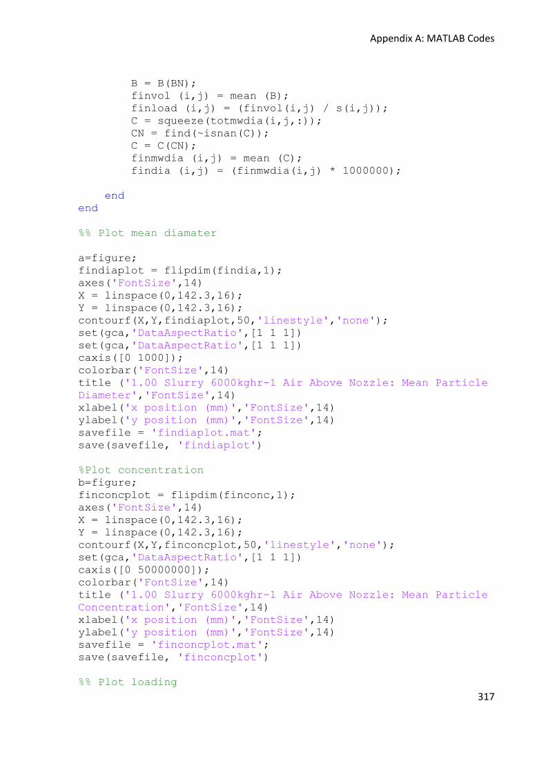
Appendix A: MATLAB Codes
317
B = B(BN);
finvol (i,j) = mean (B);
finload (i,j) = (finvol(i,j) / s(i,j));
C = squeeze(totmwdia(i,j,:));
CN = find(~isnan(C));
C = C(CN);
finmwdia (i,j) = mean (C);
findia (i,j) = (finmwdia(i,j) * 1000000);
end
end
%% Plot mean diamater
a=figure;
findiaplot = flipdim(findia,1);
axes('FontSize',14)
X = linspace(0,142.3,16);
Y = linspace(0,142.3,16);
contourf(X,Y,findiaplot,50,'linestyle','none');
set(gca,'DataAspectRatio',[1 1 1])
set(gca,'DataAspectRatio',[1 1 1])
caxis([0 1000]);
colorbar('FontSize',14)
title ('1.00 Slurry 6000kghr-1 Air Above Nozzle: Mean Particle
Diameter','FontSize',14)
xlabel('x position (mm)','FontSize',14)
ylabel('y position (mm)','FontSize',14)
savefile = 'findiaplot.mat';
save(savefile, 'findiaplot')
%Plot concentration
b=figure;
finconcplot = flipdim(finconc,1);
axes('FontSize',14)
X = linspace(0,142.3,16);
Y = linspace(0,142.3,16);
contourf(X,Y,finconcplot,50,'linestyle','none');
set(gca,'DataAspectRatio',[1 1 1])
caxis([0 50000000]);
colorbar('FontSize',14)
title ('1.00 Slurry 6000kghr-1 Air Above Nozzle: Mean Particle
Concentration','FontSize',14)
xlabel('x position (mm)','FontSize',14)
ylabel('y position (mm)','FontSize',14)
savefile = 'finconcplot.mat';
save(savefile, 'finconcplot')
%% Plot loading

Appendix A: MATLAB Codes
318
c=figure;
finloadplot = flipdim(finload,1);
axes('FontSize',14)
X = linspace(0,142.3,16);
Y = linspace(0,142.3,16);
contourf(X,Y,finloadplot,50,'linestyle','none');
set(gca,'DataAspectRatio',[1 1 1])
caxis([0.0 0.001]);
colorbar('FontSize',14)
title ('1.00 Slurry 6000kghr-1 Air Above Nozzle: Mean Particle
Volume Fraction','FontSize',14)
xlabel('x position (mm)','FontSize',14)
ylabel('y position (mm)','FontSize',14)
savefile = 'finloadplot.mat';
save(savefile, 'finloadplot')
%Directory/folder for PIV image files
cd ('C:\Users\Guy\Desktop\PIV MATLAB Codes');
A.2.3 Particle PIV data handling and Plotting
PIV cross correlation was conducted with the binary images created using the code shown in
§0, using the TSI PIV software. The output from this analysis was loaded into a 3D matrix and
the velocity parameters are calculated in a similar manner to those in (§0).
%% RoySoft 2009
%% Written by G. Hassall
%% Based on codes by K. Chung and G. Neal
%Directory/folder for vector files
cd ('C:\Users\Guy\Desktop\particle vec files\above
nozzle\1000-6000');
%%%Load Vector Files%%%
%%%%%%%%%%%%%%%%%%%%%%%%%%%%%%%%%%%%%%%%%%%%%%%%%%%%%%%%%%%%%%
%%%%%%%%
nfiles = input ('Last Frame? (e.g. 499) >> ')
fname3 = ['Test 1000kg 6000kg
air004934.T000.D000.P049.H000.L.vec'];
%%One vector file is loaded here, assuming first file ends
with 00000.vec%%
s=csvread([fname3],1,0);
G=s;
%%%The rest of files are loaded here as a loop%%%
for i = (4935 : nfiles);

Appendix A: MATLAB Codes
319
if i < 10
fname3 = ['Test 1000kg 6000kg
air00100',int2str(i),'.T000.D000.P049.H000.L.vec'];
elseif 100 > i & i > 9
fname3 = ['Test 1000kg 6000kg
air0010',int2str(i),'.T000.D000.P049.H000.L.vec'];
elseif 1000 > i & i > 99
fname3 = ['Test 1000kg 6000kg
air001',int2str(i),'.T000.D000.P049.H000.L.vec'];
else
fname3 = ['Test 1000kg 6000kg
air00',int2str(i),'.T000.D000.P049.H000.L.vec'];
end
if exist (fname3)>0
s=csvread([fname3],1,0);
G2=s;
G=cat(3,G,G2);
end
end
clear G2;
%remove false values
[D,L]=find(G(:,5,:)<1);%finds all where 'false' is indicated
by the software
for l=1:length(D);
G(D(l),3:4,L(l))=NaN;%sets the velocities and the 5th
column to zero for the false vectors
l=l+1;
end
%removing filled vectored errors
[D,L]=find(G(:,5,:)>1);%finds all where 3G software has
added/filled vector
for l=1:length(D);
G(D(l),5,L(l))=1;%sets the 5th column to one for the
filled vectors
l=l+1;
end
% Enter correct number of spots for width and hieght of image
for reshaping
f = input('number of spots?') %enter number of spots image is
split into
%%%%%%%%%%%%%%%%%%%%%%%%%%%%%%%%%%%%%%%%%%%%%%%%%%%%%%%%%%%%%%
%%%%%%%%%%%%%
%x increases down rows
%y increases along columns
sizeG=size(G);

Appendix A: MATLAB Codes
320
sizeG=sizeG(3);
for i = 1:1:sizeG; %%works through loop for i values from 1
to size of G
U=G(:,3,i); %% Cuts out U velocities from G matrix
UU=reshape(U,f,[]); %% moves column of U velocities in U
matrix into 63 by 63 square matrix(top left is X1, Y1 and
bottom left is Xn, Y1)
Umatrix(:,:,i)=UU; %% Creates 3D U matrix with each U value
stacked behind previous
V=G(:,4,i); %% as above for V
VV=reshape(V,f,[]);
Vmatrix(:,:,i)=VV;
Vec=G(:,5,i); %% cuts of the CHC column from the
3D matrix G
VVec=reshape(Vec,f,[]); %% creates 63 by 63 matrix as
above
Vecmatrix(:,:,i)=VVec; %% stacks matrices
clear U UU V VV Vec VVec;
end;
% remove NaN entries
Umean = nan(f,f); %% set up required matrices to be
filled (f= no spots)
Vmean = nan(f,f);
RMSU = nan(f,f);
RMSV = nan(f,f);
RSUV = nan(f,f);
TKE = nan(f,f);
URes = nan(f,f);
for i=1:f;
for j = 1:f; %% Runs a loop from 1 to 63 to
generate all of below for each column of matrix
U = squeeze(squeeze(Umatrix(i,j,:))); %% cuts out
row by row from 3D stack on Umatrix (63 by 63 matrix of each
value stacked in turn)
V = squeeze(squeeze(Vmatrix(i,j,:)));
NU = find(~isnan(U)); %%
NV = find(~isnan(V));
U = U(NU);
V = V(NU);
AU=size(U);
AV=size(V);
Kount(i,j)=AU(1); %% counts
number of vectors in each spot over the full time period of
study
if AU(1) > 1
Umean(i,j)=mean(U);
Vmean(i,j)=mean(V);

Appendix A: MATLAB Codes
321
URes (i,j) =
((((Umean(i,j).^2))+((Vmean(i,j)).^2)).^0.5);
for h=(1 : AU);
UZ = U(h,1);
VZ = V(h,1);
UURes (h,1) = (((UZ.^2)+(VZ.^2)).^0.5);
end
UResSTD (i,j) = STD(UURes);
end
end
end
%Plot Tangential Velocity
Umeanplot = rot90(Umean);
%Plot Radial Velocity
Vmeanplot = rot90(Vmean);
%Plot Resultant Velocity
UResplot = rot90(URes);
UResplot(15:16,:) = nan;
UResplot(1,:) = nan;
%Umeanplot = rot90(Umean);
%Umeanplot(15:16,:) = nan;
Umeanplot(1,:) = nan;
%Vmeanplot = rot90(Vmean);
%Vmeanplot(15:16,:) = nan;
Vmeanplot(1,:) = nan;
c=figure;
axes('FontSize',14)
X = linspace(0,142.4,15);
Y = linspace(0,142.4,15);
contourf(X,Y,UResplot,50,'linestyle','none');
caxis([0.0 0.5]);
set(gca,'DataAspectRatio',[1 1 1])
colorbar('FontSize',14)
title ('Above Nozzle - Low Slurry Flowrate and Low Air
Flowrate : Velocity Magnitude','FontSize',14)
xlabel('x position (mm)','FontSize',14)
ylabel('y position (mm)','FontSize',14)
hold on
scale = 0.75;
quiver(X,Y,Umeanplot, Vmeanplot, scale,'k','LineWidth',1);
hold off
cd('C:\Users\Guy\Desktop\PIV MATLAB Codes');

Appendix B: Wall Deposition Example Calculations
322
B. Appendix B – Wall Deposition Example Calculations
This appendix shows example calculations of how the amount of deposition in different
areas and entire area of the spray dryer was calculated and turned into a yield expression. In
order to calculate deposition over the entire area of dryer, it was then split into sections and
the deposition per unit area values obtained were extrapolated over these areas to estimate
the total amount of material deposited over these sections. By summing the material
deposited in these sections, the total amount of material deposited over the entire dryer
was obtained and compared to the total amount of slurry sprayed during the entire period
of dryer operation, enabling calculation of a yield value.
The first stage in this calculation was to split the spray dryer into sections, each of which
contained a measurement location. Figure B.1 shows how the dryer was split into these
simplified geometries, cylinders for the dryer shell and a cone for the dryer cone. The area of
the walls in each of these sections was calculated (using basic geometry equations) and the
areas calculated for each are displayed in Table B.1.
Table B.1: Detergent Formulations for Impact Experiments
Section Shape Height (m) Diameter (m) Wall Area (m2)
10.5 m to 18 m Cylinder 7.5 1.7 40.1
7.5 m to 10.5 m Cylinder 3.0 1.7 16.0
4.5 m to 7.5 m Cylinder 3.0 1.7 16.0
0 m to 4.5 m Cylinder 4.5 1.7 24.0
cone Cone 2.2 1.7 11.0
Total 107.1

Appendix B: Wall Deposition Example Calculations
323
Wall Deposition (E) 12.00 m
Wall Deposition (D) 9.00 m
Wall Deposition (C) 6.00 m
Wall Deposition (A) -3.00 m
1.7 m
Wall Deposition (B) 3.00 m
7.5 m
4.5 m
2.2 m
3.0 m
3.0 m
Figure B.1: Sections used in estimation of spray dryer internal wall area
The total amount of material deposited over the entire area of each section was calculated
by multiplying the deposition per unit area calculated through the measurements (§3.4) by
the total area of each section as shown in Table 3.2. Summing these figures allowed the total
deposition on the dryer to be calculated, thus giving an estimation of the amount of slurry
lost to wall deposition during dryer operation.

Appendix C: Fluid Dynamics Further Data
324
C. Appendix C – Fluid Dynamics in a Detergent Spray Dryer (Further Data)
This Appendix displays extra results and data that were not included in Chapter five but do
have relevance on the fluid dynamics in spray dryers.
C.1 Normalised Time Averaged Flow Fields
Figure C.1 shows the same flow fields with velocity values normalised against the inlet
tangential velocity values for each experimental condition as displayed in Table 5.1 (§5.2).
Comparing the normalised values of velocity magnitude for the three flow fields displayed
for different flow rates of air the higher position (Figure C.1 a, b and c) shows how
normalised velocity does not increase with increasing airflow rate. This indicates that the
structure of the flow (vortex) is affected by flow rate and can be described as self-impating.

Appendix C: Fluid Dynamics Further Data
325
x position (mm)
y p
ositio
n (
mm
)
Above Nozzle - Medium Flowrate: Normalised Velocity Magnitude
0 20 40 60 80 100 120 140 1600
20
40
60
80
100
120
140
160
0
0.05
0.1
0.15
0.2
0.25
0.3
0.35
0.4
0.45
0.5
x position (mm)
y p
ositio
n (
mm
)Below Nozzle - High Flowrate: Normalised Velocity Magnitude
0 20 40 60 80 100 120 140 1600
20
40
60
80
100
120
140
160
0
0.05
0.1
0.15
0.2
0.25
0.3
0.35
0.4
0.45
0.5
x position (mm)
y p
ositio
n (
mm
)
Above Nozzle - Low Flowrate: Normalised Velocity Magnitude
0 20 40 60 80 100 120 140 1600
20
40
60
80
100
120
140
160
0
0.05
0.1
0.15
0.2
0.25
0.3
0.35
0.4
0.45
0.5
x position (mm)
y p
ositio
n (
mm
)
Above Nozzle - High Flowrate: Normalised Velocity Magnitude
0 20 40 60 80 100 120 140 1600
20
40
60
80
100
120
140
160
0
0.05
0.1
0.15
0.2
0.25
0.3
0.35
0.4
0.45
0.5
aa b
c d
Figure C.1: Flow Field Plots of Velocity Magnitude Normalised Values: (a) low-position with high-flowrate, (b)
high-position with low-flowrate, (c) high-position with medium-flowrate and (d) high-position with high-
flowrate.

Appendix C: Fluid Dynamics Further Data
326
x position (mm)
y p
ositio
n (
mm
)Below Nozzle - High Flowrate: Normalised Radial Velocity
0 20 40 60 80 100 120 140 1600
20
40
60
80
100
120
140
160
-0.2
-0.15
-0.1
-0.05
0
0.05
x position (mm)
y p
ositio
n (
mm
)
Above Nozzle - Low Flowrate: Normalised Radial Velocity
0 20 40 60 80 100 120 140 1600
20
40
60
80
100
120
140
160
-0.2
-0.15
-0.1
-0.05
0
0.05
x position (mm)
y p
ositio
n (
mm
)
Above Nozzle - Medium Flowrate: Normalised Radial Velocity
0 20 40 60 80 100 120 140 1600
20
40
60
80
100
120
140
160
-0.2
-0.15
-0.1
-0.05
0
0.05
x position (mm)
y p
ositio
n (
mm
)
Above Nozzle - High Flowrate: Normalised Radial Velocity
0 20 40 60 80 100 120 140 1600
20
40
60
80
100
120
140
160
-0.2
-0.15
-0.1
-0.05
0
0.05
aa b
c d
Figure C.2: Flow Field Plots of Normalised Values of Radial Velocity: (a) low-position with high-flowrate, (b)
high-position with low-flowrate, (c) high-position with medium-flowrate and (d) high-position with high-
flowrate.
As with the velocity magnitude, and radial velocity, normalised values of radial and
tangential velocities, Figure C.2 and Figure C.3, show similar trends and again indicate that
the vortex is self impating.

Appendix C: Fluid Dynamics Further Data
327
x position (mm)
y p
ositio
n (
mm
)Below Nozzle - High Flowrate: Normalised Tangential Velocity
0 20 40 60 80 100 120 140 1600
20
40
60
80
100
120
140
160
0
0.05
0.1
0.15
0.2
0.25
0.3
0.35
0.4
0.45
0.5
x position (mm)
y p
ositio
n (
mm
)
Above Nozzle - Low Flowrate: Normalised Tangential Velocity
0 20 40 60 80 100 120 140 1600
20
40
60
80
100
120
140
160
0
0.05
0.1
0.15
0.2
0.25
0.3
0.35
0.4
0.45
0.5
x position (mm)
y p
ositio
n (
mm
)
Above Nozzle - Medium Flowrate: Normalised Tangential Velocity
0 20 40 60 80 100 120 140 1600
20
40
60
80
100
120
140
160
0
0.05
0.1
0.15
0.2
0.25
0.3
0.35
0.4
0.45
0.5
x position (mm)
y p
ositio
n (
mm
)
Above Nozzle - High Flowrate: Normalised Tangential Velocity
0 20 40 60 80 100 120 140 1600
20
40
60
80
100
120
140
160
0
0.05
0.1
0.15
0.2
0.25
0.3
0.35
0.4
0.45
0.5
aa b
c d
Figure C.3: Flow Field Plots of Normalised Values of Tangential Velocity: (a) low-position with high-flowrate,
(b) high-position with low-flowrate, (c) high-position with medium-flowrate and (d) high-position with high-
flowrate.
C.2 Turbulent Parameters
C.2.1 Turbulent Kinetic Energy
Figure C.4 shows plots of turbulent kinetic energy (§2.5.3) for all experimental conditions.
Values of TKE between 0.2 and 0.5 kJkg-1 are seen in the lower position and values between
0.1 and 0.5 kJkg-1 in the higher position (excluding edge effects as seen on previous plots).

Appendix C: Fluid Dynamics Further Data
328
Values of TKE would be expected to reflect the same trends as turbulence intensity (§5.4)
and indeed this is the case. In position L, TKE appears to increase with distance from the
wall as with the turbulence intensity, again this trend is not so obvious in position H.
Increasing flow rate appears to increase TKE values, as was seen with the turbulence
intensity. This means that more of the fluid’s energy is dissipated though turbulence in the
lower position (closer to the air inlets) and also as flow rate is increased.
x position (mm)
y p
ositio
n (
mm
)
Below Nozzle - High Flowrate: Turbulent Kinetic Energy
0 20 40 60 80 100 120 140 1600
20
40
60
80
100
120
140
160
0
0.05
0.1
0.15
0.2
0.25
0.3
0.35
0.4
0.45
0.5
x position (mm)
y p
ositio
n (
mm
)
Above Nozzle - Low Flowrate: Turbulent Kinetic Energy
0 20 40 60 80 100 120 140 1600
20
40
60
80
100
120
140
160
0
0.05
0.1
0.15
0.2
0.25
0.3
0.35
0.4
0.45
0.5
x position (mm)
y p
ositio
n (
mm
)
Above Nozzle - Medium Flowrate: Turbulent Kinetic Energy
0 20 40 60 80 100 120 140 1600
20
40
60
80
100
120
140
160
0
0.05
0.1
0.15
0.2
0.25
0.3
0.35
0.4
0.45
0.5
x position (mm)
y p
ositio
n (
mm
)
Above Nozzle - High Flowrate: Turbulent Kinetic Energy
0 20 40 60 80 100 120 140 1600
20
40
60
80
100
120
140
160
0
0.05
0.1
0.15
0.2
0.25
0.3
0.35
0.4
0.45
0.5
a b
c d
Figure C.4: Turbulent Kinetic Energy Plots: (a) low-position with high-flowrate, (b) high-position with low-
flowrate, (c) high-position with medium-flowrate and (d) high-position with high-flowrate.

Appendix C: Fluid Dynamics Further Data
329
C.2.2 Reynolds Stresses
Reynolds stress (§ 2.5.3) values for all experimental conditions are shown in Figure C.5. The
largest values of Reynolds stresses are seen in the lower position – high flowrate (a)
conditions, ranging from 0.0 to 0.04. increasing the air flowrate in the higher experimental
position (b) to (c) to (d) increases the values of Reynolds stresses seen, from 0.0 to 0.01 for
the low flow, through to 0.0 to 0.02 at medium flow and then 0.0 and 0.04 at high flowrate.
x position (mm)
y p
ositio
n (
mm
)
Above Nozzle - High Flowrate: Reynolds Stresses
0 20 40 60 80 100 120 140 1600
20
40
60
80
100
120
140
160
0
0.005
0.01
0.015
0.02
0.025
0.03
x position (mm)
y p
ositio
n (
mm
)
Above Nozzle - Medium Flowrate: Reynolds Stresses
0 20 40 60 80 100 120 140 1600
20
40
60
80
100
120
140
160
0
0.005
0.01
0.015
0.02
0.025
0.03
x position (mm)
y p
ositio
n (
mm
)
Below Nozzle - High Flowrate: Reynolds Stresses
0 20 40 60 80 100 120 140 1600
20
40
60
80
100
120
140
160
0
0.005
0.01
0.015
0.02
0.025
0.03
x position (mm)
y p
ositio
n (
mm
)
Above Nozzle - Low Flowrate: Reynolds Stresses
0 20 40 60 80 100 120 140 1600
20
40
60
80
100
120
140
160
0
0.005
0.01
0.015
0.02
0.025
0.03
a b
c d
Figure C.5: Reynolds Stress Plots: (a) low-position with high-flowrate, (b) high-position with low-flowrate, (c)
high-position with medium-flowrate and (d) high-position with high-flowrate.

Appendix C: Fluid Dynamics Further Data
330
These values and how they increase with decreasing distance to the air inlets and increase
with increasing flowrate further reflect the trends in turbulence shown by all turbulent
parameters calculated. Increasing values of Reynolds stresses show increased force being
applied on the steady flow by the fluctuating component and therefore increased levels of
turbulent motion in the flow. Similar trends can be seen in Figure C.6, which shows values of
Reynolds stresses normalised against tangential inlet air velocity for each experimental
condition.
x position (mm)
y p
ositio
n (
mm
)
Above Nozzle - High Flowrate: Normalised Reynolds Stresses
0 20 40 60 80 100 120 140 1600
20
40
60
80
100
120
140
160
0
0.001
0.002
0.003
0.004
0.005
0.006
0.007
0.008
0.009
0.01
x position (mm)
y p
ositio
n (
mm
)
Above Nozzle - Medium Flowrate: Normalised Reynolds Stresses
0 20 40 60 80 100 120 140 1600
20
40
60
80
100
120
140
160
0
0.001
0.002
0.003
0.004
0.005
0.006
0.007
0.008
0.009
0.01
x position (mm)
y p
ositio
n (
mm
)
Above Nozzle - Low Flowrate: Normalised Reynolds Stresses
0 20 40 60 80 100 120 140 1600
20
40
60
80
100
120
140
160
0
0.001
0.002
0.003
0.004
0.005
0.006
0.007
0.008
0.009
0.01
x position (mm)
y p
ositio
n (
mm
)
Below Nozzle - High Flowrate: Normalised Reynolds Stresses
0 20 40 60 80 100 120 140 1600
20
40
60
80
100
120
140
160
0
0.001
0.002
0.003
0.004
0.005
0.006
0.007
0.008
0.009
0.01
a b
c d
Figure C.6: Normalised Reynolds Stress Plots: (a) low-position with high-flowrate, (b) high-position with low-
flowrate, (c) high-position with medium-flowrate and (d) high-position with high-flowrate.

Appendix D: Particle Dynamics Analysis Methods
331
D. Appendix D – Particle Dynamics Analaysis Methods
The complexity of the images captured, i.e. the range of grayscale values, presented a
challenge in terms of developing a suitable analysis route that would allow particle size,
concentration and loading details to be obtained as well as allowing PIV cross-correlation to
be conducted to obtain particle velocity fields (§3.5.5). In this section, the nature of the
captured images and the steps taken to develop a suitable image analysis route are
described. Details on how particle size, concentration and loading parameters were
calculated are given along with details on how cross-correlation was conducted to obtain
particle flow fields. The possible errors encountered in this work are also reviewed.
D.1 PIV Images Captured
The nature of the images captured during these experiments presented a challenge in terms
of obtaining quantitative data through image analysis and cross correlation. Examples of
images captured are shown in Figure D.1.
a b
Figure D.1: Example of PIV Images captured (a) position L; (b) position H)

Appendix D: Particle Dynamics Analysis Methods
332
In both of the images, a range of brightness is observable for the particles (grayscale values).
In addition the image shown for Position H appears brighter (contains more pixels of higher
grayscale values) than that in the lower position. Grayscale histograms of these images are
displayed in Figure D.2, so that the spread of values can be studied quantitatively. The peak
of the distribution position H is further to the right, indicating the presence of a greater
number of brighter pixels than for position L.

Appendix D: Particle Dynamics Analysis Methods
333
0 50 100 150 200 250
0
1
2
3
4
5
6
7
8
9
10x 10
4 Below Nozzle - Typical Greyscale Histogram
Greyscale Value
Nu
mb
er
of P
ixe
ls
0 50 100 150 200 250
0
1
2
3
4
5
6
7
8
9
10x 10
4 Above Nozzle - Typical Greyscale Histogram
Greyscale Value
Nu
mb
er
of P
ixe
lsa
b
Figure D.2: Histograms of greyscale values for the images shown in Figure 6.1: (a) position L; (b) position H.
The ranges of grayscale values exhibited by the images require investigation of the
phenomena leading to these results. Four main phenomena/issues have been considered:

Appendix D: Particle Dynamics Analysis Methods
334
Dissipation of light by particles between the laser-source and image area and
between the image area and camera.
Reflection/scattering of laser light could illuminate particles outside of the laser
sheet.
The development of a gradient in light intensity within the laser sheet as it behaves
as a Gaussian beam beyond its waist.
Issues with the large pixel resolution used, meaning that the number of pixels
covering each particle is low and therefore results in half occupied pixels with lower
grayscale values.
A further important question is whether all particles visible in the image are fully within the
laser sheet or whether some visible particles are partly or completely outside it.
Each of these issues will now be discussed in more detail before final conclusions on what
can be seen in these images, and why, are drawn.
Dissipation – light dissipated by the in-plane particles within the laser sheet will cause
reduction in intensity with distance away from the laser source. In addition scattered light
will be dissipated by out of plane particles present between the measurement plane and the
camera. Both will cause in-plane particles to appear to be less bright (giving lower grayscale
values). As the particle loading in the dryer varies with both space and time, the amount of
light dissipated will vary between different areas of the images and between frames.
Additionally, images above the nozzle (position H) would experience less dissipation due to
lower particle loading, giving brighter images (higher grayscale values). Conversely below

Appendix D: Particle Dynamics Analysis Methods
335
the nozzle (position L) where particle loading is known to be higher, the images are less
bright. Figure 6.1 gives circumstantial evidence to support this hypothesis.
Reflection / Scattering of Light – light reflected and scattered from the dryer walls and
particles within the dryer results in light travelling outside of the laser sheet, meaning that
particles outside of the laser sheet volume can appear to be illuminated in images. This
phenomena has been reported before, for imaging of gas-liquid flows in stirred tanks using
PIV (Chung et al. (2009)). This was kept to a minimum by ensuring the depth of field of the
camera was as fully contained in the laser sheet as possible.
Gaussian Beam – the laser sheet used can be considered as Gaussian in the vertical plane. At
the waist in the laser sheet, the light can be considered to be truly coherent with no gradient
in intensity through the vertical plane. Beyond the waist, the beam diverges such that its
thickness in the vertical plane increases, causing a gradient in intensity of the light to
develop across the vertical plane. The laser sheet then ceases to be a coherent light source
and will illuminate particles to different grayscale values, depending on their position within
the laser sheet. Calculations of the thickness of a Gaussian laser sheet are covered later
(§D.3).
Pixel Resolution – To maximise the field of view within the tower, a large pixel size was used
(120-150 µm pixel-1). Consequently particles in the flow smaller than 150 µm (or those
larger than 150 µm but only partially within the laser sheet) may not cover an entire pixel.
This will give a lower than expected grayscale value and may indeed be indistinguishable
from background noise in the image.

Appendix D: Particle Dynamics Analysis Methods
336
Since each of the phenomena above is equally possible it is most likely that the
characteristics of the images are a product of all four working in combination. This prompts
an interesting question as to whether the particles seen are all inside the laser sheet; in turn
this presents an interesting quandary in terms of which particles are included in the image
analysis and which are discarded.
D.2 Image Analysis – Choice of Threshold
The challenge in particle detection is the selection of a threshold value with which to
binarize the image; i.e. choice of a grayscale value above which all pixels are taken to be
particles and therefore white, and below which every pixel is background and therefore
black. Once obtained binary images can be used to obtain particle parameters using the
image analysis toolbox of MATLAB 7.1 software (Mathworks Inc.).
Initially the automated threshold calculation algorithm “graythresh” within the image
analysis toolbox of MATLAB 7.1 software (Mathworks Inc.), was considered to be the
obvious choice for calculating a threshold level for images. This algorithm uses Otsu’s
method, which chooses the threshold to minimise the intraclass variance of the black and
white pixels. This is achieved by assuming that the image contains two classes of pixels
(foreground and background), and therefore there is a bimodal distribution of grayscale
values on the image histogram. The optimum threshold value is then calculated to separate
the two classes such that their combined spread (intra-class variance) is at a minimum value.
The main issue with employing this algorithm is the assumption that there is a bimodal
distribution of grayscale values in the image to be thresholded. This is clearly not the case
for images captured during this work as shown in Figure D.2. Despite these concerns, data

Appendix D: Particle Dynamics Analysis Methods
337
was produced using this algorithm and results for particle volume fraction is shown in Figure
D.3.
r/R Position
0.860.880.900.920.940.960.981.00
Part
icle
Volu
me F
raction
0.00000
0.00005
0.00010
0.00015
0.00020
0.00025
1000kg slurry 6000kg air below nozzle
1200kg slurry 6000kg air below nozzle
1200kg slurry 8000kg air below nozzle
Average Loading for 1200 kghr-1 slurry (15 sec)
1000kg slurry 6000kg air above nozzle
1200kg slurry 6000kg air above nozzle
1200kg slurry 8000kg air above nozzle
Average Loading for 1000kghr-1 slurry (15 sec)
Figure D.3: Particle Volume Fraction as a Function of Radial Position Calculated with graythresh algorithm
The horizontal lines of this graph represent a mean particle volume fraction, with a
residence time of 15 seconds (an expected residence time, Amador (2009)), this was
calculated by dividing the volume of the amount of slurry sprayed within 15 seconds by the
total volume of the dryer, to give a volume fraction. Examination of this data and
comparison with the mean particle volume fraction calculated, shows that, apart from very
close to the wall, the measured particle volume fraction is lower than the mean value. In
practice, it would be expected that the particle concentrations would be higher over the
whole measured area, since it is well known that the maximum particle volume fraction is

Appendix D: Particle Dynamics Analysis Methods
338
close to the dryer wall (Bayly (2008)), owing to particles being thrown out towards the wall
by the centripetal forces of the swirling air flow. Therefore it can be concluded that Otsu’s
method over estimates the required threshold value, selecting only the brightest particles in
the images and excluding many pixels which represent particles. Since this method was the
only automated method available in the image analysis toolbox of MATLAB 7.1 software
(Mathworks Inc.), it was decided to develop a manual method for identifying the threshold
values.
The first step in the development of a thresholding method was to examine how changing
the threshold value (greyscale value running from 0 to 256) affected the number of particles
detected in an image. Examples of these plots are shown in Figure D.4, where the number of
particles are plotted on a logarithmic scale. Figure D.4 a is taken for a dataset at position H
and Figure D.4 b is taken at position L. Each sub-figure shows data from five images (A, B, C,
D and E selected from evenly spaced points throughout the dataset) to demonstrate the
variation.

Appendix D: Particle Dynamics Analysis Methods
339
1
10
100
1000
10000
100000
0 50 100 150 200 250
Nu
mb
er o
f Par
ticl
e D
etec
ted
Threshold Value
Image A
Image B
Image C
Image D
Image E
1
10
100
1000
10000
100000
0 50 100 150 200 250
Nu
mb
er
of
Pa
rtic
les
De
tect
ed
Thresholding Value
Image A
Image B
Image C
Image D
Image E
a
b
Figure D.4: Number of particles detected as a function of threshold value: (a) position H; (b) position L
For all images, the number of particles can be seen to initially decrease rapidly with
increasing threshold value after which the number of particles detected changes less rapidly.
For the below nozzle data, the number of particles detected appears to reach a plateau of

Appendix D: Particle Dynamics Analysis Methods
340
shallow gradient, for the above nozzle data, this is less apparent. These plots show that the
effect of thresholding value on the number of particles detected is always present, but is less
significant once threshold values increase beyond greyscale values of 51 particularly for the
below nozzle data.
The basis used for obtaining a thresholding value for all image sets was to assume that only
particles in focus could be in the laser sheet. Therefore the grayscale values of in and out-of-
focus particles could form the basis for choice of threshold level. This was achieved by
manually surveying a selection of images from each dataset and identifying in and out-of-
focus particles. The range of grayscale values seen in each was summarised, allowing the
minimum grayscale value for in-focus particle to be identified. This was used as the
threshold, thus ensuring all out-of-focus particles were classed as background. Figure D.5
gives an example of this process, where particles are selected from the image, (Figure D.5a)
based on their focus; their corresponding grayscale values are noted on Figure D.5b.

Appendix D: Particle Dynamics Analysis Methods
341
7
8
9
11
11
9
7
4
4
3
4
4
3
3
4
4
3
4
3
3
2
3
5
4
3
4
5
4
4
6
8
8
8
9
5
2
3
2
4
4
4
3
4
4
5
4
2
3
3
5
13
5
2
4
4
4
4
7
7
7
7
5
4
2
2
3
3
5
3
2
3
3
4
4
3
3
2
2
5
4
4
5
9
7
4
6
7
7
6
3
3
2
2
3
3
3
3
5
5
3
4
4
7
6
3
3
3
4
5
7
49
15
4
5
5
6
4
4
7
3
2
3
3
4
6
8
6
4
3
4
12
10
4
3
15
12
9
7
6
6
3
4
4
5
4
4
2
4
5
5
5
23
22
6
4
6
8
10
10
11
12
15
12
11
8
8
8
9
6
3
3
5
5
6
4
5
3
5
7
29
31
9
4
4
6
7
7
10
11
12
10
8
5
9
8
21
10
3
5
4
5
5
5
4
4
4
5
9
7
6
4
4
5
6
7
9
11
9
7
7
6
7
6
8
7
5
4
6
4
6
4
4
4
5
5
5
6
6
4
6
7
8
7
7
6
7
6
5
6
5
5
5
5
4
5
5
5
5
3
3
4
5
4
5
5
6
5
10
24
12
5
8
7
6
6
5
6
4
5
4
4
3
3
4
5
4
3
3
4
5
5
4
4
4
12
31
202
36
10
5
5
4
3
4
3
3
4
5
3
4
5
6
6
6
5
7
3
4
6
6
4
7
7
13
26
16
7
6
4
3
4
4
4
4
3
4
4
4
4
6
7
12
9
12
4
5
5
4
5
10
10
6
7
6
5
19
7
4
3
4
7
5
4
4
3
4
5
5
7
4
5
3
4
4
3
5
5
8
9
5
3
4
4
8
5
3
4
6
8
8
4
4
3
4
5
6
10
2
2
3
4
4
4
3
3
6
5
4
4
4
3
3
3
2
3
7
8
4
5
4
3
5
4
4
5
4
4
4
3
3
3
3
4
6
4
3
2
5
4
3
4
3
4
4
4
3
2
4
4
6
6
4
2
4
2
4
4
4
3
4
3
4
3
4
3
3
3
4
4
6
4
4
3
3
3
5
4
8
11
6
5
5
3
5
3
4
4
3
2
4
3
4
5
4
3
3
3
5
4
4
2
2
3
5
4
4
5
4
5
5
2
4
3
4
4
3
3
5
3
4
6
3
2
2
3
4
3
4
3
2
2
4
3
5
5
3
3
3
2
3
2
4
3
3
3
4
4
4
3
3
3
3
2
2
2
4
4
3
3
5
5
4
3
3
4
3
1
2
2
3
3
4
4
3
5
3
5
3
4
3
4
3
3
3
3
3
4
6
8
3
4
4
3
3
2
3
3
3
4
3
3
4
4
5
5
3
3
3
3
2
2
2
3
3
3
6
9
5
5
3
2
3
3
3
3
4
3
4
3
3
4
4
4
4
4
2
3
2
3
3
6
5
4
5
7
5
4
3
2
3
3
3
3
5
5
8
6
3
5
3
3
3
4
3
2
0
3
8
22
15
6
4
5
6
4
3
2
2
2
3
3
6
8
66
27
5
4
4
3
5
3
3
2
2
7
19
112
53
10
5
4
5
4
5
4
3
3
4
3
4
8
42
20
8
5
4
3
3
4
3
3
2
4
8
23
16
7
4
4
5
4
4
4
4
3
3
3
4
4
6
4
6
4
5
3
4
4
4
1
3
3
4
5
4
3
3
3
3
4
4
3
4
3
3
2
2
3
2
4
4
4
4
3
4
4
3
3
3
3
4
3
2
2
3
2
4
3
3
2
2
0
2
0
2
3
2
3
3
2
3
3
3
4
3
4
3
3
3
2
3
2
2
2
3
2
4
4
3
2
3
2
2
2
4
3
4
3
3
3
4
4
3
3
3
2
3
2
2
2
3
2
5
4
3
3
2
1
2
3
2
4
4
4
3
4
3
4
4
3
3
4
5
4
4
3
3
3
2
3
5
4
4
2
4
1
2
2
3
4
14
6
4
4
5
3
3
3
4
6
13
4
4
4
4
3
2
2
6
5
4
2
2
2
2
4
3
4
6
4
4
5
5
3
4
4
3
5
5
4
4
4
4
2
2
2
7
5
4
3
3
1
2
3
4
4
5
3
4
4
5
4
5
4
4
8
12
6
4
3
3
2
2
2
5
3
3
3
3
2
3
3
2
2
4
3
4
3
5
3
4
4
5
8
12
6
4
3
2
2
3
1
4
4
4
4
4
3
4
3
3
3
3
3
3
4
3
3
2
3
4
3
4
3
4
4
5
4
2
3
3
3
3
4
5
6
5
4
5
4
3
4
3
3
3
2
4
3
4
3
3
3
4
5
8
7
4
3
4
3
4
4
4
7
4
6
5
3
2
2
2
2
3
3
3
3
4
5
4
3
4
6
13
13
7
6
3
3
4
5
6
8
7
8
7
4
3
3
2
3
3
3
3
4
6
12
7
3
4
5
6
11
8
13
7
11
5
6
8
9
11
14
10
5
2
2
2
2
3
2
4
4
5
6
4
2
3
4
7
7
6
6
11
16
4
6
9
11
14
14
14
5
2
4
2
3
4
3
4
3
4
4
3
2
3
5
15
12
5
5
4
5
5
6
12
14
18
10
5
4
4
3
3
3
3
3
5
3
4
5
2
2
2
3
12
19
29
7
5
6
6
14
41
73
58
18
8
5
6
4
5
5
4
5
6
4
4
5
3
2
3
4
7
16
20
10
3
4
8
39
210
255
223
42
10
7
6
5
5
5
5
7
5
5
4
3
3
2
4
3
6
8
12
7
3
4
34
44
255
255
255
49
18
23
13
8
6
5
4
5
5
4
3
3
3
1
4
4
5
8
10
7
4
5
6
25
125
255
96
29
32
41
24
12
6
4
4
6
7
6
4
2
4
3
5
3
4
4
4
4
4
5
3
5
18
25
17
14
25
29
19
12
8
3
3
5
7
5
3
3
4
3
5
4
3
2
3
4
5
3
3
4
9
7
7
4
4
4
2
4
8
9
10
6
7
7
6
6
8
10
12
15
16
17
19
17
16
13
8
5
4
3
4
3
3
2
1
3
6
9
5
5
6
5
5
5
7
11
12
13
13
15
16
5
5
3
4
5
8
11
11
11
8
52
15
6
7
9
9
13
16
17
18
20
18
16
12
10
13
8
5
Green = in focus: More than 30
Red = out of focus: less than 30
a b
Figure D.5: (a) Example of particle selection to obtain threshold value; (b) corresponding grayscale values.
Table D.1 shows values for both the manually calculated threshold value (used in the final
analysis) and the threshold value calculated by the graythresh algorithm. The value
produced by the latter is always greater than the manually calculated value, and this
difference, is responsible for the lower particle volume fractions calculated using the
graythresh algorithm. Examining the contents of Table D.1 leads to the conclusion that the
differences in greyscale values between graythresh and the manual method are very small in
position H and hugely different in position L. This observation can be explained by
considering the differences in the images obtained from the two positions, as shown in the
previous sections (Figure D.1 to D.4). These differences mean that the graythresh algorithm,
which assumes a binary distribution of greyscale values works better position H images,

Appendix D: Particle Dynamics Analysis Methods
342
where there is a smaller range of greyscale values than position L images (for the reasons
listed in D.1). Therefore the more successful application of graythresh to position H images
results in a greyscale value for thresholding closer to the one obtained through the manual
method, where as for position L, the graythresh algorithm fails to get close to the manual
method value. Example of the MATLAB codes written for this analysis are displayed in
Appendix A.
Table D.1: Thresholding levels for all datasets
Relative Slurry
Flowrate
Air Flowrate
(kghr-1)
Graythresh
Thresholding grayscale
Value
Manual Thresholding
grayscale Value
Position H
1.00 6000 102 87
1.20 6000 108 95
1.20 8000 102 92
Position L
1.00 6000 100 33
1.20 6000 92 28
1.20 8000 97 26
D.3 Calculation of Size, Conentration and Loading Parameters
Once binary images were obtained using the manual method for obtaining the threshold,
the “regionalprops” algorithm within the MATLAB image analysis toolbox was used to
automatically calculate and list key parameters for each particle in the binary image. This
algorithm works by identifying and numbering each particle and then creating a matrix

Appendix D: Particle Dynamics Analysis Methods
343
which lists selected parameters of each particle. For the purpose of this work, for each
particle, the position of the centroid was listed as a pair of x and y coordinates along with
the equivalent diameter of a circle with the same area as the particle i.e.
2/14
P
A
Ad ( D.1 )
Where AP is the particle area as measured by the algorithm and dA is the area equivalent
diameter.
This matrix of particle properties and positions was created for 1 image in each image pair
obtained, (2000 images per experimental condition) and then all of the individual image
matrices were collated and used to calculate mean data for the whole set of images. The
particle data were sorted as function of position within the image based on the centroid
coordinates; by binning particles based on their position, plots of particle parameters as a
function of position within the image were created. Mean particle diameter data was
calculated as the mean diameter of all particles located with each area, as the image was
split into a 16 × 16 grid of equally sized squares. The value given by MATLAB was converted
from pixels into metres or micrometres. Particle size distributions were calculated by binning
particles based on their diameters, so that a count per diameter in pixels could be created.
This count was then turned into a mass fraction of the total number of particles assuming
spherical particles with a constant density across all diameters. The bin sizes used were then
converted from pixels into metres or micrometres.
To calculate the number concentration and volume fraction of particles in the image or a
specific area of the image, the volume occupied by the laser sheet is required. The depth of

Appendix D: Particle Dynamics Analysis Methods
344
the lasersheet was calculated at the two extremes of the image area, as shown in the cross-
section in Figure D.6. The cross-sectional area of the image was then calculated by treating
this as a trapezium, thusly:
)(
2
121 zzyA (D.2)
The value of the cross-sectional area obtained was then multiplied by the value of the x
dimension of the image area, to give the representative volume. This calculation was
repeated for each image, or section of image as required.
y
x
y
z1 z2
z1 z2
x
Image, viewed from the side
Cross-section of lasersheet, showing depth at top and bottom of image
Cross-sectional area of image
Volume of image
Figure D.6: Area of lasersheet covered by image
The thickness of the lasersheet was calculated by using assuming it acted as a Gaussian
beam. The divergence of a Gaussian beam beyond its waist is shown in Figure D.7.

Appendix D: Particle Dynamics Analysis Methods
345
Figure D.7: The divergence of a Gaussian beam around the waist
The value of w(z), half the thickness of the laser sheet as a function of distance from its
waist, as shown in Figure D.7, was calculated using equation (D.3), given below:
2
0 1)(
Rz
zwzw (D.3)
The Rayleigh length (ZR), is calculated using equation (D.4) below. The Rayleigh length is the
distance from the waist at which the cross section of the beam (thickness in this case) has
doubled.
2
0wzR (D.4)
In addition the angular spread of the sheet can be calculated as shown below, note Θ in
Figure D.7 is twice the value given using equation (D.5).
0w
(D.5)
To obtain particle number concentrations the total number of particles in each area of the
image was divided by the volume calculated for each specific area of the image. To obtain
particle volume fractions, particle volume, VP was calculated using spherical equivalence
(‘regionalprops’ algorithm in MATLAB)

Appendix D: Particle Dynamics Analysis Methods
346
6
3
AP
dV
(D.6)
The volume of particles in each area of the image was then summed and divided by the
volume calculated for each specific area of the image, to give the volume fraction.
D.4 Particle PIV Cross-Correlation
Cross-correlation of PIV images was conducted using binary images produced using the
method developed in §D.2 thus reducing errors from particles not in the focus (calibration)
range of the camera.
The high-resolution PIV algorithm (Nyquist grid) within the TSI Insight 3G software supplied
with the PIV equipment was used to conduct cross-correlation of the binary images. The
settings used in this algorithm were chosen to minimise errors in the calculation of the
velocity vectors. No velocity vector was produced for an interrogation spot containing less
than 16 particles and particles below 2 pixels in size were ignored. Hence particles less than
400 µm in diameter were not included in this analysis. To maximise the number of particles
in each integration spot whilst maintaining a reasonable resolution, an interrogation spot
size of 64 × 64 pixels was used. Cross-correlation was conducted for 2000 image pairs (4
seconds) for each experimental condition. The velocity vector files were processed using
MATLAB 7.1 software (Mathworks Inc.), in a similar manner to that of the air flow vectors
(§3.5).

Appendix D: Particle Dynamics Analysis Methods
347
D.5 Sources of Potential Error in Analysis Methods
The images captured presented a significant challenge in developing image analysis routes
which would allow reliable data to be obtained and minimise error. However, despite these
efforts there are still several significant potential sources of error that need to be considered
in this analysis. Also of note is that the vast majority of errors are systemic, with the
consequence that comparison between datasets can be made with confidence although
absolute values of the parameters may be shifted from the true values. Sources of systemic
error are:
Thresholding Value – the grayscale value chosen for thresholding represents the cut-off for
particles to be included in the analysis, therefore this can influence all results produced.
Owing to the fact that different thresholding values were used for different data-sets (which
have differing grayscale distributions) then the influence of this potential error can change
between datasets. The effect of this error was examined in Figure D.4.
Focusing – it is assumed that the depth of field is larger than the lasersheet thickness and
therefore all illuminated particles are in focus, and furthermore in focus particles are within
the lasersheet. If particles are out of focus this will lead to their diameter being incorrectly
calculated, in turn affecting size and loading data. In addition out of focus particles may be
included or rejected by thresholding. This error is systemic between datasets in the same
experimental position as the camera was only focused once in each position (f-stop kept
constant). Since the camera was carefully focused this error is minimised.
Resolution – as discussed previously, a large pixel resolution was used during this work to
maximize the area imaged. This means that the number of pixels covering each particle is
Appendix D: Particle Dynamics Analysis Methods
348
low and therefore results in half occupied pixels with lower grayscale values. This introduces
an error in partly illuminated pixels that can be eliminated during thresholding, meaning that
particle size can be underestimated, or in the worst case small particles can be eliminated.
Issues with how particle shape is displayed by a small number of pixels can also lead to
errors with how the equivalent diameter is calculated. This error comes from mis-estimation
of particle size owing to resolution and is expressed as an absolute error of ±1 pixel on mean
particle diameter plots (Figure D.2). This error was not accounted for on volume calculations
due to being combined with errors on assuming spherical particles, as discussed next.
Orientation and shape of particles – using the equivalent diameters will not only create
errors on the diameters calculated, but will also introduce errors into calculating particle
volumes. In addition, assuming that all particles are spherical will also introduce errors as
detergent powders are known to be irregularly shaped, meaning that volumes are
under/over estimated. Errors could also be introduced by the orientation of particles in the
laser sheet, although this could be eliminated if it is assumed that their orientation is
random due to the large number of particles imaged.

Appendix E: Particle Impacts Statistical Analysis
349
E. Appendix E – Particle Characterisation and Impacts Statistical Analysis
The purpose of this appendix is to display the full datasets for the statistical analysis
conducted on the particle impacts results shown in Chapter 7.
E.1 Correlation of all Variables
Presented in table E.1 below is the correlation values obtained between all of the variables
examined in Chapter 7. This table is formatted by colour to aid visualisation of the trends,
yellow cells indicate little correlation between the two variables, and green cells mean that
there is a positive correlation between the two variables, meaning they increase/decrease
with each other and red cells mean there is a negative correlation between then variables
and one increases/decreases the other. The shade of green/red shown in the cell indicates
the strength of the correlation, with darker greens showing stronger positive correlations
and darker reds showing stronger negative correlations.

Appendix E: Particle Impacts Statistical Analysis
350
LAS content
SiO2 content
Representative
Diam
eter
Envelope Density
Apparent D
ensity
Moisture
Content
eRH
Unconfined
Young's Modulus
Unconfined Yield
Stress
Confined Yield
Stress
Confined Joint
Stress
Impact V
elocity
Norm
al Impact
Velocity
Impact A
ngle
Breakage
Fraction
Num
ber of
Fragments
Restitution
Coefficient
Norm
al
Restitution
Rebound A
ngle
from Im
pact
Rebound A
ngle
from Surface
LAS content 1.00 -0.28 0.00 -0.50 -0.81 0.15 -0.01 -0.84 -0.88 0.16 -0.08 0.01 0.01 0.00 -0.04 -0.01 -0.10 -0.07 -0.02 -0.03
SiO2 content -0.28 1.00 0.00 -0.11 -0.14 0.62 -0.49 0.01 0.49 0.40 0.34 0.00 0.00 0.00 -0.02 -0.10 0.09 0.20 0.00 0.03
Representative Diameter 0.00 0.00 1.00 0.67 -0.34 0.59 0.12 -0.20 0.10 -0.30 -0.48 0.00 0.00 0.00 0.62 0.62 0.00 -0.23 0.08 0.07
Envelope Density -0.50 -0.11 0.67 1.00 0.38 0.07 0.29 0.51 0.37 -0.39 -0.13 -0.01 -0.01 0.00 0.34 0.36 0.04 -0.13 0.06 0.04
Apparent Density -0.81 -0.14 -0.34 0.38 1.00 -0.59 0.31 0.92 0.50 -0.17 0.18 -0.02 -0.02 0.00 -0.22 -0.22 0.06 0.05 0.00 -0.02
Moisture Content 0.15 0.62 0.59 0.07 -0.59 1.00 -0.17 -0.49 0.05 0.25 -0.24 0.01 0.01 0.00 0.36 0.30 0.03 -0.09 0.05 0.08
eRH -0.01 -0.49 0.12 0.29 0.31 -0.17 1.00 0.29 -0.35 0.15 -0.36 0.00 0.00 0.00 0.02 0.02 -0.04 -0.27 0.03 0.00
Unconfined Young's Modulus -0.84 0.01 -0.20 0.51 0.92 -0.49 0.29 1.00 0.61 -0.07 0.23 -0.02 -0.02 0.00 -0.17 -0.17 0.07 0.07 0.00 -0.01
Unconfined Yield Stress -0.88 0.49 0.10 0.37 0.50 0.05 -0.35 0.61 1.00 -0.17 0.08 -0.01 -0.01 0.00 0.14 0.10 0.11 0.13 0.02 0.04
Confined Yield Stress 0.16 0.40 -0.30 -0.39 -0.17 0.25 0.15 -0.07 -0.17 1.00 -0.03 0.02 0.02 0.00 -0.26 -0.30 0.02 0.04 -0.02 -0.02
Confined Joint Stress -0.08 0.34 -0.48 -0.13 0.18 -0.24 -0.36 0.23 0.08 -0.03 1.00 -0.01 -0.01 0.00 -0.41 -0.39 0.02 0.30 -0.06 -0.05
Impact Velocity 0.01 0.00 0.00 -0.01 -0.02 0.01 0.00 -0.02 -0.01 0.02 -0.01 1.00 0.86 0.00 0.59 0.58 -0.02 -0.23 0.09 0.11
Normal Impact Velocity 0.01 0.00 0.00 -0.01 -0.02 0.01 0.00 -0.02 -0.01 0.02 -0.01 0.86 1.00 0.45 0.59 0.59 -0.48 -0.49 -0.38 -0.31
Impact Angle 0.00 0.00 0.00 0.00 0.00 0.00 0.00 0.00 0.00 0.00 0.00 0.00 0.45 1.00 0.13 0.13 -0.95 -0.70 -0.98 -0.93
Breakage Fraction -0.04 -0.02 0.62 0.34 -0.22 0.36 0.02 -0.17 0.14 -0.26 -0.41 0.59 0.59 0.13 1.00 0.87 -0.17 -0.39 -0.03 0.02
Number of Fragments -0.01 -0.10 0.62 0.36 -0.22 0.30 0.02 -0.17 0.10 -0.30 -0.39 0.58 0.59 0.13 0.87 1.00 -0.18 -0.40 -0.03 0.00
Restitution Coefficient -0.10 0.09 0.00 0.04 0.06 0.03 -0.04 0.07 0.11 0.02 0.02 -0.02 -0.48 -0.95 -0.17 -0.18 1.00 0.71 0.94 0.86
Normal Restitution Coefficient -0.07 0.20 -0.23 -0.13 0.05 -0.09 -0.27 0.07 0.13 0.04 0.30 -0.23 -0.49 -0.70 -0.39 -0.40 0.71 1.00 0.60 0.60
Rebound Angle from Impact -0.02 0.00 0.08 0.06 0.00 0.05 0.03 0.00 0.02 -0.02 -0.06 0.09 -0.38 -0.98 -0.03 -0.03 0.94 0.60 1.00 0.91
Rebound Angle from Surface -0.03 0.03 0.07 0.04 -0.02 0.08 0.00 -0.01 0.04 -0.02 -0.05 0.11 -0.31 -0.93 0.02 0.00 0.86 0.60 0.91 1.00
Particle PropertiesIm
pactR
esponse
Particle Properties Impact Response
Figure E.1: Correlation values of particle impacts variables

Appendix E: Particle Impacts Statistical Analysis
351
E.2 Modelling of Response Variables
To further understand the effect of impact pararmeters, particle size and formulation on
impact behaviour, response surface models were fit to the three main responses, namely
breakage fraction, restitution coefficent and rebound angle. Terms not significant at the 5%
significance level were removed from the model, meaning that only the key parameters
were used in these models.
E.2.1 Breakage Fraction
As shown previously, Figure E.2 shows that the largest effects on breakage fraction are from
rep. diameter and impact velocity. For both of these effects the biggest impact occurs
moving from low to mid levels with the effect flattening off at higher levels, this is
particularly evident for rep diameter. By optimising the model to minimise breakage fraction
it can be seen that this occurs at the mid level of SiO2, and low levels of the other 3 factors.
Figure E.2: Breakage fraction response models for key parameters

Appendix E: Particle Impacts Statistical Analysis
352
E.2.2 Restitution Coefficent
Figure E.3 shows that the largest effect on restitution coefficient comes from impact angle.
Other parameters that have significant, but much smaller effects, are LAS and SiO2 content,
representative diameter and impact velocity.
Figure E.3: Restitution Coefficent response models for key parameters
E.2.3 Rebound Angle from Impact
Figure E.4 shows that the largest effect on rebound angle from the impact comes from
impact angle, as with restitution coefficent. Other parameters that have significant, but
much smaller effects, are LAS and SiO2 content, representative diameter and impact velocity.
Figure E.4: Rebound angle from impact response models for key parameters