NEER WORKING PAPER SERIES

WHY DOES HIGH INFLATION RAISE INFLATION UNCERTAINTY?

Laurence Ball

Working Paper No. 3224

NATIONAL BUREAU OF ECONOMIC RESEARCH1050 Massachusetts Avenue

Cambridge, MA 02138January 1990

I am grateful for excellent research assistance from Aniruddha Dasgupta, andfor many helpful suggestions from Alan Blinder, Stephen Cecchetti, RobertGibbons, David Romer, Lawrence Summers, and seminar participants Carleton,Columbia, NBER, the New York Fed, Princeton, Rochester, the University ofQuebec at Montreal, Yale, and Wilfred Laurier. The NSF provided financialsupport. This paper is part of NBER's research program in EconomicFluctuations. Any opinions expressed are those of the author not those of theNational Bureau of Economic Research.

NBER Working Paper #3224January 1990

WHY DOES HIGH INFLATION RAISE INFLATION UNCERTAINTY?

A5STRACT

This paper presents a model of monetary policy in which a rise ininflation raises uncertainty about future inflation. When inflation is low,there is a consensus that the monetary authority will try to keep it low. Wheninflation is high, policyniakers face a dilemma: they would like to disinflate,but fear the recession that would result. The public does not know the tastesof future policymakers, and thus does not know whether disinflation will occur.

Laurence BallDepartment of EconomicsPrinceton UniversityPrinceton, NJ 08544-1017

Economists frequently argue that a rise in current inflation leads to

greater uncertainty about future inflation. This idea is a central theme, for

example, in Okun's (1971) 'The Mirage of Steady Inflation' and in Friedman's

(1977) Nobel Lecture. Many empirical studies provide evidence of such an

effect. But the accompanying explanations for the effect are usually loose

(Okun, for example, uses an analogy to driving over a bumpy road). It

appears that economists find the inflation level-uncertainty relation plausible

but have trouble pinning down why. This paper attempts to improve our

understanding of this relation by presenting a model that predicts it.'

The idea behind the model is simple: high inflation creates uncertainty

about future monetary policy. To understand why, consider first a period of

low inflation, such as the early 60s in the United States. In this situation, it

is a good bet that the Fed is happy with the status quo and will attempt to

prolong it. Inflation may rise at some point for a reason exogenous to the

Fed, such as spending on Viet Nam. It is unlikely, however, that the Fed

will simply decide that it is desirable to inflate.

Contrast this situation with a time of high inflation, such as the late

70s. Now it is not obvious what the Fed will do, because it faces a dilemma:

it would like to disinflate but fears the recession that would probably

result. It is likely that disinflation will occur eventually, but the timing is

uncertain. It depends on factors that are difficult to gauge in advance, such

as the values and opinions of FOMC members and the political pressures that

they face. In the late 70s, it would have been difficult to predict that sharp

disinflation would arrive in 1981_82.2

These ideas are similar to some previous discussions of inflation

uncertainty. Logue and Willet (1976) argue that "at higher average rates [of

inflation] government financial policy will tend to be less stable as it tries to

1

bring inflation under control while avoiding steep recession." Fischer and

Modigliani (1978) suggest that "governments typically announce unrealistic

stabilization programs as the inflation rate rises, thus increasing uncertainty

about what the actual path of prices will be.' And Friedman argues that '[a)

burst of inflation produces strong pressure to counter it. Policy goes from

one direction to the other, encouraging wide variation in,.. inflation." The

common theme is that high inflation creates uncertainty about how policy will

respond,

This paper formalizes this idea by applying recent advances in the

positive theory of monetary policy, Specifically, I make two modifications to

Barro and Gordon's (1983b) model of the repeated game between the Fed and

the public. First, following Canzoneri (1985), I introduce exogenous shocks

that cause low—inflation equilibria to break down occasionally. The economy

alternates between periods of high and low inflation, and I can compare

uncertainty in the two situations. Second, following Alesina (1987), I capture

policy uncertainty by assuming that there are two policymakers who alternate

in power stochastically. The conservative policymaker (C) views inflation as

very costly relative to unemployment, while the liberal (L) views inflation as

less costly. (As described below, a switch in policymakers is interpreted

broadly as a regime change that need not involve new personnel.)

These assumptions lead naturally to a link between inflation and

uncertainty. C hates inflation, so when inflation is low he tries to keep it

low and when it is high he disinflates. L also tries to prolong low inflation

-- that is, he resists the temptation to create an inflationary boom -- but he

is not willing to create a recession to disinflate. L's behavior results from a

crucial asymmetry: as explained below, the welfare gain from a boom is

smaller than the cost of a recession. When inflation is low, the public is

2

certain of future policy because C and L do the same thing. High inflation

creates uncertainty because the policymakers respond differently to the

disinflation dilemma and the public does not know who will be in charge.

There are two versions of my model. In the first, as in previous work,

policymakers attach a cost to the level of inflation. While this specification is

plausible, the subject of the paper suggests an alternative. The

inflation-uncertainty link is important because it helps to explain why

inflation is costly: economists often argue that inflation has small costs if it

is perfectly anticipated but larger costs if it raises uncertainty. Motivated

by this view, the second model includes a cost of uncertainty as well as a

smaller coat that depends on the inflation level. This specification creates a

paradox: conservatives view inflation as costly because it creates uncertainty,

but uncertainty arises from their efforts to disinflate (along with liberals'

resistance). It appears that conservatives would do better by accepting high

inflation. I show, however, that this may not be true.

The rest of the paper contains five sections. Section II presents the

basic model. Section III describes behavior that produces an

inflation—uncertainty link, and Section IV determines when this behavior is an

equilibrium. Section V considers the model with a coat of uncertainty, and

Section VI concludes.

II. THE MODEL

The modal combines elements of Barro—Gordon (1983a,b), Canzoneri (1985),

and Alesina (1987). There are two policymakers, C and L. Their loss

functions are

(1) (Ut — 70)2+ a.n , i=C,L ; aC>a.L

3

0.where Z. is policymaker 1 S loss in period t, U is actual unemployment, U is

optimal unemployment (a constant), n is inflation, and a is a taste parameter.

C views inflation as more costly relative to unemployment than L does.

The policymakers face a short run Phillips curve:

(2) Ut — — "V U0 + 1

where uN is the natural rate of unemployment arxi is expected inflation

at t given information at t-1. As in previous work, uN>U0 creates the

time-consistency problem that leads to inflation. (The as&sptions that

and that the coefficient on 7.T_fle equals one are normalizations on

the units of U and it.) Substituting (2) into (1) yields the loss in terms of

actual and unexpected inflation:

(3) Z, —— 1)2 +

The policymakers gain and lose power stochastically. For simplicity, the

probability that C is in power in a given period is a constant, c. L is in

power with probability 1—c. One can interpret a change of policymakers as

an election or appointment of a new Fed chairman. But it is more realistic to

interpret it broadly as a policy shift, probably resulting from an FOMC

meeting, that does not require new personnel. For example, the Fed may

first act liberal, tolerating high inflation, but then crack down because it

decides that the problem is serious or succumbs to political pressure.3

As in Canzoneri, the Fed does not control inflation perfectly. This

assumption is needed for high inflation to arise occasionally, since (in the

equilibrium below) policymakers never inflate on purpose. Each period, the

policymaker in power chooses a target inflation rate ii. With probability q, ashock causes actual inflation to deviate from the target. That is,

4

with probability l—q

Tr + with probability q

The shock t is distributed symmetrically around zero, with greatest density

at zero. The public does not observe t, so it cannot tell whether a rise in

inflation is intentional. One should think of q as fairly small: a shock is an

occasional event, such as a significant shift in the money demand function.

(The role of this assumption is explained below.)4

The two policymakere play a simple repeated game. At the start of each

period, the public sets expected inflation; expectations are assumed to be

rational. Then the current policymaker is determined and he chooses the

target i. Finally, the inflation shock (if any) arrives, determining actual

inflation. In choosing n, the policyinaker in power minimizes the expected

present value of his loss, with discount factor fi, putting equal weight on

periods when he is in and out of power. Each policymaker takes the other's

behavior as given.

III. A PROPOSED EQUILIBRIUM

This section and the next show how the model can produce a positive

relation between inflation and uncertainty. This section describes behavior

by the two policymakers that implies such a relation. The next section

determines when this behavior is an equilibrium and discusses other possible

equilibria.

The proposed equilibrium is presented in Table I. It is a modification of

the equilibrium for one policymaker in Barro—Gordon (1983b) and Canzoneri

(1985). Expected inflation and the policymakers' inflation targets depend on

inflation in the previous period. If previous inflation was non—positive, then

5

expected inflation is zero and both policymakers target zero. If previous

inflation was positive, then expected inflation is positive. In this

situation, C still targets zero but L targets >O (the value of is

determined below). Since L is in power with probability 1-c, rational

expectations implies Intuitively, when expected inflation is

zero, both policymakers are deterred from inflating by the 'punishment" of

higher expected inflation in the next period. When expected inflation is

positive, C disinflates but L does not, because he is not willing to create a

recession.

Over time, the economy alternates between periods of high (positive) and

low (non—positive) inflation. Policymakers try to prolong low inflation, but at

some point a shock causes inflation to rise, and expected inflation rises in

the following period. Inflation remains high as long as L is in power but

returns to zero when C arrives. (In general, inflation could also return to

zero through a large negative shock, but this is ruled out below.)5

As in Canzoneri, a rise in inflation caused by a shock must raise

expected inflation because the shock is unobservable. If the public,

believing that the rise is accidental, continues to expect low inflation -— that

is, if there is no punishment -- then the Fed can gain by faking positive

shocks. Thus it cannot be an equilibrium for expected inflation to stay low.

(The public does ignore negative shocks, because the Fed has no incentive to

cheat in that direction.) Note that the behavior of expectations is realistic:

when actual inflation rises or falls, expectations follow.

Table I implies a positive relation between current inflation and

uncertainty about next period's inflation. If t is non-positive, then next

period's target, is sure to be zero. i n is positive, then is

zero with probability c and with probability 1-c; its variance is c(l-c)2.

6

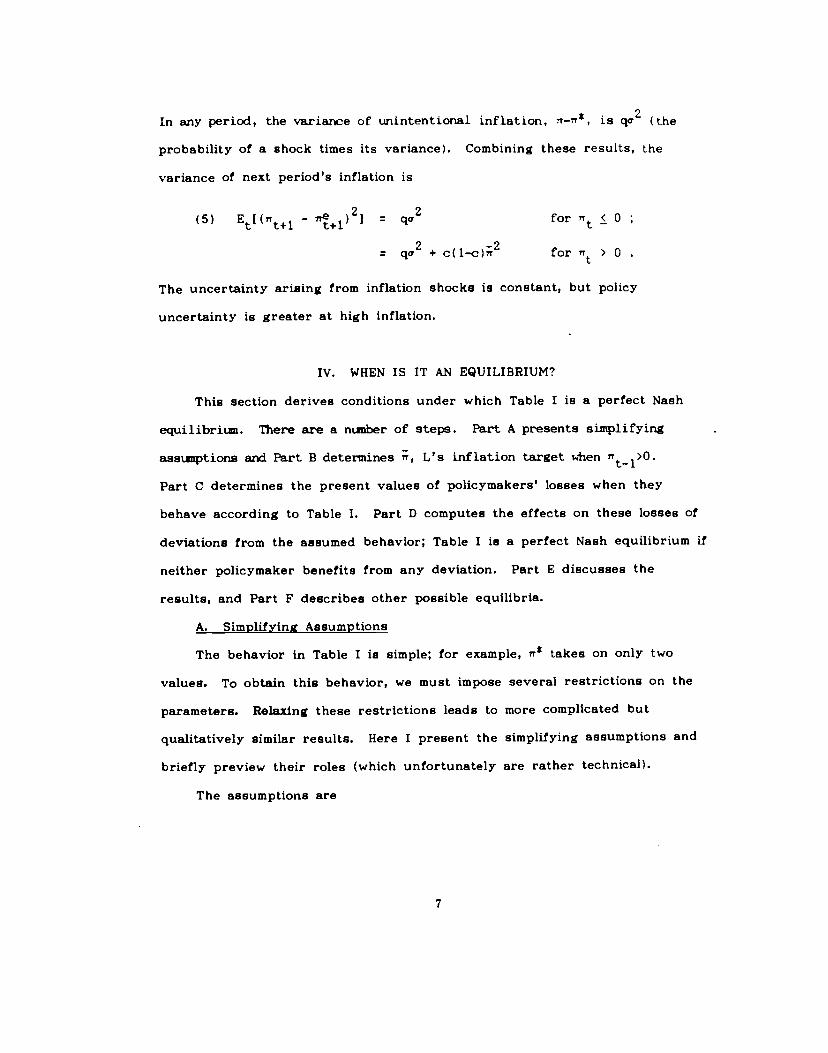
In any period, the variance of unintentional inflation, 7T7T*, is qo (the

probability of a shock times its variance). Combining these results, the

variance of next period's inflation is

(5) E[(n1 — qa2 for 0

2 —2= qc + c(l-c) for > 0

The uncertainty arising from inflation shocks is constant, but policy

uncertainty is greater at high inflation.

IV. WHEN IS IT AN EQUILIBRIUM?

This section derives conditions under which Table I is a perfect Nash

equilibriun. There are a nunber of steps. Part A presents simplifying

aasunptions arid Part B detei:,n,ines r, L's inflation target when

Part C determines the present values of policymakers' losses when they

behave according to Table I. Part D computes the effects on these losses of

deviations from the assumed behavior; Table I is a perfect Nash equilibrium if

neither policymaker benefits from any deviation. Part E discusses the

results, and Part F describes other possible equilibria.

A. Simplifying Assumptions

The behavior in Table I is simple; for example, n takes on only two

valueg. To obtain this behavior, we must impose several restrictions on the

parameters. Relaxing these restrictions leads to more complicated but

qualitatively similar results. Here I present the simplifying assumptions and

briefly preview their roles (which unfortunately are rather technical).

The assumptions are

7

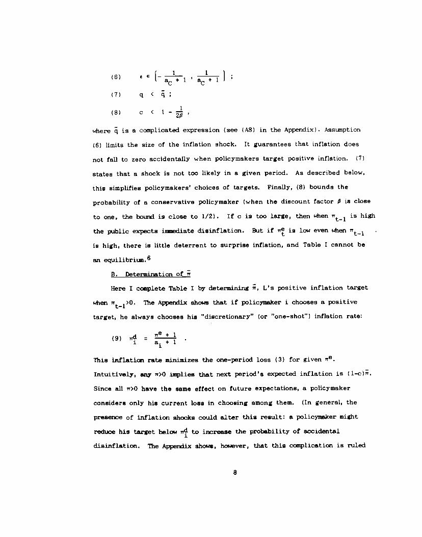
(6)[ a+ 1 ' a'+ 1 1

(7) q <

(8) c <

where q is a complicated expression (see (A8) in the Appendix). Assumption

(6) limits the size of the inflation shock. It guarantees that inflation does

not fall to zero accidentally when policymakers target positive inflation. (7)

states that a shock is not too likely in a given period. As described below,

this simplifies policymakers' choices of targets. Finally, (8) bounds the

probability of a conservative policymaker (when the discount factor is close

to one, the bound is close to 1/2). If c is too large, then when is high

the iblic expects isinediate disinflation. But if is low even when

is high, there is little deterrent to surprise inflation, and Table I cannot be

an equilibriun.6

B. Determination of n

Here I complete Table I by determining n, L's positive inflation target

when The Appendix shows that if policyineker i chooses a positive

target, he always chooses his "discretionary" (or "one—shot") inflation rate:

e + 1

1 a.+11

This Inflation rate minimizes the one—period loss (3) for given 71.e

Intuitively, any i>O implies that next period's expected inflation is (l—c).

Since all i'>O have the same effect on future expectations, a pohcymaker

considers only his current loss in choosing among them. (In general, the

presere of inflation shocks could alter this result: a policyineker might

reduce his target below ,4 to irxrease the probability of accidental

disinflation. The Appendix shows, howsver, that this complication is ruled

8

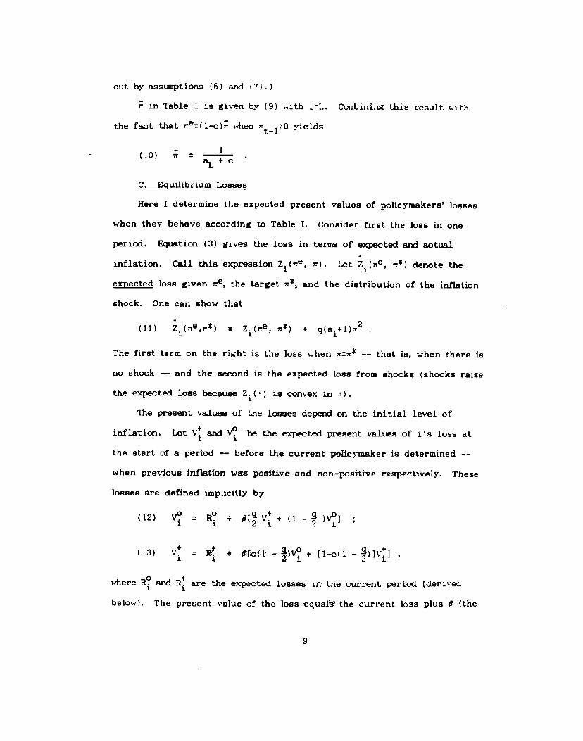
out by assunptions (6) and (7).)

in Table I is given by (9) with iL. Combining this result with

the fact that ir(1-c) when yields

(10) n

C. Equilibrium Losses

Here I determine the expected present values of policymakers' losses

when they behave according to Table I. Consider first the loss in one

period. Equation (3) gives the loss in terms of expected and actual

inflation. Call this expression Z(ne, 7) Let Z.(n5, ,r*) denote the

expected loss given e, the target ire, and the distribution of the inflation

shock. One can show that

(11) Z.(77e,7T*) Z.(ne, *) + q(a.+1)72

The first term on the right is the loss when n'r —— that is, when there is

no shock —— and the second is the expected loss from shocks (shocks raise

the expected loss because Z is convex in n).

The present values of the losses depend on the initial level of

inflation. Let V and v? be the expected present values of i's loss at

the start of a period -— before the current policymaker is determined --

when previous inflation was positive and non—positive respectively. These

losses are defined implicitly by

(12) v? R° .,. V + (1 — )V?]

(13) V + [c(] + [1—c(1 —

where R° and are the expected losses in the current period (derived

below). The present value of the loss equa1 the current loss plus P (the

9

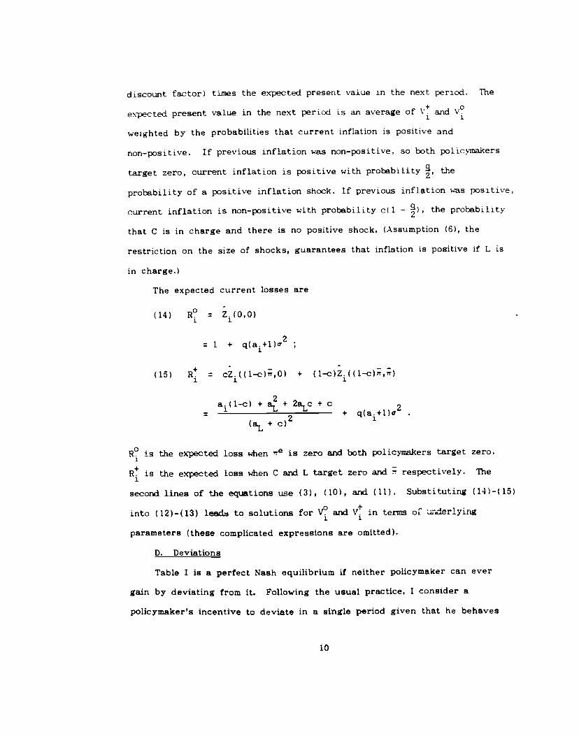
discount factor) times the expected present value in the next poriod. The

expected present value in the next period is an average of and V

weighted by the probabilities that current inflation is positive and

non-positive. If previous inflation was non-positive, so both poiicymakers

target zero, current inflation is positive with probability , the

probability of a positive inflation shock. If previous inflation was positive,

current inflation is non-positive with probability c(1 - ), the probability

that C is in charge and there is no positive shock. (Assumption (6), the

restriction on the size of shocks, guarantees that inflation is positive if L is

in charge.)

The expected current losses are

(14) R? Z.(O,O)

1 + q(a+1)a2

(15) R cZ.((l—c),0) + (1—c)Z.((1--c)',;)

2a.(l-c)+a+2a,c+c2

2+ q(a1+l)cT

(a. + C)

is the expected loss when e is zero and both policymakers target zero.

is the expected loss when C and L target zero and respectively. The

second lines of the equations use (3), (10), and (11). Substituting (14)—(15)

into (12)—(13) leac6 to solutions for V and V in terms oc ArIderlyirtg

parameters (these complicated expressions are omitted).

D. Deviations

Table I is a perfect Nash equilibrium if neither policymaker can ever

gain by deviating from it. Following the usual practice, I consider a

policymaker's incentive to deviate in a single period given that he behaves

10

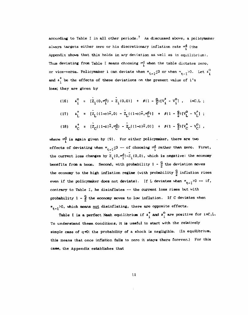
according to Table I in all other periods.7 As discussed above, a pol icyme.ker

always targets either zero or his discretionary inflation rate .rd (the

Appendix shows that this holds in any deviation as well as in equilibrium).

Thus deviating from Table I means choosing 4 when the table dictates zero,

or vice-versa. Policymaker i can deviate when <0 or when r >0. Lett—l— t—1 1

and be the effects of these deviations on the present value of i's

loss; they are given by

(16) [Z(O,7) — Z.(O,O)] + (l — — v?i , iC,L

(17) [ZL((1_c)t0) — ZL((1_c)?r,7r)] + (1 — )[V — V]

(18) — Z,0)] + (1 — )(V — V]

where 74 is again given by (9). For either policyme.ker, there are two

effects of deviating when - -- of choosing 74 rather than zero. First,

the current loss changes by Z(O,TT)_Z(0,0), which is negative: the economy

benefits from a boom. Secor, with probability 1 - the deviation moves

the economy to the high inflation regime (with probability inflation rises

even if the policymaker does not deviate). If L deviates when -- if,contrary to Table I, he disinflates -- the current loss rises but with

probability 1 - the economy moves to low inflation. If C deviates when

which means not disthflating, there are opposite effects.

Table I is a perfect Nash equilibritin if and are positive for iC,L.

To understand these. conditions, it is useful to start with the relatively

simple case of q40: the probability of a shock is negligible. (In equilibrium,

this means that once inflation falls to zero it stays there forever.) For this

case, the Appendix establishes that

11

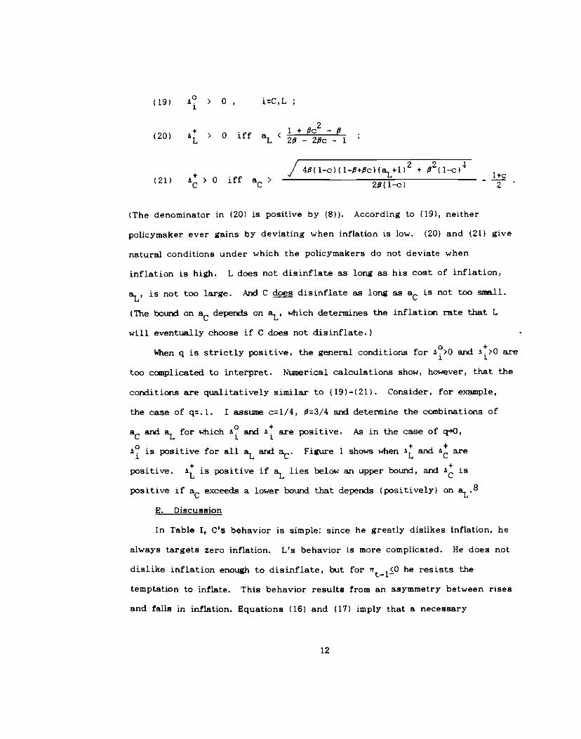
(19) ° > 0 , iC,L

20 > 0 fl+ -

L1 a1 2-2Pc-1

/ 4(1-c)(1-+c)(+1)2 ++ V L l+c

(21) > 0 iff a > 2(1—c) - 2

(The denominator in (20) is positive by (8)). According to (19), neither

policymaker ever gains by deviating when inflation is low. (20) and (21) give

natural conditions under which the policymakers do not deviate when

inflation is high. L does not disinflate as long as his cost of inflation,

aL, is not too large. Arid C does disinflate as long as a is not too sme.ll.

(The bound on a depends on a,, which determines the inflation rate that L

will eventually choose if C does not disinflate.)

When q is strictly positive, the general conditions for >0 and :>o are

too complicated to interpret. Numerical calculations show, however, that the

conditions are qualitatively similar to (19)-(21). Consider, for example,

the case of q.1. I assume c=1/4, =3/4 and determine the combinations of

and a.L for which arid are positive. As in the case of q-i'O,

is positive for all a.L and a. Figure 1 shows when and are

positive. is positive if a.L lies below an upper bound, and ig

positive if a exceeds a lower bound that depends (positively) on aL.8

E. Discussion

In Table I, C's behavior is simple: since he greatly dislikes inflation, he

always targets zero inflation. L's behavior is more complicated. He does not

dislike inflation enough to disinflate, but for 7rt he resists the

temptation to inflate. This behavior results from an asymmetry between rises

and falls in inflation. Equations (16) and (17) imply that a necessary

12

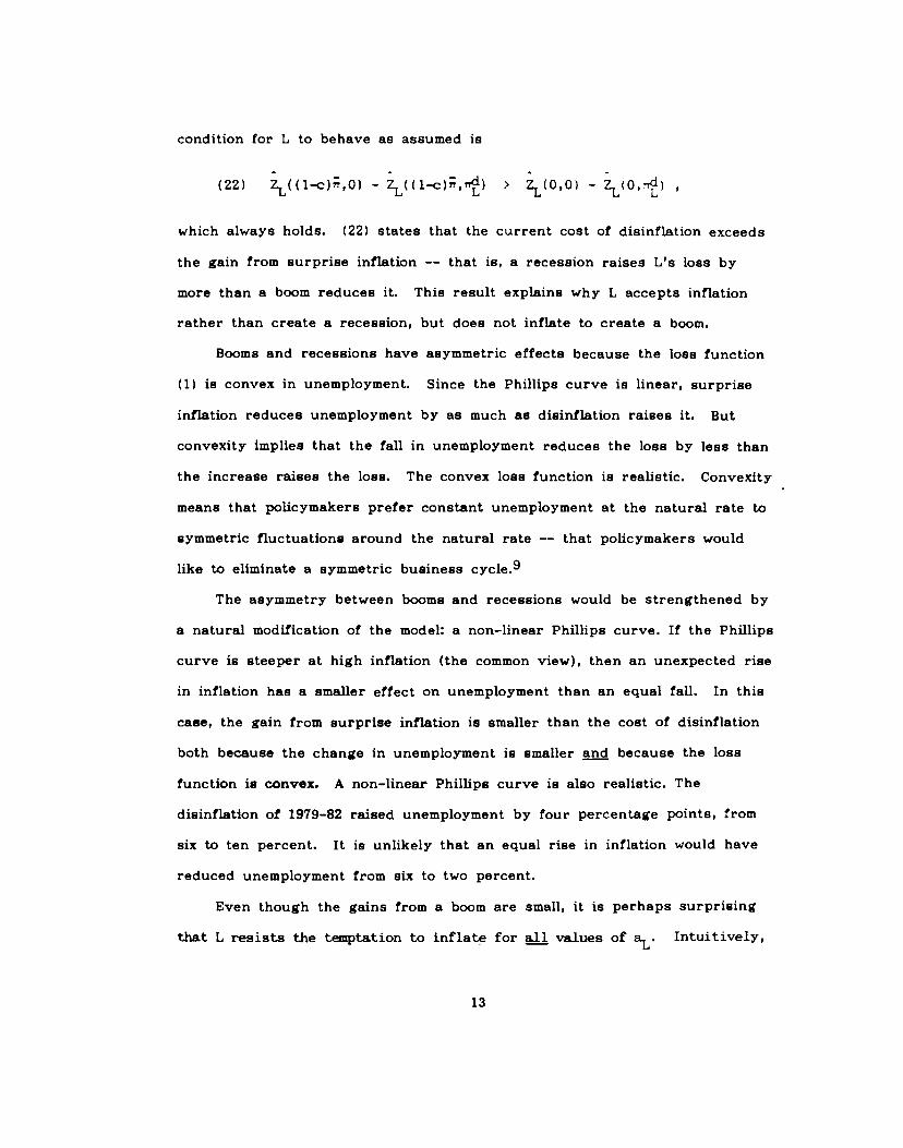
condition for L to behave as assumed is

(22) ZL( (l—c),O) — ZL( ( l—c),n) > Z)OO) — ZL(O,r)

which always holds. C22 states that the current cost of disinflation exceeds

the gain from surprise inflation —- that is, a recession raises L's loss by

more than a boom reduces it. This result explains why L accepts inflation

rather than create a recession, but does not inflate to create a boom.

Booms and recessions have asymmetric effects because the 1068 function

(1) is convex in unemployment. Since the Phillips curve is linear, surprise

inflation reduces unemployment by as much as disinflation raises it. But

convexity implies that the fall in unemployment reduces the loss by less than

the increase raises the loss. The convex loss function is realistic. Convexity

means that policymakers prefer constant unemployment at the natural rate to

symmetric fluctuations around the natural rate -— that policymakers would

like to eliminate a symmetric business cycle.9

The asymmetry between booms and recessions would be strengthened by

a natural modification of the model: a non-linear Phillips curve. If the Phillips

curve is steeper at high inflation (the common view), then an unexpected ri8e

in inflation has a smaller effect on unemployment than an equal fall. In this

case, the gain from surprise inflation is smaller than the cost of disinflation

both because the change in unemployment is smaller and because the loss

function is convex. A non—linear Phillips curve is also realistic. The

disinflation of 1979—82 raised unemployment by four percentage points, from

six to ten percent. It is unlikely that an equal rise in inflation would have

reduced unemployment from six to two percent.

Even though the gains from a boom are small, it is perhaps surprising

that L resists the temptation to inflate for J. values of a.. Intuitively,

13

it appears that a very small aL would lead L to accept high inflation for even

a small short r'..n gain. Indeed, L would inflate for aL gufficiently small if

inflation remained high forever. But if L inflates, he is eventually replaced

by C, who creates a costly recession to disinflate. Even if L does not view

inflation as costly per se, he is deterred from creating it by the future cost

of eliminating it.

F. Other Equilibria

This section concludes with a brief discussion of possible equilibria

besides Table I. There are two issues. First, since Table I is an equilibrium

only for certain parameter values, I ask what happens in other cases.

Second, I describe equilibria that coexist with Table I.

Other Parameter Values: Not surprisingly, different ranges of parameter

values imply different equilibria. One noteworthy possibility is presented in

Table II. Here I label the two policymakers liberal (L) and radical (R), and

assume that aL>aR. As in Table I, L prolongs low inflation but does not

disinflate. R always inflates -— that is, he always sets 'j. He is so

indifferent to inflation that when inflation is low he raises it to gain a

one-period boom. Table II can be an equilibrium if a lies in a moderate

range and a. is very small. This equilibrium yields a negative relation

between inflation and uncertainty: if inflation is high, both policymakers keep

it high, while if inflation is low one policymaker keeps it low and the other

inflates.10

This result shows that a positive inflation—uncertainty relation depends

on assumptions about parameter values as well as on the basic model.

However, the conditions for a negative relation -— in particular, the condition

that aR is very su.li -- appear iinrealistic. It is unlikely that any Fed

chairman would consider inflation so harmless that he would intentionally

14

move the economy from low to high inflation. Policymakers disagree about

the response to high inflation, but there is a consensus that low inflation

should be prolonged.

Multiple Equilibria: As in other infinite—horizon models of monetary

policy, there are many perfect Nash equilibria for given parameter values.

This paper will not attempt a full analysis of the multiplicity problem, but

one should note two equilibria that coexist with Table I. First, as usual

there is an equilibriiin in which policykers always target their

discretionary inflation rates, 14. Since policynkers' behavior is constant,

inflation uncertainty is constant. Second, as in Barro—Gordon (1983b) and

Canzoneri, there can be equilibria with finite "punishment periods." When a

shock raises inflation, expected inflation rises but then falls automatically

after one or more periods: disinflation does not require a recession.

(Temporary punishment is sufficient to deter surprise inflation.) If the

punishment period is short aod a is not huge, C accepts high inflation

during the period to avoid the cost of immediate disinflation. L does the

same, so there is little policy uncertainty.11

A reason for focusing on the equilibrium in Table I is realism. In Table

I, changes in actual inflation lead to changes in expected inflation. This

appears consistent with U.S. experience. It is unrealistic to assume that

expected inflation is constant, as in the discretionary equilibrium, and very

unrealistic to assume that it falls automatically after a punishment period.

V. COSTS OF UNCERTAINTY

A. Motivation

The last section assumes that policymakers attach a cost to the level of

inflation. While this assumption is plausible, the subject of the paper

15

suggests an alternative. Economists are interested in the inflation—

uncertainty link largely because it helps to ecplain why inflation is costly.

The costs of anticipated inflation, such as deadweight loss from the inflation

tax, appear small. But if inflation causes uncertainty, there may be

significant costs, such as greater risk in long-term nominal arrangements

(Jaffee and Kleiman, 1977; Fischer and Modiguiani, 1978). Motivated by this

view, this section assumes that policymakers' losses depend on uncertainty

about inflation as well as the current level. The effect of the current level

can be small or even zero.

This version of the model raises a new issue. In the previous section,

uncertainty arises from C's efforts to disinflate, along with L's resistance.

C's motivation is his view that inflation is costly. But if the main cost of

inflation is uncertainty, it appears that C creates the cost by trying to

eliminate it! If C simply accepted high inflation, like L, then uncertainty

would diminish. The major cost of inflation would be reduced, and no

recession would be required. Why does C not take this course?

This section contains two results relevant to this issue. First, Table I,

with ita positive inflation—uncertainty relation, can be art equilibrium even

when the model includes a cost of uncertainty. Second, while there is another

equilibrium with high but stable inflation (the discretionary equilibrium), C

may not prefer this equilibrium. As suggested by Fischer and Summers

(1989), reducing the costs of inflation -— in this case by reducing

uncertainty —— can raise the level of inflation so much that policymakers are

worse off.

B. A Positive Inflation-Uncertainty Relation

Here I add a cost of uncertainty to policymakers' loss functions and

show that the behavior in Table I can remain an equilibrium. Modify the loss

16

function, (1), to be

(23) Z. (Ut_U°)2 + a. + bEt[rrt+i -

This specification attaches costs to both the current level of inflation arid the

variance of next period's inflation. The former can be interpreted as

deadweight loss from the inflation tax, and the latter as increased risk innominal contracts. One should think of a. as small, so that a.rr2 is small formoderate inflation rates.

We can deter,ujne when Table I is an equilibrium with the approach of thelast section. it is again l/(a.+c). (The cost of uncertainty does not

affect L's choice of because uncertainty is the same for all n>O.)

Once again, Table I is an equilibrium if policymakers cannot gain from any

deviation: A°, > 0. Here, policyinakers take account of the degree of

uncertainty implied by positive and non—positive inflation (see (5)). For the

case of q-O, calculations parallel to Section IV show that

(24) &° > 0 , i:C, L

(25) > 0 iff a.(2—2c—1) + bLc(l_c) < l—fl+flc2

(26) > 0 iff afl(l—c2) + afl(1—c) + bc(l_c)(l+a) >

(1_P+Pc)(1+a.L)2 — fi(c—c2)

The results for q>0 are again qualitatively similar.

Conditions (24)—(26) are generalizations of (19)—(21), the corresponding

conditions in the basic model. C and L never deviate from Table I when

For ir11>O, they do not deviate as long as their distastes for

inflation are strong and weak enough respectively. Here, policymaker i's

17

distaste for inflation is neasured by a linear combination of a. and b.. ote

that if a.'O, (24)—(26) are satisfied for ranges of b and b.. Thus the

equilibrium in Table I survives even if uncertainty is the only cost of

inflation.

As in the basic model, C disinflates because he views inflation as very

costly. Here this result seems paradoxical, because the major cost of

inflation —— uncertainty -— results from C's efforts to disinflate. Nonetheless

this situation can be a perfect Nash equilibrium. When inflation is high, the

public expects C to disinflate and L not to disinflate. The resulting

uncertainty has large costs (e.g. there is less investment). Under Nash

behavior, C takes expectations as given, and thus takes it as given that high

inflation creates costly uncertainty. He disinflates to move the economy to

the low-inflation regime, in which the public is certain of future policy.

C. Does C Prefer the Discretionary Equilibrium?

As in the basic model, many equilibria can coexist with Table I. In

particular, as long as a.L and a are positive, there is an equilibriun in

which policyukers always target their discretionary inflation , IT.

Here I compare C's losses in this equilibrium to his losses in Table I to see

which equilibrium he prefers. It seems natural to focus on equilibria that

policymakers prefer, and previous authors usually do. A loose but intuitively

appealing justification is that policymakers can guide the economy to a

desired equilibrium, for example through policy announcements. In most

models, policymakers prefer equilibria like Table I, in which inflation is often

low, to the discretionary equilibrium. In the current model, however, it may

appear that C prefers the discretionary equilibrium, because his efforts to

disinflate in Table I create costly uncertainty. This suggests that C will try

to guide the economy to the discretionary equilibrium by publicly forswearing

18

disinflation.12

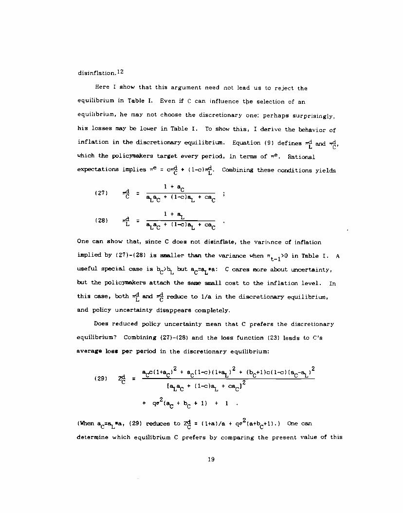
Here I show that this argument need not lead us to reject the

equilibrium in Table I. Even if C can influence ttie selection of an

equilibrium, he may not choose the discretionary one: perhaps surprisingly

his losses may be lower in Table I. To show this, I derive the behavior of

inflation in the discretionary equilibrium. Equation (9) defineg and 7T,

which the policymakers target every period, in terms of i. Rational

expectations implies ,Te C1 + (1-c) TT. Combining these corxiitiong yield.s

I +a(27) 1d C

C aa + (1-c) aL + ca

1+(28) 71d

L + (1-c)+

One can show that, since C does not disinflate, the variance of inflation

implied by (27)-(28) is smaller than the variance when -1>0 in Table I. A

useful special case is bC>bL but aC_aLua: C cares mere about icertainty,

but the policymakers attach the same small cost to the inflation level. In

this case, both az*1 reduce to 1/a in the discretionary equilibrium,

and policy uncertainty disappears completely.

Does reduced policy uncertainty mean that C prefers the discretionary

equilibrium? Combining (27)—(28) and the loss function (23) leads to C's

average 1088 per period in the discretionary equilibrium:

— ac(1+a)2 + aC(1_c)(l+a,L)2 + (b+1)c(1_c)(a_aL)2

(aLac + (1-c) a.L + CSC]

+ qa (aC+bC+ 1) + 1

(When aC:aLIa, (29) reduces to (1+a)/a + q2(a+b+1).) One can

determine which equilibrium C prefers by comparing the present value of this

19

loss to C's losses in Table 1, which are derived with an approach parallel to

Section IVC.13

The relation between C's losses in Table I and in the discretionary

equilibrium is ambiguous. Rather than present the general conditions for C

to prefer Table I, I illustrate the possibility with two special cases. The

first, which is not surprising, is bb.-O: as in the basic model, the cost of

inflation depends only on its level. In this case (or for b. close to zero),

one can show that C prefers Table I because the level of inflation is often

Low. The second case, which is less obvious, is aL a - 0. In this case,

the expression in (29) approaches infinity. C's losses in Table I 'emain

finite, so he prefers that equilibrium.

Thus C prefers Table I not only if the cost of inflation depends entirely

on the level (b.0), but also if the cost of the level is small (a.-ø0).14 The

second case is important because, as discussed bo, small values of a are

realistic. The explanation for this case is that small a imply very high

inflation targets in the discretionary equilibrisn (as aL and a approach

zero, the targets approach infinity). In Table I, by contrast, targets are

always moderate: even when t_1>O the possibility of disinflation holds down

,,e, and hence L's target (as a.-O, approaches 1/c < as). When aL and a are

small, moving from Table I to the discretionary equilibrium raises the level of

inflation so much that C is worse off even though there is less uncertainty

and the cost per unit of inflation is small. This result illustrates Fischer

and Summers's (1989) point that trying to reduce the costs of inflation -- in

this case by reducing the resulting uncertainty -— can be counterproductive.

This drawback to the discretionary equilibrium seems realistic. Suppose

that Paul Voicker, hoping to reduce uncertainty, announced in 1979 that he

would accept high inflation permanently rather than disinflate. This might

20

have led to very high inflation: as Okun (1971) argues, inflation may rise

considerably if the public believes that the Fed has given up the fightagainst inflation.

VI. CONCLUSION

This paper presents a model in which a rise in inflation raises

uncertainty about future monetary policy, and thus about future inflation.

When inflation is low, there is a consensus that the monetary authority will

try to keep it low. When inflation is high, policymakers face a dilemma: they

would like to disinflate, but fear the recession that would result. Since the

public does not know the tastes of future policymakers, it does not know

whether disinflation will occur.

Is policy uncertainty an important source of the inflation

level—uncertainty relation in actual economies? In principle, the relation

could arise instead from the reaction of the private economy to high

inflation. Hasbrouck (1979) shows, for example, that high trend inflation can

raise variability by making money demand more responsive to shocks. Ball,

Mankiw, and Romer (1988) argue that high inflation reduces nominal rigidity

and thus steepens the short run Phillips curve; a steeper Phillips curve

implies that inflation varies more as demand fluctuates. Finally, it appears

possible that high inflation destabilizes the relation between the money stock

and the Fed's policy instruments, thereby magnifying monetary control

errors.15

It seems unlikely, however, that these explanations for the

level-uncertainty link are the whole story. The following may be a useful

thought experiment. Suppose that a Constitutional Amendment imposes severe

punishment on any Fed chairman who lets inflation deviate too much from x,

21

and that everyone therefore knows that the Fed will try to produce x.

Compare inflation uncertainty when x is zero to uncertainty when x is ten

percent. It is possible that money demand or the money multiplier is less

stable when the target is ten percent, and thus that actual inflation varies

more. But with a firm commitment to the target, the variance is probably

small in both cases. The important difference between zero and ten percent

inflation in actual economies is not the Fed's ability to hit these targets if it

wants to, but rather the degree of uncertainty about whether the target will

change.

I conclude by pointing out a limitation of my model. In the model, high

inflation creates uncertainty only about disinflation -- about whether inflation

will return to a low level. In actual economies, it appears that high inflation

also creates uncertainty about whether inflation will rise further. Okun

argues that if the Fed accepts high inflation to accomodate a shock, the

public fears that inflation will rise again if there is another shock. In

contrast, a nonaccornodative policy shows that the Fed is committed to

keeping inflation under control. Future research should try to formalize

these ideas.

22

APPENDIX

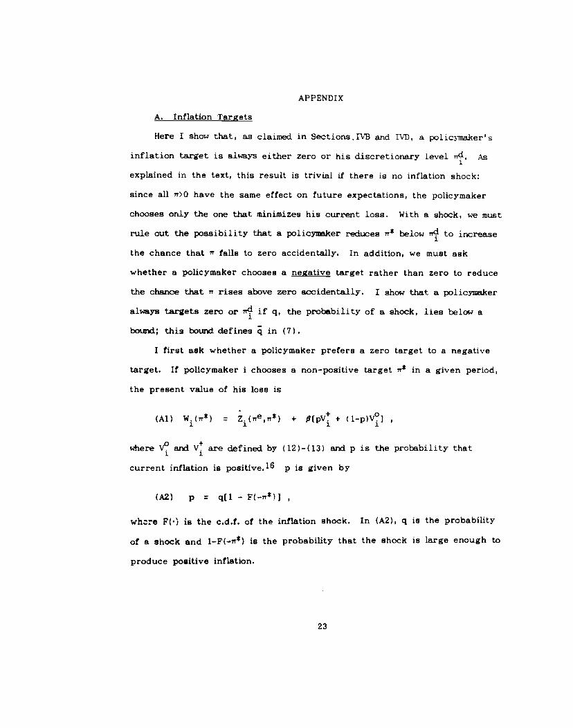
A. Inflation Targets

Here I show that, as claimed in Sections.IVB and I, a policymaker's

inflation target is always either zero or his discretionary level 74. As

explained in the text, this result is trivial if there is no inflation shock:

since all 77>0 have the same effect on future expectations, the policymaker

chooses only the one that minimizes his current loss. With a shock, we must

rule out the possibility that a policyn.ker reduces 77* below r4 to increase

the chance that i falls to zero accidentally. In addition, we must ask

whether a policymaker chooses a neZative target rather than zero to reduce

the chance that n rises above zero accidentally. I show that a policymaker

always targets zero or 74 if q, the probability of a shock, lies below a

bowd; this bound defines in (7).

I first ask whether a policymaker prefers a zero target to a negative

target. If policymaker i chooses a non-positive target 77* in a given period,

the present value of his loss is

(Al) W.(,T*) = Z(7e,,Y*) + [pV + (1—p)V?]

where V and V are defined by (12 )-( 13) and p is the probability that

current inflation is positive.16 p is given by

(A2) p q(1 — F(—lTt)]

where F(S) is the c.d.f. of the inflation shock. In (A2), q is the probability

of a shock and 1_F(1,*) is the probability that the shock is large enough to

produce positive inflation.

23

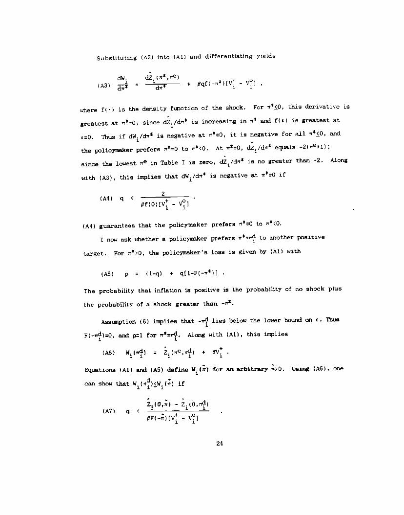
Substituting (A2) into (Al) and differentiating yields

dW.

(A3) + aqf(_*)(V — V°]

where f() is the density function of the shock. For 1T4<O, this derivative jgreatest at ,1*O, since dZ/d7r* is increasing in i and f(t) is greatest at

tO. Thus if dW./dn* is negative at it is negative for all ,r*<O, and

the policynker prefers ,r*:O to At ,T:O, dZ./d7T j9 _2(,Te+l);

since the lowest ife in Table I is zero, dzi/dlT* is no greater than -2. Along

with (A3), this implies that dW./d'T* is negative at r:O if

(A4) q <2

f(O)[V. — v?i1 1

(A4) guarantees that the policymaker prefers ir:O to ,T*(O.

I now ask whether a policynker prefers 1TTr' to another positive

target. For TT*>O, the policyinaker's loss is given by (Al) with

(A5) p (l—q) + q[l_F(_n*))

The probability that inflation is positive is the probability of no shock plus

the probability of a shock greater than -.

Assunption (6) implies that -7 lies below the lower bound on e. Thus

F( _1'T4):O, and p1 for ir:n. Along with (Al), this implies

(A6) W(i4) Z(e,1) +

Equations (Al) and (A5) define W; for an arbitrary rr)O.. Using (A6), one

can show that W. (i)<W. (ii) if1 11

z (0,;) - 2. (O,)(A7) q <

1 1

-

24

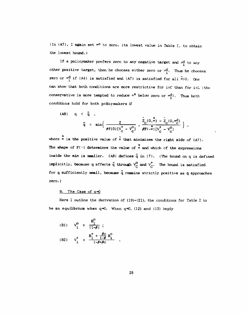
(In (A7), I again set to zero, its lowest value in Table I, to obtainthe lowest bound.)

If a policymaker prefers zero to any negative target and 74 to any

other positive target, then he chooses either zero or 74. Thus he chooses

zero or 74 if (AU is satisfied and (A7) is satisfied for all rr>O. One

can show that both conditions are more restrictive for iC than for iL (theconservative is more tesipted to reduce 7T below zero or Thus both

conditions hold for both policymakers if

(AS) q <

Z (O,ir) — z (0,nd)- .1 2 c c cq mini ,f(O)[V — VI F(—n)[V — V°]

where it is the positive value of it that minimizes the right side of (A7).

The shape of F(•) determines the value of it and which of the expressions

inside the mm is snller. (AS) defines in (7). (The bound on q is defined

implicitly, because q affects through V and V. The bound is satisfied

for q sufficiently sn.1l, because resmins strictly positive as q approaches

zero.)

B. The Case of g-'O

Here I outline the derivation of (19)—(21), the conditions for Table I to

be an equilibrium when q-O. When q-sO, (12) and (13) imply

R°(Bi) v?

(1—a)

+ — R°ID) - l— 1

'., i -

25

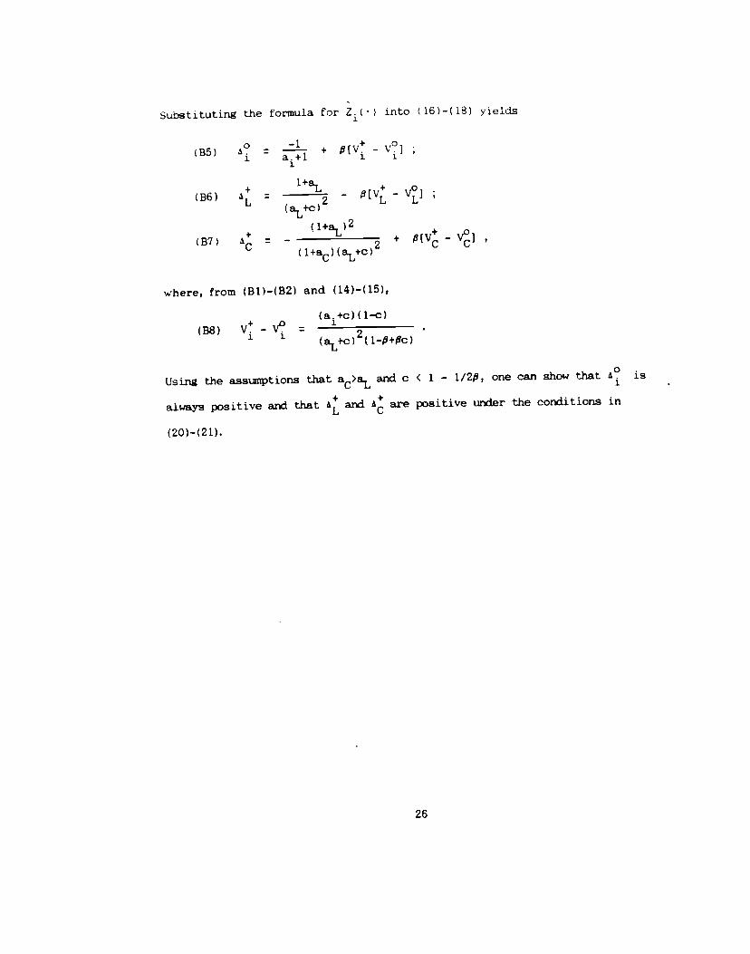
Substituting the formula for Z.() into (16)-(18) yields

(B5) + —

1+a.

(B6) - - V](aL+c)

(1+a. )2

(B?)— L

2+

(l+aC)(aL+C)

where, from (B1)—(B2) and (14)—(15),

a. +c ) ( 1—c

(B8) v4—v? 121 1

(a.b+c) (1—+fic)

Using the assumptions that aC>aL azxi c < 1 - 1/2, one can show that is

always positive and that and are positive urier the corKiitions in

(20)—(21).

26

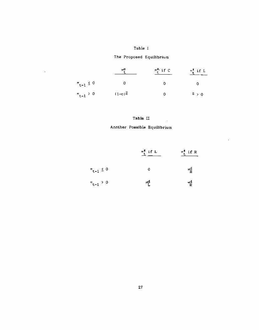
Table I

The Proposed Equilibrium

_______

if C if L

77t1<O 0 0 0

0

Table II -

Another Possible Equilibrium

irifL ifR

7•Tt.10 0

I

27

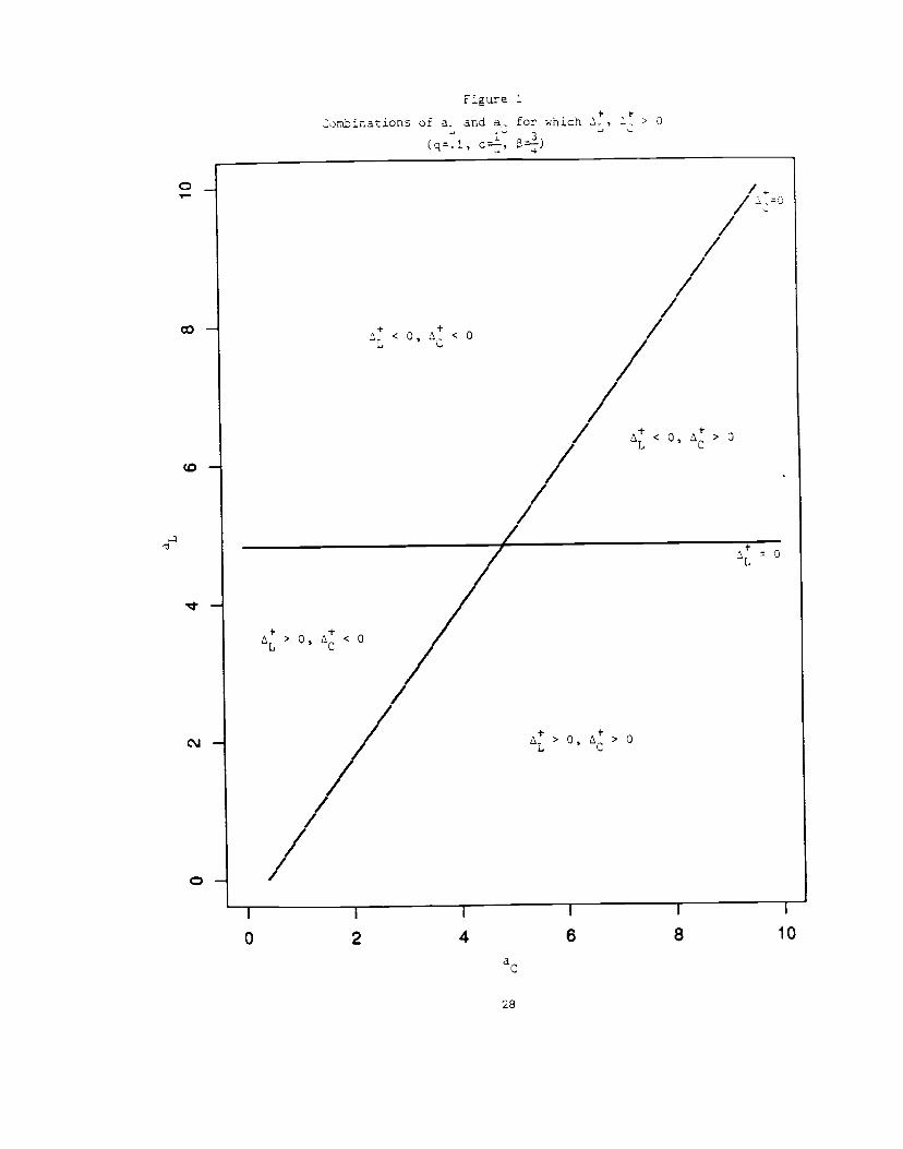
Figure 1

onbinationS of ar and a for which > 3

- 3(q.l, c, 3)

tC-

< 0, < 0

(0-< 0, > 0

> 0, < 0

= 0

CJ- > 0, > 0C

0-

0

I I I I

2 4 6 8

a0

28

10

NOTES

1. Evidence of an inflation-uncertainty link is presented by Okun (1971),Logue and Willet (1976), Jaffee and Kleimari (1977), and Taylor (1981). Whilethe evidence is not conclusive (see Engle [19831), it appears to be widelyaccepted. In any case, this paper treats the inflation—uncertainty link as afact to be explained. Cukierman and Meltzer (1986) and Devereux (1989)present other recent explanations; these papers are discussed below.

2. As this example suggests, the model is meant to apply primarily tomoderate—inflation countries like the U.S. The experience of high inflationcountries (e.g. in Latin America) depends largely on factors that I ignore,such as the use of seignorage to finance budget deficits.

3. It would be realistic to introduce serial correlation in who is incharge, or to let c depend on the state of the economy. But thesemodifications would greatly complicate the analysis.

4. This specification is a simplification of Canzoneri's model. InCanzoneri, a shock arrives every period. In addition, the inflation shock isderived by assuming that the Fed chooses the money stock and that moneydemand is stochastic. The money demand shock is observable -- the publicinfers it from the money stock and the price level -— but the Fed has aforecast of the shock that is private information. Adopting this moresophisticated approach would not change my main results.

5. The result that inflation remains high until C creates a recession is adeparture from Barro—Gordon and Canzoneri. In those papers, inflation failscostlessly after a brief "punishment period." This difference is discussed inSection IVF.

6. If poLicymakers alternate in power according to a Markov process, (8)can be replaced by the assumption that the transition probabilities aresmall. In this case it is not necessary to restrict the unconditionalprobability that C is in power. This approach introduces other complications,however.

7. For a class of repeated games including the one considered here,Sorin (1988) shows that a set of strategies is a perfect equilibrium if one canrule out single—period deviations.

8. Cetrus paribus, raising q increases the rnge of parametersfor which AL>O az decreases the range for which >0. That is, itmakes both policymakers more likely to prolong higii inflation. A largeq makes disinflation less attractive because disinflation is quicklyreversed through a positive inflation shock. -

Recall that ass1nption (7) restricts q to lie below the bourxl q. For qstrictly positive, the sufficient condJ.tins for Table I to be an equilibrhnincliie this restriction as well as A°, A . >0. (q depends on all theparameters and the density function' foi the inflation shock. Thus, for agiven q>0, the bound may be satisfied in some cases and not in others.)

29

9. The asymmetry between rises and falls in unexpected inflation isdiscussed by Hoshi (1988). In his model, the asymmetry can lead to multipleequilibria for the level of inflation.

10. In the equilibrium in Table I, L does not create surprise inflationeven if aL is very small, because inflation leads to a recession when Cdisinflates. In Table II, R does inflate for small aR because he knows thatnobody will dJ.sinflate.

11. For further discussion of these equilibria and others, see Fischer

(1986) and Rogoff (1987).

12. This idea is informal because there is rio formal theory of howannouncements move the economy from one Nash equilibrium to another.

Taylor (1983) argues that the economy is likely to arrive at an equilibrium

that policymakers prefer. Rogoff (1987) expresses doubts. Other authorsoften focus on desirable equilibria without providing a justification.

13. For the results below, it does not matter whether one assumes aninitial state of or t-1>° in calculating the present value of the lossin Table I.

14. C may prefer the discretionary equilibrium to Table I if both abc are large -- that is, if he strongly dislikes both a high level ofinflation and a high variance.

15. Cukierman and Meltzer (1986) and Devereux (1989) present othertheories of the inflation-uncertainty link. These papers, like the currentone, use models of time—consistent policy in the Barro-Gordon tradition. Inboth papers, an exogenous increase in the variance of a shock, which raisesthe variance of inflation, also raises average inflation in the discretionaryequilibrium. In Cukierman-Meltzer, a larger variance of monetary controlerrors makes it harder for the public to detect an intentional increase ininflation. This raises a policymaker's gain from inflating, and thus raisesequilibrium inflation. In Devereux, a higher variance of real shocks reducesequilibrium wage indexation, which increases the temptation to inflate byincreasing the real effects of inflation surprises. In both models, as inHasbrouck and Ball—Marikiw—Romer, inflation varies more around apolicymaker's target when the average target is high. In my model, highinflation raises uncertainty about whether the target itself will change (seethe discussion below).

16. The aunption that V and v? are given by (12 ) -(13) means thatthe policymakers obey Table I in all future periods. That is, as in the text Iconsider a single—period deviation from the equilibrium.

30

REFERENCES

Alesma, Alberto. "Macroeconomic Policy as a Repeated Game in a Two-PartySystem," rterly Journal of Economics 102 (August, 1987): 651—678.

Ball, Laurence, I. Gregory Mankiw, and David Earner. 'The New KeynesianEconcmics and the Output-Inflation Trade-off," Brookings Papers onEconomic Activity 1988:1: 1—65.

Barro, Robert and David Gordon. "A Positive Theory of Monetary Policy ina Natural Rate Model," Journal of Political Economy 91 (August1983): 589—610. (1983a)

______

and

_______.

"Roles, Discretion, and Reputation in a Model ofMonetary Policy," Journal of Monetary Economics 12 (July 1983):101—121. (1983b)

Canzoneri, Matthew. "Monetary Policy Games and the Role of PrivateInforntion," American Economic Review 75 (December 1985): 1056—1070.

Cukiermen, Alex and Allan Meltzer. "A Theory of Ambiguity, Credibility,and Inflation uzar Discretion and Asyninetric Information," Econcinetrica54 (September 1986): 1099—1128.

Devereux, Michael. "A Positive Theory of Inflation and InflationVariance," Economic Inquiry 27 (January 1989): 105—116.

Eagle, Robert. "Estimates of the Variaie of U. S. Inflation Based uponthe ARCH Model," Journal of Money, Credit, and Banking 15 (August 1983):262—301,

Fischer, Stanley, "Time Consistent Monetary and Fiscal Policies: ASurvey," Mimeo, MIT, 1986.

______

and Franco Modigliani, "Towards an Understanding of theReal Effects and Costs of Inflation," Weltwirtschaftliches Archiv 114(1978): 810—833.

______

and Lawrence Simmers. "Should Nations Learn to Live withInflation?," American Economic Review 79 (May 1989).

Friedman, Milton. "Nobel Lecture: Inflation and Unemployment," Journal ofPolitical Economy 85 (June, 1977): 451—472.

Hasbrouck, Joel. "Price Variability and Lagged Adjustment in Money Demand,"Mimeo, University of Pennsylvania, 1979.

Hoshi, Takeo. Government Reputation and Monetary Policy. Dissertation,MIT, 1988.

31

Jaf fee, Dwight and Kleimen, Ephraim. "The Welfare Implications of UnevenInflation." In Erik Lurs:iberg, Inflation Theory and Anti-Inflation Policy.Boulder, Colorado: Westview Press, 1977.

Logue, Dennis and Thx.s Willet. "A Note on the Relation Between the Rate

and Variability of Inflation," Economica 43 (May 1976): 151—158.

Okun, Arthur. "The Mirage of Steady Inflation." Brookings Papers onEconomic Activity 1971:2: 485—498.

Rogoff, Kenneth. "Reputation, Coordination and Monetary Policy," Miro,

Stanford University (rch 1987).

Sorin, Sylvain. "Supergames (On Some Recent Advances) ," Mimeo, Universi teLouis Pasteur (April 1988).

Taylor, John. "On the Relation Between the Variability of Inflation and

the Average Inflation Rate," in The Costs and Consequences of Inflation,

Carnegie—Rochester Conference Series on Public Policy, Vol. 15,

North-Holland, Autiinn 1981, Pp. 57—871

_________

"Cc*rinenta," Journal of Monetary Economics 12 (July 1983):

123—125.

32