Vulnerability Analysis of Large Concrete Dams using the

Continuum Strong Discontinuity Approach and Neural Networks

Manolis Papadrakakis1, Vissarion Papadopoulos1, Nikos D. Lagaros1

and

Javier Oliver2, Alfredo E. Huespe2, and Pablo Sánchez2

Abstract: Probabilistic analysis is an emerging field of structural engineering which is very

significant in structures of great importance like dams, nuclear reactors etc. In this work a

Neural Networks (NN) based Monte Carlo Simulation (MCS) procedure is proposed for the

vulnerability analysis of large concrete dams, in conjunction with a non-linear finite element

analysis for the prediction of the bearing capacity of the Dam using the Continuum Strong

Discontinuity approach. The use of NN was motivated by the approximate concepts inherent in

vulnerability analysis and the time consuming repeated analyses required for MCS. The Rprop

algorithm is implemented for training the NN utilizing available information generated from

selected non-linear analyses. The trained NN is then used in the context of a MCS procedure to

compute the peak load of the structure due to different sets of basic random variables leading to

close prediction of the probability of failure. This way it is made possible to obtain rigorous

estimates of the probability of failure and the fragility curves for the SCALERE (Italy) dam for

various predefined damage levels and various flood scenarios. The uncertain properties

(modeled as random variables) considered, for both test examples, are the Young’s modulus, the

Poisson’s ratio, the tensile strength and the specific fracture energy of the concrete.

Key words: Reliability analysis, Fragility curves, Vulnerability, Monte Carlo Simulation, Soft

Computing, Neural Networks, Continuum Strong Discontinuity Approach

1 Institute of Structural Analysis and Seismic Research, National Technical University of Athens, Athens 15780, Greece 2 Technical University of Catalonia (UPC), Campus Nord UPC, Edifici C-1, C/Jordi Girona 1-3, 08034 Barcelona, Spain

1

1 INTRODUCTION

The theory and methods of structural vulnerability have been developed significantly during the

last twenty years and have been documented in an increasing number of publications. These

advancements in structural reliability theory and the attainment of more accurate quantification

of the uncertainties associated with structural loads and resistances have stimulated the interest in

the probabilistic treatment of structures. The vulnerability of a structure or its probability of

failure under various loading scenarios is an important factor in the design, construction

monitoring and maintenance procedures of dams since it investigates the probability of the

structure to successfully complete its design requirements. Therefore, vulnerability analysis is at

the heart of risk analysis methodologies that have been developed for very important structures

like dams and subsidies essentially the decision making procedures, leading to safety measures

that the owners and the Dam engineers have to take into account due to the aforementioned

uncertainties. Although from a theoretical point of view the field has reached a stage where the

developed methodologies are becoming widespread, from a computational point of view serious

obstacles have been encountered in practical implementations.

First and second order reliability methods that have been developed to estimate structural

reliability [1-3] lead to elegant formulations requiring prior knowledge of only the means and

variances of the component random variables and the definition of a differentiable failure

function. For small-scale problems these types of methods prove to be very efficient, but for

large-scale problems and/or large number of random variables Monte Carlo Simulation (MCS)

methods seem to be superior. In fact simulation methods are the only methods available to treat

practical reliability problems in complex structures where a complete non-linear three-

dimensional modelling is required (for example capturing the failure mode mechanisms in dams

where the arch-effect, or vault-effect, plays a major role in the structural response [4]).

Furthermore, in this type of structures is not possible to establish “a priori” the failure surfaces

determining the structural collapse.

The Basic MCS is simple to use, but for typical structural reliability problems the computational

effort involved becomes excessive due to the enormous sample size and consequently the CPU

2

time required for each Monte Carlo run. To reduce the computational effort more elaborate

simulation methods, called variance reduction techniques, have been developed. Despite the

improvement in the efficiency of the basic MCS variance reduction techniques, they still require

disproportionate computational effort for treating practical reliability problems. This is the

reason why very few successful numerical investigations are known in estimating the probability

of failure of real-world structures and are mainly concerned with simple elastic frames and

trusses [5-7].

In the present paper a Neural Networks (NN) based Monte Carlo Simulation (MCS) procedure is

proposed for the vulnerability analysis of large concrete dams, in conjunction with a non-linear

finite element analysis for the prediction of the bearing capacity of the Dam using the Continuum

Strong Discontinuity Approach (CSDA) [4, 8]. The use of artificial intelligence techniques, such

as Neural Networks (NN), in structural reliability analysis has been reported in a number of

publications [9-11], in which the efficiency as well as the accuracy of this methodology for

obtaining close predictions of the probability of failure in complex structural systems is

demonstrated. The principal advantage of a properly trained NN is that it requires a trivial

computational effort to produce an acceptable approximate solution. The Rprop algorithm is

implemented for training the NN utilizing available information generated from selected non-

linear analyses. The trained NN is then used in the context of a MCS procedure to compute the

peak load of the Dam due to different sets of basic random variables leading to close prediction

of its probability of failure.

Once a NN is trained to produce acceptable estimates of the peak loads of the dam, rigorous

calculations of fragility curves can be subsequently obtained by performing a number of

reliability analyses associated with various predefined damage levels of the dam and various

flood scenarios. The proposed combined NN-CSDA methodology is first demonstrated through a

simple “academic” example involving a concrete beam test subjected to a loading system placed

in four points. From this initial demonstration the capacity of the CSDA to model and predict

material failure is assessed through comparisons with corresponding experimental results, while

the ability of the NN to predict close estimates of the peak loads with and consequently of the

probability of failure is validated. The aforementioned calculations are then repeated for the

3

vulnerability analysis of SCALERE (Italy) dam demonstrating the efficiency as well as the

applicability of the proposed methodology in large and complex structural systems. The

uncertain properties (modeled as random variables) considered for this example are the Young’s

modulus, the Poisson’s ratio, the tensile strength and the specific fracture energy of the concrete.

2 CONTINUUM STRONG DISCONTINUITY APPROACH TO MATERIAL FAILURE

2.1 Motivation

Phenomenological modeling of material failure, in structural mechanics, aims at capturing the

formation of those macroscopically observable discontinuities in the displacement field which,

depending on the context, are termed, cracks, fractures, slip lines etc. They are identified as the

locus of those material points where loss, and eventual exhaustion, of the material capacity to

carry stresses (material failure) takes place, and, as they spread through the structure, are

responsible for the progressive reduction of the structural tangent stiffness to zero (identifying

the structural failure and the critical load stage) or to negative values (identifying post-critical

stages). The mechanical modeling of the onset and progression of displacement discontinuities

(technically termed strong-discontinuities) can be approached from a wide range of options

which can be classified into two large groups: 1) continuum approaches, based on the use of

non-linear continuum (stress-strain) constitutive models, equipped with strain-softening to

capture the progressive loss of the strength of the material as strain increases, and 2) discrete

approaches (also termed cohesive or non-linear fracture mechanics based approaches) lying on

the insertion, at predetermined discontinuity paths, of specific traction-separation laws (also

equipped with softening for the same purpose) whereas the bulk of the structure remains in

elastic state.

As for numerical procedures, the continuum approaches have been traditionally used in

connection with standard finite elements resulting in the so called smeared approaches. They do

not require an “a priori” knowledge of the discontinuity path which is “a posteriori” identified

through those element patches where concentration of intense deformations (strain localization

or weak discontinuities) occur. However, there is a strong dependency of the captured

discontinuity paths on the mesh orientation (mesh bias dependency); they often result in stress-

4

locking effects and translate into lack of robustness and enormous difficulties to reach the

structural critical and post-critical stages.

On the other hand, discrete approaches often resort to specific finite elements with zero

thickness, placed along the sides of the regular elements, to capture a real strong discontinuity.

However, either the position of those finite elements has to be determined before the analysis,

thus limiting the prediction capability of the method, or a continuous remeshing to set them

appropriately has to be done. This requires sophisticated remeshing procedures, leading to

unaffordable computational costs when large three-dimensional structures and multiple

discontinuities are aimed at being modeled.

The above considerations justify the very limited capacity of those classical strategies to be

applied to vulnerability analysis purposes, based on the Monte Carlo Simulation methods

requiring a large number of complex simulations.

In recent years some alternatives have emerged, belonging to the family of the so called strong

discontinuity approaches, as an attempt to overcome the problems of the previous approaches. In

particular, the continuum strong discontinuity approach (CSDA), which has been adopted here,

is equipped with recent and advanced ingredients in order to make it an efficient and robust

strategy for solving complex three-dimensional multi-crack problems. The fundamental features

of CSDA are the following:

A real displacement discontinuity (crack) is considered in the mathematical description of

the displacement field, through the so called strong discontinuity kinematics [12-14], (see

Figure 1). The displacement, u , and strain, ε , fields in a body Ω experiencing a strong

discontinuity across the crack surface, , are then described as: S

[ ][ ]

⎩⎨⎧

Ω∈∀Ω∈∀

=+=−

+

xx

xuxuxu01

)( SS HH ;)()( (1)

[ ][ ])(unbounded

singular

symS

(bounded)regular

)(δ)( nuxxux ⊗+== )()( S ε∇ε

(2)

5

where in Eq. (1) is the displacement jump, is a step function and in Eq. (2) is

a Dirac’s delta function, which is regularized for computational purposes.

[ ][ ]u SH Sδ

A unique continuum constitutive model (stress/strain) is used to model both the material

behaviour at the bulk and at the discontinuity interface [14]. The model is equipped with

strain softening, to reproduce the material de-cohesion as cracking occurs. The softening

modulus is regularized to match with the unbounded strains in Eq. (2). Therefore, the

complete analysis is performed within a continuum setting. Nevertheless, it can be shown

that the selected continuum 3D material model is automatically projected into a 2D

discrete model (traction-separation law) at the discontinuity interface as the strong

discontinuity kinematics in Eqs. (1, 2) develop. For practical purposes, that discrete model

is neither derived nor implemented, but the results at the failure interface are the same than

if it were been effectively implemented. Therefore, both, the volume and surface

dissipative effects, taking place during the material failure, are captured in a common

continuum context.

The use of finite elements with embedded discontinuities [13] makes possible to adopt

rather coarse meshes, without affecting the accuracy of the results (see Figure 2) and not

requiring remeshing procedures. Those elements basically consist of enriching the standard

finite elements crossed by the crack path, with additional, discontinuous, deformation

modes that capture the displacement discontinuities (cracks) occurring inside the element.

These deformation modes have an elemental support. Therefore, the corresponding

enriching degrees of freedom can be condensed at the elemental level, so that the

enrichment does not enlarge the size of the system of equations to be solved, and multiple

cracks can be captured, even in coarse meshes, at a reduced computational cost.

The critical conditions for the material failure, and the directions of its propagation, are

checked at every step in the whole structure (looking for the singularity of the so called

localization tensor [13]). This means that the material cracks are captured without any “a

priori” knowledge of them. Then, a so-called global tracking algorithm [15] is used to

determine which elements are capturing the crack path and, therefore, have to be enriched.

The (recently introduced) implicit-explicit integration scheme is used to integrate the rate

(non-linear) constitutive equations [16]. This ensures positiveness and constancy, during a

given time step, of the algorithmic tangent stiffness, and translates into dramatic

6

improvements of the robustness of the linearization procedure and a large reduction (to

only one) of the number of iterations per time step. Specific arc-length strategies are

implemented to control the error introduced by that implicit-explicit algorithm.

Additional theoretical aspects of the CSDA are described in detail in [12-16].

2.2 Experimental assessment of the CSDA: the four point bending test

In order to asses the capacity of the CSDA to model and predict material failure a, very well-

known, experimental benchmark test, widely used for numerical validation in computational

failure mechanics, is reproduced here. It corresponds to the four point bending test sketched in

Figure 3a. A notched concrete beam, whose material is characterized by the following

parameters: Young’s modulus MPaE 24800= , Poisson’s ratio 18.0=ν , tensile strength

Mpau 8.2=σ , fracture energy , and thickness 156mm, is supported at two points

and subjected to a loading system imposing two forces in points A and B. The load-displacement

system is controlled until reaching the complete failure of the beam. The experimental setting is

shown in Figure 3b and the results have been reported by Arrea and Ingrafea (1982) [17].

mNG f /100=

The experimentally observed failure mode displays a crack crossing the specimen from the tip of

the notch toward the load application point B, as shown in Figures 3c and 3d.

The selected constitutive model to reproduce the material behaviour is a classical isotropic

continuum damage model described in [12-14]. The initial behaviour, under increasing strains, is

elastic, characterized by the elastic properties E and ν , up to reaching the limit elastic strength

characterized by the tensile strength uσ . Beyond this point, a progressive deterioration of the

secant stiffness reduces the material strength to zero, through a softening behaviour characterized

by the fracture energy . fG

In Figure 3e the numerically obtained failure mode, using the CSDA under the plane-stress

hypothesis, is shown. It is characterized by a curved crack path resembling very well the

experimental one. The plot of Figure 3f displays the experimental envelope of the structural

responses, load P vs. CMSD (crack-mouth sliding displacement) curves, and the numerically

7

obtained results. It can be observed that the numerical structural response lies completely into the

experimental band. The numerical simulation of the complete structural failure can be done, in a

very robust manner, in very few minutes of CPU using a single personal computer. In addition,

the independence of the obtained results on the orientation of the finite element mesh (mesh

objectivity) can be shown. This example exemplifies the ability of the selected computational

material failure setting (the CSDA) to provide fast and reliable numerical results to be used for

the purposes of this work as detailed in subsequent sections.

3 STRUCTURAL RELIABILITY ANALYSIS

In the design of structural systems, limiting uncertainties and increasing safety is an important

issue to be considered. Structural vulnerability, which is defined as the probability that the

system meets some specified demands for a specified time period under specified environmental

conditions, is used as a probabilistic measure to evaluate the integrity (available risk) of

structural systems.

The probability of failure pf can be determined using a time invariant reliability analysis

procedure with the following relationship

(3) dt)t(f )t(F1dt)t(f )t(F]SR[pp RsSRf ∫∫

∞

∞−

∞

∞−

−==<=

where R denotes the structure’s bearing capacity and S the external loads. The randomness of R

and S can be described by known probability density functions fR(t) and fS(t), with FR(t)=p[R<t],

FS(t)=p[S<t] being the cumulative probability density functions of R and S, respectively.

Most often a limit state function is defined as G(R,S)=S-R and the probability of structural

failure is given by

(4) f R

G 0

p p[G(R,S) 0] f (R) f (S)dRdS≥

= ≥ = ∫ S

It is practically impossible to evaluate pf analytically for complex and/or large-scale structures,

especially in the case of the Vulnerability Analysis of large concrete dams considered in the

present study. In such cases the integral of Eq. (4) can be calculated only approximately using

either simulation methods, such as the Monte Carlo Simulation (MCS), or approximation

8

methods like the first order reliability method (FORM) and the second order reliability method

(SORM), or response surface methods (RSM) [1-3,18]. Despite its high computational cost,

MCS is considered as a reliable method and is commonly used for the evaluation of the

probability of failure in computational mechanics, either for comparison with other methods or

as a standalone reliability analysis tool.

In reliability analysis the MCS method is often employed when an analytical solution is not

attainable and the failure domain can not be expressed or approximated by an analytical form.

This is mainly the case in problems of complex nature with a large number of basic variables

where all other reliability analysis methods are not applicable. Expressing the limit state function

as G(x)<0, where x=(x1,x2,...,xM) is the vector of the random variables, Eq. (4) can be written as

(5) f x

G(x) 0

p f (x≥

= ∫ )dx

where fx(x) denotes the joint probability of failure for all random variables. Since MCS is based

on the theory of large numbers (N∞) an unbiased estimator of the probability of failure is given

by

N

f jj 1

1p IN

∞

=∞

= ∑ (x ) (6)

in which I(xj) is an indicator for “successful” and “unsuccessful” simulations defined as

(7) ⎩⎨⎧

<≥

=0)G(x if 00)G(x if 1

)x(Ij

jj

thus in every violation a successful simulation is encountered and the failure counter is increased

by 1.

It is important in structural reliability using simulation methods, to efficiently and accurately

evaluate the probability of failure for a load scenario. In order to estimate pf an adequate number

of Nsim independent random samples is produced using a specific, usually uniform, probability

density function of the vector x. The value of the failure function is computed for each random

sample xj and the Monte Carlo estimation of pf is given in terms of sample mean by

9

H

fsim

NpN

≅ (8)

where NH is the number of successful simulations.

4 MULTI-LAYER PERCEPTRONS

A multi-layer perceptron is a feed-forward neural network, consisting of a number of units

(neurons) linked together that attempts to create a desired relation in an input/output set of

learning patterns. A learning algorithm tries to determine a set of parameters called weights, in

order to achieve the right response for each input vector applied to the network. The numerical

minimization algorithms used for the training generate a sequence of weight matrices through an

iterative procedure. To apply an algorithmic operator A we need a starting weight matrix w(0),

while the iteration formula can be written as follows

(9) (t+1) (t) (t) (t)w = (w )=w +ΔwA

All numerical methods applied are based on the above formula. The changing part of the

algorithm Δw(t) is further decomposed into two parts as

(10) (t) (t)

tΔw =a d

where d(t) is a desired search direction of the move and at the step size in that direction.

The training methods can be divided into two categories. Algorithms that use global knowledge

of the state of the entire network, such as the direction of the overall weight update vector, which

are referred to as global techniques. In contrast local adaptation strategies are based on weight

specific information only such as the temporal behaviour of the partial derivative of this weight.

The local approach is more closely related to the neural network concept of distributed

processing in which computations can be made independent to each other. Furthermore, it

appears that for many applications local strategies achieve faster and reliable prediction than

global techniques despite the fact that they use less information [19].

4.1 Global Adaptive Techniques

The algorithms most frequently used in the NN training are the steepest descent, the conjugate

gradient and the Newton’s methods with the following direction vectors:

10

Steepest descent method: (t) (t)d (w= −∇E )

Conjugate gradient method: ( t ) ( t ) ( t 1)t 1d (w ) d −−= −∇ +βE where βt is defined:

t 1 t t t 1 t 1/ Fletcher-Reeves− − −β = ⋅ ⋅E E E E∇ ∇ ∇ ∇

Newton’s method: 1(t ) (t ) ( t )d H(w ) (w−

⎡ ⎤= − ∇⎣ ⎦ E )

The convergence properties of optimization algorithms for differentiable functions depend on

properties of the first and/or second derivatives of the function to be optimized. When

optimization algorithms converge slowly for neural network problems, this suggests that the

corresponding derivative matrices are numerically ill-conditioned. It has been shown that these

algorithms converge slowly when rank-deficiencies appear in the Jacobian matrix of a neural

network, making the problem numerically ill-conditioned [20].

4.2 Local Adaptive Techniques

To improve the performance of weight updating, two completely different approaches have been

proposed, namely Quickprop [21] and Rprop [22].

The Quickprop method

This method is based on a heuristic learning algorithm for a multi-layer perceptron, developed

by Fahlman [21], which is partially based on the Newton’s method. Quickprop is one of most

frequently used adaptive learning paradigms. The weight updates are based on estimates of the

position of the minimum for each weight, obtained by solving the following equation for the two

following partial derivatives

t-1 t

ij ij

and w∂ ∂∂ ∂wE E

(11)

and the weight update is implemented as follows

t

ij(t) (t-1)ij ij

t-1 t

ij ij

ww w

- w w

∂∂

Δ = Δ∂ ∂∂ ∂

E

E E

(12)

The learning time can be remarkably improved compared to the global adaptive techniques.

11

The Rprop method

Another heuristic learning algorithm with locally adaptive learning rates based on an adaptive

version of the Manhattan-learning rule and developed by Riedmiller and Braun [22] is the

Resilient backpropagation abbreviated as Rprop. The weight updates can be written

(t) (t) tij ij

ij

w η sgn w

⎛ ⎞∂Δ = − ⎜ ⎟⎜ ⎟∂⎝

E

⎠ (13)

where

(t-1) t t-1ij max

ij ij

(t) (t-1) t t-1ij ij min

ij ij(t-1)ij

min(α η ,η ), if 0w w

η max(b η ,η ), if 0 w w

η , otherwise

∂ ∂⎧ ⋅ ⋅⎪ ∂ ∂⎪⎪ ∂ ∂⎪= ⋅ ⋅ <⎨ ∂ ∂⎪⎪⎪⎪⎩

E E

E E

>

(14)

where α=1.2, b= 0.5, ηmax=50 and ηmin=0.1 [23]. The learning rates are bounded by upper and

lower limits in order to avoid oscillations and arithmetic underflow. It is interesting to note that,

in contrast to other algorithms, Rprop employs information about the sign and not the magnitude

of the gradient components. In this work the Rprop learning algorithm is used since it has been

proved by the authors the most efficient one in terms of generalization and rapid convergence of

the training procedure [24].

4.3 NN based MC Simulation

Vulnerability analysis of large concrete dams using Monte Carlo Simulation is a highly intensive

computational problem which makes conventional approaches incapable of treating large scale

problems even in today's powerful computers. In the present study the use of NN was motivated

by the approximation concepts inherent in vulnerability analysis. The idea here is to train a NN

to provide computationally inexpensive estimates of analysis outputs required for the reliability

analysis problem. The major advantage of a trained NN over the conventional process, under the

provision that the predicted results fall within acceptable tolerances, is that results can be

produced in a few clock cycles, representing orders of magnitude less computational effort than

the conventional computational process.

12

An NN is trained utilizing available information generated from selected CSDA analyses. The

CSDA analysis data was processed to obtain input and output pairs which were used to produce a

trained NN. The trained NN is then used to predict the peak load due to different sets of basic

random variables. After the peak loads are predicted, close estimates of the probability of failure

are obtained by means of MCS. The predicted values for the peak loads should resemble closely,

though not identically, to the corresponding values of the CSDA analyses which are considered

“exact”. It appears that the use of a properly selected and trained NN can eliminate any limitation

on the sample size used for MCS and on the dimensionality of the problem, due to the drastic

reduction of the computing time required for the repeated analyses.

As it was mentioned earlier the main objective of this study is to investigate the ability of the NN

to predict the peak load and incorporate the NN in the framework of reliability analysis. This

objective comprises the following tasks: (i) select the proper training/testing set, (ii) find the

suitable neural network architecture and (iii) train the neural network. The appropriate selection

of input-output training data is one of the most important parts in NN training. Although the

number of training patterns may not be the only concern, the distribution of samples is of greater

importance. The number of conventional CSDA analysis calculations performed in this study

ranges between 50 to 200 samples, while some of them are used to test the accuracy of the NN

predictions with respect to the “exact” results obtained from the CSDA. The selection of the

training set is based on the requirement that the full range of possible results should be

represented in the training procedure. In order to fulfil the requirement that the full range of

possible results should be represented, the training set is generated randomly using the Latin

Hypercube Sampling within the bounds: mean value ± 6σ, where the percent variation is

99.9999998, since in both test examples considered the random variables follow the normal

distribution.

There are typically two types of networks, namely fully and patterned connected networks. In

this work a fully connected network is used. In a fully connected network, each node in a layer is

connected to all the nodes of the previous and the next layer. The number of nodes to be used in

the hidden layers is not known in advance, for this reason the learning process initiates with a

relatively small number of hidden nodes (10 in this study) and gradually increase the number of

13

hidden nodes and next, until achieving the desired convergence. The NN configuration achieving

the desired convergence, for both test examples, has one hidden layer with 20 hidden nodes.

Tests performed for more than one hidden layer showed no significant improvement in the

obtained results [9, 20].

After the selection of the suitable NN architecture and the training procedure, the network is then

used to provide predictions of the peak load corresponding to different values of the input

random variables. The results are then processed by means of MCS to calculate the probability

of failure pf. Similarly for the vulnerability analysis of concrete dams using the MCS the

computed peak loads are compared to the corresponding external loading leading to the

computation of the probability of structural failure according to Eq. (6). The considered external

loads correspond to various flood scenarios and include a constant self-weight and an increasing

fictitious density of the water (and the corresponding hydrostatic pressure). It must be mentioned

here that by approximating the “exact” solution with a NN prediction of the peak load, the

accuracy of the predicted pf depends not only on the accuracy of the NN prediction of the peak

load but also on the sensitivity of pf with regard to a slightly modified, due to the NN

approximation, sample space of resistances [9].

5 NUMERICAL RESULTS

Two test examples have been considered to illustrate the efficiency of the proposed NN based

methodology, one academic and one real world test example. In both test examples the

probability of failure is estimated using the basic MCS. Elastic modulus, Poisson’s ratio, tensile

strength and fracture energy are considered to be random variables in both test examples,

following the normal distribution. The NN software used in this study is based on the back

propagation algorithm developed by the authors [20].

5.1 Assessment of the combined NN-CSDA methodology: the four point bending test

The first test example is considered for performing a parametric study with respect to the

number of training patterns that are required in order to train properly the NN. For this reason

numerical results have been obtained, in terms of the peak load, for training sets composed by

50, 100, 150 and 200 sets of random material properties. The concrete mechanical parameters

14

for this test example are summarised in Table 1 where mean values and standard deviations for

the four random variables considered are shown. To assess the four different training sets

reliability analysis is performed. A sample size equal to 1000 is used for calculating the

probability of failure. The corresponding external loading, leading to the computation of the

probability of failure, according to Eq. (6), is considered to be equal to 90 kN. In Figures 4a and

4b the value of the CMSD value and the peak load for each of the 1000 samples is depicted,

while in Figure 5 the peak load versus the CMSD value for all the samples is shown.

The four different training sets are first compared with respect to their prediction ability in a

selected set of 10 patterns randomly selected from the 1000 samples mentioned above. The

capability of the four training sets to predict the peak load factor is shown in Table 2. As it can

be observed the peak load predicted based on the NN50 training set is the worst one while the

NN100, NN150 and NN200 perform equally well with respect to the CDSA prediction. As it was

mention earlier, once an acceptable trained NN is obtained in predicting the peak load factors,

the probability of failure for each test case is estimated by means of the NN-based Monte Carlo

Simulation. The results of this calculation are provided in Table 3. The probability of failure for

the case of the exact calculations pf_CDSA = 1.00% while for the case of the neural networks

pf_NN50 = 0.60%, pf_NN100 = 0.90%, pf_NN150 = 1.00% and pf_NN200 = 1.00%. According to a

previous work of the authors if the number of samples is increased the NN100 will converge

closely to the pf_CDSA [9].

5.2 Dam test example

A large concrete arch dam has been considered as a second test example in order to illustrate the

feasibility of the proposed methodology. First, the probability of failure of the Dam is computed

for a given water level while at a next step, fragility curves are obtained for various predefined

damage levels of the dam and various flood scenarios. The probability of failure for each damage

level and each scenario is estimated using the NN-based MCS in conjunction with the CSDA for

the prediction of the peak load of the dam. The uncertain properties (modeled as random

variables) considered for the Dam are the Young’s modulus, the Poisson’s ratio, the tensile

15

strength and the specific fracture energy of the concrete. All random variables are assumed to be

Gaussian.

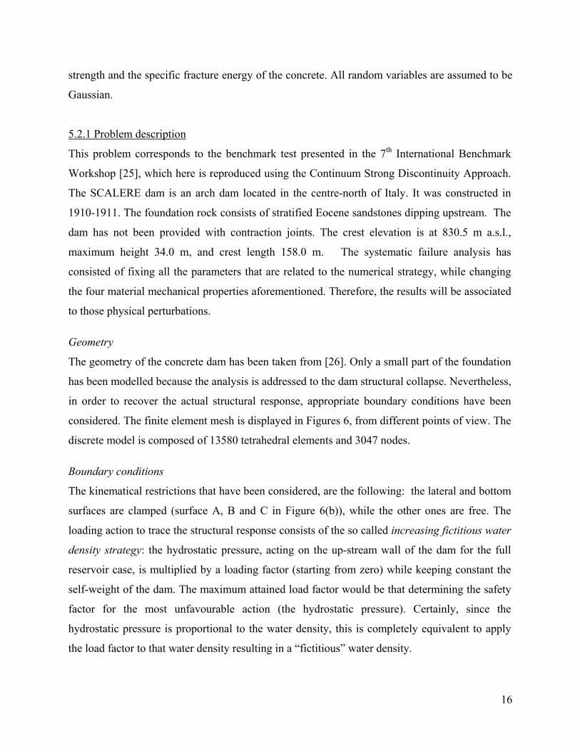
5.2.1 Problem description

This problem corresponds to the benchmark test presented in the 7th International Benchmark

Workshop [25], which here is reproduced using the Continuum Strong Discontinuity Approach.

The SCALERE dam is an arch dam located in the centre-north of Italy. It was constructed in

1910-1911. The foundation rock consists of stratified Eocene sandstones dipping upstream. The

dam has not been provided with contraction joints. The crest elevation is at 830.5 m a.s.l.,

maximum height 34.0 m, and crest length 158.0 m. The systematic failure analysis has

consisted of fixing all the parameters that are related to the numerical strategy, while changing

the four material mechanical properties aforementioned. Therefore, the results will be associated

to those physical perturbations.

Geometry

The geometry of the concrete dam has been taken from [26]. Only a small part of the foundation

has been modelled because the analysis is addressed to the dam structural collapse. Nevertheless,

in order to recover the actual structural response, appropriate boundary conditions have been

considered. The finite element mesh is displayed in Figures 6, from different points of view. The

discrete model is composed of 13580 tetrahedral elements and 3047 nodes.

Boundary conditions

The kinematical restrictions that have been considered, are the following: the lateral and bottom

surfaces are clamped (surface A, B and C in Figure 6(b)), while the other ones are free. The

loading action to trace the structural response consists of the so called increasing fictitious water

density strategy: the hydrostatic pressure, acting on the up-stream wall of the dam for the full

reservoir case, is multiplied by a loading factor (starting from zero) while keeping constant the

self-weight of the dam. The maximum attained load factor would be that determining the safety

factor for the most unfavourable action (the hydrostatic pressure). Certainly, since the

hydrostatic pressure is proportional to the water density, this is completely equivalent to apply

the load factor to that water density resulting in a “fictitious” water density.

16

This is not the most common scenario adopted in dam design, but it is considered more

acceptable from the structural failure point of view. Eventually, the resulting pressure for every

load factor could be translated into an equivalent height of the water above the dam crest

(increasing overflow strategy).

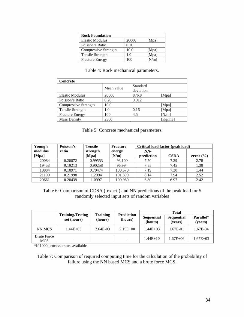
Material properties

The adopted (average) mechanical properties are the following: Both materials, rock and

concrete, have been modelled by an isotropic continuum damage model [12]. The analysis

assumes uncertainty for the concrete modelling and deterministic for the rock foundation.

Consequently, the results evaluate the “structural collapse” rather than the “structure-foundation

collapse”. The rock foundation is modelled providing appropriate boundary conditions. The rock

and concrete mechanical parameters are summarised in Tables 4 and 5, respectively. In Table 5

mean values and standard deviations for the four random variables considered are shown.

Summary of introduced hypotheses

The principal hypotheses considered to solve all the proposed cases are the following:

Two materials are modelled: rock and concrete.

No interface elements between the rock foundation and the concrete are considered.

The rock has been assumed as deterministic.

The four concrete material properties (Young’s modulus, Poisson’s ratio, tensile strength

and Fracture energy) are defined taking into account variations via a probability density

function. Its mean values are displayed in Table 5.

A unique numerical scenario has been adopted. Only the mechanical parameters for

concrete are modified.

Linear geometric analyses are performed.

Hydraulic fracture phenomena have been included.

A multi-crack procedure, allowing for multiples failure surfaces, has been considered in all

cases.

5.2.2 Probability of failure

Numerical results have been obtained, in terms of the load factor, for 100 sets of basic random

material properties. Figure 8 shows the load factor evolution as a function of the horizontal

17

displacement for a given set of input parameters (x-direction of the P-Node located in the dam

crest, see Figures 6(a)). The peak load (peak load factor) identifies the maximum carrying

capacity of the structure (critical load) under increasing loading processes. The post peak

response in Figure 8 corresponds to the post-critical response of the structure, which would not

be traced in an actual case of structural collapse under increasing loads, but allows identifying

the failure mode (fracture paths) responsible for the structural collapse. The iso-displacement

maps (Figures 9(a)) and the geometry in the deformed configuration (Figures 9(b)) display the

typical failure mechanism. It is formed by the conjunction of two primary macro cracks

propagating across the concrete bulk, as shown in Figures 10(a) and 10(b). However, the

complete dissipative process also considers a number of secondary discontinuity surfaces, in

both the dam domain and the rock foundation.

From the 100 CDSA analyses performed with the CSDA, 95 randomly selected are chosen to

give the pairs (inputs-outputs) for the NN training. The remaining 5 are used to test the accuracy

of the NN predictions with respect to the “exact” results obtained from the CSDA. Table 6

presents the results of this comparison, while in Figure 11 the performance of the trained NN for

the 95 training patterns is show. It can be observed that the relative error of peak load factor

predicted with the NN and the CDSA is approximate 2.78% which is considered as adequate for

the needs of the subsequent reliability analysis. Once an acceptable trained NN is obtained in

predicting the peak load factors, the probability of failure for each test case is estimated by

means of the NN-based Monte Carlo Simulation described earlier. Results of this calculation are

presented in Figure 12. The fictitious water density for this calculation takes the deterministic

value of 13KN/m2 which corresponds to an extreme flood condition (~8m above the maximum

water level). From this figure it can be observed that the MCS converges after 108 simulations to

a probability of failure pf =5x10-7%.

The feasibility of the proposed methodology for computing the probability of failure in large and

complex structural systems is demonstrated in Table 7. In this table, a comparison of the required

computing time for the calculation of the probability of failure using the NN based MCS and the

basic brute force MCS is presented. It can be seen that the enormous computational cost required

for a brute-force MCS procedure makes this method prohibitive for this kind of problems. Even

18

if 1000 processors were available the required computing time for such calculation would be

~1670 years. With the use of NN in the context of a MCS this time is reduced to ~1.500 hours. In

the present application, a sequential solution procedure was adopted in two personal computers.

The total time required for the above calculations was approximately 1 month.

5.2.3 Fragility curves

Once the NN based MCS is established for obtaining close predictions of the probability of

failure of a dam for a given level of external loading, rigorous calculations of fragility curves can

be subsequently obtained by performing a number of reliability analyses associated with various

predefined damage levels of the dam and various flood scenarios. These calculations are

performed with a minimum additional computational cost. Results of the aforementioned

calculation are shown in Figure 13 where the computed flood fragility curves for SCALERE dam

are presented. In this figure, each water fictitious density γ is assumed to correspond to different

water level and therefore to a different flood case scenario. In this work for each fictitious water

density γ 1.0E+09 NN based MC simulations are performed. In every simulation a check was

performed in order to fulfil that the sample drawn was within the bounds of the NN sampling:

mean value ± 6σ. In case that a sample was outside of these bounds it was rejected.

Three different damage levels are considered:

• Moderate damage

• Severe damage

• Structural collapse

Moderate damage is assumed to correspond to 60% of the peak load of the dam and is associated

with damages that can be easily repaired without affecting the dam operation. Severe damage is

assumed to correspond to the 80% of the peak load and is associated with extensive damages

requiring immediate retrofit and rehabilitation actions. Structural collapse is assumed to

correspond to the 100% of the peak load. In order to obtain the three fragility curves shown in

Figure 13, for each NN based MC simulation the predicted peak load is compared with the limit

19

states for the three damage levels considered. From the fragility curves of Figure 13, useful

conclusions can be derived for the dam behaviour under ordinary and extraordinary loading

conditions.

6 CONCLUDING REMARKS

This paper presents an application of Neural Networks to the reliability analysis of large

concrete dams in which failure is predicted with the Continuum Strong Discontinuity Approach.

The approximate concepts that are inherent in reliability analysis and the time consuming

requirements of repeated structural analyses involved in Monte Carlo Simulation motivated the

use of Neural Networks.

The computational effort involved in the conventional Monte Carlo Simulation becomes

excessive in large-scale problems because of the large sample size and the computing time

required for each Monte Carlo run. The use of Neural Networks can practically eliminate any

limitation on the scale of the problem and the sample size used for Monte Carlo Simulation

provided that the predicted critical load factors, corresponding to different simulations, fall

within acceptable tolerances. A Back Propagation Neural Network algorithm is successfully

applied to produce approximate estimates of the critical load factors, regardless the size or the

complexity of the problem, leading to very close predictions of the probability of failure. The

methodology presented could therefore be implemented for predicting accurately and at a

fraction of computing time the probability of failure of large and complex structures.

Acknowledgements: This research was funded by EC in the framework of the Integrity

Assessment of Large Concrete Dams European Research Network NW-IALAD. This support is

gratefully acknowledged.

REFERENCES

1. Shinozuka M. (1983), “Basic analysis of structural safety”, J. of Str. Engrg., ASCE, 109:

721-739.

2. Madsen H.O., Krenk S. and Lind N.C., Methods of Structural Safety, Prentice-Hall,

Englewood Cliffs, New Jersey, (1986).

20

3. Chrinstensen P.T., Reliability and Optimisation of Structural Systems '88, Proceedings of

the 2nd IFIP WG7.5, London, Springer-Verlag, (1988).

4. Oliver J. (1996a), “Modelling strong discontinuities in solids mechanics via strain

softening constitutive equations. Part 1: Fundamentals.”, Int. J. Num. Meth. Eng.; 39(21):

3575-3600.

5. T.Y. Kam, R.B. Corotis and E.C. Rossow, (1983), “Reliability of non-linear framed

structures”, J. of Struct. Engrg., ASCE, 109: 1585-1601.

6. Y. Fujimoto, M. Iwata and Y. Zheng, Fitting-Adaptive Importance Sampling Reliability

Analysis, Computational Stochastic Mechanics, P. D. Spanos and C. A. Brebbia, eds,

Computational Mechanics Publications, 15-26, (1991) .

7. J.E. Pulido, T.L. Jacobs and E.C. Prates De Lima, (1992), “Structural reliability using

Monte-Carlo simulation with variance reduction techniques on elastic-plastic structures”,

Computers & Structures, 43: 419-430.

8. Oliver J. (1996b), “Modelling strong discontinuities in solids mechanics via strain

softening constitutive equations. Part 2: Numerical simulation.” Int. J. Num. Meth. Eng.;

39(21): 3601-3623.

9. Papadrakakis M., Papadopoulos V., Lagaros N.D., (1996) “Structural reliability analysis of

elastoplastic structures using neural networks and Monte Carlo simulation”, Comp. Meth.

Appl. Mech. Eng., 136: 145-163.

10. Hurtado J.E. and Alvarez D.A., (2001), “Neural network based reliability analysis: a

comparative study”, Comput. Methods Appl. Mech. Engrg., 191(1-2): 113-132.

11. Adeli H., (2001), “Neural networks in civil engineering: 1989-2000”, Computer-Aided

Civil and Infrastructure Engineering, 16(2): 126-142.

12. Oliver J., Huespe A.E., Pulido M.D.G., Chaves E., (2002) “From continuum mechanics to

fracture mechanics: the strong discontinuity approach.” Engineering Fracture Mechanics;

69: 113-136.

13. Oliver J., Huespe A.E., (2004). “Theoretical and computational issues in modelling

material failure in strong discontinuity scenarios.” Computer Methods in Applied

Mechanics and Engineering; 193: 2987-3014.

21

14. Oliver J., Huespe A.E. (2004), “Continuum approach to material failure in strong

discontinuity settings.” Computer Methods in Applied Mechanics and Engineering; 193:

3195-3220.

15. Oliver J., Huespe A.E., Samaniego E., Chaves E.W.V., (2004). “Continuum approach to

the numerical simulation of material failure in concrete.” International Journal for

Numerical and Analytical Methods in Geomechanics; 28: 609-632.

16. Oliver J., Huespe A.E., Blanco S. and Linero D.L., (2005), “Stability and robustness issues

in l modelling of material failure in the strong discontinuity approach.” Comp. Meth in

Appl. Mech. Eng., submitted for publication.

17. Arrea M., Ingraffea A.R., “Mixed-mode crack propagation in mortar and concrete”,

Technical Report No.81-134, Department of Structural Engineering, Cornell University,

New York, (1982).

18. Frangopol D.M. and Moses F., “Reliability-based structural optimization”, in Adeli H.

(ed.), Advances in design optimization, Chapman-Hall, 492-570, (1994).

19. Schiffmann W., Joost M., Werner R., (1993), “Optimization of the back-propagation

algorithm for training multi-layer perceptrons”, Technical report, University of Koblenz,

Institute of Physics.

20. Lagaros N.D. and Papadrakakis M., (2004), “Learning improvement of neural networks

used in structural optimization”, Advances in Engineering Software, 35: 9-25.

21. Fahlman S., “An empirical study of learning speed in back-propagation networks”,

Carnegie Mellon: CMU-CS-88-162 (1988).

22. Riedmiller M. and Braun H., “A direct adaptive method for faster back-propagation

learning: The RPROP algorithm,” in Ruspini H. (Ed.), Proc. of the IEEE International

Conference on Neural Networks (ICNN), San Francisco, 586-591 (1993).

23. Riedmiller M., “Advanced Supervised Learning in Multi-layer Perceptrons: From Back-

propogation to Adaptive Learning Algorithms,” University of Karlsruhe: W-76128

Karlsruhe (1994).

24. Lagaros N.D., Stefanou G. and Papadrakakis M., (2005), “Soft computing hybrid

simulation of highly skewed non-gaussian stochastic fields”, Comput. Methods Appl.

Mech. Engrg., (to appear).

22

25. Giuseppetti G, Mazzŕ G, Meghella M., Fanelli M., “Evaluation of ultimate strength of

gravity dams with curved shape against sliding”, Seventh benchmark workshop on

numerical analysis dams, September 24-26, 2003, Bucharest, Romania.

http://www.rocold.ro/themea.htm.

26. Thematic network on the integrity assessment of large concrete dams (NW-IALAD),

http://nw-ialad.uibk.ac.at/.

23

FIGURES

Figure 1: Strong discontinuity kinematics

Figure 2: Finite elements with embedded discontinuities

24

Figure 3: Four-point bending test- (a) Geometrical description, (b) Experimental setup,

(c) Crack surface after the experiment, d) Experimental crack, (e) Numerically obtained

crack path and (f) Numerical and experimental structural responses.

25

(a)

(b)

Figure 4: Four-point bending test – (a) CMSD and (b) Peak load for the 1000 samples.

26

Figure 5: Four-point bending test – Peak load vs. CMSD value for the 1000 samples.

27

(a)

(b)

P

Figure 6: Dam Geometry and finite element mesh- (a) Upstream view. (b) Inferior view.

28

Figure 7: Load factor evolution.

Figure 8: Dam analysis- Load factor vs. P-Node (see figure 6) horizontal displacement.

29

(a)

(b)

Figure 9: Dam analysis- (a) Iso-displacement maps, (b) Deformed configuration

(a)

(b)

Figure 10: Dam analysis- Paths of primary cracks, (a) upstream and (b) downstream view.

30

4

5

6

7

8

9

10

1 15 29 43 57 71 85

Sample

Peak

load

(kN

)exactpredicted

Figure 11: Performance of the trained NN for the 95 training patterns.

0.0E+00

1.0E-07

2.0E-07

3.0E-07

4.0E-07

5.0E-07

6.0E-07

50 100

150

200

500

1000

5000

1000

050

000

1000

00

5000

00

1000

000

5000

000

1000

0000

5000

0000

1000

0000

0

5000

0000

01E

+09

Simulations

p f (%

)

Figure 12: Probability of failure calculated with the NN based MCS for various numbers of simulations.

31

0.0

20.0

40.0

60.0

80.0

100.0

0 1 2 3 4 5 6 7 8 9 10

Increased water density γ

p f (%

)

Structural collapseSevere damageModerate damage

Figure 13: Flood fragility curves for Scalere dam computed with the NN-MCS approach

32

TABLES

Concrete beam

Mean value Standard deviation

Elastic Modulus 24700 1087.23 [Mpa] Poisson’s Ratio 0.18 0.0108 Tensile Strength 2.8 0.448 [Mpa] Fracture Energy 100 4.5 [N/m]

Table 1: Concrete beam: mechanical parameters.

Peak load (kN) Young’s modulus [Mpa]

Poisson’s ratio

Tensile strength [Mpa]

Fracture energy [N/m]

CSDA NN50-prediction

NN100-prediction

NN150-prediction

NN200-prediction

23266 0.159 2.98 56.85 117.77 114.82 115.24 115.33 115.83 24603 0.177 2.89 59.54 120.32 121.48 121.33 121.38 120.69 23845 0.167 3.81 63.47 130.37 131.75 129.70 130.29 131.41 24238 0.172 2.55 64.80 117.15 117.87 118.14 118.04 117.09 26451 0.203 3.28 68.11 134.34 137.55 136.97 137.54 137.41 24137 0.171 2.80 70.83 124.84 122.86 123.20 123.25 123.37 22400 0.147 2.03 72.99 104.53 107.01 107.03 107.20 106.03 20852 0.126 1.56 73.38 90.09 95.07 94.62 95.35 93.74 20779 0.125 2.28 75.15 107.60 104.53 103.83 104.08 103.46 25626 0.191 3.46 77.64 141.95 140.61 139.69 140.13 140.69

Table 2: Comparison of CDSA (‘exact’) and NN predictions of the peak load for 10

randomly selected input sets of random variables

CSDA NN50-prediction NN100-prediction NN150-prediction NN200-prediction 1.00% 0.60% 0.90% 1.00% 1.00%

Table 3: Comparison of the probability of failure calculated by the CDSA and the NN

based procedure for 1000 simulations (applied load 90 kN).

33

Rock Foundation Elastic Modulus 20000 [Mpa] Poisson’s Ratio 0.20 Compressive Strength 10.0 [Mpa] Tensile Strength 1.0 [Mpa] Fracture Energy 100 [N/m]

Table 4: Rock mechanical parameters.

Concrete

Mean value Standard deviation

Elastic Modulus 20000 876.8 [Mpa] Poisson’s Ratio 0.20 0.012 Compressive Strength 10.0 [Mpa] Tensile Strength 1.0 0.16 [Mpa] Fracture Energy 100 4.5 [N/m] Mass Density 2300 [Kg/m3]

Table 5: Concrete mechanical parameters.

Critical load factor (peak load) Young’s modulus [Mpa]

Poisson’s ratio

Tensile strength [Mpa]

Fracture energy [N/m]

NN-prediction CSDA error (%)

20084 0.20072 0.99553 93.100 7.50 7.29 2.78 19453 0.19213 0.90258 96.994 7.55 7.45 1.38 18884 0.18971 0.79474 100.570 7.19 7.30 1.44 21199 0.21998 1.2994 101.590 8.14 7.94 2.52 20661 0.20439 1.0997 109.960 6.80 6.97 2.42

Table 6: Comparison of CDSA (‘exact’) and NN predictions of the peak load for 5

randomly selected input sets of random variables

Total Training/Testing set (hours)

Training (hours)

Prediction (hours) Sequential

(hours) Sequential

(years) Parallel* (years)

NN MCS 1.44E+03 2.64E-03 2.15E+00 1.44E+03 1.67E-01 1.67E-04

Brute Force MCS - - - 1.44E+10 1.67E+06 1.67E+03

*If 1000 processors are available

Table 7: Comparison of required computing time for the calculation of the probability of failure using the NN based MCS and a brute force MCS.

34