
Volume-3-Issue-3-March-2017.pdf - Engineering Journal IJOER
188
-
Upload
khangminh22 -
Category
Documents
-
view
7 -
download
0
Transcript of Volume-3-Issue-3-March-2017.pdf - Engineering Journal IJOER


Page | i
Preface
We would like to present, with great pleasure, the inaugural volume-3, Issue-3, March 2017, of a scholarly
journal, International Journal of Engineering Research & Science. This journal is part of the AD
Publications series in the field of Engineering, Mathematics, Physics, Chemistry and scienc Research
Development, and is devoted to the gamut of Engineering and Science issues, from theoretical aspects to
application-dependent studies and the validation of emerging technologies.
This journal was envisioned and founded to represent the growing needs of Engineering and Science as an
emerging and increasingly vital field, now widely recognized as an integral part of scientific and technical
investigations. Its mission is to become a voice of the Engineering and Science community, addressing
researchers and practitioners in below areas
Chemical Engineering
Biomolecular Engineering Materials Engineering
Molecular Engineering Process Engineering
Corrosion Engineering
Civil Engineering
Environmental Engineering Geotechnical Engineering
Structural Engineering Mining Engineering
Transport Engineering Water resources Engineering
Electrical Engineering
Power System Engineering Optical Engineering
Mechanical Engineering
Acoustical Engineering Manufacturing Engineering
Optomechanical Engineering Thermal Engineering
Power plant Engineering Energy Engineering
Sports Engineering Vehicle Engineering
Software Engineering
Computer-aided Engineering Cryptographic Engineering
Teletraffic Engineering Web Engineering
System Engineering
Mathematics
Arithmetic Algebra
Number theory Field theory and polynomials
Analysis Combinatorics
Geometry and topology Topology
Probability and Statistics Computational Science
Physical Science Operational Research
Physics
Nuclear and particle physics Atomic, molecular, and optical physics
Condensed matter physics Astrophysics
Applied Physics Modern physics
Philosophy Core theories

Page | ii
Chemistry
Analytical chemistry Biochemistry
Inorganic chemistry Materials chemistry
Neurochemistry Nuclear chemistry
Organic chemistry Physical chemistry
Other Engineering Areas
Aerospace Engineering Agricultural Engineering
Applied Engineering Biomedical Engineering
Biological Engineering Building services Engineering
Energy Engineering Railway Engineering
Industrial Engineering Mechatronics Engineering
Management Engineering Military Engineering
Petroleum Engineering Nuclear Engineering
Textile Engineering Nano Engineering
Algorithm and Computational Complexity Artificial Intelligence
Electronics & Communication Engineering Image Processing
Information Retrieval Low Power VLSI Design
Neural Networks Plastic Engineering
Each article in this issue provides an example of a concrete industrial application or a case study of the
presented methodology to amplify the impact of the contribution. We are very thankful to everybody within
that community who supported the idea of creating a new Research with IJOER. We are certain that this
issue will be followed by many others, reporting new developments in the Engineering and Science field.
This issue would not have been possible without the great support of the Reviewer, Editorial Board
members and also with our Advisory Board Members, and we would like to express our sincere thanks to
all of them. We would also like to express our gratitude to the editorial staff of AD Publications, who
supported us at every stage of the project. It is our hope that this fine collection of articles will be a valuable
resource for IJOER readers and will stimulate further research into the vibrant area of Engineering and
Science Research.
Mukesh Arora
(Chief Editor)

Page | iii
Board Members
Mukesh Arora(Editor-in-Chief)
BE(Electronics & Communication), M.Tech(Digital Communication), currently serving as Assistant Professor in the
Department of ECE.
Dr. Omar Abed Elkareem Abu Arqub
Department of Mathematics, Faculty of Science, Al Balqa Applied University, Salt Campus, Salt, Jordan, He
received PhD and Msc. in Applied Mathematics, The University of Jordan, Jordan.
Dr. AKPOJARO Jackson
Associate Professor/HOD, Department of Mathematical and Physical Sciences,Samuel Adegboyega University,
Ogwa, Edo State.
Dr. Ajoy Chakraborty
Ph.D.(IIT Kharagpur) working as Professor in the department of Electronics & Electrical Communication
Engineering in IIT Kharagpur since 1977.
Dr. Ukar W.Soelistijo
Ph D , Mineral and Energy Resource Economics,West Virginia State University, USA, 1984, Retired from the post of
Senior Researcher, Mineral and Coal Technology R&D Center, Agency for Energy and Mineral Research, Ministry
of Energy and Mineral Resources, Indonesia.
Dr. Heba Mahmoud Mohamed Afify
h.D degree of philosophy in Biomedical Engineering, Cairo University, Egypt worked as Assistant Professor at MTI
University.
Dr. Aurora Angela Pisano
Ph.D. in Civil Engineering, Currently Serving as Associate Professor of Solid and Structural Mechanics (scientific
discipline area nationally denoted as ICAR/08"–"Scienza delle Costruzioni"), University Mediterranea of Reggio
Calabria, Italy.
Dr. Faizullah Mahar
Associate Professor in Department of Electrical Engineering, Balochistan University Engineering & Technology
Khuzdar. He is PhD (Electronic Engineering) from IQRA University, Defense View,Karachi, Pakistan.
Dr. S. Kannadhasan
Ph.D (Smart Antennas), M.E (Communication Systems), M.B.A (Human Resources).
Dr. Christo Ananth
Ph.D. Co-operative Networks, M.E. Applied Electronics, B.E Electronics & Communication Engineering
Working as Associate Professor, Lecturer and Faculty Advisor/ Department of Electronics & Communication
Engineering in Francis Xavier Engineering College, Tirunelveli.

Page | iv
Dr. S.R.Boselin Prabhu
Ph.D, Wireless Sensor Networks, M.E. Network Engineering, Excellent Professional Achievement Award Winner
from Society of Professional Engineers Biography Included in Marquis Who's Who in the World (Academic Year
2015 and 2016). Currently Serving as Assistant Professor in the department of ECE in SVS College of Engineering,
Coimbatore.
Dr. Maheshwar Shrestha
Postdoctoral Research Fellow in DEPT. OF ELE ENGG & COMP SCI, SDSU, Brookings, SD
Ph.D, M.Sc. in Electrical Engineering from SOUTH DAKOTA STATE UNIVERSITY, Brookings, SD.
Zairi Ismael Rizman
Senior Lecturer, Faculty of Electrical Engineering, Universiti Teknologi MARA (UiTM) (Terengganu) Malaysia
Master (Science) in Microelectronics (2005), Universiti Kebangsaan Malaysia (UKM), Malaysia. Bachelor (Hons.)
and Diploma in Electrical Engineering (Communication) (2002), UiTM Shah Alam, Malaysia
Dr. D. Amaranatha Reddy
Ph.D.(Postdocteral Fellow,Pusan National University, South Korea), M.Sc., B.Sc. : Physics.
Dr. Dibya Prakash Rai
Post Doctoral Fellow (PDF), M.Sc.,B.Sc., Working as Assistant Professor in Department of Physics in Pachhuncga
University College, Mizoram, India.
Dr. Pankaj Kumar Pal
Ph.D R/S, ECE Deptt., IIT-Roorkee.
Dr. P. Thangam
BE(Computer Hardware & Software), ME(CSE), PhD in Information & Communication Engineering, currently
serving as Associate Professor in the Department of Computer Science and Engineering of Coimbatore Institute of
Engineering and Technology.
Dr. Pradeep K. Sharma
PhD., M.Phil, M.Sc, B.Sc, in Physics, MBA in System Management, Presently working as Provost and Associate
Professor & Head of Department for Physics in University of Engineering & Management, Jaipur.
Dr. R. Devi Priya
Ph.D (CSE),Anna University Chennai in 2013, M.E, B.E (CSE) from Kongu Engineering College, currently working
in the Department of Computer Science and Engineering in Kongu Engineering College, Tamil Nadu, India.
Dr. Sandeep
Post-doctoral fellow, Principal Investigator, Young Scientist Scheme Project (DST-SERB), Department of Physics,
Mizoram University, Aizawl Mizoram, India- 796001.

Page | v
Mr. Abilash
MTech in VLSI, BTech in Electronics & Telecommunication engineering through A.M.I.E.T.E from Central
Electronics Engineering Research Institute (C.E.E.R.I) Pilani, Industrial Electronics from ATI-EPI Hyderabad, IEEE
course in Mechatronics, CSHAM from Birla Institute Of Professional Studies.
Mr. Varun Shukla
M.Tech in ECE from RGPV (Awarded with silver Medal By President of India), Assistant Professor, Dept. of ECE,
PSIT, Kanpur.
Mr. Shrikant Harle
Presently working as a Assistant Professor in Civil Engineering field of Prof. Ram Meghe College of Engineering
and Management, Amravati. He was Senior Design Engineer (Larsen & Toubro Limited, India).

Table of Contents
S.No Title Page
No.
1
Applied Biotechnology: Isolation and Detection of an Efficient Biosurfactant from
Pseudomonas sp. Comparative Studies against Chemical Surfactants María E. Mainez, Diana M. Müller, Marcelo C. Murguía
Digital Identification Number: Paper-March-2017/IJOER-FEB-2017-15
01-07
2
Combination of emodin with antibiotics against methicillin-resistant Staphylococcus
aureus isolated from clinical specimens Su-Mi Cha, Eun-Jin Jang, Sung-Mi Choi, Jeong-Dan Cha
Digital Identification Number: Paper-March-2017/IJOER-JAN-2017-11
08-18
3
Three Level Security Technique of Image Steganography with Digital Signature
Framework Rahul Kamboj, Madhav Prasad Khanal
Digital Identification Number: Paper-March-2017/IJOER-MAR-2017-1
19-22
4
A novel framework for a pull oriented product development and planning based on
Quality Function Deployment Omid Fatahi Valilai, Hossein Reyhani Kivi
Digital Identification Number: Paper-March-2017/IJOER-MAR-2017-2
23-31
5
A Car Window Segmentation Algorithm Based on Region Segmentation and Boundary
Constraint Li Xi-ying, Li Fa-wen, Zhou Zhi-hao, Deng Yuan-chang
Digital Identification Number: Paper-March-2017/IJOER-MAR-2017-4
32-40
6
Flow production of practical and quantitative capillary driven-flow immune sensing chip
using a circumferentially-grooved island micro-surface Yusuke Fuchiwaki, Kenji Goya, Masato Tanaka, Hiroki Takaoka, Kaori Abe, Masatoshi
Kataoka, Toshihiko Ooie
Digital Identification Number: Paper-March-2017/IJOER-MAR-2017-5
41-49
7
Reinforcement Q-Learning and ILC with Self-Tuning Learning Rate for Contour
Following Accuracy Improvement of Biaxial Motion Stage Wei-Liang Kuo, Ming-Yang Cheng, Hong-Xian Lin
Digital Identification Number: Paper-March-2017/IJOER-MAR-2017-8
50-56
8
Tool Wear and Process Cost Optimization in WEDM of AMMC using Grey Relational
Analysis B. Haritha Bai, G. Vijaya Kumar, Anand babu. K
Digital Identification Number: Paper-March-2017/IJOER-NOV-2016-14
57-63
9
The Effect of welding method and heat treatment on creep resistance of Inconel 718 sheet
welds Zenon A. Opiekun, Agnieszka Jędrusik
Digital Identification Number: Paper-March-2017/IJOER-FEB-2017-8
64-76

10
Standardization of the Central Console of Police Vehicles – An Outline of the Diagnosed
Needs Piotr ŁUKA, Andrzej URBAN
Digital Identification Number: Paper-March-2017/IJOER-MAR-2017-6
77-82
11
Microfluidics and Sensors for DNA Analysis Vishal M Dhagat, Faquir C Jain
Digital Identification Number: Paper-March-2017/IJOER-MAR-2017-13
83-91
12
Effect of Solid Particle Density on Hydraulic Performance of a Prototype Sewage Pump Xiao-Jun Yang, Yu-Liang Zhang, Zhen-Gen Ying, Yan-Juan Zhao
Digital Identification Number: Paper-March-2017/IJOER-MAR-2017-17
92-101
13
New Finite Element for modeling connections in 2D small frames - Static Analysis Chadi Azoury, Assad Kallassy, Ibrahim Moukarzel
Digital Identification Number: Paper-March-2017/IJOER-MAR-2017-10
102-121
14
Preparation of activated carbon from orange peel and its application for phenol removal Loriane Aparecida de Sousa Ribeiro, Liana Alvares Rodrigues, Gilmar Patrocínio Thim
Digital Identification Number: Paper-March-2017/IJOER-MAR-2017-23
122-129
15
Mechanical properties of thermoset-metal composite prepared under different process
conditions Gean Vitor Salmoria, Felix Yañez-Villamizar, Aurelio Sabino-Netto
Digital Identification Number: Paper-March-2017/IJOER-MAR-2017-32
130-135
16
Design, Analysis & Performance Check of A Multi-Story (G+23) RCC Building by
Pushover Analysis using Sap 2000 Shahana Rahman, Mr. Ashish Yadav, Dr. Vinubhai R. Patel
Digital Identification Number: Paper-March-2017/IJOER-MAR-2017-29
136-140
17
Nonlinear Dynamic Time History Analysis of Multistoried RCC Residential G+23 Building
for Different Seismic Intensities Pruthviraj N Juni, Dr. S.C. Gupta, Dr. Vinubhai R. Patel
Digital Identification Number: Paper-March-2017/IJOER-MAR-2017-31
141-148
18
Sequential Famous Route Analysis Based on Multisource Social Media D.Sugapriya, B.Pavithra, G.Suganya, M.Antony Robert Raj
Digital Identification Number: Paper-March-2017/IJOER-MAR-2017-26
149-154
19
Gene Expression Chromosomal Correlations in Tumors of Mesodermal Origin: The Case
of Rhabdomyosarcoma and Acute Lymphoblastic Leukemia Viktoria Papadimitriou, George I. Lambrou
Digital Identification Number: Paper-March-2017/IJOER-MAR-2017-33
155-160
20
Innovation and development of air transport in Slovakia Darina MATISKOVÁ
Digital Identification Number: Paper-March-2017/IJOER-MAR-2017-24
161-164

21
Design and Implementation of a Smart Security System Using GSM Technologies Via
Short Message Service(SMS) and Calling Function Prof. Yogesh.S.Kale, Siddhant Sakhare, Sanket Bokade, Nikhil Nandkar, Kaustubh Goswami
Digital Identification Number: Paper-March-2017/IJOER-MAR-2017-30
165-170
22
Solar Power Satellite by Wireless Power Transmission Shuchi Shukla, Navin Kumar
Digital Identification Number: Paper-March-2017/IJOER-MAR-2017-38
171-178

International Journal of Engineering Research & Science (IJOER) ISSN: [2395-6992] [Vol-3, Issue-3, March- 2017]
Page | 1
Applied Biotechnology: Isolation and Detection of an Efficient
Biosurfactant from Pseudomonas sp. Comparative Studies
against Chemical Surfactants María E. Mainez
1, Diana M. Müller
2, Marcelo C. Murguía
3*
1Environment Group. Institute of Technological Development for the Chemical Industry. National Council of Scientific and
Technical Research (CONICET). Güemes 3450, (3000) Santa Fe, Argentina. 2Laboratory of Applied Chemistry. Faculty of Biochemistry and Biological Sciences. National University of the Litoral
(UNL). Ciudad Universitaria, (3000) Santa Fe, Argentina. 3Environment Group. Institute of Technological Development for the Chemical Industry. National Council of Scientific and
Technical Research (CONICET). Güemes 3450, (3000) Santa Fe, Argentina.
Abstract— The use of biosurfactants became essential because of its multiple properties and applications. The high toxicity
to the environment led to search for new alternatives such as the reduction or replacement by biological surfactants. Because
of this, it is in our interest to produce biosurfactants from a non-pathogenic Pseudomonas. We obtained lower values of
critical micelle concentration (CMC) from the culture broth than obtained from dodecyl sulfate sodium (SDS) and Pluronic
F-68, used as pure surfactans. We found values of critical micellar concentration close to 0.15 mg/L in the purified fraction
by adsorption chromatography. We determine by mass spectrometry this strain possibly produces two families of
biosurfactants. Majority fraction might be formed by cyclic lipopeptides whose molecular weights could be located in the
range of 1100-1200 Da. However, it is necessary perform confirmatory structural studies and to determine the specific
structure of these analytes.
Keywords— Biosurfactants, Critical Micellar Concentration, Mass Spectrometry, Pseudomonas, Surfactants.
I. INTRODUCTION
Biosurfactants are a group of secondary metabolites synthesized by a great variety of micro-organisms. The properties of
biosurfactants include the reduction of surface and interfacial tensions between liquids, solids and gases [1]. Due to their
biodegradability and low critical micelle concentration (CMC) are ideal surfactants for environmental application [2]. These
molecules have been studied extensively and now we have a good amount of information regarding their production, types
and properties [3]. The principal action of these molecules will depend on its specific structure and production characteristics
[4].
Biosurfactants possess a nonpolar region of long chain fatty acids and polar hydrophilic groups, such as carbohydrate, amino
acid phosphate or cyclic peptides [5]. Because of this can be divided into two groups, low molecular mass this class includes
phospholipids, glycolipids and lipopeptides. In general, show lower surface and interstitial tension. Another group is high
molecular mass that used as emulsion stabilizing agents such as polymeric surfactants and lipoproteins [6], [3].
When are compared with synthetic surfactants, biosurfactants have several advantages, including high biodegradability, low
toxicity, low irritancy, and compatibility with human skin [7], [8].
Biosurfactants not only act modifying the surface properties, but also alteration of compound bio-availability and interaction
with membranes [9]. This explain their importance in the area of the therapeutic and biomedical [10], [8], [4].
Certain species of Pseudomonas are able to produce and excrete biosurfactants of great interest [11], [12]. The genomes of its
species are very varied and flexible. This is reflected in their versatile secondary metabolism, which enables the production
of a wide variety of organic compounds displaying a range of biological function including surfactants [13], [14]. The
objective of this work is to produce biosurfactants with low values of CMC in culture supernatant and to identify the family
of surfactant belong to which it belongs. It is important we to obtain these type of compounds from a non-pathogenic
Pseudomonas. With this work, we started the studio of production of a surfactant of biological origin that can compete in the
near future with synthetic surfactants.

International Journal of Engineering Research & Science (IJOER) ISSN: [2395-6992] [Vol-3, Issue-3, March- 2017]
Page | 2
II. MATERIALS AND METHODS
2.1 Microorganism
Bacterial strains were isolated from local soil (wild-type strain). It was identified as the genus Pseudomonas (strain B204).
This strain was ceded for the Laboratory of Microbiology of the Faculty of Biochemistry and Biological Sciences, of the
National University of the Litoral (UNL), Santa Fe, Argentina.
2.2 Production of biosurfactants from Pseudomonas sp.
Pseudomonas spp. was cultured, under controlled conditions of temperature and agitation, in an enriched medium similar to
the published by Xia et al. (2004), pH 6.5-7.0 and using glycerol as source of carbon. Biosurfactant production was
corroborated by measurements of surface tension of the culture supernatants, whose value should be between 31.5 and 37.5
mN/m. The pure cultures that comply this requirement were conditioned with a phosphate buffer and then were concentrated
by ultra-filtration. The concentrated product (retentate) obtained was filtered until their sterility. Finally, it was lyophilized
for storing to long term.
2.3 Extraction and quantification of biosurfactants
A technique of acidic precipitation was carried out, followed of extractions with solvents. At 3 mL of the concentrated
lyophilized product was acidified to pH= 2 with 6 N hydrochloric acid and was extracted with an equal volume of
chloroform/ethanol 3:1 (v/v) mixture and water as co-solvent of extraction, which was repeated three times. The phase
obtained was dehydrated with anhydrous Sodium Sulfate, filtered and evaporated to dryness in rotary evaporator and finally
weighed. With this data was calculated the % (w/w) and % (w/v) for estimating the yield of production for Pseudomonas.
Previously was performed a test of precipitation of biosurfactants and was isolated using acid precipitation. The precipitation
of biosurfactants was confirmed for the increased in the tension surface of a known sample.
2.4 Thin layer chromatography (TLC)
The extraction was analyzed by thin layer chromatography (TLC), using silica gel 60 Fluka, for the biosurfactants
compounds. As mobile phase was used chloroform/methanol/water 65:15:2 (v/v/v). The TLC plates were revealed with
ultraviolet light and a solution of sulfuric acidic to 10% (v/v) in ethanol and were kept at 105 ºC for 5 min.
2.5 Critical micellar concentration (CMC)
A solution of lyophilized retentate of 2.4 mg/mL was prepared from which were made several dilutions in ultrapure water.
The surface tension was measure at room temperature (25 °C) and it was compared with the measure of ultrapure water. The
surface tension was determined by a Tensiometer Du Nouy (CSC Scientific Company, Fairfax Unites States), according to
Du Nouy’s ring method [15].
2.6 Analysis for mass spectrometry
The analyzes obtained by the technique of acidic precipitation were determined by electrospray ionization-mass spectrometry
(ESI-MS). Negative and positive mass spectra were obtained on SQD2 single quadrupole mass spectrometer (Waters,
Milford United States). The scan range used was 300 to 3000 m/z with the objective of detecting different families of
biosurfactants. Methanol was used to dissolve the precipitate and was filtered with syringe filter of 0.22 µm Millipore. Were
optimized the necessary parameters for to carry out then a chromatographic separation.
2.7 Isolation of majority biosurfactan by adsorption Chromatography
From of 1 g of lyophilized retentate at 45% (w/w) the biosurfactants were isolated by adsorption chromatography. A column
of 30 cm long with 2 cm of internal diameter was used, to which was added 17 g of silica gel 60 to obtain a height of about
10 cm.
Chromatography was performed with a gradient of ethyl acetate: ethanol. The column wash was carried out with methanol.
Chromatography was monitored by TLC in the same way as explained above. The thin layers were revealed with ultraviolet

International Journal of Engineering Research & Science (IJOER) ISSN: [2395-6992] [Vol-3, Issue-3, March- 2017]
Page | 3
light and a solution of sulfuric acidic to the 10% (v/v) in ethanol and were kept at 105 ºC for 5 min. For the detection of
peptides, the dry plates were sprayed with a solution of 0.25% (v/v) ninhydrin in acetone.
The CMC of the fraction isolated by the column was determined in the same way as for the lyophilized retentate. In this case,
it was started from an aqueous solution of 0.5 mg/mL of purified biosurfactant.
2.8 Ultra liquid performance chromatography (LC/MS) of the majority fraction
The analysis was performed in a SQD2 single quadrupole mass spectrometer (Waters) coupled to H-CLASS HPLC system
(Waters, Milford United States). Ionization negative mode was used for chromatography experiments. The sample was
dissolved in acetonitrile/water 1:1 (v/v) and was eluted with a water/acetonitrile gradient. The dimensions of column were
2.1 by 5 mm (ACQUITY BEH C18 1.7 µm, Waters, Milford United States), the injection volume was 3 µL and the flow rate
was set to 0.3 mL/min. Spectra were taken in the m/z range of 300 to 3000 Da. The spray voltage of the mass spectrometer
was 2 kV and the cone voltage 90 V. The desolvation temperature was 623 ºK and source temperature 423 ºK. The ion
energy was set to 1 V. Mass Lynx (ver. 4.1) software was used for analysis and post processing.
2.9 Spectral scanning of fraction isolated of chromatography
The spectral scanning was performed of 200 to 800 nm in spectrophotometer UV-Visible (Perkin Ermer, Buenos Aires,
Argentina) Lambda 20 software was used for analysis. The sample was dissolved in acetonitrile/water 4:1 (v/v).
III. RESULTS
3.1 Production, extraction and quantification of total biosurfactants
Through the values obtained from surface tension, we could ensure that we produce surfactants from nonpathogenic
Pseudomonas. The values of surface tension (γ) measured in the culture broths were between 33 and 34 mN/m at a dilution
1/3000 (γwater = 72.5 mN/m at 24 °C). The pH of broths was between 7.9 and 8.5 and their cellular concentration of 109-10
10
CFU/ml. In the same dilution of retentate, the surface tension was 31 mN/m and lower values than 25 mN/m, showed the
undiluted solution. The pH to the retentate was kept at 7.5. The tension superficial of undiluted permeate was around 25
mN/m, but increased to values close to water when was diluted to half.
The retentate was lyophilized and it was stored to -20 °C without losing its properties in the evaluated year. The yield of the
process of lyophilized was 4.2 % (w/v).
We were able to estimate the amount of active principle released in the culture supernatant using the technique acidic
precipitation. The yield of production was of 45 % (w/w) and 2% (w/v), possibly the rest consisting of proteins and the
components of the culture medium. TLC plates were performed with isolated active principle and were observed in the plates
two retention factor (Rf) values of 0.4 and 0.7, respectively. These showed positive reactions to sulfuric acidic reagent and in
light ultraviolet.
It is important to clarify that was confirmed the precipitation of compounds of interest to pH 2 by surface tension
measurements. A solution of γ = 28.5 mN/m at pH 7.5 increased the surface tension at 63 mN/m when the pH was decreased
to 3.
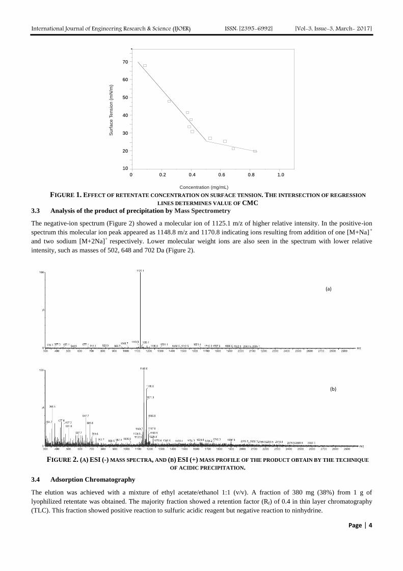
3.2 Critical micelle concentration of the retentate (CMC)
The CMC is minimum surfactant concentration from which spontaneously begins the formation of micelles in the solution
and for this reason the value of surface tension (γ) does not decrease more. The values of γ were plotted versus the values of
concentration of different dilutions (Figure1) and the value of CMC of retentate was calculated from the turning point of the
curve obtained. The value of CMC resulted to be 0.3 mg/mL and the surface tension was decreased to 29.6 mN/m.
International Journal of Engineering Research & Science (IJOER) ISSN: [2395-6992] [Vol-3, Issue-3, March- 2017]
Page | 4
0 0.2 0.4 0.6 0.8 1.0
10
20
30
40
50
60
70
0 0.2 0.4 0.6 0.8 1.0
10
20
30
40
50
60
70
Su
rfa
ce T
ensio
n (
mN
/m)
Concentration (mg/mL) FIGURE 1. EFFECT OF RETENTATE CONCENTRATION ON SURFACE TENSION. THE INTERSECTION OF REGRESSION
LINES DETERMINES VALUE OF CMC
3.3 Analysis of the product of precipitation by Mass Spectrometry
The negative-ion spectrum (Figure 2) showed a molecular ion of 1125.1 m/z of higher relative intensity. In the positive-ion
spectrum this molecular ion peak appeared as 1148.8 m/z and 1170.8 indicating ions resulting from addition of one [M+Na]+
and two sodium [M+2Na]+
respectively. Lower molecular weight ions are also seen in the spectrum with lower relative
intensity, such as masses of 502, 648 and 702 Da (Figure 2).
FIGURE 2. (A) ESI (-) MASS SPECTRA, AND (B) ESI (+) MASS PROFILE OF THE PRODUCT OBTAIN BY THE TECHNIQUE
OF ACIDIC PRECIPITATION.
3.4 Adsorption Chromatography
The elution was achieved with a mixture of ethyl acetate/ethanol 1:1 (v/v). A fraction of 380 mg (38%) from 1 g of
lyophilized retentate was obtained. The majority fraction showed a retention factor (Rf) of 0.4 in thin layer chromatography
(TLC). This fraction showed positive reaction to sulfuric acidic reagent but negative reaction to ninhydrine.
(a)
(b)

International Journal of Engineering Research & Science (IJOER) ISSN: [2395-6992] [Vol-3, Issue-3, March- 2017]
Page | 5
CMC value was determined to confirm that isolated fraction from the column has surfactant activity. To calculate this was
made a graph of surface tension versus concentration as shown in Figure 3. A value of CMC of 0.15 mg/mL was obtained.
The value of surface tension at that concentration reached values of 29.6 mN/m.
0.0 0.10 0.15 0.20 0.25 0.30
10
15
20
25
30
35
40
45
50
55
60
65
70
75
Surf
ace
Te
nsio
n (
mN
/m)
Concentration (mg/mL) FIGURE 3. EFFECT OF ISOLATED BIOSURFACTANT CONCENTRATION ON SURFACE TENSION. THE INTERSECTION OF
REGRESSION LINES DETERMINES VALUE OF CMC
3.5 Analysis by LC-MS
The majority fraction was analyzed by electrospray ionization-mass spectrometry (ESI-MS) coupled to a HPLC system. As
shown in Figure 4 a series of negatively charged ions were observed in major faction isolated by adsorption chromatography.
The analytes were eluted to a gradient of acetonitrile/water to 0.1% formic acid 65:35 (v/v) to 80:20 (v/v).
A retention time (RT) of 9.21 minutes was obtained by liquid chromatography-mass spectrometry LC-MS for the ion with
the highest relative intensity in the form of negative ionization (Figure 4).This could be related to the deprotonated ion [M-
H]-
1125.1 observed in electrospray ionization-negative ion mode (ESI-) mass spectrum, and with their corresponding
sodiated ions m/z 1148.9 and 1171.8 found in electrospray ionization-positive ion mode (ESI+) mass spectrum (see Figure
2). The chromatogram showed also other less intense peaks m/z 1111; 1139 and 1154. These ions were not present in the
(ESI-) mass spectrum of the product of precipitation in the Figure 2.
FIGURE 4. LC ESI-MS PROFILE IN NEGATIVE IONIZATION OF THE MAJOR FRACTION. THE SCAN RANGE WAS M/Z 300
TO 3000 DA.
3.6 Spectral scanning
The fraction obtained by chromatography showed a maximum of absorbance at 210 nm.

International Journal of Engineering Research & Science (IJOER) ISSN: [2395-6992] [Vol-3, Issue-3, March- 2017]
Page | 6
IV. DISCUSSION
The amount of surfactant needed to achieve the lowest possible surface tension is defined as the CMC, typically ranges from
1 to 200 mg/L for biological surfactants [16]. In the present study, the CMC of the crude biosurfactants and the purified
majority fraction were investigated. It was possible to obtain a product with attractive surface tension values from
unconcentrated culture broth. Values of CMC of dodecyl sulfate sodium (SDS) and Pluronic F-68, two chemical surfactants,
were reported by O. Pornsunthorntawee et al. (2008) [17]. They found that Pluronic F-68 and SDS are able to reduce the
surface tension of pure water in 42.8 and 28.6 mN/m, and the CMC values were approximately 350 and 1280 mg/L,
respectively. In our case, were obtained lower values than pure chemical surfactants listed above. The retentate, reduced the
surface tension of ultrapure water to 29.6 mN/m and the value of CMC was 300 mg/L. Even lower values were found for the
fraction isolated by chromatography, which indicates that the compounds with greater surface activity were purified.
There are a wide variety of microorganisms have ability to produce biosurfactants, the genus Pseudomonas stands among
them. It was reported that the strains of the genus Pseudomonas can produce cyclic lipopeptides and glycolipids such as
rhamnolipids, these are two biosurfactants that differ in their structure and molecular weight [18]. The aim of our work is
only identify the family of biosurfactants, since that in order to determine the specific structure of the compounds; it would
necessary to perform Nuclear Magnetic Resonance studies and analysis of MS/MS.
Masses between 1000 and 1200 Da were observed by mass spectrometry and a maximum absorbance at 210 nm was found in
the spectral scanning. This latter might indicate the presence of compounds in its structure containing peptide bonds, this
could explain the high molecular weight found. The family of the compounds best known that contains hydrophobic and
hydrophilic amino acids in their structure and surfactants activities are denominated cyclic lipopeptides [19]. There are two
lipopeptides well described in the literature that belong to group of Viscosin, this are Viscosin and WLIP (white line-
inducing principle). Its structure is very similar and both of them have a molecular weight of around of 1126 Da and 1149 Da
when they form adducts with ion sodium [13], [20], [21]. The analytes observed by mass spectrometry could to form part of
this family. The isolated compounds may not have free amino groups in their structure; this explains why the ninhydrin
reaction was negative. This happens with Viscosin and WLIP. In contrast Viscosinamide has glutamine in its structure and
the reaction of ninhydrin is positive [22].
Masses of 502, 648 and 702 Da were found, indicating that there possibly other family of compounds released to the culture
broth for the strain used. These masses were described for mono and dirhamnolipids. Variations in rhamnolipid structures
and their possible molecular weights are well known and are reported [23].
By acid precipitation and subsequent extraction we isolated and identified total biosurfactants. By acid precipitation
technique we quantified total surfactant, and with extraction with solvents were eliminated proteins and other possible
contaminants. However, in order to determine what proportion each produces, it is necessary to isolate each family of
compounds. We isolate by adsorption chromatography a fraction of higher yield. The percentage of the major fraction
corresponded to 84 % (w/w) of biosurfactants produced by Pseudomonas. In this fraction they were observed masses of 1100
to 1200 Da.
V. CONCLUSION
In the present work, we produce biosurfactants from non pathogenic Pseudomonas. We have obtained a possible product
with surfactant activity through the addition of an ultrafiltration step in the production process, which is able to compete with
a synthetic surfactant. This we demonstrate it with the CMC values achieved.
We detected two families of analytes secreted in the culture supernatant by mass spectrometry. We were able to isolate the
majority fraction by adsorption chromatography; we believe that the strain used produced cyclic lipopeptides due to the
molecular weights found. However, it is necessary to perform nuclear magnetic resonance studies and other structural studies
that allow the detection of functional groups and confirm the above. We will continue to work on the characterization of the
analytes found (biosurfactants), with possible applications as adjuvants in the agricultural sector.
ACKNOWLEDGEMENTS
The present work is partially supported by the National Council of Scientific and Technical Research (CONICET) and the
National University of the Litoral (UNL) of Argentina.

International Journal of Engineering Research & Science (IJOER) ISSN: [2395-6992] [Vol-3, Issue-3, March- 2017]
Page | 7
REFERENCES
[1] L. Sim, O. P. Ward, and Z. Y. Li, “Production and characterisation of a biosurfactant isolated from Pseudomonas aeruginosa UW-1”,
J. Ind. Microbiol. Biotechnol., vol 19, pp. 232–238, 1997.
[2] M. Nitschke, S. G. V. A. O. Costa, and J. Contiero, “Rhamnolipid Surfactants: An Update on the General Aspects of These
Remarkable Biomolecules”. Biotechnol. Prog., vol 21, pp.1593–1600, 2005.
[3] S. Mukherjee, P. Das, and R. Sen, “Towards commercial production of microbial surfactants”, Trends. Biotechnol., vol 24, pp. 509–
515, 2006.
[4] J. D´aes, K. De Maeyer, E. Pauwelyn, and M. Höfte, “Biosurfactants in plant-Pseudomonas interactions and their importance to
biocontrol”, Environ. Microbiol. Rep., vol 2, pp. 359–372, 2010.
[5] R. Thenmozhi, A. Sornalaksmi, D. Praveenkumar, and A. Nagasathya, “Characterization of biosurfactant produced by bacterial
isolates from engine oil contaminated soil”, Adv. Environ. Biol., vol 5, pp. 2402–2408, 2011.
[6] M. Nitschke, and S. G. V. A. O. Costa, “Biosurfactants in food industry”, Trends. Food. Sci. Technol., vol. 18, pp. 252–259, 2007.
[7] I. M. Banat, R. S. Makkar and S. S Cameotra, “Potential commercial applications of microbial surfactants”, Appl. Microbiol.
Biotechnol. Vol. 53, pp. 495–508, 2000.
[8] S. S. Cameotra, and R. S. Makkar, “Recent applications of biosurfactants as biological and immunological molecules”, Curr. Opin.
Microbiol., vol. 7, pp. 262–266, 2004.
[9] V. Singh, “Biosurfactant – Isolation, Production, Purification & Significance”, Int. J. Sci. Re.s Publ., vol. 2, pp. 2250–3153, 2012.
[10] L. Rodrigues, I. M. Banat, J. Teixeira, and R. Oliveira, “Biosurfactants: Potential applications in medicine”, J. Antimicrob.
Chemother. Vol. 57, pp. 609–618, 2006.
[11] S. P. Lim, N. Roongsawang, K. Washio, and M. Morikawa, “Functional analysis of a pyoverdine synthetase from Pseudomonas sp.
MIS38”, Biosci. Biotechnol. Biochem., vol. 71, pp. 2002–2009, 2007.
[12] S. P. Lim, N. Roongsawang, K. Washio, and M. Morikawa, “Flexible exportation mechanisms of arthrofactin in Pseudomonas sp.
MIS38”, J. Appl. Microbiol., vol. 107, pp. 157–166, 2009.
[13] H. Gross, and J. E. Loper, “Genomics of secondary metabolite production by Pseudomonas spp”, Nat. Prod. Rep., vol. 26, pp. 1408–
1446, 2009.
[14] D. Haas, and G. Défago, “Biological control of soil-borne pathogens by fluorescent pseudomonads”, Nat. Rev. Microbiol., vol. 3, pp.
307–319, 2005.
[15] W. J. Xia, Z. B. Luo, H. P. Dong, L. Yu, Q. F. Cui, and Y. Q. Bi, “Synthesis, Characterization, and Oil Recovery Application of
Biosurfactant Produced by Indigenous Pseudomonas aeruginosa WJ-1 Using Waste Vegetable Oils”, Appl. Biochem. Biotechnol.,
vol. 166, pp. 1148–1166, 2012.
[16] Y. Zhang, and R. M Miller, “Enhanced octadecane dispersion and biodegradation by a Pseudomonas rhamnolipid surfactant
(biosurfactant)”. Appl. Environ. Microbiol., vol. 58, pp. 3276-82, 1992.
[17] O. Pornsunthorntawee, P. Wongpanit, S. Chavadej, M. Abe, and R. Rujiravanit, “Structural and physicochemical characterization of
crude biosurfactant produced by Pseudomonas aeruginosa SP4 isolated from petroleum-contaminated soil”, Bioresour. Technol., vol.
99, pp. 1589–1595, 2008.
[18] J. Toribio-Jiménez, J. C. V. Aradillas, Y. Romero Ramírez, M. A. Rodríguez Barrera, J. D. González Chávez, J. Luna Guevara, and J.
L. Noyola Aguirre, “Pseudomonas sp productoras de biosurfactantes”, Tlamati, vol. 5, pp. 66–82, 2014.
[19] J. M. Raaijmakers, I. De Bruijn, and M. J. D. De Kock, “Cyclic Lipopeptide Production by Plant-Associated Pseudomonas spp.:
Diversity, Activity, Biosynthesis, and Regulation”, Mol. Plant-Microbe Interact., vol. 19, pp. 699–710, 2006.
[20] H. Rokni Zadeh, W. Li, A. Sanchez Rodriguez A, D. Sinnaeve, J. Rozenski, J. C. Martins, and R. De Mot, “Genetic and functional
characterization of cyclic lipopeptide white-line-inducing principle (WLIP) production by rice rhizosphere isolate pseudomonas
putida RW10S2”, Appl. Environ. Microbiol., vol. 78, pp. 4826–4834, 2012.
[21] H. S. Saini, B. E. arrag n Huerta, A. Lebr n Paler, J. E. Pemberton, R. R. ue , A. M. Burns, M. T. Marron, C. J. Seliga, A. A.
L. Gunatilaka, and R. M. Maier, “Efficient Purification of the Biosurfactant Viscosin from Pseudomonas libanensis Strain M9-3 and
Its Physicochemical and Biological Properties”, J. Nat. Prod., vol. 71, pp. 1011–1015, 2008.
[22] T. H. Nielsen, C. Christophersen, U. Anthoni, and J. Sorensen, “Viscosinamide, a new cyclic depsipeptide with surfactant and
antifungal properties produced by Pseudomonas fluorescens DR54”, J. Appl. Microbiol., vol. 87, pp. 80–90, 1999.
[23] A. M. Abdel Mawgoud, F. Lépine, and E. Dé iel, “Rhamnolipids: diversity of structures, microbial origins and roles”, Appl.
Microbiol. Biotechnol., vol. 86, pp. 1323–1336, 2010.

International Journal of Engineering Research & Science (IJOER) ISSN: [2395-6992] [Vol-3, Issue-3, March- 2017]
Page | 8
Combination of emodin with antibiotics against methicillin-
resistant Staphylococcus aureus isolated from clinical specimens Su-Mi Cha
1, Eun-Jin Jang
2, Sung-Mi Choi
3, Jeong-Dan Cha
4*
1,4Department of Oral Microbiology and Institute of Oral Bioscience, Chonbuk National University, Jeonju, 561-756,
Republic of Korea 2Department of Dental Technology, Daegu Health College, Daegu, South Korea.
3Department of Dental Hygiene, Daegu Health College, Daegu, South Korea
Abstract— Emodin (3-methyl-1,6,8-trihydroxyanthraquinone), a natural anthraquinone compound, is an active
compound derivative isolated from the rhizome of Rheum undulatum L, an herb widely used as a laxative in
traditional Korean medicine. Emodin has been reported to have a variety of biological activities, such as anti-
cancer, vasorelaxation, immunosuppressive, anti-inflammatory and wound healing properties. In this study,
emodin was evaluated against 20 clinical isolates of MRSA, either alone or in combination with antibiotics. The
emodin exhibited strong antibacterial activity against isolates MRSA with MICs/MBCs ranged between 64-
256/64-512 μg/mL, for ampicillin 64-512/128-1024 μg/mL, and for oxacillin 8-64/16-64 μg/mL. The combination
of emodin plus oxacillin or ampicillin was reduced by ≥4-fold against isolates MRSA tested, evidencing a
synergistic effect as defined by a FICI of ≤ 0.5. Furthermore, a time-kill study evaluating the growth of the tested
bacteria was completely attenuated after 2-6 h of treatment with the 1/2 MIC of emodin, regardless of whether it
was administered alone or with oxacillin (1/2 MIC) or ampicillin (1/2 MIC). In conclusion, emodin exerted
synergistic effects when administered with oxacillin or ampicillin and the antibacterial activity and resistant
regulation of emodin against clinical isolates of MRSA might be useful in controlling MRSA infections.
Keywords— emodin, methicillin-resistant Staphylococcus aureus, minimum inhibitory concentrations, minimum
bactericidal concentrations, time-kill curves, fractional inhibitory concentration.
I. INTRODUCTION
Staphylococcus aureus is both a commensal bacterium and a human pathogen. Approximately 50% to 60% of individuals are
intermittently or permanently colonized with S. aureus and, thus, there is relatively high potential for infections [1, 2].
Indeed, S. aureus is among the most prominent causes of bacterial infections in the United States and other industrialized
countries. Simultaneously, it is a leading cause of bacteremia and infective endocarditis (IE) as well as osteoarticular, skin
and soft tissue, pleuropulmonary, and devicerelated infections [3, 4]. Methicillin-sensitive S. aureus (MSSA) and methicillin-
resistant S. aureus (MRSA) are major causes of life-threatening infections including surgical site infections, bacteraemia,
pneumonia and catheter-associated infections, leading to significant morbidity and mortality [5-7]. There is a very limited
antimicrobial armamentarium to treat MRSA infections, of which vancomycin (a glycopeptide) and linezolid (an
oxazolidinone antibiotic) are the major antibiotics [8, 9]. Antimicrobial drugs effective for treatment of patients infected with
MRSA are limited. Thus, it is important and valuable to find compounds that potentiate antimicrobial activity of antibiotics.
Plant medicines are used on a worldwide scale to prevent and treat infectious diseases [10, 11]. They are of great demand
both in the developed as well as developing countries for the primary health care needs due to their wide biological and
medicinal activities, higher safety margin and lesser costs [12, 13]. At the same time, because of the difficulty in developing
chemical synthetic drugs and because of their side-effects, scientists are making more efforts to search for new drugs from
plant resources to combat clinical multidrug-resistant microbial infections [13-15].
Emodin (3-methyl-1,6,8-trihydroxyanthraquinone), a natural anthraquinone compound, is an active compound derivative
isolated from the rhizome of Rheum undulatum L, an herb widely used as a laxative in traditional Korean medicine [16, 17].
Emodin has been reported to have a variety of biological activities, such as anti-cancer, vasorelaxation, immunosuppressive,
anti-inflammatory, antibacterial activity, and wound healing properties [18-22]. Emodin is shown to significantly inhibit
biofilm formation in P. aeruginosa, induces proteolysis of a known AHL-binding protein, and can be used as a potential QS
inhibitor for the control of biofilm formation and growth [23]. Emodin from Polygonum cuspidatum exhibits strong

International Journal of Engineering Research & Science (IJOER) ISSN: [2395-6992] [Vol-3, Issue-3, March- 2017]
Page | 9
antibacterial activity against Haemophilus parasuis in vitro. The antibacterial mechanism of emodin to H. parasuis attributed
to producing alterations on the physical structure and increasing cell membrane permeability [24].
In this study, the antimicrobial activities of emodin against methicillin-resistant Staphylococcus aureus isolated in a clinic
were assessed using broth microdilution method and the checkerboard and time-kill methods for synergistic effect of the
combination with antibiotics.
II. MATERIALS AND METHODS
2.1 Preparation of bacterial strains
20 isolates of methicillin-resistant Staphylococcus aureus isolated from the Wonkwang University Hospital, as well as
standard strains of methicillin-sensitive S. aureus (MSSA) ATCC 25923 and methicillin-resistant S. aureus (MRSA) ATCC
33591 were used. Antibiotic susceptibility was determined in testing the inhibition zones (inoculums 0.5 McFarland
suspension, 1.5×10⁸ CFU/ml) and MIC/MBC (inoculums 5×10
5 CFU/ml) for strains, measured as described in the National
Committee for Clinical Laboratory Standards (NCCLS, 1999). Briefly, the growth of bacteria was examined at 37°C in
0.95 mL of BHI broth containing various concentrations of emodin. These tubes were inoculated with 5 × 10⁵ colony-
forming units (CFU)/mL of an overnight culture grown in BHI broth, and incubated at 37°C. After 24 h of incubation, the
optical density (OD) was measured spectrophotometrically at 550 nm. Three replicates were measured for each concentration
of tested drugs. To rapidly identifying the methicillin-resistance, presence of mecA gene in MRSA isolates was detected
using PCR method as the following [25].
2.2 Minimum inhibitory concentrations/minimum bactericidal concentrations assay
The antimicrobial activities of emodin against clinical isolates MRSA 20 and reference strains were determined via the broth
dilution method [26, 27]. The minimum inhibitory concentrations (MICs) were recorded as the lowest concentration of test
samples resulting in the complete inhibition of visible growth. For clinical strains, MIC50s and MIC90s, defined as MICs at
which, 50 and 90%, respectively of the isolates were inhibited, were determined. The minimum bactericidal concentrations
(MBCs) were determined based on the lowest concentration of the extracts required to kill 99.9% of bacteria from the initial
inoculum as determined by plating on agar.
2.3 Checkerboard dilution test
The synergistic combinations were investigated in the preliminary checkerboard method performed using the MRSA, MSSA,
and one clinical isolate strains via MIC determination [26, 27]. The fractional inhibitory concentration index (FICI) and
fractional bactericidal concentration index (FBCI) are the sum of the FICs and FBCs of each of the drugs, which were
defined as the MIC and MBC of each drug when used in combination divided by the MIC and MBC of each drug when used
alone. The FIC and FBC index was calculated as follows: FIC = (MIC of drug A in combination/MIC of drug A alone) +
(MIC of drug B in combination/MIC of drug B alone) and FBC = (MBC of drug A in combination/MBC of drug A alone) +
(MBC of drug B in combination/MBC of drug B alone). FIC indices (FICI) and FBCI were interpreted as follows: ≤ 0.5,
synergy; >0.5-≤1.0, additive; >1.0-≤2.0, indifference; and >2.0, antagonism.
2.4 Time-kill curves
The bactericidal activities of the drugs evaluated in this study were also evaluated using time-kill curves constructed using
the isolated and reference strains. Cultures with an initial cell density of 5-8×10⁶
CFU/ml were exposed to the MIC of
emodin alone, or emodin (1/2 MIC) plus oxacillin (1/2 MIC) or emodin (1/2 MIC) plus ampicillin (1/2 MIC). Viable counts
were conducted at 0, 0.5, 1, 2, 3, 4, 5, 6, 12, and 24 h by plating aliquots of the samples on agar and subsequent incubation
for 24 hours at 37°C. All experiments were repeated several times and colony counts were conducted in duplicate, after
which the means were determined.
III. RESULTS AND DISCUSSION
The results of the antibacterial activity showed that the emodin exhibited inhibitory activities against isolates MRSA and
reference stains, MRSA ATCC33591 and MSSA ATCC25923. In Table 1, the emodin displayed varying degrees of activity
against clinical isolated MRSA 1-20 with MIC in the range of 64-256 µg/mL and MBC in the range of 64-256 µg/mL. The
MICs/MBCs for ampicillin were determined to be either 64/128 or 1024/2048 μg/mL; for oxacillin, either 8/16 or 64/64
μg/mL against MRSA 1-20 isolates. The range of MIC50 and MIC90 were 16-64 μg/mL and 64-256 μg/mL against MRSA 1-
20 isolates, respectively. Various anthraquinones constitute an important class of phytochemicals which possess diverse

International Journal of Engineering Research & Science (IJOER) ISSN: [2395-6992] [Vol-3, Issue-3, March- 2017]
Page | 10
biological activities against MRSA [21, 28, 29]. A chemical structure-activity relationship study revealed that two hydroxyl
units at the C-1 and C-2 positions of anthraquinone play important roles in antibiofilm and anti-hemolytic activities [28].
Emodin exhibits strong antibacterial activity against H. parasuis in vitro [24]. Emodin exhibits antimicrobial activity against
a broad range of gram-positive, including S. aureus, and Mycobacterium tuberculosis as well as other microorganisms [21,
24, 30].
TABLE 1
ANTIBACTERIAL ACTIVITY OF EMODIN AND ANTIBIOTICS IN ISOLATED MRSA AND SOME OF REFERENCE
BACTERIA
1MSSA (ATCC 25923): reference strain Methicillin-sensitive Staphylococcus aureus.
2MRSA (ATCC 33591): reference strain Methicillin-resistant Staphylococcus aureus.
3MRSA (1-20): Methicillin-resistant Staphylococcus aureus isolated a clinic.
Combination antibiotic therapy has been studied to promote the effective use of antibiotics in increasing in vivo activity of
antibiotics, in preventing the spread of drug-resistant strains, and in minimizing toxicity [26, 31, 32]. The combination of
oxacillin and emodin showed in a reduction in the MICs/MBCs for all bacteria, with the MICs/MBCs of 8/16 or 64/128
μg/mL for oxacillin becoming 2-8/4-16 μg/mL and reduced by ≥4-fold in most of S. aureus tested, evidencing a synergistic
effect as defined by a FICI of ≤ 0.5 except clinic MRSA 8, 11, and 15 at MIC and clinic MRSA 1, 4, 10, 15, and 17 at MBC
(Table 2). In combination with emodin, the MICs/MBCs for ampicillin were reduced by ≥4-fold in most of S. aureus tested,
evidencing a synergistic effect as defined by a FICI of ≤ 0.5 except clinic MRSA 7, 9, and 19 at MIC and clinic MRSA 4, 7,
10, 12, and 19 at MBC by FICI of > 0.625 (Table 3). The some plant derived compounds can improve the in vitro activity of
some cell-wall inhibiting antibiotics by directly attacking the same target site, that is, peptidoglycan [21, 33].
Samples emodin (μg/mL) Ampicillin Oxacillin
MIC50< MIC90< (1) MIC/MBC MIC/MBC (μg/mL)
MSSA ATCC 25923 1 64 256 256/512 8/16 0.25/1
MRSA ATCC 33591 2 32 128 128/256 1024/2048 8/16
MRSA 13 8 64 64/128 512/1024 16/32
MRSA 2 16 64 64/128 128/256 16/32
MRSA 3 32 64 128/256 512/2048 8/16
MRSA 4 64 128 256/256 256/512 16/64
MRSA 5 32 128 128/256 128/256 16/32
MRSA 6 16 64 64/128 256/512 8/32
MRSA 7 16 64 64/256 128/512 16/32
MRSA 8 32 128 128/256 256/512 8/32
MRSA 9 32 256 256/512 256/512 32/64
MRSA 10 64 128 256/256 64/128 8/16
MRSA 11 32 128 128/256 128/256 16/64
MRSA 12 16 64 64/64 256/512 32/64
MRSA 13 16 64 64/128 64/128 64/64
MRSA 14 16 64 64/128 128/512 16/32
MRSA 15 32 128 128/256 64/128 16/32
MRSA 16 32 128 128/256 128/256 16/32
MRSA 17 64 256 256/256 128/256 8/16
MRSA 18 64 256 256/512 64/128 16/32
MRSA 19 16 64 64/128 128/256 16/64
MRSA 20 32 128 128/256 128/512 16/32

International Journal of Engineering Research & Science (IJOER) ISSN: [2395-6992] [Vol-3, Issue-3, March- 2017]
Page | 11
TABLE 2
SYNERGISTIC EFFECTS OF EMODIN WITH OXACILLIN IN ISOLATED MRSA AND SOME OF REFERENCE
BACTERIA
1The MIC and MBC of emodin with oxacillin
2 the FIC/FBC index
3MSSA (ATCC 25923): reference strain Methicillin-sensitive Staphylococcus aureus.
4MRSA (ATCC 33591): reference strain Methicillin-resistant Staphylococcus aureus.
5MRSA (1-20): Methicillin-resistant Staphylococcus aureus isolated a clinic.
Samples Agent
MIC/MBC (μg/mL)
FIC/FBC FICI/FBCI2 Outcome
Alone Combinati
on1
MSSA ATCC 25923
3
Emodin 256/512 128/256 0.5/0.5 0.75/0.75
Additive/
Additive Oxacillin 0.25/1 0.0625/0.25 0.25/0.25
MRSA ATCC 33591
4
Emodin 128/256 32/64 0.25/0.25 0.5/0.5
Synergistic/
Synergistic Oxacillin 8/16 2/4 0.25/0.25
MRSA 15
Emodin 64/128 16/32 0.25/0.25 0.5/0.75
Synergistic/
Additive Oxacillin 16/32 4/16 0.25/0.5
MRSA 2 Emodin 64/128 16/32 0.25/0.25
0.5/0.5 Synergistic/
Synergistic Oxacillin 16/32 4/8 0.25/0.25
MRSA 3 Emodin 128/256 32/64 0.25/0.25
0.5/0.5 Synergistic/
Synergistic Oxacillin 8/16 2/4 0.25/0.25
MRSA 4 Emodin 256/256 64/128 0.25/0.5
0.5/0.75 Synergistic/
Additive Oxacillin 16/64 4/16 0.25/0.25
MRSA 5 Emodin 128/256 32/64 0.25/0.25
0.5/0.5 Synergistic/
Synergistic Oxacillin 16/32 4/8 0.25/0.25
MRSA 6 Emodin 64/128 16/32 0.25/0.25
0.5/0.5 Synergistic/
Synergistic Oxacillin 8/32 2/4 0.25/0.25
MRSA 7 Emodin 64/256 16/32 0.25/0.125
0.5/0.375 Synergistic/
Synergistic Oxacillin 16/32 4/8 0.25/0.25
MRSA 8 Emodin 128/256 64/64 0.5/0.25
0.75/0.5 Additive/
Synergistic Oxacillin 8/32 2/8 0.25/0.25
MRSA 9 Emodin 256/512 64/128 0.25/0.25
0.5/0.5 Synergistic/
Synergistic Oxacillin 32/64 8/16 0.25/0.25
MRSA 10 Emodin 256/256 64/128 0.25/0.5
0.5/0.75 Synergistic/
Additive Oxacillin 8/16 2/4 0.25/0.25
MRSA 11 Emodin 128/256 64/64 0.5/0.25
0.75/0.375 Additive/
Synergistic Oxacillin 16/64 4/8 0.25/0.125
MRSA 12 Emodin 64/64 8/16 0.125/0.25
0.375/0.5 Synergistic/
Synergistic Oxacillin 32/64 8/16 0.25/0.25
MRSA 13 Emodin 64/128 16/32 0.25/0.25
0.375/0.5 Synergistic/
Synergistic Oxacillin 64/64 8/16 0.125/0.25
MRSA 14 Emodin 64/128 8/32 0.125/0.25
0.375/0.5 Synergistic/
Synergistic Oxacillin 16/32 4/8 0.25/0.25
MRSA 15 Emodin 128/256 32/64 0.25/0.25
0.75/0.75 Additive/
Additive Oxacillin 16/32 8/16 0.5/0.5
MRSA 16 Emodin 128/256 32/64 0.25/0.25
0.5/0.5 Synergistic/
Synergistic Oxacillin 16/32 4/8 0.25/0.25
MRSA 17 Emodin 256/256 64/128 0.25/0.5
0.5/1.0 Synergistic/
Additive Oxacillin 8/16 2/8 0.25/0.5
MRSA 18 Emodin 256/512 64/128 0.25/0.25
0.5/0.5 Synergistic/
Synergistic Oxacillin 16/32 4/8 0.25/0.25
MRSA 19 Emodin 64/128 16/32 0.25/0.25
0.5/0.375 Synergistic/
Synergistic Oxacillin 16/64 4/8 0.25/0.125
MRSA 20 Emodin 128/256 32/64 0.25/0.25
0.5/0.5 Synergistic/
Synergistic Oxacillin 16/32 4/8 0.25/0.25

International Journal of Engineering Research & Science (IJOER) ISSN: [2395-6992] [Vol-3, Issue-3, March- 2017]
Page | 12
TABLE 3
SYNERGISTIC EFFECTS OF EMODIN WITH AMPICILLIN IN ISOLATED MRSA AND SOME OF REFERENCE
BACTERIA
1The MIC and MBC of emodin with ampicillin
2 the FIC/FBC index
3MSSA (ATCC 25923): reference strain Methicillin-sensitive Staphylococcus aureus
4MRSA (ATCC 33591): reference strain Methicillin-resistant Staphylococcus aureus
5MRSA (1-20): Methicillin-resistant Staphylococcus aureus isolated a clinic
Samples Agent MIC/MBC (μg/mL)
FIC/FBC FICI/FBCI2 Outcome
Alone Combination1
MSSA ATCC
25923 3
Emodin 256/512 64/128 0.25/0.25 0.75/0.75
Additive/
Additive Ampicillin 8/16 4/8 0.5/0.5
MRSA ATCC
33591 4
Emodin 128/256 32/64 0.25/0.25 0.5/0.5
Synergistic/
Synergistic Ampicillin 1024/2048 256/512 0.25/0.25
MRSA 15
Emodin 64/128 16/32 0.25/0.25 0.375/0.375
Synergistic/
Synergistic Ampicillin 512/1024 64/128 0.125/0.125
MRSA 2 Emodin 64/128 16/32 0.25/0.25
0.5/0.5 Synergistic/
Synergistic Ampicillin 128/256 32/64 0.25/0.25
MRSA 3 Emodin 128/256 32/64 0.25/0.25
0.375/0.3125 Synergistic/
Synergistic Ampicillin 512/2048 64/128 0.125/0.0625
MRSA 4 Emodin 256/256 64/128 0.25/0.5
0.5/0.75 Synergistic/
Additive Ampicillin 256/512 64/128 0.25/0.25
MRSA 5 Emodin 128/256 32/64 0.25/0.25
0.5/0.5 Synergistic/
Synergistic Ampicillin 128/256 32/64 0.25/0.25
MRSA 6 Emodin 64/128 16/32 0.25/0.25
0.5/0.375 Synergistic/
Synergistic Ampicillin 256/512 64/64 0.25/0.125
MRSA 7 Emodin 64/256 32/128 0.5/0.5
1.0/0.75 Additive/
Additive Ampicillin 128/512 64/128 0.5/0.25
MRSA 8 Emodin 128/256 32/64 0.25/0.25
0.5/0.5 Synergistic/
Synergistic Ampicillin 256/512 64/128 0.25/0.25
MRSA 9 Emodin 256/512 64/64 0.25/0.125
0.75/0.375 Additive/
Synergistic Ampicillin 256/512 128/128 0.5/0.25
MRSA 10 Emodin 256/256 64/128 0.25/0.5
0.5/0.75 Synergistic/
Additive Ampicillin 64/128 16/32 0.25/0.25
MRSA 11 Emodin 128/256 32/64 0.25/0.25
0.5/0.5 Synergistic/
Synergistic Ampicillin 128/256 32/64 0.25/0.25
MRSA 12 Emodin 64/64 16/32 0.25/0.5
0.375/0.625 Synergistic/
Additive Ampicillin 256/512 32/64 0.125/0.125
MRSA 13 Emodin 64/128 16/16 0.25/0.125
0.5/0.375 Synergistic/
Synergistic Ampicillin 64/128 16/32 0.25/0.25
MRSA 14 Emodin 64/128 16/16 0.25/0.125
0.5/0.25 Synergistic/
Synergistic Ampicillin 128/512 32/64 0.25/0.125
MRSA 15 Emodin 128/256 32/64 0.25/0.25
0.5/0.5 Synergistic/
Synergistic Ampicillin 64/128 16/32 0.25/0.25
MRSA 16 Emodin 128/256 32/64 0.25/0.25
0.5/0.5 Synergistic/
Synergistic Ampicillin 128/256 32/64 0.25/0.25
MRSA 17 Emodin 256/256 64/64 0.25/0.25
0.5/0.5 Synergistic/
Synergistic Ampicillin 128/256 32/64 0.25/0.25
MRSA 18 Emodin 256/512 64/128 0.25/0.25
0.5/0.5 Synergistic/
Synergistic Ampicillin 64/128 16/32 0.25/0.25
MRSA 19 Emodin 64/128 32/64 0.5/0.5
0.75/0.75 Additive/
Additive0 Ampicillin 128/256 32/64 0.25/0.25
MRSA 20 Emodin 128/256 32/64 0.25/0.25
0.375/0.375 Synergistic/
Synergistic Ampicillin 128/512 16/64 0.125/0.125

International Journal of Engineering Research & Science (IJOER) ISSN: [2395-6992] [Vol-3, Issue-3, March- 2017]
Page | 13
The efficacy of emodin administered with oxacillin or ampicillin on standard (MSSA and MRSA) and clinical isolates of
MRSA (MRSA 1-20) was confirmed by time-kill curve experiment (Fig. 1-4). Cultures of each strain of bacteria with a cell
density of 5-8×10⁶
CFU/mL were exposed to the MIC of emodin alone or/and emodin (1/2 MIC) with oxacillin (1/2 MIC)
or/and ampicillin (1/2 MIC). Interestingly, the combination of the emodin plus oxacillin or/and ampicillin exhibited a steady
reduction of 5-8 × 10⁶ CFU/mL to 10
3 CFU/mL within 6 h and did not recover within 24 h, as compared to that observed
with emodin (MIC) alone. A powerful bactericidal effect was exerted when a combination of drugs was utilized. Although
emodin has no influence on genes related to cell wall synthesis and lysis as well as β-lactamase activity and drug
accumulation, emodin reduces membrane fluidity and disrupted membrane integrity [21]. This perturbation of the cell
membrane coupled with the action of β-lactams on the transpeptidation of the cell membrane could lead to the enhanced
antimicrobial effect [32, 33].
FIG. 1. TIME-KILL CURVES OF MIC OF EMODIN ALONE AND 1/2 MIC OF EMODIN WITH 1/2 MIC OF
OXACILLIN OR AMPICILLIN AGAINST ISOLATES MRSA (1-4) AND METHICILLIN-SENSITIVE S. AUREUS
(MSSA) ATCC 25923 AND METHICILLIN-RESISTANT S. AUREUS (MRSA) ATCC 33591 STRAINS. BACTERIA
WERE INCUBATED WITH EMODIN ALONE (●) AND WITH AMPICILLIN (○) OR OXACILLIN (▼) OVER TIME. CFU,
COLONY-FORMING UNITS.

International Journal of Engineering Research & Science (IJOER) ISSN: [2395-6992] [Vol-3, Issue-3, March- 2017]
Page | 14
FIG. 2. TIME-KILL CURVES OF MIC OF EMODIN ALONE AND 1/2 MIC OF EMODIN WITH 1/2 MIC OF
OXACILLIN OR AMPICILLIN AGAINST ISOLATES MRSA (5-10). BACTERIA WERE INCUBATED WITH EMODIN
ALONE (●) AND WITH AMPICILLIN (○) OR OXACILLIN (▼) OVER TIME. CFU, COLONY-FORMING UNITS.

International Journal of Engineering Research & Science (IJOER) ISSN: [2395-6992] [Vol-3, Issue-3, March- 2017]
Page | 15
FIG. 3. TIME-KILL CURVES OF MIC OF EMODIN ALONE AND 1/2 MIC OF EMODIN WITH 1/2 MIC OF
OXACILLIN OR AMPICILLIN AGAINST ISOLATES MRSA (11-16). BACTERIA WERE INCUBATED WITH EMODIN
ALONE (●) AND WITH AMPICILLIN (○) OR WITH OXACILLIN (▼) OVER TIME. CFU, COLONY-FORMING UNITS.
International Journal of Engineering Research & Science (IJOER) ISSN: [2395-6992] [Vol-3, Issue-3, March- 2017]
Page | 16
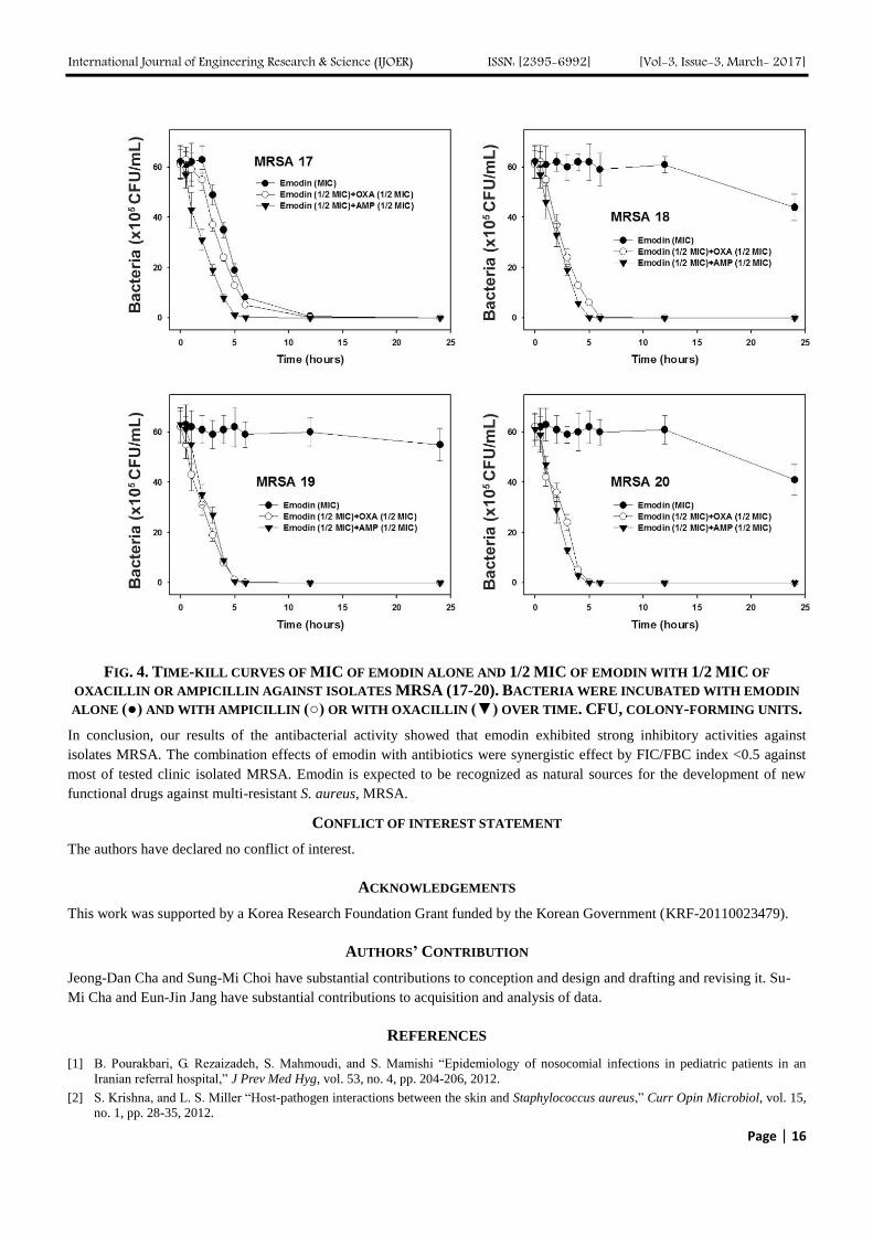
FIG. 4. TIME-KILL CURVES OF MIC OF EMODIN ALONE AND 1/2 MIC OF EMODIN WITH 1/2 MIC OF
OXACILLIN OR AMPICILLIN AGAINST ISOLATES MRSA (17-20). BACTERIA WERE INCUBATED WITH EMODIN
ALONE (●) AND WITH AMPICILLIN (○) OR WITH OXACILLIN (▼) OVER TIME. CFU, COLONY-FORMING UNITS.
In conclusion, our results of the antibacterial activity showed that emodin exhibited strong inhibitory activities against
isolates MRSA. The combination effects of emodin with antibiotics were synergistic effect by FIC/FBC index <0.5 against
most of tested clinic isolated MRSA. Emodin is expected to be recognized as natural sources for the development of new
functional drugs against multi-resistant S. aureus, MRSA.
CONFLICT OF INTEREST STATEMENT
The authors have declared no conflict of interest.
ACKNOWLEDGEMENTS
This work was supported by a Korea Research Foundation Grant funded by the Korean Government (KRF-20110023479).
AUTHORS’ CONTRIBUTION
Jeong-Dan Cha and Sung-Mi Choi have substantial contributions to conception and design and drafting and revising it. Su-
Mi Cha and Eun-Jin Jang have substantial contributions to acquisition and analysis of data.
REFERENCES
[1] B. Pourakbari, G. Rezaizadeh, S. Mahmoudi, and S. Mamishi “Epidemiology of nosocomial infections in pediatric patients in an
Iranian referral hospital,” J Prev Med Hyg, vol. 53, no. 4, pp. 204-206, 2012.
[2] S. Krishna, and L. S. Miller “Host-pathogen interactions between the skin and Staphylococcus aureus,” Curr Opin Microbiol, vol. 15,
no. 1, pp. 28-35, 2012.

International Journal of Engineering Research & Science (IJOER) ISSN: [2395-6992] [Vol-3, Issue-3, March- 2017]
Page | 17
[3] B. E. Cleven, M. Palka-Santini, J, Gielen, S. Meembor, M. Kronke, and O. Krut “Identification and characterization of bacterial
pathogens causing bloodstream infections by DNA microarray,” J Clin Microbiol, vol. 44, no. 7, pp. 2389-2397, 2006.
[4] A. Zecconi, and F. Scali “Staphylococcus aureus virulence factors in evasion from innate immune defenses in human and animal
diseases,” Immunol Lett, vol. 150, no. 1-2, pp.12-22, 2013.
[5] S. Stefani, and P. E. Varaldo “Epidemiology of methicillin resistant staphylococci in Europe,” Clin Microbiol Infect, vol. 9, no. 12,
pp. 1179-1186, 2003.
[6] E. J. Choo, and H. F. Chambers “Treatment of Methicillin-Resistant Staphylococcus aureus Bacteremia,” Infect Chemother, vol. 48,
no. 4, pp. 267-273, 2016.
[7] S. M. Purrello, J. Garau, E. Giamarellos, T. Mazzei, F. Pea, A. Soriano, and S. Stefani “Methicillin-resistant Staphylococcus aureus
infections: A review of the currently available treatment options,” J Glob Antimicrob Resist, vol. 7, pp.178-186, 2016.
[8] J. Yue, B. R. Dong, M. Yang, X. Chen, T. Wu, and G. J. Liu “Linezolid versus vancomycin for skin and soft tissue infections,”
Cochrane Database Syst Rev, vol. 7, no. 1, pp.CD008056, 2016.
[9] C. Eckmann, D. Nathwani, W. Lawson, S. Corman, C. Solem, J. Stephens, C. Macahilig, J. Li, C. Charbonneau, N. Baillon-Plot, and
S. Haider “Comparison of vancomycin and linezolid in patients with periopheral vascular disease and/or diabetes in an observational
European study of complicated skin and soft-tissue infections due to methicillin resistant Staphylococcus aureus,” Clin Microbiol
Infect, vol. 21 no. Suppl 2, pp. S33-9, 2015.
[10] P. Dahiya, and S. Purkayastha “Phytochemica screening and antimicrobial activity of some medicinal plant multi-drug resistant
bacteria from clinical isolates,” Indian J Pharm Sci, vol. 74, no. 5, pp. 443-450, 2012.
[11] X. Su, A. B. Howell, and D. H. D'Souza “Antibacterial effects of plant-derived extracts on methicillin-resistant Staphylococcus
aureus,” Foodborne Pathog Dis, vol. 9, no. 6, pp. 573-578, 2012.
[12] F. Aqil, M. S. Khan, M. Osais, and I. Ahmad “Effect of certain bioactive plant extracts on clinical isolates of beta-lactamase
producing methicillin-resistant Staphylococcus aureus,” J Basic Microbiol, vol. 45, no. 2, pp. 106-114, 2005.
[13] J. N. Eloff “Which extractant should be used for the screening and isolation of antimicrobial components from plants?,” J
Ethnopharmacol, vol. 60, no. 1, pp. 1-8, 1998.
[14] D. E. Djeussi, J. A. K. Noumedem, B. T. Ngadjui, and V. Kuete “Antibacterial and antibiaotic-modulation activity of six
Cameroonian medicinal plants against Gran-negative multi-drug resistant phenotypes,” Bmc Compem Altern, vol. 4, no. 16, pp.124,
2016.
[15] J. Rios, and M. Recio “Medicinal plants and antimicrobial activity,” J Ethnopharmacol, vol. 100, no. 1-2, pp. 80-84, 2005.
[16] S. Z. Choi, S. O. Lee, K. U. Jang, S. H. Chung, S. H. Park, H. C. Kang, E. Y. Yang, H. J. Cho, and K. R. Lee “Antidiabetic stilbene
and anthraquinone derivatives from Rheum undulatum,” Arch Pharm Res, vol. 28, no. 9, pp. 1027-1030, 2005.
[17] Y. Li, H. Liu, X. Ji, and J. Li “Optimized separation of pharmacologically active anthraquinones in rhubarb by capillary
electrochromatography,” Electrophoresis, vol. 21, no. 15, pp. 3109-3115, 2000.
[18] J. Lu, Y. Xu, X, Wei, Z. Zhao, J. Xue, and P. Liu “Emodin Inhibits the Epithelial to Mesenchymal Transition of Epithelial Ovarian
Cancer Cells,” Biomed Res Int, vol. 2016, pp. 6253280, 2016.
[19] S. Y. Park, M. L. Jin, M. J. Ko, G. Park, and Y. W. Choi “Anti-neuroinflammatory Effect of Emodin in LPS-Stimulated Microglia:
Involvement of AMPK/Nrf2 Activation,” Neurochem Res, vol. 41, no. 11, pp. 2981-2992, 2016.
[20] C. L. Zhang, L. N. Cong, R. Wang, Y. Wang, K. T. Ma, L. Zhao, J. Q. Si, and L. Li “Emodin-induced increase in expression of β1
subunit of BKCa channel mediates relaxation of cerebral basilar artery in spontaneously hypertensive rats,” Sheng Li Xue Bao, vol.
66, no. 3, pp. 289-94, 2014.
[21] M. Liu, W. Peng, R. Qin, Z. Yan, Y. Cen, X. Zheng, X. Pan, W. Jiang, B. Li, X. Li, and H. Zhou “The direct anti-MRSA effect of
emodin via damaging cell membrane,” Appl Microbiol Biotechnol, vol. 99, no. 18, pp.7699-709, 2015.
[22] X. Y. Dai, W. Nie, Y. C. Wang, Y. Shen, Y. Li, and S. J. Gan “Electrospun emodin polyvinylpyrrolidone blended nanofibrous
membrane: a novel medicated biomaterial for drug delivery and accelerated wound healing,” J Mater Sci Mater Med, vol. 23, no. 11,
pp. 2709-2716, 2012.
[23] X. Ding, B. Yin, L. Qian, Z. Zeng, Z. Yang, H. Li, Y. Lu, and S. Zhou “Screening for novel quorum-sensing inhibitors to interfere
with the formation of Pseudomonas aeruginosa biofilm,” J Med Microbiol. vol. 60, no. Pt 12, pp.1827-1834, 2011.
[24] L. Li, X, Song, Z. Yin, R. Jia, Z. Li, X. Zhou, Y. Zou, L. Li, L. Yin, G. Yue, G. Ye, C. Lv, W. Shi, and Y. Fu “The antibacterial
activity and action mechanism of emodin from Polygonum cuspidatum against Haemophilus parasuis in vitro,” Microbiol Res, vol.
186-187, pp. 139-145, 2016.
[25] F. Wallet, M. Roussel-Delvallez, and R. J. Courcol “Choice of a routine method for detecting methicillin-resistance in staphylococci,”
J Antimicrob Chemother, vol. 37, no. 5, pp. 901-909, 1996.
[26] M. W. Climo, R. L. Patron, and G. L. Archer “Combinations of vancomycin and beta-lactams are synergistic against staphylococci
with reduced susceptibilities to vancomycin,” Antimicrob Agents Chemother, vol. 43, no. 7, pp. 1747-1753, 1999.
[27] J. D. Cha, J. H. Lee, K. M. Choi, S. M. Choi, and J. H. Park “Synergistic Effect between Cryptotanshinone and Antibiotics against
Clinic Methicillin and Vancomycin-Resistant Staphylococcus aureus,” Evid Based Complement Alternat Med. Vol. 2014, pp. 450572,
2014.
[28] J. H. Lee, Y. G. Kim, S. Y. Ryu, and J. Lee “Calcium-chelating alizarin and other anthraquinones inhibit biofilm formation and the
hemolytic activity of Staphylococcus aureus,” Sci Rep, vol. 14, no. 6, pp. 19267, 2016.
[29] L. K. Omosa, J. O. Midiwo, A. T. Mbaveng, S. B. Tankeo, J. A. Seukep, I. K. Voukeng, J. K. Dzotam, J. Isemeki, S. Derese, R. A.
Omolle, T. Efferth, and V. Kuete “Antibacterial activities and structure-activity relationships of a panel of 48 compounds from

International Journal of Engineering Research & Science (IJOER) ISSN: [2395-6992] [Vol-3, Issue-3, March- 2017]
Page | 18
Kenyan plants against multidrug resistant phenotypes,” Springerplus, vol. 27, no. 1, pp. 901, 2016.
[30] D. Dey, R. Ray, and B. Hazra “Antitubercular and antibacterial activity of quinonoid natural products against multi-drug resistant
clinical isolates,” Phytother Res, vol. 28, no. 7, pp.1014-1021, 2014.
[31] B. Périchon, and P. Courvalin “Synersism between beta-lactams and glycopeptides against VanA-type methicillin-resistant
Staphylococcus aureus and heterologous expression of the vanA operon,” Antimicrob Agents Chemother, vol. 50, no. 11, pp. 3622-
3630, 2006.
[32] R. Qin, K. Xiao, B. Li, W. Jiang, W. Peng, J. Zheng, and H. Zhou “The combination of catechin and epicatechin gallate from Fructus
crataegi potentiates beta-lactam antibiotics against methicillin-resistant Staphylococcus aureus (MRSA) in vitro and in vivo,” Int J
Mol Sci, vol. 14, no. 1, pp. 1802-1821, 2013.
[33] J. G. Holler, H. C. Slotved, P. Mølgaard, C. E. Olsen, and S. B. Christensen “Chalcone inhibitors of the NorA efflux pump in
Staphylococcus aureus whole cells and enriched everted membrane vesicles,” Bioorg Med Chem, vol. 20, no. 14, pp. 4514-4521,
2012.

International Journal of Engineering Research & Science (IJOER) ISSN: [2395-6992] [Vol-3, Issue-3, March- 2017]
Page | 19
Three Level Security Technique of Image Steganography with
Digital Signature Framework
Rahul Kamboj1, Madhav Prasad Khanal
2
1PG Scholar, Department of ECE, Punjab College of Engineering & Technology, Lalru, PUNJAB -140501
2Asst. Professor, Department of ECE, Punjab College of Engineering & Technology, Lalru, PUNJAB -140501
Abstract— Steganography technique is more popular in recent years due to high level security involved in transferring the
data. In image stegnography scheme the secret message is hidden inside a digital image by using different techniques. Least
significant bit (LSB) is the commonly used technique foe embedding the information inside a cover image. A three level
security scheme has been developed by using MATLAB with digital signature framework. The developed technique has a
simpler approach as compared to other complex technique involved in secure transmission of data. The results are analyzed
for different images using Peak Signal to noise ratio (PSNR) and the results reveals that the average PSNR value is
enhanced by 15.83% compared to the reference values.
Keywords — Image steganography, PSNR, MATLAB, LSB, Digital signature.
I. INTRODUCTION
As the usage of internet is increasing rapidly with digitization the main concern in the field of information technology (IT)
and communication is security of data. Stegnography is the art and science of invisible communication. This technology
conceal a message or an image within another image making it completely hidden that helps in secure transmission of
information over insecure channel [1]. Image stegnography works on concept of hiding information exclusively in the form
of images. Stegnography and cryptography techniques are used for security dealing with passing of secured information.
Cryptography deals with maintain secrecy of content message whereas stegnography aims on maintain the secrecy of
message. Data hiding method by improved LSB substitution process [2] which improves the PSNR with respect to image
quality and computation work. The stego image quality can be greatly improved with minimum computational complexity by
applying LSB image hiding method. The effectiveness of the proposed method is verified experimentally by achieving the
balance between the security and the image quality. Exhaustive literature review of different stenographic techniques and
their classification of the passed decade [3] highlighting the visual quality of the image provides a guideline for researchers
and scientist. A method for hiding information on billboard display is presented [4] for online hiding of information on the
output screen on the output screen of the instrument. Private marking system using symmetric key steganographic techniques
and LSB techniques is used for hiding the secret information. Babloo Saha and Suchi Sharma [5] compiled research work in
the field of stegnography deployed in spatial, transform and compression domain of digital images and conclude that
transform domain techniques make changes in the frequency coefficients instead of manipulating the image pixels directly,
leading to the minimum level of distortion thus preferred over spatial domain techniques. Framework to support the concept
of image stegnography with structural design signature environment is given by Alam and Islam [6]. The experimental work
by the author was conducted on smaller domain with a future plan to perform the experiment on standard data sets to test the
effectiveness of framework. Arun Kumar et al. [7] proposed two simple fuzzy filters for the removal of impulse and gaussian
noise in gray scale and color images. Hsien-Wei-Yang [8] proposed a reversible data hiding algorithm based on interleaving
maximum-minimum histogram. In view of the above discussion the present work incorporates a MATLAB scheme for three
level secure transmissions of data with digital signature framework.
II. METHODOLOGY
Following methodology is adopted for carrying out the proposed work as follows:
1. Selection of stego image-1 (SI-1) from the database.
2. Selection of cover image (CI-1) from the database.
3. Hide stego image-1 (SI-1) into cover image (CI-1) using LSB method which is modified by using MATLAB. The
MATLAB program is modified in such a manner that instead changing only one bit, the program intends to change
more than one bit for security purpose.
4. Apply the digital signature on the cover image-1 (CI-1) after embedding stego image into it.

International Journal of Engineering Research & Science (IJOER) ISSN: [2395-6992] [Vol-3, Issue-3, March- 2017]
Page | 20
5. Selection of cover image-2 (CI-2) from the database.
6. Now cover image-1 (CI-1) will act as stego image for cover image-2 (CI-2) providing three level of security.
7. Obtained image from step 6 is the final cover image to transmit.
8. Receiving of CI-2 at the receiver end.
9. Apply the reverse LSB on CI-2 to obtain CI-1.
10. Apply the digital signature on CI-1 to obtain cover image with stego image.
11. Again apply reverse LSB on CI-1 to obtain the stego image.
Now we will compare the proposed work with the work in [6] on the basis of PSNR.
2.1 Simulation Tool
MATLAB R2011a was used for simulation work and computations were done on computer with specifications as shown in
Table 1.
TABLE 1
SPECIFICATIONS OF TOOL USED
Computer Core 2 Duo or higher
RAM 3 MB
Platform Windows 7
Other hardware Keyboard, Mouse
Software MATLAB 2011a
III. RESULTS AND DISCUSSION
Experimental investigation was conducted by creating different scenarios by using various set of images. The input to the
MATLAB scheme was provided with three images for providing security with the help of stegnography. On running the
developed scheme a window will be open from which we select the host image 1 from the data base and then a new window
will open by which we select the host image 2 that will act as stego image and will hide in host image 1. Finally the last
image as message image is selected that is to be encrypted, this image will hide in the host image 2 and to retrieve the
message at the receiver end we apply a digital signature for decryption process to start and thus receiving the message image
at the receiver end. The image quality was measured by using peak signal-to-noise ratio (PSNR). As images of different
schemes are compared in terms of the PSNR which is estimated in decibel (dB) and higher PSNR value indicate a better
image quality and is defined as:
MSEPSNR
2
10
255log10 (1)
Where MSE (Mean Square Error) is defined as
w
i
h
j
ijij shwh
MSE1 1
2)(1
(2)
where w and h are the width and height of the image respectively and hij and sij are the pixel values of host and stego image at
[i, j] respectively..
Images used in the present work for different scenario is shown in Table 2, where the first column represents images as Host
1, second column represents the images as Host 2 and third column represents the message images taken for four different
scenarios and comparative analysis of present work and reference work [6] is shown in Table 3.

International Journal of Engineering Research & Science (IJOER) ISSN: [2395-6992] [Vol-3, Issue-3, March- 2017]
Page | 21
TABLE 2
IMAGES USED FOR DIFFERENT SCENARIOS
Scenarios
Column 1(Host 1)
Column 2(Host 2)
Column 3(Message Image)
1
2
3
4
To compare the present results with the result of previous experimental studies the performance factor (PSNR) found in
literature are summarized in Table 3. The literature review reveals that the analysis using three level securities with digital
signature framework employed in the analysis has not been performed previously. So it is difficult to make direct comparison
of the present study with the result obtain in previous study. However commonly used parameter for measuring image quality
is peak signal to noise ratio (PSNR) is used in the present work.

International Journal of Engineering Research & Science (IJOER) ISSN: [2395-6992] [Vol-3, Issue-3, March- 2017]
Page | 22
TABLE 3
COMPARATIVE ANALYSIS FOR PSNR VALUES
IV. CONCLUSION
A scheme has been developed for secure transmission of high quality data with minimum distortion in the image. The
developed scheme saves the computational time and reduces the complexity of the problem as compared to other techniques
like DCT (Discrete cosine transform), DWT. The enhancement in the PSNR values for different scenarios from highest to
lowest are: Scenario 3 (16.21%), Scenario 1 (15.86%), Scenario 2 (15.81%) and Scenario 4 (15.45%). Thus the result shows
that the developed algorithm ensures higher quality of data and high encryption level.
ACKNOWLEDGEMENTS
I am greatly thankful to principal and the management of Punjab College of Engineering & Technology, Lalru, PUNJAB for
motivation, encouragement and providing facility to carry out this research work.
REFERENCES
[1] Ms.G.S.Sravanthi, Mrs.B.Sunitha Devi, S.M.Riyazoddin & M.Janga Reddy “A Spatial Domain Image Steganography Technique
Based on Plane Bit Substitution Method.” Intertional Journal of Computer Application volume 5-No.7 October 2009.
[2] Vijay Kumar Sharma, Vishal Shrivastava, “A Steganography algorithm for hiding image in image by improved LSB substitution by
minimizes detection”. Journal of Theoretical and Applied Information Technology (JATIT), Vol. 36 No.1.
[3] Hussain and Mureed Hussain, “A Survey of Image Steganography Techniques. International Journal of Advanced Science and
Technology” Vol. 54, May, 2013.
[4] Shashikala Channalli, Ajay Jadhav, “Steganography An Art of Hiding Data. International Journal on Computer Science and
Engineering” Vol.1 (3), 2009, 137-141.
[5] Babloo Saha and Shuchi Sharma, “Steganographic Techniques of Data Hiding using Digital Images”. Defense Science Journal, Vol.
62, No. 1, January 2012, pp. 11-18.
[6] Fahim Irfan Alam, Md. Mohaiminul Islam, “An Investigation into Image Hiding Steganography with Digital Signature Framework”.
IEEE, Vol. 6, No. 13, pp. 978-1-4799- 400, 2013.
[7] S.Arunkumar, Ravi Tej Akula, Rishabh Gupta & M.R.Vimala Devi, “Fuzzy Filters to the Reduction of Impulse and Gaussian Noise in
Gray and Color Images”. International Journal of Recent Trends in Engineering, Vol. 1, No. 1, May 2009.
[8] Hsien-Wei Yang, “Interleaving Max-Min Difference Histogram Shifting Data Hiding Method”. Journal of software, VOL. 5, NO. 6,
JUNE 2010.
Scenario Host-1 Host-2 Message Image Proposed
Work
Reference
Work [6]
Percentage
Enhancement
in PSNR
Values
1 Rahul1 Bird Objects 44.0736 38.04 15.86
2 Rahul2 Rahul1 Cameraman 44.7862 38.67 15.81
3 Rahul2 Rahul3 Rahul4 44.7875 38.57 16.12
4 Butterfly Pepper Rahul2 44.7858 38.79 15.45

International Journal of Engineering Research & Science (IJOER) ISSN: [2395-6992] [Vol-3, Issue-3, March- 2017]
Page | 23
A novel framework for a pull oriented product development and
planning based on Quality Function Deployment Omid Fatahi Valilai
1, Hossein Reyhani Kivi
2
1Assistant Professor, Industrial Engineering, Sharif University of Technology, Azadi Street, Tehran, Iran
2M.Sc., Industrial Engineering, Khatam University, Molasadra street, Tehran, Iran
Abstract— Nowadays, manufacturing organizations face with increasing pressures from the frequent changes in product
type, continuous demand fluctuations and unexpected changes in customer requirements. In order to survive in this turbulent
environment, manufacturing organizations must become flexible and responsive to these dynamic changes in the business
environment. In this research, this papers has reviewed the current literature in the area of pull-oriented product systems
and has suggested a novel framework for a pull-oriented product development system compatible with today’s manufacturing
environments. In the proposed framework, using the Quality Function Deployment (QFD) 4-stage matrix, a framework for
product development has been proposed. The paper has used four general processes for products assembly. The framework
provides capabilities for customer order analyze by a decision support system for order acceptance/rejection decision.
Moreover, the accepted orders are prioritized into high and low priority orders, considering profitability of orders and a
proposed assemble-to-order (ATO) production system for pull-oriented environments will handle the orders’ fulfilment. The
validity of proposed framework has been investigated by process analysis and simulating a scenario.
Keywords— Product development system, Pull-oriented system, Quality Function Deployment (QFD), Assemble-to-order
production (ATO).
I. INTRODUCTION
In a highly competitive environment, manufacturing organizations need a suitable production policy for the control of the
production line so that the resources including machines as well as the buffer can be better utilized in conducting the
manufacturing activities [1]. Manufacturing companies use different production policies to satisfy customers’ demands. The
most applicable production policies are Make-To-Stock (MTS), Make-To-Order (MTO), Assemble-To-Order (ATO) and
Engineer-To-Order (ETO). Each policy has some specific advantages and disadvantages. Among them, MTS and MTO
systems have been widely used in the production companies. In MTS companies, the customers’ demands are satisfied with
stocked inventories of finished products. The dominant features of such systems are short delivery time, heavy storage cost
and low flexibility in responding to customized needs of customers. A substantial proportion of the research prior to 1990 in
the production planning area had been aimed at the needs of MTS companies [2, 3]. On the other hand, MTO companies
produce their products based on the customers’ orders. Long delivery time, low storage cost and higher flexibility in
responding to customers’ demands are the main features of MTO systems [3, 4].
The success of an MTO system is heavily dependent on the selectivity of an order acceptance policy that seeks to maximize
the average revenue per unit cost of requested capacity when demand exceeds capacity. It is noteworthy that the rejection of
an order may have strategic repercussions for future customer relations, and may drastically change order arrival rates and
patterns. The decision an MTO system has to make for an incoming order is whether to accept, negotiate or reject it
depending on the available capacity, the profit contribution margin of the order and expected arrival times for future orders.
A negotiation process of an order is only worth pursuing if accepting it may contribute significantly to generate more
revenues per installed capacity and market niche development. Resorting to an order acceptance policy is thus a key
decision-making problem at the interface between marketing/sales functions and production planning [5].

International Journal of Engineering Research & Science (IJOER) ISSN: [2395-6992] [Vol-3, Issue-3, March- 2017]
Page | 24
Unlike the make-to-stock manufacturing mode which holds finished products in stock as a buffer against demand variability,
MTO production systems must hold production capacity and workin- process inventories to accept only orders of the most
profitable type. The main issue is thus how to selectively accept/reject/negotiate in order to maximize cumulative profit
gains. In the absence of a more elaborated policy, orders are accepted on a ‘first-come-first-serve’ basis. If the available
capacity is not enough to process an arriving order on time, the order is rejected [6].
The build-to-order supply chain (BTO-SC) or make-to-order (MTO) system has received a great deal of attention in recent
years because of the success of high-tech companies such as Dell, BMW, Compaq, and Gateway. In recent years, BTO-SCM
has become prevalent among high-tech companies, including traditional manufacturing companies such as automobile
companies. BTO-SC can be defined as ‘‘the system that produces goods and services based on individual customer
requirements in a timely and cost competitive manner by leveraging global outsourcing, the application of information
technology and through the standardization of components and delayed product differentiation strategies” [7].
Recent years have proven a number of changes in companies’ production policies and they are gradually moving more to
hybrid MTS/MTO production mode. In a MTS/MTO production mode, a portion of the production system operates in a MTS
mode and the remaining portion operates in a MTO mode. A proper combination of MTO and MTS can exploit the
advantages of both lower inventory and short delivery time [3].
Assemble-to-order (ATO) production is a popular strategy used by firms that seek to be responsive and cost-efficient at the
same time. ATO is particularly attractive when component supply lead-times are long or the supply processes are capacitated
compared to final assembly. Furthermore, by pooling components stocks, an ATO strategy can reduce the cost of offering
high product variety. Hence, by using this strategy a firm can shorten its response time to its customers and offer a high
variety of the end product. An example of such practice is used by computer manufacturers and mail order retailers [8].
The assemble-to-order (ATO) strategy emerges in manufacturing environments where many finished products are assembled
from a relatively small set of standard components and subassemblies. In a typical ATO manufacturing environment,
components and subassemblies are acquired according to a forecast, while finished products are assembled only after actual
customers’ orders have been received. In other words, component and subassemblies are replenished in a make-to-stock
(MTS) fashion, but finished products are assembled in a make-to-order (MTO) manner. Such a hybrid planning approach is
particularly advantageous in situations where the assembly time of a product is considerably shorter than the procurement
and/or manufacturing time of its components and subassemblies; thus, making a tradeoff between inventory holding cost,
product variety, and delivery time achievable [9].
Successful and innovative product (or service) development is highly correlated with the company’s success and reason for
existence. It is imperative that a company’s main purpose for existing is to provide goods and/or services to meet and even
exceed the expectations of their customers [10]. To survive, companies need to transform themselves from production-
focused to value-adding design-focused businesses [11]. Requirement understanding plays an important role in product
design. Conventionally, customer needs come from questionnaires which are mainly collected by customer investigations
[12]. Nowadays, QFD has been applied in a wide variety of quality control, decision-making, product design and
improvement, etc. It is a customer-driven approach that can create a high level of buy-in and reach a better control of the
problem [13].
Mass customization is a manufacturing approach to produce customized products based on customer requirements while
maintaining the high quality and efficiency of mass production. Compared with the traditional mass production approach,
mass customization can offer large variations of products to the market while leveraging the economies of scale and scope
within the manufacturing capabilities of enterprises. One-of-a-kind production (OKP) is a special type of mass customization
where each product is created based on requirement of an individual customer [14].

International Journal of Engineering Research & Science (IJOER) ISSN: [2395-6992] [Vol-3, Issue-3, March- 2017]
Page | 25
The purpose of this paper is to propose a framework for a pull-oriented product development system. In the first process, the
paper has used quality house for translating customer demands into technical specifications. Customer order aanalyzed by
decision support system for order acceptance/rejection decision. In sales and support product process orders are prioritized
into high and low priority orders, considering profit of order. In other two processes the Production planning and
manufacturing operations have been considered.
II. LITERATURE REVIEW
The literature review on pull-oriented product development issue indicates that lot attention has been paid to this issue in the
production environments. Moreover, the existing research regarding this issue has been mostly focused on MTO production
environments. Hendry and Kingsman [2] first emphasized on the importance of order entry stage in production
environments, especially in MTO environments where the delivery date management becomes more crucial.
M.Kalantari et al [3], M. Ebadian et al [15], K.L.Choy et al [16] and S. Hemmati et al [17] presented a decision-making
structure for the order entry stage in make-to-order environments. The aim of the proposed structures is to manage the
arriving orders so that the MTO system just proceeds to produce those arriving orders which are feasible and profitable for
the system. S. Hemmati et al [17] proposed structure composed of three phases. At the first phase, arriving orders are
prioritized into high and low priority orders, considering characteristics of order and customer and utilizing technique for
order performance by similarity to ideal solution (TOPSIS). At the second phase, rough-cut capacity was calculated for each
order regarding priority level and so, acceptance or rejection decision is taken based on it. Finally, at the third phase, the
previous phase accepted orders are evaluated based on their due dates and material arrival times and final decisions for orders
are made. M. Ebadian et al [15] proposed decision support system is comprised of five steps. At the first step, the customers
are prioritized based on a fuzzy TOPSIS method. Rough-cut capacity and rough-cut inventory are calculated in the second
step and in case of unavailability in capacity and materials, some undesirable orders are rejected. Also, proper decisions are
made about non-rejected orders. At the next step, prices and delivery dates of the non-rejected orders are determined by
running a mixed-integer mathematical programming model. At the fourth step, a set of guidelines are proposed to help the
organization negotiate over price and due date with the customers. In the next step, if the customer accepts the offered price
and delivery date, the order is accepted and later considered in the production schedule of the shop floor, otherwise the order
is rejected.
van der Laan et al [18] extend the PUSH and PULL control strategies to evaluate numerically the effects of lead-time
duration and lead-time variability on total expected costs in production/inventory systems with remanufacturing. Although
both strategies are non-optimal, they are relatively easy to analyze numerically and, more importantly, they are actually used
in practice. The most important outcomes of the study are, that for both control strategies: (i) manufacturing lead-times have
a larger influence on system costs than remanufacturing lead-times; (ii) a larger remanufacturing lead-time may sometimes
result in a cost decrease; and (iii) a larger variability in the manufacturing lead-time may sometimes result in a cost decrease.
Sharma and Agrawal [1] presented a multistage serial production system. A generalized model has been developed with the
use of probabilistic demand situations for the end product. The demand situations considered are binomial, exponential,
lognormal and Poisson. These demand patterns are used as input parameter for various production control policies. The
output values for performance parameters are obtained by simulation.
The literature available on BTO-SCM has been classified based on the nature of the decision-making areas and then sub-
classified to focus on solving problems with modeling and analysis. Gunasekaran and Ngai [7] have focused mostly on the
modeling aspect of the BTO-SC, but have not extended our efforts to empirical research. They have developed a unified
framework for modeling and analyzing BTO-SCM and suggest some future research directions.

International Journal of Engineering Research & Science (IJOER) ISSN: [2395-6992] [Vol-3, Issue-3, March- 2017]
Page | 26
The objective of Ozbayrak et al [19] paper is to estimate the manufacturing and product costs by using activity-based costing
(ABC) method in an advanced manufacturing system that is run under either material requirements planning (MRP) or just in
time (JIT) system. ABC is a method that can overcome many of the limitations of traditional costing systems. This paper
reports and discusses the implementation of the ABC alongside a mathematical and simulation model to estimate the
manufacturing and product cost in an automated manufacturing system. The potential effects of manufacturing planning and
control strategies implemented on financial structure of the manufacturing system are initially analyzed. ABC has been used
to model the manufacturing and product costs.
Ioannou and Dimitriou [20] consider the problem of dynamically updating the manufacturing lead times estimates that are
used in MRP systems. Once a new order with specific and known processing requirements enters a make-to-order
manufacturing system, an exact completion time estimate is assigned to it that is based on the system’s current status. The
approach that is suggested addresses multi-machine, multi-product manufacturing environments with no special
configuration of their resources: To this objective, simple, iterative algorithms are used to substitute the fixed lead time
estimates of typical MRP systems. The results that are presented underline the significant improvement of the proposed
approach over static, constant MRP lead time estimates that are as yet exclusively resorted to.
Olhager and Prajogo [21] analyze these improvement initiatives and their impact on business performance. In particular, they
explore potential differences between make-to-order (MTO) and make-to-stock (MTS) firms. They use data from 216
Australian manufacturing firms. They find a clear difference of improvement focus between MTO and MTS firms. MTO
firms exhibit a significant impact of supplier integration on business performance, but not for lean practices and supplier
rationalization. The situation is completely reversed for MTS firms, since they have significant effects for internal lean
practices and supplier rationalization, but not for logistics integration with supplier.
ElHafsi [22] study a pure assemble-to-order system subject to multiple demand classes where customer orders arrive
according to a compound Poisson process. The finished product is assembled from m different components that are produced
on m distinct production facilities in a make-to-stock fashion. He shows that the optimal production policy of each
component is a state-dependent base-stock policy and the optimal inventory allocation policy is a multi-level state-dependent
rationing policy. Using numerical experimentation, he first studies the system behavior as a function of order size variability
and order size. He shows that the optimal average cost rate is more sensitive to order size variability than to order size. He
also compares the optimal policy to the first-come first-serve policy and show that there is great benefit to inventory
rationing. He also propose two simple heuristics and show that these can effectively mimic the optimal policy which is
generally much more difficult to determine and, especially, to implement.
III. FRAMEWORK DESCRIPTION
Through the aforementioned section, the paper has achieved the requirements for framework by literature review in pull-
oriented product development. So, the paper has focused on fulfilling those requirements in the proposed framework.
Because of, have developed a framework in level-0 that includes four general processes (fig. 1). In review pre-order and
customer process, the paper has used quality house for translating customer demands into technical specifications, and
provides capabilities for customer order analyze by a decision support system for order acceptance/rejection decision. The
second process (product sales and support) orders are prioritized into high and low priority orders, considering profit of
order. Our third process in level-0 IDEF0 model included two QFD matrixes, this matrix are product design and process
design. Furthermore, this process includes production planning, overall planning, master production scheduling (MPS) and
inventory control (fig. 2). Fig. 2 is a level-1 IDEF0 model process of production planning (operation & overall plan). First
stage of these processes is production planning (A21) that contains QFD second matrix. In this process, product concepts are
created during this phase and part specifications are documented with product design matrix by product designers. The
second process in fig. 2 is master production scheduling (MPS).

International Journal of Engineering Research & Science (IJOER) ISSN: [2395-6992] [Vol-3, Issue-3, March- 2017]
Page | 27
A0
Review pre-order and customer
A1
Product sales and support
A2
Production plannig(Operational & Overall plan)
A3
Producing product
Pre-order
Customer indicators
Order accaptence or rejection
Order
Pre-orderreviewer
Manufacturingcapacity
Sales experts & manager
Prioritization description
Inventory details
MRP Approach
Product designers
Producingteam
Product
Long term production details
Technical designers
FMEAanalysis
Demand,Supply &Financial
plan
Assembly parts
Material to product
Process designers
Product &Process
Standards
Technical Specifications
QCstandards
QC Team
purchasing
Production linestrategy
FIG. 1: FOUR GENERAL PROCESSES LEVEL-0 IDEF0 MODEL
This process include QFD third matrix. During process planning, manufacturing processes are flowcharted and process
parameters (or target values) are documented. In other words, production processes will be planned according to product
concepts and Production scheduling is performed. Third process of fig.2 belongs to the inventory control. In this process be
done purchasing, material and assembly parts sent. Moreover, the paper has also shown the level-2 of inventory control stage
in fig.3. In this level, our processes composed from raw material (A231) and assembly part (A232). The assembly part
process’s task is reception operation process chart (OPC) and needed parts sent.
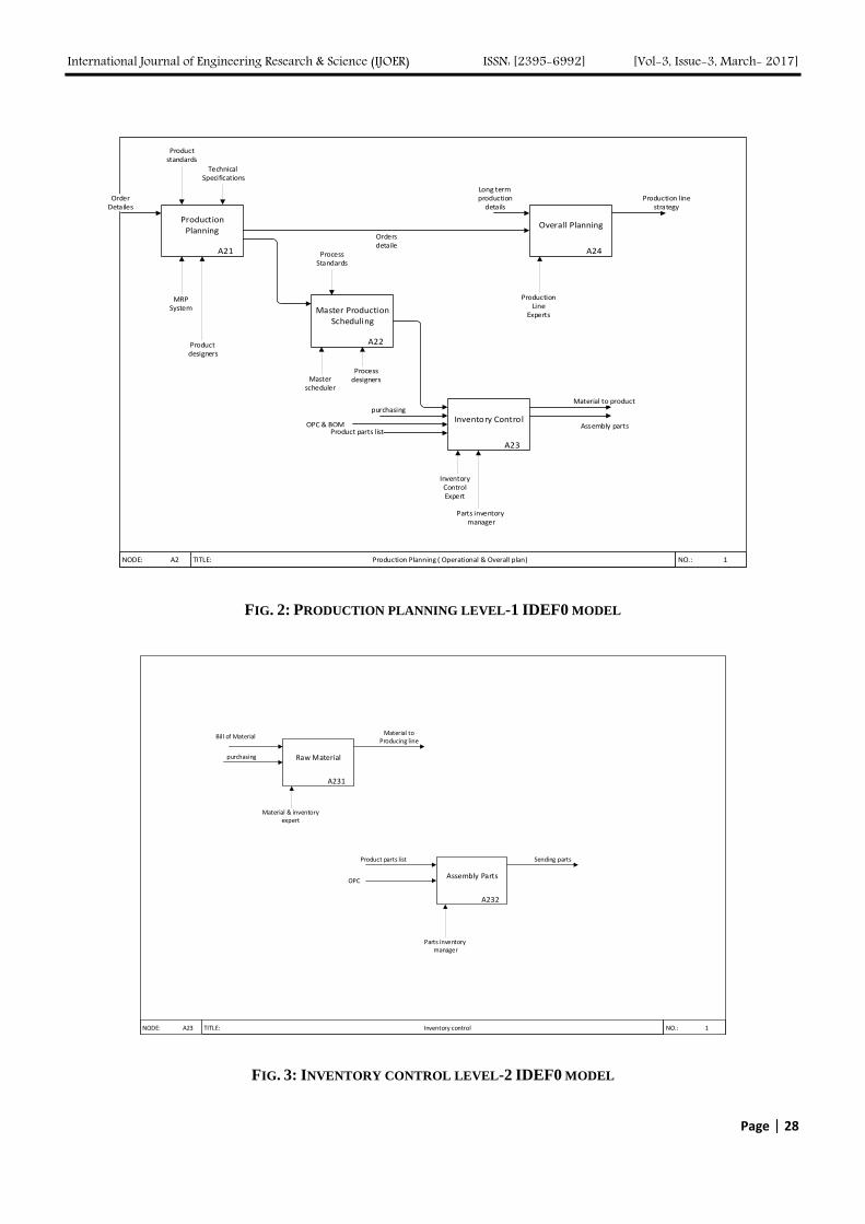
International Journal of Engineering Research & Science (IJOER) ISSN: [2395-6992] [Vol-3, Issue-3, March- 2017]
Page | 28
TITLE:NODE: NO.: 1A2 Production Planning ( Operational & Overall plan)
A21
Production Planning
A22
Master Production Scheduling
A23
Inventory Control
A24
Overall Planning
Long term production
detailsOrder
Detailes
Masterscheduler
Ordersdetaile
purchasingMaterial to product
Production linestrategy
Inventory ControlExpert
ProductionLine
Experts
MRPSystem
Assembly parts OPC & BOM
Parts inventory manager
Product parts list
Process designers
Process Standards
Product designers
Product standards
Technical Specifications
FIG. 2: PRODUCTION PLANNING LEVEL-1 IDEF0 MODEL
TITLE:NODE: NO.: 1A23 Inventory control
A231
Raw Material
A232
Assembly Parts
Bill of MaterialMaterial to
Producing line
purchasing
Product parts list Sending parts
Parts inventory manager
Material & inventory expert
OPC
FIG. 3: INVENTORY CONTROL LEVEL-2 IDEF0 MODEL

International Journal of Engineering Research & Science (IJOER) ISSN: [2395-6992] [Vol-3, Issue-3, March- 2017]
Page | 29
And the raw material process’s task is purchasing material and sent it to producing line. Our last level-0 processes is
producing product (A3). This process contained phase 4 of QFD matrix. Finally, in this stage product assembly will be done,
performance indicators are created to monitor the production process. The quality assurance department will analysis with
FMEA as to which process poses the most risk and controls are put in place to prevent failures.
IV. THE USE OF QFD
In this research, the customer demands and requirements in product have been considered by using of Quality function
deployment 4-stage matrix. Each of the four phases in a QFD process uses a matrix to translate customer requirements from
initial planning stages through production control. Each phase, or matrix, represents a more specific aspect of the product's
requirements. Relationships between elements are evaluated for each phase. Only the most important aspects from each
phase are deployed into the next matrix [23].
Phase 1, Product Planning: Building the House of Quality. Led by the marketing department, Phase1, or product planning, is
also called The House of Quality. Many organizations only get through this phase of a QFD process. Phase1 documents
customer requirements, warranty data, competitive opportunities, product measurements, competing product measures, and
the technical ability of the organization to meet each customer requirement. Getting good data from the customer in Phase1 is
critical to the success of the entire QFD process.
Phase 2, Product Design: This phase2 is led by the engineering department. Product design requires creativity and innovative
team ideas. Product concepts are created during this phase and part specifications are documented. Parts that are determined
to be most important to meeting customer needs are then deployed into process planning, or Phase3.
Phase 3, Process Planning: Process planning comes next and is led by manufacturing engineering. During process planning,
manufacturing processes are flowcharted and process parameters (or target values) are documented.
Phase 4, Process Control: And finally, in production planning, performance indicators are created to monitor the production
process, maintenance schedules, and skills training for operators. Also, in this phase decisions are made as to which process
poses the most risk and controls are put in place to prevent failures. The quality assurance department in concert with
manufacturing leads Phase4.
In framework that presented in this research, each of the four phases in a QFD process used in the different stages of
framework and the fulfillment of customer needs in the configuration and assembly of products. In this model, the paper used
the first phase of QFD in the review pre-order and customer process A0 (fig.1). In this process after reaching the customer
with special demands, this demands translated to technical specifications of parts with technical designers. In this process it
becomes clear what the configuration of the product can be offered to customers. The paper has considered the second phase
of QFD matrix in the production planning process A21 (fig.2). In this process, product designers choose the best
configuration of components and parts according to technical specifications. Master production scheduling A22 (fig.2)
included third phase of QFD matrix. In this phase, after identifying the product components and configuration in earlier
phases, product assembly processes are considered. Required materials and parts allocated for product configuration and
production scheduling. Last phase of QFD matrix considered in producing product process A3 (fig.1). In this process,
manufacturing process control and product quality assurance have been considered.
V. BENEFITS OF OUR FRAMEWORK
In this section, the paper will review proposed framework and will be considered the advantage of this. The motivation of
this research is meet customer requirements, a decision support system for order accept or reject, a ATO system to reduce
costs of design and product manufacturing. These factors have been considered and solutions for fulfilling these requirements
are proposed. For this purpose, the processes and tools that are responsive to our needs in framework are used. Despite our
efforts the proposed framework will not be perfect but will have advantages to other models. So the paper pointed out the
advantages of our framework to show that our proposed processes have a great effect on to achieve the objectives of product
development frameworks. Of the most important one, the following items can be described:
Benefits of Using QFD: Customer driven: The focus is on customer wants, not what the company thinks the customer
wants. The "Voice of the Customer" drives the development process. Reduced development time: The likelihood of
design changes is reduced as the QFD process focusses on improvements to be made to satisfy key customer
requirements. Careful attention to customer requirements reduces the risk that changes will be required late in the

International Journal of Engineering Research & Science (IJOER) ISSN: [2395-6992] [Vol-3, Issue-3, March- 2017]
Page | 30
project life cycle. Time is not spent developing insignificant functions and features. Reduced development costs: The
identification of required changes occurs early in the project life cycle. Minimizing changes following production
reduces warranty costs and product support costs.
Benefits of DSS: Helps in saving time: Research has demonstrated that decision support systems help to reduce
decision cycle time for an organization. DSS provides timely information, which is then used for decision making and
results in enhanced employee productivity. Improves efficiency: Another advantage of DSS is efficient decision
making, resulting in better decisions. This is because use of DSS results in quick transfer of information, better data
analyses, thus resulting in efficient decisions. Enhanced organizational control: Due to the use of DSS business
transaction data is easily available for monitoring the performance of employees and ad hoc querying. It thus leads to
enhanced understanding of business operations for the management.
Benefits of ATO: Businesses that want the ability to make a large number of different products from common parts
benefit the most from assemble to order method. They can stock the common parts and sell varied customized products
to meet customer needs. Another key benefit of assemble to order method is that businesses can reduce errors in the
delivery of products. For example, a business that sells computers to customers can reduce the amount of errors when
choosing this method rather than the options method.
Benefits of the FMEA: The FMEA procedure is a highly effective way to evaluate processes, services or products. It is
as valuable for revealing areas needing improvement as it is for guiding the development of new processes. It is a
logical, structured way to identify areas of concern while reducing development time and cost. It’s also valuable when
the intent is to apply a particular (typically successful) process of one product or service to another. It has proven to be
an effective way to identify how to improve areas where performance might be lagging, such as sales or customer
satisfaction ratings or high expense to income ratios, for example.
Furthermore, the framework has enabled the prioritization of orders into high and low priority orders, considering profit of
orders that reduce the risk of lost sales lucrative orders. Also, the proposed framework has overall planning that takes long-
term data from the production line. This process, provide data and offers a long-term strategy that cause increase efficiency
and reduce the idle time.
VI. CONCLUSIONS
Although the bulk of research on production planning and control has taken into account the ATO systems, most of the
companies have to work in a ATO environment in practice to decrease their production costs and also improve their
customers service level and demands. The paper has used Quality function deployment (QFD) 4-stage matrix to meet the
customer requirements. With the appearance of ATO systems, many issues have been coming up regarding the planning and
scheduling of such systems. One of these issues, which have a direct impact on the customer satisfaction, is the matter of
acceptance/rejection of new arriving orders to the system with respect to the resource limitations and customer importance.
Other of these is an accurate translation customer demands to product features. This research has proposed a novel
framework for pull-oriented product development system (ATO system) by using the QFD.
The main future research which can be considered for our study is (i) the implementation of this framework in a real
production environment (ii) Prepare a case study for this framework
REFERENCES
[1] S. a. N. A. Sharma, "Selection of a pull production control policy under different demand situations for a manufacturing system by
AHP-algorithm," Elsevier, pp. 1622-1632, 2008.
[2] B. K. L.C. Hendry, "Production planning systems and their applicability to make-to-order companies," European Journal of
Operational Research 40, pp. 1-15, 1989.
[3] M. R. ,. M. E. Mahdokht Kalantari, "A decision support system for order acceptance/rejection in hybrid MTS/MTO production
systems," Applied Mathematical Modelling 35, 2011.
[4] M. M. N.P. Dellaert, "Production strategies for a stochastic lot-sizing problem with constant capacity," European Journal of
Operational Research 92, pp. 281-301, 1996.
[5] D. C. A. P. M. Zorzini, "Due date (DD) quotation and capacity planning in make-to order companies: Results from an empirical
analysis," Int. J. Production Economics 112, p. 919–933, 2008.
[6] E. M. Facundo Arredondo, "Learning and adaptation of a policy for dynamic order acceptance in make-to-order manufacturing,"
Computers & Industrial Engineering 58, pp. 70-83, 2010.

International Journal of Engineering Research & Science (IJOER) ISSN: [2395-6992] [Vol-3, Issue-3, March- 2017]
Page | 31
[7] E. W. N. Angappa Gunasekaran, "Modeling and analysis of build-to-order supply chains," European Journal of Operational Research
195, 2009.
[8] M. ElHafsi, "Optimal integrated production and inventory control of an assemble-to-order system with multiple non-unitary demand
classes," European Journal of Operational Research 194, p. 127–142, 2009.
[9] F. C. E. Mohebbi, "The impact of component commonalityin an assemble-to-order environment under supplyand demand
uncertainty," Omega 33, p. 472 – 482, 2005.
[10] e. a. Zaim Selim, "Use of ANP weighted crisp and fuzzy QFD for product development," Expert Systems with Applications, pp. 4464-
4474, 2014.
[11] W. e. a. Yan, "A stakeholder-oriented innovative product conceptualization strategy based on fuzzy integrals," Advanced Engineering
Informatics, pp. 210-209, 2009.
[12] P. J. a. Y. L. Jin Jian, "Translating online customer opinions into engineering characteristics in QFD: A probabilistic language
analysis approach," Engineering Applications of Artificial Intelligence, pp. 115-127, 2015.
[13] J. Z. a. Y. C. Zhong Shuya, "Determination of target values of engineering characteristics in QFD using a fuzzy chance-constrained
modelling approach," Neurocomputing, pp. 125-135, 2014.
[14] D. X. ,. Y. T. Gang Hong, "Rapid identification of the optimal product configuration and its parameters based on customer-centric
product modeling for one-of-a-kind production," Computers in Industry 61, p. 270–279, 2010.
[15] M. R. F. J. S. T. R. T.-M. M. Ebadian, "A new decision-making structure for the order entry stage in make-to-order environments,"
Int. J. Production Economics 111, p. 351–367, 2008.
[16] Y. L. H. C. T. P. C. K. G. H. S. K. K.L. Choy, "A hybrid scheduling decision support model for minimizing job tardiness in a make-
to-order based mould manufacturing environment," Expert Systems with Applications 38, pp. 1931-1941, 2011.
[17] M. E. &. A. N. Hemmati Samira, "A new decision making structure for managing arriving orders in MTO environments," Expert
Systems with Applications, pp. 2669-2676, 2012.
[18] M. S. R. D. Van der Laan Erwin, "An investigation of lead-time effects in manufacturing/remanufacturing systems under simple
PUSH and PULL control strategies," European Journal of Operational Research , pp. 195-214, 1999.
[19] M. A. &. A. K. T. Özbayrak M., "Activity-based cost estimation in a push/pull advanced manufacturing system," International
journal of production economics, pp. 49-65, 2004.
[20] S. George Ioannou, "Lead time estimation in MRP/ERP for make-to-order manufacturing systems," Int. J.ProductionEconomics139,
pp. 551-563, 2012.
[21] D. Jan Olhager, "The impact of manufacturing and supply chain improvement initiatives: A survey comparing make-to-order and
make-to-stock firms," Omega 40, pp. 159-165, 2012.
[22] M. ElHafsi, "Optimal integrated production and inventory control of an assemble-to-order system with multiple non-unitary demand
classes," European Journal of Operational Research 194, p. 127–142, 2009.
[23] BRIEF, PRODUCT "Quality Function Deployment", 2012: Creative Industries Research Institute.

International Journal of Engineering Research & Science (IJOER) ISSN: [2395-6992] [Vol-3, Issue-3, March- 2017]
Page | 32
A Car Window Segmentation Algorithm Based on Region
Segmentation and Boundary Constraint Li Xi-ying
1, Li Fa-wen
2, Zhou Zhi-hao
3, Deng Yuan-chang
4
1,2,3,4Guangdong Province Key Laboratory of Intelligent Transportation Systems
1,2,3,4Key Laboratory of Video and Image Intelligent Analysis and Application Technology, MPS, China
1,2,3,4School of Engineering, Sun Yat-sen University, Guangzhou 510006, China
*Corresponding author PH: (86)20-39332772;
FAX: (86)20-39332775
Email addresses: [email protected] (Yuanchang Deng)
Abstract— To enable locate and segment the window of a car accurately in complex environment, a segmentation
algorithm based on region segmentation and boundary constraint is proposed. At first, multi-scale and undirected graph
based on region segmentation algorithm is applied to segment the vehicle graph into some small zones and sort according to
set rules; then combine and merge the small zones in sequence, The merged region with the maximum boundary smoothness
is served as the candidate window; finally judge for windows by combining with geometrical parameters. The experimental
results show that the algorithm is accurate in segmentation, the result of the segmentation can maintain the shape and size of
the window, therefore the fitness for purpose is strong and the application prospect is wide.
Keywords— graph-based segmentation region mergence,chain code,boundary smoothness,geometrical
characteristics.
I. INTRODUCTION
With the rapid development of intelligent transportation system in China, the passenger detection plays an important role in
traffic safety and traffic orderly operation. For example, the construction of HOV (High Occupancy Vehicle) dedicated lane
is a feasible way to improve highway capacity. To guarantee the legal and reasonable use of HOV lanes, it becomes
necessary to count the passengers in the vehicle. Again, the detection for wearing condition of the driver’s seat belt helps to
promote the safety of driving, so it is particularly important to locate the driver’s position quickly. In addition, it allows as
much as possible to observe physical characteristics and driving behavior of front row driver and passenger through the
windows. Therefore, as the basic procedure of passenger detection, quick and precise locating car windows can significantly
improve the speed and accuracy of passenger detection.
Car window location is a challenging issue, as the conditions of lighting, camera position and etc. in actual environment are
complicate and variable, which makes it difficult to precisely segment vehicle windows from its body, meanwhile, due to the
color depth of the body itself, part of the body color is difficult to distinguish with the windows, making it be more difficult
for the segmentation of the window. Therefore, the focus of this paper is to segment and position windows accurately in
complex natural environment.
There has been some researches for vehicle window location and extraction. Based on the characteristic that the edges of
vehicle windows is closely linear, Hao et al.[1]
proposed a vehicle window detection method based on linear characteristic, by
carrying out differential operation to the adjacent frames of video image, this method detects upper and lower boundaries of
the vehicle windows by combining horizontal linear filtering with Hough transform, obtains right and left boundaries by
applying template matching, this method has a better effect of vehicle window detection for video sequence image, but the
locating accuracy is not high when locating the vehicle windows of pictures with non-fixed time sequence and much bigger
phase difference. Li et al.[2]
proposed an window location algorithm based on Hough transform, which applies Hough
transform to detect the horizontal straight line, and obtains two sides of the boundary to locate the window by further
combining with the integral projection, this algorithm can enable quick locating of vehicle window with simple edges and
clear image, however the location fails because it is difficult to find out the line segments when there are much more edges
with the image in the vehicle window and the vehicle shooting angle is away from the positive direction. As the body color
consistency is high, Wang et al.[3]
made full use of the feature that the color difference of window region in the HSV color
model is greater than that of the body to distinguish between the windows and the body, this algorithm has much better
segmentation effect to vehicles with dark color. As the shape of the vehicle window is similar to that of a isosceles trapezoid,
Hou et al.[4]
proposed an algorithm that the generalized Hough transform is used to map the boundary points of the image to

International Journal of Engineering Research & Science (IJOER) ISSN: [2395-6992] [Vol-3, Issue-3, March- 2017]
Page | 33
the parameter space, which is transformed into the clustering problem in the parameter space, and the parameters satisfying
most of the boundary points are found to locate the window. Nevertheless, the calculation of this algorithm is relatively large
and the results greatly affected by the size of the window. Zhang Yi et al.[5]
put forward a vehicle window algorithm by
combining a mean chrominance function with color block method, this method is much more complicated, and needs to
know the general location of window within the whole vehicle under the different angles of vehicle picture. As the
distinction of vehicle’s contour as well as colors and shapes of various parts is much higher, Lu et al.[6]
designed a method
which first segments the vehicle image into many small regions, constructs the appearance consistency model by using the
similarity of regions and position relationship, and marks the various parts of the vehicle, the construction of this algorithm
model is dependent on manual marking of various parts of a vehicle, and the amount of calculation is much bigger. Based on
the color difference average value of HSV color model, Wang Yunqiong et al.[7]
proposed a technique for vehicle window
detection, which utilizes the color difference function of the chromaticity singularity of HSV color model and locate the front
window by the method of texture detection function for roof rack, the calculation amount of this technique is small and the
locating speed is quick, but the effect of window detection is much worse under much stronger lighting environment. As the
window detection difficulty is bigger under the influence by factors as dim lighting, indistinct motion and etc., Liu Zhifang et
al.[8]
applied the genetic algorithm which is constructed based on chromaticity function curves to carry out segmentation and
location, this algorithm is strong in anti-noise capacity, but the algorithm is complicated and calculation amount is large.
Yang H.Y et al.[9]
proposed a method by combining the edge, color, energy and gradient features with least square support
vector machines to carry out image segmentation. PATEL H.N et al.[10]
put forward a method by using the weight of strength,
color, direction and edge in the image to detect the target approximate position, enabling the segmentation of image; Wang et
al.[11]
applies the principle of graph segmentation, uses threshold segmentation and horizontal vertical crossover strategy to
propose - peak filtering to produce trusted taillights, achieves vehicle collision brake detection by combining with SVM
classifier training.
This paper puts forward a vehicle segmentation algorithm based on region segmentation and boundary constraint. By using
multi-scale parameters to segment the vehicle image, this algorithm guarantees reasonable segmentation of vehicle window
in conditions whether the light is strong or dim and whether the vehicle color is dark or light; then carry out restraint to the
area and boundary of candidate regions and recombine them to the vehicle window region, enabling to keep actual size and
shape of the window and allowing precise location and extraction of vehicle window.
II. ALGORITHM
The flow of vehicle window segmentation algorithm is shown in Fig. 1.
Step 1: Image normalization: Normalize the size of input color vehicle image to 200×220 pixels.
Step 2: Image pre-segmentation: By using the graph-based segment algorithm[12,13]
to carry out segmentation to the input
image, the input parameters include sigma, K and minRegion, where sigma is the Gaussian filtering parameter, K can control
the size of small region obtained from segmentation, minRegion is the area threshold, the regions less than the threshold will
be merged. The pre-segmentation results in different scales can be obtained by changing the value taken for K. According the
order of scale parameter K from big to small, carry out vehicle window extraction of segmented image in succession for each
scale.
Step 3: Obtain the initial vehicle window region: First set a reference point for mass center of the vehicle window region,
find mass center of segmented small regions at the upper half of the image, sort the distance from mass center to the
reference point in the order of small to big, take the small zones corresponding to minimum distance as the initial
combination window regions.
Step 4: Region combination and merging: Merge the small regions into the combined vehicle window region in succession
according to the order, find the area of this region at this time, if the area is smaller than the set threshold, find the boundary
smoothness; if the area is bigger than the set threshold, remove this small zone.
Step 5: Obtain the candidate window region: Take the combined vehicle window region at maximum boundary smoothness,
perform morphological open operation to remove the spike while smoothing the boundary of the region, and consider it as a
candidate window region.
Step 6: Feature calculation and judgment: Extract area, rectangularitry, length-to-width ratio and etc. from the candidate
vehicle window region, judge whether all is within the range of set threshold or not, it is the vehicle window if acceptable, if
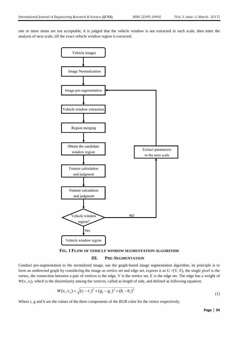
International Journal of Engineering Research & Science (IJOER) ISSN: [2395-6992] [Vol-3, Issue-3, March- 2017]
Page | 34
one or more items are not acceptable, it is judged that the vehicle window is not extracted in such scale, then enter the
analysis of next scale, till the exact vehicle window region is extracted.
FIG. 1 FLOW OF VEHICLE WINDOW SEGMENTATION ALGORITHM
III. PRE-SEGMENTATION
Conduct pre-segmentation to the normalized image, use the graph-based image segmentation algorithm, its principle is to
form an undirected graph by considering the image as vertice set and edge set, express it as G =(V, E), the single pixel is the
vertex, the connection between a pair of vertices is the edge, V is the vertice set, E is the edge set. The edge has a weight of
W(vi ,vj), which is the dissimilarity among the vertices, called as length of side, and defined as following equation:
222 )()()(),( jijijiyi bbggrrvvW (1)
Where r, g and b are the values of the three components of the RGB color for the vertex respectively.

International Journal of Engineering Research & Science (IJOER) ISSN: [2395-6992] [Vol-3, Issue-3, March- 2017]
Page | 35
Use Dif(C1 ,C2) to express the difference between two regions, which is defined as the minimum length of connection edges
between two regions. The internal heterogeneity of the region is characterized by the maximum length connection edges
inside the region, which is expressed as:
)(max)( ),( ewCInt ECMSTe (2)
Where, MST(C ,E) represents the minimum spanning tree of region C. The basis of region merging:
Dif(C1,C2)<min(Int(C1),Int(C2)) (3)
As it is impossible for Int(C) to effectively estimate the local feature of regional data in the condition that the regional area is
very small, which is easy to result in over-segmentation, therefore add a penalty function that is pertinent to the area, that is
τ(C)=K/|C| (4)
Where, |C| represents the area of C, K is the set point. The basis of region merging is changed to:
Dif(C1,C2)<min(Int(C1)+τ(C1),Int(C2)+τ(C2)) (5)
When the regional area is much smaller, the value of penalty function is significantly affected by the value of K, which
always plays a major role in region merging; when the regional area is much bigger, the role of the penalty function will be
reduced, the local feature of the data itself will play a major role. The larger the K value is, the greater the region of the
segmentation result will be.
The image is normalized to 200×220 pixels, take sigma=0.2, min. Region=500, K=[1.8k, 1.5k, 1.3k, k, 0.7k, 0.5k, 0.2k],
where k=400. As shown in Fig.2, the leftmost is the original image, the second, then the segmentation effect images from the
second image from the left when K=1.8k,k,0.2k. It is observed that the smaller the K value is, the more the number of
segmented regions will become; the smaller the region area is, the much more clear the segmentation for different objects in
the original image.
FIG.2 ORIGINAL IMAGE AND SEGMENTATION EFFECT
IV. VEHICLE WINDOW EXTRACTION
As the brightness and saturation in vehicle window region is much lower, the body and window of white and light color
vehicle are generally easy to be distinguished and segmented, however when the light is sufficient, the persons and objects in
the vehicle also become much more clear, causes the brightness or color feature in the vehicle windows to be much stronger,
it always not possible to segment the vehicle window accurately no matter either the gray level or color feature is based. It is
much easier to combine the body of black and dark color vehicle with the window. Therefore, the multi-scales segmentation
to the vehicle image is carried out, the vehicle window extraction is performed according to the scales from small to big, till
the accurate vehicle window is obtained.
4.1 Combination of vehicle window regions
The vehicle window region is always segmented into several small zones, it is necessary to combine them together for
subsequent judgment. As the vehicle windows are located at the upper part of the vehicle image, just the analysis to the upper
part of the image is required. The procedures for combining the segmented small zones into vehicle windows are as follows:
1) Among the segmented images, first find the centroid of various small zones, mark various small zones with centroid
located at upper part of the image, express its set as “region”.

International Journal of Engineering Research & Science (IJOER) ISSN: [2395-6992] [Vol-3, Issue-3, March- 2017]
Page | 36
2) The width and length of the image is width and height, take the points with coordinate of [width/2, height*3/8] in the
image as the mass center reference point P of the vehicle window, calculate the Euclidean distance from the mass center
of region in the set to point P, and sort the regions from small to big based on this distance. If the closer the region
centroid to the reference point P is, the more likely to belong to the internal window region will be, this can guarantee
the combination of zones starts from the inside of the vehicle window.
3) The first small zone in the region is taken as the initial vehicle region, and written as “Re”. Put the small zones in region
into the Re, and combine them with the zones in Re. After certain zone is merged each time, calculate the area of Re at
this moment, if the area is larger than the threshold (taking value 9500), this zone will be removed, as it possibly is the
zone outside the vehicle window; the area is smaller than the threshold, it is considered as a successful combination,
calculate the boundary smoothness of Re at this moment, save it in the array and save the vehicle window region at this
moment. Continue to combine the subsequent small zone till the region is processed completely.
FIG.3 ZONE COMBINATION
As shown in Fig.3, the numbers in the image are the marks of zones in the region after sorting, the reference point P of
centroid for zone 1 is the closest one, then comes zone 2, the rest can be done in the same manner. The zone 1 is combined
with zones 2 and 3 successively, however the adding of zone 4 will cause the total area to exceed the threshold, therefore the
zone 4 will not be combined.
The vehicle window region obtained by using the area to restrain the combination will not only guarantee that the vehicle
window will not be combined with other part of the vehicle body, but also not miss any zone within the window region,
ensuring the accuracy of final result.
4.2 Extraction of candidate vehicle window region
The shape of vehicle window is approximately trapezoidal, its boundary is consisted of approximately four straight segments,
and therefore boundary of window region obtained from present algorithm should be also smooth enough. The small zones
obtained by using the segmentation method in present paper are irregular in shape, when the zones are combined with the
vehicle window and the boundary of the candidate window region is analyzed, if it is the closer to the actual zones of the
window, its boundary will me smoother. The present paper calculates the boundary smoothness based on the extraction of
region boundary chain codes.
4.2.1 Chain code
Chain code [14]
refers to 8 possible directional values of the line connecting adjacent pixels, for each pixel dot, the adjacent
dots will use the continuation direction to represent the directional code.
FIG.4 CHAIN CODE DEFINITION

International Journal of Engineering Research & Science (IJOER) ISSN: [2395-6992] [Vol-3, Issue-3, March- 2017]
Page | 37
The definition of 8 directional chain codes is as shown in Fig.4. If one is added to the chain code value, its direction is that
rotates by 45° in counterclockwise direction, its direction will be rotate in counterclockwise direction with the increase of
chain code values. Each pixel has only 8 adjacent dots, the chain code value will be 0 to 7, 8 in all.
The chain code of region boundary depends upon the start point and the direction of boundary follow-up. The paper takes
clockwise direction. After binarizing the combined regions, it is easy to obtain the boundary sequence, and find the boundary
chain code, which is expressed as Ccode.
4.2.2 Boundary smoothness
Any point on the boundary has a chain code A1 pointing this point and the chain code A2 pointing to next point. Mutual
relationship of chain codes A1 and A2 is called as “relative chain code”, the relative chain code will become zero when they
point to same direction. If A2 is rotated relative to A1 in counterclockwise direction, the relative chain code will take values
of 1 to 4 according to the size of the angles, corresponding to rotate by 45°, 90°, 135° and 180°; the relative chain code will
take values of -1 to -3, corresponding to rotate by 45°, 90° and 135° along clockwise direction.
The paper defines the boundary smoothness tb to measure the degree of boundary that is composed of vehicle window tends
to be straight line segment. First, calculate the generalized relative chain code Dcode:
Dcode=Ccode(i+3)-Ccode(i) (6)
That is to subtract the chain code of current point from last three digits in the chain code. If the boundary is a straight line
segment at this moment, Dcode is zero. The calculation of tb is as shown in equation (7):
tb=num(Dcode==0)/num(Dcode) (7)
That is the ration of number of zero values in relative chain code, num() is the function for number of statistics.
The larger the tb is, indicates the more smooth the boundary will be, the smaller the degree of bumps on the border, the
closer the region tends to be a regular shape (trapezoid). Take the region with maximum tb as the candidate window region,
use 10×10 square structure to conduct morphological open operation, remove the long and further smooth the region
boundaries as the final candidate window region.
4.3 Feature judgment
The region with maximum boundary smoothness may not be the ideal window, therefore it is still necessary to carry out final
judgment to the candidate window. As the shape of window is approximate to trapezoid, and the difference among the
windows of different types of cars is not big. The paper judges whether it is the window depending on the area of window
region area, rectangularity extent and the ratio of length to width t.
1) By combining the area threshold in case of above-mentioned combination of region, the area of window should satisfy
5000 < area < 9500.
2) Calculation of rectangularity
extent=area/areaBox (8)
Where, areaBox is the area of smallest circumscribed rectangle of the region. The bigger the rectangularity, the closer the
region is to the rectangle.
The window region is approximate to the trapezoid not a rectangle, therefore it will be acceptable is extent >0.85 is satisfied.
3) The ratio of height to width of car is about 0.5, by taking into consideration that the shooting angle of the image may
reduce the height of window in the image, the present paper takes the ratio of height to width of 0.25 < t < 0.55.
If the candidate window region meets above 3 conditions, it is considered that the window is accurately segmented;
otherwise, it is considered that the extraction of window in current scale of segmentation fails, carry out the analysis of next
scale till the window is accurately segmented.
V. EXPERIMENTAL RESULTS AND ANALYSIS
To verify the effectiveness of the algorithm in present paper, the front image of vehicle taken by the surveillance camera at
the intersection is used for experiment. There are 720 images covering 20 types of cars with various colors in different

International Journal of Engineering Research & Science (IJOER) ISSN: [2395-6992] [Vol-3, Issue-3, March- 2017]
Page | 38
lighting environment. The sizes of the images are normalized to 200×220 pixels. The algorithm is realized by MATLAB
r2013a, and runs under the condition of Intel 3.6G HZ and 2 GB RAM.
5.1 Experimental evaluation method
Same as Lu[6]
, the present paper evaluates the algorithm in two aspects: locating performance and segmentation performance.
The locating performance reflects the degree of difference of widow position coordinates obtained by present algorithm from
the actual coordinates. Here the coordinates of window position refers to the coordinates of circumscribed rectangle in
window region. The locating error will be measured by the average of distance between corresponding vertices of two
rectangles, as it is expressed in equation (9):
4
)( rblbrtltloc
DDDDE
(9)
Where, Eloc represents the locating error, Dlt,Drt,Dlb,Drb are the distance between corresponding top left, top right, bottom left,
bottom right vertices of two rectangles respectively. Finally, the locating error has to be normalized by using width of
image.
The segmentation performance reflects the degree of fit between the window region and the actual window region obtained
by this algorithm. This is not only related with accurate expression of the size and the shape of the window, but also related
with complete extraction of image information in the window region. The segmentation performance is measured by using
the Jaccard distance between the region obtained by the algorithm and actual region of the window, as it is expressed in
equation (10):
SRGT
SRGTEseg
1
(10)
Where, Eseg represents the segmentation error, GT (ground truth) represents actual window region, SR (segmented region) is
the region from segmentation.
5.2 Algorithm comparison
The algorithm in this paper will be compared with the algorithm proposed by Hao[1]
, the algorithm of Hao[1]
is to find four
boundaries of the window by combining the edge detection with Hough transform, and locate the extraction of the window.
FIG.5 CUMULATIVE LOCATING ERROR FIG.6 CUMULATIVE SEGMENTATION ERROR
In Fig.5, the horizontal axis is the locating error normalized by the width of the image, the vertical axis accounts for the
proportion in the total number of images. The red line is the performance of the proposed algorithm in this paper, the green
line is the performance of Hao [1]
algorithm. It can be seen that the locating performance of present algorithm is better,
especially prominent, the proportion of small errors is close to 40%, and this also shows that the present algorithm locating
effect is good.

International Journal of Engineering Research & Science (IJOER) ISSN: [2395-6992] [Vol-3, Issue-3, March- 2017]
Page | 39
In Fig.6, the horizontal axis is the segmentation error, the vertical axis accounts for the proportion in the total number of
images. The red line is the performance of the present algorithm, the green line is the performance of Hao[1]
algorithm. The
performance of present algorithm is obviously better. This is because this algorithm can only segment partial region of the
vehicle window, however the segmentation results of the present algorithm can be better fit the edge of the window region.
5.3 Effect of algorithm
Some segmentation effects of the algorithm in this paper are shown in Fig.7, the abstraction of window is marked with a blue
area. It can be seen that this algorithm has a good segmentation effect for various colors of vehicles. In lower half part of
Fig.7, two groups at left and right are original images of vehicles and their window segmentation images under darker and
stronger light conditions respectively. It can be known from the image that this algorithm can also have much better locating
and segmentation effect even under the influence of different light, and shows better robustness for the test photos.
It can be known from Fig.7 that this algorithm can not only locate the position of window accurately, but also much better fit
the segmented vehicle window region with edges of original vehicle window, and maintain the shape and size of the original
window. This feature allows the window obtained by this algorithm can be applied in analysis of object in the window, such
as detection of safety belt and number of passengers, but also further extract the window shape feature to apply for vehicle
type recognition
FIG.7 ORIGINAL IMAGE OF VEHICLE AND WINDOW SEGMENTATION IMAGE
VI. CONCLUSION
This paper has analyzed the advantages and disadvantages of current vehicle window location algorithm, proposed a vehicle
window segmentation algorithm based on region segmentation and boundary constraint. First the region segmentation shall
be carried out for the car image according to the color feature, then the small regions will be combined and merged, finally
the window region is obtained by combining the geometrical features of the vehicle window. The algorithm result not only
locates the vehicle window accurately, but also keeps the shape and size of the window, which has laid a foundation for
subsequent application of vehicle window image. The experiments show that the algorithm has better segmentation results
for cars with different colors and different lighting conditions.
ACKNOWLEDGEMENTS
This work was supported by Science and Technology Planning project of Guangdong Province, China(NO.
2013B090200020).
REFERENCES
[1] Hao Xiaoli, Hou Dianfu. Vehicle Window Detection based Online Features[C]. International Symposium on Instrumentation &
Measurement, Sensor Network and Automation (IMSNA), 2012:261-263.
[2] Li Dongmei, Hao Xiaoli. An Window Location Algorithm Based on Hough Transform [J]. China Measurement Technology, 2007,
33(3):50-53.
[3] Wang Yafu. A Window Region Identification Method and Device Based on Sobel Edge Detection [P]. China: CN104636713A,
2015.05.20.
[4] Hou Dianfu. Study in Vehicle Window Detection Technology [D]. Beijing Jiaotong University, 2011.
[5] Zhang Yi, Luo Zhongliang, Shao Peng, Chen Jiancheng. Designing and Realization on Shield Algorithm[J]. Journal of Xi’an
Aerotechnical College, 2006, 24(1):12-14.
[6] Lu Wenhao, Lian Xiaochen, L.Yuille Alan. Parsing Semantic Parts of Cars Using Graphical Models and Segment Appearance
Consistency[C]. Proceedings of the British Machine Vision Conference (BMVC), 2014.
[7] Wang Yunqiong, You Zhisheng. A Fast Algorithm for Localization Vehicle’s Window Based on The Mean of
Chromatism[J].Computer Applications and Software,2004,21(1):78-79.
[8] Liu Zhifang, Xu Xin, You Zhisheng, Cao Gang. Localization Vehicle’s Window Based on a Genetic Algorithm[J].Application
Research of Computers,2002,11(1):72-74

International Journal of Engineering Research & Science (IJOER) ISSN: [2395-6992] [Vol-3, Issue-3, March- 2017]
Page | 40
[9] YANG H Y,ZHANG X J,WANG X Y. LS-SVM-based image segmentation using pixel color-texture descriptors[J]. Pattern Analysis
Applications, 2014, 17(2):341-359.
[10] PATEL H N,JAIN R K,JOSHI M V. Fruit detection using improved multiple features based algorithm[J]. International Journal of
Computer Applications, 2011,13(2):1-5.
[11] Xueming Wang,Jinhui Tang,Jianwei Niu,Xiaoke Zhao. Vision-based two-step brake detection method for vehicle collision
avoidance[J]. Neurocomputing, 2016,173(2):450-461.
[12] Koen E.A.van de Sande, Jasper R.R.Uijlings, Theo gevers, etal. Segmentation as Selective Search for Object Recognition[C]. IEEE
International Conference on Computer Vision, 2011:1879-1886.
[13] Jiang Huaizu, Wang Jingdong, Yuan Zejian, etal. Automatic Salient Object Segmentation Based on Context and Shape Prior[C].
Proceedings of the British Machine Vision Conference (BMVC), 2011, 100.1-100.12.
[14] Tan Jianhao, Zhang Jing. Identify for the Concave-Convex of Peripherals Based on Chain code Diference[J]. Science Technology and
Engineering, 2007, 7(5):769-770.

International Journal of Engineering Research & Science (IJOER) ISSN: [2395-6992] [Vol-3, Issue-3, March- 2017]
Page | 41
Flow production of practical and quantitative capillary driven-
flow immune sensing chip using a circumferentially-grooved
island micro-surface
Yusuke Fuchiwaki1*
, Kenji Goya2, Masato Tanaka
3, Hiroki Takaoka
4, Kaori Abe
5,
Masatoshi Kataoka 6, Toshihiko Ooie
7
1-7Health Research Institute, National Institute of Advanced Industrial Science and Technology (AIST), 2217-14, Hayashi-
cho, Takamatsu, Kagawa 761-0395, Japan 1CEA-LETI, Minatec Campus, 17 rue des Martyrs, 38054 Grenoble Cedex 9, France
Abstract— Practical immunoassay chip devices are high-priority needs in point-of-care testing (POCT) for rapid
diagnoses. Compared to conventional POCT microchip devices, our report describes a manufacturing process involving
laser ablation, inkjet deposition, and cover film sealing that is superior to that used for practical mass production of
microchip devices, and produces devices capable of sensitive and reproducible measurements using a capillary-flow-driven
system at a practical point-of-care setting. To promote sensitivity and reproducibility, circular islands surrounded by 10-µm-
deep grooves were prepared to provide uniformity of printed antibody spots on a capillary flow immunoassay chip. The
island surface enabled dense antibody fixation due to droplet surface tension as well as antibody determination by enzyme
linked immunosorbent assay (ELISA), which demonstrated greater sensitivity than that of a device using a non-island
surface. The luminescence intensity of the spots of the carboxyterminal propeptide of type I procollagen (PICP) exhibited a
good linear relation with PICP concentration in the range 0-600 ng·mL-1
, which is suitable for clinical estimation in blood.
Keywords— Capillary driven flow, Sensing Chip, grooved Island, immunoassay chip, ELISA.
I. INTRODUCTION
Analysis of biomarkers when the patient is located is known as point-of-care testing (POCT), and needs to be a simple and
rapid medical diagnostic method [1-3]. Most of the available POCT devices involve immunoassay systems, and enzyme-
linked immunosorbent assay (ELISA) has been utilized as a standard analytical system due to its sensitivity and specificity
[4]. Because a practical and simple POCT device must be easily available to the end user in many environments, a capillary-
driven flow system is a good candidate because it does not require electrical power and is easy to operate. Indeed, a capillary-
driven, flow-based immuno chromatographic assay is considered the simplest commercially available POCT device in the
diagnostic market. Therefore, a capillary-driven, flow-based immunoassay system was developed for an ELISA using a
piezoelectric inkjet printing system [5-7].
Practical approaches for immobilizing antibodies on a microchannel surface include microfluidic patterning [8],
photolithography [9], physical entrapment [10], micro-contact printing [11, 12], and inkjet printing [5-7]. Among these
approaches, printing has many advantages, such as simplicity, flexibility, low cost, minimal consumption of reagents, and
simultaneous patterning of multiple reagents [13]. Many important studies have been successfully reported by printing
technologies, for example, electrohydrodynamic printing [14], water-based inkjet printing [15] and printed wiring board
assembly [16]. These features allow the mass production of this device [17]. Although inkjet printing can precisely deposit a
drop of antibody solution at the picoliter level on a microchannel surface, a high concentration of antibodies can destabilize
the ejection spray from the nozzle head due to its high viscosity, which is a problem for the development of a diagnostic
immunoassay system. Accurate ELISA measurements require printing spots of identical size and equivalent amounts of
antibody immobilization, which ensures reproducible determination by chemical luminescence.
To overcome the viscosity problem, a solution with a high concentration of antibodies was continuously deposited and
immobilized on a circumferentially-grooved island micro surface. The island microstructure enables formation of a spherical
droplet by surface tension, producing a precise antibody spot and the same amount of antibody deposition. In addition, the
droplet does not adhere to the wall of the microchannel surface and the antibody spots have a uniform size, even when the
ejection spray may become uneven.

International Journal of Engineering Research & Science (IJOER) ISSN: [2395-6992] [Vol-3, Issue-3, March- 2017]
Page | 42
For the practical mass production of circumferentially-grooved island microchannel surfaces, laser ablation offers many
advantages over other micromachining techniques, such as a highly precise, fast, and non-contact fabrication process. A
transparent plastic device made of a cyclic olefin copolymer (COC) is more appropriate than other conventional materials,
such as silicon and glass, for this purpose because COC possesses versatile thermal and chemical surface properties. An
ultraviolet (UV) pulsed laser can directly ablate and locally modify a COC surface, with the best surface quality provided by
a KrF laser at 193 nm, a wavelength strongly absorbed by COC [18, 19].
The present study describes a capillary-driven, flow-based immunoassay chip that could be mass produced using a UV
pulsed laser system and a piezoelectric inkjet printing system. Ultraviolet pulse lasers and inkjet printers represent mature
technologies for which antibody immobilization techniques have been established. In addition, a capillary-driven flow
system does not require external power or moving off-chip components. Thus, the development of stable antibody
immobilization on a circumferentially-grooved island on a microchannel surface could provide a model diagnostic POCT
system that is readily adaptable in many POC situations.
II. EXPERIMENTAL WORK
2.1 Reagents
The monoclonal anti-PICP antibody used was Clone PC8-7 (Takara Bio Inc., Otsu, Japan) and was supplied in a Procollagen
type I C-peptide (PIP) EIA Kit (Takara). The blocking and washing solutions were purchased from Sumitomo Bakelite Co.
Ltd, Tokyo, Japan. The microchip was refrigerated at a temperature of 4°C when not in use.
2.2 Equipment
The circumferentially-grooved island structure was formed using a nanosecond pulse laser (LPX-305i, Coherent Inc.), at 500
mJ and 25 W. Movement of the XYZ stages was controlled with a computer under the focused laser spot. A video
microscope system allowed accurate positioning and in situ monitoring of the laser micromachining process.
The inkjet printing head (PulseInjector®: Cluster Technology Co., Ltd., Osaka, Japan) was a piezoelectric-driven drop-on-
demand plastic head with an epoxy resin; it exhibited very low biomolecular adsorption compared with glass. The inkjet
system deposited and fixed the primary antibodies (Clone PC8-7, Takara) in the spotting buffer (BSX2321, Sumitomo
Bakelite Co., Ltd., Tokyo, Japan) on the microchannel surface. Combining the PulseInjector® with a dedicated driving unit
(WaveBuilder®: Cluster Technology Co., Ltd., Osaka, Japan) allowed easy adjustment of the ejection drive waveform,
ejection rate, and driving voltage, enabling picoliter droplets to be ejected. A derivative drive waveform produced by a
function generator with a user-friendly interface provided stable ejection, and the droplets were ejected at a frequency of 1
kHz and jetting voltage of 8 V. The volume of a single discharged droplet of primary antibodies was 50 pL, and 100-1000
shots were discharged onto the surface of the microchannel to provide the optimal volume. The PulseInjector® used a 25-μm
diameter ejection hole.
2.3 Microchip fabrication by laser ablation and inkjet printing
A photograph and illustration of the immunoassay chip are shown in Figure 1(a). The chip was fabricated from COC and the
surface treated with a polymer solution containing p-nitro phenyl ester, a commercial polymer coating from Sumitomo
Bakelite Co., Ltd., which binds to amino groups in proteins and immobilizes the antibodies on the microchannel surface [6,
7]. The linear channel was 100-µm deep and 300-µm wide. Sample and reagents were introduced into the respective port of
the channel and capillary-driven flow was used to fill the channel (Figure 1(b)). To realize a large quantity of antibody
immobilization, the island surface of the 10-μm-deep and 150-μm-wide circular groove on the channel was formed by UV
nanosecond laser ablation and antibody droplets were deposited onto the surface of the microchannel using a piezoelectric
inkjet system (Figure 1c). Following deposition, the microchip surface was sealed with a cover film made of 33-μm-thick
polymethylmethacrylate (Toyo Ink MFG. Co., Ltd., Tokyo, Japan). All samples and reagents for the sandwich ELISA assay
were infused into the microchannel from a 1.0–mm-diameter inlet reservoir using a dropper. The outlet reservoir was located
on the other side of the microchannel.

International Journal of Engineering Research & Science (IJOER) ISSN: [2395-6992] [Vol-3, Issue-3, March- 2017]
Page | 43
(A) (B)
(C)
FIGURE 1: SCHEMATIC VIEW OF IMMUNOSENSING MICROCHIP SYSTEM AND CONSECUTIVE ANTIBODY
PRINTING SYSTEM. (A) PHOTOGRAPH AND ILLUSTRATION OF MICROCHIP, (B) CAPILLARY-DRIVEN-FLOW
SYSTEM USING DROPPER AND LUMINESCENCE DETERMINATION BY ELISA, (C) CONSECUTIVE ANTIBODY
PRINTING PROCESS UTILIZING LASER PROCESSING, INKJET DEPOSITION, AND COVER FILM SEALING.
III. RESULTS AND DISCUSSION
3.1 Precise formation of printed antibody spots
Inkjet printing of antibody droplets is advantageous for on-demand manufacturing systems because it enables picoliter
quantities to be deposited and reduces the total number of operations. However, depositing a greater concentration of
antibody solution onto a microchannel surface with adequate reproducibility is difficult. High sensitivity demands that the
primary antibodies are highly concentrated in the microchannel, but this requires a high-viscosity liquid that destabilizes
ejection of the antibody droplet from the inkjet head. Such destabilizing ejection causes the droplets to adhere to the wall of
the microchannel due to surface tension and has a negative effect on the uniformity of the printed spots. To avoid adherence
to the microchannel wall, an island structure on the microchannel surface was formed to allow uniformly printed antibody

International Journal of Engineering Research & Science (IJOER) ISSN: [2395-6992] [Vol-3, Issue-3, March- 2017]
Page | 44
spots. A circumferentially-grooved island structure retains the spherical form of a large droplet due to surface tension. A
circular grooved island surrounded by 10-µm-deep grooves was prepared and the uniformity of the printed antibody spots
was compared for the case with and without islands (Figures 2(a,b)). Three spots were prepared on each microchannel, and 9
spots on 3 microchannels were compared. The results showed that good uniformity was obtained using islands (Figure 2(a)),
but not without islands. Surface areas were calculated using Adobe Photoshop, which enables the measurement of the spots
using the ruler tool. The surface area of the printed spots with the islands was 6.02 µm2 with a relative standard deviation
(RSD) of 0.9%. The surface area of spots without islands was 5.65 µm2 with a RSD was 31.3%. This indicates that grooved-
island surfaces were effective in providing uniformity of printed spots.
FIGURE 2: COMPARISON OF PRIMARY ANTIBODY DEPOSITION ONTO ISLAND MICROCHANNEL SURFACES AND
NON-ISLAND MICROCHANNEL SURFACES. (A) IMAGE OF ANTIBODY DEPOSITION ONTO ISLAND SURFACE AND
PHOTOGRAPH SHOWING ANTIBODY SPOTS, (B) IMAGE OF ANTIBODY DEPOSITION ONTO A NON-ISLAND
SURFACE AND PHOTOGRAPH SHOWING ANTIBODY SPOTS.
(A)
(B)

International Journal of Engineering Research & Science (IJOER) ISSN: [2395-6992] [Vol-3, Issue-3, March- 2017]
Page | 45
3.2 Dense antibody deposition onto microchannel surface
The grooved-island structure should limit the spot area of antibody inkjet deposition, which allows dense primary antibody
deposition and the capture of a large amount of antigen, leading to greater sensitivity. To assess this effect, Cy5 conjugated
primary antibodies were prepared by the protocol specified for the Cy5® Fast Conjugation Kit (ab188288, Abcam, Tokyo,
Japan), Cy5 was deposited on island and non-island surfaces, and the signal intensities were compared after 10-min
incubation at room temperature (Figure 3). The resulting images were measured using a confocal laser scanning microscope
(Zeiss LSM 410) equipped with a He-Ne laser (emission wavelength 633 nm) (Zeiss, Oberkochen, Germany). This laser was
used to excite the Cy5 fluorophore using a FT 655 dichroic beam splitter and an RG 665 emission long pass filter.
FIGURE 3: SURFACE IMAGES AFTER PRINTING AND MICROSCOPIC IMAGES OF CY5-CONJUGATED ANTIBODY
ON COC MICROCHANNEL SURFACE, AND COMPARISON OF THE RELATIVE FLUORESCENCE INTENSITY AT 100,
500, AND 1000 SHOTS.
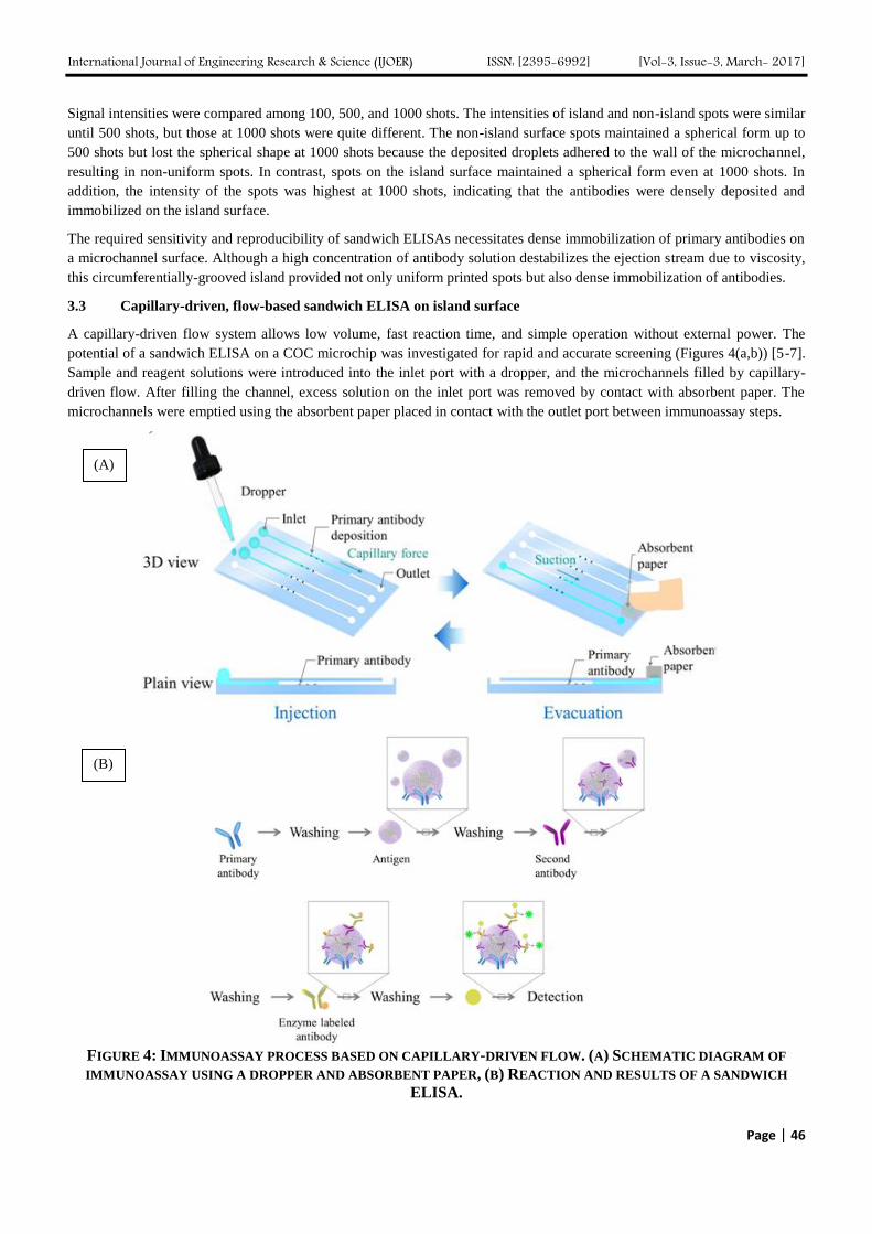
International Journal of Engineering Research & Science (IJOER) ISSN: [2395-6992] [Vol-3, Issue-3, March- 2017]
Page | 46
Signal intensities were compared among 100, 500, and 1000 shots. The intensities of island and non-island spots were similar
until 500 shots, but those at 1000 shots were quite different. The non-island surface spots maintained a spherical form up to
500 shots but lost the spherical shape at 1000 shots because the deposited droplets adhered to the wall of the microchannel,
resulting in non-uniform spots. In contrast, spots on the island surface maintained a spherical form even at 1000 shots. In
addition, the intensity of the spots was highest at 1000 shots, indicating that the antibodies were densely deposited and
immobilized on the island surface.
The required sensitivity and reproducibility of sandwich ELISAs necessitates dense immobilization of primary antibodies on
a microchannel surface. Although a high concentration of antibody solution destabilizes the ejection stream due to viscosity,
this circumferentially-grooved island provided not only uniform printed spots but also dense immobilization of antibodies.
3.3 Capillary-driven, flow-based sandwich ELISA on island surface
A capillary-driven flow system allows low volume, fast reaction time, and simple operation without external power. The
potential of a sandwich ELISA on a COC microchip was investigated for rapid and accurate screening (Figures 4(a,b)) [5-7].
Sample and reagent solutions were introduced into the inlet port with a dropper, and the microchannels filled by capillary-
driven flow. After filling the channel, excess solution on the inlet port was removed by contact with absorbent paper. The
microchannels were emptied using the absorbent paper placed in contact with the outlet port between immunoassay steps.
FIGURE 4: IMMUNOASSAY PROCESS BASED ON CAPILLARY-DRIVEN FLOW. (A) SCHEMATIC DIAGRAM OF
IMMUNOASSAY USING A DROPPER AND ABSORBENT PAPER, (B) REACTION AND RESULTS OF A SANDWICH
ELISA.
(B)
(A)

International Journal of Engineering Research & Science (IJOER) ISSN: [2395-6992] [Vol-3, Issue-3, March- 2017]
Page | 47
Circular islands surrounded by a 10-µm-deep groove allowed uniformity of printed antibody spots and the solutions in the
microchannel could be completely replaced by capillary-driven flow. Therefore, the suitability of this approach was
examined by measuring the luminescence intensity based on a sandwich ELISA on islanid and non-island surfaces at 0, 100,
500, and 1000 shots (Figures 5(a,b)). The results showed that the luminescence intensity for 5 spots at 300 mg·mL-1
PICP
varied with the number of shots. The intensities of island and non-island spots were similar at 0, 100, and 500 shots, but were
different at 1000 shots. The intensity of island spots was greater than that of non-island spots, even though both surfaces had
the same amount of primary antibodies deposited. In addition, the variation in island surface spots at 500 and 1000 shots was
less than that of the non-island spots. The variation was determined by the RSD, which for island surface spots was 2.37% at
500 shots and 4.08% at 1000 shots and for non-island spots was 6.86% at 500 shots and 27.2% at 1000 shots. Thus, the
island surface prevents antibody droplets from adhering to the wall of the microchannel, allows a dense antibody solution to
be deposited and fixed on the island surface. These results indicate that the circumferentially-grooved island surface provides
high sensitivity and reproducibility compared to a non-island surface.
FIGURE 5: QUANTITATIVE SANDWICH ELISA USING ISLAND AND NON-ISLAND MICROCHANNEL SURFACES AT
0, 100, 500, AND 1000 SHOTS. (A) LUMINESCENCE INTENSITY OF ISLAND SURFACE SPOTS AT 0, 100, 500, AND
1000 SHOTS, (B) LUMINESCENCE INTENSITY OF NON-ISLAND SURFACE SPOTS AT 0, 100, 500, AND 1000 SHOTS.
The effects of the capillary-driven flow channel response on 0-600 ng·mL-1
PICP were also investigated for island and non-
island surfaces (Figure 6). The luminescence intensity for both island and non-island spots increased with PICP
concentration. The mean luminescence intensity for 5 different spots was plotted against PICP concentration and provided a
linear relation. The intensity of island surface spots was greater overall than that of non-island surface spots. The 0-600
ng·mL-1
PICP concentration is adequate for clinical estimation of PICP in blood [20, 21].
(B)
(A)

International Journal of Engineering Research & Science (IJOER) ISSN: [2395-6992] [Vol-3, Issue-3, March- 2017]
Page | 48
FIGURE 6: QUANTITATIVE SANDWICH ELISA USING CAPILLARY-DRIVEN FLOW CHANNEL RESPONSE FOR 0-
600 ngmL-1
PICP ON (●) ISLAND MICROCHANNEL SURFACES AND (○) NON-ISLAND MICROCHANNEL
SURFACES.
These results demonstrated that inkjet deposition of a concentrated antibody solution onto a circumferentially-grooved island
surface produced a device suitable for a capillary-driven-flow microfluidic immunoassay. Thus, this system enables sensitive
and reproducible determination of PIPC concentration and is a promising methodology for a practical POC setting.
IV. CONCLUSIONS
A novel and simple approach for developing a sandwich ELISA based on a capillary-driven flow system for sensitive and
reproducible measurement of PICP was developed. The circumferentially-grooved island surface allowed uniformity in
printing of antibody spots onto a microchannel surface, enabling concentrated antibody solution fixation due to the droplet’s
surface tension. Evaluation of the precision of antibody spot printing demonstrated that the variation in the surface area of
spots was 0.05% RSD on the island surface and 31.3% for spots on the non-island surface. The spots on the island surface
maintained a spherical form even at 1000 shots of antibody inkjet deposition, and produced greater luminescence intensity
than those on the non-island surface. In contrast, spots on the non-island surface lost their spherical form after 500 shots and
had slightly reduced luminescence intensity. A concentrated antibody solution was deposited at 1000 shots on the island
surface and the spot intensity in a sandwich ELISA was greater than that for the non-island surface. The intensity of 0-600
ngmL-1
PICP spots showed a concentration-dependent relation and were greater overall than that for spots on non-island
surfaces.
This microfluidic ELISA system using capillary-driven flow possesses many advantages for POC situations, such as simple
operation, minimal sample consumption, and rapid results. The antibody immobilization process was performed
consecutively using laser processing, inkjet deposition, and cover film sealing. This process is driven by mechatronic
operation, which provides high throughput. This report demonstrates the potential of practical POC chip fabrication in the
future.
ACKNOWLEDGEMENTS
This work was supported by a Grant-in-Aid for Scientific Research from the Ministry of Education, Culture, Sports, Science
and Technology, Japan (No. 16K05833).
REFERENCES
[1] P. St-Louis, Status of point-of-care testing: promise, realities, and possibilities, Clin. Biochem 33 (2000) 427–440.
[2] D. Mark, S. Haeberle, G. Roth, F. von Stetten, R. Zengerle, Microfluidic lab-on-a-chip platforms: requirements, characteristics and
applications Chemical Society Reviews 39 (2010) 1153–1182.
[3] P. von Lode, Point-of-care immunotesting: approaching the analytical performance of central laboratory methods, Clin Biochem 38
(2005) 591–606.

International Journal of Engineering Research & Science (IJOER) ISSN: [2395-6992] [Vol-3, Issue-3, March- 2017]
Page | 49
[4] J. Ramo´n-Azco´n, R. Galve, F. Sa´nchez-Baeza, M.P. Marco, Development of an Enzyme-Linked Immunosorbent Assay for the
Determination of the Linear Alkylbenzene Sulfonates and Long-Chain Sulfophenyl Carboxylates Using Antibodies Generated by
Pseudoheterologous Immunization, Analytical Chemistry 78 (2006) 71–81.
[5] Y. Fuchiwaki, Y. Yabe, Y. Adachi, M. Tanaka, K. Abe, M. Kataoka, T. Ooie, Inkjet monitoring technique with quartz crystal
microbalance (QCM) sensor for highly reproducible antibody immobilization, 219 Sens. Actuators A (2014) 1–5.
[6] S. Yatsushiro, R. Akamine, S. Yamamura, M. Hino, K. Kajimoto, K. Abe, H. Abe, J. Kido, M. Tanaka, Y. Shinohara, Y. Baba, T.
Ooie, M. Kataoka, Quantitative Analysis of Serum Procollagen Type I C-Terminal Propeptide by Immunoassay on Microchip, 6 PLoS
ONE (2011) e18807
[7] K. Abe, Y. Hashimoto, S. Yatshushiro, S. Yamamura, M. Bando, Y. Hiroshima, J. Kido, M. Tanaka, Y. Shinohara, T. Ooie, T. Baba,
M. Kataoka, Simultaneous Immunoassay Analysis of Plasma IL-6 and TNF-α on a Microchip, 8 PLoS ONE (2013) e53620
[8] Z. Yin, S.C. Tao, R. Cheong, H. Zhu, A. Levchenko, An integrated micro-electro-fluidic and protein arraying system for parallel
analysis of cell responses to controlled microenvironments, Integrative Biology 2 (2010) 416–423.
[9] L.K. Fiddes, H.K.C. Chan, B. Lau, E. Kumacheva, A.R. Wheeler, Durable, region-specific protein patterning in microfluidic
channels, Biomaterials 31 (2010) 315–320.
[10] K. Sato, M. Yamanaka, H. Takahashi, M. Tokeshi, H. Kimura, Microchip-based immunoassay system with branching multichannels
for simultaneous determination of interferon-gamma. Electrophoresis 23 (2002) 734–739.
[11] A. Khademhosseini, K.Y. Suh, S. Jon, G. Eng, J. Yeh, A soft lithographic approach to fabricate patterned microfluidic channels,
Analytical Chemistry 76 (2004) 3675–3681.
[12] T.F. Didar, A.M. Foudeh, M. Tabrizian, Patterning multiplex protein microarrays in a single microfluidic channel, Analytical
Chemistry 84 (2012) 1012–1018.
[13] C. Wei, H. Qin, C. P. Chiu, Y. S. Lee, J. Dong, Drop-on-demand E-jet printing of continuous interconnects with AC-pulse modulation
on highly insulating substrates, 37, Journal of Manufacturing Systems (2015) 505-510
[14] Y. Han, C. Wei, J. Dong, Droplet formation and settlement of phase-change ink in high resolution electrohydrodynamic (EHD) 3D
printing, 20, Journal of Manufacturing Processes (2015) 485–491
[15] Y. Gua, A. Wua, H. Sohnb, C. Nicolettia, Z. Iqbalc, J. F. Federici, Fabrication of rechargeable lithium ion batteries using water-based
inkjet printed cathodes, 20, Journal of Manufacturing Processes (2015) 198-205.
[16] S.H.G. Teng, S.S. Garimella, Manufacturing Cost Modeling in Printed Wiring Board Assembly, 17, Journal of Manufacturing
Systems (1998) 87-96.
[17] F. Belachew, L. Christina, K. Liisa, J. Leena-Sisko, J. Heli, H. Leena, Patterned Immobilization of Antibodies within Roll-to-Roll Hot
Embossed Polymeric Microfluidic Channels, 8 PLoS ONE (2013) e68918
[18] P. Irina-Alexandra, S. Alexandros, B. Giannis, K. Gabriella, G. Savas, Nanosecond and femtosecond UV laser ablation of polymers:
Influence of molecular weight, Applied Surface Science 255 (2009) 9856–9860
[19] T. Daniel, T. Thanongsak, C. Joaquim, O. Tugrul, Nanosecond pulsed laser micromachining of PMMA-based microfluidic channels,
J. Manufacturing Process 14 (2012) 435-442.
[20] A.M. Parfitt, L. S. Simon, A. R. Villanueva and S. M. Krane, Correlation with iliac bone formation rates and comparison with total
alkaline phosphatase, J. Bone Miner. Res. 2 (1987) 427-436.
[21] K. Kohda, N. Ito, M. Ohwada, K. Morita, N. Watanabe, Y. Kohgo, Y. Mogi and Y. Niitsu, Diagnostic value of measurement of serum
type I procollagen carboxy terminal peptides in patients with scirrhous carcinoma of the stomach. Gut 32 (1991) 624-629.

International Journal of Engineering Research & Science (IJOER) ISSN: [2395-6992] [Vol-3, Issue-3, March- 2017]
Page | 50
Reinforcement Q-Learning and ILC with Self-Tuning Learning
Rate for Contour Following Accuracy Improvement of Biaxial
Motion Stage Wei-Liang Kuo
1, Ming-Yang Cheng
2, Hong-Xian Lin
3
Department of Electrical Engineering, National Cheng Kung University, Tainan, Taiwan
Abstract—Biaxial motion stages are commonly used in precision motion applications. However, the contour following
accuracy of a biaxial motion stage often suffers from system nonlinearities and external disturbances. To deal with the
above-mentioned problem, a control scheme consisting of a reinforcement Q-learning controller with a self-tuning learning
rate and two iterative learning controllers is proposed in this paper. In particular, the reinforcement Q-learning controller is
used to compensate for friction and also cope with the problem of dynamics mismatch between different axes. In addition,
one of the two iterative learning controllers is used to suppress periodic external disturbances, while the other one is
employed to adjust the learning rate of the reinforcement Q-learning controller. Results of contour following experiments
indicate that the proposed approach is feasible.
Keywords—Reinforcement Learning, Q-Learning, Iterative Learning Control (ILC), Contour Following.
I. INTRODUCTION
Contour following is commonly seen in industrial processes such as machining, cutting, polishing, deburring, painting and
welding. In these industrial processes, product quality depends on contour following accuracy. Generally speaking, better
contour following accuracy can be achieved by reducing tracking errors and/or contour error [14]. As a matter of fact,
tracking error reduction is one of the most important research topics in the contour following problems of multi-axis motion
stage [1]-[4]. Due to factors such as external disturbance, system nonlinearity, servo lag and mismatch in axis dynamics,
contour following accuracy of the multi-axis motion stage may not be able to meet the accuracy requirements [5]-[7].
There are many existing approaches that can be used in practice to reduce tracking error of a multi-axis motion stage [9]-
[12]. For example, the commonly used multi-loop feedback control scheme with command feedforward is very effective in
reducing tracking error caused by the servo lag phenomenon [8]. In addition, advanced control schemes such as sliding mode
control and adaptive control can be used to reduce tracking error as well. Recently, the number of studies exploiting the
paradigm of artificial neural network to improve contour following accuracy of multi-axis motion stage has risen steadily
[13]-[22]. For instance, Wen and Cheng [13] proposed a fuzzy CMAC with a critic-based learning mechanism to cope with
external disturbance and nonlinearity so as to reduce tracking error. Later on, Wen and Cheng [15] further proposed a
recurrent fuzzy cerebellar model articulation controller with a self-tuning learning rate to improve contour following
accuracy for a piezoelectric actuated dual-axis micro motion stage. In addition to tracking error reduction, the paradigm of
artificial neural network has been applied to different fields such as wind power generation [24], the game of Go [22], and
object grasping using robots [25]. Generally, a neural network needs to be trained before it can be used to solve a particular
problem. Among different training mechanisms for neural networks, reinforcement learning is the one that has received a lot
of attention recently [21]. In this paper, a control scheme consisting of a reinforcement Q-learning controller with an
adjustable learning rate and two iterative learning controllers (ILC) is proposed to improve contour following accuracy of a
bi-axial motion stage. In the proposed approach, the reinforcement Q-learning controller is responsible for friction
compensation and also deals with the dynamics mismatch between different axes. In addition, one of the two ILCs is
exploited to deal with the adverse effects due to periodic external disturbances from repetitive motions, while the other ILC
is exploited to tune the learning rate of Q-learning based on current tracking error so as to further improve contour following
accuracy.
The remainder of the paper is organized as follows. Section 2 gives a brief review on reinforcement learning and iterative
learning control. Section 3 introduces the proposed control scheme. Experimental results and conclusions are provided in
Section 4 and 5, respectively.

International Journal of Engineering Research & Science (IJOER) ISSN: [2395-6992] [Vol-3, Issue-3, March- 2017]
Page | 51
II. BRIEF REVIEW ON REINFORCEMENT LEARNING AND ITERATIVE LEARNING CONTROL
Since the proposed control scheme exploits the idea of reinforcement learning and iterative learning control, brief reviews on
these two research topics will be provided in this section.
2.1 Reinforcement Learning and Q-Learning
In general, learning mechanisms of artificial neural networks can be divided into three types: supervised learning,
unsupervised learning and reinforcement learning. Unlike the other two types of learning which either need training pairs or
expected final outcome, reinforcement learning “learns” proper actions by maximizing the reward simply based on the
reward/penalty resulting from previous action and current environment. Fig. 1 illustrates a typical control block diagram that
employs reinforcement Q-learning.
In general, the reinforcement Q-learning controller can be expressed as:
1 1 1(s ,a ) (s ,a ) [r Q (s ,a ) Q (s ,a )]maxi
t t t t t t t t t t i t t ia
Q Q
(1)
Where Qt(st ,at): the Q value corresponding to the state st and action at in the Q-table; s: state; ai: action; i: action index in
action space; t: learning rate; r: reward; γ:discount factor. 1 1max ( , )i
at t iQ s a is the maximum value of Q corresponding to state
st+1and action ai; t: time variable.
C
Q-Learning
Pcmdex yj
+-+
+UfbG
Action
Reward
FIG. 1 A TYPICAL CONTROL BLOCK DIAGRAM THAT EMPLOYS REINFORCEMENT BASED Q-LEARNING
The probability of selecting action ai in Q-learning is described by (2).
( , )
( , )( , )
i
iQ s a
i iQ s a
eP s a
e
(2)
2.2 Iterative Learning Controller
As reported in many previous studies, ILC is effective in suppressing periodic disturbances caused by repetitive motions [17-
19]. Fig. 2 is the block diagram for a control scheme consisting of a feedback controller and a control law based ILC [16]. In
Fig. 2, Uilc is the control force generated by ILC, L is the learning function and F is a low-pass filter. All the tracking error ex
and the control force Uilc generated by ILC in the previous iteration are stored and used to update Uilc in the current iteration.
The total control force Uj in the jth iteration to the plant G is the sum of Uilc and the feedback controller output Ufb.
+-Contoller Plant
cmdpjy
++
xe
uFBu
ILC
Memory
++ ju
Memory
L
Q
FIG. 2 BLOCK DIAGRAM FOR A CONTROL SCHEME CONSISTING OF A FEEDBACK CONTROLLER AND A
CONTROL LAW BASED ILC

International Journal of Engineering Research & Science (IJOER) ISSN: [2395-6992] [Vol-3, Issue-3, March- 2017]
Page | 52
Based on Fig.2, the relationship between output yj in the jth iteration and input Pcmd can be described as:
1 1(1 ) (1 )j j cmdy GC G U GC GC P (3)
where the total control force Uj+1 in the j+1th iteration is updated using Eq. (4)
1 1( )j j j jU F U Le Ce (4)
where ej, and uj are the tracking error and total control force in the jth iteration, respectively. Note that in Eq. (4), Cej+1 can be
regarded as the feedback control force. The control force Uilc generated by ILC aims at reducing the tracking error. Namely,
better performance of ILC leads to smaller tracking error so that feedback control force decreases as well.
III. THE PROPOSED REINFORCEMENT Q-LEARNING CONTROLLER WITH AN ADJUSTABLE LEARNING RATE
Fig. 3 illustrates the block diagram for the control scheme consisting of a feedback controller, a control law based ILC, and
the proposed reinforcement Q-learning controller with an adjustable rate.
C
Q-Learning
Pcmdex yj
+-+
+
ILC-based Reinforcement
Q-learning
Ufb
Uj
ILC
ILC
Learning
rate
GPITj
LSF1/4
+
-
V_ex
actionState
Reward
FIG. 3 BLOCK DIAGRAM FOR THE CONTROL SCHEME CONSISTING OF A FEEDBACK CONTROLLER, A CONTROL
LAW BASED ILC, AND THE PROPOSED REINFORCEMENT Q-LEARNING CONTROLLER WITH AN ADJUSTABLE
RATE.
In the proposed approach, the reinforcement Q-learning controller is modified as:
1 1 1max( , ) (e , ) [r (e ,a ) (e ,a )]i
t t t t t t ilc t t t i t t ia
Q e a Q a L Q Q (5)
Compared with Eq. (1), the learning rate t in the conventional Q-learning algorithm is replaced by Lilc in Eq. (5), where Lilc
is updated using Eq. (6)
1[ ]
j jilc ilc jL F L Le (6)
where Lilc_j+1 is the learning rate for the reinforcement Q-learning controller in the j+1th iteration. Note that in this paper, the
value of Lilc is constrained to be between zero and one. Moreover, in this paper, the aim is to reduce the tracking error of a
multi-axis motion stage. As a result, the state s in Eq. (1) is replaced by tracking error e in Eq. (5). In addition, three possible
actions accelerate, decelerate and maintain constant velocity, and can be selected for at in Eq. (5) to adjust the velocity
command for the motion stage. The probability of selecting action ai in the Q-learning algorithm is rewritten as:
(e, )
(e, )(e, )
i
iQ a
i iQ a
eP a
e (7)
where the state is the tracking error e.
In this paper, the action space A consists of three actions
1 2 3A a ,a ,a (8)
where a1: accelerate: a2: decelerate; a3: maintain constant speed.

International Journal of Engineering Research & Science (IJOER) ISSN: [2395-6992] [Vol-3, Issue-3, March- 2017]
Page | 53
In this paper, the reward is designed to reduce tracking error. In particular, the reward is determined using Eq. (9).
1
1 1
1
100, if 0
0, if 0
1, if 0
t t
t t t
t t
e e
r e e
e e
(9)
Fig. 4 illustrates the block diagram of the motion control scheme for a bi-axial motion stage proposed in this paper. In Fig.4,
the velocity command cmd_x for the x-axis consists of the control force Uilc_x generated by ILC, the feedback control force
Ufb_x, and the control force URL_x generated by the reinforcement Q-learning controller. It can be expressed as:
cmd_x fb _ x ilc _ x RL _ xU U U (10)
where
1fb _ x jU C e (11)
( )ilc _ x j jU F u L e (12)
RL _ xU v v (13)
Note that the velocity command for the y-axis is designed similarly.
In Fig. 4, the reinforcement Q-learning controller with adjustable learning rate is responsible for friction compensation and
also deals with the dynamics mismatch between the x-axis and y-axis. Fig. 4 also shows that two ILCs are employed in the
proposed motion control scheme. In particular, one ILC is exploited to adjust the learning rate of the reinforcement Q-
learning controller, while the other ILC is exploited to deal with the adverse effects due to periodic external disturbances so
as to further reduce tracking error.
Q-Learning
ILC-based Reinforcement
Q-learning
ILC
Learning
rate
actionState
xR
yR
xE
yE
pxK
pyK
cx xPI
yPI
yP
xP1
S
1
S
x
y
cy
Real-tim
e NU
RB
S In
terpolato
r
Ball-screw XY
motion stage
LSF1/4
LSF1/4
ILC
ILC
FIG. 4 THE BLOCK DIAGRAM OF THE PROPOSED MOTION CONTROL SCHEME FOR A BI-AXIAL MOTION STAGE.
IV. EXPERIMENTAL RESULTS
Fig. 5 shows a the photograph of the bi-axial motion stage used to assess the effectiveness of the proposed approach. Fig. 6 (a)
shows the circle-shaped contour represented in NURBS form used in the contour following experiment. Under S-curve
acceleration/deceleration motion planning, a NURBS interpolator [23] is employed to convert the circle-shaped contour into
the position commands for the x-axis (Fig. 6(b)) and y-axis (Fig. 6(c)). The duration time for each circle following is 9.5
seconds. In each experiment, circle following will be performed seven times (i.e. seven iterations). In total, four different
control schemes are tested in the contour following experiments. They are:
Control scheme #1: PI type feedback controller combined with an ILC.
Control scheme #2: PI type feedback controller combined with a reinforcement Q-learning controller with a fixed learning
rate.
Control scheme #3: PI type feedback controller combined with an ILC and a reinforcement Q-learning controller with a fixed
learning rate.

International Journal of Engineering Research & Science (IJOER) ISSN: [2395-6992] [Vol-3, Issue-3, March- 2017]
Page | 54
Control scheme #4: PI type feedback controller combined with an ILC and a reinforcement Q-learning controller with
adjustable learning rate.
Due to the limitations in the paper length, only the experimental results of the tracking error in the x-axis for these four tested
control schemes are shown in Fig. 7. In addition, performance indices in terms of root mean square of tracking error (RMS),
average of integral of absolute tracking error (AIAE), and maximum tracking error (MAX) are listed in TABLE 1.
FIG. 5 PHOTOGRAPH OF THE BI-AXIAL MOTION STAGE USED IN THIS PAPER.
FIG. 6 (A) CIRCLE SHAPED CONTOUR REPRESENTED IN NURBS FORM (B) POSITION COMMANDS FOR X-AXIS,
(C) POSITION COMMANDS FOR Y-AXIS.
FIG. 7 EXPERIMENTAL RESULTS OF TRACKING ERROR IN THE X-AXIS (A) CONTROL SCHEME #1 (B) CONTROL
SCHEME #2 (C) CONTROL SCHEME #3 (D) CONTROL SCHEME #4

International Journal of Engineering Research & Science (IJOER) ISSN: [2395-6992] [Vol-3, Issue-3, March- 2017]
Page | 55
FIG. 8 THE VALUES OF THE LEARNING RATE OF THE REINFORCEMENT Q-LEARNING CONTROLLER VARIES
WITH RESPECT TO TIME.
TABLE 1
TRACKING ERROR COMPARISON AMONG FOUR TESTED CONTROL SCHEMES
Tracking error of X axis
RMS(μm) AIAE(μm) Max(μm)
Scheme #1 19.22 17.01 35.79
Scheme #2 9.48 5.16 35.08
Scheme #3 4.28 2.33 17.63
Scheme #4 2.62 1.51 9.93
Fig. 7(a) shows the tracking error of the circle following experiment using control scheme #1. Since the ILC will be activated
after the 1st iteration, the tracking error for the first 9.5 seconds in Fig. 7(a) can be regarded as the results for using the PI
feedback control only. Clearly, tracking error gradually decreases after the 2nd
iteration, indicating that ILC indeed is
effective in suppressing periodic external disturbance. Based on the experimental results shown in Fig. 7(b)~(d), the tracking
error for using control schemes #2, #3 or #4 all converges much faster than that for using the control scheme #1. These facts
indicate that the reinforcement Q-learning controller is indeed effective in reducing tracking error since control schemes #2,
#3 or #4 all include a reinforcement Q-learning controller. In particular, the proposed control scheme (i.e. control scheme)
has the best performance among the four tested control schemes.
Fig. 8 shows the values of the learning rate of the reinforcement Q-learning controller in the proposed control scheme varies
with respect to time. After three iterations (after 28.5 seconds), the learning rate only changes slightly since the tracking error
becomes very small after three iterations.
V. CONCLUSION
This paper has proposed a motion control scheme consisting of two ILCs and one reinforcement Q-learning controller for
contour following accuracy improvement. In particular, one ILC is used to tune the learning rate of the reinforcement Q-
learning controller that is mainly used to cope with system nonlinearities, while the other ILC is exploited to suppress
periodic disturbance during repetitive contour following motions. Results of contour following experiments conducted on a
bi-axial motion stage indicate that the proposed control scheme is feasible and outperforms other control schemes also tested
in the experiment.
ACKNOWLEDGEMENTS
The authors would like to thank the MOST of Taiwan for their support of this research under Grant MOST 105-2221-E-006-
105-MY3.
REFERENCES
[1] F. Hiroshi and T. Tadashi, “High-Precision Control of Ball-Screw-Driven Stage Based on Repetitive Control Using n-Times Learning
Filter,” IEEE Trans. Ind. Electron, vol. 61, pp. 3694–3703, 2014.
[2] Y. Li and Q. Xu, “Design and Robust Repetitive Control of a New Parallel-Kinematic XY Piezostage for Micro/Nanomanipulation,”
IEEE/ASME Trans. Mechatronics, vol. 17, pp. 1120–1132, 2012.
[3] C. Hu, B. Yao, Z. Chen and Q. Wang, “Adaptive Robust Repetitive Control of an Industrial Biaxial Precision Gantry for Contouring
Tasks,” IEEE Trans. Control Systems Technology, vol. 19, pp. 1559–1568, 2011.

International Journal of Engineering Research & Science (IJOER) ISSN: [2395-6992] [Vol-3, Issue-3, March- 2017]
Page | 56
[4] K.-C. Yang, and C. Hsieh, “Nanometer Positioning of a Dual-Drive Gantry Table with Precise Yaw Motion Control,” J. CSME, vol.
36, no. 2, pp. 107–117, 2015.
[5] M. Tomizuka, “Zero Phase Error Tracking Algorithm for Digital Control,” ASME J Dyn Syst Meas Control, vol. 109, pp. 65–68,
1987.
[6] G. Cheng, K. Peng, B.-M. Chen, and T.-H. Lee, “Improving Transient Performance in Tracking General References Using Composite
Nonlinear Feedback Control and Its Application to High-Speed XY-Table Positioning Mechanism,” IEEE Trans. Ind. Electron, vol.
54, pp. 1039–1051, 2007.
[7] E.C. Park, H. Lim and C.-H. Choi, “Position Control of X-Y Table at Velocity Reversal Using Presliding Friction Characteristics,”
IEEE Trans. Control Systems Technology, vol. 11, pp. 24–31, 2003.
[8] M. -C. Tsai, I.-F. Chiu and M. -Y. Cheng, “Design and Implementation of Command and Friction Feedforward Control for CNC
Motion Controllers,” IEE proceedings, Control Theory and Applications, vol. 151, Issue 1, pp. 13–20, Jan. 2004.
[9] Y. Koren, “Cross-Coupled Biaxial Computer Control for Manufacturing Systems,” ASME J Dyn Syst Meas Control, vol. 102, pp.
265–272, 1980.
[10] M.-Y. Cheng and C.-C. Lee, “Motion Controller Design for Contour-Following Tasks Based on Real-Time Contour Error
Estimation,” IEEE Trans. Ind. Electron, vol. 54, pp. 1686–1695, 2007.
[11] K.-H. Su, and M.-Y. Cheng, “Contouring Accuracy Improvement Using Cross-Coupled Control and Position Error Compensator,”
International Journal of Machine Tools and Manufacture, vol. 48, pp. 1444–1453, 2008.
[12] H.-R. Chen, M.-Y. Cheng, C.-H. Wu, and K.-H. Su, “Real Time Parameter Based Contour Error Estimation Algorithms for Free Form
Contour Following,” International Journal of Machine Tools & Manufacture, vol. 102, pp.1–8, 2016.
[13] C.-M. Wen, and M.-Y. Cheng, “Contouring Accuracy Improvement of a Piezo-Actuated Micro Motion Stage Based on Fuzzy
Cerebellar Model Articulation Controller,” Control Engineering Practice, vol. 20, pp. 1195–1205, 2012.
[14] C.-Y. Chen and M.-Y. Cheng, “Velocity Field Control and Adaptive Virtual Plant Disturbance Compensation for Planar Contour
Following Tasks,” IET Control Theory & Applications, vol. 6, pp. 1182–1191, 2012.
[15] C.-M. Wen and M.-Y. Cheng, “Development of a Recurrent Fuzzy CMAC with Adjustable Input Space Quantization and Self-Tuning
Learning Rate for Control of a Dual-Axis Piezoelectric Actuated Micromotion Stage,” IEEE Trans. Ind. Electron, vol. 60, pp. 5105–
5115, 2013.
[16] D.A. Bristow, M. Tharayil and A.G. Alleyne, “A Survey of Iterative Learning Control,” IEEE Control Systems Magazine, vol. 26, pp.
96–114, 2006.
[17] C.-L. Chen and K.-S. Li, “Observer-Based Robust AILC for Robotic System Tracking Problem,” J. CSME, vol. 30, no. 6, pp. 483–
491, 2009.
[18] C.-K. Chen, C.-J. Lin, J. Hwang and C.-W. Hung, “The Iterative Learning Control of a Stewart Platform System,” J. CSME, vol. 34,
no. 1, pp. 21–30, 2013.
[19] K.L. Barton and A.G. Alleyne, “A Cross-Coupled Iterative Learning Control Design for Precision Motion Control,” IEEE Trans.
Control Systems Technology, vol. 16, pp. 1218–1231, 2008.
[20] M. Wiering and I. Martijn van Otterlo, Reinforcement Learning: State-of-the-Art. Germany: Springer-Verlag Berlin Heidelberg, 2012.
[21] R.S. Sutton and A.G. Barto, Reinforcement Learning : An Introduction. 2nd ed. London, England: in progress, 2012.
[22] D. Silver, A. Huang, C.J. Maddison, A. Guez, L. Sifre, G.V.D. Driessche, J. Schrittwieser, et al. “Mastering the Game of Go with
Deep Neural Networks and Tree Search,” Nature, vol. 529, pp. 484–489, 2016.
[23] M.-Y. Cheng, M.-C. Tsai and J.-C. Kuo, “Real-Time NURBS Command Generators for CNC Servo Controllers,” International
Journal of Machine Tools and Manufacture, vol. 42, pp. 801–813, 2002.
[24] Chun Wei, Zhe Zhang, Wei Qiao and Liyan Qu, “Reinforcement-Learning-Based Intelligent Maximum Power Point Tracking Control
for Wind Energy Conversion Systems,” IEEE Trans. Ind. Electron, vol. 62, no. 10, pp. 6360–6370, 2015.
[25] Sergey Levine, Peter Pastor, Alex Krizhevsky and Deirdre Quillen, “Learning Hand-Eye Coordination for Robotic Grasping with
Deep Learning and Large-Scale Data Collection,” unpublished.

International Journal of Engineering Research & Science (IJOER) ISSN: [2395-6992] [Vol-3, Issue-3, March- 2017]
Page | 57
Tool Wear and Process Cost Optimization in WEDM of AMMC
using Grey Relational Analysis B. Haritha Bai
1, G. Vijaya Kumar
2*, Anand babu. K
3
1Teaching Assistant,
2Post Doctoral Fellow,
3Research Scholar
1,2,3Department of Mechanical Engineering, S. V. University, Tirupathi - 517 502, Andhra Pradesh, India
Abstract— Wire Electrical Discharge Machining (WEDM) endorsed sensation in the production of newer materials,
especially for the aerospace and medical industries. Using WEDM technology, convoluted cuts can be made through
difficult-to-machine electrically conductive components with the high degree of accessible accuracy and the fine surface
quality make WEDM priceless. In other hand Aluminum Metal Matrix Composites (AMMCs) are the precise materials for
marine, automobile, aerospace, defense, and sports industries which are difficult to cut by conventional methods of
machining. In this paper an optimal set of material and machining parameters is derived using hybrid approach called grey-
fuzzy approach. For this AMMC samples are produced as per the taguchi experimental design by considering combined
material and wire EDM parameters and machined using WEDM machine. The obtained responses such as kerf width, tool
wear, process cost and surface roughness are optimized using grey-fuzzy approach which is obtained by combining grey
relational analysis and fuzzy logic.
Keywords— Wire EDM, AMMCs, Taguchi design, tool wear, process cost Grey-fuzzy.
I. INTRODUCTION
Aluminum Metal Matrix Composites (AMMCs) are the well-defined materials for marine, automobile, aerospace, defense,
and sports industries, as they have high strength to weight ratio, and possess superior physical and mechanical properties
compared to non-reinforced alloys and traditional metals. However, the presence of abrasive reinforcements in the ductile
matrix causes rapid tool wear and hence tool failure. This leads to an increase in machining cost, production time and poor
quality of machined components. On the other hand, some techniques such as electric discharge machining (EDM) and wire
electric discharge machining (WEDM) are quite successful for machining of AMMCs. EDM has limited applications as it
can be used only for drilling purpose. WEDM seems to be a better choice as it conforms to easy control and can machine
intricate and complex shapes. The setting for the various process parameters required in WEDM process play crucial role in
achieving optimal performance. Effective and economical WEDM of AMMCs will open new areas of applications for
AMMCs.
II. LITERATURE REVIEW
Very few studies have been undertaken in WEDM of MMCs. Further, most of these studies have been done by using one-
parameter-at-a-time approach, which may not explain the effects of interaction among various parameters. Some of past
studies on WEDM of MMCs are follows. Sahandilya.P, Jain.P.K. & Jain.N.K [1] investigated made on consider the effect of
voltage, pulse-on time, pulse-off time and wire feed rate on MRR and kerf in WEDM of SiCp/6061 AlMMC. Effect of input
process parameters show that maximum value of MRR and minimum value of kerf are obtained at lower level of voltage,
lower level of pulse-on time. D.Satish kumar & M. Kanthababu & V.Vajjiravelu [2] investigated WEDM of Al/SiCp MMCs
in various volume fractions (5%, 10% and 15% of SiC) prepared through stir casting process considering MRR and Ra as
outputs. And they concluded the microstructure of stir cast composite shows discrete localized pool/agglomeration of SiC
particles indicating constrain of the process for attaining uniform microstructure. Rajesh Kumar Bhuyan, B.C.Routara, Arun
Kumar Parida, A.K.Sahoo [3] investigate the effect of process parameters such as pulse on time(Ton), peak current (Ip) and
flushing pressure (Fp) , metal removal rate (MRR), tool wear rate (TWR) and surface roughness (SR) during electrical
discharge machining (EDM) of Al-SiC12% MMC .The experiment is followed by Central composite design (CCD) method
under different combination of process parameters. K.Zakariaa, Z.Ismaila, N.Redzuana and K.W.Dalgarnob [4] investigate
the effect of wire EDM cutting parameters for evaluating of Additive Manufacturing Hybrid Metal Material. Hybrid metal
materials produce through Additive Manufacturing of Indirect Selective Laser Sintering. It high light those important
parameters to be considered in wire cutting process of FeCuSn hybrid metal material produce by Additive Manufacturing of

International Journal of Engineering Research & Science (IJOER) ISSN: [2395-6992] [Vol-3, Issue-3, March- 2017]
Page | 58
Indirect Selective Laser Sintering process for fabricating the near net shape metal component. Ravindranadh Bobbili,
V.Madhu, A.K.Gogia [5] investigates wire-EDM process parameters of ballistic grade aluminium alloy. Experimentation has
been planned as per Taguchi technique. Three performance characteristics namely material removal rate (MRR), surface
roughness (SR) and gap current (GC) have been chosen for this study. Yonghua Zhao,Masanori Kunieda, Kohzoh Abe [6]
were experimentally investigated the performance of EDM slicing of SiC wafers, the fundamental characteristics of EDM of
SiC single crystal. Ibrahem Maher, Liew Hui Ling, Ahmed A, D.Sarha, M. Hamdi [7] experimentally investigated the
WEDM for improving process parameters. They concluded that the peak current and pulse on time are the most significant
parameters affecting the cutting speed, surface roughness and heat affected zone. The wire tension has minor effect on the
cutting speed and heat affected zone but it has great effect on the surface roughness. Cheol-SooLee, Eun-YoungHeo, Jong-
MinKim, In-HughChoi, Dong-WonKim [8] investigated this paper presents an effective model to estimate the electrode wear
of EDM. The wear amount depends on discharging environment such as material type and hole shapes. The electrode wear
makes it difficult to control precise electrode feeding. Therefore, this study proposes an electrode wear estimation model. V.
Chengal Reddy, N. Deepthi, N.Jayakrishna [9] studied the effect of various process parameters such as pulse on time, pulse
off time, wire tension, current, upper flush and lower flush for Aluminium HE30. Vukcevic and Delijic, [10] were observed
an increased interest on metal matrix composite, mostly light metal based, which have found their applications in many
industry branches, among others in the aircraft industry, automotive, and armaments ones, as well as in electrical engineering
and electronics, etc. M. Rosso, [11] studied applications of the metal matrix and ceramic matrix composites and their
process technologies. M. Dyzia, J. OEleziona, [12] have developed and studied the mechanical properties of Aluminium
matrix composites reinforced with AlN particles formed in stir casting. G. Rajyalakshmi, Dr. P. Venkata Ramaiah [13]
Factors like pulse on time, pulse off time, corner servo voltage, wire feed rate, wire tension, servo feed, spark gap voltage
and dielectric flow rate have been found to play a significant role in rough cutting operations for maximizations of MRR,
minimization of surface roughness and minimization of spark gap in WEDM. Dewan Muhammad Nuruzzaman [14]
investigated aluminium-aluminium oxide MMCs of different percentages of aluminium oxide. It is observed that density of
the composite specimen increases with increase in aluminium oxide volume fraction and the density of the composites are
higher for 20 ton compaction load than density obtained for 10 compaction load. H. K. Shivanand, Mahagundappa M. Benal,
S. C. Sharma, N. Govindraju,[15] compared Powder Metallurgy method and stir casting method for producing the AMMC
through testing of mechanical properties and conclude that stir casting method is best suitable for preparation of AMMC.
Mr. Anand and S. Shivade [16] attempt was made to review the different multi-optimization method used in WEDM for
optimization of process parameters such as MRR, Surface roughness, kerf width, machining time, dimensional deviation.
Both the performance parameters, MRR and surface roughness are optimized in one optimal input setting using Grey
relational analysis method. According to the literature survey it observed that very little work has been reported on WEDM
of MMCs. Past studied not clearly concluded the list of input parameters and responses. So, there is much more scope to see
effects of input parameters on outputs. Kerf width, tool wear response is not focused more. Surface roughness is mostly used
which essential to measure because it states the quality of machining. Compared six and seventh series of aluminium alloys.
seventh series is not used more and fifth series of aluminium alloys are also less. Coming to reinforcement materials silicon
carbide is mostly used and fly ash and aluminium oxide is not used more. So this research is focused on WEDM of AMMCs
which are reinforced with fly ash, aluminium oxide and silicon carbide by considering kerf width, surface roughness, tool
wear and process cost as machining responses and one in each series of fifth, sixth and seventh series of aluminium alloys as
base material.
III. DESIGN OF EXPERIMENTS AND PREPARATION OF ALUMINIUM METAL MATRIX COMPOSITES
In the present work nine AMMC samples are produced using stir casting furnace as per Taguchi L27 experimental design
(Table. 2) which is obtained by considering material and WEDM parameters (Table 1). To produce AMMCs, First the stir
casting furnace with graphite crucible is switched on and allow it to raise the temperature up to 500OC then the required
amount of base material is poured into the crucible and the temperature is raised up to 850OC and allow it to maintain the
same up to complete melting of base material. At 675OC, the wetting agent Mg of 1% is added to the base material. Then the
reinforcement particles are added slowly to the molten base material while the stirrer rotating. Before adding the
reinforcement particles they are heated for 2 hrs upto 1000OC to oxidise their surfaces. After mixing, the temperature of the
slurry is raised upto 850OC for getting improved fluidity and stirring is continued upto 5 minuits. Then the mixed slurry was
poured in different preheated steel dies to produce the samples.

International Journal of Engineering Research & Science (IJOER) ISSN: [2395-6992] [Vol-3, Issue-3, March- 2017]
Page | 59
TABLE 1
INFLUENTIAL PARAMETERS AND THEIR LEVELS
S. No. Influential parameters Level 1 Level 2 Level 3
Material Parameters
1 Base material (BM) Al5052 Al6082 Al7075
2 Type of reinforcement material (RM) SiC Al2O3 Flyash
3 Percentage of reinforcement particle (PRFM) 2.5 5 10
WEDM Parameters
4
Pulse on time(Ton) 108 110 112
5 Pulse off time (Toff) 56 58 60
6 Water pressure(wp) 3 7 10
7 Wire feed (Wf) 1 2 3
8 Servo feed (SF) 1030 1050 1070
TABLE.2
TAGUCHI DESIGN OF EXPERIMENTS
Exp. AMMC Material parameters WEDM parameters
Run Sample
No No. BM RFM PRFM Ton Toff Wf Wp SF
1
1
5052 FA 2.5 108 56 1 3 1030
2 5052 FA 2.5 108 58 2 7 1050
3 5052 FA 2.5 108 60 3 10 1070
4
2
5052 SIC 5 110 56 1 3 1050
5 5052 SIC 5 110 58 2 7 1070
6 5052 SIC 5 110 60 3 10 1030
7
3
5052 Al2O3 10 112 56 1 3 1070
8 5052 Al2O3 10 112 58 2 7 1030
9 5052 Al2O3 10 112 60 3 10 1050
10
4
6082 FA 5 112 56 2 10 1030
11 6082 FA 5 112 58 3 3 1050
12 6082 FA 5 112 60 1 7 1070
13
5
6082 SIC 10 108 56 2 10 1050
14 6082 SIC 10 108 58 3 3 1070
15 6082 SIC 10 108 60 1 7 1030
16
6
6082 Al2O3 2.5 110 56 2 10 1070
17 6082 Al2O3 2.5 110 58 3 3 1030
18 6082 Al2O3 2.5 110 60 1 7 1050
19
7
7075 FA 10 110 56 3 7 1030
20 7075 FA 10 110 58 1 10 1050
21 7075 FA 10 110 60 2 3 1070
22
8
7075 SIC 2.5 112 56 3 7 1050
23 7075 SIC 2.5 112 58 1 10 1070
24 7075 SIC 2.5 112 60 2 3 1030
25
9
7075 Al2O3 5 108 56 3 7 1070
26 7075 Al2O3 5 108 58 1 10 1030
27 7075 Al2O3 5 108 60 2 3 1050

International Journal of Engineering Research & Science (IJOER) ISSN: [2395-6992] [Vol-3, Issue-3, March- 2017]
Page | 60
IV. EXPERIMENTATION
The experiments were conducted at ultra cut WEDM Machine (supplied by Vellore Wire Cut. Pvt. ltd) as per the taguchi
design of experiments and the experimental data is recorded in the Table 3. For these experiments, brass wire is used as
electrode and water as dielectric fluid.
V. IDENTIFICATION OF OPTIMUM PARAMETERS COMBINATION
Step 1: Pre-processing of Experimental Data
Data pre-processing is required where the range and unit in one data sequence may differ from the others. In data pre-
processing, the original sequence is transformed to a comparable sequence. Depending on the quality characteristic of a data
sequence, there are various methodologies of data pre-processing are available.
For quality characteristic of the “larger – the - better”, the original sequence can be normalized as
(k) =
(1)
For quality characteristic of the “smaller – the - better” the original sequence, can be normalized as
(k) =
(2)
Where i = 1…, m; k = 1…, n. m is the number of experimental data items and n is the number of parameters. (k) Denotes
the original sequence, (k) the sequence after the data pre-processing, max
(k) the largest value of (k), min
(k) the
smallest value of (k), and is the desired value. For the experimental values of, tool wear and process cost, smaller-
the-better is applicable. Hence, its experimental values are normalized using Eqs1&2 as shown in Table 3.
TABLE 3
EXPERIMENTAL RESULT AND NORMALIZED VALUES OF EXPERIMENTAL RESULTS Exp. No Experimental results Normalized values of experimental Results
Tool wear Process Cost Tool wear Process cost
1 0.018 633.76 0.3043 0.6652
2 0.01 519.94 0.6521 0.7828
3 0.014 533.65 0.4782 0.748
4 0.018 477.10 0.3043 0.8271
5 0.025 395.013 0 0.9119
6 0.018 569.51 0.3043 0.7316
7 0.015 698.01 0.4347 0.5988
8 0.011 705.15 0.6086 0.5915
9 0.018 1277.726 0.3043 0
10 0.013 567.53 0.5217 0.7336
11 0.009 394.61 0.6956 0.9123
12 0.012 346.43 0.5652 0.962
13 0.019 781.30 0.2608 0.5128
14 0.013 822.94 0.5217 0.4698
15 0.013 987.93 0.5217 0.2993
16 0.015 408.89 0.4347 0.8975
17 0.016 658.75 0.3913 0.6394
18 0.009 510.02 0.6956 0.7937
19 0.019 569.12 0.2608 0.732
20 0.014 394.61 0.4782 0.9123
21 0.016 414.84 0.3913 0.8194
22 0.014 352.18 0.4782 0.9561
23 0.002 309.74 1 1
24 0.014 568.32 0.4782 0.7328
25 0.013 470.60 0.5217 0.8338
26 0.012 600.17 0.5652 0.9996
27 0.015 561.82 0.4347 0.7394

International Journal of Engineering Research & Science (IJOER) ISSN: [2395-6992] [Vol-3, Issue-3, March- 2017]
Page | 61
TABLE 4
GREY RELATIONAL COEFFICIENTS AND GREY RELATIONAL GRADE
S.No Grey Relational Coefficients Grey Relational
Grade
Tool wear Cost
1 0.6216 0.429 0.5253
2 0.4399 0.389 0.41445
3 0.5111 0.4 0.45555
4 0.6216 0.376 0.4988
5 1 0.3541 0.67705
6 0.621 0.4059 0.51345
7 0.534 0.455 0.4945
8 0.451 0.458 0.4545
9 0.6216 1 0.8108
10 0.4893 0.405 0.44715
11 0.4182 0.354 0.3861
12 0.4693 0.3419 0.4056
13 0.6572 0.4936 0.5754
14 0.4893 0.5155 0.5024
15 0.4893 0.6255 0.5574
16 0.5349 0.3585 0.4467
17 0.5609 0.4388 0.49985
18 0.4182 0.3864 0.4023
19 0.6572 0.4058 0.5315
20 0.511 0.354 0.4325
21 0.5609 0.3789 0.4699
22 0.5111 0.3433 0.4272
23 0.333 0.33 0.3315
24 0.5111 0.4055 0.4583
25 0.4893 0.3748 0.43205
26 0.4693 0.4167 0.443
27 0.5349 0.4033 0.4691
Step II: Determine the grey relational coefficient
After data pre-processing, the grey relation coefficient (k) for the k
th performance characteristics in the i
th experiment can
be determined using the Eq.3
(k) =
(3)
Where, is the deviation sequence of the reference sequence and the comparability sequence?
= ‖ (k)
(k)‖
=
(k)
=
(k)
(k) denotes the reference sequence and
(k) denotes the comparability sequence. is distinguishing or identification
coefficient and its value is between ‘0’ and ‘1’. The value may be adjusted based on the actual system requirements. A value
of ζ is the smaller and the distinguished ability is the larger. ζ = 0.5 is generally used. The Grey Relational coefficients of tool
wear and process cost are shown in the Table.4.

International Journal of Engineering Research & Science (IJOER) ISSN: [2395-6992] [Vol-3, Issue-3, March- 2017]
Page | 62
Step III: Determination of Grey relational grade
The grey relational grade is defined as
=
(4)
The grey relational grade represents the level of correlation between the reference sequence and the comparability
sequence. If the two sequences are identical, then the value of grey relational grade is equal to 1. The grey relational grade
values are calculated for each factor at each level and the optimal level for each factor is identified based on their individual
grey relational grade values. The optimal level of any influential factor has highest grey relational grade (GRG) value among
their considered levels. Grey relational Grade is shown in the Table 4.
TABLE 5
GRG FOR EACH LEVEL OF INFLUENTIAL FACTORS
GRG for each level of influential factors
Level BM RM PRFM TON TOFF WP WF SF
1 0.538267 0.452006 0.440128 0.486072 0.486511 0.454544 0.478250 0.492272
2 0.469211 0.504611 0.474700 0.496894 0.460150 0.490283 0.478006 0.490739
3 0.443894 0.494756 0.536544 0.468406 0.504711 0.506544 0.495117 0.468361
Delta 0.094372 0.052606 0.096417 0.028489 0.044561 0.052000 0.017111 0.023911
Rank 2 3 1 6 5 4 8 7
FIG 1: GRG FOR EACH LEVEL OF INFLUENTIAL FACTORS
Step V Obtaining optimal combination of influential factors
After determining the GRG, the effect of each parameter is separated based on GRG at different levels. The mean values of
GRG for each level of the influential factors and the effect of influential factors on multi responses in rank wise are
summarized in Table 6 Basically, larger GRG means it is close to the product quality. Thus, a higher value of the GRG is
desirable. From the Table 6 and fig 1, the optimal combination of influential factors is
BM1RM2PRM3TON2TOFF3WP3WF3SF1. This means Base material at level 1 ie; 5052, Reinforcement material at level 2
ie; AL2O3 Percentage of Reinforcement material at level 3 ie; 10, TONat level 2 ie; 112, TOFF at level 3 ie; 60, WP at level
3 ie; 10, WF at level 3 ie; 3, SF at level 1 ie; 1050.
VI. CONFORMATION TEST
For the obtained optimal combination, confirmation test has been conducted and compared the results with initial set of
parameters. These results are satisfactory as the responses for optimal combination shows better performance.

International Journal of Engineering Research & Science (IJOER) ISSN: [2395-6992] [Vol-3, Issue-3, March- 2017]
Page | 63
TABLE 6
COMPARISON OF RESPONSES BETWEEN AMMC WITH INITIAL COMBINATION AND OPTIMAL COMBINATION
Combination Combination of Controllable Parameters Tool wear Process cost GRG
Initial set
BM 2RM2PRM2TON2TOFF2WF2WP2SF2
0.018 476 0.5812
Optimal set BM1RM2PRM3TON2TOFF3WF2WP3SF1 0.008 350 0.7902
Gain N/A 0.01 126 0.2090
% of Gain N/A 55.55 26.47 35.96
VII. CONCLUSIONS
After analyzing the data of obtained influential factors combination, it is concluded that PRFM, BM and RM are the most
significant parameters which influence th multi responses WP and TOFF are the medium influenced parameters on multi
responses TON, SF and WF are influenced lastly the multi responses. Also grey relational grade of the optimal combination
is increased about 35.96%
REFERENCES
[1] Shandilya. P, Jain. P. K, Jain. N. K “Wire electric discharge of metal matrix composite”. Damm International scientific book,
2011. pp. 383-400.
[2] D. Satishkumar, M. Kanthababu, V. Vajjiravelu “Investigation of wire electrical discharge machining characteristics of
Al6063/SiCp composites.” International Journal of advanced manufacturing technology.” October 2011. 56:975–986.
[3] 3.Rajesh Kumar Bhuyan, B.C.Routara, Arun Kumar Parida, A.K.Sahoo “Parametric optimization of Al-SiC12% metal matrix
composite machining by EDM.” 5th International & 26th All India Manufacturing Technology, Design and Research Conference
(AIMTDR 2014) December 12th–14th, 2014.
[4] K. Zakaria, Z. Ismaila , N.Redzuana and K.W. Dalgarnob “Effect of wire EDM cutting parameters for evaluating of Additive
Manufacturing Hybrid Metal Material.” 2nd International Materials, Industrial, and Manufacturing Engineering Conference,
MIMEC2015, 4-6 February 2015, Bali Indonesia 532 – 537.
[5] Ravindranadh Bobbili, V. Madhu, A.K. Gogia “Multi response optimization of wire-EDM process parameters of ballistic grade
aluminium alloy.” Engineering Science and Technology, an International Journal 18 (2015) 720e726.
[6] Yonghua Zhaoa, Masanori Kuniedaa, Kohzoh Abeba “Study of EDM cutting of single crystal silicon carbide.” Science Direct
Precision Engineering 38 (2014) 92– 99.
[7] Ibrahem Maher, liew Hui Ling “Improve WEDM performance at different machining parameters.” IFAC(2015) 105-110.
[8] Cheol-Soo Lee, Eun-YoungHeo, Jong-MinKim, In-HughChoi,Dong-WonKim “Electrode wear estimation model for EDM
drilling.” Robotics and Computer-Integrated Manufacturing 36(2015)70–75.
[9] V. Chengal Reddya, N. Deepthib, N.Jayakrishna “Multiple Response Optimization of Wire EDM on Aluminium HE30 by using
Grey Relational Analysis.” Materials Today: Proceedings 2 ( 2015 ) 2548 – 2554.
[10] Vukcevic, M. and Delijic, K. “Some New Directions in Aluminum Based PM Materials for Automotive Applications” Materials in
Technological, 2002 36, pp101-105.
[11] M. Rosso “Ceramic and metal matrix composites: Routes and properties” Journal of Materials Processing Technology 175 (2006)
364–375.
[12] M. Dyzia, J. OEleziona “Aluminium matrix composites reinforced with AlN particles formed by in situ reaction”
Archives of Materials Science and Engineering Volume 31, Issue 1, May 2008, Pages 17-20.
[13] G. Rajyalakshmi “Simulation, Modelling and Optimization of Process parameters of Wire EDM using Taguchi –Grey Relational
Analysis.” ISSN: 2278-7844 2012 IJAIR.
[14] Dewan Muhammad Nuruzzaman “Fabrication and Mechanical Properties of Aluminium-Aluminium Oxide Metal Matrix.”
International Journal of Mechanical & Mechatronics Engineering IJMME-IJENS Vol:15 No:06.
[15] Mr. Anand and S. Shivade1 “A review on advanced multi-optimization methods for WEDM.” International Journal of Scientific
Research Engineering & Technology (IJSRET) Volume 2 Issue 7 pp 435-439 October 2013.

International Journal of Engineering Research & Science (IJOER) ISSN: [2395-6992] [Vol-3, Issue-3, March- 2017]
Page | 64
The Effect of welding method and heat treatment on creep
resistance of Inconel 718 sheet welds
Zenon A. Opiekun1, Agnieszka Jędrusik
2
Rzeszów University of Technology, Department of Foundry and Welding, Al. Powstańców Warszawy, Poland
Abstract— The paper presents results of a study on the effect of welding technique and heat treatment on structure and
creep resistance of welded joints made on thin (0.5–1.2 mm) Inconel 718 sheet with the use of GTAW and laser method
without filler metal. Technological high-temperature creep tests consisted in measuring the time to rupture for sheet metal
without and with welded joints under constant stress σ = 150 MPa and at constant temperature tc = (860 ± 2)°C.
Sheet metal joints made with the use of GTAW method and laser-welded are characterized with a three-zone macrostructure,
including the weld with size of dendritic grains depending on welding method, the heat-affected zone (HAZ), and the base
material (BM). For GTAW method, with increasing sheet metal thickness, the observed values of parameter λ2s (distance
between axes of second-order branches of dendritic grains) decrease from about 12 µm to 8 µm, and similarly, in case of
laser welding, λ2s values decrease from about 9.6 µm to 5 µm with increasing sheet metal thickness.
Thin sheet Inconel 718 in as-delivered condition high-temperature creep-tested have the time to rupture on the level of 12 h
at elongation of about 48%. Similar time-to-rupture values characterize the joints made by laser welding. GTAW joints are
characterized by about 30% shorter time to rupture and elongation less by about 45%.
The microstructure change induced by heat treatment (solution treatment and two-stage ageing) resulted in significant
increase of creep resistance properties of both base metal and laser-welded joints. The time to rupture of heat-treated
specimens of thin Inconel 718 sheet and laser-welded joints creep-tested at 860°C ± 2°C under stress of 150 MPa was about
19.5 h with elongation ranging from 23% to 33%.
Keywords— Inconel 718, GTAW, laser welding, heat treatment, microstructure, high-temperature creep.
I. INTRODUCTION
Inconel 718, a nickel-based alloy, belongs to a large group of heat-resisting and creep-resisting metallic materials used to
manufacture a variety of welded structures, especially in aircraft industry where they are used for exhaust components in
PW400 and CF6 jet engines [1–4]. The alloy shows good weldability and can be heat-treated by precipitate strengthening [5–
9]. Components made of thin Inconel 718 sheet can work at high temperatures which in case of combustion chambers can
reach 1300°C [2, 8].
In operating conditions, welded structures with components made of the alloy are subject to both high temperatures and large
stresses. In view of the above, creep-resisting properties of welded joints in such structures are of great importance.
The sources of concentrated heat streams used to weld Inconel 718 sheet include: electric arc in GTAW welding method [10–
12] and a beam of monochromatic light in case of laser welding.
The paper concerns the effect of the two welding methods used for welding thin Inconel 718 sheet [13, 14] and heat
treatment on structure and the time to rupture of obtained joints measured in high-temperature creep test.
II. MATERIAL AND METHODOLOGY
The material used in the study was thin Inconel 718 alloy sheet with thickness 0.5 mm, 0.9 mm, and 1.2 mm. Chemistry of
each material type was determined with the use of emission spectrometer Q4 TASMAN (Bruker). Table 1 summarizes
average chemical composition of the examined sheet metal samples.

International Journal of Engineering Research & Science (IJOER) ISSN: [2395-6992] [Vol-3, Issue-3, March- 2017]
Page | 65
TABLE 1
CHEMISTRY OF 0.5-mm, 0.9-mm, and 1.2-mm THICK INCONEL 718 SHEET SPECIMENS USED IN THE STUDY
(AVERAGE FROM 5 MEASUREMENTS FOR EACH SHEET THICKNESS).
Sheet
thickness
(mm)
Alloy components (% wt.)
Cr Fe Nb Mo Ti Al Si C B N Ni
0.5 17.30 16.20 5.20 2.45 1.0 0.55 0.16 0.050 0.022 0.040 balance
0.9 17.20 16.30 5.25 2.50 1.20 0.57 0.17 0.061 0.021 0.038 balance
1.2 17.28 16.15 5.30 2.38 1.18 0.54 0.14 0.059 0.023 0.041 balance
For the purpose of the study, sheet alloy specimens were prepared with joints arc-welded by means of GTAW methods and
with joints obtained with the use of monochromatic light beam generated by TruLaser Robot 5020 (TRUMPF). Heat
treatment of thin sheet metal specimens with welded joins was carried out in Nabertherm N 61/H electric chamber furnace
according to schematic diagram shown in Fig. 1.
FIG. 1 — SCHEMATIC DIAGRAM REPRESENTING THE COURSE OF HEAT TREATMENT APPLIED TO THIN
INCONEL 718 SHEET WITH GTAW AND LASER JOINTS.
The sheet metal was arc-welded in argon atmosphere according to GTAW method or laser-welded. Based on results of visual
inspection, the best welds were identified and corresponding parameters of welding were adopted in further analysis. The
best GTAW joints were obtained when welding parameters were I = 20 A/80 ms, 30 A/80 ms, and 40 A/80 ms for 0.5-mm,
0.9-mm, and 1.2-mm thick sheet metal, respectively. The welding rate VGTAW = 200 mm/min was the same for all sheet
grades, with arc length τA = 3 mm; diameter of non-consumable electrode (W + 2%Y2O3) sharpened at angle 45° was Ø = 2.4
mm, and consumption of argon with purity 99.95% Ar was 8 L/min.
Similarly, the following parameters were adopted for further studies concerning laser welding of thin Inconel 718 sheet:
welding rate VL = 300 mm/min; focal length fl = 340 mm; laser power P = 690 W, 780 W, and 990 W for 0.5-mm, 0.9-mm,
and 1.2-mm thick sheet metal, respectively.
Examination of creep resistance of welded joints in thin Inconel 718 sheet consisted in determining their time to rupture in
the course of technological high-temperature creep tests under conditions of constant stress σ = 150 MPa and constant
temperature tc = (860 ± 2)°C [15]. For the purpose of this study, specimens (Fig. 2) with Ø8 mm holes in the holder portion
were prepared. The specimens were fixed in holders by means of Ø8 mm mandrels (Fig. 3). Holders and mandrels were
made of creep-resisting cobalt-based alloy MAR-M509 [16].

International Journal of Engineering Research & Science (IJOER) ISSN: [2395-6992] [Vol-3, Issue-3, March- 2017]
Page | 66
FIG. 2 — AN EXAMPLE SPECIMEN USED FOR HIGH-TEMPERATURE CREEP RESISTANCE TESTS.
FIG. 3 — WPM ZST 3/3 CREEP TESTING MACHINE. A — A VIEW OF OPEN FURNACE WITH SPECIMEN
MOUNTED IN HOLDERS BY MEANS OF MANDRELS; B — THE INSTALLED THERMOCOUPLES.
The creep tests were carried out as per standard [17] on WPM ZST3/3 (VEB Werkstoffprüfmaschinen Leipzig) creep testing
machine equipped with three-zone LAB TEMP (Thermocraft Incorporated, USA) heating furnace operating at maximum
temperature of 1200°C. 3 specimens were prepared and tested for each of the welding methods and each sheet metal
thickness, for material both without and after heat treatment.
Fig. 3 shows a view of the creep testing machine with mounted specimen and three thermocouples attached along its length.
2.1 Preparation of metallographic sections for structural examination
Metallographic inspection (examination of microstructure and macrostructure) of welded joints made on 0.5-mm, 0,9-mm,
and 1.2-mm thick sheet was carried out on metallographic sections prepared before and after heat treatment. The sections
were obtained by means of mechanical polishing of transverse sections of the joints and etching with Kalling’s reagent.
Images were taken by means of Neophot 2 metallographic optical microscope equipped with advanced image acquisition and
analysis system Multiscan V.08 and scanning electron microscope (SEM) VEGA 3 (Tescan) coupled with X-ray
microanalysis adapter INCA x-art (Oxford).
III. RESULTS
3.1 Metallographic examination
Metallographic examination included observations of macrostructure and microstructure of welded joints made on thin
Inconel 718 sheet specimens in as-delivered condition (not treated thermally) and after heat treatment. Revealing the
macrostructure of joints was necessary to asses its shape, adjust the technological processes of GTAW and laser welding, and
check the welds for possible presence of hot cracks.
3.2 Macrostructure of welded joints on sheet metal in as-delivered condition and after heat treatment
Examples of macrostructure observed in welded joints on thin Inconel 718 sheet in as-delivered condition made with the use
of electric arc and laser are presented in Figs. 4–6, while Fig. 7 shows the microstructure after heat treatment.
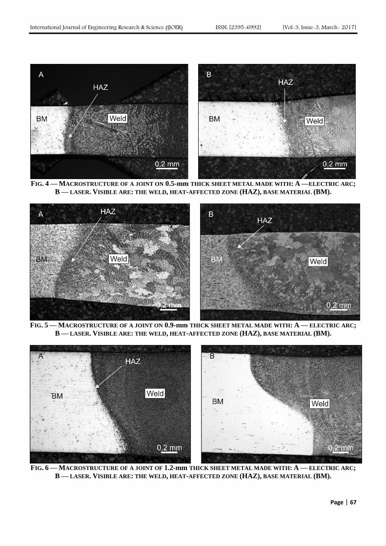
International Journal of Engineering Research & Science (IJOER) ISSN: [2395-6992] [Vol-3, Issue-3, March- 2017]
Page | 67
FIG. 4 — MACROSTRUCTURE OF A JOINT ON 0.5-mm THICK SHEET METAL MADE WITH: A —ELECTRIC ARC;
B — LASER. VISIBLE ARE: THE WELD, HEAT-AFFECTED ZONE (HAZ), BASE MATERIAL (BM).
FIG. 5 — MACROSTRUCTURE OF A JOINT ON 0.9-mm THICK SHEET METAL MADE WITH: A — ELECTRIC ARC;
B — LASER. VISIBLE ARE: THE WELD, HEAT-AFFECTED ZONE (HAZ), BASE MATERIAL (BM).
FIG. 6 — MACROSTRUCTURE OF A JOINT OF 1.2-mm THICK SHEET METAL MADE WITH: A — ELECTRIC ARC;
B — LASER. VISIBLE ARE: THE WELD, HEAT-AFFECTED ZONE (HAZ), BASE MATERIAL (BM).

International Journal of Engineering Research & Science (IJOER) ISSN: [2395-6992] [Vol-3, Issue-3, March- 2017]
Page | 68
FIG. 7 — MACROSTRUCTURE OF A LASER-WELDED JOINT OF: A — 0.5-mm; B — 0.9-mm THICK SHEET
METAL AFTER HEAT TREATMENT. VISIBLE ARE: THE WELD, HEAT-AFFECTED ZONE (HAZ), BASE MATERIAL
(BM).
In thin sheet metal joints obtained with the use of different sources of concentrated heat streams, i.e. electric arc and laser
light beam, one can distinguish between three characteristic structures: the weld, the heat-affected zones (HAZs), and the
base material (BM).
Grains in welded joints have different morphology (shape and size) depending on welding method and parameters. Also the
heat-affected zones of welded joints have different widths and grain sizes depending on the used welding methods and
welding parameters such as current intensity, laser power, and welding rate.
3.3 Microstructure of welded joints on sheet metal in as-delivered condition and after heat treatment
Example result of microstructure examination of welded joints made on thin Inconel 718 sheet are presented in Figs. 8–11
for the material in as-delivered condition and in Fig. 12 for heat-treated specimens.
FIG. 8 — MICROSTRUCTURE OF AN ARC-WELDED JOINT OF 0.5-mm THICK SHEET METAL. A — OPTICAL
MICROSCOPE; B, C — SEM.
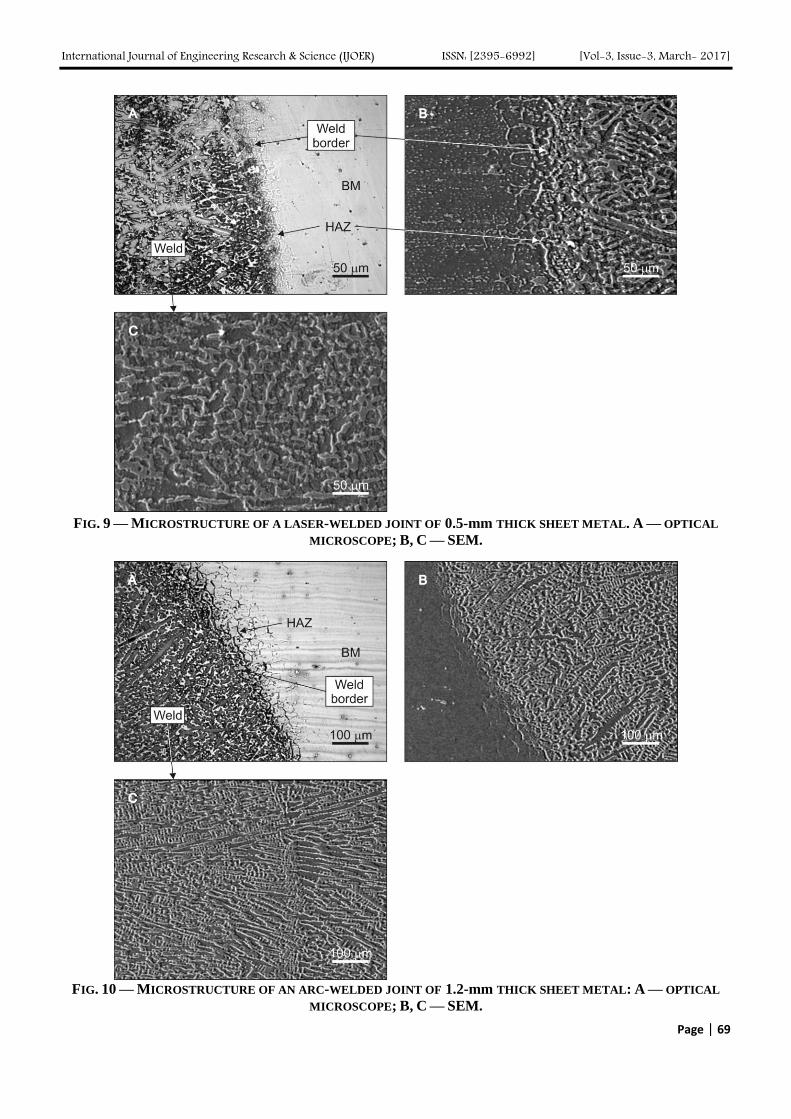
International Journal of Engineering Research & Science (IJOER) ISSN: [2395-6992] [Vol-3, Issue-3, March- 2017]
Page | 69
FIG. 9 — MICROSTRUCTURE OF A LASER-WELDED JOINT OF 0.5-mm THICK SHEET METAL. A — OPTICAL
MICROSCOPE; B, C — SEM.
FIG. 10 — MICROSTRUCTURE OF AN ARC-WELDED JOINT OF 1.2-mm THICK SHEET METAL: A — OPTICAL
MICROSCOPE; B, C — SEM.

International Journal of Engineering Research & Science (IJOER) ISSN: [2395-6992] [Vol-3, Issue-3, March- 2017]
Page | 70
FIG. 11 — MICROSTRUCTURE OF A LASER-WELDED JOINT OF 1.2-mm THICK SHEET METAL. A — OPTICAL
MICROSCOPE; B, C — SEM.
FIG. 12 — SEM IMAGES OF MICROSTRUCTURE OF A LASER-WELDED JOINT OF 1.2-mm THICK SHEET METAL
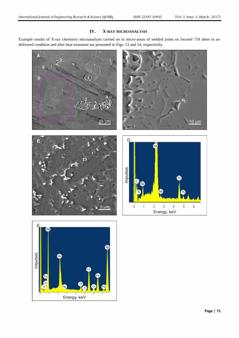
International Journal of Engineering Research & Science (IJOER) ISSN: [2395-6992] [Vol-3, Issue-3, March- 2017]
Page | 71
IV. X-RAY MICROANALYSIS
Example results of X-ray chemistry microanalysis carried on in micro-areas of welded joints on Inconel 718 sheet in as-
delivered condition and after heat treatment are presented in Figs. 13 and 14, respectively.

International Journal of Engineering Research & Science (IJOER) ISSN: [2395-6992] [Vol-3, Issue-3, March- 2017]
Page | 72
Micro-area No. Element content (% wt.)
C Ni Nb Cr Fe Ti Mo
1 20.20
(64.0)*
1.70
(1.30)
70.80
(29.0) — —
7.30
(5.70) —
1′ 19.5 1.80 74.36 — — 4.34 —
2 — 56.33 4.50 19.43 18.63 1.11 —
3 — 56.97 3.91 19.23 18.88 1.02 —
4 — 55.73 3.67 20.17 19.25 1.18 —
5 — 60.28 4.34 16.85 15.20 0.90 2.43
6 — 55.88 3.92 20.02 18.96 1.22 —
7 19.80 1.60 71.25 — — 6.90 —
8 — 57.9
(55.7) —
20.8
(22.7)
20.4
(20.6)
0.9
(1.0) —
* Figures in parentheses denote element content in atomic %
FIG. 13 — MICROSTRUCTURE OF: A — BM; AND B, C —GTAW JOINT OF 0.9-mm THICK SHEET METAL IN
AS-DELIVERED CONDITION WITH MARKED X-RAY MICROANALYSIS AREAS NOS. 1–8. ENERGY SPECTRA OF X-
RAYS SCATTERED FROM: D — MICRO-AREA NO. 1; AND E — MICRO-AREA NO. 8. THE TABLE SUMMARIZES
RESULTS OF X-RAY MICROANALYSIS.
Microstructure of Inconel 718 sheet in as-delivered condition reveals large grains of phase γ with carbides of MC type reach
in niobium and titanium (Nb, Ti)C precipitated unevenly inside and on borders of the grains. Moreover, structure of the sheet
metal contains irregular intermetallic phases rich in nickel, chromium, iron, niobium, and titanium. These are probably
topologically close-packed (TCP) phases (σ phases). These phases correspond to compositions Ni(Cr, Fe, Nb) and Ni(Cr, Fe,
Nb, Ti).
The seams in the joints welded both with electric arc and laser are characterized with dendritic structure. In welded joints of
sheet metal in as-delivered condition, irregular eutectic composed of intermetallic phases (σ phases) and MC-type carbides is
located on boundaries of phase γ dendritic grain branches.
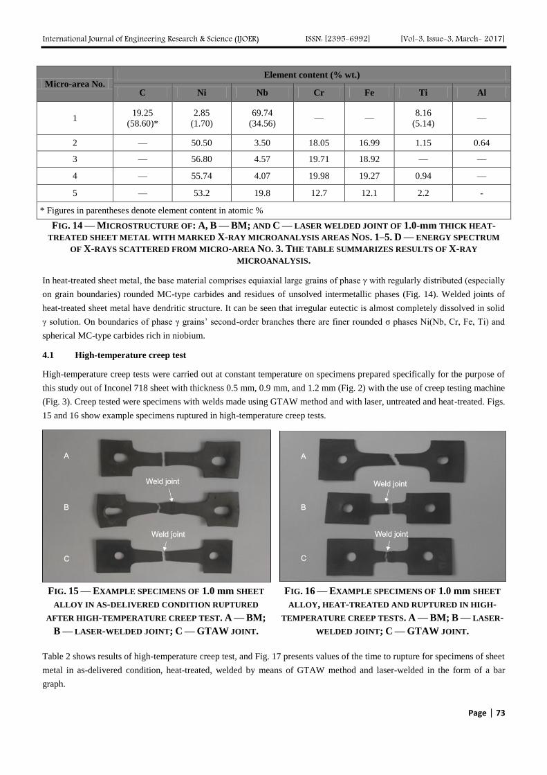
International Journal of Engineering Research & Science (IJOER) ISSN: [2395-6992] [Vol-3, Issue-3, March- 2017]
Page | 73
Micro-area No. Element content (% wt.)
C Ni Nb Cr Fe Ti Al
1 19.25
(58.60)*
2.85
(1.70)
69.74
(34.56) — —
8.16
(5.14) —
2 — 50.50 3.50 18.05 16.99 1.15 0.64
3 — 56.80 4.57 19.71 18.92 — —
4 — 55.74 4.07 19.98 19.27 0.94 —
5 — 53.2 19.8 12.7 12.1 2.2 -
* Figures in parentheses denote element content in atomic %
FIG. 14 — MICROSTRUCTURE OF: A, B — BM; AND C — LASER WELDED JOINT OF 1.0-mm THICK HEAT-
TREATED SHEET METAL WITH MARKED X-RAY MICROANALYSIS AREAS NOS. 1–5. D — ENERGY SPECTRUM
OF X-RAYS SCATTERED FROM MICRO-AREA NO. 3. THE TABLE SUMMARIZES RESULTS OF X-RAY
MICROANALYSIS.
In heat-treated sheet metal, the base material comprises equiaxial large grains of phase γ with regularly distributed (especially
on grain boundaries) rounded MC-type carbides and residues of unsolved intermetallic phases (Fig. 14). Welded joints of
heat-treated sheet metal have dendritic structure. It can be seen that irregular eutectic is almost completely dissolved in solid
γ solution. On boundaries of phase γ grains’ second-order branches there are finer rounded σ phases Ni(Nb, Cr, Fe, Ti) and
spherical MC-type carbides rich in niobium.
4.1 High-temperature creep test
High-temperature creep tests were carried out at constant temperature on specimens prepared specifically for the purpose of
this study out of Inconel 718 sheet with thickness 0.5 mm, 0.9 mm, and 1.2 mm (Fig. 2) with the use of creep testing machine
(Fig. 3). Creep tested were specimens with welds made using GTAW method and with laser, untreated and heat-treated. Figs.
15 and 16 show example specimens ruptured in high-temperature creep tests.
FIG. 15 — EXAMPLE SPECIMENS OF 1.0 mm SHEET
ALLOY IN AS-DELIVERED CONDITION RUPTURED
AFTER HIGH-TEMPERATURE CREEP TEST. A — BM;
B — LASER-WELDED JOINT; C — GTAW JOINT.
FIG. 16 — EXAMPLE SPECIMENS OF 1.0 mm SHEET
ALLOY, HEAT-TREATED AND RUPTURED IN HIGH-
TEMPERATURE CREEP TESTS. A — BM; B — LASER-
WELDED JOINT; C — GTAW JOINT.
Table 2 shows results of high-temperature creep test, and Fig. 17 presents values of the time to rupture for specimens of sheet
metal in as-delivered condition, heat-treated, welded by means of GTAW method and laser-welded in the form of a bar
graph.

International Journal of Engineering Research & Science (IJOER) ISSN: [2395-6992] [Vol-3, Issue-3, March- 2017]
Page | 74
FIG. 17 — THE TIME TO RUPTURE MEASURED IN HIGH-TEMPERATURE CREEP TEST OF INCONEL 718 SHEET
SPECIMENS. TEST CONDITIONS: T = 860°C, σ = 150 MPa.
The obtained results indicate that thin Inconel 718 sheet in as-delivered condition demonstrates a significantly shorter time to
rupture in high-temperature creep tests than the heat-treated material. The welding method has significant effect on the time
to rupture in the adopted high-temperature creep test conditions in case of sheet metal in both as-delivered condition and heat
treated. Welded joints made with laser show the time to rupture values almost twice as high as those obtained for electric arc
welding in argon atmosphere. Joints in Inconel 718 sheet specimens made with laser and heat treated demonstrate creep
resistance similar to this of the base material (heat-treated sheet metal subject to high-temperature creep test).
When creep-tested at high temperatures, heat-treated Inconel 718 sheet specimens with GTAW joints got ruptured in the area
of welded joints, just like those welded with the same method but in as-delivered condition. The joints made with the use of
electric arc are characterized with lower creep resistance, and the time to rupture demonstrated by them in the high-
temperature creep test has the value by about 30% lower than the time to rupture observed for sheet metal in as-delivered
condition. GTAW joints of heat-treated sheet alloy show higher values of the time to rupture in the creep tests. The time to
rupture value for sheet metal welded by means of GTAW and heat treated is similar to this characterizing base material
without heat treatment (in as-delivered condition).
V. CONCLUSIONS
The initial material selected for the study were three grades of thin (0.5-mm, 0.9-mm, and 1.2-mm thick) sheet metal in as-
delivered condition, rolled out of nickel-based Inconel 718 alloy. The material contained about 17% Cr, 16% Fe, 5.0% Nb,
2.5% Mo, 1.0% Ti, 0.60% Al, and 0.05% C. Total content of other elements such as Si, Mn, B, and N did not exceed 0.25%.
The microstructure of sheet metal reveals equiaxial grains of phase γ with dimensions of about (100 ± 15) μm with a small
quantity of irregular phases σ and spherical carbides of MC-type sparsely distributed in the matrix. Intermetallic (TPC-type)
phases σ have complex and diversified chemical composition (Fig. 13). These phases contain Nb and can be therefore
described as Ni(Cr, Fe, Nb, Ti). There are also phases without Nb, Ni(Cr, Fe, Ti), as well as those without Ti, Ni(Cr, Fe, Nb).
Carbides of MC type sparsely distributed in structure of the sheet metal contain mainly Nb and Ti and small quantities of
nickel. They can be described as (Nb, Ti)C.
Thin Inconel 718 sheet in as-delivered condition with such microstructure shows good tensile strength on the level of about
(850 ± 30) MPa at high plasticity, and elongation on the level of (30 ± 3)% [15]. The creep resistance of sheet metal in as-
delivered condition determined by means of the time to rupture measured in high-temperature creep tests at temperature
860°C and under stress 150 MPa was 12 h at elongation of 48%.
Structure change induced by thermal treatment of Inconel 718 sheet consisting in solution treatment starting from
temperature 1010°C/8 h/H2O and two-stage ageing at temperatures 720°C/8 h and 620°C/8 h resulted in significant
improvement of their strength properties. Tensile strength on the level of 1240 MPa was obtained with elongation similar to
this measured for sheet metal in as-delivered condition [15].
Heat treatment (solution treatment and ageing) of Inconel 718 alloy sheet resulted in changes of morphological features
characterizing its microstructure.

International Journal of Engineering Research & Science (IJOER) ISSN: [2395-6992] [Vol-3, Issue-3, March- 2017]
Page | 75
Mixtures σ-phase with diversified chemical composition irregularly distributed in the alloy’s microstructure (Fig. 13) were
almost entirely dissolved in solid solution of phase γ. Unsolved phase σ remaining in microstructure of Inconel 718 occurs on
the form of fine rounded particles (Fig. 14). Similarly, MC-type carbides rich in niobium and titanium remaining in the
alloy’s microstructure have spherical shapes and are present in the form of fine particles on boundaries of γ phase grains.
It has been found that the current intensity I on the level of 80 A and the welding rate Vs = 200 mm/min were GTAW
parameters most favorable from the point of view of thermal efficiency ηc and HAZ size. Such parameters of Inconel 718
sheet welding allowed to obtain good welded joints (Figs. 4–7) with minimum HAZ widths ranging from about 50 µm
to 100 µm (Figs. 10–12).
Limited heat efficiency of laser light beam means that higher power levels must be used when welding thin Inconel 718 alloy
sheet. Good joints on 0.7–0.9 mm thick sheet were obtained for laser with power of 400 W and welding rate of the order of
25 mm/s. For such laser welding parameters, the welded joints had virtually no HAZ (Figs. 4B, 5B, and 6B) or widths of
their HAZs did not exceed 40 µm (Figs. 9 and 11).
The seams in the joints welded both with electric arc and laser reveal dendritic structure. Value of the structural parameter λ2s
characterizing dendritic grains of the joints depends on the welding method and decreases with increasing sheet metal
thickness. In case of GTAW, increase of sheet metal thickness from 0.5 mm through 0.9 mm to 1.2 mm is accompanied by
reduction of λ2s parameter value from 12 µm through 10 µm to 8 µm. Similarly, in case of laser-welded joints, with sheet
metal thickness increasing from 0.5 mm to 1.2 mm, λ2s values decrease from 9.6 µm to 5µm.
Boundaries of second-order branches of dendritic grains observed in welded joints on sheet metal in as-delivered condition
made with the use of both GTAW and laser method are the locations where irregular eutectic (Fig. 13A) composed of σ
phase and MC-type carbides can be found. Heat treatment (solution treatment and ageing) of welded sheet metal joints
resulted in almost complete dissolution of σ phases and disappearance of irregular eutectic. On boundaries of joint grains’
second-order branches there are fine rounded MC-type carbides surrounded with residues of σ phase (Fig. 14C).
A measure of creep-resisting properties of thin sheet Inconel 718 in as-delivered condition, heat-treated and welded with the
use of GTAW and laser method is the time to rupture at adopted high-temperature creep conditions (Table 2, Fig. 17). The
obtained results in combination with conclusions drawn from of microstructure examination of welded joints before and after
heat treatment show that the use of laser welding allows to increase the time to rupture of heat-treated joints by nearly 62% in
comparison with BM in as-delivered condition and by about 80% with respect to the time to rupture observed in GTAW
joints made on sheet in as-delivered condition.
Specimens of sheet metal in as-delivered condition welded with the use of laser method and heat treated get ruptured outside
the welded joint areas (Fig. 15B and 16B). It can be therefore concluded that laser-welded joints demonstrate higher creep
resistance than the base material.
REFERENCES
[1] Ruedl E., 1975 Phase transformation in the alloy Hastelloy B, Materials Research Bulletin 10, 16-22
[2] Agarwal D.C., 2002 Chronology of Developments in Ni-Mo Alloys: The Last 70 Years, Corrosion 58, 27-29
[3] Bloom D.S, Putnam J.W., Grant. N., 1952: Trans. AIME, Journal of Metals 194, 1, 626
[4] Lancaster J., 1992: Handbook of structural welding: processes, materials and methods used in the welding of major structures,
pipelines and process plant, Abington Publishing, Cambridge, 56-58
[5] Hong J. K., Park J. H., Park N. K., Eom J. S., Kim M. B., Kang G. Y., 2008: Microstructures and mechanical properties of Inconel
718 welds by CO2 laser welding, Journal of Materials Processing Technology, 1132-1138
[6] Gozlan. E., Bamberger. M. S., Dirnfeld. F., Prinz. B., Klodt. J., 1991: Topologically close-packed precipitations and phase diagrams
of Ni-Mo-Cr and Ni-Mo-Fe and of Ni-Mo-Fe with constant additions of chromium, Materials Science and Engineering A, 141,85
[7] Durand-Charne M., 1997: The microstructure of superalloy, Institut National Polytechnique de Grenoble, 48-52
[8] Yukawa N., Hida M., Imura T., Kawamura M., Mizuno Y., 1972: Structure of Chromium Rich Cr-Ni, Cr-Fe, Cr-Co and Cr-Ni-Fe
Alloy Particles Made By Evaporation In Argon, Metallurgy Transaction 3, 47
[9] Klein J. H., Brooks C. R., Stansbury E. E., 1970: The establishment of long-range order in NiCr using electron microscopy, Physica
Status Solidi 38, 831
[10] Dupont J. N., Michael J. R., and Newbury B. D., 1999: The weldability of an advanced corrosion-resistant alloy in investigated and
linked to microstructural development in the fusion zone. Welding Journal 78(12): 708-s to 415-s
[11] Savage W. F., and Lundin C. D., 1965: The Verestraint test. Welding Journal 44(10): 433-s to 442-s

International Journal of Engineering Research & Science (IJOER) ISSN: [2395-6992] [Vol-3, Issue-3, March- 2017]
Page | 76
[12] Savage W. F., and Lundin C. D., 1966: Application of the Verestraint technique to the study of weldability. Welding Journal
45(11):497-s to 503-s
[13] Broks J. A., and Thompson A. W., 1991: Microstructural deveploment and solidification craking suspectibility of austenic stainless
steel welds. International Materials Reviews 36: 16-44
[14] Knorowski G. A., Cieslak M. J., Headley T. J., Roming A. D., and Hammelter W. F., 1989: Inconel 718: a solidification diagram.
Metallurgical Transactions A 20 A:2149-2158
[15] Jędrusik A., 2015: „Technology of cutting, cleaning nad laser welding of thin sheet metal made of nickel alloy Inconel 718” Doctor
thesis, Rzeszow University of Technology
[16] Opiekun Z., 2011: Temperature influence of ceramic form on the structure of cobalt alloy MAR-M509 castings. Acta Metallurgica
Sinica (English letters) 24(1) 23-33
[17] E-139-00 Standard Test Methods Conducting Creep. Creep-Rupture, and Stress-Rupture Test of Metallic Materials.

International Journal of Engineering Research & Science (IJOER) ISSN: [2395-6992] [Vol-3, Issue-3, March- 2017]
Page | 77
Standardization of the Central Console of Police Vehicles – An
Outline of the Diagnosed Needs Piotr ŁUKA
1, Andrzej URBAN
2
1PhD Piotr Łuka, head of the Social Security Faculty of the Security and Public Order at the Police Academy in
Szczytno. 2Associate Professor, PhD Eng. Andrzej Urban, Associate Professor at the Social Security Faculty of the Security
and Public Order at the Police Academy in Szczytno.
Abstract— The authors bring closer the results of social studies conducted on a group of respondents - policemen using
police cars during their everyday duty. The study seeks to answer the question: how to improve the daily duty and integrate
the devices that are used for the everyday activities by the law enforcement services which contribute to safety or public
order? It also seeks information and guidance concerning the actions to be taken in the future for the devices installed in
police cars to be the most ergonomic and safest for their users.
Keywords— Safety, traffic, device integration, police car.
I. INTRODUCTION
The publication is the result of the social studies performed during the project implemented in the field of defense and
security under tender No. 7/2015 funded by the National Centre for Research and Development entitled "Development of
police vehicles classification depending on their purpose and standardization of the central console of vehicles in the scope of
arrangement and installation of ICT systems and control devices of special purpose signals" No. DOB-BIO7/04/02/2015. The
project is implemented by a scientific consortium composed of the Police Academy in Szczytno - project leader, the
Automotive Industry Institute from Warsaw and the company Marvel Sp. z o. o. from Lodz. The beneficiary of the effects of
research and development in this project are to be the services reporting to the Minister of the Interior and Administration.
The assumptions established in the project fit in well with the current priorities of the Chief of Police [1] for the years 2016-
2018. One of the seven priorities established by the Polish Police Headquarters include: improving the quality of the tasks
performed by police officers and the employees of the Police by providing the optimal duty / work conditions. One of the
specific tasks indicated for the implementation in this regard by the Polish Police Headquarters is equipping the Police with
computer and communications hardware (including mobile devices and enabling the use of the functionality of information
systems used by the Police) and transport equipment.
II. MATERIALS & METHODS
The project implementation began in December 2015 and has been lasting for 36 months. The main objective of the project is
to develop a directory of vehicles and to prepare documentation for the modification of the central console and the electrical
system of the vehicles (depending on the classification) with respect to the standardization and enabling the installation of
communications and ICT equipment at the locations adapted for this purpose along with the implementation of the document
for use in proceedings when purchasing vehicles [3]. One of the results of the project was conducting surveys. The aim of
this study was to collect reviews from the users of Police vehicles and draw conclusions for further exploration prospects.
Based on the available data, it was found that the Polish Police operates a total of 21 794 vehicles. This number includes 13
821 passenger vehicles (including 6 145 marked and 7676 unmarked units). Outside the indicated category, the Police also
uses SUVs, pick-ups, utility vehicles, off-road RD-Video vehicles, van-type vehicles, trucks, buses and special purpose
vehicles [2]. In order to obtain information about the preferences of the users of the Police vehicles with respect to the need
for the modification of the central console of the field units of the Police, a study was conducted using the method of
diagnostic survey. The study was carried out from April to June 2016. It was participated by a total of 354 police officers
from the garrisons in Malopolska, Wielkopolska, Warmia-Mazury and the policemen during training and vocational training
at the Police Academy in Szczytno. The policemen during training were the representatives of all the of the Polish Police
garrisons. For the purpose of the study, a research tool was developed in the form of a questionnaire consisting of 22
questions.

International Journal of Engineering Research & Science (IJOER) ISSN: [2395-6992] [Vol-3, Issue-3, March- 2017]
Page | 78
The study used a questionnaire prepared by the employees of the Police Academy in Szczytno and the Automotive Industry
Institute in Warsaw. The study was preceded by obtaining the approval of the Chief of Police. The main purpose of the study
was to find out user reviews concerning the Police vehicles with respect to the solutions functioning in them, as well as their
assessment and preferences concerning the planned future solutions. Participants responded to a series of questions relating
in particular to the vehicle’s type and purpose which are the most commonly used in the Police and the type of additional
devices in the vehicles. Further questions concerned the safety and efficiency of the operations related to the use of the
devices installed in the vehicles. The policemen also commented on the location of the installation of the equipment,
assessing the aptness of the location in the vehicle. The policemen were also asked what kind of other, not currently installed
in the Police vehicles, devices should be there in the future. One of the important questions was also the one concerning the
need for the integration of the devices in the vehicles and those used as part of their duties.
The study showed that the policemen (in prevention, crime units) mostly use passenger marked vehicles (44% respondents)
and passenger unmarked vehicles (30% respondents).
DIAGRAM 1. INTENDED USE OF THE MOST COMMONLY USED VEHICLES. [Source: own research carried out under the project No. DOB-BIO7/04/02/2015]
Patrol and intervention vehicles are the most frequently used in everyday duty (Diagram 1) of the respondents - 50%.
Another category of the vehicles that were used the most frequently were the traffic ones - 9% of the respondents and convoy
vehicles - 7% of respondents. 1% of the respondents indicated the vehicles of road technicians and ecology. 31% of the
respondents indicated "other" as the most commonly used vehicles.
DIAGRAM NO. 2. IS THE INTEGRATION OF THE OPERATION OF THE DEVICES INSTALLED IN THE VEHICLE IN
ONE CONTROL PANEL (TOUCH SCREEN) JUSTIFIED? [Source: own research carried out under the project No. DOB-BIO7/04/02/2015]
The question of whether the integration of the operation of the devices installed in the vehicles in one control panel was
justified (Diagram 2) was answered "yes" by 55% of the respondents and "rather yes" by 29%. A total of as many as 84% of
the responding policemen claimed that such a solution was justified. The results confirmed the validity of the undertaken
development work aimed at integrating the devices used by officers during their daily duty. On the other hand, 13%
disagreed. 7% percent claimed strongly that the integration was not needed, and 6% expressed the view that it was rather
unnecessary.
n=354
n=354

International Journal of Engineering Research & Science (IJOER) ISSN: [2395-6992] [Vol-3, Issue-3, March- 2017]
Page | 79
DIAGRAM 3. WHAT IS THE RATIONALE BEHIND THE INTEGRATION OF THE OPERATION OF THE DEVICES
INSTALLED IN THE VEHICLE IN A SINGLE CONTROL PANEL? [Source: own research carried out under the project No. DOB-BIO7/04/02/2015]
Justifying the need for integrating the operation of the devices in vehicles (Diagram 3), the respondents most often indicated,
as the most important, the need for increasing their safety while driving (55% of respondents). It was followed by the need
for the integration of operating the devices in the vehicle (20% of respondents), as justified by increasing the safety of the
users of vehicles during traffic incidents or improving the ergonomics of the interior of the vehicle.
Typically, Police vehicles are equipped with radio stations and devices for operating light and sound signals. The respondents
were asked questions concerning the safe use of the devices while performing duties (Diagrams 4 and 5).
DIAGRAM 4. SAFE OPERATING DEVICES FOR OPERATING LIGHT AND SOUND SIGNALS DURING THE
PERFORMANCE OF DUTIES [Source: own research carried out under the project No. DOB-BIO7/04/02/2015]
The users of Police vehicles were also asked about the possibility (due to the location) of the safe and efficient
operation of the light- and sound-signal control devices during driving the vehicle (Diagram 4). The responses
show that 19% of the users said that the devices did not enable safe and efficient use while driving. Another 6%
of the respondents also had doubts about the proper installation of the devices, checking the answer "rather not".
In total, 24% of the respondents had reservations about the installation of the devices. 71% of the respondents felt
that the location enabled safe and efficient operation. The analysis of this distribution of responses raises
concerns. Almost every fourth vehicle user points to the lack of the safe and efficient use of the light- and sound-
signal control devices. The results force conducting research to undertake further studies concerning the use of
simulators and the Eye Tracker System.
n=354
n=354

International Journal of Engineering Research & Science (IJOER) ISSN: [2395-6992] [Vol-3, Issue-3, March- 2017]
Page | 80
DIAGRAM 5. SAFETY OF THE USE OF A RADIO STATION DURING THE PERFORMANCE OF DUTIES [Source: own research carried out under the project No. DOB-BIO7/04/02/2015]
The question concerning the possibility (due to the location) of the safe and efficient operation of a radio station during
driving the vehicle (Diagram 5) was responded by a total of 16% of the respondents with the claim that the radio station did
not enable simultaneous safe and efficient use of it while driving. On the other hand, a total of 78% of the respondents felt
that the location of the radio station enabled safe and efficient use (43% of respondents replied "yes", and 35% "rather yes").
DIAGRAM 6. RISK ASSOCIATED WITH THE CURRENT LOCATION OF LIGHT- AND SOUND-SIGNAL CONTROL
DEVICES [Source: own research carried out under the project No. DOB-BIO7/04/02/2015]
The respondents were also asked about the risks of the current location of the light- and sound-signal control
device in the vehicles they use (Diagram 6). It turned out that as many as 53% of the respondents fear the possible
detaching of the device and injuring the driver or passengers. Another 23% of the respondents believe that the
injury of the driver or a passenger not wearing seat belts is possible. The result indicates the need for the
verification of the current rules and practices of the installation of such devices in Police vehicles.
DIAGRAM 7. RISK ASSOCIATED WITH THE CURRENT LOCATION OF A RADIO STATION [Source: own research carried out under the project No. DOB-BIO7/04/02/2015]
n=354
n=354
n=354

International Journal of Engineering Research & Science (IJOER) ISSN: [2395-6992] [Vol-3, Issue-3, March- 2017]
Page | 81
Similarly to the question described in Diagram 6, the respondents were asked about the risks associated with the current
location of the radio station in their vehicles (Diagram 7). It turned out that as many as 57% of the respondents fear the
possible detaching of the device and injuring the driver or passengers. On the other hand, 22% of the respondents believe that
the injury of the driver or a passenger not wearing seat belts is possible. Conclusions from the analysis of the responses are
the same as with respect to the question relating to the installation of the light- and sound-signal control device.
DIAGRAM 8. RISK ASSOCIATED WITH THE CURRENT DVR LOCATION
[Source: own research carried out under the project No. DOB-BIO7/04/02/2015]
The responses to the question concerning the risks associated with the current DVR location (Diagram 8) are even worse. In
this case, 70% of the respondents indicated their concern about the possible detaching of the device and injuring the driver or
passengers. 10% of the respondents also indicated the possible injury of the driver or a passenger not wearing seat belts.
DIAGRAM 9: WHAT DEVICES, OTHER THAN THE CURRENTLY INSTALLED IN THE VEHICLES, SHOULD BE
THERE IN THE VEHICLES / ON THE CONSOLE OF THE VEHICLES? [Source: own research carried out under the project No. DOB-BIO7/04/02/2015]
Responding to the question concerning other devices than the currently installed in the vehicles that should be there in the
vehicles / on the console of the vehicles in the future (Diagram 9), the respondents most frequently pointed to the need for
GPS navigation (31%), the rear camera screen (24%), a portable computer (23%), a portable radio (6%) and a card payment
terminal (6%) in their vehicles.
DIAGRAM 10. WHAT OTHER DESIRED FUNCTIONALITY SHOULD BE THERE ON THE CONSOLE OF POLICE
CARS? [Source: own research carried out under the project No. DOB-BIO7/04/02/2015]
n=354
n=354
n=354

International Journal of Engineering Research & Science (IJOER) ISSN: [2395-6992] [Vol-3, Issue-3, March- 2017]
Page | 82
Responding to the question concerning other desired functionalities of the devices installed on the console of police cars
(Diagram 10), the respondents most frequently pointed to fast locking / unlocking devices (50% of the respondents), and the
voice control of devices (43% of the respondents).
III. CONCLUSION AND EXPLORATORY PERSPECTIVE
On the basis of the research material collected, referring it to the previously established research assumptions, it can be
concluded that it is justified to design the modifications of the central console and the electrical system of vehicles with
respect to their standardization and enabling the installation of communications and ICT equipment in appropriate locations.
It is indicated in the needs signaled in the field research conducted on the users of the Police vehicles. Particularly
noteworthy are the ones that have been exposed in the paper, relating to the safety and, subsequently, the ergonomics and the
possibility of efficient operating duty vehicles. The needs diagnosed on the basis of the users’ reviews will be, in the later
stages of the research, confronted with the technical capabilities in the field of the safe and ergonomic installation of devices
in the vehicles. Account will be taken of the limitations of the current standards and regulations, and the requirements
specified by vehicle manufacturers and the manufacturers of the equipment installed in the vehicles. Noteworthy and worthy
of further research is the information collected from the users of the vehicles (Diagrams 4 and 5) reading that operating such
additional devices as a radio or a light- and sound-signal control console, as assessed by some of the respondents, increases
the risk of road accidents during the use of the devices while driving. In turn, diagrams 6, 7 and 8 show the concerns of
policemen related to the possible detaching of the device and injuring the driver or passengers. The result suggests the need
for the verification of the current rules and practices of the installation of such devices in duty vehicles.
REFERENCES
[1] Priorities and priority tasks of the Chief of Police for the years 2016-2018 approved by the Chief of Police
(http://bip.kgp.policja.gov.pl/kgp/priorytety-kgp).
[2] Agreement No. DOB-BIO7/04/02/2015 on the execution and financing of the project implemented in the field of
defense and security under tender No. 7/2015 entitled "Development of police vehicles classification depending on their
purpose and standardization of the central console of vehicles in the scope of arrangement and installation of ICT
systems and control devices of special purpose signals".
[3] Statistical data obtained from the Logistics Bureau of the Polish Police Headquarters, as at 31.12.2015.

International Journal of Engineering Research & Science (IJOER) ISSN: [2395-6992] [Vol-3, Issue-3, March- 2017]
Page | 83
Microfluidics and Sensors for DNA Analysis Vishal M Dhagat
1*, Faquir C Jain
2 Department of Electrical & Computer Engineering, University of Connecticut 371 Fairfield Way; U-4157
Storrs, Connecticut 06269-4157 USA
Abstract— The manipulation of fluids in microchannels has been studied extensively due to its vast array of applications
including genome sequencing, single cell detection, cost and time reduction with electronic microdevices. Microfluidics has
the potential to influence subject areas from chemical synthesis and biological analysis to optics and information technology.
The review paper introduces the advancement of microfluidics in DNA analysis. Wherever possible commercially available
device information is also provided to emphasize the importance of that particular technology and its scope. It will briefly
introduce you to different types of biosensor technology currently researched and one example that make the conceptual
design into a reality.
Keywords— Biosensor, DNA, Electrical, Microfluidics, PDMS.
I. INTRODUCTION
Microfluidics drives the advance technology to perform biological and chemical experiments at micro and nanometer scale,
at affordable cost with minimal material consumption and optimal results. In microfluidic devices fluidic components are
miniaturized and integrated together, leading to a realization of an entire “lab on a chip,” in the same way that a
microelectronic circuit is a whole computer on a chip [1]. There has been keen interest in achieving the full potential of this
approach and, consequently, the development of many microfluidic devices and fabrication methods. Elastomeric materials
such as polydimethylsiloxane (PDMS) have excellent alternatives to the silicon and glass used in new devices fabricated by
MEMS (microelectromechanical systems) processes. Simplified device fabrication and the possibility of incorporating
densely integrated microvalves into designs have helped microfluidics to expand into a ubiquitous technology that has found
applications in many diverse fields.
Microfluidics is the science and technology of systems that process or manipulate small (10-9
to 10-6
liters) amounts of
fluids, using channels with dimensions less than tens to hundreds of micrometers. Applications of microfluidic
technologies offer many useful capabilities: the ability to use minuscule quantities of samples and reagents and to carry
out separations and detections with high resolution and sensitivity; low cost; short times for analysis; and small
footprints for the analytical devices [2]. Microfluidics exploits its most prominent characteristic, small size and less
distinct characteristics of fluids in microchannels. It offers new capabilities in the control of concentrations of molecules
in space and time. Microfluidics is a key to advancing molecular sensor based on bioassays including immunoassay, cell
separation, DNA amplification and analysis [2]. It processes a vast number of parallel experiments rapidly with the tiny
amount of reagents and chemicals. A reduction in size to the micrometer scale will usually not change the nature of
molecular reactions, but laws of scale for surface per volume, molecular diffusion, and heat transport enable dramatic
increases in throughput. The research for drugs demands robust and fast methods to find, refine and test a likely drug
with relatively low cost. The discovery of a unique molecule with new qualities out of a nearly unlimited number of
possibilities is laborious, time-consuming and relies heavily on technological resources that are available for handling
small liquid volumes, automation, and high-through-put processing and analysis [1]. Initially, the concept of
microfluidics solely dedicated to significantly reducing sample consumption and increasing efficiency in separation
methods such as electrophoresis, but eventually low costs of mass production of microchips and automation of reaction
systems for commercial use. At the time of review, there are many commercially available microfluidic devices made by
prominent companies like Agilent Technologies, Evotec Technologies, Hitachi, and Fluidigm Technology [2].
II. MICROFLUIDIC DEVICE FABRICATION
Microfluidic devices are fabricated using standard photolithographic techniques using the replica molding method because
it allows for simple, low-cost prototyping of microchannels. For rapid prototyping, polydimethylsiloxane-covered cover
glasses are suitable for sealing devices. PDMS is spun onto a cover slip to a thickness of several microns and allowed to
cure. The PDMS comes into contact with the chip containing trenches [3]. Fig. 1 shows typical processing steps of the
microfluidic device fabrication.

International Journal of Engineering Research & Science (IJOER) ISSN: [2395-6992] [Vol-3, Issue-3, March- 2017]
Page | 84
FIG. 1. MICROFLUIDIC DEVICE FABRICATION PROCESS [3]
III. DEOXYRIBONUCLEIC ACID (DNA)
Deoxyribonucleic Acid is one of the most used scientific terms in biotechnology. DNA is a biopolymer consisting of
repeating units, i.e., four types of nucleotides, adenine (A), thymine (T), guanine (G), and cytosine (C). Each nucleotide is
comprised of nucleobases and sugars as shown in fig. 2. These nucleobases are linked to ester bonds between the sugar and
the phosphate groups, the backbone of DNA polymers. DNA double helix structure is a direct result of two DNA polymers
with complementary base sequences paired following the Watson-Crick rule, A-T, and G-C. DNAs are the carriers of genetic
information encoded by the sequence of four nucleotides, which transmits to RNA that directs protein synthesis process [4].
Each base pair is 3.4 Angstroms apart, and because each base pair is rotated 36 degrees on the previous pair, the helix repeats
every 34 Angstroms. The average size of a protein-coding gene is 30 kbp, and the average mass of a base pair is 650 Da. The
longest gene in the human genome is Titin (80 791 bp) while the most extended piece of synthetic DNA is the Mycoplasma
genitalium bacterial genome (582 970 bp). Because of the negatively charged phosphate ions in the backbone, DNA has an
overall negative charge [5].
FIG. 2. DNA DOUBLE HELIX STRUCTURE FORMED WITH SUGAR-PHOSPHATE BACKBONE [4].
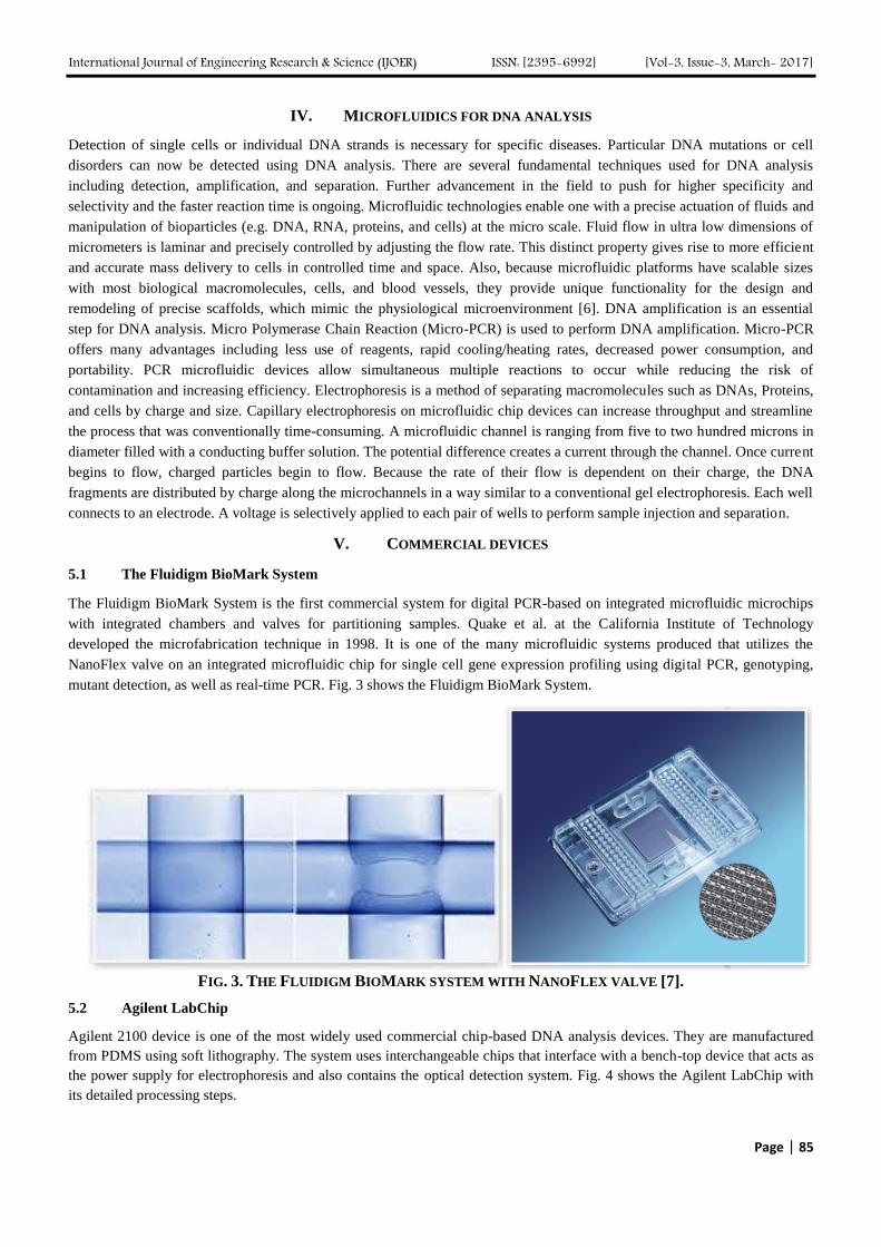
International Journal of Engineering Research & Science (IJOER) ISSN: [2395-6992] [Vol-3, Issue-3, March- 2017]
Page | 85
IV. MICROFLUIDICS FOR DNA ANALYSIS
Detection of single cells or individual DNA strands is necessary for specific diseases. Particular DNA mutations or cell
disorders can now be detected using DNA analysis. There are several fundamental techniques used for DNA analysis
including detection, amplification, and separation. Further advancement in the field to push for higher specificity and
selectivity and the faster reaction time is ongoing. Microfluidic technologies enable one with a precise actuation of fluids and
manipulation of bioparticles (e.g. DNA, RNA, proteins, and cells) at the micro scale. Fluid flow in ultra low dimensions of
micrometers is laminar and precisely controlled by adjusting the flow rate. This distinct property gives rise to more efficient
and accurate mass delivery to cells in controlled time and space. Also, because microfluidic platforms have scalable sizes
with most biological macromolecules, cells, and blood vessels, they provide unique functionality for the design and
remodeling of precise scaffolds, which mimic the physiological microenvironment [6]. DNA amplification is an essential
step for DNA analysis. Micro Polymerase Chain Reaction (Micro-PCR) is used to perform DNA amplification. Micro-PCR
offers many advantages including less use of reagents, rapid cooling/heating rates, decreased power consumption, and
portability. PCR microfluidic devices allow simultaneous multiple reactions to occur while reducing the risk of
contamination and increasing efficiency. Electrophoresis is a method of separating macromolecules such as DNAs, Proteins,
and cells by charge and size. Capillary electrophoresis on microfluidic chip devices can increase throughput and streamline
the process that was conventionally time-consuming. A microfluidic channel is ranging from five to two hundred microns in
diameter filled with a conducting buffer solution. The potential difference creates a current through the channel. Once current
begins to flow, charged particles begin to flow. Because the rate of their flow is dependent on their charge, the DNA
fragments are distributed by charge along the microchannels in a way similar to a conventional gel electrophoresis. Each well
connects to an electrode. A voltage is selectively applied to each pair of wells to perform sample injection and separation.
V. COMMERCIAL DEVICES
5.1 The Fluidigm BioMark System
The Fluidigm BioMark System is the first commercial system for digital PCR-based on integrated microfluidic microchips
with integrated chambers and valves for partitioning samples. Quake et al. at the California Institute of Technology
developed the microfabrication technique in 1998. It is one of the many microfluidic systems produced that utilizes the
NanoFlex valve on an integrated microfluidic chip for single cell gene expression profiling using digital PCR, genotyping,
mutant detection, as well as real-time PCR. Fig. 3 shows the Fluidigm BioMark System.
FIG. 3. THE FLUIDIGM BIOMARK SYSTEM WITH NANOFLEX VALVE [7].
5.2 Agilent LabChip
Agilent 2100 device is one of the most widely used commercial chip-based DNA analysis devices. They are manufactured
from PDMS using soft lithography. The system uses interchangeable chips that interface with a bench-top device that acts as
the power supply for electrophoresis and also contains the optical detection system. Fig. 4 shows the Agilent LabChip with
its detailed processing steps.

International Journal of Engineering Research & Science (IJOER) ISSN: [2395-6992] [Vol-3, Issue-3, March- 2017]
Page | 86
FIG. 4. AGILENT LABCHIP IS SHOWN WITH THE PROCESSING STEPS [8].
VI. DNA SENSOR METHODS
DNA sensors ought to detect, record, and indicate a physical or chemical property, with potential capability for further
processing. DNA biosensor is a “compact logical device or unit incorporating a biological or biologically derived sensitive
‘recognition’ element integrated or associated with a physicochemical transducer [4]. Fig. 5 shows a typical structure of a
biosensor. A sensor can be broken down into three elements: (1) recognition element, (2) transducer and (3)
amplifier/processor. Recognition refers to binding of target molecules in our case the DNA. Binding of DNA induces the
sensing effect, or the physical or chemical changes, due to a detection event. Desired characteristics for this stage include:
1. Selectivity – Only the target DNA generates sensing effect
2. Sensitivity – Large sensing effect with a small amount
3. Resolution – A good indication of the amount of captured DNA
4. Dynamic Range – Not saturated with a large quantity of DNA
FIG. 5. THE CONFIGURATION OF A BIOSENSOR SHOWING BIO-RECOGNITION, INTERFACE, AND
TRANSDUCTION ELEMENTS [4].
Transduction refers to the conversion of the detection event into a useful, measurable signal that is usually an electrical signal
of either voltage or current [4]. Most transducers are physical sensors that convert the sensing effect of molecular binding
into measurable electrical signals. The signal from the transducer has to be measured or recorded and interpreted as the

International Journal of Engineering Research & Science (IJOER) ISSN: [2395-6992] [Vol-3, Issue-3, March- 2017]
Page | 87
quantity of molecular activity. High levels or signal processing may be needed to retrieve meaningful data in most cases.
Signal processing is performed mostly done by digital processors and computers [5]. Sensors through signal transductions
convert the detection event into a measurable signal. Chemical, physical and biological quantities transformed into a
detectable signal, mostly an electrical signal. DNA sensors fall into three types, namely optical transduction, electrical
transduction, and mechanical transduction [5].
VII. OPTICAL BIOSENSOR
Optical biosensors are a powerful detection and analysis tool that has large applications in biomedical research, health- care,
pharmaceuticals, environmental monitoring, and homeland security. They are immune to electromagnetic interference;
capable of performing remote sensing, and can provide multiplexed detection within a single device. There are two screening
protocols in optical biosensing: fluorescence-based detection and label-free detection [5]. A surface plasmon wave (SPW) is
a charge density oscillation that occurs at the interface of two media with dielectric constants of opposite signs, such as a
metal (gold or silver) and a dielectric. There are four basic methods to excite the SPR, as shown in Fig. 6: prism coupling,
waveguide coupling, fiber optic coupling, and grating coupling. In the prism coupling configuration (Fig. 6(A)), the incident
light is totally reflected at the prism–metal interface and generates an evanescent field penetrating into the metal layer. At the
resonant angle or resonant wavelength, the propagation constant of the evanescent field matches that of the SPW, and as a
result, the photon will have couple into the SPW [5].
FIG. 6. VARIOUS SPR SENSOR CONFIGURATIONS. (A) PRISM COUPLING, (B) WAVEGUIDE COUPLING, (C)
OPTICAL FIBER COUPLING, (D) SIDE-POLISHED FIBER COUPLING, (E) GRATING COUPLING AND (F) LONG-
RANGE AND SHORT-RANGE SURFACE PLASMON [5].
The following research demonstrates a Localized Surface Plasmin Resonance (LSPR) Biosensor. The major discovery
reported is that triangular silver nanoparticles fabricated by nanosphere lithography do indeed function as unexpectedly
sensitive and selective nanoscale affinity biosensors. LSPR Nano sensors as shown in fig 7. possess at least two unique
characteristics modified by changing nanoparticle size and shape: (1) modest refractive sensitivity on the order of 1 part in
102 and (2) a short-range, sensing length scale determined by the characteristic decay length of the local electromagnetic
field. These two factors combine to yield an areal mass sensitivity of ∼100-1000 pg/mm2, which is only a factor of 100
poorer than the best propagating SPR sensitivities. LSPR Nano sensors retain all of the other desirable features of SPR
spectroscopy [6].

International Journal of Engineering Research & Science (IJOER) ISSN: [2395-6992] [Vol-3, Issue-3, March- 2017]
Page | 88
FIG. 7. LSPR NANOBIOSENSOR: (A) AFM IMAGE OF THE AG NANOPARTICLES. (B) SURFACE CHEMISTRY OF
THE AG NANOBIOSENSOR. (C) SCHEMATIC REPRESENTATION OF SA BINDING TO A BIOTINYLATED AG
NANOBIOSENSOR [6].
VIII. MECHANICAL BIOSENSOR
Mechanical interactions are fundamental to biology. Mechanical forces of synthetic origin determine motility and adhesion
on the cellular scale and govern transport and affinity on the molecular level. Biological sensing in the mechanical devices
provides unique opportunities to measure forces, displacements and mass changes from cellular and subcellular processes. A
basic design of the cantilever chip is shown in fig. 8. Nanomechanical systems are particularly well matched in size with
molecular interactions, and provide a basis for biological probes with single-molecule.
FIG. 8. THE BASIC DESIGN OF THE CANTILEVER CHIP WITH FOUR INTEGRATED PIEZORESISTORS PLACED IN
AN ON-CHIP WHEATSTONE BRIDGE [9].
The following research presents a cantilever-based biochemical sensor with piezoresistive read-out as shown in figure 8,
optimized for measuring surface stress. The resistors and the electrical wiring on the chip are encapsulated in Low-Pressure
Chemical Vapor Deposition (LPCVD) silicon nitride so that the chip is well suited for operation in liquids. The wiring is
titanium silicide, which in contrast to conventional metal wiring—is compatible with the high-temperature LPCVD coating
process [9]. The 1/f noise is found from the measured spectral noise density shown in Fig. 9. The lowest curve is for no
applied voltage and reflects the Johnson noise, whereas the other three curves show 1/f noise for three different supply
voltages.
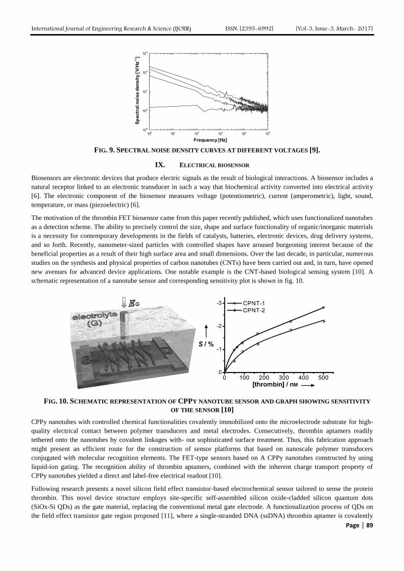
International Journal of Engineering Research & Science (IJOER) ISSN: [2395-6992] [Vol-3, Issue-3, March- 2017]
Page | 89
FIG. 9. SPECTRAL NOISE DENSITY CURVES AT DIFFERENT VOLTAGES [9].
IX. ELECTRICAL BIOSENSOR
Biosensors are electronic devices that produce electric signals as the result of biological interactions. A biosensor includes a
natural receptor linked to an electronic transducer in such a way that biochemical activity converted into electrical activity
[6]. The electronic component of the biosensor measures voltage (potentiometric), current (amperometric), light, sound,
temperature, or mass (piezoelectric) [6].
The motivation of the thrombin FET biosensor came from this paper recently published, which uses functionalized nanotubes
as a detection scheme. The ability to precisely control the size, shape and surface functionality of organic/inorganic materials
is a necessity for contemporary developments in the fields of catalysts, batteries, electronic devices, drug delivery systems,
and so forth. Recently, nanometer-sized particles with controlled shapes have aroused burgeoning interest because of the
beneficial properties as a result of their high surface area and small dimensions. Over the last decade, in particular, numerous
studies on the synthesis and physical properties of carbon nanotubes (CNTs) have been carried out and, in turn, have opened
new avenues for advanced device applications. One notable example is the CNT-based biological sensing system [10]. A
schematic representation of a nanotube sensor and corresponding sensitivity plot is shown in fig. 10.
FIG. 10. SCHEMATIC REPRESENTATION OF CPPY NANOTUBE SENSOR AND GRAPH SHOWING SENSITIVITY
OF THE SENSOR [10]
CPPy nanotubes with controlled chemical functionalities covalently immobilized onto the microelectrode substrate for high-
quality electrical contact between polymer transducers and metal electrodes. Consecutively, thrombin aptamers readily
tethered onto the nanotubes by covalent linkages with- out sophisticated surface treatment. Thus, this fabrication approach
might present an efficient route for the construction of sensor platforms that based on nanoscale polymer transducers
conjugated with molecular recognition elements. The FET-type sensors based on A CPPy nanotubes constructed by using
liquid-ion gating. The recognition ability of thrombin aptamers, combined with the inherent charge transport property of
CPPy nanotubes yielded a direct and label-free electrical readout [10].
Following research presents a novel silicon field effect transistor-based electrochemical sensor tailored to sense the protein
thrombin. This novel device structure employs site-specific self-assembled silicon oxide-cladded silicon quantum dots
(SiOx-Si QDs) as the gate material, replacing the conventional metal gate electrode. A functionalization process of QDs on
the field effect transistor gate region proposed [11], where a single-stranded DNA (ssDNA) thrombin aptamer is covalently

International Journal of Engineering Research & Science (IJOER) ISSN: [2395-6992] [Vol-3, Issue-3, March- 2017]
Page | 90
attached to the QD surface, which specifically binds to thrombin as shown in figure 11. The sensing operation of the QD-
gated FET operates by increasing the threshold voltage. This increase in threshold voltage was experimentally observed, in
addition to the corresponding decrease of the MOSFETs drain current [11].
FIG. 11. QUANTUM DOT GATE FIELD EFFECT TRANSISTOR THROMBIN BIOSENSOR [11]
Figure 12 below shows the ID-VG and ID-VD transfer characteristics, respectively, of the fabricated transistor having a W/L
ratio of 10μm / 26μm. As evident from the features, the substitution of the conventional metal gate electrode with site-
specific self-assembled SiOx-cladded Si quantum dots atop a 40Å thermally grown gate insulator demonstrates the feasibility
of configuring a QD gate FET as a biosensing device.
25
gate electrode with site-specific self-assembled SiOx-cladded Si quantum dots atop a 40Å
thermally grown gate insulator demonstrates the feasibility of configuring a QD gate FET
as a biosensing device.
(a)
(b)
Figure 2.6: (a) ID-VG and (b) ID-VD transfer characteristics of the liquid top-gated QD
Gate FET in the absence of ssDNA functionalization.
Having demonstrated control device characteristics in the absence of
functionalization, the QDs were then decorated with ssDNA thrombin aptamers per the
procedure previously outlined, followed by additions of increasing Thrombin
concentrations to the gate region. Figure 2.7 (a) below shows the ID-VG transfer
characteristics after additions of Thrombin, with a constant drain voltage of 0.5V and a
gate voltage swept from 0-2 V.
FIG. 12. ID-VG AND ID-VD TRANSFER CHARACTERISTICS OF THE LIQUID TOP-GATED QUANTUM DOT
FET [11].
As evident from Figure 13, there is a definite increase in threshold voltage as higher Thrombin concentration is present at the
gate, according to the threshold voltage equation for an NMOS transistor.

International Journal of Engineering Research & Science (IJOER) ISSN: [2395-6992] [Vol-3, Issue-3, March- 2017]
Page | 91
FIG. 13. ID-VG TRANSFER CHARACTERISTICS OF THE SSDNA THROMBIN APTAMER FUNCTIONALIZED
QDG GET WITH ADDITIONS OF THROMBIN PROTEIN [11]
X. CONCLUSION
Microfluidics offers revolutionary new capabilities for the future of DNA sensing. The manipulation of small volumes of
fluid with precise dynamic control over concentrations provides the key to advancement. The paper gives a detailed insight
into the world of novel biosensors and it’s feasibility. It also introduces the audience to the importance of microfluidics and
its application in DNA sensing technologies. Commercially available devices for DNA separation and analysis are explored.
Nanotechnology enables development of vast types of sensors to analyze metabolites that in turn drives the diagnostic
methods in medicine and research.
REFERENCES
[1] Whitesides, G. M. (2006). The origins and the future of microfluidics. Nature, 442(7101), 368-73. doi:10.1038/nature05058
[2] Dittrich, P. S., & Manz, A. (2006). Lab-on-a-chip: Microfluidics in drug discovery. Nature Reviews. Drug Discovery, 5(3), 210-218. doi:10.1038/nrd1985
[3] Tegenfeldt, J. O., Prinz, C., Cao, H., Huang, R. L., Austin, R. H., Chou, S. Y., . . . Sturm, J. C. (2004). Micro- and nanofluidics for DNA analysis. Analytical and Bioanalytical Chemistry, 378(7), 1678-1692. doi:10.1007/s00216-004-2526-0
[4] Chambers, J. P., Arulanandam, B. P., Matta, L. L., Weis, A., & Valdes, J. J. (2008). Biosensor recognition elements. Current Issues in Molecular
Biology, 10(1-2), 1. doi:10.21775/cimb.010.001
[5] Fan, X., White, I. M., Shopova, S. I., Zhu, H., Suter, J. D., & Sun, Y. (2008). Sensitive optical biosensors for unlabeled targets: A review. Analytica
Chimica Acta, 620(1-2), 8-26. doi:10.1016/j.aca.2008.05.022
[6] Haes, a. J., & Van Duyne, R. P. (2002). A nanoscale optical biosensor: Sensitivity and selectivity of an approach based on the localized surface
plasmon resonance spectroscopy of triangular silver nanoparticles. Journal of the American Chemical Society, 124(35), 10596-10604. doi:Article
[7] Fluidigm. (2014). Www.fluidigm.com. Retrieved from https://www.fluidigm.com/products/biomark-hd-system
[8] Agilent. (2014). Http://Www.genomics.agilent.com/. Retrieved from http://www.genomics.agilent.com/en/Bioanalyzer-System/2100-Bioanalyzer-
Instruments/?cid=AG-PT-106&tabId=AG-PR-1001
[9] Rasmussen, P. A., Thaysen, J., Hansen, O., Eriksen, S. C., & Boisen, A. (2003). Optimised cantilever biosensor with piezoresistive read-out.
Ultramicroscopy, 97(1-4), 371-376. doi:10.1016/S0304-3991(03)00063-9
[10] Yoon, H., Kim, J., Lee, N., Kim, B., & Jang, J. (2008). A novel sensor platform based on aptamer-conjugated polypyrrole nanotubes for label-free
electrochemical protein detection. Chembiochem : A European Journal of Chemical Biology, 9(4), 634-641. doi:10.1002/cbic.200700660
[11] Croce, R. A., Jr. (2012). Functionalization and characterization of nanomaterial gated field-effect transistor-based biosensors and the design of a
multi-analyte implantable biosensing platform Available from Available from Dissertations & Theses @ University of Connecticut; ProQuest
Dissertations & Theses Global. (1239427597).
(http://ezproxy.lib.uconn.edu/login?url=http://search.proquest.com.ezproxy.lib.uconn.edu/docview/1239427597?accountid=14518). doi:1239427597

International Journal of Engineering Research & Science (IJOER) ISSN: [2395-6992] [Vol-3, Issue-3, March- 2017]
Page | 92
Effect of Solid Particle Density on Hydraulic Performance of a
Prototype Sewage Pump Xiao-Jun Yang
1, Yu-Liang Zhang
2, Zhen-Gen Ying
3, Yan-Juan Zhao
4
1,2,3College of Mechanical Engineering, Quzhou University, Quzhou 324000, China
4College of Information Engineering, Quzhou College of Technology, Quzhou 324000, China
Abstract— A frozen rotor method based on a mixture multiphase flow model, an RNG k–ε dual-equation turbulence model,
and a SIMPLE algorithm is used to perform a numerical simulation of steady flow in a sewage pump that transports solid
and liquid phase flows. The method is also utilized to analyze the effect of solid-phase particle density on the hydraulic
performance of the sewage pump and predict the wear degree of the overflow components. Results of the study indicate that
with the increasing density of solid particles, the head curve of the pump initially decreased and then increased, that is, the
head curve had the minimum value. Additionally, the efficiency curve of the pump increased, decreased, and then increased
again, indicating an insignificant overall change. Meanwhile, the pump shaft power showed a monotonic upward trend.
When the solid-phase density is less than, equal to, and greater than the liquid-phase density, solid-phase concentration on
the blade pressure surface shows a distribution law more than, equal to, and less than 10%, respectively. With the increase
in density of the delivered solid particles, solid-phase concentration on the blade pressure surface shows a decreasing trend.
Keywords— sewage pump, particle density, frozen rotor method, numerical calculation.
I. INTRODUCTION
Sewage pumps consist of both solid- and liquid-phase flow pumps and are key equipment for urban channel cleanout. Many
scholars at home and abroad have carried out in-depth and meticulous research on sewage pumps and have achieved
productive results. Engin et al considered a centrifugal pump with a semi-closed impeller as the object of study to compare
the performance of the pump in delivering water, sand, and other media with different hardness. They likewise provided a
conclusion regarding the relationship between particle size and pump performance. The deviation between predicted and
measured values of the solid- and liquid-phase head of delivery was –20~+15% [1]. Gandhi et al. carried out an experimental
study on the performance of a centrifugal pump with a closed impeller in delivering water, mortar, and a solid–liquid mixture
of zinc tailings. When the solid concentration was smaller than 20%, the relationship between the pump head and the flow
could be confirmed through the relational expression of the water’s working conditions. When the solid concentration was
higher than 20%, the effect of solid particles on the pump performance should be considered [2]. Yuan et al. carried out a
numerical simulation of solid–liquid two-phase turbulence inside a non-overloaded mud pump [3]. Findings suggested that
backflow occurred in the inlet and velocity slip between two phases, and turbulent kinetic energy and dissipation rates
reached their peaks at the junction of the pressure surface and the suction surface. Li et al. conducted an experimental study
on the effect of solid particle properties, including concentration and particle size, on the external characteristics of
centrifugal pumps[4]. Under the working condition of small flow, efficiency value increased slightly, the stable working area
decreased, and the optimal efficiency point moved to the small flow direction. Zhang et al. performed a numerical research
on solid–liquid two-phase flow field in a low specific speed centrifugal pump by means of numerical calculation [5]. The
obvious jet flow-wake structure occurred near a volute tongue, and it was more obvious with the increase of volume fraction.
Zhang et al. made a numerical simulation of the start-up characteristics of a high specific speed centrifugal pump for solid–
liquid two-phase flow by means of a dynamic grid [6]. Harry et al. carried out an experimental study on a centrifugal pump
blade made of high chromium white iron and aluminum alloy through a Coriolis experiment [7] to obtain different wear
modes on the centrifugal pump blade as it delivers mud. Veselin et al. put forward a new wear prediction method based on a
fast experiment and mathematical analysis [8] to substitute a costly and time-consuming traditional slurry pump wear test
with weak applicability. The error between the predicted results and the experimental results was less than 3%. Pagalthivarthi
et al. studied the effects of operational parameters, pump flow and velocity, particle diameter, different geometries, curve of
tongue, and width of volute on erosion wear on particles through a numerical calculation [9]. Dong et al. conducted a study
and found that particle size and shape, liquid velocity, and other flow parameters had a great impact on erosion pit on the
surface of wet parts, and that the degree of distortion and maximum stress of the pit increased with the increase of particle
size [10]. Li et al. revealed the impact of internal flow characteristics on the wear characteristics of solid–liquid two-phase
centrifugal pump [11].

International Journal of Engineering Research & Science (IJOER) ISSN: [2395-6992] [Vol-3, Issue-3, March- 2017]
Page | 93
Therefore, studying the internal flow of the pump to provide a theoretical basis for realizing a high-performing and stable-
operating pump design is needed. The present study aims to conduct a numerical simulation and analysis on solid-liquid two-
phase flow pump to analyze the impact of the density of solid-phase particles on sewage pump performance, including the
hydraulic performance of sewage pump and wear degree of wet parts.
II. PUMP MODEL AND CALCULATION METHOD
2.1 Pump model and computational grid
The pump model used for the computation was a medium specific speed centrifugal pump, with a specific speed of ns=129.3.
Its basic performance parameters were as follows: flow rate Q=50m3/h, head H=20.54m, velocity n=2900r/min, shaft power
Pa=3.54kW, efficiency η=79.5% and net positive suction head NPSHC=2.59m. The main dimensions of the pump were as
follows: inlet diameter Dj=76mm, hub diameter dh=0mm, impeller outlet diameter D2=137mm, impeller outlet width
b2=14mm, blade outlet angle β2=30°, blade number Z=6, blade wrap angle =104.5°, volute base circle diameter D3=145mm,
and volute inlet width b3=30mm.
2.2 Computational grid
The commercial software UG was used to create a 3D model of the internal computing area. The appropriate extension of the
straight-tube suction chamber was made to eliminate the influence of the given inlet speed. An appropriate extension of the
pump outlet was also carried out to better calculate convergence. As shown in Fig.1, the commercial grid partitioning
software GAMBIT2.3.16 was used to create a grid division of the computational domain. Tetrahedral meshes were adopted
in the impeller rotation region and volute static region, with mesh numbers 435,530 and 597,127 respectively. Hexahedral
meshes were used in the suction chamber and outlet extension, with mesh numbers of 152,827 and 54,944 respectively. The
total mesh number of the overall computational domain was 1,240,428. This number was not enough to simulate the micro
flow in the boundary layer of simulation but was sufficient for the macro flow and macro characteristic capturing in the
pump. Mesh quality checking revealed that the equiangular slope and equidimensional slope of the mesh were not more than
0.83.Mesh quality was good at around 30 near wall Y+.
(A) IMPELLER AREA (B) VOLUTE AREA
FIG.1 COMPUTATIONAL MESH
2.3 Governing equations
The 3D unsteady turbulent flow of incompressible fluid in a centrifugal pump can be described by Reynolds-averaged
equations.
2
' '
0i
i
i i ij i i j
j i j j j
u
x
u u upu F u u
t x x x x x
(1)
Where prefers to fluid density, and' '
i ju u refers to mean Reynolds stress.

International Journal of Engineering Research & Science (IJOER) ISSN: [2395-6992] [Vol-3, Issue-3, March- 2017]
Page | 94
Unsteady turbulent flow calculation used in the present study used the RNG k–ε two-equation model to close the mean
Reynolds stress. RNG k–ε turbulent model, which considers the rotation and swirling flow in the mean flow, can better
process the flow with high strain rate and great streamline curvature.
2.4 Multiphase flow model
This study aims to make a 3D turbulent flow calculation of incompressible viscous fluid by using the commercial code
FLUENT software based on a finite volume method. The multiphase flow model in numerical computation used the
algebraic slip mixture model [12] based on Euler's method to complete the calculation of solid–liquid two-phase flow. In the
calculation, the particles were treated as quasi fluid.
2.5 Solution settings
The dynamic and static coupling between rotor and stator in numerical calculation was achieved by means of the frozen rotor
method. Velocity inlet and free output were respectively used as the boundary conditions of the inlet and outlet. No-slip
boundary condition was applied on all solid walls considering viscosity, and standard wall function was used in near-wall
low Reynolds number region to deal with the problem from the high Reynolds number turbulence model. The coupling
between velocity and pressure was calculated by using SIMPLE algorithm. First-order upwind scheme was used for the
spatial discretization of the convection term. The central difference scheme with two-order accuracy was used for the spatial
discretization of diffusion terms. The linear standard format was used for spatial discretization of the source terms
considering that solid particles were uniform spherical particles with unchanged physical properties. The convergence
criterion of each control equation was 0.0001.
2.6 Computational scheme
To explore the effect of solid-phase properties on hydraulic transport performance as the sewage pump delivers solid–liquid
two-phase flow, the following computational scheme was formulated:
Under a designed flow rate (Q=50m3/h) with10%solid-phase concentration and 0.10mmparticle diameter, numerical
calculation was conducted for a solid–liquid two-phase flow field under five conditions when the particle densities were 500,
1000, 1500, 2000,and 2500kg/m3.
III. ANALYSIS OF RESULTS
3.1 External characteristics
Pump inlet and outlet pressures and the external characteristics under five particle densities obtained from the numerical
calculation are shown in Figs.2 and 3. In Fig. 2, the densities of solid particles in delivering solid–liquid two-phase flow were
500, 1000, 1500, 2000, and 2500kg/m3. The values of total pressure at pump inlet were-0.259,-0.281, -0.302, -0.323, and -
0.358kPa, respectively, and the values of total pressure at pump outlet were 128.582, 133.377, 138.662, 146.071, and
153.524, respectively. With the increase of the density of solid particles, the total pressures of the pump inlet and of the pump
outlet showed a trend of monotonic decline and rising. The calculation result of external characteristics in Fig.3 shows that
when the densities of solid particles in solid–liquid two-phase flow were 500, 1000, 1500, 2000, and 2500kg/m3, the
calculated heads were 14.00, 13.80, 13.66, 13.74, and 13.81, respectively, and the calculated efficiencies were 47.02%,
47.17%, 47.097%, 47.36%, and 47.49%,respectively. The calculated shaft powers were 3.850, 3.982, 4.145, 4.344, and
4.551kW, respectively. With the increase of the density of solid particles, the pump head curve showed an initially
decreasing then increasing trend and reached the minimum value of 13.66m when the density of solid particles was
1500kg/m3.The pump efficiency curve showed an initially increasing then decreasing trend. Nevertheless, the absolute value
of the overall change was not significant. At the same time, pump shaft power showed a monotonic upward trend.
Previous research has shown that under the assumption of non-viscous and non-granular force, the equation met by solid-
liquid two-phase flow in the impeller is deduced theoretically. Based on the conclusion, the pump head delivering two-phase
flow was lower than the head delivering liquid-phase flow when the particle density was more than the liquid-phase density.
On the contrary, the pump head increased. The calculation results in this study proved that the conclusion is completely
correct.

International Journal of Engineering Research & Science (IJOER) ISSN: [2395-6992] [Vol-3, Issue-3, March- 2017]
Page | 95
FIG.2 EFFECTS OF PARTICLE DENSITY ON PUMP
INLET AND OUTLET PRESSURES
FIG.3 EFFECTS OF PARTICLE DENSITY ON THE
EXTERNAL CHARACTERISTICS OF THE PUMP
3.2 Pressure surface characteristics
The effects of the density of solid particles obtained from the numerical calculation on the performance parameters of blade
pressure surface are shown in Fig.4. Fig. 4(a) shows the influence of total pressure distribution along the blade. The total
pressure on the blade pressure surface increased with the increase of the semi diameter. Findings also showed that the second
half of the blade pressure surface was the main point of the increase in pressure. Meanwhile, with the increase of the density
of solid particles, total pressure on the blade pressure surface showed a gradual increasing trend. The corresponding densities
of solid particles were 500, 1000, 15003, 2000, and 2500kg/m
3. In the front of the blade pressure surface, the total pressures
were 11.488, 10.490, 7.918, 6.820, and 6.419kPa, respectively. When the relative length of the middle of blade was 0.5, total
pressures were 162.641, 161.726, 160.032, 163.475, and 167.60kPa.In the tailing of the blade pressure surface, total
pressures were 202.057, 207.212, 209.95, 215.042, and 221.334kPa. In the tailing of the blade pressure surface, total pressure
drop occurred due to the influence of jet-wake flow.
Fig. 4(b) shows the obtained distribution of solid-phase concentration on the blade pressure surface. Under different densities
of delivering particles, the solid-phase concentration on the blade pressure surface showed a completely opposite distribution
status. In the case of particle density (500 kg/m3), the density of solid-phase concentration was smaller than the density of
delivering medium water (1000kg/m3). The solid-phase concentration on the blade pressure surface was more than 10%
because when particle density is lighter than water, particles suspend in the water medium. Under centrifugal force and blade
force, solid particles suspended in the water medium gather on the blade pressure surface, causing solid-phase concentration
to significantly increase from the front edge of the blade. Findings indicated that, in this case, the blade pressure surface bore
more severe dynamic attacks and wears. However, in consideration of the small density of solid particles, wear degree will
be further studied. In the front edge, middle, and tailing of the blade pressure surface, instantaneous solid concentrations
were 10.382%, 16.544%, and 12.257%, respectively. When the delivered solid-phase density was 1000kg/m3, solid-phase
density was completely equal to water density, and solid phase was equal to water medium. These factors were completely
mixed together and suspended. Therefore, the calculation result showed that the solid-phase density on the overall blade
pressure surface is always about 10%, which is equal to the calculated solid-phase density of the incoming flow. Findings
revealed that the wear on the blade pressure surface was completely similar. In three cases, the densities of solid particles
were 1500, 2000, and 2500kg/m3. Starting from the front edge of the blade pressure surface, the concentration of solid-phase
particles gradually decreased and dynamically stabilized. Solid-phase concentration was smaller than 10%, which indicated
that, in these three cases, the wear on the blade pressure surface was not severe. Large densities of particles also entailed
large inertial force of particles. Although particle concentration was not high, a greater degree of wear still occurred. This
finding needs further confirmation. In the three cases presented, the instantaneous solid-phase concentrations in the front
edge of the blade pressure surface were 9.878%, 10.048%, and 10.187%,respectively.In the middle of the blade pressure
surface, instantaneous solid-phase concentrations were 6.15%, 4.48%, and 3.343%, respectively. In the tailing of the blade
pressure surface, instantaneous solid-phase concentrations were 8.275%, 7.536%, and 6.908%, respectively. With the
increase in density of delivering solid particles, solid-phase concentrations on the blade pressure surface showed a gradual
declining trend. This finding indicated that the degree of wear increasingly lessened, which was mainly related to the inertial

International Journal of Engineering Research & Science (IJOER) ISSN: [2395-6992] [Vol-3, Issue-3, March- 2017]
Page | 96
force of solid particles. If the inertial force was greater, the ability of particles to escape from the restraint of the blade
pressure surface would be stronger; otherwise, it would be weaker.
In terms of vorticity [Fig.4(c)], the densities of solid particles in five cases were 500, 1000, 1500, 2000,and
2500kg/m3,respectively.At position 0.2, which was relatively long from the front edge of the blade pressure surface, the
obtained vorticity values were 4723.99, 5467.7, 5922.38, 6000.75,and 6016.79s–1
; at position 0.5, the obtained vorticity
values were 4998.75,6544.94,7552.63,7804.41,and 7883.16s–1
,respectively; and at position 0.8, the obtained vorticity values
were 8780.93, 9692.48, 10462.4,10838.3,and 10958s–1
,respectively. With the increase in density of delivering particles, the
vorticity value on the blade pressure surface showed an increasing trend.
For turbulent kinetic energy [Fig.4 (d)], turbulent dissipation rate [Fig.4(e)], and turbulence intensity [Fig.4(f)], the changing
characteristics were generally consistent. In five cases, the densities of delivering solid particles were 500, 1000, 1500,
2000,and 2500kg/m3,respectively.At position 0.5, which was relatively long from the front edge of the blade pressure
surface, turbulent kinetic energies were 4.36109, 3.18985, 2.20454, 1.66049,and 1.28034m2·s
–2,respectively; turbulent
dissipation rates were 22872.9, 14340.3, 8247.05, 5389.18,and 3650.25m2·s
–3,respectively; and turbulence intensities were
1.636%, 1.395%, 1.164%, 1.015%, and 0.897%. With the increase in density of delivering solid particles, the turbulence
effect on blade pressure surface decreased gradually, and flow was more stable. However, in terms of any kind of delivery
concentration, turbulent kinetic energy, turbulent dissipation rate, and turbulence intensity, the minimum value from the front
edge gradually decreased and then increased.
(A)TOTAL PRESSURE
(B)SOLID-PHASE CONCENTRATION
(C)VORTICITY
(D)TURBULENT KINETIC ENERGY
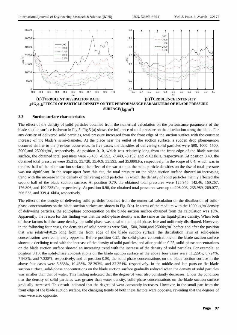
International Journal of Engineering Research & Science (IJOER) ISSN: [2395-6992] [Vol-3, Issue-3, March- 2017]
Page | 97
(E)TURBULENT DISSIPATION RATE
(F)TURBULENCE INTENSITY
FIG.4 EFFECTS OF PARTICLE DENSITY ON THE PERFORMANCE PARAMETERS OF BLADE PRESSURE
SURFACE(kg/m3)
3.3 Suction surface characteristics
The effect of the density of solid particles obtained from the numerical calculation on the performance parameters of the
blade suction surface is shown in Fig.5. Fig.5 (a) shows the influence of total pressure on the distribution along the blade. For
any density of delivered solid particles, total pressure increased from the front edge of the suction surface with the constant
increase of the blade’s semi-diameter. At the place near the outlet of the suction surface, a sudden drop phenomenon
occurred similar to the previous occurrence. In five cases, the densities of delivering solid particles were 500, 1000, 1500,
2000,and 2500kg/m3, respectively. At position 0.10, which was relatively long from the front edge of the blade suction
surface, the obtained total pressures were -5.459, -6.553, -7.449, -8.192, and -9.021kPa, respectively. At position 0.40, the
obtained total pressures were 35.215, 35.728, 35.469, 35.593, and 35.880kPa, respectively. In the scope of 0.4, which was in
the first half of the blade suction surface, the effect of the variation in the solid particle densities on the rise of total pressure
was not significant. In the scope apart from this site, the total pressure on the blade suction surface showed an increasing
trend with the increase in the density of delivering solid particles, in which the density of solid particles mainly affected the
second half of the blade suction surface. At position 0.70, the obtained total pressures were 125.945, 142.46, 160.267,
176.806, and 190.735kPa, respectively. At position 0.90, the obtained total pressures were up to 208.003, 235.989, 269.077,
306.533, and 339.416kPa, respectively.
The effect of the density of delivering solid particles obtained from the numerical calculation on the distribution of solid-
phase concentrations on the blade suction surface are shown in Fig. 5(b). In terms of the medium with the 1000 kg/m3density
of delivering particles, the solid-phase concentration on the blade suction surface obtained from the calculation was 10%.
Apparently, the reason for this finding was that the solid-phase density was the same as the liquid-phase density. When both
of these factors had the same density, the solid phase was equal to the liquid phase, free and uniformly distributed. However,
in the following four cases, the densities of solid particles were 500, 1500, 2000,and 2500kg/m3 before and after the position
that was relatively0.25 long from the front edge of the blade suction surface; the distribution laws of solid-phase
concentration were completely opposite. Before position 0.25, the solid-phase concentrations on the blade suction surface
showed a declining trend with the increase of the density of solid particles, and after position 0.25, solid-phase concentrations
on the blade suction surface showed an increasing trend with the increase of the density of solid particles. For example, at
position 0.10, the solid-phase concentrations on the blade suction surface in the above four cases were 11.229%, 8.724%,
7.963%, and 7.338%, respectively; and at position 0.80, the solid-phase concentrations on the blade suction surface in the
above four cases were 5.868%, 19.458%, 28.393%, and 32.351%, respectively. In the middle and late parts on the blade
suction surface, solid-phase concentrations on the blade suction surface gradually reduced when the density of solid particles
was smaller than that of water. This finding indicated that the degree of wear also constantly decreases. Under the condition
that the density of solid particles was greater than water density, solid-phase concentrations on the blade suction surface
gradually increased. This result indicated that the degree of wear constantly increases. However, in the small part from the
front edge of the blade suction surface, the changing trends of both these factors were opposite, revealing that the degrees of
wear were also opposite.

International Journal of Engineering Research & Science (IJOER) ISSN: [2395-6992] [Vol-3, Issue-3, March- 2017]
Page | 98
Fig.5(c) shows the vorticity distribution on the blade suction surface in cases of different densities of delivering solid
particles. Vorticity distribution characteristics in five kinds of delivering density were basically the same, showing a
gradually declining trend from the front edge of the blade suction surface. Furthermore, the effect of different densities on
vorticity values was not significant.Figs.5(d), 5(e), and5(f) show the respective distributions of turbulent kinetic energy,
turbulent dissipation rate, and turbulence intensity along the blade suction surface under different densities of delivering solid
particles. Generally, these factors had similar changing characteristics, namely, increasing with the increase of the densities
of delivering solid particles. Three parties reflected time-averaged characteristics of turbulence.
(A)TOTAL PRESSURE
(B)SOLID-PHASE CONCENTRATION
(C)VORTICITY
(D)TURBULENT KINETIC ENERGY
(E)TURBULENT DISSIPATION RATE
(F)TURBULENCE INTENSITY
FIG.5 EFFECTS OF PARTICLE DENSITIES ON THE PERFORMANCE PARAMETERS OF BLADE SUCTION
SURFACE(kg/m3)

International Journal of Engineering Research & Science (IJOER) ISSN: [2395-6992] [Vol-3, Issue-3, March- 2017]
Page | 99
3.4 Particle concentration on the blade pressure surface
Fig. 6 shows the distribution of particle concentration on the blade pressure surface in five densities of delivering solid-phase
particles. The figure illustrates that when particle density (500 kg/m3) is smaller than liquid-phase (water) density, the solid-
phase concentrations on two sides of the blade pressure surface are considerably higher; when the density of solid-phase
particles (1000 kg/m3) was equal to liquid-phase density, the distribution of solid-phase concentration on the blade pressure
surface was more uniform. This result is clearly related to their similar densities. In three cases where the densities of
delivering solid-phase particles were 1500, 2000,and 2500kg/m3, with the increase of the density of delivering solid particles,
the distribution area of solid-phase concentration on the pressure surface shrank to the inlet. This finding indicated that the
wear area and the wear degree on the blade pressure surface decreased.
(A) 500 (B)1000 (C)1500 (D)2000 (E)2500
FIG.6 DISTRIBUTION OF THE PARTICLE CONCENTRATIONS ON THE BLADE PRESSURE SURFACE UNDER
DIFFERENT PARTICLE DENSITIES (kg/m3)
3.5 Particle concentration on the blade suction surface
Fig. 7 shows the distribution of particle concentration on the blade suction surface in five densities of delivering solid-phase
particles. When particle density (500 kg/m3) was smaller than the liquid-phase (water) density, the solid-phase concentration
on the first half of the blade suction surface was higher than that on the second half of the blade suction surface. The wear
was more serious. When the density of solid-phase particles (1000 kg/m3) was equal to liquid-phase density, the distribution
of solid-phase concentration on the blade suction surface was more uniform. Therefore, the degree of wear was also
consistent. In three cases where the densities of delivering solid-phase densities were 1500, 2000, and 2500kg/m3, the density
of particles was apparently greater than the liquid-phase density. With the increase of the density of delivering solid particles,
solid-phase volume fraction on the second half of the suction surface was higher. This finding indicated that the degree of
wear on the blade suction surface was constantly increasing.
(A) 500 (B)1000 (C)1500 (D)2000 (E)2500
FIG.7 DISTRIBUTION OF PARTICLE CONCENTRATIONS ON THE BLADE SUCTION SURFACE UNDER DIFFERENT
PARTICLE DENSITIES (kg/m3)
3.6 Particle concentration on volute surface
Fig. 8 shows the distribution of particle concentration on volute surface under five different densities of delivering solid-
phase particles. When the density of delivering solid particles (1000 kg/m3) was equal to the liquid-phase density (1000
kg/m3), solid-phase volume fraction on volute surface was very uniform. The degree of wear in this case was the same.
However, when the particle density was smaller or greater than the liquid-phase density (500, 1500, 2000, and 2500 kg/m3),
the solid-phase volume concentration on volute surface was more or less non-uniform. The degrees of wear on volute surface
under these four cases were not the same.

International Journal of Engineering Research & Science (IJOER) ISSN: [2395-6992] [Vol-3, Issue-3, March- 2017]
Page | 100
(A) 500 (B)1000 (C)1500 (D)2000 (E)2500
FIG.8 DISTRIBUTION OF PARTICLE CONCENTRATIONS ON VOLUTE SURFACE UNDER DIFFERENT PARTICLE
DENSITIES (kg/m3)
IV. CONCLUSION
1) With the increase of the density of solid particles, the total pressure of both the pump inlet and the pump outlet showed
a trend of monotonic decline. Pump calculation head curve showed a trend of first declining and then rising, reaching
the minimum value of 13.66m when the density of solid particles was 1500kg/m3.The pump efficiency curve showed a
trend of initial rise and decline and then rise, but its change was not significant. The pump shaft power showed a trend
of monotonic rise.
2) When particle density was smaller than, equal to, and greater than liquid-phase concentration, solid-phase concentration
on the blade pressure surface showed the distribution laws more than, equal to, and smaller than 10%, respectively.
With the increase in the density of solid particles, solid-phase concentration on the blade pressure surface showed a
gradually declining trend. These findings indicated that the wear and tear was getting smaller and smaller.
3) In the middle and late half of the blade suction surface, when the density of solid particles was smaller than that of
water, solid-phase concentration on the blade suction surface gradually decreased. This result indicated that the wear
and tear was constantly smaller and smaller. In the case where the density of solid particles was greater than water
density, solid-phase concentration on the blade suction surface increased gradually. This finding indicated that the wear
and tear constantly increased. However, in a small part from the front edge of the blade suction surface, the change
trends of both were opposite. This finding showed that the degree of wear was opposite.
ACKNOWLEDGEMENTS
The work was supported by the Zhejiang Provincial Science and Technology Project (No.2015C31129, No.2016C31127),
Academic Foundation of Quzhou University (No.XNZQN201508).
REFERENCES
[1] Engin T, Gur M. Performance characteristics of centrifugal pump impeller with running tip clearance pumping solid-liquid
mixtures[J]. Journal of Fluids Engineering, 2001, 123(3): 532-538.
[2] Gandhi B K, Singh S N, Seshadn V. Effect of speed on the performance characteristics of a centrifugal slurry pump[J]. Journal of
Hydraulic Engineering, 2002, 128(2): 225-233.
[3] Yuan Shouqi, Zhang Peifang, Zhang Jinfeng. Numerical simulation of 3-D dense solid- liquid two- phase turbulent flow in a non-
clogging mud pump[J]. Chinese Journal of Mechanical Engineering, 2004, 17(4):623-627.
[4] Li Yi, Zhu Zuchao, He Weiqiang, et al. Numerical simulation and experimental research on the influence of solid phase characteristics
on centrifugal pump performance[J]. Chinese Journal of Mechanical Engineering, 2012, 25(6): 1184-1189.
[5] Zhang Yuliang, Li Yi, Cui Baoling, et al. Numerical simulation and analysis of solid-liquid two-phase flow in centrifugal pump[J].
Chinese Journal of Mechanical Engineering, 2013, 26(1): 53-60.
[6] Zhang Yuliang, Li Yi, Zhu Zuchao, et al. Computational analysis of centrifugal pump delivering solid-liquid two-phase flow during
startup period[J]. Chinese Journal of Mechanical Engineering, 2014, 27(1): 178-185.

International Journal of Engineering Research & Science (IJOER) ISSN: [2395-6992] [Vol-3, Issue-3, March- 2017]
Page | 101
[7] Harry H T, Graeme R A. Experimental study on erosive wear of some metallic materials using Coriolis wear testing approach[J].
Wear, 2005, (258): 458-469.
[8] Veselin B. Erosive wear model of slurry pump impeller[J]. Journal of Tribology, 2010, 132(2): 021602.1~5.
[9] Pagalthivarthi K V, Gupta P K, Tyagi V, et al. CFD prediction of erosion wear in centrifugal slurry pumps for dilute slurry flows[J].
Journal of Computational Multiphase Flows, 2011, 3(4): 225-245.
[10] Dong Xing, Zhang Hailu, Wang Xinyong. Finite element analysis of wear for centrifugal slurry pump[C]. The 6th International
Conference on Mining Science & Technology, 2009, (1): 1532-1538.
[11] Li Yi, Zhu Zuchao, He Zhaohui, et a1. Abrasion characteristic analyses of solid-liquid two-phase centrifugal pump[J]. Journal of
Thermal Science, 2010, 20(3): 283-287.
[12] Sanyal J, Vasquez S, Roy S, et al. Numerical simulation of gas-liquid dynamics in cylindrical bubble column reactors [J]. Chemical
Engineering Science, 1999, 54(21):5071-5083.

International Journal of Engineering Research & Science (IJOER) ISSN: [2395-6992] [Vol-3, Issue-3 March- 2017]
Page | 102
New Finite Element for modeling connections in 2D small frames
- Static Analysis Chadi Azoury
1, Assad Kallassy
2, Ibrahim Moukarzel
3
1Mechanical Engineering Department, Lebanese University, Lebanon 2Civil Engineering Department, Lebanese University, Lebanon
3Faculty of Engineering, Lebanese University, Lebanon
Abstract — The paper presents a proposal to create a new one-dimensional (1-D) finite element that can substitute for the
three-dimensional (3-D) finite model of connection elements in static analysis. The study is conducted on a simple small
frame. First, a 3-D model is constructed, followed by the construction of an equivalent two-dimensional (2-D) one. At the
final stage, the results of the static analysis of many proposed 1-D element models are compared with the results of the 2-D
model. With a special treatment of the connection elements, the results of the analysis of the new 1-D finite element models
agree well with the results of the 2-D model.
Keywords: Structures, Finite element methods, Condensation, Timoshenko beam, Connection element, and Small frames.
Notations
E Young’s elastic modulus
v Poisson coefficient
density
I moment of inertia
E I flexural beam stiffness = E × I
t frame thickness
K(n×n) stiffness matrix of order n
L(n×m) rectangular matrix with n rows and m columns
EB Euler-Bernoulli
sh shear deformation
FE finite element
DOF degree-of-freedom
I. INTRODUCTION
To perform a static analysis of a frame, 3-D finite elements are usually used in the meshing process. A large number of
elements are required, which in turn requires a large number of DOF and consequently, a great deal of work. The main
objective consists of developing a 1-D model made up of simple 1-D elements to replace the 3-D model made up of
tetrahedral prisms or brick elements. To perform a static analysis, the calculation of the stiffness matrix is required.
In order to find the best 1-D finite meshing element, 3-D meshing is used, and 2-D and 1-D models are consecutively
constructed.
All calculations are done by using ANSYS Version 16.2 and MATLAB Version 7. A simple frame is used in the
calculations.
II. TEST STRUCTURE
Our test structure will be of this form:
0.065 m
Clamped Base
0.075 m
0.02 m
0.02 m
FIGURE 1: TEST STRUCTURE

International Journal of Engineering Research & Science (IJOER) ISSN: [2395-6992] [Vol-3, Issue-3 March- 2017]
Page | 103
The beam section of the test structure is rectangular (0.02×0.02 m2). The mechanical characteristics are: Poisson coefficient
v = 0.31, density = 78000 N/m3
, and elastic modulus E = 184 GPa. The test structure is clamped at its base and consists of 5
structural elements shown in Figure 2.
X
Y
Z
Left
column Right
column
Left
corner Right
corner
Horizontal
beam
FIGURE 2: TEST STRUCTURE CONSTRUCTED IN ANSYS® R16.2
Different types of elements are used in the meshing processes. In static analysis, the comparison between different models is
based on the deformation in the XY plan of the structure. These models are compared in 2 load cases illustrated in
Figure 3:
Case 1: a body load of 78000 N/m3 along the vertical axis of the horizontal beam
Case 2: a body load of 78000 N/m3 along the horizontal axis of the left column
F G
No l
oad
No l
oad
Central line
Body load along Y -
X
Y
Load case 1 Load case 2
F G
No load
Body l
oad
alo
ng X
+
No l
oad
Central line
FIGURE 3: TEST STRUCTURE WITH LOAD CASES 1 AND 2

International Journal of Engineering Research & Science (IJOER) ISSN: [2395-6992] [Vol-3, Issue-3 March- 2017]
Page | 104
III. 3D AND 2D MODELING
The 3D model of the test structure is meshed using H8 volumetric finite elements with 8 nodes. Each column is modeled
using 8×8×16 = 1024 elements and each corner includes 8×8×8 = 512 elements. The horizontal beam is modeled using
8×8×16 = 1024 elements. In total, it is equal to 4096 elements with 5265 nodes (see Figure 4).
FIGURE 4: 3D TEST STRUCTURE MODELLED USING H8 FINITE ELEMENTS
Figures 5 and 6 show the total displacement contours of the frame under load case 1 and 2.
FIGURE 5: THREE-DIMENSIONAL DEFORMED TEST STRUCTURE UNDER LOAD CASE 1
FIGURE 6: THREE-DIMENSIONAL DEFORMED TEST STRUCTURE UNDER LOAD CASE 2
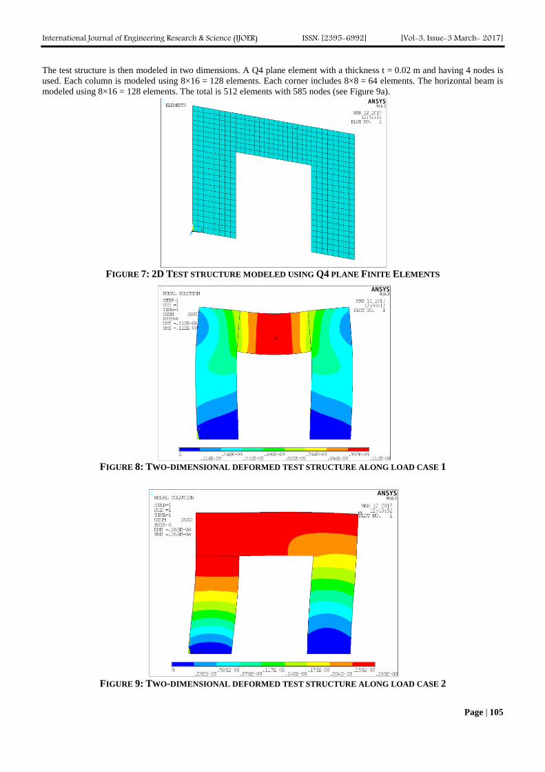
International Journal of Engineering Research & Science (IJOER) ISSN: [2395-6992] [Vol-3, Issue-3 March- 2017]
Page | 105
The test structure is then modeled in two dimensions. A Q4 plane element with a thickness t = 0.02 m and having 4 nodes is
used. Each column is modeled using 8×16 = 128 elements. Each corner includes 8×8 = 64 elements. The horizontal beam is
modeled using 8×16 = 128 elements. The total is 512 elements with 585 nodes (see Figure 9a).
FIGURE 7: 2D TEST STRUCTURE MODELED USING Q4 PLANE FINITE ELEMENTS
FIGURE 8: TWO-DIMENSIONAL DEFORMED TEST STRUCTURE ALONG LOAD CASE 1
FIGURE 9: TWO-DIMENSIONAL DEFORMED TEST STRUCTURE ALONG LOAD CASE 2

International Journal of Engineering Research & Science (IJOER) ISSN: [2395-6992] [Vol-3, Issue-3 March- 2017]
Page | 106
Figures 8 and 9 have similar maps as Figures 5 and 6. The different models are compared using the displacement of 65 points
on the central line of the longitudinal symmetrical plan of the structure.
FIGURE 10 : LONGITUDINAL SYMMETRICAL PLAN OF THE STRUCTURE SHOWING THE 65 CENTRAL LINE
POINTS
In order to establish a comparison between both FE models and using both load cases, UX and UY displacements of nodes
on the central line, along the X and Y axis respectively, are plotted on the same graph (see Figure 11 – 10).
FIGURE 11 : UX (m) CENTRAL LINE DISPLACEMENT ALONG AXE X (LOAD CASE 1)
FIGURE 12 : UY (m) CENTRAL LINE DISPLACEMENT ALONG AXE Y (LOAD CASE 1)
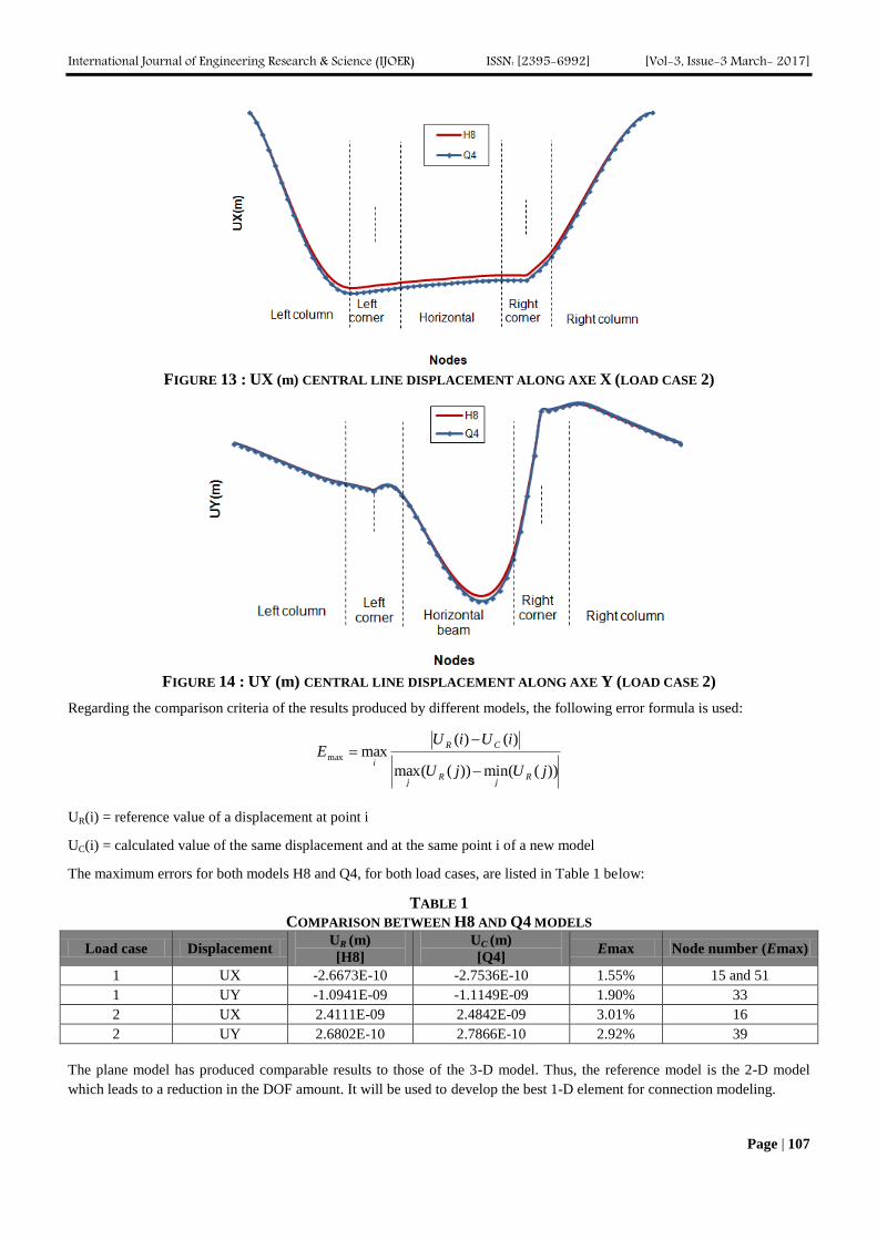
International Journal of Engineering Research & Science (IJOER) ISSN: [2395-6992] [Vol-3, Issue-3 March- 2017]
Page | 107
FIGURE 13 : UX (m) CENTRAL LINE DISPLACEMENT ALONG AXE X (LOAD CASE 2)
FIGURE 14 : UY (m) CENTRAL LINE DISPLACEMENT ALONG AXE Y (LOAD CASE 2)
Regarding the comparison criteria of the results produced by different models, the following error formula is used:
))((min))((max
)()(maxmax
jUjU
iUiUE
Rj
Rj
CR
i
UR(i) = reference value of a displacement at point i
UC(i) = calculated value of the same displacement and at the same point i of a new model
The maximum errors for both models H8 and Q4, for both load cases, are listed in Table 1 below:
TABLE 1
COMPARISON BETWEEN H8 AND Q4 MODELS
Load case Displacement UR (m)
[H8]
UC (m)
[Q4] Emax Node number (Emax)
1 UX -2.6673E-10 -2.7536E-10 1.55% 15 and 51
1 UY -1.0941E-09 -1.1149E-09 1.90% 33
2 UX 2.4111E-09 2.4842E-09 3.01% 16
2 UY 2.6802E-10 2.7866E-10 2.92% 39
The plane model has produced comparable results to those of the 3-D model. Thus, the reference model is the 2-D model
which leads to a reduction in the DOF amount. It will be used to develop the best 1-D element for connection modeling.

International Journal of Engineering Research & Science (IJOER) ISSN: [2395-6992] [Vol-3, Issue-3 March- 2017]
Page | 108
IV. ONE-DIMENSIONAL CLASSICAL MODELING
In this section, 1-D elements are used for the test structure. Since the structure is not the slender type, we know that Euler-
Bernoulli beams are not adequate. Therefore, we will use Timoshenko beams with 2 nodes per element and 3 DOF per node
(Timoshenko model).
UX1
UY1
RZ1
UX2
UY2
RZ2
L
FIGURE 15 : TWO-NODE BEAMS
The transformation from the Q4 model to the 1-D model is shown in Figures 12 and 13. The volumetric charge is
transformed into linear charge.
F G
F G
78 KN/m3
0.0312 KN/m
FIGURE 16 : TRANSFORMATION OF THE Q4 MODEL INTO A 1-D MODEL (LOAD CASE 1)
F G
F G
78 K
N/m
3
0.0
312 K
N/m
FIGURE 17 : TRANSFORMATION OF THE Q4 MODEL INTO A 1-D MODEL (LOAD CASE 2)
The left and right columns are modeled using 16 elements each. The horizontal beam is also modeled using 16 elements.
Both left and right corners are modeled using 4 horizontal linear elements and 4 vertical linear elements, i.e. a total of 64

International Journal of Engineering Research & Science (IJOER) ISSN: [2395-6992] [Vol-3, Issue-3 March- 2017]
Page | 109
beam elements. The following figures show the deformed test structure in the 2 load cases as applicable to both models: the
reference model Q4 and the Timoshenko model.
FIGURE 18 : UX (m) DISPLACEMENT OF CENTRAL LINE NODES ALONG X (LOAD CASE 1)
FIGURE 19 : UY (m) DISPLACEMENT OF CENTRAL LINE NODES ALONG Y (LOAD CASE 1)
FIGURE 20 : UX (m) DISPLACEMENT OF CENTRAL LINE NODES X (LOAD CASE 2)

International Journal of Engineering Research & Science (IJOER) ISSN: [2395-6992] [Vol-3, Issue-3 March- 2017]
Page | 110
FIGURE 21 : UY (m) DISPLACEMENT OF CENTRAL LINE NODES Y (LOAD CASE 2)
None of the 1-D models produces proximate results in comparison with those given by the Q4 model. Improved models
using Timoshenko beams are shown below.
V. FIRST IMPROVED MODEL: CQ CORNER QUAD
A new CQ element is suggested for the corners, based on the utilization of Q4 surface elements since the Q4 modeling and
the H8 modeling produce close results. Non-corner elements are still modeled as Timoshenko beams. One way to connect
two different meshing types is explained by Dohrmann and al, [4] and [5], and Quiroz and al [9]. Kattner and al [8] explain
how modeling joints between frame columns and beams is performed.
The interface between the new CQ element on the one hand and the horizontal and vertical beams on the other hand, is
considered rigid in our case. The corner element of 0.02 m × 0.02 m and 0.02 m in thickness is meshed using Q4 elements of
0.02/8 m × 0.02/8 m which produces 64 elements and 81 nodes in total, hence 81×2 DOF: 17 × 2 interface DOF and 64 × 2
non-interface DOF (see next Figure).
Rigid link
Rigid link 64 (Q4) elements
A A B
C D
q 1
q 2
q 3
q 4
q 5
q 6
FIGURE 22 : LEFT CORNER WITH RIGID LINKS
The elementary stiffness matrix ke(8,8) of the Q4 element is mentioned in Cook [2]. By assembling the 64 Q4 elements, the
global stiffness matrix of the corner is K(162,162).
Using static condensation, the global stiffness matrix is reduced to Kc(34,34) after elimination of the 128 non-interface DOF
[3].

International Journal of Engineering Research & Science (IJOER) ISSN: [2395-6992] [Vol-3, Issue-3 March- 2017]
Page | 111
To find matrix Kc(34,34), we use the formula for static condensation. In Matlab code:
krr=K(1:34,1:34);
krc=K(1:34,35:162);
kcr=K(35:162,1:34);
kcc=K(35:162,35:162);
Kc=krr-krc*inv(kcc)*kcr;
The AB interface is supposed to be rigid. Then, 3 DOF (q1, q2, q3) are enough to determine the DOF of the AB interface:
- q1: horizontal displacement of the midpoint of segment AB
- q2: vertical displacement of the midpoint of segment AB
- q3: rotation of segment AB around its midpoint
The same applies to the BC interface where the DOF (q4, q5, q6) of the midpoint in BC determine the DOF of the rigid
interface BC.
The reduced stiffness matrix Kr(6,6) is given by: Kr = LTKcL, where L(34×6) is the matrix giving the values of the DOF
relative to interfaces AB and BC, from degrees q1, q2, q3, q4, q5, and q6.
L=[
1 0 0 0 0 0
0 1 -4*a 0 0 0
1 0 0 0 0 0
0 1 -3*a 0 0 0
1 0 0 0 0 0
0 1 -2*a 0 0 0
1 0 0 0 0 0
0 1 -1*a 0 0 0
1 0 0 0 0 0
0 1 0 0 0 0
1 0 0 0 0 0
0 1 1*a 0 0 0
1 0 0 0 0 0
0 1 2*a 0 0 0
1 0 0 0 0 0
0 1 3*a 0 0 0
0 0 0 1 0 4*b
0 1 4*a 0 0 0
0 0 0 1 0 3*b
0 0 0 0 1 0
0 0 0 1 0 2*b
0 0 0 0 1 0
0 0 0 1 0 1*b
0 0 0 0 1 0
0 0 0 1 0 0
0 0 0 0 1 0
0 0 0 1 0 -1*b
0 0 0 0 1 0
0 0 0 1 0 -2*b
0 0 0 0 1 0
0 0 0 1 0 -3*b
0 0 0 0 1 0
0 0 0 1 0 -4*b
0 0 0 0 1 0 ];
The stiffness matrix Kr(6×6) is a function of:
The length a of side AB
The length b of side BC

International Journal of Engineering Research & Science (IJOER) ISSN: [2395-6992] [Vol-3, Issue-3 March- 2017]
Page | 112
The elastic modulus E of the material in part ABCD
The Poisson coefficient v
The thickness of the frame t
The stiffness matrix of the left corner beam of the test structure is given numerically by:
kleft=[
4.6660e+009 1.5022e+009 -5.2058e+006 -4.6660e+009 -1.5022e+009 -2.6432e+007
1.5022e+009 4.6660e+009 2.6432e+007 -1.5022e+009 -4.6660e+009 5.2058e+006
-5.2058e+006 2.6432e+007 3.7398e+005 5.2058e+006 -2.6432e+007 -5.7599e+004
-4.6660e+009 -1.5022e+009 5.2058e+006 4.6660e+009 1.5022e+009 2.6432e+007
-1.5022e+009 -4.6660e+009 -2.6432e+007 1.5022e+009 4.6660e+009 -5.2058e+006
-2.6432e+007 5.2058e+006 -5.7599e+004 2.6432e+007 -5.2058e+006 3.7398e+005]
With a simple transformation, we can obtain the stiffness matrix of the right corner beam:
kright=[
4.6660e+009 -1.5022e+009 -5.2058e+006 -4.6660e+009 1.5022e+009 -2.6432e+007
-1.5022e+009 4.6660e+009 -2.6432e+007 1.5022e+009 -4.6660e+009 -5.2058e+006
-5.2058e+006 -2.6432e+007 3.7398e+005 5.2058e+006 2.6432e+007 -5.7599e+004
-4.6660e+009 1.5022e+009 5.2058e+006 4.6660e+009 -1.5022e+009 2.6432e+007
1.5022e+009 -4.6660e+009 2.6432e+007 -1.5022e+009 4.6660e+009 5.2058e+006
-2.6432e+007 -5.2058e+006 -5.7599e+004 2.6432e+007 5.2058e+006 3.7398e+005]
Finally, the CQ model of the constructed frame is as follows:
Timoshenko
element
CQ elements
A B
C D
N
O Left
corner
Right
corner
M
P
Q
R
FIGURE 23 : DESCRIPTION OF THE CQ MODEL
- MN, OP and QR are Timoshenko beams
- NO is a CQ element with a Kr left(6×6) stiffness matrix
- PQ is a CQ element with a Kr right(6×6) stiffness matrix
Figures 24 to 27 show static results under load cases 1 and 2.
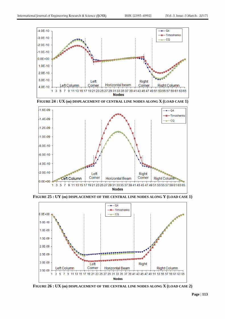
International Journal of Engineering Research & Science (IJOER) ISSN: [2395-6992] [Vol-3, Issue-3 March- 2017]
Page | 113
FIGURE 24 : UX (m) DISPLACEMENT OF CENTRAL LINE NODES ALONG X (LOAD CASE 1)
FIGURE 25 : UY (m) DISPLACEMENT OF THE CENTRAL LINE NODES ALONG Y (LOAD CASE 1)
FIGURE 26 : UX (m) DISPLACEMENT OF THE CENTRAL LINE NODES ALONG X (LOAD CASE 2)

International Journal of Engineering Research & Science (IJOER) ISSN: [2395-6992] [Vol-3, Issue-3 March- 2017]
Page | 114
FIGURE 27 : UY (m) DISPLACEMENT OF THE CENTRAL LINE NODES ALONG Y (LOAD CASE 2)
The graphs show that the results of the CQ model are very close to those of the Q4 model. Table 2 shows the results of both
models for both load cases. The last column gives the node number corresponding to the highest error value Emax.
TABLE 2
COMPARISON OF BOTH MODELS AND ALL LOAD CASES
Load case
Displacement UR (m) [Q4]
Model UC (m) Emax Node number
( Emax) 1 UX 2.8613E-10 Timoshenko 1.9284E-10 16.28% 14 or 52 1 UY -1.1149E-09 Timoshenko -1.5148E-09 35.87% 33 2 UX 2.3397E-09 Timoshenko 2.7944E-09 18.19% 36 or 37 2 UY 2.7866E-10 Timoshenko 1.645E-10 30.38% 39 1 UX -2.7536E-10 CQ -2.6053E-10 2.59% 15 or 51 1 UY -3.1495E-10 CQ -3.3374E-10 1.69% 17 or 49 2 UX 2.3947E-09 CQ 2.4623E-09 2.70% 28 2 UY 9.7806E-11 CQ 8.2391E-11 4.10% 25
It can be said from the previous table, that the CQ model produces the best approximation to the Q4 model.
VI. SECOND IMPROVED MODEL: RIGID INTERFACE EVERYWHERE (RQ)
In this paragraph, we propose a linear finite element to replace Timoshenko beams in the vertical and horizontal beams. This
new element is constructed using the same procedure for the corner elements as in the previous paragraph.
Consider a strip in the beam that is between two consecutive nodes of the midline (see next figure).
UX1
UY1
RZ1
UX2
UY2
RZ2
a
b
0.02 m
FIGURE 28: RQ ELEMENT

International Journal of Engineering Research & Science (IJOER) ISSN: [2395-6992] [Vol-3, Issue-3 March- 2017]
Page | 115
The total length of this element is 0.02 m (from bottom to top). The thickness (along z direction) is always 0.02 m. a = b =
0.045/16 = 0.0028125 m.
The element is discretized in 8 Q4 elements along its length. Therefore, we have a total of 9 nodes and 18 DOF for each
interface.
We will assume that plane sections of beams in bending (Timoshenko hypothesis), displacements of nodes that are in the
same cut-section are displacements of a rigid body, given by 3 DOFs:
UX = Displacement along the X axis of the center of the section
UY = Displacement along the Y axis of the center of the section
RZ = Rotation around the Z axis
Therefore, the displacements of all the nodes of this element are given by 6 DOFs; 3 DOFs for the left cut-section and 3
DOFs for the right cut-section. This will give us the elementary stiffness matrix ke(6,6). In order to determine ke(6,6), we
know that the stiffness matrix for one Q4 element is given by:
The global matrix is K(36,36).
The matrix of the rigid interface is given by:
R=[
1 0 4*b 0 0 0
0 1 0 0 0 0
0 0 0 1 0 4*b
0 0 0 0 1 0
1 0 3*b 0 0 0
0 1 0 0 0 0
0 0 0 1 0 3*b
0 0 0 0 1 0
1 0 2*b 0 0 0
0 1 0 0 0 0
0 0 0 1 0 2*b
0 0 0 0 1 0
1 0 1*b 0 0 0
0 1 0 0 0 0
0 0 0 1 0 1*b
0 0 0 0 1 0
1 0 0 0 0 0
0 1 0 0 0 0
0 0 0 1 0 0
0 0 0 0 1 0
1 0 -1*b 0 0 0
0 1 0 0 0 0
0 0 0 1 0 -1*b
0 0 0 0 1 0
1 0 -2*b 0 0 0
0 1 0 0 0 0
0 0 0 1 0 -2*b
0 0 0 0 1 0
1 0 -3*b 0 0 0
0 1 0 0 0 0
0 0 0 1 0 -3*b
0 0 0 0 1 0
1 0 -4*b 0 0 0
0 1 0 0 0 0
0 0 0 1 0 -4*b
0 0 0 0 1 0 ]
Therefore, K = LT×Kc×L. (Kc is the condensed matrix). We obtain:

International Journal of Engineering Research & Science (IJOER) ISSN: [2395-6992] [Vol-3, Issue-3 March- 2017]
Page | 116
k=E*t/(v^2-1)*b/a*[
-8, 0, 0, 8, 0, 0
0, 4*v-4, 2*a*(v-1), 0, -4*v+4, 2*a*(v-1)
0,2*a*(v-1),-128/3*b^2-4/3*a^2+4/3*a^2*v, 0,-2*a*(v-1), 128/3*b^2-2/3*a^2+2/3*a^2*v
8, 0, 0,-8, 0, 0
0, -4*v+4, -2*a*(v-1), 0, 4*v-4, -2*a*(v-1)
0,2*a*(v-1), 128/3*b^2-2/3*a^2+2/3*a^2*v, 0,-2*a*(v-1),-128/3*b^2-4/3*a^2+4/3*a^2*v]
Our new modeling is shown in the next figure:
RQ element
made from 8
Q4 elements
CQ element
A B
C D
O
O’
RQ element
made from 8
Q4 elements
H
H’
FIGURE 29: RQ MODEL FOR THE HORIZONTAL AND VERTICAL BEAMS WHILE CQ ELEMENT AT THE CORNERS
HO and O’H’ are beam elements formed from 8 Q4 elements. OO’ is a corner element.
The following graphs show the displacements along X and Y, for the two load cases for all the models that we have
considered so far (Q4, Timoshenko, CQ, and RQ):
FIGURE 30 : UX (m) DISPLACEMENT OF THE CENTRAL LINE NODES ALONG X (LOAD CASE 1)

International Journal of Engineering Research & Science (IJOER) ISSN: [2395-6992] [Vol-3, Issue-3 March- 2017]
Page | 117
FIGURE 31 : UY (m) DISPLACEMENT OF THE CENTRAL LINE NODES ALONG Y (LOAD CASE 1)
FIGURE 32: UX (m) DISPLACEMENT OF THE CENTRAL LINE NODES ALONG X (LOAD CASE 2)
FIGURE 33 : UY (m) DISPLACEMENT OF THE CENTRAL LINE NODES ALONG Y (LOAD CASE 2)

International Journal of Engineering Research & Science (IJOER) ISSN: [2395-6992] [Vol-3, Issue-3 March- 2017]
Page | 118
VII. FOURTH IMPROVED MODEL (RQw)
The graphs of the previous paragraph show that the RQ model is a little stiffer than the CQ model. In order to give it a certain
flexibility, we will add two DOFs (warping) for every node of the previous paragraph:
A new element is constructed from the RQ model that allows a plane section of a beam to deform a cubic or quadratic
deformation after solicitation. Therefore, two DOFs will be added on each node:
A warping (in terms of y2) that allows a quadratic displacement of the plane section and another warping term (in terms of y
3)
that allows a cubic displacement of the plane section. The following figure illustrates the 5 DOFs on each node for the new
element.
1st DOF
Translation UX
2nd DOF
Translation UY
3rd DOF
Rotation RZ
4th DOF
Warp y2
5th DOF
Warp y3
FIGURE 34: THE 5 DOFS FOR THE RQW MODEL
For this element with 5 DOFs per node we expect a stiffness matrix k(10,10). The terms of the 4th
and 5th
degree of the
stiffness degree are calculated as follows:
We find the global matrix K(36,36), then matrix L of the rigid link:
L=[
1 0 4*b -16*b^2 64*b^3 0 0 0 0 0
0 1 0 0 0 0 0 0 0 0
0 0 0 0 0 1 0 4*b -16*b^2 64*b^3
0 0 0 0 0 0 1 0 0 0
1 0 3*b -9*b^2 27*b^3 0 0 0 0 0
0 1 0 0 0 0 0 0 0 0
0 0 0 0 0 1 0 3*b -9*b^2 27*b^3
0 0 0 0 0 0 1 0 0 0
1 0 2*b -4*b^2 8*b^3 0 0 0 0 0
0 1 0 0 0 0 0 0 0 0
0 0 0 0 0 1 0 2*b -4*b^2 8*b^3
0 0 0 0 0 0 1 0 0 0
1 0 1*b -1*b^2 1*b^3 0 0 0 0 0
0 1 0 0 0 0 0 0 0 0
0 0 0 0 0 1 0 1*b -1*b^2 1*b^3
0 0 0 0 0 0 1 0 0 0
1 0 0 0 0 0 0 0 0 0
0 1 0 0 0 0 0 0 0 0
0 0 0 0 0 1 0 0 0 0
0 0 0 0 0 0 1 0 0 0
1 0 -1*b -1*b^2 -1*b^3 0 0 0 0 0
0 1 0 0 0 0 0 0 0 0
0 0 0 0 0 1 0 -1*b -1*b^2 -1*b^3
0 0 0 0 0 0 1 0 0 0
1 0 -2*b -4*b^2 -8*b^3 0 0 0 0 0
0 1 0 0 0 0 0 0 0 0
0 0 0 0 0 1 0 -2*b -4*b^2 -8*b^3
0 0 0 0 0 0 1 0 0 0
1 0 -3*b -9*b^2 -27*b^3 0 0 0 0 0
0 1 0 0 0 0 0 0 0 0
0 0 0 0 0 1 0 -3*b -9*b^2 -27*b^3
0 0 0 0 0 0 1 0 0 0
1 0 -4*b -16*b^2 -64*b^3 0 0 0 0 0
0 1 0 0 0 0 0 0 0 0
0 0 0 0 0 1 0 -4*b -16*b^2 -64*b^3
0 0 0 0 0 0 1 0 0 0 ];

International Journal of Engineering Research & Science (IJOER) ISSN: [2395-6992] [Vol-3, Issue-3 March- 2017]
Page | 119
We can find:
k = LT*K*L
the stiffness matrix k for the left corner with (warp) is given numerically by:
kleft =
4.6660e+009 1.5022e+009 -5.2058e+006 -7.3236e+004 -4.3907e+002 -4.6660e+009 -1.5022e+009 -2.6432e+007 2.5186e+005 -1.8964e+003
1.5022e+009 4.6660e+009 2.6432e+007 -2.5186e+005 1.8964e+003 -1.5022e+009 -4.6660e+009 5.2058e+006 7.3236e+004 4.3907e+002
-5.2058e+006 2.6432e+007 3.7398e+005 -1.6755e+003 2.7583e+001 5.2058e+006 -2.6432e+007 -5.7599e+004 -1.1072e+002 -4.2280e+000
-7.3236e+004 -2.5186e+005 -1.6755e+003 2.8150e+001 -1.2750e-001 7.3236e+004 2.5186e+005 -1.1072e+002 -4.7061e+000 8.7138e-005
-4.3907e+002 1.8964e+003 2.7583e+001 -1.2750e-001 2.6159e-003 4.3907e+002 -1.8964e+003 -4.2280e+000 8.7138e-005 -4.0191e-004
-4.6660e+009 -1.5022e+009 5.2058e+006 7.3236e+004 4.3907e+002 4.6660e+009 1.5022e+009 2.6432e+007 -2.5186e+005 1.8964e+003
-1.5022e+009 -4.6660e+009 -2.6432e+007 2.5186e+005 -1.8964e+003 1.5022e+009 4.6660e+009 -5.2058e+006 -7.3236e+004 -4.3907e+002
-2.6432e+007 5.2058e+006 -5.7599e+004 -1.1072e+002 -4.2280e+000 2.6432e+007 -5.2058e+006 3.7398e+005 -1.6755e+003 2.7583e+001
2.5186e+005 7.3236e+004 -1.1072e+002 -4.7061e+000 8.7138e-005 -2.5186e+005 -7.3236e+004 -1.6755e+003 2.8150e+001 -1.2750e-001
-1.8964e+003 4.3907e+002 -4.2280e+000 8.7138e-005 -4.0191e-004 1.8964e+003 -4.3907e+002 2.7583e+001 -1.2750e-001 2.6159e-003
With a simple transformation, we can find the stiffness matrix of the right corner of our structure:
kright =
4.6660e+009 -1.5022e+009 -5.2058e+006 -7.3236e+004 -4.3907e+002 -4.6660e+009 1.5022e+009 -2.6432e+007 2.5186e+005 -1.8964e+003
-1.5022e+009 4.6660e+009 -2.6432e+007 2.5186e+005 -1.8964e+003 1.5022e+009 -4.6660e+009 -5.2058e+006 -7.3236e+004 -4.3907e+002
-5.2058e+006 -2.6432e+007 3.7398e+005 -1.6755e+003 2.7583e+001 5.2058e+006 2.6432e+007 -5.7599e+004 -1.1072e+002 -4.2280e+000
-7.3236e+004 2.5186e+005 -1.6755e+003 2.8150e+001 -1.2750e-001 7.3236e+004 -2.5186e+005 -1.1072e+002 -4.7061e+000 8.7138e-005
-4.3907e+002 -1.8964e+003 2.7583e+001 -1.2750e-001 2.6159e-003 4.3907e+002 1.8964e+003 -4.2280e+000 8.7138e-005 -4.0191e-004
-4.6660e+009 1.5022e+009 5.2058e+006 7.3236e+004 4.3907e+002 4.6660e+009 -1.5022e+009 2.6432e+007 -2.5186e+005 1.8964e+003
1.5022e+009 -4.6660e+009 2.6432e+007 -2.5186e+005 1.8964e+003 -1.5022e+009 4.6660e+009 5.2058e+006 7.3236e+004 4.3907e+002
-2.6432e+007 -5.2058e+006 -5.7599e+004 -1.1072e+002 -4.2280e+000 2.6432e+007 5.2058e+006 3.7398e+005 -1.6755e+003 2.7583e+001
2.5186e+005 -7.3236e+004 -1.1072e+002 -4.7061e+000 8.7138e-005 -2.5186e+005 7.3236e+004 -1.6755e+003 2.8150e+001 -1.2750e-001
-1.8964e+003 -4.3907e+002 -4.2280e+000 8.7138e-005 -4.0191e-004 1.8964e+003 4.3907e+002 2.7583e+001 -1.2750e-001 2.6159e-003
The following figures show the displacements along X et Y, for both the load cases, for all models (Reference model: Q4
model, Timoshenko model, CQ model, RQ, model and RQw).
FIGURE 35: UX (m) DISPLACEMENT OF THE CENTRAL LINE NODES ALONG X (LOAD CASE 1)

International Journal of Engineering Research & Science (IJOER) ISSN: [2395-6992] [Vol-3, Issue-3 March- 2017]
Page | 120
FIGURE 36: UY (m) DISPLACEMENT OF THE CENTRAL LINE NODES ALONG Y (LOAD CASE 1)
FIGURE 37: UX (m) DISPLACEMENT OF THE CENTRAL LINE NODES ALONG X (LOAD CASE 2)
FIGURE 38: UY (m) DISPLACEMENT OF THE CENTRAL LINE NODES ALONG Y (LOAD CASE 2)

International Journal of Engineering Research & Science (IJOER) ISSN: [2395-6992] [Vol-3, Issue-3 March- 2017]
Page | 121
The previous graphs show that the RQw is more flexible than RQ, whereas CQ gives best results.
VIII. SUMMARY
The following table summarizes the results coming from all models:
TABLE 3
COMPARISON OF ALL MODELS AND ALL LOAD CASES
Model Node
(where E = Emax) Load case Displacement
Emax par rapport à H8
Emax par rapport à Q4
H8 15 ou 51 1 UX 0% 1.55% H8 33 1 UY 0% 1.90% H8 16 2 UX 0% 3.01% H8 39 2 UY 0% 2.92% Q4 15 ou 51 1 UX 1.55% 0% Q4 33 1 UY 1.90% 0% Q4 16 2 UX 3.01% 0% Q4 39 2 UY 2.92% 0%
Timoshenko 14 ou 52 1 UX 15.22% 16.28% Timoshenko 33 1 UY 38.45% 35.87% Timoshenko 36 ou 37 2 UX 21.48% 18.19% Timoshenko 38 ou 39 2 UY 28.44% 30.38%
CQ 15 ou 51 1 UX 1.52% 2.59% CQ 17 ou 49 1 UY 2.74% 1.69% CQ 28 2 UX 5.52% 2.70% CQ 25 2 UY 4.48% 4.10% RQ 14 ou 52 1 UX 6.30% 7.61% RQ 33 1 UY 7.71% 9.44% RQ 16 2 UX 6.48% 9.19% RQ 37 2 UY 8.72% 10.97% RQw 14 ou 52 1 UX 4.34% 5.71% RQw 33 1 UY 4.34% 5.37% RQw 17 2 UX 1.66% 4.52% RQw 36 2 UY 6.77% 7.84%
It is obvious that the CQ model gives best results when comparing with the Q4 model.
IX. CONCLUSION
Replacing the volumetric modeling of a simple frame by traditional 1-D elements leads to a weak simulation in static
analysis. It is found out that the problem arises from corner connections. Modeling these connections by rigid links produces
a stiff structure. Using CQ elements at the corners improves the results in the static analysis. Consequently, the number of
elements and the number of DOF of the finite element model are dramatically reduced from hundreds of thousands to merely
hundreds.
REFERENCES
[1] Alghamdi, S, “Dynamic stiffness matrix and load functions of Timoshenko beam using the transport matrix”, Computers and
Structures, 79 (2001) 1175-1185.
[2] Cook R. Concepts and applications of finite element analysis. 4th Edition. Wiley 2002.
[3] Craig R. Structural Dynamics – An introduction to computer methods. John Wiley & Sons 1981.
[4] Dohrmann CR, Key SW, Heinstein MW. “A method for connecting dissimilar finite element meshes in two dimensions”.
International Journal For Numerical Methods In Engineering 2000; 48 (5), pp. 655-678.
[5] Dohrmann CR, Key SW, Heinstein MW. “Methods for connecting dissimilar three-dimensional finite element meshes”. International
Journal For Numerical Methods In Engineering 2000; 47, pp. 1057-1080.
[6] Hoit M. Computer Assisted Structural Analysis and Modeling. Prentice-Hall 1995.
[7] Kassimali A. Structural Analysis. Second edition. Brooks/Cole 1999.
[8] Kattner M, Crisinel M. “Finite element modeling of semi-rigid composite joints”. Computers and Structures 2000; 78, pp. 341-353.
[9] Quiroz L, Beckers P. “Non-conforming mesh gluing in the finite elements method”. International Journal For Numerical Methods In
Engineering 1995; 38 (13), pp. 2165-2184.
[10] Rao S. Mechanical Vibrations. 4th Edition. Pearson Education 2004.

International Journal of Engineering Research & Science (IJOER) ISSN: [2395-6992] [Vol-3, Issue-3, March- 2017]
Page | 122
Preparation of activated carbon from orange peel and its
application for phenol removal Loriane Aparecida de Sousa Ribeiro
1, Liana Alvares Rodrigues
2*,
Gilmar Patrocínio Thim3
1,3Instituto Tecnológico de Aeronáutica-ITA/CTA, Praça Mal. Eduardo Gomes 50, CEP 12228-900, São José dos Campos,
São Paulo, Brazil. 2Departamento de Engenharia Química, Escola de Engenharia de Lorena-EEL/USP, Estrada Municipal do Campinho S/N,
CEP 12602-810, Lorena, São Paulo, Brazil
Abstract— Activated carbon obtained from orange peel (ACO) was used as a phenol adsorbent. ACO was characterized by
X-ray diffraction, Raman spectroscopy, scanning electronic microscopy (SEM) and energy dispersive spectroscopy (EDS).
The functional groups present on the sample, were determined by Boehm titration, and it was also determined the point of
zero charge (pHpzc). ACO is mainly constituted by micropores, and its structure is turbostratic and lamellar with inorganic
impurities. The Boehm titration indicated the basic behavior of the sample. The phenol optimum dosage was 0.1 g/50 cm3
which was determined by the adsorption study. The maximum adsorption level was in the pH range of 4-8 and its kinetics
was described by a pseudo second order model. The equilibrium data have fit very well the Langmuir and Sips isotherms
models.
Keywords— adsorption, agricultural waste, biomass, orange peel, phenol.
I. INTRODUCTION
Brazil is the largest producer of oranges in the world, and it is responsible for about 30% of the world production[1].
Basically, almost all Brazilian´s orange production is used to produce orange juice[2].The European Union is the major
consumer of orange juice, being 96% of it imported from Brazil[3]. The fruit is compounded of 50 % (w/w) of juice and
the other 50 % of peel, pulp, seeds and membranes[2,4], being its peel, the primary byproduct during the orange juice
processing[2]. Part of this waste material is used to produce pet food, fiber (pectin), fuel, essential oils, fertilizers, anti-
oxidizing compounds and adsorbents [2,5,6]. However, the major part of the fruit after juice production becomes litter and is
discarded to environment by juice industries [5]. Thus, changing the orange peel, which is a low cost agricultural waste, into
a useful material, such as adsorbents that can add value to this residue and contribute to the problem of biomass disposal[7].
The phenol molecules and phenol-constituted substances are essential for several industrial processes, such as: rubber, dye,
pharmaceutical and pesticide production and oil refining [8,9]. Nevertheless, their presence in water supply poses risks of
water quality degradation and aquatic life death, moreover, it can inhibit the microbial community normal activities and
cause carcinogenicity in animals [8,10]. Therefore, the discard of this kind of effluent is controlled by environmental offices
and the maximum concentration allowed to this effluent is 0.002 mg/L [11]. The industries responsible for phenol
contaminated effluent have to remove the phenol before discarding it in the environment in order to comply with the levels
demanded by environmental agencies [12].
There are several methods proposed to remove phenol from industrial effluent, such as: biological treatment, adsorption on
activated carbon, reverse osmosis, ionic exchange, solvent extraction, ultrasonic degradation and TiO2 oxidation [13].
Among these methods, the adsorption process is the cheapest, simplest and fastest one for phenol removal [12]. Activated
carbon is considered to be an effective method for phenol removal from contaminated effluents due to its elevated surface
area, microporosity, and high adsorption capacity [14]. Nonetheless, phenol adsorption is economically unfeasible due to its
elevated cost of production [7]. An alternative to reduce the activated carbon production cost is to use an abundant and low
cost carbon source, such as agricultural or industrial waste to produce it [15]. Activated carbon from orange peel has been
obtained with an elevated surface area and pore volume [16]. Consequently, activated carbon obtained from orange peel has
emerged as a potential alternative for activated carbon production.
The main objective of this paper is to study the adsorption process of phenol in the activated carbon obtained from the orange
peel. Its goal is to obtain a low cost activated carbon able to remove phenol from industrial effluent and concomitantly
enhance the value of an abundant biomass and solve its disposal problem.

International Journal of Engineering Research & Science (IJOER) ISSN: [2395-6992] [Vol-3, Issue-3, March- 2017]
Page | 123
II. METHODOLOGY
2.1 Synthesis of the activated carbon from orange peel (citrus sinensis)
The activated carbon was prepared following these seven steps:
1. Rinsing it with deionized water;
2. Drying it in an oven at 100 C until constant mass;
3. Milling and sieving it (4-8 mesh);
4. Carbonizing it in a tubular furnace under argon flow, from 25 C to 800 C at a heating rate of 30 C/min, which was
maintained at 1073K for 1 hour;
5. Turning off the argon flow and turning on CO2 at 100 cm3/min. Maintaining the samples under this condition for 3
hours;
6. Turning off the CO2 flow and turning on the argon at 100 cm3/min, switching off the heating system;
7. Milling and sieving it (325 mesh). Sample in this stage was called ACO.
2.2 Characterization
The point of zero charge (pHpzc) was determined using the methodology described in several papers [12,17,18]. ACO (0.05
g) was added to several flasks containing 25 cm3 of KNO3 (concentrations 10
-1 and 10
-2 M) solutions which the initial pH
values (pHi) were adjusted in the pH range of 2–8 using 0.1 M of HCl or NaOH. Then, the equilibrium was carried out in a
thermostatic linear shaker for 24 h at 298 K. The dispersions were then filtered and the final pH of the solutions (pH f) was
determined. The point of zero charge was found from a plot of (pHi − pHf) versus pHi. The Boehm method was used to
determine the amount of the oxygenated chemical groups [19], where one gram of ACO was placed in 25 cm3 of the
following aqueous solutions: sodium hydroxide, sodium carbonate, sodium ethoxide, sodium bicarbonate and hydrochloric
acid. The vials were sealed, shaken for 24hs and then filtered. The filtrate was titrated with HCl or NaOH to determine the
base or acid excess, respectively.
The sample morphology was observed in a Scanning Electron Microscope (SEM), Zeiss model EVO MA 10. Energy
dispersive spectroscopy (EDS) measurements were carried out in an Oxford INCA Energy Microanalysis System which was
incorporated to SEM. Raman spectroscopy was carried out in a Renishaw 2000 equipment using ionic laser of Ar+ (=514.5
nm). Powders were analyzed in a X ray diffraction equipment, using a PANalytical X’Pert PRO MPD 3060 diffractometer,
equipped with a X’celerator detector, operating at 45 kV and 25 mA with CuK radiation. XRD patterns were collected in
the 2 range from 10 to 90º at scan speed of 0.42 º s-1
and step size of 0.017°.
2.3 Adsorption study
Adsorption studies were carried out in amber glass flasks of 100 cm3, where ACO was mixed to a phenol aqueous solution
(50 cm3), being stirred in a thermostatic shaker. The supernatant solution was separated from the adsorbent by filtration. The
phenol concentration in the supernatant was spectrophotometrically determined using UV–VIS absorbance
spectrophotometery at 269 nm [20]. Solutions, with higher concentration than the ones detected by the spectrophotometer,
were determined by dilution. Adsorption kinetics was performed using 0.1 g of ACO, in a period from 0 to 24 hours, without
adjusting its pH, 25 C and a phenol initial concentration of 1000 mg/dm3. The pH effect was carried out using 0.1 g of ACO,
during 3hs, with a pH range between 2 and 12, at a temperature of 25 C and a phenol initial concentration of 1000 mg/dm3.
Dosage effect was accomplished using ACO mass range between 0.1 and 0.5 g, bath time of 3 hours, without adjusting its
pH, at a temperature of 25 C and a phenol initial concentration of 1000 mg/dm3. The isotherm adsorption was obtained
using 0.1 g of ACO, bath time of 3 hours, without adjusting its pH, at a temperature of 25 C and phenol initial concentration
ranging from 50 to 1000 mg/L.
III. RESULTS AND DISCUSSION
3.1 Characterization
The pHPZC is the pH in which the surface charge of a material is zero. The surface of an amphoretic material is positively
charged if the medium pH is lower than pHPZC. On the other hand, it is negatively charged if the medium pH is higher than
pHPZC [7]. The pHPZC of ACO is 10.5, indicating a basic character in water.
The number of basic sites on the ACO surface was determined from the amount of hydrochloric acid that reacted with the
activated carbon. The number of acid sites was determined under the following assumptions: a) there are only carboxylic,
lactonic, phenolic and carbonyl groups on ACO, b) NaOH neutralizes the carboxylic, lactonic and phenolic groups; c)

International Journal of Engineering Research & Science (IJOER) ISSN: [2395-6992] [Vol-3, Issue-3, March- 2017]
Page | 124
Na2CO3 neutralizes the carboxylic and lactonic groups; d) NaHCO3 neutralizes only the carboxylic groups; and e) NaOC2H5
neutralizes the carbonyl (quinoid-type), carboxylic, lactonic and phenolic groups. This procedure is called Boehm titration
and is described in several papers [7,19]. Table 1 shows the amount of acid and basic groups present on the ACO surface.
The amount of basic groups (3.38) is higher than the acid groups (1.19). Therefore, the sample is predominantly basic.
TABLE 1
SURFACE FUNCTIONAL GROUPS FOR ACO
Acid sites
Basic sites
(mmol g-1
) Carboxyl
(mmol g-1
) Lactones (mmol g
-1)
Phenols
(mmol g-1
)
Carbonyl (quinoid-type)
(mmol g-1
)
0.00
0.00 1.19 0.00 3.38
Fig. 1 shows the Raman spectrum of ACO sample, which shows peaks centered at 1361 and 1583 cm-1
. These peaks are
attributed to the D band (1200-1400 cm-1
) and G band (1500-1600 cm-1
), respectively [22].
FIGURE 1. RAMAN PROFILE OF THE ACO SAMPLE FIGURE 2. X RAY DIFFRACTOGRAM OF THE ACO
SAMPLE
A Gaussian deconvolution method was used to obtain the half width of band G (100.5 cm-1
), which is much higher than the
graphite value (15-23 cm-1
), indicating that the crystallinity of the ACO sample is much lower than the graphite [23]. The
value of the average lateral sizes (La), calculated from Raman data by using Equation 1 [23], is 2.42 nm.
( ) Ga L
D
IL C
I (1)
In equation 1, ID and IG are areas of D band and G band, respectively, and C(L)=Co+LC1. Where, Co is equal to -12.6 nm;
L is the wavelength and C1 is equal to 0.033.
Fig. 2 shows the X ray diffraction profile (XRD) of the ACO sample, where one can see broad peaks centered at 24.86 and
44.05 (2), which are associated to Muller index of (002) and (101) [24]. These peaks are characteristics of a turbostratic
structure of graphite micro crystallites and they mean that ACO has an intermediate structure between amorphous carbon and
graphite [23].
Using Gaussian deconvolution on XRD data, one could use the peak at 24.86 to estimate both the spacing of aromatic ring
layers (d002) and the crystallite thickness (Lc) [25]. However, the average lateral size (La-XRD) of the crystallites was
determined using the peak at (101) [25]. The d002 (0.352 nm) was calculated using Bragg’s law and the crystallite size Lc
(0.601 nm) and La-XRD (2.60 nm) were determined using Scherrer’s equation [25]. The value of d002 (0.352 nm) was higher
than the one of pure graphite (0.336-0.337 nm), due to a lower crystalline degree of the ACO sample in relation to the
graphite [23]. It can be observed several sharp and less intense peaks besides peaks at 24.86 and 44.05 (2), which may be
related to inorganic materials that were already present in the biomass. Comparing the value of La previously determined by

International Journal of Engineering Research & Science (IJOER) ISSN: [2395-6992] [Vol-3, Issue-3, March- 2017]
Page | 125
Raman spectroscopy (2.42) with that determined by XRD (2.60), it can be concluded that they are very close. Nevertheless,
the La determination by XRD is considered much more accurate than the Raman spectroscopy one [23].
The morphology of the ACO sample can be observed in Fig. 3A and 3B.
(A)
(B)
FIGURE 3. SEM IMAGES OF THE ACO AT DIFFERENT ENLARGEMENTS
These Figures show that the particles are non-uniform, i.e. without a predominant form. In addition, Fig. 3B shows that the
ACO has a lamellar structure.
Energy dispersive spectroscopy (EDS) was used to determine the chemical composition of the ACO sample and its results
are shown in Table 2.
TABLE 2
RESULTS OF ENERGY DISPERSIVE SPECTROSCOPY (EDS) MEASUREMENTS
Element
C O Mg P S Cl K Ca Fe
% Weight 65.0 18.0 0.4 1.2 0.5 0.2 7.8 6.6 0.3
% Atomic 77.5 16.0 0.3 0.5 0.2 0.1 2.9 2.4 0.1
This table shows that the ACO is constituted of several elements, such as: magnesium, phosphorus, surfer, chlorine,
potassium, calcium, and iron. According to [26] and [27], most of these elements are a characteristic of the orange peel
composition. The concentration of potassium (2.9 %) and calcium (2.4 %) is much higher than the others, but their
concentrations are considered normal in Brazilian oranges. The presence of oxygen is an indication that the ACO had a lot of
oxygenated groups on its surface.
3.2 Adsorption
The kinetic data of phenol adsorption onto the ACO are shown in Fig. 4.
FIGURE 4. CONTACT TIME EFFECT ON ADSORBED PHENOL CONCENTRATION

International Journal of Engineering Research & Science (IJOER) ISSN: [2395-6992] [Vol-3, Issue-3, March- 2017]
Page | 126
For the ACO, the contact time of 3 hs is needed to establish the phenol adsorption equilibrium. At this stage, the adsorbed
phenol amount is 88 mg g-1
, i.e. 19 % of the initial amount. The kinetic data were fitted using pseudo first-order and pseudo
second-order kinetic models [28]. The kinetic results are shown in Table 3. It can be observed from Table 3 that the
correlation coefficient (R2) for pseudo first-order kinetic model (0.88) was much lower than R
2 for the pseudo-second order
model (1.00), indicating that the kinetic of adsorption process is more accurately represented by the pseudo second-order
kinetic model. In addition, the comparison between the equilibrium concentration obtained from Fig. 4 (qe = 88 mg g-1
) and
that one from pseudo-first order (qe = 23.60 mg g-1
) and from pseudo-second order (qe = 87.64 mg g-1
) reinforces that the
adsorption kinetic process of phenol onto the ACO can be described by a pseudo-second order model.
TABLE 3
KINETIC PARAMETERS OF PHENOL ADSORPTION ON THE ACO
C0
(mg L-1
)
Pseudo first-order Pseudo second-order
K1
(h-1
)
qe
(mg g-1
) R
2 K2
(h-1
)
qe
(mg g-1
) R
2
1000 0.92 23.60 0.88 0.11 87.64 1.00
Fig. 5 shows the adsorption percentage (%) and adsorption capacity (qe) of the phenol as a function of the ACO dosage,
where the ACO dosage ranged from 0.01 to 0.5 g.
FIGURE 5. EFFECT OF ADSORBENT DOSE ON THE ADSORPTION OF PHENOL ONTO THE ACO
It can be observed that the phenol removal (%) and the phenol adsorption capacity (qe) depend strongly on the ACO dosage.
However, these two properties have distinct dependence on the ACO dosage, i.e. the removal efficiency increased with the
dosage while the adsorption capacity decreased. The former may happen due to an increase in the adsorption sites with an
increase in the ACO dosage [29]. Nevertheless, a higher adsorbent dose results in a lower adsorption capacity due to
overcrowding of adsorbent particles, resulting in a decrease in the availability of adsorption sites [7]. In order to carry out
further studies we have to choose a “work dosage”, in which both the equilibrium concentration and the removal amount
have meaningful values. Consequently, in the next studies, an ACO dosage of 0.1 mg g-1
will be used.
The effect of pH on phenol adsorption is showed in Fig. 6.
FIGURE 6. EFFECT OF SOLUTION PH ON THE ADSORPTION OF PHENOL ONTO THE ACO
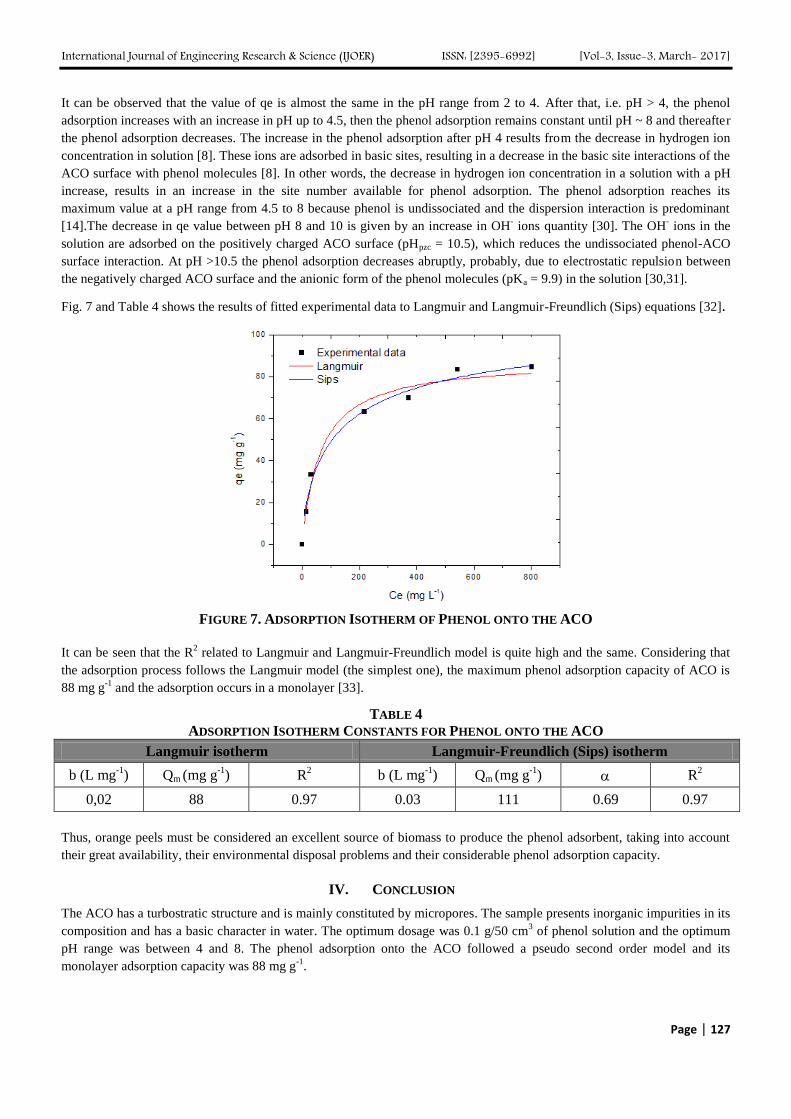
International Journal of Engineering Research & Science (IJOER) ISSN: [2395-6992] [Vol-3, Issue-3, March- 2017]
Page | 127
It can be observed that the value of qe is almost the same in the pH range from 2 to 4. After that, i.e. pH > 4, the phenol
adsorption increases with an increase in pH up to 4.5, then the phenol adsorption remains constant until pH ~ 8 and thereafter
the phenol adsorption decreases. The increase in the phenol adsorption after pH 4 results from the decrease in hydrogen ion
concentration in solution [8]. These ions are adsorbed in basic sites, resulting in a decrease in the basic site interactions of the
ACO surface with phenol molecules [8]. In other words, the decrease in hydrogen ion concentration in a solution with a pH
increase, results in an increase in the site number available for phenol adsorption. The phenol adsorption reaches its
maximum value at a pH range from 4.5 to 8 because phenol is undissociated and the dispersion interaction is predominant
[14].The decrease in qe value between pH 8 and 10 is given by an increase in OH- ions quantity [30]. The OH
- ions in the
solution are adsorbed on the positively charged ACO surface (pHpzc = 10.5), which reduces the undissociated phenol-ACO
surface interaction. At pH >10.5 the phenol adsorption decreases abruptly, probably, due to electrostatic repulsion between
the negatively charged ACO surface and the anionic form of the phenol molecules (pKa = 9.9) in the solution [30,31].
Fig. 7 and Table 4 shows the results of fitted experimental data to Langmuir and Langmuir-Freundlich (Sips) equations [32].
FIGURE 7. ADSORPTION ISOTHERM OF PHENOL ONTO THE ACO
It can be seen that the R2 related to Langmuir and Langmuir-Freundlich model is quite high and the same. Considering that
the adsorption process follows the Langmuir model (the simplest one), the maximum phenol adsorption capacity of ACO is
88 mg g-1
and the adsorption occurs in a monolayer [33].
TABLE 4
ADSORPTION ISOTHERM CONSTANTS FOR PHENOL ONTO THE ACO
Langmuir isotherm Langmuir-Freundlich (Sips) isotherm
b (L mg-1
) Qm (mg g-1
) R2
b (L mg-1
) Qm (mg g-1
) R2
0,02 88 0.97 0.03 111 0.69 0.97
Thus, orange peels must be considered an excellent source of biomass to produce the phenol adsorbent, taking into account
their great availability, their environmental disposal problems and their considerable phenol adsorption capacity.
IV. CONCLUSION
The ACO has a turbostratic structure and is mainly constituted by micropores. The sample presents inorganic impurities in its
composition and has a basic character in water. The optimum dosage was 0.1 g/50 cm3 of phenol solution and the optimum
pH range was between 4 and 8. The phenol adsorption onto the ACO followed a pseudo second order model and its
monolayer adsorption capacity was 88 mg g-1
.

International Journal of Engineering Research & Science (IJOER) ISSN: [2395-6992] [Vol-3, Issue-3, March- 2017]
Page | 128
ACKNOWLEDGEMENTS
The authors gratefully acknowledge CNPq, Fapesp andCAPES for financial support.
REFERENCES
[1] J.J.T. Gama, C.M. Sylos, Major carotenoid composition of Brazilian Valencia orange juice: Identification and quantification by
HPLC, Food Res. Int. 38 (2005) 899–903.
[2] H.R.M. Barros, T.A.P.C. Ferreira, M.I. Genovese, Antioxidant capacity and mineral content of pulp and peel from commercial
cultivars of citrus from Brazil, Food Chem. 134 (2012) 1892–1898.
[3] M.T.P.S. Clerici, Nutritional bioactive compounds and technological aspects of minor fruits grown in Brazil, Food Res. Int. 44
(2011) 1658–1670.
[4] L.D. Fiorentin, B.T. Menon, S.T.D. Barros, N.C. Pereira, O.C.M. Lima, A.N. Modenes, Isotermas de sorção do resíduo
agroindustrial bagaço de laranja, Rev. Bras. Eng. Agrícola E Ambient. 14 (2010) 653–659.
[5] A.M. Alexandrino, H.G. De Faria, C. Giatti, M. De Souza, R.M. Peralta, Aproveitamento do resíduo de laranja para a produção de
enzimas lignocelulolíticas por Pleurotus ostreatus ( Jack : Fr ), Ciência E Tecnol. Aliment. 27 (2007) 364–368.
[6] M.E.R. Cantu, Journal of Analytical and Applied Pyrolysis Pyrolysis of sweet orange ( Citrus sinensis ) dry peel, 86 (2009) 245–251.
[7] L.A. Rodrigues, M.L.C.P. da Silva, M.O. Alvarez-Mendes, A.R. Coutinho, G.P. Thim, Phenol removal from aqueous solution by
activated carbon produced from avocado kernel seeds, Chem. Eng. J. 174 (2011) 49–57.
[8] Q.-S. Liu, T. Zheng, P. Wang, J.-P. Jiang, N. Li, Adsorption isotherm, kinetic and mechanism studies of some substituted phenols on
activated carbon fibers, Chem. Eng. J. 157 (2010) 348–356.
[9] L.A. Rodrigues, T.M.B. Campos, M.O. Alvarez-Mendes, A.R. Coutinho, K.K. Sakane, G.P. Thim, Phenol removal from aqueous
solution by carbon xerogel, J. Sol-Gel Sci. Technol. (2012).
[10] K. Lin, J. Pan, Y. Chen, R. Cheng, X. Xu, Study the adsorption of phenol from aqueous solution on hydroxyapatite nanopowders., J.
Hazard. Mater. 161 (2009) 231–40.
[11] X. Zeng, Y. Fan, G. Wu, C. Wang, R. Shi, Enhanced adsorption of phenol from water by a novel polar post-crosslinked polymeric
adsorbent., J. Hazard. Mater. 169 (2009) 1022–8.
[12] L.A. Rodrigues, L.A. Sousa Ribeiro, G.P. Thim, R.R. Ferreira, M.O. Alvarez-Mendez, A.D.R. Coutinho, Activated carbon derived
from macadamia nut shells: an effective adsorbent for phenol removal, J. Porous Mater. (2012).
[13] G. Dursun, H. Ciçek, A.Y. Dursun, Adsorption of phenol from aqueous solution by using carbonised beet pulp., J. Hazard. Mater.
125 (2005) 175–82.
[14] B.H. Hameed, a a Rahman, Removal of phenol from aqueous solutions by adsorption onto activated carbon prepared from biomass
material., J. Hazard. Mater. 160 (2008) 576–81.
[15] A. Bhatnagar, M. Sillanpää, Utilization of agro-industrial and municipal waste materials as potential adsorbents for water
treatment—A review, Chem. Eng. J. 157 (2010) 277–296.
[16] J.C. Moreno-Piraján, L. Giraldo, Heavy Metal Ions Adsorption from Wastewater Using Activated Carbon from Orange Peel, E-
Journal Chem. 9 (2012) 926–937.
[17] L. Wang, J. Zhang, A. Wang, Removal of methylene blue from aqueous solution using chitosan-g-poly(acrylic acid)/montmorillonite
superadsorbent nanocomposite, Colloids Surfaces A Physicochem. Eng. Asp. 322 (2008) 47–53.
[18] L.A. Rodrigues, L.J. Maschio, R.E. da Silva, M.L.C.P. da Silva, Adsorption of Cr(VI) from aqueous solution by hydrous zirconium
oxide., J. Hazard. Mater. 173 (2010) 630–6.
[19] H. Boehm, Some aspects of the surface chemistry of carbon blacks and other carbons, Carbon N. Y. 32 (1994) 759–769.
[20] L. Zhu, Y. Deng, J. Zhang, J. Chen, Adsorption of phenol from water by N-butylimidazolium functionalized strongly basic anion
exchange resin., J. Colloid Interface Sci. 364 (2011) 462–8.
[21] K.S.W. Sing, D.H. Everett, R.A.W. Haul, L. Moscou, R.A. Pierotti, J. Rouquérol, T. Siemieniewska, Reporting physisorption data
for gas/solid systems with special reference to the determination of surface area and porosity (Recommendations 1984), Pure Appl.
Chem. 57 (1985) 603–619.
[22] C.M.L. Barbosa, M.T.C. Sansiviero, Decomposição térmica de complexos de Zn e Cd com isomaleonitriladitiolato (imnt), Quim.
Nova. 28 (2005) 761–765.
[23] O.O. Sonibare, T. Haeger, S.F. Foley, Structural characterization of Nigerian coals by X-ray diffraction, Raman and FTIR
spectroscopy, Energy. 35 (2010) 5347–5353.
[24] S.-S. Tzeng, K.-H. Hung, T.-H. Ko, Growth of carbon nanofibers on activated carbon fiber fabrics, Carbon N. Y. 44 (2006) 859–865.
[25] D. Li, H. Wang, X. Wang, Effect of microstructure on the modulus of PAN-based carbon fibers during high temperature treatment
and hot stretching graphitization, J. Mater. Sci. 42 (2007) 4642–4649.
[26] A. K. Bejar, N. B. Mihoubi, N. Kechaou, Moisture sorption isotherms – Experimental and mathematical investigations of orange
(Citrus sinensis) peel and leaves, Food Chem. 132 (2012) 1728–1735.
[27] A.U. Mahmood, J. Greenman, A.H. Scragg, Orange and potato peel extracts: Analysis and use as Bacillus substrates for the
production of extracellular enzymes in continuous culture, Enzyme Microb. Technol. 22 (1998) 130–137.
[28] L.A. Rodrigues, M.L.C.P. da Silva, Thermodynamic and kinetic investigations of phosphate adsorption onto hydrous niobium oxide
prepared by homogeneous solution method, Desalination. 263 (2010) 29–35.

International Journal of Engineering Research & Science (IJOER) ISSN: [2395-6992] [Vol-3, Issue-3, March- 2017]
Page | 129
[29] A. Shukla, Y.-H. Zhang, P. Dubey, J.L. Margrave, S.S. Shukla, The role of sawdust in the removal of unwanted materials from
water., J. Hazard. Mater. 95 (2002) 137–52.
[30] H.B. Senturk, D. Ozdes, A. Gundogdu, C. Duran, M. Soylak, Removal of phenol from aqueous solutions by adsorption onto
organomodified Tirebolu bentonite: equilibrium, kinetic and thermodynamic study., J. Hazard. Mater. 172 (2009) 353–62.
[31] M.H. El-Naas, S. a Al-Muhtaseb, S. Makhlouf, Biodegradation of phenol by Pseudomonas putida immobilized in polyvinyl alcohol
(PVA) gel., J. Hazard. Mater. 164 (2009) 720–5.
[32] V.V.S. Guilarduci, J.P. Mesquita, P.B. Martelli, H.F. Gorgulho, Adsorção de fenol sobre carvão ativado em meio alcalino, Quim.
Nova. 29 (2006) 1226–1232.
[33] L.A. Rodrigues, M.L.C.P. Silva, Adsorption kinetic, thermodynamic and desorption studies of phosphate onto hydrous niobium
oxide prepared by reverse microemulsion method, Adsorption. 16 (2010) 173–181.

International Journal of Engineering Research & Science (IJOER) ISSN: [2395-6992] [Vol-3, Issue-3, March- 2017]
Page | 130
Mechanical properties of thermoset-metal composite prepared
under different process conditions Gean Vitor Salmoria
1*, Felix Yañez-Villamizar
2, Aurelio Sabino-Netto
3
CIMJECT, Department of Mechanical Engineering, Federal University of Santa Catarina, 88040-900 Florianopolis, Santa
Catarina, Brazil
Abstract— This paper reports a study on the morphology and mechanical behavior of a thermoset-metal composite used in
prototype molds as a function of the process conditions. The investigation of the mechanical properties of epoxy-aluminum
specimens post-cured using different routines showed that they are related to the self-controlled diffusion characteristic of
thermoset polymeric systems. A high-temperature post-cure routine resulted in higher values for the modulus, stiffness and
glass transition temperature, Tg, for the specimens. The fracture surfaces analysis showed the presence of defects, which
appeared as empty spaces in the epoxy matrix, due to the mixing and casting process. The defect size and the specimen
strength showed a direct correlation. The Weibull modulus was 7.95 for the epoxy specimens characterizing low toughness
and the presence of defects in the material, as revealed by fractography. The probability of failure increased rapidly to 50%
for applied stress greater than 38 MPa.
Keywords— Thermoset-metal, mechanical properties, process conditions.
I. INTRODUCTION
Thermoset resin curing permits the rapid manufacturing of parts and objects by casting. The main applications of thermoset
curing are the production of prototypes and parts used in the automobile, electrical, biomedical and aerospace industries.
Thermoset curing is also applied in the manufacture of functional prototypes, such as prototype tools [1-7]. The thermal and
mechanical properties are of great importance for prototype tools such as molds for the injection of thermoplastics, since
these tools are subjected to particular work conditions, with temperature variations and mechanical requirements [7-12].
The mechanical properties of parts or tools manufactured by thermoset curing are dependent on the degree of cure of the
resin. Manufacturing parameters, such as mixing, curing, post-curing and resin characteristics (monomers, oligomers and
curing agent composition), maximum density of cross-linking, photosensitivity, rate and degree of cure, and post-cure
method are very important in relation to the structure and properties of the part or tool [10-17]. Knowledge of the relationship
between the thermoset resin structure and properties is useful in the manufacturing process, application and quality control of
tools. Prototype molds with molding blocks produced by thermoset polymer resins have low mechanical properties compared
to conventional steel tools. Prototype molds produced by casting of a thermoset-metal composite are commonly used to
produce a small series of polymeric parts [5, 7 12, 14-17]. During injection molding, the mold is subjected to several types of
loading, either static or dynamic. This means that the composite in the molding blocks needs to have good mechanical
performance to avoid premature failure of the prototype mold. This paper reports a study on the morphology and mechanical
behavior of an epoxy-aluminum composite used in prototype molds as a function of the post-cure process conditions.
II. MATERIALS AND METHODS
2.1 Materials
An epoxy polymer containing 30% aluminum by weight, supplied by Hunstman as RenCast 436, was mixed with the
appropriate curing agent, Ren HY 150, obtained from the same company. The material is an epoxy system base in bisphenol
A and phenol novolac derivatives.
2.2 Mixture Procedure
In order to determine the effect of the post-cure process on the mechanical properties of the epoxy-aluminum composite, the
mixture of epoxy pre-polymer with aluminum particles and curing agent was prepared applying mechanical stirring (85 rpm)
for 2 min at 20 mmHg. The mixture was poured into silicone rubber models to fabricate the test specimens.

International Journal of Engineering Research & Science (IJOER) ISSN: [2395-6992] [Vol-3, Issue-3, March- 2017]
Page | 131
2.3 Cure and Post-cure Procedure
Experiments were carried out to evaluate the influence of the post-cure on the tensile strength and the dynamic mechanical
properties of the material. Specimens were cured at room temperature for 24 h, according to the procedure suggested by the
supplier, and post-cured in a conventional thermal oven using the post-cure routines shown in Table 1.
TABLE 1
POST-CURE ROUTINES APPLIED TO THE CASTING EPOXY SPECIMENS
Specimens Post-cure routine
A 2 h at 70ºC ; 2 h at 90ºC; 2 h at 120ºC; 2h at 150ºC
B 4 h at 90ºC ; 4 h at 150ºC
C 4 h at 70ºC ; 4 h at 150ºC
2.4 Tensile Tests
Tensile test specimens were obtained, according to the standard ASTM D638 type I, using the epoxy-aluminum composite.
Five specimens were tested for each post-cure cycle, at uniaxial tension and at room temperature, using an EMIC universal
testing machine with a displacement rate of 5mm/min. The Young’s modulus was determined through the stress–strain
correlation considering the linear region (Table 2). The strain was measured using an incremental extensometer.
2.5 Fractography
Fracture surfaces of the tensile specimens were observed with a scanning electron microscope (Philips XL30) in order to
investigate the fracture topography. Each specimen was coated with gold in a Bal-Tec Sputter Coater SCD005. Fracture
image analysis was carried out using Analysis Pro 2.11.002©Soft-imaging Software GmbH in order to investigate the failure.
2.6 Dynamic Mechanical Analysis (DMA)
Dynamic mechanical analysis was carried out on specimens with dimensions of 10 mm x 40 mm x 3.5 mm over a
temperature range of -70ºC to 200 °C using a DMTA analyzer (Elkin-Palmer Instruments) in the three bending point mode
geometry, according to the standard ASTM D5023. The specimens were scanned isochronally at 3 °C/min. The damping
Hz.
III. RESULTS AND DISCUSSION
Figure 1 presents the stress-strain curves for the post-cured specimens. Table 2 shows the main values for the elastic modulus
and the tensile strength for the post-cured specimens and it can be observed that specimens post–cured using routine A
presented higher tensile strength values.
FIGURE 1. STRESS VERSUS STRAIN CURVES FOR THE EPOXY SPECIMENS POST-CURED USING DIFFERENT
ROUTINES.

International Journal of Engineering Research & Science (IJOER) ISSN: [2395-6992] [Vol-3, Issue-3, March- 2017]
Page | 132
TABLE 2
ELASTIC MODULUS AND TENSILE STRENGTH VALUES FOR SPECIMENS POST-CURED USING DIFFERENT
ROUTINES. Post-cure routine Elastic Modulus [MPa] Tensile strength [MPa]
A 6270 (±200) 37 (±3)
B 6350 (±300) 33 (±3) C 6220 (±300) 35 (±3)
These results are related to the self-controlled diffusion characteristic of the thermoset polymeric systems, leading to a
greater improvement in the crosslink density when gradual thermo-curing ramp routines are applied, i.e. in A routine.
FIGURE 2. STORAGE MODULUS E´ AND TAN CURVES FOR THE EPOXY SPECIMENS POST-CURED USING
DIFFERENT ROUTINES.
The storage modulus E´ and Tan are properties related to the stiffness and toughness of epoxy systems. Post-cure routine B
resulted in higher modulus and stiffness values for the specimens. The glass transition temperature, Tg, is obtained when Tan
is maximum and higher Tg values were obtained for the B specimens confirming a higher cure degree.
FIGURE 3. FRACTURE SURFACES OF SPECIMENS POST-CURED USING DIFFERENT ROUTINES.

International Journal of Engineering Research & Science (IJOER) ISSN: [2395-6992] [Vol-3, Issue-3, March- 2017]
Page | 133
The fracture surface analysis showed the presence of small defects which appeared as empty spaces (bubbles) in the epoxy
matrix, probably due to the mixing and casting process. The investigation of the relationship between the defect size and the
specimen strength showed a direct correlation, as observed in Figure 4.
FIGURE 4. RELATIONSHIP BETWEEN DEFECT SIZE AND STRENGTH FOR EPOXY SPECIMENS.
The Weibull modulus characterizes the material friability and the influence of defects. Figure 5 shows the slope of the curve
for the Weibull modulus, with a value of 7.95 for the epoxy specimens, characterizing low toughness and defects in the
material, as shown in the fractography analysis, independent of the post-cure process applied.
FIGURE 5. THE WEIBULL MODULUS CHARACTERIZING THE MATERIAL FRIABILITY
Figure 6 shows the probability of failure as a function of the applied stress. For an applied stress higher than 30 MPa the
failure probability increases rapidly reaching 50% and 80% when the stress is close to 38 and 42 MPa, respectively.
FIGURE 6. THE FAILURE PROBABILITY FOR EPOXY SPECIMENS.

International Journal of Engineering Research & Science (IJOER) ISSN: [2395-6992] [Vol-3, Issue-3, March- 2017]
Page | 134
IV. CONCLUSIONS
The relationship between the resin structure and properties provides useful information for the casting manufacturing,
application and quality control of tools. The mechanical properties of epoxy-aluminum specimens post-cured by different
routines were found to be related to self-controlled diffusion, which is characteristic of thermoset polymeric systems. A
greater improvement in the crosslink density occurred when gradual thermo-curing ramp routines were applied, reaching
higher tensile strength values and a lower number of defects due to a more homogenous cure. A high-temperature post-cure
routine resulted in higher values for the modulus, stiffness and glass transition temperature, Tg, for the specimens. The
fracture surface analysis showed the presence of defects due to the mixing and casting process, which appeared as empty
spaces in the epoxy matrix. The defect size and the specimen strength showed a direct correlation. The Weibull modulus was
7.95 for the epoxy specimens, characterizing low toughness and defects in the material, as observed by fractography. For
applied stress higher than 38 MPa the failure probability increased rapidly to 50%. The results demonstrate that epoxy-
aluminum composites show interesting thermal and mechanical properties for tools manufacturing. However, the aluminum
content and manufacturing defects can limit their use under critical conditions such as specific geometries and in high stress
molding.
V. ACKNOWLEDGMENTS
The authors would like to thank FAPESC-PRONEX, CNPq and AEB (Brazilian Aerospace Agency) for financial support.
REFERENCES
[1] Jacob P.F. (1999) From Rapid Prototyping to Rapid Tooling, ASME, New York.
[2] Salmoria G.V., Gonzalez V.J, Ahrens C.H, Soldi V, Pires A.T.N. (2005). Stereolithography Somos 7110 photosensitive resin: study
of curing kinetic and thermal degradation. Journal of Material Processing Technology. 168 (11), 164–71.
doi:10.1016/j.jmatprotec.2004.11.012
[3] Salmoria G.V., Ahrens C.H., Fredel M., Soldi V, Pires A.T.N. (2005). Stereolithography Somos 7110 resin: mechanical behaviour
and fractography of parts post-cured by different methods. Polymer Testing 24, 157–62. doi:10.1016/j.polymertesting.2004.09.008
[4] Westphal M.G., Pouzada A.S., Salmoria G.V., Ahrens C.H. (2006). Performance and Friction Properties of Injection Hybrid Molds
with Stereolitography Molding Zones. Materials Science Forum. 514, 1673-1677.
doi:10.4028/www.scientific.net/MSF.514-516.1673
[5] Gonçalves M.W., Salmoria G.V., Pouzada A.S. (2007). Study of tribological properties of molds obtained by stereolithography.
Virtual and Physical Prototyping. 2, 29-36. doi:10.1080/17452750701295765
[6] Salmoria G.V., Lafratta F.H., Biava M.M., Ahrens C.H. (2008) Rapid Manufacturing and Rapid Tooling of Polymer Miniaturized
Parts Using Stereolithography. Journal of the Brazilian Society of Mechanical Sciences and Engineering. 30 (1), 7-10.
http://dx.doi.org/10.1590/S1678-58782008000100002
[7] Salmoria, G.V., Ahrens .C.H., Villamizar F.A.Y., Sabino-Netto A.C. (2008). Influência do Desempenho Térmico de Moldes
Fabricados com Compósito Epóxi/Alumínio nas Propriedades de PP Moldado por Injeção. Polímeros. 18 (3), 262-269.
http://dx.doi.org/10.1590/S0104-14282008000300013
[8] Sabino Netto, A.C., Salmoria, G.V., Ahrens, C.H., Pouzada, A.S.(2008). Fritction Properties of Steel Fibre Reinforced Epoxy
Composites used in Molding Blocks of Hybrid Molds, Materials Science Forum, 587, 217-221.
doi:10.4028/www.scientific.net/MSF.587-588.217
[9] Salmoria G.V., Klauss P., Pires A.T.N. (2008). Investigations on cure kinetics and thermal degradation of stereolithography Renshape
5260 photosensitive resin. Polymer Testing. 27, 698–704. doi:10.1016/j.polymertesting.2008.05.008
[10] Sabino Netto, A.C., Salmoria, G.V., Ahrens, C.H., Pouzada, A.S. (2008). Mechanical properties of epoxy composites filled with short
steel fibres for hybrid injection molds, Advanced Materials Forum, 587, 217-221. doi: 10.4028/www.scientific.net/MSF.587-588.222
[11] Salmoria, G.V., Ahrens .C.H., Beal V.E., Soldi V., Pires A.T.N. (2009). Evaluation of post-curing and laser manufacturing parameters
on the properties of SOMOS 7110 photosensitive resin used in stereolithography. Materials and Design. 30, 758-763.
doi:10.1016/j.matdes.2008.05.016
[12] Leite J.L., Rasteiro M.G., Salmoria G.V., Ahrens C.H., Pouzada, A.S. (2010). Epoxy/steel fiber composites-A simple model to predict
the fiber sedimentation. Polymer Composites. 31, 1378-1386. doi:10.1002/pc.20923
[13] Martinho P.G., Sabino-Netto A.C., Salmoria G.V., Pouzada A.S, (2011). Hybrid Molds with Epoxy-Based Composites – Effects of
Materials and Processing on Molding Shrinkage and Warpage. Internatinal Polymer Processing., 26 (3) 256-264. doi:
10.3139/217.2435
[14] Souza C.F.M., Leite J.L., Salmoria G.V., Pouzada A.S. (2013). Influence of graphite and carbon nanotubes on the mechanical and
electrical properties of cast epoxy composites. Materials Science Forum. 730, 909-914.

International Journal of Engineering Research & Science (IJOER) ISSN: [2395-6992] [Vol-3, Issue-3, March- 2017]
Page | 135
doi:10.4028/www.scientific.net/MSF.730-732.909
[15] Neves A.F., Salmoria G.V., Ahrens C.H., Pouzada A.S., Silva M.A. (2013). Assessment of Injection Molded Parts of PP/Nanoclay
Produced with Hybrid Molds. Materials Science Forum. 730, 963-968. doi:10.4028/www.scientific.net/MSF.730-732.963
[16] Leite J.L., Salmoria G.V., Ahrens C.H., Pouzada A.S. (2013). Characterization of epoxy/steel fibres composites for hybrid injection
molds. Materials Science Forum. 730, 277-282. doi:10.4028/www.scientific.net/MSF.730-732.277
[17] Leite Howarth J.L., Pouzada A.S., Maia J.M., Salmoria G.V., Ahrens C.H. (2013). A study on fiber sedimentation velocity in
epoxy/steel fiber composites used for hybrid injection molds. Journal of Composite Materials 47, 2436-2447. doi:
10.1177/0021998313509861

International Journal of Engineering Research & Science (IJOER) ISSN: [2395-6992] [Vol-3, Issue-3, March- 2017]
Page | 136
Design, Analysis & Performance Check of A Multi-Story (G+23)
RCC Building by Pushover Analysis using Sap 2000 Shahana Rahman
1, Mr. Ashish Yadav
2, Dr. Vinubhai R. Patel
3
1M.tech Student: Structural Engineering with Specialization in offshore Structures, UPES, Dehradun, India
2Assistant Professor (SS) Civil Engg Department, UPES, Dehradun, India
3Ph. D. Structural Engg, Zarna Associate, Vadodara, Gujarat, India
Abstract— Pushover analysis is one of the most-used nonlinear static procedures for the seismic assessment of structures,
due to its simplicity, efficiency in modeling and low computational time. The previous studies about pushover analysis are
almost based on symmetric building structures and unidirectional earthquake excitation. This analysis is conducted to
evaluate the seismic capacities of a asymmetric-plan building. The seismic response of RC building frame in terms of
performance point and the effect of earthquake forces on multi storey building frame with the help of pushover analysis is
carried out in this paper. In the present study the building frame is designed as per IS 456:2000 and IS 1893:2002. The main
objective of this study is to check the kind of performance a building can give when designed as per Indian Standards. The
pushover analysis of the building frame is carried out by using structural analysis and design software SAP 2000 (version
14).
Keywords— Capacity Curve, Performance Point, Pushover analysis, RC building.
I. INTRODUCTION
Pushover analysis is stated as a nonlinear analysis in which, the nonlinear load-deformation characteristics are determined
directly by incorporating the mathematical model of the building frame. The response of individual components and elements
of buildings can be calculated separately. Each element shall be exposed to monotonically increasing lateral loads. During an
earthquake, the inertia forces generated act as the lateral loads. As the intensity of the load increases, the structure is pushed.
Due this, cracks are generated at various locations. When it exceeds the elastic limit, yielding occurs and it leads to plastic
hinge formations along the span of the member. The deformations are recorded as a function of the increasing lateral load up
to the failure of various structural components. This load incremental process is discontinued when the target displacement is
reached at the roof level. Target displacement is the maximum expected displacement by combining both elastic and inelastic
responses of the building under selected earthquake ground motion. Pushover analysis evaluates the structural performance
by computing the force, drift capacity and seismic demand by a nonlinear static analysis algorithm. The analysis accounts for
material inelasticity, geometrical nonlinearity and the redistribution of internal forces. The seismic demand parameters are
component deformations, component forces, global displacements (at roof or any other reference points), storey drifts and
storey forces.
The static pushover analysis is mainly based on the assumption that the response of the structure is regulated by the first
mode of vibration and mode shape, or by the first few modes of vibration, and that this shape remains constant throughout
the elastic and inelastic response of the structure. This provides the basis for transforming a dynamic problem into a static
problem.
Capacity spectrum method is another approach for getting the target displacement. The basic assumption is that, for the
nonlinear SDOF system, the maximum inelastic deformation can be approximated from corresponding value of the linear
elastic SDOF system with an equivalent period and damping, and it is same as the displacement coefficient method. In this
method the term ductility is incorporated in calculation of effective period and damping. In the capacity spectrum method the
pushover curve is considered in the form of acceleration-displacement response spectrum (ADRS) format, and is termed as
capacity spectrum. The Figure.1 shows the ADRS format for the capacity spectrum method.

International Journal of Engineering Research & Science (IJOER) ISSN: [2395-6992] [Vol-3, Issue-3, March- 2017]
Page | 137
FIG. 1 ADRS FORMAT
II. MATERIALS AND METHODS
TABLE 1
MATERIALS
Material/Section Grade/Size Unit Material/Section Grade/Size Unit
Concrete grade M30
slab thickness 0.15 M
Steel grade Fe500
wall thickness 0.23 M
E ( concrete ) 27386.12788 N/mm2 Density of concrete 25 kN/m
3
E ( steel ) 210000 N/mm2 Density of brick work 20 kN/m
3
Beam 0.4 x 0.6 m live Load 3 KN/m2
Column 0.6 x 0.6 m
Software Used: SAP2000 V.14.00 and all the analysis (i.e. base shear) have done by using IS 1893.
2.1 Analysis In SAP2000
The 23 storey residential building is in seismic zone III (Location Vadodara). For the analysis of the building, the basic
computer model in the usual manner was created. The figure (2) shows the 3-D model of the building Frame for the pushover
analysis of the building the properties of the various plastic hinges such as flexural, shear, torsional and joint hinges are
defined. For every beam and column the hinge length is calculated as half of their effective depth. Shear failure mostly occur
in beams and columns owing to inadequate shear design. There are a lot of existing buildings which are not detailed as per IS
13920: 1993. Also, poor construction practice may lead to shear failure in framed building in the event of severe
earthquakes. This residential building was designed as per IS 456:2000 and detailed as per IS 13920:1993, for adequate main
and shear reinforcements, corresponding to the ultimate moment capacity level. When there is no prior failure in shear,
flexural plastic hinges will be developed along with the predicted values of ultimate moment capacity. Therefore, it is
obvious for a code designed building to fail in flexure and not in shear and there is no need of shear hinge modeling.
Spectral Displacement, Sd
Spectral
Acceleration, Sa Design Level Earthquake
(15-20% Damping)
Yield (Damage)
Level Earthquake
(5-10% Damping)

International Journal of Engineering Research & Science (IJOER) ISSN: [2395-6992] [Vol-3, Issue-3, March- 2017]
Page | 138
3D MODEL
PLASTIC HINGE MODELING
FIGURE 2
III. RESULT AND DISCUSSION
A static non-linear (pushover) analysis of the residential building was carried out using SAP2000. The maximum roof
displacement of 0.64 m was chosen to be applied. For pushover analysis the various pushover cases are considered such as
push gravity, push X (i.e. loads are applied in X direction), push Y (i.e. loads are applied in Y direction). The various load
combinations are also used for this purpose. On the above residential building frame the non-linear static pushover analysis
was performed to investigate the performance point of the building frame in terms of base shear and displacement. After
pushover analysis the demand curve and capacity curves are plotted to get the performance point of the structure. The
performance point is obtained as per ATC 40 capacity spectrum method. The base shear for PUSH X load case is 10202.70
KN and for PUSH Y base shear at performance point is at 13505.90 KN as shown in figure 3 and 4.
FIGURE 3 CAPACITY CURVE IN X-DIRECTION

International Journal of Engineering Research & Science (IJOER) ISSN: [2395-6992] [Vol-3, Issue-3, March- 2017]
Page | 139
FIGURE 4 CAPACITY CURVE IN Y-DIRECTION
The design base shear of the building frame is found to be 2300 KN as per calculation. After performing the analysis the base
shear at performance point is found to be 10202.70 KN for X directional loading and 13505.90 KN for Y directional loading,
which is greater than design base shear. Since at the performance point base shear is greater than the design base shear the
building frame is safe under the earthquake loading. Both the pushover curves show no decrease in the load carrying capacity
of buildings suggesting good structural behavior. Also due to the demand curve intersects the capacity curve near the elastic
range, the structure has a good resistance.
TABLE 2
DISTRIBUTION OF DESIGN BASE SHEAR Story/Floor Height From Ground Lumped Mass Wi* hi^2 Distribution Of Base Shear Shear
i hi(Meter) Wi(KN)
(KN) (KN)
23(roof) 69 3352.6 15961728.6 210.8625534 210.862553
22 66 4630.13 20168846.28 266.4407178 477.303271
21 63 4630.13 18376985.97 242.7693317 720.072603
20 60 4630.13 16668468 220.1989404 940.271543
19 57 4630.13 15043292.37 198.7295437 1139.00108
18 54 4630.13 13501459.08 178.3611417 1317.36222
17 51 4630.13 12042968.13 159.0937344 1476.45596
16 48 4630.13 10667819.52 140.9273218 1617.38328
15 45 4630.13 9376013.25 123.8619039 1741.24518
14 42 4630.13 8167549.32 107.8974808 1849.14267
13 39 4630.13 7042427.73 93.0340523 1942.17672
12 36 4630.13 6000648.48 79.27161853 2021.44834
11 33 4630.13 5042211.57 66.61017946 2088.05852
10 30 4630.13 4167117 55.04973509 2143.10825
9 27 4630.13 3375364.77 44.59028542 2187.69854
8 24 4630.13 2666954.88 35.23183046 2222.93037
7 21 4630.13 2041887.33 26.97437019 2249.90474
6 18 4630.13 1500162.12 19.81790463 2269.72264
5 15 4630.13 1041779.25 13.76243377 2283.48507
4 12 4630.13 666738.72 8.807957614 2292.29303
3 9 4630.13 375040.53 4.954476158 2297.24751
2 6 4630.13 166684.68 2.201989404 2299.449503
1 3 4630.13 41671.17 0.550497351 2300
0(Ground) 0 0 0 0 2300
VB(KN) 2300
∑Wihi^2 174103818.8
Design Base shear = 2300 KN (Calculated as per IS 1893 guidelines)

International Journal of Engineering Research & Science (IJOER) ISSN: [2395-6992] [Vol-3, Issue-3, March- 2017]
Page | 140
IV. CONCLUSION
The performance of reinforced concrete frames was investigated using the pushover analysis. As a result of the work that
was completed in this study, the following conclusions were made:
1. It is concluded that the residential building frame used for pushover analysis is seismically safe, because of the
performance point base shear is greater than design base shear.
2. Since the demand curve intersects the capacity curve near the elastic range, the structure has a good resistance and high
safety against collapse.
3. The behavior of properly detailed reinforced concrete frame building is adequate as indicated by the intersection of the
demand and capacity curves.
REFERENCES
[1] Applied Technology Council (ATC-40), “Seismic Evaluation and Retrofit of Concrete Buildings”, Vol- 1 and 2,1996.
[2] Neena Panandikar Hede, K. S. Babunarayan, “Effect of Variation of Plastic Hinge Length on the Results of Non-Linear Analysis”,
IJRET: International Journal of Research in Engineering and Technology, Vol- nov, pp-439–443, 2013.
[3] Federal Emergency Management Agency - FEMA 356 “Prestandard and Commentary for Seismic Rehabilitation of Buildings”,
Department of Homeland Security Federal Emergency Management Agency, Washington, 2000.
[4] Durgesh C. Rai, “Guidelines on Seismic Evaluation and Strengthening of Existing Buildings”, Indian Institute of Technology Kanpur,
2005.
[5] Freeman S.A, “Prediction of Response of Concrete Buildings to Severe Earthquake Motion”, Douglas McHenry International
Symposium on Concrete and Concrete Structures, SP-55, American Concrete Institute, pp. 589- 605, 1978.
[6] Anil K. Chopra and Rakesh K. Goel, “A Modal Pushover Analysis Procedure for Estimating Seismic Demands for Buildings”,
Earthquake Engineering and Structural Dynamics, Vol -31(3), pp 561 -582, 2002.
[7] Emrah Erduran, and Ahmet Yakut, “Vulnerability Assessment of Reinforced Concrete Moment Resisting Frame Buildings”, Journals
of Structural Engineering, ASCE, Vol- 133, pp- 576-586, 2007.
[8] Akanshu Sharma, G. R. Reddy, K. K. Vaze, R. Eligehausen, “Pushover Experiment and Analysis of a Full Scale Non-seismically
Detailed RC Structures”, Engineering Structures, Vol- 46, pp.218-233, 2014.
[9] Federal Emergency Management Agency - FEMA 440,“Improvement of Nonlinear Static Seismic Analysis Procedures”, Department
of Homeland Security Federal Emergency Management Agency, Washington, 2005.
[10] Federal Emergency Management Agency - FEMA 273,“Guidelines for the seismic rehabilitation of buildings”, Washington (DC):
Building Seismic Safety Council; 1997.
[11] SAP User Manual, version 15, Berkeley (CA, USA): Computer and Structures, Inc., 2000.
[12] IS 456: 2000, “Plain and Reinforced Concrete - Indian Standard Code of Practice”, Bureau of Indian Standards, New Delhi, India.

International Journal of Engineering Research & Science (IJOER) ISSN: [2395-6992] [Vol-3, Issue-3, March- 2017]
Page | 141
Nonlinear Dynamic Time History Analysis of Multistoried RCC
Residential G+23 Building for Different Seismic Intensities Pruthviraj N Juni
1, S.C. Gupta
2, Dr. Vinubhai R. Patel
3
1M.tech Student: Structural Engineering With Specialization In offshore Structures, UPES, Dehradun , India
2Associate Dean (COES), UPES, Dehradun, India
3Ph. D. Structural Engg, Zarna Associate, Vadodara, Gujarat, India
Abstract— In this paper study of nonlinear dynamic time history analysis of Twenty three storied RCC residential building
considering different seismic/earthquake intensities is carried out and response of such building due to earthquake is studied.
The building under consideration is modeled with the help of SAP2000V.14.00 software. Five different time histories have
been used considering seismic intensities V, VI, VII, VIII, IX and X on Modified Mercalli's Intensity scale (MMI) for
developing the relationship between seismic intensities and seismic responses. The outcome of the study shows similar
variation pattern in Seismic responses i.e. base shear and storey displacements with intensities V to X. From the study it is
recommended that analysis of multistoried RCC building using Time History method became necessary to ensure safety
against earthquake force.
Keywords— Multistoried buildings, Scaling, Seismic responses, Time history analysis.
I. INTRODUCTION
All over the world, there is a high demand for construction of tall buildings due to increasing urbanization and spiraling
population, and earthquakes have the potential for causing the greatest damages to those high rise structures. Since
earthquake forces are random in nature and unpredictable, the engineering tools need to be sharpened for analyzing structures
under the action of these forces. Earthquake loads are required to be carefully modeled so as to assess the real behavior of
structure with a clear understanding that damage is expected but it should be regulated. Analyzing the structure for various
earthquake intensities and checking for multiple criteria at each level has become an essential exercise for the last couple of
decades ( Romy and Prabha, 2011).
Earthquake causes different shaking intensities at different locations and the damage induced in buildings at various locations
is also different. Therefore, it is necessary to construct a structure which is earthquake resistance at a particular intensity of
shaking a structure, and not so much the magnitude of an earthquake. Even though same magnitudes of earthquakes are
occurring due to its varying intensity, it results into dissimilar damaging effects in different regions. Therefore, it is necessary
to study variations in seismic behavior of multistoried RCC frame building for different seismic intensities in terms of
various responses such as lateral displacement and base shear. It is necessary to understand the seismic behavior of buildings
having similar layout under different intensities of earthquake. For determination of seismic response it is necessary to carry
out seismic analysis of the structure using different available methods (Duggal, 2010).
II. STRUCTURAL MODELING AND ANALYSIS
The finite element analysis software SAP 2000 Nonlinear is utilized to create 3D model and run all analyses. The software is
able to predict the geometric nonlinear behavior of space frames under static or dynamic loadings, taking into account both
geometric nonlinearity and material inelasticity.
2.1 Problem Statements
2.1.1 Structural plan:

International Journal of Engineering Research & Science (IJOER) ISSN: [2395-6992] [Vol-3, Issue-3, March- 2017]
Page | 142
FIGURE 1: STRUCTURAL PLAN
2.1.2 Architectural Plan
FIGURE 2: ARCHITECTURAL PLAN

International Journal of Engineering Research & Science (IJOER) ISSN: [2395-6992] [Vol-3, Issue-3, March- 2017]
Page | 143
3 D MODEL IN SAP DISPLACEMENT MODEL IN SAP
FIGURE 3
TABLE 1
DIFFERENT TIME HISTORY CONSIDERED FOR STUDY
S.No. EQ Date Magnitude Richter Scale P.G.A.G
1 Bhuj, India 26-Jan-01 6.9 0.11
2 Koyana, India 11-Dec-64 6.5 0.489
3 Anza, USA 25-Feb-80 4.7 0.11
4 Nahanni, Canada 23-Dec-85 6.9 0.489
5 Northbridge, USA 17-Jan-94 6.7 0.489
III. MATERIALS AND METHODS
TABLE 2
MATERIALS
Material/Section Grade/Size Unit Material/Section Grade/Size Unit
Concrete grade M30
slab thickness 0.15 m
Steel grade Fe500
wall thickness 0.23 m
E ( concrete ) 27386.12788 N/mm2 Density of concrete 25 kN/m3
E ( steel ) 210000 N/mm2 Density of brick work 20 kN/m3
Beam 0.4 x 0.6 m live Load 3 KN/m2
Column 0.6 x 0.6 m
Software : SAP2000 V.14.00
IV. RESULTS AND DISCUSSION
Results obtained from the analysis are tabulated in below Tables .Graphical representations of variations in results are shown
in Figures. The graph shows that similar variations in seismic responses namely base shear and displacement with intensities
V to X.
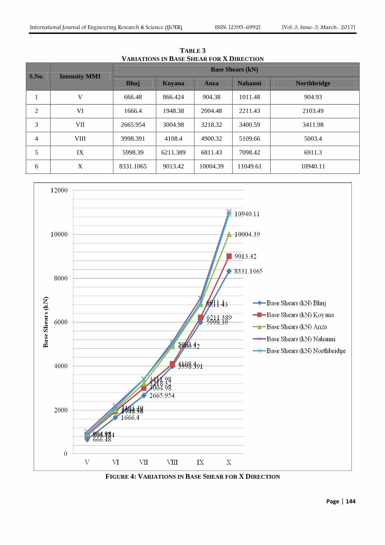
International Journal of Engineering Research & Science (IJOER) ISSN: [2395-6992] [Vol-3, Issue-3, March- 2017]
Page | 144
TABLE 3
VARIATIONS IN BASE SHEAR FOR X DIRECTION
S.No. Intensity MMI Base Shears (kN)
Bhuj Koyana Anza Nahanni Northbridge
1 V 666.48 866.424 904.38 1011.48 904.93
2 VI 1666.4 1948.38 2004.48 2211.43 2103.49
3 VII 2665.954 3004.98 3218.32 3400.59 3411.98
4 VIII 3998.391 4108.4 4900.32 5109.66 5003.4
5 IX 5998.39 6211.389 6811.43 7098.42 6911.3
6 X 8331.1065 9013.42 10004.39 11049.61 10940.11
FIGURE 4: VARIATIONS IN BASE SHEAR FOR X DIRECTION

International Journal of Engineering Research & Science (IJOER) ISSN: [2395-6992] [Vol-3, Issue-3, March- 2017]
Page | 145
TABLE 4
VARIATIONS IN BASE SHEAR FOR Y DIRECTION
S.No. Intensity MMI Base Shears(kN)
Bhuj Koyana Anza Nahanni Northbridge
1 V 888.651 920.44 1102.43 1390.11 1750.39
2 VI 2221.62 2444.92 2780.44 3001.29 3640.11
3 VII 3554.62 3842.46 4100.39 4400.41 4711.39
4 VIII 5331.9 5711.39 6008.82 6344.92 6748.31
5 IX 7997.86 8211.79 8411.99 8791.79 9124.48
6 X 11108.142 11209.4 11600.11 12001.92 12409.18
FIGURE 5: VARIATIONS IN BASE SHEAR FOR Y DIRECTION
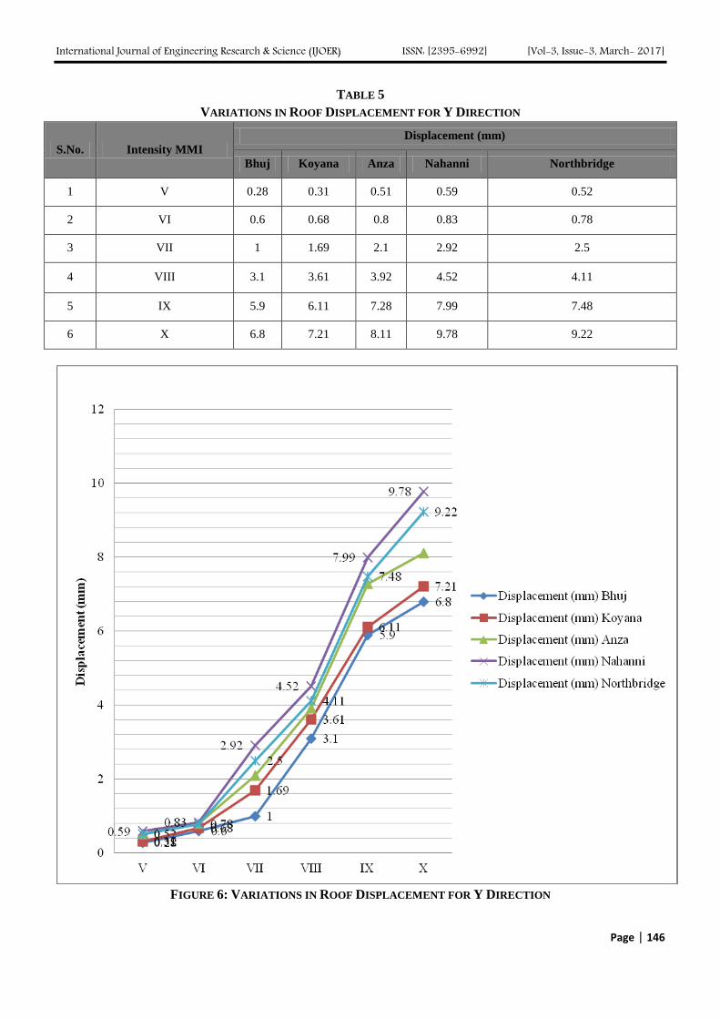
International Journal of Engineering Research & Science (IJOER) ISSN: [2395-6992] [Vol-3, Issue-3, March- 2017]
Page | 146
TABLE 5
VARIATIONS IN ROOF DISPLACEMENT FOR Y DIRECTION
S.No. Intensity MMI
Displacement (mm)
Bhuj Koyana Anza Nahanni Northbridge
1 V 0.28 0.31 0.51 0.59 0.52
2 VI 0.6 0.68 0.8 0.83 0.78
3 VII 1 1.69 2.1 2.92 2.5
4 VIII 3.1 3.61 3.92 4.52 4.11
5 IX 5.9 6.11 7.28 7.99 7.48
6 X 6.8 7.21 8.11 9.78 9.22
FIGURE 6: VARIATIONS IN ROOF DISPLACEMENT FOR Y DIRECTION

International Journal of Engineering Research & Science (IJOER) ISSN: [2395-6992] [Vol-3, Issue-3, March- 2017]
Page | 147
TABLE 6
VARIATIONS IN ROOF DISPLACEMENT FOR X DIRECTION
S.No. Intensity MMI
Displacement (mm)
Bhuj Koyana Anza Nahanni Northbridge
1 V 0.53 0.629 0.739 0.811 0.844
2 VI 1.02 1.24 1.439 1.591 1.433
3 VII 2.06 2.93 2.811 3.318 3.12
4 VIII 4.09 4.5 4.426 6.019 5.811
5 IX 8.92 9.21 8.298 12.48 11.129
6 X 9.2 10.03 12.37 14.11 13.482
FIGURE 7: VARIATIONS IN ROOF DISPLACEMENT FOR X DIRECTION
V. CONCLUSION
1. The seismic responses namely base shear, storey displacements and storey drifts in both the directions are found to vary
in similar pattern with intensities (V to X) for all the Time Histories and both the models considered for the study.
2. The values of seismic responses namely base shear, storey displacement and storey drifts for all the Time Histories and
both the models are found to be of increased order for seismic intensities varying from V to X.

International Journal of Engineering Research & Science (IJOER) ISSN: [2395-6992] [Vol-3, Issue-3, March- 2017]
Page | 148
3. The maximum value of base shear, storey displacement and storey drift (X and Y directions) for seismic intensities of
VI, VII, VIII, IX and X are found to be nearly more by 2.50, 4.005, 7.56, 16.83, and 17.35 times, respectively as
compared to seismic intensity of V for both the models (i.e., with and without soft story) and for all the time histories.
4. As Time History Analysis is a realistic method used for seismic analysis, it provides a better check to the safety of
structures analyzed and designed bythe method specified in IS code.
REFERENCES
[1] Duggal S K (2010), “Earthquake Resistance Design of Structure”, Fourth Edition, Oxford University Press, New Delhi.
[2] Haselton C B and Whittaker A S (2012), “Selecting and Scaling Earthquake Ground Motions for Performing Response-History
Analyses”, The 15th World Conference on Earthquake Engineering.
[3] Romy M and Prabha C (2011), “Dynamic Analysis of RCC Buildings with Shear Wall”, International Journal of EarthSciences and
Engineering, ISSN 0974-5904, Vol. 04, 659-662.
[4] Shaha V and Karve S (2010), “Illustrated Design of Reinforced Concrete Buildings”, Sixth Edition, Structures Publication, Pune.
[5] Wilkinson S and Hiley R (2006), “A Non-Linear Response History Model for the Seismic Analysis of High-Rise Framed Buildings”,
Computers and Structures, Vol. 84.

International Journal of Engineering Research & Science (IJOER) ISSN: [2395-6992] [Vol-3, Issue-3, March- 2017]
Page | 149
Sequential Famous Route Analysis Based on Multisource Social
Media D.Sugapriya
1, B.Pavithra
2, G.Suganya
3, M.Antony Robert Raj
4
1,2,3U.G. Students, Dept of CSE, Alpha College of Engineering, Chennai. 4Asst.prof.Dept of CSE, Alpha College of Engineering, Chennai.
Abstract— As an infrastructural and profitable industry, tourism is vital in present day economy and incorporates
distinctive extensions and capacities. In the event that it is created suitably, social relations and monetary improvement of
nations will be developed and given. Web advancement as a associated tool within the web assumes an extremely deciding
part in tourism achievement and appropriate misuse of it can prepare for greater improvement and accomplishment of this
industry. Then again, the measure of information in the present world has been expanded and investigation of substantial
arrangements of information that is alluded to as large information has been changed over into a key way to deal with
upgrade rivalry and set up new strategies meant for improvement, development, advancement, and upgrade of the quantity of
clients. Today, huge in sequence is vital issues of statistics supervision in computerized age and one of the primary open
doors in tourism industry for ideal misuse of most extreme data. Huge information can shape encounters of keen travel.
Surprising development of these information sources has enlivened new Strategies to comprehend the financial marvel in
various fields. The systematic approach of huge information underscores the limit of information accumulation and
investigation with a phenomenal degree, profundity and scale for taking care of the issues of genuine and utilizations it. In
fact, enormous information examinations open the ways to different open doors for building up the present day learning or
changing our comprehension of this extension and bolster basic leadership in tourism industry. The reason for this review is
to show accommodation of huge information examination to find behavioral examples in tourism industry and propose a
model for utilizing information in tourism.
Keywords— Travel proposal, geo-labeled photographs, online networking, sight and sound data recovery.
I. INTRODUCTION
Programmed travel suggestion is an imperative issue in both research and industry. Enormous media, particularly the twist of
web-based social networking (e.g., Facebook, Flick, Twitter and so forth.) offers awesome chances to address numerous
testing issues, for example, GPS estimation [1], [2] also, travel suggestion [3]. Travelog sites (e.g., www.igougo.com) offer
rich portrayals about historic points also, voyaging background composed by clients. Moreover, group contributed
photographs with metadata (e.g., labels, date taken, scope and so on.) via web-based networking media record clients' day by
day life and travel involvement. These information are not just helpful for solid POIs (purposes of enthusiasm) ming [4],
travel courses ming, yet give a chance to prescribe customized travel POIs and courses in light of client's advantage. There
are two principle challenges for programmed travel suggestion. To begin with, the prescribed POIs ought to be customized to
client enthusiasm since various clients may lean toward distinctive sorts of POIs. Take New York City for instance. A few
people may incline toward social spots like the Metropolitan Museum, while others may incline toward the cityscape like the
Central Park. Other than travel topical intrigue, different qualities including utilization capacity (i.e., extravagance,
economy), favored going by season (i.e., summer, pre-winter) and favored going by time (i.e., morning, night) may likewise
be useful to give customized travel proposal.
Consequently, it is not steady to suggest a progressive travel course (i.e., a gathering of POIs) rather than individual POI. It is
extensively extra wearisome and additionally dreary for customers to organize travel game plan than individual POIs. In
perspective of the way that the alliance between the zones in addition to opening time of different POIs should be considered.
For example, it may regardless not be a nice recommendation if each one of the POIs endorsed for one day are in four
corners of the conurbation, instead of the way that the customer may be excited about all the individual POIs.
In disconnected module, the topical bundle space is mined from online networking consolidating travelogs and community
contributed photographs. Four travel conveyances (i.e., topical intrigue, time, season and cost) of every point are portrayed in
topical bundle space. Taking the upside of the complementation of the two online networking.
Online module concentrates on mining client bundle and prescribing customized POI arrangement in view of client bundle.
To start with, labels of client's photograph set are mapped to topical bundle space to get client's topical intrigue dispersion. It

International Journal of Engineering Research & Science (IJOER) ISSN: [2395-6992] [Vol-3, Issue-3, March- 2017]
Page | 150
is hard to get client's utilization ability specifically from the printed portrayals of photographs. In any case, the subjects client
intrigued in could some way or another mirror these traits.
Existing reviews on travel suggestion mining celebrated travel POIs and courses are predominantly from four sorts of
enormous web-based social networking, GPS direction [5], However, general travel course arranging can't well meet clients'
close to home prerequisites. Customized travel proposal suggests the POIs and courses by mining client's travel records [6],
[7], [8].
II. PROBLEM STATEMENT
Development and success of organizations rely on upon having reasonable data about clients, providers and their exhibitions.
The broad volume of multi-media frameworks has assumed a noteworthy part being developed and development of
enormous information. Social sites, advanced mobile phones, and different types of gear of clients including PCs and
portable workstations have permitted billions of individuals over the world to take part in information conception. In nearby
prospect this is normal that enormous information investigation will be utilized broadly in promoting and in addition
interpersonal organizations. Without a doubt, enormous information ought to impact all divisions particularly the modern
ones; this is done through joining the information from various areas of financial association with outer information.
III. LITERATURE SURVEY
3.1 TITLE: Smart Tourism Destinations
AUTHOR: Buhalis, D., & Amaranggana, A.
DESCRIPTION:
The quick change of developments familiarizes cleverness with all affiliations and gatherings. The Stylish Visiting the appeal
intention thought ascends out of the change of Smart Cities. With development being introduced on all affiliations and
substances, objectives will abuse coordinated efforts between general identifying advancement and their social portions to
reinforce the change of guest experiences. By applying insightful thought to address pioneers' needs some time as of late, in
the midst of and after their trek, objectives could assemble their clout level. These paper provision to abuse from the
revolutionize of elegant Cities by intangible configuration for stylish sightseeing target through researching tourism
applications in objective and tending to both open entryways and troubles it had.
3.2 TITLE: Personalized travel package recommendation
AUTHOR: Q. Liu, Y. Ge, Z. Li, E. Chen, and H. Xiong
DESCRIPTION:
As the universes of trade, amusement, travel, and Internet innovation turn out to be all the more inseparably connected, new
sorts of business information get to be distinctly accessible for imaginative utilize and formal examination. To be sure, this
paper gives an investigation of abusing on the web travel data for customized travel bundle suggestion. A basic test along this
line is to address the extraordinary qualities of travel information, which recognize travel bundles from customary things for
suggestion. To this end, first break down the qualities of the travel bundles and build up a Tourist-Area-Season Topic show,
which can separate the subjects adapted on both the voyagers and the natural elements (i.e. areas, travel seasons) of the
scenes? In view of this TAST show, a mixed drink approach on customized travel bundle proposal. Finally, evaluation of this
model and the mixed drink approach on certifiable travel bundle information. The exploratory outcomes demonstrate that the
model can viably catch the one of a variety superiority of the travel information and the mixed drink approach is
subsequently considerably more viable than conventional suggestion strategies for travel bundle proposal.
3.3 TITLE: Recommending friends and locations based on individual location history
AUTHOR: Y. Zheng, L. Zhang, Z. Ma, X. Xie
DESCRIPTION:
The expanding accessibility of subject securing improvements (GPS, GSM programs, etc.) empowers contributors to log the
discipline histories with spatio-transient know-how. Such actual subject histories suggest, to a couple measure, customers'
pursuits in spots, and convey us chances to realise the relationship amongst clients in addition to spot. This paper depicts ,
transporting in the direction of this track along through afford an report of a bespoke accessory as well as pasture

International Journal of Engineering Research & Science (IJOER) ISSN: [2395-6992] [Vol-3, Issue-3, March- 2017]
Page | 151
recommender on behalf of the ecological information frameworks on the web. Within the original circumstances, on this
advocated framework, a distinctive persons stopover to a geospatial locale on this present fact are utilized as their understood
appraisals on that subject. Later, measure the likeness between purchasers regarding their area histories and prescribe to
every client a gathering of potential companions in a GIS individual’s team. 1/3, we verify an man or woman's benefits in an
association of unvisited locales by using including his/her area historical past and those of exclusive consumers. Some
unvisited areas that can coordinate their tastes can be prescribed to the man or woman.
IV. SYSTEM ARCHITECTURE
Proposed concept deals with providing database by using hadoop tool able to analyze no limitation of data in addition to
simple add number of machines to the cluster and getting results with less time, high throughput and maintain cost is very
cheap as well as by using joins , partitions and bucketing techniques in hadoop see in Fig. 1.
FIG.1. ARCHITECTURE OF THE SYSTEM
To enhance the effectiveness in the terns of bringing the information quick. By methods for when existing or dynamic
information required getting concerning examination reason whether information expectation is unrealistic there are chances
it is organized or might be unstructured else it would have semi structured information. So on assortment of information
investigation is must. So first information preprocessing will go too happened.
V. MODELS AND DESIGN GOALS
5.1 Data Preprocessing Module:
While mining the information, to gather information from various source frameworks notwithstanding in different record
designs, for instance level documents with delimiters (CSV) and additionally XML files. To accumulate information from
different frameworks that development information in clandestine configurations nobody too utilizes for long haul. The
changing over stride may include different information controls, assume moving, part and interpreting and additionally
combining, sorting turning and in addition more. For example, a client name may be part into first and additionally last
names or else dates may be changed to the standard ISO format.At next stride stacking information into information
stockroom should be possible in group forms or else push by line.
5.2 Data Intake via Sqoop
Apache Sqoop is an apparatus intended to exchange information amongst Hadoop and social databases. Sqoop can import
information from a RDBMS such MySQL as well as Oracle Database dependent on HDFS and also then fare the information
invert later than information has been adjusted utilizing MapReduce. Sqoop interfaces with a relational database ( RDBMS)
all the way through its java database connection ( JDBC) connector along with depends on the database to depict the
database blueprint for information to be transported in. Both import and fare use MapReduce, which furnishes parallel
operation with adaptation to internal failure. All through import, Sqoop peruses the table, push by line, into HDFS sees in
Fig.2.

International Journal of Engineering Research & Science (IJOER) ISSN: [2395-6992] [Vol-3, Issue-3, March- 2017]
Page | 152
FIG. 2. SQOOP ARCHITECTURE
5.3 Data Analytic With Hive
Hive is an open-source data warehousing illumination will going to harps on pinnacle of Hadoop. Hive ropes problem
elucidate in a SQL-like as an authoritative lingo - HiveQL, that are going to masterminded into guide decrease occupations
which executed on Hadoop. What's more, HiveQL supports tradition portrays scripts to be piece into inquiries. The lingo
consists of a species system with hold up for table’s enclosed primitive sorts moreover congregation like assemblage as well
as above and beyond maps, and in addition established associations of the same. The significant IO libraries can be wide to
request data in custom configurations. Hive additionally involves a framework index, Hive-Metastore, holding patterns
notwithstanding insights, which is valuable in information.
5.4 Data Analytic Module with pig
It is an impossible to miss state data managing vernacular which will gives a full rich system of amassed data sorts and in
addition over the navigate of execute a substitute traits of proceed ahead the data chiefs. The tongue for Pig can't keep away
from being pig Latin. Pig handles each structure and unstructured tongue. It's thinking about all things high of the guide
diminish technique running establishment. The scriptt generally used for investigating the data in Hadoop by means of Pig
utilization is recognized as Pig Latin. Recalling a conclusive focus to play out a particular undertaking Programmers using
Pig and when programming engineers require to make a Pig script by making utilization of the Pig Latin script moreover
implement them in the midst of any of the implementation instruments (Grunt Shell as well as UDFs ). Functioning as
anticipated to implementation, these scripts will get ahead of by methods for an upgrading of revolutionize which leaving to
related by the Pig Framework, intention of most obligatory yield. Inside, Apache Pig change these scripts into a get-together
of MapReduce associations, likewise, it will make the thing sketcher's occupation coordinate.
5.5 Data Analytic With Mapreduce
The MapReduce encoding sculpt is made out of two primitive capacities that is Map and in addition Reduce. The info
information for a MapReduce program is a rundown of <key, value> matches notwithstanding along these lines the Map()
capacity is helpful to each combine and furthermore create an arrangement of halfway combines, e.g. <key, list(value)>.
After that the Reduce() capacity is utilitarian to each middle of the road combine, prepare estimations of the rundown, and in
addition deliver aggregate last outcomes. Moreover, there are additional capacities in the MapReduce execution display for
instance rearrange and sort, for dealing with middle information. On the Map side the rearrange capacity will be connected,
and also execute information trade by key after Map(). Along these lines, information among a similar key will be
communicate to a solitary Reduce work. The sort capacity be propelled on the Reduce side later than information trade. By
utilizing key information going to sort field to gathering every one of the sets by methods for a similar key for further
handling.
The mapper discharges a halfway key-esteem combine for each word in an archive. The reducer aggregates up all means
each word
Algorithm 1. MapReduce Execution
___________________________________________
1. Class MAPPER
2. method Map(prid a, prname d)
3. For all term t doc d do
4. Emit(term t, count 1)

International Journal of Engineering Research & Science (IJOER) ISSN: [2395-6992] [Vol-3, Issue-3, March- 2017]
Page | 153
class Reducer
i. method Reduce(term t, counts [c1, c2, . . .])
ii. method Reduce(term t, counts [c1, c2, . . .])
iii. sum ← 0
iv. for all count c counts [c1, c2, . . .] do
v. sum ← sum + c
vi. Emit(term t, count sum)
_____________________________
This reckoning determines the live of event of every word in an exceedingly substance assemblage, that is that the underlying
stage certain instance, structure a unigram tongue depiction (i.e., chance dissemination in more than words in Associate in
Nursing amassing). Input key qualities sets secure the type of (prid, prname) sets that top off on high of the scattered record
structure, some place the past could be a choose symbol for the report, and likewise the primary duplicate of the document
itself. The clerk get Associate in Nursing info key-regard be part of, tokenizes the report, and what is more unleash a middle
key-regard coordinate for every word: the prid itself fills in because the key, and also the entire favored fills in because the
regard (hint that we have seen the prid once). The MapReduce execution framework ensured that each one qualities
connected with the much identical key area unit gotten in lightweight of current circumstances the reducer. Henceforth, in
our guide decrease count, merely need to combination all numbers (ones) connected with every word. The reducer will
properly this, and likewise unleash last key-regard sets with the prid because the key, and also the contemplate the regard.
VI. RESULTS AND EVALUATION
By and huge for graphical portrayal in hadoop R accent for the foremost half utilizes. R is code likewise as condition used as
a district of enlargement to planned exceptionally to work out functions and factual. it's divergent from completely different
insights instruments and to boot different process accent as an example S as R is totally develop expected for measurable
data[10]. R is Associate in Nursing open supply and free factual program which may use for each measurable would like and
calculations. As of currently contains informational assortment in hadoop cluster but for analyazation that has to speak to in
graphical organization in Fig.4. demonstrates the vital development within the amount of specific MapReduce programs
registered with our essential ASCII text file administration framework the MapReduce library logs measurements regarding
the procedure assets used by the folks for many of the tuime in keeping with ratings thatis that the real followable path by
most of the folks will conclude once analyzation
FIG.4. ANALYZATION FOR HIGHEST ROOT FIG.5. ANALYZATION FOR TOTAL TIME VISITING
PLACE
In Fig.5. depicts the graphical similarly as applied mathematics illustration once analyzing each path booth with reference to
time by means that of ato reach at explicit destination by that root can take less time to. thus for all destination purpose there
ar some root which is able to go via directly or indirectly until to it purpose.So that root can take shortest time to achieve
there.

International Journal of Engineering Research & Science (IJOER) ISSN: [2395-6992] [Vol-3, Issue-3, March- 2017]
Page | 154
VII. CONCLUSION
Huge information alludes to an extraordinary open door for all travel foundations and tourism. It considerably affects enter
forms in tourism industry however its impact is certainly in essential stages. A few segments and organizations are presently
trying or utilizing huge information in sight of establishment up till now a bulky amount of them have not even now made
any move in such manner. All organizations that were examined in this report had no restriction with the theory that
enormous information can possibly change the business altogether. The vital point is moving from potential to reality at any
rate in a little scale.
Suitability of endeavors is comprehensive through the make utilize of of colossal data; along these lines, remarkable
affiliations are by and by focusing on securing and surveying the data related to customers that has been secured in lodgings
or customers' information and in addition collaborations amidst an exact ultimate objective to abuse their required models
and data. Colossal data is to a great degree basic in light emission snippet of data that it delicate a proper information about
business. In this comportment, it has been seen as a progression hotspot for tourism affiliations and tourism industry.
Capacity of colossal data in tourism industry is greatly uncommon and the related affiliations should not disregard the
criticalness of this degree.
A portion of the headings for future work is we can utilize start offers taking after future extension:
1. Computation will be In-Memory
2. Dynamic spilling information conceivable to examine
REFERENCES
[1] H. Liu, T. Mei, J. Luo, H. Li, and S. Li, “Finding perfect rendezvous on the go: Accurate mobile visual localization and its
applications to routing,” in Proc. 20thACMInt. Conf. Multimedia, 2012, pp. 9–18.
[2] J. Li, X. Qian, Y. Y. Tang, L. Yang, and T. Mei, “GPS estimation for places of interest from social users’ uploaded photos,” IEEE
Trans. Multimedia, vol. 15, no. 8, pp. 2058–2071, Dec. 2013.
[3] S. Jiang, X. Qian, J. Shen, Y. Fu, and T. Mei, “Author topic model based collaborative filtering for personalized POI
recommendation,” IEEE Trans.Multimedia, vol. 17, no. 6, pp. 907–918, Jun. 2015.
[4] J. Sang, T. Mei, T. J. Sun, S. Li, and C. Xu, “Probabilistic sequential POIs recommendation via check-in data,” in Proc. ACM
SIGSPATIAL Int. Conf. Adv. Geographic Inform. Syst., 2012, pp. 402–405.
[5] Y. Zheng, L. Zhang, Z. Ma, X. Xie, and W. Ma, “Recommending friends and locations based on individual location history,” ACM
Trans. Web, vol. 5, no. 1, p. 5, 2011.
[6] Y. Shi, P. Serdyukov, A. Hanjalic, and M. Larson, “Personalized landmark recommendation based on geo-tags from photo sharing
sites,” in Proc. 5th AAAI Conf. Weblogs Social Media, 2011, vol. 11, pp. 622–625.
[7] M. Clements, P. Serdyukov, A. de Vries, and M. Reinders, “Personalised travel recommendation based on location cooccurrence,”
arXiv preprint arXiv:1106.5213, 2011.
[8] X. Lu, C. Wang, J. Yang, Y. Pang, and L. Zhang, “Photo2trip: Generating travel routes from geo-tagged photos for trip planning,” in
Proc. Int. Conf. Multimedia, 2010, pp. 143–152.
[9] Marine-Roig, E., & Clavé, S. A. (2015). Tourism analytics with massive user-generated content: A case study of Barcelona. Journal of
Destination Marketing & Management, 4(3), 162-172.
[10] https://www.statsoft.com/Portals/0/.../WhitePapers/R_Integration_White_Paper.pdf

International Journal of Engineering Research & Science (IJOER) ISSN: [2395-6992] [Vol-3, Issue-3, March- 2017]
Page | 155
Gene Expression Chromosomal Correlations in Tumors of
Mesodermal Origin: The Case of Rhabdomyosarcoma and Acute
Lymphoblastic Leukemia
Viktoria Papadimitriou1, George I. Lambrou
*
1,2Graduate Program “Metabolic Bones Diseases”, National and Kapodistrian University of Athens, Medical School, Mikras
Asias 75, 11527, Goudi, Athens, Greece 2First Department of Pediatrics, Choremeio Research Laboratory, National and Kapodistrian University of Athens, Thivon &
Levadeias, 11527, Goudi, Athens, Greece
Abstract-since the advent of high throughput methodologies, like microarrays, the load of genomic data has increased geometrically and
along with that the need for computational methods which will interpret these data. In the present work we have studied the common gene
expression patterns between two tumor cell types of mesodermal origin. In particular, we have attempted to find causal relations between
gene expression levels with respect to chromosomal location. We have found that several genes manifested significant relations, using
regression analysis and as such they could pose interesting targets for further investigations. This type of analysis can lead to the
understanding of the common mechanisms that transform physiological cells to malignant, as well as it reveals a new holistic way to
understand the dynamics of tumor onset as well as the mechanistic of oncogenic drivers. Such approaches could prove to be useful in the
prediction of genomic targets that could be further studied in order to unravel the mechanics of tumor ontogenesis.
Keywords-Acute Lymphoblastic Leukemia, Chromosomal correlations, Mesoderm, Microarrays, Rhabdomyosarcoma.
I. INTRODUCTION
Acute lymphoblastic leukemia (ALL) and rhabdomyosarcoma (RMS) are two type of tumors, which originate from the
embryonic mesoderm. ALL is the most frequent malignancy, which appears during childhood. Acute leukemia originates
from the undifferentiated lymphoblast, which does not develop into the mature lymphoid cell, giving rise to a tumor. RMS is
a rare cancer in childhood. This represents 5-8% of all tumors in childhood, but the sarcomas of head and neck are 12% of all
neoplasias in childhood. RMS originates from myoblast or cells that will form the skeletal muscle. These are different from
the smooth cells. RMS can be created at any part of the body, which has skeletal muscle but frequently appears in the head
and neck. The embryonal form of RMS is most common at birth, which consists of spindle cells and botryoid form with
better prognosis, but the alveolar form mainly appears in childhood and adolescence. ALL and RMS consist of cells that are
undifferentiated, immortal and with the potential to divide infinitely. Myoblasts originate from the dorsal (paraxial)
mesoderm, while blood cells derive from the lateral mesoderm that gives rise to the splachnic mesoderm and this to the
hemangioblastic tissue. ALL and many alveolar RMS in childhood present chromosomal translocations, like the PAX3-
FKHR, that is an indicator of poor prognosis and associated with metastasis [1].
During embryogenesis, blood cells originate from two sites. From the ventral mesoderm near the yolk sac, which gives rise
to the intra-embryonic hematopoietic precursors, but the hematopoietic cells that last throughout the entire life time of an
organism are derived from the mesodermal area surrounding the aorta. This differentiation is regulated with a network of
various genes, which leads to two similar cell types with others functions and roles in the body. There are several factors that
affect gene regulation, which means that aberrations in the regulatory network would lead to tumor cells.
Further on, it has been previously reported that correlation in gene expression and in particular, chromosomal correlation
implies common gene regulation [1, 2]. Yet, it is also known that correlation does not imply causality. In that sense, it is of
great importance if we would be able to infer gene regulatory mechanisms from chromosomal expression levels.
The present study concerns the extension of a previous work, where gene expression analysis was extensively investigated in
two cell lines. The T-cell acute lymphoblastic leukemia CCRF-CEM cell line and the rhabdomyosarcoma TE-671 cell line.
We used these cell lines to investigate common patterns of cellular function between the two systems. These two cell types
would normally had differentiated into cells of blood and muscle cells but in an unknown stage this normal differentiation
stopped and began an informal, uncontrolled proliferation which created the malignancy. The intervening stages and led in
tumor genesis are unknown.

International Journal of Engineering Research & Science (IJOER) ISSN: [2395-6992] [Vol-3, Issue-3, March- 2017]
Page | 156
Thus, in the present work we attempted to investigate common gene regulation based on chromosomal correlations. Yet, we
have tried to move a step forward and find probable etiological relations in gene expression patterns. The present work
focuses towards approaches that utilize biological along with mathematical tools, in order to unravel mechanisms in gene
expression patterns. Further on, it moves towards a direction that attempts to interpret gene regulation not from the
differential point of view but from common gene expression patterns.
II. MATERIALS AND METHODS
2.1 Cell Cultures
The CCRF-CEM (ALL) and the TE-671 (RMS) cell lines were used as the model, both obtained from the European
Collection of Cell Cultures (ECACC). The CCRF-CEM cell line, a CD4+
[3] and CD34+ presenting cell line [4], was initially
obtained from the peripheral blood of a 2 year old Caucasian female. It was diagnosed as lymphosarcoma which progressed
later on to acute leukemia [5]. The child was undergone irradiation therapy and chemotherapy prior to obtaining the cell line.
Although remission was achieved at various stages, the disease progressed rapidly [5]. The cell line was observed to have
undergone minor changes after long-term culture, except for the presence of dense granules in the nucleoli [6]. Finally, the
CCRF-CEM cell line has been reported to manifest autocrine catalase activity which participates to its mechanisms of growth
and progression [7].The TE-671 cell line was initially reported to have been obtained from a cerebellar medulloblastoma,
before irradiation therapy, of a six-year old Caucasian female [8] and characterized later on [9]. However, it is today known
that this cell line is parental if not identical to the RD [10] rhabdomyosarcoma cell line. However, several reports still refer to
this cell line as medulloblastoma [11, 12]. The experimental process of cell treatment has been described previously [1].
2.2 Experimental Procedures
Experimental procedures have been described previously in detail by our group [1]. In brief, factors estimated, included cell
proliferation, cell cycle distribution and microarray experimentation. For the assay of mRNA levels two sets of microarray
chips were used: cDNA microarray chips (4.8k genes) obtained from TAKARA (IntelliGene™ II Human CHIP 1) [13] and
microarray chips (9.6k genes) from the Institut fuer Molekularbiologie und Tumorforschung, Microarray Core Facility of the
Philipps-Universitaet, Marburg Germany (IMT9.6k). Microarray experimentation has been previously described in our
previous work [1]. The microarray data have been submitted to the GEO Database under the Accession Number GSE34522.
2.3 Microarray Data Analysis
Microarray data pre-processing analysis was performed with ImaGene®v.6.0Software (BioDiscovery Inc, CA) and
ARMADA software (National Hellenic Research Foundation, Athens Greece) [14]. Data were collected from exported text
file and data pre-processing was performed using the Microsoft Excel® environment. Background correction has been
performed by using the robust loess-based background correction(rLsBC) approach, as proposed by Sifakis et al. (2011) [15].
The background corrected signal intensities were further normalized in order to mitigate the effect of extraneous, non-
biological variation in the measured gene expression levels. Genes were tested for their significance in differential expression
using a z-test. Genes were considered to be significantly differentially expressed if they obtained a p-value <0.05. The False
Discovery Rate (FDR) was calculated as previously described [16-18]. There was a FDR of 1% for p<0.05 for the
IntelliGene microarray chip, and a FDR of 9% for p<0.01 for the IMT 9.6k microarray chip. Calculating the FDR for the
combination of both platforms gives a FDR of 6% for p<0.01.
2.4 Chromosomal Regressions and Data Analysis
Chromosome mapping was performed with Genesis 1.7.2 (Technische Universitaet-Graz, Austria) using Pearson’s
correlation, Spearman’s rank order correlation [2, 19, 20] and WebGestalt web-tool (Vanderbilt University, The Netherlands,
http://bioinfo.vanderbilt.edu/gotm/) [21].2D Chromosomal regressions have been performed among the similarly expressed
genes between RMS (TE-671) and ALL (CCRF-CEM). 3D chromosomal regressions were performed between similarly
expressed genes of RMS and ALL as well as we added the third dimension, which was the log2 transformed ratio of the
respective genes. Regressions and data analysis were performed with the Matlab® computational environment (The
Mathworksm Inc. Natick, MA). For linear 2D regressions the binomial equation was used of the form f(x)=y=ax2+bx+c,
while for the 3D regressions the equation of the form f(x,y)=z=ay+bx+c.

International Journal of Engineering Research & Science (IJOER) ISSN: [2395-6992] [Vol-3, Issue-3, March- 2017]
Page | 157
III. RESULTS
Regression analysis was performed in order to find probable causal relations in gene expression with respect to cell type and
chromosomal distribution. In particular, we have used genes that manifested similar expression levels, meaning that they
were those that were not differentially expressed. We have performed two different kinds of regression analysis. One
included a 2D regression of the form y=ax2+bx+c and the second of the form z=ay+bx+c. 2D regressions manifested
significant relations between the two cell types and in particular for chromosome 1 with an R2=0.82 (Fig. 1A), chromosome
3 with an R2=0.82 (Fig. 1B), chromosome 8 with an R
2=0.89 (Fig. 1C), chromosome 13 with an R
2=0.71 (Fig. 1D),
chromosome 14 with an R2=0.91 (Fig. 1E), chromosome 15 with an R
2=0.69 (Fig. 1F), chromosome 16 with an R
2=0.89
(Fig. 1G), chromosome 17 with an R2=0.81 (Fig. 1H), chromosome 21 with an R
2=0.88 (Fig. 1I), chromosome 22 with an
R2=0.97 (Fig. 1J) and chromosome X with an R
2=0.71 (Fig. 1K).
FIGURE 1. REGRESSIONS OF GENE EXPRESSION DATA BETWEEN CCRF-CEM AND TE-671 CELLS, WITH RESPECT TO
CHROMOSOMAL EXPRESSION. SIGNIFICANT RELATIONS WERE FOUND FOR CHROMOSOMES 1 (A), 3 (B), 8 (C), 13 (D), 14
(E), 15 (F), 16 (G), 17 (H), 21 (I), 22 (J) and X (K).
Although 2D regressions manifested significant relations with regard to gene expression, still the revealed functions did not
have the complete set of the definition of a function. In other words, for every xD(f), there are two y, which can be
described as x1, x2D(f): x1≠x2 f(x1)=f(x2), or y1=y2, where D(f) is the definition domain of f, and x, y are the expression
levels of each gene. The question that came up from this observation, was that the manifested correlations could provide
more information if another dimension could be added to the calculations. The solution to this question came from the
observation that the log2 transformed ratio of TE-671 gene expression levels over the CCRF-CEM gene expression levels,
could be added as the third dimension. Thus, we have formulated a new relation z=ay+bx+c or f(x,y)=ay+bx+c, wherez can

International Journal of Engineering Research & Science (IJOER) ISSN: [2395-6992] [Vol-3, Issue-3, March- 2017]
Page | 158
be formulated as 2logx
zy
. Thus, the aforementioned equations become
2logx
ay bx cy
. The results of the
3D regression are presented in Fig. 2.
FIGURE 2. 3D REGRESSIONS OF GENE EXPRESSION DATA BETWEEN CCRF-CEM AND TE-671 CELLS AND THEIR
RESPECTIVE LOG2 TRANSFORMED RATIO WITH RESPECT TO CHROMOSOMAL EXPRESSION. SIGNIFICANT RELATIONS WERE
FOUND FOR CHROMOSOMES 1 (A) WITH BIHARMONIC FUNCTION, 1 (B) WITH A LINEAR FUNCTION, 7 (C), 9 (D), 10 (E), 11
(F), 13 (G), 21 (H) andX (I).
In particular, 3D regression analysis manifested significant relations between the two cell types and their ratio, and in
particular for chromosome 1 with an R2=1 (Fig. 2A) and with the use of the biharmonic function, chromosome 1 with an
R2=0.71 (Fig. 2B) with the use of the aforementioned linear function, chromosome 7 with an R
2=0.98 (Fig. 2C),
chromosome 9 with an R2=0.96 (Fig. 2D), chromosome 10 with an R
2=0.81 (Fig. 2E), chromosome 11 with an R
2=0.92 (Fig.
2F), chromosome 13 with an R2=0.85 (Fig. 2G), chromosome 21 with an R
2=0.72 (Fig. 2H) and chromosome X with an
R2=0.87 (Fig. 2I).
It appeared that relations in three dimensions manifested better results for the specified chromosomes as compared to two
dimensional regressions. This observation, shows that probably a third dimension is necessary in order to comprehend gene
regulatory mechanisms.
IV. DISCUSSION
In the present study we used computational and mathematical approaches in order to answer the question whether, a causal
relation between gene expression levels of two cell types, could be found based on their chromosomal distribution. We have
found that such significant relations could be found both using 2D as well as 3D regression methods. Especially, 2D
regressions manifested very good relations among cell types with respect to chromosomes, yet without manifesting a clear
causal relation. On the other hand, 3D regressions manifested better results suggesting that causal multi-dimensional relations
probably exist. At the same time, the fact that certain genes and chromosomes manifest significant correlations between two
different cell types, yet of similar origin, implies that they could probably consist common regulatory mechanisms of tumor
ontogenesis. In our previous work we have reported that ANXA4 (Chromosome 2), NP25 (Chromosome 3), VEGFC
(Chromosome 4), PDLIM7 and THBS4 (Chromosome 5), CUL7 (Chromosome 6), CD36 (Chromosome 7), BNIP3L

International Journal of Engineering Research & Science (IJOER) ISSN: [2395-6992] [Vol-3, Issue-3, March- 2017]
Page | 159
(Chromosome 8), CDC2 and IL2RA (Chromosome 10), MAB21L1 and FOXO1 (Chromosome 13), TCL1A (Chromosome
14), FEM1B (Chromosome 15), CFDP1 and MMP2 (Chromosome 16), RTTN (Chromosome 18), PDCD5 (Chromosome
19), , NNAT and ZNF313 (Chromosome 20), MBNL3, PLAC1, RPS6KA3 and CD40LG (Chromosome X) were genes
found to participate in cell differentiation and embryonal processes[1]. These genes were found to manifest significant
correlations both in the 2D as well as in 3D regressions. This finding consist of an important observation since it is probable
that these genes could possess a common machinery, either through their gene regulation or aberrations, that drives tumor
ontogenesis for the two cell types under investigation.
V. CONCLUSION
The present approach attempted to find common regulatory mechanisms in gene expression patterns of two cell types. In
particular, we have attempted to discover possible causal relations in gene expression patterns. We have found evidence that
such correlations could exist and it is probable that certain genes could be of great significance in tumor ontogenesis. Such
approaches could prove to be useful in the prediction of genomic targets that could be further studied in order to unravel the
mechanics of tumor ontogenesis.
ACKNOWLEDGEMENTS
VP: This work was funded in part by the National and Kapodistrian University of Athens, Medical School.GIL: This work
was funded in part by the National and Kapodistrian University of Athens, Medical School. Authors’ Contributions: VP:
performed computational experiments, drafted the manuscript, proof-read the manuscript. GIL: conceived the idea,
performed computational experiments, wrote Matlab code, performed data analysis and drafted the manuscript, gave final
permission for submission.
COMPETING INTEREST, DISCLOSURES AND CONFLICT OF INTEREST
The authors have nothing to disclose and no conflict of interest
REFERENCES
[1] G. I. Lambrou, A. Zaravinos, M. Adamaki, D. A. Spandidos, F. Tzortzatou-Stathopoulou, and S. Vlachopoulos, "Pathway
simulations in common oncogenic drivers of leukemic and rhabdomyosarcoma cells: a systems biology approach," Int J Oncol, vol.
40, pp. 1365-90, May 2012.
[2] B. A. Cohen, R. D. Mitra, J. D. Hughes, and G. M. Church, "A computational analysis of whole-genome expression data reveals
chromosomal domains of gene expression," Nat Genet, vol. 26, pp. 183-6, Oct 2000.
[3] L. Miranda, J. Wolf, S. Pichuantes, R. Duke, and A. Franzusoff, "Isolation of the human PC6 gene encoding the putative host
protease for HIV-1 gp160 processing in CD4+ T lymphocytes," Proc Natl Acad Sci U S A, vol. 93, pp. 7695-700, Jul 23 1996.
[4] C. Naujokat, O. Sezer, H. Zinke, A. Leclere, S. Hauptmann, and K. Possinger, "Proteasome inhibitors induced caspase-dependent
apoptosis and accumulation of p21WAF1/Cip1 in human immature leukemic cells," Eur J Haematol, vol. 65, pp. 221-36, Oct 2000.
[5] G. E. Foley, H. Lazarus, S. Farber, B. G. Uzman, B. A. Boone, and R. E. McCarthy, "Continuous Culture of Human Lymphoblasts
from Peripheral Blood of a Child with Acute Leukemia," Cancer, vol. 18, pp. 522-9, Apr 1965.
[6] B. G. Uzman, G. E. Foley, S. Farber, and H. Lazarus, "Morphologic variations in human leukemic lymphoblasts (CCRF-CEM cells)
after long-term culture and exposure to chemotherapeutic agents. A study with the electron microscope," Cancer, vol. 19, pp. 1725-
42, Nov 1966.
[7] P. A. Sandstrom and T. M. Buttke, "Autocrine production of extracellular catalase prevents apoptosis of the human CEM T-cell line
in serum-free medium," Proc Natl Acad Sci U S A, vol. 90, pp. 4708-12, May 15 1993.
[8] R. M. McAllister, H. Isaacs, R. Rongey, M. Peer, W. Au, S. W. Soukup, et al., "Establishment of a human medulloblastoma cell
line," Int J Cancer, vol. 20, pp. 206-12, Aug 15 1977.
[9] H. S. Friedman, S. H. Bigner, R. D. McComb, S. C. Schold, Jr., J. F. Pasternak, D. R. Groothuis, et al., "A model for human
medulloblastoma. Growth, morphology, and chromosomal analysis in vitro and in athymic mice," J Neuropathol Exp Neurol, vol. 42,
pp. 485-503, Sep 1983.
[10] R. M. McAllister, J. Melnyk, J. Z. Finkelstein, E. C. Adams, Jr., and M. B. Gardner, "Cultivation in vitro of cells derived from a
human rhabdomyosarcoma," Cancer, vol. 24, pp. 520-6, Sep 1969.
[11] C. M. Yeung, B. S. An, C. K. Cheng, B. K. Chow, and P. C. Leung, "Expression and transcriptional regulation of the GnRH receptor
gene in human neuronal cells," Mol Hum Reprod, vol. 11, pp. 837-42, Nov 2005.
[12] E. S. Chu, T. K. Wong, and C. M. Yow, "Photodynamic effect in medulloblastoma: downregulation of matrix metalloproteinases and
human telomerase reverse transcriptase expressions," Photochem Photobiol Sci, vol. 7, pp. 76-83, Jan 2008.
[13] H. W. Chung, S. W. Park, J. B. Chung, J. K. Kang, J. W. Kim, H. S. Kim, et al., "Differences in genetic expression profiles between
young-age and old-age gastric adenocarcinoma using cDNA microarray for endocrine disruptor study," Oncol Rep, vol. 12, pp. 33-9,
Jul 2004.
[14] A. Chatziioannou, P. Moulos, and F. N. Kolisis, "Gene ARMADA: an integrated multi-analysis platform for microarray data
implemented in MATLAB," BMC Bioinformatics, vol. 10, p. 354, 2009.

International Journal of Engineering Research & Science (IJOER) ISSN: [2395-6992] [Vol-3, Issue-3, March- 2017]
Page | 160
[15] E. G. Sifakis, A. Prentza, D. Koutsouris, and A. A. Chatziioannou, "Evaluating the effect of various background correction methods
regarding noise reduction, in two-channel microarray data," Comput Biol Med, Nov 8.
[16] Y. Klipper-Aurbach, M. Wasserman, N. Braunspiegel-Weintrob, D. Borstein, S. Peleg, S. Assa, et al., "Mathematical formulae for
the prediction of the residual beta cell function during the first two years of disease in children and adolescents with insulin-
dependent diabetes mellitus," Med Hypotheses, vol. 45, pp. 486-90, Nov 1995.
[17] J. D. Storey and R. Tibshirani, "Statistical significance for genomewide studies," Proc Natl Acad Sci U S A, vol. 100, pp. 9440-5,
Aug 5 2003.
[18] J. D. Storey and R. Tibshirani, "Statistical methods for identifying differentially expressed genes in DNA microarrays," Methods Mol
Biol, vol. 224, pp. 149-57, 2003.
[19] A. Sturn, J. Quackenbush, and Z. Trajanoski, "Genesis: cluster analysis of microarray data," Bioinformatics, vol. 18, pp. 207-8, Jan
2002.
[20] F. Reyal, N. Stransky, I. Bernard-Pierrot, A. Vincent-Salomon, Y. de Rycke, P. Elvin, et al., "Visualizing chromosomes as
transcriptome correlation maps: evidence of chromosomal domains containing co-expressed genes--a study of 130 invasive ductal
breast carcinomas," Cancer Res, vol. 65, pp. 1376-83, Feb 15 2005.
[21] B. Zhang, D. Schmoyer, S. Kirov, and J. Snoddy, "GOTree Machine (GOTM): a web-based platform for interpreting sets of
interesting genes using Gene Ontology hierarchies," BMC Bioinformatics, vol. 5, p. 16, Feb 18 2004.

International Journal of Engineering Research & Science (IJOER) ISSN: [2395-6992] [Vol-3, Issue-3, March- 2017]
Page | 161
Innovation and development of air transport in Slovakia Darina MATISKOVÁ
Technical University in Košice, Faculty of Manufacturing Technologies with seat in Prešov, Bayerova 1, 080 01 Prešov,
Slovakia
Abstract— This contribution is theory disassemble potential, innovation and development of air transport in Slovakia. The
paper deals with the possibilities of aviation production in Slovakia that has currently been going through recession mainly
caused by dynamic changes in aviation infrastructure in the country. Rapid development of new technologies in aviation
reflects continual pressure on producers of aircrafts and aircraft components in Slovakia aiming to succeed with the
production not only in the country but in the world as well. On the contrary, it all is conditioned by complicated legislation
that is reflected in the insecurity of the Slovak aviation industry.
Keywords— Potential, effectivity, aviation technology, production of aircrafts, aviation.
I. INTRODUCTION
Slovakia's aerospace sector, as a part of the aerospace and defence (A&D) sector, must be seen in context of both Europe and
the entire world. This sector always includes both civil and defence/military elements. On the civil side this sector and its
market is cyclical depending on the acquisition plans of airlines, which fluctuate considerably, especially in a period of
uncertain economic expectations and global security concerns. On the defence side, demand depends on the defence budgets
and procurement policies of governments, which in turn depend on geopolitical developments and the changing perception of
threats.[3]
The main trends and the position of the sector should be understood in the context of the following aspects.[3]
Disunity in aviation legislation and the competition within the category of ultralight aircrafts („ULA“) production in
surrounding states causes producers of aviation technology significant problems. The advantage is high individual strong-
mindedness of such producers to conquer the difficulties. That is why they have been looking for opportunities on such
aviation market where they are currently able to find the customer base for their products also in abroad.
Aviation production potential of Slovakia used to have a long tradition during the epoch of the Czecho-Slovak Republic
despite the fact it found its way in the production of aircraft components and supportive logistics. In the domain of aviation,
Slovakia used to be respected industrial country with advanced development base. For example, development and production
of aircraft engines in Považská Bystrica used to be one of the top ones in the world. In present, after having separated the
industry of the former republic and because of the impact of the world-wide economical depression the possibilities of
demand in aviation have been limited. In the last decade, many companies have been trying to restructure their production
because while operating as assistance producers in favour of foreign aviation producers their share was insignificant.
In European aviation industry, Slovakia acts as a country making use of foreign support. Many Slovak aviation companies
have been looking for investors that could be offered their advantages and professional man-power despite the competitive
environment of surrounding states. Aviation industry is dependant on acquisition plans of aviation companies of which many
have terminated (for example Sky Europe, Slovair) because of economic reasons. Reduction in aviation has recently been
evident also in the army corps that consequently causes the increase in number of pilots and aviation professionals on the
labour market.
Presently, aviation transport in Slovakia has found its way in acquirement of low cost air transporters with full operating
support. Slovak aviation production specializes in the production of reliable smaller engine and motor less aircrafts (ULA
aircrafts and sport aircrafts) and their components. Produced aircrafts are equipped by modern avionics and their production
is on high-quality technological level.
II. AIRCRAFT PRODUCTION IN SLOVAKIA
Economy laws apply within aviation industry in the same way as in other branches of industry. Especially security and
stability in aviation industry determine tendency and ways to achieve high material and development level in aviation and

International Journal of Engineering Research & Science (IJOER) ISSN: [2395-6992] [Vol-3, Issue-3, March- 2017]
Page | 162
consequently by that also the attention of investors dealing with development of regional air transport and the production of
ULA aircrafts to aviation.
As for the legislation in Slovakia, security standards are given by the Civil Aviation Authority of the Slovak Republic that by
establishment of the regulations enables to apply progressive opportunities to ULA producers. Many types of aircrafts are
certified more easily abroad than in the country and that is reflected in the attitude of many foreign investors.
In present, there are several ULA producers that directly produce aircrafts or unit components. These are such as:
AEROSPOOL s.r.o., Prievidza – deals with production of sport aircrafts, type sailplane WT 3 and ULA aircrafts WT 9
Dynamic. The WT 9 Dynamic reaches high quality namely due to its advanced construction, precise hand-work and
using the latest aviation materials. The vision of the company to the future is orientation to the production of four-seat
aircraft and using the latest technologies.
AEROPRO s.r.o., Nitra – produces ULA aircrafts EUROFOX 2K and 3K. The aircrafts are constructed as concora
high-wing monoplane. Double-beam wing contains Junker´s flap that functions as a flaperon. The fuselage is of truss
construction made of steel tubes. The tail parts of the aircraft are made as a tube flat truss construction. The undercraft
of EUROFOX-2K is classic with back stern wheel and as for the EUROFOX -3K, there is the undercraft of 3-wheels
type operated by the front wheel.
COMP-LET s.r.o., Senica – produces ULA aircraft type SHARK and deals with serial production of composite
components for ultralight aircrafts.
TOMARK s.r.o., Prešov – specializes in the production of Viper SD-4 ultralight aircraft that is highly appreciated for
its equipment and its flying abilities. The aircraft is made for sport an recreational flying and uses modern display
systems „Glass cockpit“.
AVAMA s.r.o., Poprad – specializes in the production of ULA aircrafts type Stylux X2 and X3 which are unite-type
and components for such an aircraft.
In Slovakia, there are other companies dealing with production of components for aircrafts and aviation. These are: DMD
Group, a.s., Trenčín, KINEX – KLF a.s., Kysucké Nové Mesto, Way Industries a.s., Krupina, VRM a.s., Trenčín and Ales
a.s., Trenčín.
III. SLOVAK AVIATION ASSOCIATIONS
In the effort to prevent certain marginal discordances while trying to keep safety rules, producers of aviation technology also
follow the programmes of other associations that are able to resolve their problems. Following associations can be
mentioned:
The Slovak Federation of Ultralight Flying (SFUL) – creates conditions for the development of recreational and
sport flying by flying sport mechanisms, their safe utilization for personal need as well their development and
construction. We can say the SFUL is the connection between administration, laws, regulations, restrictions and bans
on one side and wish-to-fly subjects on the other side. It has been trying to eliminate restricting pressure on wish-to-fly
subjects and so that favourable conditions for flying with lower costs and good feeling from recreational and sport
flying be created. It is subordinated to the Civil Aviation Authority of the Slovak Republic.
Association of Aviation Producers of the Slovak Republic (ZLV SR) – is independent, non-political and open
professional organisation that joins legal and personal entities with the subject of enterprise within the production of
aviation and space industry and other associated activities in the domain of army, civil and sport aviation industry or
other legal and personal entity in connected domains with the seat in the Slovak Republic. By its effective activity it has
been trying to enforce interests of the Slovak aviation industry and to gain support to establish conditions for its
stabilization and further development on all the levels of management.
Work results of the organisations should be reflected in the support of creation national legislation that would effectively
utilize international obligations and rights of the state, highly qualified and effective organisation that would act in civil
aviation and that would make conditions in educational system and development in the favour of aviation development.

International Journal of Engineering Research & Science (IJOER) ISSN: [2395-6992] [Vol-3, Issue-3, March- 2017]
Page | 163
IV. LEGISLATIVE AND PRODUCTION PROBLEMS IN PRODUCTION OF ULA AIRCRAFTS IN SLOVAKIA
In present, the legislation in the production process of ULA aircrafts is subordinated to the EASA agency and that causes
several problems. In present, aircraft producers are under pressure not only to respect criteria of exact procedures in
production but also on the production of harmful emissions, noise and safety rules. Current legislation puts small producers
under pressure to keep the same rules that must be kept when producing big transport aircrafts. That is why the statutory text
of legislation laws for the production and certification of the ULA aircrafts is just a clear obstacle. Slovak producers try to
fight the problem. Many documents and audit reports that double-check conformity of certifications of aircraft components
producers used in certain type of ULA aircrafts are obstacle as well. [4]
Cooperation of auditors is difficult and not easy to overcome without economic impact on an aircraft producer and on the
total price of aviation mechanism. When producing aircrafts in Slovakia, design system in flying and technology guidebooks
for control and certification of produced aircrafts is poorly specified. Producers have to complete various guidebooks and
respect another complicated legislation and that consequently increases the price of a produced aircraft.[1,4]
Every used component must be certified when used within an aircraft whether it is construction, dense or composite material.
Aviation wiring material has probational-certified values that are given by their producers. Even in this case there may be
discordancies when applying during the production of an aircraft.
Producers of aviation mechanisms in Slovakia positively appreciate knowledge ability of Slovak aviation specialists who
apply in their companies. But in consideration of abovementioned limitations our aviation specialists look for options to self-
full fill in surrounding countries mainly in the Czech Republic.[5]
The importance of ULA aircrafts production in Slovakia is supported by the fact, that there is quality labour potential that is
able to overcome obstructions given to the Slovak producers. It is necessary to mention that disunity of legislation is also in
Europe itself as the meaning of regulations for each EU country is individually adjusted by regional authorities in order to
make it advantageous on the aviation market. (see the conditions for flying ULA aircraft in France) Many skilled
professionals support the idea to conceptually resolve ambiguity in legislation according to the model of the USA legislation
that is elaborated in detail and on high level.
V. MARKET CONDITIONS, PRODUCTION AND PROMOTION OF ULA AIRCRAFTS
Producers of ULA aircrafts in Slovakia are dependent on conditions of essential material components supply, wiring material
and other components mainly from the countries where aviation industry is highly developed. That is why producers expect
the same conditions when selling an aircraft as for the other competitive producers from other countries have. This ability to
compete should be reflected in the presentation of final product – an aircraft – where quality level of the product is shown in
compliance with its price. This is how the support of developed aviation countries is possible to be appreciated so that
Slovakia finds respectable place on the international aviation market.[3]
Current governmental support of aviation research and development is significantly limited because economic base and
efficiency of repayment time of invested money depends on unbelievable determination of individuals and torso of Slovak
aviation educational institutions dealing with aviation studies and research. The possibility to improve this situation is to
have higher amount of financial resources to develop national sport flying with the impact on development of good skills also
in other aviation disciplines.
To prove competent, it is necessary for small producers of aviation technology in the country to look for the options to
participate in European projects dealing with production of small and middle aircrafts within the territory of surrounding
states. Of course, provided the quality production and using developed technologies. Presently, the dominant sales places are
northern European countries and Germany, France, Belgium and England. Direction of the EU requires strict export licences
issued by the country of origin that are nowadays very difficult to obtain.[5]
Promotion and presentation of Slovak aviation products are mainly done at various home and foreign workshops and public
flying performances where they win admiration.
VI. CONCLUSION
Transition of the Slovak aviation industry to partial stagnation was influenced by many factors whether it was the historical
background of the country, economic situation or dependency of our aviation on countries with developed aviation base.
Support for development of aviation production must be oriented also towards further education to support and develop

International Journal of Engineering Research & Science (IJOER) ISSN: [2395-6992] [Vol-3, Issue-3, March- 2017]
Page | 164
education in technical and aviation branches as well as to the support of Slovak aviation associations and aero clubs where
there is the very first contact of people with aviation technology. It is necessary to improve and look for compromise
solutions in legislation so that there is no difference between our and other EU countries. Last but not least, it is necessary to
preserve aviation traditions in production and reparation of aviation technology, in aviation research and education and in
organizing various aviation events that end in not only verbal agreements but in concrete realisation team resolutions as well.
REFERENCES
[1] Čiesko, J.: Production of Aviation Technology in Slovakia in Present and its Perspectives. Košice : Almanac of International
Scientific Conference Aeronautics 07, 24. – 25.10. 2007.
[2] Matisková, D., Pavelenko, S.: Strategy of Choosing Technologies to Cut Materials. In: Management of Manufacturing Systems.
Prešov. FVT TU 2004, s. 151 – 155, ISBN 8080732094
[3] Slovak Agency for Development of Investments and Busines. Aviation Industry; www.sario.sk
[4] Zákon č. 143/1998 Z. z. Zákon o civilnom letectve (letecký zákon) a o zmene a doplnení niektorých zákonov
[5] Čapek , J, Klíma, R, Zbíralová, J. : Civilní letectví ve světle práva, ISBN 80-86199-95-3, 2014.

International Journal of Engineering Research & Science (IJOER) ISSN: [2395-6992] [Vol-3, Issue-3, March- 2017]
Page | 165
Design and Implementation of a Smart Security System Using
GSM Technologies Via Short Message Service(SMS) and Calling
Function
Prof. Yogesh.S.Kale1, Siddhant Sakhare
2, Sanket Bokade
3, Nikhil Nandkar
4,
Kaustubh Goswami5
Yeshwantrao Chavan College of Engineering, Wanadongri, Nagpur, India
Abstract— This paper proposes the development of a GSM – based smart security system. It is a combination of electronic
devices /equipment working together to detect a fire and any human moment. GSM SIM-300, Microcontroller, Sensors have
been used to realize this system. This is a cost effective system that detects fire or smoke or human presence and sends alert
information to a registered mobile phone for quick and immediate action thereby, avoiding unnecessary and costly industrial
and domestic breakdown. A Short Message Service (SMS) and a Calling function is used as a method of wireless connection
in the designed system.
Keywords— GSM SIM-300, Microcontroller, cost effective, SMS, Calling function, wireless connection.
I. INTRODUCTION
What is a security system? Security is the degree of protection against damages, danger, loss and crime. A security system
provides a form of protection that ensures the safety and security of the assets and the threat but is not limited to the
elimination of either the asset or the threat. Now a day's wireless technology is used instead of wired topological connection.
GSM (Global System for Mobile Communication) technology makes used to communicate input signal from appliances to
output message on device. That means after detection of any intrusion GSM Modem sends the appropriate message to
registered phone. The signals or data which is comes from sensors or other equipment digitize it by GSM module and send it
to receiver. The wireless communication is increasing day by day [2]. This has motivated us to use mobile phones to identify
the problem and to receive a feedback SMS about the security and safety. The system operates with the help of sensors
installed in this system.
Existing systems
1. Wired System,
2. RF Based Security System,
3. Web enabled Security System.
Disadvantage of Existing Systems
1. Difficult to maintain
2. Need internet access
3. Distance.
Proposed System
The proposed system uses GSM module which enables us to know the security status when we are away.
II. ARCHITECTURE OF THE SYSTEM
It can be implemented to any levels of the security system. The architecture of the system mainly consists of three
components the GSM MODEM and the interface circuit that include the different sensors used. The function of the GSM
MODEM is the remote communication between the user and the controller through the RS232 serial communication
standard. The function of the controller is to continuously check the inputs coming from the different sensor and send
message through the GSM network in case of emergency. The microcontroller is connected to different devices like smoke
detector, stepper motor, PIR motion detector sensor. The GSM is connected with the user, police station, and fire brigade

International Journal of Engineering Research & Science (IJOER) ISSN: [2395-6992] [Vol-3, Issue-3, March- 2017]
Page | 166
through the mobile cellular network [1], [3]. An interface circuit has been designed which includes sensors as input devices.
Then the programmed microcontroller has been connected to the interface circuit and the GSM MODEM through the serial
port of the GSM MODEM.
FIG 1: BLOCK DIAGRAM OF CIRCUIT
2.1 Sensing Devices
2.1.1 PIR Sensor
A Pyroelectric Infrared Sensor (PIR sensor) is an electronic sensor, in that type of sensor measures the infrared (IR) light
radiating from objects or human in its field of view. The normal sensor emits the radiation but in this sensor detect the
radiation. The PIR Sensor has a range of approximately 20 feet (6 meters). The sensor is designed to identify the slowly
changing conditions that would happen normally as the daily progresses and the environmental condition changes, but it
responds by making its output when sudden changes occur, such as when there is motion. This device is designed mainly for
indoor use. Operation outside or in very high temperatures may affect stability negatively [1]. Due to the high sensitivity of
PIR sensor device, it is not recommended to use the same condition like rapid environmental changes and strong shock or
vibration and also not working in direct sun light or direct wind from a heater or air condition.
FIG 2: PIR SENSOR
2.1.2 Gas and Smoke Sensor:
A gas detector is a device that detects the presence of gases in an area, often as part of a safety system. This type of
equipment is used to detect a gas leak and interface with a control system so a process can be automatically shut down. A gas
detector can sound an alarm to operators in the area where the leak is occurring, giving them the opportunity to leave. This
type of device is important because there are many gases that can be harmful to organic life, such as humans or animals.

International Journal of Engineering Research & Science (IJOER) ISSN: [2395-6992] [Vol-3, Issue-3, March- 2017]
Page | 167
FIG 3: GAS SENSOR
2.2 GSM Modem:
GSM (Global System for Mobile Communication) is a wireless network system that uses a mobile operator and functions
just like a mobile phone. The GSM modem has a SIM card slot, thus giving the modem a mobile number of its own and
enabling it to activate communication over the network. The user can send or receive an SMS as well as make or receive
voice calls over the modem interface. The GSM modem may be connected to a computer directly through the serial port or
to a microcontroller using RS232. Thus the modem can be used to develop embedded applications. There are a set of AT
commands that are used to establish communication between the microcontroller and the GSM modem. The GSM modem
used in this security system uses SIM300 module. It has a power and network LED making it convenient to debug. There is
also a wire antenna on the modem to provide better reception. SIM300 has an adjustable baud rate of 1200-115200bps.
However, in this system it is set to 9600bps [3]. The GSM modem consumes only 0.25A during normal operation and about
1A during transmission.
FIG 4: GSM MODEM USING SIM300 MODULE
TABLE 1
AT COMMANDS
AT Command Meaning
AT+CMGS Send message
AT+CMSS Send message from storage
AT+CMGF=1 To set in text format
AT+CMGD Delete message
ATD Dial command
ATH Hold command
2.3 ATMEGA16 Microcontroller:
ATmega16 is an 8-bit microcontroller which delivers high performance at a low power consumption rate. It has an advanced
RISC (Reduced Instruction Set Computing) architecture. The maximum frequency of operation is 16MHz at 4.5V. It has
16KB of in-system self-programmable flash program memory, 1KB of internal static RAM and 512 bytes of internal
EEPROM. The microcontroller is a 40 pin IC out of which 32 pins are programmable I/O ports. These ports are divided into
four groups of 8 pins each called PORTA, PORTB, PORTC and PORTD [2], [5]. The IC and its pin configuration are shown
in Figure.

International Journal of Engineering Research & Science (IJOER) ISSN: [2395-6992] [Vol-3, Issue-3, March- 2017]
Page | 168
FIG 5: PIN CONFIGURATION OF ATmega16
2.4 Relay Driver Circuit:
Relays are components which allow a low-power circuit to switch a relatively high current on and off, or to control signals
that must be electrically isolated from the controlling circuit itself. Newcomers to electronics sometimes want to use a relay
for this type of application, but are unsure about the details of doing so. To make a relay operate, you have to pass a suitable
‘pull-in’ and ‘holding’ current (DC) through its energizing coil [5]. And generally relay coils are designed to operate from a
particular supply voltage often 12V or 5V.
FIG. 6: RELAY
2.5 LCD Display
LCD (Liquid Crystal Display) screen is an electronic display module and find a wide range of applications. A 16x2 LCD
display is very basic module and is very commonly used in various devices and circuits. These modules are preferred over
seven-segments and other multi segment LEDs. The reasons being: LCDs are economical; easily programmable; have no
limitation of displaying special & even custom characters (unlike in seven segments), animations and so on. A 16x2 LCD
means it can display 16 characters per line and there are 2 such lines. This LCD has two registers, namely, Command and
Data. The command register stores the command instructions given to the LCD. The data register stores the data to be
displayed on the LCD [4].
FIG. 7: LCD DISPLAY

International Journal of Engineering Research & Science (IJOER) ISSN: [2395-6992] [Vol-3, Issue-3, March- 2017]
Page | 169
2.6 Working Control and Interface Circuit
Nowadays, microcontrollers are so cheap and easily available that it is common to use them instead of simple logic circuits
like counters for the sole purpose of gaining some design flexibility and saving some space. Some machines and robots will
even rely on a multitude of microcontrollers, each one dedicated to a certain task. each one dedicated to a certain task [5].
Most recent microcontrollers are “In System Programmable”, meaning that you can modify the program being executed,
without removing the microcontroller from its place.
FIG. 8: SCHEMATIC OF THE CIRCUIT
2.7 Working of The System:
The system is fully controlled by the microcontroller and the microcontroller will continuously monitor the sensors, detector
and GSM modem. If the voltage level of sensor input pins goes to one (1) then it will send the “AT + CMGS =USER
MOBILE NUMBER” to GSM modem through serial port. The GSM modems will response with the character “>”. After
receiving “>” character microcontroller again send the type of security problem SMS + CTRL Z to GSM Modem. GSM
modem will send the type of problem to user [4], [6]. For example any moment detected in security area at the time
microcontroller pin number 39 goes to logical one (1). Microcontroller sensed the change and immediately send AT + CMGS
= ‟+88888888888” to GSM modem, GSM modem give “>”character to microcontroller. After receiving “>” Character
microcontroller again sends the “MOMENT DETECTED” SMS to GSM Modem. GSM modem sends the SMS to user. After
the SMS has been sent a call is being initiated. “ATD USER MOBILE NUMBER” this command can be used to request a
call to a registered number. A maximum of five inputs are given on a temporary basis and more number of inputs can be
given as per the requirement [6].

International Journal of Engineering Research & Science (IJOER) ISSN: [2395-6992] [Vol-3, Issue-3, March- 2017]
Page | 170
III. RESULTS
FIG. 9: WORKING MODEL FIG. 10: SMS FEATURE FIG. 11: CALL FEATURE
IV. CONCLUSION
In this project, a low cost, user-friendly, simple, secure and universally acceptable solution for security has been introduced.
This approach has achieved the target to control the device remotely using an GSM-based system satisfying user needs and
requirements. The system is cost-effective as compared to the previously existing systems in the market and can be easily
implemented with high reliability and security. The basic level of security control and remote monitoring has been
implemented. The system is extendible and more levels can be further developed. Hence, we can conclude that the required
goals and objectives have been achieved.
REFERENCES
[1] Anurag Kumar,, Bharadwaj Amrutur ―Wireless sensor networks for human intruder detection‖ ,Journal of the Indian Institute of
Science ,VOL 90:3 Jul–Sep 2010.
[2] Arulogn,o.t.,Adigun,a.Okedirn o ―Design and Development of a Security Surveillance System based on Wireless Sensor Network”
International Journal of Innovative Science, Engineering & Technology, Vol. 1 Issue 4, march 2014.
[3] M.Sravan Kumar, M.Mounika, L.Ramya Pavani, E.Ranadeep, B.Siddhartha, K.B.V.S.R.Subramanyam “GSM BASED
INDUSTRIAL SECURITY SYSTEM” INTERNATIONAL JOURNAL OF CURRENT ENGINEERING AND SCIENTIFIC
RESEARCH (IJCESR) 2394-0697, VOLUME-2, ISSUE-5, 2015.
[4] Nikhil Agarwal, G.Subramanya Nayak "Microcontroller based Home Security System with Remote Monitoring" Special Issue of
International Journal of Computer Applications (0975 – 8887) International Conference on Electronic Design and Signal Processing
(ICEDSP) 2012.
[5] Hwang, I.-K., Lee, D.-S. and Baek, J.-W. (2009) Home Network Configuring Scheme for All Electric Appliances using ZigBee-
Based Integrated Remote Controller. IEEE Transactions on Consumer Electronics, 55, 1300-1307.
[6] Lee, H.-B., Park, J.-L., Park, S.-W., Chung, T.-Y. and Moon, J.-H. (2010) Interactive Remote Control of Legacy Home Appliances
through a Virtually Wired Sensor Network. IEEE Transactions on Consumer Electronics, 56, 2241-2248.

International Journal of Engineering Research & Science (IJOER) ISSN: [2395-6992] [Vol-3, Issue-3, March- 2017]
Page | 171
Solar Power Satellite by Wireless Power Transmission
Shuchi Shukla1, Navin Kumar
2
Abstract— A immense anxiety has been voiced in latest years over the general use of energy, the partial supply of
resources, and the pollution of the environment from the use of current energy conversion systems. Electrical power accounts
for much of the energy consumed. Much of this power is wasted during transmission from power plant generators to the
consumer. The resistance of the wire used in the electrical grid distribution system causes a loss of 26-30% of the energy
generated. This loss implies that our current system of electrical distribution is only 70-74% efficient.
Nikola Tesla is greatest known for his remarkable statement concerning the wireless transmission of electrical power. His
first efforts towards this end started in 1891 and were future to simply "disturb the electrical equilibrium in the nearby
portions of the earth... to bring into operation in any way some instrument." In other words the entity of his experiments was
simply to create effects locally and detect them at a distance.
Keywords— Power Transmission, Nikola Tesla, Electrical Power, Electrical Distribution.
I. INTRODUCTION
It is recognized that electromagnetic energy is linked with the propagation of electromagnetic waves. In theory, we can
utilize all electromagnetic waves for a wireless power transmission (WPT). The distinction between the WPT and
communication systems is only efficiency. Maxwell’s Equations show that the electromagnetic field and its power diffuse to
all directions. Though we transmit energy in a communication system, the transmitted energy is diffused to all directions.
Though the conventional power is adequate for a transmission of information, the efficiency from the transmitter to receiver
is quiet low. Therefore, we do not call it the WPT system.
WPT is a point-to-point power transmission. For the WPT, we had enhanced concentrate power to receiver. It was prove that
the power transmission efficiency can approach close to 100%. We can added concentrate the transmitted microwave power
to the receiver aperture areas with taper technique of the transmitting antenna power distribution. Renowned power tapers of
the transmitting antenna are Gaussian taper, Taylor distribution, and Chepachet distribution. Such taper of the transmitting
antenna is usually used for suppression of side lobes. It correspond to increase in the power transmission efficiency.
Concerning the power transmission efficiency of the WPT, there are some good optical approaches in Russia.
Future appropriate and major application of the WPT via microwave is a Space Solar Power Satellite (SPS). The SPS is a
gigantic satellite considered as an electric power plant orbiting the Geostationary Earth Orbit (GEO). It consists of mainly
three segments; solar energy collector to convert the solar energy into DC (direct current) electricity, DC-to-microwave
converter, and large antenna array to beam down the microwave power to the ground. The first solar collector can be
moreover photovoltaic cells or else solar thermal turbine. The second DC-to-microwave converter of the SPS can be either
microwave tube system and/or semiconductor system. It may be their combination. The third segment is a gigantic antenna
array.
Table 1.1 shows some characteristic parameters of the transmitting antenna of the SPS. An amplitude taper on the
transmitting antenna is adopt in order to amplify the beam collection efficiency and to reduce side lobe level in almost all
SPS design. A characteristic amplitude taper is called 10 dB Gaussian in which the power density in the center of the
transmitting antenna is ten times larger than that on the edge of the transmitting antenna.
The SPS is anticipated to be operational around 2030. Before understanding of the SPS, we can think about other
applications of WPT. In recent years, mobile devices advanced considerably and have need of decreasing power
consumption. It means that we can utilize the diffused weak microwave power as power source of the mobile devices with
low power consumption such as RF-ID. The RF-ID is radio IC-tug with wireless power transmission and wireless
information. This is a new WPT application like broadcasting.

International Journal of Engineering Research & Science (IJOER) ISSN: [2395-6992] [Vol-3, Issue-3, March- 2017]
Page | 172
TABLE 1
TYPICAL PARAMETERS OF TRANSMITTING ANTENNA OF THE SPS [7]
JAXA: Japan Aerospace Exploration Agency, NASA: National Aeronautics and Space Administration, DOE: US
Department of Energy
II. HISTORY OF WIRELESS POWER TRANSMISSION
In 1864, James C. Maxwell predict the survival of radio waves by means of mathematical model. In 1884, John H. Poynting
realize that the Poynting vector would play an significant role in quantify the electromagnetic energy. In 1888, bolstered by
Maxwell's theory, Heinrich Hertz succeed in performance new evidence of radio waves by his spark-gap radio transmitter.
The forecast and evidence of the radio wave in the end of 19th century was initiate of the wireless power transmission.
During the identical period of Marchese G. Marconi and Reginald Fessenden who are pioneer of communication via radio
waves, Nicola Tesla suggested an idea of the wireless power transmission and carried out the first WPT experiment in
1899[1][2]. He said “This energy will be composed all over the globe rather in small amounts, ranging from a fraction of one
to a few horse-powers. One of its chief use will be the illumination of isolated homes”. He actually built a gigantic coil which
was connected to a high mast of 200-ft with a 3 ft-diameter ball at its top. He fed 300 Kw power to the Tesla coil resonated at
150 kHz. The RF potential at the top sphere reach 100 MV.
Unfortunately, he abortive because the transmitted power was diffused to all directions with 150 kHz radio waves whose
wave length was 21 km.
To deliberate the transmitted power and to enlarge transmission efficiency, we have to use higher frequency than that used by
Tesla. In 1930s, much progress in generating high-power microwaves, namely 1-10 GHz radio waves, was achieved by
invention of the magnetron and the klystron. After World War II, high power and high efficiency microwave tubes were
advanced by expansion of radar technology. We can concentrate a power to receiver with microwaves. We call the wireless
power transmission with microwaves as microwave power transmission (MPT). Based on the development of the microwave
tubes during the World War II, W. C. Brown started the First MPT research and development in 1960.

International Journal of Engineering Research & Science (IJOER) ISSN: [2395-6992] [Vol-3, Issue-3, March- 2017]
Page | 173
FIGURE 1 MPT DEMONSTRATION WITH HELICOPTER BY W.C. .BROWN
First of all, he made a retina, rectifying antenna which he named, for receiving and rectifying microwaves. The efficiency of
the first rectenna developed in 1963 was 50 % at output 4WDC and 40% at output 7WDC, respectively [3].
With the rectenna, he succeeds in MPT experiments to wired helicopter in 1964 and to free-flied helicopter in1968 (Fig. 1).
In 1970s; he tried to increase DC-RF-transmission-RF-DC total efficiency with 2.45 GHz microwave. In 1970, overall DC-
DC total efficiency was only 26.5 % at 39WDC in Marshall Space Flight Center.
In parallel, he and his team succeed in the major MPT demonstration in 1975 at the Venus Site of JPL Goldstone Facility
(fig 2). Distance between a transmitting parabolic antennas, whose diameter was 26m, and a rectenna array, whose size was
3.4 m x 7.2 m, was 1 mile.
FIG. 2: FIRST GROUND-TO-GROUND MPT
EXPERIMENT IN 1975 AT THE VENUS SITE OF JPL
GOLDSTONE FACILITY
FIG.3: STATIONARY HIGH ALTITUDE RELAY
PLATFORM.
After 1990s, many MPT laboratory and field experiments were carried out in the world. We often use 2.45 GHz or 5.8 GHz
of the ISM band (ISM=Industry, Science, and Medical) for the MPT system. A Canadian group demonstrated fuel-free
airplane flight experiment with MPT in 1987 which was called SHARP (Stationary High Altitude Relay Platform) with 2.45
GHz.
In USA, there were many MPT investigated and growth projects after W. C. Brown: for instance, retro directive microwave
transmitters, rectenna, new devices and microwave circuit technologies.
In Japan, there were a lot of field MPT experiments such as fuel-free airplane flight experiment with MPT phased array with
2.411 GHz in 1992, ground-to-ground MPT experiment with Power Company and universities in 1994-95.

International Journal of Engineering Research & Science (IJOER) ISSN: [2395-6992] [Vol-3, Issue-3, March- 2017]
Page | 174
FIG. 4 . GROUND-TO-GROUND MPT EXPERIMENT IN JAPAN IN 1994-95
III. RECENT TRENDS
Antennas for Microwave Power Transmission: All antennas can be practical for both the MPT system and communication
systems, for example, Yagi-Uda antenna, horn antenna, parabolic antenna, micro strip antenna, phased array antenna or any
extra type of antenna.
To predetermined target of the MPT system, we typically select a large parabolic antenna, for example, in MPT
demonstration in 1975 at the Venus Site of JPL Goldstone Facility and in ground-to-ground MPT experiment in 1994-95 in
Japan. In the fuel-free airship light experiment with MPT in 1995 in Japan, they changed a direction of the parabolic antenna
to pursue the moving airship.
However, we have to employ a phased array antenna for the MPT from/to moving transmitter/receiver which comprise the
SPS because we have to control a microwave beam direction exactly and quickly. The phased array is a directive antenna
which generates a beam form whose shape and direction by the relative phases and amplitudes of the waves at the individual
antenna elements.
It is likely to guide the direction of the microwave beam. The antenna elements might be dipoles [1], slot antennas, or any
other type of antenna, even parabolic antennas [2, 3]. In some MPT experiments in Japan, the phased array antenna was
adopted to steer a direction of the microwave beam (Fig.5).
All SPS is designed with the phased array antenna.
FIG.5. PHASED ARRAY USED IN JAPANESE FIELD MPT EXPERIMENT
Recent Technologies for Transmitters: The knowledge working for generation of microwave radiation is an vital topic for the
MPT system. We require higher efficient generator/amplifier for the MPT system than that for the wireless communication

International Journal of Engineering Research & Science (IJOER) ISSN: [2395-6992] [Vol-3, Issue-3, March- 2017]
Page | 175
system. For highly efficient beam collection on rectenna array, we require highly stabilized and precise phase and amplitude
of microwaves for phased array system for the MPT.
There are two types of microwave generators/amplifiers. One is a microwave tube and the other is semiconductor amplifier.
Magnetron: Magnetron is a cross field tube in which electrons emitted from the cathode take cyclical path to the anode. The
magnetron is self-oscillatory device in which the anode contains a resonant RF structure. The magnetron has long history
from invention by A. W. Hull in 1921.
The sensible and well-organized magnetron tube attracted worldwide attention only after K. Okabe proposed divided anode-
type magnetron in 1928. Magnetron technologies received a boost during the World War II, especially with the Japanese
Army. The magnetrons were also useful for microwave ovens. As a result, the magnetron of 500 – 1,000 W is widely in use
for microwave ovens in 2.45 GHz, and is a relatively inexpensive oscillator (below $5). There is a net global capacity of
45.5GW/year for all magnetrons used in microwave ovens whose production is 50– 55 millions. It was W. C. Brown who
invented a voltage controlled oscillator with a cooker-type magnetron in PLL.
Semiconductor Amplifier: After 1980s, semiconductor devices became leading in microwave world in its place of the
microwave tubes. This was driven by advances in mobile phone networks. The semiconductor device is expected to expand
microwave applications, for example, phased array and active included antenna (AIA), because of its manageability and mass
productivity. After 1990s, some MPT experiments were approved out in Japan with phased array of semiconductor
amplifiers.
Typical semiconductor devices for microwave circuits are FET (Field Effect Transistor), HBT (Hetero junction Bipolar
Transistor), and HEMT (High Electron Mobility Transistor). Present materials for the semiconductor devices are Si for lower
frequency below a few GHz and GaAs for higher frequency.. It is simple to control phase and amplitude through the
microwave circuits with semiconductor devices, for example, amplifiers, phase shifters, modulators, and so on.
At present, new materials are underneath development to allow semiconductor devices yield increased output power and
efficiency.
Transmitter Issues and Answers for Space Use: Largest MPT application is a SPS in which over GW microwave will be
transmitted from space to ground at distance of 36,000km. In the SPS, we will use microwave transmitters in space. For
space use, the microwave transmitter will be required lightness to reduce launch cost and higher efficiency to reduce heat
problem.
A weight of the microwave tube is lighter than that of the semiconductor amplifier when we compare the weight by power-
weight ratio (kg/kW). The microwave tube can generate/amplify higher power microwave than that by the semiconductor
amplifier. Kyoto University’s groups have developed a light weight phase controlled magnetron called COMET, Compact
Microwave Energy Transmitter with a power-weight ratio below 25g/W (fig.6.)
FIG. 6 COMPACT MICROWAVE ENERGY TRANSMITTER WITH THE PCM (COMET)
The COMET includes DC/Converters, a control circuit of the phase controlled magnetron with 5.8 GHz, a heat radiation
circuit, a wave guide, and an antenna [4]. The power-weight ratio of the COMET is lightest weight in all microwave
generators and amplifiers. TWTA for satellite use has lighter power weight ratio: 220Wat 2.45GHz at 2.65 kg (the TWTA
weighs 1.5kg, the power supply weighs 1.15kg). 130W at 5.8 GHz at 2.15 kg (the TWTA weighs 0.8kg, the power supply
weighs 1.35kg). Hence, they can deliver12g/W and 16.5g/W, respectively. They do not include a heat radiation circuit, a
wave guide, and an antenna.

International Journal of Engineering Research & Science (IJOER) ISSN: [2395-6992] [Vol-3, Issue-3, March- 2017]
Page | 176
IV. RECENT TECHNOLOGICAL TRENDS
Retro directive Beam Control: A microwave power transmission is suitable for a power transmission from/to moving
transmitters/targets. Therefore, accurate target detection and high efficient beam forming are important. Retro directive
system is always used for SPS.
A corner reflector is most basic retro directive system. The corner reflectors consist of perpendicular metal sheets, which
meet at an apex. Incoming signals are reflected back in the direction of arrival through multiple reflections off the wall of the
reflector. Van Atta array is also a basic technique of the retro directive system. This array is made up of pairs of antennas
spaced equidistant from the center of the array, and connected with equal length transmission lines. The signal received by an
antenna is re-radiated by its pair, thus the order of re-radiating elements are inverted with respect to the center of the array,
achieving the proper phasing for retro directivity.
Usual retro directive system have phase conjugate circuits in each receiving/transmitting antenna, which play same role as
pairs of antennas spaced equidistant from the center of the array in Van Atta array. The signal is called a pilot signal. We do
not need any phase shifters for beam forming. The retro-directive system is usually used for satellite communication,
wireless LAN, military, and so on.
(A) TWO-SIDED CORNER REFLECTOR, (B) VAN ATTA ARRAY, (C) RETRODIRECTIVE ARRAY WITH PHASE
CONJUGATE CIRCUITS.
Environmental Issues: One of the characteristics of the MPT is to use more intense microwave than that in wireless
communication systems. Therefore, we have to consider MPT safety for humans.
Interaction with Atmosphere: In general, effect of atmosphere on microwaves is quite small. There are absorption and
scatter by air, rain, and irregularity of air refraction ratio. In 2.45 GHz and 5.8 GHz, the absorption by water vapor and
oxygen dominate the effect in the air. Especially, it is enough to consider only absorption by the oxygen in the microwave
frequency. It is approximately 0.007 dB/km. In the SPS case, the amount of total absorption through the air from space is
approximately 0.035 dB.
Interaction with Space Plasmas: When microwaves from SPS propagate through ionospheric plasmas, some interaction
between microwaves and the ionospheric plasmas occurs. It is well known that refraction, Faraday rotation, scintillation, and
absorption occur between weak microwave used for satellite communication and the plasmas. However, influence on the
MPT system is negligible. It is nonlinear interaction between intense microwave and the space plasmas that we have to
investigate before the commercial SPS. We theoretically predict that the following may occur: heating of the plasmas, plasma
hall effect, thermal self-focusing effect of the microwave beam, and three-wave interactions and excitation of electrostatic
waves in MHz bands. These interactions don’t not occur in existent satellite communication systems because microwave
power is very weak.
V. RECENT TRENDS: WIRELESS POWER TRANSMISSION–RECEIVERS AND RECTIFIERS
Point-to-point MPT system needs a large receiving area with a rectenna array because one rectenna element receives and
creates only a few W. Especially for the SPS, we need a huge rectenna site and a power network connected to the existing
power networks on the ground. On contrary, there are some MPT applications with one small rectenna element such as RF-
ID.

International Journal of Engineering Research & Science (IJOER) ISSN: [2395-6992] [Vol-3, Issue-3, March- 2017]
Page | 177
Recent Technologies of Rectenna: The word “rectenna” is composed of “rectifying circuit” and “antenna”. The rectenna can
receive and rectify a microwave power to DC. The rectenna is passive element with a rectifying diode, operated without any
power source. The circuit, especially diode, mainly determines the RF-DC conversion efficiency. Silicon Schottky barrier
diodes were usually used for earlier rectenna. New devices like SiC and GaN are expected to increase the efficiency. The
rectenna with FET or HEMT appear ed recently. The single shunt full-wave rectifier is always used for the rectenna. It
consists of a diode inserted in the circuit in parallel, a λ/4 distributed line, and a capacitor inserted in parallel. In an ideal
situation, 100% of the received microwave power should be converted into DC power.
Recent Technologies of Rectenna Array: The rectenna will be used as an array for high power MPT because one rectenna
element rectifies a few W only. For usual phased array antenna, mutual coupling and phase distribution are problems to
solve. For the rectenna array, problem is different from that of the array antenna because the rectenna array is connected not
in microwave phase but in DC phase.
When we connect two rectenna in series or in parallel, they will not operate at their optimum power output and their
combined power output will be less than that if operated independently. This is theoretical prediction.
VI. EFFICIENCY
We classify the MPT efficiency roughly into three stages; DC-RF conversion efficiency which includes losses caused by
beam forming, beam collection efficiency which means ratio of all radiated power to collected power on a receiving antenna,
and RF-DC conversion efficiency.
RF-DC Conversion Efficiency: The RF-DC conversion efficiency of the rectenna or the CWC is over 80 % of experimental
results as shown. Decline of the efficiency is caused by array connection loss, change of optimum operation point of the
rectenna array caused by change of connected load, trouble of the rectenna, and any losses on the systems, for example,
DC/AC conversion, cables, etc. [6] However, it is easier to realize higher efficiency than that on the other two stages.
(A)EFFECIENCY OF 2.45 GHZ RECTENNA (B)EFFECIENCY OF 5.8 GHZ RECTENNA[2]
FIG. 7 EFFICIENCY OF RECTENNA ELEMENT
Beam Collection Efficiency: The beam collection efficiency depends on the transmitter and receiver aperture areas, the
wavelength, and the separation distance between the two antennas.
VII. CONCLUSION
Electrical energy can be reasonably transmitted without wires to any terrestrial distance. The monetary transmission of power
without wires is of vital importance to man.
This knowledge opened up the possibility of constructing power stations on the moon. These power stations will be able of
transmitting power to earth using microwave energy. Such microwave energy would then be changed into electricity using a
huge array of rectenna receivers on the earth.
However with all the challenge that face wide-scale consumption of this new technology wireless power transmission for
solar power satellite is still measured as a next-generation power transmission system.
REFERENCES
[1] Tesla, N., “The transmission of electric energy without wires”, Electrical World, March 5, 1904
[2] Brown, W. C., “Beamed microwave power transmission and its application to space”, IEEE Trans. Microwave Theory Tech., vol. 40,
no. 6, 1992, pp.1239-1250

International Journal of Engineering Research & Science (IJOER) ISSN: [2395-6992] [Vol-3, Issue-3, March- 2017]
Page | 178
[3] Kaya, N., S. Ida, Y. Fujino, and M. Fujita, “Transmitting antenna system for airship demonstration of Space Energy and
Transportation” IEEE Vol.1, No.4, 1996, pp.237-245
[4] Fujiwara, E., Y. Takahashi, N. Tanaka, K. Saga, “Compact Microwave Energy Transmitter (COMET)”, Proc. of Japan-US Joint
Workshop on SSPS (JUSPS), 2003, pp.183-185.
[5] Hatsuda, T., K. Ueno, M. Inoue, “Solar power satellite interference assessment”, IEEE, Vol. 3, No. 4, Dec. 2002, pp.65-70
[6] McSpadden, J. O., L. Fun, and K. Chang, “A High Conversion Efficiency 5.8 GHz Rectenna”, IEEE MTT-S Digest, 1997, pp.547-550