
Volume 1 - Micrositios del Cinvestav > Home
556
Poggi-Varaldo, H.M.; Bretón-Deval, L.M.; Camacho-Pérez, B.; Escamilla-Alvarado, C.; Escobedo-Acuña, G.; Hernández-Flores, G.; Muñoz-Páez, K.M.; Romero-Cedillo, L.; Sastre-Conde, I.; Macarie, H.; Solorza-Feria, O.; Ríos-Leal, E.; Esparza-García, F. Environmental Biotechnology and Engineering - 2014 Volume 1 ISBN – 978-607-9023-28-7
-
Upload
khangminh22 -
Category
Documents
-
view
3 -
download
0
Transcript of Volume 1 - Micrositios del Cinvestav > Home
Poggi-Varaldo, H.M.; Bretón-Deval, L.M.; Camacho-Pérez, B.; Escamilla-Alvarado, C.; Escobedo-Acuña, G.; Hernández-Flores, G.;
Muñoz-Páez, K.M.; Romero-Cedillo, L.; Sastre-Conde, I.; Macarie, H.; Solorza-Feria, O.;
Ríos-Leal, E.; Esparza-García, F.
Environmental Biotechnology and Engineering - 2014
Volume 1 ISBN – 978-607-9023-28-7

Poggi-Varaldo, H.M.; Bretón-Deval, L.M.; Camacho-Pérez, B.; Escamilla-Alvarado, C.; Escobedo-
Acuña, G.; Hernández-Flores, G.; Muñoz-Páez, K.M.; Romero-
Cedillo, L.; Sastre-Conde, I.; Macarie, H.; Solorza-Feria, O.; Ríos-
Leal, E.; Esparza-García, F.
“Environmental Biotechnology and Engineering – 2014”
Volume 1
ISBN - 978-607-9023-28-7
México D.F., México, 2014

Are property and responsibility of Authors. All or any part of this publication may be reproduced or transmitted, by any means, electronic or mechanical (Including photocopying, recording or any recovery system and storage), and must be included with the corresponding citation of this compendious and their authors. Environmental Biotechnology and Engineering – 2014 Editors Héctor Poggi Varaldo, Beni Camacho Pérez, and others. D.R. © This Edition Centro de Investigación y de Estudios Avanzados del I.P.N. Cinvestav 2014 Publisher Bonumedia Amores 1166-4 Col. Del Valle Del. Benito Juarez CP 03100 CD version 400 copies ISBN Vol. 1: 978-607-9023-28-7 ISBN Complete: 978-607-9023-27-0 Printed in Mexico November 28th 2014
Environmental Biotechnology and Engineering - 2014
i
Content
Page How to cite an article/chapter of this book iii Preface iv Section 1. Renewable and Alternative Energies and Biorefineries 1 Section 2. Sustainability and Environmental System Analysis 254 Section 3. Risk Assessment and Environmental Impact 374 Section 4. Air Pollution and Climate Change 434 Section 5. Aquifer Remediation 475 Section 6. Soil and Sediment Remediation 539 Section 7. Wastewater Treatment 700 Section 8. Solid Waste Management and Treatment 916 Section 9. Hazardous Waste Management and Treatment 996 Section 10. Environmental Toxicology 1060 Section 11. Microbial Ecology 1092 Section 12. Molecular Biology Applications to Environmental Problems 1249 Section 13. Control and Modelling of Environmental Processes 1320 Section 14. Environmental Chemistry 1410 Section 15. Environmental Health 1440 Section 16. Environmental Nanotechnology 1458 Section 17. Miscellaneous 1491
Environmental Biotechnology and Engineering - 2014
ii
Content of Volume 1
Page How to cite an article/chapter of this book iii Preface iv Section 1. Renewable and Alternative Energies and Biorefineries 1 Section 2. Sustainability and Environmental System Analysis 254 Section 3. Risk Assessment and Environmental Impact 374 Section 4. Air Pollution and Climate Change 434 Section 5. Aquifer Remediation 475
Environmental Biotechnology and Engineering - 2014
iii
How to cite an article of this book For example, the chapter by Oscar H. Ortiz-Méndez; Leopoldo J. Ríos-González; José A. Rodríguez-de la Garza; German Aroca-Arcaya, entitled “CHAPTER 1.1. ETHANOL PRODUCTION FROM ENZYMATIC HYDROLYSATES OF Agave lechuguilla PRETREATED BY AUTOHYDROLYSIS” published in the pages 5 to 13 of this book, should be cited as follows: Ortiz-Mendez, O.H.; Rios-Gonzalez, L.J.; Rodríguez-de la Garza, J.A.; Aroca-Arcaya, G. (2014). Chapter 1.1. Ethanol production from enzymatic hydrolysates of Agave lechuguilla pretreated by autohydrolysis. In: Poggi-Varaldo, H.M.; Bretón-Deval, L.M.; Camacho-Pérez, B.; Escamilla-Alvarado, C.; Escobedo-Acuña, G.; Hernández-Flores, G.; Muñoz-Páez, K.M.; Romero-Cedillo, L.; Sastre-Conde, I.; Macarie, H.; Solorza-Feria, O.; Ríos-Leal, E.; Esparza-García, F. (Editors): Environmental Biotechnology and Engineering – 2014, Volume 1, pages 5-13. Ed. Cinvestav, Mexico D.F., Mexico.

Environmental Biotechnology and Engineering - 2014
iv
Preface Environmental Biotechnology and Environmental Engineering are two faces of a modern, valuable, and indispensable scientific and technical coin. The growing significance and awareness of environmental problems, caused especially by use of fossil resources in connection with industrial pathways of production, depletion of finite natural resources, mismanagement of renewable resources, etc., have led to the development of both disciplines. They have their own historical roots, i.e., one has blossomed from Biotechnology and the other has grown from the old Civil and Sanitary Engineering. Yet, they have developed in full fledged branches of knowledge and specialization, and at the same time they complement each other. Regarding Environmental Biotechnology, its contributions span from environmentally-friendly and cost effective “end-of-the-pipe” solutions to environmental pollution and problems (bioremediation of soils and aquifers, biological waste treatment), to the development of sustainable alternatives for their prevention and alleviation, such as the replacement of fossil fuels by biohydrogen and methane from wastes and futuristic “biorefineries”. Biotechnology has the potential of a reduction of operational and investment costs for the design and operation of more sustainable processes based on microbes and other living organisms as agents. Yet, so far the sustainability of technical processes is more the exception than the rule. In this regard, Environmental Biotechnology is a serious candidate to provide substantial advances in the near future On the other hand, Environmental Engineering has developed several significant fields of research and applications (everything matters in Environmental Engineering; natural sciences and social sciences are as significant to its practice as classical engineering skills); some of them partially overlap with Environmental Biotechnology (for instance, biological waste treatment), whereas other subjects are original and cover issues that Environmental Biotechnology can not, and have proved to be of use to other branches of knowledge. With respect to this, we would like to highlight a significant contribution of Environmental Engineering that has trascended to other fields of Engineering and Technology: sound Environmental Engineering has designed the imprescindible framework of System Engineering Analysis applied to environmental issues, also known as Life Cycle Analysis (LCA) and other denominations. The contemporary history of industry and technology has sadly taught us that new technological solutions and new processes derived from Environmental Biotechnology (and from other fields of knowledge) should be examined under the light of LCA and environmental impact analysis before attempting their implementation. Very often, a precipitated and immature application of a new product or process has led to adverse impacts on health and the environment that have become technical, ethical and economic burdens to modern societies. The synergistic interaction of Environmental Biotechnology and Environmental Engineering has a tremendous potential for making outstanding contributions to the sustainable development and sustainable management of resources in modern societies. To a great extent, we expect that these contributions will also positively impact on societies’ organization and improve people’s conscience, education and habits. Sustainable development should become the basis for the life of future generations as opposed to over-exploitation of non-renewable energy and material resources.
Environmental Biotechnology and Engineering - 2014
v
In 2003, a group of pioneering biotechnologists in Mexico led by Dr. Hector M. Poggi-Varaldo, Dr. Fernando Esparza-García and Professor Elvira Ríos-Leal, accompanied by a constellation of international scientists such as Dr. Isabel Sastre-Conde from Spain, Dr. Hervé Macarie from France, Dr. Franco Cecchi and Dr. Paolo Pavan from Italy, Dr. E. Foresti from Brazil, Dr. Irene Watson-Craik from Scotland, Dr. Jose Luis Sanz from Spain, and others, identified a gap in the dissemination of both Environmental Biotechnology and Environmental Engineering. This was particularly true for developing countries, although the situation in developed countries was not much better. On the one hand, there were several international and regional events dealing with Biotechnology but no international event was devoted to Environmental Biotechnology. At most, Environmental Biotechnology has one or two sessions in a Biotechnology Congress. On the other hand, most regional Environmental Engineering events showed a strong commercial component that negatively competed with the exchange of advanced knowledge and the formation of research networks. Moreover, Environmental Biotechnology and Environmental Engineering are two dynamic drives with a strong interaction, and the scientific community could obtain several advantages from their joint diffusion. In short, there was a need for an international event dedicated to both disciplines, with a strong vocation for serious dissemination of scientific and technological knowledge, as well as research networking. The synthesis to this diagnostic was to launch a new event focussed on both disciplines. In this way, the First International Meeting on Environmental Biotechnology and Engineering was born and held in 2004 in Mexico City. This first event was co-organized by the Dept. of Biotechnology and Bioengineering of CINVESTAV del IPN in Mexico, the IRD of France, the IMIA from Spain, the Mexican Polytechnic Institute (IPN) from Mexico, the National University of Mexico (UNAM, México), the University of Hidalgo (UAEH, México), among others. The event was backed-up by a diverse International Scientific Committee that had the contributions of outstanding scientists and professionals from Brazil, Italy, Spain, Scotland, France, and Mexico. After the Second International Meeting on Environmental Biotechnology and Engineering also held in Mexico City, Mexico, in 2006, we had the satisfaction to see that the 3rd International Meeting on Environmental Engineering held in Palma de Mallorca had exponentially grown and matured. Its outreach was multiplied by a factor of 10 compared to that of the 1st IMEBE. The Organizing Committee led by Dr. Isabel Sastre-Conde and Dr. Hervé Macarie should be congratulated for the success and resonance of the third version of this event. This fact is a confirmation of the original diagnostic: the scientific community was avid of an international event with the characteristics of the IMEBE now ISEBE. Indeed, the name of the event has been changed from Meeting to Symposium, in order to reflect the increases on both quantity and quality. So, in 2014, the name of the event is the Fourth International Symposium on Environmental Biotechnology and Engineering. This book entitled Environmental Biotechnology and Engineering-2014 in three volumes, contains the edited articles of the contributions presented in the 4ISEBE and it is both a reference and a reminder. It is a reference of fine research and works on Environmental Biotechnology and Environmental Engineering, for personal and Library

Environmental Biotechnology and Engineering - 2014
vi
consultation, since several copies of the books will also be distributed among the main Universities of the countries that have participated in the event. Furthermore, the book is a reminder of the efforts that we should still make in order to improve our environment and quality of life, as well as the commitment in further continuing the dissemination and exchange of these efforts in the upcoming 5th ISEBE. We want to acknowledge all authors of the works presented in the 4ISEBE. Also, we express our gratitude to the support to 4ISEBE from our alma mater the CINVESTAV del IPN and its Department of Biotechnology and Bioengineering, CONACYT (Mexican Council of Science and Technology of Mexico), the Institute de Recherche et Developpement and IMBE from France, the American Chemical Society from the USA, la Fundacion Semilla from the Baleares Islands, Spain, the Mexican Society of Biotechnology and Bioengineering (SMBB), the Mexican Association of Solar Energy (ANES), the Mexican Society for Hydrogen (SMH), and a constellation of Mexican private companies and Mexican higher education institutions, among others. Without their varied contributions and support, the 4ISEBE would have not happened. We are also very grateful to Ms Ana Lucía Castro-Ríos for her excellent work in the production of the CD-ROM books of 4ISEBE. Finally, we are very grateful to the members of the Scientific Committee who have evaluated the articles published in this book. We look forward to meeting all of you and as well as a stream of new participants in the next 5th ISEBE in 2016. Professor Dr. Héctor M. Poggi-Varaldo

Environmental Biotechnology and Engineering - 2014
1
Section 1. Renewable and Alternative Energies and Biorefineries
Environmental Biotechnology and Engineering - 2014
2
Page Chapter 1.1. Ethanol production from enzymatic hydrolysates of Agave lechuguilla pretreated by autohydrolysis. Oscar H. Ortiz-Méndez; Leopoldo J. Ríos-González; José A. Rodríguez-de la Garza; Germán Aroca-Arcaya 5 Chapter 1.2. Environmental and economic sustainability analysis of lignocellulosic bioethanol production. G. Magaña; D. R. Gómez, M. Solís; A. Sanchez 14 Chapter 1.3. Coconut water utilization for bioethanol production Alma R. Domínguez-Bocanegra, Jorge Torres-Muñoz, Ricardo Aguilar-López 24 Chapter 1.4. Biological pretreatment of Agave lechuguilla by Phanerochaete chrysosporium. Ricardo Reyna-Martinez; Thelma K. Morales-Martinez; Leopoldo J. Rios-Gonzalez; Jose A. Rodríguez-de la Garza; Julio C. Montañez-Saenz 29 Chapter 1.5. Producción de hidrógeno a partir de Chlorella sp. y Chlamydomonas sp. Erica M. Hernández-Hernández, Roxana Olvera-Ramírez, Claudia A. Cortés-Escobedo 38 Chapter 1.6. Biohydrogen production at indoor ambient temperature using cheese whey as substrate: evaluation of process performance and determination of microbial communities Karla M. Muñoz-Páez; Héctor M. Poggi-Varaldo; Jaime García-Mena; Elvira Ríos-Leal; Selvasankar Murugesan; Alberto Piña-Escobedo; María T. Ponce-Noyola; Ana C. Ramos-Valdivia; Ireri V. Robles- González; Nora Ruiz-Ordáz; Lourdes Villa- Tanaca, N. Rinderknecht-Seijas 45 Chapter 1.7. Comparison of the hydrogen production and the related microbial community in fluidized bed bioreactors operated at two temperatures: indoor ambient and mesophilic temperature. Karla M. Muñoz-Páez; Héctor M. Poggi-Varaldo; Elvira Ríos Leal; Jaime García-Mena; Selvasankar Murugesan; Alberto Piña-Escobedo 58 Chapter 1.8. Hydrogen role as a part of CO2 hyper-combustion reaction mechanism. José C. Hernández-López; José Á. Dávila-Gómez 67 Chapter 1.9. Evaluation of methane emissions and bioenergetic potential in Comarca Lagunera of Northern México. Itzcóatl Muñoz-Jiménez, Inty O. Hernández-De Lira, Lilia E. Montañez-Hernández, Nagamani Balagurusamy 78 Chapter 1.10. Anaerobic digestion fully enhanced by merging the biomethanation of syngas from solid digestates Serge R. Guiot, Ruxandra Cimpoia, Lionel Dath, Jérémy Ollier, Rony Das, Silvia Sancho Navarro 84 Chapter 1.11. Producción de lípidos en la biomasa de Trichoderma sp. con un cultivo estacionario y extraídos con tres técnicas para la obtención de biodiésel. Daniel Vélez-Martínez; Ma. Remedios Mendoza-López; †Jesús S. Cruz-Sánchez; Rosalba Argumedo-Delira 92

Environmental Biotechnology and Engineering - 2014
3
Chapter 1.12. Growth of Chlorella vulgaris and Nannochloris oculata in effluents of tilapia farming for the production of fatty acids with potential in biofuel production Yesica I. Ferrer-Álvarez; Luis A. Ortega-Clemente; Ignacio A. Pérez-Legaspi; Martha P. Hernández-Guevara; Elvira Ríos-Leal; Paula N. Robledo-Narváez; Héctor M. Poggi-Varaldo 101 Chapter 1.13. Produccion de biocombustibles a partir de organismos fotosinteticos Alejandra B. Otero-Barrera, Alma R. Domínguez-Bocanegra, Jorge Torres-Muñoz, Ricardo Aguilar-López 114 Chapter 1.14. Caracterización y producción del biodiesel a partir de aceite de cocina usado y evaluación del desempeño y emisiones del motor diesel con mezclas B5, B10 y B20 Víctor H. Castillo-Barragán; Ricardo M. Aguilar-Valdivia; Alejandro Torres-Aldaco; Helen D. Lugo-Méndez; Raúl Lugo-Leyte 121 Chapter 1.15. Generación simultánea de metano, hidrógeno y energía eléctrica en bioceldas anaeróbicas acopladas de cultivos mixtos. José D. Bárcenas-Torres; Ismael Arroyo-Tena; Eliel R. Romero-García; José F. Covián-Nares; Gerardo M. Chávez-Campos. 137 Chapter 1.16. Caracterización cinética y metabólica de cultivos aislados de ensilado productores de electricidad José D. Bárcenas-Torres; María de C. Cano-Correa; Adriana del Á. Guzmán-Tèllez 152 Chapter 1.17. Estudio preliminar del comportamiento voltaico de celda de combustible micro- biana, empleando lodo anaerobio proveniente de la región semidesértica del estado de Coahuila Juan A.Ugalde-Medellín; M. Fernanda Rodríguez-Flores; Mónica M. Rodríguez-Garza; José A. Rodríguez-de la Garza; Yolanda Garza-García 163 Chapter 1.18. Microbial fuel cell fitted with an alternative proton exchange membrane treating landfill leachates. Giovanni Hernández-Flores; Omar Solorza-Feria; Héctor M. Poggi-Varaldo; Juvencio Galíndez-Mayer; Elvira Ríos-Leal; María T. Ponce-Noyola; Tatiana Romero-Castañón 172 Chapter 1.19. Bioelectricity production from municipal leachate in a microbial fuel cell Ana Line Vázquez-Larios; Héctor M. Poggi-Varaldo; Omar Solorza-Feria; Elvira Ríos-Leal; M. Teresa Ponce-Noyola; Rosa de G. González-Huerta; José Tapia-Ramírez; Carlos Cruz-Cruz 188 Chapter 1.20. Membranes in microbial fuel cells: a review. Giovanni Hernández-Flores; Héctor M. Poggi-Varaldo; Omar Solorza-Feria; Juvencio Galíndez-Mayer; Elvira Ríos-Leal; María T. Ponce-Noyola; Noemí Rinderknecht-Seijas; Tatiana Romero-Castañón 200 Chapter 1.21. El principio de cascada aplicado a la biorrefinería de residuos sólidos urbanos para la generación de productos de valor agregado: una revisión Leticia Romero-Cedillo; Héctor M. Poggi-Varaldo; M. Teresa Ponce-Noyola; Ana C. Ramos-Valdivia; Elvira Ríos-Leal; Carlos M. Cerda-García Rojas; José I. Tapia-Ramírez; Jaime García-Mena 210 Chapter 1.22. Agro-industrial residues and wastes as feedstock for lignocellulosic biofuels coproduction using advanced biorefinery schemes. Salvador R. González-Vaca; Víctor Sevilla-Güitrón; Martín Murguía; Gabriela Magaña; Arturo Sanchez 220
Environmental Biotechnology and Engineering - 2014
4
Chapter 1.23. Integration of a biorefinery model for the production of hydrogen, methane, enzymes and hydrolysates from the organic fraction of municipal solid wastes Carlos Escamilla-Alvarado; Héctor M. Poggi-Varaldo; Teresa Ponce-Noyola; Elvira Ríos-Leal Fernando Esparza-García; Josefina Barrera-Cortés; Jaime García-Mena; Ireri Robles-González; Noemi Rinderknecht-Seijas 230 Chapter 1.24. Dimensionamiento de una planta de biogás para producción de energía eléctrica Juan C. Paredes-Ramírez; David Sampablo-Cruz; Alejandro Torres-Aldaco; Raúl Lugo-Leyte; Ignacio Aguilar-Adaya; Helen Lugo-Méndez 244
Environmental Biotechnology and Engineering - 2014
5
CHAPTER 1.1. ETHANOL PRODUCTION FROM ENZYMATIC HYDROLYSATES OF
Agave lechuguilla PRETREATED BY AUTOHYDROLYSIS
Oscar H. Ortiz-Méndez (1); Leopoldo J. Ríos-González* (1); José A. Rodríguez-de la Garza (1); German Aroca-Arcaya (2)
(1) Biotechnology Department, Chemistry Faculty, Universidad Autonoma de Coahuila, México. (2) Environmental Biotechnology Lab. of Biochemistry Engineering Faculty, Pontificia Universidad Catolica de Valparaiso, Chile. ABSTRACT Agave lechuguilla was used as feedstock for production of second generation bioethanol following a scheme based on fractionation by autohydrolysis, enzymatic hydrolysis and fermentation of hydrolysates. Autohydrolysis pretreatment was carried out in a Parr reactor at 200 rpm. Pretreated substrate was subjected to enzymatic hydrolysis with commercial cellulase Accellerase 1500 (Genencor®). Enzymatic hydrolysis was performed using a enzyme load of 100 FPU (Filter Paper Units) per gram of glucan in sodium citrate buffer (pH 4.8) at 50 °C, 150 rpm for 48 h and 20% (w/v). The enzymatic hydrolysate was used for ethanol fermentation using Saccharomyces cerevisiae ATCC 4126. The hydrolysate was supplemented with 10 g/L of yeast extract and 20 g/L of peptone at pH 5.5. Fermentation was carried out at 100 rpm agitation rate for 10 h at 30 °C. Enzymatic hydrolysis of recovered substrate showed a maximum yield of 72%, with a glucose concentration of 59 g/L, obtaining 25.4 g/L of ethanol during fermentation process by S. cerevisiae representing a 91% conversion value according to theoretical ethanol yield.
Key words: Agave lechuguilla, autohydrolysis, enzymatic hydrolysis, ethanol.
Introduction Commercial biofuels are already a reality in several countries: for example, in Brazil and U.S., first generation bioethanol is produced at large scale from sugarcane and corn starch, respectively. However, the production of biofuels from feedstocks suitable as food or feed entails a number of undesirable consequences, particularly the shortage of supply (and the concomitant increase in price) of basic foods (Fischer et al., 2010). Because of this, there is growing interest in new sources of feedstocks for biofuels that can be cultivated without competing for key resources such as land and water with food crops (Nuñez et al., 2011). ------------- *Author for correspondence
Environmental Biotechnology and Engineering - 2014
6
Agave has been grown largely for fiber and for alcoholic beverage production in the North American continent and has high sugar and cellulose content. It also has high drought resistance and water-use efficiency and can be grown on marginal lands in arid conditions (Borland et al., 2009; Somerville et al., 2010). There are at least 200 species worldwide; more than 150 can be found in Mexico (Garcia-Mendoza, 2007). Agave lechuguilla (lechuguilla) is a very common plant in the Chihuahuan Desert, covering large areas of the arid and semiarid lands of northern Mexico (200,000 km2) (Nobel and Quero, 1986; Márquez y col., 1996). Lechuguilla fiber is used in metal polishing brushes, furniture and car seat filling, carpets and cleaning brushes, as construction material in combination with thermoplastic resins and has recently been suggested as a concrete reinforcement (Pando et al., 2008). High content of structural carbohydrates present in Agave lechuguilla make this plant a potential biomass feedstock for biofuel production (Vieria et al., 2002). Lignocellulosic materials (LCM), such as Agave lechuguilla, are more attractive feedstocks for bioethanol production than starchy materials or sugars, as these latter can be used as food of feed. However, LCM are difficult to process because of their heterogeneous and rigid nature. LCM contain three major polymeric components (cellulose, hemicelluloses, and lignin) interpenetrated in a three-dimensional matrix (Buruiana et al., 2014). Some of the advantages of second generation bioethanol are as follows (Gnansounou, 2010): increased reduction in greenhouse gas (GHG) emissions compared to the first generation bioethanol; possibility of using low-cost feedstocks; and geographical diversity of supply. Bioethanol production from LCM may involve three major steps (Romaní et al., 2011; Wyman et al., 2005): (a) pretreatment of the raw material to increase its susceptibility to further processing (with the eventual generation of valuable byproducts); (b) enzymatic hydrolysis of cellulose to obtain sugars, and (c) biological conversion of sugars to ethanol. The pretreatment of LCMs is considered as first step in a biorefinery (Moniz et al., 2013; Yáñez et al., 2009), being the main barrier, due to its recalcitrante complex structure that is formed by its three main componentes (hemicellulose, lignin and cellulose). A wide number of technologies have been proposed for fractionation of LCMs in aqueous álcali and acid media, or mechanical pretreatments to increase enzymatic digestibility (Cardona et al., 2014; Kang et al., 2013; Talebnia et al., 2010). In this context, hydrothermal treatment, also known as autohydrolysis or liquid hot compressed water, (pretreatment employed in this study). This pretreatment yields or produces a liquid phase (hydrolysate) composed by hemicellulose derived compounds (mainly oligosaccharides and monosaccharides) and solid phase enriched in cellulose and lignin (Garrote et al., 1999). The aim of the present work was to assess biotehanol production by Saccharomyces cerevisiae from enzymatic hydrolysates of Agave lechuguilla.
Environmental Biotechnology and Engineering - 2014
7
Materials and methods Feedstock. Agave lechuguilla cogollos (sprout from the centre of the plant) were collected from the Ejido Independencia from the municipality of Jaumave, Tamaulipas, México (georeference: Latitude: 23°32'02'' N and Longitude: 99°24'03'' W). The ‘cogollos’ were air-dried in a Koleff tray dehydrator model KL10 (Querétaro, México) at 45 °C to obtain constant weight, subsecuently were milled and sieved in a Retsch SM100 cutting mill (Retsch, Haan, Germany) to 2 mm diameter particles. The material was mixed to obtain a homogeneous sample and stored at room temperature until used. Compositional analysis. Cellulose, hemicellulose and lignin composition of milled Agave lechuguilla (MAL) were determined according to National Renewable Energy Laboratory (NREL) analytical methods (Sluiter et al., 2011). MAL (300 mg) was hydrolyzed with 72% (v/v) H2SO4 for 1 h at 30 °C. After first hydrolysis, the acid was diluted to 4% concentration by adding distilled water. Second hydrolysis was carried out by autoclaving the reaction mixture at 121 °C for 1 h. Filtration of the autoclaved solution was carried out through 0.2 µ filters for HPLC analysis and the solid residues remained after filtration was used to determine the acid insoluble lignin. HPLC (Agilent 1260 Infinity, Agilent Co.) analysis was carried out using H2SO4 at 5 mM as mobile phase with a flow rate of 0.6 mL/min and BioRad Aminex HPX-87H column (7.8 x 300 mm; Bio-Rad Chemical Division, Richmond, CA, USA) was used. Oven temperature was maintained at 45 °C and the sugars were detected using (Refractive Index) RI detector. Extractives and ashes were also determined by the NREL methods (NREL/TP-510-42619 and NREL/TP-510-42622 respectively). Water content was determined with a MB45 Moisture Analyzer (OHAUS; Parsippany, NJ). Protein content was determined by Kjeldahl method and pectin content was determined according Iglesias and Lozano (2004). Autohydrolysis pretreatment of milled Agave lechuguilla. Autohydrolysis pretreat-ments of MAL were performed in a stainless steel reactor (Parr Instruments Company, USA) with a total volume of 3.75 L. Temperature was controlled through a Parr PID controller (model 4848). Pretreatment process was optimized and the pretreatment was carried out in a range of 160–200 °C, and optimized conditions or pretreatment process were established (data not shown in present work). The reactor was loaded with MAL and distilled water. Pretreatment was conducted under agitation at 200 rpm. Enzymatic hidrolysis of selected pretreated milled Agave lechuguilla. Enzymatic hydrolysis using a commercial cellulase concentrate Acellerase 1500 from Genencor® of pretreated MAL was carried out by duplicate in 1L Erlenmeyer flasks, containing 38 g (pretreated MAL) in 68.56 g of 100 mM citrate buffer (pH 4.8) equivalent to a 20% (w/w). Finally a 100 FPU per gram of glucan enzyme load was added. Tests were carried out by duplicate and incubated in an orbital shaker at 50 °C, 200 rpm for 120 h. Glucose content released in the reactions was quantified by HPLC. The yield of enzymatic hydrolysis of pretreated MAL was calculated as according to following equation:

Environmental Biotechnology and Engineering - 2014
8
[1] Microorganism, growth conditions and inoculum. Saccharomyces cerevisiae ATCC 4126 yeast strain was used as inoculum in the experiments. Cultures of this yeast were maintained at 4 °C in Petri dishes containing YPD-agar medium with the following composition (g/L): glucose (20), peptone (20), yeast extract (10) and agar (20). For fermentation tests one colony was inoculated in 125 mL Erlenmeyer flasks containing 100 mL of YPD medium, which were maintained in an orbital shaker at 30 °C and 100 rpm, for 24 h. After this time, the obtained inoculum was recovered and used in the fermentation tests. For liquid flask cultures, a constant inoculum volume was used (10%). Enzymatic hydrolysates fermentation. Fermentation was performed in 100 mL Erlenmeyer flasks which contained 70 mL of the hydrolysate obtained. Peptone (20 g/L) and yeast extract (10 g/L) were added to the medium. The flasks were incubated in an orbital shaker at 30 °C, 100 rpm for 9.5 h. Aliquot were taken every 2 h in 2ml Eppendorf vials and centrifuged at 10,000 rpm for 10 min. Subsequently samples were filtered with hydrophilic poly-vinylidene-di-fluoride membranes (PVDF) pore size 0.22 µm for further analysis of glucose and ethanol concentration by HPLC. Glucose and ethanol concentration ethanol were analyzed by HPLC as described earlier. Ethanol yield, conversion efficiency and etanol productivity were calculated according to equation 2, 3 and 4. Theoretical maximum ethanol yield used was 0.51 g Ethanol/g glucose). Cellular growth (biomass) was determined by measuring optical density of cells using a UV/Vis spectrometer (Cary 50Bio, purchased at Instrumentacion Analitica S.A. de C.V. authorized distributor in Mexico of Varian Palo, Alto, CA, USA) at 660 nm and correlated with dry weight. Biomass yield was calculated according to equation 5.
[2]
[3]
[4]
[5] Results and discussion Compositional analysis. Chemical composition of MAL is shown in table 1; it can be
Environmental Biotechnology and Engineering - 2014
9
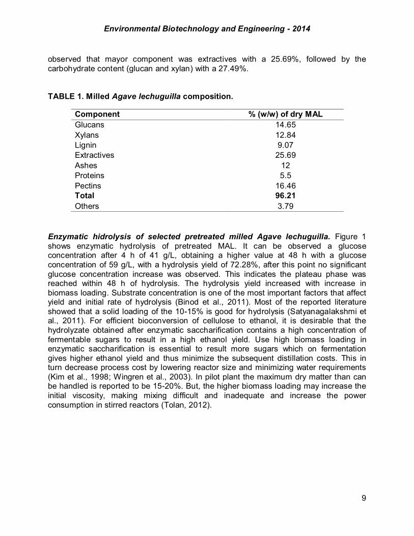
observed that mayor component was extractives with a 25.69%, followed by the carbohydrate content (glucan and xylan) with a 27.49%. TABLE 1. Milled Agave lechuguilla composition.
Enzymatic hidrolysis of selected pretreated milled Agave lechuguilla. Figure 1 shows enzymatic hydrolysis of pretreated MAL. It can be observed a glucose concentration after 4 h of 41 g/L, obtaining a higher value at 48 h with a glucose concentration of 59 g/L, with a hydrolysis yield of 72.28%, after this point no significant glucose concentration increase was observed. This indicates the plateau phase was reached within 48 h of hydrolysis. The hydrolysis yield increased with increase in biomass loading. Substrate concentration is one of the most important factors that affect yield and initial rate of hydrolysis (Binod et al., 2011). Most of the reported literature showed that a solid loading of the 10-15% is good for hydrolysis (Satyanagalakshmi et al., 2011). For efficient bioconversion of cellulose to ethanol, it is desirable that the hydrolyzate obtained after enzymatic saccharification contains a high concentration of fermentable sugars to result in a high ethanol yield. Use high biomass loading in enzymatic saccharification is essential to result more sugars which on fermentation gives higher ethanol yield and thus minimize the subsequent distillation costs. This in turn decrease process cost by lowering reactor size and minimizing water requirements (Kim et al., 1998; Wingren et al., 2003). In pilot plant the maximum dry matter than can be handled is reported to be 15-20%. But, the higher biomass loading may increase the initial viscosity, making mixing difficult and inadequate and increase the power consumption in stirred reactors (Tolan, 2012).
Component % (w/w) of dry MAL Glucans 14.65 Xylans 12.84 Lignin 9.07 Extractives 25.69 Ashes 12 Proteins 5.5 Pectins 16.46 Total 96.21 Others 3.79
Environmental Biotechnology and Engineering - 2014
10
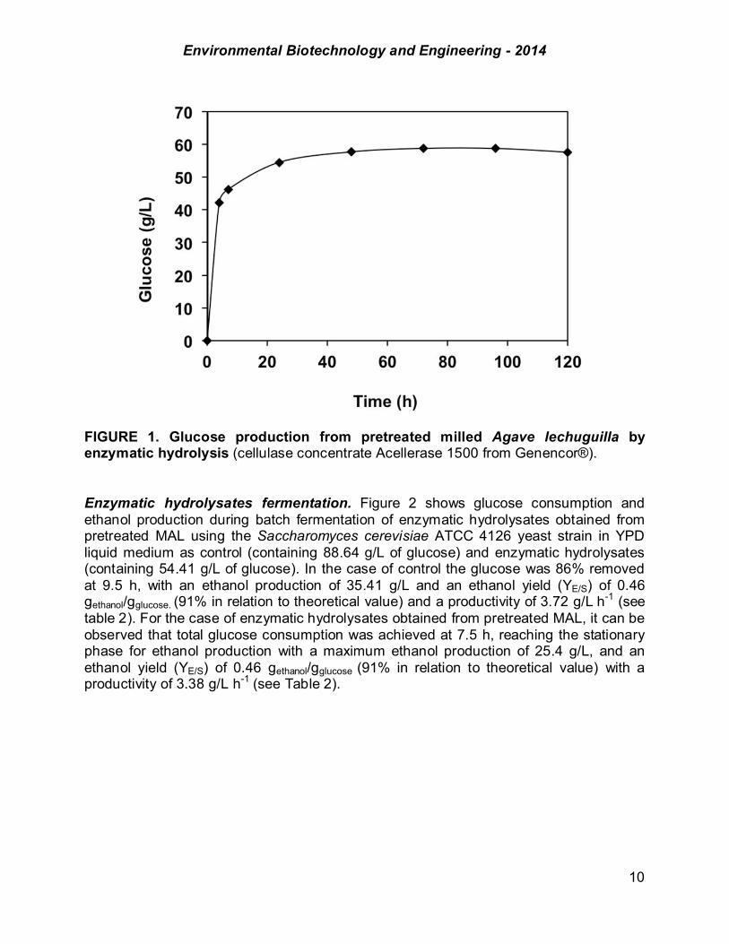
FIGURE 1. Glucose production from pretreated milled Agave lechuguilla by enzymatic hydrolysis (cellulase concentrate Acellerase 1500 from Genencor®). Enzymatic hydrolysates fermentation. Figure 2 shows glucose consumption and ethanol production during batch fermentation of enzymatic hydrolysates obtained from pretreated MAL using the Saccharomyces cerevisiae ATCC 4126 yeast strain in YPD liquid medium as control (containing 88.64 g/L of glucose) and enzymatic hydrolysates (containing 54.41 g/L of glucose). In the case of control the glucose was 86% removed at 9.5 h, with an ethanol production of 35.41 g/L and an ethanol yield (YE/S) of 0.46 gethanol/gglucose. (91% in relation to theoretical value) and a productivity of 3.72 g/L h-1 (see table 2). For the case of enzymatic hydrolysates obtained from pretreated MAL, it can be observed that total glucose consumption was achieved at 7.5 h, reaching the stationary phase for ethanol production with a maximum ethanol production of 25.4 g/L, and an ethanol yield (YE/S) of 0.46 gethanol/gglucose (91% in relation to theoretical value) with a productivity of 3.38 g/L h-1 (see Table 2).

Environmental Biotechnology and Engineering - 2014
11
FIGURE 2. Batch fermentation of enzymatic hydrolysates obtained from pretreated MAL using the Saccharomyces cerevisiae ATCC 4126 yeast strain. Glucose consumption (Filled markers) and ethanol production (unfilled markers) in control ( ) and enzymatic hydrolysates ( ).
FIGURE 3. Saccharomyces cerevisiae ATCC biomass growth in control.
Environmental Biotechnology and Engineering - 2014
12
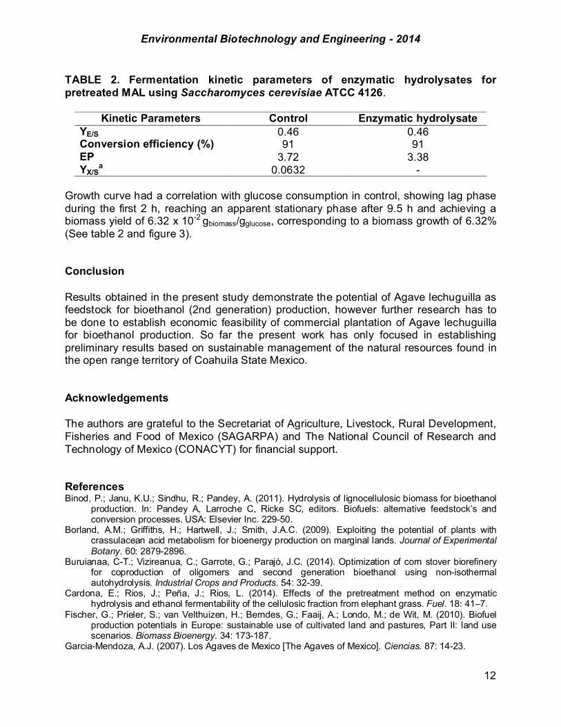
TABLE 2. Fermentation kinetic parameters of enzymatic hydrolysates for pretreated MAL using Saccharomyces cerevisiae ATCC 4126.
Kinetic Parameters Control Enzymatic hydrolysate YE/S 0.46 0.46 Conversion efficiency (%) 91 91 EP 3.72 3.38 YX/S
a 0.0632 -
Growth curve had a correlation with glucose consumption in control, showing lag phase during the first 2 h, reaching an apparent stationary phase after 9.5 h and achieving a biomass yield of 6.32 x 10⁻² gbiomass/gglucose, corresponding to a biomass growth of 6.32% (See table 2 and figure 3). Conclusion Results obtained in the present study demonstrate the potential of Agave lechuguilla as feedstock for bioethanol (2nd generation) production, however further research has to be done to establish economic feasibility of commercial plantation of Agave lechuguilla for bioethanol production. So far the present work has only focused in establishing preliminary results based on sustainable management of the natural resources found in the open range territory of Coahuila State Mexico. Acknowledgements The authors are grateful to the Secretariat of Agriculture, Livestock, Rural Development, Fisheries and Food of Mexico (SAGARPA) and The National Council of Research and Technology of Mexico (CONACYT) for financial support. References Binod, P.; Janu, K.U.; Sindhu, R.; Pandey, A. (2011). Hydrolysis of lignocellulosic biomass for bioethanol
production. In: Pandey A, Larroche C, Ricke SC, editors. Biofuels: alternative feedstock’s and conversion processes. USA: Elsevier Inc. 229-50.
Borland, A.M.; Griffiths, H.; Hartwell, J.; Smith, J.A.C. (2009). Exploiting the potential of plants with crassulacean acid metabolism for bioenergy production on marginal lands. Journal of Experimental Botany. 60: 2879-2896.
Buruianaa, C-T.; Vizireanua, C.; Garrote, G.; Parajó, J.C. (2014). Optimization of corn stover biorefinery for coproduction of oligomers and second generation bioethanol using non-isothermal autohydrolysis. Industrial Crops and Products. 54: 32-39.
Cardona, E.; Rios, J.; Peña, J.; Rios, L. (2014). Effects of the pretreatment method on enzymatic hydrolysis and ethanol fermentability of the cellulosic fraction from elephant grass. Fuel. 18: 41–7.
Fischer, G.; Prieler, S.; van Velthuizen, H.; Berndes, G.; Faaij, A.; Londo, M.; de Wit, M. (2010). Biofuel production potentials in Europe: sustainable use of cultivated land and pastures, Part II: land use scenarios. Biomass Bioenergy. 34: 173-187.
Garcia-Mendoza, A.J. (2007). Los Agaves de Mexico [The Agaves of Mexico]. Ciencias. 87: 14-23.

Environmental Biotechnology and Engineering - 2014
13
Garrote, G.; Domínguez, H.; Parajó, J.C. (1999). Hydrothermal processing of lignocellulosic materials. Holz als Roh- und Werkstoff. 57: 191-202.
Gnansounou, E. (2010). Production and use of lignocellulosic bioethanol in Europe: current situation and perspectives. Bioresource Technology. 101: 4842-4850.
Kang, K.E.; Han, M.; Moon, S-K.; Kang, H-W.; Kim, Y.; Cha, Y-L. (2013). Optimization of alkali-extrusion pretreatment with twin-screw for bioethanol production from Miscanthus. Fuel. 109: 520-526.
Kim, E.; Irwin, D.C.; Walker, L.P.; Wilson, D.B. (1998). Factorial optimization of a six cellulose mixture. Bioengineering and Biotechnology. 58: 494-501.
Márquez, A.; Casaruang, N.; González, I.; Colunga-GarcíaMarín, P. (1996). Cellulose extraction from Agave lechuguilla fibers. In: Notes, Economic Botany. 50(4): 465-468.
Moniz, P.; Pereira, H.; Quilhó, T.; Carvalheiro, F. (2013). Characterisation and hydrothermal processing of corn straw towards the selective fraction of hemicelluloses. Industrial Crops and Products. 50: 145-53.
Nobel, P.S.; Quero, E. (1986). Environmental productivity indices for a Chihuahuan Desert CAM plant, Agave lechuguilla. Ecology. 67(1): 1-11.
Núñez, H.M.; Rodríguez, L.F.; khanna, M. (2011). Agave for tequila and biofuels: an economic assessment and potential opportunities. GCB Bioenergy. 3: 43-57.
Pando-Moreno, M.; Pulido, R.; Castillo, D.; Jurado, E.; Jiménez, J. (2008). Estimating fiber for lechuguilla (Agave lecheguilla Torr., Agavaceae), a traditional non-timber forest product in Mexico. Forest Ecology and Management. 255: 3686–3690
Romaní, A.; Garrote, G.; López, F.; Parajó, J.C. 2011. Eucalyptus globulus wood fractionation by autohydrolysis and organosolv delignification. Bioresource Technology. 102: 5896-5904.
Satyanagalakshmi, K.; Sindhu, R.; Binod, P.; Janu, K.U.; Sukumaran, R.K.; Pandey, A. (2011). Bioethanol production from acid pretreated water hyacinth by separate hydrolysis and fermentation. Journal of Scientific and Industrial Research. 70: 156-161.
Sluiter, A.; Hames, B.; Ruiz, R.; Scralata, C.; Sluiter, J.; Templeton, D. (2011). Determination of structural carbohydrates and lignina in biomass. NREL/TP-51042618. Laboratory Analytical Procedure (LAP), National Renewable Energy Laboratory.
Somerville, C.; Youngs, H.; Taylor C.; Davis, S.C.; Long, S.P. (2010). Feedstocks for lignocellulosic biofuels. Science. 329: 790-792.
Talebnia, F.; Karakashev, D.; Angelidaki, I. (2010). Production of bioethanol from wheat straw: an overview on pretreatment, hydrolysis and fermentation. BioresourceTechnology. 101(13): 4744-53.
Tolan J. (2012). Iogen’s process for producing ethanol from cellulosic biomass. Clean Technologies and Environmental Policy. 3:339-345.
Vieira, M.C.; Heinze, T.; Antonio-Cruz, R.; Mendoza-Martinez, A.M. (2002). Cellulose derivatives from cellulosic material isolated from Agave lechuguilla and fourcroydes. Cellulose. 9: 203-212.
Wingren, A.; Galbe, M.; Zacchi, G. (2003). Techno-economic evaluation of producing ethanol from softwood: comparison of SSF and SHF and identification of bottlenecks. Biotechnology Progress. 19: 1109-1117.
Wyman, C.E.; Dale, B.E.; Elander, R.T.; Holtzapple, M.; Ladisch, M.R.; Lee, Y.Y. (2005). Coordinated development of leading biomass pretreatment technologies. Bioresource Technology. 96, 1959-1966.
Yáñez, R.; Romaní, A.; Garrote, G.; Alonso, J.L.; Parajó, J.C. (2009). Processing of Acacia dealbata in aqueous media: first step of a wood biorefinery. Industrial & Engineering Chemistry Research. 48(14): 6618–26.

Environmental Biotechnology and Engineering - 2014
14
CHAPTER 1.2. ENVIRONMENTAL AND ECONOMIC SUSTAINABILITY ANALYSIS OF LIGNOCELLULOSIC BIOETHANOL PRODUCTION
G. Magaña; D. R. Gómez, M. Solís; A. Sanchez*
Centro de Investigación y de Estudios Avanzados del IPN, Unidad Guadalajara de Ingeniería Avanzada, Zapopan, Jalisco.
ABSTRACT This work proposes a method to analyze the environmental and economic sustainability of lignocellulosic bioethanol production processes. The method quantifies the impacts of prospective processes such as bioethanol and electricity coproduction. Since there are no commercial plants for the production of lignocellulosic ethanol in operation, but only pilot and demonstration facilities, most of the available current analyses are based on data difficult to trace.
The proposed method is based on a process engineering approach and is composed by four main elements: the conceptual design (comprises a process flow sheet, mathematical models and an economic analysis), the application of the Process Analysis Method (PAM, providing a set of well supported indicators), the indicator analysis (consists on examining the indicator-results to extract conclusions when comparing different schemes) and the weighting process (integrates the indicator results into a global one using dimensional functions and scaling factors).
A comparison of four different schemes for lignocellulosic bioethanol production is presented as a case study. The systems named PETA 3.0 and PETA 3.2 are single product plants while BIOREF 3.0 and BIOREF 3.2 are multipurpose biorefineries. All systems coproduce lignocellulosic ethanol and electricity. The BIOREF schemes have an extra stage (dark fermentation) to produce biohydrogen which is fed to the cogeneration stage aiming to increase the production of electricity. The 3.2 schemes include energy integration and water recirculation. A total of 11 indicators were generated (6 for the environmental and 5 for the economic domain) and calculated. The indicator analysis showed that BIOREF emits 31% more GHG than PETA due to the large amount of CO2 produced in the dark fermentation stage. Besides, the discharged water of BIOREF is of lower quality owing mostly to the aggregates of the dark fermentation stage. Also, monosaccharides availability on the alcoholic fermentation stage represents a higher bioethanol production for PETA schemes which is translated into a larger impact than BIOREF schemes on the yield and contribution to the country’s economy indicators. The 3.2 schemes present a lower impact than PETA schemes in the environmental domain mainly due to water recirculation. Energy integration contributes in a reduction about 4% and 2% of total production cost (TPC) for PETA and BIOREF, respectively.
---------------- *Author for correspondence

Environmental Biotechnology and Engineering - 2014
15
Regarding the weighting analysis, BIOREF 3.0 scheme is the least sustainable due to the great amount of CO2 produced and the lower bioethanol production. Water recirculation and energy integration contributes on making PETA 3.2 the most sustainable scheme together with the highest bioethanol production and the lowest TPC. Key words: sustainability analysis, lignocellulosic bioethanol production, sustainability method, process analysis. Introduction Over the past decades liquid biofuels have been considered as an alternative to substitute fossil fuels. Due to the carbon debt, the indirect land use change (ILUC) and the alimentary crisis associated to first generation biofuels (1G), the usage of lignocellulosic feedstocks has been encouraged for liquid biofuels production (Holzner et al, 2012). Also, the development of more efficient processes and the establishment of government directives for the production of second and third generation (2G and 3G) biofuels have been promoted.
These lignocellulosic biofuels are considered as a potential alternative for diminishing GHG emissions, improve the energy security and contribute to the countries’ economy (Cardona et al. 2007; Sanchez et al. 2008). However, their economic, environmental and social impacts must be assessed in order to reduce or avoid negative effects (e.g. the alimentary-energy crisis associated with the first generation biofuels (Mitchell, 2008)). There is an increasing effort in developing methods for evaluating economic, environmental and social impacts (Gaasbeek et al., 2013; Schepelmann et al., 2009; Mata et al., 2013). Nevertheless, most of these methods focus only on the environmental impacts analysis with a macroeconomic approach. Therefore, the production processes are usually evaluated in general terms (Bird et al., 2011; ISO, 2006; Global Bioenergy Partnership, 2011). The Calcas Project presents an extensive review of the existing methods and tools for impacts evaluation (Schepelmann et al., 2009), most of them are based on the Life Cycle Assessment (LCA) which is usually focused on the assessment of GHG emissions and energy balances. However, since the LCA is based on measurements, its results are highly dependent on the available information, the assumptions made and the type of framework employed for their execution (Sanchez et al., 2014). Regarding lignocellulosic bioethanol production, since no commercial production plants are in operation, the need for the development of methods that evaluate the sustainability of these prospective production processes, has been increasing in importance.
Based on a process engineering approach, this work presents a method to assess the sustainability of biochemical platforms for lignocellulosic bioethanol production. This method provides a well-supported set of indicators to evaluate the impacts of the plant. Also, an indicator by indicator analysis is carried out and applying dimensional functions and scaling factors, a global sustainability value can be calculated (Sanchez et al., 2014). This is explained in the methodology section. As a case study and, focusing on the Mexican context, the sustainability assessment of four conceptual lignocellulosic biorefinery schemes for the coproduction of bioethanol and electricity was carried out. The calculated indicator values and their analysis, as well as the global
Environmental Biotechnology and Engineering - 2014
16
value obtained, are presented in the results and discussion section. Some final remarks regarding the presented method are mentioned in the conclusions section.
Methodology
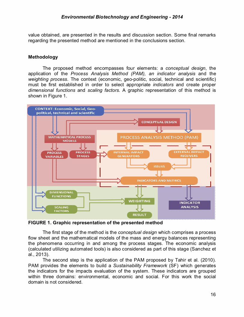
The proposed method encompasses four elements: a conceptual design, the application of the Process Analysis Method (PAM), an indicator analysis and the weighting process. The context (economic, geo-politic, social, technical and scientific) must be first established in order to select appropriate indicators and create proper dimensional functions and scaling factors. A graphic representation of this method is shown in Figure 1.
FIGURE 1. Graphic representation of the presented method
The first stage of the method is the conceptual design which comprises a process flow sheet and the mathematical models of the mass and energy balances representing the phenomena occurring in and among the process stages. The economic analysis (calculated utilizing automated tools) is also considered as part of this stage (Sanchez et al., 2013).
The second step is the application of the PAM proposed by Tahir et al. (2010). PAM provides the elements to build a Sustainability Framework (SF) which generates the indicators for the impacts evaluation of the system. These indicators are grouped within three domains: environmental, economic and social. For this work the social domain is not considered.
Environmental Biotechnology and Engineering - 2014
17
The elements of the PAM are: 1.System boundaries. Identifying inputs/outputs and activities. 2.Internal Impact Generators (IIG). The process activities generating the impacts. 3.External Impact Receivers (EIR). The entities or social groups being affected by
the IIG. 4.Issues. The EIR concerns regarding the process impacts. 5.Indicators. Created to represent the associated impacts with each issue. 6.Metrics. Quantifiers for the indicators. Can be one or more. Figure 1 shows the main elements of the SF, within the delimited area by the dotted line. The indicator analysis consists on examining each metric value and its associated
indicator, in order to get conclusions about the indicator impacts and the involved process activities. The analysis proves to be useful when comparing different schemes, therefore normalizing regarding a chosen scheme (the selection can be based on relevant characteristics for comparison purposes such as simplicity, standard technology, etc.) is a simple and effective analysis technique that is applied in the present work.
The weighting process integrates the indicator values into a global result employing dimensional functions and scaling factors, thus the sustainability of a specific scheme can be determined. The dimensional functions serve to translate all indicators to the same units so they can be added up later. These functions are created based on information classified among one of the three following categories: taxes, policies and duties, market value and total production cost (TPC) (Sanchez et al., 2014)]. The scaling factors are defined as the coefficients providing a relative importance to the dimensionalized metrics related to specific geopolitical and economic context of the production facility.
Case study The schemes to be assessed are four biorefineries for the coproduction of lignocellulosic bioethanol and electricity. Two of them, named PETA 3.0 and PETA 3.2, are single product plants. Also, a couple of multipurpose biorefineries (BIOREF 3.0 and BIOREF 3.2) are evaluated. The 3.2 schemes include water recirculation and energy integration. The feedstock for all schemes is 2,000 ton/day with a composition of 70% of polysaccharides dry base (Sanchez et al., 2014; Sanchez et al., 2013; Gonzalez et al., 2014).
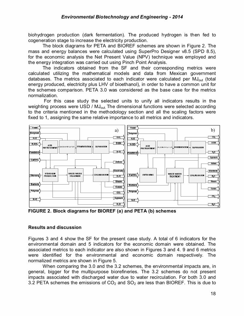
The production process for PETA schemes is conformed of seven stages: acid pretreatment (conditioning the feedstock), overliming (inhibitors removal and pH adjustment), saccharification (polysaccharides depolymerization), fermentation (bioethanol production), separation (alcohol concentration), waste water treatment (water recycling and biogas production) and cogeneration (electricity and steam generation). BIOREF scheme has a similar configuration with an additional stage for
Environmental Biotechnology and Engineering - 2014
18
biohydrogen production (dark fermentation). The produced hydrogen is then fed to cogeneration stage to increase the electricity production.
The block diagrams for PETA and BIOREF schemes are shown in Figure 2. The mass and energy balances were calculated using SuperPro Designer v8.5 (SPD 8.5), for the economic analysis the Net Present Value (NPV) technique was employed and the energy integration was carried out using Pinch Point Analysis.
The indicators obtained from the SF and their corresponding metrics were calculated utilizing the mathematical models and data from Mexican government databases. The metrics associated to each indicator were calculated per MJout (total energy produced, electricity plus LHV of bioethanol), in order to have a common unit for the schemes comparison. PETA 3.0 was considered as the base case for the metrics normalization.
For this case study the selected units to unify all indicators results in the weighting process were USD / MJout. The dimensional functions were selected according to the criteria mentioned in the methodology section and all the scaling factors were fixed to 1, assigning the same relative importance to all metrics and indicators.
FIGURE 2. Block diagrams for BIOREF (a) and PETA (b) schemes Results and discussion
Figures 3 and 4 show the SF for the present case study. A total of 6 indicators for the environmental domain and 5 indicators for the economic domain were obtained. The associated metrics to each indicator are also shown in Figures 3 and 4. 9 and 6 metrics were identified for the environmental and economic domain respectively. The normalized metrics are shown in Figure 5.
When comparing the 3.0 and the 3.2 schemes, the environmental impacts are, in general, bigger for the multipurpose biorefineries. The 3.2 schemes do not present impacts associated with discharged water due to water recirculation. For both 3.0 and 3.2 PETA schemes the emissions of CO2 and SO2 are less than BIOREF. This is due to
a) b)

Environmental Biotechnology and Engineering - 2014
19
the great quantity of CO2 produced in the dark fermentation (which is part of the BIOREF schemes). Multipurpose schemes discharge water with higher COD and dissolved pollutants than PETA schemes. The calculated value for the End Use Energy (EER) indicator, which is frequently evaluated, is larger for PETA schemes than BIOREF, owing mostly by PETA’s bigger bioethanol production. Therefore, PETA covers a larger percentage of its own energy demand compared to multipurpose biorefineries, despite BIOREF burning the produced biohydrogen in the cogeneration stage.
FIGURE 3. Environmental sustainability framework.
With the indicator analysis is possible to identify the process stages with a large impact in the sustainability of a given production process. For this case study, the dark fermentation in BIOREF schemes was identified as the stage with the largest impact since it uses the pentoses for hydrogen production generating a high quantity of CO2 as a coproduct. Thus, bioethanol production is lower in BIOREF schemes. In addition, the CO2 present in the hydrogen production output increases the energy demand since more energy is required to heat the stream in the cogeneration process. Then, the energy from the produced biohydrogen does not have a substantial contribution to the cogeneration stage and the energy efficiency of the BIOREF schemes is lower than
Environmental Biotechnology and Engineering - 2014
20
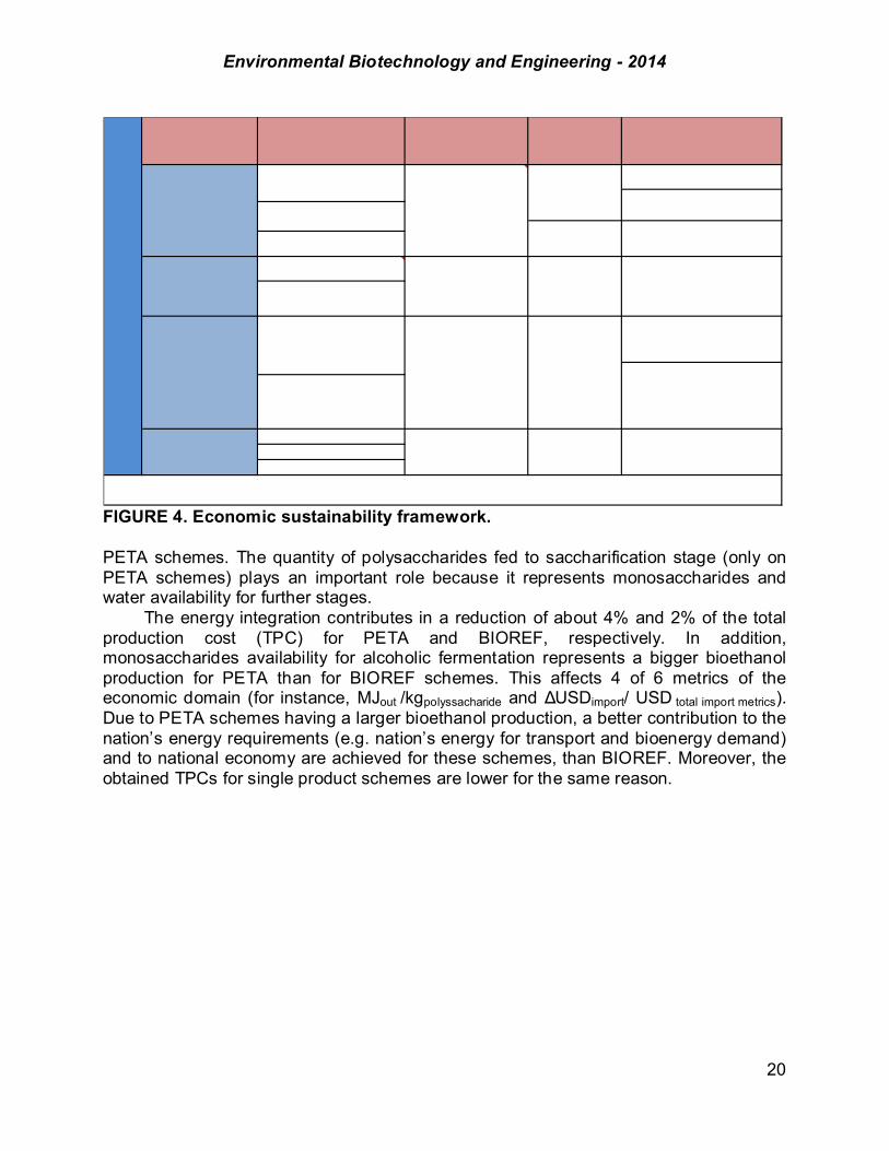
FIGURE 4. Economic sustainability framework. PETA schemes. The quantity of polysaccharides fed to saccharification stage (only on PETA schemes) plays an important role because it represents monosaccharides and water availability for further stages. The energy integration contributes in a reduction of about 4% and 2% of the total production cost (TPC) for PETA and BIOREF, respectively. In addition, monosaccharides availability for alcoholic fermentation represents a bigger bioethanol production for PETA than for BIOREF schemes. This affects 4 of 6 metrics of the economic domain (for instance, MJout /kgpolyssacharide and !USDimport/ USD total import metrics). Due to PETA schemes having a larger bioethanol production, a better contribution to the nation’s energy requirements (e.g. nation’s energy for transport and bioenergy demand) and to national economy are achieved for these schemes, than BIOREF. Moreover, the obtained TPCs for single product schemes are lower for the same reason.
Environmental Biotechnology and Engineering - 2014
21
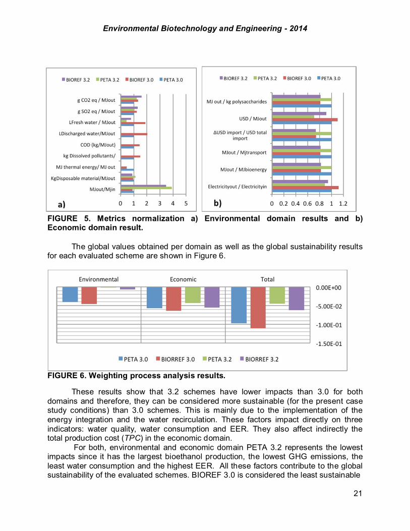
FIGURE 5. Metrics normalization a) Environmental domain results and b) Economic domain result.
The global values obtained per domain as well as the global sustainability results for each evaluated scheme are shown in Figure 6.
FIGURE 6. Weighting process analysis results.
These results show that 3.2 schemes have lower impacts than 3.0 for both domains and therefore, they can be considered more sustainable (for the present case study conditions) than 3.0 schemes. This is mainly due to the implementation of the energy integration and the water recirculation. These factors impact directly on three indicators: water quality, water consumption and EER. They also affect indirectly the total production cost (TPC) in the economic domain.
For both, environmental and economic domain PETA 3.2 represents the lowest impacts since it has the largest bioethanol production, the lowest GHG emissions, the least water consumption and the highest EER. All these factors contribute to the global sustainability of the evaluated schemes. BIOREF 3.0 is considered the least sustainable

Environmental Biotechnology and Engineering - 2014
22
scheme because it causes the highest impacts in both domains (no energy integration and water recirculation are included and the bioethanol production is the lowest). Conclusion The proposed method analyzes the sustainability of the coproduction of lignocellulosic bioethanol and electricity biorefineries from a process engineering approach in order to improve potential economic and environmental positive impacts from the design process. Additionally, this method provides the basis to identify the process activities affecting the sustainability of the production schemes. For the present case, the partial or total usage of the available sugars for the alcoholic fermentation stage was found to be an important factor for the analyzed schemes’ sustainability. Also, the implementation of energy integration and water recirculation contributes to the sustainability of the schemes in both domains.
GHG emissions jointly with energy integration, water recirculation and available monosaccharides for the alcoholic fermentation were identified as the main factors for PETA 3.2 and BIOREF 3.0 being the most and the least sustainable schemes respectively.
Acknowledgments Partial financial support from the Sustainability Energy Fund of the Secretary of Energy, Mexico (grant SENER 2010-150001) is kindly acknowledged. The VPN analysis tools were provided by Mr. Victor Sevilla. References Bird v; Cowie A.; Cherubini F.; Jungmeier G. (2011). Using a life cycle assessment approach to estimate
the net greenhouse gas emissions of bioenergy. Technical report, International Energy Agency, 2011.
Cardona C.; Sanchez O. (2007). Fuel ethanol production: process design trends and integration opportunities. Bioresource Technology, 98:2415-2457.
Gaasbeek A.; Meijer E. (2013). Handbook on a novel methodology for the sustainability impact assessment of new technologies. Technical report. Prosuite, 2013.
Global Bioenergy Partnership (2011). http://www.globalbioenergy.org/fileadmin/user upload/gbep/docs/Indicators/; accessed 09 June 2014.
Gonzalez SR.; Sanchez A.; Sevilla V.; Murguia M. (2014). Biofuels and electricity coproduction. A possible solution for the agro-industrials wastes treatment. Proceedings of the XXXV Mexican Academy Meeting of Chemical Engineering Research and Education (in Spanish), Puerto Vallarta, Jalisco, Mexico, 2014.
Holzner M.; Valero I.; Bockstaller N.; Rhomberg S. (2012). http://europa.eu/rapid/press-release_IP-12-1112_en.htm, 11 October 2013.
International Organization for Standardization (ISO)(2006). Environmental management – life cycle assessment – principles and framework. ISO 14040:2006, 2006.
Mata M.; Caetano N.; Costa C.A.V.; Sikdar S.K.; and Martins A. A. (2013). Sustainability analysis of biofuels through the supply chain using indicators. Sustainable Energy Technologies and Assessments, 3:53–30.
Mitchell D (2008). http://ssrn.com/abstract=1233058, accessed 10 January 2013. Sanchez A.; Magaña G.; Gomez D.R.; Solis M.; Banares-Alcantara R. (2014). Bidimensional sustainability
analysis of lignocellulosic ethanol production processes. Method and case study. In press. Biofuels,

Environmental Biotechnology and Engineering - 2014
23
Bioproducts and Biorefining. Sanchez A.; Sevilla-Güitrón V.; Gutierrez L.; Magaña G. (2013). Parametric analysis of 2G enzymatic
ethanol production costs and energy efficiency in medium-scale agriculture sectors. Fuel. 113:165–179.
Sanchez O.; Cardona C. (2008). Trends in biotechnological production of fuel ethanol from different feedstocks. Bioresource Technology, 99: 5270-5295.
Schepelmann P.; Ritthoff M.; Jeswani H.; Azapagic A.; Soumalainen K. (2009). Options for deepening and broadening LCA. Technical report, Co-ordination Action for innovation in Life- Cycle Analysis for Sustanability, 2009.
Tahir A. C.; Darton R.C. (2010). The Process Analysis Method of selecting indicators to quantify the sustainability performance of a business operation. Journal of Cleaner Production. 18:1598–1607.

Environmental Biotechnology and Engineering - 2014
24
CHAPTER 1.3 COCONUT WATER UTILIZATION FOR BIOETHANOL PRODUCTION
Alma R. Domínguez-Bocanegra* (1), Jorge Torres-Muñoz (2), Ricardo Aguilar-López (1)
(1) Departamento de Biotecnología y Bioingeniería, CINVESTAV-IPN, México D.F., México. (2) Departamento de Control Automático CINVESTAV-IPN, México D.F., México ABSTRACT The development of a fermentation process using carbon sources is of great economic importance for the production of biofuels on a commercial scale as is the case of coconut water for the production of bioethanol from Saccharomyces cerevisiae. Coconut is used for various purposes in the food and cosmetic industry but often coconut water is discharged into sewers, in spite of components such as sugars, vitamins, minerals, enzymes, amino acids, cytokinins, and phytohormones (natural hormones). Coconut wate is also very low in calories and has no fat content, which makes it an excellent food. So, the aim of this study was to use coconut water as a substrate to grow to Saccharomyces cerevisiae and obtain bioethanol. Coconut water was obtained from a company north of Mexico City. Saccharomyces cerevisiae cells were grown in YM medium (1% glucose, 0.3% yeast extract, 0.3% malt extract, 0.5% casein peptone) for 24 hours at constant temperature of 28 °C and stirrer speed 150 rpm and these cells were used as inoculum for our fermentation. The experiments were conducted in 500 mL flasks with 350 mL of coconut water no nutrient was added or YM medium. The cultures were inoculated with 35 mL YM medium in the exponential phase and incubated using a gyrating shaker at 150 rpm and 28°C, for 5 day. Samples were taken every two hours and reducing sugars were quantified according Miller, 1959, dry weight, cell number, optical density and ethanol concentration using a gas chromatograph. The results obtained indicate the coconut water turned out to be an excellent substrate for Saccharomyces cerevisiae to grow reaching a maximum growth of 90x106 cell per milliliter at 36 hours with a substrate consumption of 95%, the maximum production bioethanol obtained at that time was 50%. Introducción El interés por el bioetanol como combustible en respuesta a la subida de los precios del petróleo es el factor más importante que influye en el mercado mundial de etanol. La escasez de petróleo y su escalada de los precios han llevado a los científicos a desarrollar fuentes de energía alternativas para sustituir el petróleo. Alertas y amenazas del calentamiento global están en aumento debido a la utilización de más de los combustibles fósiles. Fuentes de combustibles alternativos como el bioetanol y el biodiesel se están produciendo para combatir estas amenazas. La producción de bioetanol a partir de biomasa de la planta ha sido objeto de considerable atención recientemente con el fin de mitigar el calentamiento y la demanda de petróleo mundial no de un recurso finito y es una emisión de gases de efecto invernadero [1]. ---------- * Author for correspondence, [email protected]
Environmental Biotechnology and Engineering - 2014
25
El etanol obtenido a partir de materiales de desecho basados en la biomasa o de fuentes renovables se llama como bioetanol y se puede utilizar como combustible, materia prima química, y un disolvente en diversas industrias. Tiene ciertas ventajas como sustitutos de petróleo, a saber. , El alcohol puede ser producido a partir de un número de recursos renovables, el alcohol como combustible se quema más limpia que el petróleo que es ambientalmente más aceptable. Es biodegradable y por lo tanto, controla la contaminación. Es mucho menos tóxico que los combustibles fósiles. Puede ser fácilmente integrado con el sistema de combustible de transporte existente, es decir, hasta un 5 % de bioetanol se puede mezclar con el combustible convencional, sin necesidad de modificación [2]. El fruto del cocotero (Cocusnucifera), es explotado comercialmente para aprovechar la cáscara (exocarpio y mesocarpio) y la nuez (endocarpio). El agua contenida en la nuez, constituye actualmente un subproducto que no es utilizado por las industrias y es eliminado en la mayoria de los procesos, sin ningún tipo de tratamiento que permita reducir los problemas de contaminación ambiental. El agua de coco contiene sustancias como azúcares, proteínas, minerales y vitaminas, que la convierten en un sustrato potencialmente bueno para la producción de biomasa o para otros fines. Algunos elementos trazas, encontrados en el agua de coco son: potasio, 312 mg/mL; fósforo 37 mg/ mL; sodio 105 mg/mL y calcio 29 mg/mL [Ramirez,S,O y col.2005]. El agua de coco tiene componentes tales como azúcares, vitaminas, minerales, electrolitos (como el potasio, magnesio, calcio, sodio y fósforo), enzimas, aminoácidos, citoquininas, y fitohormonas (hormonas naturales). El desarrollo de un proceso de fermentación usando fuentes de carbono económicas es de suma importancia para la producción de biocombustibles a escala comercial como es el caso del agua de coco residual para la producción de bioetanol a partir de Saccharomyces cerevisiae. El coco es utilizado para varios fines en la industria cosmetológica y alimentaria pero en muchas ocasiones el agua de coco va parar al alcantarillado lo que es lamentable ya que esta agua presenta un gran valor nutricional porque contiene vitaminas, acidos grasos, pero principalmente azucares como la glucosa y fructuosa. El objetivo del presente estudio fue utilizar agua de coco como sustrato para obtener biomasa de Sacharomyces cerevisae y producción de etanol. Materiales y métodos El agua de coco se obtuvo de una empresa al norte de la ciudad de México. Las células de Sacharomyces cerevisae se hicieron crecer en medio liquido YM (glucosa 10 g/L, extracto de levadura 5 g/L, extracto de malta 5g/L, peptona de caseína g/l), durante 28 horas a temperatura ambiente 28 ± 2oC y agitación continua 150 rpm estas células sirvieron como inóculo. Los experimentos se llevaron a cabo en frascos de 500 mL de capacidad total con 350 mL de jugo de tuna y 10% de inoculo v/v en fase de crecimiento exponencial, los cultivos se incubaron a temperatura ambiente 28 ± 2oC, agitación continua 150 rpm. Se tomaron muestras cada dos horas y se cuantifico azucares reductores de acuerdo Miller, 1959, peso seco, número de células, densidad óptica y etanol utilizando un cromatografía de gases.

Environmental Biotechnology and Engineering - 2014
26
FIGURA 1. Diagrama del protocolo del experimento. Resultados y discusión El pH del medio se mantuvo constante ya que se encontró dentro del intervalo para que la cepa creciera adecuadamente y obtener el etanol (Tabla 1).
TABLA 1. Composición típica del agua de coco.

Environmental Biotechnology and Engineering - 2014
27
En las cinéticas de crecimiento microbiano utilizando el agua de coco como sustrato, las ks obtenidas muestran que existe una mayor afinidad del microrganismo por el sustrato presente en el agua de coco (Fig. 1), de la misma manera µmax muestra que hubo una mayor velocidad de crecimiento en el blanco ya que el medio YM contenía los nutrientes específicos que el microrganismo necesita favoreciendo su optimo crecimiento. Respecto al trabajo elaborado por Ramirez & Molina (2005) se obtuvo un pH entre 4-4.5 que es similar a lo obtenido en este trabajo ya que ese es el pH requerido para favorecer un buen crecimiento microbiano.
Conclusión Se concluye que el agua de coco es un sustrato apto para el crecimiento de la levadura Saccharomyces cerevisiae. Por tanto, este resultado alentador abre las posibilidades de utilizar el agua de coco para la obtención de etanol por medio de fermentación alcohólica con esta levadura.

Environmental Biotechnology and Engineering - 2014
28
Referencias Aguilar, B &FranYios, J. 2003.A study of the yeast cell wall composition and structure in response to
growth conditions and mode of cultivation. Letters in Applied MIcrobiology 37: 268 – 274. Ariza, B. y González, L. 1997. Producción de proteína unicelular a partir de levadura y melaza de caña de
azúcar como sustrato. Tesis de Bacteriología. Pontificia Universidad Javeriana. Facultad de Ciencias. Departamento de Bacteriología. Bogotá. Colombia. 22-27pp.
Biosca, J. Fernandez Ma. R. Larroy, C. Gonzalez, E.Pares, X. 2002. Descripción y funciones metabólicas de los alcohol deshidrogenasas de Saccharomyces cerevisiae. Algunos aspectos de ingeniería metabólica aplicados a la fabricación de la cerveza. Universidad Autónoma de Barcelona.
Ramirez, S,O. Molina, C,M. 2005. Evaluación de parámetros cinéticos para la Saccharomyces cerevisiae utilizando agua de coco como sustrato. Ingeniería 15 (1,2): 91-102,

Environmental Biotechnology and Engineering - 2014
29
CHAPTER 1.4. BIOLOGICAL PRETREATMENT OF Agave lechuguilla BY Phanerochaete chrysosporium
Ricardo Reyna-Martinez (1); Thelma K. Morales-Martinez (1);
Leopoldo J. Rios-Gonzalez* (1); José A. Rodríguez-de la Garza (1); Julio C. Montañez-Saenz (2)
(1) Biotechnology Department, Chemistry Faculty, Universidad Autonoma de Coahuila, México. (2) Department of Chemical Engineering, Chemistry Faculty, Universidad Autonoma de Coahuila, México. ABSTRACT Agave lechuguilla biological pretreatment was optimized in solid state fermentation by Phanerocheate chrysosporium. Pretreatment was carried out under stationary cultivation method using milled and dehydrated Agave lechuguilla biomass. Biomass chemical composition was as following; cellulose 21%, hemicellulose 7.7% and lignin 13.5%, kirk medium was added according to humidity levels. An orthogonal experimental design (L9(34)) was used to optimize the pretreatment conditions. Nine pretreatments were carried out to evaluate the effect of humidity (40, 60 and 80%), temperature (30, 35 and 40 °C), incubation time (10, 15 and 20 days) and inoculum concentration (4, 5 and 6 µl of spore suspension). Results showed a maximum lignin degradation of 29% by P. chrysosporium, with no cellulose lost during the process. Incubation time had a statistically significantly higher influence during lignin degradation (63%), followed by temperature (32%), meanwhile humidity and inoculum concentration had no statistical significance. Finally, results showed that under optimum conditions 41% lignin degradation can be achieved. Key words: Agave lechuguilla, pretreatment, Phanerocheate chrysosporium. Introduction Currently, corn is the primary raw material for ethanol production in the United States (Farrell et al., 2006). However, lignocellulosic biomass has the potential to provide a more economical feedstock as a result of its widespread availability, sustainable production, less intensive agricultural management, and positive environmental impacts (Dunn et al., 1993). Lignocellulosic feedstocks as Agave lechuguilla are becoming more attractive because of their low cost and widespread availability, which makes them suitable for large scale and sustainable ethanol production (Buruiana et al., 2014). Agave lechuguilla (lechuguilla) is a very common plant in the Chihuahuan Desert, ------------ *Author for correspondence
Environmental Biotechnology and Engineering - 2014
30
covering large areas of the arid and semiarid lands of northern Mexico (200,000 km2) (Nobel and Quero, 1986; Márquez y col., 1996). Lechuguilla fiber is used in metal polishing brushes, furniture and car seat filling, carpets and cleaning brushes, as construction material in combination with thermoplastic resins and has recently been suggested as a concrete reinforcement (Pando et al., 2008). High content of structural carbohydrates present in Agave lechuguilla make this plant a potential biomass feedstock for biofuel production (Vieria et al., 2002). A major barrier in the commercialization of a lignocellulose based ethanol process is the pretreatment, which constitutes one-third of the total production costs (NREL, 2000). Lignocellulose is well designed naturally to resist enzymatic attack owing to the complexity of lignin and hemicellulose structures, and the hydrophobicity of the plant cell wall. Therefore, the accessibility to the holocellulose portion of the lignocellulose is a barrier in any biomass hydrolysis process. Removing lignin and hemicellulose, reduction of cellulose crystallinity, and increase of porosity during the pretreatment processes can significantly improve the enzymatic hydrolysis of cellulose in the lignocellulosic material (Singh and Chen, 2008). Therefore, the goal of pretreatment is to make the cellulose accessible to hydrolysis for conversion to sugars then biofuels. Various pretreatment techniques change the physical and chemical structure of the lignocellulosic biomass and improve hydrolysis rates. Existing pretreatment methods have largely been developed on the basis of physical and/or chemical technologies that typically use either steam, chemicals like acid, base, and oxidant or their combinations (Gonçalves and Schuchardt, 2002; Varga et al., 2003, 2004; Liu and Wyman, 2004; Teymouri et al., 2004). However, most physical and chemical pretreatments are associated with high-energy input and costly equipment. Furthermore, special handling is usually needed to remove detrimental compounds as well as acidic or alkaline wastewaters generated during chemical pretreatments (Keller et al., 2003). A benign alternative to harsh chemicals is microbial pretreatment, which employs microorganisms especially fungi and their enzyme systems to breakdown lignin present in lignocellulosic biomass. Fungal pretreatment has been previously explored to upgrade lignocellulosic materials for feed and paper applications (Hadar et at., 1993; Camarero et al., 1994; Messner et al., 1994), and recently this environment friendly approach has received renewed attention as a pretreatment technique for enhancing enzymatic saccharification and fermentation of lignocellulosic biomass to ethanol. Several basidiomycetes such as Phanerochaete chrysosporium, Ceriporiopsis subvermispora, Phlebia subserialis, and Pleurotus ostreatus have been examined on different lignocellulosic biomass to evaluate their delignification efficiencies (Keller et al., 2003; Hatakka, 1983; Sawada et al., 1995; Taniguchi et al., 2005). It has been highlighted that microbial pretreatment has potential advantages over the prevailing physiochemical pretreatment technologies due to reduced energy and material costs, relatively simple equipment, and use of biological catalysts (Keller et al., 2003). However, the feasibility of microbial pretreatment is still questioned, mainly due to the extremely long treatment time as well as the difficulty in selectively degrading lignin (Hatakka, 1983). P. chrysosporium is one of the most investigated white rot fungus for pretreatment because of its high growth rate compared to many other basidiomycetes, exceptional
Environmental Biotechnology and Engineering - 2014
31
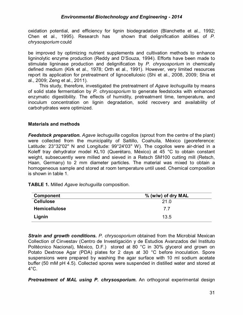
oxidation potential, and efficiency for lignin biodegradation (Blanchette et al., 1992; Chen et al., 1995). Research has shown that delignification abilities of P. chrysosporium could be improved by optimizing nutrient supplements and cultivation methods to enhance ligninolytic enzyme production (Reddy and D’Souza, 1994). Efforts have been made to stimulate ligninase production and delignification by P. chrysosporium in chemically defined medium (Kirk et al., 1978; Orth et al., 1991). However, very limited resources report its application for pretreatment of lignocellulosic (Shi et al., 2008, 2009; Shia et al., 2009; Zeng et al., 2011). This study, therefore, investigated the pretreatment of Agave lechuguilla by means of solid state fermentation by P. chrysosporium to generate feedstocks with enhanced enzymatic digestibility. The effects of humidity, pretreatment time, temperature, and inoculum concentration on lignin degradation, solid recovery and availability of carbohydrates were optimized. Materials and methods Feedstock preparation. Agave lechuguilla cogollos (sprout from the centre of the plant) were collected from the municipality of Saltillo, Coahuila, México (georeference: Latitude: 23°32'02'' N and Longitude: 99°24'03'' W). The cogollos were air-dried in a Koleff tray dehydrator model KL10 (Querétaro, México) at 45 °C to obtain constant weight, subsecuently were milled and sieved in a Retsch SM100 cutting mill (Retsch, Haan, Germany) to 2 mm diameter particles. The material was mixed to obtain a homogeneous sample and stored at room temperature until used. Chemical composition is shown in table 1. TABLE 1. Milled Agave lechuguilla composition.
Component % (w/w) of dry MAL Cellulose 21.0 Hemicellulose 7.7
Lignin 13.5 Strain and growth conditions. P. chrysosporium obtained from the Microbial Mexican Collection of Cinvestav (Centro de Investigación y de Estudios Avanzados del Instituto Politécnico Nacional), México, D.F.) stored at 80 °C in 30% glycerol and grown on Potato Dextrose Agar (PDA) plates for 2 days at 30 °C before inoculation. Spore suspensions were prepared by washing the agar surface with 10 ml sodium acetate buffer (50 mM pH 4.5). Collected spores were suspended in distilled water and stored at 4°C. Pretreatment of MAL using P. chrysosporium. An orthogonal experimental design
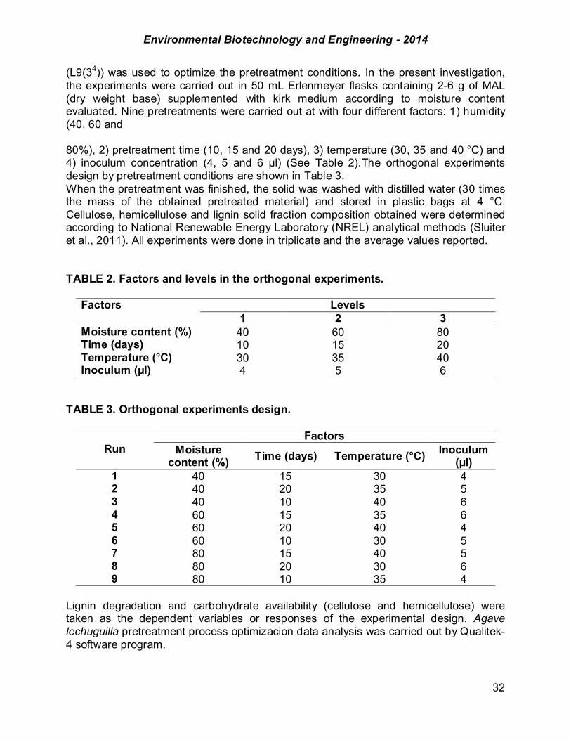
Environmental Biotechnology and Engineering - 2014
32
(L9(34)) was used to optimize the pretreatment conditions. In the present investigation, the experiments were carried out in 50 mL Erlenmeyer flasks containing 2-6 g of MAL (dry weight base) supplemented with kirk medium according to moisture content evaluated. Nine pretreatments were carried out at with four different factors: 1) humidity (40, 60 and 80%), 2) pretreatment time (10, 15 and 20 days), 3) temperature (30, 35 and 40 °C) and 4) inoculum concentration (4, 5 and 6 µl) (See Table 2).The orthogonal experiments design by pretreatment conditions are shown in Table 3. When the pretreatment was finished, the solid was washed with distilled water (30 times the mass of the obtained pretreated material) and stored in plastic bags at 4 °C. Cellulose, hemicellulose and lignin solid fraction composition obtained were determined according to National Renewable Energy Laboratory (NREL) analytical methods (Sluiter et al., 2011). All experiments were done in triplicate and the average values reported. TABLE 2. Factors and levels in the orthogonal experiments.
Factors Levels 1 2 3 Moisture content (%) 40 60 80 Time (days) 10 15 20 Temperature (°C) 30 35 40 Inoculum (µl) 4 5 6
TABLE 3. Orthogonal experiments design.
Run Factors
Moisture content (%) Time (days) Temperature (°C) Inoculum
(µl) 1 40 15 30 4 2 40 20 35 5 3 40 10 40 6 4 60 15 35 6 5 60 20 40 4 6 60 10 30 5 7 80 15 40 5 8 80 20 30 6 9 80 10 35 4
Lignin degradation and carbohydrate availability (cellulose and hemicellulose) were taken as the dependent variables or responses of the experimental design. Agave lechuguilla pretreatment process optimizacion data analysis was carried out by Qualitek-4 software program.

Environmental Biotechnology and Engineering - 2014
33
Results and discussion Figure 1 and table 4 shows the parameters studied and the effect of each parameter (Les is better) and ANOVA for the taguchi design (L9(34) for the pretreatment and deslignification process of Agave lechuguilla by Phanerocheate chrysosporium. Results obtained showed that time and temperature were the parameters with significant difference, level 1 for temperature (30°C) and level 2 for time (15 days) were above the media. Humidity and concentration had no significant difference over the process. TABLE 4. ANOVA and Taguchi design (L9(34)).
According to Tukey test cellulose composition of Agave lechuguilla no difference between Medias was observed, meaning this that cellulose was preserved during the pretreatment or delignification process. Figure 2 shows that incubation time was the factor with more significance over lignin degradation (63.33%) followed by temperature (32.04%), which was establish by preliminary studies and turn out to be 30°C the optimum temperature. Humidity and inoculum concentration had no significant influence over the process (1.98% y 1.19% respectively). Table 5 displays the combination of factors with optimum level for validation of pretreatment of Agave lechuguilla process by Phanerocheate chrysosporium. Data obtained for optimum levels were: Humidity (level 1 – 40%), pretreatment time (level 2 – 15 days), Temperature (Level 2 – 30 °C) and Inoculum concentration (level 3 – 6 µl). Acoording to the conditions established the results of combination of the factors and levels is 7.9% for final lignin and a degradation efficiency of 41%. Haddadin et al. (2002), reported that peroxidase and laccase activity during lignin degradation of a byproduct of olive oil production process by different basidiomycetes studied was optimum in a temperature range of 25°C – 30°C, concurring with results obtained in the present study. In the case of results obtained for time, it concurs with reported by Shi et al. (2008), in which the established that 14 days was the optimum time for lignin degradation of rice straws by Phanerochaete chrysosporium with a 60% of humidity.
Source DF Sum of squares (SS)
Variance (V) F value Percentage P
(%) Humidity 2 1.369 0.684 1.296 1.98 Time 2 41.502 20.751 41.429 63.33 Temperature 2 21.036 10.518 20.962 32.04 Inoculum 2 0.854 0.427 0.78 1.19 Error 18 0.659 0.036 1.46 Total 26 65.422 100.00

Environmental Biotechnology and Engineering - 2014
34
FIGURE 1. Main effect or parameters assessed for the present work (Less is better). Humidity, time, temperature and inoculum concentration.
Humidity Time
Temperature Inoculum
Level Level
Level Level

Environmental Biotechnology and Engineering - 2014
35
FIGURE 2. Significant factors. TABLE 5. Optimum condition for lignin degratation by Phanerochaete chrysosporium.
Serial No. Factor Value Level Contribution 1 Humidity 40 1 -0.226 2 Time 15 2 -1.56 3 Temperature 30 1 -0.993 4 Inoculum 6 3 -0.204 Total contribution by all factors -2.984 Yield average 10.937 Expected results of all factors 7.9
Conclusion Delignification of Agave lechuguilla biomass was achieved in solid fermentation by Phanerochaete chrysosporium (maximum lignin degradation of 29%), with no significant losses in cellulose content. Pretreatment time showed to be the most important factor during lignin degradation (63.33%), followed by temperature (32.04%), meanwhile humidity and inoculum concentration had no significant influence over the process. Finally, it can be stated that with optimum condition a 41% of lignin degradation can be achieved. References Blanchette, R.A.; Burnes, T.A.; Eerdmans, M.M.; Akhtar, M. (1992). Evaluating isolates of
Humidity Time Temperature Inoculum Error
Environmental Biotechnology and Engineering - 2014
36
Phanerochaete chrysosporium and Ceriporiopsis subvermispora for use in biological pulping processes. Holz- forschung. 46: 109-15.
Camarero, S.; Galletti, G.C; Martinez, A.T. (1994). Preferential degradation of phenolic lignin units by two white rot fungi. Applied and Environmental Microbiology. 60: 4509-4516.
Chen, J.; Fales, S.L.; Varga, G.A.; Royse, D.J. (1995). Biodegradation of cell wall components of maize stover colonized by white-rot fungi and resulting impact on in-vitro digestibility. Journal of Science and Food Agriculture. 68: 91-98.
Dunn, C.P.; Stearns, F.; Guntenspergen, G.R.; Sharpe, D.M. (1993). Ecological benefits of the conservation reserve program. Conservation Biolology. 7 (1): 132-139.
Farrell, A.E.; Plevin, R.J.; Turner, B.T.; Jones, A.D.; O‘Hare, M.; Kammen, D.M. (2006). Ethanol can contribute to energy and environmental goals. Science. 311: 506-508.
Gonçalves, A.R.; Schuchardt, U. (2002). Hydrogenolysis of lignins: influence of the pretreatment using microwave and ultrasound irradiations. Applied Biochemistry and Biotechnology. 98: 1213-1219.
Hadar, Y.; Kerem, Z.; Gorodecki, B. (1993). Biodegradation of lignocellulosic agricultural waste by Pleurotus ostreatus. Journal of Biotechnology. 30: 133-139.
Haddadin, M.S.; Natour, R.A.; Qsous, A.S.; Robinson, R.K. (2002). Biodegradation of lignin in olive pomace by freshly-isolates species of basidiomycete. Bioresource technology. 82:131-137
Hatakka, A.I. (1983). Pretreatment of wheat straw by white-rot fungi for enzymatic saccharification of cellulose. European Journal of Applied Microbiology and Biotechnology. 18: 350-357.
Keller, F.A.; Hamilton, J.E.; Nguyen, Q.A. (2003). Microbial pretreatment of biomass potential for reducing severity of thermo-chemical biomass pretreatment. Applied Biochemistry and Biotechnology. 105: 27–41.
Kirk T.K.; Schultz, E.; Connors, W.J.; Zeikus, J.G. (1978). Influence of culture parameters on lignin metabolism by Phanerochaete chrysosporium. Archives of Microbiology. 117: 277-285.
Liu, C.; Wyman, C.E. (2004). Impact of fluid velocity on hot water only pretreatment of corn stover in a flowthrough reactor. Applied Biochemistry and Biotechnology. 115: 977-988.
Márquez, A.; Casaruang, N.; González, I.; Colunga-GarcíaMarín, P. (1996). Cellulose extraction from Agave lechuguilla fibers. In: Notes, Economic Botany. 50(4): 465-468.
Messner, K.; Srebotnik, E. (1994). Biopulping: an overview of develop- ments in an environmentally safe paper-making technology. FEMS Microbiology Reviews. 13: 351-64.
Nobel, P.S.; Quero, E. (1986). Environmental productivity indices for a Chihuahuan Desert CAM plant, Agave lechuguilla. Ecology. 67(1): 1-11.
NREL (National Renewable Energy Laboratory). (2000). Technical report: determining the cost of producing ethanol from corn starch and lignocellulosic feedstocks, NREL/TP-580-28893.
Orth, A.B.; Denny, M.; Tien, M. (1991). Overproduction of lignin-degrading enzymes by an isolate of Phanerochaete chrysosporium. Applied and Environmental Microbiology. 57: 2591-2596.
Pando-Moreno, M.; Pulido, R.; Castillo, D.; Jurado, E.; Jiménez, J. (2008). Estimating fiber for lechuguilla (Agave lecheguilla Torr., Agavaceae), a traditional non-timber forest product in Mexico. Forest Ecology and Management. 255: 3686–3690
Reddy C.A.; D’Souza, T.M. (1994). Physiology and molecular biology of the lignin peroxidases of Phanerochaete chrysosporium. FEMS Microbiology Reviews. 13: 137-152.
Sawada, T.; Nakamura, Y.; Kobayashi, F.; Kuwahara, M.; Watanabe, T. (1995). Effects of fungal pretreatment and steam explosion on enzymatic saccharification of plant biomass. Biotechnology and Bioengineering. 48: 719-24.
Shi J.; Chinn M.S.; Sharma-Shivappa, R.R. (2008). Microbial pretreatment of cotton stalks by solid state cultivation of Phanerochaete chrysosporium. Bioresource Technology. 99: 6556–6564.
Shi, J.; Sharma-Shivappa, R.R.; Chinn, M.S. (2009). Microbial pretreatment of cotton stalks by submerged cultivation of Phanerochaete chrysosporium. Bioresource Technology. 100: 4388-4395.
Shia, J.; Sharma-Shivappa, R.R.; Chinn, M.; Howell N. (2009). Effect of microbial pretreatment on enzymatic hydrolysis and fermentation of cotton stalks for ethanol production. Biomass and Bioenergy. 33: 88-96.
Singh, D.; Chen, S. (2008). The white-rot fungus Phanerochaete chrysosporium: conditions for the production of lignin-degrading enzymes. Applied Microbiology and Biotechnology. 81: 399-417.
Taniguchi, M.; Suzuki, H.; Watanabe, D.; Sakai, K.; Hoshino, K.; Tanaka, T. (2005). Evaluation of pretreatment with Pleurotus ostreatus for enzymatic hydrolysis of rice straw. Journal of Bioscience and Bioengineering. 100: 637-43.

Environmental Biotechnology and Engineering - 2014
37
Teymouri, F.; Laureano-Perez, L.; Alizadeh, H.; Dale, B.E. (2004). Ammonia fiber explosion treatment of corn stover. Applied Biochemistry and Biotechnology. 115: 951-963.
Varga, E.; Reczey, K.; Zacchi, G. (2004). Optimization of steam pretreatment of corn stover to enhance enzymatic digestibility. Applied Biochemistry and Biotechnology. 114: 509-523.
Varga, E.; Schmidt, A.S.; Reczey, K.; Thomsen, A.B. (2003). Pretreatment of corn stover using wet oxidation to enhance enzymatic digestibility. Applied Biochemistry and Biotechnology. 104: 37-50.
Vieira, M.C.; Heinze, T.; Antonio-Cruz, R.; Mendoza-Martinez, A.M. (2002). Cellulose derivatives from cellulosic material isolated from Agave lechuguilla and fourcroydes. Cellulose. 9: 203-212.
Zeng, J.; Singh, D.; Chen S. (2011). Biological pretreatment of wheat straw by Phanerochaete chrysosporium supplemented with inorganic salts. Bioresource Technology. 102: 3206–3214.

Environmental Biotechnology and Engineering - 2014
38
CHAPTER 1.5 PRODUCCIÓN DE HIDRÓGENO A PARTIR DE Chlorella SP. Y Chlamydomonas SP.
Erica M. Hernández-Hernández* (1), Roxana Olvera-Ramírez (2),
Claudia A. Cortés-Escobedo (3)
(1) ENCB-IPN, D.F., México. (2) ENCB-IPN, Distrito Federal, México (3) CIITEC-IPN, Azcapotzalco, Distrito Federal, México. RESUMEN La obtención de energía impacta fuertemente el ambiente, como alternativa ante esta problemática existen las tecnologías del hidrógeno. Se ha descubierto que algunas algas verdes unicelulares y cianobacterias tienen la capacidad de generar hidrógeno molecular (H2) fotosintéticamente, proceso al que se le llama biofotólisis. El objetivo de esta investigación fue evaluar la producción de H2 en cultivos de Chlorella sp. y Chlamydomonas sp,, empleando el medio mineral BG-11 sin azufre en cultivos en suspensión e inmovilizados en alginato de sodio. Se obtuvieron las cinéticas de crecimiento de ambas cepas, valorando el efecto de la inmovilización celular sobre su crecimiento. Posteriormente se realizaron pruebas de producción de hidrógeno, sometiendo a estrés por ausencia de azufre en el medio de cultivo. Se observó que la inmovilización influye en ambas cepas sobre el crecimiento modificando la tendencia de crecimiento exponencial a lineal, sin embargo no afecta su sobrevivencia ni reproducción. En las pruebas de producción de hidrógeno se obtuvo que Chlamydomonas tiene mayor potencial de producción, particularmente en condiciones de inmovilización. Chlorella sólo en condiciones de inmovilización produjo hidrógeno, sin embargo no se descarta su potencialidad. Concluyendo que la técnica de inmovilización con alginato de sodio no afecta la producción de hidrogeno en las cepas utilizadas y facilita la manipulación de los organismos favoreciendo la producción de hidrógeno a una escala mayor. Palabras clave: algas, biohidrógeno, biofotólisis, Chlamydomonas, inmovilización, energía. Introducción Desde el siglo pasado la humanidad ha utilizado a los combustibles fósiles para cubrir sus necesidades energéticas recurriendo a su combustión para proveerse de electricidad y calor. El uso de estos recursos naturales implica, además de su cercano y progresivo agotamiento, un constante deterioro ambiental, que se manifiesta en emisiones de CO2, NOx, y SOx, favoreciendo el agravamiento del efecto invernadero, un --------------------- *Author for correspondence: [email protected]
Environmental Biotechnology and Engineering - 2014
39
aumento progresivo de la desertización y la erosión y una modificación de los mayores ecosistemas mundiales con la consecuente desaparición de biodiversidad (Díaz Coutiño & Escárcega Castellanos, 2009; Laborde & Rubiera Gonzalez, 2010) Sin embargo contrario a lo que se piensa los escenarios mundiales están cambiando rápidamente, trazándose un nuevo horizonte en el mercado energético. La implementación de tecnologías menos contaminantes cada vez más eficientes reconfiguran el panorama de la producción de electricidad. La tendencia mundial hacia la disminución de combustibles fósiles se ve reflejada en la capacidad de generación eléctrica, donde la participación de otras fuentes primarias va en crecimiento. Lamentablemente, México aún depende de fuentes fósiles en 76.6%, aumentando su dependencia en el gas natural (SENER, 2013). El reto en la actualidad es reducir la demanda de combustibles fósiles para igualar y en el menor de los casos disminuir la tasa de agotamiento, con respecto a la de uso; administrando de la mejor manera los recursos que quedan para facilitar la transición a lo que sigue, energéticamente hablando. Por lo tanto es de importancia tener una visión realista de las posibilidades y los problemas asociados con el uso de las energías renovables. (Hall & Ramirez-Pascualli, 2013; Al-Hallaj & Kisynski, 2001). La producción limpia y renovable no necesariamente debe provenir de una sola fuente, es decir existe la posibilidad de obtener sistemas híbridos, que eficiente la obtención de dicha energía, de acuerdo con las características y necesidades de cada consumidor. Fusionando en este caso diversas fuentes energéticas. La energía solar, la eólica, la océanica, la geotérmica, la obtenida a partir de biomasa y las tecnologías del hidrógeno, son formas de obtención de energía que ofrecen múltiples ventajas ambientales de manera individual y mucho más si se fusionan o acoplan para obtener sistemas eficientes encaminados a la obtención energética sustentable. Particularmente en este trabajo se explora una fuente biológica de hidrógeno, el cual es sabido que ofrece grandes ventajas energéticas y ambientales si se aprovecha como un vector energético. El hidrógeno que es obtenido a partir de fuentes biológicas es denominado biohidrógeno, y existen microorganismos capaces de producirlo si se tienen las condiciones necesarias, para lo cual se han encontrado diversas maneras de inducir dicho proceso. A pesar de que estos métodos de producción biológica de hidrógeno en la actualidad son muy poco eficientes, tienen como ventaja que el costo de producción y ambiental es bajo, por lo que se deben centrar intereses en el desarrollo científico y tecnológico para hacer más eficientes los sistemas de producción biofotolítica de hidrógeno. Para la investigación aplicada de este sistema de producción biológica de hidrógeno es fundamental tener en cuenta dos factores; que ésta se debe principalmente a la presencia celular de enzimas tales como la Fe-hidrogenasa que pueden ser inhibidas por la presencia de oxígeno y que el manejo de estos organismos a gran escala se dificulta debido a su carácter microscópico. Es por ello que a través de este trabajo se busca evaluar las condiciones de producción de hidrógeno con células inmovilizadas en esferas de alginato, con la finalidad de aportar elementos que favorezcan la obtención de dicho gas a partir de microalgas considerando que es factible realizar este proceso en un sistema en dos etapas.

Environmental Biotechnology and Engineering - 2014
40
Materiales y métodos Se utilizaron cepas de Chlorella sp. proporcionada por el Laboratorio de Fisiología Vegetal, ENCB-IPN y de Chlamydomonas sp. proporcionada por el Laboratorio de Hidrobiología Experimental, ENCB-IPN. Cultivo y cinética de crecimiento. Los cultivos en suspensión se realizaron en medio mineral BG-11 completo (Rippka, Deruelles, Waterbury, Herdman, & Stainer, 1979), centrifugando 25ml de cosecha a 3500rpm durante 30 minutos en una centrífuga Damon/IEC Division PR-6000, la cual fue resuspendida en 25ml de medio BG-11 completo; dicho concentrado celular se aforó a 700ml con medio de cultivo en un matraz Erlenmeyer de 1L y se colocó tapón de caucho y tubería correspondiente. Para los cultivos inmovilizados previamente se preparó medio mineral BG-11 omitiendo la adición de la solución de K2HPO4 durante su preparación; esto para prevenir la formación de fosfato de calcio lo cual podría provocar la ruptura de las esferas de inmovilización. En 150ml de dicho medio, se disolvieron 2.8g de alginato de sodio de media viscosidad (SIGMA, 9005-383) a punto de ebullición. Una vez disuelto se esterilizó y se dejó enfriar a temperatura ambiente. Adicionalmente se centrifugaron 25ml de cosecha a 3500 rpm durante 30 minutos, el concentrado de biomasa obtenido se resuspendió en 25ml de medio BG-11 sin K2HPO4. Este concentrado celular se incorporó con la solución alginato-medio de cultivo preparada anteriormente. Posteriormente se descargó por goteo esta última mezcla en 200ml de solución de CaCl2 (0.1M) para la formación de las esferas de inmovilización las cuales se dejaron en agitación durante 20 minutos, finalmente se enjuagaron con medio de cultivo sin K2HPO4 y se colocaron en un matraz Erlenmeyer de 1 L aforando a 700 ml del mismo medio, colocando un tapón de caucho y tubería de vidrio. Ambos cultivos fueron colocados en aireación constante y fotoperiodo de 12 horas luz y 12 horas de oscuridad, los procedimientos mencionados se realizaron para ambas cepas y por duplicado. Para obtener la cinética de crecimiento de cada cepa y de cada variación estudiada se tomaron alícuotas de 10ml para los cultivos en suspensión y una esfera de inmovilización para los inmovilizados. Dichas muestras se tomaron cada 3 días, desde el día uno hasta el 36, fueron mantenidas en refrigeración y oscuridad hasta su procesamiento. Todas las muestras fueron evaluadas por cuantificación de clorofila utilizando la técnica SCOR-UNESCO (1980). Inducción de estrés por ausencia de azufre en el medio. Se preparó medio de cultivo libre de azufre y de fosfato para su utilización en cultivos inmovilizados y medio de cultivo únicamente sin azufre para los cultivos en suspensión. Esto se realizó omitiendo la adición de las soluciones de MgSO4, K2HPO4 y la solución de micronutrientes durante la preparación del medio. Se cosecharon 200 ml de los cultivos en suspensión, los cuales fueron centrifugados a 3500rpm durante 30 minutos para eliminar el medio de crecimiento. El concentrado de biomasa se resuspendió en 250 ml medio de cultivo libre de azufre, y fue colocado en un frasco de vidrio con tapón de caucho tubería en aireación constante y fotoperiodo durante 7 días. Para los cultivos inmovilizados se procedió de manera similar, sin embargo para la eliminación del medio de cultivo de crecimiento sólo fue necesario decantar.
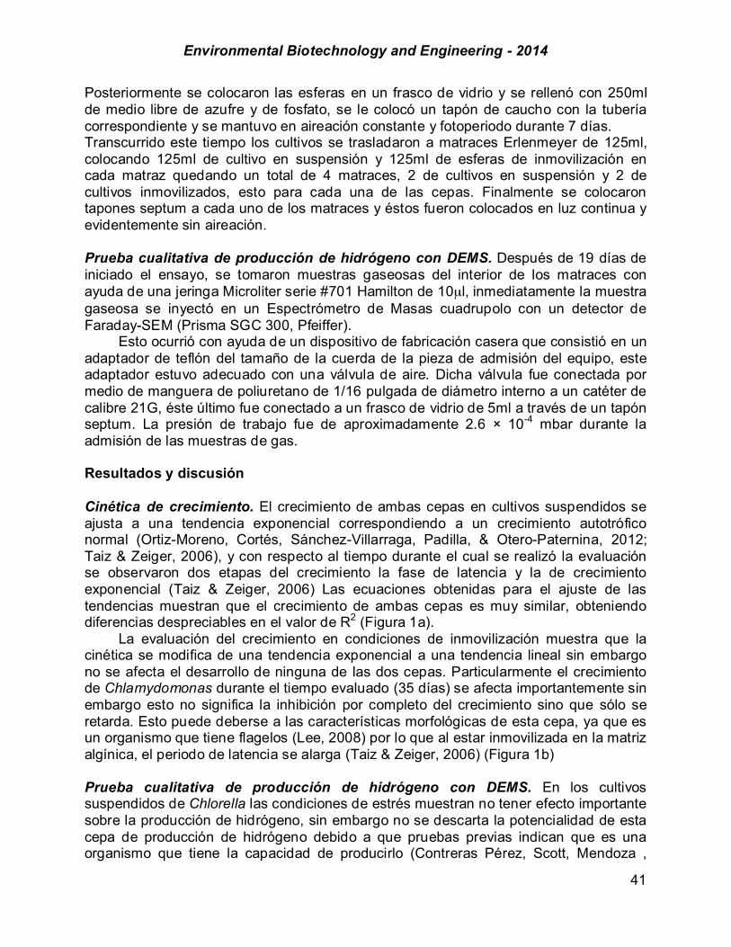
Environmental Biotechnology and Engineering - 2014
41
Posteriormente se colocaron las esferas en un frasco de vidrio y se rellenó con 250ml de medio libre de azufre y de fosfato, se le colocó un tapón de caucho con la tubería correspondiente y se mantuvo en aireación constante y fotoperiodo durante 7 días. Transcurrido este tiempo los cultivos se trasladaron a matraces Erlenmeyer de 125ml, colocando 125ml de cultivo en suspensión y 125ml de esferas de inmovilización en cada matraz quedando un total de 4 matraces, 2 de cultivos en suspensión y 2 de cultivos inmovilizados, esto para cada una de las cepas. Finalmente se colocaron tapones septum a cada uno de los matraces y éstos fueron colocados en luz continua y evidentemente sin aireación. Prueba cualitativa de producción de hidrógeno con DEMS. Después de 19 días de iniciado el ensayo, se tomaron muestras gaseosas del interior de los matraces con ayuda de una jeringa Microliter serie #701 Hamilton de 10µl, inmediatamente la muestra gaseosa se inyectó en un Espectrómetro de Masas cuadrupolo con un detector de Faraday-SEM (Prisma SGC 300, Pfeiffer). Esto ocurrió con ayuda de un dispositivo de fabricación casera que consistió en un adaptador de teflón del tamaño de la cuerda de la pieza de admisión del equipo, este adaptador estuvo adecuado con una válvula de aire. Dicha válvula fue conectada por medio de manguera de poliuretano de 1/16 pulgada de diámetro interno a un catéter de calibre 21G, éste último fue conectado a un frasco de vidrio de 5ml a través de un tapón septum. La presión de trabajo fue de aproximadamente 2.6 ! 10-4 mbar durante la admisión de las muestras de gas. Resultados y discusión Cinética de crecimiento. El crecimiento de ambas cepas en cultivos suspendidos se ajusta a una tendencia exponencial correspondiendo a un crecimiento autotrófico normal (Ortiz-Moreno, Cortés, Sánchez-Villarraga, Padilla, & Otero-Paternina, 2012; Taiz & Zeiger, 2006), y con respecto al tiempo durante el cual se realizó la evaluación se observaron dos etapas del crecimiento la fase de latencia y la de crecimiento exponencial (Taiz & Zeiger, 2006) Las ecuaciones obtenidas para el ajuste de las tendencias muestran que el crecimiento de ambas cepas es muy similar, obteniendo diferencias despreciables en el valor de R2 (Figura 1a). La evaluación del crecimiento en condiciones de inmovilización muestra que la cinética se modifica de una tendencia exponencial a una tendencia lineal sin embargo no se afecta el desarrollo de ninguna de las dos cepas. Particularmente el crecimiento de Chlamydomonas durante el tiempo evaluado (35 días) se afecta importantemente sin embargo esto no significa la inhibición por completo del crecimiento sino que sólo se retarda. Esto puede deberse a las características morfológicas de esta cepa, ya que es un organismo que tiene flagelos (Lee, 2008) por lo que al estar inmovilizada en la matriz algínica, el periodo de latencia se alarga (Taiz & Zeiger, 2006) (Figura 1b) Prueba cualitativa de producción de hidrógeno con DEMS. En los cultivos suspendidos de Chlorella las condiciones de estrés muestran no tener efecto importante sobre la producción de hidrógeno, sin embargo no se descarta la potencialidad de esta cepa de producción de hidrógeno debido a que pruebas previas indican que es una organismo que tiene la capacidad de producirlo (Contreras Pérez, Scott, Mendoza ,
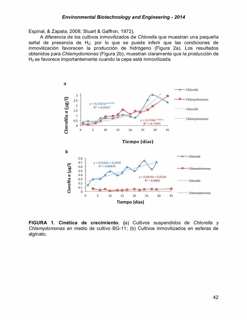
Environmental Biotechnology and Engineering - 2014
42
Espinal, & Zapata, 2008; Stuart & Gaffron, 1972), A diferencia de los cultivos inmovilizados de Chlorella que muestran una pequeña señal de presencia de H2; por lo que se puede inferir que las condiciones de inmovilización favorecen la producción de hidrógeno (Figura 2a). Los resultados obtenidos para Chlamydomonas (Figura 2b), muestran claramente que la producción de H2 se favorece importantemente cuando la cepa está inmovilizada.
FIGURA 1. Cinética de crecimiento. (a) Cultivos suspendidos de Chlorella y Chlamydomonas en medio de cultivo BG-11; (b) Cultivos inmovilizados en esferas de alginato.
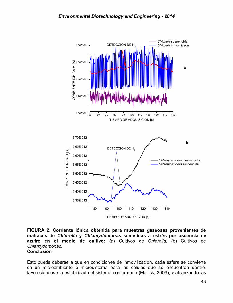
Environmental Biotechnology and Engineering - 2014
43
FIGURA 2. Corriente iónica obtenida para muestras gaseosas provenientes de matraces de Chlorella y Chlamydomonas sometidas a estrés por asuencia de azufre en el medio de cultivo: (a) Cultivos de Chlorella; (b) Cultivos de Chlamydomonas. Conclusión Esto puede deberse a que en condiciones de inmovilización, cada esfera se convierte en un microambiente o microsistema para las células que se encuentran dentro, favoreciéndose la estabilidad del sistema conformado (Mallick, 2006), y alcanzando las
50 60 70 80 90 100 110 120 130 140 1501.00E-011
1.20E-011
1.40E-011
1.60E-011
1.80E-011 Chlorella suspendida Chlorella inmovilizada
CO
RR
IEN
TE IO
NIC
A H
2 [A
]
TIEMPO DE ADQUISICION [s]
DETECCION DE H2
80 90 100 110 120 130 140
5.35E-012
5.40E-012
5.45E-012
5.50E-012
5.55E-012
5.60E-012
5.65E-012
5.70E-012
Chlamydomonas inmovilizada Chlamydomonas suspendida
CO
RR
IEN
TE IO
NIC
A H
2 [A
]
TIEMPO DE ADQUISICION [s]
DETECCION DE H2
a
b

Environmental Biotechnology and Engineering - 2014
44
condiciones de anaerobiosis más rápidamente, y así mismo la activación de los complejos enzimáticos que coadyuvan en la producción del gas de interés (Melis & Happe, 2001; Contreras Pérez, Scott, Mendoza , Espinal, & Zapata, 2008). Cabe mencionar que al finalizar estas pruebas los cultivos de Chlorella en suspensión mostraron una coloración amarilla oscura, indicando ligera muerte celular. Los cultivos de Chlamydomonas no mostraron cambio de color. Esto indica que Chlamydomonas tiene mejor resistencia a las condiciones de estrés con respecto a Chlorella (Melis & Happe, 2001). Chlorella y Chlamydomonas no son afectadas por la aplicación de técnicas de inmovilizacón en el potencial de producción de hidrógeno, por lo que son susceptibles de explotación a gran escala utilizando esta técnica, para favorecer y optimizar la manipulación de estos microorganimos en sistemas en dos etapas, para la generación de energía eléctrica a partir del hidrógeno que producen Agradecimientos Por el apoyo brindado a los directores del PROYECTO SIP 2014076 y PROYECTO CONACYT 160333 Referencias Al-Hallaj, S., & Kisynski, K. (2001). Hybrid hydrogen systems. Stationary and transportation applications.
New York: Springer-Verlag. Contreras Pérez, J. B., Scott, J. A., Mendoza , C. L., Espinal, G., & Zapata, Z. (2008). Potencial de algas
verdes para la producción fotobiológica de hidrógeno. Ciencia y Sociedad, 23(3), 307-327. Díaz Coutiño , R., & Escárcega Castellanos, S. (2009). Desarrollo sustentable. Una oportunidad para la
vida. México, D.F.: McGraw-Hill Interamericana Editores. Hall, C. A., & Ramirez-Pascualli, C. A. (2013). The first half of the age of oil an exploration of the work of
Colin Campbell and Jean Laherrère. New York, USA: Springer. Laborde, M. A., & Rubiera Gonzalez, F. (2010). La economía del hidrógeno. En M. A. Laborde , & F.
Rubiera Gonzalez, La energía del hidrógeno (págs. 7-10). Madrid, España: CYTED. Lee, R. E. (2008). Phycology. Cambridge, UK: Cambridge University Press. Mallick, N. (2006). Immobilization of microalgae. En J. M. Guisán, Methods in Biotechnology:
Immobilization of Enzymes and Cells (segunda ed., Vol. 22, págs. 373-383). Totowa, NJ: Humana Press Inc.
Melis, A., & Happe, T. (Noviembre de 2001). Hydrogen Production. Green Algae as a Source of Energy. Plant Physiology, 127, 740–748.
Ortiz-Moreno, M. L., Cortés, C. E., Sánchez-Villarraga, J., Padilla, J., & Otero-Paternina, A. M. (2012). Evaluación del crecimiento de la microalga Chlorella sorokiniana en diferentes medios de cultivo en condiciones autotróficas y mixotróficas. ORINOQUIA, 16(1), 12-20.
Rippka, R., Deruelles, J., Waterbury, J. B., Herdman, M., & Stainer, R. Y. (1979). Gen Microbiol 111, 1-61. SENER. (2013). Prospectiva del Sector Eléctrico 2013-2027. México, D.F.: Secretaria de energía. Stuart, T. S., & Gaffron, H. (1972). The Mechanism of Hydrogen Photoproduction by Several Algae.
Planta (Berl), 91-100. Taiz, L., & Zeiger, E. (2006). Fisiología Vegetal. España: Universitat Jaume I

Environmental Biotechnology and Engineering - 2014
45
CHAPTER 1.6. BIOHYDROGEN PRODUCTION AT INDOOR AMBIENT TEMPERATURE USING CHEESE WHEY AS SUBSTRATE: EVALUATION OF
PROCESS PERFORMANCE AND DETERMINATION OF MICROBIAL COMMUNITIES
Karla M. Muñoz-Páez (1); Héctor M. Poggi-Varaldo* (1); Jaime García-Mena (2);
Elvira Ríos-Leal (1); Selvasankar Murugesan (3); Alberto Piña-Escobedo (2); María T. Ponce-Noyola (1); Ana C. Ramos-Valdivia (1); Ireri V. Robles- González (4); Nora Ruiz-Ordáz (5); Lourdes Villa- Tanaca (5), N. Rinderknecht-Seijas (6)
(1) Dept. Biotechnology and Bioengineering, CINVESTAV- IPN, México DF, México; (2) Dept. Genetics and Molecular Biology, CINVESTAV- IPN, México DF, México; (3) Dept. Pharmacology, CINVESTAV- IPN, México DF, México; (4) NOVA Universitas. Oax., México; (5) ENCB-IPN. México, D.F.; (6) ESIQIE- IPN, México D.F., México ABSTRACT The use of CW as substrate for biological H2 production could be an attractive alternative for waste CW management. The information on H2 production at ambient temperature using CW as substrate is still scarce, in spite that the H2 production at indoor ambient temperature would allow for substantial energy savings. Another important aspect in bioH2 production revolves around the microbial communities harbored in biological reactors; knowledge in this area would foster finding relationships between process performance and biocatalysts that could be useful for improving process design and operation. Thus, the objectives of this work were (i) to assess the H2 production in anaerobic fluidized bed reactors (lab scale) at ambient temperature using CW as substrate, and (ii) to characterize the microbial community anchored in the bioparticles of the bioreactors. Bioreactors were operated at two periods, with organic loading of 10 g/(L.day): (i) sucrose and (ii) cheese whey. The study of the microbial community diversity was made by massive semiconductor sequencing of a 16S rDNA library. The main response variable was: H2 productivity (NmLH2/Lbed.day). The H2 productivity with CW was 10 fold lower than that with sucrose i.e., 1011 and 101NmLH2/Lbed.day, respectively. With CW the H2 production progressively decreased and finally stoppedThe taxonomic analysis showed that the bacterial community composition in the bioparticles significantly changed after the feed with CW. With sucrose, the main genera detected were Firmicutes (65-70%) and Bacteroidetes (20-25%) whereas when CW as substrate, Firmicutes presence increased up to 91% and Bacteroidetes decreased as low as 1.7%. The presence of LAB’s was confirmed; they had a little increment with the change to CW (2.8 to 6.1% of Lactobacillales). We concluded that the process of H2 production using CW as substrate needs a strategy to avoid the effects of LABs. ------------------ *Author for correspondence: [email protected]

Environmental Biotechnology and Engineering - 2014
46
The change of substrate seemed to be related to substantial changes of the microbial community. The best performance of our bioreactors was related to a lower ratio of Firmicutes-to-Bacteroidetes. Key words: biohydrogen, cheese whey, indoor temperature, microbial community. Introduction Hydrogen as biofuel had several advantages: (i) had high energy content per unit mass (142 kJ/g; Das & Veziroglu, 2008); (ii) it is safe (Das & Veziroglu, 2008) and (iii) it is environmentally friendly (Mizuno et al., 2002), among others. The biological production processes could be divided into: photoheterotrophic fermentation, photolysis and dark fermentation (Hallenbeck & Ghosh, 2009). The use of organic wastes as substrate of the biological processes can be auxiliary of both waste treatment and energy recovery. The practicability of H2 production by dark fermentation from organic waste has been demonstrated (Yang et al., 2007; Prakasham et al., 2009; Sekoai et al., 2014). One organic waste that could be used is cheese whey (CW). The CW is the liquid that separates from the cheese manufacture, containing a high content of organic matter (mainly lactose) and low bicarbonate alkalinity (Malaspina et al., 1996; Valencia-Denicia & Ramirez-Castillo, 2009). There are several parameters that influence the yields on hydrogen production. One of them is the operational temperature. The temperature could impact: (i) the growth rate of microorganisms; (ii) distribution of aqueous products, (iii) substrate degradation and (iv) the metabolic activity of microorganisms (Lee et al., 2006; Mu et al., 2006). The main works on H2 production are made at mesophilic and thermophilic temperature, but the heat energy used to maintain higher operational temperatures could diminish the net energy gain of biofuels production (Perera et al., 2012). Therefore, the H2 production at ambient temperature is attractive due to the save on processes energy expenses such as heating. Actually, little is known on dark fermentation of CW at ambient temperature. Another issue that could influence the biohydrogen production is the type of bioreactor. The fluidized bed bioreactor consists in a glass column with an inert material support that contains microorganisms in form of biofilm. The bioparticles (material support plus microorganisms) are in suspension due to the drag force (Qureshi et al., 2005; Hawkes et al., 2007). The knowledge of the microbial community is essential in order to understand the bioreactor processes (Miura et al., 2007).The Massive semiconductor sequencing of 16S rDNA library is one of the next-generation sequencing technologies that could monitor millions, and potentially billions, of simultaneous sequencing reactions (Merriman et al., 2012). Thus, the objectives of this work were (i) to assess the H2 production in anaerobic fluidized bed reactors (lab scale) at ambient temperature using CW as substrate, and (ii) to characterize the microbial community anchored in the bioparticles of the bioreactors.

Environmental Biotechnology and Engineering - 2014
47
Materials and methods Experimental design. The experimental design evaluated the H2 production at ambient temperature in AFBR using cheese whey as substrate. Bioreactors were operated at two periods defined for the substrate used with at 10 g/(L.day) organic loading: (i) sucrose and (ii) cheese whey. The main response variable was: H2 productivity (NmLH2/Lbed.day)
The ratio of acetic-to-butyric acid (A/B) is a parameter that could indicate the metabolic pathway favoured in the fermentative process (Muñoz-Páez et al. (2012b). Inocula and substrate.The inoculum of the AFBR was digestates from methanogenic anaerobic digesters degrading sucrose operated at mesophilic temperature. The digestates were pre-treated by heat-shock (90ºC, 1h) in order to select for H2-producing bacteria.
The stage with sucrose was fed with the following synthetic wastewater: (mg/L; Zhang et al., 2007; Leite et al., 2008): CH4N2O (125); CaCl2*6H2O (47); NiSO4*6H2O (1); FeSO4*7H20 (5); FeCl3*6H2O (0.5); CoCl2*2H2O (0.08); NaHCO3 (1 g/L); SeO2 (0.07); KH2PO4 (85); K2HPO4 (21.7); Na2HPO4*2H2O (33.4).
The cheese was in powder and had the following characteristics: 0.85% fat, pH 6.3, 12.6 % protein and 5 .58% of ash.
Experimental setup. The AFBR consisted of a glass column of 4.5 cm internal diameter, 185 cm length and 3 L capacity. Granular activated carbon (1 L; 1-2 mm diameter) was used as bed. The hydraulic residence time (HRT) was 1 day fluidized bed volume basis; (Muñoz-Páez et al., 2013). Analyses. The H2 and CH4 concentration were determined in a Gow-Mac chromatograph (model 350) with a thermal conductivity detector and Molecular Sieve 5A packed column: injector, detector and column temperatures were 25, 100 and 25 ºC, respectively. Argon was the carrier gas (Muñoz-Páez et al., 2013; Valdez-Vazquez et al., 2009). The acids and solvents concentration were determined in the effluent after filtration through a glass-membrane filter. An aliquot of the filtrate was injected in a gas chromatography Varian Star 3400 equipped with FID. The injector and detector temperatures were set at 250ºC with N2 as a carrier gas with a 20 mL/min flow rate. The oven temperature was programmed as follows: 60 ºC for 2 min, increasing to 140 ºC at 5ºC/min, and then kept constant at 140ºC for another 6 min. A 50 m 0.32 mm internal diameter fused silica capillary column coated with 0.2 mm CP-Wax 57 CB was used. DNA preparation and massive semiconductor sequencing of 16S rDNA library. Genomic DNA was extracted from bioparticles of the AFBR using the PowerSoil® DNA Isolation Kit of MO BIO Laboratories, Inc. The sequencing was performed at Ion Torrent PGM. The primers used for the amplification targeted the V3 region of the 6S rDNA. The forward primer was V3-341F with 12bp Golay barcode (Fierer et al., 2008) and adapters for massive sequencing; the antisense primer V3-518R containing A and Truncated P1 adapters (Whiteley et al., 2010).
The PCR mixture consisted of: (i) 1X Buffer, (ii) 2 mM MgCl2, (iii) 0.2 mM dNTP´s, (iv) 0.025U/µL Taq DNA, (v) 0.2µM of each primer, and (iv) 10 ng of DNA template. Amplification was performed in a GeneAmp PCR System 2700 Thermocycler (Applied

Environmental Biotechnology and Engineering - 2014
48
Biosystems) with an initial denaturation (95°C for 5 min) followed by 30 cycles of denaturation (94°C for 15 s), annealing (62°C for 15 s) and extension (72°C for 15 s) and final extension (72°C for 10 min).
The PCR products were purified by electrophoretic separation on 2% agarose gel and using Wizard SV Gen PCR Clean-Up System (Promega). The concentration of PCR amplicons was measured by NanoDrop spectrophotometer (ThermoScientific).
After purification, the samples were sent out for the barcoded library preparation and sequencing on an Ion Torrent PGM with 316 chip using the Ion Sequencing 200 bp kit (Life Technologies) according to the standard protocol (Ion Xpress_ Plus gDNA and Amplicon Library Preparation, Life Technologies). The sequence reads were filtered by the PGM software to remove low quality and polyclonal sequences; and sequences matching the 3’-adapter were automatically trimmed and filtered.
The demultiplex of the sequenced data was performed using a Sequenced data-Microbiota analysis Ion torrent PGM software, Torrent_Suite v 4.0.2. It was based on their barcodes and poor quality reads were eliminated from the datasets, i.e. quality score <20, containing homopolymers >6, length <200 nt, and containing errors in primers and barcodes. The analysis of the demultiplexed sequencing data was made with the program QIIME version 1.8.0 software pipeline (Caporaso et al., 2010). Closed reference Operational taxonomic units (OTU) were determined at 97% similarity level with UCLUST Algorithm (Edgar, 2010).
Chimera Slayer was used in order to detect and removed chimeras from the datasets (DeSantis et al., 2006). Sequence alignments were done against the Greengenes core set (Haas et al., 2011). Statistical analysis of the OTU table Microbial diversity had been assessed through both alpha and beta diversity. Using rarefied OTU tables, alpha diversities were calculated using various matrixes like Shannon, PD whole tree, chao1, observed species.
The beta diversity analysis was calculated using UniFrac analysis (Vázquez-Baeza et al., 2013), by a phylogenetic tree computed with FastTree and a rarefiled biom table as inputs. Abundance of the bacterial groups at different taxonomic levels (phylum, order, and genus) was separately explored with a Principal Component Analysis (PCA) and Unweighted Pair Group Method with Arithmetic mean (UPGMA) Clustering. Diversity estimation. The results of the massive semiconductor sequencing of 16S rDNA library were analyzed using the Shannon-Weaver diversity index, defined as (Shannon, 1948):
[1] where: pi : is often the proportion of individuals belonging to the i species in the dataset of interest, in decimals S: is the total number of species.

Environmental Biotechnology and Engineering - 2014
49
Results and discussion Operation with sucrose. The fluidized bed reactor was operated for 30 days with a Bv of 10 g sucrose/Lbed.day in order to start up the system. The average H2 productivity obtained was 1011 NmL H2/Lbed.day with a H2 pseudoyield of 4.51 mmol H2/gCODfed (Table 1). There was obtained a ratio of the sum of volatile organic acid divided the sum of solvent products (!) of 3.9; this indicate a high concentration of solvents in the effluent and the fermentation could be diverted to a solvent production. Indeed, almost 24% of the soluble microbial products in the effluent were solvents (Table 1). Ethanol was the main solvent and it is known that the ethanolic fermentation is related to low production of H2 (Koskinen et al., 2007). Operation with cheese whey. With the change to CW as substrate the productivity decreased to 101 ca. NmLH2/Lbed.day, which was almost 10 times lower than the H2 productivity observed in the operation with sucrose (Table 1). The pH in the effluent of the AFBR was around 4-5; that low values of pH could be related to a high accumulation of organic acids, however, in this case, the organic acid accumulation diminished in the same way as pH.
We detected lactic acid in the effluent, and this could indicate the presence of lactic acid bacteria (LAB, Noike et al., 2002). This type of bacteria is related to low H2 production (Noike et al., 2002; Escamilla-Alvarado et al., 2012) as a combination of H2 sink when hexoses are fermented to lactic acid as well as inhibitory effects of LAB on H2-producing bacteria. There are three known mechanisms that can explain the antimicrobial activities of LAB: (i) increased amount of organic acids that can cause rapid acidification of the medium (Daeschel, 1989), (ii) nutrient competition (Noike et al., 2002), and (iii) generation of antimicrobial compounds (Jay, 1982; Klaenhammer, 1988). Noike et al., (2002) investigated the effect of LAB on H2 fermentation of organic waste and suggested that the inhibitory effect on H2 production could be explained by the excretion of bacteriocins.
Bacteriocins are proteins that have activity towards gram-positive bacteria, frequently include organisms capable of sporulation such as Clostridium and/ or food pathogens (Klaenhammer, 1988; Nettles & Barefoot, 1993; De Vuyst & Vandamme, 1994; Cotter et al., 2005). In this work, the inoculum had a shock treatment in order to eliminate the microorganisms that are the main competitors of the H2-producers, such as methanogenic archeae and LAB’s that cannot sporulate (Noike et al., 2002; Azbar et al., 2009). It seems that the shock treatment was not sufficient to eradicate these microorganisms; the detection of methane during the operation with and early operation of sucrose (Muñoz-Páez et al., 2013) could support that affirmation.

Environmental Biotechnology and Engineering - 2014
50
TABLE 1. Average performance of anaerobic fluidized bed reactor at ambient
temperature using cheese whey as substrate.
Parameter Sucrose (S) Cheese whey (CW) pH H2 concentration (%) H2 productivity (NmL H2/L bed day) (mmol H2/gCOD day)
4.27 ± 0.12 39.4 ± 8.5
1 011 ± 339
4.2
4.31 ± 0.07 11.8 ± 1.6
101 ± 25
0.4
Acetic acid Propionic acid Butiric acid Lactic acid Acetone Methanol Ethanol Butanol EtOH/SMP (%) BuOH/SMP (%) HAc/SMP (%) HPr/SMP (%) HBu/SMP (%) A/B TVOA (mg COD/L) SMP (mg COD/L) !, TVOA/SOLV
885 ± 362 282 ± 140
4 392 ± 1 570 ND ND ND
1193 ± 822 477 ± 98
17.1 ± 10.8 6.9 ± 1.8
12.0 ± 2.5 3.9 ± 1.7
60.1 ± 6.4 0.20 ± 0.02
5 559± 2027 7 229 ± 2 320
3.9 ± 2.6
289 ± 149 14.2 ± 13.7
299 ± 28 0.07 ± 0.02
ND ND
117 ± 67 77 ± 12
14.0 ± 4.6 9.8 ± 1.1
35.1 ± 9.3 1.6 ± 1.3
39.4 ± 14.1 1.0 ± 0.6
602 ± 135 796. ± 215 3.2 ± 0.6
Notes: Average results were obtained under steady-state conditions: S: day 8 to 22; CW: and CW-NaCl: day 15 to 22. A/B: acetic to butyric acid ratio. EtOH: ethanol; BuOH: butanol; HAc: acetate; HPr: propionate; HBu: butyrate; TVOA: total volatile organic acids= HAc+HPr+HBu; SMP: soluble microbial products=TVOA+EtOH+BuOH. Based in COD/L.
The ratio ! was 3.2 a little lower than the obtained with sucrose. The percentage of solvents was similar (24%) but more butanol was produced WITH CW than with sucrose. Table 2 shows several works focused on H2 generation using CW as substrate; it could be observed that our work is in the middle range of hydrogen pseudoyield. It is important to highlight that thermophilic or mesophilic temperatures of operation were used in the other works, whereas in this study we operated the process at ambient temperature. Massive semiconductor sequencing of 16srDNA library. The phyla of the sequences detected with the massive semiconductor sequencing are displayed in Figure 1. The main phyla observed in both stages are Firmicute, Proteobacteria, Bacteroidetes and Actinobacteria. In the sucrose stage, the abundance of the phyla was: 70% Firmicute, 6%, Proteobacteria, 21% Bacteroidetes and 3% Actinobacteria.
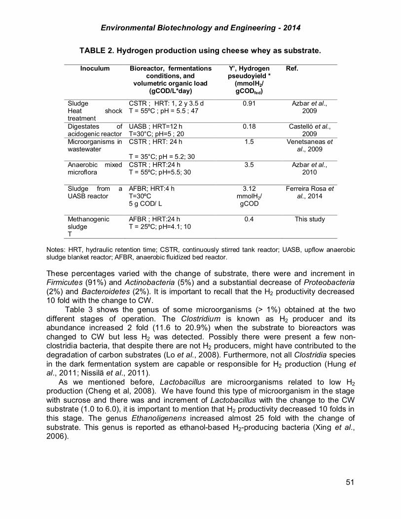
Environmental Biotechnology and Engineering - 2014
51
TABLE 2. Hydrogen production using cheese whey as substrate.
Inoculum Bioreactor, fermentations conditions, and
volumetric organic load (gCOD/L*day)
Y’, Hydrogen pseudoyield *
(mmolH2/ gCODfed)
Ref.
Sludge Heat shock treatment
CSTR ; HRT: 1, 2 y 3.5 d T = 55ºC ; pH = 5.5 ; 47
0.91 Azbar et al., 2009
Digestates of acidogenic reactor
UASB ; HRT=12 h T=30°C; pH=5 ; 20
0.18 Castelló et al., 2009
Microorganisms in wastewater
CSTR ; HRT: 24 h T = 35°C; pH = 5.2; 30
1.5 Venetsaneas et al., 2009
Anaerobic mixed microflora
CSTR ; HRT:24 h T = 55ºC; pH=5.5; 30
3.5 Azbar et al., 2010
Sludge from a UASB reactor
AFBR; HRT:4 h T=30ºC 5 g COD/ L
3.12 mmolH2/ gCOD
Ferreira Rosa et al., 2014
Methanogenic sludge T
AFBR ; HRT:24 h T = 25ºC; pH=4.1; 10
0.4 This study
Notes: HRT, hydraulic retention time; CSTR, continuously stirred tank reactor; UASB, upflow anaerobic sludge blanket reactor; AFBR, anaerobic fluidized bed reactor. These percentages varied with the change of substrate, there were and increment in Firmicutes (91%) and Actinobacteria (5%) and a substantial decrease of Proteobacteria (2%) and Bacteroidetes (2%). It is important to recall that the H2 productivity decreased 10 fold with the change to CW. Table 3 shows the genus of some microorganisms (> 1%) obtained at the two different stages of operation. The Clostridium is known as H2 producer and its abundance increased 2 fold (11.6 to 20.9%) when the substrate to bioreactors was changed to CW but less H2 was detected. Possibly there were present a few non-clostridia bacteria, that despite there are not H2 producers, might have contributed to the degradation of carbon substrates (Lo et al., 2008). Furthermore, not all Clostridia species in the dark fermentation system are capable or responsible for H2 production (Hung et al., 2011; Nissilä et al., 2011).
As we mentioned before, Lactobacillus are microorganisms related to low H2 production (Cheng et al, 2008). We have found this type of microorganism in the stage with sucrose and there was and increment of Lactobacillus with the change to the CW substrate (1.0 to 6.0), it is important to mention that H2 productivity decreased 10 folds in this stage. The genus Ethanoligenens increased almost 25 fold with the change of substrate. This genus is reported as ethanol-based H2-producing bacteria (Xing et al., 2006).

Environmental Biotechnology and Engineering - 2014
52
FIGURE 3. Phylum level identification of all sequences.
Table 4 shows the Shannon-Weaver index of the operation stages, it can observe that they decreased to the change to CW. In general, the microflora of bioreactors fed with CW was less diverse than that of the bioreactors fed with sucrose.

Environmental Biotechnology and Engineering - 2014
53
TABLE 3. Microorganisms profiles (phylum, class, order and genus) at different stages of operation
Note: * the species in each genus are not identified yet
TABLE 4. Shannon-Weaver Index of the different stages of operation.
Shannon-Weaver Index
Substrate sucrose
Substrate cheese whey
H10 H2 He
0.38 1.27 0.88
0.16 0.54 0.38
Phylum Class Order Genus Abundance (%)
S CW Actinobacteria Actinobacteria
Actinomycetales Propionibacteriaceae
(family) 1.3 0.4
Bifidobacteriales Bifidobacteriaceae (family)
0.1 4.6
Bacteroidetes Bacteroidia Bacteroidales Bacteroides 6.9 0.1 Prevotella 11.1 1.6
Firmicutes Bacilli Bacillales Sporolactobacillus 19.9 1.4 Lactobacillales Lactobacillus 1.0 6.0
Lactococcus 1.2 0.0 Clostridia Clostridiales Clostridiales (order)* 2.8 0.3
Clostridiaceae (familiy)*
1.7 10.1
Clostridium 11.6 20.9 Lachnospiraceae (family)*
7.2 0.5
Coprococcus 1.6 0.1 Lachnospira 1.0 0.1 Ruminococcaceae (family)*
3.5 9.3
Anaerofilum 0.1 2.2 Ethanoligenens 1.2 30.4 Faecalibacterium 7.0 0.4 Oscillospira 1.5 0.6 Ruminococcus 1.6 7.3
Proteobacteria Gammaproteobacteria
Aeromonadales Succinivibrio 1.2 0.4 Enterobacteriales Enterobacteriaceae
(family)* 2.4 0.7

Environmental Biotechnology and Engineering - 2014
54
Conclusion
• The H2 productivity using CW as substrate was almost 10 fold lower than the obtained using sucrose.
• The H2 pseudoyield was in the middle of the range of H2 production using CW reported in other works that performed the dark fermentation of CW at higher temperatures.
• The main phyla detected were Firmicutes, Bacteroidetes, Proteobacteria and Actinobacteria. The abundance of the phyla changed with the change of substrate
• Presence of Lactobacillus was related with low H2 productivity; we found Clostridium in all the stages of operation
Acknowledgements The authors wish to thank SECITI-GDF for support with projects PICCO 10-27 and PICCO 10-28 and CINVESTAV del IPN for financial support to this research, and CONACYT for a graduate scholarship to KMM-P. The excellent help of Professor Elvira Ríos Leas, Mr Cirino Chávez-Rojas and Mr Gustavo Medina as well as Mr Rafael Hernández-Vera from the GBAER-EBRE Group, CINVESTAV del IPN, is gratefully acknowledged.

Environmental Biotechnology and Engineering - 2014
55
References Azbar, N.; Dokgoz, F.T.C. (2010). The effect of dilution and L-malic acid addition on bio-hydrogen
production with Rhodopseudomonas palustris from effluent of an acidogenic anaerobic reactor. International Journal of Hydrogen Energy.35: 5674-5682.
Azbar, N.; Dokgoz, F.T.C.; Tuba, F. Keskin, T.; Korkmaz, K.S.; Syed, H.M. (2009). Continuous fermentative hydrogen production from cheese whey wastewater under thermophilic anaerobic conditions. International Journal of Hydrogen Energy.34. 7441–7447
Caporaso, J.G.; Kuczynski, J.; Stombaugh, J.; Bittinger, K.; Bushman, F.D.; Costello, E.K.; Fierer, N.; Pena, A.G.; Goodrich, J.K.; Gordon, J.I.; Huttley, G.A; Kelley, S.T.; Knights, D.; Koenig, J.E.; Ley, R.E.; Lozupone, C.A.; McDonald, D.; Muegge, B.D.; Pirrung, M.; Reeder, J.; Sevinsky, J.R.; Tumbaugh, P.J.; Walters, W.A.; Widmann, J.; Yatsunenko, T.; Zaneveld, J., Knight, R. (2010). QIIME allows analysis of high-throughput community sequencing data. Nature Methods.7:335-336.
Castello, E.; García y Santos, C.; Iglesias, T.; Paolino. G.; Wenzel, J.; Borzacconi, L.; Etchebehere, C. (2009). Feasibility of biohydrogen production from cheese whey using a UASB reactor: Links between microbial community and reactor performance. International Journal of Hydrogen Energy. 34(14): 5674-5682
Cotter, P.D.; Hill, C.; Ross, R.P. (2005). Bacteriocins: developing innate immunity for food. Nature Rev Microbiol. 3: 777–788
Cheng, C.-H., Hung, C.-H., Lee, K.-S., Liau, P.-Y., Liang, C.-M., Yang, L.-H., Lin, P.-J., Lin, C.-Y. (2008). Microbial community structure of a starch-feeding fermentative H2 production reactor operated under different incubation conditions. International Journal of Hydrogen Energy. 33: 5242–5249.
Daeschel, M.A. (1989). Antimicrobial substances from lactic acid bacteria for use as food preservatives. Food Technology. 43:164–167.
Das, D.; Veziroglu, N.T. (2008). Advances in biological hydrogen production processes. International Journal of Hydrogen Energy. 33: 6046-6057.
De Vuyst, L. & Vandamme, E.J. (1994) Antimicrobial potential of lactic acid bacteria, p. 91–142. In L. De Vuyst and E. J. Vandamme (ed.), Bacteriocins of lactic acid bacteria: microbiology, genetics and applications. Blackie Academic & Professional, London, United Kingdom.
DeSantis, T.Z.; Hugenholtz, P.; Larsen, N.; Rojas, M.; Brodie, E.L.; Keller, K.; Huber, T.; Dalevi, D.; Hu, P.; Andersen, G.L. (2006). Greengenes a chimera-checked 16S rRNA gene database and workbench compatible with ARB. Applied Environmental Microbiology. 72:5069–5072
Edgar, R.C. (2010). Search and clustering orders of magnitude faster than BLAST. Bioinformatics. 26(19): 2460-2461.
Escamilla-Alvarado, C.; Ríos-Leal, E.; Ponce-Noyola, M.T.; Poggi-Varaldo, H.M. (2012). Gas biofuels from solid substrate hydrogenogenicemethanogenic fermentation of the organic fraction of municipal solid waste. Process Biochemistry. 47(11):1572-1587.
Ferreira Rosa, P.R.; Christine Santos, S.; Kimiko Sakamoto, I.; Amâncio Varesche, M.B.; Luiz Silva, E. (2014). Hydrogen production from cheese whey with ethanol-type fermentation: Effect of hydraulic retention time on the microbial community composition. Bioresource Technology. 161:10–19
Fierer, N.; Hamady, M.; Lauber, C.L.; Knight, R. (2008). The influence of sex, handedness, and washing on the diversity of hand surface bacteria. Proceedings of the National Academy of Sciences USA. 105(46): 17994–17999.
Hallenbeck, P.C.; Ghosh, D. (2009). Advances in fermentative biohydrogen production: the way forward?. Trends in Biotechnology. 27(5): 287-297.
Haas, B.J.; Gevers, D.; Earl, A.M.; Feldgarden, M.; Ward, D.V.; Giannoukos, G.; Ciulla, D.; Tabbaa, D.; Highlander, S.K.; Sodergren, E.; Methé, B.; DeSantis, T.D. (2011). The Human Microbiome Consortium, J.F. Petrosino, R. Knight, B.W. Birren, Chimeric 16S rRNA sequence formation and detection in Sanger and 454-pyrosequenced PCR amplicons. Genome Research. 21:494-504.
Hawkes, F.R.; Hussy, I.; Kyazze, G.; Dinsdale, R.; Hawkes, D.L. (2007). Continuous dark fermentative hydrogen production by mesophilic microflora: principles and progress. International Journal of Hydrogen Energy.32:172–84.
Hung, C.-H.; Chang, Y.-T.; Chang, Y.-J. (2011). Roles of microorganisms other than Clostridium and Enterobacter in anaerobic fermentative biohydrogen production systems – A review. Bioresource Technology.102: 8437–8444
Jay, J.M. (1982). Antimicrobial properties of diacetyl. Applied and Environmental Microbiology. 44: 525–32 Klaenhammer, T.R. (1988). Bacteriocins of lactic acid bacteria. Biochimie.70: 337–349.
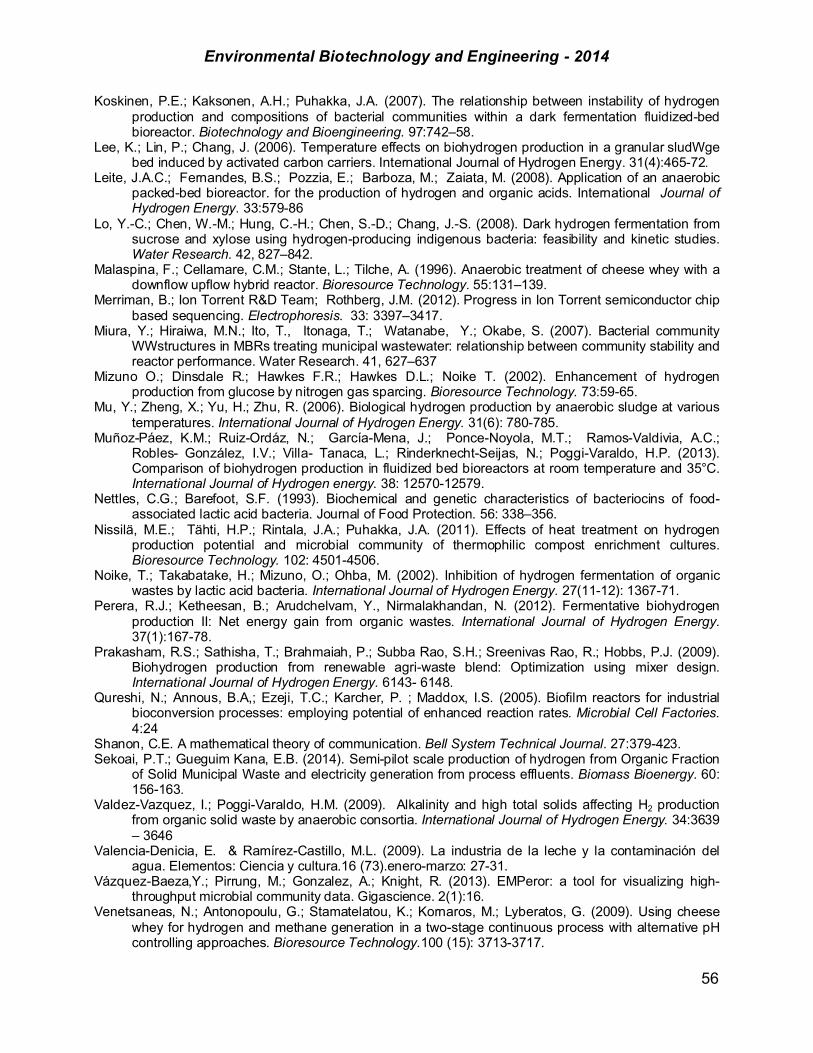
Environmental Biotechnology and Engineering - 2014
56
Koskinen, P.E.; Kaksonen, A.H.; Puhakka, J.A. (2007). The relationship between instability of hydrogen production and compositions of bacterial communities within a dark fermentation fluidized-bed bioreactor. Biotechnology and Bioengineering. 97:742–58.
Lee, K.; Lin, P.; Chang, J. (2006). Temperature effects on biohydrogen production in a granular sludWge bed induced by activated carbon carriers. International Journal of Hydrogen Energy. 31(4):465-72.
Leite, J.A.C.; Fernandes, B.S.; Pozzia, E.; Barboza, M.; Zaiata, M. (2008). Application of an anaerobic packed-bed bioreactor. for the production of hydrogen and organic acids. International Journal of Hydrogen Energy. 33:579-86
Lo, Y.-C.; Chen, W.-M.; Hung, C.-H.; Chen, S.-D.; Chang, J.-S. (2008). Dark hydrogen fermentation from sucrose and xylose using hydrogen-producing indigenous bacteria: feasibility and kinetic studies. Water Research. 42, 827–842.
Malaspina, F.; Cellamare, C.M.; Stante, L.; Tilche, A. (1996). Anaerobic treatment of cheese whey with a downflow upflow hybrid reactor. Bioresource Technology. 55:131–139.
Merriman, B.; Ion Torrent R&D Team; Rothberg, J.M. (2012). Progress in Ion Torrent semiconductor chip based sequencing. Electrophoresis. 33: 3397–3417.
Miura, Y.; Hiraiwa, M.N.; Ito, T., Itonaga, T.; Watanabe, Y.; Okabe, S. (2007). Bacterial community WWstructures in MBRs treating municipal wastewater: relationship between community stability and reactor performance. Water Research. 41, 627–637
Mizuno O.; Dinsdale R.; Hawkes F.R.; Hawkes D.L.; Noike T. (2002). Enhancement of hydrogen production from glucose by nitrogen gas sparcing. Bioresource Technology. 73:59-65.
Mu, Y.; Zheng, X.; Yu, H.; Zhu, R. (2006). Biological hydrogen production by anaerobic sludge at various temperatures. International Journal of Hydrogen Energy. 31(6): 780-785.
Muñoz-Páez, K.M.; Ruiz-Ordáz, N.; García-Mena, J.; Ponce-Noyola, M.T.; Ramos-Valdivia, A.C.; Robles- González, I.V.; Villa- Tanaca, L.; Rinderknecht-Seijas, N.; Poggi-Varaldo, H.P. (2013). Comparison of biohydrogen production in fluidized bed bioreactors at room temperature and 35°C. International Journal of Hydrogen energy. 38: 12570-12579.
Nettles, C.G.; Barefoot, S.F. (1993). Biochemical and genetic characteristics of bacteriocins of food-associated lactic acid bacteria. Journal of Food Protection. 56: 338–356.
Nissilä, M.E.; Tähti, H.P.; Rintala, J.A.; Puhakka, J.A. (2011). Effects of heat treatment on hydrogen production potential and microbial community of thermophilic compost enrichment cultures. Bioresource Technology. 102: 4501-4506.
Noike, T.; Takabatake, H.; Mizuno, O.; Ohba, M. (2002). Inhibition of hydrogen fermentation of organic wastes by lactic acid bacteria. International Journal of Hydrogen Energy. 27(11-12): 1367-71.
Perera, R.J.; Ketheesan, B.; Arudchelvam, Y., Nirmalakhandan, N. (2012). Fermentative biohydrogen production II: Net energy gain from organic wastes. International Journal of Hydrogen Energy. 37(1):167-78.
Prakasham, R.S.; Sathisha, T.; Brahmaiah, P.; Subba Rao, S.H.; Sreenivas Rao, R.; Hobbs, P.J. (2009). Biohydrogen production from renewable agri-waste blend: Optimization using mixer design. International Journal of Hydrogen Energy. 6143- 6148.
Qureshi, N.; Annous, B.A,; Ezeji, T.C.; Karcher, P. ; Maddox, I.S. (2005). Biofilm reactors for industrial bioconversion processes: employing potential of enhanced reaction rates. Microbial Cell Factories. 4:24
Shanon, C.E. A mathematical theory of communication. Bell System Technical Journal. 27:379-423. Sekoai, P.T.; Gueguim Kana, E.B. (2014). Semi-pilot scale production of hydrogen from Organic Fraction
of Solid Municipal Waste and electricity generation from process effluents. Biomass Bioenergy. 60: 156-163.
Valdez-Vazquez, I.; Poggi-Varaldo, H.M. (2009). Alkalinity and high total solids affecting H2 production from organic solid waste by anaerobic consortia. International Journal of Hydrogen Energy. 34:3639 – 3646
Valencia-Denicia, E. & Ramírez-Castillo, M.L. (2009). La industria de la leche y la contaminación del agua. Elementos: Ciencia y cultura.16 (73).enero-marzo: 27-31.
Vázquez-Baeza,Y.; Pirrung, M.; Gonzalez, A.; Knight, R. (2013). EMPeror: a tool for visualizing high-throughput microbial community data. Gigascience. 2(1):16.
Venetsaneas, N.; Antonopoulu, G.; Stamatelatou, K.; Kornaros, M.; Lyberatos, G. (2009). Using cheese whey for hydrogen and methane generation in a two-stage continuous process with alternative pH controlling approaches. Bioresource Technology.100 (15): 3713-3717.

Environmental Biotechnology and Engineering - 2014
57
Whiteley, P.; Haracopos, D.; Knivsberg, A.M.; Reichelt, K.L.; Parlar, S.; Jacobsen, J.; Seim, A.; Pedersen, L., Schondel, M., Shattock, P. (2010). The ScanBrit randomised, controlled, single-blind study of a gluten- and casein-free dietary intervention for children with autism spectrum disorders. Nutritional Neuroscience.13:287
Xing, D.; Ren, N.; Li, Q.; Lin, M.; Wang, A.; Zhao, L. (2006) Ethanoligenens harbinense gen. nov., sp. nov., isolated from molasses waste water. International Journal Systematic and Evolutionary Microbiology. 56: 755–760.
Yang, P.; Zhang, R.H.; MeGarvey, J.; Benernann, J.R. (2007). Biohydrogen production from cheese processing wastewater by anaerobic fermentation using mixed microbial communities. International Journal of Hydrogen Energy. 32:4761–71
Zhang, Z.P.; Tay, J.H. ; Show, K.Y.; Yan, R.; Liang, D.T.; Lee, D.J.; Jiang, W.J. (2007). Biohydrogen production in a granular activated carbon anaerobic fluidized bed reactor. International Journal of Hydrogen Energy. 32:185–191.
Notation AFBR anaerobic fluidized bed bioreactor CW cheese whey HRT hydraulic retention time Greek characters ! ratio of the sum of volatile organic acid divided the sum of solvent products
Environmental Biotechnology and Engineering - 2014
58
CHAPTER 1.7. COMPARISON OF THE HYDROGEN PRODUCTION AND THE RELATED MICROBIAL COMMUNITY IN FLUIDIZED BED BIOREACTORS
OPERATED AT TWO TEMPERATURES: INDOOR AMBIENT AND MESOPHILIC TEMPERATURE
Karla M. Muñoz-Páez (1); Héctor M. Poggi-Varaldo* (1); Elvira Ríos Leal (1); Jaime
García-Mena (2); Selvasankar Murugesan (3); Alberto Piña-Escobedo (2) (1) Dept. Biotechnology and Bioengineering, CINVESTAV- IPN, México DF, México; (2) Dept. Genetics and Molecular Biology, CINVESTAV- IPN, México DF, México; (3) Dept. Pharmacology, CINVESTAV- IPN, México DF, México;
ABSTRACT Cheese whey (CW) is a dairy wastewater that has high organic matter content and low alkalinity. The use of CW as substrate for hydrogen production could provide a positive solution to waste CW management and treatment. One significant parameter in H2 production is the operation temperature. Interestingly, most of the works have been focused on either mesophilic or thermophilic bioH2 processes. Yet, if the H2 production at ambient temperature could be or the same order to that obtained at mesophilic, the energy savings could be huge and boost the economic feasibility of bioH2 from CW. Thus, the main goals of this work were (i) to evaluate the H2 production in lab scale fluidized bed reactors operated at indoor ambient and mesophilic temperature and (ii) to determine the microbial community anchored in the bioparticles of the bioreactors. The organic rate was 5 g CW/L. day. The microbial community was determined by massive semiconductor sequencing of a 16S rDNA library. The major response variables were: H2 productivity (NmLH2/Lbed.day) and Shannon-Weaver index (H’10). The reactors were feed with sucrose for 10 days and afterwards the feed was changed to CW. In the stage with CW, the reactor at ambient temperature exhibited a H2 productivity of 92.12 (NmLH2/Lbed.day), whereas there was not H2 production at mesophilic temperature. Interestingly, the pH of both reactors were very close (4.3 ± 0.2 and 4.1 ± 0.2); this pH is in a range when some authors detect that the fermentation shifted to solventogenesis. The taxonomic analysis showed that the phyla found in the bioreactor operated at indoor ambient temperature were: Actinobacteria (54.4%), Firmicutes (26.4%), Bacteroidetes (13.2 %) Proteobacteria (5.7%), and Cyanobacteria (0.1%). The corresponding findings at mesophilic temperature were: Actinobacteria (0.9%), Firmicutes (87.6%), Bacteroidetes (8.6 %) and Proteobacteria (2.7%). The H’10 at ambient temperature was 0.48 whereas at mesophilic was 0.2, this indicated that the community at ambient temperature was more diverse than at mesophilic temperatures. Clostridiales was the principal order of the phylum Firmicutes at both temperatures. It was more abundant at mesophilic temperature than at indoor ambient temperature (86.9% and 25.5% of the total orders, respectively). ------------------ *Author for correspondence: [email protected]

Environmental Biotechnology and Engineering - 2014
59
It is interestingly, that the phylum Actinobacteria was more abundant at indoor ambient temperature than at mesophilic temperature.. We can conclude that, on the one hand, the reactors at ambient temperature had better performance that the mesophilic ones. On the other hand, it seems that the presence of Actinobacteria was related to the better performance of indoor temperature reactors than mesophilic ones. Key words: ambient temperature, cheese whey, mesophilic temperature microbial community. Introduction Hydrogen has been considered as a good option to be used as biofuel due to its environmentally friendly (Mizuno et al., 2002) and could be stored, transported and used to fulfill the energy needs (Das and Veziroglu, 2001). The biological production processes could be classified as following: photolysis, phototrophic fermentation and dark fermentation (Mohan, 2008). The dark fermentation could be carried out using organic wastes as substrate. This process has the advantage that could help to both waste treatment and energy recovery (Sekoai et al., 2014). The dairy industry generates many residues (Ferchichi et al., 2005), one of them is the cheese whey (CW). The CW has the milk components that are not integrated in the casein coagulation. CW consists of the 85–95% of the milk volume and retains the 55% of the nutrients (Siso, 1996). Another aspect that affects the dark fermentation is the temperature, could modify the growth rate of microorganisms, the substrate degradation, the metabolic activity and the distribution of aqueous products (Lee et al., 2006; Mu et al., 2006). Many of the works using CW as substrate were at mesophilic and thermophilic temperatures but little is known about the performance of the operation at ambient temperature. This low temperature cold give an option with a lower spend of energy in the operation of the reactor. To gain insight on the microbial community is very important because it could lead to a better understanding of the bioreactor processes (Miura et al., 2007). The Massive semiconductor sequencing of 16S rDNA library is one of the next-generation sequencing technologies that could monitor millions, and potentially billions, of simultaneous sequencing reactions (Merriman et al., 2012) and could be a good tool in order to know the microbial community in the reactors. Thus, the objectives of this work were (i) to evaluate the H2 production in lab scale fluidized bed reactors operated at indoor ambient and mesophilic temperature and (ii) to determine the microbial community anchored in the bioparticles of the bioreactors Materials and methods Experimental design. The experimental design compared the H2 production and the microbial community in a lab scale fluidized bed bioreactors at two different temperatures: (i) ambient and (ii) mesophilic temperature. The main response variable was: H2 productivity (NmLH2/Lbed.day) and the Shannon-Weaver index (H’10).

Environmental Biotechnology and Engineering - 2014
60
Inocula and substrate. The inoculum of the AFBR was digestates (with heat-shock treatment) from methanogenic anaerobic digesters degrading sucrose operated at mesophilic temperature. The bioreactors were fed with 5 g CW/Lbed.day and 0.85 g de NaCl. The CW was in powder and had the following characteristics: 0.85% fat, pH 6.3, 12.6 % protein and 5 .58% of ash.
Experimental setup. The AFBR consisted of a glass column of 4.5 cm internal diameter, 185 cm length and 3 L capacity. Granular activated carbon (1 L; 1-2 mm diameter) was used as bed. The hydraulic residence time (HRT) was 1 day (fluidized bed volume basis; Muñoz-Páez et al., 2013). Analyses. The H2 and CH4 concentration were determined in a Gow-Mac chromatograph (model 350) with a thermal conductivity detector and Molecular Sieve 5A packed column: injector, detector and column temperatures were 25, 100 and 25 ºC, respectively. Argon was the carrier gas (Muñoz-Páez et al., 2013; Valdez-Vazquez et al., 2009). The acids and solvents concentration were determined in the effluent after filtration through a glass-membrane filter. An aliquot of the filtrate was injected in a gas chromatography Varian Star 3400 equipped with FID. The injector and detector temperatures were set at 250ºC with N2 as a carrier gas with a 20 mL/min flow rate. The oven temperature was programmed as follows: 60 ºC for 2 min, increasing to 140 ºC at 5ºC/min, and then kept constant at 140ºC for another 6 min. A 50 m 0.32 mm internal diameter fused silica capillary column coated with 0.2 mm CP-Wax 57 CB was used. DNA preparation and massive semiconductor sequencing of 16S rDNA library. Genomic DNA was extracted from bioparticles of the AFBR using the PowerSoil® DNA Isolation Kit of MO BIO Laboratories, Inc. The sequencing was performed at Ion Torrent PGM. The primers used for the amplification targeted the V3 region of the 6S rDNA. The forward primer was V3-341F with 12bp Golay barcode (Fierer et al., 2008) and adapters for massive sequencing; the antisense primer V3-518R containing A and Truncated P1 adapters (Whiteley et al., 2010). The PCR mixture consisted of: (i) 1X Buffer, (ii) 2 mM MgCl2, (iii) 0.2 mM dNTP´s, (iv) 0.025U/µL Taq DNA, (v) 0.2µM of each primer, and (iv) 10 ng of DNA template. Amplification was performed in a GeneAmp PCR System 2700 Thermocycler (Applied Biosystems) with an initial denaturation (95°C for 5 min) followed by 30 cycles of denaturation (94°C for 15 s), annealing (62°C for 15 s) and extension (72°C for 15 s) and final extension (72°C for 10 min). The PCR products were purified by electrophoretic separation on 2% agarose gel and using Wizard SV Gen PCR Clean-Up System (Promega). The concentration of PCR amplicons was measured by NanoDrop spectrophotometer (ThermoScientific).
After purification, the samples were sent out for the barcoded library preparation and sequencing on an Ion Torrent PGM with 316 chip using the Ion Sequencing 200 bp kit (Life Technologies) according to the standard protocol (Ion Xpress_ Plus gDNA and Amplicon Library Preparation, Life Technologies). The sequence reads were filtered by the PGM software to remove low quality and polyclonal sequences; and sequences matching the 3’-adapter were automatically trimmed and filtered.
The demultiplex of the sequenced data was performed using a Sequenced data-

Environmental Biotechnology and Engineering - 2014
61
Microbiota analysis Ion torrent PGM software, Torrent_Suite v 4.0.2. It was based on their barcodes and poor quality reads were eliminated from the datasets, i.e. quality score <20, containing homopolymers >6, length <200 nt, and containing errors in primers and barcodes. The analysis of the demultiplexed sequencing data was made with the program QIIME version 1.8.0 software pipeline (Caporaso et al., 2010). Closed reference Operational taxonomic units (OTU) were determined at 97% similarity level with UCLUST Algorithm (Edgar, 2010).
It was used the Chimera Slayer in order to detect and removed chimeras from the datasets (DeSantis et al., 2006). Sequence alignments were done against the Greengenes core set (Haas et al., 2011). Statistical analysis of the OTU table Microbial diversity had been assessed through both alpha and beta diversity. Using rarefied OTU tables, alpha diversities were calculated using various matrixes like Shannon, PD whole tree, chao1, observed species.
The beta diversity analysis was calculated using UniFrac analysis (Vázquez-Baeza et al., 2013), by a phylogenetic tree computed with FastTree and a rarefiled biom table as inputs. Abundance of the bacterial groups at different taxonomic levels (phylum, order, and genus) was separately explored with a Principal Component Analysis (PCA) and Unweighted Pair Group Method with Arithmetic mean (UPGMA) Clustering. Diversity estimation. The results of the massive semiconductor sequencing of 16S rDNA library were analyzed using the Shannon-Weaver diversity index, defined as (Shannon, 1948):
[1] where: pi : is the proportion of individuals belonging to the i species in the dataset of interest, in decimals; S: is the total number of species. Results and discussion The H2 productivity at ambient temperature was 0.8 mmolH2/gCOD day whereas no H2 production was detected at ambient temperature (Table 1). The pH was very close at both temperatures, the values were lower than 4.5; pH known as the limit to beginning of the solventogenesis but very low percentage of solvents were detected (Table 2).
TABLE 1. Average performance of anaerobic fluidized bed reactor at ambient and mesophilic temperature
Reactor pH H2 concentration in biogas
(%)
H2 productivity (NmL H2/L bed day)
(mmol H2/gCOD day) Ambient
Mesophilic
4.3 ± 0.2
4.1 ± 0.2
14.5 ± 3.1
0.0 ± 0.0
92.1 0.8 0.0 0.0
Note: Average results were obtained under steady-state conditions

Environmental Biotechnology and Engineering - 2014
62
TABLE 2. Soluble microbial products of the anaerobic fluidized bed reactor at
ambient temperature using cheese whey as substrate Soluble microbial product
(gCOD/L) Ambient
Mesophilic
MtOH/SMP (%) EtOH/SMP (%) BuOH/SMP (%) HAc/SMP (%) HPr/SMP (%) HBu/SMP (%) A/B TVOA (mg COD/L) SMP (mg COD/L)
ND 15.7 ± 14.9
6.1 ± --- 8.6 ± --- 1.3 ± ---
68.2 ± 9.4 0.11 ± ---
2258 ± 2139 2598 ± 1959
1.2 ± --- 4.5 ± --- 0.4 ± ---
52.3 ± 13.0 8.7 ± 2.0
31.8 ± 8.9 1.8 ± 0.9
1699 ± 935 1837 ± 988
Notes: A/B: acetic to butyric acid ratio. MetOH: methanol; EtOH: ethanol; BuOH: butanol; HAc: acetate; HPr: propionate; HBu: butyrate; TVOA: total volatile organic acids= HAc+HPr+HBu; SMP: soluble microbial products=TVOA+EtOH+BuOH. Based in COD/L. ND: no detected.
The main acid detected was butyric at ambient temperature and acetic at mesophilic temperature. Figure 1 shows the phyla of the microorganisms in the bioreactors. It was observed almost the same phyla at both temperatures but with different percentages.
FIGURE 1. Phylum level identification of all sequences. At ambient temperature: 54.4% Actinobacteria, 5.7%, Proteobacteria, 26.4% Firmicutes, 13.2% Bacteroidetes and 0.1% Cyanobacteria, whereas at mesophilic ones: 0.9% Actinobacteria, 2.7%, Proteobacteria, 87.6% Firmicutes, 8.6% Bacteroidetes and 0.0% Cyanobacteria. It seems that with mesophilic temperature the phylum Firmicutes was favoured. The H’10 at ambient temperature was 0.5 whereas at mesophilic was 0.2 (Table 3), this indicates that the community at ambient temperature was more diverse than at mesophilic temperature. Table 4 shows the genus of some microorganisms (> 1%) obtained at the two different stages of operation. Clostridium was the principal order of the phylum Firmicutes at both temperatures. It was more abundant at mesophilic temperature than at indoor ambient temperature (86.9% and 25.5% of the total orders, respectively).

Environmental Biotechnology and Engineering - 2014
63
It is known that these microorganisms are hydrogen producers and could be expected that the abundance of Clostridium was related to H2 productivity, but that not happen in this experiment. It is interestingly, that the phylum Actinobacteria was more abundant at indoor ambient temperature than at mesophilic temperature. Bifidobacterium was the main order of this phylum. This type of microorganisms has been reported to coexist with hydrogen producers and they could contribute to the degradation of carbon substrates than then may be utilized by Clostridium.
TABLE 3. Shannon-Weaver Index of the bioreactor consortia at different temperatures of operation.
Shannon-Weaver Index
Ambient Mesophilic
H10 0.5 0.2

Environmental Biotechnology and Engineering - 2014
64
TABLE 4. Microorganisms profiles (phylum, class, order and genus) at different stages of operation.
Notes: * the species belonging to each genus are not identified yet. A: ambient; M: mesophilic
Conclusion
• The reactor at ambient temperature had better performance that the mesophilic ones.
• The presence of Actinobacteria was related to the better performance of indoor temperature reactors than mesophilic ones.
Acknowledgements The authors wish to thank SECITI-GDF for support with projects PICCO 10-27 and PICCO 10-28 and CINVESTAV del IPN for financial support to this research, and CONACYT for a graduate scholarship to KMM-P. The excellent help of Professor Elvira Ríos Leas, Mr Cirino Chávez-Rojas and Mr Gustavo Medina as well as Mr Rafael Hernández-Vera from the GBAER-EBRE Group, CINVESTAV del IPN, is gratefully acknowledged.
Phylum Class Order Genus Abundance (%)
A M Actinobacteria Actinobacteria
Actinomycetales Propionibacteriaceae
(family) 5.5 0.3
Streptomyces 1.2 0.0 Bifidobacteriales Bifidobacterium 44.3 0.0
Bacteroidetes Bacteroidia Bacteroidales Bacteroides 1.0 0.8 Prevotella 11.4 7.3
Firmicutes Clostridia Clostridiales Clostridiales (order)* 1.1 1.2 Clostridiaceae (familiy)*
1.6 5.8
Clostridium 7.7 26.3 Lachnospiraceae (family)*
3.6 2.1
Ruminococcaceae (family)*
1.8 7.3
Anaerofilum 0.0 1.5 Ethanoligenens 0.3 24.7 Faecalibacterium 3.7 1.9 Oscillospira 1.1 0.5 Ruminococcus 1.2 12.3
Proteobacteria Gammaproteobacteria
Aeromonadales Succinivibrio 2.1 1.2

Environmental Biotechnology and Engineering - 2014
65
References Caporaso, J.G.; Kuczynski, J.; Stombaugh, J.; Bittinger, K.; Bushman, F.D.; Costello, E.K.; Fierer, N.;
Pena, A.G.; Goodrich, J.K.; Gordon, J.I.; Huttley, G.A; Kelley, S.T.; Knights, D.; Koenig, J.E.; Ley, R.E.; Lozupone, C.A.; McDonald, D.; Muegge, B.D.; Pirrung, M.; Reeder, J.; Sevinsky, J.R.; Tumbaugh, P.J.; Walters, W.A.; Widmann, J.; Yatsunenko, T.; Zaneveld, J., Knight, R. (2010). QIIME allows analysis of high-throughput community sequencing data. Nature Methods.7:335-336.
DeSantis, T.Z.; Hugenholtz, P.; Larsen, N.; Rojas, M.; Brodie, E.L.; Keller, K.; Huber, T.; Dalevi, D.; Hu, P.; Andersen, G.L. (2006). Greengenes a chimera-checked 16S rRNA gene database and workbench compatible with ARB. Applied Environmental Microbiology. 72:5069–5072
Edgar, R.C. (2010). Search and clustering orders of magnitude faster than BLAST. Bioinformatics. 26(19): 2460-2461.
Fierer, N.; Hamady, M.; Lauber, C.L.; Knight, R. (2008). The influence of sex, handedness, and washing on the diversity of hand surface bacteria. Proceedings of the National Academy of Sciences USA. 105(46): 17994–17999.
Haas, B.J.; Gevers, D.; Earl, A.M.; Feldgarden, M.; Ward, D.V.; Giannoukos, G.; Ciulla, D.; Tabbaa, D.; Highlander, S.K.; Sodergren, E.; Methé, B.; DeSantis, T.D. (2011). The Human Microbiome Consortium, J.F. Petrosino, R. Knight, B.W. Birren, Chimeric 16S rRNA sequence formation and detection in Sanger and 454-pyrosequenced PCR amplicons. Genome Research. 21:494-504.
Lee, K.; Lin, P.; Chang, J. (2006). Temperature effects on biohydrogen production in a granular sludWge bed induced by activated carbon carriers. International Journal of Hydrogen Energy. 31(4):465-72.
Merriman, B.; Ion Torrent R&D Team; Rothberg, J.M. (2012). Progress in Ion Torrent semiconductor chip based sequencing. Electrophoresis. 33: 3397–3417.
Miura, Y.; Hiraiwa, M.N.; Ito, T., Itonaga, T.; Watanabe, Y.; Okabe, S. (2007). Bacterial community WWstructures in MBRs treating municipal wastewater: relationship between community stability and reactor performance. Water Research. 41, 627–637
Mizuno O.; Dinsdale R.; Hawkes F.R.; Hawkes D.L.; Noike T. (2002). Enhancement of hydrogen production from glucose by nitrogen gas sparcing. Bioresource Technology. 73:59-65.
Mohan, V.S. (2008). Fermentative hydrogen production with simultaneous wastewater treatment: influence of pretreatment and system operating conditions. Journal of Scientific and Industrial Research. 67 (11): 950–961.
Mu, Y.; Zheng, X.; Yu, H.; Zhu, R. (2006). Biological hydrogen production by anaerobic sludge at various temperatures. International Journal of Hydrogen Energy. 31(6): 780-785.
Muñoz-Páez, K.M.; Ruiz-Ordáz, N.; García-Mena, J.; Ponce-Noyola, M.T.; Ramos-Valdivia, A.C.; Robles- González, I.V.; Villa- Tanaca, L.; Rinderknecht-Seijas, N.; Poggi-Varaldo, H.P. (2013). Comparison of biohydrogen production in fluidized bed bioreactors at room temperature and 35°C. International Journal of Hydrogen energy. 38: 12570-12579.
Shanon, C.E. A mathematical theory of communication. Bell System Technical Journal. 27:379-423. Sekoai, P.T.; Gueguim Kana, E.B. (2014). Semi-pilot scale production of hydrogen from Organic Fraction
of Solid Municipal Waste and electricity generation from process effluents. Biomass Bioenergy. 60: 156-163.
Siso, M. I. G. (1996). The biotechnological utilization of cheese whey: a review. Bioresource Technology. 57: 1–11.
Valdez-Vazquez, I.; Poggi-Varaldo, H.M. (2009). Alkalinity and high total solids affecting H2 production from organic solid waste by anaerobic consortia. International Journal of Hydrogen Energy. 34:3639 – 3646
Vázquez-Baeza,Y.; Pirrung, M.; Gonzalez, A.; Knight, R. (2013). EMPeror: a tool for visualizing high-throughput microbial community data. Gigascience. 2(1):16.
Whiteley, P.; Haracopos, D.; Knivsberg, A.M.; Reichelt, K.L.; Parlar, S.; Jacobsen, J.; Seim, A.; Pedersen, L., Schondel, M., Shattock, P. (2010). The ScanBrit randomised, controlled, single-blind study of a gluten- and casein-free dietary intervention for children with autism spectrum disorders. Nutritional Neuroscience.13:287
Notation AFBR anaerobic fluidized bed bioreactor

Environmental Biotechnology and Engineering - 2014
66
CW cheese whey HRT hydraulic retention time.

Environmental Biotechnology and Engineering - 2014
67
CHAPTER 1.8. HYDROGEN ROLE AS A PART OF CO2 HYPER-COMBUSTION REACTION MECHANISM
José C. Hernández-López; José Á. Dávila-Gómez
UAM-AZCAPOTZALCO, Depto. de Energia, Mexico, D.F., Mexico. ABSTRACT Within the hydrogen investigation project by the Sustainable Technologies Area on hyper-combustion with CO2, which would substitute air as oxidizer, it was designed and built a cannon type shot probe to introduce fuel / air mixtures, and proceed to their ignition through an electric arc. Construction of the prototype required design and additional set up of a circuit of generation and maintenance of electric arc, as well as the use of specialized laboratory equipment for feeding the device and obtaining final gases samples to be analyzed. This work presents the results of tests performed during the starting operation using LP gas as fuel and air from the ambient as oxidizer; the tests contemplated the study of fuel / air ratio burning range –proposed in the initial phase of experimentation to verify the correct operation of the device–; and their characterization with regard to the observations made. The test of device was performed using 60 ml volume standard mixtures at 1 bar absolute pressure of LP gas / air; the results show the acceleration of the combustion to detonation and the existence of a specific combustion range; noting responses with characteristic odors, different sounds and divers delays of time. Gases remaining from these tests were analyzed by gas chromatography, showing the presence of hydrogen (H2) as part of the performing mechanism; so –besides to the expected causes of the "failed tests"–, by the existence of deposits of carbon at electrode, spark plug; therefore there are evidences of a primary wet gas reaction mechanism, along with other secondary reactions (e.g. Bosch and Sabatier). As a general conclusion, hydrocarbon fuels and, in particular, hydrogen, participate in the reaction mechanism, based on their composition and the oxidizer used, in such a way that its specific studio is potentiated completely through this exploratory work; additionally, that the observance of the detonation phenomenon, highlights its importance. Preliminary tests with LPG/CO2 mixtures provide strength to this evidence. Key words: carbon, combustion, detonation, hydrocarbon fuels, hydrogen, Hyper-combustion, Ignition, LP gas ------------------ *Author for all correspondence: [email protected]

Environmental Biotechnology and Engineering - 2014
68
Introduction Hydrocarbon combustion problem with oxygen is that water production, of wide energy release when hydrogen is considered but less when it is carbon dioxide produced by carbon. The following sequence, for the neutral combustion of hydrocarbons, should carefully be analyzed: Hydrocarbons + Air " CO2 + 2 H2O (g) + Inerts from Air (+Energy release) [1]
where carbon dioxide (CO2), can be estimated from the number of carbons in the hydrocarbon (eg methane (CH4), which contains an equivalent gram (E-g) of carbon (C) produced, also, an equivalent-gram of CO2; propane (C3H8), 3 E-g of C and 3 E-g of CO2; butane (C4H10), 4 E-g of C and 4 E-g of CO2 and so for. Methane is the main component of commercial natural gas and Propane-butane, the majors components of LP gas (LPG). Meanwhile, water steam, H2O, due to a ratio of half the number of hydrogens on the hydrocarbon for each water molecule at output, that is, the methane containing four hydrogens produce 2 molecules of water; propane 8 hydrogens and 4 of water, respectively. CH4 + 2O2 " CO2 + 2H2O [2] So, in the most abundant and worldwide used hydrocarbons, one third of global energy production has to do with methane, the main component of natural gas (NG). By oxygen employed, as methane uses half to produce two molecules of water and only one of carbon dioxide, it could be possible to retrieve half that oxygen using the resulting carbon dioxide as oxidizer for the following combustion, may increase the amount of energy available for a given volume of fuel gas; thus energy production would be less harmful to the environment (empowering as well, the chances of sustainability of energy production). In the literature there are few but good references that support the premise of interest: related to the combustion of hydrogen, not with air but recombining carbon dioxide present in exhaust gas of ordinary combustion, resulting in hydrogen equilibrium water shift gas reaction (Castillo-Mejía & Dávila-Gómez, 2012): Water steam + Carbon monoxide " Carbon dioxide + Hydrogen [3]
Thus, at low temperatures, Sabatier (web site), Nobel Prize in Chemistry 1912; using a nickel wall tube and a H2/CO2 ratio of 4 and temperatures of roughly 300 to 400°C, an exothermic reaction shows that motivates this work: Carbon dioxide + 4 Hydrogen " 2 H2O (g) + Methane [4]
The reaction was also studied by Bosch reaction (Bosch, web site), where the methane is reduced to carbon by means of a hydrogen carbon dioxide oxidation from 2:1 ratio, so that it is obtained a secondary system which replaces the methane, by carbon.

Environmental Biotechnology and Engineering - 2014
69
Carbon dioxide + 2 Hydrogen " 2 Water steam + Carbon [5] Equation 5 is really a couple of reactions integrated, the first one, the reverse water gas shift, fast, reaction. CO2 + H2 " CO + H2O [5a] and the second, slow, which controls the reaction rate.
CO + H2 " C + H2O [5b]
The main difference between these approaches to this work is that, it is not considered a catalytic method to performing a thermal reaction in the search for evidence of carbon and water products (equation 5b), at temperatures much higher than those specified for traditional combustion activation. Thus, it can be summarized that although in both strategies just cited it was the same reactions as objects of study; it remains a catalytic process while the second, our, objective is to study the reaction of wet gas and their influence on induced detonations.
Materials and methods First, we sought to create a device capable of providing the opportunity to experience the combustion of mixtures of methane - carbon dioxide method, purely experimental, sleving of factors, which consists of introducing a specific amount of mixture into the device, seal it and after giving a violent electric shock inside to produce a shock wave that activates the reaction and start the auto-ignition along a tube of constant length (so you can define the existence of a deflagration or detonation ), the experiment is repeated changing only the mixture, both the amount of oxidizer (air or CO2) and the fuel (LPG). Having secured the safe operation of the device with controlled gas mixtures LP Gas - air, proceeded to explore the beach of combustion. The monitoring process is done through the analysis of sampling results from the extraction of gases produced by deflagration or detonation and subsequent analysis by gas chromatography equipment. The distance that the ejected hose went out bung serving mixture was measured. According to the results, in most cases, if not in all positive, occurred in response a detonation. That is, a rapid combustion of the speed of sound may be accompanied this flame immediately following the initial shock wave (Fig. 1).
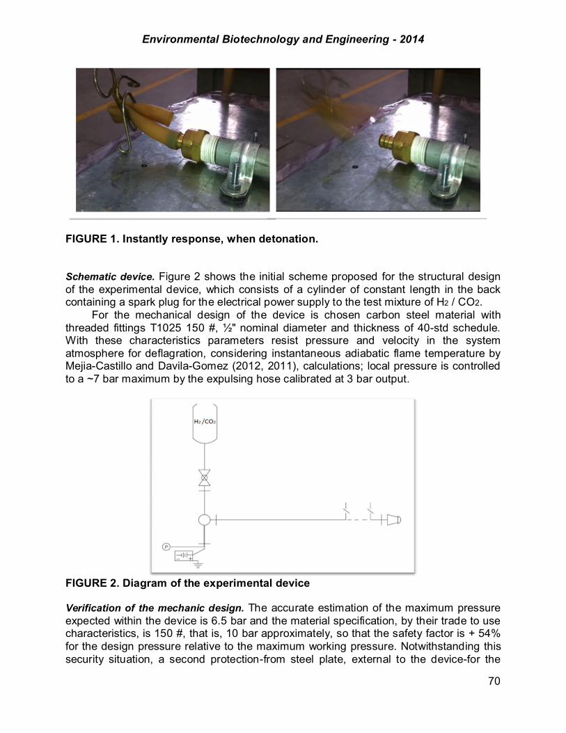
Environmental Biotechnology and Engineering - 2014
70
FIGURE 1. Instantly response, when detonation. Schematic device. Figure 2 shows the initial scheme proposed for the structural design of the experimental device, which consists of a cylinder of constant length in the back containing a spark plug for the electrical power supply to the test mixture of H2 / CO2. For the mechanical design of the device is chosen carbon steel material with threaded fittings T1025 150 #, "" nominal diameter and thickness of 40-std schedule. With these characteristics parameters resist pressure and velocity in the system atmosphere for deflagration, considering instantaneous adiabatic flame temperature by Mejia-Castillo and Davila-Gomez (2012, 2011), calculations; local pressure is controlled to a ~7 bar maximum by the expulsing hose calibrated at 3 bar output.
FIGURE 2. Diagram of the experimental device Verification of the mechanic design. The accurate estimation of the maximum pressure expected within the device is 6.5 bar and the material specification, by their trade to use characteristics, is 150 #, that is, 10 bar approximately, so that the safety factor is + 54% for the design pressure relative to the maximum working pressure. Notwithstanding this security situation, a second protection-from steel plate, external to the device-for the

Environmental Biotechnology and Engineering - 2014
71
possible containment due to destructive detonation wave off the estimated calculation is incorporated. Resulting device design. In Figure 3, the parties that make up the device are designed. In table 2, the indicated parts numbered 1 to 9 are listed.
FIGURE 3. Top view of the experimental device (Autodesk Inventor)
TABLE 1. Experimental device, part description
Experimental Protocol. The experimental protocol was as follows: after installing the device, that includes connecting the spark plug wires and avoid grounding between base and device; checking arc correctly function and making a sweep by injecting air through; plugging and evacuating the device; measure volume of mix fuel-oxygen injected, according to calculations and to wait for mixing, it is proceeded to turn on electric arc and observe if a deflagration or detonation happened. Then sampling for gas chromatography analysis was made and repeat cycle with new conditions.

Environmental Biotechnology and Engineering - 2014
72
Results and discussion In this paper a comparative estimate of the temperature is introduced, from the composition obtained from the reductive combustion to oxidant complete combustion. Using methane, the largest component of commercial natural gas, as well as advanced concepts derived from combustion diagrams thermodynamic equilibrium, the basis of the simulated actual combustion. The range of the adiabatic temperature calculation is made from the upper (rich 2), to the lower limit of inflammation (richness of 0.5), with atmospheric air as oxidizer. This means that the combustion process is limited by the equilibrium known as "wet gas" that is set when at least three of the following: carbon dioxide, hydrogen, water vapor and carbon monoxide are in the same atmosphere. Whereby high temperature, hydrogen and carbon dioxide may react to generate water vapor and carbon atom, this changing our traditional combustion oxygen (O2) for carbon dioxide (CO2); so in mixtures where the oxygen, carbon dioxide and hydrogen only produce atomic carbon and water. In multifactorial experimentation, various mixtures, ranging from saturated fuel mixtures, even some with the same poverty, hoping to explore the beach combustion were tested. Referring to Table 3, we see that there are no mixtures in which blasts of greater intensity, as in the case of mixing with air factor 0.45; which was repeated 5 times watching various results ranging from repetition in the pattern of knock intensity, to the absence of the same, this being a sensitive point of interest for analysis is referred to as carburizing carbon produced by the and deposited in the reaction modifying the power plug of the spark.
TABLE 2. Tests detonation LPG-Air, several air factors and response
Air factor 0,23 0,27 0,30 0,32 0,34 0,36 0,37 0,38 0,41 0,41 0,45
Shot Length
Air factor 0,45 0,45 0,45 0,45 0,55 0,61 0,64 0,73 0,76 0,78 0,79
Shot Length
Air factor 0,80 0,81 0,82 0,83 0,91 0,91 0,96 0,96 0,98 1,00 1,06
Shot Length 240

Environmental Biotechnology and Engineering - 2014
73
FIGURE 1. Global Test. Air Factor - Plug ejection length for detonations Air - LPG
Beach combustion, in which the mixtures with lower to 0.32 air factor no detonations were clearly observed; in the same manner to values not exceeding 1.06 are presented; although in some cases close to that value, they did so, intermittently (It can be interpreted as incipient carburization on the spark plug). Then eight experimental runs, observed in Table 3, were redone and samples of the remaining gases in the specimen were taken, the tests are considered of broad interest in the beach of detonation and analyzed by gas chromatography method.
For a better interpretation of graphs, detonation P2 was of low intensity, in which the hose which serves to cap had not sufficient push power to get expelled but swelled was presented. On the other hand, the P5' was a detonation whose expulsion was prevented, for comparative purposes, obtaining remaining intact detonation products. Chromatograms of the analyzed samples are shown in Fig. 2. For the interpretation of the charts three responses were observed in all analyzes, the first one is given time to 1.7 seconds, which represents the presence of hydrogen (H2), on the other hand the second time beginning about 1.9 seconds is a product of combustion not fully identified but it is assumed to be related to carbon monoxide (CO), the third response is identified as carbon dioxide (CO2), with presence in all analyzes. It should be noted that sampling is carried back to cover the specimen after detonation. To
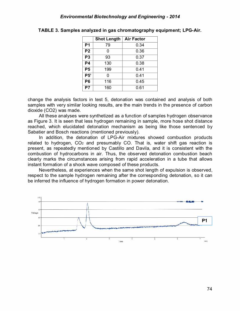
Environmental Biotechnology and Engineering - 2014
74
TABLE 3. Samples analyzed in gas chromatography equipment; LPG-Air.
Shot Length Air Factor P1 79 0.34 P2 0 0.36 P3 93 0.37 P4 130 0.38 P5 199 0.41 P5' 0 0.41 P6 116 0.45 P7 160 0.61
change the analysis factors in test 5, detonation was contained and analysis of both samples with very similar looking results, are the main trends in the presence of carbon dioxide (CO2) was made. All these analyses were synthetized as a function of samples hydrogen observance as Figure 3. It is seen that less hydrogen remaining in sample, more hose shot distance reached, which elucidated detonation mechanism as being like those sentenced by Sabatier and Bosch reactions (mentioned previously). In addition, the detonation of LPG-Air mixtures showed combustion products related to hydrogen, CO2 and presumably CO. That is, water shift gas reaction is present, as repeatedly mentioned by Castillo and Davila, and it is consistent with the combustion of hydrocarbons in air. Thus, the observed detonation combustion beach clearly marks the circumstances arising from rapid acceleration in a tube that allows instant formation of a shock wave composed of these products. Nevertheless, at experiences when the same shot length of expulsion is observed, respect to the sample hydrogen remaining after the corresponding detonation, so it can be inferred the influence of hydrogen formation in power detonation.
P1
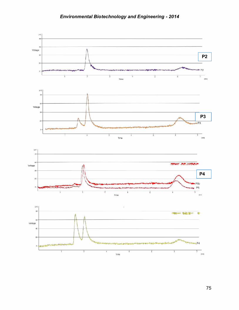
Environmental Biotechnology and Engineering - 2014
75
P2
P3
P4

Environmental Biotechnology and Engineering - 2014
76
FIGURE 2. Results of gas chromatography P1 - P7
FIGURE 3. Correlation between produced hydrogen remaining and
hose shot length
& P5’
P6
P7
Environmental Biotechnology and Engineering - 2014
77
Conclusion A device was designed to meet the objective presented in the reference from which the prototype was built; construction of the prototype required the additional design and fabrication of an electric arc circuit generation and maintenance, and the use of specialized laboratory equipment for supply to the probe acceleration (shot) where the tests were performed. The test device was made using mixtures of LPG-Air (normalized to 1 bar), the results show the acceleration of combustion and the existence of a range (combustion beach), of detonations and, particularly, odor and sound observed. For the results of these tests were analyzed, by chromatography, tails gas showing the presence of hydrogen (H2) as part of the mechanism and, through the "failed" tests, evidence of the existence of carbon deposits at level of trigger electrode; thus indicating water shift gas type mechanism and Bosch gas reaction, that presents themselves as a main significant finding. The hydrogen content of hydrocarbon fuels participates in the reaction mechanism, based on their composition and the oxidizer used, in such a way that its specific study is potentiated completely through this exploratory work; additionally, that the observance of the detonation phenomenon, highlights its importance. Preliminary tests with LPG/CO2 mixtures provide strength to this evidence. References Bosch, C. http://en.wikipedia.org/wiki/Bosch_reaction Brupbacher, J. M; Kern, R.D.; O'Grady, B.V. (1976). J. Physical Chem 80 (10): 1031. Castillo-Mejía, D.; Dávila-Gómez, J. A. (2012). Temperatura adiabática y Equilibrio Químico de la
Combustión Real. Influencia del Hidrógeno Presente. Revista Cubana de Química. Vol. XXIV No. 3 Septiembre-Diciembre: 243-248.
Castillo Mejía, D.; Dávila Gómez, J. A. (2011). Cálculo de la temperatura adiabática de la combustión simulada. 4° Congreso Internacional de Ingenierías mecánica, eléctrica, electrónica, mecatrónica y computacional. Memorias Técnicas 4CIMEEM Vol 4 (1) #58, México. Septiembre 2011.
Sabatier, P. http://en.wikipedia.org/wiki/Sabatier_reaction.

Environmental Biotechnology and Engineering - 2014
78
CHAPTER 1.9. EVALUATION OF METHANE EMISSIONS AND BIOENERGETIC POTENTIAL IN COMARCA LAGUNERA OF NORTHERN MÉXICO
Itzcóatl Muñoz-Jiménez, Inty O. Hernández-De Lira,
Lilia E. Montañez-Hernández, Nagamani Balagurusamy*
Laboratorio de Biorremediación, Escuela de Ciencias Biológicas, Universidad Autónoma de Coahuila, México ABSTRACT Comarca Lagunera in the northern México is well known to be one of the principal cattle activity zones of México, and one of the principal milk producers in Latin America. According to the last population census of livestock by Secretary of Agriculture, Livestock, Rural Development, Fisheries and Food (SAGARPA) in 2012, Comarca Lagunera has a total of 427, 874 heads of dairy cattle, and the manure production from these dairy cattles is approximately 8557.5 tons.day-1. However, there are other types of livestock such as beef cattle (137,157 heads), pigs (72481) and more than 49 million of poultry. These numbers suggest that the region is producing enormous quantities of animal manure and their potential in methane emission and bioenergy production have not yet been evaluated. Based on the Guidelines for National Greenhouse Gas Inventories of IPCC, we estimated that the potential of methane emission in Comarca Lagunera is 50.27 Gg CH4, equivalent of 1055.67 Gg CO2. Based on our laboratory scale experimental data, the bioenergy potential using anaerobic digestion for the livestock manure management was approximately 3.72 TJ, which can generate 0.25 GWh of electricity. Whereas theoretically, the region has a bioenergy potential of 143 TJ, equivalent of 9.92 Gwh. Keywords: biogas, greenhouse gases, livestock manure, methane potential Introduction The massive increase in the number of ruminants, the emissions from fossil fuel extraction, the expansion of rice paddies, natural wetlands, agriculture, and landfills and generation of large quantities of organic wastes are the dominant anthropogenic CH4 sources (IPCC, 2013). Anaerobic digestion (AD) is a well established biotechnology for the treatment of different types of wastes resulting in the methane production, which can be used as renewably energy source (Balagurusamy and Ramasamy, 1999; Almeida et al., 2011). Methane, the final product of AD, is one of the principal Greenhouse gases (GHG) too and it is produced when organic material is decomposed under anaerobic conditions. Methane have a warming potential 21 times more than carbon dioxide (CO2) ------------- *Author for correspondence

Environmental Biotechnology and Engineering - 2014
79
(Kumar et al., 2004) and contributes to global warming. However adequate management of organic wastes can help to reduce the methane emissions and resultant global warming, and at the same time can be used to generate electric energy (Kheshgi et al., 1999) and thereby reduce our dependence on fossil fuels (Smith et al., 2008). Methane emissions worldwide from agriculture and livestock manure increased from 187 to 224 Tg CH4 Yr-1 that equals to 4,704 CO2 Eq (IPCC, 2006) between 2000 and 2009. In Mexico the major source of GHG emissions is due to energy sector, and their contribution is about 75% of the total emissions, principally the use of fossil fuels that contributes 64% of the total emissions, and agriculture contributes 46,146 Gg CO2 Eq (7%). In case of methane emissions, the annual emission in Mexico is estimated to be 1,823 Gg CH4 (INE, 2002). In Comarca Lagunera of Mexico, manure management using anaerobic digestion is being promoted in order to treat the wastes and to reduce the costs of operation in terms of electricity use in local farms. Cattle manure is widely used as substrate in AD and around of 60 biodigesters fed with animal manures had been installed in the region. However, all the total waste generated by the other type of livestock (beef cow, pigs and poultry) is not currently exploited. There are various reports on animal methane emissions (Johnson and Ward, 1996; Møller et al., 2003; Gonzalez-Ávalos and Ruiz-Suárez, 2001) and calculations of total methane production worldwide using the guidelines of IPCC, however there are almost no recent studies on the methane emissions and bioenergy potential of Comarca Lagunera, which is the principal milk producers of Mexico. In this study, methane emission is estimated using the Guidelines for National Greenhouse Gas Inventories of IPCC (2006) and and bioenergy potential of Comarca Lagunera of México is determined using laboratory scale experimental data and based on IPCC guidelines.
Materials and Methods The ultimate methane production (Bo) from four different animal manures was determined in an experiment carried out using batch reactors (600 ml) fed with 10% total solids of each manure. Working volume of the reactors was 150 ml including the inoculum (10%) and were maintained at ambient temperature (37±5 °C), with a total digestion period of 75 days. Substrate. Four different animal manures (swine, poultry and beef and dairy cow manures) were used as substrate, since they represent the four mayor livestock heads in the region with a total number of heads of 49,783.700 of which 72,481 heads correspond to pig cattle, 49,136,014 heads to poultry broilers and 438, 048 and 137,157 heads to dairy and beef cattle respectively. All the samples were collected from different local farms in the same period of the year. Inoculum. Inoculum was obtained from the interior of a working anaerobic biodigester fed with dairy manure, located in a local farm. Methane production. Methane production was measured by gas chromatography using a Clarus-600 Gas Chromatograph equipped with a flame ionization detector (FID),
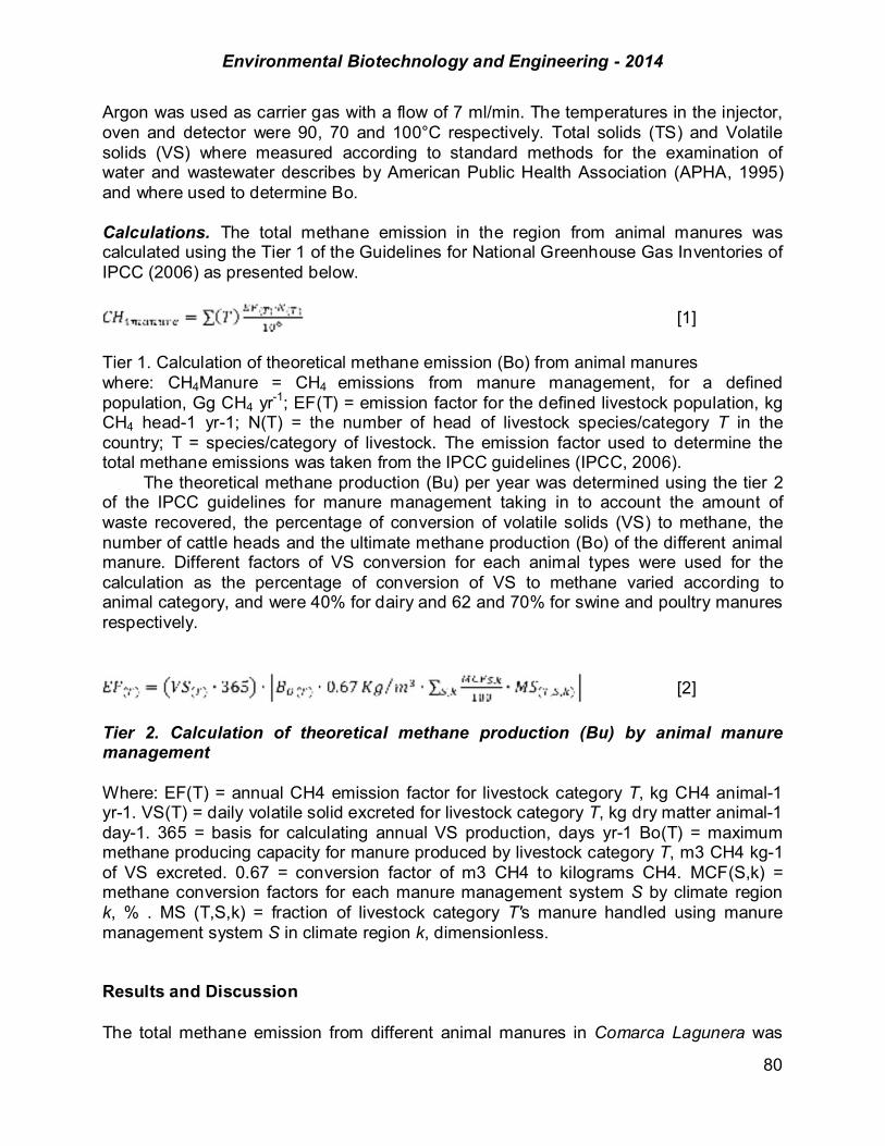
Environmental Biotechnology and Engineering - 2014
80
Argon was used as carrier gas with a flow of 7 ml/min. The temperatures in the injector, oven and detector were 90, 70 and 100°C respectively. Total solids (TS) and Volatile solids (VS) where measured according to standard methods for the examination of water and wastewater describes by American Public Health Association (APHA, 1995) and where used to determine Bo.
Calculations. The total methane emission in the region from animal manures was calculated using the Tier 1 of the Guidelines for National Greenhouse Gas Inventories of IPCC (2006) as presented below.
[1]
Tier 1. Calculation of theoretical methane emission (Bo) from animal manures where: CH4Manure = CH4 emissions from manure management, for a defined population, Gg CH4 yr-1; EF(T) = emission factor for the defined livestock population, kg CH4 head-1 yr-1; N(T) = the number of head of livestock species/category T in the country; T = species/category of livestock. The emission factor used to determine the total methane emissions was taken from the IPCC guidelines (IPCC, 2006). The theoretical methane production (Bu) per year was determined using the tier 2 of the IPCC guidelines for manure management taking in to account the amount of waste recovered, the percentage of conversion of volatile solids (VS) to methane, the number of cattle heads and the ultimate methane production (Bo) of the different animal manure. Different factors of VS conversion for each animal types were used for the calculation as the percentage of conversion of VS to methane varied according to animal category, and were 40% for dairy and 62 and 70% for swine and poultry manures respectively.
[2] Tier 2. Calculation of theoretical methane production (Bu) by animal manure management Where: EF(T) = annual CH4 emission factor for livestock category T, kg CH4 animal-1 yr-1. VS(T) = daily volatile solid excreted for livestock category T, kg dry matter animal-1 day-1. 365 = basis for calculating annual VS production, days yr-1 Bo(T) = maximum methane producing capacity for manure produced by livestock category T, m3 CH4 kg-1 of VS excreted. 0.67 = conversion factor of m3 CH4 to kilograms CH4. MCF(S,k) = methane conversion factors for each manure management system S by climate region k, % . MS (T,S,k) = fraction of livestock category T's manure handled using manure management system S in climate region k, dimensionless. Results and Discussion The total methane emission from different animal manures in Comarca Lagunera was
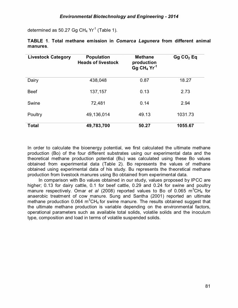
Environmental Biotechnology and Engineering - 2014
81
determined as 50.27 Gg CH4 Yr-1 (Table 1). TABLE 1. Total methane emission in Comarca Lagunera from different animal manures. Livestock Category Population
Heads of livestock Methane
production Gg CH4 Yr-1
Gg CO2 Eq
Dairy 438,048 0.87 18.27
Beef 137,157 0.13 2.73
Swine 72,481 0.14 2.94
Poultry 49,136,014 49.13 1031.73
Total 49,783,700 50.27 1055.67
In order to calculate the bioenergy potential, we first calculated the ultimate methane production (Bo) of the four different substrates using our experimental data and the theoretical methane production potential (Bu) was calculated using these Bo values obtained from experimental data (Table 2). Bo represents the values of methane obtained using experimental data of his study. Bu represents the theoretical methane production from livestock manures using Bo obtained from experimental data. In comparison with Bo values obtained in our study, values proposed by IPCC are higher; 0.13 for dairy cattle, 0.1 for beef cattle, 0.29 and 0.24 for swine and poultry manure respectively. Omar et al (2008) reported values to Bo of 0.065 m3CH4 for anaerobic treatment of cow manure. Sung and Santha (2001) reported an ultimate methane production 0.064 m3CH4 for swine manure. The results obtained suggest that the ultimate methane production is variable depending on the environmental factors, operational parameters such as available total solids, volatile solids and the inoculum type, composition and load in terms of volatile suspended solids.
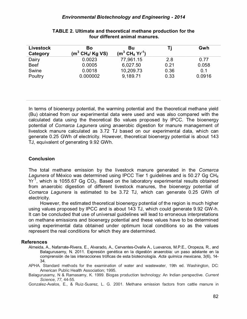
Environmental Biotechnology and Engineering - 2014
82
TABLE 2. Ultimate and theoretical methane production for the four different animal manures.
Livestock Category
Bo (m3 CH4/ Kg VS)
Bu (m3 CH4 Yr-1)
Tj Gwh
Dairy Beef Swine Poultry
0.0023 0.0005 0.0018
0.000002
77,961.15 6,027.50
10,209.73 9,189.71
2.8 0.21 0.36 0.33
0.77 0.058
0.1 0.0916
In terms of bioenergy potential, the warming potential and the theoretical methane yield (Bu) obtained from our experimental data were used and was also compared with the calculated data using the theoretical Bo values proposed by IPCC. The bioenergy potential of Comarca Lagunera using anaerobic digestion for manure management of livestock manure calculated as 3.72 TJ based on our experimental data, which can generate 0.25 GWh of electricity. However, theoretical bioenergy potential is about 143 TJ, equivalent of generating 9.92 GWh. Conclusion The total methane emission by the livestock manure generated in the Comarca Lagunera of México was determined using IPCC Tier 1 guidelines and is 50.27 Gg CH4 Yr-1, which is 1055.67 Gg CO2. Based on the laboratory experimental results obtained from anaerobic digestion of different livestock manures, the bioenergy potential of Comarca Lagunera is estimated to be 3.72 TJ, which can generate 0.25 GWh of electricity. However, the estimated theoretical bioenergy potential of the region is much higher using values proposed by IPCC and is about 143 TJ, which could generate 9.92 GW-h. It can be concluded that use of universal guidelines will lead to erroneous interpretations on methane emissions and bioenergy potential and these values have to be determined using experimental data obtained under optimum local conditions so as the values represent the real conditions for which they are determined.
References Almeida, A., Nafarrate-Rivera, E., Alvarado, A., Cervantes-Ovalle A., Luevanos, M.P.E., Oropeza, R., and
Balagurusamy, N. 2011. Expresión genética en la digestión anaerobia: un paso adelante en la comprensión de las interacciones tróficas de esta biotecnología. Acta química mexicana, 3(6), 14-34.
APHA. Standard methods for the examination of water and wastewater, 19th ed. Washington, DC: American Public Health Association; 1995.
Balagurusamy, N & Ramasamy, K. 1999. Biogas production technology: An Indian perspective. Current Science, 77, 44-55.
Gonzalez-Avalos, E., & Ruiz-Suarez, L. G. 2001. Methane emission factors from cattle manure in
Environmental Biotechnology and Engineering - 2014
83
Mexico. Bioresource Technology, 80(1), 63-71. INE, 2002. Inventario nacional de emisiones de gases de efecto invernadero 1994-1998. Instituto
Nacional de Ecología. México, p. 41-60. IPCC, 2006: Guidelines for National Greenhouse Gas Inventories. IPCC, 2013: Climate Change 2013: The Physical Science Basis. Contribution of Working Group I to the
Fifth Assessment Report of the Intergovernmental Panel on Climate Change [Stocker, T.F., D. Qin, G.-K. Plattner, M. Tignor, S.K. Allen, J. Boschung, A. Nauels, Y. Xia, V. Bex and P.M. Midgley (eds.)]. Cambridge University Press, Cambridge, United Kingdom and New York, NY, USA, 1535 pp.
Johnson, D.E., Ward, G.M. 1996.Estimates of animal methane emissions. Environmental Monitoring and Assessment. 42:133-141.
Kheshgi, H. S., Jain, A. K., Kotamarthi, V. R., & Wuebbles, D. J. 1999. Future atmospheric methane concentrations in the context of the stabilization of greenhouse gas concentrations. Journal of Geophysical Research: Atmospheres (1984–2012), 104(D16), 19183-19190.
Kumar, S., Gaikwad, S. A., Shekdar, A. V., Kshirsagar, P. S., & Singh, R. N. 2004. Estimation method for national methane emission from solid waste landfills. Atmospheric Environment, 38(21), 3481-3487.
Møller, H. B., Sommer, S. G., & Ahring, B. K. 2004. Methane productivity of manure, straw and solid fractions of manure. Biomass and bioenergy, 26(5), 485-495.
Omar, R., Harun, R. M., Mohd Ghazi, T. I., Wan Azlina, W. A. K. G., Idris, A., & Yunus, R. 2008. Anaerobic treatment of cattle manure for biogas production. In Proceedings Philadelphia, Annual meeting of American Institute of Chemical Engineers (pp. 1-10).
Smith, P., Martino, D., Cai, Z., Gwary, D., Janzen, H., Kumar, P., & Smith, J. 2008. Greenhouse gas mitigation in agriculture. Philosophical Transactions of the Royal Society B: Biological Sciences, 363(1492), 789-813.
Sung, S. & Santha, H. 2001. Performance of temperature-phased anaerobic digestion (TPAD) system treating dairy cattle wastes. Tamkang Journal of Science and Engineering, 4, 301–310

Environmental Biotechnology and Engineering - 2014
84
CHAPTER 1.10. ANAEROBIC DIGESTION FULLY ENHANCED BY MERGING THE BIOMETHANATION OF SYNGAS FROM SOLID DIGESTATE
Serge R. Guiot (1,5), Ruxandra Cimpoia (1), Lionel Dath (2), Jérémy Ollier (3), Rony
Das (4), Silvia Sancho Navarro (1,5)
(1) National Research Council Canada (NRC), Energy, Mining and Environment Portfolio, Bioengineering Group, Montreal, Canada H4P 2R2
(2) Haute Ecole Provinciale de Hainaut–Condorcet, Dpt. Agro-industries et Biotechnologies, B-7810 Maffle (Belgique)
(3) Université Joseph Fourier, Dpt. Génie Des Procédés, F-38041 Grenoble (France) (4) University of British Columbia, Dpt. Civil Engineering, Vancouver, Canada V6T 1Z4 (5) Université de Montréal, Dpt. Microbiology, Infectiology and Immunology, Montreal, Canada H3C 3J7 ABSTRACT Microorganisms can be used to convert the syngas main compounds (carbon monoxide, CO, and H2) into methane. In the present study, the syngas biomethanation potential was studied via co-digestion with food waste (FW). A 2 L mesophilic completely stirred tank reactor (CSTR) was operated with an average hydraulic retention time (HRT) of 28 days, a FW organic loading rate of 1 and 2 g volatile solids (VS) per liter of reactor (RXR) and per day. The co-digestion methane potential was not significantly affected by CO at a 0.2 atm partial pressure (pCO); however, higher pCO resulted in delay and relatively decreased methane production. In the CSTR a maximum CO conversion rate (12 mmol CO/g VS.d) occurred at a CO inflow of # mol/LRXR.d, a pCO of 0.2 atm, and a 0.04 d-1 gaseous HRT. Under these conditions, the VS destruction efficiency attained 71%, and the CH4 yield could mount to 0.7 LSTP CH4/g VS degraded, due to the contribution of CO to the methane production. If the residual solid digestate would be further dried, then gasified to produce syngas, which would afterwards be processed in the AD system, one may expect a methane yield boosted by 20 to 50% by the syngas addition, depending on the AD degradation efficiency. Key words: anaerobic digestion, methane, organic wastes, digestate, syngas, biomethanation Introduction The digester sludge, or digestate, produced by an anaerobic digester is a combination of inert solids that were fed with the substrate, recalcitrant volatile solids that could not be degraded biologically, and bacterial biomass that grew as a result of feeding on the degradable portion of the volatile solids fed with the feedstock. This is potentially an alternative source of humic material, nutrients and minerals to the agricultural soil. It may be used directly or separated into liquid and solid part. The liquid ------------------ *Author for correspondence: [email protected]
Environmental Biotechnology and Engineering-2014
85
digestate is often recycled to the digestion process. In certain periods of a year the solid digestate may be used in agriculture directly; in most cases however it must be stabilized before being applied to the fields, using aerobic treatment (composting). For various reasons the composting of the digestate residue is sometimes not possible (lack of space for a composting facility, difficulty of selling the compost due to social unacceptability or market saturation, inadequate regulation, incompatibility with agricultural, horticultural or forestry practices, etc). These digestate surpluses, composted or not, then end up in landfill or incinerators. Alternatively the digestate may be treated by thermal methods, such as gasification, which requires higher solid content. Mechanical dehydration by means of continuous centrifuges provides solid content about 30 % with positive calorific value. The lower heating value (LHV) of anaerobic digestate can be up to 14 MJ/kg dry solid. Digestate produced from feedstock with higher fiber content tends to have a higher LHV. This energy content can be extracted by gasification of the digestate mechanically dehydrated to produce a synthesis gas (syngas). Depending on the heat content of the solid digestate, additional thermal drying may be necessary to be able to support an auto-thermal gasification of the digestate. The solids content required for a self-supporting thermal gasification may range from 40 to 70% or more. Thermal methods are more expensive than composting due to high energy demand for dehydration and drying, sophisticated processes involved and strict monitoring requirements. Otherwise, the main product of gasification, the synthesis gas or syngas, can be used as a fuel or if further processed, as a basis chemical. The solid residues, ash or char, are recyclable as soil amendments to reduce its acidity, its needs in fertilizers and potash and its emissions of greenhouse gases (nitrous oxide, methane). Gasification is a thermochemical degradation at high temperature (generally above 500°C) with minimal introduction of oxygen, if any (the stoichiometric combustion ratio (oxidizer/fuel) is set between 0 and 1). The presence of oxygen is controlled to maintain the gasification process energetically self-sufficient. Syngas is mainly composed of carbon monoxide (CO) and hydrogen (up to 85% for the total of both). Other components of syngas are water vapor, methane, light hydrocarbons, particulates and volatile impurities. Syngas without nitrogen has a LHV between 8 and 16 MJ/Nm3. After adequate cleaning to remove moisture, particulates, tars and impurities, syngas can be used for heat or electricity production with adapted internal combustion engines, boilers, gas turbines, or fuel cells. But it can also be used as a basis chemical in various catalytic processes of chemical transformation. For example, the methanation of syngas is used to enrich the syngas into methane, and thus turn it into renewable natural gas (RNG) for re-injection into the grid after removal of CO2 and impurities. Methanation includes the water-gas shift reaction for increasing the H2/CO ratio and the nickel-catalyzed reduction of CO and CO2 into methane and water (Ridler and Twigg 1996). The methanation product is thus a gas rich in methane, but still containing water vapor and CO2. This well-established process is costly due to the chemical catalyst, its energy demand, and the need to pretreat the syngas to remove impurities. The catalytic reaction usually involves high pressure and temperature, and the catalyst can be poisoned by impurities and tends to have low product specificity (Gallei & Schwab 1999). To circumvent these disadvantages and use milder treatments with minimal chemical and energy, the power of microorganisms can be harnessed to biochemically convert
Environmental Biotechnology and Engineering-2014
86
the syngas compounds into biogas, at ambient temperature and pressure, which we called biomethanation, by analogy to the term used in chemical catalysis, and by distinction with the term biomethanization used for anaerobic digestion of organic matter. A small number of microbes can reduce the CO from syngas into methane (Methanobacterium thermoautotrophicum, Methanothermobacter wolfeii, Methanobrevibacter arboriphilicus, Methanocaldococcus jannaschii, Methanopyrus kandleri, Methanosaeta thermophila, Methanosarcina acetivorans, M. barkeri) (Henstra et al 2007; Sokolova et al 2009). We previously showed that sludge from anaerobic digestion (AD) had a non-negligible CO-consuming methanogenic potential, without a particular adaptation was required (Guiot et al. 2011). With such a mixed anaerobic consortium, other indirect reactions also occur. For instance: carboxydotrophic (i.e. CO-consuming) hydrogenogenesis (enzymatic water-gas shift reaction) (Zhao et al 2011), followed by either the methanogenic reduction of CO2, or carboxydotrophic methanogenesis; CO-homoacetogenesis followed by acetoclastic methanogenesis; oxidation of CO into formic acid, followed by its reduction into CH4 (Sancho-Navarro et al. 2014). Regardless of the specific reaction, the methane yield is 0.25 mol of CH4 per mol of CO, plus 0.25 mol of CH4 per mol of H2. Based on the range of CO and H2 typically contained in syngas, this is equivalent to about 0.2 to 0.4 Nm3 of methane production per kilogram of VS gasified, depending on the syngas composition (i.e. CO between 30 and 60 % (vol./vol.), H2 between 60 and 25%, and CO2 between 35 and 3%), and when the syngas is efficiently introduced and dissolved in the anaerobic mixed liquor. The purpose of this study was to study the syngas biomethanation potential via co-digestion with food waste (FW). Materials and methods Specific activity tests. The tests were performed using 120 mL serum bottles for substrates in solution and 60 mL serum bottles for gaseous substrates, in triplicate, with endogenous controls (without substrate). The bottles were filled with 20 mL of inoculum diluted with 0.05 M phosphate buffer at pH 7.5 to an initial concentration of 5 g volatile suspended solids (VSS)/L for the tests with liquid substrates, and at a concentration of 2 g VSS/L for the gaseous substrates, with hydrogenotrophic (CO2/H2) and carboxydotrophic (CO) tests. To establish anaerobic conditions in the tests with liquid substrates the bottles were capped, sealed and flushed with N2/CO2 gas (80/20%, v/v) to obtain 1 atm of total pressure in the headspace. Then, the bottles were injected with the substrate solution to obtain an initial concentration of 3000 mg/L, except for the endogenous controls. In the case of the carboxydotrophic tests, once the bottles were capped and sealed, they were flushed with N2 gas (100%) for 3 minutes. Afterwhich, CO was injected into the bottles under anaerobic conditions, using a gas tight syringe (model 1750 gas-tight syringe, Hamilton, Reno, NV), to obtain 20% CO in the headspace. The bottles were incubated in a rotary shaker, 35 ± 3 ºC, at 200 rpm in the dark. (New Brunswick, Edison, NJ). The hydrogenotrophic activity tests were prepared like the former bottles, but flushed with H2/CO2 (80/20%, v/v), pressurized to 2.5 atm in the headspace, and shaken at 400 rpm to maximize the gas-liquid mass transfer.

Environmental Biotechnology and Engineering-2014
87
Biochemical methane potential tests. The biochemical methane potential (BMP) assays were prepared based on the method of Cornacchio et al. (1986). A few modifications were made to adapt the test to high solid samples as previously detailed (Frigon et al. 2012). The inoculum consisting of industrial granular sludge (Lassonde Inc., Rougemont, QC, Canada) was starved for 48 hours prior to the start-up of the assays, by incubation at 35°C and at agitation at 150 rpm with no substrate. Triplicate bottles (500 mL) were prepared anaerobically under a constant flow of a gas mix (80% N2, 20% CO2) for each experimental digestion. Before sealing, the pH was adjusted to 7.0, if necessary, when the bottles were ready. The volumes of inoculum suspension, FW mix and substrate solution introduced in the bottles were adjusted so to have 5 g VSS/L, 2 and 1 g COD/L for inoculum, FW and substrate, respectively. In addition to the substrate and inoculum volumes, a typical bottle contained two mL of defined media, two mL of bicarbonate buffer and 0.5 mL of 1.25% Na2S-cysteine solution. The recipes for the different solutions and the procedure for their preparation are detailed elsewhere (Frigon et al. 2012). The final volume was adjusted to 100 mL for all bottles using boiled demineralized water. The assays were conducted until the methane production became negligible (< 3 mL d-1). The bottles were incubated at 35°C with an agitation of 150 rpm. Control bottles were prepared to correct for endogenous methane production from the assays. The control bottles were identical to the test bottles, excepted that the waste suspension was replaced with the same volume of deoxygenated water. Analytical methods. The gas composition (O2, H2, CH4, N2, CO, CO2) was determined injecting 250 L of gas in an Agilent 6890 gas chromatograph (Wilmington, DE) equipped with a TCD and a 5 m x 2.1 mm Carboxen-1000 column (Supelco, Belafonte, PA) with argon as the carrier gas. The column temperature was held at 60 ºC for 7 min and increased to 225 ºC at a rate of 60 ºC per min. Volatile fatty acids (VFA) (acetate, propionate and butyrate) and alcohols (methanol, ethanol, acetone, 2-propanol, tert-butanol, n-propanol, sec-butanol and n-butanol) were measured on an Agilent 6890 gas chromatograph (Wilmington, DE) equipped with a flame ionization detector (FID) as described previously (Guiot et al. 2011). The volatile solids (VS), VSS and chemical oxygen demand (COD) analyses were performed according to standard methods (Eaton et al. 2005). Reactor setup. The 2 L glass continuously stirred tank reactor (CSTR) was equipped with a laboratory stirrer (Talboys, Throemner LLC, Thorofare NJ) operated at 60 rpm. Several sampling ports were located on top and were used for gas line connections, sensor installation, and sludge sampling. The reactor temperature was controlled by a probe (DP-41, Omega Engineering Inc, Stamford, CT) and maintained at 35ºC by circulating water from a thermostatic bath (RK12418-30, Cole Parmer, Niles, IL) through the reactor water jacket. The pH was measured (electrode 405-DPAS-SC-K8S, Mettler Toledo GmbH, Urdorf, CH) and controlled between 6.9 and 7.8 using 0.1M NaOH or 0.1M HCl with a pH controller (PHP-194, Omega Engineering Inc, Stamford, CT). The feeding gas whose CO (Praxair Canada Inc, Mississauga, ON, CA) content was adjusted using nitrogen gas (Praxair Canada Inc) was bubbled at the center of the reactor bottom. The gas flow rates were measured and controlled by thermal mass flow meters (M100B, M10MB, 247D, MKS, Wilmington, MA). The gas exited the reactor through a pressure valve (TM Swagelok, Solon, OH) to maintain the reactor headspace
Environmental Biotechnology and Engineering-2014
88
at the desired pressure (manometer 0-60PSI, US Gauge, Ira Township, MI). The gas phase was recycled with a compressor (UN036STI, Neuberger Inc, Trenton, NJ) at a flow rate of ~ 50 mL/min. In the gas recycle, an empty column was used as a condenser and foam trap. To achieve a semi-continuous mode of operation, part of the reactor liquid was removed through the sludge sampling port every two or three days, and replaced with the equivalent volume of waste feed. The amount of removed liquid and the strength of the feed suspension were selected so to obtain a desired hydraulic retention time (HRT) and organic load. Results and discussion The syngas (carbon monoxide (CO), or CO + H2, or CO + H2 +CO2) biomethanation potential was studied via co-digestion with food waste (FW) and various single carbon sources (cellulose, glucose, acetate, propionate). A commercial dog food (89 g dry solid (SS)/kg) mixed with carrots (11 g SS/kg) was used as synthetic food waste (FW). The carbon/nitrogen/ phosphorus ratio of FW was approximately 100/6/0.7. The inoculum (granular sludge) originated from an industrial digester (Lassonde, Rougemont, Qc). The specific methanogenic activity [mmol CH4/g dry microbial biomass·day] on the above substrates, added separately, ranked as follows: CO [0.6] < FW [1.1 – 1.3] < cellulose [1.4] < glucose [1.5] < propionate [1.9] < acetate [4.3] < H2 [54]. The above substrates were tested for their biomethane potential (BMP) in presence or not of CO, at different organic loads and co-substrates ratios in batch tests (22 in triplicate). While methane was the main end-product, acetate, propionate and acetone, and traces of propanol, ethanol, methanol were also detected in the co-digestion process. The accumulation of NH4
+ is also observed in presence of food waste. In the co-digestion mode with food waste, it was observed a reduction (by about one third) of the carboxydotrophic activity of microbial populations, because of the accumulation of ammonium produced from waste, as well as the competition between FW and CO as carbon sources for the populations. CO had a smaller impact on the hydrolysis and acidogenesis activities than on the acetogenic and methanogenic ones. The BMP of the co-digested substrates was not significantly affected by CO at a 0.2 atm partial pressure (pCO); however, higher CO concentration resulted in delay and relatively decreased methane production. Then, the co-digestion of carbon monoxide with food waste (FW) was studied in CSTR reactors at the laboratory scale. A 2 L mesophilic CSTR was operated in the semi-batch mode with an average HRT of 28 days, and a FW organic loading rate (OLR) of 1 g VS per liter of reactor (RXR) and per day, then on the continuous mode, with a HRT of 21 days and an OLR of 2 g VS/LRXR·d, for an overall period of over 300 days. When the CSTR was operated in presence of FW and CO (i.e. on the co-digestion mode), a maximum CO conversion rate (12 mmol CO/g VS.d) occurred at a CO inflow of # mol/LRXR.d, with a CO/FW ratio of 0.18 mol CO/g VS (4 Nm3 CO/kg VS), a pCO of 0.2 atm, and a 0.04 d-1 gaseous HRT. However, during the co-digestion regime (CO + FW) the efficiency of organic solids destruction was 71%, while the removal efficiency of the COD combined (FW + CO) could barely reach 39%, with at best, a methane yield of 0.135 LSTP CH4/g COD added, namely because of the poor mass transfer of CO to the liquid phase and the potential of CO to inhibit the microbial populations, particularly the methanogenic archaea. However, the methane yield relative to the solids degradation

Environmental Biotechnology and Engineering-2014
89
could mount to 0.7 LSTP CH4/g VS degraded, due to the contribution of CO to the methane production. By comparison, during the waste digestion without CO, the VS destruction efficiency could attain 84 % and the CH4 conversion yield, between 0.215 and 0.28 LSTP CH4/g COD added or 0.30 and 0.40 LSTP CH4/g VS added, i.e. between 0.30 and 0.39 LSTP CH4/g COD destroyed. Beyond a CO/FW ratio of 0.18 mol CO/g VS, the CH4 yield relative to the organic solids added decreased by at least 40%, despite the presence of CO as an additional carbon source. The gas-liquid mass transfer and the reactor’s feeding regime (CO/FW ratio) might be the main process limitations. It can be presumed that actual syngas (40% CO - 40% H2 - 20% CO2) added as co-digestion substrate would not affect the methanogenic specific activity but would delay the process kinetics. However there is a need to test the co-digestion regime with complete syngas, i.e. CO with hydrogen and CO2, and to assess the maximum CO/FW (below the current ratio of 0.18 mol CO/g VS) that would not significantly impede the food waste degradation efficiency (limit of the technology). Below this threshold, one may expect a methane yield boosted by about 20% by the syngas addition. Food waste is usually quite easily amenable to AD, however biosolids or manure are significantly less biodegradable, with a non-digested residue (solid digestate) of 50 to 40%. For instance, in case of a biosolids 50% conversion by conventional AD, the CH4 yield would be at the most 0.25 Nm3/kg VS fed. If the digestate (the other 50% of VS) is further dried, then gasified to produce syngas, which is processed in the AD system, an additional 0.15 Nm3/kg VS fed could in theory be expected (Figure 1).
FIGURE 1. Concept of coupling anaerobic digestion (AD) and gasification (B) compared to conventional AD with pretreatment (A).

Environmental Biotechnology and Engineering-2014
90
Conclusion This type of coupling of gasification with existing AD facilities should maximize the energy potential of organic waste without increasing the number of processing steps. However, thermal processes are more expensive than the composting due to the high energy demand, particularly for drying, and the complexity of the process leading to higher capital and operational costs. Nevertheless, if such a thermal treatment of the digestate would be implemented to extract the digestate residual energy, there would be no need to apply a chemical or thermal pretreatment upstream of the AD to maximize its solid degradation efficiency and biogas yield. The elimination of the preprocessing step may hopefully offset (partially or fully) the additional costs associated with drying and gasification of digestate. In the context of a biorefinery incorporating several technologies, biomass gasification would complement anaerobic digestion. The ‘wet’ waste would be digested and the residual solid digestate gasified with ‘dry’ materials such as litter mixed with wood shavings, wood by-products, dry plant material such as straw or corn husks, slowly degradable municipal solid wastes (MSW) such as construction household waste, wood wastes, tires, plastics. MSW are typically composed of compostable or digestible organic materials (food, yard, garden) for 17% at around 30% dryness, and of other non-compostable organics for 54 % at around 45% dryness on average, and of inert wastes (metals, glass and other inerts) for 29%. Anaerobic digestion of the first fraction, at a degradation efficiency of 60% and a yield of 0.5 Nm3 CH4/kg VS degraded, could generate 15 Nm3 CH4 per metric ton of MSW. If this is complemented by gasification of the second fraction of other organics combined with biomethanation of the syngas produced, at a conservative integrated yield of 0.25 Nm3 CH4/kg solid gasified, this would add up 60 Nm3 CH4, resulting hence in a total of about 75 Nm3 CH4 per metric ton of MSW i.e. five times the potential by anaerobic digestion alone. However the energy-intensiveness of gasification may mitigate the net energy output. Acknowledgements The study was partially supported by the Clean Energy Fund and the ecoENERGY Innovation Initiative from the Office of Energy Research and Development (OERD) of Natural Resources Canada (projects I12.017B and BIOI.013). One author (S.S.N.) was supported by the Natural Sciences and Engineering Research Council of Canada (grant 185778-2009). References Cornacchio, L.; Hall, E.R.; Trevors, J.T. (1986). Modified serum bottle testing procedures for industrial
wastewaters. In: Technology transfer workshop on laboratory scale anaerobic treatability testing technique, Wastewater Technology Center, Environment Canada.
Eaton, A.D., Clesceri, L.S., Rice, E.W., and Greenberg, A.E. (eds). 2005. Standard methods for the examination of water and wastewater. 21st ed. American Public Health Association, American Water Works Association, Water Environment Federation, Washington, D.C.
Frigon, J.C.; Mehta, P.; Guiot, S.R. (2012). Impact of mechanical, chemical and enzymatic pretreatments on the methane yield from the anaerobic digestion of switchgrass. Biomass Bioenergy 36(1):1-11. DOI: 10.1016/j.biombioe.2011.02.013.
Gallei, E.; Schwab, E. (1999). Development of technical catalysts. Catalysis Today 51(3-4): 535-546. DOI:

Environmental Biotechnology and Engineering-2014
91
10.1016/S0920-5861(99)00039-5. Guiot, S.R. ; Cimpoia, R.; Carayon, G. (2011). Potential of wastewater-treating anaerobic granules for
biomethanation of synthesis gas. Environ. Sci. Technol. 45(5): 2006–2012. DOI: 10.1021/es102728m.
Henstra, A.M.; Sipma, J.; Rinzema, A.; Stams, A.J.M. (2007). Microbiology of synthesis gas fermentation for biofuel production. Curr. Opinions Biotech. 18(3): 200-206. DOI: 10.1016/j.copbio.2007.03.008.
Ridler, D.R.; Twigg M.V. (1996). Catalyst Handbook, Manson Publishing, London, UK. Sancho-Navarro, S.; Cimpoia, R.; Bruant, G.; Guiot, S.R. (2014). Specific inhibitors for identifying
pathways for methane production from carbon monoxide by a non-adapted anaerobic mixed culture. Can. J. Microbiol. 60(6): 407-415. DOI: 10.1139/cjm-2013-0843.
Sokolova, T.G.; Henstra, A.-M.; Sipma, J.; Parshina, S.N.; Stams, A.J.M.; Lebedinsky, A.V. (2009). Diversity and ecophysiological features of thermophilic carboxydotrophic anaerobes. FEMS Microbiol. Ecol. 68(2): 131-141. DOI: 10.1111/j.1574-6941.2009.00663.x.
Zhao, Y.; Cimpoia, R.; Liu, Z.; Guiot, S.R. (2011). Kinetics of CO conversion into H2 by Carboxydothermus hydrogenoformans. Appl. Microbiol. Biotech. 91(6): 1677-1684, DOI: 10.1007/s00253-011-3509-7.

Environmental Biotechnology and Engineering-2014
92
CHAPTER 1.11. PRODUCCIÓN DE LÍPIDOS EN LA BIOMASA DE Trichoderma sp. CON UN CULTIVO ESTACIONARIO Y EXTRAÍDOS CON TRES TÉCNICAS PARA LA
OBTENCIÓN DE BIODIÉSEL
Daniel Vélez-Martínez (1); Ma. Remedios Mendoza-López (1); †Jesús S. Cruz-Sánchez (1); Rosalba Argumedo-Delira*(1)
(1) Universidad Veracruzana, Unidad de Servicios de Apoyo en Resolución Analítica (SARA), Xalapa, Veracruz, México. RESUMEN En los últimos años se ha prestado mucha atención a la exploración de los aceites microbianos para la producción de biodiesel, que son producidos por algunos microorganismos oleaginosos, tales como las microalgas, levaduras, bacterias y hongos filamentosos. Considerando lo anterior la presente investigación tuvo como objetivo evaluar la producción de lípidos en la biomasa del hongo Trichoderma sp. H-1 con un cultivo estacionario a 25 °C y la extracción de los lípidos con tres técnicas para la generación de biodiésel a partir de la reacción de transesterificación, utilizando como catalizador BF3. Los resultados muestran que con la técnica de extracción de lípidos modificada de Blight y Dyer (1959), Folch et al. (1956) y Ramos et al. (2010) se obtuvo el 18.4 %, 10.3% y 17.1% de lípidos respectivamente. Con lo que respecta a la reacción de transesterificacion efectuada a los lípidos obtenidos con las tres técnicas antes mencionadas se encontró que el componente mayoritario del biodiésel conseguido presenta diferencias para los lípidos extraídos con Ramos et al. (2010), ya que el éster metílico del ácido palmítico (40.8%) es el componente mayoritario, mientras que para técnicas de extracción de Folch et al. (1956) y Blight y Dyer (1959) el componente mayoritario fue el éster metílico del ácido linoléico con 41.2 y 37.6% respectivamente. Las condiciones de cultivo y las técnicas de extracción de lípidos utilizadas son un factor determinante para la obtención de biodiésel a partir de lípidos fúngicos, por lo tanto la modificación de algunas de estas condiciones podría incrementar su eficiencia y viabilidad. Palabras clave: Lípidos, biomasa fúngica, Trichoderma, cultivo estacionario Introducción Los combustibles fósiles han ofrecido oportunidades asombrosas durante el siglo XX, pero ahora la humanidad tiene que enfrentarse a los retos derivados de su sobreexplotación, y a su uso casi exclusivo que ha hecho a un lado a otras fuentes alternativas de energía durante varios años, adicionalmente las reservas de los combustibles fósiles están disminuyendo progresivamente y su demanda aumenta exponencialmente al crecer la población mundial (Angenent et al., 2004; Armaroli y ----------------- *Author for correspondence
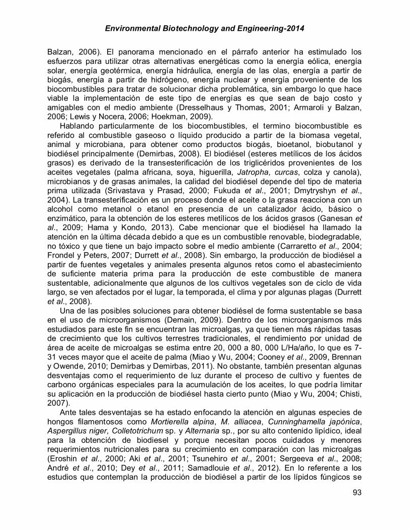
Environmental Biotechnology and Engineering-2014
93
Balzan, 2006). El panorama mencionado en el párrafo anterior ha estimulado los esfuerzos para utilizar otras alternativas energéticas como la energía eólica, energía solar, energía geotérmica, energía hidráulica, energía de las olas, energía a partir de biogás, energía a partir de hidrógeno, energía nuclear y energía proveniente de los biocombustibles para tratar de solucionar dicha problemática, sin embargo lo que hace viable la implementación de este tipo de energías es que sean de bajo costo y amigables con el medio ambiente (Dresselhaus y Thomas, 2001; Armaroli y Balzan, 2006; Lewis y Nocera, 2006; Hoekman, 2009).
Hablando particularmente de los biocombustibles, el termino biocombustible es referido al combustible gaseoso o líquido producido a partir de la biomasa vegetal, animal y microbiana, para obtener como productos biogás, bioetanol, biobutanol y biodiésel principalmente (Demirbas, 2008). El biodiésel (esteres metílicos de los ácidos grasos) es derivado de la transesterificación de los triglicéridos provenientes de los aceites vegetales (palma africana, soya, higuerilla, Jatropha, curcas, colza y canola), microbianos y de grasas animales, la calidad del biodiésel depende del tipo de materia prima utilizada (Srivastava y Prasad, 2000; Fukuda et al., 2001; Dmytryshyn et al., 2004). La transesterificación es un proceso donde el aceite o la grasa reacciona con un alcohol como metanol o etanol en presencia de un catalizador ácido, básico o enzimático, para la obtención de los esteres metílicos de los ácidos grasos (Ganesan et al., 2009; Hama y Kondo, 2013). Cabe mencionar que el biodiésel ha llamado la atención en la última década debido a que es un combustible renovable, biodegradable, no tóxico y que tiene un bajo impacto sobre el medio ambiente (Carraretto et al., 2004; Frondel y Peters, 2007; Durrett et al., 2008). Sin embargo, la producción de biodiésel a partir de fuentes vegetales y animales presenta algunos retos como el abastecimiento de suficiente materia prima para la producción de este combustible de manera sustentable, adicionalmente que algunos de los cultivos vegetales son de ciclo de vida largo, se ven afectados por el lugar, la temporada, el clima y por algunas plagas (Durrett et al., 2008).
Una de las posibles soluciones para obtener biodiésel de forma sustentable se basa en el uso de microorganismos (Demain, 2009). Dentro de los microorganismos más estudiados para este fin se encuentran las microalgas, ya que tienen más rápidas tasas de crecimiento que los cultivos terrestres tradicionales, el rendimiento por unidad de área de aceite de microalgas se estima entre 20, 000 a 80, 000 L/Ha/año, lo que es 7-31 veces mayor que el aceite de palma (Miao y Wu, 2004; Cooney et al., 2009, Brennan y Owende, 2010; Demirbas y Demirbas, 2011). No obstante, también presentan algunas desventajas como el requerimiento de luz durante el proceso de cultivo y fuentes de carbono orgánicas especiales para la acumulación de los aceites, lo que podría limitar su aplicación en la producción de biodiésel hasta cierto punto (Miao y Wu, 2004; Chisti, 2007).
Ante tales desventajas se ha estado enfocando la atención en algunas especies de hongos filamentosos como Mortierella alpina, M. alliacea, Cunninghamella japónica, Aspergillus niger, Colletotrichum sp. y Alternaria sp., por su alto contenido lipídico, ideal para la obtención de biodiesel y porque necesitan pocos cuidados y menores requerimientos nutricionales para su crecimiento en comparación con las microalgas (Eroshin et al., 2000; Aki et al., 2001; Tsunehiro et al., 2001; Sergeeva et al., 2008; André et al., 2010; Dey et al., 2011; Samadlouie et al., 2012). En lo referente a los estudios que contemplan la producción de biodiésel a partir de los lípidos fúngicos se

Environmental Biotechnology and Engineering-2014
94
encuentra el de Lunin et al. (2013), donde se emplean los lípidos de especies que pertenecen al género Cunninghamella para la producción de este combustible, y reportan que el número de cetano (CN) para el biodiésel obtenido es de 55.68 MJ kg-1 vs 51.74 MJ kg-1 del biodiésel producido a base de aceite de colza. Otro hongo que ha servido como materia prima para la producción de biodiésel es Aspergillus sp., el biocombustible obtenido correlaciona bien con los estándares establecidos (Subhash y Mohan, 2011).
Tomando en consideración los antecedentes mencionados y que la mayoría de los estudios reportan la obtención de los lípidos fúngicos bajo cultivos con agitación, la presente investigación tuvo como objetivo evaluar la producción de lípidos en la biomasa del hongo Trichoderma sp. H-1 con un cultivo estacionario a 25 °C y la extracción de los lípidos con tres técnicas para la generación de biodiésel a partir de la reacción de transesterificación, utilizando como catalizador BF3 Materiales y métodos Microorganismo y condiciones de cultivo. Trichoderma sp. H-1 se aisló de suelo rizosférico de helecho de la USBI, Xalapa-Veracruz México. El hongo Trichoderma sp. H-1 se creció en cajas de Petri con PDA marca (Bioxon ®) a 22 °C por 5 días. Transcurrido este tiempo, se cortaron discos individuales de PDA con micelio del hongo (7 mm de diámetro). Posteriormente a un biorreactor de plástico de 10 L de capacidad, se le adiciono 6 L del medio mineral estéril (g L-1) 0.25 CaCl2; 0.25 MnCl2; 0.15 MgCl2; 0.5 (NH4)2SO4; 0.5 NaH2PO4; 50 Glucosa; pH 4.2, luego se inocularon 300 discos del hongo. Después se incubaron a temperatura ambiente por 10 días (se realizaron tres repeticiones). La biomasa fúngica obtenida de los biorreactores se dejó secar a temperatura ambiente, una vez seca la biomasa se molió con un mortero. Extracción de lípidos. 1).Bligh y Dyer (1959) modificada. Se pesó en un tubo de ensayo 0.33 g de la biomasa fúngica seca, luego se le agregaron 3 mL de una mezcla de CHCl3/CH3OH (1:2) y se mantuvo en agitación durante 2 horas. Después de transcurrido este tiempo se centrifugó por 15 minutos a 2500 rpm. Posteriormente la muestra fue pasada a un matraz de 50 mL para eliminar los solventes en un rotavapor y el contenido de lípidos se determinó gravimétricamente.
2) Folch et al. (1956) modificada. En un tubo de ensayo, se pesó 0.33 g de biomasa fúngica, luego se adicionaron 6 mL de una solución de CHCl3/CH3OH (2:1) y se agito en un agitador tipo vórtex por espacio de 1 minuto. Después se dejó reposar la mezcla (tubo 1) durante 24 h a 4 °C y se protegió de la luz, de tal forma que se favoreciera la extracción completa de los lípidos. Posteriormente en un agitador tipo vórtex se agitó la mezcla por espacio de 1 minuto. Luego se centrifugo a 4500 rpm por 20 min, recuperando la fase orgánica con una pipeta Pasteur, y se pasó a un tubo de vidrio de 15 mL (tubo 2). Mientras que a la biomasa residual se le agregaron 3 mL de CHCl3/CH3OH (2:1), la mezcla se agitó en un agitador tipo vórtex por espacio de un minuto y se centrifugo nuevamente a 4500 rpm por 20 min recuperando la fase orgánica en el tubo 2. Después al extracto del tubo 2 se le agregó una solución salina de NaCl al 0.58% (3 mL), de modo que la solución final CHCl3/CH3OH/H2O tuviese una proporción

Environmental Biotechnology and Engineering-2014
95
(8:4:3), esta mezcla se agitó en un agitador tipo vórtex por 1 min. Luego se centrifugo a 4500 rpm por 10 min, separando el 90% de la fase superior. A continuación se recuperó la fase inferior (CHCl3), con una pipeta Pasteur (recuperando el 90% de esta fase), colocando la fase clorofórmica recuperada en un nuevo tubo (tubo 3). La fase acuosa remanente se lavó con 1 mL de CHCl3, mezclando en un agitador tipo vórtex para después centrifugar nuevamente a 4500 rpm durante 10 min, posteriormente se recuperó la fase inferior (CHCl3) colocándola en el tubo 3. Finalmente se evaporó la fase clorofórmica del tubo 3 en baño maría a 70 °C, y el contenido de lípidos se determinó gravimétricamente. 3) Ramos et al. 2010 modificada. En un tubo de ensayo, se pesó 0.33 g de la biomasa fúngica, a la cual se le agregó 6 mL de una solución de hexano:isopropanol (3:2), y luego se agitó en un agitador tipo vórtex hasta que la biomasa se dispersó. Posteriormente se dejó reposar por 24 horas a 4 °C y se protegió de la luz, de tal forma que se favoreciera la extracción completa de los lípidos. Subsiguientemente en un agitador tipo vórtex se agitó la mezcla por espacio de 1 min. Después se centrifugó a 4500 rpm por 20 min, recuperando el extracto con una pipeta Pasteur y se pasó a un tubo de vidrio de 15 mL. Mientras que a la biomasa residual se le agregaron 3 mL de una solución de hexano:isopropanol (3:2), la mezcla se agitó en un agitador tipo vórtex por 1 min y se centrifugó nuevamente a 4500 rpm por 20 min, el extracto obtenido se recuperó en el tubo anterior. Finalmente se evaporó la fase orgánica en baño maría a 95 °C, y el contenido de lípidos se determinó gravimétricamente. Transesterificación modificada (Morrison y Smith, 1946). A cada respectiva muestra de lípidos se le adicionó 1 mL de BF3 en CH3OH al 14%, posteriormente se calentó durante 30 min a 80°C con agitación. Después se realizó la extracción de los ésteres metílicos utilizando 1 mL de hexano grado HPLC, luego el extracto hexánico, se secó con Na2SO4 y se filtró, para su posterior inyección al cromatógrafo de gases acoplado a espectrometría de masas (Agilent Technologies® Mod. 5975 inert XL). Análisis estadístico. Para la extracción de lípidos y la transesterificación se empleó un diseño experimental completamente al azar utilizando un factorial un factorial 3x1 (tres métodos de extracción y un hongo filamentoso). Cada tratamiento tuvo tres repeticiones. Los datos obtenidos fueron analizados mediante análisis de varianza y la prueba de comparación de medias (Tukey, !=0.05) con el programa estadístico SAS. Resultados y discusión Extracción de lípidos. Bajo las condiciones de cultivo estacionario se obtuvo un promedio de 0.1966 g L-1 de biomasa seca en cada biorreactor (Figura 1). En el caso de la extracción de lípidos, el método que presentó una mayor extracción fue la modificación de Bligh y Dyer (1959) con un promedio de 18.4%, sin embargo, la cantidad de lípidos extraídos por las tres metodologías usadas no presentó diferencias estadísticas (Tabla 1).
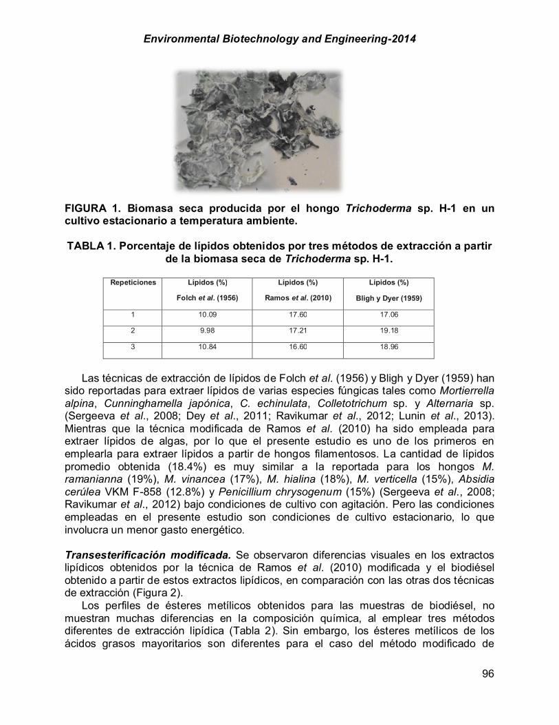
Environmental Biotechnology and Engineering-2014
96
FIGURA 1. Biomasa seca producida por el hongo Trichoderma sp. H-1 en un cultivo estacionario a temperatura ambiente. TABLA 1. Porcentaje de lípidos obtenidos por tres métodos de extracción a partir
de la biomasa seca de Trichoderma sp. H-1.
Repeticiones Lípidos (%)
Folch et al. (1956)
Lípidos (%)
Ramos et al. (2010)
Lípidos (%)
Bligh y Dyer (1959)
1 10.09 17.60 17.06
2 9.98 17.21 19.18
3 10.84 16.60 18.96
Las técnicas de extracción de lípidos de Folch et al. (1956) y Bligh y Dyer (1959) han
sido reportadas para extraer lípidos de varias especies fúngicas tales como Mortierrella alpina, Cunninghamella japónica, C. echinulata, Colletotrichum sp. y Alternaria sp. (Sergeeva et al., 2008; Dey et al., 2011; Ravikumar et al., 2012; Lunin et al., 2013). Mientras que la técnica modificada de Ramos et al. (2010) ha sido empleada para extraer lípidos de algas, por lo que el presente estudio es uno de los primeros en emplearla para extraer lípidos a partir de hongos filamentosos. La cantidad de lípidos promedio obtenida (18.4%) es muy similar a la reportada para los hongos M. ramanianna (19%), M. vinancea (17%), M. hialina (18%), M. verticella (15%), Absidia cerúlea VKM F-858 (12.8%) y Penicillium chrysogenum (15%) (Sergeeva et al., 2008; Ravikumar et al., 2012) bajo condiciones de cultivo con agitación. Pero las condiciones empleadas en el presente estudio son condiciones de cultivo estacionario, lo que involucra un menor gasto energético. Transesterificación modificada. Se observaron diferencias visuales en los extractos lipídicos obtenidos por la técnica de Ramos et al. (2010) modificada y el biodiésel obtenido a partir de estos extractos lipídicos, en comparación con las otras dos técnicas de extracción (Figura 2).
Los perfiles de ésteres metílicos obtenidos para las muestras de biodiésel, no muestran muchas diferencias en la composición química, al emplear tres métodos diferentes de extracción lipídica (Tabla 2). Sin embargo, los ésteres metílicos de los ácidos grasos mayoritarios son diferentes para el caso del método modificado de
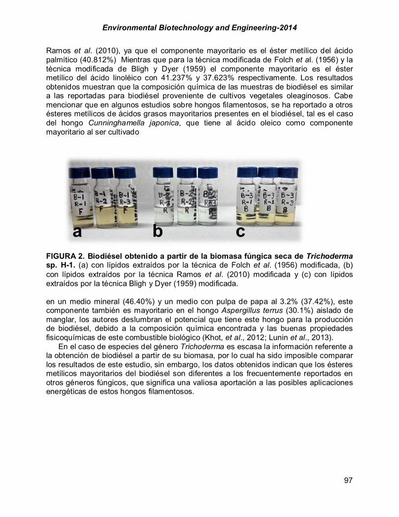
Environmental Biotechnology and Engineering-2014
97
Ramos et al. (2010), ya que el componente mayoritario es el éster metílico del ácido palmítico (40.812%) Mientras que para la técnica modificada de Folch et al. (1956) y la técnica modificada de Bligh y Dyer (1959) el componente mayoritario es el éster metílico del ácido linoléico con 41.237% y 37.623% respectivamente. Los resultados obtenidos muestran que la composición química de las muestras de biodiésel es similar a las reportadas para biodiésel proveniente de cultivos vegetales oleaginosos. Cabe mencionar que en algunos estudios sobre hongos filamentosos, se ha reportado a otros ésteres metílicos de ácidos grasos mayoritarios presentes en el biodiésel, tal es el caso del hongo Cunninghamella japonica, que tiene al ácido oleico como componente mayoritario al ser cultivado
FIGURA 2. Biodiésel obtenido a partir de la biomasa fúngica seca de Trichoderma sp. H-1. (a) con lípidos extraídos por la técnica de Folch et al. (1956) modificada, (b) con lípidos extraídos por la técnica Ramos et al. (2010) modificada y (c) con lípidos extraídos por la técnica Bligh y Dyer (1959) modificada. en un medio mineral (46.40%) y un medio con pulpa de papa al 3.2% (37.42%), este componente también es mayoritario en el hongo Aspergillus terrus (30.1%) aislado de manglar, los autores deslumbran el potencial que tiene este hongo para la producción de biodiésel, debido a la composición química encontrada y las buenas propiedades fisicoquímicas de este combustible biológico (Khot, et al., 2012; Lunin et al., 2013). En el caso de especies del género Trichoderma es escasa la información referente a la obtención de biodiésel a partir de su biomasa, por lo cual ha sido imposible comparar los resultados de este estudio, sin embargo, los datos obtenidos indican que los ésteres metílicos mayoritarios del biodiésel son diferentes a los frecuentemente reportados en otros géneros fúngicos, que significa una valiosa aportación a las posibles aplicaciones energéticas de estos hongos filamentosos.

Environmental Biotechnology and Engineering-2014
98
TABLA 2. Perfil de ésteres metílicos del biodiésel obtenido a partir de los lípidos de Trichoderma sp., determinado por cromatografía de gases.
Folch et al. (1956)
modificada
Ramos et al. (2010)
modificada
Bligh y Dyer (1959) modificada
ÁCIDO GRASO TIEMPO DE RETENCIÓN (MIN) % ÁREA % ÁREA % ÁREA
ÁCIDOS GRASOS SATURADOS
Ácido pelargónico (C9:0) 5.987 --- 0.647 ---
Ácido caprico (C10:0) 6.937 --- 0.134 ---
Ácido mirístico (C14:0) 11.280 0.179 0.449 0.224
Ácido pentadecílico (C15:0) 12.545 0.329 0.501 0.366
Ácido palmítico (C16:0) 14.061 24.231 40.812 25.907
Ácido margárico (C17:0) 15.886 0.361 0.540 0.422
Ácido esteárico (C18:0) 18.261 4.227 9.294 5.589
Ácido araquídico (C20:0) 25.505 0.262 0.655 0.300
ÁCIDOS GRASOS MONOINSATURADOS
Ácido palmitoleico (C16:1) 13.758 1.416 1.051 1.278
Ácido oleico (C18:1) 17.717 24.016 26.712 24.995
ÁCIDOS GRASOS POLIINSATURADOS
Ácido hexadecadienoico (C16:2) 13.826 0.224 0.104 0.240
Ácido linoléico (C18:2) 17.609 41.237 16.275 37.623
Ácido linolénico (C18:3) 17.757 3.518 1.902 3.056
Total de lípidos 100.000 99.075 100.000
Conclusión Se concluye que: - los aceites fúngicos de Trichoderma sp. H-1 obtenidos a través de un cultivo estacionario son una materia prima alternativa para obtener biodiésel, con una ventaja energética, - no se encontraron diferencias estadísticas entre los lípidos totales obtenidos por las tres técnicas de extracción y - la composición química de los ésteres metílicos mayoritarios, presentó variaciones en la técnica modificada de Ramos et al. (2010) puesto que el componente mayoritario es el éster metílico del ácido palmítico. Agradecimientos Los autores le agradecen al CONACyT el financiamiento de esta investigación (55784) y al †Dr. Jesús Samuel Cruz Sánchez por su inmenso apoyo.
Environmental Biotechnology and Engineering-2014
99
Referencias Aki, T.; Nagahata, Y.; Ishihara, K.; Tanaka, Y.; Morinaga, T.; Higashiyama, K.; Akimoto, K.; Fugikawa, S.;
Kawamoto, S.; Shigeta, S.; Ono, K.; Suzuki, O. (2001). Production of arachidonic acid by filamentous fungus Mortierella alliacia strain YN-15. Journal of the American Oil Chemists' Society. 78: 599-604.
André, A.; Diamantopoulou, P.; Philippoussis, A.; Sarris, D.; Komaitis, M.; Papanikolaou, S. (2010). Biotechnological conversions of bio-diesel derived waste glycerol into added-value compounds by higher fungi: production of biomass, single cell oil and oxalic acid. Industrial Crops and Products. 31: 407-416.
Angenent, L.T.; Karim, K.; Al-Dahhan, M.H.; Wrenn, B.A.; Domíguez-Espinosa, R. (2004). Production of bioenergy and biochemicals from industrial and agricultural wastewater. Trends in Biotechnology. 22: 477-485.
Armaroli, N.; Balzan, B. (2006). The future of energy supply: Challenges and opportunities. Renewable Energies. Angewandte Chemie International Edition. 45: 2-17.
Bligh, E.G.; Dye, W.J. (1959). A rapid method of total lipid extraction and purification. Canadian Journal of Biochemistry and Physiology. 37: 911-917.
Brennan, L.; Owende, P. (2010). Biofuels from microalgae—a review of technologies for production, processing, and extractions of biofuels and co-products. Renewable and Sustainable Energy Reviews. 14: 557-577.
Carraretto, C.; Macor, A.; Mirandola, A.; Stoppato, A.; Tonon, S. (2004). Biodiesel as alternative fuel: Experimental analysis and energetic evaluations. Energy. 29: 2195-2211.
Chisti, Y. (2007). Biodiesel from microalgae. Biotechnology Advances. 25: 294-306. Cooney, M.; Young, G.; Nagle, N. (2009). Extraction of bio-oils from microalgae. Separation and
Purification Reviews. 38: 291-325. Demain, A.L. (2009). Biosolutions to the energy problem. Journal of Industrial Microbiology and
Biotechnology. 36: 319-332. Demirbas, A. (2008). Biofuels sources, biofuel policy, biofuel economy and global biofuel projections.
Energy Conversion and Management. 49: 2106-2116. Demirbas, A.; Demirbas, M.F. (2011). Importance of algae oil as a source of biodiesel. Energy Conversion
and Management. 52: 163-170. Dey, P.; Banerjee, J.; Maiti, M.K. (2011). Comparative lipid profiling of two endophytic fungal isolates –
Colletotrichum sp. and Alternaria sp. having potential utilities as biodiesel feedstock. Bioresource Technoloogy. 102: 5815-5823.
Dmytryshyn, S.L.; Dalai, A.K.; Chaudhari, S.T.; Mishra, H.K.; Reaney, M.J. (2004). Synthesis and characterization of vegetable oil derived esters: evaluation for their diesel additive properties. Bioresource Technology. 92: 55-64.
Dresselhaus, M.S.; Thomas, I.L. (2001). Alternative energy technologies. Nature. 414: 332-337. Durrett, T.P.; Benning, C.; Ohlrogge, J. (2008). Plant triacylglycerols as feedstocks for the production of
biofuels. The Plant Journal. 54: 593-607. Eroshin, V.K.; Satroutdinov, A.D.; Dedyukhina, E.G.; Chistyakova, T.I. (2000). Arachidonic acid production
by Mortierella alpine with growth-coupled lipid synthesis. Proceedings of the Chemical Society. 35: 1171-1175.
Folch, J.; Lees, M.; Sloane-Stanley, G.H. (1957). A simple method for the isolation and purification of total lipids from animal tissues. Journal of Biological Chemistry. 226: 497-509.
Frondel, M.; Peters, J. (2007). Biodiesel: a new oildorado?. Energy Policy. 35: 1675-1684. Fukuda, H.; Kondo, A.; Noda, H. (2001). Biodiesel fuel production by transesterification of oils. Journal of
Bioscience and Bioengineering. 92: 405-416. Ganesan, D.; Rajendran, A.; Thangavelu, V. (2009). An overview on the recent advances in the
transesterification of vegetable oils for biodiesel production using chemical and biocatalysts. Reviews in Environmental Science and Biotechnology. 8: 367-394.
Hama, S.; Kondo, A. (2013). Enzymatic biodiesel production: An overview of potential feedstocks and process development. Bioresource Technology. 135: 386-395.
Hoekman, S.K. (2009). Biofuels in the U.S. – Challenges and Opportunities. Renewable Energy. 34: 14-22.
Khot, M.; Kamat, S.; Zinjarde, S.; Pant, A.; Chopade, B.; RaviKumar, A. (2012). Single cell oil of oleaginous fungi from the tropical mangrove wetlands as a potential feedstock for biodiesel.

Environmental Biotechnology and Engineering-2014
100
Microbial Cell Factories.11, 1-13. Lewis, N.S.; Nocera, D.G. (2006). Powering the planet: Chemical challenges in solar energy utilization.
Proceedings of the National Academy of Sciences. 103: 15729-15735. Lunin, V.V.; Sergeeva, Ya.E.; Galanina, L.A.; Mysyakina, I.S.; Ivashechkin, A.A.; Bogdan, V.I.; Feofilova,
E.P. (2013). Biodiesel fuel production from lipids of filamentous fungi. Applied Biochemistry and Microbiology. 49: 46-52.
Miao, X.L.; Wu, Q.Y. (2004). Bio-oil fuel production from microalgae after heterotrophic growth. Renewable Energy Resources. 4: 41-44.
Morrison, W.R.; Smith, L.M. (1946). Preparation of fatty acid methyl esters and dimethylacetals from lipids with boron fluoride-methanol. Journal of Lipid Research. 5: 605-608.
Ramos, C. (2010). Maximization of Scenedesmus dimorphus lipid yield for the production of biodiesel. Tesis de Doctorado. Universidad Politécnica de Puerto Rico.
Ravikumar, K.; Dakshayini, J.; Girisha, S.T. (2012). Biodiesel production from oleaginous fungi. International Journal of Life Sciences. 6: 43-49.
Samadlouie, H.; Hamidi-Esfahani, Z.; Alavi, S.; Soltani-Najafabadi, M.; Sahari, M.A.; Abbasi, S. (2012). Statistical approach to optimization of fermentative production of oil and arachidonic acid from Mortierella alpine CBS 754.68. African Journal of Microbiology Research. 6: 1559-1567.
SAS Institute Inc. 2010. The SAS system for windows, ver. 9.0. SAS Institute Inc, Cary, North Carolina. Sergeeva, Ya.E.; Galanina, L.A.; Andrianova, D.A.; Feofilova, E.P. (2008). Lipids of filamentous fungi as a
material for producing biodiesel fuel. Applied Biochemistry and Microbiology. 44: 523-527. Srivastava, A.; Prasad, R. (2000). Triglycerides-based diesel fuels. Renewable and Sustainable Energy
Reviews. 4: 111-133. Subhash, G.V.; Mohan, S.V. (2011). Biodiesel production from isolated oleaginous fungi Aspergillus sp.
Using corncob waste liquor as a substrate. Bioresource Technology. 102: 9286-9290. Tsunehiro, A.; Yumiko, N.; Katsuyuki, I.; Yoshio, T.; Tsutomu, M.; Kenichi, H.; Kengo, A.; Shigeaki, F.;
Seiji, K.; Seiko, S.; Kazuhisa, O.; Osamu, S. (2001). Production of arachidonic acid by filamentous fungus, Mortierella alliacea strain YN-15. Journal of the American Oil Chemists' Society. 78: 599-604.

Environmental Biotechnology and Engineering-2014
101
CHAPTER 1.12. GROWTH OF Chlorella vulgaris AND Nannochloris oculata IN EFFLUENTS OF TILAPIA FARMING FOR THE PRODUCTION OF FATTY ACIDS
WITH POTENTIAL IN BIOFUEL PRODUCTION
Yesica I. Ferrer-Álvarez (1), Luis A. Ortega-Clemente* (1), Ignacio A. Pérez-Legaspi (1), Martha P. Hernández-Guevara (1), Elvira Ríos-Leal (2),
Paula N. Robledo-Narváez (3), Héctor M. Poggi-Varaldo (2)
(1) ITBOCA, DEPI. Boca del Río, Veracruz, México. (2) CINVESTAV del IPN, México D.F., México. (3) ITSTB, Depto. Inv., Tierra Blanca, Veracruz, México ABSTRACT The use of microalgae in wastewater treatment and its biotechnological exploitation for the production of biofuels is a potential environmental application. Microalgal growth takes place in the presence of CO2, light and other nutrients such as nitrogen and phosphorus available in effluents, which allows its further use. Some species of microalgae are notable due to their lipid composition and fatty acid profile suitable for biofuel production. During the present study a factorial 23 experimental design was conducted, which assessed three factors: i) two species of microalgae (Chlorella vulgaris and Nannochloris oculata), ii) two types of culture media (wastewater of tilapia farming "ET" and Bold’s Basal Medium "MB") and iii) two types of lighting (multi-LED lamps and white light) at an intensity of continuous light of 79.88 µmol m-2 s-1. Microalgae were inoculated in 16 photobioreactors (8 L capacity) in 6 L of medium (ET or MB) at an initial concentration of 1.0 X 10⁶ cells mL-1 at 20 ± 2 °C for 10 days. The above was done to determine cell density, biomass production, lipid and fatty acid productivity. The highest average cell density as well as the greater productivity of biomass observed in the treatments was C. vulgaris treatment in MB and multi-LED lighting (8.83 x 10⁷ cells mL-1 and 0.0854 gL-1 d-1, respectively). Although the majority of lipid production was obtained in the exponential phase of N. oculata cultivated in multi-LED in both treatments (MB with 58% and ET with 52%), generally the cultivation of both species was maintained in ET and were those that presented the major lipid productivity (2-18 mgL-1 d-1) in comparison with those cultivated in MB. Fatty acids palmitic, stearic, oleic, linoleic, linolenic and eicosanoic (C16-C20) were presented in both species of microalgae in concentrations between 26 and 74%. We conclude that cultivation of N. oculata and/or C. vulgaris in ET illuminated with multi-LED is an economic and sustainable alternative for the production of biodiesel because it can represent up to 58% of lipids with a fatty acid profile optimal up to 74% of the total fatty acids. Key words: wastewater of tilapia farming, biofuels, fatty acids, Chlorella vulgaris, Nannochloris oculata ------------ *Author for all correspondence: [email protected]
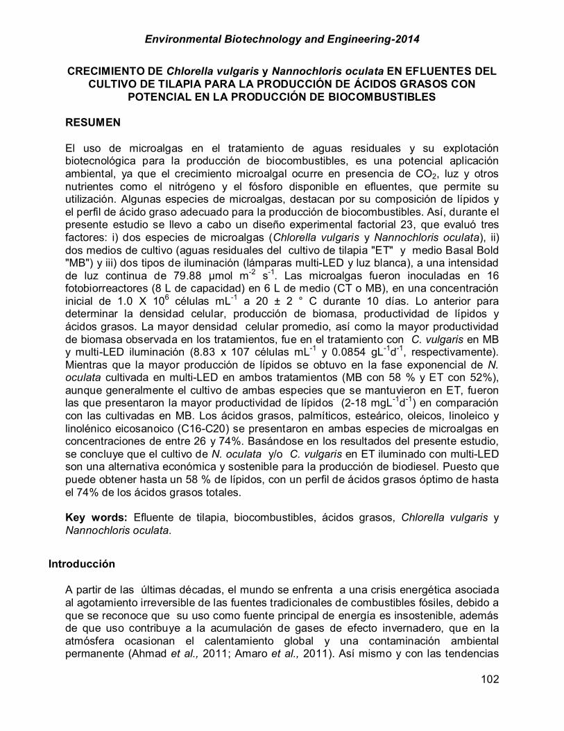
Environmental Biotechnology and Engineering-2014
102
CRECIMIENTO DE Chlorella vulgaris y Nannochloris oculata EN EFLUENTES DEL CULTIVO DE TILAPIA PARA LA PRODUCCIÓN DE ÁCIDOS GRASOS CON
POTENCIAL EN LA PRODUCCIÓN DE BIOCOMBUSTIBLES
RESUMEN El uso de microalgas en el tratamiento de aguas residuales y su explotación biotecnológica para la producción de biocombustibles, es una potencial aplicación ambiental, ya que el crecimiento microalgal ocurre en presencia de CO2, luz y otros nutrientes como el nitrógeno y el fósforo disponible en efluentes, que permite su utilización. Algunas especies de microalgas, destacan por su composición de lípidos y el perfil de ácido graso adecuado para la producción de biocombustibles. Así, durante el presente estudio se llevo a cabo un diseño experimental factorial 23, que evaluó tres factores: i) dos especies de microalgas (Chlorella vulgaris y Nannochloris oculata), ii) dos medios de cultivo (aguas residuales del cultivo de tilapia "ET" y medio Basal Bold "MB") y iii) dos tipos de iluminación (lámparas multi-LED y luz blanca), a una intensidad de luz continua de 79.88 µmol m-2 s-1. Las microalgas fueron inoculadas en 16 fotobiorreactores (8 L de capacidad) en 6 L de medio (CT o MB), en una concentración inicial de 1.0 X 10⁶ células mL-1 a 20 ± 2 ° C durante 10 días. Lo anterior para determinar la densidad celular, producción de biomasa, productividad de lípidos y ácidos grasos. La mayor densidad celular promedio, así como la mayor productividad de biomasa observada en los tratamientos, fue en el tratamiento con C. vulgaris en MB y multi-LED iluminación (8.83 x 10⁷ células mL-1 y 0.0854 gL-1d-1, respectivamente). Mientras que la mayor producción de lípidos se obtuvo en la fase exponencial de N. oculata cultivada en multi-LED en ambos tratamientos (MB con 58 % y ET con 52%), aunque generalmente el cultivo de ambas especies que se mantuvieron en ET, fueron las que presentaron la mayor productividad de lípidos (2-18 mgL-1d-1) en comparación con las cultivadas en MB. Los ácidos grasos, palmíticos, esteárico, oleicos, linoleico y linolénico eicosanoico (C16-C20) se presentaron en ambas especies de microalgas en concentraciones de entre 26 y 74%. Basándose en los resultados del presente estudio, se concluye que el cultivo de N. oculata y/o C. vulgaris en ET iluminado con multi-LED son una alternativa económica y sostenible para la producción de biodiesel. Puesto que puede obtener hasta un 58 % de lípidos, con un perfil de ácidos grasos óptimo de hasta el 74% de los ácidos grasos totales. Key words: Efluente de tilapia, biocombustibles, ácidos grasos, Chlorella vulgaris y Nannochloris oculata.
Introducción
A partir de las últimas décadas, el mundo se enfrenta a una crisis energética asociada al agotamiento irreversible de las fuentes tradicionales de combustibles fósiles, debido a que se reconoce que su uso como fuente principal de energía es insostenible, además de que uso contribuye a la acumulación de gases de efecto invernadero, que en la atmósfera ocasionan el calentamiento global y una contaminación ambiental permanente (Ahmad et al., 2011; Amaro et al., 2011). Así mismo y con las tendencias
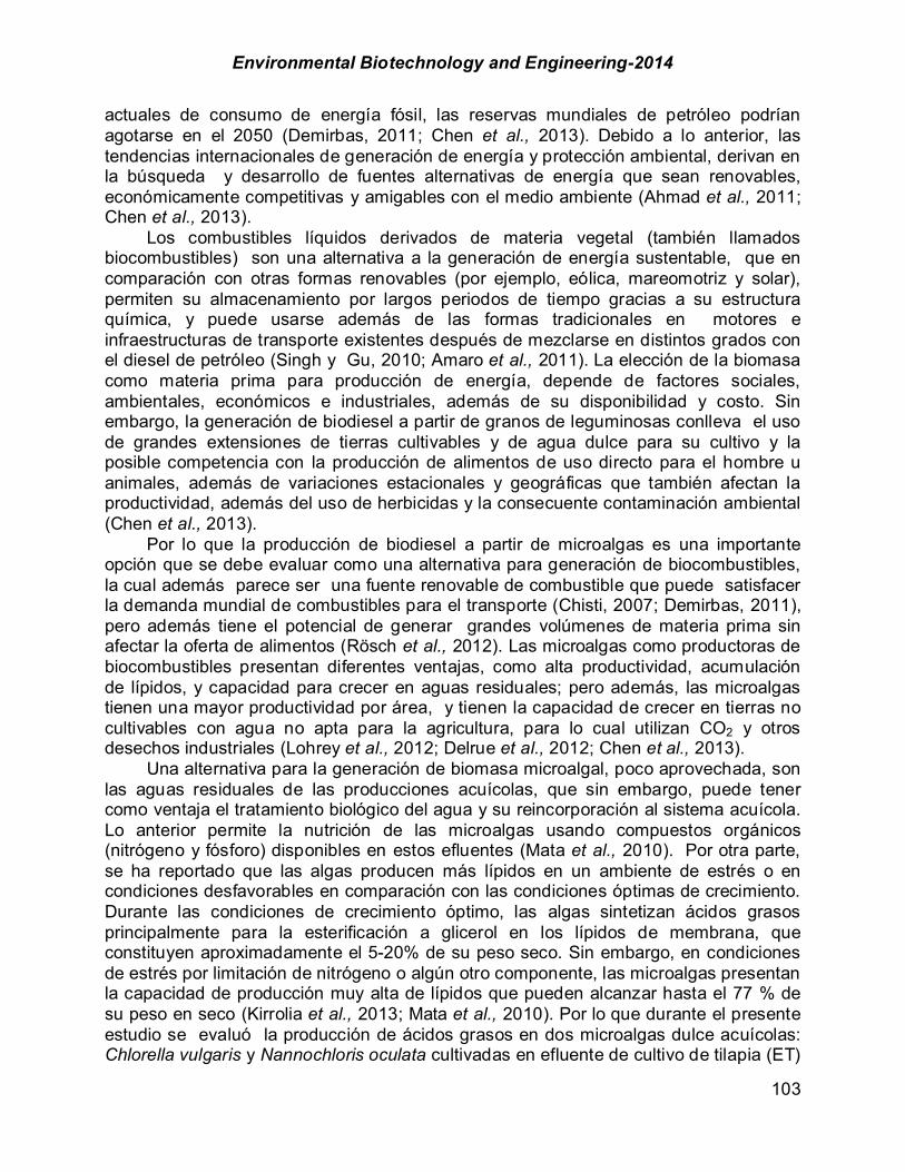
Environmental Biotechnology and Engineering-2014
103
actuales de consumo de energía fósil, las reservas mundiales de petróleo podrían agotarse en el 2050 (Demirbas, 2011; Chen et al., 2013). Debido a lo anterior, las tendencias internacionales de generación de energía y protección ambiental, derivan en la búsqueda y desarrollo de fuentes alternativas de energía que sean renovables, económicamente competitivas y amigables con el medio ambiente (Ahmad et al., 2011; Chen et al., 2013). Los combustibles líquidos derivados de materia vegetal (también llamados biocombustibles) son una alternativa a la generación de energía sustentable, que en comparación con otras formas renovables (por ejemplo, eólica, mareomotriz y solar), permiten su almacenamiento por largos periodos de tiempo gracias a su estructura química, y puede usarse además de las formas tradicionales en motores e infraestructuras de transporte existentes después de mezclarse en distintos grados con el diesel de petróleo (Singh y Gu, 2010; Amaro et al., 2011). La elección de la biomasa como materia prima para producción de energía, depende de factores sociales, ambientales, económicos e industriales, además de su disponibilidad y costo. Sin embargo, la generación de biodiesel a partir de granos de leguminosas conlleva el uso de grandes extensiones de tierras cultivables y de agua dulce para su cultivo y la posible competencia con la producción de alimentos de uso directo para el hombre u animales, además de variaciones estacionales y geográficas que también afectan la productividad, además del uso de herbicidas y la consecuente contaminación ambiental (Chen et al., 2013). Por lo que la producción de biodiesel a partir de microalgas es una importante opción que se debe evaluar como una alternativa para generación de biocombustibles, la cual además parece ser una fuente renovable de combustible que puede satisfacer la demanda mundial de combustibles para el transporte (Chisti, 2007; Demirbas, 2011), pero además tiene el potencial de generar grandes volúmenes de materia prima sin afectar la oferta de alimentos (Rösch et al., 2012). Las microalgas como productoras de biocombustibles presentan diferentes ventajas, como alta productividad, acumulación de lípidos, y capacidad para crecer en aguas residuales; pero además, las microalgas tienen una mayor productividad por área, y tienen la capacidad de crecer en tierras no cultivables con agua no apta para la agricultura, para lo cual utilizan CO2 y otros desechos industriales (Lohrey et al., 2012; Delrue et al., 2012; Chen et al., 2013). Una alternativa para la generación de biomasa microalgal, poco aprovechada, son las aguas residuales de las producciones acuícolas, que sin embargo, puede tener como ventaja el tratamiento biológico del agua y su reincorporación al sistema acuícola. Lo anterior permite la nutrición de las microalgas usando compuestos orgánicos (nitrógeno y fósforo) disponibles en estos efluentes (Mata et al., 2010). Por otra parte, se ha reportado que las algas producen más lípidos en un ambiente de estrés o en condiciones desfavorables en comparación con las condiciones óptimas de crecimiento. Durante las condiciones de crecimiento óptimo, las algas sintetizan ácidos grasos principalmente para la esterificación a glicerol en los lípidos de membrana, que constituyen aproximadamente el 5-20% de su peso seco. Sin embargo, en condiciones de estrés por limitación de nitrógeno o algún otro componente, las microalgas presentan la capacidad de producción muy alta de lípidos que pueden alcanzar hasta el 77 % de su peso en seco (Kirrolia et al., 2013; Mata et al., 2010). Por lo que durante el presente estudio se evaluó la producción de ácidos grasos en dos microalgas dulce acuícolas: Chlorella vulgaris y Nannochloris oculata cultivadas en efluente de cultivo de tilapia (ET)

Environmental Biotechnology and Engineering-2014
104
y medio Basal Bold (MB) en dos sistemas de iluminación, con el propósito de determinar su potencial para la generación de biocombustibles.
Materiales y métodos Preparación del cultivo de las microalgas. El estudio se realizó en el Laboratorio de Alimento Vivo (LAV) del Instituto Tecnológico de Boca del Río. Para el estudio se usaron dos cepas de microalgas de agua dulce: Chlorella vulgaris y Nannochloris oculata, las cuales se obtuvieron de la colección del Departamento de Acuacultura del Centro de Investigación Científica y de Educación Superior de Ensenada (CICESE) clave CLV2, y de la colección de la Universidad de Texas (UTEX) código: LB2194, respectivamente. La resiembra de las cepas se realizó en medio Basal Bold (MB) estéril en cinco matraces de 125 ml con 100 ml del medio, a partir de un inoculo en suspensión de 20 ml, los cuales se mantuvieron en condiciones controladas de laboratorio a un fotoperiodo de 24 horas de luz sin aireación, y una temperatura de 18ºC en una cámara de luz a 18.5 µmol m-2 s-1. El cultivo a mayor escala de C. vulgaris y N. oculata se realizó en cuatro matraces Erlenmeyer de 1000 ml, con 750 ml de MBB estéril y 100 ml de inoculo en suspensión (1x10⁶ cel/ml) de resiembra, se mantuvieron en fotoperiodos de 24 horas de luz con aireación constante a temperatura de 18 ºC en una cámara de luz a 79.88 µmol m-2 s-1. Sistemas de cultivo. Para el cultivo de las microalgas C. vulgaris y N. oculata, se usó 16 fotobiorreactores, los cuales consistieron en unidades hexagonales de acrílico de 15 cm de diámetro por 45 cm de alto, con una capacidad de 8 L, y cerrados completamente por una tapa superior horadada, en la que se colocaron dos tubos de cristal de 5 mm de diámetro, uno para proveer oxígeno y homogenizar el cultivo mediante una bomba (ELITE MÁXIMA, 30 Gl). El segundo tubo de cristal se uso para tomar muestras para dar seguimiento al cultivo. Durante el estudio, los fotobioreactores se colocaron en dos estructuras para tener dos módulos, los cuales se iluminaron individualmente mediante los siguientes esquemas: módulo 1) la iluminación de los fotobioreactores se genero a partir de cuatro reflectores multi-LED (RF-240HFS 30W) energizados por dos baterías (Surrette S-600 ciclo profundo 6V, 450 Ah) conectada a cinco paneles solares (Módulos Policristalinos de145 W, colocados la parte superior del techo del Laboratorio LAV), modulo 2) consistió de cuatro de lámparas de luz blanca ( 40 watts) energizadas con corriente directa (220 Volts); ambos sistemas (Figura 1) mantuvieron una intensidad de 79.88 µmol m-2 s-1 y que se tuviera una densidad inicial de 1x10⁶ cel/ml. El volumen del inóculo a usar, se determinó mediante conteo celular en una cámara de Neubauer (Pica-Granados et al., 2004). Diseño experimental. El diseño experimental consistió de un factorial 23, para un total 8 tratamientos con una réplica cada tratamiento (16 unidades experimentales), en donde se evaluaron tres factores: A) Tipo de microalga, B) Tipo de medio de cultivo y C) Tipo de iluminación a dos niveles cada uno. El modelo a seguir para el análisis estadístico así como la combinación de los tratamientos fue el siguiente: cuatro unidades experimentales (fotobioreactores) con dos tipos de iluminación multi-LED, dos

Environmental Biotechnology and Engineering-2014
105
con MB y dos con ET. Por cada medio de cultivo, se inoculo por separado con C. vulgaris y N. oculata. En los cuatro tratamientos restantes sólo cambio el tipo de iluminación por luz blanca. Se evaluó la densidad celular (cel/ml), porcentaje de lípidos (%), producción de biomasa (gL-1d-1), producción de lípidos (mgL-1d-1) y cuantificación de ácidos grasos (%).Todos resultados fueron expresados como media ± desviación estándar. El análisis estadístico de los resultados fue mediante un análisis de varianza ANOVA para un nivel de significancia elegido de P = 0.05, utilizando Stat Soft, Inc. (2004) STATISTICA V.7.
FIGURA 1. Tipos de iluminación en los sistemas de cultivo. a) Reflector multi-LED; b) Reflector de luz blanca.
Preparación de las unidades experimentales. A las unidades experimentales se les agregaron 6 L del medio de cultivo para las microalgas correspondiente a cada tratamiento, ocho fotobioreactores con MB estéril (control), que se preparó previamente siguiendo las especificaciones indicadas por Nichols, (1973), y a los otros ocho con ET estéril colectado de un estanque de cultivo de tilapia a cielo abierto, localizado en el Instituto Tecnológico de Boca del Río, previamente filtrada mediante una columna empacada con una malla para fitoplancton de 100 µm, algodón y fibra de poliéster para remover la materia orgánica. Después el agua se incorporó a los fotobioreactores respectivos y se procedió a su desinfección mediante 0.8 ml/L de hipoclorito de sodio, posteriormente se mantuvieron durante tres horas con aireación continua como método para eliminar algún organismo presente en el ET. El cloro residual fue neutralizado con 0.75 g/L de tiosulfato de sodio pentahidratado (Na2S2O3 * 5 H2O), durante dos horas en aireación continua. Posteriormente se determinó la concentración inicial de NH4-N, NO2-
a) b)
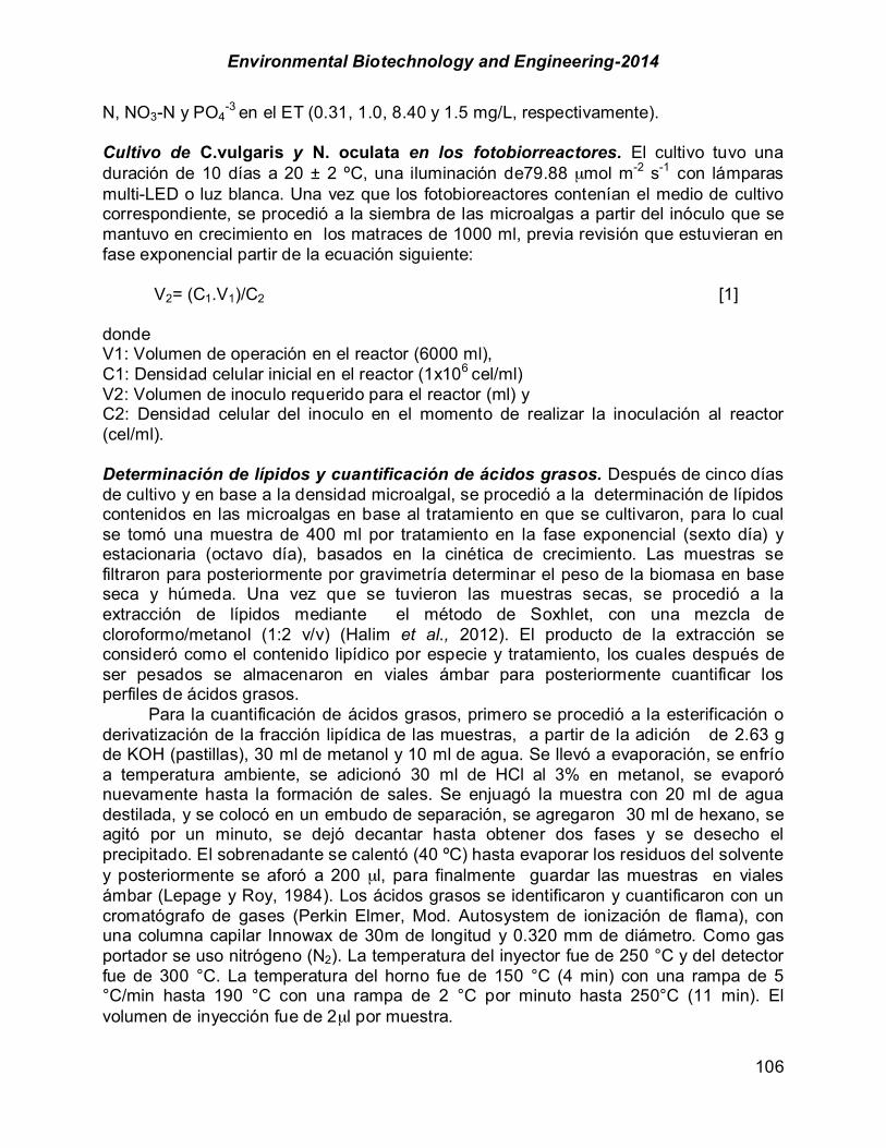
Environmental Biotechnology and Engineering-2014
106
N, NO3-N y PO4-3 en el ET (0.31, 1.0, 8.40 y 1.5 mg/L, respectivamente).
Cultivo de C.vulgaris y N. oculata en los fotobiorreactores. El cultivo tuvo una duración de 10 días a 20 ± 2 ºC, una iluminación de79.88 µmol m-2 s-1 con lámparas multi-LED o luz blanca. Una vez que los fotobioreactores contenían el medio de cultivo correspondiente, se procedió a la siembra de las microalgas a partir del inóculo que se mantuvo en crecimiento en los matraces de 1000 ml, previa revisión que estuvieran en fase exponencial partir de la ecuación siguiente:
V2= (C1.V1)/C2 [1]
donde V1: Volumen de operación en el reactor (6000 ml), C1: Densidad celular inicial en el reactor (1x10⁶ cel/ml) V2: Volumen de inoculo requerido para el reactor (ml) y C2: Densidad celular del inoculo en el momento de realizar la inoculación al reactor (cel/ml). Determinación de lípidos y cuantificación de ácidos grasos. Después de cinco días de cultivo y en base a la densidad microalgal, se procedió a la determinación de lípidos contenidos en las microalgas en base al tratamiento en que se cultivaron, para lo cual se tomó una muestra de 400 ml por tratamiento en la fase exponencial (sexto día) y estacionaria (octavo día), basados en la cinética de crecimiento. Las muestras se filtraron para posteriormente por gravimetría determinar el peso de la biomasa en base seca y húmeda. Una vez que se tuvieron las muestras secas, se procedió a la extracción de lípidos mediante el método de Soxhlet, con una mezcla de cloroformo/metanol (1:2 v/v) (Halim et al., 2012). El producto de la extracción se consideró como el contenido lipídico por especie y tratamiento, los cuales después de ser pesados se almacenaron en viales ámbar para posteriormente cuantificar los perfiles de ácidos grasos. Para la cuantificación de ácidos grasos, primero se procedió a la esterificación o derivatización de la fracción lipídica de las muestras, a partir de la adición de 2.63 g de KOH (pastillas), 30 ml de metanol y 10 ml de agua. Se llevó a evaporación, se enfrío a temperatura ambiente, se adicionó 30 ml de HCl al 3% en metanol, se evaporó nuevamente hasta la formación de sales. Se enjuagó la muestra con 20 ml de agua destilada, y se colocó en un embudo de separación, se agregaron 30 ml de hexano, se agitó por un minuto, se dejó decantar hasta obtener dos fases y se desecho el precipitado. El sobrenadante se calentó (40 ºC) hasta evaporar los residuos del solvente y posteriormente se aforó a 200 µl, para finalmente guardar las muestras en viales ámbar (Lepage y Roy, 1984). Los ácidos grasos se identificaron y cuantificaron con un cromatógrafo de gases (Perkin Elmer, Mod. Autosystem de ionización de flama), con una columna capilar Innowax de 30m de longitud y 0.320 mm de diámetro. Como gas portador se uso nitrógeno (N2). La temperatura del inyector fue de 250 °C y del detector fue de 300 °C. La temperatura del horno fue de 150 °C (4 min) con una rampa de 5 °C/min hasta 190 °C con una rampa de 2 °C por minuto hasta 250°C (11 min). El volumen de inyección fue de 2µl por muestra.
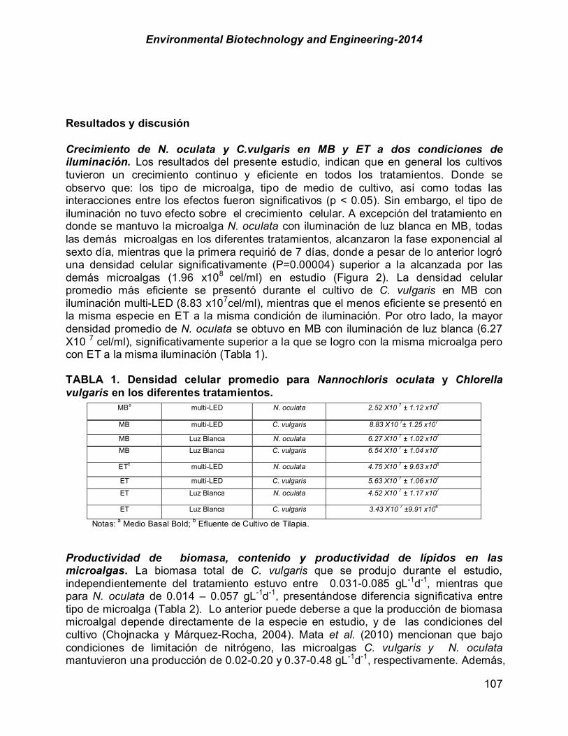
Environmental Biotechnology and Engineering-2014
107
Resultados y discusión
Crecimiento de N. oculata y C.vulgaris en MB y ET a dos condiciones de iluminación. Los resultados del presente estudio, indican que en general los cultivos tuvieron un crecimiento continuo y eficiente en todos los tratamientos. Donde se observo que: los tipo de microalga, tipo de medio de cultivo, así como todas las interacciones entre los efectos fueron significativos (p < 0.05). Sin embargo, el tipo de iluminación no tuvo efecto sobre el crecimiento celular. A excepción del tratamiento en donde se mantuvo la microalga N. oculata con iluminación de luz blanca en MB, todas las demás microalgas en los diferentes tratamientos, alcanzaron la fase exponencial al sexto día, mientras que la primera requirió de 7 días, donde a pesar de lo anterior logró una densidad celular significativamente (P=0.00004) superior a la alcanzada por las demás microalgas (1.96 x10⁸ cel/ml) en estudio (Figura 2). La densidad celular promedio más eficiente se presentó durante el cultivo de C. vulgaris en MB con iluminación multi-LED (8.83 x10⁷cel/ml), mientras que el menos eficiente se presentó en la misma especie en ET a la misma condición de iluminación. Por otro lado, la mayor densidad promedio de N. oculata se obtuvo en MB con iluminación de luz blanca (6.27 X10 7 cel/ml), significativamente superior a la que se logro con la misma microalga pero con ET a la misma iluminación (Tabla 1). TABLA 1. Densidad celular promedio para Nannochloris oculata y Chlorella vulgaris en los diferentes tratamientos.
Notas: a Medio Basal Bold; b Efluente de Cultivo de Tilapia.
Productividad de biomasa, contenido y productividad de lípidos en las microalgas. La biomasa total de C. vulgaris que se produjo durante el estudio, independientemente del tratamiento estuvo entre 0.031-0.085 gL-1d-1, mientras que para N. oculata de 0.014 – 0.057 gL-1d-1, presentándose diferencia significativa entre tipo de microalga (Tabla 2). Lo anterior puede deberse a que la producción de biomasa microalgal depende directamente de la especie en estudio, y de las condiciones del cultivo (Chojnacka y Márquez-Rocha, 2004). Mata et al. (2010) mencionan que bajo condiciones de limitación de nitrógeno, las microalgas C. vulgaris y N. oculata mantuvieron una producción de 0.02-0.20 y 0.37-0.48 gL-1d-1, respectivamente. Además,
MBa multi-LED N. oculata 2.52 X10 7 ± 1.12 x10⁷
MB multi-LED C. vulgaris 8.83 X10 7± 1.25 x10⁷
MB Luz Blanca N. oculata 6.27 X10 7 ± 1.02 x107 MB Luz Blanca C. vulgaris 6.54 X10 7 ± 1.04 x10⁷
ETb multi-LED N. oculata 4.75 X10 7 ± 9.63 x10⁶
ET multi-LED C. vulgaris 5.63 X10 7 ± 1.06 x10⁷ ET Luz Blanca N. oculata 4.52 X10 7 ± 1.17 x10⁷
ET Luz Blanca C. vulgaris 3.43 X10 7 ±9.91 x10⁶
Environmental Biotechnology and Engineering-2014
108
la situación de estrés en que se dio el cultivo, ocasionó que las microalgas generaran un mayor contenido de lípidos del 75 % en comparación de lo que se espera que produzcan (20-50 %), con una productividad de biomasa inferior de 0.02 gL-1d-1 en relación a lo esperado de 0.40 gL-1d-1.
De manera contraria al reporte anterior, los resultados de la presente investigación indican que N. oculata presentó una menor producción de biomasa en comparación con C. vulgaris, generando en todos los tratamientos mayores porcentajes de lípidos (10 - 58 %). Los resultados muestran que el mayor contenido de lípidos se alcanzó con N. oculata en condiciones de iluminación multi-LED en MB y ET con 58 y 52 %, respectivamente, en la fase exponencial de crecimiento. Por otra parte, la productividad de lípidos (mgL-1d-1) para ambas especies fue variable, tanto por tipo de medio como iluminación, alcanzando productividades de 2-18 mgL-1d-1. C. vulgaris fue quien presentó la mayor productividad para ambos medios (MB y ET). Sin embargo, para C. vulgaris en MB con iluminación multi-LED, la mayor productividad fue en la fase estacionaria (17.83 mgL-1d-1) a diferencia en ET con luz blanca como iluminación que fue en la fase exponencial (17.30 mgL-1d-1). Es decir, que la productividad de lípidos depende principalmente de la tipo de microalga, tipo de medio de cultivo, condición de iluminación y fase de crecimiento (Tabla 2).
En otro estudio, Chiu et al. (2008) reportan que en cultivos semicontinuos de Chlorella sp., con baja y alta densidad celular para la reducción de CO2, obtuvieron una productividad de biomasa de 0.037 a 0.053 gL-1d-1, valores promedio similares a los que se obtuvieron en la presente investigación para ambas cepas en todas las condiciones de cultivo. Por otro lado, Liang et al. (2009) reportan productividades de biomasa de 0.010 - 0.254 gL-1d-1 en cultivo de C. vulgaris en condiciones de crecimiento autotróficos, heterotróficos y mixotróficos, con un contenido de lípidos máximo de 38 % en condiciones autotróficas. El contenido de lípidos fue muy similares al alcanzado por C. vulgaris en ET con iluminación blanca de 37 % en una productividad promedio de biomasa de 0.04 gL-1d-1 (Tabla 2). Estos resultados al igual que los reportados por Liang et al. (2009), indican que bajo condiciones de estrés debido a una baja concentración de nitrógeno principalmente nitratos, provoca un incremento en el contenido de lípidos en la biomasa en un intervalo de 15 a 58 % (peso seco) dependiendo de la especie de microalga (Kirrolia et al., 2013; Mata et al., 2010). Considerando a los cultivos en ET como una condición de estrés por su limitación de nitrógeno comparado con el MB, los resultados muestran que para ambas microalgas, el porcentaje y la productividad de lípidos para cultivos en ET fueron mayores (25-42 %) que en MB (6-35 %) principalmente en aquellos tratamiento iluminados con luz blanca (Tabla 2), siendo este un comportamiento ya observado (Kirrolia et al., 2013; Mata et al., 2010). Por otra parte, Rodolfi et al. (2009) reporta que después de analizar 30 especies de microalgas y seleccionar cuatro (dos marinas y dos dulce acuícolas) por su alta productividad de biomasa y contenido de lípidos, observaron que la especie marina Nannochloropsis sp. F&M-M24 alcanzó un contenido de lípidos del 60 % en cultivos con limitación de nitrógeno; observando también que el contenido de ácidos grasos aumentó al incrementar la iluminación (hasta 32.5 % de biomasa seca) y tras una limitación de nitrógeno y fosforo (hasta un 50%). Por lo tanto, la productividad de biomasa y lípidos se puede ver incrementada hasta un 60 % en condiciones de cultivo con déficit de nitrógeno y alta concentración de CO2 (Kirrolia et al., 2013; Mata et al., 2010; Gouveia y Oliveira, 2009; Chiu et al., 2009; Rodolfi et al., 2009; Liang et al., 2009).
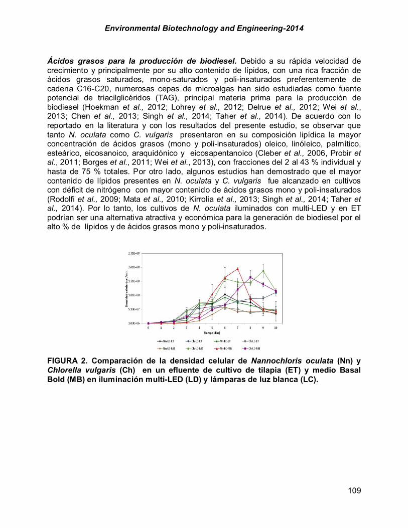
Environmental Biotechnology and Engineering-2014
109
Ácidos grasos para la producción de biodiesel. Debido a su rápida velocidad de crecimiento y principalmente por su alto contenido de lípidos, con una rica fracción de ácidos grasos saturados, mono-saturados y poli-insaturados preferentemente de cadena C16-C20, numerosas cepas de microalgas han sido estudiadas como fuente potencial de triacilglicéridos (TAG), principal materia prima para la producción de biodiesel (Hoekman et al., 2012; Lohrey et al., 2012; Delrue et al., 2012; Wei et al., 2013; Chen et al., 2013; Singh et al., 2014; Taher et al., 2014). De acuerdo con lo reportado en la literatura y con los resultados del presente estudio, se observar que tanto N. oculata como C. vulgaris presentaron en su composición lipídica la mayor concentración de ácidos grasos (mono y poli-insaturados) oleico, linóleico, palmítico, esteárico, eicosanoico, araquidónico y eicosapentanoico (Cleber et al., 2006, Probir et al., 2011; Borges et al., 2011; Wei et al., 2013), con fracciones del 2 al 43 % individual y hasta de 75 % totales. Por otro lado, algunos estudios han demostrado que el mayor contenido de lípidos presentes en N. oculata y C. vulgaris fue alcanzado en cultivos con déficit de nitrógeno con mayor contenido de ácidos grasos mono y poli-insaturados (Rodolfi et al., 2009; Mata et al., 2010; Kirrolia et al., 2013; Singh et al., 2014; Taher et al., 2014). Por lo tanto, los cultivos de N. oculata iluminados con multi-LED y en ET podrían ser una alternativa atractiva y económica para la generación de biodiesel por el alto % de lípidos y de ácidos grasos mono y poli-insaturados.
FIGURA 2. Comparación de la densidad celular de Nannochloris oculata (Nn) y Chlorella vulgaris (Ch) en un efluente de cultivo de tilapia (ET) y medio Basal Bold (MB) en iluminación multi-LED (LD) y lámparas de luz blanca (LC).
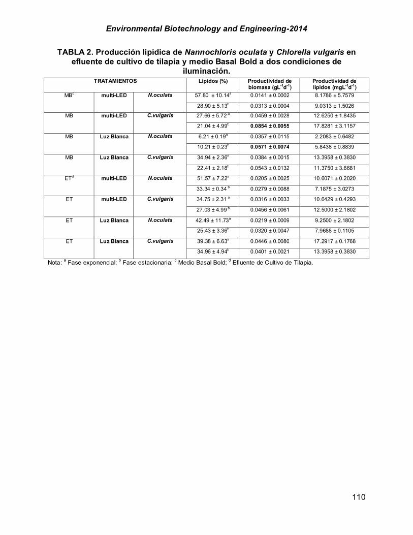
Environmental Biotechnology and Engineering-2014
110
TABLA 2. Producción lipídica de Nannochloris oculata y Chlorella vulgaris en efluente de cultivo de tilapia y medio Basal Bold a dos condiciones de
iluminación.
Nota: a Fase exponencial; b Fase estacionaria; c Medio Basal Bold; d Efluente de Cultivo de Tilapia.
TRATAMIENTOS Lípidos (%) Productividad de biomasa (gL-1d-1)
Productividad de lípidos (mgL-1d-1)
MBc multi-LED N.oculata 57.80 ± 10.14a 0.0141 ± 0.0002 8.1786 ± 5.7579
28.90 ± 5.13b 0.0313 ± 0.0004 9.0313 ± 1.5026
MB multi-LED C.vulgaris 27.66 ± 5.72 a 0.0459 ± 0.0028 12.6250 ± 1.8435
21.04 ± 4.99b 0.0854 ± 0.0055 17.8281 ± 3.1157
MB Luz Blanca N.oculata 6.21 ± 0.19a 0.0357 ± 0.0115 2.2083 ± 0.6482
10.21 ± 0.23b 0.0571 ± 0.0074 5.8438 ± 0.8839
MB Luz Blanca C.vulgaris 34.94 ± 2.36a 0.0384 ± 0.0015 13.3958 ± 0.3830
22.41 ± 2.18b 0.0543 ± 0.0132 11.3750 ± 3.6681
ETd multi-LED N.oculata 51.57 ± 7.22a 0.0205 ± 0.0025 10.6071 ± 0.2020
33.34 ± 0.34 b 0.0279 ± 0.0088 7.1875 ± 3.0273
ET multi-LED C.vulgaris 34.75 ± 2.31 a 0.0316 ± 0.0033 10.6429 ± 0.4293
27.03 ± 4.99 b 0.0456 ± 0.0061 12.5000 ± 2.1802
ET Luz Blanca N.oculata 42.49 ± 11.73a 0.0219 ± 0.0009 9.2500 ± 2.1802
25.43 ± 3.36b 0.0320 ± 0.0047 7.9688 ± 0.1105
ET Luz Blanca C.vulgaris 39.38 ± 6.63a 0.0446 ± 0.0080 17.2917 ± 0.1768
34.96 ± 4.94b 0.0401 ± 0.0021 13.3958 ± 0.3830

Environmental Biotechnology and Engineering-2014
111
TABLA 3. Composición porcentual (%) de ácidos grasos en la fracción de lípidos extraídos de Nannochloris oculata y Chlorella vulgaris cultivadas en
fotobioreactores en efluente de tilapia y medio Basal Bold en dos condiciones de Iluminación (Multi-LEDs y lámparas de luz blanca).
Nota: a Iluminación multi-LED, b Iluminación Luz Blanca. Conclusión La mayor densidad celular promedio observada en los tratamientos fue con C. vulgaris cultivada en MB con iluminación multi-LED (8.83 x10⁷cel/ml). Así mismo, la productividad más alta de biomasa la presentó C. vulgaris en MB en iluminación multi-LED (0.0854 gL-1d-1). N. oculata con iluminación multi-LED alcanzó los mayores porcentajes de lípidos en ambos medios (MB y ET) con 58 y 52 %, respectivamente. La productividad de lípidos (mgL-1d-1) para ambas especies fue variable (2-18 mgL-1d-1), tanto para el tipo medio de cultivo como para la condición de iluminación, siendo C. vulgaris quien presentó la productividad más alta con 18 mgL-1d-1, para ambos medios (MB y ET). La composición de los ácidos grasos en los diferentes tratamientos, fueron principalmente los ácidos grasos saturados e insaturados de cadena C:16 a C:20, donde los mayores porcentajes se presentaron en los tratamiento con ET, destacando los ácido palmítico, oleico, linóleico, linólenico y eicosanoico. Fue C. vulgaris en ET con iluminación multi-LED quien presentó el mayor porcentaje total de los ácidos grasos C:16 a C:18 con 74 %. Finalmente en base a los resultados del presente estudio, se concluye que, los cultivos de N. oculata y/o C. vulgaris en ET iluminados con multi-LED son una alternativa económica y sustentable, en un esquema de cultivo de microalgas con mayor potencial generador de biodiesel, debido a que se puede obtener hasta 58 % de lípidos, los cuales tienen un perfil de ácidos grasos óptimo, ya que en su composición se obtuvo hasta 74 % de ácidos grasos totales.
Ácido graso Formula química
Tratamientos/ (%) Nn-LDa-ET Nn-LD-MB Nn-LCb-ET Nn-LC-MB Ch-LD-ET Ch-LD-MB Ch-LC-ET Ch-LC-MB
Ac. Laúrico C12:0 0.00 0.00 0.00 0.00 0.00 0.00 0.00 0.00
Ac. Mirístico C14:0 0.67 0.00 0.00 0.00 0.00 0.06 0.00 0.00 Ac. Palmítico C16:0 11.66 1.58 12.00 9.41 8.32 6.10 1.91 7.29
Ac. Esteárico C18:0 6.06 1.54 16.97 8.55 19.65 2.08 10.90 3.32
Ac. Oleico C18:1 13.68 6.40 18.37 9.25 14.81 13.05 7.06 7.23
Ac. Linóleico C18:2 12.15 7.98 12.83 10.26 4.55 1.92 1.44 3.78
Ac. Linólenico C18:3 6.97 2.81 0.00 2.59 6.46 3.21 3.64 2.55
Ac. Eicosanoico C20:1 12.09 6.11 5.65 30.77 16.01 8.35 8.44 10.24
Ac. Araquidónico C20:4 1.26 0.00 3.18 0.00 3.83 7.59 15.09 12.24
Total 64.54 26.42 69.00 70.83 73.63 42.36 48.48 46.65
Environmental Biotechnology and Engineering-2014
112
Agradecimientos Los autores agradecen a la Dirección General de Educación Superior Tecnológica (DGEST) por el apoyo y financiamiento del proyecto DGEST: 4237.11-PR 001. Al Consejo Nacional de Ciencia y Tecnología (CONACyT) por la beca de maestría otorgada a la Biol. Yesica I. Ferrer Álvarez. Referencias Ahmad, A.L.; Yasin, N.H.M.; Derek, C.J.C.; Lim, J.K. (2011). Microalgae as a sustainable energy source
for biodiesel production: A review. Renew. Sust. Energ. Rev. 15: 584-593. Amaro, H. M.; Guedes, A. C.; Malcata, F. X. (2011). Advances and perspectives in using microalgae to
produce biodiesel. Appl. Energ. 88: 3402-3410. Borges, L.; Morón-Villarreyes, J.A.; Montes D´Oca, M.G.; Abreu, P.C. (2011). Effects of floculants on lipid
extraction and fatty acid composition of the microalgae Nannochloropsis oculata and Thalassiosira weissflogii. Biomass. Bioenergy. 35: 4449-4454.
Chen, C.Y.; Zhao, X. Q.; Yen, H. W.; Ho, S. H.; Cheng, C. L.; Lee, D.J.; Bai, F. W.; Chang, J.S. (2013). Microalgae-based carbohydrates for biofuel production. Biochem. Eng. J. 78:1-10
Chisti, Y. (2007). Biodiesel from microalgae. Biotechnol. Adv. 25: 294-306. Chiu, S.Y.; Kao, C.Y.; Tsai, M.T.; Ong, S.C.; Chen, C.H.; Lin, C.S. (2009). Lipid accumulation and CO2
utilization of Nannochloropsis oculata in response to CO2 aeration. Bioresour. Technol. 100: 833-838.
Chiu, S.Y.; Kao, C.Y.; Tsai, M.T.; Ong, S.C.; Chen, C.H.; Lin, C.S. (2008). Reduction of CO2 by a high-density culture of Chlorella sp. in a semicontinuous photobioreactor. Bioresour. Technol. 99: 3389-3396.
Chojnacka, K.; Marquez-Rocha, F.J. (2004). Kinetic and stoichiometric relationships of the energy and carbon metabolism in the culture of microalgae. Biotechnol. 3: 21-34.
Delrue, F.; Setier, P. A.; Sahut, C.; Cournac, L.; Roubaud, A.; Peltier, G.; Froment, A. K. (2012). Aneconomic, sustainability, and energetic model of biodiesel production from microalgae. Bioresour. Technol. 111: 191-200.
Demirbas, A. (2011). Biodiesel from oilgae biofixation of carbondioxide by microalgae: A solution to pollution problems. Appl. Energ. 88: 3541-3547.
Gouveia, L.; Oliveira, A.C. (2009). Microalgae as a raw material for biofuels production. J. Ind. Microbiol. Biotechnol. 36: 269–74.
Halim, R.; Michael, D.; Paul, K.; Webley, A. (2012). Extraction of oil from microalgae for biodisel production: A review, Biotechnol. Adv. 30: 709-732.
Hoekman, S.K.; Broch, A.; Robbins, C.; Ceniceros, E.; Natarajan, M. (2012). Review of biodiesel composition, properties, and specifications. Renew. Sust. Energ. Rev. 16:143-169.
Kirrolia, A.; Bishnoi, N.R.; Singh, R. (2013). Microalgae as a boon for sustainable energy production and its future research & development aspects. Renew. Sustain Energy Rev. 20: 642-256.
Lepage, G.; Roy, C.C. (1984). Improved recovery of fatty acid through direct transterification without prior extraction of purification. Lipid. Res. 25: 1391-1396.
Liang, Y.N.; Sarkany, N.; Cui, Y. (2009). Biomass and lipid productivities of Chlorella vulgaris under autotrophic, heterotrophic and mixotrophic growth conditions. Biotechnol. Lett. 31: 1043-1049.
Lohrey, C.; Kochergin, V. (2012). Biodiesel production from microalgae: Co-location with sugar mills. Bioresour. Technol. 108: 76-82.
Mata, T.M.; Martins, A.A.; Caetano, N.S. (2010). Microalgae for biodiesel production and other applications: a review. Renew. Sust. Energ. Rev. 14: 217-232.
Nichols, H. W. (1973). Growth media freshwater. In J. R. Stein (ed.), Handbook of physiological methods . Cambridge University Press. 7-24.
Pica-Granados, Y.; Ronco, A.; Díaz, M.C. (2004). Método de enumeración celular basado en el uso de hemocitómetro Neubauer. En: Castillo, G. (ed.). Ensayos toxicológicos y métodos de evaluación de calidad de aguas. Estandarización, intercalibración, resultados y aplicaciones. México: IMTA: 54-63.
Environmental Biotechnology and Engineering-2014
113
Probir, D.; Aziz, S.S.; Obbard, J.P. (2011). Two phase microalgae growth in the open system for enhanced lipid productivity. Renew. Energ. 36(9): 2524-2528.
Rodolfi, L.; Zittelli, G.C.; Bassi, N.; Padovani, G.; Biondi, N.; Bonini, G.; Tredici, M.R. (2009). Microalgae for oil: strain selection, induction of lipid synthesis and outdoor mass cultivation in a low-cost photobioreactor. Biotechnol. Bioeng. 102: 100-112.
Rösch, C.; Skarka, J.; Wegerer, N. (2012), Materials flow modeling of nutrient recycling in biodiesel production from microalgae. Bioresour. Technol. 107: 191-199.
Singh, J.; Gu, S. (2010). Commercialization potential of microalgae for biofuels production. Renew. Sust. Energ. Rev. 14: 2596-2610.
Singh, B .; Guldhe, A.; Rawat, I.; Buxn, F. (2014). Towards a sustainable approach for development of biodiesel from plant and microalgae. Renew. Sust. Energ. Rev. 29: 216-245.
Taher, H.; Al-Zuhair, S.; Al-Marzouqi. A.H.; Haik, Y.; Farid, M. (2014). Effective extraction of microalgae lipids from wet biomass for biodiesel production. Biomass Bioenerg. http://dx.doi.org/10.1016/j.biombioe.2014.02.034 0961-9534/ª.
Wei, L.; Huang, X.; Huang, Z.; Zhou, Z. (2013). Orthogonal test design for optimization of lipid accumulation and lipid property in Nannochloropsis oculata for biodiesel production. Bioresour. Technol. 147: 534-538.

Environmental Biotechnology and Engineering-2014
114
CHAPTER 1.13. PRODUCCION DE BIOCOMBUSTIBLES A PARTIR DE ORGANISMOS FOTOSINTETICOS
Alejandra B. Otero-Barrera (1), Alma R. Domínguez-Bocanegra* (1), Jorge Torres-Muñoz (2),
Ricardo Aguilar-López (3) (1) División de Ingeniería Química y Bioquímica TESE, Edo. De Méx.; México. (2) Departamento de Control Automático CINVESTAV-IPN, México D.F., México (3) Departamento de Biotecnología y Bioingeniería, CINVESTAV-IPN, México D.F., México RESUMEN Las reservas de combustibles fósiles se agotan, el tratamiento de residuos es cada vez más costoso y problemático, el crecimiento poblacional requiere mayor cantidad de energía y el cambio climático es una realidad, asociado principalmente a los gases de efecto invernadero producidos por la contaminación derivada de combustibles fósiles. Estos factores, aunados a la eminente extinción de las fuentes fósiles a mediano y/o largo plazo, han originado una crisis energética global que, a su vez, ha motivado una mayor conciencia ambientalista y ha incentivado enormemente la búsqueda de biocombustibles los cuales, por su propio origen, son amigables con el medio ambiente. Nuestro país no es ajeno a esta situación y, por ende, el desarrollo de tecnologías de biocombustibles eficientes, que impacten significativa y positivamente, no sólo desde el punto de vista ambiental, sino también desde el punto de vista de generación de empleos, es una demanda de alta prioridad. Es claro que hoy en día, existen diversas alternativas a la economía del petróleo y una de ellas es la energía renovable basada en la conversión de recursos agroindustriales, materia prima de segunda generación, que no representa ningún problema potencial para el abasto de alimentos, o bien el uso de biomasa de algas o microalgas marinas, que se identifican como biomasa de tercera generación. Además, se sabe que el desarrollo y producción másica y económica de esta energía se deben fundamentar en el concepto de biorrefinería. Los sectores industriales adoptan ahora distintos enfoques de este concepto para generar productos químicos y alimenticios similares a los convencionales, así como biomoléculas, biomateriales, biocombustibles y bioenergía, sobre la premisa de conservar la seguridad alimentaria, cuidar el uso apropiado de la tierra y hacer un uso integral de los productos y subproductos de los cultivos. Introducción En México existen diversos grupos de investigación dedicados al desarrollo de biocombustibles, pero se requiere aun de nuevos y diversos enfoques que faciliten eventualmente la transferencia de tecnología. El objetivo del presente trabajo es reportar avances en la producción de biocombustibles a partir de organismos fotosintéticos. ------------- *Autor para correspondencia, [email protected]
Environmental Biotechnology and Engineering-2014
115
Las microalgas en la producción de biocombustible. Las microalgas son microorganismos fotosintéticos que crecen rápidamente gracias a su estructura unicelular, como las algas verdes (Chlorophyta) y las diatomeas (Bacillariophyta). Algunas han sido estudiadas con propósitos farmacéuticos, para consumo humano y como fuente de energía. Son fáciles de cultivar, pueden crecer con pocos cuidados utilizando agua no apta para consumo humano y es fácil obtener sus nutrientes, por ejemplo, de aguas residuales. Las microalgas se reproducen mediante la fotosíntesis para convertir luz solar en energía química, completando un ciclo de vida regularmente. Pueden crecer en prácticamente todas partes, requiriendo simplemente luz solar, nutrientes sencillos, y suficiente aireación. Se pueden adaptar a vivir en una gran variedad de condiciones ambientales, y pueden alcanzar hasta un 30% de contenido de aceite en peso húmedo. Las microalgas pueden ser la materia prima para combustibles renovables como el biodiesel, el metano, el hidrógeno y el etanol. Estos biocombustibles no contienen azufre y se desempeñan tan bien como el diesel del petróleo, además de que reducen emisiones de materia particularmente, CO2 e hidrocarburos. Las microalgas pueden remover el CO2 de las emisiones de gases de la industria para producir grasas, ácidos grasos poli-insaturados, aceite, tintes naturales, azúcares, pigmentos, antioxidantes; después de la extracción; la biomasa algal puede ser procesada para obtener etanol, metano y al final puede utilizarse como fertilizante orgánico debido a su proporción de N:P. En los últimos 50 años se ha llevado a cabo una extensa investigación en microalgas y en cómo pueden ser utilizadas en una amplia variedad de procesos. Se concluye que su uso en la producción de biocombustible de bajo costo es técnicamente factible, pero aún se requiere aplicar investigación y desarrollo a largo plazo para alcanzar la producción necesaria. Los precios a la alza del petróleo crudo convergen con la urgencia en la reducción de emisiones contaminantes y el efecto invernadero, dando lugar al interés en la producción de biocombustibles partiendo de las microalgas. El mercado potencial de biocombustibles rebasa con mucho la disponibilidad de aceites vegetales; incluso la superficie cultivable no basta para cubrir la demanda mundial, y el punto no se encuentra en perder biodiversidad por el desmonte de selvas, ni reducir las cosechas destinadas al consumo humano. El contenido promedio de lípidos en las microalgas alcanza el 70%. Las especies más comunes (Chlorella, Crypthecodinium, Cylindrotheca, Dunaliella, Isochrysis, Nannochloris, Nannochloropsis, Neochloris, Nitzschia, Phaeodactylum, Porphyridium, Schizochytrium, Tetraselmis) tienen niveles de aceite de 20 a 50%. También es significativa la composición en ácidos grasos, ya que tienen efecto en las características del biocombustible producido. En rendimiento en aceite de las microalgas es mayor que el de los vegetales. El maíz puede producir 172 litros de aceite/ha/año utilizando 66 m2/año/kg biodiesel; el rendimiento del aceite de palma es de 5,366 L en 2 m2, en contraste con las microalgas que producen 136,900 litros en solamente 0.1 m2.
Environmental Biotechnology and Engineering-2014
116
Procesos de producción de biocombustible con microalgas. El proceso de producción de biocombustible parte de una unidad de producción que determinará la viabilidad financiera, donde las microalgas crecerán; continúa con la separación de las células del medio líquido de cultivo y con la subsecuente extracción de lípidos. De aquí se produce el biocombustible mediante una reacción de transesterificación. Se han seguido otros procesos como el rompimiento (“cracking”) térmico o pirólisis, que induce a la descomposición térmica de triglicéridos y otros compuestos orgánicos en moléculas simples, como alcanos, alquenos, sustancias aromáticas y ácidos carboxílicos. La figura 1 muestra un esquema de las etapas en la producción de biocombustible algal, iniciando con la selección de la especie de microalga con base en las condiciones locales, el diseño y la implementación del sistema de cultivo. Continúa con la cosecha, el procesamiento y extracción de aceite para el suministro de materia prima a la unidad productora de biocombustible. La selección del sitio dependerá de la demanda y suministro de agua, de la salinidad y propiedades químicas, la topografía y geología del terreno, la propiedad del mismo, las condiciones climáticas (temperatura, evaporación, precipitación) y la disponibilidad de fuentes de nutrientes y carbono. Es determinante definir si la operación será en forma masiva o continua, y si los sistemas serán abiertos o cerrados. Estas decisiones dependerán a su vez de la especie seleccionada y de la posibilidad de combinar el crecimiento algal con una estrategia de control de contaminación de alguna industria, de emisiones gaseosas, del nitrógeno y fósforo de aguas residuales. Para aumentar la biomasa, las microalgas (40-50% de carbono) dependen del suministro de carbono y luz para completar el proceso de fotosíntesis. Las microalgas pueden cambiar su estructura interna y excretar compuestos para hacer disponibles los nutrientes o para limitar el crecimiento de competidores; pueden adoptar un metabolismo autotrófico, heterotrófico o mixotrófico, como lo hacen algunas cepas de Chlorella, Haematococcus y Spirulina. Los nutrientes son vitales para el crecimiento algal, como lo es el equilibrio de los parámetros; la luz y la temperatura son los factores abióticos limitantes, seguidos de la concentración de O2 y CO2, el pH y la salinidad. Los factores bióticos limitantes son la presencia de algas indeseables, levaduras, hongos, bacterias, virus y protozoarios. Una turbulencia adecuada resuelve estos problemas; los efectos de éstos y otros factores en el crecimiento algal han sido ampliamente examinados. La cosecha de algas consiste en la recuperación de la biomasa del medio de cultivo, lo que contribuye con el 20 al 30% del costo de producción de biomasa. En el caso de biocombustibles, el método de cosecha más común es la microfiltración (“microstraining”), la filtración en banda sinfín, la flotación y colecta de supernadante, y la sedimentación. La cosecha se facilita por la disponibilidad de mallas finas de poliéster; la calidad deseada del producto definirá el método de cosecha. El procesado es la mayor limitación económica en la producción de productos básicos de bajo costo (combustibles y alimentos). Es complejo discutir sobre el procesado porque es muy específico y depende del producto final deseado. Los métodos más comunes para secar microalgas son el secado por aspersión, el de barril, la deshidratación por congelamiento y el secado al sol. Este último no es adecuado para producir alga en polvo, y el método de rocío no es rentable para la producción de biocombustible.
Environmental Biotechnology and Engineering-2014
117
Después del secado continúa el rompimiento celular para liberar los metabolitos. Para la producción de biocombustible deben extraerse lípidos y ácidos grasos; normalmente se realiza una extracción por solventes de la biomasa liofilizada, método rápido y eficiente que reduce la degradación. El biocombustible es una mezcla de ésteres de alquilos de ácidos grasos obtenidos mediante esterificación de aceites vegetales o grasas animales. La materia prima de estos lípidos se compone de triglicéridos en un 90 a 98% de su peso. Las microalgas pueden cultivarse en sistemas abiertos como lagos o estanques, y en sistemas cerrados en condiciones controladas llamados foto bio-reactores (FBRs). Los primeros sistemas son fáciles y baratos de construir y operar, pero están expuestos a las condiciones climáticas y ocupan mayor superficie; por su parte los FBRs aunque alcanzan mayores concentraciones celulares y biomasa, requieren de mayor inversión y costos de operación, que los hacen más atractivos para acuicultura que para producir biocombustibles. Los estanques y los FBRs no son tecnologías que compitan; donde está el reto es en la ingeniería genética. Dependiendo de las condiciones locales y de los materiales disponibles se diseñará el sistema de cultivo que puede variar en forma, tamaño, materiales de construcción, pendientes y tipo de agitación, que definen la productividad, costo y vida útil. Los materiales e instalaciones van desde aireadores de paleta, compresores, canales de corriente rápida, columnas, cilindros, plástico, vidrio, cemento, PVC, fibra de vidrio, poliuretano, membranas de plástico, polietileno. En ocasiones se utilizan estanques rústicos para reducir gastos, pero habrá limo y sedimentos en suspensión. Diversas empresas y grupos de investigación trabajan para desarrollar un biocombustible basado en algas que sustituya al petróleo. Los coches "movidos" por algas podrían no ser tan raros en los próximos años. Diversas empresas y equipos de investigación en todo el mundo proponen sistemas experimentales que extraen hidrógeno o aceite para biodiésel de estos organismos, y que incluso eliminan de paso el contaminante dióxido de carbono (CO2) emitido en las centrales eléctricas. No obstante, los científicos todavía tienen que hacer frente a diversos desafíos que permitan a estos biocombustibles basados en algas ser competitivos frente a los combustibles fósiles. Hidrógeno y biodiésel de algas. La idea de utilizar algas como combustible ecológico no es nueva. En 1978, en plena crisis petrolífera se creaba en Estados Unidos el "Programa de Especies Acuáticas". En 1996, y tras 25 millones de dólares (unos 17 millones de euros) invertidos, se ponía fin al proyecto ante los escasos resultados. Sin embargo, un petróleo cada vez más caro y escaso y la creciente relevancia dada a las energías renovables han despertado de nuevo el interés por las algas. En este sentido, nadie sabe cuál será la energía renovable que triunfe en los próximos años, por lo que los inversores tienen que cubrir todas las posibilidades, incluidas las algas. Algunos emprendedores pioneros conocidos, como Craig Venter o Robert Metcalfe, ya han invertido varios millones de dólares en este tipo de proyectos, cada vez más numerosos, y en algunos casos sorprendentes. Así, un equipo de diseño de Filadelfia, el 2012 Collaborative, ha propuesto un curioso sistema para el desarrollo delnuevo barrio de Vatnsm$ri, en Reykjavík (Islandia). La idea consiste en crear piscinas con algas que produzcan hidrógeno, salvando así algunos de los principales inconvenientes de este componente, considerado el combustible del futuro por muchos expertos. En la actualidad, la
Environmental Biotechnology and Engineering-2014
118
obtención del hidrógeno empleado en las células de combustible requiere de una fuente de energía. Por otra parte, su transporte también supone un coste energético adicional. Una hectárea de algas puede producir entre 30 y 250 veces más aceite que una hectárea de soja. Los diseñadores estadounidenses se basan en los experimentos de científicos de la Universidad de Berkeley, que han trabajado con una especie de alga, la Chlamydomonas reinhardtii, la cual libera hidrógeno en vez de CO2 cuando no tiene suficiente oxígeno. Por lo tanto, se trataría de crear grandes contenedores para estas algas, en unas condiciones que les permitan sobrevivir pero generando un hidrógeno que luego se podría utilizar en el mismo lugar de su producción. Sus responsables estiman que, una vez optimizado el proceso, una de estas piscinas de diez metros de diámetro podría suministrar hidrógeno para el consumo semanal de una docena de coches. No obstante, la mayor parte de las investigaciones se centran en las propiedades de las algas para producir un aceite que puede ser utilizado posteriormente como biocombustibles. En este caso, las ventajas son muy diversas, según sus defensores. La productividad de las algas es mucho mayor que la de otros elementos vegetales utilizados en la actualidad para producir biocombustibles. Así, dependiendo de la especie de alga y de la eficiencia del sistema, una hectárea de algas puede producir entre 30 y 250 veces más aceite que una hectárea de soja, por ejemplo. Por otra parte, las algas no son utilizadas de manera generalizada como alimento, pudiendo crecer con agua salada o no potable y en terrenos desaprovechados para uso agrícola. Por ello, su explotación masiva no interferiría con la producción alimenticia, como ocurre con ciertos biocombustibles. Además, el biodiésel procedente de algas no es tóxico (no contiene sulfuros ni sulfatos) y es altamente biodegradable. Asimismo, los productos derivados de las algas podrían tener más aplicaciones para industrias como la plástica, la farmacéutica o la alimentaria. En otros casos, el cultivo de algas que producen más carbohidratos y menos aceite podrían utilizarse para generar etanol, un tipo de alcohol que también se utiliza como biocombustible. Los expertos incluso afirman que estos procesos podrían trasladarse a las refinerías para reproducir los productos elaborados con petróleo.
Algunos proyectos incluso cumplen más de una función al mismo tiempo. Producir algas para biodiésel alimentadas con los gases de efecto invernadero generados en las centrales eléctricas. En este sentido se mueven diversas empresas, como las norteamericanas GreenFuel Technologies, creada por Isaac Berzin, un científico de cohetes del Instituto Tecnológico de Massachussets (MIT) o Solix Biofuels, fundada por el ingeniero de la Universidad de Colorado Jim Sears. Sus responsables están estudiando diversas variedades de algas con una alta densidad de aceite y de crecimiento rápido. En Alemania, investigadores de la Universidad Superior Politécnica de Bremen, el Instituto Alfred Wegener para la Investigación Marina y varias compañías como la eléctrica E.ON colaboran en un proyecto similar, al que han denominado "Mitigación del Gas de Efecto Invernadero".
Por su parte, un equipo de expertos de la empresa UOP (Grupo Honeywell) trabaja en un proyecto para producir JP-8, un combustible militar usado por aviones de la OTAN, a partir de materias primas alternativas. Entre las opciones estudiadas se encuentran las algas, que están siendo evaluadas por expertos de la Universidad Estatal de Arizona. El proyecto cuenta con una subvención de 6,7 millones de dólares
Environmental Biotechnology and Engineering-2014
119
(unos cuatro millones y medio de euros) de la DARPA, la Agencia de Proyectos de Investigación Avanzada del departamento de Defensa de EEUU. Sus responsables esperan completar el proyecto para fines de 2008, y esperan que también pueda utilizarse en aviones civiles. Una superficie dos veces la Comunidad Valenciana cultivada con algas podría suplir la producción mundial diaria de petróleo. Las iniciativas para aprovechar las algas como combustible se multiplican por todo el mundo. En Nueva Zelanda, la empresa Aquaflow afirma estar consiguiendo buenos resultados con sus biocombustibles de algas. La compañía Algae Biofuel, con equipos en Arizona y Australia, asegura que sus algas requieren muy poco espacio para crecer. En Israel, la empresaSeambiotic ha patentado una técnica que produce un litro de combustible por cada cinco kilos de una macroalga del Mediterráneo. En Argentina, la multinacional Oil Fox ha llegado a un acuerdo con el gobierno de la provincia sureña de Chubut para sembrar cuatro variedades de algas marinas y producir aceite. Por su parte, científicos japoneses de la Universidad de Ciencia y Tecnología Marina de Tokio trabajan en un proyecto para producir etanol a gran escala mediante el procesamiento de las macroalgas Sargasso. En España, la empresa BioFuel Systems (BFS), con participación de Cristian Gomis, científico de la Universidad de Alicante, investiga un tipo de biopetróleo basado en microalgas que también absorben el CO2 de las actividades industriales. Según sus responsables, una superficie dos veces la Comunidad Valenciana cultivada con algas podría suplir la producción mundial diaria de petróleo. Asimismo, aseguran que la luz solar de España es ideal para el cultivo de algas, y por tanto, para la producción de este tipo de biocombustible. Algas como combustible.Diversas empresas y grupos de investigación trabajan para desarrollar un biocombustible basado en algas que sustituya al petróleo Inconvenientes y desafíos. Las empresas y grupos de investigación mencionados cuentan con biocombustible de algas que podrían estar en breve en las gasolineras, aunque asumen que su introducción en el mercado de manera generalizada y competitiva respecto al petróleo podría tardar varios años. En este sentido, el Laboratorio Nacional de Energías Renovables de EEUU (NREL) publicaba en 2006 un informe sobre biocombustibles en el que afirmaba que la tecnología de aprovechamiento de algas tiene un bajo grado de madurez, por lo que sugería incrementar la investigación. Los científicos tienen así por delante algunos desafíos a los que hacer frente, como dar con la especie de alga que contenga la mayor densidad de aceite y crezca lo más rápido posible. Por otro lado, un informe publicado el año pasado por la agencia gubernamental británica Global Watch indicaba que una de las grandes dificultades de trabajar con algas es su alto contenido en agua, lo que conlleva problemas en su manipulación, extracción de su contenido útil y transporte. Una de las grandes dificultades de trabajar con algas es su alto contenido en agua. Asimismo, el lugar idóneo para garantizar el crecimiento de estos organismos es otro elemento que trae de cabeza a los especialistas. Las algas se comportan como pequeñas biosferas en las que si se modifica un elemento se alteran sus condiciones iniciales. Por ejemplo, si se multiplican demasiado rápido, pueden acabar muriendo al agotar su sustento. Por otro lado, la entrada de algún organismo extraño en el cultivo

Environmental Biotechnology and Engineering-2014
120
puede provocar modificaciones graves que lo echen a perder. Por ello, los investigadores todavía no se ponen de acuerdo sobre cuál puede ser el mejor método de cultivo. Los estanques abiertos son más económicos que los controlados, pero tienen más riesgos de resultar alterados por algún elemento extraño. Una alternativa a estos sistemas es la propuesta por David A. Summers. Este ingeniero minero de la Universidad de Missouri-Rolla está cultivando microalgas en la mina experimental de su universidad, porque cree que el control que ofrece este ambiente cerrado presenta más ventajas que el inconveniente de perder la luz solar directa. Por otra parte, los defensores de los avances en biotecnología confían en que podrían desarrollarse algas a la carta o mezclar especies naturales, que permitirían facilitar su cultivo y aumentar su rendimiento. Asimismo, las investigaciones genéticas podrían ayudar a conocer mejor los sistemas de producción de aceite en las algas. En cualquier caso, los expertos consideran que el éxito de los biocombustibles basados en algas, al igual que otros combustibles alternativos, dependerá de la evolución de los precios del petróleo, y si refleja realmente sus costes medioambientales.
Environmental Biotechnology and Engineering-2014
121
CHAPTER 1.14. CARACTERIZACIÓN Y PRODUCCIÓN DEL BIODIESEL A PARTIR DE ACEITE DE COCINA USADO Y EVALUACIÓN DEL DESEMPEÑO Y EMISIONES DEL MOTOR DIESEL CON MEZCLAS B5, B10 Y B20
Víctor H. Castillo-Barragán* (1); Ricardo M. Aguilar-Valdivia (1);
Alejandro Torres-Aldaco (1); Helen D. Lugo-Méndez (1); Raúl Lugo-Leyte (1) (1) UAM-I, Div. CBI., México DF, México. RESUMEN En México se consumen anualmente 2,500 millones de litros de aceite vegetal, y la mayoría de estos aceites después de utilizarse, son vertidos en las alcantarillas, provocando problemas graves de contaminación de aguas y suelos; incrementando los costos de tratamiento de las aguas residuales en forma considerable. Cuando se utiliza biodiesel en un motor, el dióxido de carbono (CO2) liberado durante la combustión se compensa con el CO2 capturado por las plantas con que se produce biodiesel; y considerando el ciclo de vida de las emisiones de gases de efecto invernadero el petro diesel tiene altas emisiones respecto del biodiesel a partir de aceite residual. En este trabajo se realizó la caracterización del aceite, biodiesel y las mezclas de biodiesel-diesel B5, B10 y B20. El biodiesel empleado se elaboró a partir de aceites residuales de cocina, con un proceso transesterificación, por medio de catálisis básica homogénea utilizando metanol (CH4) e Hidróxido de Sodio (NaOH) al 1% en masa como catalizador. Se evaluaron las propiedades de índice de acidez, yodo, éster peróxido, humedad, punto de nube, densidad y poder calorífico inferior; para compararlos con las normas americana y europea. También se evaluó el desempeño del motor diésel utilizando las mezclas B5, B10 y B20; los resultados se compararon con lo obtenido al utilizar diésel PEMEX. El biodiesel obtenido cumple con lo establecido por la norma ASTM D-6751. En el motor las mezclas biodiesel-diesel presentan una mejora en su desempeño mecánico utilizando B20 y una mejora en las emisiones de CO2 utilizando B10 respecto a lo obtenido utilizando diésel PEMEX.
ABSTRACT In Mexico 2,500 million liters of vegetable oil consumed annually, and most of these oils after use, are dumped into the sewers, causing serious soil and water pollution; increasing costs of wastewater treatment considerably. Biodiesel when used in an engine, the carbon dioxide (CO2) released during combustion is compensated by the CO2 captured by plants that biodiesel is produced; and considering the life cycle emissions of greenhouse gases have high petro diesel emissions for biodiesel from waste oil. ------------- *Author for correspondence
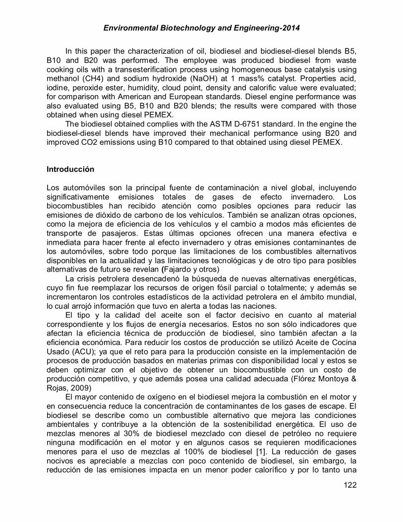
Environmental Biotechnology and Engineering-2014
122
In this paper the characterization of oil, biodiesel and biodiesel-diesel blends B5, B10 and B20 was performed. The employee was produced biodiesel from waste cooking oils with a transesterification process using homogeneous base catalysis using methanol (CH4) and sodium hydroxide (NaOH) at 1 mass% catalyst. Properties acid, iodine, peroxide ester, humidity, cloud point, density and calorific value were evaluated; for comparison with American and European standards. Diesel engine performance was also evaluated using B5, B10 and B20 blends; the results were compared with those obtained when using diesel PEMEX. The biodiesel obtained complies with the ASTM D-6751 standard. In the engine the biodiesel-diesel blends have improved their mechanical performance using B20 and improved CO2 emissions using B10 compared to that obtained using diesel PEMEX.
Introducción Los automóviles son la principal fuente de contaminación a nivel global, incluyendo significativamente emisiones totales de gases de efecto invernadero. Los biocombustibles han recibido atención como posibles opciones para reducir las emisiones de dióxido de carbono de los vehículos. También se analizan otras opciones, como la mejora de eficiencia de los vehículos y el cambio a modos más eficientes de transporte de pasajeros. Estas últimas opciones ofrecen una manera efectiva e inmediata para hacer frente al efecto invernadero y otras emisiones contaminantes de los automóviles, sobre todo porque las limitaciones de los combustibles alternativos disponibles en la actualidad y las limitaciones tecnológicas y de otro tipo para posibles alternativas de futuro se revelan (Fajardo y otros)
La crisis petrolera desencadenó la búsqueda de nuevas alternativas energéticas, cuyo fin fue reemplazar los recursos de origen fósil parcial o totalmente; y además se incrementaron los controles estadísticos de la actividad petrolera en el ámbito mundial, lo cual arrojó información que tuvo en alerta a todas las naciones.
El tipo y la calidad del aceite son el factor decisivo en cuanto al material correspondiente y los flujos de energía necesarios. Estos no son sólo indicadores que afectan la eficiencia técnica de producción de biodiesel, sino también afectan a la eficiencia económica. Para reducir los costos de producción se utilizó Aceite de Cocina Usado (ACU); ya que el reto para para la producción consiste en la implementación de procesos de producción basados en materias primas con disponibilidad local y estos se deben optimizar con el objetivo de obtener un biocombustible con un costo de producción competitivo, y que además posea una calidad adecuada (Flórez Montoya & Rojas, 2009)
El mayor contenido de oxígeno en el biodiesel mejora la combustión en el motor y en consecuencia reduce la concentración de contaminantes de los gases de escape. El biodiesel se describe como un combustible alternativo que mejora las condiciones ambientales y contribuye a la obtención de la sostenibilidad energética. El uso de mezclas menores al 30% de biodiesel mezclado con diesel de petróleo no requiere ninguna modificación en el motor y en algunos casos se requieren modificaciones menores para el uso de mezclas al 100% de biodiesel [1]. La reducción de gases nocivos es apreciable a mezclas con poco contenido de biodiesel, sin embargo, la reducción de las emisiones impacta en un menor poder calorífico y por lo tanto una
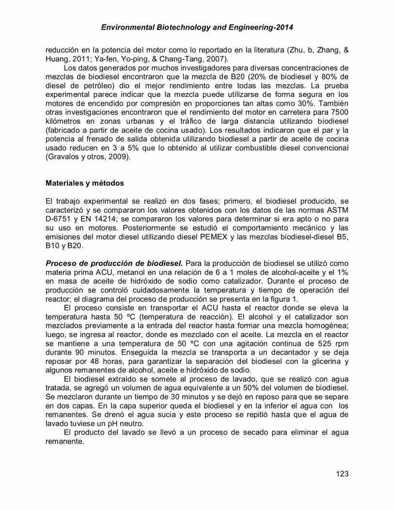
Environmental Biotechnology and Engineering-2014
123
reducción en la potencia del motor como lo reportado en la literatura (Zhu, b, Zhang, & Huang, 2011; Ya-fen, Yo-ping, & Chang-Tang, 2007).
Los datos generados por muchos investigadores para diversas concentraciones de mezclas de biodiesel encontraron que la mezcla de B20 (20% de biodiesel y 80% de diesel de petróleo) dio el mejor rendimiento entre todas las mezclas. La prueba experimental parece indicar que la mezcla puede utilizarse de forma segura en los motores de encendido por compresión en proporciones tan altas como 30%. También otras investigaciones encontraron que el rendimiento del motor en carretera para 7500 kilómetros en zonas urbanas y el tráfico de larga distancia utilizando biodiesel (fabricado a partir de aceite de cocina usado). Los resultados indicaron que el par y la potencia al frenado de salida obtenida utilizando biodiesel a partir de aceite de cocina usado reducen en 3 a 5% que lo obtenido al utilizar combustible diesel convencional (Gravalos y otros, 2009). Materiales y métodos El trabajo experimental se realizó en dos fases; primero, el biodiesel producido, se caracterizó y se compararon los valores obtenidos con los datos de las normas ASTM D-6751 y EN 14214; se compararon los valores para determinar si era apto o no para su uso en motores. Posteriormente se estudió el comportamiento mecánico y las emisiones del motor diesel utilizando diesel PEMEX y las mezclas biodiesel-diesel B5, B10 y B20. Proceso de producción de biodiesel. Para la producción de biodiesel se utilizó como materia prima ACU, metanol en una relación de 6 a 1 moles de alcohol-aceite y el 1% en masa de aceite de hidróxido de sodio como catalizador. Durante el proceso de producción se controló cuidadosamente la temperatura y tiempo de operación del reactor; el diagrama del proceso de producción se presenta en la figura 1. El proceso consiste en transportar el ACU hasta el reactor donde se eleva la temperatura hasta 50 ºC (temperatura de reacción). El alcohol y el catalizador son mezclados previamente a la entrada del reactor hasta formar una mezcla homogénea; luego, se ingresa al reactor, donde es mezclado con el aceite. La mezcla en el reactor se mantiene a una temperatura de 50 ºC con una agitación continua de 525 rpm durante 90 minutos. Enseguida la mezcla se transporta a un decantador y se deja reposar por 48 horas, para garantizar la separación del biodiesel con la glicerina y algunos remanentes de alcohol, aceite e hidróxido de sodio. El biodiesel extraído se somete al proceso de lavado, que se realizó con agua tratada, se agregó un volumen de agua equivalente a un 50% del volumen de biodiesel. Se mezclaron durante un tiempo de 30 minutos y se dejó en reposo para que se separe en dos capas. En la capa superior queda el biodiesel y en la inferior el agua con los remanentes. Se drenó el agua sucia y este proceso se repitió hasta que el agua de lavado tuviese un pH neutro. El producto del lavado se llevó a un proceso de secado para eliminar el agua remanente.
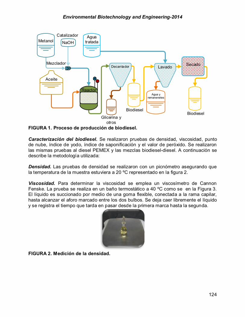
Environmental Biotechnology and Engineering-2014
124
FIGURA 1. Proceso de producción de biodiesel. Caracterización del biodiesel. Se realizaron pruebas de densidad, viscosidad, punto de nube, índice de yodo, índice de saponificación y el valor de peróxido. Se realizaron las mismas pruebas al diesel PEMEX y las mezclas biodiesel-diesel. A continuación se describe la metodología utilizada:
Densidad. Las pruebas de densidad se realizaron con un picnómetro asegurando que la temperatura de la muestra estuviera a 20 ºC representado en la figura 2. Viscosidad. Para determinar la viscosidad se emplea un viscosímetro de Cannon Fenske. La prueba se realiza en un baño termostático a 40 ºC como se en la Figura 3. El líquido es succionado por medio de una goma flexible, conectada a la rama capilar, hasta alcanzar el aforo marcado entre los dos bulbos. Se deja caer libremente el líquido y se registra el tiempo que tarda en pasar desde la primera marca hasta la segunda.
FIGURA 2. Medición de la densidad.
Glicerina y otros
Aceite
Mezclador
Reactor
MetanolCatalizador
NaOH
Biodiesel
Decantador
Agua y remanenetes
Biodiesel
Lavado Secado
Agua tratada

Environmental Biotechnology and Engineering-2014
125
FIGURA 3. Medición de la viscosidad. Punto de nube. Para la determinación de éste parámetro se introduce en un tubo de ensayo con tapa y un termómetro de caratula digital un volumen de 10 ml y luego se sumerge en un baño de hielo con sal a una temperatura de -13 ºC, como se muestra en la Figura 4. La temperatura del fluido en el tubo de ensaye baja hasta presentarse el fenómeno y la temperatura es registrada.
FIGURA 4. Medición del punto de nube. Índice de yodo. Es la medida de la instauración de las grasas y aceites y se expresa en términos del número de centigramos de yodo absorbido por gramo de muestra (% de yodo absorbido) se muestra en la figura 5. Haciendo uso de la norma NMX-F-152-SCFI-2011 ALIMENTOS - ACEITES Y GRASAS VEGETALES O ANIMALES - DETERMINACIÓN DEL ÍNDICE DE YODO POR EL MÉTODO CICLOHEXANO.

Environmental Biotechnology and Engineering-2014
126
FIGURA 5. Muestra antes y después de la titulación con yodo. Índice de saponificación. El índice de saponificación es la cantidad de hidróxido potasio expresado en miligramos de KOH, necesaria para saponificar un gramo de aceite o grasa como se muestra en la figura 6. Se utilizó la Norma mexicana para el índice de saponificación NMX-F-174-SCFI-2006: ALIMENTOS – ACEITES Y GRASAS VEGETALES O ANIMALES DETERMINACIÓN DEL ÍNDICE DE SAPONIFICACIÓN.
FIGURA 6. Prueba del índice de saponificación. Número de acidez. El índice de acidez es el número que se expresa en miligramos de hidróxido de potasio requeridos para neutralizar los ácidos libres que existen en un gramo de grasa. Se utilizó la norma NMX-K-418-1976 DETERMINACIÓN DEL NÚMERO DE ÁCIDEZ EN ACEITES ESENCIALES Y PRODUCTOS AROMÁTICOS.
FIGURA 7. Muestra de ACU antes y después de la prueba de número de acidez. Poder calorífico. Para determinar el poder calorífico se utilizó el equipo IKA C2000, se utilizó el método dinámico a 25ºC que cumple con las normas ASTM D1989, D240, D5865, D4809, D5468 y E711.
Environmental Biotechnology and Engineering-2014
127
FIGURA 8. Equipo IKA 2000.
Resultados de la caracterización. Con el proceso de producción presentado en la ¡Error! No se encuentra el origen de la referencia. se obtiene un rendimiento del 85%. En la ¡Error! No se encuentra el origen de la referencia. se presentan los resultados de la caracterización del diesel, biodiesel y las mezclas B5, B10 y B20. Además se comparan con los valores de las normas ASTM D-6751. Pruebas del rendimiento mecánico del motor diesel. El biodiesel obtenido y las mezclas con diesel PEMEX, fue probado en la Planta Piloto del Laboratorio Termodinámica, Turbomaquinaria y Energías Renovables de la Universidad Autónoma Metropolitana - Iztapalapa, en un motor diesel Robín modelo DY23-2D monocilíndrico de cuatro tiempos enfriado por aire. El módulo de prueba del motor diesel alcanza una velocidad máxima de 2,400 rpm generando una potencia cercana a 1.5 kW. El motor tiene una relación de compresión de 19 y el volumen barrido del cilindro es de 0.28 litros, que corresponde a un diámetro de 73 mm y una carrera de 67 mm. El motor esta acoplado al módulo MASTER2000, presentado en la figura 7. Este dispositivo controla a un dinamómetro CC y el motor diesel. El número de revoluciones del motor se establecen en el panel de control del equipo MASTER2000. La velocidad del motor diesel se modificó desde las 1200 rpm hasta 1900 rpm a cada 100 rpm con un total de 7 registros por prueba. Cada uno de los registros incluye los datos del motor y emisiones. En la figura 11 se muestra el arreglo del sistema de pruebas seguido.

Environmental Biotechnology and Engineering-2014
128
TABLA 1. Resultados de las pruebas de caracterización del biodiesel, diesel y mezclas biodiesel-diesel.
FIGURA 9. MASTER2000. Para obtener los parámetros ambientales se utilizó un analizador de gases
BOSH modelo BEA 350 presentado en la figura 10. Con el equipo se midieron las emisiones de CO, CO2, HC, lambda y la opacidad de los gases de escape.
FIGURA 10. BOSH BEA 350.
PRUEBA Biodiesel (b-100) Diesel B-5 B-10 B-50 Límite de la
norma ASTM
Índice de saponificación (mg KOH/mg) 160.33 338.5 311.7 293.44 111.13 -
Índice de yodo (gr yodo/100 gr) 107.076 -21.17 -6.113 0.4623 111.715 -
Número de acidez (mg KOH/mg) 0.6489 0.6461 0.6476 .8318 0.739 0.8 max
Punto nube (ºC) -11.067 -10.333 -10.567 -10.833 -11 - Densidad a 20°C (g/cm3) 0.8231 0.8233 0.83575 0.8335 0.9085 - Viscosidad (cSts) 5.8451 2.9043 3.1187 3.3051 4.3792 1.9-6 Poder Calorífico (kJ/kg) 39157 43856 44421 45659 36773 -

Environmental Biotechnology and Engineering-2014
129
FIGURA 11. Diagrama del sistema de prueba del motor diesel. Resultados Se evaluaron las mezclas B5, B10 y B20 en el motor diesel y se comparó su comportamiento con el obtenido al utilizar diesel PEMEX. En la figura 12 se muestra que la mezcla B20 tiene menor diferencia promedio de 9% a lo obtenido con diesel PEMEX. Y la mezclas B5 y B10 difieren el 13.1 y 21.3% respectivamente. La máxima potencia fue alcanzada con la mezcla B10 cerca de las 1500 rpm cuando entregó poco más de 570 W. El comportamiento de las mezclas, como se muestra en la figura 12, es de mayor inestabilidad en comparación a el diesel PEMEX, resulta derivado del cambio en el índice de cetano del biodiesel según Cherng (Cherng-Yuan Lin & Hsiu-An Lin, 2006) y Szybist (Szybist, Song, Alam, & Boehman, 2007) difiere cerca del 10% respecto al diesel de petróleo.
El torque, se muestra en la figura 13, en promedio un aumento del 12.7, 22.4 y 6.4% utilizando las mezclas B5, B10 y B20 respectivamente, en comparación con lo obtenido al utilizar diesel PEMEX. El menor consumo específico de combustible promedio (CEC) se obtuvo con la mezcla B10 siendo 27.2% menor que las diesel PEMEX. También las mezclas B5 y B20 reducen el CEC como se muestra en la figura 14, sin embargo tienen un comporta-miento similar al obtenido con el diesel PEMEX. En la zona de máxima potencia del motor se tiene también la zona de menor CEC, esto significa que ese intervalo de revoluciones, 1,500 a 1600 rpm, es la zona donde se obtiene la máxima potencia con el mínimo CEC.

Environmental Biotechnology and Engineering-2014
130
FIGURA 12. Potencia del motor con mezclas B5, B10, B20 y diesel PEMEX a diferentes rpm.
FIGURA 13. Torque del motor con mezclas B5, B10, B20 y diesel PEMEX a diferentes rpm.
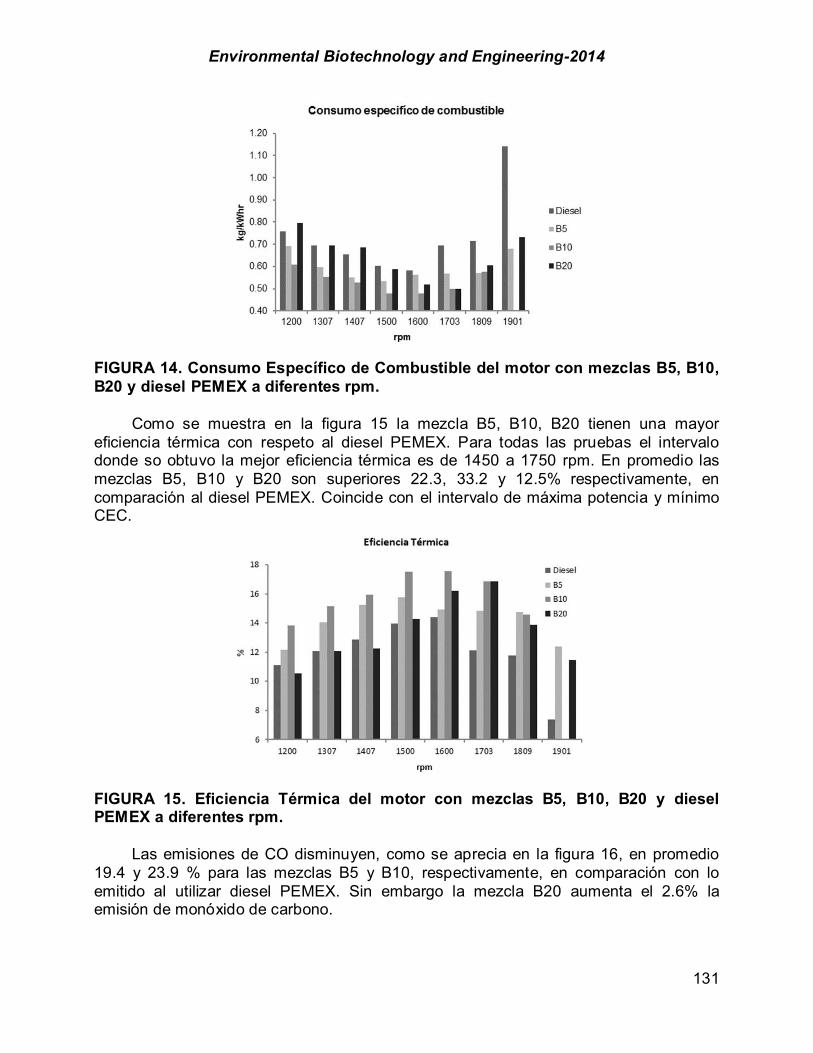
Environmental Biotechnology and Engineering-2014
131
FIGURA 14. Consumo Específico de Combustible del motor con mezclas B5, B10, B20 y diesel PEMEX a diferentes rpm. Como se muestra en la figura 15 la mezcla B5, B10, B20 tienen una mayor eficiencia térmica con respeto al diesel PEMEX. Para todas las pruebas el intervalo donde so obtuvo la mejor eficiencia térmica es de 1450 a 1750 rpm. En promedio las mezclas B5, B10 y B20 son superiores 22.3, 33.2 y 12.5% respectivamente, en comparación al diesel PEMEX. Coincide con el intervalo de máxima potencia y mínimo CEC.
FIGURA 15. Eficiencia Térmica del motor con mezclas B5, B10, B20 y diesel PEMEX a diferentes rpm. Las emisiones de CO disminuyen, como se aprecia en la figura 16, en promedio 19.4 y 23.9 % para las mezclas B5 y B10, respectivamente, en comparación con lo emitido al utilizar diesel PEMEX. Sin embargo la mezcla B20 aumenta el 2.6% la emisión de monóxido de carbono.
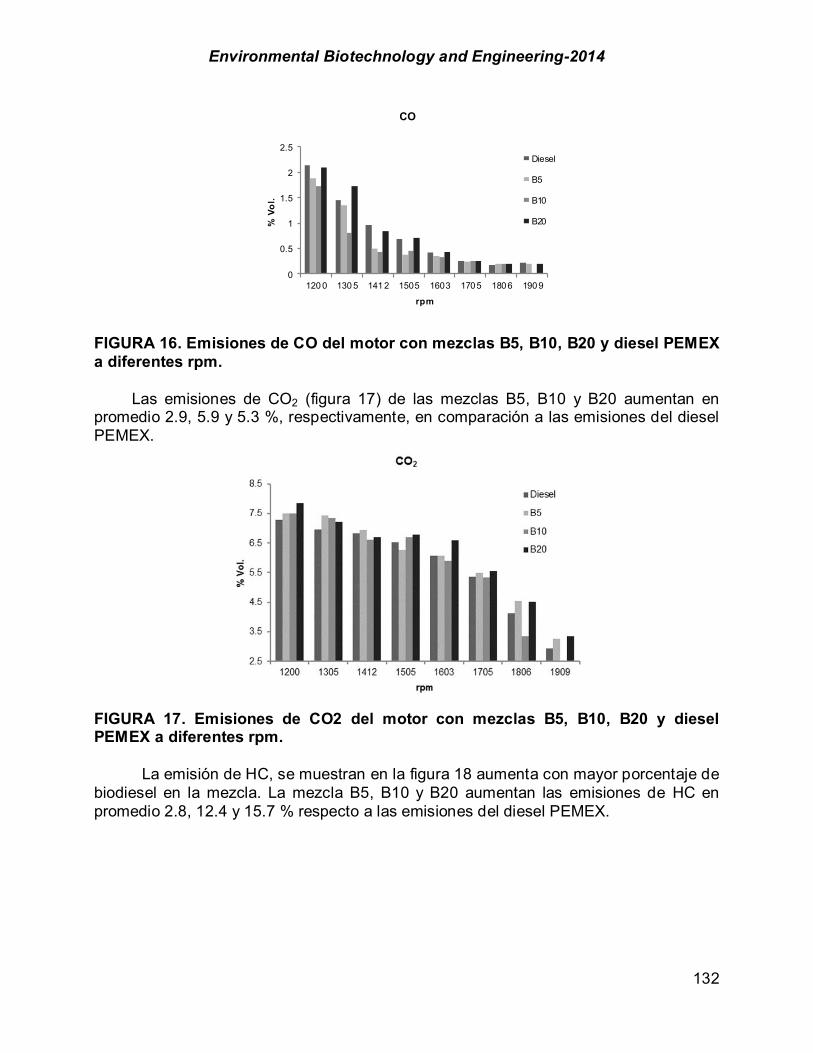
Environmental Biotechnology and Engineering-2014
132
FIGURA 16. Emisiones de CO del motor con mezclas B5, B10, B20 y diesel PEMEX a diferentes rpm. Las emisiones de CO2 (figura 17) de las mezclas B5, B10 y B20 aumentan en promedio 2.9, 5.9 y 5.3 %, respectivamente, en comparación a las emisiones del diesel PEMEX.
FIGURA 17. Emisiones de CO2 del motor con mezclas B5, B10, B20 y diesel PEMEX a diferentes rpm.
La emisión de HC, se muestran en la figura 18 aumenta con mayor porcentaje de biodiesel en la mezcla. La mezcla B5, B10 y B20 aumentan las emisiones de HC en promedio 2.8, 12.4 y 15.7 % respecto a las emisiones del diesel PEMEX.
0
0.5
1
1.5
2
2.5
120 0 130 5 141 2 1505 1603 1705 1806 190 9%
Vol
.
rpm
CO
Diesel
B5
B10
B20
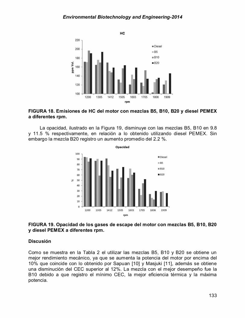
Environmental Biotechnology and Engineering-2014
133
FIGURA 18. Emisiones de HC del motor con mezclas B5, B10, B20 y diesel PEMEX a diferentes rpm. La opacidad, ilustrado en la Figura 19, disminuye con las mezclas B5, B10 en 9.8 y 11.5 % respectivamente, en relación a lo obtenido utilizando diesel PEMEX. Sin embargo la mezcla B20 registro un aumento promedio del 2.2 %.
FIGURA 19. Opacidad de los gases de escape del motor con mezclas B5, B10, B20 y diesel PEMEX a diferentes rpm. Discusión Como se muestra en la Tabla 2 el utilizar las mezclas B5, B10 y B20 se obtiene un mejor rendimiento mecánico, ya que se aumenta la potencia del motor por encima del 10% que coincide con lo obtenido por Sapuan [10] y Masjuki [11], además se obtiene una disminución del CEC superior al 12%. La mezcla con el mejor desempeño fue la B10 debido a que registro el mínimo CEC, la mejor eficiencia térmica y la máxima potencia.
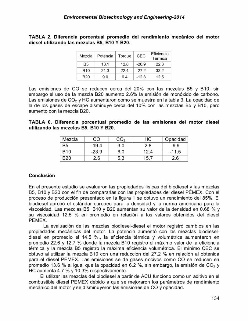
Environmental Biotechnology and Engineering-2014
134
TABLA 2. Diferencia porcentual promedio del rendimiento mecánico del motor diesel utilizando las mezclas B5, B10 Y B20.
Mezcla Potencia Torque CEC Eficiencia Térmica
B5 13.1 12.8 -20.9 22.3 B10 21.3 22.4 -27.2 33.2 B20 9.0 6.4 -12.3 12.5
Las emisiones de CO se reducen cerca del 20% con las mezclas B5 y B10, sin embargo el uso de la mezcla B20 aumento 2.6% la emisión de monóxido de carbono. Las emisiones de CO2 y HC aumentaron como se muestra en la tabla 3. La opacidad de la de los gases de escape disminuye cerca del 10% con las mezclas B5 y B10, pero aumento con la mezcla B20. TABLA 0. Diferencia porcentual promedio de las emisiones del motor diesel utilizando las mezclas B5, B10 Y B20.
Mezcla CO CO2 HC Opacidad B5 -19.4 3.0 2.8 -9.9 B10 -23.9 6.0 12.4 -11.5 B20 2.6 5.3 15.7 2.6
Conclusión En el presente estudio se evaluaron las propiedades físicas del biodiesel y las mezclas B5, B10 y B20 con el fin de compararlas con las propiedades del diesel PEMEX. Con el proceso de producción presentado en la figura 1 se obtuvo un rendimiento del 85%. El biodiesel aprobó el estándar europeo para la densidad y la norma americana para la viscosidad. Las mezclas B5, B10 y B20 aumentan su valor de la densidad en 0.68 % y su viscosidad 12.5 % en promedio en relación a los valores obtenidos del diesel PEMEX.
La evaluación de las mezclas biodiesel-diesel el motor registró cambios en las propiedades mecánicas del motor. La potencia aumentó con las mezclas biodiesel-diesel en promedio el 14.5 %., la eficiencia térmica y volumétrica aumentaron en promedio 22.6 y 12.7 % donde la mezcla B10 registro el máximo valor de la eficiencia térmica y la mezcla B5 registro la máxima eficiencia volumétrica. El mínimo CEC se obtuvo al utilizar la mezcla B10 con una reducción del 27.2 % en relación al obtenida para el diesel PEMEX. Las emisiones se de gases nocivos como CO se reducen en promedio 13.6 % al igual que la opacidad en 6.2 %, sin embargo, la emisión de CO2 y HC aumenta 4.7 % y 10.3% respectivamente. El utilizar las mezclas del biodiesel a partir de ACU funciono como un aditivo en el combustible diesel PEMEX debido a que se mejoraron los parámetros de rendimiento mecánico del motor y se disminuyeron las emisiones de CO y opacidad.
Environmental Biotechnology and Engineering-2014
135
Referencias Agudelo S., J., Benjumea, P., Gómez Meneses, E., & Pérez Bayer, J. (2003). Biodiesel. Una revisión del
desempeño mecánico y ambiental. Ingeniería y Desarrollo(13), 1-14. Amin, T.-K., Saidina Amin, N., & Hossein, M. (2013). A review on novel processes of biodiesel production
from waste cooking oil. Applied Energy(104), 683–710. Bailey, A. (1984). Aceites y Grasas Industriales. Barcelona: Reverté S.A. Cheng, F. (1945). China produces fuels from vegetable oils. Chem. Metall. Eng , 52-99. Cherng-Yuan Lin, & Hsiu-An Lin. (2006). Diesel engine performance and emission characteristics of
biodiesel produced by the peroxidation process. Fuel(85), 298–305. Chhetri, A. B., Watts, K. C., & Islam, M. R. (2008). Waste Cooking Oil as an Alternate Feedstock for
Biodiesel Production. Energies(1), 3-18. Fajardo, J., Meza, J., Abuchar, A., Julio, F., Díaz, A., & Navas, O. (s.f.). Estudio del desempeño mecánico
y ambiental de los motores de encendido por compresión al utilizar biodiesel como combustible. FBDS. (2005). Liquid Biofuels For Transportation in Brazil. German Technical Cooperation (GTZ),
Fundação Brasileira para o Desenvolvimento. Felizardo, P., Correia, M. J., Raposo, I., Mendes, J. F., Berkemeier, R., & Bordado, J. M. ( 2006).
Production of biodiesel from waste frying oils. Waste Management(26), 487–494. Flórez Montoya, A. A., & Rojas, A. F. (2009). Efecto de la proporción de mezclas biodiesel/petrodiesel en
el desempeño mecánico-ambiental de motores. Ingeniería y competitividad, 11(2), 63-78. Gravalos, I., Gialamas, T., Koutsofitis, Z., Kateris, D., Xyradakis, P., & Tsiropoulos, Z. (2009). Comparison
of performance characteristics of agricultural tractor diesel engine operating on home and industrially produced biodiesel. International Journal of Energy Research(33), 1048–1058.
Issariyakul, T., Kulkarni, M. G., Dalai, A. K., & Bakhshi, N. N. (2007). Production of biodiesel from waste fryer grease using mixed methanol/ethanol system. Fuel Processing Technology, 88, 429–436.
John, R., Agudelo, S., Pedro, B., & Gómez Meneses, E. (2003). Una revisión del desempeño mecánico y ambiental. redaylc, 1-14.
John, R., Agudelo, S., Pedro, B., Gómez Meneses, E., & Pérez Bayer, J. (2003). Una revisión del desempeño mecánico y ambiental. redaylc, 1-14.
Knothe, G. (2001). Historical perspective on vegetable oil-based diesel fuels. AOCS Inform 12, 1103-1107.
Lin, Y.-f., Wu, Y.-p. G., & Chang, C.-T. (2007). Combustion characteristics of waste-oil produced biodiesel/diesel fuel blends. FUEL, 86, 1772–1780.
Lin, Y.-f., Wu, Y.-p. G., & Chang, C.-T. (2007). Combustion characteristics of waste-oil produced biodiesel/diesel fuel blends. Fuel, 86, 1772-1780.
Masjuki, H., Abdulmuin, M., & Miasted, S. (1996). Investigations on preheated palm oil. Proceedings of the Institution of Mechanical Engineers (IMechE), 131-138.
Mollenhauer, K., & Tschoeke, H. (2010). Handbook of Diesel Engines. Verlag Berlin Heidelberg: Springer. National Renewable Energy Laboratory. (2009). Biodiesel Handling and Use Guide (Vol. 4). PROFECO. (Octubre de 2010). Estudio de calidad: aceites vegetales comestibles "La sartén por el
mango". Revista del consumidor, 36-47. Sagar, A. D. (1995). Automobiles and global warming: alternative fuels and other option for carbon dioxide
emissions reduction. Ecological impact assessment, 15:241-274. Sapuan, S. M., Masjuki, H., & Azlan, A. (1996). The use of palm oil as diesel substitute. Proceedings of
ImechE, 210, 47. Sheinbaum-Pardo, C., Calderon-Irazoque, A., & Ramirez-Suarez, M. (2013). Potencial of diesel from
waste cooking oil in Mexico. sciverse scienceDirect, 230-238. Solomon, S., Qin, D., M. Manning, Z. C., Marquis, M., Averyt, K., Tignor, M., & Miller, H. (2007).
Contribution of Working Group I to the Fourth Assessment Report of the Intergovernmental Panel on Climate Change. Cambridge, United Kingdom and New York: Cambridge University Press.
Szybist, J. P., Song, J., Alam, M., & Boehman, A. L. (2007). Biodiesel combustion, emissions and emission control. Fuel Processing Technology(88), 679–691.
Talebian-Kiakalaieh, A., Amin, N. A., & Mazaheri, H. (2013). A review on novel processes of biodiesel production from waste cooking oil. Applied Energy(104), 683–710.
Environmental Biotechnology and Engineering-2014
136
Tanaka, S., Kobayashi, T., Kamiyama, K., & Bildan, M. (1997). Effects of thermochemical pretreatment on the anaerobic digestion of waste activated sludge. Water Science of Technology, 35(8), 209-215.
UNESA. (2005). Forestación y Reforestación. Sumideros de Carbono. En: Metodologías para la Implementación de los Mecanismos flexibles de Kioto - Mecanismo de Desarrollo Limpio en Latinoamérica.
Uzun, B. B., K$l$ça, M., Özbay, N., Pütüna, A. E., & Pütün, E. (2012). Biodiesel production from waste frying oils: Optimization of reaction parameters and determination of fuel properties. Energy(44), 347-351.
Wang, R. (1988). Development of biodiesel fuel. Taiyangneng Xuebao 9, 434-436. Y. C. Sharma , B. Singh, & S. N. Upadhyay. (2008). Advancements in development and characterization
of biodiesel: A review. Fuel, 87, 2355-2373. Yaakob, Z., Mohammada, M., Alherbawi, M., & Alam, Z. (2013). Overview of the production of biodiesel
from Waste cooking oil. Renewable and Sustainable Energy Reviews(18), 184–193. Ya-fen, L., Yo-ping, G., & Chang-Tang, C. (2007). Combustion characteristics of waste-oil produced
biodiesel/diesel fuel blends. FUEL, 86, 1772–1780. Zhang, Y., Dubé, M. A., McLean, D. D., & Kates, M. (2003). Biodiesel production from waste cooking oil:
1. Process design and technological assessment. Bioresource Technology, 89, 1-16. Zhu, L., b, C. C., Zhang, W., & Huang, Z. (2011). Combustion, performance and emission characteristics
of a DI diesel engine fueled with ethanol–biodiesel blends. Fuel(90), 1743–1750.
Environmental Biotechnology and Engineering-2014
137
CHAPTER 1.15. GENERACIÓN SIMULTÁNEA DE METANO, HIDRÓGENO Y ENERGÍA ELÉCTRICA EN BIOCELDAS ANAERÓBICAS ACOPLADAS DE
CULTIVOS MIXTOS
José D. Bárcenas-Torres*; Ismael Arroyo-Tena; Eliel R. Romero-García; José F. Covián-Nares; Gerardo M. Chávez-Campos.
ITM, Morelia, Mich., México. RESUMEN Se construyeron biopilas generadoras de energía eléctrica a partir de dos cultivos microbianos generadores de hidrógeno-metano, colocando en el ánodo cultivos autóctonos de Bacillus subtilis aislados a partir del ensilado de maíz en su etapa de metabolismo fermentativo, y en el cátodo un consorcio microbiano metanogénico previamente caracterizado. Inicialmente los reactores fueron alimentados diariamente con 15 ml de una solución de 30 g/l de sacarosa para el cultivo hidrogenogénico y 15 ml de una solución de 20 g/l de acetato de potasio para el cultivo metanogénico hasta obtener los mayores rendimientos de degradación. Posteriormente fueron acoplados en una conformación de biopila en reactores de 250 ml, acondicionados con sensores que median temperatura, pH, voltaje y corriente acoplados a una tarjeta electrónica recolectora de datos, y analizados en el software NI Labview.
Se probó la influencia de la agitación y la temperatura en un diseño experimental 22 sobre el incremento de las variables de eficiencia, demostrando condiciones óptimas a 100 rpm y 37 °C, con constante de reacción de K= 0.00165 l/mg·h, y una tasa específica de consumo de sustrato q= 0.0485 h-1.
Las eficiencias de generación de energía eléctrica (Ie-), producción de biogás (PCH4; PH2), degradación de materia orgánica ("DQO) y coulombica (EC) fueron determinadas cuando se suministraron diferentes concentraciones de sacarosa y acetato de potasio en la alimentación y manteniendo condiciones estables de pH, temperatura y resistencia externa (4.7 k ). Los resultados demuestran mayores rendimientos (Ie-; EC; "DQO) cuando se alimentan sacarosa en el cátodo y acetato en el ánodo. De manera interesante se obtuvo una menor generación de ácidos orgánicos y mayor generación de butanodiol cuando se suministra acetato en ambos reactores y una notable disminución de la generación de metano sin afectar los rendimientos de generación de voltaje y corriente. La incorporación de dos reactores acoplados en un sistema hidrogenogénico-metanogénico es capaz de generar energías integrales simultaneas a partir de sustratos simples, lo que la convierte en una alternativa prominente para el aprovechamiento de efluentes líquidos contaminantes. -------------- *Author for correspondence

Environmental Biotechnology and Engineering-2014
138
ABSTRACT Bio-batteries for electric power generation were built using two microbial cultures producers of hydrogen-methane. In the anode we place native cultures of Bacillus subtilis, they were isolated from corn silage in his fermentative metabolism stage, while at the cathode we use a methanogenic microbial consortium, it was previously characterized. Initially, the reactors were fed daily with 15 ml of sucrose solution (30 g/l) for cultures hydrogen generators and 15 ml of potassium acetate solution (20 g/l) for growing methanogenic cultures. We maintained this condition until obtain the highest yield degradation. Subsequently both cultures were coupled like bio-batteries in reactors of 250 mL., they were equipped with sensors for temperature, pH, dissolved oxygen, voltage and current. All sensors were coupled to an electronic data collector card. The data were analyzed using NI Labview software.
We tested the influence of agitation and the temperature on increasing the variables efficiency using an experimental design 22. We find optimal conditions at 100 rpm and 37 °C, with a constant of reaction K = 0.00165 l/mg•h, and a specific rate of substrate consumption q = 0.0485 h-1.
The efficiencies in the generation of electric energy (Ie-), biogas production (PCH4; PH2), degradation of organic matter ("DQO) and coulombica (EC) were determined each time that we provided different concentrations of sucrose and acetate of potassium in the fed. We maintain stable conditions of pH, temperature and external resistance (4.7 k ) for each experiment. The results show higher yields (EC; #DQO) when we supply sucrose in the cathode and acetate in the anode. Interestingly we obtained a lower generation of organic acids and high generation of Butanediol when we supplied acetate in both reactors, and a remarkable reduction in the methane generation without affecting the yield of voltage and current generation.
The incorporation of two coupled reactors to hidrogengenic-methanogenic system is capable of generating simultaneous integral energies using simple substrates, which makes it a prominent alternative for use of contaminated liquid effluents. Key words: Bacillus subtillis, bioelectricity, biopiles, hydrogenogenic, methanogenic Introducción En los últimos años se han desarrollado diversas tecnologías que se enfocan en la utilización de la energía acumulada en la biomasa de desechos, para ser redirigida a otras formas de energía que la humanidad pueda utilizar como son: la metanogénesis (CH4), hidrogenogénesis (H2) y la bioelectricidad (Logan et al., 2010). Cuando son producidos por medios biológicos y a partir de sustratos contaminantes, se consideran una fuente de energía renovable y sustentable. Estudios recientes demuestran que sistemas acoplados en serie para la producción de hidrógeno y metano en etapas separadas y alimentados con los efluentes gastados de la hidrogenogénesis pueden mantener muy buenos rendimientos tanto de la generación de hidrógeno y metano como en la degradación de compuestos contaminantes. (Escamilla-Alvarado et al. 2010; Liu et al. 2006; Ueno et al. 2007).
Más recientemente las Pilas de Combustible microbiano (PCM) han tomado mayor aceptación al generar energía eléctrica y degradar compuestos contaminantes

Environmental Biotechnology and Engineering-2014
139
incluso persistentes (Haiping Luo et al. 2008). Los sistemas PCM más comunes son conformados por una cámara anaeróbica (ánodo) y otra cámara aeróbica (cátodo), sin embargo existen sistemas que cuentan con ambas cámaras ya sean aeróbicas o anaérobicas (Ringeisen et al. 2007; Catal et al. 2011). Los estudios relacionados con las PCM se centran principalmente en la optimización de la generación de energía variando la composición y estructura del ánodo (Revelo et al. 2013; Alzate-Gaviria et al. 2010), incluyendo mediadores redox para el metabolismo microbiano (Sacco et al. 2010), mejora en las condiciones de la biopelícula (Katuri et al. 2012) y la manipulación genética de los microorganismos que participan en el funcionamiento de las mismas (Katuri et al. 2012).
Numerosos estudios reportan la generación de bioelectricidad a partir de cultivos únicos o consorcios microbianos, siendo utilizados principalmente Geobacter (Bond et al. 2003), Shewanella (Bretschger et al. 2010), Bacillus (Vanita et al. 2012), Lodos activados (Buitrón et al. 2011), sedimentos (Helder 2012). Sin embargo hasta el momento no ha sido reportada la utilización de cultivos distintos en ambas cámaras de las PCM para la generación de energía eléctrica.
Finalmente, en un balance global energético se deben tomar en cuenta aspectos como el gasto energético por el suministro de aire y los costos de operación y mantenimiento. Y son estos últimos aspectos los que motivan la realización de este trabajo, para probar las eficiencias de aprovechamiento integral de energía en un sistema anaerobio Metanogénico-Hidrogenogénico-Productor de Electricidad (MG-HG-RPE), que lejos de representar un gasto energético, representan una oportunidad para solucionar los problemas energéticos y de contaminación de agua.
Materiales y métodos
Construcción del sistema PCM. El sistema PCM consiste en dos reactores de vidrio idénticos marca Adams & Chittenden Scientific Glass, modelo 250.40.3, con capacidad de 250 ml. Cada uno con tres orificios laterales adaptados para i) introducir alimentación al sistema y toma de muestra, ii) recolección de gases y iii) gaseado. Los reactores fueron unidos herméticamente por la parte lateral, únicamente separados por una membrana de intercambio protónico de Nafion® NR12 con un área superficial 5 cm2 y espesor de 50.8 µm. Por la parte superior de cada reactor se adaptó un electrodo de grafito tipo barra de área superficial 75 cm2 y grosor de 1 cm. Técnicas Analíticas. Para la medición y recolección de datos de las variables de voltaje, temperatura, intensidad de corriente, pH y oxígeno disuelto se integró un sistema de medición y almacenamiento de datos automatizado, acoplado a través de una interfaz conectada de la pila de combustible microbiano a un software diseñado en el programa labVIEW, utilizando una tarjeta de adquisición de datos NI USB de NATIONAL INSTRUMENTS y conectando dos terminales a los electrodos de grafito de la PCM y 2 sensores al interior de cada reactor, además de un termopar externo que graficó las lecturas obtenidas almacenadas e interpretadas en tiempo real.
La concentración de materia orgánica remanente se determinó mediante la técnica DQO de reflujo cerrado y la concentración de biomasa medida como sólidos suspendidos volátiles (APHA, AWWA & WPCF, 1992). La identificación de los
Environmental Biotechnology and Engineering-2014
140
compuestos intermediarios y cuantificación de la presencia de gases de combustión fue realizada mediante un cromatógrafo de gases (GC) (modelo 2601B; Instrumentos SRI) equipado con una columna de 3 m Molsieve 5A 80/100 (Altech Associates, Inc., Bannockburn, IL) con argón como el portador gas a 80°C, utilizado detectores de conductividad térmica (TCD) y con un límite de detección de 0.01%. Para mantener condiciones estables de temperatura externa se utilizó una cámara de incubación de vidrio templado recubierta de material de aislamiento. Para mantener condiciones anóxicas, antes de cada experimento los reactores H y M fueron gaseados con Nitrógeno. Microorganismos empleados (M y H). Cada uno de los reactores del sistema PCM fue cargado con dos diferentes cultivos microbianos. El reactor catódico (M) fue cargado por un consorcio microbiano metanogénico, mientras que el reactor anódico (H) contenía Bacillus subtillis en su fase de metabolismo fermentativo.
La obtención del consorcio metanogénico se realizó según los procedimientos descritos por Poggi-Varaldo et al., (1997). La obtención de B. subtillis se realizó por aislamiento de una muestra de ensilado en su fase de deterioro aerobico, proveniente de la población de Queréndaro, Michoacán. El aislamiento de los microorganismos se realizó por ciclos de aislamiento-resiembra en placa, utilizando agar Coulombia como medio de crecimiento selectivo y siguiendo los procedimientos recomendados por Tallent et al. (2012) Efecto de la agitación y calentamiento. Para establecer las condiciones ideales tanto de agitación y calentamiento se evaluó un diseño experimental 22 que consistió en cuatro ensayos distintos con una duración de 24 horas cada uno: ensayo 1, agitación de 100 rpm y 37°C; ensayo 2, agitación de 100 rpm y 25°C; ensayo 3, sin agitación y 37°C; y ensayo 4, sin agitación y 25°C.
Se alimentó al inició de cada ensayo 20 ml de una solución de 20 g/l de acetato de potasio y 30 g/l de sacarosa a los reactores M y H respectivamente, además de una solución de 20 mL que contenía los micronutrientes metalicos: FeCl2·4H2O (0.00994 g/l), CuCl2·2H2O (0.00085 g/l), ZnCl2 (0.00068 g/l), MnCl2·4H2O (0.00099 g/l), NiCl2·2H2O (0.00119 g/l), (NH4)6Mo7O2·4H2O (0.00618 g/l), Na2SeO4·5H2O (0.0014 g/l), N2WO4·2H2O (0.00156 g/l), CoCl2·6H2O (0.00119 g/l) y macronutrientes NH4Cl (2.8 g/l), K2HPO4 (2.5 g/l), MgSO4·7H2O (1.0 g/l), CaCl2·2H2O (0.1 g/l).
Las constantes de afinidad “K” al consumo de sustrato y la velocidad específica de consumo de sustrato fueron determinadas a partir de las expresiones: dS/dt =-K1Se; y q = ( s)/(X)(th) = K2Se, donde Se = Concentración de sustrato remanente de materia orgánica de cada reactor M y H (mg DQO/L); S = Sustrato consumido; X = concentración de celulas por reactor (20 mgSSV/L para el reactor M y 5 mgSSV/L para el reactor H); y tH = tiempo de duración de cada ensayo (1 día). Efecto de la concentración y tipo de sustrato. Consistió en realizar 6 ensayos diferentes con una duración de 96 horas cada uno, alimentando las concentraciones de micro y macronutriente descritas anteriormente y concentraciones de 5, 15 y 30 g/l de una solución de sacarosa, y 3, 10 y 20 g/l de solución de acetato de potasio a manera de pulsos en el reactor anodico, mientras que el reactor catódico fue alimentado permanentemente con 20 g/l de una solución de acetato de potasio.

Environmental Biotechnology and Engineering-2014
141
Inicialmente a cada cambio de tipo de sustrato se contempló un periodo de 96 horas sin alimentación con la intención de eliminar la mayor cantidad de materia orgánica y reducir la probabilidad de error por el consumo de sustratos remanentes de etapas anteriores. El sistema PCM fue operado bajo un régimen anóxico a 37°C, pH de 7 y una agitación de 100 rpm. El rendimiento energético del sistema durante las etapas experimentales fue calculado de acuerdo a lo siguiente: la intensidad de corriente (I) se expresa como I=V/R=Q/t, donde; I=Intensidad de corriente, V=Voltaje, Q=Carga, t=Tiempo. Así pues la potencia energética del sistema (watts) se calculó a través de la expresión P=I*V. Calculando la producción de energía a partir de la expresión E=P*t, donde; P=Potencia (watts), E=Energía espontánea (joules). Finalmente el total de coulombs obtenidos de manera experimental se calcularon por la integración de la gráfica de la potencia generada en el tiempo, "E=#(dP/dt), donde; "E=Energía total del sistema generada en la etapa correspondiente, P=Potencia espontánea calculada en el tiempo (watts) y t=Tiempo de duración del ensayo. La eficiencia coulombica fue determinada a partir de la ecuación: Ec = (Cp/Cti)*100%, donde Cp es el total de coulombs obtenidos de manera experimental y calculados por la integración de la intensidad de corriente en el tiempo (# (dI/dt)); y Cti, es la cantidad teórica máxima de coulombs que pueden obtenerse por el consumo de sustrato calculada a partir de la expresión Cti = [ (F*b*S*V) / M ], los valores referenciados son F, Constante de Faraday = 96,485.3399 Coulombs/mol·e-; b, Número de moles de electrones producido por mol de sustrato (44 mol de e-/mol de sacarosa; y 8 mol de e-/mol de acetato de potasio); S, Concentración de sustrato en el medio del reactor anódico (5, 15, 30 g/l para sacarosa; y 3, 10, 20 g/l para acetato de potasio); V, Volumen del líquido en el reactor anódico (V = 0.225 l); y M, Peso molecular del sustrato empleado en el reactor anódico (Sacarosa = 342.2965 g/mol, y acetato de potasio = 98.15 g/mol). Resultados y discusión Efecto de la agitación y calentamiento. La figura 1 describe como la generación de voltaje se ve afectada en diferentes circunstancias, obteniendo voltajes promedio visiblemente superiores con agitación a 100 rpm y calentamiento a 37 oC (0.0765±0.044) que con solo agitación, calentamiento o sin ninguno de ellos (0.0702±0.041; 0.0532±0.023; 0.0476 ±0.034). Li et al. (2013); Behera et al. (2011); y Wang et al. (2008), han demostrado que la temperatura es un factor influyente y determinante en la generación de energia por celdas de combustible microbiano, corroborando los resultados obtenidos del comportamiento biocinético de los experimentos (figura 1), donde existe un mayor consumo de materia orgánica (de 47.6% a 57.11%) y generación de gradiente de voltaje (de 0.09 a 0.14 V) al incrementar la temperatura de 25oC a 37oC a las mismas condiciones de agitación (100 rpm). Sin embargo la influencia de la agitación (mezclado) demuestra tener mayor impacto en el consumo de la materia orgánica y la generación de grandiente de voltaje a las mismas condiciones operacionales de

Environmental Biotechnology and Engineering-2014
142
temperatura, siempre que exista agitación, dado que permite a los microorganismos tener mayor contacto con el sustrato, con los electrodos transportadores de electrones y aumentar la tranferencia de masa de los protones hidrógeno generados y difundidos a travéz de la membrana. La capacidad de los microorganismos para consumir la materia orgánica y generar energía también es demostrada por los valores de afinidad (figura 1; K1 = 0.00165 l/mg•h, K2 = 0.00143 l/mg•h), demostrando que mayor valor de “K”, se percibe una mayor velocidad del consumo del sustrato y mayor tasa de generación de voltaje y energía.
FIGURA 1. Porcentaje de materia orgánica aprovechada como gradiente de voltaje. Efecto de la concentración y tipo de sustrato. Sacarosa (5 g/L) en el reactor anódico H y acetato (20 g/L) en el reactor catodico M. Al inicio del ensayo y durante las primeras 48 horas de operación se observó una oscilación en la generación de voltaje demostrando cambios aparentes de polaridad, sin embargo se observó además un consumo notorio de materia orgánica en ambos reactores, destacando el consumo en el reactor metanogénico de 116 a 96.2 mg DQO/l. El comportamiento observado en las primeras 48 horas de operación refleja en primera instancia el tiempo de generación e intercambio de protones que son producidos por los microorganismos hidrogenogénicos, que migran desde el medio del reactor
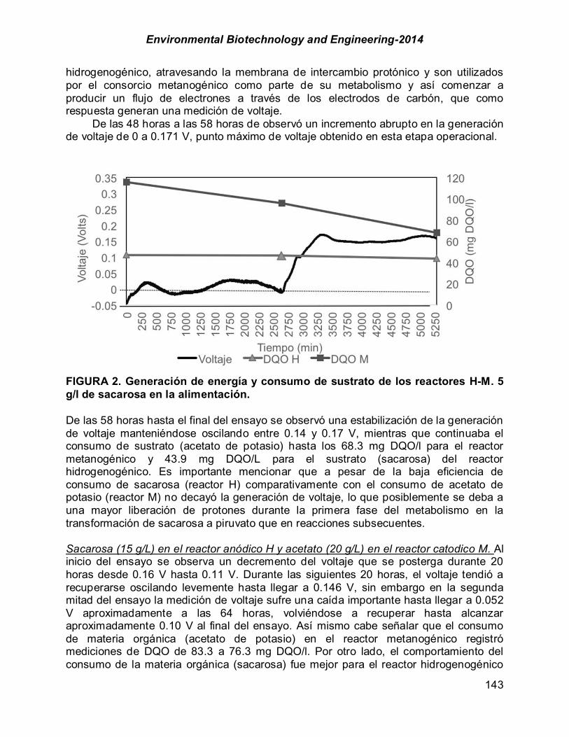
Environmental Biotechnology and Engineering-2014
143
hidrogenogénico, atravesando la membrana de intercambio protónico y son utilizados por el consorcio metanogénico como parte de su metabolismo y así comenzar a producir un flujo de electrones a través de los electrodos de carbón, que como respuesta generan una medición de voltaje. De las 48 horas a las 58 horas de observó un incremento abrupto en la generación de voltaje de 0 a 0.171 V, punto máximo de voltaje obtenido en esta etapa operacional.
FIGURA 2. Generación de energía y consumo de sustrato de los reactores H-M. 5 g/l de sacarosa en la alimentación.
De las 58 horas hasta el final del ensayo se observó una estabilización de la generación de voltaje manteniéndose oscilando entre 0.14 y 0.17 V, mientras que continuaba el consumo de sustrato (acetato de potasio) hasta los 68.3 mg DQO/l para el reactor metanogénico y 43.9 mg DQO/L para el sustrato (sacarosa) del reactor hidrogenogénico. Es importante mencionar que a pesar de la baja eficiencia de consumo de sacarosa (reactor H) comparativamente con el consumo de acetato de potasio (reactor M) no decayó la generación de voltaje, lo que posiblemente se deba a una mayor liberación de protones durante la primera fase del metabolismo en la transformación de sacarosa a piruvato que en reacciones subsecuentes. Sacarosa (15 g/L) en el reactor anódico H y acetato (20 g/L) en el reactor catodico M. Al inicio del ensayo se observa un decremento del voltaje que se posterga durante 20 horas desde 0.16 V hasta 0.11 V. Durante las siguientes 20 horas, el voltaje tendió a recuperarse oscilando levemente hasta llegar a 0.146 V, sin embargo en la segunda mitad del ensayo la medición de voltaje sufre una caída importante hasta llegar a 0.052 V aproximadamente a las 64 horas, volviéndose a recuperar hasta alcanzar aproximadamente 0.10 V al final del ensayo. Así mismo cabe señalar que el consumo de materia orgánica (acetato de potasio) en el reactor metanogénico registró mediciones de DQO de 83.3 a 76.3 mg DQO/l. Por otro lado, el comportamiento del consumo de la materia orgánica (sacarosa) fue mejor para el reactor hidrogenogénico

Environmental Biotechnology and Engineering-2014
144
yendo de 43.9 a 26.3 mg DQO/l, destacando que el mayor consumo de materia orgánica se registró durante las primeras 48 horas.
FIGURA 3. Generación de energía y consumo de sustrato de los reactores H-M. 15 g/l de sacarosa en la alimentación. Si bien la gráfica muestra un decremento en la generación de voltaje, comparativamente con el ensayo previo se puede concluir que en promedio se generó mayor voltaje, ya que se alcanzaron picos máximos con lecturas similares, mostrando una mayor estabilidad en cuanto a la generación constante de voltaje. Lo anterior puede deberse a que este ensayo no se observó una etapa de adaptación, también es posible que los mejores rendimientos fueran alcanzados horas posteriores a la terminación del ensayo ya que si bien se observó buen consumo de sustrato en el reactor hidrogenogénico, fue pobre la degradación para el reactor metanogénico, lo que sugiere que quizá el metabolismo no se llevó a cabo de manera completa, provocando los decrementos en el gráfico descritos en el párrafo anterior. Sacarosa (30 g/L) en el reactor anódico H y acetato (20 g/L) en el reactor catodico M. Durante las primeras 30 horas del ensayo se observa un ligero aumento del voltaje precedido de un decremento importante, comenzando alrededor de 0.15 V y llegando a 0.066 V. Posterior a ello el gráfico muestra un ascenso constante de voltaje para alcanzar una medición de máxima de 0.317 V a las 80 horas. Se observa un buen consumo de materia orgánica tanto en el reactor metanogénico (acetato de potasio), como en el reactor hidrogenogénico (sacarosa), registrando mediciones de 89.6 a 38.5 mg DQO/l para el reactor M y de 65.7 a 29.3 mg DQO/l, destacando que el mayor consumo de materia orgánica para ambas se registró durante las primeras 48 horas. Se puede concluir que la mayor cantidad de degradación se produjo durante las primeras horas del ensayo, sin embargo la mayor generación de voltaje se produjo durante la segunda mitad. Esto se debe a que los protones (H+) y electrones generados durante el metabolismo (en la primera mitad del ensayo) son utilizados posteriormente
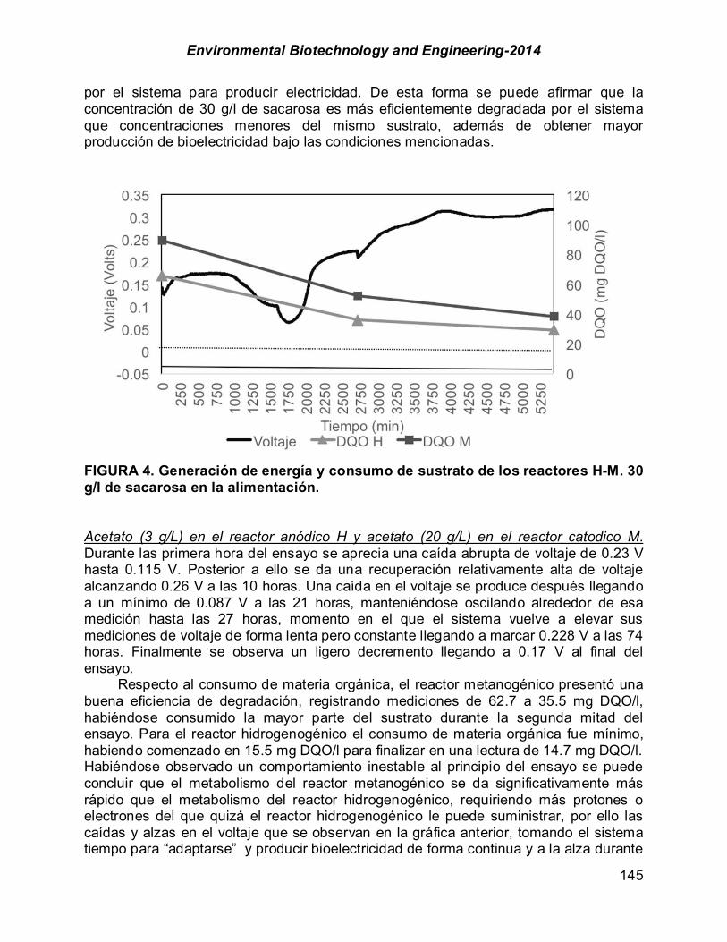
Environmental Biotechnology and Engineering-2014
145
por el sistema para producir electricidad. De esta forma se puede afirmar que la concentración de 30 g/l de sacarosa es más eficientemente degradada por el sistema que concentraciones menores del mismo sustrato, además de obtener mayor producción de bioelectricidad bajo las condiciones mencionadas.
FIGURA 4. Generación de energía y consumo de sustrato de los reactores H-M. 30 g/l de sacarosa en la alimentación.
Acetato (3 g/L) en el reactor anódico H y acetato (20 g/L) en el reactor catodico M. Durante las primera hora del ensayo se aprecia una caída abrupta de voltaje de 0.23 V hasta 0.115 V. Posterior a ello se da una recuperación relativamente alta de voltaje alcanzando 0.26 V a las 10 horas. Una caída en el voltaje se produce después llegando a un mínimo de 0.087 V a las 21 horas, manteniéndose oscilando alrededor de esa medición hasta las 27 horas, momento en el que el sistema vuelve a elevar sus mediciones de voltaje de forma lenta pero constante llegando a marcar 0.228 V a las 74 horas. Finalmente se observa un ligero decremento llegando a 0.17 V al final del ensayo. Respecto al consumo de materia orgánica, el reactor metanogénico presentó una buena eficiencia de degradación, registrando mediciones de 62.7 a 35.5 mg DQO/l, habiéndose consumido la mayor parte del sustrato durante la segunda mitad del ensayo. Para el reactor hidrogenogénico el consumo de materia orgánica fue mínimo, habiendo comenzado en 15.5 mg DQO/l para finalizar en una lectura de 14.7 mg DQO/l. Habiéndose observado un comportamiento inestable al principio del ensayo se puede concluir que el metabolismo del reactor metanogénico se da significativamente más rápido que el metabolismo del reactor hidrogenogénico, requiriendo más protones o electrones del que quizá el reactor hidrogenogénico le puede suministrar, por ello las caídas y alzas en el voltaje que se observan en la gráfica anterior, tomando el sistema tiempo para “adaptarse” y producir bioelectricidad de forma continua y a la alza durante

Environmental Biotechnology and Engineering-2014
146
más tiempo.
FIGURA 5. Generación de energía y consumo de sustrato de los reactores H-M. 3 g/l de acetato de potasio en la alimentación.
Acetato (10 g/L) en el reactor anódico H y acetato (20 g/L) en el reactor catodico M. Al igual que en el ensayo anterior se observa una caída de voltaje durante los primeros 30 minutos comenzando en 0.16 V y llegando a 0.0166 V. Igualmente se da una recuperación de voltaje posterior hasta 0.156 V a las 7 horas. De igual forma, una caída en el voltaje se produce después hasta 0.083 V a las 15 horas, recuperándose también de forma lenta y constante llegando a producir 0.215 V a las 66 horas. En cuanto a consumo de materia orgánica, el reactor metanogénico presentó nuevamente una buena eficiencia de degradación, registrando mediciones de 51.8 a 31 mg DQO/l, habiéndose consumido casi la misma cantidad de sustrato durante la primera y la segunda mitad del ensayo. Para el reactor hidrogenogénico el consumo de materia orgánica fue mayor que el ensayo anterior, habiendo comenzado en 16.6 mg DQO/l para finalizar en una lectura de 12.8 mg DQO/l. El comportamiento comparado con el ensayo en el que se suministró acetato de potasio en 3 g/l es muy similar al observado con 10 g/l, sin embargo los tiempos de caída y recuperación de voltaje son más cortos, lo que sugiere que a mayor concentración, mayor y más rápida será la generación de protones y electrones requeridos por el reactor metanogénico.

Environmental Biotechnology and Engineering-2014
147
FIGURA 6. Generación de energía y consumo de sustrato de los reactores H-M. 10 g/l de acetato de potasio en la alimentación.
Acetato (20 g/L) en el reactor anódico H y acetato (20 g/L) en el reactor catodico M. Nuevamente se aprecia una caída de voltaje durante la primera hora del ensayo comenzando en 0.155 V y llegando a 0.09 V, recuperándose y mostrando un alza de voltaje hasta 0.2 V a las 7 horas. Así mismo una caída en el voltaje se produce después hasta 0.046 V a las 20 horas, recuperándose un poco más rápido hasta llegar a producir 0.195 V a las 34 horas. Posteriormente oscila alrededor de 0.19 V hasta las 63 horas, momento en el que es apreciable la disminución del voltaje alcanzando 0.154 V a las 80 horas. En cuanto a consumo de materia orgánica, el reactor metanogénico presentó una buena eficiencia de degradación, registrando mediciones desde 45.2 a 21.1 mg DQO/l, habiéndose consumido casi la misma cantidad de sustrato durante la primera y la segunda mitad del ensayo. Para el reactor hidrogenogénico el consumo de materia orgánica se llevó a cabo prácticamente en su totalidad, habiendo comenzado en 18.1 mg DQO/l para finalizar en una lectura de 6.9 mg DQO/l. El comportamiento de la gráfica de voltaje sigue siendo similar a los dos anteriores, esta vez con caídas mayores en duración y valor de voltaje, y alzas más lentas. También se observa que al recuperarse el voltaje oscila poco tiempo en su lectura máxima, tendiendo a la baja hacia el final del ensayo. Lo anterior posiblemente se deba a que la concentración de sustrato suministrada sobrepasa los requerimientos del cultivo de B. Subtillis. Así mismo la caída en el voltaje al final del ensayo apoyada con las eficiencias en la degradación de materia orgánica tanto de H como de M sugiere que el metabolismo de los microorganismos se encontraba a la baja debido a la poca concentración de sustrato reportada.

Environmental Biotechnology and Engineering-2014
148
FIGURA 7. Generación de energía y consumo de sustrato de los reactores H-M. 20 g/l de acetato de potasio en la alimentación.
FIGURA 8. Generación global de energía de los reactores H-M. Eficiencias degradativa y energética. La generación de potencia en la PCM (Figura 8) siguió una cinética de saturación; es decir, de utilización del sustrato en sistemas biológicos en función de la concentración y la velocidad de transporte (Liu y Logan, 2004). Como se puede observar en la figura 8, la potencia promedio de cada etapa incrementó a medida que la concentración de sacarosa aumentó. A pesar del comportamiento poco estable al consumo del sustrato sacarosa, el potencial máximo obtenido fue de 21.22 µW, alcanzado al final del ensayo con la máxima concentración de sacarosa. Comparativamente con el comportamiento de generación de potencia
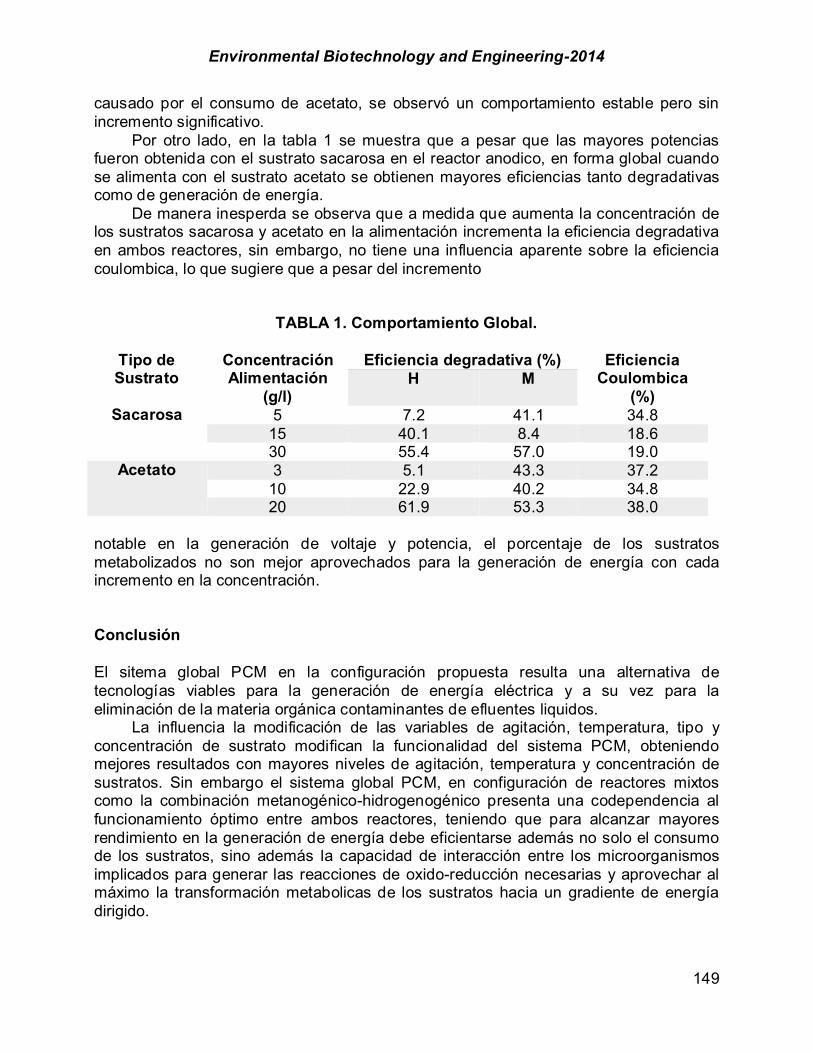
Environmental Biotechnology and Engineering-2014
149
causado por el consumo de acetato, se observó un comportamiento estable pero sin incremento significativo. Por otro lado, en la tabla 1 se muestra que a pesar que las mayores potencias fueron obtenida con el sustrato sacarosa en el reactor anodico, en forma global cuando se alimenta con el sustrato acetato se obtienen mayores eficiencias tanto degradativas como de generación de energía. De manera inesperda se observa que a medida que aumenta la concentración de los sustratos sacarosa y acetato en la alimentación incrementa la eficiencia degradativa en ambos reactores, sin embargo, no tiene una influencia aparente sobre la eficiencia coulombica, lo que sugiere que a pesar del incremento
TABLA 1. Comportamiento Global.
Tipo de Sustrato
Concentración Alimentación
(g/l)
Eficiencia degradativa (%) Eficiencia Coulombica
(%) H M
Sacarosa 5 7.2 41.1 34.8 15 40.1 8.4 18.6 30 55.4 57.0 19.0
Acetato 3 5.1 43.3 37.2 10 22.9 40.2 34.8 20 61.9 53.3 38.0
notable en la generación de voltaje y potencia, el porcentaje de los sustratos metabolizados no son mejor aprovechados para la generación de energía con cada incremento en la concentración. Conclusión El sitema global PCM en la configuración propuesta resulta una alternativa de tecnologías viables para la generación de energía eléctrica y a su vez para la eliminación de la materia orgánica contaminantes de efluentes liquidos. La influencia la modificación de las variables de agitación, temperatura, tipo y concentración de sustrato modifican la funcionalidad del sistema PCM, obteniendo mejores resultados con mayores niveles de agitación, temperatura y concentración de sustratos. Sin embargo el sistema global PCM, en configuración de reactores mixtos como la combinación metanogénico-hidrogenogénico presenta una codependencia al funcionamiento óptimo entre ambos reactores, teniendo que para alcanzar mayores rendimiento en la generación de energía debe eficientarse además no solo el consumo de los sustratos, sino además la capacidad de interacción entre los microorganismos implicados para generar las reacciones de oxido-reducción necesarias y aprovechar al máximo la transformación metabolicas de los sustratos hacia un gradiente de energía dirigido.

Environmental Biotechnology and Engineering-2014
150
Agradecimientos Los autores agradecemos a la DGEST por el financiamiento del proyecto 4623.11-P Referencias APHA, AWWA and WPCF, 1992. Standard Methods for the Examination of Water and Wastewater, 18th
ed. APHA, Washington, DC, 1527 p. Alzate-Gaviria, L.; González, K.; Peraza, I.; García, O.; Domínguez-Maldonado, J.; Vázquez, J.; Tzec-
Simá,M.; Canto-Canché, B. (2010). Evaluación del desempeño e identificación de exoelectrógenos en dos tipos de celdas de combustible microbianas con diferente configuración en el ánodo. Interciencia [en línea] 2010, 35. [fecha de consulta: 15 de agosto de 2014] Disponible en: <http://www.redalyc.org/articulo.oa?id=33913146004> ISSN 0378-1844.
Behera M.; Murthy S. S.; Ghangrekar M.M. (2011). Effect of operating temperatura on performance of microbial fuel cell. Water Sci Technol. 64(4):917-22.
Bond, D. R.; Lovley D. R. (2003). Electricity production by Geobacter sulfurreducens attached to electrodes. Applied and Enviromental Microbiology, 69: 1548-1555.
Bretschger, O.; Cheung, A. C. M.; Mansfeld F.; Nealson K. H. (2010). Comparative Microbial Fuel Cell Evaluations of Shewanella spp. Electroanalysis. 22: 883–894.
Buitrón, G.; Pérez, J. (2011). Producción de electricidad en celdas de combustible microbianas utilizando agua residual: efecto de la distancia entre electrodos. TIP Revista Especializada en Ciencias Químico-Biológicas, 14(1): 5-11.
Catal, T.; Cysneiros, D.; O’Flaherty, V., Leech, D. (2011). Electricity generation in a single-chamber microbial fuel cells using a carbón source sampled from anaerobic reactor utilizing grass silage. Bioresource Technology. 102: 404-410.
Escamilla-Alvarado, C.; Ponce-Noyola, M.T.; Poggi-Varaldo, H.M. (2010). Energetic potential of two-stage hydrogenesis-methanogenesis fermentation of the organic fraction of municipal solid waste. Proceedings of the 14th International Biotechnology Symposium, Rimini, Italy, 2010.
Haiping, L.; Guangli, L.; Renduo, Z.; Song, J. (2008). Phenol degradation in microbial fuel cells. Chemical Engineering Journal. 147: 259-264.
Helder M. (2012). Design criteria for the Plant-Microbial Fuel Cell: Electricity generation with living plants –from lab to application. PhD thesis, Wageningen University, Wageningen, The Netherlands.
Katuri, K. P.; Enright A. M.; O’Flaherty, V.; Leech, D. (2012). Microbial analysis of anodic biofilm in a microbial fuel cell using slaughterhouse wastewater. International Symposium on Bioelectrochemistry and Bioenergetics, 21st BES 2011, 24: 164-171.
Li, L. H.; Sun Y. M., Yuan, Z. H., Kong, X. Y.; Li, Y. (2013). Effect of temperatura change on power generation of microbial fuel cell. Environ Technol. 34(13-169: 1929-34.
Liu, D.; Zeng, R. J.; Angelidaki, I. (2006). Hydrogen and methane production from household solid waste in the two-stage fermentation process. Water Res, Vol. 40, pp. 2230.
Liu, H.; Logan, B. (2004). Electricity generation using an air-cathode single chamber microbial fuel cell in the presence and absence of a proton exchange membrane. Env. Sci. Technol. 38:4040-4046.
Logan, B.E.; Regan, J.M. (2006). Microbial fuel cells: Challenges and applications. Environ. Sci. Technol. 40: 5172-5180.
Poggi-Varaldo, H.M.; Valdés, L.; Fernández-Villagómez, G.; Esparza-García F. (1997). Solid substrate anaerobic co-digestion of paper mill sludge, biosolids, and municipal solid waste. Water Sci. Technol. 35: 197-204.
Revelo, Dolly M.; Hurtado, Nelson H.; Ruiz, Jaime O. (2013). Celdas de combustible microbianas (ccms): un reto para la remoción de materia orgánica y la generación de energía eléctrica. Información tecnológica, 24(6), 17-28.
Ringeisen, B. R.; Ray, R.; Little, B. (2007). A miniature microbial fuel cell operating with an aerobic anode chamber, Journal of Power Sources, 165: 591-597.
Sacco, N.; Pataccini, G.; Bonetto, M. C.; Cortón, E. (2010). Celdas de combustible sedimentarias para la generación de electricidad en ambientes sumergidos. Proceedings Ibensensor 2010, Lisbon, Portugal, 2010.
Tallent, M. S.; Kotewicz K. M.; Strain, E. A.; Bennett, R. W.; Efficient Isolation and Identification of Bacillus cereus Group, Journal of Aoac International. 95:2.

Environmental Biotechnology and Engineering-2014
151
Ueno Y.; Fukui H.; Goto M. (2007). Operation of a two-stage fermentation process producing hydrogen and methane from organic waste. Environ Sci Technol, 41: 1413.
Vanita, R. M.; Chien-Cheng, C.; Hau-Ren, C.; Chien-Yen, C.; Min-Jen, T.; Kai-Chien, C.; Ruey-Chyuan, S.; Young-Fo, C. (2012). A Single-Chamber Microbial Fuel Cell without an Air Cathode. International Journal of Molecular Sciences. 13(3): 3933-3948.
Wang, X.; Feng, Y. J.; Qu, Y. P.; Li, D.M.; Li, H.; Ren, N. Q. (2008). Effect of temperatura on performance of microbial fuel cell using beer wastewater. Huan Jing Ke Xue. 29(11):3128-32.
Environmental Biotechnology and Engineering-2014
152
CHAPTER 1.16. CARACTERIZACIÓN CINÉTICA Y METABÓLICA DE CULTIVOS AISLADOS DE ENSILADO, PRODUCTORES DE ELECTRICIDAD
José D. Bárcenas-Torres*; María de C. Cano-Correa; Adriana del Ángel Guzmán-Tèllez ITM- Div. Ing. Qca. y Bqca, Morelia Mich. México; RESUMEN Con el aislamiento de dos microorganismos con características diferentes, de una muestra de ensilado de maíz, se pudo obtener una producción significativa de electricidad (150 mV), dichos microorganismos fueron sometidos a una serie de técnicas microbiológicas para su identificación morfológica macro y microscópicamente, encontrando que se trataba de dos tipos de microorganismos Gram positivos capaces de generar esporas, su caracterización bioquímica fue realizada mediante el test API 50 CH (Biomérieux), encontrando que pertenecían al género Bacillus con un porcentaje de similitud de 76 % con B. mojavensis y de 93 % con B. subtilis para el primer y segundo cultivo respectivamente. En otra etapa subsecuente se realizaron cinéticas de consumo de sustratos fácilmente asimilables en condiciones tanto aerobias como anaerobias, obteniendo que ambos microorganismos presentaban mayores eficiencia en condiciones anaerobias en la asimilación del acetato de sodio (B. Mojavensis, 99.35%; B. subtilis 43.02%). Finalmente se evidencio la capacidad de los cultivos aislados en la generación de bioelectricidad (150 mV) cuando se opera una pila de combustible microbiano en condiciones anaerobias y alimentando acetato como única fuente de carbono, conteniendo a B. subtilis en la sección catódica y a B. mojavansis en la sección anódica del biorreactor. Con esto se concluye que es una alternativa altamente promisora para la producción de electricidad y el saneamiento de aguas residuales y con ello atacar dos de los problemas más graves que afectan a la sociedad hoy en día. ABSTRACT We isolateD two microorganisms with characteristics different from a sample of corn silage, could get a significant production of electricity (150 mV), such microorganisms were subjected to a series of microbiological techniques for ------------------- *Author for correspondence
Environmental Biotechnology and Engineering-2014
153
morphological identification macro and microscopically, finding that it was of two types of microorganisms Gram positive capable of generating spores, its biochemical characterization was performed using the API 50 CH (bioMérieux) test, finding belonging to the genus Bacillus with a percentage of 76% similarity with B. mojavensis and 93% with B. subtilis for the first and second crop respectively. In another subsequent stage were kinetics of consumption of easily assimilable substrates in conditions both aerobic and anaerobic, obtaining that both microorganisms were greater efficiency under anaerobic conditions in the acetate of sodium (B. Mojavensis, 99.35% acetate; B. subtilis 43.02%). We were able to generate bioelectricity (150 mV) when operating an anaerobic microbial fuel cell and feeding acetate as sole carbon source, containing B. subtilis cathodic section and B. subtilis mojavansis in the anodic section of the bioreactor. Key words: microbial full cell, bioenergy, microbial characterization Introducción En la actualidad la demanda de energía ha incrementado de manera exponencial junto el crecimiento de la población. La producción de hidrógeno de manera biológica es una alternativa sustentable para la producción de biocombustibles. El hidrógeno es un gas, que se obtiene a partir de la electrólisis del agua, pero no es rentable debido a los altos requerimientos de energía en el proceso de producción (Karapinar I. et al 2005). La manera más eficiente de hacer uso del hidrógeno producido bioquímicamente es empleándolo en celdas de combustible microbianas, el cual es un biorreactor que utiliza microorganismos como catalizadores para convertir la energía química almacenada en los sustratos orgánicos en energía eléctrica (Zhao F, et al, 2008). Existe evidencia de la capacidad de esta tecnología. Por ejemplo, Bacillus tequiliensis, fue asilado de una celda de combustible microbiana, obteniendo una producción de 250 mV. (Deepika J. et al., 2013), se reporta la presencia de microorganismos del genero Bacillus en la etapa 4 del ensilaje (Weinberg Z, et al., 1997). La mayoría de las cepas de Bacillus son microorganismos mesófilos, productores de esporas, obtienen sus ganancias energéticas a través de la glucolisis en condiciones aerobias y en condiciones anaerobios a través de la reducción de nitratos. En el proceso de oxidación de la materia orgánica en condiciones anaeróbicas se produce CO2 protones y electrones, mientras que en condiciones aeróbicas únicamente se produciría CO2 y agua. Por ello resulta de interés mantener condiciones anaeróbicas para la generación de electrones:
12 22 11+ 13 2 ! 12 2 + 48 ++ 48 " [1] Los electrones generados son transferidos hacia el electrodo negativo, esta trasferencia puede ocurrir de dos maneras, a través de proteínas conductoras de la membrana celular o bien por mediadores. Los mediadores o lanzadores de protones son sustancias con propiedades redox que actúan como intermediarios entre la membrana celular y el ánodo. Pueden ser añadidos externamente o bien ser excretados como resultado del propio metabolismo microbiano y de esta manera usarlos en las pilas de combustibles microbianas. El objetivo de esta investigación fue aislar, caracterizar bioquímicamente, evaluar
Environmental Biotechnology and Engineering-2014
154
cinéticamente y comprobar si eran capaces los microorganismos aislados de producir un gradiente de protones para la producción de bioelectricidad en una pila de combustible microbiano. Materiales y métodos La metodología empleada se plantea en 4 etapas: 1) Obtención de microorganismos de interés; 2) Caracterización morfológica y bioquímica; 3) Evaluación cinética de los microorganismo aislados, usando sustratos como acetato de sodio y glucosa; y 4) Generación de energía eléctrica, y que se detallan a continuación: Obtención de microorganismos. Para la obtención microorganismos generadores de energía eléctrica se consideró microorganismos como Bacillus y Clostridium, ya que son productores de hidrógeno e intervienen en procesos de generación de energía eléctrica, se encuentran como microorganismos no deseados en ensilado de maíz durante la fase de deterioro aeróbico (Kumar S. et al.,1999).Para la obtención del inoculo se pesaron 15 g de muestra de ensilado de maíz proveniente de Sociedad de productores del Municipio de Queréndaro Michoacán, se trituro en una cápsula de porcelana, seguido de la adición de 10 ml de solución buffer de fosfatos pH 7.2, después se mezcló con 90 ml de solución buffer antes mencionada y 5 mililitros de medio mineral Van Ginkel (Ramón Ma. Mujal Rosas, 2010) se sometió a agitación y ebullición por una hora. Se dejó reposar la muestra durante 30 minutos y se transfirió el sobrenadante a dos tubos estériles, en los cuales uno de ellos se sometió a un choque térmico con baño maría a 80 °C por 5 minutos y posteriormente a baño de hielo, el segundo tubo se usó como control. Se tomó alícuota de 10 ml de cada tubo y se transfirió a dos tubos con 40 ml de caldo nutritivo, estos se llevó a cabo en una cámara de CO2 se sembró una muestra del sobrenadante por estría en agar Columbia; se incubaron a 35 °C por 24 horas, el crecimiento de los tubos se transfirió a medio caldo de res estéril, se incubó en condiciones anaerobias por 48 horas y se transfirió el crecimiento nuevamente en agar Columbia y se incubó en condiciones anóxicas por 24 horas.
Caracterización morfológica y bioquímica. La identificación morfológica se hizo mediante la observación de las colonias en las placas de agar Columbia, se llevaron a cabo tinciones de Gram y Wirtz-Conklin, posteriormente para la identificación bioquímica, se sembró en agar Columbia en tubos con forma en pico el microorganismo aislado, se incubo por 18 horas a 35± 1 °C; Se realizó un lavado de microorganismos con solución buffer 7.2 estéril con 3 lavados a 3500 rpm por 3 minutos, la pastilla obtenida se llevó al patrón 2 escala de McFarland leída a 610 nm en un espectrofotómetro UV-VIS, una vez obtenido el patrón 2 se utilizó el doble de volumen de pastilla se transfirió el crecimiento a las ampolletas de medio API 50 CHB/E, conjuntamente se realizó hidratación de charolas de incubación y el contenido de la ampolleta se sembró en 50 cúpulas contenidos en las pruebas API 50 CHB/E, para cada microorganismo, se llevó acabo por duplicado; después las charolas se incubaron a 35±1°C, se leyeron a las 24 h y las 48 h y se interpretan los resultados con el software apiweb, se realizaron pruebas bioquímicas adicionales como la catalasa y la oxidasa.

Environmental Biotechnology and Engineering-2014
155
Cinética de consumo de sustratos. Se realizó un lavado de los microorganismos se colocó el crecimiento en un agitador de vortex y se agitó por 1 minuto posteriormente se transfirió a tubos para centrifugar estériles, donde se centrifugaron a 3500 rpm por 3 minutos; se desechó el sobrenadante; se homogenizó la pastilla con buffer de fosfatos a un pH de 7.2; la pastilla se resuspendió nuevamente con 10 ml del buffer anteriormente usado repitiendo por 3 veces; Se transfirió una alícuota de 2 ml de los microorganismos con 500 mL, buffer de fosfatos antes mencionado con solución estéril de sacarosa (30 g/L) y acetato de sodio (20 g/L) según el caso y 5 ml de medio mineral Van Ginkel en cada reactor. Para su evaluación. Se adaptaron en total 8 matraces adaptados como reactores, en experimento 22 se realizó por duplicado. Se colocaron en una parrilla con agitación a 30 rpm. Se sellaron herméticamente y se les inyectó gas de dióxido de carbono para asegurar un ambiente anaerobio. En los reactores aerobios se les colocó un magneto estéril para llevar a cabo la agitación una vez que se acondicionaron en la parrilla de agitación, se colocaron dentro de una incubadora donde se mantuvieron a una temperatura de 35±2°C se hizo un primer monitoreo de “tiempo 0”, asimismo se monitoreo el pH con tiras reactivas, y la cantidad de materia orgánica (DQO) inicial en cada uno de los 8 reactores. Ensayos de generación de energía eléctrica. Se realizó un ensayo generación de energía eléctrica, como producto del metabolismo del microorganismo, a partir del consumo de acetato de sodio en condiciones anóxicas. En dos matraces kitasato de 250 ml se colocó entre ellos una membrana de Nafión NR12 espesor de 50.8 µm; a cada uno se colocó una barra de grafito la cual estuvo en contacto con los microorganismos; se colocó una solución acetato de sodio (20 g/L) en cada matraz. Se realizó un lavado de ambos microorganismos se pasaron los microorganismos suspendidos en dos matraces acondicionados como reactores, donde en cada reactor debe haber un microorganismos diferente y se sellaron ambos reactores; se gasearon con CO2 y se colocaron en agitación constante y lenta (30 rpm aproximadamente) en una parrilla de agitación a 36°C se conectaron los reactores a un multímetro donde se tomó la lectura del voltaje generado por un periodo de tiempo de cero hasta que la producción de electricidad fue constante. Resultados y discusión Aislamiento y caracterización microbiana. Se obtuvieron dos tipos de microorga-nismos (S1 Y S2) con diferente morfología lo que se prosiguió a realizarles tinciones, obteniendo cadenas bacilares alargadas gram positivos, pero con diferente morfología bacilar uno más delgados (S2) en comparación a (S1). En la prueba de formación de esporas, los resultados demostraron que ambos aislados S1 y S2 ver Figura 1; fueron capaces de generar estructuras similares a las esporas bacterianas bajo las condiciones empleadas en el protocolo descrito en la metodología, sin embargo la morfología al microscopio de la espora no se mostró característica al género Clostridium, ya que el Clostridium botulinum y Clostridium esporogenes forma esporas subterminales esferoides de diámetro mayor al de la célula vegetativa (Campbell L. et al., 1985)

Environmental Biotechnology and Engineering-2014
156
FIGURA 1. Tinción de esporas para el microorganismo S1, observado al microscopio electrónico con objetivo de 100X. Para conocer de mejor manera la identidad de los géneros aislados así como su metabolismo; se realizaron 49 pruebas bioquímicas pertenecientes al sistema miniaturizado API 50 CHB/E y dos complementarias de los cuales se muestran los resultados en la tabla 2 donde las pruebas bioquímicas se realizaron por duplicado para cada uno de los microorganismos aislados y fue evidente que no hubo ninguna diferencia significativa entre las pruebas con el duplicado de cada uno de ellos. Pero si entre S1 Y S2, ambos microorganismos fueron catalasa positiva y oxidasa positiva, en la TABLA 1 podemos observar que S2 es capaz de fermentar más azucares que S1. Las pruebas API se realizaron por duplicado para asegurar un resultado confiable, ya que no se contó con cepas control caracterizadas, para llevar a cabo un aseguramiento de calidad en los resultados. En la tabla 2 se muestra los resultados obtenidos con un software apropiado para interpretar el test API 50/CH donde los resultados favorecen para el microorganismos S1 a B. Mojavesis y para el microorganismos S2 a B. subtilis con un 82 % y un 93 % de porcentaje de similitud respectivamente. Cinética de consumo de sustratos. Para la caracterización de los aislados obtenidos, se evalúo la capacidad de consumo de sustratos carbonados a diferentes ambientes tal y como se describió en la metodología. Cuando se cultiva, un microorganismo y tiene los nutrientes necesarios, estos empiezan a reproducirse siguiendo un comportamiento, hasta el momento que se agota el sustrato y entran en una fase estacionaria. La tasa de remoción de DQO más alta fue la obtenida en condiciones anaerobias con un porcentaje de 99.35% con S1, utilizando el sustrato acetato de sodio, resulto ser más eficiente en condiciones anaeróbicas en comparación que cuando se dispuso al microorganismo en presencia de oxígeno obteniendo un 90.99%, en cuanto a S2 tuvo una eficiencia muy parecida en el consumo de acetato sodio en atmósfera con y sin oxígeno, con una remoción de DQO de 96.52 y 96.33 %, respectivamente. En el caso del agotamiento de sacarosa, la remoción de DQO para S1 resulto de 43.30% en condiciones aeróbicas y en anaeróbicas fue de 35.86 %, para S2 se obtuvo una remoción de DQO de 43.02% cuando se sometió a atmósfera aeróbica y en
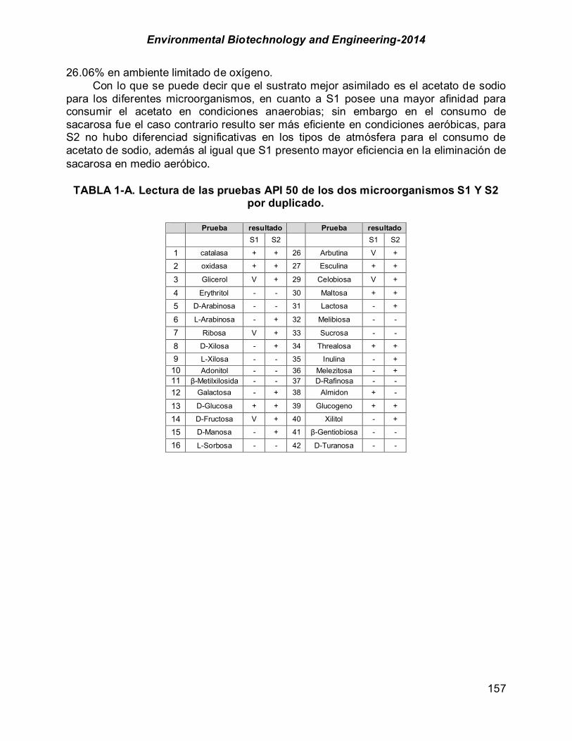
Environmental Biotechnology and Engineering-2014
157
26.06% en ambiente limitado de oxígeno. Con lo que se puede decir que el sustrato mejor asimilado es el acetato de sodio para los diferentes microorganismos, en cuanto a S1 posee una mayor afinidad para consumir el acetato en condiciones anaerobias; sin embargo en el consumo de sacarosa fue el caso contrario resulto ser más eficiente en condiciones aeróbicas, para S2 no hubo diferenciad significativas en los tipos de atmósfera para el consumo de acetato de sodio, además al igual que S1 presento mayor eficiencia en la eliminación de sacarosa en medio aeróbico.
TABLA 1-A. Lectura de las pruebas API 50 de los dos microorganismos S1 Y S2 por duplicado.
Prueba resultado Prueba resultado S1 S2 S1 S2
1 catalasa + + 26 Arbutina V +
2 oxidasa + + 27 Esculina + +
3 Glicerol V + 29 Celobiosa V +
4 Erythritol - - 30 Maltosa + +
5 D-Arabinosa - - 31 Lactosa - +
6 L-Arabinosa - + 32 Melibiosa - -
7 Ribosa V + 33 Sucrosa - -
8 D-Xilosa - + 34 Threalosa + +
9 L-Xilosa - - 35 Inulina - + 10 Adonitol - - 36 Melezitosa - + 11 $-Metilxilosida - - 37 D-Rafinosa - - 12 Galactosa - + 38 Almidon + -
13 D-Glucosa + + 39 Glucogeno + +
14 D-Fructosa V + 40 Xilitol - +
15 D-Manosa - + 41 $-Gentiobiosa - -
16 L-Sorbosa - - 42 D-Turanosa - -
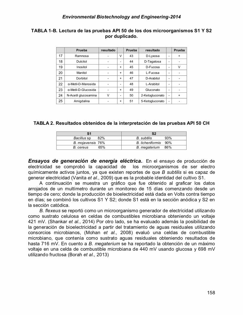
Environmental Biotechnology and Engineering-2014
158
TABLA 1-B. Lectura de las pruebas API 50 de los dos microorganismos S1 Y S2 por duplicado.
Prueba resultado Prueba resultado Prueba
17 Ramnosa - V 43 D-Lyxosa - +
18 Dulcitol - - 44 D-Tagatosa - -
19 Inositol - + 45 D-Fucosa - V
20 Manitol - + 46 L-Fucosa - -
21 Dorbitol - + 47 D-Arabitol - -
22 !-Metil-D-Manosida - - 48 L-Arabitol - -
23 !-Metil-D-Glucosida - + 49 Gluconato - -
24 N-Acetil glucosamina V - 50 2-Ketogluconato - +
25 Amigdalina - + 51 5-Ketogluconato - -
TABLA 2. Resultados obtenidos de la interpretación de las pruebas API 50 CH
S1 S2
Bacillus sp 82% B. subtilis 93% B. mojavensis 76% B. licheniformis 90% B. cereus 65% B. megaterium 86%
Ensayos de generación de energía eléctrica.. En el ensayo de producción de electricidad se comprobó la capacidad de los microorganismos de ser electro químicamente activos juntos, ya que existen reportes de que B subtilis si es capaz de generar electricidad (Vanita et al., 2009) que es la probable identidad del cultivo S1. A continuación se muestra un gráfico que fue obtenido al graficar los datos arrojados de un multímetro durante un monitoreo de 15 días comenzando desde un tiempo de cero; donde la producción de bioelectricidad está dada en Volts contra tiempo en días; se combinó los cultivos S1 Y S2; donde S1 está en la sección anódica y S2 en la sección catódica. B. flexeus se reportó como un microorganismo generador de electricidad utilizando como sustrato celulosa en celdas de combustibles microbiana obteniendo un voltaje 421 mV. (Shankar et al., 2014) Por otro lado, se ha evaluado además la posibilidad de la generación de bioelectricidad a partir del tratamiento de aguas residuales utilizando consorcios microbianos, (Mohan et al., 2008) evaluó una celdas de combustible microbiano, que contenía como sustrato aguas residuales obteniendo resultados de hasta 716 mV. En cuento a B. megaterium se ha reportado la obtención de un máximo voltaje en una celda de combustible microbiana de 440 mV usando glucosa y 698 mV utilizando fructosa (Borah et al., 2013)

Environmental Biotechnology and Engineering-2014
159
Sust
rato
(g/L
)
FIGURA 2. Cinéticas de los reactores, en condiciones aerobias y anaerobias.
Sust
rato
(g/L
)
Tiempo (h)
Environmental Biotechnology and Engineering-2014
160
FIGURA 3. Producción de voltaje.
Tomando en cuenta que la obtención máxima de voltaje en el presente trabajo fue de 150 mV, la generación de bioelectricidad fue baja comparativamente con los estudios anteriores. Se proponen tres rutas metabólicas (Ramos et al., 2000.y Schiling, 2006) que son propuestas para la producción de bioelectricidad. En la primera ruta metabólica se propone el consumo de acetato en condiciones anaerobias donde entra después de haberse llevado a cabo la glucolisis, si se parte de acetato de producen dos moléculas de NAD+ ; si se parte del lactato se reducen 4 moléculas de NADH.+H+ (Ramos et al., 2000). Por otro lado las vías de glucolisis es la alternativa para diferentes bacterias además de oxidar la glucosa, la vía opcional más frecuente es la vía de las pentosas fosfato, otra opción consiste en la vía Entner-Doudoff. La vía de las pentosas opera simultáneamente con la glucolisis para oxidar la glucosa y permite degradar azucares de cinco carbonos además de la glucosa, bacterias que utilizan la vías de las pentosas fosfato son B.subtilis, E.coli, Lauonosstoc mesenteroides y Enterococcus Fecalis (Tortora et al., 2007). La ecuación global de la glucólisis seria la siguiente por cada molécula de glucosa se generan, dos moléculas de piruvato, dos moléculas de NADH + H+ y dos ATP se puede sintetizar de la siguiente manera:
Glucosa + 2 NAD+ + 2ADP + 2 Pi " 2 Piruvato + 2 NADH + 2 H+ + 2 ATP [2]
Cuando existen condiciones con limitación de nitrato partiendo del piruvato puede tomar tres caminos, como fermentación láctica, también puede que producir acetil-CoA más ATP y acido acético y producir acetoina con reacción reversible de butanediol. +
(Monteros et al., 2005).Tanto a S1 y S2 se les añadió en el medio mineral de micronutrientes para favorecer la producción de hidrogeno. Si existe un limitación de oxigeno trae consigo cambios en su metabolismo celular, tales como ajustes en las rutas metabólicas y en las velocidades de utilización de las fuentes de carbono, en el flujo de electrones para el mantenimiento del balance redox,
0
0.02
0.04
0.06
0.08
0.1
0.12
0.14
0.16
0.0 2.0
Vol
taje
(V
olts
)
Tiempo (Dias)

Environmental Biotechnology and Engineering-2014
161
en los mecanismos para la producción de energía y en ciertas reacciones biosintéticas (Nakano et. al., 1997) una de las principales rutas afectadas por la presencia o ausencia de oxigeno es la glucólisis, fundamentalmente en el destino del piruvato y el NADH siguiendo una ruta alterna haciendo uso del nitrato del medio. También se han propuesto rutas metabólicas donde se lleva a cabo la fermentación de materia orgánica para B. subtilis donde se reducen los nitratos a hasta obtener el ión amonio obteniendo como producto dos moléculas de NADH+H+ (Monteros et al., 2005). Los electrones generados de la oxidación de NADH.+H+. + 2 e- son transferidos hacia el electrodo negativo y hacia el ánodo, esta trasferencia puede ocurrir de dos maneras, a través de proteínas conductoras de la membrana celular o bien a través de mediadores. Los mediadores o lanzadores de protones son sustancias con propiedades redox que actúan como intermediarios entre la membrana celular y el ánodo. Pueden ser añadidos externamente o bien ser excretados como resultado del propio metabolismo microbiano Conclusión Se aislaron dos tipos diferentes de microorganismos nombrados S1 y S2, Gram positivos formadores de esporas, catalasa-oxidasa positivos, y que por ensayos bioquímicos presentarón similitud de identidad con cepas pertenecientes al género Bacillus. Para el cultivo S1 se obtuvo los siguientes porcentajes de similitud: Bacillus sp. 82%, B. mojavensis 76% y B.cereus 65%, mientras que el cultivo S2 presentó porcentajes de similitud con B. subtilis de 93%, B.licheniformis 90% y B.megaterium 86%. Cabe mencionar que se debe proseguir con la identificación a nivel molecular (16 S) para una caracterización completa. Se determinó que S1 y S2 poseen mayor afinidad por el sustrato de acetato de sodio en condiciones limitadas de oxigeno logrando una remoción de DQO del 99.35 y 96.33 por ciento respectivamente, además S1 y S2 en condiciones aerobias rindieron un porcentaje de remoción de DQO de 90.99 y 96.52% correspondientemente, a la degradación de sacarosa, que se metabolizo con una menor velocidad en 48 horas el porcentaje de remoción no supero la degradación del 50% de materia orgánica en ambiente aerobio. El ensayo de producción de electricidad se comprobó que las bacterias son productoras de electricidad obteniendo voltaje de 150 mV a partir de la fermentación de acetato de sodio, en condiciones limitadas de oxigeno que fue donde se presentó un porcentaje de remoción mayor de DQO, de acuerdo la cinética de consumo de sustratos simples que se llevó a cabo, manteniéndolas a una temperatura de 35 ± 2 °C, en una incubadora y manteniéndola en agitación de 30 rpm aproximadamente. Agradecimientos Los autores agradecn a la DGEST el financiamiento del proyecto 4623.11-P

Environmental Biotechnology and Engineering-2014
162
Referencias Borah D., More S. (2013). Construction of double chambered microbial fuel cell (MFC) using household
materials and Bacillus megaterium isolate from tea garden soil. Adv. Biol. Res. 7 (5): 136-140. Claus D., Berkeleyr.C.W. (1986). The genus Bacillus. J. Sci, XX:1105-1139 Davis, Dulbecco, Eisen, Ginsberg, Wood, (2005) Tratado de microbiologia. 2da edición Ed Mc Graw hill .
56 Deepika J., Meignanaksmis., Thilagra R.W. (2013). A study of bioelctricity production by the synergist
action of production bacillus tequilensis DMR-5 Pseudomonas aeroginosa DMR-3 isolated from rumen fluid. Am. J. Environ. Sci. (5): 424-430.
Donald A.S., Fenlon D.R.,Seddon, B. (1995). The relationships between ecophysiology, indigenous microflora and growth of Listeria monocytogenes in grass silage. J. Appl. Bacteriol. 79: 141-148.
Ramos Cruz H., Hoffmannt., Marinom., Nedjari H. Dreesen O., Jahn P.G. (2000). Fermentative metabolism of Bacillus subtilis: Physiology and regulation of gene expression (2000) J. Bacteriol. 10.1128/JB.182.11.3072-3080.2000.
Environmental Biotechnology and Engineering-2014
163
CHAPTER 1.17. ESTUDIO PRELIMINAR DEL COMPORTAMIENTO VOLTAICO DE CELDA DE COMBUSTIBLE MICROBIANO, EMPLEANDO LODO ANAEROBIO
PROVENIENTE DE LA REGIÓN SEMIDESÉRTICA DEL ESTADO DE COAHUILA
Juan A.Ugalde-Medellín; M. Fernanda Rodríguez-Flores; Mónica M. Rodríguez-Garza*; José A. Rodríguez-de la Garza;
Yolanda Garza-García;
Biotechnology Department, Chemistry Faculty, Universidad Autónoma de Coahuila, México RESUMEN Una celda de combustible microbiana o CCM es una tecnología emergente, destinada a la producción de energía eléctrica directamente de la biodegradación de materia orgánica por bacterias. En este tipo de sistemas los microorganismos producen energía a partir de compuestos orgánicos e inorgánicos por medio de reacciones de óxido reducción, generando así electrones los cuales liberan al medio extracelular para que sean capaces de llegar a un aceptor final, en este caso, un electrodo toma el papel de dicho aceptor permitiendo que los electrones liberados circulen a través de un circuito electroquímico, generando corriente eléctrica. En cuanto a la capacidad de generación de energía se conoce que el uso de consorcios o cultivos mixtos son capaces de generar densidades de energía mayores que aquellas cámaras que utilizan cultivos puros, además se han buscado estrategias para incrementar la potencia voltaica de las CCM pero los estudios en su mayoría se han centrado en el diseño mismo de la celda o en el tipo de sustrato utilizable. El objetivo de este estudio es el de evaluar una serie de celdas combustible microbianas montadas a partir de consorcios microbianos obtenidos de sedimentos de cuerpos de agua con características y capacidades únicas y propias de la región semidesértica del estado de Coahuila. Empleando para este estudio un diseño de celdas de dos cámaras en H, previamente utilizado y cuyos rendimientos al trabajar con lodos anaerobios generaron resultados favorables. El enriquecimiento de microorganismos exoelextrogénicos sobre electrodos de acero inoxidable cubiertos de grafito se realizó en forma de batch alimentado, durante 5 semanas, usando el mismo medio al usar un sistema de CCM. Los resultados preliminares de trabajo en la celda muestran evidencia de la formación de biopelícula exoelectrogénica. Palabras clave: exoelectrógenicos, celda de combustible microbiana, sedimentos Introducción En la actualidad ha crecido el interés por encontrar fuentes de energía alterna, esto debido, al claro aumento desmedido en el uso de energía eléctrica, aunado a la sobrepoblación en los países con mayor consumo de recursos, ha llevado a la necesidad de encontrar fuentes de energía renovable para satisfacer este enorme ----------------- *Author for all correspondence: [email protected]
Environmental Biotechnology and Engineering-2014
164
consumo energético. Esta vertiente apunta a que en próximos años el consumo de energía y recursos aumentara vertiginosamente (Calderón & P, 2004), aunado claro a la contaminación medioambiental, la depredación humana a los ecosistemas y del desecho inadecuado de productos tóxicos.
En los últimos años, este desgaste ambiental ha ido generado concientización en las sociedades actuales, las cuales han centrado cada vez más recursos en limpiar sus tecnologías, sin embargo, se debe comenzar a centrar esfuerzos en desarrollar, difundir y utilizar tecnologías completamente limpias. El principal inconveniente está en que después de todo el daño generado al planeta existen zonas repletas de contaminantes ya sea en mayor o menor grado; esta contaminación existe tanto en zonas despobladas como pobladas por el hombre, lo cual no solo atenta contra la salud de las personas, sino también contra el delicado equilibrio natural de las diferentes biosferas, lo que representa un foco rojo de alerta, por lo cual debemos tomar acciones y medidas lo más pronto posible desarrollando tecnologías que no solo sean limpias y amigables al medio ambiente, sino también debemos centrar esfuerzos en desarrollar tecnologías que sean capaces de remediar los estragos medioambientales ya ocasionados. Tal es el caso de la contaminación del agua sea cual sea su procedencia, y, pese a que podamos encontrar nuevas tecnologías que nos permitan generan energía de forma limpia, el agua es por el momento irremplazable, siendo un recurso vital que necesitamos preservar, por lo tanto el intereses político mundial, social y vital ha motivado el encontrar solucione, para alcanzar así uno de los grandes pilares de la sustentabilidad (Castillo, 2012).
Los altos niveles de materia orgánica biodegradable en ciertos tipos de efluentes como lo es el agua doméstica, industrial o del mismo campo, han ganado importancia y no solo por incrementar su potabilización, sino por el potencial aprovechamiento de este tipo de materia orgánica en energía. Esto gracias al empleo de una tecnología que actualmente está cobrando mayor fuerza y es el uso de celdas de combustible microbianas o MFC (microbial fuel cell) las cuales son capaces gracias a los de microorganismos presentes en ellas de, no solo eliminar algunos de los contaminantes disueltos en el agua, sino también, de generar energía eléctrica gracias a su peculiar metabolismo empleando una celda de combustible (Mara Alejandra & Lizcano-valbuena, William H; Bravo, 2012).
Las celdas de combustible fueron descubiertas originalmente por William Grove en 1839, pero fue gracias al desarrollo de la carrera espacial que las celdas de combustible (entre ellas las microbianas) encontraron un uso práctico y se popularizaron como fuentes alternativas de energía. Las celdas de combustible originalmente propuestas son dispositivos que producen electricidad y calor a raíz de la combustión a alta temperatura o combinado hidrogeno con oxígeno sin involucrar un proceso de alta temperatura (Rozo & Tibaquirá, 2007), sin embargo esto conlleva a ciertos problemas implícitos en los materiales empleados en la celda y su manejo. Una opción de este tipo de energías alternas son las celdas de combustible microbianas o MFC por sus siglas en inglés (Microbial Fuel Cell), las cuales han atraído a atención de los investigadores durante los últimos 15 años como una opción para la generación de energía a partir de biomasa residual siendo así una herramienta biotecnológica por el empleo de microorganismos que actúen como biocatalizadores sobre la materia orgánica para la obtención directa de energía (Alzate-gaviria et al., 2010) y en algunos casos la bioremediación del agua.

Environmental Biotechnology and Engineering-2014
165
Environmental Biotechnology and Engineering-2014
166
Materiales y métodos Muestreo. los sedimentos con los que se ha trabajado fueron recolectados en el municipio de Paredón Coahuila, a las afueras del mismo municipio, el estanque de donde se obtuvo presenta una amplia biodiversidad tanto animal como vegetal; la recolección se realizó siguiendo lo ya mencionado en la literatura (Bonetto, 2010): se tomó sedimento y agua a 15 cm de profundidad y a 10 cm de la orilla. Se registraron el pH y algunas de las características organolépticas de la misma fosa de agua. Se cubrieron los recipientes en papel aluminio y fueron preservados a 4°C hasta su procesamiento y caracterización fisicoquímica. Caracterización fisicoquímica de las muestras. Las muestras presentaron ligera turbidez, con fuere olor a azufre y presencia de algas macroscópicas. Se determinaron los siguientes parámetros fisicoquímicos: PO3 (NMX-AA-029-SCFI-2001), SO4 (NMX-AA-074-1981), Dureza (NMX-AA-072-SCFI-2001), pH (NMX-AA-008-SCFI-2011), NO2 (NMX-AA-079-SCFI-2001) y DQO (NMX-AA-030-SCFI-2001). Acondicionamiento de los electrodos anódicos. Para la generación de la biopelícula se utilizaron como electrodos placas de acero inoxidable recubiertas de grafito de 11 a 12cm2 de superficie por cara, 100mL de la muestra de sedimento, y medio líquido, diseñado en el departamento (Rodríguez-Martinez J. et.al), y cuya fuente de carbonos es glucosa, hasta completar un volumen de 250mL. Los electrodos se incubaron a la misma temperatura de la muestra del sedimento hasta observar una disminución de la concentración de sulfato inicial y un aumento en la cantidad de DQO. Periódicamente se tomaron alícuotas para evaluar los parámetros de: DQO, proteínas totales, sulfatos totales y pH inicial y final. Preparación y generación de energía en las celdas de combustible microbianas. Para el ensamblaje de las cámaras se adecuaron ocho electrodos de acero inoxidable (cuatro de ellos destinados a la cámara catódica y los otros cuatro a la cámara anódica), todos soldados a dos cables y recubiertos completamente de grafito. Una vez transcurridas las 6 semanas se armaron 3 celdas de diseño en H, utilizándose en el cátodo una solución de ferrocianuro de potasio además del electrodo correspondiente, en el armado se empleó una membrana de CMI 7000, y en cuanto al ánodo se empleó medio líquido y el electrodo previamente acondicionado además de un 30% en volumen de sedimento. Se empleó un control negativo el cual contenía en el compartimento anódico un electrodo sin microorganismos. Para registrar los datos de voltaje en la celda se utilizó un sistema de adquisición de datos DattaLogger Madge Tech de 8 canales acoplado a una computadora. Durante este tiempo se tomaron alícuotas periódicas para determinar sulfatos y DQO. Una vez concluido el experimento se tomaron muestras del ánodo y se desarrollaron cultivos en presencia y ausencia de oxígeno en placas de agar nutritivo, agar bacteriológico y de agar bacteriológico preparado con el agua de la muestra. Paralelamente se obtuvo material de los electrodos con el cual se llevó acabo amplificación del material genético.

Environmental Biotechnology and Engineering-2014
167
Resultados y discusión Caracterización fisicoquímica de las muestras. Los resultados de la caracterización se presentan en la tabla 1.
TABLA 1. Caracterización de las muestras de agua.
Tal como se aprecia en la tabla 1 las dos muestras de Paredón Coahuila presentan características similares. Para el estudio, se empleó la muestra dos por contar con concentraciones más elevadas de sulfatos, fosfatos y DQO. Seguimiento de la incubación del sedimento de Paredón. De acuerdo a las determinaciones realizadas en la etapa de acondicionamiento de los electrodos a partir del sedimento, observamos un aumento de la cantidad de DQO a partir de la semana número 4, lo que concuerda en tiempo con una disminución de la concentración de sulfato total; en cuanto al pH se aprecia una ligera acidificación del mismo, comenzando con un pH inicial de 7 disminuyó a un pH final de 6.8. Los resultados de las determinaciones están expresados en las siguientes gráficas, donde la concentración expresada está en función de mg/L y semanas de muestreo.
Las graficas1 y 2 muestran que después de la semana 4 hay un crecimiento logarítmico en cuanto a la concentración de DQO y un descenso de la concentración del sulfato total, lo que indica que los microorganismos están creciendo y multiplicándose en el medio de cultivo y como se espera también sobre los electrodos.
Analito Muestra Concentración Nitratos M1 No detectable
M2 No detectable Fosfatos M1 0.04 mg/L
M2 0.08 mg/L DQO M 1 0 mg/L
M2 0.01 mg/L Sulfatos M1 2.474 mg/L
M2 2.609 mg/L pH
M1 7 M2 7
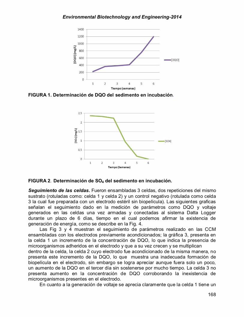
Environmental Biotechnology and Engineering-2014
168
FIGURA 1. Determinación de DQO del sedimento en incubación.
FIGURA 2. Determinación de SO4 del sedimento en incubación. Seguimiento de las celdas. Fueron ensambladas 3 celdas, dos repeticiones del mismo sustrato (rotuladas como: celda 1 y celda 2) y un control negativo (rotulada como celda 3 la cual fue preparada con un electrodo estéril sin biopelícula). Las siguientes graficas señalan el seguimiento dado en la medición de parámetros como DQO y voltaje generados en las celdas una vez armadas y conectadas al sistema Datta Logger durante un plazo de 6 días, tiempo en el cual podemos afirmar la existencia de generación de energía, como se describe en la Fig. 4.
Las Fig 3 y 4 muestran el seguimiento de parámetros realizado en las CCM ensambladas con los electrodos previamente acondicionados; la gráfica 3, presenta en la celda 1 un incremento de la concentración de DQO, lo que indica la presencia de microorganismos adheridos en el electrodo y que a su vez crecen y se multiplican dentro de la celda, la celda 2 cuyo electrodo fue acondicionado de la misma manera, no presenta este incremento de la DQO, lo que muestra una inadecuada formación de biopelícula en el electrodo, sin embargo se logra apreciar aunque fuera solo un poco, un aumento de la DQO en el tercer día sin sostenerse por mucho tiempo. La celda 3 no presenta aumento en la concentración de DQO corroborando la inexistencia de microorganismos presentes en el electrodo. En cuanto a la generación de voltaje se aprecia claramente que la celda 1 tiene un

Environmental Biotechnology and Engineering-2014
169
decrecimiento en el voltaje sin embargo se aprecian picos generados por la energía producida por los microorganismos. La celda 2 presenta un decaimiento del voltaje aún más marcado que en la celda 1. En la celda 3 sin microorganismos, se aprecia un descenso gradual del voltaje sin modificaciones ni picos, con tendencia a descarga total. Esto nos indica la presencia de una biopelícula anodofilica en la celda 1, y confirma de presencia de microorganismos con capacidad exoelectrogénica. Pruebas para verificar la presencia de biopelícula en el electrodo. Tanto en las cajas, la de agar nutritivo y el agar bacteriológico preparado con agua de Paredón estéril, e incubadas con y sin oxígeno presente hubo crecimiento de microorganismos. La Fig. 5 muestra dos de los cultivos con mayor crecimiento. Se realizaron resiembras, aislamiento, frotis y tinción de Gram, encontrándose en el agar bacteriológico abundantes cocos y en el agar nutritivo una multitud de microorganismos diferentes. En la imagen de la derecha se observan dos morfologías similares pero con color ligeramente amarillento. En la tinción de frotis de ambas cajas se logran apreciar tres morfologías diferentes de bacterias Gram positivas,
FIGURA 1. Monitoreo por DQO en Celdas.
FIGURA 3. Monitoreo de la materia orgánica (DQO) en los licores de las celdas.
FIGURA 4. Monitoreo de la generación de energía de las celdas.
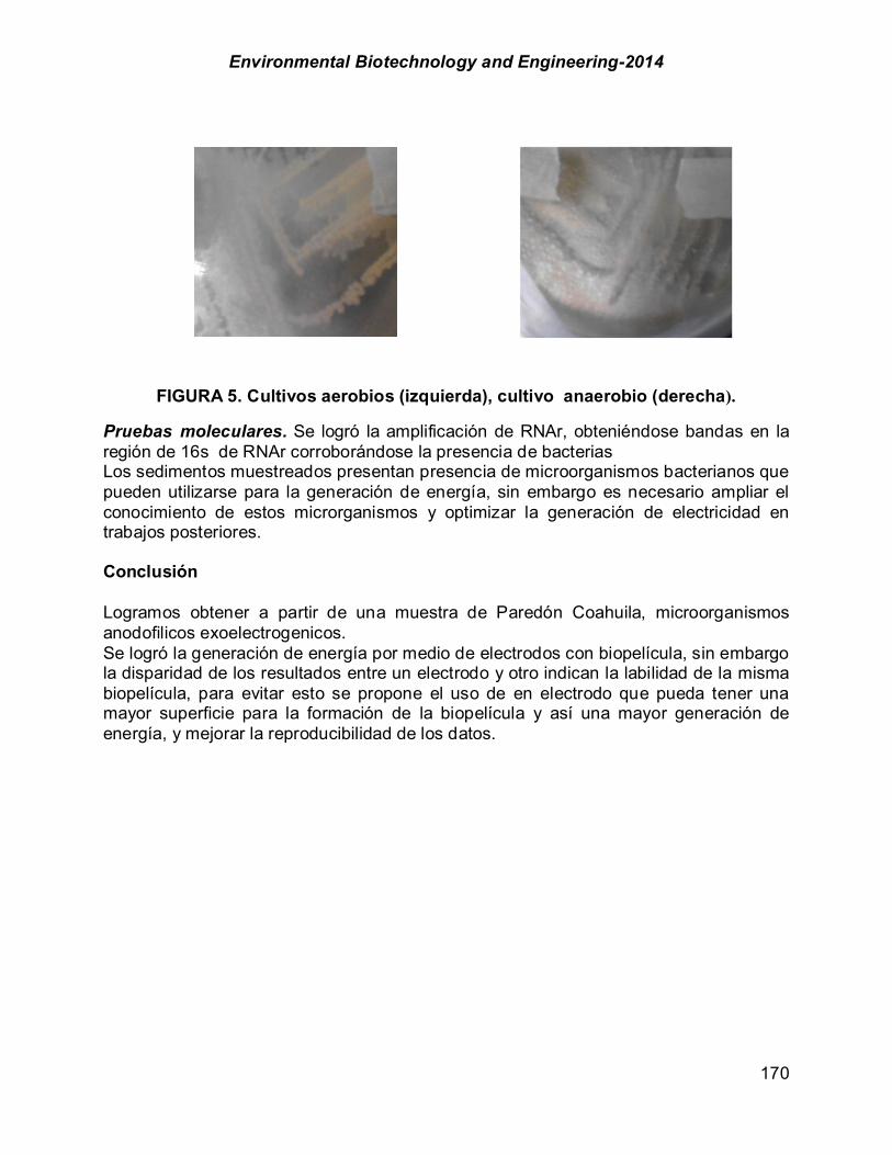
Environmental Biotechnology and Engineering-2014
170
FIGURA 5. Cultivos aerobios (izquierda), cultivo anaerobio (derecha).
Pruebas moleculares. Se logró la amplificación de RNAr, obteniéndose bandas en la región de 16s de RNAr corroborándose la presencia de bacterias Los sedimentos muestreados presentan presencia de microorganismos bacterianos que pueden utilizarse para la generación de energía, sin embargo es necesario ampliar el conocimiento de estos microrganismos y optimizar la generación de electricidad en trabajos posteriores. Conclusión Logramos obtener a partir de una muestra de Paredón Coahuila, microorganismos anodofilicos exoelectrogenicos. Se logró la generación de energía por medio de electrodos con biopelícula, sin embargo la disparidad de los resultados entre un electrodo y otro indican la labilidad de la misma biopelícula, para evitar esto se propone el uso de en electrodo que pueda tener una mayor superficie para la formación de la biopelícula y así una mayor generación de energía, y mejorar la reproducibilidad de los datos.

Environmental Biotechnology and Engineering-2014
171
Agradecimientos Se agradece al Consejo Nacional de Ciencia y Tecnología de México (CONACYT) por becas de Maestría en Biotecnología y a la Universidad Autónoma de Coahuila a través del Departamento de Biotecnología por brindar apoyo al presente trabajo. Referencias Alzate-Gaviria, L.; González, K.; Peraza, I.; García, O.; Domínguez-Maldonado, J; Vázquez, J.; Canto-
Canché, M.T.B. (2010). Evaluación del desempeño e identificación de exoelectrógenos en dos tipos de celdas de combustible microbianas con diferente configuración en el ánodo, 35, 19–25.
Bonetto-Sacco, N.C; Pataccin, G. (2010). Celdas de Combustible Sedimentarias para la Generación de Electricidad en Ambientes Sumergidos, (November), 9–11.
Calderón, M.; Mesa, L. (2004). Principios de funcionamiento y construcción de una celda de combustible de ácido fosfórico (PAFC).
Castillo-Rutely, C. B. (2012). Evaluación electroquímica de materiales anódicos y su aplicación en celdas de combustible. Tesis.
Lizcano-Valbuena, M.A.; William, H; Bravo, E. (2012). Actividad electrogénica de lodos del lago de la universidad del valle, 161–167.
NMX-AA-008-SCFI-2011; Norma Oficial Mexicana; Análisis de agua - Determinación de pH - método de prueba
NMX-AA-029-SCFI-2001; Norma Oficial Mexicana; Análisis de aguas - Determinación de fósforo total en aguas naturales, residuales y residuales tratadas - método de prueba
NMX-AA-030-SCFI-2001; Norma Oficial Mexicana; Análisis de agua - Determinación de la demanda química de oxígeno en aguas naturales, residuales y residuales tratadas - método de prueba
NMX-AA-074-1981; Norma Oficial Mexicana; Análisis de agua - Determinación del ion sulfato NMX-AA-072-SCFI-2001; Norma Oficial Mexicana; Análisis de agua - Determinación de dureza total en
aguas naturales, residuales y residuales tratadas - método de prueba NMX-AA-079-SCFI-2001; Norma Oficial Mexicana; Análisis de aguas - Determinación de nitratos en
aguas naturales, potables, residuales y residuales tratadas - método de prueba Rodríguez-Martínez, J.; Martínez-Amador, S.Y.; Garza-García, Y., Soria-Ortiz, A.I. (2007). Evaluation of
nitrate reduction, sulfate reduction and methanogenesis by biofilms system on Opuntia imbricata. Libro electrónico de Memorias de Congreso Internacional de Química Industrial 07. (ISBN-970-694-390-0).p.105-112
Rozo, S.M.; Tibaquirá, J.E. (2007). Celdas de combustible tipo membrana de intercambio protónico, XIII, 279–283.
Abreviaturas 16s Medida de sedimentación propio de ribosomas procariotes. CCM Celda de combustible microbiana. DQO Demanda química de oxígeno. MFC Microbial fuell cel. RNAr Ácido ribonucleico ribosomal.
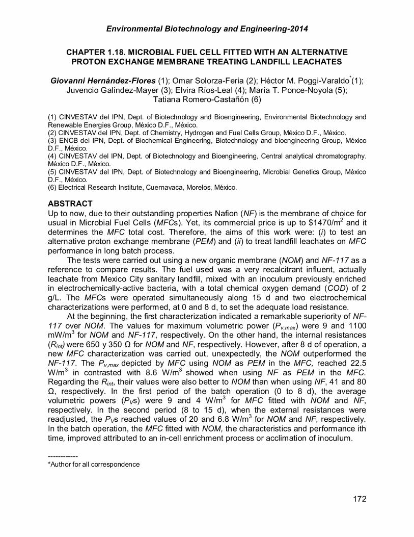
Environmental Biotechnology and Engineering-2014
172
CHAPTER 1.18. MICROBIAL FUEL CELL FITTED WITH AN ALTERNATIVE PROTON EXCHANGE MEMBRANE TREATING LANDFILL LEACHATES
Giovanni Hernández-Flores (1); Omar Solorza-Feria (2); Héctor M. Poggi-Varaldo*(1);
Juvencio Galíndez-Mayer (3); Elvira Ríos-Leal (4); María T. Ponce-Noyola (5); Tatiana Romero-Castañón (6)
(1) CINVESTAV del IPN, Dept. of Biotechnology and Bioengineering, Environmental Biotechnology and Renewable Energies Group, México D.F., México. (2) CINVESTAV del IPN, Dept. of Chemistry, Hydrogen and Fuel Cells Group, México D.F., México. (3) ENCB del IPN, Dept. of Biochemical Engineering, Biotechnology and bioengineering Group, México D.F., México. (4) CINVESTAV del IPN, Dept. of Biotechnology and Bioengineering, Central analytical chromatography. México D.F., México. (5) CINVESTAV del IPN, Dept. of Biotechnology and Bioengineering, Microbial Genetics Group, México D.F., México. (6) Electrical Research Institute, Cuernavaca, Morelos, México. ABSTRACT Up to now, due to their outstanding properties Nafion (NF) is the membrane of choice for usual in Microbial Fuel Cells (MFCs). Yet, its commercial price is up to $1470/m2 and it determines the MFC total cost. Therefore, the aims of this work were: (i) to test an alternative proton exchange membrane (PEM) and (ii) to treat landfill leachates on MFC performance in long batch process. The tests were carried out using a new organic membrane (NOM) and NF-117 as a reference to compare results. The fuel used was a very recalcitrant influent, actually leachate from Mexico City sanitary landfill, mixed with an inoculum previously enriched in electrochemically-active bacteria, with a total chemical oxygen demand (COD) of 2 g/L. The MFCs were operated simultaneously along 15 d and two electrochemical characterizations were performed, at 0 and 8 d, to set the adequate load resistance. At the beginning, the first characterization indicated a remarkable superiority of NF-117 over NOM. The values for maximum volumetric power (Pv,max) were 9 and 1100 mW/m3 for NOM and NF-117, respectively. On the other hand, the internal resistances (Rint) were 650 y 350 # for NOM and NF, respectively. However, after 8 d of operation, a new MFC characterization was carried out, unexpectedly, the NOM outperformed the NF-117. The Pv,max depicted by MFC using NOM as PEM in the MFC, reached 22.5 W/m3 in contrasted with 8.6 W/m3 showed when using NF as PEM in the MFC. Regarding the Rint, their values were also better to NOM than when using NF, 41 and 80 #, respectively. In the first period of the batch operation (0 to 8 d), the average volumetric powers (PVs) were 9 and 4 W/m3 for MFC fitted with NOM and NF, respectively. In the second period (8 to 15 d), when the external resistances were readjusted, the PVs reached values of 20 and 6.8 W/m3 for NOM and NF, respectively. In the batch operation, the MFC fitted with NOM, the characteristics and performance ith time, improved attributed to an in-cell enrichment process or acclimation of inoculum. ------------ *Author for all correspondence

Environmental Biotechnology and Engineering-2014
173
The COD removals at the end of the batch operation (15 d) were ~40% and 30% for NOM and NF, respectively. In this study, the NOM hold promise as PEM for replacing the more expensive NF-117 membrane in MFCs. Key words: Alternative exchange membrane, Nafion® 117, Microbial fuel cell, Landfill leachates Introduction Nowadays the humankind depends heavily on the use of petroleum oil and consequently faces two great risks: the inevitable depletion and the environmental pollution caused during exploration, transport, combustion of oil-based fuels. Thus, the investigation to develop new renewable energy sources as well as bioenergies has notably increased in the last years (Cheng-Dar et al., 2001; Logan and Regan 2006; Das et al., 2001). Microbial fuel cells (MFCs) are a promising technology that generates electrical power from a wide range of soluble substrates (organic or inorganic), wastes included. It constitutes an interesting alternative to produce electrical energy and provide wastewater treatment simultaneously. (Logan and Rabaey, 2012; Hou et al., 2014; Pant et al., 2010). A MFC is an electro-biochemical reactor capable of directly converting organic matter into electricity; the process is driven by microorganisms (biocatalysts) which act as catalysts for the anoxic oxidation of the substrate (“fuel”) in the anodic chamber (Modin and Gustavsson, 2014; Poggi-Varaldo et al., 2009; Vazquez-Larios et al., 2010). The substrate e. g. wastewater is oxidized anaerobically and release electrons and protons. The electrons are collected by the anode (an intermediate external electron acceptor), and flow through an external circuit with a load resistance to produce electricity. On the other hand, the protons pass through a separator or membrane reaching the cathode. Finally, at the cathode the electrons react with protons and molecular oxygen producing water in what is known as the oxygen reduction reaction (Poggi-Varaldo et al., 2009; Vazquez-Larios et al., 2010; Du et al., 2007; Lefebvre et al., 2008; Ouitrakul et al., 2007; Yang et al., 2010). In order to increase the MFC efficiency, several conditions of MFC operation and components have been the subject of intensive research such as the type of biocatalysts, membrane (electrolyte) or separators, temperature, pH, substrates, the type and materials of electrodes, electrode catalysts, cell configuration and architecture, among others (Logan and Regan 2006; Yang et al., 2010; Kim et al., 2014; Belleville et al., 2011; Zhou et al., 2011). The protonic exchange membrane (PEM) is an important piece in the configuration of the MFCs. The main advantages of the membranes in MFCs are listed below (Liu and Logan, 2004; Logan, 2008; Wen-Wei et al., 2011): - To separate the anodic from the cathodic chamber (Fig 1.) - To increase the Coulombic efficiency (CE) reducing the flux of the oxygen from the cathode chamber to the solution in the anode chamber - To keep the anoxic conditions for the biocatalysts in the anode chamber - As a barrier to the transfer of other ions between the chambers
Environmental Biotechnology and Engineering-2014
174
- To reduce the substrate flux from the anode to cathode (Fig 1.) - To ensure an efficient and sustainable operation along the time - To isolate the catalyst from the cathode in single-chamber MFCs However, there are disadvantages related to the PEM use. The main one is the high cost of standard membranes (Liu and Logan, 2004; Logan, 2008; Wen-Wei et al., 2011). Logan (2008) reported that Nafion® can cost $1400/m2 (Logan, 2008). Currently the cost has increasing up to $1733/m2 (Hernández-Flores, 2013). Furthermore, its use affects negatively the power generated by the MFC due to the increase of the internal resistance (Rint) (Logan, 2008; Wen-Wei et al., 2011; Xia et al., 2013). Nafion® 117 (NF), a perfluorinated membrane, due to their good properties, is the most common used as PEM in MFCs, however is very expensive and their cost is reflected in the production cost of the MFC (Logan, 2008; Logan et al., 2006; Poggi-Varaldo et al., 2010; Sivasankaran and Sangeetha, 2011). Nowadays, one of the challenges of the MFCs is the scaling up, but it depends of the performance MFC and cost materials (Wen-Wei et al., 2011; Wei et al., 2011). In order to replace the NF as PEM, in recent years, several polymeric membranes has been studied, such as ultrafiltration and microfiltration membranes, sulphonated polyether ether ketone membrane, anion and cation exchange membranes, bipolar membrane, forward osmosis membrane (Logan and Regan 2006; Yang et al., 2010; Logan, 2008; Wen-Wei et al., 2011; Logan et al., 2006; Sivasankaran and Sangeetha, 2011; Wei et al., 2011; Zhang et al., 2011). However, these polymeric membranes also are expensive. Recently, Sivasankaran and Sangeetha (2011) developed a sulphonated polyether ether ketone (SPEEK) to use in a MFC instead of NF. The PV,max produced by their system, using dairy wastewater and domestic wastewater as influent were 5.7 ± 0.2 and 3.2 ± 0.2 W/m3, respectively. The SPEEK was compared with NF and they report that the SPEEK membrane produced 55.2% higher power density than NF. By the other hand, in order to reduce the costs there are some alternatives for instance: - Membraneless MFCs - New alternative materials Membrane-less MFCs have been studied because of a membrane is not strictly necessary in a MFC. The water conducts the protons by itself, however, the most of the works operated without a membrane, the CE is low (Yang et al., 2010; Liu and Logan, 2004; Logan, 2008; Wen-Wei et al., 2011; Logan et al., 2006). Liu and Logan (2004) explored the bioelectricity generation in a membrane-less MFC, in order to increase the energy output and reduce the cost. They reported a power density of 146 ± 8 mW/m2 and 20% of CE for their membrane-less MFC. In contrast, their MFC fitted with NF membrane displayed a power density of 28 ± 3 mW/m2 and 28% of CE. Regarding new materials as PEMs, to reduce costs but to keep the CE and obtain a volumetric power (PV) attractive, there are few studies such as glass fibers or glass wool, salt bridge, other materials and configurations such as assemblies (Logan, 2008; Wen-Wei et al., 2011; Min et al., 2005; Kargi and Eker, 2007). Therefore, the objective of this work was to compare the effect of membrane type on the performance of MFC operated in long batch process, using actual leachates from Mexico City sanitary landfill and inoculum previously enriched (E-in) in electrochemically-active bacteria (EAB). The tested PEMs were a new organic

Environmental Biotechnology and Engineering-2014
175
membrane (NOM) and NF as reference.
FIGURE 1. A MFC divided by a membrane. Materials and methods Experimental design. The experiment consisted of the operation in a long batch process of the MFCs using a NOM and NF (as control) fitted in the MFCs as PEMs. The MFCs were packed with graphite flakes (GF) as anode and loaded with a mixture of inoculum previously enriched in EAB and a very recalcitrant, actual leachate from Mexico City sanitary landfill. The mix was in a proportion 80% EAB and 20% actual leachate. The MFCs were operated along 15 d. The long batch process was divided in two periods; 0 to 8 and 8 to 15 d. The first period was operated under the first external resistance (Rext) defined by the first electrochemical characterization in time 0 d. The second electrochemical characterization was carried out at 8 d, then, the Rext value was readjusted and the second period started. The main response variables studied in the characterizations electrochemical were the maximum volumetric power (PV,max) and the internal resistance (Rint) of the MFCs, whereas along the long batch process the average PV, the chemical oxygen demand (COD) removal (çCOD), and the current (IMFC) were the response variables analyzed. The experiments were carried out at ambient temperature, with no mechanical mixing not heating and in a single compartment, air-cathode MFCs. Microbial fuel cell. The MFCs were two horizontal cylinders built in Plexiglas 80 mm long and 57 mm internal diameter. The anodic chambers were packed with GF as anodic material with surface area of 0.28 m2. Its anodic material was treated heating to 550 °C. The surface area was obtained as follow. A large sample of material was screened and the fraction collected was between meshes 10 and 6 (diameters 2 mm and 3.55 mm, respectively); of this fraction, five 20 g subsamples were taken and weighed. Afterwards, the number of particles in each subsample were determined and annotated. An average number of particles was estimated. With this number, the average weight of particle of each material was estimated and using the equations shown below, it was possible to calculate the surface area of the mass of material
Anodic chamber
Substrate
O2
H+
Catodic chamber
Membrane
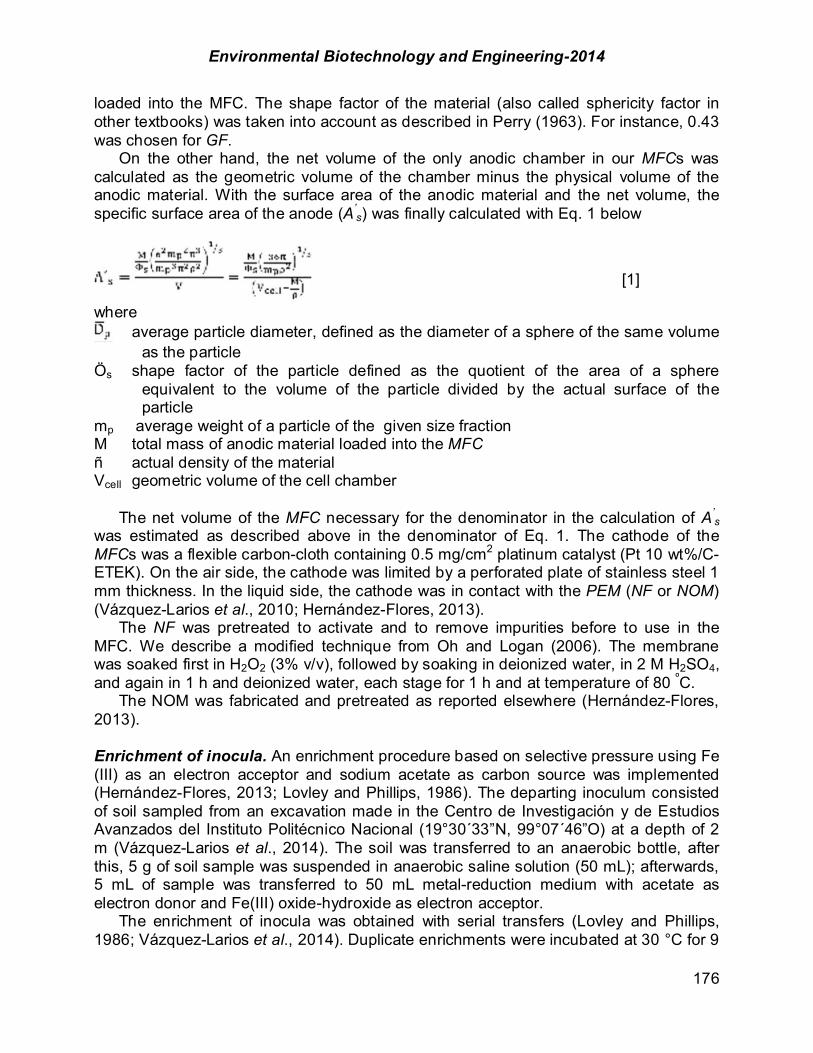
Environmental Biotechnology and Engineering-2014
176
loaded into the MFC. The shape factor of the material (also called sphericity factor in other textbooks) was taken into account as described in Perry (1963). For instance, 0.43 was chosen for GF. On the other hand, the net volume of the only anodic chamber in our MFCs was calculated as the geometric volume of the chamber minus the physical volume of the anodic material. With the surface area of the anodic material and the net volume, the specific surface area of the anode (A’
s) was finally calculated with Eq. 1 below
[1]
where average particle diameter, defined as the diameter of a sphere of the same volume
as the particle Ös shape factor of the particle defined as the quotient of the area of a sphere
equivalent to the volume of the particle divided by the actual surface of the particle
mp average weight of a particle of the given size fraction M total mass of anodic material loaded into the MFC ñ actual density of the material Vcell geometric volume of the cell chamber The net volume of the MFC necessary for the denominator in the calculation of A’
s was estimated as described above in the denominator of Eq. 1. The cathode of the MFCs was a flexible carbon-cloth containing 0.5 mg/cm2 platinum catalyst (Pt 10 wt%/C-ETEK). On the air side, the cathode was limited by a perforated plate of stainless steel 1 mm thickness. In the liquid side, the cathode was in contact with the PEM (NF or NOM) (Vázquez-Larios et al., 2010; Hernández-Flores, 2013). The NF was pretreated to activate and to remove impurities before to use in the MFC. We describe a modified technique from Oh and Logan (2006). The membrane was soaked first in H2O2 (3% v/v), followed by soaking in deionized water, in 2 M H2SO4, and again in 1 h and deionized water, each stage for 1 h and at temperature of 80 ºC. The NOM was fabricated and pretreated as reported elsewhere (Hernández-Flores, 2013). Enrichment of inocula. An enrichment procedure based on selective pressure using Fe (III) as an electron acceptor and sodium acetate as carbon source was implemented (Hernández-Flores, 2013; Lovley and Phillips, 1986). The departing inoculum consisted of soil sampled from an excavation made in the Centro de Investigación y de Estudios Avanzados del Instituto Politécnico Nacional (19°30´33”N, 99°07´46”O) at a depth of 2 m (Vázquez-Larios et al., 2014). The soil was transferred to an anaerobic bottle, after this, 5 g of soil sample was suspended in anaerobic saline solution (50 mL); afterwards, 5 mL of sample was transferred to 50 mL metal-reduction medium with acetate as electron donor and Fe(III) oxide-hydroxide as electron acceptor. The enrichment of inocula was obtained with serial transfers (Lovley and Phillips, 1986; Vázquez-Larios et al., 2014). Duplicate enrichments were incubated at 30 °C for 9
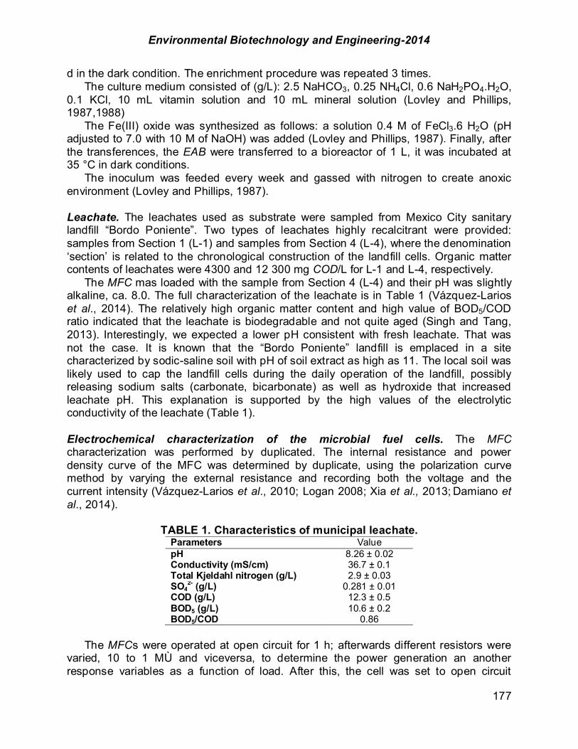
Environmental Biotechnology and Engineering-2014
177
d in the dark condition. The enrichment procedure was repeated 3 times. The culture medium consisted of (g/L): 2.5 NaHCO3, 0.25 NH4Cl, 0.6 NaH2PO4.H2O, 0.1 KCl, 10 mL vitamin solution and 10 mL mineral solution (Lovley and Phillips, 1987,1988) The Fe(III) oxide was synthesized as follows: a solution 0.4 M of FeCl3.6 H2O (pH adjusted to 7.0 with 10 M of NaOH) was added (Lovley and Phillips, 1987). Finally, after the transferences, the EAB were transferred to a bioreactor of 1 L, it was incubated at 35 °C in dark conditions. The inoculum was feeded every week and gassed with nitrogen to create anoxic environment (Lovley and Phillips, 1987). Leachate. The leachates used as substrate were sampled from Mexico City sanitary landfill “Bordo Poniente”. Two types of leachates highly recalcitrant were provided: samples from Section 1 (L-1) and samples from Section 4 (L-4), where the denomination ‘section’ is related to the chronological construction of the landfill cells. Organic matter contents of leachates were 4300 and 12 300 mg COD/L for L-1 and L-4, respectively. The MFC mas loaded with the sample from Section 4 (L-4) and their pH was slightly alkaline, ca. 8.0. The full characterization of the leachate is in Table 1 (Vázquez-Larios et al., 2014). The relatively high organic matter content and high value of BOD5/COD ratio indicated that the leachate is biodegradable and not quite aged (Singh and Tang, 2013). Interestingly, we expected a lower pH consistent with fresh leachate. That was not the case. It is known that the “Bordo Poniente” landfill is emplaced in a site characterized by sodic-saline soil with pH of soil extract as high as 11. The local soil was likely used to cap the landfill cells during the daily operation of the landfill, possibly releasing sodium salts (carbonate, bicarbonate) as well as hydroxide that increased leachate pH. This explanation is supported by the high values of the electrolytic conductivity of the leachate (Table 1). Electrochemical characterization of the microbial fuel cells. The MFC characterization was performed by duplicated. The internal resistance and power density curve of the MFC was determined by duplicate, using the polarization curve method by varying the external resistance and recording both the voltage and the current intensity (Vázquez-Larios et al., 2010; Logan 2008; Xia et al., 2013; Damiano et al., 2014).
TABLE 1. Characteristics of municipal leachate.
Parameters Value pH 8.26 ± 0.02 Conductivity (mS/cm) 36.7 ± 0.1 Total Kjeldahl nitrogen (g/L) 2.9 ± 0.03 SO4
2- (g/L) 0.281 ± 0.01 COD (g/L) 12.3 ± 0.5 BOD5 (g/L) 10.6 ± 0.2 BOD5/COD 0.86
The MFCs were operated at open circuit for 1 h; afterwards different resistors were varied, 10 to 1 MÙ and viceversa, to determine the power generation an another response variables as a function of load. After this, the cell was set to open circuit

Environmental Biotechnology and Engineering-2014
178
conditions for 1 h in order to check the adequacy of the procedure (values of initial and final open circuit voltages should be close). The voltage was measured and recorded with a Multimeter ESCORT 3146A. The current was calculated by the Ohm’s law (Eq. 2) and the Rint was calculated as the slope of the linear section of the curve voltage versus the current intensity (Vázquez-Larios et al., 2010; Logan et al., 2006). The PV was calculated according the Eq. 3:
[2]
[3] where IMFC is the current intensity of the MFC in A, EMFC is the voltage delivered by the cell in V, Rext is the external resistance connected to the cell in # and Vcell is the net volume of the anodic chamber. The initial COD and biomass concentration in the MFC liquor were ca. 2000 mg O2/L and 1900 VSS/L respectively. The pH and the electrical conductivity were 9 and 39 mS/cm, respectively. The COD and VSS of the inoculum enriched in Fe (III)-reducing bacteria seed bioreactor and MFCs were determined according to the Standard Methods (APHA, 1989). Results and discussion Electrochemical characterizations. The physical characteristics of the anodic material GF are showed in the table 2. This anodic material has a big surface area c.a. 0.3 m2. The MFCs fitted with their respective PEMs were electrochemical characterized at 0 d, it leads to define the Rext to start the power generation. The MFC fitted with NOM showed discouraging values (Table 3, Figure 2a).
TABLE 2. Selected physical characteristics of graphite flakes.
Characteristics Values Working net volume (m3) 7.22!10-5 ± 5.05!10-6 Anodic actual surface (m2) 0.28 ± 0.08 A’s
a (m2/m3) 1302 ± 91 Conductance (S)b 0.13 ± 0.04
Notes: aRelationship between the anode surface area to cell volume, also known as specific surface area of the anode; b Electrical conductance of the material, expressed in Siemens. The Rint and Pv,max were 650 # and 9 mW/m3, whereas the MFC fitted with NF displayed a Rint and Pv,max of 350 # and 1100 mW/m3, respectively (Table 3, Figure 3a). In this first test, the NF was far better than NOM. However, after 8 d, in the second electrochemical characterization the MFC fitted with NOM improve their performance, reaching a Pv,max of 22500 mW/m3 (Table 3, Figure 2b). The Rint decreased 94% (40 #) and the Pv,max increased 4 magnitude orders, it was very encouraging.
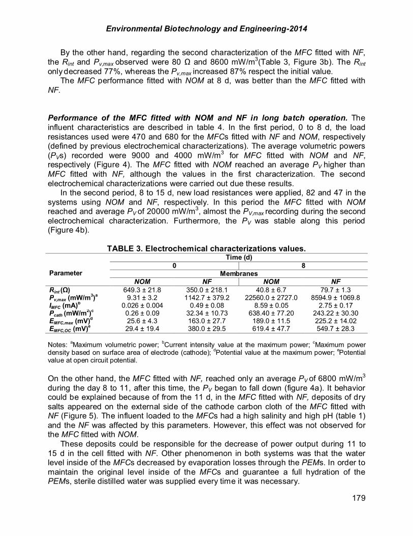
Environmental Biotechnology and Engineering-2014
179
By the other hand, regarding the second characterization of the MFC fitted with NF, the Rint and Pv,max observed were 80 # and 8600 mW/m3(Table 3, Figure 3b). The Rint only decreased 77%, whereas the Pv,max increased 87% respect the initial value. The MFC performance fitted with NOM at 8 d, was better than the MFC fitted with NF. Performance of the MFC fitted with NOM and NF in long batch operation. The influent characteristics are described in table 4. In the first period, 0 to 8 d, the load resistances used were 470 and 680 for the MFCs fitted with NF and NOM, respectively (defined by previous electrochemical characterizations). The average volumetric powers (PVs) recorded were 9000 and 4000 mW/m3 for MFC fitted with NOM and NF, respectively (Figure 4). The MFC fitted with NOM reached an average PV higher than MFC fitted with NF, although the values in the first characterization. The second electrochemical characterizations were carried out due these results. In the second period, 8 to 15 d, new load resistances were applied, 82 and 47 in the systems using NOM and NF, respectively. In this period the MFC fitted with NOM reached and average PV of 20000 mW/m3, almost the PV,max recording during the second electrochemical characterization. Furthermore, the PV was stable along this period (Figure 4b).
TABLE 3. Electrochemical characterizations values. Parameter
Time (d) 0 8
Membranes NOM NF NOM NF
Rint (!) 649.3 ± 21.8 350.0 ± 218.1 40.8 ± 6.7 79.7 ± 1.3 Pv,max (mW/m3)a 9.31 ± 3.2 1142.7 ± 379.2 22560.0 ± 2727.0 8594.9 ± 1069.8 IMFC (mA)b 0.026 ± 0.004 0.49 ± 0.08 8.59 ± 0.05 2.75 ± 0.17 Pcath (mW/m2)c 0.26 ± 0.09 32.34 ± 10.73 638.40 ± 77.20 243.22 ± 30.30 EMFC,max (mV)d 25.6 ± 4.3 163.0 ± 27.7 189.0 ± 11.5 225.2 ± 14.02 EMFC,OC (mV)e 29.4 ± 19.4 380.0 ± 29.5 619.4 ± 47.7 549.7 ± 28.3 Notes: aMaximum volumetric power; bCurrent intensity value at the maximum power; cMaximum power density based on surface area of electrode (cathode); dPotential value at the maximum power; ePotential value at open circuit potential. On the other hand, the MFC fitted with NF, reached only an average PV of 6800 mW/m3
during the day 8 to 11, after this time, the PV began to fall down (figure 4a). It behavior could be explained because of from the 11 d, in the MFC fitted with NF, deposits of dry salts appeared on the external side of the cathode carbon cloth of the MFC fitted with NF (Figure 5). The influent loaded to the MFCs had a high salinity and high pH (table 1) and the NF was affected by this parameters. However, this effect was not observed for the MFC fitted with NOM. These deposits could be responsible for the decrease of power output during 11 to 15 d in the cell fitted with NF. Other phenomenon in both systems was that the water level inside of the MFCs decreased by evaporation losses through the PEMs. In order to maintain the original level inside of the MFCs and guarantee a full hydration of the PEMs, sterile distilled water was supplied every time it was necessary.
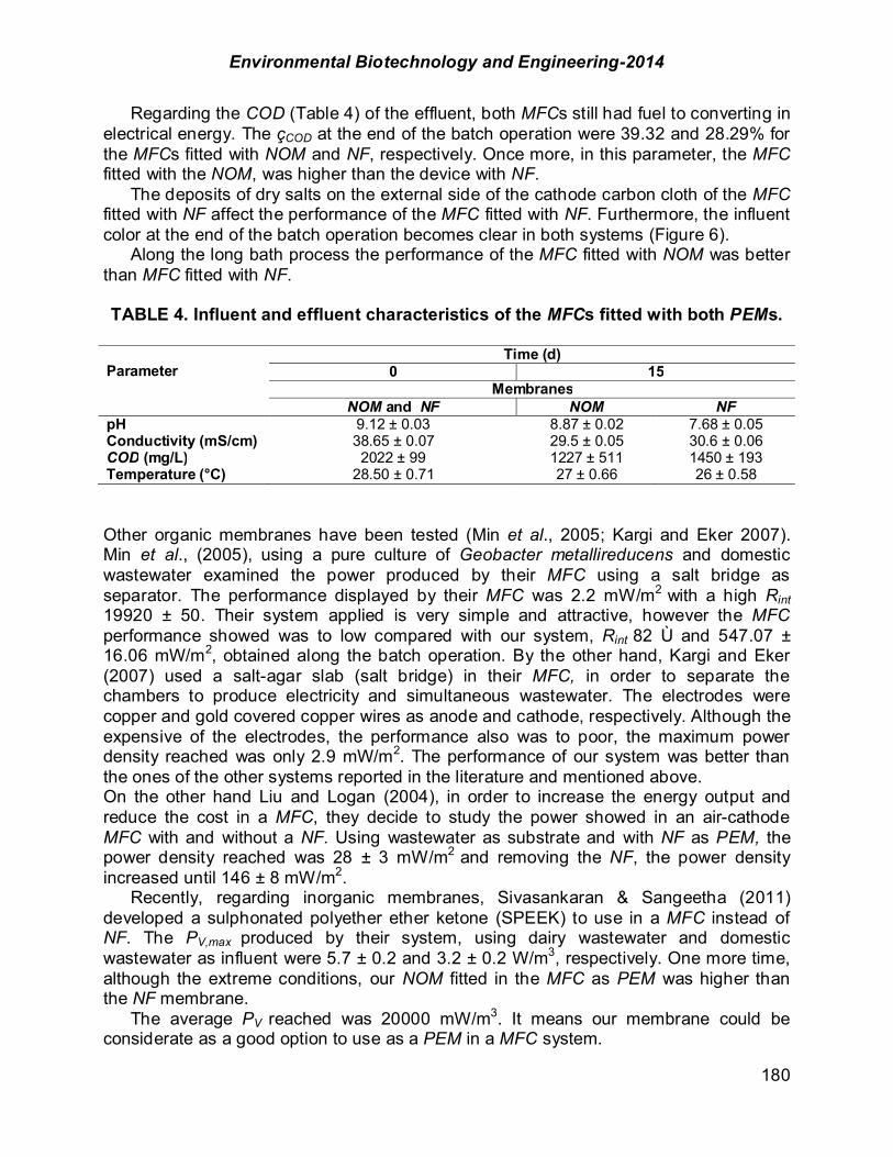
Environmental Biotechnology and Engineering-2014
180
Regarding the COD (Table 4) of the effluent, both MFCs still had fuel to converting in electrical energy. The çCOD at the end of the batch operation were 39.32 and 28.29% for the MFCs fitted with NOM and NF, respectively. Once more, in this parameter, the MFC fitted with the NOM, was higher than the device with NF. The deposits of dry salts on the external side of the cathode carbon cloth of the MFC fitted with NF affect the performance of the MFC fitted with NF. Furthermore, the influent color at the end of the batch operation becomes clear in both systems (Figure 6). Along the long bath process the performance of the MFC fitted with NOM was better than MFC fitted with NF. TABLE 4. Influent and effluent characteristics of the MFCs fitted with both PEMs.
Parameter
Time (d) 0 15
Membranes NOM and NF NOM NF
pH 9.12 ± 0.03 8.87 ± 0.02 7.68 ± 0.05 Conductivity (mS/cm) 38.65 ± 0.07 29.5 ± 0.05 30.6 ± 0.06 COD (mg/L) 2022 ± 99 1227 ± 511 1450 ± 193 Temperature (°C) 28.50 ± 0.71 27 ± 0.66 26 ± 0.58 Other organic membranes have been tested (Min et al., 2005; Kargi and Eker 2007). Min et al., (2005), using a pure culture of Geobacter metallireducens and domestic wastewater examined the power produced by their MFC using a salt bridge as separator. The performance displayed by their MFC was 2.2 mW/m2 with a high Rint 19920 ± 50. Their system applied is very simple and attractive, however the MFC performance showed was to low compared with our system, Rint 82 Ù and 547.07 ± 16.06 mW/m2, obtained along the batch operation. By the other hand, Kargi and Eker (2007) used a salt-agar slab (salt bridge) in their MFC, in order to separate the chambers to produce electricity and simultaneous wastewater. The electrodes were copper and gold covered copper wires as anode and cathode, respectively. Although the expensive of the electrodes, the performance also was to poor, the maximum power density reached was only 2.9 mW/m2. The performance of our system was better than the ones of the other systems reported in the literature and mentioned above. On the other hand Liu and Logan (2004), in order to increase the energy output and reduce the cost in a MFC, they decide to study the power showed in an air-cathode MFC with and without a NF. Using wastewater as substrate and with NF as PEM, the power density reached was 28 ± 3 mW/m2 and removing the NF, the power density increased until 146 ± 8 mW/m2. Recently, regarding inorganic membranes, Sivasankaran & Sangeetha (2011) developed a sulphonated polyether ether ketone (SPEEK) to use in a MFC instead of NF. The PV,max produced by their system, using dairy wastewater and domestic wastewater as influent were 5.7 ± 0.2 and 3.2 ± 0.2 W/m3, respectively. One more time, although the extreme conditions, our NOM fitted in the MFC as PEM was higher than the NF membrane. The average PV reached was 20000 mW/m3. It means our membrane could be considerate as a good option to use as a PEM in a MFC system.

Environmental Biotechnology and Engineering-2014
181
FIGURE 2. Electrochemical characterization of the MFC fitted with NOM at (a) 0 d and (b) 8 d.
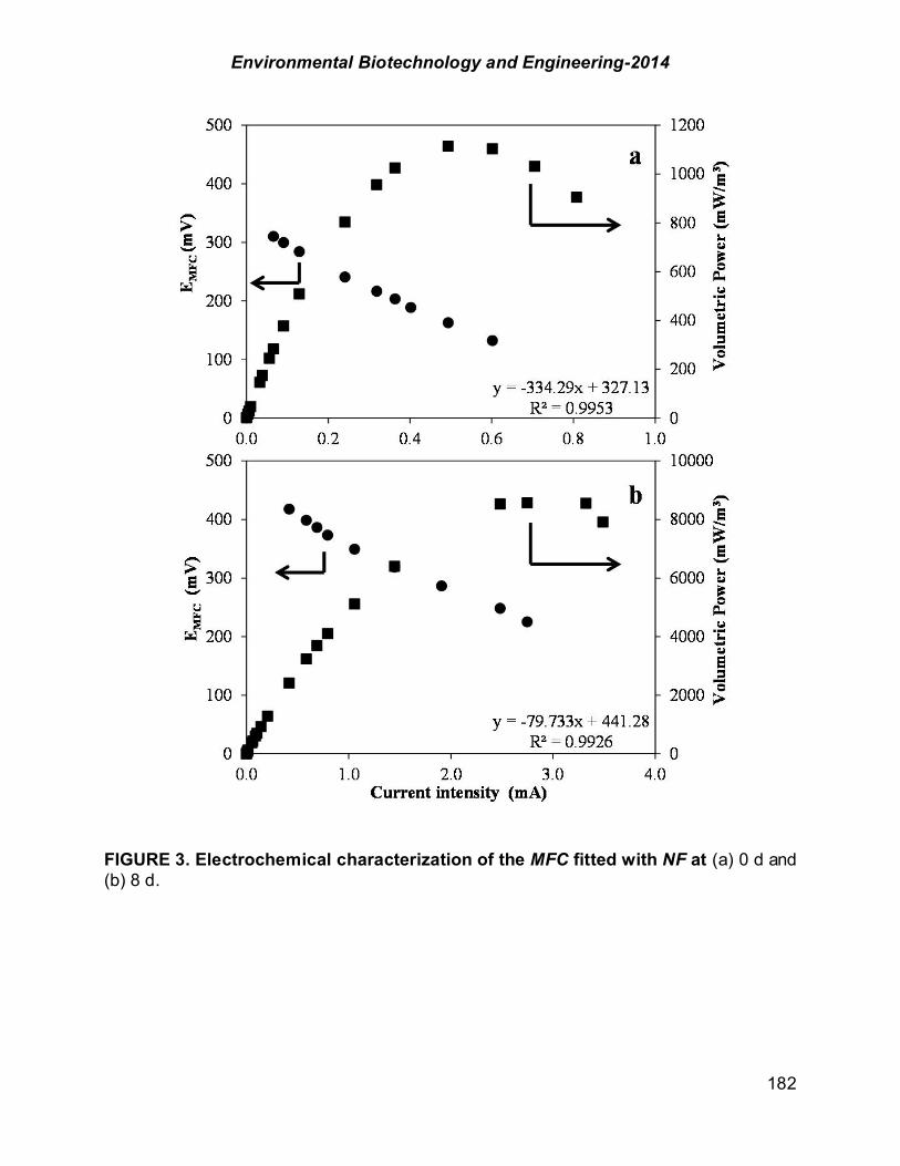
Environmental Biotechnology and Engineering-2014
182
FIGURE 3. Electrochemical characterization of the MFC fitted with NF at (a) 0 d and (b) 8 d.
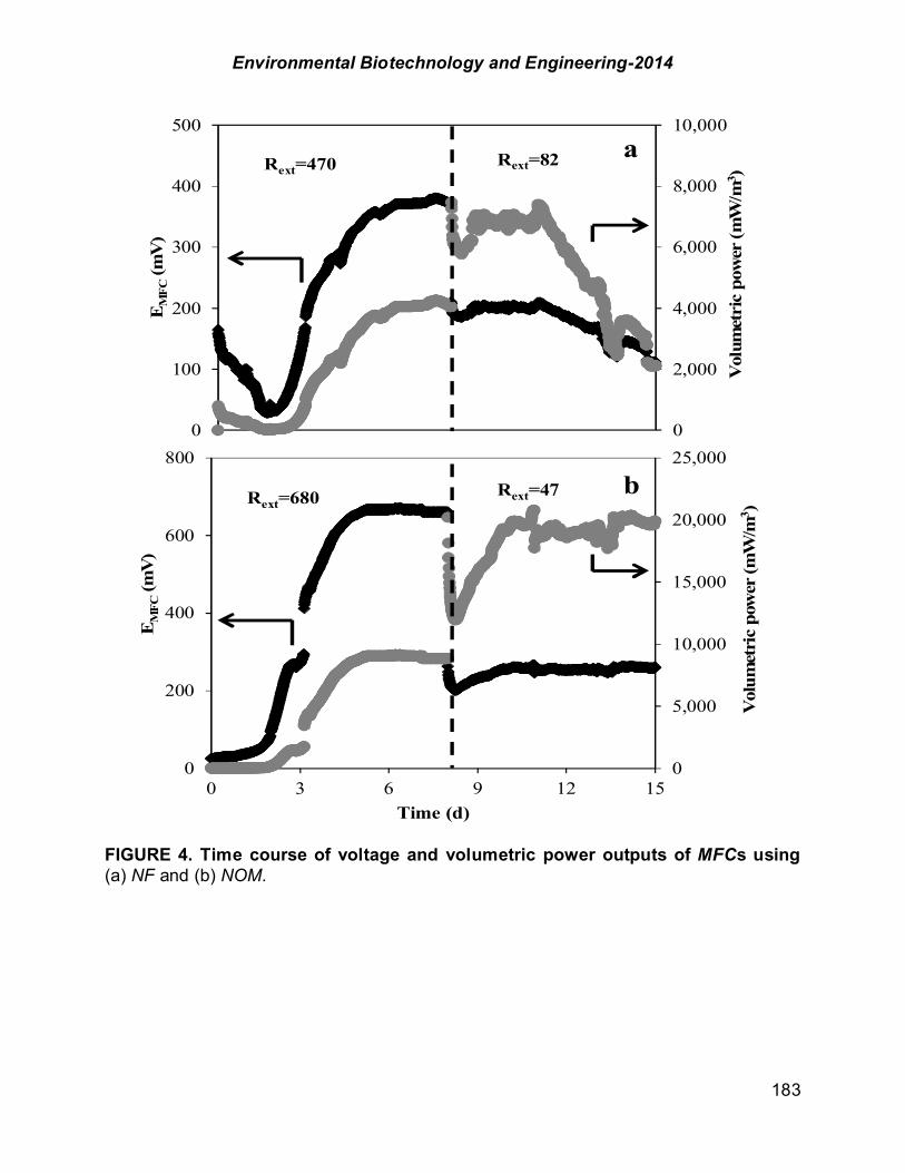
Environmental Biotechnology and Engineering-2014
183
FIGURE 4. Time course of voltage and volumetric power outputs of MFCs using (a) NF and (b) NOM.
0
5,000
10,000
15,000
20,000
25,000
0
200
400
600
800
0 3 6 9 12 15
EM
FC(m
V)
Time (d)
Vol
umet
ric
pow
er(m
W/m
3 )
0
2,000
4,000
6,000
8,000
10,000
0
100
200
300
400
500
EM
FC(m
V)
Rext=470
Vol
umet
ric
pow
er(m
W/m
3 )
a
b
Rext=82
Rext=680 Rext=47
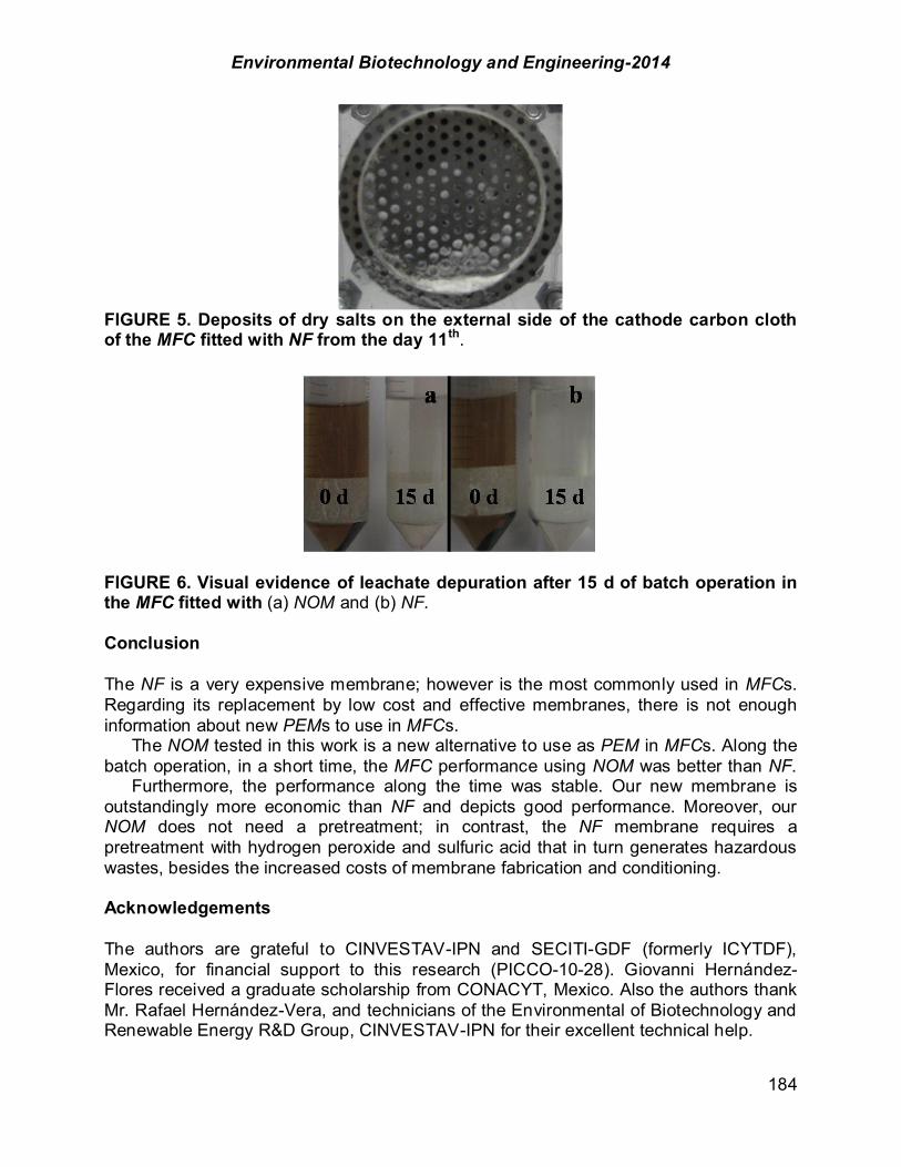
Environmental Biotechnology and Engineering-2014
184
FIGURE 5. Deposits of dry salts on the external side of the cathode carbon cloth of the MFC fitted with NF from the day 11th.
FIGURE 6. Visual evidence of leachate depuration after 15 d of batch operation in the MFC fitted with (a) NOM and (b) NF. Conclusion The NF is a very expensive membrane; however is the most commonly used in MFCs. Regarding its replacement by low cost and effective membranes, there is not enough information about new PEMs to use in MFCs. The NOM tested in this work is a new alternative to use as PEM in MFCs. Along the batch operation, in a short time, the MFC performance using NOM was better than NF. Furthermore, the performance along the time was stable. Our new membrane is outstandingly more economic than NF and depicts good performance. Moreover, our NOM does not need a pretreatment; in contrast, the NF membrane requires a pretreatment with hydrogen peroxide and sulfuric acid that in turn generates hazardous wastes, besides the increased costs of membrane fabrication and conditioning. Acknowledgements The authors are grateful to CINVESTAV-IPN and SECITI-GDF (formerly ICYTDF), Mexico, for financial support to this research (PICCO-10-28). Giovanni Hernández-Flores received a graduate scholarship from CONACYT, Mexico. Also the authors thank Mr. Rafael Hernández-Vera, and technicians of the Environmental of Biotechnology and Renewable Energy R&D Group, CINVESTAV-IPN for their excellent technical help.

Environmental Biotechnology and Engineering-2014
185
References APHA, (1989). Standard methods for examination of water and wastewater. 17th ed. APHA-AWWA-WEF,
Washington DC. Belleville, P.; Strong, P. J.; Dare, P. H.; Gapes, D. J. (2011). Influence of nitrogen limitation on
performance of a microbial fuel cell. Water Sci. Technol. 63: 1752-1757. Cheng-Dar, Y.; Chung-Ming, L.; Liou, E. M. L. (2001). A transition toward a sustainable energy future:
feasibility assessment and development strategies of wind power in Taiwan. Energy Policy. 29: 951-963.
Damiano, L.; Jambeck, J. R.; Ringelberg, D. B. (2014). Municipal Solid Waste Landfill Leachate Treatment and Electricity Production Using Microbial Fuel Cells. Appl. Biochem. Biotechnol. 173: 472–485.
Das, D.; Veziroglu, T. N. (2001). Hydrogen production by biological processes: a survey of literature. Int J. Hydrogen Energy. 26: 13-28.
Du, Z.; Li, H.; Gu, T. (2007). A state of the art review on microbial fuel cells: A promising technology for wastewater treatment and bioenergy. Biotechnol. Adv. 25: 464–482.
Hernández-Flores, G. (2013). Interim Report. Sc D Thesis, CINVESTAV-IPN, México, D.F. Hou, J.; Liu, Z.; Yang, S.; Zhou, Y. (2014). Three-dimensional macroporous anodes based on stainless
steel fiber felt for high-performance microbial fuel cells. Journal of Power Sources. 258: 204-209. Kargi, F.; Eker, S. (2007). Electricity generation with simultaneous wastewater treatment by a microbial
fuel cell (MFC) with Cu and Cu-Au electrodes. J. Chem. Technol. Biotechnol. 82: 658-662. Kim, Y.; Shin, S. H.; Chang, I. S.; Moon, S. H. (2014). Characterization of uncharged and sulfonated
porous poly(vinylidene fluoride) membranes and their performance in microbial fuel cells. Journal of Membrane Science. 463: 205–214.
Lefebvre, O.; Al-Mamun, A.; Ooi, W. K.; Ng, H. Y.; Tang, Z.; Chua, D. H.C. (2008). An insight into cathode options for microbial fuel cells. Water Sci Technol. 57: 2031–2037.
Liu, H.; Logan, B. E. (2004). Electricity generation using an air-cathode single chamber microbial fuel cell in the presence and absence of a proton exchange membrane. Environ. Sci. Technol. 38: 4040–4046.
Logan, B. E. (2008). Microbial fuel cells. John Wiley-Interscience. New Jersey, USA. Logan, B. E.; Hamelers, B.; Rozendal, R.; Schröder, U.; Keller, J.; Freguia, S.; Aelterman,P.; Verstraete,
W.; Rabaey, K. (2006). Microbial fuel cells: Methodology and technology. Environ. Sci. Technol. 40: 5181-5192.
Logan, B. E.; Rabaey, K. (2012). Conversion of wastes into bioelectricity and chemicals by using microbial electrochemical technologies. Science. 337: 686-690.
Logan, B. E.; Regan, J. M. (2006). Microbial challenges and harnessing the metabolic activity of bacteria can provide energy for a variety of applications, once technical and cost obstacles are overcome. Environ. Sci. Technol. 5172–5180.
Lovley, D. R.; Phillips, E. J. P. (1986). Organic matter mineralization with reduction of ferric iron in anaerobic sediments. Appl. Environ. Microbiol. 51: 683-689.
Lovley, D. R.; Phillips, E. J. P. (1987). Rapid assay for microbially reducible ferric iron in aquatic sedimens. Appl. Environ. Microbiol. 53: 1536-1540.
Lovley, D. R.; Phillips, E. J. P. (1988). Novel mode of microbial energy metabolism: organic carbon oxidation coupled to dissimilatory reduction of iron or manganese. Appl. Environ. Microbiol. 54: 1472-1480.
Min, B.; Cheng, S.; Logan, B. E. (2005). Electricity generation using membranes and salt bridge microbial fuel cells. Water Research. 39: 1675-1686.
Modin, O.; Gustavsson, D. J. (2014). Opportunities for microbial electrochemistry in municipal wastewater treatment–an overview. Water Sci. Technol. 69(7): 1359-1372.
Oh, S. E.; Logan, B. E. (2006). Proton exchange membrane and electrode surface areas as factors that affect power generation in microbial fuel cells. Appl Microbiol Biotechnol. 70: 162–169.
Ouitrakul, S.; Sriyudthsak, M.; Charojrochkul, S.; Kakizono. T. (2007). Impedance analysis of bio-fuel cell electrodes. Biosens. Bioelectron. 23: 721-727.
Pant, D.; Bogaert, G. V.; Diels, L.; Vanbroekhoven, K. (2010). A review of the substrates used in microbial fuel cells (MFCs) for sustainable energy production. Bioresour. Technol. 101: 1533–1543.
Perry, R. (1963). Chemical Engineers Handbook, pp 5.50 & ff 4th ed., McGraw-Hill Co, New York. Poggi-Varaldo, H. M.; Carmona-Martínez, A.; Vázquez-Larios, A. L.; Solorza-Feria, O. (2009). Effect of
inoculum type on the performance of a microbial fuel cell fed with spent organic extracts from hydrogenogenic fermentation of organic solid wastes. J. New Mater. Electrochem. Syst. 12: 49-54.
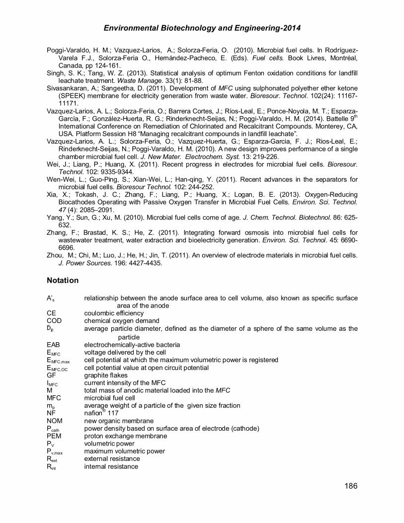
Environmental Biotechnology and Engineering-2014
186
Poggi-Varaldo, H. M.; Vazquez-Larios, A.; Solorza-Feria, O. (2010). Microbial fuel cells. In Rodríguez-Varela F.J., Solorza-Feria O., Hernández-Pacheco, E. (Eds). Fuel cells. Book Livres, Montréal, Canada, pp 124-161.
Singh, S. K.; Tang, W. Z. (2013). Statistical analysis of optimum Fenton oxidation conditions for landfill leachate treatment. Waste Manage. 33(1): 81-88.
Sivasankaran, A.; Sangeetha, D. (2011). Development of MFC using sulphonated polyether ether ketone (SPEEK) membrane for electricity generation from waste water. Bioresour. Technol. 102(24): 11167-11171.
Vazquez-Larios, A. L.; Solorza-Feria, O.; Barrera Cortes, J.; Ríos-Leal, E.; Ponce-Noyola, M. T.; Esparza-García, F.; González-Huerta, R. G.; Rinderknecht-Seijas, N.; Poggi-Varaldo, H. M. (2014). Battelle 9th International Conference on Remediation of Chlorinated and Recalcitrant Compounds. Monterey, CA, USA. Platform Session H8 “Managing recalcitrant compounds in landfill leachate”.
Vazquez-Larios, A. L.; Solorza-Feria, O.; Vazquez-Huerta, G.; Esparza-Garcia, F. J.; Rios-Leal, E.; Rinderknecht-Seijas, N.; Poggi-Varaldo, H. M. (2010). A new design improves performance of a single chamber microbial fuel cell. J. New Mater. Electrochem. Syst. 13: 219-226.
Wei, J.; Liang, P.; Huang, X. (2011). Recent progress in electrodes for microbial fuel cells. Bioresour. Technol. 102: 9335-9344.
Wen-Wei, L.; Guo-Ping, S.; Xian-Wei, L.; Han-qing, Y. (2011). Recent advances in the separators for microbial fuel cells. Bioresour Technol. 102: 244-252.
Xia, X.; Tokash, J. C.; Zhang, F.; Liang, P.; Huang, X.; Logan, B. E. (2013). Oxygen-Reducing Biocathodes Operating with Passive Oxygen Transfer in Microbial Fuel Cells. Environ. Sci. Technol. 47 (4): 2085–2091.
Yang, Y.; Sun, G.; Xu, M. (2010). Microbial fuel cells come of age. J. Chem. Technol. Biotechnol. 86: 625-632.
Zhang, F.; Brastad, K. S.; He, Z. (2011). Integrating forward osmosis into microbial fuel cells for wastewater treatment, water extraction and bioelectricity generation. Environ. Sci. Technol. 45: 6690-6696.
Zhou, M.; Chi, M.; Luo, J.; He, H.; Jin, T. (2011). An overview of electrode materials in microbial fuel cells. J. Power Sources. 196: 4427-4435.
Notation A’s relationship between the anode surface area to cell volume, also known as specific surface
area of the anode CE coulombic efficiency COD chemical oxygen demand
average particle diameter, defined as the diameter of a sphere of the same volume as the particle
EAB electrochemically-active bacteria EMFC voltage delivered by the cell EMFC,max cell potential at which the maximum volumetric power is registered EMFC,OC cell potential value at open circuit potential GF graphite flakes IMFC current intensity of the MFC M total mass of anodic material loaded into the MFC MFC microbial fuel cell mp average weight of a particle of the given size fraction NF nafion® 117 NOM new organic membrane Pcath power density based on surface area of electrode (cathode) PEM proton exchange membrane PV volumetric power Pv,max maximum volumetric power Rext external resistance Rint internal resistance

Environmental Biotechnology and Engineering-2014
187
SPEEK sulphonated polyether ether ketone Vcell geometric volume of the cell chamber Greek characters çCOD chemical oxygen demand removal ñ actual density of the material Ös shape factor of the particle defined as the quotient of the area of a sphere equivalent to the
volume of the particle divided by the actual surface of the particle

Environmental Biotechnology and Engineering-2014
188
CHAPTER 1.19. BIOELECTRICITY PRODUCTION FROM MUNICIPAL LEACHATE IN A MICROBIAL FUEL CELL
Ana Line Vázquez-Larios (1); Héctor M. Poggi-Varaldo*(1); Omar Solorza-Feria (1); Elvira Ríos-Leal (1); M. Teresa Ponce-Noyola (1); Rosa de G. González-Huerta (2);
José Tapia-Ramírez (1); Carlos Cruz-Cruz (1) (1) CINVESTAV- IPN, México DF, México; (2) ESIQIE-IPN, Mexico D.F., Mexico ABSTRACT The objective of this work was to evaluate (i) the effect of four inocula enriched in Fe(III)-reducing (soil origin or sulphate-reducing origin), bacteria and Mn(IV)-reducing bacteria and sulphate reducing (In-EFe(III)-S, In-EFe(III)-SR, In-EMn(IV) and In-SR respectively), and (ii) the effect of chalcogenide cathodic catalyst, for treatment and bioelectricity production from municipal leachate in a microbial fuel cell. The MFC-G consisted of a horizontal cylinder built Plexiglass 90 mm long and 57 mm internal diameter. The opposing faces of the cylindrical shell were fitted with corresponding sets of an assemblage of (inside to outside) proton exchange membrane (Nafion 117), a Toray flexible carbon-cloth containing 0.5 mg/cm2 platinum catalyst (Pt 10 wt%/C-ETEK) and 1 mg/cm2 RuxMoySez . Each assemblage was corresponded with anodes made of granular graphite. The anode chamber volume was 100 mL. The cells were loaded with 20 mL of municipal leachate. The cells were loaded with 80 mL of four inocula enriched in (IV)-reducing bacteria and sulphate reducing. Each face (I and II) of the MFC-G was characterized by separate (I and II), in series and parallel connection. Parallel connection of faces increased PV-max. In general parallel connection of electrode faces significantly decreased the internal resistance of the device (Rint). The cells were connected in parallel for 300 h of operation. The cells were connected to an Rext= 100 Ù. The volumetric power average were up to values 26 424, 25 548, 25 752 and 13 379 mW/m3 for In-EFe(III)-S, In-EFe(III)-SR, In-EMn(IV) and In-SR respectively. The high PV-ave obtained for our enriched inocula could be attributed to the increasing the total electrode surface area by the application of graphite, and this, in turn, could have improved the electron transfer microbe-to-anode and feasible presence the species of electrochemically active bacteria. Our results demonstrate the promising application of graphite granules anode and inocula enriched on treatment and additional benefits of bioelectricity generation from a recalcitrant municipal leachate. This, in turn, could have improved the electron transfer microbe-to-anode. The power values achieved in this work (13 W/m3 for the chalcogenide catalyst, and 25 W/m3 for Pt) were higher than results of MFC treating leachate in the literature. Finally, application of enriched in Fe(III) and Mn (IV)-reducing bacteria significantly improved the performance that used RuxMoySez as a cathodic catalyst for ORR. Key words: cathodic catalyst; enriched inocula; leachate; microbial fuel cell -------------- *Author for correspondence
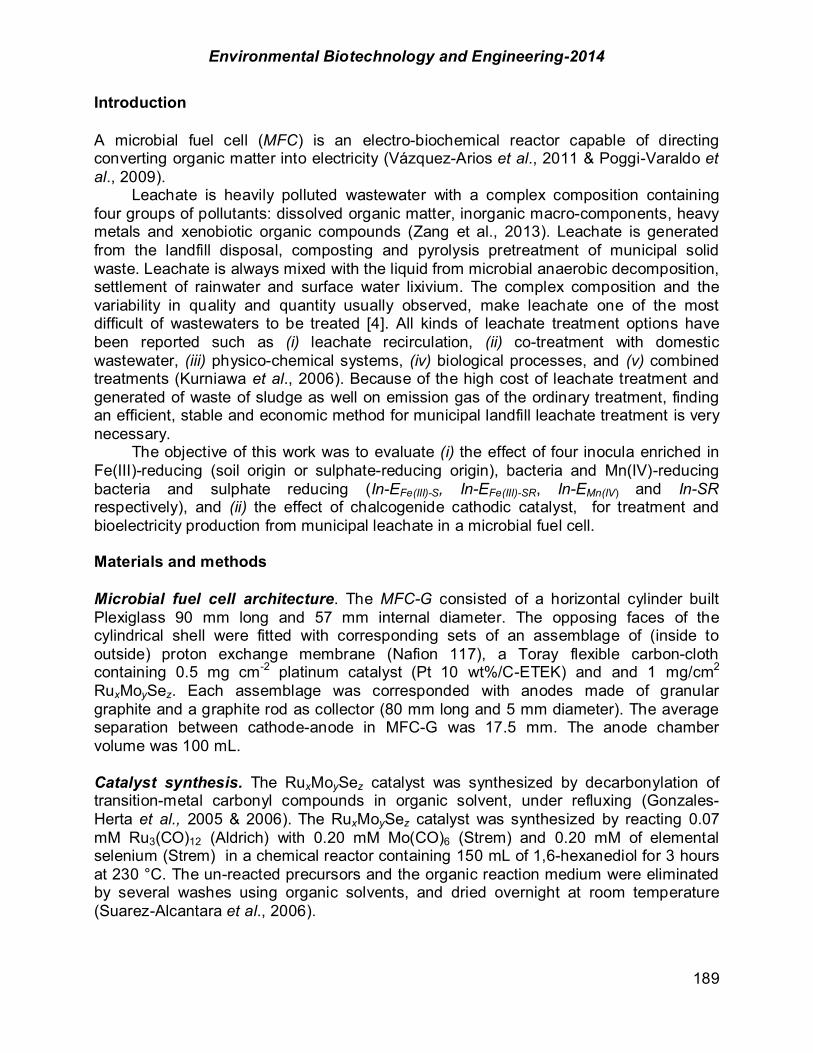
Environmental Biotechnology and Engineering-2014
189
Introduction A microbial fuel cell (MFC) is an electro-biochemical reactor capable of directing converting organic matter into electricity (Vázquez-Arios et al., 2011 & Poggi-Varaldo et al., 2009). Leachate is heavily polluted wastewater with a complex composition containing four groups of pollutants: dissolved organic matter, inorganic macro-components, heavy metals and xenobiotic organic compounds (Zang et al., 2013). Leachate is generated from the landfill disposal, composting and pyrolysis pretreatment of municipal solid waste. Leachate is always mixed with the liquid from microbial anaerobic decomposition, settlement of rainwater and surface water lixivium. The complex composition and the variability in quality and quantity usually observed, make leachate one of the most difficult of wastewaters to be treated [4]. All kinds of leachate treatment options have been reported such as (i) leachate recirculation, (ii) co-treatment with domestic wastewater, (iii) physico-chemical systems, (iv) biological processes, and (v) combined treatments (Kurniawa et al., 2006). Because of the high cost of leachate treatment and generated of waste of sludge as well on emission gas of the ordinary treatment, finding an efficient, stable and economic method for municipal landfill leachate treatment is very necessary. The objective of this work was to evaluate (i) the effect of four inocula enriched in Fe(III)-reducing (soil origin or sulphate-reducing origin), bacteria and Mn(IV)-reducing bacteria and sulphate reducing (In-EFe(III)-S, In-EFe(III)-SR, In-EMn(IV) and In-SR respectively), and (ii) the effect of chalcogenide cathodic catalyst, for treatment and bioelectricity production from municipal leachate in a microbial fuel cell. Materials and methods Microbial fuel cell architecture. The MFC-G consisted of a horizontal cylinder built Plexiglass 90 mm long and 57 mm internal diameter. The opposing faces of the cylindrical shell were fitted with corresponding sets of an assemblage of (inside to outside) proton exchange membrane (Nafion 117), a Toray flexible carbon-cloth containing 0.5 mg cm-2 platinum catalyst (Pt 10 wt%/C-ETEK) and and 1 mg/cm2 RuxMoySez. Each assemblage was corresponded with anodes made of granular graphite and a graphite rod as collector (80 mm long and 5 mm diameter). The average separation between cathode-anode in MFC-G was 17.5 mm. The anode chamber volume was 100 mL. Catalyst synthesis. The RuxMoySez catalyst was synthesized by decarbonylation of transition-metal carbonyl compounds in organic solvent, under refluxing (Gonzales-Herta et al., 2005 & 2006). The RuxMoySez catalyst was synthesized by reacting 0.07 mM Ru3(CO)12 (Aldrich) with 0.20 mM Mo(CO)6 (Strem) and 0.20 mM of elemental selenium (Strem) in a chemical reactor containing 150 mL of 1,6-hexanediol for 3 hours at 230 °C. The un-reacted precursors and the organic reaction medium were eliminated by several washes using organic solvents, and dried overnight at room temperature (Suarez-Alcantara et al., 2006).

Environmental Biotechnology and Engineering-2014
190
Municipal leachates. The cells were loaded with 20 mL of municipal leachates sampled from the Mexico City landfill “Bordo Poniente” stage 4 (Etapa 4). The characterization of the leachate is given in Table 1. The relatively high organic matter content and high value of BOD5/COD ratio indicated that the leachate is biodegradable, and likely not very aged. Interestingly, we expected a lower pH consistent with fresh leachate (Kurniawan et al., 2006). That was not the case. It is known that the landfill is emplaced in a site whose soil is sodic-saline soil with pH as high as 11 (Renou et al., 2008). The local soil was likely used to cap the landfill cells during the daily operation of the landfill, possibly releasing sodium salts (carbonate, bicarbonate) as well as hydroxides that increased leachate pH. This explanation is supported by the high values of the electrolytic conductivity of the leachate (Table 1).
TABLE 1. Characteristics of municipal leachate.
Parameters Value pH 8.26 ± 0.02 Conductivity (mS/cm) 36.7 ± 0.1 Total Kjeldahl nitrogen (g/L) 2.9 ± 0.03 SO4
2- (g/L) 0.281± 0.01 COD (g/L) 12.3± 0.5 BOD5 (g/L) 10.6± 0.2 BOD5/COD 0.86
Sample collection and enrichment of inoculum. The inoculum enrichment was obtained with three serial transfers of the culture, described below. Sample from soil was collected in the CINVESTAV-IPN (19° 30´33”N, 99° 07´46”O) to a depth of 2 m. The sample was transferred to an anaerobic bottle. 5 g of soil sample was suspended in 50 mL of anaerobic saline solution; afterwards, a 5 mL of sample was transferred to 50 mL metal-reduction medium with acetate as electron donor and Fe(III) oxide-hydroxide as electron acceptor. A sample of sulphate-reducing sludge was taken from a complete mix sulphate reducing semi-continuous bioreactor that acted as seed reactor (1,2) and handled in a similar way as the soil sample. The enrichment of inoculum were obtained with serial transfers. Duplicate enrichments were incubated at 30 °C for 9 d in the dark condition. The enrichment procedure was repeated 3 times. For the procedure of enrichment Mn(IV) of soil sample was similar way as the enrichment Fe(III). Duplicate enrichments were incubated at 30 °C for 15 d in the dark condition. The enrichment procedure was repeated 3 times. The culture medium consisted of (g/L): 2.5 NaHCO3, 0.25 NH4Cl, 0.6 NaH2PO4.H2O, 0.1 KCl, 10 mL vitamin solution and 10 mL mineral solution (Lovley & Phillips, 1997; Lovley & Phillips, 1988). The Fe(III) oxide was synthesized as follows: a solution 0.4 M of FeCl3.6 H2O (pH adjusted to 7.0 with 10 M of NaOH) was added, according to the technique described by Lovley & Phillips (1988). The MnO2 was synthesized by slowly adding a solution of MnCl2 (30 mM) to basic solution of KMnO4 (20 mM) which was stirred with a magnetic stir bar. This procedure is similar to a previously described technique (Lovley & Phillips, 1988).
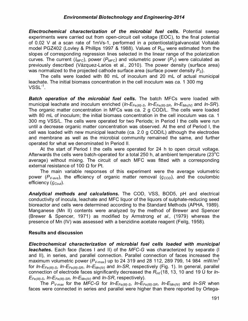
Environmental Biotechnology and Engineering-2014
191
Electrochemical characterization of the microbial fuel cells. Potential sweep experiments were carried out from open-circuit cell voltage (EOC), to the final potential of 0.02 V at a scan rate of 1mVs-1, performed in a potentiostat/galvanostat Voltalab model PGZ402 (Lovley & Phillips 1997 & 1988). Values of Rint were estimated from the slopes of corresponding regression lines selected in the linear range of the polarization curves. The current (IMFC), power (PMFC) and volumetric power (PV) were calculated as previously described (Vázquez-Larios et al., 2010). The power density (surface area) was normalized to the projected cathode surface area (surface power density PS). The cells were loaded with 80 mL of inoculum and 20 mL of actual municipal leachate. The initial biomass concentration in the cell inoculum was ca. 1 300 mg VSSL-1. Batch operation of the microbial fuel cells. The batch MFCs were loaded with municipal leachate and inoculum enriched (In-EFe(III)-S, In-EFe(III)-SR, In-EMn(IV) and In-SR). The organic matter concentration in MFCs was ca. 2 g COD/L. The cells were loaded with 80 mL of inoculum; the initial biomass concentration in the cell inoculum was ca. 1 300 mg VSS/L. The cells were operated for two Periods; in Period I the cells were run until a decrease organic matter concentration was observed. At the end of Period I, the cell was loaded with new municipal leachate (ca. 2.0 g COD/L) although the electrodes and membrane as well as the microbial community remained the same, and further operated for what we denominated In Period II. At the start of Period I the cells were operated for 24 h to open circuit voltage. Afterwards the cells were batch-operated for a total 250 h, at ambient temperature (23oC average) without mixing. The circuit of each MFC was fitted with a corresponding external resistance of 100 # for Pt. The main variable responses of this experiment were the average volumetric power (PV-ave), the efficiency of organic matter removal (çCOD), and the coulombic efficiency (çCoul). Analytical methods and calculations. The COD, VSS, BOD5, pH and electrical conductivity of inocula, leachate and MFC liquor of the liquors of sulphate-reducing seed bioreactor and cells were determined according to the Standard Methods (APHA, 1989). Manganese (Mn II) contents were analyzed by the method of Brewer and Spencer (Brewer & Spencer, 1971) as modified by Armstrong et al., (1979) whereas the presence of Mn (IV) was assessed with a benzidine acetate reagent (Feilg, 1958). Results and discussion Electrochemical characterization of microbial fuel cells loaded with municipal leachates. Each face (faces I and II) of the MFC-G was characterized by separate (I and II), in series, and parallel connection. Parallel connection of faces increased the maximum volumetric power (PV-max) up to 24 319 and 28 112, 289 799, 14 984 mW/m3 for In-EFe(III)-S, In-EFe(III)-SR, In-EMn(IV) and In-SR, respectively (Fig. 1). In general, parallel connection of electrode faces significantly decreased the Rint (18, 13, 10 and 19 Ù for In-EFe(III)-S, In-EFe(III)-SR, In-EMn(IV) and In-SR, respectively). The PV-max for the MFC-G for In-EFe(III)-S, In-EFe(III)-SR, In-EMn(IV) and In-SR when faces were connected in series and parallel were higher than there reported by Ortega-

Environmental Biotechnology and Engineering-2014
192
Martínez et al. (2013), Vázquez-Larios et al. (2013), Ortega-Martinez et al. (2012) and Ieropoulos et al. (2008) . Ortega-Martinez et al. (2013) evaluated enriched (E-In) inoculum on the characteristics of parallelepiped cell. Their values of PV-max were 1 772 and 5 804 mW/m3 for the faces connected in series and parallel. Vazquez-Larios et al. (2013) were to evaluate Pt as a catalyst, graphite triangular with anodic material, inoculum sulphate-reducing and model extract similar to the leachate found in the biological hydrogen production from the organic faction of the municipal solid waste that neither contained a mixture of acetic, propionic and butyric acids as well as acetone and methanol and mineral salts. The PV-max for faces I and II connected in parallel and series were 2 094 and 3 098 mW/m3. Ortega-Martinez et al. (2012) characterized a novel, multi-face parallelepiped MFC; this cell was fitted with a ‘sandwich’ cathode-membrane-anode assemblage in five of their faces. When the 5 faces of the cell were connected in series and parallel, the PV-max achieved values of 62 and 570 mW/m3. Ieropoulos et al., (2008) compared the performance two small size MFCs connected in parallel using acetate as the substrate and anaerobic sludge, the PV-max 860 mW/m3.
Parallel connection of faces increased the maximum volumetric power PV-max up to 14 521, 15 825, 16 359 and 9293 mWm-3 (Figure 2), compared with series connection 10 377, 12 778, 10 685 and 6 842 mWm-3. Parallel connection significantly decreased the Rint of the cells and almost doubled volumetric power. The PV-max for the MFC-G (In-EFe(III)-S, In-EFe(III)-SR, In-EMn(IV) and In-SR) when faces were connected in series and parallel were higher than those reported by Ortega-Martinez et al. (2012), Puig et al. (2011) and Ieropoulos et al. (2008). Our PV-max was superior to that reported by Ortega-Martinez et al. (2013) for the characterization of a novel, multi-face parallelepiped MFC (Pt for ORR); this cell was fitted with a ‘sandwich’ cathode-membrane-anode assemblage in five of their faces. When the 5 faces of the MFC-P were connected in series and parallel, the PV-max achieved values of 62 and 570 mWm-3, respectively. On the other hand, Puig et al. (2011) also characterized an air-cathode MFC loaded with landfill leachate and estimated a PV-max of 278.2 mWm-3. Ieropoulos et al. (2008) compared the performance of two small size MFCs connected in parallel using acetate as the substrate and a seed that consisted of anaerobic sludge; the characterization studies gave a PV-max of 860 mWm-3. The relatively higher PV-max in our MFCs could be attributed to the increase of the total electrode surface area by the application of granular graphite, and this, in turn, could have improved the electron transfer microbe-to-anode process (Vázquez Larios et al., 2013). Also, our work demonstrated that parallel connection of cell faces was more appropriate. On the other hand, the increase of power could also be ascribed to the use of the enriched inoculum. It is known that dissimilatory metal reducing bacteria are capable of the reduction of soil metal oxides such as MnO2, FeOOH and very often exhibit exoelectrogenic (electrochemical activity) properties (Ortega-Martínez et al., 2013; Sathish-Kumar et al., 2013; Wang et al., 2010). This, in turn, is related to improved electron transfer to anode and improved cell characteristics and performance (Ortega-Martínez et al., 2013; Sathish-Kumar et al., 2013).
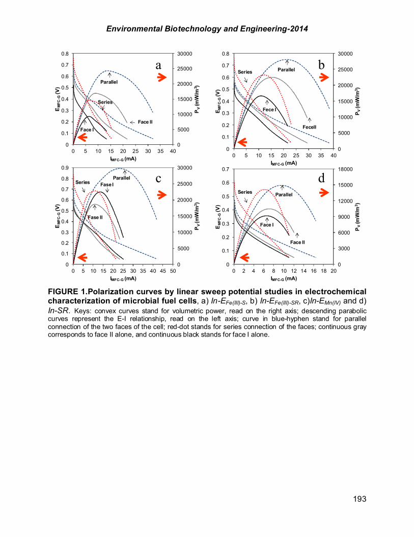
Environmental Biotechnology and Engineering-2014
193
FIGURE 1.Polarization curves by linear sweep potential studies in electrochemical characterization of microbial fuel cells, a) In-EFe(III)-S, b) In-EFe(III)-SR, c)In-EMn(IV) and d) In-SR. Keys: convex curves stand for volumetric power, read on the right axis; descending parabolic curves represent the E-I relationship, read on the left axis; curve in blue-hyphen stand for parallel connection of the two faces of the cell; red-dot stands for series connection of the faces; continuous gray corresponds to face II alone, and continuous black stands for face I alone.
0
3000
6000
9000
12000
15000
18000
0
0.1
0.2
0.3
0.4
0.5
0.6
0.7
0 2 4 6 8 10 12 14 16 18 20
PV
(mW
/m3 )
EM
FC-G
(V)
IMFC-G (mA)
0
5000
10000
15000
20000
25000
30000
0
0.1
0.2
0.3
0.4
0.5
0.6
0.7
0.8
0.9
0 5 10 15 20 25 30 35 40 45 50
PV
(mW
/m3 )
EM
FC-G
(V)
IMFC-G (mA)
0
5000
10000
15000
20000
25000
30000
0
0.1
0.2
0.3
0.4
0.5
0.6
0.7
0.8
0 5 10 15 20 25 30 35 40
P V(m
W/m
3 )
E MFC
-G(V
)
IMFC-G (mA)
0
5000
10000
15000
20000
25000
30000
0
0.1
0.2
0.3
0.4
0.5
0.6
0.7
0.8
0 5 10 15 20 25 30 35 40
PV
(mW
/m3 )
EM
FC-G
(V)
IMFC-G (mA)
ParallelSeries Fase I
Fase II
ParallelSeries
Face I
Face II
ParallelSeries
Fece I
FeceII
Parallel
Series
Face IFace II
a b
c d

Environmental Biotechnology and Engineering-2014
194
FIGURE 2.Polarization curves by linear sweep potential studies in electrochemical characterization of microbial fuel cells, a) In-EFe(III)-S, b) In-EFe(III)-SR, c)In-EMn(IV) and d) In-SR. Keys: convex curves stand for volumetric power, read on the right axis; descending parabolic curves represent the E-I relationship, read on the left axis; curve in blue-hyphen stand for parallel connection of the two faces of the cell; red-dot stands for series connection of the faces; continuous gray corresponds to face II alone, and continuous black stands for face I alone. Results of batch operation of microbial fuel cells loaded with municipal leachate. Fig. 3 shows the time course of cell potential the MFC-G in the batch operation of the cells using two enriched inocula, namely, the inoculum enriched in Fe (III)-reducing bacteria (either one soil origin, In-EFe(III)-S or sulphate-reducing origin, In-EFe(III)-SR), inoculum enriched in Mn (IV)-reducing bacteria, sulphate reducing and MFC-G without inoculum. The cells were connected to a Rext of 100 Ù whereas their two faces of each cell were connected in parallel. The gray area (0 to 24 h) in Fig. 3 shows that the open circuit potential (the 21 h and without a resistance in the external circuit) of the cells were 0.516, 0.499, 0.500, 0.358 and 0.061 V for In-EFe(III)-S, In-EFe(III)-SR, In-EMn(IV) , In-SR and without inocul1m, respectively. Two repeated cycles were carried out (Period I and Period II in Fig. 3), where treated leachate was removed and replaced by a new leachate load, whereas the microbial culture and electrodes remained the same. The PV-ave for period II the cells In-EFe(III)-S, In-EFe(III)-SR, In-EMn(IV) and In-SR were
0
3000
6000
9000
12000
15000
18000
0
0.1
0.2
0.3
0.4
0.5
0.6
0.7
0.8
0 2 4 6 8 10 12 14 16 18 20
PV
(mW
/m3 )
EM
FC-G
(V)
IMFC-G (mA)
0
3000
6000
9000
12000
15000
18000
0
0.1
0.2
0.3
0.4
0.5
0.6
0.7
0.8
0 5 10 15 20 25 30
PV
(mW
/m3 )
E MFC
-G(V
)
IMFC-G (mA)
0
3000
6000
9000
12000
15000
18000
0
0.1
0.2
0.3
0.4
0.5
0.6
0.7
0.8
0 5 10 15 20 25 30
PV
(mW
/m3 )
EM
FC-G
(V)
IMFC-G (mA)
0
3000
6000
9000
12000
0
0.1
0.2
0.3
0.4
0.5
0.6
0.7
0.8
0 5 10 15 20
PV
(mW
/m3 )
EM
FC-G
(V)
IMFC-G (mA)
ParallelSeries
Face I
Face II
Parallel
Series
Face I
Face II
ParallelSeries
Face I
Face II
Parallel
Series
Face I
Face II
a b
c d

Environmental Biotechnology and Engineering-2014
195
higher than there reported by Zhang et al. (2008), Puig et al. (2011), Rikame et al. (2012), Özkaya et al., (2013) and Vazquez-Larios et al. (2011). Zhang et al. (2008) evaluated a novel upflow air-cathode membrane-free microbial fuel cell (UAMMFC). The UAMMFC could continuously generate electricity from leachate for an operational period of time (50 h); a maximum volumetric power of 12 800 mW/m3 was reported. Puig et al. (2011) operated an air, single chamber MFC and Pt catalyst in the cathode to treat landfill leachate in two operation periods. In Period I dilute leachate with 0.507 g COD/L, the authors reported a very low PV of 6.1 mW/m3. In Period II the organic matter content was increased to 1.48 and 8.51 g COD/L, the PV were 106 to 344 mW/m3, respectively. Rikame et al. (2012) evaluated a two-chambered MFC with carbon electrodes for food waste leachate, the PV was 15 140 mW/m3 (çCOD = 90%). Özkaya et al. (2013) assessed the performance of a two-chambered, continuous MFC with new Ti–TiO2 electrodes for bioelectricity generation from young landfill leachate. They found a PV of 1 920 mW/m3. Vazquez-Larios et al., (2011) evaluated a new cell design with extended electrode surface (larger î, specific surface or surface area of electrode to cell volume) and the assemblage or “sandwich” arrangement of the anode-PEM-cathode (AMC arrangement) and model leachate, similar to that produced in the biological hydrogen production from the organic fraction of the municipal solid waste. A low to moderate PV of 606 mW/m3 was achieved. The high PV-ave achieved in our work could be attributed to the combined effects of increased concentrations of exoelectrogenic bacteria as well as increased total anodic surface area by the use of graphite flakes (Vazquez-Larios et al., 2013).
Figure 4 shows the time course of cell potential (MFC-G; either inocula In-EFe(III)-S, In-EFe(III)-SR, In-EMn(IV) , In-SR and without inoculum) when their two faces were connected in parallel. The batch runs lasted for ca. 250 h.
FIGURE 3. Time course of voltage outputs of MFC-G cell using a inoculum enriched in Fe (III)-reducing bacteria (either one soil origin, In-EFe(III)-S and sulphate-reducing origin, In-EFe(III)-SR), inoculum enriched in Mn (IV)-reducing bacteria (In-EMn(IV)), inoculum sulphate reducing (In-SR) and without inoculum.
0.0
0.1
0.2
0.3
0.4
0.5
0.6
0.7
0.8
0.9
1.0
0 50 100 150 200 250 300
EM
FC-G
(V)
Time (h)
I II
EMFC-CA
In-EFe(III)-SIn-EFe(III)-SR
In-EMn(IV)
In-SR
without inoculum
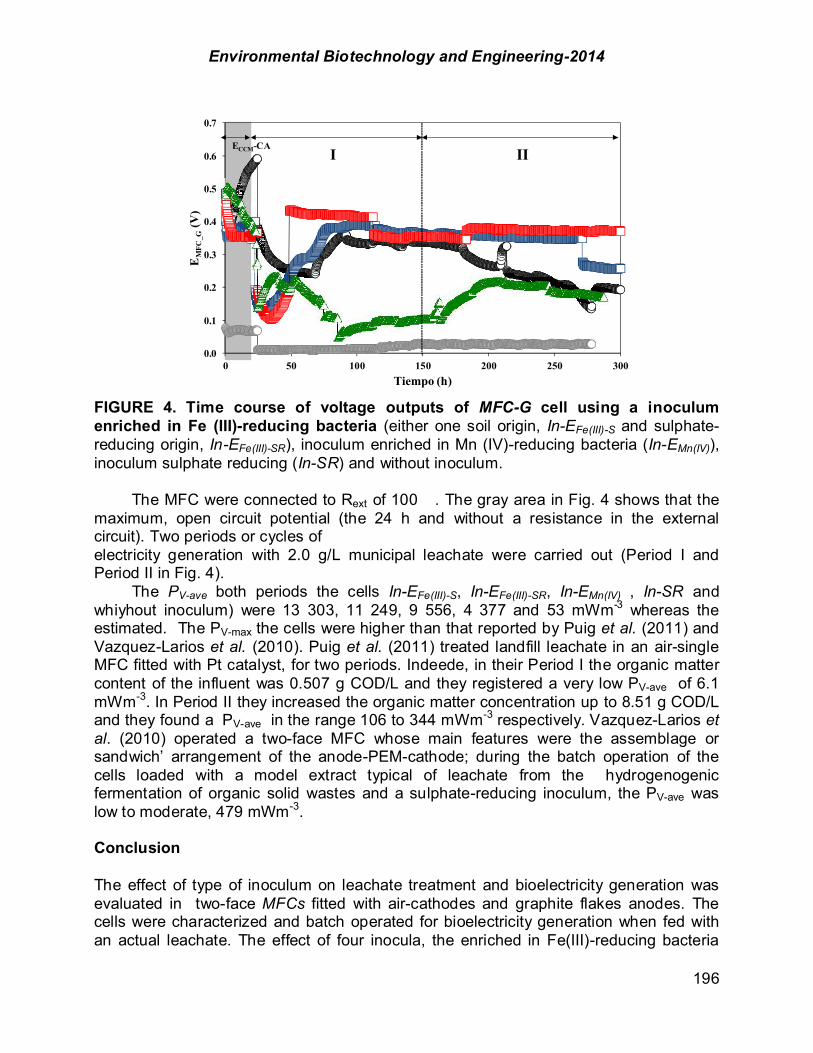
Environmental Biotechnology and Engineering-2014
196
FIGURE 4. Time course of voltage outputs of MFC-G cell using a inoculum enriched in Fe (III)-reducing bacteria (either one soil origin, In-EFe(III)-S and sulphate-reducing origin, In-EFe(III)-SR), inoculum enriched in Mn (IV)-reducing bacteria (In-EMn(IV)), inoculum sulphate reducing (In-SR) and without inoculum. The MFC were connected to Rext of 100 . The gray area in Fig. 4 shows that the maximum, open circuit potential (the 24 h and without a resistance in the external circuit). Two periods or cycles of electricity generation with 2.0 g/L municipal leachate were carried out (Period I and Period II in Fig. 4). The PV-ave both periods the cells In-EFe(III)-S, In-EFe(III)-SR, In-EMn(IV) , In-SR and whiyhout inoculum) were 13 303, 11 249, 9 556, 4 377 and 53 mWm-3 whereas the estimated. The PV-max the cells were higher than that reported by Puig et al. (2011) and Vazquez-Larios et al. (2010). Puig et al. (2011) treated landfill leachate in an air-single MFC fitted with Pt catalyst, for two periods. Indeede, in their Period I the organic matter content of the influent was 0.507 g COD/L and they registered a very low PV-ave of 6.1 mWm-3. In Period II they increased the organic matter concentration up to 8.51 g COD/L and they found a PV-ave in the range 106 to 344 mWm-3 respectively. Vazquez-Larios et al. (2010) operated a two-face MFC whose main features were the assemblage or sandwich’ arrangement of the anode-PEM-cathode; during the batch operation of the cells loaded with a model extract typical of leachate from the hydrogenogenic fermentation of organic solid wastes and a sulphate-reducing inoculum, the PV-ave was low to moderate, 479 mWm-3. Conclusion The effect of type of inoculum on leachate treatment and bioelectricity generation was evaluated in two-face MFCs fitted with air-cathodes and graphite flakes anodes. The cells were characterized and batch operated for bioelectricity generation when fed with an actual leachate. The effect of four inocula, the enriched in Fe(III)-reducing bacteria
0.0
0.1
0.2
0.3
0.4
0.5
0.6
0.7
0 50 100 150 200 250 300
EM
FC_G
(V)
Tiempo (h)
I IIECCM-CA

Environmental Biotechnology and Engineering-2014
197
(either one from soil origin, In-EFe(III)-S or sulphate-reducing origin, In-EFe(III)-SR) inoculum enriched in Mn (IV)-reducing bacteria (In-EMn(IV)), inoculum sulphate reducing (In-SR) was assessed. Parallel connection of faces increased the max volumetric power up to 24,319 and 28,112, 28,799, and 14,984 mW/m3 for In-EFe(III)-S, In-EFe(III)-SR, In-EMn(IV) and In-SR, respectively, y. In general parallel connection of electrode faces significantly decreased the Rint (18, 13, 10 and 19 Ù for In-EFe(III)-S, In-EFe(III)-SR, In-EMn(IV) and In-SR, respectively). In the batch operation where the cells were connected to an Rext of 100 Ù, the average volumetric power PV-ave were 26 424 ± 482, 25 548 ± 744, 25 752 and 13 379 mW/m3 for In-EFe(III)-S, In-EFe(III)-SR, In-EMn(IV) and In-SR, respectively. The high PV-ave achieved in our work could be attributed to the combined effects of increased concentrations of exoelectrogenic bacteria as well as increased total anodic surface area by the use of graphite flakes. This, in turn, could have improved the electron transfer microbe-to-anode. The highest power values achieved in this work (25 to 30 W/m3) were higher than or comparable to power thresholds typical of the anaerobic digestion of municipal wastewaters (5 to 50 W/m3). To the best of our knowledge, it is the first time that volumetric powers as high as 26 W/m3 are reported in the treatment of actual leachates in MFC. Our results constitute a firm step towards sustainable remediation of recalcitrant leachates. Acknowledgements The ICyTDF now SECITI-GDF (PICCO 10-28) and CINVESTAV-IPN (Mexico) financial support to this research is gratefully acknowledged. The authors wish to thank the help of Mr. Rafael Hernández-Vera from the Environmental Biotechnology and Renewable Energies R&D Group of the Dept. of Biotechnology and Bioengineering, as well as the Research Assistants and Technicians from the Hydrogen and Fuel Cell Group, Dept Chemistry, CINVESTAV. References APHA. (1971) Standard methods for the examination of water and wastewater. 17th ed. Washington, DC,
USA: American Public Association. Armstrong PB, Lyons WB, Gaudette HE. (1979). Application of formaldoxime colorimetric method for the
determination of manganese in the pore water of anoxic estuarine sediments. Estuaries. 2(3):198-201.
Brewer PG, Spencer DW. Colorimetric determination of manganese in anoxic waters. Limnol Oceanogr.16:107-112.
Feigl, F. (1958). Spot tests in inorganic analysis. Elsevier, New York, N.Y. Ieropoulus I, Greenman J, Melhuish C. (2008). Microbial fuel cell based on carbon veil electrodes: Stack
configuration and acalability. Int J Energy Res 32 (13): 1228–1240. Kurniawan, TA, W-H, Lo, YS Chan, G. (2006). Physico-chemical treatments for removal of recalcitrant
contaminants from landfill leachate, Journal of Hazardous Materials. B129: 80–100 Lovley, D. R., Phillips, E. J. P. (19979. “Rapid assay for microbially reducible ferric iron in aquatic
sediments”. Appl. Environ. Microbiol. 3:1536-40. Lovley, D.R., Phillips, E. J. P. (1988). Novel mode of microbial energy metabolism: organic carbon
oxidation coupled to dissimilatory reduction of iron or manganese. Appl. Environ. Microbiol. 54:1472-80.
Ortega-Martínez A, Juárez-López K, Solorza-Feria O, Ponce-Noyola MT, Ríos-Leal E, Rinderknecht-

Environmental Biotechnology and Engineering-2014
198
Seijas N, Poggi-Varaldo HM (2012). Parallel connection and sandwich electrodes lower the internal resistance in a microbial fuel cell. J New Mater Electrochem Syst. 15(3):187-194.
Ortega-Martinez A C, Juarez-Lopez K, Solorza-Feria O, Ponce-Noyola MT, Galindez-Mayer J, Rinderknecht-Seijas N, Poggi-Varaldo HM. (2013). Analysis of microbial diversity of inocula used in a five-face parallelepiped and standard microbial fuel cells. Int J Hydrogen Energy.38(28):12589-12599.
Ozkaya B, Cetinkaya AY, Cakmakci M, Karadag D, Sahinkaya E.(2013) Electricity generation from young landfill leachate in a microbial fuel cell with a new electrode material. Bioprocess and Biosystems Engineering.36:399-405.
Poggi-Varaldo, H.M., Carmona-Martinez, A., Vazquez-Larios, A.L., Solorza-Feria O. (2009). Effect of inoculum type on the performance of a microbial fuel cell fed with spent organic extracts from hydrogenogenic fermentation of organic solid wastes. J New Mater Electrochem Syst.12(1):49-54.
Puig S, Serra M, Coma M, Cabre M, Balaguer MD, Colprim J. (2011) Microbial fuel cell application in landfill leachate treatment. J Hazard Mater.185(2-3): 763-767.
Renou, S., Givaudan, JG , Poulain, S., Dirassouyan, F., Moulin P. (2008) Landfill leachate treatment: Review and opportunity. J Hazard Mater.150: 468–493.
Rikame, S. S., Mungray, A. A., Mungray, A. K. 2012. Electricity generation from acidogenic food waste leachate using dual chamber mediator less microbial fuel cell. Int. Biodeter Biodegr. 75: 131-137.
Sathish- Kumar K., Solorza-Feria O., Hernández-Vera R., Vazquez-Huerta G., Poggi-Varaldo
H.M. (2012)Comparison of Various Techniques to Characterize a Single Chamber Microbial Fuel Cell Loaded with Sulfate Reducing Biocatalysts. J New Mater Electrochem Syst .15(3):195-201.
Sathish-Kumar K., Solorza-Feria O., Vázquez-Huerta G., Luna-Arias J.P., Poggi-Varaldo H.M. (2012). Electrical Stress-directed Evolution of Biocatalysts Community Sampled from A Sodic-saline Soil for Microbial Fuel Cells. J New Mater Electrochem Syst .15(3): 181-186
Vázquez-Larios AL, Solorza-Feria O, González-Huerta R de G, Ponce-Noyola MT, Barrera-Cortés J, Rinderknecht-Seijas N, Poggi-Varaldo HM. (2013).Effect of Two Anodic Materials and RuxMoySez as a Cathode Catalyst on the Performance of Two Singlw Chamber Microbial Fuel Cells. J New Mater Electrochem Syst.16(3):163-170.
Vazquez-Larios AL, Solorza-Feria O, Vazquez-Huerta G, Esparza-Garcia F, Rios-Leal E, Rinderknecht-Seijas N, Poggi-Varaldo HM. (2010). A new design improves performance of a single chamber microbial fuel cell. J New Mater Electrochem Syst.13(3): 219-2
Vazquez-Larios, A. L., Solorza-Feria, O., Vazquez-Huerta, G., Rios-Leal, E., Rinderknecht-Seijas, N., Poggi-Varaldo, H.M. (2011). Internal resistance and performance of microbial fuel cells: influence of cell configuration and temperature. J. New Mater Electrochem Syst. 14(2): 99-105.
Vazquez-Larios, A.L., Solorza-Feria, O., Vazquez-Huerta, G, Esparza-Garcia, F., Rinderknecht-Seijas, N., Poggi-Varaldo, H.M.. (2011). Effects of architectural changes and inoculum type on internal resistance of a microbial fuel cell designed for the treatment of leachates from the dark hydrogenogenic fermentation of organic solid wastes. Int J Hydrogen Energy 36: 6199.
Zhang, J. N., Zhao, Q. L., You, S. J., Jiang, J. Q., Ren, N. Q. (2008). Continuous electricity production from leachate in a novel upflow air-cathode membrane-free microbial fuel cell. Bioprocess Biosyst. Eng. 36(4): 399-405.
Zhang, Q-Q, Tian, B-H, Zhang, X., Ghulam, A., Fang, C-R, He, R. (2013) Investigation on characteristics of leachate and concentrated leachate in three landfill leachate treatment plants, Waste Management. 33: 2277–2286
Notation EAB Electrochemically active bacteria EMFC-ave Average potential EMFC-max Maximum power density EMFC-OCP Open circuit potential IMFC Current intensity In-EFe(III)-S Inoculum enriched in Fe (III)-reducing bacteria (soil origin) In-EFe(III)-SR Inoculum enriched in Fe (III)-reducing bacteria (sulphate-reducing origin) In-SR Inoculum sulphate-reducing MFC Microbial fuel cell PMFC Cell power

Environmental Biotechnology and Engineering-2014
199
PS-ave Average power density PS-max Maximum power density PV Volumetric power PV-ave Average volumetric power PV-max Maximum volumetric power Rext External resistant Rint Internal resistant UAMMFC Upflow air-cathode membrane-free microbial fuel cell Greek characters çCOD Organic matter removal efficiency (COD basis) çcoul Coulombic efficiency

Environmental Biotechnology and Engineering-2014
200
CHAPTER 1.20. MEMBRANES IN MICROBIAL FUEL CELLS: A REVIEW Giovanni Hernández-Flores (1); Héctor M. Poggi-Varaldo*(1); Omar Solorza-Feria (2); Juvencio Galíndez-Mayer (3); Elvira Ríos-Leal (4); María T. Ponce-Noyola (5); Noemí
Rinderknecht-Seijas (6); Tatiana Romero-Castañón (7) (1) CINVESTAV del IPN, Dept. of Biotechnology and Bioengineering, Environmental Biotechnology and Renewable Energies Group, México D.F., México. (2) CINVESTAV del IPN, Dept. of Chemistry, Hydrogen and Fuel Cells Group, México D.F., México. (3) ENCB del IPN, Dept. of Biochemical Engineering, Biotechnology and bioengineering Group, México D.F., México. (4) CINVESTAV del IPN, Dept. of Biotechnology and Bioengineering, Central analytical chromatography. México D.F., México. (5) CINVESTAV del IPN, Dept. of Biotechnology and Bioengineering, Microbial Genetics Group, México D.F., México. (6) ESIQIE del IPN, Division of Basic Sciences. Escuela Superior de Ingeniería Química e Industrias Extractivas, México D.F. (7) Electrical Research Institute, Cuernavaca, Morelos, México. ABSTRACT Currently, most of the Microbial Fuel Cells (MFCs) are devices designed and focused to produce electrical energy and waste treatment. We can describe a MFC constituted mainly by the following items: anode, cathode, microorganisms, substrates and proton exchange membrane (PEM). Usually, the role of a PEM is to divide the electrodes, the anode from the cathode in a MFC. Regarding the costs, the use of membranes could represent around the 40% of the MFC total cost. The aim of this work was to critically review the state of the art on membranes in MFCs. The scope of this review includes (i) the different membranes used in MFCs, (ii) costs and performance of typical membranes used, (iii) configuration of membranes in MFCs, (iv) membraneless MFCs, and (v) perspectives on PEMs. An ideal membrane separator must have some characteristics such as high proton conductivity, biocompatibility, good mechanical properties, low oxygen transfer, low permeability to substrate, good chemical and thermal stability, and low cost. The most common membrane used is Nafion®, a perflourinated membrane, due to their excellent proton conductivity, nevertheless Nafion is too expensive. Nafion belongs to the type of cation exchange membranes, also known as PEMs. In order to reduce the costs, other types of proton exchange materials have been tested in MFCs such as salt bridge, anion exchange membranes, microfiltration and ultrafiltration membranes, bipolar membranes, among others. However, studies focused on low cost and or natural polymers for PEM are still scarce. Alternatively, in some works, the MFCs have been operated without a membrane. Yet it was found that the CE substantially decreased. ------------ *Author for all correspondence
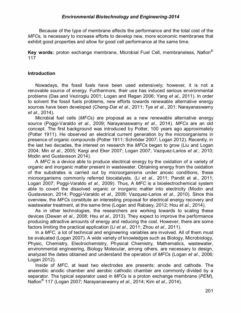
Environmental Biotechnology and Engineering-2014
201
Because of the type of membrane affects the performance and the total cost of the MFCs, is necessary to increase efforts to develop new, more economic membranes that exhibit good properties and allow for good cell performance at the same time. Key words: proton exchange membrane, Microbial Fuel Cell, membraneless, Nafion® 117 Introduction Nowadays, the fossil fuels have been used extensively; however, it is not a renovable source of energy. Furthermore, their use has induced serious environmental problems (Das and Veziroglu 2001; Logan and Regan 2006; Yang et al., 2011). In order to solvent the fossil fuels problems, new efforts towards renewable alternative energy sources have been developed (Cheng-Dar et al., 2011; Tye et al., 201; Narayanaswamy et al., 2014). Microbial fuel cells (MFCs) are proposal as a new renewable alternative energy source (Poggi-Varaldo et al., 2009; Narayanaswamy et al., 2014). MFCs are an old concept. The first background was introduced by Potter, 100 years ago approximately (Potter 1911). He observed an electrical current generation by the microorganisms in presence of organic compounds (Potter 1911; Schröder 2007; Logan 2012). Recently, in the last two decades, the interest on research the MFCs began to grow (Liu and Logan 2004; Min et al., 2005; Kargi and Eker 2007; Logan 2007; Vazquez-Larios et al., 2010; Modin and Gustavsson 2014). A MFC is a device able to produce electrical energy by the oxidation of a variety of organic and inorganic matter present in wastewater. Obtaining energy from the oxidation of the substrates is carried out by microorganisms under anoxic conditions, these microorganisms commonly referred biocatalysts. (Li et al., 2011; Pandit et al., 2011; Logan 2007; Poggi-Varaldo et al., 2009). Thus, A MFC is a bioelectrochemical system able to covert the dissolved organic or inorganic matter into electricity (Modin and Gustavsson, 2014; Poggi-Varaldo et al., 2009; Vazquez-Larios et al., 2010). Since this overview, the MFCs constitute an interesting proposal for electrical energy recovery and wastewater treatment, at the same time (Logan and Rabaey, 2012; Hou et al., 2014). As in other technologies, the researchers are working towards to scaling these devices (Dewan et al., 2008; Hsu et al., 2013). They expect to improve the performance producing attractive amounts of energy and reducing the cost. However, there are some factors limiting the practical application (Li et al., 2011; Zhou et al., 2011). In a MFC, a lot of technical and engineering variables are involved. All of them must be evaluated (Logan 2007). A wide variety of knowledges such as Biology, Microbiology, Physic, Chemistry, Electrochemistry, Physical Chemistry, Mathematics, wastewater, environmental engineering, Biology Molecular, among others, are necessary to design, analyzed the dates obtained and understand the operation of MFCs (Logan et al., 2006; Logan 2012). Inside of MFC, at least two electrodes are presents: anode and cathode. The anaerobic anodic chamber and aerobic cathodic chamber are commonly divided by a separator. The typical separator used in MFCs is a proton exchange membrane (PEM), Nafion® 117 (Logan 2007; Narayanaswamy et al., 2014; Kim et al., 2014).
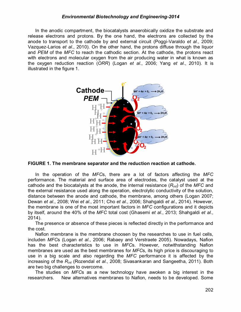
Environmental Biotechnology and Engineering-2014
202
In the anodic compartment, the biocatalysts anaerobically oxidize the substrate and release electrons and protons. By the one hand, the electrons are collected by the anode to transport to the cathode by and external circuit (Poggi-Varaldo et al., 2009; Vazquez-Larios et al., 2010). On the other hand, the protons diffuse through the liquor and PEM of the MFC to reach the cathodic section. At the cathode, the protons react with electrons and molecular oxygen from the air producing water in what is known as the oxygen reduction reaction (ORR) (Logan et al., 2006; Yang et al., 2010). It is illustrated in the figure 1.
FIGURE 1. The membrane separator and the reduction reaction at cathode. In the operation of the MFCs, there are a lot of factors affecting the MFC performance. The material and surface area of electrodes, the catalyst used at the cathode and the biocatalysts at the anode, the internal resistance (Rint) of the MFC and the external resistance used along the operation, electrolytic conductivity of the solution, distance between the anode and cathode, the membrane, among others (Logan 2007; Dewan et al., 2008; Wei et al., 2011; Cho et al., 2006; Shahgaldi et al., 2014). However, the membrane is one of the most important factors in MFC configurations and it depicts by itself, around the 40% of the MFC total cost (Ghasemi et al., 2013; Shahgaldi et al., 2014). The presence or absence of these pieces is reflected directly in the performance and the cost. Nafion membrane is the membrane choosen by the researches to use in fuel cells, includen MFCs (Logan et al., 2006; Rabaey and Verstraete 2005). Nowadays, Nafion has the best characteristics to use in MFCs. However, notwithstanding Nafion membranes are used as the best membranes for MFCs, its high price is discouraging to use in a big scale and also regarding the MFC performance it is affected by the increasing of the Rint (Rozendal et al., 2008; Sivasankaran and Sangeetha, 2011). Both are two big challenges to overcome. The studies on MFCs as a new technology have awoken a big interest in the researchers. New alternatives membranes to Nafion, needs to be developed. Some

Environmental Biotechnology and Engineering-2014
203
considerations must be taken in account for propose new alternatives membranes or separators. To develop new alternative membranes to apply in MFCs is a difficult task, there are limited works related to new alternative membranes tested in MFCs (Grzebyk and PoŸniak 2005; Li et al., 2011; Choi et al., 2012; Kim et al., 2014). The aim of this work was to critically review the state of the art on membranes in MFCs. The scope of this review includes (i) the different membranes used in MFCs, (ii) costs and performance of typical membranes used, (iii) configuration of membranes in MFCs, (iv) membraneless MFCs, and (v) perspectives on PEMs. Membrane separator functions in MFCs. A membrane separator has some important functions in MFCs. One of them is to prevent the short circuiting between the electrodes (Figure 2). On the other hand, the membrane acts as a channel to conduct the protons to the cathode and avoid the oxygen diffusion into the anodic compartment from the cathode. The substrate flux from the anode to cathode is also reduced by the membrane separator (Figure 2) (Logan 2007).
FIGURE 2. A MFC divided by a membrane separator. The oxygen in the anodic chamber affects negatively the MFCs performance (Watson et al., 2011). The oxygen is an alternative electron acceptor for the biocatalyst at the anode. It plays versus anode and is toxic to them. In the case of the facultative bacteria (also present in the anodic chamber), the oxygen is used as the first option as terminal electron acceptor instead of the anodic material, then the Coulombic efficiency (CE) decrease. In the case of the anode potential, it become more positive, decreasing the current density (Harnisch and Schröder 2009; Watson et al., 2011). The EC is one of the dates that must be included in the data reported as MFC performace. The CE ( coul) is defined as the transfer efficiency of the available electrons to the anode. It is the total Coulombs actually transferred to the anode from the substrate, to maximum possible Coulombs if all substrate removal were converted in current (Logan et al., 2006; Logan 2007; Li et al., 2011; Liu and Logan 2004). The coul is calculated as follows (Poggi-Varaldo et al., 2010):
(1)
Anodic chamber
Substrate
O2
H+
Catodic chamber
Membrane

Environmental Biotechnology and Engineering-2014
204
where ACS is the actual charge due the substrate obtained by the Eq. 2 and CTS is the theoretical charge due the substrate calculate by the Eq. 2.
[1]
[2]
IMFC current intensity over time delivered by the cell F is Faraday’s constant, 96 485.33 Coulombs/mol e- bCOD is the number of electrons exchanged per mole of oxygen generated by chemical
oxygen demand (COD), 4 CODi initial COD (g/L) CODf final COD (g/L) V the volume of liquid in the anode compartment (L) MCOD molecular weight of oxygen (32 gO2/mol COD) However, the coul is adversely affected by others factors such as the own bacterial growth, competitive processes and the utilization of alternate electron acceptors in the influent by the microorganisms (Logan et al., 2006) Regarding to the Rint of the MFCs, the presence of a membrane separator brings by itself the increasing of Rint affecting adversely the power generation (Kim et al., 2014). Also the membrane, along the operation generates pH gradients (Rozendal et al. 2006; Kim et al., 2007). One alternative to improve the MFC performance is removing the membrane from the system and decreasing the distance, between the electrodes. Both, reduce the ohmic losses (Liu and Logan 2004; Logan et al., 2006; Vazquez-Larios et al., 2010).
Ideal membranes. A membrane must perform a lot of characteristics to be considerate as an ideal membrane. Some researchers characterize their membranes out of the cell before to apply to the MFC (Hernández-Flores 2014; Narayanaswamy et al., 2014; Kim et al., 2014). The most of them synthesize and apply the membrane separators directly in MFCs, evaluating the membrane in situ. A membrane could be considerate as an ideal membrane to use in a MFC whether has the follow properties: a high proton conductivity, waterproof, low thickness, impermeability to the oxygen and cations such as Na+, K+, Ca2+, Mg2+ and NH4
+, good mechanical properties, chemical stability, low values of Rint, impermeability to gases such as H2, N2 and definitely a low price. Regarding using the membrane directly in MFC we can add the following properties: low average Rint of the device, long stability or durability along the operation time under different operating conditions, biofouling resistance, nonbiodegradable, high CE and an attractive overall power density (Peighambardoust et al., 2010; Li et al., 2011; Watson et al., 2011; Rismani-Yazdi et al., 2011; Brunetti et al., 2012; Logan 2010; Kim et al., 2014). Unfortunately, there is not an ideal membrane. There are membranes that depict some of the most important properties and this allows the membranes can be applied
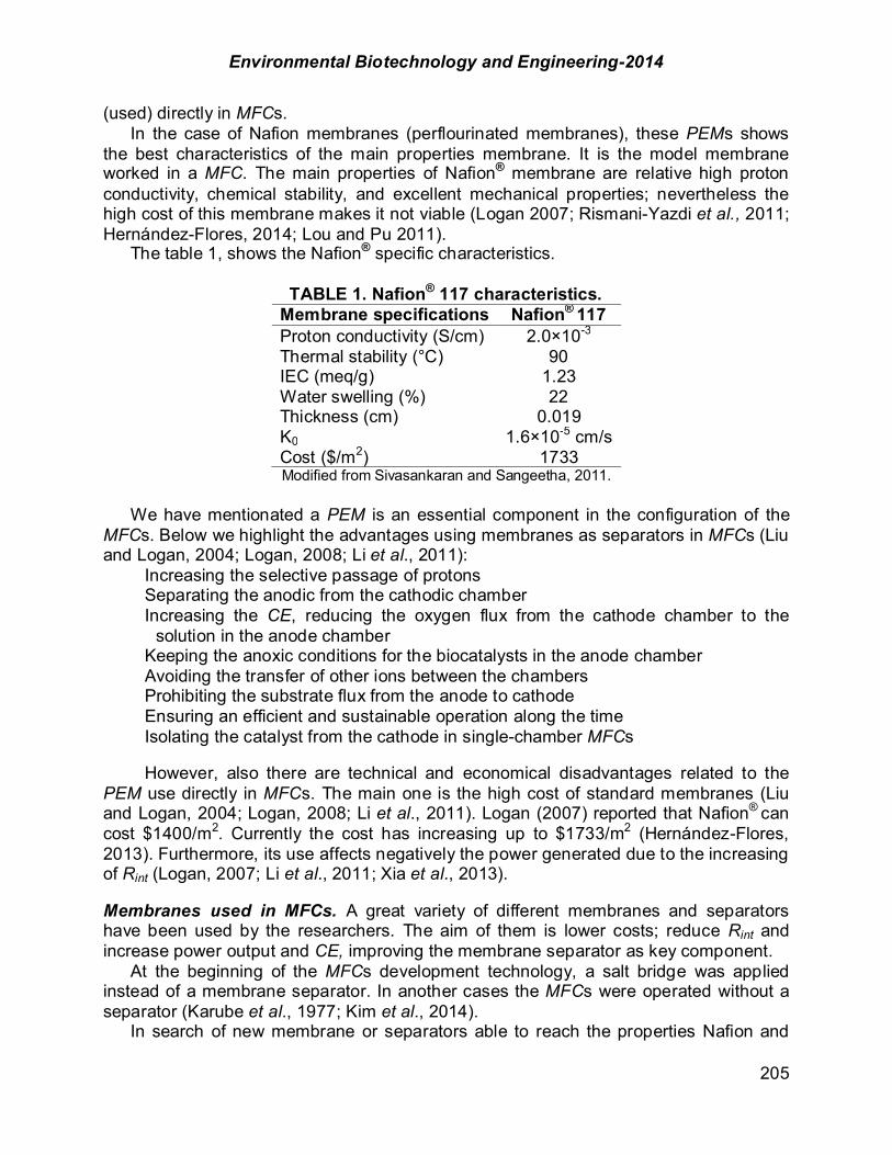
Environmental Biotechnology and Engineering-2014
205
(used) directly in MFCs. In the case of Nafion membranes (perflourinated membranes), these PEMs shows the best characteristics of the main properties membrane. It is the model membrane worked in a MFC. The main properties of Nafion® membrane are relative high proton conductivity, chemical stability, and excellent mechanical properties; nevertheless the high cost of this membrane makes it not viable (Logan 2007; Rismani-Yazdi et al., 2011; Hernández-Flores, 2014; Lou and Pu 2011). The table 1, shows the Nafion® specific characteristics.
TABLE 1. Nafion® 117 characteristics. Membrane specifications Nafion® 117 Proton conductivity (S/cm) 2.0!10-3 Thermal stability (°C) 90 IEC (meq/g) 1.23 Water swelling (%) 22 Thickness (cm) 0.019 K0 1.6!10-5 cm/s Cost ($/m2) 1733 Modified from Sivasankaran and Sangeetha, 2011.
We have mentionated a PEM is an essential component in the configuration of the MFCs. Below we highlight the advantages using membranes as separators in MFCs (Liu and Logan, 2004; Logan, 2008; Li et al., 2011): Increasing the selective passage of protons Separating the anodic from the cathodic chamber Increasing the CE, reducing the oxygen flux from the cathode chamber to the
solution in the anode chamber Keeping the anoxic conditions for the biocatalysts in the anode chamber Avoiding the transfer of other ions between the chambers Prohibiting the substrate flux from the anode to cathode Ensuring an efficient and sustainable operation along the time Isolating the catalyst from the cathode in single-chamber MFCs
However, also there are technical and economical disadvantages related to the PEM use directly in MFCs. The main one is the high cost of standard membranes (Liu and Logan, 2004; Logan, 2008; Li et al., 2011). Logan (2007) reported that Nafion® can cost $1400/m2. Currently the cost has increasing up to $1733/m2 (Hernández-Flores, 2013). Furthermore, its use affects negatively the power generated due to the increasing of Rint (Logan, 2007; Li et al., 2011; Xia et al., 2013). Membranes used in MFCs. A great variety of different membranes and separators have been used by the researchers. The aim of them is lower costs; reduce Rint and increase power output and CE, improving the membrane separator as key component. At the beginning of the MFCs development technology, a salt bridge was applied instead of a membrane separator. In another cases the MFCs were operated without a separator (Karube et al., 1977; Kim et al., 2014). In search of new membrane or separators able to reach the properties Nafion and

Environmental Biotechnology and Engineering-2014
206
reduce cost, many membranes or separator have been studied. Here there are some of them: Zirfon® membrane, sulphonated polyether ether ketone membrane (SPEEK), ultrafiltration and microfiltration membranes, anion and cation exchange membranes, bipolar membrane, forward osmosis membrane, Cloth (J-cloth) separator, glass fiber separator, cation exchange layer made of purified kaolin, porous porcelain coated with Nafion-117 solution, polystyrene and divinylbenzene with sulfonic acid groups, dialysis membranes, organic polymers, spray coated to thin layers of hydrophilic cation exchange, anion exchange and neutral polymers, porous fabrics and course-pore filter material, selemion HSF, polytetrafluoroethylene membrane, isoporo membrane filter, biomax ultrafiltration disc, glass wool, nylon membranes, polycarbonate membranes, cellulose nitrate membranes, kaolin, porcelain and polyethylene membranes interpolymer, forward osmosis membrane (Grzebyk and Pozniak, 2005; Min et al., 2005; Logan et al., 2006; Logan and Regan 2006; Logan, 2007; Zhang et al., 2009; Yang et al., 2010; Pant et al., 2010; Lefebvre et al., 2011; Li et al., 2011; Sivasankaran and Sangeetha, 2011; Wei et al., 2011; Zhang et al., 2011; Watson et al., 2011; Hernández-Flores, 2014). Membraneless MFCs. MFCs without a separator or membrane were one of the first configurations used in the principle of MFCs (Min et al., 2005; Kim et al., 2014). The basis to propose MFCs operating without membranes or separators is due to the water has the property of conducting the protons by itself (Logan 2007). Then, the membrane is not strictly necessary in a MFC configuration. There are some disadvantages using Membraneless MFCs. The absence of a separator allow the substrate and oxygen diffusion, it affects reducing the CE and microorganism activity bioelectrocatalytic (Liu et al., 2005; Yang et al., 2010; Liu and Logan, 2004; Logan, 2007; Li et al., 2011; Logan et al., 2006). Regarding the substrate diffusion, this causes a rapid formation of biofilm at the cathode, it is called biofouling. This causes deactivation of the cathode and reduce the MFC performace (Tartakovsky and Guiot, 2006). Liu and Logan (2004) used a membrane-less MFC to the bioelectricity generation. Their objective was to increase the energy output and reduce the cost. The results obtained by them were a power density of 146 ± 8 mW/m2 and 20% of CE for their membrane-less MFC. In contrast, their MFC fitted with Nafion membrane displayed a power density of 28 ± 3 mW/m2 and 28% of CE. In another case, Liu et al., 2005 and Cheng et al., 2006 proposed a configuration to reduce the oxygen diffusion. They separated the electrodes in the MFC, however it increase the Rint. The researches have concluded a separator or membrane is necessary to ensure an efficient and sustainable MFC operation (Harnisch and ShrÖder, 2009). Perspectives on PEMs. The challenge of developing alternative membranes to use in MFCs is task taken only by a few researchers (Kim et al., 2014). However, to find a new membrane able to reach attractive MFC performance with a low cost is necessary for a cost-effective scaling upof the MFCs. Acknowledgements

Environmental Biotechnology and Engineering-2014
207
The authors are grateful to CINVESTAV-IPN, SECITI-GDF (formerly ICYTDF), Mexico, for financial support to this research (PICCO-10-28), and CONACYT for an Infrastrucutr Project support to the Environmental Biotechnology and Renewable Energies Group. Giovanni Hernández-Flores received a graduate scholarship from CONACYT, Mexico. Also the authors thank Mr. Rafael Hernández-Vera, and technicians of the Environmental of Biotechnology and Renewable Energy R&D Group, CINVESTAV-IPN for their excellent technical help. References Brunetti, A.; Fontananova, E.; Donnadioa, A.; Casciola, M.; Di Vona, M. L.; Sgreccia, E.; Driolia, E.;
Barbieri, G. (2012). New approach for the evaluation of membranes transport properties for polymer electrolyte membrane fuel cells. Journal of Power Sources. 205: 222-230.
Cheng-Dar, Y.; Chung-Ming, L.; Liou, E. M. L. (2001). A transition toward a sustainable energy future: feasibility assessment and development strategies of wind power in Taiwan. Energy Policy. 29: 951-963.
Cheng, S.; Liu,H.; Logan, B. E. (2006). Increased power generation in a continuous flow MFC with advective flow through the porous anode and reduced electrode spacing. Environ. Sci. Technol. 40: 2426–2432.
Cho, K.-Y.; Jung, H.-Y.; Sung, K. A.; Kim, W.-K.; Sung, S.-J.; Park, J.-K.; Choi, J.-H.; Sung, Y.-E. (2006). Preparation and characteristics of Nafion membrane coated with a PVdF copolymer/recast Nafion blend for direct methanol fuel cell. Journal of Power Sources. 159: 524–528.
Choi, T. H.; Won, Y.-B.; Lee, J.-W.; Shin, D.W.; Lee, Y. M.; Kim, M.; Park, H. B. (2012). Electrochemical performance of microbial fuel cells based on disulfonated poly(arylene ether sulfone) membranes, J. Power Sources 220: 269–279.
Das, D.; Veziroglu, T. N. (2001). Hydrogen production by biological processes: a survey of literature. Int J. Hydrogen Energy. 26: 13-28.
Dewan, A.; Beyenal, H.; Lewandowski, Z. (2008). Scaling up Microbial Fuel Cells. Environ. Sci. Technol. 42: 7643–7648.
Ghasemi, M.; Daud, W. R. W.; Hassan, S. H. A.; Oh, S.-E.; Ismail, M.; Rahimnejad, M.; Jahim, J. M. (2013) Nano-structured carbon as electrode material in microbial fuel cells: a comprehensive review. Journal of Alloys and Compounds. 580: 245–255.
Grzebyk, M.; Po!niak, G. (2005). Microbial fuel cells (MFCs) with interpolymer cation exchange membranes. Sep. Purif. Technol. 41: 321–328.
Harnisch, F.; Schröder, U. (2009). Selectivity versus Mobility: Separation of Anode and Cathode in Microbial Bioelectrochemical Systems. ChemSusChem 2: 921–926.
Hernández-Flores, G. (2014). Interim Report. Sc D Thesis, CINVESTAV-IPN, México, D.F. Hsu, L., Chadwick, B., Kagan, J., Thacher, R., Wotawa-Bergen, A., Richter, K. (2013). Scale up
considerations for sediment microbial fuel Cells. RSC Adv. 3: 15947–15954. Karube, I.; Matsunaga, T.; Tsuru, S.; Suzuki, S. (1977). Biochemical fuel cell utilizing immobilized cells of
clostridium butyricum. Biotechnol. Bioeng.19: 1727–1733 Kim, J. R.; Cheng, S.; Oh, S.-E.; Logan, B. E. (2007). Power Generation Using Different Cation, Anion and
Ultrafiltration Membranes in Microbial Fuel Cells. Environ. Sci. Technol. 41: 1004-1009. Lefebvre, O.; Shen, Y.; Tang, Z.; Uzabiaga, A.; Chang, I. S.; Ng, H. Y. (2011). A comparison of
membranes and enrichment strategies for microbial fuel cells. Bioresour. Technol. 102: 6291-6294. Li, W.-W; Guo-Ping, S.; Xian-Wei, L.; Han-qing, Y. (2011). Recent advances in the separators for
microbial fuel cells. Bioresour Technol. 102: 244-252. Liu, H.; Logan, B. E. (2004). Electricity generation using an air-cathode single chamber microbial fuel cell
in the presence and absence of a proton exchange membrane. Environ. Sci. Technol. 38: 4040–4046. Liu, H.; Cheng, S.; Logan, B. E. (2005). Power generation in fed-batch microbial fuel cells as a function of
ionic strength, temperature, and reactor configuration. Environ. Sci. Technol. 39: 5488–5493. Logan, B. E. (2007). Microbial fuel cells. John Wiley-Interscience. New Jersey, USA. Logan, B. E. (2010). Scaling up microbial fuel cells and other bioelectrochemical systems. Appl. Microbiol.
Biotechnol. 85: 1665-1671.

Environmental Biotechnology and Engineering-2014
208
Logan, B. E.; Regan, J. M. (2006). Microbial challenges and harnessing the metabolic activity of bacteria can provide energy for a variety of applications, once technical and cost obstacles are overcome. Environ. Sci. Technol. 5172–5180.
Logan, B. E.; Hamelers, B.; Rozendal, R.; Schröder, U.; Keller, J.; Freguia, S.; Aelterman,P.; Verstraete, W.; Rabaey, K. (2006). Microbial fuel cells: Methodology and technology. Environ. Sci. Technol. 40: 5181-5192.
Lou, L.; Pu, H. (2011). Preparation and properties of proton exchange membranes based-on Nafion® and phosphonic acid-functionalized hollow silica spheres. International Journal of Hydrogen Energy. 36: 3123-3130
Min, B.; Cheng, S.; Logan, B. E. (2005). Electricity generation using membranes and salt bridge microbial fuel cells. Water Research. 39: 1675-1686.
Pandit S., Sengupta, A., Kale S., Das, D. (2011). Performance of electron acceptors in catholyte of a two-chambered microbial fuel cell using anion exchange membrane. Bioresour Technol. 102: 2736-2744.
Pant, D.; Bogaert, G. V.; Smet, M. D; Diels, L.; Vanbroekhoven, K. (2010). Use of novel permeable membrane and air cathode in acetate microbial fuel cells. Electrochimica Acta. 55: 7710-7716.
Pant, D.; Bogaert, G. V.; Diels, L.; Vanbroekhoven, K. (2010). A review of the substrates used in microbial fuel cells (MFCs) for sustainable energy production. Bioresour. Technol. 101: 1533–1543.
Peighambardoust, S. J.; Rowshanzamir, S.; Amjadi, M. (2010). Review of the proton exchange membranes for fuel cell applications. International Journal of Hydrogen Energy. 35: 9349-9384.
Poggi-Varaldo, H. M.; Vazquez-Larios, A.; Solorza-Feria, O. (2010). Microbial fuel cells. In Rodríguez-Varela F.J., Solorza-Feria O., Hernández-Pacheco, E. (Eds). Fuel cells. Book Livres, Montréal, Canada, pp 124-161.
Potter, M. C. Electrical Effects Accompanying the Decomposition of Organic Compounds. Proc. R. Soc. London, Ser. B. 84: 260-276.
Rabaey, K.; Verstraete, W. (2005). Microbial fuel cells: novel biotechnology for energy generation. Trends Biotechnol. 23: 291–298.
Rismani-Yazdi,H.; Carver, S. M.; Christy, A. D.; Tuovinen, O. H. (2008). Cathodic limitations in microbial fuel cells: an overview. J. Power Sources. 180: 683-694.
Rozendal, R. A.; Hamelers, H. V. M.; Rabaey, K.; Keller, J.; Buisman, C. J. N. (2008). Towards practical implementation of bioelectrochemical wastewater treatment. Trends Biotechnol. 26: 450–459.
Rozendal,R. A.; Hamelers, H. V. V.; Guisman, C. J. N. (2006). Effects of Membrane Cation Transport on pH and Microbial Fuel Cell Performance Environ. Sci. Technol. 40: 5206–5211.
Shahgaldi, S.; Ghasemi, M.; Wan, D. W. R.; Yaakob, Z.; Sedighi, M.; Alam, J.; Ismail, A. F. (2014). Performance enhancement of microbial fuel cell by PVDF/Nafion nanofibre composite proton exchange membrane. Fuel Processing Technology. 124: 290–295.
Sivasankaran, A.; Sangeetha, D. (2011). Development of MFC using sulphonated polyether ether ketone (SPEEK) membrane for electricity generation from waste water. Bioresour. Technol. 102(24): 11167-11171.
Tartakovsky, B.; Guiot, S. R. (2006). A comparison of air and hydrogen peroxide oxygenated microbial fuel cell reactors. Biotechnol. Prog. 22: 241–246.
Tye, Y. Y., Lee, K. T., Abdullah, W.N.W, Leh, C.P. (2011). Second-generation bioethanol as a sustainable energy source in Malaysia transportation sector: Status, potential and future prospects. Renewable and Sustainable Energy Reviews. 15: 4521-4536.
Vazquez-Larios, A. L.; Solorza-Feria, O.; Vazquez-Huerta, G.; Esparza-Garcia, F. J.; Rios-Leal, E.; Rinderknecht-Seijas, N.; Poggi-Varaldo, H. M. (2010). A new design improves performance of a single chamber microbial fuel cell. J. New Mater. Electrochem. Syst. 13: 219-226.
Watson, V. J.; Saito, T.; Hickner, M. A.; Logan, B. E. (2011). Polymer coatings as separator layers for microbial fuel cell cathodes. Journal of Power Sources.196: 3009–3014.
Wei, J.; Liang, P.; Huang, X. (2011). Recent progress in electrodes for microbial fuel cells. Bioresour. Technol. 102: 9335-9344.
Xia, X.; Tokash, J. C.; Zhang, F.; Liang, P.; Huang, X.; Logan, B. E. (2013). Oxygen-Reducing Biocathodes Operating with Passive Oxygen Transfer in Microbial Fuel Cells. Environ. Sci. Technol. 47 (4): 2085–2091.
Yang, Y.; Sun, G.; Xu, M. (2010). Microbial fuel cells come of age. J. Chem. Technol. Biotechnol. 86: 625-632.
Zhang, F.; Brastad, K. S.; He, Z. (2011). Integrating forward osmosis into microbial fuel cells for
Environmental Biotechnology and Engineering-2014
209
wastewater treatment, water extraction and bioelectricity generation. Environ. Sci. Technol. 45: 6690-6696
Zhang, X.; Cheng, S.; ‡, Wang, X.; Huang, X.; Logan, B. E. (2009). Separator Characteristics for Increasing Performance of Microbial Fuel Cells. Environ. Sci. Technol. 43: 8456-8641.
Zhou, M.; Chi, M.; Luo, J.; He, H.; Jin, T. (2011). An overview of electrode materials in microbial fuel cells. J. Power Sources. 196: 4427-4435.
.
.Notation CE coulombic efficiency MFC microbial fuel cell ORR oxygen reduction reaction PEM proton exchange membrane Rint internal resistance SPEEK sulphonated polyether ether ketone Greek characters $coul coulombic efficiency
Environmental Biotechnology and Engineering-2014
210
CHAPTER 1.21. EL PRINCIPIO DE CASCADA APLICADO A LA BIORREFINERÍA DE
RESIDUOS SÓLIDOS URBANOS PARA LA GENERACIÓN DE PRODUCTOS DE VALOR AGREGADO: UNA REVISIÓN
Leticia Romero-Cedillo (1); Héctor M. Poggi-Varaldo* (1); M. Teresa Ponce-Noyola (1); Ana C. Ramos-Valdivia (1); Elvira Ríos-Leal (1); Carlos M. Cerda-García Rojas (2); José
I. Tapia-Ramírez (3); Jaime García-Mena (3)
(1) CINVESTAV-IPN, DBB, México DF, México; (2) CINVESTAV-IPN, DQ, México DF, México; (3) CINVESTAV-IPN, DGBM, México DF, México; RESUMEN La energía alternativa se puede producir a través de una biorrefinería, utilizando residuos orgánicos de muy bajo costo y renovables, para generar biocombustibles y otros productos de valor agregado como son las enzimas, ácidos orgánicos, aditivos, solventes, aminoácidos, etc. Para esto es necesario seguir el principio de cascada, que se refiere al uso de los residuos orgánicos como materia prima en procesos secuenciales para así obtener el máximo rendimiento en productos y una mayor ganancia. En el caso de la biorrefinería HMZS (hidrógeno, metano, enzimas y sacarificación), se utiliza el “principio de cascada inversa”, para producir primero bioenergía mediante la degradación de la fracción orgánica de residuos sólidos urbanos (FORSU) durante la fermentación oscura. Mediante la integración de etapas secuenciales en la biorrefinería HMZS se ha logrado diversificar el uso de estos residuos y obtener holocelulasas. Sin embargo, uno de los retos que se presentan es aprovechar la cantidad de celulosa disponible en los sólidos residuales utilizando pretratamientos, que favorezcan el acceso de las enzimas y mejoren el rendimiento en la obtención de azúcares fermentables. Los métodos comúnmente utilizados para este fin, son la explosión por vapor, organosolv, enzimático, hidrólisis ácida, tratamiento ácido diluido e hidrólisis alcalina. Este último tiene la ventaja de llevarse a cabo a bajas temperaturas y de los tratamientos químicos, es uno de los métodos más efectivos para el rompimiento de los enlaces éster entre la lignina, celulosa y hemicelulosa, además de que evita la fragmentación de los polímeros de hemicelulosa. Por lo anterior, es importante conocer la efectividad de los pretratamientos en los sólidos que contienen una cantidad importante de celulosa para ser aprovechados nuevamente en el mismo proceso de biorrefinería y explorar su potencial en la obtención de otros productos. Palabras clave: biorrefinería, pretratamientos, celulosa, holocelulasas ------------------ *Author for correspondence: [email protected]

Environmental Biotechnology and Engineering-2014
211
Introducción
Los procesos integrados, el estudio de la biomasa y la tecnología en biorrefinería han sido objeto de estudio e investigación desde los años 90´s. Recientemente la conversion de materia prima renovable para producir biocombustibles, ha llegado a ser una opción prometedora pues también se han generado productos de alto valor agregado. Uno de los principales productos de la biorrefinería son los biocombustible, que se generan a partir de fuentes renovables, lo que la convierte en una alternative atractiva pues ayuda a minimizar la quema de combustibles fósiles y emisiones de CO2. Los biocombustibles derivados del aprovechamiento de la biomasa de plantas o de desechos orgánicos podrían ayudar a reducir la dependencia de los hidrocarburos y la producción de CO2 a la atmósfera (Osamu et al., 1989). A lo largo de la historia, los esquemas de producción industrial han evolucionado, partiendo de la producción de azúcar, hidrólisis de almidón, sacarificación de madera, formación y separación de furfural, celulosa y producción de pulpa, hasta llegar a la síntesis de ácido levulínico, lípidos, vanillina a partir de lignina y la fermentación de ácido láctico (Demirbas, 2009). La obtención de estos productos se realiza a partir de biomasa que se compone principalmente de tres tipos de polímeros orgánicos: celulosa, hemicelulosa y lignina. Sin embargo la proporción estos varía dependiendo de el tipo de residuo, por ejemplo están los desechos de origen agroindustrial, pastos, plantas, plantas acuáticas y cultivos (Naik et al., 2010). Esta variedad es importante para generar una amplia gama de productos finales o bien de precursores de otros compuestos de interés. Por ejemplo, los metabolitos secundarios, pueden emplearse en la síntesis de compuestos químicos de alto valor agregado como son los aditivos y saborizantes para alimentos, la síntesis de fármacos, producción de cosméticos, y alimento para animales, por mencionar algunos (Clark, 2007). Cabe mencionar que las tecnologías emergentes en el área de biorrefinería, se han planteado el mejoramiento de dichos procesos mediante el uso de pretratamientos con el objetivo de llevar una hidrólisis y posterior aprovechamiento de la biomasa celulósica. En la presente revisión se presenta un panorama de la biorrefinería de desechos urbanos enfocada en la biomasa de residuos agrícolas, pretratamientos utilizados para aumentar la disponibilidad de celulosa y los bioproductos generados en estos procesos. Biomasa como fuente de energía renovable, potencial y disponibilidad La biomasa aunque es una material prima renovable tiene algunas limitantes con respecto a la tasa de utilización, pues la máxima disponibilidad teórica de la biomasa está limitada por la capacidad de producción primaria de la biósfera. Aún con el avance científico, la comprensión del funcionamiento de la biósfera y sus ecosistemas está lejos de completarse. Lo anterior queda demostrado cuando al utilizar la biomasa para un fin no alimentario, se afecta al mecanismo functional

Environmental Biotechnology and Engineering-2014
212
básico de la cadena alimenticia de cualquier ecosistema. Por lo tanto, es una responsabilidad compartida de la humanidad, tartar de asegurar que este límite en los ecosistemas no sea rebasado debido a la búsqueda del desarrollo en varios ámbitos (Ghatak, 2011). Para ser una alternativa viable, comparada con una refinería de petróleo, la biorrefinería debe tener un suministro confinable de la materia prima durante toda su vida útil, la cual puede ser de 10-30 años, o incluso más (Stephen et al., 2010). Esto es muy importante ya que la material prima representa el 40-60% de los costos de operación en una biorrefinería típica (Caputo et al., 2005). La biomasa terrestre total tiene un potencial energético de 65 TW, y apenas se aprovecha un 6.32%, lo cual representa una producción de 1.33 TW a partir de biomasa de alimentos y 1.28 TW empleando biomasa de residuos de madera. Se espera que la eficiencia en su uso, alcance el 12.3% (Zhang, 2013). Se han utilizado una gran variedad de materias primas con aplicaciones en biorrefinería, a partir de campos de cultivo, residuos agrícolas, recursos forestales, desechos urbanos e industriales y algas. Algunos estudios con materias primas incluyen: algas verde azules, Chlorella vulgaris, residuos de cítricos, desechos lácteos, desechos de alimentos, cultivos energéticos, glycerol, jatropha, lignin, microalgas, Miscanthus, residuos municipales, residuos orgánicos, arroz, algas, bagazo de caña, pastos de rápido crecimiento y trigo. La disponibilidad de recursos no parece ser un problema, pues se estima un rendimiento annual de material lignocelulósica resultante de la fotosíntesis de 1.3X10⁹ (Kajaste, 2014) Para la elección de la material prima que se empleará, no existe una regla universal, sin embargo la selección se hace tomando en cuenta varios factores. Los aspectos más considerados son las condiciones climáticas, la ubicación, entorno socioeconómico y las políticas del gobierno, estos influyen en la disponbilidad de la material prima. Debido a que uno de los principios fundamentales de la biorrefinería es la sostenibilidad, el suministro de materias primas debe ajustarse a esos parámetros (Ghatak, 2011). Índice de Potencial de Generación en residuos agrícolas. En Brasil, se han realizado evaluaciones de diferentes residuos agrícolas con el fin de encontrar desechos con el mayor potencial considerando su disponibilidad y la magnitud del cultivo. Es así como otro de los aspectos importantes para el diseño de una biorrefinería, es el cálculo del Índice de Potencial de Generación (IPG), el cual es una relación entre las toneladas de residuos totales de determinada biomasa (tTR), y toneladas totales de cultivo que se producen. Por ejemplo, por cada 1000 kg de azúcar de caña que se cultivam, se generan 220 kg de residuos (tTRSC), por lo cual su GP=0.22 tTR/tTSC (Carneiro et al., 2013). En la tabla 1 se muestran los índices de Potencial de Generación (IPG), de residuos agrícolas y de animales, que se han evaluado en Brasil.

Environmental Biotechnology and Engineering-2014
213
TABLA 1. Estimación del índice de Potencial de Generación (PG) en residuos agrícolas y animales en Brasil
Materia prima Índice de Potencial de Generación (tTR/tCultivo)
Azúcar de caña Naranja
0.22 0.50
Yuca 0.20 Tabaco 0.75 Excreta de cerdo 0.06 Excreta de vaca 0.07
Notas: tTR= toneladas de residuo total; tCultivo= toneladas de cultivo total
A continuación se describen aspectos y características de la biomasa de residuos agrícolas que son empleados como materia prima en un procesos de biorrefinería. Biorrefinería de resíduos agrícolas Este tipo de residuos constituyen una categoría importante al ser una fuente de material prima con gran potencial para su uso en biorrefinerías, pues no afectan la disponibilidad alimentaria. En un sentido amplio, los residuos agrícolas son aquéllos que han sido producidos por la industria agroalimentaria, por medio de su operación diaria. Tales desechos pueden ser hojas, raíces, semillas, residuos de madera y residuos de animales; todos estos residuos, representan billones de toneladas anuales y están disponibles en gran cantidad, son renovables y prácticamente gratis. La principal composición de esta biomasa es celulosa, hemicelulosa y lignina (Taherzadeh y Karimi, 2007). La composición típica de resiudos agrícolas es 40-50% celulosa, 25-35% hemicelulosa, 15-20% lignin. Sin embargo la biomasa puede emplearse en multiples aplicaciones como en la obtención de biocombustibles, productos químicos y como fuente de energía. Algunos sub-productos que se obtienen de la biorrefinería de residuos agricolas son: resinas, películas de pollímeros, plásticos biodegradables, agentes floculantes y principalmente celulosa, papel y fibras textiles que resultan de la fermentación de lignocelulosa. En la tabla 2 se muestran algunos bioproductos generados a partir de diferentes residuos agrícolas (Carneiro et al., 2013).
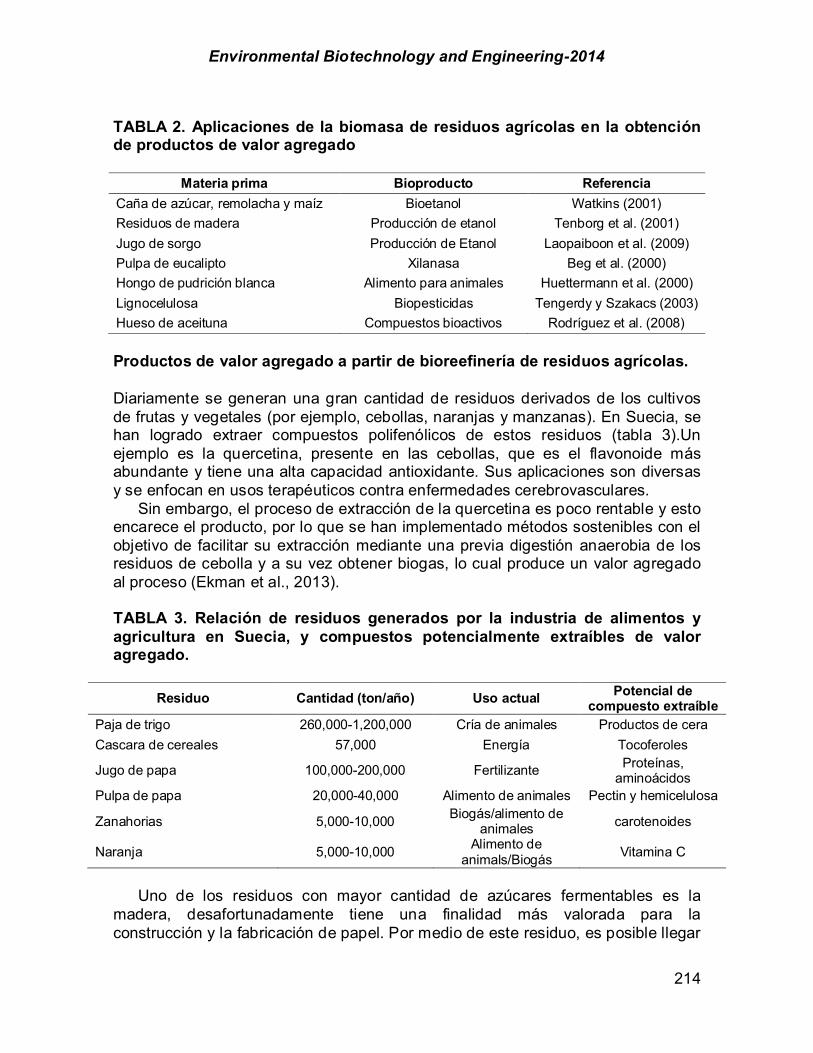
Environmental Biotechnology and Engineering-2014
214
TABLA 2. Aplicaciones de la biomasa de residuos agrícolas en la obtención de productos de valor agregado
Materia prima Bioproducto Referencia Caña de azúcar, remolacha y maíz Bioetanol Watkins (2001) Residuos de madera Producción de etanol Tenborg et al. (2001) Jugo de sorgo Producción de Etanol Laopaiboon et al. (2009) Pulpa de eucalipto Xilanasa Beg et al. (2000) Hongo de pudrición blanca Alimento para animales Huettermann et al. (2000) Lignocelulosa Biopesticidas Tengerdy y Szakacs (2003) Hueso de aceituna Compuestos bioactivos Rodríguez et al. (2008) Productos de valor agregado a partir de bioreefinería de residuos agrícolas. Diariamente se generan una gran cantidad de residuos derivados de los cultivos de frutas y vegetales (por ejemplo, cebollas, naranjas y manzanas). En Suecia, se han logrado extraer compuestos polifenólicos de estos residuos (tabla 3).Un ejemplo es la quercetina, presente en las cebollas, que es el flavonoide más abundante y tiene una alta capacidad antioxidante. Sus aplicaciones son diversas y se enfocan en usos terapéuticos contra enfermedades cerebrovasculares. Sin embargo, el proceso de extracción de la quercetina es poco rentable y esto encarece el producto, por lo que se han implementado métodos sostenibles con el objetivo de facilitar su extracción mediante una previa digestión anaerobia de los residuos de cebolla y a su vez obtener biogas, lo cual produce un valor agregado al proceso (Ekman et al., 2013). TABLA 3. Relación de residuos generados por la industria de alimentos y agricultura en Suecia, y compuestos potencialmente extraíbles de valor agregado.
Residuo Cantidad (ton/año) Uso actual Potencial de compuesto extraíble
Paja de trigo 260,000-1,200,000 Cría de animales Productos de cera Cascara de cereales 57,000 Energía Tocoferoles
Jugo de papa 100,000-200,000 Fertilizante Proteínas, aminoácidos
Pulpa de papa 20,000-40,000 Alimento de animales Pectin y hemicelulosa
Zanahorias 5,000-10,000 Biogás/alimento de animales carotenoides
Naranja 5,000-10,000 Alimento de animals/Biogás Vitamina C
Uno de los residuos con mayor cantidad de azúcares fermentables es la madera, desafortunadamente tiene una finalidad más valorada para la construcción y la fabricación de papel. Por medio de este residuo, es posible llegar

Environmental Biotechnology and Engineering-2014
215
a producir 45L (35.5 kg) de etanol, a partir de 100 kg de pesos seco de biomasa. El etanol lignocelulósico se ha producido por más de 100 años por medio de una hidrólisis ácida. Cabe mencionar, que entre los productos de valor agregado más destacados están las xylanasas y celulasas. Se han logrado aislar microorganismos con actividad ceulolítica, tal es el caso de la bacteria Cellulomonas flavigena PR-22 (Ponce-Noyola et al., 1995) aislada de bagazo de caña. Esta cepa ha sido utilizada posteriormente en procesos de sacarificación a partir de biomasa vegetal con el objetivo de obtener bioetanol (Rojas et al., 2011). En trabajos recientes con C.flavígena PR-22 se obtuvieron actividades xilanolíticas en el rango de 1800-3900 UI/ghol-1, y para enzimas celulolíticas se tuvieron actividades de 220-420 UI/ghol-1 (Escamilla et al., 2013). En este último se empleó como biomasa renovable la fracción orgánica de residuos sólidos urbanos, que se caracteriza por contener celulosa en un rango del 60-70% lo que favorece la producción de estas enzimas. Paralelamente se han integrado procesos o pretratamientos de biomasa que tienen como finalidad aumentar la disponibilidad de celulosa al transformarla de su estado cristalino a su estado amorfo. Uno de los métodos exitosos es el proceso BALI, que tiene por objetivo utilizar por lo menos el 80%de la biomasa y transformarla a productos de valor agregado. El proceso consiste en cuatro pasos principales, primero un pretratamiento químico y fraccionamiento, en el que la lignina es solubilizada, la cristalinidad de la celulosa es reducida y la hemicelulosa es conservada o hidrolizada a monosacáridos solubles. La fase sólida que contiene celulosa y hemicelulosa es sometida a una hidrólisis enzimática que genera hexosas y pentosas. Estos azúcares fermentables son utilizados para la producción de etanol y otros compuestos. Por su parte, la lignina recuperada se utiliza en la fabricación de agentes dispersantes, aglutinantes y emulsificantes (Rodsrud et al., 2012) Pretratamientos aplicados a la biomasa lignocelulósica Uno de los inconvenientes que presenta este tipos de biomasa es su estructura compleja ya que dificulta la hidrólisis de celulosa, debido a las fuertes interacciones entre la lignina y hemicelulosa, que reducen el acceso a la superficie de área de la celulosa (Manzanares et al., 2012). Por lo anterior, los pretratamientos son una herramienta necesaria para incrementar el acceso de las enzimas a la biomasa celulósica y mejorar el rendimiento en la obtención de azúcares fermentables (Mood et al., 2013). Los métodos comúnmente utilizados para este fin, son la explosión por vapor, hidrólisis ácida, tratamiento ácido diluido e hidrólisis alcalina (Sun, 2002). Con el paso del tiempo se han desarrollado otros pretratamientos para la biomasa lignocelulósica que son efectivos como el proceso de organosolv y la hidrólisis enzimática (Chiaramonti et al., 2012). A continuación se describen brevemente algunos de los pretratamientos utilizados para el acondiciona miento de este tipo de biomasa.
Environmental Biotechnology and Engineering-2014
216
Explosión de vapor. Este método requiere de una alta presión que inicia la reacción de hidrólisis que más adelante es reducida de forma repentina, exponiendo la materia prima a una descompresión explosiva que modifica la estructura de la biomasa aumentando la accesibilidad a la estructura. Se lleva a cabo a un rango de temperaturas de 180-220°C, una presión de 1-1.23 MPa y un tiempo de retención de 2-10 minutos (Ruíz et al., 2006). Con el objetivo de aumentar la recuperación de celulosa y hemicelulosa, el SO2 puede ser añadido al sistema de explosión. Dependiendo del tipo de biomasa tratada el porcentaje de SO2 puede variar, por ejemplo la fracción de la masa en madera seca es del 1 al 5% (Eklund et al., 1995). El uso de SO2 para el tratamiento de residuos de madera ha generado de alta producción de azúcares, donde el máximo rendimiento de glucosa (95%) se ha obtenido utilizando el 1% de SO2 y tratando la biomasa a 200°C (Ohgren et al., 2007). Hidrólisis ácida. Los ácidos concentrados son una opción para el pretratamiento de biomasa celulósica de residuos agrícolas y de madera. El ácido sulfúrico es el ácido más utilizado, mientras que otro tipo de ácidos como el nítrico y el clorhídrico aún se siguen investigando (Taherzade et al., 2007). Este método puede realizarse a temperatura ambiente utilizando ácidos concentrados que han mostrado eficiencia en la hidrólisis de materia lignocelulósica, sin embargo es costoso y el proceso resulta potencialmente peligroso (Chiaramonti et al., 2012). Ácido diluido. Este método es uno de los más efectivos para la degradación de hemicelulosa y lignina y representa la opción más adecuada con respecto al resto de los pretratamientos químicos (Mussatto et al., 2004). El ácido clorhídrico y el ácido sulfúrico se utilizan diluidos a concentraciones del 2% al 5% y el proceso se lleva acabo a temperaturas alrededor de los 150-250°C a una presión de 2 a 24 atm (Cheng et al., 2012; Hsu, 1996). Se han reportado altos rendimientos de conversión de celulosa a glucosa del 93.1% utilizando el pre-tratamiento ácido diluido, en comparación con un pre-tratamiento de lavado (69.6%) y menor al 20% sin tratamiento (Wi, et al., 2011). Organosolv. Con este método, la biomasa es tratada con un solvente orgánico mezclado con ácido sulfúrico. Se utilizan principalmente etanol, metanol, acetona, glicol etileno, glicol trietileno y fenol como solventes. La lignina hidrolizada después del pre-tratamiento queda disuelta en la fase organofílica, después es recuperada por filtración y una reacción de precipitación; por su parte la celulosa queda en el residuo o fracción sólida y la hemicelulosa en la fracción soluble en agua en forma de monómero u oligómeros de azúcar (Hallac et al., 2010). El pretratamiento se lleva acabo a una temperatura de 180°C, durante 60 minutos y utilizando ácido sulfúrico al 1.25% (Kautto et al., 2013). Hidrólisis alcalina. El mecanismo de la hidrólisis alcalina se basa en la saponificación de los enlaces éster intermoleculares entrecruzados con la lignina y parte de hemicelulosa, la reducción de los entrecruzamientos tiende a aumentar la porosidad del material (Chiaramonti et al., 2012). El pretratamiento se puede llevar

Environmental Biotechnology and Engineering-2014
217
a cabo a bajas temperaturas pero con un tiempo relativamente largo y a altas concentraciones de alcalinidad. De los tratamientos químicos, es uno de los más efectivos métodos para el rompimiento de los enlaces éster entre la lignina, celulosa y hemicelulosa, además evita la fragmentación de los polímeros de hemicelulosa (Gaspar et al., 2007). Para esta técnica se utilizan soluciones alcalinas como el hidróxido de amonio, hidróxido de sodio y el hidróxido de calcio. Los vínculos arilo alquilo en la lignina se anclan rápidamente bajo condiciones alcalinas y la reacción es controlada por los enlaces de la estructura primaria, la cual no es sensible a los iones (OH-), mientras el pH no sea mayor de 10. Una de las soluciones alcalinas utilizadas por su bajo costo es el carbonato de sodio al 1M, pues es más fácil de recuperar que el hidróxido de sodio; el pretratamiento se lleva durante 24 h a 60°C y la biomasa es recuperada por filtración y lavada con agua a un pH de 7.0 (Park et al., 2012). Hidrólisis enzimática. En un estudio reciente se ha evaluado el efecto de la digestión enzimática de endoglucanasas, xylanasas y pectinasas, previa a un proceso de fermentación anaerobia de residuos con alto contenido de fibra en la pulpa seca de remolacha (85.1%) y en bagazo de lúpulo (57.7%). Las concentraciones de azúcares reductores en los hidrolizados de remolacha y lúpulo aumentaron en un 88.9% y 59.4%, respectivamente; además tuvieron un incremento en el rendimiento de gas metano del 13 al 19%, en comparación con los residuos sin hidrolizar (Zieminski et al., 2012). Conclusión Para la implementación de un proceso de biorrefinería es necesario evaluar el entorno en el que se desarrollará, para cumplir con el principio de sostenibilidad y al mismo tiempo utilizar materia prima renovable que no compita con el abastecimiento o demanda alimenticia de la población. Por lo anterior, los residuos agrícolas constituyen una fuente de materia prima viable y sostenible que además de generar biocombustibles, pueden derivar en otros compuestos de interés como las enzimas, diversos metabolitos o compuestos químicos. Para maximizar la obtención de estos bioproductos, es necesario aplicar técnicas o pretratamientos que modifiquen la estructura de los principales componentes de la biomasa, como la celulosa, y hacerla fácil de degradar, lo que puede resultar en mayores rendimientos y paralelamente una disminución de residuos, favoreciendo al medio ambiente.
Environmental Biotechnology and Engineering-2014
218
Agradecimientos LRC agradece al CONACYT por la beca otorgada para estudios de posgrado. Referencias Beg B, Bhushan M, Kapoor GS, Hoondal. (2000). Enhanced production of a termostable xylanase
from Streptomyces sp., QG-11-3 and its application in biobleaching of eucalyptus kraft pulp. Enzyme and Microbial Technology; 27:459–66.
Caputo AC, Palumbo M, Pelagagge PM, Scacchia F. (2005). Economics of biomass energy utilization in combustion and gasification plants: effects of logistic variables. Biomass Bioenergy; 28:35–51.
Carneiro TF, Berni MD, Dorileo IL, Rostagno MA. (2013). Biorefinery study of availability of agriculture residues and wastes for integrated biorefineries in Brazil. Resources, Conservation and Recycling 2013; 77: 78– 88.
Cheng, L., Keener, T., Lee, J., Zhou, X. (2012). Dilute acid pretreatment for cellulosic alcohol production. Biomass Conv. Bioref. 2:169–177.DOI 10.1007/s13399-012-0039-1.
Chiaramonti, D., Prussi, M., Ferrero, S., Oriani, L., Ottonello, P., Torre, P., Cherchi, F. (2012). Review of pretreatment processes for lignocellulosic etanol production, and development of an innovative method. Biomass and bioenergy, 46:25-35.
Clark JH, Green. (2007). Chemistry for the second generation biorefinery-sustainable chemical manufacturing base don biomass. J Chem Technol Biotechnol; 82: 603-609.
Demirbas MF. Biorefineries for biofuel upgrading: a critical review. (2009). Applied Energy; 86:151–61.
Eklund R, Galbe M, Zacchi G. (1995). The influence of SO2 and H2SO4 impregnation of willow prior to steam pretreatment. Bioresour Technol; 52(3):225e9.
Ekman A, Campos M, Lindahl S, Co M, Börjesson P, Nordberg Karlsson, Turner C. (2013). Bioresource utilisation by sustainable technologies in new value-added biorefinery concepts-two case studies from food and forest industry. Journal of cleaner production; 57: 46-58.
Escamilla-Alvarado, C., Poggi-Varaldo, H.M., Ponce-Noyola, M.T. (2013). Use of organic waste for the production of added-value holocellulases with Cellulomonas flavigena PR-22 and Trichoderma reesei MCG 80. Waste Management & Research, August; vol. 31, 8: pp. 849-858.
Gaspar, M., Kalman, G., Reckzey, K. (2007). Corn fiber as a raw material for hemicellulose and etanol production. Process. Biochem., 42(7): 1135-9.
Ghatak HR. (2011). Biorefineries from the perspective of sustainability: feedstocks, products, and processes. Renewable and Sustainable Energy Reviews; 15:4042–52.
Hallac, Bassem., Sannigrahi, Poulomi, Pu, Y., Ray, M., Ragauskas, A. (2010). Effect of etanol organosolv pretreatment on enzymatic hydrolysis of Buddleja davidii stem biomass. Ind. Eng. Chem. Res., 49: 1467–1472.
Hsu, T.A. (1996). Pretreatment of biomass. In: Wyman CE, editor. Handbook on bioethanol: production and utilization. Washington DC: Taylor & Francis, ISBN 1-56032-553-4; pp. 179-212.
Huettermann A, Hamza AS, Chet I, Majcherchyk A, Fouad T, Badr A, Cohen R, Persky L, Hadar Y. (2000). Recycling of agricultural wastes by white-rot fungi for the production of fodder for ruminants. Agro Food Industry Hi-Tech; 11(6):29–32.
Kajaste R. (2014). Chemicals from biomass-managing greenhouse gas emissions in biorefinery production chains-a review. Journal of cleaner production; 75:1-10.
Kautto J, Realff M, Ragauskas A. (2013). Design and simulation of an organosolv process for bioetanol production. Biomass Conv. Bioref; 3: 199-212.
Environmental Biotechnology and Engineering-2014
219
Laopaiboon L, Nuanpeng S, Srinophakun P, Klanrit P, Laopaiboon P. (2009). Ethanol production
from sweet sorghum juice using very high gravity technology: effects of carbon and nitrogen supplementations. Bioresource Technology; 100(18):4176–4182.
Manzanarez, P., Ballesteros, I., Negro, M.J., Oliva, J.M., González, A. (2012) Biological conversion of forage sorghum biomass to ethanol by steam explosion pretreatment and simultaneous hydrolysis and fermentation at high solid content. Biomass Conv. Bioref. 2:123–132.
Mood, S., Golfeshan, A., Tabatabaei, M., Jouzani, G., Najafi, G., Gholami, M., Ardjmnad. (2013). Renewable and Sustainable Energy Reviews 27, 77–93.
Mussatto, S., Roberto, I.C. (2004). Alternatives for detoxification of diluted-acid lignocellulosic
hydrolyzates for use in fermentative processes: a review. Bioresur Technol. 93 (1): 1-10. Naik SN, Vaibhav V. Goud, Prasant K. Rout, Ajay K. Dalai. (2010). Production of first and second
generation biofuels: A comprehensive review. Renewable and Sustainable Energy Reviews; 14: 578-597.
Ohgren K. (2007). Effect of hemicellulose and lignin removal on enzymatic hydrolysis of steam-pretreated corn stover. Bioresour Technol; 98(13):2503e10.
Osamu K, Carl HW. Biomass Handbook. Gordon Breach Science Publisher; (1989). Park YC, Kim JS. (2012). Comparison of various alkaline pretreatment methods of lignocellulosic
biomass. Energy; 47: 31-35. Ponce-Noyola, T. y de la Torre, M. (1995). Isolation of a high-specific growth-rate mutant of
Cellulomonas flavigena on sugar cane bagasse. Appl Microbiol Biotechnol 42, 709-712. Rodríguez G, Lama A, Rodríguez R, Jiménez A, Guilléna R, Fernández-Bolaños J. (2008). Olive
stone an attractive source of bioactive and valuable compounds. Bioresource Technology; 09(13):5261–9.
Rodsrud G, Lersch M, Sjöde A. (2012). History and future of world’s most advanced biorefinery in operation. Biomass and Bioenergy; 46:46-59.
Rojas-Rejón, O., Poggi-Varaldo, H.M., Ramos-Valdivia, A.C., Martínez-Jiménez, A., Crisitiani-Urbina, E., De la Torre-Martínez, M., Ponce-Noyola, T. (2011). Production of cellulases and xylanases under catabolic repression conditions from mutant PR-22 of Cellulomonas flavigena. J Ind. Microbiol Biotechnol; 38:257–264.
Ruiz, E., Cara, C., Ballesteros, M., Manzanares, P., Ballesteros, I., Castro, E. (2006). Ethanol production from pretreated olive tree Wood and sunflower stalks by an SSF process. Appl Biochem Biotechnol; 129-132
Stephen JD, Sokhansanj S, Bi X, Sowlati T, Kloeck T, Townley-Smith Ll. (2010). The impact of agricultural residue yield range on the delivered cost to a biorefinery in the Peace River region of Alberta, Canada. Biosyst Eng; 105:298–305.
Sun Y, Cheng J. (2002). Hydrolysis of lignocellulosic materials for ethanol production: a review. Bioresour Technol. 83(1):1-11.
Taherzadeh MJ, Karimi K. (2007). Enzymatic-based hydrolysis processes for ethanol from lignocellulosic materials: a review. Bio Resources; 2(4):707–38.
Tenborg C, Galbe M, Zacchi G. (2001). Reduced inhibition of enzymatic hydrolysis of steam-pretreated softwood. Enzyme and Microbial Technology; 28: 835–844
Tengerdy RP, Szakacs G. (2003). Bioconversion of lignocellulose in solid substrate fermentation. Biochemical Engineering Journal; 13(2-3):169–79.
Watkins K. Ethanol’s sunny day. Chemical and Engineering News (2001):21. Wi, S.G., Chung, B.Y., Lee, Y.G., Yang, D.J., Bae, H.J. (2011). Enhanced enzymatic hydrolysis of
rapeseed straw by popping pretreatment for bioethanol production. Bioresource Technology, 102(10):5788–5793.
Zhang YH. (2013). Next generation biorefineries will solve the food, biofuels, and environmental trilemma in the energy-food-water nexus. Energy Science and Engineering; 1(1): 27-41.
Zieminski K, Romanowska I, Kowalska M. (2012). Enzymatic pretreatment of lignocellulosic wastes to improve biogás production. Waste Management; 32: 1131-1137.

Environmental Biotechnology and Engineering-2014
220
CHAPTER 1.22. AGRO-INDUSTRIAL RESIDUES AND WASTES AS FEEDSTOCK FOR LIGNOCELLULOSIC BIOFUELS COPRODUCTION USING
ADVANCED BIOREFINERY SCHEMES.
Salvador R. González-Vaca; Víctor Sevilla-Güitrón; Martín Murguía; Gabriela Magaña; Arturo Sanchez*
Centro de Investigación y de Estudios Avanzados del IPN - Unidad Guadalajara de Ingeniería Avanzada. Av. del Bosque 1145, Col. El Bajío, Zapopan, Jalisco, 45019, MEXICO. Tel: +52 (33)3777-3600 Ext. 1102 ABSTRACT This work presents a comparative analysis of an advanced biorefinery scheme (ABS) for biofuels (i.e. bioethanol, biogas and biohydrogen) co-production and electricity cogeneration against a conventional biorefinery plant (CBP). Agro-industrial residues and wastes from the cheese and tequila industries as well as crop residues are used under muti-feedstock strategies. The analysis is based on calculations of the total production cost (TPC) and the end-use energy ratio (EER); feasible conditions are established for achieving acceptable TPC in mid-size agriculture sectors.
The ABS flowsheet consists of seven stages (pretreatment, dark fermentation, enzymatic saccharification, alcoholic fermentation, separation, waste water treatment and cogeneration) and is fed by wheat straw, cheese whey, vinasses (these last two with high COD) and some other raw materials. The products are lignocellulosic bioethanol and electricity. The produced biogas and biohydrogen are fed to the cogeneration stage for electricity production. The CBP flowsheet is fed only with wheat straw, using all monosaccharides in the alcoholic fermentation and does not consider biohydrogen production. The steady state mass and energy models as well as equipment capital were solved with state-of-the-art simulation tools for the 100 – 2,000 ton DB/day capacity interval and polysaccharides content (pc) (35% -70%) of the main feedstock (i.e. wheat straw). All other feedstocks were adjusted proportionally. The Net Present Value (NPV) technique was employed for the economic evaluation. The EER, defined as the ratio of energy produced (steam, electricity and chemical energy of ethanol) and total energy consumed in the process, was calculated using data from the energy balances. A TPC quasi-linear section was identified for 2,000, 1,000 and 500 ton DB/day capacities and 45%, 55%, and 70% pc respectively. The results in this area are not larger than 20% of the minimum TPC obtained (1.28 USD/l etOH for 2,000 ton DB/day and 70% pc) with 100% EER. Results for the best TPC of the ABS were compared against the CBP TCP results ($0.93 USD/l etOH and EER 110%). The paper discusses the operational, technological and economic ----------- *Author for correspondence

Environmental Biotechnology and Engineering-2014
221

Environmental Biotechnology and Engineering-2014
222
conditions giving rise to these results. Although ABS TCP is 38% higher than the CBP counterpart, the ABS could be a solution for the treatment of agro-industrial residues and wastes since it take advantage of biofuels production, reducing its high COD index and providing an income from wastes and residues than will certainly help to pay the investment of treatment equipment. Key words: advanced biorefinery scheme, conventional borefinery plant, end-use energy ratio, lignocellulosic bioethanol production, lignocellulosic biofuels coproduction, total production cost. Introduction Fossil fuels have been essential in meeting a substantial portion of the global energy demand. With the continuous growth of population and industrial activities, the world´s energy consumption is projected to increase by 44% from 2006 to 2030 (EIA, 2009). In addition, liquid fuels are expected to remain as the world main energy source with a current consumption of approximately 90 million barrels per day (EIA, 2009). The dwindling fossil-energy resources coupled with the increasing energy demand will ultimately lead to the exhaustion of fossil fuels (Shafiee et al., 2008). This underlines the need to develop alternative energy sources including biofuels.
Lignocellulosic materials are currently considered as an alternative for the production of lignocellulosic biofuels that may alleviate the expected energy demands and contributing to the mitigation of the negative impacts caused by the production and use of first generation biofuels worldwide (e.g. [Balat et al., 2009; Gallagher, 2008]).
Therefore, the concept of integrated biorefinery is capturing great attention worldwide, in which the production is based on agro-industrial wastes and residues, generating greater economic viability through the co-products production. An integrated biorefinery is a multiproduct-multipropose plant that uses biomass as feedstock and combining biological and chemicals process can produce a broad menu of high value added products (Gil, 2009).
Besides crop residues (e.g. wheat straw), some other industrial wastes such as cheese whey and tequila vinasses, which are highly polluting, and produced in large quantity (Buitrón et al., 2010), can be considered as feedstock in a biorefinery scheme for producing co-products with high energetic potential (i.e. biohydrogen and biogas). Therefore, employing these production schemes may contribute to solving the environmental pollution problem caused by these industrial sectors (Antonopoulou, 2008).
This paper evaluates an advanced biorefinery scheme (ABS) from a techno-economic point of view, based on its total production cost (TPC) and its end-used energy ratio (EER), establishing parameters to determinate feasible conditions for achieving an acceptable TPC in mid-size agriculture sectors in México. Also a comparison between its best TPC and EER against those obtained for a conventional biorefinery plant (CBP), is presented.
For this evaluation, in addition to wheat straw, two agro-industrial residues
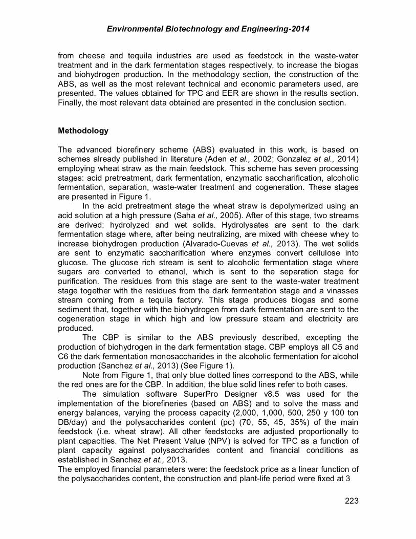
Environmental Biotechnology and Engineering-2014
223
from cheese and tequila industries are used as feedstock in the waste-water treatment and in the dark fermentation stages respectively, to increase the biogas and biohydrogen production. In the methodology section, the construction of the ABS, as well as the most relevant technical and economic parameters used, are presented. The values obtained for TPC and EER are shown in the results section. Finally, the most relevant data obtained are presented in the conclusion section. Methodology The advanced biorefinery scheme (ABS) evaluated in this work, is based on schemes already published in literature (Aden et al., 2002; Gonzalez et al., 2014) employing wheat straw as the main feedstock. This scheme has seven processing stages: acid pretreatment, dark fermentation, enzymatic saccharification, alcoholic fermentation, separation, waste-water treatment and cogeneration. These stages are presented in Figure 1.
In the acid pretreatment stage the wheat straw is depolymerized using an acid solution at a high pressure (Saha et al., 2005). After of this stage, two streams are derived: hydrolyzed and wet solids. Hydrolysates are sent to the dark fermentation stage where, after being neutralizing, are mixed with cheese whey to increase biohydrogen production (Alvarado-Cuevas et al., 2013). The wet solids are sent to enzymatic saccharification where enzymes convert cellulose into glucose. The glucose rich stream is sent to alcoholic fermentation stage where sugars are converted to ethanol, which is sent to the separation stage for purification. The residues from this stage are sent to the waste-water treatment stage together with the residues from the dark fermentation stage and a vinasses stream coming from a tequila factory. This stage produces biogas and some sediment that, together with the biohydrogen from dark fermentation are sent to the cogeneration stage in which high and low pressure steam and electricity are produced.
The CBP is similar to the ABS previously described, excepting the production of biohydrogen in the dark fermentation stage. CBP employs all C5 and C6 the dark fermentation monosaccharides in the alcoholic fermentation for alcohol production (Sanchez et al., 2013) (See Figure 1).
Note from Figure 1, that only blue dotted lines correspond to the ABS, while the red ones are for the CBP. In addition, the blue solid lines refer to both cases.
The simulation software SuperPro Designer v8.5 was used for the implementation of the biorefineries (based on ABS) and to solve the mass and energy balances, varying the process capacity (2,000, 1,000, 500, 250 y 100 ton DB/day) and the polysaccharides content (pc) (70, 55, 45, 35%) of the main feedstock (i.e. wheat straw). All other feedstocks are adjusted proportionally to plant capacities. The Net Present Value (NPV) is solved for TPC as a function of plant capacity against polysaccharides content and financial conditions as established in Sanchez et at., 2013. The employed financial parameters were: the feedstock price as a linear function of the polysaccharides content, the construction and plant-life period were fixed at 3

Environmental Biotechnology and Engineering-2014
224
and 15 years respectively, an interest rate of 6%, equity of 70% with investor´s back-payment starting in 3 years. Equipment prices were considered similar to the US average (Perry, 1999; Douglas, 1988) whilst salaries and local income tax (30%) were taken from the Mexican National Institute of Geography and Statistics (INEGI, 2012).
The EER defined as the ratio of energy produced (steam, electricity and chemical energy of ethanol) to the total energy consumed in the process (Patterson 1996), was calculated using data from the energy balances.
Two response surfaces for TPC and EER were obtained as function of plant capacity and feedstock polysaccharides content. The best TPC value for the ABS was found, and compared against the TPC for CBP to define which of two schemes is more profitable. Subsequently, the response EER surface was analyzed for conditions to which greater energetically efficiency is obtained. Results and discussion The sensitivity of TPC and EER values for ABS was explored for plant capacities of 100, 250, 500, 1,000 and 2,000 ton DB/day and feedstock polysaccharides content (i.e. wheat straw) of 35, 45, 55 and 70% w/w.
Table 1 shows the resulting ethanol TPC of ABS versus plant capacity and pc (% w/w). Each value within the table represents a (capacity, feedstock pc) plant. As expected, the smallest TPC value ($1.28 USD/l EtOH) was calculated for the largest plant with the highest polysaccharides content (2,000 ton DB/day and 70%). The corresponding TPC for CBP with the same capacity plant and pc was $0.93 USD/l EtOH. The larger TPC for ABS is attributed mainly to larger capital expenditures to treat the cheese whey and vinasses in the hydrogen production process and waste-water treatment respectively. However, considerable smaller plants with feedstock of different pc produce ethanol at relatively acceptable cost.

Environmental Biotechnology and Engineering-2014
225
FIGURE 1. Process block diagrams for ABS and CBP.

Environmental Biotechnology and Engineering-2014
226
Figure 1 shows that TPC tendency presents the typical exponential
decaying shape as a function of plant capacity. In addition, the plot has a quasi-linear section from 500 ton DB/day onwards and the expected linear dependence of total pc (% w/w).
FIGURE 2. Response surface based on TPC versus plant capacity and polysaccharides content for ABS.
This section can be identified for medium scale sector bounded by a region where TPC values are acceptable. Those values are: 2,000 ton DB/day, 45% pc; 1,000 ton DB/day, 55%; 500 ton DB/day, 70% pc (see section bounded at Table 1). Therefore, a 500-1,000 capacity would be a very attractive alternative to explore further since these plants are technically and economic feasible.
Table 2 shows the resulting EER versus plant capacity and pc (% w/w). Each value within the table represents a (capacity, feedstock pc) plant. The largest
35% 45% 55% 70%100 4.98$ 4.00$ 3.37$ 2.92$ 250 2.85$ 2.37$ 2.05$ 1.84$ 500 2.18$ 1.84$ 1.62$ 1.50$
1,000 1.94$ 1.66$ 1.47$ 1.37$ 2,000 1.77$ 1.53$ 1.37$ 1.28$
TABLE 1. Total ethanol production cost (USD/l EtOH) for ABS.Polysaccharides content (% w/w)
Plant capacity (ton DB/day)
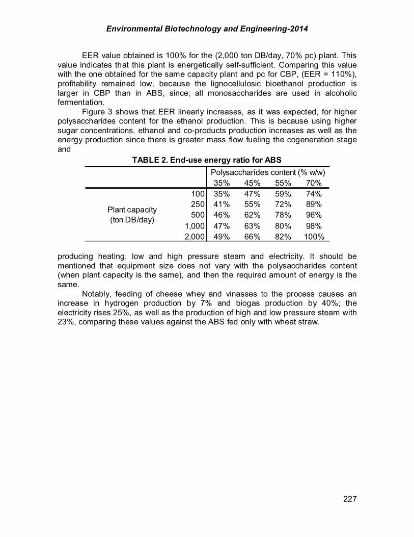
Environmental Biotechnology and Engineering-2014
227
EER value obtained is 100% for the (2,000 ton DB/day, 70% pc) plant. This value indicates that this plant is energetically self-sufficient. Comparing this value with the one obtained for the same capacity plant and pc for CBP, (EER = 110%), profitability remained low, because the lignocellulosic bioethanol production is larger in CBP than in ABS, since; all monosaccharides are used in alcoholic fermentation.
Figure 3 shows that EER linearly increases, as it was expected, for higher polysaccharides content for the ethanol production. This is because using higher sugar concentrations, ethanol and co-products production increases as well as the energy production since there is greater mass flow fueling the cogeneration stage and
producing heating, low and high pressure steam and electricity. It should be mentioned that equipment size does not vary with the polysaccharides content (when plant capacity is the same), and then the required amount of energy is the same.
Notably, feeding of cheese whey and vinasses to the process causes an increase in hydrogen production by 7% and biogas production by 40%; the electricity rises 25%, as well as the production of high and low pressure steam with 23%, comparing these values against the ABS fed only with wheat straw.
35% 45% 55% 70%100 35% 47% 59% 74%250 41% 55% 72% 89%500 46% 62% 78% 96%
1,000 47% 63% 80% 98%2,000 49% 66% 82% 100%
TABLE 2. End-use energy ratio for ABSPolysaccharides content (% w/w)
Plant capacity (ton DB/day)
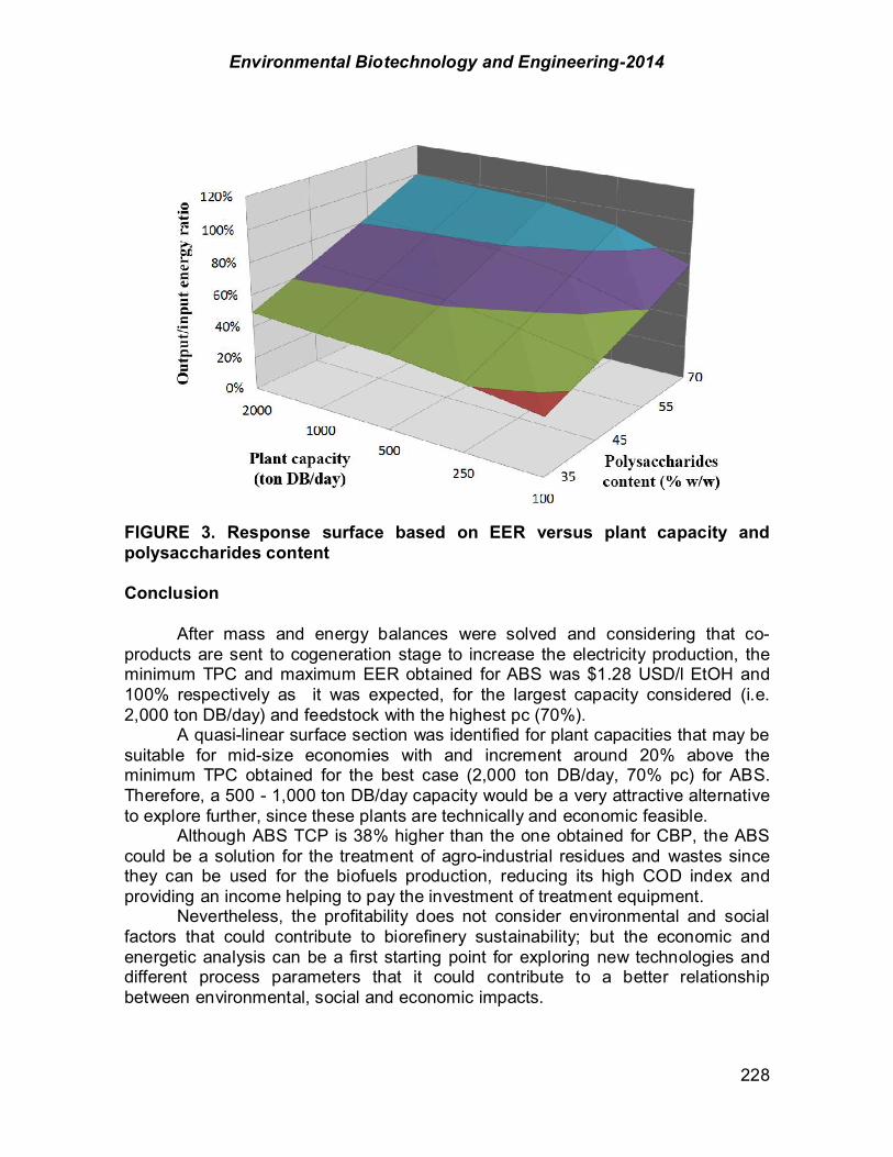
Environmental Biotechnology and Engineering-2014
228
FIGURE 3. Response surface based on EER versus plant capacity and polysaccharides content Conclusion
After mass and energy balances were solved and considering that co-products are sent to cogeneration stage to increase the electricity production, the minimum TPC and maximum EER obtained for ABS was $1.28 USD/l EtOH and 100% respectively as it was expected, for the largest capacity considered (i.e. 2,000 ton DB/day) and feedstock with the highest pc (70%).
A quasi-linear surface section was identified for plant capacities that may be suitable for mid-size economies with and increment around 20% above the minimum TPC obtained for the best case (2,000 ton DB/day, 70% pc) for ABS. Therefore, a 500 - 1,000 ton DB/day capacity would be a very attractive alternative to explore further, since these plants are technically and economic feasible.
Although ABS TCP is 38% higher than the one obtained for CBP, the ABS could be a solution for the treatment of agro-industrial residues and wastes since they can be used for the biofuels production, reducing its high COD index and providing an income helping to pay the investment of treatment equipment.
Nevertheless, the profitability does not consider environmental and social factors that could contribute to biorefinery sustainability; but the economic and energetic analysis can be a first starting point for exploring new technologies and different process parameters that it could contribute to a better relationship between environmental, social and economic impacts.
Environmental Biotechnology and Engineering-2014
229
Acknowledgments Partial financial support for Secretary of Energy (SENER), Mexico under grant SENER-2010-150001 is kindly acknowledged, V.S. acknowledges financial support from CONACyT, Mexico in the form of PhD scholarship 94387. References Aden, A.; Ruth, M.; Ibsen, K.; Jechura, J.; Neeves, K.; Sheehan, J.; Wallace, B. (2002).
Lignocellulosic biomass to ethanol process design and economics utilizing co-current dilute acid prehydrolysis and enzymatic hydrolysis for corn stover. National Renewable Energy Laboratory (NREL). NREL/TP-510-32438.
Alvarado-Cuevas, Z.; Ordoñez, L.; Ornelas, J.; León-Rodríguez, A. (2013). Nitrogen source impact hydrogen production by Escherichia coli using cheese whey as substrate. New Biotechnology. Vol. 30, Num. 6
Antonopoulou, G.; Stamatelatou, K.; Venetsaneas, N.; Kornaros, M.; Lyberatos, G. (2008). Biohydrogen and methane production from cheese whey in a two-stage anaerobic process. Ind Eng Chem Res. 47: 5227-5233
Balat, M.; Balat, H. (2009). Recent trends in global production and utilization of bioethanol fuel. Appl Energy. 86:2273-82.
Buitrón, G.; Carvajal, C. (2010). Biohydrogen production from tequila vinasses in an anaerobic sequencing batch reactor: effect of initial substrate concentration, temperature and hydraulic retention time. Int J Hydrogen Energy. 101: 9071-7
Douglas, J.M. (1988). Conceptual design of chemical processes. McGraw Hill. Energy Information Administration (EIA), (2009). Annual energy outlook 2009 with projections to
2030. Available online at: http://www.eia.doe.gov/oiaf/aeo/pdf/0383(2009).pdf. Gallagher, E. (2008). The Gallagher review of the indirect effects of biofuels production. Renew
Fuels Agency. Gil, J.M. (2009). The biofuels future: integrated biorefineries (In Spanish). University of Valladolid.
University Campus of Palencia Gonzalez, S.R.; Sanchez, A.; Sevilla, V.; Murguía M. (2014). Biofuels and electricity coproduction. A
possible solution for the agro-industrial wastes treatment. In J. G. Segovia, editor. Proceedings of the XXXV Encuentro de la Academia Mexicana de Investigación y Docencia en Ingeniería Química A. C., Puerto Vallarta, Jalisco, México.
INEGI (2012).www.inegi.org.mx/sistemas/bie/default.aspx?idserPadre=10100390#D101 00390; accessed 03 July 2014.
Patterson, M.G. (1996). What is energy efficiency? Concepts, indicators and methodological issues. Energy Policy. 24 (5): 377-90.
Perry, R.H.; Green D.W. (1999). Perry’s chemical engineering handbook. McGraw Hill. Saha, B.C.; Iten, L.B.; Cotta, M.A.; Wu, Y.V. (2005). Dilute acid pretreatment enzymatic scarification
and fermentation of wheat Straw to ethanol”. Process Biochemistry. 40: 3693-700. Sanchez, A.; Sevilla-Güitrón, V.; Magaña, G.; Gutierrez, L. (2013). Parametric analysis of total cost
and energy efficiency of 2G enzymatic ethanol production. FUEL. 113: 165-179. Shafiee, S; Topal, E. (2008). When will fossil fuel reserves be diminished. Energy Policy. 1,181-189.

Environmental Biotechnology and Engineering-2014
230
CHAPTER 1.23. INTEGRATION OF A BIOREFINERY MODEL FOR THE PRODUCTION OF HYDROGEN, METHANE, ENZYMES AND HYDROLYSATES
FROM THE ORGANIC FRACTION OF MUNICIPAL SOLID WASTES
Carlos Escamilla-Alvarado (1); Héctor M. Poggi-Varaldo*(1); Teresa Ponce-
Noyola (1); Elvira Ríos-Leal (1); Fernando Esparza-García (1); Josefina Barrera-Cortés (1); Jaime García-Mena (1); Ireri Robles-González (2); Noemi
Rinderknecht-Seijas (3). (1) CINVESTAV- IPN, México DF, México. (2) Nova Universitas, Oaxaca, México. (3) ESIQIE-IPN, México DF, México. ABSTRACT A lab-scale biorefinery model was developed and tested. It comprised four stages for the production of hydrogen, methane, holocellulolytic enzymes and hydrolysates (H-M-Z-S). The hydrogen-producing process (H-stage) was fed with the organic fraction of municipal solid wastes (OFMSW). This stage generated organic purges namely fermented solids (FS), which were fed to the other stages of the biorefinery. The methanogenic stage (M-stage) produced methane from the FS. For the enzymes production (Z-stage), Trichoderma reesei MCG 80 was used. In the saccharification process (S-stage), the enzyme extract from Z-stage was used for the production of sugars from FS. In the H-stage, the semi-continuous process had a productivity over 200 NmL H2/kgr/d at thermophilic regime and 21 d mass retention time, whereas in the batch process the yield was over 1 980 mol H2/g VS at thermophilic conditions without the addition of phosphate salts nor nitrogen in the form of activated sludge. The productivity in M-stage was 2 000 NmL CH4/kgr/d at thermophlic regime. In Z-stage, the FS at 1 %VS gave 1.46 FPU/mL and 0.98 IUCMC/mL. Using the fermenters at fed-batch regime and fed with FS at 1.5 %VS, 2.06 FPU/mL and 1.23 IUCMC/mL were obtained. In S-stage, saccharification efficiencies were up to 65 %VSb for the FS. After 72 h of saccharification it was possible to retrieve and recycle the enzyme extract. From the analysis of the experimental data, it was established that the best configuration for the biorefinery model was a series-parallel process. The main contributions of this work were: (i) the technical bench-scale demonstration of a 4 stages biorefinery model based on an inverse cascading approach, and (ii) the use of the FS from H-stage as a building block for other bioproducts (i.e. methane, enzymes and hydrolysates). Key words: biorefinery, enzymes, hydrogen, methane, organic wastes ------------------ *Author for correspondence: [email protected]

Environmental Biotechnology and Engineering-2014
231
Introduction La implementación de procesos para la obtención de bioproductos en procesos serie/paralelo a partir de biomasa, emulando los procesos de refinación del petróleo, ha demostrado ser posible y está retomando fuerza (Zeikus, 1980, Angenent et al., 2004; Kamm & Kamm, 2004; Poggi-Varaldo et al., 2014). A partir de procesos biotecnológicos se pueden producir biocombustibles como el biohidrógeno, metano o bioetanol. También ha sido posible obtener otros bioproductos con alto valor agregado como las enzimas (Escamilla-Alvarado et al., 2013a). El biohidrógeno como biocombustible es una de las alternativas al uso tradicional de los combustibles fósiles (Levin et al., 2004). Es considerado un combustible limpio y con alto poder calorífico. Su utilización se puede realizar por combustión directa o mediante celdas de combustible. Como subproductos de la hidrogenogénesis por fermentación oscura se obtienen cantidades considerables de ácidos orgánicos (ácidos acético, butírico, propiónico, láctico, entre otros) y solventes que pueden utilizarse como materia prima para la síntesis de otros productos químicos (Lipinski, 1981), o como sustrato de otros procesos biológicos, como la metanogénesis, las celdas de combustible microbianas o la fermentación heterotrófica (Xie et al., 2008; Zhu et al., 2008; Escamilla-Alvarado et al., 2012; Poggi-Varaldo et al., 2014). La digestión anaerobia es vista como un proceso robusto y estable, con el potencial de convertir la materia orgánica de los residuos orgánicos en energía en forma de metano. A diferencia del hidrógeno, cuya combustión sólo produce agua, la combustión del metano produce también un gas de combustión con un contenido mayoritario de dióxido de carbono. Al tratarse de un combustible con un sólo átomo de carbono, se evita la producción de gases como el CO, SO3, SO4, NO3, NO4, generados por otros combustibles fósiles y que causan más daño a la atmósfera (Demirbas, 2004). Dentro de la gama de biocombustibles, el metano es el que presentaría el mejor escenario de uso y distribución, ya que existe una infraestructura ampliamente extendida para la distribución de gas natural que se podría adaptar fácilmente a la del metano, por lo que no se necesitaría infraestructura compleja adicional. Las xilanasas y las celulasas son enzimas cuya producción por hongos o bacterias se induce en presencia de materiales celulósicos y lignocelulósicos, como el bagazo de caña, cascarilla de arroz y fibra de trigo, entre otros (Senthilkumar et al., 2005; Badhan et al., 2007; Rojas-Rejón et al., 2011). Estas enzimas tienen un alto interés industrial como en el tratamiento de la pasta de celulosa, en la industria textil, en la clarificación de jugos, etc. Se llegó a estimar que el crecimiento del mercado mundial de las enzimas industriales fue de mil millones a 1.5 mil millones de dólares de 1995 al 2000 (Schäfer et al., 2005). Novozymes, una de las principales empresas biotecnológicas productora de enzimas, ha visto un crecimiento de sus ventas del 7 - 8 % anual desde 2008 (Novozymes, 2013). La principal industria consumidora de enzimas es la de detergentes, le siguen la panificadora, de bebidas y lácteos, así como la alimenticia y de la pulpa y papel. Se estima que en 2018 tan sólo el mercado
Environmental Biotechnology and Engineering-2014
232
mundial de enzimas para el ramo alimenticio crezca a 2.3 mil millones de dólares (Markets & Markets, 2014). Un campo en donde la aplicación de enzimas se encuentra en desarrollo es en el de obtención de biocombustibles por medio de la sacarificación de biomasa vegetal (Zhuang et al., 2007). La distribución de enzimas para este tipo de actividad es del 16 % del total del mercado (Novozymes, 2013). La sacarificación de la biomasa lignocelulósica es un proceso en el cual, por medio de la acción de celulasas y xilanasas, se obtienen azúcares fermentables con aplicación potencial para la producción de bioetanol, biobutanol, y otros solventes (Ballesteros et al., 2004; Lin & Tanaka, 2006). Los cultivos y residuos agrícolas constituyen principalmente la biomasa lignocelulósica utilizada en los procesos de sacarificación (Mes-Hartree et al., 1988; Holtzapple et al., 1991; Mesa et al., 2010). También se han sacarificado sustratos menos usuales como residuos orgánicos municipales (Clanet et al., 1988; Ballesteros et al., 2010), residuos de comida (Vavouraki et al., 2013). El objetivo de este trabajo fue integrar un proceso modelo de biorrefinería de cuatro etapas (H-M-Z-S), para la obtención de biohidrógeno, metano, holocelulasas y sacarificados. Materiales y métodos Configuración de la biorrefinería. De acuerdo a resultados previos (Escamilla-Alvarado et al., 2013a; Escamilla-Alvarado et al., 2013b; Escamilla-Alvarado et al., 2014), se propuso que la configuración de la biorrefinería H-M-Z-S sea un proceso serie-paralelo (Fig. 1). Comienza con la alimentación de FORSU a la Etapa H para la producción de hidrógeno y sólidos fermentados (SF). Una porción de los SF generados en esta etapa se alimentó tal cual a la Etapa M para la producción de metano y generación de sólidos diferidos (SD). Los SD podrían ser usados potencialmente como acondicionador de suelos. La porción de SF que no se alimentó a la Etapa M, fue sometida a un tratamiento de lavado para extraer los lixiviados (Lx), principalmente constituidos por ácidos orgánicos y solventes. Estos SF lavados (SFL) son alimentados a la Etapa Z y a la Etapa S. En la Etapa Z se realiza la producción de enzimas usando el hongo T. reesei MCG 80 alimentado con SFL. Las enzimas producidas son recuperadas en forma de extracto concentrado (Ez) tras un proceso de centrifugación (C) y ultrafiltración (UF). El Ez puede ser comercializado para otros procesos (e.g. sacarificación, deslavado de mezclilla, clarificación de jugos, etc.). El sedimento de la centrifugación fueron los sólidos re-fermentados (SRF), constituidos por sustrato residual y biomasa de T. reesei, que pueden ser utilizados como alimento de ganado. El filtrado (F) del proceso de ultrafiltración está conformado por sales y compuestos de bajo peso molecular (< 10 kDa). Éstos pueden ser utilizados como suplemento para medios de cultivo de otros procesos biotecnológicos. La Etapa S utiliza SFL y extracto enzimático Ez para la obtención de sacarificados. Tras la sacarificación se realizó una centrifugación (C) para separar los sólidos hidrolizados (SH) del medio líquido que contiene los licores

Environmental Biotechnology and Engineering-2014
233
sacarificados (LS) y la enzima residual (Ez,r). Estos dos últimos componentes se separan más adelante por ultrafiltración (UF). La Ez,r es reutilizada en la misma Etapa S para reducir el consumo de extracto concentrado Ez de la Etapa Z. Los licores sacarificados LS se pueden utilizar en procesos de producción de bioetanol o como sustrato de otros procesos biotecnológicos, mientras que los SH podrían utilizarse como suplemento de sustrato para otros procesos biológicos. FIGURA. 1. Diagrama de bloques de operación serie-paralelo del modelo de biorrefinería H-M-Z-S. FORSU, fracción orgánica de residuos sólidos urbanos; SF, sólidos fermentados; SD sólidos digeridos; TL, tratamiento de lavado; Lx, lixiviados; SFL, sólidos fermentados lavados; C, centrifugación; UF, ultrafiltración; SRF, sólidos re-fermentados; B, biomasa; Ez, extracto enzimático concentrado; F, filtrados; LS, licores sacarificados; Ez,r, enzima residual; SH, sólidos hidrolizados. Producción de hidrógeno o Etapa H. Se utilizaron digestores anaerobios en sustrato sólido acidogénicos (DASS-A) para la producción de hidrógeno. El tipo y configuración de los digestores se basó en lo reportado en trabajos previos (Poggi-Varaldo et al., 1997; Escamilla-Alvarado et al., 2012). La alimentación de los digestores consistió en una mezcla de residuos sólidos orgánicos y papel, denominada FORSU. El contenido de sólidos totales (ST) en la FORSU se ajustó con una solución amortiguadora de fosfatos a 20.9 %p/p. Los digestores anaerobios consistieron de frascos de vidrio de 1 litro, cerrados con un tapón de hule con perforaciones para venteo y purga. El volumen másico de operación fue de 500 g. Se siguió la estrategia de inoculación reportada por
Environmental Biotechnology and Engineering-2014
234
Poggi-Varaldo et al. (1997). El régimen termofílico se llevó a cabo en una cabina de madera a 55 ºC (± 0.1). Una vez alcanzada la operación estable a 35 d TRM, los digestores fueron sometidos a choque térmico a 92 ºC, 90 min y operados a continuación a 21 d TRM (Escamilla-Alvarado et al., 2013b). Producción de metano o Etapa M. Los SF provenientes de la Etapa H fueron usados como sustrato. La configuración de los digestores anaerobios fue similar a la de la Etapa H, siguiendo la estrategia de inoculación reportada por Poggi-Varaldo et al. (1997). La operación se llevó a cabo a a 55 ºC (± 0.1) y 28 d TRM (Escamilla-Alvarado et al., 2014). Lavado de sólidos fermentados. Se realizó en una primera etapa con etanol grado industrial en una relación 10% psólidos secos/vetanol con agitación a 120 rpm durante 10 min. Se filtraron los sólidos y se realizó otro lavado con agua destilada en ebullición en una relación 10% psólidos secos/vag ebull con agitación a 120 rpm durante 10 min. Posteriormente se filtraron los sólidos y se secaron a 60 ºC, 24 h para eliminar toda humedad (Escamilla-Alvarado et al., 2013a). Producción de enzimas o Etapa Z. Se utilizaron SF lavados para la producción enzimática con Trichoderma reesei MCG 80. El crecimiento a 30 ºC en fermentadores se realizó utilizando como sustrato los SF a 1.5 %SV en medio Mandels a pH 4.8 (Escamilla-Alvarado et al. 2013a), inoculados a una relación 1:10 v/v con suspensión micelial de 6 d de crecimiento. Los reactores tipo Sixfors (Infors HT, Suiza) tuvieron un volumen de trabajo de 450 mL, con agitación en un intervalo 350 – 450 rpm proporcionada por dos propelas Rushton de 6 paletas cada una. El pH se midió con electrodo Fermprobe (Broadly-James Corp., EUA). Durante la fermentación se realizó prueba de pureza en agar papa-desxtrosa y/o agar de infusión cerebro corazón. Se les realizó seguimiento por visualización en microscopio, vertiendo 20 L de micelio en suspensión en un portaobjetos, dejándolo secar a temperatura ambiente, fijando con ácido acético 40%, secando nuevamente y tiñendo con una gota de azul de lactofenol. Producción de sacarificados o Etapa S. Se sacarificaron SF lavados usando las enzimas holocelulósicas del extracto enzimático de la Etapa Z (Extracto Tr). Los ensayos se realizaron en matraz Erlenmeyer de 125 mL con 25 mL de volumen de operación, a 50 ºC, 150 rpm, 72 h. La concentración del sustrato fue 2 %SV en regulador de citratos 0.05 M (ácido cítrico monohidratado: 4.388 g/L; citrato de sodio dihidratado: 8.562 g/L, pH 5.0), y carga de extracto enzimático de 60 FPU/g SV (Escamilla-Alvarado et al., 2014). Análisis. El contenido de hidrógeno y metano en el biogás se analizó en un cromatógrafo de gases GOW-MAC modelo 350 equipado con detector de conductividad térmica. Las temperaturas del inyector, columna y detector fueron 37, 70 y 100 ºC respectivamente, usando argón como gas acarreador. Se utilizó una columna empacada Molecular Sieve 5A. Los análisis de humedad, sólidos totales y sólidos volátiles se realizaron

Environmental Biotechnology and Engineering-2014
235
siguiendo el método de Poggi-Varaldo et al. (1999) basado en el método estándar APHA-AWWA-WPFC (1985). El análisis de celulosa se realizó por el método colorimétrico modificado de Updegraff (1969), comparando contra un estándar de glucosa a 490 nm. El análisis de la lignina insoluble en ácido se realizó en base gravimétrica (Effland, 1977), donde los carbohidratos se hidrolizan y solubilizan en 72% H2SO4 ácido sulfúrico y la materia insoluble es cuantificada como lignina. El contenido de hemicelulosa se determinó a partir de la diferencia entre la masa de la holocelulosa y la celulosa. La holocelulosa se determinó por cloración de las muestras usando NaClO; la diferencia de peso de las muestras antes y después de la cloración da el contenido de holocelulosa. Cuando hubo presencia significativa de cenizas, se realizó una corrección del peso (AOAC, 1984). Las determinaciones enzimáticas de xilanasas (Xx), endocelulasas (CMCx) y celulasas (FPx) se realizaron midiendo los azúcares reductores liberados por el método del ácido dinitrosalicílico (Miller, 1959), de acuerdo a Mandels et al. (1974). Las actividades se expresaron en Unidades Internacionales (UI), definidas como micromoles de D-xilosa o glucosa (determinados como azúcares reductores) liberados por minuto bajo condiciones estándar de ensayo. La cuantificación de azúcares reductores se realizó midiendo la absorbancia a 550 nm, y comparándolo contra curvas estándar del correspondiente azúcar (Eveleigh et al., 2009; Escamilla-Alvarado, 2014). La actividad de $-glucosidasa se determinó con la liberación de nitrofenol a partir de la hidrólisis de 0.95 mL de solución 1mM de p-nitrofenil-$-D-glucopiranósido (p-NPG) como sustrato. Una unidad de actividad se definió como la cantidad de enzima que libera 1 mol de nitrofenol por min (Wang et al., 2010). La proteína extracelular se determinó por el método de Lowry et al. (1951), leyendo la absorbancia a 750 nm. La absorbancia registrada se comparó contra una curva estándar realizada con albúmina de suero bovino en el intervalo de 0 a 500 g (Sigma-Aldrich, E.U.A). El análisis estadístico se realizó con el software Design-Expert v7.1.6 (Stat-Ease Inc., Mineapolis). El análisis de significancia entre ensayos se realizó mediante la prueba t ocupando el software SigmaPlot v11.0 (Systat Software, Inc., Germany). Resultados y discusión Etapa H. La productividad de hidrógeno fue en promedio 200 NmL H2/kgr/d. Este resultado fue mejor al obtenido con FORSU trabajando a 35 %ST (Escamilla-Alvarado et al., 2012), el cuál fue aproximadamente diez veces menor. Esta mejora notable en el resultado se atribuyó a la menor concentración de sustrato en el digestor (20.9 %ST), lo cuál mejoró la agitación del medio y la transferencia de masa en el sistema.
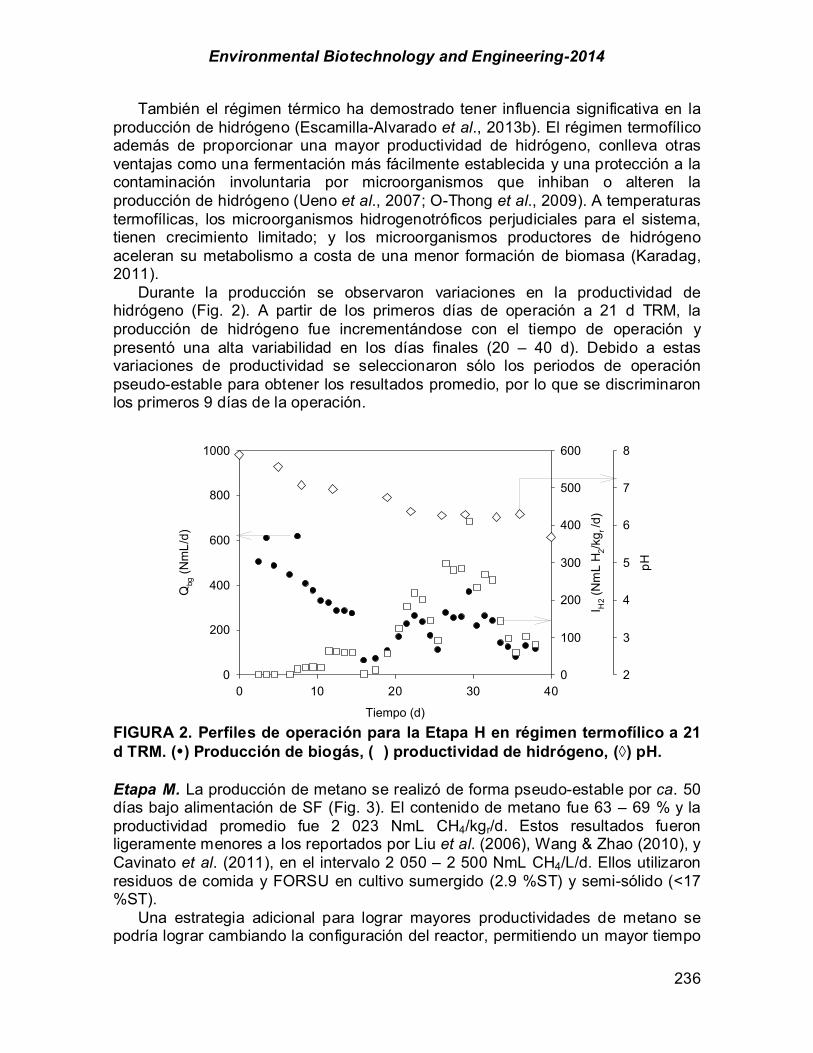
Environmental Biotechnology and Engineering-2014
236
También el régimen térmico ha demostrado tener influencia significativa en la producción de hidrógeno (Escamilla-Alvarado et al., 2013b). El régimen termofílico además de proporcionar una mayor productividad de hidrógeno, conlleva otras ventajas como una fermentación más fácilmente establecida y una protección a la contaminación involuntaria por microorganismos que inhiban o alteren la producción de hidrógeno (Ueno et al., 2007; O-Thong et al., 2009). A temperaturas termofílicas, los microorganismos hidrogenotróficos perjudiciales para el sistema, tienen crecimiento limitado; y los microorganismos productores de hidrógeno aceleran su metabolismo a costa de una menor formación de biomasa (Karadag, 2011). Durante la producción se observaron variaciones en la productividad de hidrógeno (Fig. 2). A partir de los primeros días de operación a 21 d TRM, la producción de hidrógeno fue incrementándose con el tiempo de operación y presentó una alta variabilidad en los días finales (20 – 40 d). Debido a estas variaciones de productividad se seleccionaron sólo los periodos de operación pseudo-estable para obtener los resultados promedio, por lo que se discriminaron los primeros 9 días de la operación. FIGURA 2. Perfiles de operación para la Etapa H en régimen termofílico a 21 d TRM. (•) Producción de biogás, ( ) productividad de hidrógeno, (") pH. Etapa M. La producción de metano se realizó de forma pseudo-estable por ca. 50 días bajo alimentación de SF (Fig. 3). El contenido de metano fue 63 – 69 % y la productividad promedio fue 2 023 NmL CH4/kgr/d. Estos resultados fueron ligeramente menores a los reportados por Liu et al. (2006), Wang & Zhao (2010), y Cavinato et al. (2011), en el intervalo 2 050 – 2 500 NmL CH4/L/d. Ellos utilizaron residuos de comida y FORSU en cultivo sumergido (2.9 %ST) y semi-sólido (<17 %ST). Una estrategia adicional para lograr mayores productividades de metano se podría lograr cambiando la configuración del reactor, permitiendo un mayor tiempo
Tiempo (d)
0 10 20 30 40
Qbg
(Nm
L/d)
0
200
400
600
800
1000
I H2 (
Nm
L H
2/kg r /
d)
0
100
200
300
400
500
600
pH
2
3
4
5
6
7
8
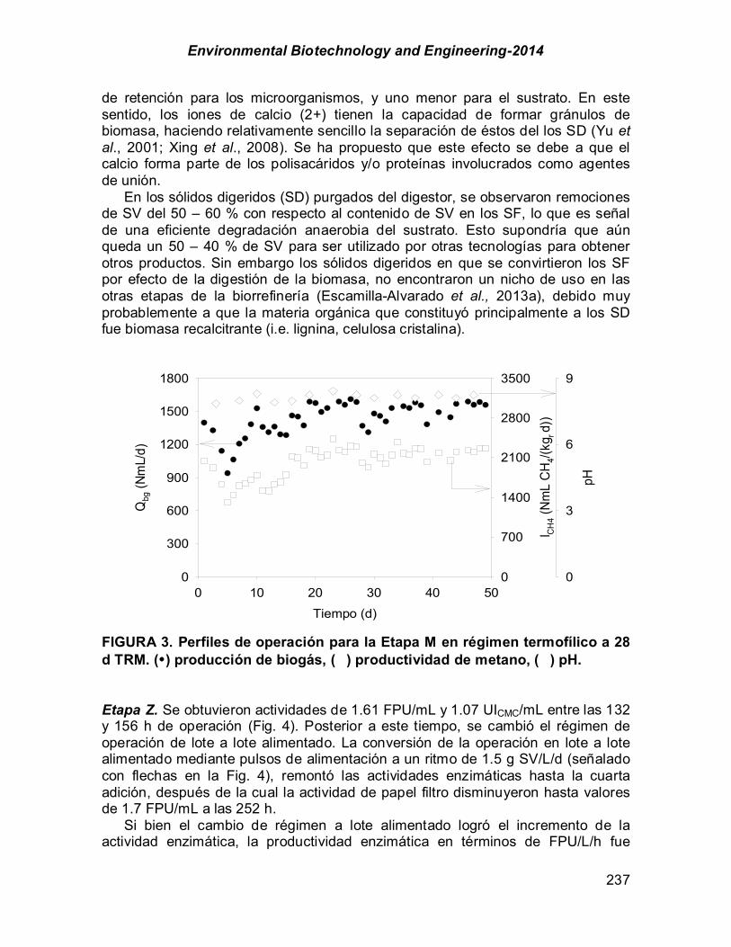
Environmental Biotechnology and Engineering-2014
237
de retención para los microorganismos, y uno menor para el sustrato. En este sentido, los iones de calcio (2+) tienen la capacidad de formar gránulos de biomasa, haciendo relativamente sencillo la separación de éstos del los SD (Yu et al., 2001; Xing et al., 2008). Se ha propuesto que este efecto se debe a que el calcio forma parte de los polisacáridos y/o proteínas involucrados como agentes de unión. En los sólidos digeridos (SD) purgados del digestor, se observaron remociones de SV del 50 – 60 % con respecto al contenido de SV en los SF, lo que es señal de una eficiente degradación anaerobia del sustrato. Esto supondría que aún queda un 50 – 40 % de SV para ser utilizado por otras tecnologías para obtener otros productos. Sin embargo los sólidos digeridos en que se convirtieron los SF por efecto de la digestión de la biomasa, no encontraron un nicho de uso en las otras etapas de la biorrefinería (Escamilla-Alvarado et al., 2013a), debido muy probablemente a que la materia orgánica que constituyó principalmente a los SD fue biomasa recalcitrante (i.e. lignina, celulosa cristalina). FIGURA 3. Perfiles de operación para la Etapa M en régimen termofílico a 28 d TRM. (•) producción de biogás, ( ) productividad de metano, ( ) pH. Etapa Z. Se obtuvieron actividades de 1.61 FPU/mL y 1.07 UICMC/mL entre las 132 y 156 h de operación (Fig. 4). Posterior a este tiempo, se cambió el régimen de operación de lote a lote alimentado. La conversión de la operación en lote a lote alimentado mediante pulsos de alimentación a un ritmo de 1.5 g SV/L/d (señalado con flechas en la Fig. 4), remontó las actividades enzimáticas hasta la cuarta adición, después de la cual la actividad de papel filtro disminuyeron hasta valores de 1.7 FPU/mL a las 252 h. Si bien el cambio de régimen a lote alimentado logró el incremento de la actividad enzimática, la productividad enzimática en términos de FPU/L/h fue
Tiempo (d)
0 10 20 30 40 50
Qbg
(Nm
L/d)
0
300
600
900
1200
1500
1800
I CH
4 (N
mL
CH
4/(kg
r d))
0
700
1400
2100
2800
3500
pH0
3
6
9
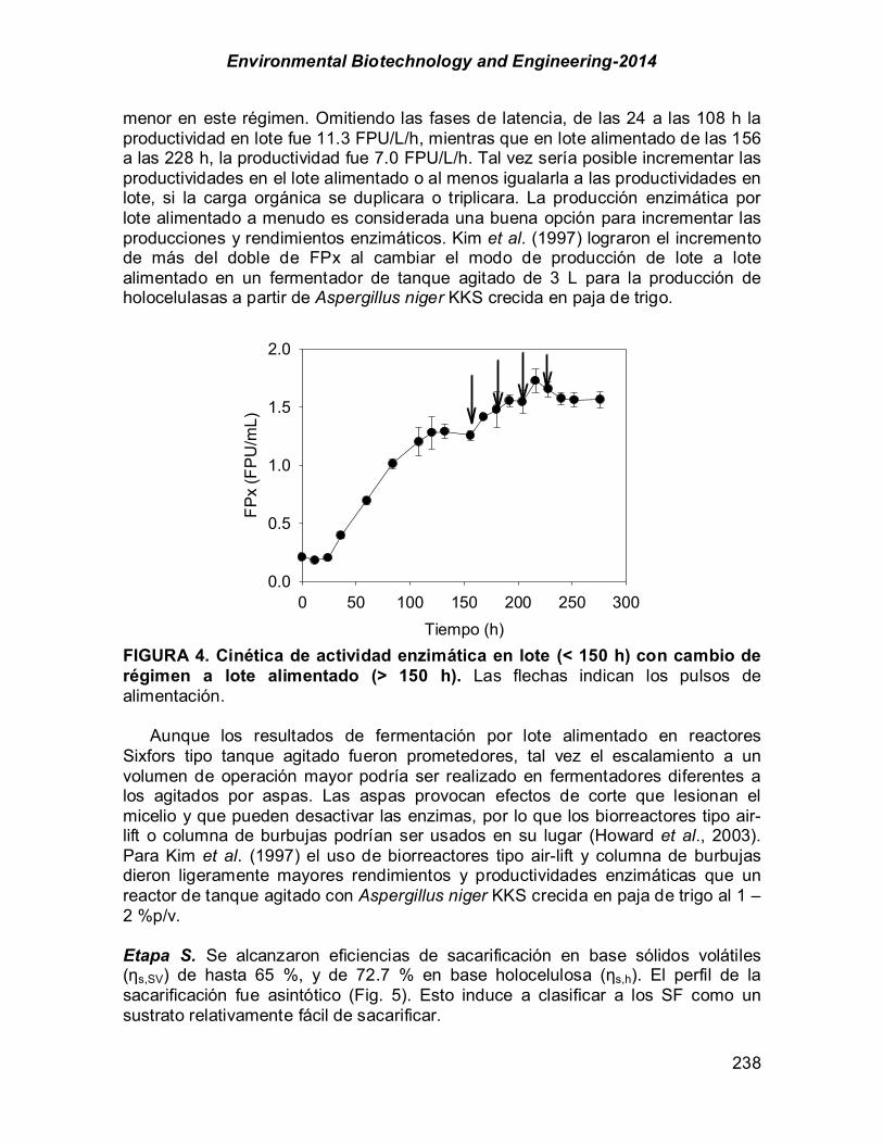
Environmental Biotechnology and Engineering-2014
238
menor en este régimen. Omitiendo las fases de latencia, de las 24 a las 108 h la productividad en lote fue 11.3 FPU/L/h, mientras que en lote alimentado de las 156 a las 228 h, la productividad fue 7.0 FPU/L/h. Tal vez sería posible incrementar las productividades en el lote alimentado o al menos igualarla a las productividades en lote, si la carga orgánica se duplicara o triplicara. La producción enzimática por lote alimentado a menudo es considerada una buena opción para incrementar las producciones y rendimientos enzimáticos. Kim et al. (1997) lograron el incremento de más del doble de FPx al cambiar el modo de producción de lote a lote alimentado en un fermentador de tanque agitado de 3 L para la producción de holocelulasas a partir de Aspergillus niger KKS crecida en paja de trigo.
FIGURA 4. Cinética de actividad enzimática en lote (< 150 h) con cambio de régimen a lote alimentado (> 150 h). Las flechas indican los pulsos de alimentación. Aunque los resultados de fermentación por lote alimentado en reactores Sixfors tipo tanque agitado fueron prometedores, tal vez el escalamiento a un volumen de operación mayor podría ser realizado en fermentadores diferentes a los agitados por aspas. Las aspas provocan efectos de corte que lesionan el micelio y que pueden desactivar las enzimas, por lo que los biorreactores tipo air-lift o columna de burbujas podrían ser usados en su lugar (Howard et al., 2003). Para Kim et al. (1997) el uso de biorreactores tipo air-lift y columna de burbujas dieron ligeramente mayores rendimientos y productividades enzimáticas que un reactor de tanque agitado con Aspergillus niger KKS crecida en paja de trigo al 1 – 2 %p/v. Etapa S. Se alcanzaron eficiencias de sacarificación en base sólidos volátiles (%s,SV) de hasta 65 %, y de 72.7 % en base holocelulosa (%s,h). El perfil de la sacarificación fue asintótico (Fig. 5). Esto induce a clasificar a los SF como un sustrato relativamente fácil de sacarificar.
Tiempo (h)0 50 100 150 200 250 300
FPx
(FP
U/m
L)
0.0
0.5
1.0
1.5
2.0

Environmental Biotechnology and Engineering-2014
239
Comparado con otros procesos de sacarificación reportados en literatura, los resultados obtenidos en esta actividad se encuentran en el intervalo superior de %s. La mayoría de los estudios de sacarificación ocupan pretratamientos químicos, térmicos o mecánicos, entre los que se encuentran los de hidrólisis ácida diluida, explosión de vapor, molido de bolas y ozonación. Por ejemplo, Ballesteros et al. (2010) ocuparon un pretratamiento térmico (160 ºC por 30 min) aplicado a residuos sólidos municipales (RSM) al 20 %ST, para obtener 35 g glucosa/L (%s,SV
= 41.6 %) con celulasas Celluclast 1.5 L (NS 50013) y ß-glucosidasas Novozyme 188 (NS 50010). Clanet et al. (1988) también sacarificaron RSM pero a una concentración menor (6 %ST).
FIGURA 5. Perfil de sacarificación de los SF. Utilizaron extracto enzimático de T. reesei CL847 y lograron una %s,SV de 48 %. A una concentración aún menor de RSM (1 %ST), Li et al. (2007) obtuvieron una alta sacarificación (%s,bcel
= 72.8 %) con una carga enzimática de T. viride (60 FPU/g) aplicada al sustrato pretratado con ácido diluido (H2SO4 al 1% v/v, 3 h, 60 ºC) seguido de pretratamiento térmico (120 ºC, 15 min). Esta combinación fue la mejor para una serie de ensayos que incluyeron pretratamientos de ácido diluido, térmico, microondas, y sus combinaciones. Con un pretratamiento aún más agresivo (H2SO4 al 0.4% v/v, 3 h y 60 ºC, seguido de explosión de vapor a 210 ºC, 3 min), Nguyen et al. (1999) lograron una %s,bcel
= 80 % para desechos sólidos mixtos a 2.7 %ST sacarificados con celulasas a 66 FPU/g celulosa. Por otro lado, Vavouraki et al. (2013) ocuparon únicamente tratamiento termoquímico (1.5% HCl, 120 ºC, 120 min) aplicado a residuos de cocina al 1 %ST, sin ningún sistema enzimático, alcanzando así una %s,SV = 57.3 %. Los pretratamientos incrementan la sacarificación de un sustrato lignocelulósico, sin embargo se debe considerar su agresividad al ambiente y costos involucrados. Al respecto, se considera que el costo del pretratamiento de
Tiempo (h)0 20 40 60 80 100
Glu
cosa
+ x
ilosa
(g/L
)
0
3
6
9
12
15
Environmental Biotechnology and Engineering-2014
240
ácido diluido es menor que los tratamientos térmicos de corta duración, y que el efecto del tratamiento térmico sobre la sacarificación es menor comparado con el efecto que tiene la carga enzimática (Li et al., 2007). Algunos pretratamientos generan inhibidores, principalmente furaldehidos, ácidos orgánicos y compuestos fenólicos derivados de la hidrólisis de la lignina (Parawira & Tekere, 2011). Conclusión Se logró la integración de un modelo de biorrefinería de cuatro etapas en una configuración serie-paralelo para la producción de hidrógeno a partir de FORSU, y de metano, enzimas y sacarificados a partir de los sólidos fermentados de la Etapa H. Los sólidos fermentados presentaron características de biodegradabilidad que permitirían su uso en otros procesos biotecnológicos. El extracto enzimático obtenido en la Etapa Z es plenamente utilizable en la sacarificación de residuos orgánicos y competitivo contra extracto comercial Celluclast. Agradecimientos Los autores agradecen al CONACYT por la beca otorgada a CE-A (209665) y por el apoyo para la investigación de enzimas (104333), al SECITI del GDF (antes ICYTDF) por el apoyo económico para la investigación de biorrefinerías (proyecto PICCO 10-27), y al CINVESTAV por los apoyos económicos para la realización de este trabajo. Referencias
Angenent, L.T., Karim, K., Al-Dahhan, M.H., Wrenn, B.A. & Dominguez-Espinosa, R. (2004).
Production of bioenergy and biochemicals from industrial and agricultural wastewater. Trends Biotechnol, 22, 477-485.
AOAC (1984) Official methods of analysis. 14th ed. Association of official analytical chemists, Washington, D.C. U.S.A.
APHA-AWWA-WPCF (1985) Standard methods for the examination of water and wastewater. 17th ed. American public health association, Washington, U.S.A.
Badhan, A.K., Chadha, B.S., Kaur, J., Saini, H.S. & Bhat, M.K. (2007). Production of multiple xylanolytic and cellulolytic enzymes by thermophilic fungus Myceliophthora sp. IMI 387099. Bioresour Technol, 98, 504-510.
Ballesteros, M., Oliva, J.M., Negro, M.J., Manzanares, P. & Ballesteros, I. (2004). Ethanol from lignocellulosic materials by a simultaneous saccharification and fermentation process (SFS) with Kluyveromyces marxianus CECT 10875. Biomass, 39, 1843-1848.
Ballesteros, M., Sáez, F., Ballesteros, I., Manzanares, P., Negro, M.J., Martínez, J.M., Castañeda, R. & Dominguez, J.M.O. (2010). Ethanol production from the organic fraction obtained after thermal pretreatment of municipal solid waste. Appl Biochem Biotechnol, 161, 423-431.
Cavinato, C., Bolzonella, D., Fatone, F., Giuliano, A. & Pavan, P. (2011). Two-phase thermophilic anaerobic digestion process for biohythane production treating biowaste: preliminary results. Wat Sci Technol, 64, 715-721.
Clanet, M., Durand, H. & Tiraby, G. (1988). Enzymatic saccharification of municipal wastes. Biotechnol Bioeng, 32, 930-934.

Environmental Biotechnology and Engineering-2014
241
Demirbas, A. (2004). Combustion characteristics of different biomass fuels. Progress in Energy and Combustion Science, 30, 219-230.
Effland, M.J. (1977). Modified procedure to determine acid-insoluble lignin in wood and pulp. TAPPI, 60, 143-144.
Escamilla-Alvarado, C. (2014) Integración de un modelo de biorrefinería para la obtención de hidrógeno, metano, enzimas y sacarificados a partir de la fracción orgánica de residuos sólidos urbanos. Departamento de Biotecnología y Bioingeniería, Centro de Investigación y de Estudios Avanzados del IPN, Mexico, D.F.
Escamilla-Alvarado, C., Poggi-Varaldo, H.M. & Ponce-Noyola, M.T. (2013a). Use of organic waste for the production of added-value holocellulases with Cellulomonas flavigena PR-22 and Trichoderma reesei MCG 80. Waste Manage Res, 31, 849-858.
Escamilla-Alvarado, C., Ponce-Noyola, M.T., Ríos-Leal, E., García-Mena, J., Rinderknecht-Seijas, N. & Poggi-Varaldo, H.M. (2014). Energy analysis of in-series biohydrogen and methane production from organic wastes Int J Hydrogen Energy, In press.
Escamilla-Alvarado, C., Ponce-Noyola, M.T., Rios-Leal, E. & Poggi-Varaldo, H.M. (2013b). A multivariable evaluation of biohydrogen production by solid substrate fermentation of organic municipal wastes in semi-continuous and batch operation. Int J Hydrogen Energy, 38, 12527-12538.
Holtzapple, M., Jun, J.-H., Ashok, G., Patibandla, S. & Dale, B. (1991). The ammonia freeze explosion (AFEX) process. Applied Biochemistry and Biotechnology, 28-29, 59-74.
Howard, R.L., Abotsi, E., Jansen van Rensburg, E.L. & Howard, S. (2003). Lignocellulose biotechnology: issues of bioconversion and enzyme production. African J Biotechnol, 2, 602-619.
Kamm, B. & Kamm, M. (2004). Principles of biorefineries. Appl Microbiol Biotechnol, 64, 137-145. Karadag, D. (2011). Anaerobic H2 production at elevated temperature (60 ºC) by enriched mixed
consortia from mesophilic sources. Int J Hydrogen Energy, 36, 458-465. Kim, S.W., Kang, S.W. & Lee, J.S. (1997). Cellulase and xylanase production by Aspergillus niger
KKS in various bioreactors. Bioresour Technol, 59, 63-67. Levin, D.B., Pitt, L. & Love, M. (2004). Biohydrogen production: prospects and limitations to
practical application. Int J Hydrogen Energy, 29, 173-185. Li, A., Antizar-Ladislao, B. & Khraisheh, M. (2007). Bioconversion of municipal solid waste to
glucose for bio-ethanol production. Bioprocess and Biosystems Engineering, 30, 189-196. Lin, V. & Tanaka, S. (2006). Ethanol fermentation from biomass resources: current state and
prospects. Appl Microbiol Biotechnol, 69, 627-642. Lipinsky, E.S. (1981). Chemicals from Biomass: Petrochemical Substitution Options. Science, 212,
1465-1471. Liu, D., Liu, D., Zeng, R.J. & Angelidaki, I. (2006). Hydrogen and methane production from
household solid waste in the two-stage fermentation process. Water Res, 40, 2230-2236. Lowry, O.H., Rosebrough, N.J., Farr, A.L. & Randall, R.J. (1951). Protein measurement with Folin-
phenol reagent. J Biol Chem, 193, 265-275. Mandels, M., Hontz, L. & Nystrom, J. (1974). Enzymatic hydrolysis of waste cellulose. Biotechnol
Bioeng, 16, 1471-1493. Markets-and-Markets (2014) Industrial Enzymes Market by Types (Carbohydrase, Protease,
Lipase), Applications (Food & Beverages, Cleaning Agents, Bio-Fuel, Animal Feed), & Geography - Global Trends & Forecasts to 2018.
Mes-Hartree, M., Dale, B.E. & Craig, W.K. (1988). Comparison of steam and ammonia pretreatment for enzymatic hydrolysis of cellulose. Applied Microbiology and Biotechnology, 29, 462-468.
Mesa, L., González, E., Ruiz, E., Romero, I., Cara, C., Felissia, F. & Castro, E. (2010). Preliminary evaluation of organosolv pre-treatment of sugar cane bagasse for glucose production: Application of 23 experimental design. Applied Energy, 87, 109-114.
Miller, G.L. (1959). Use of dinitrosalicylic acid reagent for determination of reducing sugar. Anal Chem, 31, 426-428.
Nguyen, Q.A., Keller, F.A., Tucker, M.P., Lombard, C.K., Jenkins, B.M., Yomogida, D.E. & Tiangco, V.M. (1999). Bioconversion of mixed solids waste to ethanol. Appl Biochem Biotechnol, 77-79, 455-472.
Novozymes (2013) The Novozymes report 2012. Bedingfield, J. (ed)Copenhagen.

Environmental Biotechnology and Engineering-2014
242
O-Thong, S., Prasertsan, P. & Birkeland, N.K. (2009). Evaluation of methods for preparing hydrogen-producing seed inocula under thermophilic condition by process performance and microbial community analysis. Bioresour Technol, 100, 909-918.
Parawira, W. & Tekere, M. (2011). Biotechnological strategies to overcome inhibitors in lignocellulose hydrolysates for ethanol production: review. Crit Rev Biotechnol, 31, 20-31.
Poggi-Varaldo, H.M., Munoz-Paez, K.M., Escamilla-Alvarado, C., Robledo-Narváez, P.N., Ponce-Noyola, M.T., Calva-Calva, G., Ríos-Leal, E., Galíndez-Mayer, J., Estrada-Vázquez, C., Ortega-Clemente, A. & Rinderknecht-Seijas, N.F. (2014). Biohydrogen, biomethane and bioelectricity as crucial components of biorefinery of organic wastes: A review. Waste Manage Res, 32, 353-365.
Poggi-Varaldo, H.M., Trejo-Espino, J., Fernandez-Villagomez, G., Esparza-Garcia, F., Caffarel-Mendez, S. & Rinderknecht-Seijas, N. (1999). Quality of anaerobic compost from paper mill and municipal solid wastes for soil amendment. Water Science and Technology, 40, 179-186.
Poggi-Varaldo, H.M., Valdés, L., Esparza-Garcia, F. & Fernández-Villagómez, G. (1997). Solid substrate anaerobic co-digestion of paper mill sludge, biosolids, and municipal solid waste. Water Sci Technol, 35, 197-204.
Rojas-Rejón, O.A., Poggi-Varaldo, H.M., Ramos-Valdivia, A.C., Martínez-Jiménez, A., Cristiani-Urbina, E., de la Torre, M. & Ponce-Noyola, M.T. (2011). Production of cellulases and xylanases under catabolic repression conditions from mutant PR-22 of Cellulomonas flavigena. J Ind Microbiol Biotechnol, 38, 257-264.
Schäfer, T., Kirk, O., Borchert, T.V., Fuglsang, C.C., Pedersen, S., Salmon, S., Olsen, H.S., Deinhammer, R. & Lund, H. (2005) Enzymes for Technical Applications. In. Biopolymers Online. Wiley-VCH Verlag GmbH & Co. KGaA.
Senthilkumar, S.R., Ashokkumar, B., Ra, K.C. & Gunasekaran, P. (2004). Purification and characterization of a low molecular weight endoxylanase from solid-state cultures of alkali-tolerant Aspergillus fischeri. Biotechnol Lett, 26, 1283-1287.
Ueno, Y., Fukui, H. & Goto, M. (2007). Operation of a two-stage fermentation process producing hydrogen and methane from organic waste. Environ Sci Technol, 41, 1413-1419.
Updegraff, D.M. (1969). Semi-micro determination of cellulose in biological material. Anal Biochem, 32, 424–428.
Vavouraki, A.I., Angelis, E.M. & Kornaros, M. (2013). Optimization of thermo-chemical hydrolysis of kitchen wastes. Waste Manage, 33, 740-745.
Wang, W., Kang, L. & Lee, Y. (2010). Production of Cellulase from Kraft Paper Mill Sludge by Trichoderma reesei Rut C-30. Appl Biochem Biotechnol, 161, 382-394.
Wang, X. & Zhao, Y. (2009). A bench scale study of fermentative hydrogen and methane production from food waste in integrated two-stage process. Int J Hydrogen Energy, 34, 245-254.
Xie, B., Cheng, J., Zhou, J., Song, W. & Cen, K. (2008). Cogeneration of hydrogen and methane from glucose to improve energy conversion efficiency. Appl Microbiol, 33, 5006-5011.
Xing, W., Dong-jie, N., Xiao-shuang, Y. & You-cai, Z. (2008). Optimization of methane fermentation from effluent of bio-hydrogen fermentation process using response surface methodology. Bioresour Technol, 99, 4292-4299.
Yu, H.Q., Tay, J.H. & Herbert, H.P.F. (2001). The roles of calcium in sludge granulation during UASB reactor start-up. Water Res, 35, 1052-1060.
Zeikus, J.G. (1980). Chemical and fuel production by anaerobic bacteria. Annu Rev Microbiol, 34, 423-464.
Zhu, H., Stadnyk, A., Béland, M. & Seto, P. (2008). Co-production of hydrogen and methane from potato waste using a two-stage anaerobic digestion process. Bioresour Technol, 99, 5078-5084.
Zhuang, J., Marchant, M.A., Nokes, S.E. & Strobel, H.J. (2007). Economic analysis of cellulase production methods for bio ethanol. Appl Engineer Agric, 23, 679-687.
Notación FORSU fracción orgánica de los residuos sólidos urbanos FPU unidad enzimática en papel filtro

Environmental Biotechnology and Engineering-2014
243
FPx actividad enzimática en papel filtro Lx lixiviados RSM residuos sólidos municipales SD sólidos digeridos SF sólidos fermentados SRF sólidos re-fermentados ST sólidos totales TRM tiempo de residencia másico

Environmental Biotechnology and Engineering-2014
244
CHAPTER 1.24. DIMENSIONAMIENTO DE UNA PLANTA DE BIOGÁS PARA PRODUCCIÓN DE ENERGÍA ELÉCTRICA
Juan C. Paredes-Ramírez* (1); David Sampablo-Cruz (1); Alejandro Torres-
Aldaco (1); Raúl Lugo-Leyte (1); Ignacio Aguilar-Adaya (1); Helen Lugo-Méndez (1)
(1) Universidad Autónoma Metropolitana Iztapalapa, Av. San Rafael Atlixco 186, Colonia Vicentina,
Iztapalapa C.P. 09340, México D.F., México.
RESUMEN La fermentación anaerobia de la materia orgánica, resulta idóneo para el tratamiento de residuos mediante la actuación de un consorcio de bacterias específicas que en ausencia de oxígeno, descomponen la materia orgánica en biogás, compuesto principalmente por CH4 y CO2, en proporciones que varían desde 50 y 50% respectivamente hasta 70 y 30%, variando el poder calorífico entre 14.3 y 28.6 MJ/m3, también proporciona un efluente con una mezcla de productos minerales (N, P, K, Ca, etc.) con gran valor fertilizante. La utilización de residuos orgánicos para producción de biogás, es una propuesta viable para mitigar problemas ambientales en zona ganaderas en diferentes regiones ganaderas en México. Se realiza un análisis termodinámico por medio de la interface Thermoflex de ciclos de potencia, se consideró una turbina de gas marca Solar de 1 MW de potencia eléctrica. Las turbinas de gas, normalmente usan como combustible principal gas natural, en este trabajo, se propone el uso de biogás como combustible alternativo para la turbina de gas, se estudió el efecto de la variación de la concentración de CH4 y CO2 de la mezcla de biogás, mediante el flujo de combustible, obtenido en las simulaciones y a partir de datos experimentales para la producción de biogás a nivel laboratorio se puede estimar el número de biodigestores necesarios para la generación de 1 MW de energía eléctrica, capaz de abastecer a una población de 1800 habitantes de acuerdo a lo reportado la CFE en el 2011. Se propone la utilización del biogás para producir electricidad en estas regiones y contribuir a diversificar la matriz energética de nuestro país y disminuir la dependencia de combustibles fósiles. Palabras clave: biodigestores, biogás, eficiencia eléctrica, turbina de gas

Environmental Biotechnology and Engineering-2014
245
ABSTRACT Anaerobic fermentation of organic matter, a process that is based on biological oxidation, is ideal for the treatment of waste by the action of a consortium of specific ----------- *Author for correspondence bacteria in the absence of oxygen, break down organic matter into biogas, composed mainly of CH4 and CO2, in amounts ranging from 50 and 50%, respectively to 70 and 30% by varying the calorific value between 14.3 and 28.6 MJ/m3, also providing an effluent with a mixture of mineral products (N, P, K , Ca, etc.) fertilizer with great value. The use of organic waste for biogas production is a viable option for mitigating environmental problems in livestock farming area in different regions in Mexico proposal. A thermodynamic analysis was performed by means of the interface Thermoflex power cycles, a gas turbine 1 Solar mark MW output was considered. Gas turbines typically use natural gas as the primary fuel, in this paper, we propose the use of biogas as an alternative fuel for gas turbine, was studied the effect of varying the concentration of CH4 and CO2 mix biogas, using fuel flow, obtained from simulations and experimental data for biogas production at laboratory can estimate the number of digesters needed to generate 1 MW of electricity, able to supply a population of 1800 inhabitants according to the CFE reported in 2011. Biogas utilization is proposed to produce electricity in these regions and help diversify the energy matrix of our country and reduce dependence on fossil fuels. Key words: digesters, biogas, electric efficiency, gas turbine Introducción La fermentación anaerobia de la materia orgánica, es un proceso que se fundamenta en la oxidación biológica de la materia orgánica resulta idóneo para el tratamiento de residuos mediante la actuación de un consorcio de bacterias específicas que en ausencia de oxígeno, descomponen la materia orgánica en biogás, compuesto principalmente por metano y dióxido de carbono, obteniendo un gas con un poder calorífico entre 14.3 – 28.6 MJ/m3, y un efluente con una mezcla de productos minerales (N, P, K, Ca, etc.) con gran valor fertilizante. El biogás gas se produce en condiciones anaerobias en un biodigestor, que descompone las excretas a través de una serie de fases; hidrólisis, acidogénesis, acetogénesis y metanogénesis, que se desarrollan de manera simultánea y secuencial Deubelin et al. (2008). La utilización de residuos orgánicos para producción de biogás, es una propuesta interesante para mitigar problemas ambientales en zona ganaderas en diferentes regiones ganaderas en México. Se propone la utilización del biogás para producir electricidad en estas regiones y
Environmental Biotechnology and Engineering-2014
246
contribuir a diversificar la matriz energética de nuestro país y disminuir la dependencia de combustibles fósiles. Existen diferentes tipos de generación de electricidad a partir del biogás, se puede llevar a cabo con motogeneradores de una capacidad entre 150 kW hasta 4000 kW. Dichos motores son ajustados para operar con diferentes poderes caloríficos y trabajan entre 1500 y 1800 RPM, en el caso, de las turbinas de gas, que son utilizadas también en la generación de energía eléctrica, utilizando como combustible gas natural. Se han implementado en la generación de energía eléctrica en plantas de biogás, como en Ecoparc I España, los residuos orgánicos se procesan convirtiéndose en biogás, que sirve de fuente de energía para los motores a gas. La electricidad generada se utiliza en la misma planta y se suministra a la red como se muestra en la figura 1. Una parte de la energía térmica se utiliza como calor de proceso en los biodigestores Weber et al. (2012).
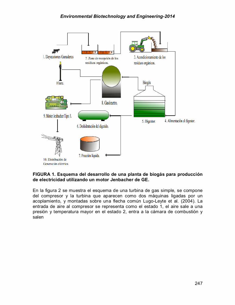
Environmental Biotechnology and Engineering-2014
247
FIGURA 1. Esquema del desarrollo de una planta de biogás para producción de electricidad utilizando un motor Jenbacher de GE. En la figura 2 se muestra el esquema de una turbina de gas simple, se compone del compresor y la turbina que aparecen como dos máquinas ligadas por un acoplamiento, y montadas sobre una flecha común Lugo-Leyte et al. (2004). La entrada de aire al compresor se representa como el estado 1, el aire sale a una presión y temperatura mayor en el estado 2, entra a la cámara de combustión y salen
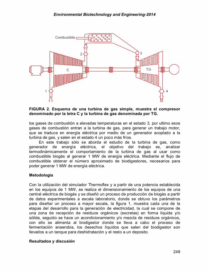
Environmental Biotechnology and Engineering-2014
248
FIGURA 2. Esquema de una turbina de gas simple, muestra el compresor denominado por la letra C y la turbina de gas denominada por TG. los gases de combustión a elevadas temperaturas en el estado 3, por ultimo esos gases de combustión entran a la turbina de gas, para generar un trabajo motor, que se traduce en energía eléctrica por medio de un generador acoplado a la turbina de gas, y salen en el estado 4 un poco más fríos. En este trabajo sólo se aborda el estudio de la turbina de gas, como generador de energía eléctrica, el objetivo del trabajo es, analizar termodinámicamente el comportamiento de la turbina de gas al usar como combustible biogás al generar 1 MW de energía eléctrica. Mediante el flujo de combustible obtener el número aproximado de biodigestores, necesarios para poder generar 1 MW de energía eléctrica. Metodología Con la utilización del simulador Thermoflex y a partir de una potencia establecida en los equipos de 1 MW, se realiza el dimensionamiento de los equipos de una central eléctrica de biogás y se diseñó un proceso de producción de biogás a partir de datos experimentales a escala laboratorio, donde se obtuvo los parámetros para diseñar un proceso a mayor escala, la figura 1, muestra cada una de la etapas del desarrollo para la generación de electricidad, la cual se compone de una zona de recepción de residuos orgánicos (excretas) en forma líquida y/o sólida, seguido se hace un acondicionamiento y/o mezcla de residuos orgánicos, con ello se alimenta al biodigestor donde se lleva a cabo el proceso de fermentación anaerobia, los desechos líquidos que salen del biodigestor son llevados a un tanque para deshidratación y el resto a un deposito. Resultados y discusión
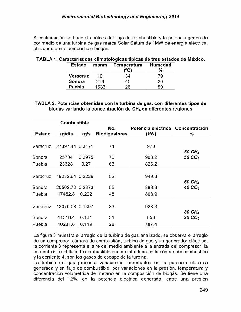
Environmental Biotechnology and Engineering-2014
249
A continuación se hace el análisis del flujo de combustible y la potencia generada por medio de una turbina de gas marca Solar Saturn de 1MW de energía eléctrica, utilizando como combustible biogás.
TABLA 1. Características climatológicas típicas de tres estados de México.
Estado msnm Temperatura (ºC)
Humedad %
Veracruz 10 34 79 Sonora 216 40 20 Puebla 1633 26 59
TABLA 2. Potencias obtenidas con la turbina de gas, con diferentes tipos de biogás variando la concentración de CH4 en diferentes regiones
Combustible
Estado kg/día kg/s No.
Biodigestores Potencia eléctrica
(kW) Concentración
%
Veracruz 27397.44 0.3171 74 970
Sonora 25704 0.2975 70 903.2 50 CH4 50 CO2
Puebla 23328 0.27 63 826.2
Veracruz 19232.64 0.2226 52 949.3
Sonora 20502.72 0.2373 55 883.3 60 CH4 40 CO2
Puebla 17452.8 0.202 48 808.9 Veracruz 12070.08 0.1397 33 923.3
Sonora 11318.4 0.131 31 858 80 CH4 20 CO2
Puebla 10281.6 0.119 28 787.4 La figura 3 muestra el arreglo de la turbina de gas analizado, se observa el arreglo de un compresor, cámara de combustión, turbina de gas y un generador eléctrico, la corriente 3 representa el aire del medio ambiente a la entrada del compresor, la corriente 5 es el flujo de combustible que se introduce en la cámara de combustión y la corriente 4, son los gases de escape de la turbina. La turbina de gas presenta variaciones importantes en la potencia eléctrica generada y en flujo de combustible, por variaciones en la presión, temperatura y concentración volumétrica de metano en la composición de biogás. Se tiene una diferencia del 12%, en la potencia eléctrica generada, entre una presión
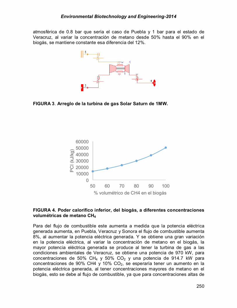
Environmental Biotechnology and Engineering-2014
250
atmosférica de 0.8 bar que sería el caso de Puebla y 1 bar para el estado de Veracruz, al variar la concentración de metano desde 50% hasta el 90% en el biogás, se mantiene constante esa diferencia del 12%.
FIGURA 3. Arreglo de la turbina de gas Solar Saturn de 1MW.
FIGURA 4. Poder calorífico inferior, del biogás, a diferentes concentraciones volumétricas de metano CH4 Para del flujo de combustible este aumenta a medida que la potencia eléctrica generada aumenta, en Puebla, Veracruz y Sonora el flujo de combustible aumenta 8%, al aumentar la potencia eléctrica generada. Y se obtiene una gran variación en la potencia eléctrica, al variar la concentración de metano en el biogás, la mayor potencia eléctrica generada se produce al tener la turbina de gas a las condiciones ambientales de Veracruz, se obtiene una potencia de 970 kW, para concentraciones de 50% CH4 y 50% CO2 y una potencia de 914.7 kW para concentraciones de 90% CH4 y 10% CO2, se esperaría tener un aumento en la potencia eléctrica generada, al tener concentraciones mayores de metano en el biogás, esto se debe al flujo de combustible, ya que para concentraciones altas de
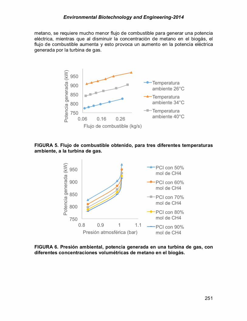
Environmental Biotechnology and Engineering-2014
251
metano, se requiere mucho menor flujo de combustible para generar una potencia eléctrica, mientras que al disminuir la concentración de metano en el biogás, el flujo de combustible aumenta y esto provoca un aumento en la potencia eléctrica generada por la turbina de gas.
FIGURA 5. Flujo de combustible obtenido, para tres diferentes temperaturas ambiente, a la turbina de gas.
FIGURA 6. Presión ambiental, potencia generada en una turbina de gas, con diferentes concentraciones volumétricas de metano en el biogás.

Environmental Biotechnology and Engineering-2014
252
FIGURA 7. Temperatura ambiente, potencia generada un una turbina de gas, con diferentes concentraciones volumétricas de metano en el biogás. Al usar los datos experimentales de presión y temperatura, de un biodigestor prototipo de 1100 litros de capacidad a nivel laboratorio, se puede estimar la cantidad de CH4 producida diariamente, con esto y el flujo de combustible necesario para la turbina , se puede hacer el estimado de cuantos biodigestores se necesitan para una potencia establecida, como se muestra en la tabla 2, donde a medida que aumenta la concentración de CH4 el número de biodigestores disminuye, aunque la potencia se ve afectada por las condiciones ambientales de cada zona. Las eficiencias reportadas por los fabricantes, son un buen punto de comparación entre un motor de gas, el cual normalmente es usado en la generación de energía eléctrica, por medio de biogás y la turbina de gas. La turbina de gas tiene una eficiencia eléctrica del 24.3% y el motor de gas ofrece una eficiencia eléctrica del 39%, esto es un aumento del 37% en la eficiencia eléctrica, con respecto a la turbina de gas. Conclusión Los resultados obtenidos en base al flujo de combustible, que varía en promedio desde los 0.0764 kg/s hasta 0.294 kg/s, en la turbina de gas, esto nos permite estimar el número de biodigestores necesarios en cada zona ganadera, con una concentración de CH4 del 60%, para Puebla se necesitan 48 biodigestores, en Sonora 55 y en Veracruz 52 para producir 1MWe de energía eléctrica con una carga diaria de estiércol de 25 m3/día para biodigestores de 1500 m3. Al usar biogás como combustible alternativo se está ahorrando 705,951 pies cúbicos de gas natural al día, un yacimiento de gas natural extrae 17 millones de pies cúbicos al día lo que representa un 4.15% de ahorro de gas natural extraído al día. Actualmente ninguna turbina de gas para generación de energía eléctrica, trabajan
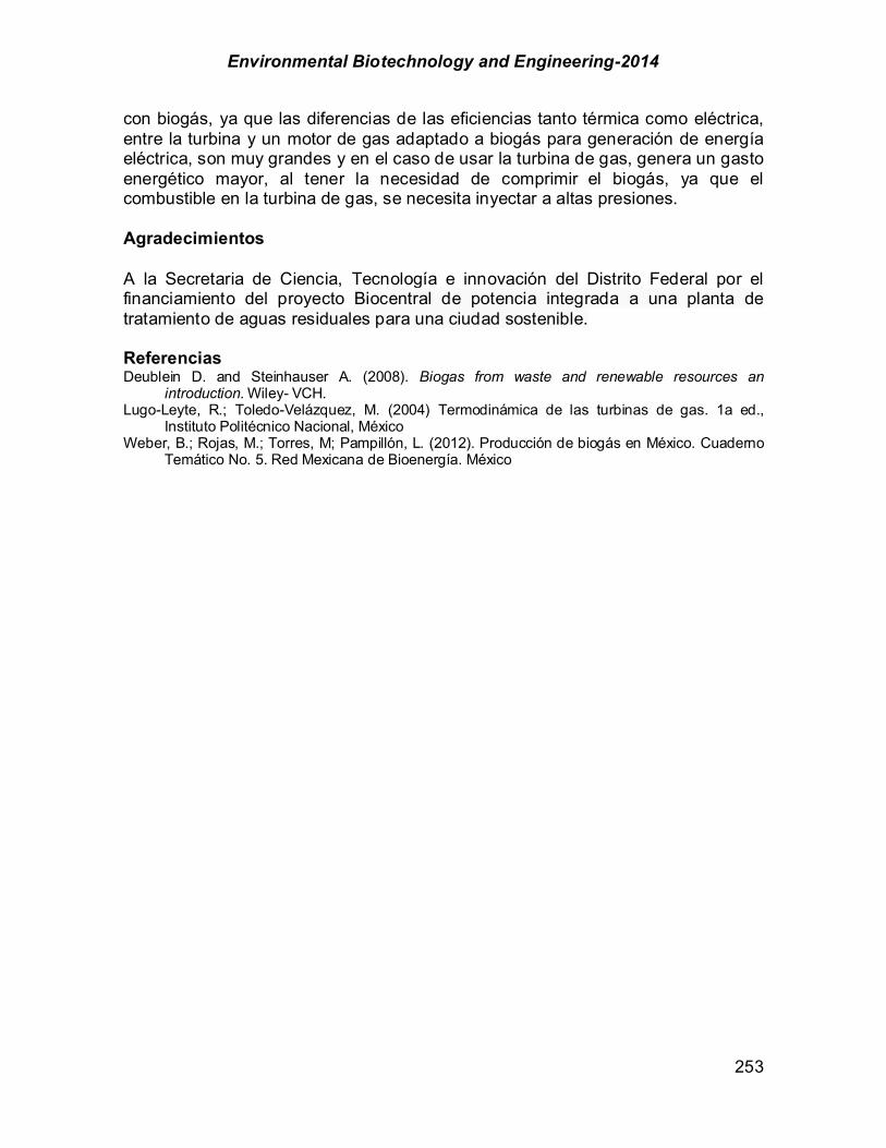
Environmental Biotechnology and Engineering-2014
253
con biogás, ya que las diferencias de las eficiencias tanto térmica como eléctrica, entre la turbina y un motor de gas adaptado a biogás para generación de energía eléctrica, son muy grandes y en el caso de usar la turbina de gas, genera un gasto energético mayor, al tener la necesidad de comprimir el biogás, ya que el combustible en la turbina de gas, se necesita inyectar a altas presiones. Agradecimientos A la Secretaria de Ciencia, Tecnología e innovación del Distrito Federal por el financiamiento del proyecto Biocentral de potencia integrada a una planta de tratamiento de aguas residuales para una ciudad sostenible. Referencias Deublein D. and Steinhauser A. (2008). Biogas from waste and renewable resources an
introduction. Wiley- VCH. Lugo-Leyte, R.; Toledo-Velázquez, M. (2004) Termodinámica de las turbinas de gas. 1a ed.,
Instituto Politécnico Nacional, México Weber, B.; Rojas, M.; Torres, M; Pampillón, L. (2012). Producción de biogás en México. Cuaderno
Temático No. 5. Red Mexicana de Bioenergía. México
Environmental Biotechnology and Engineering-2014
254
Section 2. Sustainability and Environmental System Analysis

Environmental Biotechnology and Engineering-2014
255
Page Chapter 2.1. Reducción en la generación de residuos sólidos peligrosos y uso eficiente del agua en un proceso de recuperación de baterias industriales al aplicar la metodología de producción más limpia. Paulina Mendoza-Alcántara; Gabriel Pineda-Flores; Carmen Monterrubio-Badillo 256 Chapter 2.2. Diagnóstico de los residuos generados por la industria petrolera en el estado de Coahuila. Micheline Gutiérrez-Priet; Myriam A. Amezcua-Allieri; Juan A. Zermeño-Eguia-Lis 273 Chapter 2.3. Stochastic aproach to economical analysis of biomass power plants Renata Varfolomejeva; Antans Sauhats; Evgenijs Kucajevs; Romans Petri"enko; Nauris Jankovskis 281 Chapter 2.4. Reconsideration of supporting scheme for renewable energy producers Renata Varfolomejeva; Marija Zima-Bo"karjova; Antans Sauhats; Romans Petricenko; Inga Umbrasko; Hasan Cobn 294 Chapter 2.5. Water saving potential in a rural community in Mexico to reduce the potable water consumption G. Gómez-Millán; S. Deegener; R. Otterpohl 307 Chapter 2.6. A low cost membrane fitted in a single chamber microbial fuel cell Giovanni Hernández-Flores; Omar Solorza-Feria; Héctor M. Poggi-Varaldo; Juvencio Galíndez-Mayer; Elvira Ríos-Leal; María T. Ponce-Noyola; Fernando J. Esparza-García; Tatiana Romero-Castañón 321 Chapter 2.7. Economic evaluation of a biorefinery for butanol production from wheat straw with a consolidated bioprocess approach Carlos Molina; Arturo Sánchez; Analí Soto; Idania Valdez-Vazquez 332 Chapter 2.8. Sustentabilidad del planeta y desarrollo sostenible en las organizaciones, un modelo para la conservacion del medio ambiente Germán Domínguez-Bocanegra 338 Chapter 2.9. Incubadora de negocios del tecnologico de estudios superiores de Ecatepec, como catalizador en la transferencia de tecnologia en las pymes del municipio de Ecatepec Germán Domínguez-Bocanegra; Fernando Cázares-Padrón; Katulli C. Corral-Miranda; Karla I. Téllez-López; Daniel Morales-Chong 343 Chapter 2.10. Potencial de sistemas pasivos de enfriamiento y calefacción como estrategias sustentables para reducir el consumo de energía en edificaciones en regiones cálido áridas José R. García-Chávez; Francisco Fernández-Melchor 354 Chapter 2.11. Diseño, caracterización y evaluación de un hábitat bioclimático sustentable en un clima cálido húmedo José R. García-Chávez; Francisco Fernández-Melchor 362

Environmental Biotechnology and Engineering-2014
256
CHAPTER 2.1. REDUCCIÓN EN LA GENERACIÓN DE RESIDUOS SÓLIDOS PELIGROSOS Y USO EFICIENTE DEL AGUA EN UN PROCESO DE RECUPERACIÓN DE BATERIAS INDUSTRIALES AL APLICAR LA
METODOLOGÍA DE PRODUCCIÓN MÁS LIMPIA
Paulina Mendoza Alcántara (1); Gabriel Pineda Flores (1); Carmen Monterrubio-Badillo*(1)
(1) IPN – Centro Mexicano para la Producción más Limpia, México DF, México.
RESUMEN
El presente trabajo se centra en la aplicación de la Metodología de Producción más Limpia en una empresa reparadora de baterías ácido-plomo ubicada en el Distrito Federal, México. El objetivo fue generar oportunidades de producción más limpia a fin de prevenir la producción de residuos sólidos peligrosos en el proceso de reparación de las baterías y fomentar el uso eficiente del agua en la empresa. Con estas oportunidades se fomentan beneficios económicos en la empresa y se disminuyen los riesgos al ser humano y al ambiente. El trabajo incluyó el levantamiento de datos, mediciones en campo y propuesta de oportunidades y recomendaciones de producción más limpia que producen los beneficios económicos y ambientales. El proceso de reparación y mantenimiento de baterías genera plomo como residuo que termina mezclándose con otro tipo de residuos convirtiéndolos en residuos peligroso, mismos que son entregados al camión recolector como residuos sólidos urbanos. Esta fuga de material representa una pérdida económica y un aspecto ambiental negativo por la alta toxicidad del metal. Otro problema importante es el derrame constante de la solución ácida de las baterías por el mal manejo que realizan los clientes y el personal de la planta, esta actividad compromete la seguridad física de los trabajadores y genera pérdidas económicas. En el diagnóstico se identificaron cuatro oportunidades de producción más limpia referentes a la prevención y gestión de los residuos así como al uso eficiente del agua. Al implantarse las cuatro oportunidades de producción más limpia, se tendrá un beneficio económico global de $ 5,926.49 pesos mx, requiriendo una inversión de $5,128.89 pesos mx. Esta inversión será recuperada en un periodo no mayor a 0.087 años. Si bien los beneficios económicos no son muy relevantes, si lo son los beneficios ambientales que se obtendrán por la implantación de las oportunidades encontradas, entre los principales se encuentran la disminución de 0.064 T de CO2eq, la disminución de 6.2 Kg de Pb que llega al flujo de residuos sólidos por tonelada de Pb fundido, disminución de los daños al suelo y en la contaminación del agua por evitar el derrame de 7.068 L/año de solución ácida.
Palabras clave: producción, limpia, oportunidades, residuos, beneficios
------------ *Author for all correspondence
Environmental Biotechnology and Engineering-2014
257
Introducción
A través del tiempo el uso de la batería acido-plomo se ha expandido, por lo que se le encuentra en diferentes prestaciones para diversas aplicaciones. Su amplio uso se debe a que el plomo es un metal de bajo costo, haciendo el proceso de fabricación rentable. Sin embargo, este metal pesado es tóxico, y puede causar daños irreversibles en el sistema nervioso en los infantes, entre otros (OIT, 1998). En México se estima que solo para el 2011 se generaron más de 30 millones de baterías de desecho, número que puede ir en aumento con la fabricación de autos eléctricos. De los cuales, aproximadamente el 80% entra a un proceso de acopio-reciclaje.
Con la publicación de la Ley General para la Prevención y Gestión Integral de Residuos en el 2003 (LGPGIR, 2013), se establecieron los lineamientos legales para el manejo adecuado de los residuos peligrosos y entre ellos para las Baterías Acido-Plomo Usadas (BAPU). Estos lineamientos propiciaron la proliferación de centros de acopio, desafortunadamente principalmente clandestinos, es decir que no acatan las medidas de seguridad ambiental interpuestas por la autoridad para evitar los impactos ambientales negativos que el proceso de acopio y recuperación genera. Partiendo de la premisa de que la mala disposición y manejo de las baterías ácido-plomo representan graves problemas ambientales, la aplicación de la metodología de la Producción más Limpia (P+L) permitió la identificación de oportunidades de mejora en una planta reparadora de baterías como la valorización de los residuos generados a través del diseño y aplicación de un plan de manejo de residuos, la reducción en la generación de residuos o evitar el verter al ambiente contaminantes tóxicos, entre otros, trayendo consigo además beneficios económicos a corto plazo para la empresa e inmediatos para el medio ambiente. Como caso de estudio, se seleccionó a una pequeña planta establecida legalmente en la Cd. de México dedicada a la recuperación de las BAPU.
El objetivo general del presente trabajo es aplicar la Metodología de Producción más Limpia (P+L), en una planta reparadora de baterías ubicada en el Distrito Federal, apoyándose en diversas herramientas de la Ingeniería Industrial, a fin de obtener beneficios económicos y ambientales, a través del desarrollo de oportunidades de P+L. El trabajo abarco desde la Fase 1 (planeación y organización) hasta la fase 4 (Estudio de factibilidad).
La producción más Limpia es una estrategia preventiva e integrada que contribuye a la protección ambiental y al desarrollo industrial (Bart Van Hoff, 2008). Su objetivo es el uso eficiente de los recursos demandados por los procesos industriales y la disminución de los residuos generados, desde su origen, que impactan negativamente al ambiente. Para productos y servicios, los puntos estratégicos se centran en la reducción de los efectos negativos al ambiente a lo largo del ciclo de vida del producto, desde la extracción de los materiales y servicios hasta su disposición final. La experiencia con producción más limpia muestra que se pueden implantar mejoras en el proceso industrial, sin ningún costo adicional o bien con costos relativamente bajos. La metodología de la

Environmental Biotechnology and Engineering-2014
258
producción más limpia consiste de cinco fases; cada una de ellas incluye diversas actividades (CMP+L, 1998), a saber:
Fase 1. Planeación y organización: involucrar y obtener el compromiso a nivel gerencial, establecer el equipo conductor del proyecto, establecer las metas de P+L, identificar barreras y soluciones.
Fase 2. Evaluación previa: Desarrollar el diagrama de flujo del proceso, medir las entradas y las calidad, seleccionar las metas de P+L.
Fase 3. Evaluación: Elaborar el balance de materiales, evaluar las causas, generar opciones de P+L, seleccionar las opciones de P+L.
Fase 4. Estudio de factibilidad: Evaluación preliminar, evaluación técnica, evaluación económica, evaluación ambiental, seleccionar opciones factibles Fase 5. Preparar el plan de P+L, implantar las opciones de P+L, supervisar y evaluar el avance, mantener las actividades de P+L. Materiales y Métodos La empresa en cuestión lleva a cabo 3 procesos generales, la reparación y mantenimiento de baterías ácido-plomo tanto industriales como automotrices, la compra/venta y acopio de baterías ácido-plomo usadas y la venta de baterías industriales (bajo pedido) y automotrices (cuentan con un stock). Los procesos pueden relacionarse entre sí dependiendo del tipo de producto que se maneje. A pesar de que la reparación y/o mantenimiento de baterías industriales ácido-plomo de ciclo profundo es la actividad principal de la empresa, las baterías automotrices son las que más circulan dentro de la nave. Diagrama de flujo del proceso de mantenimiento – reparación de baterías industriales. El principal proceso de la empresa es el mantenimiento-reparación de las baterías. En la Figura 1 se muestra el diagrama de flujo del proceso de mantenimiento para el que se consideraron las siguientes actividades: recepción de baterías industriales, almacenamiento, prueba de carga y descarga, reparación, hidratación de celdas y almacenamiento. Las entradas y salidas de los subprocesos de soldadura y fundición están consideradas en el proceso de reparación. La emisión de los humos metálicos del Pb se da en ambos, mientras que el CO2 solo es liberado durante la soldadura de los conectores. Se encontró que varios de los subproductos o residuos del proceso de mantenimiento-reparación, son clasificados dentro de los peligrosos de acuerdo con la legislación nacional. Otros gases altamente activos y con riesgo de generar una explosión son el hidrógeno y el oxígeno, que como ya se comentó anteriormente, se producen durante la carga de la batería. Balance de materia. Se partió de la identificación de puntos críticos del proceso, donde ya están establecidos los principales materiales, o residuos que se generan. La información que se recolectó para el cálculo del balance proviene de los datos de producción con los que cuenta el encargado de la planta y de la caracterización de residuos que se llevó a cabo.

Environmental Biotechnology and Engineering-2014
259
FIGURA 1. Proceso de mantenimiento-reparación de baterías industriales
El derrame de la solución ácida ocurre durante el acopio (recepción) de las
baterías para su posterior reciclado. La única actividad que incluye este proceso es el traslado o almacenamiento. Los datos recolectados son estimaciones hechas a través de la observación aleatoria del proceso y las bitácoras de baterías recicladas que lleva el encargado de producción. La Figura 2 ejemplifica las entradas y las salidas del proceso en cuanto a la solución ácida se refieren durante un mes.
Como ya se mencionó, el derrame ocurre durante el acopio (recepción) de las baterías para su posterior reciclado. La única actividad que incluye este proceso es el traslado o almacenamiento. Los datos recolectados son estimaciones hechas a través de la observación aleatoria del proceso y las bitácoras de baterías recicladas que lleva el encargado de producción. Los datos considerados para el balance son los siguientes:
En promedio se reciclan 40 T de baterías por mes, en su mayoría de auto de diferentes tamaños. Para este balance se supone que las 40 T se refieren exclusivamente a baterías para un auto tipo sedán cuyo peso individual es de

Environmental Biotechnology and Engineering-2014
260
aproximadamente 21 kg. El peso obtenido de solución ácida por batería es de 3 Kg. El volumen derramado de ácido se estimó a partir de la observación del proceso. Se obtuvo que el derrame mínimo que ocurre cuando una batería es manejada inadecuadamente es de aproximadamente 50 ml, este evento ocurre cada 16 baterías recibidas. Se considera que la densidad de la solución ácida es de 1 kg/L (igual a la densidad del agua).
FIGURA 2. Balance de materia del proceso de acopio. Aa= 5714.28 kg/mes; Ac= 5.95 L/mes; Ar= 5708.33 kg/mes, considerando 32%wt de H2SO4; masa de H2SO4 derramado= 1.09 kg/mes; V= 0.589 L/mes H2SO4, considerando densidad= 1.849 kg/L Balance residuos plomo-antimonio. Para realizar el balance del plomo que se derrama al piso y llega al flujo de residuos se requirieron los siguientes datos:
La cantidad aproximada de piezas fundidas por mes se obtuvo de la observación del proceso y datos del encargado de la planta. Se estima que por mes se funden alrededor de 30 piezas, aunque no todos los meses esto sucede. Se realizó un pequeño muestreo para determinar el peso de las piezas fundidas. La empresa invirtió en la fabricación de un molde para formar las piezas. Cada pieza fundida tiene un peso de 100 g.
A través de la caracterización del flujo de residuos se encontró que se generan 920 g de Pb en él al mes. A través de la observación se sabe que el Pb proviene de la fundición y la preparación. Sin embargo, se considera que el Pb proviene únicamente de la fundición, pues el generado como residuo en la preparación, es difícil de cuantificar. En la Figura 3 se representa el balance de materia por mes para el proceso de fundición donde se incluyen los datos necesarios para realizarlos.
Para la emisión de gases solo se calculó la emisión de CO2 utilizando factores de emisión por el tipo de combustible fósil que se utiliza, el gas LP. Los datos
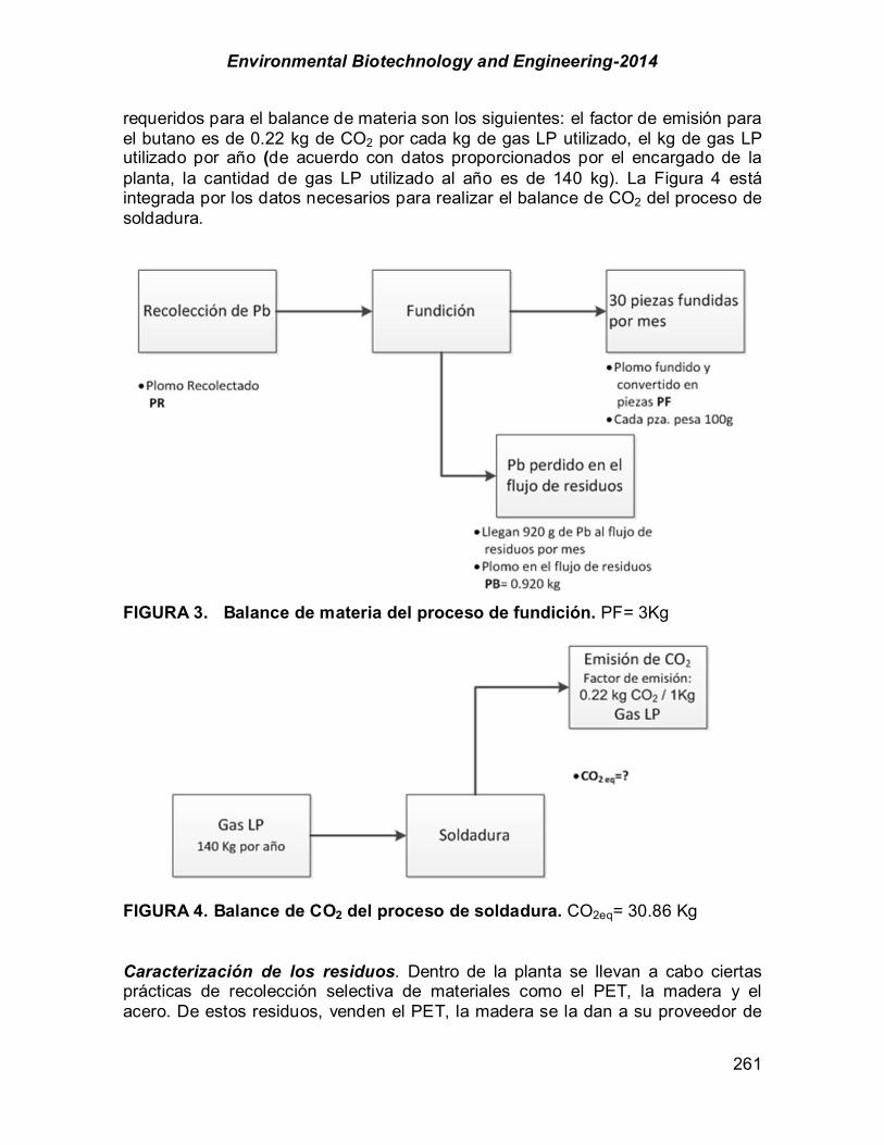
Environmental Biotechnology and Engineering-2014
261
requeridos para el balance de materia son los siguientes: el factor de emisión para el butano es de 0.22 kg de CO2 por cada kg de gas LP utilizado, el kg de gas LP utilizado por año (de acuerdo con datos proporcionados por el encargado de la planta, la cantidad de gas LP utilizado al año es de 140 kg). La Figura 4 está integrada por los datos necesarios para realizar el balance de CO2 del proceso de soldadura.
FIGURA 3. Balance de materia del proceso de fundición. PF= 3Kg
FIGURA 4. Balance de CO2 del proceso de soldadura. CO2eq= 30.86 Kg Caracterización de los residuos. Dentro de la planta se llevan a cabo ciertas prácticas de recolección selectiva de materiales como el PET, la madera y el acero. De estos residuos, venden el PET, la madera se la dan a su proveedor de

Environmental Biotechnology and Engineering-2014
262
tarimas para que las repare, el acero se regala la mayoría de las ocasiones. En la Tabla 1 se muestra la caracterización de los residuos.
TABLA 1. Caracterización del flujo de residuos
Residuo Cantidad (g/día) % Residuo Cantidad
(g/día) %
No valorizable Valorizable Fibras 0.71 0.09 Vidrio 21.86 2.65 Polvo 179.6 21.80 Cartón 51.14 6.21
Otros 2.29 0.28 Papel oficina 60.71 7.37
Papel encerado 3.29 0.40 Madera 87 10.56 Tapas plástico para unicel 5.14 0.62 Latas
aluminio 8.57 1.04
Unicel 6.71 0.82 Pet 11.86 1.44 Envolturas 12.57 1.53 Periódico 12.43 1.51 Bolsas de plástico 10.14 1.23 Acero 52 6.31 Plástico recipientes 10.14 1.23 Restos de
comida 156.14 18.96
Desechos baño 45 5.46 Plomo antimonio 46 5.58
Plástico 40.43 4.91 Subtotal 495.29 61.64 Subtotal 328.43 38.36 TOTAL 823.71 100.000
Es responsabilidad del generador buscar la reutilización o el reciclado de los
residuos que genera (LGPGIR, 2003), por lo que otra importante forma de separar los residuos es tomando como base su valor comercial. Es fundamental recordar que parte de los residuos que tienen un valor comercial ya se separan en la empresa, pero existen fugas de material por diversas razones que se explicaran más adelante. La cantidad de residuos con valor comercial es considerable, ocupando un 20.3% del total del flujo (el resto de los residuos ya se comercializan en la planta), porcentaje que se puede traducir en ganancias económicas para la organización. Medición del consumo de agua. En relación al consumo de agua, la empresa comparte la toma de agua con una empresa vecina, por lo que el recibo se reparte en partes iguales. El agua llega de la red y se almacena en una cisterna, de aquí el líquido sube a los tinacos que alimentan todos los servicios de la empresa vecina y los baños y lavabos de la empresa caso. Adicionalmente, la empresa reparadora de baterías requiere agua libre de impurezas, por lo tanto se instaló una bomba de agua de la cisterna a dos tambos colocados en la planta, de donde se envía a los filtros para limpiarla y utilizarla posteriormente en la hidratación de las celdas. El baño es utilizado únicamente por los trabajadores de la planta (todos
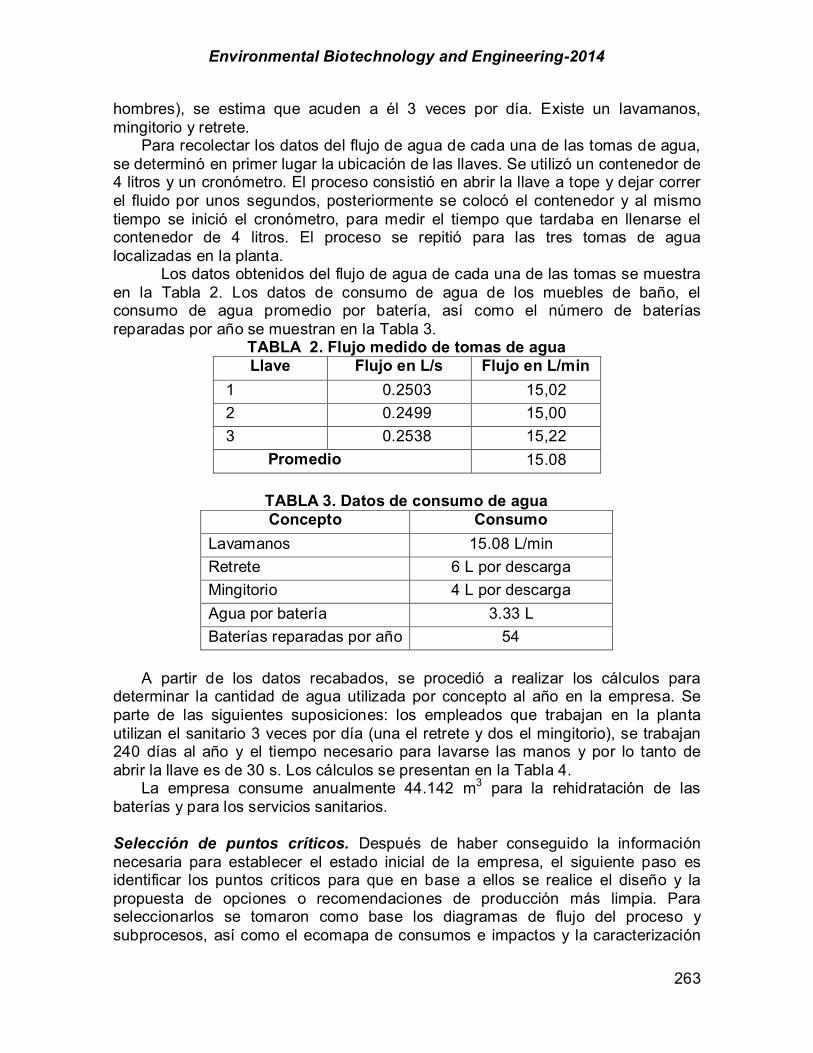
Environmental Biotechnology and Engineering-2014
263
hombres), se estima que acuden a él 3 veces por día. Existe un lavamanos, mingitorio y retrete.
Para recolectar los datos del flujo de agua de cada una de las tomas de agua, se determinó en primer lugar la ubicación de las llaves. Se utilizó un contenedor de 4 litros y un cronómetro. El proceso consistió en abrir la llave a tope y dejar correr el fluido por unos segundos, posteriormente se colocó el contenedor y al mismo tiempo se inició el cronómetro, para medir el tiempo que tardaba en llenarse el contenedor de 4 litros. El proceso se repitió para las tres tomas de agua localizadas en la planta.
Los datos obtenidos del flujo de agua de cada una de las tomas se muestra en la Tabla 2. Los datos de consumo de agua de los muebles de baño, el consumo de agua promedio por batería, así como el número de baterías reparadas por año se muestran en la Tabla 3.
TABLA 2. Flujo medido de tomas de agua Llave Flujo en L/s Flujo en L/min
1 0.2503 15,02 2 0.2499 15,00 3 0.2538 15,22
Promedio 15.08
TABLA 3. Datos de consumo de agua Concepto Consumo
Lavamanos 15.08 L/min Retrete 6 L por descarga Mingitorio 4 L por descarga Agua por batería 3.33 L Baterías reparadas por año 54
A partir de los datos recabados, se procedió a realizar los cálculos para
determinar la cantidad de agua utilizada por concepto al año en la empresa. Se parte de las siguientes suposiciones: los empleados que trabajan en la planta utilizan el sanitario 3 veces por día (una el retrete y dos el mingitorio), se trabajan 240 días al año y el tiempo necesario para lavarse las manos y por lo tanto de abrir la llave es de 30 s. Los cálculos se presentan en la Tabla 4.
La empresa consume anualmente 44.142 m3 para la rehidratación de las baterías y para los servicios sanitarios.
Selección de puntos críticos. Después de haber conseguido la información necesaria para establecer el estado inicial de la empresa, el siguiente paso es identificar los puntos críticos para que en base a ellos se realice el diseño y la propuesta de opciones o recomendaciones de producción más limpia. Para seleccionarlos se tomaron como base los diagramas de flujo del proceso y subprocesos, así como el ecomapa de consumos e impactos y la caracterización

Environmental Biotechnology and Engineering-2014
264
del flujo de residuos. Con la ayuda de las herramientas mencionadas, los puntos críticos identificados son los siguientes:
TABLA 4. Consumo anual de agua en la empresa por uso de sanitarios y
mantenimiento de baterías
Concepto Usuarios Uso por día L/min
descarga Tiempo
accionamiento min
Días al año
consumo m3/año
Lavamanos 5 3 15.08 0.5 240 27.162
Retrete 5 1 6 N/A 240 7.2 Mingitorio 5 2 4 N/A 240 9.6
Subtotal 43.96
Bat reparadas por año L/por bat consumo
m3/año Baterías reparadas 54 3.33 0.17982
Total 44.142
Derrame de la solución acida de las baterías. Durante su almacenamiento ya sea al llegar a la nave para su posterior revisión o para su acopio, en ocasiones ocurren derrames de ácido sobre el suelo de concreto. El derrame se da cuando los clientes llevan sus baterías para acopio y no tienen cuidado al apilarlas y/o transportarlas. El derrame del ácido tiene diversas afectaciones tanto al ambiente como al personal que labora dentro de la planta. Además la solución es un elemento de la batería que es vendido a las empresas recicladoras, y/o puede reintegrarse al proceso para utilizarlo en baterías reparadas, por lo que los derrames representan también fugas económicas. Energía eléctrica almacenada en las baterías. Durante el procedimiento de mantenimiento a las baterías, los puntos críticos localizados se encuentran durante el ciclo de carga de la batería. Durante el primer paso del ciclo, la batería es cargada a través de los cargadores de perillas, y transcurrido el tiempo de reposo, son conectadas a otro dispositivo cuya labor es simular el uso de la batería (descargarla). La energía almacenada es simplemente desechada sin que sea utilizada para algún otro propósito. Residuos plomo-antimonio. Como ya se mencionó anteriormente, existen fugas de este material que no tan solo tiene un valor económico importante, sino que es tóxico y al colarse al flujo de residuos convierte en residuo peligroso aquello con lo que se mezcla. Estas fugas se dan específicamente en dos subprocesos, durante la reparación y la fundición. En ambos casos el plomo-antimonio que cae o es derramado en el suelo, llega a mezclarse con el polvo u otros residuos pequeños que hay en el taller, haciendo prácticamente imposible separarlo.

Environmental Biotechnology and Engineering-2014
265
Emisión de gases. Los gases que se liberan al ambiente son el hidrógeno, oxígeno, CO2 y humos de plomo. Los dos primeros se generan durante la carga de la batería. Cada una de las celdas que la componen a una batería tiene diferentes capacidades de carga debido a su uso. Al someterse al proceso de carga, para conseguir que todas lleguen a su máximo nivel de energía, algunas se sobrecargan, lo que genera liberación de oxígeno e hidrógeno por el agotamiento del agua de la solución (Gasquet., 2010). Durante el proceso de soldadura se generan humo de plomo y el CO2 se produce por el uso de butano y oxígeno para fundir el plomo-antimonio y unir los conectores intercelda con las celdas reparadas de la batería. Este último también se presenta durante la fundición y vaciado de piezas. Generación de residuos. A través de la caracterización de residuos, fue posible determinar qué tipo de residuos se generan y si son valorizables o no. Se determinó que existe la presencia de residuos peligrosos que no son tratados con precaución, y que convierten a residuos inertes en peligrosos. Como es el caso de las carcasas donde son colocadas las celdas que en conjunto forman las baterías, están hechas de acero y al encontrarse en contacto con la solución ácida, se convierten en residuos peligrosos; el polvo de plomo-antimonio o las diminutas virutas del mismo material que se combinan con la tierra proveniente del exterior entre otros. Consumo de agua. Al realizar la medición del líquido en la empresa por año, se determinó que el consumo anual de agua en la empresa es de 44.142 m3 para la rehidratación de las baterías y los servicios sanitarios (43.96 m3 para servicios y 0.17982m3 para baterías). Al ver el estado y tipo de muebles de baño instalados en la planta (sin dispositivos para ahorrar agua), las oportunidades de reducir el consumo en esta área son importantes. Resultados
Se presenta las oportunidades de producción más limpia, de acuerdo a lo observado en los recorridos realizados, a los balances de materiales y a la información proporcionada por el personal de la empresa
Oportunidad 1. Valoración de residuos. En la empresa se generan residuos de diversos tipos, entre los que se puede citar el PET, latas de aluminio, el plomo-antimonio, etc. Actualmente se hacen algunos esfuerzos para manejar adecuadamente los residuos, sin embargo no todos han sido valorados. Una de las principales oportunidades de producción más limpia se encuentra en la venta de determinados residuos. El PET es uno de los más llamativos, la empresa ya realiza esfuerzos por recolectarlos de forma separada. Sin embargo, este residuo se hizo presente en la caracterización. Estas fugas se deben a que existe un gran flujo de personas ajenas a la empresa que entran a la planta. Colocar botes para recolectar exclusivamente botellas de PET y señalizarlos adecuadamente, puede
Environmental Biotechnology and Engineering-2014
266
ayudar a recolectar el 100% del residuo que se genera en la planta. Se observa que la recolección del PET es una buena práctica más que la aplicación de alguna tecnología para aprovechar este residuo.
Para realizar la estimación de la generación anual de cada residuo se tomó como base el promedio de generación diaria para cada residuo encontrado en la caracterización. Se consideró que los días laborales al año son 240 (quitando los días festivos únicamente). Se estima que por año la empresa genera 197.726 Kg de residuos, de los cuales existen 8 componentes valorizables: PET, periódico, latas de aluminio, vidrio, cartón, acero, papel de oficina y madera; sin embargo no todos son considerados dentro de la valorización, por lo que se excluye el periódico, el vidrio, la madera y el cartón. Como ya se comentó anteriormente, el PET y la madera son recolectados en la actualidad para obtener un beneficio económico al vender el primero, y suministrar como materia prima el segundo a su proveedor de tarimas. Por ley en el Distrito Federal los generadores de residuos urbanos deben entregarlos de forma separada al camión recolector de basura. Esto se traduce a que es obligación de todos separar el flujo de residuos en orgánicos e inorgánicos. Para cumplir con la Ley, es necesario contar con recipientes para almacenar los residuos de forma separada. Se recomienda colocarlos en el mismo lugar donde actualmente se hace y vaciarlos dos o tres veces por semana. No se requiere manejarlos de forma especial. Los recipientes deben estar señalizados para que los generadores, sean o no de la empresa, los coloquen en lugar adecuado. Recipientes de los mismos colores pero de capacidades menores deben colocarse en las oficinas para el personal administrativo.
De los residuos que se encontraron en el flujo, los que cuentan con un mayor valor económico son el Acero, el PET, el papel de oficina y las latas de aluminio. Para estos productos se indagó sobre el pecio por kilogramo en el mercado. Cabe recordar que aunque el plomo se puede vender como residuo es mejor reintegrarlo al proceso para formar parte de un nuevo conector. En la tabla anterior no se considera el PET que se separa desde su generación del flujo de residuos, se estima que se reciclan alrededor de 75 kg al año lo que equivale a $450.00.
Adicionalmente a los recipientes para residuos orgánicos e inorgánicos, y con la intención de facilitar la recolección de los residuos valorizables, es conveniente contar con recipientes especiales para su almacenamiento y así evitar que se vayan al flujo de residuos inorgánicos por no contar con un lugar específico para cada uno. En el caso del PET, ya se cuenta con un tambo de 200 L donde se almacena, sin embargo, se recomienda colocar uno más pequeño a la entrada de la planta para que las personas ajenas a la empresa coloquen ahí sus botellas y no en los botes generales de residuos inorgánicos. Para el papel se puede utilizar una caja de plástico colocada de preferencia en las oficinas para evitar su contaminación; y para el acero (el no contaminado con residuos de ácido proveniente del electrolito de la batería) se puede utilizar un bote de las mismas dimensiones que los utilizados para los residuos orgánicos e inorgánico; los trozos de madera que pueden ser reutilizados son colocados actualmente en un área dentro de la zona de tarimas. Todos deben llevar su correspondiente leyenda.

Environmental Biotechnology and Engineering-2014
267
La única inversión necesaria para llevar a cabo la recolección separada de los residuos orgánicos, inorgánicos y valorizables, será con motivo de la adquisición de los botes, una caja de cartón y letreros señalizando para qué es cada contenedor.
Para el periodo simple de recuperación de la inversión, se consideran como beneficios los obtenidos de reciclar el PET que apareció en el flujo de residuos, el papel y el acero que dan un total de $305.61 pesos. La inversión para recolectar los residuos de forma adecuada es de $200.00, que será recuperada en 8 meses. Si bien los beneficios económicos son bajos, lo más importante de esta oportunidad serán los beneficios ambientales, así como el cumplimiento con la legislación ambiental mexicana vigente. La separación de los residuos no representa mayor dificultad que la de colocar los contenedores con sus letreros y hacer uso adecuado de ellos, además de que existe un fundamento legal para hacerlo. Es necesario destinar un lugar fijo y suficiente para los contenedores, con el objetivo de evitar la confusión o mezcla con cualquier otro material o residuo en la planta. Dentro de la empresa existe espacio para colocar los botes adecuadamente. No hay ningún impedimento técnico para llevar a cabo esta opción. A pesar de que los beneficios económicos son relativamente bajos, los ambientales son mayores como se comentará a continuación. La empresa genera anualmente 197.73 kg de basura actualmente, recuperando los residuos valorizables que se mencionaron más arriba, se disminuiría la cantidad de residuos que son entregados al camión recolector, además de que se reduce la presión sobre la explotación de los recursos naturales necesarios para producir los materiales que se consumen en la empresa y la contaminación sobre los ecosistemas. En la Tabla 5 se muestran los beneficios que se obtendrán al valorar los residuos generados en la planta.
TABLA 5. Beneficios que se obtendrán por la valorización de los residuos
generados en la planta
Beneficios ambientales
Reducción en emisiones de CO2eq 0.063944 T CO2eq
Reducción en volumen ocupado en relleno sanitario 0.17 m3
Beneficios económicos $ 305.61
Inversión $ 200.00
PSRI 0.65 años Oportunidad 2. Buenas prácticas operativas durante la fundición y preparación de piezas de plomo. El plomo se genera como residuo en los procesos de fundición y reparación de las baterías. El material para fundir proviene
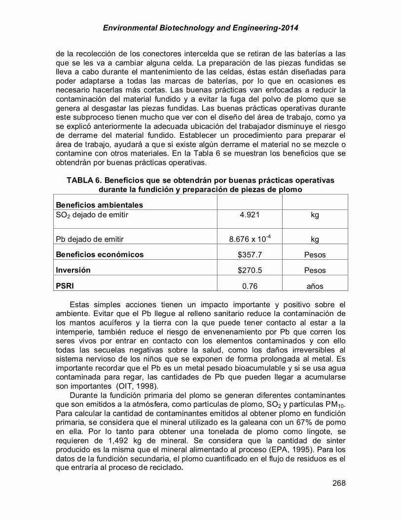
Environmental Biotechnology and Engineering-2014
268
de la recolección de los conectores intercelda que se retiran de las baterías a las que se les va a cambiar alguna celda. La preparación de las piezas fundidas se lleva a cabo durante el mantenimiento de las celdas, éstas están diseñadas para poder adaptarse a todas las marcas de baterías, por lo que en ocasiones es necesario hacerlas más cortas. Las buenas prácticas van enfocadas a reducir la contaminación del material fundido y a evitar la fuga del polvo de plomo que se genera al desgastar las piezas fundidas. Las buenas prácticas operativas durante este subproceso tienen mucho que ver con el diseño del área de trabajo, como ya se explicó anteriormente la adecuada ubicación del trabajador disminuye el riesgo de derrame del material fundido. Establecer un procedimiento para preparar el área de trabajo, ayudará a que si existe algún derrame el material no se mezcle o contamine con otros materiales. En la Tabla 6 se muestran los beneficios que se obtendrán por buenas prácticas operativas.
TABLA 6. Beneficios que se obtendrán por buenas prácticas operativas durante la fundición y preparación de piezas de plomo
Beneficios ambientales SO2 dejado de emitir
4.921
kg
Pb dejado de emitir 8.676 x 10⁻⁴ kg
Beneficios económicos $357.7 Pesos
Inversión $270.5 Pesos
PSRI 0.76 años
Estas simples acciones tienen un impacto importante y positivo sobre el ambiente. Evitar que el Pb llegue al relleno sanitario reduce la contaminación de los mantos acuíferos y la tierra con la que puede tener contacto al estar a la intemperie, también reduce el riesgo de envenenamiento por Pb que corren los seres vivos por entrar en contacto con los elementos contaminados y con ello todas las secuelas negativas sobre la salud, como los daños irreversibles al sistema nervioso de los niños que se exponen de forma prolongada al metal. Es importante recordar que el Pb es un metal pesado bioacumulable y si se usa agua contaminada para regar, las cantidades de Pb que pueden llegar a acumularse son importantes (OIT, 1998).
Durante la fundición primaria del plomo se generan diferentes contaminantes que son emitidos a la atmósfera, como partículas de plomo, SO2 y partículas PM10. Para calcular la cantidad de contaminantes emitidos al obtener plomo en fundición primaria, se considera que el mineral utilizado es la galeana con un 67% de pomo en ella. Por lo tanto para obtener una tonelada de plomo como lingote, se requieren de 1,492 kg de mineral. Se considera que la cantidad de sinter producido es la misma que el mineral alimentado al proceso (EPA, 1995). Para los datos de la fundición secundaria, el plomo cuantificado en el flujo de residuos es el que entraría al proceso de reciclado.

Environmental Biotechnology and Engineering-2014
269
Los factores de emisión de plomo para la obtención secundaria del plomo considerados para los cálculos son con equipos de control, mientras que para el SO2 lo que se presentan son sin control de las emisiones (EPA, 1995). Estas consideraciones se hacen con el fin de realizar cálculos que se aproximen a la cantidad de contaminantes que se dejan de emitir al reciclar plomo.
Oportunidad 3. Reducción en el consumo de agua. A partir de los datos recolectados en la medición del consumo de agua y los puntos donde se utilizan, se encontraron diferentes oportunidades para disminuir la cantidad de agua consumida principalmente durante el uso de las instalaciones sanitarias. Lo referente al consumo de agua para la elaboración de la solución ácida, no se puede modificar pues se alteraría el funcionamiento de las baterías.
La empresa comparte la toma de agua con una empresa vecina, por lo que el recibo se reparte en partes iguales al pagarse. El agua llega de la red y se almacena en una cisterna, de aquí el líquido sube a los tinacos que alimentan todos los servicios de la empresa vecina y los baños y lavabos de la empresa caso. Adicionalmente, la empresa reparadora de baterías requiere agua libre de impurezas, por lo tanto se instaló una bomba que lleva agua de la cisterna a dos tambos colocados en la planta, de donde se envían a los filtros para limpiar el agua y poder utilizarla en la hidratación de las celdas. El baño es utilizado únicamente por los trabajadores de la planta (todos hombres), se estima que acuden a él 3 veces por día.
Para la reducción en el consumo en el lavamanos se propone la instalación de una válvula reguladora para el flujo de agua en tubería de suministro cuya función será disminuir el flujo por segundo de la llave de 15.09 a 1.5 L/min. Se obtiene un ahorro de 24.462 m3 por año de agua.
Para la reducción en el consumo en el mingitorio se proponen la sustitución del mingitorio actual que por descarga utiliza 4 litros por uno que por descarga utilice 0.5 litros, el costo del equipo es de $4,200.00 pesos (a noviembre 2013). Se obtiene un ahorro de 8.4 m3 por año de agua.
Para la reducción en el consumo en el retrete se propone agregar dos botellas de PET de un litro llenas de agua en la caja del retrete para disminuir la cantidad del líquido que se descarga en cada uso de 6 a 4 litros. Al aplicar esta sencilla opción se reduce el consumo de agua en 3 m3 por año. A continuación se tratarán por separado las oportunidades encontradas en cada punto de consumo de agua dentro de las instalaciones sanitarias.
Los beneficios ambientales consisten en disminuir considerablemente la cantidad de agua utilizada en la empresa, se dejan de consumir en total 35.86 m3 al año, así se disminuye la presión ambiental ejercida sobre el recurso no renovable. En la Tabla 7 se muestran los beneficios que se obtendrán por reducir el consumo de agua. Oportunidad 4. Redistribución y diseño del área de trabajo. Esta oportunidad se desarrolla a partir de la información generada y recopilada en ecomapa de emisiones y consumos y en la selección de puntos críticos. Se observó que las áreas de procesos consecutivos se encuentran alejadas unas de otras, haciendo
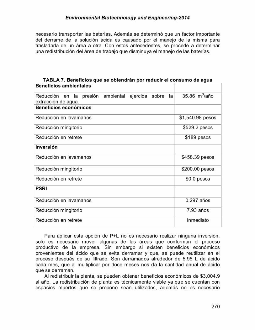
Environmental Biotechnology and Engineering-2014
270
necesario transportar las baterías. Además se determinó que un factor importante del derrame de la solución ácida es causado por el manejo de la misma para trasladarla de un área a otra. Con estos antecedentes, se procede a determinar una redistribución del área de trabajo que disminuya el manejo de las baterías.
TABLA 7. Beneficios que se obtendrán por reducir el consumo de agua
Beneficios ambientales
Reducción en la presión ambiental ejercida sobre la extracción de agua.
35.86 m3/año
Beneficios económicos
Reducción en lavamanos $1,540.98 pesos
Reducción mingitorio $529.2 pesos
Reducción en retrete $189 pesos
Inversión
Reducción en lavamanos
$458.39 pesos
Reducción mingitorio $200.00 pesos
Reducción en retrete $0.0 pesos
PSRI
Reducción en lavamanos 0.297 años
Reducción mingitorio 7.93 años
Reducción en retrete Inmediato
Para aplicar esta opción de P+L no es necesario realizar ninguna inversión,
solo es necesario mover algunas de las áreas que conforman el proceso productivo de la empresa. Sin embargo si existen beneficios económicos provenientes del ácido que se evita derramar y que, se puede reutilizar en el proceso después de su filtrado. Son derramados alrededor de 5.95 L de ácido cada mes, que al multiplicar por doce meses nos da la cantidad anual de ácido que se derraman.
Al redistribuir la planta, se pueden obtener beneficios económicos de $3,004.9 al año. La redistribución de planta es técnicamente viable ya que se cuentan con espacios muertos que se propone sean utilizados, además no es necesario

Environmental Biotechnology and Engineering-2014
271
reubicar las instalaciones eléctricas (por el cambio del área de descarga) o de ningún tipo. La recuperación de la inversión es inmediata. En la Tabla 8 se muestran los beneficios por redistribuir y diseñar el área de trabajo.
Los mayores beneficios son ambientales con la puesta en marcha de esta opción. Reduce el riesgo de accidentes y daños al personal y la probabilidad de derrame de la solución ácida, también se disminuye el uso del montacargas y con ello, la demanda eléctrica para cargar las baterías de los mismos. Otro residuo que se reduce es el Pb que se derrama al suelo durante el proceso de la fundición. Los daños al ambiente y a la salud de los seres vivos que el Pb representa son importantes, evitando que este residuo llegue al flujo de residuos y con ello al relleno sanitario, disminuye la probabilidad de que estos componentes causen daño.
TABLA 8. Beneficios que se obtendrán por redistribuir y diseñar el área de trabajo
Beneficios ambientales
Disminuir la cantidad de Pb que llega al flujo de residuos
6.2 Kg
Disminuir los daños al suelo por el derrame de la solución ácida
7.068 L/año de solución ácida
Disminuir la contaminación del agua por el derrame de la solución ácida
7.068 L/año de solución ácida
Beneficios económicos $3,004.00
Inversión No requerida
PSRI Inmediato
Conclusiones
Al aplicar la metodología se obtuvieron 4 oportunidades de producción más limpia, de las que podemos destacar la implementación de un plan de manejo de residuos, el rediseño del área de trabajo y la reducción en el consumo de agua. Los beneficios ambientales son el principal objetivo de cada una de las propuestas hechas. Estas oportunidades de producción más limpia estuvieron principalmente enfocadas a la disminución y/o eliminación de residuos tóxicos vertidos al ambiente principalmente plomo y solución ácida. Considerando que la Producción más limpia es una estrategia preventiva e integrada que contribuye a la protección ambiental y al desarrollo industrial, su principal objetivo es el uso eficiente de los recursos demandados por los procesos industriales y la disminución de los residuos generados, desde su origen, que impactan negativamente al ambiente. Por lo tanto podemos concluir que los objetivos planteados en el presente proyecto se cumplieron.
Environmental Biotechnology and Engineering-2014
272
Se hace evidente que las oportunidades de mejora para empresas del ramo pueden ser atractivas a los directivos por los beneficios ambientales y económicos que se producen a través de cambios mínimos en el proceso, el diseño del área de trabajo o de la forma de manejar los residuos que se generan día con día. Referencias CMP+L (1998). Guía de Producción más Limpia. 1ª ed., Tres Guerras. Gasquet., H. L. (2010). Energía alternativa de México. http://www.enalmex.com/paginas/como.htm; acceso el 27 de Febrero de 2012. EPA (1995) Environmental Protection Agency, office of Air Quality Planning And Standards. (1995). Compilation of air pollutant emission factors. LGPGIR (2003), Ley General para la Prevención y Gestión Integral de Residuos. Diario Oficial de la Federación, Mexico. OIT (1998). Enciclopedia de la salud y seguridad en el trabajo. Madrid, España: OIT. Bart Van Hoof (2008). Producción más limpia, alfaomega. México.

Environmental Biotechnology and Engineering-2014
273
CHAPTER 2.2. DIAGNÓSTICO DE LOS RESIDUOS GENERADOS POR LA INDUSTRIA PETROLERA EN EL ESTADO DE COAHUILA
Micheline Gutiérrez Priet (1); Myriam A. Amezcua Allieri* (1); Juan A. Zermeño
Eguia Lis (1) (1) Instituto Mexicano del Petróleo. Eje Central Lázaro Cárdenas No. 152 Col. San Bartolo Atepehuacan, México, D.F., 07730, México.
RESUMEN Los procesos industriales, sin exceptuar los de la industria petrolera, tienen que adaptarse a marcos normativos y mecanismos que controlen y reduzcan los residuos que generan en sus actividades. Atendiendo a esta problemática en México, la Ley General para la Prevención y Gestión Integral de los Residuos (LGPGIR), establece y fomenta la gestión integrada de los residuos mediante la aplicación de herramientas, estrategias y acciones contempladas en los Programas Estatales de Prevención y Gestión Integral de Residuos (PEPGIR). Con base en el PEPGIR el trabajo presentado identifica las áreas de oportunidad en cuanto al manejo y aprovechamiento de los residuos generados por la industria petrolera en el estado de Coahuila, siendo éste el estado que opera el proyecto más importante en el país de gas no asociado. El análisis está orientado a la gestión responsable de los residuos, donde se proponen una serie de alternativas autorizadas por la Secretaría del Medio Ambiente y Recursos Naturales (SEMARNAT) de acuerdo con la infraestructura disponible en el estado, para el manejo de los residuos acorde con su composición y a lo establecido por el marco legal en la materia. Palabras clave: Áreas de oportunidad, manejo responsable, PEPGIR, sedimentos de hidrocarburos. ABSTRACT Industrial oil processes have to adapt to the environmental regulations and mechanisms to control and reduce the waste that they generate in their activities. In response to this problem in Mexico, the General Law for the Prevention and Management of Waste (LGPGIR) provides and promotes integrated waste management through the application of tools, strategies and actions develop by the State Programs Prevention and Management Integral Waste (PEPGIR). Based on the PEPGIR the present work identifies opportunity areas on the management and recovery of waste generated by the oil industry in Coahuila State, which has the most important not associated gas project inside of the country. This analysis is focused to the responsible waste management, where is proposed several alternatives presents in the State authorized by Secretariat of Environment and Natural Resources (SEMARNAT) according to their composition and regulations. ------------ *Author for all correspondence
Environmental Biotechnology and Engineering-2014
274
Keywords: Hydrocarbons sediments, responsible management, opportunity areas, PEPGIR. Introducción Si bien la generación de residuos es inherente a toda actividad industrial y casi se podría decir humana, hasta finales del siglo pasado la sociedad tomó conciencia de la gravedad del problema y, por lo tanto, se comenzaron a establecer las medidas que pudieran minimizar sus efectos. Coincidiendo con la época de mayor desarrollo y mayor presión sobre el medio ambiente, en la década de los años 70 en los Estados Unidos de América y la Unión Europea, se comienza a dictar las primeras normas y leyes para limitar la generación de residuos y definir los criterios para su eliminación (Castellanos et al., 2003).
Atendiendo a esta problemática en México se publicó en el 8 de octubre de 2003 en el Diario Oficial de la Federación la Ley General para la Prevención y Gestión Integral de los Residuos (LGPGIR), misma que entró en vigor el 6 de enero de 2004, y cuya última versión es del 7 de junio de 2013, y el 30 de noviembre de 2006 fue publicado su Reglamento que entró en vigor el 30 de diciembre de ese mismo año. En su carácter de Ley General o Marco, tiene por objeto garantizar el derecho de toda persona al medio ambiente adecuado y propiciar el desarrollo sustentable a través de la prevención de la generación, la valorización y la gestión integral de los residuos peligrosos, de los residuos sólidos urbanos y de manejo especial; prevenir la contaminación de sitios con estos residuos y llevar a cabo su remediación (Gutiérrez, 2006).
La industria petrolera es una fuente importante de residuos y al no darles un manejo adecuado se convierten en una amenaza latente tanto para los ecosistemas como para el hombre. Un buen manejo de los residuos no solo contribuirá al entorno ambiental y social sino también económico. Actualmente Petróleos Mexicanos (PEMEX) enfrenta diferentes retos para obtener el mayor valor posible de los hidrocarburos y sus derivados y a su vez contribuir al desarrollo sustentable del país, es decir, requiere desarrollar acciones que no sólo satisfagan la demanda energética sino también acciones que enfrenten los desafíos en materia de sustentabilidad ambiental (PEMEX, 2012), bajo este contexto, este trabajo atiende la necesidad planteada en la acción 5 del PEPGIR, la cual se encuentra enfocada al análisis de los residuos generados por la industria petrolera en Coahuila (SEMARNAT, 2012). En el trabajo se describen los principales residuos que se generan en las instalaciones de la industria petrolera en Coahuila, identificando los procesos y las actividades de las que se derivan, para posteriormente identificar áreas de oportunidad y con base a ello proponer alternativas de manejo acorde con la Ley, ya que un buen manejo de los residuos no solo contribuye al entorno ambiental y social sino también económico. Materiales y Métodos

Environmental Biotechnology and Engineering-2014
275
La información analizada que se presenta en el trabajo, parte principalmente de un cuestionario elaborado como apoyo en el marco de los objetivos del PEPGIR de Coahuila, el cual fue enviado por medio de la Secretaría del Medio Ambiente de Coahuila a PEMEX, solicitando apoyo con la información requerida en el cuestionario y así fortalecer el Programa Estatal y los vínculos con la entidad en favor de acciones en el tema de residuos. Aunado a lo anterior se reforzó la información recabada con datos obtenidos de las Cédulas de Operación Anual (COA) del estado de Coahuila, siendo este un mecanismo de reporte anual que sirve como un instrumento de consolidación de los requerimientos de reporte contemplados en la Ley General del Equilibrio Ecológico y Protección al Ambiente (LGEEPA), los reglamentos y normas que de ella se derivan en lo relativo a las emisiones atmosféricas, descargas de aguas residuales, uso de sustancias listadas, generación y transferencia de residuos de manejo especial y peligrosos. El análisis se realizó durante el período 2008-2009 y 2012, la información analizada se desarrolló bajo el siguiente esquema:
1. Por subsidiaria se abordaron los siguientes aspectos: • Tipos de instalaciones. • Generación de residuos. • Transferencia de residuos generados. • Manejo de los residuos reportados.
2. Se clasificó la información en generación y manejo, por parte de generación se contemplaron los siguientes puntos:
• Por instalación. • Por tipo de residuo. • Por actividad: trabajos de mantenimiento, trabajos de limpieza y
trabajos de operación. • Por origen.
3. En cuanto al manejo se trabajaron con los siguientes aspectos: • Cantidad transferida. • Autorización de la empresa prestadora de servicios. • Tratamiento aplicado.
4. Una vez analizada la información se prosiguió a homologar los tratamientos reportados por las empresas prestadoras de servicios con las autorizaciones que se tienen registradas ante la Secretaría de Media Ambiente y Recursos Naturales (Semarnat). 5. Se realizó una descripción de los residuos identificados mediante reportes técnicos. 6. Se llevó a cabo la descripción de los tratamientos empleados. 7. Se identificaron las áreas de oportunidad para el aprovechamiento y mejora del manejo de residuos en cada subsidiaria de PEMEX. 8. Se sugirieron alternativas de manejo para los residuos identificados de acuerdo a su potencialidad y factibilidad técnica.
Resultados y Discusión
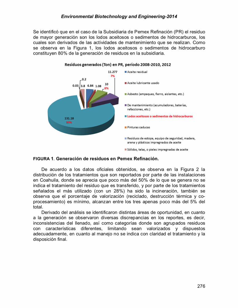
Environmental Biotechnology and Engineering-2014
276
Se identificó que en el caso de la Subsidiaria de Pemex Refinación (PR) el residuo de mayor generación son los lodos aceitosos o sedimentos de hidrocarburos, los cuales son derivados de las actividades de mantenimiento que se realizan. Como se observa en la Figura 1, los lodos aceitosos o sedimentos de hidrocarburo constituyen 80% de la generación de residuos en la subsidiaria.
FIGURA 1. Generación de residuos en Pemex Refinación.
De acuerdo a los datos oficiales obtenidos, se observa en la Figura 2 la distribución de los tratamientos que son reportados por parte de las instalaciones en Coahuila, donde se aprecia que poco más del 50% de lo que se genera no se indica el tratamiento del residuo que es transferido, y por parte de los tratamientos señalados el más utilizado (con un 28%) ha sido la incineración, también se observa que el porcentaje de valorización (reciclado, destrucción térmica y co-procesamiento) es mínimo, alcanzan entre los tres apenas poco más del 5% del total.
Derivado del análisis se identificaron distintas áreas de oportunidad, en cuanto a la generación se observaron diversas discrepancias en los reportes, es decir, inconsistencias del llenado, así como categorías donde son agrupados residuos con características diferentes, limitando sean valorizados y dispuestos adecuadamente, en cuanto al manejo no se indica con claridad el tratamiento y la disposición final.
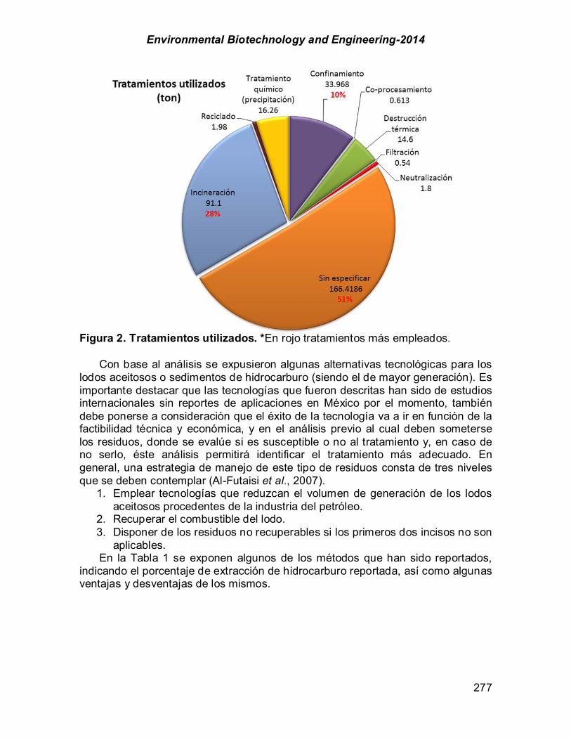
Environmental Biotechnology and Engineering-2014
277
Figura 2. Tratamientos utilizados. *En rojo tratamientos más empleados.
Con base al análisis se expusieron algunas alternativas tecnológicas para los
lodos aceitosos o sedimentos de hidrocarburo (siendo el de mayor generación). Es importante destacar que las tecnologías que fueron descritas han sido de estudios internacionales sin reportes de aplicaciones en México por el momento, también debe ponerse a consideración que el éxito de la tecnología va a ir en función de la factibilidad técnica y económica, y en el análisis previo al cual deben someterse los residuos, donde se evalúe si es susceptible o no al tratamiento y, en caso de no serlo, éste análisis permitirá identificar el tratamiento más adecuado. En general, una estrategia de manejo de este tipo de residuos consta de tres niveles que se deben contemplar (Al-Futaisi et al., 2007).
1. Emplear tecnologías que reduzcan el volumen de generación de los lodos aceitosos procedentes de la industria del petróleo.
2. Recuperar el combustible del lodo. 3. Disponer de los residuos no recuperables si los primeros dos incisos no son
aplicables. En la Tabla 1 se exponen algunos de los métodos que han sido reportados,
indicando el porcentaje de extracción de hidrocarburo reportada, así como algunas ventajas y desventajas de los mismos.
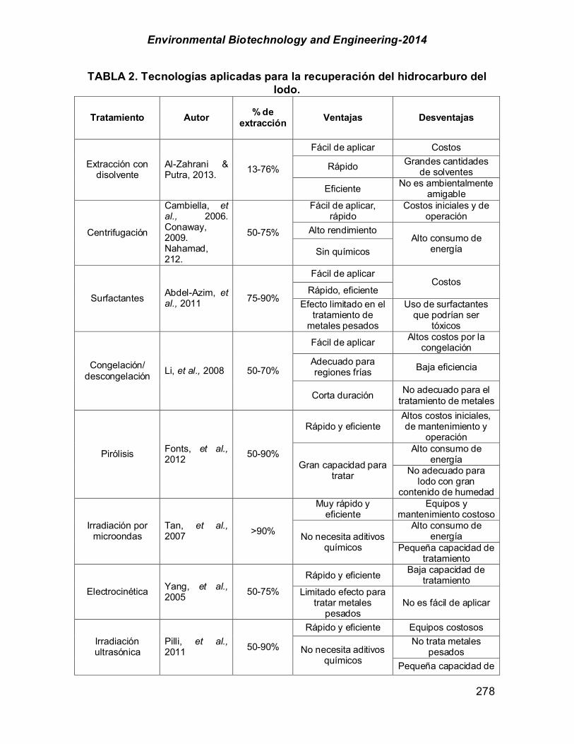
Environmental Biotechnology and Engineering-2014
278
TABLA 2. Tecnologías aplicadas para la recuperación del hidrocarburo del lodo.
Tratamiento Autor % de extracción Ventajas Desventajas
Extracción con disolvente
Al-Zahrani & Putra, 2013. 13-76%
Fácil de aplicar Costos
Rápido Grandes cantidades de solventes
Eficiente No es ambientalmente amigable
Centrifugación
Cambiella, et al., 2006. Conaway, 2009. Nahamad, 212.
50-75%
Fácil de aplicar, rápido
Costos iniciales y de operación
Alto rendimiento Alto consumo de
energía Sin químicos
Surfactantes Abdel-Azim, et al., 2011 75-90%
Fácil de aplicar Costos
Rápido, eficiente Efecto limitado en el
tratamiento de metales pesados
Uso de surfactantes que podrían ser
tóxicos
Congelación/ descongelación Li, et al., 2008 50-70%
Fácil de aplicar Altos costos por la congelación
Adecuado para regiones frías Baja eficiencia
Corta duración No adecuado para el tratamiento de metales
Pirólisis Fonts, et al., 2012 50-90%
Rápido y eficiente Altos costos iniciales, de mantenimiento y
operación
Gran capacidad para tratar
Alto consumo de energía
No adecuado para lodo con gran
contenido de humedad
Irradiación por microondas
Tan, et al., 2007 >90%
Muy rápido y eficiente
Equipos y mantenimiento costoso
No necesita aditivos químicos
Alto consumo de energía
Pequeña capacidad de tratamiento
Electrocinética Yang, et al., 2005 50-75%
Rápido y eficiente Baja capacidad de tratamiento
Limitado efecto para tratar metales
pesados No es fácil de aplicar
Irradiación ultrasónica
Pilli, et al., 2011 50-90%
Rápido y eficiente Equipos costosos
No necesita aditivos químicos
No trata metales pesados
Pequeña capacidad de

Environmental Biotechnology and Engineering-2014
279
tratamiento
Espuma de flotación
Moosai & Dawe, 2003 50-75%
Fácil de aplicar Rendimiento relativamente bajo
No requiere gran consumo de energía
Se utiliza gran cantidad de agua
No es adecuada para el tratamiento de lodos
aceitosos con alta viscosidad
No trata metales pesados
Dentro de las propuestas realizadas fue considerado la valorización
energética, con el uso de los residuos como combustible alterno en la industria cementera (infraestructura presente en el estado), actividad avalada bajo convenios establecidos por parte de la SEMARNAT y la Cámara del Cemento en México (CANACEM). Conclusión La información proporcionada permitió dimensionar la situación e identificar áreas susceptibles de mejora para el manejo responsable de los residuos que son generados por la industria petrolera en la entidad. Derivado del análisis se pudo identificar la necesidad de llevar un registro fidedigno de la generación de los residuos, con el fin de promover una toma de decisiones acertada acerca del manejo responsable de los residuos teniendo en consideración que un correcto llenado de las bases de datos, con categorías definidas y agrupadas acorde con las características de los residuos, facilitará determinar con mayor precisión las tecnologías apropiadas para su aprovechamiento y disposición final. Además de dar la trazabilidad del residuo obligado por la Ley.
Actualmente en la entidad las industrias cementeras, bajo la autorización de la SEMARNAT, indican que los lodos aceitosos o sedimentos de hidrocarburos pueden ser utilizados como combustible alterno al igual que otros residuos que se derivan de la industria petrolera, actividad que debe realizarse bajo las condiciones técnicas adecuadas, para evitar la emisión de contaminantes a la atmósfera. Agradecimientos Los autores agradecen al Gobierno del estado de Coahuila por las facilidades proporcionadas para la realización del presente trabajo. Referencias Abdel-Azim, A.; Abdul-Raheim, M.; Kamel, R. K.; Abdel-Raouf, M. E. (2011).
Demulsifier Systems applied to breakdown petroleum sludge. Journal of Petroleum Science and Engineering. 78 (2): 364–370.

Environmental Biotechnology and Engineering-2014
280
Al-Futaisi, A.; Jamrah, A.; Yaghi, B.; Taha, R. (2007). Assessment of alternative management techniques of tank bottom petroleum sludge in Oman. J. Hazard. Mater. 141: 557–564.
Al-Zahrani, S. M.; Putra, M. D. (2013). Used lubricating oil regeneration by various solvent extraction techniques. Journal of Industrial and Engineering Chemistry. 19 (2): 536-539.
Cambiella, A.; Benito, J.; Pazos, C.; Coca, J. (2006). Centrifugal separation efficiency in the treatment of waste emulsified oils. Chem. Eng. Res. Des. 84: 69-76.
Castellanos, P. R.; Picabea, A.J.; Ubanel, J.A.; García, J.A.; Alique, J.L.; Tercero, S.P.; Gómez, M.R. (2003). Residuos: Alternativas de Gestión.
Fonts, I.; Gea, G.; Azuara, M.; Ábrego, J.; Arauzo, J. (2012). Sewage sludge pyrolysis for liquid production: A review. Elsevier, 16, 2781-2805. Salamanca, España: Ediciones Universidad Salamanca.
Gutiérrez Avedoy, V.J. (2006). Diagnóstico básico para la gestión integral de residuos. México.
Li, C.; He, G.; Dong, C.; Liu, H.; Xiao, G.; & Liu, Y. (2008). Effect of oil phase transition on freeze/Thaw-induced demulsification of water-in-oil emulsions. Langmuir, 5291-5298.
Moosai, R.; Dawe, R. A. (2003). Gas attachment of oil droplets for gas flotation for oily wastewater cleanup. Sep. Purif. Technol. 33: 303-3014.
PEMEX. 2012, Informe de Responsabilidad Social. 60–61. Pilli, S.; Bhunia, P.; Yan, S.; LeBlanc, R.; Tyagi, R. D.; Surampalli, R.Y. (2011).
Ultrasonic pretreatment of sludge: a review. Ultrason. Sonochem. 18, p. 1-18.
SEMARNAT. 2012. Programa Nacional para la Prevención y Gestión Integral de Residuos 2008-2012. 33-41.
Tan, W., Yang, X.-G., & Tan, X.-F. (2007). Study on demulsification of crude oil emulsions by microwave chemical method. Sci Technology:1367-1377.
Yang, L.; Nakhla, G.; Bassi, A. (2005). Electro-kinetic dewatering of oily sludges. Sep. Sci. Technol. 42: 130-140.

Environmental Biotechnology and Engineering-2014
281
CHAPTER 2.3. STOCHASTIC APROACH TO ECONOMICAL ANALYSIS OF BIOMASS POWER PLANTS
Renata Varfolomejeva* (1); Antans Sauhats (1); Evgenijs Kucajevs (1);
Romans Petri"enko (1); Nauris Jankovskis (1, 2)
(1) RTU, Institute of Power Engineering, Riga, Latvia; (2) JSC Latvenergo, Riga, Latvia; ABSTRACT The global community is motivated to move towards renewable energy supply and market based operation in power systems. In the core of this change is an aspiration of the reduced the influence of power generation on the environment and the increased power supply efficiency, which is achieved through market conditions and free competition within generation and sales of energy. These new conditions define significant changes in the design and planning of the operation of the biomass stations. First step in the power plant development project is pre-feasibility study. As a result of such study, a developer would choose a place of construction, type of fuel, the connection scheme to the power grid, would estimate the necessary capital expenses, the energy to be produced, production costs and profits from the energy sales. Economic analysis is an important part of the pre-feasibility study of the power plant. Usually, power plant design is evaluated in terms of the profit maximization and the following economic criteria, e.g. NPV, IRR, payback time. The introduction of the markets in power systems substantially changes the approach to economic analysis of the power plant profitability. Free market and competition implies uncertainty. Consequently, the energy prices and revenues of power producers are subject to significant fluctuations. The criteria for profit maximization for the stakeholders shall be reformulated. The uncertain and random parameters, such as the ambient temperature, thermal energy consumption, price of energy has to be taken into account. The task assumes a stochastic form. An additional input information is needed in a large volume. As a result, the problem becomes much more complicated and requires new algorithms and software tools to solve it. This paper proposes a procedure to estimate the average value of these criteria taking into account random nature of the variables and using the historic values of parameters. Besides, we use neural network based algorithm to predict processes in future from the historical data. We capture information on various input parameters, such as temperatures prices etc from the internet. A case study is conducted on a realistic project of the cogeneration biomass power plant (2 MW) and demonstrates the advantages of the stochastic approach. ------------------ *Author for correspondence: [email protected]
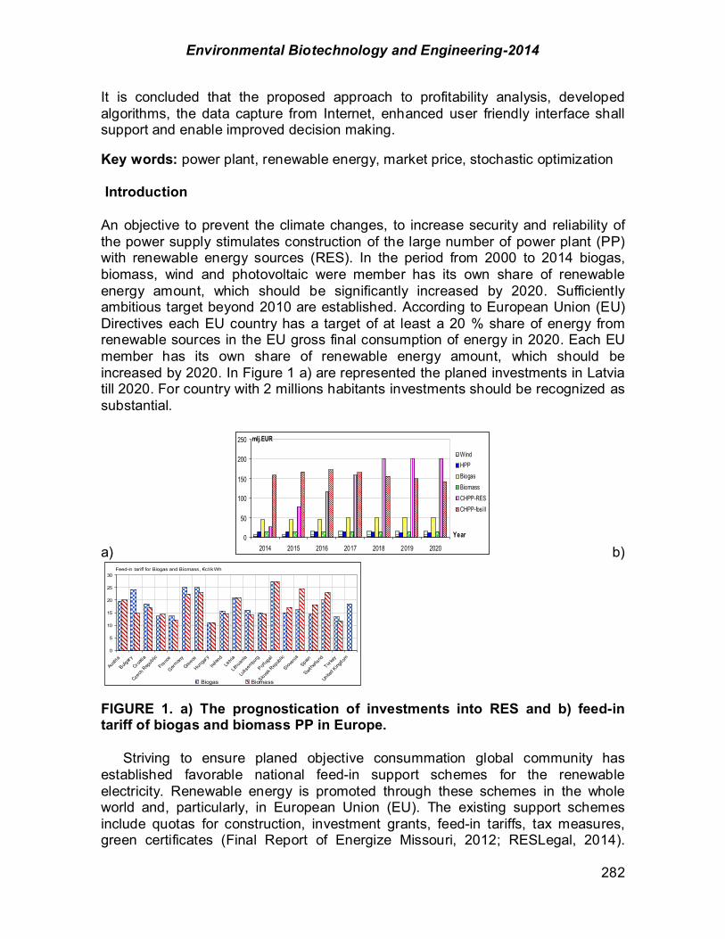
Environmental Biotechnology and Engineering-2014
282
It is concluded that the proposed approach to profitability analysis, developed algorithms, the data capture from Internet, enhanced user friendly interface shall support and enable improved decision making. Key words: power plant, renewable energy, market price, stochastic optimization Introduction An objective to prevent the climate changes, to increase security and reliability of the power supply stimulates construction of the large number of power plant (PP) with renewable energy sources (RES). In the period from 2000 to 2014 biogas, biomass, wind and photovoltaic were member has its own share of renewable energy amount, which should be significantly increased by 2020. Sufficiently ambitious target beyond 2010 are established. According to European Union (EU) Directives each EU country has a target of at least a 20 % share of energy from renewable sources in the EU gross final consumption of energy in 2020. Each EU member has its own share of renewable energy amount, which should be increased by 2020. In Figure 1 a) are represented the planed investments in Latvia till 2020. For country with 2 millions habitants investments should be recognized as substantial.
a) b)
FIGURE 1. a) The prognostication of investments into RES and b) feed-in tariff of biogas and biomass PP in Europe. Striving to ensure planed objective consummation global community has established favorable national feed-in support schemes for the renewable electricity. Renewable energy is promoted through these schemes in the whole world and, particularly, in European Union (EU). The existing support schemes include quotas for construction, investment grants, feed-in tariffs, tax measures, green certificates (Final Report of Energize Missouri, 2012; RESLegal, 2014).
0
50
100
150
200
250
2014 2015 2016 2017 2018 2019 2020
Year
mlj.EUR
WindHPPBiogasBiomassCHPP-RESCHPP-fosi ll
Feed-in tariff for Biogas and Biomass, #ct/kWh
0
5
10
15
20
25
30
Austr
ia
Bulgary
Croati
a
Czech
Rep
ublic
Franc
e
German
y
Greece
Hunga
ry
Irelan
dLa
tvia
Lithu
ania
Luks
embu
rg
Portug
al
Slovak
Rep
ublic
Sloven
ia
Spain
Swithe
rland
Turke
y
Unite
d King
dom
Biogas Biomass
Environmental Biotechnology and Engineering-2014
283
Frequently, the support is provided by a guaranteed purchase price, which is significantly higher than the market price of electricity. Supported by feed-in tariffs (Figure 1. b)) the biogas and biomass PP are developing especially rapidly in the northern Europe. It is nature to require that RES development shall be achieved in a possibly most cost efficient manner. First and highly important for effectiveness ensuring step in the design of new power plants should be devoted to the feasibility study. As a result of this study is selected place of construction, type of fuel, the connection diagram to the power grid, is estimated the necessary capital expenses, the amount of produced energy, the proceeds from its sales and cost of production. Usually, power plants planning issues are formulated in the form of profit maximization problems. For this purpose, designers use a number of economical criteria, such as NPV, IRR, payback time (Bennett, 2003; Buljevich et al., 1999). In this paper we limit ourselves using only NPV, while generality is not lost, since outlined below algorithm can be easily extended to compute and other economical criteria. In general, the goal of this paper is to propose a new methodology of feasibility studies, that allows selection of PP structure and parameters taking into account the hourly variation of a market situation. We solve such problem using stochastic approach for a small bio PP feasibility study (first contribution of the paper). We apply data bases, which are available by Internet and Smart grids means; artificial neural network for random processes prediction The second contribution of the paper is the case study that demonstrates the proposed methodology and algorithm workability. The rest of the paper is organized as follows: first, the shortcomings of existing methodologies are formulated, second, the algorithm of revenues calculation is presented, and the third, the case study illustrating the proposed methodology in the realistic set-up is described. Shortcomings of existed methodologies The complicated process of the technical-economical evaluation of the highly expensive energy units installations, in particular power plants, include several stages, as follows:
• Forecasts of the demand for the energy supply (heat and the electricity) for the period of 20 – 30 years; • Preliminary choice of the competitiveness of the various options for the energy supply for the customers; • Development of the sketches for the chosen alternatives and feasibility studies; • The choice of the best alternative and decision making on the implementation of the project; • The implementation of the project.
The last three stages are connected with the necessity to evaluate main economic indices: NPV, IRR, (Bennett et.al., 2003; Buljevich 1999). To evaluate these indices we need to determine the income ( )iTI from the energy sales and
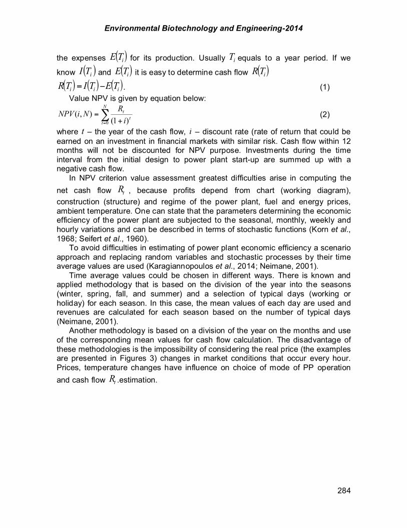
Environmental Biotechnology and Engineering-2014
284
the expenses ( )iTE for its production. Usually iT equals to a year period. If we
know ( )iTI and ( )iTE it is easy to determine cash flow ( )iTR
( ) ( ) ( )iii TETITR %= . (1) Value NPV is given by equation below:
"= +
=N
tt
t
iRNiNPV
0 )1(),( (2)
where t – the year of the cash flow, i – discount rate (rate of return that could be earned on an investment in financial markets with similar risk. Cash flow within 12 months will not be discounted for NPV purpose. Investments during the time interval from the initial design to power plant start-up are summed up with a negative cash flow. In NPV criterion value assessment greatest difficulties arise in computing the net cash flow tR , because profits depend from chart (working diagram), construction (structure) and regime of the power plant, fuel and energy prices, ambient temperature. One can state that the parameters determining the economic efficiency of the power plant are subjected to the seasonal, monthly, weekly and hourly variations and can be described in terms of stochastic functions (Korn et al., 1968; Seifert et al., 1960). To avoid difficulties in estimating of power plant economic efficiency a scenario approach and replacing random variables and stochastic processes by their time average values are used (Karagiannopoulos et al., 2014; Neimane, 2001). Time average values could be chosen in different ways. There is known and applied methodology that is based on the division of the year into the seasons (winter, spring, fall, and summer) and a selection of typical days (working or holiday) for each season. In this case, the mean values of each day are used and revenues are calculated for each season based on the number of typical days (Neimane, 2001). Another methodology is based on a division of the year on the months and use of the corresponding mean values for cash flow calculation. The disadvantage of these methodologies is the impossibility of considering the real price (the examples are presented in Figures 3) changes in market conditions that occur every hour. Prices, temperature changes have influence on choice of mode of PP operation and cash flow tR .estimation.
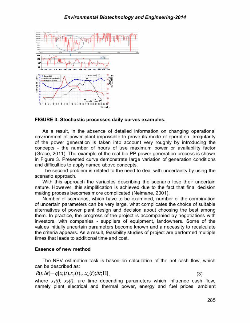
Environmental Biotechnology and Engineering-2014
285
0
200
400
600
800
1000
1200
1400
1600
1800
2000
3024 3360 3696 4032 4368 4704
Hour's amount
Generated power, kW
FIGURE 3. Stochastic processes daily curves examples. As a result, in the absence of detailed information on changing operational environment of power plant impossible to prove its mode of operation. Irregularity of the power generation is taken into account very roughly by introducing the concepts - the number of hours of use maximum power or availability factor (Grace, 2011). The example of the real bio PP power generation process is shown in Figure 3. Presented curve demonstrate large variation of generation conditions and difficulties to apply named above concepts. The second problem is related to the need to deal with uncertainty by using the scenario approach. With this approach the variables describing the scenario lose their uncertain nature. However, this simplification is achieved due to the fact that final decision making process becomes more complicated (Neimane, 2001). Number of scenarios, which have to be examined, number of the combination of uncertain parameters can be very large, what complicates the choice of suitable alternatives of power plant design and decision about choosing the best among them. In practice, the progress of the project is accompanied by negotiations with investors, with companies - suppliers of equipment, landowners. Some of the values initially uncertain parameters become known and a necessity to recalculate the criteria appears. As a result, feasibility studies of project are performed multiple times that leads to additional time and cost. Essence of new method The NPV estimation task is based on calculation of the net cash flow, which can be described as:
];);(),...(),([),( 21 &'=' ttxtxtxttR n( , (3) where x1(t), x2(t), are time depending parameters which influence cash flow, namely plant electrical and thermal power, energy and fuel prices, ambient
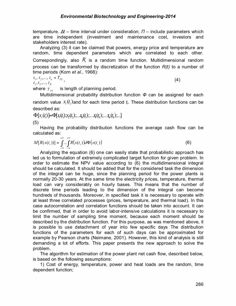
Environmental Biotechnology and Engineering-2014
286
temperature. !t – time interval under consideration; ! – include parameters which are time independent (investment and maintenance cost, investors and stakeholders interest rate). Analyzing (3) it can be claimed that powers, energy price and temperature are random, time dependent parameters which are correlated to each other. Correspondingly, also tR is a random time function. Multidimensional random process can be transformed by discretization of the function R(t) to a number of time periods (Korn et al., 1968):
K
PLnttt
Tttt,...,,,...,,
21
21 < , (4)
where PLT is length of planning period. Multidimensional probability distribution function " can be assigned for each random value )( ii tx and for each time period ti. These distribution functions can be described as:
]);...();...;();...;();...;();([)]([ 112211 knknii txtxtxtxtxtx )=) (5) Having the probability distribution functions the average cash flow can be calculated as:
( ) ( ))()(...))](([ iii txdtxRtxRM )= ##+*
*%
+*
*%
(6)
Analyzing the equation (6) one can easily state that probabilistic approach has led us to formulation of extremely complicated target function for given problem. In order to estimate the NPV value according to (6) the multidimensional integral should be calculated. It should be added that for the considered task the dimension of the integral can be huge, since the planning period for the power plants is normally 20-30 years. At the same time the electricity prices, temperature, thermal load can vary considerably on hourly bases. This means that the number of discrete time periods leading to the dimension of the integral can become hundreds of thousands. Moreover, in specified task it is necessary to operate with at least three correlated processes (prices, temperature, and thermal load). In this case autocorrelation and correlation functions should be taken into account. It can be confirmed, that in order to avoid labor-intensive calculations it is necessary to limit the number of sampling time moment, because each moment should be described by the distribution function. For this purpose, as was mentioned above, it is possible to use detachment of year into few specific days The distribution functions of the parameters for each of such days can be approximated for example by Pearson charts (Neimane, 2001). However, this kind of analysis is still demanding a lot of efforts. This paper presents the new approach to solve the problem. The algorithm for estimation of the power plant net cash flow, described below, is based on the following assumptions: 1) Cost of energy, temperature, power and heat loads are the random, time dependent function;

Environmental Biotechnology and Engineering-2014
287
2) Considerable amount of data from the past is available (databases formed by supervisory control and data acquisition (SCADA) system); 3) The records from the past can be projected into the future processes; 4) Projection of the records from the „past” xpast into the „future” processes xfut can be performed by using one of the stochastic processes forecasting parametric or artificial intelligence based methods (Gurney, 1997; Hassoum et al., 1995). In this paper the following two procedures are used (see Figure 4. a)):
• the linear algebraic expressions that describe changes in the characteristics of the random process in time (for example average value of prices in the future). It is assumed that such changes reflect the expert’s opinion; • the records of the past processes with anticipated changes are summing up. In this case, the planned future load can be added to the historical load records. For this purpose library of thermal energy consumer’s demand records was created.
a) b) FIGURE 4. Scheme of processes prediction and an algorithm structures. 5) The random process of parameters xfut variations is ergodic (Seifert et al., 1960) (the term is used to describe a dynamical system which, broadly speaking, has the same behavior averaged over time as averaged over the space of all the system's states). In this case:
( )"=
+'+=k
iii ittxRtxRM
1
,)())](([ (7)
where k - is the number of hours in year, 8760 hours; R[x(ti)] – profit in hour i. The adoption (7) instead of (6) allows us to calculate the average value of the annual expenditure on the basis of multidimensional casual process with x1, x2 The new method is based on the following assumptions and requirements (Figure 5):

Environmental Biotechnology and Engineering-2014
288
1. The forecast of influenced parameters of designed power plant should be used. The prediction should cover the entire planning period (20-30 years) up to every hour. 2. Mode of operation of the plant and, accordingly, the cash flow should be defined for each hour, depending on the specific conditions of the planed day. De facto we propose short term planning methodology (Ravn et al., 2004) incorporate into long term planning tasks. 3. Feed of huge volume of input data should be provided. For this purpose we are using Internet (power market prices (Nord Pool Spot, 2014) and ambient temperature) and Smart grid technologies (including SCADA and a Geographic Information System (GIS), which allow the creation of multi layered maps and thermal load historical data records). 4. Results of the feasibility study have to be represented in the form of software, providing the ability to change the conditions (scenario) of the operation of power plant. The introduced algorithm of the Figure 4. b) contains programming blocks which are providing the simulating options and optimization processes for power plant regime planning according set influenced processes (models of influenced processes variation and optimization of the unit mode of operation). The description of operation mode. The optimization of the unit mode operation goes out from the frames of this paper, because has been extensively discussed in the literature see (Ravn et al., 2004). In the task of short term planning various approaches to obtain approximate solution for the PP regime parameters selection over a daily or even longer horizon has been proposed For the facilitation the power plants designing special software, for example, Termoflow (Termoflow homepage, 2014) are used. These programs contain the knowledge base, which generalizes experience of designing similar facilities, and provides a rational choice of several, the most efficient structures and equipment for implementation of power plant under design. Named software provides ability to calculate the profit of power plant in given mode of operation and prices. Mentioned calculations can be used to create models of plants that can be implemented in programs that are independent of Thermoflow. For this purpose, it is necessary to use a called program to carry out calculations of fuel consumption (Sfi) for different modes of power plant operation:
),,( ieitifi TPQMS = , (8) where i is number of modes of operation, Qti is heat consumption, Pei electrical power and Ti ambient temperature. M is a procedure, generated by the Thermoflow program, which provides calculation of fuel consumption for a given operation mode i. To overcome the issue of the calculations accuracy can take the opportunity of approximating the M via polynomials where coefficients may be selected using, for instance, the method of least squares. Simulating and forecasting of the random processes realization. Let us make the following assumptions to build the model for the forecasting of the processes realizations:
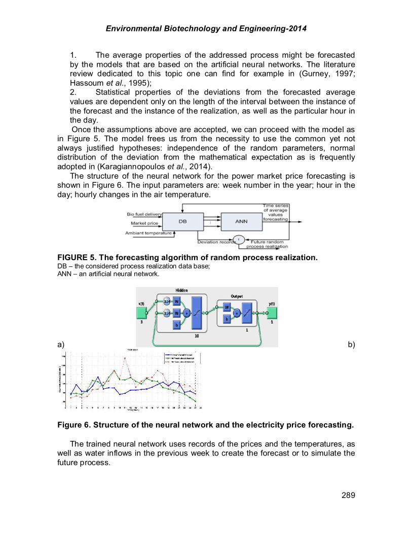
Environmental Biotechnology and Engineering-2014
289
1. The average properties of the addressed process might be forecasted by the models that are based on the artificial neural networks. The literature review dedicated to this topic one can find for example in (Gurney, 1997; Hassoum et al., 1995); 2. Statistical properties of the deviations from the forecasted average values are dependent only on the length of the interval between the instance of the forecast and the instance of the realization, as well as the particular hour in the day. Once the assumptions above are accepted, we can proceed with the model as
in Figure 5. The model frees us from the necessity to use the common yet not always justified hypotheses: independence of the random parameters, normal distribution of the deviation from the mathematical expectation as is frequently adopted in (Karagiannopoulos et al., 2014). The structure of the neural network for the power market price forecasting is shown in Figure 6. The input parameters are: week number in the year; hour in the day; hourly changes in the air temperature.
FIGURE 5. The forecasting algorithm of random process realization. DB – the considered process realization data base; ANN – an artificial neural network.
a) b)
Figure 6. Structure of the neural network and the electricity price forecasting. The trained neural network uses records of the prices and the temperatures, as well as water inflows in the previous week to create the forecast or to simulate the future process.
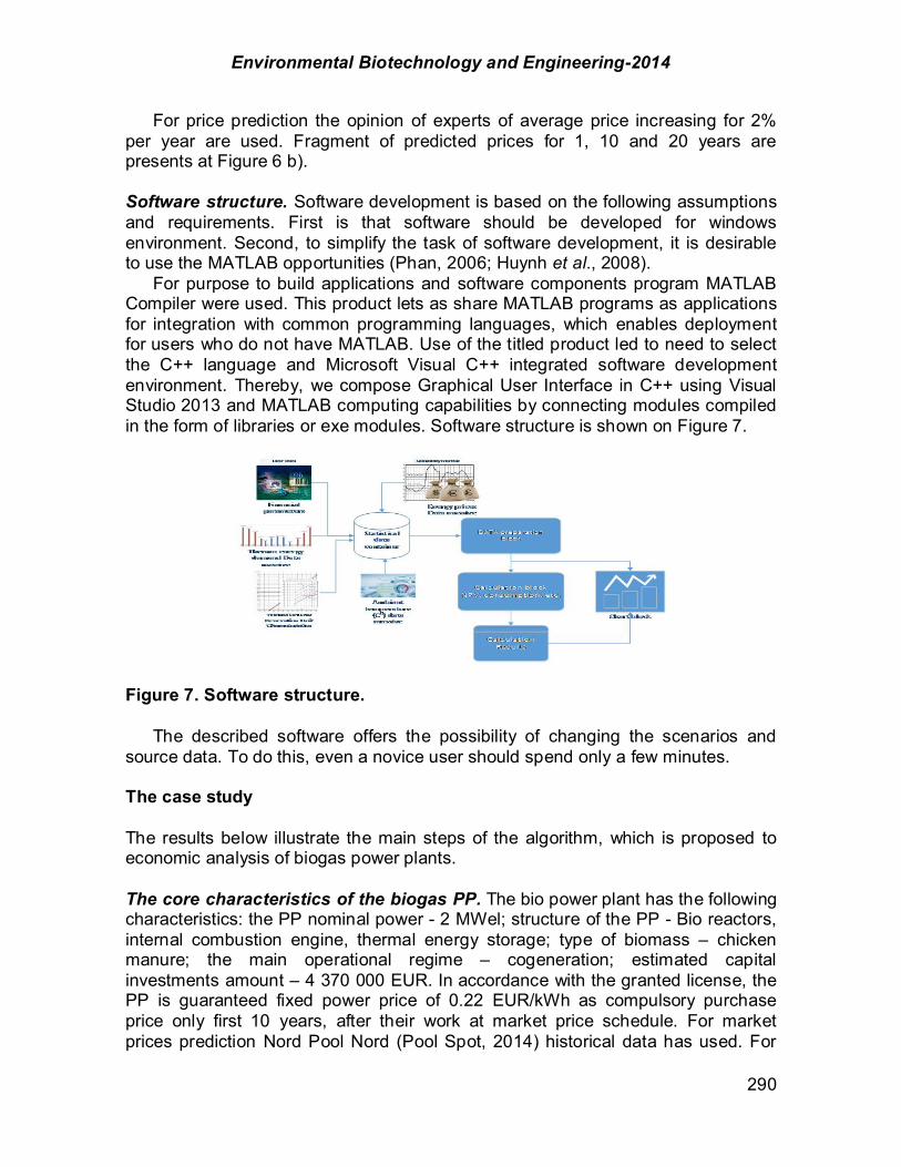
Environmental Biotechnology and Engineering-2014
290
For price prediction the opinion of experts of average price increasing for 2% per year are used. Fragment of predicted prices for 1, 10 and 20 years are presents at Figure 6 b). Software structure. Software development is based on the following assumptions and requirements. First is that software should be developed for windows environment. Second, to simplify the task of software development, it is desirable to use the MATLAB opportunities (Phan, 2006; Huynh et al., 2008). For purpose to build applications and software components program MATLAB Compiler were used. This product lets as share MATLAB programs as applications for integration with common programming languages, which enables deployment for users who do not have MATLAB. Use of the titled product led to need to select the C++ language and Microsoft Visual C++ integrated software development environment. Thereby, we compose Graphical User Interface in C++ using Visual Studio 2013 and MATLAB computing capabilities by connecting modules compiled in the form of libraries or exe modules. Software structure is shown on Figure 7.
Figure 7. Software structure. The described software offers the possibility of changing the scenarios and source data. To do this, even a novice user should spend only a few minutes. The case study The results below illustrate the main steps of the algorithm, which is proposed to economic analysis of biogas power plants. The core characteristics of the biogas PP. The bio power plant has the following characteristics: the PP nominal power - 2 MWel; structure of the PP - Bio reactors, internal combustion engine, thermal energy storage; type of biomass – chicken manure; the main operational regime – cogeneration; estimated capital investments amount – 4 370 000 EUR. In accordance with the granted license, the PP is guaranteed fixed power price of 0.22 EUR/kWh as compulsory purchase price only first 10 years, after their work at market price schedule. For market prices prediction Nord Pool Nord (Pool Spot, 2014) historical data has used. For
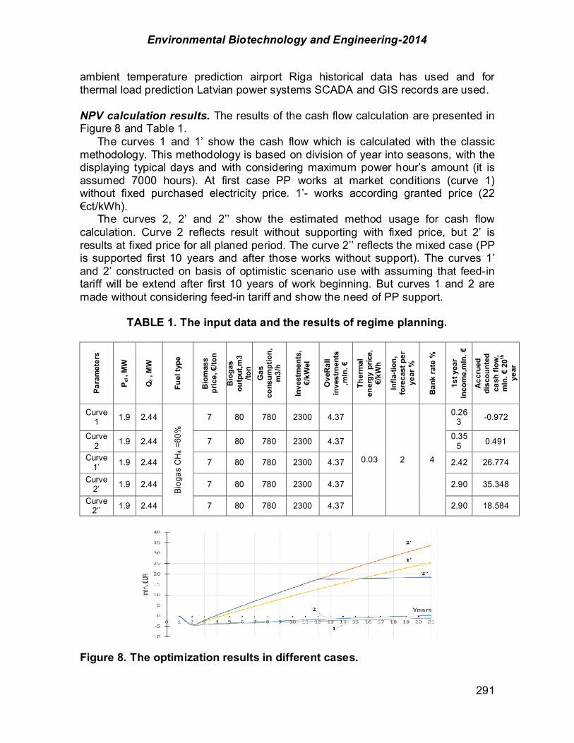
Environmental Biotechnology and Engineering-2014
291
ambient temperature prediction airport Riga historical data has used and for thermal load prediction Latvian power systems SCADA and GIS records are used. NPV calculation results. The results of the cash flow calculation are presented in Figure 8 and Table 1. The curves 1 and 1’ show the cash flow which is calculated with the classic methodology. This methodology is based on division of year into seasons, with the displaying typical days and with considering maximum power hour’s amount (it is assumed 7000 hours). At first case PP works at market conditions (curve 1) without fixed purchased electricity price. 1’- works according granted price (22 #ct/kWh). The curves 2, 2’ and 2’’ show the estimated method usage for cash flow calculation. Curve 2 reflects result without supporting with fixed price, but 2’ is results at fixed price for all planed period. The curve 2’’ reflects the mixed case (PP is supported first 10 years and after those works without support). The curves 1’ and 2’ constructed on basis of optimistic scenario use with assuming that feed-in tariff will be extend after first 10 years of work beginning. But curves 1 and 2 are made without considering feed-in tariff and show the need of PP support.
TABLE 1. The input data and the results of regime planning.
Para
met
ers
P el ,
MW
Qt ,
MW
Fuel
type
Bio
mas
s pr
ice,
!/to
n
Bio
gas
outp
ut,m
3 /to
n G
as
cons
umpt
ion,
m3/
h
Inve
stm
ents
, !/
kWel
Ove
Ral
l in
vest
men
ts
,mln
. !
Ther
mal
en
ergy
pric
e,
!/kW
h
Infla
-tion
, fo
reca
st p
er
year
%
Ban
k ra
te %
1st y
ear
inco
me,
mln
. !
Acc
rued
di
scou
nted
ca
sh fl
ow,
mln
. ! 2
0th
year
Curve 1 1.9 2.44
Bio
gas
CH
4 =60
%
7 80 780 2300 4.37
0.03 2 4
0.263 -0.972
Curve 2 1.9 2.44 7 80 780 2300 4.37 0.35
5 0.491
Curve 1’ 1.9 2.44 7 80 780 2300 4.37 2.42 26.774
Curve 2’ 1.9 2.44 7 80 780 2300 4.37 2.90 35.348
Curve 2’’ 1.9 2.44 7 80 780 2300 4.37 2.90 18.584
Figure 8. The optimization results in different cases.

Environmental Biotechnology and Engineering-2014
292
The results of offered method are more attractive for investors, and could be explained with factors, as: 1. The forecast of the reduced consumption of PP thermal energy own needs. 2. The prediction of the greater working times of the PP units at maximum price hours. Conclusion To diminish the influence of the energy industry on the climate change, the global community involves various renewable resources support schemes. As the result of these measures, the number and installed capacity of the power plants with the renewable energy fuel is growing rapidly. With the market conditions and tools implementation on power system operation and planning the feasibility study tasks conditions change substantially, necessity to take into account stochastic nature of variables appear. The stochastic approach to the power plants feasibility study requires a large amount of input information. The difficulties of collecting input data can be overcome by using the opportunities of the Internet and smart grid technologies The software accompanying the description of the feasibility studies provides wide opportunities to consider additional scenarios and take into account new information Acknowledgement Development of this paper has been co-financed by the European Social Fund within the project „Exploration and Solving of Energy Systems’ Strategic Development and Management Technically-Economic Problems”, project agreement No. 2013/0011/1DP/1.1.1.2.0/13/APIA/VIAA/028. References
(Nord Pool Spot, 2014): www.nordpool.com (RESLegal, 2014) Legal Sources on Renewable Energy: http://www.res-legal.eu/, May 2014. (Termoflow homepage, 2014): www.thermoflow.com. Bennett, F.L. (2003). The management of construction: a project life cycle approach. 1st ed.
Burlington: Butterworth-Heinemann. Buljevich, E.C.; Park, Y.S. (1999). Project Financing and the International Financial Markets. USA:
Kluwer Academic Publishers Group. Final Report of Energize Missouri Renewable Energy Study Subgrant. Feasibility Study for a
Biomass Electrical Power Plant in the Viburnum Region. Revised March 12, 2012: 51. Grace, J. Leith Renewable Energy Plant: Combined Heat and Power Feasibility Study. Forth
Energy, January 2011. Gurney, K. (1997). An Introduction to Neural Networks London: Routledge. Hassoum, M. (1995). Fundamentals of artificial neural networks, Massachusetts Institute of
Technology. Huynh H.T, Lai V.S. (2008). Stochastic Simulation and Applications in Finance with MATLAB
Programs, Wiley.
Environmental Biotechnology and Engineering-2014
293
Karagiannopoulos, S.; Vrettos, E; Andersson, G; Zima, M. (2014). Scheduling and real-time control of flexible loads and storage in electricity markets under uncertainty. Proceedings of EEM14. 1-5.
Korn, G., Korn, T. (1968). “Mathematical handbook”, McGraw-Hill Book Company. M. Gray, R. Probability, Random Processes, and Ergodic Properties. Information Systems
Laboratory, Electrical Engineering Department, Stanford University 2010: 205. Phan J, Matlab C/C++ Book, 4th ed. LePhan Publishing, 2006 Ravn H; Riisom J; Schaumburg-Müller, C; Straarup, S.N. (2004). Modelling Danish Local CHP on
Market Conditions, Proc. 6th IAEE European Conference: Modelling in Energy Economics and Policy.
V. Neimane (2001). “On development planning of electricity distribution networks”, Ph.D. thesis, Royal Inst. of Technology, Stockholm, Sweden, 2001.
W. Seifert, W.; Carl W., Steeg. (1960) Control Systems Engineering. Jr. McGraw-Hill Book Company, INC., New York, Toronto, London.
Environmental Biotechnology and Engineering-2014
294
CHAPTER 2.4. RECONSIDERATION OF SUPPORTING SCHEME FOR RENEWABLE ENERGY PRODUCERS
Renata Varfolomejeva* (1); Marija Zima-Bo"karjova (2); Antans Sauhats (1);
Romans Petricenko (1); Inga Umbrasko (1); Hasan Coban (1)
(1) RTU, Riga Technical University, Riga, Latvia; (2) ABB Corporate Research, Switzerland. ABSTRACT Striving to prevent climate changes, global community has established favourable national feed-in support schemes for the renewable electricity. Renewable energy is promoted through these schemes in the whole world and, particularly, in European Union (EU). Frequently, the support is provided by a guaranteed purchase price, which is significantly higher than the market price of electricity. In EU, an Electricity Market Law prescribes that an electricity producer, which operates renewable energy sources, may acquire the right to sell all the produced electricity within the framework of the mandatory procurement at a guaranteed purchase price. As a result all the energy, which is produced from renewable energy sources, is sold to the public trader at a guaranteed purchase price, but the public trader sells and buys energy at the market prices, which vary significantly over the time. All electricity consumers pay the difference. The main drawback of the described support scheme is related to the absence of the coordination of power plant operation with the electricity market price or indirectly, electricity demand. This paper demonstrate that cooperation of the public trader (PT) and power plant (PP) operator in the market conditions could minimize additional cost of the support for the consumers and/or provide an additional income to PT and the PP owner. For this purpose, the coalition between PT and PP will be formed (creation of such coalition does not contradict the norms of law). Then, using scenario approach, planning problem of the day-ahead PP operation will be formulated as maximization of the expected total profit over the day taking into account profits of both PT and PP. Co-operative game theory and the Shapley value can be applied for the fair additional profit allocation. We demonstrate the advantages of the collaboration by the case study of a small hydro PP and the PT. The modification of the schedule of the PP to adjust to the electricity market prices and, thus, the electricity demand creates an additional income for the PT. It is concluded that the support principles of PP have to be reviewed. Proposed stochastic approach, formulation of the objective function and Shapley allocation for the additional revenues can increase the effectiveness of the operation of any kind of PP, provided that the daily power production is controllable, but water or fuel resources are constrained. ------------------ *Author for correspondence: [email protected]

Environmental Biotechnology and Engineering-2014
295
Key words: power plant, renewable energy, market price, co-operative game, stochastic optimization. Introduction Electric power systems dominantly in the last two decades are in the process of the restructuring, involving two major trends: 1. The market principles are introduced into the production and sales of energy to ensure cost effective power supply. 2. An objective to prevent the climate changes, to increase security and reliability of the power supply stimulates construction of the large number of PP with renewable energy sources (RES): in the period from 2000 to 2014 biogas, biomass, wind and photovoltaic were member has its own share of renewable energy amount, which should be increased by 2020. These objectives shall be achieved in a possibly most cost efficient manner. Support policies offer long-term guaranteed payments to the owners of the PP that produces electricity from RES. The existing support schemes include quotas for construction, investment grants, feed-in tariffs, tax measures, green certificates (Final Report of Energize Missouri, 2012; Ragwitz et al., 2007; RESLegal, 2014). Feed-in tariffs are significantly higher than the electricity market price. Commonly, it results in that all the energy, which is produced from RES, is sold to a public trader at a guaranteed purchase price. Simultaneously, the public trader sells and buys energy at the market price that varies significantly over the time. All the electricity consumers (or ratepayers) pay the difference (these costs are included in energy tariff in the form of the component of the mandatory procurement (CMP)). The main drawback of the described support scheme is related to the lack of coordination of PP operation with the electricity market or indirectly, electricity demand. For example, in order to maximize the profit the RES PP could produce energy by own discretization in hours when the load is minimal. All RES technologies could be divided into two classes from the perspective of the operation flexibility, as follows: - Unregulated (the possibility of turn-on/switch-off is the only way of adjusting the operation, for example, wind, solar photovoltaic, solar thermal, tidal and etc. - Regulated. In this case, the operator could increase or decrease the production within the technical constraints of the plant and fuel reserve or water in reservoir. Further, we will discuss small-scale hydropower plants (HPP) with the regulation capability. However, proposed methodology can also be applied to the optimization of the different types of regulated RES plants. The best production plan is determined through formulating and solving the optimization problem. It is natural to assume that for this task the objective function shall reflect the power plant profit. Therefore, we can say that the optimization result in the significant extent depends on the support schemes. There are five different types of feed-in tariff: 1. Fixed feed-in tariff: The determination of fixed prices for each type of renewable according to amended regulations (e.g. Germany, Portugal, Lithuania),
Environmental Biotechnology and Engineering-2014
296
2. Time-dependent feed-in tariff: The determination of two or three different (day/night, peak/off-peak) prices for each type of renewable according to amended regulations (e.g. Spain for biomass and hydro for Hungary), 3. Indexed feed-in tariff: Prices are not known in the time of investment, indexed to another parameter like; natural gas price (e.g. Latvia), 4. Adjusting feed-in tariff: Tariffs are not linked to time of installation, also applicable for existing projects (e.g. Bulgaria and Czech Republic), 5. Target-price feed-in tariff: The tariff guarantees fixed price according to amended regulations, producer sell its electricity in market, the difference between market and fixed prices are paid after (Denmark) (Final Report of Energize, 2012; RESLegal, 2014). Feed in tariffs is most common policy mechanism to promote renewable energy and cogeneration. Since it provides uninterrupted grid access, guaranteed period and fixed price for purchase (Ragwitz et al., 2007). Today the tendency of reconsideration of supporting schemes is increased with extension of the technical facilities and economical needs to decrease the growing of additional costs for consumers. For the reducing the consumer’s electricity costs, the reconsideration of supporting schemes for the power plants which produce energy from RES and have got possibility to regulate energy production is offered. The given mechanism allows decrease additional costs of consumers with not reducing electricity producer’s incomes. For the realization of this goal is needed to carry in corrections into existed legislation. In general, the goal of this paper is to propose a support mechanism that allows adapting the PP operation to the market situation. We solve a bidding problem for a small HPP with the limited water inflow and, more importantly, we show that the new support scheme may create additional revenues (first contribution of the paper) once the coalition between HPP operator and the PT is established. The creation of the coalition under consideration does not contradict the norms of law. In this case, the PP operation mode will be adjusted to the interests of all the actors and to the current market situation. For the fair allocation of the additional gain the co-operative game theory approaches can be applied, namely, Shapley value. The day-ahead operation planning of the HPP is formulated as the maximization of the total average profit during the day. Profits of both the PT and the HPP are considered. Stochastic nonlinear programming is applied. Second important contribution of the paper is in the proposed algorithm, which includes the above mentioned methods. The third contribution is the case study that considers small HPP data and demonstrates that the PT and the HPP coalition create opportunity to gain the additional income by adjusting the operating mode to the electricity market prices. The rest of the paper is organized as follows: first, the power plant production planning and operation task is formulated, and second, the case study illustrating the proposed method in the realistic set-up is presented.

Environmental Biotechnology and Engineering-2014
297
Defining the cost efficient renewable: case the HPP production. We propose optimization based planning of the HPP production and split of the profit between trader producer and the customers. Definition of the deterministic optimization problem. The definition of the HPP production schedule shall target revenue maximization. To achieve efficient operation of the scheduling of the HPP water reservoir in time will be performed. Short term operation is coupled with the mid- to long term planning, for example taking into account weekly planning horizon pTt = (7 x 24 = 168 hours). Supported by the feed-in tariffs, power plant will solve optimization problem which may be presented as: { } { } maxminmaxmin
* ,,,...,1;,maxarg lllwwwTiwcw iipisi ,,,,=-= " .. . (1)
where [ sc ] - a guaranteed purchase price; [ iw ] - the power production levels [
.-- iRw ti ; ]; *iw - the power production levels, that corresponds to the maximal
revenue; il - the water levels.
The optimization task is choosing such [ iw ] in accordance with the constraints, that are representing the conditions on the maximal and minimal reservoir level, allowable power of the generator and the water inflow and the spillage balance. This type of the optimization problem (1) has been extensively discussed in the literature see. Various approaches to this problem have been proposed at (Fleten et al., 2008; Karagiannopoulos et al., 2014; Kristoffersen et al., 2007). Let us note that the problem (1) is not linked to the variation of the market prices and, therefore, not linked to the energy demand and the conditions of the energy production by the other power plants. After the matching of the supply and demand offers of all the players in the market, hourly energy prices [ ic ] are known. So, one can compute the expenses for the support of the HPP that is rewarded by the fixed tariff:
.-+%+= """ iwcwcc iiiss ,** . (2) The expression (2) can be used as a basis for the formulations of the next optimization problem. For the definition of this problem lets us assume: 1. Stakeholders of the HPP shall obtain the profit that is guaranteed by the law or regulations and provided by the solution of the optimization problem (1). 2. Stakeholders of HPP might require the additional profit in the case if the schedule is realized that requires less of the subsidies. 3. The objective function of the new optimization problem shall maximize the income from selling the energy at the market price with the considering constrains as in (1): { } .-+= " iwcw iii ,maxarg** , (3) 4. Additionally obtained profit R' :

Environmental Biotechnology and Engineering-2014
298
"" +%+=' ***iiii wcwcR , (4)
is shared among the participants. The problem (3) has been also discussed in the literature (Karagiannopoulos et al., 2014), and can be solved by one of the earlier proposed methods or else by the proposed algorithm as described below (the advantages of that will be shown). The stochastic problem statement. Future market prices and water inflow in the river are the main processes which impact HPP revenues. Both processes are hard to predict because of unexpected market and weather conditions. Therefore, one shall approach it with the stochastic problem statement. Let us assume that the income R for the planning period can be described by some, in the general case, nonlinear function:
( ) ( )&=''= %+%+ ,,,,,,,,, XvcccllwwwR tttttottot (( , (5)
where otw - the PP production as bid to be submitted to day ahead market; +' tw -
the positive (increase of production) deviation of the production; %' tw - the negative
(decrease of production) deviation of the production; ol - an initial reservoir level;
tl - level of the reservoir at the end of the planning interval t =T; tc - day - ahead
market prices; +tc - intra-day market retail prices; %
tc - intra-day purchasing prices;
tv - water inflow; X - the joint set of all the stochastic parameters; & - set of all the deterministic parameters. The revenues are the function of many random variables (the number of variables is growing as the planning horizon is approximated by the discrete time intervals) and, therefore, are also random. For such conditions one can formulate the problem of the maximization of the average (expected) revenue ][ R/ (W. Seifert; 1960):
( ) )(,....][ XdXRR )&=/ ##+*
*%
+*
*%
(6)
Applying (7) to determining the expected revenue, one can encounter significant difficulties that are caused by the high dimensionality of the integral and the probability function )(X) . When the duration of the planning interval is 168 hours and the number of random processes is two (e.g. water inflow and day-ahead market prices), the dimensionality of the set of random parameters is 2*168. The curse of the dimensionality and the proposed cure. The number of the optimization variables is growing as the planning horizon expands. Many nonlinear programming methods are losing the practical applicability once the number of variables is reaching several hundreds. Simultaneously, linear programming methods are operational with the thousands of variables. However, the linearization is leading to the loss in precision. To overcome this constraint, we suggest the following algorithm, as presented in Figure 1 that combines:
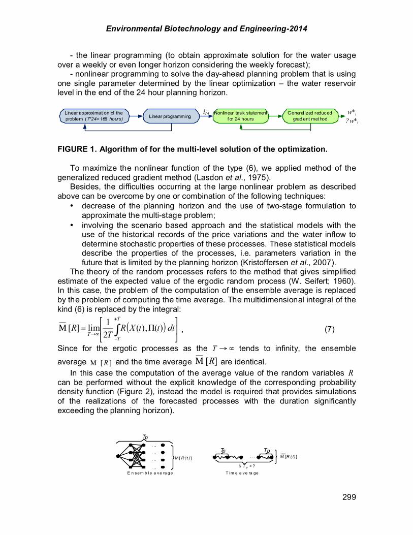
Environmental Biotechnology and Engineering-2014
299
- the linear programming (to obtain approximate solution for the water usage over a weekly or even longer horizon considering the weekly forecast); - nonlinear programming to solve the day-ahead planning problem that is using one single parameter determined by the linear optimization – the water reservoir level in the end of the 24 hour planning horizon.
FIGURE 1. Algorithm of for the multi-level solution of the optimization. To maximize the nonlinear function of the type (6), we applied method of the generalized reduced gradient method (Lasdon et al., 1975). Besides, the difficulties occurring at the large nonlinear problem as described above can be overcome by one or combination of the following techniques:
• decrease of the planning horizon and the use of two-stage formulation to approximate the multi-stage problem;
• involving the scenario based approach and the statistical models with the use of the historical records of the price variations and the water inflow to determine stochastic properties of these processes. These statistical models describe the properties of the processes, i.e. parameters variation in the future that is limited by the planning horizon (Kristoffersen et al., 2007).
The theory of the random processes refers to the method that gives simplified estimate of the expected value of the ergodic random process (W. Seifert; 1960). In this case, the problem of the computation of the ensemble average is replaced by the problem of computing the time average. The multidimensional integral of the kind (6) is replaced by the integral:
( ) 01
234
5&=/ #
+
%*6
T
TT
dtttXRT
R )(,)(21lim][ , (7)
Since for the ergotic processes as the *6T tends to infinity, the ensemble
average ][ R/ and the time average ][R/ are identical. In this case the computation of the average value of the random variables R can be performed without the explicit knowledge of the corresponding probability density function (Figure 2), instead the model is required that provides simulations of the realizations of the forecasted processes with the duration significantly exceeding the planning horizon).
Linear approximation of the problem (7*24=168 hours) Linear programming
Nonlinear task statement f or 24 hours
Generalized reduced gradient method
l2 4 w*i
?w*i
. ..
. ..
. ..
. ..
Tp
M [ R( t ) ]
E n se m b le a ve ra g e
Tp Tp.. . M [R ( t) ]
S T p > ?
T im e a ve ra ge

Environmental Biotechnology and Engineering-2014
300
FIGURE 2. Transformation of the stochastic optimization problem. Simulating and forecasting of the random processes realization. Let us make the following assumptions to build the model for the forecasting of the process realizations: 1. The average properties of the addressed process might be forecasted by the models that are based on the artificial neural networks. The literature review dedicated to this topic one can find for example in (Ramos et al., 2002); 2. Statistical properties of the deviations from the forecasted average values are dependent only on the length of the interval between the instance of the forecast and the instance of the realization, as well as the particular hour in the day. Once the assumptions above are accepted, we can proceed with the model as in Figure 3. The model frees us from the necessity to use the common yet not always justified hypotheses: independence of the random parameters, normal distribution of the deviation from the mathematical expectation as is frequently adopted in (Karagiannopoulos et al., 2014). The structure of the neural network for the electricity price forecasting and the water inflow is shown in Figure 4. The input parameters are: week number in the year; hour in the day; hourly changes in the air temperature.
FIGURE 3. The forecasting algorithm of random process realization. DB – the considered process realization data base; ANN – an artificial neural network. The trained neural network is using recordings of the prices and the temperatures, as well as water inflows in the previous week to create the forecast or to simulate the future process. The example of the forecast is shown in Figure 5.
FIGURE 4. Structure of the neural network for the electricity price forecasting
Environmental Biotechnology and Engineering-2014
301
Shapley distribution. The final step in the proposed renewable support scheme is allocation of the additional profit among the participating parties. Several papers suggest application of the Shapley value and the similar Aumann-Shapley value to cost and/or profit allocation problems in power systems, including firm-energy rights allocation among hydro power plants, expansion planning, congestion management, inter-TSO compensations, ancillary services, fixed asset costs and loss allocation (Faria et al., 2009; Junqueira et al., 2007). The main idea of this paper is based of getting the additional income from the coalition creation between HPP and public trader. The Shapley value is one way to distribute the total gains to the players, assuming that they all collaborate. According to the Shapley value, the amount that player i gets given a coalitional game ( )Nv, is:
( ){ }
{}( ) ( )( )SviSvn
SnSv
iNSi %
%%= "
7
\ !
!1!)(8 . (8)
where S - the coalition of players; ( )Sv - the worth of coalition S, describes the total expected sum of payoffs
the members of S can obtain by cooperation; {}( )iSv - the sum extends over all subsets S of N not containing player I;
n - is the total number of players. In this paper the simplified description of power system relations between PT and HPP is considered. PT is not producing energy, but provides HPP regimes planning and produced energy purchasing. The contribution of the HPP is only possible in a coalition with the PT and is independent of the participation or non-participation of other PP in the coalition. Computing the Shapley value for players in this coalition leads to the expression, as follows: {}( ) ( )( ) 2/)( SviSvvi %= 8 . Therefore, the additional income from establishing the coalition shall be split in half. The case study The results below illustrate all the steps of the novel support scheme that is proposed for the cost efficient renewable integration in the electricity markets and the system. The core electrical characteristics of the HPP. The small hydro power plant has the following characteristics: the nominal power of the HPP equals 19.28 MW; change restrictions of water drop in a reservoir about 130.5 m-124.32 m; the turbine maximum water permeability after the turbine and the water throughput is around 17 m3/sec.; the area of the reservoir surface is 250000 m2. In accordance with the granted license, the HPP is guaranteed fixed power price of 0.07$/kWh as compulsory purchase price, or correspondingly is encouraged for the maximum power generation. Natural water inflow and the market price forecasting. The simulation of the random process in mid-term is performed by the artificial neural network. The structure of the ANN was given in Figure 4 and the algorithm in Figure 3.
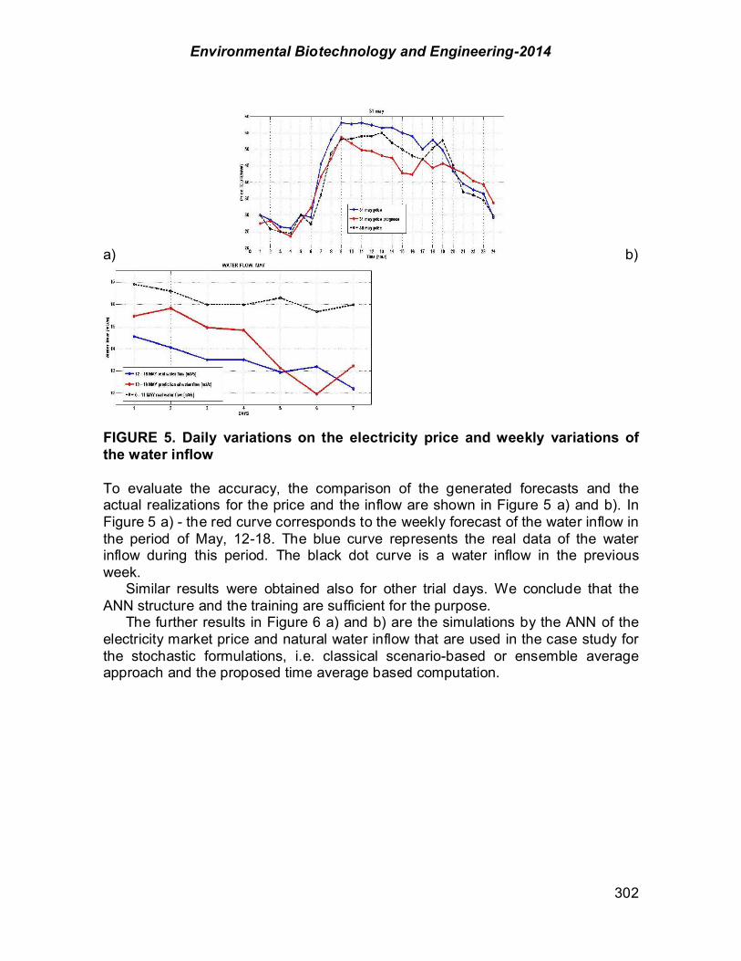
Environmental Biotechnology and Engineering-2014
302
a) b)
FIGURE 5. Daily variations on the electricity price and weekly variations of the water inflow To evaluate the accuracy, the comparison of the generated forecasts and the actual realizations for the price and the inflow are shown in Figure 5 a) and b). In Figure 5 a) - the red curve corresponds to the weekly forecast of the water inflow in the period of May, 12-18. The blue curve represents the real data of the water inflow during this period. The black dot curve is a water inflow in the previous week. Similar results were obtained also for other trial days. We conclude that the ANN structure and the training are sufficient for the purpose. The further results in Figure 6 a) and b) are the simulations by the ANN of the electricity market price and natural water inflow that are used in the case study for the stochastic formulations, i.e. classical scenario-based or ensemble average approach and the proposed time average based computation.

Environmental Biotechnology and Engineering-2014
303
a) b)
FIGURE 6. Natural water inflow and forecasted electricity market price charts example. The use of the water during the week. Using the forecasts of the prices and the water inflow and applying the liberalized algorithm to solve the problem for 168 hours horizon, we can find optimal distribution for the water usage. The sample results of such optimization are presented in Figure 7. In the first 48 hours we observe relatively high prices resulting in the full usage of the available water. In the following period we anticipate lower prices, therefore the water gets accumulated
FIGURE 7. Water level variations during the weekly planning. Let us note that for the detailed nonlinear planning of the production in the first day, we only use the obtained reservoir level at the 24th hour. The evaluation of the accuracy of the time average approximation. To evaluate the accuracy of the proposed time average method, we conduct the
127,2462336
128,4924672
126 126 126 126 126 126
125,5
126
126,5
127
127,5
128
128,5
129
0 12 24 36 48 60 72 84 96 108 120 132 144 156 168hours
Water level, m
0,02
0,025
0,03
0,035
0,04
0,045
0,05
0,055
0,06
0,065Market price schedule $/kWh
Water level chart for 168 hours in linear task statement Electricity market price schedule

Environmental Biotechnology and Engineering-2014
304
analysis for two different planning time horizons 2T when computing the expression (7): 2T=64 hours and 2T=168 hours. The maximal deviation in the results provided by both approaches was only 1.33%, which is considerably smaller than the gained additional profit (as will be shown below). Let us note that the application of the scenario-based approach and the computation of the ensemble average, the total duration of the simulation and the computational processes have been tens or even hundreds time longer. The allocation of the additional profit. The results of the optimization (1) and (3) are presented in Figure 8. a) and b). The revenues according to the time average approach for 24 h ahead are determined by using the multi-dimensional process with the duration of 168 hours. To determine the sensitivity of the income on the water inflow, three scenarios are considered as depicted in Figure 8.
a) b)
FIGURE 8. Generated power according a) market price schedule and b) fixed tariff (0.07 $/kWh). According to the generated power chart, it is seen that in the market conditions SHPP generates maximum power during the hours then price is maximal (exhaust all permitted water before the dam and store that in lower price hours). Simultaneously, if we consider the case of the feed-in tariff, it tries to produce the maximal energy. So, the difference between these two generated power profiles and the obtained revenues provides the additional income, which should be distributed according to the formula (8). The results of the allocation of the additional income are presented in the Table 1.
TABLE 1. PT and PP incomes within the framework of feed in tariff and market price.

Environmental Biotechnology and Engineering-2014
305
Participants Water natural inflow change (Fig.3.) for 24
hours , m3/sec
Income without any coalition,
according feed-in tariff, $
An additional income from
coalition creation, $
Income with the additional
gain from coalition, $
HPP 1st water inflow 6909.56 881.16 7790.72 (11.3%) 2nd water inflow 4228.07 639.16 4867.23 (13.1%) 3rd water inflow 9652.94 893.39 10546.33 (8.5%)
PT 1st water inflow 0 881.16 881.16 2nd water inflow 0 639.16 639.16 3rd water inflow 0 893.39 893.39
This example demonstrates that both the HPP and the public trader could additionally get some income from the cooperation (by transaction through the bilateral contacts). The total welfare that is approximately of 20% higher than without the coordination, we consider to be significant. Conclusion To diminish the influence of the energy industry on the climate change, the global community involves various renewable resources support schemes. As the result of these measures, the number and installed capacity of the power plants with the renewable energy fuel is growing rapidly. Support schemes or subsidies and the feed-in tariff, in particular, are inconsistent with the market mechanisms in the energy sector and do not contribute to the development of the economic efficiency in the renewable segment. Collaboration of the power plant and the wholesaler can bring addition profit gain and shall stimulate energy production by the power plant in accordance with the schedule that is matching the demand curve and the possibilities of the rest of energy producers (or other market participants) A creation of coalition does not require the repeal of the existing legislation on support of renewable energy sources. At the same time the results of this work can be considered as an argument for amendments of legislation in the future. Short term planning (day ahead) and profit allocation can be fulfilled on the base of forecasts of the process, stochastic programming and the Shapley value. Acknowledgement Development of this paper has been co-financed by the European Social Fund within the project „Exploration and Solving of Energy Systems’ Strategic Development and Management Technically-Economic Problems”, project agreement No. 2013/0011/1DP/1.1.1.2.0/13/APIA/VIAA/028.
Environmental Biotechnology and Engineering-2014
306
References
Faria, E.; Barroso, L.A.; Kelman, R.; Granville, S.; Pereira, M.V. (2009). Allocation of Firm-Energy
rights among hydro plants: An Aumann-Shapley approach. In Power Systems. Proceedings of IEEE Transactions on. 24(2): 541-551.
Final Report of Energize Missouri Renewable Energy Study Subgrant. Feasibility Study for a Biomass Electrical Power Plant in the Viburnum Region. Revised March 12, 2012: 51.
Fleten, S.E.; Kristoffersen, T.K. (2008). Short-term hydropower production planning by stochastic programming. Computers & Operations Research. 35: 2656 2671.
Junqueira, M.; da Costa, L. C.; Barroso, L. A.; Oliveira, G. C.; Thome, L. M.; Pereira, M. V. (2007). An Aumann-Shapley approach to allocate transmission service cost among network users in electricity markets. In Power Systems, IEEE Transactions on. 22:1532- 1546.
Karagiannopoulos, S.; Vrettos, E; Andersson, G; Zima, M. Scheduling and real-time control of flexible loads and storage in electricity markets under uncertainty. Proceedings of EEM14, 2014: 1-5.
Kristoffersen, T.K. (2007). Stochastic Programming with Applications to Power Systems. Working Paper . 1: 185.
Leon S.; Lasdon et.al. (1975). Design and testing of a generalized reduced gradient code for nonlinear optimization. Case Western Reserve university Office of Noval Research, No 353.
M. Gray; R. (2010). Probability, Random Processes, and Ergodic Properties. Information Systems Laboratory, Electrical Engineering Department, Stanford University: 205.
Narahari, Y. (2009). Lecture Notes, Game Theory. Cooperative game theory. Department of Computer Science and Automation, India. 1-12.
Ramos M.; Exposito A., Santos J. Influence of ANN-based market price forecasting uncertainty on optimal bidding. Proceedings of the 14th PSCC Conference. Sevilla, Spain, June 24-28, 2002. session 7. paper 1: 1.-6.
Ragwitz, A.; Held-Fraenhofer ISI, A.; Resch, G.; Faber, T.; etc. Final Report of OPT RES Assessment and optimisation of renewable energy support schemes in the European electricity market, Karlaruhe, February 2007: 246.
(RESLegal, 2014) Legal Sources on Renewable Energy: http://www.res-legal.eu/, May 2014. W. Seifert, W.; Carl W., Steeg. Control Systems Engineering. Jr. McGraw-Hill Book Company, INC.,
New York, Toronto, London, 1960. Zima-Bockarjova M., Matevosyan J., Zima M., and Sdoder L. (2010). Sharing of profit from coordinated operation planning and bidding of hydro and wind power.// Proc. of the IEEE Transactions on Power Systems. 25(3):1663-1673.
Environmental Biotechnology and Engineering-2014
307
CHAPTER 2.5. WATER SAVING POTENTIAL IN A RURAL COMMUNITY IN MEXICO TO REDUCE THE POTABLE WATER CONSUMPTION
Gómez-Millán, G.* (1); Deegener, S. (1); Otterpohl, R. (1)
(1) University of Technology Hamburg-Harburg, Institute of Wastewater Management and Water Protection, Hamburg, Germany.
ABSTRACT In order to reach a sustainable future, society must move towards a goal where efficient and appropriate water use is the rule, and not the exception. There are abundant resources for water supply that are available, and not used to their full potential. To contribute and enhance the use of sustainable methods, this project studies the practices related to water and sanitation of a small community in rural Mexico. Different technologies to reduce freshwater consumption have been analyzed. Three technologies have been identified and have been further investigated: harvesting rainwater, reusing greywater, and using Terra Preta Sanitation system, as well as promoting an integrated system with the purpose to enhance and live under a sustainable way with less impact on the environment. These three alternatives technologies are compared next to the traditional practices and the integrated system performance in a cost-benefit analysis. From geological and meteorological data, the rainwater harvesting potential has been determined; greywater reuse, from studying the traditional practices of the inhabitants and the best suitable technology for the users; Terra Preta sanitation, as a method of containment and sanitization of human excreta serves an important role of preventing the spread of diseases, and protecting both environmental and human health. Interviews with the main identified stakeholders (NGO, government, independent sponsors) took place during a visit to Mexico. The benefits were ranked according to the three pillars (economical, social and environmental) of sustainable development. The system with the greatest beneficial outcomes is offered by the integrated system. The construction cost of an integrated system is around 1220 # per household. This resulted with the community receiving a huge amount of benefits from it. Key Words: wastewater treatment, sustainable development, rainwater harvesting, terra preta sanitation, rural Mexico. ------------------ *Author for correspondence

Environmental Biotechnology and Engineering-2014
308
Introduction Before looking for alternative water sources, the first thing to consider is water saving measures. The priority is to save, to reuse rather than to dispose. Water reuse is beneficial, not only because facilitates water resources to be regained, but also because it reduces environmental impacts. Among the different options for water reuse such as industrial, irrigation, and ground water recharge, water recycling within rural environments is the least developed. Freshwater is a fundamental requirement for human survival and socio-economic development and must therefore be prudently managed.
Water recycling usually integrates the reuse of black, grey or rainwater. Greywater has great potential for reuse due to its availability (constituting 50-80% of the total domestic wastewater; Eriksson et al., 2002; Hernández et al., 2007; Morel & Diener, 2006) and its low concentration of pollutants compared with combined household wastewater (Hernández et al., 2007; Li et al., 2008). In terms of organic contents, greywater displays related characteristics to municipal wastewater (Eriksson et al., 2002). It contains significant concentrations of materials with potential negative environmental and health impact, such as salts, surfactants, oils, synthetic chemicals and microbial contaminants (Travis et al., 2010). Greywater is fairly easy to treat, because it has low contents of nutrients. The composition of greywater is not similar to domestic wastewater in terms of nutrient, microbiological contamination and organics. Mainly, the treatment concepts applied originated from wastewater treatment (Li et al., 2009; Weissenbacher & Müllegger, 2009).
Rainwater harvesting (RWH) systems are today employed worldwide for potable and agricultural water supply (Heggen, 2000). Even though some stakeholders are still reluctant to implement RWH systems in new development, new commercial buildings (car washing centers, schools and in service water demanding industries) have realized of the positive benefits of the implementation of such systems (Herrmann & Schmida, 1999). RWH is usually considered multi-benefit due its decrease drinking water uptake from public supply networks and offers significant on-site retention storage (Grandet et al., 2010). Several RWH systems have been constructed in Denmark during recent years, and more than 100,000 decentralized rainwater storage tanks in Germany during the last 10 years. This is with the objective to save drinking water resources, in a way to use rainwater for toilet flushing and clothes washing and for using greywater for toilet flushing.
Ecological Sanitation (EcoSan) helps decreasing water consumption, due the use of waterless systems, and brings back nutrients to the soil. This system includes a network of environmentally and economically sound management that take into account water, energy and nutrients. A study in Sweden (Hanæus et al., 1997) showed that the successful operation of a urine separation system is very dependent on well-designed toilets and a user behavior that promotes a high degree of separation. This tendency towards dry sanitation is being driven by a rising public consciousness of impending water shortages. An innovative

Environmental Biotechnology and Engineering-2014
309
alternative in dry sanitation that has the potential for mass production and installation on a large scale is Terra Preta Sanitation.
The intent of this work is to evaluate the water saving potential of a small community, with reuse systems of domestic wastewater, rainwater harvesting, and Terra Preta sanitation system. Thus, having in mind this aim, the main objective of the study is to reduce the freshwater consumption in the context of the community “La Cebolleta” (The Shallot). The results shall contain a process related approach according to domestic wastewater systems, and ecological sanitation. The overall goal is to help the community of La Cebolleta, Jalisco to reduce its freshwater consumption, increase its livelihood, and promote sustainable development. Materials and methods Case study: La Cebolleta. Mexico is a country of great contrasts and gaps on water. The distribution of the resource is highly variable regionally, and is closely linked to meeting basic social needs, since the availability of water quantity and quality is a necessary condition for social, economic and environment viability of Mexico. On the issue of water are especially visible the implications of current preservation and care about their availability for future generations.
The region of study is located in the border of two states Jalisco and Nayarit. Since there is little information available about climate, geology, and geomorphology of this community, some of the characteristics of the closest city to this location (approximate 90 km northeast), Huejuquilla el Alto, were taken.
It is located approximate 1500 metres above sea level. It is situated in the north part of Jalisco estate on the coordinates 22º 31’ 02’’ north latitude and 104º 29’ 23’’ west longitude. It is delimited to the north with Zacatecas estate, to the south with Bolaños municipality, to the east with Zacatecas estate and to the west with Nayarit.
The climate of the municipality is dry with dry winter and spring, and semiwarm without a defined winter season. The average annual temperature is 20.6 ºC, and has an average annual rainfall of 700 mm of rainfall from June to October. The maximum annual average temperature from the closest city (Zacatecas, around 200 km far from the community) is 17.5 ºC, and the minimum annual average temperature is 9.5 ºC (SMN , 2010). The prevailing winds are southwesterly.
Almost half of the territory consists of areas of poor quality pastures. In the mountainous forests are composed mainly pine and oak trees.
The community depends 100% of wild water sources, since they are not connected to the water supply, and must carry long distances, and biological contamination that may present a hazard to health. Besides, the difficulty to obtain a supply is insufficient to maintain adequate levels of hygiene for the community. Due to this, it generally wears out people’s certainty of water access.
The aim of this analysis was to evaluate the freshwater consumption and the sustainable development of the selected community. There are three main institutions working at the community, National Institute of Social Development (INDESOL), an NGO called Proyecto Concentrarte A. C. and Isla Urbana (IU). These organizations work with the community to teach the inhabitants through
Environmental Biotechnology and Engineering-2014
310
seminars and art workshops the importance of sustainable development and water management.
This small community comprises around 180 inhabitants, most of them are children and women. Jennifer White from Isla Urbana (IU) commented there are 48 men, 63 women, and 68 children. There are about 25 houses in the community1.
This community, 100% indigenous Wirrarika (Huichol), live in a state of extreme poverty, lacking all basic services like electricity, water, sanitation and garbage collection. The inhabitants in the community do not have a proper wastewater treatment facility or management. The wastewater coming from household does not go to any stream, river, wastewater treatment plant, or any facility, but it is discharged to the soil near households.
There was an assistant program a couple of years ago to collect the manure from the farm animals (pigs, cows, chickens) and gather biowaste and biogas. Sadly, it did not succeed because the farm animals do not stay only in one place. There is not a proper facility where the farm animals live and the biowaste can be collected.
They have latrines, which they do not use. Probably because the inhabitants are used to go into the woods to defecate, or there was no proper education previous the installation of these facilities. Open defecation not only pollutes ground waters, it contaminates agricultural produce, helps the spread of diseases such as diarrhea and cholera (Wateraid, 2009). The water potential concept of the household comprises the following components:
o Greywater treatment. o Rainwater harvesting. o Sanitation system. o Integrated system (all of the above systems connectedotmai).
Results and discussion The great need for potable water supply, sanitation, and low-cost wastewater treatment technologies offers a high potential chance for application of on-site, small and community scale technology. Decentralized collection for wastewater treatment provides a better mean for achieving sustainability compared to transport through pipeline network and treat a large amount of municipal wastewater to a treatment facility.
Greywater treatment system. The importance of the processing of the greywater, that are soapy water originating in laundries or washrooms, in which these effluents contain large quantities of organic matter and bacteria, and although are not as dangerous as the black water (originating from the W.C.), upon being incorporated to a body of water they generate a type of contamination called eutrophication, that damages severely the aquatic life. Besides, if these effluents are still for more than twelve hours, the organic matter that contains break down 1 Due to adaptation for 5 inhabitants per household (180 inhabitants in total), 35 households are established in the community instead of 25 households.

Environmental Biotechnology and Engineering-2014
311
3.6 m
0.7 m
Fat trap Homemade wetland 0.9
m
Sink
and the bacteria multiply acquiring similar characteristics to the black water, causing risks to the health and contamination of the environment.
The technology ideally implemented on this community would be the ecological sink. The ecological sink could be used to wash the food before eating, to wash clothes and to wash dishes.
The ecological sink is a system that reproduces the environment of wetlands (swamps) to favour the purification of the sewage with the aid of plants and the associated bacteria to its roots. This is achieved for the proliferation of aerobic and anaerobic bacteria in the base of the biofilter that facilitate the degradation of the contaminants in assimilated substances by the plants.
The integral system is composed of two structures (Figure 1): the fat trap and the homemade wetland. The fat trap is a system of three chambers in which the grease is eliminated and the major number of particles; the first camera is filled with granulated materials (gravel and sand). The two following chambers are filled of small pieces of PET bottles. The biofilter is composed of two chambers in which the fine particles they are eliminated and the bad smells; the two chambers are filled with granulated materials (stone ball of 10 cm, gravel of 1", river stone of 4 mm, and sand of 2 mm of diameter). In the surface are placed plants of species that can develop deep roots as the ones that grow next to the rivers or streams (reed, gannet, lily, tule, Taiwan grass, etc.), preferably those, which can be found in the region (IMTA, 2020). FIGURE 1. Greywater treatment system with dimensions.
The main goals of the greywater treatment system (ecological sink) are to facilitate the task of users (mostly women) in rural communities to wash food, clothes and dishes; treat greywater, and reuse it on-site. With the water stored in the cisterns, the users have available water without the need to walk long distances.
Godfrey et al., (2009) studied a case of cost-benefit analysis of greywater reuse in residential schools in India (mechanical and chemical treatment), obtaining that the benefits exceed the costs of the system. Health benefits were the major contribution of the greywater reuse system. Rainwater harvesting system. During dry season, the inhabitants go to the stream to collect water. They take water back to the village to fill up the cisterns. They do this to collect more water for the upcoming days, and have water in the
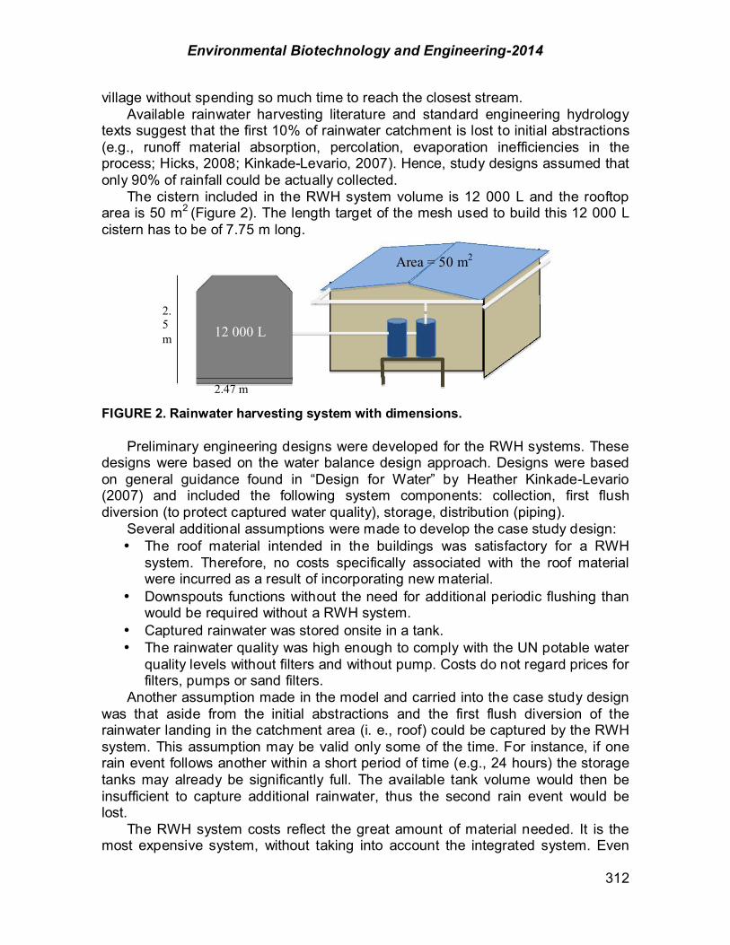
Environmental Biotechnology and Engineering-2014
312
12 000 L
2.47 m
2.5 m
Area = 50 m2
village without spending so much time to reach the closest stream. Available rainwater harvesting literature and standard engineering hydrology
texts suggest that the first 10% of rainwater catchment is lost to initial abstractions (e.g., runoff material absorption, percolation, evaporation inefficiencies in the process; Hicks, 2008; Kinkade-Levario, 2007). Hence, study designs assumed that only 90% of rainfall could be actually collected.
The cistern included in the RWH system volume is 12 000 L and the rooftop area is 50 m2 (Figure 2). The length target of the mesh used to build this 12 000 L cistern has to be of 7.75 m long. FIGURE 2. Rainwater harvesting system with dimensions.
Preliminary engineering designs were developed for the RWH systems. These designs were based on the water balance design approach. Designs were based on general guidance found in “Design for Water” by Heather Kinkade-Levario (2007) and included the following system components: collection, first flush diversion (to protect captured water quality), storage, distribution (piping).
Several additional assumptions were made to develop the case study design: • The roof material intended in the buildings was satisfactory for a RWH
system. Therefore, no costs specifically associated with the roof material were incurred as a result of incorporating new material.
• Downspouts functions without the need for additional periodic flushing than would be required without a RWH system.
• Captured rainwater was stored onsite in a tank. • The rainwater quality was high enough to comply with the UN potable water
quality levels without filters and without pump. Costs do not regard prices for filters, pumps or sand filters.
Another assumption made in the model and carried into the case study design was that aside from the initial abstractions and the first flush diversion of the rainwater landing in the catchment area (i. e., roof) could be captured by the RWH system. This assumption may be valid only some of the time. For instance, if one rain event follows another within a short period of time (e.g., 24 hours) the storage tanks may already be significantly full. The available tank volume would then be insufficient to capture additional rainwater, thus the second rain event would be lost.
The RWH system costs reflect the great amount of material needed. It is the most expensive system, without taking into account the integrated system. Even

Environmental Biotechnology and Engineering-2014
313
though it offers the biggest amount of environmental and social benefits like comfortability, high quality water supply, and sustainable technology implementation, among others.
Terra Preta Sanitation system. Terra Preta Sanitation (TPS) system is a dry sanitation system based on a two-phase treatment of biowaste after the collection: first lactic acid fermentation microorganisms treat it, after that by the vermicomposting process2 (Ottherpohl & Buzie, 2011). This system includes urine diversion, addition of a charcoal mixture, and successive degradation paths that transform faecal matter into favourably fertile humus-like organic matter that can be used even in urban agriculture. Right after each user relieved himself/ herself a mix of charcoal powder complemented with cut wood and some limestone/ volcanic soil to cover the faeces. Leaving this bucket under anaerobic settings a lacto-fermentation course is started. The toilet lid needs to be kept sealed to provide anaerobic conditions. The occasional opening of the lid during the use will not significantly affect the process. After the bucket is full, it will be sealed and collected to let the lacto-fermentation process fully take place. It will then be subjected to a vermicomposting process.
The cost of building a latrine is high in relation to household income in many rural communities, requiring unaffordable technical and financial resources. It was carried out under the assumption that abandoning the practice of open defecation is not only linked to the presence or absence of water or latrines, but also to social determinants (habits, poor sanitation practices).
In order to improve sustainability in this community, a social, economic and environmental model is to be implemented using a community level system.
Feces and urine buckets from the households can be collected every day from the whole community. Terra Preta soil can be produced through the vermicomposting process of feces and composting urine.
The TPS system is the least expensive system from the four scenarios studied in this thesis. The benefits that this system can offer, that none of the other system has (ecological sink or RWH system) is the possibility to use the product on the soil, giving back the nutrients to the earth. In general, the system provides to the community more economical benefits. For example, there is a potential to improve agricultural profit using terra preta soil. Plus, this system includes a waste management network and in the long-term the compost could be sold to other communities or bigger cities as soil improver, due the carbon sequestration properties.
Conventional system. The conventional system considered in this work does not include rainwater harvesting system, wastewater treatment system nor sanitation facilities (ecological sanitation). The habits to relief themselves in the woods (open defecation); going to the stream to take showers and to collect water for daily use; direct discharge on the soils from domestic wastewater were considered as 2 Vermicomposting is the process that uses earthworms to turn organic waste into nutrient-rich compost. It is also called Vermiculture.

Environmental Biotechnology and Engineering-2014
314
conventional system. Due to this, no cost for these practices is included in this work. Integrated system. The integrated system includes the RWH system connected to the ecological sink (greywater treatment) and an ecological toilet using TPS system. Benefit Analysis. It is important to notice that Table 1 is oriented to elevate the environmental pillar out of the three pillars. For the integrated pillar, that had the highest scores not only on the economical side, but also for social benefits. It demonstrates that even pushing up the other two pillars, the integrated system can be the feasible alternative for the community.
Water efficient reuse technology should be put high on the agenda, as well as counteracting soil depletion by returning organic constituents after suitable treatment.
The benefit analysis consists of a scale from 0 to 3. This numbers represent: 0 – Deficient, bad 1 – Average, medium 2 – Satisfactory, good 3 – More than enough, very good
Table 1 compares the five projected scenarios ranking them on benefit basis. According to the sustainable development definition, the nine factors are classified rendering them to each of the three pillars (economy, society and environment). The benefits are oriented to elevate the environmental pillar from economical and social pillar. The nine factors are defined below.
Economic pillar Costs: related to the investment costs and capital costs (i. e. filter change). Savings: related to possible economical savings as profit of system usage. Business potential: related to possible business potential as system profit (i. e.
charcoal sale). Social pillar Hygienic safety: related to the safety level offered to the user by handling the
system (i. e. RWH system effluent). Integral learning: related to learning progress promoting rural development
through system usage, seminars, talks, workshops with the community inhabitants. Comfortability: related to ease of use and comfort for the users. Environmental pillar Water consumption saving: related to the amount of water saved by the system. Material consumption: related to the amount of material used in the construction
of the system, or further material needs during operation and maintenance. Transport: related to transportation needs during first installation and further
maintenance logistics.
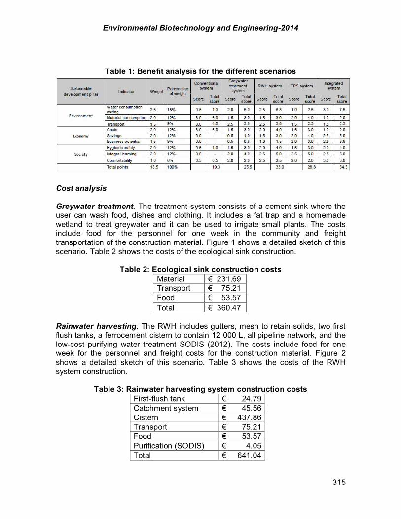
Environmental Biotechnology and Engineering-2014
315
Table 1: Benefit analysis for the different scenarios
Cost analysis Greywater treatment. The treatment system consists of a cement sink where the user can wash food, dishes and clothing. It includes a fat trap and a homemade wetland to treat greywater and it can be used to irrigate small plants. The costs include food for the personnel for one week in the community and freight transportation of the construction material. Figure 1 shows a detailed sketch of this scenario. Table 2 shows the costs of the ecological sink construction.
Table 2: Ecological sink construction costs Material % 231.69 Transport % 75.21 Food % 53.57 Total % 360.47
Rainwater harvesting. The RWH includes gutters, mesh to retain solids, two first flush tanks, a ferrocement cistern to contain 12 000 L, all pipeline network, and the low-cost purifying water treatment SODIS (2012). The costs include food for one week for the personnel and freight costs for the construction material. Figure 2 shows a detailed sketch of this scenario. Table 3 shows the costs of the RWH system construction.
Table 3: Rainwater harvesting system construction costs First-flush tank % 24.79 Catchment system % 45.56 Cistern % 437.86 Transport % 75.21 Food % 53.57 Purification (SODIS) % 4.05 Total % 641.04

Environmental Biotechnology and Engineering-2014
316
If a cistern is already installed, the cost of materials for each system is between 3000 and 4500 pesos (170.5 to 255.7 %3) and all materials can be purchased at local hardware stores according to Isla Urbana. This does not only benefit local economy, but it also ensures homeowners who can build and repair the system themselves, without having to look in specialty stores. Terra Preta sanitation system. The system comprises the bins to collect the feces and urine, biochar for the first month, lactic acid bacteria (LAB), finishing costs for the toilet. The costs include food for one week for the personnel and freight costs for the construction material.
For the biochar, the design input of about 1 kg biochar per user per month. In the initial stage, the biochar could be shipped to the site from Monterrey (Sierra, 2010), but by the second month, the biochar could be produced on-site.
On the other hand, a mixture can be prepared with water, milk lactic acid bacteria (LAB) with the appropriate amount of sugar (3-5% by weight). 2.5 L of this mixture can be added to the bottom of the bin at the beginning of the week with an additional sugar source (molasses, kitchen waste or table sugar). The feces are then covered with charcoal. It takes around one week to build the latrine with its two chambers, a construction worker and a helper.
The cost of food for one week for the construction worker, a helper and one member of the staff is calculated as Table 4 shows.
Table 4: Terra Preta sanitation system construction costs
Material % 22.32 Finishing costs % 20.00 Technical equipment
% 22.00
Food % 40.00 Transport % 75.21 Total % 179.53
Integrated system. The integrated system includes the three different systems implemented in the community. The rainwater harvesting system is connected to the greywater treatment system for easier use. The costs include food for one week and a half for the personnel, and freight costs for the construction material. Table 5 shows the construction costs for this system.
Table 5: Integrated system construction costs Material % 826.68 Transport % 225.62 Food % 166.67 Total % 1,218.97
3 Subsidized Price. Isla Urbana got assistance from HSBC Bank for the rainwater harvesting systems.
Environmental Biotechnology and Engineering-2014
317
The integrated approach alternative should play a significant role in the water optimization work in the developing world. A sustainable project brings autonomy and ensures long-run benefits. Net Present Value. It is the value of a specific stream of future cash flows presented in today’s currency (euros). The considered time span should be the lowest commune multiple of the expected useful lives of each alternative and should have a reasonable length regarding water management investments. Here, 10 years as the lowest commune multiple offers a good value for the considered time span.
The year 2012 will be taken as reference point; even though some RWH systems have been installed, the initial investments are distributed over several years; this thesis constitutes only a preliminary cost estimation and the expected dates of investment cannot be foreseen at this stage.
For the scenarios to be comparable with each other, the overall costs are transformed to the project cost’s present value. For this, all single costs in the future, like reinvestments, must be discounted using the following equation for time-discrete formula (Equation 1):
(1)
where t the time of the cash flow i the discount rate Rt the net cash flow at time t I0 the investment costs
According to the definition of Net Present Value (NPV), to calculate it the initial cost of a project has to be compared to the total value of future revenue. For this project, the revenues were taken as assumptions are:
• For the RWH system and the ecological sink, the 2-3 hours spent to go to the stream to collect water, can be invested to make handcrafts on the rainy season. Assuming they will earn 2000 % per year from handcrafts.
• For the RWH and TPS, assuming two inhabitants of each household go to the doctor per month due to infections and ciprofloxacin is recommended with a unit price of 10 % per case with 12 capsules of 500 mg each. They could save up to 470 % per year with RWH and TPS system.
• For the TPS, assuming that they use a ton of fertilizers per year with a cost of 250 %. The TPS system could substitute the use of fertilizers on agricultural soil after a couple of years.
Cost Benefit Analysis (CBA).The cost-benefit analysis involves the benefit score ranking made in Table 1. The investment costs for the construction of each system as Table 6 shows with the present value for each scenario.
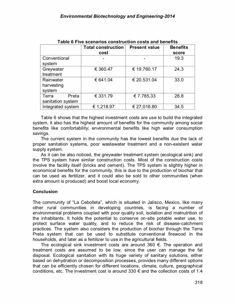
Environmental Biotechnology and Engineering-2014
318
Table 6 Five scenarios construction costs and benefits Total construction
cost Present value Benefits
score Conventional system
- - 19.3
Greywater treatment
% 360.47 % 19.760.17 24.3
Rainwater harvesting system
% 641.04 % 20.531.04 33.0
Terra Preta sanitation system
% 331.79 % 7.785.33 28.8
Integrated system % 1,218.97 % 27,018.80 34.5
Table 6 shows that the highest investment costs are use to build the integrated system, it also has the highest amount of benefits for the community among social benefits like comfortability; environmental benefits like high water consumption savings.
The current system in the community has the lowest benefits due the lack of proper sanitation systems, poor wastewater treatment and a non-existent water supply system.
As it can be also noticed, the greywater treatment system (ecological sink) and the TPS system have similar construction costs. Most of the construction costs involve the facility itself (bricks and cement). The TPS system is slightly higher in economical benefits for the community, this is due to the production of biochar that can be used as fertilizer, and it could also be sold to other communities (when extra amount is produced) and boost local economy. Conclusion
The community of “La Cebolleta”, which is situated in Jalisco, Mexico, like many other rural communities in developing countries, is facing a number of environmental problems coupled with poor quality soil, isolation and malnutrition of the inhabitants. It holds the potential to conserve on-site potable water use, to protect surface water quality, and to reduce the risk of disease-catchment practices. The system also considers the production of biochar through the Terra Preta system that can be used to substitute conventional firewood in the households, and later as a fertilizer to use in the agricultural fields.
The ecological sink investment costs are around 360 %. The operation and treatment costs are assumed to be low, since the user can manage the fat disposal. Ecological sanitation with its huge variety of sanitary solutions, either based on dehydration or decomposition processes, provides many different options that can be efficiently chosen for different locations, climate, culture, geographical conditions, etc. The investment cost is around 330 % and the collection costs of 1.4

Environmental Biotechnology and Engineering-2014
319
% per month assuming the collection and treatment are close to the community. The rainwater harvesting systems shows a promising performance, due to the comfort offer to bring high quality potable water to the household. Feeding systems without pumps, to lower costs, are possible, especially on terrains with high natural slope as it is the case in “La Cebolleta” and due the natural high-quality properties of the rainfall. The evasion from the inhabitants to boil the water can be improved by the solar water disinfection method. The cost analysis of the three scenarios, compared to the conventional practices and the integrated system alternative demonstrates that the integrated system requires a high construction investment (1220 %), but also provides the community with economical, environmental and social benefits. To implement a project like this in the entire community, approaching an institution like a Bank (HSBC Group) or the government could consider giving a loan or subsidizing part of the project.
The treatment train systems analyzed in this work offer high benefits with low investment costs. The water and wastewater savings are significant and could help reduce the pressure on water resources especially in water scarce regions. The alternative water supply, water reuse and sanitation approach has a huge potential for implementation and successful operation in countries like Mexico. Thus, it should be explored and effectively implemented providing that local conditions and user’s preferences match the chosen option. Acknowledgements The author would like to gratefully acknowledge the financial support provided by the Mexican National Council for Science and Technology (CONACyT) within the convening “Scholarships abroad 2012”; duration: October 2010 to September 2012. I want to thank especially to M. Sc. Pedro Álvarez-Ícaza from the Mexican National Commission for Knowledge and Use of Biodiversity (CONABIO), who suggested very helpful contacts in Mexico City related to my research project. References Eriksson, E.; Auffarth, K.; Henze, M.; Ledin, A. (2002). Characteristics of grey wastewater. Urban
Water. 4: 85-104. Godfrey, S.; Labhasetwar, P.; Wate, S. (2009). Greywater reuse in residential schools in Madhya
Pradesh, India-A case study of cost-benefit analysis. Resources, Conservation and Recycling. 53: 287-293.
Grandet, C.; Binning, P.J.; Mikkelsen, P.S.; Blanchet, F. (2010). Effects of rainwater harvesting on centralized urban water supply systems. Water Science and Technology: Water Supply. 10 (4): 570-576.
Hanæus, J.; Hellström, D.; Johansson, E. (1997). A study of a urine separation system in an ecological village in northern Sweden. Water Science and Technology. 35 (9): 153-160.
Heggen, R. J. (2000). Rainwater catchment and the challenges of sustainable development. Water Science and Technology. 42 (1-2): 141-145.
Hernández L.; L., Zeeman, G.; Temmink, H.; Buisman, C. (2007). Characterisation and biological treatment of greywater. Water Science and Technology. 56 (5) 193-200.
Herrmann, T.; Schmida, U. (1999). Rainwater utilisation in Germany: efficiency, dimensioning, hydraulic and environmental aspects. Urban Water. 1: 307-316.

Environmental Biotechnology and Engineering-2014
320
Hicks, B. (2008). A Cost-Benefit Analysis of Rainwater Harvesting at Commercial Facilities in Arlington County, Virginia. Masters project. Duke University. Nicholas School oft he Environment and Earth Sciences.
IMTA (Instituto Mexicano de Tecnología del Agua). (2010). Tecnologías ecológicas: una alternativa
para dotar de agua y saneamiento a las zonas rurales. Available from World Wide Web: http://www.imta.mx, accessed on 10 October 2012.
Kinkade-Levario, H. (2007). Design for Water–Rainwater Harvesting, Stormwater Catchment, and Alternate Water Reuse. Gabriola Island, British Columbia, Canada. New Society Publishers.
Li, F.; Behrendt, J.; Wichmann, K.; Otterpohl, R. (2008). Resources and nutrients oriented greywater treatment for non-potable reuses. Water Science and Technology. 57 (12): 1901- 1907.
Li, F.; Wichmann, K.; Otterpohl, R. (2009) Review of the technological approaches for greywater treatment and reuses. Science of the Total Environment. 407: 3439-3449.
Morel, A.; Diener, S. (2006). Greywater management in low and middle-income countries. Review of different treatment systems for households or neighbourhoods. Swiss Federal Institute of Aquatic Science and Technology (Eawag). Bübendor, Switzerland. Available from World Wide Web: http://www.sandec.ch, accessed on 23 May 2012.
Otterpohl, R.; Buzie. C. (2011). Wastewater: Reuse-Oriented Wastewater Systems Low- and High-Tech Approaches for Urban Areas. In Waste: A Handbook for Management, 1st ed., Elsevier, 2011: 127-136.
Sierra Alcazár, H.B. (2010). Biocarb. Artesano Natural. Available from World Wide Web: empresarionatural.com/compartir/biocarb.pdf, accessed on 10 October 2012.
SODIS. (2012). How does it work? Available from World Wide Web: http://www.sodis.ch/methode/anwendung/index_EN, accessed on 10 October 2012.
SMN (Servicio Meteorólogico Nacional). (2010). Annual Average Maximum Temperature for Zacatecas, Zacatecas. (1951-1980 Period). Available from World Wide Web: http://smn.cna.gob.mx, accessed on 01 June 2012.
Travis, M. J.; Wiel-Shafran, A.; Weisbrod, N.; Adar, E.; Gross, A. (2010). Greywater reuse for irrigation: Effect on soil properties. Science of the Total Environment. 408: 2501-2508.
Wateraid. (2009) Towards total sanitation –Socio-cultural barriers and triggers to total sanitation in West Africa. Report. Available from World Wide Web: http://www.wateraid.org/other/startdownload.asp?DocumentID=410&mode=plugin, accessed on 26 July 2012.
Weissenbacher, N.; Müllegger, E. (2009). Combined greywater reuse and rainwater harvesting in an office building in Austria: analyses of practical operation. Greywater –treatment and reuse (Sustainable Sanitation Practice) 1 (10) 4-9.
Notation
EcoSan ecological sanitation INDESOL National Institute of Social Development IU Isla Urbana LAB lactic acid bacteria NGO non-governmental organization NPV net present value RWH rainwater harvesting TPS terra preta sanitation Currency exchange and measures 1 EUR = 16.8 Mexican peso (21.09.12) 1 ha = 2.471 acres

Environmental Biotechnology and Engineering-2014
321
CHAPTER 2.6. A LOW COST MEMBRANE FITTED IN A SINGLE CHAMBER MICROBIAL FUEL CELL
Giovanni Hernández-Flores (1); Omar Solorza-Feria (2);
Héctor M. Poggi-Varaldo*(1); Juvencio Galíndez-Mayer (3); Elvira Ríos-Leal (4); María T. Ponce-Noyola (5); Fernando J. Esparza-García (6);
Tatiana Romero-Castañón (7) (1) CINVESTAV del IPN, Dept. of Biotechnology and Bioengineering, Environmental Biotechnology and Renewable Energies Group, México D.F., México. (2) CINVESTAV del IPN, Dept. of Chemistry, Hydrogen and Fuel Cells Group, México D.F., México. (3) ENCB del IPN, Dept. of Biochemical Engineering, Biotechnology and bioengineering Group, México D.F., México. (4) CINVESTAV del IPN, Dept. of Biotechnology and Bioengineering, Central analytical chromatography. México D.F., México. (5) CINVESTAV del IPN, Dept. of Biotechnology and Bioengineering, Microbial Genetics Group, México D.F., México. (6) CINVESTAV del IPN, Dept. of Biotechnology and Bioengineering, Biochemical Ecology Group, México D.F., México. (7) Electrical Research Institute, Cuernavaca, Morelos, México. ABSTRACT The perfluorosulfonic acid membranes, such as Nafion®, are the typical membranes used in microbial fuel cell (MFC) to separate the anode from cathode. Nafion is considered as a proton exchange membrane (PEM) and their use in MFCs determines the performance and the total cost of the device. Thereby, the objectives of this research were (i) to evaluate the potential of a new organic membrane (NOM) based on agar, on a single chamber MFC (SCH-MFC) and (ii) to estimate its cost and compare to that Nafion® 117 (NF-117). The SCH-MFCs employed were two horizontal cylinder built in Plexiglas 80 mm long and 57 mm internal diameter. Graphite flakes were used as anodic material and the air-cathode was in direct contact with the winger. The SCH-MFC was loaded with a model extract found in the biological hydrogen production from the organic fraction of the municipal solid wastes. A sulfate-reducing inoculum was seeded in the SCH-MFC and the membranes tested were NOM and NF-117. Before to fit to the SCH-MFC, the membranes were hydrated. The SCH-MFC performance was determined using the polarization curve method, by varying the external resistances and recording both the voltage and the current intensity. The maximum volumetric powers (PV,max) were 2146 and 14246 mW/m3 for NOM and NF-117, respectively, whereas the internal resistances (Rint) were 112 and 110 # using NOM and NF-117, respectively. The PV,max delivered using NOM was ~15% of that with NF-117, and although the Rint value was in the same order of the NF-117, this relatively low value, was encouraging. ------------ *Author for all correspondence
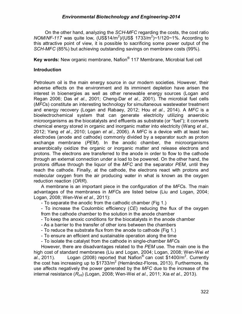
Environmental Biotechnology and Engineering-2014
322
On the other hand, analyzing the SCH-MFC regarding the costs, the cost ratio NOM/NF-117 was quite low, (US$14/m2)/(US$ 1733/m2)~1/120~1%. According to this attractive point of view, it is possible to sacrificing some power output of the SCH-MFC (85%) but achieving outstanding savings on membrane costs (99%). Key words: New organic membrane, Nafion® 117 Membrane, Microbial fuel cell Introduction Petroleum oil is the main energy source in our modern societies. However, their adverse effects on the environment and its imminent depletion have arisen the interest in bioenergies as well as other renewable energy sources (Logan and Regan 2006; Das et al., 2001; Cheng-Dar et al., 2001). The microbial fuel cells (MFCs) constitute an interesting technology for simultaneous wastewater treatment and energy recovery (Logan and Rabaey, 2012; Hou et al., 2014). A MFC is a bioelectrochemical system that can generate electricity utilizing anaerobic microorganisms as the biocatalysts and effluents as substrate (or “fuel”); it converts chemical energy stored in organic and inorganic matter into electricity (Wang et al., 2012; Yang et al., 2010; Logan et al., 2006). A MFC is a device with at least two electrodes (anode and cathode) commonly divided by a separator such as proton exchange membrane (PEM). In the anodic chamber, the microorganisms anaerobically oxidize the organic or inorganic matter and release electrons and protons. The electrons are transferred to the anode in order to flow to the cathode through an external connection under a load to be powered. On the other hand, the protons diffuse through the liquor of the MFC and the separator PEM, until they reach the cathode. Finally, at the cathode, the electrons react with protons and molecular oxygen from the air producing water in what is known as the oxygen reduction reaction (ORR). A membrane is an important piece in the configuration of the MFCs. The main advantages of the membranes in MFCs are listed below (Liu and Logan, 2004; Logan, 2008; Wen-Wei et al., 2011):
- To separate the anodic from the cathodic chamber (Fig 1.) - To increase the Coulombic efficiency (CE) reducing the flux of the oxygen from the cathode chamber to the solution in the anode chamber - To keep the anoxic conditions for the biocatalysts in the anode chamber - As a barrier to the transfer of other ions between the chambers - To reduce the substrate flux from the anode to cathode (Fig 1.) - To ensure an efficient and sustainable operation along the time - To isolate the catalyst from the cathode in single-chamber MFCs
However, there are disadvantages related to the PEM use. The main one is the high cost of standard membranes (Liu and Logan, 2004; Logan, 2008; Wen-Wei et al., 2011). Logan (2008) reported that Nafion® can cost $1400/m2. Currently the cost has increasing up to $1733/m2 (Hernández-Flores, 2013). Furthermore, its use affects negatively the power generated by the MFC due to the increase of the internal resistance (Rint) (Logan, 2008; Wen-Wei et al., 2011; Xia et al., 2013).
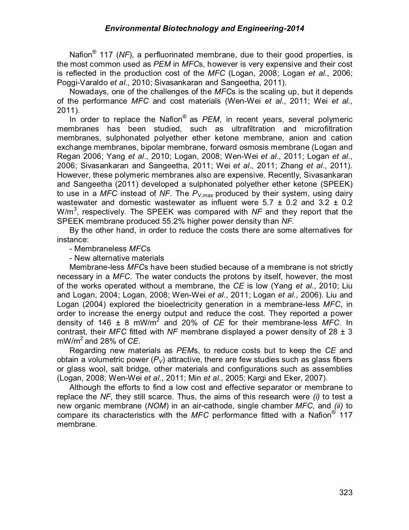
Environmental Biotechnology and Engineering-2014
323
Nafion® 117 (NF), a perfluorinated membrane, due to their good properties, is the most common used as PEM in MFCs, however is very expensive and their cost is reflected in the production cost of the MFC (Logan, 2008; Logan et al., 2006; Poggi-Varaldo et al., 2010; Sivasankaran and Sangeetha, 2011). Nowadays, one of the challenges of the MFCs is the scaling up, but it depends of the performance MFC and cost materials (Wen-Wei et al., 2011; Wei et al., 2011). In order to replace the Nafion® as PEM, in recent years, several polymeric membranes has been studied, such as ultrafiltration and microfiltration membranes, sulphonated polyether ether ketone membrane, anion and cation exchange membranes, bipolar membrane, forward osmosis membrane (Logan and Regan 2006; Yang et al., 2010; Logan, 2008; Wen-Wei et al., 2011; Logan et al., 2006; Sivasankaran and Sangeetha, 2011; Wei et al., 2011; Zhang et al., 2011). However, these polymeric membranes also are expensive. Recently, Sivasankaran and Sangeetha (2011) developed a sulphonated polyether ether ketone (SPEEK) to use in a MFC instead of NF. The PV,max produced by their system, using dairy wastewater and domestic wastewater as influent were 5.7 ± 0.2 and 3.2 ± 0.2 W/m3, respectively. The SPEEK was compared with NF and they report that the SPEEK membrane produced 55.2% higher power density than NF. By the other hand, in order to reduce the costs there are some alternatives for instance:
- Membraneless MFCs - New alternative materials
Membrane-less MFCs have been studied because of a membrane is not strictly necessary in a MFC. The water conducts the protons by itself, however, the most of the works operated without a membrane, the CE is low (Yang et al., 2010; Liu and Logan, 2004; Logan, 2008; Wen-Wei et al., 2011; Logan et al., 2006). Liu and Logan (2004) explored the bioelectricity generation in a membrane-less MFC, in order to increase the energy output and reduce the cost. They reported a power density of 146 ± 8 mW/m2 and 20% of CE for their membrane-less MFC. In contrast, their MFC fitted with NF membrane displayed a power density of 28 ± 3 mW/m2 and 28% of CE. Regarding new materials as PEMs, to reduce costs but to keep the CE and obtain a volumetric power (PV) attractive, there are few studies such as glass fibers or glass wool, salt bridge, other materials and configurations such as assemblies (Logan, 2008; Wen-Wei et al., 2011; Min et al., 2005; Kargi and Eker, 2007). Although the efforts to find a low cost and effective separator or membrane to replace the NF, they still scarce. Thus, the aims of this research were (i) to test a new organic membrane (NOM) in an air-cathode, single chamber MFC, and (ii) to compare its characteristics with the MFC performance fitted with a Nafion® 117 membrane.
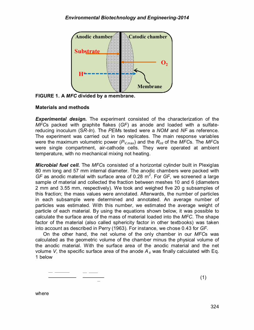
Environmental Biotechnology and Engineering-2014
324
FIGURE 1. A MFC divided by a membrane. Materials and methods Experimental design. The experiment consisted of the characterization of the MFCs packed with graphite flakes (GF) as anode and loaded with a sulfate-reducing inoculum (SR-In). The PEMs tested were a NOM and NF as reference. The experiment was carried out in two replicates. The main response variables were the maximum volumetric power (PV,max) and the Rint of the MFCs. The MFCs were single compartment, air-cathode cells. They were operated at ambient temperature, with no mechanical mixing not heating. Microbial fuel cell. The MFCs consisted of a horizontal cylinder built in Plexiglas 80 mm long and 57 mm internal diameter. The anodic chambers were packed with GF as anodic material with surface area of 0.28 m2. For GF, we screened a large sample of material and collected the fraction between meshes 10 and 6 (diameters 2 mm and 3.55 mm, respectively). We took and weighed five 20 g subsamples of this fraction; the mass values were annotated. Afterwards, the number of particles in each subsample were determined and annotated. An average number of particles was estimated. With this number, we estimated the average weight of particle of each material. By using the equations shown below, it was possible to calculate the surface area of the mass of material loaded into the MFC. The shape factor of the material (also called sphericity factor in other textbooks) was taken into account as described in Perry (1963). For instance, we chose 0.43 for GF. On the other hand, the net volume of the only chamber in our MFCs was calculated as the geometric volume of the chamber minus the physical volume of the anodic material. With the surface area of the anodic material and the net volume V, the specific surface area of the anode A’
s was finally calculated with Eq. 1 below
(1)
where
Anodic chamber
Substrate
O2
H+
Catodic chamber
Membrane
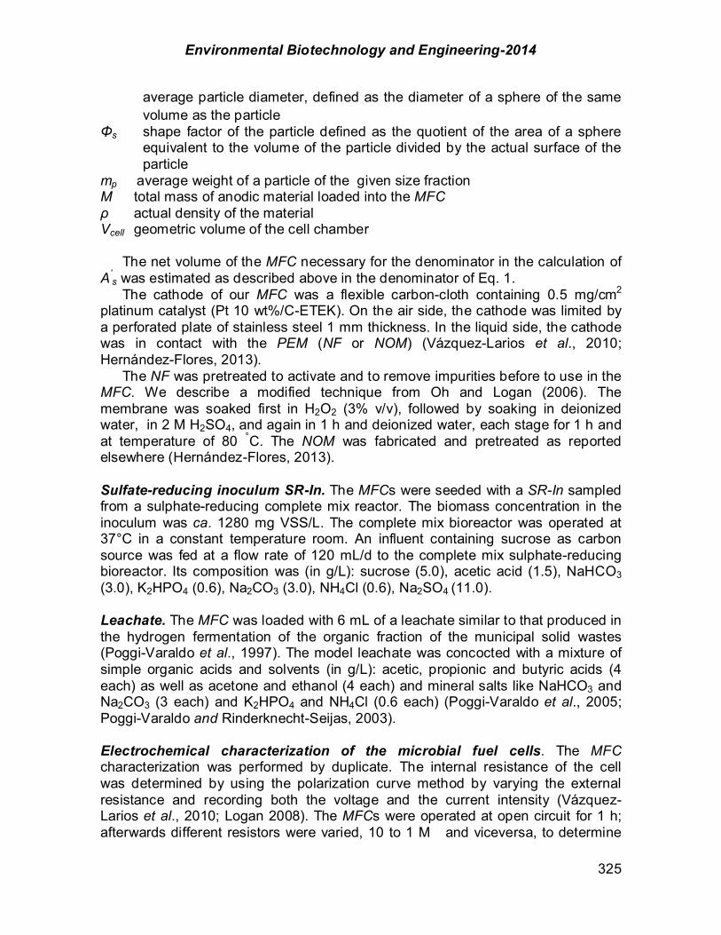
Environmental Biotechnology and Engineering-2014
325
average particle diameter, defined as the diameter of a sphere of the same volume as the particle
"s shape factor of the particle defined as the quotient of the area of a sphere equivalent to the volume of the particle divided by the actual surface of the particle
mp average weight of a particle of the given size fraction M total mass of anodic material loaded into the MFC # actual density of the material Vcell geometric volume of the cell chamber The net volume of the MFC necessary for the denominator in the calculation of A’
s was estimated as described above in the denominator of Eq. 1. The cathode of our MFC was a flexible carbon-cloth containing 0.5 mg/cm2 platinum catalyst (Pt 10 wt%/C-ETEK). On the air side, the cathode was limited by a perforated plate of stainless steel 1 mm thickness. In the liquid side, the cathode was in contact with the PEM (NF or NOM) (Vázquez-Larios et al., 2010; Hernández-Flores, 2013). The NF was pretreated to activate and to remove impurities before to use in the MFC. We describe a modified technique from Oh and Logan (2006). The membrane was soaked first in H2O2 (3% v/v), followed by soaking in deionized water, in 2 M H2SO4, and again in 1 h and deionized water, each stage for 1 h and at temperature of 80 °C. The NOM was fabricated and pretreated as reported elsewhere (Hernández-Flores, 2013). Sulfate-reducing inoculum SR-In. The MFCs were seeded with a SR-In sampled from a sulphate-reducing complete mix reactor. The biomass concentration in the inoculum was ca. 1280 mg VSS/L. The complete mix bioreactor was operated at 37°C in a constant temperature room. An influent containing sucrose as carbon source was fed at a flow rate of 120 mL/d to the complete mix sulphate-reducing bioreactor. Its composition was (in g/L): sucrose (5.0), acetic acid (1.5), NaHCO3 (3.0), K2HPO4 (0.6), Na2CO3 (3.0), NH4Cl (0.6), Na2SO4 (11.0). Leachate. The MFC was loaded with 6 mL of a leachate similar to that produced in the hydrogen fermentation of the organic fraction of the municipal solid wastes (Poggi-Varaldo et al., 1997). The model leachate was concocted with a mixture of simple organic acids and solvents (in g/L): acetic, propionic and butyric acids (4 each) as well as acetone and ethanol (4 each) and mineral salts like NaHCO3 and Na2CO3 (3 each) and K2HPO4 and NH4Cl (0.6 each) (Poggi-Varaldo et al., 2005; Poggi-Varaldo and Rinderknecht-Seijas, 2003). Electrochemical characterization of the microbial fuel cells. The MFC characterization was performed by duplicate. The internal resistance of the cell was determined by using the polarization curve method by varying the external resistance and recording both the voltage and the current intensity (Vázquez-Larios et al., 2010; Logan 2008). The MFCs were operated at open circuit for 1 h; afterwards different resistors were varied, 10 to 1 M and viceversa, to determine

Environmental Biotechnology and Engineering-2014
326
the power generation an another response variables as a function of load. After this, the cell was set to open circuit conditions for 1 h in order to check the adequacy of the procedure (values of initial and final open circuit voltages should be close). The voltage was measured and recorded with a Multimeter ESCORT 3146A. The current was calculated by the Ohm’s law (Eq. 2) and the Rint was calculated as the slope of the linear section of the curve voltage versus the current intensity (Vázquez-Larios et al., 2010; Logan et al., 2006). The volumetric power (PV) was calculated according the Eq. 3:
(2)
(3) where IMFC is the current intensity of the MFC in A, EMFC is the voltage delivered by the cell in V, Rext is the external resistance connected to the cell in # and Vcell is the net volume of the anodic chamber. The initial chemical oxygen demand (COD) and biomass concentration in the cell liquor were ca. 3334 ± 106 mg O2/L and 920 ± 71 VSS/L respectively. The pH and the electrical conductivity were 7.63 ± 0.03 and 16.75 ± 0.07 mS/cm respectively. The COD and VSS of the liquors of sulphate-reducing seed bioreactor and cells were determined according to the Standard Methods (APHA, 1989). Results and discussion Assessment of the NOM as PEM in MFCs. The NOM was fitted to the MFC to be evaluated as a PEM. At the same time, NF also was fitted to a second MFC. The MFCs were operated under the same conditions. Table 1 exhibits some properties of the anodic material (GF) used to pack the MFCs. The working net volume used to obtain the PV,max was 7.22!10-5 m3.
TABLE 1. Selected physical characteristics of graphite flakes. Characteristics Values Working net volume (m3) 7.22!10-5 ± 5.05!10-6 Anodic actual surface (m2) 0.28 ± 0.08 A’s
a (m2/m3) 1302 ± 91 Conductance (S)b 0.13 ± 0.04
Notes: aRelationship between the anode surface area to cell volume, also known as specific surface area of the anode; b Electrical conductance of the material, expressed in Siemens. The Fig. 2 shows the electrochemical characterization of both MFCs. The Rint and PV,max for the NOM-fitted MFC were 112.0 # and 2146 mW/m3, respectively
(Fig. 2b). On the other hand for NF-fitted MFC (Fig. 2a), the Rint and and PV,max were 110.1 # and 14,246 mW/m3 (Table 2). Regarding the Rint the values obtained
Environmental Biotechnology and Engineering-2014
327
were in the same order for both membranes in MFC. These results were very encouraging. The power delivered with NOM was 15% of that with Nafion® 117 as PEM. However, the cost ratio NOM/Nafion was quite low, ($14/m2)/($1733/m2)~ 1/120~1% (Table 3). These results point out to a trade-off between sacrificing some power output of the cell (85%) but achieving outstanding savings on membrane costs (99%). Comparing our results with other works, Min et al. (2005), using a pure culture of Geobacter metallireducens and domestic wastewater examined the power produced by their MFC using a salt bridge as separator. The performance displayed by their MFC was 2.2 mW/m2 with a high Rint of 19920 ± 50. The maximum voltage recorded by them was 22 mV using a resistance of 1000 , whereas in our system using the NOM, 124 mV was recorded with a resistance of 110 . The MFC performance was too low compared with our system, 60.73 ± 14.32 mW/m2 and Rint 111.96 ± 5.25 (Table 2). By the other hand, Kargi and Eker (2007) used a MFC fitted with salt-agar slab (salt bridge) to treat a synthetic wastewater composed of diluted molasses with simultaneous electricity generation. The electrodes were copper and gold-covered-copper wires as anode and cathode, respectively. The salt-agar slab used as separator depict a low cost for their system, nevertheless, the electrodes cost is high. The MFC performance reported was too poor, the maximum power density reached was only 2.9 mW/m2, a maximum power density lower than our results showed in Table 2.
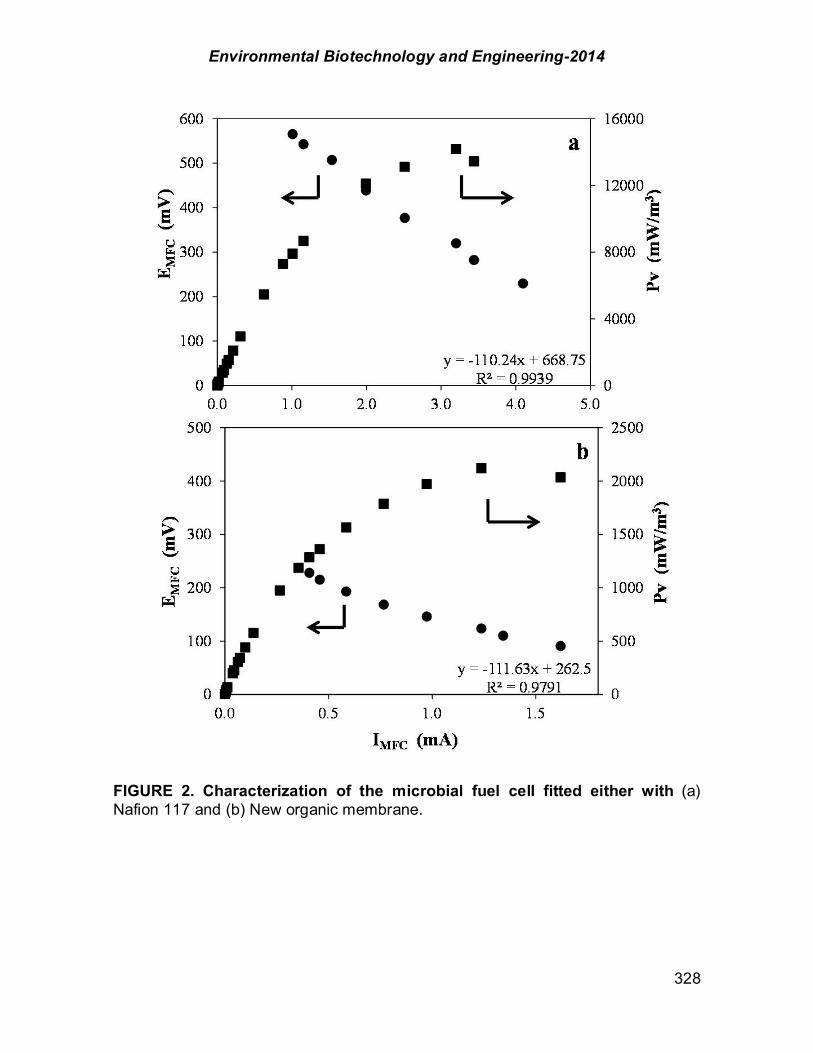
Environmental Biotechnology and Engineering-2014
328
FIGURE 2. Characterization of the microbial fuel cell fitted either with (a) Nafion 117 and (b) New organic membrane.
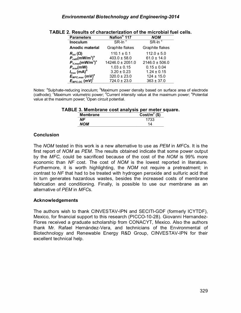
Environmental Biotechnology and Engineering-2014
329
TABLE 2. Results of characterization of the microbial fuel cells. Parameters Nafion® 117 NOM Inoculum SR-In a SR-In a Anodic material Graphite flakes Graphite flakes Rint (!) 110.1 ± 0.1 112.0 ± 5.0 Pcath(mW/m2)b 403.0 ± 58.0 61.0 ± 14.0 PV,max(mW/m3)c 14246.0 ± 2051.0 2146.0 ± 506.0 Pmax(mW) 1.03 ± 0.15 0.15 ± 0.04 Imax (mA)d 3.20 ± 0.23 1.24 ± 0.15 EMFC,max (mV)e 320.0 ± 23.0 124 ± 15.0 EMFC,OC (mV)f 724.0 ± 23.0 363 ± 37.0
Notes: aSulphate-reducing inoculum; bMaximum power density based on surface area of electrode (cathode); cMaximum volumetric power; dCurrent intensity value at the maximum power; ePotential value at the maximum power; fOpen circuit potential.
TABLE 3. Membrane cost analysis per meter square.
Membrane Cost/m2 ($) NF 1733 NOM 14
Conclusion The NOM tested in this work is a new alternative to use as PEM in MFCs. It is the first report of NOM as PEM. The results obtained indicate that some power output by the MFC, could be sacrificed because of the cost of the NOM is 99% more economic than NF cost. The cost of NOM is the lowest reported in literature. Furthermore, it is worth highlighting, the NOM not require a pretreatment; in contrast to NF that had to be treated with hydrogen peroxide and sulfuric acid that in turn generates hazardous wastes, besides the increased costs of membrane fabrication and conditioning. Finally, is possible to use our membrane as an alternative of PEM in MFCs. Acknowledgements The authors wish to thank CINVESTAV-IPN and SECITI-GDF (formerly ICYTDF), Mexico, for financial support to this research (PICCO-10-28). Giovanni Hernandez-Flores received a graduate scholarship from CONACYT, Mexico. Also the authors thank Mr. Rafael Hernández-Vera, and technicians of the Environmental of Biotechnology and Renewable Energy R&D Group, CINVESTAV-IPN for their excellent technical help.
Environmental Biotechnology and Engineering-2014
330
References APHA,(1989). Standard methods for examination of water and wastewater. 17th ed. APHA-AWWA-
WEF, Washington DC. Cheng-Dar, Y.; Chung-Ming, L.; Liou, E. M. L. (2001). A transition toward a sustainable energy
future: feasibility assessment and development strategies of wind power in Taiwan. Energy Policy. 29: 951-963.
Das, D.; Veziroglu, T. N. (2001). Hydrogen production by biological processes: a survey of literature. Int J. Hydrogen Energy. 26: 13-28.
Hernández-Flores, G. (2013). Interim Report. Sc D Thesis, CINVESTAV-IPN, México, D.F. Hou, J.; Liu, Z.; Yang, S.; Zhou, Y. (2014). Three-dimensional macroporous anodes based on
stainless steel fiber felt for high-performance microbial fuel cells. Journal of Power Sources. 258: 204-209.
Kargi, F.; Eker, S. (2007). Electricity generation with simultaneous wastewater treatment by a microbial fuel cell (MFC) with Cu and Cu-Au electrodes. J. Chem. Technol. Biotechnol. 82: 658-662.
Liu, H.; Logan, B. E. (2004). Electricity generation using an air-cathode single chamber microbial fuel cell in the presence and absence of a proton exchange membrane. Environ. Sci. Technol. 38: 4040–4046.
Logan, B. E. (2008). Microbial fuel cells. John Wiley-Interscience. New Jersey, USA. Logan, B. E.; Hamelers, B.; Rozendal, R.; Schröder, U.; Keller, J.; Freguia, S.; Aelterman,P.;
Verstraete, W.; Rabaey, K. (2006). Microbial fuel cells: Methodology and technology. Environ. Sci. Technol. 40: 5181-5192.
Logan, B. E.; Rabaey, K. (2012). Conversion of wastes into bioelectricity and chemicals by using microbial electrochemical technologies. Science. 337: 686-690.
Logan, B. E.; Regan, J. M. (2006). Microbial challenges and harnessing the metabolic activity of bacteria can provide energy for a variety of applications, once technical and cost obstacles are overcome. Environ. Sci. Technol. 5172–5180.
Min, B.; Cheng, S.; Logan, B. E. (2005). Electricity generation using membranes and salt bridge microbial fuel cells. Water Research. 39: 1675-1686.
Oh, S. E.; Logan, B. E. (2006). Proton exchange membrane and electrode surface areas as factors that affect power generation in microbial fuel cells. Appl Microbiol Biotechnol. 70: 162–169.
Perry, R. (1963). Chemical Engineers Handbook, pp 5.50 & ff 4th ed., McGraw-Hill Co, New York. Poggi-Varaldo, H. M.; Alzate-Gaviria, L. M.; Perez-Hernandez,A.; Nevarez-Morillon,V. G.;
Rinderknecht-Seijas, N. (2005). A side-by-side comparison of two systems of sequencing coupled reactors for anaerobic digestion of the organic fraction of municipal solid waste. Waste Manage. Res. 23: 270-280.
Poggi-Varaldo, H. M.; Rinderknecht-Seijas, N. (2003). A differential availability enhancement factor for the evaluation of pollutant availability in soil treatments. Acta Biotechnologica. 23: 271-280.
Poggi-Varaldo, H. M.; Valdés, L.; Esparza-García, F. J.; Fernández-Villagómez, G. (1997). Solid susbtrate anaerobic co-digestion of paper mill sludge, bio-solids, and municipal solid waste. Water Sci. Technol. 35: 197-204.
Poggi-Varaldo, H. M.; Vazquez-Larios, A.; Solorza-Feria, O. (2010). Microbial fuel cells. In Rodríguez-Varela F.J., Solorza-Feria O., Hernández-Pacheco, E. (Eds). Fuel cells. Book Livres, Montréal, Canada, pp 124-161.
Sivasankaran, A.; Sangeetha, D. (2011). Development of MFC using sulphonated polyether ether ketone (SPEEK) membrane for electricity generation from waste water. Bioresour. Technol. 102(24): 11167-11171.
Vazquez-Larios, A. L.; Solorza-Feria, O.; Vazquez-Huerta, G.; Esparza-Garcia, F. J.; Rios-Leal, E.; Rinderknecht-Seijas, N.; Poggi-Varaldo, H. M. (2010). A new design improves performance of a single chamber microbial fuel cell. J. New Mater. Electrochem. Syst. 13: 219-226.
Wang, H.; Park, J. D.; Ren, Z. (2012). Active energy harvesting from microbial fuel cells at the maximum power point without using resistors. Environ. Sci. Technol. 46: 5247-5252
Wei, J.; Liang, P.; Huang, X. (2011). Recent progress in electrodes for microbial fuel cells. Bioresour. Technol. 102: 9335-9344.
Environmental Biotechnology and Engineering-2014
331
Wen-Wei, L.; Guo-Ping, S.; Xian-Wei, L.; Han-qing, Y. (2011). Recent advances in the separators for microbial fuel cells. Bioresour Technol. 102: 244-252.
Xia, X.; Tokash, J. C.; Zhang, F.; Liang, P.; Huang, X.; Logan, B. E. (2013). Oxygen-Reducing Biocathodes Operating with Passive Oxygen Transfer in Microbial Fuel Cells. Environ. Sci. Technol. 47 (4): 2085–2091.
Yang, Y.; Sun, G.; Xu, M. (2010). Microbial fuel cells come of age. J. Chem. Technol. Biotechnol. 86: 625-632.
Zhang, F.; Brastad, K. S.; He, Z. (2011). Integrating forward osmosis into microbial fuel cells for wastewater treatment, water extraction and bioelectricity generation. Environ. Sci. Technol. 45: 6690-6696.
Notation A’s relationship between the anode surface area to cell volume,
also known as specific surface area of the anode CE coulombic efficiency COD chemical oxygen demand
average particle diameter, defined as the diameter of a sphere of the same volume as the particle
EMFC voltage delivered by the cell EMFC,max cell potential at which the maximum volumetric power is
registered EMFC,OC cell potential value at open circuit potential GF graphite flakes IMFC current intensity of the MFC M total mass of anodic material loaded into the MFC MFC microbial fuel cell mp average weight of a particle of the given size fraction NF nafion® 117 NOM new organic membrane ORR oxygen reduction reaction Pcath power density based on surface area of electrode (cathode) PEM proton exchange membrane PV volumetric power Pv,max maximum volumetric power Rext external resistance Rint internal resistance SCH-MFC single chamber MFC SR-In sulfate-reducing inoculum Vcell geometric volume of the cell chamber Greek characters & actual density of the material 's shape factor of the particle defined as the quotient of the area of a
sphere equivalent to the volume of the particle divided by the actual surface of the particle
Environmental Biotechnology and Engineering-2014
332
CHAPTER 2.7. ECONOMIC EVALUATION OF A BIOREFINERY FOR BUTANOL PRODUCTION FROM WHEAT STRAW WITH A CONSOLIDATED
BIOPROCESS APPROACH
Carlos Molina (1,5); Arturo Sánchez (2); Analí Soto (2); Idania Valdez Vazquez* (1,4)
(1) Depto. de Ciencias Ambientales, DICIVA, Universidad de Guanajuato CIS, Guanajuato, México. (2) Unidad de Ingeniería Avanzada, Centro de Investigación y Estudios Avanzados (CINVESTAV), Av. del Bosque 1145, Zapopan 45019, Jalisco, México. (4) Unidad Académica Juriquilla, Instituto de Ingeniería, UNAM. E-mail: [email protected]; [email protected]. (5) Depto. de Ingeniería Química, Biomédicas y Electrónica. DCI, Universidad de Guanajuato, Guanajuato, México. ABSTRACT A conventional biochemical platform for lignocelullosic transformation into biofuels comprises four steps which are pretreatment, enzymatic hydrolysis, fermentation and downstream process. Nevertheless, an alternative in order to reduce the number of stages are consolidated bioprocess (CBP). In this CBP the number of unit operation can be reduce due to all the operation realized separately, in a conventional platform, can be realized in just one unit. The objective of this work was to design a plant flowsheet of a non-conventional biorefinery using wheat straw as feedstock to obtain butanol using microbial consortia with a CBP approach. The conceptual design, mass and energy balances were performed using SuperPro Designer v8.5. The feedstock composition was (in dry basis) of 44.8% of cellulose, 26.6% of hemicellulose and 6.8% of lignin. The plant capacity was defined in 2200 MT dry basis/day. The main processing stages were (i) milling and fibers hydration, (ii) hydrogen production, (iii) butanol and acetone production, (iv) methane production, (v) downstream processes and (vi) cogeneration plant. The operating conditions for each reactor (temperature, solid load, dilution rate and inoculum) were based on experimental results obtained in our laboratory and literature. Three sceneries were assayed in order to observe the influence of hydraulic retention time (HRT) and butanol concentration on butanol production cost (NPV). These three sceneries considered HRT of 8 h, 24 h, 40 h and 72 h, and three different concentrations of butanol: 9.95 g/L, 15 g/L and 19.4 g/L. These butanol concentrations were adapted from literature. In the best scenery (19.4 g/L and 8 h), the butanol production plant had a capacity of 70 X 106 kg/yr. In addition acetone (18 X 106 kg/yr) was also produced. The products methane and hydrogen were burned in the cogeneration step. In cogeneration plant was possible produced all the vapor and electricity demands of the total plant. The butanol production cost was estimated in $1.17/kg which is competitive with the synthetic butanol cost and is similar to other reports that use conventional biochemical platform. The results also showed that the butanol concentration and HRT have great influence over the net present value (NPV). ------------ *Author for all correspondence
Environmental Biotechnology and Engineering-2014
333
Introduction Oil is a finite resource which is used to power the modern world. In all the world, billions of tons of gasoline are used every year. Sustainable alternatives must be developed to offset the upcoming oil shortages and resulting rise in gas prices (Berg et al.,2009). Biobutanol is one of the bioalcohols that had gained considerable attention in recent years. Biobutanol has special merits over other bioalcohols such as ethanol in that its properties such as low vapor pressure, high energy density, octane number, energy content, low hygroscopicity, and low water solubility are very similar to gasoline (Ranjan et al., 2012). This work was focused on the development of a biorefinery for Biobutanol production. A biorefinery is defined as a facility that integrates different biomass conversion processes and equipment to produce biofuels, biomaterials, heat and/or power. In a lignocellulosic biorefineries, the carbohydrate fraction (hemicellulose and cellulose) is separated and fermented into useful products such as gaseous and/or liquid biofuels. Conventional biochemical biorefineries use saccharification to perform the cellulose hydrolysis, and then fermentation from the obtained simple sugars (Sánchez et al., 2013). This biorefinery configuration has high operating costs and relative low yields (based on the feedstock processed). As an alternative, the consolidated bioprocess (CB) integrates the enzyme production, saccharification and fermentation into a single unit which could decrease the operating cost and improve the yield (Lynd et al., 2005), reducing initial inversion attributed to equipment.
The objective of this work was to design a plant flowsheet of a non-conventional biorefinery using wheat straw as feedstock to obtain butanol using microbial consortia with a CBP approach.
Methodology The methodology described in this work use data obtained from our laboratory and international literature. The feedstock was wheat straw (WS) with the next composition: cellulose 44.8%, hemicellulose 25.6%, lignin, 6.8%, ash 6.15%, other solids 9.3% and water 7.35% in dry base (DB) which was reported by Jackowia et al., 2010. With this composition, the WS price was fixed in 40$/MT due to polysaccharides composition according to Sánchez et al., 2013.
Plant description. Figure 1, describes the flow diagram proposed for this process. The plant contained 6 principal stages which are (i) milling and hydration, (ii) hydrogen production, (iii) butanol production, (iv) methane production, (v) downstream processes and (vi) cogeneration processes.
The physical pretreatment was compoused miling and hydration. The milling process reduces the WS size until 2-3 mm and then WS was conducted to hydration process. In hydration process, WS was place in contact with a filter liquid effluent from a methanogenic reactor in order to expand the WS fibers. The hydration process was reported previously by Lara et al., 2014.

Environmental Biotechnology and Engineering-2014
334
FIGURE 1. Process block diagram
The hydrogen production process was used as biological process in order to transform the xylan contained on WS to hydrogen. In our laboratory experience, the 100% of xylan is used in this process and transformed to hydrogen and carbon dioxide. This process permit obtained free cellulose. The temperature of this reactor was fixed at 37°C and the hydrogen production was according to the reactions reported by Valdez-Vazquez and Poggi-Varaldo., 2010. The effluent of this reactor was filtered and separated in two fractions, liquid and solid. The liquid fraction of hydrogen production step was fed to an anaerobic reactor due to the high contain of organic acids as acetic and butyric acid and the solid fraction was fed to butanol production step.
The effluent obtained from methanogenic reactor was filter obtained two fractions, liquid and solid. The liquid fraction was used to feed the hydration process described previously and the solid fraction was used in cogeneration process.
The butanol, acetone and ethanol step, used the solid fraction from the hydrogen effluent at a concentration of 100g/L. The concentration was adjusted with fresh water. The butanol concentration was fixed according to Table 1, and were tested three scenarios. In addition four hydraulic retention times (HRT) were used 8h, 24 h, 40 h and 72 h according to Bahl et al., 1982.
The downstream process was realized using the configuration described by Kramer et al., 2010. This consist in one external extraction column, which used mesitylene as extract agent, followed by three distillation columns in order to purify the butanol and acetone produced by this process.
The final step, cogeneration, was based in the model described by Sánchez et al., 2013. In this process was generated steam and power using the methane, hydrogen and solid residues generated in the biorefinery.
TABLE 1. Scenarios tested for solventogenic step
Scenarios
g/L Reference Butanol Aceton
e Ethano
l 1 9.95 3.5 0.4 Annous and Blaschek, 1991 2 15 7.5 1 Annous and Blaschek, 1991

Environmental Biotechnology and Engineering-2014
335
3 19.4 4.8 0.8 Annous and Blaschek, 1991
Mass and energy balance. The model was built in stationary process using Superpro Designer v8.5 (SPD). The values of any properties were taken from data base of SPD, Seader and Henley (2011) and free software ChemSep v6.96. SPD calculated the energy requirements and electric power required. The energy integration of the plant was realized using pinch method according to Linnhoff and Hindmarsh, (1982).
Financial investment and assumptions. The price and calculation data were based on July 2014 prices. It was assumed that the plant was operated for 330 days/year. The capital would be borrowed for 10 years at interest rates of 6%. The project life time was fixed in 30 years with straight line depreciation. Federal taxes were considered between 20–40% on profit. An inflation factor of 2% and 4% was considered for this exercise. The fermentation byproduct acetone and electricity generated by the process were sold for byproduct credit.
Results and discussion A plant based on a CB was realized. Were tested three scenarios in order to obtain a low butanol production cost. The lowest cost was obtained under the conditions of scenario 3, a HRT of 8 h and considering an inflation factor of 2%. The production cost of butanol with these conditions was 1.17$/kg. This can be observed in Figure 2.
FIGURE 2. Hydraulic retention time (HRT) -vs- butanol cost. Comparison of three scenarios and four HRT. Inflation factor 2%,
This plant was designed to produce butanol from wheat straw with butanol production capacity of 70 X 106 kg/year. For this plant, total plat cost was projected to be US$313,580,000.
The heating and cooling requirements with 2200 MT of WS/day were 81.74 MW and 16.13 MW respectively. The electricity requirement was 11.9 kW-h X107. The vapor requirements that was not satisfied by integration method was satisfied using steam of low pressure produce in the cogeneration plant. The electricity produce in
1
1.4
1.8
2.2
2.6
3
8 24 40 72
But
anol
cos
t ($/
kg)
HRT (h)
Scenary 1
Scenary 2Scenary 3
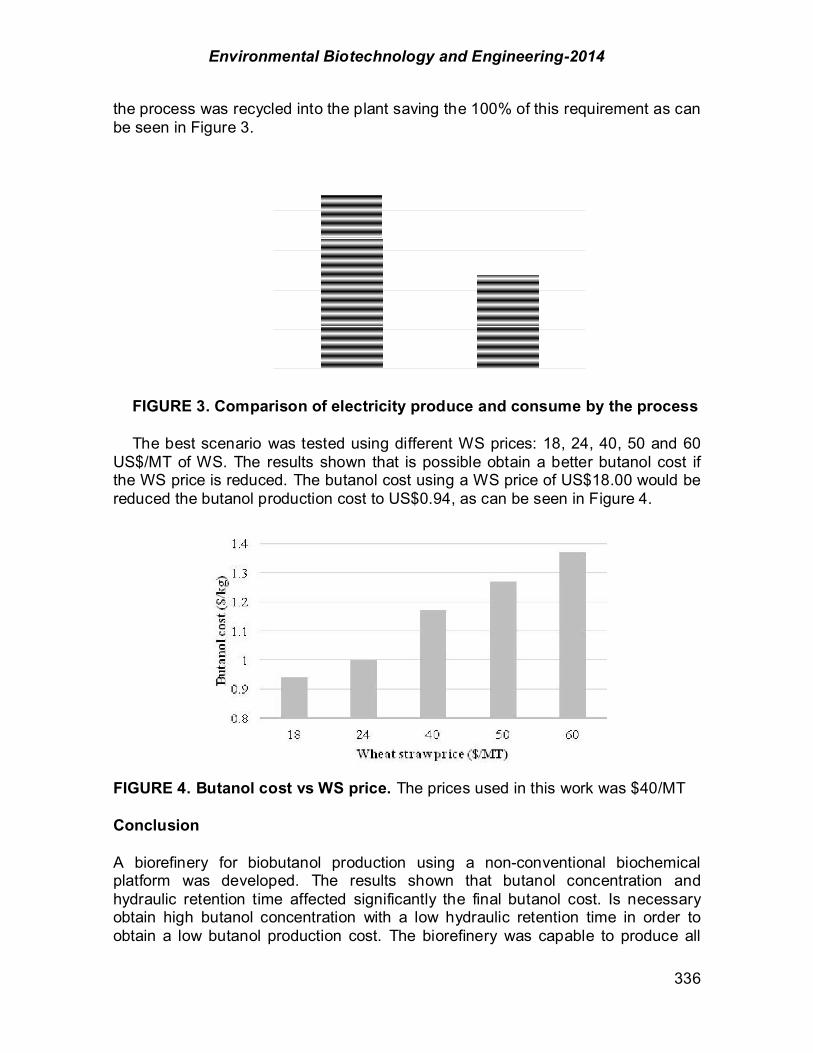
Environmental Biotechnology and Engineering-2014
336
the process was recycled into the plant saving the 100% of this requirement as can be seen in Figure 3.
FIGURE 3. Comparison of electricity produce and consume by the process
The best scenario was tested using different WS prices: 18, 24, 40, 50 and 60
US$/MT of WS. The results shown that is possible obtain a better butanol cost if the WS price is reduced. The butanol cost using a WS price of US$18.00 would be reduced the butanol production cost to US$0.94, as can be seen in Figure 4.
FIGURE 4. Butanol cost vs WS price. The prices used in this work was $40/MT Conclusion A biorefinery for biobutanol production using a non-conventional biochemical platform was developed. The results shown that butanol concentration and hydraulic retention time affected significantly the final butanol cost. Is necessary obtain high butanol concentration with a low hydraulic retention time in order to obtain a low butanol production cost. The biorefinery was capable to produce all
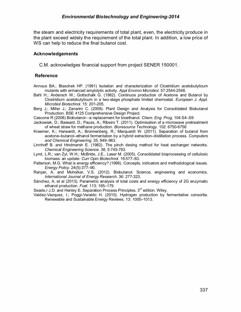
Environmental Biotechnology and Engineering-2014
337
the steam and electricity requirements of total plant, even, the electricity produce in the plant exceed widely the requirement of the total plant. In addition, a low price of WS can help to reduce the final butanol cost.
Acknowledgements
C.M. acknowledges financial support from project SENER 150001.
Reference Annous BA.; Blaschek HP. (1991) Isolation and characterization of Clostridium acetobutylicum
mutants with enhanced amylolytic activity. Appl Environ Microbiol. 57:2544-2548. Bahl H.; Andersch W.; Gottschalk G. (1982). Continuos production of Acetone and Butanol by
Clostridium acetobutylicum in a two-stage phosphate limited chemostat. European J. Appl. Microbiol Biotechnol. 15: 201-205.
Berg J.; Miller J.; Zanarini C. (2009). Plant Design and Analysis for Consolidated Biobutanol Production. BSE 4125 Comprehensive Design Project.
Cascone R (2008) Biobutanol—a replacement for bioethanol. Chem. Eng. Prog. 104:S4–S9 Jackowiak, D.; Bassard, D.; Pauss, A.; Ribeiro T. (2011). Optimisation of a microwave pretreatment
of wheat straw for methane production. Bioresource Technology. 102: 6750-6756 Kraemer, K.; Harwardt, A.; Bronnenberg, R.; Marquardt W. (2011). Separation of butanol from
acetone–butanol–ethanol fermentation by a hybrid extraction–distillation process. Computers and Chemical Engineering. 35, 949–963.
Linnhoff B. and Hindmarsh E. (1982). The pinch desing method for heat exchanger networks. Chemical Engineering Science. 38, 5:745-763.
Lynd, L.R.; van Zyl, W.H.; McBride, J.E., Laser M. (2005). Consolidated bioprocessing of cellulosic biomass: an update. Curr Opin Biotechnol. 16:577–83.
Patterson, M.G. What is energy efficiency? (1996). Concepts, indicators and methodological issues. Energy Policy. 24(5):377–90.
Ranjan, A. and Moholkar, V.S. (2012). Biobutanol: Science, engineering and economics. International Journal of Energy Research. 36: 277-323.
Sánchez, A. et al (2013). Parametric analysis of total costs and energy efficiency of 2G enzymatic ethanol production. Fuel. 113: 165–179.
Seade,r J.D. and Henley E. Separation Process Principles. 3rd edition. Wiley. Valdez-Vazquez, I.; Poggi-Varaldo H. (2010). Hydrogen production by fermentative consortia.
Renewable and Sustainable Energy Reviews. 13: 1000–1013.

Environmental Biotechnology and Engineering-2014
338
CHAPTER 2.8. SUSTENTABILIDAD DEL PLANETA Y DESARROLLO SOSTENIBLE EN LAS ORGANIZACIONES, UN MODELO PARA LA
CONSERVACION DEL MEDIO AMBIENTE
Germán Domínguez Bocanegra* (1)
(1) División de Contaduría y Administración, Tecnológico de Estudios Superiores de Ecatepec [email protected] Introducción Desde el siglo pasado el mundo se encuentra preocupado por la situación del calentamiento global, provocado por la elevada contaminación del planeta, detonado principalmente por la industria, por tal motivo y después de la segunda guerra mundial en 1946 en Ginebra Suiza nace la Organización Internacional de Normalización (ISO), la cual busca la estandarización a nivel internacional, por lo que se convirtió en el organismo internacional para el establecimiento de normas, trabajando con cuerpos nacionales de normalización, departamentos de gobierno y representantes de la industria principalmente corporaciones transnacionales; todas las normas desarrolladas por ISO son voluntarias, por consenso y del sector privado, al ser una institución no gubernamental, no tiene autoridad para imponer sus normas en ningún país u organización Blanco, (2004)
El principal objetivo las normas ISO es que buscan la sustentabilidad del planeta ya que el desarrollo sostenible se ha convertido en el principal concepto de investigación y estudio relacionado con la conservación del medio ambiente. (Normas ISO)
En la Figura 1 se puede observar el esquema del Sistema de Gestión de Calidad donde podemos observar las diferentes etapas del proceso. Como la norma no es obligatoria muchos de los empresarios hacen caso omiso, actualmente las universidades a través de posgrados como es el caso de la Maestría en Producción más limpia que se imparte en el Instituto Politécnico Nacional que tiene como finalidad, formar profesionales que eficienten sistemas productivos, bajo un enfoque de prevención de la contaminación mediante el uso de herramientas como producción más limpia, eficiencia energética, evaluación de tecnologías ambientales o el análisis de ciclo de vida.
"La Producción más Limpia es una estrategia ambiental preventiva integrada que se aplica a los procesos, productos y servicios a fin de aumentar la eficiencia y reducir los riesgos para los seres humanos y el medio ambiente” (Centro de producción más limpia de Nicaragua).
Beneficios de la producción más limpia: • Posicionarse competitivamente en el mercado nacional e internacional de
cara a los tratados de libre comercio. • Responder a las tendencias internacionales que emergen en cuanto a
normas y estándares ambientales. ------------ *Author for all correspondence
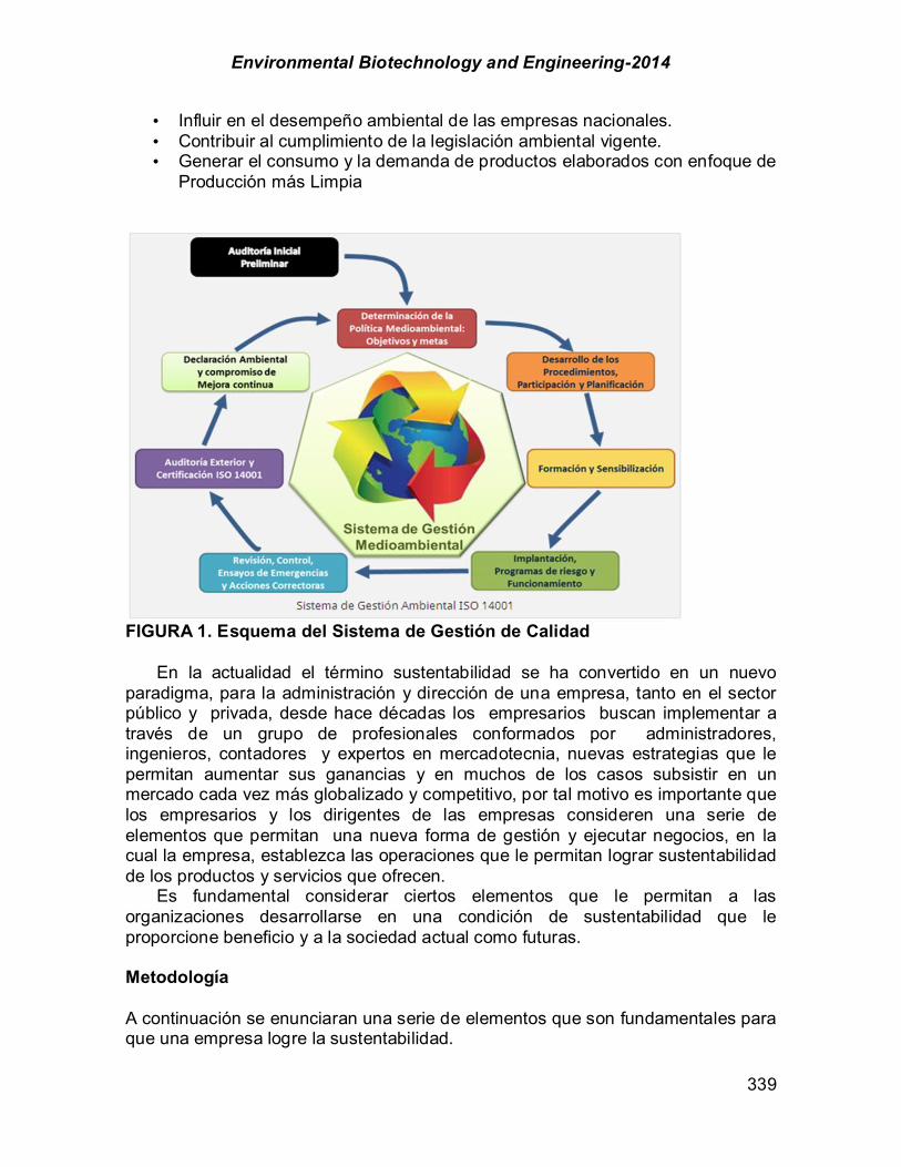
Environmental Biotechnology and Engineering-2014
339
• Influir en el desempeño ambiental de las empresas nacionales. • Contribuir al cumplimiento de la legislación ambiental vigente. • Generar el consumo y la demanda de productos elaborados con enfoque de
Producción más Limpia
FIGURA 1. Esquema del Sistema de Gestión de Calidad
En la actualidad el término sustentabilidad se ha convertido en un nuevo paradigma, para la administración y dirección de una empresa, tanto en el sector público y privada, desde hace décadas los empresarios buscan implementar a través de un grupo de profesionales conformados por administradores, ingenieros, contadores y expertos en mercadotecnia, nuevas estrategias que le permitan aumentar sus ganancias y en muchos de los casos subsistir en un mercado cada vez más globalizado y competitivo, por tal motivo es importante que los empresarios y los dirigentes de las empresas consideren una serie de elementos que permitan una nueva forma de gestión y ejecutar negocios, en la cual la empresa, establezca las operaciones que le permitan lograr sustentabilidad de los productos y servicios que ofrecen.
Es fundamental considerar ciertos elementos que le permitan a las organizaciones desarrollarse en una condición de sustentabilidad que le proporcione beneficio y a la sociedad actual como futuras. Metodología A continuación se enunciaran una serie de elementos que son fundamentales para que una empresa logre la sustentabilidad.

Environmental Biotechnology and Engineering-2014
340
• La ética y responsabilidad social y empresarial • El involucramiento positivo por parte de los dirigentes del gobierno en turno • Disminuir y de ser posible erradicar la corrupción • Programas de innovación tecnológica para las empresas • Programas de capacitación, evaluación del desempeño y de desarrollo del
capital humano en las organizaciones • La implementación de Sistemas de Gestión de Calidad Ambiental
La Responsabilidad Social Empresarial (RSE) es inherente a la empresa,
recientemente se ha convertido en una nueva forma de gestión y de hacer negocios, en la cual la empresa se ocupa de que sus operaciones sean sustentables en lo económico, lo social y lo ambiental, reconociendo los intereses de los distintos grupos con los que se relaciona Cajiga, (2010) y buscando la preservación del medio ambiente y la sustentabilidad de las generaciones futuras (Fórum de empresa)
Para cumplir con la responsabilidad social empresarial las empresas deben cumplir con las siguientes dimensiones Cajiga, (2010)
• Dimensión económica interna, su responsabilidad se enfoca a la generación y distribución del valor agregado entre colaboradores y accionistas, considerando no sólo las condiciones de mercado sino también la equidad y la justicia. Se espera de la empresa que genere utilidades y se mantenga viva y pujante (sustentabilidad).
• Dimensión económica externa, implica la generación y distribución de bienes y servicios útiles y rentables para la comunidad, además de su aportación a la causa pública vía la contribución impositiva. Asimismo, la empresa debe participar activamente en la definición e implantación de los planes económicos de su región y su país.
• Dimensión social interna, implica la responsabilidad compartida y subsidiaria de Inversionistas, directivos, colaboradores y proveedores para el cuidado y fomento de la calidad de vida en el trabajo y el desarrollo integral y pleno de todos ellos.
• Dimensión sociocultural y política externa, conlleva a la realización de acciones y aportaciones propias y gremiales seleccionadas para contribuir con tiempo y recursos a la generación de condiciones que permitan y favorezcan la expansión del espíritu empresarial y el pleno desarrollo de las comunidades y, por tanto, a un entorno de mercado favorable para el desarrollo de su negocio.
• En su dimensión ecológica interna, implica la responsabilidad total sobre las repercusiones ambientales de sus procesos, productos y subproductos; y, por lo tanto, la prevención —y en su caso remedio— de los daños que causen o pudieran causar.
• Dimensión ecológica externa, conlleva a la realización de acciones específicas para contribuir a la preservación y mejora de la herencia ecológica común para el bien de la humanidad actual y futura.

Environmental Biotechnology and Engineering-2014
341
Otro aspecto a considerar es la difusión de los programas de apoyo que ofrecen distintas dependencias como es el INAFED de la Secretaría de Gobernación con sus programa de desarrollo institucional ambiental, programa de desarrollo forestal entre otros, como también el CONACYT, COMECYT y la Secretaria de Economía a través del INADEM, que ofrecen apoyos para adquirir nuevas tecnologías permitiendo actualizar la maquinaria y equipo que se utiliza por parte del empresario y por ende mejorara sus procesos.
Es indispensable considerar que cuando se aplique un sistema de gestión de calidad del medio ambiente, se debe ofrecer capacitación a todos los niveles de la organización para que se familiaricen totalmente con el objetivo de calidad ambiental que se busca.
Al implementar un sistema de gestión calidad del medio ambiente, bajo un esquema de responsabilidad social y empresarial, sin descuidar ninguna de las dimensiones antes mencionadas, se puede considerar que una empresa cumple con los requisitos de sustentabilidad ambiental mejorando su imagen corporativa con la comunidad a través de productos y servicios conocidos como ecológicos o verdes, logrando un efecto psicológico positivo en el consumidor, que le permita al empresario contar con una ventaja competitiva para mejorar la venta de sus productos o servicios.
Resultados

Environmental Biotechnology and Engineering-2014
342
Conclusión El involucramiento de manera ética, por parte del gobierno, empresarios, comunidad y la implementación de estrategias para que permitan disminuir la corrupción son fundamentales para que se logren los objetivos de calidad ambiental, establecidos por los órganos internacionales como el apoyo para la adquisición de nuevas tecnologías y la capacitación constante de los colaboradores sobre el uso de las mismas, sin olvidar evaluar y recompensar el desempeño por cada uno de ellos. Referencias Blanco C. (2004) Gestión Ambiental “Camino al desarrollo sostenible“ Primera edición, Editorial San José (Costa Rica), EUNED, CR. ISBN 9968-31-273-8 El concepto de responsabilidad social empresarial, Centro Mexicano para la Filantropía,
03/07/2104. www.sosteniblepedia.org/index.php?...Públicos...grupos_de_interés_(sta... Manual de Contenidos de Fórum Empresa. 04/07/2104 Más información en www.empresa.org ISO 14001 Sistema de Gestión del Medio Ambiente. 04/07/2014. www.normas-iso.com/iso-14001 Centro de producción más limpia de Nicaragua. 01/07/2104.
www.cmpl.ipn.mx/portal/.../CesarBarahona-ONUDI-CNPL-NIC.pdf

Environmental Biotechnology and Engineering-2014
343
CHAPTER 2.9. INCUBADORA DE NEGOCIOS DEL TECNOLOGICO DE ESTUDIOS SUPERIORES DE ECATEPEC, COMO CATALIZADOR EN LA TRANSFERENCIA DE
TECNOLOGIA EN LAS PYMES DEL MUNICIPIO DE ECETEPEC
Germán Domínguez Bocanegra* (1); Fernando Cázares Padrón (1); Katulli Carmina Corral Miranda (1); Karla Ivette Téllez López (1);
Daniel Morales Chong (1).
(1) Maestría en Gestión Administrativa División de Contaduría y Administración Tecnológico del Estudios Superiores de Ecatepec [email protected]
Introducción En la actualidad podemos comprobar la importancia que tuvo la creación de las incubadoras de negocios dentro de las universidades en la década pasada, se ha convertido en un motor de suma importancia para el Estado de México, no solo al ofrecer la consultoría para la creación de nuevos negocios y asesoría en distintos rubros administrativos y técnicos para las empresas ya establecidas, como también en la generación de nuevos empleos para el país, con el transcurso del tiempo y la experiencia adquirida dentro de la incubadora del Tecnológico de Estudios Superiores de Ecatepec los funcionarios, consultores y docentes de distintas áreas del conocimiento, analizaron que la Incubadora puede participar como un catalizador en la transferencia de tecnología, debido a que muchos de las empresas incubadas con el apoyo de diversos consultores y profesores generan nuevas tecnologías o mejoras a las ya establecidas. Como es caso INENREN, establecido en 2008 como persona física con actividad empresarial; que logró el registro del RENIECYT, Registro Nacional de Instituciones y Empresas Científicas y Tecnológicas, del Consejo Nacional de Ciencia y Tecnología (CONACYT) que le permitió acceder y obtener financiamiento por parte del COMECYT, de $ 434000, en otros casos por lo general quedan como un bonito reconocimiento al esfuerzo sin obtener el beneficio esperado tanto para el empresario como para la comunidad. Metodología Para iniciar el proceso de Transferencia de Tecnología en el Estado de México, es muy conveniente analizar el diagnostico que se llevó a cabo en el Foro Científico y Tecnológico, AC (FCCyT), en el periodo 2004-2011, que nos permitirá un panorama más amplio de la situación actual en materia de transferencia de la tecnología el cual se divide en 5 apartados: ------------ *Author for all correspondence
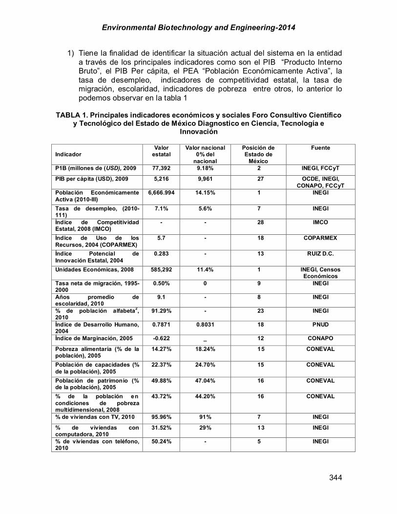
Environmental Biotechnology and Engineering-2014
344
1) Tiene la finalidad de identificar la situación actual del sistema en la entidad a través de los principales indicadores como son el PIB “Producto Interno Bruto”, el PIB Per cápita, el PEA “Población Económicamente Activa”, la tasa de desempleo, indicadores de competitividad estatal, la tasa de migración, escolaridad, indicadores de pobreza entre otros, lo anterior lo podemos observar en la tabla 1
TABLA 1. Principales indicadores económicos y sociales Foro Consultivo Científico y Tecnológico del Estado de México Diagnostico en Ciencia, Tecnología e
Innovación
Indicador
Valor estatal
Valor nacional 0% del
nacional
Posición de Estado de
México
Fuente
P1B (millones de (USD), 2009 77,392 9.18% 2 INEGI, FCCyT
PIB per cápita (USD), 2009 5,216 9,961 27 OCDE, INEGI, CONAPO, FCCyT
Población Económicamente Activa (2010-III)
6,666.994 14.15% 1 INEGI
Tasa de desempleo, (2010-111)
7.1% 5.6% 7 INEGI
Índice de Competitividad Estatal, 2008 (IMCO)
- - 28 IMCO
Índice de Uso de los Recursos, 2004 (COPARMEX)
5.7 - 18 COPARMEX
Índice Potencial de Innovación Estatal, 2004
0.283 - 13 RUIZ D.C.
Unidades Económicas, 2008 585,292 11.4% 1 INEGI, Censos Económicos
Tasa neta de migración, 1995-2000
0.50% 0 9 INEGI
Años promedio de escolaridad, 2010
9.1 - 8 INEGI
% de población alfabeta2, 2010
91.29% - 23 INEGI
Índice de Desarrollo Humano, 2004
0.7871 0.8031 18 PNUD
Índice de Marginación, 2005 -0.622 _ 12 CONAPO
Pobreza alimentaria (% de la población), 2005
14.27% 18.24% 15 CONEVAL
Población de capacidades (% de la población), 2005
22.37% 24.70% 15 CONEVAL
Población de patrimonio (% de la población), 2005
49.88% 47.04% 16 CONEVAL
% de la población en condiciones de pobreza multidimensional, 2008
43.72% 44.20% 16 CONEVAL
% de viviendas con TV, 2010 95.96% 91% 7 INEGI
% de viviendas con computadora, 2010
31.52% 29% 13 INEGI
% de viviendas con teléfono, 2010
50.24% - 5 INEGI

Environmental Biotechnology and Engineering-2014
345
Se realiza un análisis estadístico de los principales agentes del Sistema Estatal de Ciencia, Tecnología e Innovación (SECTI) en el Estado de México abarcando del 2004-2010, elaborado por el Sistema de Información Empresarial (SIEM), como es la estructura de las empresas registradas al RENIECYT, como se puede observar en la figura 1
FIGURA 1. Integrantes del RENIECYT en el estado en el 2012
Los registros de la Asociación Mexicana de Parques Industriales Privados (AMPIP) los cuales se observan en la figura 2 y tabla 2, como también se analiza el acervo de recursos destinados a la ciencia y tecnología, incluyendo investigadores miembros del Sistema Nacional de Investigadores (SIN), la matrícula universitaria y estudios de posgrado comprendidos en el periodo 2004-2009 de igual forma los centros de investigación con los que cuenta el estado así mismo los programas acreditados por el Consejo para la Acreditación de la Educación Superior (COPAES) además el (PNPC) y la productividad científica lo cual podemos observar en la figura 3.
FIGURA 2.Distribución de parques Industriales e incubadoras en el Estado

Environmental Biotechnology and Engineering-2014
346
TABLA 2. Descripción general de los parques industriales en el estado.
Descripción General Totales
Total empresas establecidas 792
Total de empleos generados 50, 697
Empresas grandes (más de 251 empleados) 253
Empresas medianas (51-250 empleados) 11
Empresas pequeñas (1150 empleados) 161
Empresas micro (0-10 empleados) 66
• En el estado de México se cuenta con 34 parques industriales registrados en el Sistema Mexicano de Promoción de Parques Industriales (SIMPPI); sin embrago, sólo 20 cuentan con información. Fuente: http://www.contactopyme.gob.mx/parques/intranets.asp
Consultado en noviembre de 2011.
FIGURA 3. Infraestructura para la investigación en el Estado de México
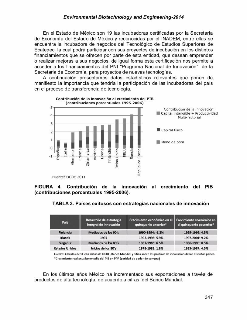
Environmental Biotechnology and Engineering-2014
347
En el Estado de México son 19 las incubadoras certificadas por la Secretaría de Economía del Estado de México y reconocidas por el INADEM, entre ellas se encuentra la incubadora de negocios del Tecnológico de Estudios Superiores de Ecatepec, la cual podrá participar con sus proyectos de incubación en los distintos financiamientos que se ofrecen por parte de esta entidad, que desean emprender o realizar mejoras a sus negocios, de igual forma esta certificación nos permite a acceder a los financiamientos del PNI “Programa Nacional de Innovación” de la Secretaria de Economía, para proyectos de nuevas tecnologías.
A continuación presentamos datos estadísticos relevantes que ponen de manifiesto la importancia que tendría la participación de las incubadoras del país en el proceso de transferencia de tecnología.
FIGURA 4. Contribución de la innovación al crecimiento del PIB (contribuciones porcentuales 1995-2006).
TABLA 3. Países exitosos con estrategias nacionales de innovación
En los últimos años México ha incrementado sus exportaciones a través de productos de alta tecnología, de acuerdo a cifras del Banco Mundial.

Environmental Biotechnology and Engineering-2014
348
FIGURA 5 .Exportación de productos de alta tecnología.
FIGURA 6. Producción científica con respecto al número de investigadores y artículos publicados.
Otro aspecto importante es el apoyo del Estado, para que empresarios mexicanos logren mayor número de registros de sus patentes y los puedan comercializar dentro y fuera del país. A partir de la década de los noventa, la legislación sobre propiedad intelectual se ha modificado para ajustarla a los nuevos tiempos, con el objeto de modernizar la normatividad en sintonía con los procesos de globalización de la economía mundial, mejorando con ello la protección de los derechos de propiedad intelectual. Estas modificaciones, que iniciaron con la Ley de Fomento y Protección de la Propiedad Industrial de 1991, tenían por objeto, entre otros, ampliar el campo de patentes en ciertas áreas del
Environmental Biotechnology and Engineering-2014
349
conocimiento que permitiera a los inventores mexicanos proteger y explotar sus invenciones a nivel nacional e internacional.
Como resultado de lo anterior, en el año 2000, de un total de 13,492 solicitudes de patente, 431 (3.2%) fueron de titulares mexicanos. En 2010 ingresaron al Instituto Mexicano de la Propiedad Industrial (lMPI) 15,527 solicitudes de patente, de las cuales 951 (6.12%) correspondieron a solicitantes mexicanos. Si bien entre el 2000 y el 2010 se observa un incremento de 120% en el número de solicitudes de mexicanos, la participación de titulares mexicanos sigue siendo baja. Las patentes concedidas a nacionales pasaron de 118 en 2000 a 229 en 2010.
Lo anterior es resultado de la difusión de información por parte del CONACYT y otros órganos como el COMECYT en el Estado de México, los cuales difunden la importancia del desarrollo de nuevas tecnologías, así como el registro de patentes en universidades, incubadoras y empresas.
3) Se realiza un análisis del SECTI; se describe como participan las instituciones del gobierno estatal, los sectores académico y empresarial como también se analizan las políticas implementadas por el CyT en la entidad, como la cantidad de recursos que se han destinado para el financiamiento del sector. El marco normativo del SECyT está encabezado por la Ley de Ciencia y Tecnología del Estado de México (LCyTEM), la cual fue publicada en el Periódico Oficial del estado el 17 de diciembre de 2004. Entre los principales temas que aborda están:
• Los principios orientadores a la actividad científica y tecnológica • Los instrumentos de apoyo a la actividad científica y tecnológica • El Programa Estatal de Ciencia y Tecnología • El Consejo Mexiquense de Ciencia y Tecnología (COMECyT) • El financiamiento a la CyT • Los recursos humanos para la CyT • La divulgación y fomento de la cultura científica tecnológica • La vinculación con el sector productivo, innovación y desarrollo tecnológico • La coordinación y descentralización
4) Se muestra resultados del Ranking Nacional de CTI, antes llamado
indicadores nacionales en CTI (ciencia, tecnología e innovación), elaborado por FCCyT, el cual describe de manera breve la metodología, las variables consideradas y los principales resultado para el Estado de México.

Environmental Biotechnology and Engineering-2014
350
FIGURA 7. Ranking Nacional en CTI del Estado de México.
FIGURAS 8 y 9. Ranking de ciencia tecnología e innovación en México.
5) Se realiza un análisis FODA en el SECTI del Estado de México.

Environmental Biotechnology and Engineering-2014
351
RESULTADOS
A continuación se mostraran los resultados obtenidos del diagnóstico practicado a los consultores de la incubadora de negocios, funcionarios del departamento de gestión tecnológica del Tecnológico de Estudios Superiores de Ecatepec y empresarios del Municipio de Ecatepec, que nos permitirá determinar si es conveniente la creación de un Centro de Transferencia de Tecnología, se utilizaran herramientas administrativas para llevar a cabo el análisis como son la Técnica del Radar y el Análisis de Campo de fuerza.
Técnica de radar
El grafico pone al descubierto que contamos con un mercado muy amplio en el Municipio de Ecatepec para el desarrollo y ofrecimiento de nuevas tecnologías.
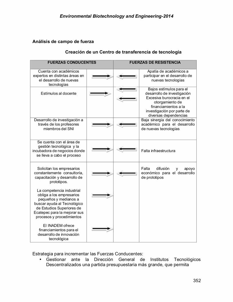
Environmental Biotechnology and Engineering-2014
352
Análisis de campo de fuerza
Creación de un Centro de transferencia de tecnología
FUERZAS CONDUCENTES FUERZAS DE RESISTENCIA
Cuenta con académicos expertos en distintas áreas en
el desarrollo de nuevas tecnologías
Apatía de académicos a participar en el desarrollo de
nuevas tecnologías
Estímulos al docente
Bajos estímulos para el desarrollo de investigación Excesiva burocracia en el
otorgamiento de financiamientos a la
investigación por parte de diversas dependencias
Desarrollo de investigación a través de los profesores
miembros del SNI
Baja sinergia del conocimiento académico para el desarrollo de nuevas tecnologías
Se cuenta con el área de gestión tecnológica y la
incubadora de negocios donde se lleva a cabo el proceso
Falta infraestructura
Solicitan los empresarios
constantemente consultoría, capacitación y desarrollo de
prototipos.
La competencia industrial obliga a los empresarios pequeños y medianos a
buscar ayuda al Tecnológico de Estudios Superiores de
Ecatepec para la mejorar sus procesos y procedimientos
El INADEM ofrece
financiamientos para el desarrollo de innovación
tecnológica
Falta difusión y apoyo económico para el desarrollo de prototipos
Estrategia para incrementar las Fuerzas Conducentes: • Gestionar ante la Dirección General de Institutos Tecnológicos
Descentralizados una partida presupuestaria más grande, que permita
Environmental Biotechnology and Engineering-2014
353
• estimular al investigador para que trabaje en el desarrollo de nuevas tecnologías.
• Se puede obtener apoyo económico del Gobierno del Estado de México, COMECYT y Tecnológico de Estudios Superiores de Ecatepec para reunir la infraestructura necesaria que requiere el Centro de Transferencia de Tecnología.
• Fomentar la formación de grupos interdisciplinarios de investigadores dentro del Tecnológico de Estudios Superiores de Ecatepec que desarrollen dentro y fuera de las instalaciones su labor.
• Desarrollar un Centro específico e independiente de Transferencia de Tecnología que permita atender de manera más eficaz las necesidades del sector productivo.
• Solicitar cursos para bajar el recurso tanto para investigadores como docentes ante las distintas dependencias que ofrecen financiamiento para el desarrollo de nuevas tecnologías
Conclusión El Tecnologico de Estudios Superiores de Ecatepec, cuenta con los elementos suficientes para creacion de un Centro de Transferencia de Tecnologia que permita de manera mas satisfactoria el desarrollo de las PYMEs del Estado de Mexico y por ende del pais, mediante el desarrollo de nuevas tecnologias y el mejor aprovechamiento de las mismas, lo que falta es unir los elementos y aplicar algunos adicionales que permita al Tecnologico de Estudios Superiores de Ecatepec brindar un mejor servicio al sector productivo del Municipio y Estado de Mexico. Referencias María Luisa Zaragoza, Elmer Solano Flores, Brenda Figueroa Ramírez, Foro Consultivo
Científico y Tecnológico Diagnostico de Ciencia y Tecnología e Innovación del Estado de México 2004-2011 p.p 9-25. www.foroconsultivo.org.mx/libros_editados/.../estado_mexico.pdf
García Martínez y Ramos Cáceres Realidad, mitos y oportunidades de las universidades en la transferencia del conocimiento
2010 “Factores que limitan la transferencia de conocimientos mediante la incubación de
empresas universitarias”p.p 6-7,10-14 www.academia.edu/.../Factores_que_limitan_la_transferencia_de_conoci. Programa Nacional de Innovación de la Secretaria de Economía Comité Intersectorial para la Innovación México 2011p.p 6-8, 20-29, 32-33, 41,
Environmental Biotechnology and Engineering-2014
354
CHAPTER 2.10. POTENCIAL DE SISTEMAS PASIVOS DE ENFRIAMIENTO Y CALEFACCIÓN COMO ESTRATEGIAS SUSTENTABLES PARA REDUCIR EL
CONSUMO DE ENERGÍA EN EDIFICACIONES EN REGIONES CÁLIDO ÁRIDAS
José Roberto García Chávez* (1); Francisco Fernández Melchor (2)
(1) Universidad Autónoma Metropolitana-Azcapotzalco. División de Ciencias y Artes para el Diseño. Departamento de Medio Ambiente. Área de Arquitectura Bioclimática. Posgrado en Diseño. San Pablo 180. Colonia Reynosa Tamaulipas. C.P. 02200, México, D.F. Tel. 52 55 5318-9110. e-mail: [email protected] (2) Universidad Autónoma Metropolitana-Azcapotzalco. División de Ciencias y Artes para el Diseño. Posgrado en Diseño. San Pablo 180. Colonia Reynosa Tamaulipas. C.P. 02200, México, D.F. e-mail: [email protected] ABSTRACT At present, hot dry regions in Mexico occupy more than seventy-five percentage of total land surface with severe climate conditions for both cooling and heating seasons. The buildings located in these regions present large energy consumption patterns due to their high dependence on air conditioning (AC) for providing comfort to the occupants, which in turns provokes the emission of huge amounts of greenhouse gasses (GHG) to the atmosphere, affecting the environment at regional al global levels. For those people who cannot afford AC in their buildings, the situation is even worse, as it severely affects their health conditions. This research work deals with the investigation of several passive cooling and heating techniques in experimental modules aimed at achieving hygrothermal conditions for building occupants. These cooling techniques involved the four environmental heat sinks and included: Ground cooling, solar control, night ventilation, direct evaporative cooling, night sky infrared radiation and thermal insulation. During the typical underheating season, direct and indirect heating techniques along with infiltration control and thermal insulation were implemented and examined. These systems were built and implemented in experimental cells during the prevailing overheating and underheating periods and the results showed that the combined effect of the strategies provided more promising synergy results than the single influence of any of them. During the underheating period, the indoor minimum temperature was 15° C, and the maximum temperature during the overheating season registered 29° C. Therefore, it is suggested to implement the combined action of the passive cooling and heating techniques in buildings located in representative hot dry regions of Mexico, to improve hygrothermal comfort and to reduce the energy consumption for AC and this would eventually reduces the emission of pollutants to the environment. Keywords: Energy, Passive Cooling, Passive Heating, Environmental Strategies, Energy Consumption, Sustainability. ------------ *Author for all correspondence
Environmental Biotechnology and Engineering-2014
355
RESUMEN Actualmente, las regiones cálidas y secas en México ocupan más de setenta y cinco años el porcentaje de la superficie total de tierras con condiciones climáticas severas para ambas estaciones de refrigeración y calefacción. Los edificios situados en estas regiones presentan patrones de consumo de energía elevados, debido a su gran dependencia del aire acondicionado (AC), para proporcionar confort a los ocupantes, lo que a su vez provoca la emisión de grandes cantidades de gases de efecto invernadero (GEI) a la atmósfera, afectando el medio ambiente a nivel mundial y regional. Para aquellas personas que no pueden permitirse el lujo de tener AC en sus edificios, la situación es aún peor, ya que afecta gravemente sus condiciones de salud. En este trabajo, se investigaron diversos sistemas de enfriamiento y calefacción pasivos, en módulos experimentales. Los sistemas investigados incluyeron los cuatro disipadores de calor ambientales, con técnicas de intercambiadores de calor aire-tierra, control solar, ventilación nocturna, aislamiento térmico, control de la infiltración, enfriamiento evaporativo directo y emisión de radiación nocturna. Estos sistemas fueron construidos e implementados en módulos experimentales y su comportamiento higrotérmico evaluado durante los períodos representativos de bajocalentamiento y sobrecalentamiento. Los resultados indicaron que el efecto combinado de los sistemas investigados presentó un comportamiento más favorable que el efecto individual de cada estrategia. Durante el período de bajocalentamiento, la temperatura mínima interior fue de 15 °C, y la temperatura máxima durante el período de sobrecalentamiento de 29 ° C. Por lo tanto, se sugiere implementar en las regiones predominantemente cálidas áridas de México, la acción combinada de los sistemas pasivos de enfriamiento y calentamiento, como los investigados en este trabajo, para mejorar el confort higrotérmico de los ocupantes de edificaciones y para reducir el consumo de energía del AC, y con la aplicación de estas medidas, es posible reducir también la emisión de contaminantes al medio ambiente. Palabras Clave: Energía, Enfriamiento Pasivo, Calentamiento Pasivo, Estrategias Ambientales, Consumo de Energía, Sustentabilidad. Introducción
El crecimiento en la población, la industrialización creciente y la intensiva urbanización, que se han extendido en diversas regiones del planeta, sobre todo a partir de mediados del siglo XX hasta la actualidad, han ocasionado un aumento excesivo en el consumo de energía, debido a las actividades antropogénicas. Además, cada vez se utiliza más energía, derivada de petróleo, carbón y/gas natural (combustibles fósiles), en diversas actividades en todos los sectores, incluyendo las edificaciones. Los gases de efecto invernadero (GEI), principalmente la quema de dióxido de carbono (CO2) se emiten al medio ambiente, lo que representa un riesgo inminente para la salud de las personas.

Environmental Biotechnology and Engineering-2014
356
Por lo tanto, es de suma importancia tener en cuenta el equilibrio adecuado de los factores ambientales que intervienen en el diseño de la arquitectura de cualquier espacio y edificio. El aumento de las emisiones de GEI en el sector de las edificaciones, representaron el 18% de las emisiones directas de CO2, de los cuales el 11% fueron por el uso del aire acondicionado (HVAC), sistemas, electrodomésticos e iluminación (IPCC, 2007). Esta situación ha provocado, junto con las emisiones de la industria y el transporte, un severo deterioro ambiental en el planeta (Figura 1).
FIGURA 1. Producción de GEI en grandes conglomerados urbanos Sistemas Bioclimáticos Aplicados en las Edificaciones en Regiones Cálido-Aridas. En la actualidad, hay aproximadamente 23 millones de viviendas con electricidad en México, situación que a su vez implica una gran demanda de electricidad y de hidrocarburos (CONAVI, 2007). La integración de estrategias bioclimáticas, basado en la aplicación de técnicas pasivas puede reducir significativamente el consumo de energía, así como proporcionar confort higrotérmico a los ocupantes y reducción de las emisiones de CO2 a la atmósfera [García Chávez, 2004). Las técnicas pasivas bioclimáticas analizadas en este trabajo, particularmente aplicables en regiones cálido áridas, incluyeron: orientación adecuada, color de la superficie apropiada, control solar, calentamiento y enfriamiento por transferencia de calor aire-tierra, ventilación natural inducida, masa térmica, aislamiento térmico, y enfriamiento evaporativo directo, ente otros. Caso de Estudio. Los sistemas bioclimáticos mencionados anteriormente fueron implementados y evaluados en módulos experimentales construidos para esta investigación. Estos módulos se encuentran al norte de la Zona Metropolitana

Environmental Biotechnology and Engineering-2014
357
del Valle México, en un área que ofrece las condiciones adecuadas para la realización de las pruebas. Los resultados se extrapolarán a lugares con clima predominantemente cálido árido del país. Estos módulos fueron construidos con paneles livianos de poliestireno, con las siguientes dimensiones: 2.44 metros de longitud, 1.22 metros de ancho y espesor 0.051metros, sobre una losa de cimentación de concreto armado (Figura 2). FIGURA 2. Infraestructura de los módulos experimentales Análisis de Asoleamiento y de Obstrucciones. Para determinar la orientación óptima de los seis módulos experimentales, se realizó el trazo del norte geográfico solar verdadero para asegurarse que los módulos tuvieran la orientación más favorable. Además, se hizo un análisis de imágenes digitales para que todos los módulos tuvieran la misma exposición a la radiación solar y evitar posibles obstrucciones y evitar el auto-sombreado entre los módulos (Figura 3) FIGURA 3. Ubicación de los módulos experimentales y análisis de asoleamiento (Ejemplo: Para Diciembre 21, 16:49 hr., con la máxima extensión de la sombra en el período de bajocalentamiento)

Environmental Biotechnology and Engineering-2014
358
Condiciones del clima en el sitio experimental. Las condiciones climáticas de la ubicación del caso de estudio indican que la temperatura promedio anual es de 17.5 ° C, el mes de mayo es el más caliente con 20 ° C y el mes más frío en enero con 14.6 ° C. La oscilación térmica promedio es de 13 K. La humedad relativa mínima en los meses de febrero, marzo y abril está por debajo de las condiciones de confort, mientras que la humedad relativa media anual es del 60%, 45% es la humedad relativa media mensual mínima, que se registra en marzo, abril, y el 74%, la humedad relativa media mensual máxima, que se registra en septiembre. Las precipitaciones varían a lo largo del año, aumentan considerablemente en junio, julio, agosto y septiembre. Siendo julio el mes más lluvioso con 189.5 mm.
La precipitación promedio anual es de 846.2 mm. Datos de viento disponible indica que la dirección del viento a lo largo de la mayor parte del año, viene de la NE, con una velocidad anual promedio de 1.4 m/segundo y un valor máximo de 2.4 m/segundo. Metodología Sistema Subterráneo de Intercambio Térmico Aire-Tierra. Para evaluar el comportamiento térmico de la estrategia de enfriamiento y calentamiento conductivos, se colocaron a una profundidad de 1.60 metros, ductos subterráneos de policloruro de vinilo (pvc) de 100 mm de diámetro, en una longitud de 24 metros (Figura 4). Los resultados se compararon con uno de los módulos, denominado “Módulo de Control”. Durante una etapa previa, se realizó una calibración de todos los módulos, consistente en llevar a cabo un registro de las temperaturas al centro de las diversas superficies interiores de los módulos, incluyendo el plafón. Este registro de las condiciones interiores se realizó durante un período representativo de 10 días consecutivos. Los resultados obtenidos indicaron que hay una consistencia en los valores de temperaturas de todos los módulos, incluyendo el “Módulo de Control”. Con base en estos resultados, la comparación de todas las estrategias bioclimáticas a evaluar es válida y confiable. Los ductos subterráneos se instalaron en el módulo experimental de prueba, la parte inferior del lado norte y se integran con un ventilador de baja potencia para extraer el aire del interior del sistema subterráneo. Se instalaron sistemas de adquisición de datos en los 4 muros interiores, el plafón y al centro del espacio de ambos módulos, el de control y el de prueba, en las mismas posiciones, para registrar los valores de temperatura de bulbo seco y humedad relativa. El registro de estos valores se realizó durante los períodos representativos de bajocalentamiento (Diciembre) y sobrecalentamiento (Marzo) del lugar de las pruebas del caso de estudio, durante 10 días consecutivos.
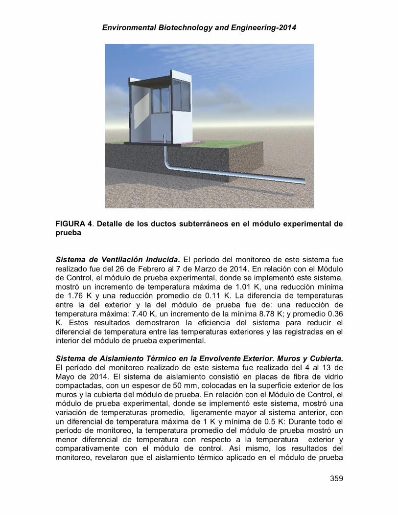
Environmental Biotechnology and Engineering-2014
359
FIGURA 4. Detalle de los ductos subterráneos en el módulo experimental de prueba Sistema de Ventilación Inducida. El período del monitoreo de este sistema fue realizado fue del 26 de Febrero al 7 de Marzo de 2014. En relación con el Módulo de Control, el módulo de prueba experimental, donde se implementó este sistema, mostró un incremento de temperatura máxima de 1.01 K, una reducción mínima de 1.76 K y una reducción promedio de 0.11 K. La diferencia de temperaturas entre la del exterior y la del módulo de prueba fue de: una reducción de temperatura máxima: 7.40 K, un incremento de la mínima 8.78 K; y promedio 0.36 K. Estos resultados demostraron la eficiencia del sistema para reducir el diferencial de temperatura entre las temperaturas exteriores y las registradas en el interior del módulo de prueba experimental. Sistema de Aislamiento Térmico en la Envolvente Exterior. Muros y Cubierta. El período del monitoreo realizado de este sistema fue realizado del 4 al 13 de Mayo de 2014. El sistema de aislamiento consistió en placas de fibra de vidrio compactadas, con un espesor de 50 mm, colocadas en la superficie exterior de los muros y la cubierta del módulo de prueba. En relación con el Módulo de Control, el módulo de prueba experimental, donde se implementó este sistema, mostró una variación de temperaturas promedio, ligeramente mayor al sistema anterior, con un diferencial de temperatura máxima de 1 K y mínima de 0.5 K: Durante todo el período de monitoreo, la temperatura promedio del módulo de prueba mostró un menor diferencial de temperatura con respecto a la temperatura exterior y comparativamente con el módulo de control. Así mismo, los resultados del monitoreo, revelaron que el aislamiento térmico aplicado en el módulo de prueba
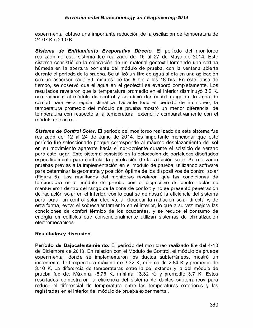
Environmental Biotechnology and Engineering-2014
360
experimental obtuvo una importante reducción de la oscilación de temperatura de 24.07 K a 21.0 K. Sistema de Enfriamiento Evaporativo Directo. El período del monitoreo realizado de este sistema fue realizado del 16 al 27 de Mayo de 2014. Este sistema consistió en la colocación de un material geotextil formando una cortina húmeda en la abertura poniente del módulo de prueba, con la ventana abierta durante el período de la prueba. Se utilizó un litro de agua al día en una aplicación con un aspersor cada 90 minutos, de las 9 hrs a las 18 hrs. En este lapso de tiempo, se observó que el agua en el geotextil se evaporó completamente. Los resultados revelaron que la temperatura promedio en el interior disminuyó 3.2 K, con respecto al módulo de control y se ubicó dentro del rango de la zona de confort para esta región climática. Durante todo el período de monitoreo, la temperatura promedio del módulo de prueba mostró un menor diferencial de temperatura con respecto a la temperatura exterior y comparativamente con el módulo de control. Sistema de Control Solar. El período del monitoreo realizado de este sistema fue realizado del 12 al 24 de Junio de 2014. Es importante mencionar que este período fue seleccionado porque corresponde al máximo desplazamiento del sol en su movimiento aparente hacia el nor-poniente durante el solsticio de verano para este lugar. Este sistema consistió en la colocación de parteluces diseñados específicamente para controlar la penetración de la radiación solar. Se realizaron pruebas previas a la implementación en el módulo de prueba, utilizando software para determinar la geometría y posición óptima de los dispositivos de control solar (Figura 5). Los resultados del monitoreo revelaron que las condiciones de temperatura en el módulo de prueba con el dispositivo de control solar se mantuvieron dentro del rango de la zona de confort y no se presentó penetración de radiación solar en el interior, con lo cual se demostró la eficiencia del sistema para lograr un control solar efectivo, al bloquear la radiación solar directa y, de esta forma, evitar el sobrecalentamiento en el interior, lo que a su vez mejora las condiciones de confort térmico de los ocupantes, y se reduce el consumo de energía en edificios que convencionalmente utilizan sistemas de climatización electromecánicos. Resultados y discusión Período de Bajocalentamiento. El período del monitoreo realizado fue del 4-13 de Diciembre de 2013. En relación con el Módulo de Control, el módulo de prueba experimental, donde se implementaron los ductos subterráneos, mostró un incremento de temperatura máxima de 3.32 K, mínima de 2.84 K y promedio de 3.10 K. La diferencia de temperaturas entre la del exterior y la del módulo de prueba fue de: Máxima: -6.76 K, mínima 13.32 K; y promedio 3.7 K. Estos resultados demostraron la eficiencia del sistema de ductos subterráneos para reducir el diferencial de temperatura entre las temperaturas exteriores y las registradas en el interior del módulo de prueba experimental.
Environmental Biotechnology and Engineering-2014
361
Período de Sobrecalentamiento. El período del monitoreo realizado fue del 10 al 23 de Marzo de 2014. En relación con el Módulo de Control, el módulo de prueba experimental, donde se implementaron los ductos subterráneos, mostró una reducción de temperatura máxima de 7.13 K, mínima de 1.14 K y promedio de 3.12 K. La diferencia de temperaturas entre la del exterior y la del módulo de prueba fue de: Máxima: 5.3 K, mínima 6.01 K; y promedio 1.22 K. Estos resultados demostraron la eficiencia del sistema de ductos subterráneos para reducir el diferencial de temperatura entre las temperaturas exteriores y las registradas en el interior del módulo de prueba experimental. FIGURA 5. Dispositivos de control solar verticales en la abertura poniente del módulo de prueba. Vista exterior e interior. Conclusiones Los resultados de esta investigación indicaron que los sistemas bioclimáticos evaluados son una alternativa prometedora para reducir el consumo de energía al tiempo que pueden contribuir a lograr condiciones de confort higrotérmicos para los ocupantes. En la siguiente etapa de este trabajo, los resultados se extrapolarán para otras regiones climáticas del país, por medio de la implementación de modelos matemáticos, donde, debido a las condiciones climáticas más severas; los resultados pueden ser aún más favorables. Por otra parte, los resultados de esta investigación se pueden incluso optimizar, con la integración de todos los sistemas bioclimáticos, evaluados individualmente en este trabajo. La integración de estos sistemas tiene un enfoque sustentable y puede aplicarse en edificios nuevos como existentes. Con la implementación de estos sistemas a nivel masivo, es viable reducir la emisión de gases de efecto invernadero, mejorar el medio ambiente y la calidad de vida. Referencias IPCC AR4 SYR (2007), Core Writing Team; Pachauri, R.K; and Reisinger, A., ed., Climate Change
2007: Synthesis Report, Contribution of Working Groups I, II and III to the Fourth Assessment Report of the Intergovernmental Panel on Climate Change, IPCC, ISBN 92-9169-122-4.
Environmental Biotechnology and Engineering-2014
362
CHAPTER 2.11. DISEÑO, CARACTERIZACIÓN Y EVALUACIÓN DE UN HÁBITAT BIOCLIMÁTICO SUSTENTABLE EN UN CLIMA CÁLIDO HÚMEDO
José Roberto García Chávez* (1); Francisco Fernández Melchor (2)
(1) Universidad Autónoma Metropolitana-Azcapotzalco. División de Ciencias y Artes para el Diseño. Departamento de Medio Ambiente. Área de Arquitectura Bioclimática. Posgrado en Diseño. San Pablo 180. Colonia Reynosa Tamaulipas. C.P. 02200, México, D.F. Tel. 52 55 5318-9110. e-mail: [email protected] (2) Universidad Autónoma Metropolitana-Azcapotzalco. División de Ciencias y Artes para el Diseño. Posgrado en Diseño. San Pablo 180. Colonia Reynosa Tamaulipas. C.P. 02200, México, D.F. e-mail: [email protected] ABSTRACT Buildings located in humid climates of Mexico present large amounts of energy consumption due to the excessive use of air conditioning systems (AC). This research presents the design, characterization and evaluation of a prototype house, as a case study, located in the city of Veracruz, Veracruz, which is representative of a typical warm humid climate. The results of this work focused on establishing criteria, strategies and systems so that the diverse architectural spaces of this habitat responded harmoniously to the surrounding natural environment. It was found that the implementation of the bioclimatic strategies can help to improve the occupant’s hygrothermal comfort conditions whilst reducing the energy consumption and the emission of greenhouse gasses to the environment. Keywords: Bioclimatic design, humid climates, health, hygrothermal comfort, energy savings. RESUMEN Las edificaciones ubicadas en climas cálidos húmedos de México, presentan un enorme consumo de energía por la excesiva utilización de sistemas de aire acondicionado (AC). En esta investigación se presenta el diseño, caracterización y evaluación de una vivienda prototipo como caso de estudio, ubicada en la ciudad de Veracruz, Veracruz; lugar con un clima representativo cálido húmedo. Los resultados de este trabajo se enfocaron a establecer criterios, estrategias y sistemas para que los diversos espacios arquitectónicos de este hábitat respondan armónicamente al entorno natural circundante.
Los resultados indicaron que la implementación de estrategias bioclimáticas en edificios habitacionales puede contribuir a mejorar las condiciones de confort higrotérmico de los ocupantes, así como a reducir el consumo de energía y la emisión de gases de efecto invernadero al medio ambiente. ------------ *Author for all correspondence
Palabras Clave: Diseño bioclimático, climas cálidos húmedos, salud, confort higrotérmico, ahorro de energía.
Environmental Biotechnology and Engineering-2014
363
Introducción El consumo de energía para la climatización artificial de edificaciones ubicadas en climas cálido húmedos es muy elevado. Esta situación provoca afectaciones económicas por el alto costo de la energía eléctrica, y emisión de gases de efecto invernadero (GEI) a la atmósfera, lo cual afecta el medio ambiente y la salud de las personas. En los edificios que no cuentan con AC, el problema es mayor porque afecta severamente la salud, eficiencia y productividad de sus ocupantes. Caso de Estudio Ciudad de Veracruz. En este trabajo, se analizó la situación del alto consumo de energía de viviendas, y su impacto en el medio ambiente y se plantearon estrategias bioclimáticas para coadyuvar a la solución de esta problemática. Se seleccionó la ciudad de Veracruz como caso de estudio, que presenta un clima cálido húmedo representativo a nivel nacional. La ciudad de Veracruz es la más grande del estado y cuenta con el puerto marítimo y comercial más importante de México, con una población total de 552,156 habitantes en 2010 (INEGI 2014). En este contexto, es importante lograr un crecimiento correctamente planeado, con un diseño de viviendas adecuado a las condiciones climáticas de altas temperaturas y elevada humedad, presentes todo el año en la región. El clima cálido húmedo de Veracruz (Figura 1) presenta una temperatura media del mes más cálido por encima de los 26°C y una precipitación pluvial anual superior a 1,000 mm. El análisis climatológico se realizó a partir de los datos obtenidos de la estación meteorológica más cercana a la ciudad, con un periodo normalizado con lecturas de 1951 a 2010 del Servicio Meteorológico Nacional (SMN, 2014). Análisis Climático de Veracruz, Veracruz. Clima Cálido Húmedo Representativ.El desarrollo del análisis climático del lugar seleccionado incluyó las siguientes variables climáticas: Temperatura. El primer parámetro analizado fue la temperatura, cuyas lecturas normalizadas indican que la temperatura media del mes más caluroso (Mayo) es de 27.8°C, lo que lo clasifica como clima característicamente “cálido”. En este análisis, se aplicó la Zona de Confort establecida por Szokolay (Szokolay, 2004), que utiliza la temperatura neutra como punto térmico medio y límites de confort de +2.5°C y -2.5°C, y se utilizó el programa Bat. Con estos límites de confort, se observa que la temperatura máxima promedio está por encima desde Febrero hasta Noviembre; la temperatura media mensual está en confort, con excepción de Diciembre, Enero y Febrero, donde se encuentra un poco por debajo de dicho confort y por último la temperatura mínima promedio todo el año se encuentra por debajo del límite inferior de la Zona de Confort (Figura 2).
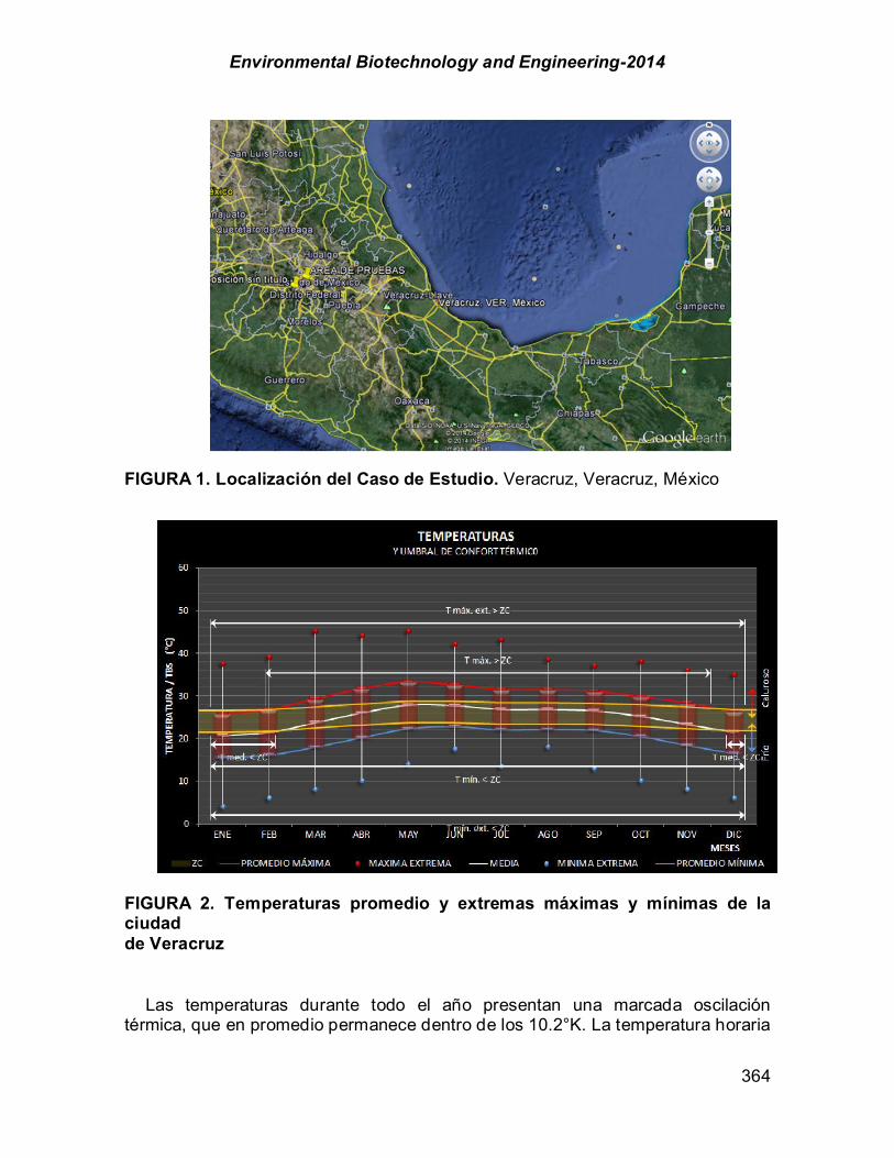
Environmental Biotechnology and Engineering-2014
364
FIGURA 1. Localización del Caso de Estudio. Veracruz, Veracruz, México
FIGURA 2. Temperaturas promedio y extremas máximas y mínimas de la ciudad de Veracruz
Las temperaturas durante todo el año presentan una marcada oscilación térmica, que en promedio permanece dentro de los 10.2°K. La temperatura horaria

Environmental Biotechnology and Engineering-2014
365
se incrementa notablemente de Abril a Septiembre, presentando un alto sobrecalentamiento de 13:00 a 19:00 horas, intensificándose en el mes de Mayo de 14:00 a 17:00 hrs con una temperatura superior a los 33°C (Figura 3). FIGURA 3. Temperaturas horarias de la ciudad de Veracruz
Las principales estrategias de diseño bioclimático para contrarrestar las altas temperaturas es el enfriamiento pasivo, ya que todo el año predominan las altas temperaturas y solo un pequeño periodo de Diciembre a Febrero presenta bajas temperaturas por las noches y mañanas. Humedad. La humedad relativa media y máxima se encuentran por encima de confort todo el año excediendo en todo momento el 70%, únicamente la humedad relativa mínima, que se presenta predominantemente por las tardes se encuentra dentro de confort (Figura 4). FIGURA 4. Humedad relativa máxima mínima y promedio de la ciudad de Veracruz.
Los elevados niveles de humedad relativa indican la importancia de implementar la estrategia de deshumidificación durante prácticamente todo el año.

Environmental Biotechnology and Engineering-2014
366
Los niveles limitadamente confortables de humedad relativa fluctúan de 12:00 a 20:00 horas, presentándose problemas de niveles de humedad del aire excesivo, las noches y mañanas, cuando todo el año se supera el 70% (Figura 5).
FIGURA 5. Humedades relativas horarias de la ciudad de Veracruz. Precipitación. La precipitación pluvial total anual es de 1,701.2 mm, lo que confirma a este clima como húmedo. Los meses que registran una alta precipitación por arriba de los 150 mm, van de Junio a Octubre; siendo el mes de Julio el que presenta una mayor precipitación mensual con 389.8 mm. Los meses de Mayo y Noviembre presentan una precipitación moderada entre los 40 a 150 mm. Los meses de Diciembre a Abril tienen una precipitación baja menor a los 40 mm (Figura 6).
FIGURA 6. Precipitación pluvial y evaporación de la ciudad de Veracruz Estrategias de Diseño Bioclimático. Requerimientos de Enfriamiento y Calentamiento Pasivos. Los requerimientos de enfriamiento y calentamiento o días grado, se relacionan con el parámetro denominado “Días-Grado”, que

Environmental Biotechnology and Engineering-2014
367
representa los requerimientos de calentamiento o enfriamiento, en grados Celsius o Kelvin (K), necesarios para alcanzar la Zona de Confort, que se acumulan, generalmente en un mes, o bien puede ser también por semana o bien a nivel horario.
Los “Días-Grado” para la ciudad de Veracruz (Figura 7), revelan que existen requerimientos tanto de calentamiento como de enfriamiento para entrar en Zona de Confort. El calentamiento es necesario durante todo el año, siendo mínimo en Junio y durante los meses de verano.
Por otra parte, los requerimientos de enfriamiento se presentan de Marzo a Noviembre. Durante los meses de Abril, Mayo y Junio, se incrementan y alcanzan un máximo de 142 K para Mayo, que es el mes más cálido.
El diagrama bioclimático anual (Figura 8), y por ser un clima cálido todo el año, indica que las principales estrategias de Diseño Bioclimático son el sombreado y control solar para contrarrestar las elevadas temperaturas, complementadas con ventilación natural, para promover las estrategias de enfriamiento y de deshumidificación.
FIGURA 7. Requerimientos de enfriamiento y calentamiento (“Días-Grado”,) para la ciudad de Veracruz
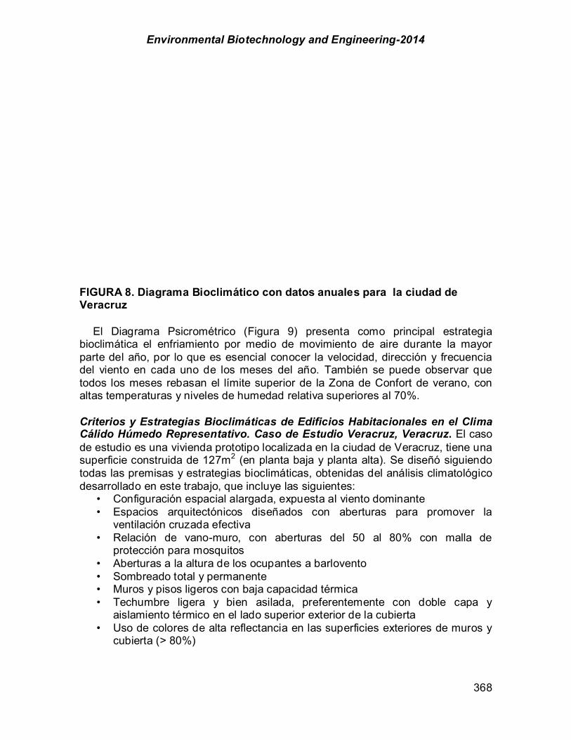
Environmental Biotechnology and Engineering-2014
368
FIGURA 8. Diagrama Bioclimático con datos anuales para la ciudad de Veracruz
El Diagrama Psicrométrico (Figura 9) presenta como principal estrategia bioclimática el enfriamiento por medio de movimiento de aire durante la mayor parte del año, por lo que es esencial conocer la velocidad, dirección y frecuencia del viento en cada uno de los meses del año. También se puede observar que todos los meses rebasan el límite superior de la Zona de Confort de verano, con altas temperaturas y niveles de humedad relativa superiores al 70%.
Criterios y Estrategias Bioclimáticas de Edificios Habitacionales en el Clima Cálido Húmedo Representativo. Caso de Estudio Veracruz, Veracruz. El caso de estudio es una vivienda prototipo localizada en la ciudad de Veracruz, tiene una superficie construida de 127m2 (en planta baja y planta alta). Se diseñó siguiendo todas las premisas y estrategias bioclimáticas, obtenidas del análisis climatológico desarrollado en este trabajo, que incluye las siguientes:
• Configuración espacial alargada, expuesta al viento dominante • Espacios arquitectónicos diseñados con aberturas para promover la
ventilación cruzada efectiva • Relación de vano-muro, con aberturas del 50 al 80% con malla de
protección para mosquitos • Aberturas a la altura de los ocupantes a barlovento • Sombreado total y permanente • Muros y pisos ligeros con baja capacidad térmica • Techumbre ligera y bien asilada, preferentemente con doble capa y
aislamiento térmico en el lado superior exterior de la cubierta • Uso de colores de alta reflectancia en las superficies exteriores de muros y
cubierta (> 80%)

Environmental Biotechnology and Engineering-2014
369
• Aislamiento térmico efectivo en cubierta y muros, con un coeficiente de conductividad de 0.034 a 0.045 W/mK, preferentemente de alta densidad, que presenta menor valor de conductividad.
FIGURA 9. Diagrama Psicrométrico con datos mensuales y zonas de estrategias de Diseño Bioclimático para la ciudad de Veracruz
La cubierta debe ser inclinada por las intensas lluvias (de más de 150 mm) presentes en el lugar analizado, principalmente de Junio a Septiembre.
El dimensionamiento y geometría de las ventanas debe permitir una adecuada ventilación y estas deben integrarse con dispositivos fijos de control solar para evitar ganancias solares y promover las pérdidas de calor del interior, entre otras estrategias bioclimáticas aplicables para climas cálido húmedos (Figura 10).
La configuración alargada permite exponer una mayor área directamente a los vientos dominantes provenientes del Noreste, para ventilar de forma cruzada los espacios, que se sugiere se implementen con aberturas de hasta un 80% en su relación vano-macizo, para promover al máximo el enfriamiento por aire en movimiento y la disipación del exceso de humedad.
J
J
F
F
M
M
A
A
M
M
J
J
J
J
A
A
S
S
O
O
N
N
D
D
DBT(°C) 5 10 15 20 25 30 35 40 45 50
AH
5
10
15
20
25
30
Comfort
Psychrometric ChartLocation: VERACRUZ, MEXDisplay: Monthly Mean Minimum/ MaximumBarometric Pressure: 101.36 kPa© W eather T oo l
SELECT ED DESIGN TECHNIQUES:1. passive solar heating 2. natural ventilation 3. indirect evaporative cooling

Environmental Biotechnology and Engineering-2014
370
FIGURA 10. Estrategias de diseño bioclimático para climas cálido húmedos
El proyecto habitación que se presenta cuenta con protección solar total y permanente en todas orientaciones y con sombreado del 100%, que se obtuvo mediante un minucioso estudio de asoleamiento y control solar para el diseño y dimensionamiento de los dispositivos de control solar, para impedir la penetración de la radiación solar y así reducir las ganancias solares directas, que pudieran provocar sobrecalentamiento en los espacios, principalmente en las calurosas tardes de verano. En el análisis del asoleamiento se utilizó el software Ecotect.
En la fachada Noreste y Suroeste (Figura 11), se proponen elementos verticales de protección solar (parteluces), para bloquear los ángulos bajos del sol, que se presentan por las mañanas y las tardes. En la fachada Sur se colocaron 4 dispositivos horizontales de protección solar (volados) de 0.60 a cada 0.75 metros para controlar el asoleamiento de medio día.

Environmental Biotechnology and Engineering-2014
371
FIGURA 11. Protección solar por las mañanas implementada en la fachada Noreste
En este tipo de clima, el enfriamiento evaporativo indirecto es una estrategia bioclimática altamente recomendable para evitar el incremento de la humedad del aire en el interior de los espacios arquitectónicos.
Cada uno de los espacios que componen la vivienda analizada están abiertos y ventilados eficientemente con un flujo de aire constante. Esta ventilación se logra a través de aberturas horizontales que corren de la parte baja a la parte alta de los muros.
Las ventanas son abatibles en todas sus fachadas y los dispositivos de control solar localizados en la parte exterior inducen el viento hacia el interior. Para propiciar mayor control al flujo de aire de esta ventilación de tipo cruzada, se implementaron aberturas de salida en la fachada Suroeste, un 25% menor a las ubicadas en la fachada Noreste (Figura 13).
Para complementar el efecto favorable del viento en la edificación, se propone una barrera de viento con vegetación perene perpendicular a los vientos dominantes a una distancia cinco veces la altura del edificio. Se colocaron palmeras en la fachada Noreste con fronda en la parte más alta para evitar la obstrucción de los vientos dominantes hacia la vivienda y para coadyuvar a sombrear parte de la cubierta.
En el desarrollo de esta propuesta de vivienda, se consideró de manera importante al viento, ya que es un factor básico para el diseño arquitectónico, debido a que ofrece beneficios adicionales, que mejoran considerablemente las condiciones de habitabilidad y confort higrotérmico de un espacio arquitectónico, tales como la renovación del aire, la disminución en el uso de sistemas de climatización artificial, entre otros. (García Chávez, J.R. 2005). El efectivo
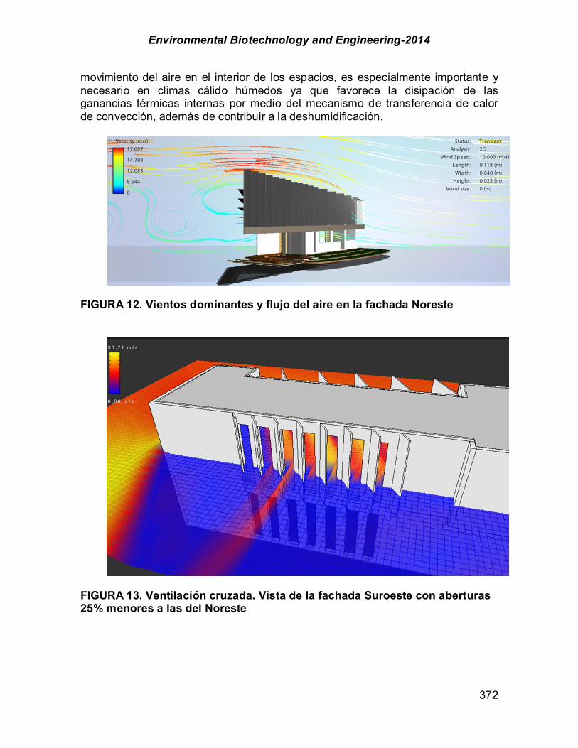
Environmental Biotechnology and Engineering-2014
372
movimiento del aire en el interior de los espacios, es especialmente importante y necesario en climas cálido húmedos ya que favorece la disipación de las ganancias térmicas internas por medio del mecanismo de transferencia de calor de convección, además de contribuir a la deshumidificación.
FIGURA 12. Vientos dominantes y flujo del aire en la fachada Noreste
FIGURA 13. Ventilación cruzada. Vista de la fachada Suroeste con aberturas 25% menores a las del Noreste
Environmental Biotechnology and Engineering-2014
373
Conclusiones La correcta adecuación de las estrategias de diseño bioclimático para un clima cálido húmedo, no solo permite lograr un hábitat confortable, sino más saludable y con un ahorro de energía eléctrica considerable por la disminución en la operación de sistemas de climatización artificial. Además, con la disminución del consumo de energía, se reduce la emisión de gases de efecto invernadero al medio ambiente (IPCC, 2014). El uso intensivo de sistemas de aire acondicionado, que en este tipo de clima, también incluye la deshumidificación, representa una afectación económica por el excesivo gasto de los recursos propios de los ocupantes y para el país una carga enorme por el otorgamiento de subsidios por alto consumo eléctrico, aplicable en esta región climática. Esta situación puede atenuarse con la implementación de una efectiva planeación en el diseño, construcción y mantenimiento de las edificaciones, considerando y aplicando criterios y estrategias bioclimáticos, integrados con sistemas de tecnologías sustentables, con base en el aprovechamiento de las energías renovables y el manejo sustentable del agua y los recursos naturales del entorno circundante al proyecto.
En la actualidad, es esencial aplicar software para la modelación y simulación del comportamiento de las edificaciones y evaluar el desempeño y ahorro energético, para obtener condiciones confortables y saludables de los ocupantes. De esta forma, es viable diseñar las edificaciones con criterios y estrategias bioclimáticos, lo que permite predecir y conocer anticipadamente su comportamiento energético (García Chávez, 2012). Esta situación puede incidir favorablemente en la construcción y operación de la edificación, para lograr importantes ahorros de energía y una significativa disminución del impacto ambiental, así como un mejoramiento en la calidad de vida, que al aplicarse a nivel masivo sirva como un ejemplo demostrativo para generar un favorable efecto multiplicador a nivel nacional. Referencias García Chávez, J.R. et al. (2012). Arquitectura Solar y Sustentabilidad. Editorial Trillas. México,
D.F. García Chávez, J. R. et al.(2005). Introducción a la Arquitectura Bioclimática. Editorial Limusa.
México, D.F. García Chávez, J. R. y Fuentes, V. (2005). Viento y Arquitectura. Ed. Trillas. México, D.F. Givoni, B. (1994). Passive and Low Energy Cooling of Buildings. Van Nostrand Reinhold. N.Y.
EE.UU. Givoni, B. Man, (1981). Climate and Architecture. Van Nostrand Reinhold., New York, U. S.A. INEGI. Instituto Nacional de Geografía y Estadística 2014.
http://www3.inegi.org.mx/sistemas/mexicocifras/default.aspx?e=30 IPCC. Intergovernmental Panel on Climate Change 2014. The Physical Science Basis. IPCC
Working Group 1 Contribution to AR5 http://www.ipcc.ch/report/ar5/wg1/ Koeningsberger, et al. (1997).Viviendas y Edificaciones en Zonas Cálidas y Tropicales Ed.
Paraninfo. Madrid, España. Olgyay, V. (1963).Design with Climate. Princeton University Press. Princeton, U,S,A. SMN. Servicio Meteorológico Nacional. CNA. Comisión Nacional del Agua 2014.
http://smn.cna.gob.mx/index.php?option=com_content&view=article&id=42&Itemid=28 Szokolay, S. (2004). Introduction to Architectural Science: The Basis of Sustainable Design.
Architectural Press- Elsevier. Oxord, U.K.

Environmental Biotechnology and Engineering-2014
374
Section 3. Risk Assessment and Environmental Impact

Environmental Biotechnology and Engineering-2014
375
Page Chapter 3.1. Physicochemical evaluation of soils and sediments near mining operations in asientos, Aguascalientes Kerry N. Mitchell; Magdalena S. Ramos-Gómez; Alma L. Guerrero-Barrera; Laura Yamamoto-Flores; Frederic Thalasso-Siret; Francisco J. Avelar-González 376 Chapter 3.2 Evaluación de daño genotóxico y neurotóxico en población expuesta a fluoruro y arsénico a través de agua de consumo Jessica Cordero-Arreola; Diana Rocha-Amador; Yolanda Alcaraz-Contreras; Raúl Morales-Villegas; Melissa Bocanegra-Salazar; Dania López-Guzmán. 390 Chapter 3.3. Quantitative microbial risk assessment for cryptosporidium and guardia in water, soil, air and vegetables from a native community in Mexico Ana P. Balderrama-Carmona; Pablo Gortáres-Moroyoqui; Cristóbal Chaidez-Quiroz; Luis H. Álvarez-Valencia 403 Chapter 3.4. Life cycle assessment (LCA) of a four-stage biorefinery model Carlos Escamilla-Alvarado; Héctor M. Poggi-Varaldo; Teresa Ponce-Noyola; Elvira Ríos-Leal; Fernando Esparza-García; Josefina Barrera-Cortés; Jaime García-Mena; Ireri Robles-González; Noemi Rinderknecht-Seijas. 414
Environmental Biotechnology and Engineering-2014
376
CHAPTER 3.1 PHYSICOCHEMICAL EVALUATION OF SOILS AND
SEDIMENTS NEAR MINING OPERATIONS IN ASIENTOS, AGUASCALIENTES Kerry N. Mitchell (1); Magdalena S. Ramos-Gómez (1); Alma L. Guerrero-Barrera
(1); Laura Yamamoto-Flores (1); Frederic Thalasso-Siret (2); Francisco J. Avelar-González* (1).
(1) UNIVERSIDAD AUTÓNOMA DE AGUASCALIENTES, Aguascalientes, México; (2) CINVESTAV- IPN, México DF, México; ABSTRACT Soils and sediments near mining activities are frequently direct receptors of mining waste and as such present a potential environmental risk. The study of this potential risk should include not only total metal quantification, but also the study of physicochemical characteristics that play an important role in their solubility, mobility and toxicity in affected sites. Thus, the aim of this study was to evaluate total metal concentrations and the physicochemical characteristics that may affect metal mobility in nearby soils and sediments of the Piedras Negras River in Asientos, Aguascalientes; an area recently affected by a substantial increase in mining activity. Soil and sediment sampling were carried out once during the dry season and once during the rainy season. Soil moisture and organic matter were initially determined. After pretreatment which consisted in drying and sieving through a 2mm mesh, cation exchange capacity and total metal content were determined. pH, redox potential, soluble salts were determined in a 1:10 dilution soil:water. Sediments from all sites were classified as very polluted according to guidelines established by the United States Environmental Protection Agency, and above the maximum permitted limits for commercial, residential and farm use according to the NOM-147-SEMARNAT/SSA1-2004 in at least 2 metals, in select cases, more than 200 times guideline values. 70% of soils from the 10 sample sites were classified in the same way. Though neutral conditions were predominant, 20% of samples from both substrates were moderately acidic in nature (<6.5). 80% of soil and sediment samples presented highly reductive conditions (-100 to -300mv). Both substrates had medium to low (<25 cmol(+)/kg) cation exchange capacities. Salinity measured as conductivity in S/cm in both substrates were found to be normal, though values obtained in sediment samples were twice as high as those obtained in soil samples. Differences between soil and sediment samples were found in values obtained for soluble salts. Nitrate concentrations were 1.5 times higher in sediments. Sulfides and sulfates had 7 and 15 times higher concentrations respectively in sediments.
It was concluded that the sample area was affected by nearby mining activities. High concentration of metals and soluble salts in sediment samples indicate that the river is a direct receptor of mine drainage; whilst soils appear to be affected by wind carried mine tailings. Current physicochemical properties may favor mobility, and thus represent an environmental toxicity risk. Key words: metals, mining, pollution, mobility, solubility, physicochemical.

Environmental Biotechnology and Engineering-2014
377
*Author for all correspondence

Environmental Biotechnology and Engineering-2014
378
Introduction Soils and sediments naturally contain trace metals due to the geology of the parent material from which they were formed (McLean and Bledsoe, 1992). But at higher concentrations, all metals, including essential metals, may cause toxic effects (Liu et al., 2008). Elevated concentrations may be due in part to atmospheric deposition, erosion or leaching of metals in soil, sediment re-suspension or evaporation from water sources (Nriagu, 1989). However, very high concentrations in soils and sediments are more frequently the result of nearby industrial, agricultural, mining and smelting activities (Bradl, 2002; Tchounwou et al., 2012.). Accumulation of metals can degrade soil quality and negatively impact the health of human, animals, and the ecosystem (Nagajyoti et al., 2010).
In order to accurately evaluate the potential environmental risk presented by metals in soils and sediments, it is necessary to study not only total metal quantification, but also the physicochemical characteristics (Howari and Banat, 2001) that play and important role in their solubility, mobility and toxicity.
pH is a physicochemical parameter that directly and indirectly affects the retention of metals in soils and sediments (Gabler, 1997) given that metal solubility decreases with increasing pH. At lower pH, higher concentrations of metals can be found in the soil solution (Peng, 2009; Sherene, 2010). However, pH is dependent on other physicochemical characteristics. Studies have shown that moisture conditions affect the pH; at saturation there is a tendency to neutrality (Van den Berg and Loch, 2000; Zheng and Zhang, 2011). The capacity for organic matter to retain metals by chelation and complexation is also affected by the pH (Kashem and Singh, 2001; Sherene, 2010). Metal retention is also affected by the soil´s or sediment´s cation exchange capacity. As a measure of the total capacity of the soil to hold exchangeable cations, the cation exchange capacity is used to indicate the negative charge present on a unit mass of soil (Peverill et al., 1999). The higher the cation exchange capacity, more easily the metal cations are attracted to these negative sites in solid particles (Atwell et al., 1999).
Another important physicochemical characteristic is salinity measured in terms of conductivity. This parameter is related to the presence of soluble salts in the soil and sediments. It has been shown that an increase in salinity increases mobility of metals due to the complex formation capacity of anions derived from metal salts and competition of salts derived from metal cations with positively charged species for the adsorption sites on the solid phase (Acosta et al., 2011; Paalman et al., 1994).
Thus, the aim of this study was to evaluate total metal concentrations and the physicochemical characteristics that may affect metal mobility in nearby soils and sediments of the Piedras Negras River in Asientos, Aguascalientes; an area recently affected by a substantial increase in mining activity. Materials and Methods Field Sampling. Samples of sediments and soils surrounding the riverbed of Piedras Negras river located in the mining town Asientos, Aguascalientes were
Environmental Biotechnology and Engineering-2014
379
taken from 10 sites once during the rainy season and once during the dry season, using the simple cross-sectional sampling method as established by the USEPA (2002).
Soil and sediment samples were classified in three groups: original sample, particulate sample and liquid extract sample using standardized techniques according to APHA-AWWA-WPCF (1998). Original sample. The following parameters were determined in unmodified samples.
• Humidity: determined using the thermo-gravimetric method with a drying time of 24 hours at 105oC (Alvarez- Benedi and Muñoz-Carpena, 2004).
• Concentration initial of metals: quantified by atomic absorption spectrophotometry after extraction and acid digestion using an acid mixture of H2O: HCl: HNO3 (USEPA, 2007).
Particulate sample. The samples were dried at a temperature of 55oC for 10 days, then ground and sifted to obtain a particle size of less than 0.5mm (Robledo-Santoyo and Maldonado-Torres, 1997). The following parameters were quantified with the obtained particulate sample.
• Organic matter content: determined using the Walkley-Black metric titration method, which included the oxidation of organic matter with potassium dichromate under acid conditions (Robledo-Santoyo and Maldonado-Torres, 1997).
• Cation exchange capacity: determined by the extraction method with 1N ammonium acetate / pH 7.0 (Robledo-Santoyo and Maldonado-Torres, 1997).
Liquid extract. To obtain samples of liquid extract, 5g of the particulate sample were placed in 50ml of distilled water to obtain a solution of 1:10 (m/v). Samples were then placed in a rotating agitator for 24 hours and then left to stand for another 24 hours (Robledo-Santoyo and Maldonado-Torres, 1997). The following parameters were determined once the liquid extract was obtained.
• pH: determined using the potentiometric method (Robledo-Santoyo and Maldonado-Torres, 1997).
• Conductivity: determined using the potentiometric method (Carter and Gregorich, 2008).
• Redox Potential: determined using the electrode method (FAO, 2006). • Soluble salts: determined using standardized HACH spectrophotometric
methods o Sulfides: methylene blue method #8131 o Sulfates: sulfaver 4 method #8051 o Cyanide: pyridine-pyrazalone method #8027
Statistical analysis. Obtained data were statistically analyzed using MiniTab Express 1.1 and Pearson´s StatChrunch.

Environmental Biotechnology and Engineering-2014
380
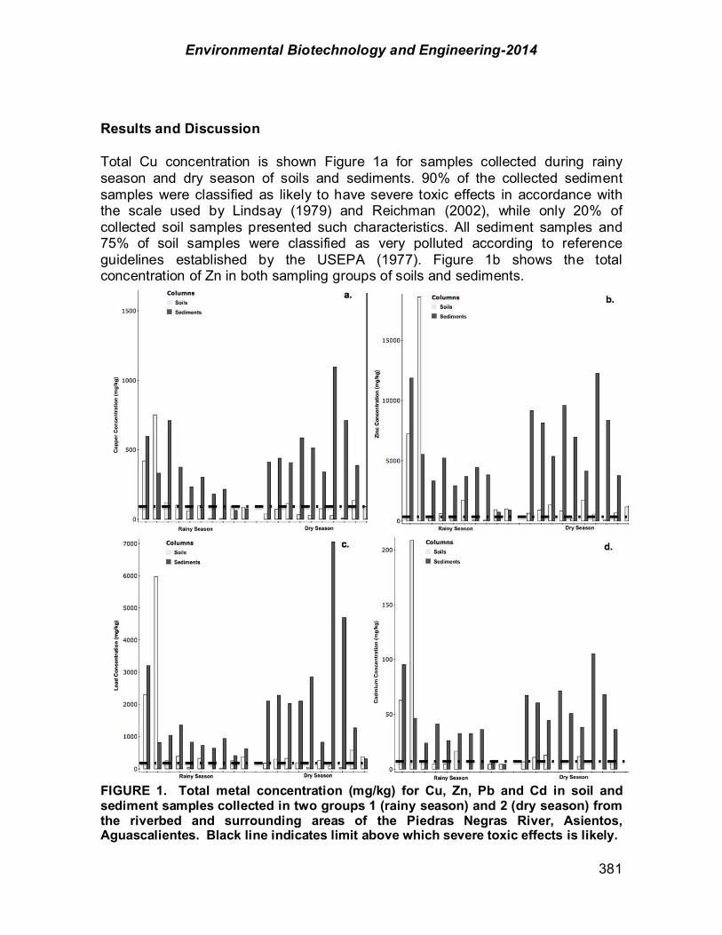
Environmental Biotechnology and Engineering-2014
381
Results and Discussion Total Cu concentration is shown Figure 1a for samples collected during rainy season and dry season of soils and sediments. 90% of the collected sediment samples were classified as likely to have severe toxic effects in accordance with the scale used by Lindsay (1979) and Reichman (2002), while only 20% of collected soil samples presented such characteristics. All sediment samples and 75% of soil samples were classified as very polluted according to reference guidelines established by the USEPA (1977). Figure 1b shows the total concentration of Zn in both sampling groups of soils and sediments.
FIGURE 1. Total metal concentration (mg/kg) for Cu, Zn, Pb and Cd in soil and sediment samples collected in two groups 1 (rainy season) and 2 (dry season) from the riverbed and surrounding areas of the Piedras Negras River, Asientos, Aguascalientes. Black line indicates limit above which severe toxic effects is likely.
Environmental Biotechnology and Engineering-2014
382
All sediment samples were classified very polluted and likely to have severe toxic effects. 80% of soil samples were considered to be very polluted and 70% were considered likely to cause severe toxic effects. Higher concentrations of both metals were observed in sediments samples as compared to soil samples. This is indicative of the riverbed being a possible direct receptor of waste material from the nearby mining activity.
The presence of these metals in such high concentrations is of importance due to their implications in environmental toxicity. According to Hambige and Krebs (2007), zinc is an essential mineral of exceptional biologic importance. However, in excessive amounts, it is damaging to many life forms (Eisler, 1993; Fosmire, 1990). Copper is also an important essential trace element for all living organisms needed for the activity of a variety of enzymes involved in critical areas of metabolism (Leone et al., 1999), however, in high concentrations it causes toxicity, due to the generation of reactive oxygen species damaging proteins, lipids and DNA (Brewer, 2010).
Values for Pb concentrations can be observed in Figure 1c All sediment samples were classified as very polluted and very likely to have severe toxic effects. 75% of soil samples were classified as very polluted while 60% presented conditions likely to have severe toxic effects. All soil and sediment samples contained concentrations of Pb above the maximum permitted limits for commercial, residential and farm use according to the NOM-147-SEMARNAT/SSA1-2004. Figure 1d shows values for Cd concentrations in samples where 85% of sediment samples were classified as very polluted and 80% were likely to cause severe toxic effects. 45% of soil samples were categorized as very toxic and 40% likely to cause severe toxic effects.
According to the US Environmental Protection Agency (USEPA) and the International Agency for Research on Cancer (IARC), as cited by Tchounwou et al. (2012), Pb and Cd are classified as either “known” or “probable” human carcinogens based on epidemiological and experimental studies. They have no established biological functions and are considered as nonessential metals and systemic toxicants that are known to induce multiple organ damage, even at lower levels of exposure.
The presence of these four metals in such high concentrations in sediment samples from this area is evidence of the riverbed being a direct receptor of mine drainage. Soil samples presented lower but significant concentrations when compared to sediment samples, and may be the result of wind dispersion of mine tailings.
It has been established that in order to study the potential risk of toxic metal pollution in soils and sediments, it is necessary to evaluate the physicochemical characteristics that play a role in the solubility and mobility of these metals (Howari and Banat, 2001). According to the classification used by Robledo and Maldonado (1997) 95% of the sediments sampled in both dry and rainy seasons had a neutral pH, 5% are classified as moderately acid (Table 1a). Although no significant differences were found, the median during the dry season was lower than during the rainy season. From Table 1b, it can be observed that 75% of the sampled soils were classified as neutral, while the remaining 25% were classified as moderately

Environmental Biotechnology and Engineering-2014
383
acid. No significant differences between the values obtained from the different seasonal periods were observed, however, as observed in the case of sediment samples, lower pH values were more prevalent during the dry season.
pH is an important factor in the mobilization of metals in soils and sediments (Fija$kowski et al., 2012) due to the hydrolysis reactions of cations caused by an increase in the concentration of protons due to the competition between them and ligands (OH-, SO4
2- etc.,) resulting in a decrease of adsorption sites (McLean and Bledsoe, 1992). This results in an increase in solubility and therefore the mobility of the metals in inverse proportion to the pH; such that an alkaline pH is not conducive to high metal mobility (Ramos-Gómez et al., 2012). Predominantly neutral conditions of the sampled sites in this study may indicate a temporary reduction in mobility. pH however is highly dependent on soil moisture content. In this study, higher percentages were observed in sediment samples, both sample groups being affected by the prevalent hydrological conditions. As moisture content increases towards saturation, the pH tends to neutrality.
TABLE 1. Values for physicochemical characteristics of sediment samples collected from the riverbed and surrounding areas of the Piedras Negras
River, Asientos, Aguascalientes a.
b.
The redox potential of the substrate is another factor that must be evaluated as it also plays a major role in the mobility of metals. Studies have shown that there can be an increase the mobility due to reduction reactions even under neutral conditions (McBride, 1994; Bollinger et al., 2003). Table 1a and b shows that 80% of soils and sediments presented highly reductive conditions according to the classification used by the USEPA (1994), the remaining 20% being classified as moderately reduced. During the dry season, obtained values showed greater
7.10 7.13 -183.00 -37.50 79.01 91.30 4.40 4.827.00 6.00 -185.00 -227.40 75.56 59.60 2.60 5.637.30 7.45 -168.60 7.40 56.87 45.60 4.48 4.537.30 6.65 -192.70 -279.90 69.55 51.30 5.89 4.967.00 7.31 -176.40 -75.80 68.06 78.20 7.53 5.477.30 6.95 -181.80 -197.30 41.92 43.50 8.48 5.987.10 7.18 -189.70 -36.90 41.37 49.60 6.54 6.247.50 6.96 -162.80 -230.10 25.48 30.80 3.89 5.127.10 7.05 -149.50 -271.90 39.79 42.10 4.31 4.967.00 6.96 -160.30 -374.20 32.11 38.40 9.65 6.87
7.00 7.39 -296.50 -83.30 19.40 18.20 5.38 4.986.00 7.26 -193.00 -54.60 17.20 17.10 4.68 3.917.30 7.23 -304.90 -113.30 14.90 18.90 4.44 2.457.20 7.40 -306.50 -50.70 19.60 20.10 4.17 3.977.20 7.02 -289.00 -87.60 17.30 17.70 8.20 6.127.20 6.12 -349.40 -295.10 12.40 13.50 1.88 3.257.80 6.33 -362.00 -226.80 17.40 17.90 1.34 1.917.20 7.32 -306.30 -208.80 14.50 15.90 5.78 2.287.10 6.46 -283.20 -381.60 17.30 18.00 5.18 2.897.40 6.36 -491.10 -229.90 18.00 18.00 3.50 2.97
Environmental Biotechnology and Engineering-2014
384
variation. This can be attributed to moisture gradients across the sampled areas as a result of the prevailing hydrological conditions of the season (Yu et al., 2006). This is reflected in less reductive conditions in certain sample sites. This prevalent reductive condition in the area studied can greatly affect metal transport possibly contributing to an accelerated migration (McLean and Bledsoe, 1992).
Metal mobility or lack thereof is also affected by the organic matter content of the studied substrate. According to the classification used by Fernández Linares et al. (2006), 90% of the sampled sediments had high organic matter content above 4% as shown in Table 1a, however, only 45% of soil samples fall within the same category. As with other physicochemical characteristics, organic matter has a direct impact on the behavior of metals, affecting solubility with complexation and chelation reactions (Kashem and Singh, 2001). Studies have shown that during decay, humic and fulvic acids whose functional groups are capable of associating with metal cations (Kyziol, 2002) are produced. However, under acidic conditions such groups are ionized resulting in the remobilization of these cations (Carrillo-Gonzalez et al., 2006), further demonstrating the close relationship between the pH and other physicochemical characteristics (Sherene, 2010), including organic matter content.
As a measure of the soil´s capacity to hold exchangeable cations, cation exchange capacity is used to indicate the net negative charge present on a mass unit of soil (Peverill et al., 1999). The higher the cation exchange capacity, more easily metal cations are attracted to the negative sites on soil and sediment particles (Atwell et al., 1999). According the classification used by Robledo and Maldonado (1997), 85% of soils and 60% of sediment samples were classified as having average cation exchange capacity. 15% and 40% respectively presented low cation exchange capacity, conditions that may contribute to a less immobilization (Atwell et al., 1999).
As per the classification of the USDA (2002), all soils (Figure 2a) are in conditions of normal salinity (<2000 µS/cm). In contrast, 5% of the sampled sediments present slightly saline conditions. However, that salinity is increasing with respect to time. This has important implications given that an increase in salinity results in an increase in mobility of metals in the soil due to the complex formation capacity of anions derived from metal salts and competition of salts derived from metal cations with positively charged species for the adsorption sites (Acosta et al., 2011; Paalman et al., 1994).
The distribution of sulfates in mg/L is shown in Figure 2c in both soils and sediments. Sediment samples contained concentrations up to 7 times more than in soils. These values indicate the presence of contamination by soluble salts, in this case sulfates, a common product of oxidation-neutralization of metal ores or waste reagents from flotation processes used in the mining industry (Gutiérrez-Ruiz et al., 2007). Sulfide concentrations were also higher in sediment samples (Figure 2d), up to 15 times higher in some cases. The presence of higher than typical concentrations of sulfides in soils and sediments may indicate constant reception of mine wastes, at a higher rate than that of the oxidation process sulfides normally undergo. The oxidation process is also important given that it produce sulfates resulting in a decrease in pH of the substrate, an important factor

Environmental Biotechnology and Engineering-2014
385
in the mobility and availability of metals (Clemente et al., 2003). Additionally in substrates where specific adsorption sites become saturated with cations and anions already present, exchange reactions predominate, resulting in competition for these sites between metals and soil ions (McLean and Bledsoe, 1992). In the presence of these inorganic ligands, the adsorption of certain metals on soil and soil constituents can be inhibited (Boulding, 1996), as such contribute to an increase in the concentration for the free metal in the liquid phase of the soil.
FIGURE 2. Salinity measured as conductivity in S/cm and concentration of soluble salts (sulfates, sulfides and cyanide) in mg/L in soil and sediment samples collected in two groups 1(rainy season) and 2 (dry season) from the riverbed and surrounding areas of the Piedras Negras River, Asientos, Aguascalientes.
Certain mining activities requires the use of great quantities of alkaline
solutions containing high concentrations of sodium cyanide, free cyanide and metal-cyanide complexes (Korte and Coulston, 1998). As such, cyanide concentrations were also measured in both substrates. Sediment samples showed higher values (Figure 2d). Cyanide biodegrades under aerobic conditions with the initial formation of ammonia, which is converted to nitrite and nitrate in presence of nitrifying bacteria (Wiemeyer Eisler, 2004). Using the soil values to represent

Environmental Biotechnology and Engineering-2014
386
typical geological characteristics, the high cyanide concentrations in sediment samples is indicative of direct and constant pollution from mining activities.
Conclusion Soils and sediments from the Piedras Negras River, Asientos, Aguascalientes were classified as very polluted with Zn, Cu, Pb, Cd according to guidelines established by the USEPA, at some sites, more than 200 times guideline values, and above the maximum permitted limits for commercial, residential and farm use according to the NOM-147-SEMARNAT/SSA1-2004 in the case of Pb and Cd. Current physicochemical properties may favor mobility and thus represent an environmental toxicity risk. Acknowledgements The authors wish to thank CONACYT for having granted a graduate scholarship for this research project. The authors also wish to thank the Universidad Autónoma de Aguascalientes for their support on this project. References Acosta, J.; Jansen, B.; Kalbitz, K.; Faz, A., & Martínez-Martínez, S. (2011). Salinity
increases mobility of heavy metals in soils. Chemosphere. 85(8): 1318–24. Alloway, B. (2013). Heavy metals in soils trace metals and mettalloids in soils and
their bioavailability. Dordrecht: Springer. Alvarez-Benedi, J. & Munoz-Carpena, R. (2004). Soil-Water-Solute Process
Characterization: An Integrated Approach. CRC Press. APHA-AWWA-WPCF. (1998). Standard Methods for the examination of water and
wastewater. 20th edition. American Public Health Association, Washington, DC.
Atwell, B.J.; Kriedemann, P.E. & Turnbull, C.G.N. (1999). Plants in action: adaptation in nature, performance in cultivation. South Yarra, Macmillan Education Australia.
Bollinger, J. & Bril, H. (2003). Effect of reductive conditions on metal mobility from wasteland solids: an example from the Mortagne-du-Nord site, France. Applied Geochemistry.18: 383–394.
Boulding, J.R. (1996). EPA Environmental Assessment Sourcebook. CRC Press. Bradl, H. (2002) Heavy metals in the environment: origin, interaction and
remediation, Vol 6. Academic, London Brewer, G.J. (2010). Copper toxicity in the general population. Clinical
Neurophysiology. 121(4): 459–460 Carrillo-Gonzalez, R.; Simunek, J.; Suave, S. & Adriano, D. (2006). Mecahnisms
and pathways of trace element mobility in soils. Advances in Agronomy. 91(06): 111 – 178.

Environmental Biotechnology and Engineering-2014
387
Carter, M.R. & Gregorich, E.G. (2008). Soil Sampling And Methods of Analysis. Canadian Society of Soil Science.
Clemente, R.; Walker, D.J.; Roig, A. & Bernal, M.P. (2003). Heavy metal bioavailability in a soil affected by mineral sulphides contamination following the mine spillage at Aznalcóllar, Spain. Biodegradation. 14(3): 199–205.
Eisler, R. (1993). Zinc hazards to fish, wildlife, and invertebrates: a synoptic review. Washington, D.C.: U.S. Dept. of the Interior, Fish and Wildlife Service.
Fernández Linares, L.C.; Rojas Avelizapa, N.G.; Roldán Carrillo, T.G.; Ramírez Islas, M.E.; Zegarra Martínez, H.G.; Hernández Romeo, R.U.; Reyes Ávila, J.; Flores Hernández, D.; Arce Ortega, J.M. (2006). Manual de técnicas de análisis de suelos aplicadas a la remediación de sitios contaminados. Instituto Mexicano del Petróleo, México, D. F.
Fija$kowski, K.; Grobelak, A. & Placek, A. (2012). The influence of selected soil parameters on the mobility of heavy metals in soils. Inzynieria I Ochrona Srodowiska. 15(1): 81–92.
Food and Agriculture Organisation of the United Nations. (2006). Guidelines for Soil Description. Food & Agriculture Org.
Fosmire, G.J. (1990). Zinc toxicity. The American Journal of Clinical Nutrition. 51(2): 225–227.
Gäbler, H.-E. (1997). Mobility of heavy metals as a function of pH of samples from an overbank sediment profile contaminated by mining activities. Journal of Geochemical Exploration. 58(2–3): 185–194.
Gutiérrez-Ruiz, M.; Romero, F.M. & González-Hernández, G. (2007). Suelos y sedimentos afectados por la dispersión de jales inactivos de sulfuros metálicos en la zona minera de Santa Bárbara, Chihuahua, México. Revista Mexicana de Ciencias Geológicas. 24(2): 170–184
Hambidge, K.M. & Krebs, N. F. (2007). Zinc deficiency: a special challenge. The Journal of Nutrition. 137(4): 1101–1105.
Howari, F.M. & Banat, K.M. (2001). Assessment of Fe, Zn, Cd, Hg, and Pb in the Jordan and Yarmouk River Sediments in Relation to Their Physicochemical Properties and Sequential Extraction Characterization. Water, Air, and Soil Pollution. 132(1-2): 43–59.
Kashem, M.A. & Singh, B. R. (2001). Metal availability in contaminated soils: II. Uptake of Cd, Ni and Zn in rice plants grown under flooded culture with organic matter addition. Nutrient Cycling in Agroecosystems. 61(3): 257–266.
Kyzio$, J. (2002). Effect of physical properties and cation exchange capacity on sorption of heavy metals onto peats. Polish Journal of Environmental Studies. 11(6): 713–718.
Leone, A. & Mercer, J.F.B. (1999). Copper Transport and Its Disorders: Molecular and Cellular Aspects; Proceedings of a Satellite Meeting of the European Human Genetic Society on Copper Transport and Its Disorders: Molecular and Cellular Aspects, Held May 21 - 25, 1997, in Sestri Levante, Italy. Springer Science & Business Media.
Lindsay, W.L. (1979). Chemical equilibria in soils. Wiley.

Environmental Biotechnology and Engineering-2014
388
Liu, J.; Goyer, R., Waalkes, M. (2008). Toxic Effects of Metals. In C. Klaassen (Ed.) Carasrett and Doulls Toxicology: The Basic Science of Poisons, (931-980) McGraw- Hill, New York.
Lock, W.H. (1996). Composite Sampling. National Environmental Health Forum McBride, M.B. (1994). Environmental Chemistry of Soils. Oxford University Press,
Incorporated. Mclean, J.E. & Bledsoe, B. E. (1992). Behavior of Metals in Soils. Ground Water
Issue (pp. 1–25). Ada, Oklahoma. Nagajyoti, P.C.; Lee, K.D. & Sreekanth, T.V.M. (2010). Heavy metals, occurrence
and toxicity for plants: a review. Environmental Chemistry Letters. 8(3): 199–216.
Nriagu, J. (1989). A global assessment of natural sources of atmospheric trace metals. Nature. 338(6210): 47–49.
Paalman, M.A.A.; Weijden, C.H.V.D. & Loch, J.P.G. (1994). Sorption of cadmium on suspended matter under estuarine conditions; competition and complexation with major sea-water ions. Water, Air, and Soil Pollution. 73(1). 49–60.
Peng, J.-F.; Song, Y.-H.; Yuan, P.; Cui, X.-Y. & Qiu, G.-L. (2009). The remediation of heavy metals contaminated sediment. Journal of hazardous materials. 161(2-3): 633– 40.
Peverill, K.I.; Sparrow, L.A. & Reuter, D.J. (1999). Soil Analysis: An Interpretation Manual. Cairo Publishing.
Ramos-Gómez, M.; Avelar, J.; Medel-Reyes, A.; Yamamoto, L.; Ramirez, M. & Rodriguez, F. (2012). Movilidad de metales en jales procedentes del distrito minero de guanajuato. Revista Internacional de Contaminación Ambiental. 28(1): 49–59.
Reichman, S.M. (2002). The Responses of Plants to Metal Toxicity. A Review Focusing on Copper, Manganese and Zinc. AMEEF Paper 14. 59 pp. Australian Minerals and Energy Environment Foundation, Melbourne
Robledo-Santoyo, E. & Maldonado-Torres, R. (1997). Manual de Procedimientos para el Analisis de Suelo. Universidad Autónoma de Chapingo.
Sherene, T. (2010). Mobility and transport of heavy metals in polluted soil environment. Biological Forum - An International Journal. 2(2): 112–121.
Tchounwou, P. B., Yedjou, C. G., Patlolla, A. K., & Sutton, D. J. (2012). Heavy Metal Toxicity and the Environment. In A. Luch (Ed.), Molecular, Clinical and Environmental Toxicology Volume 3: Environmental Toxicology (Vol. 101, pp. 133–164). Basel: Springer Basel.
U.S. Environmental Protection Agency. (1977). Guidelines for the Pollutional Classification of Great Lakes Habor Sediments. 905R77106. USEPA, Region V. Chicago
U.S. Environmental Protection Agency (2002). Region 9 Preliminary Remediation Goals (PRG). 167.
U.S. Environmental Protection Agency. (2007). Flame Atomic Absorption Spectrophotometry (EPA Method 7000B).
Van Den Berg, G.A. & Loch, J.P.G. (2000). Decalcification of soils subject to periodic waterlogging. European Journal of Soil Science. 51(1): 27–33.
Environmental Biotechnology and Engineering-2014
389
Wuana, R.A., & Okieimen, F.E. (2011). Heavy Metals in Contaminated Soils: A Review of Sources, Chemistry, Risks and Best Available Strategies for Remediation. ISRN Ecology
Yu, K.; Faulkner, S.P. & Patrick, W. H. (2006). Redox potential characterization and soil greenhouse gas concentration across a hydrological gradient in a Gulf coast forest. Chemosphere. 62(6): 905–14.
Zheng, S. & Zhang, M. (2011). Effect of moisture regime on the redistribution of heavy metals in paddy soil. Journal of Environmental Sciences. 23(3): 434–443.
Environmental Biotechnology and Engineering-2014
390
CHAPTER 3.2 EVALUACIÓN DE DAÑO GENOTÓXICO Y NEUROTÓXICO EN POBLACIÓN EXPUESTA A FLUORURO Y ARSÉNICO A TRAVÉS DE AGUA
DE CONSUMO
Jessica Cordero-Arreola (1); Diana Rocha-Amador (2); Yolanda Alcaraz-Contreras (2); Raúl Morales-Villegas (3);
Melissa Bocanegra-Salazar (4); Dania López-Guzmán* (1).
(1) Facultad de Ciencias Químicas, Universidad de Juárez del Estado de Durango. Durango, México. (2) Departamento de Farmacia. División de Ciencias Naturales y Exactas. Universidad de Guanajuato. México. (3) CIACYT-Medicina. Universidad Autónoma de San Luis Potosí. México. (4)Facultad de Ciencias Forestales. Universidad Juárez del Estado de Durango. Durango. México. RESUMEN
La presencia natural de contaminantes como el fluoruro (F-) y el arsénico (As) en agua de consumo, cuyo origen es generalmente subterráneo es de los principales problemas de salud pública a nivel mundial, llegando a afectar incluso varios estados de la República Mexicana, entre ellos Durango y Guanajuato. Debido a los efectos en salud que se han asociado a estos contaminantes, el objetivo del presente estudio pre-experimental de tipo transversal analítico fue evaluar algunos de los efectos en salud en mujeres adultas residentes de la ciudad de Durango y Lo de Sierra, Guanajuato expuestos a F- y As mediante agua de consumo humano. Se determinaron concentraciones de F- mediante potenciometría con electrodo ion selectivo y el análisis de As se realizó por espectrometría de fluorescencia atómica mediante generador de hidruros (EAA-GH), posteriormente se evaluó coeficiente intelectual total (CI) en los participantes mediante el uso de la prueba Beta III y daño genotóxico mediante la técnica de micronúcleos (MN) en células epiteliales de mucosa oral.
El presente trabajo arrojó como resultado una importante exposición ambiental, ya que se encontró que la población de Durango está expuesta a concentraciones de 4.11 mg F-/L (3.44-4.67 mgF-/L) y 0.056 mgAs/L (0.027-0.068.5 mgAs/L), mientras que la población de Guanajuato está expuesta a concentraciones de 5.81 mg F-/L (4.71-6.65 mg F-/L) y 0.026 mgAs/L (0.019-0.040 mgAs/L). De la misma manera en cuanto a la evaluación de CI de los participantes se obtuvo como resultado que el 100% de los individuos evaluados obtuvieron valores de CI total por debajo del puntaje promedio. En cuanto a la presencia de MN, estos se observaron con una media de 3.75 en la población de Durango y 2.35 en la población de Guanajuato.
------------ *Autor para correspondencia
Environmental Biotechnology and Engineering-2014
391
Estos resultados evidencian que pese a que existen instituciones tanto
nacionales como internacionales (Secretaria de Salud y Organización Mundial de la Salud, respectivamente) que sugieren concentraciones óptimas tanto para F- como para As en agua de consumo, estas se encuentran por encima de lo recomendado, lo cual puede representar futuras afectaciones a la salud en poblaciones expuestas de manera constante, sin embargo se considera importante seguir investigando el tema e informar a las autoridades, para evitar que la gravedad del daño sea mayor, pudiendo relacionarse incluso con el origen de enfermedades como cáncer.
Palabras Clave: Fluoruro, Arsénico, Agua, Genotoxicidad, Neurotoxicidad. Introducción Tanto el fluoruro (F-) como el arsénico (As) han sido reconocidos como los contaminantes inorgánicos en agua de consumo humano más ampliamente distribuidos en el mundo y las concentraciones de los mismos dependen de la naturaleza del suelo de cada lugar (Guha et al., 2010; Smedley., et al 2002). Esta exposición puede llegar a ocasionar diversas afectaciones entre las cuales destacamos daños en la actividad locomotora y el aprendizaje, efectos teratogénicos, genotóxicos y carcinogénicos (Alvarado Silva 2001; Rivas et al., 2005; San-Xiang Wang et al., 2007; Wasserman et al., 2006). Actualmente la Organización Mundial de la Salud (OMS) recomienda concentraciones de 0.5 mg F-/L y 0.010 mg As/L, mientras que las NOM-127-SSA1-1994 y NOM-201-SSA1-2002 para la calidad del agua en México permiten concentraciones de 1.5 mgF-/L y 0.025 mgAs/L tanto en agua distribuida por la red hidráulica como en aguas embotelladas (OMS 2006; NOM-127-SSA1-1994, NOM-201-SSA1-2002).
El consumo crónico de agua con concentraciones de F- y As por encima de lo recomendado por la OMS pueden ocasionar diversos daños a la salud, dependiendo del tiempo y la dosis de exposición, como lo afectaciones digestivas, cardiacos, reproductivos, renales, inmunológicos, endocrinos, óseos y problemas del sistema nervioso central, afectando la actividad locomotora y el aprendizaje, así como dermatosis y efectos teratogénicos, genotóxicos y carcinogénicos en el caso del As. (OMS, 2006; Rocha, 2005).
Se entiende por neurotoxicidad a la capacidad de inducir efectos adversos en el sistema nervioso central, los nervios periféricos u órganos de los sentidos. Considerando pues, como producto neurotóxico, a aquel capaz de inducir un patrón constante de disfunción neural o cambios en la química o estructura del sistema nervioso, causando alteraciones en la capacidad de aprendizaje y retención de memoria, entre otros. Dichas alteraciones son asociadas a diferentes mecanismos de acción neurotóxica (neuropatías, axonopatias y mielonopatias) que determinan la interacción directa entre el sistema nervioso (SN) y la toxina o sus metabolitos (Moser, et al, 2008). Dado que el F- es capaz de atravesar la
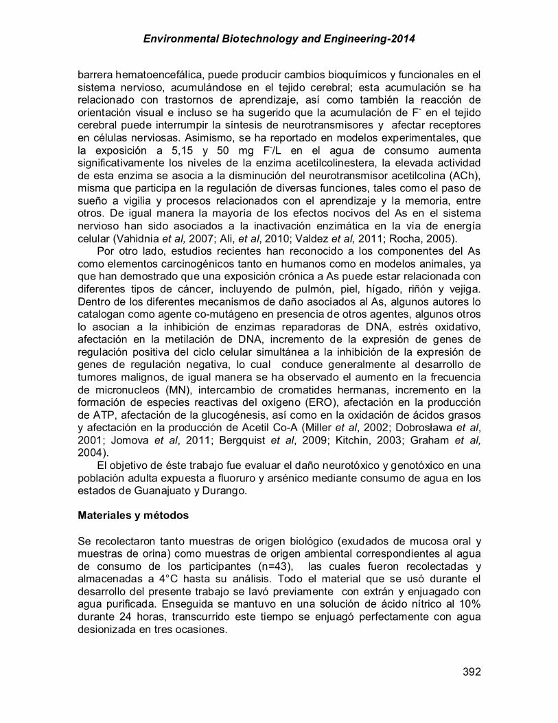
Environmental Biotechnology and Engineering-2014
392
barrera hematoencefálica, puede producir cambios bioquímicos y funcionales en el sistema nervioso, acumulándose en el tejido cerebral; esta acumulación se ha relacionado con trastornos de aprendizaje, así como también la reacción de orientación visual e incluso se ha sugerido que la acumulación de F- en el tejido cerebral puede interrumpir la síntesis de neurotransmisores y afectar receptores en células nerviosas. Asimismo, se ha reportado en modelos experimentales, que la exposición a 5,15 y 50 mg F-/L en el agua de consumo aumenta significativamente los niveles de la enzima acetilcolinestera, la elevada actividad de esta enzima se asocia a la disminución del neurotransmisor acetilcolina (ACh), misma que participa en la regulación de diversas funciones, tales como el paso de sueño a vigilia y procesos relacionados con el aprendizaje y la memoria, entre otros. De igual manera la mayoría de los efectos nocivos del As en el sistema nervioso han sido asociados a la inactivación enzimática en la vía de energía celular (Vahidnia et al, 2007; Ali, et al, 2010; Valdez et al, 2011; Rocha, 2005).
Por otro lado, estudios recientes han reconocido a los componentes del As como elementos carcinogénicos tanto en humanos como en modelos animales, ya que han demostrado que una exposición crónica a As puede estar relacionada con diferentes tipos de cáncer, incluyendo de pulmón, piel, hígado, riñón y vejiga. Dentro de los diferentes mecanismos de daño asociados al As, algunos autores lo catalogan como agente co-mutágeno en presencia de otros agentes, algunos otros lo asocian a la inhibición de enzimas reparadoras de DNA, estrés oxidativo, afectación en la metilación de DNA, incremento de la expresión de genes de regulación positiva del ciclo celular simultánea a la inhibición de la expresión de genes de regulación negativa, lo cual conduce generalmente al desarrollo de tumores malignos, de igual manera se ha observado el aumento en la frecuencia de micronucleos (MN), intercambio de cromatides hermanas, incremento en la formación de especies reactivas del oxígeno (ERO), afectación en la producción de ATP, afectación de la glucogénesis, así como en la oxidación de ácidos grasos y afectación en la producción de Acetil Co-A (Miller et al, 2002; Dobros$awa et al, 2001; Jomova et al, 2011; Bergquist et al, 2009; Kitchin, 2003; Graham et al, 2004).
El objetivo de éste trabajo fue evaluar el daño neurotóxico y genotóxico en una población adulta expuesta a fluoruro y arsénico mediante consumo de agua en los estados de Guanajuato y Durango.
Materiales y métodos Se recolectaron tanto muestras de origen biológico (exudados de mucosa oral y muestras de orina) como muestras de origen ambiental correspondientes al agua de consumo de los participantes (n=43), las cuales fueron recolectadas y almacenadas a 4°C hasta su análisis. Todo el material que se usó durante el desarrollo del presente trabajo se lavó previamente con extrán y enjuagado con agua purificada. Enseguida se mantuvo en una solución de ácido nítrico al 10% durante 24 horas, transcurrido este tiempo se enjuagó perfectamente con agua desionizada en tres ocasiones.

Environmental Biotechnology and Engineering-2014
393
Cuantificación de Fluoruro en agua. Para la cuantificación de F- se utilizó el método potenciométrico con electrodo ion selectivo a microescala reportado por Guevara Ruiz y Ortiz Pérez en el año 2009. Se realizó en base a una curva de calibración construida a partir de una serie de estándares con concentraciones conocidas. Los estándares se prepararon a partir de una solución stock de 100 mgF-/L, obteniendo concentraciones finales de 0.4, 0.6, 0.8, 1, 3,5 y 8 mgF-/L. Se tomaron 500 µL de las muestras y se vertieron en tubos de plástico de 5 mL, posteriormente se añadieron 500 µL de solución TISAB. Se agitaron perfectamente utilizando un vortex. Una vez que se comprobó que el equipo estuviera trabajando en óptimas condiciones, se efectuó la medición de cada uno de los estándares y de las muestras de agua y orina por triplicado, para lo cual se empleó el potenciómetro marca Beckman Coulter serie 500 y un electrodo Thermo Cientific. Para el cálculo de la concentración de iones Fluoruro se realizó una curva estándar de calibración en escala semilogarítmica, en donde el potencial medido en milivolts se graficó en la escala aritmética y la concentración de F- en escala logarítmica. Usando el sistema de regresión lineal se interpolaron los resultados obtenidos de las muestras para conocer las concentraciones de los iones fluoruro. Se empleó como control de calidad un estándar certificado de 100 ± 0.8 mgF-/L (High Purity Standards Lote # 0735446), se prepararon dos estándares, correspondientes a 1 y 2 mgF- /L, los cuales se analizaron de la misma manera que las muestras y se calculó su concentración en base a la curva de calibración. Cuantificación de Arsénico en agua. Para la cuantificación de As se utilizó el método de espectrometría de fluorescencia atómica por generación de hidruros (EAA-GH) en el equipo Millenium Excalibur con auto muestreador PSA 20.400. La cuantificación de As total se efectuó con base en una curva construida por una serie de 6 estándares con concentraciones de 0.001, 0.003, 0.005, 0.01, 0.025, 0.040 y 0.070 mgAs/L, mismas que se prepararon a partir de una solución de 1 mgAs/L. Para el cálculo de la concentración de As se realizó una curva de calibración donde la altura de pico se graficó en el eje de las ordenadas y la concentración de arsénico en el eje de las abscisas. Usando el sistema de regresión lineal fue posible interpolar los resultados obtenidos de las muestras para determinar las concentraciones de As. Se empleó como control de calidad el estándar certificado NIST 1643e, este contenía un valor medio de 0.058 mgAs/L, mismo que se preparó y analizó de la misma manera que las muestras de agua. Evaluación de daño genotóxico mediante ensayo de micronúcleos (MN). Se evaluó el daño genótoxico mediante el ensayo de MN en células epiteliales de mucosa oral, las cuales funcionan como excelente biomarcador al ser posiblemente el método menos invasivo disponible para medir el daño en el ADN en los seres humanos (Holland et al, 2008). Las muestras fueron obtenidas mediante un raspado en la parte interna de la mejilla de cada individuo con cepillo citológico, evitando tener contacto con lengua y dientes. El protocolo se detalla en la Figura 1.
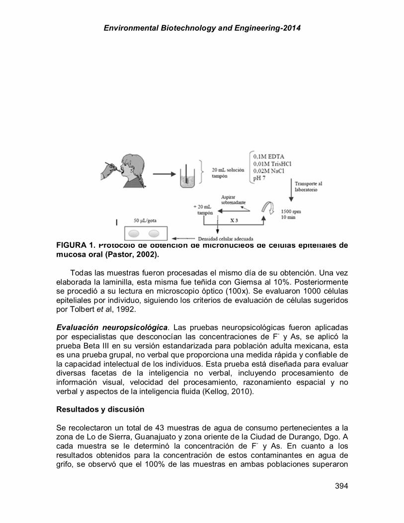
Environmental Biotechnology and Engineering-2014
394
FIGURA 1. Protocolo de obtención de micronúcleos de células epiteliales de mucosa oral (Pastor, 2002).
Todas las muestras fueron procesadas el mismo día de su obtención. Una vez
elaborada la laminilla, esta misma fue teñida con Giemsa al 10%. Posteriormente se procedió a su lectura en microscopio óptico (100x). Se evaluaron 1000 células epiteliales por individuo, siguiendo los criterios de evaluación de células sugeridos por Tolbert et al, 1992. Evaluación neuropsicológica. Las pruebas neuropsicológicas fueron aplicadas por especialistas que desconocían las concentraciones de F- y As, se aplicó la prueba Beta III en su versión estandarizada para población adulta mexicana, esta es una prueba grupal, no verbal que proporciona una medida rápida y confiable de la capacidad intelectual de los individuos. Esta prueba está diseñada para evaluar diversas facetas de la inteligencia no verbal, incluyendo procesamiento de información visual, velocidad del procesamiento, razonamiento espacial y no verbal y aspectos de la inteligencia fluida (Kellog, 2010). Resultados y discusión Se recolectaron un total de 43 muestras de agua de consumo pertenecientes a la zona de Lo de Sierra, Guanajuato y zona oriente de la Ciudad de Durango, Dgo. A cada muestra se le determinó la concentración de F- y As. En cuanto a los resultados obtenidos para la concentración de estos contaminantes en agua de grifo, se observó que el 100% de las muestras en ambas poblaciones superaron

Environmental Biotechnology and Engineering-2014
395
los límites recomendados por la OMS, para ambos contaminantes. De igual manera el 100% de las muestras correspondientes a la población de Durango superaron lo establecido por la normatividad mexicana (1.5 mgF-/L y 0.025 mgAs/L), mientras que en las muestras correspondientes a la población de Guanajuato se encontró que el 100% de las muestras sobrepasaron los límites establecidos para la concentración de F- y un 92% las concentraciones de As. Comparando ambos resultados con lo establecido por la Normatividad Mexicana podemos notar un incremento en la concentración de contaminantes en las muestras pertenecientes a la población de Durango de hasta 3.11 veces mayor en el caso de F- y 2.74 veces en el caso del As, mientras en la población de Guanajuato, se observó un exceso de F- hasta en 4.45 veces y solo un aumento de 1.1 veces en cuanto a concentraciones de As nos referimos. En la Tabla 1 se presentan las concentraciones de F- y As en agua de grifo de las poblaciones evaluadas, estos resultados coinciden con estudios anteriores, donde se han reportado concentraciones similares de F- y As, como lo es el trabajo de Vega et al., 2001, donde reporto concentraciones medias de 5.37mgF-/L y concentraciones de 0.050 a 0.146 mgAs/L en muestras del Valle del Guadiana, Dgo. Sin embrago existen otros trabajos como el de Chávez del año 2010 donde ser reportan concentraciones menores a 2 mgF-/L y concentraciones menores de 0.053 mgAs/L en pozos del Valle del Guadiana, pese a que estos resultados son un tanto contradictorios, esto puede deberse a la variabilidad de las zonas de trabajo, otro dato que es importante señalar es que no existen hasta el momento antecedentes específicos de la zona de Lo de Sierra, Gto. Sin embargo se tienen reportes de zonas cercanas a Lo de Sierra, como lo son los trabajos de Rodríguez et al., 2011, donde se reportan concentraciones de 1-25 mgF-/L en Irapuato, Gto, y Rodríguez et al., 2006 reportaron concentraciones de hasta 0.30 mgAs/L en Copal, Irapuato y concentraciones de hasta 0.40 mgAs/L en Salamanca, Irapuato De manera adicional se evaluó la presencia de F- en orina como marcador de exposición, observando que el 84% de la población perteneciente al estado de Durango superó el límite de intervención ambiental (LIA), conocido como la concentración a la que no se presentan efectos adversos (2 mg/L de orina), dato establecido por la Agencia de Protección Ambiental de los Estados Unidos (USEPA) y así mismo se observó esta situación en el 41% de la población perteneciente a Guanajuato (Tabla 2). TABLA 1. Concentraciones de Fluoruro y Arsénico en agua de grifo de cada
comunidad.
Durango X ± DEa
(min-máx)
Guanajuato
X ± DEa
(min-máx)
F- (mg/L)
4.11± 0.33 (3.44-4.67)
5.81±0.45 (4.71-6.65)
As
(mg/L)
0.056 ± 0.112 (0.027-0.068)
0.031 ± 0.004 (0.019-0.040)

Environmental Biotechnology and Engineering-2014
396
Notas: a Media aritmética ± desviación estándar; entre paréntesis se muestra el valor mínimo y máximo. Durango (n=20); Lo de Sierra (n=23)
TABLA 2. Concentraciones de Fluoruro en orina por zona.
Durango X ± DEa
(min-máx)
Guanajuato X ± DEa
(min-máx)
F- en orina
4.47±2.33 (1.6-11.52)
2.36±1.53 (0.75-5.4)
>2 mg F-/ L (%)
84
41
Notas: a Media aritmética ± desviación estándar; entre paréntesis se muestra el valor mínimo y máximo. Durango (n=20); Lo de Sierra (n=23).
Posterior a la cuantificación de los contaminantes se procedió a la evaluación de los daños asociados a dicha intoxicación, esto aplicando pruebas psiconeurológicas que permitieron la evaluación de diferentes áreas dentro de la inteligencia. En el caso de la evaluación neuropsicológica los resultados obtenidos mostraron que el 100% de la población evaluada obtuvo un puntaje inferior al promedio (<90 puntos), mostrando una media de 71.64 en el caso de la población de Durango y 70.16 en el caso de la población de Guanajuato. Estos resultados se analizaron estadísticamente mediante el empleo de la prueba T- Student, se observó una distribución normal y que no existe significancia estadística entre ambas poblaciones (p> 0.05). Estos resultados son importantes ya que indican que la persona con este puntaje puede presentar una afectación en la habilidad para comprender situaciones complejas y enfrentar y resolver ciertas complicaciones a través del razonamiento, así como también la también la destreza en general. En la Tabla 3 se muestran los datos poblacionales que pudieran ser confusores en el análisis por lo que fueron tomados en cuenta para la evaluación neuropsicológica (edad y nivel socioeconómico o NSE). En las Tablas 4 y 5 se muestran los resultados del Cl por clasificación en ambas poblaciones. Los resultados arrojados por la encuesta socioeconómica del AMAI se puede observar que existe una predominancia del NSE clase D+ en el caso de Durango y D en la población de Guanajuato. Ambas clases se caracterizan por carecer de la mayoría de servicios y bienes satisfactores, aspiran a contar con los servicios sanitarios mínimos y en promedio la escolaridad del jefe de familia es primaria o secundaria incompleta. No se observaron diferencias significativas entre ambas localidades en cuanto al NSE, ni en cuanto a la edad. En cuanto a los resultados obtenidos por la prueba Beta III se observa que los participantes en ambas

Environmental Biotechnology and Engineering-2014
397
comunidades obtuvieron un puntaje inferior al promedio (80-89), siendo los más bajos los que presentan una frecuencia mayor, sin embrago no se observan mayor diferencia en cuanto a la media obtenida en ambas localidades. Pese a que se ha comprobado en estudios anteriores que existe una relación entre el bajo CI y la exposición a F- y As debemos tener en cuenta la presencia de variables confusoras como lo son el nivel de estudios y la exposición a otro tipo de contaminantes como el plomo, estas variables deberán tomarse en cuenta para analizar estadísticamente la significancia de cada una de ellas De igual manera es importante señalar que trabajos anteriores de otros autores, como lo son San Xiang et al., 2007, Wasserman et al., 2006 y Rocha en el año 2007 han reportado una relación similar a la encontrada en nuestro trabajo donde se observa que a mayor exposición de dichos contaminantes, existe mayor daño intelectual, sin embrago estos trabajos han contado con la participación de población infantil, por lo que nuestro trabajo es el primer en su tipo donde se analiza población adulta.
TABLA 3. Características generales de poblaciones participantes.
Durango X ± DEa
(min-máx)
Guanajuato
X ± DEa (min-máx)
Edad (años)
34.32±7.49
(27-57)
34.65±19.09
(22-47) NSE(%)
E D
D+ C
C+ A/B
0
25.7 40.9
18.18 12.1 3.0
30.5 36.1 30.5 2.8 0 0
Notas: a Media aritmética ± Desviación Estándar; entre paréntesis se muestra el valor mínimo y máximo. NSE: Nivel Socio-Económico
TABLA 4. Clasificación y frecuencia de coeficiente intelectual por zonas.
Clasificación
Durango (%)
Guanajuato (%)
Extremadamente bajo
39
50
Limítrofe
42
37.5
Promedio bajo
18
12.5
Promedio
0
0
Promedio alto
0
0
Superior
0
0

Environmental Biotechnology and Engineering-2014
398
TABLA 5. Puntuación de la prueba Beta III por zona.
Durango X ± DEa
(min-máx)
Guanajuato
X ± DEa
(min-máx) Puntaje Prueba
Beta III
71.64±7.84 (56-87)
70.16±7.73
(56-82) Notas: a Media aritmética ± desviación estándar; entre paréntesis se muestra el valor mínimo y máximo.
En cuanto a la evaluación de daño genotóxico se observó mayor presencia de MN en la población de Durango respecto a la de Guanajuato hasta por 1.58 veces debido a que la genotoxicidad se asocia de manera directa al As la presencia de MN se considera como un biomarcador de efecto, por lo que se sugiere que la población de Durango está mayormente expuesta a dicho contaminante, en la Tabla 6 se observan las tendencias en cuanto a la presencia de MN. Estos resultados se analizaron estadísticamente, observando una distribución normal por lo que se procedió a analizarlos mediante una T- Student observando que no existe significancia estadística entre ambas poblaciones (p> 0.05). En cuanto a la presencia de MN existen estudios anteriores como lo es el caso de Basu et al, 2002, Aposhian et al, 1997 y Gonsebatt et al,1997 en los que se observa una relación estrecha entre altas concentraciones de As y la presencia de MN en diferentes poblaciones siendo este último el único de los anteriores que conto con población mexicana, donde se encontraron relaciones similares entre la presencia de MN y As a lo reportado en el presente trabajo. No obstante es de suma importancia mencionar que existen factores o variables que pueden afectar la presencia de MN en mucosa oral tanto de manera ambiental como lo es la presencia de hidrocarburos aromáticos policíclicos, así como también de manera ocupacional (uso de fertilizantes, pesticidas, óxido de etileno, uso de reactivos de tipo industrial como lo son el tolueno, hexano y acetona) y de igual manera factores como lo son el uso de uso de drogas, solventes y tabaco. Aunque es sabido que factores como los mencionados anteriormente afectan la presencia de MN también se sabe que es el As el contaminante al que más se le atribuye la presencia de MN (Holland, 2008).
TABLA 6. Presencia de MN por zona.
Durango X ± DEa
(min-máx)
Guanajuato X ± DEa
(min-máx)
3.75±2.0 (1-8)
2.35±1.34
(0-5) Notas: a Media aritmética ± desviación estándar; entre paréntesis se muestra el valor mínimo y máximo.
Environmental Biotechnology and Engineering-2014
399
Se realizó un análisis exploratorio de los datos para evaluar la normalidad de las variables. Las puntuaciones de las pruebas neuropsicológicas y la presencia de micronúcleos se ajustaron a la distribución normal por lo que se utilizó como prueba estadística paramétrica la prueba T- Student. El nivel de significancia que se estableció fue de 0.05. Todo el análisis se realizó con el paquete estadístico SPSS versión 10.0. Al comparar las puntuaciones totales de las evaluaciones neuropsicológicas y la presencia de MN, entre ambas poblaciones se observó que no existe significancia estadística entre ellas, lo que indica que el estado de residencia de las participantes en el estudio no es una variable que haya afectado la presencia de MN ni la puntuación de coeficiente intelectual. Por lo que una vez analizados estadísticamente los datos podemos inferir que ambas poblaciones son de características similares. Conclusión
Mediante el presente trabajo se encontraron concentraciones de contaminantes (F-
y As) en agua de grifo por encima de los límites máximos permisibles establecidos tanto por la Normatividad Mexicana como por la OMS, por lo que se considera al consumo de este fluido vital como un riesgo a la salud. El análisis poblacional de daños a la salud mostro como resultado que ambas poblaciones tienen un puntaje de coeficiente intelectual inferior al promedio, según lo ya estandarizado para poblaciones mexicanas adultas, sin embargo se considera importante la evaluación de otras variables que pudieran afectar este puntaje. En el caso de la evaluación de daño genotóxico por la presencia de MN de acuerdo a nuestro trabajo y trabajos citados anteriormente podemos inferir que la exposición a elementos tóxicos como el As a través del agua de consumo puede generar riesgos potenciales para la salud, ya que se ha demostrado que elevadas frecuencias de MN pueden ser el origen de diferentes tipos de cáncer. Sin embargo es importante el tener en cuenta otras variables que puedan afectar la presencia de MN. Debido a todo lo anterior es importante informar a la población sobre los riesgos a los que pueden estar expuestos por el consumo y uso de este tipo de agua sobre todo en lugares donde el agua potable es de origen subterráneo. De igual manera consideramos importante informar a las autoridades ya que esta situación puede ocasionar problemas de salud pública en un futuro sobretodo en personas con una exposición crónica y en futuras generaciones.
Agradecimientos Los autores agradecemos la participación del grupo de trabajo perteneciente al Laboratorio de Técnicas Instrumentales y Estudios Biofarmacéuticos de la Facultad de Ciencias Químicas (Unidad Durango), de la Universidad Juárez del Estado de Durango y al Laboratorio de Bioquímica de la Facultad de Medicina, de la Universidad Autónoma de San Luis Potosí. El presente trabajo fue financiado por PROMEP, Redes Temáticas de Colaboración Académica “Red Universitaria en Salud Ambiental”. Folio PROMEP/103.5/12/2155, Convocatoria 2011, con beca de estudiante. A través del proyecto titulado: “Escenarios de riesgo por acuíferos
Environmental Biotechnology and Engineering-2014
400
contaminados: el caso de la contaminación por Arsénico y Flúor en los acuíferos de Durango, Guanajuato y San Luis Potosí”. Referencias Ali Nurshad, Ashraful Hoque, Abedul Haque, Kazi A Salam, Rezaul Karim, Aminur Rahman, Khairul
Islam, Zahangir Saud, Abdul Khalek, Anwarul Akhand, Mostaque Hossain, Abul Mandal, Rezaul Karim, Hideki Miyataka, Seiichiro Himeno, Khaled Hossain.(2010). Association between arsenic exposure and plasma cholinesterase activity: A Population Based Study in Bangladesh”. Environmental Health. 9:36.
Alvarado Silva L. (2001). Cuantificación de Arsénico y Flúor en agua de consumo en localidades de seis estados de la República Mexicana con Hidrofluorosis Endémica. Tesis de Licenciatura en Q.F.B., UASLP, México 2001.
Aposhian, H.; Arroyo, A.; Cebrian, M.E.; Del Razo, L.M.; Hurlbut, K.M.; Dart, R.C.; Gonzalez-Ramirez, D.; Kreppel, H.; Speisky, H.; Smith, A.; Gonsebatt, M.E.; Ostrosky- Wegman, P.; Aposhian, M.M. (1997). DMPS-arsenic challenge test. Increased urinary excretion of monomethylarsonic acid in humans given dimercaptopropane sulfonate. J. Pharmacol. Exp. Ther. 282: 192–200.
Basu, A.; Mahata, J.; Roy, A.K.; Sarkar, J.N.; Poddar, G.; Nandy, A.K.; Sarkar, P.K.; Dutta, P.K.; Banerjee, A.; Das, M.; Ray, K.; Roychaudhury, S.; Natarajan, A.T.; Nilsson, R.; Giri, A.K. (2002).Enhanced frequency of micronuclei in individuals exposed to arsenic through drinking water in West Bengal, India. Mutat. Res. 516: 29–40.
Bergquist, E.R.; Fischer, R.J.; Sugden, K.D.; Martin, B.D. (2009). Inhibition by methylated organo-arsenicals of the respiratory 2-oxo-acid dehydrogenases”. Journal of Organometallic Chemistry. 694: 973–980.
Chávez Soto, M.J. (2010). Evaluación de riesgo por la presencia de contaminantes en agua destinada al uso y consumo humano del acuífero del Valle del Guadiana. Tesis para obtener el grado de Maestro en Ciencias de Gestión Ambiental. Instituto Politécnico Nacional. Durango, México.
Dobroslawa Gradecka, Jadwiga Palus, Wojciech W%sowicz. (2001). Selected mechanisms of genotoxic effects of inorganic arsenic compounds. International Journal of Occupational Medicine and Environmental Health. 14 (4), 317-328.
Gonsebatt, M.E.; Vega, L.; Salazar, A.M.; Montero, R.; Guzmán, P.; Blas, J.; Del Razo, L.M.; Garcia-Vargas, G.; Albores, A.; Cebrian, M.E.; Kelsh, M.; Ostrosky-Wegman. (1997).Cytogenetic effects in human exposure to arsenic. Mutat. Res. 386: 219–228.
Graham Evans Barbara, Cohly Haly, Yu Hongtao, Tchounwou Paul. (2004). Arsenic-induced genotoxic and cytotoxic effects in human keratinocytes, melanocytes and dendritic cells. International Journal of Environmental Research and Public Health. 1(2), 83–89.
Guevara Ruiz, P.; Ortiz Pérez, M.D. (2009). Adaptación a microescala del método potenciométrico con electrodo ion selectivo para la cuantificación de fluoruro. Rev. Int. Contam. Ambient. 25 (2): 87-94.
Guha Mazumder, Debendra Nath, Ghosh Aloke, Kanti Majumdar Kunal, Ghosh Nilima, Chandan Saha, Rathindra Nath, Guha Mazumder. (2010). Arsenic contamination of ground water and its health impact on population of District of Nadia, West Bengal, India. Indian Journal of Community Medicine. 35(2): 331–338.
Holland, N.; Bolognesi, C.; Kirsch-Volders, M.; Bonassi, S.; Zeiger, E.; Knasmueller, S.; Fenech, M. (2008). The micronucleus assay in human buccal cells as a tool for biomonitoring DNA damage: The HUMN project perspective on current status and knowledge gaps. Mutation Research. 659: 93 –108.
Jomova, K.; Jenisova, Z.; Feszterova, M.; Liska, J.; Hudecova, D.; Rhodes, C.; Valko, M. (2011). Arsenic: toxicity, oxidative stress and human disease. Journal of Applied Toxicology. 31 (2): 95–107.
Kellog, C.E.; Morton, N.W. (2010). Beta-III: instrumento no verbal de inteligencia. Prueba completa. Manual moderno.
Environmental Biotechnology and Engineering-2014
401
Kitchin, Kirk; Ahmad Sarfaraz. (2003). Oxidative stress as a possible mode of action for arsenic carcinogenesis. Toxicology Letters. 137(1–2): 3–13.
Miller Wilson, Schipper Hyman, Lee Janet, Singer Jack, Waxman Samuel. (2002). Mechanisms of action of arsenic trioxide. Cancer Research. 62: 3893.
Moser, Virginia; Aschner, Michael; Richardson, Rudy. (2008). Toxic Responses of the Nervous System In; Klassen, C.; Watkins, J. Casarett y Doull. Fundamentos de Toxicología. Seventh Edition. United States of America. Mcgraw-Hill. Unit 5. Cap.16.
Norma Oficial Mexicana NOM-127-SSA1- 1994. “Salud Ambiental, agua para uso y consumo humano. Límites permisibles de calidad y tratamientos a que debe someterse el agua para su potabilización”. México, DF: Diario Oficial de la Federación, 20 de octubre de 2000.
Norma Oficial Mexicana NOM-201-SSA1-2002, “Productos y servicios. Agua y hielo para consumo humano, envasados y a granel. Especificaciones sanitarias”. México, DF: Diario Oficial de la Federación, 1 de agosto de 2002.
OMS. “Guidelines for Drinking Water Quality: Fluoride in Drinking Water”. World Health Organization 2006.
Pastor Benito, S. (2002). Biomonitorizacion de cuatro poblaciones agrícolas europeas, expuestas a plaguicidas, mediante el ensayo de micronúcleos. Universidad Autónoma de Barcelona. Tesis Doctoral. Barcelona, España.
Rivas Gutiérrez, J.; Huerta Vega, L. (2005). Fluorosis dental: Metabolismo, distribución y absorción del fluoruro. Revista de la Asociación Dental Mexicana. 62(6).
Rocha Amador, D.O. (2005). Efectos sobre el sistema nervioso central por la exposición simultánea a flúor y arsénico”. Universidad Autónoma de San Luis Potosí. Tesis de Licenciatura En Q.F.B. UASLP, México.
Rocha Amador, D.; Navarro, M.; Carrizales, L.; Morales, R.; Calderon, J. (2007). Decreased Intelligence in childrens and exposure to fluoride and arsenic in drinking water. Cad. Saúde Púlica. Rio de Janeiro. 23. Sup 4.
Rodríguez, R.; Armienta, A.; Morales, I. (2006). Subsidencia y contaminación acuífera: ni desastre ni conflicto. Retos de la Investigación del agua en México. Instituto de Geofísica. Universidad Autónoma de México.
Rodríguez, R.; Armienta, A.; Morales, I. (2011). Análisis de riesgos asociados a arsénico y flúor en el agua subterránea de Irapuato Salamanca, Gto. Tercer encuentro universitario del agua. Universidad Nacional Autónoma de México.
San-Xiang Wang, Zheng-Hui Wang, Xiao-Tian Cheng, Jun Li, Zhi-Ping Sang, Xiang-Dong Zhang, Ling-Ling Han, Xiao-Yan Qiao, Zhao-Ming Wu, and Zhi-Quan Wang. (2007). Arsenic and Fluoride exposure in drinking water: Children’s IQ and growth in Shanyin County, Shanxi Province, China. Environmental Health Perspectives. 115 (4).
Smedley, P.L.; Kinniburgh, D.G. (2002). A Review of the source, behaviour and distribution of arsenic in natural waters. Applied Geochemistry. (17) 517–568.
Tolbert, P.; Shy, C.; Allen, J. (1992). Micronuclei and other nuclear anomalies in buccal smears: methods development. Mutation Research. 271(1):69-77.
Vahidnia, A.; Van Der Voet, G.; Wolff, F. (2007). Arsenic Neurotoxicity, Review. Human and Experimental Toxicology. 26: 823–832.
Valdez Jiménez, L.; Soria Fregozo, C.; Miranda Beltrán, M.; Gutiérrez Coronado, O.; Pérez Vega, M. (2011). Efectos del Flúor sobre el Sistema Nervioso Central. Sociedad Española De Neurología. 26(5): 297-300.
Vega Gleason, S. (2001). Riesgo sanitario ambiental por la presencia de arsénico y fluoruros en los acuíferos de México”. Comisión Nacional del Agua, Gerencia del Saneamiento y Calidad del Agua. México D.F.
Wasserman, G.; Liu, X.; Parvez, F.; Ahsan, H.; Levy, D.; Factor-Litvak, P.; Kline, J.; Van Geen, A.; Slavkovich, V.; LoIacono, N.; Cheng, Z.; Zheng, Y.; Graziano, J. (2006). Water manganese exposure and children’s intellectual function in Araihazar, Bangladesh. Environment Health Perspective. 114 (1):124–9.

Environmental Biotechnology and Engineering-2014
402
Abreviaturas. AMAI Asociación Mexicana de Agencias de Investigación de Mercados y Opinión Pública. As Arsénico. CI Coeficiente Intelectual EAA-GH Espectrometría de Fluorescencia Atómica con Generador de Hidruros. F- Fluoruro. F Flúor. L Litro mg Miligramos. mL Mililitro MN Micronúcleo. NOM Norma Oficial Mexicana. NSE Nivel Socioeconómico. OMS Organización Mundial de la Salud. SN Sistema Nervioso. US EPA Agencia de Protección Ambiental de los Estados Unidos.
Environmental Biotechnology and Engineering-2014
403
CHAPTER 3.3. QUANTITATIVE MICROBIAL RISK ASSESSMENT FOR Cryptosporidium AND Giardia IN WATER, SOIL, AIR AND VEGETABLES
FROM A NATIVE COMMUNITY IN MEXICO
Ana Paola Balderrama-Carmona (1); Pablo Gortáres-Moroyoqui* (1); Cristóbal Chaidez-Quiroz (2); Luis H. Álvarez-Valencia (1,3)
(1) ITSON, Dept. of Biotechnology and Food Sciences, Cd. Obregón, Sonora, México. (2) CIAD, Dept. of Food Safety, Culiacán, Sinaloa, México; (3) UANL, Faculty of Chemical, San Nicolás de los Garza, NL, México. ABSTRACT Cryptosporidium oocysts and Giardia cysts are ubiquitous in the world especially in those places where health services are inaccessible. Quantitative microbial risk assessment (QMRA) has data useful for creating environmental quality guidelines. The goal for this study was to perform risk assessment analysis for Cryptosporidium and Giardia (oo)cysts in well water, soil, air dust, and vegetables in Pótam a small town and one of eight main Yaqui communities located in the northwest of Mexico. The minimal risks of giardiasis due to well water drinking (8,400:10000) were higher than established (1:10000). High risks of cryptosporidiosis and giardiasis were detected from soil samples, especially for children. The (oo)cyst concentration in air dust is not related to the concentration of total suspended particles detected. Serrano chili and saladette tomatoes were vegetables tested where their (oo)cysts pollution is due to possible indirect pollution with water, soil, and potential contamination by host when choosing vegetables. The total annual risks infection for both parasites was1:1.The concentrations of (oo)cysts in the environmental samples produced high risks (1:1). Key words: quantitative microbial risk assessment, cryptosporidiosis, giardiasis, total risk in the environment. Introduction Microbial contaminants use the environment as a source of transport threatening the health of animals and humans. Actually the emerging pathogens representing those agents which were not historically recognized to produce diseases, examples are:Clostridium botulinum, Campylobacter jejuni, Yersinia sp., Cryptosporidium parvum and Giardia intestinalis. In Latin America are approximately 200 million people per year experience symptoms of giardiasis (Ortega, 2006). In México the seroprevalence of Giardia intestinalis is more than 50% in all economic status (Cedillo-Rivera et al., 2009). On the other hand the rate of seropositivity of Cryptosporidium parvum in urban population of Latin America is 64% (Fayer, 2004). Cryptosporidium parvum and Giardia intestinalis (oo)cysts are worldwide distributed. ------------ *Author for all correspondence: [email protected]
Environmental Biotechnology and Engineering-2014
404
The (oo)cysts are resistance to conventional water treatment due to: small size, flexibility, and structure this forms allows move easily in water, soil, air, and food, where they can remain viable from weeks to months (Gerwig et al., 2002;Shaber et al., 2008). The US Environmental Protection Agency (EPA) recommended for drinking water a treatment for be provided to ensure that populations are not subject to risk of infection for Cryptosporidium and Giardia of greater than 1:10,000 (10-4) for a yearly exposure, and that this is an acceptable level of safety for potable water (Barbeau et al., 2001) however is not guidelines about this microorganisms in Mexico where procedures for determining water quality are to monitor the fecal coliforms and helminthic eggs nonetheless according to several studies as Diaz et al., 2003; Chaidez et al, 2005; Castro-Espinoza et al. 2009; Mota et al, 2009 Cryptosporidium parvum and Giardia intestinalis (oo)cysts have been recurrently in water and food samples in northwestern México. Nevertheless Cryptosporidium oocysts and Giardia cysts can be in air and soil especially in rural areas, because in these places there are not enough infrastructures, which favor the ingestion of soil air and fresh food for people (Doyle et al., 2012).
Cryptosporidium and Giardia (oo) cysts pose risk to the public health because: they are a latent stage transmitted to their hosts, human or animal, by the fecal-oral route. The incidental consumption of between 1 to 100 (oo)cysts can infected healthy persons. Quantitative microbiological risk assessment (QMRA) has become a powerful prediction tool that estimates the potential health effects associated with the exposure of an individual and/or population to pathogenic biological agent. The QMRA method includes four steps: hazard identification, hazard characterization, exposure assessment and risk characterization (Haas et al., 1999). The goal of this study was to assess the human health risks of infection by Cryptosporidium and Giardia (oo)cysts due to the exposition of water, soil, air, and vegetables in Pótam, Mexico. Materials and Methods Research description area. Pótam belongs to Yaqui nation consisting in 8 villages in municipality of Guaymas, Sonora Mexico with a population close to 6417 (INEGI, 2011). It is located 10 meters above sea level in a global position of 27 ° 37 '35 "N, 110 ° 24' 52" west longitude. Its main economic activities include field work, employment in industry, and fisheries. Hazard identification and characterization. Drinking water, soil, air, and vegetable samples were collected for one and a half year (September 2009 through March 2011) according with ICR method (USEPA, 1996), which consist in that the Cryptosporidium and Giardia (oo) cysts are concentrated from a large volume of water or air samples by retention on a filter. Retained particulates are evaluated from the filter with an elution solution and are concentrated by centrifugation. The (oo) cysts of the parasites are separated to particular range from other particulates fragments by flotation on a percoll-sucrose solution with a specific gravity of 1.1. A monolayer of the water layer/percoll-sucrose interface is

Environmental Biotechnology and Engineering-2014
405
placed on a membrane filter, stained with indirect fluorescent antibody (IFA), and examined under an epifluorescence microscope. Cyst and oocyst are classified according to specific criteria (immunofluorescence, size, shape, and internal morphological characteristic) and the results are reported in terms of cyst/oocysts per 100 L.
Water samples were collected from a well (depth of 7 meters), that is for all the people in the area the provider of drinking water which don’t have any treatment before consumption. Sample collection of large volumes of water (average = 285.93 L) was conducted employing a filtration device equipped with a 1µm nominal porosity polypropylene filter (Parker, M39R10A-RS) at flow rates of no more than 4 liters per minute next the air samples were collected in the town center using a portable air sampler (Graseby GMW) at an elevation to 1.70 meters; were passed air volumes with a flow rate of 1200 to 1800 L per minute by a WhatmanTM 934-AH TM of 90 mm filter for 120 minutes, then sample sites for soil were strategically placed in order to represent a large part of the locality and were collected marking a box of 0.9 m2 picking surface samples from 0-5 cm depth taking about 2-3 kg of the soil, finally in the place where the populations bought food conventionally were acquired samples of vegetables which were rinsed with well water according to the traditional way of washing food.
Water and air filters were washing by hand with 3 L and 200 ml of elution solution respectively. Regarding samples of soil and vegetables were processed added 200 ml of eluting solution at 20 g of homogenate soil (each sample was treated separately) and a complete vegetal (around 100g) . All the samples were washed for 30 min next were centrifuged at 1.050 x g for 10 min obtaining pellets of water, soil, air and vegetables that were purified with Percoll (P4937 Sigma 1.13 g/mL) and sucrose by density gradient later was apply indirect immunofluorescence staining (Aqua Glo TM G/C kit), next was used a Axiolab Carl Zeiss epifluorescence microscope samples were observed looking apple green fluorescence spherical objects 4 to 6 microns for oocysts forms and from 5 to 10 microns with aspect oval cysts to end were calculated the results according to method formula going the results to cysts or oocysts per liter.
Quality control. The recovery efficiency (R) was evaluated using seeded water (water with known numbers of (oo)cysts, which were previously counted in a Neubauer chamber), which was also processed according to the ICR method (EPA/600/R-957178) previously described. The R value was expressed as a percentage and was calculated as followed (Ec 1): R= (Co-C)
Co
(1) Where Co is the initial concentration of the known number of (oo)cysts in the water, and C is the estimated (oo)cyst concentration at the end of the ICR method. Triplicate measurements were evaluated. The results were reported using arithmetic means.
Environmental Biotechnology and Engineering-2014
406
Exposure assessment. The exposure (N) was calculated following the equation adapted from Ryu and Abbaszadegan (2008) and Mota et al. (2009): N=CR-1IM (2)
Where N is the exposure of individuals to infectious stages of Cryptosporidium and Giardia (oo)cysts, C is the geometric means, minimum and maximum concentration of Cryptosporidium or Giardia [(oo)cysts/ L], R is the recovery efficiency of the method, I is the fraction of infective pathogens detected, and M is the daily consumption of well water, air, soil and vegetables. Dose response modelling and risk characterization. The exponential dose-response model established by Haas (1983) was elect to determine the probability of infection from consumption of Cryptosporidium and Giardia (oo)cysts the exponential model is:
Pi =1- e-rN (3)
Where,Pi is the probability of infection resulting from daily ingestion of the
number of pathogens (N), r is the average number of organisms which must be ingested to initiate an infection. The best- fit r values for Cryptosporidium and Giardia are 0.0199 and 0.00419 respectively (Haas et al., 1999).
Estimated of daily risk may be extrapolated to the risk of infection over extended periods of time using the following Equation: Pi year =1-(1-Pi)
(n)
(4)
Where Pi (year) are the probability infection after n (350) days. Assuming that the risk of infection from both parasites is independent, total risk can be estimated using the following Equation:
=Pi totalpi=nPi=1
(5)
Results and discussion Well water. Presence of Cryptosporidium parvum and Giardia intestinalis (oo)cysts were positive in 100% of samples (n=18). Number of Cryptosporidium parvum oocysts per liter of well water ranged from 0.32 to 5.5 with a geometric mean of 1.62 whereas in case of Giardia intestinalis cysts were within a range of 0.52-5.25,

Environmental Biotechnology and Engineering-2014
407
with a geometric mean of 2.52. Detection limit of method was 0.125 (oo) cysts /L. For QMRA purposes is assumed that all (oo) cysts are viable. Recovery percentages were 38% for Cryptosporidium parvum and 48% for Giardia intestinalis. For daily consumption of water used the amount obtained in the study by Howard and Bartram (2003) which in average conditions concluded that considering gender and age, water ingest in human is about 2 liters of water per day. Daly et al., (2010), investigated the presence of Giardia cysts in shallow water well after a waterborne outbreak occurred. According to Leal (2012), Pótam well water should not be used for human consumption, as it does not meet the requirements of the Mexican Norms (NOM-127-SSA1-1994). Leal (2012) reported that the Pótam community from sewer infrastructure and the use of latrines is common and are constructed nearby well water.
Table 1 provides an estimate of infection due to exposure of (oo)cysts of Cryptosporidium parvum and Giardia intestinalis in well water. Probabilities were calculated for daily and annual risks of infection.
TABLE 1 Dairy and annual risks for Cryptosporidium parvum and Giardia intestinalis in well water, soil, dust, green paper and red tomato about
geometric mean concentration. Cryptosporidium parvum Giardia intestinalis Dairy risk Annual risk Dairy risk Annual risk
Well water 3.5 E-2 9.9 E-1 1.19 E-1 1 Soil 1.2 E-2 9.8 E-1* 2.5 E-2 9.9 E-1 Air 3.7 E-1 1* 6.6 E-1 1*
Green chili N/A N/A 6.5 E-1 1+ Tomato 4.1 E-1 1+ 9.3 E-1 1+
Notes: * 365 and +180 days of exposure. Exponential model: Cryptosporidium parvum: r=0.0199 Giardia intestinalis: r=0.00419 (Haas et al.,1999; Mota et al., 2009).
Barbeau et al. (2000) estimated that annual risk for Cryptosporidium in treated drinking water systems is 8.4E-4, this result is lower than the presented in this study. Cummins et al., (2010) showed that in chlorinated water the daily and annually probability of illness by Cryptosporidium oocysts are 3.02E$5 and 1.10E$2 respectively verifying that treated water reduces the risks of infection.
QMRA of Ryu and Abbaszadegan (2008) estimated the risks of Cryptosporidium and Giardia in surface water reported a daily risk of 8.51E-8 and annual of 2.98E-5 for Cryptosporidium, and for Giardia a daily risk of 1.63E-6 and 5.7E-4 per year. These values are lower than the reported in well water in this investigation, however allowing that this surface water has a lower concentration of (oo)cysts that well water tested. Well water in Pótam does not receive any treatment and Pótam well is located in shallow thereby facilitating intrusion of treated water. In the study presented by Razzolini et al. (2011), annual probability of Giardia infection due to ingestion of contaminated well water was 9.99E-1 which is approximated as the reported herein.

Environmental Biotechnology and Engineering-2014
408
Soil. Presence of Cryptosporidium parvum oocysts was positive in 52% and Giardia intestinalis cysts in 57% of samples tested (n=21). Quantity of Cryptosporidium parvum oocysts per gram of soil ranged from 6.25-43.75 with 14.75 of geometric mean, while in case of cysts of Giardia intestinalis were in a range concentration of 6.25-87.5, a geometric mean of 22.9, being limit of detection method 6.25 (oo)cyst/ g. Prevailing soil composition of Pótam is: clay loam texture, humidity in ranges between 1.33-6.31%, bulk density of 1.1 g/cm3, and 0.47-1.98% of organic matter. These features are consistent with proximity of community with the Rio Yaqui. Recovery percentages in soil were 10.18% for Cryptosporidium and 20.83% for Giardia. In terms of intake were accepted values given in manual exposure USEPA (1997), which are 0.02 g of soil per day per person, and took into account that for children under seven years the values are highest, we adopted that land consumption is 0.5 g per day according to research by Calabrese et al. (1997), all this parameters were adapted to exposure assessment and that all (oo) cysts founded are viable. Risks of giardiasis and cryptosporidiosis in children under 7 years due to ingestion of soil are not covered by total risk prediction research part. Values in table 1 meet daily and annual risks of disease due to consumption of (oo)cysts of Cryptosporidium parvum and Giardia intestinalis through soil.
According to geometric mean concentration in soil for Cryptosporidium parvum daily risk probability is 1.2 E-2 and 9.8 E-1 at a year compared with results in children less than seven years daily risk is 2.6 E-2 and the annual risk is 1. Geometric mean concentration of Giardia intestinalis cysts in soil has a daily risk of 2.5 E-2 and 9.9 E-1 per year, while in children daily and annual probabilities were 4.8 E-1 and 1 respectively. One can observe that for young children the risk for these diseases due to the consumption of land is higher. Cedillo-Rivera et al. (2009) investigated that in Mexico, Giardia antibody in serum occurs in 34% of the people during the ages from 3 to 8 years. It may be noted that risks of giardiasis or cryptosporidiosis in Pótam is higher due consumption of well water. However, human and animal fecal contamination is common in small communities, so that the risk in soil can be found underestimated because sampling was performed in households that have latrines. Although the soil is clayey is not ruled out the intrusion of contaminants into groundwater. Air. Presence of Cryptosporidium parvum oocysts was positive in 60% and Giardia intestinalis cysts in 80% of samples tested (n=12). Numbers of Cryptosporidium parvum oocysts per liter of air ranged from 0.0012 to 0.011, with geometric mean of 0.0032; while in case of cysts of Giardia intestinalis were within a range of 0.001-0.008, with geometric mean of 0.0025 being detection limit of method 0.0001 (oo) cysts/L of air. TSP values ranging from 21.5 to 1844 µ/m3 higher than the proposed Mexican Norm (NOM-024-SSA1-1993) guideline of 210 µg/m3 .One can see that in 75% of the months sampled exceeds this limits. There is not a strong tendency among (oo) cysts concentrations, and TSP detected. Also TSP results are not statistically significant between months sampled (p> 0.05). TSP concentrations are quite low in first’s three samplings, because those days it rained
Environmental Biotechnology and Engineering-2014
409
in the community. In months from November to January TSP values growth because these are dry seasons (Abrahams, 2002). Is no significant differences between months sampled as research of Hrsak et al. (2001) where no significant difference was found in seasons of a year, especially when location is rural. Estimated consumption of air is 5.616 L/day this according to volume of air consumed in average for human being, depending on the age and sex of the population of Pótam (Malhotra, 2007; Sonora Health Secretary, 2011). Recoveries determined from air filter elution were, 16.19% of Cryptosporidium parvum oocysts, and 15.38% for Giardia intestinalis cysts. Estimated daily cryptosporidiosis risk corresponding to geometric mean concentration of oocysts found in air filter and is 3.7 E-1 and the annual is 1. Giardiasis risks were calculated daily in 6.6 E-1 and at year in 1 (Table 1).These results are come near to than assessed in water, although numerous studies have underlined that the primary means of transmission of these parasites is through contaminated water. However, reported cases have occurred in developed countries where sanitation and paved deficiencies is not observed. People in Pótam are living most of days in open spaces and not in the interior (home, work areas, transportation) as do people who live in developing countries. Vegetables. After a descriptive study determined by the application of surveys using random sampling of 70 respondents, 96% said that daily consumed vegetables grown in the Township or brought from Yaqui Valley of Cajeme. Food highlights include: potatoes (90%), beans (97%), rice (70%), onion (68%) tomato (95%) and green chili (97%). This research utilizes the tomato and chili because its consumption is mainly raw in the form of sauces.
In green chili presence of Cryptosporidium parvum oocysts was negative nonetheless cysts of Giardia intestinalis were found in 42.8% of samples tested (n=7). Values of Giardia intestinalis cysts per gram of chili ranged from 1.9-4.5 cysts/g with a geometric mean of 3.07. Recovery rates were 16% for Cryptosporidium parvum oocysts and 13% for Giardia intestinalis cysts. Exposure is of 180 days being seasoned period for green chili. According to Agroproduce (2007), Mexico is the largest consumer of green chili in the world with 19 g of chili per capita. Sonora is the third largest producer of green chili in Mexico being the winter months (November to January) when lower production of this plant exists in the state. Risks associated with giardiasis by consuming raw green chili, according geometric mean concentration of cysts in daily risk is 6.5 E-1 and annual risk is 1.QMRA by Mota et al. (2009) estimated concentration of (oo)cysts in irrigation water retained on vegetables and reported that annual risk of infection with Cryptosporidium infection associated with consumption of peppers are 1.7 E-5 and 2.53E-4 for Giardia. Higher values were obtained in this study because we used wash water for concentration research.
In tomato Presence of Cryptosporidium parvum oocysts was positive in 14.28% and Giardia intestinalis cysts in 57% of samples tested (n = 7). Quantities of Cryptosporidium parvum oocysts per gram of tomato was in ranges of 0.58-1.43, with a geometric mean of 0.905 while in case of Giardia intestinalis cysts were within a range of 0.58-2.86, with a geometric mean of 1.22, being detection limit of
Environmental Biotechnology and Engineering-2014
410
method of 1.25 (oo) cysts/g (with a regular tomato of 100 g). Recovery rates were 19% for Cryptosporidium parvum oocysts and 15% for Giardia intestinalis cysts. According San Martin (2011) in Mexico consumption of tomato has been increasing in recent years. The consumption of tomato per capita in México is average from 2004-2008 about 12.82 kg at year per person. One can observed that in table 1 risks associated with cryptosporidiosis and giardiasis through consumption of raw tomatoes are allowing geometric mean concentrations of Cryptosporidium parvum oocysts are 4.1 E-1 in a daily view and 1 per year. In the case of geometric mean concentrations of Giardia intestinalis are 9.3 E-1 per day and 1 yearly. Mota et al. (2009) reported that annual risk of infection with Cryptosporidium associated with consumption of tomatoes is 5.17 E-5 and 7.66E-4 for Giardia. Higher values were obtained in this investigation. Concentration of (oo) cyst found in this investigation was higher than irrigation water because summarizes the concentration in vegetable samples and well water which was washed with. The higher risks in green chili and tomato are explicable with the correlation of parameters such as consumption, which is much higher in Mexico than in the U.S. and days of exposure per year are higher in this research. Total Risk. Finally total annual risks are 1 for both Cryptosporidium and Giardia in water, soil air and vegetables together. The risks proposed by USEPA guideline are 1infection for 10 000 individuals for year. Risks for cryptosporidiosis in this work are higher than risk estimated by Ryu and Abbaszadegan (2008) and Mota et al. (2009) both studies were conducted with surface waters. These waters are generally circulating and it causes more easily contaminate than groundwater. Is knowledge that (oo)cysts are resistant to adverse environmental conditions nevertheless are affected by desiccation, in well conditions are ideals for the conservation of (oo)cyst hence these are more resistant in groundwater than in surface water (Korich et al., 1990).
QMRA performed by Hunter et al. (2011) for Cryptosporidiosis and Giardiasis from small water supplies in England and France showed consistent data to the one conducted in Pótam. Both investigations were carried out in rural water supplies and estimated an annual risk of infection for 25-28% for Cryptosporidium and 0.4 to 0.7% for Giardia also explained that supplies with lower quality risk may be greater. Large part of the Pótam population suffers from gastrointestinal infections poorly or not treated. According to Department of Epidemiology of National Health System, in rural health center from Pótam in period of August 2009 to November 2010 only 3 diagnosed cases of giardiasis were reported, however, 373 more cases are misdiagnosed as intestinal infections of others. Luna-Alvarez (2011) calculated a zero prevalence of (oo)cysts of Cryptosporidium parvum and Giardia intestinalis, in stool examined in people from Pótam during October 2010 to February 2011. However (oo)cyst excretion in the people affected is not permanent or constant; this means that two or three continuous negative tests do not rule out that is infected. Risks may be overestimated as the cysts and oocysts were not confirmed viable. Furthermore, the reagent used has different degrees of cross-reactivity with cysts and oocysts from other species, which may be non-pathogenic for humans. It is possible that people in the community have acquired immunity to
Environmental Biotechnology and Engineering-2014
411
Cryptosporidium and Giardia (oo)cysts because these are found ubiquitously in all the environment of Pótam (McAnulty et al. 2000), so is recommended subsequent studies: detection and identification of Cryptosporidium and Giardia species and detect possible acquired immunity to cryptosporidiosis and giardiasis in Pótam population. Conclusion The quantitative microbial risk assessment performed in water, soil, air, and vegetables (tomato and chili) from Pótam indicated that mean annual risk for cryptosporidiosis and giardiasis is 1. The QMRA is useful for creating environmental quality guidelines. The results from the present generate useful information to mitigate parasites contamination in the different environments evaluated. Acknowledgements The authors express their appreciation to the Programa para el Mejoramiento del Profesorado de la Secretaría de Educación Pública (PROMEP-SEP) for funding this study through the project entitled “Study of Emerging Pollutants and Ecotoxicology” given to the Thematic Network of Researchers and Academic Bodies for the Study of Emerging Pollutants and Ecotoxicology. Ana Paola Balderrama also acknowledges the Council of Science and Technology of Mexico (CONACYT) for providing a scholarship to support her doctoral studies (Grant-230209). References Abrahams, P.W. (2002). Soils: their implications to human health. The Science of Total
Environment 291:1-32. Agroproduce. (2007).http://www.oeidrus-oaxaca.gob.mx/produce/abril07/contenido.pdf, accessed
Abril 2011. Barbeau, B.; Payment, P.; Coallier, J.; Clement, B. and Prevost, M. (2001). Evaluating the risk of
infection from the presence of Giardia and Cryptosporidium in drinking water. Quantitative Microbiology. 2:37-54.
Calabrese, E.J.; Stanek, E.J. and Barnes, R. (1997). Soil ingestion rates in children identified by parental observation as likely high soil ingesters. Journal of Soil Contamination. 6(3):271-279
Castro-Espinoza, L.; Gortáres-Moroyoqui, P.; Mondaca-Fernández, I.; Meza-Montenegro, M.M.; Balderas-Cortez, J.J.; López-Cervantes, J. and Lares-Villa, F. (2009). Patógenos emergentes como restricción para el reuso de las aguas residuales municipales tratadas de Cd. Obregón, Sonora. Revista Latinoamericana de Recursos Naturales. 5(1):9-21.
Cedillo-Rivera, R.; Leal, Y.A.; Yépez-Mulia, L.; Gómez-Delgado, A.; Ortega-Pierres, G.; Tapia-Conyer, R.; Muñoz, O. (2009). Seroepidemiology of Giardiasis in Mexico. American Journal of Tropical Medicine and Hygiene. 80(1): 6-10

Environmental Biotechnology and Engineering-2014
412
Chaidez, C.; Soto, M.; Gortáres, P. and Mena, K. (2005). Occurrence of Cryptosporidium and Giardia in irrigation water and its impact on the fresh produce industry. International Journal of Environmental Health Research. 15:339–345.
Cummins, E.; Kennedy, R. and Cormican, M. (2010). Quantitative risk assessment of Cryptosporidium in tap water in Ireland. Science of Total Environment. 408:740-753.
Daly, E.R.; Roy, S.J.; Blaney, D.D.; Manning, J.S.; Hill, V.R.; Xiao, L. and Stull, J.W. (2010). Outbreak of Giardiasis associated with a community drinking-water source. Epidemiology and Infection. 138(4):491-500.
Departamento General de Epidemiologia. (2010). Department of Epidemiology of the National Health System, Guaymas, Sonora municipally
Díaz, M.; Leyva, E.; Mata, V. and González, H. (2003). Incidencia y viabilidad de Cryptosporidium parvum en el agua potable de Cd. Obregón, Sonora, México. Revista Internacional de Contaminación Ambiental. 19(2):67-72.
Doyle, J.; Blais, J.; Holmes, R. and White, P. (2012). A soil ingestion pilot study of a population following a traditional lifestyle typical of rural or wilderness areas. Science of Total Environment. 424: 110–120
Fayer, R. (2004). Cryptosporidium: a waterborne zoonotic parasite. Veterinary Parasitology. 126: 37-56.
Graczyk, T.K.; Kacprzak, M.; Neczaj, E.; Tamang, L.; Graczyk, H.; Lucy, F.E. and Girouard, A.S. (2008). Occurrence of Cryptosporidium and Giardia in sewage sludge and solid waste landfill leachate and quantitative comparative analysis of sanitization treatments on pathogen inactivation. Environmental Reserch. 106(1):27-33.
Haas, C.N.; Rose, J.B. and Gerba, C.P. (1999). Quantitative microbial risk assessment. 1st ed. John Wiley & Sons, NY.
Howard, G.and Bartram, J. (2003).http://whqlibdoc.who.int/hq/2003/WHO_SDE_WSH_03.02.pdf, accessed in 06 January 2010.
Hrsak, J.; Sisovic, A. and Sega, K. (2001). Seasonal differences in the levels of suspended particulate matter and heavy metals in the vicinity of a waste dump. Atmospheric Environmental. 35(20): 3543-3546.
Hunter, P.R.; Anderle de Sylor, M.; Risebro, H.L.;Gordon, L.N.; Kay, D. and Hartemann, P. (2011). Quantitative Microbial Risk Assessment of Cryptosporidiosis and Giardiasis from Very Small Private Water Supplies. Risk Analisys. 31(2):228-236.
INEGI(2011).http://www.inegi.org.mx/prod_serv/contenidos/espanol/bvinegi/productos/censos/poblacion/2010/panora_socio/son/panorama_son.pdf, accessed in 10 February 2011.
Korich, D.G.; Mead, J.R.; Madore, M.S.; Sinclair, N.A. and Sterling, C.R. (1990). Effects of ozone, chlorine dioxide, chlorine, and monochloramine on Cryptosporidium parvum oocyst viability. Appl. Environnental Microbiology. 56(5):1423-1428.
Leal-Almanza, J. (2012). Evaluación de la calidad microbiológica del agua de consumo humano de la comunidad de Pótam, Río Yaqui, Sonora. Master in Science Thesis. Instituto Tecnológico de Sonora. Cd. Obregón, Sonora, México.
Luna-Alvarez, M.A. (2011). Prevalencia e incidencia de parásitos intestinales Giardia intestinalis y Cryptospordium parvum en la población de Pótam, Sonora. Biotechnology Engineer Thesis. Instituto Tecnologico de Sonora. Cd. Obregon, Sonora, México.
Malhotra A. (2007). Low-tidal-volume ventilation in the acute respiratory distress syndrome. New England Journal of Medicine. 357: 1113-1120
Mena, K.D. (2006). Risk Assessment of Parasites in Food. In YR Ortega ed.Foodborne parasites. 275-284. Editorial Board,GA, USA.
McAnulty, J.M.; Keene, W.E.; Leland, D.; Hoesly, F.; Hinds, B.; Stevens, G. and Fleming, D.W. (2000). Contaminated drinking water in one town manifesting as an outbreak of cryptosporidiosis in another. Epidemiol Infect. 125:79-86.
Mota, A.; Mena, K.D.; Soto-Beltran, M.; Tarwater, P. and Chaidez, C. (2009). Risk assessment of Cryptosporidium and Giardia in water irrigation fresh produce in Mexico. Journal of Food Protection.72 (10): 2184–2188
NOM-024-SSA1(1993). http://www.sma.df.gob.mx/simat/proteccion/(ante)nom-024-ssa1-1993.pdf), accessed in 12 March 2010.

Environmental Biotechnology and Engineering-2014
413
NOM-127-SSA1(1994). http://www.salud.gob.mx/unidades/cdi/nom/127ssa14.html, accessed in May 2011.
Ortega, Y.R. (2006). Molecular Tools for the Identification of Foodborne Parasites. In YR Ortega ed. Foodborne parasites,119-145. Editorial Board GA.
Razzolini, M.T.; Weir, M.H.; Matte, M.H.; Matte, G.R.; Fernandes, L.N. and Rose, J.B. (2011). Risk of Giardia infection for drinking water and bathing in a peri-urban area in Sao Paulo,
Brazil. International Journal of Environmental Health Research. 21(3): 222-234 Rose, J.B.; Haas, C.N. and Regli, S. (1991). Risk assessment and control of waterborne giardiasis.
American Journal of Public Health. 81: 709-713. Ryu, H. and Abbaszadegan, M. (2008). Long-term study of Cryptosporidium and Giardia occurrence
and quantitative microbial risk assessmentin surface waters of Arizona in the USA .Journal of Water Health. 06(2):263-273
San Martín, C. (2011). Producción de tomate (Solanum lycopersicum) en diferentes granulometrías de Tezontle. Master thesis in sciences. Colegio de Posgraduados. Montecillo Texcoco Edo. de México.
Shaber, N.A.; Slifko, T.R. and Wanielista M. 2008. Occurrence of Cryptosporidium, Giardia, and Metals in Florida Stormwater Ponds and Assessment as Alternative Water Supplies for Irrigation. Available in URL. Proceeding of the 9th Biennial Conference on Stormwater Research and Watershed Management, Tampa, Florida, 2007.
Sonora Health Secretary. (2011). Database directly provided by the local medical clinic. USEPA (1996). http://www.epa.gov/microbes/documents/icrmicro.pdf, accessed in August 2009 USEPA(1997).http://cfpub.epa.gov/ncea/cfm/recordisplay.cfm?deid=12464&CFID=91183937&CFT
OKEN=42064918&jsessionid=cc30cb3015f6ee9a71812a11106930441f4e#Downloadaccessed February 2012.
Environmental Biotechnology and Engineering-2014
414
CHAPTER 3.4. LIFE CYCLE ASSESSMENT (LCA) OF A FOUR-STAGE
BIOREFINERY MODEL
Carlos Escamilla-Alvarado (1); Héctor M. Poggi-Varaldo*(1); Teresa Ponce-Noyola (1); Elvira Ríos-Leal (1); Fernando Esparza-García (1); Josefina Barrera-
Cortés (1); Jaime García-Mena (1); Ireri Robles-González (2); Noemi Rinderknecht-Seijas (3).
(1) CINVESTAV- IPN, México DF, México; (2) Nova Universitas, Oaxaca, México; (3) ESIQIE-IPN, México DF, México. ABSTRACT The goal and scope were to perform the LCA of a novel four-stage biorefinery model H-M-Z-S that converts the organic fraction of municipal solid waste (OFMSW) into bioenergy (hydrogen and methane) and bioproducts (holocellulolytic enzymes and hydrolysates). The functional unit was 1 ton OFMSW 20 %TS fed to hydrogen producing stage (H-stage). Production data and series-parallel configuration of the biorefinery were obtained from lab-scale experiments with extrapolations and assumptions typical of scale-up of industrial processes. Inventory data and processes were acquired and modified from SimaPro v7.1.8 libraries. The characterization of the impacts was effected using method CML 2001. The OFMSW is fermented after H-stage, and then allocated as substrate to the other stages: 40 % to methane producing stage (M-stage), 40 % to enzyme production stage (Z-stage), 20 % to saccharification stage (S-stage). The H-stage was proposed to provide energy through a PEM fuel cell, whereas M-stage produced heat and power through a combined cycle plant. In terms of power the biorefinery was self-sustainable requiring 73 % of the electricity produced, yet there was a deficit of energy for heating the Z and S stages. Up to 45 % of the heating requirements had to be supplied from natural gas burnt in a heat boiler. Overall, the net energetic balance was near zero. The CO2 balance was found negative mainly due to the fixation of CO2 from air into the biomass, meaning that the biorefinery saved GHG from environment. This was reflected in the global warming potential category, which had savings of -130 kg CO2,eq. The main impact on abiotic resource depletion was ascribed to natural gas used to supply the heat deficit in Z and S stages, whereas the ozone layer depletion was affected principally by the transport of the natural gas in pipeline. Regarding acidification, eutrophication and photochemical oxidation, the major impacts were observed due to the biogas and energy production in M-stage. The final use of the bioproducts is as replacement of similar commodities produced by conventional technologies. Key words: biofuels, biorefinery, organic wastes, life cycle assessment ------------------ *Author for correspondence: [email protected]
415
415
Introducción El uso desmedido de los combustibles fósiles no renovables (i.e. petróleo, gas, carbón) tiene como consecuencias su agotamiento, contaminación ambiental y problemas económicos y sociales. De acuerdo con estimaciones del Panel Intergubernamental sobre Cambio Climático, el costo para las naciones desarrolladas de cumplir con 5.2% de reducción de emisiones de gases de invernadero (GEI) para el 2012 con respecto a 1990, podría oscilar entre 0.2 y 2.0% de su producto interno bruto (PIB), y entre 0.1 y 1.0% del mismo si se estableciera un mercado de emisiones entre estos países. México se comprometió a reducir anualmente 50 millones de toneladas de emisiones de dióxido de carbono equivalente para el 2012, y una reducción del 30 % de GEI para el 2020 (Semarnat, 2009). Para lograr esto es necesario desarrollar nuevas tecnologías y procesos más limpios. Los biocombustibles como el biogás, biohidrógeno o el bioetanol, se derivan de fuentes biológicas y son considerados como energías renovables que pueden sustituir a los combustibles fósiles al mismo tiempo que reducen la emisión de gases de efecto invernadero (Islas et al., 2007; Poggi-Varaldo et al., 2014). Existen muchas fuentes de biomasa que pueden usarse para producir bioenergía. Actualmente la biomasa para producir bioenergía puede obtenerse de residuos y cultivos dedicados. La bioenergía a partir de residuos es una alternativa promisoria. Utilizar materia que no tiene, aparentemente, algún uso adicional es atractivo. Los residuos sólidos municipales (RSM) tienen un alto contenido de material orgánico (fracción orgánica de los residuos sólidos urbanos, FORSU), que varía entre 40 y 60 % dependiendo de la población dónde se originan (INEGI, 2009), y que pudiera ser aprovechado como sustrato para procesos biotecnológicos. Actualmente, en nuestro país se dispone todo el conjunto de los RSM en rellenos sanitarios y vertederos a cielo abierto sin un correcto separamiento (Semarnat, 2009), desaprovechando el valioso contenido orgánico de la FORSU. Mediante el modelo de biorrefinería se busca aprovechar la composición compleja de la biomasa vegetal en la FORSU, y su versatilidad como sustrato en procesos biotecnológicos donde se obtienen una variedad de bioproductos (Poggi-Varaldo et al., 2014). Bajo este concepto, se desarrolló un proceso de cuatro etapas para la obtención de biohidrógeno, metano, holocelulasas y sacarificados (Escamilla-Alvarado, 2014) que demostró ser tecnológicamente factible. Sin embargo, el desarrollo de estos nuevos procesos debe sustentarse no sólo en análisis de factibilidad tecnológica y económica, sino también en análisis de factibilidad ambiental. La evaluación de ciclo de vida (LCA por sus siglas en inglés) es un conjunto de protocolos y metodologías para evaluar los impactos ambientales y consumo de recursos durante la prestación de servicios o generación de productos. La evaluación de la emisión de gases de efecto invernadero (GEI) se basa, en el Protocolo para la Cuantificación de Gases de Efecto Invernadero para las Actividades de Manejo de Residuos (EpE, 2007), las directrices del IPCC (2006) y las ISO 14040 y 14044 (ISO, 2006a y 2006b). La realización de una LCA se enfoca en al menos tres grupos principales, o áreas de protección: salud humana, medio ambiente y recursos naturales (Kirkeby, 2005). De acuerdo a los estándares ISO (2006a), una LCA tiene cuatro fases iterativas (Fig. 1): (i) definición de un objetivo y alcance, (ii) análisis de inventarios del ciclo de vida, (iii) evaluación de impacto y (iv) interpretación.
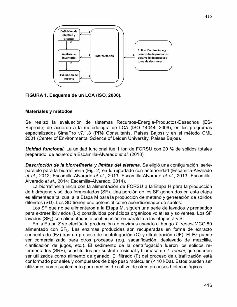
416
416
FIGURA 1. Esquema de un LCA (ISO, 2006). Materiales y métodos Se realizó la evaluación de sistemas Recursos-Energía-Productos-Desechos (ES-Reprode) de acuerdo a la metodología de LCA (ISO 14044, 2006), en los programas especializados SimaPro v7.1.8 (PRé Consultants, Países Bajos) y en el método CML 2001 (Center of Environmental Science of Leiden University, Países Bajos). Unidad funcional. La unidad funcional fue 1 ton de FORSU con 20 % de sólidos totales preparado de acuerdo a Escamilla-Alvarado et al. (2013) Descripción de la biorrefinería y límites del sistema. Se eligió una configuración serie-paralelo para la biorrefinería (Fig. 2) en lo reportado con anterioridad (Escamilla-Alvarado et al., 2012; Escamilla-Alvarado et al., 2013; Escamilla-Alvarado et al., 2013; Escamilla-Alvarado et al., 2014; Escamilla-Alvarado, 2014). La biorrefinería inicia con la alimentación de FORSU a la Etapa H para la producción de hidrógeno y sólidos fermentados (SF). Una porción de los SF generados en esta etapa es alimentada tal cual a la Etapa M para la producción de metano y generación de sólidos diferidos (SD). Los SD tienen uso potencial como acondicionador de suelos. Los SF que no se alimentaron a la Etapa M, siguen una serie de lavados y prensados para extraer lixiviados (Lx) constituidos por ácidos orgánicos volátiles y solventes. Los SF lavados (SFL) son alimentados a continuación en paralelo a las etapas Z y S. En la Etapa Z se efectúa la producción de enzimas usando el hongo T. reesei MCG 80 alimentado con SFL. Las enzimas producidas son recuperadas en forma de extracto concentrado (Ez) tras un proceso de centrifugación (C) y ultrafiltración (UF). El Ez puede ser comercializado para otros procesos (e.g. sacarificación, deslavado de mezclilla, clarificación de jugos, etc.). El sedimento de la centrifugación fueron los sólidos re-fermentados (SRF), constituidos por sustrato residual y biomasa de T. reesei, que pueden ser utilizados como alimento de ganado. El filtrado (F) del proceso de ultrafiltración está conformado por sales y compuestos de bajo peso molecular (< 10 kDa). Éstos pueden ser utilizados como suplemento para medios de cultivo de otros procesos biotecnológicos.
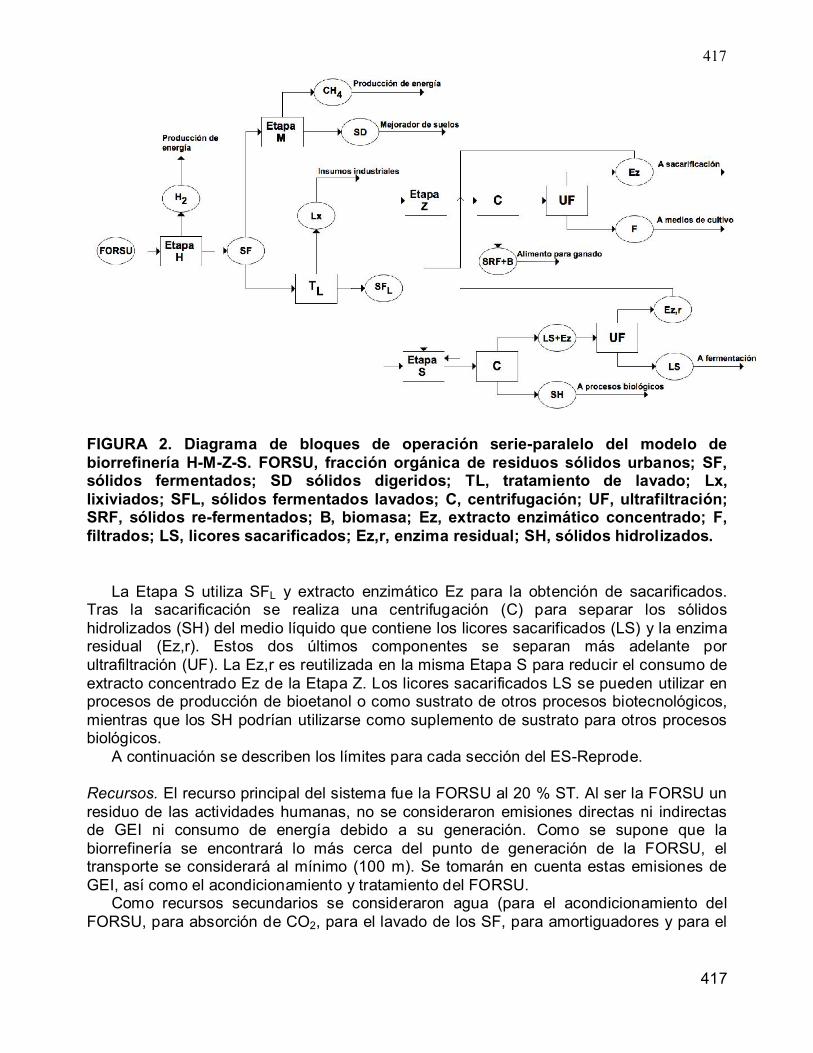
417
417
FIGURA 2. Diagrama de bloques de operación serie-paralelo del modelo de biorrefinería H-M-Z-S. FORSU, fracción orgánica de residuos sólidos urbanos; SF, sólidos fermentados; SD sólidos digeridos; TL, tratamiento de lavado; Lx, lixiviados; SFL, sólidos fermentados lavados; C, centrifugación; UF, ultrafiltración; SRF, sólidos re-fermentados; B, biomasa; Ez, extracto enzimático concentrado; F, filtrados; LS, licores sacarificados; Ez,r, enzima residual; SH, sólidos hidrolizados. La Etapa S utiliza SFL y extracto enzimático Ez para la obtención de sacarificados. Tras la sacarificación se realiza una centrifugación (C) para separar los sólidos hidrolizados (SH) del medio líquido que contiene los licores sacarificados (LS) y la enzima residual (Ez,r). Estos dos últimos componentes se separan más adelante por ultrafiltración (UF). La Ez,r es reutilizada en la misma Etapa S para reducir el consumo de extracto concentrado Ez de la Etapa Z. Los licores sacarificados LS se pueden utilizar en procesos de producción de bioetanol o como sustrato de otros procesos biotecnológicos, mientras que los SH podrían utilizarse como suplemento de sustrato para otros procesos biológicos. A continuación se describen los límites para cada sección del ES-Reprode. Recursos. El recurso principal del sistema fue la FORSU al 20 % ST. Al ser la FORSU un residuo de las actividades humanas, no se consideraron emisiones directas ni indirectas de GEI ni consumo de energía debido a su generación. Como se supone que la biorrefinería se encontrará lo más cerca del punto de generación de la FORSU, el transporte se considerará al mínimo (100 m). Se tomarán en cuenta estas emisiones de GEI, así como el acondicionamiento y tratamiento del FORSU. Como recursos secundarios se consideraron agua (para el acondicionamiento del FORSU, para absorción de CO2, para el lavado de los SF, para amortiguadores y para el

418
418
medio de cultivo de T. reesei), sales y compuestos (para amortiguadores y medio de cultivo de T. reesei). Energía. Se calculó la generación de energía a partir de celdas de combustible para el hidrógeno producido en la Etapa H (%eléctrica = 80 %), y de una planta de ciclo combinado para el metano producido en la Etapa M (%eléctrica = 55 %, %calórica = 20 %). Los consumos de electricidad y energía por transporte y operación de los procesos, se obtuvieron de las librerías de SimaPro, cálculos a partir de los datos experimentales de la biorrefinería H-M-Z-S, y de los reportes en literatura. La Tabla 1 muestra los elementos para cada etapa que se tomaron en cuenta para el balance de energía TABLA 1. Descripción de consumos y producción de energía Etapa Consumo Producción/recuperación Recolección/ acondicionamiento
Transporte de FORSU, molienda, mezclado, bombeo del FORSU al almacenamiento.
NA
H Transporte de FORSU al reactor, intercambiador de calor, calentamiento del reactor, purificación y compresión del hidrógeno.
Conversión del H2 a electricidad en celda de combustible.
M Transporte de SF al reactor, intercambiador de calor, calentamiento del reactor, compresión y purificación del metano, bombeo de SD
Combustión del CH4 en planta de ciclo combinado para producción de electricidad y vapor. Recuperación de calor de SD.
Lavado de sólidos Transporte de SF, 2 filtro prensa, 2 mezclador, filtro rotatorio, calentamiento del agua de lavado, transporte de SFL al almacenamiento.
Recuperación de calor de lixiviados.
Z Transporte de SFL al reactor, bombeo del inóculo, bombeo del medio, calentamiento del reactor, bombeo a centrífuga, operación de centrífuga, bombeo del extracto enzimático, ultrafiltración, bombeo de sólidos refermentados
NA
S Transporte de SFL al reactor, bombeo de extracto enzimático, bombeo del amortiguador, intercambiadores de calor, calentamiento del reactor, bombeo a centrífuga, operación de centrífuga, bombeo del hidrolizado, ultrafiltración, bombeo de sólidos hidrolizados
Recuperación de calor de hidrolizados
Notas: SD, sólidos digeridos; SF, sólidos fermentados; SFL, sólidos fermentados lavados Productos. Además del hidrógeno, metano, enzimas y sacarificados como productos principales, también produjeron otros materiales cuyos potenciales usos no se consideraron en el presente modelado por falta de información:
• Etapa M: SD como mejorador de suelos en tierras de cultivo. • Lavado de SF: lixiviados como insumos industriales. • Etapa Z: sólidos re-fermentados (SRF) y biomasa como alimento para ganado,
concentrado enzimático como insumo para procesos de sacarificación y los filtrados como suplemento en medios de cultivo.

419
419
• Etapa S: sólidos hidrolizados (SH) como suplemento de sustrato para procesos biológicos, sacarificados como sustrato para la obtención de etanol.
Desecho. Se consideraron las emisiones directas e indirectas de GEI de origen fósil por abasto adicional de energía, cuando la energía (calórica y/o eléctrica) proporcionada por las etapas H y M no fue suficiente para abastecer los requerimientos de la biorrefinería. Además se tomaron en cuenta las emisiones fugitivas de metano y generación de NOx y SOx por efecto de los procesos de combustión. Análisis de inventarios de ciclo de vida. De estudios previos (Escamilla-Alvarado et al., 2014) se seleccionaron los resultados más significativos de las actividades experimentales del proceso H-M-Z-S (Tabla 2). De las librerías de SimaPro v7.1.8 (PRé Consultants, 2008) se eligieron procesos similares a los propuestos en la biorrefinería H-M-Z-S. TABLA 2. Condiciones experimentales y resultados seleccionados de la biorrefinería H-M-Z-S
FORSU H – semi-continuo M – semi-continuo
Papel 40 %p/p y RSO 60 %p/p 20 %ST
Alimentación: FORSU 20 %ST T = 55 ºC TRM = 21 d I = 250 NmL H2/kgr/d [H2] = 30 % Êp = 256 kJ/kgbs
Alimentación: SF 18.4 % ST T = 55 ºC TRM = 28 d I = 2 200 NmL CH4/kgr/d [CH4] = 65 % Êp = 11 800 kJ/kgbs
FS lavados Z - fermentador S - lote
T = 60 ºC N = 120 rpm t = 10 min 80 %ST
Alimentación: SF 1.5 %SV N = 450 rpm T = 30 ºC top = 4 d FPx: 1 611 FPU/L CMCx: 1 067 IU/L Xilanasas: 3 113 IU/L
Alimentación: SF 8.6a %SV Carga enzimática: Ext Tr N = 150 rpm T = 50 ºC top = 48 h %s,h b = 74.6 %
Notas: RSO, residuos sólidos orgánicos; a valor extrapolado; b eficiencia de sacarificación en base holocelulosa. Balance de masa. De acuerdo a la unidad funcional, la corriente de entrada del sustrato fue 1 ton de FORSU (20 %ST) (Tabla 3). Como los SF fueron el sustrato de las etapas M, Z y S, su distribución fue discrecional. Se repartieron 40 % a la Etapa M, 40 % a la Etapa Z, y 20 % a la Etapa S. El balance de masa contempló algunas sustancias auxiliares en la operación de la biorrefinería. Tal es el caso de la solución de monoetanolamina (MEA) que se utilizó para purificar el hidrógeno y metano del biogás en las etapas H y M. La producción de los lixiviados extraídos de los SF en el tratamiento de lavado, se distribuyó en las corrientes de salida de las etapas Z y S proporcionalmente a la cantidad de SF que se consumieron

420
420
en cada etapa. Se muestran las cantidades de CO2 biogénico producido por las fermentaciones y digestión de las etapas H, M y Z. TABLA 3. Balance de masa del modelo de biorrefinería Etapa Corriente de entrara Tonbh Corriente de salida Tonbh H RSO 0.480 SF 0.975 Papel 0.081 Pérdidas por evaporación 0.0001 Agua 0.439 H2 0.0005 Solución MEA 1.660 CO2 0.024 Solución MEA 1.660 Total 2.660
Total 2.660
M SF 0.390 SD 0.328 Solución MEA 1.753 Pérdidas por evaporación 0.020 CH4 0.017 CO2 0.025 Solución MEA 1.753 Total 2.143
Total 2.143
Z SF 0.390 Lixiviados 0.912 Agua de lavado 0.593 SRF 0.050 Inóculo 0.349 Concentrado enzimático 0.342 Medio Mandels 3.071 Filtrado 3.080 CO2 0.006 Total 4.404 Total 4.404 S SF 0.195 Lixiviados 0.456 Agua de lavado 0.297 SH 0.013 Enzima fresca 0.012 Enzima reciclada 0.029 Enzima reciclada 0.029 LS 0.263 Amortiguador citratos 0.228 Total 0.761 Total 0.761 Notas: LS, licores sacarificados; MEA, monoetanolamina; RSO, residuos sólidos orgánicos; SF, sólidos fermentados; SRF, sólidos re-fermentados; SH, sólidos hidrolizados. Análisis de tecnologías. Las principales tecnologías que se ocuparon en la evaluación de sistemas ES-Reprode se muestran en la Tabla 4. Los flujos de las corrientes principales de reactivos y productos se ajustaron con los datos del balance global de masa mientras que los flujos de corrientes secundarias o complementarios se ajustaron con los datos de las librerías. Los pasos uno y dos corresponden a la recolección de los residuos sólidos orgánicos (RSO) y del papel como constituyentes de la FORSU, y su acondicionamiento con sales de fosfato como amortiguador de pH. En el paso 1 se consideró el consumo de CO2 del aire para la constitución de los RSO y del papel. Se consideraron también cargas ambientales por transporte de los RSO y del papel en vehículo de 3.5 ton dentro de la biorrefinería.

421
421
TABLA 4. Tecnologías incluídas en la evaluación de sistemas y sus principales flujos Paso Producción DdC a
(%) Consumo Tecnología
(en inglés) Observaciones de la tecnología
Recolección/acondicionamiento 1 RSO 25 %ST +
papel 99 %ST 1 kg 100 CO2, en el aire 0.5663 kg Biowaste at
collection point
Transporte dentro de biorrefinería
0.0001 t*km Transport van <3.5t
220 000 t*km/vehículo, Suiza/Europa
2 FORSU acondicionada 20 %ST
1 kg 100 RSO 25 %TS + papel 99 %TS
0.5610 kg Biowaste at collection point
Agua de acondicionamiento
0.4392 kg Tap water Suiza.
Fosfatos en roca 0.0362 kg b Dry rock or dried wet rock processing
Promedio de mezcla de tecnologías, EUA.
Etapa H 3 Biogás de FORSU
acondicionada 1 m3 20 FORSU
acondicionada 20 %ST
57.1429 kg Biogas from biowaste
Planta de digestión anaerobia de desechos orgánicos, 10 000t/año, 25 años, termofílica, digestión en una etapa, con post-composteo, Suiza.
SF 16.2 %ST 55.7381 kg
80 CO2, biogénico 1.3750 kg
CO2, biogénico 1.3750 kg - Calor (sustituido) 9.6674 MJ Biogas burned in cogen
Eficiencia electr. 0.32, Eficiencia calorífica 0.55, Suiza.
Electricidad (sustituida)
0.3737 kWh Electricity, low voltage
Voltaje medio a bajo, Suiza e importaciones.
4 Hidrógeno al 99% de biogás
1 m3 100 Biogás de FORSU acondicionada
3.3333 m3 Methane 96% purification
Instalaciones para producción de químicos. Composición de una planta química basada en una unidad de destilación, Suiza.
Electricidad (sustituida)
1.1100 kWh c Electricity, medium voltage
Voltaje alto a medio, Suiza e importaciones.
5 Electricidad de H2 al 99% en celda PEM
1 kWh 100 Hidrógeno al 99% de biogás
0.3564 m3 Electricity, biogas, alloc. exergy, PEM future
Celda de combustible PEM, 2 kW salida eléctrica,15 años o 80 000 h de operación. Eficiencia eléctrica 32 %, eficiencia total 87%, Europa central.
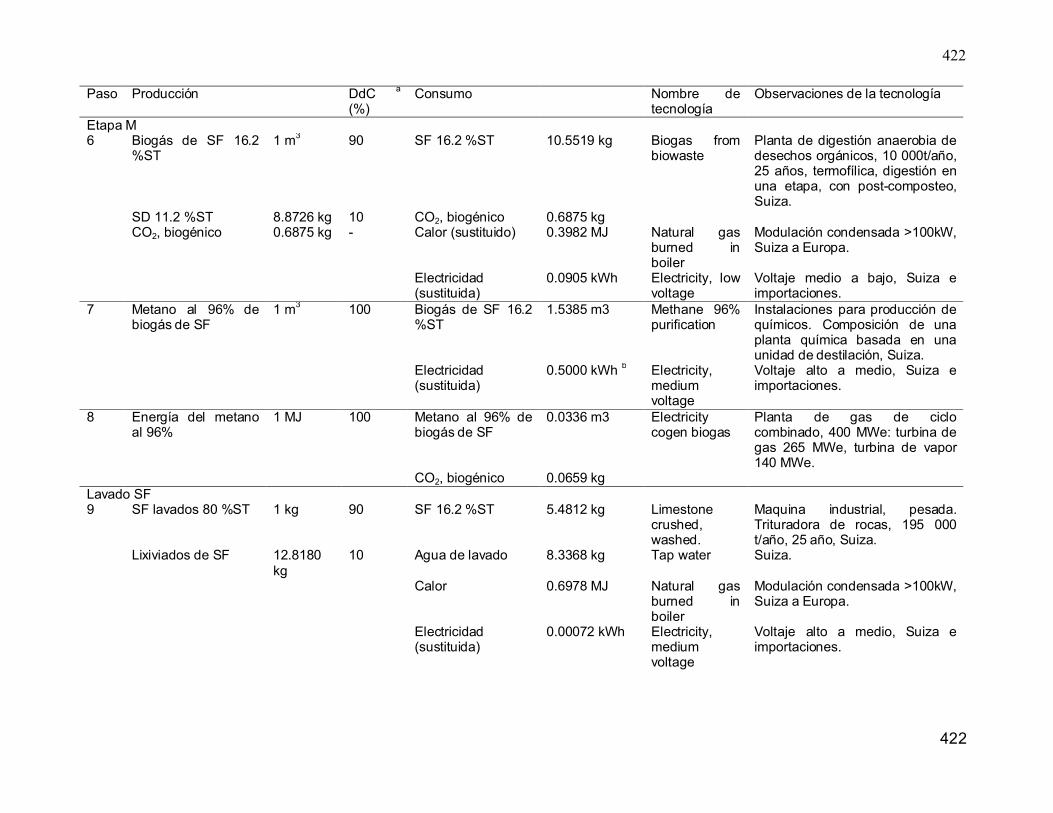
422
422
Paso Producción DdC a
(%) Consumo Nombre de
tecnología Observaciones de la tecnología
Etapa M 6 Biogás de SF 16.2
%ST 1 m3 90 SF 16.2 %ST 10.5519 kg Biogas from
biowaste Planta de digestión anaerobia de desechos orgánicos, 10 000t/año, 25 años, termofílica, digestión en una etapa, con post-composteo, Suiza.
SD 11.2 %ST 8.8726 kg 10 CO2, biogénico 0.6875 kg CO2, biogénico 0.6875 kg - Calor (sustituido) 0.3982 MJ Natural gas
burned in boiler
Modulación condensada >100kW, Suiza a Europa.
Electricidad (sustituida)
0.0905 kWh Electricity, low voltage
Voltaje medio a bajo, Suiza e importaciones.
7 Metano al 96% de biogás de SF
1 m3 100 Biogás de SF 16.2 %ST
1.5385 m3 Methane 96% purification
Instalaciones para producción de químicos. Composición de una planta química basada en una unidad de destilación, Suiza.
Electricidad (sustituida)
0.5000 kWh b Electricity, medium voltage
Voltaje alto a medio, Suiza e importaciones.
8 Energía del metano al 96%
1 MJ 100 Metano al 96% de biogás de SF
0.0336 m3 Electricity cogen biogas
Planta de gas de ciclo combinado, 400 MWe: turbina de gas 265 MWe, turbina de vapor 140 MWe.
CO2, biogénico 0.0659 kg Lavado SF 9 SF lavados 80 %ST 1 kg 90 SF 16.2 %ST 5.4812 kg Limestone
crushed, washed.
Maquina industrial, pesada. Trituradora de rocas, 195 000 t/año, 25 año, Suiza.
Lixiviados de SF 12.8180 kg
10 Agua de lavado 8.3368 kg Tap water Suiza.
Calor 0.6978 MJ Natural gas burned in boiler
Modulación condensada >100kW, Suiza a Europa.
Electricidad (sustituida)
0.00072 kWh Electricity, medium voltage
Voltaje alto a medio, Suiza e importaciones.

423
423
Paso Producción DdC a
(%) Consumo Nombre de
tecnología Observaciones de la tecnología
Etapa Z 10 Enzimas
concentradas 10 veces
1 kg 80 SF lavados 80 %ST
0.2080 kg Proteins from grass/Syrup from sugar beet molasses
Planta de fermentación para etanol, 90 000 t etanol/año, 20 años, EUA, trigo como recurso.
Filtrados de SRF 9 kg 15 Agua para fermentación
8.9737 kg Tap water Suiza.
SRF 90 %ST 0.2019 kg 5 Agua para inóculo 1.0202 kg Tap water Suiza. CO2, biogénico 0.0567 kg - Calor 0.2183 MJ d Natural gas
burned in boiler
Modulación condensada >100kW, Suiza a Europa.
Electricidad (sustituida)
0.2000 kWh b Electricity, medium voltage
Voltaje alto a medio, Suiza e importaciones.
Etapa S 11 Sacarificados al
6.19% 1 kg 90 SF lavados 80
%ST 0.1355 kg Proteins from
grass/Syrup from sugar beet molasses
Planta de fermentación para etanol, 90 000 t etanol/año, 20 años, EUA, trigo como recurso.
SH 90 %TS 0.0480 kg 10 Agua para sacarificación
0.8663 kg Tap water Suiza
Enzimas concentradas 10 veces
0.0462 kg
Calor 0.0488 MJ d Natural gas burned in boiler
Modulación condensada >100kW, Suiza a Europa.
Electricidad (sustituida)
0.0800 kWh b Electricity, medium voltage
Modulación condensada >100kW, Suiza a Europa.
Notas: a distribución de cargas contaminantes, b valor sujeto a verificación, c valor probablemente sobrestimado, d valor probablemente subestimado; RSO, residuos sólidos orgánicos; ST, sólidos totales; FORSU, fracción orgánica de residuos sólidos urbanos; SF sólidos fermentados; PEM, membrana de intercambio de protones; SD, sólidos digeridos; SRF, sólidos refermentados; SH, sólidos hidrolizados

Environmental Biotechnology and Engineering-2014
424
La Etapa H incluye los pasos de producción de biogás a partir de FORSU acondicionada (paso 3), la purificación del hidrógeno (paso 4) y la generación de electricidad en celda de combustible PEM (paso 5). En el paso 3 se emitió CO2 como producto de la fermentación. Tanto el calor como la electricidad requeridas en la Etapa 3 se consideraron abastecidas por la generación de las mismas en la biorrefinería. En la Etapa M se consideró la producción de biogás a partir de SF (paso 6), la purificación del metano al 96 % (paso 7) y la conversión de éste en calor y electricidad en una planta de ciclo combinado (paso 8). En el paso 6 se generaron SD y CO2 de origen biogénico por la digestión anaerobia. La actividad de lavado de los SF para su posterior alimentación a las etapas Z y S se basó en una tecnología de trituración de piedras y su lavado con agua. Se consideró agua de lavado adicional para la constitución de los lixiviados. La electricidad fue abastecida por la biorrefinería, pero el calor se generó a partir de la quema de gas natural en caldera. La Etapa Z consideró el consumo SF lavados, agua y calor para la producción del extracto enzimático concentrado. Se generaron también SRF y CO2 de origen biogénico por la fermentación. En la Etapa S se consideró el consumo de SF lavados, agua, enzimas concentradas y calor para la producción de sacarificados y SH. Escenario de comparación. Se realizó la comparación a nivel de impactos ambientales de la biorrefinería contra un modelo de relleno sanitario utilizando la misma unidad funcional de 1 ton FORSU 20 %ST. Las consideraciones iniciales del relleno sanitario fueron: - Tecnología ubicada en Suiza en el año 2000. - Considerando materiales orgánicos e inorgánicos, la degradabilidad a lo largo
de 100 años es del 18.73 %. - Se incluyó sistema de recolección de lixiviados, y su respectivo tratamiento en
planta tratadora de aguas residuales con recolección de gas. - Se consideraron emisiones a la atmósfera a corto plazo por la quema del
biogás y por los lixiviados. También se consideraron las cargas del tratamiento de los lixiviados a corto plazo (0 – 100 años) en la planta tratadora de aguas (incluyendo la disposición de sus lodos en incinerador municipal). Se incluyeron las emisiones a mantos freáticos a largo plazo debido al rompimiento de la geomembrana.
Evaluación ambiental. Se evaluaron seis categorías de impactos ambientales: agotamiento abiótico, acidificación, eutroficación, calentamiento global, agotamiento de capa de ozono y oxidación fotoquímica.
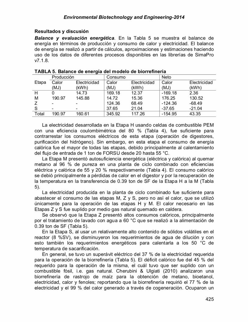
Environmental Biotechnology and Engineering-2014
425
Resultados y discusión Balance y evaluación energética. En la Tabla 5 se muestra el balance de energía en términos de producción y consumo de calor y electricidad. El balance de energía se realizó a partir de cálculos, aproximaciones y estimaciones haciendo uso de los datos de diferentes procesos disponibles en las librerías de SimaPro v7.1.8. TABLA 5. Balance de energía del modelo de biorrefinería
Etapa Producción Consumo Neto Calor (MJ)
Electricidad (kWh)
Calor (MJ)
Electricidad (kWh)
Calor (MJ)
Electricidad (kWh)
H 0 14.73 169.18 12.37 -169.18 2.36 M 190.97 145.88 14.72 15.36 176.25 130.52 Z - - 124.36 68.49 -124.36 -68.49 S - - 37.65 21.04 -37.65 -21.04 Total 190.97 160.61 345.92 117.26 -154.95 43.35 La electricidad desarrollada en la Etapa H usando celdas de combustible PEM con una eficiencia coulombimétrica del 80 % (Tabla 4), fue suficiente para contrarrestar los consumos eléctricos de esta etapa (operación de digestores, purificación del hidrógeno). Sin embargo, en esta etapa el consumo de energía calórica fue el mayor de todas las etapas, debido principalmente al calentamiento del flujo de entrada de 1 ton de FORSU desde 20 hasta 55 °C. La Etapa M presentó autosuficiencia energética (eléctrica y calórica) al quemar metano al 96 % de pureza en una planta de ciclo combinado con eficiencias eléctrica y calórica de 55 y 20 % respectivamente (Tabla 4). El consumo calórico se debió principalmente a pérdidas de calor en el digestor y por la recuperación de la temperatura en la transferencia de 0.39 ton de SF de la Etapa H a la M (Tabla 5). La electricidad producida en la planta de ciclo combinado fue suficiente para abastecer el consumo de las etapas M, Z y S, pero no así el calor, que se utilizó únicamente para la operación de las etapas H y M. El calor necesario en las Etapas Z y S fue suplido por medio gas natural quemado en caldera. Se observó que la Etapa Z presentó altos consumos calóricos, principalmente por el tratamiento de lavado con agua a 60 °C que se realizó a la alimentación de 0.39 ton de SF (Tabla 5). En la Etapa S, al usar un relativamente alto contenido de sólidos volátiles en el reactor (8 %SV), se disminuyeron los requerimientos de agua de dilución y con esto también los requerimientos energéticos para calentarla a los 50 °C de temperatura de sacarificación. En general, se tuvo un superávit eléctrico del 37 % de la electricidad requerida para la operación de la biorrefinería (Tabla 5). El déficit calórico fue del 45 % del requerido para la operación de la misma, el cuál tuvo que ser suplido con un combustible fósil, i.e. gas natural. Cherubini & Ulgiati (2010) analizaron una biorrefinería de rastrojo de maíz para la obtención de metano, bioetanol, electricidad, calor y fenoles; reportando que la biorrefinería requirió el 77 % de la electricidad y el 99 % del calor generado a través de cogeneración. Ocuparon un

Environmental Biotechnology and Engineering-2014
426
pretratamiento térmico para hidrolizar la biomasa, ocupando los azúcares C6 y C5 para la fermentación alcohólica, los aceites pirolíticos de la lignina para producir fenoles, y los residuos de lignina y de la fermentación para la producción de energía. En términos de energía neta, sumando calor y electricidad, la biorrefinería tuvo un balance de cero; es decir, no hubo ganancia ni pérdida energética. La ventaja de haber obtenido sobreproducción eléctrica, es que este tipo de energía tiene mayor valor agregado que la energía calórica. Este postulado podría ser demostrado realizando un balance de exergía, o energía aprovechable en forma de trabajo, ya que la energía eléctrica tiene un mayor valor exergético que la energía calórica de temperatura menor a 100 °C (Goedkoop et al., 2009; Schubert et al., 2009). Evaluación ambiental. Como primer paso para comparar la sustentabilidad ambiental de la biorrefinería se realizó un balance de CO2 siguiendo la siguiente fórmula:
CO2,neto = (CO2,biogenico + (CO2,fósil – (CO2,biomasa [1] la cual considera el CO2 producido en la biorrefinería H-M-Z-S por procesos biológicos (116.1 kg CO2), el CO2 de origen fósil por efectos de la quema de combustibles fósiles (8.01 kg CO2) y el consumo de CO2 de la atmósfera consecuencia de su integración a la biomasa vegetal (317.6 kg CO2). El resultado del balance fue – 193.5 kg CO2/ton FORSU; lo que indica que se tienen ahorros de CO2 al utilizar la biomasa de la FORSU en la producción de biocombustibles y bioproductos. El CO2 biogénico que no fue liberado en los procesos de biorrefinería, se asume que se encuentra aún fijado en los SD, SRF, SH, enzimas, lixiviados y LS que se produjeron en las etapas M, Z y S. El análisis del destino final de estos productos requiere mayor información sobre las tecnologías que los usarían para evaluar correctamente sus cargas ambientales. El proceso que tuvo la mayor aportación en los impactos ambientales fue la producción de energía en planta de ciclo combinado de la Etapa M, pues tuvo el mayor impacto en acidificación y en calentamiento global (Fig. 3a y 3c). Los principales compuestos con impacto en la acidificación fueron el dióxido de azufre, ácido sulfhídrico, amoniaco y óxidos de nitrógeno por ser productos de la combustión del metano al 96 % de pureza o como subproductos de la digestión anaerobia. Justamente el proceso con mayor impacto (Fig. 3a) fue la producción de energía en la planta de ciclo combinado. Le siguieron la digestión de SF en la Etapa M y la fermentación de la FORSU en la Etapa H. En eutroficación, los principales compuestos con mayor impacto fueron el amoniaco, óxidos de nitrógeno, fósforos y compuestos orgánicos. En esta categoría, la producción y uso de los fosfatos aparece como el tercer proceso con mayor impacto (Fig. 3b). En cuarto lugar aparece la fermentación de la FORSU, ya que en este proceso se produjeron los SF que se ocuparon como sustrato en las demás etapas, y las cargas ambientales de su uso recayeron justamente en su proceso de producción (Tabla 6).
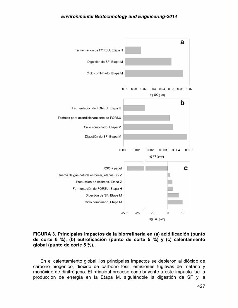
Environmental Biotechnology and Engineering-2014
427
FIGURA 3. Principales impactos de la biorrefinería en (a) acidificación (punto de corte 6 %), (b) eutroficación (punto de corte 5 %) y (c) calentamiento global (punto de corte 5 %). En el calentamiento global, los principales impactos se debieron al dióxido de carbono biogénico, dióxido de carbono fósil, emisiones fugitivas de metano y monóxido de dinitrógeno. El principal proceso contribuyente a este impacto fue la producción de energía en la Etapa M, siguiéndole la digestión de SF y la
kg PO4-eq
0.000 0.001 0.002 0.003 0.004 0.005
Digestión de SF, Etapa M
Ciclo combinado, Etapa M
Fosfatos para acondicionamiento de FORSU
Fermentación de FORSU, Etapa H
kg SO2-eq
0.00 0.01 0.02 0.03 0.04 0.05 0.06 0.07
Ciclo combinado, Etapa M
Digestión de SF, Etapa M
Fermentación de FORSU, Etapa H
kg CO2-eq
-275 -250 -50 0 50
Ciclo combinado, Etapa M
Digestión de SF, Etapa M
Fermentación de FORSU, Etapa H
Producción de enzimas, Etapa Z
Quema de gas natural en boiler, etapas S y Z
RSO + papel
a
b
c

Environmental Biotechnology and Engineering-2014
428
fermentación de FORSU (Fig. 3c). Las etapas S y Z tuvieron impactos ligeramente menores que las demás etapas principalmente debidos a la quema de gas natural para abastecer su calentamiento. La FORSU, constituida por RSO y papel, proveyó los impactos negativos en forma de CO2 fijado de la atmósfera. En la Tabla 6 se muestran los impactos ambientales más significativos para la biorrefinería en base 1 ton de FORSU como unidad funcional, y para la disposición directa de la misma cantidad de FORSU en relleno sanitario como proceso comparativo. La biorrefinería presentó mayores impactos en el agotamiento abiótico, acidificación y agotamiento de la capa de ozono que el relleno sanitario. El agotamiento abiótico fue mayor en la biorrefinería por el uso de gas natural en los procesos de calentamiento de las etapas Z y S, mientras que la acidificación y la eutroficación se vieron influenciadas por los procesos de producción de energía en la planta de ciclo combinado y de digestión anaerobia de la Etapa M (Fig. 3). En las categorías de eutroficación y calentamiento global, la disposición en relleno sanitario tuvo mayores impactos que la biorrefinería. Esto se pudo deber a que la tecnología de relleno sanitario consideró las emisiones de filtraciones de lixiviados, emisiones a la atmósfera por la incineración del biogás y emisiones fugitivas de gases de efecto invernadero. En el caso de la eutroficación, los compuestos orgánicos como el amoniaco, nitratos y óxidos de nitrógeno (reportados en base DQO), fueron los principales contribuyentes a este impacto por la vía aire y agua, mientras que el fósforo fue el principal contribuyente a la eutroficación vía suelo. TABLA 6. Impactos totales de la biorrefinería. Categoría de impacto Biorrefinería Relleno sanitario Agotamiento abiótico (kg Sb-eq.) 0.140 0.082 Acidificación (kg SO2-eq.) 0.202 0.160 Eutroficación (kg PO4-eq.) 0.019 1.43 Calentamiento global 100a (kg CO2-eq.) -128 50.7 Agotamiento de la capa de ozono 40a (kg CFC11-eq.)
2.96 E-06 1.70 E-06
Oxidación fotoquímica (kg C2H4-eq.) 0.009 0.075 En la categoría de calentamiento global la biorrefinería demostró un impacto negativo (ahorro de cargas ambientales), mientras que el relleno sanitario tuvo un impacto positivo (daño al ambiente). Este impacto positivo en el relleno sanitario se debió a las considerables emisiones fugitivas de metano biogénico que no pueden ser adecuadamente retenidas para ser quemadas y reducir su impacto ambiental en forma de CO2. Con el objetivo de hacer una comparación más sencilla entre la biorrefinería y el relleno sanitario, los impactos se normalizaron al multiplicarse por sus respectivos factores de referencia, de acuerdo al método CML 2001 (V2.04 / World, 1995). El resultado nos da un valor normalizado adimensional que puede sumarse entre todos los valores de los impactos evaluados, y así comparar el

Environmental Biotechnology and Engineering-2014
429
“impacto” total de una tecnología con respecto a otra. La suma de los impactos normalizados en la biorrefinería fue negativa -1.32 x 10⁻¹², mientras que la del relleno sanitario fue 1.38 x 10⁻¹¹ (Fig. 4). Esto señala que esta tecnología es más favorables para el ambiente que el relleno sanitario. La categoría de calentamiento global fue la causante del ahorro de impactos normalizados en la biorrefinería, mientras que la principal categoría con impactos en el relleno sanitario fue la eutroficación seguida del calentamiento global.
FIGURA 4. Impactos normalizados para los escenarios de biorrefinería y relleno sanitario. En el análisis de ciclo de vida de tres opciones de manejo de bagazo con recuperación de energía usando el método EDIP/UMIP 97, Kiatkittpong et al. (2009) determinaron que la digestión anaerobia superaba al relleno sanitario y a la incineración en todos los aspectos ambientales. En el caso de los rellenos sanitarios, su beneficio ambiental depende significativamente de la eficiencia de recolección del biogás y de los lixiviados (Manfredi & Christensen, 2009). Una baja recolección de biogás permite mayores emisiones de metano, el cual tiene un potencial de calentamiento global al menos 25 veces superior al del CO2. Si bien con la incineración Kiatkittipong et al. (2009) obtuvieron mejor desempeño ambiental que con el relleno sanitario con baja eficiencia de recolección de biogás, éstos no mejoraron el desempeño ambiental de la digestión anaerobia principalmente debido a los mayores impactos en oxidación fotoquímica por parte de la incineración. Una forma de hacer ambientalmente favorables a los rellenos sanitarios es dotándolos de tecnologías adicionales, como la recirculación intensiva de lixiviados o la aireación convectiva después de la extracción exhaustiva de metano tras los primeros 10 años de operación (Manfredi & Christensen, 2009).
Escenario
Biorrefinería Relleno sanitario
Impa
ctos
nor
mal
izad
os (-
)
-4x10-12
0
4x10-12
8x10-12
12x10-12
16x10-12
Agotamiento abiótico Acidificación Eutroficación Calientamiento global
100 años Agotamiento de capa de ozono 40 años Oxidación fotoquímica
Environmental Biotechnology and Engineering-2014
430
Por lo general, se considera que la digestión anaerobia es una mejor opción comparada con el compostaje y la incineración, principalmente por las mayores cantidades de generación de electricidad y los créditos ambientales por emisiones evitadas debido a la sustitución de los combustibles fósiles como energéticos (Hanandeh & El-Zein, 2010). Para poder considerar a la digestión anaerobia además como un sumidero de carbono, los biosólidos producidos deben aplicarse a suelos con material húmico microbiológicamente estable (Peters & Rowley, 2009). Los procesos biológicos de tratamiento de residuos orgánicos pueden tener considerables impactos ambientales de eutroficación o acidificación, sin embargo las principales ventajas se observan en la recuperación de energía en términos de emisiones de calentamiento global evitadas al sustituir la generación de energía mediante combustibles fósiles (Boldrin et al., 2011). En el caso de la biorrefinería H-M-Z-S, además de darle tratamiento a la FORSU, se tuvo superávit de energía eléctrica y se generaron bioproductos (enzimas y sacarificados). Justamente, se ha señalado que la obtención de bioproductos proveería de beneficios económicos a la biorrefinería (Fahd et al., 2012). Además la biorrefinería tiene la ventaja adicional de ser ambientalmente favorable en comparación con la tecnología de relleno sanitario. Conclusión
• Tomando como unidad funcional 1 ton de FORSU al 20 % ST como alimentación de la biorrefinería, se tuvo un superávit eléctrico del 37 % de la electricidad requerida para la operación de la biorrefinería.
• Hubo déficit de energía calórica del 45 % de la requerida para la operación de la biorrefinería, que fue suplido con quema de gas natural.
• El balance de energía neto considerando la electricidad y calor producidos menos los consumidos fue de cero.
• La biorrefinería presentó impactos negativos (ahorros) en el calentamiento global debido a la fijación de CO2 atmosférico en la biomasa.
• Comparando la biorrefinería H-M-Z-S contra la tecnología de relleno sanitario, el relleno sanitario presentó los mayores impactos, principalmente por efecto del calentamiento global debido a emisiones fugitivas de metano y en la eutroficación del ambiente por los lixiviados.
• La biorrefinería representa una alternativa eléctrica, económica y ambientalmente favorable en comparación con la disposición de FORSU en relleno sanitario.
Agradecimientos Los autores agradecen al CONACYT por la beca otorgada a CE-A (no. de registro 209665) y por el apoyo para la investigación de enzimas (no. 104333), al SECITI

Environmental Biotechnology and Engineering-2014
431
del GDF (antes ICYTDF) por el apoyo económico para la investigación de biorrefinerías (proyecto PICCO 10-27), y al CINVESTAV por los apoyos económicos para la realización de este trabajo. Referencias Boldrin, A., Neidel, T.L., Damgaard, A., Bhander, G.S., Moller, J. & Christensen, T.H. (2011).
Modelling of environmental impacts from biological treatment of organic municipal waste in EASEWASTE. Waste Manage, 31, 619-630.
Cherubini, F. & Ulgiati, S. (2010). Crop residues as raw materials for biorefinery systems – A LCA case study. Appl Energy, 87, 47-57.
Escamilla-Alvarado, C. (2014) Integración de un modelo de biorrefinería para la obtención de hidrógeno, metano, enzimas y sacarificados a partir de la fracción orgánica de residuos sólidos urbanos. Departamento de Biotecnología y Bioingeniería, Centro de Investigación y de Estudios Avanzados del IPN, Mexico, D.F.
Escamilla-Alvarado, C., Poggi-Varaldo, H.M. & Ponce-Noyola, M.T. (2013). Use of organic waste for the production of added-value holocellulases with Cellulomonas flavigena PR-22 and Trichoderma reesei MCG 80. Waste Manage Res, 31, 849-858.
Escamilla-Alvarado, C., Ponce-Noyola, M.T., Ríos-Leal, E., García-Mena, J., Rinderknecht-Seijas, N. & Poggi-Varaldo, H.M. (2014). Energy analysis of in-series biohydrogen and methane production from organic wastes Int J Hydrogen Energy, In press.
Escamilla-Alvarado, C., Ponce-Noyola, M.T., Rios-Leal, E. & Poggi-Varaldo, H.M. (2013). A multivariable evaluation of biohydrogen production by solid substrate fermentation of organic municipal wastes in semi-continuous and batch operation. Int J Hydrogen Energy, 38, 12527-12538.
Escamilla-Alvarado, C., Ríos-Leal, E., Ponce-Noyola, M.T. & Poggi-Varaldo, H.M. (2012). Gas biofuels from solid substrate hydrogenogenic–methanogenic fermentation of the organic fraction of municipal solid waste. Process Biochem, 47, 1572-1587.
Fahd, S., Fiorentino, G., Mellino, S. & Ulgiati, S. (2012). Cropping bioenergy and biomaterials in marginal land: The added value of the biorefinery concept. Energy, 79-93.
Goedkoop, M., Oele, M., Schryver, A.d. & Vieira, M. (2008) SimaPro Database Manual. Methods library. The Netherlands.
Hanandeh, A.E. & El-zein, A. (2010). The development and application of multi-criteria decision-making tool with consideration of uncertainty: The selection of a management strategy for the bio-degradable fraction in the municipal solid waste. Bioresource Technology, 101, 555-561.
INEGI (2009) Anuario estadístico de los Estados Unidos Mexicanos. Instituto Nacional de Geografía. ISSN 0188-8692 Mexico.
IPCC (2006) Guidelines for national greenhouse gas inventories, volume 4, Agriculture, forestry and other land use. The Intergornmental Panel on Climate Change.
Islas, J., Manzini, F. & Masera, O. (2007). A prospectiv study of bioenergy in Mexico. Energy, 32, 2306-2320.
ISO (2006) ISO 1044. Environmental management - Life cycle assessment - Requirements and guidelines. The International Organization for Standardization. Geneva, Switzerland.
ISO (2006) ISO 14040. Environmental management - Life cycle assessment - Principles and framework. The Internation Organization for Standardization. Geneva, Switzerland.
Kiatkittipong, W., Wongsuchoto, P. & Pavasant, P. (2009). Life cycle assessment of bagasse waste management options. Waste management (New York, N.Y.), 29, 1628-1633.
Kirkeby, J. (2005) Modelling of life cycle assessment of solid waste management systems and technologies. Environmental Department, DTU, Kgs. Lyngby, Denmark.
Manfredi, S. & Christensen, T.H. (2009). Environmental assessment of solid waste landfilling technologies by means of LCA-modeling. Waste Manage, 29, 32-43.
Peters, G.M. & Rowley, H.V. (2009). Environmental comparison of biosolids management systems using life cycle assessment. Environ Sci Technol, 43, 2674-2679.
Poggi-Varaldo, H.M., Munoz-Paez, K.M., Escamilla-Alvarado, C., Robledo-Narváez, P.N., Ponce-Noyola, M.T., Calva-Calva, G., Ríos-Leal, E., Galíndez-Mayer, J., Estrada-Vázquez, C.,

Environmental Biotechnology and Engineering-2014
432
Ortega-Clemente, A. & Rinderknecht-Seijas, N.F. (2014). Biohydrogen, biomethane and bioelectricity as crucial components of biorefinery of organic wastes: A review. Waste Manage Res, 32, 353-365.
Pré (2008). SimaPro 7.1.9 - PRé Consultants. B.V. Plotterweg 12, 3821 AD Amersfoort. The Netherlands, www.pre.nl
Schubert, R., Schellnhuber, H.J., Buchmann, N., Epiney, A., Griesshammer, R., Kulessa, M., Messner, D., Rahmstorf, S. & Schmid, J. (2009) Future Bioenergy and Sustainable Land Use. Eartshcan, Malta.
Semarnat (2009) Informe de la situación del medio ambiente en México. Edición 2008. Compendio de estadísticas ambientales. México.
Notación FORSU fracción orgánica de los residuos sólidos urbanos ES-Reprode evaluación de sistemas Recursos-Energía-Productos-Desechos GEI gases de efecto invernadero H-M-Z-S biorrefinería de cuatro etapas para la producción de hidrógeno, metano,
enzimas y sacarificados LCA evaluación de ciclo de vida, del inglés Life Cycle Assessment Lx lixiviados MEA monoetanolamina PEM membrane de intercambio protónico, del inglés Proton Exchange
Membrane RSM residuos sólidos municipals RSO residuos sólidos orgánicos SD sólidos digeridos SF sólidos fermentados SH sólidos hidrolizados SRF sólidos re-fermentados ST sólidos totales

Environmental Biotechnology and Engineering-2014
433
LIST OF COAUTHORS: Carlos Escamilla-Alvarado, Sc D, presenting author. Same address and e-mail as those of Dr. H.M. Poggi-Varaldo Teresa Ponce-Noyola, Sc D, Full Professor. CINVESTAV, Dept. Biotechnology and Bioengineering, Microbial Genetics Group P.O. Box 14-740, México DF, 07000, México. Tel: 5255 5747 3800 ext 4317 E-mail: [email protected] Elvira Ríos-Leal, Full Professor CINVESTAV, Dept. Biotechnology and Bioengineering, Analysis Central, ibidem Tel: 5255 5747 3800 E-mail: [email protected] Fernando Esparza-García, Sc D, Full Professor CINVESTAV, Dept. Biotechnology and Bioengineering, Biochemical Ecology, ibidem Tel: 5255 5747 3800 E-mail: [email protected] Josefina Barrera-Cortes, Sc D, Full Professor CINVESTAV, Dept. Biotechnology and Bioengineering, Intelligent Control, ibidem Tel: 5255 5747 3800 E-mail: [email protected] Jaime García-Mena, Sc D, Full Professor CINVESTAV, Dept. of Genetics and Molecular Biology, ibidem Tel: 5255 5747 3800 E-mail: [email protected] Ireri Robles-Gonzalez, Sc D, Full Professor Nova Universitas E-mail: [email protected] Noemi Rindercknecht-Seijas, Full Professor ESIQIE-IPN E-mail: [email protected] Héctor M. Poggi-Varaldo, Sc D, Full Professor. Author to whom all correspondence should be addresed CINVESTAV, Dept. Biotechnology and Bioengineering, Environmental Biotechnology and Renewable Energies R&D Group; P.O. Box 14-740, México DF, 07000, México. Tel: 5255 5747 3800 ext 4324, Fax. 5255 5747 3313, E-mail: [email protected]

Environmental Biotechnology and Engineering-2014
434
Section 4. Air Pollution and Climate Change
Environmental Biotechnology and Engineering-2014
435
Page Chapter 4.1. Oxidation of methane in biotrickling filters inoculated with methanotrophic bacteria Manuel Cáceres; Juan C. Gentina; Germán Aroca 436 Chapter 4.2. Bio-oxidation of methane in a membrane reactor with a biofilm of methylomicrobium album Germán Aroca Arcaya; María J. Cárdenas; Alberto Aguirre; Matías Gómez; Sebastián Madrid; Juan C. Gentina 446
Chapter 4.3. Simultaneous treatment of dimethyl disulfide and hydrogen sulfide vapors in an alkaline biotrickling filter Luis Arellano-García; Sergio Revah 454 Chapter 4.4. Impacto de las características fisicoquímicas y dinámica de carbono en suelo, después de nueve años de la reintroducción con vegetacion nativa en un suelo perturbado Martha V. Almanza-Estrada; Blanca G. Elías-Balandrán; María M. Vargas-Zúñiga; Yazmín A. Sánchez-Ruan; Alejandra Gutiérrez-Vázquez; Juan A. Mejía-Gómez; Jaquelina González-Castañeda 460
Environmental Biotechnology and Engineering-2014
436
CHAPTER 4.1. OXIDATION OF METHANE IN BIOTRICKLING FILTERS INOCULATED WITH METHANOTROPHIC BACTERIA
Manuel Cáceres; Juan Carlos Gentina; Germán Aroca*
School of Biochemical Engineering, Pontificia Universidad Católica de Valparaíso. Av. Brasil 2147, Valparaíso, Chile. Tel.: 56-32-2273641 Fax: 56-32-2273803. E-mail: [email protected] ABSTRACT Methane (CH4) is considered the second largest contributor to the greenhouse effect with a global warming potential (GWP) of 23 related to carbon dioxide (CO2). The oxidation of CH4 using biological systems has been proposed as an alternative to mitigate greenhouse gas emissions with low concentration of CH4. In the case of biofilters, non-specific inoculums have been used, leading to reports with a wide range of removal efficiencies. The main objective of this work was to characterize the oxidation of CH4 in biotrickling filters (BTF) packed with polyethylene rings for supporting a biofilm of a mixture of methanotrophic bacteria type I and II, Methylomicrobium album and Methylocystis sp. Two identical BTF were set up with columns of clear PVC (height: 1.2 m; i.d.: 0.15 m) and packed with 0.020 m3 of polyethylene rings (1333 m2·m-3, 77% free volume) and then inoculated with a mixture of methanotrophic bacteria Methylomicrobium album and Methylocystis sp. Both BTF were operated at the same conditions. The inlet stream was a gas mixture of air and CH4 at different concentrations. The CH4 elimination capacity (EC) was measured once the steady state was reached. At all conditions tested both BTF showed a similar behaviour. The maximum EC was 5.2 gCH4·m-3·h-1 at inlet concentration of 3.9% (v/v) and EBRT of 67 minutes. Even though the EC is rather low, the maximum specific elimination capacity obtained is similar to the values reported in literature, i.e.: 0.004 gCH4·m-
2·h-1. It means that the low EC is due to the low specific area of the packing material used. The CH4 removal efficiency decreased rapidly when the gas flow rate increased. For a given EBRT, the increase in the inlet concentration of CH4 decreases the removal efficiency. A mass balance made to the bioreactors confirms the overall reaction of CH4 bio-oxidation, i.e.: each mole of CH4 oxidized consumed 2 moles of O2 and produced 1 mol of CO2. The maximum reduction of CO2 equivalents was 98.5 gCO2eq·m-3·h-1, this value was achieved at a load rate of 23.2 gCH4·m-3·h-1. Due the high void fraction of polyethylene rings no pressure drop or clogging problems were detected after one year of operation. Key words: biofiltration, biotrickling, methane, methanotrophs, oxidation. ------------------ * Corresponding Author
Environmental Biotechnology and Engineering-2014
437
Introduction Methane (CH4) is considered the second largest contributor to the greenhouse effect with a global warming potential (GWP) of 23 related to carbon dioxide (CO2), for this reason there is a growing interest to reduce anthropogenic emissions of this gas when is not feasible to use it as a fuel due to its low concentration in the mixture. In these cases, a cost effective method is to oxidize CH4 emissions is to use methane-oxidizing bacteria (MOB), also called methanotrophs, which use CH4 as carbon and energy source (López et al, 2013). The first metabolic transformation is the oxidation of CH4 to methanol, catalyzed by the enzyme Methane Mono-Oxygenase (MMO). In a second reaction methanol is converted in formaldehyde by a methanol dehydrogenase. Then the carbon from CH4 can be assimilated into biomass by the RuMP or serine pathway, depending on the microorganism, giving rise to the classification of methanotrophs type I and II respectively, or released as carbon dioxide (CO2) a by-product of the energy transduction during the oxidation of CH4 (Hanson and Hanson, 1996). The proposed stoichiometry for overall reaction considers that the bio-oxidation of 1 mol of CH4 requires 2 mol of oxygen (O2) and generates 1 mol of CO2 (Havran et al, 2011). There are many anthropogenic sources of emissions with low concentration of CH4 that normally are emitted to the atmosphere: abandoned landfills, livestock facilities, animal houses and some sections of waste water treatment plants. In these cases, the biological treatment systems are a solution with positive environmental impact. The bio-oxidation of CH4 has been successfully applied in landfills using open covers of compost bio-augmented with MOB (Scheutz et al, 2009) achieving good methane reductions but without control of the operational conditions. Different configurations of closed bioreactors have been tested for the microbial oxidation of CH4, looking for a configuration that allows a better control of the operational variables to improve the removal capacity and efficiency. The main problem observed in the bio-oxidation of CH4 is the low solubility of CH4 in water, which causes high residence times are required to achieve moderate removal efficiencies. Organic packing materials, like compost or soils, are the most used in the bio-oxidation of CH4 due its high availability and because it can be used as nutrient supply, however it can have long term start-up and short lifetime, and problems associated with high pressure drop and channeling can appear during the operation (Veillete et al, 2012). On the other hand, inorganic packing materials present several advantages as good mechanical resistance, low-pressure drop, and defined physical properties to provide a more stable behavior in long-term operation. Biotrickling filters have been also tested at different operational conditions for testing the effect of nutrients concentrations, pH and temperature in the bio-oxidation of CH4 (Nikiema et al, 2009; Rocha-Ríos et al, 2009; Pfluger et al, 2011; Veillete et al, 2011). Usually non-specific inoculums have been used, leading to reports with a wide range of removal efficiencies. The main objective of this work was to characterize the oxidation of CH4 in biotrickling filters packed with polyethylene rings for supporting a biofilm of a
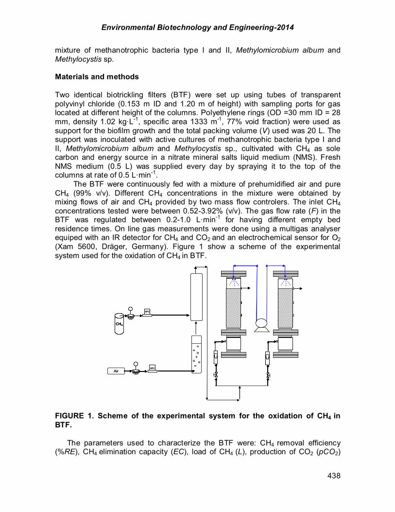
Environmental Biotechnology and Engineering-2014
438
mixture of methanotrophic bacteria type I and II, Methylomicrobium album and Methylocystis sp. Materials and methods Two identical biotrickling filters (BTF) were set up using tubes of transparent polyvinyl chloride (0.153 m ID and 1.20 m of height) with sampling ports for gas located at different height of the columns. Polyethylene rings (OD =30 mm ID = 28 mm, density 1.02 kg·L-1, specific area 1333 m-1, 77% void fraction) were used as support for the biofilm growth and the total packing volume (V) used was 20 L. The support was inoculated with active cultures of methanotrophic bacteria type I and II, Methylomicrobium album and Methylocystis sp., cultivated with CH4 as sole carbon and energy source in a nitrate mineral salts liquid medium (NMS). Fresh NMS medium (0.5 L) was supplied every day by spraying it to the top of the columns at rate of 0.5 L·min-1. The BTF were continuously fed with a mixture of prehumidified air and pure CH4 (99% v/v). Different CH4 concentrations in the mixture were obtained by mixing flows of air and CH4 provided by two mass flow controlers. The inlet CH4 concentrations tested were between 0.52-3.92% (v/v). The gas flow rate (F) in the BTF was regulated between 0.2-1.0 L·min-1 for having different empty bed residence times. On line gas measurements were done using a multigas analyser equiped with an IR detector for CH4 and CO2 and an electrochemical sensor for O2 (Xam 5600, Dräger, Germany). Figure 1 show a scheme of the experimental system used for the oxidation of CH4 in BTF. FIGURE 1. Scheme of the experimental system for the oxidation of CH4 in BTF. The parameters used to characterize the BTF were: CH4 removal efficiency (%RE), CH4 elimination capacity (EC), load of CH4 (L), production of CO2 (pCO2)
MFC
CH4
MFC
Air
CH4
MFC
CH4
MFC
Air
CH4
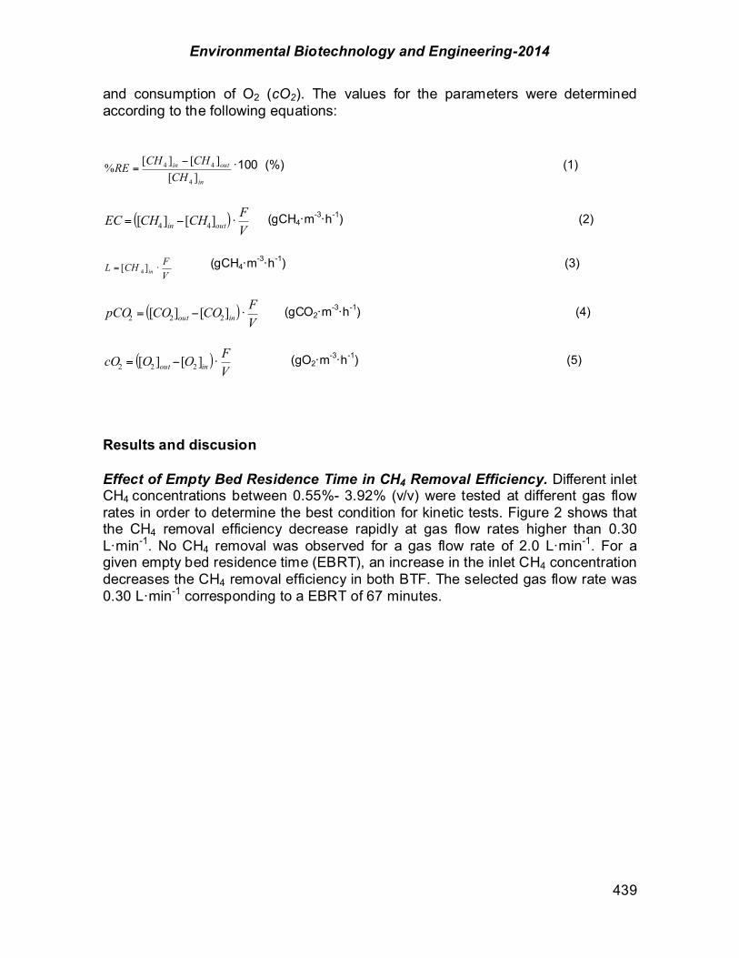
Environmental Biotechnology and Engineering-2014
439
and consumption of O2 (cO2). The values for the parameters were determined according to the following equations:
·100 (%) (1)
(gCH4·m
-3·h-1) (2)
(gCH4·m
-3·h-1) (3)
(gCO2·m-3·h-1) (4)
(gO2·m-3·h-1) (5)
Results and discusion Effect of Empty Bed Residence Time in CH4 Removal Efficiency. Different inlet CH4 concentrations between 0.55%- 3.92% (v/v) were tested at different gas flow rates in order to determine the best condition for kinetic tests. Figure 2 shows that the CH4 removal efficiency decrease rapidly at gas flow rates higher than 0.30 L·min-1. No CH4 removal was observed for a gas flow rate of 2.0 L·min-1. For a given empty bed residence time (EBRT), an increase in the inlet CH4 concentration decreases the CH4 removal efficiency in both BTF. The selected gas flow rate was 0.30 L·min-1 corresponding to a EBRT of 67 minutes.
in
outin
CHCHCHRE][
][][%
4
44 %=
( )VFCHCHEC outin ·][][ 44 %=
VFCHL in ·][ 4=
( )VFCOCOpCO inout ·][][ 222 %=
( )VFOOcO inout ·][][ 222 %=

Environmental Biotechnology and Engineering-2014
440
FIGURE 2. Methane removal efficiency of the BTF (clear: BTF1, solid: BTF2) as function of the EBRT at inlet CH4 concentrations of 0.5% v/v (triangle), 1.0% v/v (square) and 2.0% v/v (circle).
Effect of the Inlet CH4 Concentration in the Elimination Capacity. The inlet and outlet concentrations of CH4 were measured to obtain the CH4 removal efficiency (RE) and elimination capacity (EC) of the BTF at different loads of CH4 reached by increasing the inlet CH4 concentration, and using a constant gas flow rate of 0.30 L·min-1. It was considered that the BTF reached the steady state once the RE remained constant (i.e., variation <5%). Figure 3 show the CH4 elimination capacity of BTF at EBRT of 67 min and different inlet CH4 concentrations.
0
10
20
30
40
50
60
70
80
90
100
0 20 40 60 80 100 120
EBRT [min]
%RE
of C
H 4
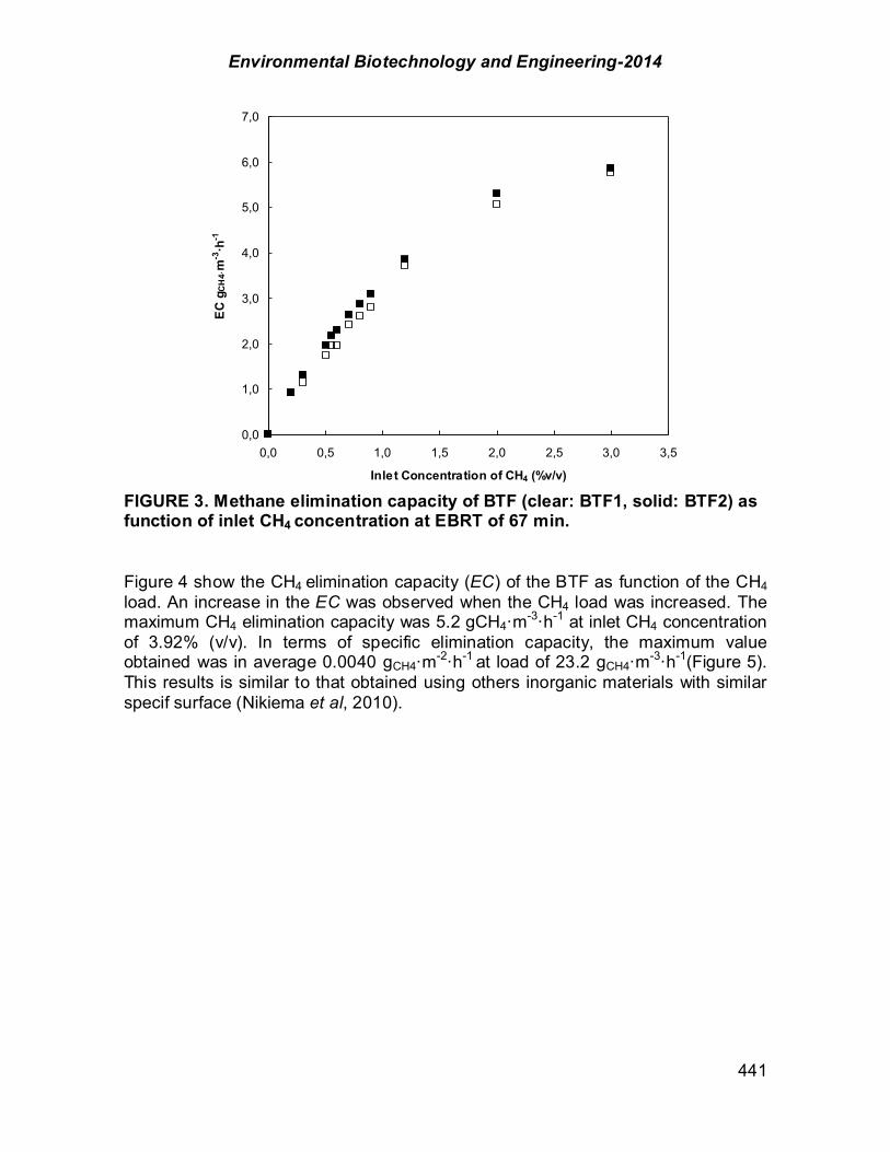
Environmental Biotechnology and Engineering-2014
441
FIGURE 3. Methane elimination capacity of BTF (clear: BTF1, solid: BTF2) as function of inlet CH4 concentration at EBRT of 67 min. Figure 4 show the CH4 elimination capacity (EC) of the BTF as function of the CH4 load. An increase in the EC was observed when the CH4 load was increased. The maximum CH4 elimination capacity was 5.2 gCH4·m-3·h-1 at inlet CH4 concentration of 3.92% (v/v). In terms of specific elimination capacity, the maximum value obtained was in average 0.0040 gCH4·m-2·h-1 at load of 23.2 gCH4·m-3·h-1(Figure 5). This results is similar to that obtained using others inorganic materials with similar specif surface (Nikiema et al, 2010).
0,0
1,0
2,0
3,0
4,0
5,0
6,0
7,0
0,0 0,5 1,0 1,5 2,0 2,5 3,0 3,5
Inlet Concentration of CH4 (%v/v)
EC g
CH
4·m
-3·h
-1
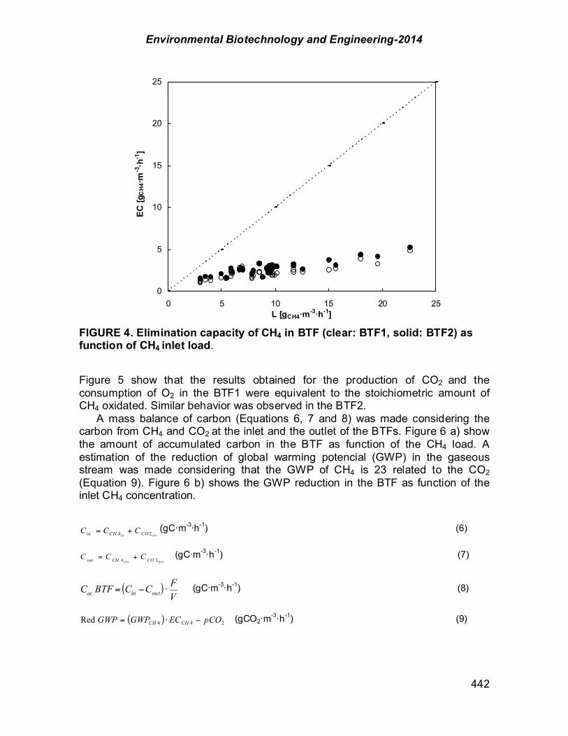
Environmental Biotechnology and Engineering-2014
442
FIGURE 4. Elimination capacity of CH4 in BTF (clear: BTF1, solid: BTF2) as function of CH4 inlet load.
Figure 5 show that the results obtained for the production of CO2 and the consumption of O2 in the BTF1 were equivalent to the stoichiometric amount of CH4 oxidated. Similar behavior was observed in the BTF2. A mass balance of carbon (Equations 6, 7 and 8) was made considering the carbon from CH4 and CO2 at the inlet and the outlet of the BTFs. Figure 6 a) show the amount of accumulated carbon in the BTF as function of the CH4 load. A estimation of the reduction of global warming potencial (GWP) in the gaseous stream was made considering that the GWP of CH4 is 23 related to the CO2 (Equation 9). Figure 6 b) shows the GWP reduction in the BTF as function of the inlet CH4 concentration.
(gC·m-3·h-1) (6)
(gC·m-3·h-1) (7)
(gC·m-3·h-1) (8)
(gCO2·m
-3·h-1) (9)
0
5
10
15
20
25
0 5 10 15 20 25L [gCH4·m-3·h-1]
EC [g
CH
4·m-3
·h-1
]
outin COCHin CCC 24 +=
putout COCHout CCC 24 +=
( )VFCCBTFC outinac ·%=
( ) 244Red pCOECGWPGWP CHCH %+=

Environmental Biotechnology and Engineering-2014
443
FIGURE 5. Moles of O2 consumed (9) and CO2 produced ( ) as function of CH4 elimination capacity. For inlet loads of CH4 below 10 gCH4m-3h-1 the amount of accumulated carbon in the BTF (Cac) was around 0.1gCm-3h-1 but when the load of CH4 was increased over 10 gCH4m-3h-1 it was observed a proportional increase of the Cac. This could be due to the higher availability of CH4 stimulate that more CH4 can be destined to generate biomass. This effect can be observed in Figure 6 b) as an increase in the reduction of CO2 equivalents when the inlet CH4 load increase. The maximium reduction of GWP was 98.5 gCO2m-3h-1 at load of 23.2 gCH4·m-3·h-1.
0,00
0,05
0,10
0,15
0,20
0,25
0,30
0,35
0,40
0,45
0,00 0,05 0,10 0,15 0,20
EC [molCH4·m-3h-1]
CO
2, O
2 [m
ol·m
-3h-1
]
O2, BTF 1
CO2, BTF 1
0
20
40
60
80
100
120
0 5 10 15 20 25
L [gCH4·m-3·h-1]
Red
GW
P [g
CO
2eq·
m-3
·h-1
]
0,00
0,10
0,20
0,30
0,40
0,50
0,60
0,70
0,80
0 5 10 15 20 25
L [gCH4 m-3h-1]
C ac
[gC
m-3
h-1]
a b a

Environmental Biotechnology and Engineering-2014
444
FIGURE 6. a) Accumulated carbon in the BTF (clear: BTF1, solid: BTF2); b) Reduction of CO2 equivalents as function of inlet load of CH4 in the BTF (clear: BTF1, solid: BTF2) Figure 7 show the concentrations of CH4 along the BTF 1 at different empty bed residence times (EBRT), and the effect of different inlet concentration of CH4. The higher variation on the CH4 concentration along the column was observed in the first section of the BTF. This effect was accentuated at inlet CH4 concentrations over 1.0% v/v. The higher variation on CH4 concentration along the BTF was observed at the lower gas velocit y tested (67 minutes of EBRT). Similar behavior was observed in the BTF 2.
FIGURE 7. Profiles of CH4 concentration along the height (H) of the BTF1 at different inlet CH4 concentration and different empty bed residence time: 9 67, 50, 40, x 30 minutes. Conclusions At all conditions tested both BTF showed a similar behavior. The maximum EC was 5.2 gCH4·m-3·h-1 at inlet concentration of 3.9% (v/v) and EBRT of 67 minutes. Even though the EC is rather low, the maximum specific elimination capacity obtained is similar to the values reported in literature, i.e.: 0.004 gCH4·m-2·h-1. It means that the low EC is due to the low specific area of the packing material used. The CH4 removal efficiency decreased rapidly when the gas flow rate increased. For a given EBRT, the increase in the inlet concentration of CH4 decreases the removal efficiency. A mass balance made to the bioreactors confirms the overall reaction of CH4 bio-oxidation, i.e.: each mole of CH4 oxidized consumed 2 moles of O2 and produced 1 mol of CO2. The maximum reduction of CO2 equivalents was 98.5 gCO2eq·m-3·h-1, this value was achieved at a load rate of 23.2 gCH4·m-3·h-1. Due the high void fraction of polyethylene rings no pressure drop or clogging problems were detected after one year of operation.
0
20
40
60
80
100
120
0 0,2 0,4 0,6 0,8 1 1,2 1,4 1,6 1,8 2 2,2 2,4 2,6
[CH4] (% v/v)
H B
TF [c
m]
Environmental Biotechnology and Engineering-2014
445
Acknowledgements This research was funded by the National Fund for Science and Technology (FONDECYT), Project 1110919, and the Pontificia Universidad Católica de Valparaíso. References Hanson R., Hanson T. Methanotrophic Bacteria. Microbiological Reviews 60 (2): 439-471, (1996). Havran V., Dudukovic M., Lo C. Conversión of Methane and Carbon Dioxide to Higher Value
Products. Ind. Eng. Chem. Res. 50:7089-7100, (2011). López J.C., Quijano G., Souza T.S., Estrada J.M, Lebrero R., Muñoz R. Biotechnologies for
greenhouse gases (CH4, N2O and CO2) abatement: state of the art and challenges. Appl Microbiol Biotechnol 97: 2277-2303, (2013).
Nikiema J., Heitz M. The use of inorganic packing materials during methane biofiltration. International Journal of Chemical Enggineering, Volume 2010, (2010).
Nikiema, J., Girard, M., Brzezinski, R., and Heitz, M. Biofiltration of methane using an inorganic filter bed: Influence of inlet load and nitrogen concentration. Canadian Journal of Civil Engineering 36(12), (2009).
Pfluger A., Wu W.M., Pieja A.J., Wan J., Rostkowski K., Criddle C. Selection of Type I and Type II methanotrophic proteobacteria in a fluidized bed reactor under non-sterile conditions. Bioresource Technology 102: 9919–9926, (2011).
Rocha Ríos J., Bordel S., Hernández S., Revah S. Methane degradation in two-phase partition bioreactors. Chemical Engineering Journal 152: 289–292, (2009).
Scheutz, C.; Bogner, J.; De Visscher, A.; Gebert, J.; Hilger, H.; Huber-Humer, M.; Kjeldsen, P. and Spokas, K.. Microbial methane oxidation processes and technologies for mitigation of landfill gas emissions. Waste Manag Res 27, (2009).
Veillete M., Viens P., Avalos Ramirez A., Brzezinski R., Heitz M. Effect of ammonium concentration on microbial population and performance of a biofilter treating air polluted with methane. Chemical Engineering Journal 171:1114-1123, (2011).
Veillete M., Girard M., Viens P., Brzezinski R., Heitz M. Function and limits of biofilters for the removal of methane in exhaust gases from the pig industry. Appl Microbiol Biotechnol. 94 (3): 601-6011, (2012).

Environmental Biotechnology and Engineering-2014
446
CHAPTER 4.2. BIO-OXIDATION OF METHANE IN A MEMBRANE REACTOR WITH A BIOFILM OF Methylomicrobium album
Germán Aroca Arcaya1,2 *;María José Cárdenas1; Alberto Aguirre 1,2; Matías
Gómez1; Sebastián Madrid1; Juan Carlos Gentina1
(1) Biochemical Engineering School, Pontificia Universidad Católica de Valparaíso, Valparaíso 2147, Chile (2) Doctoral Program in Biotechnology, Programa Conjunto Pontificia Universidad Católica de Valparaíso – Universidad Técnica Federico Santa María, Valparaíso 1680, Chile. ABSTRACT Methane (CH4) is an organic gas emitted from natural and anthropogenicsources. It represents approximately 23% of total emissions of greenhouse gases worldwide. According to the latest report of the IPCC, methane has a global warming potential 34 times greater than CO2 on a time scale of 100 years. Common methods for eliminating methane in industry are combustion to generate energy, or just burn it in flares. However 55% of anthropogenic methane emissions cannot be thermally oxidised because its low concentration or the imposibility to collect it. Technologies based in the action of microorganisms with the ability of oxidizing methane have been proposed and tested in configurations like bio-layers, biofilters and biotrickling filters. Due to its low solubility in aqueous phase the efficiency and removal capacity of these systems is rather low making difficult its applications at large scales. The membrane biofilm reactors (MBfRs) represent an alternative the conventional biofiltration systems for eliminating pollutants in air. They are characterized by high gas utilization efficiency and high specific area for biofilm. MBfRs have been described previously for TCE removal, reduction of oxidized contaminants such as perchlorate, nitrate, bromate, chromate and selenate, treating wastewater, but there is no reports related to methane bio-oxidation. The aim of this work was to evaluate the performance of aMBfRs for bio-oxidizing CH4. The system was operated at 30°C and pH 6.8 under different CH4 specific loading rates using Methylomicrobium album as inoculum for forming a biofilm over a polydimethylsiloxane (PDMS) hydrophobic membrane with enhanced properties for separating methane.The results showed that an increase in CH4 specific loading rate from 51 to 169 [g CH4/m2h] resulted in an increase in specific elimination capacity of CH4 from 10 to 36,5 [g CH4/m2h], however the CH4 removal efficiency at CH4 loads tested ranged between 19 and 22%. This behavior showed that an increase in the CH4 availability in the gas phase of the reactor jointly with a high activity of the biofilm that was growing on the membrane were important for the improvement of CH4 transfer rate along the membrane, and thus for the improvement of CH4 elimination capacity of the system. Key words: global warming, membrane biofilm reactor, methane oxidation, Methylomicrobium album. ------------------ *Author for correspondence
Environmental Biotechnology and Engineering-2014
447
Introduction Methane (CH4) is the simplest hydrocarbon and the primary component of natural gas. It is emitted from natural and anthropogenic sources and represents approximately 23% of total emissions of greenhouse gases worldwide. According to the latest report of the IPCC, methane has a global warming potential 34 times greater than CO2 on a time scale of 100 years(IPCC, 2013).Atmospheric concentrations of CH4 has grown from a preindustrial value of about 715 parts per billion (ppb) to 1,782 ppb in 2007 (GMI, 2010). Global anthropogenic methane emissions are projected to increase 23% by 2020.Although methane is emitted into the atmosphere in smaller quantities, annual CH4 emissions are the second most abundant GHG and contribute to over one-third of today´s anthopogenic warming. Human activities like livestock (enteric fermentation), coal mining, natural gas and oil production, landfills, wastewater, and agricultural practices represent 70 percent of the world’s methane emissions (EPA, 2010). Several treatment options have been developed from methane emissions, according to the concentration in the gas mixture. When its concentration is above 30 % it can be utilized for energy generation whereas its concentration is close to 20%are burned to produce CO2 (Haubrichset al, 2006) being possible to negotiate carbon bonus through this operation. Nevertheless, 55% of anthropogenic methane emissions are below the lower explosive limit (LEL) for CH4 (4,4 %) and cannot be thermally oxidized (Avalos Ramirez et al., 2012). In such cases, biological oxidation can be an effective mitigation alternative. Methanotrophs are a unique group of gram-negative aerobic bacteria capable of utilizing methane as sole carbon and energy source. They are present in a wide variety of environments, playing an important role in the oxidation of methane in the natural world (Jiang et al, 2011). These microorganisms are included in a broader class called methylotrophs, which oxidize C1 compounds such as methanol, methylamine, formate, carbon monoxide and dimethylsulfide (Bowman, 2011). Many methanotrophs are also capable of oxidizing a wide variety of other substrates, including some compound but they do not grow on these (Canfield et al, 2005).Most methanotrophs are classified according to morphological features and carbon assimilation pathway into two groups: gamma-(type I methanotrophs) and alpha-proteobacteria (type II methanotrophs) (Bürgmann, 2011).Type I use the ribulose monophosphate pathway (RuMP) where three molecules of formaldehyde are assimilated forming a three-carbon intermediate (glyceraldehyde-3-phosphate), whereas in the serine pathway, two molecules of formaldehyde and one molecule of CO2are utilized in each cycle forming a three-carbon intermediate (2-phosphoglycerate). Both intermediates are subsequently used for biosynthesis of cell material (Anthony, 1982). A defining characteristic of methanotrophs is methane mono-oxygenaseenzyme (MMO) which catalyzes the oxidation of methane to methanol (first step of metabolic pathway). MMO has two distinct forms: a soluble cytoplasmic form (sMMO) and a particulate membrane-associated (pMMO). The presence of copper determines which type of MMO is expressed (Sodenrer, 2007).The most well-known methanotrophs are assigned to the genus Methylomicrobium(Jiang et al, 2011).
Environmental Biotechnology and Engineering-2014
448
Many microbial processes can use dissolved gases as substrates for microbial growth, but their low water solubility limit their use. The membrane biofilm reactor (MBfR) represents an alternative that provides a gaseous substrate crossing a hydrophobic membrane while the naturally-forming biofilm on the surface catalyzes some reactions (Nerenberg, 2005). Biofilms are densely packed communities of microbial cells that grow on living or inert surfaces and surround themselves with extracellular polymeric substances (EPS) allowing them to develop complex three-dimensional, resilient, attached communities.Some advantages of MBfRs are high gas utilization efficiency and high specific surface area for biofilm accumulation (Kelly &Nerenberg, 2012).Due to its nature, the gaseous substrate would be more available to the biofilm growing on the other side of the membrane.MBfRs have been described previously for TCE removal, reduction of oxidized contaminants such as perchlorate, nitrate, bromate, chromate and selenite (Modín, 2010) but there are no reports related with methane. The aim of this work was to evaluate the performance of a membrane biofilm reactor for bio-oxidizing CH4, using a polydimethylsiloxane membrane specifically designed for methane separations. Materials and methods Microorganism andculture conditions. Methylomicrobium album ATCC 3003 was grown on ATCC medium 1306, a nitrate mineral salts (NMS), supplemented with 7.2 M copperat pH 6.8. The culture was carried out in 125 ml flasks containing 15 ml sterile medium and 10 ml inoculum (0.1 g L -1) with push-button valves. An atmosphere of 40% methane and 60% air was injected into the flasks. These were incubated in the dark at 30°C with shaking (200 rpm). Biomass was measured by optical density at 600 nm (OD600) using a spectrophotometer (Shimdzdu UV-150-02). Membrane biofilm reactor configuration. A laboratory-scale reactor was designed using a polydimethylsiloxane (PDMS) hydrophobic membrane (InstitutfürPolymerforschung, Germany) with an effective area of 80 cm2. The two polyethylene modules (liquid and gas chamber) were constructed with an outside area of 352.8 cm2 and 5 cm of thickness. The total volume of each module was 40 cm3. Acrylic covers were used for covering the modules. NMS medium was circulated between the bioreactor and a flask with 300 ml (liquid volume) using a peristaltic pump (Masterflex, USA). The mixture of gases was prepared by mixing air and methane, keeping constant the concentration ofmethane in 5 % v/v, calibrating the flows of the gases using two rotameters (Cole-Parmer, USA), entering to a gas mixer (8.7 L of volume).The inflow and outflow of gas mixture in the MBfR was measured usingrotameters and manometers (Cole-Parmer, USA). Two gas and two liquid sampling points were locatedin the input and output lines. Methane was measured using a Dräger X-am® 5000multi-gas detector equipped with an IR-EX sensor.

Environmental Biotechnology and Engineering-2014
449
Start up of the Membrane Biofilm Reactor. The start up of the MBfR was carried out by circulating 300 ml of NMS medium and 60 ml of inoculum with an initial concentration of 1.5 g L-1 biomass of during 21 days throughout the liquid chamber, at 30 °C and a rate of 5 ml min-1. At the same time, gas mixture was fed into the gas chamber at a rate of 0.8 L min-1. The pressure inside the reactor was kept at approximately1 atm. MBfR Operation. The gas mixture was fed at different flows (0.3, 0.4, 0.5, 06, 0.7, 0.8, 0.9 and 1 L min-1) into the MBfR, i.e.: different residence time (8, 6, 4.8, 4, 3.5, 3, 2.7 and 2.4 s-1) respectively. Each flow was kept during 3 days. Each run was performed for duplicate.Every 7 days, the medium and the inoculum were centrifuged (5000 rpm min-1 for 15 min). The supernatant was eliminated and the biomass was re-suspended in 60 ml of medium and mixed with 300 ml of NMS fresh medium, which was circulated at 5 ml min-1. Results and Discussion Figure 1 shows the Elimination Capacity and the Removal Efficiency of the MBfR during the operation at different residence time, feeding a mixture of 5 % v/v of methane.
FIGURE 1. Variations in CH4 loading rate ( ), CH4 elimination capacity (#), CH4 removal efficiency ( ) and residence time ( ) during the continuous operation of a membrane biofilm reactor inoculated with Methylomicrobium album. Numbers I to VIII represent each period of time when a particular residence time was established. Data are showedas mean value with differences of less than 10%. Changes in residence time and hence in the CH4 loading rate, caused variation in the removal efficiency and the CH4 elimination capacity.
Experimental time [days]
0 5 10 15 20 25
Loa
ding
rate
[gC
H4/m
3 h]; E
limin
atio
n ca
paci
ty [g
CH
4/m3 h]
0
5000
10000
15000
20000
25000
30000
35000
40000
Met
hane
rem
oval
effi
cien
cy [%
]
19,0
19,5
20,0
20,5
21,0
21,5
22,0
Res
iden
ce ti
me
[s]
2
3
4
5
6
7
8
9 I II III IV V VI VII VIII

Environmental Biotechnology and Engineering-2014
450
As figure 2 shows, there is a lineal relation between CH4 loading rate and the CH4 elimination capacity. At a loading rate of 10125 [gCH4/m3h], the CH4 elimination capacity was the lowest (1967 gCH4/m3h), while higher CH4 loading rates resulted in higher CH4 elimination capacities. The maximum EC value obtained was 7297 [gCH4/m3h].
FIGURE 2. Elimination capacity of methane (#) and methane removal efficiency ( ) at different loading rates during the continuous operation of a membrane biofilm reactor inoculated with Methylomicrobium album. Data are showedas mean value with differences of less than 10%. It is possible to observe an almost lineal relation between specific CH4 loading rate and specific elimination capacity of CH4 (see figure 3), where the latter ranged between 10 and 35 [gCH4/m2h]. The increase in the specific EC in the system can be explained by an improvement in the mass transfer of methane across the membrane when the specific loading rate of CH4 was raised, thus at high specific loading rates the mass transfer of CH4 was favored which finally could affect positively the activity of the biofilm, obtaining in this way high specific EC values for CH4. The CH4 elimination capacities obtained in this system exceed in one or two orders of magnitude the EC values obtained in conventional biofilters and biotrickling filters (Streese&Stegmann, 2003; Nikiema&Heitz, 2009; Park et al., 2009; Ramirez et al., 2012; Ménardet al., 2014; Estrada et al., 2014; Kim et al., 2014;). In addition, the maximum value of specific EC obtained in this study (37 [gCH4/m2h]) is one of the highest values of specific EC reported in the literature (Wilshusenet al., 2004; Nikiema&Heitz, 2010; Haththotuwaet al., 2012) for the removal of CH4 in a biological system, the only higher value was the reported by Pawlowskaet al (2011), who reached a specific CH4 oxidation rate of 43 [gCH4/m2h] in a conventional biofilter. All of this information shows the potential of
Loading rate [gCH4/m3h]
5000 10000 15000 20000 25000 30000 35000
Elim
inat
ion
capa
city
[gC
H4/m
3 h]
1000
2000
3000
4000
5000
6000
7000
8000
Met
hane
rem
oval
effi
cien
cy (%
)
15
16
17
18
19
20
21
22

Environmental Biotechnology and Engineering-2014
451
membrane biofilm reactors using Methylomicrobium album to remove poor soluble compounds, such as methane.
FIGURE 3. Specific elimination capacity of methane ( ) and methane removal efficiency ( ) at different specific loading rates of methane during the continuous operation of a membrane biofilm reactor inoculated with Methylomicrobium album. Data are showedas mean value with differences of less than 10%. In contrast to the high EC and specific EC values, the CH4 removal efficiencies obtained in this system ranged between 19 and 22%, so that the MBfR’s performance can be improved. This process can be done by optimizing the configuration of the reactor, the operational variables (liquid recirculation rate, nutrients supply), and by enhancing the mass transfer of CH4. With respect to the configuration of the reactor, one strategy for reaching better CH4 oxidation rates would be to increase the specific surface area of membrane, which in this system was 200 [m2m-3], a value lower than the typical used (500 [m2m-3]) in several studies (Reijet al., 1995; De Bo et al., 2003; Kumar et al., 2008; Alvarez-Hornoset al., 2011; Kumar et al., 2009; Lebreroet al., 2013) of waste gas treatment by MBfRs. Within the strategies to improve the mass transfer of CH4 in the system, probably the most promising is the use of new membrane’s materials which allow to increase the CH4 availability to biofilm or the use of chemical compounds, which have high affinity for CH4 (for example silicone oil), in the liquid phase of the bioreactors.
Specific loading rate [gCH4/m2h]
40 60 80 100 120 140 160 180
Spec
ific
elim
inat
ion
capa
city
[gC
H4/
m2 h]
5
10
15
20
25
30
35
40
Met
hane
rem
oval
effi
cien
cy [%
]
15
16
17
18
19
20
21
22

Environmental Biotechnology and Engineering-2014
452
In summary, this study has demonstrated the feasibility of using a membrane biofilm reactor inoculated with Methylomicrobium album for the removal of low concentrations of methane at high loading rates. Conclusion The high specific elimination capacity of CH4 achieved in this study is related with an improvement of mass transfer of methane across the membrane due to an increase in the specific loading rate of CH4 in the system. These results confirm the suitability of aMBfR inoculated with Methylomicrobium album for removinglow concentration of methane at high specific loading rates. However, in order to improve the CH4 removal efficiency, it is imperative to implement strategies for optimizing the mass transfer of CH4 across the membrane, the configuration of the reactor and the operational variables of the system. Acknowledgments This study was supported by Pontificia Universidad Católica de Valparaíso (PUCV). The authors would like to thank the technical personnel of Biochemical Engineering School (PUCV) for their support during the project. References Alvarez-Hornos, F.; Volckaert D, Heynderickx, P.; Van Langenhove, H. (2011). Performance of a
composite membrane bioreactor for the removal of ethyl acetate from waste air. Bioresour. Technol; 102: 8893:8898.
Anthony, C. (1982). The Biochemistry of Methylotrophs. 1st ed., Academic Press INC, NY. Avalos Ramírez, A.; Jones, P.J.; Heitz, M. (2012).Improvement of methane biofiltration by addition
of non-ionic surfactants to biofilters packed with inert materials.Process Biochem. 47: 76-82. Bowman, J. (2000). The Prokaryotes: An Evolving Electronic Resource for the Microbiological
Community, Release 3.1. Springer, New York. Bürgmann, H. (2011). Methane Oxidation (Aerobic).Swiss Federal Institute of Aquatic Science and
Technology, Switzerland. Canfield, D.; Thamdrup, B.; Kristensen, E. (2005). Advances in Marine Biology. Aquatic
Geomicrobiology. Volume 48., Elsevier Academic Press, USA. De Bo, I.; Van Langenhove, H.; Pruuost, P.; De Neve, J.; Pieters.; Vankelecom, I.; Dick E. (2003).
Investigation of the permeability and selectivity of gases and volatile organic compounds for polydimethylsiloxane membranes. J. of Membrane Science; 215: 303-319.
Environmental Protection Agency (2010). www.epa.gov/globalmethane/pdf/2010-accomplish-report/usg_fullreport_2010_3.pdf; accessed 15 May 2014.
Estrada, J.; Lebrero, R.; Quijano, G.; Pérez, R.; Figueroa-González, I.; García-Encina, P.; Muñoz R. (2014). Methane abatement in a gas-recycling biotrickling filter: Evaluating innovative operational strategies to overcome mass transfer limitations. ChemEng J; 253:385-393.
Global Methane Iniciative (2010). www.globalmethane.org/about/methane.aspx#container; accessed 23 April 2014.
Haththotuwa, C; Hettiaratchi, J; Hunte, C. 2012. Actively aerated methanobiofilters to control methane emissions from landfills. Int. J. of Environmental Technology and Management; 15: 333-345.
Haubrichs, R., Widmann. R. (2006). Evaluation of aerated biofilter systems for microbial methane oxidation of poor landfill gas. Waste Management, Volume 26, pp. 408-416.
Environmental Biotechnology and Engineering-2014
453
Intergovernmental Panel on Climate Change (2013). Fifth Assessment Report (AR5). http://www.climatechange2013.org/images/report/WG1AR5_Chapter06_FINAL.pdf/; accessed 07 June 2014.
Jiang, H.; Chen Y.; Jiang, P.; Zhang, C.; Smith, T.; Murrel, C.; Xing, X. (2010) Methanotrophs: Multifunctional bacteria with promising applications in environmental bioengineering. Biochemical Enginnering 49: 277-288.
Kelly, M.; Nerenberg, R. (2012).The membrane biofilm reactor (MBfR) for water and wastewater treatment: Principles, applications ,and recent developments. BioresourceTechnology.122: 83–94.
Kim, T.; Jeong, S.; Cho K. (2014). Functional rigidity of a methane biofilter during the temporal microbial succession. Appl Microbiol Biotechnol; 98:3275–3286.
Kumar A, Dewulf J, van Langenhove. (2008). Membrane-based biological waste gas treatment. ChemEng J; 136: 82-91.
Kumar, A.; Dewulf, J.; Vercruyssen, A.; Van Langenhove, H. (2009). Performance of a composite membrane bioreactor treating toluene vapors: Inocula selection, reactor performance and behavior under transient conditions. Bioresour. Technol; 100: 2381-2387.
Lebrero, R.; Volckaert, D.; Perez, R.; Muñoz, R.; Van Langenhove, H. (2013). A membrane bioreactor for the simultaneous treatment of acetone, toluene, limonene and hexane at trace level concentrations. Water Research; 47: 2199-2212.
Ménard, C.; Ramirez, A.;Heitz, M. (2014). Kinetics of simultaneous methane and toluene biofiltration in an inert packed bed. J Chem Technol Biotechnol; 89: 597–602
Modín, O.; Fukushi, K.; Nakajima, F.; Yamamoto, K. (2010). Nitrate removal and biofilm characteristics in methanotrophic membrane biofilm reactor with various gas supply regimes. Water Research44: 85– 96.
Nerenberg, R. (2005). Membrane biofilm reactors for water and wastewater treatment. Proceedings of Borchardt Conference: A seminar on Advances in Water and Wasterwater Treatment, Ann Arbor, Michigan, 2005.
Nikiema, J.; Heitz, M. (2009). The Influence of the Gas Flow Rate During Methane Biofiltration on an Inorganic Packing Material.Canadian J ChemEng; 87:136-142.
Nikiema, J.; Heitz, M. (2010). The Use of Inorganic Packing Materials during Methane Biofiltration.Int. J. of Chemical Engineering, 149:1-8.
Park, S.; Lee, C.; Ryu, C.; Sung K. (2009). Biofiltration for Reducing Methane Emissions from Modern Sanitary Landfills at the Low Methane Generation Stage. Water Air Soil Pollut; 196:19-27.
Paw$owska, M.; Rozej, A.; Stepniewski, W. (2011). The effect of bed properties on methane removal in an aerated biofilter – Model studies. Waste Manage; 31: 903-913.
Ramirez, A.;Jones, J.; Heitz, M. (2012). Methane treatment in biotrickling filters packed with inert materials in presence of a non-ionic surfactant. J Chem Technol Biotechnol; 87: 848–853.
Reij, M.; De Goijer, K.; De Bont, J.; Hartmans, S. (1995). Membrane bioreactor with porous hydrophophic membrane as gas-liquid contactor for waste gas treatment. BiotechnolBioeng; 45: 105-109.
Sodenrer, T. (2007). Copper Acquisition by Methanotrophic Bacteria. Department of Environmental Sciences. Swiss Federal Institute of Technology, Switzerland.
Streese, J.; Stegmann, R. (2003). Microbial oxidation of methane from old landfills in biofilters. Waste Manage; 23:573-580.
Wilshusen, J.; Hettiaratchi, J.; Stein, V. (2004). Long-term behavior of passively aerated compost methanotrophic biofilter columns. Waste Manage; 24:643-653.

Environmental Biotechnology and Engineering-2014
454
CHAPTER 4.3. SIMULTANEOUS TREATMENT OF DIMETHYL DISULFIDE AND HYDROGEN SULFIDE VAPORS IN AN ALKALINE BIOTRICKLING FILTER
Luis Arellano-García (1); Sergio Revah *(2)
(1) Dept. of Process Engineering and Hydraulics. UAM Iztapalapa, México DF, México; (2) Dept. of Process and Technology UAM Cuajimalpa, México DF, México; ABSTRACT An air stream polluted with a mixture of dimethyl disulfide (DMDS) and hydrogen sulfide (H2S) was treated in an alkaline biotrickling filter (ABTF). The ABTF was inoculated with an alkaliphilic sulfooxidizing bacteria consortium (ASBC) which was adapted to sulfides consumption from soil and water samples taken from a soda lake in Texcoco, Mexico. After a year treating DMDS vapors in concentrations close to 150 ppmv, the H2S feeding to the ABTF started with concentrations ranging 20-30 ppmv. During first days it was observed that the H2S interfered the DMDS removal, nonetheless it seemed the ASBC was adapted to the consumption of both sulfides after 20 days where complete removal was registered. Loads of DMDS and H2S as high as 110 and 60 g m-3 h-1 respectively, were treated with removal efficiencies higher than 95%, in this conditions the corresponding inlet concentrations of DMDS and H2S were 430-450 ppmv. Non-odorous sulfate and carbon dioxide were determined as the main products of sulfides degradation. Keywords: alkaliphilic bacteria, biotrickling filter, dimethyl disulfide, hydrogen sulfide Introduction The exposure to odors caused by sulfides is a cause of concern due to its noxious effects and toxicity. Moreover the World Health Organization recently categorized the persistence of odorants as a type of air pollution. The treatment of sulfide-polluted air in biotrickling filters (BTF) has been proved to be a cheap and efficient process to remove the pollutants from air streams. Lately alkalinity has been utilized in BTFs as novel characteristic to foster the removal of acid sulfides as hydrogen sulfide (H2S), ethanethiol, carbon disulfide and dimethyl disulfide treated individually (González-Sánchez et al. 2008; Arellano-García et al. 2010; Arellano-García et al. 2012). It is known that odor pollution associated to reduced sulfur compounds (RSC) is produced by a mixture of sulfides and mercaptans, which concentration and composition rely on the source (Smet et al. 1998), nonetheless in the RSC emissions H2S is characterized to be the most frequently found and which presence implies important hazards to health. In previous studies of low concentration of sulfides removal in neutral biofilters and BTF the interference of H2S over the removal of other RSC was observed (Cho et al. 1991; Ramírez et al. 2011). Some authors used a two-stage BTF system to attain a satisfactory degradation of a mixture of sulfides, removing
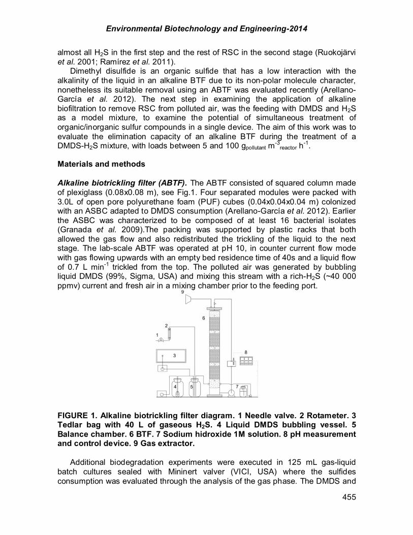
Environmental Biotechnology and Engineering-2014
455
almost all H2S in the first step and the rest of RSC in the second stage (Ruokojärvi et al. 2001; Ramírez et al. 2011). Dimethyl disulfide is an organic sulfide that has a low interaction with the alkalinity of the liquid in an alkaline BTF due to its non-polar molecule character, nonetheless its suitable removal using an ABTF was evaluated recently (Arellano-García et al. 2012). The next step in examining the application of alkaline biofiltration to remove RSC from polluted air, was the feeding with DMDS and H2S as a model mixture, to examine the potential of simultaneous treatment of organic/inorganic sulfur compounds in a single device. The aim of this work was to evaluate the elimination capacity of an alkaline BTF during the treatment of a DMDS-H2S mixture, with loads between 5 and 100 gpollutant m-3
reactor h-1. Materials and methods Alkaline biotrickling filter (ABTF). The ABTF consisted of squared column made of plexiglass (0.08x0.08 m), see Fig.1. Four separated modules were packed with 3.0L of open pore polyurethane foam (PUF) cubes (0.04x0.04x0.04 m) colonized with an ASBC adapted to DMDS consumption (Arellano-García et al. 2012). Earlier the ASBC was characterized to be composed of at least 16 bacterial isolates (Granada et al. 2009).The packing was supported by plastic racks that both allowed the gas flow and also redistributed the trickling of the liquid to the next stage. The lab-scale ABTF was operated at pH 10, in counter current flow mode with gas flowing upwards with an empty bed residence time of 40s and a liquid flow of 0.7 L min-1 trickled from the top. The polluted air was generated by bubbling liquid DMDS (99%, Sigma, USA) and mixing this stream with a rich-H2S (~40 000 ppmv) current and fresh air in a mixing chamber prior to the feeding port.
FIGURE 1. Alkaline biotrickling filter diagram. 1 Needle valve. 2 Rotameter. 3 Tedlar bag with 40 L of gaseous H2S. 4 Liquid DMDS bubbling vessel. 5 Balance chamber. 6 BTF. 7 Sodium hidroxide 1M solution. 8 pH measurement and control device. 9 Gas extractor. Additional biodegradation experiments were executed in 125 mL gas-liquid batch cultures sealed with Mininert valver (VICI, USA) where the sulfides consumption was evaluated through the analysis of the gas phase. The DMDS and
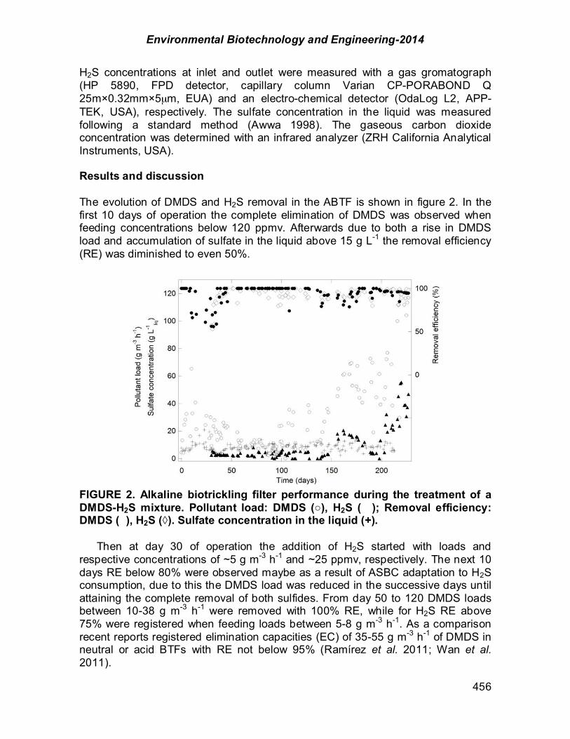
Environmental Biotechnology and Engineering-2014
456
H2S concentrations at inlet and outlet were measured with a gas gromatograph (HP 5890, FPD detector, capillary column Varian CP-PORABOND Q 25m!0.32mm!5µm, EUA) and an electro-chemical detector (OdaLog L2, APP-TEK, USA), respectively. The sulfate concentration in the liquid was measured following a standard method (Awwa 1998). The gaseous carbon dioxide concentration was determined with an infrared analyzer (ZRH California Analytical Instruments, USA). Results and discussion The evolution of DMDS and H2S removal in the ABTF is shown in figure 2. In the first 10 days of operation the complete elimination of DMDS was observed when feeding concentrations below 120 ppmv. Afterwards due to both a rise in DMDS load and accumulation of sulfate in the liquid above 15 g L-1 the removal efficiency (RE) was diminished to even 50%.
FIGURE 2. Alkaline biotrickling filter performance during the treatment of a DMDS-H2S mixture. Pollutant load: DMDS ($), H2S ( ); Removal efficiency: DMDS ( ), H2S ("). Sulfate concentration in the liquid (+). Then at day 30 of operation the addition of H2S started with loads and respective concentrations of ~5 g m-3 h-1 and ~25 ppmv, respectively. The next 10 days RE below 80% were observed maybe as a result of ASBC adaptation to H2S consumption, due to this the DMDS load was reduced in the successive days until attaining the complete removal of both sulfides. From day 50 to 120 DMDS loads between 10-38 g m-3 h-1 were removed with 100% RE, while for H2S RE above 75% were registered when feeding loads between 5-8 g m-3 h-1. As a comparison recent reports registered elimination capacities (EC) of 35-55 g m-3 h-1 of DMDS in neutral or acid BTFs with RE not below 95% (Ramírez et al. 2011; Wan et al. 2011).

Environmental Biotechnology and Engineering-2014
457
Afterwards the DMDS and H2S loads were augmented progressively to examine the ABTF maximum capacity. In the last days of the operation reported here, loads of DMDS and H2S as high as 110 and 60 g m-3 h-1 were treated with RE higher than 95%, these removal rates are comparable, and in the DMDS case, superior to what is reported by other authors until now. Sulfate and carbon dioxide were determined to be the main products of DMDS and H2S biodegradation in the ABTF. Even when in batch cultures the addition of H2S produced a delay in the DMDS degradation (data not shown), in the continuous operation at lab scale the interference of H2S over DMDS degradation was observed just during 10 days after which the ABTF seemed to be adapted to the consumption of both sulfides. Conclusion Satisfactory removal of a mixture of DMDS-H2S mixture can be attained in an alkaline biotrickling filter inoculated with alkaliphilic adapted bacteria. Unlike to previous studies the H2S was not observed to interfere with the DMDS degradation, furthermore the treatment of both compounds were effectively carried out in a BTF at pH10 which might represent an advantage over previously reported two-stage biofiltration systems. As perspective the reduction of the gas residence times when treating RSC mixtures in the ABTF should be investigated in order to investigate the maximum performance at short gas contact times typical of field biofilters application. Acknowledgements The authors would like to thank CONACYT for financing this project (I0017-166451) and LAG scholarship. References Arellano-García, L.; Gonzalez-Sanchez, A.; Baquerizo, G.; Hernandez-Jimenez, S.; Revah, S.
(2010). Treatment of carbon disulfide and ethanethiol vapors in alkaline biotrickling filters using an alkaliphilic sulfo-oxidizing bacterial consortium. Journal of Chemical Technology and Biotechnology 85(3): 328-335.
Arellano-García, L.; González-Sánchez, A.; Van Langenhove, H.; Kumar, A.; Revah, S. (2012). Removal of odorant dimethyl disulfide under alkaline and neutral conditions in biotrickling filters. Water Science & Technology 66(8): 1641-1646.
Awwa, A. (1998). Standard methods for the examination of water and wastewater. Washington, DC Standard Methods for the Examination of Water and Wastewater 20.
Cho, K.-S.; Hirai, M.; Shoda, M. (1991). Degradation characteristics of hydrogen sulfide, methanethiol, dimethyl sulfide and dimethyl disulfide by Thiobacillus thioparus DW44 isolated from peat biofilter. Journal of Fermentation and Bioengineering 71(6): 384-389.
González-Sánchez, A.; Revah, S.; Deshusses, M. A. (2008). Alkaline biofiltration of H2S odors. Environmental science & technology 42(19): 7398-7404.
Granada, C.; Revah, S.; Le Borgne, S. (2009). Diversity of culturable bacteria in an alkaliphilic sulfur-oxidizing microbial consortium. Advanced Materials Research 71: 137-140.
Ramírez, M.; Fernández, M.; Granada, C.; Le Borgne, S.; Gómez, J. M.; Cantero, D. (2011). Biofiltration of reduced sulphur compounds and community analysis of sulphur-oxidizing bacteria. Bioresource technology 102(5): 4047-4053.

Environmental Biotechnology and Engineering-2014
458
Ruokojärvi, A.; Ruuskanen, J.; Martikainen, P. J.; Olkkonen, M. (2001). Oxidation of gas mixtures containing dimethyl sulfide, hydrogen sulfide, and methanethiol using a two-stage biotrickling filter. Journal of the Air & Waste Management Association 51(1): 11-16.
Smet, E.; Lens, P.; Van Langenhove, H. (1998). Treatment of waste gases contaminated with odorous sulfur compounds. Critical Reviews in Environmental Science and Technology 28(1): 89-117.
Wan, S.; Li, G.; An, T.; Guo, B. (2011). Co-treatment of single, binary and ternary mixture gas of ethanethiol, dimethyl disulfide and thioanisole in a biotrickling filter seeded with Lysinibacillus sphaericus RG-1. Journal of Hazardous Materials 186(2): 1050-1057.

Environmental Biotechnology and Engineering-2014
459
LIST OF COAUTHORS: Luis Arellano-García, Ph.D. Candidate, presenting author. Departamento de Ingeniería de Procesos e Hidráulica, Universidad Autónoma Metropolitana-Iztapalapa Av. San Rafael Atlixco 186, Col. La Vicentina, México D.F., C.P. 09340 E-mail: [email protected] Dr. Sergio Revah, Professor and Researcher; Author to whom all correspondence should be addresed Departamento de Procesos y Tecnología, Universidad Autónoma Metropolitana-Cuajimalpa Av.Vasco de Quiroga 4871, Col. Santa Fe Cuajimalpa, México D.F., C.P. 05300 Tel: +52 5558046556 E-mail: [email protected]
Environmental Biotechnology and Engineering-2014
460
CHAPTER 4.4. IMPACTO DE LAS CARACTERÍSTICAS FISICOQUÍMICAS Y DINÁMICA DE CARBONO EN SUELO, DESPUÉS DE NUEVE AÑOS DE LA
REINTRODUCCIÓN CON VEGETACION NATIVA EN UN SUELO PERTURBADO
Martha V. Almanza-Estrada (1); Blanca G. Elías-Balandrán (2); María M. Vargas-Zúñiga (1); Yazmín A. Sánchez-Ruan (1); Alejandra Gutiérrez-Vázquez (1); Juan A.
Mejía-Gómez (1); Jaquelina González-Castañeda*(1) (1) DICIVA, CIS, UNIVERSIDAD DE GUANAJUATO, Irapuato, Gto., México; (2) UNIVERSIDAD POLITÉCNICA BICENTENARIO, Silao, Gto., México ABSTRACT CO2 is considered a greenhouse gas (GHG), the capture of this on the ground provides for the replacement of organic matter and is proposed as an alternative for mitigation. The objective of this work was to evaluate the impact of the physico-chemical characteristics and dynamics of carbon in soil, after nine years of the reintroduction of native vegetation: huisache (Acacia schaffneri) and gatuño (Mimosa monancistra), in a disturbed soil, in the state of Guanajuato. Sampling to a depth of 0-20 cm under the canopy of the plants in the dry season (May) and after the rains (November) in 2010 were performed. The physicochemical characterization was done by the Mexican Official Standard NOM-021-RECNAT-2000. The dynamics of carbon at laboratory level, was carried out using the technique reported by Jenkinson and Powlson (1976), which allows to quantify the carbon content in the soil (expressed as CO2 production). Statistical analysis was performed using the Tukey test at p <0.05, of three replications per treatment, in triplicate. All the treatments showed a significant difference with respect to the witness (T) for both pH with water as with CaCl2, showing values between 7.87 and 6.90 (May and November respectively) and can be categorized neutral to moderately alkaline. For the EC values between 0.27 and 0.42 dSm-1 were observed, showing a negligible effect of salinity. The bulk density corresponded to clay soils (1.00 and 1.11 gcm-3). The saturation capacity was higher for treatments with respect to control. The organic matter was higher in November as expected, soils classified as low in May (1.03 to 1.24%), while for November as medium (1.51 to 1.87%). The dynamics of carbon showed lower production of CO2 in T than in treatments in May HCM at 28 days of incubation, showed the highest values (953 mg C-CO2kgss-1), while GSM in November for the same incubation period produced 2058 mg C-CO2kgss-1, globally observed from 1.84 to 2.4 times the production of CO2, between May and November for treatment, while for witnesses production remained. So it is concluded that the reintroduction of native vegetation, as expected, did not significantly change the physicochemical characteristics of the soil, however carbon capture itself, being an alternative to mitigate the effects of greenhouse gases. Key words: carbon dynamics, physicochemical properties, reintroduction of native vegetation.
Environmental Biotechnology and Engineering-2014
461
RESUMEN El CO2 es considerado un gas de efecto invernadero (GEI), su captura en el suelo contempla el recambio de materia orgánica y se propone como una alternativa para la mitigación. El objetivo de este trabajo fue evaluar el impacto de las características fisicoquímicas y la dinámica de carbono en suelo, después de nueve años de la reintroducción con vegetación nativa: huizache (Acacia schaffneri) y gatuño (Mimosa monancistra), en un suelo perturbado, en el estado de Guanajuato. Se realizaron muestreos a una profundidad de 0 a 20 cm bajo el dosel de las plantas en época de sequía (mayo) y después de las lluvias (noviembre), en el año 2010. La caracterización fisicoquímica se hizo mediante la Norma Oficial Mexicana NOM-021-RECNAT-2000. La dinámica de carbono a nivel laboratorio, se realizó mediante la técnica reportada por Jenkinson y Powlson (1976), la cual permite cuantificar el contenido de carbono en el suelo (expresado como producción de CO2). El análisis estadístico se hizo mediante la Prueba de Tukey a p<0.05, de tres repeticiones por tratamiento, por triplicado. Todos los tratamientos mostraron diferencia significativa con respecto al Testigo (T), para pH tanto con agua como con CaCl2, mostrando valores entre 7.87 y 6.90 (mayo y noviembre respectivamente), pudiendo clasificarse de medianamente alcalinos a neutros. Para la CE se observaron valores entre 0.27 y 0.42 dSm-1, mostrando un efecto despreciable de salinidad. La densidad aparente correspondió a suelos arcillosos (1.00 y 1.11 gcm-3). La capacidad de saturación fue mayor para los tratamientos con respecto al testigo. La Materia Orgánica, fue mayor en noviembre, como era de esperarse, clasificándose los suelos como bajo para mayo (1.03 a 1.24%), en tanto que para noviembre como medio (1.51 a 1.87%). La dinámica de carbono mostró menor producción de CO2 en T que en los tratamientos, en mayo HCM a los 28 días de incubación, mostró los valores más altos (953 mg C-CO2kgss-1), en tanto que GSM en noviembre para el mismo periodo de incubación produjo 2058 mg C-CO2kgss-1, de manera global se observó de 1.84 a 2.4 veces la producción de CO2, entre mayo y noviembre para los tratamientos, en tanto que para los testigos la producción se mantuvo. Por lo que se concluye que la reintroducción de vegetación nativa, como era de esperarse, no modificó significativamente, las características fisicoquímicas del suelo, sin embargo la captura de carbono sí, siendo una alternativa para mitigar los efectos de los GEI. Palabras clave: Características fisicoquímicas, dinámica de carbono, reintroducción de vegetación nativa. Introducción En la actualidad uno de los problemas que aquejan en gran medida al ser humano es el cambio climático derivado principalmente de las actividades humanas, al degradar el medio ambiente, a través de la deforestación, (Cruz et al., 2011), incremento en el uso de combustibles fósiles, contaminación de mares y ríos, lo que limita la disponibilidad de agua, la diversidad de plantas y animales, a su vez,
Environmental Biotechnology and Engineering-2014
462
el cambio de uso del suelo incrementa los gases de efecto invernadero (GEI) como, CO2, CH4, NOx, vapor de agua, por mencionar algunos. Las concentraciones de GEI, la cubierta vegetal y la radiación solar, son algunos de los factores que alteran el equilibrio energético del planeta. El incremento de las emisiones entre 1970 y 2004, fue del 70%, el CO2, independientemente de su origen, ya sea natural, como subproducto de la quema de combustibles fósiles, gas, carbón, biomasa, entre otros, se utiliza como referencia de los GEI, asignándole un valor de 1. En el año 2005, se reportaron 379 ppm para CO2 y 1774 ppm para CH4, lo que muestra una gran acumulación en los últimos 650 000 años (ICPP, 2007). La vegetación y el suelo de manera natural retienen de 20 a 100 veces más C por unidad de área que los sistemas agrícolas. Gorte (2009), reporta el efecto de la deforestación y el cambio del uso del suelo de 1850 a 1987, con un incremento entre 80 y 150GtC derivado de dichas actividades, así mismo, señala que los bosques almacenan cerca del 45% del carbono global, considerados como importantes sumideros o reservorios de carbono, al unirse a compuestos orgánicos que son almacenados como materia orgánica. Estos reservorios incluyen vegetación viva en tronco, ramas, hojas, raíces, flores y frutos, detritos en la hojarasca y suelo. Sin embargo, dicha acumulación depende del tipo de ecosistema, composición vegetal y latitud (Ordoñez et a.l, 2001; Percy et al., 2003; Beedlow et al., 2004; Miquelajauregui, 2013). El secuestro de carbono y la reducción de emisiones, han sido el centro de atención en las reuniones internacionales posteriores al Protocolo de Kyoto (Gorte, 2009). La mitigación del cambio climático mediante una mejor captura de carbono forestal puede ser una opción relativamente de bajo costo, con otros beneficios ambientales, como son la producción de O2, disminución de la erosión, captura de agua, entre otros. Cabe mencionar, que su cuantificación se enfrenta a distintos desafíos como la incorporación de carbono, ya sea de forma natural o por manejo forestal, el seguimiento y la verificación de los resultados, ya que son a mediano y largo plazo, las variaciones del ciclo del carbono y el clima. La dinámica C de un bosque está dominada por la asimilación de CO2 a través de la fotosíntesis, la liberación a través de la respiración, la transferencia en forma de hoja, madera, raíz, exudación de compuestos orgánicos en la rizosfera, la descomposición en suelo y finalmente la incorporación a la atmósfera nuevamente (De Jong et al., 2000. Malhi et al., 2000; Harmon, 2001; Zambrano et al., 2004; Luis et al., 2007; Orellana et al., 2012). En las regiones áridas y semiáridas existe una gran variedad de especies nativas que funcionan como colonizadores naturales en estos ecosistemas, tienen la capacidad de establecerse rápidamente, en el estado de Guanajuato (México), destacan tres especies: el mezquite (Prosopis laevigata), huizache (Acacia schaffneri) y gatuño (Mimosa monancistra). Otro aspecto importante, en el caso de estas leguminosas, es la capacidad de cubrir con las necesidades de C, N, P, entre otros nutrientes, así como el desarrollo de asociaciones simbióticas con bacterias fijadoras de N o con hongos formadores de micorrízas en las raíces de las plantas, lo que aumenta la disponibilidad de C, N, agua, micro y macronutrientes del suelo (Olalde et al., 2002 y Reyes et al., 2002).
Environmental Biotechnology and Engineering-2014
463
Las propiedades químicas que influyen de manera directa en las reacciones del suelo, son la acidez o alcalinidad expresada como pH, una variable que puede afectar propiedades químicas, así como, biológicas y físicas del suelo. El pH puede ser alterado por la presencia de contaminantes (como los fertilizantes, pesticidas entre otros) e influye en la velocidad de degradación bioquímica de éstos, en la solubilidad, capacidad de absorción coloidal, entre otros. La estructura del suelo está dada por la forma en que se arreglan sus fases sólido, liquida y gaseosa (Etchevers et al., 2005). En condiciones naturales las plantas pueden sobrevivir en sistemas ecológicos balanceados sin interferencia humana. Lo anterior muestra que la labranza tradicional, con el exceso de laboreo, deteriora dicha estructura del suelo, desacelera la oxidación de la materia orgánica y produce daños mecánicos a los agregados, incluyendo la compactación y el rompimiento de los mismos. Lo que aumenta la pérdida de los microorganismos como son las, bacterias, hongos, actinomicetos, hongos formadores de micorrizas y bacterias fijadoras de nitrógeno, entre otros, que ayudan a la degradación de la materia orgánica, limitando la mineralización de nutrientes como C y N. Por otro lado los gastos se incrementan, al aplicar más fertilizantes, plaguicidas e insecticidas, impidiendo así un desarrollo sustentable de las cosechas (Porta et al., 2003). Materiales y métodos En el estado de Guanajuato, México, en el año 2001, en un suelo perturbado, se reintrodujeron dos especies de leguminosas nativas huizache (Acacia schaffneri) y gatuño (Mimosa monancistra) inoculadas o no con hongos micorrícicos al momento del trasplante, nueve años después, se realizaron dos muestreos uno en época de sequía (mayo 2010) y otro después de la época de lluvia (noviembre 2010),en lotes distribuidos al azar, de cuatro tratamientos con tres repeticiones cada uno y tres lotes testigo (Tabla 1). La recolección de las muestras se hicieron a una profundidad de 0-20 cm, bajo el dosel de las plantas, los suelos se secaron al aire, se tamizaron con malla de 2mm, se etiquetaron y almacenaron a temperatura ambiente hasta su análisis.
TABLA 1. Descripción de los tratamientos, trasplantados en el año 2001 y muestreados en 2010*
Clave Tratamiento
T Testigo
HSM Huizache sin inóculo de hongos micorrícicos al momento del trasplante en 2001
HCM Huizache con inóculo de hongos micorrícicos al momento del trasplante en 2001
GSM Gatuño sin inóculo de hongos micorrícicos al momento del trasplante en 2001

Environmental Biotechnology and Engineering-2014
464
GCM Gatuño con inóculo de hongos micorrícicos al momento del trasplante en 2001
*Tratamientos y repeticiones distribuidos al azar La caracterización fisicoquímica se hizo mediante la Norma Oficial Mexicana NOM-021-RECNAT-2000. Capacidad de Retención de Agua, a esta capacidad se le conoce también como capacidad de campo. Esta se determinó mediante la adición de agua al suelo, la diferencia de peso entre el peso del suelo saturado con agua y peso del suelo seco, fue el agua retenida (Valdés, 2001). Densidad Aparente. En cuanto a densidad aparente esta fue determinada mediante el método del cilindro, dividiendo el peso del suelo seco entre el volumen del suelo expresado como g/cm3 (Muñoz, 2006). pH. Para la determinación de pH, se siguió el procedimiento de la Norma Oficial Mexicana NOM-021-RECNAT-2000 AS-02 y AS-23. La medición se realizó con un potenciómetro marca HANNA, modelo HI 991301. Conductividad Eléctrica. Para la conductividad eléctrica (CE) se siguió el procedimiento AS-18 de la Norma Oficial Mexicana NOM-021-RECNAT-2000, usando un potenciómetro marca HANNA, modelo HI 991301. Materia Orgánica. La determinación de Materia orgánica (MO), se hizo conforme lo señalado en el procedimiento AS-07 de la Norma Oficial Mexicana NOM-021-RECNAT-2000. Dinámica de Carbono. La dinámica de carbono a nivel laboratorio, se realizó mediante la técnica reportada por Jenkinson y Powlson (1976), la cual permite cuantificar el contenido de C en el suelo (expresado como producción de C-CO2). Este es uno de los métodos más usados, el cual consiste en la capacidad de absorción de un álcali para atrapar el CO2, teniendo la ventaja de formar un ácido débil. Cuando el NaOH reacciona con el CO2 se forma CO3
2-, en equilibrio, el cual es titulado posteriormente con un ácido. Análisis Estadístico. El análisis estadístico se hizo mediante la Prueba de Tukey a p<0.05, de seis repeticiones por tratamiento y cada tratamiento por triplicado, para todas las determinaciones. Los análisis se realizaron con el programa estadístico Minitab 16. Resultados y discusión Todos los tratamientos mostraron diferencia estadística significativa con respecto a T, como se observa en la Tabla 2, el pH mostró valores entre 7.80 y 7.90 para Mayo de 2001, en tanto que para 2010, los valores disminuyeron entre 7.22 y7.42
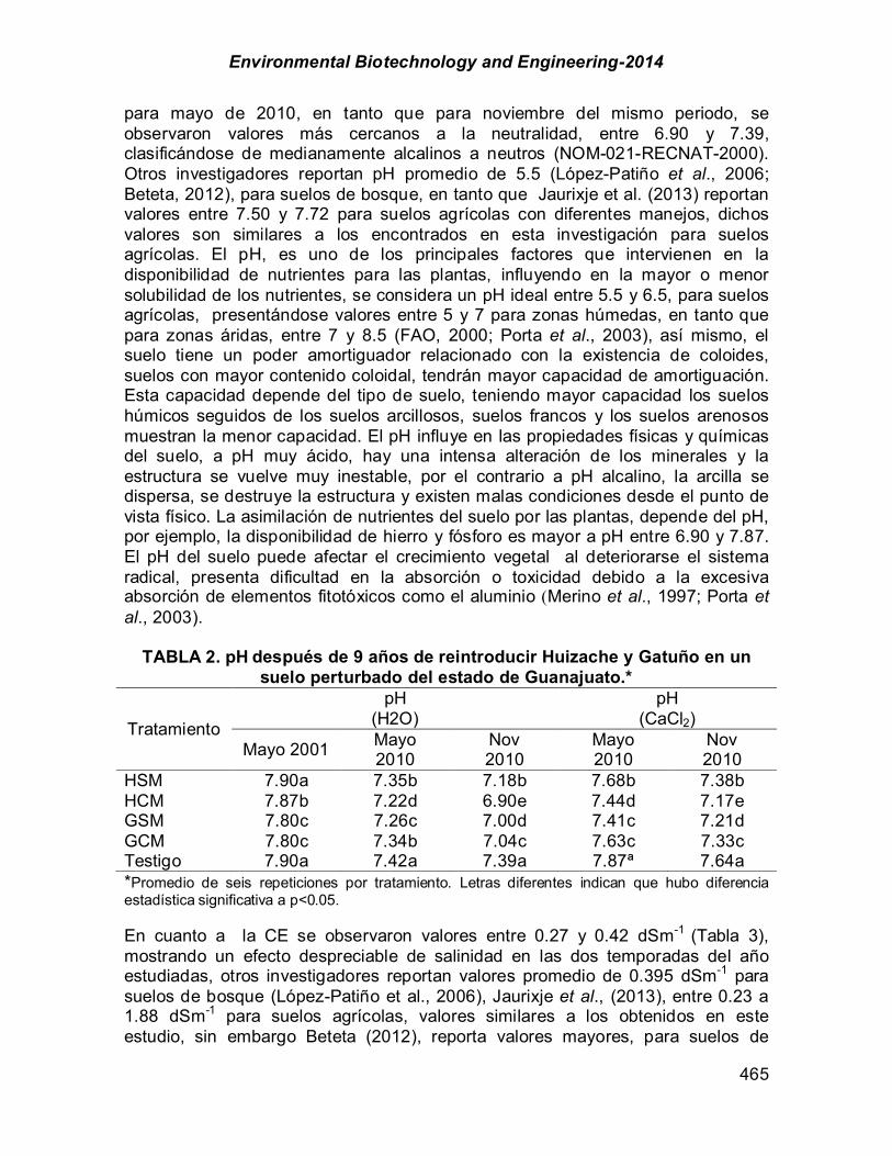
Environmental Biotechnology and Engineering-2014
465
para mayo de 2010, en tanto que para noviembre del mismo periodo, se observaron valores más cercanos a la neutralidad, entre 6.90 y 7.39, clasificándose de medianamente alcalinos a neutros (NOM-021-RECNAT-2000). Otros investigadores reportan pH promedio de 5.5 (López-Patiño et al., 2006; Beteta, 2012), para suelos de bosque, en tanto que Jaurixje et al. (2013) reportan valores entre 7.50 y 7.72 para suelos agrícolas con diferentes manejos, dichos valores son similares a los encontrados en esta investigación para suelos agrícolas. El pH, es uno de los principales factores que intervienen en la disponibilidad de nutrientes para las plantas, influyendo en la mayor o menor solubilidad de los nutrientes, se considera un pH ideal entre 5.5 y 6.5, para suelos agrícolas, presentándose valores entre 5 y 7 para zonas húmedas, en tanto que para zonas áridas, entre 7 y 8.5 (FAO, 2000; Porta et al., 2003), así mismo, el suelo tiene un poder amortiguador relacionado con la existencia de coloides, suelos con mayor contenido coloidal, tendrán mayor capacidad de amortiguación. Esta capacidad depende del tipo de suelo, teniendo mayor capacidad los suelos húmicos seguidos de los suelos arcillosos, suelos francos y los suelos arenosos muestran la menor capacidad. El pH influye en las propiedades físicas y químicas del suelo, a pH muy ácido, hay una intensa alteración de los minerales y la estructura se vuelve muy inestable, por el contrario a pH alcalino, la arcilla se dispersa, se destruye la estructura y existen malas condiciones desde el punto de vista físico. La asimilación de nutrientes del suelo por las plantas, depende del pH, por ejemplo, la disponibilidad de hierro y fósforo es mayor a pH entre 6.90 y 7.87. El pH del suelo puede afectar el crecimiento vegetal al deteriorarse el sistema radical, presenta dificultad en la absorción o toxicidad debido a la excesiva absorción de elementos fitotóxicos como el aluminio (Merino et al., 1997; Porta et al., 2003).
TABLA 2. pH después de 9 años de reintroducir Huizache y Gatuño en un suelo perturbado del estado de Guanajuato.*
Tratamiento
pH (H2O)
pH (CaCl2)
Mayo 2001 Mayo 2010
Nov 2010
Mayo 2010
Nov 2010
HSM 7.90a 7.35b 7.18b 7.68b 7.38b HCM 7.87b 7.22d 6.90e 7.44d 7.17e GSM 7.80c 7.26c 7.00d 7.41c 7.21d GCM 7.80c 7.34b 7.04c 7.63c 7.33c Testigo 7.90a 7.42a 7.39a 7.87ª 7.64a *Promedio de seis repeticiones por tratamiento. Letras diferentes indican que hubo diferencia estadística significativa a p<0.05. En cuanto a la CE se observaron valores entre 0.27 y 0.42 dSm-1 (Tabla 3), mostrando un efecto despreciable de salinidad en las dos temporadas del año estudiadas, otros investigadores reportan valores promedio de 0.395 dSm-1 para suelos de bosque (López-Patiño et al., 2006), Jaurixje et al., (2013), entre 0.23 a 1.88 dSm-1 para suelos agrícolas, valores similares a los obtenidos en este estudio, sin embargo Beteta (2012), reporta valores mayores, para suelos de

Environmental Biotechnology and Engineering-2014
466
bosque, entre 1.32 y 1.44 dSm-1 en temporada de sequía y lluvias respectivamente. La conductividad eléctrica en suelo es proporcional al contenido de sales disueltas ionizadas en solución, un suelo sin problemas de salinidad, presenta conductividades eléctricas menores a 2 dSm-1, concentraciones mayores indican suelos salinos.
TABLA 3. Conductividad eléctrica y salinidad después de 9 años de reintroducir Huizache y Gatuño en un suelo perturbado del estado de
Guanajuato.*
Tratamiento
CE (dSm-1)
Salinidad (g/L)
Mayo 2010
Nov 2010 Mayo 2010 Nov
2010 HSM 0.32c 0.37c 0.19c 0.24b HCM 0.30d 0.37b 0.21b 0.23c GSM 0.35a 0.42a 0.22a 0.24b GCM 0.34b 0.37b 0.22ª 0.27a Testigo 0.27e 0.31e 0.17d 0.20d *Promedio de seis repeticiones por tratamiento. Letras diferentes indican que hubo diferencia estadística significativa a p<0.05. En el caso del suelo la CE depende de al menos tres factores que lo constituyen, la matriz, el contenido de electrolitos susceptibles de conducir la corriente eléctrica y la humedad, a su vez la matriz depende de la composición química, la textura, la estructura y la porosidad, un suelo arenoso muestra conductividades eléctricas más altas que los suelos arcillosos, lo que relaciona la interacción del agua con las partículas del suelo, un suelo arcilloso presenta un mayor número de partículas que al ser más pequeñas, presentan una mayor superficie de contacto, por ello los solutos permanecen más fuertemente retenidos en la matriz de las arcillas, de naturaleza eléctrica negativa, detectando una CE menor en la solución, a diferencia de un suelo arenoso, que no retiene solutos (Duponnois et al., 2000; Porta et al, 2003). El suelo como todo cuerpo poroso tiene dos densidades. La densidad real, que corresponde a la densidad media de sus partículas sólidas y la densidad aparente, que incluye el volumen de los poros. La densidad aparente refleja el contenido total de porosidad en un suelo y es importante para el manejo de los mismos, indica la compactación, facilidad de circulación de agua y aire (Llorca-Llorca, 1991; Porta et al., 2003;), en cuanto mayor sea la densidad aparente en un suelo, la compactación es menor, la circulación de agua es mucho mejor, como es el caso de un suelo arenoso, en contraste, un suelo con menor densidad aparente es más compacto, como el caso de un suelo arcilloso. Jaurixje et al. (2013), reportan valores entre 1.32 a 1.43 gcm-3 para suelos agrícolas, en esta investigación la densidad aparente fue menor, lo que correspondió a suelos minerales arcillosos (1.00 y 1.11 gcm-3) según la clasificación de la NOM-021-RECNAT-2000 (Tabla
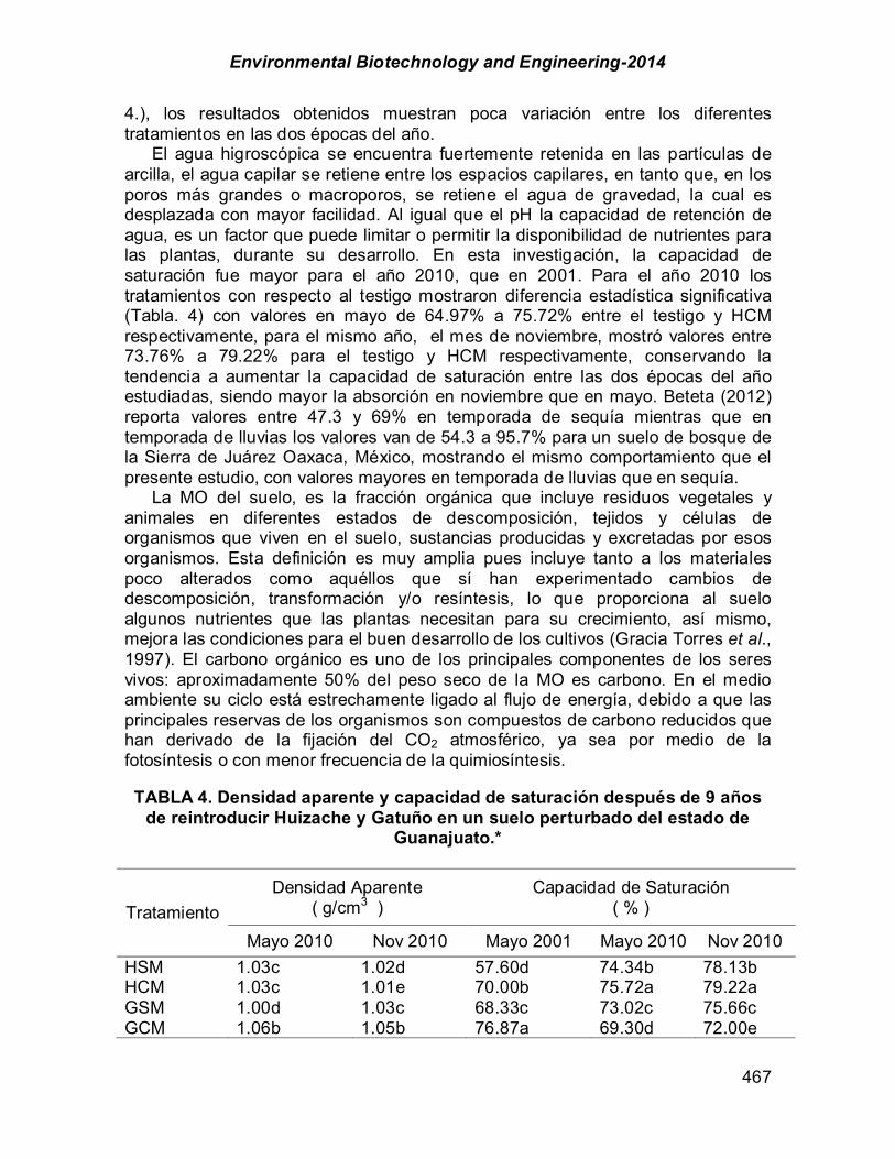
Environmental Biotechnology and Engineering-2014
467
4.), los resultados obtenidos muestran poca variación entre los diferentes tratamientos en las dos épocas del año. El agua higroscópica se encuentra fuertemente retenida en las partículas de arcilla, el agua capilar se retiene entre los espacios capilares, en tanto que, en los poros más grandes o macroporos, se retiene el agua de gravedad, la cual es desplazada con mayor facilidad. Al igual que el pH la capacidad de retención de agua, es un factor que puede limitar o permitir la disponibilidad de nutrientes para las plantas, durante su desarrollo. En esta investigación, la capacidad de saturación fue mayor para el año 2010, que en 2001. Para el año 2010 los tratamientos con respecto al testigo mostraron diferencia estadística significativa (Tabla. 4) con valores en mayo de 64.97% a 75.72% entre el testigo y HCM respectivamente, para el mismo año, el mes de noviembre, mostró valores entre 73.76% a 79.22% para el testigo y HCM respectivamente, conservando la tendencia a aumentar la capacidad de saturación entre las dos épocas del año estudiadas, siendo mayor la absorción en noviembre que en mayo. Beteta (2012) reporta valores entre 47.3 y 69% en temporada de sequía mientras que en temporada de lluvias los valores van de 54.3 a 95.7% para un suelo de bosque de la Sierra de Juárez Oaxaca, México, mostrando el mismo comportamiento que el presente estudio, con valores mayores en temporada de lluvias que en sequía. La MO del suelo, es la fracción orgánica que incluye residuos vegetales y animales en diferentes estados de descomposición, tejidos y células de organismos que viven en el suelo, sustancias producidas y excretadas por esos organismos. Esta definición es muy amplia pues incluye tanto a los materiales poco alterados como aquéllos que sí han experimentado cambios de descomposición, transformación y/o resíntesis, lo que proporciona al suelo algunos nutrientes que las plantas necesitan para su crecimiento, así mismo, mejora las condiciones para el buen desarrollo de los cultivos (Gracia Torres et al., 1997). El carbono orgánico es uno de los principales componentes de los seres vivos: aproximadamente 50% del peso seco de la MO es carbono. En el medio ambiente su ciclo está estrechamente ligado al flujo de energía, debido a que las principales reservas de los organismos son compuestos de carbono reducidos que han derivado de la fijación del CO2 atmosférico, ya sea por medio de la fotosíntesis o con menor frecuencia de la quimiosíntesis. TABLA 4. Densidad aparente y capacidad de saturación después de 9 años
de reintroducir Huizache y Gatuño en un suelo perturbado del estado de Guanajuato.*
Tratamiento
Densidad Aparente ( g/cm3 )
Capacidad de Saturación ( % )
Mayo 2010 Nov 2010 Mayo 2001 Mayo 2010 Nov 2010 HSM 1.03c 1.02d 57.60d 74.34b 78.13b HCM 1.03c 1.01e 70.00b 75.72a 79.22a GSM 1.00d 1.03c 68.33c 73.02c 75.66c GCM 1.06b 1.05b 76.87a 69.30d 72.00e
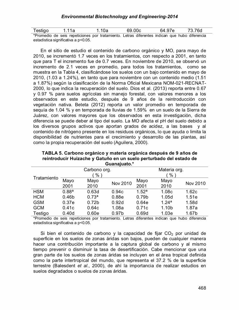
Environmental Biotechnology and Engineering-2014
468
Testigo 1.11a 1.10a 69.00c 64.97e 73.76d *Promedio de seis repeticiones por tratamiento. Letras diferentes indican que hubo diferencia estadística significativa a p<0.05. En el sitio de estudio el contenido de carbono orgánico y MO, para mayo de 2010, se incrementó 1.7 veces en los tratamientos, con respecto a 2001, en tanto que para T el incremento fue de 0.7 veces. En noviembre de 2010, se observó un incremento de 2.1 veces en promedio, para todos los tratamientos, como se muestra en la Tabla 4, clasificándose los suelos con un bajo contenido en mayo de 2010, (1.03 a 1.24%), en tanto que para noviembre con un contenido medio (1.51 a 1.87%) según la clasificación de la Norma Oficial Mexicana NOM-021-RECNAT-2000, lo que indica la recuperación del suelo. Dios et al. (2013) reporta entre 0.67 y 0.97 % para suelos agrícolas sin manejo forestal, con valores menores a los observados en este estudio, después de 9 años de la reintroducción con vegetación nativa. Beteta (2012) reporta un valor promedio en temporada de sequía de 1.04 % y en temporada de lluvias de 1.59% en un suelo de la Sierra de Juárez, con valores mayores que los observados en esta investigación, dicha diferencia se puede deber al tipo del suelo. La MO afecta el pH del suelo debido a los diversos grupos activos que aportan grados de acidez, a las bases y al contenido de nitrógeno presente en los residuos orgánicos, lo que ayuda o limita la disponibilidad de nutrientes para el crecimiento y desarrollo de las plantas, así como la propia recuperación del suelo (Aguilera, 2000).
TABLA 5. Carbono orgánico y materia orgánica después de 9 años de reintroducir Huizache y Gatuño en un suelo perturbado del estado de
Guanajuato.*
Tratamiento
Carbono org. ( % )
Materia org. ( % )
Mayo 2001
Mayo 2010 Nov 2010 Mayo
2001 Mayo 2010 Nov 2010
HSM 0.88ª 0.63d 0.94c 1.52ª 1.08c 1.62c HCM 0.46b 0.73ª 0.88e 0.79b 1.05d 1.51e GSM 0.37e 0.72b 0.92d 0.64e 1.24ª 1.58d GCM 0.41c 0.64c 1.08a 0.71c 1.10b 1.87a Testigo 0.40d 0.60e 0.97b 0.69d 1.03e 1.67b *Promedio de seis repeticiones por tratamiento. Letras diferentes indican que hubo diferencia estadística significativa a p<0.05. Si bien el contenido de carbono y la capacidad de fijar CO2 por unidad de superficie en los suelos de zonas áridas son bajos, pueden de cualquier manera hacer una contribución importante a la captura global de carbono y al mismo tiempo prevenir o disminuir la tasa de desertificación. Cabe mencionar que una gran parte de los suelos de zonas áridas se incluyen en el área tropical definida como la parte intertropical del mundo, que representa el 37.2 % de la superficie terrestre (Balesdent et al., 2000), de ahí la importancia de realizar estudios en suelos degradados o suelos de zonas áridas.
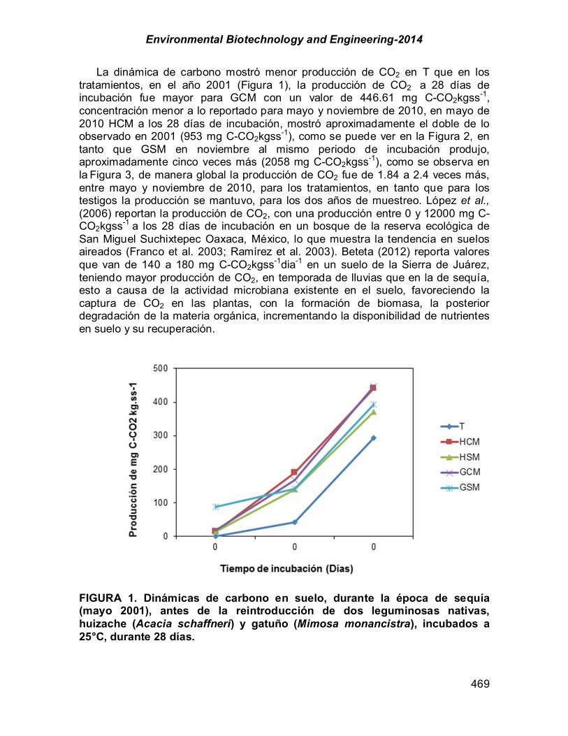
Environmental Biotechnology and Engineering-2014
469
La dinámica de carbono mostró menor producción de CO2 en T que en los tratamientos, en el año 2001 (Figura 1), la producción de CO2 a 28 días de incubación fue mayor para GCM con un valor de 446.61 mg C-CO2kgss-1, concentración menor a lo reportado para mayo y noviembre de 2010, en mayo de 2010 HCM a los 28 días de incubación, mostró aproximadamente el doble de lo observado en 2001 (953 mg C-CO2kgss-1), como se puede ver en la Figura 2, en tanto que GSM en noviembre al mismo periodo de incubación produjo, aproximadamente cinco veces más (2058 mg C-CO2kgss-1), como se observa en la Figura 3, de manera global la producción de CO2 fue de 1.84 a 2.4 veces más, entre mayo y noviembre de 2010, para los tratamientos, en tanto que para los testigos la producción se mantuvo, para los dos años de muestreo. López et al., (2006) reportan la producción de CO2, con una producción entre 0 y 12000 mg C-CO2kgss-1 a los 28 días de incubación en un bosque de la reserva ecológica de San Miguel Suchixtepec Oaxaca, México, lo que muestra la tendencia en suelos aireados (Franco et al. 2003; Ramírez et al. 2003). Beteta (2012) reporta valores que van de 140 a 180 mg C-CO2kgss-1dia-1 en un suelo de la Sierra de Juárez, teniendo mayor producción de CO2, en temporada de lluvias que en la de sequía, esto a causa de la actividad microbiana existente en el suelo, favoreciendo la captura de CO2 en las plantas, con la formación de biomasa, la posterior degradación de la materia orgánica, incrementando la disponibilidad de nutrientes en suelo y su recuperación.
FIGURA 1. Dinámicas de carbono en suelo, durante la época de sequía (mayo 2001), antes de la reintroducción de dos leguminosas nativas, huizache (Acacia schaffneri) y gatuño (Mimosa monancistra), incubados a 25°C, durante 28 días.

Environmental Biotechnology and Engineering-2014
470
Las concentraciones observadas en este estudio son similares a las reportadas en los suelos desérticos, los cuales pueden producir hasta 1000 mgCO2Kgss-1 (Lal, 2005). Los resultados reportados por Herrera- Arreola et al (2007), muestran que la producción de C-CO2, en gatuño y huizache, en suelo bajo el dosel con adición de hojarasca, se ve afectada por la altura de las plantas, obteniéndose mayor producción en las plantas con mayor altura, gatuño con una altura de 1.5m, 79 mgC-kg-1día-1, en tanto que para huizache con 3.6m, fue de 70 mgC-kg-1día-1. Así mismo, otros investigadores reportan el incremento en la producción de CO2, con el transcurso de los días de incubación por efecto de la respiración de los microorganismos (Marin et al, 2009; Segura et al 2005; Jenkinson, 1988), lo que corresponde con lo observado en esta investigación.
FIGURA 2. Dinámicas de carbono en suelo, durante la época de sequía (mayo 2010), a 9 años después de la reintroducción de dos leguminosas nativas, huizache (Acacia schaffneri) y gatuño (Mimosa monancistra), incubados a 25°C, durante 28 días.
0
200
400
600
800
1000
1200
7 14 28
Pro
ducc
ión
de C
-CO
2(m
g kg
ss-1
)
Incubación (Días)
T
HCM
HSM
GCM
GSM

Environmental Biotechnology and Engineering-2014
471
FIGURA 3. Dinámicas de carbono en suelo, después de la época de lluvia (noviembre 2010), a los 4 años después de la reintroducción de dos leguminosas nativas, huizache (Acacia schaffneri) y gatuño (Mimosa monancistra), incubados a 25°C, durante 28 días. Conclusión La reintroducción de vegetación nativa huizache (Acacia schaffneri) y gatuño (Mimosa monancistra), en un suelo perturbado, como era de esperarse, no modificó significativamente las características fisicoquímicas del suelo, sin embargo la captura de carbono sí, lo que reduce el tiempo de recuperación, por lo que se propone seguir investigando como una alternativa para mitigar los efectos de los GEI, como modelo de reservorio o sumidero forestal y con ello mitigar el cambio climático. Referencias Aguilera, S.M., (2000). Importancia de la protección de la materia orgánica en suelos. Simposio
Proyecto Ley Protección de Suelo. Valdivia, Chile, Boletín N° 14. p. 77-85. Balesdent J. Chenu C., Balabane M. (2000). Relationship of the soil organic matter dynamics to
physical protection and tillage. Soil tillage Research. 53:215-220. Beedlow Peter A, Tingey David T, Phillips Donald L, Hogsett William E, Olszyk David M. (2004).
Rising atmospheric CO2 and carbon sequestration in forests. Front Ecol Environ; 2(6): 315–322.
Beteta O. (2012). Caracterización y dinámicas de carbono y nitrógeno de suelos forestales, en Santa Maria Yavesia, Oaxaca. Tesis de licenciatura en Ciencias Ambientales. Universidad de la Sierra de Juárez. Ixtlan de Juárez Oaxaca, México
Cruz G, Etchevers J. (2011). Contenidos de carbono orgánico de suelos someros en pinares y abetales de áreas protegidas de México Agrociencia. 45(8):849-862.
De Jong Ben, Castillo Miguel A. (2000). Dinámica de cambio de uso de suelo y emisiones de carbono en el trópico húmedo de México. El Colegio de la Frontera Sur (ECOSUR). México
Dios J, Colazo J, Buschiazzo. (2003). Dinámica del carbono orgánico en suelos de la provincia de San Luis. Instituto nacional de Tecnología Agropecuaria. San Luis, Argentina.
0
500
1000
1500
2000
2500
7 14 28Pro
ducc
ión
de C
-CO
2(m
g kg
ss-1
)
Tiempo de incubación (Días)
T
HCM
HSM
GCM
GSM

Environmental Biotechnology and Engineering-2014
472
Duponnois R., Founoune H., Lesueur D., Thioulouse J., Neyra M. (2000). Australian Journal of Experimental Agriculture. 40: (3) 443-450.
Etchevers B., Montreal M, Hidalgo M, Acosta M, Padilla C, López R. (2005). Manual para la determinación de carbono en la parte aérea y subterránea de sistemas de producción en laderas. Colegio de posgraduados México 28 pp.
FAO. (2000). Sistemas de uso de la tierra en los trópicos húmedos, la emisión y secuestro de CO2. World Soil Resources Reports88. Roma. pp.31.
Franco-Hernández, O., Mckelligan-González, A.N., Lopez-Olguin, A.M., Espinosa-Ceron, F., Escamilla-Silva, E., Dendooven, L. (2003). Dynamics of carbon, nitrogen, and phosphorous in soil amended with irradiated, pasteurized and limed biosolids. Biores. Technol.87, 93-102
García Torres L., González Fernández, editores (1997). Agricultura de conservación: Fundamentos agronómicos, medioambientales y económicos. Asociación Española de Laboreo de conservación/suelos vivos. España. pp. 372.
Gorte Ross W. (2009). Carbon Sequestration in Forests Congressional Research Service. EUA. Harmon Mark E. (2001). Carbon sequestration in forests, addressing the scale question Department
of Forest Science, Oregon State University, Corvallis, OR 97331-5752 Herrera-Arreola G., Y. Herrera, B.G. Reyes-Reyes, L. Dendooven. (2007). Mesquite (Prosopis
juliflora (Sw.) DC.), huisache (Acacia farnesiana (L.)Willd.)and catclaw (Mimosa biuncifera Benth.) and their effect on dynamics of carbon and nitrogen in soils of the semi-arid highlands of Durango Mexico. Journal of Arid Environments 69.
IPCC. (2007). Cambio climático: Informe de síntesis. Contribución de los Grupos de trabajo I, II y III al Cuarto Informe de evaluación del Grupo Intergubernamental de Expertos sobre el Cambio Climático [Equipo de redacción principal: Pachauri, R.K. y Reisinger, A. (directores de la publicación)]. IPCC, Ginebra, Suiza, pp. 104
Jaurixje M, Torres D, Mendoza B, Henríquez M, Contreras J. (2013). Propiedades físicas y químicas del suelo y su relación con la actividad biológica bajo diferentes manejos en la zona de Quíbor, Estado Lara. Barquisimeto. Venezuela Bioagro Barquisimeto abr. 2013. .25/1.
Jenkinson D.S.(1988).The determination of microbial biomass carbon and nitrogen in soil. Advances in Nitrogen Cycling in Agricultural Ecosystem. (Eds.): Wilson, J.R. CAB, Wallingford. pp.368-386.
Jenkinson, D.S. and Powlson D.S. (1976). Effect of biocidal treatments on metabolism in soil. Lal, R. (2005). Forest soils and carbon sequestration. Forest Ecology and Management 220 242-
258. Lopez-Patiño, J. I., Gutiérrez-Ortiz M. R., Santiago-Romero H., Franco Hernandez M O. (2006).
Funcionamiento biológico de suelo de bosque de San Miguel Suchixtepec Oax. V Congreso Intenacional y XI Nacional de Ciencias Ambientales del 6 al 9 de junio en Oaxtepec Morelos México.
Luis-Mejía Salomón, Gómez-Guerrero Armando, Etchevers-Barra Jorge D. Ángeles-Pérez Gregorio, López-López Miguel A., Horwath William R. (2007). Acumulación de carbono orgánico en el suelo en reforestaciones de Pinus michoacana. Agrociencia 41: 711-721.
Llorca-Llorca R. (1991). Prácticas de Edafología. Universidad Politécnica de Valencia. Valencia, España. p. 30-24.
Malhi Y, Grace J. (2000). Tropical forests and atmospheric carbon dioxide Elsevier Science Ltd. TREE vol. 15, no. 8
Marin-Spiotta E., E. Silver, W.L., Swanston, C.W. Ostertag, R. (2009). Soil organic matter dynamics during 80 years of reforestation tropical pasturesl Glob. Change. Biol. 15:1584-1597
Martinez E, Fuentes J,Acevedo E.(2008). Carbono orgánico y propiedades del suelo Suelo Nutr. Veg. Temuco, Chile.8 (1) 2008 (68-96) a method for measuring soil biomass. Soil Biology & Biochemistry 8, 209-213.
Merino A., Ouro G., Edeso J.M. (1997). Efectos de la preparación del terreno sobre las propiedades de los suelos en plantaciones forestales. Edafología. 3:347-359.
Miquelajauregui, Y. (2013). Modelos de simulación de la dinámica del carbono. En J.A. Blanco (Ed.). Aplicaciones de modelos ecológicos a la gestión de recursos naturales. Barcelona: Omnia Science. (pp. 15-38).

Environmental Biotechnology and Engineering-2014
473
Muñoz Vargas M. (2006). Dinámica del carbono orgánico del suelo en ecosistemas de la zona mediterránea de Chile, Tesis de doctorado en ciencias de recursos naturales Universidad de la frontera, Temuco Chile.
NOM-021-RECNAT-2000. Norma Oficial Mexicana. Que establece las especificaciones de fertilidad, salinidad y clasificación de suelos. Estudio, muestreo y análisis. DOF.31 de diciembre de 2002.
Olalde-Portugal V., Varela Fregoso L., Dendooven L.( 2002). C and N dynamics in soil from the central higlands of Mexico as affected by mesquite (Prosopiss pp.) and huizache (Acacia tortuosa): a laboratory investigation. Applied Soil Ecology 19.
Ordoñez Jose A, Masera O. (2001). Captura de carbono ante el cambio climático, Madera y bosques. ): Instituto de Ecología, A.C. Xalapa, México 7(1): 3-12
Orellana-Rivadeneyra G., Sandoval-Solís M.L., Linares-Fleites G., García-Calderón N. E y Tamariz-Flores J.V.(2012). Descripción de la dinámica de carbono en suelos forestales mediante un modelo de reservorios. ACI. 3(1): 123-135.
Percy K.E., Jandl R., Hall J.P. Lavingne M. (2003) The Role of Forests in Carbon Cycles, Sequestration, and Storage, Issue 1: Forests and the Global Carbon Cycle: Sources and Sinks, Federal Office and Research Centre for Forests, Vienna, Austria
Porta J., Lopez-Acevedo M., Roquero C., (2003). Edafología para la agricultura y el medio ambiente. 3rd ed., S.A. MUNDI-PRENSA LIBROS. Madrid España. pp 39-61.
Ramírez, FI, Lucho, CC, Escamilla, SE, Dendooven, L. (2003). Characteristics, and carbon and nitrogen dynamics in soil irrigated with wastewater for different lenghts of time. Biores. Technol.85, 179-187.
Reyes-Reyes G., Baron-Ocampo L., Cuali-Alvarez I., Frías-Hernández J.T,. Olalde Portugal V, Varela-Fregoso L. Dendooven L. (2002). C and N dynamics in soil from the central highlands of Mexico as affected by mesquite (Prosopis spp.) and huisache (Acacia tortuosa) a laboratory investigation. App. Soil. Ecol. 19:27-34.
Segura-Castruita M.A., Sánchez-Guzmán P., Ortiz-Solorio C.A, Gutiérrez-Castorena M.C. (2005). Carbono orgánico de los suelos de México. Terra Latinoamericana. 23(1):21-28.
Valdés, M. (2001). Manual de ecología microbiana del suelo. Escuela Nacional de Ciencias Biológicas. Instituto Politécnico Nacional. México.
Zambrano Alexis, Franquis Félix, Infante Angel. (2004) Emisión y Captura de Carbono en los Suelos en Ecosistemas Forestales. Rev. For. 35:11-20.
Notación. CE Conductividad Eléctrica CO2 Dióxido de carbono GEI gas de efecto invernadero ppm partes por millón GtC gigatoneladas de Carbono mg C-CO2kgss-1 mg de carbono por kg de suelo seco. MO Materia Orgánica

Environmental Biotechnology and Engineering-2014
474
LISTA DE COAUTORES: Martha V. Almanza Estrada, Tesista de Ingeniería Ambiental Misma dirección que Jaquelina González-Castañeda. E-mail: [email protected] Blanca G. Elías-Balandrán, Estadía de Ingeniería en Agrotecnología. Universidad Politécnica Bicentenario, Carretera Silao-Romita Km 2, San Juan de los Duran, C.P. 36283, Silao, Guanajuato, México. Tel. (472) 72 38 700. E-mail:[email protected] María M. Vargas-Zúñiga, Tesista de Ingeniería Ambiental Misma dirección que Jaquelina González-Castañeda. E-mail: [email protected] Yazmín A. Sánchez-Ruan, Tesista de Ingeniería Ambiental Misma dirección que Jaquelina González-Castañeda. E-mail: [email protected] Alejandra Gutiérrez-Vázquez, Estudiante de Ingeniería Ambiental. Misma dirección que Jaquelina González-Castañeda. E-mail: [email protected] Juan A. Mejía-Gómez, Profesor-Investigador. Misma dirección que Jaquelina González-Castañeda. E-mail: [email protected] Jaquelina González-Castañeda, Profesor-Investigador. Autor a quien debe ser dirigida toda la correspondencia. DICIVA, Departamento de Ciencias Ambientales, CIS, UNIVERSIDAD DE GUANAJUATO, Km. 9. Carretera Irapuato-Silao. Ex Hacienda El Copal, Apdo. Postal: 311, C.P.36000, Irapuato, Guanajuato, México. Tel:01(462)6241889, Ext.: 1530, Fax: (462)6242484. E-mail: [email protected]

Environmental Biotechnology and Engineering-2014
475
Section 5. Aquifer Remediation

Environmental Biotechnology and Engineering-2014
476
Page Chapter 5.1. Production of a photosynthetic microbial consortium in a flat-panel airlift photobioreactor in batch and semicontinuous culture outdoors Dulce J. Hernández-Melchor; Eliseo Cristiani-Urbina; José F. Esparza-García; Rosa O. Cañizares-Villanueva 477 Chapter 5.2. Disminución del efecto inhibitorio del 2-clorofenol sobre la nitrificación en un reactor de lotes secuenciados (SBR) Miguel Martínez-Jardines; Anne-Claire Texier; Emmanuel Pérez-Alfaro; Flor Cuervo-López 485 Chapter 5.3 Inducción de embriones somáticos en Typha domingensis Hernández-Piedra G.; Ruiz-Carrera V. 497 Chapter 5.4. Evaluación de la actividad emulsificante y surfactante de un consorcio microbiano degrador de hidrocarburos nativo de un cenote Manuel A. Lizardi-Jiménez; Cesar Hernández-Flores; Stefano Decler; A. Jiménez-González; S.A. Medina–Moreno 515 Chapter 5.5. Combining abiotic and biotic processes for aggressive treatment of chlorinated ethenes Daniel Leigh 535
Environmental Biotechnology and Engineering-2014
477
CHAPTER 5.1. PRODUCTION OF A PHOTOSYNTHETIC MICROBIAL CONSORTIUM IN A FLAT-PANEL AIRLIFT PHOTOBIOREACTOR IN BATCH
AND SEMICONTINUOUS CULTURE OUTDOORS
Dulce Jazmín Hernández Melchor (1); Eliseo Cristiani Urbina (2); José Fernando Esparza García (1), Rosa Olivia Cañizares Villanueva*(1)
(1) CINVESTAV- IPN, México DF, México; (2) ENCB-IPN, México DF, México;
ABSTRACT Cyanobacteria are oxygenic phototrophic organisms, distributed in aquatic and terrestrial environments. They have the capability to produce high value compounds useful in different areas of biotechnological interest. One strategy that has been used to improve the productivity of cyanobacteria and algae in photobioreactors is to scale up its production in semicontinuous culture. In our research group a photosynthetic microbial consortium (MC) with nitrogen fixation capability, was studied. It consists primarily of cyanobacteria, so its potential use as a biofertilizer has been proposed. The aim of this study was to produce the MC in a flat-panel airlift photobioreactor of 150 L capacity (PBR) in batch and semicontinuous culture outdoors, and to evaluate its productivity and nitrogen fixation capability. The maximum value of the biomass in batch culture in the PBR was obtained at 14 day with 600 mg L-1. The productivity at the end of the batch culture was 28.6 mg L-1 d-1. The maximum value of the nitrogenase activity was obtained at 14 day equal to 4814 nmol ethene g-1 dry weight h-1. In the second experiment was realized the growth of the MC during three growth cycles in semicontinuous mode. The productivity obtained at the end of each cycle was 43.7, 33.4 and 67.7 mg L-1 d-1 respectively. The maximum values of the nitrogenase activity was obtained at the end of each cycle and were 4963, 5366 y 5689 nmol ethene g-1 dry weight h-1 respectively. The values of the nitrogenase activity obtained in this study for the MC in a PBR in batch and semicontinuous culture were approximately two and three times higher that reported for Anabaena variabilis Sao (2678 nmol eteno g-1 dry weight h-1) and Nostoc muscorum DOH (2237 nmol eteno g-1 dry weight h-1). In conclusion was possible to produce the MC in a PBR in batch and semicontinuous mode outdoors, without affecting the nitrogen fixation capability. This strategy can be used to produce the MC in a large scale. Key words: consortium, photobiorreactor, semicontinous, biofertilizer, scale up ------------------ *Author for correspondence: [email protected]
Environmental Biotechnology and Engineering-2014
478
Introducción
Las cianobacterias son organismos fotosintéticos con requerimientos simples para su crecimiento (luz, CO2, N, P, K), las podemos encontrar distribuidas en diversos ambientes acuáticos y terrestres (Thajuddin y Subramanian, 2005). Tienen la capacidad de producir compuestos con alto valor agregado para diferentes áreas de interés biotecnológico como son alimentos, aditivos, pigmentos, dietas para acuacultura, metabolitos secundarios y tratamiento de aguas residuales. También han sido ampliamente utilizadas por su capacidad de fijación de CO2, remoción de óxido nítrico y su capacidad de fijación de nitrógeno (Carvalho et al., 2006). Sin embargo, a pesar de este enorme potencial el número de aplicaciones a escala industrial aun es limitado, debido a la baja eficiencia de utilización de la luz para la producción de biomasa microalgal; por lo que se han desarrollado diversos fotobiorreactores para su producción a gran escala. Una estrategia que se ha utilizado para mejorar la productividad de cianobacterias y algas a gran escala en fotobiorreactores es su producción semicontinua, el cual ofrece ventajas tales como obtener una producción elevada y constante de inóculo, altas tasas de crecimiento, además de ayudar a prolongar el tiempo de operación de reactores (Reichert et al., 2006). Existen reportes en la literatura sobre el empleo del sistema de cultivo por lote secuencial o semicontinuo par la producción de Tetraselmis subcordiformis en un rectangular air-lift footobioreactor de 10.5 L (Zheng et al., 2011), y para la producción de Haematococcus pluvialis Issarapayup et al., 2009 en un fotobiorreactor tipo air lift de cara plana de 17 L en régimen semicontinuo, y en ambos se mencionan incrementos en la productividad de biomasa superiores a los obtenidos en cultivos por lote. Debido a la importancia de las cianobacterias y microalgas en el sector biotecnológico, en el grupo de trabajo se estudio la capacidad de fijación de nitrógeno de un consorcio microbiano fotosintético (CM) para su uso potencial como biofertilizante, habiéndose demostrado que posee una alta capacidad para incorporar nitrógeno molecular. En base a lo anterior el objetivo del presente estudio fue producir este consorcio microbiano fotosintético en un fotobiorrector air-lift de cara plana (FBR) de 150 L en cultivo por lote y semicontinuo a la intemperie, y evaluar su productividad y capacidad para fijar nitrógeno. Metodología Microorganismo. Se utilizó un consorcio microbiano fotosintético, aislado de un campo arrocero ubicado en la comunidad de Alpuyeca, Estado de Morelos, México (Reyna et al., 2012). Este CM fue escalado y propagado en un medio mineral sin fuente de nitrógeno (BG110) (Rippka et al., 1979). Fotobiorreactor. El cultivo del CM se llevó a cabo en un fotobiorreactor tipo air-lift de cara plana de 150 L de volumen útil, previamente caracterizado hidrodinámicamente y en su transferencia de masa (Hernández et al., 2014).
Environmental Biotechnology and Engineering-2014
479
Los experimentos se realizaron La producción del CM se realizó en el mes de Junio (2013) en la Unidad experimental de cultivo de algas del Departamento de Biotecnología y Bioingeniería del CINVESTAV-IPN Zacatenco México, D.F. El volumen de trabajo del FBR fue de 100 L de medio de cultivo y 50 L de inóculo, la operación fue en lote con un flujo de aire de 80 L min-1. El cultivo se mantuvo a la intemperie hasta alcanzar el valor máximo de biomasa en base seca al día 14. El cultivo semicontinuo inicio con un cultivo por lote, y una vez alcanzada la concentración máxima de biomasa se retiró el 50 % del volumen de cultivo y se sustituyó por medio fresco, procedimiento que se realizó por tres ciclos. La duración de cada ciclo de cultivo se determinó en base a la concentración máxima de biomasa obtenida en la fase logarítmica de crecimiento en cultivo por lote y fue igual a 600 mg L-1. Los ciclos de cultivo tuvieron una duración de 7, 7 y 5 d cada uno. Técnicas analíticas. La cantidad de luz incidente en ambas caras del fotobiorreactor fue medida con un radiómetro Quantitherm (Light Meter Thermometer) Hansatech Instruments LTD (QRT1) PE32 1JLUK. La temperatura y la luz se midieron tres veces diariamente (mañana, medio día y tarde). Peso seco de biomasa. Se filtraron alícuotas de 15 mL de cultivo empleando membranas de celulosa de 5 m de diámetro de poro (Millipore®) y se secaron en horno a 70 ºC durante 24 h (Tredici et al., 1991). Actividad de Nitrogenasa (ensayo de reducción de acetileno). La actividad de nitrogenasa se determinó por el método propuesto por Venkataraman (1981) modificando el tiempo de incubación de 30 min a 5 días. Se colocaron 10 mL de cultivo en botellas serológicas de 25 mL selladas herméticamente y se eliminó 1 mL de aire del espacio vacío, y se remplazó con 1 mL de acetileno. Las botellas se incubaron durante 5 d a 21 ± 2ºC con una intensidad luminosa de 80 mol m$2 s$1 y un fotoperiodo (luz: oscuridad) de 12: 12 h. La presencia de eteno se evaluó en un cromatógrafo de gases Varian CP3380 FID bajo las siguientes condiciones: T columna = 60ºC, T inyector = 200ºC, T detector = 250ºC, Columna: Carbowax 1540/Porapak Q 1/8” ! 6 ft, acarreador: N gas, 15 psi. Resultados y Discusión En la figura 1 se muestra la producción de biomasa del CM en base seca en cultivo por lote en el FBR de 150 L en cultivo por lote. La máxima concentración de biomasa se obtuvo al día 14 y fue de 600 mg L-1, con una productividad de 28.6 mg L-1 d-1. La temperatura promedio registrada en el interior del FBR durante el cultivo fue de 23 ± 4ºC, y el promedio de luz incidente fue de 210 µmol fotones m-
2 s-2. Los parámetros de luz y temperatura previamente mencionados, no afectaron la productividad de biomasa del CM a través del tiempo; lo que indica probablemente su adaptación a las condiciones de operación del FBR, así como a las condiciones ambientales. La adaptación de cultivos de microalgas a la intemperie durante su producción en fotobiorreactores ha sido previamente

Environmental Biotechnology and Engineering-2014
480
reportada por Richmond y Cheng-Wu (2001), en sus estudios con Nannochloropsis sp. empleando fotobiorreactores de cara plana de 200 L.
FIGURA 1. Crecimiento vs tiempo en cultivo por lote a la intemperie Con la finalidad de superar la productividad de biomasa del CM obtenida en los cultivos por lote, se llevó a cabo una cinética empleando tres ciclos de cultivo semicontinuo en el mismo FBR. En la figura 2 se muestra el comportamiento de la biomasa a través del tiempo; y se observa en la primera gráfica el cultivo por lote hasta alcanzar la concentración de biomasa establecida para iniciar los ciclos del cultivo semicontinuo. Los valores de productividad de biomasa de cada ciclo fueron 43.7, 33.4 y 67.7 mg L-1 d-1 respectivamente. El aumento en la productividad de biomasa al cambiar de un sistema por lote a uno semicontinuo, fue previamente reportado por Henrard et al. (2011) quienes lograron incrementar la producción y la velocidad específica de crecimiento de Cyanobium sp. al operar en cultivo semicontinuo un fotobiorreactor vertical tubular de 2 L, con una tasa de recambio del 50 % por 10 ciclos. La temperatura promedio registrada en el interior del FBR durante el cultivo semicontinuo durante los tres ciclos fue de 20 ± 4ºC y el promedio de luz incidente fue de 233 µmol fotones m-2 s-2. Los valores registrados de luz y temperatura del cultivo semicontinuo fueron similares a los obtenidos en cultivo por lote en el mismo FBR.
0
200
400
600
800
0 2 4 6 8 10 12 14
Peso
sec
o (m
g / L
)
t (d)

Environmental Biotechnology and Engineering-2014
481
FIGURA 2. Crecimiento vs tiempo durante tres ciclos en cultivo semicontinuo a la intemperie (a: cultivo por lote; b: cultivo semicontinuo)
La productividad de biomasa en cultivo semicontinuo a la intemperie resultó aproximadamente dos veces superior a la obtenida en cultivo por lote. Este comportamiento ha sido reportado por diversos autores empleando fotobiorreactores de diferente escala y geometría operando en cultivo semicontinuo (Travieso et al., 2001; Reichert et al., 2006). La capacidad demostrada por el Cm para fijar nitrógeno potencializa su posible aplicación como biofertilizante, por lo que resulta necesario establecer las mejores condiciones para su crecimiento sin afectar ésta. Por lo anterior, se determinó la capacidad del CM para fijar nitrógeno durante su crecimiento en cultivo por lote y semicontinuo. En la Tabla 1 se muestran los máximos valores de actividad de nitrogenasa obtenidos al final del cultivo por lote y al final de cada ciclo de cultivo en semicontinuo, mismos que fueron aproximadamente dos veces superiores a lo reportado para las cianobacterias Anabaena variabilis Sao (2678 nmol eteno / g peso seco h) y Nostoc muscorum DOH (2237 nmol eteno / g peso seco h) (Kannaiyan et al., 1997; Kannaiyan, 2002).
TABLA 1. Actividad de nitrogenasa del CM en el FBR de 150 L al final del cultivo por lote y al final de cada ciclo en cultivo semicontinuo
Sistema Actividad de nitrogenasa
(nmol eteno g-1 peso seco h-1) Lote 4814
Ciclo 1 4963 Ciclo 2 5366 Ciclo 3 5689
Los valores de actividad de nitrogenasa obtenidos en los diferentes ciclos de cultivo semicontinuo fueron superiores al del cultivo por lote y a lo reportado en otros estudios, lo que demuestra que éste modo de operación permite mejorar la producción de biomasa sin afectar la fijación de nitrógeno del CM.
0
200
400
600
800
0 20 40Peso
sec
o (m
g / L
)t (d)
a b
Environmental Biotechnology and Engineering-2014
482
Conclusiones El cultivo semicontinuo favoreció la producción de biomasa y la fijación de nitrógeno del CM en un FBR de 150 L a la intemperie, lo que brinda la posibilidad de su producción constante para su aplicación como biofertilizante. Referencias Carvalho A. P., Meireles L. A., Malcata F. X. (2006). Microalgal reactors: a review
of enclosed system designs and performances. Biotechnol. Progr. 22: 1490-1506.
Henrard A. A., de Morais M. G., Costa J.A.V. (2011). Vertical tubular photobioreactor for semicontinuous cultura of Cyanobium sp. Bioresource Technol. 102: 4897-4900.
Issarapayup K., Powtongsookb S., Pavasant P. (2009). Flat panel airlift photobioreactors for cultivation of vegetative cells of microalga Haematococcus pluvialis. J. Biotechnol. 142: 227-232.
Kannaiyan S., Aruna S. J., Merina P. K. S. Hall D. O. (1997). Immobilized cyanobacteria as a biofertilizer for rice crops. J. Appl. Phycol. 9: 167–174.
Kannaiyan, S. (2002). Biofertilizers for sustainable crop production. En: Kannaiyan S. (ed.) Biotechnology of Biofertilizers. Narosa Publishing House, New Delhi, India, 9–49 pp.
Reichert C. C., Reinehr C. O., Costa J. A. V. (2006). Semicontinuous cultivation of the cyanobacterium Spirulina platensis in a closed photobioreactor. Braz. J. Chem. Eng. 23 (1): 23-28.
Reyna V. R., Hernández M. D., Vázquez H. M., Cañizares V. R. O. (2012). Isolation of a photosynthetic microbial consortium formed mainly by cyanobacteria with capacity to fix nitrogen. Int. J. Environ. Eng. 4 (3/4):183-196.
Richmond A., Cheng-Wu Z. (2001). Optimization of a flat plate glass reactor for mass production of Nannochloropsis sp. outdoors. J. Biotechnology 85: 259–269.
Rippka R., Deruelles J., Waterbury J. B., Herdman M., Stanier R. Y. (1979). Generic assignments, strain histories and properties of pure cultures of cyanobacteria. J. Gen. Microbiol. 111: 1-61.
Thajuddin N., Subramanian G. (2005). Cyanobacterial biodiversity and potential applications in biotechnology. Curr. Sci. 89(1): 47-57.
Travieso L., Hall D.O., Rao K.K., Benítez F., Sánchez E., Borja R. (2001). A helical tubular photobioreactor producing Spirulina in a semicontinuous mode. Int. Biodeter. Biodegr. 47: 151-155.
Tredici M. R., Carlozzi P., Chini-Zitelli G., Materassi R. (1991). A vertical alveolar panel (VAP) for outdoor mass cultivation of microalgae and cyanobacteria. Bioresource Technol. 38: 153-159.
Venkataraman G.S. (1981). Blue-green algae for rice production. Food and Agriculture Organization of the United Nations. Rome, IT. Página 102.

Environmental Biotechnology and Engineering-2014
483
Zheng Y., Chen Z., Lu H., Zhang W. (2011). Optimization of carbon dioxide fixation and starch accumulation by Tetraselmis subcordiformis in a rectangular airlift photobioreactor. Afr. J. Biotechnol. 10 (10): 1888-1901.

Environmental Biotechnology and Engineering-2014
484
LIST OF COAUTHORS: Dulce Jazmín Hernández Melchor, Dr. Candidate, presenting author. CINVESTAV, Dept. Biotechnology and Bioengineering, México DF, 07000, México. Tel: 5255 5747 3800, Fax. 5255 5747 3313 E-mail: [email protected] Dr. Eliseo Cristiani Urbina, Full Professor ENCB-IPN, Prolongación Avda Carpio s/n, Col. Santo Tomás, México D.F., 04578, México. Tel.: (5255) 5629 0000 E-mail: [email protected] Dr. José Fernando Esparza García, Full Professor CINVESTAV, Dept. Biotechnology and Bioengineering, México DF, 07000, México. Tel: 5255 5747 3800, Fax. 5255 5747 3313 E-mail: [email protected] Dr. Rosa Olivia Cañizares Villanueva, Full Professor. Author to whom all correspondence should be addresed CINVESTAV, Dept. Biotechnology and Bioengineering, México DF, 07000, México. Tel: 5255 5747 3800, Fax. 5255 5747 3313 E-mail: [email protected]

Environmental Biotechnology and Engineering-2014
485
CHAPTER 5.2. DISMINUCIÓN DEL EFECTO INHIBITORIO DEL 2-CLOROFENOL SOBRE LA NITRIFICACIÓN EN UN REACTOR DE LOTES
SECUENCIADOS (SBR)
Miguel Martínez-Jardines (1); Anne-Claire Texier (1); Emmanuel Pérez-Alfaro (1); Flor Cuervo-López *(1)
(1) UAM-Iztapalapa, Departamento de biotecnología CBS, fisiología microbiana, México DF, México. RESUMEN Se evaluó el comportamiento metabólico de un proceso nitrificante en dos reactores de lotes secuenciados (SBR) inoculados con lodos previamente expuestos a compuestos fenólicos. El SBR1 fue inoculado con un lodo previamente expuesto a 2-clorofenol (2-CP), mientras que el SBR2 se inoculó con un lodo previamente expuesto a p-cresol. Se realizaron 6 ciclos de operación de 30 días cada uno en presencia de 20 mg de carbono de 2-clorofenol (2-CP)/l. Se observó un efecto inhibitorio del 2-CP en los reactores SBR, pues las velocidades específicas disminuyeron de acuerdo a un control. Sin embargo, a lo largo de los ciclos de operación el efecto inhibitorio sobre el proceso nitrificante fue disminuyendo. Al final del ciclo 6, se observó un proceso nitrificante estable en el reactor SBR1, con una eficiencia de consumo de amonio del 100% y un rendimiento de producción de nitrato cercano a 1, mientras que una nitrificación parcial se presentó en el SBR2, con eficiencias de consumo de amonio cercanas al 100% pero con una acumulación de nitrito y rendimientos de producción de nitrato de 0.23. En ambos reactores y después del ciclo 2 de operación, se presentaron eficiencias de consumo de 2-CP del 100%. Palabras clave: 2-clorofenol, nitrificación, reactor de lotes secuenciados.
Environmental Biotechnology and Engineering-2014
486
ABSTRACT The metabolic behavior of a nitrification process into two sequencing batch reactors (SBR) inoculated with sludge previously exposed to phenolic compounds was evaluated. The SBR1 was inoculated with sludge previously exposed to 2-chlorophenol (2-CP), while the SBR2 was inoculated with sludge previously exposed to p-cresol. 6 cycles of 30 days operation are each performed in the presence of 20 mg of carbon of 2-chlorophenol (2-CP)/l. An inhibitory effect of 2-CP in the SBR reactors was observed, as it the specific rates decreased according to a control. However, during the operation cycles the inhibitory effect on the nitrification process decreased. At the end of cycle 6, a stable process was observed in nitrifying reactor SBR1, with an ammonium consumption efficiency of 100% and a nitrate production yield close to 1, while a partial nitrification was presented in SBR2, with an ammonium consumption efficiency near of 100% but with an accumulation of nitrite and a nitrate production yield of 0.23. In both reactors and after of 2 cycles of operation, 2-CP consumption efficiencies of 100% were presented. Key words: 2-chlorophenol, nitrification, sequencing batch reactors. ------------------ *Author for correspondence: [email protected]

Environmental Biotechnology and Engineering-2014
487
Introducción Uno de los compuestos contaminantes nitrogenados encontrados en efluentes tanto industriales como municipales es el amonio (NH4
+). Debido a las actividades humanas, la cantidad generada de amonio cada vez es mayor (Bremmen, 2002). Particularmente, los efluentes de la industria química, refinería del petróleo, la textil, tenerías, procesadoras de alimentos y papel, producción de látex, manufactureras de explosivos, plaguicidas, entre otras, contienen altas concentraciones de compuestos nitrogenados (Lens y col., 2001). En ecosistemas acuáticos el amonio es uno de los causantes de la eutroficación, que trae como consecuencia la muerte de organismos por asfixia (Bock y col., 1986; Prosser, 1989). Además, la contaminación por nitrógeno inorgánico podría inducir efectos perjudiciales sobre la salud humana (Camargo y Alonso, 2007).
La nitrificación es la oxidación biológica del amonio a nitrato (NO3-) a través de
nitrito (NO2-). Se trata de un proceso respiratorio aerobio donde las bacterias
nitrificantes utilizan amonio o nitrito como fuente de energía, dióxido de carbono como fuente de carbono y oxígeno molecular como aceptor final de electrones (Prosser, 1989).
Además del amonio, los compuestos fenólicos pueden estar presentes en los efluentes industriales en altas concentraciones. Dentro de los compuestos fenólicos, los halogenados, en particular los clorados como el 2-Clorofenol (2-CP), se encuentran contaminando suelos y acuíferos, debido a su uso generalizado como parte estructural de pesticidas y preservantes en la industria de la madera (Puhakka y col. 1995). Aunque actualmente su uso para este fin está prohibido en casi todo el mundo, en muchos países madereros, los problemas de contaminación por clorofenoles persisten debido a su alta vida media en el ambiente (Gallego y col., 1998).
Aunque las bacterias amonio oxidantes presentan cierta capacidad para oxidar materia orgánica, también está bien documentada la alta sensibilidad de las bacterias nitrificantes a los efectos tóxicos o inhibitorios de los compuestos orgánicos (Schweighofer y col., 1996, Texier y col., 2012).
Existen pocos trabajos en la literatura que abordan el efecto del 2-CP en un proceso nitrificante. (Satoh y col., 2005, Inui y col., 2002, Pérez-Alfaro y col. 2013), además se ha encontrado que utilizando lodos previamente expuestos al 2-CP se observan mejoras en el proceso (Beristain-Montiel y col., 2010, 2011).
Hay diversos trabajos en la literatura que reportan el uso de reactores de lotes secuenciados (SBR) para tratar aguas sintéticas con amonio y algunos compuestos aromáticos mediante la nitrificación, reportándose algunos efectos de la materia orgánica sobre el proceso respiratorio (Texier y Gómez, 2007).
El objetivo de este estudio fue evaluar el efecto de la 2-CP en un lodo nitrificante previamente expuestos a compuestos fenólicos mediante velocidades específicas de consumo sustratos (q N-NH4
+, q 2-CP) y generación de productos (qN-NO3
-) en un SBR.

Environmental Biotechnology and Engineering-2014
488
Material y métodos Dos reactores de lotes secuenciados (SBR1 y SBR2) se establecieron. El SBR1 se inoculó con un lodo nitrificante previamente expuesto al 2-CP. El SBR2 se inoculó con un lodo nitrificante que había sido alimentado con NH4
+ y p-cresol. La experimentación se llevó a cabo en cuatro etapas. En primer lugar, se llevaron a cabo ensayos abióticos con el fin de establecer la posible pérdida de 2-CP en los sistemas SBR. En una segunda etapa, se llegó a un estado estacionario nitrificante en los reactores SBR. En una tercera etapa, se llevaron a cabo cinéticas nitrificantes control en ambos reactores SBR. Los reactores fueron alimentados con 80 mg de N-NH4
+/l y 210 mg de C-NaHCO3/l. Finalmente, se añadieron 20 mg de C-2-CP/l en cada reactor con el fin de evaluar el efecto de 2-CP en la nitrificación. Ensayos cinéticos se llevaron a cabo a lo largo de los ciclos de operación (llenado = 30 min, tiempo de reacción = 30 d; sedimentación = 30 min y de drenado = 2 h). La agitación se llevó a cabo a 200 rpm a temperatura ambiente y con una aireación intermitente de oxígeno puro durante tres minutos dos veces por día para ambos reactores.
El Amonio fue analizado por un electrodo selectivo (Phoenix electrode company, USA) como se reporta por Silva y col., 2011. Nitrito y nitrato fueron determinados por electroforesis capilar (Beckman Coulter). El 2-CP fue analizado por HPLC (Perkin Elmer, series 200) usando una columna de fase reversa C-18 (Phenomenex, USA) y un detector de UV a 274 nm. La fase móvil fue acetonitrilo/agua (60/40, v/v) en un flujo de 1.5 ml/min como se reporta por Martínez-Hernández y col., 2011. El método de Lowry fue empleado para medir la concentración de proteína microbiana. Oxígeno disuelto y pH fueron medidos por electrodos selectivos (Hanna HI98186 OD y Digi-Sense digital pH, respectivamente).
La actividad microbiana fue evaluada en términos de eficiencias de (E, [mg d N o C consumido/mg de N o C alimentado] 100), rendimientos de producción (Y, [mg de N producido/mg de N consumido]) y velocidades específicas de consumo de sustratos y generación de productos (q, [mg de N o C/g de proteína día]) las cuales se calcularon mediante ajustes lineales y exponenciales utilizando el paquete NCSS, donde se buscó que los modelos fueran significativos y con el mayor r2 posible. Resultados y discusión
Ensayos abióticos. Mostraron que después de 6 d de experimentación, el 96.4% del C-2-CP se mantuvo en el cultivo, por lo tanto, la pérdida de este compuesto fue insignificante. Cinética nitrificante control. Los valores obtenidos en las variables de respuesta (tabla 1), nos muestran comportamientos cinéticos similares entre ambos reactores, indicando asimismo, que bajo las condiciones experimentales, es posible llevar a cabo la nitrificación de manera adecuada. Se presentaron
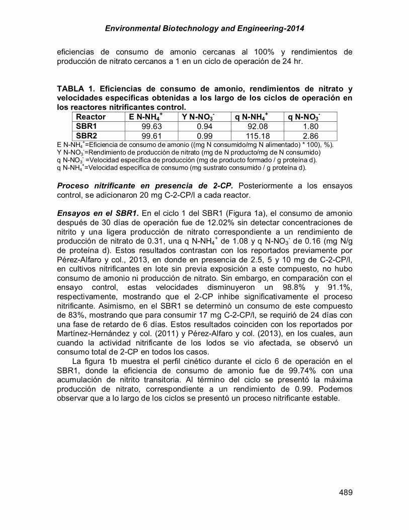
Environmental Biotechnology and Engineering-2014
489
eficiencias de consumo de amonio cercanas al 100% y rendimientos de producción de nitrato cercanos a 1 en un ciclo de operación de 24 hr. TABLA 1. Eficiencias de consumo de amonio, rendimientos de nitrato y velocidades específicas obtenidas a los largo de los ciclos de operación en los reactores nitrificantes control.
Reactor E N-NH4+ Y N-NO3
- q N-NH4+ q N-NO3
- SBR1 99.63 0.94 92.08 1.80 SBR2 99.61 0.99 115.18 2.86
E N-NH4+=Eficiencia de consumo de amonio ((mg N consumido/mg N alimentado) * 100), %).
Y N-NO3-=Rendimiento de producción de nitrato (mg de N producto/mg de N consumido)
q N-NO3- =Velocidad específica de producción (mg de producto formado / g proteína d).
q N-NH4+=Velocidad específica de consumo (mg sustrato consumido / g proteína d).
Proceso nitrificante en presencia de 2-CP. Posteriormente a los ensayos control, se adicionaron 20 mg C-2-CP/l a cada reactor. Ensayos en el SBR1. En el ciclo 1 del SBR1 (Figura 1a), el consumo de amonio después de 30 días de operación fue de 12.02% sin detectar concentraciones de nitrito y una ligera producción de nitrato correspondiente a un rendimiento de producción de nitrato de 0.31, una q N-NH4
+ de 1.08 y q N-NO3- de 0.16 (mg N/g
de proteína d). Estos resultados contrastan con los reportados previamente por Pérez-Alfaro y col., 2013, en donde en presencia de 2.5, 5 y 10 mg de C-2-CP/l, en cultivos nitrificantes en lote sin previa exposición a este compuesto, no hubo consumo de amonio ni producción de nitrato. Sin embargo, en comparación con el ensayo control, estas velocidades disminuyeron un 98.8% y 91.1%, respectivamente, mostrando que el 2-CP inhibe significativamente el proceso nitrificante. Asimismo, en el SBR1 se determinó un consumo de este compuesto de 83%, mostrando que para consumir 17 mg C-2-CP/l, se requirió de 24 días con una fase de retardo de 6 días. Estos resultados coinciden con los reportados por Martínez-Hernández y col. (2011) y Pérez-Alfaro y col. (2013), en los cuales, aun cuando la actividad nitrificante de los lodos se vio afectada, se observó un consumo total de 2-CP en todos los casos.
La figura 1b muestra el perfil cinético durante el ciclo 6 de operación en el SBR1, donde la eficiencia de consumo de amonio fue de 99.74% con una acumulación de nitrito transitoria. Al término del ciclo se presentó la máxima producción de nitrato, correspondiente a un rendimiento de 0.99. Podemos observar que a lo largo de los ciclos se presentó un proceso nitrificante estable.
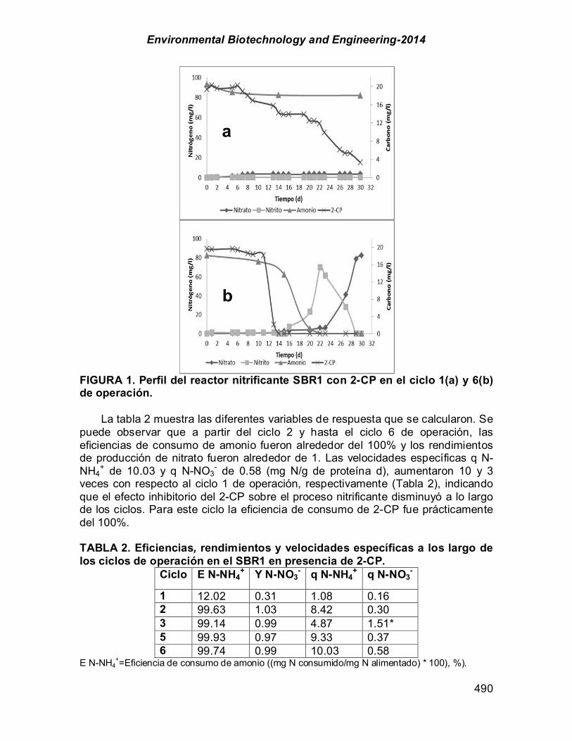
Environmental Biotechnology and Engineering-2014
490
FIGURA 1. Perfil del reactor nitrificante SBR1 con 2-CP en el ciclo 1(a) y 6(b) de operación.
La tabla 2 muestra las diferentes variables de respuesta que se calcularon. Se puede observar que a partir del ciclo 2 y hasta el ciclo 6 de operación, las eficiencias de consumo de amonio fueron alrededor del 100% y los rendimientos de producción de nitrato fueron alrededor de 1. Las velocidades específicas q N-NH4
+ de 10.03 y q N-NO3- de 0.58 (mg N/g de proteína d), aumentaron 10 y 3
veces con respecto al ciclo 1 de operación, respectivamente (Tabla 2), indicando que el efecto inhibitorio del 2-CP sobre el proceso nitrificante disminuyó a lo largo de los ciclos. Para este ciclo la eficiencia de consumo de 2-CP fue prácticamente del 100%.
TABLA 2. Eficiencias, rendimientos y velocidades específicas a los largo de los ciclos de operación en el SBR1 en presencia de 2-CP.
Ciclo E N-NH4+ Y N-NO3
- q N-NH4+ q N-NO3
-
1 12.02 0.31 1.08 0.16 2 99.63 1.03 8.42 0.30 3 99.14 0.99 4.87 1.51* 5 99.93 0.97 9.33 0.37 6 99.74 0.99 10.03 0.58
E N-NH4+=Eficiencia de consumo de amonio ((mg N consumido/mg N alimentado) * 100), %).
a
b
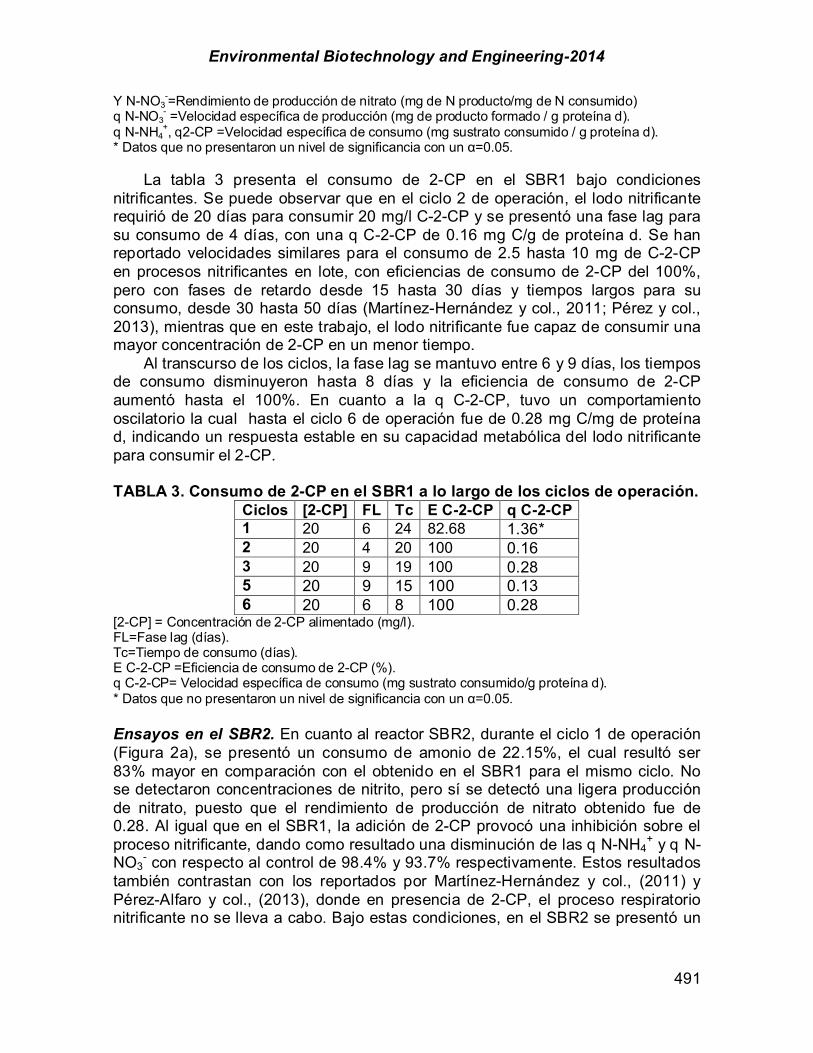
Environmental Biotechnology and Engineering-2014
491
Y N-NO3-=Rendimiento de producción de nitrato (mg de N producto/mg de N consumido)
q N-NO3- =Velocidad específica de producción (mg de producto formado / g proteína d).
q N-NH4+, q2-CP =Velocidad específica de consumo (mg sustrato consumido / g proteína d).
* Datos que no presentaron un nivel de significancia con un !=0.05.
La tabla 3 presenta el consumo de 2-CP en el SBR1 bajo condiciones nitrificantes. Se puede observar que en el ciclo 2 de operación, el lodo nitrificante requirió de 20 días para consumir 20 mg/l C-2-CP y se presentó una fase lag para su consumo de 4 días, con una q C-2-CP de 0.16 mg C/g de proteína d. Se han reportado velocidades similares para el consumo de 2.5 hasta 10 mg de C-2-CP en procesos nitrificantes en lote, con eficiencias de consumo de 2-CP del 100%, pero con fases de retardo desde 15 hasta 30 días y tiempos largos para su consumo, desde 30 hasta 50 días (Martínez-Hernández y col., 2011; Pérez y col., 2013), mientras que en este trabajo, el lodo nitrificante fue capaz de consumir una mayor concentración de 2-CP en un menor tiempo.
Al transcurso de los ciclos, la fase lag se mantuvo entre 6 y 9 días, los tiempos de consumo disminuyeron hasta 8 días y la eficiencia de consumo de 2-CP aumentó hasta el 100%. En cuanto a la q C-2-CP, tuvo un comportamiento oscilatorio la cual hasta el ciclo 6 de operación fue de 0.28 mg C/mg de proteína d, indicando un respuesta estable en su capacidad metabólica del lodo nitrificante para consumir el 2-CP. TABLA 3. Consumo de 2-CP en el SBR1 a lo largo de los ciclos de operación.
Ciclos [2-CP] FL Tc E C-2-CP q C-2-CP 1 20 6 24 82.68 1.36* 2 20 4 20 100 0.16 3 20 9 19 100 0.28 5 20 9 15 100 0.13 6 20 6 8 100 0.28
[2-CP] = Concentración de 2-CP alimentado (mg/l). FL=Fase lag (días). Tc=Tiempo de consumo (días). E C-2-CP =Eficiencia de consumo de 2-CP (%). q C-2-CP= Velocidad específica de consumo (mg sustrato consumido/g proteína d). * Datos que no presentaron un nivel de significancia con un !=0.05. Ensayos en el SBR2. En cuanto al reactor SBR2, durante el ciclo 1 de operación (Figura 2a), se presentó un consumo de amonio de 22.15%, el cual resultó ser 83% mayor en comparación con el obtenido en el SBR1 para el mismo ciclo. No se detectaron concentraciones de nitrito, pero sí se detectó una ligera producción de nitrato, puesto que el rendimiento de producción de nitrato obtenido fue de 0.28. Al igual que en el SBR1, la adición de 2-CP provocó una inhibición sobre el proceso nitrificante, dando como resultado una disminución de las q N-NH4
+ y q N-NO3
- con respecto al control de 98.4% y 93.7% respectivamente. Estos resultados también contrastan con los reportados por Martínez-Hernández y col., (2011) y Pérez-Alfaro y col., (2013), donde en presencia de 2-CP, el proceso respiratorio nitrificante no se lleva a cabo. Bajo estas condiciones, en el SBR2 se presentó un

Environmental Biotechnology and Engineering-2014
492
consumo de 2-CP de 42%, es decir, el lodo nitrificante fue capaz de consumir 9 mg C-2-CP/l en 23 días con una fase de retardo de 7 días.
La figura 2b muestra el perfil cinético durante la operación del ciclo 6 en el SBR2. Se observa un consumo total de amonio al final del ciclo de operación, dando como resultado una eficiencia de consumo de este compuesto del 100%. El amonio consumido se oxidó mayoritariamente a nitrito y una ligera producción de nitrato, presentando un rendimiento de nitrato de 0.23. Estos resultados indican que se presentó una nitrificación parcial.
FIGURA 2. Perfil del reactor nitrificante SBR2 con 2-CP en el ciclo 1(a) y 6(b) de operación.
De manera similar a los resultados obtenidos en el SBR1, las velocidades específicas q N-NH4
+ y q N-NO3- (9.28 y 0.21 mg N/g de proteína d), aumentaron 5
y 0.8 veces respectivamente con relación al ciclo 1 de operación (Tabla 4), indicando que el efecto inhibitorio del 2-CP sobre el proceso nitrificante disminuyó a lo largo de los ciclos. Para este ciclo la eficiencia de consumo de 2-CP en el SBR2 fue del 100%.
a
b

Environmental Biotechnology and Engineering-2014
493
Tabla 4. Eficiencias, rendimientos y velocidades específicas a los largo de los ciclos de operación en el SBR2 en presencia de 2-CP.
Ciclo E N-NH4+ Y N-NO3
- q N-NH4+ q N-NO3
-
1 22.15 0.28 1.82 0.18 2 14.04 0.28 1.28 0.075 3 50.26 0.22 2.70 0.34 5 99.79 0.43 10.02 1.06* 6 99.76 0.23 9.28 0.21
E N-NH4+=Eficiencia de consumo de amonio ((mg N consumido/mg N alimentado) * 100), %).
Y N-NO3-=Rendimiento de producción de nitrato (mg de N producto/mg de N consumido)
q N-NO3- =Velocidad específica de producción (mg de producto formado / g proteína d).
q N-NH4+, q2-CP =Velocidad específica de consumo (mg sustrato consumido / g proteína d).
* Datos que no presentaron un nivel de significancia con un !=0.05.
Con el lodo utilizado en el SBR2, que había estado previamente expuesto a p-cresol, había sido posible consumir hasta 50 mg/l de C-2-CP en ensayos nitrificantes en lote, con eficiencias de consumo de amonio de 16% (Silva y col., 2011). En este trabajo se obtuvieron eficiencias de consumo de amonio del 50% en presencia de 20 mg/l de C-2-CP, por lo cual es posible decir que se logró un mejor desempeño en la nitrificación.
De acuerdo a la tabla 5, en el SBR2, el consumo de 2-CP en el ciclo 1 de operación y en condiciones nitrificantes, fue de 8.4 mg/l C-2-CP después de 24 días y una fase lag de 6 días. Bajo estas condiciones se alcanzó una qC-2-CP de 0.05 mg C/g de proteína d.
Al transcurso de los ciclos, la fase lag se mantuvo entre 7 y 4 días, los tiempos de consumo del compuesto halogenado disminuyeron hasta 15 días y la eficiencia de consumo de 2-CP aumentó hasta el 100%. En cuanto a la qC-2-CP, esta aumentó hasta 4 veces en el ciclo 6 de operación (0.2 mg C/g de proteína d).
Beristain-Montiel y col. (2011), pudieron observar un incremento de hasta 5 veces en las velocidades específicas de consumo de 2-CP en un reactor SBR anaerobio (ASBR) y utilizando un lodo metanogénico previamente expuesto al 2-CP. Tabla 5. Consumo de 2-CP en el SBR2 a lo largo de los ciclos de operación.
Ciclos [2-CP] FL Tc EC-2-CP qC-2-CP 1 20 6 24 42.62 0.05 2 20 7 21 100 0.149 3 20 6 22 100 0.16 5 20 4 20 100 0.30 6 20 5 15 100 0.20
[2-CP] = Concentración de 2-CP alimentado (mg/l). FL=Fase lag (días). Tc=Tiempo de consumo (días). E C-2-CP =Eficiencia de consumo de 2-CP (%). Q C-2-CP= Velocidad específica de consumo (mg sustrato consumido/g proteína d).

Environmental Biotechnology and Engineering-2014
494
En este trabajo se encontró que en ambos reactores, al final del ciclo 6, se observó una disminución en el efecto inhibitorio del 2-CP sobre el proceso nitrificante. Estos resultados pueden estar asociados a la utilización de un lodo previamente expuesto a compuestos fenólicos y a la utilización de un reactor de tipo SBR. Sin embargo, con los lodos nitrificantes que estuvieron en contacto previo con el 2-CP, fue posible obtener un mejor desempeño en la nitrificación y en el consumo del compuesto aromático, en comparación con los lodos que estuvieron expuestos al p-cresol, puesto que el consumo de 2-CP, de amonio y su oxidación a nitrato, así como sus respectivas velocidades específicas, fueron mayores. Estos resultados sugieren que además del uso de un reactor SBR, la historia del lodo juega un papel determinante en los procesos respiratorios. Conclusión
La adición de 20 mg C-2-CP/l a los reactores SBR provocó un efecto inhibitorio sobre el proceso nitrificante, el cual disminuyó a lo largo de los ciclos. Después de 6 ciclos de operación, se obtuvo una eficiencia de consumo de amonio de 99.14% en el SBR1 y de 99.76% en el SBR2. Los Y fueron 0.99 y 0.23 para el SBR1 y SBR2 respectivamente. La E del 2-CP fue de 100% en ambos reactores. El uso de lodos previamente expuestos a compuestos fenólicos y la utilización de un SBR resultó en una disminución del efecto inhibitorio del 2-CP sobre el proceso nitrificante, consiguiéndose un mejor desempeño con los lodos previamente expuestos al 2-CP. Agradecimientos
Este trabajo fue apoyado por el Consejo Nacional de Ciencia y Tecnología de México (proyecto No. CONACYT-CB-2011-01-165174).
Referencias Beristain-Montiel L., Gómez-Hernández J., Monroy-Hermosillo O., Cuervo-López F. and Ramírez-
Vives F. (2010). Methanization and mineralization of 2-chlorophenol by anaerobic digestion. Water Science and technology. 62(8): 1791–1798.
Beristain-Montiel L., Gómez J., Monroy O., Cuervo-López F., Ramírez-Vives F., (2011). Biodegradation of 2-chlorophenol (2CP) in an anaerobic sequencing batch reactor (ASBR). Water Science and technology. 65(10): 1721–1728
Bock E; Koops HP, Harms H and Anhlers B, (1986) In nitrification. (L.I: Prosser ed.). Especial publications of the society for general microbiology. 20: 17-38
Breemen N.V. (2002). Nitrogen cycle: Natural organic tendency. Nature. 415: 381-382 Camargo J.A and Alonso A. (2007). Contaminación por nitrógeno inorgánico en los ecosistemas
acuáticos: problemas medio ambientales, criterios de calidad del agua, e implicaciones del cambio climático. Ecosistemas 16 (2): 98-110.
Gallego A., Molina Tirado L.B., Fortunato M.S., Bevilacqua S., Camardella H., Kabbas S., Cenzano M.L., Gómez C.E., D’Aquino M., Korol S. Higa L.E. (1998). Biodegradación de 2-clorofenol en reactores aeróbicos empleando microorganismos autóctonos. Asociación Peruana de Ingeniería Sanitaria y Ambiental; AIDIS. Gestión ambiental en el siglo XXI. Lima, APIS. pp.1-8.
Inui T., Tanaka Y., Okayasu Y. and Tanaka H. (2002). Application of toxicity monitor using nitrifying bacteria biosensor to sewerage systems. Water Science and technology. 45: 271-278.
Lens, P. and Kuenen, J. (2001). The biological sulfur cycle: novel opportunities for environmental biotechnology. Water Science and technology. 44(8): 57-66.
Environmental Biotechnology and Engineering-2014
495
Martinez-Hernandez S., Texier A-C., Cuervo-López F., Gomez J. (2011). 2-Chlorophenol and its effect on the nitrifying sludge, J. Hazard.Mater. 185: 1592–1595.
Pérez-Alfaro J. E., Buitrón G., Gomez J., Texier A-C. and Cuervo-López F. M. (2013). Kinetic and Physiological Evaluation of Ammonium and Nitrite Oxidation Processes in Presence of 2-Chlorophenol. Applied Biochemistry and Biotechnology. 169(3):990-1000.
Prosser, J.I. (1989) autrophic nitrification in bacteria. Adv. Microb. Physiol. 30.pp 125-181 Puhakka JA, Melin ES, Jarvinen KT (1995) Fluidized-bed biofilms for chlorophenol mineralization.
Water Science and technology. 31:227–235 Satoh H., Sasaki, Y., Nakamura Y., Okabe S., Suzuki T. (2005). Use of microelectrodes to
investigate the effects of 2-chlorophenol on microbial activities in biofilms. Wiley Interscience. 91: 133-137.
Silva C.D., Gómez J., Beristain-Cardoso R. (2011). Simultaneous removal of 2-chlorophenol, phenol, p-cresol and p-hydroxybenzaldehyde under nitrifying conditions: Kinetic study. Bioresource Technology. 102: 6464–6468
Schweighofer P., Nowak O., Svardal K. and Kroiss H. (1996). Steps towards the upgrading of a municipal WWTP affected by nitrification inhibiting compounds-A case study. Water Science and Technology. 33(12): 39-46.
Texier A-C. and Gomez J. (2007). Simultaneous nitrification and p-cresol oxidation in anitrifying sequencing batch reactor. Water research. 41: 315-322.
Texier Anne-Claire, Zepeda Alejandro, Gómez Jorge and Cuervo-López Flor (2012). Simultaneous Elimination of Carbon and Nitrogen Compounds of Petrochemical Effluents by Nitrification and Denitrification, Petrochemicals, DrVivek Patel (Ed.)
Notación 2-CP 2-clorofenol E eficiencia de consumo SBR reactor de lotes secuenciados Y rendimiento de producción q velocidad específica

Environmental Biotechnology and Engineering-2014
496
TYPE OF PRESENTATION RECOMMENDED BY THE SYMPOSIUM: Oral LIST OF COAUTHORS: Miguel Martínez-Jardines, Candidate, presenting author. Same address and e-mail as those of Dra. Flor Cuervo-López Dr. Anne-Claire Texier, Full Professor UAM- Iztapalapa, Dept. Biotechnology CBS, Microbial physiology, Av. San Rafael Atlixco 186, Col. Vicentina, Iztapalapa D.F., 09340, México. Tel.: 5804-4600 ext.2659 E-mail: [email protected], [email protected] M. in C. Emmanuel Pérez-Alfaro, UAM- Iztapalapa, Dept. Biotechnology CBS, Microbial physiology, Av. San Rafael Atlixco 186, Col. Vicentina, Iztapalapa D.F., 09340, México. Tel.: 5804-4600 ext.2848 E-mail: [email protected] Dr. Flor Cuervo-López, Full Professor. Author to whom all correspondence should be addresed UAM- Iztapalapa, Dept. Biotechnology CBS, Microbial physiology, Av. San Rafael Atlixco 186, Col. Vicentina, Iztapalapa D.F., 09340, México. Tel.: 5804-6408 E-mail: [email protected]

Environmental Biotechnology and Engineering-2014
497
CHAPTER 5.3 INDUCCIÓN DE EMBRIONES SOMÁTICOS EN Typha domingensis
Hernández-Piedra G (1); Ruiz-Carrera V*(1)
(1) Centro de Investigación para la Conservación y Aprovechamiento de Recursos Tropicales (CICART). Universidad Juárez Autónoma de Tabasco, Villahermosa, Tabasco. México. RESUMEN La producción de embriones somáticos como método de propagación para la macrófita acuática emergente Typha domingensis fue investigada con énfasis en la etapa de inducción. El experimento fue bifactorial aleatorizado (2 x 3) de plantas in vitro en cultivo por lote agitado. Los factores analizados fueron el ambiente de cultivo (luz y oscuridad) y las concentraciones de 2,4-D (0.5, 1.0 y 2.0 mg·L-1). El medio de cultivo fue 0.5MS líquido con 3% de sacarosa. La evolución de características celulares embriogénicas y no embriogénicas fue evaluada durante dos meses. La inducción embriogénica detonó en el ápice caulinar. Después de 3 a 4 semanas de cultivo, fueron formados los callos embriogénicos friables y nodulares no embriogénicos. Las células nodulares adquirieron cierto grado de competencia embriogénica con 2,4-D indiferente al ambiente de cultivo. Sin embargo, la mayor productividad de células embriogénicas se presentó en 0.5 y 1.0 mg·L-1 de 2,4-D (p > 0.05). El 50% de los tratamientos registraron embriones somáticos en la sexta semana. El embrión somático presentó suspensor unido al explante y protuberancia en el extremo distal. Los nódulos celulares embriogénicos y un tercio de los embriones somáticos mostraron oscurecimiento progresivo en el tiempo. El potencial de expresión y mapa de destino de embriones somáticos de Typha domingensis se presentan como avance biotecnológico para la repoblación sustentable de humedales ante los escenarios de cambio en la biodiversidad y los servicios ecosistémicos asociados. Palabras clave: micropropagación, macrófita, embrión somático, mapa destino.
Environmental Biotechnology and Engineering-2014
498
ABSTRACT The production of somatic embryos as a method of propagation for the emergent aquatic macrofita Typha domingensis was investigated with emphasis in the induction stage. The experiment was bivariate randomized (2 x 3) of in vitro plants in agitated batch culture. The factors analyzed were the environment of cultivation (light and dark) and concentrations of 2,4-D (0.5, 1.0 and 2.0 mg·L-1). The culture medium was 0.5MS liquid with 3% sucrose. The evolution of embryogenic and non-embryogenic cell characteristics was evaluated for two months. The embryogenic induction detonated at the caulinar apex. After 3-4 weeks of culture, calluses embryogenic friables and nodulares non-embryogenic were formed. The nodular cells acquired some degree of embryogenic competence with 2, 4-D indifferent to the culture environment. However, higher productivity of embryogenic cell was in 0.5 y 1.0 mg·L-1 of 2,4-D (p > 0.05). The 50% of treatments registered somatic embryos in the sixth week. The embryo somatic showed a suspensor attached to the explant and protuberance at the distal end. The embryogenic cell nodules and one-third of the somatic embryos showed progressive darkening over time. The potential for expression and map of destination of somatic embryos of Typha domingensis are presented as biotechnological advance for the sustainable repopulation of wetlands to the scenarios of change in biodiversity and associated ecosystem services. Key words: micropropagation, wetland plant, somatic embryo, destination map -------------- *Author por correspondencia: [email protected]

Environmental Biotechnology and Engineering-2014
499

Environmental Biotechnology and Engineering-2014
500
Introducción La espadaña (Typha domingensis) es una planta acuática emergente de
amplia distribución y elevada productividad en los ecosistemas limnéticos someros considerada maleza acuática. Además, enfrenta la amenaza de sobreexplotación por interés económico (Auld 1996), no obstante que la abundancia de esta vegetación constituye un componente clave para la sustentabilidad ambiental del ecosistema acuático (Zedler 2004; Lorenzen et al. 2000). Las malas prácticas de manejo, sumadas a los impactos del cambio climático, afectan la dinámica y el tamaño de las comunidades de esta vegetación acuática (Pachauri & Reisinger 2007; Auld 1996) y se pronostica que ambos afectarán negativamente en los servicios ambientales que brinda el ecosistema.
La amenaza de sobrexplotación del género Typha reside en su potencial como materia prima para biocombustible de tercera generación (Hernández-Piedra 2009; Suda et al. 2009; Czakó et al. 2006; Estime et al. 2003; Rogers 2003). También es usado con menor impacto en la construcción de humedales artificiales para remediar aguas eutrofizadas (Sheoran 2006; Paris et al. 2005; Hidalgo et al. 2005; Odjegba & Fasidi 2004; Vara Prasad & De Oliveira 2003; Estime et al. 2003; Rogers 2003), como especie de ornato, recurso alimenticio (Stevens & Hoag 2000; Arenas & Escarpa 2003). La vulnerabilidad potencial de T. domingensis requiere desarrollar investigación sobre su biología del desarrollo y para generar métodos de propagación modernos y eficientes que eviten la probable erradicación de esta especie por el manejo inadecuado del ecosistema acuático.
La embriogénesis somática es un sistema modelo clave para estudios embriológicos (Von Arnold 2008; Quiroz-Figueroa et al. 2006) y ofrece la oportunidad de desarrollar ciencia básica sobre la biología reproductiva de T. domingensis, ya que existe poco conocimiento al respecto. La técnica de embriogénesis somática permite producir plantas a pequeña escala y alta velocidad a través de la manipulación de los componentes químicos y físicos del sistema de cultivo. Las microestructuras vegetales regeneran mediante procesos de organogénesis y embriogénesis directa e indirecta.
La embriogénesis somática directa deriva de células predeterminadas embriogénicamente, mientras que la indirecta generalmente es de un callo (Von Arnold 2008). En la división, elongación, polaridad y diferenciación celular que conduce a la embriogénesis somática participan una amplia variedad de señales moleculares y ambientales. Las moleculares incluyen compuestos exógenos, como los reguladores de crecimiento y nutrientes, y compuestos extracelulares entre las que se han citado a los polisacáridos de pared celular y glicoproteínas (Von Arnold 2008; Quiroz-Figueroa et al. 2006; Fehér et al. 2003). La auxina 2,4-D ha sido el fitorregulador comúnmente empleado en las rutas embriogénicas directa o indirecta (Machakova et al. 2008; Jenik & Barton 2005). En Vallisneria americana (Álvarez 2007), Phragmites australis (Máthé et al. 2000), Brasenia schreberi (Oh et al. 2008) y T. domingensis usaron el 2,4-D en concentraciones de %1, & 4, % 3 y % 2 mg·L-1 para la inducción embriogénica directa. En Nymphoides cristatum (Niranjan et al. 2008), Typha latifolia (Rogers et al. 1998) y Picea abies (Filonova et al. 2000) se ha combinado el 2,4-D con otras fitohormonas como picloram, tiaduzuron y benziladenina. En muchos sistemas, el proceso de maduración del
Environmental Biotechnology and Engineering-2014
501
embrión somático procede en condiciones libres de auxina (Fehér 2008). En las especies como T. latifolia (Rogers et al. 1998), P. abies (Filonova et al. 2000), P. australis (Máthé et al. 2000), V. americana (Álvarez 2007), B. schreberi (Oh et al. 2008) y N. cristatum (Niranjan et al. 2008), la iluminación de los cultivos (presencia o ausencia) fue un factor en la inducción del embrión somático.
En esta investigación el interés fue describir el desarrollo morfológico de embriones de T. domingensis a través del proceso progresivo de embriogénesis somática con énfasis en la etapa de inducción, La descripción morfológica del proceso de embriogénesis somática es relevante para ampliar el conocimiento de la biología reproductiva de T. domingensis y puede mejorar las aplicaciones prácticas al conducir a una alternativa de propagación sustentable y de rehabilitación de ecosistemas limnéticos impactados.
Materiales y métodos Especie focal. Typha domingensis Pers. (Espadañal) es una herbácea perenne que forma parte de la vegetación acuática enraizada emergente distribuida a lo largo de todo el continente Americano (Novelo & Ramos 2007). En México está ampliamente distribuida en las regiones cálido húmedas por debajo de los 1000 m de altitud (Rzedowski & Rzedowski 2005). La planta presenta rizoma estolonífero, hojas simples lineares y tallos que emergen del agua a una altura máxima de 2.5 m. La inflorescencia terminal de color café claro en forma de espiga alargada y cilíndrica se sitúa sobre una bráctea linear. La espiga masculina hasta de 42 cm de largo y 1.5 cm de ancho se encuentra sobre la espiga femenina de 48 cm de largo y 2 cm de diámetro. Esta especie llega a producir 250 000 flores por inflorescencia. El fruto es seco, tipo aquenio, de aproximadamente 1.5 mm de largo, el cual contiene una semilla diminuta de endospermo farinoso (Stevens & Hoag 2000). El aquenio está cubierto de un folículo persistente denominado perianto.
Los aquenios de T. domingensis se recolectaron en el año 2008 en un microembalse artificial urbano de la ciudad de Villahermosa, Tabasco, México (17º 59´26” y 17º 59´17” N y 92º 58´16” y 92º58´37” O). Los aquenios permanecieron almacenados 18 meses en un desecador de sílica gel. Viabilidad de semillas. La viabilidad de las semillas se comprobó mediante ensayos de germinación in vitro en cultivo estático. El aquenio fue agitado en agua purificada (1:1 g/mL) cuatro ocasiones (Lorenzen et al. 2000). El perianto desprendido se separó del sobrenadante cada 20 min. Las semillas fueron preesterilizadas 10 min en 30% de etanol, esterilizadas 10 min en solución de NaClO (10% de Cloralex® v/v) y lavadas tres veces en agua estéril. Cada transferencia fue realizada con agitación manual. La germinación se realizó con 10 (± 1) semillas. La unidad de cultivo fueron frascos comerciales de vidrio (Ø 5 cm: h 7 cm) con 50 mL de agua purificada esterilizados con tapas de policarbonato (Magenta®) a 121 °C y 104 kPa durante 25 min. Las plantas regeneraron en cuartos de cultivo con temperatura ambiental de 25°C ± 5, luz blanca de 20 µmol de fotones m-2·s-1 y fotoperiodo de 16 hr luz. El porcentaje de germinación se estimó a nueve días [% G= (semilla germinadas/semillas totales) x 100] usando
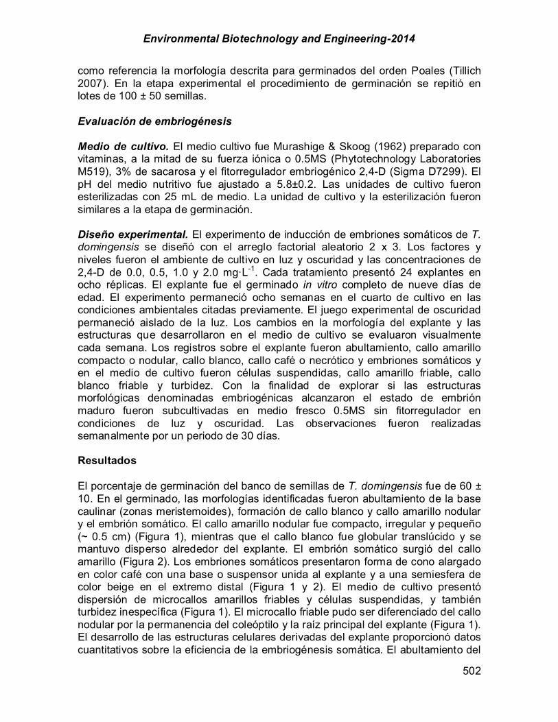
Environmental Biotechnology and Engineering-2014
502
como referencia la morfología descrita para germinados del orden Poales (Tillich 2007). En la etapa experimental el procedimiento de germinación se repitió en lotes de 100 ± 50 semillas. Evaluación de embriogénesis Medio de cultivo. El medio cultivo fue Murashige & Skoog (1962) preparado con vitaminas, a la mitad de su fuerza iónica o 0.5MS (Phytotechnology Laboratories M519), 3% de sacarosa y el fitorregulador embriogénico 2,4-D (Sigma D7299). El pH del medio nutritivo fue ajustado a 5.8±0.2. Las unidades de cultivo fueron esterilizadas con 25 mL de medio. La unidad de cultivo y la esterilización fueron similares a la etapa de germinación. Diseño experimental. El experimento de inducción de embriones somáticos de T. domingensis se diseñó con el arreglo factorial aleatorio 2 x 3. Los factores y niveles fueron el ambiente de cultivo en luz y oscuridad y las concentraciones de 2,4-D de 0.0, 0.5, 1.0 y 2.0 mg·L-1. Cada tratamiento presentó 24 explantes en ocho réplicas. El explante fue el germinado in vitro completo de nueve días de edad. El experimento permaneció ocho semanas en el cuarto de cultivo en las condiciones ambientales citadas previamente. El juego experimental de oscuridad permaneció aislado de la luz. Los cambios en la morfología del explante y las estructuras que desarrollaron en el medio de cultivo se evaluaron visualmente cada semana. Los registros sobre el explante fueron abultamiento, callo amarillo compacto o nodular, callo blanco, callo café o necrótico y embriones somáticos y en el medio de cultivo fueron células suspendidas, callo amarillo friable, callo blanco friable y turbidez. Con la finalidad de explorar si las estructuras morfológicas denominadas embriogénicas alcanzaron el estado de embrión maduro fueron subcultivadas en medio fresco 0.5MS sin fitorregulador en condiciones de luz y oscuridad. Las observaciones fueron realizadas semanalmente por un periodo de 30 días. Resultados El porcentaje de germinación del banco de semillas de T. domingensis fue de 60 ± 10. En el germinado, las morfologías identificadas fueron abultamiento de la base caulinar (zonas meristemoides), formación de callo blanco y callo amarillo nodular y el embrión somático. El callo amarillo nodular fue compacto, irregular y pequeño (~ 0.5 cm) (Figura 1), mientras que el callo blanco fue globular translúcido y se mantuvo disperso alrededor del explante. El embrión somático surgió del callo amarillo (Figura 2). Los embriones somáticos presentaron forma de cono alargado en color café con una base o suspensor unida al explante y a una semiesfera de color beige en el extremo distal (Figura 1 y 2). El medio de cultivo presentó dispersión de microcallos amarillos friables y células suspendidas, y también turbidez inespecífica (Figura 1). El microcallo friable pudo ser diferenciado del callo nodular por la permanencia del coleóptilo y la raíz principal del explante (Figura 1). El desarrollo de las estructuras celulares derivadas del explante proporcionó datos cuantitativos sobre la eficiencia de la embriogénesis somática. El abultamiento del

Environmental Biotechnology and Engineering-2014
503
explante se observó a los 14 días, pero el porcentaje más alto fue registrado a 21 días en los cultivos expuestos a 2,4-D en 0.5 y 2.0 mg·L-1, en luz y oscuridad. Los callos amarillo y blanco desarrollaron sobre el abultamiento a los 21 y 28 días, respectivamente. Los porcentajes de cultivos con callo blanco fueron relativamente muy bajos respecto a los de callo amarillo. El callo amarillo nodular presentó elevado porcentaje en 0.5 y 1.0 mg·L-1 de 2,4-D y máximo incremento entre los 44 y 58 días. El mayor porcentaje de callo blanco se registró en 2.0 mg L-1 de 2,4-D en ambos ambientes y el nivel de producción no varío desde los 28 días.
Figura 1 Morfologías celulares generadas en Typha domingensis. En la base caulinar del explante (a) (b) (c) (d) y suspendidas en el medio de cultivo (e) (f) y (g). Callo amarillo nodular (a), callo amarillo nodular con necrosis moderada (b),
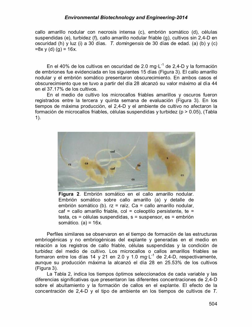
Environmental Biotechnology and Engineering-2014
504
callo amarillo nodular con necrosis intensa (c), embrión somático (d), células suspendidas (e), turbidez (f), callo amarillo nodular friable (g), cultivos sin 2,4-D en oscuridad (h) y luz (i) a 30 días. T. domingensis de 30 días de edad. (a) (b) y (c) =8x y (d) (g) = 16x.
En el 40% de los cultivos en oscuridad de 2.0 mg·L-1 de 2,4-D y la formación de embriones fue evidenciada en los siguientes 15 días (Figura 3). El callo amarillo nodular y el embrión somático presentaron obscurecimiento. En ambos casos el obscurecimiento que se tuvo a partir del día 28 alcanzó su valor máximo al día 44 en el 37.17% de los cultivos.
En el medio de cultivo los microcallos friables amarillos y oscuros fueron registrados entre la tercera y quinta semana de evaluación (Figura 3). En los tiempos de máxima producción, el 2,4-D y el ambiente de cultivo no afectaron la formación de microcallos friables, células suspendidas y turbidez (p > 0.05), (Tabla 1).
Figura 2. Embrión somático en el callo amarillo nodular. Embrión somático sobre callo amarillo (a) y detalle de embrión somático (b). rz = raíz. Ca = callo amarillo nodular, caf = callo amarillo friable, col = coleoptilo persistente, te = testa, cs = células suspendidas, s = suspensor, es = embrión somático. (a) = 16x.
Perfiles similares se observaron en el tiempo de formación de las estructuras
embriogénicas y no embriogénicas del explante y generadas en el medio en relación a los registros de callo friable, células suspendidas y la condición de turbidez del medio de cultivo. Los microcallos o callos amarillos friables se formaron entre los días 14 y 21 en 2.0 y 1.0 mg·L-1 de 2,4-D, respectivamente, aunque su producción máxima la alcanzó el día 28 en 25.53% de los cultivos (Figura 3).
La Tabla 2, indica los tiempos óptimos seleccionados de cada variable y las diferencias significativas que presentaron las diferentes concentraciones de 2,4-D sobre el abultamiento y la formación de callos en el explante. El efecto de la concentración de 2,4-D y el tipo de ambiente en los tiempos de cultivos de T.

Environmental Biotechnology and Engineering-2014
505
domingensis con máximos porcentajes de respuestas in vitro sobre el explante y en el medio de cultivo fue significativo con 2,4-D y se presentó en las variables de abultamiento y callo amarillo sobre el explante (p 0.05). El abultamiento de la base caulinar fue superior en la concentración 0.5 mg·L-1 respecto a los cultivos que presentaron 2.0 mg·L-1 y fue similar a 1.0 mg·L-1. En las concentraciones de 0.5 y 1.0 mg L-1 de 2,4-D fue también superior el porcentaje de cultivos con callo amarillo. El embrión somático no registró diferencias significativas en las concentraciones de 2,4-D y condiciones de cultivo ensayadas (p > 0.05).
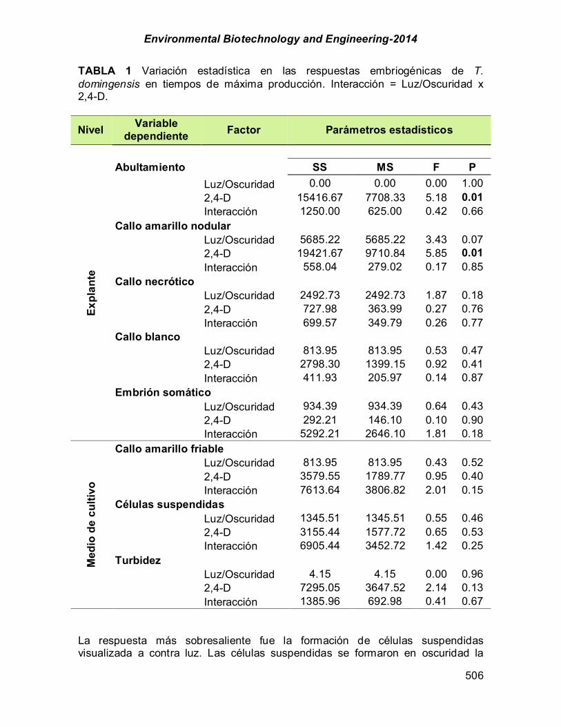
Environmental Biotechnology and Engineering-2014
506
TABLA 1 Variación estadística en las respuestas embriogénicas de T. domingensis en tiempos de máxima producción. Interacción = Luz/Oscuridad x 2,4-D.
Nivel Variable dependiente Factor Parámetros estadísticos
Expl
ante
Abultamiento SS MS F P Luz/Oscuridad 0.00 0.00 0.00 1.00 2,4-D 15416.67 7708.33 5.18 0.01 Interacción 1250.00 625.00 0.42 0.66
Callo amarillo nodular Luz/Oscuridad 5685.22 5685.22 3.43 0.07 2,4-D 19421.67 9710.84 5.85 0.01 Interacción 558.04 279.02 0.17 0.85
Callo necrótico Luz/Oscuridad 2492.73 2492.73 1.87 0.18 2,4-D 727.98 363.99 0.27 0.76 Interacción 699.57 349.79 0.26 0.77
Callo blanco Luz/Oscuridad 813.95 813.95 0.53 0.47 2,4-D 2798.30 1399.15 0.92 0.41 Interacción 411.93 205.97 0.14 0.87
Embrión somático Luz/Oscuridad 934.39 934.39 0.64 0.43 2,4-D 292.21 146.10 0.10 0.90 Interacción 5292.21 2646.10 1.81 0.18
Med
io d
e cu
ltivo
Callo amarillo friable Luz/Oscuridad 813.95 813.95 0.43 0.52 2,4-D 3579.55 1789.77 0.95 0.40 Interacción 7613.64 3806.82 2.01 0.15
Células suspendidas Luz/Oscuridad 1345.51 1345.51 0.55 0.46 2,4-D 3155.44 1577.72 0.65 0.53 Interacción 6905.44 3452.72 1.42 0.25
Turbidez Luz/Oscuridad 4.15 4.15 0.00 0.96 2,4-D 7295.05 3647.52 2.14 0.13 Interacción 1385.96 692.98 0.41 0.67
La respuesta más sobresaliente fue la formación de células suspendidas visualizada a contra luz. Las células suspendidas se formaron en oscuridad la

Environmental Biotechnology and Engineering-2014
507
primera semana en 2.0 mg·L-1 de 2,4-D y con luz en la segunda en las concentraciones de 1.0 y 2.0 mg·L-1 de 2,4-D. Los cultivos con células suspendidas presentaron promedio mayor de 80 % en luz y 0.5 mg·L-1 de 2,4-D, entre los días 51 y 58 (Figura 1).

Environmental Biotechnology and Engineering-2014
508
TABLA 2 Porcentajes de cultivos con estructuras embriogénicas adheridas al explante y suspendidas.
0.5 1.0 2.0Abultamiento 21 100a 81.85ab 56.25b
Callo blanco 28 6.66 18.75 25.00Callo amarillo nodular 44 86.66a 87.50a 43.75b
Callo necrótico 44 36.66 40.62 56.25Embrion somático 51 13.33 18.75 56.25Friabilidad 58 13.33 31.25 31.25Turbidez 28 6.66 18.75 37.5Células suspendidas 58 66.66 68.75 50.00
Variable dependiente 2,4-D (mg L-1)
Explante
Medio de
cultivo
Nivel Tmax
Promedios con literales iguales no fueron significativamente diferentes (p 0.05). Tmax= Tiempo de máxima producción en días.
FIGURA 3. Mapa destino que ilustra los cambios en la morfología in vitro de los germinados deTypha domingensis durante 56 días de cultivo en luz y obscuridad en el gradiente de 2,4-D estudiado (Etapa de inducción).

Environmental Biotechnology and Engineering-2014
509
El medio de cultivo presentó un aspecto blanquecino (Figura 1) o turbidez. La turbidez del medio de cultivo se registró a partir del séptimo día en el tratamiento de 2.0 mg·L-1 de 2,4-D en un ambiente con luz y hasta los 28 días en el tratamiento 1.0 mg·L-1 de 2,4-D en ausencia de luz. El aumento de números de cultivos con turbidez se mantuvo asociado al incremento de la concentración del 2,4-D. En la etapa de maduración, el necrosamiento del callo amarillo nodular, microcallo y el embrión somático persistió y sin haber reportado diferencias respecto a la de inducción embriogénica (Figura 3). Discusión
En el germinado y el medio de cultivo de T. domingensis se revelaron estructuras celulares ampliamente descritas por la literatura como precursoras del embrión somático (Quiroz-Figueroa et al. 2006; Fehér et al. 2003). La zona de abultamiento sobre la conexión hoja-raíz que en el germinado de T. domingensis corresponde a la sección del hipocótilo y la funda cotiledonar fue la señal primaria del efecto embriogénico del 2,4-D. Otras plantas acuáticas como T. latifolia, Cymodosea nodosa y V. americana (Álvarez 2007; Pérez et al. 2007; Rogers 2003; Rogers et al.1998) han reportado respuestas similares referente al sitio de acción para este tipo de explante. El abultamiento ha sido descrito como una etapa previa a la formación de callo debido a que el sitio presenta características fisiológicas y anatómicas que influyen en el desarrollo de la planta. Desde el punto de vista estructural el hipocótilo y el hipérfilo cotiledonar pertenecen a un complejo órgano de almacenamiento del embrión, el cotiledón (Tillich 2007); ambos rodean la zona meristemática perteneciente al brote apical del germinado que es la fuente de auxina endógena (Fehér et al. 2003), de esta zona derivó el callo amarillo nodular.
El callo de T. domingenesis fue similar a las descripciones morfológicas y de coloración descritas en germinados de las plantas acuáticas T. latifolia, T. angustifolia (Nandakumar et al. 2005; Rogers 2003; Rogers et al. 1998), V. americana (Álvarez 2007) y C. nodosa (Pérez et al. 2007), embriones cigótico de Oryza sativa (Menesses et al. 2005; Mariani et al. 2002) e inflorescencias de P. australis (Lauzer et al. 2000) y Panicum virgatum (Burris et al. 2009). La coloración amarilla del callo en T. domingensis indicó su condición embriogénica, pero la evidencia fue concluyente cuando del callo amarillo se originaron embriones somáticos.
Los callos de T. domingensis presentaron necrosis moderada a severa al finalizar el experimento de inducción embriogénica, sin embargo la mayoría de los callos registraron carácter embriogénico. El necrosamiento progresivo de las estructuras celulares embriogénicas fue adjudicado al estrés oxidativo que provocó el envejecimiento del cultivo (Benson 2000). No obstante varios autores han notificado que el tejido café o necrótico no es necesariamente perjudicial en la morfogénesis, inclusive se ha observado la formación de embriones somático alrededor de las áreas necrosadas, señalando que esta característica puede ser esencial para la iniciación de la embriogénesis (George & Davies 2008). En plantas terrestres como Coffea arabica el callo embriogénico se ha reportado café (fenolizado) (Quiroz-Figueroa et al. 2006) mientras que en Tehobroma cacao esta

Environmental Biotechnology and Engineering-2014
510
característica inhibe la embriogénesis considerándose una especie recalcitrante (Alemanno et al. 2003).
El callo blanco y los microcallos suspendidos de T. domingensis no presentaron potencial embriogénico u organogénico. En P. australis el callo blanco se ha reportado como no embriogénico y se caracterizó por su superficie viscosa (Lauzer et al. 2000), pero en otros como P. virgatum este tipo de callo, denominado tipo II, fue ideal para iniciar cultivos de suspensiones celulares al ser altamente friables, de rápido crecimiento y sumamente regenerativo (Burris et al. 2009). En N. cristatum los dos tipos de callos blanco y amarillo formaron embriones somáticos, solo que en el callo blanco se produjeron tardíamente y después de varios subcultivos (Niranjan et al. 2008). En T. domingensis no se descartó la posibilidad que el callo blanco evolucione a la condición embriogénica en otras condiciones experimentales.
La morfogénesis de los embriones somáticos de T. domingensis fue similar a la reportada en otras plantas acuáticas emergentes como Oryza sativa (Vega et al. 2009; Menesses et al. 2005; Mariani et al. 2002), T. latifolia (Rogers 2003), P. communis (Yang et al. 2003), P. australis (Máthé et al. 2000) y especies terrestre P. abies (Filonova et al. 2000), Cocus nucifera (Azpeitia et al. 2009), Phoenix dactilifera (Sané et al. 2006). Lo anterior, porque la morfogénesis de embriones somáticos puede ocurrir por diferentes vías de desarrollo (Von Arnold 2008; Quiroz-Figueroa et al. 2006). La embriogénesis somática no es del todo clara, la hipótesis señala que la vía de desarrollo directa se obtiene de células embriogénicamente predeterminadas mientras que la vía indirecta surge a partir de células indiferenciadas generalmente de un callo (Von Arnold 2008). Los germinados de T. domingensis desarrollaron el callo y de este derivó el embrión somático. Al parecer esta vía ha sido la más recurrente en otras monocotiledóneas como O. sativa, T. domingensis, P. australis y C. nuciferas (Vega et al. 2009; Rogers 2003; Máthé et al. 2000; Azpeitia et al. 2009). Aunque la embriogénesis somática directa se ha observado en el embrión cigótico de Oryza sativa (Mariani et al. 2002) y Daucus carota (Nishiwaki et al. 2000).
Otra vía de la embriogénesis somática corresponde a su origen unicelular o multicelular. La última se origina a partir de agregados de células simétricas o asimétricas denominados masas proembriogénicas, solamente diferenciadas por la presencia del suspensor cuando proviene de una sola célula (Quiroz-Figueroa et al. 2006). La formación del suspensor se ha relacionado con la definición del embrión somático y ha sido la estructura clave para dictaminar no solo el origen del embrión sino su estado de desarrollo (Vega 2009). En el caso de T. domingensis el suspensor fue identificado, aunque para para confirmar que la vía unicelular fue expresada son necesarios estudios histológicos.
La producción de callo embriogénico y algunas fases tempranas de formación del embrión somático en la especie T. domingensis fueron favorecidas por las tres concentraciones de 2,4-D ensayadas, en ausencia y presencia de luz. Aunque el 2,4-D fue el único factor que influyó en la formación del callo embriogénico en T. domingensis.
Dentro del género Typha, las especies T. latifolia y T. domingensis han sido más investigadas con fines de propagación y transformación genética. La inducción en medio de cultivo semisólido es común en los protocolos de inducción
Environmental Biotechnology and Engineering-2014
511
embriogénica. Rogers et al. (1998) y Nandakumar et al. (2005) produjeron callo organogénico en 5.0 mg·L-1 de 2,4-D a los 8 y 25 días en germinados de T. latifolia, mientras que Czakó et al. (2006) reportó la inducción de callo organogénico y embriogénico en las inflorescencias en concentración de auxina diez veces menor. El último caso fue similar a T. domingensis, ya que la callogénesis se registró en concentraciones bajas de auxina. Lauzer et al. (2000) obtuvo callogénesis en P. australis en 1.0, 2.0 y 4.0 mg·L-1 de 2, 4-D a partir de inflorescencias inmaduras, no obstante la producción óptima de callo embriogénico requirió el doble de la concentración de 2,4-D y fue tres veces menor respecto a los resultados obtenidos en los germinados de esta especie en cultivo líquido agitado.
El callo embriogénico inducido en los germinados de T. domingensis fue en morfología equiparable a las estructuras descritas en varias especies. Similar a las especies de P. australis, O. sativa, P. virgatum y C. nucifera en la superficie del callo amarillo fue distinguido el embrión somático (Burris et al. 2009; Vega et al. 2009; Menneses et al. 2005; Azpeitia et al. 2003; Lauzer et al. 2000). En el embrión somátcico de T. domingensis fue visible la masa embrional y el suspensor y estas se han descrito en el embrión somático temprano de la gimnosperma P. abies (Von Arnold 2008). En la monocotiledónea O. sativa la estructura tipo suspensor fue distinguida en el embrión somático en fase de elongación (Vega 2009). En las gimnospermas la embriogénesis temprana incluye las fases posteriores cuando el suspensor comienza a enlongar hasta el establecimiento de la radícula, mientras que en angiospermas son etapas de transición a la fase cotiledonar que es la estructura temporal en el desarrollo al promover el continuo crecimiento del propio embrión (Von Arnold 2008). Tanto en P. abies como en O. sativa esta diferenciación se ha registrado en un medio libre de auxina y en algunos casos en concentración baja de 2,4-D. El tiempo entre la aparición del embrión somático y fases sucesivas de desarrollo es corto (Vega et al. 2009; Von Arnold 2008; Mariani et al. 2002). En T. domingensis la aparición del embrión somático sucedió mas tarde en presencia de 2,4-D.
Aunque la presencia de callo blanco fue relativamente baja en T. domingensis, se observó una tendencia correlativa entre los porcentajes de callo blanco, friabilidad y turbidez. En P. virgatum (Burris et al. 2009) estas estructuras callosas fueron descritas como translúcidas y suaves figurando en forma de callo sumamente quebradizo o friable que ha sido denominado tipo II o ideal para iniciar suspensiones celulares.
La división, elongación, polaridad y diferenciación celular son respuestas desencadenadas por una variedad de señales no solo hormonales sino también ambientales, como la luz. Sin embargo, la inducción por luz no ha sido determinante en la expresión embriogénica de diferentes explantes. En las especie acuáticas O. sativa (Mariani et al. 2002; Nandakumar et al. 2005), T. latifolia (Rogers et al. 1998), P. virgatum (Burris et al. 2009), B. schreberi (Oh et al. 2008) y la terrestre P. abies (Filonova et al. 2000) la condición de oscuridad produjo callo embriogénico, mientras que en N. cristatum (Niranjan et al. 2008) y P. australis (Máthé et al. 2000) la luz indujo la respuesta embriogénica. En particular, T. domingensis produjo todas sus estructuras embriogénicas en luz y oscuridad. El tamaño, color, forma y otras características visuales de los callos y
Environmental Biotechnology and Engineering-2014
512
embriones somáticos de T. domingensis permitieron establecer el mapa destino de la vía embriogénica. Conclusión El conjunto de los resultados en el cultivo de lote agitado proporcionó la técnica en la etapa de inducción del callo embriogénico en germinados de T. domingensis En especial informó sobre la selección de la concentración de 2,4-D óptima para iniciar el protocolo de embriogénesis somática y mejorar las etapas de expresión y maduración del embrión. El estímulo o inhibición de la luz puede ser determinante para guiar el proceso de embriogénesis hacia la expresión del embrión somático maduro, pero son necesarios estudios histoquímicos y metabólicos que lo confirmen. Referencias Alemanno, L.; Ramos, T.; Gargadenec, A.; Andary, C.; Michaux-Ferriere, N. (2003). Localization
and identification of phenolic compounds in Theobroma cacao L. somatic embryogenesis. Annals of Botany 92: 613-623.
Álvarez, A. (2007). Inducción directa de embriones somáticos en la especie sumergida Vallisneria americana. Tesis de Licenciatura en Biología. Universidad Juárez Autónoma de Tabasco.
Arenas, P.; Scarpa, F.G. (2003). The consumption of Typha domingensis Pers. (Typhaceae) polen among the ethnic groups of the Gran Chaco, South. America. Economic Botany. 57(2): 181-188.
Auld, B.A. (1996). Criterios económicos para el desarrollo del manejo de malezas. En: Labrada, R.; Caseley, J.C.; Parker, C. (Eds). Manejo de malezas para países en desarrollo. Producción y Protección Vegetal 120. Roma: FAO.
Azpeitia, M.A.; Sáenz, C.L.; Chan, J.; Oropeza, S.C. (2003). Inducción de embriones somático en explantes de plúmula de cocotero por ácido abscísico y polietilenglicol. Revista Fitotecnia Mexicana. 26(4): 309-318.
Azpeitia, M.A.; Chan ,J.; Sáenz, C.L.; Oropeza, S.C. (2009). Influencia de la subdivisión del callo embriogénico en la formación de embriones somáticos de cocotero. Agricultura Técnica en México. 35(1): 39-48.
Benson, E.E. (2000). Special symposium: In vitro plant recalcitrance do free radicals have a role in plant tissue culture recalcitrance?. Vitro Cellular & Developmental Biology. 36 (3):163-170.
Burris, J.N.; Mann, D.G.J.; Joyce, B.L.; Stewart, Jr. C.N. (2009). An improved tissue culture system for embryogenic callus production and plant regeneration in switchgrass. Bioenergy Research. 2:267-274.
Czakó, M.; Feng, X.; He, Y.; Gollapudi, S.; Márton, L. (2006) In vitro propagation of wetland monocots for phytoremediation. In: Mackova, M.; Dowling, D.N.; Macek, T. (Eds). Phytoremediation and rhizoremediation: Theoretical background. pp. 217-225, Netherlands: Springer.
Estime, L.; O´Shea, M.; Borst, M.; Gerrity, J.; Liao, S. (2003). Effect of phosphorus concentration on the growth of cattail callus cells. Journal of Plant Nutrition. 26(3):691-707.
Fehér, A.; Pasternak, T.P.; Dudits, D. (2003). Transition of somatic plant cells to an embryogenic state. Plant cell, Tissue and Organ Culture. 74:201-228.
Fehér, A. (2008). The initiation phase of somatic embryogenesis: what we know and what we don’t. Acta Biologica Szegediensis. 52(1):53-56.
Filonova, L.H.; Bozhkov, P.V.; Von Arnold, S. (2000). Developmental pathway of somatic embryogenesis in Picea abies as revealed by time-lapse tracking. Journal of experimental Botany. 51(343): 249-264.
Environmental Biotechnology and Engineering-2014
513
George, E.F.; Davies, W. (2008). Effects of the physical environment. In: George, E.F.; Hall, M.A.; Klerk, G.J.D. (Eds). Plant Propagation by Tissue Culture. pp. 423-465, Netherlands: Springer.
Hernández-Piedra G. 2009. Plantas acuáticas emergentes como fuente de biocombustibles. Tesis de licenciatura en Biología. Universidad Juárez Autónoma de Tabasco.
Hidalgo, J.C.; Junod, J.M.; Sandoval, M.E. (2005). Recientes aplicaciones de la depuración de aguas residuales con plantas acuáticas. Theoría. 14 (3): 209-222.
Jenik, P.D.; Barton, M.K. (2005). Surge and destroy: the role of auxin in plant embryogenesis. Development. 132 (16).
Lauzer, D.; Dallaire, S.; Vincent, G. (2000). In vitro propagation of reed grass by somatic embryogenesis. Plant Cell, Tissue and Organ Culture. 60: 229-234.
Lorenzen, B.; Brix, H.; Mc Kee, K.L.; Mendelssohn, I.A.; Miao, S. (2000). Seed germination of two everglades species, Cladium jamaincense and Typha domingensis. Aquatic Botany. 66: 169-180.
Machakova, I.; Zazimalova, E.; George, E.F. (2008). Plant Growth regulators I: Introduction auxins their analogues and inhibitors. In: George, E.F.; Hall, M.A.; Klerk, G.J.D. (Eds). Plant Propagation by Tissue Culture. Netherlands: Springer. p. 175-204.
Mariani, T.S.; Miyake, H.; Takeoka, Y. (2002). Direct somatic embryogenesis in rice (Oryza sativa L.) structural and developmental patterns. Journal Matematika dan Sains. 7 (2):53-56.
Máthé, C.; Hamvas, M.M.; Grigorszky, I.; Vasas, G.; Molnár, E.; Power, B.; Davey, M.R.; Borbély, G. (2000). Plant regeneration from embryogenic cultures of Phragmites australis (Cav.) Trin. Ex steud. Plant cell, Tissue and organ culture. 63: 81-84.
Murashige, T.; Skoog, F.; (1962). A revised medium for rapid growth and bioassay with tobacco tissue culture. Physiologia Plantarum. 15: 473-479.
Nandakumar, R.; Chen, L.; Rogers, S.M.D. (2005). Agrobacterium-mediated transformation of the wetland monocot Typha latifolia L. (Broadleaf cattail). Plant Cell Reports. 23:744–750.
Niranjan, M.H.; Sudarshana, S.; Girisha, T. (2008). Direct somatic embryogenesis and plant regeneration from leaf explants of Nymphoides cristatum: A medicinally important plant. Global Journal of Biotechnology & Biochemistry. 3 (2): 79-82.
Nishiwaki, M.; Fujino, K.; Koda, Y.; Masuda, K.; Kikuta, Y. (2000). Somatic embryogenesis induced by the simple application of abscisic acid to carrot (Daucus carota L.) seedlings in culture. Planta. 211:756-759.
Novelo, A.; Ramos, L. (2007). Vegetación acuática. En: Bueno, J.; Álvarez, F.; Santiago, S. (Eds). Biodiversidad del estado de Tabasco. pp.111-135, México: UNAM-CONABIO.
Odjegba, V.J.; Fasidi, I.O. (2004). Accumulation of trace elements by Pistia stratiotes: implications for phytoremediation. Ecotoxicology. 13(7):637-646.
Oh, M.J.; Kim, S.W.; Liu, I.R.; Na, H.R.; Choi, H.K. (2008). High frequency plant regeneration from zygotic-embryo-derived embryogenic cell suspension cultures of watershield (Brasenia schreberi). Plant Biotechnology. 2:87-92
Pachauri, R.K.; Reisinger, A. (2007). Cambio climático 2007: Informe de síntesis. Contribución de los Grupos de trabajo I, II y III al cuarto informe de evaluación del Grupo Intergubernamental de Expertos sobre el Cambio climático. Ginebra: IPCC.
Paris, C.; Hadad, H.; Maine, M.A.; Suñe, N. (2005). Eficiencia de dos macrófitas flotantes libres en la absorción de metales pesados. Limnetica. 24(3-4): 237-244.
Pérez, E.N.; García, P.J.; Robaina, R.R. (2007). Propagación in vitro de Cymodosea nodosa para su utilización en la restauración de sebadales. Vector Plus. 74-81.
Quiroz-Figueroa, F.; Rojas-Herrera, R.; Galaz-Avalos, R.; Loyola-Vargas, V. (2006). Embryo production through somatic embryogenesis can be used to study cell differentiation in plants. Plant Cell, Tissue and Organ Culture. 86:285-30
Rogers, S.D.; Beech, J.; Sarma, K.S. (1998). Shoot regeneration and plant acclimatization of the wetland monocot cattail (Typha latifolia). Plant Cell Reports. 18: 71-75.
Rogers, S.M.D. (2003). Tissue culture and wetland establishment of the freshwater monocots Carex, Juncus, Scirpus, and Typha. In Vitro Cellular & Developmental Biology-Plant. 39(1): 1-5.
Rzedowski, G.C.; Rzedowski, J. (2005). Flora fanerogámica del Valle de México. México: Instituto de Ecología, A.C. y Comisión Nacional para el Conocimiento y Uso de la Biodiversidad.
Environmental Biotechnology and Engineering-2014
514
Sané, D.; Aberlenc-Bertossi, F.; Gassama-Dia, Y.K.; Sagna, M.; Trouslot, M.F.; Duval, Y.; Borgel, A. (2006). Histocytological analysis of callogénesis and somatic embryogenesis from cell suspensions of date palm (Phoenix dactylifera). Annals of Botany. 98:301-308.
Sheoran, A.S. (2006). A laboratory treatment study of acid mine water of wetlands with emergent macrophyte (Typha angustata). International Journal of Mining, Reclamation and Environment. 14 (1):209-222.
Stevens, M.; Hoag, C. (2000). Southern cattail, Typha domingensis Pers. Guide plant. USDA, NRCS
Suda, K.; Shahbazi, A.; Li, Y. (2009). The feasibility of using cattails from constructed wetlands to produce bioethanol. In Nzewi, E.; Reddy, G.; Luster-Teasly, S.; Kabadi, V.; Chang, S.; Schimmel, K.; Uzochukuwu, G. Proceedings of the 2007 National Conference on Environmental Science and Technology. p.9-15, New York: Springer.
Tillich, H. (2007). Seedling diversity and the homologies of seedling organs in the order Poales (Monocotyledons). Annals of Botany. 1:1-17.
Vara Prasad, M.N.; De Oliveira, F.H. (2003). Metal hyperaccumulation in plants: Biodiversity prospecting for phytoremediation technology. Electron Journal of Biotechnology. 6(3): 285-321.
Vega, R.; Vásquez, N.; Espinoza, A.M.; Gatica, A.M.; Valdez-Melara, M. (2009). Histology of somatic embryogenesis in rice (Oryza sativa). Revista Biología Tropical. 57(1):141-150.
Von Arnold, S. (2008). Somatic embryogenesis. In: George, E.F.; Hall, M.A.; Klerk, G.J.D. (Eds). Plant Propagation by Tissue Culture. p. 335-354, Netherlands: Springer.
Yang, Y.; Guo, Y.; Guo, Z.; Lin, J. (2003). Regeneration and large-scale propagation of Phragmites communis through somatic embryogenesis. Plant Cell, Tissue and Organ Culture. 75: 287-290.
Zedler, J.B.; Kercher, S. (2004). Causes and consequences of invasive plants in wetlands: Opportunities, opportunists, and outcomes. Critical Reviews in Plant Sciences. 23:431-452.
Environmental Biotechnology and Engineering-2014
515
CHAPTER 5.4. EVALUACIÓN DE LA ACTIVIDAD EMULSIFICANTE Y SURFACTANTE DE UN CONSORCIO MICROBIANO DEGRADOR DE
HIDROCARBUROS NATIVO DE UN CENOTE
Manuel Alejandro Lizardi-Jiménez * (1); Cesar Hernández-Flores (2); Stefano Decler (2); A. Jiménez - González (1); S.A. Medina - Moreno (1)
(1)Universidad Politécnica de Pachuca, Ingeniería en Biotecnología, Pachuca, México. (2)Universidad Politécnica de Quintana Roo, Ingeniería en biotecnología, Cancún, Quintana Roo
ABSTRACT Ground oil spills, and its principal components are susceptible to biodegradation through microbial consortium. The objective of this work is to evaluate the biosurfactants (BS) and/or bioemulsifiers (BE) production from a microbial consortium degrader of hydrocarbons. The effect of the carbon/nitrogen relation (C/N) and pH was determined on the production of the microbial consortium degrader of hydrocarbons. Samples were taken from a sinkhole located in Cancun Quintana Roo, Naphtalene and Phenanthrene were identified as a contaminant, which belong to the Aromatics Policyclycs hydrocarbons group by the compliance of the NMX-AA-117-SCFI-2001. The sinkholes native consortium was cultured on 1 liter bubble column bioreactor, with an initial pH of 6, 7 and 8 on the mineral medium (Lizardi-Jimenez y col, 2014). As carbon sources oil Crudo Maya (CM) and Diesel were used for the production of BS. For both substrates a 3 relations C/N: 3, 6 and 9 g C (g N)-1. It was tested on 18 minibioreactors with different conditions. A kinetic production of BS was taken to each bioreactor during 4 days. The culture medium was centrifuged to 12000 rpm during 30 min and 4ºC. The surface tension of the cultures was determined with a Platinum-Iridium ring tensiometer on a constant temperature of 25ºC, and using as reference fluids distilled water and diesel. A kinetic production of BS and EA (emulsifying activity) of the 18 bioreactors was taken during 4 days. In conclusion, the BS and BE production changes with the variation of pH and the C/N relation, the surface tension and the emulsifying activity also are affected. The best rate of production is generated by a C/N relation of 6:1 of diesel and CM, together with a pH of 6. RESUMEN Los derrames de petróleo en suelo, y sus componentes principales son susceptibles de biodegradación mediante consorcios microbianos. Este trabajo tiene como objetivo evaluar la producción de biosurfactantes (BS) y/o bioemulsificantes (BE) a partir de un consorcio microbiano degradador de hidrocarburos. Se determinó el efecto de la relación carbono/nitrógeno (C/N) y pH en la producción de consorcio microbiano degradador de hidrocarburos. Se muestreó un cenote con ubicación en Cancún Quintana Roo, se identificó como contaminado por los hidrocarburos Fenantreno y Naftaleno que corresponden a hidrocarburos del grupo Aromáticos Policíclicos bajo el cumplimiento de la NMX-AA-117-SCFI-2001. Se cultivó el consorcio nativo del cenote en bioreactores de columna de burbuja de 1 litro, con medio mineral a pH inicial de 6, 7 y 8 (Lizardi-Jimenez y col, 2014). Se emplearon como fuentes de carbono el Petróleo Crudo
Environmental Biotechnology and Engineering-2014
516
Maya (CM) y el diésel para la producción de BS. Para ambos sustratos se empleó 3 relaciones C/N: 3, 6 y 9 g C (g N)-1. Se ensayó en 18 minibiorreactores con diferentes condiciones. Se llevó una cinética de producción de BS a cada biorreactor por 4 días. El medio de cultivo se centrifugó a 12000 rpm durante 30 min y 4°C. La tensión superficial de los cultivos se determinó con un tensiómetro de anillo de Platino-Iridio a una temperatura constante de 25°C, y utilizando como fluidos de referencia agua destilada y diésel. Se llevó la cinética de producción de BS y AE (actividad emulsificante) de los 18 biorreactores durante 4 días. En conclusión, la producción de biosurfactantes y bioemulsifictantes cambia con la variación del pH y relación C/N, la tensión superficial y la actividad emulsificante también se ven afectadas. La relación C/N de 6:1 de diésel y crudo maya, en conjunto con un pH de 6, generan las mejores tasas de producción de BS. Palabras clave: actividad emulsificante (emulsifying activity), bioemulsificantes (bioemulsifiers), biosurfactantes (biosurfactants), cenote (sinkhole), consorcio hidrocarbonoclasta (hydrocarbonoclastic consortium), crudo Maya (crude Maya), diésel (diesel). Introducción
El petróleo con que México cuenta, constituye un recurso esencial para el desarrollo del país. No obstante a los beneficios que el petróleo proporciona, la sociedad en general también reconoce la grave problemática ambiental local, regional y global debida a su utilización (González, Yañez, & Bahuer, 2001). Los derrames de petróleo en suelo, y sus componentes principales son susceptibles de biodegradación mediante consorcios microbianos, por lo que ha surgido un gran interés industrial y de investigación por la generación de tecnologías capaces de recuperar sitios contaminados por derrames de petróleo (Mehrnia, Towfighi, Bonakdarpour, & Akbainejad, 2005). Distintas tecnologías se han desarrollado para la recuperación de sitios contaminados con hidrocarburos, como la excavación y confinamiento, extracción con vapor, estabilización y solidificación, lavado de suelos, extracción crítica de fluidos, precipitación química, vitrificación, desorción térmica, incineración, entre otras (Skladany & Metting, 1993). Desafortunadamente, muchos de estos tratamientos fisicoquímicos no destruyen a los hidrocarburos sino que los transfieren de un lugar a otro, por otra parte, algunos de estos métodos suelen ser costos ya que generan subproductos tóxicos que requieren tratamientos posteriores. A diferencia de los procesos fisicoquímicos, el uso de sistemas biológicos en el tratamiento de sitios contaminados es una tecnología efectiva con la que se puede lograr la mineralización de los hidrocarburos, es decir, pueden oxidarlos hasta CO2 y H2O. Esto es posible ya que la mayoría de las moléculas presentes en el crudo de petróleo y productos refinados pueden ser biodegradados, la secuencia generalizada en orden decreciente de biodegradabilidad se presenta de la siguiente manera: n-alcanos, monoaromáticos, alcanos cíclicos y poliaromáticos, mientras que los asfaltenos son considerados como no biodegradables. Los microorganismos degradadores de hidrocarburos pueden ser aislados de muy

Environmental Biotechnology and Engineering-2014
517
diversos ecosistemas, aunque una estrategia lógica es aislarlos de sitios contaminados con petróleo o sus derivados (Korda, Santas, Tenente, & Santas , 1997). Las raíces de algunas plantas que crecen de manera natural en sitios contaminados con hidrocarburos es otra fuente de microorganismos ya que el microambiente que se desarrolla en la rizósfera de tales plantas promueve el crecimiento de poblaciones microbianas que han demostrado ser eficaces degradadores de hidrocarburos (Díaz, Ramírez, Gutiérrez, & Favela, 2003).
Tales tratamientos biológicos para biorremediación es la utilización de biorreactores de diferentes geometrías que potencialicen los fenómenos de trasferencia de masa, como en la hidrodinámica del medio. Una configuración muy utilizada son los biorreactores airlift (BAL). Los cuales utilizan una agitación neumática para el mezclado, sin utilizar una mecánica, que puede tener un efecto negativo en la pared celular.
Los reactores tubulares con placa plana (RTPP) es un tipo de configuración cuya característica es la forma con la que se da la recirculación del medio líquido, debido a una placa plana que se encuentra dividiendo un reactor tubular en forma horizontal dejando un espacio entre el fondo y la superficie. La aireación se coloca en el fondo del reactor de un lado que divide la placa plana, haciendo de este lado, la zona riser, que es por donde se origina el flujo de aire y del otro lado la zona downcomer, que es por donde desciende las burbujas de aire, hasta encontrarse de nuevo donde se originaron. Realizando un eficiente mezclado característico de este tipo de biorreactores. Los tratamientos biológicos son muy utilizados en los RTPP por este tipo de ventajas en la transferencia de masa.
El objetivo del presente trabajo es evaluar la actividad emulsificante y surfactante de un consorcio microbiano degradador de hidrocarburos nativo de un cenote mediante diferentes relaciones Carbono/Nitrógeno (C/N) de diésel y crudo maya, además de diferentes pH del medio mineral. Microorganismos degradadores de hidrocarburos. A diferencia de los procesos fisicoquímicos, el uso de sistemas biológicos en el tratamiento de sitios contaminados es una tecnología efectiva con la que se puede lograr la mineralización de los hidrocarburos, es decir, pueden oxidarlos hasta CO2 y H2O. Esto es posible ya que la mayoría de las moléculas presentes en el crudo de petróleo y productos refinados pueden ser biodegradados, la secuencia generalizada en orden decreciente de biodegradabilidad se presenta de la siguiente manera: n-alcanos, monoaromáticos, alcanos cíclicos y poliaromáticos, mientras que los asfaltenos son considerados como no biodegradables (Van Hamme, Singh, & Ward , 2003).
La biodegradación de hidrocarburos es un proceso que usualmente requiere la cooperación de varias especies microbianas, esto es particularmente cierto cuando se pretende lograr la mineralización completa de los contaminantes ya que los microorganismos de manera individual sólo pueden metabolizar determinadas clases de hidrocarburos, por lo tanto, el uso de poblaciones mixtas con diferentes capacidades metabólicas, generalmente produce un aumento en la tasa de consumo de los hidrocarburos (Ghazali, Abdul, Salleh, & Basri, 2004).
En la Tabla 1 se presenta una revisión de la diversidad microbiana capaz de degradar hidrocarburos (Salanitro, 2001), en la cual se muestran las diferentes

Environmental Biotechnology and Engineering-2014
518
clases de hidrocarburos y los procesos metabólicos involucrados en su degradación, se observa que Pseudomonas es un género versátil ya que es capaz de degradar a una amplia variedad de hidrocarburos, en donde las hidroxilasas y oxigenasas son las enzimas clave de los procesos de degradación.
La baja solubilidad en medios acuosos de una gran cantidad de hidrocarburos es uno de los principales retos a superar en los procesos de biodegradación ya que los hidrocarburos tienden a formar fases líquidas no acuosas que son prácticamente inaccesibles para el consumo microbiano; una de las principales estrategias que utilizan los microorganismos para incrementar la solubilidad de los hidrocarburos es la producción de BS.
Clase de hidrocarburo
Compuestos representativos
Microorganismos Características Metabólicas
Alcanos C4;C38 Pseudomonas Acinetobacter Rhodococcus Nocardia Burkholderia
Enzima principal: alcano hidroxilasa inducible, requiere O2 y NADPH. Secuencia metabólica: alcano alcohol aldehído ácido $-oxidación (unidades de dos carbonos)
Alquenos C2;C16 Methylococcus Methylosinus Consorcios
Enzima principal: monooxigenasa 1-alquenos de C3-C16, secuencia metabólica: Oxidación terminal o subterminal 1-alcanoles o 2-alcanoles !-hidroxiácido $-oxidación (unidades de dos carbonos). 1-alquenos de C2 y C4 epóxidos (por metanotrofos y propanotrofos)
Isoalcanos (alcanos ramificados)
Ramificados con mono y
dimetilos
Pseudomonas Brevibacterium Consorcios
Enzimas: alcano hidroxilasa, monooxigenasa, dioxigenasa Secuencia: oxidación a alcoholes, ácidos y diácidos
Ramificados con múltiples meti los
Pseudomonas Brevibacterium Consorcios
Hidrocarburos ternarios (t-butil, por ejemplo) y cuaternarios (2,2-dimetil alcanos, por ejemplo) son difíciles de degradar, por lo que se pueden acumular alcoholes o ácidos. Pristano, fitano y escualeno se oxidan a ácidos que pueden ser incorporados a lípidos celulares o seguir la $-oxidación (unidades de dos carbonos)
Cicloalcanos n-alquil cicloalcanos
Xanthobacter sp Consorcios
El ataque al anillo es usualmente oxidativo, en algunos casos se utiliza sólo como fuente de energía o carbono y el ácido adípico es un metabolito. El grupo alquilo es oxidado por $-oxidación.
Monoaromáticos Benceno y alquilbencenos
(BTEX)
Pseudomonas sp Syntrophus Consorcios
Enzima principal: dioxigenasa. Secuencia metabólica: BencenoÆcatecolÆ $-ceto adipato. ToluenoÆ benzoato, o-cresol, p-cresol, m-cresol, 3-meti l catecol.
Poliaromáticos Naftaleno, fenantreno, antraceno,
pireno
Pseudomonas Rhodococcus Consorcios
Enzimas: monooxigenasa y dioxigenasa La oxidación es usualmente por metabolismo secuencial del anillo
Heterocíclicos Tiofenos, dibenzotiofenos,
ácidos
Pseudomonas Syntrophus Bacterias sulfatoreductoras
Tiofenos son (cometabolizados) degradados a CO2 o solamente desulfurados. Parcial o completa oxidación
Environmental Biotechnology and Engineering-2014
519
TABLA 3. Microorganismos y procesos metabólicos involucrados en la degradación de diferentes clases de hidrocarburos. Biosurfactantes y bioemulsificantes. BS y BE son moléculas anfifílicas principalmente producidas por microorganismos incluyendo bacterias, levaduras y hongos. Poseen radicales hidrofóbicos y hidrofílicos, son capaces de mostrar diversas actividades superficiales que, entre otros roles, ayudan a solubilizar sustratos hidrofóbicos (Desai & Banat, 1997). Los BS son generalmente de bajo peso molecular, consisten principalmente en glicolípidos y algunas pequeñas cadenas de lipopétidos mientras que altos pesos moleculares de agentes tensoactivos como lipopétidos se describen como BE. Todos tienen propiedades como tensoactivos promoviendo la disminución de la tensión superficial (TS) y la tensión interfacial.
Existen pocos hongos productores de BS, mientras que hay una amplia variedad de bacterias capaces de producirlos, donde Pseudomonas, Bacillus, Acinetobacter y Candida son los géneros más versátiles en la producción de BS. Se ha observado que la presencia de algunos hidrocarburos en medios acuosos es el resultado de la formación de micelas de BS en las que se deposita el hidrocarburo, proceso conocido como solubilización, donde la concentración del hidrocarburo en la fase acuosa depende principalmente de la concentración de surfactante (Bai, Brusseau, & Miller, 1997). Por lo anterior, se piensa que la producción de BS es determinante en la degradación de hidrocarburos como los alcanos, cuya solubilidad en agua no excede los 60 mg L-1 (Salanitro, 2001).
Existen 11 métodos destacados para seleccionar, detectar o evaluar microorganismos productores potenciales de BS y BE: hemólisis de eritrocitos (Carrillo, Mardaraz, Pitta-Alvarez, & Giulett, 1996), análisis de forma de gotas axisimétricas (ADSA) (Van der Vegt, Van der Mei, Noordmans, & Busscher, 1991), hidrofobicidad de la superficie celular (Rosenberg, Gutnick, & Rosenberg, 1980), difusión de aceite (Morikawa, Hirata, & Imanaka, 2000), portaobjetos de cristal inclinado placa de agar azul (Siegmund & Wagner, 1991), actividad emulsificante (Ellaiah, 2002), método de placa de agar recubierta con hidrocarburo (Morikawa, Ito, & Imanaka, 1992) y la técnica de cromatografía de colonia directa (Matsuyama, Sogawa, & Yano, 1987). Método de placa de agar recubierta con hidrocarburo. Un consorcio microbiano es un conjunto de microrganismos que llevan un objetivo en común, como es la biodegradación de un sustrato. Una investigación con este tipo de material biológico, es la identificación de qué microrganismo se encuentran en el consorcio. En este consorcio en particular, la necesidad de identificar la estrategia que se utiliza para el consumo de sustratos hidrofóbicos es fundamental para una optimización de la biorremediación. En el presente trabajo se pretende evaluar un posible consumo por formas emulsificadas. El primer hecho que sustente un posible consumo por formas emulsificadas, es la determinación de si existe microrganismos presentes en el consorcio en cuestión, productores de BS. Existen
naftenoicos, piridina
Bacterias desnitrificantes Consorcios
de compuestos nitroheterocíclicos (piridina y quinolina, por ejemplo)

Environmental Biotechnology and Engineering-2014
520
diversos métodos para tal identificación. Uno de ellos es el método de placa de agar recubierta con hidrocarburo.
La biomasa es situada en placas de agar cubiertas superficialmente de hidrocarburo y es incubado por una semana a una temperatura deseada. Colonias rodeadas por un halo emulsificado son detectadas como productores de BS (Morikawa, Ito, & Imanaka, 1992). Actividad emulsificante. El efecto de los surfactantes en un medio ya sea acuoso o sólido, cambia las características físicas presentes, modificando la interacción química de los líquidos. La AE es la medida con la que el BS une sustratos hidrofóbicos al agua para formar una emulsión. Entre más grande sea la AE más pequeño será el tamaño medio de las partículas hidrofóbicas, aumentando el área de contacto hacia el microrganismo.
El caldo de cultivo de centrifuga a 10, 000 rpm/15 min/4 °C. El sobrenadante (3 mL) es mezclado con hidrocarburo (0.5 mL) y agitado vigorosamente durante 2 min. Se deja reposando por 24 h para separar la fase acuosa de la fase oleosa (Jagtap, Yavankar, Pardesi, & Chopade, 2009). El medio mineral (MM) es usado como blanco. La absorbancia de la fase acuosa es medida. Una absorbancia de unidades de 0.01 a 400 nm multiplicado por el factor de dilución es considerado como unidad de actividad emulsificante por mililitro (EU/mL) (Patil & Chopade , 2001a) (Patil & Chopade, 2001b). Materiales y métodos Determinación de mejores condiciones para la producción de BS Consorcio hidrocarbonoclasta. Un cenote con ubicación en Cancún Quintana Roo coordenadas Latitud: 21º 9' 41.13" N y Longitud: 86º 52' 23.77" W se identificó como contaminado por los hidrocarburos Fenantreno y Naftaleno que corresponden a hidrocarburos del grupo Aromáticos Policíclicos bajo el cumplimiento de la NMX-AA-117-SCFI-2001. Por lo que se aisló la microbiota autóctona de dicho Cenote Matriz y se dejó crecer en biorreactores airlift columna de burbuja de 1 litro (Lizardi, Bautista, Ordaz, & Velarde, 2014). Medio de Cultivo. El medio mineral utilizado para las cinéticas de producción de BS tiene la siguiente composición (g L-1): 6.75 de NaNO3, 2.15 de K2HPO4, 1.13 de KCl y 0.63 de MgSO4•7H2O. Se utilizó 6, 7 y 8 de pH inicial y fue ajustado con HCl 1. 0.N. Producción de biosurfactantes a partir de diésel, crudo maya y relaciones C/N. Se ensayaron como fuentes de carbono el Petróleo Crudo Maya (CM) y el diésel para la producción de BS. Para ambos sustratos se empleó 3 relaciones carbono/nitrógeno C/N: 3, 6 y 9 g C g-1 N. Producción de biomasa en reactores semilla. El consorcio se inoculó en 18 botellas serológicas de 50 mL con 12.5 mL de MM y 1.25 mL de biomasa. Se
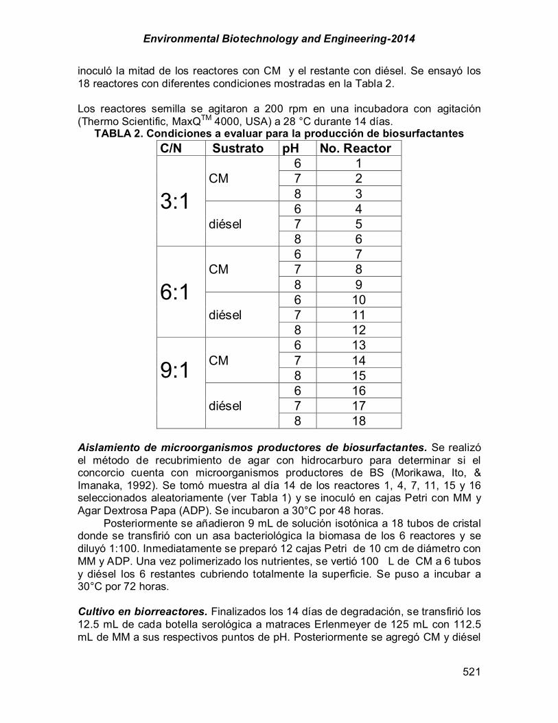
Environmental Biotechnology and Engineering-2014
521
inoculó la mitad de los reactores con CM y el restante con diésel. Se ensayó los 18 reactores con diferentes condiciones mostradas en la Tabla 2. Los reactores semilla se agitaron a 200 rpm en una incubadora con agitación (Thermo Scientific, MaxQTM 4000, USA) a 28 °C durante 14 días.
TABLA 2. Condiciones a evaluar para la producción de biosurfactantes C/N Sustrato pH No. Reactor
3:1 CM
6 1 7 2 8 3
diésel 6 4 7 5 8 6
6:1 CM
6 7 7 8 8 9
diésel 6 10 7 11 8 12
9:1
CM 6 13 7 14 8 15
diésel 6 16 7 17 8 18
Aislamiento de microorganismos productores de biosurfactantes. Se realizó el método de recubrimiento de agar con hidrocarburo para determinar si el concorcio cuenta con microorganismos productores de BS (Morikawa, Ito, & Imanaka, 1992). Se tomó muestra al día 14 de los reactores 1, 4, 7, 11, 15 y 16 seleccionados aleatoriamente (ver Tabla 1) y se inoculó en cajas Petri con MM y Agar Dextrosa Papa (ADP). Se incubaron a 30°C por 48 horas.
Posteriormente se añadieron 9 mL de solución isotónica a 18 tubos de cristal donde se transfirió con un asa bacteriológica la biomasa de los 6 reactores y se diluyó 1:100. Inmediatamente se preparó 12 cajas Petri de 10 cm de diámetro con MM y ADP. Una vez polimerizado los nutrientes, se vertió 100 L de CM a 6 tubos y diésel los 6 restantes cubriendo totalmente la superficie. Se puso a incubar a 30°C por 72 horas. Cultivo en biorreactores. Finalizados los 14 días de degradación, se transfirió los 12.5 mL de cada botella serológica a matraces Erlenmeyer de 125 mL con 112.5 mL de MM a sus respectivos puntos de pH. Posteriormente se agregó CM y diésel
Environmental Biotechnology and Engineering-2014
522
a su matraz correspondiente conservando su C/N anterior. Se dejó agitando por 14 días a 200 rpm a 28°C los 18 matraces. Cuantificación de biosurfactantes. Se llevó una cinética de producción de BS a cada biorreactor cada 24 horas, por 4 días. El medio de cultivo se centrifugó (HERMLE LABORTECHNIK, Z 36 HK, GER) a 12000 rpm durante 30 min y 4°C, a 3 mL del sobrenadante libre de células se agregaron 20 L de CM o diésel, según lo que le corresponda a la muestra. Posteriormente la mezcla se agitó en vórtex (Barnstead Thermolyne, modelo: M16715, USA) durante 2 min, después de 24 h reposando, la fase acuosa se separó y se determinó la densidad óptica a 400 nm (DO400) (Patil & Chopade , 2001a) en un espectrofotómetro (JASCO JENWAY, modelo: 6405, USA). Mediante la ecuación 1 se determinó la concentración del biosurfactante (CBS) en mg equivalentes de Tween 20 por litro del sobrenadante libre de células.
Actividad Emulsificante. Se llevó una cinética de la AE a cada biorreactor cada 24 horas, por 72 h. El caldo de cultivo se centrifugó a 12000 rpm durante 30 min y 4°C. Se toma 3 mL sobrenadante y se agregó 20 L de CM o diésel, según lo que le corresponda a la muestra y se agita con vórtex durante 2 min, después de 24 h reposando, la fase acuosa se separó. Se midió la absorbancia en unidades de 0.01 a 400 nm multiplicado por el factor de dilución es considerado como 1 unidad de actividad emulsificante por mL (AE mL-1). El MM se usa como blanco. pH. El pH se determinó directamente en el caldo de cultivo con un potenciómetro Oakton 510 Series (Cole-Parmer, USA). Tensión superficial. La tensión superficial de los cultivos se determinó con un tensiómetro de anillo de Platino-Iridio (Cole-Parmer, Modelo: TS9149G08, USA) a una temperatura constante de 25°C, y utilizando como fluidos de referencia agua destilada y diésel. Se tomó sólo una lectura a las 72 h de los 18 biorreactores. Transferencia de la mejor relación C/N y pH a un reactor tubular con placa plana. En un trabajo anterior se caracterizó la hidrodinámica de un RTPP de cristal con un volumen de operación de 1.3 L, una altura total de 34.5 cm, una longitud de placa plana de 27 cm y un diámetro de 7 cm (Decle, 2014). La velocidad superficial de la fase gaseosa (Ug) más eficiente fue de 4.331 cm s-1 con una altura de 1 cm de la placa plana con respecto al fondo del reactor. El RTPP fue montado a una Ug de 4.331 cm s-1 y a 1 cm de espacio entra la placa plana y el fondo del reactor junto a la mejor relación C/N y pH obtenida. Resultados y Discusión Selección de mejores condiciones de producción de BS
(1)

Environmental Biotechnology and Engineering-2014
523
Identificación de microorganismos productores de biosurfactantes. Finalizada la incubación, se observó claramente en 2 placas el halo emulsificante determinando que en el consorcio hidrocarbonoclasta hay microorganismos productores de BS. Las placas que mostraron claramente un halo emulsificante fue el matraz 8 (ver Figura 1) y 11 (ver Figura 2) de la Tabla 1. Ambos coincidieron en tener como relación C/N 6:1 y 6 como pH, difiriendo únicamente en los sustratos; CM y diésel, respectivamente.
FIGURA 4. Identificación de microorganismos productores de
BS con diésel La presencia de microrganismos productores de BS en el consorcio hidrocarbonoclasta puede sugerir que al menos en alguna proporción este consorcio utiliza los tensoactivos para consumir los sustratos hidrofóbicos. Cuantificación del BS. Se llevó la cinética de producción de BS de aquellos microorganismos productores de tensoactivos durante 4 días de los 18
FIGURA 3. Identificación de microorganismos productores de BS con CM
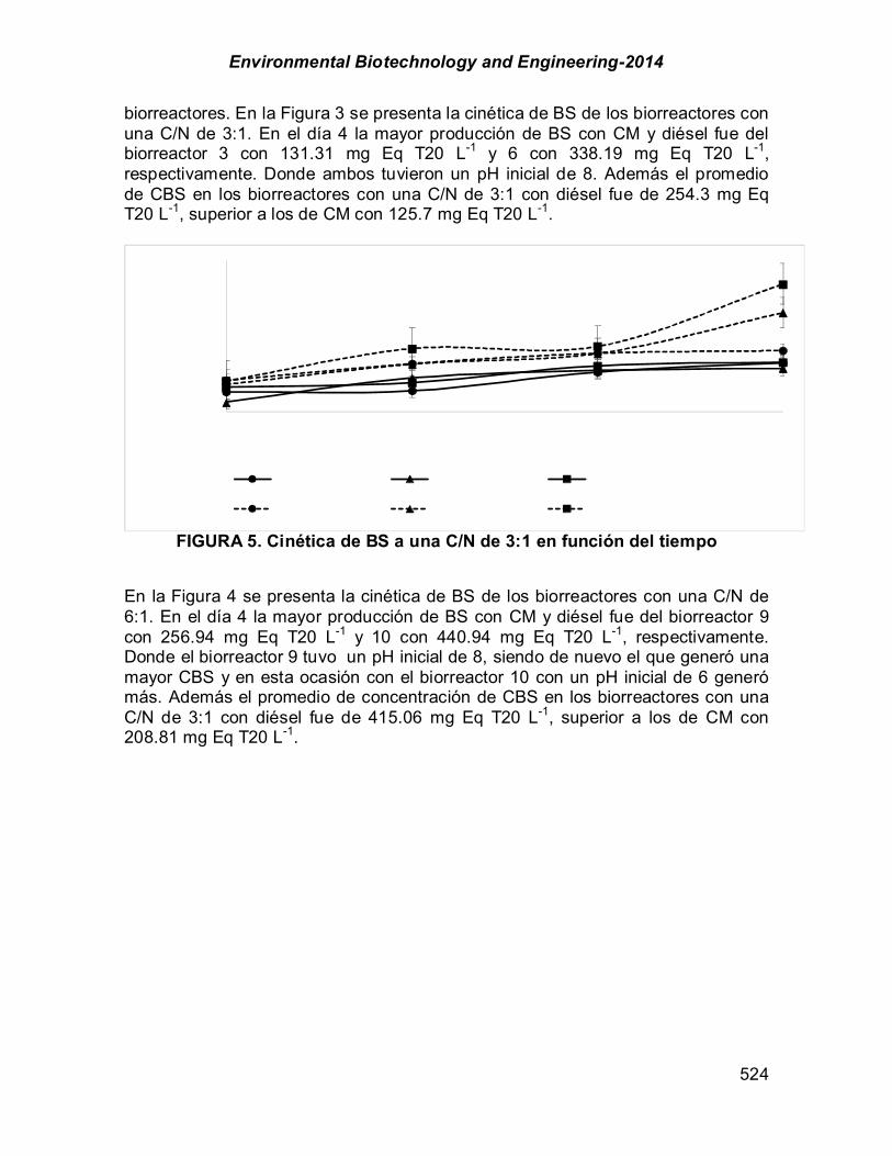
Environmental Biotechnology and Engineering-2014
524
biorreactores. En la Figura 3 se presenta la cinética de BS de los biorreactores con una C/N de 3:1. En el día 4 la mayor producción de BS con CM y diésel fue del biorreactor 3 con 131.31 mg Eq T20 L-1 y 6 con 338.19 mg Eq T20 L-1, respectivamente. Donde ambos tuvieron un pH inicial de 8. Además el promedio de CBS en los biorreactores con una C/N de 3:1 con diésel fue de 254.3 mg Eq T20 L-1, superior a los de CM con 125.7 mg Eq T20 L-1.
FIGURA 5. Cinética de BS a una C/N de 3:1 en función del tiempo
En la Figura 4 se presenta la cinética de BS de los biorreactores con una C/N de 6:1. En el día 4 la mayor producción de BS con CM y diésel fue del biorreactor 9 con 256.94 mg Eq T20 L-1 y 10 con 440.94 mg Eq T20 L-1, respectivamente. Donde el biorreactor 9 tuvo un pH inicial de 8, siendo de nuevo el que generó una mayor CBS y en esta ocasión con el biorreactor 10 con un pH inicial de 6 generó más. Además el promedio de concentración de CBS en los biorreactores con una C/N de 3:1 con diésel fue de 415.06 mg Eq T20 L-1, superior a los de CM con 208.81 mg Eq T20 L-1.
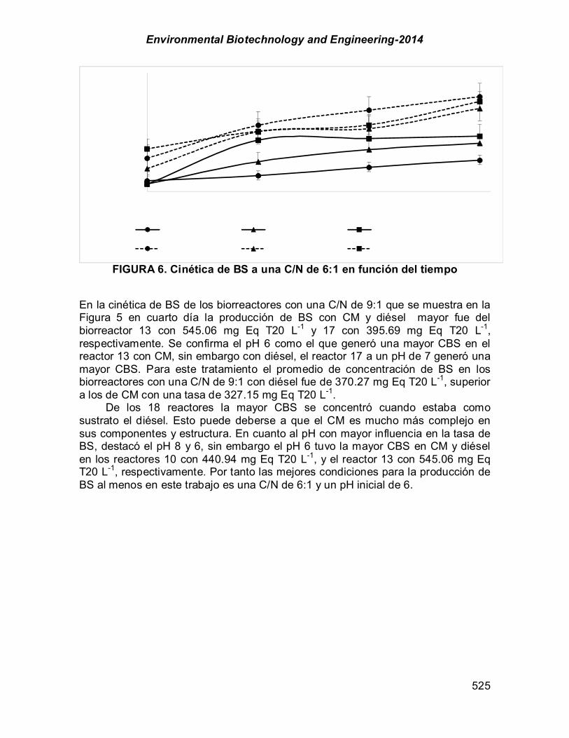
Environmental Biotechnology and Engineering-2014
525
FIGURA 6. Cinética de BS a una C/N de 6:1 en función del tiempo
En la cinética de BS de los biorreactores con una C/N de 9:1 que se muestra en la Figura 5 en cuarto día la producción de BS con CM y diésel mayor fue del biorreactor 13 con 545.06 mg Eq T20 L-1 y 17 con 395.69 mg Eq T20 L-1, respectivamente. Se confirma el pH 6 como el que generó una mayor CBS en el reactor 13 con CM, sin embargo con diésel, el reactor 17 a un pH de 7 generó una mayor CBS. Para este tratamiento el promedio de concentración de BS en los biorreactores con una C/N de 9:1 con diésel fue de 370.27 mg Eq T20 L-1, superior a los de CM con una tasa de 327.15 mg Eq T20 L-1.
De los 18 reactores la mayor CBS se concentró cuando estaba como sustrato el diésel. Esto puede deberse a que el CM es mucho más complejo en sus componentes y estructura. En cuanto al pH con mayor influencia en la tasa de BS, destacó el pH 8 y 6, sin embargo el pH 6 tuvo la mayor CBS en CM y diésel en los reactores 10 con 440.94 mg Eq T20 L-1, y el reactor 13 con 545.06 mg Eq T20 L-1, respectivamente. Por tanto las mejores condiciones para la producción de BS al menos en este trabajo es una C/N de 6:1 y un pH inicial de 6.

Environmental Biotechnology and Engineering-2014
526
FIGURA 7. Cinética de BS a una C/N de 9:1 en función del tiempo
Actividad Emulsificante. Una vez obtenida la cinética de producción de BS, se llevó la cinética de la AE de aquellos microorganismos productores de tensoactivos durante 4 días de los 18 biorreactores. La cinética de AE de los biorreactores con una C/N de 3:1 se muestra en la Figura 6. En el cuarto día, la mayor tasa de AE con CM y diésel fue del biorreactor 3 con 0.59 UE mL-1 y 6 con 1.70 UE mL-1, respectivamente. Ambos tuvieron un pH inicial de 8. El promedio de AE en los biorreactores con una C/N de 3:1 con diésel fue de 1.25 UE mL-1, superior a los de CM con 0.56 UE mL-1.
Con el presente trabajo se puede sugerir que la relación C/N y el pH están relacionados con la tasa AE en este consorcio.
FIGURA 8. Cinética de AE a una C/N de 3:1 en función del tiempo
En la Figura 7 se presenta la cinética de AE de los biorreactores con una C/N
de 6:1. En el día 4, la mayor producción de BS con CM y diésel fue del biorreactor

Environmental Biotechnology and Engineering-2014
527
9 con 1.26 UE mL-1 con un pH de 8 y 10 con 2.24 UE mL-1 a un pH de 6, respectivamente. Según el promedio de AE en los biorreactores con una C/N de 6:1 con diésel fue de 2.11 UE mL-1, superior a los de CM con 1.01 UE mL-1, puede sugerir que el diésel es menos complejo en su degradación, que el CM.
FIGURA 9. Cinética de AE a una C/N de 6:1 en función del tiempo
La Figura 8 muestra la cinética de AE de los reactores con una C/N de 9:1.
En el último día de la cinética la mayor AE con CM y diésel fue del biorreactor 13 con 2.80 UE mL-1 y 17 con 2 UE mL-1, respectivamente. El reactor 13 tuvo un pH inicial de 6, destacándose por segunda vez con la mayor tasa de AE y en esta ocasión con el biorreactor 17 con un pH inicial de 7 generó más. De acuerdo al promedio de la concentración de AE en los biorreactores con una C/N de 9:1 con diésel fue de 1.87 UE mL-1, superior a los de CM con 1.64 UE mL-1.
El diésel, según los resultados genera mayor AE, resultado de la producción de BS del consorcio, a diferencia del CM. Misma situación en las cinéticas de BS. Se puede deber a la gran complejidad que muestra el CM en cuanto a composición. Las cinéticas se llevaron sólo por 4 días. En ninguna de ellas se notó una fase estacionaria, por lo que se sugiere realizar estos experimentos a tiempos superiores a 4 días para poder determinar las tasas máximas de este consorcio en cuestión. La relación C/N y el pH, tienen un efecto significativo en la AE. La relación C/N con mayores tasas fue la de 6:1 y el pH de 6 generó los valores más altos.

Environmental Biotechnology and Engineering-2014
528
FIGURA 10. Cinética de AE a una C/N de 9:1 en función del tiempo
Tensión Superficial. La TS se ve disminuida cuando hay presencia de BS. Se midió la TS de los 18 reactores descritos en la Tabla 2. El promedio de los 18 reactores fue de 60.32 60.32 dinas cm-1.
Se midió la TS de los 18 reactores con sus respectivas condiciones ya descritas el día 4. En promedio todos los reactores mostraron 60.32 dinas cm-1
(ver Tabla 3). A una relación C/N de 3:1 con CM y diésel, la menor TS fue del reactor 1
con 59.9 dinas cm-1 y el reactor 6 con 61.5 dinas cm-1, respectivamente. A una relación C/N de 6:1 con CM y diésel la menor TS fue del reactor 9 con 54.4 dinas cm-1 y el reactor 10 con 58.2 dinas cm-1, respectivamente. A una relación C/N de 9:1 con CM y diésel la menor TS fue del reactor 8 con 48.87 dinas cm-1 y el reactor 16 con 56.5 dinas cm-1, respectivamente. La TS fue siempre menor a la del agua (72.75 dinas cm s-1) lo que puede sugerir la presencia de tensoactivos que reducen la TS. Además con el presente trabajo se puede sugerir que la relación C/N y el pH están relacionados de una manera indirecta con la TS debido a los BS producidos de este consorcio.
TABLA 3. Tensión Superficial del día 4 de los 18 reactores
Tensión Superficial C/N Sustrato pH Reactor dinas cm-1
3 CM 6 1 59.90 7 2 66.23
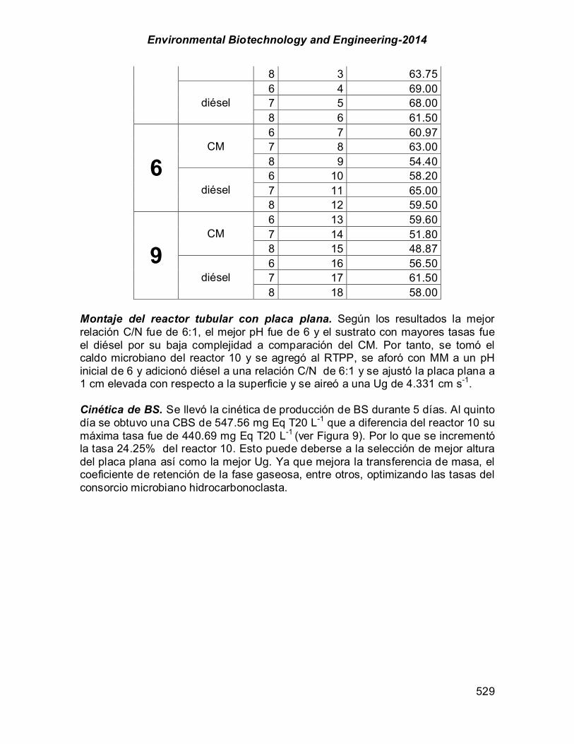
Environmental Biotechnology and Engineering-2014
529
8 3 63.75
diésel 6 4 69.00 7 5 68.00 8 6 61.50
6 CM
6 7 60.97 7 8 63.00 8 9 54.40
diésel 6 10 58.20 7 11 65.00 8 12 59.50
9 CM
6 13 59.60 7 14 51.80 8 15 48.87
diésel 6 16 56.50 7 17 61.50 8 18 58.00
Montaje del reactor tubular con placa plana. Según los resultados la mejor relación C/N fue de 6:1, el mejor pH fue de 6 y el sustrato con mayores tasas fue el diésel por su baja complejidad a comparación del CM. Por tanto, se tomó el caldo microbiano del reactor 10 y se agregó al RTPP, se aforó con MM a un pH inicial de 6 y adicionó diésel a una relación C/N de 6:1 y se ajustó la placa plana a 1 cm elevada con respecto a la superficie y se aireó a una Ug de 4.331 cm s-1. Cinética de BS. Se llevó la cinética de producción de BS durante 5 días. Al quinto día se obtuvo una CBS de 547.56 mg Eq T20 L-1 que a diferencia del reactor 10 su máxima tasa fue de 440.69 mg Eq T20 L-1 (ver Figura 9). Por lo que se incrementó la tasa 24.25% del reactor 10. Esto puede deberse a la selección de mejor altura del placa plana así como la mejor Ug. Ya que mejora la transferencia de masa, el coeficiente de retención de la fase gaseosa, entre otros, optimizando las tasas del consorcio microbiano hidrocarbonoclasta.
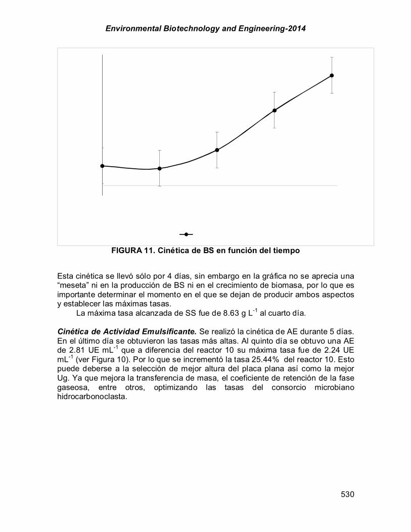
Environmental Biotechnology and Engineering-2014
530
FIGURA 11. Cinética de BS en función del tiempo
Esta cinética se llevó sólo por 4 días, sin embargo en la gráfica no se aprecia una “meseta” ni en la producción de BS ni en el crecimiento de biomasa, por lo que es importante determinar el momento en el que se dejan de producir ambos aspectos y establecer las máximas tasas.
La máxima tasa alcanzada de SS fue de 8.63 g L-1 al cuarto día. Cinética de Actividad Emulsificante. Se realizó la cinética de AE durante 5 días. En el último día se obtuvieron las tasas más altas. Al quinto día se obtuvo una AE de 2.81 UE mL-1 que a diferencia del reactor 10 su máxima tasa fue de 2.24 UE mL-1 (ver Figura 10). Por lo que se incrementó la tasa 25.44% del reactor 10. Esto puede deberse a la selección de mejor altura del placa plana así como la mejor Ug. Ya que mejora la transferencia de masa, el coeficiente de retención de la fase gaseosa, entre otros, optimizando las tasas del consorcio microbiano hidrocarbonoclasta.

Environmental Biotechnology and Engineering-2014
531
FIGURA 12. Cinética de AE en función del tiempo
La Figura 10 muestra que al cuarto día se alcanzó 2.81 UE mL-1, sin embargo el comportamiento de la AE muestra, al menos en el cuarto día, se encontraba en una fase exponencial. Este trabajo se limitó al cuarto día, por tal motivo, se sugiere establecer la tasa máxima de AE, así como de BS, capaz de este consorcio, mediante una cinética con más de 4 días. Cinética de tensión superficial. Se llevó la cinética de TS durante 5 días. Al quinto día se obtuvo una TS de 46 dinas cm-1 que a diferencia del reactor 10 su máxima tasa fue de 58.20 dinas cm-1 (ver Figura 11). Por lo que se disminuyó la tasa 26.52% del reactor 10. La caracterización hidrodinámica aumentó las tasas de una manera significativa.
Según los resultados obtenidos, las diferentes relaciones C/N de los sustratos hidrofóbicos así como diferentes pH sobre el medio mineral en la producción de biosurfactantes de este consorcio hidrocarbonoclasta es importante para obtener las mejores tasas de tensoactivos, además de una previa caracterización hidrodinámica del reactor donde se lleva a cabo el proceso biológico.

Environmental Biotechnology and Engineering-2014
532
FIGURA 13. Cinética de TS en función del tiempo
La estrategia del consorcio por degradar sustratos hidrofóbicos, ya sea por
formas emulsificadas o por contacto directo, no ha sido dilucidada. Sin embargo, mediante este trabajo se sabe que existen microorganismos productores de tensoactivos. Por tanto, las formas emulsificadas es un método ya sea parcial o total para degradar sustratos hidrofóbicos en este consorcio. Conclusión El consorcio cuenta con microrganismos productores de biosurfactantes al presentar un desplazamiento del sustrato crudo maya y diésel mediante un halo emulsificante.
La producción de biosurfactantes o bioemulsifictantes cambia con la variación del pH y relación C/N y consecuentemente, la tensión superficial y la actividad emulsificante. Según los resultados obtenidos, la relación C/N de 6:1 de diésel y crudo maya, en conjunto con un pH de 6, generan las mejores tasas de producción de BS.
Se aumentó los rendimientos de producción de biosurfactantes, la actividad emulsificante y la tensión superficial, debido a la optimización hidrodinámica del reactor tubular con placa plana.
Es necesario determinar los microrganismos que componen al consorcio y los tipos de biosurfactantes o bioemulsifictantes producidos; así como la morfología para determinar la composición de su superficie celular. Además, se sugiere determinar y evaluar el efecto en la producción de biosurfactantes por otros factores, como la temperatura, otras configuraciones de reactores, entre otros.
El presente trabajo muestra cinéticas de 4 o 5 días, sin embargo en ninguna de ellas se notó una fase estacionaria. Por lo que se sugiere realizar las mismas
Environmental Biotechnology and Engineering-2014
533
cinéticas mostradas en esta memoria pero aumentando el tiempo, con el fin de encontrar las tasas máximas de producción de este consorcio.
Por último, establecer la estrategia de consumo de este consorcio, sea por formas emulsificadas o contacto directo para estudiar y optimizar la biodegradación de sustratos hidrofóbicos. Referencias Bai, G., Brusseau, M. L., & Miller, R. M. (1997). Biosurfactants-enhanced removal of residual
hydrocarbon from soil. Journal of Contaminates Hydrology. , 157-170. Carrillo, P. G., Mardaraz, C., Pitta-Alvarez, S. I., & Giulett, A. M. (1996). Isolation and selec- tion of
biosurfactant producing bacteria. World J Microbiol Biotechnol(12), 82-84. Decle, C. S. (2014). Diseño de biorreactores airlift para la producción de un consorcio microbiano
degradador de hidrocarburos. Cancún, Quintana Roo: Universidad Politécnica de Quintana Roo.
Desai, J. D., & Banat, I. M. (1997). Microbial production of surfactants and their commercial potential. Microbiol Mol Biol Rev, 61:47-64.
Díaz, I. J., Ramírez, H., Gutiérrez, M., & Favela, E. (2003). Biodegradation of Maya crude oil by bacterial strains and a defined mixed culture isolated from Cyperus laxus rhizosphere soil in a contaminated site. Canadian Journal of Microbiology., 49: 755-761.
Ellaiah, P. (2002). Production of glycolipids containing biosurfactant by Pseudomonas spe- cies. Indian J Exp Biol, 1083-1086.
Ghazali, F. M., Abdul, R. N., Salleh, A. B., & Basri, M. (2004). Biodegradation of hydrocarbons in soil by microbial consortium. International Biodeterioration & Biodegradation., 54:61-67.
González, G., Yañez, G., & Bahuer, M. (2001). Medio ambiente. Capítulo 5. En: Prospectiva de la Investigación y Desarrollo Tecnológico del Sector Petrolero al año 2025. Instituto Mexicano del Petróleo. Instituto Mexicano del Petróleo, 117-133.
Jagtap, S., Yavankar, S., Pardesi, k., & Chopade, B. (2009). Production of bioemulsifier by Acinetobacter sp. from healthy human skin of tribal population. Ind J Expt Biol, 50-62.
Korda, A., Santas, P., Tenente, A., & Santas , R. (1997). Petroleum hydrocarbon bioremediation: sampling and analytical techniques, in situ treatments and commercial microorganisms currently used. Applied Microbiology and Biotechnology, 48: 677-686.
Lizardi, M., Bautista, L., Ordaz, A., & Velarde, R. (2014). Airlift Bioreactor for hydrocarbon water pollution remediation in tourism development pole. Desalination and Water Treatment, 2-5.
Matsuyama, T., Sogawa, M., & Yano, I. (1987). Direct colony thin-layer chromatography and rapid characterization of serratia marcescens mutants defective in production of wetting agents. Appl Environ Microbiol, 53: 1186–1188.
Mehrnia, M. J., Towfighi, B., Bonakdarpour, B., & Akbainejad, M. (2005). Gas Hold-up and oxygen transfer in a draft-tube airlift bioreactor with petroleum based liquids. Biochemical Engineering Journal, 22: 105-110.
Morikawa, M., Hirata, Y., & Imanaka, T. (2000). A study on the structure-function relation- ship of lipopeptide biosurfactants. Biochim Biophys Acta 1488: 211–218. Biochim Biophys Acta, 1488: 211–218.
Morikawa, M., Ito, M., & Imanaka, T. (1992). Isolation of a new surfactin producer Bacillus pumilusA-1, and cloning and nucleotide sequence of the regulator gene, psf-1. J Ferm Bioeng, 74: 255–261.
Patil, J. R., & Chopade , B. A. (2001a). Distribution and in vitro antimicrobial suscepti- bility of Acinetobacter species on the skin of healthy humans. Natl Med J India, 14: 204–208.
Patil, J. R., & Chopade, B. A. (2001b). Studies on bioemulsifier production by Acinetobacter strains isolated from healthy human skin. J Appl Microbiol, 91: 290–298.

Environmental Biotechnology and Engineering-2014
534
Rosenberg, M., Gutnick, D. L., & Rosenberg, E. (1980). Adherence of bacteria to hydro- carbons: a simple method for measuring cell-surface hydrophobicity. FEMS Microbiol Lett 9: 29–33. FEMS Microbiol Lett, 9: 29–33.
Salanitro, J. P. (2001). Bioremediation of petroleum hydrocarbons in soil. Advances in Agronomy. 72:53-105. Advances in Agronomy., 72:53-105.
Siegmund, I., & Wagner, F. (1991). New method for detecting rhamnolipids excreted by Pseudomonas spp. during growth on mineral agar. Biotechnol Tech 5: 265–268., 5: 265–268.
Skladany, G. J., & Metting, F. B. (1993). Bioremediation of contaminated soil. In: Soil Microbial Ecology, applications in agricultural and environmental management. . En M. Dekker, Soil Microbial Ecology, applications in agricultural and environmental management. . USA.
Van der Vegt, W., Van der Mei, H. C., Noordmans, J., & Busscher, H. J. (1991). Assessment of bacterial biosurfactant production through axisymmetric drop shape analysis by profile. Appl Microbiol Biotechnol, 35: 766–770.
Van Hamme, J. D., Singh, A., & Ward , O. P. (2003). Recent advances in petroleum microbiology. Microbiology and Molecular Biology Reviews, 67: 503-549.
Environmental Biotechnology and Engineering-2014
535
CHAPTER 5.5. COMBINING ABIOTIC AND BIOTIC PROCESSES FOR
AGGRESSIVE TREATMENT OF CHLORINATED ETHENES
Daniel Leigh
Peroxychem LLC, Walnut Creek CA, USA
Abstract Soil and groundwater at Concord Naval Weapons Station in Concord, CA has been affected by a discharge of trichloroethene (TCE). The Navy intends divest the property under the Base Realignment and Closure (BRAC) program. To expedite the Navy’s goals, an aggressive treatment approach combining biological and abiotic processes is being applied to remediate the TCE.
A TCE plume extends approximately 700 feet down gradient from the source area and up to 100 feet below ground surface. The aquifer consists of unconsolidated silt, sands and clays. Groundwater in the treatment area is highly aerobic. A pilot test previously conducted by CB&I demonstrated that application of enhanced biostimulation with bioaugmentation resulted in complete degradation the CE concentration from approximately 5,000 microgram per liter (µg/L) to less than 1 µg/L.
Approach/Activities. The Navy conducted a Design Optimization Test (DOT) to evaluate enhancement of the biological approach by addition of in situ chemical reduction (ISCR). This process was selected to more aggressively treat the contaminants, reduce the potential for generation of toxic degradation products and to provide long lasting substrates reduce the potential for rebound of the contaminants.
The DOT applied abiotic processes by distribution of zero valent iron (ZVI) to provide a long lasting substrate which degrades TCE while minimizing the generation of daughter products such as dichoroethene (DCE) and vinyl chloride (VC). The DOT optimized the biological degradation process by amending the ZVI with a combination of organic substrates including sodium lactate and Emulsified Lecithin Substrate® (FMC Environmental Solutions, Inc). Lactate was applied to create reducing conditions in the amendment water prior to injection and to establish the bioaugmentation culture in the aerobic aquifer. ELS® was distributed through the aquifer to provide a long-lasting substrate to treat potential residual contaminants. Bioaugmentation was conducted using a VC respiring culture (SDC-9™; CB&I Federal Services LLC).
Substrate distribution was conducted using direct push technology. At each interval, the aquifer was first primed by fracturing the aquifer. Following confirmation of fracture development, ZVI suspended in guar was injected into the
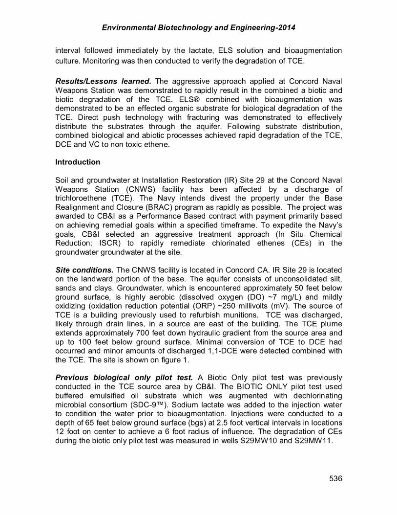
Environmental Biotechnology and Engineering-2014
536
interval followed immediately by the lactate, ELS solution and bioaugmentation culture. Monitoring was then conducted to verify the degradation of TCE. Results/Lessons learned. The aggressive approach applied at Concord Naval Weapons Station was demonstrated to rapidly result in the combined a biotic and biotic degradation of the TCE. ELS® combined with bioaugmentation was demonstrated to be an effected organic substrate for biological degradation of the TCE. Direct push technology with fracturing was demonstrated to effectively distribute the substrates through the aquifer. Following substrate distribution, combined biological and abiotic processes achieved rapid degradation of the TCE, DCE and VC to non toxic ethene. Introduction Soil and groundwater at Installation Restoration (IR) Site 29 at the Concord Naval Weapons Station (CNWS) facility has been affected by a discharge of trichloroethene (TCE). The Navy intends divest the property under the Base Realignment and Closure (BRAC) program as rapidly as possible. The project was awarded to CB&I as a Performance Based contract with payment primarily based on achieving remedial goals within a specified timeframe. To expedite the Navy’s goals, CB&I selected an aggressive treatment approach (In Situ Chemical Reduction; ISCR) to rapidly remediate chlorinated ethenes (CEs) in the groundwater groundwater at the site. Site conditions. The CNWS facility is located in Concord CA. IR Site 29 is located on the landward portion of the base. The aquifer consists of unconsolidated silt, sands and clays. Groundwater, which is encountered approximately 50 feet below ground surface, is highly aerobic (dissolved oxygen (DO) ~7 mg/L) and mildly oxidizing (oxidation reduction potential (ORP) ~250 millivolts (mV). The source of TCE is a building previously used to refurbish munitions. TCE was discharged, likely through drain lines, in a source are east of the building. The TCE plume extends approximately 700 feet down hydraulic gradient from the source area and up to 100 feet below ground surface. Minimal conversion of TCE to DCE had occurred and minor amounts of discharged 1,1-DCE were detected combined with the TCE. The site is shown on figure 1. Previous biological only pilot test. A Biotic Only pilot test was previously conducted in the TCE source area by CB&I. The BIOTIC ONLY pilot test used buffered emulsified oil substrate which was augmented with dechlorinating microbial consortium (SDC-9™). Sodium lactate was added to the injection water to condition the water prior to bioaugmentation. Injections were conducted to a depth of 65 feet below ground surface (bgs) at 2.5 foot vertical intervals in locations 12 foot on center to achieve a 6 foot radius of influence. The degradation of CEs during the biotic only pilot test was measured in wells S29MW10 and S29MW11.
Environmental Biotechnology and Engineering-2014
537
FIGURE 2: Concord Naval Weapons Station IR Site 29. The TCE plume is shown in yellow in both photographs
The biotic only pilot test demonstrated that application of resulted in complete degradation the TCE and daughter products concentration from approximately 5,000 microgram per liter (µg/L) to less than 1 µg/L in approximately 550 days. The Biotic Only pilot test area is shown on figure 2. FIGURE 3: Biotic only and DOT pilot test well and injection locations
In situ chemical reduction approach: ISCR was selected for this site to enhance the biotic process demonstrated to be applicable during the initial biotic only pilot test. The biotic degradation of TCE results in the stoichiometric sequential production of toxic daughter products including DCE (primarily the cis 1,2- isomer), and vinyl chloride (VC), which are subsequently reduced to non-toxic ethene and ethane. The abiotic degradation process primarily bypasses the generation of these toxic degradation product by the $-elimination pathway which temporarily generates unstable chlorinated acetylenes which may be converted to ethene and ethane. The hypothetical degradation pathways of the biotic and abiotic approach are shown in figure 3.
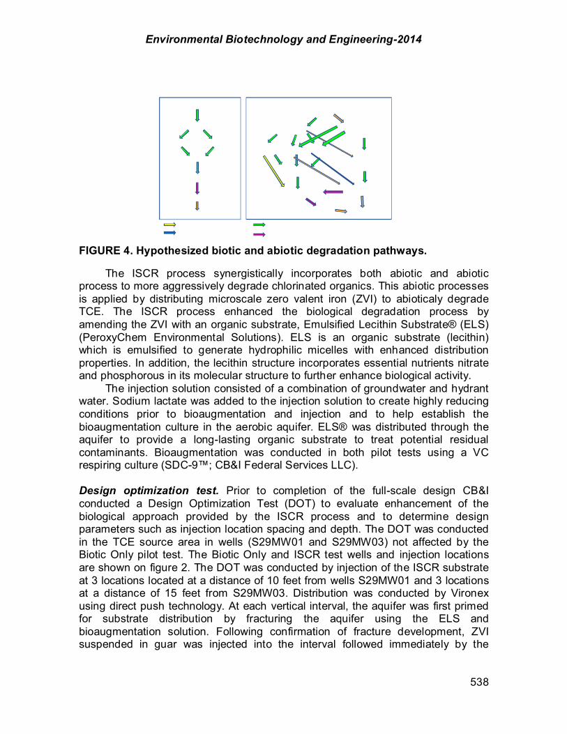
Environmental Biotechnology and Engineering-2014
538
FIGURE 4. Hypothesized biotic and abiotic degradation pathways.
The ISCR process synergistically incorporates both abiotic and abiotic process to more aggressively degrade chlorinated organics. This abiotic processes is applied by distributing microscale zero valent iron (ZVI) to abioticaly degrade TCE. The ISCR process enhanced the biological degradation process by amending the ZVI with an organic substrate, Emulsified Lecithin Substrate® (ELS) (PeroxyChem Environmental Solutions). ELS is an organic substrate (lecithin) which is emulsified to generate hydrophilic micelles with enhanced distribution properties. In addition, the lecithin structure incorporates essential nutrients nitrate and phosphorous in its molecular structure to further enhance biological activity.
The injection solution consisted of a combination of groundwater and hydrant water. Sodium lactate was added to the injection solution to create highly reducing conditions prior to bioaugmentation and injection and to help establish the bioaugmentation culture in the aerobic aquifer. ELS® was distributed through the aquifer to provide a long-lasting organic substrate to treat potential residual contaminants. Bioaugmentation was conducted in both pilot tests using a VC respiring culture (SDC-9™; CB&I Federal Services LLC).
Design optimization test. Prior to completion of the full-scale design CB&I conducted a Design Optimization Test (DOT) to evaluate enhancement of the biological approach provided by the ISCR process and to determine design parameters such as injection location spacing and depth. The DOT was conducted in the TCE source area in wells (S29MW01 and S29MW03) not affected by the Biotic Only pilot test. The Biotic Only and ISCR test wells and injection locations are shown on figure 2. The DOT was conducted by injection of the ISCR substrate at 3 locations located at a distance of 10 feet from wells S29MW01 and 3 locations at a distance of 15 feet from S29MW03. Distribution was conducted by Vironex using direct push technology. At each vertical interval, the aquifer was first primed for substrate distribution by fracturing the aquifer using the ELS and bioaugmentation solution. Following confirmation of fracture development, ZVI suspended in guar was injected into the interval followed immediately by the

Environmental Biotechnology and Engineering-2014
539
lactate, ELS solution and bioaugmentation culture. Monitoring was then conducted to verify the degradation of TCE. Water conditioning. Prior to groundwater treatment water is conditioned to assure that the injection solution is conducive to reductive dechlorination and favorable for the bioaugmentation culture. Conditioned water is generated by mixing sodium lactate with available water. The indigenous bacteria rapidly utilize the lactate to establish highly reducing conditions conducive to reductive dechlorination in the water prior to injection. All the lactate is added to the conditioning water in the water conditioning area.
Four 10,000 gallon tanks were filled with water. Hydrant water was used to fill the tanks initially because insufficient water was generated from the existing wells. Two wells were later installed in the treatment area and were determined to provide groundwater at a sustained rate of approximately 6 gallons per minute. Because hydrant water is difficult for the base to supply and because the use of groundwater has substantial benefits, groundwater is pumped from the on-site wells to the conditioning tanks were it is conditioned and pumped back to the conditioned water supply tanks in the treatment area for substrate blending and injection. Because site groundwater is being used, highly reducing conditions are rapidly established in the conditioning tanks and minimal hydrant water is required. The water conditioning and substrate staging area is shown in figure 4. FIGURE 5. Water conditioning area showing water conditioning tanks and lactate, ELS and iron storage areas. Treatment area is approximately # mile from the water conditioning area ELS solution preparation: Only conditioned water is used for mixing the ELS and bioaugmentation solution and the iron and guar solution. The ELS, iron and lactate are staged at the water conditioning area. All the lactate (~1%) is added to the water in the conditioning area. The ELS, iron and guar are brought to the treatment area as needed. The mixing of these substrates is conducted in two, mostly separate systems. The ELS is emulsified directly from the concentrate to an injection solution at the target injection concentration (~3%). The injection solution is prepared in batches at the amount required for each injection location. Two solution tanks are available so that one can be used while the other is being mixed.
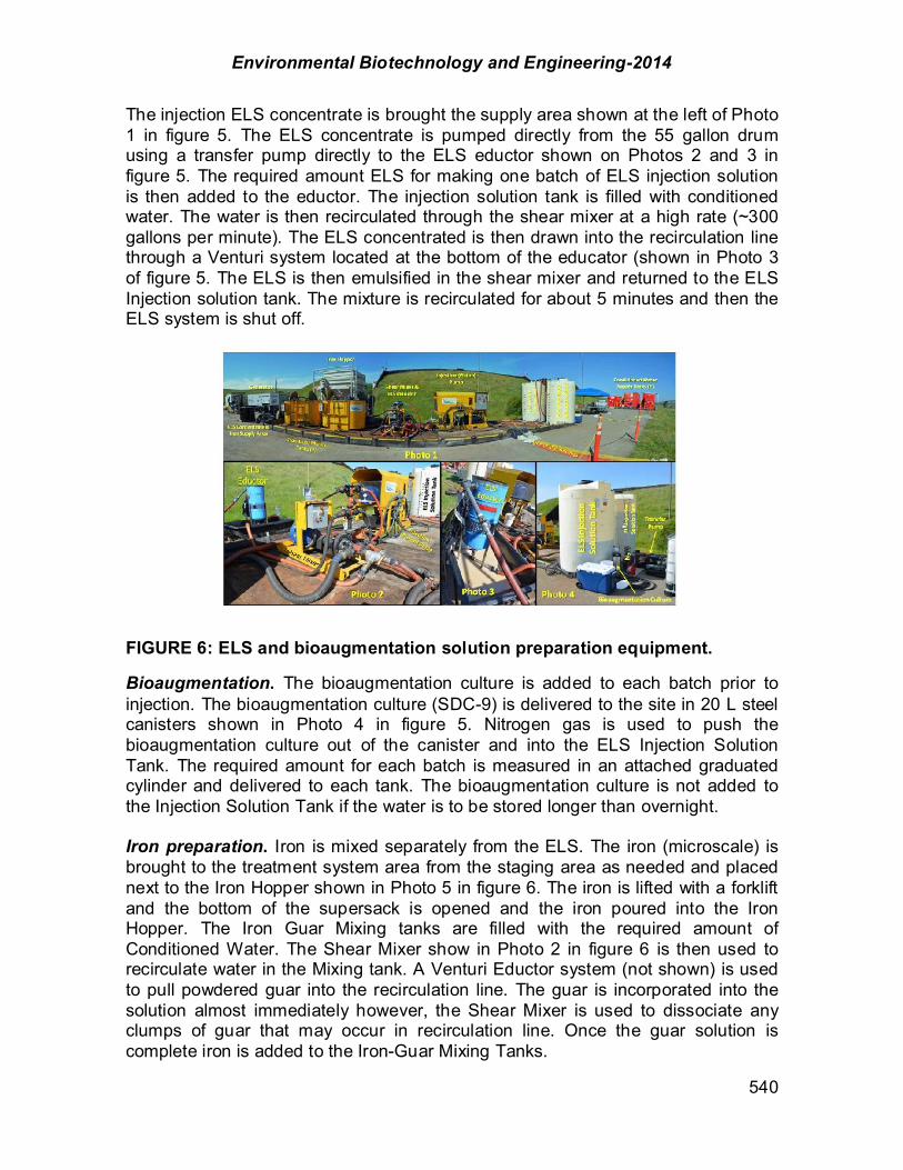
Environmental Biotechnology and Engineering-2014
540
The injection ELS concentrate is brought the supply area shown at the left of Photo 1 in figure 5. The ELS concentrate is pumped directly from the 55 gallon drum using a transfer pump directly to the ELS eductor shown on Photos 2 and 3 in figure 5. The required amount ELS for making one batch of ELS injection solution is then added to the eductor. The injection solution tank is filled with conditioned water. The water is then recirculated through the shear mixer at a high rate (~300 gallons per minute). The ELS concentrated is then drawn into the recirculation line through a Venturi system located at the bottom of the educator (shown in Photo 3 of figure 5. The ELS is then emulsified in the shear mixer and returned to the ELS Injection solution tank. The mixture is recirculated for about 5 minutes and then the ELS system is shut off.
FIGURE 6: ELS and bioaugmentation solution preparation equipment.
Bioaugmentation. The bioaugmentation culture is added to each batch prior to injection. The bioaugmentation culture (SDC-9) is delivered to the site in 20 L steel canisters shown in Photo 4 in figure 5. Nitrogen gas is used to push the bioaugmentation culture out of the canister and into the ELS Injection Solution Tank. The required amount for each batch is measured in an attached graduated cylinder and delivered to each tank. The bioaugmentation culture is not added to the Injection Solution Tank if the water is to be stored longer than overnight. Iron preparation. Iron is mixed separately from the ELS. The iron (microscale) is brought to the treatment system area from the staging area as needed and placed next to the Iron Hopper shown in Photo 5 in figure 6. The iron is lifted with a forklift and the bottom of the supersack is opened and the iron poured into the Iron Hopper. The Iron Guar Mixing tanks are filled with the required amount of Conditioned Water. The Shear Mixer show in Photo 2 in figure 6 is then used to recirculate water in the Mixing tank. A Venturi Eductor system (not shown) is used to pull powdered guar into the recirculation line. The guar is incorporated into the solution almost immediately however, the Shear Mixer is used to dissociate any clumps of guar that may occur in recirculation line. Once the guar solution is complete iron is added to the Iron-Guar Mixing Tanks.

Environmental Biotechnology and Engineering-2014
541
The iron is weighed on a scale when transferred to the Hopper. The required mass of iron per batch is transferred from the Iron Hopper to the Iron-Guar Mixing tanks via a Screw Auger shown in Photo 5 and Photo 6 of figure 6. The hoppers each contain two paddle mixers that continuously stir the iron guar mixture while in the tanks to prevent the iron from settling out of suspension. FIGURE 7: Iron and guar mixing equipment, injection pump and injection rig.
Injection process. The substrate is distributed to the aquifer using direct push technologies. To distribute the substrate in the aquifer a Geoprobe 8040 rig pushes the injection rod to the predetermined injection interval. Injections intervals are 2.5 feet vertically and extend from 45 to 100 feet below ground surface. The injections proceed from top down to minimize the potential for distribution into previously fractured zones. Two Geoprobe 8040 rigs were used to push the injection rods into the aquifer. A high pressure line which transfers the injection solution runs from the piston pump to the injection rig. An in-line manifold allow for the injection solution to be alternately switched between injection rigs. The injection rigs are shown in Photo 8 on figure 6.
The injection process is described as an iron sandwich. Firstly half of the predetermined volume of the batch ELS-Bio solution for the interval is drawn into the injection pump where it is delivered to the injection point that was previously pushed to the desired depth. The injection is conducted at pressures ranging from 1,000 to 1,500 pounds per square inch (PSI) at a flow rate of approximately 50 gallons per minute (gpm). At this pressure, the aquifer is instantly fractured and the bio solution is injected into the fractures. After the first half of that solution is injected (about 1 minute), the total iron for the interval in injected followed by the remainder of the ELS-Bio solution. The injection process takes about 3 to 5 minutes per interval. The injection rod is then pushed 2 " feet further into the aquifer to the next injection interval. When all the intervals are completed the injection rig is moved to the next injection location and the process is repeated.
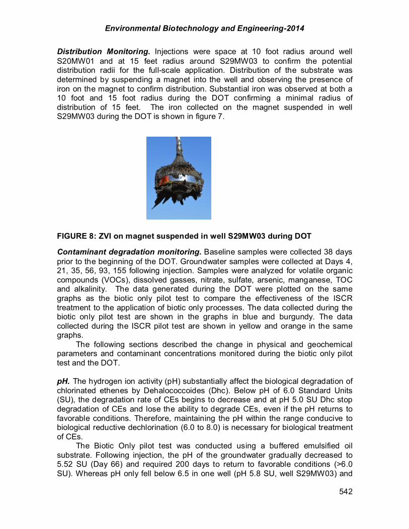
Environmental Biotechnology and Engineering-2014
542
Distribution Monitoring. Injections were space at 10 foot radius around well S20MW01 and at 15 feet radius around S29MW03 to confirm the potential distribution radii for the full-scale application. Distribution of the substrate was determined by suspending a magnet into the well and observing the presence of iron on the magnet to confirm distribution. Substantial iron was observed at both a 10 foot and 15 foot radius during the DOT confirming a minimal radius of distribution of 15 feet. The iron collected on the magnet suspended in well S29MW03 during the DOT is shown in figure 7. FIGURE 8: ZVI on magnet suspended in well S29MW03 during DOT
Contaminant degradation monitoring. Baseline samples were collected 38 days prior to the beginning of the DOT. Groundwater samples were collected at Days 4, 21, 35, 56, 93, 155 following injection. Samples were analyzed for volatile organic compounds (VOCs), dissolved gasses, nitrate, sulfate, arsenic, manganese, TOC and alkalinity. The data generated during the DOT were plotted on the same graphs as the biotic only pilot test to compare the effectiveness of the ISCR treatment to the application of biotic only processes. The data collected during the biotic only pilot test are shown in the graphs in blue and burgundy. The data collected during the ISCR pilot test are shown in yellow and orange in the same graphs.
The following sections described the change in physical and geochemical parameters and contaminant concentrations monitored during the biotic only pilot test and the DOT.
pH. The hydrogen ion activity (pH) substantially affect the biological degradation of chlorinated ethenes by Dehalococcoides (Dhc). Below pH of 6.0 Standard Units (SU), the degradation rate of CEs begins to decrease and at pH 5.0 SU Dhc stop degradation of CEs and lose the ability to degrade CEs, even if the pH returns to favorable conditions. Therefore, maintaining the pH within the range conducive to biological reductive dechlorination (6.0 to 8.0) is necessary for biological treatment of CEs.
The Biotic Only pilot test was conducted using a buffered emulsified oil substrate. Following injection, the pH of the groundwater gradually decreased to 5.52 SU (Day 66) and required 200 days to return to favorable conditions (>6.0 SU). Whereas pH only fell below 6.5 in one well (pH 5.8 SU, well S29MW03) and
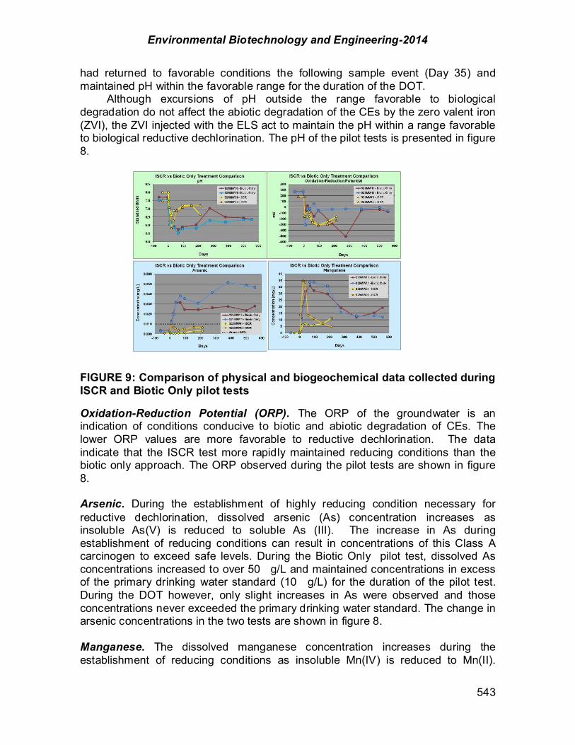
Environmental Biotechnology and Engineering-2014
543
had returned to favorable conditions the following sample event (Day 35) and maintained pH within the favorable range for the duration of the DOT.
Although excursions of pH outside the range favorable to biological degradation do not affect the abiotic degradation of the CEs by the zero valent iron (ZVI), the ZVI injected with the ELS act to maintain the pH within a range favorable to biological reductive dechlorination. The pH of the pilot tests is presented in figure 8.
FIGURE 9: Comparison of physical and biogeochemical data collected during ISCR and Biotic Only pilot tests
Oxidation-Reduction Potential (ORP). The ORP of the groundwater is an indication of conditions conducive to biotic and abiotic degradation of CEs. The lower ORP values are more favorable to reductive dechlorination. The data indicate that the ISCR test more rapidly maintained reducing conditions than the biotic only approach. The ORP observed during the pilot tests are shown in figure 8. Arsenic. During the establishment of highly reducing condition necessary for reductive dechlorination, dissolved arsenic (As) concentration increases as insoluble As(V) is reduced to soluble As (III). The increase in As during establishment of reducing conditions can result in concentrations of this Class A carcinogen to exceed safe levels. During the Biotic Only pilot test, dissolved As concentrations increased to over 50 g/L and maintained concentrations in excess of the primary drinking water standard (10 g/L) for the duration of the pilot test. During the DOT however, only slight increases in As were observed and those concentrations never exceeded the primary drinking water standard. The change in arsenic concentrations in the two tests are shown in figure 8. Manganese. The dissolved manganese concentration increases during the establishment of reducing conditions as insoluble Mn(IV) is reduced to Mn(II).
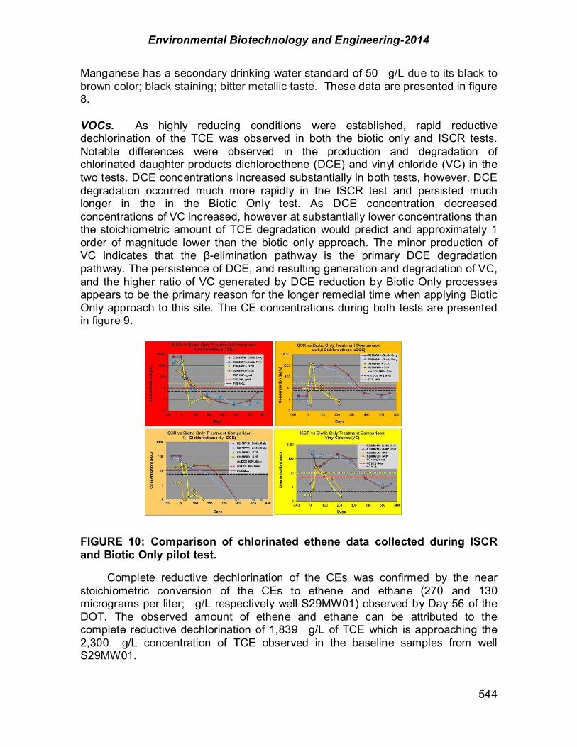
Environmental Biotechnology and Engineering-2014
544
Manganese has a secondary drinking water standard of 50 g/L due to its black to brown color; black staining; bitter metallic taste. These data are presented in figure 8. VOCs. As highly reducing conditions were established, rapid reductive dechlorination of the TCE was observed in both the biotic only and ISCR tests. Notable differences were observed in the production and degradation of chlorinated daughter products dichloroethene (DCE) and vinyl chloride (VC) in the two tests. DCE concentrations increased substantially in both tests, however, DCE degradation occurred much more rapidly in the ISCR test and persisted much longer in the in the Biotic Only test. As DCE concentration decreased concentrations of VC increased, however at substantially lower concentrations than the stoichiometric amount of TCE degradation would predict and approximately 1 order of magnitude lower than the biotic only approach. The minor production of VC indicates that the $-elimination pathway is the primary DCE degradation pathway. The persistence of DCE, and resulting generation and degradation of VC, and the higher ratio of VC generated by DCE reduction by Biotic Only processes appears to be the primary reason for the longer remedial time when applying Biotic Only approach to this site. The CE concentrations during both tests are presented in figure 9. FIGURE 10: Comparison of chlorinated ethene data collected during ISCR and Biotic Only pilot test.
Complete reductive dechlorination of the CEs was confirmed by the near stoichiometric conversion of the CEs to ethene and ethane (270 and 130 micrograms per liter; g/L respectively well S29MW01) observed by Day 56 of the DOT. The observed amount of ethene and ethane can be attributed to the complete reductive dechlorination of 1,839 g/L of TCE which is approaching the 2,300 g/L concentration of TCE observed in the baseline samples from well S29MW01.
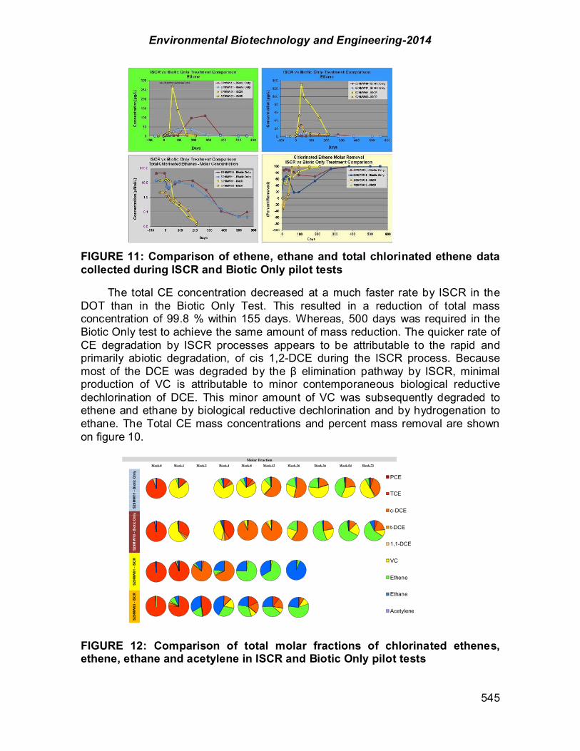
Environmental Biotechnology and Engineering-2014
545
Week 72Week 0 Week 12Week 8 Week 54Week 36Week 26Week 2Week 1 Week 4
S29M
W01
- IS
CR
S29M
W11
- B
iotic
Onl
yS2
9MW
03 -
ISC
RS2
9MW
10 -
Bio
tic O
nly
Molar Fraction
PCE
TCE
c-DCE
t-DCE
1,1-DCE
VC
Ethene
Ethane
Acetylene
FIGURE 11: Comparison of ethene, ethane and total chlorinated ethene data collected during ISCR and Biotic Only pilot tests
The total CE concentration decreased at a much faster rate by ISCR in the DOT than in the Biotic Only Test. This resulted in a reduction of total mass concentration of 99.8 % within 155 days. Whereas, 500 days was required in the Biotic Only test to achieve the same amount of mass reduction. The quicker rate of CE degradation by ISCR processes appears to be attributable to the rapid and primarily abiotic degradation, of cis 1,2-DCE during the ISCR process. Because most of the DCE was degraded by the $ elimination pathway by ISCR, minimal production of VC is attributable to minor contemporaneous biological reductive dechlorination of DCE. This minor amount of VC was subsequently degraded to ethene and ethane by biological reductive dechlorination and by hydrogenation to ethane. The Total CE mass concentrations and percent mass removal are shown on figure 10.
FIGURE 12: Comparison of total molar fractions of chlorinated ethenes, ethene, ethane and acetylene in ISCR and Biotic Only pilot tests
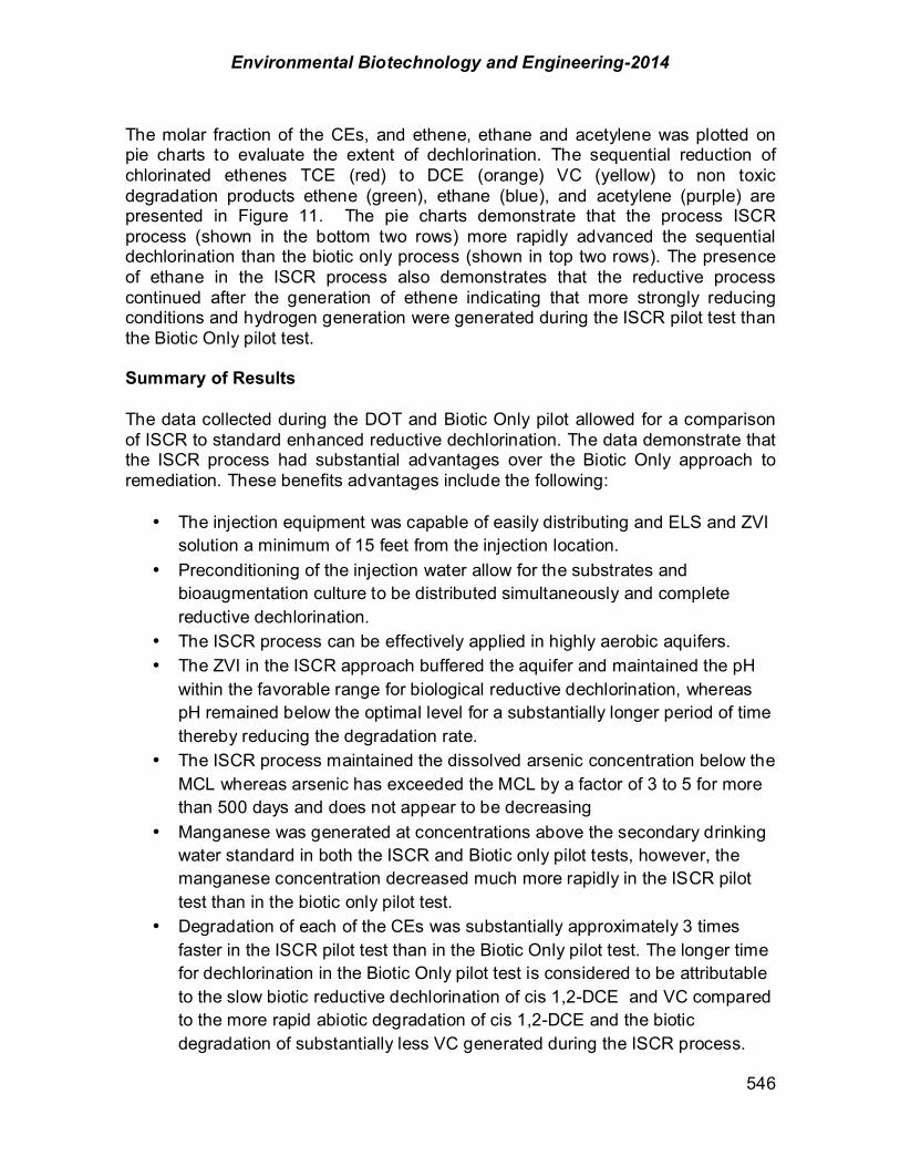
Environmental Biotechnology and Engineering-2014
546
The molar fraction of the CEs, and ethene, ethane and acetylene was plotted on pie charts to evaluate the extent of dechlorination. The sequential reduction of chlorinated ethenes TCE (red) to DCE (orange) VC (yellow) to non toxic degradation products ethene (green), ethane (blue), and acetylene (purple) are presented in Figure 11. The pie charts demonstrate that the process ISCR process (shown in the bottom two rows) more rapidly advanced the sequential dechlorination than the biotic only process (shown in top two rows). The presence of ethane in the ISCR process also demonstrates that the reductive process continued after the generation of ethene indicating that more strongly reducing conditions and hydrogen generation were generated during the ISCR pilot test than the Biotic Only pilot test. Summary of Results The data collected during the DOT and Biotic Only pilot allowed for a comparison of ISCR to standard enhanced reductive dechlorination. The data demonstrate that the ISCR process had substantial advantages over the Biotic Only approach to remediation. These benefits advantages include the following:
• The injection equipment was capable of easily distributing and ELS and ZVI solution a minimum of 15 feet from the injection location.
• Preconditioning of the injection water allow for the substrates and bioaugmentation culture to be distributed simultaneously and complete reductive dechlorination.
• The ISCR process can be effectively applied in highly aerobic aquifers. • The ZVI in the ISCR approach buffered the aquifer and maintained the pH
within the favorable range for biological reductive dechlorination, whereas pH remained below the optimal level for a substantially longer period of time thereby reducing the degradation rate.
• The ISCR process maintained the dissolved arsenic concentration below the MCL whereas arsenic has exceeded the MCL by a factor of 3 to 5 for more than 500 days and does not appear to be decreasing
• Manganese was generated at concentrations above the secondary drinking water standard in both the ISCR and Biotic only pilot tests, however, the manganese concentration decreased much more rapidly in the ISCR pilot test than in the biotic only pilot test.
• Degradation of each of the CEs was substantially approximately 3 times faster in the ISCR pilot test than in the Biotic Only pilot test. The longer time for dechlorination in the Biotic Only pilot test is considered to be attributable to the slow biotic reductive dechlorination of cis 1,2-DCE and VC compared to the more rapid abiotic degradation of cis 1,2-DCE and the biotic degradation of substantially less VC generated during the ISCR process.
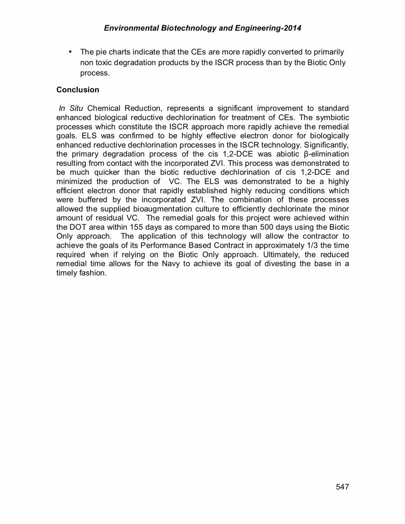
Environmental Biotechnology and Engineering-2014
547
• The pie charts indicate that the CEs are more rapidly converted to primarily non toxic degradation products by the ISCR process than by the Biotic Only process.
Conclusion In Situ Chemical Reduction, represents a significant improvement to standard enhanced biological reductive dechlorination for treatment of CEs. The symbiotic processes which constitute the ISCR approach more rapidly achieve the remedial goals. ELS was confirmed to be highly effective electron donor for biologically enhanced reductive dechlorination processes in the ISCR technology. Significantly, the primary degradation process of the cis 1,2-DCE was abiotic $-elimination resulting from contact with the incorporated ZVI. This process was demonstrated to be much quicker than the biotic reductive dechlorination of cis 1,2-DCE and minimized the production of VC. The ELS was demonstrated to be a highly efficient electron donor that rapidly established highly reducing conditions which were buffered by the incorporated ZVI. The combination of these processes allowed the supplied bioaugmentation culture to efficiently dechlorinate the minor amount of residual VC. The remedial goals for this project were achieved within the DOT area within 155 days as compared to more than 500 days using the Biotic Only approach. The application of this technology will allow the contractor to achieve the goals of its Performance Based Contract in approximately 1/3 the time required when if relying on the Biotic Only approach. Ultimately, the reduced remedial time allows for the Navy to achieve its goal of divesting the base in a timely fashion.


![Filologia dei testi a stampa, Cagliari, CUEC, 2008 [pdf integrale del volume]](https://static.fdokumen.com/doc/165x107/6324f849c9c7f5721c01d64a/filologia-dei-testi-a-stampa-cagliari-cuec-2008-pdf-integrale-del-volume.jpg)