AgroLifeScientific Journal

Volume 7, No. 2, 2018

University of Agronomic Sciencesand Veterinary Medicine of Bucharest

BucharesTDecember, 2018

AgroLifeScientific Journal

Volume 7, No. 2

EDITORIAL TEAM

General Editor: Prof. PhD Sorin Mihai CÎMPEANU Executive Editor: Prof. PhD Gina FÎNTÎNERU

Deputy Executive Editor: Prof. PhD Doru Ioan MARIN

Members: Adrian ASĂNICĂ, Lenuța Iuliana EPURE, Leonard ILIE, Viorel ION, Sorin IONIȚESCU, Ștefana JURCOANE, Monica Paula MARIN, Aneta POP, Răzvan TEODORESCU, Elena TOMA, Ana VÎRSTA

Linguistic editor: Elena NISTOR

Secretariate: Roxana FRANZUTTI

PUBLISHERS:

University of Agronomic Sciences and Veterinary Medicine of Bucharest Address: 59 Mărăşti Blvd., District 1, Postal Code 011464, Bucharest, Romania

E-mail: agrolifejournal@usamv.ro; Webpage: http://agrolifejournal.usamv.ro

CERES Publishing House Address: 29 Oastei Street, District 1, Bucharest, Romania

Phone: +40 21 317 90 23 E-mail: edituraceres@yahoo.com; Webpage:www.editura-ceres.ro

Copyright 2018 To be cited: AgroLife Sci. J. - Vol. 7, No. 2, 2018

The mission of the AgroLife Scientific Journal is to publish original research relevant to all those involved in different fields of agronomy and life sciences. The publishers are not responsible for the opinions published in the Volume.

They represent the authors’ point of view.

ISSN 2285-5718; ISSN - L 2285-5718

5

EDITORIAL BOARD Bekir Erol AK - University of Harran, Sanliurfa, Turkey Ioan Niculae ALECU - University of Agronomic Sciences and Veterinary Medicine of Bucharest, Romania Adrian ASĂNICĂ - University of Agronomic Sciences and Veterinary Medicine of Bucharest, Romania Sarah BAILLIE - Bristol Veterinary School, University of Bristol, United Kingdom Narcisa Elena BĂBEANU - University of Agronomic Sciences and Veterinary Medicine of Bucharest, Romania Silviu BECIU - University of Agronomic Sciences and Veterinary Medicine of Bucharest, Romania Diego BEGALLI - University of Verona, Italy Laurenţiu-George BENGA - Central Unit for Animal Research and Welfare Affairs at the University Hospital,

Heinrich Heine University Dusseldorf, Germany Stefano CASADEI - University of Perugia, Italy Fulvio CELICO - University of Molise, Italy Gheorghe CIMPOIEŞ - Agrarian State University, Moldova Sorin Mihai CÎMPEANU - University of Agronomic Sciences and Veterinary Medicine of Bucharest, Romania Drago CVIJANOVIC - Institute of Agricultural Economics, Belgrade, Serbia Eric DUCLOS-GENDREU - Spot Image, GEO-Information Services, France André FALISSE - University of Liège, Gembloux Agro-Bio Tech, Gembloux, Belgium Gina FÎNTÎNERU - University of Agronomic Sciences and Veterinary Medicine of Bucharest, Romania Luca Corelli GRAPPADELLI - University of Bologna, Italy Horia GROSU - University of Agronomic Sciences and Veterinary Medicine of Bucharest, Romania Armagan HAYIRLI - Ataturk University, Erzurum, Turkey Jean-Luc HORNICK - Faculté de Médecine Vétérinaire, Université de Liège, Belgium Dorel HOZA - University of Agronomic Sciences and Veterinary Medicine of Bucharest, Romania Mostafa A.R. IBRAHIM - University of Kafrelsheikh, Egypt Viorel ION - University of Agronomic Sciences and Veterinary Medicine of Bucharest, Romania Mariana IONIŢĂ - University of Agronomic Sciences and Veterinary Medicine of Bucharest, Romania Horst Erich KÖNIG - Institute of Anatomy, Histology and Embriology, University of Veterinary Medicine

Vienna, Austria Francois LAURENS - French National Institute for Agricultural Research, France Huub LELIEVELD - GHI Association Netherlands and EFFoST Executive Committee, Netherlands Doru Ioan MARIN - University of Agronomic Sciences and Veterinary Medicine of Bucharest, Romania Monica Paula MARIN - University of Agronomic Sciences and Veterinary Medicine of Bucharest, Romania Mircea MIHALACHE - University of Agronomic Sciences and Veterinary Medicine of Bucharest, Romania Françoise PICARD-BONNAUD - University of Angers, France Aneta POP - University of Agronomic Sciences and Veterinary Medicine of Bucharest, Romania Mona POPA - University of Agronomic Sciences and Veterinary Medicine of Bucharest, Romania Agatha POPESCU - University of Agronomic Sciences and Veterinary Medicine of Bucharest, Romania Sri Bandiati Komar PRAJOGA - Padjadjaran University Bandung, Indonesia Narayanan RANGESAN - University of Nevada, Reno, USA Svend RASMUSSEN - University of Copenhagen, Denmark Peter RASPOR - Faculty of Biotechnology, University of Ljubljana, Slovenia Marco Dalla ROSA - Faculty of Food Technology, Università di Bologna, Polo di Cesena, Italy Sam SAGUY - The Hebrew University of Jerusalem, Israel Philippe SIMONEAU - Université d’Angers, France Vasilica STAN - University of Agronomic Sciences and Veterinary Medicine of Bucharest, Romania Alvaro STANDARDI - University of Perugia, Italy Florin STĂNICĂ - University of Agronomic Sciences and Veterinary Medicine of Bucharest, Romania Răzvan TEODORESCU - University of Agronomic Sciences and Veterinary Medicine of Bucharest, Romania André THEWIS - University of Liège, Gembloux Agro-Bio Tech, Gembloux, Belgium Ana VÎRSTA - University of Agronomic Sciences and Veterinary Medicine of Bucharest, Romania David C. WEINDORF - Texas Tech University, USA

6

7

CONTENTS Model to estimate the optimal blooming and flowers harvesting interval in Lisianthus exaltatum in relation to vegetation period - Maria BĂLA, Cristina NAN, Olimpia IORDĂNESCU, Robert DRIENOVSKY, Florin SALA …………………………………………………………………………. 9 Heavy metals and the radioactivity in boletus (Boletus edulis), and chantarelle mushrooms (Cantharellus cibarius) in Transylvanian area - Aurelia COROIAN, Antonia ODAGIU, Zamfir MARCHIȘ, Vioara MIREȘAN, Camelia RĂDUCU, Camelia OROIAN, Adina Lia LONGODOR …. 17 Non-destructive method for determining the leaf area of the energetic poplar - Vlad-Cătălin CÂNDEA-CRĂCIUN, Ciprian RUJESCU, Dorin CAMEN, Dan MANEA, Alma L. NICOLIN, Florin SALA …………………………………………………………………………………………………….. 22 Food traceability through web and smart phone for farmer’s agriculture products in India with help of web API's technology - Keshav DANDAGE ………………………………………………….. 31 The role of native ornamental plants in ensuring the habitat needs of birds in urban ecosystems. Case study - Cismigiu Garden, Bucharest - Mirela DRAGOȘ, Angela PETRESCU, George-Laurențiu MERCIU, Cristina POSNER …………………………………………………………………. 43 The testing of some products in order to monitor the Cameraria ohridella Deschka-Dimić species (Lepidoptera: Gracilariidae) - Marilena FLORICEL, Ion MITREA, Ion OLTEAN, Teodora FLORIAN, Mircea I. VARGA, Iuliana VASIAN, Vasile C. FLORIAN, Ionuț B. HULUJAN ………… 53 Changes in fatty acids composition of Longissimus dorsi muscle, brain, liver and heartas effect to hempseed addition in pigs feeding - Mihaela HĂBEANU, Anca GHEORGHE, Mariana ROPOTĂ, Smaranda Mariana TOMA, Monica MARIN ………………………………………………………….. 61 Characterization of some walnut (Juglans regia L.) biotypes based on the biometrical and biochemical parameters of nuts - Olimpia IORDĂNESCU, Maria BĂLA, Florin SALA, Daniela SCEDEI, Melinda TOTH ……………………………………………………………………………….. 68 Trends of agricultural management in Romania - Adina Magdalena IORGA, Carina DOBRE …… 76 Do rural development measures improve vitality of rural areas in Romania? - Gabriele MACK, Gina FÎNTÎNERU, Andreas KOHLER ………………………………………………………………….. 82 Activity of peroxidase and catalase in soils as influenced by some insecticides and fungicides - MARIA-MIHAELA MICUȚI, LILIANA BĂDULESCU, AGLAIA BURLACU, FLORENTINA ISRAEL-ROMING ………………………………………………………………………………………. 99 Comparative analysis of soil tillage systems regarding economic efficiency and the conversion efficiency of energy invested in the agrosystem of winter wheat - Grigore MOLDOVAN, Teodor RUSU, Paula Ioana MORARU .................................................................................................................. 105 Extracellular laccase production in submerged culture of some white-rot fungi and their impact for textile dyes decolorisation - Gabriela POPA, Bogdan Mihai NICOLCIOIU, Radu TOMA …….. 116 Results regarding the impact of crop rotation and fertilisation on the grain yield and some plant traits at maize cultivated on sandy soils in South Romania - Marin ȘTEFAN, Dumitru GHEORGHE, Viorel ION ......................................................................................................................... 124

8

MODEL TO ESTIMATE THE OPTIMAL BLOOMING

AND FLOWERS HARVESTING INTERVAL IN Lisianthus exaltatum IN RELATION TO VEGETATION PERIOD

Maria BĂLA, Cristina NAN, Olimpia IORDĂNESCU,

Robert DRIENOVSKY, Florin SALA

Banat University of Agricultural Sciences and Veterinary Medicine „King Michael I of Romania” from Timisoara, 119 Calea Aradului Street, 300645, Timișoara, Romania,

Phone: +40 256 277091; Emails: mariabalamonicabala@yahoo.com; nan_cristina@yahoo.com; olimpia.iordanescu@yahoo.com; drienovsky_robert@yahoo.ro;

florin_sala@usab-tm.ro

Corresponding author email: florin_sala@usab-tm.ro Abstract The study followed the flowering dynamics over a 84-days vegetation period, at four genotypes of the species Lisianthus exaltatum Salisb. The biological material was represented by the Twinkles Dark Blue (TDB), Arena Series Rose (ASRose), Arena Series Red (ASRed) and Heidi Salmon (HS) genotypes. In relation to the biology of the analyzed genotypes, the vegetation period (VP) under study was of 84 days during which, five flower-counting moments were delineated at 14-days intervals, VP28, VP42, VP56, VP70 and VP84. Based on the average number of flowers open at the time of determination, the highest number of flowers was found in the TDB genotype, followed by genotypes HS, ASRose and ASRed. On the basis of the univariate statistics analysis, the highest variance was found for genotypes TDB (10.6194) and ASRose (10.24407) and a lower variance in HS genotypes (5.60978) and ASRed (5.0022), respectively. The coefficient of variation (CV) had the highest value for the ASRose genotype (CV = 111.4428), followed by the ASRed genotype (CV = 86.0215), then TDB (CV = 66.5049) and HS (CV = 62.4178), respectively. The statistical regression analysis facilitated the development of a model of a grade 3 polynomial equation and smoothing spline models (for the ASRose, ASRed and HS genotypes), models that most accurately described the flowering dynamics in relation to the vegetation period. Thus, a model of a grade 3 polynomial equation facilitated the estimation of flowering over the study period to the TDB genotype under R2 = 0.996, F = 90.681, p = 0.0770. In the other three genotypes smoothing spline models described the most accurate growth dynamics during the vegetation period under conditions of ɛi = 0.2098 at the ASRose genotype, ɛi = 0.0593 at the ASRed genotype and ɛi = 0.0607 in the HS hybrid. Clustering analysis has facilitated the classification and grouping of observational moments from the study period into two distinct, statistically safe clusters, Coph. corr = 0.899. Key words: flowers, Lisianthus, polynomial equation, smoothing spline model, vegetation period. INTRODUCTION As a relatively new crop for cut flowers, Lisianthus ranked relatively fast in the top ten in the international market, especially due to its very good post-harvest time, then it’s beautiful flowers, in the form of roses, of the colorful flowers colored in blue, but also a in wide range of floral designs such as sizes and colors available through improved genotypes (Harbaugh, 2007; Baris and Uslu, 2009; Uddin et al., 2013). With the highly diversified and improved genetic material (species, hybrids and varieties) grown predominantly for cut flowers, the importance of Lisianthus (Eustoma grandiflorum Salisb.) has increased greatly

over the last decades, also associated with consumer sensitivity and preference for these flowers, being one of the important categories for cut flowers in the US market, then Europe, Asia and Australia (Harbaugh et al., 2000; Barba-Gonzalez et al., 2017). Among the conditions of vegetation, a pronounced effect is represented by the high temperatures that cause the rosette and the con-tinuous vegetative growth of Eustoma grandiflorum. As a result, many studies have compared the behavior of the biological material represented by varieties and hybrids of the genus Lisianthus in cultivation conditions characterized especially by high temperatures (Harbaugh et al., 1992; Ohkawa et al., 1991,

Studies concerning the comparative situation of wine producers in Romania and Switzerland - Petrică ŞTEFAN, Stefan MANN ……………………………………………………………………….. 132 Physiological and metabolic responses of functional lactic acid bacteria to stress factors - Iulia-Roxana ȘTEFAN, Călina-Petruța CORNEA, Silvia-Simona GROSU-TUDOR, Medana ZAMFIR 139 Prebiotic content and probiotic effect of Kombucha fermented pollen - Elena UTOIU, Anca OANCEA, Ana-Maria STANCIUC, Laura M. ȘTEFAN, Agnes TOMA, Angela MORARU, Camelia Filofteia DIGUȚA, Florentina MATEI, Călina Petruța CORNEA, Florin OANCEA ………………… 149 Contribution to the knowledge of Transylvanian meadow’s biodiversity: short report on herbs and arthropods from Seliştat (Braşov County, Romania) - Mala-Maria STAVRESCU-BEDIVAN, Emilia Brînduşa SĂNDULESCU, Ionela DOBRIN ……………………………………………………. 157 Safflower yields and quality depending on cultivation technology in the irrigated conditions - Raisa VOZHEHOVA, Viktor USHKARENKO, Mykhailo FEDORCHUK, Pavlo LYKHOVYD, Serhii KOKOVIKHIN, Serhii VOZHEHOV …………………………………………………………………… 163

9

MODEL TO ESTIMATE THE OPTIMAL BLOOMING

AND FLOWERS HARVESTING INTERVAL IN Lisianthus exaltatum IN RELATION TO VEGETATION PERIOD

Maria BĂLA, Cristina NAN, Olimpia IORDĂNESCU,

Robert DRIENOVSKY, Florin SALA

Banat University of Agricultural Sciences and Veterinary Medicine „King Michael I of Romania” from Timisoara, 119 Calea Aradului Street, 300645, Timișoara, Romania,

Phone: +40 256 277091; Emails: mariabalamonicabala@yahoo.com; nan_cristina@yahoo.com; olimpia.iordanescu@yahoo.com; drienovsky_robert@yahoo.ro;

florin_sala@usab-tm.ro

Corresponding author email: florin_sala@usab-tm.ro Abstract The study followed the flowering dynamics over a 84-days vegetation period, at four genotypes of the species Lisianthus exaltatum Salisb. The biological material was represented by the Twinkles Dark Blue (TDB), Arena Series Rose (ASRose), Arena Series Red (ASRed) and Heidi Salmon (HS) genotypes. In relation to the biology of the analyzed genotypes, the vegetation period (VP) under study was of 84 days during which, five flower-counting moments were delineated at 14-days intervals, VP28, VP42, VP56, VP70 and VP84. Based on the average number of flowers open at the time of determination, the highest number of flowers was found in the TDB genotype, followed by genotypes HS, ASRose and ASRed. On the basis of the univariate statistics analysis, the highest variance was found for genotypes TDB (10.6194) and ASRose (10.24407) and a lower variance in HS genotypes (5.60978) and ASRed (5.0022), respectively. The coefficient of variation (CV) had the highest value for the ASRose genotype (CV = 111.4428), followed by the ASRed genotype (CV = 86.0215), then TDB (CV = 66.5049) and HS (CV = 62.4178), respectively. The statistical regression analysis facilitated the development of a model of a grade 3 polynomial equation and smoothing spline models (for the ASRose, ASRed and HS genotypes), models that most accurately described the flowering dynamics in relation to the vegetation period. Thus, a model of a grade 3 polynomial equation facilitated the estimation of flowering over the study period to the TDB genotype under R2 = 0.996, F = 90.681, p = 0.0770. In the other three genotypes smoothing spline models described the most accurate growth dynamics during the vegetation period under conditions of ɛi = 0.2098 at the ASRose genotype, ɛi = 0.0593 at the ASRed genotype and ɛi = 0.0607 in the HS hybrid. Clustering analysis has facilitated the classification and grouping of observational moments from the study period into two distinct, statistically safe clusters, Coph. corr = 0.899. Key words: flowers, Lisianthus, polynomial equation, smoothing spline model, vegetation period. INTRODUCTION As a relatively new crop for cut flowers, Lisianthus ranked relatively fast in the top ten in the international market, especially due to its very good post-harvest time, then it’s beautiful flowers, in the form of roses, of the colorful flowers colored in blue, but also a in wide range of floral designs such as sizes and colors available through improved genotypes (Harbaugh, 2007; Baris and Uslu, 2009; Uddin et al., 2013). With the highly diversified and improved genetic material (species, hybrids and varieties) grown predominantly for cut flowers, the importance of Lisianthus (Eustoma grandiflorum Salisb.) has increased greatly

over the last decades, also associated with consumer sensitivity and preference for these flowers, being one of the important categories for cut flowers in the US market, then Europe, Asia and Australia (Harbaugh et al., 2000; Barba-Gonzalez et al., 2017). Among the conditions of vegetation, a pronounced effect is represented by the high temperatures that cause the rosette and the con-tinuous vegetative growth of Eustoma grandiflorum. As a result, many studies have compared the behavior of the biological material represented by varieties and hybrids of the genus Lisianthus in cultivation conditions characterized especially by high temperatures (Harbaugh et al., 1992; Ohkawa et al., 1991,

AgroLife Scientific Journal - Volume 7, Number 2, 2018ISSN 2285-5718; ISSN CD-ROM 2285-5726; ISSN ONLINE 2286-0126; ISSN-L 2285-5718

10

1994; Bradley et al., 2000; Zaccai and Edri, 2002). For floral induction, Eustoma requires passing through a period of lower temperatures, which in cultivation conditions becomes a mandatory treatment (Li et al., 2015). Harbaugh et al. (1992) considered that a significant percentage of rosette plants that did not bloom in an acceptable period (≈140 days) are a very important factor limiting Lisianthus production with negative economic effects. Due to the increasing demand for Lisianthus in the flower market, a series of studies and improvement programs have followed the floral induction by technological and bioche-mical means, through ample processes of improvement (Harbaugh, 2007; Barba-Gonzalez et al., 2017 a, b). Using improvement programs, F1 seed hybrids were obtained with bloom uniformity throughout the year, eradication of rosettes, better heat tolerance, a larger variety of petals, flowers of varying sizes and shapes, flowers with double petals and high resistance to disease (Harbaugh, 2007). Various studies have evaluated the resistance of Lisianthus plants to Fusarium and Botrytis cinerea, the most common diseases (Harbaugh and McGovern, 2000; Wegulo and Vilchez, 2007). Modern techniques of molecular biology have led to Lisianthus various colors and perfume of different flowers, but also variable flowering time. Molecular and reproductive in vitro tech-nologies aim to increase plant post-trans-plant tolerance, heat tolerance, photo rejuvena-tion corrections through day neutrality, early flow-ering and longer flower life, increased resis-tance to Fusarium (Harbaugh, 2007; Barba-Gonzalez et al., 2017). Modern techno-logies based on biotechnology have many ad-vantages for inducing advantageous floral attri-butes in ornamental plants (Noman et al., 2017). Through interspecific crossing between Eustoma exaltatum and Eustoma grandiflorum, followed by programmed and rigorous selections, valuable hybrid forms were obtained in the following generations: F1, BC1, S1 and S2. Thus, wide variations of color were obtained based on the colors of the parents used in the breeding program, while the forms with a better heat tolerance were selected (Barba-Gonzalez et al., 2017a, b). Also by biotechnology-based methods a pigmentation

of petals and sepals in Lisianthus was obtained and induction of changes in different floral characteristics (Schwinn et al., 2014). At the same time, some significant phenotypic alterations have been reported in Lisianthus transgenic plants in terms of reducing the number of flowers and the flowering time (Zuker et al., 2001; Casanova et al., 2004; Aranovich et al., 2007; Thiruvengadam and Yang, 2009; Ruokolainen et al., 2011). Due to the dependence of Lisianthus plants on photoperiods, some studies evaluated the influence of two photoperiod regimens (long day and short day) on the floral transition to Lisianthus plants (Eustoma grandiflora (Raf) Shinn.) and highlighted the strong influence of this environmental factor on floral induction (Zaccai and Edri, 2002). The effect of the vernalization and post-vernalization process on flowering has also been studied at Eustoma grandiflorum (Nakano et al., 2011). Studies of aspects of "gene expression" for floral induction at Eustoma grandiflorum have also been performed (Nakano et al., 2011; Li et al., 2015). Aspects of growth and physiology of Lisianthus plants have been studied in relation to growing media and growth stimulators (Crăciun and Băla, 2015 a, b, 2016 a, b). The present study aimed to evaluate the flowering dynamics of some genotypes of Lisianthus exaltatum Salisb., in relation to the vegetation period. MATERIALS AND METHODS Biological material Four genotypes belonging to Lisianthus exaltatum Salisb.: Twinkles Dark Blue (TDB), Arena Series Rose (ASRose), Arena Series Red (ASRed) and Heidi Salmon (HS) represent the studied biological material. Twinkles Dark Blue (TDB) is a genotype of dark blue flowers, with large and simple petals. It has a height of up to 100 cm, being recommended for curbs or cut flowers. Arena Series Red (ASRed) is a high-quality genotype with bright red double flowers, unique for Lisianthus. The flowers have a diameter of up to 6 cm and the height of the stem is 80-100 cm; blooming is late. Arena Series Rose (ASRose) is a genotype belonging to the Lisianthus Arena Series group. The ASRose hybrid has double pink-rose flowers.

Flower stems are strong and 80-100 cm long. Heidi Salmon (HS) is a simple, large, pink-salmon-type genotype. It has early flowering, and the height of the floral stems up to 100 cm. Experimental conditions Plants of the four genotypes were grown on a substrate of 2: 3: 1 soil, peat and sand, in nutrient pots with a volume of 10 dm3. The experiments were conducted in greenhouse with controlled temperature and humidity, with the recommended germination temperature of 18-22ºC at TDB, ASRed and ASRose, respecti-vely 22-24ºC at SH. The rising temperature was reduced to 16-22ºC. Studied floral index The number of flowers opened in dynamics during the vegetation period has been studied with a total time span of 84 days. Determina-tions were made at 14-days intervals, res-pectively at 28, 42, 56, 70 and 84 days. Statistical analysis of experimental data The distribution of the number of open flowers in relation to the vegetation period of the four Lisianthus genotypes was analyzed with the statistical method in the Excel 2007 application and the PAST software (Hammer et al., 1997). The variance analysis facilitated LSD in order to compare the differences between the variants and the significance attribution in relation to LSD framing. The overall data was analyzed based on variance and coefficient of variation (CV). The behavior of the experimental data according to the vegetation period was described by polynomial models, the splines model and the database and tabular calculations. For the smoothing spline model, predictive error testing was calculated using the relationship (1), looking for the mean error value to be as close to zero.

n/

yyysn/

n

1i i

iin

1ii �

��

����

� ����

�

����

���� ��

�� (1)

The evolution of values for the number of open flowers was also described by the growth index from the fixed base Ii/1 = ysi/ys1. This index expressed the degree of multiplication and the evolution of the number of flowers at the moments of determination during the vegeta-tion period compared to the initial value, con-sidered as the fixed base. For the polynomial equation, statistical safety parameters of the identified relationship were the correlation

coefficient (R2), the statistical safety parameter p, the sample F. RESULTS AND DISCUSSIONS The experimental results on the number of opened flowers during the vegetation period for the four genotypes cultivated in similar con-ditions, revealed the differential behavior of each of them. The variation of the average number of flowers during the vegetation period, at the unit determinations, was between 0.88-8.66 for TDB genotype, 0.00-7.12 for ASRose genotype, 0.50-5.88 for ASRed genotype and 1.12-7.00 for HS genotype, detailed experimental data being shown in Tables 1-4.

Table 1. The effect of vegetation period on flowers number of Twinkles Dark Blue (TDB) genotype

Vegetation period (days)

Number of flowers Differences / Significance

28-14 3.62 4.00 -0.38

42-14 8.62 4.00 4.62***

56-14 7.88 4.00 3.88***

70-14 3.50 4.00 -0.50

84-14 0.88 4.00 -3.12ººº

42-28 8.62 3.62 5.00***

56-28 7.88 3.62 4.26***

70-28 3.50 3.62 -0.12

84-28 0.88 3.62 -2.74ººº

56-42 7.88 8.62 -0.74

79-42 3.50 8.62 -5.12ººº

84-42 0.88 8.62 -7.74ººº

70-56 3.50 7.88 -4.38ººº

84-56 0.88 7.88 -7.00ººº

84-70 0.88 3.50 -2.62ººº

LSD5% = 0.66; LSD0.1% = 0.87; LSD0.01% = 1.12

Table 2. The effect of vegetation period on flowers number of Arena Series Rose (ASRose) genotype

Vegetation period (days)

Number of flowers Differences / Significance

28-14 0.00 0.00 0.00

42-14 5.37 0.00 5.37***

56-14 7.12 0.00 7.12***

70-14 1.62 0.00 1.62***

84-14 0.25 0.00 0.25

42-28 5.37 0.00 5.37***

56-28 7.12 0.00 7.12***

70-28 1.62 0.00 1.62***

84-28 0.25 0.00 0.25

56-42 7.12 5.37 1.75***

79-42 1.62 5.37 -3.75

84-42 0.25 5.37 -5.12ººº

70-56 1.62 7.12 -5.50ººº

84-56 0.25 7.12 -6.87ººº

84-70 0.25 1.62 -1.37ººº

LSD5% = 0.66; LSD0.1% = 0.87; LSD0.01% = 1.12

11

1994; Bradley et al., 2000; Zaccai and Edri, 2002). For floral induction, Eustoma requires passing through a period of lower temperatures, which in cultivation conditions becomes a mandatory treatment (Li et al., 2015). Harbaugh et al. (1992) considered that a significant percentage of rosette plants that did not bloom in an acceptable period (≈140 days) are a very important factor limiting Lisianthus production with negative economic effects. Due to the increasing demand for Lisianthus in the flower market, a series of studies and improvement programs have followed the floral induction by technological and bioche-mical means, through ample processes of improvement (Harbaugh, 2007; Barba-Gonzalez et al., 2017 a, b). Using improvement programs, F1 seed hybrids were obtained with bloom uniformity throughout the year, eradication of rosettes, better heat tolerance, a larger variety of petals, flowers of varying sizes and shapes, flowers with double petals and high resistance to disease (Harbaugh, 2007). Various studies have evaluated the resistance of Lisianthus plants to Fusarium and Botrytis cinerea, the most common diseases (Harbaugh and McGovern, 2000; Wegulo and Vilchez, 2007). Modern techniques of molecular biology have led to Lisianthus various colors and perfume of different flowers, but also variable flowering time. Molecular and reproductive in vitro tech-nologies aim to increase plant post-trans-plant tolerance, heat tolerance, photo rejuvena-tion corrections through day neutrality, early flow-ering and longer flower life, increased resis-tance to Fusarium (Harbaugh, 2007; Barba-Gonzalez et al., 2017). Modern techno-logies based on biotechnology have many ad-vantages for inducing advantageous floral attri-butes in ornamental plants (Noman et al., 2017). Through interspecific crossing between Eustoma exaltatum and Eustoma grandiflorum, followed by programmed and rigorous selections, valuable hybrid forms were obtained in the following generations: F1, BC1, S1 and S2. Thus, wide variations of color were obtained based on the colors of the parents used in the breeding program, while the forms with a better heat tolerance were selected (Barba-Gonzalez et al., 2017a, b). Also by biotechnology-based methods a pigmentation

of petals and sepals in Lisianthus was obtained and induction of changes in different floral characteristics (Schwinn et al., 2014). At the same time, some significant phenotypic alterations have been reported in Lisianthus transgenic plants in terms of reducing the number of flowers and the flowering time (Zuker et al., 2001; Casanova et al., 2004; Aranovich et al., 2007; Thiruvengadam and Yang, 2009; Ruokolainen et al., 2011). Due to the dependence of Lisianthus plants on photoperiods, some studies evaluated the influence of two photoperiod regimens (long day and short day) on the floral transition to Lisianthus plants (Eustoma grandiflora (Raf) Shinn.) and highlighted the strong influence of this environmental factor on floral induction (Zaccai and Edri, 2002). The effect of the vernalization and post-vernalization process on flowering has also been studied at Eustoma grandiflorum (Nakano et al., 2011). Studies of aspects of "gene expression" for floral induction at Eustoma grandiflorum have also been performed (Nakano et al., 2011; Li et al., 2015). Aspects of growth and physiology of Lisianthus plants have been studied in relation to growing media and growth stimulators (Crăciun and Băla, 2015 a, b, 2016 a, b). The present study aimed to evaluate the flowering dynamics of some genotypes of Lisianthus exaltatum Salisb., in relation to the vegetation period. MATERIALS AND METHODS Biological material Four genotypes belonging to Lisianthus exaltatum Salisb.: Twinkles Dark Blue (TDB), Arena Series Rose (ASRose), Arena Series Red (ASRed) and Heidi Salmon (HS) represent the studied biological material. Twinkles Dark Blue (TDB) is a genotype of dark blue flowers, with large and simple petals. It has a height of up to 100 cm, being recommended for curbs or cut flowers. Arena Series Red (ASRed) is a high-quality genotype with bright red double flowers, unique for Lisianthus. The flowers have a diameter of up to 6 cm and the height of the stem is 80-100 cm; blooming is late. Arena Series Rose (ASRose) is a genotype belonging to the Lisianthus Arena Series group. The ASRose hybrid has double pink-rose flowers.

Flower stems are strong and 80-100 cm long. Heidi Salmon (HS) is a simple, large, pink-salmon-type genotype. It has early flowering, and the height of the floral stems up to 100 cm. Experimental conditions Plants of the four genotypes were grown on a substrate of 2: 3: 1 soil, peat and sand, in nutrient pots with a volume of 10 dm3. The experiments were conducted in greenhouse with controlled temperature and humidity, with the recommended germination temperature of 18-22ºC at TDB, ASRed and ASRose, respecti-vely 22-24ºC at SH. The rising temperature was reduced to 16-22ºC. Studied floral index The number of flowers opened in dynamics during the vegetation period has been studied with a total time span of 84 days. Determina-tions were made at 14-days intervals, res-pectively at 28, 42, 56, 70 and 84 days. Statistical analysis of experimental data The distribution of the number of open flowers in relation to the vegetation period of the four Lisianthus genotypes was analyzed with the statistical method in the Excel 2007 application and the PAST software (Hammer et al., 1997). The variance analysis facilitated LSD in order to compare the differences between the variants and the significance attribution in relation to LSD framing. The overall data was analyzed based on variance and coefficient of variation (CV). The behavior of the experimental data according to the vegetation period was described by polynomial models, the splines model and the database and tabular calculations. For the smoothing spline model, predictive error testing was calculated using the relationship (1), looking for the mean error value to be as close to zero.

n/

yyysn/

n

1i i

iin

1ii �

��

����

� ����

�

����

���� ��

�� (1)

The evolution of values for the number of open flowers was also described by the growth index from the fixed base Ii/1 = ysi/ys1. This index expressed the degree of multiplication and the evolution of the number of flowers at the moments of determination during the vegeta-tion period compared to the initial value, con-sidered as the fixed base. For the polynomial equation, statistical safety parameters of the identified relationship were the correlation

coefficient (R2), the statistical safety parameter p, the sample F. RESULTS AND DISCUSSIONS The experimental results on the number of opened flowers during the vegetation period for the four genotypes cultivated in similar con-ditions, revealed the differential behavior of each of them. The variation of the average number of flowers during the vegetation period, at the unit determinations, was between 0.88-8.66 for TDB genotype, 0.00-7.12 for ASRose genotype, 0.50-5.88 for ASRed genotype and 1.12-7.00 for HS genotype, detailed experimental data being shown in Tables 1-4.

Table 1. The effect of vegetation period on flowers number of Twinkles Dark Blue (TDB) genotype

Vegetation period (days)

Number of flowers Differences / Significance

28-14 3.62 4.00 -0.38

42-14 8.62 4.00 4.62***

56-14 7.88 4.00 3.88***

70-14 3.50 4.00 -0.50

84-14 0.88 4.00 -3.12ººº

42-28 8.62 3.62 5.00***

56-28 7.88 3.62 4.26***

70-28 3.50 3.62 -0.12

84-28 0.88 3.62 -2.74ººº

56-42 7.88 8.62 -0.74

79-42 3.50 8.62 -5.12ººº

84-42 0.88 8.62 -7.74ººº

70-56 3.50 7.88 -4.38ººº

84-56 0.88 7.88 -7.00ººº

84-70 0.88 3.50 -2.62ººº

LSD5% = 0.66; LSD0.1% = 0.87; LSD0.01% = 1.12

Table 2. The effect of vegetation period on flowers number of Arena Series Rose (ASRose) genotype

Vegetation period (days)

Number of flowers Differences / Significance

28-14 0.00 0.00 0.00

42-14 5.37 0.00 5.37***

56-14 7.12 0.00 7.12***

70-14 1.62 0.00 1.62***

84-14 0.25 0.00 0.25

42-28 5.37 0.00 5.37***

56-28 7.12 0.00 7.12***

70-28 1.62 0.00 1.62***

84-28 0.25 0.00 0.25

56-42 7.12 5.37 1.75***

79-42 1.62 5.37 -3.75

84-42 0.25 5.37 -5.12ººº

70-56 1.62 7.12 -5.50ººº

84-56 0.25 7.12 -6.87ººº

84-70 0.25 1.62 -1.37ººº

LSD5% = 0.66; LSD0.1% = 0.87; LSD0.01% = 1.12

12

Table 3. The effect of vegetation period on flowers number of Arena Series Rose (ASRose) genotype

Vegetation period (days)

Number of flowers Differences / Significance

28-14 0.50 0.25 0.25 42-14 3.00 0.25 2.75*** 56-14 5.88 0.25 5.63*** 70-14 3.12 0.25 2.87*** 84-14 0.50 0.25 0.25 42-28 3.00 0.50 2.50*** 56-28 5.88 0.50 5.38*** 70-28 3.12 0.50 2.62*** 84-28 0.50 0.50 0.00 56-42 5.88 3.00 2.88*** 79-42 3.12 3.00 0.12 84-42 0.50 3.00 -2.50ººº 70-56 3.12 5.88 -2.76ººº 84-56 0.50 5.88 -5.38ººº 84-70 0.50 3.12 -2.62ººº

LSD5% = 0.66; LSD0.1% = 0.87; LSD0.01% = 1.12

The Univariate statistical analysis eased the identification of the genotype behavior based on the experimental data obtained in terms of bloom in relation to the vegetation period. A higher variance was recorded for genotypes TDB (10.6194) and ASRose (10.24407) and a lower variance for genotypes HS (5.60978), respectively ASRed (5.0022).

Table 4. The effect of vegetation period on flowers

number of Heidi Salmon (HS) genotype

Vegetation period (days)

Number of flowers Differences / Significance

28-14 3.12 1.88 1.24*** 42-14 5.50 1.88 3.62*** 56-14 7.00 1.88 5.12*** 70-14 2.38 1.88 0.50 84-14 1.12 1.88 -0.76 42-28 5.50 3.12 2.38*** 56-28 7.00 3.12 3.88*** 70-28 2.38 3.12 -0.74 84-28 1.12 3.12 -2.00ººº 56-42 7.00 5.50 1.50*** 79-42 2.38 5.50 -3.12ººº 84-42 1.12 5.50 -4.38ººº 70-56 2.38 7.00 -4.62ººº 84-56 1.12 7.00 -5.88ººº 84-70 1.12 2.38 -1.26ººº

LSD5% = 0.66; LSD0.1% = 0.87; LSD0.01% = 1.12

The coefficient of variation, showing the non-uniformity of the analyzed parameter (flowering), had the highest value for the ASRose genotype (CV = 111.4428), followed by the ASRed genotype (CV = 86.0215), then TDB genotype (CV = 66.5049) and HS genotype (CV = 62.4178). The specific statistical analysis evaluated the interdependence between the number of

flowers and the vegetation period and eased the development of patterns of behavior for the studied genotypes in relation to time (in days). These models were of the polynomial equation and smoothing spline type. In case of TDB genotype, a model of the type polynomial equation 3rd degree, equation (2), described most accurately the blooming behavior in relation to the vegetation period, under R2 = 0.996, F = 90.681, p = 0.0770. The graphical distribution of the number of opened flowers during the vegetation period is shown in Figure 1. y = 0.0002278x3–0.04515x2+2.686x–41.24 (2) In case of ASRose genotype, the distribution of flowers in relation to the vegetation period was best described by a smoothing spline model, the values and terms of the equation being shown in Table 5, and the graphical distribution in Figure 2.

Figure 1. The distribution of the number of flowers for TDB genotype, smoothing spline model

Similarly, in case of ASRed and HS genotypes, the distribution of flowers during the vegetation period was best described by smoothing spline models, the values and terms of the equations being shown in Table 6 for ASRed and Table 7 for the HS genotype with the graphical representation in Figures 3 and 4, respectively. Multivariate analysis has eased the obtaining of a clustering group of the moments during the vegetative period with statistical safety, Coph. Corr. = 0.899.

VP28

VP42

VP56

VP70

VP84

24 32 40 48 56 64 72 80 88Days

0

1

2

3

4

5

6

7

8

9

No

Table 5. Spline - statistics of given data point for describing the variation of ASRose flower values

No xi ASRose

yi ysi ɛi Ii/1 1 28 0.5 0.568 0.137 1.000

2 42 5.37 5.438 0.013 9.567

3 56 7.12 6.644 0.067 11.690

4 70 1.62 2.095 0.293 3.685

5 84 0.25 0.115 0.540 0.202

ɛi = 0.2098

Figure 2. The distribution of the number of flowers for

ASRose genotype, smoothing spline model

Table 6. Spline - statistics of given data point for describing the variation of ASRed flower values

No xi ASRed yi ysi ɛi Ii/1

1 28 0.500 0.474 0.051 1.000 2 42 3.000 3.226 0.075 6.798 3 56 5.880 5.488 0.067 11.566 4 70 3.120 3.331 0.067 7.019 5 84 0.500 0.482 0.036 1.016 ɛi = 0.0593

Figure 3. The distribution of the number of flowers for

ASRed genotype, smoothing spline model

Table 7. Spline - statistics of given data point for describing the variation of HS flower values

No xi ASRed

yi ysi ɛi Ii/1

1 28 3.120 3.123 0.0008 1.000 2 42 5.500 5.641 0.0257 1.807 3 56 7.000 6.618 0.0546 2.119 4 70 2.380 2.712 0.1394 0.868 5 84 1.120 1.027 0.0829 0.329

ɛi = 0.0607

Figure 4. The distribution of the number of flowers for HS genotype, smoothing spline model

Two distinct clusters resulted, a C1 cluster comprising VP52 and VP56 variants of the vegetation period, with the best results on the number of open flowers and a cluster C2 with VP28 and VP70 variants and an independent position of VP84 with the smallest number of opened flowers. The graphical distribution is shown in Figure 5. From the analysis of the dendrogram with the classification of the variants given by the number of flowers at the moment of determination, it was concluded that the most efficient harvesting periods for cut flowers were VP42 and VP56. In VP28, TDB genotype with an average number of 3.62 flowers per floral stem and HS genotype with 3.12 flowers per floral stem were revealed. They are early hybrids, but with insufficient number of flowers opened at that time for profitability to be capitalized.

VP28

VP42

VP56

VP70

VP8424 32 40 48 56 64 72 80 88

Days

0.0

0.8

1.6

2.4

3.2

4.0

4.8

5.6

6.4

7.2

8.0

No

VP28

VP42

VP56

VP70

VP84

24 32 40 48 56 64 72 80 88Days

0.0

0.6

1.2

1.8

2.4

3.0

3.6

4.2

4.8

5.4

6.0

No

VP28

VP42

VP56

VP70

VP8424 32 40 48 56 64 72 80 88

Days

1.6

2.4

3.2

4.0

4.8

5.6

6.4

7.2

8.0

No

13

Table 3. The effect of vegetation period on flowers number of Arena Series Rose (ASRose) genotype

Vegetation period (days)

Number of flowers Differences / Significance

28-14 0.50 0.25 0.25 42-14 3.00 0.25 2.75*** 56-14 5.88 0.25 5.63*** 70-14 3.12 0.25 2.87*** 84-14 0.50 0.25 0.25 42-28 3.00 0.50 2.50*** 56-28 5.88 0.50 5.38*** 70-28 3.12 0.50 2.62*** 84-28 0.50 0.50 0.00 56-42 5.88 3.00 2.88*** 79-42 3.12 3.00 0.12 84-42 0.50 3.00 -2.50ººº 70-56 3.12 5.88 -2.76ººº 84-56 0.50 5.88 -5.38ººº 84-70 0.50 3.12 -2.62ººº

LSD5% = 0.66; LSD0.1% = 0.87; LSD0.01% = 1.12

The Univariate statistical analysis eased the identification of the genotype behavior based on the experimental data obtained in terms of bloom in relation to the vegetation period. A higher variance was recorded for genotypes TDB (10.6194) and ASRose (10.24407) and a lower variance for genotypes HS (5.60978), respectively ASRed (5.0022).

Table 4. The effect of vegetation period on flowers

number of Heidi Salmon (HS) genotype

Vegetation period (days)

Number of flowers Differences / Significance

28-14 3.12 1.88 1.24*** 42-14 5.50 1.88 3.62*** 56-14 7.00 1.88 5.12*** 70-14 2.38 1.88 0.50 84-14 1.12 1.88 -0.76 42-28 5.50 3.12 2.38*** 56-28 7.00 3.12 3.88*** 70-28 2.38 3.12 -0.74 84-28 1.12 3.12 -2.00ººº 56-42 7.00 5.50 1.50*** 79-42 2.38 5.50 -3.12ººº 84-42 1.12 5.50 -4.38ººº 70-56 2.38 7.00 -4.62ººº 84-56 1.12 7.00 -5.88ººº 84-70 1.12 2.38 -1.26ººº

LSD5% = 0.66; LSD0.1% = 0.87; LSD0.01% = 1.12

The coefficient of variation, showing the non-uniformity of the analyzed parameter (flowering), had the highest value for the ASRose genotype (CV = 111.4428), followed by the ASRed genotype (CV = 86.0215), then TDB genotype (CV = 66.5049) and HS genotype (CV = 62.4178). The specific statistical analysis evaluated the interdependence between the number of

flowers and the vegetation period and eased the development of patterns of behavior for the studied genotypes in relation to time (in days). These models were of the polynomial equation and smoothing spline type. In case of TDB genotype, a model of the type polynomial equation 3rd degree, equation (2), described most accurately the blooming behavior in relation to the vegetation period, under R2 = 0.996, F = 90.681, p = 0.0770. The graphical distribution of the number of opened flowers during the vegetation period is shown in Figure 1. y = 0.0002278x3–0.04515x2+2.686x–41.24 (2) In case of ASRose genotype, the distribution of flowers in relation to the vegetation period was best described by a smoothing spline model, the values and terms of the equation being shown in Table 5, and the graphical distribution in Figure 2.

Figure 1. The distribution of the number of flowers for TDB genotype, smoothing spline model

Similarly, in case of ASRed and HS genotypes, the distribution of flowers during the vegetation period was best described by smoothing spline models, the values and terms of the equations being shown in Table 6 for ASRed and Table 7 for the HS genotype with the graphical representation in Figures 3 and 4, respectively. Multivariate analysis has eased the obtaining of a clustering group of the moments during the vegetative period with statistical safety, Coph. Corr. = 0.899.

VP28

VP42

VP56

VP70

VP84

24 32 40 48 56 64 72 80 88Days

0

1

2

3

4

5

6

7

8

9

No

Table 5. Spline - statistics of given data point for describing the variation of ASRose flower values

No xi ASRose

yi ysi ɛi Ii/1 1 28 0.5 0.568 0.137 1.000

2 42 5.37 5.438 0.013 9.567

3 56 7.12 6.644 0.067 11.690

4 70 1.62 2.095 0.293 3.685

5 84 0.25 0.115 0.540 0.202

ɛi = 0.2098

Figure 2. The distribution of the number of flowers for

ASRose genotype, smoothing spline model

Table 6. Spline - statistics of given data point for describing the variation of ASRed flower values

No xi ASRed yi ysi ɛi Ii/1

1 28 0.500 0.474 0.051 1.000 2 42 3.000 3.226 0.075 6.798 3 56 5.880 5.488 0.067 11.566 4 70 3.120 3.331 0.067 7.019 5 84 0.500 0.482 0.036 1.016 ɛi = 0.0593

Figure 3. The distribution of the number of flowers for

ASRed genotype, smoothing spline model

Table 7. Spline - statistics of given data point for describing the variation of HS flower values

No xi ASRed

yi ysi ɛi Ii/1

1 28 3.120 3.123 0.0008 1.000 2 42 5.500 5.641 0.0257 1.807 3 56 7.000 6.618 0.0546 2.119 4 70 2.380 2.712 0.1394 0.868 5 84 1.120 1.027 0.0829 0.329

ɛi = 0.0607

Figure 4. The distribution of the number of flowers for HS genotype, smoothing spline model

Two distinct clusters resulted, a C1 cluster comprising VP52 and VP56 variants of the vegetation period, with the best results on the number of open flowers and a cluster C2 with VP28 and VP70 variants and an independent position of VP84 with the smallest number of opened flowers. The graphical distribution is shown in Figure 5. From the analysis of the dendrogram with the classification of the variants given by the number of flowers at the moment of determination, it was concluded that the most efficient harvesting periods for cut flowers were VP42 and VP56. In VP28, TDB genotype with an average number of 3.62 flowers per floral stem and HS genotype with 3.12 flowers per floral stem were revealed. They are early hybrids, but with insufficient number of flowers opened at that time for profitability to be capitalized.

VP28

VP42

VP56

VP70

VP8424 32 40 48 56 64 72 80 88

Days

0.0

0.8

1.6

2.4

3.2

4.0

4.8

5.6

6.4

7.2

8.0

No

VP28

VP42

VP56

VP70

VP84

24 32 40 48 56 64 72 80 88Days

0.0

0.6

1.2

1.8

2.4

3.0

3.6

4.2

4.8

5.4

6.0

No

VP28

VP42

VP56

VP70

VP8424 32 40 48 56 64 72 80 88

Days

1.6

2.4

3.2

4.0

4.8

5.6

6.4

7.2

8.0

No

14

Figure 5. Clusterial grouping of variants based on Euclidean distances, in relation to the number of flowers

during the vegetation period In VP42, TDB genotype was revealed with an average of 8.66 flowers opened on the floral stem, followed by HS genotype with an average number of 5.50 flowers/stem and ASRose with an average number of 5.37 flowers/stem, while the ASRed genotype has registered 3.00 flowers/stem. In VP56 there was the highest average number of flowers on the floral stem, 7.88 for TDB genotype, 7.12 for ASRose genotype, 7.00 for HS genotype and 5.88 for ASRed genotype. In VP70 with a higher average number of flowers there were observed TDB genotype with 3.50, ASRed genotype with 3.12, followed by HS genotype with 2.38 and ASRose genotype with 1.62. In VP84 all genotypes showed a small number of flowers ranging from 0.25 for ASRose genotype and 0.12 for HS genotype. Due to the particular vegetation requirements of Lisianthus species, as well as the increase in the interest of cultivating different genotypes, a series of studies evaluated the behavior of the biological material from germination to flowering, paying attention to the height of the plants (floral stems) to floral buds, duration to bloom, number of floral buds per plant, number of flowers per plant and flower duration to senescence (Uddin et al., 2013).

The size, color and pigmentation of petals have also been carried out in researches with particular emphasis on these cut flowers in general and especially for the Lisianthus genus (Uddin et al., 2002). The behavior of hybrids of Lisianthus grandiflorum Shinn has been studied under different conditions of nutrition without soil (Fascella et al., 2009) or the influence of Lisianthus inoculated mycorrhizals on floral indices of practical and economic interest (Meir et al., 2010). The level of nutrition of plants generally affects their growth and development, the number of flowers and their persistence (Sala, 2011). In this context, it has been studied the influence of nutritional salts upon Lisianthus plants physiological indices such as foliar surface, chlorophyll content, stem diameter, floral buds (Hernández-Pérez et al., 2016). New non-destructive methods, based on artificial intelligence, for the determination of plants’ foliar surface and their relation to various pathogens have been developed, including application to Lisianthus (Sala et al., 2015; Anitha et al., 2016; Drienovsky et al., 2017 a, b). In the present study, the uniform nutrition medium did not generate any differentiation of the flowering flow of Lisianthus plants, which was determined only by genotype in relation to the vegetation period. CONCLUSIONS The four studied Lisianthus genotypes showed a specific variation of flowering with a high average number of flowers opened at VP42 and V56, which also represents optimal harvesting and capitalization periods for cut flowers. The variation coefficient (CV) values revealed a higher variation in ASRose hybrid bloom dynamics and a reduced variation in the HS genotype, the other two having intermediate values. Bloom dynamics has been most accurately described by a polynomial 3rd grade model for TDB genotype and by smoothing spline patterns in ASRose, ASRed and HS genotypes, based on which it is possible to estimate the optimal moment of harvesting and capitalization as cut flowers.

100

97

60

97

10

9

8

7

6

5

4

3

2

1

Dis

tanc

e

VP70

VP28

VP84

VP42

VP56

ACKNOWLEDGEMENTS The authors thank to the staff of the Didactic and Research Base of the Banat University of Agricultural Sciences and Veterinary Medicine „King Michael I of Romania” from Timisoara, Romania to facilitate this research. REFERENCES Anitha K., Sharathkumar M., Kumar P.J., Jegadeeswari

V., 2016. A simple, non-destructive method of leaf area estimation in Lisianthus, Eustoma grandiflora (Raf). Shinn. Current Biotica 9 (4): p. 313-321.

Aranovich D., Lewinsohn E., Zaccai M., 2007. Post-harvest enhancement of aroma in transgenic Lisianthus (Eustoma grandiflorum) using the Clarkia breweri benzyl alcohol acetyl transferase (BEAT) gene. Postharvest Biol. and Biotech. 43: p. 255-260.

Barba-Gonzalez R., Tapia-Campos E., Lara-Bañuelos T.Y., Cepeda-Cornejo V., 2017 a. Eustoma breeding, interspecific hybridization and cytogenetics. Acta Horticulturae 1167: p. 197-204.

Barba-Gonzalez R., Tapia-Campos E., Lara-Bañuelos T.Y., Cepeda-Cornejo V., 2017 b. Lisianthus (Eustoma) breeding through interspecific hybridization. Acta Horticulturae 1171: p. 241-244.

Baris M.E., Uslu A., 2009. Cut flower production and marketing in Turkey. African Journal of Agricultural Research 4 (9): p. 765-771.

Bradley M.J., Rains R.S., Manson J.L., Davies K.M., 2000. Flower pattern stability in genetically modified Lisianthus (Eustoma grandiflorum) under commercial growing conditions. New Zeeland Journal of Crop and Horticultural Science 28 (3): p. 175-184.

Casanova E., Valdés A.E., Zuker A., Fernández B., Vainstein A., Trillas M.I., Moysset L., 2004. Rol C-transgenic carnation plants: adventitious organogenesis and levels of endogenous auxin and cytokinins. Plant Science 167 (3): p. 551-560.

Craciun (Nan) C., Băla M., 2015 a. Study of the dynamics of Lisianthus plant growth during the growing period. Journal of Horticulture, Forestry and Biotechnology 19 (2): p. 108-112.

Craciun (Nan) C., Băla M., 2015 b. Research concerning the effect of some growth stimulators on the plants height of certain Lisianthus varieties. Journal of Horticulture, Forestry and Biotechnology 19 (2): p. 103-107.

Craciun (Nan) C., Băla M., 2016 a. Study of the dynamics of Lisianthus exaltatum leaves number during the vegetation period. Journal of Horticulture, Forestry and Biotechnology 20 (2): p. 63-68.

Craciun (Nan) C., Băla M., 2016 b. Research concerning the effect of some growth stimulators on the leaves number of certain Lisianthus exaltatum varieties. Journal of Horticulture, Forestry and Biotechnology 20 (2): p. 59-62.

De Almeida J.M., Calaboni C., Rodrigues P.H.V., 2016. Lisianthus cultivation using differentiated light

transmission nets. CAMPINAS-SP 22 (2): p. 143-146.

Drienovsky R., Nicolin L.A., Rujescu C., Sala F., 2017a. Scan Leaf Area - A software application used in the determination of the foliar surface of plants. Research Journal of Agricultural Science 49 (4): p. 215-224.

Drienovsky R., Nicolin L.A., Rujescu C., Sala F., 2017b. Scan Sick & Healthy Leaf - A software application for the determination of the degree of the leaves attack. Research Journal of Agricultural Science 49 (4): p. 225-233.

Fascella G., Agnello S., Delmonte F., Sciortino B., Giardina G., 2009. Crop response of Lisianthus (Eustoma grandiflorum Shinn.) hybrids grown in soilless culture. Acta Horticulturae 807: p. 559-564.

Hammer Ø., Harper D.A.T., Ryan P.D., 2001. PAST: Paleontological statistics software package for education and data analysis. Palaeontologia Electronica 4 (1): p. 1-9.

Harbaugh B.K., Roh M.S., Lawson R.H., Pemberton B., 1992. Rosetting of Lisianthus cultivars exposed to high temperature. Hort. Science 27 (8): p. 885-887.

Harbaugh B.K., McGovern R.J., 2000. Susceptibility of forty-six Lisianthus cultivars to Fusarium crown and stem rot. Hort. Technology 10 (4): p. 816-819.

Harbaugh B.K., Bell M.L., Liang R., 2000. Evaluation of forty-seven cultivars of Lisianthus as cut flowers. Hort. Technology 10 (4): p. 812-815.

Harbaugh B.K., 2007. Lisianthus. In: Anderson N.O. (eds) Flower Breeding and Genetics. Springer, Dordrecht, p. 644-663.

Hernández-Pérez A., Valdez-Aguilar L.A., Villegas-Torres O.G., Alia-Tejacal I., Trejo-Téelez L.I., Sainz-Aispuro M. de J., 2016. Effects of ammonium and calcium on Lisianthus growth. Horticulture, Environment, and Biotechnology 57 (2): p. 123-131.

Islam N., Patil G.G., Gislerød H.R., 2005. Effect of photoperiod and light integral on flowering and growth of Eustoma grandiflorum (Raf.) Shinn. Scientia Horticulturae 103: p. 441-451.

Jivan C., Sala F., 2014. Relationship between tree nutritional status and apple quality. Horticultural Science 41 (1): p. 1-9.

Li K.-H., Chuang T.-H., Hou C.-J., Yang C.-H., 2015. Functional analysis of the FT homolog from Eustoma grandiflorum reveals its role in regulating A and C functional MADS box genes to control floral transition and flower formation. Plant Molecular Biology Reporter 33 (4): p. 770-782.

Loyola López N., Gurmán Cornejo S., 2009. Post-harvest evaluation of Lisianthus (Eustoma grandiflorum) cv. ʻHeidiʼ, destined as flower to the local market. Idesia 27 (2): p. 61-70.

Meir D., Pivonia S., Levita R., Dori I., Ganot L., Meir S., Salim S., Resnick N., Wininger S., Shlomo E., Koltai H., 2010. Application of mycorrhizae to ornamental horticultural crops: Lisianthus (Eustoma grandiflorum) as a test case. Spanish Journal of Agricultural Research 8 (S1): p. S5-S10.

Nakano Y., Kawashima H., Kinoshita T., Yoshikawa H., Hisamatsu T., 2011. Characterization of FLC, SOC1 and FT homologs in Eustoma grandiflorum: effects of vernalization and post-vernalization conditions on

15

Figure 5. Clusterial grouping of variants based on Euclidean distances, in relation to the number of flowers

during the vegetation period In VP42, TDB genotype was revealed with an average of 8.66 flowers opened on the floral stem, followed by HS genotype with an average number of 5.50 flowers/stem and ASRose with an average number of 5.37 flowers/stem, while the ASRed genotype has registered 3.00 flowers/stem. In VP56 there was the highest average number of flowers on the floral stem, 7.88 for TDB genotype, 7.12 for ASRose genotype, 7.00 for HS genotype and 5.88 for ASRed genotype. In VP70 with a higher average number of flowers there were observed TDB genotype with 3.50, ASRed genotype with 3.12, followed by HS genotype with 2.38 and ASRose genotype with 1.62. In VP84 all genotypes showed a small number of flowers ranging from 0.25 for ASRose genotype and 0.12 for HS genotype. Due to the particular vegetation requirements of Lisianthus species, as well as the increase in the interest of cultivating different genotypes, a series of studies evaluated the behavior of the biological material from germination to flowering, paying attention to the height of the plants (floral stems) to floral buds, duration to bloom, number of floral buds per plant, number of flowers per plant and flower duration to senescence (Uddin et al., 2013).

The size, color and pigmentation of petals have also been carried out in researches with particular emphasis on these cut flowers in general and especially for the Lisianthus genus (Uddin et al., 2002). The behavior of hybrids of Lisianthus grandiflorum Shinn has been studied under different conditions of nutrition without soil (Fascella et al., 2009) or the influence of Lisianthus inoculated mycorrhizals on floral indices of practical and economic interest (Meir et al., 2010). The level of nutrition of plants generally affects their growth and development, the number of flowers and their persistence (Sala, 2011). In this context, it has been studied the influence of nutritional salts upon Lisianthus plants physiological indices such as foliar surface, chlorophyll content, stem diameter, floral buds (Hernández-Pérez et al., 2016). New non-destructive methods, based on artificial intelligence, for the determination of plants’ foliar surface and their relation to various pathogens have been developed, including application to Lisianthus (Sala et al., 2015; Anitha et al., 2016; Drienovsky et al., 2017 a, b). In the present study, the uniform nutrition medium did not generate any differentiation of the flowering flow of Lisianthus plants, which was determined only by genotype in relation to the vegetation period. CONCLUSIONS The four studied Lisianthus genotypes showed a specific variation of flowering with a high average number of flowers opened at VP42 and V56, which also represents optimal harvesting and capitalization periods for cut flowers. The variation coefficient (CV) values revealed a higher variation in ASRose hybrid bloom dynamics and a reduced variation in the HS genotype, the other two having intermediate values. Bloom dynamics has been most accurately described by a polynomial 3rd grade model for TDB genotype and by smoothing spline patterns in ASRose, ASRed and HS genotypes, based on which it is possible to estimate the optimal moment of harvesting and capitalization as cut flowers.

100

97

60

97

10

9

8

7

6

5

4

3

2

1

Dis

tanc

e

VP70

VP28

VP84

VP42

VP56

ACKNOWLEDGEMENTS The authors thank to the staff of the Didactic and Research Base of the Banat University of Agricultural Sciences and Veterinary Medicine „King Michael I of Romania” from Timisoara, Romania to facilitate this research. REFERENCES Anitha K., Sharathkumar M., Kumar P.J., Jegadeeswari

V., 2016. A simple, non-destructive method of leaf area estimation in Lisianthus, Eustoma grandiflora (Raf). Shinn. Current Biotica 9 (4): p. 313-321.

Aranovich D., Lewinsohn E., Zaccai M., 2007. Post-harvest enhancement of aroma in transgenic Lisianthus (Eustoma grandiflorum) using the Clarkia breweri benzyl alcohol acetyl transferase (BEAT) gene. Postharvest Biol. and Biotech. 43: p. 255-260.

Barba-Gonzalez R., Tapia-Campos E., Lara-Bañuelos T.Y., Cepeda-Cornejo V., 2017 a. Eustoma breeding, interspecific hybridization and cytogenetics. Acta Horticulturae 1167: p. 197-204.

Barba-Gonzalez R., Tapia-Campos E., Lara-Bañuelos T.Y., Cepeda-Cornejo V., 2017 b. Lisianthus (Eustoma) breeding through interspecific hybridization. Acta Horticulturae 1171: p. 241-244.

Baris M.E., Uslu A., 2009. Cut flower production and marketing in Turkey. African Journal of Agricultural Research 4 (9): p. 765-771.

Bradley M.J., Rains R.S., Manson J.L., Davies K.M., 2000. Flower pattern stability in genetically modified Lisianthus (Eustoma grandiflorum) under commercial growing conditions. New Zeeland Journal of Crop and Horticultural Science 28 (3): p. 175-184.

Casanova E., Valdés A.E., Zuker A., Fernández B., Vainstein A., Trillas M.I., Moysset L., 2004. Rol C-transgenic carnation plants: adventitious organogenesis and levels of endogenous auxin and cytokinins. Plant Science 167 (3): p. 551-560.

Craciun (Nan) C., Băla M., 2015 a. Study of the dynamics of Lisianthus plant growth during the growing period. Journal of Horticulture, Forestry and Biotechnology 19 (2): p. 108-112.

Craciun (Nan) C., Băla M., 2015 b. Research concerning the effect of some growth stimulators on the plants height of certain Lisianthus varieties. Journal of Horticulture, Forestry and Biotechnology 19 (2): p. 103-107.

Craciun (Nan) C., Băla M., 2016 a. Study of the dynamics of Lisianthus exaltatum leaves number during the vegetation period. Journal of Horticulture, Forestry and Biotechnology 20 (2): p. 63-68.

Craciun (Nan) C., Băla M., 2016 b. Research concerning the effect of some growth stimulators on the leaves number of certain Lisianthus exaltatum varieties. Journal of Horticulture, Forestry and Biotechnology 20 (2): p. 59-62.

De Almeida J.M., Calaboni C., Rodrigues P.H.V., 2016. Lisianthus cultivation using differentiated light

transmission nets. CAMPINAS-SP 22 (2): p. 143-146.

Drienovsky R., Nicolin L.A., Rujescu C., Sala F., 2017a. Scan Leaf Area - A software application used in the determination of the foliar surface of plants. Research Journal of Agricultural Science 49 (4): p. 215-224.

Drienovsky R., Nicolin L.A., Rujescu C., Sala F., 2017b. Scan Sick & Healthy Leaf - A software application for the determination of the degree of the leaves attack. Research Journal of Agricultural Science 49 (4): p. 225-233.

Fascella G., Agnello S., Delmonte F., Sciortino B., Giardina G., 2009. Crop response of Lisianthus (Eustoma grandiflorum Shinn.) hybrids grown in soilless culture. Acta Horticulturae 807: p. 559-564.

Hammer Ø., Harper D.A.T., Ryan P.D., 2001. PAST: Paleontological statistics software package for education and data analysis. Palaeontologia Electronica 4 (1): p. 1-9.

Harbaugh B.K., Roh M.S., Lawson R.H., Pemberton B., 1992. Rosetting of Lisianthus cultivars exposed to high temperature. Hort. Science 27 (8): p. 885-887.

Harbaugh B.K., McGovern R.J., 2000. Susceptibility of forty-six Lisianthus cultivars to Fusarium crown and stem rot. Hort. Technology 10 (4): p. 816-819.

Harbaugh B.K., Bell M.L., Liang R., 2000. Evaluation of forty-seven cultivars of Lisianthus as cut flowers. Hort. Technology 10 (4): p. 812-815.

Harbaugh B.K., 2007. Lisianthus. In: Anderson N.O. (eds) Flower Breeding and Genetics. Springer, Dordrecht, p. 644-663.

Hernández-Pérez A., Valdez-Aguilar L.A., Villegas-Torres O.G., Alia-Tejacal I., Trejo-Téelez L.I., Sainz-Aispuro M. de J., 2016. Effects of ammonium and calcium on Lisianthus growth. Horticulture, Environment, and Biotechnology 57 (2): p. 123-131.

Islam N., Patil G.G., Gislerød H.R., 2005. Effect of photoperiod and light integral on flowering and growth of Eustoma grandiflorum (Raf.) Shinn. Scientia Horticulturae 103: p. 441-451.

Jivan C., Sala F., 2014. Relationship between tree nutritional status and apple quality. Horticultural Science 41 (1): p. 1-9.

Li K.-H., Chuang T.-H., Hou C.-J., Yang C.-H., 2015. Functional analysis of the FT homolog from Eustoma grandiflorum reveals its role in regulating A and C functional MADS box genes to control floral transition and flower formation. Plant Molecular Biology Reporter 33 (4): p. 770-782.

Loyola López N., Gurmán Cornejo S., 2009. Post-harvest evaluation of Lisianthus (Eustoma grandiflorum) cv. ʻHeidiʼ, destined as flower to the local market. Idesia 27 (2): p. 61-70.

Meir D., Pivonia S., Levita R., Dori I., Ganot L., Meir S., Salim S., Resnick N., Wininger S., Shlomo E., Koltai H., 2010. Application of mycorrhizae to ornamental horticultural crops: Lisianthus (Eustoma grandiflorum) as a test case. Spanish Journal of Agricultural Research 8 (S1): p. S5-S10.

Nakano Y., Kawashima H., Kinoshita T., Yoshikawa H., Hisamatsu T., 2011. Characterization of FLC, SOC1 and FT homologs in Eustoma grandiflorum: effects of vernalization and post-vernalization conditions on

16

HEAVY METALS AND THE RADIOACTIVITY IN BOLETUS (Boletus edulis), AND CHANTERELLE MUSHROOMS

(Cantharellus cibarius) IN TRANSYLVANIAN AREA

Aurelia COROIAN, Antonia ODAGIU, Zamfir MARCHIȘ, Vioara MIREȘAN, Camelia RĂDUCU, Camelia OROIAN, Adina Lia LONGODOR

University of Agricultural Sciences and Veterinary Medicine of Cluj-Napoca, Faculty of Animal Science and Biotechnologies, 3-5 Mănăştur Street, 400372

Cluj-Napoca, Romania

Corresponding author: zamfirmarchis@usamvcluj.ro

Abstract

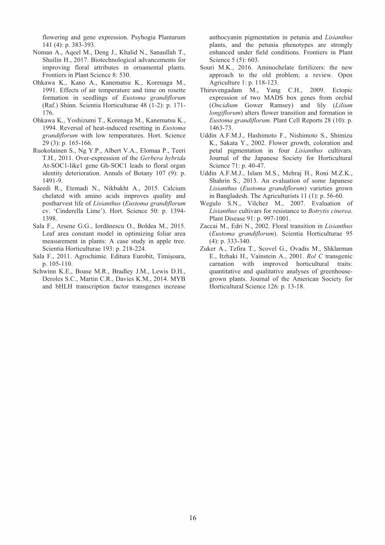
Due to the pollution from the environment, the heavy metals also contaminate the mushrooms. The pollution degree depends on several factors such as climate, area of origin, mushroom composition, humidity level, and radioactivity. Samples were collected from the following areas: Sălaj, Cluj, Braşov, Baia Mare, Satu Mare, Bistriţa-Năsăud. The content of fat, protein, humidity, heavy metal (Pb and Cd) and fungi radionuclides (Boletus edulis) and chanterelle mushrooms (Cantharellus cibarius) were evaluated. The content of Cs 137 in (Boletus edulis) built in the Baia Mare area and the lowest in the Brasov area. Cs 134 showed the lowest values in yellow sponges compared to dry boletus. Key words: Boletus edulis, Cantharellus cibarius, Pb, Cd, Cs 137, Cs 134. INTRODUCTION Heavy metals are important pollutants in the environment and can cause problems for organisms and their bioaccumulation in the food chain can have adverse effects on human health. Heavy metals can affect human health through two mechanisms: first by increasing the presence of heavy metals in the air, water, soil and food, and secondly by changing the chemical structure inside the organism (Ejazul Islam, 2007). The presence of heavy metals in the food chain has been reported in many countries and is being watched with great attention by both the population and government agencies (Ejazul Islam, 2007). The bioaccumulation of heavy metals in the agro-food chain can be extremely dangerous for human health. Edible high-cadmium mushrooms can pose a risk to the health of the consumer (Borui Liu, 2015). The mushrooms throo their composition are considered foods with nutritional benefits beneficial to the human body. It has a high content of carbohydrates, proteins, fats and minerals (Latiff et al., 1996). The mushrooms are commonly used in the diet of people suffering from various diseases, such as

hypertension, various cancers, hypercholesterolemia (Talpur et al., 2002; Jeong et al., 2010; Lavi, Friesem, Geresh, Hadar and Schwart, 2006; Sullivan, Smith and Rowan, 1998). Due to environmental pollution, environmental contaminants, such as heavy metals, are also found in living organisms. Mushrooms have the ability to assimilate the heavy metals, this aspect is greatly influenced by the environmental factors, the area, the chemical composition of the mushrooms (Garcia, Alonso, Fernández and Melgar, 1998). Due to the fact that the possibility of assimilation of heavy metals is high, the competent authorities in the field of food safety require that these parameters to be determined when the mushrooms are marketed as a raw material for obtaining different mushroom products. A high level of heavy metals may present a toxicological aspect for consumers (Garcia et al., 1998; Zhu et al., 2011). The climate in Transylvania is favorable to the development of edible wild mushrooms in this part of Romania. The rains in the summer and autumn periods favor a high production of wild edible mushrooms. The legumes in addition to components such as proteins, vitamins, iron,

flowering and gene expression. Psyhogia Plantarum 141 (4): p. 383-393.

Noman A., Aqeel M., Deng J., Khalid N., Sanaullah T., Shuilin H., 2017. Biotechnological advancements for improving floral attributes in ornamental plants. Frontiers in Plant Science 8: 530.

Ohkawa K., Kano A., Kanematsu K., Korenaga M., 1991. Effects of air temperature and time on rosette formation in seedlings of Eustoma grandiflorum (Raf.) Shinn. Scientia Horticulturae 48 (1-2): p. 171-176.

Ohkawa K., Yoshizumi T., Korenaga M., Kanematsu K., 1994. Reversal of heat-induced resetting in Eustoma grandiflorum with low temperatures. Hort. Science 29 (3): p. 165-166.

Ruokolainen S., Ng Y.P., Albert V.A., Elomaa P., Teeri T.H., 2011. Over-expression of the Gerbera hybrida At-SOC1-like1 gene Gh-SOC1 leads to floral organ identity deterioration. Annals of Botany 107 (9): p. 1491-9.

Saeedi R., Etemadi N., Nikbakht A., 2015. Calcium chelated with amino acids improves quality and postharvest life of Lisianthus (Eustoma grandiflorum cv. ʻCinderella Limeʼ). Hort. Science 50: p. 1394-1398.

Sala F., Arsene G.G., Iordănescu O., Boldea M., 2015. Leaf area constant model in optimizing foliar area measurement in plants: A case study in apple tree. Scientia Horticulturae 193: p. 218-224.

Sala F., 2011. Agrochimie. Editura Eurobit, Timișoara, p. 105-110.

Schwinn K.E., Boase M.R., Bradley J.M., Lewis D.H., Deroles S.C., Martin C.R., Davies K.M., 2014. MYB and bHLH transcription factor transgenes increase

anthocyanin pigmentation in petunia and Lisianthus plants, and the petunia phenotypes are strongly enhanced under field conditions. Frontiers in Plant Science 5 (5): 603.

Souri M.K., 2016. Aminochelate fertilizers: the new approach to the old problem; a review. Open Agriculture 1: p. 118-123.

Thiruvengadam M., Yang C.H., 2009. Ectopic expression of two MADS box genes from orchid (Oncidium Gower Ramsey) and lily (Lilium longiflorum) alters flower transition and formation in Eustoma grandiflorum. Plant Cell Reports 28 (10): p. 1463-73.

Uddin A.F.M.J., Hashimoto F., Nishimoto S., Shimizu K., Sakata Y., 2002. Flower growth, coloration and petal pigmentation in four Lisianthus cultivars. Journal of the Japanese Society for Horticultural Science 71: p. 40-47.

Uddin A.F.M.J., Islam M.S., Mehraj H., Roni M.Z.K., Shahrin S., 2013. An evaluation of some Japanese Lisianthus (Eustoma grandiflorum) varieties grown in Bangladesh. The Agriculturists 11 (1): p. 56-60.

Wegulo S.N., Vilchez M., 2007. Evaluation of Lisianthus cultivars for resistance to Botrytis cinerea. Plant Disease 91: p. 997-1001.

Zaccai M., Edri N., 2002. Floral transition in Lisianthus (Eustoma grandiflorum). Scientia Horticulturae 95 (4): p. 333-340.

Zuker A., Tzfira T., Scovel G., Ovadis M., Shklarman E., Itzhaki H., Vainstein A., 2001. Rol C transgenic carnation with improved horticultural traits: quantitative and qualitative analyses of greenhouse-grown plants. Journal of the American Society for Horticultural Science 126: p. 13-18.

17

HEAVY METALS AND THE RADIOACTIVITY IN BOLETUS (Boletus edulis), AND CHANTERELLE MUSHROOMS

(Cantharellus cibarius) IN TRANSYLVANIAN AREA

Aurelia COROIAN, Antonia ODAGIU, Zamfir MARCHIȘ, Vioara MIREȘAN, Camelia RĂDUCU, Camelia OROIAN, Adina Lia LONGODOR

University of Agricultural Sciences and Veterinary Medicine of Cluj-Napoca, Faculty of Animal Science and Biotechnologies, 3-5 Mănăştur Street, 400372

Cluj-Napoca, Romania

Corresponding author: zamfirmarchis@usamvcluj.ro

Abstract

Due to the pollution from the environment, the heavy metals also contaminate the mushrooms. The pollution degree depends on several factors such as climate, area of origin, mushroom composition, humidity level, and radioactivity. Samples were collected from the following areas: Sălaj, Cluj, Braşov, Baia Mare, Satu Mare, Bistriţa-Năsăud. The content of fat, protein, humidity, heavy metal (Pb and Cd) and fungi radionuclides (Boletus edulis) and chanterelle mushrooms (Cantharellus cibarius) were evaluated. The content of Cs 137 in (Boletus edulis) built in the Baia Mare area and the lowest in the Brasov area. Cs 134 showed the lowest values in yellow sponges compared to dry boletus. Key words: Boletus edulis, Cantharellus cibarius, Pb, Cd, Cs 137, Cs 134. INTRODUCTION Heavy metals are important pollutants in the environment and can cause problems for organisms and their bioaccumulation in the food chain can have adverse effects on human health. Heavy metals can affect human health through two mechanisms: first by increasing the presence of heavy metals in the air, water, soil and food, and secondly by changing the chemical structure inside the organism (Ejazul Islam, 2007). The presence of heavy metals in the food chain has been reported in many countries and is being watched with great attention by both the population and government agencies (Ejazul Islam, 2007). The bioaccumulation of heavy metals in the agro-food chain can be extremely dangerous for human health. Edible high-cadmium mushrooms can pose a risk to the health of the consumer (Borui Liu, 2015). The mushrooms throo their composition are considered foods with nutritional benefits beneficial to the human body. It has a high content of carbohydrates, proteins, fats and minerals (Latiff et al., 1996). The mushrooms are commonly used in the diet of people suffering from various diseases, such as

hypertension, various cancers, hypercholesterolemia (Talpur et al., 2002; Jeong et al., 2010; Lavi, Friesem, Geresh, Hadar and Schwart, 2006; Sullivan, Smith and Rowan, 1998). Due to environmental pollution, environmental contaminants, such as heavy metals, are also found in living organisms. Mushrooms have the ability to assimilate the heavy metals, this aspect is greatly influenced by the environmental factors, the area, the chemical composition of the mushrooms (Garcia, Alonso, Fernández and Melgar, 1998). Due to the fact that the possibility of assimilation of heavy metals is high, the competent authorities in the field of food safety require that these parameters to be determined when the mushrooms are marketed as a raw material for obtaining different mushroom products. A high level of heavy metals may present a toxicological aspect for consumers (Garcia et al., 1998; Zhu et al., 2011). The climate in Transylvania is favorable to the development of edible wild mushrooms in this part of Romania. The rains in the summer and autumn periods favor a high production of wild edible mushrooms. The legumes in addition to components such as proteins, vitamins, iron,

flowering and gene expression. Psyhogia Plantarum 141 (4): p. 383-393.

Noman A., Aqeel M., Deng J., Khalid N., Sanaullah T., Shuilin H., 2017. Biotechnological advancements for improving floral attributes in ornamental plants. Frontiers in Plant Science 8: 530.

Ohkawa K., Kano A., Kanematsu K., Korenaga M., 1991. Effects of air temperature and time on rosette formation in seedlings of Eustoma grandiflorum (Raf.) Shinn. Scientia Horticulturae 48 (1-2): p. 171-176.

Ohkawa K., Yoshizumi T., Korenaga M., Kanematsu K., 1994. Reversal of heat-induced resetting in Eustoma grandiflorum with low temperatures. Hort. Science 29 (3): p. 165-166.

Ruokolainen S., Ng Y.P., Albert V.A., Elomaa P., Teeri T.H., 2011. Over-expression of the Gerbera hybrida At-SOC1-like1 gene Gh-SOC1 leads to floral organ identity deterioration. Annals of Botany 107 (9): p. 1491-9.

Saeedi R., Etemadi N., Nikbakht A., 2015. Calcium chelated with amino acids improves quality and postharvest life of Lisianthus (Eustoma grandiflorum cv. ʻCinderella Limeʼ). Hort. Science 50: p. 1394-1398.

Sala F., Arsene G.G., Iordănescu O., Boldea M., 2015. Leaf area constant model in optimizing foliar area measurement in plants: A case study in apple tree. Scientia Horticulturae 193: p. 218-224.

Sala F., 2011. Agrochimie. Editura Eurobit, Timișoara, p. 105-110.

Schwinn K.E., Boase M.R., Bradley J.M., Lewis D.H., Deroles S.C., Martin C.R., Davies K.M., 2014. MYB and bHLH transcription factor transgenes increase

anthocyanin pigmentation in petunia and Lisianthus plants, and the petunia phenotypes are strongly enhanced under field conditions. Frontiers in Plant Science 5 (5): 603.

Souri M.K., 2016. Aminochelate fertilizers: the new approach to the old problem; a review. Open Agriculture 1: p. 118-123.

Thiruvengadam M., Yang C.H., 2009. Ectopic expression of two MADS box genes from orchid (Oncidium Gower Ramsey) and lily (Lilium longiflorum) alters flower transition and formation in Eustoma grandiflorum. Plant Cell Reports 28 (10): p. 1463-73.

Uddin A.F.M.J., Hashimoto F., Nishimoto S., Shimizu K., Sakata Y., 2002. Flower growth, coloration and petal pigmentation in four Lisianthus cultivars. Journal of the Japanese Society for Horticultural Science 71: p. 40-47.

Uddin A.F.M.J., Islam M.S., Mehraj H., Roni M.Z.K., Shahrin S., 2013. An evaluation of some Japanese Lisianthus (Eustoma grandiflorum) varieties grown in Bangladesh. The Agriculturists 11 (1): p. 56-60.

Wegulo S.N., Vilchez M., 2007. Evaluation of Lisianthus cultivars for resistance to Botrytis cinerea. Plant Disease 91: p. 997-1001.

Zaccai M., Edri N., 2002. Floral transition in Lisianthus (Eustoma grandiflorum). Scientia Horticulturae 95 (4): p. 333-340.

Zuker A., Tzfira T., Scovel G., Ovadis M., Shklarman E., Itzhaki H., Vainstein A., 2001. Rol C transgenic carnation with improved horticultural traits: quantitative and qualitative analyses of greenhouse-grown plants. Journal of the American Society for Horticultural Science 126: p. 13-18.

AgroLife Scientific Journal - Volume 7, Number 2, 2018ISSN 2285-5718; ISSN CD-ROM 2285-5726; ISSN ONLINE 2286-0126; ISSN-L 2285-5718

18

calcium can also contain toxic substances on a wide range of concentrations. The studies in this field show the fact that the accumulation of metals in vegetables can be a direct threat to the human organism (Turkdogan et al., 2003). It has been reported that ingested metals (lead, cadmium, mercury), more than half, come from food of vegetable origin (vegetables, fruits, cereals, mushrooms). There are several factors that influence the toxicity threshold of heavy metals in the soil-culture system, such as soil type, soil pH, organic matter content, as well as other chemical and biochemical soil parameters. At present, agronomic practices are being pursued in order to minimize the availability of heavy metals in the soil. These practices aim to use organic matter and changing the pH. Such programs can be used in certain areas where heavy metals pollution is not expanded (Ejazul Islam et al., 2007). Heavy metals are potential contaminants for the environment and for human health and can cause problems for the consumer. At present, throughout the world there is a lot of attention to them, because they can have toxic effects even at quite low limits (Das, 1990). Thus, there have been reports of various human diseases, disorders, malformations due to metal toxicity (Jarup, 2003). Lead can reach the human body by eating food or drinking water containing lead (from the water pipes that were glued with lead); by using care products, from air and water. Lead can affect almost every organ in the body. It mainly affects the nervous system in both children and adults. Long-term exposure to lead acts to: increased blood pressure, can lead to anemia in the elderly; to decrease the performance of the nervous system, ankles and sensitive wrists; can damage the kidneys. In the case of pregnant women exposed to high amounts of lead, it can lead to spontaneous abortions (ATSDR, 2007). For some heavy metals the cumulative effect is the most significant property, and this effect is met at Hg, Cd, Pb, their toxicity is triggered in the moment of accumulation of a certain amount that can release extremely serious illnesses and irreversible consequences (Helferich, 2001). The purpose of this paper was to evaluate the

levels of Pb, Cd, Cs 134 and Cs 137 from wild edible mushrooms (Boletus edulis, Cantharellus cibarius) from 6 areas in Transylvania.

MATERIALS AND METHODS A total of 5 samples of dried Boletus (Boletus edulis) and 5 samples of dried chanterelle mushrooms (Cantharellus cibarius) were collected for each area from Transylvania (Cluj, Brasov, Sălaj, Satu Mare, Baia Mare and Bistriţa-Năsăud). The samples were dried before performing the analyzes. The following parameters were analyzed: physicochemical parameters (fat, protein and humidity). Fat and protein was analyzed by the Soxhlet and Gerber method. The humidity was determined according to SR ISO 24557. The microbiological parameters analyzed are: (Salmonella spp. according to SR ISO 16649-2: 2007; NTG-SR EN ISO 4833: 2003; Enterobacteriaceae SR ISO 21528-2:2007; Yeasts and molds SR ISO 21527-2:2009). Lead was determined according to SR EN 14082: 2003; LOD - 0.05 mg/kg; LOQ - 0.1 mg/kg. The cadmium was analyzed according to SR-EN 14082:2008, LOD - 0.02 mg/kg; LOQ -0.04 mg/kg. Atomic Absorption Spectrometry SAA (AAS) for Lead and Cadmium Level Analysis (Boletus edulis and Cantharellus cibarius), Cs 137 and Cs 134 Radionuclides were analyzed using gamma-ray spectrometry. RESULTS AND DISCUSSIONS The results obtained for the edible wild mushrooms from the Transylvanian areal has shown a similar level of the analized heavy metals with the levels found in literature. Table 1 presents the mean values and variability for Cs 137 and Cs 134 of Boletus edulis in different areas of Transylvania. Cs 137 in Boletus edulis varied thus 18.2 ± 1.15 for the analyzed samples from the Cluj area and 44.12 ± 2.03 to those in the Baia Mare area. This is also influenced by the pollution in this area. High values for Cs 137 showed also the

samples analyzed in the Satu Mare area (38.20 ± 1.06). Increased values for Cs 137 in Boletus edulis are also observed in the Bistriţa-Năsăud area (26.32 ± 1.72), followed by Sălaj (21.32 ± 0.84). The area with the lowest Cs 137 content is Braşov (12.9 ± 0.99), being considered a less polluted area compared to other areas (Table 1).

Table 1. The Cs 137 and Cs 134 content in dried boletus (Boletus edulis) colected from different areas

of Transylvania Area Cs 137 Cs 134

X±sx V% X±sx V% Cluj 18.2±1.15 14.09 2.65±0.27 23.08

Braşov 12.9±0.99 17.18 2.90±0.13 10.24 Sălaj 21.32±0.84 8.85 7.02±0.35 11.10

Satu Mare 38.20±1.06 6.21 6.34±0.25 8.98 Baia Mare 44.12±2.03 10.30 8.54±0.22 5.86 Bistriţa- Năsăud

26.32±1.72 14.61 2.38±0.20 19.01

All values are mean ± SD; n = 5. Cs 134, similar to Cs 137, show the highest average values in the Baia Mare, Sălaj and Satu Mare areas. Cs 134, shows the lowest values (2.38 ± 0.20) in Bistriţa Năsăud and the highest (8.54 ± 0.22) in Baia Mare. Aspects signaled in the literature regarding the degree of conta-mination in Baia Mare and Satu Mare are also observed in the results presented in Table 1.

Table 2. The Pb and Cd levels in dried boletus (Boletus edulis) colected from different areas in Transylvania

Area Pb (mg/kg) Cd (mg/kg) X±sx V% X±sx V%

Cluj 0.17±0.03 32.37 0.18±0.01 13.41 Braşov 0.15±0.01 14.65 0.12±0.01 21.08

Sălaj 0.24±0.03 29.75 1.17±0.04 6.86 Satu Mare 0.28±0.02 5.62 1.26±0.14 24.40 Baia Mare 0.34±0.01 5.62 1.32±0.01 2.53

Bistriţa-Năsăud 0.19±0.02 20.16 0.78±0.05 14.09

All values are mean±SD; n = 5. Table 2 presents the average values and the variability of the content of Pb and Cd in dried Boletus edulis in different areas of Transylvania. The highest content of Pb and Cd is in Satu Mare, Baia Mare and the lowest in Braşov and Cluj. The level of Pb in Boletus edulis thus varied to 0.15 ± 0.01 in Braşov and 0.34 ± 0.01 in the Baia Mare area. High values were also observed in the Satu Mare area (0.28 ± 0.02) followed by Sălaj (0.24 ± 0.03). Cd showed the highest level (1.32 ± 0.01) in Baia Mare, followed by Satu Mare (1.26 ± 0.14) and Sălaj (1.17 ± 0.04). The lowest values are in the Bistriţa-Năsăud area (0.78 ± 0.05), followed by Cluj (0.18 ± 0.01) and Braşov (0.12 ± 0.01)..

Table 3. Humidity in dried boletus (Boletus edulis) colected from different areas in Transylvania

Colection area

Parameter

Baia Mare Cluj Braşov Sălaj Satu Mare Bistriţa-Năsăud

X±sx V% X±sx V% X±sx V% X±sx V% X±sx V% X±sx V%

Fat 0.44±0.02 11.72 0.46±0.02 7.61 0.43±0.02 9.26 0.41±0.01 7.90 0.42±0.02 8.42 0.41±0.01 7.51

Protein 2.86±0.04 3.10 2.92±0.02 1.72 2.70±0.06 4.83 2.74±0.06 5.22 2.82±0.05 3.57 2.60±0.07 5.99

Humidity 16.61±0.44 5.93 16.44±0.60 8.20 15.41±0.33 4.85 17.08±0.33 4.37 17.71±0.14 1.79 14.35±0.24 3.67

All values are mean±SD; n = 5. Table 3 shows the fat, protein and moisture content of Boletus edulis from different areas of Transylvania. The fat varied in the range 0.41 ± 0.01 for Boletus edulis in the Bistriţa-Năsăud and Sălaj area and 0.46 ± 0.02 in the Cluj area. The protein presented the lowest average values for the samples in the Bistriţa-

Năsăud area (2.60 ± 0.07) the higher values are in Cluj area (2.92 ± 0.02). The humidity varied in the range 14.35 ± 0.24 of Bistriţa-Năsăud and 17.71 ± 0.14 in Satu Mare. Table 4 shows the microbiological parameters of Boletus edulis of the collection area.

19

calcium can also contain toxic substances on a wide range of concentrations. The studies in this field show the fact that the accumulation of metals in vegetables can be a direct threat to the human organism (Turkdogan et al., 2003). It has been reported that ingested metals (lead, cadmium, mercury), more than half, come from food of vegetable origin (vegetables, fruits, cereals, mushrooms). There are several factors that influence the toxicity threshold of heavy metals in the soil-culture system, such as soil type, soil pH, organic matter content, as well as other chemical and biochemical soil parameters. At present, agronomic practices are being pursued in order to minimize the availability of heavy metals in the soil. These practices aim to use organic matter and changing the pH. Such programs can be used in certain areas where heavy metals pollution is not expanded (Ejazul Islam et al., 2007). Heavy metals are potential contaminants for the environment and for human health and can cause problems for the consumer. At present, throughout the world there is a lot of attention to them, because they can have toxic effects even at quite low limits (Das, 1990). Thus, there have been reports of various human diseases, disorders, malformations due to metal toxicity (Jarup, 2003). Lead can reach the human body by eating food or drinking water containing lead (from the water pipes that were glued with lead); by using care products, from air and water. Lead can affect almost every organ in the body. It mainly affects the nervous system in both children and adults. Long-term exposure to lead acts to: increased blood pressure, can lead to anemia in the elderly; to decrease the performance of the nervous system, ankles and sensitive wrists; can damage the kidneys. In the case of pregnant women exposed to high amounts of lead, it can lead to spontaneous abortions (ATSDR, 2007). For some heavy metals the cumulative effect is the most significant property, and this effect is met at Hg, Cd, Pb, their toxicity is triggered in the moment of accumulation of a certain amount that can release extremely serious illnesses and irreversible consequences (Helferich, 2001). The purpose of this paper was to evaluate the

levels of Pb, Cd, Cs 134 and Cs 137 from wild edible mushrooms (Boletus edulis, Cantharellus cibarius) from 6 areas in Transylvania.

MATERIALS AND METHODS A total of 5 samples of dried Boletus (Boletus edulis) and 5 samples of dried chanterelle mushrooms (Cantharellus cibarius) were collected for each area from Transylvania (Cluj, Brasov, Sălaj, Satu Mare, Baia Mare and Bistriţa-Năsăud). The samples were dried before performing the analyzes. The following parameters were analyzed: physicochemical parameters (fat, protein and humidity). Fat and protein was analyzed by the Soxhlet and Gerber method. The humidity was determined according to SR ISO 24557. The microbiological parameters analyzed are: (Salmonella spp. according to SR ISO 16649-2: 2007; NTG-SR EN ISO 4833: 2003; Enterobacteriaceae SR ISO 21528-2:2007; Yeasts and molds SR ISO 21527-2:2009). Lead was determined according to SR EN 14082: 2003; LOD - 0.05 mg/kg; LOQ - 0.1 mg/kg. The cadmium was analyzed according to SR-EN 14082:2008, LOD - 0.02 mg/kg; LOQ -0.04 mg/kg. Atomic Absorption Spectrometry SAA (AAS) for Lead and Cadmium Level Analysis (Boletus edulis and Cantharellus cibarius), Cs 137 and Cs 134 Radionuclides were analyzed using gamma-ray spectrometry. RESULTS AND DISCUSSIONS The results obtained for the edible wild mushrooms from the Transylvanian areal has shown a similar level of the analized heavy metals with the levels found in literature. Table 1 presents the mean values and variability for Cs 137 and Cs 134 of Boletus edulis in different areas of Transylvania. Cs 137 in Boletus edulis varied thus 18.2 ± 1.15 for the analyzed samples from the Cluj area and 44.12 ± 2.03 to those in the Baia Mare area. This is also influenced by the pollution in this area. High values for Cs 137 showed also the

samples analyzed in the Satu Mare area (38.20 ± 1.06). Increased values for Cs 137 in Boletus edulis are also observed in the Bistriţa-Năsăud area (26.32 ± 1.72), followed by Sălaj (21.32 ± 0.84). The area with the lowest Cs 137 content is Braşov (12.9 ± 0.99), being considered a less polluted area compared to other areas (Table 1).

Table 1. The Cs 137 and Cs 134 content in dried boletus (Boletus edulis) colected from different areas

of Transylvania Area Cs 137 Cs 134

X±sx V% X±sx V% Cluj 18.2±1.15 14.09 2.65±0.27 23.08

Braşov 12.9±0.99 17.18 2.90±0.13 10.24 Sălaj 21.32±0.84 8.85 7.02±0.35 11.10

Satu Mare 38.20±1.06 6.21 6.34±0.25 8.98 Baia Mare 44.12±2.03 10.30 8.54±0.22 5.86 Bistriţa- Năsăud

26.32±1.72 14.61 2.38±0.20 19.01

All values are mean ± SD; n = 5. Cs 134, similar to Cs 137, show the highest average values in the Baia Mare, Sălaj and Satu Mare areas. Cs 134, shows the lowest values (2.38 ± 0.20) in Bistriţa Năsăud and the highest (8.54 ± 0.22) in Baia Mare. Aspects signaled in the literature regarding the degree of conta-mination in Baia Mare and Satu Mare are also observed in the results presented in Table 1.

Table 2. The Pb and Cd levels in dried boletus (Boletus edulis) colected from different areas in Transylvania

Area Pb (mg/kg) Cd (mg/kg) X±sx V% X±sx V%

Cluj 0.17±0.03 32.37 0.18±0.01 13.41 Braşov 0.15±0.01 14.65 0.12±0.01 21.08

Sălaj 0.24±0.03 29.75 1.17±0.04 6.86 Satu Mare 0.28±0.02 5.62 1.26±0.14 24.40 Baia Mare 0.34±0.01 5.62 1.32±0.01 2.53

Bistriţa-Năsăud 0.19±0.02 20.16 0.78±0.05 14.09

All values are mean±SD; n = 5. Table 2 presents the average values and the variability of the content of Pb and Cd in dried Boletus edulis in different areas of Transylvania. The highest content of Pb and Cd is in Satu Mare, Baia Mare and the lowest in Braşov and Cluj. The level of Pb in Boletus edulis thus varied to 0.15 ± 0.01 in Braşov and 0.34 ± 0.01 in the Baia Mare area. High values were also observed in the Satu Mare area (0.28 ± 0.02) followed by Sălaj (0.24 ± 0.03). Cd showed the highest level (1.32 ± 0.01) in Baia Mare, followed by Satu Mare (1.26 ± 0.14) and Sălaj (1.17 ± 0.04). The lowest values are in the Bistriţa-Năsăud area (0.78 ± 0.05), followed by Cluj (0.18 ± 0.01) and Braşov (0.12 ± 0.01)..

Table 3. Humidity in dried boletus (Boletus edulis) colected from different areas in Transylvania

Colection area

Parameter

Baia Mare Cluj Braşov Sălaj Satu Mare Bistriţa-Năsăud

X±sx V% X±sx V% X±sx V% X±sx V% X±sx V% X±sx V%

Fat 0.44±0.02 11.72 0.46±0.02 7.61 0.43±0.02 9.26 0.41±0.01 7.90 0.42±0.02 8.42 0.41±0.01 7.51

Protein 2.86±0.04 3.10 2.92±0.02 1.72 2.70±0.06 4.83 2.74±0.06 5.22 2.82±0.05 3.57 2.60±0.07 5.99

Humidity 16.61±0.44 5.93 16.44±0.60 8.20 15.41±0.33 4.85 17.08±0.33 4.37 17.71±0.14 1.79 14.35±0.24 3.67

All values are mean±SD; n = 5. Table 3 shows the fat, protein and moisture content of Boletus edulis from different areas of Transylvania. The fat varied in the range 0.41 ± 0.01 for Boletus edulis in the Bistriţa-Năsăud and Sălaj area and 0.46 ± 0.02 in the Cluj area. The protein presented the lowest average values for the samples in the Bistriţa-

Năsăud area (2.60 ± 0.07) the higher values are in Cluj area (2.92 ± 0.02). The humidity varied in the range 14.35 ± 0.24 of Bistriţa-Năsăud and 17.71 ± 0.14 in Satu Mare. Table 4 shows the microbiological parameters of Boletus edulis of the collection area.

20

Table 4. Microbiological parameters from dried boletus (Boletus edulis) colected from different areas of Transylvania Colection area

Parameter Baia Mare Cluj Braşov Sălaj Satu Mare Bistriţa-Năsăud

Salmonella spp. Absent/25 g Absent/25 g Absent/25 g Absent/25 g Absent/25 g Absent/25 g E. coli beta gluc. Positive <10 ufc/g <10 ufc/g <10 ufc/g <10 ufc/g <10 ufc/g <10 ufc/g

TGN 1.3 E+3 ufc/g 1.2E+3 ufc/g 1.5 E+3 ufc/g 1.3 E+3 ufc/g 1.7E+3 ufc/g 1.2E+3 ufc/g Enterobacteriaceae <10 ufc/g <10 ufc/g <10 ufc/g <10 ufc/g <10 ufc/g <10 ufc/g Yeasts and molds <100 ufc/g <100 ufc/g <100 ufc/g <100 ufc/g <100 ufc/g <100 ufc/g

Table 5. The content of Cs 137 and Cs 134 from dried chanterelle mushrooms (Cantharellus cibarius)

collected from different areas Area Cs 137 Cs 134

X±sx V% X±sx V% Cluj 17.38±0.77 9.97 1.50±0.16 23.37

Braşov 18.61±0.44 5.33 1.25±0.09 16.90 Sălaj 24.28±0.39 3.57 4.57±0.36 17.56

Satu Mare 32.40±1.37 9.44 7.08±0.40 12.77 Baia Mare 34.98±0.87 5.56 7.84±0.44 12.48 Bistriţa- Năsăud

22.48±0.98 9.77 1.88±0.17 20.69

All values are mean±SD; n = 5. Table 5 shows the average level and variability for Cs 137 and Cs 134 from dried chanterelle mushrooms. The Baia Mare, Satu Mare and Sălaj areas showed the highest average values for Cs 137, respectively 34.98 ± 0.87 in Baia Mare and the lowest in Sălaj (24.28 ± 0.39). The lowest values can be observed in Cluj, Braşov and Bistriţa-Năsăud. These areas are considered less polluted compared to Satu Mare, Baia Mare and Sălaj. These areas have been polluted in the past due to the industry, and there are currently factories industrial pollutants. It can be noticed that Cs 137, Cs 134 in the dried chanterelle mushrooms are in the highest quantities in the Baia Mare, Satu Mare and Sălaj areas. Cs 134 in dried chanterelle mushrooms was 7.84 ± 0.44 in Baia Mare, followed by Satu Mare (7.08 ± 0.40). The mean

values for Pb in dry chanterelle mushrooms are in the range 0.12 ± 0.01 in Braşov and 0.30 ± 0.01 in Baia Mare. Cadmium is in the range 0.60 ± 0.04 in Braşov and 1.13 ±0.1 in Baia Mare (Table 6).

Table 6. The level of Pb and Cd from dried chanterelle mushrooms (Cantharellus cibarius) collected from different areas of Transylvania

Area Pb (mg/kg) Cd (mg/kg) X±sx V% X±sx V%

Cluj 0.14±0.02 27.16 0.76±0.05 15.34 Braşov 0.12±0.01 16.72 0.60±0.04 14.31 Sălaj 0.18±0.01 11.27 0.85±0.08 20.31

Satu Mare 0.25±0.02 14.36 1.05±0.09 18.12 Baia Mare 0.30±0.01 6.45 1.13±0.11 21.57 Bistriţa-Năsăud

0.15±0.01 22.02 0.75±0.05 14.21

All values are mean±SD; n = 5. Table 7 shows the physico-chemical parameters of dried chanterelle mushrooms. The fat is in the range (0.50 ± 0.03) for the chanterelle mushrooms in the Baia Mare area and (0.60 ± 0.03) for the Braşov area. The protein varies (1.5 ± 0.06) in Cluj and (1.66 ± 0.06) in Satu Mare. The humidity varies between 11.43 ± 0.18 in Baia Mare and 12.56 ± 0.21 in Satu Mare. Chanterelle mushrooms have a higher fat content than boletus (Tables 3 and 7). The protein is higher in dried boletus (Boletus edulis) compared to dried chanterelle mushrooms (Cantharellus cibarius).

Table 7. Humidity in dried chanterelle mushrooms (Cantharellus cibarius) colected

from different areas in Transilvania

Colection area

Parameter Baia Mare Cluj Braşov Sălaj Satu Mare Bistriţa-Năsăud

X±sx V% X±sx V% X±sx V% X±sx V% X±sx V% X±sx V% Fat 0.50±0.03 11.45 0.52±0.04 16.37 0.60±0.03 10.04 0.59±0.06 24.18 0.55±0.03 13.54 0.57±0.04 13.59

Protein 1.55±0.05 6.80 1.5±0.067 8.67 1.59±0.05 7.20 1.61±0.07 10.03 1.66±0.06 7.76 1.65±0.04 5.83

Humidity 11.43±0.18 3.54 12.03±0.19 3.48 12.14±0.39 7.24 11.74±0.32 6.07 12.56±0.21 3.71 11.82±0.31 5.82

All values are mean±SD; n = 5.

Table 8. Microbiological parameters from dried chanterelle mushrooms (Cantharellus cibarius) colected from different areas in Transilvania

Colection area

Parametre Baia Mare Cluj Braşov Sălaj Satu Mare Bistriţa-Năsăud Salmonella spp. Absent/25 g Absent/25 g Absent/25 g Absent/25 g Absent/25 g Absent/25 g E. coli beta gluc.

Positive <10 ufc/g <10 ufc/g <10 ufc/g <10 ufc/g <10 ufc/g <10 ufc/g

NTG 1.5E+3 ufc/g 1.3 E+3 ufc/g 1.7 E+3 ufc/g 1.3 E+3 ufc/g 1.6 E+3 ufc/g 1.4 E+3 ufc/g Enterobacteriaceae <10 ufc/g <10 ufc/g <10 ufc/g <10 ufc/g <10 ufc/g <10 ufc/g Yeasts and molds <100 ufc/g <100 ufc/g <100 ufc/g <100 ufc/g <100 ufc/g <100 ufc/g

All values are mean±SD; n = 5. The results of the microbiological examination for the analyzed samples correspond to the order ANSVSA 27/2011 (Tables 4 and 8). CONCLUSIONS The fat content of dried boletus (Boletus edulis) regardless of the harvesting area is lower compared to the chanterelle mushrooms (Cantharellus cibarius). The protein has higher values for Boletus edulis compared to Cantharellus cibarius. The chemical composition of the mushrooms, the fat content, the protein and the humidity, influence the way of heavy metals assimilation. Lead, cadmium, Cs 137 and Cs 134 are in smaller quantities in Cantharellus cibarius compared to Boletus edulis. REFERENCES Borui Liu, Qing Huang, Huajie, Cai, Xiang Guo, 2015.

Study of heavy metal concentrations in wild edible mushrooms in Yunnan Province, China. Food Chemistry, vol. 188, p. 294-300.

Das A., 1990. Metal ion induced toxicity and detoxification by chelation therapy. In: 1st (ed) A text book on medical aspects of bioinorganic chemistry, CBS, Delhi, p. 17-58.

Ejazul Islam, Xiao-e Yang, Zhen-li He, Qaisar Mahmood, 2007. Assessing potential dietary toxicity of heavy metals in selected vegetables and food crops. J. Zhejiang Univ. Sci. B 8 (1): p. 1-13.

Helferich W., Winter C.K., 2001. Food Toxicology. CRC Press LLC.

Jarup L., 2003. Hazards of heavy metal contamination. British Medical Bulletin 68: p. 167-182.

Latiff L.A., Daran A.B.M., Mohamed A.B., 1996. Relative distribution of minerals in the pileus and stalk of some selected edible mushrooms. Food Chemistry, 56 (2), p. 115-121.

Lavi D., Friesem S., Geresh Y., Hadar B., 2006. Schwart An aqueous polysaccharide extract from the edible mushroom Pleurotus ostreatus induces antiproliferative and pro-apoptotic effect on HT-29 colon cancer cells. Cancer Letters, 244, p. 61-70.

Talpur N.A., Echard B.W., Fan A.Y., Jaffari O., Bagchi D., Preuss H.G., 2002. Antihypertensive and metabolic effects of whole Maitake mushroom powder and its fractions in two rat strains. Molecular and Cellular Biochemistry, 237, p. 129-136.

Sullivan R., Smith J.E., Rowan N.J., 1998. Medicinal mushrooms and cancer therapy translating a traditional practice into western medicine. Perspectives in Biology and Medicine, 49, p. 159-170.

Jeong S.C., Jeong Y.T., Yang B.K., Islam R., Koyalamudi S.R., Pang G. et al., 2010. White button mushroom (Agaricus bisporus) lowers blood glucose and cholesterol levels in diabetic and hypercholesterolemic rats. Nutrition Research, 30, p. 49-56.

Türkdogan M.K., Kilicel F., Kara K., Tuncer I., Uygan I., 2003. Heavy metals in soil, vegetables and fruit in the endemic upper gastrointestinal cancer region of Turkey. Environ. Toxicol. Pharmacol. 13 (3): p. 175-179.

***ATSDR, 2007. Public Health Statement for Heptachlor and Heptachlor Epoxide.

21

Table 4. Microbiological parameters from dried boletus (Boletus edulis) colected from different areas of Transylvania Colection area

Parameter Baia Mare Cluj Braşov Sălaj Satu Mare Bistriţa-Năsăud

Salmonella spp. Absent/25 g Absent/25 g Absent/25 g Absent/25 g Absent/25 g Absent/25 g E. coli beta gluc. Positive <10 ufc/g <10 ufc/g <10 ufc/g <10 ufc/g <10 ufc/g <10 ufc/g

TGN 1.3 E+3 ufc/g 1.2E+3 ufc/g 1.5 E+3 ufc/g 1.3 E+3 ufc/g 1.7E+3 ufc/g 1.2E+3 ufc/g Enterobacteriaceae <10 ufc/g <10 ufc/g <10 ufc/g <10 ufc/g <10 ufc/g <10 ufc/g Yeasts and molds <100 ufc/g <100 ufc/g <100 ufc/g <100 ufc/g <100 ufc/g <100 ufc/g

Table 5. The content of Cs 137 and Cs 134 from dried chanterelle mushrooms (Cantharellus cibarius)

collected from different areas Area Cs 137 Cs 134

X±sx V% X±sx V% Cluj 17.38±0.77 9.97 1.50±0.16 23.37

Braşov 18.61±0.44 5.33 1.25±0.09 16.90 Sălaj 24.28±0.39 3.57 4.57±0.36 17.56

Satu Mare 32.40±1.37 9.44 7.08±0.40 12.77 Baia Mare 34.98±0.87 5.56 7.84±0.44 12.48 Bistriţa- Năsăud

22.48±0.98 9.77 1.88±0.17 20.69

All values are mean±SD; n = 5. Table 5 shows the average level and variability for Cs 137 and Cs 134 from dried chanterelle mushrooms. The Baia Mare, Satu Mare and Sălaj areas showed the highest average values for Cs 137, respectively 34.98 ± 0.87 in Baia Mare and the lowest in Sălaj (24.28 ± 0.39). The lowest values can be observed in Cluj, Braşov and Bistriţa-Năsăud. These areas are considered less polluted compared to Satu Mare, Baia Mare and Sălaj. These areas have been polluted in the past due to the industry, and there are currently factories industrial pollutants. It can be noticed that Cs 137, Cs 134 in the dried chanterelle mushrooms are in the highest quantities in the Baia Mare, Satu Mare and Sălaj areas. Cs 134 in dried chanterelle mushrooms was 7.84 ± 0.44 in Baia Mare, followed by Satu Mare (7.08 ± 0.40). The mean

values for Pb in dry chanterelle mushrooms are in the range 0.12 ± 0.01 in Braşov and 0.30 ± 0.01 in Baia Mare. Cadmium is in the range 0.60 ± 0.04 in Braşov and 1.13 ±0.1 in Baia Mare (Table 6).

Table 6. The level of Pb and Cd from dried chanterelle mushrooms (Cantharellus cibarius) collected from different areas of Transylvania

Area Pb (mg/kg) Cd (mg/kg) X±sx V% X±sx V%

Cluj 0.14±0.02 27.16 0.76±0.05 15.34 Braşov 0.12±0.01 16.72 0.60±0.04 14.31 Sălaj 0.18±0.01 11.27 0.85±0.08 20.31

Satu Mare 0.25±0.02 14.36 1.05±0.09 18.12 Baia Mare 0.30±0.01 6.45 1.13±0.11 21.57 Bistriţa-Năsăud

0.15±0.01 22.02 0.75±0.05 14.21

All values are mean±SD; n = 5. Table 7 shows the physico-chemical parameters of dried chanterelle mushrooms. The fat is in the range (0.50 ± 0.03) for the chanterelle mushrooms in the Baia Mare area and (0.60 ± 0.03) for the Braşov area. The protein varies (1.5 ± 0.06) in Cluj and (1.66 ± 0.06) in Satu Mare. The humidity varies between 11.43 ± 0.18 in Baia Mare and 12.56 ± 0.21 in Satu Mare. Chanterelle mushrooms have a higher fat content than boletus (Tables 3 and 7). The protein is higher in dried boletus (Boletus edulis) compared to dried chanterelle mushrooms (Cantharellus cibarius).

Table 7. Humidity in dried chanterelle mushrooms (Cantharellus cibarius) colected

from different areas in Transilvania

Colection area

Parameter Baia Mare Cluj Braşov Sălaj Satu Mare Bistriţa-Năsăud

X±sx V% X±sx V% X±sx V% X±sx V% X±sx V% X±sx V% Fat 0.50±0.03 11.45 0.52±0.04 16.37 0.60±0.03 10.04 0.59±0.06 24.18 0.55±0.03 13.54 0.57±0.04 13.59

Protein 1.55±0.05 6.80 1.5±0.067 8.67 1.59±0.05 7.20 1.61±0.07 10.03 1.66±0.06 7.76 1.65±0.04 5.83

Humidity 11.43±0.18 3.54 12.03±0.19 3.48 12.14±0.39 7.24 11.74±0.32 6.07 12.56±0.21 3.71 11.82±0.31 5.82

All values are mean±SD; n = 5.

Table 8. Microbiological parameters from dried chanterelle mushrooms (Cantharellus cibarius) colected from different areas in Transilvania

Colection area

Parametre Baia Mare Cluj Braşov Sălaj Satu Mare Bistriţa-Năsăud Salmonella spp. Absent/25 g Absent/25 g Absent/25 g Absent/25 g Absent/25 g Absent/25 g E. coli beta gluc.

Positive <10 ufc/g <10 ufc/g <10 ufc/g <10 ufc/g <10 ufc/g <10 ufc/g

NTG 1.5E+3 ufc/g 1.3 E+3 ufc/g 1.7 E+3 ufc/g 1.3 E+3 ufc/g 1.6 E+3 ufc/g 1.4 E+3 ufc/g Enterobacteriaceae <10 ufc/g <10 ufc/g <10 ufc/g <10 ufc/g <10 ufc/g <10 ufc/g Yeasts and molds <100 ufc/g <100 ufc/g <100 ufc/g <100 ufc/g <100 ufc/g <100 ufc/g

All values are mean±SD; n = 5. The results of the microbiological examination for the analyzed samples correspond to the order ANSVSA 27/2011 (Tables 4 and 8). CONCLUSIONS The fat content of dried boletus (Boletus edulis) regardless of the harvesting area is lower compared to the chanterelle mushrooms (Cantharellus cibarius). The protein has higher values for Boletus edulis compared to Cantharellus cibarius. The chemical composition of the mushrooms, the fat content, the protein and the humidity, influence the way of heavy metals assimilation. Lead, cadmium, Cs 137 and Cs 134 are in smaller quantities in Cantharellus cibarius compared to Boletus edulis. REFERENCES Borui Liu, Qing Huang, Huajie, Cai, Xiang Guo, 2015.

Study of heavy metal concentrations in wild edible mushrooms in Yunnan Province, China. Food Chemistry, vol. 188, p. 294-300.

Das A., 1990. Metal ion induced toxicity and detoxification by chelation therapy. In: 1st (ed) A text book on medical aspects of bioinorganic chemistry, CBS, Delhi, p. 17-58.

Ejazul Islam, Xiao-e Yang, Zhen-li He, Qaisar Mahmood, 2007. Assessing potential dietary toxicity of heavy metals in selected vegetables and food crops. J. Zhejiang Univ. Sci. B 8 (1): p. 1-13.

Helferich W., Winter C.K., 2001. Food Toxicology. CRC Press LLC.

Jarup L., 2003. Hazards of heavy metal contamination. British Medical Bulletin 68: p. 167-182.

Latiff L.A., Daran A.B.M., Mohamed A.B., 1996. Relative distribution of minerals in the pileus and stalk of some selected edible mushrooms. Food Chemistry, 56 (2), p. 115-121.

Lavi D., Friesem S., Geresh Y., Hadar B., 2006. Schwart An aqueous polysaccharide extract from the edible mushroom Pleurotus ostreatus induces antiproliferative and pro-apoptotic effect on HT-29 colon cancer cells. Cancer Letters, 244, p. 61-70.

Talpur N.A., Echard B.W., Fan A.Y., Jaffari O., Bagchi D., Preuss H.G., 2002. Antihypertensive and metabolic effects of whole Maitake mushroom powder and its fractions in two rat strains. Molecular and Cellular Biochemistry, 237, p. 129-136.

Sullivan R., Smith J.E., Rowan N.J., 1998. Medicinal mushrooms and cancer therapy translating a traditional practice into western medicine. Perspectives in Biology and Medicine, 49, p. 159-170.

Jeong S.C., Jeong Y.T., Yang B.K., Islam R., Koyalamudi S.R., Pang G. et al., 2010. White button mushroom (Agaricus bisporus) lowers blood glucose and cholesterol levels in diabetic and hypercholesterolemic rats. Nutrition Research, 30, p. 49-56.

Türkdogan M.K., Kilicel F., Kara K., Tuncer I., Uygan I., 2003. Heavy metals in soil, vegetables and fruit in the endemic upper gastrointestinal cancer region of Turkey. Environ. Toxicol. Pharmacol. 13 (3): p. 175-179.

***ATSDR, 2007. Public Health Statement for Heptachlor and Heptachlor Epoxide.

22

NON-DESTRUCTIVE METHOD FOR DETERMINING THE LEAF AREA OF THE ENERGETIC POPLAR

Vlad-Cătălin CÂNDEA-CRĂCIUN, Ciprian RUJESCU, Dorin CAMEN, Dan MANEA,

Alma L. NICOLIN, Florin SALA

Banat University of Agricultural Sciences and Veterinary Medicine “King Michael I of Romania” from Timişoara, 119 Calea Aradului Street, 300645, Timișoara, Romania,

Phone: +40 256 277055; Fax +40 256 200296

Corresponding author email: rujescu@usab-tm.ro Abstract Four genotypes of poplar energetic were evaluated, being determined for a random sample of leaves, leaf area (LA), perimeter (P), length (L) and width (W). High values of the correlation coefficients between the series of data determined by these parameters have been identified, which indicated a geometrically well-defined pattern of the leaves. This gave the possibility to determine a calculation formula which, based on the product of leaf length and width, corrected with a specific constant (k) of each genotype, helped to obtain the foliar surface under the conditions of a minimum acceptable error, and safe statistical. The approximation relation of the foliar surface (LA) is LA = l . W . k. It was chosen opted for such a relationship, to the detriment of other models, because it is defined by a simple expression that can be used efficiently when calculations for a high volume of samples are required. The foliar surface constants k was obtained for each genotype, which made it easier to obtain optimal foliar surfaces based on the dimensional parameters of the leaves. The k values were different for each genotype, and are within the range (0.62, 0.74). Key words: energetic poplar, leaf area, model, prediction error, surface constant. INTRODUCTION Leaves are expressive organs of the plants, in relation to biotypes, pedoclimatic conditions, age, being an important element in the description and classification of species, subspecies, varieties (McDowell et al., 2002; Herrera, 2013). At the leaf level, certain plant reactions to environmental conditions are evident, the leaves being analyzed in relation to the degree of tolerance or sensitivity of plants to biotic or abiotic stress factors, diseases or pests (Fernàdez-Martínez et al., 2013; Drienovsky et al., 2017 a). The leaves are also active photosynthetic organs, with a major role in the capture of solar energy and the conversion into biochemical energy through the photosynthesis process, for application of the foliar fertilizers and treatments, which are influenced by the pedoclimatic conditions, crops technologies and the state of the plant nutrition (Jivan and Sala, 2014; Rawashdeh and Sala, 2015 a, b, 2016; Peguero-Pina et al., 2016). Starting from the foliar surface, for the characterization of

plants, a series of indices are calculated which give information about the relationship of plants, cultures or vegetal cover with the reception of solar energy or productivity, such as: specific leaf area (SLA), leaf area index LAI), leaf area duration (LAD), specific leaf weight (SLW), net assimilation rate (NAR) (Weiss et al., 2004; Shipley, 2006). Knowing the foliar surface is important in relation to a number of environmental, physiological and technological factors. For the determination of the foliar surface are known destructive methods, which involve the detachment of the leaves (gravimetric methods, planimetric methods etc.) and non-destructive methods, without detachment of the leaves. Non-destructive methods are usually based on the measurement of dimensional leaf parameters, on calculation methods based on observations on correlations between the foliar surface and the dimensional parameters and are sometimes combined with imaging methods (Jonckheere et al., 2004; Kirk et al., 2009; Behera et al., 2010). Although sometimes approximations, corrections, or other

AgroLife Scientific Journal - Volume 7, Number 2, 2018ISSN 2285-5718; ISSN CD-ROM 2285-5726; ISSN ONLINE 2286-0126; ISSN-L 2285-5718

procedures that may be subjective, these methods are often easy, direct, low cost and often sufficiently high precision for a particular purpose. Non-destructive methods have been increasingly interested in various research and studies (Blanco and Folegatti, 2003; Pandey and Singh, 2011; Drienovsky et al., 2017 b; Sala et al., 2017). Mathematical models for the estimation of foliar surface with leaf dimensional parameters, length (L) or width (W), or their product (L x W), were obtained using regression analysis (Blanco and Folegatti, 2003; Mokhtarpour et al., 2010; Rouphael et al., 2010). Determination of the foliar surface based on the dimensional parameters of the leaves, length and width, by means of some models, was carried out in various studies, with increasing accuracy (Litschmann et al., 2013; Sala et al., 2015; Souto et al., 2017). Non-destructive methods of foliar surface determination are of interest in extensive studies that use a large amount of experimental samples, where time or human variables resource required raises problems, or when other, more accurate methods generate economic problems involving high costs. Also, such methods are of interest in very young

biological material studies, such as saplings, at where leaf detachment affects their subsequent growth. Moreover, these methods find their place in experiments where the foliar surface determinations are performed repeatedly at different time intervals, and the repeated and important quantity harvesting of the leaves could cause disturbances in the development of the plants. The present study aimed to determine a leaf area models for four energy poplar clones, starting from the two parameters, the leaf length (L) and width (W) and a surface constant for each biotype (k). MATERIALS AND METHODS Obtaining leaf samples The biological material was represented by four energy poplar genotypes, denominated Clone 2, ..., Clone 5, typical leaves within each genotype being shown in Figure 1. Random harvested material was represented by a total of 200 leaves, equally distributed from the four poplar genotypes studied (n = 50 leaves). The leaf form is deltoid to clone C2 and C4, deltoid-cordiform to clone C3, and cordiform to clone C5.

Clone 2 Clone 3 Clone 4 Clone 5 Model

Figure 1. Representative leaves for poplar genotypes studied

Geographical location of experience and pedoclimatic conditions The experience was located in the area of Giulvaz, Timiş County, Romania GPS location: 45.53 N, 20.95 E. The soil in the experimental field is chernozem, moderately strong gley with pH = 7.17, humus content H = 3.43%. Planting distance of trees is 3 x 2m. The age of the plantation is four years. Evaluated parameters and their characteristics Individual leaf lengths (L) and their width (W) were individually measured with a precision of

± 0.5 mm. Using the Image J software (Rasband, 1997), based on scanned images in a 1: 1 ratio, the surface of each leaf (SLA) or perimeter (PER) was determined. Based on a high resolution imaging method, SLA values were considered as close to reality, with errors being negligible. The parameters analyzed were variable in size: the length of a minimum of 5.7 cm and a maximum of 20.3 cm and the width of a minimum of 5.5 cm and a maximum of 20.6 cm. The average length was 11.7 cm and the average width was 12.08 cm. Standard

23

NON-DESTRUCTIVE METHOD FOR DETERMINING THE LEAF AREA OF THE ENERGETIC POPLAR

Vlad-Cătălin CÂNDEA-CRĂCIUN, Ciprian RUJESCU, Dorin CAMEN, Dan MANEA,

Alma L. NICOLIN, Florin SALA

Banat University of Agricultural Sciences and Veterinary Medicine “King Michael I of Romania” from Timişoara, 119 Calea Aradului Street, 300645, Timișoara, Romania,

Phone: +40 256 277055; Fax +40 256 200296

Corresponding author email: rujescu@usab-tm.ro Abstract Four genotypes of poplar energetic were evaluated, being determined for a random sample of leaves, leaf area (LA), perimeter (P), length (L) and width (W). High values of the correlation coefficients between the series of data determined by these parameters have been identified, which indicated a geometrically well-defined pattern of the leaves. This gave the possibility to determine a calculation formula which, based on the product of leaf length and width, corrected with a specific constant (k) of each genotype, helped to obtain the foliar surface under the conditions of a minimum acceptable error, and safe statistical. The approximation relation of the foliar surface (LA) is LA = l . W . k. It was chosen opted for such a relationship, to the detriment of other models, because it is defined by a simple expression that can be used efficiently when calculations for a high volume of samples are required. The foliar surface constants k was obtained for each genotype, which made it easier to obtain optimal foliar surfaces based on the dimensional parameters of the leaves. The k values were different for each genotype, and are within the range (0.62, 0.74). Key words: energetic poplar, leaf area, model, prediction error, surface constant. INTRODUCTION Leaves are expressive organs of the plants, in relation to biotypes, pedoclimatic conditions, age, being an important element in the description and classification of species, subspecies, varieties (McDowell et al., 2002; Herrera, 2013). At the leaf level, certain plant reactions to environmental conditions are evident, the leaves being analyzed in relation to the degree of tolerance or sensitivity of plants to biotic or abiotic stress factors, diseases or pests (Fernàdez-Martínez et al., 2013; Drienovsky et al., 2017 a). The leaves are also active photosynthetic organs, with a major role in the capture of solar energy and the conversion into biochemical energy through the photosynthesis process, for application of the foliar fertilizers and treatments, which are influenced by the pedoclimatic conditions, crops technologies and the state of the plant nutrition (Jivan and Sala, 2014; Rawashdeh and Sala, 2015 a, b, 2016; Peguero-Pina et al., 2016). Starting from the foliar surface, for the characterization of

plants, a series of indices are calculated which give information about the relationship of plants, cultures or vegetal cover with the reception of solar energy or productivity, such as: specific leaf area (SLA), leaf area index LAI), leaf area duration (LAD), specific leaf weight (SLW), net assimilation rate (NAR) (Weiss et al., 2004; Shipley, 2006). Knowing the foliar surface is important in relation to a number of environmental, physiological and technological factors. For the determination of the foliar surface are known destructive methods, which involve the detachment of the leaves (gravimetric methods, planimetric methods etc.) and non-destructive methods, without detachment of the leaves. Non-destructive methods are usually based on the measurement of dimensional leaf parameters, on calculation methods based on observations on correlations between the foliar surface and the dimensional parameters and are sometimes combined with imaging methods (Jonckheere et al., 2004; Kirk et al., 2009; Behera et al., 2010). Although sometimes approximations, corrections, or other

procedures that may be subjective, these methods are often easy, direct, low cost and often sufficiently high precision for a particular purpose. Non-destructive methods have been increasingly interested in various research and studies (Blanco and Folegatti, 2003; Pandey and Singh, 2011; Drienovsky et al., 2017 b; Sala et al., 2017). Mathematical models for the estimation of foliar surface with leaf dimensional parameters, length (L) or width (W), or their product (L x W), were obtained using regression analysis (Blanco and Folegatti, 2003; Mokhtarpour et al., 2010; Rouphael et al., 2010). Determination of the foliar surface based on the dimensional parameters of the leaves, length and width, by means of some models, was carried out in various studies, with increasing accuracy (Litschmann et al., 2013; Sala et al., 2015; Souto et al., 2017). Non-destructive methods of foliar surface determination are of interest in extensive studies that use a large amount of experimental samples, where time or human variables resource required raises problems, or when other, more accurate methods generate economic problems involving high costs. Also, such methods are of interest in very young

biological material studies, such as saplings, at where leaf detachment affects their subsequent growth. Moreover, these methods find their place in experiments where the foliar surface determinations are performed repeatedly at different time intervals, and the repeated and important quantity harvesting of the leaves could cause disturbances in the development of the plants. The present study aimed to determine a leaf area models for four energy poplar clones, starting from the two parameters, the leaf length (L) and width (W) and a surface constant for each biotype (k). MATERIALS AND METHODS Obtaining leaf samples The biological material was represented by four energy poplar genotypes, denominated Clone 2, ..., Clone 5, typical leaves within each genotype being shown in Figure 1. Random harvested material was represented by a total of 200 leaves, equally distributed from the four poplar genotypes studied (n = 50 leaves). The leaf form is deltoid to clone C2 and C4, deltoid-cordiform to clone C3, and cordiform to clone C5.

Clone 2 Clone 3 Clone 4 Clone 5 Model

Figure 1. Representative leaves for poplar genotypes studied

Geographical location of experience and pedoclimatic conditions The experience was located in the area of Giulvaz, Timiş County, Romania GPS location: 45.53 N, 20.95 E. The soil in the experimental field is chernozem, moderately strong gley with pH = 7.17, humus content H = 3.43%. Planting distance of trees is 3 x 2m. The age of the plantation is four years. Evaluated parameters and their characteristics Individual leaf lengths (L) and their width (W) were individually measured with a precision of

± 0.5 mm. Using the Image J software (Rasband, 1997), based on scanned images in a 1: 1 ratio, the surface of each leaf (SLA) or perimeter (PER) was determined. Based on a high resolution imaging method, SLA values were considered as close to reality, with errors being negligible. The parameters analyzed were variable in size: the length of a minimum of 5.7 cm and a maximum of 20.3 cm and the width of a minimum of 5.5 cm and a maximum of 20.6 cm. The average length was 11.7 cm and the average width was 12.08 cm. Standard

24

deviations showed high values compared to averages, namely 2.67 for length and 2.81 for width respectively. Hence, there is a relative heterogeneity of the series, indicated by the high values of the coefficients of variation defined as the ratio of the standard deviation to the mean: 0.22 and 0.23, respectively. The series of leaf perimeters strongly correlated with their surface, r = 0.96, significant with p <0.001. The leaf perimeter strongly correlated with the corresponding leaf width (W) with the leaf length (L), in both cases the correlation coefficient was high, i.e. approximately r = 0.96, significantly with p <0.001. The strong correlation between the L and W series, with r = 0.93, significant with p <0.001, indicated a well-defined pattern of leaves. Thus, the long-legged leaves keep the proportions in the case of the width and similarly with the low length also have the same low width. Moreover, the ratio between leaf length and width indicated values close to the unit averaging 0.97. This ratio is not highly variability, with a standard deviation of 0.08 and a variation coefficient of about 0.082. The length and width were therefore approximately equal, observing in the testing of the difference between the averages that at = 1.39 was obtained, being in the null hypothesis acceptance region. Mathematical model The geometric shape is well contoured and the leaves preserve the proportions and implicitly the elements of geometric sense. The contour can be approximated by a quadrilateral having the perpendicular diagonals (L, respectively W), the diagonal corresponding to the length being the axis of symmetry. Such a quadrilateral has the surface of the relationship WL5.0A ��� . Moreover, the correlation between the surface series and the diagonal product WL � is very strong, with r = 0.98, significant at p <0.001. However, due to the presence of irregular contour elements or of another geometric nature, it was necessary to correct the relation of calculus of the area described by the previous formula. Thus, the surface of each leaf was roughly calculated (LA) using a relationship (1):

kWLLA ��� (1) where: k represents a constant specific to each genotype. This is the proposed method for the approximate calculation of the foliar surface. The values of k were statistically determined by tracking prediction errors ( i� ), representing the differences between the calculated area values (LA) and those measured by scan (SLA), then reported to SLA, the relation (2).

i

iii SLA

SLALA ��� (2)

During the study for the values i� , the term "prediction errors" was briefly used. Determination of k constants was done in the sense that their values led to minimum predictive errors. Corresponding to the "i",

n,...,1i � index, the values of the parameters evaluated for each of the „n” leaves was evaluated. Specifically, the value of k has been determined, which achieves the minimum of a regression function denoted � �k� , determined

for the coordinate points � �� �k,k *� where:

n)k(

n

1ii

*��

���

nSLA

SLAkWLn

1i i

iii��

���

� (3)

Practically � �k*� showed the evolution of average prediction errors of the calculation model (1) compared to the measured SLA surfaces, depending on the k values and � �k�

the theoretical path followed by the � �� �k,k *� coordinate points. This route was determined using the regression paradigm as a functional model using the Past 3 application (Hammer et al., 2001). The value of k was determined analytically, being in fact the abscissa of the minimal point of the � �k� parabola. The calculation reasoning was repeated for each poplar genotype. Knowing the length L and the width W of a leaf, once determined the value of k, it could lead to an approximation of the foliar surface for the genotype in question, using a simple geometric calculation, described by relation (1). As an observation, we mention that a method

of optimizing the value of k was chosen, in which the differences between two values, one calculated and one measured values were measured, relative to the measured value, and not a method in which only the direct differences between sizes. The varied leaf size due to different periods of vegetation, leaf location, or genotypes could lead to a high degree of subjectivity when assessing only the direct difference between surfaces obtained by two methods. Reporting the direct difference between two sizes to the most accurate one in this case has become a much more objective indicator. The same aspects led to the idea of the inefficiency of using a � �W,LLA �� regression model as an approximate method of calculating the foliar surface. Although such a regression model would have been easily determined using specific software applications, because regression theory uses the least squares method of direct differences between the values of two sets of data, it could occur in multiple situations with a subjective character. Another reason for choosing the approximate foliar model (1) is precisely its simplicity. Even though the literature suggests some approxi-mation models with sometimes slightly higher precision, however, often the proposed expressions have a wider form. Using an extended computation formula would not raise problems for the foliar surface assess-ment in some small plants where there is no need or large sample volumes. However, in the case of poplar, the formation of an objective image on the leaf image implies, in accordance with the principles of statistics, the evaluation of a sample with a high volume of elements. This could make the evaluation process diffi-cult by another process with a higher difficulty. Model performance evaluation The evaluation of the level of precision provided by the computational model (1) of the foliar surface was performed by following four indicators, for all n = 200 cumulated samples: - the prediction error size,

*� n/SLA

SLALAn

1i i

ii���

����

� �� �

�

previously indicated, which, in the case of a high performance model, tends to zero; - the level of association of the measured

results with the calculated ones, following the correlation and slope coefficient (m) for the regression line SLA = m . LA; Nash-Sutclife efficiency index values (E), respective Willmot’s index (d):

� �

�

�

�

�

��

���

� �

���

n

1i

2_____

i

n

1i

2ii

SLASLA

LASLA1E

,

� �

�

�

�

�

���

����

����

���

n

1i

2_____

i

_____

i

n

1i

2ii

SLASLASLALA

SLALA1d

values that point toward to 1, for a high performance model. Methods of testing and validating the perfor-mance of some computational models have been commonly used in specialized studies (Willmott et al., 2011; Silva et al., 2018). RESULTS AND DISCUSSIONS Regarding the first poplar genotype (Clone C2), the data were grouped into a table, as Table 1 form. For limitations of the exposure area, from the values for n = 50 evaluated leaves, only the more representative data were presented, and some were exposed by rounding. For k values, from k = 0.57 incremented with a constant step of 0.01, to k = 0.67, the surface values were calculated using the relation

kWLLA ��� , respectively the prediction errors �i.

The mean prediction error values n)k(

n

1ii

*��

���

, are shown in Table 2. The regression function determined for the data

in Table 2 is: � � 728.5k18.18k57.14k 2 ���� and the graphical representation is shown in Figure 2, curve a). The value of k for which � �k� achieves a minimum is:

623.057.14218.18k �

��

��.

25

deviations showed high values compared to averages, namely 2.67 for length and 2.81 for width respectively. Hence, there is a relative heterogeneity of the series, indicated by the high values of the coefficients of variation defined as the ratio of the standard deviation to the mean: 0.22 and 0.23, respectively. The series of leaf perimeters strongly correlated with their surface, r = 0.96, significant with p <0.001. The leaf perimeter strongly correlated with the corresponding leaf width (W) with the leaf length (L), in both cases the correlation coefficient was high, i.e. approximately r = 0.96, significantly with p <0.001. The strong correlation between the L and W series, with r = 0.93, significant with p <0.001, indicated a well-defined pattern of leaves. Thus, the long-legged leaves keep the proportions in the case of the width and similarly with the low length also have the same low width. Moreover, the ratio between leaf length and width indicated values close to the unit averaging 0.97. This ratio is not highly variability, with a standard deviation of 0.08 and a variation coefficient of about 0.082. The length and width were therefore approximately equal, observing in the testing of the difference between the averages that at = 1.39 was obtained, being in the null hypothesis acceptance region. Mathematical model The geometric shape is well contoured and the leaves preserve the proportions and implicitly the elements of geometric sense. The contour can be approximated by a quadrilateral having the perpendicular diagonals (L, respectively W), the diagonal corresponding to the length being the axis of symmetry. Such a quadrilateral has the surface of the relationship WL5.0A ��� . Moreover, the correlation between the surface series and the diagonal product WL � is very strong, with r = 0.98, significant at p <0.001. However, due to the presence of irregular contour elements or of another geometric nature, it was necessary to correct the relation of calculus of the area described by the previous formula. Thus, the surface of each leaf was roughly calculated (LA) using a relationship (1):

kWLLA ��� (1) where: k represents a constant specific to each genotype. This is the proposed method for the approximate calculation of the foliar surface. The values of k were statistically determined by tracking prediction errors ( i� ), representing the differences between the calculated area values (LA) and those measured by scan (SLA), then reported to SLA, the relation (2).

i

iii SLA

SLALA ��� (2)

During the study for the values i� , the term "prediction errors" was briefly used. Determination of k constants was done in the sense that their values led to minimum predictive errors. Corresponding to the "i",

n,...,1i � index, the values of the parameters evaluated for each of the „n” leaves was evaluated. Specifically, the value of k has been determined, which achieves the minimum of a regression function denoted � �k� , determined

for the coordinate points � �� �k,k *� where:

n)k(

n

1ii

*��

���

nSLA

SLAkWLn

1i i

iii��

���

� (3)

Practically � �k*� showed the evolution of average prediction errors of the calculation model (1) compared to the measured SLA surfaces, depending on the k values and � �k�

the theoretical path followed by the � �� �k,k *� coordinate points. This route was determined using the regression paradigm as a functional model using the Past 3 application (Hammer et al., 2001). The value of k was determined analytically, being in fact the abscissa of the minimal point of the � �k� parabola. The calculation reasoning was repeated for each poplar genotype. Knowing the length L and the width W of a leaf, once determined the value of k, it could lead to an approximation of the foliar surface for the genotype in question, using a simple geometric calculation, described by relation (1). As an observation, we mention that a method

of optimizing the value of k was chosen, in which the differences between two values, one calculated and one measured values were measured, relative to the measured value, and not a method in which only the direct differences between sizes. The varied leaf size due to different periods of vegetation, leaf location, or genotypes could lead to a high degree of subjectivity when assessing only the direct difference between surfaces obtained by two methods. Reporting the direct difference between two sizes to the most accurate one in this case has become a much more objective indicator. The same aspects led to the idea of the inefficiency of using a � �W,LLA �� regression model as an approximate method of calculating the foliar surface. Although such a regression model would have been easily determined using specific software applications, because regression theory uses the least squares method of direct differences between the values of two sets of data, it could occur in multiple situations with a subjective character. Another reason for choosing the approximate foliar model (1) is precisely its simplicity. Even though the literature suggests some approxi-mation models with sometimes slightly higher precision, however, often the proposed expressions have a wider form. Using an extended computation formula would not raise problems for the foliar surface assess-ment in some small plants where there is no need or large sample volumes. However, in the case of poplar, the formation of an objective image on the leaf image implies, in accordance with the principles of statistics, the evaluation of a sample with a high volume of elements. This could make the evaluation process diffi-cult by another process with a higher difficulty. Model performance evaluation The evaluation of the level of precision provided by the computational model (1) of the foliar surface was performed by following four indicators, for all n = 200 cumulated samples: - the prediction error size,

*� n/SLA

SLALAn

1i i

ii���

����

� �� �

�

previously indicated, which, in the case of a high performance model, tends to zero; - the level of association of the measured

results with the calculated ones, following the correlation and slope coefficient (m) for the regression line SLA = m . LA; Nash-Sutclife efficiency index values (E), respective Willmot’s index (d):

� �

�

�

�

�

��

���

� �

���

n

1i

2_____

i

n

1i

2ii

SLASLA

LASLA1E

,

� �

�

�

�

�

���

����

����

���

n

1i

2_____

i

_____

i

n

1i

2ii

SLASLASLALA

SLALA1d

values that point toward to 1, for a high performance model. Methods of testing and validating the perfor-mance of some computational models have been commonly used in specialized studies (Willmott et al., 2011; Silva et al., 2018). RESULTS AND DISCUSSIONS Regarding the first poplar genotype (Clone C2), the data were grouped into a table, as Table 1 form. For limitations of the exposure area, from the values for n = 50 evaluated leaves, only the more representative data were presented, and some were exposed by rounding. For k values, from k = 0.57 incremented with a constant step of 0.01, to k = 0.67, the surface values were calculated using the relation

kWLLA ��� , respectively the prediction errors �i.

The mean prediction error values n)k(

n

1ii

*��

���

, are shown in Table 2. The regression function determined for the data

in Table 2 is: � � 728.5k18.18k57.14k 2 ���� and the graphical representation is shown in Figure 2, curve a). The value of k for which � �k� achieves a minimum is:

623.057.14218.18k �

��

��.

26

In conclusion, for the first studied poplar genotype (clone C2), the proposed relationship for the approximate determination of the individual foliar surface is: 62.0WLLA ��� . The whole approach described above was repeated for all the other leaves harvested from the other three poplar genotypes (clones C3, C4, C5) in a number of n = 50 samples for each genotype. We summed up to only present the

table indicating the values )k(*� , Table 3.

For clone C3, the expression of the regression function determined for the values in Table 3

is: � � 605.6k78.18k43.13k 2 ���� and it is graphically represented in Figure 2, curve b). The value of k that leads to the minimum of

this function is: 699.0

43.13278.18k �

��

��.

Thus, the approximate expression of the foliar surface for clone 3 is: 7.0WLLA ��� .

Table 1. Parameter values for leaves harvested from the first poplar genotype (Clone C2)

Leaf code Li Wi SLAi

LAi k=0.57

�i k=0.57

LA k=0.58

�i k=0.58 LAi

k=0.6 �i

k=0.62 LAi k=0.67

�i k=0.67

C41_1 14.5 12.6 114.4 104.1 0.0898 106.0 0.0739 … 113.3 0.0100 … 122.4 0.0698

C41_2 6.2 5.5 19.9 19.4 0.0248 19.8 0.0077 … 21.1 0.0606 … 22.8 0.1461

… … … … … … … … … … … … …

C41_9 9.7 9.8 61.0 54.2 0.1117 55.1 0.0961 … 58.9 0.0338 … 63.7 0.0440

C41_10 9.75 9.15 54.2 50.9 0.0615 51.7 0.0450 … 55.3 0.0207 … 59.8 0.1030

C42_1 11.8 12.1 96.5 81.0 0.1599 82.5 0.1452 … 88.1 0.0863 … 95.3 0.0126

C42_2 12.1 10.95 86.8 75.5 0.1301 76.8 0.1148 … 82.1 0.0537 … 88.8 0.0225

… … … … … … … … … … … … …

C42_9 14.3 14.25 133.6 116.2 0.1304 118.2 0.1151 … 126.3 0.0541 … 136.5 0.0221

C42_10 9 10.05 60.7 51.6 0.1499 52.5 0.1350 … 56.1 0.0753 … 60.6 0.0008

C43_1 13.1 13.35 115.1 99.7 0.1337 101.4 0.1185 … 108.4 0.0578 … 117.2 0.0181

C43_2 11.7 10.7 75.0 71.4 0.0489 72.6 0.0323 … 77.6 0.0344 … 83.9 0.1178

… … … … … … … … … … … … …

C43_9 16.5 16.7 184.3 157.1 0.1476 159.8 0.1327 … 170.8 0.0729 … 184.6 0.0018

C43_10 8.6 9.2 52.1 45.1 0.1348 45.9 0.1197 … 49.1 0.0589 … 53.0 0.0168

C44_1 17.3 17.4 199.8 171.6 0.1413 174.6 0.1262 … 186.6 0.0660 … 201.7 0.0093

C44_2 16.9 17.1 188.6 164.7 0.1264 167.6 0.1111 … 179.2 0.0498 … 193.6 0.0267

… … … … … … … … … … … … …

C44_9 10.2 9.6 61.4 55.8 0.0910 56.8 0.0751 … 60.7 0.0113 … 65.6 0.0684

C44_10 9 8.05 41.1 41.3 0.0037 42.0 0.0213 … 44.9 0.0917 … 48.5 0.1798

C45_1 15.7 15.5 149.4 138.7 0.0713 141.1 0.0550 … 150.9 0.0101 … 163.0 0.0915

C45_2 15.3 17.15 190.0 149.1 0.2153 151.7 0.2015 … 162.2 0.1464 … 175.2 0.0776

… … … … … … … … … … … … …

C45_9 9.6 8.35 45.8 45.7 0.0031 46.5 0.0143 … 49.7 0.0842 … 53.7 0.1717

C45_10 8.3 7.95 39.1 37.6 0.0375 38.3 0.0206 … 40.9 0.0468 … 44.2 0.1313

Table 2. The mean values of predictive errors given by the foliar plot values calculated as compared

to the ones measured for the first clone genotype (Clone C2) for various k values

k n/

n

1ii ���

����

���

�

k

n/n

1ii ���

����

���

�

k

n/n

1ii ���

����

���

�

0.57 0.100194 0.61 0.060109 0.65 0.069166 0.58 0.087397 0.62 0.058257 0.66 0.078162 0.59 0.076379 0.63 0.059625 0.67 0.089491 0.60 0.066715 0.64 0.063684

Table 3. Average predictive error values, based on the values of foliar surfaces calculated in comparison to the measured values, for poplar genotypes - Clones C3, C4 and C5 for different k values

Clone C3 Clone C4 Clone C5

k � � n/k*

n

1ii ���

����

���� �

�

k

� � n/k*n

1ii ���

����

���� �

�

k

� � n/k*n

1ii ���

����

���� �

�

0.65 0.074324 0.63 0.083959 0.68 0.075765

0.66 0.06426 0.64 0.07207 0.69 0.065467

0.67 0.054804 0.65 0.063072 0.7 0.057469

0.68 0.047896 0.66 0.056749 0.71 0.05115

0.69 0.044616 0.67 0.052148 0.72 0.048317

0.70 0.042617 0.68 0.050144 0.73 0.046453

0.71 0.044166 0.69 0.050866 0.74 0.047141

0.72 0.048667 0.7 0.05358 0.75 0.050976

0.73 0.056127 0.71 0.059956 0.76 0.056439

0.74 0.066673 0.72 0.068376 0.77 0.063532

0.75 0.077844 0.73 0.077547 0.78 0.072977

Figure 2. Theoretical � �k� course of average prediction errors based on k values:

a) Clone C2; b) Clone C3; c) Clone C4; d) Clone C5

27

In conclusion, for the first studied poplar genotype (clone C2), the proposed relationship for the approximate determination of the individual foliar surface is: 62.0WLLA ��� . The whole approach described above was repeated for all the other leaves harvested from the other three poplar genotypes (clones C3, C4, C5) in a number of n = 50 samples for each genotype. We summed up to only present the

table indicating the values )k(*� , Table 3.

For clone C3, the expression of the regression function determined for the values in Table 3

is: � � 605.6k78.18k43.13k 2 ���� and it is graphically represented in Figure 2, curve b). The value of k that leads to the minimum of

this function is: 699.0

43.13278.18k �

��

��.

Thus, the approximate expression of the foliar surface for clone 3 is: 7.0WLLA ��� .

Table 1. Parameter values for leaves harvested from the first poplar genotype (Clone C2)

Leaf code Li Wi SLAi

LAi k=0.57

�i k=0.57

LA k=0.58

�i k=0.58 LAi

k=0.6 �i

k=0.62 LAi k=0.67

�i k=0.67

C41_1 14.5 12.6 114.4 104.1 0.0898 106.0 0.0739 … 113.3 0.0100 … 122.4 0.0698

C41_2 6.2 5.5 19.9 19.4 0.0248 19.8 0.0077 … 21.1 0.0606 … 22.8 0.1461

… … … … … … … … … … … … …

C41_9 9.7 9.8 61.0 54.2 0.1117 55.1 0.0961 … 58.9 0.0338 … 63.7 0.0440

C41_10 9.75 9.15 54.2 50.9 0.0615 51.7 0.0450 … 55.3 0.0207 … 59.8 0.1030

C42_1 11.8 12.1 96.5 81.0 0.1599 82.5 0.1452 … 88.1 0.0863 … 95.3 0.0126

C42_2 12.1 10.95 86.8 75.5 0.1301 76.8 0.1148 … 82.1 0.0537 … 88.8 0.0225

… … … … … … … … … … … … …

C42_9 14.3 14.25 133.6 116.2 0.1304 118.2 0.1151 … 126.3 0.0541 … 136.5 0.0221

C42_10 9 10.05 60.7 51.6 0.1499 52.5 0.1350 … 56.1 0.0753 … 60.6 0.0008

C43_1 13.1 13.35 115.1 99.7 0.1337 101.4 0.1185 … 108.4 0.0578 … 117.2 0.0181

C43_2 11.7 10.7 75.0 71.4 0.0489 72.6 0.0323 … 77.6 0.0344 … 83.9 0.1178

… … … … … … … … … … … … …

C43_9 16.5 16.7 184.3 157.1 0.1476 159.8 0.1327 … 170.8 0.0729 … 184.6 0.0018

C43_10 8.6 9.2 52.1 45.1 0.1348 45.9 0.1197 … 49.1 0.0589 … 53.0 0.0168

C44_1 17.3 17.4 199.8 171.6 0.1413 174.6 0.1262 … 186.6 0.0660 … 201.7 0.0093

C44_2 16.9 17.1 188.6 164.7 0.1264 167.6 0.1111 … 179.2 0.0498 … 193.6 0.0267

… … … … … … … … … … … … …

C44_9 10.2 9.6 61.4 55.8 0.0910 56.8 0.0751 … 60.7 0.0113 … 65.6 0.0684

C44_10 9 8.05 41.1 41.3 0.0037 42.0 0.0213 … 44.9 0.0917 … 48.5 0.1798

C45_1 15.7 15.5 149.4 138.7 0.0713 141.1 0.0550 … 150.9 0.0101 … 163.0 0.0915

C45_2 15.3 17.15 190.0 149.1 0.2153 151.7 0.2015 … 162.2 0.1464 … 175.2 0.0776

… … … … … … … … … … … … …

C45_9 9.6 8.35 45.8 45.7 0.0031 46.5 0.0143 … 49.7 0.0842 … 53.7 0.1717

C45_10 8.3 7.95 39.1 37.6 0.0375 38.3 0.0206 … 40.9 0.0468 … 44.2 0.1313

Table 2. The mean values of predictive errors given by the foliar plot values calculated as compared

to the ones measured for the first clone genotype (Clone C2) for various k values

k n/

n

1ii ���

����

���

�

k

n/n

1ii ���

����

���

�

k

n/n

1ii ���

����

���

�

0.57 0.100194 0.61 0.060109 0.65 0.069166 0.58 0.087397 0.62 0.058257 0.66 0.078162 0.59 0.076379 0.63 0.059625 0.67 0.089491 0.60 0.066715 0.64 0.063684

Table 3. Average predictive error values, based on the values of foliar surfaces calculated in comparison to the measured values, for poplar genotypes - Clones C3, C4 and C5 for different k values

Clone C3 Clone C4 Clone C5

k � � n/k*

n

1ii ���

����

���� �

�

k

� � n/k*n

1ii ���

����

���� �

�

k

� � n/k*n

1ii ���

����

���� �

�

0.65 0.074324 0.63 0.083959 0.68 0.075765

0.66 0.06426 0.64 0.07207 0.69 0.065467

0.67 0.054804 0.65 0.063072 0.7 0.057469

0.68 0.047896 0.66 0.056749 0.71 0.05115

0.69 0.044616 0.67 0.052148 0.72 0.048317

0.70 0.042617 0.68 0.050144 0.73 0.046453

0.71 0.044166 0.69 0.050866 0.74 0.047141

0.72 0.048667 0.7 0.05358 0.75 0.050976

0.73 0.056127 0.71 0.059956 0.76 0.056439

0.74 0.066673 0.72 0.068376 0.77 0.063532

0.75 0.077844 0.73 0.077547 0.78 0.072977

Figure 2. Theoretical � �k� course of average prediction errors based on k values:

a) Clone C2; b) Clone C3; c) Clone C4; d) Clone C5

28

The regression function for the clone 4 data, with the graphical distribution in Figure 2, curve c), has the expression: � � 758.5k73.16k26.12k 2 ����

and the value k which gives the minimum of

this function is: 682.0

26.12273.16k �

��

��

The approximate expression of the foliar surface is: 68.0WLLA ��� . Similarly, for the fourth poplar genotype (clone C5), the regression function with graphical distribution in Figure 2, curve d) is: � � 994.5k27.16k12.11k 2 ���� , and k value,

which gives the minimum of this function is:

731.012.11227.16k �

��

��

The approximate calculation of a leaf surface for this genotype can be made using the expression: 73.0WLLA ��� .

The graphical representation in Figure 2 was done using the Foo Plot application. Model validation. Using the four computa-tional relationships and aggregating in a single series all four series of values of i� differences expressed as a percentage, the data in Table 4 was obtained, where some parameters of the cumulative series are presented. It is worth noting that about 75% of i� diffe-rences do not exceed 6.9% of the real leaf area, 50% do not exceed 3.83% and about 25% do not exceed 1.98%, if the proposed method of calculation is used. With the exception of three outlier values, cal-culated using the interquartile range � �IQR5.1Q,IQR5.1Q 31 �� multiplication, the maximum difference was 14.2%. Approximately 25% of the i� difference values were between 6.9% and 14.2%. These aspects can also be noted in the box and jitter plot of Figure 3.

Table 4. Statistical indicators for the cumulative series (n = 200) of prediction errors expressed per cent, given by the values of the foliar surfaces calculated as compared to the measured ones

n (volume) 200 Max 14.2% First quartile (Q1) 1.98% Interquartile range (IQR) 4.91% Median 3.83% Q1-1,5 IQR -5.38% Third quartile (Q3) 6.90% Q3+1.5 IQR 14.28% Min 0.1% Outliers 14.6%, 14.8%, 67.4%

Figure 3. Box and jitter plot of distribution of predictive error series values between measured

and calculated foliar surface area values, based on their size (min = 0.1%, max = 14.2%, n = 200)

The values obtained are similar to those reported in the literature. Thus, the length and width of the leaves, as independent factors, were used in the construction of P. kurroa leaf surface approximation models. In this sense, the relationship of form y = 0.333 + 0.603 LW was proposed (Kumar and Sharma, 2013), that indicated a high level of association between measured and calculated values. For the

estimation of the leaf area of Combretum leprosum Mart. a mathematical relationship based on L and W has been proposed, through a similar expression as a form A=0.7103.L.W (Candido et al., 2013). For the leaves of Rosa sempervirens a relationship was proposed, of the form: LA=0.717.L.W+0.56 (Fascella et al., 2013). To test the association between the series of measured and calculated values,

aggregating all 200 data and using the Past 3/Linear/Bivariate application with zero intercept, the relationship was obtained: y = 1.0234 x (Figure 4), so the slope value was m = 1.0234. The standard error for the coefficient obtained was 0.0041 and the 95% confidence interval for m was (1.014; 1.032). The value of the correlation coefficient was r = 0.99 with p <0.001. The prediction error, which had a low value *�= 0.0493, and the Nash-Sutcliffe (E), Willmot's (d) index: E = 0.97, d = 0.99 close to 1, showed a high degree of confidence in the calculations obtained, using the model given by equation (1). Similar values describing the degree of precision of foliar surface estimation models

were indicated for tomato and cucumber leaves, the relationship between the estimated area of the measured one being given by the expression: y = 1.017 x, and having a high level of correlation coefficient of R2 = 0.98 (Blanco, 2003). For the testing and validation of the proposed model for estimating the surface of marigold pots, a relationship of a type y = 0.948 x + 0.49 with R2 = 0.987, was indicated (Giuffrida et al., 2011). In the proposed model for Rosa sempervirens surface approximation, the relationship between predicted and measured values was y = 0.965 x + 0.089 with R2 = 0.953 (Fascella et al., 2013).

Figure 4. Testing the association between the series of measured values of foliar surfaces (SLA)

and the calculated (LA) for the four poplar species, respectively the residual histogram (cm2)

CONCLUSIONS The foliar surface constants k was obtained for each genotype, which made it easier to obtain optimal foliar surfaces based on the dimensional parameters of the leaves. The surface of each leaf at the four poplar genotypes studied was approximated using the relationship: kWLLA ��� . It was chosen opted for such a relationship, to the detriment of other models, because it is defined by a simple expression that can be used efficiently when calculations for a high volume of samples are required. REFERENCES Behera S.K., Srivastava P., Pathre U.V., Tuli R., 2010.

An indirect method of estimating leaf area index in Jatropha curcas L. using LAI-2000 Plant Canopy

Analyzer. Agricultural and Forest Meteorology. 150 (2): p. 307-311, Doi:10.1016/J.Agrformet. 2009.11.009.

Blanco F.F., Folegatti M.V., 2003. A new method for estimating the leaf area index of cucumber and tomato plants. Horticultura Brasileira. 21 (4): p. 666-669, Doi:10.1590/S0102-05362003000400019.

Candido W.S., Coelho M.F.B., Maia S.S.S., Cunha C.S.M., Silva R.C.P., 2013. Model to estimate the leaf area of Combretum leprosum Mart. Acta Agronómica. 62 (1): p. 37-41.

Drienovsky R., Nicolin L.A., Rujescu C., Sala F., 2017a. Scan Sick & Healthy Leaf - A software application for the determination of the degree of the leaves attack. Research Journal of Agricultural Science, 49 (4): p. 225-233.

Drienovsky R., Nicolin L.A., Rujescu C., Sala F., 2017b. Scan LeafArea - A software application used in the determination of the foliar surface of plants. Research Journal of Agricultural Science, 49 (4): p. 215-224.

Fascella G., Darwich S., Rouphael Y., 2013. Validation of a leaf area prediction model proposed for rose, Chilean Journal of Agricultural Research, 73 (1): p. 73-76.

29

The regression function for the clone 4 data, with the graphical distribution in Figure 2, curve c), has the expression: � � 758.5k73.16k26.12k 2 ����

and the value k which gives the minimum of

this function is: 682.0

26.12273.16k �

��

��

The approximate expression of the foliar surface is: 68.0WLLA ��� . Similarly, for the fourth poplar genotype (clone C5), the regression function with graphical distribution in Figure 2, curve d) is: � � 994.5k27.16k12.11k 2 ���� , and k value,

which gives the minimum of this function is:

731.012.11227.16k �

��

��

The approximate calculation of a leaf surface for this genotype can be made using the expression: 73.0WLLA ��� .

The graphical representation in Figure 2 was done using the Foo Plot application. Model validation. Using the four computa-tional relationships and aggregating in a single series all four series of values of i� differences expressed as a percentage, the data in Table 4 was obtained, where some parameters of the cumulative series are presented. It is worth noting that about 75% of i� diffe-rences do not exceed 6.9% of the real leaf area, 50% do not exceed 3.83% and about 25% do not exceed 1.98%, if the proposed method of calculation is used. With the exception of three outlier values, cal-culated using the interquartile range � �IQR5.1Q,IQR5.1Q 31 �� multiplication, the maximum difference was 14.2%. Approximately 25% of the i� difference values were between 6.9% and 14.2%. These aspects can also be noted in the box and jitter plot of Figure 3.

Table 4. Statistical indicators for the cumulative series (n = 200) of prediction errors expressed per cent, given by the values of the foliar surfaces calculated as compared to the measured ones

n (volume) 200 Max 14.2% First quartile (Q1) 1.98% Interquartile range (IQR) 4.91% Median 3.83% Q1-1,5 IQR -5.38% Third quartile (Q3) 6.90% Q3+1.5 IQR 14.28% Min 0.1% Outliers 14.6%, 14.8%, 67.4%

Figure 3. Box and jitter plot of distribution of predictive error series values between measured

and calculated foliar surface area values, based on their size (min = 0.1%, max = 14.2%, n = 200)

The values obtained are similar to those reported in the literature. Thus, the length and width of the leaves, as independent factors, were used in the construction of P. kurroa leaf surface approximation models. In this sense, the relationship of form y = 0.333 + 0.603 LW was proposed (Kumar and Sharma, 2013), that indicated a high level of association between measured and calculated values. For the

estimation of the leaf area of Combretum leprosum Mart. a mathematical relationship based on L and W has been proposed, through a similar expression as a form A=0.7103.L.W (Candido et al., 2013). For the leaves of Rosa sempervirens a relationship was proposed, of the form: LA=0.717.L.W+0.56 (Fascella et al., 2013). To test the association between the series of measured and calculated values,

aggregating all 200 data and using the Past 3/Linear/Bivariate application with zero intercept, the relationship was obtained: y = 1.0234 x (Figure 4), so the slope value was m = 1.0234. The standard error for the coefficient obtained was 0.0041 and the 95% confidence interval for m was (1.014; 1.032). The value of the correlation coefficient was r = 0.99 with p <0.001. The prediction error, which had a low value *�= 0.0493, and the Nash-Sutcliffe (E), Willmot's (d) index: E = 0.97, d = 0.99 close to 1, showed a high degree of confidence in the calculations obtained, using the model given by equation (1). Similar values describing the degree of precision of foliar surface estimation models

were indicated for tomato and cucumber leaves, the relationship between the estimated area of the measured one being given by the expression: y = 1.017 x, and having a high level of correlation coefficient of R2 = 0.98 (Blanco, 2003). For the testing and validation of the proposed model for estimating the surface of marigold pots, a relationship of a type y = 0.948 x + 0.49 with R2 = 0.987, was indicated (Giuffrida et al., 2011). In the proposed model for Rosa sempervirens surface approximation, the relationship between predicted and measured values was y = 0.965 x + 0.089 with R2 = 0.953 (Fascella et al., 2013).

Figure 4. Testing the association between the series of measured values of foliar surfaces (SLA)

and the calculated (LA) for the four poplar species, respectively the residual histogram (cm2)

CONCLUSIONS The foliar surface constants k was obtained for each genotype, which made it easier to obtain optimal foliar surfaces based on the dimensional parameters of the leaves. The surface of each leaf at the four poplar genotypes studied was approximated using the relationship: kWLLA ��� . It was chosen opted for such a relationship, to the detriment of other models, because it is defined by a simple expression that can be used efficiently when calculations for a high volume of samples are required. REFERENCES Behera S.K., Srivastava P., Pathre U.V., Tuli R., 2010.

An indirect method of estimating leaf area index in Jatropha curcas L. using LAI-2000 Plant Canopy

Analyzer. Agricultural and Forest Meteorology. 150 (2): p. 307-311, Doi:10.1016/J.Agrformet. 2009.11.009.

Blanco F.F., Folegatti M.V., 2003. A new method for estimating the leaf area index of cucumber and tomato plants. Horticultura Brasileira. 21 (4): p. 666-669, Doi:10.1590/S0102-05362003000400019.

Candido W.S., Coelho M.F.B., Maia S.S.S., Cunha C.S.M., Silva R.C.P., 2013. Model to estimate the leaf area of Combretum leprosum Mart. Acta Agronómica. 62 (1): p. 37-41.

Drienovsky R., Nicolin L.A., Rujescu C., Sala F., 2017a. Scan Sick & Healthy Leaf - A software application for the determination of the degree of the leaves attack. Research Journal of Agricultural Science, 49 (4): p. 225-233.

Drienovsky R., Nicolin L.A., Rujescu C., Sala F., 2017b. Scan LeafArea - A software application used in the determination of the foliar surface of plants. Research Journal of Agricultural Science, 49 (4): p. 215-224.

Fascella G., Darwich S., Rouphael Y., 2013. Validation of a leaf area prediction model proposed for rose, Chilean Journal of Agricultural Research, 73 (1): p. 73-76.

30

Fernàdez-Martínez J., Zacchini M., Elena G., Fernàdez-

Marin B., Fleck I., 2013. Effect of environmental stress factors on ecophysiological traits and susceptibility to pathogens of five Populus clones throughout the growing season. Tree Physiology. 33: p. 618-627, doi: 10.1093/treephys/tpt039.

Giuffrida F., Rouphael Y., Toscano S., Scuderi D., Romano D., Rivera C.M., Colla G., Leonardi C., 2011. A simple model for nondestructive leaf area estimation in bedding plants. Photosynthetica. 49 (3): 380-388, doi: 10.1007/s11099-011-0041-z.

Hammer Ø., Harper D.A.T., Ryan P.D., 2001. PAST: paleontological statistics software package for education and data analysis. Palaeontologia Electronica, 4 (1): p. 1-9.

Herrera A., 2013. Responses to flooding of plant water relations and leaf gas exchange in tropical tolerant trees of a black-water wetland. Frontiers in Plant Science. 4: 106, doi: 10.3389/fpls.2013.00106.

Jivan C., Sala F., 2014. Relationship between tree nutritional status and apple quality, Horticultural Science. 41 (1): p. 1-9, Doi: https://doi.org/ 10.17221/152/2013-HORTSCI.

Jonckheere I., Fleck S., Nachaerts K., Muys B., Coppin P., Weiss M., Baret F., 2004. Review of methods for in situ leaf area index determination: Part I. Theories, sensors and hemispherical photography. Agricultural and Forest Metrology. 121: p. 19-35, Doi: 10.1016/j.agrformet.2003.08.027.

Kirk K., Andersen H.J., Thomsen A.G., Jørgensen J.R., Jørgensen R.N., 2009. Estimation of leaf area index in cereal crops using red-green images. Biosystems Engineering. 104: p. 308-317, https://doi.org/ 10.1016/j.biosystemseng.2009.07.001.

Kumar R., Sharma S., 2013. Simulation and validation of leaf area prediction model for Picrorhiza kurroa - An endangered medicinal plant of Western Himalaya. Journal of Medicinal Plants Research. 7 (20): p. 1467-1474. doi: 10.5897/JMPR12.967.

Litschmann T., Vávra R., Falta V., 2013. Non-destructive leaf area assessment of chosen apple cultivars. Vědecké Práce Ovocnářské. 23: p. 205-212.

McDowell N., Barnard H., Bond B., Hinckley T., Hubbard R., Ishii H., Köstner B., Magnani F., Marshall J., Meinzer F., Phillips N., Ryan M., Whitehead D., 2002. The relationship between tree height and leaf area: sapwood area ratio. Oecologia. 132 (1): p. 12-20, Doi 10.1007/s00442-002-0904-x.

Mokhtarpour H., Teh C.B.S., Saleh G., Selamat A.B., Asadi M.E., Kamkar B., 2010. Non-destructive esti-mation of maize leaf area, fresh weight, and dry weight using leaf length and leaf width. Commu-nications in Biometry and Crop Science. 5 (1): 19-26.

Pandey S.K., Singh H., 2011. A simple, cost-effective method for leaf area estimation. Journal of Botany. 2011: p. 1-6, doi: 10.1155/2011/658240.

Peguero-Pina J.J., Sancho-Knapik D., Flexas J., Galmés J., Niinemets Ü., Gil-Pelegrin E., 2016. Light acclimation of photosynthesis in two closely related firs (Abies pinsapo Boiss. And Abies alba Mill.): the

role of leaf anatomy and mesophyll conductance to CO2. Tree Physiology. 36 (3): p. 300-310, Doi: https://doi.org/10.1093/treephys/tpv114.

Rasband W.S., 1997. Image J. U. S. National Institutes of Health, Bethesda, Maryland, USA, p. 1997-2014.

Rawashdeh H., Sala F., 2015a. Effect of some micronutrients on growth and yield of wheat and its leaves and grain content of iron and boron. Bulletin USAMV, Series Agriculture. 72 (2), p. 503-508.

Rawashdeh M.H., Sala F., 2015b. Foliar application with iron as a vital factor of wheat crop growth, yield quantity and quality: A Review. International Journal of Agricultural Policy and Research. 3 (9), p. 368-376.

Rawashdeh H., Sala F., 2016. The effect of iron and boron foliar fertilization on yield and yield components of wheat. Romanian Agricultural Research. 33: p. 1-9.

Rouphael Y., Mouneimne A.H., Ismail A., Mendoza-De Gyves E., Rivera C.M., Colla G., 2010. Modeling individual leaf area of rose (Rosa hybrida L.) based on leaf length and width measurement. Photosynthetica. 48 (1): p. 9-15, Doi: https://doi.org/10.1007/s11099-010-0003-x.

Sala F., Arsene G.-G., Iordanescu O., Boldea M., 2015. Leaf area constant model in optimizing foliar area measurement in plants: A case study in apple tree. Scientia Horticulturae, 193: p. 218-224, Doi: https://doi.org/10.1016/j.scienta.2015.07.008.

Sala F., Iordanescu O., Dobrei A., 2017. Fractal analysis as a tool for pomology studies: case study in apple. AgroLife Scientific Journal. 6 (1): p. 224-233.

Shipley B., 2006. Net assimilation rate, specific leaf area and leaf mass ratio: which is most closely correlated with relative growth rate? A meta-analysis. Functional Ecology. 20: p. 565-574, Doi: 10.1111/j.1365-2435.2006.01135.x.

Silva V.P.R., Silva R.A., Maciel G.F., Braga C.C., Silva J.L.C.Jr., Souza E.P., Almeida R.S.R., Silva M.T., Holanda R.M., 2018. Calibration and validation of the Aqua Crop model for the soybean crop grown under different levels of irrigation in the Motopiba region, Brazil. Ciência Rural. 48: 1-8, Doi: 10.1590/0103-8478cr20161118.

Souto A.G.L., Cordeiro M.H.M., Rosado L.D.S., Dos Santos C.E.M., Bruckner C.H., 2017. Non-destructive estimation of leaf area in passion fruit (Passiflora edulis L.). Australian Journal of Crop Science. 11 (12): p. 1534-1538, Doi: 10.21475/ajcs.17.11.12.pne662.

Weiss M., 2004. Review of methods for in situ leaf area index (LAI) determination: Part II. Estimation of LAI, errors and sampling. Agricultural and Forest Meteorology. 121 (1-2): p. 37-53, Doi. https://doi.org/10.1016/j.agrformet.2003.08.001.

Willmott C.J., Robenson S.M., Matsuura K., 2011. A refined index of model performance. International Journal of Climatology. 32: p. 2088-2094, Doi: 10.1002/joc.2419.

FOOD TRACEABILITY THROUGH WEB AND SMART PHONE FOR FARMER’S AGRICULTURE PRODUCTS IN INDIA WITH HELP

OF WEB API'S TECHNOLOGY

Keshav DANDAGE

Universidad Politécnica de Madrid, Departamento de Ingeniería Agroforestal, E.T.S.I. Agronómica, Alimentaria y Biosistemas, Ciudad Universitaria, s/n. 28040-Madrid, Spain Tel., +34 91 336.5620

Corresponding author email: k.dandage@alumnos.upm.es

Abstract Indian farming sector is mainly occupied by marginal, small, medium and large landholding farmers. These farmers are working consistently on their own or contract farm for financial sustainability, and to feed themselves and the nation; simultaneously they are also geared up for healthy food access and food production. Though food traceability of agriculture products in India is at the initial stage, many public and private enterprises have taken initiatives to establish the best agro-food produce traceability system in the country. This paper focuses on smart phone and other devices that provide Indian farmers a new identity and an easy platform to access domestic and international market. In addition, this paper presents the way of collecting information through web-based traceability portal from government databases like UIDAI, APEDA, GS1 India, Soil Health, InfoLNet, and AGMARK to mitigate the food fraud vulnerability, consumer health risk hazards, and recall issues. Furthermore, this paper aims to create a compatible one-touch secure remote access, which would give third-party services to consumer, retailer, exporter, and food business, and ultimately it would help the farmers to raise their income (earning) level and provide them the best market valuation through the online cloud-based web portal. Key words: cloud computing, farmers, food traceability, ICTs, India, web APIs. INTRODUCTION Food traceability is the key element in today's food market. Product tracing has become mainstream and has the ability to trace potentially contaminated product, the consumption of which may cause an adverse health impact, through the supply chain (Aung and Chang, 2014; McEntire et al., 2010). In addition to this the Traceability at any stage in the food chain has become necessary to ensure food product quality and safety to prevent from unintentional act with unintentional harm (Spink and Moyer, 2011). The recent article, „Assessing the Value and Role of Seafood Traceability from an Entire Value-Chain Perspective” introduces the seven comprehensive, sustained, and intensive benefits of traceability systems which construct and develop an hidden driving force behind every successful business which are as follows: Improve quality, Improve product recalls, Improve inventory tracking, Improve food safety, Improve customer service, Respond to consumer demand and Verify harvest date and

location (Sterling et al., 2015). Further, controlling is the major monitoring part of every system, though it has been framed strongly, as well as more action is required to bring improvements in the current traceability system (Sterling et al., 2015; Thakur and Hurburgh, 2009). The fifth-generation technology has completely changed the way of doing farming, increased the crop yield, and has brought super innovative technology in food business. In the present time, technology has entered almost every field from science to fiction. There is a shift from the old technology which is lagging behind in today’s globalized world, to the upgraded technology which is increasing the feasibility and efficiency of doing business. Even though, it is unrealistic to think that technology alone would bring solution to all the problems related to production and development of the country, still all the recent experiences shows the positive correlation between the technological development and productivity of food supply chains (Organisation Economic Cooperation

31

Fernàdez-Martínez J., Zacchini M., Elena G., Fernàdez-

Marin B., Fleck I., 2013. Effect of environmental stress factors on ecophysiological traits and susceptibility to pathogens of five Populus clones throughout the growing season. Tree Physiology. 33: p. 618-627, doi: 10.1093/treephys/tpt039.

Giuffrida F., Rouphael Y., Toscano S., Scuderi D., Romano D., Rivera C.M., Colla G., Leonardi C., 2011. A simple model for nondestructive leaf area estimation in bedding plants. Photosynthetica. 49 (3): 380-388, doi: 10.1007/s11099-011-0041-z.

Hammer Ø., Harper D.A.T., Ryan P.D., 2001. PAST: paleontological statistics software package for education and data analysis. Palaeontologia Electronica, 4 (1): p. 1-9.

Herrera A., 2013. Responses to flooding of plant water relations and leaf gas exchange in tropical tolerant trees of a black-water wetland. Frontiers in Plant Science. 4: 106, doi: 10.3389/fpls.2013.00106.

Jivan C., Sala F., 2014. Relationship between tree nutritional status and apple quality, Horticultural Science. 41 (1): p. 1-9, Doi: https://doi.org/ 10.17221/152/2013-HORTSCI.

Jonckheere I., Fleck S., Nachaerts K., Muys B., Coppin P., Weiss M., Baret F., 2004. Review of methods for in situ leaf area index determination: Part I. Theories, sensors and hemispherical photography. Agricultural and Forest Metrology. 121: p. 19-35, Doi: 10.1016/j.agrformet.2003.08.027.

Kirk K., Andersen H.J., Thomsen A.G., Jørgensen J.R., Jørgensen R.N., 2009. Estimation of leaf area index in cereal crops using red-green images. Biosystems Engineering. 104: p. 308-317, https://doi.org/ 10.1016/j.biosystemseng.2009.07.001.

Kumar R., Sharma S., 2013. Simulation and validation of leaf area prediction model for Picrorhiza kurroa - An endangered medicinal plant of Western Himalaya. Journal of Medicinal Plants Research. 7 (20): p. 1467-1474. doi: 10.5897/JMPR12.967.

Litschmann T., Vávra R., Falta V., 2013. Non-destructive leaf area assessment of chosen apple cultivars. Vědecké Práce Ovocnářské. 23: p. 205-212.

McDowell N., Barnard H., Bond B., Hinckley T., Hubbard R., Ishii H., Köstner B., Magnani F., Marshall J., Meinzer F., Phillips N., Ryan M., Whitehead D., 2002. The relationship between tree height and leaf area: sapwood area ratio. Oecologia. 132 (1): p. 12-20, Doi 10.1007/s00442-002-0904-x.

Mokhtarpour H., Teh C.B.S., Saleh G., Selamat A.B., Asadi M.E., Kamkar B., 2010. Non-destructive esti-mation of maize leaf area, fresh weight, and dry weight using leaf length and leaf width. Commu-nications in Biometry and Crop Science. 5 (1): 19-26.

Pandey S.K., Singh H., 2011. A simple, cost-effective method for leaf area estimation. Journal of Botany. 2011: p. 1-6, doi: 10.1155/2011/658240.

Peguero-Pina J.J., Sancho-Knapik D., Flexas J., Galmés J., Niinemets Ü., Gil-Pelegrin E., 2016. Light acclimation of photosynthesis in two closely related firs (Abies pinsapo Boiss. And Abies alba Mill.): the

role of leaf anatomy and mesophyll conductance to CO2. Tree Physiology. 36 (3): p. 300-310, Doi: https://doi.org/10.1093/treephys/tpv114.

Rasband W.S., 1997. Image J. U. S. National Institutes of Health, Bethesda, Maryland, USA, p. 1997-2014.

Rawashdeh H., Sala F., 2015a. Effect of some micronutrients on growth and yield of wheat and its leaves and grain content of iron and boron. Bulletin USAMV, Series Agriculture. 72 (2), p. 503-508.

Rawashdeh M.H., Sala F., 2015b. Foliar application with iron as a vital factor of wheat crop growth, yield quantity and quality: A Review. International Journal of Agricultural Policy and Research. 3 (9), p. 368-376.

Rawashdeh H., Sala F., 2016. The effect of iron and boron foliar fertilization on yield and yield components of wheat. Romanian Agricultural Research. 33: p. 1-9.

Rouphael Y., Mouneimne A.H., Ismail A., Mendoza-De Gyves E., Rivera C.M., Colla G., 2010. Modeling individual leaf area of rose (Rosa hybrida L.) based on leaf length and width measurement. Photosynthetica. 48 (1): p. 9-15, Doi: https://doi.org/10.1007/s11099-010-0003-x.

Sala F., Arsene G.-G., Iordanescu O., Boldea M., 2015. Leaf area constant model in optimizing foliar area measurement in plants: A case study in apple tree. Scientia Horticulturae, 193: p. 218-224, Doi: https://doi.org/10.1016/j.scienta.2015.07.008.

Sala F., Iordanescu O., Dobrei A., 2017. Fractal analysis as a tool for pomology studies: case study in apple. AgroLife Scientific Journal. 6 (1): p. 224-233.

Shipley B., 2006. Net assimilation rate, specific leaf area and leaf mass ratio: which is most closely correlated with relative growth rate? A meta-analysis. Functional Ecology. 20: p. 565-574, Doi: 10.1111/j.1365-2435.2006.01135.x.

Silva V.P.R., Silva R.A., Maciel G.F., Braga C.C., Silva J.L.C.Jr., Souza E.P., Almeida R.S.R., Silva M.T., Holanda R.M., 2018. Calibration and validation of the Aqua Crop model for the soybean crop grown under different levels of irrigation in the Motopiba region, Brazil. Ciência Rural. 48: 1-8, Doi: 10.1590/0103-8478cr20161118.

Souto A.G.L., Cordeiro M.H.M., Rosado L.D.S., Dos Santos C.E.M., Bruckner C.H., 2017. Non-destructive estimation of leaf area in passion fruit (Passiflora edulis L.). Australian Journal of Crop Science. 11 (12): p. 1534-1538, Doi: 10.21475/ajcs.17.11.12.pne662.

Weiss M., 2004. Review of methods for in situ leaf area index (LAI) determination: Part II. Estimation of LAI, errors and sampling. Agricultural and Forest Meteorology. 121 (1-2): p. 37-53, Doi. https://doi.org/10.1016/j.agrformet.2003.08.001.

Willmott C.J., Robenson S.M., Matsuura K., 2011. A refined index of model performance. International Journal of Climatology. 32: p. 2088-2094, Doi: 10.1002/joc.2419.

AgroLife Scientific Journal - Volume 7, Number 2, 2018ISSN 2285-5718; ISSN CD-ROM 2285-5726; ISSN ONLINE 2286-0126; ISSN-L 2285-5718

FOOD TRACEABILITY THROUGH WEB AND SMART PHONE FOR FARMER’S AGRICULTURE PRODUCTS IN INDIA WITH HELP

OF WEB API'S TECHNOLOGY

Keshav DANDAGE

Universidad Politécnica de Madrid, Departamento de Ingeniería Agroforestal, E.T.S.I. Agronómica, Alimentaria y Biosistemas, Ciudad Universitaria, s/n. 28040-Madrid, Spain Tel., +34 91 336.5620

Corresponding author email: k.dandage@alumnos.upm.es

Abstract Indian farming sector is mainly occupied by marginal, small, medium and large landholding farmers. These farmers are working consistently on their own or contract farm for financial sustainability, and to feed themselves and the nation; simultaneously they are also geared up for healthy food access and food production. Though food traceability of agriculture products in India is at the initial stage, many public and private enterprises have taken initiatives to establish the best agro-food produce traceability system in the country. This paper focuses on smart phone and other devices that provide Indian farmers a new identity and an easy platform to access domestic and international market. In addition, this paper presents the way of collecting information through web-based traceability portal from government databases like UIDAI, APEDA, GS1 India, Soil Health, InfoLNet, and AGMARK to mitigate the food fraud vulnerability, consumer health risk hazards, and recall issues. Furthermore, this paper aims to create a compatible one-touch secure remote access, which would give third-party services to consumer, retailer, exporter, and food business, and ultimately it would help the farmers to raise their income (earning) level and provide them the best market valuation through the online cloud-based web portal. Key words: cloud computing, farmers, food traceability, ICTs, India, web APIs. INTRODUCTION Food traceability is the key element in today's food market. Product tracing has become mainstream and has the ability to trace potentially contaminated product, the consumption of which may cause an adverse health impact, through the supply chain (Aung and Chang, 2014; McEntire et al., 2010). In addition to this the Traceability at any stage in the food chain has become necessary to ensure food product quality and safety to prevent from unintentional act with unintentional harm (Spink and Moyer, 2011). The recent article, „Assessing the Value and Role of Seafood Traceability from an Entire Value-Chain Perspective” introduces the seven comprehensive, sustained, and intensive benefits of traceability systems which construct and develop an hidden driving force behind every successful business which are as follows: Improve quality, Improve product recalls, Improve inventory tracking, Improve food safety, Improve customer service, Respond to consumer demand and Verify harvest date and

location (Sterling et al., 2015). Further, controlling is the major monitoring part of every system, though it has been framed strongly, as well as more action is required to bring improvements in the current traceability system (Sterling et al., 2015; Thakur and Hurburgh, 2009). The fifth-generation technology has completely changed the way of doing farming, increased the crop yield, and has brought super innovative technology in food business. In the present time, technology has entered almost every field from science to fiction. There is a shift from the old technology which is lagging behind in today’s globalized world, to the upgraded technology which is increasing the feasibility and efficiency of doing business. Even though, it is unrealistic to think that technology alone would bring solution to all the problems related to production and development of the country, still all the recent experiences shows the positive correlation between the technological development and productivity of food supply chains (Organisation Economic Cooperation

32

Development -OECD, 2014). However, before adoption and implementation of these technologies, especially in developing countries like India, the farmers need to be provided with some short training or technical education. It has been found that farmers from developing countries are less interested in using new smart technology though it is available in their territory, because technology requires specific parameters like internet access with ultra-bandwidth and electric power, and if farmer fails to meet these basic criteria, he would not get benefit from technology; additionally lack of knowledge and low rate of literacy amongst Indian farmer community is yet another factor responsible for slow paced in technology (Mahendra Dev, 2012). In India, farmers are still using traditional way of farming, from cultivation to harvesting, and from market to consumer. An unpredictable weather conditions, loss of agriculture land due to soil erosion, and bad impact of pests and diseases on crop eliminate the profit and productivity of smallholder farmers. In this scenario only the latest information and giant source of knowledge would bring the transformation with support of smart technology which is available in smartphones (mobile Phone) such as sensors, GPS (Global Positioning System), and GIS (Geographic Information System), which supplies unlimited services to farmers. In recent years, role of ICTs (Information and Communication Technologies) and IoTs (Internet of Things) have increased significantly and solved many challenging issues related to agriculture field across India. Cloud computing in agriculture provide an open platform for innovation and information services. The appropriate use of this technology would help farmers in terms of accessibility and affordability. A. Competitive advantage of food traceability to value chain management in India. In today’s world Agro-food sector is facing more competition at all level of development in international market and self-contained (regional) country market ((FAO, 2011; Organisation Economic Cooperation Development -OECD, 2014). Customers and food businesses both are desiring best and quality products. Large agriculture producers and agriculture business sectors are trying to

ensure more sustainable, safe, innovative and competitive food supply. On the other hand, demand of agriculture food product has highly increased with growing population resulting into reduction of current and future supply of production of food which has effected equilibrium, quantity and prices in market. The concept of food traceability has been extensively researched and several researchers have expressed their views on the parameters that business firm need to take into consideration for developing food traceability system at various levels which includes production, processing, and distribution as well as in retail and foodservice (Sterling et al., 2015). The new ICTs and IoTs based technologies, including electronic barcode, RFID, Infrared, GPS, and Biometric Sensors etc., would play a vital role in monitoring the problems faced by farmers and other actors involved in supply chain and enhance the efficacy of traceability systems for future. An identified definition of traceability which is useful for many research area, defines traceability as, „the ability to access any or all information relating to that which is under consideration, throughout its entire life cycle, by means of recorded identifications” (Olsen and Borit, 2013). In India, many traditional food businesses have entered the modern food industry to take advantage of upgraded technology for value addition and quality production (IBEF, 2014; India Brand Equity Foundation, 2017). In India, the largest portion of household income or revenue is spent on food and groceries. The food supply chain is very complex system in India, where all categories of actors are involved in this race, from hawker, street seller to retail shops and food companies. An effective supply value chain management process would certainly add values to traceability system by minimizing potential risk and maximizing likelihood for system to remain fair and open, and build up greater transparency in retail and food services. B. Farmer profitability: managing risk in agriculture supply chain in India. Currently, India’s large group of smallholder farmers are engaged in producing the food for giant population around 1,200 million, while owning less than 2.00 hectares of farmland (Singh,

Kumar and Woodhead, 2002). An increased cost of raw materials and other production inputs has rendered farming business less competitive in the country and has put an enormous strain on profits of manufactures which poses a great risk to the supply chain. If this crisis continues, farmer’s downfall would find more ground to grow and unthinkable situation might occur in coming years, most likely as a direct result of economic downturn and recession. But if the younger generation equipped with the latest technology decide to enter the farming field then this scenario might change. With the support of young educated farmers and right directional education, farming production and farming related business would become more profitable in less than a decade. In addition, this might help the food production in India to flourish and reach great height. Thus, the current scenario in India is profitable for Indian agricultural industry, local fruit and vegetables growers due to dissemination of information and increased involvement of young and educated people in smart farming program and this gives clear indication of the start of a new trend of running an agricultural business in the 21st century (Pen, 2010). The most successful and influential companies in India, including Reliance and Tata, have already initiated ‘start up business plan’ for local grower to find new value-added products and niche markets through their websites and social media which provides technically sophisticated business savvy with an entrepreneurial approach, including use of wide varieties of technology and information tools from newspapers, radio and television, to the Internet, mobile technologies and social media. For illustration let us of take the farming profitability in India, in current year 2016-2017. The State-level BT (Bacillus thuringiensis) Cotton Crop farming expenditure data estimate suggests that farmer has spent near about 60 per cent expenditures on fertilizers, pesticides and labor activity, and their total amount of net income earned is between 30 to 60 percent during monsoon cropping season (Kharif season from July to October) (Table 1).

Table 1. Farmer’s expenditure

US Dollar Exchange rates against INR for October 2016, 1 US Dollar = 66.5409 INR (Rupees). Source: Hindustan Times and Estimates Provided by Farmers of Maharashtra, calculation done by authors

The above table shows the remarkable expenditures which eliminated the profit of farmers where the cutting cost of labor and fertilizers only work out to make a profit. Only increasing productivity and reducing the cost of production would be beneficial for making profits and sustaining farm enterprises. Whereas in the present time the new initiatives have changed the face of agriculture, and “coordinating entrepreneur” has gained more popularity among farmers group in India. The interfering role of intermediaries are eliminated and they are directly working with farmers to find out better market and promote their products. Beside this, it gives a new identity to high-quality food product through their responsible supply chain management system. Supply chain enables to control the flow of products and information if openly shared with a variety of parties including suppliers of raw materials, manufacturers, retailers and consumers. According to Global Food Traceability Centre (GFTC), supply chain is the system of organizations, people, activities, information and resources involved in producing and/or

Particulars Expenditure Cost (year 2016)

Ploughing $ 10.51 - 15.02 Seeds $ 30.05 - 36.06 Labour - Sowing Spraying Harvesting (hand Picking)

$ 7.51 - 10.51 $ 45.08 - 60.11 $ 90.11 - 97.68

Chemical Fertilizer $ 75.14 - 105.19 Chemical Pesticides $ 75.14 - 90.17 Weeding $ 30.05 - 37.57 Irrigation/drip $ 30.05 - 37.57 Fuel and electricity costs $ 30.05 - 37.57 Market charges (per quintal) $ 30.05 - 37.57 Administrative and field cost (per farmer)

$ 7.51

Total $ 461.31 - 572.53

Average yield 12 - 13 quintals

Gross income (rate: $ 65.04 per quintal)

$ 780.48 - 845.52

Net Income $ 207.95 to 384.21 profit

33

Development -OECD, 2014). However, before adoption and implementation of these technologies, especially in developing countries like India, the farmers need to be provided with some short training or technical education. It has been found that farmers from developing countries are less interested in using new smart technology though it is available in their territory, because technology requires specific parameters like internet access with ultra-bandwidth and electric power, and if farmer fails to meet these basic criteria, he would not get benefit from technology; additionally lack of knowledge and low rate of literacy amongst Indian farmer community is yet another factor responsible for slow paced in technology (Mahendra Dev, 2012). In India, farmers are still using traditional way of farming, from cultivation to harvesting, and from market to consumer. An unpredictable weather conditions, loss of agriculture land due to soil erosion, and bad impact of pests and diseases on crop eliminate the profit and productivity of smallholder farmers. In this scenario only the latest information and giant source of knowledge would bring the transformation with support of smart technology which is available in smartphones (mobile Phone) such as sensors, GPS (Global Positioning System), and GIS (Geographic Information System), which supplies unlimited services to farmers. In recent years, role of ICTs (Information and Communication Technologies) and IoTs (Internet of Things) have increased significantly and solved many challenging issues related to agriculture field across India. Cloud computing in agriculture provide an open platform for innovation and information services. The appropriate use of this technology would help farmers in terms of accessibility and affordability. A. Competitive advantage of food traceability to value chain management in India. In today’s world Agro-food sector is facing more competition at all level of development in international market and self-contained (regional) country market ((FAO, 2011; Organisation Economic Cooperation Development -OECD, 2014). Customers and food businesses both are desiring best and quality products. Large agriculture producers and agriculture business sectors are trying to

ensure more sustainable, safe, innovative and competitive food supply. On the other hand, demand of agriculture food product has highly increased with growing population resulting into reduction of current and future supply of production of food which has effected equilibrium, quantity and prices in market. The concept of food traceability has been extensively researched and several researchers have expressed their views on the parameters that business firm need to take into consideration for developing food traceability system at various levels which includes production, processing, and distribution as well as in retail and foodservice (Sterling et al., 2015). The new ICTs and IoTs based technologies, including electronic barcode, RFID, Infrared, GPS, and Biometric Sensors etc., would play a vital role in monitoring the problems faced by farmers and other actors involved in supply chain and enhance the efficacy of traceability systems for future. An identified definition of traceability which is useful for many research area, defines traceability as, „the ability to access any or all information relating to that which is under consideration, throughout its entire life cycle, by means of recorded identifications” (Olsen and Borit, 2013). In India, many traditional food businesses have entered the modern food industry to take advantage of upgraded technology for value addition and quality production (IBEF, 2014; India Brand Equity Foundation, 2017). In India, the largest portion of household income or revenue is spent on food and groceries. The food supply chain is very complex system in India, where all categories of actors are involved in this race, from hawker, street seller to retail shops and food companies. An effective supply value chain management process would certainly add values to traceability system by minimizing potential risk and maximizing likelihood for system to remain fair and open, and build up greater transparency in retail and food services. B. Farmer profitability: managing risk in agriculture supply chain in India. Currently, India’s large group of smallholder farmers are engaged in producing the food for giant population around 1,200 million, while owning less than 2.00 hectares of farmland (Singh,

Kumar and Woodhead, 2002). An increased cost of raw materials and other production inputs has rendered farming business less competitive in the country and has put an enormous strain on profits of manufactures which poses a great risk to the supply chain. If this crisis continues, farmer’s downfall would find more ground to grow and unthinkable situation might occur in coming years, most likely as a direct result of economic downturn and recession. But if the younger generation equipped with the latest technology decide to enter the farming field then this scenario might change. With the support of young educated farmers and right directional education, farming production and farming related business would become more profitable in less than a decade. In addition, this might help the food production in India to flourish and reach great height. Thus, the current scenario in India is profitable for Indian agricultural industry, local fruit and vegetables growers due to dissemination of information and increased involvement of young and educated people in smart farming program and this gives clear indication of the start of a new trend of running an agricultural business in the 21st century (Pen, 2010). The most successful and influential companies in India, including Reliance and Tata, have already initiated ‘start up business plan’ for local grower to find new value-added products and niche markets through their websites and social media which provides technically sophisticated business savvy with an entrepreneurial approach, including use of wide varieties of technology and information tools from newspapers, radio and television, to the Internet, mobile technologies and social media. For illustration let us of take the farming profitability in India, in current year 2016-2017. The State-level BT (Bacillus thuringiensis) Cotton Crop farming expenditure data estimate suggests that farmer has spent near about 60 per cent expenditures on fertilizers, pesticides and labor activity, and their total amount of net income earned is between 30 to 60 percent during monsoon cropping season (Kharif season from July to October) (Table 1).

Table 1. Farmer’s expenditure

US Dollar Exchange rates against INR for October 2016, 1 US Dollar = 66.5409 INR (Rupees). Source: Hindustan Times and Estimates Provided by Farmers of Maharashtra, calculation done by authors

The above table shows the remarkable expenditures which eliminated the profit of farmers where the cutting cost of labor and fertilizers only work out to make a profit. Only increasing productivity and reducing the cost of production would be beneficial for making profits and sustaining farm enterprises. Whereas in the present time the new initiatives have changed the face of agriculture, and “coordinating entrepreneur” has gained more popularity among farmers group in India. The interfering role of intermediaries are eliminated and they are directly working with farmers to find out better market and promote their products. Beside this, it gives a new identity to high-quality food product through their responsible supply chain management system. Supply chain enables to control the flow of products and information if openly shared with a variety of parties including suppliers of raw materials, manufacturers, retailers and consumers. According to Global Food Traceability Centre (GFTC), supply chain is the system of organizations, people, activities, information and resources involved in producing and/or

Particulars Expenditure Cost (year 2016)

Ploughing $ 10.51 - 15.02 Seeds $ 30.05 - 36.06 Labour - Sowing Spraying Harvesting (hand Picking)

$ 7.51 - 10.51 $ 45.08 - 60.11 $ 90.11 - 97.68

Chemical Fertilizer $ 75.14 - 105.19 Chemical Pesticides $ 75.14 - 90.17 Weeding $ 30.05 - 37.57 Irrigation/drip $ 30.05 - 37.57 Fuel and electricity costs $ 30.05 - 37.57 Market charges (per quintal) $ 30.05 - 37.57 Administrative and field cost (per farmer)

$ 7.51

Total $ 461.31 - 572.53

Average yield 12 - 13 quintals

Gross income (rate: $ 65.04 per quintal)

$ 780.48 - 845.52

Net Income $ 207.95 to 384.21 profit

34

moving a food product to the consumer. Many leading Indian companies like TCS (Tata Consultancy Services), ITC (India Tobacco Company), Reliance and Tech Mahindra are actively involved in preparing the latest tools and technology related to supply chain management software to secure supply chain tracking and traceability for food security. C. Farmer trading gateway through direct and stepwise process in India. Farmer is the main driving force for both market and farm produce as shown in the below figure 1 since they make their earning by selling out their farm production that majorly comes from farm field, greenhouse or new designed polyhouse. In India, most of the farm and greenhouse or polyhouse are run by farming community. As input (farm production), the farmer purchases the materials like seed, fertilizer, pesticides from the government recommended or private supplier. As output (trading gateway) farmer sells them out which helps to generate the cash flow for farmer who in turn spends this cash flow on seedling, fertilizers, and pesticides during farm production. At the end, an earned farm produce becomes cash generating commodities when it enters into market through complex process gateway basically which is stepwise and direct process. Stepwise process. In this process, the farmer has to contact a particular authority either government or private firm for selling out earned farm produce. In this case farmer has inverse relationship with trading actors like manufacturer, exporter, distributor, retailer, and consumer / end user. It means trading actors and consumer are completely unaware about the source and farmer, as well as intermediaries and broker are the main dealer who mostly deal with farmer or grower. Direct process. In this process, the farmer has to contact the various trading actors and are self-responsible to find out the right market for their produce. In this case, farmer develops the direct relationship with the trading actors like manufacturer, exporter, distributor, retailer, and consumer/end user on base of behavior and quality products. It means direct to consumer market, and farmer can directly get connected with trading actors and consumers without intermediaries and broker.

Figure 1. Farmer trading gateway through direct and stepwise process in India

D. Go connected with technology in Indian agro food sector: certification, product ID, packaging and labelling. A long time ago, food was produced traditionally and consumed locally in own territory, and generally most of the consumers were preferred to buy sustai-nably-grown food products from local farmers (Painter, 2007). There was no need for packaging, and hence quality of food and risk associated with regional foods always remain entangled (AZEVEDO, 2015). With the rise and success of barcode, the face of doing businesses of new generation has changed and it has led to reformation in information sector, and unveiled many ways for retailers by providing them mobile and ubiquitous business (Milne, 2013). The understanding of modern technologies such as the ICTs, IoTs, mobile computing, customer relationship management (CRM) software, Barcode, Biometric, RFID (Radio Frequency Identification), and infrared techniques have helped to develop smart product packaging digitally and become global (Dandage, Badia-Melis and Ruiz-García, 2017). According to Yadav et al. (2015), in India contemporary food issues have increased from biological and chemical contamination to the use of technologies applied to modern agro-food systems for processing and manu-facturing. This has resulted into food shortage and food safety issues, as well as affects individual and society. These affected and industrialized foods are checked and controlled by regulatory body like FSSAI (Food Safety

INPUT- Farm Production

Cash Flow

OUTPUT- Trading Gateway

Trading Gateway

and Standards Authority of India) and BIS (Bureau of Indian Standards) where interaction of standardized rules and procedures tightly develop the security and help to produce more safety food for the consumer and business. At the same time, it gives a systematic approach to perform advance product road-mapping and support to solve the unpredictable activities in India (Yadav et al., 2015). Product ID, packaging and labelling for Indian food products According to Mintel Purchase Intelligence, smart packaging gives vital or central impor-tance to brand to gain an easy entry into market, retail, or wholesale selling, that ulti-mately facilitate trust in brand, and acceptance in new categories (Mintel, 2017). In terms of food, in India, many leading non-alcoholic beverage industries like Dabur India, Red Bull, Tetra Pak, Pearl Drinks Ltd, Bengal Beverages, Jain Irrigation Systems, Coca-Cola India and PepsiCo India are using the high tech aseptic Packaging from Tetra Pak India, and readable Labelling along with electronic barcode from GS1 India to enlarge their presence, visibility and interaction with consumers (TNN, 2017). In India, compliance with FSSAI regulations is the only way to sort out problems (food-related public health risks) before they turn into se-rious outbreak in terms of food safety, quality, packaging and labelling. According to the GS1 India, an electronic barcode is the perfect gateway to identify the product by using tracing and tracking process and it has worked well for point-of-sale systems. Today’s handy mobile smart technology is able to access readily, and create more awareness along with transparency in consumer, and supply chain sector. In the recent times, Hologram, alphanumeric code, and GI (Geographical Indication) tag are being used as product identification and labelling that is printed on packaged food stuff in Indian market as well as international market (Dandage et al., 2017). The labelling of food products also plays a pivotal role for preventing illness caused by spoiling food. There have been some new initiatives in this area in the recent times that has changed the way of doing business. A graduate student of Brunel University, United Kingdom, Solveiga Pakstaite, created a bio reactive expiry label (gelatin based sticker)

which is a one-touch system that alerts when food decays, as a result label turns from smooth (fresh) to bumpy (expired) unlike "Sell-By, Best-Before" and “Use-By” dating systems (Pakstaite, 2015). Similarly, researchers at the University of Alberta are creating smart labels for food packages that can detect harmful microbes like E. coli and Salmonella that causes food borne illness. It would be helpful for consumers and food suppliers, as a result the label would change its color when food comes in contact with bacteria (Pratt, 2015). Food safety system and quality certification for Indian food products and food business As the food world rapidly expanding, there is an urgent need to innovate and change the outdated methods by applying food safety management plan. Food business needs to set up the right protocols to meet all the require-ments as per FSS (Food Safety and Standards) Act, 2006. This would help business run on the right track and there are more chances for it to flourish rapidly. In addition, the food safety management and quality control system help to impose the strong preventive measures against food frauds, brand damage, monetary losses, and public health risk. The preventive controls include food safety agencies, anti-fraud regulations, and law enforcement agencies, which works under FSSAI and BIS India. Both have ongoing effort to secure the food supply chain, and managing food safety risk. In India, Specific controls and Management System Standards in Food Safety involves Indian standards/ International Organization for Standardization) IS/ISO 22000: 2005 for Food Safety Management Systems - Requirements for any organization in the food chain, IS 15000: 2013 for Hazard Analysis and Critical Control Point (HACCP)- Requirement for any Organization in the Food Chain, IS/ISO 22005: 2007/ISO 22005: 2007 for Traceability in the Feed and Food Chain - General Principles and Basic Requirements for Systems Design and Implementation, and IS/ISO 22006: 2009/ISO 22006: 2009 for Quality Management Systems Guidelines for the Application of ISO 9001: 2008 to Crop Production (BIS, 2015). It regulates manufacture, storage, distribution, sale, and import of food to promote health and safety of consumers. FSSAI authorities have recently announced that e-tailers (local and

35

moving a food product to the consumer. Many leading Indian companies like TCS (Tata Consultancy Services), ITC (India Tobacco Company), Reliance and Tech Mahindra are actively involved in preparing the latest tools and technology related to supply chain management software to secure supply chain tracking and traceability for food security. C. Farmer trading gateway through direct and stepwise process in India. Farmer is the main driving force for both market and farm produce as shown in the below figure 1 since they make their earning by selling out their farm production that majorly comes from farm field, greenhouse or new designed polyhouse. In India, most of the farm and greenhouse or polyhouse are run by farming community. As input (farm production), the farmer purchases the materials like seed, fertilizer, pesticides from the government recommended or private supplier. As output (trading gateway) farmer sells them out which helps to generate the cash flow for farmer who in turn spends this cash flow on seedling, fertilizers, and pesticides during farm production. At the end, an earned farm produce becomes cash generating commodities when it enters into market through complex process gateway basically which is stepwise and direct process. Stepwise process. In this process, the farmer has to contact a particular authority either government or private firm for selling out earned farm produce. In this case farmer has inverse relationship with trading actors like manufacturer, exporter, distributor, retailer, and consumer / end user. It means trading actors and consumer are completely unaware about the source and farmer, as well as intermediaries and broker are the main dealer who mostly deal with farmer or grower. Direct process. In this process, the farmer has to contact the various trading actors and are self-responsible to find out the right market for their produce. In this case, farmer develops the direct relationship with the trading actors like manufacturer, exporter, distributor, retailer, and consumer/end user on base of behavior and quality products. It means direct to consumer market, and farmer can directly get connected with trading actors and consumers without intermediaries and broker.

Figure 1. Farmer trading gateway through direct and stepwise process in India

D. Go connected with technology in Indian agro food sector: certification, product ID, packaging and labelling. A long time ago, food was produced traditionally and consumed locally in own territory, and generally most of the consumers were preferred to buy sustai-nably-grown food products from local farmers (Painter, 2007). There was no need for packaging, and hence quality of food and risk associated with regional foods always remain entangled (AZEVEDO, 2015). With the rise and success of barcode, the face of doing businesses of new generation has changed and it has led to reformation in information sector, and unveiled many ways for retailers by providing them mobile and ubiquitous business (Milne, 2013). The understanding of modern technologies such as the ICTs, IoTs, mobile computing, customer relationship management (CRM) software, Barcode, Biometric, RFID (Radio Frequency Identification), and infrared techniques have helped to develop smart product packaging digitally and become global (Dandage, Badia-Melis and Ruiz-García, 2017). According to Yadav et al. (2015), in India contemporary food issues have increased from biological and chemical contamination to the use of technologies applied to modern agro-food systems for processing and manu-facturing. This has resulted into food shortage and food safety issues, as well as affects individual and society. These affected and industrialized foods are checked and controlled by regulatory body like FSSAI (Food Safety

INPUT- Farm Production

Cash Flow

OUTPUT- Trading Gateway

Trading Gateway

and Standards Authority of India) and BIS (Bureau of Indian Standards) where interaction of standardized rules and procedures tightly develop the security and help to produce more safety food for the consumer and business. At the same time, it gives a systematic approach to perform advance product road-mapping and support to solve the unpredictable activities in India (Yadav et al., 2015). Product ID, packaging and labelling for Indian food products According to Mintel Purchase Intelligence, smart packaging gives vital or central impor-tance to brand to gain an easy entry into market, retail, or wholesale selling, that ulti-mately facilitate trust in brand, and acceptance in new categories (Mintel, 2017). In terms of food, in India, many leading non-alcoholic beverage industries like Dabur India, Red Bull, Tetra Pak, Pearl Drinks Ltd, Bengal Beverages, Jain Irrigation Systems, Coca-Cola India and PepsiCo India are using the high tech aseptic Packaging from Tetra Pak India, and readable Labelling along with electronic barcode from GS1 India to enlarge their presence, visibility and interaction with consumers (TNN, 2017). In India, compliance with FSSAI regulations is the only way to sort out problems (food-related public health risks) before they turn into se-rious outbreak in terms of food safety, quality, packaging and labelling. According to the GS1 India, an electronic barcode is the perfect gateway to identify the product by using tracing and tracking process and it has worked well for point-of-sale systems. Today’s handy mobile smart technology is able to access readily, and create more awareness along with transparency in consumer, and supply chain sector. In the recent times, Hologram, alphanumeric code, and GI (Geographical Indication) tag are being used as product identification and labelling that is printed on packaged food stuff in Indian market as well as international market (Dandage et al., 2017). The labelling of food products also plays a pivotal role for preventing illness caused by spoiling food. There have been some new initiatives in this area in the recent times that has changed the way of doing business. A graduate student of Brunel University, United Kingdom, Solveiga Pakstaite, created a bio reactive expiry label (gelatin based sticker)

which is a one-touch system that alerts when food decays, as a result label turns from smooth (fresh) to bumpy (expired) unlike "Sell-By, Best-Before" and “Use-By” dating systems (Pakstaite, 2015). Similarly, researchers at the University of Alberta are creating smart labels for food packages that can detect harmful microbes like E. coli and Salmonella that causes food borne illness. It would be helpful for consumers and food suppliers, as a result the label would change its color when food comes in contact with bacteria (Pratt, 2015). Food safety system and quality certification for Indian food products and food business As the food world rapidly expanding, there is an urgent need to innovate and change the outdated methods by applying food safety management plan. Food business needs to set up the right protocols to meet all the require-ments as per FSS (Food Safety and Standards) Act, 2006. This would help business run on the right track and there are more chances for it to flourish rapidly. In addition, the food safety management and quality control system help to impose the strong preventive measures against food frauds, brand damage, monetary losses, and public health risk. The preventive controls include food safety agencies, anti-fraud regulations, and law enforcement agencies, which works under FSSAI and BIS India. Both have ongoing effort to secure the food supply chain, and managing food safety risk. In India, Specific controls and Management System Standards in Food Safety involves Indian standards/ International Organization for Standardization) IS/ISO 22000: 2005 for Food Safety Management Systems - Requirements for any organization in the food chain, IS 15000: 2013 for Hazard Analysis and Critical Control Point (HACCP)- Requirement for any Organization in the Food Chain, IS/ISO 22005: 2007/ISO 22005: 2007 for Traceability in the Feed and Food Chain - General Principles and Basic Requirements for Systems Design and Implementation, and IS/ISO 22006: 2009/ISO 22006: 2009 for Quality Management Systems Guidelines for the Application of ISO 9001: 2008 to Crop Production (BIS, 2015). It regulates manufacture, storage, distribution, sale, and import of food to promote health and safety of consumers. FSSAI authorities have recently announced that e-tailers (local and

36

wholesale shops, e-commerce companies) also require to obtain license/registrations under FSSAI and comply with other relevant regula-tions (Ministry of Health and Family Welfare and Food Safety and Standards Authority of India, 2016). E. Cloud service and web API's maximizes usefulness of Food Safety System Data in India. In present days, the adoption of cloud computing is more beneficial for the enterprises that results in better interaction with customers, scalability, immediacy, cost containment, efficiency, and accessibility for the instance and emerging market of business. According to Gartner research report, the cloud based CRM market expected to grow at higher CAGR (compound annual growth rate) during forecast period (between 2018 to 2020) in India. These growing services would be helpful for small and medium size enterprises (SMEs) and government agencies where Infrastructure as a Service (Iaas) is set at the top which captures nearly half of the total cloud based market which is estimated to reach USD 2.03 billion by 2020 as compared to other services like Software as a Service (Saas) which is around USD 1 Billion, and Platform as a Service (Paas) would reach about USD 0.29 billion (Gartner, 2016). Amazon web services (AWS) gives the precise definition of cloud computing, it is the on-demand delivery of compute power, database storage, applications, and other IT resources through a cloud services platform via the internet (Amazon, 2006). It is more bene-ficial for the supply chain industry where product can be tracked easily without worrying about loss of product during transport, as well as it can get more real-time accuracy and traceability across the entire supply chain, and cut down transactional cost. In India, the world famous Indian IT (Information Technology) companies such as TCS, Infosys, Wipro, Tech Mahindra, Oracle financial services, Mindtree, Mphasis, Rolta, and Cyient etc., are playing a major role for developing the supply chain of the country more efficiently and effectively. Nevertheless, cloud computing is still in its early stage, and faces more challenges related to data security, and lack of quality infrastructure across the country (Ray and Lakshmana, 2017; TechSci Research, 2015). Many new emerged cloud

based CRM services provider companies like Tally Solutions, Protostar, WorkXmate, Busy Infotech, Karyins India, Intuit Technologies, Foradian, SAP India, Marg Compusoft, and Ramco System are playing the lead role in operating CRM market in India and are wor-king in close collaboration with small scale business at affordable rate. According to Gart-ner report, most of the manufactures and produ-cers have adopted this advanced technology to scale up small business, with integrating food safety management solution like cloud based ERP (Enterprise resource Planning) system that facilitates real-time control, electronic docu-ment control, quality, and traceability, as well as increase effectiveness with more customer retention (Gartner, 2016; TechSci Research, 2015). In today's competitive world and marketplaces, the business enterprises have to go through innovation, upgradation of technology, and adoption of new technology; in order to maximize their production, the firm needs to start using cloud infrastructure coupled with API´s (Application programme Interfaces) connectivity which gives a single unified platform to rapidly expose enterprise data to mobile devices, web apps and connected things in secured control way, and simultaneously contribute to the business growth (IBM, 2016). As recently suggested by an international analyst firm Gartner that web APIs are fast innovative solutions which have digitally transformed the activities of businesses to respond rapidly and change their needs accordingly (Gartner, 2014). Similarly, Boomi (2015) reported that web APIs deliver the real business value to the enterprise, reduce time-to-market and resolve errors (Boomi, 2015). Companies, employees and customers all together interact with web APIs to provide secure access to real-time data sharing (Mulesoft, 2017). A web API has thus become the digital gateway that connects different category of devices and applications (Mobile devices, cloud computing, Internet of Things, big data and social networks), and helps to connect sensors to internet and with each other. A web API technology, which has made things easy to deploy for enterprises and end users, and hence API needs to be tracked and managed (Gartner, 2014; Mulesoft, 2017).

MATERIALS AND METHODS The web application generated to support the traceability system has been developed following methodological procedures The view of the architecture The web API facilitates seamless connectivity and helps to deliver data by simply running back and forth between applications, cloud servers, databases, and devices which allows computer to operate them.

Figure 2. Sequence architecture of an entire application Source: Dell Boomi; 2015, IBM, 2016 and MuleSoft,

2017

The above Figure 2 shows the entire application process is divided into two parts which are Back-End and Front-End process. In Back-End process application data is extracted and processed through API like simple object access protocol (SOAP) or representational state transfer (REST) calls, whichever is preferred by users, and delivers to graphical user interface (Front-End) which allows users to interact with web application or software. This API gateway is managed and monitored by API management service Platform like IBM, MuleSoft and Dell Boomi. API gateway receives request from Uniform Resource Locator (URL) which uses the hypertext transfer protocol (HTTP) or hypertext transfer protocol secure (HTTPS) as server for the Front-end application. As the server connection is established from the Front-End program the API result is displayed on web page (Graphical user interface) whenever user makes a certain request thorough web browser to web server application. Methodological approach for the generation of web-based traceability portal Today most of the users are familiar with the process of searching on web browser. On this baseline, the web-based traceability portal

would respond properly, the user requested information is obtained through the creation of collaborative environments for data processing, archiving, and transmission, and creates front end displayed is created in a web browser which enables the retrieval of information using the web. As shown in below figure 3, User Devices, Graphical User Interface using Dreamweaver software, API-single unified platform helps to monitor and control to all web APIs, and the data service providers (Web Servers) all are the main actors which combi-nable creates the online web-based traceability portal. The web-based Traceability portal is simply website, where hypertext markup language (HTML) or Extensible markup language (XML) and JavaScript are used to write web pages using software tools like Dreamweaver by Adobe. Users would access this website with the help of available devices like mobile, tablet, laptop, and personal computer etc. through the web browser (like Google Chrome, Fire fox, Internet Explorer). Further, as can be seen in the figure, web browser connects to web server through API (single unified platform) and sends HTTP request for the desired web pages, then web server receives request and checks availability for the desired web page, web browser again receives the page back and the connection is closed. With the help of sign-up form, the user like consumer, retailer, manufacturer, exporter, food business entrepreneurs and other actors would get registered to access the farmer’s data. In user profile page, user would be able to search local farmers using the drop-down menu and quick filtering checkbox, for example, in this case user selects a particular information like soil health card holder (about soil nutrients) in Jalgaon District. Then user directly interacts with Soil health website to access the soil nutrient database to find out if any farmer from Jalgaon district is a soil health card holder. If the page exists, the web server sends it back and would display the list of all farmers from Jalgaon district who are soil health card holders on webpage of online web-based traceability portal, and the same applies to all websites. If the server cannot find the requested page, it would send an HTTP 404 error message (404 means 'Page Not Found').

37

wholesale shops, e-commerce companies) also require to obtain license/registrations under FSSAI and comply with other relevant regula-tions (Ministry of Health and Family Welfare and Food Safety and Standards Authority of India, 2016). E. Cloud service and web API's maximizes usefulness of Food Safety System Data in India. In present days, the adoption of cloud computing is more beneficial for the enterprises that results in better interaction with customers, scalability, immediacy, cost containment, efficiency, and accessibility for the instance and emerging market of business. According to Gartner research report, the cloud based CRM market expected to grow at higher CAGR (compound annual growth rate) during forecast period (between 2018 to 2020) in India. These growing services would be helpful for small and medium size enterprises (SMEs) and government agencies where Infrastructure as a Service (Iaas) is set at the top which captures nearly half of the total cloud based market which is estimated to reach USD 2.03 billion by 2020 as compared to other services like Software as a Service (Saas) which is around USD 1 Billion, and Platform as a Service (Paas) would reach about USD 0.29 billion (Gartner, 2016). Amazon web services (AWS) gives the precise definition of cloud computing, it is the on-demand delivery of compute power, database storage, applications, and other IT resources through a cloud services platform via the internet (Amazon, 2006). It is more bene-ficial for the supply chain industry where product can be tracked easily without worrying about loss of product during transport, as well as it can get more real-time accuracy and traceability across the entire supply chain, and cut down transactional cost. In India, the world famous Indian IT (Information Technology) companies such as TCS, Infosys, Wipro, Tech Mahindra, Oracle financial services, Mindtree, Mphasis, Rolta, and Cyient etc., are playing a major role for developing the supply chain of the country more efficiently and effectively. Nevertheless, cloud computing is still in its early stage, and faces more challenges related to data security, and lack of quality infrastructure across the country (Ray and Lakshmana, 2017; TechSci Research, 2015). Many new emerged cloud

based CRM services provider companies like Tally Solutions, Protostar, WorkXmate, Busy Infotech, Karyins India, Intuit Technologies, Foradian, SAP India, Marg Compusoft, and Ramco System are playing the lead role in operating CRM market in India and are wor-king in close collaboration with small scale business at affordable rate. According to Gart-ner report, most of the manufactures and produ-cers have adopted this advanced technology to scale up small business, with integrating food safety management solution like cloud based ERP (Enterprise resource Planning) system that facilitates real-time control, electronic docu-ment control, quality, and traceability, as well as increase effectiveness with more customer retention (Gartner, 2016; TechSci Research, 2015). In today's competitive world and marketplaces, the business enterprises have to go through innovation, upgradation of technology, and adoption of new technology; in order to maximize their production, the firm needs to start using cloud infrastructure coupled with API´s (Application programme Interfaces) connectivity which gives a single unified platform to rapidly expose enterprise data to mobile devices, web apps and connected things in secured control way, and simultaneously contribute to the business growth (IBM, 2016). As recently suggested by an international analyst firm Gartner that web APIs are fast innovative solutions which have digitally transformed the activities of businesses to respond rapidly and change their needs accordingly (Gartner, 2014). Similarly, Boomi (2015) reported that web APIs deliver the real business value to the enterprise, reduce time-to-market and resolve errors (Boomi, 2015). Companies, employees and customers all together interact with web APIs to provide secure access to real-time data sharing (Mulesoft, 2017). A web API has thus become the digital gateway that connects different category of devices and applications (Mobile devices, cloud computing, Internet of Things, big data and social networks), and helps to connect sensors to internet and with each other. A web API technology, which has made things easy to deploy for enterprises and end users, and hence API needs to be tracked and managed (Gartner, 2014; Mulesoft, 2017).

MATERIALS AND METHODS The web application generated to support the traceability system has been developed following methodological procedures The view of the architecture The web API facilitates seamless connectivity and helps to deliver data by simply running back and forth between applications, cloud servers, databases, and devices which allows computer to operate them.

Figure 2. Sequence architecture of an entire application Source: Dell Boomi; 2015, IBM, 2016 and MuleSoft,

2017

The above Figure 2 shows the entire application process is divided into two parts which are Back-End and Front-End process. In Back-End process application data is extracted and processed through API like simple object access protocol (SOAP) or representational state transfer (REST) calls, whichever is preferred by users, and delivers to graphical user interface (Front-End) which allows users to interact with web application or software. This API gateway is managed and monitored by API management service Platform like IBM, MuleSoft and Dell Boomi. API gateway receives request from Uniform Resource Locator (URL) which uses the hypertext transfer protocol (HTTP) or hypertext transfer protocol secure (HTTPS) as server for the Front-end application. As the server connection is established from the Front-End program the API result is displayed on web page (Graphical user interface) whenever user makes a certain request thorough web browser to web server application. Methodological approach for the generation of web-based traceability portal Today most of the users are familiar with the process of searching on web browser. On this baseline, the web-based traceability portal

would respond properly, the user requested information is obtained through the creation of collaborative environments for data processing, archiving, and transmission, and creates front end displayed is created in a web browser which enables the retrieval of information using the web. As shown in below figure 3, User Devices, Graphical User Interface using Dreamweaver software, API-single unified platform helps to monitor and control to all web APIs, and the data service providers (Web Servers) all are the main actors which combi-nable creates the online web-based traceability portal. The web-based Traceability portal is simply website, where hypertext markup language (HTML) or Extensible markup language (XML) and JavaScript are used to write web pages using software tools like Dreamweaver by Adobe. Users would access this website with the help of available devices like mobile, tablet, laptop, and personal computer etc. through the web browser (like Google Chrome, Fire fox, Internet Explorer). Further, as can be seen in the figure, web browser connects to web server through API (single unified platform) and sends HTTP request for the desired web pages, then web server receives request and checks availability for the desired web page, web browser again receives the page back and the connection is closed. With the help of sign-up form, the user like consumer, retailer, manufacturer, exporter, food business entrepreneurs and other actors would get registered to access the farmer’s data. In user profile page, user would be able to search local farmers using the drop-down menu and quick filtering checkbox, for example, in this case user selects a particular information like soil health card holder (about soil nutrients) in Jalgaon District. Then user directly interacts with Soil health website to access the soil nutrient database to find out if any farmer from Jalgaon district is a soil health card holder. If the page exists, the web server sends it back and would display the list of all farmers from Jalgaon district who are soil health card holders on webpage of online web-based traceability portal, and the same applies to all websites. If the server cannot find the requested page, it would send an HTTP 404 error message (404 means 'Page Not Found').

38

Figure 3. Architecture of an entire application of farmer production traceability system

Source: Dell Boomi; 2015, IBM, 2016 and MuleSoft, 2017

Besides this, if the user needs an information with respect to other variables like the proof of national identification card from UIDAI (Unique Identification Authority of India), registered farm information from APEDA (Agricultural and Processed Food Products Export development Authority), GLN ( Global Location Number) from GS1 India, Residual analysis, it is a testing of produce from NHRDF (National Horticulture Research and Development Foundation) or InfoLNet (Indian food laboratory network) and final grading and quality certification from AGMARK, then in such case online web based traceability portal

interacts with web APIs that aggregates information from all concerned websites (like UIDAI, APEDA, GS1 India, Soil Health, NHRDF or InfoLNet, and AGMARK as per user’s request. Whereas through the web API interfaces, online traceability portal gets information from the server database of websites over the internet to find soil health card, GLN of field, farm registration information and other variables, and the concerned API then connects to particular server database of websites. Then web server gives response through API like SOAP or REST calls to user request and delivers the

requested information right back to the online web based traceability portal which is then displayed to the user. RESULTS FROM GRAPHICAL USER INTERFACE (FRONT-END) PROGRAM This below Figure 4 represents the home page of the application (web-based traceability portal) where user get registered with help of „Join Free” registration form and access the entire registry of farmers through this home page.

Figure 4. Home Page of the application

In this below Figure 5 Indoor Facilities has presented for the registered user where user can select the farmers from their neighborhood area by clicking on particular area, easily find out the information of the produces according to their location.

Figure 5. Indoor Facilities presented

after registering by User

In this below Figure 6, user would select the particular choice of produces from their nearby location using drop down menu and filtering the database using check box options

Figure 6. Using drop down menu and filtering the

database with Checkbox options In this below Figure 7, user finds the list total requested farmers, and in this farmers list, all farmers are registered along with their identification has been verified using secured Aadhar web API techniques, so all the information will be accessed to user only after completing the authentication process.

Figure 7. List of farmers presented on table with Farmer

ID, Province, and Horticulture crop In this below Figure 8, all the registered users must have their own mobile number, so user can easily receive one-time password securely on their own devices. The user enters the one-time password which has received on their mobile phone, and then an authentication server validates the logon request. It removes the possibility of a user registering with fake mobile number, this module checks the existence of mobile number and the ability of user to access the mobile number. This is the very important process which has to complete by all the users so by this process there is no fake user will be entertained and cheated to the farmers and neither be taken for granted and disadvantages of farmers confidential registry information.

39

Figure 3. Architecture of an entire application of farmer production traceability system

Source: Dell Boomi; 2015, IBM, 2016 and MuleSoft, 2017

Besides this, if the user needs an information with respect to other variables like the proof of national identification card from UIDAI (Unique Identification Authority of India), registered farm information from APEDA (Agricultural and Processed Food Products Export development Authority), GLN ( Global Location Number) from GS1 India, Residual analysis, it is a testing of produce from NHRDF (National Horticulture Research and Development Foundation) or InfoLNet (Indian food laboratory network) and final grading and quality certification from AGMARK, then in such case online web based traceability portal

interacts with web APIs that aggregates information from all concerned websites (like UIDAI, APEDA, GS1 India, Soil Health, NHRDF or InfoLNet, and AGMARK as per user’s request. Whereas through the web API interfaces, online traceability portal gets information from the server database of websites over the internet to find soil health card, GLN of field, farm registration information and other variables, and the concerned API then connects to particular server database of websites. Then web server gives response through API like SOAP or REST calls to user request and delivers the

requested information right back to the online web based traceability portal which is then displayed to the user. RESULTS FROM GRAPHICAL USER INTERFACE (FRONT-END) PROGRAM This below Figure 4 represents the home page of the application (web-based traceability portal) where user get registered with help of „Join Free” registration form and access the entire registry of farmers through this home page.

Figure 4. Home Page of the application

In this below Figure 5 Indoor Facilities has presented for the registered user where user can select the farmers from their neighborhood area by clicking on particular area, easily find out the information of the produces according to their location.

Figure 5. Indoor Facilities presented

after registering by User

In this below Figure 6, user would select the particular choice of produces from their nearby location using drop down menu and filtering the database using check box options

Figure 6. Using drop down menu and filtering the

database with Checkbox options In this below Figure 7, user finds the list total requested farmers, and in this farmers list, all farmers are registered along with their identification has been verified using secured Aadhar web API techniques, so all the information will be accessed to user only after completing the authentication process.

Figure 7. List of farmers presented on table with Farmer

ID, Province, and Horticulture crop In this below Figure 8, all the registered users must have their own mobile number, so user can easily receive one-time password securely on their own devices. The user enters the one-time password which has received on their mobile phone, and then an authentication server validates the logon request. It removes the possibility of a user registering with fake mobile number, this module checks the existence of mobile number and the ability of user to access the mobile number. This is the very important process which has to complete by all the users so by this process there is no fake user will be entertained and cheated to the farmers and neither be taken for granted and disadvantages of farmers confidential registry information.

40

Figure 8. Providing security for farmer’s data using One

Time Password (Authentication Page) Once an authentication is done by user the next page will appear to user which is final result page, which can be seen in below figure 9, where user finds farmers registry and know everything about farmers and their produces certification like Soil health card, Geographic location number and residue analysis test certificate. The below (Figure 9) result page has been divided into three sections including basic information of farmers, traceability information and farm location. With help of these information the user can be easily developed the contact with particular requested farmer by all means like email, mobile number and postal address. All the information like soil nutrients, product laboratory testing report, quality and grading certificates and the farm geographic location number, have been obtained through government web servers using web API technique for the beneficial of farmers and users like consumer, distributor, traders, exporters, and manufacturers.

Figure 9. Final Result page

CONCLUSIONS In today’s globalized world food safety has become a major concern and this has increased the importance of traceability, in particular traceability of food products. Technologies which help to develop traceability system, especially in agri-food sector, has started gaining popularity in this changed scenario. Within this context, the present paper tried to analyze the contribution of web services and web API technology for the development of web-based farmer production traceability system (FPTS) for agricultural products in India. This system would enable buyers and sellers to use agro products which have traceability code. Further, farmer’s production traceability system would help companies to improve the food safety management involving self-monitoring, inspection and certification and improve the process of fresh food products supply chain and market penetration. The government initiatives such as UIDAI, APEDA, InfoLNet, Soil Health Card, GS1 India and AGMARK would facilitate the Farmer’s products traceability system function efficiently and enable the agro-food business to better manage their risk by allowing them to identify the perishable food products. Thus, the web-based application of Farmer’s Traceability System provides a platform to the farmers and Agro-firms, manufactures, distributors and consumers to connect with each other and lead to greater transparency and efficiency. As shown in the Figure 3, with the help of easily available devices like smartphone, tablet and laptop the users would be able to easily access the cloud-based web portal which display appropriate information and available certificates regarding farmer’s raw material and its quality on the screens, it is easy to read and understand even by those having no knowledge of technology. This is done by means of web APIs which displays the details about the current data which is stored in the government database (Web Server). With the help of farmer’s traceability system would thus, help the consumers get the complete history of the purchase farmer product resulting into build up trust between the consumers and the producers.

LIMITATIONS AND FUTURE RECOMMENDATIONS 1. Still the government database is not readily available for public, and it shows many errors and dis matching with other old database 2. Web servers and Web API both modern technological web development application, which are useful and easy to communicate over internet with seamless access, need to be developed by government for their available database 3. Web API is the best way for integration with mobile or other website, where custom web services should be provided by Indian public and private IT service providers to the layman. ACKNOWLEDGEMENTS This research did not receive any specific grant from funding agencies in the public, commercial, or not-for-profit sectors. REFERENCES Aung Myo Min, Yoon Seok Chang, 2014. Traceability in

a Food Supply Chain: Safety and Quality Perspectives. Food Control 39 (1): p. 172-84.

Azevedo Elaine De, 2015. O Ativismo Alimentar Na Perspectiva Do Locavorismo. Ambiente & Sociedade 18 (3): p. 81-98. Retrieved (http://www.scielo.br/ scielo.php?script=sci_arttext&pid=S1414753X2015000300006&lng=pt&nrm=iso&tlng=en).

Boomi, 2015. Personal Computer Companies; Dell Boomi API Management Makes It Easier and More Cost Effective to Create, Publish and Manage APIs. Information Technology Newsweekly 73. Retrieved (https://boomi.com/press-releases/dell-boomi-api-management-makes-easier-cost-effective-create-publish-manage-apis/).

Dandage K., Badia-Melis R., Ruiz-García L., 2017. Indian Perspective in Food Traceability: A Review. Food Control. 71: p. 217-27.

Gartner, 2014. Which New and Old Applications Will Enable Digital Business? Retrieved (https://www.gartner.com/ doc/2831022/new-old-applications-enable-digital).

Gartner, 2016. Gartner Says Worldwide Public Cloud Services Market Is Forecast to Reach $ 204 Billion in 2016. Retrieved (https://www.gartner.com/ newsroom/id/3592917).

Mahendra Dev S., 2012. Small Farmers in India: Challenges and Opportunities. Indira Gandhi Institute of Development Research (IGIDR) (June): 2012-14.

McEntire Jennifer C. et al., 2010. Traceability (Product Tracing) in Food Systems: An IFT Report Submitted to the FDA. Vol. 1: Technical Aspects and Recommendations. Comprehensive Reviews in Food Science and Food Safety 9 (1): p. 92-158.

Milne Alistair, 2013. The Rise and Success of the Barcode: Some Lessons for Financial Services. Journal of Banking Regulation 14 (3-4): p. 241-54.

Mintel, 2017. Global Packaging Trends 2018 | Mintel.com. Retrieved (http://www.mintel.com/ global-packaging-trends/).

Olsen P., Borit M., 2013. How to Define Traceability. Trends in Food Science and Technology. 29 (2): p. 142-50.

Painter K., 2007. An Analysis of Food-Chain Demand for Differentiated Farm Commodities : Implications for the Farm Sector Report to Ag of the Middle. 3-46. Retrieved, https://www.rd.usda.gov/files/RR215.pdf.

Pakstaite S., 2015. Bio-Reactive Food Expiry Label. Retrieved (http://www.google.si/patents/US20170082589?hl=sl&cl=en).

Pen J.B., 2010. A Symposium Sponsored by The Federal Reserve Bank of Kansas City. Retrieved (https://pdfs.semanticscholar.org/1a7a/19c78539051e42aad72511f8f099120e9ad5.pdf).

Pratt S., 2015. What Does Your Gut Say? - New Trail. Retrieved (https://www.ualberta.ca/newtrail/featurestories/what-does-your-gut-say).

Ray S. and Lakshmana K.V., 2017. IT Layoffs: Amid Fears of Job Losses, FITE Takes up the Fight | Business-News | Hindustan Times. Retrieved January 2, 2018 (http://www.hindustantimes.com/business-news/it-layoffs-amid-fears-of-job-losses-fite-takes-up-the-fight/story-mQOrqo7jXQ8rGjCUzCkuFO.html).

Singh R.B., Kumar P., Woodhead T., 2002. Smallholder Farmers in India: Food Security and Agricultural Policy. Food and Agricultural Organization of the United Nations. Retrieved (http://www.apaari.org/ wp-content/uploads/2009/08/small-farmers-in-india1.pdf).

Spink J., Douglas C.M., 2011. Defining the Public Health Threat of Food Fraud. Journal of Food Science. 76 (9).

Sterling B. et al., 2015. Assessing the Value and Role of Seafood Traceability from an Entire Value-Chain Perspective. Comprehensive Reviews in Food Science and Food Safety. 14 (3): p. 205-68.

Thakur M., Charles R.H., 2009. Framework for Implementing Traceability System in the Bulk Grain Supply Chain. J. of Food Eng. 95 (4): p. 617-26.

Yadav I.C. et al., 2015. Current Status of Persistent Organic Pesticides Residues in Air, Water, and Soil, and Their Possible Effect on Neighboring Countries: A Comprehensive Review of India. Science of the Total Environment 511: p. 123-37.

***Amazon. 2006. What Is Cloud Computing? - Amazon Web Services. Retrieved (https://aws.amazon.com/ what-is-cloud-computing/?nc1=f_cc).

***BIS, 2015. Indian Standards Locater. Retrieved (http://164.100.105.199:8071/php/BIS/IndStndrdLocatr/SubSubGroupStndrds.php?SubGId=18).

***FAO, 2011. The State of Food Insecurity in the World, 2011. What Does International Proce

41

Figure 8. Providing security for farmer’s data using One

Time Password (Authentication Page) Once an authentication is done by user the next page will appear to user which is final result page, which can be seen in below figure 9, where user finds farmers registry and know everything about farmers and their produces certification like Soil health card, Geographic location number and residue analysis test certificate. The below (Figure 9) result page has been divided into three sections including basic information of farmers, traceability information and farm location. With help of these information the user can be easily developed the contact with particular requested farmer by all means like email, mobile number and postal address. All the information like soil nutrients, product laboratory testing report, quality and grading certificates and the farm geographic location number, have been obtained through government web servers using web API technique for the beneficial of farmers and users like consumer, distributor, traders, exporters, and manufacturers.

Figure 9. Final Result page

CONCLUSIONS In today’s globalized world food safety has become a major concern and this has increased the importance of traceability, in particular traceability of food products. Technologies which help to develop traceability system, especially in agri-food sector, has started gaining popularity in this changed scenario. Within this context, the present paper tried to analyze the contribution of web services and web API technology for the development of web-based farmer production traceability system (FPTS) for agricultural products in India. This system would enable buyers and sellers to use agro products which have traceability code. Further, farmer’s production traceability system would help companies to improve the food safety management involving self-monitoring, inspection and certification and improve the process of fresh food products supply chain and market penetration. The government initiatives such as UIDAI, APEDA, InfoLNet, Soil Health Card, GS1 India and AGMARK would facilitate the Farmer’s products traceability system function efficiently and enable the agro-food business to better manage their risk by allowing them to identify the perishable food products. Thus, the web-based application of Farmer’s Traceability System provides a platform to the farmers and Agro-firms, manufactures, distributors and consumers to connect with each other and lead to greater transparency and efficiency. As shown in the Figure 3, with the help of easily available devices like smartphone, tablet and laptop the users would be able to easily access the cloud-based web portal which display appropriate information and available certificates regarding farmer’s raw material and its quality on the screens, it is easy to read and understand even by those having no knowledge of technology. This is done by means of web APIs which displays the details about the current data which is stored in the government database (Web Server). With the help of farmer’s traceability system would thus, help the consumers get the complete history of the purchase farmer product resulting into build up trust between the consumers and the producers.

LIMITATIONS AND FUTURE RECOMMENDATIONS 1. Still the government database is not readily available for public, and it shows many errors and dis matching with other old database 2. Web servers and Web API both modern technological web development application, which are useful and easy to communicate over internet with seamless access, need to be developed by government for their available database 3. Web API is the best way for integration with mobile or other website, where custom web services should be provided by Indian public and private IT service providers to the layman. ACKNOWLEDGEMENTS This research did not receive any specific grant from funding agencies in the public, commercial, or not-for-profit sectors. REFERENCES Aung Myo Min, Yoon Seok Chang, 2014. Traceability in

a Food Supply Chain: Safety and Quality Perspectives. Food Control 39 (1): p. 172-84.

Azevedo Elaine De, 2015. O Ativismo Alimentar Na Perspectiva Do Locavorismo. Ambiente & Sociedade 18 (3): p. 81-98. Retrieved (http://www.scielo.br/ scielo.php?script=sci_arttext&pid=S1414753X2015000300006&lng=pt&nrm=iso&tlng=en).

Boomi, 2015. Personal Computer Companies; Dell Boomi API Management Makes It Easier and More Cost Effective to Create, Publish and Manage APIs. Information Technology Newsweekly 73. Retrieved (https://boomi.com/press-releases/dell-boomi-api-management-makes-easier-cost-effective-create-publish-manage-apis/).

Dandage K., Badia-Melis R., Ruiz-García L., 2017. Indian Perspective in Food Traceability: A Review. Food Control. 71: p. 217-27.

Gartner, 2014. Which New and Old Applications Will Enable Digital Business? Retrieved (https://www.gartner.com/ doc/2831022/new-old-applications-enable-digital).

Gartner, 2016. Gartner Says Worldwide Public Cloud Services Market Is Forecast to Reach $ 204 Billion in 2016. Retrieved (https://www.gartner.com/ newsroom/id/3592917).

Mahendra Dev S., 2012. Small Farmers in India: Challenges and Opportunities. Indira Gandhi Institute of Development Research (IGIDR) (June): 2012-14.

McEntire Jennifer C. et al., 2010. Traceability (Product Tracing) in Food Systems: An IFT Report Submitted to the FDA. Vol. 1: Technical Aspects and Recommendations. Comprehensive Reviews in Food Science and Food Safety 9 (1): p. 92-158.

Milne Alistair, 2013. The Rise and Success of the Barcode: Some Lessons for Financial Services. Journal of Banking Regulation 14 (3-4): p. 241-54.

Mintel, 2017. Global Packaging Trends 2018 | Mintel.com. Retrieved (http://www.mintel.com/ global-packaging-trends/).

Olsen P., Borit M., 2013. How to Define Traceability. Trends in Food Science and Technology. 29 (2): p. 142-50.

Painter K., 2007. An Analysis of Food-Chain Demand for Differentiated Farm Commodities : Implications for the Farm Sector Report to Ag of the Middle. 3-46. Retrieved, https://www.rd.usda.gov/files/RR215.pdf.

Pakstaite S., 2015. Bio-Reactive Food Expiry Label. Retrieved (http://www.google.si/patents/US20170082589?hl=sl&cl=en).

Pen J.B., 2010. A Symposium Sponsored by The Federal Reserve Bank of Kansas City. Retrieved (https://pdfs.semanticscholar.org/1a7a/19c78539051e42aad72511f8f099120e9ad5.pdf).

Pratt S., 2015. What Does Your Gut Say? - New Trail. Retrieved (https://www.ualberta.ca/newtrail/featurestories/what-does-your-gut-say).

Ray S. and Lakshmana K.V., 2017. IT Layoffs: Amid Fears of Job Losses, FITE Takes up the Fight | Business-News | Hindustan Times. Retrieved January 2, 2018 (http://www.hindustantimes.com/business-news/it-layoffs-amid-fears-of-job-losses-fite-takes-up-the-fight/story-mQOrqo7jXQ8rGjCUzCkuFO.html).

Singh R.B., Kumar P., Woodhead T., 2002. Smallholder Farmers in India: Food Security and Agricultural Policy. Food and Agricultural Organization of the United Nations. Retrieved (http://www.apaari.org/ wp-content/uploads/2009/08/small-farmers-in-india1.pdf).

Spink J., Douglas C.M., 2011. Defining the Public Health Threat of Food Fraud. Journal of Food Science. 76 (9).

Sterling B. et al., 2015. Assessing the Value and Role of Seafood Traceability from an Entire Value-Chain Perspective. Comprehensive Reviews in Food Science and Food Safety. 14 (3): p. 205-68.

Thakur M., Charles R.H., 2009. Framework for Implementing Traceability System in the Bulk Grain Supply Chain. J. of Food Eng. 95 (4): p. 617-26.

Yadav I.C. et al., 2015. Current Status of Persistent Organic Pesticides Residues in Air, Water, and Soil, and Their Possible Effect on Neighboring Countries: A Comprehensive Review of India. Science of the Total Environment 511: p. 123-37.

***Amazon. 2006. What Is Cloud Computing? - Amazon Web Services. Retrieved (https://aws.amazon.com/ what-is-cloud-computing/?nc1=f_cc).

***BIS, 2015. Indian Standards Locater. Retrieved (http://164.100.105.199:8071/php/BIS/IndStndrdLocatr/SubSubGroupStndrds.php?SubGId=18).

***FAO, 2011. The State of Food Insecurity in the World, 2011. What Does International Proce

42

THE ROLE OF NATIVE ORNAMENTAL PLANTS IN ENSURING THE HABITAT NEEDS OF BIRDS IN URBAN ECOSYSTEMS.

CASE STUDY - CISMIGIU GARDEN, BUCHAREST

Mirela DRAGOȘ1, Angela PETRESCU2, George-Laurențiu MERCIU3, Cristina POSNER3

1University of Bucharest, Faculty of Geography, Doctoral School „Simion Mehedinti” - Nature and

Sustainable Development, 1 N. Bălcescu Blvd., 010074, Bucharest, Romania 2„Grigore Antipa” National Museum of Natural History, 1 Șos. Kiseleff, 011341

Bucharest, Romania 3University of Bucharest, Faculty of Geography, Department of Geomorphology, Pedology,

Geomatics, 1 N. Bălcescu Blvd., 010074, Bucharest, Romania

Corresponding author email: mir.dragos25@gmail.com Abstract Birds are a taxonomic group significantly affected by urbanization. The present study brings a new component to the restoration of the oldest public garden in Bucharest, namely the biodiversity component. In order to monitor the bird species and their areas of nesting, the transect and point counts methods with 22 fixes points established at a 100 m interval have been used. The vegetation in this ecosystem is of particular importance especially for the feeding of the avian community and for shelter, and less for nesting. Over a year there are 55 species of birds, whose life depend on the vegetation of the park, and which use over 47 main plant species (trees and shrubs) for food, nest, and shelter. As a conclusion, understanding the correlations between the vegetation component of urban ecosystems and avifauna, as customized in this case study, helps to understand the current landscape design needs of urban areas under new environmental policies, to benefit from biodiversity at socio-economic and cultural level within the capital city. Key words: urban green space, biodiversity, bird preferences, conservation, ecosystem health. INTRODUCTION For decades, the conservation of biological diversity has been limited only to protected areas, which currently cover about 15% of the land surface (McDonald, 2008) and where biodiversity is protected from human threats. Biodiversity plays a fundamental role in the functioning of ecosystems and its ability to deliver long-term ecosystem services (Rosenfeld et al., 1998; Konijnendijk et al., 2000; Oberndorfer et al., 2007; Eysenbach, 2008). The importance of maintaining the complexity of habitats is required to support the diversity of species of urban parks and their sustainability in providing food (Tzilkowski et al., 1986; Thompson et al., 1993; Jokimäki, 1999; Fernández-Juricic and Jokimäki, 2001; Oberndorfer et al., 2007; Hopkins and Goodwin, 2011; Dragos et al., 2017). This biodiversity also contributes to the health and

wellbeing of the human population (Kuo, 2003; Chivian and Bernstein, 2004; Abraham et al., 2010). Birds live in almost all types of habitats and occupy various ecological niches, thus contributing to ecological diversity. In biocenoses including birds, which are the most numerous, their presence is an indicator of the quality of ecosystems (Bibby, 1999; Ely and Pitman, 2014; Idilfitri et al., 2014). The main ecological function performed by most birds is their important role in the general dynamics of ecosystems, but also in the relations and interactions between biocenotic factors (Fernández-Juricic, 2000; Papadopol and Petrescu, 2006). Landscape fragmentation and loss of habitats are the main causes for the decline of bird populations and other species from a range of taxonomic groups in urban areas (Fernández-Juricic and Jokimäki, 2001; Chivian and Bernstein, 2004; Fernández-Juricic, 2004). As a

Volatility Affect Domestic Economies and Food Security? Retrieved (http://www.fao.org/ catalog/ inter-e.htm).

***IBEF, 2014. Indian Food Industry, Food Processing Industry in India, Statistics. Ibef. Retrieved (https://www.ibef.org/industry/indian-food-industry.aspx).

***IBM, 2016. The API Economy - API Connect. Retrieved (https://developer.ibm.com/apiconnect/docs/the-api-economy/).

***India Brand Equity Foundation. 2017. Agriculture in India: Industry Overview, Market Size, Role in Development...| IBEF. IBEF. Retrieved (https://www.ibef.org/industry/agriculture-india.aspx).

***Ministry of Health and Family Welfare and Food Safety and Standards Authority of India, 2016. Food Safety and Standards. Retrieved

(http://old.fssai.gov.in/Amendments_Gazettee_Notifications/Amendments_FSS_Regulation_Food_Business_License_Regis.aspx).

***Mulesoft, 2017. API Strategy Resources | MuleSoft. Retrieved (https://www.mulesoft.com/resources/api-strategy).

***Organisation Economic Cooperation Development (OECD), 2014. Competition Issues in the Food Chain Industry. P. 489 in. Retrieved (https://www.oecd.org/ daf/competition/CompetitionIssuesintheFoodChainIndustry.pdf).

***TechSci Research, 2015. India Cloud Computing Market Forecast And Opportunities, 2020. Retrieved (https://www.giiresearch.com/report/tsci325299-india-cloud-computing-market-forecast.html).

***TNN, 2017. The A-Z of Tetra Paks - Times of India. Retrieved (https://timesofindia.indiatimes.com/life-style/health-fitness/diet/The-A-Z-of-tetra-paks/articleshow/45165737.cms).

43

THE ROLE OF NATIVE ORNAMENTAL PLANTS IN ENSURING THE HABITAT NEEDS OF BIRDS IN URBAN ECOSYSTEMS.

CASE STUDY - CISMIGIU GARDEN, BUCHAREST

Mirela DRAGOȘ1, Angela PETRESCU2, George-Laurențiu MERCIU3, Cristina POSNER3

1University of Bucharest, Faculty of Geography, Doctoral School „Simion Mehedinti” - Nature and

Sustainable Development, 1 N. Bălcescu Blvd., 010074, Bucharest, Romania 2„Grigore Antipa” National Museum of Natural History, 1 Șos. Kiseleff, 011341

Bucharest, Romania 3University of Bucharest, Faculty of Geography, Department of Geomorphology, Pedology,

Geomatics, 1 N. Bălcescu Blvd., 010074, Bucharest, Romania

Corresponding author email: mir.dragos25@gmail.com Abstract Birds are a taxonomic group significantly affected by urbanization. The present study brings a new component to the restoration of the oldest public garden in Bucharest, namely the biodiversity component. In order to monitor the bird species and their areas of nesting, the transect and point counts methods with 22 fixes points established at a 100 m interval have been used. The vegetation in this ecosystem is of particular importance especially for the feeding of the avian community and for shelter, and less for nesting. Over a year there are 55 species of birds, whose life depend on the vegetation of the park, and which use over 47 main plant species (trees and shrubs) for food, nest, and shelter. As a conclusion, understanding the correlations between the vegetation component of urban ecosystems and avifauna, as customized in this case study, helps to understand the current landscape design needs of urban areas under new environmental policies, to benefit from biodiversity at socio-economic and cultural level within the capital city. Key words: urban green space, biodiversity, bird preferences, conservation, ecosystem health. INTRODUCTION For decades, the conservation of biological diversity has been limited only to protected areas, which currently cover about 15% of the land surface (McDonald, 2008) and where biodiversity is protected from human threats. Biodiversity plays a fundamental role in the functioning of ecosystems and its ability to deliver long-term ecosystem services (Rosenfeld et al., 1998; Konijnendijk et al., 2000; Oberndorfer et al., 2007; Eysenbach, 2008). The importance of maintaining the complexity of habitats is required to support the diversity of species of urban parks and their sustainability in providing food (Tzilkowski et al., 1986; Thompson et al., 1993; Jokimäki, 1999; Fernández-Juricic and Jokimäki, 2001; Oberndorfer et al., 2007; Hopkins and Goodwin, 2011; Dragos et al., 2017). This biodiversity also contributes to the health and

wellbeing of the human population (Kuo, 2003; Chivian and Bernstein, 2004; Abraham et al., 2010). Birds live in almost all types of habitats and occupy various ecological niches, thus contributing to ecological diversity. In biocenoses including birds, which are the most numerous, their presence is an indicator of the quality of ecosystems (Bibby, 1999; Ely and Pitman, 2014; Idilfitri et al., 2014). The main ecological function performed by most birds is their important role in the general dynamics of ecosystems, but also in the relations and interactions between biocenotic factors (Fernández-Juricic, 2000; Papadopol and Petrescu, 2006). Landscape fragmentation and loss of habitats are the main causes for the decline of bird populations and other species from a range of taxonomic groups in urban areas (Fernández-Juricic and Jokimäki, 2001; Chivian and Bernstein, 2004; Fernández-Juricic, 2004). As a

Volatility Affect Domestic Economies and Food Security? Retrieved (http://www.fao.org/ catalog/ inter-e.htm).

***IBEF, 2014. Indian Food Industry, Food Processing Industry in India, Statistics. Ibef. Retrieved (https://www.ibef.org/industry/indian-food-industry.aspx).

***IBM, 2016. The API Economy - API Connect. Retrieved (https://developer.ibm.com/apiconnect/docs/the-api-economy/).

***India Brand Equity Foundation. 2017. Agriculture in India: Industry Overview, Market Size, Role in Development...| IBEF. IBEF. Retrieved (https://www.ibef.org/industry/agriculture-india.aspx).

***Ministry of Health and Family Welfare and Food Safety and Standards Authority of India, 2016. Food Safety and Standards. Retrieved

(http://old.fssai.gov.in/Amendments_Gazettee_Notifications/Amendments_FSS_Regulation_Food_Business_License_Regis.aspx).

***Mulesoft, 2017. API Strategy Resources | MuleSoft. Retrieved (https://www.mulesoft.com/resources/api-strategy).

***Organisation Economic Cooperation Development (OECD), 2014. Competition Issues in the Food Chain Industry. P. 489 in. Retrieved (https://www.oecd.org/ daf/competition/CompetitionIssuesintheFoodChainIndustry.pdf).

***TechSci Research, 2015. India Cloud Computing Market Forecast And Opportunities, 2020. Retrieved (https://www.giiresearch.com/report/tsci325299-india-cloud-computing-market-forecast.html).

***TNN, 2017. The A-Z of Tetra Paks - Times of India. Retrieved (https://timesofindia.indiatimes.com/life-style/health-fitness/diet/The-A-Z-of-tetra-paks/articleshow/45165737.cms).

AgroLife Scientific Journal - Volume 7, Number 2, 2018ISSN 2285-5718; ISSN CD-ROM 2285-5726; ISSN ONLINE 2286-0126; ISSN-L 2285-5718

44

result, one out of eight species of birds is threatened with extinction, and this percentage continues to increase due to the more general destruction of habitats, climate change and invasive species (BirdLife International). This study aims to increase the knowledge about the contribution of native ornamental plants, with a primarily decorative purpose for the Cismigiu Garden, but used as a habitat for a whole range of birds, both as a resting and nesting site, as well as a source of food. The authors of the study address the correlations between the different habitats and the birds living in the urban habitat of Cismigiu Garden. Bucharest hosts an impressive number of bird species, throughout the year, over 150 in number (Papadopol and Petrescu, 1991, 2006), both sedentary and migratory - summer or winter guests.

STUDY AREA - CISMIGIU GARDEN The Cismigiu Garden is an official special public amenity created by landscape architect Carl Friederich Wilhem Meyer (1814-1852), and the only public space in Bucharest that preserves the stylistic characteristics conceived by its creator (El-Shamali, 2010). Within the confines of the Cismigiu public garden the landscape architect, Meyer correlated the plans of the garden with the Romanian socio-ecological characteristics observed by him in the 19th century Bucharest and its surroundings. The setting he created as closer to the natural landscape with which the inhabitants were accustomed, and the character of space - as a lacustrine site - was not substantially changed, although the area took the form of an arranged space. Due to its age and its method of landscaping, it was classified as a historical monument of national importance, according to the Historic Monuments List (2015), position 962, B-II-a-19655. At the beginning of the 20th century, the garden underwent many substantial changes, such as the relandscaping of the garden, proposed by the architect F. Rebhun (Panoiu, 2011). Now, the Cismigiu Garden has a total area of 182,200 sqm, of which landscaped green areas are 98,400 sqm, the rest representing pedestrian alleys, playgrounds, public spaces, facilities

and administrative areas (Cismigiu Zonal Urban Plan, Bucharest City Hall, 2006). MATERIALS AND METHODS The preferences of bird species for plants species found in the Cismigiu Garden were observed and analyzed. The authors made a phenological division of the avian community into: sedentary birds (staying all year round in this ecosystem), summer guest birds (migratory birds remaining and nesting in the park), winter guests (birds visiting the park only during the winter) and transit birds (migratory birds that only stop to rest and feed in the park during the spring and autumn passing). The birds studied were classified into the following trophic groups: phytophagous, which feed on fruits, seeds, buds; carnivorous, whose main food is insects and other invertebrates, micromammals and birds, and omnivores, with a varied diet. In order to analyze the relationship between bird species and vegetation, a Geographic Information System was created. This supposes the creation of a database containing information on vegetation such as: location, species identification, height, age class, vitality class etc. (RegVer). Subsequently, the information was processed and represented cartographically (tree density, location of tree species according to age etc.). Species identification is important because allows a correlation between birds needs and vegetation type. In addition, native ornamental species provide food and shelter throughout the year to local and/or migratory fauna species. For the monitoring of nesting, transit (migratory) and wintering species in the studied area, the method of transects combined with the fixed-point method were used. The number of transects and fixed points have been determined according to the particularities of the area (topography, vegetation etc.), so that the transects in the study zone capture all the specific habitats, in order to analyze the habitat-species relationship. The transects established at the start of the monitoring were used throughout the study. Thus, 22 fixed points were selected, two for each of the 11 vegetation sectors, set at a distance of 100 m

from each other, sufficient for a good sampling (Yair et al., 2014), so that the collected data are relevant for the investigation. At each fixed point the stationing was done for 10 minutes and each time the following data were recorded: the fixed point from which the observation was made, the observed bird species, the number of individuals for each species, the type of activity carried out by the bird (food, nest, rest), the habitat where bird and plant species were registered. Through monitoring at fixed points, the authors sought to find data on the diversity of bird species, specific composition/qualitative assessment on different periods (nesting, wintering and migration). The observations were made between September 2015 and September 2016.

Figure 1. Cismigiu Garden Zoning,

in the study of bird-plants relationship

From September 2015 to February 2016, one survey per month, and from March 2016 to September 2016, two survey per month were made. Overall, there were 20 field trips, with 440 listening/observation points. The surface of the garden was divided into several study areas or plots, taking into account the vegetation, correlated with the ecosystem requirements of the birds. Thus, the authors identified two categories: areas with a natural aspect and moderate anthropic influence (8 plots) and areas with very strong anthropic influence (3 plots) (Figure 1). RESULTS AND DISCUSSIONS

The Cismigiu Garden avian community is taxonomically composed of 55 bird species, belonging to 5 orders, 18 families, 33 genera. The largest order belongs to Passeriformes, with 46 species. Of the 139 plant species found in Cismigiu Garden, data analysis revealed that only 47 species of native ornamental plants (trees and shrubs) are used predominantly, over one year, by the species of birds that compose the avian community (Figure 2).

Figure 2. Preferences of birds for trees and shrubs in

terms of food, nest and shelter needs

45

result, one out of eight species of birds is threatened with extinction, and this percentage continues to increase due to the more general destruction of habitats, climate change and invasive species (BirdLife International). This study aims to increase the knowledge about the contribution of native ornamental plants, with a primarily decorative purpose for the Cismigiu Garden, but used as a habitat for a whole range of birds, both as a resting and nesting site, as well as a source of food. The authors of the study address the correlations between the different habitats and the birds living in the urban habitat of Cismigiu Garden. Bucharest hosts an impressive number of bird species, throughout the year, over 150 in number (Papadopol and Petrescu, 1991, 2006), both sedentary and migratory - summer or winter guests.

STUDY AREA - CISMIGIU GARDEN The Cismigiu Garden is an official special public amenity created by landscape architect Carl Friederich Wilhem Meyer (1814-1852), and the only public space in Bucharest that preserves the stylistic characteristics conceived by its creator (El-Shamali, 2010). Within the confines of the Cismigiu public garden the landscape architect, Meyer correlated the plans of the garden with the Romanian socio-ecological characteristics observed by him in the 19th century Bucharest and its surroundings. The setting he created as closer to the natural landscape with which the inhabitants were accustomed, and the character of space - as a lacustrine site - was not substantially changed, although the area took the form of an arranged space. Due to its age and its method of landscaping, it was classified as a historical monument of national importance, according to the Historic Monuments List (2015), position 962, B-II-a-19655. At the beginning of the 20th century, the garden underwent many substantial changes, such as the relandscaping of the garden, proposed by the architect F. Rebhun (Panoiu, 2011). Now, the Cismigiu Garden has a total area of 182,200 sqm, of which landscaped green areas are 98,400 sqm, the rest representing pedestrian alleys, playgrounds, public spaces, facilities

and administrative areas (Cismigiu Zonal Urban Plan, Bucharest City Hall, 2006). MATERIALS AND METHODS The preferences of bird species for plants species found in the Cismigiu Garden were observed and analyzed. The authors made a phenological division of the avian community into: sedentary birds (staying all year round in this ecosystem), summer guest birds (migratory birds remaining and nesting in the park), winter guests (birds visiting the park only during the winter) and transit birds (migratory birds that only stop to rest and feed in the park during the spring and autumn passing). The birds studied were classified into the following trophic groups: phytophagous, which feed on fruits, seeds, buds; carnivorous, whose main food is insects and other invertebrates, micromammals and birds, and omnivores, with a varied diet. In order to analyze the relationship between bird species and vegetation, a Geographic Information System was created. This supposes the creation of a database containing information on vegetation such as: location, species identification, height, age class, vitality class etc. (RegVer). Subsequently, the information was processed and represented cartographically (tree density, location of tree species according to age etc.). Species identification is important because allows a correlation between birds needs and vegetation type. In addition, native ornamental species provide food and shelter throughout the year to local and/or migratory fauna species. For the monitoring of nesting, transit (migratory) and wintering species in the studied area, the method of transects combined with the fixed-point method were used. The number of transects and fixed points have been determined according to the particularities of the area (topography, vegetation etc.), so that the transects in the study zone capture all the specific habitats, in order to analyze the habitat-species relationship. The transects established at the start of the monitoring were used throughout the study. Thus, 22 fixed points were selected, two for each of the 11 vegetation sectors, set at a distance of 100 m

from each other, sufficient for a good sampling (Yair et al., 2014), so that the collected data are relevant for the investigation. At each fixed point the stationing was done for 10 minutes and each time the following data were recorded: the fixed point from which the observation was made, the observed bird species, the number of individuals for each species, the type of activity carried out by the bird (food, nest, rest), the habitat where bird and plant species were registered. Through monitoring at fixed points, the authors sought to find data on the diversity of bird species, specific composition/qualitative assessment on different periods (nesting, wintering and migration). The observations were made between September 2015 and September 2016.

Figure 1. Cismigiu Garden Zoning,

in the study of bird-plants relationship

From September 2015 to February 2016, one survey per month, and from March 2016 to September 2016, two survey per month were made. Overall, there were 20 field trips, with 440 listening/observation points. The surface of the garden was divided into several study areas or plots, taking into account the vegetation, correlated with the ecosystem requirements of the birds. Thus, the authors identified two categories: areas with a natural aspect and moderate anthropic influence (8 plots) and areas with very strong anthropic influence (3 plots) (Figure 1). RESULTS AND DISCUSSIONS

The Cismigiu Garden avian community is taxonomically composed of 55 bird species, belonging to 5 orders, 18 families, 33 genera. The largest order belongs to Passeriformes, with 46 species. Of the 139 plant species found in Cismigiu Garden, data analysis revealed that only 47 species of native ornamental plants (trees and shrubs) are used predominantly, over one year, by the species of birds that compose the avian community (Figure 2).

Figure 2. Preferences of birds for trees and shrubs in

terms of food, nest and shelter needs

46

Figure 3. Birds-plants correlations in Cismigiu Garden, in which the present bird species are represented, the birds' preferences for native plant species, as well as the value of native plant species to the birds

The bird-plant relationship and the preferences of the 55 species of birds for certain plant species in the search for food (Figure 3), as well as their use as a nesting place and shelter, were analyzed and illustrated (Figure 5). Also, the characteristic diet of each bird species was observed (Figure 4). Of the plant species hosting the avifauna of Cișmigiu Garden, only 17 taxa are extensively

used by a large number of birds, including: Carpinus spp., Morus spp., Malus spp., Crataegus spp., Vaccinium spp., Vitis spp. and Parthenocissus spp. Most of the ecological niche elements in birds are directly related to the plant physiognomy of the habitat. We analyzed which vegetation layer (and which plant species) is frequently used for feeding, nesting (Figure 5), or for

other functions such as resting. This kind of analysis provides valuable information on avifauna diversity that is directly related to the diversity of the niches offered by the environment at some point, during the year. The nutritional resources of each layer of vegetation evolve quantitatively and qualitatively at a seasonal pace, with profound repercussions on qualitative and quantitative physiognomy on the avian communities that uses them (Papadopol and Petrescu, 1991, 2006).

Figure 4. Species of birds observed in Cismigiu Garden

and the characteristic diet of each species

In the analysis of the habitats coexisting in the Cismigiu Garden, four layers were distinguished as feeding areas: (a) the soil with the herbaceous bed; (b) shrubs/bushes/trees; (c) the trunk; (d) the tree canopy tops and the airspace between tree crowns. As it can be seen in Figure 5, each species has been assigned only one possibility to occupy a vegetation bed where to look for food or nesting areas, although there is a natural tendency for each species of birds to explore and occupy other layers, which, in a given season or situation, can offer them optimal environmental conditions. The conditions offered by Cismigiu Garden as nesting territory, illustrated in Figure 5, show that birds prefer some niches, such as trees' canopy, bushes and shrubs, hollows and high buildings adjacent to the garden. This preference strengthens our belief that those areas are the ones that offer maximum safety for nesting and offspring. The grassy soil, the herbs and the tops of the canopies are occupied by few species. a) The soil areas covered by an herbaceous bed represent the layer used almost all year round by a varied avifauna, depending on their trophic adaptations, insectivores in the summer, granivorous in winter or all year round. It is important to note that a small part of the avifauna remains in this area throughout the year (the sedentary: Passer domesticus and Passer montanus). Under the conditions of the Cismigiu Garden, this layer is used with caution in all seasons, but in vernal, autumnal and hibernal seasons this is a space generally explored by granivorous species (Carduelis spp., Fringilla spp. and Eritachus spp.). This group of birds, which prefer the herbaceous layer, in the conditions of the analyzed park, use up to 20 species of plants for food, 11 plant species for nesting, and 13 species for shelter/resting (Figure 6). Ground birds are affected by the anthropic influence of park users (adults, children, pets, maintenance works).

47

Figure 3. Birds-plants correlations in Cismigiu Garden, in which the present bird species are represented, the birds' preferences for native plant species, as well as the value of native plant species to the birds

The bird-plant relationship and the preferences of the 55 species of birds for certain plant species in the search for food (Figure 3), as well as their use as a nesting place and shelter, were analyzed and illustrated (Figure 5). Also, the characteristic diet of each bird species was observed (Figure 4). Of the plant species hosting the avifauna of Cișmigiu Garden, only 17 taxa are extensively

used by a large number of birds, including: Carpinus spp., Morus spp., Malus spp., Crataegus spp., Vaccinium spp., Vitis spp. and Parthenocissus spp. Most of the ecological niche elements in birds are directly related to the plant physiognomy of the habitat. We analyzed which vegetation layer (and which plant species) is frequently used for feeding, nesting (Figure 5), or for

other functions such as resting. This kind of analysis provides valuable information on avifauna diversity that is directly related to the diversity of the niches offered by the environment at some point, during the year. The nutritional resources of each layer of vegetation evolve quantitatively and qualitatively at a seasonal pace, with profound repercussions on qualitative and quantitative physiognomy on the avian communities that uses them (Papadopol and Petrescu, 1991, 2006).

Figure 4. Species of birds observed in Cismigiu Garden

and the characteristic diet of each species

In the analysis of the habitats coexisting in the Cismigiu Garden, four layers were distinguished as feeding areas: (a) the soil with the herbaceous bed; (b) shrubs/bushes/trees; (c) the trunk; (d) the tree canopy tops and the airspace between tree crowns. As it can be seen in Figure 5, each species has been assigned only one possibility to occupy a vegetation bed where to look for food or nesting areas, although there is a natural tendency for each species of birds to explore and occupy other layers, which, in a given season or situation, can offer them optimal environmental conditions. The conditions offered by Cismigiu Garden as nesting territory, illustrated in Figure 5, show that birds prefer some niches, such as trees' canopy, bushes and shrubs, hollows and high buildings adjacent to the garden. This preference strengthens our belief that those areas are the ones that offer maximum safety for nesting and offspring. The grassy soil, the herbs and the tops of the canopies are occupied by few species. a) The soil areas covered by an herbaceous bed represent the layer used almost all year round by a varied avifauna, depending on their trophic adaptations, insectivores in the summer, granivorous in winter or all year round. It is important to note that a small part of the avifauna remains in this area throughout the year (the sedentary: Passer domesticus and Passer montanus). Under the conditions of the Cismigiu Garden, this layer is used with caution in all seasons, but in vernal, autumnal and hibernal seasons this is a space generally explored by granivorous species (Carduelis spp., Fringilla spp. and Eritachus spp.). This group of birds, which prefer the herbaceous layer, in the conditions of the analyzed park, use up to 20 species of plants for food, 11 plant species for nesting, and 13 species for shelter/resting (Figure 6). Ground birds are affected by the anthropic influence of park users (adults, children, pets, maintenance works).

48

Figure 5. Foraging and nesting territories of bird species observed in Cismigiu Garden

Figure 6. Bird-plants relationship for herbaceous layer

b) The park layer of shrubs/bushes/trees is visited for a period of time or inhabited for a season, especially by insectivorous Passeriformes, migratory and summer guests. The birds using the trees and shrubs canopies to search for food during summer use up to 20 species of native plants for food and over 10 species of plants for nesting (Figure 7).

Figure 7. Birds-plants relationship for the tree

and shrub crowns

Figure 8. Birds-plants relationship within the

insectivorous bird group

Turdus species (pilaris, iliacus, viscivorus) are winter species with an omnivorous feeding regimen during the cold period and use the bushes and the tree crowns of Cismigiu Garden only for food and shelter (Figure 7). The sedentary birds, which are graminivorous or omnivores during the winter, change their feeding regime in insectivorous, when they breed their chicks. This phenomenon is regular, annual and seasonal (Papadopol and Petrescu, 2006), and is related to the appearance of foliage, accompanied by an explosion of invertebrate populations that are the source of food for this group (Figure 8). c) Avifauna using the trunk layers for food, nesting and shelter is quantitatively and qualitatively poor, although there are many trees aged between 30 and over 100 years. This niche is regularly frequented, especially in winter by species such as: Dendrocopos spp., Parus spp., Sitta europaea caesia. Some species search the bark and collect the food from its surface, such as Sitta, Certhia and Parus, and other species search for food under the bark or inside the trunk (Figure 9). The woodpeckers (Dendrocopos, Certhia, Picus), from the food point of view, are always linked to ecosystems that contain old trees with various insect-related diseases (Doniță et al., 1977). The number of plants used by this category reaches up to 10-12 plant species, as well as nest and shelter. Parus spp. and Sitta europaea

49

Figure 5. Foraging and nesting territories of bird species observed in Cismigiu Garden

Figure 6. Bird-plants relationship for herbaceous layer

b) The park layer of shrubs/bushes/trees is visited for a period of time or inhabited for a season, especially by insectivorous Passeriformes, migratory and summer guests. The birds using the trees and shrubs canopies to search for food during summer use up to 20 species of native plants for food and over 10 species of plants for nesting (Figure 7).

Figure 7. Birds-plants relationship for the tree

and shrub crowns

Figure 8. Birds-plants relationship within the

insectivorous bird group

Turdus species (pilaris, iliacus, viscivorus) are winter species with an omnivorous feeding regimen during the cold period and use the bushes and the tree crowns of Cismigiu Garden only for food and shelter (Figure 7). The sedentary birds, which are graminivorous or omnivores during the winter, change their feeding regime in insectivorous, when they breed their chicks. This phenomenon is regular, annual and seasonal (Papadopol and Petrescu, 2006), and is related to the appearance of foliage, accompanied by an explosion of invertebrate populations that are the source of food for this group (Figure 8). c) Avifauna using the trunk layers for food, nesting and shelter is quantitatively and qualitatively poor, although there are many trees aged between 30 and over 100 years. This niche is regularly frequented, especially in winter by species such as: Dendrocopos spp., Parus spp., Sitta europaea caesia. Some species search the bark and collect the food from its surface, such as Sitta, Certhia and Parus, and other species search for food under the bark or inside the trunk (Figure 9). The woodpeckers (Dendrocopos, Certhia, Picus), from the food point of view, are always linked to ecosystems that contain old trees with various insect-related diseases (Doniță et al., 1977). The number of plants used by this category reaches up to 10-12 plant species, as well as nest and shelter. Parus spp. and Sitta europaea

50

caesia have higher variability and search a larger number of plants, up to 20 species, because they use only the trunk surface (Figure 9).

Figure 9. Birds-plants relationship in bird's preference

for tree trunks

The species that populate these spaces are different in size, shape, abundance, distribution, trophic position, ecological function or desired territory (feeding, resting, breeding). Knowing their role in the ecosystem, as well as their presence or absence, these bird species are essential in assessing the opportunities for habitat preservation. d) The tree canopy tops are not used by many bird species as nesting places because these areas and the airspace between trees are used as a feeding area by two tertiary consumers in the trophic pyramid of this urban ecosystem, Falco tinunculus and Falco subbuteo. It is well known that the two species mentioned in urban ecosystems feed mainly on smaller birds, which currently represent the substitute for their natural food, the micromammals (Papadopol and Petrescu, 2006). The maintenance and management of the green space network should take into account the species living in these areas, their life cycle, migration, and that many species coexist in an urban ecosystem. For example, birds, during reproduction, build their nest at branch bifurcation. Cutting these branches through

inadequate maintenance can disturb their life cycle and lead to a reduction in bird species within cities (Radu, 1984). So far, the long-term development strategies of plantations have not been taken into account, so nowadays, besides the problem of public agglomeration and the lack of a regulation of use, the plants are also threatened by the lack of resources, leading to the ecological imbalance of the garden (El-Shamali, 2010). The restoration model must meet the protection and conservation needs of a declared monument due to the particularity of the area and its current social and urban functions that need to be met. Currently, the support capacity of the Cișmigiu Garden is exceeded because of over-exploitation for leisure, to the detriment of the fragile ecosystem, specific to any historical space of this kind. In line with the European legislative recommendations on the conservation/restoration rules of the cultural landscape, authorities must provide the public with new, modern recreational spaces in order to decongest or release from anthropic pressure and protect historic gardens. At present, signs of physiological deterioration of vegetation are observed in the study area, one cause being the competition for resources of various plant specimens, as result of the large variety of species introduced here in the first half of the 20th century (El-Shamali, 2010). CONCLUSIONS The present study brings a new component to the restoration of a historic site, namely the biodiversity component. This component exists intrinsically within the Cișmigiu Garden, since at the origin the decorative vegetation was largely native and only the design accents were made with allohtonous species, which means a real support in sustaining the native species of fauna or, it could be said, of avifauna. Understanding the correlations between the vegetation component of urban ecosystems and avifauna, as customized in this case study, helps to understand the needs of current landscape design under new environmental policies, in order to benefit from biodiversity at socio-economic and cultural level within the capital city.

The vegetation in this ecosystem is of particular importance, especially for the feeding of the avian community and for shelter, and less for nesting. Over a year, were identified 55 species of birds, whose life depend on the vegetation of the park, and which use over 47 main plant species (trees and shrubs) for food, nest and shelter. On the one hand, the birds noticed in Cișmigiu are species that live their life in the garden, where they nest and feed. On the other hand, there are species around the park that come here for food. Other bird species just feed in the garden during migrations (the stay time varies from one day, in spring, to a few weeks, in autumn). The birds were classified into three trophic groups: phytophagous, carnivorous, and omnivores, and the characteristic diet of each species was observed. The number of plants used for nesting is lower, but also the number of bird species that use them is lower. This may be due to the fact that under the current conditions of the park there is no optimal safety for the growth of the laying of eggs, they being disturbed by anthropic interventions, such as: cutting the trees' branches, cutting grass, the use of pesticides and raticides, which are often more dangerous for insectivorous birds than for insects and rodents. In urban parks, ecological design through the integration of native plants is an essential condition for the conservation of the biodiversity, and, in particular, for the benefit of bird species. This requires a careful knowledge of the relationship between the characteristics of native ornamental plants and the diet, the nesting, and feeding places of birds. Equally important in the ecological design of green areas is the diversity of plant species, as well as the structural diversity through the vegetation's layering and spreading. REFERENCES Abraham A., Sommerhalder K., Abel T., 2010.

Landscape and well-being: a scoping study on the health-promoting impact of outdoor environments. International J. of Public Health, 55 (1), p. 56-59.

Bibby C.J., 1999. Making the most of birds as environmental indicators, In: Adams N.J. and Slotow R.H. (eds.) Proc. 22 Int. Ornithol. Congr., Durban. Ostrich 70 (1), p. 81-88.

Chivian E., Bernstein A.S., 2004. Embedded in nature: human health and biodiversity. Environmental Health Perspectives, 112 (1), A12-A14.

Doniță N., Purcelean Ș., Ceianu I., Beldie A., 1977. Ecologie forestieră (cu elemente de ecologie generală). Editura Ceres, București.

Dragos M., Petrescu A., Merciu G.-L., 2017. Analysis of vegetation from satelite images correlated to the bird species presence and the state of health of the ecosystems of Bucharest during the period 1991 to 2006, Geographica Pannonica, 21 (1), p. 9-25.

El-Shamali S.A., 2010. Contribuții privind studiul creațiilor din România ale peisagistului Carl Friederich Meyer și punerea acestora în valoare în contemporaneitate (PhD Thesis). București: Universitatea de Științe Agronomice și Medicină Veterinară București.

Ely M., Pitman S., 2014. Green Infrastructure - Life support for Human Habitats - The complling evidence for incorporating nature into urban environments, Green Infrastructure Project, Botanic Gardens of South Australia, www.botanicgardens.sa.gov.au/greeninfrastructure (accessed October 12, 2017).

Eysenbach M., 2008. Park system function and services. From recreation to re-creation. American Planning Association.

Fernández-Juricic E., 2000. Avifaunal use of linear strips in an urban landscape. Conservation Biology, 14, p. 513-521.

Fernández-Juricic E., Jokimäki J., 2001. A habitat island approach to conserving birds in urban landscapes: case studies from southern and northern Europe. Biodiversity and Conservation, 10, 2023-2043.

Fernández-Juricic E., 2004. Spatial and temporal analysis of the distribution of forest specialists in an urban-fragmented landscape (Madrid, Spain). Implications for local and regional bird conservation. Landsc. Urban Plan., 69, p. 17-32.

Hopkins G., Goodwin C., 2011. Living Architecture: green roofs and walls. Collingwood, VIC, CSIRO Publishing, 287 pp.

Idilfitri S., Sulaiman S., Salleh N.S., 2014. Role of ornamental plants for bird community' habitats in urban parks, In: AMER International Conference on Quality of Life Procedia-Social and Behavioral Sciences, 153, p. 666-677.

Jokimäki J., 1999. Occurrence of breeding bird species in urban parks: effects of park structure and broad- scale variables. Urban Ecosystems, 3, p. 21-34.

Konijnendijk C.C., Randrup Thomas B., Nilsson K., 2000. Urban forestry research in Europe: an overview. Arboriculture and Urban Forestry, 23 (3), p. 152-161.

Kuo F.E. 2003. The role of arboriculture in a healthy social ecology: Invited review article for a special section. Journal of Arboriculture, 29 (3), p. 148-155.

McDonald R.I., 2008. Global urbanization: can ecologists identify a sustainable way forward? Front. Ecol. Environ, 6 (2), p. 99-104.

Oberndorfer E., Lundholm J., Bass B., Coffman R.R., Doshi H., Dunett N., Gaffin S., Kohler M., Liu K.K.Y., Rowe B., 2007. Green roofs as urban

51

caesia have higher variability and search a larger number of plants, up to 20 species, because they use only the trunk surface (Figure 9).

Figure 9. Birds-plants relationship in bird's preference

for tree trunks

The species that populate these spaces are different in size, shape, abundance, distribution, trophic position, ecological function or desired territory (feeding, resting, breeding). Knowing their role in the ecosystem, as well as their presence or absence, these bird species are essential in assessing the opportunities for habitat preservation. d) The tree canopy tops are not used by many bird species as nesting places because these areas and the airspace between trees are used as a feeding area by two tertiary consumers in the trophic pyramid of this urban ecosystem, Falco tinunculus and Falco subbuteo. It is well known that the two species mentioned in urban ecosystems feed mainly on smaller birds, which currently represent the substitute for their natural food, the micromammals (Papadopol and Petrescu, 2006). The maintenance and management of the green space network should take into account the species living in these areas, their life cycle, migration, and that many species coexist in an urban ecosystem. For example, birds, during reproduction, build their nest at branch bifurcation. Cutting these branches through

inadequate maintenance can disturb their life cycle and lead to a reduction in bird species within cities (Radu, 1984). So far, the long-term development strategies of plantations have not been taken into account, so nowadays, besides the problem of public agglomeration and the lack of a regulation of use, the plants are also threatened by the lack of resources, leading to the ecological imbalance of the garden (El-Shamali, 2010). The restoration model must meet the protection and conservation needs of a declared monument due to the particularity of the area and its current social and urban functions that need to be met. Currently, the support capacity of the Cișmigiu Garden is exceeded because of over-exploitation for leisure, to the detriment of the fragile ecosystem, specific to any historical space of this kind. In line with the European legislative recommendations on the conservation/restoration rules of the cultural landscape, authorities must provide the public with new, modern recreational spaces in order to decongest or release from anthropic pressure and protect historic gardens. At present, signs of physiological deterioration of vegetation are observed in the study area, one cause being the competition for resources of various plant specimens, as result of the large variety of species introduced here in the first half of the 20th century (El-Shamali, 2010). CONCLUSIONS The present study brings a new component to the restoration of a historic site, namely the biodiversity component. This component exists intrinsically within the Cișmigiu Garden, since at the origin the decorative vegetation was largely native and only the design accents were made with allohtonous species, which means a real support in sustaining the native species of fauna or, it could be said, of avifauna. Understanding the correlations between the vegetation component of urban ecosystems and avifauna, as customized in this case study, helps to understand the needs of current landscape design under new environmental policies, in order to benefit from biodiversity at socio-economic and cultural level within the capital city.

The vegetation in this ecosystem is of particular importance, especially for the feeding of the avian community and for shelter, and less for nesting. Over a year, were identified 55 species of birds, whose life depend on the vegetation of the park, and which use over 47 main plant species (trees and shrubs) for food, nest and shelter. On the one hand, the birds noticed in Cișmigiu are species that live their life in the garden, where they nest and feed. On the other hand, there are species around the park that come here for food. Other bird species just feed in the garden during migrations (the stay time varies from one day, in spring, to a few weeks, in autumn). The birds were classified into three trophic groups: phytophagous, carnivorous, and omnivores, and the characteristic diet of each species was observed. The number of plants used for nesting is lower, but also the number of bird species that use them is lower. This may be due to the fact that under the current conditions of the park there is no optimal safety for the growth of the laying of eggs, they being disturbed by anthropic interventions, such as: cutting the trees' branches, cutting grass, the use of pesticides and raticides, which are often more dangerous for insectivorous birds than for insects and rodents. In urban parks, ecological design through the integration of native plants is an essential condition for the conservation of the biodiversity, and, in particular, for the benefit of bird species. This requires a careful knowledge of the relationship between the characteristics of native ornamental plants and the diet, the nesting, and feeding places of birds. Equally important in the ecological design of green areas is the diversity of plant species, as well as the structural diversity through the vegetation's layering and spreading. REFERENCES Abraham A., Sommerhalder K., Abel T., 2010.

Landscape and well-being: a scoping study on the health-promoting impact of outdoor environments. International J. of Public Health, 55 (1), p. 56-59.

Bibby C.J., 1999. Making the most of birds as environmental indicators, In: Adams N.J. and Slotow R.H. (eds.) Proc. 22 Int. Ornithol. Congr., Durban. Ostrich 70 (1), p. 81-88.

Chivian E., Bernstein A.S., 2004. Embedded in nature: human health and biodiversity. Environmental Health Perspectives, 112 (1), A12-A14.

Doniță N., Purcelean Ș., Ceianu I., Beldie A., 1977. Ecologie forestieră (cu elemente de ecologie generală). Editura Ceres, București.

Dragos M., Petrescu A., Merciu G.-L., 2017. Analysis of vegetation from satelite images correlated to the bird species presence and the state of health of the ecosystems of Bucharest during the period 1991 to 2006, Geographica Pannonica, 21 (1), p. 9-25.

El-Shamali S.A., 2010. Contribuții privind studiul creațiilor din România ale peisagistului Carl Friederich Meyer și punerea acestora în valoare în contemporaneitate (PhD Thesis). București: Universitatea de Științe Agronomice și Medicină Veterinară București.

Ely M., Pitman S., 2014. Green Infrastructure - Life support for Human Habitats - The complling evidence for incorporating nature into urban environments, Green Infrastructure Project, Botanic Gardens of South Australia, www.botanicgardens.sa.gov.au/greeninfrastructure (accessed October 12, 2017).

Eysenbach M., 2008. Park system function and services. From recreation to re-creation. American Planning Association.

Fernández-Juricic E., 2000. Avifaunal use of linear strips in an urban landscape. Conservation Biology, 14, p. 513-521.

Fernández-Juricic E., Jokimäki J., 2001. A habitat island approach to conserving birds in urban landscapes: case studies from southern and northern Europe. Biodiversity and Conservation, 10, 2023-2043.

Fernández-Juricic E., 2004. Spatial and temporal analysis of the distribution of forest specialists in an urban-fragmented landscape (Madrid, Spain). Implications for local and regional bird conservation. Landsc. Urban Plan., 69, p. 17-32.

Hopkins G., Goodwin C., 2011. Living Architecture: green roofs and walls. Collingwood, VIC, CSIRO Publishing, 287 pp.

Idilfitri S., Sulaiman S., Salleh N.S., 2014. Role of ornamental plants for bird community' habitats in urban parks, In: AMER International Conference on Quality of Life Procedia-Social and Behavioral Sciences, 153, p. 666-677.

Jokimäki J., 1999. Occurrence of breeding bird species in urban parks: effects of park structure and broad- scale variables. Urban Ecosystems, 3, p. 21-34.

Konijnendijk C.C., Randrup Thomas B., Nilsson K., 2000. Urban forestry research in Europe: an overview. Arboriculture and Urban Forestry, 23 (3), p. 152-161.

Kuo F.E. 2003. The role of arboriculture in a healthy social ecology: Invited review article for a special section. Journal of Arboriculture, 29 (3), p. 148-155.

McDonald R.I., 2008. Global urbanization: can ecologists identify a sustainable way forward? Front. Ecol. Environ, 6 (2), p. 99-104.

Oberndorfer E., Lundholm J., Bass B., Coffman R.R., Doshi H., Dunett N., Gaffin S., Kohler M., Liu K.K.Y., Rowe B., 2007. Green roofs as urban

52

ecosystems: ecological structures, functions, and services. Bio Science 57: p. 823-833.

Panoiu A., 2011. Evoluția orașului București. Editura Fundației Arhitext Design, București.

Papadopol A., Petrescu A., 1991. L’avifaune de la zone de la ville de Bucarest et de ses environs: aspects écologiques et évolution à travers les années. Trav. Mus. Nat. His. Nat. Gr. Antipa 31, p. 427-443.

Papadopol A., Petrescu A., 2006. Contribuții la cunoașterea hranei, a relațiilor și grupărilor trofice la unele specii de păsări din România. Muzeul Olteniei Craiova. Studii și comunicări. Științele naturii, 22, p. 248-257.

Radu D., 1984. Păsările din peisajele României. Editura Sport-Turism, București.

Rosenfeld A.H., Akbari H., Romm J.J., Pomerantz M., 1998. Cool communities: strategies for heat island mitigation and smog reduction. Energy and Buildings, 28 (1), p. 51-62.

Thompson P.S., Greenwood J.D., Greenaway K., 1993. Birds in European gardens in the winter and spring of 1988-89. Bird Study, 40, p. 120-134.

Tzilkowski W.M., Wakeley J.S., Morris L.J., 1986. Relative use of municipal street trees by birds during summer in State College, Pennsylvania. Urban Ecology, 9, p. 387-398.

Yair P., Yoram Y.-T., Tal A.-M., Anat B., 2014. The effect of plant richness and urban garden structure on bird species richness, diversity and community structure. Landscape and Urban Planning 122, p. 186-195.

***Cismigiu Zonal Urban Plan, Bucharest City Hall, 2006; http://urbanism.pmb.ro accessed (accessed July 25, 2017).

***Historic Monuments List, 2015. http://www.cultura.ro/sites/default/files/inline-files/LMI-B.pdf (accessed January 26, 2018).

***Sattelite immage processing. Source: Esri, DigitalGlobe, GeoEye, Earthstar Geographics, CNES/Airbus DS, USDA, USDS, AEX, Getmapping, Aerogrid, IGN, IGP, awisstopo, and GIS User Community.

***https://www.birdlife.org/. ***https://www.regver.pmb.ro.

THE TESTING OF SOME PRODUCTS IN ORDER TO MONITOR THE Cameraria ohridella DESCHKA-DIMIĆ SPECIES (Lepidoptera: Gracilariidae)

Marilena FLORICEL1, Ion MITREA1, Ion OLTEAN2, Teodora FLORIAN2,

Mircea I. VARGA2, Iuliana VASIAN3, Vasile C. FLORIAN2, Ionuț B. HULUJAN2

1Craiova University, Faculty of Horticulture, A. I. Cuza Street, no. 13, Craiova, Romania; marilena_niculescu@yahoo.com, mitreaion@yahoo.com

2University of Agricultural Sciences and Veterinary Medicine Cluj-Napoca, Faculty of Agriculture, 3-5 Calea Manastur, 400372, Cluj-Napoca, Romania; ion.oltean@yahoo.com,

teodora.florian@usamvcluj.ro, varga_mrc@yahoo.com, vasile.florian@usamvcluj.ro, hulujan_ionut95@yahoo.com

3Babes-Bolyai University, "Raluca Ripan" Institute for Research in Chemistry, 30 Fantanele Street, 400294, Cluj-Napoca, Romania; iulianavasian@yahoo.com

Corresponding author email: teodora.florian@usamvcluj.ro

Abstract The horse-chestnut leaf miner - Cameraria ohridella Deschka-Dimić (Order: Lepidoptera, Family: Gracilariidae) is a serious threat to chestnut trees in cities, as well as a potential threat to biodiversity on the whole. In the period 2016-2017, a research was carried out to monitor and test certain products against the Cameraria ohridella species. These tests were carried out in two locations in Cluj-Napoca and Caracal. Pheromone baits traps were used in three variants (V1, V2, and V3) and were installed in four different places in U.A.S.V.M. Cluj-Napoca Campus and three other places in Constantin Poroineanu Park in Caracal. The synthesis of the pheromone baits was done at Babes-Bolyai University, Cluj-Napoca. During the study it has been noted that the horse-chestnut leaf miner, generally develops three generations/year. In the Caracal area, the maximum population density is reached at the end of July - the first decade of August, and in Cluj-Napoca area in the second decade of August. The total number of adults captured during the period 2016-2017, in Cluj-Napoca is 95756 and 15977 in Caracal. Key words: pest, horse-chestnut leaf miner, traps, horse-chestnut. INTRODUCTION Horse-chestnut (Aesculus hippocastanum L.) is a large, decorative tree, commonly grown in urban green spaces, whose foliar apparatus is infested with a new pest, the horse-chestnut leaf miner - Cameraria ohridella Deschka-Dimić (Order: Lepidoptera, Family: Gracilariidae). It is a serious threat to chestnut trees in cities, as well as a potential threat to biodiversity on the whole (Paterska et al., 2017). This species was first reported in 1985 in Macedonia (Simova-Tosic and Filov, 1985) and described and classified by Deschka and Dimić (1986). The favorable climatic conditions, ease of adaptation, low number of specific parasites, Penobius saulius Walter, Closterocerus trifasciatus Westword, Minotetrastichus frontalis Ness (Pocock and Evans, 2014),

Minotetractichus frontalis, Pnigalio agraules are responsible for a 37% parasitism (Bhatti and Shaw, 2013), and the most important ones are on the hibernating pupae (Nováková et al., 2016; Kopacka and Zemek, 2017). Perju et al. (2004, 2007) and Oltean et al. (2006, 2015) identified 16 species of Hymenoptera parasitoid in Cluj area. From the family Pteromalidae was identified: Pteromalus semotus Walk. Most of them belong to the family Eulophidae: Minotetrastichus frontalis Ness., Pnigalio agraules Walk., Pnigalio pectinicornis L., Closterocerus trifasciatus Westw., Sympiesis sericeicornis Ness., Pediobius saulius Walk., Minotetrastichus platanellus Merc., Baryscapus nigroviolaceus Ness., Chrysocharis sp., Closterocerus lyonetiae Ferr., Pediobius sp., Pnigalio soemius Walk., Pnigalio sp. Was reported also a specie of the family Encirtidae, but

53

ecosystems: ecological structures, functions, and services. Bio Science 57: p. 823-833.

Panoiu A., 2011. Evoluția orașului București. Editura Fundației Arhitext Design, București.

Papadopol A., Petrescu A., 1991. L’avifaune de la zone de la ville de Bucarest et de ses environs: aspects écologiques et évolution à travers les années. Trav. Mus. Nat. His. Nat. Gr. Antipa 31, p. 427-443.

Papadopol A., Petrescu A., 2006. Contribuții la cunoașterea hranei, a relațiilor și grupărilor trofice la unele specii de păsări din România. Muzeul Olteniei Craiova. Studii și comunicări. Științele naturii, 22, p. 248-257.

Radu D., 1984. Păsările din peisajele României. Editura Sport-Turism, București.

Rosenfeld A.H., Akbari H., Romm J.J., Pomerantz M., 1998. Cool communities: strategies for heat island mitigation and smog reduction. Energy and Buildings, 28 (1), p. 51-62.

Thompson P.S., Greenwood J.D., Greenaway K., 1993. Birds in European gardens in the winter and spring of 1988-89. Bird Study, 40, p. 120-134.

Tzilkowski W.M., Wakeley J.S., Morris L.J., 1986. Relative use of municipal street trees by birds during summer in State College, Pennsylvania. Urban Ecology, 9, p. 387-398.

Yair P., Yoram Y.-T., Tal A.-M., Anat B., 2014. The effect of plant richness and urban garden structure on bird species richness, diversity and community structure. Landscape and Urban Planning 122, p. 186-195.

***Cismigiu Zonal Urban Plan, Bucharest City Hall, 2006; http://urbanism.pmb.ro accessed (accessed July 25, 2017).

***Historic Monuments List, 2015. http://www.cultura.ro/sites/default/files/inline-files/LMI-B.pdf (accessed January 26, 2018).

***Sattelite immage processing. Source: Esri, DigitalGlobe, GeoEye, Earthstar Geographics, CNES/Airbus DS, USDA, USDS, AEX, Getmapping, Aerogrid, IGN, IGP, awisstopo, and GIS User Community.

***https://www.birdlife.org/. ***https://www.regver.pmb.ro.

AgroLife Scientific Journal - Volume 7, Number 2, 2018ISSN 2285-5718; ISSN CD-ROM 2285-5726; ISSN ONLINE 2286-0126; ISSN-L 2285-5718

THE TESTING OF SOME PRODUCTS IN ORDER TO MONITOR THE Cameraria ohridella DESCHKA-DIMIĆ SPECIES (Lepidoptera: Gracilariidae)

Marilena FLORICEL1, Ion MITREA1, Ion OLTEAN2, Teodora FLORIAN2,

Mircea I. VARGA2, Iuliana VASIAN3, Vasile C. FLORIAN2, Ionuț B. HULUJAN2

1Craiova University, Faculty of Horticulture, A. I. Cuza Street, no. 13, Craiova, Romania; marilena_niculescu@yahoo.com, mitreaion@yahoo.com

2University of Agricultural Sciences and Veterinary Medicine Cluj-Napoca, Faculty of Agriculture, 3-5 Calea Manastur, 400372, Cluj-Napoca, Romania; ion.oltean@yahoo.com,

teodora.florian@usamvcluj.ro, varga_mrc@yahoo.com, vasile.florian@usamvcluj.ro, hulujan_ionut95@yahoo.com

3Babes-Bolyai University, "Raluca Ripan" Institute for Research in Chemistry, 30 Fantanele Street, 400294, Cluj-Napoca, Romania; iulianavasian@yahoo.com

Corresponding author email: teodora.florian@usamvcluj.ro

Abstract The horse-chestnut leaf miner - Cameraria ohridella Deschka-Dimić (Order: Lepidoptera, Family: Gracilariidae) is a serious threat to chestnut trees in cities, as well as a potential threat to biodiversity on the whole. In the period 2016-2017, a research was carried out to monitor and test certain products against the Cameraria ohridella species. These tests were carried out in two locations in Cluj-Napoca and Caracal. Pheromone baits traps were used in three variants (V1, V2, and V3) and were installed in four different places in U.A.S.V.M. Cluj-Napoca Campus and three other places in Constantin Poroineanu Park in Caracal. The synthesis of the pheromone baits was done at Babes-Bolyai University, Cluj-Napoca. During the study it has been noted that the horse-chestnut leaf miner, generally develops three generations/year. In the Caracal area, the maximum population density is reached at the end of July - the first decade of August, and in Cluj-Napoca area in the second decade of August. The total number of adults captured during the period 2016-2017, in Cluj-Napoca is 95756 and 15977 in Caracal. Key words: pest, horse-chestnut leaf miner, traps, horse-chestnut. INTRODUCTION Horse-chestnut (Aesculus hippocastanum L.) is a large, decorative tree, commonly grown in urban green spaces, whose foliar apparatus is infested with a new pest, the horse-chestnut leaf miner - Cameraria ohridella Deschka-Dimić (Order: Lepidoptera, Family: Gracilariidae). It is a serious threat to chestnut trees in cities, as well as a potential threat to biodiversity on the whole (Paterska et al., 2017). This species was first reported in 1985 in Macedonia (Simova-Tosic and Filov, 1985) and described and classified by Deschka and Dimić (1986). The favorable climatic conditions, ease of adaptation, low number of specific parasites, Penobius saulius Walter, Closterocerus trifasciatus Westword, Minotetrastichus frontalis Ness (Pocock and Evans, 2014),

Minotetractichus frontalis, Pnigalio agraules are responsible for a 37% parasitism (Bhatti and Shaw, 2013), and the most important ones are on the hibernating pupae (Nováková et al., 2016; Kopacka and Zemek, 2017). Perju et al. (2004, 2007) and Oltean et al. (2006, 2015) identified 16 species of Hymenoptera parasitoid in Cluj area. From the family Pteromalidae was identified: Pteromalus semotus Walk. Most of them belong to the family Eulophidae: Minotetrastichus frontalis Ness., Pnigalio agraules Walk., Pnigalio pectinicornis L., Closterocerus trifasciatus Westw., Sympiesis sericeicornis Ness., Pediobius saulius Walk., Minotetrastichus platanellus Merc., Baryscapus nigroviolaceus Ness., Chrysocharis sp., Closterocerus lyonetiae Ferr., Pediobius sp., Pnigalio soemius Walk., Pnigalio sp. Was reported also a specie of the family Encirtidae, but

54

unidentified. The parasited larvae percentage ranged from 5.7-8.9%, and on pupae had values between 6.1-10.4%. The percentage of parasited pupae is much higher in the second period of biological cycle, especially in pupae of the second generation. These are the conditions that offer the pest the possibility of rapidly multiplying and spreading, covering almost the whole of Europe: Serbia (Dimić and Mihajlović, 1993), Germany (Butin and Füfrer, 1994; Heitland and Freise, 2002), Bulgaria (Draganova and Tomov, 2000; Trenchef et al., 2000), Sweden (Gilbert et al., 2005), Lithuania (Ozolinćius, 2010), Belgium (Prince and Prince, 2001). In our country this pest was reported in the Western area - Lovrin/Timişoara, in 1996 by Şandru (Şandru, 1998; Vişoiu and Poşta, 2000). Then, this pest spread to the central area (Perju, 2000; Perju and Oltean, 2001; Perju et al., 2003), southern area of the country (Perju et al., 2002; Bădescu, 2003) and in the eastern part of the country (Perju et al., 2003). Lately, the insect has expanded its habitat and it was reported in Bucharest, Constanţa, Iaşi (Perju, 2002, 2003; Vișoiu and Poșta, 2000; Bădescu, 2003; Oltean et al., 2006). In order to prevent and mitigate the effects of this pest it is necessary to follow the biological cycle (Talmaciu et al., 2017), to detect trends in population dynamics, to monitor (Oltean et al., 2005; Niculescu and Mitrea, 2016), and to take the appropriate measures by different methods. Bioproducts based on Beauveria bassiana and Metarhizium anisopliae are recommended for bio-control of this species (Schemmer, 2016; Barta, 2018) in order to protect useful entomofauna (Kopacka and Zemek, 2017; Mösch et al., 2018). The chemical control is difficult, costly, with environmental effects (Pop and Oltean, 2007; Pop et al., 2007, 2008; Tsygankova et al., 2015), for example, fipronil and neonicotinoids affect the useful entomofauna, especially bees (Pisa et al., 2015). For this reason, three types of pheromone baits were synthesized and tested in terms of their functionality in catching males. Considering the possibility of using sex attractant pheromones in order to monitor the population numerical density dynamics, to notify of the chemical treatments for control and especially to control by the mass catching

of males, we considered that the synthesis and testing of the attractiveness of the three pheromone baits variants is of great relevance, and they can be used in the integrated control programs. The synthesis of pheromone baits was performed at Babes-Bolyai University (B.B.U.) Cluj-Napoca, and the testing of their functionality was carried out in two locations: Cluj-Napoca and Caracal. MATERIALS AND METHODS The composition of the pheromone baits for Cameraria ohridella Deschka-Dimić is as follows:

� Fer1= E8, Z10-14 Ald (1 mg/bait); � Fer2= E8, Z10-14 Ald (0.5 mg/bait);

� Fer3= E8, Z10-14 Ald + E10 – 12 Acetate (0.5 + 0.5 mg/bait) (E10 - 12 Acetate from V3 shows synergism in Phyllonorycter blancardella). Traps with pheromone baits (Fer1, Fer2, and Fer3) were installed in different locations. In Caracal, the traps were located in three places, in three reoccurrences: the Stadium Area, the Lake Area, and the Main Alley in Constantin Poroineanu Park in Caracal. In Cluj-Napoca, the traps were located in the University of Agricultural Sciences and Veterinary Medicine (U.A.S.V.M.) Cluj-Napoca Campus, in four places (in four reoccurrences in 2016 and in three reoccurrences in 2017): the Back of the Assembly Hall, Pedology, Shop and Platform.

Figure 1. Trap installation in Constantin Poroineanu Park

in Caracal (original)

The traps were located on 19.05.2016 and 10.05.2017 in the U.A.S.V.M. Cluj-Napoca Campus and on 19.06.2016 and 26.04.2017 in Constantin Poroineanu Park in Caracal (Figure 1). The pheromone bait capsule was changed to a 6 weeks interval. The catching traps were read weekly in Constantin Poroineanu Park in Caracal, but also in the U.A.S.V.M. Cluj-Napoca Campus (Figure 2).

Figure 2. Cameraria ohridella Deschka-Dimić catch

detail in the U.A.S.V.M. Cluj-Napoca Campus (original) RESULTS AND DISCUSSIONS The results obtained as regards the monitoring of the Cameraria ohridella Deschka-Dimić adults flight and the functionality of the pheromone variants tested are shown in Figures 3-6. From the data shown in Figures 1 and 2, it appears that in the U.A.S.V.M. Cluj-Napoca Campus, in the installed traps there were captured a total number of 58613 adults during the entire monitored period in 2016, respectively a total number of 37143 in 2017. In both years, the largest number of adults were captured in the first half of August, a period overlapping the second and third generation flight. In 2016 the flight of adults to the hibernate generation began at the beginning of the last decade of May. This year there were two highlights of the flight curve, the first peak being in the first decade of July, and the second in the last decade of August. At the peak of August, the catches made accounted for more than 40% of the total annual. In 2017, when

temperatures were higher than the lower thermal threshold since the end of April, the first adults were reported in pheromone traps in the first decade of May. Regarding the flight curve, three maximums were recorded: the second decade of June, the first decade of July and the second decade of August. In both years the adult flight ended in the end of the first decade of September. If we compare the total number of catches taken on the trapping locations, it is found that it the point next to the Pedology discipline, the largest number of catches was recorded each year: 18479 samples in 2016 (representing about 32% of the total catches) and 14762 samples in 2017 (representing about 40% of the total catches). Instead, the lowest number of catches was recorded on the campus platform: 11722 samples in 2016 (representing about 20% of the total catches) and 10682 samples in 2017 (representing about 21% of the total catches). This situation is explained by the fact that from the campus platform leaves are gathered every autumn and thus it is destroyed the hibernating biological reserve, while near Pedology the fallen leaves remain on the bed of the watercourse crossing the campus. This aspect shows the importance of gathering and destroying fallen leaves. Figures 3-4 show the evolution of catches noted for the three pheromone formulations tested.

Figure 3. Evolution of catches (Cameraria ohridella

Deschka-Dimić) in the U.A.S.V.M. Cluj-Napoca Campus, 2016

55

unidentified. The parasited larvae percentage ranged from 5.7-8.9%, and on pupae had values between 6.1-10.4%. The percentage of parasited pupae is much higher in the second period of biological cycle, especially in pupae of the second generation. These are the conditions that offer the pest the possibility of rapidly multiplying and spreading, covering almost the whole of Europe: Serbia (Dimić and Mihajlović, 1993), Germany (Butin and Füfrer, 1994; Heitland and Freise, 2002), Bulgaria (Draganova and Tomov, 2000; Trenchef et al., 2000), Sweden (Gilbert et al., 2005), Lithuania (Ozolinćius, 2010), Belgium (Prince and Prince, 2001). In our country this pest was reported in the Western area - Lovrin/Timişoara, in 1996 by Şandru (Şandru, 1998; Vişoiu and Poşta, 2000). Then, this pest spread to the central area (Perju, 2000; Perju and Oltean, 2001; Perju et al., 2003), southern area of the country (Perju et al., 2002; Bădescu, 2003) and in the eastern part of the country (Perju et al., 2003). Lately, the insect has expanded its habitat and it was reported in Bucharest, Constanţa, Iaşi (Perju, 2002, 2003; Vișoiu and Poșta, 2000; Bădescu, 2003; Oltean et al., 2006). In order to prevent and mitigate the effects of this pest it is necessary to follow the biological cycle (Talmaciu et al., 2017), to detect trends in population dynamics, to monitor (Oltean et al., 2005; Niculescu and Mitrea, 2016), and to take the appropriate measures by different methods. Bioproducts based on Beauveria bassiana and Metarhizium anisopliae are recommended for bio-control of this species (Schemmer, 2016; Barta, 2018) in order to protect useful entomofauna (Kopacka and Zemek, 2017; Mösch et al., 2018). The chemical control is difficult, costly, with environmental effects (Pop and Oltean, 2007; Pop et al., 2007, 2008; Tsygankova et al., 2015), for example, fipronil and neonicotinoids affect the useful entomofauna, especially bees (Pisa et al., 2015). For this reason, three types of pheromone baits were synthesized and tested in terms of their functionality in catching males. Considering the possibility of using sex attractant pheromones in order to monitor the population numerical density dynamics, to notify of the chemical treatments for control and especially to control by the mass catching

of males, we considered that the synthesis and testing of the attractiveness of the three pheromone baits variants is of great relevance, and they can be used in the integrated control programs. The synthesis of pheromone baits was performed at Babes-Bolyai University (B.B.U.) Cluj-Napoca, and the testing of their functionality was carried out in two locations: Cluj-Napoca and Caracal. MATERIALS AND METHODS The composition of the pheromone baits for Cameraria ohridella Deschka-Dimić is as follows:

� Fer1= E8, Z10-14 Ald (1 mg/bait); � Fer2= E8, Z10-14 Ald (0.5 mg/bait);

� Fer3= E8, Z10-14 Ald + E10 – 12 Acetate (0.5 + 0.5 mg/bait) (E10 - 12 Acetate from V3 shows synergism in Phyllonorycter blancardella). Traps with pheromone baits (Fer1, Fer2, and Fer3) were installed in different locations. In Caracal, the traps were located in three places, in three reoccurrences: the Stadium Area, the Lake Area, and the Main Alley in Constantin Poroineanu Park in Caracal. In Cluj-Napoca, the traps were located in the University of Agricultural Sciences and Veterinary Medicine (U.A.S.V.M.) Cluj-Napoca Campus, in four places (in four reoccurrences in 2016 and in three reoccurrences in 2017): the Back of the Assembly Hall, Pedology, Shop and Platform.

Figure 1. Trap installation in Constantin Poroineanu Park

in Caracal (original)

The traps were located on 19.05.2016 and 10.05.2017 in the U.A.S.V.M. Cluj-Napoca Campus and on 19.06.2016 and 26.04.2017 in Constantin Poroineanu Park in Caracal (Figure 1). The pheromone bait capsule was changed to a 6 weeks interval. The catching traps were read weekly in Constantin Poroineanu Park in Caracal, but also in the U.A.S.V.M. Cluj-Napoca Campus (Figure 2).

Figure 2. Cameraria ohridella Deschka-Dimić catch

detail in the U.A.S.V.M. Cluj-Napoca Campus (original) RESULTS AND DISCUSSIONS The results obtained as regards the monitoring of the Cameraria ohridella Deschka-Dimić adults flight and the functionality of the pheromone variants tested are shown in Figures 3-6. From the data shown in Figures 1 and 2, it appears that in the U.A.S.V.M. Cluj-Napoca Campus, in the installed traps there were captured a total number of 58613 adults during the entire monitored period in 2016, respectively a total number of 37143 in 2017. In both years, the largest number of adults were captured in the first half of August, a period overlapping the second and third generation flight. In 2016 the flight of adults to the hibernate generation began at the beginning of the last decade of May. This year there were two highlights of the flight curve, the first peak being in the first decade of July, and the second in the last decade of August. At the peak of August, the catches made accounted for more than 40% of the total annual. In 2017, when

temperatures were higher than the lower thermal threshold since the end of April, the first adults were reported in pheromone traps in the first decade of May. Regarding the flight curve, three maximums were recorded: the second decade of June, the first decade of July and the second decade of August. In both years the adult flight ended in the end of the first decade of September. If we compare the total number of catches taken on the trapping locations, it is found that it the point next to the Pedology discipline, the largest number of catches was recorded each year: 18479 samples in 2016 (representing about 32% of the total catches) and 14762 samples in 2017 (representing about 40% of the total catches). Instead, the lowest number of catches was recorded on the campus platform: 11722 samples in 2016 (representing about 20% of the total catches) and 10682 samples in 2017 (representing about 21% of the total catches). This situation is explained by the fact that from the campus platform leaves are gathered every autumn and thus it is destroyed the hibernating biological reserve, while near Pedology the fallen leaves remain on the bed of the watercourse crossing the campus. This aspect shows the importance of gathering and destroying fallen leaves. Figures 3-4 show the evolution of catches noted for the three pheromone formulations tested.

Figure 3. Evolution of catches (Cameraria ohridella

Deschka-Dimić) in the U.A.S.V.M. Cluj-Napoca Campus, 2016

56

The data show that in 2016 the largest number of adults was captured in V1 pheromone traps, with a total of 21720 adults (representing about 37% of the total catches). In V2 pheromone traps, 19053 adults (representing about 33%) were captured, and 17840 adults (representing about 30% of the total catches) were captured in V3 pheromone traps

Figure 4. Evolution of catches (Cameraria ohridella

Deschka-Dimić) in the U.A.S.V.M. Cluj-Napoca Campus, 2017

In 2017, the largest number of adults was captured in V3 pheromone traps, with a total of 16455 adults (representing about 44% of the catches), followed by V2 pheromone traps, with a total of 13034 adults (representing about 35%), and the smallest number of catches were in V1 pheromone traps, with a total of 7654 adults (representing about 21% of the total catches). Differences between the pheromone variants tested during the two experimental years may be due to climatic differences between the years in terms of temperature, precipitation and light intensity, aspects also showed in other specialized works. Thus, Nowinszky and Puskás (2013) show that trap functionality depends on the dynamics of climatic factors, and Nowinszky et al. (2017) also shows the effect of light on trap functionality. By

accumulating the catches made in the two years of research by the three pheromone formulations, we find that out of the 95756 adults captured, 34295 adults (36% of the total) were captured in V3, 32087 adults (34% of the total) were captured in V2, and 29374 adults (31% of the total) were captured in V1. From the data shown in Figures 5 and 6 it results that in Constantin Poroineanu Park in Caracal, in the installed traps, a total number of 3009 adults were captured during the entire monitored period in 2016 and a number of 12977 adults in 2017. In this location, the numerical population density is lower than in the Cluj area. In 2016, the flight of adults of the hibernate generation began at the beginning of the first decade of May. Two flight curve peaks were reported, the first in the last decade of June, and the second in the first decade of August. In 2017, the first adults were reported in the first decade of May, a situation comparable to that reported in Cluj. Regarding to the flight curve, there were only two maximums: the second decade of June and the last decade of August. At the peak of August, the catches made accounted for over 45% of the total annual. In this area the maximum catches are made at the end of July - the beginning of August, compared to Cluj area, where this takes place about two weeks later. In 2016 adult flight ended in the last decade of September, and in 2017 towards the end of the first decade of September. In 2016, the largest number of adults were captured in V3 pheromone traps, namely 1086 adults (representing about 36% of the total catches), then in V1 pheromone traps, with 1065 adults (representing about 35% of the total catches), and the smallest catches were in V2 pheromone traps, with a number of 858 adults (representing about 29% of the total catches). In 2017, the largest number of adults were captured in V2 pheromone traps, namely 5282 adults (representing about 41% of the total catches), then in V3 pheromone traps with a total of 4026 adults (representing about 31% of the total catches), and the fewest catches were in V1 pheromone traps, which captured 3669 adults (representing about 28% of the total catches). We can notice that in this locality the attraction power of pheromone formulations

also showed differences from one year to the next, as was also noted in the Cluj area. This confirms the influence of climatic factors on the functionality of various pheromone formulations. In this area out of the total of 15986 adults captured during the two years, 38% are in V2 variant (6140 adults), 32% are in V3 variant (5112 adults), and 30% of the catches were made in V1 variant (4734 adults).

Figure 5. Evolution of catches (Cameraria ohridella Deschka-Dimić) in Constantin Poroineanu Park in

Caracal, 2016

Figure 6. Evolution of catches (Cameraria ohridella Deschka-Dimić) in Constantin Poroineanu Park in

Caracal, 2017 Tables 1 and 2 show the statistical interpret-tation based on the Duncan test of the results obtained with regard to the influence of the experimental area characteristics and the climatic conditions specific to each experi-mental year.

Table 1. The efficacy of pheromone variants in catching the Cameraria ohridella species, depending on location

Variant Average number of catches % Difference Significance Duncan Test

Cluj-Napoca

average 4505.71 100.0 0.00 C Fer1 3990.63 88.6 -515.08 o B Fer2 4554.00 101.1 48.29 - C Fer3 4972.50 110.4 466.79 * C

Caracal

average 888.13 100.0 0.00 C Fer1 789.00 88.8 -99.13 - A

Fer2 1023.38 115.2 135.25 - A

Fer3 852.00 95.9 -36.13 - A LSD (p 5%) - 449.06 LSD (p 1%) - 610.37

LSD (p 0.1%) - 817.46 DS - 450.10

57

The data show that in 2016 the largest number of adults was captured in V1 pheromone traps, with a total of 21720 adults (representing about 37% of the total catches). In V2 pheromone traps, 19053 adults (representing about 33%) were captured, and 17840 adults (representing about 30% of the total catches) were captured in V3 pheromone traps

Figure 4. Evolution of catches (Cameraria ohridella

Deschka-Dimić) in the U.A.S.V.M. Cluj-Napoca Campus, 2017

In 2017, the largest number of adults was captured in V3 pheromone traps, with a total of 16455 adults (representing about 44% of the catches), followed by V2 pheromone traps, with a total of 13034 adults (representing about 35%), and the smallest number of catches were in V1 pheromone traps, with a total of 7654 adults (representing about 21% of the total catches). Differences between the pheromone variants tested during the two experimental years may be due to climatic differences between the years in terms of temperature, precipitation and light intensity, aspects also showed in other specialized works. Thus, Nowinszky and Puskás (2013) show that trap functionality depends on the dynamics of climatic factors, and Nowinszky et al. (2017) also shows the effect of light on trap functionality. By

accumulating the catches made in the two years of research by the three pheromone formulations, we find that out of the 95756 adults captured, 34295 adults (36% of the total) were captured in V3, 32087 adults (34% of the total) were captured in V2, and 29374 adults (31% of the total) were captured in V1. From the data shown in Figures 5 and 6 it results that in Constantin Poroineanu Park in Caracal, in the installed traps, a total number of 3009 adults were captured during the entire monitored period in 2016 and a number of 12977 adults in 2017. In this location, the numerical population density is lower than in the Cluj area. In 2016, the flight of adults of the hibernate generation began at the beginning of the first decade of May. Two flight curve peaks were reported, the first in the last decade of June, and the second in the first decade of August. In 2017, the first adults were reported in the first decade of May, a situation comparable to that reported in Cluj. Regarding to the flight curve, there were only two maximums: the second decade of June and the last decade of August. At the peak of August, the catches made accounted for over 45% of the total annual. In this area the maximum catches are made at the end of July - the beginning of August, compared to Cluj area, where this takes place about two weeks later. In 2016 adult flight ended in the last decade of September, and in 2017 towards the end of the first decade of September. In 2016, the largest number of adults were captured in V3 pheromone traps, namely 1086 adults (representing about 36% of the total catches), then in V1 pheromone traps, with 1065 adults (representing about 35% of the total catches), and the smallest catches were in V2 pheromone traps, with a number of 858 adults (representing about 29% of the total catches). In 2017, the largest number of adults were captured in V2 pheromone traps, namely 5282 adults (representing about 41% of the total catches), then in V3 pheromone traps with a total of 4026 adults (representing about 31% of the total catches), and the fewest catches were in V1 pheromone traps, which captured 3669 adults (representing about 28% of the total catches). We can notice that in this locality the attraction power of pheromone formulations

also showed differences from one year to the next, as was also noted in the Cluj area. This confirms the influence of climatic factors on the functionality of various pheromone formulations. In this area out of the total of 15986 adults captured during the two years, 38% are in V2 variant (6140 adults), 32% are in V3 variant (5112 adults), and 30% of the catches were made in V1 variant (4734 adults).

Figure 5. Evolution of catches (Cameraria ohridella Deschka-Dimić) in Constantin Poroineanu Park in

Caracal, 2016

Figure 6. Evolution of catches (Cameraria ohridella Deschka-Dimić) in Constantin Poroineanu Park in

Caracal, 2017 Tables 1 and 2 show the statistical interpret-tation based on the Duncan test of the results obtained with regard to the influence of the experimental area characteristics and the climatic conditions specific to each experi-mental year.

Table 1. The efficacy of pheromone variants in catching the Cameraria ohridella species, depending on location

Variant Average number of catches % Difference Significance Duncan Test

Cluj-Napoca

average 4505.71 100.0 0.00 C Fer1 3990.63 88.6 -515.08 o B Fer2 4554.00 101.1 48.29 - C Fer3 4972.50 110.4 466.79 * C

Caracal

average 888.13 100.0 0.00 C Fer1 789.00 88.8 -99.13 - A

Fer2 1023.38 115.2 135.25 - A

Fer3 852.00 95.9 -36.13 - A LSD (p 5%) - 449.06 LSD (p 1%) - 610.37

LSD (p 0.1%) - 817.46 DS - 450.10

58

Table 2. The influence of climatic conditions on the efficacy of pheromone variants in catching the Cameraria ohridella species

Variant Average number of catches % Difference Significance Duncan Test

2016

average 2609.38 100.0 0.00 C

Fer1 2892.50 110.9 283.13 - CD

Fer2 2524.63 96.8 -84.75 - BC

Fer3 2411.00 92.4 -198.38 - B

2017

average 2784.46 100.0 0.00 C

Fer1 1887.13 67.8 -897.33 ooo A

Fer2 3052.75 109.6 268.29 - DE

Fer3 3413.50 122.6 629.04 ** E LSD (p 5%) - 449.06 LSD (p 1%) - 610.37

LSD (p 0.1%) - 817.46 DS - 450.10

It was found that significant differences between tested pheromone variants occur only in the case of a large number of capture. The best pheromone have been proven to be (Fer3) and (Fer2) forms, with significant differences from formulation (Fer1). In the case of the Caracal experience, there are no significant differences between pheromone variants, probably because of the lower number of catches. Comparing pheromone efficiency over the two experimental years, it can be noticed that although in 2016 Fer1 recorded the most catches, with no significant difference from the other two formulations, in 2017 it was the least effective. In 2017 the most potent pheromone was Fer3 (3413 catches). CONCLUSIONS The horse-chestnut leaf miner, Cameraria ohridella Deschka-Dimić, generally develops three generations/year. In the Caracal area, the maximum population density is reached at the end of July - the first decade of August, and in the Cluj area in the second decade of August. The total number of adults captured during the period 2016-2017, in the U.A.S.V.M. Cluj-Napoca Campus is 95756 and 15977 in Constantin Poroineanu Park in Caracal.

It is noted that in Caracal the numerical population density is lower compared to that in the Cluj area, this parameter being determined by the climatic zones and the strategies applied in the control of this pest. In the U.A.S.V.M. Cluj-Napoca Campus, the largest number of adults captured during the two experimental years was in V3 pheromone traps (E8, Z10-14 Ald + E10 – 12 Acetate; 0.5+ 0.5 mg/bait), followed by V2 pheromone traps (E8, Z10-14 Ald; 0.5 mg/bait), and the lowest catches were made by V1 pheromone traps (E8, Z10-14 Ald; 1 mg/bait). In Constantin Poroineanu Park, the largest number of adults captured were in V2 pheromone traps, followed by V3 pheromone traps, and the lowest number of catches was in V1 variant. The functionality of the various pheromone components is dependent on the climatic characteristics specific to each year. Pheromones could be used in monitoring, forecasting and notification of chemical treatments, as well as in direct action of combat by mass catching of adults. The gathering and destruction of fallen leaves contribute to reducing the biological reserve of Cameraria ohridella Deschka-Dimić species.

REFERENCES Barta M., 2018. In planta bioassay on the effects of

endophytic Beauveria strains against larvae of horse-chestnut leaf miner (Cameraria ohridella). Biological Control, 121, p. 88-98.

Bhatti I., Ozanne C., Shaw P., 2013. Parasitoids and parasitism rates of the horse chestnut leaf miner Cameraria ohridella Deschka and Dimić [Lepidoptera: Gracillariidae] across four sites in south-west London. Arboricultural Journal: The International Journal of Urban Forestry, 35 (3), p. 147-159.

Bădescu A.P., 2003. Molia minieră a castanului ornamental (The horse-chestnut leaf miner). Sănătatea Plantelor, 57.

Butin H., Führer E., 1994. Kastanien - Minisrmotte (Cameraria ohridella Deschka-Dimić) ein neuer chädling an Aesculus hippocastanum. Nachrichtenblatt des Deutschen Pflanzenschutzdienstes, 46 (5).

Deschka G., Dimić N., 1986. Cameraria ohridella sp.n. (Lep., Lithocolletidae) aus Mazedonien, Jugoslawien. Acta Entomol. Jugosl., Vol. 22/1, p. 11-23, Zagreb.

Dimić N., Mihajlović L., 1993. Sirenje areala minera crestena Cameraria ohridella (Deschka - Dimić), (Lep., Lithocolletidae ) njegovi prirodni neprijatelji. Zbornik rezimea XXI skupa entomologie Jugoslavije: 333, Beograd.

Draganova S., Tomov R., 2000. Gungal phatogens on Cameraria ohridella Deschka-Dimić (Lep., Gracillariidae) in Bulgaria, Pant Sience, 37.

Gilbert M., Guichard S., Freise Grégoire J.C., Heitland W., Straw N., Tilbury C., Augustin S., 2005. Ferecasting Cameraria ohridella invasion dynamics in rcently invaded countries: from validation to prediction, Journal of Applied Ecology, 42.

Heitland W., Freise J., 2002. Distribution of the horse chestnut leaf miner Cameraria ohridella (Lepidoptera, Gracillariidae) in Germania. VIIth European Congress of Entomology, Greece.

Kopacka M., Zemek R., 2017. Spatial variability in the level of infestation of the leaves of horse chestnut by the horse chestnut leaf miner, Cameraria ohridella (Lepidoptera: Gracillariidae) and in the number of adult moths and parasitoids emerging from leaf litter in an urban environment. European J. of Entomology, 114, p. 42-52. doi: 10.14411/eje.2017.007.

Mösch S., Eilers E.J., Hommes M., 2018. Biocontrol of Cameraria ohridella by insectivorous birds in different landscape contexts. Bio Control, 63 (2), p. 215-225.

Niculescu M.F., Mitrea I., 2017. Studies On The Biology And Ecology The Horse-Chestnut Leaf Miner Cameraria ohridella Deschka-Dimic. Annals of the University of Craiova-Agriculture, Montanology, Cadastre Series, 46 (2), p. 116-120.

Nováková P., Holuša J., Horák, J., 2016. The role of geography and host abundance in the distribution of parasitoids of an alien pest. PeerJ, 4, e1592.

Nowinszky L., Puskás J., 2013. The light-trap catch of horse chestnut leaf miner (Cameraria ohridella

Deschka et Dimić, Lepidoptera: Gracillariidae) depending on the solar activity featured by Q-index. International Journal of Geology, Agriculture and Environmental Sciences, 1 (1), p. 32-35.

Nowinszky L., Puskás J., 2017. Light-Trap Catch of Insects in Connection with Environmental Factors. In: Biological Control of Pest and Vector Insects. In Tech, Capter 5, p. 97-118, DOI: 10.5772/66251.

Oltean I., Ghizdavu I., Perju T., Bunescu H., Bodiş I., Porca M., Dinuţă A., Oprean I., Gănscă L., Maxim S., Ciotlăuş I., 2005. The horse chestnut leaf-mines, Cameraria ohridella Deschka-Dimic species monitoring with the aid of sexual attractants. Buletin USAMV-CN, A, 60/2005, p. 90-95.

Oltean I., Perju T., Ghizdavu I., Bunescu H., Bodiş I., Gânscă L., Oprean I., Ciotlăuş I., Maxim S., 2006. Molia minieră a castanului, Cameraria ohridella Deschka-Dimić. Editura AcademicPres, Cluj-Napoca, 115 pp., ISBN 973-744-047-1; 978-973-744-047-1.

Oltean I., Soporan C., Florian V., Varga M., Macavei L., Florian T, 2015. Results on Parasitic Level of Larvae and Pupae of Cameraria ohridella Deschka-Dimić. Bulletin USAMV Series Agriculture, 72 (1)/2015, p. 187-192, DOI 10.15835/buasvmcn-agr: 11156.

Ozorinčius R., 2010. Klimato kaita ir lietuvos ekosistemu tvarumas: literaturos apžvalga. Miškininkyste No. 2 (68).

Paterska M., Bandurska H., Wysłouch J., Molińska-Glura M., Moliński K., 2017. Chemical composition of horse-chestnut (Aesculus) leaves and their susceptibility to chestnut leaf miner Cameraria ohridella Deschka & Dimić. Acta Physiologiae Plantarum, 39 (4), 105. DOI 10.1007/s11738-017-2404-y.

Perju T., Andriescu I., Ureche C., Oltean I., Trifan A., Timuş A., 2007. Complexul de parazitoizi ai moliei miniere Cameraria ahridella Deschka-Dimic, dăunătoare castanului ornamental Aesculus hippocastanum în România, Chişinău, 2007, Lucrări ştiinţifice, vol 15 (3), p. 233-237.

Perju T., 2000. Atac în parcul cu castani - Molia minieră a castanului ornamental (Cameraria ohridella). Adevărul de Cluj nr. 29734/17-VIII.

Perju T., Oltean I., 2001. La dinamique des populations de la mineuse du feuillage (Cameraria ohridella Deschka-Dimić), insecte nuisible du chataignier ornamental (Aesculus hippocastanum L.). Bul Inf. Soc. Lepidopterologică Română, vol.12, no.1-4.

Perju T., Oltean I., 2002. L'extension et le dynamique des populations de la Mineuse du Feuillage (Cameraria ohridella Deschka-Dimić) insecte nuisible du chátaigner ornemental (Aesculus hippocastanum L.). Scientific Annals of „Alexandru Ioan Cuza” University of Iasi. ISSN 1224-581X, Tom XLVIII.

Perju T., Oltean I., Grigoruța D., 2003. Molia minieră – Cameraria ohridella Deschka-Dimić - dăunătoare castanului ornamental. Volumul Simpozionului Științific Internațional "70 ani ai Universității Agrare de Stat din Moldova ", Chișinău, 7-8 octombrie 2003.

Perju T., Oltean I., Oprean I., Ecobici M., 2004. The pests of horse chestnut thee - Aesculus

59

Table 2. The influence of climatic conditions on the efficacy of pheromone variants in catching the Cameraria ohridella species

Variant Average number of catches % Difference Significance Duncan Test

2016

average 2609.38 100.0 0.00 C

Fer1 2892.50 110.9 283.13 - CD

Fer2 2524.63 96.8 -84.75 - BC

Fer3 2411.00 92.4 -198.38 - B

2017

average 2784.46 100.0 0.00 C

Fer1 1887.13 67.8 -897.33 ooo A

Fer2 3052.75 109.6 268.29 - DE

Fer3 3413.50 122.6 629.04 ** E LSD (p 5%) - 449.06 LSD (p 1%) - 610.37

LSD (p 0.1%) - 817.46 DS - 450.10

It was found that significant differences between tested pheromone variants occur only in the case of a large number of capture. The best pheromone have been proven to be (Fer3) and (Fer2) forms, with significant differences from formulation (Fer1). In the case of the Caracal experience, there are no significant differences between pheromone variants, probably because of the lower number of catches. Comparing pheromone efficiency over the two experimental years, it can be noticed that although in 2016 Fer1 recorded the most catches, with no significant difference from the other two formulations, in 2017 it was the least effective. In 2017 the most potent pheromone was Fer3 (3413 catches). CONCLUSIONS The horse-chestnut leaf miner, Cameraria ohridella Deschka-Dimić, generally develops three generations/year. In the Caracal area, the maximum population density is reached at the end of July - the first decade of August, and in the Cluj area in the second decade of August. The total number of adults captured during the period 2016-2017, in the U.A.S.V.M. Cluj-Napoca Campus is 95756 and 15977 in Constantin Poroineanu Park in Caracal.

It is noted that in Caracal the numerical population density is lower compared to that in the Cluj area, this parameter being determined by the climatic zones and the strategies applied in the control of this pest. In the U.A.S.V.M. Cluj-Napoca Campus, the largest number of adults captured during the two experimental years was in V3 pheromone traps (E8, Z10-14 Ald + E10 – 12 Acetate; 0.5+ 0.5 mg/bait), followed by V2 pheromone traps (E8, Z10-14 Ald; 0.5 mg/bait), and the lowest catches were made by V1 pheromone traps (E8, Z10-14 Ald; 1 mg/bait). In Constantin Poroineanu Park, the largest number of adults captured were in V2 pheromone traps, followed by V3 pheromone traps, and the lowest number of catches was in V1 variant. The functionality of the various pheromone components is dependent on the climatic characteristics specific to each year. Pheromones could be used in monitoring, forecasting and notification of chemical treatments, as well as in direct action of combat by mass catching of adults. The gathering and destruction of fallen leaves contribute to reducing the biological reserve of Cameraria ohridella Deschka-Dimić species.

REFERENCES Barta M., 2018. In planta bioassay on the effects of

endophytic Beauveria strains against larvae of horse-chestnut leaf miner (Cameraria ohridella). Biological Control, 121, p. 88-98.

Bhatti I., Ozanne C., Shaw P., 2013. Parasitoids and parasitism rates of the horse chestnut leaf miner Cameraria ohridella Deschka and Dimić [Lepidoptera: Gracillariidae] across four sites in south-west London. Arboricultural Journal: The International Journal of Urban Forestry, 35 (3), p. 147-159.

Bădescu A.P., 2003. Molia minieră a castanului ornamental (The horse-chestnut leaf miner). Sănătatea Plantelor, 57.

Butin H., Führer E., 1994. Kastanien - Minisrmotte (Cameraria ohridella Deschka-Dimić) ein neuer chädling an Aesculus hippocastanum. Nachrichtenblatt des Deutschen Pflanzenschutzdienstes, 46 (5).

Deschka G., Dimić N., 1986. Cameraria ohridella sp.n. (Lep., Lithocolletidae) aus Mazedonien, Jugoslawien. Acta Entomol. Jugosl., Vol. 22/1, p. 11-23, Zagreb.

Dimić N., Mihajlović L., 1993. Sirenje areala minera crestena Cameraria ohridella (Deschka - Dimić), (Lep., Lithocolletidae ) njegovi prirodni neprijatelji. Zbornik rezimea XXI skupa entomologie Jugoslavije: 333, Beograd.

Draganova S., Tomov R., 2000. Gungal phatogens on Cameraria ohridella Deschka-Dimić (Lep., Gracillariidae) in Bulgaria, Pant Sience, 37.

Gilbert M., Guichard S., Freise Grégoire J.C., Heitland W., Straw N., Tilbury C., Augustin S., 2005. Ferecasting Cameraria ohridella invasion dynamics in rcently invaded countries: from validation to prediction, Journal of Applied Ecology, 42.

Heitland W., Freise J., 2002. Distribution of the horse chestnut leaf miner Cameraria ohridella (Lepidoptera, Gracillariidae) in Germania. VIIth European Congress of Entomology, Greece.

Kopacka M., Zemek R., 2017. Spatial variability in the level of infestation of the leaves of horse chestnut by the horse chestnut leaf miner, Cameraria ohridella (Lepidoptera: Gracillariidae) and in the number of adult moths and parasitoids emerging from leaf litter in an urban environment. European J. of Entomology, 114, p. 42-52. doi: 10.14411/eje.2017.007.

Mösch S., Eilers E.J., Hommes M., 2018. Biocontrol of Cameraria ohridella by insectivorous birds in different landscape contexts. Bio Control, 63 (2), p. 215-225.

Niculescu M.F., Mitrea I., 2017. Studies On The Biology And Ecology The Horse-Chestnut Leaf Miner Cameraria ohridella Deschka-Dimic. Annals of the University of Craiova-Agriculture, Montanology, Cadastre Series, 46 (2), p. 116-120.

Nováková P., Holuša J., Horák, J., 2016. The role of geography and host abundance in the distribution of parasitoids of an alien pest. PeerJ, 4, e1592.

Nowinszky L., Puskás J., 2013. The light-trap catch of horse chestnut leaf miner (Cameraria ohridella

Deschka et Dimić, Lepidoptera: Gracillariidae) depending on the solar activity featured by Q-index. International Journal of Geology, Agriculture and Environmental Sciences, 1 (1), p. 32-35.

Nowinszky L., Puskás J., 2017. Light-Trap Catch of Insects in Connection with Environmental Factors. In: Biological Control of Pest and Vector Insects. In Tech, Capter 5, p. 97-118, DOI: 10.5772/66251.

Oltean I., Ghizdavu I., Perju T., Bunescu H., Bodiş I., Porca M., Dinuţă A., Oprean I., Gănscă L., Maxim S., Ciotlăuş I., 2005. The horse chestnut leaf-mines, Cameraria ohridella Deschka-Dimic species monitoring with the aid of sexual attractants. Buletin USAMV-CN, A, 60/2005, p. 90-95.

Oltean I., Perju T., Ghizdavu I., Bunescu H., Bodiş I., Gânscă L., Oprean I., Ciotlăuş I., Maxim S., 2006. Molia minieră a castanului, Cameraria ohridella Deschka-Dimić. Editura AcademicPres, Cluj-Napoca, 115 pp., ISBN 973-744-047-1; 978-973-744-047-1.

Oltean I., Soporan C., Florian V., Varga M., Macavei L., Florian T, 2015. Results on Parasitic Level of Larvae and Pupae of Cameraria ohridella Deschka-Dimić. Bulletin USAMV Series Agriculture, 72 (1)/2015, p. 187-192, DOI 10.15835/buasvmcn-agr: 11156.

Ozorinčius R., 2010. Klimato kaita ir lietuvos ekosistemu tvarumas: literaturos apžvalga. Miškininkyste No. 2 (68).

Paterska M., Bandurska H., Wysłouch J., Molińska-Glura M., Moliński K., 2017. Chemical composition of horse-chestnut (Aesculus) leaves and their susceptibility to chestnut leaf miner Cameraria ohridella Deschka & Dimić. Acta Physiologiae Plantarum, 39 (4), 105. DOI 10.1007/s11738-017-2404-y.

Perju T., Andriescu I., Ureche C., Oltean I., Trifan A., Timuş A., 2007. Complexul de parazitoizi ai moliei miniere Cameraria ahridella Deschka-Dimic, dăunătoare castanului ornamental Aesculus hippocastanum în România, Chişinău, 2007, Lucrări ştiinţifice, vol 15 (3), p. 233-237.

Perju T., 2000. Atac în parcul cu castani - Molia minieră a castanului ornamental (Cameraria ohridella). Adevărul de Cluj nr. 29734/17-VIII.

Perju T., Oltean I., 2001. La dinamique des populations de la mineuse du feuillage (Cameraria ohridella Deschka-Dimić), insecte nuisible du chataignier ornamental (Aesculus hippocastanum L.). Bul Inf. Soc. Lepidopterologică Română, vol.12, no.1-4.

Perju T., Oltean I., 2002. L'extension et le dynamique des populations de la Mineuse du Feuillage (Cameraria ohridella Deschka-Dimić) insecte nuisible du chátaigner ornemental (Aesculus hippocastanum L.). Scientific Annals of „Alexandru Ioan Cuza” University of Iasi. ISSN 1224-581X, Tom XLVIII.

Perju T., Oltean I., Grigoruța D., 2003. Molia minieră – Cameraria ohridella Deschka-Dimić - dăunătoare castanului ornamental. Volumul Simpozionului Științific Internațional "70 ani ai Universității Agrare de Stat din Moldova ", Chișinău, 7-8 octombrie 2003.

Perju T., Oltean I., Oprean I., Ecobici M., 2004. The pests of horse chestnut thee - Aesculus

60

hippocastanum L. in Romania. Journal Central European Agriculture, Croaţia 5 (4): p. 331-336.

Pisa L.W., Amaral-Rogers V., Belzunces L.P., Bonmatin J.M., Downs C.A., Goulson, D., Morrissey C.A., 2015. Effects of neonicotinoids and fipronil on non-target invertebrates. Environmental Science and Pollution Research, 22 (1), p. 68-102.

Pocock M.J., Evans D.M., 2014. The success of the horse-chestnut leaf-miner, Cameraria ohridella, in the UK revealed with hypothesis-led citizen science. PloS one, 9 (1), e86226.

Pop D., Oltean I., 2007. Researches regarding sexual dimorphism of Cameraria ohridella Deschka- Dimič, pest of chestnut tree. Symposium ”Conservation of horticultural germoplasm, achievements and prospects”, USAMV Cluj-Napoca, 11-12 september 2007, p. 226-230.

Pop D., Oltean I., Părău T., 2008. Research regarding the chemical fighting of Cameraria ohridella Deschka-Dimic specie by applying at ground the systematic insecticides. Buletin USAMV-CN, A, 65(1)/2008, pp. 204.

Pop D., Pop O., Cuc G., Oltean I., 2007. Studies regar-ding the morphology of horse chestnut leafminer's larva Cameraria ohridella Deschka- Dimič. Buletin USAMV-CN, A, 63-64/2007, p. 267-270.

Prince W., de Prince J., 2001. The occurance of Cameraria ohridella in Belgium (Lepidoptera-Gracilariidae). Phegea Verensging Entomologie, X, 29 (3).

Șandru D.I., 1998. Larva minieră a frunzelor de castan (Cameraria ohridella). Sănătatea Plantelor, 6, 29.

Schemmer R., Chládeková P., Medo J., Barta M., 2016. Natural Prevalence of Entomopathogenic Fungi in Hibernating Pupae of Cameraria ohridella (Lepidoptera: Gracillariidae) and Virulence of Selected Isolates. Plant Protection Science, 52 (3).

Simova-Tosic D., Filov S., 1985. Contribution to the horse chestnut miner. Zastita bilja, 36, p. 235-239.

Talmaciu N., Talmaciu M., Miroiu C., Herea M., 2017. Observations on the Biology of the Cameraria ohridella Deschka-Dimic Species (Leaf Mining Moth), Dangerous Pest of the Chestnut Trec. Annals of the University of Craiova-Agriculture, Montanology, Cadastre Series, 46 (1), p. 290-296.

Trenchev S., Tomov R., Trencheva K., 2000. Curent status of Cameraria ohridella (Deschka-Dimić), 1986 in Bulgaria and strategy of control. For. sci; 3, 55.

Tsygankova V.A., Stefanovska T.R., Andrusevich Y.V., Ponomarenko S.P., Yemets A.I., Grigoryuk I.O., Blume Y.B., 2015. Rnai-Mediated Effect of Biostimulant Regoplant in Protection of Common Horse Chestnut of Aesculus L. Genus against the Damaging Action of Horse Chestnut Leaf Miner Cameraria ohridella Deschka-Dimic. Journal of Biology and Nature, 4 (1), p. 19-38.

Vișoiu D., Poșta D., 2000. Cercetări privind biologia, depistarea și combaterea defoliatorului castanului - Cameraria ohridella Deschka-Dimić. Lucr. Şt. Simpoz.: Prezent şi perspectivă în horticultură: Fac. Horticultură, USAMV Cluj-Napoca, p. 136-138.

CHANGES IN FATTY ACIDS COMPOSITION OF

Longissimus dorsi MUSCLE, BRAIN, LIVER AND HEARTAS EFFECT TO HEMPSEED ADDITION IN PIGS FEEDING

Mihaela HĂBEANU1, Anca GHEORGHE1, Mariana ROPOTĂ1,

Smaranda Mariana TOMA1, Monica MARIN2

1National Research-Development Institute for Animal Biology and Nutrition, Balotești, Romania

2University of Agronomic Sciences and Veterinary Medicine of Bucharest, 59 Mărăști Blvd, District 1, Bucharest, Romania

Corresponding author email: mihaela.habeanu@ibna.ro

Abstract The hempseed is a low-cost ingredient rich in n-3 fatty acids (FA). This study aimed to assess the FA concentration in different pig tissuesin combination with the performance as effect of the dietary addition of hempseed. Twenty hybrid Topigs (38.64 kg) were assigned to a 30d trial into 2 groups: C group received a basal diet and HS group received the same basal diet with 5% hempseed Jubileu variety. The FA were determined by gas chromatography. The n-3 rich diet altered highly significantly PUFA concentration in Longissimus dorsi, liver, heart and brain, especially n-3 PUFA (P<0.0001) without modifying significantly the performances. The brain and liver had registered the highest concentration of long chain FA in the HS diet (5.26% in liver, 5.04% in brain compared to 1.61% in heart). Long-chain FA were not identified in the Longissimus dorsi, whatever the diet. By addition of hempseed the C18:3n3 was increased significantly in all tissues except the brain. As the PUFA increased the peroxidability index also increased, especially in the liver and brain. We can conclude that the hempseed has a valuable nutritive potential, especially in n-3 PUFA, which led to a positive alteration of beneficial FAs.

Key words: hempseed, n-3 FA, pigs, PUFA, tissue.

INTRODUCTION Hemp (Cannabis sativa L.) botanically is a species of fruits with Delta-D-Tetrahy-drocannabinol (THC) content conform to European law (EU Council regulation 1782/2003, OJEU 2003). In recent years, interest has grown in the medicinal uses of hemp due to its remarkably low toxicity (Vinod, 2011). Industrial hemp, with content of delta-9-tetrahydrocannabinoid (THC) < 0.02 was accepted to be cultivated in EU countries. THC, the main psychoactive component of hemp, is an appetite promoting agent which occurs naturally in the nervous and immune systems of animals (Vinod, 2011) and may be the cause to overeating and metabolic syndrome in normal animals (Hayatghaibi and Karimi, 2007). Because of the hempseed content in highly digestible protein, amino acids and essential fatty acids (EFA), it could be marketed as a valuable product for animal feeding and as a health-promoting (Callaway,

2004; Russo and Reggiani, 2013). Hempseeds contain about 30% oil, more than 80% being unsaturated FA (Russo and Reggiani, 2013) which improves immunity (Khan et al., 2010). The essential FA as linoleic FA occurs at about 55%, linolenic FA about 20%, gamma-linolenic FA ranges from 1 to 4% and stearidonic FA is present at about 0.5-2.0%. These FAs govern growth, vitality and the state of mind. However, little is known about their functioning in the body (Lynn, 1992). The ratio of n-6: n-3 is near the ideal value for an efficient metabolic conversion (Callaway and Pate, 2009). Recent considerations suggest an optimal n-6: n-3 ratio between 2: 1 and 3: 1 (Simopoulos et al., 2000). Classical diets including soya or sunflower can lead to too much n-6 FA. Generally, the hempseeds are used for cattle and poultry. The very low digestibility of the fibre component limit its use in pig feeds (Göhl, 1982). The Jubileu hemp variety was approved in Romania for the production of seed and oil since 2012 (900-

61

hippocastanum L. in Romania. Journal Central European Agriculture, Croaţia 5 (4): p. 331-336.

Pisa L.W., Amaral-Rogers V., Belzunces L.P., Bonmatin J.M., Downs C.A., Goulson, D., Morrissey C.A., 2015. Effects of neonicotinoids and fipronil on non-target invertebrates. Environmental Science and Pollution Research, 22 (1), p. 68-102.

Pocock M.J., Evans D.M., 2014. The success of the horse-chestnut leaf-miner, Cameraria ohridella, in the UK revealed with hypothesis-led citizen science. PloS one, 9 (1), e86226.

Pop D., Oltean I., 2007. Researches regarding sexual dimorphism of Cameraria ohridella Deschka- Dimič, pest of chestnut tree. Symposium ”Conservation of horticultural germoplasm, achievements and prospects”, USAMV Cluj-Napoca, 11-12 september 2007, p. 226-230.

Pop D., Oltean I., Părău T., 2008. Research regarding the chemical fighting of Cameraria ohridella Deschka-Dimic specie by applying at ground the systematic insecticides. Buletin USAMV-CN, A, 65(1)/2008, pp. 204.

Pop D., Pop O., Cuc G., Oltean I., 2007. Studies regar-ding the morphology of horse chestnut leafminer's larva Cameraria ohridella Deschka- Dimič. Buletin USAMV-CN, A, 63-64/2007, p. 267-270.

Prince W., de Prince J., 2001. The occurance of Cameraria ohridella in Belgium (Lepidoptera-Gracilariidae). Phegea Verensging Entomologie, X, 29 (3).

Șandru D.I., 1998. Larva minieră a frunzelor de castan (Cameraria ohridella). Sănătatea Plantelor, 6, 29.

Schemmer R., Chládeková P., Medo J., Barta M., 2016. Natural Prevalence of Entomopathogenic Fungi in Hibernating Pupae of Cameraria ohridella (Lepidoptera: Gracillariidae) and Virulence of Selected Isolates. Plant Protection Science, 52 (3).

Simova-Tosic D., Filov S., 1985. Contribution to the horse chestnut miner. Zastita bilja, 36, p. 235-239.

Talmaciu N., Talmaciu M., Miroiu C., Herea M., 2017. Observations on the Biology of the Cameraria ohridella Deschka-Dimic Species (Leaf Mining Moth), Dangerous Pest of the Chestnut Trec. Annals of the University of Craiova-Agriculture, Montanology, Cadastre Series, 46 (1), p. 290-296.

Trenchev S., Tomov R., Trencheva K., 2000. Curent status of Cameraria ohridella (Deschka-Dimić), 1986 in Bulgaria and strategy of control. For. sci; 3, 55.

Tsygankova V.A., Stefanovska T.R., Andrusevich Y.V., Ponomarenko S.P., Yemets A.I., Grigoryuk I.O., Blume Y.B., 2015. Rnai-Mediated Effect of Biostimulant Regoplant in Protection of Common Horse Chestnut of Aesculus L. Genus against the Damaging Action of Horse Chestnut Leaf Miner Cameraria ohridella Deschka-Dimic. Journal of Biology and Nature, 4 (1), p. 19-38.

Vișoiu D., Poșta D., 2000. Cercetări privind biologia, depistarea și combaterea defoliatorului castanului - Cameraria ohridella Deschka-Dimić. Lucr. Şt. Simpoz.: Prezent şi perspectivă în horticultură: Fac. Horticultură, USAMV Cluj-Napoca, p. 136-138.

AgroLife Scientific Journal - Volume 7, Number 2, 2018ISSN 2285-5718; ISSN CD-ROM 2285-5726; ISSN ONLINE 2286-0126; ISSN-L 2285-5718

CHANGES IN FATTY ACIDS COMPOSITION OF

Longissimus dorsi MUSCLE, BRAIN, LIVER AND HEARTAS EFFECT TO HEMPSEED ADDITION IN PIGS FEEDING

Mihaela HĂBEANU1, Anca GHEORGHE1, Mariana ROPOTĂ1,

Smaranda Mariana TOMA1, Monica MARIN2

1National Research-Development Institute for Animal Biology and Nutrition, Balotești, Romania

2University of Agronomic Sciences and Veterinary Medicine of Bucharest, 59 Mărăști Blvd, District 1, Bucharest, Romania

Corresponding author email: mihaela.habeanu@ibna.ro

Abstract The hempseed is a low-cost ingredient rich in n-3 fatty acids (FA). This study aimed to assess the FA concentration in different pig tissuesin combination with the performance as effect of the dietary addition of hempseed. Twenty hybrid Topigs (38.64 kg) were assigned to a 30d trial into 2 groups: C group received a basal diet and HS group received the same basal diet with 5% hempseed Jubileu variety. The FA were determined by gas chromatography. The n-3 rich diet altered highly significantly PUFA concentration in Longissimus dorsi, liver, heart and brain, especially n-3 PUFA (P<0.0001) without modifying significantly the performances. The brain and liver had registered the highest concentration of long chain FA in the HS diet (5.26% in liver, 5.04% in brain compared to 1.61% in heart). Long-chain FA were not identified in the Longissimus dorsi, whatever the diet. By addition of hempseed the C18:3n3 was increased significantly in all tissues except the brain. As the PUFA increased the peroxidability index also increased, especially in the liver and brain. We can conclude that the hempseed has a valuable nutritive potential, especially in n-3 PUFA, which led to a positive alteration of beneficial FAs.

Key words: hempseed, n-3 FA, pigs, PUFA, tissue.

INTRODUCTION Hemp (Cannabis sativa L.) botanically is a species of fruits with Delta-D-Tetrahy-drocannabinol (THC) content conform to European law (EU Council regulation 1782/2003, OJEU 2003). In recent years, interest has grown in the medicinal uses of hemp due to its remarkably low toxicity (Vinod, 2011). Industrial hemp, with content of delta-9-tetrahydrocannabinoid (THC) < 0.02 was accepted to be cultivated in EU countries. THC, the main psychoactive component of hemp, is an appetite promoting agent which occurs naturally in the nervous and immune systems of animals (Vinod, 2011) and may be the cause to overeating and metabolic syndrome in normal animals (Hayatghaibi and Karimi, 2007). Because of the hempseed content in highly digestible protein, amino acids and essential fatty acids (EFA), it could be marketed as a valuable product for animal feeding and as a health-promoting (Callaway,

2004; Russo and Reggiani, 2013). Hempseeds contain about 30% oil, more than 80% being unsaturated FA (Russo and Reggiani, 2013) which improves immunity (Khan et al., 2010). The essential FA as linoleic FA occurs at about 55%, linolenic FA about 20%, gamma-linolenic FA ranges from 1 to 4% and stearidonic FA is present at about 0.5-2.0%. These FAs govern growth, vitality and the state of mind. However, little is known about their functioning in the body (Lynn, 1992). The ratio of n-6: n-3 is near the ideal value for an efficient metabolic conversion (Callaway and Pate, 2009). Recent considerations suggest an optimal n-6: n-3 ratio between 2: 1 and 3: 1 (Simopoulos et al., 2000). Classical diets including soya or sunflower can lead to too much n-6 FA. Generally, the hempseeds are used for cattle and poultry. The very low digestibility of the fibre component limit its use in pig feeds (Göhl, 1982). The Jubileu hemp variety was approved in Romania for the production of seed and oil since 2012 (900-

62

1,200 kg seed/ha) and new ways for its valorisation in animal feeding are experi-mented. It is a very early variety, resistant to low temperatures in spring and fall. The aim of this paper was to assess the effect of including 5% Jubileu hempseed in pig diets on per-formances and distribution of FAs to different tissues. The level of 5% hempseed in pigs feeding is recommended by EFSA (2011), although no scientific data is available for edible tissues of the pigs or performances. MATERIALS AND METHODS Animals and diets The animals were supplied by NRDIABN (INCDBNA) Balotesti, Romania. All experi-mental procedures were approved by the Ethical Committee of NRDIABN Balotesti in agreement with the legislation for the protection of animals. The feeding trial was carried out for 30 days on 20 hybrids Topigs [♀ Large White x Hybride (Large White x Pietrain) ♂ × Talent, mainly Duroc]. Animals were allocated randomly into two homogenous groups (C diet which consists of the basal diet without hempseed incorporated and HS diet with addition of 5% hempseed in the diet). The experimental animals showed no signs or indications of diarrhoea or other clinical disorders. The initial average weight was 38.64 ± 0.99 Kg. The nutrient composition of the feed was in agreement with that specified in the guide of Topigs hybrid (Table 1). All pigs were given isolipid and isonitrogenous diets. Both of the groups had similar level of essential amino acids (lysine and methionine + cystine). The animals were fed ad libitum twice daily. The leftovers and the feed intake were recorded daily. The Jubileu variety of the hempseed replaced 30% of the soybean meal in the diet of the HS group. The hempseed was ground and screened through 8 mm mash sieves and analysed chemically. Sampling, measurements and analyses The animals were weighed in the beginning and at the end of the experiment in order to determine their body weight and the average daily gain. Twelve hours before slaughtering, the access of the animals to feed was restricted. All pigs were stunned electrically, exsanguined and trimmed at an authorized slaughterhouse.

Around 150 g samples of muscles Longissimus dorsi from the right half carcass of each animal, liver, heart and brain was collected, in order to determine the lipids and FA centesimal composition. The tissue samples have been transformed into a homogenous fine powder with IKA® A 11 basic mill, using liquid nitrogen.

Table 1. Diets feedstuff and nutrient composition

Ingredients (g/kg as feed basis)

C diet HS diet

Maize 629.1 600.2 Rice flour 100.0 100.0 Hemp seed (var. Jubileu) - 50.0 Soybean meal 150.0 120.0 Sunflower meal 80.0 90.0 DL-Methionine 0.1 0.1 L-Lysine 2.8 3.2 Calcium carbonate 16.5 17.0 Monocalcium phosphate 6.5 4.5 Salt 4.0 4.0 Premix choline 1.0 1.0 Vitamin-mineral premix 10.0 10.0 Nutrient analysed composition (g/kg feed) Dry matter 867.9 867.4 ME (kcal/kg) 3028 3067 Crude protein 160.7 158.5 Ether extract 37. 6 38.2 Lysine 9.7 9.7 Methionine + cystine 6.0 6.0 Calcium 9.0 9.0 Phosphorus 6.8 6.9

Chemical composition. The gross chemical composition of the ingredients, compound feed and tissue were determined by standardized methods as per Commission Regulation (EC) no. 152 (OJEU, 2009). The crude protein of the ingredients and of the tissue was determined using a semiautomatic classical Kjeldahl method which consists in the decomposition of the feed sample by heating with sulphuric acid, in the presence of catalysts, to reduce the organic nitrogen to ammonium ions that can be determined by distillation followed by titration. The fat was extracted using an improved version of the classical method by continuous extraction in solvent, followed by fat measu-rement with Soxhlet after solvent removal. The crude fibre was determined with a classical semiautomatic Fibertec-Tecator method. Fatty acids. The fatty acids were determined by gas chromatography using a Perkin Elmer-Clarus 500 gas chromatograph (Massachusetts,

United States), fitted with Flame Ionization Detector (FID) and capillary separation column with high polar stationary phase Agilent J&WGC Columns, (United States), DB-23 dimensions 60m x 0.250 mm x 0.25 μm. After lipid extraction from the samples, the FAs were transformed into methyl esters by transme-thylation. The components were separated in the capillary chromatograph column. The methylated FAs from the sample were separated according to chain length, to the level of unsaturation and to the geometry of the double bonds (method described by Hăbeanu et al., 2011). The mean values for FA compo-sition were presented as g FA/100 g total FA ester methyl (%). Peroxidation index. The peroxidation index (IP) was calculated by the equation reported by Hu et al. (1989). IP = (% dienoic × 1) + (% trienoic × 2) + (% tetraenoic × 3) + (% pentaenoic × 4) + (% hexaenoic × 5). Antioxidant activity. The antioxidant activity of the HS was determined by the DPPH method according to Arnous et al. (2001) with slight modifications, as previously reported Chedea et al. (2016). Cannabinoid analysis. The cannabinoid content was determined by the colorimetric method, which consists of a colour scale, with grades from 1 to 10, corresponding to 0-1.0% THC content. Statistical analysis The data of the experiment were processed with SPSS - general linear model (SPSS, 2011) at 10%, 5%, 1% and 0.001% significance level. The response to the HS diet in different tissue was dependent variable, and the animal group was a fixed factor. The interaction of diet x tissue was determined as well. The results were expressed as mean value and standard error of the mean (SEM). RESULTS AND DISCUSSIONS Chemical composition According to Regulation (EU) No 1307 (OJEU, 2013) areas used for the production of hemp are eligible hectares if the varieties have a THC content not exceeding 0.2%. Commission Regulation (EFSA, 2015) lists the feed materials that can be used in animal nutrition as

hempseeds, hemp expeller and hemp oil. The hempseed used in our trial had the THC content of 0.0139%, lower than that noticed by EFSA (2015). In our study the hempseed Jubileu used had: 89.67% dry matter; 21.26% protein; 27.70 (%) fat; 28.82% cellulose. Figure 1 shows the FA composition of the hemp seed Jubileu compared to soybean meal (a) and the FA composition of diets (b).

Figure 1. Fatty acids, fat and peroxidability index in

hempseed var. Jubileu, soybean meal (a) and fatty acids composition of diets (b)

The concentration of C18: 3n-3 FA was close to that reported by Uluata and Zdemir (2012), 17.06% than 21.51%, respectively. The high concentration of n-3 and polyunsaturated FA (PUFA) of the hempseed Jubileu led to an n-6: n-3 ratio of 3.20. Positively correlated with this was the peroxidability index which was higher in hempseed than soybean meal (90.47 vs.63.2). The soybean meal used in C diet had lower content in PUFA (56.41%) and of both n-6 (49.62%) and n-3 FAs (6.79%) compared to hempseed. The antiradical activity was 83.58 ± 2.36 µM TE (trolox equivalents)/g seeds. PerformanceEFSA (2011) noted that no data were available for pig feeding with hemp but suggested that 10

63

1,200 kg seed/ha) and new ways for its valorisation in animal feeding are experi-mented. It is a very early variety, resistant to low temperatures in spring and fall. The aim of this paper was to assess the effect of including 5% Jubileu hempseed in pig diets on per-formances and distribution of FAs to different tissues. The level of 5% hempseed in pigs feeding is recommended by EFSA (2011), although no scientific data is available for edible tissues of the pigs or performances. MATERIALS AND METHODS Animals and diets The animals were supplied by NRDIABN (INCDBNA) Balotesti, Romania. All experi-mental procedures were approved by the Ethical Committee of NRDIABN Balotesti in agreement with the legislation for the protection of animals. The feeding trial was carried out for 30 days on 20 hybrids Topigs [♀ Large White x Hybride (Large White x Pietrain) ♂ × Talent, mainly Duroc]. Animals were allocated randomly into two homogenous groups (C diet which consists of the basal diet without hempseed incorporated and HS diet with addition of 5% hempseed in the diet). The experimental animals showed no signs or indications of diarrhoea or other clinical disorders. The initial average weight was 38.64 ± 0.99 Kg. The nutrient composition of the feed was in agreement with that specified in the guide of Topigs hybrid (Table 1). All pigs were given isolipid and isonitrogenous diets. Both of the groups had similar level of essential amino acids (lysine and methionine + cystine). The animals were fed ad libitum twice daily. The leftovers and the feed intake were recorded daily. The Jubileu variety of the hempseed replaced 30% of the soybean meal in the diet of the HS group. The hempseed was ground and screened through 8 mm mash sieves and analysed chemically. Sampling, measurements and analyses The animals were weighed in the beginning and at the end of the experiment in order to determine their body weight and the average daily gain. Twelve hours before slaughtering, the access of the animals to feed was restricted. All pigs were stunned electrically, exsanguined and trimmed at an authorized slaughterhouse.

Around 150 g samples of muscles Longissimus dorsi from the right half carcass of each animal, liver, heart and brain was collected, in order to determine the lipids and FA centesimal composition. The tissue samples have been transformed into a homogenous fine powder with IKA® A 11 basic mill, using liquid nitrogen.

Table 1. Diets feedstuff and nutrient composition

Ingredients (g/kg as feed basis)

C diet HS diet

Maize 629.1 600.2 Rice flour 100.0 100.0 Hemp seed (var. Jubileu) - 50.0 Soybean meal 150.0 120.0 Sunflower meal 80.0 90.0 DL-Methionine 0.1 0.1 L-Lysine 2.8 3.2 Calcium carbonate 16.5 17.0 Monocalcium phosphate 6.5 4.5 Salt 4.0 4.0 Premix choline 1.0 1.0 Vitamin-mineral premix 10.0 10.0 Nutrient analysed composition (g/kg feed) Dry matter 867.9 867.4 ME (kcal/kg) 3028 3067 Crude protein 160.7 158.5 Ether extract 37. 6 38.2 Lysine 9.7 9.7 Methionine + cystine 6.0 6.0 Calcium 9.0 9.0 Phosphorus 6.8 6.9

Chemical composition. The gross chemical composition of the ingredients, compound feed and tissue were determined by standardized methods as per Commission Regulation (EC) no. 152 (OJEU, 2009). The crude protein of the ingredients and of the tissue was determined using a semiautomatic classical Kjeldahl method which consists in the decomposition of the feed sample by heating with sulphuric acid, in the presence of catalysts, to reduce the organic nitrogen to ammonium ions that can be determined by distillation followed by titration. The fat was extracted using an improved version of the classical method by continuous extraction in solvent, followed by fat measu-rement with Soxhlet after solvent removal. The crude fibre was determined with a classical semiautomatic Fibertec-Tecator method. Fatty acids. The fatty acids were determined by gas chromatography using a Perkin Elmer-Clarus 500 gas chromatograph (Massachusetts,

United States), fitted with Flame Ionization Detector (FID) and capillary separation column with high polar stationary phase Agilent J&WGC Columns, (United States), DB-23 dimensions 60m x 0.250 mm x 0.25 μm. After lipid extraction from the samples, the FAs were transformed into methyl esters by transme-thylation. The components were separated in the capillary chromatograph column. The methylated FAs from the sample were separated according to chain length, to the level of unsaturation and to the geometry of the double bonds (method described by Hăbeanu et al., 2011). The mean values for FA compo-sition were presented as g FA/100 g total FA ester methyl (%). Peroxidation index. The peroxidation index (IP) was calculated by the equation reported by Hu et al. (1989). IP = (% dienoic × 1) + (% trienoic × 2) + (% tetraenoic × 3) + (% pentaenoic × 4) + (% hexaenoic × 5). Antioxidant activity. The antioxidant activity of the HS was determined by the DPPH method according to Arnous et al. (2001) with slight modifications, as previously reported Chedea et al. (2016). Cannabinoid analysis. The cannabinoid content was determined by the colorimetric method, which consists of a colour scale, with grades from 1 to 10, corresponding to 0-1.0% THC content. Statistical analysis The data of the experiment were processed with SPSS - general linear model (SPSS, 2011) at 10%, 5%, 1% and 0.001% significance level. The response to the HS diet in different tissue was dependent variable, and the animal group was a fixed factor. The interaction of diet x tissue was determined as well. The results were expressed as mean value and standard error of the mean (SEM). RESULTS AND DISCUSSIONS Chemical composition According to Regulation (EU) No 1307 (OJEU, 2013) areas used for the production of hemp are eligible hectares if the varieties have a THC content not exceeding 0.2%. Commission Regulation (EFSA, 2015) lists the feed materials that can be used in animal nutrition as

hempseeds, hemp expeller and hemp oil. The hempseed used in our trial had the THC content of 0.0139%, lower than that noticed by EFSA (2015). In our study the hempseed Jubileu used had: 89.67% dry matter; 21.26% protein; 27.70 (%) fat; 28.82% cellulose. Figure 1 shows the FA composition of the hemp seed Jubileu compared to soybean meal (a) and the FA composition of diets (b).

Figure 1. Fatty acids, fat and peroxidability index in

hempseed var. Jubileu, soybean meal (a) and fatty acids composition of diets (b)

The concentration of C18: 3n-3 FA was close to that reported by Uluata and Zdemir (2012), 17.06% than 21.51%, respectively. The high concentration of n-3 and polyunsaturated FA (PUFA) of the hempseed Jubileu led to an n-6: n-3 ratio of 3.20. Positively correlated with this was the peroxidability index which was higher in hempseed than soybean meal (90.47 vs.63.2). The soybean meal used in C diet had lower content in PUFA (56.41%) and of both n-6 (49.62%) and n-3 FAs (6.79%) compared to hempseed. The antiradical activity was 83.58 ± 2.36 µM TE (trolox equivalents)/g seeds. PerformanceEFSA (2011) noted that no data were available for pig feeding with hemp but suggested that 10

64

% hempseed cake or 5 % hempseed could be used for pigs. Our data confirm this hypothesis. Data on body weight (BW), average daily gain (ADG), feed intake (FI) and feed conversion ratio (FCR) are given in Table 2. Table 2. Effect of the diets on zootechnical performance,

carcass quality and lipid content of the tissue1

Performance Dietary treatment

SEM P Value*

C HS Initial weight (kg) 39.10 38.30 0.24 0.09 Final weight (kg) 66.60 66.10 0.82 0.78 ADG (kg) 0.980 0.993 0.03 0.83 Feed intake 2.77 2.63 0.06 0.30 Feed: gain 2.85 2.65 Carcass quality Back fat thickness (mm)

9.14 8.85 0.31 0.66

Muscle thickness (mm)

45.29 49.70 1.97 0.28

Lean meat (%) 60.89 61.76 0.44 0.35

Lipid content (g-1DM) Longissimus dorsi 6.54 6.33 0.82 0.91 Liver 7.82 7.83 0.32 0.99 Brain 40.27 40.21 0.59 0.96 Heart 7.33 6.62 0.51 0.52 1N = 10 animals/treatment; C, control diet; HS, hempseed (var. Jubileu) diet; SEM, standard error of means.*P>0.05 no significate differences between groups.

Thus, an addition of 5% of hempseed in the diet had no adverse effects on pig performance. On the contrary, ADG was 6% higher in HS diet compared to C diet, whereas FCR was 12% lower than in C diet. Table 2 also shows the results regarding the lipid content of Longissimus dorsi muscle, liver, brain and heart. The lipid content of the tissue was not affected significantly by the diet. The brain had the highest level of fat, followed by the liver and heart. Fatty acids transfer from diet to different organs The changes of the fatty acids concentration as effect of two diets or tissue (Longissimus dorsi, brain, liver and heart) are presented in Table 3. The dietary addition of hempseed as n-3 rich vegetable source is reflected in FA deposited in pig tissues. The intake of C18: 3n-3 and PUFA was about 3.6, respectively 0.99 times higher in animals fed with HS diet, which increased C18: 3n-3 and PUFA level in the tissue and decreased n-6: n-3 ratio.

Table 3. Mean and SEM of fatty acids composition in the two diets distinguished by the level of n-3 PUFA and in Longissimus dorsi muscle, liver, brain and heart tissues as effect of the diets

Fatty acids (% of total FAME)

Diet Tissue SEM P value Longissimus

dorsi Liver Brain Heart

C HS C HS C HS C HS C HS Diet Tissue 14:0 0.74 0.70 1.39 1.55 0.41 0.38 0.42 0.31 0.77 0.57 0.07 NS *** 16:0 19.23 18.21 25.15 25.31 16.28 13.98 16.72 16.41 18.76 17.12 0.66 * *** 16:1 1.96 1.70 3.33 3.26 1.06 0.87 1.64 1.40 1.84 1.28 0.15 + *** 18:0 17.63 18.02 12.73 12.09 22.72 23.53 20.93 21.95 14.12 14.52 0.75 NS *** Total trans 18:1 0.10 0.10 - - 0.32 0.30 0.06 - - 0.10 0.02 NS *** 18:1c-9 27.34 25.56 44.46 42.97 15.42 13.29 25.39 25.32 24.06 20.64 1.76 * *** 18:2n-6 11.67 12.98 9.04 10.22 14.78 18.09 1.59 0.96 21.28 22.67 1.28 * *** 18:3n-3 0.30 0.96 0.24 1.09 0.34 0.91 0.25 0.13 0.37 0.91 0.15 * NS 18:4n-3 0.28 0.33 0.06 0.01 0.25 0.22 0.76 0.91 0.05 0.17 0.05 NS *** CLA 0.59 0.66 - - 0.33 0.42 1.65 1.75 0.38 0.47 0.10 NS *** 20:3n-3 0.34 0.39 0.08 0.17 0.50 0.56 0.40 0.42 0.37 0.43 0.03 * *** 20:4n-6 8.30 8.41 1.26 1.20 16.52 15.61 8.52 9.08 6.91 7.75 0.86 NS *** 22:1n-9 0.07 0.05 0.02 0.01 0.01 - 0.05 0.05 0.20 0.15 0.01 NS *** 20:5n-3 0.23 0.43 - - 0.62 1.22 0.12 - 0.18 0.48 0.06 *** *** 22:5n-3 0.59 1.00 - - 1.76 2.74 0.19 0.31 0.38 0.95 0.15 *** *** 22-6n-3 1.32 1.56 - - 0.89 1.30 4.34 4.73 0.02 0.18 0.30 NS ** Total SFA 38.78 37.97 40.10 39.72 41.20 39.48 39.15 39.51 34.69 33.17 0.50 NS *** Total MUFA 34.81 32.73 48.38 46.63 19.95 16.86 37.49 37.70 33.43 29.73 1.73 *** *** Total PUFA 25.77 28.59 11.49 13.43 38.25 42.84 22.55 22.34 30.81 35.85 1.78 *** *** Total n-6 PUFA 22.54 23.79 11.09 12.14 33.68 35.62 16.14 15.68 29.26 31.71 1.59 NS *** Total n-3 PUFA 3.16 4.72 0.39 1.29 4.42 6.96 6.28 6.68 1.54 4.09 0.41 *** *** n-6:n-3 15.48 8.31 31.28 16.74 7.64 5.17 2.60 2.37 20.44 8.92 1.67 *** *** PI (%)1 53.72 59.98 14.76 17.44 85.18 93.99 67.34 69.29 47.61 59.36 4.43 *** ***

SEM, standard error of means; NS (P>0.10); + (P<0.10); *P<0.05; **P< .01; ***P<0.001. FAME, fatty acids ester methyl; SFA, saturated fatty acids; MUFA, monounsaturated fatty acids; PUFA, polyunsaturated fatty acids; Total SFA : C8:0+ C10:0+ C12:0+ C14:0 + C15:0 + C16:0 + C17:0 + C18:0+ C20:0+C24:0; total MUFA: C15:1+ C16:1 + 17:1 + Total trans 18:1+ C18:1cis-9 + C18:1 cis 7 + C20:1 n-9 + C22:1 n-9 + C24:1n-9; Total PUFA: C18:2n-6 + C18:3n-6 +C18:3n-3 + C18:4 n-3 + CLA + C20:2n-6 + C20:3n-3 + C20:4n-6 + C22:2n-6 + C20:5n-3 + C22:3n-6 +C22:3n-3+ C22:4 n-6 + C22:5 n-3 + C22:6n-3.1PI, peroxidability index.

Thus, highly significant effects of hempseed addition in the diet mainly concerned the unsaturated FA (the concentration of MUFAs were 1.06 times lower in HS diet and that of PUFAs were 1.06 times higher in HS diet), total n-3 FA (1.49 times higher in HS diet than C diet), C20: 5n-3 (1.86 times higher by addition of hempseed) and C22: 5n-3 FA (1.69 times higher in HS diet compared to C diet). An pronounced effect had the dietary treatment to the following FA: C18: 3n-3 (P = 0.017), C18: 2n-6 (p = 0.025), C20: 3n-3 (P = 0.038), cis-9 -18: 1 (P = 0.019), C16: 0 (P = 0.047). Due to high dietary level of n-3 FA in HS diet the ratio n-6: n-3 decreased significantly (1.86 times). As we anticipated, while the level of the unsaturated FA increased, the SFA decreased. Correlated positively with the level of the PUFA, the PI was highly significantly influenced by the diet as well, due to their overall susceptibility to peroxidation. The higher tissue incorporation of C18: 3n-3 with n-3 lipid supplemented diet is reflected in long chain FA, i.e. C22: 5n-3 FA (1.55 times higher deposition in the liver, 1.63 times higher deposition in the brain, 2.5 times higher level in heart tissue respectively) and C22-6n-3 (1.46 times higher in liver tissue, 1.08 times higher in the brain and 9 times higher in the heart). C20: 5n-3 FA was not identified in Longissimus dorsi and in the brain of HS diet animals as well, while in the liver the HS diet had the most pronounced effect (P<0.0001). The higher deposition of total n-3 FA in all tissues with HS diet (P<0.0001) highly stimulated the decrease of the n-6: n-3 ratio. Except the brain, total n-6 PUFA increased (P<0.0001). The mean value of C20: 4n-6 arachidonic FA was influenced (P<0.0001) by the tissue. The lowest concentration of this FA was in Longissimus dorsi muscle whereas the highest level was in the liver of C group. The cis-9-18:1FA was influenced (P<0.001) by the tissue. Except the brain, the saturated FA (SFA) decreased (P<0.0001) in the tissue from HS group although the dietary treatment did not have significant effect. The liver had the higher concentration of total SFA in C diet. The most predominant SFAs were (P<0.0001) by the tissue. The interaction between the dietary treatment and tissue was highly significant for C20: 5n-3 and C22: 5n-3 long chain FA. In all

tissues, the PI increased by addition of hempseed in the diet due to high level of PUFA more exposed to peroxidation processes. DISCUSSIONS The studies published on the physiological effects of the hempseed, especially on pig are few, even though hempseed, as n-3 FA and essential amino acids rich source, has been used for many years in human diets. As we showed above, the nutrient value of hempseed used in our study pointed an elevated concentration of n-3 PUFA, a ratio n-6: n-3 of 3.20 close to the level recommended for a positive therapeutic effect and stronger antioxidant properties reflected in the antiradical activity. In our study a 5% level of hempseed in the diet of the finishing pigs did not affect significantly the growth perfor-mances and carcass characteristics. Our results are in line with the study of Mourot and Guillevic (2015) and confirmed previous results obtained using other n-3 rich sources as camelina oil, camelina meal, linseed oil (Leskanich et al., 1997; Hăbeanu et al., 2011; Hăbeanu et al., 2014b) or by changing the n-3: n-6 ratio (Duan et al., 2014). To our knowledge, except Mourout and Guillevic (2015) who tested the effect of hemp oil on fatty acids incorporation in Longissimus dorsi muscle, backfat and liver, there are no data reporting about the distribution of FA in different organs of the pigs as effect of dietary addition of the hemp. The present paper reported FAs variation between Longissimus dorsi muscle, liver, brain and heart. The Longissimus dorsi muscle, liver, heart and brain contained significantly different proportions of total lipid but there was no effect of the diet. It is known that n-3 FA metabolism is influenced by n-6 FA metabolism (Thomas et al., 2009) and both C18: 3n-3 and C18: 2n-6 are precursors of the long chain FA which has significant importance in the immune reaction and in brain development (Goyens et al., 2006; Sirot et al., 2008). However, there still is controversy on the capability of the dietary C18: 3n-3 to be converted into adequate levels of long chain FA, especially C22:6n-3 (Barcelo-Coblijnand Murphy, 2009). While the long chain FA (C20: 5n-3 and C22: 5n-3) were

65

% hempseed cake or 5 % hempseed could be used for pigs. Our data confirm this hypothesis. Data on body weight (BW), average daily gain (ADG), feed intake (FI) and feed conversion ratio (FCR) are given in Table 2. Table 2. Effect of the diets on zootechnical performance,

carcass quality and lipid content of the tissue1

Performance Dietary treatment

SEM P Value*

C HS Initial weight (kg) 39.10 38.30 0.24 0.09 Final weight (kg) 66.60 66.10 0.82 0.78 ADG (kg) 0.980 0.993 0.03 0.83 Feed intake 2.77 2.63 0.06 0.30 Feed: gain 2.85 2.65 Carcass quality Back fat thickness (mm)

9.14 8.85 0.31 0.66

Muscle thickness (mm)

45.29 49.70 1.97 0.28

Lean meat (%) 60.89 61.76 0.44 0.35

Lipid content (g-1DM) Longissimus dorsi 6.54 6.33 0.82 0.91 Liver 7.82 7.83 0.32 0.99 Brain 40.27 40.21 0.59 0.96 Heart 7.33 6.62 0.51 0.52 1N = 10 animals/treatment; C, control diet; HS, hempseed (var. Jubileu) diet; SEM, standard error of means.*P>0.05 no significate differences between groups.

Thus, an addition of 5% of hempseed in the diet had no adverse effects on pig performance. On the contrary, ADG was 6% higher in HS diet compared to C diet, whereas FCR was 12% lower than in C diet. Table 2 also shows the results regarding the lipid content of Longissimus dorsi muscle, liver, brain and heart. The lipid content of the tissue was not affected significantly by the diet. The brain had the highest level of fat, followed by the liver and heart. Fatty acids transfer from diet to different organs The changes of the fatty acids concentration as effect of two diets or tissue (Longissimus dorsi, brain, liver and heart) are presented in Table 3. The dietary addition of hempseed as n-3 rich vegetable source is reflected in FA deposited in pig tissues. The intake of C18: 3n-3 and PUFA was about 3.6, respectively 0.99 times higher in animals fed with HS diet, which increased C18: 3n-3 and PUFA level in the tissue and decreased n-6: n-3 ratio.

Table 3. Mean and SEM of fatty acids composition in the two diets distinguished by the level of n-3 PUFA and in Longissimus dorsi muscle, liver, brain and heart tissues as effect of the diets

Fatty acids (% of total FAME)

Diet Tissue SEM P value Longissimus

dorsi Liver Brain Heart

C HS C HS C HS C HS C HS Diet Tissue 14:0 0.74 0.70 1.39 1.55 0.41 0.38 0.42 0.31 0.77 0.57 0.07 NS *** 16:0 19.23 18.21 25.15 25.31 16.28 13.98 16.72 16.41 18.76 17.12 0.66 * *** 16:1 1.96 1.70 3.33 3.26 1.06 0.87 1.64 1.40 1.84 1.28 0.15 + *** 18:0 17.63 18.02 12.73 12.09 22.72 23.53 20.93 21.95 14.12 14.52 0.75 NS *** Total trans 18:1 0.10 0.10 - - 0.32 0.30 0.06 - - 0.10 0.02 NS *** 18:1c-9 27.34 25.56 44.46 42.97 15.42 13.29 25.39 25.32 24.06 20.64 1.76 * *** 18:2n-6 11.67 12.98 9.04 10.22 14.78 18.09 1.59 0.96 21.28 22.67 1.28 * *** 18:3n-3 0.30 0.96 0.24 1.09 0.34 0.91 0.25 0.13 0.37 0.91 0.15 * NS 18:4n-3 0.28 0.33 0.06 0.01 0.25 0.22 0.76 0.91 0.05 0.17 0.05 NS *** CLA 0.59 0.66 - - 0.33 0.42 1.65 1.75 0.38 0.47 0.10 NS *** 20:3n-3 0.34 0.39 0.08 0.17 0.50 0.56 0.40 0.42 0.37 0.43 0.03 * *** 20:4n-6 8.30 8.41 1.26 1.20 16.52 15.61 8.52 9.08 6.91 7.75 0.86 NS *** 22:1n-9 0.07 0.05 0.02 0.01 0.01 - 0.05 0.05 0.20 0.15 0.01 NS *** 20:5n-3 0.23 0.43 - - 0.62 1.22 0.12 - 0.18 0.48 0.06 *** *** 22:5n-3 0.59 1.00 - - 1.76 2.74 0.19 0.31 0.38 0.95 0.15 *** *** 22-6n-3 1.32 1.56 - - 0.89 1.30 4.34 4.73 0.02 0.18 0.30 NS ** Total SFA 38.78 37.97 40.10 39.72 41.20 39.48 39.15 39.51 34.69 33.17 0.50 NS *** Total MUFA 34.81 32.73 48.38 46.63 19.95 16.86 37.49 37.70 33.43 29.73 1.73 *** *** Total PUFA 25.77 28.59 11.49 13.43 38.25 42.84 22.55 22.34 30.81 35.85 1.78 *** *** Total n-6 PUFA 22.54 23.79 11.09 12.14 33.68 35.62 16.14 15.68 29.26 31.71 1.59 NS *** Total n-3 PUFA 3.16 4.72 0.39 1.29 4.42 6.96 6.28 6.68 1.54 4.09 0.41 *** *** n-6:n-3 15.48 8.31 31.28 16.74 7.64 5.17 2.60 2.37 20.44 8.92 1.67 *** *** PI (%)1 53.72 59.98 14.76 17.44 85.18 93.99 67.34 69.29 47.61 59.36 4.43 *** ***

SEM, standard error of means; NS (P>0.10); + (P<0.10); *P<0.05; **P< .01; ***P<0.001. FAME, fatty acids ester methyl; SFA, saturated fatty acids; MUFA, monounsaturated fatty acids; PUFA, polyunsaturated fatty acids; Total SFA : C8:0+ C10:0+ C12:0+ C14:0 + C15:0 + C16:0 + C17:0 + C18:0+ C20:0+C24:0; total MUFA: C15:1+ C16:1 + 17:1 + Total trans 18:1+ C18:1cis-9 + C18:1 cis 7 + C20:1 n-9 + C22:1 n-9 + C24:1n-9; Total PUFA: C18:2n-6 + C18:3n-6 +C18:3n-3 + C18:4 n-3 + CLA + C20:2n-6 + C20:3n-3 + C20:4n-6 + C22:2n-6 + C20:5n-3 + C22:3n-6 +C22:3n-3+ C22:4 n-6 + C22:5 n-3 + C22:6n-3.1PI, peroxidability index.

Thus, highly significant effects of hempseed addition in the diet mainly concerned the unsaturated FA (the concentration of MUFAs were 1.06 times lower in HS diet and that of PUFAs were 1.06 times higher in HS diet), total n-3 FA (1.49 times higher in HS diet than C diet), C20: 5n-3 (1.86 times higher by addition of hempseed) and C22: 5n-3 FA (1.69 times higher in HS diet compared to C diet). An pronounced effect had the dietary treatment to the following FA: C18: 3n-3 (P = 0.017), C18: 2n-6 (p = 0.025), C20: 3n-3 (P = 0.038), cis-9 -18: 1 (P = 0.019), C16: 0 (P = 0.047). Due to high dietary level of n-3 FA in HS diet the ratio n-6: n-3 decreased significantly (1.86 times). As we anticipated, while the level of the unsaturated FA increased, the SFA decreased. Correlated positively with the level of the PUFA, the PI was highly significantly influenced by the diet as well, due to their overall susceptibility to peroxidation. The higher tissue incorporation of C18: 3n-3 with n-3 lipid supplemented diet is reflected in long chain FA, i.e. C22: 5n-3 FA (1.55 times higher deposition in the liver, 1.63 times higher deposition in the brain, 2.5 times higher level in heart tissue respectively) and C22-6n-3 (1.46 times higher in liver tissue, 1.08 times higher in the brain and 9 times higher in the heart). C20: 5n-3 FA was not identified in Longissimus dorsi and in the brain of HS diet animals as well, while in the liver the HS diet had the most pronounced effect (P<0.0001). The higher deposition of total n-3 FA in all tissues with HS diet (P<0.0001) highly stimulated the decrease of the n-6: n-3 ratio. Except the brain, total n-6 PUFA increased (P<0.0001). The mean value of C20: 4n-6 arachidonic FA was influenced (P<0.0001) by the tissue. The lowest concentration of this FA was in Longissimus dorsi muscle whereas the highest level was in the liver of C group. The cis-9-18:1FA was influenced (P<0.001) by the tissue. Except the brain, the saturated FA (SFA) decreased (P<0.0001) in the tissue from HS group although the dietary treatment did not have significant effect. The liver had the higher concentration of total SFA in C diet. The most predominant SFAs were (P<0.0001) by the tissue. The interaction between the dietary treatment and tissue was highly significant for C20: 5n-3 and C22: 5n-3 long chain FA. In all

tissues, the PI increased by addition of hempseed in the diet due to high level of PUFA more exposed to peroxidation processes. DISCUSSIONS The studies published on the physiological effects of the hempseed, especially on pig are few, even though hempseed, as n-3 FA and essential amino acids rich source, has been used for many years in human diets. As we showed above, the nutrient value of hempseed used in our study pointed an elevated concentration of n-3 PUFA, a ratio n-6: n-3 of 3.20 close to the level recommended for a positive therapeutic effect and stronger antioxidant properties reflected in the antiradical activity. In our study a 5% level of hempseed in the diet of the finishing pigs did not affect significantly the growth perfor-mances and carcass characteristics. Our results are in line with the study of Mourot and Guillevic (2015) and confirmed previous results obtained using other n-3 rich sources as camelina oil, camelina meal, linseed oil (Leskanich et al., 1997; Hăbeanu et al., 2011; Hăbeanu et al., 2014b) or by changing the n-3: n-6 ratio (Duan et al., 2014). To our knowledge, except Mourout and Guillevic (2015) who tested the effect of hemp oil on fatty acids incorporation in Longissimus dorsi muscle, backfat and liver, there are no data reporting about the distribution of FA in different organs of the pigs as effect of dietary addition of the hemp. The present paper reported FAs variation between Longissimus dorsi muscle, liver, brain and heart. The Longissimus dorsi muscle, liver, heart and brain contained significantly different proportions of total lipid but there was no effect of the diet. It is known that n-3 FA metabolism is influenced by n-6 FA metabolism (Thomas et al., 2009) and both C18: 3n-3 and C18: 2n-6 are precursors of the long chain FA which has significant importance in the immune reaction and in brain development (Goyens et al., 2006; Sirot et al., 2008). However, there still is controversy on the capability of the dietary C18: 3n-3 to be converted into adequate levels of long chain FA, especially C22:6n-3 (Barcelo-Coblijnand Murphy, 2009). While the long chain FA (C20: 5n-3 and C22: 5n-3) were

66

increased by the dietary addition of hempseed (P<0.0001), C22: 6n-3 was not affected significantly by the diet. The probable explanation on this insignificant influence of the diet on C22: 6n-3 consists in the competition for Δ6 desaturase activity between C18: 3n-3 and the precursor for C22: 6n-3 (Cameron et al., 2000). Probably that the location of lipogenesis synthesis the tissue influenced differently the deposition of long chain FA. Previous studies are controversial regarding the effect of C18: 3n-3 rich diet on C22: 6n-3 at tissue level (Enser et al., 2000; Corino et al., 2008; Hăbeanu et al., 2014a).The most pronounced effect on the long chain FA was noticed in the liver and brain, whereas these FA were not identified in the Longissimus dorsi irrespective of the diet, contrary to the studies of Mourot and Guillevic (2015) with hempseed oil-based diet, or Hăbeanu et al. (2014b) with linseed oil in the diet. As anticipated, our data confirmed that the diet rich in n-3 FA by addition of hempseed markedly changed the level of the total n-3 PUFA (P<0.0001). The n-6: n-3 ratio was reduced highly significantly as well, in agreement with Mourot and Guillevic (2015) with hemp oil-supplemented diet, and Hăbeanu et al. (2014b) with linseed oil-based diet. Generally, it is highlighted the fact that in pigs, the saturated FA are deposited in a higher concentration in tissues than the unsaturated FA, but using the n-3 PUFA rich diet, this statement changed. Thus, in our study the total SFAs decreased except the brain in all tissues of HS group especially due to the C16: 0 FA which was significantly affected by the diet. The distribution of C18: 3n-3 clearly appeared to be influenced by the diet than by the tissue, without any interaction between diet x tissue. Unexpectedly, in the brain the concentration of C18: 3n-3 was lower in HS diet than in C diet probably due to its higher conversion into total long chain FA (8% higher in HS diet than C diet). The liver and brain had the highest concentrations in n-3 PUFA and C20: 4n-6, which led to a higher value of the PI in these tissues. The accretion of C20: 4 n-6 at a high level in the brain is crucial for brain development. Although the diet had no significant influence on this FA, the tissue had a highly significant effect (1.82 times higher in

the liver than in brain, 2.19 times higher than in heart and 13.05 times higher than in Longissimus dorsi, respectively). CONCLUSIONS A 5% level of hempseed incorporated in the diet markedly changed the PUFA concentration in Longissimus dorsi muscle, liver, heart and brain without altered the performances. The lipid contend was not affected by the dietary treatment. It seems that the brain and liver displayed the most pronounced effect of the n-3 rich diet on long chain FAs. The hempseed supplemented diet had a positive effect on n-3 PUFA and correlated negatively with this on n-6: n-3 ratio. However, the higher level of unsaturated FA increased the level of the peroxidability index. The liver is more susceptible to peroxidation than other tissues, follow by the brain that had a higher level of lipid on dry matter bases. Thus, in order to increase the level of incorporation of hempseed, the addition of antioxidant is advised.

ACKNOWLEDGEMENTS This research was supported by the Ministry of Agriculture and Rural Development of Romania under project ADER 6.1.1. REFERENCES Arnous A., Makris D., Kefalas P., 2001. Effect of

principal polyphenolic components in relation to antioxidant characteristics of aged wines. J. Agric. Food Chem., 49, p. 5736-5742.

Barcelo-Coblijn G., Murphy E.J., 2009. Alpha-linolenic acid and its conversion to longer chain n-3acids: benefits for human health and a role in maintaining tissue n-3 fatty acid levels. Prog. Lipid Res., 48, p. 355-374.

Callaway J.C., Pate D.W., 2009. Hempseed oil. Gourmet and Health-Promoting Specialty Oils. Chapter 5, p. 185-213. Available from. http://www.finola.fi/ Hempseed oil chapter.

Callaway J.C., 2004. Hempseed as a nutritional resource: An overview. Euphytica, 140, p. 65-72.

Cameron N.D., Wood J.D., Enser M., Wihittington F.M., Penman J.C., Robinson A.M., 2000. Sensitivity of pig genotypes to short-term manipulation of plasma fatty acids by feeding linseed. Meat Sci., 56, p. 379-386.

Chedea V.S., Pelmus R.S., Cismileanu A.E., Pistol G.C., Palade L.M., Taranu I., 2016. Total polyphenols

content, antioxidant activity and stability of a grape pomace incorporated in animal feed. Scientific Papers: Animal Science and Biotechnologies, 49 (1), p. 1-5.

Corino C., Musella M., Mourot J., 2008. Influence of extruded linseed on growth, carcass composition, and meat quality of slaughtered pigs at one hundred ten and one hundred sixty kg of live weight. J. Anim. Sci., 86, p. 1850-1860.

Duan Y., Li F., Li L., Fan J., Sun X., Yin Y., 2014. n-6: n-3 PUFA ratio is involved in regulating lipid metabolism and inflammation in pigs. Br. J. Nutr., 111 (3), p. 445-451.

Enser M., Richardson R.I., Wood J.D., Gill B.P., Sheard P.R., 2000. Feeding linseed to increase the n-3 PUFA of pork: Fatty acid composition of muscle, adipose tissue, liver and sausages. Meat Sci., 55, p. 201-212.

Göhl B., 1982. Les aliments du bétail sous les tropiques. FAO, Division de Production et Santé Animale, Roma, Italy, 530 pp.

Goyens P.L.L., Spilker M.E., Zock P.L., Katan M.B., Mensink R.P., 2006. Conversion of a-linolenic acid in humans is influenced by the absolute amounts of a-linolenic acid and linoleic acid in the diet and not by their ratio. Am. J. Clin. Nutr., 84, p. 44-53.

Hayatghaibi H., Karimi I., 2007. Hypercholesterolemic effect of drug-type Cannabis sativa L. seed (Marijuana Seed) in Guinea pig. Pakistan J. Nutr., 6 (1), p. 59-62.

Hăbeanu M., Hebean V., Taranu I., Ropota M., Lefter N., Marin D., 2011. Dietary ecologic camelina oil - a beneficial source of n-3 PUFA in muscle tissue and health status in finishing pig. Rom. Biotechnol. Lett., 16 (5), p. 6564-6571.

Hăbeanu M., Thomas A., Bispo E., Gobert M., Gruffat D., Durand D., Bauchart D., 2014a. Extruded linseed and rapeseed both influenced fatty acid composition of total lipids and their polar and neutral fractions in Longissimus thoracis and semitendinosus muscles of finishing Normand cows. Meat Sci., 96, p. 99-106.

Hăbeanu M., Lefter N., Gheorghe A., Nagy Al., Marin D., Ropotă M., 2014b. Effects of dietary flaxseed oil on the muscle fatty acid composition in Mangalitsa pigs in an extensive rearing system. S. Afr. J. Anim. Sci., 44 (3), p. 240-244.

Hu M.L., Frankel E.N., Leibovitz B.E., Tappel A.L., 1989. Effect of dietary lipids and vitamin E on in vitro lipid peroxidation in rat liver and kidney homogenates. J. Nutr., 119, p. 1574-1582.

Khan R.U., Durrani F.R., Chand N., Anwar H., 2010. Influence of feed supplementation with Cannabis sativa on quality of broilers carcass. Pak. Vet. J., 30 (1), p. 34-38.

Leskanich C.O., Matthews K.R., Warkup C.C., Noble R.C., Hazzledine M., 1997. The effect of dietary oil

containing (n-3) fatty acids on the fatty acid, physicochemical, and organoleptic characteristics of pig meat and fat. J. Anim. Sci., 75, p. 673-683.

Lynn O., 1992. Hemp seed: the most nutritionally complete food source in the world. Hemp Line Journal, 1 (1), 14-15. Available form: https://ratical.org/renewables/hempseed1.htm.

Mourot J., Guillevic M., 2015. Effect of introducing hemp oil into feed on the nutritional quality of pig meat. Ocl. Oils Fat Crop Li., 22 (6), D 612.

Russo R., Reggiani R., 2013. Variability in antinutritional compounds in hempseed meal of italian and french varieties. Plant, 1 (2), p. 25-29.

Simopoulos A.P., Leaf A., Salem N., 2000. Workshop statement on the essentiality of and recommended dietary intakes from omega-6 and omega-3 fatty acids. Prostaglandins Leukot Essent Fatty Acids, 63 (3), p. 119-21.

Sirot V., Oseredzuk M., Bemrah–Aouachria N., Volatier J.L., Leblanc J.C., 2008. Lipid and fatty acid composition of fish and seafood consumed in France: CALIPSO study. J. Food Compost Anal., 21, p. 8-16.

Thomas B.J., Salem N. Jr, Sinclair A.J., Cunnane S.C., 2009. α–Linolenic acid supplementation and conversion to n-3 long chain polyunsaturated fatty acids in humans. Prostaglandins LeukotEssent Fatty Acids, 80 (2-3), p. 85-91.

Uluata S., Zdemir N.O., 2012. Antioxidant activities and oxidative stabilities of some unconventional oilseeds. J. Am. Oil Chem. Soc., 89, p. 551-559.

Vinod B., 2011. Medicinal Chemistry of Cannabinoids-An Overview. Int. J. Pharm. Biomed. Sci., 2 (4), p. 1841-1844.

***EFSA (European Food Safety Authority), 2011. Scientific opinion on the safety of hemp (Cannabis genus) for use as animal feed. EFSA Journal 9(3), 41.

***EFSA (European Food Safety Authority), 2015. Scientific opinion on the risks for human health related to the presence of tetrahydrocannabinol (THC) in milk and other food of animal origin. EFSA panel on contaminants in the food chain (CONTAM). EFSA Journal, 13 (6), 4141.

***OJEU (Official Journal of the European Union L 270), 2003. Council Regulation (EC) No 1782/2003. Series L 46, p. 1-70.

***OJEU (Official Journal of the European Union L 347), 2013. Council Regulation (EC) No 1307/2013.

***OJEU (Official Journal of the European Union L 54), 2009. Commission Regulation (EC) No 152/2009 laying down the methods of sampling and analysis for the official control of feed. Series L 155, p. 1-66.

***SPSS, 2011. Statistics version 20.0. IBM SPSS Inc, USA.

67

increased by the dietary addition of hempseed (P<0.0001), C22: 6n-3 was not affected significantly by the diet. The probable explanation on this insignificant influence of the diet on C22: 6n-3 consists in the competition for Δ6 desaturase activity between C18: 3n-3 and the precursor for C22: 6n-3 (Cameron et al., 2000). Probably that the location of lipogenesis synthesis the tissue influenced differently the deposition of long chain FA. Previous studies are controversial regarding the effect of C18: 3n-3 rich diet on C22: 6n-3 at tissue level (Enser et al., 2000; Corino et al., 2008; Hăbeanu et al., 2014a).The most pronounced effect on the long chain FA was noticed in the liver and brain, whereas these FA were not identified in the Longissimus dorsi irrespective of the diet, contrary to the studies of Mourot and Guillevic (2015) with hempseed oil-based diet, or Hăbeanu et al. (2014b) with linseed oil in the diet. As anticipated, our data confirmed that the diet rich in n-3 FA by addition of hempseed markedly changed the level of the total n-3 PUFA (P<0.0001). The n-6: n-3 ratio was reduced highly significantly as well, in agreement with Mourot and Guillevic (2015) with hemp oil-supplemented diet, and Hăbeanu et al. (2014b) with linseed oil-based diet. Generally, it is highlighted the fact that in pigs, the saturated FA are deposited in a higher concentration in tissues than the unsaturated FA, but using the n-3 PUFA rich diet, this statement changed. Thus, in our study the total SFAs decreased except the brain in all tissues of HS group especially due to the C16: 0 FA which was significantly affected by the diet. The distribution of C18: 3n-3 clearly appeared to be influenced by the diet than by the tissue, without any interaction between diet x tissue. Unexpectedly, in the brain the concentration of C18: 3n-3 was lower in HS diet than in C diet probably due to its higher conversion into total long chain FA (8% higher in HS diet than C diet). The liver and brain had the highest concentrations in n-3 PUFA and C20: 4n-6, which led to a higher value of the PI in these tissues. The accretion of C20: 4 n-6 at a high level in the brain is crucial for brain development. Although the diet had no significant influence on this FA, the tissue had a highly significant effect (1.82 times higher in

the liver than in brain, 2.19 times higher than in heart and 13.05 times higher than in Longissimus dorsi, respectively). CONCLUSIONS A 5% level of hempseed incorporated in the diet markedly changed the PUFA concentration in Longissimus dorsi muscle, liver, heart and brain without altered the performances. The lipid contend was not affected by the dietary treatment. It seems that the brain and liver displayed the most pronounced effect of the n-3 rich diet on long chain FAs. The hempseed supplemented diet had a positive effect on n-3 PUFA and correlated negatively with this on n-6: n-3 ratio. However, the higher level of unsaturated FA increased the level of the peroxidability index. The liver is more susceptible to peroxidation than other tissues, follow by the brain that had a higher level of lipid on dry matter bases. Thus, in order to increase the level of incorporation of hempseed, the addition of antioxidant is advised.

ACKNOWLEDGEMENTS This research was supported by the Ministry of Agriculture and Rural Development of Romania under project ADER 6.1.1. REFERENCES Arnous A., Makris D., Kefalas P., 2001. Effect of

principal polyphenolic components in relation to antioxidant characteristics of aged wines. J. Agric. Food Chem., 49, p. 5736-5742.

Barcelo-Coblijn G., Murphy E.J., 2009. Alpha-linolenic acid and its conversion to longer chain n-3acids: benefits for human health and a role in maintaining tissue n-3 fatty acid levels. Prog. Lipid Res., 48, p. 355-374.

Callaway J.C., Pate D.W., 2009. Hempseed oil. Gourmet and Health-Promoting Specialty Oils. Chapter 5, p. 185-213. Available from. http://www.finola.fi/ Hempseed oil chapter.

Callaway J.C., 2004. Hempseed as a nutritional resource: An overview. Euphytica, 140, p. 65-72.

Cameron N.D., Wood J.D., Enser M., Wihittington F.M., Penman J.C., Robinson A.M., 2000. Sensitivity of pig genotypes to short-term manipulation of plasma fatty acids by feeding linseed. Meat Sci., 56, p. 379-386.

Chedea V.S., Pelmus R.S., Cismileanu A.E., Pistol G.C., Palade L.M., Taranu I., 2016. Total polyphenols

content, antioxidant activity and stability of a grape pomace incorporated in animal feed. Scientific Papers: Animal Science and Biotechnologies, 49 (1), p. 1-5.

Corino C., Musella M., Mourot J., 2008. Influence of extruded linseed on growth, carcass composition, and meat quality of slaughtered pigs at one hundred ten and one hundred sixty kg of live weight. J. Anim. Sci., 86, p. 1850-1860.

Duan Y., Li F., Li L., Fan J., Sun X., Yin Y., 2014. n-6: n-3 PUFA ratio is involved in regulating lipid metabolism and inflammation in pigs. Br. J. Nutr., 111 (3), p. 445-451.

Enser M., Richardson R.I., Wood J.D., Gill B.P., Sheard P.R., 2000. Feeding linseed to increase the n-3 PUFA of pork: Fatty acid composition of muscle, adipose tissue, liver and sausages. Meat Sci., 55, p. 201-212.

Göhl B., 1982. Les aliments du bétail sous les tropiques. FAO, Division de Production et Santé Animale, Roma, Italy, 530 pp.

Goyens P.L.L., Spilker M.E., Zock P.L., Katan M.B., Mensink R.P., 2006. Conversion of a-linolenic acid in humans is influenced by the absolute amounts of a-linolenic acid and linoleic acid in the diet and not by their ratio. Am. J. Clin. Nutr., 84, p. 44-53.

Hayatghaibi H., Karimi I., 2007. Hypercholesterolemic effect of drug-type Cannabis sativa L. seed (Marijuana Seed) in Guinea pig. Pakistan J. Nutr., 6 (1), p. 59-62.

Hăbeanu M., Hebean V., Taranu I., Ropota M., Lefter N., Marin D., 2011. Dietary ecologic camelina oil - a beneficial source of n-3 PUFA in muscle tissue and health status in finishing pig. Rom. Biotechnol. Lett., 16 (5), p. 6564-6571.

Hăbeanu M., Thomas A., Bispo E., Gobert M., Gruffat D., Durand D., Bauchart D., 2014a. Extruded linseed and rapeseed both influenced fatty acid composition of total lipids and their polar and neutral fractions in Longissimus thoracis and semitendinosus muscles of finishing Normand cows. Meat Sci., 96, p. 99-106.

Hăbeanu M., Lefter N., Gheorghe A., Nagy Al., Marin D., Ropotă M., 2014b. Effects of dietary flaxseed oil on the muscle fatty acid composition in Mangalitsa pigs in an extensive rearing system. S. Afr. J. Anim. Sci., 44 (3), p. 240-244.

Hu M.L., Frankel E.N., Leibovitz B.E., Tappel A.L., 1989. Effect of dietary lipids and vitamin E on in vitro lipid peroxidation in rat liver and kidney homogenates. J. Nutr., 119, p. 1574-1582.

Khan R.U., Durrani F.R., Chand N., Anwar H., 2010. Influence of feed supplementation with Cannabis sativa on quality of broilers carcass. Pak. Vet. J., 30 (1), p. 34-38.

Leskanich C.O., Matthews K.R., Warkup C.C., Noble R.C., Hazzledine M., 1997. The effect of dietary oil

containing (n-3) fatty acids on the fatty acid, physicochemical, and organoleptic characteristics of pig meat and fat. J. Anim. Sci., 75, p. 673-683.

Lynn O., 1992. Hemp seed: the most nutritionally complete food source in the world. Hemp Line Journal, 1 (1), 14-15. Available form: https://ratical.org/renewables/hempseed1.htm.

Mourot J., Guillevic M., 2015. Effect of introducing hemp oil into feed on the nutritional quality of pig meat. Ocl. Oils Fat Crop Li., 22 (6), D 612.

Russo R., Reggiani R., 2013. Variability in antinutritional compounds in hempseed meal of italian and french varieties. Plant, 1 (2), p. 25-29.

Simopoulos A.P., Leaf A., Salem N., 2000. Workshop statement on the essentiality of and recommended dietary intakes from omega-6 and omega-3 fatty acids. Prostaglandins Leukot Essent Fatty Acids, 63 (3), p. 119-21.

Sirot V., Oseredzuk M., Bemrah–Aouachria N., Volatier J.L., Leblanc J.C., 2008. Lipid and fatty acid composition of fish and seafood consumed in France: CALIPSO study. J. Food Compost Anal., 21, p. 8-16.

Thomas B.J., Salem N. Jr, Sinclair A.J., Cunnane S.C., 2009. α–Linolenic acid supplementation and conversion to n-3 long chain polyunsaturated fatty acids in humans. Prostaglandins LeukotEssent Fatty Acids, 80 (2-3), p. 85-91.

Uluata S., Zdemir N.O., 2012. Antioxidant activities and oxidative stabilities of some unconventional oilseeds. J. Am. Oil Chem. Soc., 89, p. 551-559.

Vinod B., 2011. Medicinal Chemistry of Cannabinoids-An Overview. Int. J. Pharm. Biomed. Sci., 2 (4), p. 1841-1844.

***EFSA (European Food Safety Authority), 2011. Scientific opinion on the safety of hemp (Cannabis genus) for use as animal feed. EFSA Journal 9(3), 41.

***EFSA (European Food Safety Authority), 2015. Scientific opinion on the risks for human health related to the presence of tetrahydrocannabinol (THC) in milk and other food of animal origin. EFSA panel on contaminants in the food chain (CONTAM). EFSA Journal, 13 (6), 4141.

***OJEU (Official Journal of the European Union L 270), 2003. Council Regulation (EC) No 1782/2003. Series L 46, p. 1-70.

***OJEU (Official Journal of the European Union L 347), 2013. Council Regulation (EC) No 1307/2013.

***OJEU (Official Journal of the European Union L 54), 2009. Commission Regulation (EC) No 152/2009 laying down the methods of sampling and analysis for the official control of feed. Series L 155, p. 1-66.

***SPSS, 2011. Statistics version 20.0. IBM SPSS Inc, USA.

68

AgroLife Scientific Journal - Volume 7, Number 2, 2018ISSN 2285-5718; ISSN CD-ROM 2285-5726; ISSN ONLINE 2286-0126; ISSN-L 2285-5718

CHARACTERIZATION OF SOME WALNUT (Juglans regia L.) BIOTYPES

BASED ON THE BIOMETRICAL AND BIOCHEMICAL PARAMETERS OF NUTS

Olimpia IORDĂNESCU, Maria BĂLA, Florin SALA, Daniela SCEDEI, Melinda TOTH

Banat University of Agricultural Sciences and Veterinary Medicine „King Michael I of Romania”

from Timişoara, 119 Calea Aradului Street, 300645, Timișoara, Romania; Phone: +40 256 277091; Emails: olimpia.iordanescu@yahoo.com; florin_sala@usab-tm.ro;

mariabalamonicabala@yahoo.com; dana_olaru78@yahoo.com; toth_luisa@yahoo.com

Corresponding author email: florin_sala@usab-tm.ro Abstract The walnut (Juglans regia L.) is an important species cultivated worldwide for both fruit and its quality wood. There are very many biotypes that are studied in relation to pedoclimatic conditions and fruit quality to identify valuable genotypes. The present study aimed at the comparative evaluation of seven walnut genotypes (B501 - B507) based on the biometric parameters of fruits, the shape and size indices and the core quality indices (% of total fruit and biochemical indices). In terms of fruit size, genotypes B502 and B501 have been revealed with very large and large nuts. The fruit mass differentiated the studied genotypes and the B502 genotype had the highest values, while on the basis of the core mass parameter, the genotypes B502 and B506 were the ones with highest values. In terms of biochemical indices, B501 and B503 genotypes had the highest content of extraction protein - fat and B501 biotype had also the highest total carbohydrate content. Clustering analysis, based on Euclidean distances, has grouped the studied genotypes as statistically safe, Coph. corr. = 0.918. From PCA analysis, PC1 explained 94.692% and PC2 4.2127% of the existing variance between the genotypes in relation to the quality index, protein, carbohydrates and fats. Key words: biometric parameter, biochemical indices, Euclidian distances, PCA, walnut. INTRODUCTION The walnut, Juglans regia L. is a species originating from Central Asia (Iran, Afghanistan, Turkey) as well as from some countries in the Balkan Peninsula and is being cultivated worldwide for its fruits and quality wood (Prasad, 2003; Rottoli and Castiglioni, 2009; Pollegioni et al., 2014, 2017). The walnut has many genotypes that are studied in relation to pedoclimatic conditions and fruit quality (Khadivi-Khub et al., 2015). The analysis and characterization of genotypes was based on morphological, fructification, stress tolerance parameters, both by classical methods and on genetic markers (Eskandari et al., 2005; Arzani et al., 2008; Ebrahimi et al., 2011; Cosmulescu and Botu, 2012), leaf study and characterization based on specific physiological indices such as foliar surface, leaf indexes, chlorophyll content, photosyn-thetic rate, and other pomologie studies (Jivan and Sala, 2014; Sala et al., 2015; Drienovski et al., 2017a, b; Kumar et al., 2017; Sala et al., 2017).

As a result of the walnut's major interest in fruit production and food consumption, many studies have analyzed and characterized the fruits and kernells in terms of specific biometric parameters and core quality (Sharma and Sharma, 2001; Solar et al., 2003; Arzani et al., 2008; Beyhan et al., 2016). The quality of nuts is dependent on genotype, but it also varies with the cultivation area, ecological factors such as soil, altitude, climatic conditions but also technological factors (Koyuncu et al., 2005; Ercisli et al., 2012; Yarilgaç et al., 2013). The walnuts core is highly appreciated for the nutritional value given by the content of minerals, fatty acids, proteins, carbohydrates, etc., these nutritional principles being evaluated in relation to genotype, vegetation and technological conditions (Amaral et al., 2003; Ozkan and Koyuncu, 2005; Martinez and Maestri, 2008). The present study aimed at the evaluation and characterization of some walnut genotypes based on biometric parameters and specific and quality indices of fruits.

MATERIALS AND METHODS For the characterization of the 7 walnut genotypes that were studied, the fruit dimensions, specific and quality indices of the fruits were evaluated. The biological material was represented by seven walnut genotypes, marked B501-B507, from Timisoara area, respectively from a private family orchard, which is why the notation was done with the B sign followed by the number that represented the trees from which the samples were taken. Biometric measurements The fruit dimensions were determined by measuring with an electronic calliper, having an accuracy of ± 0.05 mm. Fruit weight was determined by weighing with a precision balance of ± 0.002 g. The size and shape indices were calculated based on the fruit size, and the percentage of kernel was calculated reporting to the fruit weight. Biochemical determinations The gross protein was determined by the Kjeldahl method of total nitrogen determination. Calculation of the total protein quantity was performed following the

mineralization of the sample and determination of the total nitrogen. Gross fat was determined by Soxhlet method for total fat determination. Measurement of total lipids was achieved by applying the Soxhlet method and total carbohydrate content was determined by the Fehling method. Statistical calculation of experimental data The experimental data were analyzed by vari-ance analysis, correlation analysis, cluster analysis based on Euclidean distances and PCA method, using PAST software (Hammer et al., 2001). RESULTS AND DISCUSSIONS The results obtained on fruit biometry, namely the large diameter, the small diameter and the height of the fruits, are presented in Tables 1-3. Walnuts’ large diameter ranged from 24.67 mm for B 503 biotype that was statistically assured, being very significant negative compared to the control and 44.00 mm for B 502 biotype that was in turn statistically assured, being very significant positive compared to the control, the value of the control variant being 32.57 mm.

Table 1. Big diameter of walnuts

No. Biotype Big diameter

(mm) Relative value

(%) Difference to the

control Significance

1 Average value of the experiment 32.57 100.00 0.00 Control 2 B 501 35.00 107.47 2.43 - 3 B 502 44.00 135.11 11.43 xxx 4 B 503 24.67 75.74 -7.90 000 5 B 504 29.67 91.10 -2.90 - 6 B 505 31.33 96.21 -1.23 - 7 B 506 32.33 99.28 -0.23 - 8 B 507 31.00 95.19 -1.57 - LSD 5%=3.02 mm LSD 1%=4.08 mm LSD 0.1%=5.43 mm

Table 2. Small diameter of walnuts

No. Biotype Small diameter (mm)

Relative value (%)

Difference to the control

Significance

1 Average value of the experiment 31.23 100.00 0.00 Control 2 B 501 33.33 106.72 2.10 x 3 B 502 39.67 127.00 8.43 xxx 4 B 503 24.67 78.98 -6.57 000 5 B 504 29.33 93.92 -1.90 - 6 B 505 30.67 98.19 -0.57 - 7 B 506 31.67 101.39 0.43 - 8 B 507 29.33 93.92 -1.90 - LSD 5%=2.10 mm LSD 1%=2.84 mm LSD 0.1%=3.78 mm

69

CHARACTERIZATION OF SOME WALNUT (Juglans regia L.) BIOTYPES

BASED ON THE BIOMETRICAL AND BIOCHEMICAL PARAMETERS OF NUTS

Olimpia IORDĂNESCU, Maria BĂLA, Florin SALA, Daniela SCEDEI, Melinda TOTH

Banat University of Agricultural Sciences and Veterinary Medicine „King Michael I of Romania”

from Timişoara, 119 Calea Aradului Street, 300645, Timișoara, Romania; Phone: +40 256 277091; Emails: olimpia.iordanescu@yahoo.com; florin_sala@usab-tm.ro;

mariabalamonicabala@yahoo.com; dana_olaru78@yahoo.com; toth_luisa@yahoo.com

Corresponding author email: florin_sala@usab-tm.ro Abstract The walnut (Juglans regia L.) is an important species cultivated worldwide for both fruit and its quality wood. There are very many biotypes that are studied in relation to pedoclimatic conditions and fruit quality to identify valuable genotypes. The present study aimed at the comparative evaluation of seven walnut genotypes (B501 - B507) based on the biometric parameters of fruits, the shape and size indices and the core quality indices (% of total fruit and biochemical indices). In terms of fruit size, genotypes B502 and B501 have been revealed with very large and large nuts. The fruit mass differentiated the studied genotypes and the B502 genotype had the highest values, while on the basis of the core mass parameter, the genotypes B502 and B506 were the ones with highest values. In terms of biochemical indices, B501 and B503 genotypes had the highest content of extraction protein - fat and B501 biotype had also the highest total carbohydrate content. Clustering analysis, based on Euclidean distances, has grouped the studied genotypes as statistically safe, Coph. corr. = 0.918. From PCA analysis, PC1 explained 94.692% and PC2 4.2127% of the existing variance between the genotypes in relation to the quality index, protein, carbohydrates and fats. Key words: biometric parameter, biochemical indices, Euclidian distances, PCA, walnut. INTRODUCTION The walnut, Juglans regia L. is a species originating from Central Asia (Iran, Afghanistan, Turkey) as well as from some countries in the Balkan Peninsula and is being cultivated worldwide for its fruits and quality wood (Prasad, 2003; Rottoli and Castiglioni, 2009; Pollegioni et al., 2014, 2017). The walnut has many genotypes that are studied in relation to pedoclimatic conditions and fruit quality (Khadivi-Khub et al., 2015). The analysis and characterization of genotypes was based on morphological, fructification, stress tolerance parameters, both by classical methods and on genetic markers (Eskandari et al., 2005; Arzani et al., 2008; Ebrahimi et al., 2011; Cosmulescu and Botu, 2012), leaf study and characterization based on specific physiological indices such as foliar surface, leaf indexes, chlorophyll content, photosyn-thetic rate, and other pomologie studies (Jivan and Sala, 2014; Sala et al., 2015; Drienovski et al., 2017a, b; Kumar et al., 2017; Sala et al., 2017).

As a result of the walnut's major interest in fruit production and food consumption, many studies have analyzed and characterized the fruits and kernells in terms of specific biometric parameters and core quality (Sharma and Sharma, 2001; Solar et al., 2003; Arzani et al., 2008; Beyhan et al., 2016). The quality of nuts is dependent on genotype, but it also varies with the cultivation area, ecological factors such as soil, altitude, climatic conditions but also technological factors (Koyuncu et al., 2005; Ercisli et al., 2012; Yarilgaç et al., 2013). The walnuts core is highly appreciated for the nutritional value given by the content of minerals, fatty acids, proteins, carbohydrates, etc., these nutritional principles being evaluated in relation to genotype, vegetation and technological conditions (Amaral et al., 2003; Ozkan and Koyuncu, 2005; Martinez and Maestri, 2008). The present study aimed at the evaluation and characterization of some walnut genotypes based on biometric parameters and specific and quality indices of fruits.

MATERIALS AND METHODS For the characterization of the 7 walnut genotypes that were studied, the fruit dimensions, specific and quality indices of the fruits were evaluated. The biological material was represented by seven walnut genotypes, marked B501-B507, from Timisoara area, respectively from a private family orchard, which is why the notation was done with the B sign followed by the number that represented the trees from which the samples were taken. Biometric measurements The fruit dimensions were determined by measuring with an electronic calliper, having an accuracy of ± 0.05 mm. Fruit weight was determined by weighing with a precision balance of ± 0.002 g. The size and shape indices were calculated based on the fruit size, and the percentage of kernel was calculated reporting to the fruit weight. Biochemical determinations The gross protein was determined by the Kjeldahl method of total nitrogen determination. Calculation of the total protein quantity was performed following the

mineralization of the sample and determination of the total nitrogen. Gross fat was determined by Soxhlet method for total fat determination. Measurement of total lipids was achieved by applying the Soxhlet method and total carbohydrate content was determined by the Fehling method. Statistical calculation of experimental data The experimental data were analyzed by vari-ance analysis, correlation analysis, cluster analysis based on Euclidean distances and PCA method, using PAST software (Hammer et al., 2001). RESULTS AND DISCUSSIONS The results obtained on fruit biometry, namely the large diameter, the small diameter and the height of the fruits, are presented in Tables 1-3. Walnuts’ large diameter ranged from 24.67 mm for B 503 biotype that was statistically assured, being very significant negative compared to the control and 44.00 mm for B 502 biotype that was in turn statistically assured, being very significant positive compared to the control, the value of the control variant being 32.57 mm.

Table 1. Big diameter of walnuts

No. Biotype Big diameter

(mm) Relative value

(%) Difference to the

control Significance

1 Average value of the experiment 32.57 100.00 0.00 Control 2 B 501 35.00 107.47 2.43 - 3 B 502 44.00 135.11 11.43 xxx 4 B 503 24.67 75.74 -7.90 000 5 B 504 29.67 91.10 -2.90 - 6 B 505 31.33 96.21 -1.23 - 7 B 506 32.33 99.28 -0.23 - 8 B 507 31.00 95.19 -1.57 - LSD 5%=3.02 mm LSD 1%=4.08 mm LSD 0.1%=5.43 mm

Table 2. Small diameter of walnuts

No. Biotype Small diameter (mm)

Relative value (%)

Difference to the control

Significance

1 Average value of the experiment 31.23 100.00 0.00 Control 2 B 501 33.33 106.72 2.10 x 3 B 502 39.67 127.00 8.43 xxx 4 B 503 24.67 78.98 -6.57 000 5 B 504 29.33 93.92 -1.90 - 6 B 505 30.67 98.19 -0.57 - 7 B 506 31.67 101.39 0.43 - 8 B 507 29.33 93.92 -1.90 - LSD 5%=2.10 mm LSD 1%=2.84 mm LSD 0.1%=3.78 mm

70

Table 3. Height of walnuts

No. Biotype Height (mm)

Relative value (%)

Difference to the control

Significance

1 Average value of the experiment 37.30 100.00 0.00 Control

2 B 501 39.67 106.34 2.36 - 3 B 502 49.33 132.25 12.03 xxx 4 B 503 27.33 73.27 -9.97 000 5 B 504 37.33 100.08 0.03 - 6 B 505 38.00 101.87 0.70 - 7 B 506 36.33 97.40 -0.97 - 8 B 507 33.67 90.25 -3.64 0 LSD 5%=3.08 mm LSD 1%=4.16 mm LSD 0.1%=5.54 mm The other biotypes recorded close values and also lose to the value of the control variant, which is why no significance was recorded. Along with B 503 biotype is also noted B501 biotype that exceeded the average value of the experiment, all the other biotypes having values below the average. The small diameter of walnuts had values ranging from 24.67 mm for B 503 biotype and 39.67 mm for B 502 biotype, with an average value of the experiment of 31.23 mm. The biotypes that exceeded the value of the control variant are: B 502 - very significant positive, B 501 - significant positive and B 506 which was not statistically assured. Values below that of the control were recorded in biotypes: B 503 - very significant negative, B 504, B 507 and B 505, none of the three was statistically assured. The height of walnuts belonging to the studied biotypes had values between 27.33 mm for B 503 biotype and 49.33 mm for B 502 biotype, with an average value of the experiment of 37.30 mm. Higher values than the control

variant were recorded in biotypes: B 502, which was the only one statistically assured, being very significant positive, but also in the biotypes: B 501, B 505 and B 504, which due to the values close to that of the control variant did not register any significance. On the opposite side there was B 503 biotype that was statistically assured, being very significant negative compared to the control, followed by B 507 biotype that was significant negative than the control and B 506 biotype that was not statistically assured. Based on the walnuts’ size, the size and shape indices were determined for the studied genotypes, and they are presented in Tables 4 and 5. According to the classification of walnuts in relation to the size index proposed by Cosmulescu and Baciu (2003) the fruits of the studied genotypes were classified into: very large walnuts, genotype B 502; large walnuts, genotype B 501 and medium walnuts, genotypes B 506, B 505, B 504, B 507 and B 503.

Table 4. Size index of walnuts

No. Biotype Size index

(mm) Relative value

(%) Difference to the

control Significance

1 Average value of the experiment 33.72 100.00 0.00 Control

2 B 501 36.00 106.75 2.28 - 3 B 502 44.33 131.47 10.61 xxx 4 B 503 25.55 75.78 -8.17 000 5 B 504 32.11 95.23 -1.61 - 6 B 505 33.33 98.84 -0.39 - 7 B 506 33.44 99.17 -0.28 - 8 B 507 31.33 92.91 -2.39 0 LSD 5%=2.35 mm DL 1%=3.18 mm DL 0.1%=4.23 mm

Table 5. Form index of walnuts

No. Biotype Form index (mm)

Walnut form

1 B 501 115.23 ovoidal 2 B 502 117.91 ovoidal 3 B 503 110.91 ovoidal 4 B 504 126.71 ellipsoidal 5 B 505 122.53 ovoidal 6 B 506 113.54 ovoidal 7 B 507 111.56 ovoidal

According to the biometric parameters of walnuts belonging to the studied biotypes, the values calculated for the shape index ranged from 110.91 for biotype B 503 and 126.71 for biotype B 504, therefore the form found in the genotypes studied was ovoidal for: B 501, B 502, B 503, B 505, B 506 and B 507; and ellipsoidal for B 504. The weight of the walnuts was between 6.8 grams for biotype B 503 and 23.20 grams for biotype B 502 with an average value of the experiment of 12.54 grams. According to the classification proposed by Cosmulescu and Baciu (2003), the studied biotypes, in terms of the character of weight, are as follows: very large walnuts, biotype B 502; large walnuts, biotypes B 501, B 505 and B 506; medium walnuts: B 504 and B 507; small walnuts: B 503. The results on the fruit mass and the core quality are presented in Tables 6 and 7. Higher values than the one of the control were obtained from the B 502 biotype, which was also significant positive in relation to it, but also by biotypes B 506 and B 501, which were not statistically assured. Lower values than the control were obtained in B 503 and B 504 biotypes, both of which were very significant negative, followed by B 505

biotype that was significant negative and B 507 biotype, which was not statistically assured. Clustering analysis, based on Euclidean distances, grouped the studied genotypes as statistically safe, Coph. corr. = 0.918, Figure 1. The core weight ranged from 2.26 g for biotype B 503 and 7.27 g for biotype B 507, with an average value of the experiment of 4.71 g (Table 7). The highest core weight values were recorded in biotypes B 502 and B 506, both of which were very significant positive than the control variant, followed by B 505 and B 501 biotypes that were not statistically assured. The lowest core weight values were recorded in biotypes B 503 and B 504, both of which were very significant negative compared to the control variant, followed by B 507 biotype that was distinctly significant negative to the control. In the improvement of walnut species the main objectives were: productivity; large and quality nuts; lateral fructification; late flowering; tolerance or resistance to bacteriosis; lesser growth size etc. As regards the size of the fruit, weighing more than 15 g and the minimum percentage of the kernel to be of 40-42%.

Table 6. Walnuts weight

No. Biotype Weight (g)

Relative value (%)

Difference to the control

Significance

1 Average value of the experiment 12.54 100.00 0.00 Control

2 B 501 13.70 109.22 1.16 - 3 B 502 23.20 184.96 10.66 xxx 4 B 503 6.80 54.21 -5.74 000 5 B 504 8.21 65.45 -4.33 000 6 B 505 10.20 81.32 -2.34 00 7 B 506 13.93 111.08 1.39 - 8 B 507 11.70 93.28 -0.84 - LSD 5%=1.67 g LSD 1%=2.25 g LSD 0.1%=3.00 g

71

Table 3. Height of walnuts

No. Biotype Height (mm)

Relative value (%)

Difference to the control

Significance

1 Average value of the experiment 37.30 100.00 0.00 Control

2 B 501 39.67 106.34 2.36 - 3 B 502 49.33 132.25 12.03 xxx 4 B 503 27.33 73.27 -9.97 000 5 B 504 37.33 100.08 0.03 - 6 B 505 38.00 101.87 0.70 - 7 B 506 36.33 97.40 -0.97 - 8 B 507 33.67 90.25 -3.64 0 LSD 5%=3.08 mm LSD 1%=4.16 mm LSD 0.1%=5.54 mm The other biotypes recorded close values and also lose to the value of the control variant, which is why no significance was recorded. Along with B 503 biotype is also noted B501 biotype that exceeded the average value of the experiment, all the other biotypes having values below the average. The small diameter of walnuts had values ranging from 24.67 mm for B 503 biotype and 39.67 mm for B 502 biotype, with an average value of the experiment of 31.23 mm. The biotypes that exceeded the value of the control variant are: B 502 - very significant positive, B 501 - significant positive and B 506 which was not statistically assured. Values below that of the control were recorded in biotypes: B 503 - very significant negative, B 504, B 507 and B 505, none of the three was statistically assured. The height of walnuts belonging to the studied biotypes had values between 27.33 mm for B 503 biotype and 49.33 mm for B 502 biotype, with an average value of the experiment of 37.30 mm. Higher values than the control

variant were recorded in biotypes: B 502, which was the only one statistically assured, being very significant positive, but also in the biotypes: B 501, B 505 and B 504, which due to the values close to that of the control variant did not register any significance. On the opposite side there was B 503 biotype that was statistically assured, being very significant negative compared to the control, followed by B 507 biotype that was significant negative than the control and B 506 biotype that was not statistically assured. Based on the walnuts’ size, the size and shape indices were determined for the studied genotypes, and they are presented in Tables 4 and 5. According to the classification of walnuts in relation to the size index proposed by Cosmulescu and Baciu (2003) the fruits of the studied genotypes were classified into: very large walnuts, genotype B 502; large walnuts, genotype B 501 and medium walnuts, genotypes B 506, B 505, B 504, B 507 and B 503.

Table 4. Size index of walnuts

No. Biotype Size index

(mm) Relative value

(%) Difference to the

control Significance

1 Average value of the experiment 33.72 100.00 0.00 Control

2 B 501 36.00 106.75 2.28 - 3 B 502 44.33 131.47 10.61 xxx 4 B 503 25.55 75.78 -8.17 000 5 B 504 32.11 95.23 -1.61 - 6 B 505 33.33 98.84 -0.39 - 7 B 506 33.44 99.17 -0.28 - 8 B 507 31.33 92.91 -2.39 0 LSD 5%=2.35 mm DL 1%=3.18 mm DL 0.1%=4.23 mm

Table 5. Form index of walnuts

No. Biotype Form index (mm)

Walnut form

1 B 501 115.23 ovoidal 2 B 502 117.91 ovoidal 3 B 503 110.91 ovoidal 4 B 504 126.71 ellipsoidal 5 B 505 122.53 ovoidal 6 B 506 113.54 ovoidal 7 B 507 111.56 ovoidal

According to the biometric parameters of walnuts belonging to the studied biotypes, the values calculated for the shape index ranged from 110.91 for biotype B 503 and 126.71 for biotype B 504, therefore the form found in the genotypes studied was ovoidal for: B 501, B 502, B 503, B 505, B 506 and B 507; and ellipsoidal for B 504. The weight of the walnuts was between 6.8 grams for biotype B 503 and 23.20 grams for biotype B 502 with an average value of the experiment of 12.54 grams. According to the classification proposed by Cosmulescu and Baciu (2003), the studied biotypes, in terms of the character of weight, are as follows: very large walnuts, biotype B 502; large walnuts, biotypes B 501, B 505 and B 506; medium walnuts: B 504 and B 507; small walnuts: B 503. The results on the fruit mass and the core quality are presented in Tables 6 and 7. Higher values than the one of the control were obtained from the B 502 biotype, which was also significant positive in relation to it, but also by biotypes B 506 and B 501, which were not statistically assured. Lower values than the control were obtained in B 503 and B 504 biotypes, both of which were very significant negative, followed by B 505

biotype that was significant negative and B 507 biotype, which was not statistically assured. Clustering analysis, based on Euclidean distances, grouped the studied genotypes as statistically safe, Coph. corr. = 0.918, Figure 1. The core weight ranged from 2.26 g for biotype B 503 and 7.27 g for biotype B 507, with an average value of the experiment of 4.71 g (Table 7). The highest core weight values were recorded in biotypes B 502 and B 506, both of which were very significant positive than the control variant, followed by B 505 and B 501 biotypes that were not statistically assured. The lowest core weight values were recorded in biotypes B 503 and B 504, both of which were very significant negative compared to the control variant, followed by B 507 biotype that was distinctly significant negative to the control. In the improvement of walnut species the main objectives were: productivity; large and quality nuts; lateral fructification; late flowering; tolerance or resistance to bacteriosis; lesser growth size etc. As regards the size of the fruit, weighing more than 15 g and the minimum percentage of the kernel to be of 40-42%.

Table 6. Walnuts weight

No. Biotype Weight (g)

Relative value (%)

Difference to the control

Significance

1 Average value of the experiment 12.54 100.00 0.00 Control

2 B 501 13.70 109.22 1.16 - 3 B 502 23.20 184.96 10.66 xxx 4 B 503 6.80 54.21 -5.74 000 5 B 504 8.21 65.45 -4.33 000 6 B 505 10.20 81.32 -2.34 00 7 B 506 13.93 111.08 1.39 - 8 B 507 11.70 93.28 -0.84 - LSD 5%=1.67 g LSD 1%=2.25 g LSD 0.1%=3.00 g

72

12.8

11.2

9.6

8.0

6.4

4.8

3.2

1.6

0.0

Dista

nce

B503

B504

B507

B505

B506

B501

B502

Figure 1. Clustering grouping of the studied biotypes based on Euclidean distances

Table 7. Core (kernel)’s weight

No. Biotype Core weight (g)

Relative value (%)

Difference to the control

Significance

1 Average value of the experiment 4.71 100.00 0.00 Control

2 B 501 4.90 103.89 0.18 - 3 B 502 6.50 137.84 1.78 xxx 4 B 503 2.26 48.02 -2.45 000 5 B 504 3.46 73.34 -1.26 000 6 B 505 4.91 104.10 0.19 - 7 B 506 7.27 154.17 2.55 xxx 8 B 507 3.74 79.35 -0.97 00 LSD 5%=0.59 g LSD 1%=0.80 g LSD 0.1%=1.07 g The percentage of walnut kernel in the studied biotypes ranged from 28.01% for B 502 biotype and 52.19% for B 506 biotype (Table 8). From the analysis of the recorded data, the valuable biotypes regarding the core percentage of the fruit are: B 506, B 505, B 504 - all of which exceed 42% of the total fruit. Of the biochemical determinants of the studied biotypes, the extracted protein was between 5.5% (B 506) and 7.3% (B 503), the gross fat had values between 46.5% (B 507) and 55.3%

(B 501), and the total carbohydrates had values that ranged from 0.7% (B 504) and 2.2% (B 501), all the values being presented in Table 9. From PCA analysis, PC1 explains 94.692% and PC2 explains 4.2127% of the existing variance within the studied genotypes, in relation to the quality index, the protein, carbohydrates and fats, Figure 2.

Table 8. Characteristics of the walnut core

No. Biotype The release of the core

Core’s extraction

Core’s color Shell’s thickness/walnut’s

weight

% core

1 B 501 easy halves dark yellow 8.8/13.7 36.34 2 B 502 easy halves brown 16.7/23.2 28.01 3 B 503 moderate quarters brown 3.7/6.3 37.76 4 B 504 moderate quarters dark yellow 4.8/8.21 41.41 5 B 505 easy halves brown 5.3/10.21 48.09 6 B 506 easy halves dark yellow 7.0/14.6 52.19 7 B 507 hard broken brown 8.7/12.7 31.49

Table 9. Chemical composition of walnut’s core

No. Biotype Extracted protein

% Gross fat

% Total carbohydrates

% 1 B 501 7.2 55.3 2.2 2 B 502 5.8 49.1 1.2 3 B 503 7.3 51.3 0.84 4 B 504 6.8 50.1 0.7 5 B 505 5.8 47.8 0.9 6 B 506 5.5 51.2 1.2 7 B 507 6.2 46.5 1.0

PRO

Fat

Carbs

B501

B502

B503

B504

B505

B506

B507

-4 -3 -2 -1 1 2 3 4 5

PC1 (%variance 94.692)

-0.9

-0.6

-0.3

0.3

0.6

0.9

1.2

1.5

1.8

PC

2 (%

varia

nce

4.21

27)

Figure 2. Principal Component Analysis for the studied walnut genotypes

73

12.8

11.2

9.6

8.0

6.4

4.8

3.2

1.6

0.0

Dista

nce

B503

B504

B507

B505

B506

B501

B502

Figure 1. Clustering grouping of the studied biotypes based on Euclidean distances

Table 7. Core (kernel)’s weight

No. Biotype Core weight (g)

Relative value (%)

Difference to the control

Significance

1 Average value of the experiment 4.71 100.00 0.00 Control

2 B 501 4.90 103.89 0.18 - 3 B 502 6.50 137.84 1.78 xxx 4 B 503 2.26 48.02 -2.45 000 5 B 504 3.46 73.34 -1.26 000 6 B 505 4.91 104.10 0.19 - 7 B 506 7.27 154.17 2.55 xxx 8 B 507 3.74 79.35 -0.97 00 LSD 5%=0.59 g LSD 1%=0.80 g LSD 0.1%=1.07 g The percentage of walnut kernel in the studied biotypes ranged from 28.01% for B 502 biotype and 52.19% for B 506 biotype (Table 8). From the analysis of the recorded data, the valuable biotypes regarding the core percentage of the fruit are: B 506, B 505, B 504 - all of which exceed 42% of the total fruit. Of the biochemical determinants of the studied biotypes, the extracted protein was between 5.5% (B 506) and 7.3% (B 503), the gross fat had values between 46.5% (B 507) and 55.3%

(B 501), and the total carbohydrates had values that ranged from 0.7% (B 504) and 2.2% (B 501), all the values being presented in Table 9. From PCA analysis, PC1 explains 94.692% and PC2 explains 4.2127% of the existing variance within the studied genotypes, in relation to the quality index, the protein, carbohydrates and fats, Figure 2.

Table 8. Characteristics of the walnut core

No. Biotype The release of the core

Core’s extraction

Core’s color Shell’s thickness/walnut’s

weight

% core

1 B 501 easy halves dark yellow 8.8/13.7 36.34 2 B 502 easy halves brown 16.7/23.2 28.01 3 B 503 moderate quarters brown 3.7/6.3 37.76 4 B 504 moderate quarters dark yellow 4.8/8.21 41.41 5 B 505 easy halves brown 5.3/10.21 48.09 6 B 506 easy halves dark yellow 7.0/14.6 52.19 7 B 507 hard broken brown 8.7/12.7 31.49

Table 9. Chemical composition of walnut’s core

No. Biotype Extracted protein

% Gross fat

% Total carbohydrates

% 1 B 501 7.2 55.3 2.2 2 B 502 5.8 49.1 1.2 3 B 503 7.3 51.3 0.84 4 B 504 6.8 50.1 0.7 5 B 505 5.8 47.8 0.9 6 B 506 5.5 51.2 1.2 7 B 507 6.2 46.5 1.0

PRO

Fat

Carbs

B501

B502

B503

B504

B505

B506

B507

-4 -3 -2 -1 1 2 3 4 5

PC1 (%variance 94.692)

-0.9

-0.6

-0.3

0.3

0.6

0.9

1.2

1.5

1.8

PC

2 (%

varia

nce

4.21

27)

Figure 2. Principal Component Analysis for the studied walnut genotypes

74

The fruit shape and size indices have been studied in other species because they facilitate the classification of fruit by quality classes for both industrialization, market and seed material (Clark et al., 2008; Anghel et al., 2017). The variation in fruit size is determined by geno-type, but also by soil conditions, mineral elements available for tree nutrition, climatic conditions and technological factors (Coggeshall, 2011; Sala, 2011). The quality indices of walnuts kernel are influenced by tree planting conditions, walnut formation conditions, harvest moment (Khir et al., 2011). Altuntas and Erkol (2010) found the variation in the physical properties of walnuts relative to the moisture content. Water regime and water stress also had a variable influence on the size of the walnuts and the quality of the walnut kernel (Ramos et al., 1978; Ogunsina and Bamgboye, 2014). CONCLUSIONS The analysis of the studied walnut biotypes (B 501-B 507) based on the biometric parameters of fruits, the shape and size indices and the core quality indices (% of the total fruit and biochemical indices) revealed some valuable biotypes both for the production of nuts, and also for germoplasm selection. Among the biotypes, B 502 and B 501 genotypes remarked with very large and large walnuts, B 502 genotype with the largest fruit weight, B 502 and B 506 genotypes with the largest core weight, B 501 and B 503 biotypes with the highest extractable protein and fats content, and B 501 biotype with the highest total carbohydrate content. REFERENCES Altuntas E., Erkol M., 2010. Physical properties of

shelled and kernel walnuts as affected by the moisture content. Czech Journal of Food Sciences 28 (6): p. 547-556.

Amaral J.S., Casal S., Pereira J.A., Seabra R.M., Oliveira B.P.P., 2003. Determination of sterol and fatty acid compositions, oxidative stability, and nutritional value of six walnut (Juglans regia L.) cultivars grown in Portugal. Journal of Agricultural and Food Chemistry 51 (26): p. .7698-7702.

Anghel A., Sala F., Nicolin L.A., 2017. Variation of some biometric parameters in oak fruits. Journal of Horticulture, Forestrey and Biotechnology 21 (2): p. 26-32.

Arzani K., Mansouri Ardakan H., Vezvaei A., Reza Roozban M., 2008. Morphological variation among Persian walnut (Juglans regia) genotypes from central Iran. New Zealand Journal of Crop and Horticultural Science 36: p. 159-168.

Beyhan O., GozleS., Gundogdu M., Ercisli S., 2016. Physico-chemical and antioxidant characteristics in fruits of walnut (Juglans regia L.) genotypes from inner Anatolia. 2016. Notulae Botanicae Horti Agrobotanici 44 (2): p. 586-592.

Clark J.R., Hemery G.E., Savill P.S., 2008.Early growth and form of common walnut (Juglans regia L.) in mixture with tree and shrub nurse species in southern England. Forestry: An International Journal of Forest Research 81 (5): p. 631-644.

Coggeshall M.V., 2011. Black walnut: A nut crop for the Midwestern United States. Hort Science 46 (3): p. 340-342.

Cosmulescu S., Botu M., 2012. Walnut biodiversity in south-western Romania resource for perspective cultivars. Pakistan Journal of Botany 44: p. 307-311.

Drienovsky R., Nicolin A.L., Rujescu C., Sala F., 2017a. Scan Leaf Area – A software application used in the determination of the foliar surface of plants. Research Journal of Agricultural Science 49 (4): p. 215-224.

Drienovsky R., Nicolin A.L., Rujescu C., Sala F., 2017b. Scan Sick & Healthy Leaf - A software application for the determination of the degree of the leaves attack. Research Journal of Agricultural Science 49 (4): p. 225-233.

Ebrahimi A., Fatahi R., Zamani Z., 2011. Analysis of genetic diversity among some Persian walnut genotypes (Juglans regia L.) using morphological traits and SSRs markers. Scientia Horticulturae 130: p. 146-151.

Ercisli S., Sayinci B., Kara M., Yildiz C., Ozturk I., 2012. Determination of size and shape features of walnut (Juglans regia L.) cultivars using image processing. Scientia Horticulturae 133 (6): p. 47-55.

Eskandari S., Hassani D., Abdi A., 2005. Investigation on genetic diversity of Persian walnut and evaluation of promising genotypes. Acta Horticulturae 705: p. 159-166.

Hammer Ø., Harper D.A.T., Ryan P.D., 2001. PAST: paleontological statistics software package for education and data analysis. Palaeontologia Electronica 4 (1): p. 1-9.

Jivan C., Sala F., 2014. Relationship between tree nutritional status and apple quality, Horticultural Science 41 (1): p. 1-9.

Khadivi-Khub Ebrahimi A., Mohammadi A., Kari A. 2015. Characterization and selection of walnut (Juglans regia L.) genotypes from seedling origin trees. Tree Genetics & Genomes 11:54.

Khir R., Pan Z., Atungulu G.G., Thompson J.F., Shao D., 2011. Size and moisture distribution characteristics of walnuts and their components. Food and Bioproces Biotechnology 6: p. 771-782.

Koyuncu M.A., Ekinci K., Gun A., 2005. The effects of altitude on fruit quality and compression load for cracking of walnuts (Juglans regia L.). Journal of Food Quality 27: p. 407-417.

Kumar, K., Kumar, S., Sankar, V., Sakthivel, T.,

Karunakaran, G., Tripathi, P.C., 2017. Non-destructive estimation of leaf area of durian (Durio zibethinus) - An artificial neural network approach. Scientia Horticulturae (219): p. 319-325.

Martinez M.L., Maestri D.M., 2008. Oil chemical variation in walnut (Juglans regia L.) genotypes grown in Argentina. European Journal of Lipid Science and Technology 110 (12): p. 1183-1189.

Ogunsina B.S., Bamgboye A.I., 2014. Pre-shelling parameters and conditions that influence the whole kernel out-turn of steam-boiled cashew nuts. Journal of the Saudy Society of Agricultural Sciences 13 (1): p. 29-34.

Ozkan G., Koyuncu M.A., 2005. Physical and chemical composition of some walnut (Juglans regia L.) genotypes grown in Turkey. Grasas y Aceites, 56 (2): p. 141-146.

Pollegioni P., Woeste K., Chiocchini F., Olimpieri I., Tortolano V., Clark J., Hemery G.E., Mapelli S., Malvolti M.E., 2014. Landscape genetics of Persian walnut (Juglans regia L.) across its Asian range. Tree Genetics & Genomes 10: p. 1027-1043.

Pollegioni P., Woeste K., Chiocchini F., Del Lungo S., Ciolfi M., Olimpieri I., Tortolano V., Clark J., Hemery G.E., Mapelli S., Malvolti M.E., 2017. Rethinking the history of common walnut (Juglans regia L.) in Europe: Its origins and human interactions. PLoS ONE 12 (3): e0172541.

Prasad R.B.N., 2003. Walnuts and Pecans. Encyclopedia of Food Sciences and Nutrition. Second Edition, p. 6071-6079.

Ramos D.E., Brown L.C., Uriu K., Marangoni B., 1978. Water stress affects size and quality of walnuts. California Agriculture, 5-6.

Rottoli M., Castiglioni E., 2009. Prehistory of plant growing and collecting in northern Italy, based on seed remains from the early Neolithic to the Chalcolithic (c.5600-2100 cal B.C.). Veg Hist Archaebot. 18: p. 91-103.

Sala F., 2011. Agrochimie. Editura Eurobit, Timișoara, 534 pp.

Sala F., Arsene G.-G., Iordanescu O., Boldea M., 2015. Leaf area constant model in optimizing foliar area measurement in plants: A case study in apple tree. Scientia Horticulturae, 193: p. 218-224.

Sala F., Iordanescu O., Dobrei A., 2017. Fractal analysis as a tool for pomology studies: case study in apple. AgroLife Scientific Journal 6 (1): p. 224-233.

Sharma O.C., Sharma S.D., 2001. Genetic divergence in seedling trees of Persian walnut (Juglans regia L.) for various metric nut and kernel characters in Himachal Pradesh. Scientia Horticulturae 88: p. 163-171.

Solar A.A., Ivančič A., Štampar F., 2003. Morphometric characteristics of fruit bearing shoots in Persian Walnut (Juglans regia L.) - Potential selection criteria for breeding. European Journal of Horticultural Science, 68 (2): p. 86-92.

Yarilgaç T., Balta M.F., Borasan L., Bülbül C., 2013. Fruit characteristics of natural walnut (Juglans regia L.) genotypes of Catak and Taspinar Villages (Corum). Acta Horticulturae, 981: p. 135-140.

75

The fruit shape and size indices have been studied in other species because they facilitate the classification of fruit by quality classes for both industrialization, market and seed material (Clark et al., 2008; Anghel et al., 2017). The variation in fruit size is determined by geno-type, but also by soil conditions, mineral elements available for tree nutrition, climatic conditions and technological factors (Coggeshall, 2011; Sala, 2011). The quality indices of walnuts kernel are influenced by tree planting conditions, walnut formation conditions, harvest moment (Khir et al., 2011). Altuntas and Erkol (2010) found the variation in the physical properties of walnuts relative to the moisture content. Water regime and water stress also had a variable influence on the size of the walnuts and the quality of the walnut kernel (Ramos et al., 1978; Ogunsina and Bamgboye, 2014). CONCLUSIONS The analysis of the studied walnut biotypes (B 501-B 507) based on the biometric parameters of fruits, the shape and size indices and the core quality indices (% of the total fruit and biochemical indices) revealed some valuable biotypes both for the production of nuts, and also for germoplasm selection. Among the biotypes, B 502 and B 501 genotypes remarked with very large and large walnuts, B 502 genotype with the largest fruit weight, B 502 and B 506 genotypes with the largest core weight, B 501 and B 503 biotypes with the highest extractable protein and fats content, and B 501 biotype with the highest total carbohydrate content. REFERENCES Altuntas E., Erkol M., 2010. Physical properties of

shelled and kernel walnuts as affected by the moisture content. Czech Journal of Food Sciences 28 (6): p. 547-556.

Amaral J.S., Casal S., Pereira J.A., Seabra R.M., Oliveira B.P.P., 2003. Determination of sterol and fatty acid compositions, oxidative stability, and nutritional value of six walnut (Juglans regia L.) cultivars grown in Portugal. Journal of Agricultural and Food Chemistry 51 (26): p. .7698-7702.

Anghel A., Sala F., Nicolin L.A., 2017. Variation of some biometric parameters in oak fruits. Journal of Horticulture, Forestrey and Biotechnology 21 (2): p. 26-32.

Arzani K., Mansouri Ardakan H., Vezvaei A., Reza Roozban M., 2008. Morphological variation among Persian walnut (Juglans regia) genotypes from central Iran. New Zealand Journal of Crop and Horticultural Science 36: p. 159-168.

Beyhan O., GozleS., Gundogdu M., Ercisli S., 2016. Physico-chemical and antioxidant characteristics in fruits of walnut (Juglans regia L.) genotypes from inner Anatolia. 2016. Notulae Botanicae Horti Agrobotanici 44 (2): p. 586-592.

Clark J.R., Hemery G.E., Savill P.S., 2008.Early growth and form of common walnut (Juglans regia L.) in mixture with tree and shrub nurse species in southern England. Forestry: An International Journal of Forest Research 81 (5): p. 631-644.

Coggeshall M.V., 2011. Black walnut: A nut crop for the Midwestern United States. Hort Science 46 (3): p. 340-342.

Cosmulescu S., Botu M., 2012. Walnut biodiversity in south-western Romania resource for perspective cultivars. Pakistan Journal of Botany 44: p. 307-311.

Drienovsky R., Nicolin A.L., Rujescu C., Sala F., 2017a. Scan Leaf Area – A software application used in the determination of the foliar surface of plants. Research Journal of Agricultural Science 49 (4): p. 215-224.

Drienovsky R., Nicolin A.L., Rujescu C., Sala F., 2017b. Scan Sick & Healthy Leaf - A software application for the determination of the degree of the leaves attack. Research Journal of Agricultural Science 49 (4): p. 225-233.

Ebrahimi A., Fatahi R., Zamani Z., 2011. Analysis of genetic diversity among some Persian walnut genotypes (Juglans regia L.) using morphological traits and SSRs markers. Scientia Horticulturae 130: p. 146-151.

Ercisli S., Sayinci B., Kara M., Yildiz C., Ozturk I., 2012. Determination of size and shape features of walnut (Juglans regia L.) cultivars using image processing. Scientia Horticulturae 133 (6): p. 47-55.

Eskandari S., Hassani D., Abdi A., 2005. Investigation on genetic diversity of Persian walnut and evaluation of promising genotypes. Acta Horticulturae 705: p. 159-166.

Hammer Ø., Harper D.A.T., Ryan P.D., 2001. PAST: paleontological statistics software package for education and data analysis. Palaeontologia Electronica 4 (1): p. 1-9.

Jivan C., Sala F., 2014. Relationship between tree nutritional status and apple quality, Horticultural Science 41 (1): p. 1-9.

Khadivi-Khub Ebrahimi A., Mohammadi A., Kari A. 2015. Characterization and selection of walnut (Juglans regia L.) genotypes from seedling origin trees. Tree Genetics & Genomes 11:54.

Khir R., Pan Z., Atungulu G.G., Thompson J.F., Shao D., 2011. Size and moisture distribution characteristics of walnuts and their components. Food and Bioproces Biotechnology 6: p. 771-782.

Koyuncu M.A., Ekinci K., Gun A., 2005. The effects of altitude on fruit quality and compression load for cracking of walnuts (Juglans regia L.). Journal of Food Quality 27: p. 407-417.

Kumar, K., Kumar, S., Sankar, V., Sakthivel, T.,

Karunakaran, G., Tripathi, P.C., 2017. Non-destructive estimation of leaf area of durian (Durio zibethinus) - An artificial neural network approach. Scientia Horticulturae (219): p. 319-325.

Martinez M.L., Maestri D.M., 2008. Oil chemical variation in walnut (Juglans regia L.) genotypes grown in Argentina. European Journal of Lipid Science and Technology 110 (12): p. 1183-1189.

Ogunsina B.S., Bamgboye A.I., 2014. Pre-shelling parameters and conditions that influence the whole kernel out-turn of steam-boiled cashew nuts. Journal of the Saudy Society of Agricultural Sciences 13 (1): p. 29-34.

Ozkan G., Koyuncu M.A., 2005. Physical and chemical composition of some walnut (Juglans regia L.) genotypes grown in Turkey. Grasas y Aceites, 56 (2): p. 141-146.

Pollegioni P., Woeste K., Chiocchini F., Olimpieri I., Tortolano V., Clark J., Hemery G.E., Mapelli S., Malvolti M.E., 2014. Landscape genetics of Persian walnut (Juglans regia L.) across its Asian range. Tree Genetics & Genomes 10: p. 1027-1043.

Pollegioni P., Woeste K., Chiocchini F., Del Lungo S., Ciolfi M., Olimpieri I., Tortolano V., Clark J., Hemery G.E., Mapelli S., Malvolti M.E., 2017. Rethinking the history of common walnut (Juglans regia L.) in Europe: Its origins and human interactions. PLoS ONE 12 (3): e0172541.

Prasad R.B.N., 2003. Walnuts and Pecans. Encyclopedia of Food Sciences and Nutrition. Second Edition, p. 6071-6079.

Ramos D.E., Brown L.C., Uriu K., Marangoni B., 1978. Water stress affects size and quality of walnuts. California Agriculture, 5-6.

Rottoli M., Castiglioni E., 2009. Prehistory of plant growing and collecting in northern Italy, based on seed remains from the early Neolithic to the Chalcolithic (c.5600-2100 cal B.C.). Veg Hist Archaebot. 18: p. 91-103.

Sala F., 2011. Agrochimie. Editura Eurobit, Timișoara, 534 pp.

Sala F., Arsene G.-G., Iordanescu O., Boldea M., 2015. Leaf area constant model in optimizing foliar area measurement in plants: A case study in apple tree. Scientia Horticulturae, 193: p. 218-224.

Sala F., Iordanescu O., Dobrei A., 2017. Fractal analysis as a tool for pomology studies: case study in apple. AgroLife Scientific Journal 6 (1): p. 224-233.

Sharma O.C., Sharma S.D., 2001. Genetic divergence in seedling trees of Persian walnut (Juglans regia L.) for various metric nut and kernel characters in Himachal Pradesh. Scientia Horticulturae 88: p. 163-171.

Solar A.A., Ivančič A., Štampar F., 2003. Morphometric characteristics of fruit bearing shoots in Persian Walnut (Juglans regia L.) - Potential selection criteria for breeding. European Journal of Horticultural Science, 68 (2): p. 86-92.

Yarilgaç T., Balta M.F., Borasan L., Bülbül C., 2013. Fruit characteristics of natural walnut (Juglans regia L.) genotypes of Catak and Taspinar Villages (Corum). Acta Horticulturae, 981: p. 135-140.

76

TRENDS OF AGRICULTURAL MANAGEMENT IN ROMANIA

Adina Magdalena IORGA, Carina DOBRE

University of Agronomic Sciences and Veterinary Medicine of Bucharest, 59 Mărăști Blvd,

District 1, Bucharest, Romania

Corresponding author email: iorga_adinam@yahoo.com Abstract The article aims to analyze the main characteristics of agriculture in Romania by focusing on the dynamics and structure of agricultural management and that of labor resources, within the 2013-2016 periods. We analyzed the main indicators of management resources and labor in agriculture provided by statistical surveys based on: the categories of farm employees, the level of training of the farm management, the age of the head of the farm, the family structure of a farm without legal statute, the types of activities involving the head of the agricultural holding without legal personality and its members by age, the size classes of the agricultural area used. The study showcases the evolution of labor and management resources involved in the Romanian rural development and the prospects for their realization in the future. Key words: farm management, farm employees, Romania. INTRODUCTION The quality of the labor resources in agriculture is the premise from which we begin to assess the development potential of any rural area (Stoian et al., 2015). In this context, a key role is played by the agricultural training of the labor force, especially of the head and upper management of the farm in question (Palicica et al., 2005). Sustainable rural development supposes some key action paths for improving the quality of labor resources in agriculture: improving the prospects of young people from rural areas on the labor market through reintegration into the education system or by attending vocational training courses in order to provide them with the professional skills required by employers, increasing investments in the agricultural entrepreneurial field, applying an employment scheme relative to age (especially for older generations), improving the occupancy structure of women, foremost through reducing workloads centered strictly on subsistence farming (Burja et al., 2014). The professional training certification of agricultural producers and the enabling to the highest potential of agricultural education across the board represents a goal of rural development in the medium and long term (Florian, 2011). The professional training of farm management staff requires complex,

technical, economic, financial and managerial training. Agricultural high schools and specialized universities should provide offers of specialization programs correlated with the needs of the agricultural labor market. Adult vocational training also requires an adequate educational offer (Steriu et al., 2013). MATERIALS AND METHODS We presented the management structure of agricultural farms and labor resources based on the statistical data provided by the Farm Structure Survey of 2013 and the Farm Structure Survey of 2016, by following the evolution of the subsequent statistical indicators: the categories of farm employees, the level of training of the farm management, the age of the head of the farm, the family structure of a farm without legal statute, the types of activities involving the head of the agricultural holding without legal personality and its members by age, the size classes of the agricultural area used. RESULTS AND DISCUSSIONS 1. Categories of employees involved in farming Regarding the permanent employees in agriculture, we notice a trend reversal. Between

AgroLife Scientific Journal - Volume 7, Number 2, 2018ISSN 2285-5718; ISSN CD-ROM 2285-5726; ISSN ONLINE 2286-0126; ISSN-L 2285-5718

2007-2013, the number of permanent workers has dropped significantly for small farms and grew for farms over 50 hectares (Iorga, 2017). In the period between 2013-2016, the number of permanent employees for large farms of over 50 hectares declined drastically (-3.927 employees). The number of temporary

employees is declining for all size classes. There are a more pronounced decrease for farms with a surface area of 2-5 ha (-107.691 temporary employees). The number of temporary employees in between 2013-2016 is of 374.343 workers (Table 1).

Table 1. Employees who worked on a farm, by categories and size class of the agricultural area used, between 2013-2016

Size class of the agricultural area

used (hectares)

For the year 2013 For the year 2016 Category of employees Category of employees

Farm management

Permanent employees

Temporary employees

Farm management

Permanent employees

Temporary employees

under 0.1 993 4,628 53,783 841 5,141 52,332

0.1-0.3 1,616 226 202,327 1,185 245 172,717 0.3-0.5 1,006 210 160,431 687 130 127,142 0.5-1 1,687 512 351,304 1,208 349 316,288 1-2 2,004 506 570,122 1,603 616 471,798 2-5 3,233 1,129 802,119 2,830 1,108 694,428

5-10 2,815 1,063 284,367 2,594 1,167 261,803 10-20 2,141 1,787 90,708 1,947 2,352 82,814 20-30 923 914 25,638 855 1,006 24,282 30-50 1,140 1,443 26,629 1,147 1,496 21,513 50-100 1,916 3,800 28,866 1,903 3,008 21,738

over 100 9,436 44,672 121,114 9,375 41,537 96,210 Total 28,910 60,890 2,717,408 26,175 58,155 2,343,065

Source: Farm Structure Survey 2013, Farm Structure Survey 2016 (FSS Statistics, accessed 2018) The number of agricultural management declined for all the size classes of the agricultural area used, except for those with a size between 30 and 50 hectares (+7) (Table 1). The largest decrease is recorded among the farm management of small agricultural areas, of 0.5-1 ha (- 479), 2-5 ha (-403), but also of those with averages area, such as 5-10 ha (-221), 10-20 ha (-194) and of large areas of

20-30 ha (-68) or over 100 ha (-61). If between 2007-2013 there was an increase of the number of people involved in upper management of farms for all size classes, not the same can be said for the 2013-2016 time period, when a drastic decrease is recorded (-2,735). The number of agricultural management staff lowered in 2016 for both males and females (-2,394 males to -341 females) (Table 2).

Table 2. Categories of employees (males) that worked in agriculture between 2013-2016 Size class of the

agricultural area used (hectares)

For the year 2013 For the year 2016 Category of employees (males) Category of employees (males)

Farm management

Permanent employees

Temporary employees

Farm management

Permanent employees

Temporary employees

under 0.1 815 2,789 31,406 690 3,107 31,660 0.1-0.3 1,354 157 123,216 1,044 140 110,377 0.3-0.5 823 137 97,297 600 81 81,948 0.5-1 1,490 293 210,302 1,054 215 201,225 1-2 1,795 325 329,310 1,437 331 292,558 2-5 2,963 759 460,520 2,562 685 423,648 5-10 2,611 704 166,530 2,418 728 165,676 10-20 1,941 1,212 55,843 1,785 1,580 53,797 20-30 814 656 16,832 759 740 15,965 30-50 1,004 1,076 17,289 1,008 1,110 14,461

50-100 1,690 2,760 19,915 1,658 2,291 15,329 over 100 8,384 36,920 85,400 8,275 3,4353 63,085

Total 25,684 47,788 1,613,860 23,290 45,361 1,469,729

Source: Farm Structure Survey 2013, Farm Structure Survey 2016

77

TRENDS OF AGRICULTURAL MANAGEMENT IN ROMANIA

Adina Magdalena IORGA, Carina DOBRE

University of Agronomic Sciences and Veterinary Medicine of Bucharest, 59 Mărăști Blvd,

District 1, Bucharest, Romania

Corresponding author email: iorga_adinam@yahoo.com Abstract The article aims to analyze the main characteristics of agriculture in Romania by focusing on the dynamics and structure of agricultural management and that of labor resources, within the 2013-2016 periods. We analyzed the main indicators of management resources and labor in agriculture provided by statistical surveys based on: the categories of farm employees, the level of training of the farm management, the age of the head of the farm, the family structure of a farm without legal statute, the types of activities involving the head of the agricultural holding without legal personality and its members by age, the size classes of the agricultural area used. The study showcases the evolution of labor and management resources involved in the Romanian rural development and the prospects for their realization in the future. Key words: farm management, farm employees, Romania. INTRODUCTION The quality of the labor resources in agriculture is the premise from which we begin to assess the development potential of any rural area (Stoian et al., 2015). In this context, a key role is played by the agricultural training of the labor force, especially of the head and upper management of the farm in question (Palicica et al., 2005). Sustainable rural development supposes some key action paths for improving the quality of labor resources in agriculture: improving the prospects of young people from rural areas on the labor market through reintegration into the education system or by attending vocational training courses in order to provide them with the professional skills required by employers, increasing investments in the agricultural entrepreneurial field, applying an employment scheme relative to age (especially for older generations), improving the occupancy structure of women, foremost through reducing workloads centered strictly on subsistence farming (Burja et al., 2014). The professional training certification of agricultural producers and the enabling to the highest potential of agricultural education across the board represents a goal of rural development in the medium and long term (Florian, 2011). The professional training of farm management staff requires complex,

technical, economic, financial and managerial training. Agricultural high schools and specialized universities should provide offers of specialization programs correlated with the needs of the agricultural labor market. Adult vocational training also requires an adequate educational offer (Steriu et al., 2013). MATERIALS AND METHODS We presented the management structure of agricultural farms and labor resources based on the statistical data provided by the Farm Structure Survey of 2013 and the Farm Structure Survey of 2016, by following the evolution of the subsequent statistical indicators: the categories of farm employees, the level of training of the farm management, the age of the head of the farm, the family structure of a farm without legal statute, the types of activities involving the head of the agricultural holding without legal personality and its members by age, the size classes of the agricultural area used. RESULTS AND DISCUSSIONS 1. Categories of employees involved in farming Regarding the permanent employees in agriculture, we notice a trend reversal. Between

2007-2013, the number of permanent workers has dropped significantly for small farms and grew for farms over 50 hectares (Iorga, 2017). In the period between 2013-2016, the number of permanent employees for large farms of over 50 hectares declined drastically (-3.927 employees). The number of temporary

employees is declining for all size classes. There are a more pronounced decrease for farms with a surface area of 2-5 ha (-107.691 temporary employees). The number of temporary employees in between 2013-2016 is of 374.343 workers (Table 1).

Table 1. Employees who worked on a farm, by categories and size class of the agricultural area used, between 2013-2016

Size class of the agricultural area

used (hectares)

For the year 2013 For the year 2016 Category of employees Category of employees

Farm management

Permanent employees

Temporary employees

Farm management

Permanent employees

Temporary employees

under 0.1 993 4,628 53,783 841 5,141 52,332

0.1-0.3 1,616 226 202,327 1,185 245 172,717 0.3-0.5 1,006 210 160,431 687 130 127,142 0.5-1 1,687 512 351,304 1,208 349 316,288 1-2 2,004 506 570,122 1,603 616 471,798 2-5 3,233 1,129 802,119 2,830 1,108 694,428

5-10 2,815 1,063 284,367 2,594 1,167 261,803 10-20 2,141 1,787 90,708 1,947 2,352 82,814 20-30 923 914 25,638 855 1,006 24,282 30-50 1,140 1,443 26,629 1,147 1,496 21,513 50-100 1,916 3,800 28,866 1,903 3,008 21,738

over 100 9,436 44,672 121,114 9,375 41,537 96,210 Total 28,910 60,890 2,717,408 26,175 58,155 2,343,065

Source: Farm Structure Survey 2013, Farm Structure Survey 2016 (FSS Statistics, accessed 2018) The number of agricultural management declined for all the size classes of the agricultural area used, except for those with a size between 30 and 50 hectares (+7) (Table 1). The largest decrease is recorded among the farm management of small agricultural areas, of 0.5-1 ha (- 479), 2-5 ha (-403), but also of those with averages area, such as 5-10 ha (-221), 10-20 ha (-194) and of large areas of

20-30 ha (-68) or over 100 ha (-61). If between 2007-2013 there was an increase of the number of people involved in upper management of farms for all size classes, not the same can be said for the 2013-2016 time period, when a drastic decrease is recorded (-2,735). The number of agricultural management staff lowered in 2016 for both males and females (-2,394 males to -341 females) (Table 2).

Table 2. Categories of employees (males) that worked in agriculture between 2013-2016 Size class of the

agricultural area used (hectares)

For the year 2013 For the year 2016 Category of employees (males) Category of employees (males)

Farm management

Permanent employees

Temporary employees

Farm management

Permanent employees

Temporary employees

under 0.1 815 2,789 31,406 690 3,107 31,660 0.1-0.3 1,354 157 123,216 1,044 140 110,377 0.3-0.5 823 137 97,297 600 81 81,948 0.5-1 1,490 293 210,302 1,054 215 201,225 1-2 1,795 325 329,310 1,437 331 292,558 2-5 2,963 759 460,520 2,562 685 423,648 5-10 2,611 704 166,530 2,418 728 165,676 10-20 1,941 1,212 55,843 1,785 1,580 53,797 20-30 814 656 16,832 759 740 15,965 30-50 1,004 1,076 17,289 1,008 1,110 14,461

50-100 1,690 2,760 19,915 1,658 2,291 15,329 over 100 8,384 36,920 85,400 8,275 3,4353 63,085

Total 25,684 47,788 1,613,860 23,290 45,361 1,469,729

Source: Farm Structure Survey 2013, Farm Structure Survey 2016

78

During the period between 2007-2013 there was an increase of the number of people involved in farm upper management (Iorga, 2017). For the 2013-2016 period the decrease of the number of people involved in farm upper

management is drastic (-2,735). The number of farm managers declined in 2016 for both males and females, especially so for males with a total of -2,394 men to -341 females (Table 3).

Table 3. Categories of employees (females) that worked in agriculture between 2013-2016

Size class of the agricultural area used (hectares)

For the year 2013 For the year 2016 Category of employees (females) Category of employees (females)

Farm management

Permanent employees

Temporary employees

Farm management

Permanent employees

Temporary employees

under 0.1 178 1,839 22,377 151 2,034 20,672 0.1-0.3 262 69 79,111 141 105 62,340 0.3-0.5 183 73 63,134 87 49 45,194 0.5-1 197 219 141,002 154 134 115,063 1-2 209 181 240,812 166 285 179,240 2-5 270 370 341,599 268 423 270,780 5-10 204 359 117,837 176 439 96,127

10-20 200 575 34,865 162 772 29,017 20-30 109 258 8,806 96 266 8,317 30-50 136 367 9,340 139 386 7,052 50-100 226 1,040 , 245 717 6,409

over 100 1,052 7,752 35,714 1,100 7,184 33,125 Total 3,226 13,102 1,103,548 2,885 12,794 873,336

Source: Farm Structure Survey 2013, Farm Structure Survey 2016 2. The level of training of a farm’s upper management The level of training of upper management staff in the agricultural field indicates, compared to 2013: a decline in people with full agricultural training (0.32%), of those with basic agricultural training (2.78%); a slight increase of those who have only practical training, directly gained on site in the farm (96.9%) (Table 4).

The level of professional training for upper management (males) with full and basic agricultural training indicates a decrease compared to 2013 (from 0.58% to 0.39% and from 4.00% to 3.49%, respectively) while noting an increase in the percentage of those who have direct practical training in the field (from 95.42% to 96.12%) (Table 5).

Table 4. Farm upper management on age groups and training levels The training level for a farm’s upper management Age groups (years of age)

15 - 24 25 - 34 35 - 44 45 - 54 55 - 64 65 and over Total Only practical farm experience 6,702 92,731 0 59,524 735,473 1,482,949 3,290,568

Basic agricultural training 392 2,831 2,981 27,239 21,172 27,244 94,486

Full agricultural training 15 633 0 2,024 3,370 3,792 10,871

Total 7,109 96,195 2,981 624,787 760,015 1,513,985 3,395,925

Source: Farm Structure Survey 2016

Table 5. Farm upper management (males) training level, on age groups The training level for a farm’s upper management Age groups (years of age), males

15 - 24 25 - 34 35 - 44 45 - 54 55 - 64 65 and over Total

Only practical farm experience 4,453 69,919 302,597 466,003 508,833 811,729 2,163,534

Basic agricultural training 198 2,331 13,449 23,086 17,538 21,877 78,479

Full agricultural training 13 508 913 1,624 2,705 3,102 8,865

Total 4,664 72,758 316,959 490,713 529,076 836,708 2,250,878

Source: Farm Structure Survey 2016

3. Ages of the farm upper management The age of upper management of a farm without legal statute is high. This is shown as 85.42% of the people with this level are over 45 years old. From the gender perspective, for all age groups involved, the majority are males,

with the highest percentage for the 35-39 and 40-44 age groups (80%). We note the gender segregation of the management of farms without legal statute is such that agricultural management remains a predominantly male occupation (Table 6).

Table 6. Farm structure, for farms without legal standing, on age groups and kinship (males)

Age groups Upper management of a farm without legal

standing

Spouse Other family members*)

Other relatives Unrelated people

Employees Total

15 - 24 4,549 0 115 0 0 0 4,664

25 - 34 71,903 49 797 0 8 1 72,758

35 - 39 117,070 258 671 0 36 0 118,035

40 - 44 197,481 354 1,081 0 5 3 198,924

45 - 54 486,647 1,084 2,739 109 108 26 490,713

55 - 64 525,429 1,131 2,317 124 67 8 529,076

65 and over 834,175 1,017 1,395 82 28 11 836,708

Total 2,237,254 3,893 9,115 315 252 49 2,250,878

*Including: son/daughter, son-in-law/daughter-in-law, nephew/niece, mother/father, mother-in-law/father-in-law, brother/sister, brother-in-law/sister-in-law, grandfather/grandmother Source: Farm Structure Survey 2016 Regarding the age group structure of farm management for farms with legal standing, we have identified the highest percentages in the

age group 45-54 years old (35.90%) and 55-64 years old (23.90%) (Figure 1).

Figure 1. Structure of management for farms without legal standing, on age groups

(Source: Farm Structure Survey, 2016)

4. The family structure of the farm without legal statute In 2016, the number of people living on farms was 5,980,245, notably lower than in previous years (year 2013). The largest number of agricultural management staff is found in farms with a size of 2-5 hectares (657,175 persons). The number of management staff for farms of 10 hectares or more represents only 2.12% of

the total. In regard to the family structure, farms are made up of: the legal head of the farm without legal statute (56.79%), the spouse (22.81%), other family members (19.41%), other relatives (0.39%), unrelated people (0.61%). Kinship and blood ties remain an important factor of relationships and cohabitation in the Romanian farm life (Table 7).

79

During the period between 2007-2013 there was an increase of the number of people involved in farm upper management (Iorga, 2017). For the 2013-2016 period the decrease of the number of people involved in farm upper

management is drastic (-2,735). The number of farm managers declined in 2016 for both males and females, especially so for males with a total of -2,394 men to -341 females (Table 3).

Table 3. Categories of employees (females) that worked in agriculture between 2013-2016

Size class of the agricultural area used (hectares)

For the year 2013 For the year 2016 Category of employees (females) Category of employees (females)

Farm management

Permanent employees

Temporary employees

Farm management

Permanent employees

Temporary employees

under 0.1 178 1,839 22,377 151 2,034 20,672 0.1-0.3 262 69 79,111 141 105 62,340 0.3-0.5 183 73 63,134 87 49 45,194 0.5-1 197 219 141,002 154 134 115,063 1-2 209 181 240,812 166 285 179,240 2-5 270 370 341,599 268 423 270,780 5-10 204 359 117,837 176 439 96,127

10-20 200 575 34,865 162 772 29,017 20-30 109 258 8,806 96 266 8,317 30-50 136 367 9,340 139 386 7,052 50-100 226 1,040 , 245 717 6,409

over 100 1,052 7,752 35,714 1,100 7,184 33,125 Total 3,226 13,102 1,103,548 2,885 12,794 873,336

Source: Farm Structure Survey 2013, Farm Structure Survey 2016 2. The level of training of a farm’s upper management The level of training of upper management staff in the agricultural field indicates, compared to 2013: a decline in people with full agricultural training (0.32%), of those with basic agricultural training (2.78%); a slight increase of those who have only practical training, directly gained on site in the farm (96.9%) (Table 4).

The level of professional training for upper management (males) with full and basic agricultural training indicates a decrease compared to 2013 (from 0.58% to 0.39% and from 4.00% to 3.49%, respectively) while noting an increase in the percentage of those who have direct practical training in the field (from 95.42% to 96.12%) (Table 5).

Table 4. Farm upper management on age groups and training levels The training level for a farm’s upper management Age groups (years of age)

15 - 24 25 - 34 35 - 44 45 - 54 55 - 64 65 and over Total Only practical farm experience 6,702 92,731 0 59,524 735,473 1,482,949 3,290,568

Basic agricultural training 392 2,831 2,981 27,239 21,172 27,244 94,486

Full agricultural training 15 633 0 2,024 3,370 3,792 10,871

Total 7,109 96,195 2,981 624,787 760,015 1,513,985 3,395,925

Source: Farm Structure Survey 2016

Table 5. Farm upper management (males) training level, on age groups The training level for a farm’s upper management Age groups (years of age), males

15 - 24 25 - 34 35 - 44 45 - 54 55 - 64 65 and over Total

Only practical farm experience 4,453 69,919 302,597 466,003 508,833 811,729 2,163,534

Basic agricultural training 198 2,331 13,449 23,086 17,538 21,877 78,479

Full agricultural training 13 508 913 1,624 2,705 3,102 8,865

Total 4,664 72,758 316,959 490,713 529,076 836,708 2,250,878

Source: Farm Structure Survey 2016

3. Ages of the farm upper management The age of upper management of a farm without legal statute is high. This is shown as 85.42% of the people with this level are over 45 years old. From the gender perspective, for all age groups involved, the majority are males,

with the highest percentage for the 35-39 and 40-44 age groups (80%). We note the gender segregation of the management of farms without legal statute is such that agricultural management remains a predominantly male occupation (Table 6).

Table 6. Farm structure, for farms without legal standing, on age groups and kinship (males)

Age groups Upper management of a farm without legal

standing

Spouse Other family members*)

Other relatives Unrelated people

Employees Total

15 - 24 4,549 0 115 0 0 0 4,664

25 - 34 71,903 49 797 0 8 1 72,758

35 - 39 117,070 258 671 0 36 0 118,035

40 - 44 197,481 354 1,081 0 5 3 198,924

45 - 54 486,647 1,084 2,739 109 108 26 490,713

55 - 64 525,429 1,131 2,317 124 67 8 529,076

65 and over 834,175 1,017 1,395 82 28 11 836,708

Total 2,237,254 3,893 9,115 315 252 49 2,250,878

*Including: son/daughter, son-in-law/daughter-in-law, nephew/niece, mother/father, mother-in-law/father-in-law, brother/sister, brother-in-law/sister-in-law, grandfather/grandmother Source: Farm Structure Survey 2016 Regarding the age group structure of farm management for farms with legal standing, we have identified the highest percentages in the

age group 45-54 years old (35.90%) and 55-64 years old (23.90%) (Figure 1).

Figure 1. Structure of management for farms without legal standing, on age groups

(Source: Farm Structure Survey, 2016)

4. The family structure of the farm without legal statute In 2016, the number of people living on farms was 5,980,245, notably lower than in previous years (year 2013). The largest number of agricultural management staff is found in farms with a size of 2-5 hectares (657,175 persons). The number of management staff for farms of 10 hectares or more represents only 2.12% of

the total. In regard to the family structure, farms are made up of: the legal head of the farm without legal statute (56.79%), the spouse (22.81%), other family members (19.41%), other relatives (0.39%), unrelated people (0.61%). Kinship and blood ties remain an important factor of relationships and cohabitation in the Romanian farm life (Table 7).

80

Table 7. Structure of kinship with the upper management of a farm without legal standing,

on size classes of the agricultural area used Size class of the

agricultural area used (hectares)

Upper management of a farm without legal standing

Spouse Other family members

Other relatives Unrelated people

Total

under 0.1 430,919 164,972 97,251 2,280 3,494 698,916 0.1-0.3 554,218 190,187 131,317 2,969 4,929 883,620 0.3-0.5 295,078 102,323 74,450 1,824 3,075 476,750 0.5-1 566,307 206,138 173,088 4,112 5,215 954,860 1-2 628,781 254,342 231,783 4,201 5,873 1,124,980 2-5 657,175 303,992 307,452 5,522 7,611 1,281,752 5-10 191,606 100,064 103,778 1,664 2,868 399,980 10-20 48,265 28,477 29,122 512 1,274 107,650 20-30 10,137 6,159 5,462 162 432 22,352 30-50 6,384 3,871 3,362 101 470 14,188

50-100 4,138 2,281 2,150 38 356 8,963 over 100 2,917 1,262 1,296 72 687 6,234

Total 3,395,925 1,364,068 1,160,511 23,457 36,284 598,0245

Source: Farm Structure Survey 2016 5. Types of activities in which the upper management of a farm without legal standing and its members are involved The structure of revenue-generating activities in which the upper management of a farm without legal standing is involved is the

following: the highest percentage is present for "Major revenue activities not related to farming" (66.32%), followed by "Subsidiary revenue activities not related to farming" (28.59%) (Table 8).

Table 8. Structure of other activities generating income for management of the farm without legal statute, year 2016

Other activities generating income Management of the farm without legal statute

TOTAL

Major revenue activities directly related to farming 19,322 38,888 Major revenue activities not related to farming 674,450 134,4370

Subsidiary revenue activities directly related to farming 32,436 61,294

Subsidiary revenue activities not related to farming 290,730 540,700 Total 1,016,938 1,985,252

Source: Farm Structure Survey 2016

The share of those who are involved in agriculture as a prime activity is very low (with a mere 1.9%) as well as for "Subsidiary revenue activities directly related to farming". CONCLUSIONS Following the analysis, there was found that: The number of agricultural management has declined for all the size classes of the agricultural area used, except for those with a size between 30 and 50 hectares. The age of upper management of a farm without legal statute is high. Thusly, 85.42% are over 45 years old. The level of training of upper management within the agricultural field indicates, when compared to 2013, a decline in the number of

people with full agricultural training and of those with basic agricultural training. In 2016, the number of people living on farms was 5,980,245. The largest number of management staff is found in farms with a size of 2-5 ha (657,175 persons). Kinship remains an important factor of relationships and cohabitation in the Romanian farm life. REFERENCES Burja C., Burja V., 2014. Sustainable Development of

Rural Areas: a Challenge for Romania. Environmental Engineering & Management Journal (EEMJ), 13 (8).

Florian V., 2011. Rural Structural Processes. Terra Noastra Publishing House, Iasi, pp: 58.

Iorga A.M., 2017. Characteristics of the Romanian Agriculture Workforce. Scientific Papers Series

Management, Economic Engineering in Agriculture and Rural Development, people, 17 (2).

Palicica L.I., Palicica M., 2005. Human resources and professional training of the rural labor force. University Horizons Publishing House, Timişoara.

Stoian E., Dinu T.A., Vlad I.M., 2015. The Quality of the Educational Programs in Romania. A Case Study in Agriculture, Agriculture for Life Conference, Life for

Agriculture, Agriculture and Agricultural Science Procedia 6 (2015), p. 696-703.

Steriu V., Otiman I.P. et al., 2013, National Strategic Framework for the Sustainable Development of the Agro-Food Sector and of Rural Areas, for 2014-2020-2030. Romanian Academy Publishing House, Bucharest, 2013.

***FSS, Statistics, 2013 and 2016. www.insse.ro.farm-structure-survey , Accessed January 04, 2018.

81

Table 7. Structure of kinship with the upper management of a farm without legal standing,

on size classes of the agricultural area used Size class of the

agricultural area used (hectares)

Upper management of a farm without legal standing

Spouse Other family members

Other relatives Unrelated people

Total

under 0.1 430,919 164,972 97,251 2,280 3,494 698,916 0.1-0.3 554,218 190,187 131,317 2,969 4,929 883,620 0.3-0.5 295,078 102,323 74,450 1,824 3,075 476,750 0.5-1 566,307 206,138 173,088 4,112 5,215 954,860 1-2 628,781 254,342 231,783 4,201 5,873 1,124,980 2-5 657,175 303,992 307,452 5,522 7,611 1,281,752 5-10 191,606 100,064 103,778 1,664 2,868 399,980 10-20 48,265 28,477 29,122 512 1,274 107,650 20-30 10,137 6,159 5,462 162 432 22,352 30-50 6,384 3,871 3,362 101 470 14,188

50-100 4,138 2,281 2,150 38 356 8,963 over 100 2,917 1,262 1,296 72 687 6,234

Total 3,395,925 1,364,068 1,160,511 23,457 36,284 598,0245

Source: Farm Structure Survey 2016 5. Types of activities in which the upper management of a farm without legal standing and its members are involved The structure of revenue-generating activities in which the upper management of a farm without legal standing is involved is the

following: the highest percentage is present for "Major revenue activities not related to farming" (66.32%), followed by "Subsidiary revenue activities not related to farming" (28.59%) (Table 8).

Table 8. Structure of other activities generating income for management of the farm without legal statute, year 2016

Other activities generating income Management of the farm without legal statute

TOTAL

Major revenue activities directly related to farming 19,322 38,888 Major revenue activities not related to farming 674,450 134,4370

Subsidiary revenue activities directly related to farming 32,436 61,294

Subsidiary revenue activities not related to farming 290,730 540,700 Total 1,016,938 1,985,252

Source: Farm Structure Survey 2016

The share of those who are involved in agriculture as a prime activity is very low (with a mere 1.9%) as well as for "Subsidiary revenue activities directly related to farming". CONCLUSIONS Following the analysis, there was found that: The number of agricultural management has declined for all the size classes of the agricultural area used, except for those with a size between 30 and 50 hectares. The age of upper management of a farm without legal statute is high. Thusly, 85.42% are over 45 years old. The level of training of upper management within the agricultural field indicates, when compared to 2013, a decline in the number of

people with full agricultural training and of those with basic agricultural training. In 2016, the number of people living on farms was 5,980,245. The largest number of management staff is found in farms with a size of 2-5 ha (657,175 persons). Kinship remains an important factor of relationships and cohabitation in the Romanian farm life. REFERENCES Burja C., Burja V., 2014. Sustainable Development of

Rural Areas: a Challenge for Romania. Environmental Engineering & Management Journal (EEMJ), 13 (8).

Florian V., 2011. Rural Structural Processes. Terra Noastra Publishing House, Iasi, pp: 58.

Iorga A.M., 2017. Characteristics of the Romanian Agriculture Workforce. Scientific Papers Series

Management, Economic Engineering in Agriculture and Rural Development, people, 17 (2).

Palicica L.I., Palicica M., 2005. Human resources and professional training of the rural labor force. University Horizons Publishing House, Timişoara.

Stoian E., Dinu T.A., Vlad I.M., 2015. The Quality of the Educational Programs in Romania. A Case Study in Agriculture, Agriculture for Life Conference, Life for

Agriculture, Agriculture and Agricultural Science Procedia 6 (2015), p. 696-703.

Steriu V., Otiman I.P. et al., 2013, National Strategic Framework for the Sustainable Development of the Agro-Food Sector and of Rural Areas, for 2014-2020-2030. Romanian Academy Publishing House, Bucharest, 2013.

***FSS, Statistics, 2013 and 2016. www.insse.ro.farm-structure-survey , Accessed January 04, 2018.

82

AgroLife Scientific Journal - Volume 7, Number 2, 2018ISSN 2285-5718; ISSN CD-ROM 2285-5726; ISSN ONLINE 2286-0126; ISSN-L 2285-5718

DO RURAL DEVELOPMENT MEASURES IMPROVE VITALITY OF RURAL AREAS IN ROMANIA?

Gabriele MACK1, Gina FÎNTÎNERU2, Andreas KOHLER1

1Agroscope, Tänikon, Switzerland; Phone: +41 58 480 32 15, +41 58 480 32 06;

Emails:gabriele.mack@agroscope.admin.ch; andreas.kohler@agroscope.admin.ch 2University of Agronomic Sciences and Veterinary Medicine of Bucharest, 59 Mărăști Blvd, District 1, Bucharest, Romania, Phone: +40 21 318 2564, Email: gina.fintineru@usamv.ro

Corresponding author email: gabriele.mack@agroscope.admin.ch

Abstract This paper evaluates the effects of rural development payments on vitality in rural Romania using counterfactual econometric methods. Our study shows that the design and uptake level of the RD measures highly influences the effects of the payments. The majority of payments focusing primarily on the competitiveness of the agricultural sector show either no or a negative effect on secondary targets such as improving quality of life of the rural population. We find that the more payments for non-agricultural activities were devoted the higher the impact on rural vitality. Key words: European rural development program, Impact evaluation, Propensity score matching, Rural vitality. INTRODUCTION Since Romania entered the European Union in 2007, the macroeconomic indicators of the overall economy have steadily improved. Despite this trend, rural areas in Romania are strongly lagging. The economic output of rural areas was in 2013 still 69% lower than that of urban regions and almost half of the people living in rural areas were exposed to poverty risk and social exclusion (European Commission, 2016). At the time of its accession to the European Union, most rural communities were suffering from a lack of basic infrastructure and an insufficient access to public services (Gherghinescu, 2008). The improvement of living conditions and quality of life in rural areas has been considered an important challenge, which has also been addressed by Romania’s agricultural policy. More than €8 billions of public funds (both EU and national) were invested via rural development measures in each of two programming periods, with a decrease, however, in the share of the total CAP budget from 51% between 2007-2013, to 42% between 2014-2020. Scientific studies that have evaluated the effects of European rural development payments (RDP) on quality of life are still rare because of the complexity and variable uptake

of these payments, the rural diversity of the European Union, and the often unclear targets of the measures (Midmore et al., 2008; Michalek, 2012). Most papers evaluating rural development payments focus on the impact on economic performance (Medonos et al., 2012; Hlavsa et al., 2017), structural change (Kirchweger et al., 2015) or employment (Petrick et al., 2011). From a methodological point of view, the evaluation of RDP on quality of life faces two major problems, as follows: (1) the use of indicators for measuring RD that consider a clear causality between RD policy and its objectives, and (2) the creation of a counterfactual situation for the evaluation of the payments. A diverse range of methods has been applied to develop RD indicators (see Michalek et al., 2012). Composite index approaches turned out to be the most suitable to measure different aspects of quality of life in rural areas and the diversification of the rural economy. The generation of a counterfactual situation was solved by Computable General Equilibrium (CGE) modelling (Psaltopoulos et al., 2011), Propensity Score Matching or Difference in Difference methodologies (Michalek, 2012; Petrick et al., 2011). The effects of Romania’s RD program in the period of 2007–2013 were evaluated only by the European Commission’s mandatory ex post evaluation program (Floria et al., 2017). A

comprehensive quantitative evaluation of how the different types of RD measures implemented during the first program period in Romania influence the living conditions of the rural population is still missing. Furthermore, although a large heterogeneity in terms of the project budgets and project designs across the regions has been observed, we do not know the extent to which these items affect the effectivity of a RD measure. To close this research gap, this paper estimates the effects of RDP during the first program period from 2007 to 2013 on the change in indicators of rural vitality for Romania. We analyze the effects of single RD measures. Furthermore, our study considers variable uptake levels of a specific measure across the regions. Thus, we analyze different total payment levels and their effects on rural vitality. The study is carried out at the community (LAU21) level using propensity score matching (PSM). The main contribution of our paper is that it evaluates a set of single RD measures, as well as different uptake levels of a specific RD measure. The remainder of this paper is organized as follows. Section 2 gives an introduction to the Romanian agricultural policy and its RD program. Section 3 focuses on the concept of measuring RD based on the composite rural vitality indicator. In Section 4, the database and methods are introduced, followed by the results and a critical discussion in Section 5 and 6. RURAL DEVELOPMENT MEASURES IN ROMANIA IN THE PERIOD OF 2007–2013 The Common European RD policy focused on four specific targets (also called axes) in the period of 2007-2013, described as follows: (Axis 1) the improvement of the competitiveness of the agricultural and forestry sector; (Axis 2) the improvement of the environment and countryside; (Axis 3) the improvement of the quality of life in rural areas; and (Axis 4) the development of integrated RD initiatives. RD measures were 1The local administrative unitsare compatible with Nomencla-ture of Territorial Units for Statistics (NUTS). The lower level (LAU2, formerly NUTS level 5) consists of municipalities or equivalent units. We refer to a LAU2 region as community.

classified based on this axes system reflecting the primary intervention logic of each measure. In 2007, at the time of Romania’s accession to the EU, the government’s priorities were to overcome subsistence levels of productivity in the agricultural sector and to improve the quality of life in rural areas, as well as to encourage the diversification of the rural economy (Floria et al., 2017). Table 1 gives an overview on Romania’s RD measures and the amounts contracted by the submitted projects under Axes 1, 3 and 4. We analyze five RD measures targeting primarily on Axis 1and secondarily on Axis 3 (Supporting young farmers; Investment in agri- and forest holdings, supporting semi-subsistence farms; Investments in processing industries; Investments in agri-forest infrastructure),two RD measures focusing primarily on Axis 3 (Investments in non-agricultural activities; Village renewal and development) and one Axis 4 measure (LEADER projects). A RURAL VITALITY INDEX FOR ANALYZING RURAL DEVELOPMENT POLICIES In the EU policy framework, RDP play a key role in maintaining or increasing rural vitality beyond agriculture in Europe (Hart et al., 2011). For this reason, we evaluate Romania’s RDP in terms of their contribution to rural vitality (RV). Thus, this section gives an overview of the concept of RV and the literature on measuring RV based on a composite index. Although the concept of RV is understood in various ways, Hart et al. (2011) stated that it generally refers to the availability of a certain level of economic opportunity, a minimum level of services and infrastructure as well as human capacity and functioning social networks to sustain the long-term viability and attractiveness of rural areas as places to live, work and visit. The land, the character of the landscape, climate and other natural factors all serve to shape the customs, traditions and identity of rural areas. Agriculture can help to sustain rural vitality through the role that the farming population and associated rural activities and traditions play in rural areas.

83

DO RURAL DEVELOPMENT MEASURES IMPROVE VITALITY OF RURAL AREAS IN ROMANIA?

Gabriele MACK1, Gina FÎNTÎNERU2, Andreas KOHLER1

1Agroscope, Tänikon, Switzerland; Phone: +41 58 480 32 15, +41 58 480 32 06;

Emails:gabriele.mack@agroscope.admin.ch; andreas.kohler@agroscope.admin.ch 2University of Agronomic Sciences and Veterinary Medicine of Bucharest, 59 Mărăști Blvd, District 1, Bucharest, Romania, Phone: +40 21 318 2564, Email: gina.fintineru@usamv.ro

Corresponding author email: gabriele.mack@agroscope.admin.ch

Abstract This paper evaluates the effects of rural development payments on vitality in rural Romania using counterfactual econometric methods. Our study shows that the design and uptake level of the RD measures highly influences the effects of the payments. The majority of payments focusing primarily on the competitiveness of the agricultural sector show either no or a negative effect on secondary targets such as improving quality of life of the rural population. We find that the more payments for non-agricultural activities were devoted the higher the impact on rural vitality. Key words: European rural development program, Impact evaluation, Propensity score matching, Rural vitality. INTRODUCTION Since Romania entered the European Union in 2007, the macroeconomic indicators of the overall economy have steadily improved. Despite this trend, rural areas in Romania are strongly lagging. The economic output of rural areas was in 2013 still 69% lower than that of urban regions and almost half of the people living in rural areas were exposed to poverty risk and social exclusion (European Commission, 2016). At the time of its accession to the European Union, most rural communities were suffering from a lack of basic infrastructure and an insufficient access to public services (Gherghinescu, 2008). The improvement of living conditions and quality of life in rural areas has been considered an important challenge, which has also been addressed by Romania’s agricultural policy. More than €8 billions of public funds (both EU and national) were invested via rural development measures in each of two programming periods, with a decrease, however, in the share of the total CAP budget from 51% between 2007-2013, to 42% between 2014-2020. Scientific studies that have evaluated the effects of European rural development payments (RDP) on quality of life are still rare because of the complexity and variable uptake

of these payments, the rural diversity of the European Union, and the often unclear targets of the measures (Midmore et al., 2008; Michalek, 2012). Most papers evaluating rural development payments focus on the impact on economic performance (Medonos et al., 2012; Hlavsa et al., 2017), structural change (Kirchweger et al., 2015) or employment (Petrick et al., 2011). From a methodological point of view, the evaluation of RDP on quality of life faces two major problems, as follows: (1) the use of indicators for measuring RD that consider a clear causality between RD policy and its objectives, and (2) the creation of a counterfactual situation for the evaluation of the payments. A diverse range of methods has been applied to develop RD indicators (see Michalek et al., 2012). Composite index approaches turned out to be the most suitable to measure different aspects of quality of life in rural areas and the diversification of the rural economy. The generation of a counterfactual situation was solved by Computable General Equilibrium (CGE) modelling (Psaltopoulos et al., 2011), Propensity Score Matching or Difference in Difference methodologies (Michalek, 2012; Petrick et al., 2011). The effects of Romania’s RD program in the period of 2007–2013 were evaluated only by the European Commission’s mandatory ex post evaluation program (Floria et al., 2017). A

comprehensive quantitative evaluation of how the different types of RD measures implemented during the first program period in Romania influence the living conditions of the rural population is still missing. Furthermore, although a large heterogeneity in terms of the project budgets and project designs across the regions has been observed, we do not know the extent to which these items affect the effectivity of a RD measure. To close this research gap, this paper estimates the effects of RDP during the first program period from 2007 to 2013 on the change in indicators of rural vitality for Romania. We analyze the effects of single RD measures. Furthermore, our study considers variable uptake levels of a specific measure across the regions. Thus, we analyze different total payment levels and their effects on rural vitality. The study is carried out at the community (LAU21) level using propensity score matching (PSM). The main contribution of our paper is that it evaluates a set of single RD measures, as well as different uptake levels of a specific RD measure. The remainder of this paper is organized as follows. Section 2 gives an introduction to the Romanian agricultural policy and its RD program. Section 3 focuses on the concept of measuring RD based on the composite rural vitality indicator. In Section 4, the database and methods are introduced, followed by the results and a critical discussion in Section 5 and 6. RURAL DEVELOPMENT MEASURES IN ROMANIA IN THE PERIOD OF 2007–2013 The Common European RD policy focused on four specific targets (also called axes) in the period of 2007-2013, described as follows: (Axis 1) the improvement of the competitiveness of the agricultural and forestry sector; (Axis 2) the improvement of the environment and countryside; (Axis 3) the improvement of the quality of life in rural areas; and (Axis 4) the development of integrated RD initiatives. RD measures were 1The local administrative unitsare compatible with Nomencla-ture of Territorial Units for Statistics (NUTS). The lower level (LAU2, formerly NUTS level 5) consists of municipalities or equivalent units. We refer to a LAU2 region as community.

classified based on this axes system reflecting the primary intervention logic of each measure. In 2007, at the time of Romania’s accession to the EU, the government’s priorities were to overcome subsistence levels of productivity in the agricultural sector and to improve the quality of life in rural areas, as well as to encourage the diversification of the rural economy (Floria et al., 2017). Table 1 gives an overview on Romania’s RD measures and the amounts contracted by the submitted projects under Axes 1, 3 and 4. We analyze five RD measures targeting primarily on Axis 1and secondarily on Axis 3 (Supporting young farmers; Investment in agri- and forest holdings, supporting semi-subsistence farms; Investments in processing industries; Investments in agri-forest infrastructure),two RD measures focusing primarily on Axis 3 (Investments in non-agricultural activities; Village renewal and development) and one Axis 4 measure (LEADER projects). A RURAL VITALITY INDEX FOR ANALYZING RURAL DEVELOPMENT POLICIES In the EU policy framework, RDP play a key role in maintaining or increasing rural vitality beyond agriculture in Europe (Hart et al., 2011). For this reason, we evaluate Romania’s RDP in terms of their contribution to rural vitality (RV). Thus, this section gives an overview of the concept of RV and the literature on measuring RV based on a composite index. Although the concept of RV is understood in various ways, Hart et al. (2011) stated that it generally refers to the availability of a certain level of economic opportunity, a minimum level of services and infrastructure as well as human capacity and functioning social networks to sustain the long-term viability and attractiveness of rural areas as places to live, work and visit. The land, the character of the landscape, climate and other natural factors all serve to shape the customs, traditions and identity of rural areas. Agriculture can help to sustain rural vitality through the role that the farming population and associated rural activities and traditions play in rural areas.

84

Table 1. Public expenditures of Rural Development (RD) Measures under Axes 1, 3 and 4 of the Romanian RD Program, 2007-2013 (Floria et al., 2017)

No Types of RD measures Code Purpose Budget Million EURO

RD measures with primary focus on Axis 1 and secondary focus on Axis 3

1 Improving knowledge transfer

111 Improving human potential to ensure the sustainable management and modernization of the agricultural and forestry sector.Vocational training and information actions.

79

2 Supporting young farmers

112 Facilitating the entry into the agricultural sector of properly qualified young farmers and generational renewal.

304*

3 Investment in agri- and forest holdings

121 122

Modernization of the nearly 3,400 large-scale agricultural and forest holdings.

819

4 Investments in processing industries

123 Supporting investments in the processing and marketing of agricultural products. Adding value to agriculture and forestry products.

720*

5 Investments in agri-forest infrastructure

125 Improvement of the infrastructure related to the development of the agricultural and forestry sector. Investments cover an access to farm and forest land, land consolidation, energy supply, water management such as improvement of irrigation networks and drainage.

568*

6 Supporting semi-subsistence farms

141 Improvement of the farm management and market orientation of small-scale agricultural holdings.

359*

7 Supporting producer groups

142 Encouraging the setting up of producer groups in agriculture and forestry to increase the competitiveness of the sector.

*22

8 Investments in advisory services

143 Strengthening the knowledge base in rural areas to restructure and improve the overall performance.

*12

Total Axis 1 agricultural activities 2,872***

RD measures with primary focus on Axis 3

9 Investments in non-agricultural activities

312 313

Support for business creation and development (non-agricultural activities); encouragement of tourism activities.

741*

10 Village renewal and development

322 Development of basic physical infrastructure and basic public services to support local development, including investments in local roads, wastewater/water supply facilities, crèches, kindergartens, after school programs, agricultural high schools, and cultural patrimony buildings.

1,596***

Total Axis 3 non-agricultural activities and village renewal 2,337

RD measures with primary focus on Axis 4 and secondary focus on Axis 3

10 LEADER projects 41, 421, 431, 432

Promoting local development and improving governance in rural areas. Implementing cooperation projects.

386386*

Total Axes 1 , 3 and 4 5,595**

Axis 1: Improving the competitiveness of the agricultural and forestry sector. Axis 3: Improving the quality of life in rural areas and encouraging diversification of the rural economy. Axis 4: LEADER approach in programming integrated RD initiatives. Source: Agency for Rural Investment Financing (AFIR), 2017. LEADER is an acronym for Liaison entre actions de développement de l’économie rurale. This translates into English as Links between the rural economy and development actions. Linkages work both ways. Where rural areas remain economically and socially vibrant, this can also help to support the continuation of economic activities such as agriculture and forestry, which in turn are important in providing environmental public goods upon which some economic sectors - such as rural tourism and recreation - depend.

The concept of RV is useful for the evaluation of RDP because it includes all aspects that are relevant for assessing RD policies (Michalek et al., 2012). Moreover, it emphasizes the importance of slowing down migration from rural to urban regions and reversing the increase in the average rural inhabitants’ age for preserving a sufficiently active population

(Turcanu, 2012). Furthermore, the concept highlights that a vital rural economy not only provides jobs, but also preserves a minimum level of services and infrastructure. However, an index that measures RV must include components from population and demo-graphics, economic structure and performance, social wellbeing and equity, and environment and sustainability (Koomen, 2011). As data for social wellbeing issues, the environment and sustainability are not available for a

comprehensive quantitative analysis in Romania, we use a socioeconomic interpret-tation of the concept of RV developed by Koomen (2011). This interpretation of RV considers attributes from three different fields, as follows: (1) population/demography attri-butes, (2) economic activities, and (3) available facilities. Attributes are measured both in terms of structure (actual state) and performance (development over time; Table 2).

Table 2. Attributes for Measuring Socioeconomic Rural Vitality

Attributes Structural indicators Performance indicators Vital population Number of residents Rate of change in number of residents Age distribution (percentage of inhabitants < 15 years) Rate of change in age distribution Vital economic activity Employment Rate of change in employment Vital facilities Number of basic facilities

(retail outlets, schools, catering establishments, basic medical services, banks/post offices)

Rate of change in basic facilities

Source: Koomen (2011) DATABASE AND METHODS Database Our database includes records on agricultural payments (Pillars I and II), population, land use, new enterprises, and distances to urban regions for 2,861 predominantly rural communities2 at the lower LAU level 2 (Table 3). Our data-base combines publicly available and on request available records from different data sources. The data on RDP were provided by the Romanian funding agency responsible for the management of the RD funds (AFIR) and are constituted by the aggregation at the LAU2 level for the overall expenditures from the EAFRD (2007-2013). This database includes the RDP for all approved projects with code measures on Axes 1, 3, and 4. The database on new enterprises in 2009-2015 distinguishes 27 different NACE3 categories. We estimate the number of new jobs generated by the new enterprises in rural communities based on the average number of employees per NACE category in Romania. As some of the parameters (e.g., Pillar I payments, structure of arable crops, and

2The Romanian National Institute of Statistics (INS) is classi-fying 2861 communities out of 3179 as predominantly rural. We excluded from our analysis the 33 rural communities be-longing to the Ilfov county because they are still in the outskirts of Romania’s capital. 3European Classification of Economic Activities.

standard output [SO] of agricultural products) are only available at the county (NUTS3) or even higher territorial level, we estimate the corresponding values for the communities (LAU2). For example, we use the average Pillar I payments per hectare of utilized agricultural area (UAA) at the county level and the total UAA at the community level to assess the Pillar I payments per community. Data on distances to urban centers (from a community to the next small town with more than 15,000 inhabitants and from a community to the capital of the county) are calculated using QGIS (an open-source cross-platform for analyzing geospatial data). As the database stems from many different data sources, not all variables are available over the identical period. Measuring rural vitality We measure RV based on two indicators describing a vital population development, one indicator describing a vital economic development and two indicators that specify the rate of change of available facilities (Table 4). A vital population development is defined by the increase of the population and rate of growth in employable inhabitants aged of 15-64 years. The latter was chosen because the emigration of the working population from rural areas to urban centers is one of the main problems for rural Romanian communities (European Commission, 2016). We measure a

85

Table 1. Public expenditures of Rural Development (RD) Measures under Axes 1, 3 and 4 of the Romanian RD Program, 2007-2013 (Floria et al., 2017)

No Types of RD measures Code Purpose Budget Million EURO

RD measures with primary focus on Axis 1 and secondary focus on Axis 3

1 Improving knowledge transfer

111 Improving human potential to ensure the sustainable management and modernization of the agricultural and forestry sector.Vocational training and information actions.

79

2 Supporting young farmers

112 Facilitating the entry into the agricultural sector of properly qualified young farmers and generational renewal.

304*

3 Investment in agri- and forest holdings

121 122

Modernization of the nearly 3,400 large-scale agricultural and forest holdings.

819

4 Investments in processing industries

123 Supporting investments in the processing and marketing of agricultural products. Adding value to agriculture and forestry products.

720*

5 Investments in agri-forest infrastructure

125 Improvement of the infrastructure related to the development of the agricultural and forestry sector. Investments cover an access to farm and forest land, land consolidation, energy supply, water management such as improvement of irrigation networks and drainage.

568*

6 Supporting semi-subsistence farms

141 Improvement of the farm management and market orientation of small-scale agricultural holdings.

359*

7 Supporting producer groups

142 Encouraging the setting up of producer groups in agriculture and forestry to increase the competitiveness of the sector.

*22

8 Investments in advisory services

143 Strengthening the knowledge base in rural areas to restructure and improve the overall performance.

*12

Total Axis 1 agricultural activities 2,872***

RD measures with primary focus on Axis 3

9 Investments in non-agricultural activities

312 313

Support for business creation and development (non-agricultural activities); encouragement of tourism activities.

741*

10 Village renewal and development

322 Development of basic physical infrastructure and basic public services to support local development, including investments in local roads, wastewater/water supply facilities, crèches, kindergartens, after school programs, agricultural high schools, and cultural patrimony buildings.

1,596***

Total Axis 3 non-agricultural activities and village renewal 2,337

RD measures with primary focus on Axis 4 and secondary focus on Axis 3

10 LEADER projects 41, 421, 431, 432

Promoting local development and improving governance in rural areas. Implementing cooperation projects.

386386*

Total Axes 1 , 3 and 4 5,595**

Axis 1: Improving the competitiveness of the agricultural and forestry sector. Axis 3: Improving the quality of life in rural areas and encouraging diversification of the rural economy. Axis 4: LEADER approach in programming integrated RD initiatives. Source: Agency for Rural Investment Financing (AFIR), 2017. LEADER is an acronym for Liaison entre actions de développement de l’économie rurale. This translates into English as Links between the rural economy and development actions. Linkages work both ways. Where rural areas remain economically and socially vibrant, this can also help to support the continuation of economic activities such as agriculture and forestry, which in turn are important in providing environmental public goods upon which some economic sectors - such as rural tourism and recreation - depend.

The concept of RV is useful for the evaluation of RDP because it includes all aspects that are relevant for assessing RD policies (Michalek et al., 2012). Moreover, it emphasizes the importance of slowing down migration from rural to urban regions and reversing the increase in the average rural inhabitants’ age for preserving a sufficiently active population

(Turcanu, 2012). Furthermore, the concept highlights that a vital rural economy not only provides jobs, but also preserves a minimum level of services and infrastructure. However, an index that measures RV must include components from population and demo-graphics, economic structure and performance, social wellbeing and equity, and environment and sustainability (Koomen, 2011). As data for social wellbeing issues, the environment and sustainability are not available for a

comprehensive quantitative analysis in Romania, we use a socioeconomic interpret-tation of the concept of RV developed by Koomen (2011). This interpretation of RV considers attributes from three different fields, as follows: (1) population/demography attri-butes, (2) economic activities, and (3) available facilities. Attributes are measured both in terms of structure (actual state) and performance (development over time; Table 2).

Table 2. Attributes for Measuring Socioeconomic Rural Vitality

Attributes Structural indicators Performance indicators Vital population Number of residents Rate of change in number of residents Age distribution (percentage of inhabitants < 15 years) Rate of change in age distribution Vital economic activity Employment Rate of change in employment Vital facilities Number of basic facilities

(retail outlets, schools, catering establishments, basic medical services, banks/post offices)

Rate of change in basic facilities

Source: Koomen (2011) DATABASE AND METHODS Database Our database includes records on agricultural payments (Pillars I and II), population, land use, new enterprises, and distances to urban regions for 2,861 predominantly rural communities2 at the lower LAU level 2 (Table 3). Our data-base combines publicly available and on request available records from different data sources. The data on RDP were provided by the Romanian funding agency responsible for the management of the RD funds (AFIR) and are constituted by the aggregation at the LAU2 level for the overall expenditures from the EAFRD (2007-2013). This database includes the RDP for all approved projects with code measures on Axes 1, 3, and 4. The database on new enterprises in 2009-2015 distinguishes 27 different NACE3 categories. We estimate the number of new jobs generated by the new enterprises in rural communities based on the average number of employees per NACE category in Romania. As some of the parameters (e.g., Pillar I payments, structure of arable crops, and

2The Romanian National Institute of Statistics (INS) is classi-fying 2861 communities out of 3179 as predominantly rural. We excluded from our analysis the 33 rural communities be-longing to the Ilfov county because they are still in the outskirts of Romania’s capital. 3European Classification of Economic Activities.

standard output [SO] of agricultural products) are only available at the county (NUTS3) or even higher territorial level, we estimate the corresponding values for the communities (LAU2). For example, we use the average Pillar I payments per hectare of utilized agricultural area (UAA) at the county level and the total UAA at the community level to assess the Pillar I payments per community. Data on distances to urban centers (from a community to the next small town with more than 15,000 inhabitants and from a community to the capital of the county) are calculated using QGIS (an open-source cross-platform for analyzing geospatial data). As the database stems from many different data sources, not all variables are available over the identical period. Measuring rural vitality We measure RV based on two indicators describing a vital population development, one indicator describing a vital economic development and two indicators that specify the rate of change of available facilities (Table 4). A vital population development is defined by the increase of the population and rate of growth in employable inhabitants aged of 15-64 years. The latter was chosen because the emigration of the working population from rural areas to urban centers is one of the main problems for rural Romanian communities (European Commission, 2016). We measure a

86

vital economic development in rural communities by the total number of new jobs created in newly established enterprises per inhabitant over the period beginning with the introduction of the RD program. Because data on basic facilities, such as retail outlets, schools, catering establishments, and basic medical services, are not available for rural communities in Romania, at LAU2 level, we use data on the area covered with buildings and roads as proxies for the available facilities (Table 4). A vigintile (20-quantile) ranking is used for aggregating the indicators to a composite rural vitality index (RVI). A community’s ranking for one indicator is determined by grouping all the communities into 20 equally large groups of communities (vigintiles). The 5% of communities in vigintile 1, with the lowest values for one indicator, receive a ranking of 1, while the 5% of communities in vigintile 20, with the highest values, receive a ranking of 20. Finally, the rankings of all the indicators are summed up to a composite RVI using weighting factors listed in Table 4. The weighting factors are determined so that all three attributes are equally considered in the index and that the RVI has a range from 1 to 20. The means and distributions of the indicators across the communities are shown in Table 6. Propensity score matching The fundamental methodological problem of evaluating the effect of RDP involves finding a good counterfactual state for a community that received the RDP support in 2007-2013 (see Khandker et al., 2009). In our study, the counterfactual state is defined by a community’s hypothetical outcome (e.g., RVI) that would have been observed without receiving RDP in 2007-2013 (see Roy, 1951; Rubin, 1974). Since the counterfactual state is not observed, the identification of the treatment effect (effect of RDP) is essentially a problem of missing data (Blundell et al., 2000). In general, the construction of the counterfactual state is usually complicated by self-selection (on observables and unobservables). Empirical data are more difficult, since it is always possible that there are unobservables affecting the distribution of RDP.We use PSM for estimating the counterfactual state. PSM attempts to reduce the bias that

could be found in an estimate of the RDP effect obtained from simply comparing the outcome variable Y among communities that received payments [Y (1)| RDP = 1]versus those that did not[Y (0)| RDP = 0], by matching techniques of covariates X. Therefore, the 2,828 predominately rural Romanian communities are divided into treatment [RDP = 1] and non-treatment [RDP = 0] groups that have similar values for all covariates X. PSM follows a two-step procedure. In the first step, it estimates a conditional probability for each community (propensity score P) for receiving RDP by considering the matching variables X (Equation 1): P(X) = Pr(RDP = 1| X = x) (1) In a second step, the mean difference between the outcomes (Y) of the treated communities and those of the untreated communities (counterfactual state) appropriately weighted by the propensity score distribution of participants, reflects the PSM estimator for the average treatment effect of the treated (ATT; Equation 2):

We calculate the PSM estimator for ATT for the outcome variables RVI. Estimating the ATT based on PSM requires two assumptions. First, the conditional indepen-dence assumption (CIA) states that, for a given set of covariates, the treatment is independent of the potential outcome. This implies, that selection is solely based on observable characteristics and that all variables that influence treatment assignment and potential outcomes simultaneously are observed. The second condition is that the ATT is only defined in the region of common support. It ensures that communities with the same X values have a positive probability of being both treated and non-treated communities. The ATT is calculated using PSmatch2 in Stata. As we do not know how the matching technique influences the results, we carry out a sensitivity analysis. Beyond the kernel matching techniques, we use the two-nearest-neighbor matching technique and ordinary least squares (OLS).

Table 3. Database Description

Variable category

Description Territo-rial level

Proxy for the distribution

to LAU2

Time Source

CAP Payments

Rural devel-opment (RD) payments

Payments for all approved projects (nine different Axis 1 measures, three Axis 3 measures, and four Axis 4 measures)

LAU2 2007-2014

AFIR /APDRP

Pillar I pay-ments

SAPS payments LEI for 2007-2015, Market support payments: 24 coupled support schemes

NUTS3 UAA 2007-2015

MADR, APIA

Socioeconomics Variables

De-mographics

Change in the number of residents over the period in % (2010-2015); Change in the sex structure Change in the age structure, 10 age classes

LAU2 2009-2016

INS

Gross domes-tic product (GDP)

GDP by county, calculated according NACE Rev. 2 NUTS3 Equally considered to LAU2

2007-2015

INS

Employment rate

Employment rate of labor resources by gender, county level NUTS3 Equally distributed to LAU2

2007-2015

INS

New enter-prises

Number of new created enterprises for 27 NACE categories LAU2 2009-2015

INS

Employees Average number of employees in 27 NACE categories NUTS0 Equally considered to LAU2

2015 INS

New jobs New jobs in new companies per 1000 employments LAU2 2009–2015

INS–own calcula-tions

Territorial/Infrastructure indicators

Distances to urban areas

Kilometers from the community to the capital of the county (NUTS3) Kilometers from the community to the next small town (15,000 inhabitants)

LAU2 2016 GIS–own calcula-tions

Touristic capacities

Touristic capacities [no. places/100 inhab.] LAU2 2007-2014

INS

Agricultural indicators

Land use Utilized agricultural area (UAA, ha) Arable land, vineyards, orchards, meadows, and pastures (ha) Non-agricultural area (ha) Area covered with buildings and roads (ha), unproductive area (ha).

LAU2 2007 2010 2014

INS

Arable crop structure

Share of the most important 15 crops NUTS3 Equally consideredto LAU2

2007-2014

INS

Animals Heads for four different animal categories (bovines, sheep, pigs, poultry)

NUTS3 UAA INS

Standard output (SO)

SO coefficients for 20 agricultural products (EURO) NUTS1 UAA 2007-2010

Eurostat

Agricultural output

Arable crops structure * arable land * SO arable products + Vineyards * SO wine + Orchards * SO fruits + Pas-tures/meadows * SO pastures + Animals * SO animals (EU-RO)

LAU2 2007-2014

Own calcula-tions

INS: Romanian National Institute of Statistics; MADR: Ministry of Agriculture and Rural Development; APIA: Agency for Payments and Intervention in Agriculture; AFIR: Agency for Financing the Rural Investments

87

vital economic development in rural communities by the total number of new jobs created in newly established enterprises per inhabitant over the period beginning with the introduction of the RD program. Because data on basic facilities, such as retail outlets, schools, catering establishments, and basic medical services, are not available for rural communities in Romania, at LAU2 level, we use data on the area covered with buildings and roads as proxies for the available facilities (Table 4). A vigintile (20-quantile) ranking is used for aggregating the indicators to a composite rural vitality index (RVI). A community’s ranking for one indicator is determined by grouping all the communities into 20 equally large groups of communities (vigintiles). The 5% of communities in vigintile 1, with the lowest values for one indicator, receive a ranking of 1, while the 5% of communities in vigintile 20, with the highest values, receive a ranking of 20. Finally, the rankings of all the indicators are summed up to a composite RVI using weighting factors listed in Table 4. The weighting factors are determined so that all three attributes are equally considered in the index and that the RVI has a range from 1 to 20. The means and distributions of the indicators across the communities are shown in Table 6. Propensity score matching The fundamental methodological problem of evaluating the effect of RDP involves finding a good counterfactual state for a community that received the RDP support in 2007-2013 (see Khandker et al., 2009). In our study, the counterfactual state is defined by a community’s hypothetical outcome (e.g., RVI) that would have been observed without receiving RDP in 2007-2013 (see Roy, 1951; Rubin, 1974). Since the counterfactual state is not observed, the identification of the treatment effect (effect of RDP) is essentially a problem of missing data (Blundell et al., 2000). In general, the construction of the counterfactual state is usually complicated by self-selection (on observables and unobservables). Empirical data are more difficult, since it is always possible that there are unobservables affecting the distribution of RDP.We use PSM for estimating the counterfactual state. PSM attempts to reduce the bias that

could be found in an estimate of the RDP effect obtained from simply comparing the outcome variable Y among communities that received payments [Y (1)| RDP = 1]versus those that did not[Y (0)| RDP = 0], by matching techniques of covariates X. Therefore, the 2,828 predominately rural Romanian communities are divided into treatment [RDP = 1] and non-treatment [RDP = 0] groups that have similar values for all covariates X. PSM follows a two-step procedure. In the first step, it estimates a conditional probability for each community (propensity score P) for receiving RDP by considering the matching variables X (Equation 1): P(X) = Pr(RDP = 1| X = x) (1) In a second step, the mean difference between the outcomes (Y) of the treated communities and those of the untreated communities (counterfactual state) appropriately weighted by the propensity score distribution of participants, reflects the PSM estimator for the average treatment effect of the treated (ATT; Equation 2):

We calculate the PSM estimator for ATT for the outcome variables RVI. Estimating the ATT based on PSM requires two assumptions. First, the conditional indepen-dence assumption (CIA) states that, for a given set of covariates, the treatment is independent of the potential outcome. This implies, that selection is solely based on observable characteristics and that all variables that influence treatment assignment and potential outcomes simultaneously are observed. The second condition is that the ATT is only defined in the region of common support. It ensures that communities with the same X values have a positive probability of being both treated and non-treated communities. The ATT is calculated using PSmatch2 in Stata. As we do not know how the matching technique influences the results, we carry out a sensitivity analysis. Beyond the kernel matching techniques, we use the two-nearest-neighbor matching technique and ordinary least squares (OLS).

Table 3. Database Description

Variable category

Description Territo-rial level

Proxy for the distribution

to LAU2

Time Source

CAP Payments

Rural devel-opment (RD) payments

Payments for all approved projects (nine different Axis 1 measures, three Axis 3 measures, and four Axis 4 measures)

LAU2 2007-2014

AFIR /APDRP

Pillar I pay-ments

SAPS payments LEI for 2007-2015, Market support payments: 24 coupled support schemes

NUTS3 UAA 2007-2015

MADR, APIA

Socioeconomics Variables

De-mographics

Change in the number of residents over the period in % (2010-2015); Change in the sex structure Change in the age structure, 10 age classes

LAU2 2009-2016

INS

Gross domes-tic product (GDP)

GDP by county, calculated according NACE Rev. 2 NUTS3 Equally considered to LAU2

2007-2015

INS

Employment rate

Employment rate of labor resources by gender, county level NUTS3 Equally distributed to LAU2

2007-2015

INS

New enter-prises

Number of new created enterprises for 27 NACE categories LAU2 2009-2015

INS

Employees Average number of employees in 27 NACE categories NUTS0 Equally considered to LAU2

2015 INS

New jobs New jobs in new companies per 1000 employments LAU2 2009–2015

INS–own calcula-tions

Territorial/Infrastructure indicators

Distances to urban areas

Kilometers from the community to the capital of the county (NUTS3) Kilometers from the community to the next small town (15,000 inhabitants)

LAU2 2016 GIS–own calcula-tions

Touristic capacities

Touristic capacities [no. places/100 inhab.] LAU2 2007-2014

INS

Agricultural indicators

Land use Utilized agricultural area (UAA, ha) Arable land, vineyards, orchards, meadows, and pastures (ha) Non-agricultural area (ha) Area covered with buildings and roads (ha), unproductive area (ha).

LAU2 2007 2010 2014

INS

Arable crop structure

Share of the most important 15 crops NUTS3 Equally consideredto LAU2

2007-2014

INS

Animals Heads for four different animal categories (bovines, sheep, pigs, poultry)

NUTS3 UAA INS

Standard output (SO)

SO coefficients for 20 agricultural products (EURO) NUTS1 UAA 2007-2010

Eurostat

Agricultural output

Arable crops structure * arable land * SO arable products + Vineyards * SO wine + Orchards * SO fruits + Pas-tures/meadows * SO pastures + Animals * SO animals (EU-RO)

LAU2 2007-2014

Own calcula-tions

INS: Romanian National Institute of Statistics; MADR: Ministry of Agriculture and Rural Development; APIA: Agency for Payments and Intervention in Agriculture; AFIR: Agency for Financing the Rural Investments

88

Table 4. Attributes and Indicators for Measuring the Performance of Rural Vitality Attribute Indicators Unit Variable Weight of the indicator / maximal

contribution to RVI Vital population development

(1) Growth of inhabitants (Ø 2009–2016) (2) Growth of employable inhabitant rate (Ø 2009–2016)

(1) % of total Inhabitants (2) Employable inhabitants rate %: inhabitants > 15 years and < 64 years / total inhabitants

Δ POP Δ EMPLOY

(1) 0.166/3.33 (2) 0.166/3.33

Vital economic development

(1) High number of new jobs in 2009–2014

(1) New jobs created by newly established enterprises / total inhabitants

NEW JOBS (1) 0.33/6.66

Attractive provision of available facilities

(1) Increase in building area in 2010–2014

(1) % of land covered with buildings: buildings, courtyards, factories, plants, silos, railway stations, hydropower etc.

Δ BUILDING

(1) 0.166/3.33

(2) Increase in communication area in 2010–2014

(2) % of land covered with communication area: lands occupied by roads of national interest, local or county interest, streets of urban and rural settlements

Δ COMMUNICATION

(2) 0.166/3.33

RVI RVI 1/20

RVI: Rural vitality index Table 5. Summary Statistics of the Matching Variables

Variable Description and Unit Mean Std. Dev. Min. Max. Matching variables X1: RV Indicators when RDP were introduced

POP 09 Population density; 2009 [inhab. / km2] 60 45 2 461 TOTAL POP 09 Total population; 2009 [inhab.] *****3,382 *****1,858 160 ****13,101 EMPLOY 09 Rate of employable population; 2009 [%] 63 5 38 80

BUILDING 10 Building area; 2010 [% of total area] 3 3 0 42 COMMUNICATION 10

Communication area; 2010 [% of total area] 2 1 0 10

Matching variables X2: Economic diversity of rural areas when RDP were introduced TOURIST 07 Touristic resources; 2007 [no. places/100 inhab.] 0.7 6.1 0.0 224.7

FOREST 07 Share of forest area; 2007 [% of total area] 23 21 0 95 Matching variables X3: Economic performance of urban regions

DIST CAPITAL Distance to the capital [km] 34 18 0 180 DIST TOWN Distance to the nearest town [km] 20 11 0 79 URBAN JOBS New jobs in urban regions of the county; 2009–

2014 [no./100 inhab.] 24 12 9 66

GDP 07 Gross domestic product; 2007 [EURO/inhab.] ****4,554 *******1,292

******2,344 ******7663

EMPLOY 07 Employment rate; 2007 [%] 62 7 48 78 Matching variables X4: Structure and economic performance of the agricultural sector of rural areas

AGRI AREA 07 Share of total agricultural area; 2007 [% of total area]

68 20 4 100

ARABLE 07 Share of arable area; 2007 [% of agricultural area]

45 27 0 95

SO AGRI Standard output of agricultural sector; 2007–2014 [EURO/ha. agr. area]

*******8,282****

*******3,759

*******1,180

*****84,598

DP PILLAR I Pillar I payments; 2007–2014 [EURO/ha. agricultural area]

452 102 157 ******1,817

YOUNG RDP for young farmers; 2007–2013 [EURO] ******67,230****

****107,946 0 *1,798,768

AGRI-HOLDING RDP for agricultural- and forest holdings; 2007–2013 [EURO]

141,728 ****373,594 0 *4,182,445

PROCESSING RDP for processing industries; 2007–2013 [EURO]

**78,527 ****344,187 0 *5,737,803

INFRA-AGRI RDP for agricultural and forest infrastructure; 2007–2013 [EURO]

168,968 ****442,696 0 *4,706,627

SUBSISTENCE RDP for semi-subsistence farmers; 2007–2013 [EURO]

**86,789 ****151,603 0 *2,248,500

NON-AGRI RDP for non-agricultural activities; 2007–2013 [EURO]

150,090 ****255,899 0 *3,019,934

VILLAGE RDP for village developments; 2007–2013 [EURO]

541,461 ****951,097 0 *7,815,846

LEADER RDP for LEADER projects; 2007–2013 [EURO] 130,447 ****231,739 0 *1,724,879

Inhab.: Inhabitants; RDP: Rural development payments

Table 6. Change in Rural Vitality of the 2,828 Rural Romanian Communities Measured Based on a Composite Rural Vitality Index (RVI)

Group of communities

Communities (total = 2,828)

RVI Δ POP Δ EMPLOY NEW JOBS Δ BUILDING Δ COMMUNICATION

Frequency Mean Mean Mean Mean Mean Mean

RVI 0–5 6% 4.22 –9% 0% 0.52 –5% –5%

RVI 5–10 58% 7.82 –4% 3% 1.12 3% –1%

RVI 10–15 33% 11.86 1% 3% 2.22 19% 25%

RVI 15–20 4% 16.31 13% 4% 3.35 40% 47%

Total 100% 9.20 –2% 3% 1.51 9% 9% Δ POP: Rate of population change (2009–2016) Δ EMPLOY: Rate of change in employable population (2009–2016) NEW JOBS: New jobs (2009–2014) [no./100 inhab.] Δ BUILDING: Change of building area (2010–2014) Δ COMMUNICATION: Change of communication area (2010–2014) Because the uptake of an RD measure may influence the results, we calculate the ATT for three different payment levels (low, medium, and high). Therefore, we divide the treated communities into three equally large groups that differ in terms of their total payments for a specific measure. In our analysis, we use four groups of matching variables X (Table 5): The first group (X1) guarantees that both the treated and untreated communities were similar in terms of RV indicators in the past when the RDP were introduced. The second group of matching variables (X2) accounts for the economic diversity of rural communities. For this reason, we match communities where the touristic resources and forest sector showed similar values in 2007. The third group of matching variables (X3) ensures that the treated and untreated rural communities are similar in terms of urban influences. We account for the commuting distance to urban centers by matching communities with the same distance to the capital of the county and the next small town. Furthermore, we account for the economic performance of urban centers nearby. Therefore, we match treated and untreated communities whose urban neighborhoods created similar numbers of new jobs due to new enterprises during 2009–2014. In addition, we match communities with similar gross domestic products (GDPs) and employment rates in 2007, before the RDP were introduced. The fourth group of matching variables (X4) captures the agricultural-based economic influences on RV based on the control

variables ‘agricultural Standard output (SO)’ and ‘Pillar I payments’. As many communities receive payments for different types of Pillar II measures, we control for all Pillar II measures for which no ATT is determined. RESULTS AND DISCUSSIONS Descriptive results: Rate of change of rural vitality Table 6 shows two important characteristics of our socio-economic RVI: (1) It is left-skewed distributed among the 2,828 rural communities; (2) An increase in the RVI is driven by a growth of all underlying indicators. This makes us confident, that our index is not dominated by a single indicator. The map in Figure 1 shows the RVIs of all the rural communities in Romania. The non-rural communities are colored dark red. Although the four RVI groups are spread over the whole country, some regional patterns can be recognized, as follows: (1) The communities with the lowest RVIs (0-

5) are more frequently located in the peripheral regions in the south, north, and east of Romania;

(2) The rural communities with the highest RVIs (15-20) are more frequently situated in the close neighborhood of non-rural communities;

(3) The rural communities in the middle RVI group (10-15) are more frequently located in the west and center of Romania.

89

Table 4. Attributes and Indicators for Measuring the Performance of Rural Vitality Attribute Indicators Unit Variable Weight of the indicator / maximal

contribution to RVI Vital population development

(1) Growth of inhabitants (Ø 2009–2016) (2) Growth of employable inhabitant rate (Ø 2009–2016)

(1) % of total Inhabitants (2) Employable inhabitants rate %: inhabitants > 15 years and < 64 years / total inhabitants

Δ POP Δ EMPLOY

(1) 0.166/3.33 (2) 0.166/3.33

Vital economic development

(1) High number of new jobs in 2009–2014

(1) New jobs created by newly established enterprises / total inhabitants

NEW JOBS (1) 0.33/6.66

Attractive provision of available facilities

(1) Increase in building area in 2010–2014

(1) % of land covered with buildings: buildings, courtyards, factories, plants, silos, railway stations, hydropower etc.

Δ BUILDING

(1) 0.166/3.33

(2) Increase in communication area in 2010–2014

(2) % of land covered with communication area: lands occupied by roads of national interest, local or county interest, streets of urban and rural settlements

Δ COMMUNICATION

(2) 0.166/3.33

RVI RVI 1/20

RVI: Rural vitality index Table 5. Summary Statistics of the Matching Variables

Variable Description and Unit Mean Std. Dev. Min. Max. Matching variables X1: RV Indicators when RDP were introduced

POP 09 Population density; 2009 [inhab. / km2] 60 45 2 461 TOTAL POP 09 Total population; 2009 [inhab.] *****3,382 *****1,858 160 ****13,101 EMPLOY 09 Rate of employable population; 2009 [%] 63 5 38 80

BUILDING 10 Building area; 2010 [% of total area] 3 3 0 42 COMMUNICATION 10

Communication area; 2010 [% of total area] 2 1 0 10

Matching variables X2: Economic diversity of rural areas when RDP were introduced TOURIST 07 Touristic resources; 2007 [no. places/100 inhab.] 0.7 6.1 0.0 224.7

FOREST 07 Share of forest area; 2007 [% of total area] 23 21 0 95 Matching variables X3: Economic performance of urban regions

DIST CAPITAL Distance to the capital [km] 34 18 0 180 DIST TOWN Distance to the nearest town [km] 20 11 0 79 URBAN JOBS New jobs in urban regions of the county; 2009–

2014 [no./100 inhab.] 24 12 9 66

GDP 07 Gross domestic product; 2007 [EURO/inhab.] ****4,554 *******1,292

******2,344 ******7663

EMPLOY 07 Employment rate; 2007 [%] 62 7 48 78 Matching variables X4: Structure and economic performance of the agricultural sector of rural areas

AGRI AREA 07 Share of total agricultural area; 2007 [% of total area]

68 20 4 100

ARABLE 07 Share of arable area; 2007 [% of agricultural area]

45 27 0 95

SO AGRI Standard output of agricultural sector; 2007–2014 [EURO/ha. agr. area]

*******8,282****

*******3,759

*******1,180

*****84,598

DP PILLAR I Pillar I payments; 2007–2014 [EURO/ha. agricultural area]

452 102 157 ******1,817

YOUNG RDP for young farmers; 2007–2013 [EURO] ******67,230****

****107,946 0 *1,798,768

AGRI-HOLDING RDP for agricultural- and forest holdings; 2007–2013 [EURO]

141,728 ****373,594 0 *4,182,445

PROCESSING RDP for processing industries; 2007–2013 [EURO]

**78,527 ****344,187 0 *5,737,803

INFRA-AGRI RDP for agricultural and forest infrastructure; 2007–2013 [EURO]

168,968 ****442,696 0 *4,706,627

SUBSISTENCE RDP for semi-subsistence farmers; 2007–2013 [EURO]

**86,789 ****151,603 0 *2,248,500

NON-AGRI RDP for non-agricultural activities; 2007–2013 [EURO]

150,090 ****255,899 0 *3,019,934

VILLAGE RDP for village developments; 2007–2013 [EURO]

541,461 ****951,097 0 *7,815,846

LEADER RDP for LEADER projects; 2007–2013 [EURO] 130,447 ****231,739 0 *1,724,879

Inhab.: Inhabitants; RDP: Rural development payments

Table 6. Change in Rural Vitality of the 2,828 Rural Romanian Communities Measured Based on a Composite Rural Vitality Index (RVI)

Group of communities

Communities (total = 2,828)

RVI Δ POP Δ EMPLOY NEW JOBS Δ BUILDING Δ COMMUNICATION

Frequency Mean Mean Mean Mean Mean Mean

RVI 0–5 6% 4.22 –9% 0% 0.52 –5% –5%

RVI 5–10 58% 7.82 –4% 3% 1.12 3% –1%

RVI 10–15 33% 11.86 1% 3% 2.22 19% 25%

RVI 15–20 4% 16.31 13% 4% 3.35 40% 47%

Total 100% 9.20 –2% 3% 1.51 9% 9% Δ POP: Rate of population change (2009–2016) Δ EMPLOY: Rate of change in employable population (2009–2016) NEW JOBS: New jobs (2009–2014) [no./100 inhab.] Δ BUILDING: Change of building area (2010–2014) Δ COMMUNICATION: Change of communication area (2010–2014) Because the uptake of an RD measure may influence the results, we calculate the ATT for three different payment levels (low, medium, and high). Therefore, we divide the treated communities into three equally large groups that differ in terms of their total payments for a specific measure. In our analysis, we use four groups of matching variables X (Table 5): The first group (X1) guarantees that both the treated and untreated communities were similar in terms of RV indicators in the past when the RDP were introduced. The second group of matching variables (X2) accounts for the economic diversity of rural communities. For this reason, we match communities where the touristic resources and forest sector showed similar values in 2007. The third group of matching variables (X3) ensures that the treated and untreated rural communities are similar in terms of urban influences. We account for the commuting distance to urban centers by matching communities with the same distance to the capital of the county and the next small town. Furthermore, we account for the economic performance of urban centers nearby. Therefore, we match treated and untreated communities whose urban neighborhoods created similar numbers of new jobs due to new enterprises during 2009–2014. In addition, we match communities with similar gross domestic products (GDPs) and employment rates in 2007, before the RDP were introduced. The fourth group of matching variables (X4) captures the agricultural-based economic influences on RV based on the control

variables ‘agricultural Standard output (SO)’ and ‘Pillar I payments’. As many communities receive payments for different types of Pillar II measures, we control for all Pillar II measures for which no ATT is determined. RESULTS AND DISCUSSIONS Descriptive results: Rate of change of rural vitality Table 6 shows two important characteristics of our socio-economic RVI: (1) It is left-skewed distributed among the 2,828 rural communities; (2) An increase in the RVI is driven by a growth of all underlying indicators. This makes us confident, that our index is not dominated by a single indicator. The map in Figure 1 shows the RVIs of all the rural communities in Romania. The non-rural communities are colored dark red. Although the four RVI groups are spread over the whole country, some regional patterns can be recognized, as follows: (1) The communities with the lowest RVIs (0-

5) are more frequently located in the peripheral regions in the south, north, and east of Romania;

(2) The rural communities with the highest RVIs (15-20) are more frequently situated in the close neighborhood of non-rural communities;

(3) The rural communities in the middle RVI group (10-15) are more frequently located in the west and center of Romania.

90

Non-rural

communities RVI 15–20 RVI10–15 RVI 5–10 RVI 0–5

Figure 1. Rural vitality index (RVI) of rural LAU2 communities in Romania (non-rural communities are indicated dark

red). Source: Authors’ calculations, using STATA’s sp map Descriptive results: RDP of treated communities Table 7 shows the payment levels and the number of treated communities of all RD measures. Basically, a growth in the payment level can be caused by a rise in the number of contracted projects (beneficiaries) or by an increase in the projects’ budget. We observe a growth in the payment level of measures supporting young and semi-subsistence farmers because the number of projects increases, while the budgets remain almost constant. In contrast, the total payments of all the other Axis 1 measures (agri- and forest holdings, agri- and forest infrastructure, and processing industries) increase due to a growth in the projects’ budget. The RDP of the Axes 3 and 4 measures (investments in non-agricultural activities and LEADER projects) rise due to an increase in the number of projects and their budgets. The regional distribution of the payments are shown in Figures 2-9 in the Appendix.

Propensity score matching Results based on kernel matching

Table 8 shows the ATT on the outcome variable RVI for all the different RD measures and payment categories. For RD measures focusing primarily on Axis 1, we find a significant positive ATT on RVI only for the payments targeting processing industries (Table 8). However, a significant increase in rural vitality can be verified only in the treated communities with a low payment level. In contrast, in the communities where high-budget processing industry projects are supported (> 680,000 EURO per project), we find no significant positive ATT on RVI and a significant negative ATT on the change in population (-1.46%, Table 9).

Table 7. Rural Development (RD) Measures and Payment Levels: Number of Treated Communities, Total Payments per Treated Community (Average), Number of Projects per Treated Community (Average),

and Project Budget (Average)

Payment category Payment category Low Medium High Low Medium High

RDP for young farmers RDP for agri-/forest holdings Total payments (EURO/tr. com.) 25,093** 63,477** 201,786** 59,344** 264,225** 1,026,496**

No. projects (no./tr. com.) 1** 3** 8** 1** 2** 3** Project budget (EURO/project) 21,215** 23,412** 25,510** 51,310** 186,816** 427,934**

No. of treated communities 668** 668** 669** 300** 301** 301**

RDP for processing industries RDP for agri- and forest infrastructure Total payments (EURO/tr. com.) 124,818** 427,776** 1,544,361** 388,216** 844,092** 1,537,901**

No. projects (no./tr. com.) 1.1** 1.2** 1.6** 1** 1** 1** Project budget (EURO/project) 116,622** 381,171** 1,140,481** 388,216** 839,421** 1,115,411**

No. of treated communities 106** 105** 105** 174** 175** 175**

RDP for semi-subsistence farmers RDP for non-agricultural activities Total payments (EURO/tr. com.) 12,787** 46,685** 227,413** 82,239** 195,916** 574,303**

No. projects (no./tr. com.) 2** 8** 42** 1** 2** 4** Project budget (EURO/project) 5,764** 5,779** 5,571** 76,085** 141,075** 136,659**

No. of treated communities 864** 864** 864** 501** 501** 500**

RDP for village developments RDP for LEADER projects Total payments (EURO/tr. com.) 980,282** 1,890,843** 2,553,744** 51,575** 131,620** 452,376**

No. projects (no./tr. com.) 1** 1** 1** 2** 3** 6** Project budget (EURO/project) 975,174** 1,890,843** 2,480,476** 35,203** 53,488** 75,668**

No. of treat. communities 285** 285** 285** 587** 587** 587** RDP: Rural development payments tr. com.: treated community A significant negative ATT on RVI is verified for payments targeting the modernization of agri-/ forest holdings. However, we find these results only in communities where projects with the highest payments per treated community were carried out (>460,000 EURO per project). The payments for the modernization of agri-/forest holdings lead to a decrease of the RVI by 0.61 (Table 8). Payments for investments in non-agricultural activities significantly increase rural vitality in all the (treated) communities (Table 8). The higher the total payments (for investments in

non-agricultural activities) are, the higher the ATT on the RVI becomes. The 95% confidence interval (CI) shows that in the communities with the highest payments, the ATT on RVI is significantly higher than in communities with lower payments. We find no evidence that the payments for village developments have an effect on RVI. For LEADER projects, a (weak) significant positive ATT on RVI for two payment levels is found (Table 8). This effect is mainly driven by a population growth of 0.9% (Table 9).

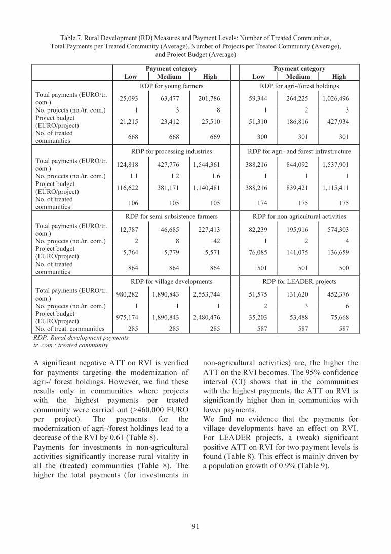
91

Non-rural

communities RVI 15–20 RVI10–15 RVI 5–10 RVI 0–5

Figure 1. Rural vitality index (RVI) of rural LAU2 communities in Romania (non-rural communities are indicated dark

red). Source: Authors’ calculations, using STATA’s sp map Descriptive results: RDP of treated communities Table 7 shows the payment levels and the number of treated communities of all RD measures. Basically, a growth in the payment level can be caused by a rise in the number of contracted projects (beneficiaries) or by an increase in the projects’ budget. We observe a growth in the payment level of measures supporting young and semi-subsistence farmers because the number of projects increases, while the budgets remain almost constant. In contrast, the total payments of all the other Axis 1 measures (agri- and forest holdings, agri- and forest infrastructure, and processing industries) increase due to a growth in the projects’ budget. The RDP of the Axes 3 and 4 measures (investments in non-agricultural activities and LEADER projects) rise due to an increase in the number of projects and their budgets. The regional distribution of the payments are shown in Figures 2-9 in the Appendix.

Propensity score matching Results based on kernel matching

Table 8 shows the ATT on the outcome variable RVI for all the different RD measures and payment categories. For RD measures focusing primarily on Axis 1, we find a significant positive ATT on RVI only for the payments targeting processing industries (Table 8). However, a significant increase in rural vitality can be verified only in the treated communities with a low payment level. In contrast, in the communities where high-budget processing industry projects are supported (> 680,000 EURO per project), we find no significant positive ATT on RVI and a significant negative ATT on the change in population (-1.46%, Table 9).

Table 7. Rural Development (RD) Measures and Payment Levels: Number of Treated Communities, Total Payments per Treated Community (Average), Number of Projects per Treated Community (Average),

and Project Budget (Average)

Payment category Payment category Low Medium High Low Medium High

RDP for young farmers RDP for agri-/forest holdings Total payments (EURO/tr. com.) 25,093** 63,477** 201,786** 59,344** 264,225** 1,026,496**

No. projects (no./tr. com.) 1** 3** 8** 1** 2** 3** Project budget (EURO/project) 21,215** 23,412** 25,510** 51,310** 186,816** 427,934**

No. of treated communities 668** 668** 669** 300** 301** 301**

RDP for processing industries RDP for agri- and forest infrastructure Total payments (EURO/tr. com.) 124,818** 427,776** 1,544,361** 388,216** 844,092** 1,537,901**

No. projects (no./tr. com.) 1.1** 1.2** 1.6** 1** 1** 1** Project budget (EURO/project) 116,622** 381,171** 1,140,481** 388,216** 839,421** 1,115,411**

No. of treated communities 106** 105** 105** 174** 175** 175**

RDP for semi-subsistence farmers RDP for non-agricultural activities Total payments (EURO/tr. com.) 12,787** 46,685** 227,413** 82,239** 195,916** 574,303**

No. projects (no./tr. com.) 2** 8** 42** 1** 2** 4** Project budget (EURO/project) 5,764** 5,779** 5,571** 76,085** 141,075** 136,659**

No. of treated communities 864** 864** 864** 501** 501** 500**

RDP for village developments RDP for LEADER projects Total payments (EURO/tr. com.) 980,282** 1,890,843** 2,553,744** 51,575** 131,620** 452,376**

No. projects (no./tr. com.) 1** 1** 1** 2** 3** 6** Project budget (EURO/project) 975,174** 1,890,843** 2,480,476** 35,203** 53,488** 75,668**

No. of treat. communities 285** 285** 285** 587** 587** 587** RDP: Rural development payments tr. com.: treated community A significant negative ATT on RVI is verified for payments targeting the modernization of agri-/ forest holdings. However, we find these results only in communities where projects with the highest payments per treated community were carried out (>460,000 EURO per project). The payments for the modernization of agri-/forest holdings lead to a decrease of the RVI by 0.61 (Table 8). Payments for investments in non-agricultural activities significantly increase rural vitality in all the (treated) communities (Table 8). The higher the total payments (for investments in

non-agricultural activities) are, the higher the ATT on the RVI becomes. The 95% confidence interval (CI) shows that in the communities with the highest payments, the ATT on RVI is significantly higher than in communities with lower payments. We find no evidence that the payments for village developments have an effect on RVI. For LEADER projects, a (weak) significant positive ATT on RVI for two payment levels is found (Table 8). This effect is mainly driven by a population growth of 0.9% (Table 9).

92

Table 8. Effect of Rural Development Payments (RDP) on the Rural Vitality Index (RVI): Results of Propensity Score Matching (PSM; Kernel Matching Technique)

Payment category Payment category

Low Medium High Total Low Medium High Total

RDP for young farmers RDP for agri-/forest holdings ATT –0.03** 0.13** 0.02** –0.09** 0.23** –0.09*** –0.61*** –0.20 95% CI upper bound 0.12** 0.45** 0.48** 0.16** 0.59** 0.24*** –0.19*** 0.09 95% CI lower bound –0.47** –0.23** –0.41** –0.35** –0.15** –0.54*** –1.09*** –0.49

RDP for processing industries RDP for agri- and forest infrastructure ATT 0.57** 0.14** 0.41** 0.31** 0.08** 0.10*** 0.11*** 0.06*** 95% CI upper bound 0.94** 0.59** 0.93** 0.60** 0.53** 0.38*** 0.54*** 0.30*** 95% CI lower bound 0.05** –0.32** –0.10** 0.01** –0.37** –0.34*** –0.28*** –0.18***

RDP for semi-subsistence farmers RDP for non-agricultural activities ATT 0.06** 0.31** 0.39** 0.18** 0.26** 0.51*** 1.37*** 0.60*** 95% CI upper bound 0.48** 0.90** 1.24** 0.67** 0.51** 0.75*** 1.56*** 0.85*** 95% CI lower bound –0.38** –0.23** –0.48** –0.32** –0.11** 0.13*** 0.82*** 0.35***

RDP for village developments RDP for LEADER projects

ATT 0.01** 0.11** –0.17** –0.03** 0.14** 0.31** 0.25* 0.25* 95% CI upper bound 0.33** 0.49** 0.20** 0.21** 0.35** 0.55** 0.51* 0.44* 95% CI lower bound –0.35** –0.27** –0.54** –0.28** –0.15** 0.05** -0.02* 0.05* ATT = Average Treatment Effect of the Treated; CI = confidence interval *** Significant at the 0.001 level or lower; ** Significant at the 0.001-0.05 level; * Significant at the 0.05-0.1 level

Table 9. ATT on the Rural Vitality Index (RVI) using Propensity Score Matching (PSM) with Kernel Matching, PSM

with Two-nearest-neighbor Matching, and Ordinary Least Squares (OLS)

Payment category Payment category

Low Medium High Low Medium High RDP for agri-/forest holdings RDP for processing industries PSM kernel matching 0.23 -0.09 -0.61*** 0.57** 0.14* 0.41* PSM two-nearest-neighbor matching 0.22 -0.13 -0.80*** 0.20* 0.20* –0.03* OLS 0.22 -0.10 -0.39** 0.50*** –0.04* 0.34*

RDP for non-agricultural

activities RDP for LEADER projects

PSM kernel matching 0.26** 0.51*** 1.37*** 0.14** 0.31** 0.25**

PSM two-nearest-neighbor matching 0.14** 0.58*** 1.45*** –0.11*** 0.27** 0.11** OLS 0.34** 0.57*** 1.46*** 0.17* 0.29** 0.35***

ATT = Average Treatment Effect of the Treated ***Significant at the 0.001 level or lower; ** Significant at the 0.001-0.05 level; * Significant at the 0.05-0.1 level Sensitivity analysis Table 9 shows the ATT on RVI for different counterfactual approaches. The sensitivity analysis is carried out only for those RD measures for which we find statistically significant results with kernel matching. The results show that PSM with kernel, PSM with two-nearest-neighbor matching, and OLS

produce similar results in terms of both the volume and significance of the ATT. This comparison shows that our results are robust with respect to the applied counterfactual method. Only a few scientific papers are available that evaluated the effects of the European RDP on RD (Michalek, 2012; Michalek et al., 2012; Bakucs et al., 2018). Furthermore, these papers

applied a different approach by analyzing the effects of total RD subsidies on RD in Eastern European countries. In contrast, our paper considers eight different RD measures and, for each measure we distinguish various uptake levels. Against this background, a discussion of our results against their research is difficult. Whilst the authors found no or low evidence that total RD subsidies effect RD in Eastern European countries, our study verifies that a few single RD measures have both, significant positive and negative effects on quality of life in rural areas. Thus, we suggest to apply from a methodological point of view an approach that focus on single RD measures rather than on total subsidies. In the following, we discuss our results against the results of the European Commission’s mandatory ex post evaluation program by Floria et al. (2017) and papers evaluating single measures. Our results show that most of the RD measures focusing primarily on Axis 1 and secondarily on Axis 3 do not contribute to an improvement of rural vitality in Romania. E.g., we find no evidence that RDP targeting semi-subsistence farmers improve rural vitality. These findings are coherent with those of Floria et al. (2017) who stated that the income support provided within the RDP for semi-subsistence farmers in Romania was not sufficient for a sustainable economic development. Infrastructure investments in the agricultural sector cover a diverse range of measures such as for example land consolidation, energy supply, irrigation networks or drainage. Our research finds no evidence that payments for infrastructure investments contribute to rural vitality. However, papers evaluating single measures such as land consolidation verified a positive contribution to slowing rural depopulation in the long-term historical perspective and to wellbeing of the rural population (Miranda et al., 2006; Lerman, 2006). For payments targeting the modernization of processing industries, we find a significant positive effect on rural vitality in only one-third of the treated communities. The public support of business creation in non-agricultural activities (e.g., the public encouragement of tourism activities) has the strongest positive effect on rural vitality of all

the analyzed measures. The results also show that the higher the public expenditures, the greater the effect on rural vitality. These findings are in line with a large branch of literature worldwide reporting the positive effects of investments in tourism on RD (Mathieson et al., 1982; Briedenhann et al., 2004; Hegarty et al., 2005). We find no evidence that investments in village development contributed to rural vitality in the first program period. These findings are in line with recent studies indicating that infrastructure investments did not represent an engine of economic growth in many countries (Ansar et al., 2016; Chen, 2017). However, infrastructure investments in rural areas may need more time to attract new enterprises and new facilities, and thus, improve the living conditions in rural areas in the long term. Regarding LEADER projects in Romania, previous research showed that the complexity of the programme, weak administrative net-works, political influence, and heritage of the socialist era inhibited the smooth introduction of the LEADER instrument (Marquardt et al., 2010). This might be one of the reasons why we receive a weak significantly positive effect of LEADER projects on RD. CONCLUSIONS This paper analyses the effects of single RD measures and different uptake levels on indicators of rural vitality for Romania. The study is carried out at the regional LAU2 level in Romania. Our study shows that the design and uptake level of the RD measures highly influences the effects of the payments. In this respect, we see further fields of research. We find for the majority of payments focusing primarily on Axis 1 have no effect on quality of life of the rural population. However, the rural population benefit from investments in non-agricultural activities and LEADER programs. REFERENCES Ansar A., Flyvbjerg B., Budzier A., Lunn D., 2016. Does

infrastructure investment lead to economic growth or economic fragility? Evidence from China. Oxford Review of Econ. Policy, 32 (3), p. 360-390.

93

Table 8. Effect of Rural Development Payments (RDP) on the Rural Vitality Index (RVI): Results of Propensity Score Matching (PSM; Kernel Matching Technique)

Payment category Payment category

Low Medium High Total Low Medium High Total

RDP for young farmers RDP for agri-/forest holdings ATT –0.03** 0.13** 0.02** –0.09** 0.23** –0.09*** –0.61*** –0.20 95% CI upper bound 0.12** 0.45** 0.48** 0.16** 0.59** 0.24*** –0.19*** 0.09 95% CI lower bound –0.47** –0.23** –0.41** –0.35** –0.15** –0.54*** –1.09*** –0.49

RDP for processing industries RDP for agri- and forest infrastructure ATT 0.57** 0.14** 0.41** 0.31** 0.08** 0.10*** 0.11*** 0.06*** 95% CI upper bound 0.94** 0.59** 0.93** 0.60** 0.53** 0.38*** 0.54*** 0.30*** 95% CI lower bound 0.05** –0.32** –0.10** 0.01** –0.37** –0.34*** –0.28*** –0.18***

RDP for semi-subsistence farmers RDP for non-agricultural activities ATT 0.06** 0.31** 0.39** 0.18** 0.26** 0.51*** 1.37*** 0.60*** 95% CI upper bound 0.48** 0.90** 1.24** 0.67** 0.51** 0.75*** 1.56*** 0.85*** 95% CI lower bound –0.38** –0.23** –0.48** –0.32** –0.11** 0.13*** 0.82*** 0.35***

RDP for village developments RDP for LEADER projects

ATT 0.01** 0.11** –0.17** –0.03** 0.14** 0.31** 0.25* 0.25* 95% CI upper bound 0.33** 0.49** 0.20** 0.21** 0.35** 0.55** 0.51* 0.44* 95% CI lower bound –0.35** –0.27** –0.54** –0.28** –0.15** 0.05** -0.02* 0.05* ATT = Average Treatment Effect of the Treated; CI = confidence interval *** Significant at the 0.001 level or lower; ** Significant at the 0.001-0.05 level; * Significant at the 0.05-0.1 level

Table 9. ATT on the Rural Vitality Index (RVI) using Propensity Score Matching (PSM) with Kernel Matching, PSM

with Two-nearest-neighbor Matching, and Ordinary Least Squares (OLS)

Payment category Payment category

Low Medium High Low Medium High RDP for agri-/forest holdings RDP for processing industries PSM kernel matching 0.23 -0.09 -0.61*** 0.57** 0.14* 0.41* PSM two-nearest-neighbor matching 0.22 -0.13 -0.80*** 0.20* 0.20* –0.03* OLS 0.22 -0.10 -0.39** 0.50*** –0.04* 0.34*

RDP for non-agricultural

activities RDP for LEADER projects

PSM kernel matching 0.26** 0.51*** 1.37*** 0.14** 0.31** 0.25**

PSM two-nearest-neighbor matching 0.14** 0.58*** 1.45*** –0.11*** 0.27** 0.11** OLS 0.34** 0.57*** 1.46*** 0.17* 0.29** 0.35***

ATT = Average Treatment Effect of the Treated ***Significant at the 0.001 level or lower; ** Significant at the 0.001-0.05 level; * Significant at the 0.05-0.1 level Sensitivity analysis Table 9 shows the ATT on RVI for different counterfactual approaches. The sensitivity analysis is carried out only for those RD measures for which we find statistically significant results with kernel matching. The results show that PSM with kernel, PSM with two-nearest-neighbor matching, and OLS

produce similar results in terms of both the volume and significance of the ATT. This comparison shows that our results are robust with respect to the applied counterfactual method. Only a few scientific papers are available that evaluated the effects of the European RDP on RD (Michalek, 2012; Michalek et al., 2012; Bakucs et al., 2018). Furthermore, these papers

applied a different approach by analyzing the effects of total RD subsidies on RD in Eastern European countries. In contrast, our paper considers eight different RD measures and, for each measure we distinguish various uptake levels. Against this background, a discussion of our results against their research is difficult. Whilst the authors found no or low evidence that total RD subsidies effect RD in Eastern European countries, our study verifies that a few single RD measures have both, significant positive and negative effects on quality of life in rural areas. Thus, we suggest to apply from a methodological point of view an approach that focus on single RD measures rather than on total subsidies. In the following, we discuss our results against the results of the European Commission’s mandatory ex post evaluation program by Floria et al. (2017) and papers evaluating single measures. Our results show that most of the RD measures focusing primarily on Axis 1 and secondarily on Axis 3 do not contribute to an improvement of rural vitality in Romania. E.g., we find no evidence that RDP targeting semi-subsistence farmers improve rural vitality. These findings are coherent with those of Floria et al. (2017) who stated that the income support provided within the RDP for semi-subsistence farmers in Romania was not sufficient for a sustainable economic development. Infrastructure investments in the agricultural sector cover a diverse range of measures such as for example land consolidation, energy supply, irrigation networks or drainage. Our research finds no evidence that payments for infrastructure investments contribute to rural vitality. However, papers evaluating single measures such as land consolidation verified a positive contribution to slowing rural depopulation in the long-term historical perspective and to wellbeing of the rural population (Miranda et al., 2006; Lerman, 2006). For payments targeting the modernization of processing industries, we find a significant positive effect on rural vitality in only one-third of the treated communities. The public support of business creation in non-agricultural activities (e.g., the public encouragement of tourism activities) has the strongest positive effect on rural vitality of all

the analyzed measures. The results also show that the higher the public expenditures, the greater the effect on rural vitality. These findings are in line with a large branch of literature worldwide reporting the positive effects of investments in tourism on RD (Mathieson et al., 1982; Briedenhann et al., 2004; Hegarty et al., 2005). We find no evidence that investments in village development contributed to rural vitality in the first program period. These findings are in line with recent studies indicating that infrastructure investments did not represent an engine of economic growth in many countries (Ansar et al., 2016; Chen, 2017). However, infrastructure investments in rural areas may need more time to attract new enterprises and new facilities, and thus, improve the living conditions in rural areas in the long term. Regarding LEADER projects in Romania, previous research showed that the complexity of the programme, weak administrative net-works, political influence, and heritage of the socialist era inhibited the smooth introduction of the LEADER instrument (Marquardt et al., 2010). This might be one of the reasons why we receive a weak significantly positive effect of LEADER projects on RD. CONCLUSIONS This paper analyses the effects of single RD measures and different uptake levels on indicators of rural vitality for Romania. The study is carried out at the regional LAU2 level in Romania. Our study shows that the design and uptake level of the RD measures highly influences the effects of the payments. In this respect, we see further fields of research. We find for the majority of payments focusing primarily on Axis 1 have no effect on quality of life of the rural population. However, the rural population benefit from investments in non-agricultural activities and LEADER programs. REFERENCES Ansar A., Flyvbjerg B., Budzier A., Lunn D., 2016. Does

infrastructure investment lead to economic growth or economic fragility? Evidence from China. Oxford Review of Econ. Policy, 32 (3), p. 360-390.

94

Bakucs Z., Fertő I., Varga Á., Benedek Z., 2018. Impact of European Union development subsidies on Hungarian regions. European Planning Studies, p. 1-16.

Blundell R. and Costa Dias M., 2000. Evaluation Methods for Non-Experimental Data. Fiscal Studies, 21 (4): p. 427-468.

Briedenhann J., Wickens E., 2004. Tourism routes as a tool for the economic development of rural areas-Vibrant hope or impossible dream? Tourism Management, 25 (1), p. 71-79.

Chen C.L., Vickerman R., 2017. Can transport infrastructure change regions’ economic fortunes? Some evidence from Europe and China. Regional Studies, 51 (1), p. 144-160.

Davidova S., Hennessy T., Thomson K., 2016. Rural Jobs and the CAP: Spitting into the Wind? In: 90th Annual Conference, April 4-6, 2016, Warwick University, Coventry, UK (No. 236364). Agricultural Economics Society.

Floria A., Brignani N., Celotti P., Nicoara A., Strat V.A., Gramillano A., 2017. Ex-, post-evaluation study of the national rural development programme 2007-2013. Available at: http://www.madr.ro/docs/dezvoltare-rurala/studii/Ex-post-evaluation-of-NRDP-2007-2013-EN.pdf.

Gherghinescu O., 2008. Poverty and social exclusion in rural areas. Final Report, Annex I. Country Studies, Country: Romania. European Communities.

Hart K., Baldock D., Weingarten P., Osterburg B., Povellato A., Vanni F., Pirzio-Biroli C., Boyes A., 2011. What tools for the European agricultural policy to encourage the provision of public goods? Study for the European Parliament’s Committee on Agriculture and Rural Development. Available at: http://www.europarl.europa.eu/studies.

Hegarty C., Przezborska L., 2005. Rural and agriotourism as a tool for reorganising rural areas in old and new member states-A comparison study of Ireland and Poland. International Journal of Tourism Research, 7 (2), p. 63-77.

Hlavsa T., Hruska M., Turkova E., 2017. The impact of investment support from the Rural Development Programme of the Czech Republic for 2007-2013 on the economic efficiency of farms. Studies in Agricultural Economics, 119.

Kirchweger S., Kantelhardt J., 2015. The dynamic effects of government-supported farm-investment activities on structural change in Austrian agriculture. Land Use Policy, 48, p. 73-93.

Khandker S.R., Koolwal G.B., Samad H.A., 2009. Handbook on impact evaluation: quantitative methods and practices. World Bank, Washington, DC.

Koomen E., 2011. Indicators of Rural Vitality. A GIS-based analysis of socio-economic development of the rural Netherlands. Vrije Universiteit Amsterdam, Faculty of Economics and Business Administration, Research Memorandum 2011-50.

Lerman Z., Cimpoieş D., 2006. Land consolidation as a factor for rural development in Moldova. Europe-Asia Studies, 58 (3), p. 439-455.

Mathieson A., Wall G., 1982. Tourism, economic, physical and social impacts. Longman.

Marquardt D., Möllers J., Buchenrieder G., 2012. Social networks and rural development: LEADER in Romania. Sociologia Ruralis, 52 (4), p. 398-431.

Medonos T., Ratinger T., Hruska M., Spicka J., 2012. The assessment of the effects of investment support measures of the Rural Development Programmes: the case of the Czech Republic. Agris on-line Papers in Economics and Informatics, 4 (4), 35.

Michalek J., 2012. Counterfactual impact evaluation of EU rural development programmes-Propensity Score Matching methodology applied to selected EU Member States. Volume 2: A regional approach. Institute for Prospective and Technological Studies, Joint Research Centre.

Michalek J., Zarnekow N., 2012. Application of the rural development index to analysis of rural regions in Poland and Slovakia. Social Indicators Research, 105(1), p. 1-37.

Midmore P., Langstaff L., Lowman S., Vaughan A., 2008. Qualitative evaluation of European rural development policy: Evidence from comparative case studies. Paper presented at the 12th Congress of the European Association of Agricultural Economists. August 26-29, Ghent.

Miranda D., Crecente R., Alvarez M.F., 2006. Land consolidation in inland rural Galicia, NW Spain, since 1950: An example of the formulation and use of questions, criteria and indicators for evaluation of rural development policies. Land Use Policy, 23 (4), p. 511-520.

Petrick M., Zier P., 2011. Regional employment impacts of Common Agricultural Policy measures in Eastern Germany: A difference-in-differences approach. Agricultural Economics, 42(2), p. 183-193.

Psaltopoulos D., Balamou E., Skuras D., Ratinger T., Sieber S., 2011. Modelling the impacts of CAP Pillar 1 and 2 measures on local economies in Europe: Testing a case study-based CGE-model approach. Journal of Policy Modeling, 33 (1), p. 53-69.

Rizov M., Davidova S., Bailey A., 2016. Employment effects of CAP payments in the UK non-farm economy. In 160th Seminar, December 1-2, 2016, Warsaw, Poland (No. 249793). European Association of Agricultural Economists.

Roy A., 1951. Some thoughts on the distribution of earnings. Oxford Economic Papers, 3(2): p. 135-145.

Rubin D.B., 1974. Estimating Causal Efects of Treatments in Randomized and Non randomized Studies. Journal of Educational Psychology, 66 (5): p. 688-701.

Turcanu L., 2012. Rural vitality in the Netherlands. Amsterdam: VU University Amsterdam.

***European Commission, 2016. CAP Context Indicators 2014-2020. Rural development in the EU. http://ec.europa.eu/agriculture/cap-indicators/context/2016/2016-Contextindicators-fiches.pdf.

APPENDIX

Non-rural

communities 201,786

EURO 63,477

EURO 25,093

EURO No

payments

Figure 2. Distribution of Rural Development Payments (RDP) for young farmers (Average payments per community). Source: Authors’ calculations, using STATA’s sp map

Non-rural

communities 1,026,496

EURO 264,225

EURO 59,344

EURO No

payments

Figure 3. Distribution of Rural Development Payments (RDP) for agri- /forest holdings (Average payments per community). Source: Authors’ calculations, using STATA’s sp map

95

Bakucs Z., Fertő I., Varga Á., Benedek Z., 2018. Impact of European Union development subsidies on Hungarian regions. European Planning Studies, p. 1-16.

Blundell R. and Costa Dias M., 2000. Evaluation Methods for Non-Experimental Data. Fiscal Studies, 21 (4): p. 427-468.

Briedenhann J., Wickens E., 2004. Tourism routes as a tool for the economic development of rural areas-Vibrant hope or impossible dream? Tourism Management, 25 (1), p. 71-79.

Chen C.L., Vickerman R., 2017. Can transport infrastructure change regions’ economic fortunes? Some evidence from Europe and China. Regional Studies, 51 (1), p. 144-160.

Davidova S., Hennessy T., Thomson K., 2016. Rural Jobs and the CAP: Spitting into the Wind? In: 90th Annual Conference, April 4-6, 2016, Warwick University, Coventry, UK (No. 236364). Agricultural Economics Society.

Floria A., Brignani N., Celotti P., Nicoara A., Strat V.A., Gramillano A., 2017. Ex-, post-evaluation study of the national rural development programme 2007-2013. Available at: http://www.madr.ro/docs/dezvoltare-rurala/studii/Ex-post-evaluation-of-NRDP-2007-2013-EN.pdf.

Gherghinescu O., 2008. Poverty and social exclusion in rural areas. Final Report, Annex I. Country Studies, Country: Romania. European Communities.

Hart K., Baldock D., Weingarten P., Osterburg B., Povellato A., Vanni F., Pirzio-Biroli C., Boyes A., 2011. What tools for the European agricultural policy to encourage the provision of public goods? Study for the European Parliament’s Committee on Agriculture and Rural Development. Available at: http://www.europarl.europa.eu/studies.

Hegarty C., Przezborska L., 2005. Rural and agriotourism as a tool for reorganising rural areas in old and new member states-A comparison study of Ireland and Poland. International Journal of Tourism Research, 7 (2), p. 63-77.

Hlavsa T., Hruska M., Turkova E., 2017. The impact of investment support from the Rural Development Programme of the Czech Republic for 2007-2013 on the economic efficiency of farms. Studies in Agricultural Economics, 119.

Kirchweger S., Kantelhardt J., 2015. The dynamic effects of government-supported farm-investment activities on structural change in Austrian agriculture. Land Use Policy, 48, p. 73-93.

Khandker S.R., Koolwal G.B., Samad H.A., 2009. Handbook on impact evaluation: quantitative methods and practices. World Bank, Washington, DC.

Koomen E., 2011. Indicators of Rural Vitality. A GIS-based analysis of socio-economic development of the rural Netherlands. Vrije Universiteit Amsterdam, Faculty of Economics and Business Administration, Research Memorandum 2011-50.

Lerman Z., Cimpoieş D., 2006. Land consolidation as a factor for rural development in Moldova. Europe-Asia Studies, 58 (3), p. 439-455.

Mathieson A., Wall G., 1982. Tourism, economic, physical and social impacts. Longman.

Marquardt D., Möllers J., Buchenrieder G., 2012. Social networks and rural development: LEADER in Romania. Sociologia Ruralis, 52 (4), p. 398-431.

Medonos T., Ratinger T., Hruska M., Spicka J., 2012. The assessment of the effects of investment support measures of the Rural Development Programmes: the case of the Czech Republic. Agris on-line Papers in Economics and Informatics, 4 (4), 35.

Michalek J., 2012. Counterfactual impact evaluation of EU rural development programmes-Propensity Score Matching methodology applied to selected EU Member States. Volume 2: A regional approach. Institute for Prospective and Technological Studies, Joint Research Centre.

Michalek J., Zarnekow N., 2012. Application of the rural development index to analysis of rural regions in Poland and Slovakia. Social Indicators Research, 105(1), p. 1-37.

Midmore P., Langstaff L., Lowman S., Vaughan A., 2008. Qualitative evaluation of European rural development policy: Evidence from comparative case studies. Paper presented at the 12th Congress of the European Association of Agricultural Economists. August 26-29, Ghent.

Miranda D., Crecente R., Alvarez M.F., 2006. Land consolidation in inland rural Galicia, NW Spain, since 1950: An example of the formulation and use of questions, criteria and indicators for evaluation of rural development policies. Land Use Policy, 23 (4), p. 511-520.

Petrick M., Zier P., 2011. Regional employment impacts of Common Agricultural Policy measures in Eastern Germany: A difference-in-differences approach. Agricultural Economics, 42(2), p. 183-193.

Psaltopoulos D., Balamou E., Skuras D., Ratinger T., Sieber S., 2011. Modelling the impacts of CAP Pillar 1 and 2 measures on local economies in Europe: Testing a case study-based CGE-model approach. Journal of Policy Modeling, 33 (1), p. 53-69.

Rizov M., Davidova S., Bailey A., 2016. Employment effects of CAP payments in the UK non-farm economy. In 160th Seminar, December 1-2, 2016, Warsaw, Poland (No. 249793). European Association of Agricultural Economists.

Roy A., 1951. Some thoughts on the distribution of earnings. Oxford Economic Papers, 3(2): p. 135-145.

Rubin D.B., 1974. Estimating Causal Efects of Treatments in Randomized and Non randomized Studies. Journal of Educational Psychology, 66 (5): p. 688-701.

Turcanu L., 2012. Rural vitality in the Netherlands. Amsterdam: VU University Amsterdam.

***European Commission, 2016. CAP Context Indicators 2014-2020. Rural development in the EU. http://ec.europa.eu/agriculture/cap-indicators/context/2016/2016-Contextindicators-fiches.pdf.

APPENDIX

Non-rural

communities 201,786

EURO 63,477

EURO 25,093

EURO No

payments

Figure 2. Distribution of Rural Development Payments (RDP) for young farmers (Average payments per community). Source: Authors’ calculations, using STATA’s sp map

Non-rural

communities 1,026,496

EURO 264,225

EURO 59,344

EURO No

payments

Figure 3. Distribution of Rural Development Payments (RDP) for agri- /forest holdings (Average payments per community). Source: Authors’ calculations, using STATA’s sp map

96

Non-rural communities

1,544,361 EURO

427,776 EURO

124,818 EURO

No payments

Figure 4. Distribution of Rural Development Payments (RDP) for processing industries (Average payments per

community). Source: Authors’ calculations, using STATA’s sp map

Non-rural

communities 1,537,901

EURO 844,092

EURO 388,2016

EURO No

payments

Figure 5. Distribution of Rural Development Payments (RDP) for agri- and forest infrastructure (Average payments per community). Source: Authors’ calculations, using STATA’s sp map

Non-rural

communities 227,413

EURO 46,685

EURO 12,787

EURO No

payments

Figure 6. Distribution of Rural Development Payments (RDP) for semi-subsistence farmers (Average payments per community). Source: Authors’ calculations, using STATA’s sp map

Non-rural

communities 574,303

EURO 195,916

EURO 82,239

EURO No

payments

Figure 7. Distribution of Rural Development Payments (RDP) for non-agricultural activities (Average payments per community). Source: Authors’ calculations, using STATA’s sp map

97

Non-rural communities

1,544,361 EURO

427,776 EURO

124,818 EURO

No payments

Figure 4. Distribution of Rural Development Payments (RDP) for processing industries (Average payments per

community). Source: Authors’ calculations, using STATA’s sp map

Non-rural

communities 1,537,901

EURO 844,092

EURO 388,2016

EURO No

payments

Figure 5. Distribution of Rural Development Payments (RDP) for agri- and forest infrastructure (Average payments per community). Source: Authors’ calculations, using STATA’s sp map

Non-rural

communities 227,413

EURO 46,685

EURO 12,787

EURO No

payments

Figure 6. Distribution of Rural Development Payments (RDP) for semi-subsistence farmers (Average payments per community). Source: Authors’ calculations, using STATA’s sp map

Non-rural

communities 574,303

EURO 195,916

EURO 82,239

EURO No

payments

Figure 7. Distribution of Rural Development Payments (RDP) for non-agricultural activities (Average payments per community). Source: Authors’ calculations, using STATA’s sp map

98

Non-rural

communities 2,553,744

EURO 1,890,843

EURO 980,282

EURO No

payments

Figure 8. Distribution of Rural Development Payments (RDP) for village developments (Average payments per community). Source: Authors’ calculations, using STATA’s sp map

Non-rural

communities 452,376

EURO 131,620

EURO 51,575

EURO No

payments

Figure 9. Distribution of Rural Development Payments (RDP) for LEADER projects (Average payments per community). Source: Authors’ calculations, using STATA’s sp map

ACTIVITY OF PEROXIDASE AND CATALASE IN SOILS AS INFLUENCED BY SOME INSECTICIDES AND FUNGICIDES

Maria-Mihaela MICUȚI, Liliana BĂDULESCU, Aglaia BURLACU,

Florentina ISRAEL-ROMING

University of Agronomic Sciences and Veterinary Medicine of Bucharest, 59 Marasti Blvd, District 1, Bucharest, Romania

Corresponding author email: mihaela.micuti@yahoo.com

Abstract In this study the levels of peroxidase and catalase activity in ecological soil treated with two insecticides and two fungicides over a 28 days period were evaluated. Peroxidases are extracellular enzymes with an important role in the oxidation of lignin and the removal of toxic substances from the environment. Catalase activity can be related to the metabolic activity of aerobic organisms and gives information about the soil fertility. The soil samples were analysed once every 7 days after the pesticides application in soil. Soil enzymes activities were measured using spectrophotometric methods. Overall, peroxidase and catalase activity was affected, positively or negatively, depending on the number of treatments applied. Key words: catalase, fungicides, insecticides, peroxidase. INTRODUCTION Over the last 40 years, the rapid increase in population density and the rise of agricultural technology has led to an increasing release of xenobiotic compounds in the environment. Pesticides, including insecticides, fungicides and herbicides, have become an integrated part of modern farming systems. Pesticides are the main sources for applied xenobiotics, with an important role both in combating pests and diseases and in improving the quantity and quality of world production. However, by repetitive and excessive application of pesticides, they ultimately reach the soil, where qualitative and quantitative changes occur in biochemical processes driven by microorganisms (Dobre et al., 2016; Sharma and Ortiz, 2002). Microorganisms are the main source for soil enzymes, only a small fraction of the enzymes being derived from plants and/or animals. According to several authors, soil enzymatic activities are considered to be suitable indicators of soil quality due to their connection with nutrient cycles and biochemical (Buturuga et al., 2016) transformations and their influence on measuring the degree of soil degradation in both natural and agro-ecosystems. In addition, they can be measured easily, in comparison

with other methods (Colombo et al., 2002; Nannipieri et al., 2002). One of the enzymes with an important role in soil fertility is catalase, which can be related to the metabolic activity of aerobic organisms (Shiyin et al., 2004; Trasar-Cepeda et al., 2007). Catalase (hydrogen peroxide oxidoreductase, EC 1.11.1.6) is an anti-oxidant enzyme that is responsible for the breakdown of hydrogen peroxide (H2O2) into water and oxygen without causing free radicals. Catalase activity is very stable in soil and shows a significant correlation with the content of organic carbon decreasing with soil depth (Alef and Nannipieri, 1995). Peroxidases (EC 1.11.1), as oxidative enzymes, use H2O2 as an electron acceptor in order to generate radical species, which then can act as catalysts for biological reactions (Passardi et al., 2007).Through this mode of action, peroxidases can be an important factor in lignin degradation, removal of hydrogen peroxide from the cell and oxidation of toxic substances (Erman and Vitello, 2002). Peroxidase activity in soil has been measured in a small number of studies. When present in soil environment, these enzymes mediate the biogeochemical processes of lignin degradation, carbon mineralization and

99

Non-rural

communities 2,553,744

EURO 1,890,843

EURO 980,282

EURO No

payments

Figure 8. Distribution of Rural Development Payments (RDP) for village developments (Average payments per community). Source: Authors’ calculations, using STATA’s sp map

Non-rural

communities 452,376

EURO 131,620

EURO 51,575

EURO No

payments

Figure 9. Distribution of Rural Development Payments (RDP) for LEADER projects (Average payments per community). Source: Authors’ calculations, using STATA’s sp map

AgroLife Scientific Journal - Volume 7, Number 2, 2018ISSN 2285-5718; ISSN CD-ROM 2285-5726; ISSN ONLINE 2286-0126; ISSN-L 2285-5718

ACTIVITY OF PEROXIDASE AND CATALASE IN SOILS AS INFLUENCED BY SOME INSECTICIDES AND FUNGICIDES

Maria-Mihaela MICUȚI, Liliana BĂDULESCU, Aglaia BURLACU,

Florentina ISRAEL-ROMING

University of Agronomic Sciences and Veterinary Medicine of Bucharest, 59 Marasti Blvd, District 1, Bucharest, Romania

Corresponding author email: mihaela.micuti@yahoo.com

Abstract In this study the levels of peroxidase and catalase activity in ecological soil treated with two insecticides and two fungicides over a 28 days period were evaluated. Peroxidases are extracellular enzymes with an important role in the oxidation of lignin and the removal of toxic substances from the environment. Catalase activity can be related to the metabolic activity of aerobic organisms and gives information about the soil fertility. The soil samples were analysed once every 7 days after the pesticides application in soil. Soil enzymes activities were measured using spectrophotometric methods. Overall, peroxidase and catalase activity was affected, positively or negatively, depending on the number of treatments applied. Key words: catalase, fungicides, insecticides, peroxidase. INTRODUCTION Over the last 40 years, the rapid increase in population density and the rise of agricultural technology has led to an increasing release of xenobiotic compounds in the environment. Pesticides, including insecticides, fungicides and herbicides, have become an integrated part of modern farming systems. Pesticides are the main sources for applied xenobiotics, with an important role both in combating pests and diseases and in improving the quantity and quality of world production. However, by repetitive and excessive application of pesticides, they ultimately reach the soil, where qualitative and quantitative changes occur in biochemical processes driven by microorganisms (Dobre et al., 2016; Sharma and Ortiz, 2002). Microorganisms are the main source for soil enzymes, only a small fraction of the enzymes being derived from plants and/or animals. According to several authors, soil enzymatic activities are considered to be suitable indicators of soil quality due to their connection with nutrient cycles and biochemical (Buturuga et al., 2016) transformations and their influence on measuring the degree of soil degradation in both natural and agro-ecosystems. In addition, they can be measured easily, in comparison

with other methods (Colombo et al., 2002; Nannipieri et al., 2002). One of the enzymes with an important role in soil fertility is catalase, which can be related to the metabolic activity of aerobic organisms (Shiyin et al., 2004; Trasar-Cepeda et al., 2007). Catalase (hydrogen peroxide oxidoreductase, EC 1.11.1.6) is an anti-oxidant enzyme that is responsible for the breakdown of hydrogen peroxide (H2O2) into water and oxygen without causing free radicals. Catalase activity is very stable in soil and shows a significant correlation with the content of organic carbon decreasing with soil depth (Alef and Nannipieri, 1995). Peroxidases (EC 1.11.1), as oxidative enzymes, use H2O2 as an electron acceptor in order to generate radical species, which then can act as catalysts for biological reactions (Passardi et al., 2007).Through this mode of action, peroxidases can be an important factor in lignin degradation, removal of hydrogen peroxide from the cell and oxidation of toxic substances (Erman and Vitello, 2002). Peroxidase activity in soil has been measured in a small number of studies. When present in soil environment, these enzymes mediate the biogeochemical processes of lignin degradation, carbon mineralization and

100

sequestration, and dissolved organic C export (Bach, 2013). The aim of this study was to examine the influence of two types of insecticides and fungicides on the enzymatic activities of peroxidases and catalases in an ecological soil. The soil was subjected to multiple treatments over a 28 days period with recommended doses by the trader, at field application rate. MATERIALS AND METHODS Soil This experimental study was conducted under greenhouse conditions and the soil was taken from the ecological department from Research Centre for the Quality Study of Food Products greenhouse. The soil used for the experiment was a mixture of soil with perlite and peat and was collected from the humus horizon (0-20 cm). Pesticides In order to determine their influence on soil enzymes activities, four types of pesticides were used: two fungicides and two insecticides, whose description is given in Table 1. All pesticides were purchased from Syngenta Romania.

Table 1. Chemical and biological classifications of pesticides

Biological classification

Common name Chemical family

Fungicide Ridomil Gold MZ 68WG (RG)

Fenilamide Dithiocarbamate

Fungicide Bravo 500 SC (BV)

Organochlorine

Insecticide Mospilan 20SG (MO)

Chlorothalonil

Insecticide Vertimec 1.8% EC (VE)

Avermectin

Soils used in the present study For this study, 1.5 kg of ecological soil was put in plastic pots of 10 cm diameter and 15 cm depth. 10 ml aqueous solution of the selected pesticides were applied at different time periods (days): 0, 7, 14 and 21. For each treatment, soil samples from the 0-15 cm depth were with drawn at every time period and were subjected to different analyses. Soil not supplemented with pesticides was used as a control sample. Soil samples were air-dried at

room temperature, cleaned by removing plant material and other debris, passed through 2 millimeter sieve and stored in sealed polyethylene bags at 4°C prior to analysis of enzymatic activities, in order to avoid the loss of moisture and inhibition of enzymatic reactions. In addition to enzymatic assays, other analyses included pH, conductivity, total dissolved solids (TDS), resistivity, dry substance and humidity. Soil pH was determined by using 1: 2.5 soil to water ratio pH meter, with glass electrode, pH range 0-14 ±1. For measuring soil moisture 1 g of soil was kept in the oven at 105°C for 3-4 hours, cooled in a desiccator and weighed. Drying continued for periods of one hour, followed by cooling in a desiccator and weighing until the sample reached the constant mass. The measurement was conducted in weighing bottles whose diameter was chosen so that the sample taken at work formed a layer of about 5 mm thick. The weighing bottle was brought to the constant mass under the same conditions as the determination (Scott and Maitre, 1988). Soil electrical conductivity (EC) is a measure of the amount of salts in soil and it is commonly expressed in units of milli Siemens per meter (mS/m) at 25°C. The electrical conductivity was determined using 20 g air-dried and passed through a 2 mm sieve soil sample mixed with 50 ml pure water (soil: water ratio - 1: 2.5). The samples were shaken for 4 hours in order to dissolve the soluble salts, filtered through Whatman No. 41 (11 cm) and measured with a platinum electrode (Rayment and Higginson, 1992). Enzyme assays Peroxidase activity was measured as the rate of substrate oxidation in the presence of added H2O2 (Burns et al., 2013). The measurement of peroxidase activity in soil was performed spectrophotometrically using pyrogallol (1, 2, 3-trihydroxybenzene) as substrate, in accordance with previous research (Floch et al., 2007; Riahi et al., 2007; Sinsabaugh et al., 2013). Sample suspensions were prepared by adding 0.1 g of fresh soil to 25 ml of 50 mMsodium acetate buffer, pH = 5. Suspension was homogenized with a Vortex Mixer (Ika Vortex 3) at high speed for 1 minute. Enzyme activities were measured by combining 1 mL of

soil suspension with 250 μL of substrate solution. Simultaneously were prepared: substrate + buffer, soil suspension + buffer, and buffer-used as blank. Each sample, including controls, received 5μL of 0.3% hydrogen peroxide. The samples were incubated in the dark at 20°C for 4 hours and determined spectrophotometrically at 460 nm. The results were calculated according to the method described by Bach (2013), and were expressed in µmol/g soil/h. The catalase activity was measured by titrating residual H2O2 with KMnO4 (Stępniewska et al., 2008; Roberge, 1978). One gram of soil sample was added to 5 mL distilled water with 1 mL of 3% hydrogen peroxide solution. The mixture was shaken and then 5 mL of 1.5 mol/L H2SO4 were added. After that, the solution was filtered and titrated using 0.05 mol/L KMnO4. One enzyme unit was calculated as the amount of enzyme that catalysed the consumption of 1 µmol of H2O2 per g soil per hour (Vijayakumar et al., 2014). The evaluations of enzymatic activities were performed in triplicates, for better precision and reproducibility. The results were processed using Microsoft Excel Tools. The relationship between pesticides influence on enzymatic activity and

soil pH, humidity and conductivity was determined by calculating linear correlation coefficients. RESULTS AND DISCUSSIONS Regarding the enzyme tested and the applied xenobiotic dose, the effects on soil enzymes activities can be positive or negative. Enzymatic activity may be influenced by soil conditions such as pH, organic matter content, moisture, and temperature (Srinivasulu, 2014). The use of pesticides can provide various results, depending on the chemical structure of active ingredients, concentration of pesticides and the specific properties of soil (Jastrzębska, 2011). As seen in Figure 1, the two insecticides (Mospilan 20 SG and Vertimec 1.8% EC) have a similar influence on soil catalase activity, exerting an increase of 58 %, respectively 74% in the first 14 days after which the catalase activity begins to decrease. At the same time a positive correlation can be observed between the influence of insecticides on catalase activity and pH (r = 0.94 for Mospilan 20 SG and r = 0.67 for Vertimec 1.8% EC).

Figure 1. Effect of pesticides on the catalase activity in soil

In Table 2 a positive correlation can be observed comparing the catalase activity in soil samples and soil moisture (r = 0.86 for Ridomil Gold MZ 68WG, r = 0.85 for Bravo500 SC, r =

0.43 for Mospilan 20SG and r = 0.76 for Vertimec 1.8% EC). Borowik (2016) demonstrated higher enzymatic activity in soils with low moisture content (20% maximum

0

0,2

0,4

0,6

0,8

1

1,2

0 7 14 21 28 0 7 14 21 28 0 7 14 21 28 0 7 14 21 28

Ridomil Gold MZ 68WG Bravo 500 SC Mospilan 20SG Vertimec 1.8 % ECµm

ol H

2O2 /

g so

l/ h

Catalase activity

101

sequestration, and dissolved organic C export (Bach, 2013). The aim of this study was to examine the influence of two types of insecticides and fungicides on the enzymatic activities of peroxidases and catalases in an ecological soil. The soil was subjected to multiple treatments over a 28 days period with recommended doses by the trader, at field application rate. MATERIALS AND METHODS Soil This experimental study was conducted under greenhouse conditions and the soil was taken from the ecological department from Research Centre for the Quality Study of Food Products greenhouse. The soil used for the experiment was a mixture of soil with perlite and peat and was collected from the humus horizon (0-20 cm). Pesticides In order to determine their influence on soil enzymes activities, four types of pesticides were used: two fungicides and two insecticides, whose description is given in Table 1. All pesticides were purchased from Syngenta Romania.

Table 1. Chemical and biological classifications of pesticides

Biological classification

Common name Chemical family

Fungicide Ridomil Gold MZ 68WG (RG)

Fenilamide Dithiocarbamate

Fungicide Bravo 500 SC (BV)

Organochlorine

Insecticide Mospilan 20SG (MO)

Chlorothalonil

Insecticide Vertimec 1.8% EC (VE)

Avermectin

Soils used in the present study For this study, 1.5 kg of ecological soil was put in plastic pots of 10 cm diameter and 15 cm depth. 10 ml aqueous solution of the selected pesticides were applied at different time periods (days): 0, 7, 14 and 21. For each treatment, soil samples from the 0-15 cm depth were with drawn at every time period and were subjected to different analyses. Soil not supplemented with pesticides was used as a control sample. Soil samples were air-dried at

room temperature, cleaned by removing plant material and other debris, passed through 2 millimeter sieve and stored in sealed polyethylene bags at 4°C prior to analysis of enzymatic activities, in order to avoid the loss of moisture and inhibition of enzymatic reactions. In addition to enzymatic assays, other analyses included pH, conductivity, total dissolved solids (TDS), resistivity, dry substance and humidity. Soil pH was determined by using 1: 2.5 soil to water ratio pH meter, with glass electrode, pH range 0-14 ±1. For measuring soil moisture 1 g of soil was kept in the oven at 105°C for 3-4 hours, cooled in a desiccator and weighed. Drying continued for periods of one hour, followed by cooling in a desiccator and weighing until the sample reached the constant mass. The measurement was conducted in weighing bottles whose diameter was chosen so that the sample taken at work formed a layer of about 5 mm thick. The weighing bottle was brought to the constant mass under the same conditions as the determination (Scott and Maitre, 1988). Soil electrical conductivity (EC) is a measure of the amount of salts in soil and it is commonly expressed in units of milli Siemens per meter (mS/m) at 25°C. The electrical conductivity was determined using 20 g air-dried and passed through a 2 mm sieve soil sample mixed with 50 ml pure water (soil: water ratio - 1: 2.5). The samples were shaken for 4 hours in order to dissolve the soluble salts, filtered through Whatman No. 41 (11 cm) and measured with a platinum electrode (Rayment and Higginson, 1992). Enzyme assays Peroxidase activity was measured as the rate of substrate oxidation in the presence of added H2O2 (Burns et al., 2013). The measurement of peroxidase activity in soil was performed spectrophotometrically using pyrogallol (1, 2, 3-trihydroxybenzene) as substrate, in accordance with previous research (Floch et al., 2007; Riahi et al., 2007; Sinsabaugh et al., 2013). Sample suspensions were prepared by adding 0.1 g of fresh soil to 25 ml of 50 mMsodium acetate buffer, pH = 5. Suspension was homogenized with a Vortex Mixer (Ika Vortex 3) at high speed for 1 minute. Enzyme activities were measured by combining 1 mL of

soil suspension with 250 μL of substrate solution. Simultaneously were prepared: substrate + buffer, soil suspension + buffer, and buffer-used as blank. Each sample, including controls, received 5μL of 0.3% hydrogen peroxide. The samples were incubated in the dark at 20°C for 4 hours and determined spectrophotometrically at 460 nm. The results were calculated according to the method described by Bach (2013), and were expressed in µmol/g soil/h. The catalase activity was measured by titrating residual H2O2 with KMnO4 (Stępniewska et al., 2008; Roberge, 1978). One gram of soil sample was added to 5 mL distilled water with 1 mL of 3% hydrogen peroxide solution. The mixture was shaken and then 5 mL of 1.5 mol/L H2SO4 were added. After that, the solution was filtered and titrated using 0.05 mol/L KMnO4. One enzyme unit was calculated as the amount of enzyme that catalysed the consumption of 1 µmol of H2O2 per g soil per hour (Vijayakumar et al., 2014). The evaluations of enzymatic activities were performed in triplicates, for better precision and reproducibility. The results were processed using Microsoft Excel Tools. The relationship between pesticides influence on enzymatic activity and

soil pH, humidity and conductivity was determined by calculating linear correlation coefficients. RESULTS AND DISCUSSIONS Regarding the enzyme tested and the applied xenobiotic dose, the effects on soil enzymes activities can be positive or negative. Enzymatic activity may be influenced by soil conditions such as pH, organic matter content, moisture, and temperature (Srinivasulu, 2014). The use of pesticides can provide various results, depending on the chemical structure of active ingredients, concentration of pesticides and the specific properties of soil (Jastrzębska, 2011). As seen in Figure 1, the two insecticides (Mospilan 20 SG and Vertimec 1.8% EC) have a similar influence on soil catalase activity, exerting an increase of 58 %, respectively 74% in the first 14 days after which the catalase activity begins to decrease. At the same time a positive correlation can be observed between the influence of insecticides on catalase activity and pH (r = 0.94 for Mospilan 20 SG and r = 0.67 for Vertimec 1.8% EC).

Figure 1. Effect of pesticides on the catalase activity in soil

In Table 2 a positive correlation can be observed comparing the catalase activity in soil samples and soil moisture (r = 0.86 for Ridomil Gold MZ 68WG, r = 0.85 for Bravo500 SC, r =

0.43 for Mospilan 20SG and r = 0.76 for Vertimec 1.8% EC). Borowik (2016) demonstrated higher enzymatic activity in soils with low moisture content (20% maximum

0

0,2

0,4

0,6

0,8

1

1,2

0 7 14 21 28 0 7 14 21 28 0 7 14 21 28 0 7 14 21 28

Ridomil Gold MZ 68WG Bravo 500 SC Mospilan 20SG Vertimec 1.8 % EC

µmol

H2O

2 / g

sol/

h

Catalase activity

102

water capacity). No obvious influence on catalase activity after application of Bravo 500 SC fungicide at recommended doses was observed. In contrast, the use of fungicide Ridomil Gold lead to a decrease in catalase activity, starting at day 14, with approximately 70%. In previous studies, Shiyin et al. (2004) found that at different doses of pesticides soil catalase activities and their hydrolysates will recover from stimulative effect, and reach the level of the enzymatic activity of a blank soil sample after about 35 days. Peroxidase activity has positive association with the insecticides application in lower doses. Regarding the peroxidase activity, analysed after pesticides treatments for 28 days, no significant differences were obtained compared to control.

A very significant correlation (r = 0.99) was observed at RG fungicide between the modification of peroxidase activity as a result of xenobiotic treatments and pH (Figure 2). A positive correlation can also be observed on the two insecticides applied. Baćmaga et al. (2016) concluded that the dose of pesticides recommended by the manufacturer generally stimulates enzyme activity. This stimulatory effect could be assigned to the adaptability of soil microorganisms, which can reduce the negative influence of chemical stressors under hostile conditions. These enzymes could also be protected by clay fractions or humic substances present in soil. The protective effect of those substances could reduce enzyme sensibility to pesticides (Baćmaga et al., 2012).

Table 2. Physico-chemical parameters of soil samples

Pesticides Day pH

Conductivity (mS/m)

TDS (ppm)

Resistivity (E+3Ω·cm)

Humidity (%)

Fungicide Ridomil Gold MZ 68WG

0 7.1 0.35 174.2 2.87 13.8 7 7.8 0.29 146.9 3.40 15.5 14 8.1 0.18 88.8 5.63 14.6 21 7.8 0.44 219.1 2.29 13.5 28 7.8 0.23 116.0 4.31 12.4

Fungicide Bravo 500 SC

0 7.1 0.35 174.2 2.87 13.8 7 7.9 0.23 116.8 4.27 12.2 14 7.9 0.26 129.0 3.88 18.1

21 8 0.25 125.8 3.98 16.3

28 8 0.39 193.0 2.59 16.2

Insecticide Mospilan 20 SG

0 7.1 0.35 174.2 2.87 13.8 7 7.6 0.45 225.7 2.22 14.4

14 7.7 0.28 138.5 3.61 16

21 7.4 0.26 129.5 3.86 15.7 28 7.4 0.37 184.3 2.71 10.1

Insecticide Vertimec 1.8% EC

0 7.1 0.35 174.2 2.87 13.8

7 7.3 0.50 248.1 2.02 16.7

14 7.5 0.27 136.8 3.65 16.8

21 7.2 0.28 137.9 3.63 15.3 28 7.2 0.81 405.0 1.23 13.4

Figure 2. Effect of pesticides on the peroxidase activity in soil

CONCLUSIONS The results obtained in the present study indicate that the two insecticides stimulate the catalase activity after the first two treatments. This increase can be related to the changes in soil pH. Instead, RG fungicide applications lead to a decrease of catalase activity. Regarding peroxidase activity, results shown that were no significant differences compared to control after insecticide application. Compared to catalase activity, the presence of RG fungicide in soil lead to an increase in peroxidase activity. There are a number of factors responsible for the various results obtained, such as chemical nature of pesticides, soil properties and biological function of soil. Even though pesticides applied in quantities recommended by the trader may cause slight changes in soil enzymatic activity, it is certain that long-term applications of pesticides may reduce soil fertility and enzymatic activity. REFERENCES Alef K., Nannipieri P., 1995. Catalase activity. In:

Methods in Applied Soil Microbiology and Biochemistry. London: Academic Press, p. 362-363.

Bach C.E., Warnock D.D., Van Horn D.J., Weintraub M.N., 2013. Measuring phenol oxidase and peroxidase activities with pyrogallol.

Baćmaga M., Boros E., Kucharski J., Wyszkowska J., 2012. Enzymatic activity in soil contaminated with the Aurora 40 WG herbicide. Environ. Prot. Eng. 38 (1): p. 91-102.

Baćmaga M., Wyszkowska J., Kucharski J., 2016. The effect of the Falcon 460 EC fungicide on soil

microbial communities, enzyme activities and plant growth. Ecotoxicology, 25: p. 1575-1587.

Borowik A., Wyszkowska J., 2016. Soil moisture as a factor affecting the microbiological and biochemical activity of soil. Vol. 62, 2016, No. 6: p. 250-255.

Burns R.G., DeForest J.L., Marxsen J., Sinsabaugh R.L., Stromberger M.E., Wallenstein M.D., Weintraub M.N., Zoppini A., 2013. Soil enzymes in a changing environment: current knowledge and future directions. Soil Biol. Biochem. 58, 216-234.

Buturugă M.D., Ştefanic G., Săndoiu D.I.,Bădulescu L., 2016. Ecological Methods of Pedo-Enzymatical Analysis for Soil Fertility Control. Romanian Biotechnological Letters, 21 (3), 11471.

Colombo C., Palumbo G., Sannino F., Gianfreda L., 2002. Chemical and biochemical indicators of managed agricultural soils. 17th World Congress of Soil Science Bangkok, Thailand 1740: p. 1-9.

Dobre A., Marin L.A., Manole C., Andrei N., Cornea C. P., 2016. E valuation of the capacity of different microorganisms to solubilize several compounds of phosphorous and zinc. Scientific Bulletin, Series F. Biotechnologies, Vol. XX, 2016.

Erman J.E., Vitello L.B., 2002. Yeast cytochrome c peroxidase: mechanistic studies via protein engineering. Biochimica et Biophysica Acta 1597: p. 193-220.

Floch C., Alarcon-Gutierrez E., Criquet S., 2007. ABTS assay of phenol oxidase activity in soil. J. Microbiol. Methods, 71, p. 319-324.

Jastrzębska E., 2011. The Effect of Chlorpyrifos and Teflubenzuron on the Enzymatic Activity of Soil. Polish J. of Environ. Stud. Vol. 20, No. 4, p. 903-910.

L-DOPA, and ABTS: Effect of assay conditions and soil type, Soil Biology & Biochemistry 67, p. 183-191.

Nannipieri P., Kandeler E., Ruggiero P., 2002. Enzyme activities and microbiological and biochemical processes in soil. In: Enzymes in the environment.

Passardi F., Bakalovic N., Teixeira F.K., Margis-Pinheiro M., Penel C. and Dunand C., 2007. Prokaryotic origins of the non-animal peroxidase superfamily and organelle-mediated transmission to eukaryotes. Genomics 89: p. 567-579.

00,20,40,60,8

11,21,41,61,8

0 7 14 21 28 0 7 14 21 28 0 7 14 21 28 0 7 14 21 28

Ridomil Gold MZ68WG

Bravo 500 SC Mospilan 20SG Vertimec 1.8 %EC

µmol

/ g so

l/ h

Peroxidase activity

103

water capacity). No obvious influence on catalase activity after application of Bravo 500 SC fungicide at recommended doses was observed. In contrast, the use of fungicide Ridomil Gold lead to a decrease in catalase activity, starting at day 14, with approximately 70%. In previous studies, Shiyin et al. (2004) found that at different doses of pesticides soil catalase activities and their hydrolysates will recover from stimulative effect, and reach the level of the enzymatic activity of a blank soil sample after about 35 days. Peroxidase activity has positive association with the insecticides application in lower doses. Regarding the peroxidase activity, analysed after pesticides treatments for 28 days, no significant differences were obtained compared to control.

A very significant correlation (r = 0.99) was observed at RG fungicide between the modification of peroxidase activity as a result of xenobiotic treatments and pH (Figure 2). A positive correlation can also be observed on the two insecticides applied. Baćmaga et al. (2016) concluded that the dose of pesticides recommended by the manufacturer generally stimulates enzyme activity. This stimulatory effect could be assigned to the adaptability of soil microorganisms, which can reduce the negative influence of chemical stressors under hostile conditions. These enzymes could also be protected by clay fractions or humic substances present in soil. The protective effect of those substances could reduce enzyme sensibility to pesticides (Baćmaga et al., 2012).

Table 2. Physico-chemical parameters of soil samples

Pesticides Day pH

Conductivity (mS/m)

TDS (ppm)

Resistivity (E+3Ω·cm)

Humidity (%)

Fungicide Ridomil Gold MZ 68WG

0 7.1 0.35 174.2 2.87 13.8 7 7.8 0.29 146.9 3.40 15.5 14 8.1 0.18 88.8 5.63 14.6 21 7.8 0.44 219.1 2.29 13.5 28 7.8 0.23 116.0 4.31 12.4

Fungicide Bravo 500 SC

0 7.1 0.35 174.2 2.87 13.8 7 7.9 0.23 116.8 4.27 12.2 14 7.9 0.26 129.0 3.88 18.1

21 8 0.25 125.8 3.98 16.3

28 8 0.39 193.0 2.59 16.2

Insecticide Mospilan 20 SG

0 7.1 0.35 174.2 2.87 13.8 7 7.6 0.45 225.7 2.22 14.4

14 7.7 0.28 138.5 3.61 16

21 7.4 0.26 129.5 3.86 15.7 28 7.4 0.37 184.3 2.71 10.1

Insecticide Vertimec 1.8% EC

0 7.1 0.35 174.2 2.87 13.8

7 7.3 0.50 248.1 2.02 16.7

14 7.5 0.27 136.8 3.65 16.8

21 7.2 0.28 137.9 3.63 15.3 28 7.2 0.81 405.0 1.23 13.4

Figure 2. Effect of pesticides on the peroxidase activity in soil

CONCLUSIONS The results obtained in the present study indicate that the two insecticides stimulate the catalase activity after the first two treatments. This increase can be related to the changes in soil pH. Instead, RG fungicide applications lead to a decrease of catalase activity. Regarding peroxidase activity, results shown that were no significant differences compared to control after insecticide application. Compared to catalase activity, the presence of RG fungicide in soil lead to an increase in peroxidase activity. There are a number of factors responsible for the various results obtained, such as chemical nature of pesticides, soil properties and biological function of soil. Even though pesticides applied in quantities recommended by the trader may cause slight changes in soil enzymatic activity, it is certain that long-term applications of pesticides may reduce soil fertility and enzymatic activity. REFERENCES Alef K., Nannipieri P., 1995. Catalase activity. In:

Methods in Applied Soil Microbiology and Biochemistry. London: Academic Press, p. 362-363.

Bach C.E., Warnock D.D., Van Horn D.J., Weintraub M.N., 2013. Measuring phenol oxidase and peroxidase activities with pyrogallol.

Baćmaga M., Boros E., Kucharski J., Wyszkowska J., 2012. Enzymatic activity in soil contaminated with the Aurora 40 WG herbicide. Environ. Prot. Eng. 38 (1): p. 91-102.

Baćmaga M., Wyszkowska J., Kucharski J., 2016. The effect of the Falcon 460 EC fungicide on soil

microbial communities, enzyme activities and plant growth. Ecotoxicology, 25: p. 1575-1587.

Borowik A., Wyszkowska J., 2016. Soil moisture as a factor affecting the microbiological and biochemical activity of soil. Vol. 62, 2016, No. 6: p. 250-255.

Burns R.G., DeForest J.L., Marxsen J., Sinsabaugh R.L., Stromberger M.E., Wallenstein M.D., Weintraub M.N., Zoppini A., 2013. Soil enzymes in a changing environment: current knowledge and future directions. Soil Biol. Biochem. 58, 216-234.

Buturugă M.D., Ştefanic G., Săndoiu D.I.,Bădulescu L., 2016. Ecological Methods of Pedo-Enzymatical Analysis for Soil Fertility Control. Romanian Biotechnological Letters, 21 (3), 11471.

Colombo C., Palumbo G., Sannino F., Gianfreda L., 2002. Chemical and biochemical indicators of managed agricultural soils. 17th World Congress of Soil Science Bangkok, Thailand 1740: p. 1-9.

Dobre A., Marin L.A., Manole C., Andrei N., Cornea C. P., 2016. E valuation of the capacity of different microorganisms to solubilize several compounds of phosphorous and zinc. Scientific Bulletin, Series F. Biotechnologies, Vol. XX, 2016.

Erman J.E., Vitello L.B., 2002. Yeast cytochrome c peroxidase: mechanistic studies via protein engineering. Biochimica et Biophysica Acta 1597: p. 193-220.

Floch C., Alarcon-Gutierrez E., Criquet S., 2007. ABTS assay of phenol oxidase activity in soil. J. Microbiol. Methods, 71, p. 319-324.

Jastrzębska E., 2011. The Effect of Chlorpyrifos and Teflubenzuron on the Enzymatic Activity of Soil. Polish J. of Environ. Stud. Vol. 20, No. 4, p. 903-910.

L-DOPA, and ABTS: Effect of assay conditions and soil type, Soil Biology & Biochemistry 67, p. 183-191.

Nannipieri P., Kandeler E., Ruggiero P., 2002. Enzyme activities and microbiological and biochemical processes in soil. In: Enzymes in the environment.

Passardi F., Bakalovic N., Teixeira F.K., Margis-Pinheiro M., Penel C. and Dunand C., 2007. Prokaryotic origins of the non-animal peroxidase superfamily and organelle-mediated transmission to eukaryotes. Genomics 89: p. 567-579.

00,20,40,60,8

11,21,41,61,8

0 7 14 21 28 0 7 14 21 28 0 7 14 21 28 0 7 14 21 28

Ridomil Gold MZ68WG

Bravo 500 SC Mospilan 20SG Vertimec 1.8 %EC

µmol

/ g so

l/ h

Peroxidase activity

104

Rayment G.E., Higginson F.R., 1992. Australian Laboratory Handbook of Soil and Water Chemical Methods. Melbourne, Inkata Press. (Australian Soil and Land Survey Handbooks, Vol. 3).

Riahi S., Moghaddam A.B., Ganjali M.R., Norouzi P., 2007. Determination of the oxidation potentials of pyrogallol and some of its derivatives: theory and experiment. J. Theor. Comput. Chem. 6, p. 331-340.

Roberge M.R., 1978. Methodology of enzymes determination and extraction. In: Soil Enzymes Academic Press., p. 341-373.

Scott and Maitre, 1988. Interaction between vegetation and groundwater research priorities for South Africa. 730/1/98.

Sharma H.C., Ortiz R., 2002. Host plant resistance to insects: An eco-friendly approach for pest management and environment conservation. J. Environ Biol 23: p. 111-135.

Shiyin L., Lixiao N., Panying P., Cheng S., Liansheng W., 2004. Effects of pesticides and their hydrolysates on catalase activity in soil. Bulletin of Environmental Contamination and Toxicology, 72: p. 600-606.

Sinsabaugh R.L., Allison S.D., Donovan P.G., 2013. Measuring phenol oxidase and peroxidase activities with pyrogallol, L-DOPA, and ABTS: Effect of assay conditions and soil type. Soil Biology & Biochemistry 67 (2013), p. 183-191.

Srinivasulu M., Rangaswamy V., 2014. Enzymes and Pesticides, Enzymes in Agricultural Sciences. OMICS Group e Books, p. 1-10.

Stępniewska Z., Woli´nska A., Ziomek J., 2009. Response of soil catalase activity to chromium contamination. Journal of Environmental Sciences 21, p. 1142-1147.

Trasar-Cepeda C., Gil-Sotres F., Leiros M.C., 2007. Thermodynamic parameters of enzymes in grassland soils from Galicia, NW Spain. Soil Biology & Biochemistry, 39: p. 311-319.

Vijayakumar A.D., Subban M., Jmbulingam J., Annamalai P., Kalaichelvan P.T., 2014. A Rapid Sensitive Detection Method by Plate Assay for Catalase Activity from Bacterium Acinetobacter calcoaceticus AV6. RRJMB, Vol. 3.

COMPARATIVE ANALYSIS OF SOIL TILLAGE SYSTEMS REGARDING ECONOMIC EFFICIENCY AND THE CONVERSION EFFICIENCY

OF ENERGY INVESTED IN THE AGROSYSTEM OF WINTER WHEAT

Grigore MOLDOVAN1, Teodor RUSU2, Paula Ioana MORARU2

1Agricultural Research and Development Station Turda, 27 Agriculturii Street, Turda, 401100,

Cluj County, Romania 2University of Agricultural Sciences and Veterinary Medicine Cluj-Napoca, 3-5 Manastur Street,

Cluj-Napoca, 400372, Romania

Corresponding author email: rusuteodor23@yahoo.com Abstract The paper presents the experimental results on the influence of different soil tillage systems and technological subsystems on the production and conversion efficiency, on the energy invested in the winter wheat crop cultivated in the Transylvanian Plain. The methodology was based on an econometric model, taking into account the combination of production factors and their limited character, as well as the two aspects of economic activity, to maximize profit and to minimize effort. The results show that by practising reduced tillage and no-tillage, the total power consumption can be reduced by 7.8%, and 12.4%, respectively, compared to the conventional system in the case of winter wheat. Up to the sowing phase (including) a decrease of 59.5% fuel consumption per hectare was achieved in the case of reduced tillage compared to the conventional system and a decrease of 78.7% fuel consumption in the no-tillage system. The highest average production was obtained whilst using the reduced tillage, followed by the one from the conventional and no-tillage systems. The highest degree of total energy efficient use ( 5.84) as well as the highest net energy ( were obtained in the reduced tillage system, followed by the no-tillage. The econometric analysis shows that any additional energy consumption of input factors in the conventional system, like human labor requirement, energy incorporated in machinery and fuel consumption had negative effects on yield and leads to a comedown of the economic and energetic balance. The aforemention factors had the following negative values of elasticity coefficients: -0.5264, -0.5965 and -0.2629. The chemical fertilizers (+0.3237) and chemicals (+0.1074) had positive effects on the wheat yield. Surprisingly, the effect of seeds was not significant. The highest quantity of energy spent for the production of winter wheat was indirect and non-renewable. Key words: soil tillage system, winter wheat, econometric analysis, energy use efficiency. INTRODUCTION In order to satisfy the growing need for food, for a population continually growing, the inten-sification of agricultural technologies, and the practice of an energo-intensive agriculture is imperative.On the other hand, this intensifi-cation, due to a continually decreasing of productive arable surfaces, led to physical soil degradation. Today it is unanimously accepted that certain components of the intensive agricultural technological systems like: excessive soil loosening (by deep plowing), elimination of

vegetal debris (or deep incorporation), excessive fertilization etc., together with the reduction of organic matter from the soil can have a significantly negative influence upon the productivity of agricultural ecosystems and the preservation of basic natural resources (soil and water; Rusu, 2013). Current preoccupations for adopting conser-vation agricultural systems resulted in the need for intensifying research in order to introduce new technological systems. These new systems need to take into consideration the cultivated species, crop rotation, soil and climate conditions, having as major objectives to

105

Rayment G.E., Higginson F.R., 1992. Australian Laboratory Handbook of Soil and Water Chemical Methods. Melbourne, Inkata Press. (Australian Soil and Land Survey Handbooks, Vol. 3).

Riahi S., Moghaddam A.B., Ganjali M.R., Norouzi P., 2007. Determination of the oxidation potentials of pyrogallol and some of its derivatives: theory and experiment. J. Theor. Comput. Chem. 6, p. 331-340.

Roberge M.R., 1978. Methodology of enzymes determination and extraction. In: Soil Enzymes Academic Press., p. 341-373.

Scott and Maitre, 1988. Interaction between vegetation and groundwater research priorities for South Africa. 730/1/98.

Sharma H.C., Ortiz R., 2002. Host plant resistance to insects: An eco-friendly approach for pest management and environment conservation. J. Environ Biol 23: p. 111-135.

Shiyin L., Lixiao N., Panying P., Cheng S., Liansheng W., 2004. Effects of pesticides and their hydrolysates on catalase activity in soil. Bulletin of Environmental Contamination and Toxicology, 72: p. 600-606.

Sinsabaugh R.L., Allison S.D., Donovan P.G., 2013. Measuring phenol oxidase and peroxidase activities with pyrogallol, L-DOPA, and ABTS: Effect of assay conditions and soil type. Soil Biology & Biochemistry 67 (2013), p. 183-191.

Srinivasulu M., Rangaswamy V., 2014. Enzymes and Pesticides, Enzymes in Agricultural Sciences. OMICS Group e Books, p. 1-10.

Stępniewska Z., Woli´nska A., Ziomek J., 2009. Response of soil catalase activity to chromium contamination. Journal of Environmental Sciences 21, p. 1142-1147.

Trasar-Cepeda C., Gil-Sotres F., Leiros M.C., 2007. Thermodynamic parameters of enzymes in grassland soils from Galicia, NW Spain. Soil Biology & Biochemistry, 39: p. 311-319.

Vijayakumar A.D., Subban M., Jmbulingam J., Annamalai P., Kalaichelvan P.T., 2014. A Rapid Sensitive Detection Method by Plate Assay for Catalase Activity from Bacterium Acinetobacter calcoaceticus AV6. RRJMB, Vol. 3.

AgroLife Scientific Journal - Volume 7, Number 2, 2018ISSN 2285-5718; ISSN CD-ROM 2285-5726; ISSN ONLINE 2286-0126; ISSN-L 2285-5718

COMPARATIVE ANALYSIS OF SOIL TILLAGE SYSTEMS REGARDING ECONOMIC EFFICIENCY AND THE CONVERSION EFFICIENCY

OF ENERGY INVESTED IN THE AGROSYSTEM OF WINTER WHEAT

Grigore MOLDOVAN1, Teodor RUSU2, Paula Ioana MORARU2

1Agricultural Research and Development Station Turda, 27 Agriculturii Street, Turda, 401100,

Cluj County, Romania 2University of Agricultural Sciences and Veterinary Medicine Cluj-Napoca, 3-5 Manastur Street,

Cluj-Napoca, 400372, Romania

Corresponding author email: rusuteodor23@yahoo.com Abstract The paper presents the experimental results on the influence of different soil tillage systems and technological subsystems on the production and conversion efficiency, on the energy invested in the winter wheat crop cultivated in the Transylvanian Plain. The methodology was based on an econometric model, taking into account the combination of production factors and their limited character, as well as the two aspects of economic activity, to maximize profit and to minimize effort. The results show that by practising reduced tillage and no-tillage, the total power consumption can be reduced by 7.8%, and 12.4%, respectively, compared to the conventional system in the case of winter wheat. Up to the sowing phase (including) a decrease of 59.5% fuel consumption per hectare was achieved in the case of reduced tillage compared to the conventional system and a decrease of 78.7% fuel consumption in the no-tillage system. The highest average production was obtained whilst using the reduced tillage, followed by the one from the conventional and no-tillage systems. The highest degree of total energy efficient use ( 5.84) as well as the highest net energy ( were obtained in the reduced tillage system, followed by the no-tillage. The econometric analysis shows that any additional energy consumption of input factors in the conventional system, like human labor requirement, energy incorporated in machinery and fuel consumption had negative effects on yield and leads to a comedown of the economic and energetic balance. The aforemention factors had the following negative values of elasticity coefficients: -0.5264, -0.5965 and -0.2629. The chemical fertilizers (+0.3237) and chemicals (+0.1074) had positive effects on the wheat yield. Surprisingly, the effect of seeds was not significant. The highest quantity of energy spent for the production of winter wheat was indirect and non-renewable. Key words: soil tillage system, winter wheat, econometric analysis, energy use efficiency. INTRODUCTION In order to satisfy the growing need for food, for a population continually growing, the inten-sification of agricultural technologies, and the practice of an energo-intensive agriculture is imperative.On the other hand, this intensifi-cation, due to a continually decreasing of productive arable surfaces, led to physical soil degradation. Today it is unanimously accepted that certain components of the intensive agricultural technological systems like: excessive soil loosening (by deep plowing), elimination of

vegetal debris (or deep incorporation), excessive fertilization etc., together with the reduction of organic matter from the soil can have a significantly negative influence upon the productivity of agricultural ecosystems and the preservation of basic natural resources (soil and water; Rusu, 2013). Current preoccupations for adopting conser-vation agricultural systems resulted in the need for intensifying research in order to introduce new technological systems. These new systems need to take into consideration the cultivated species, crop rotation, soil and climate conditions, having as major objectives to

106

optimize the soil productivity and at the same time to preserve the basic natural resources and reduce the risk of environment pollution. The most important advantages of conservation tillage systems (minimum tillage, no-tillage, mulch tillage etc.) (Stošić et al., 2017) are: restoring the organic matter and preserving water, especially during the drought years (Melaj et al., 2003); reducing soil erosion (Basic et al., 2004); improving and ensuring the biological life of the environment and natural habitat for many species of living micro-organisms (with an important role in the biological nitrogen fixation and in the normal ongoing of physical, chemical and biological natural processes in the soil which result in maintaining fertility) (Bottinelli et al., 2010); improving the level of organic carbon, with an important role in the crop production (Reicosky and Aecher, 2007); improving the soil physical characteristics, with an important role in ensuring the best vegetation conditions for plants (Gus and Rusu, 2011; Esfahani et al., 2017); and reducing the energy and labour consumption (Rathke et al., 2007; Nail et al., 2007). There are also a few disadvantages of applying reduced tillage systems, ,ike: the modification of pedomorphological and physical soil indicators in a certain direction takes place slowly (Constantin, 2008); morphological heterogeneity of soil horizons transversally (Cara et al., 2008); low protein content in the case of wheat (Cociu and Alionte, 2011); low protein and gluten content in the case of durum wheat, both in the reduced and no-tillage systems compared to the conventional system (Andrzej et al., 2014); an increased emission of N2O (Rochette, 2008); more sources for diseases and pests (Fernandez et al., 2008); reduced productions (Jug et al., 2011; Stošić, 2012); production reductions of up to 20-25% for corn (Filipović et al., 2004; Sartori and Peruzii, 1994) more evident in the no-tillage system; losses can limit to 5-10% in the case of winter wheat, which is considered the most highly adapted to reduced or no-tillage systems (Filipović et al., 2004).

Using only certain production indicators to highlight how agrosystems work does not reflect exactly the ecological impact of the crop system practised. The energetic analysis is a multidisciplinary concept with both energetic and technologically specific connotations (Zadmirzaei et al., 2015). The multilateral evaluation of energetic consumptions in the producing agrosystems may suggest solutions to the applied techno-logical systems and subsystems with a view to optimize their agroecological placement, taking into account the soil agrophysical charac-teristics, the climate, the biological resources, and the technical capital; all in a sustainable context, in order to improve the relation consumption-efficiency and the soil pedomor-phological and physical indicators by reducing the risk of erosion.The objective of this paper is to obtain a comparative analysis of soil tillage systems regarding economic efficiency and the conversion efficiency of energy and determine the laws of variation in time and space of some economic and energy indicators (depending on the variation of quantifiable inputs) using an econometric model - the Cobb-Douglas function. MATERIALS AND METHODS Starting with the very important role of winter wheat in the agro-food system, analysis of the conversion efficiency of the energy invested in the wheat agrosystem allows us to evaluate the specific energy consumed in order to obtain harvest units under different production conditions. In order to convey as accurately as possible the effects of practising soil tillage systems and technological subsystems, in other words to know the variation of physical laws governing in time and space of certain economic and energetic indicators, according to the variation of input, quantifiable factors, an econometric model was used (Cobb-Douglas function) like:

Y = f (x)* exp (u) (1) which can also be written as: In = + * ln + ; i = 1, 2,..,n

and j = 1, 2, ..., m (2) where:

- economic indicator (production); - production elasticity coefficients compared

to the input factors; - vector of the input factors used by the

producer; - proportionality coefficient; - term of the experimental error.

The management decisions regarding the combination of production factors taking into consideration their limited character and also the two aspects of an economic activity are to maximize profit in order to minimize effort. This decisions will be facilitated by these production functions. The most important indicator of these functions is the production elasticity. The production elasticity, compared to the factors determining it is defined as a ratio between the percentage modification of production and the percentage modification of resources (the changeable factor). The production percentage increases when the consumption in a certain factor increases by one percent. Therefore, if we have Q-production and K-capital factor (input) we will have:

= and , where:

= = = = �

(ratio between the marginal and average efficiency). Also, for the complete study, the following indicators of energetic efficiency shall be calculated: - rate of energy efficiency (energetic efficiency) ( ):

= (3)

- productive energy (Ep):

Ep = (4)

- specific energy ( ):

= (5)

- net energy ( :

= - (6) In order to estimate the equivalent energy of input factors, the standard energetic indicators were used (Table 1).

Table 1. Energies specific to agriculture production

No. Input/output Unit Energy equivalent [MJ/unit] Reference

1 Input

1.1 Human labor h 1.96 Beheshti et al., 2010; Hatirli et al., 2005

1.2 Diesel fuel l 56.31 Naderlloo et al., 2013; Singh, 2002

1.3 Machinery h 62.7 Naderlloo et al., 2013; Singh, 2002

1.4 Nitrogen (N) kg 78.1 Fakher et al., 2014; Beheshti et al., 2010

1.5 Phosphate ( ) kg 17.4 Fakher et al., 2014; Esengun et al., 2007

1.6 Potassium ( ) kg 13.7 Beheshti et al., 2010; Esengun et al., 2007

1.7 Herbicides kg 269 Karaagac et al., 2011; Ferrago, 2003

1.8 Fungicides kg 115 Fakher et al., 2014; Hussain et al., 2010

1.9 Insecticides kg 214 Karaagac et al., 2011; Ferrago, 2003

1.10 Transportation MJ· · 4.5 Kitani, 1999; Fluck and Baird, 1982

1.11 Wheat seeds kg 15.7 Gökdoğan et al., 2016; Cicek et al., 2011

2 Output

2.1 Wheat kg 14.7 Ozkan et al., 2004; Cicek et al., 2011;

2.2 Straw kg 9.25 Moghimi et al.,2013;Tabatabaeefar et al., 2009

107

optimize the soil productivity and at the same time to preserve the basic natural resources and reduce the risk of environment pollution. The most important advantages of conservation tillage systems (minimum tillage, no-tillage, mulch tillage etc.) (Stošić et al., 2017) are: restoring the organic matter and preserving water, especially during the drought years (Melaj et al., 2003); reducing soil erosion (Basic et al., 2004); improving and ensuring the biological life of the environment and natural habitat for many species of living micro-organisms (with an important role in the biological nitrogen fixation and in the normal ongoing of physical, chemical and biological natural processes in the soil which result in maintaining fertility) (Bottinelli et al., 2010); improving the level of organic carbon, with an important role in the crop production (Reicosky and Aecher, 2007); improving the soil physical characteristics, with an important role in ensuring the best vegetation conditions for plants (Gus and Rusu, 2011; Esfahani et al., 2017); and reducing the energy and labour consumption (Rathke et al., 2007; Nail et al., 2007). There are also a few disadvantages of applying reduced tillage systems, ,ike: the modification of pedomorphological and physical soil indicators in a certain direction takes place slowly (Constantin, 2008); morphological heterogeneity of soil horizons transversally (Cara et al., 2008); low protein content in the case of wheat (Cociu and Alionte, 2011); low protein and gluten content in the case of durum wheat, both in the reduced and no-tillage systems compared to the conventional system (Andrzej et al., 2014); an increased emission of N2O (Rochette, 2008); more sources for diseases and pests (Fernandez et al., 2008); reduced productions (Jug et al., 2011; Stošić, 2012); production reductions of up to 20-25% for corn (Filipović et al., 2004; Sartori and Peruzii, 1994) more evident in the no-tillage system; losses can limit to 5-10% in the case of winter wheat, which is considered the most highly adapted to reduced or no-tillage systems (Filipović et al., 2004).

Using only certain production indicators to highlight how agrosystems work does not reflect exactly the ecological impact of the crop system practised. The energetic analysis is a multidisciplinary concept with both energetic and technologically specific connotations (Zadmirzaei et al., 2015). The multilateral evaluation of energetic consumptions in the producing agrosystems may suggest solutions to the applied techno-logical systems and subsystems with a view to optimize their agroecological placement, taking into account the soil agrophysical charac-teristics, the climate, the biological resources, and the technical capital; all in a sustainable context, in order to improve the relation consumption-efficiency and the soil pedomor-phological and physical indicators by reducing the risk of erosion.The objective of this paper is to obtain a comparative analysis of soil tillage systems regarding economic efficiency and the conversion efficiency of energy and determine the laws of variation in time and space of some economic and energy indicators (depending on the variation of quantifiable inputs) using an econometric model - the Cobb-Douglas function. MATERIALS AND METHODS Starting with the very important role of winter wheat in the agro-food system, analysis of the conversion efficiency of the energy invested in the wheat agrosystem allows us to evaluate the specific energy consumed in order to obtain harvest units under different production conditions. In order to convey as accurately as possible the effects of practising soil tillage systems and technological subsystems, in other words to know the variation of physical laws governing in time and space of certain economic and energetic indicators, according to the variation of input, quantifiable factors, an econometric model was used (Cobb-Douglas function) like:

Y = f (x)* exp (u) (1) which can also be written as: In = + * ln + ; i = 1, 2,..,n

and j = 1, 2, ..., m (2) where:

- economic indicator (production); - production elasticity coefficients compared

to the input factors; - vector of the input factors used by the

producer; - proportionality coefficient; - term of the experimental error.

The management decisions regarding the combination of production factors taking into consideration their limited character and also the two aspects of an economic activity are to maximize profit in order to minimize effort. This decisions will be facilitated by these production functions. The most important indicator of these functions is the production elasticity. The production elasticity, compared to the factors determining it is defined as a ratio between the percentage modification of production and the percentage modification of resources (the changeable factor). The production percentage increases when the consumption in a certain factor increases by one percent. Therefore, if we have Q-production and K-capital factor (input) we will have:

= and , where:

= = = = �

(ratio between the marginal and average efficiency). Also, for the complete study, the following indicators of energetic efficiency shall be calculated: - rate of energy efficiency (energetic efficiency) ( ):

= (3)

- productive energy (Ep):

Ep = (4)

- specific energy ( ):

= (5)

- net energy ( :

= - (6) In order to estimate the equivalent energy of input factors, the standard energetic indicators were used (Table 1).

Table 1. Energies specific to agriculture production

No. Input/output Unit Energy equivalent [MJ/unit] Reference

1 Input

1.1 Human labor h 1.96 Beheshti et al., 2010; Hatirli et al., 2005

1.2 Diesel fuel l 56.31 Naderlloo et al., 2013; Singh, 2002

1.3 Machinery h 62.7 Naderlloo et al., 2013; Singh, 2002

1.4 Nitrogen (N) kg 78.1 Fakher et al., 2014; Beheshti et al., 2010

1.5 Phosphate ( ) kg 17.4 Fakher et al., 2014; Esengun et al., 2007

1.6 Potassium ( ) kg 13.7 Beheshti et al., 2010; Esengun et al., 2007

1.7 Herbicides kg 269 Karaagac et al., 2011; Ferrago, 2003

1.8 Fungicides kg 115 Fakher et al., 2014; Hussain et al., 2010

1.9 Insecticides kg 214 Karaagac et al., 2011; Ferrago, 2003

1.10 Transportation MJ· · 4.5 Kitani, 1999; Fluck and Baird, 1982

1.11 Wheat seeds kg 15.7 Gökdoğan et al., 2016; Cicek et al., 2011

2 Output

2.1 Wheat kg 14.7 Ozkan et al., 2004; Cicek et al., 2011;

2.2 Straw kg 9.25 Moghimi et al.,2013;Tabatabaeefar et al., 2009

108

The balance of energy to achieve productivity energy was achieved with the relationship:

= + + (7)

where: - direct active energy (energy coming from:

human labor, diesel fuel, irrigation, electricity); - indirect active energy (energy necessary

to produce certain products consumed in one production process: seeds, pesticides, fungicides, herbicides, chemical fertilizers etc.);

- passive energy (it refers to expenses related to the energy incorporated in machinery and which is transmitted to the agricultural product: depreciations etc.). For the study of the maximum efficiency of energetic resources and the reduction of energy consumptions, another energy balance was also researched:

+ (8) where:

- energy of renewable resources (human labor, seeds, water for irrigation);

- energy of non-renewable resources (fuel, pesticides, fertilization,electricity, machinery). The vector estimator of model parameters is determined from Gauss’ normal equations by M.C.M.M.P. with the relation:

= * (9) Testing the hypothesis for autocorrelation or non-correlation of errors and the validation of results supposes finding out the Durbin-Watson indicator (Jula, 2011) with the relation:

DW = (10)

The residual sum from the above relation (11) is calculated using the formula:

* *y (11) where: X - matrix of experimental conditions; y - matrix of experimental results; � - column vector of coefficients n - number observations; The correlation is expressed in % as an indicator of association, and was determined with the relation:

= (12)

The data used in this study is based on the results obtained in the experiments at the Agricultural Research and Development Station Turda, during 2009-2013, on a Phaeosiom, with a clayey-loamy texture, neutral pH and 3.5% content of humus. The energy required for each tillage system was determined by measuring the fuel consumption with the volumetric machine and the labour was recorded by monitoring the time up to the end of each activity from each treatment. For the levelling action, the experimental field was left as a fallow field for one year, after which it was plowed. The experiment was organized on batches of 50 m x 8 m each, disposed in subdivized parcels as follows: - conventional tillage system (CT) included: mouldboard plowing 22-25 cm deep, disk harrow (8 cm) + rotary harrow (2 pas-sings), combination harrow, sowing + fertili-zation (SUP 29 - pneumatic seed drills); - conservative tillage with reduced tillage (RT) included: heavy disk harrow (10-12 cm), sowing + fertilization (Directa 400 - direct sowing); - no-tillage system (NT) included: sowing + fertilization (Directa 400- direct sowing). The main plots were represented by the soil tillage system, where as the subplots were re-presented by blocks, initially randomly disposed, with the crop rotation, in a 4 year rotation: soybean-winter wheat-corn- spring two-row barley. The experimental agricultural years, characterized by temperature and rainfall regime were very different. Year 2009/2010 was warm, with annual average temperatures of 10.3°C, which meant +1.4°C above the multiannual average over 55 years (8.9°C). As far as rainfall, there was a deficit of 27.2 l/mp compared to the multiannual average (520.6 mm).The agricultural year 2010-2011 was a rainy year, precipitation exceeding the multiannual average by 226.2 mm and temperature by 0.6°C.

The agricultural year 2011-2012, was a normal year from regarding temperature. Rainfall was scarce, making it a slightly droughty year, with a deficit of 20.6 mm compared to the multiannual average. The agricultural year 2012-2013 was a normal from the point of view of rainfall, with just one deficit of 12.2 mm, but when it comes to temperature it was a very hot year, exceeding the multiannual average by +1.5°C, the hottest months being July-August. RESULTS AND DISCUSSIONS The experimental results on the characteristics studied for each cultivated species, according to the soil tillage practised were evaluated on each year. Based on the analysis of tillage systems in the case of the winter wheat crop (Table 2), results show that the conventional soil tillage recorded the highest fuel consumption. By practising the reduced tillage system, 34.7 liters of fuel were saved, meaning a reduction of 59.5% of the energy spent per hectare, compared to CT system, and a reduction of 78.7% in the NT variant. By calculating one of the most important energetic indicators, partial specific energy ( · ) (the consumption from the systems tested up to the sowing phase), and comparing it to the production average during these 4 years, we noticed that in the NT system is the highest saving of energy per

kilogram/product, that is 0.121 · , which means a reduction, up to this technological phase, of the specific expense, by 78.2% compared to the CT system and by 41.8% compared to the RT system.As far as human labor requirement is concerned (productivity), there is a reduced productivity in the CT system, of 4.284 h· while in the RT and NT systems there is a saving of 70.1%, respectively 79.1%. The energy invested in the agrocenosis of the winter wheat crop is presented in Table 3. Setting up the percentages of the energy consumed per unit of main agricultural productwas assessed up to harvest and transport (including) time. By analyzing the values of energy equivalent to input factors one can notice that total input/hectare in the production of winter wheat varies according to the system applied. The highest consumption was registered in the CT system, 23538.9

, followed by the RT system with an energy saving of 7.8% and by the NT, of 12.4%, compared to the CT system. The highest contribution to total energy ( in all systems was the fertilization factor with a variation of up to 7% among the systems. The contribution of the fuel factor to total input varied according to the tillage system as follows: 21.81% in the CT system, 16.5% in the RT system, and 14.5% in the NT system.

Table 2. Energy and labour requirement of different soil tillage systems (up to sowing)

Tillage system Fuel diesel L·

(average years)

Energy · (average)

Rate work ha·

Productivity

h· h·

Conventional tillage system, average yield = 5920 kg·ha-1

Ploughing with reversible plough Discing + harrow Combinator SowingFertilization

29.5 2 x 7.5

6.8 5.2 1.8

0.281 0.143 0.065 0.049 0.017

0.630 1.371 1.560 1.02

2.875

0.268 0.123 0.108 0.165 0.059

1.587 0.729 0.641 0.980 0.347

Total 58.3 0.555 - 0.723 4.284

Conservative system with reduced work, average yield = 6370 kg·ha-1

Discing with heavy disk Direct sowing + fertilization

13.4 10.2

0.118 0.090

2.08 1.25

0.076 0.125

0.481 0.800

Total 23.6 0.208 - 0.201 1.281

No-tillage system, average yield = 5780 kg·ha-1

Direct sowing + fertilization 12.4 0.121 1.12 0.154 0.893

109

The balance of energy to achieve productivity energy was achieved with the relationship:

= + + (7)

where: - direct active energy (energy coming from:

human labor, diesel fuel, irrigation, electricity); - indirect active energy (energy necessary

to produce certain products consumed in one production process: seeds, pesticides, fungicides, herbicides, chemical fertilizers etc.);

- passive energy (it refers to expenses related to the energy incorporated in machinery and which is transmitted to the agricultural product: depreciations etc.). For the study of the maximum efficiency of energetic resources and the reduction of energy consumptions, another energy balance was also researched:

+ (8) where:

- energy of renewable resources (human labor, seeds, water for irrigation);

- energy of non-renewable resources (fuel, pesticides, fertilization,electricity, machinery). The vector estimator of model parameters is determined from Gauss’ normal equations by M.C.M.M.P. with the relation:

= * (9) Testing the hypothesis for autocorrelation or non-correlation of errors and the validation of results supposes finding out the Durbin-Watson indicator (Jula, 2011) with the relation:

DW = (10)

The residual sum from the above relation (11) is calculated using the formula:

* *y (11) where: X - matrix of experimental conditions; y - matrix of experimental results; � - column vector of coefficients n - number observations; The correlation is expressed in % as an indicator of association, and was determined with the relation:

= (12)

The data used in this study is based on the results obtained in the experiments at the Agricultural Research and Development Station Turda, during 2009-2013, on a Phaeosiom, with a clayey-loamy texture, neutral pH and 3.5% content of humus. The energy required for each tillage system was determined by measuring the fuel consumption with the volumetric machine and the labour was recorded by monitoring the time up to the end of each activity from each treatment. For the levelling action, the experimental field was left as a fallow field for one year, after which it was plowed. The experiment was organized on batches of 50 m x 8 m each, disposed in subdivized parcels as follows: - conventional tillage system (CT) included: mouldboard plowing 22-25 cm deep, disk harrow (8 cm) + rotary harrow (2 pas-sings), combination harrow, sowing + fertili-zation (SUP 29 - pneumatic seed drills); - conservative tillage with reduced tillage (RT) included: heavy disk harrow (10-12 cm), sowing + fertilization (Directa 400 - direct sowing); - no-tillage system (NT) included: sowing + fertilization (Directa 400- direct sowing). The main plots were represented by the soil tillage system, where as the subplots were re-presented by blocks, initially randomly disposed, with the crop rotation, in a 4 year rotation: soybean-winter wheat-corn- spring two-row barley. The experimental agricultural years, characterized by temperature and rainfall regime were very different. Year 2009/2010 was warm, with annual average temperatures of 10.3°C, which meant +1.4°C above the multiannual average over 55 years (8.9°C). As far as rainfall, there was a deficit of 27.2 l/mp compared to the multiannual average (520.6 mm).The agricultural year 2010-2011 was a rainy year, precipitation exceeding the multiannual average by 226.2 mm and temperature by 0.6°C.

The agricultural year 2011-2012, was a normal year from regarding temperature. Rainfall was scarce, making it a slightly droughty year, with a deficit of 20.6 mm compared to the multiannual average. The agricultural year 2012-2013 was a normal from the point of view of rainfall, with just one deficit of 12.2 mm, but when it comes to temperature it was a very hot year, exceeding the multiannual average by +1.5°C, the hottest months being July-August. RESULTS AND DISCUSSIONS The experimental results on the characteristics studied for each cultivated species, according to the soil tillage practised were evaluated on each year. Based on the analysis of tillage systems in the case of the winter wheat crop (Table 2), results show that the conventional soil tillage recorded the highest fuel consumption. By practising the reduced tillage system, 34.7 liters of fuel were saved, meaning a reduction of 59.5% of the energy spent per hectare, compared to CT system, and a reduction of 78.7% in the NT variant. By calculating one of the most important energetic indicators, partial specific energy ( · ) (the consumption from the systems tested up to the sowing phase), and comparing it to the production average during these 4 years, we noticed that in the NT system is the highest saving of energy per

kilogram/product, that is 0.121 · , which means a reduction, up to this technological phase, of the specific expense, by 78.2% compared to the CT system and by 41.8% compared to the RT system.As far as human labor requirement is concerned (productivity), there is a reduced productivity in the CT system, of 4.284 h· while in the RT and NT systems there is a saving of 70.1%, respectively 79.1%. The energy invested in the agrocenosis of the winter wheat crop is presented in Table 3. Setting up the percentages of the energy consumed per unit of main agricultural productwas assessed up to harvest and transport (including) time. By analyzing the values of energy equivalent to input factors one can notice that total input/hectare in the production of winter wheat varies according to the system applied. The highest consumption was registered in the CT system, 23538.9

, followed by the RT system with an energy saving of 7.8% and by the NT, of 12.4%, compared to the CT system. The highest contribution to total energy ( in all systems was the fertilization factor with a variation of up to 7% among the systems. The contribution of the fuel factor to total input varied according to the tillage system as follows: 21.81% in the CT system, 16.5% in the RT system, and 14.5% in the NT system.

Table 2. Energy and labour requirement of different soil tillage systems (up to sowing)

Tillage system Fuel diesel L·

(average years)

Energy · (average)

Rate work ha·

Productivity

h· h·

Conventional tillage system, average yield = 5920 kg·ha-1

Ploughing with reversible plough Discing + harrow Combinator SowingFertilization

29.5 2 x 7.5

6.8 5.2 1.8

0.281 0.143 0.065 0.049 0.017

0.630 1.371 1.560 1.02

2.875

0.268 0.123 0.108 0.165 0.059

1.587 0.729 0.641 0.980 0.347

Total 58.3 0.555 - 0.723 4.284

Conservative system with reduced work, average yield = 6370 kg·ha-1

Discing with heavy disk Direct sowing + fertilization

13.4 10.2

0.118 0.090

2.08 1.25

0.076 0.125

0.481 0.800

Total 23.6 0.208 - 0.201 1.281

No-tillage system, average yield = 5780 kg·ha-1

Direct sowing + fertilization 12.4 0.121 1.12 0.154 0.893

110

Table 3. Energy balance of wheat crops production for the period 2009-2013 (for the whole production)

Type of energy Unit Consumption, (average years)

Energy

CT RT NT CT RT NT

Human labour h 13.6 8.4 7.9 26.65 16.46 15.48

Energy incorporated in machinery h 32.5 27.7 14.6 2037.7 1736.8 915.4

Diesel fuel L 91.2 63.9 53.2 5135.5 3598.2 2995.6

Fertilizer kg 11630 11630 11630

Nitrogen (N) 120 120 120

Phosphate ( ) 92 92 92

Potassium ( O) 48 48 48

Chemicals: herbicide, fungicides, insecticides kg 470.1 470.1 811.5

Wheat seed kg 270 270 270 4239 4239 4239

Total input energy 23538.9 21690.6 20607

Total output energy 117756 126703 115509

Wheat grain kg 5920 6370 5780 87024 93639 84966

Straw kg 3322 3575 3302 30732 33064 30543

Considering the human labor, the lowest consumption, of 15.48 was emphasized in the NT system. Due to the machine system used, a high expense with the incorporated value, (2037.7 in the case of the CT system was noticed. The results regarding the use of energy in the winter wheat crop (Table 4) we noticed that the highest degree of efficient energy use was obtained in the RT system ( 5.84). The lowest indicator of the productive energy was in the CT system (Ep=0.25) which together with the indicator of the specific consumption which was the highest ( =3.97) in this study showed that the conventional soil tillage system is a low efficiency system ( , with the lowest net energy (94220 Mj ). Net energy close to this value was also obtained in the case of the NT system, but for this technological variant, the efficiency rate of using the energy was much higher (

The other energy balances were also researched for the study of maximum efficiency of energetic resources and the reduction of energy consumptions (Table 5). The energy distribution according to this classification is as follows: direct energy in the CT system was 21.93%, in the RT system 16.66%, and in the NT system 14.61%; differences up to 100% of total energy is indirect energy. Table 5 shows that the highest quantity of energy spent in the production of winter wheat was indirect and non-renewable energy. To this end, the following components contributed greatly (in order): fertilization, seed, fuel consumption, and energy incorporated in machinery. At the same time, the high contribution of the components highlighted show their intensive use in current agrosystems, which calls for a detailed study on the relation between the energy of input factors and the productive energy (output).

Table 4. Indicators of energy use of wheat crops production

Type of indicators Unit Quantity

CT RT NT

Input energy Mj 23538.9 21690.6 20607.0

Output energy Mj 117756 126703 115509

Energy use efficiency ( ) - 5.00 5.84 5.61

Energy productivity (Ep) Mj 0.25 0.29 0.28

Specific energy ( ) Mj 3.97 3.41 3.56

Net energy ( ) Mj 94220 105012 94902

Table 5.Total energy input in the form of direct, indirect, renewable, non-renewable energy for wheat

Type of energy Unit Quantity

CT RT NT

Direct energy Mj 5162.15 3614.66 3011.08

Indirect energy Mj 18376.75 18075.94 17595.92

Renewable energy Mj 4265.65 4255.46 4254.48

Non-renewable energy Mj 19273.25 17435.14 16352.52

Total energy input Mj 23538.9 21690.6 20607.0

In order to emphasize the different impact of input factors on the level of production obtained, in other words in order to determine the contribution rate for each one with positive or negative effect on the production obtained we decided to use the Cobb-Douglas function with it’s specific indicators. We will approach this study in the case of the the conventional wheat cultivation system, using the econometric model according to equation 2, both for the analysis of the input factor with the productive energy relation as well as for the impact of direct, indirect, renewable and non-renewable energies on the production. Thus, we will emphasize the physical laws governing in time and space of these indicators with economic and energetic effect, according to the variation of input factors. The values of equivalent energies of the input factors, as well as the final form determined from the models and the values of elasticity coefficients which appreciate each one’s effect are presented in Table 6. The results show that the input energies of the factors: chemical fertilization, preventing and treatment products have a positive effect on the output, which means that in the case of an increase by one unit for each one, the production increases by 0.32%, respectively by 0.11%. On the contrary, one can say that any additional energy consumption for the other factors: consumption of human labour, energy incorporated in machinery and the one associated to the fuel consumed, with negative values of the elasticity coefficients (- 0.5264; - 0.5965; - 0.2629), results in worsening of the economic and energetic balance.

In order to test the series correlation of errors, in other words in order to see if a previously dependent value is or is not affected by the error of the other dependent value, the Durbin-Watson indicator was calculated (DW). For the significance threshold of , and the number of exogenous factors, k=6, from the Durbin-Watson table, the two indicators:

(lower limit) and 2.832 (upper limit) were taken. Using relation 11, the calculated Durbin-Watson indicator fits into the following interval: d which allowed us to make decisions (one cannot decide upon autocorrelation). The results of this study, in the case of cultivating wheat in the CT system, during a period with oscillating climate phenomena (2009-2012), significantly reflected the variations of temperature and rainfall, which shows once again that climate changes have a negative effect upon production and production costs. A secondary objective of this study was to determine the relation between the total output and the balance components of the input energy. One can notice the big percentage of energy consumption from the indirect category (78.07%) and from the non-renewable one (81.87%), as well as their different impact on the total output. From the econometric model used for studying the relation of renewable and non-renewable components of energy, results showpositive effect of renewable energy upon production. According to the size and sign of the elasticity coefficients (Table 6) one can appreciate the influence of renewable and non-renewable components of energy upon total output in this wheat cultivating system.

111

Table 3. Energy balance of wheat crops production for the period 2009-2013 (for the whole production)

Type of energy Unit Consumption, (average years)

Energy

CT RT NT CT RT NT

Human labour h 13.6 8.4 7.9 26.65 16.46 15.48

Energy incorporated in machinery h 32.5 27.7 14.6 2037.7 1736.8 915.4

Diesel fuel L 91.2 63.9 53.2 5135.5 3598.2 2995.6

Fertilizer kg 11630 11630 11630

Nitrogen (N) 120 120 120

Phosphate ( ) 92 92 92

Potassium ( O) 48 48 48

Chemicals: herbicide, fungicides, insecticides kg 470.1 470.1 811.5

Wheat seed kg 270 270 270 4239 4239 4239

Total input energy 23538.9 21690.6 20607

Total output energy 117756 126703 115509

Wheat grain kg 5920 6370 5780 87024 93639 84966

Straw kg 3322 3575 3302 30732 33064 30543

Considering the human labor, the lowest consumption, of 15.48 was emphasized in the NT system. Due to the machine system used, a high expense with the incorporated value, (2037.7 in the case of the CT system was noticed. The results regarding the use of energy in the winter wheat crop (Table 4) we noticed that the highest degree of efficient energy use was obtained in the RT system ( 5.84). The lowest indicator of the productive energy was in the CT system (Ep=0.25) which together with the indicator of the specific consumption which was the highest ( =3.97) in this study showed that the conventional soil tillage system is a low efficiency system ( , with the lowest net energy (94220 Mj ). Net energy close to this value was also obtained in the case of the NT system, but for this technological variant, the efficiency rate of using the energy was much higher (

The other energy balances were also researched for the study of maximum efficiency of energetic resources and the reduction of energy consumptions (Table 5). The energy distribution according to this classification is as follows: direct energy in the CT system was 21.93%, in the RT system 16.66%, and in the NT system 14.61%; differences up to 100% of total energy is indirect energy. Table 5 shows that the highest quantity of energy spent in the production of winter wheat was indirect and non-renewable energy. To this end, the following components contributed greatly (in order): fertilization, seed, fuel consumption, and energy incorporated in machinery. At the same time, the high contribution of the components highlighted show their intensive use in current agrosystems, which calls for a detailed study on the relation between the energy of input factors and the productive energy (output).

Table 4. Indicators of energy use of wheat crops production

Type of indicators Unit Quantity

CT RT NT

Input energy Mj 23538.9 21690.6 20607.0

Output energy Mj 117756 126703 115509

Energy use efficiency ( ) - 5.00 5.84 5.61

Energy productivity (Ep) Mj 0.25 0.29 0.28

Specific energy ( ) Mj 3.97 3.41 3.56

Net energy ( ) Mj 94220 105012 94902

Table 5.Total energy input in the form of direct, indirect, renewable, non-renewable energy for wheat

Type of energy Unit Quantity

CT RT NT

Direct energy Mj 5162.15 3614.66 3011.08

Indirect energy Mj 18376.75 18075.94 17595.92

Renewable energy Mj 4265.65 4255.46 4254.48

Non-renewable energy Mj 19273.25 17435.14 16352.52

Total energy input Mj 23538.9 21690.6 20607.0

In order to emphasize the different impact of input factors on the level of production obtained, in other words in order to determine the contribution rate for each one with positive or negative effect on the production obtained we decided to use the Cobb-Douglas function with it’s specific indicators. We will approach this study in the case of the the conventional wheat cultivation system, using the econometric model according to equation 2, both for the analysis of the input factor with the productive energy relation as well as for the impact of direct, indirect, renewable and non-renewable energies on the production. Thus, we will emphasize the physical laws governing in time and space of these indicators with economic and energetic effect, according to the variation of input factors. The values of equivalent energies of the input factors, as well as the final form determined from the models and the values of elasticity coefficients which appreciate each one’s effect are presented in Table 6. The results show that the input energies of the factors: chemical fertilization, preventing and treatment products have a positive effect on the output, which means that in the case of an increase by one unit for each one, the production increases by 0.32%, respectively by 0.11%. On the contrary, one can say that any additional energy consumption for the other factors: consumption of human labour, energy incorporated in machinery and the one associated to the fuel consumed, with negative values of the elasticity coefficients (- 0.5264; - 0.5965; - 0.2629), results in worsening of the economic and energetic balance.

In order to test the series correlation of errors, in other words in order to see if a previously dependent value is or is not affected by the error of the other dependent value, the Durbin-Watson indicator was calculated (DW). For the significance threshold of , and the number of exogenous factors, k=6, from the Durbin-Watson table, the two indicators:

(lower limit) and 2.832 (upper limit) were taken. Using relation 11, the calculated Durbin-Watson indicator fits into the following interval: d which allowed us to make decisions (one cannot decide upon autocorrelation). The results of this study, in the case of cultivating wheat in the CT system, during a period with oscillating climate phenomena (2009-2012), significantly reflected the variations of temperature and rainfall, which shows once again that climate changes have a negative effect upon production and production costs. A secondary objective of this study was to determine the relation between the total output and the balance components of the input energy. One can notice the big percentage of energy consumption from the indirect category (78.07%) and from the non-renewable one (81.87%), as well as their different impact on the total output. From the econometric model used for studying the relation of renewable and non-renewable components of energy, results showpositive effect of renewable energy upon production. According to the size and sign of the elasticity coefficients (Table 6) one can appreciate the influence of renewable and non-renewable components of energy upon total output in this wheat cultivating system.

112

Table 6. Econometric estimation results of input for wheat production for the period 2009-2013

Type of energy / exogenous factors Consumption, ln Average 2009 2010 2011 2012

Human labor 3.375 3.476 2.861 3.406 3.2795 Machinery 7.567 7.625 7.636 7.647 7.6187 Diesel fuel 8.492 8.549 8.561 8.571 8.5432 Fertilizer 9.328 9.216 9.215 9.626 9.3462 Chemicals 5.925 6.066 6.019 6.498 6.1270 Wheat seed 8.191 8.223 8.456 8.501 8.3427 Renewable energy 8.1981 8.2317 8.4600 8.5067 8.3491 Non-renewable energy 9.8219 9.7817 9.7829 10.0514 9.8599 Direct energy 8.497 8.556 8.564 8.577 8.5485 Indirect energy 9.751 9.697 9.755 10.036 10.0603 Total input 10.0018 9.9741 10.0206 10.2448 10.065 Outputs (endogenous factor)-Production 11.672 11.500 11.809 11. 700 11.6702 Model: y= + ln + ln + ln + ln + ln ln + Constant = + 16.4904 Human labor

Machinery = - 0.5965

Diesel fuel Fertilizer = + 0.3237 Chemicals = + 0.1074 Wheat seed 0.000139 (ns) Durbin – Watson (DW) DW = 1.08 Correlation, 0.98 Model: y= + ln + ln + Constant 9.1364 Renewable energy Non-renewable = - 0.3523 Durbin–Watson (DW) DW = 2.38 Correlation, 0.99

The standard deviations of the coefficients are calculated with the relation (Jula, 2011):

= (13)

where :

= = 0.00262 - mean square of

residual error; -element situated on the main

diagonal line of the reverse matrix: ; The sum of squares of standard deviations of estimators is calculated:

= 0.00262* =

For the significance threshold of from the Student table, the theoretical value of

the test, is compared to the calculated value in order to appreciate the significance of each coefficient. From an econometric point of view, by analy-zing the process of cultivating winter wheat according to the elasticity scalewe conclude a production process with a decreasing scale efficiency, -which practically means that a certain increase of the input factors generates an increase of the output, to a smaller extent. Testing the autocorrelation error hypothesis, starting from the supposition of the lack of correlation between the terms of the error variable from the econometric model imposed the calculation of Durbin-Watson indicator. For the significance threshold of and the number of exogenous factors, k = 2 from Durbin-Watson table, the two indicators:

(the lower limit) and 1.562

(the upper limit) were taken; the Durbin-Watson indicator was calculated, to fit into the following interval: DW

which allowed us to take the decision: errors are independent, therefore one can accept the independence hypothesis of the values of residual variables. CONCLUSIONS Mechanized systems are energy intensive, but by practising reduced tillage and no-tillage systems the energy consumption can be reduced by 7.8%, respectively, 12.4% compareed to the conventional system in the case of winter wheat crop. The highest degree of energy efficient use ( 5.84) as well as the highest net energy was obtained in the reduced tillage system, followed by no-tillage system. The use of an increased number of machinery for conventional tillage leads to water reduction in the soil, soil compacting and destruction of soil structure, most of the times accounting for reduced productions. The lowest indicator of productive energy is found in the conventional tillage system (Ep = 0.25) which, together with the indicator of specific consumption, the highest ( = 3.97) in this study, showed that the conventional system is a low efficiency one ( . Regarding the production of winter wheat, the highest percentage of energetic consumptions is held by indirect energy given mainly by the energy of consumed chemical fertilization. The economical and energetic analyses, in order to improve the relation consumption - efficiency, emphasized that any additional energy consumption in the conventional system of input factors like: consumption of human labor, energy incorporated in machinery and the one due to the fuel consumed, with negative values of the elasticity coefficients (-0.5264; -0.5965; -0.2629), results in the worsening of the economic and energetic balance. Also, the chemical fertilizers (+0.3237) and chemicals (+0.1074) had positive effects on the wheat yield. The effect of seeds was not significant.

The results show that the process of cultivating winter wheat in the conventional system can be seen as a production process with a decreasing scale efficiency, which practically means that a certain increase of the „input” factors generates an increase of the output, to a smaller extent. In order to get the best energy consumption in the agricultural production, there are two ways: either we increase productivity by maintaining existing consumptions at the same level or we reduce consumed energy by using different methods without affecting productivity. ACKNOWLEDGEMENTS This work was supported by a grant of the Ministery of Research an Innovation, CCCDI-UEFISCDI, project number PN-III-P1-1.2-PCCDI-2017-0056: Functional collaboration model between public research organizations and the economic environment for the provision of high-level scientific and technological services in the field of bio-economy, within PNCDI III. REFERENCES Andrzej W., Boguslaw M., Anna S., 2014. Effect of

tillage system and previous crop on grain yield grain quality and weed infestation of durum wheat. Rom. Agri. Res., 31, p. 129-137.

Basic F., Kisić I., Mesić M., Nestroy O., Butorac A., 2004. Tillage and crop management effects on soil erosion in central Croatia. Soil & Till. Res., 78, p. 197-206.

Beheshti T.I., Keyhani A., Rafiee S., 2010. Energy balance in Iran’s agronomy (1990-2006). Renewable and Sustainable Energy Reviews, 14, p. 849-855.

Bottinelli N., Hallaire V., Menasseri-Aubry S., Le Guillou C., Cluzeau D., 2010. Abundance and stability of below ground earthworm casts influenced by tillage intensity and depth. Soil & Till. Res., 106, p. 263-267.

Cara M., Jitareanu G., Filipov F., Coroi I., Topa D., 2008. Effect of soil tillage systems on pedomor-fological and physical soil indicators. Scientific Papers, Agronomy, 51, p. 279-284.

Cicek A., Altintas G., Erdal G., 2011. Energy consumption patterns and economic analysis of irrigated wheat and rainfed wheat production: case

113

Table 6. Econometric estimation results of input for wheat production for the period 2009-2013

Type of energy / exogenous factors Consumption, ln Average 2009 2010 2011 2012

Human labor 3.375 3.476 2.861 3.406 3.2795 Machinery 7.567 7.625 7.636 7.647 7.6187 Diesel fuel 8.492 8.549 8.561 8.571 8.5432 Fertilizer 9.328 9.216 9.215 9.626 9.3462 Chemicals 5.925 6.066 6.019 6.498 6.1270 Wheat seed 8.191 8.223 8.456 8.501 8.3427 Renewable energy 8.1981 8.2317 8.4600 8.5067 8.3491 Non-renewable energy 9.8219 9.7817 9.7829 10.0514 9.8599 Direct energy 8.497 8.556 8.564 8.577 8.5485 Indirect energy 9.751 9.697 9.755 10.036 10.0603 Total input 10.0018 9.9741 10.0206 10.2448 10.065 Outputs (endogenous factor)-Production 11.672 11.500 11.809 11. 700 11.6702 Model: y= + ln + ln + ln + ln + ln ln + Constant = + 16.4904 Human labor

Machinery = - 0.5965

Diesel fuel Fertilizer = + 0.3237 Chemicals = + 0.1074 Wheat seed 0.000139 (ns) Durbin – Watson (DW) DW = 1.08 Correlation, 0.98 Model: y= + ln + ln + Constant 9.1364 Renewable energy Non-renewable = - 0.3523 Durbin–Watson (DW) DW = 2.38 Correlation, 0.99

The standard deviations of the coefficients are calculated with the relation (Jula, 2011):

= (13)

where :

= = 0.00262 - mean square of

residual error; -element situated on the main

diagonal line of the reverse matrix: ; The sum of squares of standard deviations of estimators is calculated:

= 0.00262* =

For the significance threshold of from the Student table, the theoretical value of

the test, is compared to the calculated value in order to appreciate the significance of each coefficient. From an econometric point of view, by analy-zing the process of cultivating winter wheat according to the elasticity scalewe conclude a production process with a decreasing scale efficiency, -which practically means that a certain increase of the input factors generates an increase of the output, to a smaller extent. Testing the autocorrelation error hypothesis, starting from the supposition of the lack of correlation between the terms of the error variable from the econometric model imposed the calculation of Durbin-Watson indicator. For the significance threshold of and the number of exogenous factors, k = 2 from Durbin-Watson table, the two indicators:

(the lower limit) and 1.562

(the upper limit) were taken; the Durbin-Watson indicator was calculated, to fit into the following interval: DW

which allowed us to take the decision: errors are independent, therefore one can accept the independence hypothesis of the values of residual variables. CONCLUSIONS Mechanized systems are energy intensive, but by practising reduced tillage and no-tillage systems the energy consumption can be reduced by 7.8%, respectively, 12.4% compareed to the conventional system in the case of winter wheat crop. The highest degree of energy efficient use ( 5.84) as well as the highest net energy was obtained in the reduced tillage system, followed by no-tillage system. The use of an increased number of machinery for conventional tillage leads to water reduction in the soil, soil compacting and destruction of soil structure, most of the times accounting for reduced productions. The lowest indicator of productive energy is found in the conventional tillage system (Ep = 0.25) which, together with the indicator of specific consumption, the highest ( = 3.97) in this study, showed that the conventional system is a low efficiency one ( . Regarding the production of winter wheat, the highest percentage of energetic consumptions is held by indirect energy given mainly by the energy of consumed chemical fertilization. The economical and energetic analyses, in order to improve the relation consumption - efficiency, emphasized that any additional energy consumption in the conventional system of input factors like: consumption of human labor, energy incorporated in machinery and the one due to the fuel consumed, with negative values of the elasticity coefficients (-0.5264; -0.5965; -0.2629), results in the worsening of the economic and energetic balance. Also, the chemical fertilizers (+0.3237) and chemicals (+0.1074) had positive effects on the wheat yield. The effect of seeds was not significant.

The results show that the process of cultivating winter wheat in the conventional system can be seen as a production process with a decreasing scale efficiency, which practically means that a certain increase of the „input” factors generates an increase of the output, to a smaller extent. In order to get the best energy consumption in the agricultural production, there are two ways: either we increase productivity by maintaining existing consumptions at the same level or we reduce consumed energy by using different methods without affecting productivity. ACKNOWLEDGEMENTS This work was supported by a grant of the Ministery of Research an Innovation, CCCDI-UEFISCDI, project number PN-III-P1-1.2-PCCDI-2017-0056: Functional collaboration model between public research organizations and the economic environment for the provision of high-level scientific and technological services in the field of bio-economy, within PNCDI III. REFERENCES Andrzej W., Boguslaw M., Anna S., 2014. Effect of

tillage system and previous crop on grain yield grain quality and weed infestation of durum wheat. Rom. Agri. Res., 31, p. 129-137.

Basic F., Kisić I., Mesić M., Nestroy O., Butorac A., 2004. Tillage and crop management effects on soil erosion in central Croatia. Soil & Till. Res., 78, p. 197-206.

Beheshti T.I., Keyhani A., Rafiee S., 2010. Energy balance in Iran’s agronomy (1990-2006). Renewable and Sustainable Energy Reviews, 14, p. 849-855.

Bottinelli N., Hallaire V., Menasseri-Aubry S., Le Guillou C., Cluzeau D., 2010. Abundance and stability of below ground earthworm casts influenced by tillage intensity and depth. Soil & Till. Res., 106, p. 263-267.

Cara M., Jitareanu G., Filipov F., Coroi I., Topa D., 2008. Effect of soil tillage systems on pedomor-fological and physical soil indicators. Scientific Papers, Agronomy, 51, p. 279-284.

Cicek A., Altintas G., Erdal G., 2011. Energy consumption patterns and economic analysis of irrigated wheat and rainfed wheat production: case

114

study for Tokat region, Turkey. Bulgarian Journal of Agricultural Science, 17, p. 378-388.

Cociu A.I., Alionte E., 2011. Yield and some quality traits of winter wheat, maize and soybean, grown in different tillage and loosening system aimed soil conservation. Rom. Agri. Res., 28, p. 109-120.

Constantin M., 2008. Dynamics of the main attributes of soil in different agricultural production conditions. Doctoral thesis, Faculty of Agriculture-Bucuresti.

Esfahani S.M.J., Naderi Mahdei K., Saadi H., Dourandish A., 2017. Efficiency and sustainability of silage corn production by data envelopment analysis and multi-functional ecological footprint: evidence from Sarayan County, Iran. J. Agr. Sci. Tech., Vol. 19, p. 1453-1468.

Esengun K., Gunduz O., Erdal G., 2007. Input-output energy analysis in dry apricot production of Turkey. Energy Conversion and Management, 48, p. 592-598.

Guş P., Rusu T., 2011. Unconventional soil tillage systems agrotechnical and economical alternative for durable agriculture. In Soil Minimum Tillage Systems, The 6th International Symposium, Ed. Risoprint Cluj Napoca, p. 11-25.

Gökdoğan O., Behlül S., 2016. Determination of energy balance of wheat production in Turkey: a case study of Eskil district of Aksaray Province. Journal of Tekirdag Agricultural Faculty, 13 (04), p. 36-43.

Jula D., 2011. Econometrics. Course Support. Institute of Economic Forecasting Bucharest.

Jug I., Jug D., Sabo M., Stipešević B., Stošić M., 2011.Winter wheat yields and yield components asaffected by soil tillage systems. Turk. J. Agric. For., 35, p. 1-7.

Hatirli S.A., Ozkan B., Fert C., 2005. An econometric analysis of energy input-output in Turkish agriculture.Renewable and Sustainable Energy Reviews, 9, p. 608-623.

Heidari M.D., Omid M., 2011. Energy use patters and econometric models of major greenhouse vegetable productions in Iran. Energy, 36, p. 220-225.

Hussain Z., Azam Khan M., Irfan M., 2010. Water energy and economic analysis of wheat production under raised bed and conventional irrigation systems: a case study from a semi-arid area of Pakistan. Soil & Till. Res., 109, p. 61-67.

Fakher K., Ahmadi M.J., Bakhshi M.R., 2014. Energy efficiency analysis and modeling the relationship between energy inputs and wheat yield in Iran. International Journal of Agricultural Management and Development, 5 (4), p. 321-330.

Fernandez M.R., Huber D., Basnyat P., Zentner R.P., 2008. Impact of agronomic practices on populations of fusarium and other fungi in cereal and noncereal crop residues on the Canadian Prairies. Soil & Till. Res., 100, p. 60-71.

Ferrago D.O., 2003. Energy cost/use in pesticide production. Encyclopedia of Pest Management.

Filipović D., Košutić S., Gospodari Z., 2004. Influence of different soil tillage systems on fuel consumption, labor requirement and yield in maize and winter wheat production. Agriculture, 10 (2), p. 17-23.

Fluck R., Baird C.D., 1982. Agricultural Energetics Connecticut. AVI.

Karaagac H.A., Aykanat S., Cakir B., Eren O., Turgut M., Barut Z., Ozturk H., 2011. Energy balance of wheat and maize crops production in Haciali Undertaking. The 11th International Congress on Mechanization and Energy in Agriculture, Istanbul, Turkey.

Kitani O., 1999. Energy for biological systems. CIGR handbook of agricultural engineering. American Society of Agricultural Engineers Publication. USA, vol. 15.

Melaj M.A., Echeverría H.E., López S.C., Studdert G., Andrade F., Barbaro N.O., 2003. Timing of nitrogen fertilization in wheat under conventional and no-tillage system. Agron. J., 95, p. 1525-1531.

Moghimi R.M., Alasti B.M., Drafsti M.A., 2013. Energy input-output and study on energy use efficiency for wheat production using DEA technique. International Journal of Agriculture and Crop Sciences, 5 (18), p. 2064-2070.

Nabavi-Pelesaraei A., Kouchaki-Penchah H., Amid S., 2014. Modelling and optimization of CO2 emissions for tangerine production using artificial neural networks and data envelopmentanalysis. International Journal of Biosciences, 47, p. 148-158.

Naderloo L., Alimardani R., Omid M., Sarmadian F., Javadikia P., Torabi M.Y., 2013. Modeling of wheat yield and sensitivity analysis based on energy inputs for three years in Abyek town, Ghazvin, Iran. Agric Eng Int: CIGR Journal, 15 (1), p. 68-77.

Ozkan B., Akcaoz H., Fert C., 2004. Energy input-output analysis in Turkish agriculture. Renew Energy, 29, p. 39-51.

Osman G., Sevim B., 2016. Determination of energy balance of wheat production in Turkey: a case study of eskil district of Aksaray Province. Journal of Tekirdag Agricultural Faculty, Turkey.

Rathke G.W., Wienhold B.J., Wilhelm W.W., Diepenbrock W., 2007. Tillage and rotation on corn-soybean energy balances in eastern Nebraska. Soil & Till. Res., 97, p. 60-70.

Reicosky D.C., Archer D.W., 2007. Moldboard plow tillage and short-term carbon dioxide release. Soil &Till. Res., 94, p. 109-121.

Rochette P., 2008. No-till increases N2O emissions in poorly aerated soils. Soil & Till. Res., 101, p. 97-100.

Rusu T., 2013. Energy efficiency and soil conservation in conventional minimum tillage and no-tillage.

International Soil and Water Conservation Research, 2 (4), p. 42-49.

Sartori L., Peruzzi A., 1994. The evolution of no-tillage in Italy: a review of the scientific literature. Proceedings of the 1st EC-Workshop Experience with the applicability of no-tillage crop production in the West-European countries, Giessen, Germany, p. 119-129.

Stošić M., 2012. Influence of reduced soil tillage andnitrogen fertilization at winter wheat and soybeangrain yields at Baranya hipogley soil type. Doctoral thesis, Faculty of Agriculture, Osijek, Croatia, 1-205.

Stošić M., Brozović B., Tadić V., Bojan S., Jug D., 2017.Effect of soil tillage and nitrogenfertilization

treatments on winter wheat grain yield. Rom. Agri. Res., 34, p. 105-111.

Singh J.M., 2002. On farm energy use pattern in different cropping systems in Haryana, India. M.S. Thesis. International Institute of Management, Univ. of Flensburg, Germany.

Tabatabaeefar A., Emamzadeh H., Ghasemi V.M., Rahimizadeh R., Karimi M., 2009. Comparison of energy of tillage systems in wheat production. Energy, 34, p. 41-45.

Zadmirzaei M., Mohammadi Limaei S., Amirteimoori A., 2015. Efficiency analysis of paper mill using data envelopment analysis models (case study: Mazandaran Wood and Paper Company in Iran). J. Agr. Sci. Tech., Vol. 17, p. 1381-1391.

115

study for Tokat region, Turkey. Bulgarian Journal of Agricultural Science, 17, p. 378-388.

Cociu A.I., Alionte E., 2011. Yield and some quality traits of winter wheat, maize and soybean, grown in different tillage and loosening system aimed soil conservation. Rom. Agri. Res., 28, p. 109-120.

Constantin M., 2008. Dynamics of the main attributes of soil in different agricultural production conditions. Doctoral thesis, Faculty of Agriculture-Bucuresti.

Esfahani S.M.J., Naderi Mahdei K., Saadi H., Dourandish A., 2017. Efficiency and sustainability of silage corn production by data envelopment analysis and multi-functional ecological footprint: evidence from Sarayan County, Iran. J. Agr. Sci. Tech., Vol. 19, p. 1453-1468.

Esengun K., Gunduz O., Erdal G., 2007. Input-output energy analysis in dry apricot production of Turkey. Energy Conversion and Management, 48, p. 592-598.

Guş P., Rusu T., 2011. Unconventional soil tillage systems agrotechnical and economical alternative for durable agriculture. In Soil Minimum Tillage Systems, The 6th International Symposium, Ed. Risoprint Cluj Napoca, p. 11-25.

Gökdoğan O., Behlül S., 2016. Determination of energy balance of wheat production in Turkey: a case study of Eskil district of Aksaray Province. Journal of Tekirdag Agricultural Faculty, 13 (04), p. 36-43.

Jula D., 2011. Econometrics. Course Support. Institute of Economic Forecasting Bucharest.

Jug I., Jug D., Sabo M., Stipešević B., Stošić M., 2011.Winter wheat yields and yield components asaffected by soil tillage systems. Turk. J. Agric. For., 35, p. 1-7.

Hatirli S.A., Ozkan B., Fert C., 2005. An econometric analysis of energy input-output in Turkish agriculture.Renewable and Sustainable Energy Reviews, 9, p. 608-623.

Heidari M.D., Omid M., 2011. Energy use patters and econometric models of major greenhouse vegetable productions in Iran. Energy, 36, p. 220-225.

Hussain Z., Azam Khan M., Irfan M., 2010. Water energy and economic analysis of wheat production under raised bed and conventional irrigation systems: a case study from a semi-arid area of Pakistan. Soil & Till. Res., 109, p. 61-67.

Fakher K., Ahmadi M.J., Bakhshi M.R., 2014. Energy efficiency analysis and modeling the relationship between energy inputs and wheat yield in Iran. International Journal of Agricultural Management and Development, 5 (4), p. 321-330.

Fernandez M.R., Huber D., Basnyat P., Zentner R.P., 2008. Impact of agronomic practices on populations of fusarium and other fungi in cereal and noncereal crop residues on the Canadian Prairies. Soil & Till. Res., 100, p. 60-71.

Ferrago D.O., 2003. Energy cost/use in pesticide production. Encyclopedia of Pest Management.

Filipović D., Košutić S., Gospodari Z., 2004. Influence of different soil tillage systems on fuel consumption, labor requirement and yield in maize and winter wheat production. Agriculture, 10 (2), p. 17-23.

Fluck R., Baird C.D., 1982. Agricultural Energetics Connecticut. AVI.

Karaagac H.A., Aykanat S., Cakir B., Eren O., Turgut M., Barut Z., Ozturk H., 2011. Energy balance of wheat and maize crops production in Haciali Undertaking. The 11th International Congress on Mechanization and Energy in Agriculture, Istanbul, Turkey.

Kitani O., 1999. Energy for biological systems. CIGR handbook of agricultural engineering. American Society of Agricultural Engineers Publication. USA, vol. 15.

Melaj M.A., Echeverría H.E., López S.C., Studdert G., Andrade F., Barbaro N.O., 2003. Timing of nitrogen fertilization in wheat under conventional and no-tillage system. Agron. J., 95, p. 1525-1531.

Moghimi R.M., Alasti B.M., Drafsti M.A., 2013. Energy input-output and study on energy use efficiency for wheat production using DEA technique. International Journal of Agriculture and Crop Sciences, 5 (18), p. 2064-2070.

Nabavi-Pelesaraei A., Kouchaki-Penchah H., Amid S., 2014. Modelling and optimization of CO2 emissions for tangerine production using artificial neural networks and data envelopmentanalysis. International Journal of Biosciences, 47, p. 148-158.

Naderloo L., Alimardani R., Omid M., Sarmadian F., Javadikia P., Torabi M.Y., 2013. Modeling of wheat yield and sensitivity analysis based on energy inputs for three years in Abyek town, Ghazvin, Iran. Agric Eng Int: CIGR Journal, 15 (1), p. 68-77.

Ozkan B., Akcaoz H., Fert C., 2004. Energy input-output analysis in Turkish agriculture. Renew Energy, 29, p. 39-51.

Osman G., Sevim B., 2016. Determination of energy balance of wheat production in Turkey: a case study of eskil district of Aksaray Province. Journal of Tekirdag Agricultural Faculty, Turkey.

Rathke G.W., Wienhold B.J., Wilhelm W.W., Diepenbrock W., 2007. Tillage and rotation on corn-soybean energy balances in eastern Nebraska. Soil & Till. Res., 97, p. 60-70.

Reicosky D.C., Archer D.W., 2007. Moldboard plow tillage and short-term carbon dioxide release. Soil &Till. Res., 94, p. 109-121.

Rochette P., 2008. No-till increases N2O emissions in poorly aerated soils. Soil & Till. Res., 101, p. 97-100.

Rusu T., 2013. Energy efficiency and soil conservation in conventional minimum tillage and no-tillage.

International Soil and Water Conservation Research, 2 (4), p. 42-49.

Sartori L., Peruzzi A., 1994. The evolution of no-tillage in Italy: a review of the scientific literature. Proceedings of the 1st EC-Workshop Experience with the applicability of no-tillage crop production in the West-European countries, Giessen, Germany, p. 119-129.

Stošić M., 2012. Influence of reduced soil tillage andnitrogen fertilization at winter wheat and soybeangrain yields at Baranya hipogley soil type. Doctoral thesis, Faculty of Agriculture, Osijek, Croatia, 1-205.

Stošić M., Brozović B., Tadić V., Bojan S., Jug D., 2017.Effect of soil tillage and nitrogenfertilization

treatments on winter wheat grain yield. Rom. Agri. Res., 34, p. 105-111.

Singh J.M., 2002. On farm energy use pattern in different cropping systems in Haryana, India. M.S. Thesis. International Institute of Management, Univ. of Flensburg, Germany.

Tabatabaeefar A., Emamzadeh H., Ghasemi V.M., Rahimizadeh R., Karimi M., 2009. Comparison of energy of tillage systems in wheat production. Energy, 34, p. 41-45.

Zadmirzaei M., Mohammadi Limaei S., Amirteimoori A., 2015. Efficiency analysis of paper mill using data envelopment analysis models (case study: Mazandaran Wood and Paper Company in Iran). J. Agr. Sci. Tech., Vol. 17, p. 1381-1391.

116

EXTRACELLULAR LACCASE PRODUCTION IN SUBMERGED CULTURE OF SOME WHITE-ROT FUNGI AND THEIR IMPACT

FOR TEXTILE DYES DECOLORISATION

Gabriela POPA, Bogdan Mihai NICOLCIOIU, Radu TOMA

University of Agronomic Sciences and Veterinary Medicine of Bucharest, 59 Marasti Blvd, District 1, Code 011464, Romania, Tel/Fax: 0374.022.802

Corresponding author email: popagabiro@yahoo.com

Abstract White-rot fungi are a group of organisms capable of biodegrading lignin due to production of a ligninolytic enzyme complex. This enzyme complex is rich in several laccase isoenzymes which found to have the ability to decolorize different classes of industrial dyes. Laccases (EC 1.10.3.2) are phenol oxidases that catalyse one-electron oxidation of many aromatic substrates. This study aimed to evaluate extracellular laccase production in submerged culture of some white-rot fungi and their potential to decolorized three textile dyes like Bemacid red (BR), Bemacid yellow (BY) and Bemacid blue (BB). We found that the best laccase producing fungi were Pleurotus ostreatus var. Florida, Ganodrema applanatum, and Trametes versicolor. Enzyme production by selected strains was recorded in six different culture media: malt extract (ME), potato dextrose (PD), mushroom complete medium (MCM), potato-malt-peptone (PMP), glucose - malt extract - yeast (GMY) and yeast - malt extract (YM). T. versicolor and P. ostreatus showed the highest laccase activities in malt extract medium. Laccase activity and dyes discoloration in submerged cultures were determined spectrophotometrically. All fungal strains were able to discolouring BB dye. These studies underline the need to explore more laccase-producing fungi which could be involved in the textile dyes degradation. Key words: laccase, submerged culture, white rot fungi, textile dyes, decolorisation. INTRODUCTION Synthetic dyes are toxic for environmental and physical or chemical treatments of textile wastewaters are expensive and sometimes unsuccessful. In the last years, research in the dye bioremediation technologies has gained more attention. Studies performed with different microbial species including fungi, bacteria or yeasts suggest that they may discolour azo dyes under certain environmental conditions (Khelifi et al., 2008). Studies on the degradation abilities of synthetic dyes or other pollutants by the white-rot fungi proved to be promising. This biodegradation capacity is supposed to result from the activities of non-specific ligninolytic enzymes secreted by these fungi, including lignin peroxidases (LiP), manganese peroxidases (MnP) and laccases (Lac) (Singh, 2006). These enzymes are responsible for degradation of cellulose, hemicellulose and lignin into low-molecular-weight compounds used in fungal nutrition (Songulashvili et al., 2007). The expression of these enzymes depends on the producing strain.

Thus, some fungi (e.g. Phanerochaete chrysosporium) can produce LiP and MnP, but not laccase (Faraco et al., 2009), others produce MnP and laccase but not LiP (e.g. Ceriporiopsis subvermispora) (Tanaka et al., 2009), while others produce all these enzymes (e.g. Irpex lacteus) (Novotny, 2009). Laccases (benzene diol: oxygen oxidoreductases; EC1.10.3.2) are multi-copper enzymes belonging to the group of blue oxidases widely distributed in nature (Kiiskinen and Saloheimo, 2004; Thurston, 1994). Laccases catalyse the oxidation of a wide spectrum of substrates, including phenolic and nonphenolic compounds as well as some recalcitrant environmental pollutants (Blanquez and Guieysse, 2008; D’Annibale et al., 2005). Due to these properties, laccases are used for many industrial purposes such as paper processing, detoxification of environmental pollutants, oxidation of dye or production of chemicals from lignin (Gianfreda et al., 1999). Laccases are also useful for the decomposition of azo dyes by oxidative methods (Michael et al., 2005). In our previous studies on laccase

AgroLife Scientific Journal - Volume 7, Number 2, 2018ISSN 2285-5718; ISSN CD-ROM 2285-5726; ISSN ONLINE 2286-0126; ISSN-L 2285-5718

producing fungi in submerged conditions and their potential in the decolorisation textile dyes it was found that laccase production is closely related to the synthetic dyes degradation and decolorisation processes (Iordache et al., 2016). In the present study the goals were to investigate the production of extracellular laccase of some white-rot fungi such as: Flammulina velutipes, Laetiporus sulphureus, Pleurotus ostreatus var. ʻFloridaʼ, Ganodrema applanatum, and Trametes versicolor and their ability to degrade textile dyes from culture media. MATERIALS AND METHODS Fungal material. Five white-rot fungi: Flammulina velutipes, Laetiporus sulphureus, Pleurotus ostreatus var. ʻFloridaʼ, Ganodrema applanatum, and Trametes versicolor, provided from the macromycete collection of the Faculty of Biotechnologies - Bucharest were used. The fungi were maintained in collection on malt extract 2% agar slants at 40C. White-rot fungi cultures of 5 days old obtained on malt extract 2% agar were used for the experiments. Textile dyes. Three textile azo-dyes named Bemacid Red N-TF (BR), Bemacid Yellow N-TF (BY) and Bemacid Blue N-TF (BB) (Figure 1), produced by Bezema AG Company, were used for decolorisation tests.

Figure 1. Dyes chemical structure

The industrial dyes were kindly provided from the National Research and Development Institute for Textiles and Leather, Bucharest. Screening for laccase activity. Determination of potent strains for laccase production was performed under solid state conditions by using malt extract agar 2% supplemented with 0.01% guaiacol. The presence of brown red colour around the mycelium was considered as guaiacol oxidizing laccase secreting organism. Liquid media for laccase production. Fungal isolates that produced laccase under solid state conditions were cultivated on six different liquid media: malt extract broth (ME), potato dextrose broth (PD), mushroom complete medium broth (MCM), potato-malt-peptone broth (PMP), yeast - malt extract broth (YM) (Kim et al., 2002) and glucose - malt extract -yeast broth (GMY) (Pickard et al., 1999). The media composition and their pH values are shown in Table 1.

Table 1. Media composition used in this study

Fungal inocula (5 mm agar plugs) were placed into separate labelled Erlenmeyer flasks (200 mL) with 100 ml of each medium. The flasks were incubated with rotary stirring (120 rpm) at 250C for 7 days, in the dark. After incubation, the fungal cultures were filtered through Whatman No. 1 filter paper (Merck). The filtrates were used for laccase activity determination. Estimation of laccase activity. Laccase activity was determined spectrophotometrically according to Kalra et al. (2013) protocol using the guaiacol as substrate. The reaction mixture contained 3 ml sodium acetate buffer (10 mM, pH 5.0), 1ml guaiacol (2 mM) and 1 ml enzyme source (filtrates of fungal culture). The mixture was incubated at 300C for 15 min. The changes in absorbance due the oxidation of guaiacol in the reaction mixture were recorded by spectrophotometer at λ 450 nm. One unit of

117

EXTRACELLULAR LACCASE PRODUCTION IN SUBMERGED CULTURE OF SOME WHITE-ROT FUNGI AND THEIR IMPACT

FOR TEXTILE DYES DECOLORISATION

Gabriela POPA, Bogdan Mihai NICOLCIOIU, Radu TOMA

University of Agronomic Sciences and Veterinary Medicine of Bucharest, 59 Marasti Blvd, District 1, Code 011464, Romania, Tel/Fax: 0374.022.802

Corresponding author email: popagabiro@yahoo.com

Abstract White-rot fungi are a group of organisms capable of biodegrading lignin due to production of a ligninolytic enzyme complex. This enzyme complex is rich in several laccase isoenzymes which found to have the ability to decolorize different classes of industrial dyes. Laccases (EC 1.10.3.2) are phenol oxidases that catalyse one-electron oxidation of many aromatic substrates. This study aimed to evaluate extracellular laccase production in submerged culture of some white-rot fungi and their potential to decolorized three textile dyes like Bemacid red (BR), Bemacid yellow (BY) and Bemacid blue (BB). We found that the best laccase producing fungi were Pleurotus ostreatus var. Florida, Ganodrema applanatum, and Trametes versicolor. Enzyme production by selected strains was recorded in six different culture media: malt extract (ME), potato dextrose (PD), mushroom complete medium (MCM), potato-malt-peptone (PMP), glucose - malt extract - yeast (GMY) and yeast - malt extract (YM). T. versicolor and P. ostreatus showed the highest laccase activities in malt extract medium. Laccase activity and dyes discoloration in submerged cultures were determined spectrophotometrically. All fungal strains were able to discolouring BB dye. These studies underline the need to explore more laccase-producing fungi which could be involved in the textile dyes degradation. Key words: laccase, submerged culture, white rot fungi, textile dyes, decolorisation. INTRODUCTION Synthetic dyes are toxic for environmental and physical or chemical treatments of textile wastewaters are expensive and sometimes unsuccessful. In the last years, research in the dye bioremediation technologies has gained more attention. Studies performed with different microbial species including fungi, bacteria or yeasts suggest that they may discolour azo dyes under certain environmental conditions (Khelifi et al., 2008). Studies on the degradation abilities of synthetic dyes or other pollutants by the white-rot fungi proved to be promising. This biodegradation capacity is supposed to result from the activities of non-specific ligninolytic enzymes secreted by these fungi, including lignin peroxidases (LiP), manganese peroxidases (MnP) and laccases (Lac) (Singh, 2006). These enzymes are responsible for degradation of cellulose, hemicellulose and lignin into low-molecular-weight compounds used in fungal nutrition (Songulashvili et al., 2007). The expression of these enzymes depends on the producing strain.

Thus, some fungi (e.g. Phanerochaete chrysosporium) can produce LiP and MnP, but not laccase (Faraco et al., 2009), others produce MnP and laccase but not LiP (e.g. Ceriporiopsis subvermispora) (Tanaka et al., 2009), while others produce all these enzymes (e.g. Irpex lacteus) (Novotny, 2009). Laccases (benzene diol: oxygen oxidoreductases; EC1.10.3.2) are multi-copper enzymes belonging to the group of blue oxidases widely distributed in nature (Kiiskinen and Saloheimo, 2004; Thurston, 1994). Laccases catalyse the oxidation of a wide spectrum of substrates, including phenolic and nonphenolic compounds as well as some recalcitrant environmental pollutants (Blanquez and Guieysse, 2008; D’Annibale et al., 2005). Due to these properties, laccases are used for many industrial purposes such as paper processing, detoxification of environmental pollutants, oxidation of dye or production of chemicals from lignin (Gianfreda et al., 1999). Laccases are also useful for the decomposition of azo dyes by oxidative methods (Michael et al., 2005). In our previous studies on laccase

producing fungi in submerged conditions and their potential in the decolorisation textile dyes it was found that laccase production is closely related to the synthetic dyes degradation and decolorisation processes (Iordache et al., 2016). In the present study the goals were to investigate the production of extracellular laccase of some white-rot fungi such as: Flammulina velutipes, Laetiporus sulphureus, Pleurotus ostreatus var. ʻFloridaʼ, Ganodrema applanatum, and Trametes versicolor and their ability to degrade textile dyes from culture media. MATERIALS AND METHODS Fungal material. Five white-rot fungi: Flammulina velutipes, Laetiporus sulphureus, Pleurotus ostreatus var. ʻFloridaʼ, Ganodrema applanatum, and Trametes versicolor, provided from the macromycete collection of the Faculty of Biotechnologies - Bucharest were used. The fungi were maintained in collection on malt extract 2% agar slants at 40C. White-rot fungi cultures of 5 days old obtained on malt extract 2% agar were used for the experiments. Textile dyes. Three textile azo-dyes named Bemacid Red N-TF (BR), Bemacid Yellow N-TF (BY) and Bemacid Blue N-TF (BB) (Figure 1), produced by Bezema AG Company, were used for decolorisation tests.

Figure 1. Dyes chemical structure

The industrial dyes were kindly provided from the National Research and Development Institute for Textiles and Leather, Bucharest. Screening for laccase activity. Determination of potent strains for laccase production was performed under solid state conditions by using malt extract agar 2% supplemented with 0.01% guaiacol. The presence of brown red colour around the mycelium was considered as guaiacol oxidizing laccase secreting organism. Liquid media for laccase production. Fungal isolates that produced laccase under solid state conditions were cultivated on six different liquid media: malt extract broth (ME), potato dextrose broth (PD), mushroom complete medium broth (MCM), potato-malt-peptone broth (PMP), yeast - malt extract broth (YM) (Kim et al., 2002) and glucose - malt extract -yeast broth (GMY) (Pickard et al., 1999). The media composition and their pH values are shown in Table 1.

Table 1. Media composition used in this study

Fungal inocula (5 mm agar plugs) were placed into separate labelled Erlenmeyer flasks (200 mL) with 100 ml of each medium. The flasks were incubated with rotary stirring (120 rpm) at 250C for 7 days, in the dark. After incubation, the fungal cultures were filtered through Whatman No. 1 filter paper (Merck). The filtrates were used for laccase activity determination. Estimation of laccase activity. Laccase activity was determined spectrophotometrically according to Kalra et al. (2013) protocol using the guaiacol as substrate. The reaction mixture contained 3 ml sodium acetate buffer (10 mM, pH 5.0), 1ml guaiacol (2 mM) and 1 ml enzyme source (filtrates of fungal culture). The mixture was incubated at 300C for 15 min. The changes in absorbance due the oxidation of guaiacol in the reaction mixture were recorded by spectrophotometer at λ 450 nm. One unit of

118

enzyme activity is defined as the amount of enzyme that oxidized 1 μmol of guaiacol per minute. Dye decolorisation tests Qualitative assay. For the qualitative assay the fungal inocula were transferred on malt extract agar medium supplemented with 200 mg/l of each dye. All samples were incubated at 250C for 7 days. For this treatment was used a control sample with no dye added. Quantitative assay. For quantitative assay fungal inocula were transferred into 100 ml malt extract broth supplemented with 200mg/l of each dye. The samples were incubated in the dark, with stirring (120 rpm), at 250C, for 10 days. After incubation, the fungal cultures were filtered through Whatman No. 1 filter paper (Merck). These filtrates were centrifuged at 8000 rpm for 10 minutes at room temperature (250C). The clear supernatants were analysed spectrophotometrically (Eppendorf UV/Vis) at a wavelength corresponding to each dye (λ340 nm for BR, λ 440 nm for BY and λ 640 nm for BB), in order to determine the decolorisation rate (%). The discoloration percentage of the dyes was calculated using formula: D (%) = 100 x (ODc-ODs)/ODc, were: ODc = absorbance (nm) of the controls, and ODs = absorbance (nm) of the samples.

RESULTS AND DISCUSSIONS Screening for laccase activity The ability of the Flammulina velutipes, Laetiporus sulphureus, Pleurotus ostreatus var. ʻFloridaʼ, Ganodrema applanatum and Trametes versicolor fungal strains to secrete extracellular laccase was carried out using a simple screening method which involves the inoculation of fungi on a solid medium (malt extract agar) containing 0.01% guaiacol as indicator. Among all isolates tested, Pleurotus ostreatus var. ʻFloridaʼ, Ganodrema applanatum and Trametes versicolor fungal strains were more efficient in laccase production than Flammulina velutipes and Laetiporus sulphureus. After seven days of culture, the extracellular oxidation of laccase by guaiacol led to the formation of characteristic red brown areas around the Pleurotus ostreatus var. ʻFloridaʼ, Ganodrema applanatum and Trametes versicolor colonies (Figure 2). Thus, amongst the 5 isolates these strains were found to be more potent for laccase production and, therefore, were used for further studies.

Figure 2. Oxidation of extracellular laccase by guaiacol and reddish brown zone formed around the fungal colonies:

1-Trametes versicolor; 2-Pleurotus ostreatus var. ʻFloridaʼ; 3-Ganodrema applanatum Determination of optimum medium for laccase production. To determine the optimum culture medium for laccase production by selected fungal strains, six different liquid media set at different pH values (ranging from 4.6 to 5.9) were used (see Table 1). Since pH has a significant effect on the growth of fungi and on laccase production, it has been investigated if the initial pH of the culture media undergoes changes during the incubation period. In all culture media it was found that the pH values - recorded at the end of the incubation period - showed significant variations from baseline (Figure 3). Very low

pH value (2.9) was observed in the PD medium of P. ostreatus and a high pH value (8.1) in the culture of P. ostreatus grown in YM medium. Slight pH changes from baseline were observed in the culture broths of G. applanatum and T. versicolor (Figure 3). This variation in pH levels from baseline may be due to the extracellular metabolites elaborated by fungi in the culture media during incubation period. Thus, the level of extracellular metabolites can alter the extracellular pH, acidifying or alkalizing the culture media.

Figure 3. pH variation in culture media of P. ostreatus ʻFloridaʼ, G. applanatum and T. versicolor

Maximum laccase activity was recorded in the filtrates of all fungal strains grown in malt extract broth, 7 days after. The optimum pH for laccase production was 6.4 for P. ostreatus ʻFloridaʼ (9.24% U/ml), 4.8 for G.

applanatum (1.87 U/ ml) and 4.4 for T. versicolor (9.91 U/ml). Among all selected strains, T. versicolor and P. ostreatus var ʻFloridaʼ showed the highest laccase activity (Figures 3 and 4).

Figure 4. Laccase activity in the filtrates of P. ostreatus, G. applanatum and T. versicolor According to Singh and Abraham (2013) in general, the growth of fungi is ideal at low pH and the maximum laccase activity of the fungus was found to be at an optimum pH 4 with maltose and peptone as ideal carbon and nitrogen sources. Our data showed a maximum laccase activity in the filtrates of all fungal strains grown in malt extract broth, with malt extract 2% and peptone as carbon and nitrogen sources and with an optimal pH value ranging between 4.4-6.4 (see Figure 3). The influence of pH on the growth, production and activity of ligninolytic enzymes, and the degradation of aromatic compounds such as lignin and environmental pollutants by basidiomycetes have been the subject of several studies (Lechner and Pappinutti, 2006; Zouari-Mechichi et al., 2006). Laccase production by mushrooms has been previously demonstrated to depend significantly on the composition of

the growing medium. The carbon source, nitrogen content and phenolic inducer compounds have been reported to have significant effects on laccase production (El-Batal et al., 2015). Dye decolourisation tests Laccase producing fungal isolates were subjected to dye decolourisation experiments. Three azo dyes Bemacid Red N-TF (BR), Bemacid Yellow N-TF (BY) and Bemacid Blue N-TF (BB) use in textile industry were chosen for this study. Screening for textile dyes decolourisation was performed on malt extract agar plates supplemented with each dye. The growing of the fungal isolates on solid media showed mycelium extension, but clear area of dyes degradation were observed after 7 days of cultivation (Figure 5).

119

enzyme activity is defined as the amount of enzyme that oxidized 1 μmol of guaiacol per minute. Dye decolorisation tests Qualitative assay. For the qualitative assay the fungal inocula were transferred on malt extract agar medium supplemented with 200 mg/l of each dye. All samples were incubated at 250C for 7 days. For this treatment was used a control sample with no dye added. Quantitative assay. For quantitative assay fungal inocula were transferred into 100 ml malt extract broth supplemented with 200mg/l of each dye. The samples were incubated in the dark, with stirring (120 rpm), at 250C, for 10 days. After incubation, the fungal cultures were filtered through Whatman No. 1 filter paper (Merck). These filtrates were centrifuged at 8000 rpm for 10 minutes at room temperature (250C). The clear supernatants were analysed spectrophotometrically (Eppendorf UV/Vis) at a wavelength corresponding to each dye (λ340 nm for BR, λ 440 nm for BY and λ 640 nm for BB), in order to determine the decolorisation rate (%). The discoloration percentage of the dyes was calculated using formula: D (%) = 100 x (ODc-ODs)/ODc, were: ODc = absorbance (nm) of the controls, and ODs = absorbance (nm) of the samples.

RESULTS AND DISCUSSIONS Screening for laccase activity The ability of the Flammulina velutipes, Laetiporus sulphureus, Pleurotus ostreatus var. ʻFloridaʼ, Ganodrema applanatum and Trametes versicolor fungal strains to secrete extracellular laccase was carried out using a simple screening method which involves the inoculation of fungi on a solid medium (malt extract agar) containing 0.01% guaiacol as indicator. Among all isolates tested, Pleurotus ostreatus var. ʻFloridaʼ, Ganodrema applanatum and Trametes versicolor fungal strains were more efficient in laccase production than Flammulina velutipes and Laetiporus sulphureus. After seven days of culture, the extracellular oxidation of laccase by guaiacol led to the formation of characteristic red brown areas around the Pleurotus ostreatus var. ʻFloridaʼ, Ganodrema applanatum and Trametes versicolor colonies (Figure 2). Thus, amongst the 5 isolates these strains were found to be more potent for laccase production and, therefore, were used for further studies.

Figure 2. Oxidation of extracellular laccase by guaiacol and reddish brown zone formed around the fungal colonies:

1-Trametes versicolor; 2-Pleurotus ostreatus var. ʻFloridaʼ; 3-Ganodrema applanatum Determination of optimum medium for laccase production. To determine the optimum culture medium for laccase production by selected fungal strains, six different liquid media set at different pH values (ranging from 4.6 to 5.9) were used (see Table 1). Since pH has a significant effect on the growth of fungi and on laccase production, it has been investigated if the initial pH of the culture media undergoes changes during the incubation period. In all culture media it was found that the pH values - recorded at the end of the incubation period - showed significant variations from baseline (Figure 3). Very low

pH value (2.9) was observed in the PD medium of P. ostreatus and a high pH value (8.1) in the culture of P. ostreatus grown in YM medium. Slight pH changes from baseline were observed in the culture broths of G. applanatum and T. versicolor (Figure 3). This variation in pH levels from baseline may be due to the extracellular metabolites elaborated by fungi in the culture media during incubation period. Thus, the level of extracellular metabolites can alter the extracellular pH, acidifying or alkalizing the culture media.

Figure 3. pH variation in culture media of P. ostreatus ʻFloridaʼ, G. applanatum and T. versicolor

Maximum laccase activity was recorded in the filtrates of all fungal strains grown in malt extract broth, 7 days after. The optimum pH for laccase production was 6.4 for P. ostreatus ʻFloridaʼ (9.24% U/ml), 4.8 for G.

applanatum (1.87 U/ ml) and 4.4 for T. versicolor (9.91 U/ml). Among all selected strains, T. versicolor and P. ostreatus var ʻFloridaʼ showed the highest laccase activity (Figures 3 and 4).

Figure 4. Laccase activity in the filtrates of P. ostreatus, G. applanatum and T. versicolor According to Singh and Abraham (2013) in general, the growth of fungi is ideal at low pH and the maximum laccase activity of the fungus was found to be at an optimum pH 4 with maltose and peptone as ideal carbon and nitrogen sources. Our data showed a maximum laccase activity in the filtrates of all fungal strains grown in malt extract broth, with malt extract 2% and peptone as carbon and nitrogen sources and with an optimal pH value ranging between 4.4-6.4 (see Figure 3). The influence of pH on the growth, production and activity of ligninolytic enzymes, and the degradation of aromatic compounds such as lignin and environmental pollutants by basidiomycetes have been the subject of several studies (Lechner and Pappinutti, 2006; Zouari-Mechichi et al., 2006). Laccase production by mushrooms has been previously demonstrated to depend significantly on the composition of

the growing medium. The carbon source, nitrogen content and phenolic inducer compounds have been reported to have significant effects on laccase production (El-Batal et al., 2015). Dye decolourisation tests Laccase producing fungal isolates were subjected to dye decolourisation experiments. Three azo dyes Bemacid Red N-TF (BR), Bemacid Yellow N-TF (BY) and Bemacid Blue N-TF (BB) use in textile industry were chosen for this study. Screening for textile dyes decolourisation was performed on malt extract agar plates supplemented with each dye. The growing of the fungal isolates on solid media showed mycelium extension, but clear area of dyes degradation were observed after 7 days of cultivation (Figure 5).

120

Figure 5. Removal of dyes from the culture media by T. versicolor, P.ostreatus ʻFloridaʼ and G. applanatum: Line A: Bemacid Red dye degradation from the culture media of T. versicolor, P. ostreatus ʻFloridaʼ and

G. applanatum Line B: Bemacid Yellow dye degradation from the culture media of T. versicolor, P. ostreatus ʻFloridaʼ and

G. applanatum; Line C: Bemacid Blue dye degradation from the culture media of T. versicolor, P. ostreatus ʻFloridaʼ and

G. applanatum Quantitative assay. Fungal isolates grown in 100 ml malt extract broth (pH 5.4) supplemented with 200 mg/l of each dye were analysed to determine their decolourisation potential. The fungal samples showed variation

in dyes decolourisation degree in submerged culture 10 days after incubation (Figure 6). No significant variation in pH level from baseline has been recorded.

Figure 6. Dyes decolourisation degree of fungal submerged cultures: Line A: BR-Bemacid Red-control; T. versicolor, P. ostreatusʻFloridaʼ, G. applanatumcultures supplemented with BR

Line B: BY-Bemacid Yellow-control; T. versicolor, P. ostreatus, G. applanatum cultures supplemented with BY; Line C: BB-Bemacid Blue-control; T. versicolor, P. ostreatus, G. applanatum cultures supplemented with BB

To determine the decolourisation rate (%) the fungal filtrates were analysed spectrophoto-metrically at a wavelength corresponding to each dye: λ340 nm for BR, λ 440 nm for BY and λ 640 nm for BB. Dyes decolourisation recorded by spectrophotometer showed that the best results were obtained against BB. The values recorded at the end of the incubation

period (on the 10th day) showed that 45.16% of BB dye was decolorized by T. versicolor, 34.12% by G. applanatum and 25.65% by P. ostreatus. For the other dyes the decolorizing rate was lower. Significant results were obtained with G. applanatum 27.71% for BR and 14.62% for BY (Figure 7).

Figure 7. Decolourisation rate (%) of textile dyes by white - rot fungi at the end of the incubation period

The dye decolourisation effect observed and recorded in broth culture and in fungal filtrates is due to the extracellular enzymes produced by fungi. It is well known that most of the white-rot fungi produce at least two of the three nonspecific enzymes like lignin peroxidase, manganese peroxidase and laccases (Pavko, 2011) which can play a synergistic role in the process of dyes degradation or other xenobiotic pollutants. The genus Trametes, which belongs to the white-rot fungi group, is assumed to be one of the main producers of laccases. T. versicolor produces both laccase and lignin peroxidase as major ligninolytic enzymes (Pazarlioglu et al., 2010); however, the role of these enzymes in decolorisation of azo dyes is not yet clear (Stoilova et al., 2010).According to the literature data, laccase activity in culture filtrate of T. versicolor was not able to decolorize azo dyes, thus indicating a role of other enzymes or cell-bound components in azo dye degradation (Swamy and Ramsay, 1999). In our studies T. versicolor was the best laccase producing fungal species of all three selected isolates for degradation of azo dyes. Pleurotus spp. is one of most extensively studied white-

rot fungi for its ligninolytic properties (Li and Shah, 2016; DaLuz et al., 2015). Pleurotus ostreatus produces as major ligninolytic enzymes laccase and lignin peroxidase (Pazarlioglu et al., 2010). Ganoderma applanatum is a mushroom used in Chinese traditional medicine and reported to have various medicinal activities, such as antitumor, antiviral, immunomodulated etc. (Lee et al., 2007). Contrary to its medicinal properties, which were studied extensively, its ligninolytic enzyme system has not been studied very well. Many studies reported that the level of ligninolytic enzymes is playing a major role in degradation of dye, which is dependent on time of incubation and species of fungi (Kunjadia et al., 2016; Koyani et al., 2013; Dos Santos et al., 2004). Different factors (dye concentration, pH and chemical media content) influencing the ability of mushroom species to degrade dyes are also documented (Singh and Singh, 2017). CONCLUSIONS In the present work, amongst five fungal isolates, three fungal strains: P. ostreatus var.

Decolourisation rate (%)

121

Figure 5. Removal of dyes from the culture media by T. versicolor, P.ostreatus ʻFloridaʼ and G. applanatum: Line A: Bemacid Red dye degradation from the culture media of T. versicolor, P. ostreatus ʻFloridaʼ and

G. applanatum Line B: Bemacid Yellow dye degradation from the culture media of T. versicolor, P. ostreatus ʻFloridaʼ and

G. applanatum; Line C: Bemacid Blue dye degradation from the culture media of T. versicolor, P. ostreatus ʻFloridaʼ and

G. applanatum Quantitative assay. Fungal isolates grown in 100 ml malt extract broth (pH 5.4) supplemented with 200 mg/l of each dye were analysed to determine their decolourisation potential. The fungal samples showed variation

in dyes decolourisation degree in submerged culture 10 days after incubation (Figure 6). No significant variation in pH level from baseline has been recorded.

Figure 6. Dyes decolourisation degree of fungal submerged cultures: Line A: BR-Bemacid Red-control; T. versicolor, P. ostreatusʻFloridaʼ, G. applanatumcultures supplemented with BR

Line B: BY-Bemacid Yellow-control; T. versicolor, P. ostreatus, G. applanatum cultures supplemented with BY; Line C: BB-Bemacid Blue-control; T. versicolor, P. ostreatus, G. applanatum cultures supplemented with BB

To determine the decolourisation rate (%) the fungal filtrates were analysed spectrophoto-metrically at a wavelength corresponding to each dye: λ340 nm for BR, λ 440 nm for BY and λ 640 nm for BB. Dyes decolourisation recorded by spectrophotometer showed that the best results were obtained against BB. The values recorded at the end of the incubation

period (on the 10th day) showed that 45.16% of BB dye was decolorized by T. versicolor, 34.12% by G. applanatum and 25.65% by P. ostreatus. For the other dyes the decolorizing rate was lower. Significant results were obtained with G. applanatum 27.71% for BR and 14.62% for BY (Figure 7).

Figure 7. Decolourisation rate (%) of textile dyes by white - rot fungi at the end of the incubation period

The dye decolourisation effect observed and recorded in broth culture and in fungal filtrates is due to the extracellular enzymes produced by fungi. It is well known that most of the white-rot fungi produce at least two of the three nonspecific enzymes like lignin peroxidase, manganese peroxidase and laccases (Pavko, 2011) which can play a synergistic role in the process of dyes degradation or other xenobiotic pollutants. The genus Trametes, which belongs to the white-rot fungi group, is assumed to be one of the main producers of laccases. T. versicolor produces both laccase and lignin peroxidase as major ligninolytic enzymes (Pazarlioglu et al., 2010); however, the role of these enzymes in decolorisation of azo dyes is not yet clear (Stoilova et al., 2010).According to the literature data, laccase activity in culture filtrate of T. versicolor was not able to decolorize azo dyes, thus indicating a role of other enzymes or cell-bound components in azo dye degradation (Swamy and Ramsay, 1999). In our studies T. versicolor was the best laccase producing fungal species of all three selected isolates for degradation of azo dyes. Pleurotus spp. is one of most extensively studied white-

rot fungi for its ligninolytic properties (Li and Shah, 2016; DaLuz et al., 2015). Pleurotus ostreatus produces as major ligninolytic enzymes laccase and lignin peroxidase (Pazarlioglu et al., 2010). Ganoderma applanatum is a mushroom used in Chinese traditional medicine and reported to have various medicinal activities, such as antitumor, antiviral, immunomodulated etc. (Lee et al., 2007). Contrary to its medicinal properties, which were studied extensively, its ligninolytic enzyme system has not been studied very well. Many studies reported that the level of ligninolytic enzymes is playing a major role in degradation of dye, which is dependent on time of incubation and species of fungi (Kunjadia et al., 2016; Koyani et al., 2013; Dos Santos et al., 2004). Different factors (dye concentration, pH and chemical media content) influencing the ability of mushroom species to degrade dyes are also documented (Singh and Singh, 2017). CONCLUSIONS In the present work, amongst five fungal isolates, three fungal strains: P. ostreatus var.

Decolourisation rate (%)

122

ʻFloridaʼ, T. versicolor and G. applanatum showed laccase activity in the presence of guaiacol as inducer. The potent strains for laccase production were grown in six different broth media each with a well-defined pH value. It was found that, in all culture media, the pH levels recorded at the end of the incubation period showed significant variations from baseline. Maximum laccase activity in the filtrates of all selected fungal strains was recorded in malt extract broth. Among all strains, T. versicolor and P. ostreatus var. ʻFloridaʼ showed the highest laccase activity at a different pH values. Many studies have been carried out on the efficacy of fungi to produce laccase and its various applications in degradation and decolourisation of synthetic dye. Investigating the dyes decolourisation efficacy of extracellular laccase produced by the three selected white rot fungi we found that these were able to discolouring BB dye. Only G. applanatum was able to discolouring both BR and BY dyes. These studies underline the need to explore more laccase-producing fungi which could be involved in the textile dyes degradation. ACKNOWLEDGEMENTS This research work was financed from Project PN II Partnership No174/2014. REFERENCES Blanquez P., Guieysse B., 2008. Continuous

biodegradation of 17-estradiol and 17-ethynylestradiol by Trametes versicolor. Journal of Hazardous Materials, 150: p. 459-462.

D’Annibale A., Ricci M., Leonardi V., Quaratino D., Mincione E., Petruccioli M., 2005. Degradation of aromatic hydrocarbons by white-rot fungi in a historically contaminated soil. Biotechnology and Bioengineering, 90: p. 723-731.

Da Luz J.M.R., Paes S.A., Ribeiro K.V.G., Mendes I.R., Kasuya M.C.M., 2015. Degradation of Green Polyethylene by Pleurotus ostreatus. PLoS One, vol. 10 (6), p. 1-12.

Dos Santos A.Z., Candido Neto J.M., Tavares C.R. et al. 2004. Screening of filamentous fungi for the decolourization of a commercial reactive dye. J Basic Microbiol.; 44: p. 288-295.

El-Batal A.I., El Kenawya N.M., Yassinb A.S., Amin M.A., 2015. Laccase production by Pleurotus ostreatus and its application in synthesis of gold nanoparticles. Biotechnology Reports 5: p. 31-39.

Faraco V., Pezzella C., Miele A., Giardina P., Sannia G., 2009. Bio-remediation of colored industrial wastewaters by the white-rot fungi Phanerochaete chrysosporium and Pleurotus ostreatus and their enzymes. Biodegradation, 20, p. 209-220.

Gianfreda L., Xu F., Bollag J.M., 1999. Laccases: a useful group of oxidoreductive enzymes. Bioremed. J. 3: p. 1-25.

Iordache O., Cornea C.P., Popa G., Diguţă C., Dumitrescu I., Vărzaru E., Rodino S., Ionescu I., Matei A., 2016. Evaluation of decolourization abilities of some textile dyes by fungal isolates. Revista Industria textilă, vol. 67, no. 3, p. 181-188.

Kalra K., Chauhan R., Shavez M., Sachdeva S., 2013. Isolation of laccase producing Trichoderma spp. and effect of pH and temperature on its activity. Int. J. Chem. Environ. Technol. 5 (5), p. 2229-2235.

Khelifi E., Gannoun H., Touhami Y., Bouallagui H., Hamdi M., 2008. Aerobic decolorization of the indigo dye-containing textile wastewater using continuous combined bioreactors. J. Hazard Mater 152: p. 683-689.

Kim S.W., Hwang H.J., Park J.P., Cho Y.J., Song C.H., Yun J.W., 2002. Mycelial growth and exobiopolymer production by submerged culture of various edible mushrooms under different media. Letters in Applied Microbiology, 34 (1), p. 56-61.

Kiiskinen L.L., Saloheimo M., 2004. Molecular cloning and expression in Saccharomyces cerevisiae of a laccase gene from the Ascomycete Melanocarpus albomyces. Appl. Environ. Microbiol. 70: p. 137-144.

Koyani R.D., Sanghvi G.V., Sharma R.K. et al., 2013. Contribution of lignin degrading enzymes in decolourisation and degradation of reactive textile dyes. Int. Biodeterior Biodegradation., 77: p. 1-9.

Kunjadia P.D., Sanghvi G.V., Kunjadia A.P., Mukhopadhyay P.N., Dave G.S., 2016. Role of ligninolytic enzymes of white rot fungi (Pleurotus spp.) grown with azo dyes. Springerplus, 5 (1): 1487.

Lechner B.E., Papinutti V.L., 2006. Production of lignocellulosic enzymes during growth and fruiting of the edible fungus Lentinus tigrinus on wheat straw. Process Biochemistry, 41, p. 594-598.

Lee W.Y., Park Y., Ahn J.K., Ka K.H., Park S.Y., 2007. Factors influencing the production of endopolysaccharide and exopolysaccharide from Ganoderma applanatum. Enz. Microb. Technol., 40: p. 249-254.

Li S., Shah N.P., 2016. Characterization, antioxidative and bifidogenic effects of polysaccharides from Pleurotus eryngii after heat treatments. Food Chem., 197, p. 240-249.

Michael M.T., Georg M.G., Astrid R., 2005. Degadation of azo dyes by laccase and ultrasound treatment. Appl. Environ. Microbiol. 71: p. 2600-2607.

Novotny Č., Cajthaml T., Svobodova K., Šušla M., Šašek V., 2009. Irpex lacteus, a white-rot fungus with biotechnological potential-review. Folia Microbiol., 54, p. 375-390.

Pavko A., 2011. Fungal Decolourization and Degradation of Synthetic Dyes Some Chemical Engineering Aspects, Waste Water - Treatment and

Reutilization, Prof. Fernando Sebastian Garcia Einschlag (Ed.), ISBN: 978-953-307-249-4.

Pazarlioglu N.K., Akkaya A., Akdogan H.A., Gungor B., 2010. Biodegradation of direct blue 15 by free and immobilized Trametes versicolor. Water Environment Research, 82, p. 579-585.

Pickard M.A., Vandertol H., Roman R., Vazquez-Duhalt R., 1999. High production of ligninolytic enzymes from white rot fungi in cereal bran liquid medium. Canadian Journal of Microbiology, 45 (7), p. 627-631.

Singh H., 2006. Mycoremediation-Fungal Bioremediation. Hoboken: Wiley Interscience; p. 421-471.

Singh N., Abraham J., 2013. Isolation of laccase producing fungus from compost soil and partial characterization of laccase. Advances in Applied Science Research, 4 (5): p. 91-98.

Singh P.K., Singh R.L., 2017. Bio-removal of Azo Dyes: A Review. Int. J. Appl. Sci. Biotechnol. Vol. 5 (2): p. 108-126.

Songulashvili G., Elisashvili V., Wasser S.P., Nevo E., Hadar Y., 2007. Basidiomycetes laccase and manganese peroxidase activity in submerged

fermentation of food industry wastes. Enzyme and Microbial Techn., 41: p. 57-61.

Stoilova I., Krastanov A., Stanchev V., 2010. Properties of crude laccase from Trametes versicolor produced by solid-substrate fermentation. Advances in Bioscience and Biotechnology, 1, p. 208-215.

Swamy J., Ramsay J.A., 1999. Effects of Mn2+ and NH4+ concentrations on laccase and manganese peroxidase production and Amaranth decolouration by Trametes versicolor. Applied Microbiology and Biotechnology, 51, p. 391-396.

Tanaka H., Koike K., Itakura S., Enoki A., 2009. Degradation of wood and enzyme production by Ceriporiopsis subvermispora. Enzyme and Microbial Technology, 45, p. 384-390.

Thurston C., 1994. The structure and function of fungal laccases. Microbiology 140: p. 19-26.

Zouari-Mechichi H., Mechichi T., Dhouib A., Sayadi S., Martínez A., Martínez M., 2006. Laccase purification and characterization from Trametes trogii isolated in Tunisia: decolourization of textile dyes by the purified enzyme. Enzyme and Microbial Technology, 39, p. 141-148.

123

ʻFloridaʼ, T. versicolor and G. applanatum showed laccase activity in the presence of guaiacol as inducer. The potent strains for laccase production were grown in six different broth media each with a well-defined pH value. It was found that, in all culture media, the pH levels recorded at the end of the incubation period showed significant variations from baseline. Maximum laccase activity in the filtrates of all selected fungal strains was recorded in malt extract broth. Among all strains, T. versicolor and P. ostreatus var. ʻFloridaʼ showed the highest laccase activity at a different pH values. Many studies have been carried out on the efficacy of fungi to produce laccase and its various applications in degradation and decolourisation of synthetic dye. Investigating the dyes decolourisation efficacy of extracellular laccase produced by the three selected white rot fungi we found that these were able to discolouring BB dye. Only G. applanatum was able to discolouring both BR and BY dyes. These studies underline the need to explore more laccase-producing fungi which could be involved in the textile dyes degradation. ACKNOWLEDGEMENTS This research work was financed from Project PN II Partnership No174/2014. REFERENCES Blanquez P., Guieysse B., 2008. Continuous

biodegradation of 17-estradiol and 17-ethynylestradiol by Trametes versicolor. Journal of Hazardous Materials, 150: p. 459-462.

D’Annibale A., Ricci M., Leonardi V., Quaratino D., Mincione E., Petruccioli M., 2005. Degradation of aromatic hydrocarbons by white-rot fungi in a historically contaminated soil. Biotechnology and Bioengineering, 90: p. 723-731.

Da Luz J.M.R., Paes S.A., Ribeiro K.V.G., Mendes I.R., Kasuya M.C.M., 2015. Degradation of Green Polyethylene by Pleurotus ostreatus. PLoS One, vol. 10 (6), p. 1-12.

Dos Santos A.Z., Candido Neto J.M., Tavares C.R. et al. 2004. Screening of filamentous fungi for the decolourization of a commercial reactive dye. J Basic Microbiol.; 44: p. 288-295.

El-Batal A.I., El Kenawya N.M., Yassinb A.S., Amin M.A., 2015. Laccase production by Pleurotus ostreatus and its application in synthesis of gold nanoparticles. Biotechnology Reports 5: p. 31-39.

Faraco V., Pezzella C., Miele A., Giardina P., Sannia G., 2009. Bio-remediation of colored industrial wastewaters by the white-rot fungi Phanerochaete chrysosporium and Pleurotus ostreatus and their enzymes. Biodegradation, 20, p. 209-220.

Gianfreda L., Xu F., Bollag J.M., 1999. Laccases: a useful group of oxidoreductive enzymes. Bioremed. J. 3: p. 1-25.

Iordache O., Cornea C.P., Popa G., Diguţă C., Dumitrescu I., Vărzaru E., Rodino S., Ionescu I., Matei A., 2016. Evaluation of decolourization abilities of some textile dyes by fungal isolates. Revista Industria textilă, vol. 67, no. 3, p. 181-188.

Kalra K., Chauhan R., Shavez M., Sachdeva S., 2013. Isolation of laccase producing Trichoderma spp. and effect of pH and temperature on its activity. Int. J. Chem. Environ. Technol. 5 (5), p. 2229-2235.

Khelifi E., Gannoun H., Touhami Y., Bouallagui H., Hamdi M., 2008. Aerobic decolorization of the indigo dye-containing textile wastewater using continuous combined bioreactors. J. Hazard Mater 152: p. 683-689.

Kim S.W., Hwang H.J., Park J.P., Cho Y.J., Song C.H., Yun J.W., 2002. Mycelial growth and exobiopolymer production by submerged culture of various edible mushrooms under different media. Letters in Applied Microbiology, 34 (1), p. 56-61.

Kiiskinen L.L., Saloheimo M., 2004. Molecular cloning and expression in Saccharomyces cerevisiae of a laccase gene from the Ascomycete Melanocarpus albomyces. Appl. Environ. Microbiol. 70: p. 137-144.

Koyani R.D., Sanghvi G.V., Sharma R.K. et al., 2013. Contribution of lignin degrading enzymes in decolourisation and degradation of reactive textile dyes. Int. Biodeterior Biodegradation., 77: p. 1-9.

Kunjadia P.D., Sanghvi G.V., Kunjadia A.P., Mukhopadhyay P.N., Dave G.S., 2016. Role of ligninolytic enzymes of white rot fungi (Pleurotus spp.) grown with azo dyes. Springerplus, 5 (1): 1487.

Lechner B.E., Papinutti V.L., 2006. Production of lignocellulosic enzymes during growth and fruiting of the edible fungus Lentinus tigrinus on wheat straw. Process Biochemistry, 41, p. 594-598.

Lee W.Y., Park Y., Ahn J.K., Ka K.H., Park S.Y., 2007. Factors influencing the production of endopolysaccharide and exopolysaccharide from Ganoderma applanatum. Enz. Microb. Technol., 40: p. 249-254.

Li S., Shah N.P., 2016. Characterization, antioxidative and bifidogenic effects of polysaccharides from Pleurotus eryngii after heat treatments. Food Chem., 197, p. 240-249.

Michael M.T., Georg M.G., Astrid R., 2005. Degadation of azo dyes by laccase and ultrasound treatment. Appl. Environ. Microbiol. 71: p. 2600-2607.

Novotny Č., Cajthaml T., Svobodova K., Šušla M., Šašek V., 2009. Irpex lacteus, a white-rot fungus with biotechnological potential-review. Folia Microbiol., 54, p. 375-390.

Pavko A., 2011. Fungal Decolourization and Degradation of Synthetic Dyes Some Chemical Engineering Aspects, Waste Water - Treatment and

Reutilization, Prof. Fernando Sebastian Garcia Einschlag (Ed.), ISBN: 978-953-307-249-4.

Pazarlioglu N.K., Akkaya A., Akdogan H.A., Gungor B., 2010. Biodegradation of direct blue 15 by free and immobilized Trametes versicolor. Water Environment Research, 82, p. 579-585.

Pickard M.A., Vandertol H., Roman R., Vazquez-Duhalt R., 1999. High production of ligninolytic enzymes from white rot fungi in cereal bran liquid medium. Canadian Journal of Microbiology, 45 (7), p. 627-631.

Singh H., 2006. Mycoremediation-Fungal Bioremediation. Hoboken: Wiley Interscience; p. 421-471.

Singh N., Abraham J., 2013. Isolation of laccase producing fungus from compost soil and partial characterization of laccase. Advances in Applied Science Research, 4 (5): p. 91-98.

Singh P.K., Singh R.L., 2017. Bio-removal of Azo Dyes: A Review. Int. J. Appl. Sci. Biotechnol. Vol. 5 (2): p. 108-126.

Songulashvili G., Elisashvili V., Wasser S.P., Nevo E., Hadar Y., 2007. Basidiomycetes laccase and manganese peroxidase activity in submerged

fermentation of food industry wastes. Enzyme and Microbial Techn., 41: p. 57-61.

Stoilova I., Krastanov A., Stanchev V., 2010. Properties of crude laccase from Trametes versicolor produced by solid-substrate fermentation. Advances in Bioscience and Biotechnology, 1, p. 208-215.

Swamy J., Ramsay J.A., 1999. Effects of Mn2+ and NH4+ concentrations on laccase and manganese peroxidase production and Amaranth decolouration by Trametes versicolor. Applied Microbiology and Biotechnology, 51, p. 391-396.

Tanaka H., Koike K., Itakura S., Enoki A., 2009. Degradation of wood and enzyme production by Ceriporiopsis subvermispora. Enzyme and Microbial Technology, 45, p. 384-390.

Thurston C., 1994. The structure and function of fungal laccases. Microbiology 140: p. 19-26.

Zouari-Mechichi H., Mechichi T., Dhouib A., Sayadi S., Martínez A., Martínez M., 2006. Laccase purification and characterization from Trametes trogii isolated in Tunisia: decolourization of textile dyes by the purified enzyme. Enzyme and Microbial Technology, 39, p. 141-148.

124

RESULTS REGARDING THE IMPACT OF CROP ROTATION AND FERTILISATION ON THE GRAIN YIELD AND SOME PLANT TRAITS AT

MAIZE CULTIVATED ON SANDY SOILS IN SOUTH ROMANIA

Marin ȘTEFAN1, Dumitru GHEORGHE2, Viorel ION3

1University of Craiova, Faculty of Agronomy, 19 Libertăţii Street, Craiova, Dolj County, Romania

2Research and Development Station for Crops on Sandy Soils Dăbuleni, 130 Victoria Street, 207220, Dăbuleni, Dolj County, Romania

3University of Agronomic Sciences and Veterinary Medicine of Bucharest, Faculty of Agriculture, 59 Mărăști Blvd, District 1, 011464, Bucharest, Romania

Abstract The reduced production capacity of sandy soils is due to their low natural fertility, but it is determined also by the way the plants are cultivated, respectively the crop technology. Fertilization according to the results of the soil analysis without considering the crop needs and the crop rotation does not represent a specific way to increase soil fertility. Under the same natural conditions, any crop - for the maximum yielding potential - requires different fertilization conditions, designated via the previous crop (precursory or pre-precursory). Substituting the positive effects of the crop rotation through increasing the rates of fertilizers does not represent a reliable way to ensure the sustainability of the agricultural system. This is due to the fact that the yielding potential of the cultivated plants is conditioned by a variety of environmental factors among which the crop rotation is one of the most important. This influence is ever more significant under the less favorable growing conditions of the sandy soils. Under these circumstances, maize requires a specific crop technology, within which an important role is played by the crop rotation as well as the efficient use of fertilizers. The conducted researches, through the obtained results have shown that on the improved sandy soils from the Southern Romanian region Oltenia, the grain yield of maize cultivated in crop rotations is higher that the grain yield obtained in conditions of monoculture. Also, using nitrogen and phosphorus chemical fertilizers on the improved sandy soils represents a reliable measure to increase maize yield. The combined influence of the studied factors (crop rotation x fertilizers) has determined an even increased yield. For the exploitation of the improved sandy soils, it is essential to have a crop rotation with plants that improve soil fertility, such as annual leguminous and green fertilizers, as well as a crop rotation that makes the maximum use of chemical fertilizers. Key words: sandy soils, maize, previous crop, nitrogen rate, grain yield, plant traits. INTRODUCTION Sandy soils are characterized by their grain size, typically having low clay content and being dominated by coarse particles, and they have lower physical, chemical and biological fertility (Unkovich, 2014). Sandy soils are low in nutrient content and water holding capacity leading to frequent application of both nutrients and water to meet crop requirements (Alshankiti and Gill, 2016). Practically, the main problems of sandy soil are moisture holding capacity and nutrients deficiency (Saleh and Kiyoshi, 2006). Crop plant is very likely to perform better under poor sandy-soil condition if management requirements are provided (Usman et al., 2013). It is clear that on sandy soils with a reduced content of humus, applying mineral fertilizers

within the crop rotations represents a certain agro technical measure to increase the yields (Gheorghe, 1997; Ştefan and Gheorghe, 2016). Many researches pointed out the importance of the crop rotation on sands and sandy soils (Antal, 1966; Duley et al., 1953; Gheorghe, 1997; Lombin, 1981; Stratula et al., 1980; Ştefan and Gheorghe, 2016). All these researches show that the yields on sandy soils does not depend only on well applying the agro technical rules, but also on the crop rotation and efficient use of fertilizers. Maize (Zea mays L.) is one of the most important cereal crops in the world agriculturally and economically both as food for human beings, feed for animals and other industrial raw materials (Mazen et al., 2015). Grain maize is an important cash crop for farms without livestock (Finke et al., 1999).

AgroLife Scientific Journal - Volume 7, Number 2, 2018ISSN 2285-5718; ISSN CD-ROM 2285-5726; ISSN ONLINE 2286-0126; ISSN-L 2285-5718

Crop rotation and nitrogen application are among the management methods that can increase maize grain yields (Stanger and Lauer, 2008). The preceding crop is an important crop technology measure with a significant influence upon the yield (Ion et al., 2015). The issue of placing the maize into the crop rotation or for how long the maize should be cultivated after itself has represented and continues to do so, the object of many researches performed under different soil and climatic conditions. The role of leguminous plants as previous crops on increasing the maize production as well as on improving the soil fertility is pointed out by the researches carried out by Lombin (1981), according to which the maize cultivated after a 7-years monoculture of peanut, known also as groundnut (Arachis hypogea) achieved an extra difference of more than 910 kg/ha compared to the maize cultivated after a 7-years monoculture of cotton and an extra difference of more than 1,980 kg/ha compared to the maize cultivated after sorghum monoculture. Nitrogen is a major nutrient-element and it is needed in large amount to increase growth and yield of maize (EL-Guibali et al., 2015). Nitrogen fertilizer is universally accepted as a key component to high maize grain yield and optimum economic return (Gehl et al., 2005). The positioning of maize in rational crop rotations after favorable previous crops and establishing the optimum rates of fertilizers represent technological measures which are extremely important within the crop technology on the improved sandy soils from the Southern Romanian region Oltenia. In this respect, the objective of this study was to establish the impact of crop rotation and fertilization on the grain yield and some plant traits at maize cultivated on the improved sandy soils in South Romania. MATERIALS AND METHODS A field experiment of long duration was implemented in order to solve the main aspects concerning the influence of crop rotation and mineral fertilization on maize cultivated on the sandy and irrigated soils from Southern Romanian region Oltenia, within Research and Development Station for Crops on Sandy Soils Dăbuleni (SCDCPN Dăbuleni). The goal of this

research was to obtain results with direct applicability into the practice, useful for the Romanian farmers growing maize on the sandy soils from South Romania. The field experiment started in 1974, but within the present paper there are presented the results, as average values, obtained in the period 2005-2011. The field experiment was a bifactorial one and it was organized by the method of subdivided plots with 4 replications. The studied factors were the following: Factor A = Crop rotation: a1 = maize monoculture; a2 = 2-years rotation: wheat + beans (as a second crop) - maize; a3 = 3-years rotation: wheat + beans (as a second crop) - maize - peas + green fertilizer (in the same year, after peas harvesting); a4 = 3-years rotation: wheat + silage maize (as a second crop) - maize - soybean; a5 = 4-years rotation: wheat + green fertilizer (in the same year, after wheat harvesting) - maize - barley + beans (as a second crop) - early potato + maize (as a second crop). Factor B = Nitrogen rate on a background of 80 kg P2O5/ha: b1 = 75 kg N/ha; b2 = 150 kg N/ha; b3 = 225 kg N/ha. The soil preparing for the maize crop was done in the spring. The field was ploughed at the depth of 23-25 cm, and then the disc harrow was passed 2-3 times according to the year conditions in view to have a good seedbed preparation. Just after the seedbed preparation, the sowing was performed at a density of 60,000 germinal seeds per hectare. The sowing took place between 14 and 28th of April, according to the climatic conditions of the year. The used maize hybrids were Fundulea 322 (FAO group 400) and Fundulea 376 (FAO group 500) created in Romania at Agricultural Research and Development Institute Fundulea. The maize plants emerged between 29th of April and 10th of May. The phosphorus fertilizers in the form of super phosphate were administered before ploughing and the ones with nitrogen in the form of ammonium nitrate were applied half before the last passing of the harrow disc and the other half before the second manual weeding.

125

RESULTS REGARDING THE IMPACT OF CROP ROTATION AND FERTILISATION ON THE GRAIN YIELD AND SOME PLANT TRAITS AT

MAIZE CULTIVATED ON SANDY SOILS IN SOUTH ROMANIA

Marin ȘTEFAN1, Dumitru GHEORGHE2, Viorel ION3

1University of Craiova, Faculty of Agronomy, 19 Libertăţii Street, Craiova, Dolj County, Romania

2Research and Development Station for Crops on Sandy Soils Dăbuleni, 130 Victoria Street, 207220, Dăbuleni, Dolj County, Romania

3University of Agronomic Sciences and Veterinary Medicine of Bucharest, Faculty of Agriculture, 59 Mărăști Blvd, District 1, 011464, Bucharest, Romania

Abstract The reduced production capacity of sandy soils is due to their low natural fertility, but it is determined also by the way the plants are cultivated, respectively the crop technology. Fertilization according to the results of the soil analysis without considering the crop needs and the crop rotation does not represent a specific way to increase soil fertility. Under the same natural conditions, any crop - for the maximum yielding potential - requires different fertilization conditions, designated via the previous crop (precursory or pre-precursory). Substituting the positive effects of the crop rotation through increasing the rates of fertilizers does not represent a reliable way to ensure the sustainability of the agricultural system. This is due to the fact that the yielding potential of the cultivated plants is conditioned by a variety of environmental factors among which the crop rotation is one of the most important. This influence is ever more significant under the less favorable growing conditions of the sandy soils. Under these circumstances, maize requires a specific crop technology, within which an important role is played by the crop rotation as well as the efficient use of fertilizers. The conducted researches, through the obtained results have shown that on the improved sandy soils from the Southern Romanian region Oltenia, the grain yield of maize cultivated in crop rotations is higher that the grain yield obtained in conditions of monoculture. Also, using nitrogen and phosphorus chemical fertilizers on the improved sandy soils represents a reliable measure to increase maize yield. The combined influence of the studied factors (crop rotation x fertilizers) has determined an even increased yield. For the exploitation of the improved sandy soils, it is essential to have a crop rotation with plants that improve soil fertility, such as annual leguminous and green fertilizers, as well as a crop rotation that makes the maximum use of chemical fertilizers. Key words: sandy soils, maize, previous crop, nitrogen rate, grain yield, plant traits. INTRODUCTION Sandy soils are characterized by their grain size, typically having low clay content and being dominated by coarse particles, and they have lower physical, chemical and biological fertility (Unkovich, 2014). Sandy soils are low in nutrient content and water holding capacity leading to frequent application of both nutrients and water to meet crop requirements (Alshankiti and Gill, 2016). Practically, the main problems of sandy soil are moisture holding capacity and nutrients deficiency (Saleh and Kiyoshi, 2006). Crop plant is very likely to perform better under poor sandy-soil condition if management requirements are provided (Usman et al., 2013). It is clear that on sandy soils with a reduced content of humus, applying mineral fertilizers

within the crop rotations represents a certain agro technical measure to increase the yields (Gheorghe, 1997; Ştefan and Gheorghe, 2016). Many researches pointed out the importance of the crop rotation on sands and sandy soils (Antal, 1966; Duley et al., 1953; Gheorghe, 1997; Lombin, 1981; Stratula et al., 1980; Ştefan and Gheorghe, 2016). All these researches show that the yields on sandy soils does not depend only on well applying the agro technical rules, but also on the crop rotation and efficient use of fertilizers. Maize (Zea mays L.) is one of the most important cereal crops in the world agriculturally and economically both as food for human beings, feed for animals and other industrial raw materials (Mazen et al., 2015). Grain maize is an important cash crop for farms without livestock (Finke et al., 1999).

Crop rotation and nitrogen application are among the management methods that can increase maize grain yields (Stanger and Lauer, 2008). The preceding crop is an important crop technology measure with a significant influence upon the yield (Ion et al., 2015). The issue of placing the maize into the crop rotation or for how long the maize should be cultivated after itself has represented and continues to do so, the object of many researches performed under different soil and climatic conditions. The role of leguminous plants as previous crops on increasing the maize production as well as on improving the soil fertility is pointed out by the researches carried out by Lombin (1981), according to which the maize cultivated after a 7-years monoculture of peanut, known also as groundnut (Arachis hypogea) achieved an extra difference of more than 910 kg/ha compared to the maize cultivated after a 7-years monoculture of cotton and an extra difference of more than 1,980 kg/ha compared to the maize cultivated after sorghum monoculture. Nitrogen is a major nutrient-element and it is needed in large amount to increase growth and yield of maize (EL-Guibali et al., 2015). Nitrogen fertilizer is universally accepted as a key component to high maize grain yield and optimum economic return (Gehl et al., 2005). The positioning of maize in rational crop rotations after favorable previous crops and establishing the optimum rates of fertilizers represent technological measures which are extremely important within the crop technology on the improved sandy soils from the Southern Romanian region Oltenia. In this respect, the objective of this study was to establish the impact of crop rotation and fertilization on the grain yield and some plant traits at maize cultivated on the improved sandy soils in South Romania. MATERIALS AND METHODS A field experiment of long duration was implemented in order to solve the main aspects concerning the influence of crop rotation and mineral fertilization on maize cultivated on the sandy and irrigated soils from Southern Romanian region Oltenia, within Research and Development Station for Crops on Sandy Soils Dăbuleni (SCDCPN Dăbuleni). The goal of this

research was to obtain results with direct applicability into the practice, useful for the Romanian farmers growing maize on the sandy soils from South Romania. The field experiment started in 1974, but within the present paper there are presented the results, as average values, obtained in the period 2005-2011. The field experiment was a bifactorial one and it was organized by the method of subdivided plots with 4 replications. The studied factors were the following: Factor A = Crop rotation: a1 = maize monoculture; a2 = 2-years rotation: wheat + beans (as a second crop) - maize; a3 = 3-years rotation: wheat + beans (as a second crop) - maize - peas + green fertilizer (in the same year, after peas harvesting); a4 = 3-years rotation: wheat + silage maize (as a second crop) - maize - soybean; a5 = 4-years rotation: wheat + green fertilizer (in the same year, after wheat harvesting) - maize - barley + beans (as a second crop) - early potato + maize (as a second crop). Factor B = Nitrogen rate on a background of 80 kg P2O5/ha: b1 = 75 kg N/ha; b2 = 150 kg N/ha; b3 = 225 kg N/ha. The soil preparing for the maize crop was done in the spring. The field was ploughed at the depth of 23-25 cm, and then the disc harrow was passed 2-3 times according to the year conditions in view to have a good seedbed preparation. Just after the seedbed preparation, the sowing was performed at a density of 60,000 germinal seeds per hectare. The sowing took place between 14 and 28th of April, according to the climatic conditions of the year. The used maize hybrids were Fundulea 322 (FAO group 400) and Fundulea 376 (FAO group 500) created in Romania at Agricultural Research and Development Institute Fundulea. The maize plants emerged between 29th of April and 10th of May. The phosphorus fertilizers in the form of super phosphate were administered before ploughing and the ones with nitrogen in the form of ammonium nitrate were applied half before the last passing of the harrow disc and the other half before the second manual weeding.

126

For controlling the weeds, herbicides were applied at soil bead preparation and in post emergency. Also, for soil loosening and weed control, there were performed two manual weedings. During the vegetation period, depending on the climatic conditions of the year, the soil humidity was maintained at over 50% of the active humidity interval into the soil (over 50% between field capacity and wilting coefficient) on the depth of 75 cm. There were applied between 5 and 12 spray irrigations. The irrigation norm was of 300 m3 water/ha for the first 2 irrigations and of 450 m3 water/ha for the other irrigations. Harvesting took place between 18th of September and 13th of October, according to the climatic conditions of the year. The field experiment was placed on a brown clay alluvial soil typically phreatic humid, sandy lamellar, with the following profile: horizon A (A0), with 25 cm depth; horizon B (B, Ia), with 25-145 cm depth; horizon BD1, phreatic humid on sandy deposits. The physical and hydro physical features of the soil, on the depth of 0-40 cm, were the following: volumetric weight (t/m3) has had values between 1.57 and 1.63; the field water capacity (%) is of 11.40; the wilting coefficient (%) is of 2.01; the active humidity interval (%) is of 9.39; the hydraulic conductivity (106 cm/s) is between 1808 and 1926; the resistance to penetration (kg/cm2) is between 7.00 and 8.25. The chemical properties of the soil, on the depth of 0-20 cm, were the following: pH (H2O) between 6.8 and 7.5; humus content (%) between 0.44 and 0.58; total nitrogen content (%) between 0.024 and 0.033; P2O5 mobile (ppm) content between 40.6 and 86.6; K2O accessible (ppm) content between 163.3 and 233.3; Zn (ppm) content of 0.75; Cu (ppm) content of 1.01; Fe (ppm) content of 0.40; Mn (ppm) content of 16.45. Regarding the climatic conditions of the years when the field experiment was performed, the average annual temperature varied between 10.9 and 11.3oC, while the multiannual average temperature is of 11.1oC. The average temperatures occurred during the maize vegetation period were slightly lower or at most equal to the multiannual average value.

The highest average monthly temperature was registered in July, the month when the maize also has the highest water demands. Concerning the pluviometry, it was noticed that in the years when the field experiment was performed, there was registered lower rainfall (522.1 mm) compared to the multiannual average (542.6 mm). For the sandy areas, the uneven rainfall influences the yields due to the fact that the sandy soil is characterized by a high permeability and low water retention capacity. All of these aspects lead to the necessity to correct the water deficit through irrigation, applying a higher number of irrigations with low irrigation norms. There were performed the following determinations: grain yield, which was reported at grain moisture content of 15.5%; 1000-grain weight (TGW); plant height; number of sterile plants. The obtained data were statistically processed through the analysis of variance (ANOVA). RESULTS AND DISCUSSIONS The obtained results have shown that on the improved sandy soils the grain yields of maize cultivated in crop rotations are superior to that obtained in monoculture conditions (Table 1). The highest grain yields of maize were achieved in the conditions of the 3-years crop rotation of wheat+beans - maize - peas+green fertilizer, respectively 53.9 q/ha, and in the conditions of the 4-years crop rotation of wheat + green fertilizer - maize – barley + beans - early potato + maize, respectively 52.9 q/ha, the yield increases compared to monoculture (control variant) registering values of 12.0 q/ha, respectively 11.0 q/ha, and the differences being statistically significant. In the 3-years crop rotation with soybean (wheat + silage maize - maize - soybean), the maize yield was higher by 8.9 q/ha compared to that obtained in monoculture conditions, but this increase in the grain yield was not enough to be statistically significant. The maize cultivated in 2-years crop rotation (wheat + beans - maize) has obtained the lowest yield compared to those obtained in the other crop rotation conditions, but still higher

by 5.1 q/ha than the yield obtained in monoculture conditions. The good results obtained by maize cultivated in 3-years crop rotation of wheat + beans - maize - peas + green fertilizer and 4-years crop rotation of wheat + green fertilizer - maize – barley + beans - early potato + maize are due mainly to the presence of annual leguminous plants (pulses) within crop rotation (peas and beans), and secondly to the effect of the green fertilizers incorporated into the soil (20-25 tons of fresh matter per hectare annually). Table 1. The influence of crop rotation on the grain yield

of maize cultivated on sandy soils in South Romania

Crop rotation Yield (q/ha)

Difference q/ha % Significance

Monoculture 41.9 control 100 - 2 years: wheat+beans - maize 47.0 5.1 112

3 years: wheat+beans - maize - peas+green fertilizer

53.9 12.0 129 *

3 years: wheat+silage maize - maize - soybean

50.8 8.9 121

4 years: wheat+green fertilizer - maize - barley+beans - early potato+maize

52.9 11.0 126 *

5% LSD 10.9 q/ha 1% LSD 15.1 q/ha 0.1% LSD 20.8 q/ha The use on the improved sandy soils of nitrogen fertilizers together with phosphorus-based fertilizers is a reliable measure of increasing grain yield of maize. Thus, the grain yield of maize increased by 18.3 q/ha at the nitrogen rate of 150 kg/ha and by 28.3 q/ha at the nitrogen rate of 225 kg/ha compared to the control variant with nitrogen rate of 75 kg/ha, the differences being very significant (Table 2). Table 2. The influence of nitrogen rate on a background of 80 kg P2O5/ha on the grain yield of maize cultivated

on sandy soils in South Romania

Nitrogen rate (kg/ha)

Yield (q/ha)

Difference q/ha % Significance

75 34.1 control 100 - 150 52.4 18.3 154 *** 225 62.4 28.3 183 ***

5% LSD 4.5 q/ha 1% LSD 5.4 q/ha 0.1% LSD 7.2 q/ha

Regarding the combined influence of the studied factors (crop rotation x fertilization), it was found that in the conditions of nitrogen rate of 75 kg/ha on a background of 80 kg P2O5/ha, there were registered yield increases in all the crop rotation variants compared to the monoculture conditions, but the differences were not statistically significant (Table 3). The lowest yield increase (difference compared to control variant) of 4.7 q/ha was recorded in the conditions of crop rotation of 2-years (wheat + beans - maize), while the highest yield increases were registered in the case of 3-years crop rotation, respectively 9.4 q/ha in the conditions of 3-years crop rotation of wheat + beans - maize - peas + green fertilizer, and 8.7 q/ha in the conditions of 3-years crop rotation of wheat + silage maize - maize - soybean. Maize grain yield increased with the increase in nitrogen rate on a background of 80 kg P2O5/ha, the differences compared to control variant (monoculture conditions and fertilization of the maize crop with the nitrogen rate of 75 kg/ha) being very significant, except for the variant when the maize was cultivated in monoculture conditions and was fertilized with 150 kg/ha of nitrogen, in this case the difference being distinct significant. The largest maize yields were obtained in the conditions of the nitrogen rate of 225 kg/ha on a background of 80 kg P2O5/ha, the highest grain yield (77.1 q/ha) being registered for the variant when the maize was cultivated in the 3-years crop rotation of wheat + beans - maize - peas + green fertilizer. Whether for the nitrogen rate of 75 kg/ha the highest grain yields were registered in the case of both 3-years crop rotations, for the nitrogen rates of 150 and 225 kg/ha the highest grain yields were registered in the case of 3-years crop rotation of wheat + beans - maize – peas + green fertilizer and in the case of 4-years crop rotation of wheat + green fertilizer - maize – barley + beans - early potato + maize. Table 3 shows that the grain yield of maize obtained in monoculture conditions but with a nitrogen rate of 225 kg/ha on a background of 80 kg P2O5/ha is smaller or comparable with the grain yields obtained in conditions of 3-years and 4-years crop rotations but with a nitrogen rate of 150 kg/ha on a background of 80 kg P2O5/ha, which means a saving of 75 kg

127

For controlling the weeds, herbicides were applied at soil bead preparation and in post emergency. Also, for soil loosening and weed control, there were performed two manual weedings. During the vegetation period, depending on the climatic conditions of the year, the soil humidity was maintained at over 50% of the active humidity interval into the soil (over 50% between field capacity and wilting coefficient) on the depth of 75 cm. There were applied between 5 and 12 spray irrigations. The irrigation norm was of 300 m3 water/ha for the first 2 irrigations and of 450 m3 water/ha for the other irrigations. Harvesting took place between 18th of September and 13th of October, according to the climatic conditions of the year. The field experiment was placed on a brown clay alluvial soil typically phreatic humid, sandy lamellar, with the following profile: horizon A (A0), with 25 cm depth; horizon B (B, Ia), with 25-145 cm depth; horizon BD1, phreatic humid on sandy deposits. The physical and hydro physical features of the soil, on the depth of 0-40 cm, were the following: volumetric weight (t/m3) has had values between 1.57 and 1.63; the field water capacity (%) is of 11.40; the wilting coefficient (%) is of 2.01; the active humidity interval (%) is of 9.39; the hydraulic conductivity (106 cm/s) is between 1808 and 1926; the resistance to penetration (kg/cm2) is between 7.00 and 8.25. The chemical properties of the soil, on the depth of 0-20 cm, were the following: pH (H2O) between 6.8 and 7.5; humus content (%) between 0.44 and 0.58; total nitrogen content (%) between 0.024 and 0.033; P2O5 mobile (ppm) content between 40.6 and 86.6; K2O accessible (ppm) content between 163.3 and 233.3; Zn (ppm) content of 0.75; Cu (ppm) content of 1.01; Fe (ppm) content of 0.40; Mn (ppm) content of 16.45. Regarding the climatic conditions of the years when the field experiment was performed, the average annual temperature varied between 10.9 and 11.3oC, while the multiannual average temperature is of 11.1oC. The average temperatures occurred during the maize vegetation period were slightly lower or at most equal to the multiannual average value.

The highest average monthly temperature was registered in July, the month when the maize also has the highest water demands. Concerning the pluviometry, it was noticed that in the years when the field experiment was performed, there was registered lower rainfall (522.1 mm) compared to the multiannual average (542.6 mm). For the sandy areas, the uneven rainfall influences the yields due to the fact that the sandy soil is characterized by a high permeability and low water retention capacity. All of these aspects lead to the necessity to correct the water deficit through irrigation, applying a higher number of irrigations with low irrigation norms. There were performed the following determinations: grain yield, which was reported at grain moisture content of 15.5%; 1000-grain weight (TGW); plant height; number of sterile plants. The obtained data were statistically processed through the analysis of variance (ANOVA). RESULTS AND DISCUSSIONS The obtained results have shown that on the improved sandy soils the grain yields of maize cultivated in crop rotations are superior to that obtained in monoculture conditions (Table 1). The highest grain yields of maize were achieved in the conditions of the 3-years crop rotation of wheat+beans - maize - peas+green fertilizer, respectively 53.9 q/ha, and in the conditions of the 4-years crop rotation of wheat + green fertilizer - maize – barley + beans - early potato + maize, respectively 52.9 q/ha, the yield increases compared to monoculture (control variant) registering values of 12.0 q/ha, respectively 11.0 q/ha, and the differences being statistically significant. In the 3-years crop rotation with soybean (wheat + silage maize - maize - soybean), the maize yield was higher by 8.9 q/ha compared to that obtained in monoculture conditions, but this increase in the grain yield was not enough to be statistically significant. The maize cultivated in 2-years crop rotation (wheat + beans - maize) has obtained the lowest yield compared to those obtained in the other crop rotation conditions, but still higher

by 5.1 q/ha than the yield obtained in monoculture conditions. The good results obtained by maize cultivated in 3-years crop rotation of wheat + beans - maize - peas + green fertilizer and 4-years crop rotation of wheat + green fertilizer - maize – barley + beans - early potato + maize are due mainly to the presence of annual leguminous plants (pulses) within crop rotation (peas and beans), and secondly to the effect of the green fertilizers incorporated into the soil (20-25 tons of fresh matter per hectare annually). Table 1. The influence of crop rotation on the grain yield

of maize cultivated on sandy soils in South Romania

Crop rotation Yield (q/ha)

Difference q/ha % Significance

Monoculture 41.9 control 100 - 2 years: wheat+beans - maize 47.0 5.1 112

3 years: wheat+beans - maize - peas+green fertilizer

53.9 12.0 129 *

3 years: wheat+silage maize - maize - soybean

50.8 8.9 121

4 years: wheat+green fertilizer - maize - barley+beans - early potato+maize

52.9 11.0 126 *

5% LSD 10.9 q/ha 1% LSD 15.1 q/ha 0.1% LSD 20.8 q/ha The use on the improved sandy soils of nitrogen fertilizers together with phosphorus-based fertilizers is a reliable measure of increasing grain yield of maize. Thus, the grain yield of maize increased by 18.3 q/ha at the nitrogen rate of 150 kg/ha and by 28.3 q/ha at the nitrogen rate of 225 kg/ha compared to the control variant with nitrogen rate of 75 kg/ha, the differences being very significant (Table 2). Table 2. The influence of nitrogen rate on a background of 80 kg P2O5/ha on the grain yield of maize cultivated

on sandy soils in South Romania

Nitrogen rate (kg/ha)

Yield (q/ha)

Difference q/ha % Significance

75 34.1 control 100 - 150 52.4 18.3 154 *** 225 62.4 28.3 183 ***

5% LSD 4.5 q/ha 1% LSD 5.4 q/ha 0.1% LSD 7.2 q/ha

Regarding the combined influence of the studied factors (crop rotation x fertilization), it was found that in the conditions of nitrogen rate of 75 kg/ha on a background of 80 kg P2O5/ha, there were registered yield increases in all the crop rotation variants compared to the monoculture conditions, but the differences were not statistically significant (Table 3). The lowest yield increase (difference compared to control variant) of 4.7 q/ha was recorded in the conditions of crop rotation of 2-years (wheat + beans - maize), while the highest yield increases were registered in the case of 3-years crop rotation, respectively 9.4 q/ha in the conditions of 3-years crop rotation of wheat + beans - maize - peas + green fertilizer, and 8.7 q/ha in the conditions of 3-years crop rotation of wheat + silage maize - maize - soybean. Maize grain yield increased with the increase in nitrogen rate on a background of 80 kg P2O5/ha, the differences compared to control variant (monoculture conditions and fertilization of the maize crop with the nitrogen rate of 75 kg/ha) being very significant, except for the variant when the maize was cultivated in monoculture conditions and was fertilized with 150 kg/ha of nitrogen, in this case the difference being distinct significant. The largest maize yields were obtained in the conditions of the nitrogen rate of 225 kg/ha on a background of 80 kg P2O5/ha, the highest grain yield (77.1 q/ha) being registered for the variant when the maize was cultivated in the 3-years crop rotation of wheat + beans - maize - peas + green fertilizer. Whether for the nitrogen rate of 75 kg/ha the highest grain yields were registered in the case of both 3-years crop rotations, for the nitrogen rates of 150 and 225 kg/ha the highest grain yields were registered in the case of 3-years crop rotation of wheat + beans - maize – peas + green fertilizer and in the case of 4-years crop rotation of wheat + green fertilizer - maize – barley + beans - early potato + maize. Table 3 shows that the grain yield of maize obtained in monoculture conditions but with a nitrogen rate of 225 kg/ha on a background of 80 kg P2O5/ha is smaller or comparable with the grain yields obtained in conditions of 3-years and 4-years crop rotations but with a nitrogen rate of 150 kg/ha on a background of 80 kg P2O5/ha, which means a saving of 75 kg

128

of nitrogen. This demonstrates that the use of high nitrogen rates cannot substitute the negative effect of monoculture on the grain yield of maize cultivated on sandy soils. Also, this demonstrated that maize makes better use of fertilizers in conditions of crop rotation than in monoculture conditions. The effect of crop rotation on yield growth was higher in the conditions of nitrogen rates of 150 and 225 kg/ha on a background of 80 kg

P2O5/ha compared to the nitrogen rate of 75 kg/ha. Analyzing the way that the studied factors (crop rotation and fertilization) influenced the maximum yield increase of 49.3 q/ha, it is noticed that fertilizers contributed to this increase by more than half (54.2%), the crop rotation with 19%, and the interaction crop rotation x fertilizers with 26.8% (Figure 1).

Table 3. Influence of crop rotation and nitrogen rate on a background of 80 kg P2O5/ha on the grain yield of maize

cultivated on sandy soils in South Romania

Crop rotation 75 kg/ha of nitrogen 150 kg/ha of nitrogen 225 kg/ha of nitrogen

Yield (q/ha)

Difference Yield (q/ha)

Difference Yield (q/ha)

Difference q/ha % Significance q/ha % Significance q/ha % Significance

Monoculture 27.8 control 100 - 43.2 15.4 155 ** 54.5 26.7 196 *** 2 years: wheat+beans - maize 32.5 4.7 117 - 48.8 21.0 176 *** 59.6 31.8 214 ***

3 years: wheat+beans - maize - peas+green fertilizer

37.2 9.4 134 - 57.4 29.6 206 *** 77.1 49.3 277 ***

3 years: wheat+silage maize - maize - soybean 36.5 8.7 131 - 53.9 26.1 194 *** 62.1 34.3 223 ***

4 years: wheat+green fertilizer - maize - barley+beans - early potato+maize

34.9 7.1 126 - 56.9 29.1 205 *** 67.9 40.1 244 ***

5% LSD 11.0 q/ha 1% LSD 14.8 q/ha 0.1% LSD 19.4 q/ha

Figure 1. Influence of crop rotation, nitrogen rate on a background of 80 kg P2O5/ha and interaction of crop rotation x nitrogen rate to achieve the maximum increase of grain yield at maize cultivate on sandy soils in South Romania

The influence of crop rotation and fertilization on morphological and yielding components at maize are presented in Tables 4, 5, and 6. The 1000-grain weight (TGW) registered higher values in conditions of 3-years and 4-years crop rotations and in conditions of increasing nitrogen rates from 75 to 150 and 225 kg/ha (Table 4). The highest TGW value (314.3 g) was registered in the conditions of 3-years crop rotation of wheat + beans - maize – peas + green fertilizer and fertilization with the nitrogen rate of 225 kg/ha on a background of 80 kg P2O5/ha.

For the nitrogen rates of 75 and 150 kg/ha, the highest TGW values were registered in the conditions of the 4-years crop rotation of wheat + green fertilizer - maize – barley + beans - early potato + maize. However, it has to be noticed that for the nitrogen rate of 150 kg/ha, the TGW value registered quite close values for conditions of 3-years crop rotation of wheat + beans - maize - peas + green fertilizer, with 295.3 g, and of 4-years crop rotation of wheat+green fertilizer - maize – barley + beans - early potato + maize, with 295.8 g.

49.3 q/ha = 100% max. yield increase Fertilizers and Crop rotation

9.4 q/ha = 19% Crop rotation

26.7 q/ha = 54.2% Fertilizers

13.2 q/ha = 26.8% Crop rotation x Fertilizers

Table 4. The influence of crop rotation and nitrogen rate on a background of 80 kg P2O5/ha on 1000-grain weight

(TGW) at maize cultivate on sandy soils in South Romania

Crop rotation

TGW (g) at different nitrogen rates Average

75 kg N/ha

150 kg N/ha

225 kg N/ha g %

Monoculture 250.7 277.3 284.0 270.7 100 2 years: wheat+beans - maize

264.0 281.6 287.0 277.5 102.5

3 years: wheat+beans - maize - peas+green fertilizer

267.6 295.3 314.3 292.4 108.0

3 years: wheat+silage maize - maize - soybean

267.3 285.8 297.9 283.7 104.8

4 years: wheat+green fertilizer - maize - barley+beans - early potato+maize

270.4 295.8 299.2 288.5 106.6

Average (g) 264.0 287.2 296.5 282.5 - % 100 108.8 112.3 - - Crop rotation Fertilizer Crop rotation x Fertilizer

5% LSD 20.5 6.9 17.1 1% LSD 27.7 9.3 22.8 0.1% LSD 32.0 12.1 29.6 The height of the maize plants was correlated directly with the increasing of the nitrogen rate from 75 to 150 and 225 kg/ha on a background of 80 kg P2O5/ha, as well as with the crop rotations, especially 3-years and 4-years crop rotations (Table 5). The highest height of the maize plants (210.1 cm) was registered in the conditions of 4-years crop rotation of wheat + green fertilizer - maize - barley + beans - early potato + maize and fertilization with the nitrogen rate of 225 kg/ha on a background of 80 kg P2O5/ha. Regarding the percentage of sterile plants, the increasing of nitrogen rate on a background of 80 kg P2O5/ha decreased the percentage of sterile plants, the smallest values being registered at the nitrogen rate of 225 kg/ha (Table 6). Also, the cultivation of maize in crop rotations decreased the percentage of sterile plants except for the nitrogen rate of 225 kg/ha, in this case the smallest percentage of sterile plants being registered in conditions of monoculture.

Table 5. The influence of crop rotation and nitrogen rate on a background of 80 kg P2O5/ha on the plant height of

maize cultivate on sandy soils in South Romania

Crop rotation

Plant height (cm) at different nitrogen rates

Average plant height

75 kg N/ha

150 kg N/ha

225 kg N/ha cm %

Monoculture 184.5 193.2 200.7 192.8 100 2 years: wheat+beans - maize

185.6 193.2 203.5 194.1 100.7

3 years: wheat+beans - maize - peas+green fertilizer

186.6 201.6 207.0 198.4 102.9

3 years: wheat+silage maize - maize - soybean

193.0 202.5 206.4 200.6 104.1

4 years: wheat+green fertilizer - maize – barley+beans - early potato+maize

189.6 205.6 210.1 201.8 104.7

Average (cm) 187.9 199.2 205.5 197.5 - % 100 106.0 109.4 - -

Crop rotation Nitrogen Crop rotation x Nitrogen 5% LSD 6.2 cm 3.3 cm 7.9 cm 1% LSD 8.4 cm 4.3 cm 10.6 cm 0.1% LSD 11.2 cm 5.6 cm 13.8 cm Table 6. The influence of crop rotation and nitrogen rate on a background of 80 kg P2O5/ha on the percentage of sterile plants of maize cultivate on sandy soils in South

Romania

Crop rotation

Percentage of sterile plants at different

nitrogen rates Average

75 kg N/ha

150 kg N/ha

225 kg N/ha %

Monoculture 15.5 8.9 4.6 9.7 2 years: wheat+beans - maize 12.0 7.2 5.2 8.1

3 years: wheat+beans - maize - peas+green fertilizer

10.6 7.6 5.1 7.8

3 years: wheat+silage maize - maize - soybean

11.4 7.8 5.7 8.3

4 years: wheat+green fertilizer - maize - barley+beans - early potato+maize

13.6 5.6 5.1 8.1

Average 12.6 7.4 5.1 8.4

129

of nitrogen. This demonstrates that the use of high nitrogen rates cannot substitute the negative effect of monoculture on the grain yield of maize cultivated on sandy soils. Also, this demonstrated that maize makes better use of fertilizers in conditions of crop rotation than in monoculture conditions. The effect of crop rotation on yield growth was higher in the conditions of nitrogen rates of 150 and 225 kg/ha on a background of 80 kg

P2O5/ha compared to the nitrogen rate of 75 kg/ha. Analyzing the way that the studied factors (crop rotation and fertilization) influenced the maximum yield increase of 49.3 q/ha, it is noticed that fertilizers contributed to this increase by more than half (54.2%), the crop rotation with 19%, and the interaction crop rotation x fertilizers with 26.8% (Figure 1).

Table 3. Influence of crop rotation and nitrogen rate on a background of 80 kg P2O5/ha on the grain yield of maize

cultivated on sandy soils in South Romania

Crop rotation 75 kg/ha of nitrogen 150 kg/ha of nitrogen 225 kg/ha of nitrogen

Yield (q/ha)

Difference Yield (q/ha)

Difference Yield (q/ha)

Difference q/ha % Significance q/ha % Significance q/ha % Significance

Monoculture 27.8 control 100 - 43.2 15.4 155 ** 54.5 26.7 196 *** 2 years: wheat+beans - maize 32.5 4.7 117 - 48.8 21.0 176 *** 59.6 31.8 214 ***

3 years: wheat+beans - maize - peas+green fertilizer

37.2 9.4 134 - 57.4 29.6 206 *** 77.1 49.3 277 ***

3 years: wheat+silage maize - maize - soybean 36.5 8.7 131 - 53.9 26.1 194 *** 62.1 34.3 223 ***

4 years: wheat+green fertilizer - maize - barley+beans - early potato+maize

34.9 7.1 126 - 56.9 29.1 205 *** 67.9 40.1 244 ***

5% LSD 11.0 q/ha 1% LSD 14.8 q/ha 0.1% LSD 19.4 q/ha

Figure 1. Influence of crop rotation, nitrogen rate on a background of 80 kg P2O5/ha and interaction of crop rotation x nitrogen rate to achieve the maximum increase of grain yield at maize cultivate on sandy soils in South Romania

The influence of crop rotation and fertilization on morphological and yielding components at maize are presented in Tables 4, 5, and 6. The 1000-grain weight (TGW) registered higher values in conditions of 3-years and 4-years crop rotations and in conditions of increasing nitrogen rates from 75 to 150 and 225 kg/ha (Table 4). The highest TGW value (314.3 g) was registered in the conditions of 3-years crop rotation of wheat + beans - maize – peas + green fertilizer and fertilization with the nitrogen rate of 225 kg/ha on a background of 80 kg P2O5/ha.

For the nitrogen rates of 75 and 150 kg/ha, the highest TGW values were registered in the conditions of the 4-years crop rotation of wheat + green fertilizer - maize – barley + beans - early potato + maize. However, it has to be noticed that for the nitrogen rate of 150 kg/ha, the TGW value registered quite close values for conditions of 3-years crop rotation of wheat + beans - maize - peas + green fertilizer, with 295.3 g, and of 4-years crop rotation of wheat+green fertilizer - maize – barley + beans - early potato + maize, with 295.8 g.

49.3 q/ha = 100% max. yield increase Fertilizers and Crop rotation

9.4 q/ha = 19% Crop rotation

26.7 q/ha = 54.2% Fertilizers

13.2 q/ha = 26.8% Crop rotation x Fertilizers

Table 4. The influence of crop rotation and nitrogen rate on a background of 80 kg P2O5/ha on 1000-grain weight

(TGW) at maize cultivate on sandy soils in South Romania

Crop rotation

TGW (g) at different nitrogen rates Average

75 kg N/ha

150 kg N/ha

225 kg N/ha g %

Monoculture 250.7 277.3 284.0 270.7 100 2 years: wheat+beans - maize

264.0 281.6 287.0 277.5 102.5

3 years: wheat+beans - maize - peas+green fertilizer

267.6 295.3 314.3 292.4 108.0

3 years: wheat+silage maize - maize - soybean

267.3 285.8 297.9 283.7 104.8

4 years: wheat+green fertilizer - maize - barley+beans - early potato+maize

270.4 295.8 299.2 288.5 106.6

Average (g) 264.0 287.2 296.5 282.5 - % 100 108.8 112.3 - - Crop rotation Fertilizer Crop rotation x Fertilizer

5% LSD 20.5 6.9 17.1 1% LSD 27.7 9.3 22.8 0.1% LSD 32.0 12.1 29.6 The height of the maize plants was correlated directly with the increasing of the nitrogen rate from 75 to 150 and 225 kg/ha on a background of 80 kg P2O5/ha, as well as with the crop rotations, especially 3-years and 4-years crop rotations (Table 5). The highest height of the maize plants (210.1 cm) was registered in the conditions of 4-years crop rotation of wheat + green fertilizer - maize - barley + beans - early potato + maize and fertilization with the nitrogen rate of 225 kg/ha on a background of 80 kg P2O5/ha. Regarding the percentage of sterile plants, the increasing of nitrogen rate on a background of 80 kg P2O5/ha decreased the percentage of sterile plants, the smallest values being registered at the nitrogen rate of 225 kg/ha (Table 6). Also, the cultivation of maize in crop rotations decreased the percentage of sterile plants except for the nitrogen rate of 225 kg/ha, in this case the smallest percentage of sterile plants being registered in conditions of monoculture.

Table 5. The influence of crop rotation and nitrogen rate on a background of 80 kg P2O5/ha on the plant height of

maize cultivate on sandy soils in South Romania

Crop rotation

Plant height (cm) at different nitrogen rates

Average plant height

75 kg N/ha

150 kg N/ha

225 kg N/ha cm %

Monoculture 184.5 193.2 200.7 192.8 100 2 years: wheat+beans - maize

185.6 193.2 203.5 194.1 100.7

3 years: wheat+beans - maize - peas+green fertilizer

186.6 201.6 207.0 198.4 102.9

3 years: wheat+silage maize - maize - soybean

193.0 202.5 206.4 200.6 104.1

4 years: wheat+green fertilizer - maize – barley+beans - early potato+maize

189.6 205.6 210.1 201.8 104.7

Average (cm) 187.9 199.2 205.5 197.5 - % 100 106.0 109.4 - -

Crop rotation Nitrogen Crop rotation x Nitrogen 5% LSD 6.2 cm 3.3 cm 7.9 cm 1% LSD 8.4 cm 4.3 cm 10.6 cm 0.1% LSD 11.2 cm 5.6 cm 13.8 cm Table 6. The influence of crop rotation and nitrogen rate on a background of 80 kg P2O5/ha on the percentage of sterile plants of maize cultivate on sandy soils in South

Romania

Crop rotation

Percentage of sterile plants at different

nitrogen rates Average

75 kg N/ha

150 kg N/ha

225 kg N/ha %

Monoculture 15.5 8.9 4.6 9.7 2 years: wheat+beans - maize 12.0 7.2 5.2 8.1

3 years: wheat+beans - maize - peas+green fertilizer

10.6 7.6 5.1 7.8

3 years: wheat+silage maize - maize - soybean

11.4 7.8 5.7 8.3

4 years: wheat+green fertilizer - maize - barley+beans - early potato+maize

13.6 5.6 5.1 8.1

Average 12.6 7.4 5.1 8.4

130

The simple correlations between yield and some maize traits as well as the correlation coefficients are shown in Table 7. The strongest correlation is between grain yield and plant height, but a good correlation is also between grain yield and TGW, the correlation coefficients of 0.96811 and 0.931777 being distinct significant (Table 7).

Table 7. Simple correlations between yield and some growth elements and productivity at maize and the

significance of correlation coefficients

Correlated elements a b r Grain yield - Plant height 166.00542 0.64637 0.96811**

Grain yield - TGW 244.8238 1.14292 0.931777**

Plant height - TGW 36.139 1.603787 0.87297** CONCLUSIONS On the improved sandy soils from Southern Romanian region Oltenia, the grain yield of maize cultivated in crop rotations is superior to that obtained in monoculture conditions. Also, the use of nitrogen fertilizers together with phosphorus-based fertilizers is a reliable measure of increasing maize grain yield. The grain yield of maize obtained under crop rotation conditions compared to that under monoculture conditions, in the variants fertilized with 150 and 225 kg/ha of nitrogen on a background of 80 kg P2O5/ha, were superior to those obtained in the variants fertilized with 75 kg/ha of nitrogen. This leads to the conclusion that the fertilizers do not diminish the role of the crop rotation, but amplify it. The use of high nitrogen rates cannot substitute the negative effect of monoculture on the grain yield of maize, the maize plants cultivated on sandy soils using in a better way the fertilizers in conditions of crop rotation compared to monoculture conditions. The obtained results have shown that, for the farmers growing maize on the improved sandy soils from Southern Romanian region Oltenia, using crop rotations which include leguminous plants and green fertilizers and associating the crop rotation with optimal rates of nitrogen fertilizers are important elements of the crop technology for increasing the grain yield at maize.

For the exploitation of the improved sandy soils, it is essential to have a crop rotation with plants that improve soil fertility, such as annual leguminous and green fertilizers, as well as crop rotations that make the maximum use of chemical fertilizers. REFERENCES

Alshankiti A., Gill S., 2016. Integrated Plant Nutrient

Management for Sandy Soil Using Chemical Fertilizers, Compost, Biochar and Biofertilizers - Case Study in UAE. Journal of Arid Land Studies, 26 (3): p. 101-106.

Antal J., 1966. Fruchtfolgeversuche zur Ermittlung des optimalen Fruchtwechsels und sur Bestinmmung des Vorfruchtwertes auf Sandboden in Sud Ungarn. Tagungsberichte 72, Deut. Akad. Landw., Berlin, p. 259-263.

Duley F.L., Russel J.C., Gooding T.H., Fox R.L., 1953. Soil Conservation and Management on Sandy Farm Land in Northeast Nebraska. Nebraska Agricultural Experiment Station Buletin, 420, 39 pp.

EL-Guibali A.H., El-Dissoky R.A., Omran S.E.H., 2015. Managing nitrogen requirements for maize crop grown on sandy soil using foliar application of nitrogen and zinc with bio-fertilization. J. Soil Sci. and Agric. Eng., Mansoura Univ., Vol. 6 (12): p. 1421-1440.

Gehl R.J., Schmidt J.P., Maddux L.D., Gordon W.B., 2005. Corn Yield Response to Nitrogen Rate and Timing in Sandy Irrigated Soils. Agronomy Journal, 97: p. 1230-1238.

Gheorghe D., 1997. Influenţa fertilizării organice la porumbul cultivat pe solurile nisipoase irrigate. Lucrări ştiinţifice SCCCPN Dăbuleni, Vol. IX, Ed. Sitech, p. 49-56.

Finke C., Möller K., Schlink S., Gerowitt B., Isselstein J., 1999. The environmental impact of maize cultivation in the European Union: Practical options for the improvement of the environmental impact - Case study Germany. Research Centre for Agriculture and Environment in cooperation with the Department of Forage and Grass Research of the Institute for Agronomy and Plant Breeding, Georg-August-University of Göttingen, 36 pp.

Ion V., Băşa A.Gh., Dumbravă M., Epure L.I., Dincă N., Toader M., 2015. Grain yield and yield components at maize under different preceding crops and soil tillage conditions. AgroLife Scientific Journal, Vol. 4, Nr. 2, p. 27-32.

Lombin L.G., 1981. Continuous Cultivation and Soil Productivity in the Semi-Arid Savanna: The Influence of Crop Rotation. Agronomy Journal, 73: p. 357-363.

Mazen A.M., Radwan D.E.M., Ahmed A.F., 2015. Growth responses of maize plants cultivated in sandy soil amended by different superabsorbant hydrogels. Journal of Plant Nutrition, 38: p. 325-337.

Saleh M.I., Kiyoshi O., 2006. Improvement of crop yield, soil moisture distribution and water use

efficiency in sandy soils by clay application. Tenth International Water Technology Conference, IWTC10, Alexandria, Egypt, p. 797-811.

Stanger T.F., Lauer J.G., 2008. Corn grain yield response to crop rotation and nitrogen over 35 years. Agronomy Journal, Vol. 100 (3): p. 643-650.

Stratula V., Pana D., Chichea I., 1980. Influence of crop rotation on the yields of crops on irrigated sandy soils in southern Oltenia. Productia Vegetala, Cereale si Plante Tehnice, Vol. 32, No.7, p. 41-45.

Ştefan M., Gheorghe D., 2016. Researches regarding the effect of crop rotation and fertilization upon the production of wheat and maize on the molic psamosoil. 16th International Multidisciplinary

Scientific Geo Conference (SGEM): Surveying Geology & Mining Ecology Management, Vol. 2, p. 295-302.

Unkovich M.J., 2014. A review of the potential constraints to crop production on sandy soils in low rainfall south-eastern Australia and priorities for research. A technical report for the Grains Research and Development Corporation. Mallee Sustainable Farming, Mildura NSW.

Usman S., Maikai A.M., Aminu A., Koko I.S., 2013. Weekly performance of maize plant under sandy soil managed with dissimilar organic materials. IOSR Journal of Agriculture and Veterinary Science (IOSR-JAVS), Vol. 2, Issue 2, p. 43-53.

131

The simple correlations between yield and some maize traits as well as the correlation coefficients are shown in Table 7. The strongest correlation is between grain yield and plant height, but a good correlation is also between grain yield and TGW, the correlation coefficients of 0.96811 and 0.931777 being distinct significant (Table 7).

Table 7. Simple correlations between yield and some growth elements and productivity at maize and the

significance of correlation coefficients

Correlated elements a b r Grain yield - Plant height 166.00542 0.64637 0.96811**

Grain yield - TGW 244.8238 1.14292 0.931777**

Plant height - TGW 36.139 1.603787 0.87297** CONCLUSIONS On the improved sandy soils from Southern Romanian region Oltenia, the grain yield of maize cultivated in crop rotations is superior to that obtained in monoculture conditions. Also, the use of nitrogen fertilizers together with phosphorus-based fertilizers is a reliable measure of increasing maize grain yield. The grain yield of maize obtained under crop rotation conditions compared to that under monoculture conditions, in the variants fertilized with 150 and 225 kg/ha of nitrogen on a background of 80 kg P2O5/ha, were superior to those obtained in the variants fertilized with 75 kg/ha of nitrogen. This leads to the conclusion that the fertilizers do not diminish the role of the crop rotation, but amplify it. The use of high nitrogen rates cannot substitute the negative effect of monoculture on the grain yield of maize, the maize plants cultivated on sandy soils using in a better way the fertilizers in conditions of crop rotation compared to monoculture conditions. The obtained results have shown that, for the farmers growing maize on the improved sandy soils from Southern Romanian region Oltenia, using crop rotations which include leguminous plants and green fertilizers and associating the crop rotation with optimal rates of nitrogen fertilizers are important elements of the crop technology for increasing the grain yield at maize.

For the exploitation of the improved sandy soils, it is essential to have a crop rotation with plants that improve soil fertility, such as annual leguminous and green fertilizers, as well as crop rotations that make the maximum use of chemical fertilizers. REFERENCES

Alshankiti A., Gill S., 2016. Integrated Plant Nutrient

Management for Sandy Soil Using Chemical Fertilizers, Compost, Biochar and Biofertilizers - Case Study in UAE. Journal of Arid Land Studies, 26 (3): p. 101-106.

Antal J., 1966. Fruchtfolgeversuche zur Ermittlung des optimalen Fruchtwechsels und sur Bestinmmung des Vorfruchtwertes auf Sandboden in Sud Ungarn. Tagungsberichte 72, Deut. Akad. Landw., Berlin, p. 259-263.

Duley F.L., Russel J.C., Gooding T.H., Fox R.L., 1953. Soil Conservation and Management on Sandy Farm Land in Northeast Nebraska. Nebraska Agricultural Experiment Station Buletin, 420, 39 pp.

EL-Guibali A.H., El-Dissoky R.A., Omran S.E.H., 2015. Managing nitrogen requirements for maize crop grown on sandy soil using foliar application of nitrogen and zinc with bio-fertilization. J. Soil Sci. and Agric. Eng., Mansoura Univ., Vol. 6 (12): p. 1421-1440.

Gehl R.J., Schmidt J.P., Maddux L.D., Gordon W.B., 2005. Corn Yield Response to Nitrogen Rate and Timing in Sandy Irrigated Soils. Agronomy Journal, 97: p. 1230-1238.

Gheorghe D., 1997. Influenţa fertilizării organice la porumbul cultivat pe solurile nisipoase irrigate. Lucrări ştiinţifice SCCCPN Dăbuleni, Vol. IX, Ed. Sitech, p. 49-56.

Finke C., Möller K., Schlink S., Gerowitt B., Isselstein J., 1999. The environmental impact of maize cultivation in the European Union: Practical options for the improvement of the environmental impact - Case study Germany. Research Centre for Agriculture and Environment in cooperation with the Department of Forage and Grass Research of the Institute for Agronomy and Plant Breeding, Georg-August-University of Göttingen, 36 pp.

Ion V., Băşa A.Gh., Dumbravă M., Epure L.I., Dincă N., Toader M., 2015. Grain yield and yield components at maize under different preceding crops and soil tillage conditions. AgroLife Scientific Journal, Vol. 4, Nr. 2, p. 27-32.

Lombin L.G., 1981. Continuous Cultivation and Soil Productivity in the Semi-Arid Savanna: The Influence of Crop Rotation. Agronomy Journal, 73: p. 357-363.

Mazen A.M., Radwan D.E.M., Ahmed A.F., 2015. Growth responses of maize plants cultivated in sandy soil amended by different superabsorbant hydrogels. Journal of Plant Nutrition, 38: p. 325-337.

Saleh M.I., Kiyoshi O., 2006. Improvement of crop yield, soil moisture distribution and water use

efficiency in sandy soils by clay application. Tenth International Water Technology Conference, IWTC10, Alexandria, Egypt, p. 797-811.

Stanger T.F., Lauer J.G., 2008. Corn grain yield response to crop rotation and nitrogen over 35 years. Agronomy Journal, Vol. 100 (3): p. 643-650.

Stratula V., Pana D., Chichea I., 1980. Influence of crop rotation on the yields of crops on irrigated sandy soils in southern Oltenia. Productia Vegetala, Cereale si Plante Tehnice, Vol. 32, No.7, p. 41-45.

Ştefan M., Gheorghe D., 2016. Researches regarding the effect of crop rotation and fertilization upon the production of wheat and maize on the molic psamosoil. 16th International Multidisciplinary

Scientific Geo Conference (SGEM): Surveying Geology & Mining Ecology Management, Vol. 2, p. 295-302.

Unkovich M.J., 2014. A review of the potential constraints to crop production on sandy soils in low rainfall south-eastern Australia and priorities for research. A technical report for the Grains Research and Development Corporation. Mallee Sustainable Farming, Mildura NSW.

Usman S., Maikai A.M., Aminu A., Koko I.S., 2013. Weekly performance of maize plant under sandy soil managed with dissimilar organic materials. IOSR Journal of Agriculture and Veterinary Science (IOSR-JAVS), Vol. 2, Issue 2, p. 43-53.

132

AgroLife Scientific Journal - Volume 7, Number 2, 2018ISSN 2285-5718; ISSN CD-ROM 2285-5726; ISSN ONLINE 2286-0126; ISSN-L 2285-5718

STUDIES CONCERNING THE COMPARATIVE SITUATION OF WINE PRODUCERS IN ROMANIA AND SWITZERLAND

Petrică ŞTEFAN1, Stefan MANN2

1University of Agronomic Sciences and Veterinary Medicine of Bucharest, 59 Mărăşti Blvd,

District 1, Bucharest, Romania, Email: stefanmarian2004@yahoo.com 2Agroscope Institut, Tänikon, CH-8356 Ettenhausen, Switzerland,

Email: stefan.mann@agroscope.admin.ch

Corresponding author email: stefanmarian2004@yahoo.com Abstract A direct study was conducted between over 200 Romanian wine producers, among the counties in which the vineyard culture is meant to be an art, to find out the degree of diversification and also marketing strategies. For the same purpose, 1,000 letters containing our questionnaires were sent to Swiss wine producers, also in the main wine-growing areas of the country, to which 443 responded. The results (for both countries) show that farmers focus on the importance of profits but we also met producers who want a sustainable business that combines tradition with innovation in wine production. More than 50% of the respondents' income, for both countries, comes from wine sales some of them are also selling grapes, especially Swiss farmers, and others, especially Romanian farmers, have another main occupation to secure the income of the family or the company they manage. More frequent is direct marketing than using intermediaries for both states, especially for Switzerland. Winemaking and events are usual marketing tools; about 10% of Romanian respondents offer playgrounds, the Swiss farmers even less. Key words: comparative situation, producers, Romania, Switzerland, wine. INTRODUCTION Romania is a truly suitable country for vineyard culture containing generous soil as well as favourable climatic conditions for this. The main 3 elements having a moderating climate are: Danube, Carpathian Mountains, Black Sea (Bibicioiu, 2013). Even if Switzerland is not very well known at international level as a wine producer and does not export too much wine, this country produces quality wine and, we can say, has a tradition in this culture, the vine is being documented on these lands many centuries ago. Actually, in the southern part of Switzerland, the climate is more favourable (Vine, 1981). Aside from their dominant effect as a climatic barrier between the north and south, the complex mountain range of the Alps additionally creates several different climatic regions (Teece et al., 1997). Even though 40% of Switzerland's surface area is mountainous, there are six vineyards that group a variety of soils and microclimates: „Valais - with over 33% of total production,

Vaud, German cantons, Geneva, Ticino, and the three-lake region” (Neuchatel) (Ştefan, 2017). The main purpose of this research was to notice if the current production conditions and financial situations satisfy the winemakers in both countries, if they practice farm tourism and if so, to what extent this activity influences the financial situation of the holding. MATERIALS AND METHODS The present paper evaluate the level of productivity and the financial satisfaction of vine growers, wine producers and traders in Romania and Switzerland on the basis of questionnaires and specific statistical data (Lădaru, 2015). In Swiss were collected responses from 443 vineyard locations with around 1,650 ha. They cover around 11% from the total area of Swiss vineyard (15,000 ha) and their surface can be found on 20 cantons of Switzerland. From 26 cantons, only in six of them the vine is less present or missing.

For Romania, most of the questionnaires were completed directly at the farm. The survey was accomplished between February 2017 and May 2017. 209 wine producers have answered our questions (altogether over 23,582 ha of vine culture) coming from both small producers (under 600 square meters of vineyards) and the big farms in Romania (over 3,000 hectares - the largest) (Ştefan et al., 2017). The questionnaire, by its simplicity, is one of the most important (mainly financially) and popular methods used in social and economic research (Dinu et al., 2014). RESULTS AND DISCUSSIONS 1. The County or Counties.In Swiss the main counties are Ticino, Waadt and Wallis and in Romania the most wine producers operate in Buzau, Prahova, Vrancea (Creţu R.C. et al., 2014). 2. Birth year.The average age of Swiss producers is 54, for Romanians is about 48. Thus the Swiss farmers give the impression of a consistency and a tradition much deeper than the Romanians. 3. Gender - for Switzerland - 89% are men and 11% are women; in Romania - 83% are men and 17% are women. This is a pleasant surprise, a high percentage of women work in a considered area of men. 4. Last graduated school - the majority of both countries have graduated the high school or even more, resulting: education occupies an important place for those interviewed. 5. Full-time/part-time activity - 58% (SWI) and 54% (ROM) of the wine producers have a full-time activity, 42% (SWI) and 46% (ROM) having only a part-time farm. As mentioned above, many producers have another main occupation, often wine production being just a passion.

6. The grapes price - Switzerland - 63% sell grapes. The average price/kg is about 3.52 CHF (3.20 EURO); getting a good price, most Swiss farmers prefer to sell the grapes directly without losing time and perhaps profit, investing in the production and sale of wine. - Romania - 33% sell grapes. The price/kg having an average of 1.64 LEI (0.4 CHF or 0.36 EURO) (1 CHF = 4.17 LEI, 1 CHF = 0.91 EURO in July 10, 2017)

Figure 1. Average selling price of grapes (EURO/kg)

Source: Own calculations The average of grapes price in Switzerland is about nine times higher than the Romanian one (proportional, of course, with the incomes and purchasing power of the inhabitants of each country). 7. The wine price Sales prices also differ a lot in favour of Swiss wines which are much more expensive than those in Romania. In the next two figures we can observe the prices and the percentage for some categories of wine in Switzerland and Romania:

133

STUDIES CONCERNING THE COMPARATIVE SITUATION OF WINE PRODUCERS IN ROMANIA AND SWITZERLAND

Petrică ŞTEFAN1, Stefan MANN2

1University of Agronomic Sciences and Veterinary Medicine of Bucharest, 59 Mărăşti Blvd,

District 1, Bucharest, Romania, Email: stefanmarian2004@yahoo.com 2Agroscope Institut, Tänikon, CH-8356 Ettenhausen, Switzerland,

Email: stefan.mann@agroscope.admin.ch

Corresponding author email: stefanmarian2004@yahoo.com Abstract A direct study was conducted between over 200 Romanian wine producers, among the counties in which the vineyard culture is meant to be an art, to find out the degree of diversification and also marketing strategies. For the same purpose, 1,000 letters containing our questionnaires were sent to Swiss wine producers, also in the main wine-growing areas of the country, to which 443 responded. The results (for both countries) show that farmers focus on the importance of profits but we also met producers who want a sustainable business that combines tradition with innovation in wine production. More than 50% of the respondents' income, for both countries, comes from wine sales some of them are also selling grapes, especially Swiss farmers, and others, especially Romanian farmers, have another main occupation to secure the income of the family or the company they manage. More frequent is direct marketing than using intermediaries for both states, especially for Switzerland. Winemaking and events are usual marketing tools; about 10% of Romanian respondents offer playgrounds, the Swiss farmers even less. Key words: comparative situation, producers, Romania, Switzerland, wine. INTRODUCTION Romania is a truly suitable country for vineyard culture containing generous soil as well as favourable climatic conditions for this. The main 3 elements having a moderating climate are: Danube, Carpathian Mountains, Black Sea (Bibicioiu, 2013). Even if Switzerland is not very well known at international level as a wine producer and does not export too much wine, this country produces quality wine and, we can say, has a tradition in this culture, the vine is being documented on these lands many centuries ago. Actually, in the southern part of Switzerland, the climate is more favourable (Vine, 1981). Aside from their dominant effect as a climatic barrier between the north and south, the complex mountain range of the Alps additionally creates several different climatic regions (Teece et al., 1997). Even though 40% of Switzerland's surface area is mountainous, there are six vineyards that group a variety of soils and microclimates: „Valais - with over 33% of total production,

Vaud, German cantons, Geneva, Ticino, and the three-lake region” (Neuchatel) (Ştefan, 2017). The main purpose of this research was to notice if the current production conditions and financial situations satisfy the winemakers in both countries, if they practice farm tourism and if so, to what extent this activity influences the financial situation of the holding. MATERIALS AND METHODS The present paper evaluate the level of productivity and the financial satisfaction of vine growers, wine producers and traders in Romania and Switzerland on the basis of questionnaires and specific statistical data (Lădaru, 2015). In Swiss were collected responses from 443 vineyard locations with around 1,650 ha. They cover around 11% from the total area of Swiss vineyard (15,000 ha) and their surface can be found on 20 cantons of Switzerland. From 26 cantons, only in six of them the vine is less present or missing.

For Romania, most of the questionnaires were completed directly at the farm. The survey was accomplished between February 2017 and May 2017. 209 wine producers have answered our questions (altogether over 23,582 ha of vine culture) coming from both small producers (under 600 square meters of vineyards) and the big farms in Romania (over 3,000 hectares - the largest) (Ştefan et al., 2017). The questionnaire, by its simplicity, is one of the most important (mainly financially) and popular methods used in social and economic research (Dinu et al., 2014). RESULTS AND DISCUSSIONS 1. The County or Counties.In Swiss the main counties are Ticino, Waadt and Wallis and in Romania the most wine producers operate in Buzau, Prahova, Vrancea (Creţu R.C. et al., 2014). 2. Birth year.The average age of Swiss producers is 54, for Romanians is about 48. Thus the Swiss farmers give the impression of a consistency and a tradition much deeper than the Romanians. 3. Gender - for Switzerland - 89% are men and 11% are women; in Romania - 83% are men and 17% are women. This is a pleasant surprise, a high percentage of women work in a considered area of men. 4. Last graduated school - the majority of both countries have graduated the high school or even more, resulting: education occupies an important place for those interviewed. 5. Full-time/part-time activity - 58% (SWI) and 54% (ROM) of the wine producers have a full-time activity, 42% (SWI) and 46% (ROM) having only a part-time farm. As mentioned above, many producers have another main occupation, often wine production being just a passion.

6. The grapes price - Switzerland - 63% sell grapes. The average price/kg is about 3.52 CHF (3.20 EURO); getting a good price, most Swiss farmers prefer to sell the grapes directly without losing time and perhaps profit, investing in the production and sale of wine. - Romania - 33% sell grapes. The price/kg having an average of 1.64 LEI (0.4 CHF or 0.36 EURO) (1 CHF = 4.17 LEI, 1 CHF = 0.91 EURO in July 10, 2017)

Figure 1. Average selling price of grapes (EURO/kg)

Source: Own calculations The average of grapes price in Switzerland is about nine times higher than the Romanian one (proportional, of course, with the incomes and purchasing power of the inhabitants of each country). 7. The wine price Sales prices also differ a lot in favour of Swiss wines which are much more expensive than those in Romania. In the next two figures we can observe the prices and the percentage for some categories of wine in Switzerland and Romania:

134

Figure 2. The Romanian wine price for 75 cl (%) Source: Own calculations

Figure 3. The Swiss wine price for 75 cl (%) Source: Own calculations

8. The mode of exploitation Only 6% of Swiss producers use organic methods to cultivate soils, 94% using conven-tional methods. In Romania: 11% - organic and

89% - conventional. Both countries possess soils in transition, from conventional to organic (Bojnec, 2006).

Figure 4. The mode of exploitation (%) Source: Own calculations 9. The agricultural area - Romania:

12.13 ha - the average of the arable land; 3.4 ha - the lands occupied by meadows; Vineyard culture with an average of over

112.83 ha/producer (if we decrease the areas of the first 10 producers in the total analysed area: 23,582.39-15,900=7,682.39/199=38.6 ha on

average per producer, this number being closer to the average of Romania);

4.87 ha - other perennial plants. � Switzerland:

8.11 hectares- arable areas; 4.81 ha - meadows; 3.78 ha/producer - vineyard 0.91 ha/producer is the average for other

perennial plants.

Figure 5. The crop area

Source: Own calculations In terms of agricultural areas, the situation changes completely: if the arable land, the pastures and other perennial plants have a relatively balanced average, the areas planted with vines in Romania exceeded the average of those cultivated in Switzerland by more than 109 hectares (almost 30 times larger). The explanation is simple: the surface of Switzerland is much smaller than Romania, Switzerland's agricultural area is much lower than that of Romania, the areas suitable for vineyard culture are much higher in Romania (Switzerland is a predominantly mountainous country while Romania has only about 33% of the country's mountainous area) and, moreover, the most of the Romanian that have been questioned are the largest vine growers. 10. Origins of the financial resources: - Romania: � 49.81 % - grapes and wine;

� 13.88% - agriculture without viticulture; � Almost 2% - rural tourism activities; � 34.32 % - other activities. - Switzerland: � 63.82% - the sale of wine or grapes; � 26.8% - agriculture; � 1.38% - tourism activities; � 8% - other activities. As can be seen, Swiss farmers have a much higher degree of financial independence, while most of the Romanian producers are forced to practice other activities to increase their income. From a touristic point of view, the results are not what we expected. Vineyard tourism does not bring too much financial benefits, for the moment, both countries, at least at the level of interviewees, having under 2% of the average of the farm incomes.

Figure 6. The financial resources origin

Source: Own calculations

135

Figure 2. The Romanian wine price for 75 cl (%) Source: Own calculations

Figure 3. The Swiss wine price for 75 cl (%) Source: Own calculations

8. The mode of exploitation Only 6% of Swiss producers use organic methods to cultivate soils, 94% using conven-tional methods. In Romania: 11% - organic and

89% - conventional. Both countries possess soils in transition, from conventional to organic (Bojnec, 2006).

Figure 4. The mode of exploitation (%) Source: Own calculations 9. The agricultural area - Romania:

12.13 ha - the average of the arable land; 3.4 ha - the lands occupied by meadows; Vineyard culture with an average of over

112.83 ha/producer (if we decrease the areas of the first 10 producers in the total analysed area: 23,582.39-15,900=7,682.39/199=38.6 ha on

average per producer, this number being closer to the average of Romania);

4.87 ha - other perennial plants. � Switzerland:

8.11 hectares- arable areas; 4.81 ha - meadows; 3.78 ha/producer - vineyard 0.91 ha/producer is the average for other

perennial plants.

Figure 5. The crop area

Source: Own calculations In terms of agricultural areas, the situation changes completely: if the arable land, the pastures and other perennial plants have a relatively balanced average, the areas planted with vines in Romania exceeded the average of those cultivated in Switzerland by more than 109 hectares (almost 30 times larger). The explanation is simple: the surface of Switzerland is much smaller than Romania, Switzerland's agricultural area is much lower than that of Romania, the areas suitable for vineyard culture are much higher in Romania (Switzerland is a predominantly mountainous country while Romania has only about 33% of the country's mountainous area) and, moreover, the most of the Romanian that have been questioned are the largest vine growers. 10. Origins of the financial resources: - Romania: � 49.81 % - grapes and wine;

� 13.88% - agriculture without viticulture; � Almost 2% - rural tourism activities; � 34.32 % - other activities. - Switzerland: � 63.82% - the sale of wine or grapes; � 26.8% - agriculture; � 1.38% - tourism activities; � 8% - other activities. As can be seen, Swiss farmers have a much higher degree of financial independence, while most of the Romanian producers are forced to practice other activities to increase their income. From a touristic point of view, the results are not what we expected. Vineyard tourism does not bring too much financial benefits, for the moment, both countries, at least at the level of interviewees, having under 2% of the average of the farm incomes.

Figure 6. The financial resources origin

Source: Own calculations

136

11. The financial situation of the farm The following ranking was performed: very good (1), good (2), fair (3), poor (4), very poor (5) (Ştefan et al., 2017). The figure below shows that although Romania is a country far inferior to Switzerland from an economic and financial point of view, yet, the Romanians think positively and are happy with their financial situation, their degree of satisfaction being superior to the Swiss one.

00,5

11,5

22,5

33,5

44,5

5

2.41 2.67 2.54

Romanian Swiss Average

Figure 7. Financial situation Source: personal calculations

12. Direct sale versus specialized distributors In Switzerland direct sales predominate (98.62%), only 1.38% of winemakers sell their wines through specialized distributors. For Romania, the situation is more balanced between direct sales (78.1%) and specialized distributors (21.9%). This is a positive aspect because producers earn more money than if intermediaries were used. 13. Facilities offered by Swiss and Romanian wine producers In percentage terms speaking the answers for tourist facilities are: - Switzerland: � 5% have pump room (only for Switzerland); � 2.5% - food services; � 6.3% - wineries; � 3.2% - accommodation; � 1.1% - playground; � 28.4% - events (tastings, fairs, exhibitions); � 8% - other services. - Romania: � 17% - food services;

� 72.7% - wineries / cellars; � 10.1% - accommodation; � 9.6% - playground; � 39.2% - events (exhibitions, fairs); � 6.7% - other services.

0102030405060708090

100

Direct saleSpecializeddistributors

78.1

21.9

98.62

1.38

88.36

11.64

Romanian Swiss Average

Figure 8. Wines type’s sale Source: personal calculations

From these answers, we can conclude that Swiss farmers are focusing on specialization, while Romanian producers tend to diversify.

17.2

72.7

10.1 9.6

39.2

6.72.56.3

3.2 1.1

28.4

810

39.5

6.6 5.4

33.8

7.3

0

10

20

30

40

50

60

70

80

90

100

Romanian Swiss Average

Figure 9. Tourist facilities (%)Source: Own calculations

14. The wine producers attitude Swiss producers: • Productivity - 4.22 points out of seven (Dodd, 2001); • In favour of tourism - 4.84 points; • Portfolio - 4.58 points; • Local authorities support - 3.9 points; • Location - 5.17 points. The Romanian farmer’s attitude: • Productivity - 6.08 points; • In favour of tourism - 4.58 points; • Portfolio - 5 points; • Local authorities support - 4 points; • The farm location - 5.6 points. From the point of view of productivity, the Romanian farmers are much more satisfied with the production obtained compared to the Swiss ones, the winemakers in both countries agree with the claim that tourism generates higher incomes, but few of the respondents practice it. Most have also managed to loyalty their clients. The state, through the local authorities, not only does not help but sometimes they confuse the situation, in both countries (Amit, 1988). From the point of view of farm location the attitude is favourable; most of the farmers are pleased regarding the landscape of the area where their holding is (Coase, 1937).

6.08

4.585

4

5.6

4.22

4.84

4.58

3.9

5.175.15

4.71

4.79

3.95

5.39

0

1

2

3

4

5

6

7

Romanian

Swiss

Average

Figure 10. The producers attitude Source: Own calculations

CONCLUSIONS Switzerland has about 15,000 hectares of vineyards, especially in the south and the west of the Federation, „the average area per producer is less than 4 hectares” (Ştefan et al., 2017) but the farmers obtain around „1 million hectolitres of wine annually, of which about 479,000 hl of red wine and 522,000 hl of white wine”) (Ştefan et al., 2017) especially for domestic consumption. Romania, through the millenary tradition of vineyards, with a multitude of historical facts related to wine, even if the present is not the desirable one, remains an important wine producer (Ştefan et al., 2017). The annual average of wine production in Romania is about 5 million hectolitres, of which less than 2 million hectolitres are marketed, the rest being self-consumption. Maximum 2% is the export of wine (Tudor, 2013). Concluding, it can be noted that both countries produce important quantities of wines of superior quality but, for different reasons (Swiss wine is not very well known, it is more expensive and Romanian wine is not well promoted abroad…), wine exports are limited (less than 2% of the annual quantity produced by each of the two countries). In contrast, the domestic wine market of each country is well developed. Tourism activities in vineyards or wine-producing farms, both in Switzerland and Romania, do not make a significant financial contribution. The attitude of the farmers: Romanians focus on productivity more than the Swiss ones. The opinions of the tourism activities on the farm are divided equally with a plus for the Swiss, as well as those related to the loyalty of the clientele, but this time with a small advantage for the Romanians. The producers of both states have negative opinions about the involvement and help given by local authorities. The farms are located in beautiful, picturesque areas. ACKNOWLEDGEMENTS This paper would not have been possible without the Project ENHANCE (“Building an

137

11. The financial situation of the farm The following ranking was performed: very good (1), good (2), fair (3), poor (4), very poor (5) (Ştefan et al., 2017). The figure below shows that although Romania is a country far inferior to Switzerland from an economic and financial point of view, yet, the Romanians think positively and are happy with their financial situation, their degree of satisfaction being superior to the Swiss one.

00,5

11,5

22,5

33,5

44,5

5

2.41 2.67 2.54

Romanian Swiss Average

Figure 7. Financial situation Source: personal calculations

12. Direct sale versus specialized distributors In Switzerland direct sales predominate (98.62%), only 1.38% of winemakers sell their wines through specialized distributors. For Romania, the situation is more balanced between direct sales (78.1%) and specialized distributors (21.9%). This is a positive aspect because producers earn more money than if intermediaries were used. 13. Facilities offered by Swiss and Romanian wine producers In percentage terms speaking the answers for tourist facilities are: - Switzerland: � 5% have pump room (only for Switzerland); � 2.5% - food services; � 6.3% - wineries; � 3.2% - accommodation; � 1.1% - playground; � 28.4% - events (tastings, fairs, exhibitions); � 8% - other services. - Romania: � 17% - food services;

� 72.7% - wineries / cellars; � 10.1% - accommodation; � 9.6% - playground; � 39.2% - events (exhibitions, fairs); � 6.7% - other services.

0102030405060708090

100

Direct saleSpecializeddistributors

78.1

21.9

98.62

1.38

88.36

11.64

Romanian Swiss Average

Figure 8. Wines type’s sale Source: personal calculations

From these answers, we can conclude that Swiss farmers are focusing on specialization, while Romanian producers tend to diversify.

17.2

72.7

10.1 9.6

39.2

6.72.56.3

3.2 1.1

28.4

810

39.5

6.6 5.4

33.8

7.3

0

10

20

30

40

50

60

70

80

90

100

Romanian Swiss Average

Figure 9. Tourist facilities (%)Source: Own calculations

14. The wine producers attitude Swiss producers: • Productivity - 4.22 points out of seven (Dodd, 2001); • In favour of tourism - 4.84 points; • Portfolio - 4.58 points; • Local authorities support - 3.9 points; • Location - 5.17 points. The Romanian farmer’s attitude: • Productivity - 6.08 points; • In favour of tourism - 4.58 points; • Portfolio - 5 points; • Local authorities support - 4 points; • The farm location - 5.6 points. From the point of view of productivity, the Romanian farmers are much more satisfied with the production obtained compared to the Swiss ones, the winemakers in both countries agree with the claim that tourism generates higher incomes, but few of the respondents practice it. Most have also managed to loyalty their clients. The state, through the local authorities, not only does not help but sometimes they confuse the situation, in both countries (Amit, 1988). From the point of view of farm location the attitude is favourable; most of the farmers are pleased regarding the landscape of the area where their holding is (Coase, 1937).

6.08

4.585

4

5.6

4.22

4.84

4.58

3.9

5.175.15

4.71

4.79

3.95

5.39

0

1

2

3

4

5

6

7

Romanian

Swiss

Average

Figure 10. The producers attitude Source: Own calculations

CONCLUSIONS Switzerland has about 15,000 hectares of vineyards, especially in the south and the west of the Federation, „the average area per producer is less than 4 hectares” (Ştefan et al., 2017) but the farmers obtain around „1 million hectolitres of wine annually, of which about 479,000 hl of red wine and 522,000 hl of white wine”) (Ştefan et al., 2017) especially for domestic consumption. Romania, through the millenary tradition of vineyards, with a multitude of historical facts related to wine, even if the present is not the desirable one, remains an important wine producer (Ştefan et al., 2017). The annual average of wine production in Romania is about 5 million hectolitres, of which less than 2 million hectolitres are marketed, the rest being self-consumption. Maximum 2% is the export of wine (Tudor, 2013). Concluding, it can be noted that both countries produce important quantities of wines of superior quality but, for different reasons (Swiss wine is not very well known, it is more expensive and Romanian wine is not well promoted abroad…), wine exports are limited (less than 2% of the annual quantity produced by each of the two countries). In contrast, the domestic wine market of each country is well developed. Tourism activities in vineyards or wine-producing farms, both in Switzerland and Romania, do not make a significant financial contribution. The attitude of the farmers: Romanians focus on productivity more than the Swiss ones. The opinions of the tourism activities on the farm are divided equally with a plus for the Swiss, as well as those related to the loyalty of the clientele, but this time with a small advantage for the Romanians. The producers of both states have negative opinions about the involvement and help given by local authorities. The farms are located in beautiful, picturesque areas. ACKNOWLEDGEMENTS This paper would not have been possible without the Project ENHANCE (“Building an

138

Excellency Network for Heightening Agricultural EcoNomic ResearCh and Education in Romania”) [Grant Agreement No. 691681 / H2020-Twinn-2015]. REFERENCES Amit R., Livnat J., 1988. Diversification strategies,

business cycles and economic performance. Strategic Management Journal 9 (2), p. 99-110.

Bibicioiu S., Creţu R.C., 2013. Enotourism: a niche tendency within the tourism market. Scientific Papers. Series "Management, Economic Engineering in Agriculture and rural development", Vol. 13, Issue 2, p. 31-40.

Bojnec S., 2006. Tourism Development in Rural Areas. Vienna: ÖGA.

Coase R.H., 1937. The nature of the firm. Economica 4, (16), p. 386-405.

Creţu R.C., Ştefan P., Bibicioiu S., 2014. Researches regarding wine as agrotouristic resource case study: "Budureasca". Scientific Papers. Series "Management, Economic Engineering in Agriculture and rural development", Vol. 14, Issue 2, p. 99-104.

Dinu T.A., Stoian E., Micu M.M., Condei R., Niculae I., 2014. Study regarding consumption of organic products in Romania. Scientific Papers. Series "Management, Economic Engineering in Agriculture and rural development", Vol. 14, Issue 2, p. 113-118.

Dodd T., Beverland M., 2001. Winery Tourism Life Cycle Development - a proposed model. Tourism Recreation Research 26 (2), p. 11-21.

Lădaru G.R., Beciu S., 2015. Trends of wine market in Romania: competitiveness and development opportunities in the context of markets globalization.

Scientific Papers. Series "Management, Economic Engineering in Agriculture and rural development", Vol. 15, Issue 2, p. 189-192.

Ştefan P., Mann S., Fintineru G., Creţu R.C., 2017. Study regarding the situation of wine producers in Romania. Scientific Papers Series " Management, Economic Engineering in Agriculture and Rural Development", Vol. 17, Issue 3, p. 391-396.

Ştefan P., Mann S., Fintineru G., 2017. Studies concerning the situation of wine producers in Switzerland. Scientific Papers Series " Management, Economic Engineering in Agriculture and Rural Development" , Vol. 17, Issue 4, p. 333-338.

Teece D.J., Pisano G., Shuen A., 1997. Dynamic capabilities and strategic management. Strategic Management Journal 18 (7), p. 509-533.

Tudor V., Alecu I.N., 2013. Management of production. Ceres Publishing House, Bucharest.

Vine R.P., 1981. Wine and the history of Western civilization. In R.P. Vine: Commercial Winemaking. Heidelberg: Springer.

***National Statistics Institute. ***Practical guide, https://www.sierretourisme.ch,

Accessed on 29.10.2017. ***Swiss are world’s top spenders on wine,

https://www.thelocal.ch, Accessed on 20.12.2017. ***Switzerland and its wines, https://vinuldincluj.com,

Accessed on 12.12.2017. ***Switzerland, https://www.wikipedia.org, Accessed on 19.12.2017. ***Top 10 places to visit in Switzerland,

http://www.expatica.com/ch, Accessed on 12.12.2017.

***The Swiss climate, http:/www.meteoswiss.admin.ch, Accessed on 04.12.2017.

PHYSIOLOGICAL AND METABOLIC RESPONSES OF FUNCTIONAL

LACTIC ACID BACTERIA TO STRESS FACTORS

Iulia-Roxana ȘTEFAN1,2, Călina-Petruța CORNEA1, Silvia-Simona GROSU-TUDOR2, Medana ZAMFIR2

1University of Agronomic Sciences and Veterinary Medicine of Bucharest, 59 Marasti Blvd,

District 1, Bucharest, Romania; Email: pccornea@yahoo.com 2Institute of Biology Bucharest, Romanian Academy, 296 Splaiul Independentei, Bucharest,

Romania; Email: iulia.stefan@ibiol.ro

Corresponding author email: pccornea@yahoo.com Abstract In our study, six functional lactic acid bacterium strains (able to produce bacteriocins, exopolysaccharides, or S-layer proteins) were subjected to different stress conditions in order to evaluate their capacity to adapt to harsh environments. They were cultivated at different temperatures, below and above their optimal growth temperatures. Moreover, they were grown in presence of bile salts or NaCl, or in acidic media. Total proteins, lactic acid production, enzymatic activities and synthesis of the metabolites of biotechnological interest were evaluated for all growth conditions. Over expression of some proteins was detected in the electrophoretic pattern of the total protein extracts from the stressed cultures compared to the control cultures. Enzymatic activities and lactic acid production were, in general, directly related with growth. The tested strains maintained their capacity to synthesize the assayed metabolites under almost all stress conditions. Bacteriocin production of two strains and exopolysaccharides production of both Leuconostoc strains were correlated with growth, while the S-layer production and the bacteriocin production by strain L. helveticus 34.9 were enhanced under stress conditions. Key words: bacteriocins, enzymes, exopolysaccharides, lactic acid bacteria, S-layer, stress. Abbreviations: NAD - Nicotinamide adenine dinucleotide NADP - Nicotinamide adenine dinucleotide phosphate NBT - Nitrobluetetrazolium PMS - Phenazinemethosulfate MTT - 3-(4, 5-dimethylthiazol-2-yl)-2, 5-Diphenyltetrazolium bromide INTRODUCTION Lactic acid bacteria (LAB) constitute a group of important microorganisms in food industry. They have a major contribution to the organoleptic qualities and final texture of the fermented food products. Naturally fermented products contain both functional and non-functional microorganisms (Tamang et al., 2016). Functional bacteria have an important role in food and feed industry. Firstly, they can enhance the bio-availability of nutrients by transforming the chemical components of raw vegetal/animal ingredients during food fermentation. Secondly, functional bacteria provide characteristics that make the final product valuable, such as polysaccharides important for texture, different proteins (i.e. surface layer proteins - S-layer), enzymes,

vitamins and other compounds important for the consumer’s health (i.e. antimicrobial substances) (Tamang, 2015; Farhad et al., 2010; Bourdichon et al., 2012; Thapa and Tamang, 2015). The microorganisms used as starter culture in fermentations are selected due to their impact on texture and aroma formation, as well as for functional properties and the quality of the final products (van de Guchte et al., 2002; Millsand De Vuyst, 2004). During the biotechnological processes of obtaining fermented food products, the bacteria have to adapt to different media conditions, such as presence of NaCl and temperatures below and above their optimal growth conditions. Furthermore, after ingestion, probiotic bacteria encounter harsh conditions in the gastro-intestinal tract, such as the presence of bile salts or low pH, to which they must resist in

139

Excellency Network for Heightening Agricultural EcoNomic ResearCh and Education in Romania”) [Grant Agreement No. 691681 / H2020-Twinn-2015]. REFERENCES Amit R., Livnat J., 1988. Diversification strategies,

business cycles and economic performance. Strategic Management Journal 9 (2), p. 99-110.

Bibicioiu S., Creţu R.C., 2013. Enotourism: a niche tendency within the tourism market. Scientific Papers. Series "Management, Economic Engineering in Agriculture and rural development", Vol. 13, Issue 2, p. 31-40.

Bojnec S., 2006. Tourism Development in Rural Areas. Vienna: ÖGA.

Coase R.H., 1937. The nature of the firm. Economica 4, (16), p. 386-405.

Creţu R.C., Ştefan P., Bibicioiu S., 2014. Researches regarding wine as agrotouristic resource case study: "Budureasca". Scientific Papers. Series "Management, Economic Engineering in Agriculture and rural development", Vol. 14, Issue 2, p. 99-104.

Dinu T.A., Stoian E., Micu M.M., Condei R., Niculae I., 2014. Study regarding consumption of organic products in Romania. Scientific Papers. Series "Management, Economic Engineering in Agriculture and rural development", Vol. 14, Issue 2, p. 113-118.

Dodd T., Beverland M., 2001. Winery Tourism Life Cycle Development - a proposed model. Tourism Recreation Research 26 (2), p. 11-21.

Lădaru G.R., Beciu S., 2015. Trends of wine market in Romania: competitiveness and development opportunities in the context of markets globalization.

Scientific Papers. Series "Management, Economic Engineering in Agriculture and rural development", Vol. 15, Issue 2, p. 189-192.

Ştefan P., Mann S., Fintineru G., Creţu R.C., 2017. Study regarding the situation of wine producers in Romania. Scientific Papers Series " Management, Economic Engineering in Agriculture and Rural Development", Vol. 17, Issue 3, p. 391-396.

Ştefan P., Mann S., Fintineru G., 2017. Studies concerning the situation of wine producers in Switzerland. Scientific Papers Series " Management, Economic Engineering in Agriculture and Rural Development" , Vol. 17, Issue 4, p. 333-338.

Teece D.J., Pisano G., Shuen A., 1997. Dynamic capabilities and strategic management. Strategic Management Journal 18 (7), p. 509-533.

Tudor V., Alecu I.N., 2013. Management of production. Ceres Publishing House, Bucharest.

Vine R.P., 1981. Wine and the history of Western civilization. In R.P. Vine: Commercial Winemaking. Heidelberg: Springer.

***National Statistics Institute. ***Practical guide, https://www.sierretourisme.ch,

Accessed on 29.10.2017. ***Swiss are world’s top spenders on wine,

https://www.thelocal.ch, Accessed on 20.12.2017. ***Switzerland and its wines, https://vinuldincluj.com,

Accessed on 12.12.2017. ***Switzerland, https://www.wikipedia.org, Accessed on 19.12.2017. ***Top 10 places to visit in Switzerland,

http://www.expatica.com/ch, Accessed on 12.12.2017.

***The Swiss climate, http:/www.meteoswiss.admin.ch, Accessed on 04.12.2017.

AgroLife Scientific Journal - Volume 7, Number 2, 2018ISSN 2285-5718; ISSN CD-ROM 2285-5726; ISSN ONLINE 2286-0126; ISSN-L 2285-5718

PHYSIOLOGICAL AND METABOLIC RESPONSES OF FUNCTIONAL LACTIC ACID BACTERIA TO STRESS FACTORS

Iulia-Roxana ȘTEFAN1,2, Călina-Petruța CORNEA1, Silvia-Simona GROSU-TUDOR2,

Medana ZAMFIR2

1University of Agronomic Sciences and Veterinary Medicine of Bucharest, 59 Marasti Blvd, District 1, Bucharest, Romania; Email: pccornea@yahoo.com

2Institute of Biology Bucharest, Romanian Academy, 296 Splaiul Independentei, Bucharest, Romania; Email: iulia.stefan@ibiol.ro

Corresponding author email: pccornea@yahoo.com

Abstract In our study, six functional lactic acid bacterium strains (able to produce bacteriocins, exopolysaccharides, or S-layer proteins) were subjected to different stress conditions in order to evaluate their capacity to adapt to harsh environments. They were cultivated at different temperatures, below and above their optimal growth temperatures. Moreover, they were grown in presence of bile salts or NaCl, or in acidic media. Total proteins, lactic acid production, enzymatic activities and synthesis of the metabolites of biotechnological interest were evaluated for all growth conditions. Over expression of some proteins was detected in the electrophoretic pattern of the total protein extracts from the stressed cultures compared to the control cultures. Enzymatic activities and lactic acid production were, in general, directly related with growth. The tested strains maintained their capacity to synthesize the assayed metabolites under almost all stress conditions. Bacteriocin production of two strains and exopolysaccharides production of both Leuconostoc strains were correlated with growth, while the S-layer production and the bacteriocin production by strain L. helveticus 34.9 were enhanced under stress conditions. Key words: bacteriocins, enzymes, exopolysaccharides, lactic acid bacteria, S-layer, stress. Abbreviations: NAD - Nicotinamide adenine dinucleotide NADP - Nicotinamide adenine dinucleotide phosphate NBT - Nitrobluetetrazolium PMS - Phenazinemethosulfate MTT - 3-(4, 5-dimethylthiazol-2-yl)-2, 5-Diphenyltetrazolium bromide INTRODUCTION Lactic acid bacteria (LAB) constitute a group of important microorganisms in food industry. They have a major contribution to the organoleptic qualities and final texture of the fermented food products. Naturally fermented products contain both functional and non-functional microorganisms (Tamang et al., 2016). Functional bacteria have an important role in food and feed industry. Firstly, they can enhance the bio-availability of nutrients by transforming the chemical components of raw vegetal/animal ingredients during food fermentation. Secondly, functional bacteria provide characteristics that make the final product valuable, such as polysaccharides important for texture, different proteins (i.e. surface layer proteins - S-layer), enzymes,

vitamins and other compounds important for the consumer’s health (i.e. antimicrobial substances) (Tamang, 2015; Farhad et al., 2010; Bourdichon et al., 2012; Thapa and Tamang, 2015). The microorganisms used as starter culture in fermentations are selected due to their impact on texture and aroma formation, as well as for functional properties and the quality of the final products (van de Guchte et al., 2002; Millsand De Vuyst, 2004). During the biotechnological processes of obtaining fermented food products, the bacteria have to adapt to different media conditions, such as presence of NaCl and temperatures below and above their optimal growth conditions. Furthermore, after ingestion, probiotic bacteria encounter harsh conditions in the gastro-intestinal tract, such as the presence of bile salts or low pH, to which they must resist in

140

order to survive and colonize the intestinal mucosa (Dunne et al., 1999). Bacteria respond differently to different types of stress conditions, depending on the species, strain and type of stress (Serrazanetti et al., 2009). One of the mechanisms developed by bacteria to adapt to environmental challenges is the synthesis of different proteins involved in ribosome stability, temperature sensing and ribosomal functions (De Angelis and Gobetti, 2004) such as chaperones and Heat Shock Proteins (HSP). Also, LAB are capable of inducing an ATR (acid tolerance response) as response to mild acid treatment. This system includes pH homeostasis, protection and repair mechanisms. Other mechanisms of resistance to acidic stress include ATPase triggered proton pumping, malo-lactic fermentation, and decarboxylation reactions among others (Serrazanetti et al., 2009). Moreover, in food industry, LAB can be exposed to osmotic stress when important quantities of NaCl are added to the product. Therefore, significant metabolic changes can occur in this case, including the induction of groEL, groESand dnaK stress proteins and membrane associated proteins (FtsH and HtrA) (van de Guchte et al., 2002). On the other hand, the stress response to the presence of bile salts was less studied and, therefore, the mechanisms of adaptation and survival in this condition are not fully described. Recent studies showed several genes and molecules involved in this process, such as genes encoding muramidases among others (Lebeer et al., 2008; Bron et al., 2004). Adaptation to stress enables a better survival of bacteria and also different performances in a system. Although stress responses originally evolved to benefit the bacterium, many of the metabolic changes occurring in stressful environments can be exploited in fermented foods. Understanding the mechanism involved in stress adaptation is important for selecting the best strains for a particular product. In our study, six bacterial strains isolated from raw or fermented foods were grown under some stress condition that can occur during industrial processing or in the gastro-intestinal tract after ingestion. Our main objective was to assess the metabolic responses and changes in the functional properties of these strains when cultivated with low temperature, body

temperature or higher, low pH, and in the presence of bile salts (BS) and sodium chloride, respectively.

MATERIALS AND METHODS

LAB strains and growth conditions

In our study, six functional lactic acid bacteria (LAB) strains isolated in our laboratory from different sources (Table 1) were tested in different growth conditions (Table 2) in order to evaluate their responses to stress factors.

Table 1. Selected bacterial strains and their functional properties

Bacterial strain Functional property

Source of isolation

Lactococcus lactis 19.3 Bacteriocins cows milk

Lactobacillus plantarum 26.1

Bacteriocins sour cream

Leuconostoc mesenteroides P109

exopolysaccharides bell pepper

Leuconostoc mesenteroides P124

exopolysaccharides yellow beans

Lactobacillus brevis FV403

S-layer brine (mixed vegetables)

Lactobacillus helveticus 34.9

S-layer, bacteriocins

fermented milk

Table 2. Growth conditions used in the present study

19.3 26.1 P109 P124 34.9 403 Low temp. 20°C 20°C 15°C 15°C 28°C 15°C Optim. temp. 28°C 28°C 28°C 28°C 37°C 37°C High temp. 37°C 37°C 37°C 37°C 42°C 42°C % NaCl 2% 5% 5% 5% 2% 5% % BS 0.1% 0.1% 0.1% 0.1% 0.1% 0.1% Initial pH 5.5 4.5 4.5 4.5 4.5 4.5

The strains preserved at -80°C in MRS medium (de Man et al., 1960) with 25% glycerol have been subcultured twice in fresh MRS broth prior to use. Lactobacillus delbrueckii subsp. bulgaricus LMG 6901T was used as indicator for the antibacterial properties of the targeted strains. Solid MRS was obtained by supple-menting the broth with 1.5% agar, while top-layer MRS was obtained with 0.7% agar. For exopolysaccharides (EPS) quantification, the two producing strains were grown in filtered MRS (MRSf) medium prepared according to Van der Meulen et al. (2007). All the incubations were carried on for 24 h. Growth evaluation Growth/survival was evaluated by measuring the optical density (OD) of the culture at 600

nm and the final pH. Moreover, the concentration of lactic acid (L.A.) produced by the strains in all the growth conditions was determined by HPLC using a Hamilton PRP-X 300 column (7 µm, 4.1 x 150 mm) based on ion exclusion (temperature of 60°C, elution with 2.5 mM H2SO4 at 0.5 ml/min). Protein extraction and quantitative determination of enzymatic activities Fifty milliliters of fresh 24 h cultures were centrifuged (13 000 x g, 10 min., 4°C), the cells were washed twice with Tris-HCl 0.1 M, pH 7.5, and resuspended in the same buffer. Afterwards, the proteins were extracted with FastPrep-24™ 5G Homogenizer (MP Biomedicals, USA) with the preset protocol for Lactococcus lactis. After a final centrifugation to eliminate the cell debris, protein content was measured with Bradford method (results not shown) (Bradford, 1976). The activities of lactate-dehydrogenase (LDH), alcohol-dehydrogenase (ADH), malate-dehydrogenase (MDH) and super-oxide dismutase (SOD) were quantitatively assessed according to spectrophotometric methods described by de Vallee and Hoch (1993) or Winterbourn et al. (1975). Gel-electrophoresis of protein extract One-dimensional Sodium Dodecyl Sulfate Polyacrylamide Gel electrophoresis (SDS-PAGE) of the whole protein extracts was conducted at a constant voltage of 90 V in the stacking gel and 180 V in the running gelin a Biometra Minigel Twin (Biometra, Germany) apparatus. Sample preparation and gels were done according to Laemmli (1970). Concen-trations of 4%, and 12% polyacrylamide were used for stacking and running gel, respectively. Broad range protein marker (Promega, USA) was used as reference and the gels were stained with Coomassie Briliant Blue R 250 (Carl Roth GmbH, Germany). Electrophoresis of intracellular enzymes The changes and variations of some intracellular enzymes (LDH, ADH, MDH, and SOD) and isoenzymes patterns of the bacterial strains cultivated under stress conditions were evaluated by one dimensional electrophoresis of the whole protein extracts as described previously, except that gels and buffers used were SDS-free. After migration, the gels were

washed gently with ultrapure water and stained with specific mixtures for every enzyme. For LDH detection, the blue bands appeared after 2 hours of incubation in the dark in a mixture containing Tris A buffer (0.2 M Tris, 1 mM EDTA, pH 8.0), 0.5 ML - or D, L - lactic acid (Merck), and 1% solutions in water of NAD+, NBT, and PMS (all three from Sigma - Aldrich), respectively (Whitt, 1970). For ADH detection, the gels were immersed in a solution of Tris A buffer, 0.5 M MgCl2, ethanol (95°), 1% solutions in water of NAD+, NBT, MTT (Sigma-Aldrich), and PMS, respectively and incubated in the dark until bands appeared (Tanksley, 1979). The detection of MDH was made by incubating the gels in the dark in a solution of Tris A buffer, 0.5 M MgCl2, and 1% solutions in water of NAD+, NBT, and PMS, until blue bands appeared. For detection of SOD isoenzymes, the gels were immersed in a solution containing Tris A buffer, 0.5 MgCl2, NAD+, NBT, and PMS (all as 1% solution in water). The incubation was carried at room temperature, under a neon tube. SODs appear as light bands on a dark background. EPS isolation and quantification The isolation and quantification of the synthetized EPS were performed as described by Degeest and De Vuyst (1999). Briefly, 50 ml of MRSf adjusted to different conditions were inoculated with 2% (v/v) overnight (ON) culture of the EPS - producing strains. After incubation, the cultures were treated with 10% (final concentration) trichloroacetic acid (TCA) in order to remove the proteins. Afterwards, the protein-freesupernatants have been mixed with cool acetone and let ON to precipitate the EPS. The precipitated EPS were dried for 48 h at 37°C and weighed in order to determine the polymer dry mass (PDM). Antibacterial properties The antibacterial activities of Lactococcus lactis 19.3, Lactobacillus plantarum 26.1 and Lactobacillus brevis 34.9 bacteriocins were tested and quantified by a modified critical dilution method described by De Vuyst et al. (1996). Briefly, the ON cultures were centrifuged (13 000 x g, 10 min, 4°C) and two-fold dilutions of each supernatant were spotted (10 µl) on fresh lawns of top-layer MRS

141

order to survive and colonize the intestinal mucosa (Dunne et al., 1999). Bacteria respond differently to different types of stress conditions, depending on the species, strain and type of stress (Serrazanetti et al., 2009). One of the mechanisms developed by bacteria to adapt to environmental challenges is the synthesis of different proteins involved in ribosome stability, temperature sensing and ribosomal functions (De Angelis and Gobetti, 2004) such as chaperones and Heat Shock Proteins (HSP). Also, LAB are capable of inducing an ATR (acid tolerance response) as response to mild acid treatment. This system includes pH homeostasis, protection and repair mechanisms. Other mechanisms of resistance to acidic stress include ATPase triggered proton pumping, malo-lactic fermentation, and decarboxylation reactions among others (Serrazanetti et al., 2009). Moreover, in food industry, LAB can be exposed to osmotic stress when important quantities of NaCl are added to the product. Therefore, significant metabolic changes can occur in this case, including the induction of groEL, groESand dnaK stress proteins and membrane associated proteins (FtsH and HtrA) (van de Guchte et al., 2002). On the other hand, the stress response to the presence of bile salts was less studied and, therefore, the mechanisms of adaptation and survival in this condition are not fully described. Recent studies showed several genes and molecules involved in this process, such as genes encoding muramidases among others (Lebeer et al., 2008; Bron et al., 2004). Adaptation to stress enables a better survival of bacteria and also different performances in a system. Although stress responses originally evolved to benefit the bacterium, many of the metabolic changes occurring in stressful environments can be exploited in fermented foods. Understanding the mechanism involved in stress adaptation is important for selecting the best strains for a particular product. In our study, six bacterial strains isolated from raw or fermented foods were grown under some stress condition that can occur during industrial processing or in the gastro-intestinal tract after ingestion. Our main objective was to assess the metabolic responses and changes in the functional properties of these strains when cultivated with low temperature, body

temperature or higher, low pH, and in the presence of bile salts (BS) and sodium chloride, respectively.

MATERIALS AND METHODS

LAB strains and growth conditions

In our study, six functional lactic acid bacteria (LAB) strains isolated in our laboratory from different sources (Table 1) were tested in different growth conditions (Table 2) in order to evaluate their responses to stress factors.

Table 1. Selected bacterial strains and their functional properties

Bacterial strain Functional property

Source of isolation

Lactococcus lactis 19.3 Bacteriocins cows milk

Lactobacillus plantarum 26.1

Bacteriocins sour cream

Leuconostoc mesenteroides P109

exopolysaccharides bell pepper

Leuconostoc mesenteroides P124

exopolysaccharides yellow beans

Lactobacillus brevis FV403

S-layer brine (mixed vegetables)

Lactobacillus helveticus 34.9

S-layer, bacteriocins

fermented milk

Table 2. Growth conditions used in the present study

19.3 26.1 P109 P124 34.9 403 Low temp. 20°C 20°C 15°C 15°C 28°C 15°C Optim. temp. 28°C 28°C 28°C 28°C 37°C 37°C High temp. 37°C 37°C 37°C 37°C 42°C 42°C % NaCl 2% 5% 5% 5% 2% 5% % BS 0.1% 0.1% 0.1% 0.1% 0.1% 0.1% Initial pH 5.5 4.5 4.5 4.5 4.5 4.5

The strains preserved at -80°C in MRS medium (de Man et al., 1960) with 25% glycerol have been subcultured twice in fresh MRS broth prior to use. Lactobacillus delbrueckii subsp. bulgaricus LMG 6901T was used as indicator for the antibacterial properties of the targeted strains. Solid MRS was obtained by supple-menting the broth with 1.5% agar, while top-layer MRS was obtained with 0.7% agar. For exopolysaccharides (EPS) quantification, the two producing strains were grown in filtered MRS (MRSf) medium prepared according to Van der Meulen et al. (2007). All the incubations were carried on for 24 h. Growth evaluation Growth/survival was evaluated by measuring the optical density (OD) of the culture at 600

nm and the final pH. Moreover, the concentration of lactic acid (L.A.) produced by the strains in all the growth conditions was determined by HPLC using a Hamilton PRP-X 300 column (7 µm, 4.1 x 150 mm) based on ion exclusion (temperature of 60°C, elution with 2.5 mM H2SO4 at 0.5 ml/min). Protein extraction and quantitative determination of enzymatic activities Fifty milliliters of fresh 24 h cultures were centrifuged (13 000 x g, 10 min., 4°C), the cells were washed twice with Tris-HCl 0.1 M, pH 7.5, and resuspended in the same buffer. Afterwards, the proteins were extracted with FastPrep-24™ 5G Homogenizer (MP Biomedicals, USA) with the preset protocol for Lactococcus lactis. After a final centrifugation to eliminate the cell debris, protein content was measured with Bradford method (results not shown) (Bradford, 1976). The activities of lactate-dehydrogenase (LDH), alcohol-dehydrogenase (ADH), malate-dehydrogenase (MDH) and super-oxide dismutase (SOD) were quantitatively assessed according to spectrophotometric methods described by de Vallee and Hoch (1993) or Winterbourn et al. (1975). Gel-electrophoresis of protein extract One-dimensional Sodium Dodecyl Sulfate Polyacrylamide Gel electrophoresis (SDS-PAGE) of the whole protein extracts was conducted at a constant voltage of 90 V in the stacking gel and 180 V in the running gelin a Biometra Minigel Twin (Biometra, Germany) apparatus. Sample preparation and gels were done according to Laemmli (1970). Concen-trations of 4%, and 12% polyacrylamide were used for stacking and running gel, respectively. Broad range protein marker (Promega, USA) was used as reference and the gels were stained with Coomassie Briliant Blue R 250 (Carl Roth GmbH, Germany). Electrophoresis of intracellular enzymes The changes and variations of some intracellular enzymes (LDH, ADH, MDH, and SOD) and isoenzymes patterns of the bacterial strains cultivated under stress conditions were evaluated by one dimensional electrophoresis of the whole protein extracts as described previously, except that gels and buffers used were SDS-free. After migration, the gels were

washed gently with ultrapure water and stained with specific mixtures for every enzyme. For LDH detection, the blue bands appeared after 2 hours of incubation in the dark in a mixture containing Tris A buffer (0.2 M Tris, 1 mM EDTA, pH 8.0), 0.5 ML - or D, L - lactic acid (Merck), and 1% solutions in water of NAD+, NBT, and PMS (all three from Sigma - Aldrich), respectively (Whitt, 1970). For ADH detection, the gels were immersed in a solution of Tris A buffer, 0.5 M MgCl2, ethanol (95°), 1% solutions in water of NAD+, NBT, MTT (Sigma-Aldrich), and PMS, respectively and incubated in the dark until bands appeared (Tanksley, 1979). The detection of MDH was made by incubating the gels in the dark in a solution of Tris A buffer, 0.5 M MgCl2, and 1% solutions in water of NAD+, NBT, and PMS, until blue bands appeared. For detection of SOD isoenzymes, the gels were immersed in a solution containing Tris A buffer, 0.5 MgCl2, NAD+, NBT, and PMS (all as 1% solution in water). The incubation was carried at room temperature, under a neon tube. SODs appear as light bands on a dark background. EPS isolation and quantification The isolation and quantification of the synthetized EPS were performed as described by Degeest and De Vuyst (1999). Briefly, 50 ml of MRSf adjusted to different conditions were inoculated with 2% (v/v) overnight (ON) culture of the EPS - producing strains. After incubation, the cultures were treated with 10% (final concentration) trichloroacetic acid (TCA) in order to remove the proteins. Afterwards, the protein-freesupernatants have been mixed with cool acetone and let ON to precipitate the EPS. The precipitated EPS were dried for 48 h at 37°C and weighed in order to determine the polymer dry mass (PDM). Antibacterial properties The antibacterial activities of Lactococcus lactis 19.3, Lactobacillus plantarum 26.1 and Lactobacillus brevis 34.9 bacteriocins were tested and quantified by a modified critical dilution method described by De Vuyst et al. (1996). Briefly, the ON cultures were centrifuged (13 000 x g, 10 min, 4°C) and two-fold dilutions of each supernatant were spotted (10 µl) on fresh lawns of top-layer MRS

142

inoculated with Lb. delbrueckii subsp. bulgaricus LMG 6901T as indicator strain. S-layer proteins detection In order to evaluate the influence of the growth conditions on the S-layer proteins synthesis, SDS-PAGE was performed as described above. ON cultures obtained under different stress conditions were centrifuged. Cells were resuspended in sample buffer (Laemmli, 1970) and boiled for five minutes to extract the proteins. The supernatant was used for SDS-PAGE. Statistical analysis All the experiments were carried out in triplicate. The quantitative determinations are shown as mean ± standard deviation (SD) and the calculations were performed using Microsoft Excel software (Microsoft Corp.). RESULTS AND DISCUSSIONS During industrial processes or during the passage through the gastro-intestinal tract, (probiotic) LAB are exposed to various stress conditions and therefore, in order to resist to all

the challenges, functional bacteria have deve-loped different mechanisms of adaptation to these stressful conditions. Understanding these mechanisms is very important from a scientific and technological point of view. Our study shows different responses of the selected functional LAB to stress factors (reduced/increased growth temperature, low initial pH, bile salts or NaCl) in terms of growth and production of several metabolites important for cell protection (S-layer), food texture (EPS), and health (bacteriocins, enzy-mes). Bacterial growth under stress conditions The growth parameters measured after 24 h of incubation are presented in Table 3. All strains grew very well under their optimal conditions. Moreover, the higher and lower temperatures did not affect significantly the growth, OD and pH values being similar with the ones for opti-mal temperature. Strains 19.3, 26.1 and FV403 showed a very good growth in the presence of NaCl and in acidic growth medium, with OD values similar with the ones for optimal conditions.

Table 3. Growth parameters under different growth conditions of Lact. lactis 19.3, Lb. fermentum 26.1, Leuc.

mesenteroides P109 and P124, Lb. helveticus 34.9, and Lb. brevis FV403

OD600nm Final pH L.A.

(mg/ml) OD600nm Final pH L.A. (mg/ml)

19.3

20°C 1.9 ± 0.1 4.6 ± 0.2 9.2 ± 0.4

26.1

20°C 5.5 ± 0.3 4.2 ± 0.3 28°C 1.9 ± 0.2 4.5 ± 0.2 10.6 ± 0.3 28°C 7.0 ± 0.1 3.9 ± 0.3 19.4 ± 0.4 37°C 1.8 ± 0.1 4.7 ± 0.1 9.7 ± 0.1 37°C 4.5 ± 0.1 3.9 ± 0.1

NaCl 2% 1.4 ± 0.1 4.6 ± 0.1 8.5 ± 0.3 NaCl 5% 4.2 ± 0.3 3.9 ± 0.2 pH 5.5 1.2 ± 0.1 4.9 ± 0.1 8.5 ± 0.1 pH 4.5 5.1 ± 0.2 3.6 ± 0.3 12.5 ± 0.5

BS 0.1% 0.8 ± 0.2 4.9 ± 0.2 3.2 ± 0.4 BS 0.1% 3.8 ± 0.2 4.1 ± 0.2 9.5 ± 0.4

P109

15°C 5.1 ± 0.5 4.9 ± 0.4 9.1 ± 0.3

P124

15°C 3.3 ± 0.4 4.6 ± 0.1 8.0 ± 0.2 28°C 4.9 ± 0.1 4.3 ± 0.2 12.3 ± 0.1 28°C 3.8 ± 0.1 4.3 ± 0.3 12.3 ± 0.3 37°C 3.0 ± 0.3 4.6 ± 0.3 12.3 ± 0.3 37°C 3.4 ± 0.2 4.5 ± 0.1 10.7 ± 0.1

NaCl 5% 2.5 ± 0.1 4.4 ± 0.1 8.3 ± 0.1 NaCl 5% 2.0 ± 0.1 5.0 ± 0.2 9.1 ± 0.4 pH 4.5 3.2 ± 0.4 4.1 ± 0.1 9.7 ± 0.3 pH 4.5 1.5 ± 0.1 4.0 ± 0.1 6.5 ± 0.4

BS 0.1% 2.3 ± 0.3 5.4 ± 0.2 6.5 ± 0.4 BS 0.1% 1.1 ± 0.1 5.7 ± 0.2 5.6 ± 0.5

34.9

28°C 3.2 ± 0.2 4.5 ± 0.3 12.8 ± 0.1

FV403

20°C 2.9 ± 0.3 5.1 ± 0.2 17.0 ± 0.4 37°C 4.3 ± 0.1 4.0 ± 0.2 18.1 ± 0.3 37°C 3.6 ± 0.1 4.4 ± 0.2 20.1 ± 0.1 42°C 3.1 ± 0.1 4.1 ± 0.3 18.6 ± 0.4 42°C 1.5 ± 0.2 4.9 ± 0.3 20.0 ± 0.3

NaCl 2% 3.4 ± 0.2 3.8 ± 0.2 13.6 ± 0.2 NaCl 5% 2.0 ± 0.1 4.6 ± 0.1 11.2 ± 0.4 pH 4.5 2.1 ± 0.1 3.8 ± 0.2 13.8 ± 0.3 pH 4.5 2.8 ± 0.1 4 ± 0.1 16.4 ± 0.3

BS 0.1% 1.2 ± 0.3 4.7 ± 0.1 3.7 ± 0.4 BS 0.1% 1.4 ± 0.5 4.6 ± 0.3 19.7 ± 0.6 The growth parameters measured after 24 h of incubation are presented in Table 3. All strains grew very well under their optimal conditions. Moreover, the higher and lower temperatures did not affect significantly the growth, OD and pH values being similar with the ones for optimal temperature. Strains 19.3, 26.1 and

FV403 showed a very good growth in the presence of NaCl and in acidic growth medium, with OD values similar with the ones for op-timal conditions. The two Leuconostoc strains and L. helveticus 34.9 were more sensitive to these stress conditions, the growth being slower than under optimal conditions.

The lowest OD values were recorded for the cultures obtained in the presence of 0.1% (w/v) bile salts. However, for almost all strains, these values were above 1. Lactic acid production was, in general, directly related with the cell growth, with the highest concentration for the control cultures and the lowest concentration for the cultures obtained in the presence of 0.1% of bile salts (Table 3).

Figure 1. SDS-PAGE patterns of the total protein extracts from the cultures obtained at different

temperatures (A), at low initial pH orin the presence of 0.1% BS (B), and in the presence of NaCl (C); MM -

molecular weight marker; M - control cultures (optimal growth conditions)

SDS-PAGE analysis of protein profiles SDS-PAGE of total proteins did not reveal significant differences for the bacterial cultures obtained at low initial pH or in the presence of

NaCl or bile salts, except an over expression of few proteins for some strains (Figure 1). On the contrary, for bacterial cultures obtained at lower/higher temperatures, SDS-PAGE analysis showed several changes in the protein profiles. The most important one is the intensification of some bands of approximately 60-70 kDa, most probably corresponding to heat shock proteins (Figure 1). Moreover, intensification or disappearance of some bands of low molecular mass (10-20 kDa) was observed. Previous studies described various enzymes and proteins involved in cell protect-tion (van de Guchte et al., 2002; Champomier-Verges et al., 2010) to stress. Chaperone proteins of approx. 60 kDa (dnaJ, dnaK), chaperonine Hs10 of 33kDa and chaperone GroS of 10 kDa are recognized as „stress proteins” and are observed as response to various stress factors as thermal stress, low pH, high pressure and osmotic stress (Champomier-Verges et al., 2010; Mills et al., 2011; Wu et al., 2012). Therefore, some bands that appeared more intense at high temperatures or in the presence of NaCl may correspond to such specific enzymes and proteins involved in cellular adaptation to stress. Detection and measurements of enzymatic activities LDH detection on SDS-PAGE gels was firstly made with both L-lactic acid and D, L - lactic acid (Figure 2). When L - lactic acid was used, bands of different intensities were observed only for Lb. plantarum 26.1 and Lb. brevis FV403. When D, L - lactic acid was used, other bands of different intensities appeared for both strains of Leuc. mesenteroides, most probably corresponding to D - LDH. Therefore, all the tests were further done with D, L - lactic acid. However, except the slight differences in the intensity of the bands, there were no other obvious changes in the electrophoretic patterns. Spectrophotometrical analysis did not show significant changes in the LDH activities. The activity of control cultures was, in general, slightly higher compared with the stressed cultures (results not shown). Spectrophotometrically, MDH activity was observed only for two Leuc. mesenteroides strains, Lb. helveticus 34.9, and Lb. brevis FV403, but without significant differences between the growth conditions (results not

143

inoculated with Lb. delbrueckii subsp. bulgaricus LMG 6901T as indicator strain. S-layer proteins detection In order to evaluate the influence of the growth conditions on the S-layer proteins synthesis, SDS-PAGE was performed as described above. ON cultures obtained under different stress conditions were centrifuged. Cells were resuspended in sample buffer (Laemmli, 1970) and boiled for five minutes to extract the proteins. The supernatant was used for SDS-PAGE. Statistical analysis All the experiments were carried out in triplicate. The quantitative determinations are shown as mean ± standard deviation (SD) and the calculations were performed using Microsoft Excel software (Microsoft Corp.). RESULTS AND DISCUSSIONS During industrial processes or during the passage through the gastro-intestinal tract, (probiotic) LAB are exposed to various stress conditions and therefore, in order to resist to all

the challenges, functional bacteria have deve-loped different mechanisms of adaptation to these stressful conditions. Understanding these mechanisms is very important from a scientific and technological point of view. Our study shows different responses of the selected functional LAB to stress factors (reduced/increased growth temperature, low initial pH, bile salts or NaCl) in terms of growth and production of several metabolites important for cell protection (S-layer), food texture (EPS), and health (bacteriocins, enzy-mes). Bacterial growth under stress conditions The growth parameters measured after 24 h of incubation are presented in Table 3. All strains grew very well under their optimal conditions. Moreover, the higher and lower temperatures did not affect significantly the growth, OD and pH values being similar with the ones for opti-mal temperature. Strains 19.3, 26.1 and FV403 showed a very good growth in the presence of NaCl and in acidic growth medium, with OD values similar with the ones for optimal conditions.

Table 3. Growth parameters under different growth conditions of Lact. lactis 19.3, Lb. fermentum 26.1, Leuc.

mesenteroides P109 and P124, Lb. helveticus 34.9, and Lb. brevis FV403

OD600nm Final pH L.A.

(mg/ml) OD600nm Final pH L.A. (mg/ml)

19.3

20°C 1.9 ± 0.1 4.6 ± 0.2 9.2 ± 0.4

26.1

20°C 5.5 ± 0.3 4.2 ± 0.3 28°C 1.9 ± 0.2 4.5 ± 0.2 10.6 ± 0.3 28°C 7.0 ± 0.1 3.9 ± 0.3 19.4 ± 0.4 37°C 1.8 ± 0.1 4.7 ± 0.1 9.7 ± 0.1 37°C 4.5 ± 0.1 3.9 ± 0.1

NaCl 2% 1.4 ± 0.1 4.6 ± 0.1 8.5 ± 0.3 NaCl 5% 4.2 ± 0.3 3.9 ± 0.2 pH 5.5 1.2 ± 0.1 4.9 ± 0.1 8.5 ± 0.1 pH 4.5 5.1 ± 0.2 3.6 ± 0.3 12.5 ± 0.5

BS 0.1% 0.8 ± 0.2 4.9 ± 0.2 3.2 ± 0.4 BS 0.1% 3.8 ± 0.2 4.1 ± 0.2 9.5 ± 0.4

P109

15°C 5.1 ± 0.5 4.9 ± 0.4 9.1 ± 0.3

P124

15°C 3.3 ± 0.4 4.6 ± 0.1 8.0 ± 0.2 28°C 4.9 ± 0.1 4.3 ± 0.2 12.3 ± 0.1 28°C 3.8 ± 0.1 4.3 ± 0.3 12.3 ± 0.3 37°C 3.0 ± 0.3 4.6 ± 0.3 12.3 ± 0.3 37°C 3.4 ± 0.2 4.5 ± 0.1 10.7 ± 0.1

NaCl 5% 2.5 ± 0.1 4.4 ± 0.1 8.3 ± 0.1 NaCl 5% 2.0 ± 0.1 5.0 ± 0.2 9.1 ± 0.4 pH 4.5 3.2 ± 0.4 4.1 ± 0.1 9.7 ± 0.3 pH 4.5 1.5 ± 0.1 4.0 ± 0.1 6.5 ± 0.4

BS 0.1% 2.3 ± 0.3 5.4 ± 0.2 6.5 ± 0.4 BS 0.1% 1.1 ± 0.1 5.7 ± 0.2 5.6 ± 0.5

34.9

28°C 3.2 ± 0.2 4.5 ± 0.3 12.8 ± 0.1

FV403

20°C 2.9 ± 0.3 5.1 ± 0.2 17.0 ± 0.4 37°C 4.3 ± 0.1 4.0 ± 0.2 18.1 ± 0.3 37°C 3.6 ± 0.1 4.4 ± 0.2 20.1 ± 0.1 42°C 3.1 ± 0.1 4.1 ± 0.3 18.6 ± 0.4 42°C 1.5 ± 0.2 4.9 ± 0.3 20.0 ± 0.3

NaCl 2% 3.4 ± 0.2 3.8 ± 0.2 13.6 ± 0.2 NaCl 5% 2.0 ± 0.1 4.6 ± 0.1 11.2 ± 0.4 pH 4.5 2.1 ± 0.1 3.8 ± 0.2 13.8 ± 0.3 pH 4.5 2.8 ± 0.1 4 ± 0.1 16.4 ± 0.3

BS 0.1% 1.2 ± 0.3 4.7 ± 0.1 3.7 ± 0.4 BS 0.1% 1.4 ± 0.5 4.6 ± 0.3 19.7 ± 0.6 The growth parameters measured after 24 h of incubation are presented in Table 3. All strains grew very well under their optimal conditions. Moreover, the higher and lower temperatures did not affect significantly the growth, OD and pH values being similar with the ones for optimal temperature. Strains 19.3, 26.1 and

FV403 showed a very good growth in the presence of NaCl and in acidic growth medium, with OD values similar with the ones for op-timal conditions. The two Leuconostoc strains and L. helveticus 34.9 were more sensitive to these stress conditions, the growth being slower than under optimal conditions.

The lowest OD values were recorded for the cultures obtained in the presence of 0.1% (w/v) bile salts. However, for almost all strains, these values were above 1. Lactic acid production was, in general, directly related with the cell growth, with the highest concentration for the control cultures and the lowest concentration for the cultures obtained in the presence of 0.1% of bile salts (Table 3).

Figure 1. SDS-PAGE patterns of the total protein extracts from the cultures obtained at different

temperatures (A), at low initial pH orin the presence of 0.1% BS (B), and in the presence of NaCl (C); MM -

molecular weight marker; M - control cultures (optimal growth conditions)

SDS-PAGE analysis of protein profiles SDS-PAGE of total proteins did not reveal significant differences for the bacterial cultures obtained at low initial pH or in the presence of

NaCl or bile salts, except an over expression of few proteins for some strains (Figure 1). On the contrary, for bacterial cultures obtained at lower/higher temperatures, SDS-PAGE analysis showed several changes in the protein profiles. The most important one is the intensification of some bands of approximately 60-70 kDa, most probably corresponding to heat shock proteins (Figure 1). Moreover, intensification or disappearance of some bands of low molecular mass (10-20 kDa) was observed. Previous studies described various enzymes and proteins involved in cell protect-tion (van de Guchte et al., 2002; Champomier-Verges et al., 2010) to stress. Chaperone proteins of approx. 60 kDa (dnaJ, dnaK), chaperonine Hs10 of 33kDa and chaperone GroS of 10 kDa are recognized as „stress proteins” and are observed as response to various stress factors as thermal stress, low pH, high pressure and osmotic stress (Champomier-Verges et al., 2010; Mills et al., 2011; Wu et al., 2012). Therefore, some bands that appeared more intense at high temperatures or in the presence of NaCl may correspond to such specific enzymes and proteins involved in cellular adaptation to stress. Detection and measurements of enzymatic activities LDH detection on SDS-PAGE gels was firstly made with both L-lactic acid and D, L - lactic acid (Figure 2). When L - lactic acid was used, bands of different intensities were observed only for Lb. plantarum 26.1 and Lb. brevis FV403. When D, L - lactic acid was used, other bands of different intensities appeared for both strains of Leuc. mesenteroides, most probably corresponding to D - LDH. Therefore, all the tests were further done with D, L - lactic acid. However, except the slight differences in the intensity of the bands, there were no other obvious changes in the electrophoretic patterns. Spectrophotometrical analysis did not show significant changes in the LDH activities. The activity of control cultures was, in general, slightly higher compared with the stressed cultures (results not shown). Spectrophotometrically, MDH activity was observed only for two Leuc. mesenteroides strains, Lb. helveticus 34.9, and Lb. brevis FV403, but without significant differences between the growth conditions (results not

144

shown). On polyacrylamide gels (Figure 3), bands with different intensities could be observed for these strains, except for Lb. helveticus 34.9. However, the staining method does not seem to be very specific, since bands corresponding, most probably, with LDH, were detected for Leuc. mesenteroides P124 and Lb. brevis FV403. Concerning the ADH activity, the analysis performed on protein extracts showed that the enzyme seems to be produced only by the two Leuc. mesenteroides strains and by Lb. brevis FV403. Generally, the ADH activity had similar values for all growth conditions, with slightly higher values for the cultures obtained under stress conditions, especially in the case of Lb. brevis FV403 grown at low initial pH or in the presence of bile salts (results not shown).

Figure 2. LDH patterns of the tested strains: first image - staining with L - lactic acid and the others - stained with

D, L - lactic acid, M - optimal growth conditions

Figure 3. MDH patterns of the tested strains M - optimal growth conditions

Figure 4. ADH patterns of the tested strains M - optimal growth conditions

The SOD activity was detected and measured only for Lact. lactis 19.3. For all stress conditions, higher values have been recorded compared with the control (Table 4). On the electrophoresis gels, a large variety of bands was observed, including in the protein extracts from other strains, proving a low specificity of the coloring method (results not shown).SODs belong to a group of antioxidant enzymes and have been shown to be involved in the protection against oxidative stress in various organisms, including LAB (Bruno-Bárcena et al., 2004), but we have also shown its potential involvement in other types of stresses, such as high or low incubation temperatures (Zamfir and Grosu-Tudor, 2014). EPS isolation and quantification Leuconostoc mesenteroides strains cultivated under optimal and stress conditions produced variable EPS quantities (Figure 5). Leuc. mesenteroides P109 was able to produce important quantities of EPS when cultivated both in optimal medium and stress conditions. As expected, the highest amount of EPS was recorded in the optimal growth conditions. The most important feature of this strain is the ability to produce EPS in presence of NaCl which can make it suitable for use in food industry (i.e. cheese industry), for texture improvement. Also, the ability of strain P109 to grow well and produce EPS in the presence of bile salts (0.1%), at low pH, and at the body temperature can recommend it as a functional strain. On the contrary, strain P124 recorded a

maximum EPS production in low temperature conditions (12.39 g/L). Synthesis of high quan-tities of EPS at low incubation temperatures can be explained as a defense mechanism of the cells against harsh environmental conditions. Both Leuconostoc mesenteroides strains showed a decrease of EPS synthesis when cultivated at a temperature higher than optimum. Furthermore, for both Leuc. mesenteroides strains, the EPS synthesis in media with low pH or supplemented with 0.1% bile salts was correlated with the bacterial growth, namely lower than for optimal conditions.

Tabel 4. SOD activities of Lact. lactis 19.3 under

different growth conditions

Sample SOD (U/mg)

19.3

20°C 7.82 28°C 2.8 37°C 7.75 NaCl 2% 6.5 pH 5.5 3.62 BS 0.1 % 4.02

Antibacterial activity Lactococcus lactis 19.3 showed an important antibacterial activity against Lb. delbrueckii subsp. bulgaricus LMG 6901T (Table 5). The highest activity was observed for bacterial cultures obtained under optimal growth condition (25,600 AU/ml), but also at lower temperature (12,800 AU/ml). Moreover, this strain maintained a lower antimicrobial activity when grown in the presence of NaCl or in the acidic medium (3,200 AU/ml), but also in the presence of bile salts (200 AU/ml). Lb. plantarum 26.1 showed the highest antimicrobial activity (800 AU/ml) against the indicator strain when grown under optimal conditions followed by cultivation at lower temperature (400 AU/ml) (Table 5). Also, a small activity of 200 AU/mL was observed in the medium with at low initial pH and in the presence of NaCl. For the other conditions, the antimicrobial activity ceased. On the contrary, Lb. helveticus 34.9 had a small activity (200 AU/mL) in optimal conditions but eight times higher in the presence of NaCl (Table 5). Moreover, the highest antibacterial activity (3,200 AU/mL) of Lb. helveticus 34.9 was observed in the cultures obtained in the presence of bile salts.

Table 5. Antimicrobial activity of the bacteriocins producing strains in different growth conditions

AU/mL

19.3

20°C 25,600 28°C 25,600 37°C 12,800 2% NaCl 3,200 0.1% BS 200 pH 5.5 3,200

26.1

20°C 400 28°C 800 37°C 0 5% NaCl 200 0.1% SB 0 4.5 200

34.9

28°C 0 37°C 200 42°C 100 2% NaCl 1,600 0.1% SB 3,200 pH 4.5 200

a.

b.

Figure 5. EPS production by Leuconostoc mesenteroides P109 (a) and P124 (b) under different growth conditions

145

shown). On polyacrylamide gels (Figure 3), bands with different intensities could be observed for these strains, except for Lb. helveticus 34.9. However, the staining method does not seem to be very specific, since bands corresponding, most probably, with LDH, were detected for Leuc. mesenteroides P124 and Lb. brevis FV403. Concerning the ADH activity, the analysis performed on protein extracts showed that the enzyme seems to be produced only by the two Leuc. mesenteroides strains and by Lb. brevis FV403. Generally, the ADH activity had similar values for all growth conditions, with slightly higher values for the cultures obtained under stress conditions, especially in the case of Lb. brevis FV403 grown at low initial pH or in the presence of bile salts (results not shown).

Figure 2. LDH patterns of the tested strains: first image - staining with L - lactic acid and the others - stained with

D, L - lactic acid, M - optimal growth conditions

Figure 3. MDH patterns of the tested strains M - optimal growth conditions

Figure 4. ADH patterns of the tested strains M - optimal growth conditions

The SOD activity was detected and measured only for Lact. lactis 19.3. For all stress conditions, higher values have been recorded compared with the control (Table 4). On the electrophoresis gels, a large variety of bands was observed, including in the protein extracts from other strains, proving a low specificity of the coloring method (results not shown).SODs belong to a group of antioxidant enzymes and have been shown to be involved in the protection against oxidative stress in various organisms, including LAB (Bruno-Bárcena et al., 2004), but we have also shown its potential involvement in other types of stresses, such as high or low incubation temperatures (Zamfir and Grosu-Tudor, 2014). EPS isolation and quantification Leuconostoc mesenteroides strains cultivated under optimal and stress conditions produced variable EPS quantities (Figure 5). Leuc. mesenteroides P109 was able to produce important quantities of EPS when cultivated both in optimal medium and stress conditions. As expected, the highest amount of EPS was recorded in the optimal growth conditions. The most important feature of this strain is the ability to produce EPS in presence of NaCl which can make it suitable for use in food industry (i.e. cheese industry), for texture improvement. Also, the ability of strain P109 to grow well and produce EPS in the presence of bile salts (0.1%), at low pH, and at the body temperature can recommend it as a functional strain. On the contrary, strain P124 recorded a

maximum EPS production in low temperature conditions (12.39 g/L). Synthesis of high quan-tities of EPS at low incubation temperatures can be explained as a defense mechanism of the cells against harsh environmental conditions. Both Leuconostoc mesenteroides strains showed a decrease of EPS synthesis when cultivated at a temperature higher than optimum. Furthermore, for both Leuc. mesenteroides strains, the EPS synthesis in media with low pH or supplemented with 0.1% bile salts was correlated with the bacterial growth, namely lower than for optimal conditions.

Tabel 4. SOD activities of Lact. lactis 19.3 under

different growth conditions

Sample SOD (U/mg)

19.3

20°C 7.82 28°C 2.8 37°C 7.75 NaCl 2% 6.5 pH 5.5 3.62 BS 0.1 % 4.02

Antibacterial activity Lactococcus lactis 19.3 showed an important antibacterial activity against Lb. delbrueckii subsp. bulgaricus LMG 6901T (Table 5). The highest activity was observed for bacterial cultures obtained under optimal growth condition (25,600 AU/ml), but also at lower temperature (12,800 AU/ml). Moreover, this strain maintained a lower antimicrobial activity when grown in the presence of NaCl or in the acidic medium (3,200 AU/ml), but also in the presence of bile salts (200 AU/ml). Lb. plantarum 26.1 showed the highest antimicrobial activity (800 AU/ml) against the indicator strain when grown under optimal conditions followed by cultivation at lower temperature (400 AU/ml) (Table 5). Also, a small activity of 200 AU/mL was observed in the medium with at low initial pH and in the presence of NaCl. For the other conditions, the antimicrobial activity ceased. On the contrary, Lb. helveticus 34.9 had a small activity (200 AU/mL) in optimal conditions but eight times higher in the presence of NaCl (Table 5). Moreover, the highest antibacterial activity (3,200 AU/mL) of Lb. helveticus 34.9 was observed in the cultures obtained in the presence of bile salts.

Table 5. Antimicrobial activity of the bacteriocins producing strains in different growth conditions

AU/mL

19.3

20°C 25,600 28°C 25,600 37°C 12,800 2% NaCl 3,200 0.1% BS 200 pH 5.5 3,200

26.1

20°C 400 28°C 800 37°C 0 5% NaCl 200 0.1% SB 0 4.5 200

34.9

28°C 0 37°C 200 42°C 100 2% NaCl 1,600 0.1% SB 3,200 pH 4.5 200

a.

b.

Figure 5. EPS production by Leuconostoc mesenteroides P109 (a) and P124 (b) under different growth conditions

146

This phenomenon has been previously described as in stress condition, the bacterial growth is slower, so the cells have more energy for the synthesis of bacteriocins. Moreover, higher concentrations of bacteriocins produced in stressful environments compensates for lactic acid deficiency, helping the bacterial cells to win in the competition for nutrients (Kanmani et al., 2012). The ability of Lb. helveticus 34.9 to produce more antimicrobial components when cultivated under stress conditions, especially in the presence of bile salts or NaCl can be an important feature of this strain. Firstly, it can be used as a functional strain because not only survives in the presence of BS, but also can act against other bacteria. Secondly, this characteristic of Lb. helveticus 34.9 to produce more antibacterial molecules under stress conditions can be exploited in food industry. Isolation of S-layer proteins Åvall-Jääskeläinen and Palva (2005) reported a molecular weight of the S-layer proteins produced by lactobacilli between 25 and 71 kDa. The SDS-PAGE electrophoresis of the extracellular proteins revealed two protein bands of 45-50 kDa, with a major one at about 47 kDa for Lb. helveticus 34.9 and a band corresponding to about 52 kDa for Lb. brevis FV 403 (Figure 6). The electrophoretic profiles of S-layer proteins showed that Lb. helveticus 34.9 synthesizes more surface layer proteins when cultivated both under optimal conditions and increased temperature. Similar results have been reported by Frece et al. (2005), the authors suggesting that these proteins are preferentially expressed in conditions of thermal stress. On the contrary, in the presence of bile salts in the medium, the band corresponding to the molecular mass of S-layer is very thin. This can also be correlated with a weaker growth of the strain in this case. On the other hand, Lb. brevis FV403 seems to be able to produce more S-layer proteins at 20°C or in the presence of NaCl or in acidic environments. Therefore, the synthesis of S-layer proteins by Lb. brevis FV403 is more intense when stress factors are applied than under optimal conditions. Yet, no significant differences were observed in protein profiles of Lb. brevis FV 403 grown under different conditions.

Figure 6. Electrophoretic profiles of S-layer proteins of Lb. helveticus 34.9 (A), and Lb. brevis FV403 (B) cultivated under different conditions: A: 1 - 28°C; 2 - 37°C; 3 - 42°C; 4 - 2% NaCl; 5 - pH 4.5;

6 - 0.1% SB; B: 1 - 20°C; 2 - 37°C; 3 - 42°C; 4 - 5% NaCl; 5 - pH 4.5;

6 - 0.1% SB; M - Molecular weight marke

CONCLUSIONS Our study shows different responses of functional LAB to various types of stress. The most important finding is that all tested strains maintained their ability to produce important metabolites (i.e., bacteriocins, EPS, S-layer), more or less in all growth conditions, making them suitable for application in food industry, as functional starter cultures. In general, the synthesis of lactic acid, the enzymatic activities (except SOD activity), and biosynthesis of the bionanotechnologically important metabolites were directly related to growth, while under stress conditions, some modifications in the protein profile were observed. However, the bacteriocin production of Lb. helveticus 34.9 was enhanced by stressful environments (i.e. acidic media, bile salts addition) as a response or adaptation system to unfavorable conditions.

ACKNOWLEDGEMENTS This study was financially supported by the research project no. RO1567-IBB05/2017 from the Institute of Biology Bucharest of the Romanian Academy, and by a grant of the Romanian National Authority for Scientific Research and Innovation, CNCS-UEFISCDI, project number PN-II-RU-TE-2014-4-0137. REFERENCES Åvall-Jääskeläinen S., Palva A., 2005. Lactobacillus

surface layers and their applications. FEMS Microbiological Reviews, 29, p. 511-529.

Bourdichon F., Casaregola S., Farrokh C., Frisvad J.C., Gerds M.L., Hammes W.P. et al., 2012. Food fermentations: microorganisms with technological beneficial use. Int. J. Food Microb. 154 (3), p. 87-97.

Bradford M., 1976. A rapid and sensitive method for the quantitation of microgram quantities of protein utilizing the principle of protein-dye binding. Anal. Biochem. 72, p. 248-254.

Bron P.A., Marco M., Hoffer S.M., Van Mullekom E., de Vos W.M., Kleerebezem M., 2004. Genetic characterization of the bile salt response in Lactobacillus plantarum and analysis of responsive promoters in vitro and in situ in the gastrointestinal tract. J. Bacteriol. 186, p. 7829-7835.

Bruno-Bárcena J.M., Andrus J.M., Libby S.L., Klaenhammer T.R., Hassan H.M., 2004. Expression of a heterologous manganese superoxide dismutase gene in intestinal lactobacilli provides protection against hydrogen peroxide toxicity. Appl. Environ Microbiol. 70 (8), p. 4702-4710.

Champomier-Verges M.C., Zagorec M., Fadd S., 2010. Proteomics: A tool for understanding lactic acid bacteria adaptation to stressful environments. In Biotechnology of lactic acid bacteria - Novel applications, by F., Raya, R.R. and Vignolo, G.M. Mozzi, Iowa, USA: Wiley-Blackwell Publishing, p. 53-72.

De Angelis M., Gobetti M., 2004. Environmental stress responses in Lactobacillus: A review. Proteomics 4, p. 106-122.

De Man J.C., Rogosa M., Sharpe M.E., 1960. A medium for the cultivation of lactobacilli. J. Appl. Bacteriol. 23, p. 130-135.

De Vuyst L., Callewaert R., Pot B., 1996. Characterisation of the antagonistic activity of Lactobacillus amylovorus DCE 471 and large scale isolation of its bacteriocin amylovorin L471. Syst Appl. Microbiol. 19, p. 9-20.

Degeest B., de Vuyst L., 1999. Indication that the nitrogen source influences both amount and size of exopolysaccharides produced by Streptococcus thermophilus LY03 and modelling of the bacterial growth and exopolysaccharides production in a complex medium. Appl. Environ. Microbiol. 65, p. 863-870.

Dunne C., Murphy L., Flynn S., O’Mahony L., O'Halloran S., Feeney M., Morrissey D., Thornton G., Fitzgerald G., Daly C., Kiely B., Quigley E., O'Sullivan G., Shanahan F., Kevin C., 1999. Probiotics: from myth to reality. Demonstration of functionality in animal models of disease and in human clinical trials. Antonie van Leeuwenhoek 76, p. 279 - 292.

Farhad M., Kailasapathy K., Tamang J.P., 2010. Health aspects of fermented foods. In Fermented foods and beverages of the world, by J.P., Kailasapathy, K. Tamang, New York: CRC Press, p. 391-414.

Frece J., Kos B., Svetec I.K., Zgaga Z., Mrša V., Šuškovic J., 2005. Importance of S-layer proteins in probiotic activity of Lactobacillus acidophilus M92. J. Appl. Microbiol. 98, p. 285-292.

Hill C., O'Driscoll B., Booth I., 1995. Acid adaption and food poisoning microorganisms. Int. J. Food Microbiol. 28, p. 245-254.

Kanmani P., Kumar R.S., Yuvaraj N., Paari K.A., Pattukumar V., Arul, V., 2012. Application of response surface methodology in the optimisation of a growth medium for enhanced natural preservative. bacteriocin production by a probiotic bacterium. Nat. Prod. Res. 26, p. 1539-1543.

Laemli U.K., 1970. Cleavage of structural proteins during the assembly of the head of bacteriophage T4. Nature 227, p. 680-685.

Lebeer S., Vanderleyden J., De Keersmaecker S.C.J., 2008. Genes and molecules of lactobacilli supporting probiotic action. Microbiol. Mol. Biol. Rev. 72, p. 728-764.

Leroy, F., De Vuyst, L., 2004. Lactic acid bacteria as functional starter cultures for the food fermentation Industry. Trends in Food Science & Technology 15, p. 67-78.

Mills S., Stanton C., Fitzgerald G.F., Ross P., 2011. Enhancing the stress responses of probiotics for a lifestyle from gut to product and back again. Microb. Cell Fact. 10 (suppl) S19.

Serrazanetti D.I., Guerzoni M.E., Corsetti A., Vogel R., 2009. Metabolic impact and potential exploitation of the stress reactions in lactobacilli. Food Microbiol. 26 (7), p. 700-711.

Tamang J.P., Watanabe K., Holzapfel W.H., 2016. Review: diversity of microorganisms in global fermented foods and beverages. Front. Microbiol. 7, 377.

Tamang J.P., 2015. Naturally fermented ethnic soybean foods of India. J. Ethnic Foods, 2, p. 8-17.

Tanksley S.D., 1979. Linkage, chromosomal association, and expression of ADH-1 and PGM-2 in tomato. Biochem Genet. 17, p. 1159-1167.

Thapa N., Tamang J.P., 2015. Functionally and therapeutic values of fermented foods. In Health Benefits of Fermented Foods, by J.P. Tamang, New York: CRC Press., p. 111-168.

van de Guchte M., Serror P., Chervaux C., Smokvina T., Ehrlich SD., Maguin E., 2002. Stress responses in lactic acid bacteria. Antonie Leeuwenhoek 82, p. 187-216.

van der Meulen R., Grosu-Tudor S.S., Mozzi F., Vaningelgem F., Zamfir M., de Valdez G.F., De

147

This phenomenon has been previously described as in stress condition, the bacterial growth is slower, so the cells have more energy for the synthesis of bacteriocins. Moreover, higher concentrations of bacteriocins produced in stressful environments compensates for lactic acid deficiency, helping the bacterial cells to win in the competition for nutrients (Kanmani et al., 2012). The ability of Lb. helveticus 34.9 to produce more antimicrobial components when cultivated under stress conditions, especially in the presence of bile salts or NaCl can be an important feature of this strain. Firstly, it can be used as a functional strain because not only survives in the presence of BS, but also can act against other bacteria. Secondly, this characteristic of Lb. helveticus 34.9 to produce more antibacterial molecules under stress conditions can be exploited in food industry. Isolation of S-layer proteins Åvall-Jääskeläinen and Palva (2005) reported a molecular weight of the S-layer proteins produced by lactobacilli between 25 and 71 kDa. The SDS-PAGE electrophoresis of the extracellular proteins revealed two protein bands of 45-50 kDa, with a major one at about 47 kDa for Lb. helveticus 34.9 and a band corresponding to about 52 kDa for Lb. brevis FV 403 (Figure 6). The electrophoretic profiles of S-layer proteins showed that Lb. helveticus 34.9 synthesizes more surface layer proteins when cultivated both under optimal conditions and increased temperature. Similar results have been reported by Frece et al. (2005), the authors suggesting that these proteins are preferentially expressed in conditions of thermal stress. On the contrary, in the presence of bile salts in the medium, the band corresponding to the molecular mass of S-layer is very thin. This can also be correlated with a weaker growth of the strain in this case. On the other hand, Lb. brevis FV403 seems to be able to produce more S-layer proteins at 20°C or in the presence of NaCl or in acidic environments. Therefore, the synthesis of S-layer proteins by Lb. brevis FV403 is more intense when stress factors are applied than under optimal conditions. Yet, no significant differences were observed in protein profiles of Lb. brevis FV 403 grown under different conditions.

Figure 6. Electrophoretic profiles of S-layer proteins of Lb. helveticus 34.9 (A), and Lb. brevis FV403 (B) cultivated under different conditions: A: 1 - 28°C; 2 - 37°C; 3 - 42°C; 4 - 2% NaCl; 5 - pH 4.5;

6 - 0.1% SB; B: 1 - 20°C; 2 - 37°C; 3 - 42°C; 4 - 5% NaCl; 5 - pH 4.5;

6 - 0.1% SB; M - Molecular weight marke

CONCLUSIONS Our study shows different responses of functional LAB to various types of stress. The most important finding is that all tested strains maintained their ability to produce important metabolites (i.e., bacteriocins, EPS, S-layer), more or less in all growth conditions, making them suitable for application in food industry, as functional starter cultures. In general, the synthesis of lactic acid, the enzymatic activities (except SOD activity), and biosynthesis of the bionanotechnologically important metabolites were directly related to growth, while under stress conditions, some modifications in the protein profile were observed. However, the bacteriocin production of Lb. helveticus 34.9 was enhanced by stressful environments (i.e. acidic media, bile salts addition) as a response or adaptation system to unfavorable conditions.

ACKNOWLEDGEMENTS This study was financially supported by the research project no. RO1567-IBB05/2017 from the Institute of Biology Bucharest of the Romanian Academy, and by a grant of the Romanian National Authority for Scientific Research and Innovation, CNCS-UEFISCDI, project number PN-II-RU-TE-2014-4-0137. REFERENCES Åvall-Jääskeläinen S., Palva A., 2005. Lactobacillus

surface layers and their applications. FEMS Microbiological Reviews, 29, p. 511-529.

Bourdichon F., Casaregola S., Farrokh C., Frisvad J.C., Gerds M.L., Hammes W.P. et al., 2012. Food fermentations: microorganisms with technological beneficial use. Int. J. Food Microb. 154 (3), p. 87-97.

Bradford M., 1976. A rapid and sensitive method for the quantitation of microgram quantities of protein utilizing the principle of protein-dye binding. Anal. Biochem. 72, p. 248-254.

Bron P.A., Marco M., Hoffer S.M., Van Mullekom E., de Vos W.M., Kleerebezem M., 2004. Genetic characterization of the bile salt response in Lactobacillus plantarum and analysis of responsive promoters in vitro and in situ in the gastrointestinal tract. J. Bacteriol. 186, p. 7829-7835.

Bruno-Bárcena J.M., Andrus J.M., Libby S.L., Klaenhammer T.R., Hassan H.M., 2004. Expression of a heterologous manganese superoxide dismutase gene in intestinal lactobacilli provides protection against hydrogen peroxide toxicity. Appl. Environ Microbiol. 70 (8), p. 4702-4710.

Champomier-Verges M.C., Zagorec M., Fadd S., 2010. Proteomics: A tool for understanding lactic acid bacteria adaptation to stressful environments. In Biotechnology of lactic acid bacteria - Novel applications, by F., Raya, R.R. and Vignolo, G.M. Mozzi, Iowa, USA: Wiley-Blackwell Publishing, p. 53-72.

De Angelis M., Gobetti M., 2004. Environmental stress responses in Lactobacillus: A review. Proteomics 4, p. 106-122.

De Man J.C., Rogosa M., Sharpe M.E., 1960. A medium for the cultivation of lactobacilli. J. Appl. Bacteriol. 23, p. 130-135.

De Vuyst L., Callewaert R., Pot B., 1996. Characterisation of the antagonistic activity of Lactobacillus amylovorus DCE 471 and large scale isolation of its bacteriocin amylovorin L471. Syst Appl. Microbiol. 19, p. 9-20.

Degeest B., de Vuyst L., 1999. Indication that the nitrogen source influences both amount and size of exopolysaccharides produced by Streptococcus thermophilus LY03 and modelling of the bacterial growth and exopolysaccharides production in a complex medium. Appl. Environ. Microbiol. 65, p. 863-870.

Dunne C., Murphy L., Flynn S., O’Mahony L., O'Halloran S., Feeney M., Morrissey D., Thornton G., Fitzgerald G., Daly C., Kiely B., Quigley E., O'Sullivan G., Shanahan F., Kevin C., 1999. Probiotics: from myth to reality. Demonstration of functionality in animal models of disease and in human clinical trials. Antonie van Leeuwenhoek 76, p. 279 - 292.

Farhad M., Kailasapathy K., Tamang J.P., 2010. Health aspects of fermented foods. In Fermented foods and beverages of the world, by J.P., Kailasapathy, K. Tamang, New York: CRC Press, p. 391-414.

Frece J., Kos B., Svetec I.K., Zgaga Z., Mrša V., Šuškovic J., 2005. Importance of S-layer proteins in probiotic activity of Lactobacillus acidophilus M92. J. Appl. Microbiol. 98, p. 285-292.

Hill C., O'Driscoll B., Booth I., 1995. Acid adaption and food poisoning microorganisms. Int. J. Food Microbiol. 28, p. 245-254.

Kanmani P., Kumar R.S., Yuvaraj N., Paari K.A., Pattukumar V., Arul, V., 2012. Application of response surface methodology in the optimisation of a growth medium for enhanced natural preservative. bacteriocin production by a probiotic bacterium. Nat. Prod. Res. 26, p. 1539-1543.

Laemli U.K., 1970. Cleavage of structural proteins during the assembly of the head of bacteriophage T4. Nature 227, p. 680-685.

Lebeer S., Vanderleyden J., De Keersmaecker S.C.J., 2008. Genes and molecules of lactobacilli supporting probiotic action. Microbiol. Mol. Biol. Rev. 72, p. 728-764.

Leroy, F., De Vuyst, L., 2004. Lactic acid bacteria as functional starter cultures for the food fermentation Industry. Trends in Food Science & Technology 15, p. 67-78.

Mills S., Stanton C., Fitzgerald G.F., Ross P., 2011. Enhancing the stress responses of probiotics for a lifestyle from gut to product and back again. Microb. Cell Fact. 10 (suppl) S19.

Serrazanetti D.I., Guerzoni M.E., Corsetti A., Vogel R., 2009. Metabolic impact and potential exploitation of the stress reactions in lactobacilli. Food Microbiol. 26 (7), p. 700-711.

Tamang J.P., Watanabe K., Holzapfel W.H., 2016. Review: diversity of microorganisms in global fermented foods and beverages. Front. Microbiol. 7, 377.

Tamang J.P., 2015. Naturally fermented ethnic soybean foods of India. J. Ethnic Foods, 2, p. 8-17.

Tanksley S.D., 1979. Linkage, chromosomal association, and expression of ADH-1 and PGM-2 in tomato. Biochem Genet. 17, p. 1159-1167.

Thapa N., Tamang J.P., 2015. Functionally and therapeutic values of fermented foods. In Health Benefits of Fermented Foods, by J.P. Tamang, New York: CRC Press., p. 111-168.

van de Guchte M., Serror P., Chervaux C., Smokvina T., Ehrlich SD., Maguin E., 2002. Stress responses in lactic acid bacteria. Antonie Leeuwenhoek 82, p. 187-216.

van der Meulen R., Grosu-Tudor S.S., Mozzi F., Vaningelgem F., Zamfir M., de Valdez G.F., De

148

Vuyst L., 2007. Screening of lactic acid bacteria isolates from dairy and cereal products for exopolysaccharide production and genes involved. Int. J. Food Microbiol. 118, 250-258. Whitt G.S., 1970. Developmental genetics of the lactate dehydrogenase isoenzymes of the fish. J. Exp. Zool. 175, p. 1-7.

Winterbourn C.C., Hawkins R.E., Brian M., Carrell R.W., 1975. The estimation of red cell superoxide dismutase activity. J. Lab.Clin. Med. 85 (2), p. 337-341.

Wu C., Zhang J., Chen W., Wang M., Du G., Chen J., 2012. A combined physiological and proteomic approach to reveal lactic-acid induced alterations in Lactobacillus casei Zhang and its mutant with enhanced lactic acid tolerance. Appl. Microbiol. Biotechnol. 93, p. 707-722.

Zamfir M., Grosu-Tudor S.S., 2014. Stress response of some lactic acid bacteria isolated from Romanian artisan dairy products. World J. Microbiol. Biotechnol. 30 (2), p. 375-384.

PREBIOTIC CONTENT AND PROBIOTIC EFFECT OF KOMBUCHA FERMENTED POLLEN

Elena UTOIU1, 2, Anca OANCEA2, Ana-Maria STANCIUC2, Laura M. ŞTEFAN2,

Agnes TOMA2, Angela MORARU3, Camelia Filofteia DIGUŢA1, Florentina Matei1, Călina Petruța CORNEA1, Florin OANCEA1, 4

1University of Agronomic Sciences and Veterinary Medicine of Bucharest, 59 Mărăști Blvd,

District 1, Bucharest, Romania 2National Institute of Research and Development for Biological Sciences (INCDSB),

296 Spl. Independenței, 060031, District 6, Bucharest, Romania 3S.C. LaboratoareleMedica SRL, 11 Frasinului Street, Otopeni, Ilfov County, Romania

4The National Institute for Research and Development in Chemistry and Petrochemistry (ICECHIM), 202 Spl. Independenței 060021, District 6 Bucharest, Romania

Corresponding author email: elena.utoiu@gmail.com

Abstract Bee pollen contains high levels of bioactive compounds but their bioavailability is restricted to human’s diet due to complex external structure of cellular wall. SCOBY fermented pollen contains compounds with prebiotic effects, such as carbohydrates, polyphenols, flavonoids and dietary fibres, but also lactic bacteria and yeasts with probiotic characteristics. In order to increase the bioavailability of pollen grains, we used an innovative pollen fermentation biotechnology using SCOBY consortium (Kombucha). The aim of this study was to assess the release of different prebiotic compounds using HPLC, spectrophotometric and enzymatic methods in both unfermented and Kombucha fermented pollen. Furthermore, the probiotic effect of fermented pollen was assessed through adesivity test of lactic acid bacteria to Caco-2 intestinal cells and observed by light microscopy. The highest content of prebiotics was obtained between 5-7 days of fermentation. Our results also showed that lactobacilli isolated from pollen fermented broth adhered to intestinal cells in a time depending manner, suggesting a probiotic effect. Overall, Kombucha fermentation increased the release of pollen prebiotics and exhibited in vitro probiotic potential. Key words: Kombucha fermented pollen, prebiotics, probiotics. INTRODUCTION Pollen is recognized for its nutritional values and its high content in bioactive compounds, including proteins (ranging between 10% and 40%), essential amino acids (around 10.4%), digestible carbohydrates (approx. 30.8%), lipids and fatty acids (ranging between 1% and 10%), phenolic compounds (approx. 1.6%), enzymes, coenzymes, vitamins and bio elements (Vassev et al., 2015; Villanueva et al., 2002; Asafova et al., 2001; Campos et al., 2008; Campos et al., 2010). However, the bioavailability of pollen bioactive compounds is limited by the complex structure of the double-layered cell wall of the pollen grains. The external layer of the pollen grains, namely exine, exhibits a strong resistance to physic-chemical factors due to sporopolenin, a

biopolymer with high stability and resistance to enzymatic biodegradation (Wiermann et al., 2005). Several studies showed that, in animals, pollen nutritional content was released by digestive juices (Roulston and Cane, 2000), while in humans was just partly digested (approx. 15% for carbohydrates and 53% for proteins) (Franchi et al., 1997). In order to increase the pollen digestibility of the current products available on the market, several approaches have been developed, such as grinding or soaking in warm water. For example, the pollen grains maintained in water for several hours swell, crack and release their content (Vassev et al., 2015). While the uncrushed pollen is used by the organism in proportion of 10-15%, the accessibility of pollen content increases up

149

Vuyst L., 2007. Screening of lactic acid bacteria isolates from dairy and cereal products for exopolysaccharide production and genes involved. Int. J. Food Microbiol. 118, 250-258. Whitt G.S., 1970. Developmental genetics of the lactate dehydrogenase isoenzymes of the fish. J. Exp. Zool. 175, p. 1-7.

Winterbourn C.C., Hawkins R.E., Brian M., Carrell R.W., 1975. The estimation of red cell superoxide dismutase activity. J. Lab.Clin. Med. 85 (2), p. 337-341.

Wu C., Zhang J., Chen W., Wang M., Du G., Chen J., 2012. A combined physiological and proteomic approach to reveal lactic-acid induced alterations in Lactobacillus casei Zhang and its mutant with enhanced lactic acid tolerance. Appl. Microbiol. Biotechnol. 93, p. 707-722.

Zamfir M., Grosu-Tudor S.S., 2014. Stress response of some lactic acid bacteria isolated from Romanian artisan dairy products. World J. Microbiol. Biotechnol. 30 (2), p. 375-384.

AgroLife Scientific Journal - Volume 7, Number 2, 2018ISSN 2285-5718; ISSN CD-ROM 2285-5726; ISSN ONLINE 2286-0126; ISSN-L 2285-5718

PREBIOTIC CONTENT AND PROBIOTIC EFFECT OF KOMBUCHA FERMENTED POLLEN

Elena UTOIU1, 2, Anca OANCEA2, Ana-Maria STANCIUC2, Laura M. ŞTEFAN2,

Agnes TOMA2, Angela MORARU3, Camelia Filofteia DIGUŢA1, Florentina Matei1, Călina Petruța CORNEA1, Florin OANCEA1, 4

1University of Agronomic Sciences and Veterinary Medicine of Bucharest, 59 Mărăști Blvd,

District 1, Bucharest, Romania 2National Institute of Research and Development for Biological Sciences (INCDSB),

296 Spl. Independenței, 060031, District 6, Bucharest, Romania 3S.C. LaboratoareleMedica SRL, 11 Frasinului Street, Otopeni, Ilfov County, Romania

4The National Institute for Research and Development in Chemistry and Petrochemistry (ICECHIM), 202 Spl. Independenței 060021, District 6 Bucharest, Romania

Corresponding author email: elena.utoiu@gmail.com

Abstract Bee pollen contains high levels of bioactive compounds but their bioavailability is restricted to human’s diet due to complex external structure of cellular wall. SCOBY fermented pollen contains compounds with prebiotic effects, such as carbohydrates, polyphenols, flavonoids and dietary fibres, but also lactic bacteria and yeasts with probiotic characteristics. In order to increase the bioavailability of pollen grains, we used an innovative pollen fermentation biotechnology using SCOBY consortium (Kombucha). The aim of this study was to assess the release of different prebiotic compounds using HPLC, spectrophotometric and enzymatic methods in both unfermented and Kombucha fermented pollen. Furthermore, the probiotic effect of fermented pollen was assessed through adesivity test of lactic acid bacteria to Caco-2 intestinal cells and observed by light microscopy. The highest content of prebiotics was obtained between 5-7 days of fermentation. Our results also showed that lactobacilli isolated from pollen fermented broth adhered to intestinal cells in a time depending manner, suggesting a probiotic effect. Overall, Kombucha fermentation increased the release of pollen prebiotics and exhibited in vitro probiotic potential. Key words: Kombucha fermented pollen, prebiotics, probiotics. INTRODUCTION Pollen is recognized for its nutritional values and its high content in bioactive compounds, including proteins (ranging between 10% and 40%), essential amino acids (around 10.4%), digestible carbohydrates (approx. 30.8%), lipids and fatty acids (ranging between 1% and 10%), phenolic compounds (approx. 1.6%), enzymes, coenzymes, vitamins and bio elements (Vassev et al., 2015; Villanueva et al., 2002; Asafova et al., 2001; Campos et al., 2008; Campos et al., 2010). However, the bioavailability of pollen bioactive compounds is limited by the complex structure of the double-layered cell wall of the pollen grains. The external layer of the pollen grains, namely exine, exhibits a strong resistance to physic-chemical factors due to sporopolenin, a

biopolymer with high stability and resistance to enzymatic biodegradation (Wiermann et al., 2005). Several studies showed that, in animals, pollen nutritional content was released by digestive juices (Roulston and Cane, 2000), while in humans was just partly digested (approx. 15% for carbohydrates and 53% for proteins) (Franchi et al., 1997). In order to increase the pollen digestibility of the current products available on the market, several approaches have been developed, such as grinding or soaking in warm water. For example, the pollen grains maintained in water for several hours swell, crack and release their content (Vassev et al., 2015). While the uncrushed pollen is used by the organism in proportion of 10-15%, the accessibility of pollen content increases up

150

too60-80%, after mechanical crushing or natural release (Bogdanov, 2014; Rimpler, 2003). Our approach was to increase the bioavailability of pollen bioactive ingredients, through a microbial fermentation of pollen using a SCOBY consortium, commonly known as Kombucha. Kombucha is a sugared black tea, fermented by a symbiotic culture of yeast and acetic acid bacteria. This beverage provides a source of both probiotic bacteria (such as lactic acid bacteria) and yeast, as well as prebiotics (micro cellulose) (Greenwalt et al., 2000; Malbasa et al., 2008; Kozyrovska and Foing, 2010). Generally, traditionally fermented foods are the best places to look for probiotic microorganisms with potential applications in food industry and health (Zamfir et al., 2014). Kombucha prebiotics support the growth of beneficial microorganisms in digestive track also by enhancing adherence to intestinal cell surfaces and, therefore, protecting the host organism from pathogen invasion (Salminen, 1996). The aim of this study was to increase the bioavailability of pollen grain bioactive ingredients by using Kombucha pollen fermentation and to demonstrate the probiotic effect of this fermented pollen through adhesion of lactic acid bacteria to Caco-2 intestinal cells. MATERIALS AND METHODS Sample preparation. An infusion of black tea (0.5%) was prepared in boiled water and filtered after 15 minutes of extraction. Then, 70 g of sugars and 50 g of fresh frozen bee collected pollen were added to the infusion. This mixture was inoculated with 100 mL/L of fermentation liquid containing the symbiotic culture of bacteria and yeast (SCOBY). As control, we used a 7% sweetened black tea infusion with bee collected pollen. The fermentation process was conducted at 28oC, for a period of 18 days and samples were collected at different time intervals (0, 3, 4, 5, 6, 7, 10 and 12 days). Quantitative carbohydrates determination. Hexoses, reducing sugars and pentoses were spectrophotometrically quantified (Iordachescu et al., 1988).

Chromatographic determination of monosaccharides by HPLC. For this determination we used an Agilent HPLC 1200 system (Agilent USA), comprising a refractive index detector, isocratic pump, and a thermostatic auto sampler. Samples were analysed on a chromatographic carbohydrate analysis column Agilent (column size: Φ 4.6 x 150 mm). 25 mL from each sample were brought to dryness at 40°C and 40 mg of dry sample was eluted in 1 mL of purified water and sonicated for 30 minutes. The monosaccharide compounds detection was made at 30oC on RID detector and column, with a mobile phase of 75% acetonitrile and 25% purified water, a 0.5 mL/min. flow, and 5 µL injection volumes. Quantification of the compounds was carried out from the pick area, in comparison with monosaccharide analytical standards (Monosaccharide Kit from SUPELCO) Standard curves were used to quantify monosaccharides concentrations using a Chemstation software. Determination of total phenolic and flavonoids compounds. The total phenolic compounds from pollen sample were measured by a slightly modified Folin-Ciocalteu method (Craciunescu et al., 2012). 150 µL of sample were mixed with 750 µL of Folin-Ciocalteu reagent, for 5 minutes, at room temperature, then added 4 ml of 15% Na2CO3 and distilled water until a final volume of 15 ml. Absorbance was measured at 765 nm after 2 h of incubation at room temperature with a UV/vis spectrophotometer (Jasco V530, Japan). The total phenolic compounds were expressed as caffeic acid equivalents. Total flavonoid content was measured through colorimetric method (Alexandru et al., 2007; Chang et al., 2002) mixing 0.5 mL of sample, 1.5 mL methanol, 0.1 mL 10% aluminium chloride, 0.1 mL of 1 M potassium acetate and 2.8 mL of distilled water and then incubated 30 minutes at room temperature. Absorbance was measured at 415 nm and flavonoid content was expressed as quercetin equivalents. Antioxidant activity. DPPH scavenging activity was measured as described by Huang (2005). 150 μL DPPH solution (0.25 mM) in methanol, 15 µL of samples and 90 µL 0.1 M Tris HCl were mixt, shaken and incubated at 37oC for 30 minutes in the dark. BHT was used as positive

control. Sample absorbance (Asample) at 520 nm was measured against methanol blank (Ablank) using a UV/visible using a microplate reader (Sunrise Tecan, Austria). Inhibition (%) was calculated using the following formula and the results were reported per gram dry weight: % Inhibition = (1-Asample/Ablank)*100. Trolox equivalent antioxidant capacity (TEAC assay) was measured using Re et al (1999) method with some modifications. The ABTS radical cation was generating by reacting a 7 mM 2.2’-azino-bis (3-ethyl-benzothiazoline-6-sulfonic acid) diammonium salt (ABTS) solution with 2.45 mM potassium persulfate solution (1: 1, v/v). The mixture was preserved in dark at room temperature for 16 h. The absorbance of ABTS radical solution was equilibrated to a value of 0.7 ± 0.02 at 734 nm. 1 mL ABTS radical solution was mixed with 0.1 mL test sample and after incubation at room temperature for 6 minutes, the absorbance was measured at 734 nm. TroloX (0-250 μM) was used to achieve a calibration curve. Absorbance was converted to equivalent activity of Trolox per g of dry weight (mg Trolox/gd.w.) based on a standard curve. Fiber content determination was performed by gravimetric method (Standard AACC 32-07) using the Megazyme Total Dietary Fiber Kit and according to the manufacturer’s instructions. This method determines soluble (SDF), insoluble (IDF) and total dietary fiber (TDF) content and the results were expressed as g/100 g of tested sample. Adhesivity test to intestinal Caco-2 cells. The in vitro assays were performed on Caco-2 cell line, derived from human Caucasian colorectal adenocarcinoma and purchased from ECACC (Sigma). The bacterial population was isolated from Kombucha fermented tea (SCOBY consortium), from which a strain of lactic acid bacteria (L5) was further used for adhesivity test. Caco-2 cells were grown in MEM culture medium (Sigma), supplemented with 10% fetal bovine serum (Biochrom) and 1% antibiotics (penicillin, streptomycin and neomycin) at 37°C and in a humidified atmosphere (5% CO2). For the experiments, Caco-2 cells were seeded on circular glass lamellae (�19 mm) placed in 12 multiwell plates at a density of 5 x 104 cells/mL and incubated in standard conditions for seven days. The culture medium

was refreshed every second days. Before the addition of the bacterial suspension the cell culture medium was discarded and replaced with antibiotics free medium. In the adhesion study has been used a lactic acid bacteria, named L5, isolated from Kombucha and identified by molecular tools as Pediococcus pentosaceus (Matei et al., 2018). The bacteria have been cultivated in MRS broth during 24 hours at 37oC. The bacterial cultures (1 x 108 CFU/mL) were washed twice with sterile PBS and equal volumes (1 mL) of the bacterial suspension were added to each well containing the cellular monolayer and incubated at 37°C. From the control well, the bacterial suspension was immediately removed and replaced with culture medium without antibiotics. After 1 h and 4 h of incubation, the unattached bacteria were removed by washing the cellular monolayer 5 times with sterile PBS, fixed in methanol for 5 minutes and Giemsa stained for 30 minutes. The lamellae with the Caco-2 monolayer and adhered bacteria were mounted in Canada balm and microscopically examined under immersion oil using Zeiss AxioSkop 40. RESULTS AND DISCUSSIONS Determination of carbohydrates. The release of carbohydrates from both unfermented and fermented pollen grains varied in a time dependent manner (Table 1).

Table 1. Carbohydrates content in unfermented and fermented pollen samples.

Sample Time

intervals (days)

Hexoses (µg/mg d.w.)

Reducing sugars (µg/mg d.w.)

Pentoses (µg/mg d.w.)

Unf

erm

ente

d po

llen

0 260.503 531.335 93.01 3 649.791 580.68 348.107 4 762.158 560.241 396.234 5 685.812 524.786 409.741 6 762.365 580.386 498.959 7 678.233 664.063 612.369 10 441.798 558.983 602.045 12 472.996 519.943 483.683

Kom

buch

a fe

rmen

ted

polle

n

0 234.783 525.514 88.93

3 249.177 203.327 71.385 4 70.783 151.263 60.365 5 81.697 188.187 89.771 6 66.387 172.832 129.538 7 71.331 145.341 77.341 10 58.567 157.042 63.223 12 45.333 251.621 67.997

The obtained results exhibited an increase of the hexoses, reducing sugars and pentoses

151

too60-80%, after mechanical crushing or natural release (Bogdanov, 2014; Rimpler, 2003). Our approach was to increase the bioavailability of pollen bioactive ingredients, through a microbial fermentation of pollen using a SCOBY consortium, commonly known as Kombucha. Kombucha is a sugared black tea, fermented by a symbiotic culture of yeast and acetic acid bacteria. This beverage provides a source of both probiotic bacteria (such as lactic acid bacteria) and yeast, as well as prebiotics (micro cellulose) (Greenwalt et al., 2000; Malbasa et al., 2008; Kozyrovska and Foing, 2010). Generally, traditionally fermented foods are the best places to look for probiotic microorganisms with potential applications in food industry and health (Zamfir et al., 2014). Kombucha prebiotics support the growth of beneficial microorganisms in digestive track also by enhancing adherence to intestinal cell surfaces and, therefore, protecting the host organism from pathogen invasion (Salminen, 1996). The aim of this study was to increase the bioavailability of pollen grain bioactive ingredients by using Kombucha pollen fermentation and to demonstrate the probiotic effect of this fermented pollen through adhesion of lactic acid bacteria to Caco-2 intestinal cells. MATERIALS AND METHODS Sample preparation. An infusion of black tea (0.5%) was prepared in boiled water and filtered after 15 minutes of extraction. Then, 70 g of sugars and 50 g of fresh frozen bee collected pollen were added to the infusion. This mixture was inoculated with 100 mL/L of fermentation liquid containing the symbiotic culture of bacteria and yeast (SCOBY). As control, we used a 7% sweetened black tea infusion with bee collected pollen. The fermentation process was conducted at 28oC, for a period of 18 days and samples were collected at different time intervals (0, 3, 4, 5, 6, 7, 10 and 12 days). Quantitative carbohydrates determination. Hexoses, reducing sugars and pentoses were spectrophotometrically quantified (Iordachescu et al., 1988).

Chromatographic determination of monosaccharides by HPLC. For this determination we used an Agilent HPLC 1200 system (Agilent USA), comprising a refractive index detector, isocratic pump, and a thermostatic auto sampler. Samples were analysed on a chromatographic carbohydrate analysis column Agilent (column size: Φ 4.6 x 150 mm). 25 mL from each sample were brought to dryness at 40°C and 40 mg of dry sample was eluted in 1 mL of purified water and sonicated for 30 minutes. The monosaccharide compounds detection was made at 30oC on RID detector and column, with a mobile phase of 75% acetonitrile and 25% purified water, a 0.5 mL/min. flow, and 5 µL injection volumes. Quantification of the compounds was carried out from the pick area, in comparison with monosaccharide analytical standards (Monosaccharide Kit from SUPELCO) Standard curves were used to quantify monosaccharides concentrations using a Chemstation software. Determination of total phenolic and flavonoids compounds. The total phenolic compounds from pollen sample were measured by a slightly modified Folin-Ciocalteu method (Craciunescu et al., 2012). 150 µL of sample were mixed with 750 µL of Folin-Ciocalteu reagent, for 5 minutes, at room temperature, then added 4 ml of 15% Na2CO3 and distilled water until a final volume of 15 ml. Absorbance was measured at 765 nm after 2 h of incubation at room temperature with a UV/vis spectrophotometer (Jasco V530, Japan). The total phenolic compounds were expressed as caffeic acid equivalents. Total flavonoid content was measured through colorimetric method (Alexandru et al., 2007; Chang et al., 2002) mixing 0.5 mL of sample, 1.5 mL methanol, 0.1 mL 10% aluminium chloride, 0.1 mL of 1 M potassium acetate and 2.8 mL of distilled water and then incubated 30 minutes at room temperature. Absorbance was measured at 415 nm and flavonoid content was expressed as quercetin equivalents. Antioxidant activity. DPPH scavenging activity was measured as described by Huang (2005). 150 μL DPPH solution (0.25 mM) in methanol, 15 µL of samples and 90 µL 0.1 M Tris HCl were mixt, shaken and incubated at 37oC for 30 minutes in the dark. BHT was used as positive

control. Sample absorbance (Asample) at 520 nm was measured against methanol blank (Ablank) using a UV/visible using a microplate reader (Sunrise Tecan, Austria). Inhibition (%) was calculated using the following formula and the results were reported per gram dry weight: % Inhibition = (1-Asample/Ablank)*100. Trolox equivalent antioxidant capacity (TEAC assay) was measured using Re et al (1999) method with some modifications. The ABTS radical cation was generating by reacting a 7 mM 2.2’-azino-bis (3-ethyl-benzothiazoline-6-sulfonic acid) diammonium salt (ABTS) solution with 2.45 mM potassium persulfate solution (1: 1, v/v). The mixture was preserved in dark at room temperature for 16 h. The absorbance of ABTS radical solution was equilibrated to a value of 0.7 ± 0.02 at 734 nm. 1 mL ABTS radical solution was mixed with 0.1 mL test sample and after incubation at room temperature for 6 minutes, the absorbance was measured at 734 nm. TroloX (0-250 μM) was used to achieve a calibration curve. Absorbance was converted to equivalent activity of Trolox per g of dry weight (mg Trolox/gd.w.) based on a standard curve. Fiber content determination was performed by gravimetric method (Standard AACC 32-07) using the Megazyme Total Dietary Fiber Kit and according to the manufacturer’s instructions. This method determines soluble (SDF), insoluble (IDF) and total dietary fiber (TDF) content and the results were expressed as g/100 g of tested sample. Adhesivity test to intestinal Caco-2 cells. The in vitro assays were performed on Caco-2 cell line, derived from human Caucasian colorectal adenocarcinoma and purchased from ECACC (Sigma). The bacterial population was isolated from Kombucha fermented tea (SCOBY consortium), from which a strain of lactic acid bacteria (L5) was further used for adhesivity test. Caco-2 cells were grown in MEM culture medium (Sigma), supplemented with 10% fetal bovine serum (Biochrom) and 1% antibiotics (penicillin, streptomycin and neomycin) at 37°C and in a humidified atmosphere (5% CO2). For the experiments, Caco-2 cells were seeded on circular glass lamellae (�19 mm) placed in 12 multiwell plates at a density of 5 x 104 cells/mL and incubated in standard conditions for seven days. The culture medium

was refreshed every second days. Before the addition of the bacterial suspension the cell culture medium was discarded and replaced with antibiotics free medium. In the adhesion study has been used a lactic acid bacteria, named L5, isolated from Kombucha and identified by molecular tools as Pediococcus pentosaceus (Matei et al., 2018). The bacteria have been cultivated in MRS broth during 24 hours at 37oC. The bacterial cultures (1 x 108 CFU/mL) were washed twice with sterile PBS and equal volumes (1 mL) of the bacterial suspension were added to each well containing the cellular monolayer and incubated at 37°C. From the control well, the bacterial suspension was immediately removed and replaced with culture medium without antibiotics. After 1 h and 4 h of incubation, the unattached bacteria were removed by washing the cellular monolayer 5 times with sterile PBS, fixed in methanol for 5 minutes and Giemsa stained for 30 minutes. The lamellae with the Caco-2 monolayer and adhered bacteria were mounted in Canada balm and microscopically examined under immersion oil using Zeiss AxioSkop 40. RESULTS AND DISCUSSIONS Determination of carbohydrates. The release of carbohydrates from both unfermented and fermented pollen grains varied in a time dependent manner (Table 1).

Table 1. Carbohydrates content in unfermented and fermented pollen samples.

Sample Time

intervals (days)

Hexoses (µg/mg d.w.)

Reducing sugars (µg/mg d.w.)

Pentoses (µg/mg d.w.)

Unf

erm

ente

d po

llen

0 260.503 531.335 93.01 3 649.791 580.68 348.107 4 762.158 560.241 396.234 5 685.812 524.786 409.741 6 762.365 580.386 498.959 7 678.233 664.063 612.369 10 441.798 558.983 602.045 12 472.996 519.943 483.683

Kom

buch

a fe

rmen

ted

polle

n

0 234.783 525.514 88.93

3 249.177 203.327 71.385 4 70.783 151.263 60.365 5 81.697 188.187 89.771 6 66.387 172.832 129.538 7 71.331 145.341 77.341 10 58.567 157.042 63.223 12 45.333 251.621 67.997

The obtained results exhibited an increase of the hexoses, reducing sugars and pentoses

152

amounts in unfermented pollen samples. The highest quantities of hexoses were obtained between 4th and 7th days of maintaining pollen in sweetened black tea (678.233-762.365 µg/mg d.w.), while the maximum amount of reducing sugars and pentoses was reached on 7th day of the experiment (612.369 µg/mg d.w.). The increased quantities of carbohydrates suggest that pollen grains were broken, releasing their content into the media. For the Kombucha fermented pollen, the hexose quantities decreased significantly, with the lowest value registered on 12th day (45.33 µg/mg d.w.). Also, the quantities of reducing sugars and pentoses decreased through the fermentation process compared to the control samples, due to yeast and bacteria metabolism from the fermented broth (Table 1). Furthermore, major monosaccharides, such as ribose, xylose, arabinose, fructose and glucose, present in investigated samples were identified and quantified by HPLC (Figure 1). The content of all tested monosaccharides increased in a time dependent manner in the unfermented pollen samples, except fructose, whose content decreased from 729.234 µg/mg

d.w. to 175.423 µg/mg d.w. (see Table 2). In the Kombucha fermented pollen samples, lower quantities of ribose, fructose and glucose were found compared to control samples, while the amount of xylose and arabinose slightly increased (Table 2). Studies showed that 34.06% of sucrose from Kombucha fermentation broth remained unfermented after 7 days, while after 21 days a reduced value (19.28%) was observed (Chen and Liu, 2000). Yeasts and bacteria in Kombucha are involved in certain metabolic activities that utilize this substrate. Via glycolysis, yeasts hydrolyse sucrose into glucose and fructose and produce carbon dioxide and ethanol, with a preference for fructose as a substrate (Carpes et al., 2009). In fermented pollen samples, the fructose content decreased during fermentation process probably due to its oxidation to acetaldehyde by the bacteria found in the broth. The same fructose profile exhibited by the unfermented pollen samples, but with significantly lower values, could indicate the damaging of double-layered cell wall of the pollen grains and the releasing of its content.

0 2.5 5 7.5 10 12.5 15 17.5 20

0

2000

4000

6000

8000

RID1 A, Refractive Index Signal (CALIBRARE KIT MONO 2017-11-23 12-46-45\027-4001.D)

3.036

3.727

4.460

5.030

5.640

6.380

6.774

7.543

- ribo

za 7.8

95 8.534

9.059

- arab

inoza

9.490

9.792

- fruct

oza

10.98

3 - gl

ucoza

12.55

6 12

.950

14.13

4 14

.652 -

sucro

za

15.96

2 16.89

8

17.66

9

18.70

8

20.37

9

2.5 5 7.5 10 12.5 15 17.5 200

2000

4000

6000

8000

RID1 A, Refractive Index Signal (CALIBRARE KIT MONO 2017-11-23 12-46-45\035-1801.D)

riboza

xiloza

arabi

noza

fructo

za

manoz

a glu

coza

galac

toza

sucro

za

lactoz

a

A) B)

Figure 1. Chromatographic sample profile: a) Kombucha fermented pollen at 10 days; b) monosaccharide analytical standards (4 mg/mL)

Furthermore, the decreasing glucose content observed during Kombucha pollen fermentation could be explained by the fact that acetic acid bacteria metabolize glucose and ethanol to gluconic acid and acetic acid (Jayabalan et al., 2014), whereas in unfermented pollen samples, the glucose content accumulates due to the absence of the bacteria. Time-dependent composition of the total phenolic compounds and flavonoids in

unfermented and fermented pollen. Plant polyphenols constitute a class of compounds that can also meet the criteria of prebiotics (Gibson et al., 2017). The contents of phenolic compounds and flavonoids in both fermented and unfermented pollen samples varied depending on the experiment time intervals, as shown in Figure 2.

Table 2. Monosaccharide content (HPLC quantification)

Sample Time

intervals (days)

Monosaccharide content (µg/ mg d.w.)

D-(-

) Rib

ose

D-(+

) Xyl

ose

D-(-

) A

rabi

nose

Fruc

tose

D-(+

) Man

ose

Glu

cose

D-(+

) G

alac

tose

Unf

erm

ente

d po

llen

(in

swee

t bla

ck

tea)

0 6.533 2.505 ND 729.243 ND 654.135 ND 3 10.991 3.812 5.333 420.150 ND 817.890 ND 6 15.485 3.954 4.004 353.190 ND 896.112 ND

10 19.831 4.031 9.366 223.3 ND 880.093 ND 12 16.443 ND 6.442 175.423 ND 954.305 ND

Kom

buch

a fe

rmen

ted

polle

n

0 10.741 ND 6.934 713.995 ND 561.095 ND 3 9.032 3.898 11.115 2.662 ND 423.850 ND 6 8.922 12.218 15.555 4.204 ND 588.808 ND

10 8.267 5.795 15.259 6.714 ND 516.748 ND 12 8.555 ND 18.559 5.043 ND 512.415 ND

In Kombucha fermented pollen samples, the amount of total phenolic compounds and flavonoids increased progressively up to 5-7 fermentation days, existing two possible explanations: 1) during fermentation process, a pollen grains breakage occurs, releasing the content and 2) degradation of complex polyphenols to small molecules due to secreted enzymes during fermentation, which is reflected in the increase of total phenolic compounds and flavonoids (Bhattacharya et al., 2011). A small increase in total phenolic compounds could also be observed in unfermented pollen, while the flavonoid content remained constant. Antioxidant activity was determined by two complementary assays: DPPH and TEAC. The scavenger activity of the free radical DPPH was expressed as degree of inhibition (%) reported to 1 g of sample dry weight, higher values of this activity indicating better antioxidant capacity of the tested sample. Overall, a better antioxidant capacity was found for Kombucha fermented pollen samples compared to control samples regardless the fermentation time. The highest values were observed between the 5th and the 7th day of fermentation (Table 3). The Kombucha fermented pollen samples presented higher values in TEAC assay than

unfermented pollen, with a maximum reached in the 5th fermentation day (8.16 mg Trolox/g dw) (Table 3). According to Campos et al. (2003), the antioxidant activity of pollen is largely assigned to phenolic compounds and flavonoids, but also, some proteins and vitamins may contribute to this biological activity. The antioxidant capacity results are correlated with the composition of the total phenolic compounds and flavonoids. Dietary fiber content. Food fibers are a mixture of complex organic substances, including hydrophilic compounds (soluble and insoluble polysaccharides, non-edible oligosaccharides) and more or less hydrophobic compounds, such as cutin, suberin and lignin (Prosky et al., 1992). The average TDF values for the unfermented pollen samples are around 14.8 g/100 g, in agreement with the findings of Fuenmayor et al. (2014). In Kombucha fermented pollen samples, it was observed that TDF content increased, reaching a maximum value on the 6th day of fermentation (19.75 g/100 g). Also the results showed that polysaccharides (cellulose and callose) constitute the most important fraction of the dietary fiber with IDS ranging between 13 g/100 g for control samples and 17.2 g/100 g for fermented samples (Table 4).

153

amounts in unfermented pollen samples. The highest quantities of hexoses were obtained between 4th and 7th days of maintaining pollen in sweetened black tea (678.233-762.365 µg/mg d.w.), while the maximum amount of reducing sugars and pentoses was reached on 7th day of the experiment (612.369 µg/mg d.w.). The increased quantities of carbohydrates suggest that pollen grains were broken, releasing their content into the media. For the Kombucha fermented pollen, the hexose quantities decreased significantly, with the lowest value registered on 12th day (45.33 µg/mg d.w.). Also, the quantities of reducing sugars and pentoses decreased through the fermentation process compared to the control samples, due to yeast and bacteria metabolism from the fermented broth (Table 1). Furthermore, major monosaccharides, such as ribose, xylose, arabinose, fructose and glucose, present in investigated samples were identified and quantified by HPLC (Figure 1). The content of all tested monosaccharides increased in a time dependent manner in the unfermented pollen samples, except fructose, whose content decreased from 729.234 µg/mg

d.w. to 175.423 µg/mg d.w. (see Table 2). In the Kombucha fermented pollen samples, lower quantities of ribose, fructose and glucose were found compared to control samples, while the amount of xylose and arabinose slightly increased (Table 2). Studies showed that 34.06% of sucrose from Kombucha fermentation broth remained unfermented after 7 days, while after 21 days a reduced value (19.28%) was observed (Chen and Liu, 2000). Yeasts and bacteria in Kombucha are involved in certain metabolic activities that utilize this substrate. Via glycolysis, yeasts hydrolyse sucrose into glucose and fructose and produce carbon dioxide and ethanol, with a preference for fructose as a substrate (Carpes et al., 2009). In fermented pollen samples, the fructose content decreased during fermentation process probably due to its oxidation to acetaldehyde by the bacteria found in the broth. The same fructose profile exhibited by the unfermented pollen samples, but with significantly lower values, could indicate the damaging of double-layered cell wall of the pollen grains and the releasing of its content.

0 2.5 5 7.5 10 12.5 15 17.5 20

0

2000

4000

6000

8000

RID1 A, Refractive Index Signal (CALIBRARE KIT MONO 2017-11-23 12-46-45\027-4001.D)

3.036

3.727

4.460

5.030

5.640

6.380

6.774

7.543

- ribo

za 7.8

95 8.534

9.059

- arab

inoza

9.490

9.792

- fruct

oza

10.98

3 - gl

ucoza

12.55

6 12

.950

14.13

4 14

.652 -

sucro

za

15.96

2 16.89

8

17.66

9

18.70

8

20.37

9

2.5 5 7.5 10 12.5 15 17.5 200

2000

4000

6000

8000

RID1 A, Refractive Index Signal (CALIBRARE KIT MONO 2017-11-23 12-46-45\035-1801.D)

riboza

xiloza

arabi

noza

fructo

za

manoz

a glu

coza

galac

toza

sucro

za

lactoz

a

A) B)

Figure 1. Chromatographic sample profile: a) Kombucha fermented pollen at 10 days; b) monosaccharide analytical standards (4 mg/mL)

Furthermore, the decreasing glucose content observed during Kombucha pollen fermentation could be explained by the fact that acetic acid bacteria metabolize glucose and ethanol to gluconic acid and acetic acid (Jayabalan et al., 2014), whereas in unfermented pollen samples, the glucose content accumulates due to the absence of the bacteria. Time-dependent composition of the total phenolic compounds and flavonoids in

unfermented and fermented pollen. Plant polyphenols constitute a class of compounds that can also meet the criteria of prebiotics (Gibson et al., 2017). The contents of phenolic compounds and flavonoids in both fermented and unfermented pollen samples varied depending on the experiment time intervals, as shown in Figure 2.

Table 2. Monosaccharide content (HPLC quantification)

Sample Time

intervals (days)

Monosaccharide content (µg/ mg d.w.)

D-(-

) Rib

ose

D-(+

) Xyl

ose

D-(-

) A

rabi

nose

Fruc

tose

D-(+

) Man

ose

Glu

cose

D-(+

) G

alac

tose

Unf

erm

ente

d po

llen

(in

swee

t bla

ck

tea)

0 6.533 2.505 ND 729.243 ND 654.135 ND 3 10.991 3.812 5.333 420.150 ND 817.890 ND 6 15.485 3.954 4.004 353.190 ND 896.112 ND

10 19.831 4.031 9.366 223.3 ND 880.093 ND 12 16.443 ND 6.442 175.423 ND 954.305 ND

Kom

buch

a fe

rmen

ted

polle

n

0 10.741 ND 6.934 713.995 ND 561.095 ND 3 9.032 3.898 11.115 2.662 ND 423.850 ND 6 8.922 12.218 15.555 4.204 ND 588.808 ND

10 8.267 5.795 15.259 6.714 ND 516.748 ND 12 8.555 ND 18.559 5.043 ND 512.415 ND

In Kombucha fermented pollen samples, the amount of total phenolic compounds and flavonoids increased progressively up to 5-7 fermentation days, existing two possible explanations: 1) during fermentation process, a pollen grains breakage occurs, releasing the content and 2) degradation of complex polyphenols to small molecules due to secreted enzymes during fermentation, which is reflected in the increase of total phenolic compounds and flavonoids (Bhattacharya et al., 2011). A small increase in total phenolic compounds could also be observed in unfermented pollen, while the flavonoid content remained constant. Antioxidant activity was determined by two complementary assays: DPPH and TEAC. The scavenger activity of the free radical DPPH was expressed as degree of inhibition (%) reported to 1 g of sample dry weight, higher values of this activity indicating better antioxidant capacity of the tested sample. Overall, a better antioxidant capacity was found for Kombucha fermented pollen samples compared to control samples regardless the fermentation time. The highest values were observed between the 5th and the 7th day of fermentation (Table 3). The Kombucha fermented pollen samples presented higher values in TEAC assay than

unfermented pollen, with a maximum reached in the 5th fermentation day (8.16 mg Trolox/g dw) (Table 3). According to Campos et al. (2003), the antioxidant activity of pollen is largely assigned to phenolic compounds and flavonoids, but also, some proteins and vitamins may contribute to this biological activity. The antioxidant capacity results are correlated with the composition of the total phenolic compounds and flavonoids. Dietary fiber content. Food fibers are a mixture of complex organic substances, including hydrophilic compounds (soluble and insoluble polysaccharides, non-edible oligosaccharides) and more or less hydrophobic compounds, such as cutin, suberin and lignin (Prosky et al., 1992). The average TDF values for the unfermented pollen samples are around 14.8 g/100 g, in agreement with the findings of Fuenmayor et al. (2014). In Kombucha fermented pollen samples, it was observed that TDF content increased, reaching a maximum value on the 6th day of fermentation (19.75 g/100 g). Also the results showed that polysaccharides (cellulose and callose) constitute the most important fraction of the dietary fiber with IDS ranging between 13 g/100 g for control samples and 17.2 g/100 g for fermented samples (Table 4).

154

0 2 4 6 8 10 12 14 16 182

4

6

8

10

12 unfermented pollen fermented pollen with Kombucha

Tota

l phe

nolic

com

poun

ds

(μg

caffe

ic a

cid

equi

vale

nts/

mg

d.w

.)

Time interval (days) A)

0 2 4 6 8 10 12 14 16 180

1

2

3

4

Flav

onoi

ds

(μg

quer

cetin

equ

ival

ents

/mg

d.w

.)

Time interval (days)

unfermented pollenfermented pollen with Kombucha

B)

Figure 2. Quantitative determination of (A) total phenolic content expressed as mg caffeic acid equivalent/g dry weight (d.w.) and (B) total flavonoid content expressed as mg quercetin equivalent/g dry weight (d.w.)

Table 3. Antioxidant capacity of samples collected at different fermentation time points

Time intervals (days)

TEAC (mg Trolox /g d.w.) %DPPH scavenging activity unfermented

pollen (control) Kombucha pollen

fermented unfermented pollen

(control) Kombucha pollen

fermented 0 4.21 4.95 0.91 1.23 3 3.96 6.13 0.92 1.87 4 4.21 6.79 0.92 1.88 5 4.58 8.16 0.93 2.24 6 4.32 7.43 0.96 2.03 7 4.14 7.37 0.96 1.99

10 4.03 7.36 0.89 1.97 12 3.89 7.23 0.87 1.76 14 4.02 7.06 0.83 1.73 18 4.12 6.98 0.81 1.72

Table 4. Dietary fiber content of unfermented and Kombucha fermented pollen

Dietary fibers g/100 g

Unfermented pollen Kombucha fermented pollen Time intervals (days) Time intervals (days)

3 6 12 3 6 12 IDF (insoluble dietary fibers) 12.86 13.02 13.24 13.74 17.19 15.8 SDF (soluble dietary fibers) 2.07 2.14 1.98 2.7 2.67 2.84 TDF (total dietary fibers) 14.67 14.89 15.03 16.31 19.75 18.62

The fermentation process increased the bioavailability of dietary fibers found in pollen grains, suggesting a prebiotic potential. Adhesion capacity to intestinal cells. Results obtained in the study showed that lactic acid bacteria L5 strain isolated from Kombucha has a good capacity to adhere in vitro to the surface of the Caco-2 cellular monolayer. The intestinal absorption by epithelial cells was already seen after 1 h of incubation. The light microscope images revealed a diffuse adhesion pattern (Figure 3) of the bacterial cells. After 4 h of incubation a considerable increase in the percentage of adhered lactobacilli on the Caco-2 monolayer was observed (Figure 3). Light microscope images showed an enhanced

adherence of L5 stain lactobacilli with a diffuse pattern. It is interesting to note that after 4 h the bacterial cells start to form aggregates (Figure 3), suggesting a diffuse-aggregative adherence pattern. Caco-2 cell line has been used as a model of the absorptive and defensive properties of the intestinal mucosa due to the spontaneous differ-rentiation process that leads to the formation of a monolayer expressing the morphological and functional characteristics of a mature enterocyte (Sambuy et al., 2005; Chauvière et al., 1992). Our results showed that lactobacilli isolated from pollen fermented broth, adhered to intestinal cells in a time depending manner, suggesting a probiotic effect.

Caco-2 Control Caco-2 + LAB L5

1 h

4 h

Figure 3. Light microscope images showing the adhesion of L5 lactobacilli strain to Caco-2 cellular monolayer

compared with the control (Caco-2 cell culture) using Giemsa staining after 1 h and 4 h of incubation CONCLUSIONS Our results confirmed the cleavage of double-layered cell wall of the unfermented and fermented pollen grains, with an increased degree of prebiotic content release for the latter. Overall, Kombucha fermentation increased the release of pollen prebiotics, such as polyphenols and dietary fibers, suggesting also a probiotic potential of the lactobacilli strain isolated from the SCOBY consortium. The bioavailability of pollen grains for the human diet is supported by the Kombucha fermentation process. ACKNOWLEDGEMENTS This work was supported by a grant of the Romanian Ministry for Research and Innovation. CNCDI - UEFISCDI, project, PN-III-P2-2.1-BG-2016-0051 3-Biotic.

REFERENCES Alexandru V., Balan M., Gaspar A., Craciunescu O.,

Moldovan L., 2007. Studies on the antioxidant activity, phenol and flavonoid contents of some selected Romanian medicinal plants used for wound healing, Rom. Biotech. Lett., 12 (6), p. 3467-3472.

Asafova N., Orlov B., Kozin R., 2001. Physiologically Active Bee Products, Y.A. Nikolaev, Nizhny Novgorod, Russia, edited by: Y.A. Nikolaev.

Bhattacharya S., Gachhui R., Sil P.C., 2011. Hepatoprotective properties of Kombucha tea against TBHP-induced oxidative stress via suppression of mitochondria dependent apoptosis. Pathophysiology 18, p. 221-234.

Bogdanov S., 2014. Pollen: Production, Nutrition and Health: A Review. Bee Product Science, http://www.bee-hexagon.net/.

Campos M.G., Webby R.F., Markham K.R., Mitchell K.A., Cunha A.P., 2003. Age-induced diminution of free radical scavenging capacity in bee pollens and the contribution of constituent flavonoids. Journal of Agricultural and Food Chemistry, Washington, v. 51, n. 3, p. 742-745.

Campos M.G.R., Bogdanov S., de Almeida-Muradian L.B., 2008. Pollen composition and standardisation of analytical methods. Journal of Apicultural Research, vol. 47, no. 2, p. 154-161.

Campos M., Firgerio C., Lopes J., Bogdanov S., 2010. What is the future of Bee-Pollen? Journal of Analytical Atomic Spectrometry, vol. 2, p. 131-144.

155

0 2 4 6 8 10 12 14 16 182

4

6

8

10

12 unfermented pollen fermented pollen with Kombucha

Tota

l phe

nolic

com

poun

ds

(μg

caffe

ic a

cid

equi

vale

nts/

mg

d.w

.)

Time interval (days) A)

0 2 4 6 8 10 12 14 16 180

1

2

3

4

Flav

onoi

ds

(μg

quer

cetin

equ

ival

ents

/mg

d.w

.)

Time interval (days)

unfermented pollenfermented pollen with Kombucha

B)

Figure 2. Quantitative determination of (A) total phenolic content expressed as mg caffeic acid equivalent/g dry weight (d.w.) and (B) total flavonoid content expressed as mg quercetin equivalent/g dry weight (d.w.)

Table 3. Antioxidant capacity of samples collected at different fermentation time points

Time intervals (days)

TEAC (mg Trolox /g d.w.) %DPPH scavenging activity unfermented

pollen (control) Kombucha pollen

fermented unfermented pollen

(control) Kombucha pollen

fermented 0 4.21 4.95 0.91 1.23 3 3.96 6.13 0.92 1.87 4 4.21 6.79 0.92 1.88 5 4.58 8.16 0.93 2.24 6 4.32 7.43 0.96 2.03 7 4.14 7.37 0.96 1.99

10 4.03 7.36 0.89 1.97 12 3.89 7.23 0.87 1.76 14 4.02 7.06 0.83 1.73 18 4.12 6.98 0.81 1.72

Table 4. Dietary fiber content of unfermented and Kombucha fermented pollen

Dietary fibers g/100 g

Unfermented pollen Kombucha fermented pollen Time intervals (days) Time intervals (days)

3 6 12 3 6 12 IDF (insoluble dietary fibers) 12.86 13.02 13.24 13.74 17.19 15.8 SDF (soluble dietary fibers) 2.07 2.14 1.98 2.7 2.67 2.84 TDF (total dietary fibers) 14.67 14.89 15.03 16.31 19.75 18.62

The fermentation process increased the bioavailability of dietary fibers found in pollen grains, suggesting a prebiotic potential. Adhesion capacity to intestinal cells. Results obtained in the study showed that lactic acid bacteria L5 strain isolated from Kombucha has a good capacity to adhere in vitro to the surface of the Caco-2 cellular monolayer. The intestinal absorption by epithelial cells was already seen after 1 h of incubation. The light microscope images revealed a diffuse adhesion pattern (Figure 3) of the bacterial cells. After 4 h of incubation a considerable increase in the percentage of adhered lactobacilli on the Caco-2 monolayer was observed (Figure 3). Light microscope images showed an enhanced

adherence of L5 stain lactobacilli with a diffuse pattern. It is interesting to note that after 4 h the bacterial cells start to form aggregates (Figure 3), suggesting a diffuse-aggregative adherence pattern. Caco-2 cell line has been used as a model of the absorptive and defensive properties of the intestinal mucosa due to the spontaneous differ-rentiation process that leads to the formation of a monolayer expressing the morphological and functional characteristics of a mature enterocyte (Sambuy et al., 2005; Chauvière et al., 1992). Our results showed that lactobacilli isolated from pollen fermented broth, adhered to intestinal cells in a time depending manner, suggesting a probiotic effect.

Caco-2 Control Caco-2 + LAB L5

1 h

4 h

Figure 3. Light microscope images showing the adhesion of L5 lactobacilli strain to Caco-2 cellular monolayer

compared with the control (Caco-2 cell culture) using Giemsa staining after 1 h and 4 h of incubation CONCLUSIONS Our results confirmed the cleavage of double-layered cell wall of the unfermented and fermented pollen grains, with an increased degree of prebiotic content release for the latter. Overall, Kombucha fermentation increased the release of pollen prebiotics, such as polyphenols and dietary fibers, suggesting also a probiotic potential of the lactobacilli strain isolated from the SCOBY consortium. The bioavailability of pollen grains for the human diet is supported by the Kombucha fermentation process. ACKNOWLEDGEMENTS This work was supported by a grant of the Romanian Ministry for Research and Innovation. CNCDI - UEFISCDI, project, PN-III-P2-2.1-BG-2016-0051 3-Biotic.

REFERENCES Alexandru V., Balan M., Gaspar A., Craciunescu O.,

Moldovan L., 2007. Studies on the antioxidant activity, phenol and flavonoid contents of some selected Romanian medicinal plants used for wound healing, Rom. Biotech. Lett., 12 (6), p. 3467-3472.

Asafova N., Orlov B., Kozin R., 2001. Physiologically Active Bee Products, Y.A. Nikolaev, Nizhny Novgorod, Russia, edited by: Y.A. Nikolaev.

Bhattacharya S., Gachhui R., Sil P.C., 2011. Hepatoprotective properties of Kombucha tea against TBHP-induced oxidative stress via suppression of mitochondria dependent apoptosis. Pathophysiology 18, p. 221-234.

Bogdanov S., 2014. Pollen: Production, Nutrition and Health: A Review. Bee Product Science, http://www.bee-hexagon.net/.

Campos M.G., Webby R.F., Markham K.R., Mitchell K.A., Cunha A.P., 2003. Age-induced diminution of free radical scavenging capacity in bee pollens and the contribution of constituent flavonoids. Journal of Agricultural and Food Chemistry, Washington, v. 51, n. 3, p. 742-745.

Campos M.G.R., Bogdanov S., de Almeida-Muradian L.B., 2008. Pollen composition and standardisation of analytical methods. Journal of Apicultural Research, vol. 47, no. 2, p. 154-161.

Campos M., Firgerio C., Lopes J., Bogdanov S., 2010. What is the future of Bee-Pollen? Journal of Analytical Atomic Spectrometry, vol. 2, p. 131-144.

156

Carpes S.T., Mourao G.B.M., de Alencar S., Masson M.L., 2009. Chemical composition and free radical scavenving activity of Apis mellifera bee pollen from southern Brazi. Braz. J. Food Technol., V. 12, N. 3, jul./set, p. 220-229.

Chang C., Yang M., Wen H., Chern J., 2002. Estimation of total flavonoid content in propolis by two complementary colorimetric methods. J. Food. Drug Anal. 10, p. 178-182.

Chauvière G., Coconnier M.H., Kerneis S., Darfeuille-Michaud A., Joly B., Servin A.L., 1992. Competitive exclusion of diarrhea genic Escherichia coli (ETEC) from human enterocyte-like Caco-2 cells by heat-killed Lactobacillus, FEMS Microbiology Letters, 91: p. 213-218.

Chen C., Liu B.Y., 2000. Changes in major components of tea fungus metabolites during prolonged fermentation. J. Appl. Microbiol., 89: p. 834-9.

Craciunescu O., Constantin D., Gaspar A., Toma L., Utoiu E., Moldovan L., 2012. Evaluation of antioxidant and cytoprotective activities of Arnica montana L. and Artemisia absinthium L. ethanolic extracts. Chemistry Central Journal, September, 6:97.

Franchi G.G., Franchi G., Corti P., Pompella A., 1997. Microspectroscopic evaluation of digestibilty of pollen grains. Plant Foods for Human Nutrition 50 (2): p. 115-126.

Fuenmayor B.C., Zuluaga D.C., Díaz M.C., Quicazán de C.M., Cosio M., Mannino S., 2014. Evaluation of the physicochemical and functional properties of Colombian bee pollen. Rev. MVZ Córdoba 19 (1): p. 4003-4014.

Fuller R., 1989. Probiotics in man and animals. J Appl. Bacteriol., 66: p. 365-378.

Gibson G.R., Hutkins R., Sanders M.E., Prescott S.L., Reimer R.A., Salminen S.J., Verbeke K., 2017. Expert consensus document: The International Scientific Association for Probiotics and Prebiotics (ISAPP) consensus statement on the definition and scope of prebiotics. Nature Reviews Gastroenterology & Hepatology.

Greenwalt C.J., Steinkraus K.H., Ledford R.A., 2000. Kombucha, the fermented tea: microbiology, composition, and claimed health effects. Journal of Food Protection, 63 (7), p. 976-981.

Huang D., Ou B., Prior R.L., 2005. The chemistry behind antioxidant capacity assays. J. Agr. Food Chem, 53: p. 1841-1856.

Iordachescu D., Dumitru, I.F., 1988. Biochimia practica, Tipografia Universitatii din Bucuresti, p. 209-214.

Jayabalan R., Malbaša R.V., Lončar E.S., Vitas J.S., Sathishkumar M., 2014. A Review on Kombucha Tea Microbiology, Composition, Fermentation, Beneficial Effects, Toxicity, and Tea Fungus. Comprehensive Reviews in Food Science and Food Safety, 13, p. 538-550.

Kozyrovska N., Foing B.H., 2010. Kombucha might be promising probiotics for consumption on the Moon. Abstract Book Cospar 38 (Bremen, Germany), P. 3.

Malbasa R., Loncar E., Vitas J., Canadanovic-Brunet J.M., 2011. Influence of starter cultures on the antioxidant activity of Kombucha beverage. Food Chemistry, 127 (4), p. 1727-1731

Matei B., Salzat J., Diguta C.F., Luta G., Cornea C.P., Utoiu E.R., Matei F., 2018. Lactic acid bacteria isolated from Kombucha as potential probiotics. Rom. Biotech. Letters, 23 (3), https://doi.org/10.26327/RBL2017.133.

Prosky L., Asp N.G., Schweizer T.F., DeVries J.W., Furda I., 1992. Determination of insoluble and soluble dietary fiber in foods and food products: Collaborative study. J. Assoc. Off. Anal. Chem. 75: p. 360-367

Re R., Pellegrini N., Proteggente A., Pannala A., Yang M., Rice-Evans C., 1999. Antioxidant activity applying an improved ABTS radical cation decolorization assay. Free Radic. Biol. Med., 26: p. 1231-1237.

Rimpler M., 2003. Von BienengesammelteBlutenpollen: Eigenschaften und Verwendung. Arztezeitschrift fur Naturheilverfahren, vol. 44, no. 3, p. 158-165.

Roulston T.H., Cane J.H., 2000. Pollen nutritional content and digestibility for animals. Plant Systematics and Evolution 222 (1-4): p. 187-209.

Salminen S., Laine M., von Wright A., Vuopio-Varkila J., Korhonen T., Mattila-Sandholm T., 1996. Development of selection criteria for probiotic strains to assess their potential in functional foods: a Nordic and European approach. Biosci. Microflora 15, p. 61-67.

Sambuy Y., De Angelis I., Ranaldi G., Scarino M.L., Stammati A., Zucco F., 2005. The Caco-2 cell line as a model of the intestinal barrier: influence of cell and culture-related factors on Caco-2 cell functional characteristics. Cell Biology and Toxicology, 21, 1: p. 1-26.

Singleton V.L., Orthofer R., Lamuela-Raventos R.M., 1999. Meth. Enzymol., 299, Academic Press, Abelson J.N., Simon M.I., eds., San Diego, p. 152.

Vassev K.K., Olczyk P., Kafmierczak J., Mencner L, Olczyk K., 2015. Bee Pollen: Chemical Composition and Therapeutic Application. Hindawi Publishing Corporation Evidence-Based Complementary and Alternative Medicine Volume, Article ID 297425, 6 pag.

Villanueva M.T.O., Marquina A.D., Serrano R.B., Abellan G.B., 2002: The importance of bee-collected pollen in the diet: a study of its composition, International Journal of Food Sciences and Nutrition 53, 217-224.

Zamfir M., Cornea C.P., de Vuyst L., Grosu-Tudor S.S., 2014. Biodiversity and biotechnological potential of lactic acid bacteria. AgroLife Scientific Journal, 3 (1), p. 169-176.

Wiermann R., Ahlers F., Schmitz-Thom I., 2005. Sporopollenin. Biopolymers Online, Wiley-VCH Verlag GmbH & Co. KGa.

CONTRIBUTION TO THE KNOWLEDGE OF TRANSYLVANIAN MEADOW’S BIODIVERSITY: SHORT REPORT ON HERBS AND

ARTHROPODS FROM SELIŞTAT (BRAŞOV COUNTY, ROMANIA)

Mala-Maria STAVRESCU-BEDIVAN, Emilia Brînduşa SĂNDULESCU, Ionela DOBRIN

University of Agronomic Sciences and Veterinary Medicine of Bucharest, 59 Mărăşti Blvd., District 1, 011464, Bucharest, Romania

Corresponding author email: mala_stavrescu@yahoo.com

Abstract Like any other Transylvanian village, Seliştat is interesting to visit and study from the perspective of the unique rural landscape in Europe nowadays, including an old tourist attraction such as the fortified church, but also meadows, shrubs and forests very rich in species. Two checklists were drawn up for herbs and arthropods inhabiting the Seliştat area, in Braşov County. The field survey took place in September 2017, at the time of mowing in the hay meadows. Plants were harvested by hand pulling and arthropods were collected with entomological net. Some biological material was determined on the field, other in laboratory. In order to create the general picture, we also considered the species mentioned on the Romanian-German informative panels located in the study area. Overall, 20 plant families (Apiaceae, Asteraceae, Balsaminaceae, Boraginaceae, Caprifoliaceae, Caryophyllaceae, Colchicaceae, Dipsacaceae, Equisetaceae, Fabaceae, Hypericaceae, Lamiaceae, Linaceae, Malvaceae, Orchidaceae, Plantaginaceae, Poaceae, Polygalaceae, Ranunculaceae, Rosaceae, Rubiaceae), five insect orders (Coleoptera, Hemiptera, Lepidoptera, Orthoptera, Neuroptera) and three spider species (Pardosa lugubris, Pisaura mirabilis, Salticus scenicus) were associated with Seliştat biodiversity. The Asteraceae and Fabaceae for plants and Hemiptera for insects were found to be the leading taxa, with respect of number of species in the analyzed sample. All species are listed in an alphabetical order of the genera and species. This report brings a contribution to the state of knowledge regarding the vegetal and invertebrate resources of Saxon villages. Key words: Saxon village, Transylvania, meadow, checklist, biodiversity. INTRODUCTION Seliştat (or Seligstadt, in German) is a Saxon little village located in Şoarş commune from the Braşov County of Romania. This quiet location, surrounded by fields and mellow hills is known for its old church-fortress. Built as early as the second half of XIVth century and preserved almost intact until today, the fortified church served as spiritual center, refuge and redoubt (Akeroyd, 2016; http://seligstadt.ro/en/; http://kirchenburgen.org/en/location/seligstadt-selistat/) (Figure 1). Typical for Transylvanian villages, houses have a large gate for hay-wagon (Akeroyd, 2016), significant aspect considering the well-known role of hay in a rural existence (Figure 2). The biodiversity of the Transylvanian landscapes with traditional villages, medieval churches, extensive flowering meadows and wealth of invertebrate wildlife has been documented before by various authors

(Akeroyd and Page, 2006; Akeroyd, 2016). However, there is no comprehensive study concerning aspects of biodiversity in Seliştat. According to Akeroyd and Page (2006), the wildflower meadows of the Saxon villages of Transylvania are probably the best that survive in lowland Europe, representing a living connection with medieval period. Hay meadows form a landscape appreciated by both locals and visitors for its aesthetic qualities (Knowles, 2011). Travelers to Transylvania return home with abiding images of haystacks (Mallows and Brummell, 2017). Pop et al. (2011) stated that the botanical diversity of a meadows represent a combination of environmental factors with the traditional land use, since hundreds of years ago. On the other hand, in the context of village restoration of church and buildings, the human-influenced ruderal plants of Saxon villages requires special conservation measures (Akeroyd, 2007). Also, Molnár et al. (2016)

157

Carpes S.T., Mourao G.B.M., de Alencar S., Masson M.L., 2009. Chemical composition and free radical scavenving activity of Apis mellifera bee pollen from southern Brazi. Braz. J. Food Technol., V. 12, N. 3, jul./set, p. 220-229.

Chang C., Yang M., Wen H., Chern J., 2002. Estimation of total flavonoid content in propolis by two complementary colorimetric methods. J. Food. Drug Anal. 10, p. 178-182.

Chauvière G., Coconnier M.H., Kerneis S., Darfeuille-Michaud A., Joly B., Servin A.L., 1992. Competitive exclusion of diarrhea genic Escherichia coli (ETEC) from human enterocyte-like Caco-2 cells by heat-killed Lactobacillus, FEMS Microbiology Letters, 91: p. 213-218.

Chen C., Liu B.Y., 2000. Changes in major components of tea fungus metabolites during prolonged fermentation. J. Appl. Microbiol., 89: p. 834-9.

Craciunescu O., Constantin D., Gaspar A., Toma L., Utoiu E., Moldovan L., 2012. Evaluation of antioxidant and cytoprotective activities of Arnica montana L. and Artemisia absinthium L. ethanolic extracts. Chemistry Central Journal, September, 6:97.

Franchi G.G., Franchi G., Corti P., Pompella A., 1997. Microspectroscopic evaluation of digestibilty of pollen grains. Plant Foods for Human Nutrition 50 (2): p. 115-126.

Fuenmayor B.C., Zuluaga D.C., Díaz M.C., Quicazán de C.M., Cosio M., Mannino S., 2014. Evaluation of the physicochemical and functional properties of Colombian bee pollen. Rev. MVZ Córdoba 19 (1): p. 4003-4014.

Fuller R., 1989. Probiotics in man and animals. J Appl. Bacteriol., 66: p. 365-378.

Gibson G.R., Hutkins R., Sanders M.E., Prescott S.L., Reimer R.A., Salminen S.J., Verbeke K., 2017. Expert consensus document: The International Scientific Association for Probiotics and Prebiotics (ISAPP) consensus statement on the definition and scope of prebiotics. Nature Reviews Gastroenterology & Hepatology.

Greenwalt C.J., Steinkraus K.H., Ledford R.A., 2000. Kombucha, the fermented tea: microbiology, composition, and claimed health effects. Journal of Food Protection, 63 (7), p. 976-981.

Huang D., Ou B., Prior R.L., 2005. The chemistry behind antioxidant capacity assays. J. Agr. Food Chem, 53: p. 1841-1856.

Iordachescu D., Dumitru, I.F., 1988. Biochimia practica, Tipografia Universitatii din Bucuresti, p. 209-214.

Jayabalan R., Malbaša R.V., Lončar E.S., Vitas J.S., Sathishkumar M., 2014. A Review on Kombucha Tea Microbiology, Composition, Fermentation, Beneficial Effects, Toxicity, and Tea Fungus. Comprehensive Reviews in Food Science and Food Safety, 13, p. 538-550.

Kozyrovska N., Foing B.H., 2010. Kombucha might be promising probiotics for consumption on the Moon. Abstract Book Cospar 38 (Bremen, Germany), P. 3.

Malbasa R., Loncar E., Vitas J., Canadanovic-Brunet J.M., 2011. Influence of starter cultures on the antioxidant activity of Kombucha beverage. Food Chemistry, 127 (4), p. 1727-1731

Matei B., Salzat J., Diguta C.F., Luta G., Cornea C.P., Utoiu E.R., Matei F., 2018. Lactic acid bacteria isolated from Kombucha as potential probiotics. Rom. Biotech. Letters, 23 (3), https://doi.org/10.26327/RBL2017.133.

Prosky L., Asp N.G., Schweizer T.F., DeVries J.W., Furda I., 1992. Determination of insoluble and soluble dietary fiber in foods and food products: Collaborative study. J. Assoc. Off. Anal. Chem. 75: p. 360-367

Re R., Pellegrini N., Proteggente A., Pannala A., Yang M., Rice-Evans C., 1999. Antioxidant activity applying an improved ABTS radical cation decolorization assay. Free Radic. Biol. Med., 26: p. 1231-1237.

Rimpler M., 2003. Von BienengesammelteBlutenpollen: Eigenschaften und Verwendung. Arztezeitschrift fur Naturheilverfahren, vol. 44, no. 3, p. 158-165.

Roulston T.H., Cane J.H., 2000. Pollen nutritional content and digestibility for animals. Plant Systematics and Evolution 222 (1-4): p. 187-209.

Salminen S., Laine M., von Wright A., Vuopio-Varkila J., Korhonen T., Mattila-Sandholm T., 1996. Development of selection criteria for probiotic strains to assess their potential in functional foods: a Nordic and European approach. Biosci. Microflora 15, p. 61-67.

Sambuy Y., De Angelis I., Ranaldi G., Scarino M.L., Stammati A., Zucco F., 2005. The Caco-2 cell line as a model of the intestinal barrier: influence of cell and culture-related factors on Caco-2 cell functional characteristics. Cell Biology and Toxicology, 21, 1: p. 1-26.

Singleton V.L., Orthofer R., Lamuela-Raventos R.M., 1999. Meth. Enzymol., 299, Academic Press, Abelson J.N., Simon M.I., eds., San Diego, p. 152.

Vassev K.K., Olczyk P., Kafmierczak J., Mencner L, Olczyk K., 2015. Bee Pollen: Chemical Composition and Therapeutic Application. Hindawi Publishing Corporation Evidence-Based Complementary and Alternative Medicine Volume, Article ID 297425, 6 pag.

Villanueva M.T.O., Marquina A.D., Serrano R.B., Abellan G.B., 2002: The importance of bee-collected pollen in the diet: a study of its composition, International Journal of Food Sciences and Nutrition 53, 217-224.

Zamfir M., Cornea C.P., de Vuyst L., Grosu-Tudor S.S., 2014. Biodiversity and biotechnological potential of lactic acid bacteria. AgroLife Scientific Journal, 3 (1), p. 169-176.

Wiermann R., Ahlers F., Schmitz-Thom I., 2005. Sporopollenin. Biopolymers Online, Wiley-VCH Verlag GmbH & Co. KGa.

AgroLife Scientific Journal - Volume 7, Number 2, 2018ISSN 2285-5718; ISSN CD-ROM 2285-5726; ISSN ONLINE 2286-0126; ISSN-L 2285-5718

CONTRIBUTION TO THE KNOWLEDGE OF TRANSYLVANIAN MEADOW’S BIODIVERSITY: SHORT REPORT ON HERBS AND

ARTHROPODS FROM SELIŞTAT (BRAŞOV COUNTY, ROMANIA)

Mala-Maria STAVRESCU-BEDIVAN, Emilia Brînduşa SĂNDULESCU, Ionela DOBRIN

University of Agronomic Sciences and Veterinary Medicine of Bucharest, 59 Mărăşti Blvd., District 1, 011464, Bucharest, Romania

Corresponding author email: mala_stavrescu@yahoo.com

Abstract Like any other Transylvanian village, Seliştat is interesting to visit and study from the perspective of the unique rural landscape in Europe nowadays, including an old tourist attraction such as the fortified church, but also meadows, shrubs and forests very rich in species. Two checklists were drawn up for herbs and arthropods inhabiting the Seliştat area, in Braşov County. The field survey took place in September 2017, at the time of mowing in the hay meadows. Plants were harvested by hand pulling and arthropods were collected with entomological net. Some biological material was determined on the field, other in laboratory. In order to create the general picture, we also considered the species mentioned on the Romanian-German informative panels located in the study area. Overall, 20 plant families (Apiaceae, Asteraceae, Balsaminaceae, Boraginaceae, Caprifoliaceae, Caryophyllaceae, Colchicaceae, Dipsacaceae, Equisetaceae, Fabaceae, Hypericaceae, Lamiaceae, Linaceae, Malvaceae, Orchidaceae, Plantaginaceae, Poaceae, Polygalaceae, Ranunculaceae, Rosaceae, Rubiaceae), five insect orders (Coleoptera, Hemiptera, Lepidoptera, Orthoptera, Neuroptera) and three spider species (Pardosa lugubris, Pisaura mirabilis, Salticus scenicus) were associated with Seliştat biodiversity. The Asteraceae and Fabaceae for plants and Hemiptera for insects were found to be the leading taxa, with respect of number of species in the analyzed sample. All species are listed in an alphabetical order of the genera and species. This report brings a contribution to the state of knowledge regarding the vegetal and invertebrate resources of Saxon villages. Key words: Saxon village, Transylvania, meadow, checklist, biodiversity. INTRODUCTION Seliştat (or Seligstadt, in German) is a Saxon little village located in Şoarş commune from the Braşov County of Romania. This quiet location, surrounded by fields and mellow hills is known for its old church-fortress. Built as early as the second half of XIVth century and preserved almost intact until today, the fortified church served as spiritual center, refuge and redoubt (Akeroyd, 2016; http://seligstadt.ro/en/; http://kirchenburgen.org/en/location/seligstadt-selistat/) (Figure 1). Typical for Transylvanian villages, houses have a large gate for hay-wagon (Akeroyd, 2016), significant aspect considering the well-known role of hay in a rural existence (Figure 2). The biodiversity of the Transylvanian landscapes with traditional villages, medieval churches, extensive flowering meadows and wealth of invertebrate wildlife has been documented before by various authors

(Akeroyd and Page, 2006; Akeroyd, 2016). However, there is no comprehensive study concerning aspects of biodiversity in Seliştat. According to Akeroyd and Page (2006), the wildflower meadows of the Saxon villages of Transylvania are probably the best that survive in lowland Europe, representing a living connection with medieval period. Hay meadows form a landscape appreciated by both locals and visitors for its aesthetic qualities (Knowles, 2011). Travelers to Transylvania return home with abiding images of haystacks (Mallows and Brummell, 2017). Pop et al. (2011) stated that the botanical diversity of a meadows represent a combination of environmental factors with the traditional land use, since hundreds of years ago. On the other hand, in the context of village restoration of church and buildings, the human-influenced ruderal plants of Saxon villages requires special conservation measures (Akeroyd, 2007). Also, Molnár et al. (2016)

158

have shown that hay meadow management regulations are important for the protection of insects. Bordered by soybean, alfalfa and corn crops, meadows from Seliştat harbor a variety of species, some of them protected or important for their medicinal properties, whilst other are considered a threat for the environment due to their invasive status. This paper aims to reveal the potential of biodiversity in a Saxon village with a real cultural value, manifested by the age of traditional houses and fortified church, but also by the richness of species encountered in the meadows ecosystems.

Figure 1. Fortified church in Seliştat (location of the village - red spot, left; map source:

https://www.google.ro/maps) Figure 2. Traditional Saxon village houses from Seliştat,

Transylvania MATERIALS AND METHODS First, data regarding the traditional landscape, biodiversity and ecological education route in Seliştat was provided by Romanian-German explanatory panels (made in the frame of a Project of the Evangelical Church of Făgăraş with the financial support of the German Ministry for Foreign Affairs) located in the vicinity of the fortified church, meadows,

shrubs, pastures and surrounding woodlands (Figure 3). Secondly, the work of John Akeroyd’s specialist within ADEPT Foundation dedicated to biodiversity conservation and community development in Transylvania was an inspiration and a real milestone in documentation of the present report (http://www.fundatia-adept.org/). In the study area, the biological material was collected in September 2017 from various sampling points (SP) (Figure 4): SP 1: 45°59′30.11″ N; 24°51′34.94″ E; SP 2: 45°59′25.31″ N; 24°51′59.14″ E; SP 3: 45°59′25.90″ N; 24°51′41.91″ E; SP 4: 45°59′13.30″ N; 24°52′4.16″ E; SP 5: 45°59′24.62″ N; 24°51′28.92″ E; SP 6: 45°59′5.22″ N; 24°52′10.65″ E;

Figure 3. Meadows from Seliştat at mowing time, September 2017

Figure 4. Sampling points for biological material The plants and arthropods were gathered by hand pulling and entomological net, respectively (Figure 5). A part of material was recorded in the fieldwork; another was preserved in alcohol 95% and identified in the laboratory of Faculty of Agriculture from USAMV Bucharest. Field identification guides were used for arthropod taxonomy (Cozari, 2008; Leraut, 2012; Rakosy, 2013). The taxonomic position and nomenclature for herbs

species were provided by several data bases as Invasive Species Compendium, Plants For A Future or The Plant List (http://www.cabi.org/isc/; http://pfaf.org/; http://www.theplantlist.org/).

Figure 5. Gathering biological material at Seliştat (September 2017)

The results of our short survey led to compiling two species checklists (one for plants, one for insects and spiders) associated with biodiversity of Seliştat. In accordance with previous study (Stavrescu-Bedivan et al., 2018), all species on the two checklists were given in alphabetical order of the scientific name of the genera. For both categories, most of the species listed herein were identified in the sampling trip. Only a small amount, noted with “*” represent the species that we found mentioned on the bilingual informative panels of Seliştat but which we have not encountered in September 2017. RESULTS AND DISCUSSIONS I. Herbs species checklist A list comprising 40 species included in 20 families was prepared. Asteraceae and Fabaceae were the most dominant, in terms of number of species: 1. Adonis aestivalis L. (summer pheasant’s

eye), Ranunculaceae*; 2. Agrimonia eupatoria L. (common

agrimony), Rosaceae; 3. Artemisia vulgaris L. (common mugwort),

Asteraceae; 4. Centaurea triumfettii All. (squarrose

knapweed), Asteraceae; 5. Cichorium intybus L. (chicory), Asteraceae;

6. Colchicum autumnale L. (autumn crocus), Colchicaceae;

7. Dactylis glomerata L. (cock’s foot), Poaceae;

8. Daucus carota (wild carrot), Apiaceae; 9. Dianthus carthusianorum L. (carthusian

pink), Caryophyllaceae*; 10. Dipsacus fullonum L. (teasel), Dipsacaceae; 11. Echium russicum J.F. Gmel. (viper’s

bugloss), Boraginaceae*; 12. Equisetum arvense L. (field horsetail),

Equisetaceae; 13. Erigeron annuus L. (Pers.) (annual

fleabane), Asteraceae; 14. Galega officinalis L. (goat’s rue), Fabaceae; 15. Galium aparine L. (goosegrass),

Rubiaceae; 16. Genista tinctoria L. (dyer’s greenweed),

Fabaceae*; 17. Hypericum perforatum L. (St. John’s wort),

Hypericaceae; 18. Impatiens glandulifera Royle (Himalayan

balsam), Balsaminaceae (Figure 6); 19. Lamium maculatum L. (spotted

deadneattle), Lamiaceae; 20. Lavatera thuringiaca L. (tree lavatera),

Malvaceae; 21. Linum flavum (golden flax), Linaceae*; 22. Lotus corniculatus L. (bird’s foot trefoil),

Fabaceae; 23. Medicago sativa L. (alfalfa), Fabaceae

(Figure 7); 24. Melilotus officinalis (sweetclover),

Fabaceae; 25. Mentha longifolia L. (Huds.) (horsemint),

Lamiaceae; 26. Orchis morio L. (green-winged orchid),

Orichidaceae*; 27. Pastinaca sativa L. (wild parsnip),

Apiaceae; 28. Plantago major L. (common plantain),

Plantaginaceae; 29. Polygala major Jacq. (milkwort),

Polygalaceae*; 30. Salvia nemorosa L. (meadow sage),

Lamiaceae; 31. Salvia nutans L. (nodding sage),

Lamiaceae*; 32. Scabiosa ochroleuca L. (cream scabious),

Dipsacaceae; 33. Senecio jacobaea L. (common ragwort),

Asteraceae;

159

have shown that hay meadow management regulations are important for the protection of insects. Bordered by soybean, alfalfa and corn crops, meadows from Seliştat harbor a variety of species, some of them protected or important for their medicinal properties, whilst other are considered a threat for the environment due to their invasive status. This paper aims to reveal the potential of biodiversity in a Saxon village with a real cultural value, manifested by the age of traditional houses and fortified church, but also by the richness of species encountered in the meadows ecosystems.

Figure 1. Fortified church in Seliştat (location of the village - red spot, left; map source:

https://www.google.ro/maps) Figure 2. Traditional Saxon village houses from Seliştat,

Transylvania MATERIALS AND METHODS First, data regarding the traditional landscape, biodiversity and ecological education route in Seliştat was provided by Romanian-German explanatory panels (made in the frame of a Project of the Evangelical Church of Făgăraş with the financial support of the German Ministry for Foreign Affairs) located in the vicinity of the fortified church, meadows,

shrubs, pastures and surrounding woodlands (Figure 3). Secondly, the work of John Akeroyd’s specialist within ADEPT Foundation dedicated to biodiversity conservation and community development in Transylvania was an inspiration and a real milestone in documentation of the present report (http://www.fundatia-adept.org/). In the study area, the biological material was collected in September 2017 from various sampling points (SP) (Figure 4): SP 1: 45°59′30.11″ N; 24°51′34.94″ E; SP 2: 45°59′25.31″ N; 24°51′59.14″ E; SP 3: 45°59′25.90″ N; 24°51′41.91″ E; SP 4: 45°59′13.30″ N; 24°52′4.16″ E; SP 5: 45°59′24.62″ N; 24°51′28.92″ E; SP 6: 45°59′5.22″ N; 24°52′10.65″ E;

Figure 3. Meadows from Seliştat at mowing time, September 2017

Figure 4. Sampling points for biological material The plants and arthropods were gathered by hand pulling and entomological net, respectively (Figure 5). A part of material was recorded in the fieldwork; another was preserved in alcohol 95% and identified in the laboratory of Faculty of Agriculture from USAMV Bucharest. Field identification guides were used for arthropod taxonomy (Cozari, 2008; Leraut, 2012; Rakosy, 2013). The taxonomic position and nomenclature for herbs

species were provided by several data bases as Invasive Species Compendium, Plants For A Future or The Plant List (http://www.cabi.org/isc/; http://pfaf.org/; http://www.theplantlist.org/).

Figure 5. Gathering biological material at Seliştat (September 2017)

The results of our short survey led to compiling two species checklists (one for plants, one for insects and spiders) associated with biodiversity of Seliştat. In accordance with previous study (Stavrescu-Bedivan et al., 2018), all species on the two checklists were given in alphabetical order of the scientific name of the genera. For both categories, most of the species listed herein were identified in the sampling trip. Only a small amount, noted with “*” represent the species that we found mentioned on the bilingual informative panels of Seliştat but which we have not encountered in September 2017. RESULTS AND DISCUSSIONS I. Herbs species checklist A list comprising 40 species included in 20 families was prepared. Asteraceae and Fabaceae were the most dominant, in terms of number of species: 1. Adonis aestivalis L. (summer pheasant’s

eye), Ranunculaceae*; 2. Agrimonia eupatoria L. (common

agrimony), Rosaceae; 3. Artemisia vulgaris L. (common mugwort),

Asteraceae; 4. Centaurea triumfettii All. (squarrose

knapweed), Asteraceae; 5. Cichorium intybus L. (chicory), Asteraceae;

6. Colchicum autumnale L. (autumn crocus), Colchicaceae;

7. Dactylis glomerata L. (cock’s foot), Poaceae;

8. Daucus carota (wild carrot), Apiaceae; 9. Dianthus carthusianorum L. (carthusian

pink), Caryophyllaceae*; 10. Dipsacus fullonum L. (teasel), Dipsacaceae; 11. Echium russicum J.F. Gmel. (viper’s

bugloss), Boraginaceae*; 12. Equisetum arvense L. (field horsetail),

Equisetaceae; 13. Erigeron annuus L. (Pers.) (annual

fleabane), Asteraceae; 14. Galega officinalis L. (goat’s rue), Fabaceae; 15. Galium aparine L. (goosegrass),

Rubiaceae; 16. Genista tinctoria L. (dyer’s greenweed),

Fabaceae*; 17. Hypericum perforatum L. (St. John’s wort),

Hypericaceae; 18. Impatiens glandulifera Royle (Himalayan

balsam), Balsaminaceae (Figure 6); 19. Lamium maculatum L. (spotted

deadneattle), Lamiaceae; 20. Lavatera thuringiaca L. (tree lavatera),

Malvaceae; 21. Linum flavum (golden flax), Linaceae*; 22. Lotus corniculatus L. (bird’s foot trefoil),

Fabaceae; 23. Medicago sativa L. (alfalfa), Fabaceae

(Figure 7); 24. Melilotus officinalis (sweetclover),

Fabaceae; 25. Mentha longifolia L. (Huds.) (horsemint),

Lamiaceae; 26. Orchis morio L. (green-winged orchid),

Orichidaceae*; 27. Pastinaca sativa L. (wild parsnip),

Apiaceae; 28. Plantago major L. (common plantain),

Plantaginaceae; 29. Polygala major Jacq. (milkwort),

Polygalaceae*; 30. Salvia nemorosa L. (meadow sage),

Lamiaceae; 31. Salvia nutans L. (nodding sage),

Lamiaceae*; 32. Scabiosa ochroleuca L. (cream scabious),

Dipsacaceae; 33. Senecio jacobaea L. (common ragwort),

Asteraceae;

160

34. Setaria glauca (L.) P. (Beauv.) (yellow

foxtail), Poaceae; 35. Solidago canadensis L. (Canadian

goldenrod), Asteraceae; 36. Symphytum officinale L. (comfrey),

Boraginaceae; 37. Tanacetum vulgare L. (tansy), Asteraceae; 38. Tragopogon pratensis L. (goat’s beard),

Asteraceae; 39. Trifolium medium L. (zigzag clover),

Fabaceae; 40. Trifolium pannonicum Jacq. (Hungarian

clover), Fabaceae.

Figure 6. Impatiens glandulifera

Figure 7. Medicago sativa

The diverse flora of the hay-meadows is conserved through land management practices as regular mowing, nowadays small tractors being used by Transylvanian farmers for cutting leys of alfalfa or clover (Akeroyd, 2016). Hay mowing has an essential ecological role, preventing shrub and forest encroachment (Linnell et al., 2016).

In September 2017, meadows of Seliştat from which we collected biological material were at the mowing time. In Figure 3 can be noticed a motorized vehicle and also hay bundles left on a field after mowing. Some plant species growing in this environment (Erigeron annuus, and Solidago canadensis) are weed known to colonize the meadows. Zimmermann et al. (2015) have classified annual fleabane and Canadian goldenrod among highly invasive alien plants species of southern Transylvania. Others herbs as Hypericum perforatum have a beneficial role for human health and therefore are collected by the local people (Pop et al., 2011; Akeroyd, 2016). Impatiens glandulifera (Figure 6) is part of riparian habitat in Seliştat village, being observed in moist environment such as roadside ditches. Farmers should take care not to spread the seeds of Himalayan balsam on their boots, due to the fact that this alien invader is an effective coloniser in the teritory of local native plants (Williams, 2011). II. Arthropod species checklist For the study area, 19 insect species and three spider species were listed. Of all five orders of insects collected from Seliştat, Hemiptera was the most numerous in species: 1. Aphrophora alni Fallén (European alder

spittle bug), Hemiptera: Aphrophoridae; 2. Calliptamus italicus L. (Italian locust),

Orthoptera: Acrididae; 3. Cercopis vulnerata Rossi (black-and-red

froghopper), Hemiptera: Cercopidae; 4. Chrysopa perla L. (green lacewing),

Neuroptera: Chrysopidae; 5. Cicadella viridis L. (green leafhopper),

Hemiptera: Cicadellidae; 6. Coreus marginatus L. (dock bug),

Hemiptera: Coreidae; 7. Coriomeris denticulatus Scopoli

(denticulate leatherbug), Heteroptera: Coreidae;

8. Decticus verrucivorus L. (wart-biter), Orthoptera: Tettigonidae;

9. Dociostaurus maroccanus Thunberg (Moroccan locust), Orthoptera: Acrididae;

10. Dolycoris baccarum L. (sloe bug), Hemiptera: Pentatomidae;

11. Euphydryas aurinia Rottemburg (marsh fritillary), Lepidoptera: Nymphalidae*;

12. Gerris lacustris L. (common pond skater),

Heteroptera: Gerridae; 13. Globicornis nigripes Fabricius Coleoptera:

Dermestidae; 14. Gryllus campestris L. (field cricket),

Orthoptera: Gryllidae*; 15. Harmonia axyridis Pallas (Asian ladybird),

Coleoptera: Coccinellidae (Figure 8); 16. Pardosa lugubris Walckenaer (wolf

spider), Araneae: Lycosidae; 17. Pisaura mirabilis Clerck (nursery web

spider), Araneae: Pisauridae; 18. Plebejus argus L. (silver-studded blue),

Lepidoptera: Lycaenidae; 19. Pyrrhocoris apterus L. (firebug),

Hemiptera: Pyrrhocoridae; 20. Salticus scenicus Clerck (zebra black

spider), Araneae: Salticidae; 21. Vanessa cardui L. (painted lady),

Lepidoptera: Nymphalidae; 22. Zygaena carniolica Scopoli (crepuscular

burnet), Lepidoptera: Zygaenidae*.

Figure 8. Harmonia axyridis on Artemisia plants In the analyzed sample of insects, only adult individuals were identified except for Moroccan locust and Italian locust, which were also found in larval stage. Euphydryas aurinia, Plebejus argus, Vanessa cardui and Zygaena carniolica were among the butterfly species that have already been observed by Loos (2014) in some Transylvanian farm lands. Of araneid species, Pardosa lugubris and Pisaura mirabilis were recorded within Făgăraş Mountains Site of Community Interest (Linnell et al., 2016). The preference of wolf spiders for meadows of Europe has been also registered by Nadolny et al. (2016).

CONCLUSIONS A total of 40 plant species under 20 families, 19 insect species belonging to five orders and three spider species were inventoried for the surrounding meadows of Seliştat, one of the Saxon villages from southern Transylvania. The resulting species checklists could be the basis for further in-depth studies that will debate the issue of biodiversity components in various Transylvanian rural landscapes. These data are important in the actual context of conservation of natural resources in the historic settlements with tourism potential. REFERENCES Akeroyd J.R., 2007. Ruderal Flora of The Saxon

Villages: A Neglected Conservation Constituency. Transylvanian Review of Systematical And Ecological Research 4: p. 65-72.

Akeroyd J.R., 2016. Transylvania: Biodiversity, Living Tradition and Future Prosperity. Bulletin of the Transilvania University of Braşov. Series IV: Philology and Cultural Studies, 9 (1): p. 83-100.

Akeroyd J.R., Page N., 2006. The Saxon Villages of southern Transylvania: conserving biodiversity in a historic landscape. In: Gafta D. and Akeroyd J.R., eds. Nature Conservation: Concepts and Practice, Springer Verlag, Heidelburg, p. 199-210.

Cozari T., 2008. Fluturii. Mică Enciclopedie, Edit. Arc, Chişinău, 160 pp.

Knowles B., 2011. Mountain hay meadows: the Romanian context and the effects of policy on High Nature Value farming, in: Knowles B. (Ed.), Mountain Hay Meadows: Hotspots of Biodiversity and Traditional Culture. Society of Biology, London, UK.

Leraut P., 2012. Le guide entomologique, Delachaux et Niestle SA Paris.

Linnell J.D.C., Kaltenborn B., Bredin Y., Gjershaug J. O., 2016. Biodiversity assessment of the Fagaras Mountains, Romania - NINA. Report 1236, 86 pp.

Loos J., 2014. Prospects for sustainable development: The future of plants and butterflies in Transylvania. Academic dissertation, 159 pp., http://opus.uni-lueneburg.de/opus/volltexte/2015/14349/pdf/Loos_Jacqueline_Dissertation_2015.pdf.

Mallows L., Brummell P., 2017. Romania: Transylvania. Bradt Travel Guides Ltd UK, Third Edition, 304 pp.

Molnár, Z., Sáfián L., Máté J., Barta, S., Sütő D.P., Molnár Á., Varga A., 2016. It Does Matter Who Leans on the Stick: Hungarian Herders’ Perspectives on Biodiversity, Ecosystem Services and their Drivers. In: Indigenous and local knowledge of biodiversity and ecosystem services in Europe and Central Asia, Paris UNESCO Publishing.

161

34. Setaria glauca (L.) P. (Beauv.) (yellow

foxtail), Poaceae; 35. Solidago canadensis L. (Canadian

goldenrod), Asteraceae; 36. Symphytum officinale L. (comfrey),

Boraginaceae; 37. Tanacetum vulgare L. (tansy), Asteraceae; 38. Tragopogon pratensis L. (goat’s beard),

Asteraceae; 39. Trifolium medium L. (zigzag clover),

Fabaceae; 40. Trifolium pannonicum Jacq. (Hungarian

clover), Fabaceae.

Figure 6. Impatiens glandulifera

Figure 7. Medicago sativa

The diverse flora of the hay-meadows is conserved through land management practices as regular mowing, nowadays small tractors being used by Transylvanian farmers for cutting leys of alfalfa or clover (Akeroyd, 2016). Hay mowing has an essential ecological role, preventing shrub and forest encroachment (Linnell et al., 2016).

In September 2017, meadows of Seliştat from which we collected biological material were at the mowing time. In Figure 3 can be noticed a motorized vehicle and also hay bundles left on a field after mowing. Some plant species growing in this environment (Erigeron annuus, and Solidago canadensis) are weed known to colonize the meadows. Zimmermann et al. (2015) have classified annual fleabane and Canadian goldenrod among highly invasive alien plants species of southern Transylvania. Others herbs as Hypericum perforatum have a beneficial role for human health and therefore are collected by the local people (Pop et al., 2011; Akeroyd, 2016). Impatiens glandulifera (Figure 6) is part of riparian habitat in Seliştat village, being observed in moist environment such as roadside ditches. Farmers should take care not to spread the seeds of Himalayan balsam on their boots, due to the fact that this alien invader is an effective coloniser in the teritory of local native plants (Williams, 2011). II. Arthropod species checklist For the study area, 19 insect species and three spider species were listed. Of all five orders of insects collected from Seliştat, Hemiptera was the most numerous in species: 1. Aphrophora alni Fallén (European alder

spittle bug), Hemiptera: Aphrophoridae; 2. Calliptamus italicus L. (Italian locust),

Orthoptera: Acrididae; 3. Cercopis vulnerata Rossi (black-and-red

froghopper), Hemiptera: Cercopidae; 4. Chrysopa perla L. (green lacewing),

Neuroptera: Chrysopidae; 5. Cicadella viridis L. (green leafhopper),

Hemiptera: Cicadellidae; 6. Coreus marginatus L. (dock bug),

Hemiptera: Coreidae; 7. Coriomeris denticulatus Scopoli

(denticulate leatherbug), Heteroptera: Coreidae;

8. Decticus verrucivorus L. (wart-biter), Orthoptera: Tettigonidae;

9. Dociostaurus maroccanus Thunberg (Moroccan locust), Orthoptera: Acrididae;

10. Dolycoris baccarum L. (sloe bug), Hemiptera: Pentatomidae;

11. Euphydryas aurinia Rottemburg (marsh fritillary), Lepidoptera: Nymphalidae*;

12. Gerris lacustris L. (common pond skater),

Heteroptera: Gerridae; 13. Globicornis nigripes Fabricius Coleoptera:

Dermestidae; 14. Gryllus campestris L. (field cricket),

Orthoptera: Gryllidae*; 15. Harmonia axyridis Pallas (Asian ladybird),

Coleoptera: Coccinellidae (Figure 8); 16. Pardosa lugubris Walckenaer (wolf

spider), Araneae: Lycosidae; 17. Pisaura mirabilis Clerck (nursery web

spider), Araneae: Pisauridae; 18. Plebejus argus L. (silver-studded blue),

Lepidoptera: Lycaenidae; 19. Pyrrhocoris apterus L. (firebug),

Hemiptera: Pyrrhocoridae; 20. Salticus scenicus Clerck (zebra black

spider), Araneae: Salticidae; 21. Vanessa cardui L. (painted lady),

Lepidoptera: Nymphalidae; 22. Zygaena carniolica Scopoli (crepuscular

burnet), Lepidoptera: Zygaenidae*.

Figure 8. Harmonia axyridis on Artemisia plants In the analyzed sample of insects, only adult individuals were identified except for Moroccan locust and Italian locust, which were also found in larval stage. Euphydryas aurinia, Plebejus argus, Vanessa cardui and Zygaena carniolica were among the butterfly species that have already been observed by Loos (2014) in some Transylvanian farm lands. Of araneid species, Pardosa lugubris and Pisaura mirabilis were recorded within Făgăraş Mountains Site of Community Interest (Linnell et al., 2016). The preference of wolf spiders for meadows of Europe has been also registered by Nadolny et al. (2016).

CONCLUSIONS A total of 40 plant species under 20 families, 19 insect species belonging to five orders and three spider species were inventoried for the surrounding meadows of Seliştat, one of the Saxon villages from southern Transylvania. The resulting species checklists could be the basis for further in-depth studies that will debate the issue of biodiversity components in various Transylvanian rural landscapes. These data are important in the actual context of conservation of natural resources in the historic settlements with tourism potential. REFERENCES Akeroyd J.R., 2007. Ruderal Flora of The Saxon

Villages: A Neglected Conservation Constituency. Transylvanian Review of Systematical And Ecological Research 4: p. 65-72.

Akeroyd J.R., 2016. Transylvania: Biodiversity, Living Tradition and Future Prosperity. Bulletin of the Transilvania University of Braşov. Series IV: Philology and Cultural Studies, 9 (1): p. 83-100.

Akeroyd J.R., Page N., 2006. The Saxon Villages of southern Transylvania: conserving biodiversity in a historic landscape. In: Gafta D. and Akeroyd J.R., eds. Nature Conservation: Concepts and Practice, Springer Verlag, Heidelburg, p. 199-210.

Cozari T., 2008. Fluturii. Mică Enciclopedie, Edit. Arc, Chişinău, 160 pp.

Knowles B., 2011. Mountain hay meadows: the Romanian context and the effects of policy on High Nature Value farming, in: Knowles B. (Ed.), Mountain Hay Meadows: Hotspots of Biodiversity and Traditional Culture. Society of Biology, London, UK.

Leraut P., 2012. Le guide entomologique, Delachaux et Niestle SA Paris.

Linnell J.D.C., Kaltenborn B., Bredin Y., Gjershaug J. O., 2016. Biodiversity assessment of the Fagaras Mountains, Romania - NINA. Report 1236, 86 pp.

Loos J., 2014. Prospects for sustainable development: The future of plants and butterflies in Transylvania. Academic dissertation, 159 pp., http://opus.uni-lueneburg.de/opus/volltexte/2015/14349/pdf/Loos_Jacqueline_Dissertation_2015.pdf.

Mallows L., Brummell P., 2017. Romania: Transylvania. Bradt Travel Guides Ltd UK, Third Edition, 304 pp.

Molnár, Z., Sáfián L., Máté J., Barta, S., Sütő D.P., Molnár Á., Varga A., 2016. It Does Matter Who Leans on the Stick: Hungarian Herders’ Perspectives on Biodiversity, Ecosystem Services and their Drivers. In: Indigenous and local knowledge of biodiversity and ecosystem services in Europe and Central Asia, Paris UNESCO Publishing.

162

Nadolny A.A., Omelko M.M., Marusik Y.M., Blagoev

G., 2016. A new species of spider belonging to the Pardosa lugubris - group (Araneae: Lycosidae) from Far East Asia. Zootaxa 4072 (2): p. 263-281.

Pop O.G., Gruia R., Mărculescu A., Onete M., 2011. Invasive alien plant species monitoring on meadow habitats sheltering medicinal and aromatic species in Piatra Craiului National Park. The 4th International Conference �Computational Mechanics and Virtual Engineering� COMEC 2011, 20-22 October 2011: p. 78-83.

Rakosy L., 2013. Fluturii diurni din România. Cunoaştere, protecţie, conservare. Ed. Mega, Cluj, 352 pp.

Stavrescu-Bedivan M.M., Săndulescu E., Gutue M., Ciceoi R., Dobrin I., 2018. Updated checklists of plant and insect species of Ilganii de Sus (Tulcea

county, Romania). Book of Abstracts, International Conference „Agriculture for Life, Life for Agriculture”, Section 1: Agronomy: 161.

Williams G., 2011. 100 Alien Invaders. Bradt Travel Guides Ltd. UK, 160 pp.

Zimmermann H., Loos J., von Wehrden H., Fisher J., 2015. Aliens in Transylvania: risk maps of invasive alien plant species in Central Romania. NeoBiota 24: p. 55-65.

***http://seligstadt.ro/en/. ***http://kirchenburgen.org/en/location/seligstadt-

selistat. ***http://www.fundatia-adept.org. *** http://www.theplantlist.org/. *** http://www.cabi.org/isc/. ***http://www.pfaf.org.

SAFFLOWER YIELDS AND QUALITY DEPENDING ON CULTIVATION TECHNOLOGY IN THE IRRIGATED CONDITIONS

Raisa VOZHEHOVA1, Viktor USHKARENKO2, Mykhailo FEDORCHUK3,

Pavlo LYKHOVYD1, Serhii KOKOVIKHIN1, Serhii VOZHEHOV4

1Institute of Irrigated Agriculture, Naddniprianske, Kherson, Ukraine, 73483, Phone: 0552361196, Email: izz.ua@ukr.net

2Kherson State Agrarian University, Kherson, 23 Stritenska Street, 73006, Phone: 0552416216, Email: office@ksau.kherson.ua

3Mykolaiv National Agrarian University, Mykolaiv, 9 Heorhiia Honhadze Street, Ukraine, 54000, Phone: 380512340136, Email: sharata@mnau.edu.ua

4Institute of Rice, Antonivka, Kherson region, Ukraine, 75705, Phone: 0553734742, Email: instofrice@gmail.com

Corresponding author email: pavel.likhovid@gmail.com Abstract The article presents the results of scientific researches devoted to investigation of safflower yields and quality depending on cultivation technology in the irrigated conditions. Field trials were carried out during 2010-2012 at the irrigated lands of the Institute of Rice of the National Academy of Agrarian Sciences of Ukraine in four replications by using the randomized split plot design method. We studied the effect on the crop yield and quality of such cultivation technology elements as: soil tillage, time of sowing, inter-row spacing and mineral fertilizers doses. We determined that all the studied factors had significant effect on the yields of safflower. The highest safflower seed yield averaged to 2.11 t ha-1 under the plowing at the depth of 20-22 cm, sowing in the 3rd decade of March with inter-row spacing of 30 cm, application of mineral fertilizers in the dose of N90P90. The yield of safflower under the lower dose of mineral fertilizers N60P60 averaged to 2.02 t ha-1, however, the difference between the treatment with N90P90 was proved to be insignificant. We also established that the studied cultivation technology elements caused significant effect on the safflower seed quality, except of husks content in the seeds. The maximum weight of 1000 seeds of 42.5 g, and the highest oil content of 29.31% were determined under the agrotechnological complex with plowing at the depth of 20-22 cm, sowing in the 3rd decade of March with inter-row spacing of 30 cm, application of mineral fertilizers in the dose of N90P90. The husks content in the seeds of the crop fluctuated within the values of 54.2-56.1%. Key words: inter-row spacing, mineral fertilization, productivity, soil tillage, time of sowing. INTRODUCTION Safflower (Carthamus tinctorius L.) is well-known industrial crop. It is cultivated for the needs of paint and varnish industry (for example, to obtain natural red and yellow dyes), oil industry and medicine (Corleto et al., 1997; Zohary and Hopf, 2000; Singh, 2007). Safflower seeds contains from 30 to 50% of oil (Camas et al., 2007), which is a rich source of fats, minerals and vitamins (Velasco et al., 2005). It might be used as an alternative for sunflower oil. International interest to safflower in the world continues to increase due to its high nutritive and industrial value and specific biological properties, for example, short period of vegetation, drought tolerance etc. Nowadays, safflower is cultivated on the large areas all

over the world. The main cultivation areas are situated in the USA, Mexico, India, China, Australia and Argentina. Gross yields of the crop are estimated to be near 500,000 mt per year (Gilbert et al., 2008). Scientists began to investigate the reaction of the crop on different cultivation practices in different climatic and agricultural conditions to supply farmers with scientifically based recommendations on the cultivation of the crop. However, cultivation technology of safflower is not studied sufficiently, especially, for the irrigated conditions. A number of agrotechnological issues still remains unsolved, viz., tillage effects on the crop productivity, influence of mineral fertilizers on yielding capacity and quality of yields, best time of sowing for different climatic zones, etc. The goal of our

163

Nadolny A.A., Omelko M.M., Marusik Y.M., Blagoev

G., 2016. A new species of spider belonging to the Pardosa lugubris - group (Araneae: Lycosidae) from Far East Asia. Zootaxa 4072 (2): p. 263-281.

Pop O.G., Gruia R., Mărculescu A., Onete M., 2011. Invasive alien plant species monitoring on meadow habitats sheltering medicinal and aromatic species in Piatra Craiului National Park. The 4th International Conference �Computational Mechanics and Virtual Engineering� COMEC 2011, 20-22 October 2011: p. 78-83.

Rakosy L., 2013. Fluturii diurni din România. Cunoaştere, protecţie, conservare. Ed. Mega, Cluj, 352 pp.

Stavrescu-Bedivan M.M., Săndulescu E., Gutue M., Ciceoi R., Dobrin I., 2018. Updated checklists of plant and insect species of Ilganii de Sus (Tulcea

county, Romania). Book of Abstracts, International Conference „Agriculture for Life, Life for Agriculture”, Section 1: Agronomy: 161.

Williams G., 2011. 100 Alien Invaders. Bradt Travel Guides Ltd. UK, 160 pp.

Zimmermann H., Loos J., von Wehrden H., Fisher J., 2015. Aliens in Transylvania: risk maps of invasive alien plant species in Central Romania. NeoBiota 24: p. 55-65.

***http://seligstadt.ro/en/. ***http://kirchenburgen.org/en/location/seligstadt-

selistat. ***http://www.fundatia-adept.org. *** http://www.theplantlist.org/. *** http://www.cabi.org/isc/. ***http://www.pfaf.org.

AgroLife Scientific Journal - Volume 7, Number 2, 2018ISSN 2285-5718; ISSN CD-ROM 2285-5726; ISSN ONLINE 2286-0126; ISSN-L 2285-5718

SAFFLOWER YIELDS AND QUALITY DEPENDING ON CULTIVATION TECHNOLOGY IN THE IRRIGATED CONDITIONS

Raisa VOZHEHOVA1, Viktor USHKARENKO2, Mykhailo FEDORCHUK3,

Pavlo LYKHOVYD1, Serhii KOKOVIKHIN1, Serhii VOZHEHOV4

1Institute of Irrigated Agriculture, Naddniprianske, Kherson, Ukraine, 73483, Phone: 0552361196, Email: izz.ua@ukr.net

2Kherson State Agrarian University, Kherson, 23 Stritenska Street, 73006, Phone: 0552416216, Email: office@ksau.kherson.ua

3Mykolaiv National Agrarian University, Mykolaiv, 9 Heorhiia Honhadze Street, Ukraine, 54000, Phone: 380512340136, Email: sharata@mnau.edu.ua

4Institute of Rice, Antonivka, Kherson region, Ukraine, 75705, Phone: 0553734742, Email: instofrice@gmail.com

Corresponding author email: pavel.likhovid@gmail.com Abstract The article presents the results of scientific researches devoted to investigation of safflower yields and quality depending on cultivation technology in the irrigated conditions. Field trials were carried out during 2010-2012 at the irrigated lands of the Institute of Rice of the National Academy of Agrarian Sciences of Ukraine in four replications by using the randomized split plot design method. We studied the effect on the crop yield and quality of such cultivation technology elements as: soil tillage, time of sowing, inter-row spacing and mineral fertilizers doses. We determined that all the studied factors had significant effect on the yields of safflower. The highest safflower seed yield averaged to 2.11 t ha-1 under the plowing at the depth of 20-22 cm, sowing in the 3rd decade of March with inter-row spacing of 30 cm, application of mineral fertilizers in the dose of N90P90. The yield of safflower under the lower dose of mineral fertilizers N60P60 averaged to 2.02 t ha-1, however, the difference between the treatment with N90P90 was proved to be insignificant. We also established that the studied cultivation technology elements caused significant effect on the safflower seed quality, except of husks content in the seeds. The maximum weight of 1000 seeds of 42.5 g, and the highest oil content of 29.31% were determined under the agrotechnological complex with plowing at the depth of 20-22 cm, sowing in the 3rd decade of March with inter-row spacing of 30 cm, application of mineral fertilizers in the dose of N90P90. The husks content in the seeds of the crop fluctuated within the values of 54.2-56.1%. Key words: inter-row spacing, mineral fertilization, productivity, soil tillage, time of sowing. INTRODUCTION Safflower (Carthamus tinctorius L.) is well-known industrial crop. It is cultivated for the needs of paint and varnish industry (for example, to obtain natural red and yellow dyes), oil industry and medicine (Corleto et al., 1997; Zohary and Hopf, 2000; Singh, 2007). Safflower seeds contains from 30 to 50% of oil (Camas et al., 2007), which is a rich source of fats, minerals and vitamins (Velasco et al., 2005). It might be used as an alternative for sunflower oil. International interest to safflower in the world continues to increase due to its high nutritive and industrial value and specific biological properties, for example, short period of vegetation, drought tolerance etc. Nowadays, safflower is cultivated on the large areas all

over the world. The main cultivation areas are situated in the USA, Mexico, India, China, Australia and Argentina. Gross yields of the crop are estimated to be near 500,000 mt per year (Gilbert et al., 2008). Scientists began to investigate the reaction of the crop on different cultivation practices in different climatic and agricultural conditions to supply farmers with scientifically based recommendations on the cultivation of the crop. However, cultivation technology of safflower is not studied sufficiently, especially, for the irrigated conditions. A number of agrotechnological issues still remains unsolved, viz., tillage effects on the crop productivity, influence of mineral fertilizers on yielding capacity and quality of yields, best time of sowing for different climatic zones, etc. The goal of our

164

study was to determine the effect of soil tillage, time of sowing, inter-row spacing and mineral fertilizers on the seed yields and quality of safflower under the irrigated conditions of the South of Ukraine. MATERIALS AND METHODS Field trials were conducted during 2010-2012 at the experimental field of the Institute of Rice of the National Academy of Agrarian Sciences of Ukraine. The coordinates of the experimental field are: latitude 46°08′34″N, longitude 32°57′15″E, 8 m above the sea level. The trials were conducted in four replications by using the randomized split plot design method. We studied such cultivation technology elements as: - A - soil tillage: A1 - disking at the depth of 14-16 cm; A2 - plowing at the depth of 20-22 cm;

- B - time of sowing: B1 - 3rd decade of March; B2 - 2nd decade of April; B3 - 3rd decade of April; - C - inter-row spacing: C1 - 30 cm; C2 - 45 cm; C3 - 60 cm; - D - mineral fertilizers dose: D1 - N0P0; D2 - N30P30; D3 - N60P60; D4 - N90P90. Climate of the zone of trials is moderately continental. It is highly influenced by the Black Sea. Weather conditions and meteorological indexes were fixed and estimated at the local meteorological station, which had been installed on the experimental field of the Institute of Rice. The years of the study conduction might be characterized as follows: 2010 - very wet year; 2011 - moderately dry year; 2012 - extremely dry year. The main meteorological indexes for the studied periods are represented in the Table 1.

Table 1. Meteorological indexes during the period of the field trials with safflower 2010 2011 2012 Months

AT, °С AH, % PA, mm AT, °С AH, % PA, mm AT, °С AH, % PA, mm -3.0 85 33.0 -1.3 88 36.2 -0.3 87 62.9 January 2.0 84 0.0 -2.4 74 4.2 -6.7 85 18.3 February 3.4 79 14.6 2.6 78 17.3 2.7 79 29.0 March 10.7 70 11.0 9.9 73 38.9 12.8 77 12.7 April 17.6 66 77.3 16.7 77 47.3 20.8 74 58.2 May 22.5 65 69.5 22.2 71 68.8 23.8 65 12.3 June 24.7 63 44.9 25.2 71 11.0 26.5 58 13.3 July 26.1 62 44.0 23.2 65 12.3 24.4 62 9.0 August 17.7 68 64.1 19.3 68 7.1 20.1 70 0.1 September 7.8 76 36.2 10.7 77 19.3 15.8 77 17.7 October 10.5 86 43.0 3.1 76 6.0 7.7 85 8.4 November 1.6 88 68.9 4.4 89 27.5 0.4 86 13.5 December 11.8 74.3 506.5 11.1 75.6 295.9 12.3 75.4 255.4 Annual

Note: AT - air temperature; AH - air humidity; PA - precipitation amounts. The soil in the trials was represented by the dark-chestnut middle-loamy soil. The soil pH fluctuated within the values of 7.0-8.5 points with a tendency to increase in the deeper layers. Natural fertility of the soil is low. The content of humus in the arable layer is just about 1.5%. Yields assessment was conducted by the entire harvesting method with help of the self-propelled combine harvester “Sampo-130”. The yields data were adjusted to the standard seed moisture. We used multi-factorial analysis of variance (ANOVA) to assess reliability of the differences between the treatments in the trials. Statistical estimation was performed for the reliability level of 95% (p<0.05). Besides, artificial neural network method was used to generalize the results of the trials.

Cultivation technology of safflower in the trials based on the common recommendations for the crop cultivation in the South of Ukraine. The fore-crop was winter barley. Primary soil tillage was carried out with accordance to the design of the trials. We used safflower cultivar ʻSoniachnyiʼ in the field trials. The crop was sown by the seed drill at the depth of 5-6 cm with an inter-row spacing adjusted to the design of the trials. Sowing was followed by rolling. We carried out pre-sprooting harrowing of the crops. At the stage of 2 leaves we conducted additional harrowing. Two inter-row cultivations were carried out on the plots with wide (60 cm) inter-row spacing. Irrigation of the crops was performed by using the frontal irrigation machine. We maintained moisture of

the field at 75-80% of its water-holding capacity. RESULTS AND DISCUSSIONS Safflower yields in 2010 fluctuated from 0.66 to 2.06 t ha-1 (Table 2). We determined the clear tendency to decrease in the crop yields with replacement of plowing with disking at the depth of 14-16 cm. The losses of the yield averaged to 0.14 t ha-1 or 9.8%. Safflower yields also decreased with wider inter-row spacing of the crops. The maximum yield of 1.60-1.69 t ha-1 were obtained at the treatments with inter-row spacing of 30 cm. While widening to 45 and 60 cm led to decrease of the yields down to 16.6-23.8 and 29.0-34.4%, respectively. Analysis of the times of sowing showed that the highest yields of safflower

seeds were provided by early sowing in the 3rd decade of March - 1.26-1.85 t ha-1. Delay in sowing of the crop led to significant yield losses, which were estimated to fluctuate within values of 4.0-31.8%. Application of mineral fertilizers provided raise of the crop yields from 1.17 to 1.40-1.59 t ha-1. However, significant improvement in the crop productivity was achieved only by application of mineral fertilizers in doses N30P30 and N60P60. Further increase in the dose to N90P90 caused insignificant enhancement in safflower yields that was estimated only in 0.02 t ha-1. Share of the studied agrotechnological treatments in their effect on the crop productivity was determined by the results of ANOVA as follows: soil tillage - 3.6%, inter-row spacing - 17.7%, mineral fertilizers doses - 26.8%, time of sowing - 42.1%.

Table 2. Safflower yields depending on cultivation technology in 2010 (t ha-1) Inter-row spacing,

сm (factor В)

Time of sowing (factor С)

Mineral fertilizers doses (factor D) Mean values by the factors

N0P0 N30P30 N60P60 N90P90 С В 1 2 3 4 5 6 7 8

Disking at the depth of 14-16 cm (factor А)

30 early 1.42 1.74 1.95 1.85 1.74

1.60 middle 1.37 1.63 1.82 1.86 1.67 late 1.11 1.37 1.58 1.49 1.39

45 early 1.17 1.43 1.58 1.63 1.45

1.22 middle 0.99 1.18 1.3 1.32 1.20 late 0.78 0.97 1.12 1.15 1.01

60 early 1.00 1.24 1.38 1.41 1.26

1.05 middle 0.84 1.02 1.12 1.14 1.03 late 0.66 0.82 0.96 0.99 0.86

Mean value by the factor D 1.04 1.27 1.42 1.43 Plowing at the depth of 20-22 cm (factor А)

30 early 1.51 1.83 2.01 2.06 1.85

1.69 middle 1.45 1.71 1.87 1.89 1.73 late 1.19 1.42 1.63 1.65 1.47

45 early 1.33 1.62 1.82 1.83 1.65

1.41 middle 1.18 1.36 1.49 1.52 1.39 late 0.97 1.11 1.31 1.33 1.18

60 early 1.15 1.41 1.56 1.60 1.43

1.20 middle 0.97 1.16 1.28 1.30 1.18 late 0.77 0.95 1.11 1.10 0.98

Mean value by the factor D 1.17 1.40 1.56 1.59 The least significant difference (LSD) at p<0.05: А - 0.034; В - 0.022; С - 0.022; D - 0.053 t ha-1

The difference in safflower yields between plowing and disking in 2011 was 0.07 t ha-1 or 4.7%. Inter-row spacing of 30 cm provided the highest safflower yield of 1.84 t ha-1. Widening of the inter-row spacing to 45 and 60 cm led to decrease in the yields down to 1.46 and 1.24 t

ha-1, respectively. As in the previous year, the maximum crop productivity was obtained at the early time of sowing and it averaged to 1.74 t ha-1. Delayed sowing caused significant yield losses - from 13.3 to 25.7%. Mineral fertilizers increased productivity of the crop up to 0.22-

165

study was to determine the effect of soil tillage, time of sowing, inter-row spacing and mineral fertilizers on the seed yields and quality of safflower under the irrigated conditions of the South of Ukraine. MATERIALS AND METHODS Field trials were conducted during 2010-2012 at the experimental field of the Institute of Rice of the National Academy of Agrarian Sciences of Ukraine. The coordinates of the experimental field are: latitude 46°08′34″N, longitude 32°57′15″E, 8 m above the sea level. The trials were conducted in four replications by using the randomized split plot design method. We studied such cultivation technology elements as: - A - soil tillage: A1 - disking at the depth of 14-16 cm; A2 - plowing at the depth of 20-22 cm;

- B - time of sowing: B1 - 3rd decade of March; B2 - 2nd decade of April; B3 - 3rd decade of April; - C - inter-row spacing: C1 - 30 cm; C2 - 45 cm; C3 - 60 cm; - D - mineral fertilizers dose: D1 - N0P0; D2 - N30P30; D3 - N60P60; D4 - N90P90. Climate of the zone of trials is moderately continental. It is highly influenced by the Black Sea. Weather conditions and meteorological indexes were fixed and estimated at the local meteorological station, which had been installed on the experimental field of the Institute of Rice. The years of the study conduction might be characterized as follows: 2010 - very wet year; 2011 - moderately dry year; 2012 - extremely dry year. The main meteorological indexes for the studied periods are represented in the Table 1.

Table 1. Meteorological indexes during the period of the field trials with safflower 2010 2011 2012 Months

AT, °С AH, % PA, mm AT, °С AH, % PA, mm AT, °С AH, % PA, mm -3.0 85 33.0 -1.3 88 36.2 -0.3 87 62.9 January 2.0 84 0.0 -2.4 74 4.2 -6.7 85 18.3 February 3.4 79 14.6 2.6 78 17.3 2.7 79 29.0 March 10.7 70 11.0 9.9 73 38.9 12.8 77 12.7 April 17.6 66 77.3 16.7 77 47.3 20.8 74 58.2 May 22.5 65 69.5 22.2 71 68.8 23.8 65 12.3 June 24.7 63 44.9 25.2 71 11.0 26.5 58 13.3 July 26.1 62 44.0 23.2 65 12.3 24.4 62 9.0 August 17.7 68 64.1 19.3 68 7.1 20.1 70 0.1 September 7.8 76 36.2 10.7 77 19.3 15.8 77 17.7 October 10.5 86 43.0 3.1 76 6.0 7.7 85 8.4 November 1.6 88 68.9 4.4 89 27.5 0.4 86 13.5 December 11.8 74.3 506.5 11.1 75.6 295.9 12.3 75.4 255.4 Annual

Note: AT - air temperature; AH - air humidity; PA - precipitation amounts. The soil in the trials was represented by the dark-chestnut middle-loamy soil. The soil pH fluctuated within the values of 7.0-8.5 points with a tendency to increase in the deeper layers. Natural fertility of the soil is low. The content of humus in the arable layer is just about 1.5%. Yields assessment was conducted by the entire harvesting method with help of the self-propelled combine harvester “Sampo-130”. The yields data were adjusted to the standard seed moisture. We used multi-factorial analysis of variance (ANOVA) to assess reliability of the differences between the treatments in the trials. Statistical estimation was performed for the reliability level of 95% (p<0.05). Besides, artificial neural network method was used to generalize the results of the trials.

Cultivation technology of safflower in the trials based on the common recommendations for the crop cultivation in the South of Ukraine. The fore-crop was winter barley. Primary soil tillage was carried out with accordance to the design of the trials. We used safflower cultivar ʻSoniachnyiʼ in the field trials. The crop was sown by the seed drill at the depth of 5-6 cm with an inter-row spacing adjusted to the design of the trials. Sowing was followed by rolling. We carried out pre-sprooting harrowing of the crops. At the stage of 2 leaves we conducted additional harrowing. Two inter-row cultivations were carried out on the plots with wide (60 cm) inter-row spacing. Irrigation of the crops was performed by using the frontal irrigation machine. We maintained moisture of

the field at 75-80% of its water-holding capacity. RESULTS AND DISCUSSIONS Safflower yields in 2010 fluctuated from 0.66 to 2.06 t ha-1 (Table 2). We determined the clear tendency to decrease in the crop yields with replacement of plowing with disking at the depth of 14-16 cm. The losses of the yield averaged to 0.14 t ha-1 or 9.8%. Safflower yields also decreased with wider inter-row spacing of the crops. The maximum yield of 1.60-1.69 t ha-1 were obtained at the treatments with inter-row spacing of 30 cm. While widening to 45 and 60 cm led to decrease of the yields down to 16.6-23.8 and 29.0-34.4%, respectively. Analysis of the times of sowing showed that the highest yields of safflower

seeds were provided by early sowing in the 3rd decade of March - 1.26-1.85 t ha-1. Delay in sowing of the crop led to significant yield losses, which were estimated to fluctuate within values of 4.0-31.8%. Application of mineral fertilizers provided raise of the crop yields from 1.17 to 1.40-1.59 t ha-1. However, significant improvement in the crop productivity was achieved only by application of mineral fertilizers in doses N30P30 and N60P60. Further increase in the dose to N90P90 caused insignificant enhancement in safflower yields that was estimated only in 0.02 t ha-1. Share of the studied agrotechnological treatments in their effect on the crop productivity was determined by the results of ANOVA as follows: soil tillage - 3.6%, inter-row spacing - 17.7%, mineral fertilizers doses - 26.8%, time of sowing - 42.1%.

Table 2. Safflower yields depending on cultivation technology in 2010 (t ha-1) Inter-row spacing,

сm (factor В)

Time of sowing (factor С)

Mineral fertilizers doses (factor D) Mean values by the factors

N0P0 N30P30 N60P60 N90P90 С В 1 2 3 4 5 6 7 8

Disking at the depth of 14-16 cm (factor А)

30 early 1.42 1.74 1.95 1.85 1.74

1.60 middle 1.37 1.63 1.82 1.86 1.67 late 1.11 1.37 1.58 1.49 1.39

45 early 1.17 1.43 1.58 1.63 1.45

1.22 middle 0.99 1.18 1.3 1.32 1.20 late 0.78 0.97 1.12 1.15 1.01

60 early 1.00 1.24 1.38 1.41 1.26

1.05 middle 0.84 1.02 1.12 1.14 1.03 late 0.66 0.82 0.96 0.99 0.86

Mean value by the factor D 1.04 1.27 1.42 1.43 Plowing at the depth of 20-22 cm (factor А)

30 early 1.51 1.83 2.01 2.06 1.85

1.69 middle 1.45 1.71 1.87 1.89 1.73 late 1.19 1.42 1.63 1.65 1.47

45 early 1.33 1.62 1.82 1.83 1.65

1.41 middle 1.18 1.36 1.49 1.52 1.39 late 0.97 1.11 1.31 1.33 1.18

60 early 1.15 1.41 1.56 1.60 1.43

1.20 middle 0.97 1.16 1.28 1.30 1.18 late 0.77 0.95 1.11 1.10 0.98

Mean value by the factor D 1.17 1.40 1.56 1.59 The least significant difference (LSD) at p<0.05: А - 0.034; В - 0.022; С - 0.022; D - 0.053 t ha-1

The difference in safflower yields between plowing and disking in 2011 was 0.07 t ha-1 or 4.7%. Inter-row spacing of 30 cm provided the highest safflower yield of 1.84 t ha-1. Widening of the inter-row spacing to 45 and 60 cm led to decrease in the yields down to 1.46 and 1.24 t

ha-1, respectively. As in the previous year, the maximum crop productivity was obtained at the early time of sowing and it averaged to 1.74 t ha-1. Delayed sowing caused significant yield losses - from 13.3 to 25.7%. Mineral fertilizers increased productivity of the crop up to 0.22-

166

0.43 t ha-1 (Table 3). The strongest effect on the yields had mineral fertilizers (with share of 30.1%). Time of sowing was on the second

place (28.8%), inter-row spacing was on the third (22.5%), and soil tillage was the last one with share of just 4.9%.

Table 3. Safflower yields depending on cultivation technology in 2011 (t ha-1) Inter-row spacing,

сm (factor В)

Time of sowing (factor С)

Mineral fertilizers doses (factor D) Mean values by the factors

N0P0 N30P30 N60P60 N90P90 С В 1 2 3 4 5 6 7 8

Disking at the depth of 14-16 cm (factor А)

30 early 1.63 1.95 2.16 2.06 1.95

1.77 middle 1.27 1.84 2.03 2.07 1.80 late 1.17 1.58 1.79 1.7 1.56

45 early 1.32 1.64 1.79 1.84 1.65

1.42 middle 1.2 1.39 1.51 1.53 1.41 late 0.99 1.18 1.33 1.36 1.22

60 early 1.19 1.45 1.59 1.62 1.46

1.23 middle 1.05 1.23 1.33 1.35 1.24 late 0.87 0.97 1.05 1.07 0.99

Mean value by the factor D 1.19 1.47 1.62 1.62 Plowing at the depth of 20-22 cm (factor А)

30 early 1.70 2.05 2.14 2.33 2.06

1.89 middle 1.64 1.9 2.06 2.14 1.94 late 1.35 1.63 1.88 1.87 1.68

45 early 1.39 1.74 1.92 1.93 1.75

1.48 middle 1.19 1.43 1.55 1.61 1.45 late 0.98 1.21 1.41 1.43 1.26

60 early 1.17 1.46 1.61 1.63 1.47

1.24 middle 0.99 1.18 1.33 1.35 1.21 late 0.83 0.98 1.16 1.18 1.04

Mean value by the factor D 1.25 1.51 1.67 1.72 The least significant difference (LSD) at p<0.05: А - 0,043; В - 0,027; С - 0,027; D - 0,061 t ha-1

Similar tendencies were observed in 2012. Plowing at the depth of 20-22 cm was considerably better than disking at the depth of 14-16 cm, and provided 0.17 t ha-1 higher yield (Table 4). The maximum yields were obtained at the treatment with inter-row spacing of 30 cm where they averaged to 1.52 t ha-1. Increased inter-row spacing led to significant yield losses (in average, 25.2-36.9%). Early sowing in the 3rd decade of March provided the highest productivity of the crop, which averaged to 1.41 t ha-1. Delayed sowing caused yield losses of 13.6-29.1%. Mineral fertilizers application significantly improved safflower yields (up to 19.1-27.8%). However, the difference between the treatments with N60P60 and N90P90 was insignificant and averaged to 0.03 t ha-1 or 2.4%. Therefore, the highest dose of mineral fertilizers cannot be considered as the best agrotechnological treatment due to the very low outlet of the nutrients availability raise in safflower yields. It is interesting that

this year the highest share of the effect on the crop productivity belonged to the factor of inter-row spacing - 29.9%. The second place belonged to the dose of applied mineral fertilizers (26.9%), whereas time of sowing was on the third place (22.7%), and soil tillage had the minimum influence on the crop productivity and occupied the least share of 3.4%. The analysis of the average safflower yields for the period of the field trials (2010-2012) approved the above-mentioned tendencies of the crop productivity formation under the studied cultivation technology treatments (Table 5). So, it was determined that plowing is better than disking, early sowing is preferable, the narrowest inter-row spacing provides the highest yields, and application of mineral fertilizers has the highest effect on the crop productivity in the dose of N60P60. The highest influence on the crop seed yields in average for three years had time of sowing (share is 31.1%). The next one factor was

mineral fertilizers with a share of the effect of 27.9%. The inter-row spacing had slightly less effect than mineral fertilizers (share is 23.4%),

and soil tillage occupied the last position in determining safflower productivity (share is 3.9%).

Table 4. Safflower yields depending on cultivation technology in 2012 (t ha-1) Inter-row spacing,

сm (factor В)

Time of sowing (factor С)

Mineral fertilizers doses (factor D) Mean values by the factors

N0P0 N30P30 N60P60 N90P90 С В 1 2 3 4 5 6 7 8

Disking at the depth of 14-16 cm (factor А) 1 2 3 4 5 6 7 8

30 early 1.40 1.52 1.76 1.74 1.61

1.43 middle 1.22 1.49 1.7 1.73 1.54 late 0.82 0.97 1.37 1.41 1.14

45 early 1.02 1.30 1.35 1.39 1.27

1.05 middle 0.84 1.03 1.14 1.15 1.04 late 0.61 0.81 0.99 1.01 0.85

60 early 0.84 1.10 1.14 1.18 1.07

0.88 middle 0.69 0.85 0.94 0.97 0.86 late 0.48 0.66 0.87 0.89 0.73

Mean value by the factor D 0.88 1.08 1.25 1.27

Plowing at the depth of 20-22 cm (factor А)

30 early 1.53 1.78 1.91 1.95 1.79

1.61 middle 1.35 1.58 1.75 1.73 1.60 late 1.12 1.39 1.62 1.65 1.45

45 early 1.19 1.50 1.55 1.60 1.46

1.22 middle 0.99 1.19 1.3 1.33 1.20 late 0.74 0.96 1.14 1.17 1.00

60 early 1.00 1.29 1.33 1.37 1.25

1.04 middle 0.82 1.07 1.14 1.15 1.05 late 0.60 0.79 0.88 0.98 0.81

Mean value by the factor D 1.04 1.28 1.40 1.44 The least significant difference (LSD) at p<0.05: А - 0,049; В - 0,033; С - 0,033; D - 0,072 t ha-1

One of the most important stages of the investigations is estimation of the qualitative parameters of the obtained crop yields. Safflower yields quality was estimated by the indexes of 1000 seeds weight, husks content, and oil content in the seeds. The studied factors significantly effected the weight of 1000 seeds of safflower. The maximum weight of 1000 seeds of the crop reached 42.5 g, and was obtained in the conditions of plowing at the depth of 20-22 cm, sowing in the 3rd decade of March with the inter-row spacing of 30 cm, and application of mineral fertilizers in the dose of N90P90 (Table 6). Disking of the soil, delayed sowing, wider inter-row spacings, and lower doses of mineral fertilizers application caused significant decrease of the index, which

reached the minimum value of 31.5 g under the disking, followed by the late sowing with the inter-row spacing of 60 cm, and no fertilizers applied. We determined that the studied cultivation technology treatments did not have any significant effect on the index of husks content of the seeds. The difference between the highest and the lowest values of the index averaged to only 1.1% that cannot be considered as a reliable difference due to the LSD value at the reliability level of 95% (Table 7). So, we conjecture that this qualitative parameter depends mostly on the features of the cultivated cultivar or hybrid of the crop, and cannot be considerably changed by the means of cultivation technology improvement.

167

0.43 t ha-1 (Table 3). The strongest effect on the yields had mineral fertilizers (with share of 30.1%). Time of sowing was on the second

place (28.8%), inter-row spacing was on the third (22.5%), and soil tillage was the last one with share of just 4.9%.

Table 3. Safflower yields depending on cultivation technology in 2011 (t ha-1) Inter-row spacing,

сm (factor В)

Time of sowing (factor С)

Mineral fertilizers doses (factor D) Mean values by the factors

N0P0 N30P30 N60P60 N90P90 С В 1 2 3 4 5 6 7 8

Disking at the depth of 14-16 cm (factor А)

30 early 1.63 1.95 2.16 2.06 1.95

1.77 middle 1.27 1.84 2.03 2.07 1.80 late 1.17 1.58 1.79 1.7 1.56

45 early 1.32 1.64 1.79 1.84 1.65

1.42 middle 1.2 1.39 1.51 1.53 1.41 late 0.99 1.18 1.33 1.36 1.22

60 early 1.19 1.45 1.59 1.62 1.46

1.23 middle 1.05 1.23 1.33 1.35 1.24 late 0.87 0.97 1.05 1.07 0.99

Mean value by the factor D 1.19 1.47 1.62 1.62 Plowing at the depth of 20-22 cm (factor А)

30 early 1.70 2.05 2.14 2.33 2.06

1.89 middle 1.64 1.9 2.06 2.14 1.94 late 1.35 1.63 1.88 1.87 1.68

45 early 1.39 1.74 1.92 1.93 1.75

1.48 middle 1.19 1.43 1.55 1.61 1.45 late 0.98 1.21 1.41 1.43 1.26

60 early 1.17 1.46 1.61 1.63 1.47

1.24 middle 0.99 1.18 1.33 1.35 1.21 late 0.83 0.98 1.16 1.18 1.04

Mean value by the factor D 1.25 1.51 1.67 1.72 The least significant difference (LSD) at p<0.05: А - 0,043; В - 0,027; С - 0,027; D - 0,061 t ha-1

Similar tendencies were observed in 2012. Plowing at the depth of 20-22 cm was considerably better than disking at the depth of 14-16 cm, and provided 0.17 t ha-1 higher yield (Table 4). The maximum yields were obtained at the treatment with inter-row spacing of 30 cm where they averaged to 1.52 t ha-1. Increased inter-row spacing led to significant yield losses (in average, 25.2-36.9%). Early sowing in the 3rd decade of March provided the highest productivity of the crop, which averaged to 1.41 t ha-1. Delayed sowing caused yield losses of 13.6-29.1%. Mineral fertilizers application significantly improved safflower yields (up to 19.1-27.8%). However, the difference between the treatments with N60P60 and N90P90 was insignificant and averaged to 0.03 t ha-1 or 2.4%. Therefore, the highest dose of mineral fertilizers cannot be considered as the best agrotechnological treatment due to the very low outlet of the nutrients availability raise in safflower yields. It is interesting that

this year the highest share of the effect on the crop productivity belonged to the factor of inter-row spacing - 29.9%. The second place belonged to the dose of applied mineral fertilizers (26.9%), whereas time of sowing was on the third place (22.7%), and soil tillage had the minimum influence on the crop productivity and occupied the least share of 3.4%. The analysis of the average safflower yields for the period of the field trials (2010-2012) approved the above-mentioned tendencies of the crop productivity formation under the studied cultivation technology treatments (Table 5). So, it was determined that plowing is better than disking, early sowing is preferable, the narrowest inter-row spacing provides the highest yields, and application of mineral fertilizers has the highest effect on the crop productivity in the dose of N60P60. The highest influence on the crop seed yields in average for three years had time of sowing (share is 31.1%). The next one factor was

mineral fertilizers with a share of the effect of 27.9%. The inter-row spacing had slightly less effect than mineral fertilizers (share is 23.4%),

and soil tillage occupied the last position in determining safflower productivity (share is 3.9%).

Table 4. Safflower yields depending on cultivation technology in 2012 (t ha-1) Inter-row spacing,

сm (factor В)

Time of sowing (factor С)

Mineral fertilizers doses (factor D) Mean values by the factors

N0P0 N30P30 N60P60 N90P90 С В 1 2 3 4 5 6 7 8

Disking at the depth of 14-16 cm (factor А) 1 2 3 4 5 6 7 8

30 early 1.40 1.52 1.76 1.74 1.61

1.43 middle 1.22 1.49 1.7 1.73 1.54 late 0.82 0.97 1.37 1.41 1.14

45 early 1.02 1.30 1.35 1.39 1.27

1.05 middle 0.84 1.03 1.14 1.15 1.04 late 0.61 0.81 0.99 1.01 0.85

60 early 0.84 1.10 1.14 1.18 1.07

0.88 middle 0.69 0.85 0.94 0.97 0.86 late 0.48 0.66 0.87 0.89 0.73

Mean value by the factor D 0.88 1.08 1.25 1.27

Plowing at the depth of 20-22 cm (factor А)

30 early 1.53 1.78 1.91 1.95 1.79

1.61 middle 1.35 1.58 1.75 1.73 1.60 late 1.12 1.39 1.62 1.65 1.45

45 early 1.19 1.50 1.55 1.60 1.46

1.22 middle 0.99 1.19 1.3 1.33 1.20 late 0.74 0.96 1.14 1.17 1.00

60 early 1.00 1.29 1.33 1.37 1.25

1.04 middle 0.82 1.07 1.14 1.15 1.05 late 0.60 0.79 0.88 0.98 0.81

Mean value by the factor D 1.04 1.28 1.40 1.44 The least significant difference (LSD) at p<0.05: А - 0,049; В - 0,033; С - 0,033; D - 0,072 t ha-1

One of the most important stages of the investigations is estimation of the qualitative parameters of the obtained crop yields. Safflower yields quality was estimated by the indexes of 1000 seeds weight, husks content, and oil content in the seeds. The studied factors significantly effected the weight of 1000 seeds of safflower. The maximum weight of 1000 seeds of the crop reached 42.5 g, and was obtained in the conditions of plowing at the depth of 20-22 cm, sowing in the 3rd decade of March with the inter-row spacing of 30 cm, and application of mineral fertilizers in the dose of N90P90 (Table 6). Disking of the soil, delayed sowing, wider inter-row spacings, and lower doses of mineral fertilizers application caused significant decrease of the index, which

reached the minimum value of 31.5 g under the disking, followed by the late sowing with the inter-row spacing of 60 cm, and no fertilizers applied. We determined that the studied cultivation technology treatments did not have any significant effect on the index of husks content of the seeds. The difference between the highest and the lowest values of the index averaged to only 1.1% that cannot be considered as a reliable difference due to the LSD value at the reliability level of 95% (Table 7). So, we conjecture that this qualitative parameter depends mostly on the features of the cultivated cultivar or hybrid of the crop, and cannot be considerably changed by the means of cultivation technology improvement.

168

Table 5. Safflower yields depending on cultivation technology in average for the studied period (2010-2012) (t ha-1) Inter-row spacing,

сm (factor В)

Time of sowing (factor С)

Mineral fertilizers doses (factor D) Mean values by the factors

N0P0 N30P30 N60P60 N90P90 С В

1 2 3 4 5 6 7 8 Disking at the depth of 14-16 cm (factor А)

30 early 1.48 1.74 1.96 1.88 1.77

1.60 middle 1.29 1.65 1.85 1.89 1.67 late 1.03 1.31 1.58 1.53 1.36

45 early 1.17 1.46 1.57 1.62 1.46

1.23 middle 1.01 1.20 1.32 1.33 1.22 late 0.79 0.99 1.15 1.17 1.02

60 early 1.01 1.26 1.37 1.40 1.26

1.05 middle 0.86 1.03 1.13 1.15 1.04 late 0.67 0.82 0.96 0.98 0.86

Mean value by the factor D 1.04 1.27 1.43 1.44

Plowing at the depth of 20-22 cm (factor А)

30 early 1.63 1.89 2.02 2.11 1.91

1.73 middle 1.48 1.73 1.89 1.92 1.76 late 1.22 1.48 1.71 1.72 1.53

1 2 3 4 5 6 7 8

45 early 1.36 1.62 1.76 1.79 1.63

1.38 middle 1.12 1.33 1.45 1.49 1.35 late 0.90 1.09 1.29 1.31 1.15

60 early 1.13 1.39 1.50 1.53 1.39

1.16 middle 0.93 1.14 1.25 1.27 1.15 late 0.73 0.91 1.05 1.09 0.94

Mean value by the factor D 1.17 1.40 1.55 1.58 The least significant difference (LSD) at p<0.05: А - 0.042; В - 0.027; С - 0.027; D - 0.061 t ha-1.

Table 6. 1000 seeds weight of safflower depending on cultivation technology in average for the studied period (2010-2012) (g)

Inter-row spacing,

сm (factor В)

Time of sowing (factor С)

Mineral fertilizers doses (factor D) Mean values by the factors

N0P0 N30P30 N60P60 N90P90 С В

1 2 3 4 5 6 7 8 Disking at the depth of 14-16 cm (factor А)

30 early 36.5 38.6 39.9 41.1 39.1

37.8 middle 36.0 37.5 38.8 40.0 38.1 late 34.5 35.6 36.8 37.9 36.2

45 early 35.3 37.4 38.7 39.8 37.8

36.4 middle 34.7 36.2 37.4 38.7 36.7 late 33.0 34.2 35.3 36.4 34.7

60 early 34.0 36.1 37.4 38.6 36.5

35.1 middle 33.4 34.9 36.1 37.3 35.4 late 31.5 32.7 33.8 35.0 33.3

Mean value by the factor D 34.3 35.9 37.1 38.3 Plowing at the depth of 20-22 cm (factor А)

30 early 37.9 40.0 41.3 42.5 40.5

39.2 middle 37.4 38.9 40.2 41.4 39.5 late 35.9 37.0 38.2 39.3 37.6

45 early 36.7 38.8 40.1 41.2 39.2

37.8 middle 36.1 37.6 38.8 40.1 38.1 late 34.4 35.6 36.7 37.8 36.1

60 early 35.4 37.5 38.8 40.0 37.9

36.5 middle 34.8 36.3 37.5 38.7 36.8 late 32.9 34.1 35.2 36.4 34.7

Mean value by the factor D 35.7 37.3 38.5 39.7 The least significant difference (LSD) at p<0.05: А - 0.74 ; В - 0.82; С - 0.88; D - 0.94 g.

Table 7. Husks content in the seeds of safflower depending on cultivation technology in average for the studied period (2010-2012) (%)

Inter-row spacing, сm

(factor В)

Time of sowing (factor С)

Mineral fertilizers doses (factor D) Mean values by the factors

N0P0 N30P30 N60P60 N90P90 С В Disking at the depth of 14-16 cm (factor А)

30 early 54.7 54.6 54.9 54.8 54.7

54.8 middle 54.9 54.8 54.6 54.5 54.7 late 55.2 55.1 54.9 54.8 55.0

45 early 55.1 55.0 54.9 54.7 54.9

55.2 middle 55.3 55.2 55.1 55.2 55.2 late 55.6 55.5 55.4 55.3 55.4

60 early 55.6 55.4 55.3 55.2 55.4

55.7 middle 55.8 55.6 55.5 55.4 55.6 late 56.1 55.9 56.1 56.0 56.0

Mean value by the factor D 55.4 55.2 55.2 55.1 Plowing at the depth of 20-22 cm (factor А)

30 early 54.3 54.2 54.2 54.2 54.2

54.7 middle 54.5 54.4 54.3 54.4 54.4 late 55.7 55.6 55.4 54.9 55.4

45 early 54.8 54.7 54.5 54.7 54.7

54.9 middle 55.0 54.9 54.7 54.9 54.9 late 55.9 55.8 54.7 54.9 55.3

60 early 55.2 55.5 54.1 54.7 54.9

55.2 middle 55.4 55.3 55.2 55.3 55.3 late 55.8 55.7 55.5 54.9 55.5

Mean value by the factor D 55.2 55.1 54.7 54.8 The least significant difference (LSD) at p<0.05: А - 0.55; В - 0.67; С - 0.89; D - 0.92%.

Oil content in safflower seeds was characterized as comparatively stable qualitative index. It fluctuated from 26.34 to 29.31% (Table 8). We determined that soil tillage treatments did not significantly effect the oil content. The difference between the treatments with plowing at the depth of 20-22 cm and disking at the depth of 14-16 cm was proved to be insignificant by the results of ANOVA. Sowing of the crop with the inter-row

spacing of 30 cm slightly increased oil content in the seeds (in average, up to 2.9%). The effect of the sowing time was slight too. The key factor of the oil content increase was application of higher doses of mineral fertilizers. Application of mineral fertilizers in doses N60-90P60-90 improved oil content in the seeds of safflower up to 2.2-2.4%, respectively, in comparison with the non-fertilized treatments.

Table 8. Oil content in the seeds of safflower depending on cultivation technology in average for the studied period (2010-2012) (%)

Inter-row spacing, сm

(factor В)

Time of sowing (factor С)

Mineral fertilizers doses (factor D) Mean values by the factors

N0P0 N30P30 N60P60 N90P90 С В Disking at the depth of 14-16 cm (factor А)

30 early 28.14 28.27 28.39 28.52 28.33

27.95 middle 27.94 28.07 28.21 28.34 28.14 late 27.22 27.34 27.45 27.57 27.39

45 early 28.19 28.32 28.44 28.57 28.38

27.85 middle 27.51 27.64 28.31 28.44 27.98 late 27.03 27.15 27.26 27.38 27.20

60 early 27.31 27.44 27.56 27.69 27.50

27.13 middle 27.19 27.32 27.46 27.59 27.39 late 26.34 26.46 26.57 26.69 26.52

Mean value by the factor D 27.43 27.55 27.74 27.86 Plowing at the depth of 20-22 cm (factor А)

30 early 27.51 28.34 29.21 29.31 28.59

28.12 middle 28.00 28.15 28.39 28.46 28.25 late 27.28 27.41 27.64 27.69 27.51

45 early 28.25 28.39 28.63 28.77 28.51

27.97 middle 27.57 27.72 28.50 28.57 28.09 late 27.09 27.22 27.45 27.50 27.32

60 early 27.37 27.51 28.15 27.81 27.71

27.54 middle 27.25 27.40 27.64 27.71 27.50 late 27.11 27.35 27.52 27.64 27.41

Mean value by the factor D 27.49 27.72 28.12 28.16 The least significant difference (LSD) at p<0.05: А - 0,.9; В - 0.34; С - 0.29; D - 0.25

169

Table 5. Safflower yields depending on cultivation technology in average for the studied period (2010-2012) (t ha-1) Inter-row spacing,

сm (factor В)

Time of sowing (factor С)

Mineral fertilizers doses (factor D) Mean values by the factors

N0P0 N30P30 N60P60 N90P90 С В

1 2 3 4 5 6 7 8 Disking at the depth of 14-16 cm (factor А)

30 early 1.48 1.74 1.96 1.88 1.77

1.60 middle 1.29 1.65 1.85 1.89 1.67 late 1.03 1.31 1.58 1.53 1.36

45 early 1.17 1.46 1.57 1.62 1.46

1.23 middle 1.01 1.20 1.32 1.33 1.22 late 0.79 0.99 1.15 1.17 1.02

60 early 1.01 1.26 1.37 1.40 1.26

1.05 middle 0.86 1.03 1.13 1.15 1.04 late 0.67 0.82 0.96 0.98 0.86

Mean value by the factor D 1.04 1.27 1.43 1.44

Plowing at the depth of 20-22 cm (factor А)

30 early 1.63 1.89 2.02 2.11 1.91

1.73 middle 1.48 1.73 1.89 1.92 1.76 late 1.22 1.48 1.71 1.72 1.53

1 2 3 4 5 6 7 8

45 early 1.36 1.62 1.76 1.79 1.63

1.38 middle 1.12 1.33 1.45 1.49 1.35 late 0.90 1.09 1.29 1.31 1.15

60 early 1.13 1.39 1.50 1.53 1.39

1.16 middle 0.93 1.14 1.25 1.27 1.15 late 0.73 0.91 1.05 1.09 0.94

Mean value by the factor D 1.17 1.40 1.55 1.58 The least significant difference (LSD) at p<0.05: А - 0.042; В - 0.027; С - 0.027; D - 0.061 t ha-1.

Table 6. 1000 seeds weight of safflower depending on cultivation technology in average for the studied period (2010-2012) (g)

Inter-row spacing,

сm (factor В)

Time of sowing (factor С)

Mineral fertilizers doses (factor D) Mean values by the factors

N0P0 N30P30 N60P60 N90P90 С В

1 2 3 4 5 6 7 8 Disking at the depth of 14-16 cm (factor А)

30 early 36.5 38.6 39.9 41.1 39.1

37.8 middle 36.0 37.5 38.8 40.0 38.1 late 34.5 35.6 36.8 37.9 36.2

45 early 35.3 37.4 38.7 39.8 37.8

36.4 middle 34.7 36.2 37.4 38.7 36.7 late 33.0 34.2 35.3 36.4 34.7

60 early 34.0 36.1 37.4 38.6 36.5

35.1 middle 33.4 34.9 36.1 37.3 35.4 late 31.5 32.7 33.8 35.0 33.3

Mean value by the factor D 34.3 35.9 37.1 38.3 Plowing at the depth of 20-22 cm (factor А)

30 early 37.9 40.0 41.3 42.5 40.5

39.2 middle 37.4 38.9 40.2 41.4 39.5 late 35.9 37.0 38.2 39.3 37.6

45 early 36.7 38.8 40.1 41.2 39.2

37.8 middle 36.1 37.6 38.8 40.1 38.1 late 34.4 35.6 36.7 37.8 36.1

60 early 35.4 37.5 38.8 40.0 37.9

36.5 middle 34.8 36.3 37.5 38.7 36.8 late 32.9 34.1 35.2 36.4 34.7

Mean value by the factor D 35.7 37.3 38.5 39.7 The least significant difference (LSD) at p<0.05: А - 0.74 ; В - 0.82; С - 0.88; D - 0.94 g.

Table 7. Husks content in the seeds of safflower depending on cultivation technology in average for the studied period (2010-2012) (%)

Inter-row spacing, сm

(factor В)

Time of sowing (factor С)

Mineral fertilizers doses (factor D) Mean values by the factors

N0P0 N30P30 N60P60 N90P90 С В Disking at the depth of 14-16 cm (factor А)

30 early 54.7 54.6 54.9 54.8 54.7

54.8 middle 54.9 54.8 54.6 54.5 54.7 late 55.2 55.1 54.9 54.8 55.0

45 early 55.1 55.0 54.9 54.7 54.9

55.2 middle 55.3 55.2 55.1 55.2 55.2 late 55.6 55.5 55.4 55.3 55.4

60 early 55.6 55.4 55.3 55.2 55.4

55.7 middle 55.8 55.6 55.5 55.4 55.6 late 56.1 55.9 56.1 56.0 56.0

Mean value by the factor D 55.4 55.2 55.2 55.1 Plowing at the depth of 20-22 cm (factor А)

30 early 54.3 54.2 54.2 54.2 54.2

54.7 middle 54.5 54.4 54.3 54.4 54.4 late 55.7 55.6 55.4 54.9 55.4

45 early 54.8 54.7 54.5 54.7 54.7

54.9 middle 55.0 54.9 54.7 54.9 54.9 late 55.9 55.8 54.7 54.9 55.3

60 early 55.2 55.5 54.1 54.7 54.9

55.2 middle 55.4 55.3 55.2 55.3 55.3 late 55.8 55.7 55.5 54.9 55.5

Mean value by the factor D 55.2 55.1 54.7 54.8 The least significant difference (LSD) at p<0.05: А - 0.55; В - 0.67; С - 0.89; D - 0.92%.

Oil content in safflower seeds was characterized as comparatively stable qualitative index. It fluctuated from 26.34 to 29.31% (Table 8). We determined that soil tillage treatments did not significantly effect the oil content. The difference between the treatments with plowing at the depth of 20-22 cm and disking at the depth of 14-16 cm was proved to be insignificant by the results of ANOVA. Sowing of the crop with the inter-row

spacing of 30 cm slightly increased oil content in the seeds (in average, up to 2.9%). The effect of the sowing time was slight too. The key factor of the oil content increase was application of higher doses of mineral fertilizers. Application of mineral fertilizers in doses N60-90P60-90 improved oil content in the seeds of safflower up to 2.2-2.4%, respectively, in comparison with the non-fertilized treatments.

Table 8. Oil content in the seeds of safflower depending on cultivation technology in average for the studied period (2010-2012) (%)

Inter-row spacing, сm

(factor В)

Time of sowing (factor С)

Mineral fertilizers doses (factor D) Mean values by the factors

N0P0 N30P30 N60P60 N90P90 С В Disking at the depth of 14-16 cm (factor А)

30 early 28.14 28.27 28.39 28.52 28.33

27.95 middle 27.94 28.07 28.21 28.34 28.14 late 27.22 27.34 27.45 27.57 27.39

45 early 28.19 28.32 28.44 28.57 28.38

27.85 middle 27.51 27.64 28.31 28.44 27.98 late 27.03 27.15 27.26 27.38 27.20

60 early 27.31 27.44 27.56 27.69 27.50

27.13 middle 27.19 27.32 27.46 27.59 27.39 late 26.34 26.46 26.57 26.69 26.52

Mean value by the factor D 27.43 27.55 27.74 27.86 Plowing at the depth of 20-22 cm (factor А)

30 early 27.51 28.34 29.21 29.31 28.59

28.12 middle 28.00 28.15 28.39 28.46 28.25 late 27.28 27.41 27.64 27.69 27.51

45 early 28.25 28.39 28.63 28.77 28.51

27.97 middle 27.57 27.72 28.50 28.57 28.09 late 27.09 27.22 27.45 27.50 27.32

60 early 27.37 27.51 28.15 27.81 27.71

27.54 middle 27.25 27.40 27.64 27.71 27.50 late 27.11 27.35 27.52 27.64 27.41

Mean value by the factor D 27.49 27.72 28.12 28.16 The least significant difference (LSD) at p<0.05: А - 0,.9; В - 0.34; С - 0.29; D - 0.25

170

We studied the effects of different cultivation technology elements on the yields and seed quality of safflower in the irrigated conditions. It was proved that safflower is a quite tolerant crop to the moisture deficit, and it could be cultivated under the conditions of deficit irrigation schedule (Bassil and Kaffka, 2002; Lovelli et al., 2007). However, water stress yet can lead to depression of the crop growth and deterioration of the oil quality, especially, in the dry conditions of the South of Ukraine (Istanbulluoglu et al., 2009; Ashrafi and Razmjoo, 2010; Hojati et al., 2011). Water deficit in important development stages of the crop has very unfavorable effect on its performance (Nabipour, 2007). Therefore we decided to conduct the field trials at the irrigated lands to provide the crop with favorable conditions during its vegetation period. A comparison of our results with results of other scientific studies devoted to safflower cultivation technology shows absence of the common opinion concerning the optimal agrotechnological treatments for the crop. For example, according to the results of our field trials safflower yields and quality indexes, such as 1000 seeds weight and oil content in the seeds, are significantly effected by the inter-row spacing of the crops. However, a number of foreign scientific works report about slight and insignificant influence of this cultivation technology parameter on the above-mentioned qualitative indexes of safflower seeds (Kolsarici and Eda, 2002; Naseri et al., 2010). At the same time some of them report the fact of obtaining the highest seed yields in the conditions of 30 cm inter-row spacing of the crops, which is in consonant with our results (Naseri et al., 2010). Besides, some other scientific works prove considerable changes in safflower yields due to the regulation of the crops inter-row spacing (Özel et al., 2004; Amoghein et al., 2012). All in all, the question remains open and needs further thorough and complex investigations to be finally settled. So as to mineral fertilizers, the general point of most scientists is that application of nutrients in higher doses improves safflower yields and seed quality. The difference is only in the optimal doses of nutrients that should be applied. For example, some scientists

recommend to apply Nitrogen in dose of N100 (Zareie et al., 2011), others claim that the best performance of the crop might be achieved under the application of N160 (Kolsarici and Eda, 2002), or even N150-200 (Rastgou et al., 2013). The results of our study proved that the highest crop yields could be obtained by application of Nitrogen in dose of N90. However, we find it unreasonable to apply this amount of fertilizers under the conditions of very slight and insignificant increase in safflower yields and quality, which was proved by the results of ANOVA. Besides, it was determined that Nitrogen fertilization promotes the crop growth and affects the yields of safflower both in the rain-fed (Dordas and Sioulas, 2008) and irrigated conditions (Dordas and Sioulas, 2009). Time of sowing is another disputable question. It was proved that this element of cultivation technology has significant effect on productivity of safflower (Mateaş and Tabără, 2010; Khalil et al., 2013). We determined significant improvement in the crop yields and seed quality with the earliest time of sowing. However, some studies report about significant increase in oil content in the seeds of safflower with late sowing (Samancı and Özkaynak, 2003). We agree with Cosge et al. (2007), who claimed that the optimal time of sowing for the crop greatly depends on the peculiarities of particular zone of crop cultivation, especially, on its climatic conditions. All in all safflower productivity highly vary depending on the ecological conditions of the cultivation environment (Demir and Kara, 2018). As it was mentioned above, cultivation technology of safflower is still insufficiently studied. A number of questions are quite debatable and remain unsettled. Soil tillage gets very little attention, time of sowing and inter-row spacing need to be adjusted to concrete agro-environmental conditions. So, further investigations in the field of safflower cultivation technology are required to provide rational and substantiated recommendations for agricultural producers, especially, taking into account high industrial and nutritive value of the crop (Dajue and Mindel, 1996; Emongor, 2010).

CONCLUSIONS The best performance of safflower in the trials was provided by the plowing at the depth of 20-22 cm, early sowing in the 3rd decade of March, inter-row spacing of 30 cm, and application of mineral fertilizers in dose of N60-90P60-90. The yileds of the crop under the above-mentioned agrotechnology reached the value of 2.02-2.11 t ha-1. The maximum weight of 1000 seeds (41.3-42.5 g) and oil content (29.21-29.31%) in the seeds also were provided by the above-mentioned agrotechnological complex. The content of husks in the seeds of safflower was not effected by the studied agricultural treatments. We recommend to cultivate safflower in the irrigated conditions by using the agrotechnological complex with plowing at the depth of 20-22 cm, sowing in the 3rd decade of March with the inter-row spacing of 30 cm, and application of mineral fertilizers in dose of N60P60 to guarantee stable yields of high-quality seeds at the level of 2.0-2.2 t ha-1. REFERENCES Amoghein R.S., Tobeh A., Jamaati-e-Somarin S., 2012.

Effect of plant density on phenology and oil yield of safflower herb under irrigated and rainfed planting systems. Journal of Medicinal Plants Research, 6 (12), p. 2493-2503.

Ashrafi E., Razmjoo K., 2010. Effect of irrigation regimes on oil content and composition of safflower (Carthamus tinctorius L.) cultivars. Journal of the American Oil Chemists' Society, 87 (5), p. 499-506.

Bassil E.S., Kaffka S.R., 2002. Response of safflower (Carthamus tinctorius L.) to saline soils and irrigation: I. Consumptive water use. Agricultural water management, 54 (1), p. 67-80.

Camas N., Cirak C., Esendal E., 2007. Seed yield, oil content and fatty acids composition of safflower (Carthamus tinctorius L.) grown in Northern Turkey conditions. Journal of Agricultural Faculty OMU, 22, p. 98-104.

Corleto A., Alba E., Polignano G.B., Vonghio G., 1997. A multipurpose species with unexploited potential and world adaptability. The research in Italy. In: IVth International Safflower Conference, Bari, Italy, 2-7 June 1997.

Cosge B., Gurbuz B., Kiralan M., 2007. Oil Content and Fatty Acid Composition of Some Safflower (Carthamus tinctorius L.) Varieties Sown in Spring and Winter. International Journal of Natural & Engineering Sciences, 1 (3), p. 11-15.

Dajue L., Mündel H.H. 1996. Safflower, Carthamus tinctorius L .(Vol. 7), Bioversity International.

Demir I., Kara K., 2018. Effect of different environment condition on yield and oil rates of safflower

(Carthamus tinctorius L.). Fresenius Environmental Bulletin, 27 (2), p. 989-995.

Dordas C.A., Sioulas C., 2008. Safflower yield, chlorophyll content, photosynthesis, and water use efficiency response to nitrogen fertilization under rainfed conditions. Industrial crops and products, 27 (1), p. 75-85.

Dordas C.A., Sioulas C., 2009. Dry matter and nitrogen accumulation, partitioning, and retranslocation in safflower (Carthamus tinctorius L.) as affected by nitrogen fertilization. Field Crops Research, 110 (1), p. 35-43.

Emongor V., 2010. Safflower (Carthamus tinctorius L.) the underutilized and neglected crop: A review. Asian Journal of Plant Science, 9 (6), p. 299-306.

Gilbert J., Knights S.E., Potter T.D., 2008. International safflower production - an overview. Agri-MC Marketing and Communication, p. 1-7.

Hojati M., Modarres-Sanavy S.A.M., Karimi M., Ghanati F., 2011. Responses of growth and antioxidan systems in Carthamus tinctorius L. under water deficit stress. Acta physiologiae plantarum, 33 (1), p. 105-112.

Istanbulluoglu A., Gocmen E., Gezer E., Pasa C., Konukcu F., 2009. Effects of water stress at different development stages on yield and water productivity of winter and summer safflower (Carthamus tinctorius L.). Agricultural Water Management, 96 (10), p. 1429-1434.

Khalil N.A.A., Dagash Y.M., Yagoub S.O., 2013. Effect of sowing date, irrigation intervals and fertilizers on safflower (Carthamus tinctorius L.) yield. Discourse Journal of Agriculture and Food Sciences, 1 (5), p. 97-102.

Kolsarici O., Eda G., 2002. Effects of different row distances and various nitrogen doses on the yield components of a safflower variety. Sesame and Safflower Newsletter, (17), p. 108-111.

Lovelli S., Perniola M., Ferrara A., Di Tommaso T., 2007. Yield response factor to water (Ky) and water use efficiency of Carthamus tinctorius L. and Solanum melongena L. Agricultural water management, 92 (1-2), p. 73-80.

Mateaş I.M., Tabără V., 2010. Research concerning the impacy of sowing time on yield in several new lines of safflower (Carthamus tinctorius L.) in the conditions of Timisoara in 2007. Research Journal of Agricultural Science, 42 (1), p. 168-174.

Nabipour M., Meskarbashee M., Yousefpour H., 2007. The effect of water deficit on yield and yield components of safflower (Carthamus tinctorius L.). Pakistan journal of biological sciences: PJBS, 10 (3), p. 421-426.

Naseri R., Fasihi K., Hatami A., Poursiahbidi M.M., 2010. Effect of planting pattern on yield, yield components, oil and protein contents in winter safflower cv. Sina under rainfed conditions. Iranian Journal of Crop Sciences, 12 (3), p. 227-238.

Özel A., Demirbilek T., Gür M.A., Çopur O., 2004. Effects of different sowing date and intrarow spacing on yield and some agronomic traits of safflower (Carthamus tinctorius L.) under Harran Plain's arid

171

We studied the effects of different cultivation technology elements on the yields and seed quality of safflower in the irrigated conditions. It was proved that safflower is a quite tolerant crop to the moisture deficit, and it could be cultivated under the conditions of deficit irrigation schedule (Bassil and Kaffka, 2002; Lovelli et al., 2007). However, water stress yet can lead to depression of the crop growth and deterioration of the oil quality, especially, in the dry conditions of the South of Ukraine (Istanbulluoglu et al., 2009; Ashrafi and Razmjoo, 2010; Hojati et al., 2011). Water deficit in important development stages of the crop has very unfavorable effect on its performance (Nabipour, 2007). Therefore we decided to conduct the field trials at the irrigated lands to provide the crop with favorable conditions during its vegetation period. A comparison of our results with results of other scientific studies devoted to safflower cultivation technology shows absence of the common opinion concerning the optimal agrotechnological treatments for the crop. For example, according to the results of our field trials safflower yields and quality indexes, such as 1000 seeds weight and oil content in the seeds, are significantly effected by the inter-row spacing of the crops. However, a number of foreign scientific works report about slight and insignificant influence of this cultivation technology parameter on the above-mentioned qualitative indexes of safflower seeds (Kolsarici and Eda, 2002; Naseri et al., 2010). At the same time some of them report the fact of obtaining the highest seed yields in the conditions of 30 cm inter-row spacing of the crops, which is in consonant with our results (Naseri et al., 2010). Besides, some other scientific works prove considerable changes in safflower yields due to the regulation of the crops inter-row spacing (Özel et al., 2004; Amoghein et al., 2012). All in all, the question remains open and needs further thorough and complex investigations to be finally settled. So as to mineral fertilizers, the general point of most scientists is that application of nutrients in higher doses improves safflower yields and seed quality. The difference is only in the optimal doses of nutrients that should be applied. For example, some scientists

recommend to apply Nitrogen in dose of N100 (Zareie et al., 2011), others claim that the best performance of the crop might be achieved under the application of N160 (Kolsarici and Eda, 2002), or even N150-200 (Rastgou et al., 2013). The results of our study proved that the highest crop yields could be obtained by application of Nitrogen in dose of N90. However, we find it unreasonable to apply this amount of fertilizers under the conditions of very slight and insignificant increase in safflower yields and quality, which was proved by the results of ANOVA. Besides, it was determined that Nitrogen fertilization promotes the crop growth and affects the yields of safflower both in the rain-fed (Dordas and Sioulas, 2008) and irrigated conditions (Dordas and Sioulas, 2009). Time of sowing is another disputable question. It was proved that this element of cultivation technology has significant effect on productivity of safflower (Mateaş and Tabără, 2010; Khalil et al., 2013). We determined significant improvement in the crop yields and seed quality with the earliest time of sowing. However, some studies report about significant increase in oil content in the seeds of safflower with late sowing (Samancı and Özkaynak, 2003). We agree with Cosge et al. (2007), who claimed that the optimal time of sowing for the crop greatly depends on the peculiarities of particular zone of crop cultivation, especially, on its climatic conditions. All in all safflower productivity highly vary depending on the ecological conditions of the cultivation environment (Demir and Kara, 2018). As it was mentioned above, cultivation technology of safflower is still insufficiently studied. A number of questions are quite debatable and remain unsettled. Soil tillage gets very little attention, time of sowing and inter-row spacing need to be adjusted to concrete agro-environmental conditions. So, further investigations in the field of safflower cultivation technology are required to provide rational and substantiated recommendations for agricultural producers, especially, taking into account high industrial and nutritive value of the crop (Dajue and Mindel, 1996; Emongor, 2010).

CONCLUSIONS The best performance of safflower in the trials was provided by the plowing at the depth of 20-22 cm, early sowing in the 3rd decade of March, inter-row spacing of 30 cm, and application of mineral fertilizers in dose of N60-90P60-90. The yileds of the crop under the above-mentioned agrotechnology reached the value of 2.02-2.11 t ha-1. The maximum weight of 1000 seeds (41.3-42.5 g) and oil content (29.21-29.31%) in the seeds also were provided by the above-mentioned agrotechnological complex. The content of husks in the seeds of safflower was not effected by the studied agricultural treatments. We recommend to cultivate safflower in the irrigated conditions by using the agrotechnological complex with plowing at the depth of 20-22 cm, sowing in the 3rd decade of March with the inter-row spacing of 30 cm, and application of mineral fertilizers in dose of N60P60 to guarantee stable yields of high-quality seeds at the level of 2.0-2.2 t ha-1. REFERENCES Amoghein R.S., Tobeh A., Jamaati-e-Somarin S., 2012.

Effect of plant density on phenology and oil yield of safflower herb under irrigated and rainfed planting systems. Journal of Medicinal Plants Research, 6 (12), p. 2493-2503.

Ashrafi E., Razmjoo K., 2010. Effect of irrigation regimes on oil content and composition of safflower (Carthamus tinctorius L.) cultivars. Journal of the American Oil Chemists' Society, 87 (5), p. 499-506.

Bassil E.S., Kaffka S.R., 2002. Response of safflower (Carthamus tinctorius L.) to saline soils and irrigation: I. Consumptive water use. Agricultural water management, 54 (1), p. 67-80.

Camas N., Cirak C., Esendal E., 2007. Seed yield, oil content and fatty acids composition of safflower (Carthamus tinctorius L.) grown in Northern Turkey conditions. Journal of Agricultural Faculty OMU, 22, p. 98-104.

Corleto A., Alba E., Polignano G.B., Vonghio G., 1997. A multipurpose species with unexploited potential and world adaptability. The research in Italy. In: IVth International Safflower Conference, Bari, Italy, 2-7 June 1997.

Cosge B., Gurbuz B., Kiralan M., 2007. Oil Content and Fatty Acid Composition of Some Safflower (Carthamus tinctorius L.) Varieties Sown in Spring and Winter. International Journal of Natural & Engineering Sciences, 1 (3), p. 11-15.

Dajue L., Mündel H.H. 1996. Safflower, Carthamus tinctorius L .(Vol. 7), Bioversity International.

Demir I., Kara K., 2018. Effect of different environment condition on yield and oil rates of safflower

(Carthamus tinctorius L.). Fresenius Environmental Bulletin, 27 (2), p. 989-995.

Dordas C.A., Sioulas C., 2008. Safflower yield, chlorophyll content, photosynthesis, and water use efficiency response to nitrogen fertilization under rainfed conditions. Industrial crops and products, 27 (1), p. 75-85.

Dordas C.A., Sioulas C., 2009. Dry matter and nitrogen accumulation, partitioning, and retranslocation in safflower (Carthamus tinctorius L.) as affected by nitrogen fertilization. Field Crops Research, 110 (1), p. 35-43.

Emongor V., 2010. Safflower (Carthamus tinctorius L.) the underutilized and neglected crop: A review. Asian Journal of Plant Science, 9 (6), p. 299-306.

Gilbert J., Knights S.E., Potter T.D., 2008. International safflower production - an overview. Agri-MC Marketing and Communication, p. 1-7.

Hojati M., Modarres-Sanavy S.A.M., Karimi M., Ghanati F., 2011. Responses of growth and antioxidan systems in Carthamus tinctorius L. under water deficit stress. Acta physiologiae plantarum, 33 (1), p. 105-112.

Istanbulluoglu A., Gocmen E., Gezer E., Pasa C., Konukcu F., 2009. Effects of water stress at different development stages on yield and water productivity of winter and summer safflower (Carthamus tinctorius L.). Agricultural Water Management, 96 (10), p. 1429-1434.

Khalil N.A.A., Dagash Y.M., Yagoub S.O., 2013. Effect of sowing date, irrigation intervals and fertilizers on safflower (Carthamus tinctorius L.) yield. Discourse Journal of Agriculture and Food Sciences, 1 (5), p. 97-102.

Kolsarici O., Eda G., 2002. Effects of different row distances and various nitrogen doses on the yield components of a safflower variety. Sesame and Safflower Newsletter, (17), p. 108-111.

Lovelli S., Perniola M., Ferrara A., Di Tommaso T., 2007. Yield response factor to water (Ky) and water use efficiency of Carthamus tinctorius L. and Solanum melongena L. Agricultural water management, 92 (1-2), p. 73-80.

Mateaş I.M., Tabără V., 2010. Research concerning the impacy of sowing time on yield in several new lines of safflower (Carthamus tinctorius L.) in the conditions of Timisoara in 2007. Research Journal of Agricultural Science, 42 (1), p. 168-174.

Nabipour M., Meskarbashee M., Yousefpour H., 2007. The effect of water deficit on yield and yield components of safflower (Carthamus tinctorius L.). Pakistan journal of biological sciences: PJBS, 10 (3), p. 421-426.

Naseri R., Fasihi K., Hatami A., Poursiahbidi M.M., 2010. Effect of planting pattern on yield, yield components, oil and protein contents in winter safflower cv. Sina under rainfed conditions. Iranian Journal of Crop Sciences, 12 (3), p. 227-238.

Özel A., Demirbilek T., Gür M.A., Çopur O., 2004. Effects of different sowing date and intrarow spacing on yield and some agronomic traits of safflower (Carthamus tinctorius L.) under Harran Plain's arid

172

conditions. Turkish Journal of Agriculture and Forestry, 28 (6), p. 413-419.

Rastgou B., Ebadi A., Vafaie A., Moghadam S.H., 2013. The effects of nitrogen fertilizer on nutrient uptake, physiological traits and yield components of safflower (Carthamus tinctorius L.). International Journal of Agronomy and Plant Production, 4 (3), p. 355-364.

Samancı B., Özkaynak E., 2003. Effect of planting date on seed yield, oil content and fatty acid composition of safflower (Carthamus tinctorius) cultivars grown in the Mediterranean region of Turkey. Journal of Agronomy and Crop Science, 189 (5), p. 359-360.

Singh R.J., 2007. Genetic Resources, Chromosome Engineering and Crop Improvement. CRC Press Inc. Boca Raton, Florida, USA.

Velasco L., Pérez-Vich B., Fernández-Martínez J.M., 2005. Identification and genetic characterization of a safflower mutant with a modified tocopherol profile. Plant Breed, 124,p. 459-463.

Zareie S., Golkar P., Mohammadi-Nejad G., 2011. Effect of nitrogen and iron fertilizers on seed yield and yield components of safflower genotypes. African Journal of Agricultural Research, 6 (16), p. 3924-3929.

Zohary D., Hopf M., 2000. Domestication of plants in the Old World, 3rd edition. Oxford University Press, Oxford.