
Federal Register / Vol. 57, No. 53 / Wednesday, March 18, 1992
Upload
khangminh22Category
view
3download
0
Vol. 12, No. 1, March, 2013

(An International Quarterly Scientific Research Journal)
EDITORS
Prof. K. P. Sharma Dr. P. K. GoelDeptt. of Botany Assoc. Prof., Deptt. of Pollution StudiesUniversity of Rajasthan Y. C. College of Science, VidyanagarJaipur-302 004, India Karad-415 124, Maharashtra, IndiaE-mail: [email protected] E-mail: [email protected]
Published by : Mrs. T. P. Goel, B-34, Dev Nagar, Tonk Road, Jaipur-302 018Rajasthan, India
Managing Office : Technoscience Publications, 2, Shila Apartment, Shila NagarKarad-415 110, Maharashtra, India
E-mail : [email protected]; [email protected]
Scope of the JournalThe Journal publishes original research/review papers covering almost all aspects ofenvironment like monitoring, control and management of air, water, soil and noisepollution; solid waste management; industrial hygiene and occupational health hazards;biomedical aspects of pollution; conservation and management of resources;environmental laws and legal aspects of pollution; toxicology; radiation and recyclingetc. Reports of important events, environmental news, environmental highlights andbook reviews are also published in the journal.
Format of Manuscript• The manuscript (mss) should be typed on a white paper in double space leaving
wide margins on both the sides.• First page of mss should contain only the title of the paper, name(s) of author(s) and
name and address of Organizations where the work has been carried out.
Continued on back inner cover......
INSTRUCTIONS TO AUTHORS
www.neptjournal.com
2, Shila Apartment, Shila Nagar, Near T.V. TowerP.O. Box 10, Karad-415 110
Maharashtra, IndiaTel. (02164) - 223070

2, Shila Apartment, Shila Nagar, P.O. Box No. 10, Karad-415 110Maharashtra, India, (Tel. 02164-223070; Mob. 9890248152)
Website: www.neptjournal.com; Email: [email protected]; [email protected]
Membership Form
Nature Environment and Pollution Technology
Name (For Individuals): Dr./Ms./Mr.______________________________________________________________
Name of Organization (For Library):______________________________________________________________
Mailing Address: _____________________________________________________________________________
_______________________________________________________________________________________________________________________________________________________________________________________________________________________________________________________________
____________________________________________________________City______________________________
District_______________________ State______________________ Country_______________ Pin__________
Tel. No. (Res.) ______________________________ Mobile _______________________________________
E-mail Address____________________________________________________________________________
Age (For Individuals only): __________
Please specify whether Student/Research Scholar/Teacher/Scientist (ü) (For Individuals)
The Membership Form can be photostated for use
PERIOD OF MEMBERSHIP AND PAYMENT DETAILS
o Annual for the year ___________ o More than one year ______________ o Life-Member
Rs. __________ D.D. No. & Date___________________________ M.O. No. & Date_______________________
Date: Signature
NOTE:1. Individual Membership is only for authors of papers in the journal.2. Institutional (Library) Membership is open to all Colleges, Universities, Institutions and Organizations.3. Please give STD CODE with your telephone number.4. Remittances can be made by M.O. or by D.D. in name of Technoscience Publications payable at Karad (Maharashtra) and be sent
to the publisher at the above address at Karad preferably by registered post.
Annual Life Overseas (Annual)SAARC* Others
Individual (Authors only) Rs. 1000 Rs. 10,000** Rs. 1200 (Indian) US$ 100Institutions/Library Rs. 2500 Rs. 25,000** Rs. 3500 (Indian) US$ 300
*Pakistan, Nepal, Srilanka, Bangladesh, Bhutan and Maldives; ** For 10 years
MEMBERSHIP FEES (Up to December, 2013)

Nature Environment and Pollution TechnologyVol. 12, No. (1), March 2013
CONTENTS
1. Jackson H. W. Chang, Jedol Dayou and Justin Sentian, Diurnal evolution of solar tadiation in UV, PARand NIR bands in high air masses 1-6
2. P. Dhevagi and S. Anusuya, Bacteriophage based pathogen reduction in sewage sludge 7-163. Jinlan Xu, Yitao Zhang, Tinglin Hung and Hai xin Deng, Growth characteristics of seven hydrocarbon-
degrading active bacteria isolated from oil contaminated soil 17-244. Kshama A. Shroff and Varsha K. Vaidya, Dead fungal biomass of Rhizopus Arrhizus for decontamination
of hexavalent chromium: Biosorption kinetics, equilibrium modelling and recovery 25-345. Yeqiu Wu, Angui Li, Jiangyan Ma, Ran Gao, Jiang Hu, Bin Xiao and Peng Zhang, Numerical studies
on smoke natural filling in an underground passage with validation by reduced-scale experiments 35-426. Najeeb K. Md and N. Vinayachandran, Chemical evolution of groundwater in the coral islands of
Lakshadweep Archipelago, India with special reference to Kavaratti island 43-507. Huang Yuhan, Chen Xiaoyan, Ding Linqiao, Zhang Songsong, Weng Min and Huang Yanxiong, The
reclamation soil suitability study of the highway dumping site based on fuzzy comprehensive evaluationmethod 51-56
8. Ahmed Hasson and Muhsin Jweeg, Soil organic carbon sequestration under pastures in arid region 57-629. Zhang Tiegang, Peng Li, Zhanbin Li and Xiaoding Guo, Effects of perennial vegetation on runoff and
erosion for field plots on Loess plateau in China 63-6810. P. Shanthi, P. Meena Sundari and T. Meenambal, Evaluating the physico-chemical characteristics of
municipal solid waste in Coimbatore city, Tamilnadu 69-7411. Guanhua Gao, Hongwei Rong, Chaosheng Zhang, Kefang Zhang and Peilan Zhang, Analysis of
microbial community in the anaerobic phosphorus sludge using molecular techniques 75-7912. Geetanjali Basak and Nilanjana Das, Zinc(II) removal by chemically treated dead biomass of yeast species 81-8613. Liu Ying, Li Yong, Jiang Yanxiong and Wang Dongmei, Study on the absorption mechanism of the
sediment to phosphorus in Yangtze River Yibin section 87-9114. G. K. Amte and Trupti V. Mhaskar, Impact of textile-dyeing industry effluent on some haematological
parameters of freshwater fish Oreochromis mossambicus 93-9815. Sheng Li, Wensheng Zhou and Jianfeng Cao, Study on groundwater environment health evaluation
based on rough set 99-10316. Augustine Chioma Affam and Malay Chaudhuri, UV photo-fenton treatment of combined chlorpyrifos,
cypermethrin and chlorothalonil pesticides aqueous solution 105-11017. Men Baohui, Lin Chunkun, Li Zhifei and Sun Boyang, Analysis of runoff changes of Niqu river in
water diversion area of western route project of south-north water transfer project 111-11418. K. C. Jagadeeshappa and Vijayakumara, Seasonal variation of physico-chemical characteristics of
water in Vignasanthe wetland of Tiptur Taluk, Tumkur district, Karnataka 115-11919. Xiaoming Wang and Benzhi Zhou, Assessment of the forest damage by Typhoon Saomai using remote
sensing and GIS 121-12420. Resham Bhalla and B. B. Waykar, Monitoring of water quality and pollution status of Godavari
river in and around Nashik region, Maharashtra 125-12921. S. Venkatasan and D. Murugan, A comparative economic analysis of organic and inorganic manure
consumption in agricultural production with special reference to Pondicherry Union Territory 131-13422. S. J. A. Bhat and S. M. Geelani, Studies on the impact of Arpa river check dams on the microenvironment
of District Bilaspur, Chhattisgarh 135-13823. Vishwas S. Patil, Sharmishtha V. Patil, H. V. Deshmukh and G. R. Pathade, Isolation of halotolerant
thermotolerant and phosphate solubilizing species of Azotobacter from the saline soil 139-142

24. S. Chandraju, Siddappa and C. S. Chidan Kumar, Studies on the impact of irrigation of distillery spentwash on the yield of cotton (Gossipium hirsutum) and groundnut (Arachis hypogaea) oil seed plants 143-146
25. Sanjay S. Sathe and Leela J. Bhosale, Socio-economic aspects of mangroves: potential of biogasproduction 147-149
26. D. N. Khairnar, Biodiversity on seed-borne fungi of pearl millet (Pennisetum typhoides) 151-15327. Asif Hanif Chaudhry, Rehan ul Haq Siddiqui, Tanveer Akhtar Malik, Kazi Muhammad Ashfaq,
Muhammad Shafiq, Rashid Mahmoodand Ghazala Yaqub, Physico-chemical analysis of hazardouseffluents from different paper industries 155-157
28. S. Chandraju, Girija Nagendraswamy and C. S. Chidan Kumar, Influence on the overall performanceof the mulberry silkworm, Bombyx mori L. CSR-19 cocoon reared with V1 mulberry leaves irrigated bydifferent proportions of spent wash 159-162
29. P. Latha, P. Thangavel, G. Rajannan and K. Arulmozhiselvan, Effect of distillery spent wash on carbonand nitrogen mineralization in red soil 163-166
30. M. J. Daisy, A. R. Raju and M. P. Subin, Qualitative phytochemical analysis and in vitro antibacterialactivity of Acmella ciliata (H.B.K) Cassini and Ichnocarpus frutescens (Linn.) R.Br. against twopathogenic bacteria 167-170
31. Sushma Jangid and S. K. Shringi, Observations on the effect of copper on growth performance, drymatter production and photosynthetic pigments of Ludwigia perennis L. 171-174
32. Abhijit Barman, An analysis of ambient air quality and categorization of exceedence factor of pollutantsin different locations of Assam 175-178
33. Rohit Srivastava, D. K. Gupta, A. K. Choudharyand M. P. Sinha, Biomass and secondary productionof earthworm Drawida willsi (Michaelsen) from a tropical agroecosystem in Ranchi, Jharkhand 179-182
34. Shun Sheng Wang , LiangJun Fei and ChuanChang Gao, Experimental study on water use efficiencyof winter wheat in different irrigation methods 183-186
35. Conferences/Symposia 80, 9236. Environmental Calendar for 2013 10437. Environmental Quotes 12038. Environment News 130, 150, 154, 158

All remittances must be made by M.O. or by D.D. in the name of Technoscience Publications payable atKarad (Maharashtra) and be sent to M/s Technoscience Publications, 2, Shila Apartment, Shila Nagar,Karad-415 110, Maharashtra, India. Outstation cheques are not accepted.
MEMBERSHIP FEES (Up to December 2013)
Annual Life Overseas (Annual)SAARC* Others
Individual (Authors only) Rs. 1000 Rs. 10,000** Rs. 1200 (Indian) US$ 100Institutions/Library Rs. 2500 Rs. 25,000** Rs. 3500 (Indian) US$ 300*Pakistan, Nepal, Srilanka, Bangladesh, Bhutan and Maldives; ** For 10 years
1 Issue 2 Issues 4 IssuesFull Page Rs. 2000 Rs. 3200 Rs. 6000Half Page Rs. 1200 Rs. 2000 Rs. 3600
ADVERTISEMET RATES
Abstractedand
Indexed
Paryavaran Abstract,New Delhi, India
Indian Science Abstracts,New Delhi, India
Elsevier BibliographicDatabases
Electronic Social and ScienceCitation Index (ESSCI)
Centre for Research Libraries Environment Abstract, U.S.A.
Chemical Abstracts, U.S.A. Zoological Records, U.K.
Pollution Abstracts, U.S.A. Indian Citation Index
Google Scholar Thomson Reuters
Index Copernicus ProQuest, U.K.
Scopus, SJR British Library
WorldCat JournalSeek
NeuJour, USA GetCited
Indian Science Zetoc, Agriquest
Sherpa Science Central
Abstracts and full papers are available on the Journal’s Website:www.neptjournal.com

EDITORS
Prof. K. P. Sharma Dr. P. K. GoelEcology Lab, Deptt. of Botany Assoc. Prof. & Head, Deptt. of Pollution StudiesUniversity of Rajasthan Y.C. College of Science, VidyanagarJaipur-302 004, India Karad-415 124, Maharashtra, IndiaE-mail: [email protected] E-mail: [email protected]
Managaing Editor at Jaipur: Dr. Subhashini Sharma, Department of Zoology, Rajasthan University, Jaipur,Rajastahn, India
Nature Environment and Pollution Technology
Business Manager: Mrs. Tara P. Goel, Technoscience Publications, 2 Shila Apartment, Shila Nagar, Post BoxNo. 10, Karad-415 110, Maharashtra, India
All correspondence regarding subscription and publication of papersin the journal must be made only at the Managing Office at Karad
1. Dr. Prof. Malay Chaudhury, Department of Civil Engineering,Universiti Teknologi PETRONAS, Malaysia
2. Dr. Saikat Kumar Basu, University of Lethbridge,Lethbridge AB, Canada
3. Dr. Sudip Datta Banik, de Instituto Politecnica Nacional(Cinevestav), Mexico
4. Dr. Elsayed Elsayed Hafez, Deptt. of of Molecular PlantPathology, Arid Land Institute, Egypt
5. Dr. Dilip Nandwani, CREES, Northern Marianas College,Northern Marina Islands, USA
6. Dr. Ibrahim Umaru, Department of Economics, NasarawaState University, Keffi, Nigeria
7. Dr. Prof. D.S. Mitchell, Albury, Australia8. Dr. Prof. Alan Heritage, Sydney, Australia9. Mr. Shun-Chung Lee, Deptt. of Resources Engineering,
National Cheng Kung University, Tainan City, Taiwan10. Samir Kumar Khanal, Deptt. of Molecular Biosciences &
Bioengineering,University of Hawaii , Honolulu, Hawaii11. Dr. Prof. P.K. Bhattacharya, Dept. of Chemical Engineer-
ing, IIT, Kanpur, U.P., India12. Dr. Prof. D.V.S. Murthy, Dept. of Chemical Engineering, IIT,
Chennai, India13. Dr. Prof. S.V.S. Chauhan, Dept. of Botany, Dr. B.R. Ambedkar
University, Agra, India14. Dr. Prof. Arvind Kumar, Vice Chancellor, Vinoba Bhave
University, Hazaribagh, Jharkhand, India15. Dr. Prof. Shashi Kant, Dept. of Botany, Jammu University,
Jammu, India16. Dr. Prof. A.B. Gupta, Dept. of Civil Engineering, MREC,
Jaipur, India17. Dr. Prof. K.C. Sharma, Dept. of Environmental Science,
M.D.S. University, Ajmer, India18. Dr. Prof. D.N. Saksena, Dept. of Zoology, Jiwaji University,
Gwalior, India19. Dr. Prof. S. Krishnamoorthy, National Institute of Technol-
ogy, Tiruchirapally, India20. Dr. Prof. M. Vikram Reddy, School of Ecology & Environmenal
Sciences, Pondicherry University, Pondicherry, India
21. Dr. Prof. (Mrs.) Madhoolika Agarwal, Dept. of Botany,B.H.U., Varanasi, India
22. Dr. Prof. M. H. Fulekar, Deptt. of Life Sciences, Universityof Mumbai, Mumbai, India
23. Dr. Prof. A.M. Deshmukh, Dept. of Microbiology, Dr. B.A.Marathwada University Sub-Centre, Osmanabad, India
24. Dr. Prof. M.P. Sinha, Dept. of Zoology, Ranchi University,Ranchi, India
25. Dr. Dr. G.R. Pathade, Dept. of Biotechnology, FergussonCollege, Pune, Maharashtra, India
26. Dr. Dr. Ashutosh Gautam, India Glycols Ltd., Kashipur (U.P.),India
27. Dr. Dr. T.S. Anirudhan, Dept. of Chemistry, University ofKerala, Trivandrum, Kerala, India
28. Dr. Ram Chandra, Industrial Toxicological ResearchCentre, Lucknow, India
29. Dr. M.G. Bodhankar, Dept. of Microbiology, YashwantraoMohite College, Pune, India
30. Dr. K. Ahmed, Assam Agriculture University, Khanapara,Guwahati, Assam, India
31. Dr. Biswajit Ruj, Dept.of Chemistry, C.M.E.R.I., Durgapur,West Bengal, India
32. Dr. Sandeep Y. Bodkhe, NEERI, Nagpur, India33. Dr. D. R. Khanna, Gurukul Kangri Vishwavidyalaya, Hardwar,
India34. Dr. S. Dawood Sharief, Dept. of Zoology, The New College,
Chennai, T. N., India35. Dr. B. N. Pandey, Dept. of Zoology, Purnia College, Purnia,
Bihar, India36. Dr. B. S. Das, Indian Institute of Technology, Kharagpur, West
Bengal, India37. Dr. Ms. Shaheen Taj, Dept. of Chemistry, Al-Ameen Arts,
Science & Commerce College, Bangalore, India38. Dr. Nirmal Kumar, J. I., ISTAR, Vallabh Vidyanagar, Gujarat,
India39. Dr. N. S. Raman,National Environmental Engineering
Research Institute, Nagpur, India
EDITORIAL ADVISORY BOARD

Jackson H. W. Chang, Jedol Dayou and Justin Sentian*Energy, Vibration and Sounds Research Group (e-VIBS), School of Science & Technology, UMS, Jalan UMS, 88400, KotaKinabalu, Malaysia*Climate Change Research Group (CCRG), School of Science & Technology, UMS, Jalan UMS, 88400, Kota Kinabalu,Malaysia
ABSTRACTSolar surface insolation appears constant from an everyday’s point of view but this quantity has been foundto be changing in small scale that may lead to climate change over an extended period of time. However, thefactors impacting this variance are always a subject of much debate. In long term observations for low airmasses, the variation is governed by cloud cover, aerosol loading, relative humidity as well as water vaporcontent. Parallel observations in high air masses for the variation of received solar radiation are ratherlacking. To fill up the existing gap, this paper aims to investigate the diurnal evolution of solar radiationspectrum in UV, PAR and NIR bands in high air masses. In the current work, a total of 25 days of global anddiffuse solar spectrum ranges from air mass 2 to 6 were collected using shadowband technique. It is foundthat the evolution pattern for all spectral components follows a high coefficient of determination with respectto global radiation. The result analysis also shows that variation of solar radiation is the least in UV fraction,followed by PAR and the most in NIR fraction. It is deduced that the broader amplitude of fraction in PAR andNIR because they incorporate variation of aerosol and water vapor. Decreasing trend in NIR fraction forconstant UV fraction is likely associated to the increase of water vapor content. While reduction of PARfraction for specific air mass interval is due to the increase in aerosol loading.
Nat. Env. & Poll. Tech.
Received: 15-11-2012Accepted: 3-12-2012
Key Words:Diurnal evolutionSolar radiationHigh air massesWater vapourAerosol
2013pp. 1-6Vol. 12ISSN: 0972-6268 No. 1Nature Environment and Pollution TechnologyAn International Quarterly Scientific Journal
Original Research Paper
INTRODUCTION
Solar surface insolation represents the amount of solar radi-ance reaches the Earth’s surface in a specified area. It hasimportant implications in various fields such as solar renew-able energy (Escobedo et al. 2011), photovoltaic module(Gottschalg et al. 2003), wastewater treatment (Mehrdadi etal. 2007), climate change (Wang et al. 2011), wind flow struc-ture and pollutant dispersion (Wang et al. 2011). Previousstudies revealed that clouds are the major modulator of solarradiation reaching the land surface; evident by findings fromsatellite data that the surface solar radiation increased at arate of 0.16W/m2/yr since 1990, which is consistent withdecreasing cloudiness observed from satellite (Pinker et al.2005). Another opinion for the attenuation of solar radianceis related to greenhouse gases (GHGs). Ambiance change inrelative humidity is also suspected to have an effect on itsdepletion. It is reported that decreasing water vapor may beresponsible for decreasing global radiation in China. Undercloud-free condition, increased anthropogenic aerosol load-ing from emissions of pollutants is responsible for decreasedsurface solar radiation (Qian et al. 2006). However, disa-greement is found by Wang et al. (2011) that negative sur-face solar radiation trends before 1990 in China can be at-tributed to increase in aerosol loading, but failed to explain
the trend reverses after 1986 while there is no sufficient evi-dence that aerosols are decreasing in these regions in the re-cent years. This is further verified in the Tibetan Plateauwhere the aerosol load contributed by human activities isstill negligible, but its decreasing rate in solar radiation wasmuch larger in magnitude than the whole China (Tang et al.2010).
Prominently, the variation of solar radiation perceivedat Earth’s surface could be attributed to various impactingfactors. It is fairly accepted that surface solar radiation nega-tively correlates with the total cloud amounts and near sur-face water vapor especially in regions at higher altitudes.However, the relationship between surface solar radiationchanges and aerosol or water vapor changes are still undermuch debate (Wang et al. 2011). Decrease in solar radiationstill cannot be fully explained neither by the increase of aero-sol loading nor decrease in water vapor.
In the past literature, long term variation of solar insola-tion in low air masses had been routinely investigated andwidely studied (Kun Yang & Koike 2002, Yeom et al. 2012,Kun Yang et al. 2006, Streets et al. 2006) but parallel obser-vations in high air masses are not frequently monitored.Besides that, producing frequent insolation with high accu-racy retrievals is important in various fields, including cli-

Vol. 12, No. 1, 2013 · Nature Environment and Pollution Technology
2 Jackson H. W. Chang et al.
mate change induced temperature rise (Ashrafi et al. 2012),numerical weather prediction, real-time monitoring of sur-face vegetation and evapotranspiration studies (Yeom et al.2012). Therefore, to fill out the observational gap for fre-quent insolation prediction, diurnal variation of solar radia-tion in UV, PAR and NIR bands in high air masses is inves-tigated in this paper. Also highlighted in this paper are theeffects of atmospheric aerosol and water vapor on solar ra-diation spectrum.
MATERIALS AND METHODS
Data and measurement site: In this study, the solar spec-trums were collected at Tun Mustapha Tower, Kota Kinabalu(116°E, 6°N, 7.844m above sea level) from 1st April to 31st
May 2012. This site was selected because it has a clear viewof sunrise to ensure that the solar pathway is not blocked byirrelevant objects or artificial buildings. Fig. 1 shows theexperimental set up over the study area where the global,and diffuse, solar radiation was measured by LR-1spectrometer (ASEQ, Canada) using shadowband technique.Table 1presents the range of detectable wavelength and otherimportant specifications of the unit.
Measurements were taken every 3 minutes averages. Theanalysis interval for each day was selected by the air massrange from 2 to 6. This range of air mass is typicallyassociated to the hours just after sunrise from 0640 to 0815hours. For lower air masses, they are not used because therate-of-change of air mass and solar irradiance issmall, failedto exemplify the variation of solar irradiance in long definedrange. Besides that, only morning values were used becausethe afternoon hours are often cloudy and overcast. On theother hand, higher air masses are avoided due to greateruncertainty in air mass caused by refraction corrections thatare increasingly sensitive toatmospheric temperature profiles(Harrison & Michalsky 1994). In our processing, air mass,m iscalculated based on geometrical solar zenith angle, which
is calculated based on Solar Position Calculator, providedby Institute of Applied Physics of the Academy of Scienceof Moldova (ARG 2012).Data reduction and analysis techniques: Prior to investi-gating the diurnal evolution of solar spectrum, it is neces-sary to ensure that the variation should not conform to theeffects of cloud loading or transits. Therefore, the raw datawere reduced by performing a cloud-masking procedure. Toavoid cloudy points from the entire data set, only spectrumswith Du Mortier’s nebulosity index (NI) and Perez’s clear-ness index e greater than 0.92 and 1.55, respectively wereselected for further analysis as discussed in Chang et al.(2012). Both threshold values are pre-determined byLangley-plot analysis where corresponding indexes that givethe highest correlation represent the most likely clear andstable atmosphere. Details of the data reduction procedureare not discussed here as it was meticulously explained inour previous work (Chang et al. 2012).
The combined algorithm identifies not only the sky typeduring the observation period but also serves as an objec-tive algorithm that selects clear sky data points from a con-tinuous time series. The fundamental algorithms for NI com-putation are shown as follows (Zain-Ahmed et al. 2002).
...(1)
The cloud ratio, is given as:
, ...(2)
Where Id,cl represents the clear sky illuminance given by:, ...(3)
whereas Ar is the Rayleigh scattering coefficient writ-ten as:
...(4)
Fig. 1: Experimental set-up over the study area Tun Mustapha Tower(116°E, 6°N, 7.844 m above sea level).
Table 1: Specifications of ASEQ spectrometer.
Specifications ASEQ LR-1 Spectrometer
Detector range 300-1100 nmResolution < 3 nm (with 200 µm fiber)
< 1 nm (with 50 µm slit)Pixels 3648Pixel size 8 µm × 200 µmPixel well depth 100,000 electronsSignal-to-noise ratio 300:1A/D resolution 14 bitFiber optic connector SMA 905 to 0.22 numerical aperture
single strand optical fiberExposure time 2.5 ms-10 sCCD reading time 14 ms

Nature Environment and Pollution Technology · Vol. 12, No. 1, 2013
3DIURNAL EVOLUTION OF SOLAR RADIATION IN UV, PAR AND NIR BANDS IN HIGH AIR MASSES
and m is the optical air mass and a is the solar altitude.The Perez’s model of clearness index, e is calculated by(Djamila et al. 2011).
, ...(5)
Where Idir is the direct irradiance and ØH is the solar ze-nith angle in radian.
The temporal evolution of the respective fractions to glo-bal is obtained directly using the measured spectrum inpixels. Each pixel measured by the unit in a given wave-length has an intensity value represented by a digital number.Though, it is not radiometrically calibrated, rationing bothspectral segments yields a unitless parameter. Therefore,analysis of fraction of UV, PAR and NIR to global radiationcan utilize the uncalibrated data in pixels.
Evolution of UV, PAR and NIR components of the solarspectrum is obtained by computing the fraction of each com-ponent to global solar radiation. It is determined by inte-grating the corresponding spectral segment in regards to thetotal measured:
, ...(6)
Where I and l are the measured intensity and wavelengthrespectively. Subscript n denotes the corresponding spectralcomponent (UV, PAR or NIR). In our division, fraction ofUV, PAR and NIR are estimated in the range of 289.71 to400nm, 400 to 700nm and 700-995.26 nm, respectively. Thesmall spectral resolution (<0.1nm) allows accuratedetermination of definite integral using trapezoid rule ofintegration:
. ...(7)
RESULTS AND DISCUSSION
Raw data reduction by cloud-masking algorithm: In thedata reduction process, the collected spectrums were assignedto an objective selection algorithm which consists of twomodels of sky classification; Perez-Du Mortier (PDM)model. The implementation of this selection algorithm is toascertain only data exhibiting clear and cloudless skies areselected for the further analysis. Fig. 2 presents the progres-sion of data reduction using PDM filtration. Initially, theraw data consist of n=730 data points, after the filtration byPDM it is reduced to n = 272 but better correlation, r2 = 0.88was remarked.
High correlation observed in the graph of solar intensityplot against air mass indicates that as air mass decreases intime evolution, solar radiation perceived at ground level in-creases proportionately. This is expected in normal solarevolution mechanism as the higher the air mass, more at-tenuations either by absorption or scattering due to Rayleighcontribution should be expected. In other words, the result-ing pattern in Fig. 2 is justifiable to presume that the re-maining data points favor a nearly clear sky or cloudlesscondition. These data points were then selected for furtherinvestigation on the diurnal evolution of solar spectrum inUV, PAR and NIR spectral components.Evolution of UV, PAR and NIR spectral irradiance toglobal radiation: Fig. 3 shows the scatter plot between glo-bal solar radiation and spectral irradiances values of UV,PAR and NIR respectively. It is noted that in general posi-tive relationship is found for all spectral components. Fit-ting obtained by linear regression of the observed points forc-ing the regression line intercept at origin indicates that high-est correlation of r2 = 0.9952 is observed in PAR segment,while UV remarks r2 = 0.8839, and NIR r2 = 0.7831. Highcoefficient of determination for all spectral components in-dicate that almost 100% of the total variance in UV, PARand NIR can be explained in terms of increasing global ra-diation (Escobedo et al. 2011).
Detailedinspectionof Fig. 3 suggests that higher scatteringwas observed in NIR and UV spectral component with respectto global radiation (G). For the NIR spectral component, onepossible explanation could be due to the limited range ofmeasureable wavelength. The unitmeasures onlywavelengthranges from 300 to 1000nm, which does not cover the wholesolar spectrum of NIR electromagnetic waves, hence resultinglower correlation coefficient. Nevertheless, its evolutionpattern still significantly indicates that the variance of NIRirradiances is governed by the total global radiation.
Fig. 2: Data reduction by cloud-masking algorithm.

Vol. 12, No. 1, 2013 · Nature Environment and Pollution Technology
4 Jackson H. W. Chang et al.
As for UV spectral component, instead of following anear-straight line regression, it increases exponentially withrespect to G. Conversely, the variation of PAR spectral com-ponent follows a nearly perfect straight line evolution. Thisimplies that the total variance in PAR has the highest por-tion associated to the evolution of global radiation in highair masses. This finding is in conjunction with results re-ported by Escobedo et al. (2011) such that highest correla-tion was remarked in PAR segment, followed by NIR andUV spectral.Statistical analysis of fraction of UV, PAR and NIR toglobal: Fig. 4 shows the frequency distribution of UV, PARand NIR fractions of G measured from air mass 2 to 6 overthe study area after the filtration procedure. The fractionsvaried from 3.30 to 4.80% for UV/G, 72.10 to 81.20% forPAR/G and 14.40 to 22.80% for NIR/G. The frequency dis-tribution follows a Gaussian distribution and the fractioncorresponding to the maximum frequencies (3.60-3.90% forUV/G, 77.30-78.60% for PAR/G and 17.20-18.60% for NIR/G) match the mean fraction indicated in Table 2.
Broader amplitude of fraction occurs in PAR and NIRbecause they incorporate short time scale variation of aero-sol and water vapor. Low variance inUV fraction is expectedbecause daily averaged ozone concentration deviates onlyby very small amount, smaller deviation should be expected
Fig. 3: Diurnal evolution of UV, PAR and NIR radiation to global radiation.
in diurnal evolution. Higher variance in NIR is associated tothe possible change of relative humidity and temperature fordecreasing air mass from 2 to 6; causing the concentrationof water vapor changes notably. Aerosol mass loading is thedominant factor responsible for attenuation of solar radia-tion in PAR region. This indicates that variation of aerosolloading has considerable effects on solar radiation but itseffects are relatively less momentous compared to total at-mospheric water vapor columnar in high air masses.Effects of atmospheric water vapor and aerosol on solarradiation spectrum: Measurements of atmospheric watervapor and aerosols in short time scale are implausible due tolack of frequent observation neitherby satellite nor by groundbase stations. Therefore, collected solar spectrum is sepa-rated into three segments (UV, PAR and NIR) and the corre-sponding temporal changes of their fraction to global is usedto exemplify the variations of water vapor and aerosols inshort time scale.
Fig. 5 presents the diurnal evolution of each segment toglobal radiation rangesfromair mass 2 to6. Evolution patternover time for UV and PAR shared a similar pattern such thatit increases with decreasing airmass. This is expectedbecausethe solar optical path length reduces for decreasing air mass,which in turn causes less attenuation of solar radiation eitherby absorption or scattering due to gaseous particles or air
Table 2: Statistical properties of G, UV, PAR and NIR observed between 1st April to 31st May 2011 over the study area.
Radiation component Fraction to global (%) Standard deviation Mean (pixels) Maximum (pixels)
UV 3.90E + 00 3.01E - 01 3.54E + 04 2.45E + 05PAR 7.78E + 01 1.20E + 00 5.62E + 05 4.02E + 06NIR 1.83E + 01 1.37E + 00 9.74E + 04 9.16E + 05
Global - - 3.79E + 06 5.18E + 06

Nature Environment and Pollution Technology · Vol. 12, No. 1, 2013
5DIURNAL EVOLUTION OF SOLAR RADIATION IN UV, PAR AND NIR BANDS IN HIGH AIR MASSES
molecules. This findings is in good agreement with resultsreported by Foyo-Moreno et al. (1998) where UV tobroadband global radiation ratio increases with decreasingoptical air mass.
However, a different pattern is observed in NIR fraction;it decreases when air mass reduces. One possible explana-tion for this pattern is likely corresponding to the increaseof atmospheric water vapor present in air. NIR wavelengthsare highly absorptive by water vapor and thus presence ofgreat amount of which subsequently causes reduction of NIRin solar spectrum (Lombardi et al. 2011). Similar results werealso reported by Wang et al. (2011) that due to the absorp-tion of solar radiation by the atmospheric water vapor, in-creases in water vapor will cause decrease in surface solarradiation.
Given that water vapor absorbs more G than UV, there-fore higher UV fraction could be associated to the presenceof higher atmospheric water vapor content (Escobedo et al.2011). Similar deduction could be applied to PAR and NIRfraction where water vapor absorbs more NIR than PARhence simultaneous higher PAR and lower NIR fractioncould be related to the presence of higher water vapor con-centration. The statistical investigations of the present datasupport this premise that increasing trend of PAR fractionmatches the decreasing trend of NIR fraction (Fig. 5). Thedecreasing trend in NIR fraction implies that as air massdecreases in time evolution, rate of extinction in NIR wave-lengths increases in proportion due to increasing amount ofwater vapor.
Another interesting trend is observed that the negativeslope in PAR fraction at air mass 3 (Fig. 5) does not corre-spond to steeper increase in NIR. Instead, it is associated tothe increase of aerosol loading. The increasing trend of aero-sol optical depth after air mass 3 matches the decreasing trendin PAR fraction (Fig. 6). Noted that the direct solar beam isalso strongly affected by aerosol amount, presence of whichin great amount significantly attenuates solar radiation ei-ther by absorption or scattering. Therefore, the steeper slopeof decrease in PAR fraction at air mass 3 should be regardedof increasing amount of aerosols but not from the effects ofwater vapor.
Till this end, the prevailing justifications suggested thatthe variation of atmospheric water vapor in small scale timeevolution is most significant in air mass ranges from 3 to 6,which is corresponding to times just after sunrise. This iswithin the expectation because sunrise heats up theatmosphere, causing rate of evaporation to increaseaccordingly and leading to higher amount of water content.Also, deducible is the variation of this parameter affects mostin NIR wavelengths (16.48-20.69%), relatively lower inPAR(83.69-86.50%) and the least in UV (3.47-4.06%). Thisfinding is also in good agreement with Xia et al. (2008) thatin more humid conditions, absorption of solar radiation inthe NIR region of the solar spectrum is enhanced, whereas
Fig. 4: Frequency distribution of UV, PAR and NIR fraction to global.
Fig. 5: Evolution of UV, PAR, and NIR fraction for air massranges from 2 to 6.
Fig. 6: Variation of AOD at 550nm wavelength from air mass 2 to 6.

Vol. 12, No. 1, 2013 · Nature Environment and Pollution Technology
6 Jackson H. W. Chang et al.
absorption in the UV region does not vary significantly.Detailed inspection of the result findings implied that undercloudless condition, diurnal evolution of solar radiation inhigh air masses could be subjected to both atmospheric watervapor andaerosol. This evolution, however, features a patternthat the depletion of solar insolation can be most likelyassociated to presence of water vapor and aerosol in ambientair.
CONCLUSION
In this study, diurnal evolution of solar radiation in UV, PARand NIR wavelengths was investigated using solar spectrumranging from air mass 2 to 6. It is found that the variance inall spectral components is mostly governed by the evolutionof global radiation where PAR remarks the highest coeffi-cient of determination. The statistical data analysis also sug-gests that UV fraction to global irradiance varies the leastwith 0.30, followed by PAR fraction, 1.20 and NIR fraction,1.37. Higher variance is observed in PAR and NIR fractionbecause longer wavelengths of light are easily affected ei-ther by aerosol or water vapor content. Decreasing patternobserved in NIR fraction in time evolution is likely associ-ated to increase of water vapor especially for day remarkswith high temperature and low relative humidity, where therate of evaporation is rapid. Although aerosol has lessermomentous effects on attenuation of solar radiation, its ef-fects are still significant especially under cloud-free skies.The decrease in PAR fraction for constant NIR fraction isdue to the effects of aerosols loading. Increase in aerosolloading causes more attenuations of solar radiation either byabsorption or scattering especially in PAR regions, evidentby the corresponding opposite trend between AOD and PARfraction. As a preliminary justification, depletion of solarinsolation is likely associated to presence of water vapor andaerosol in ambient air for high air masses.
REFERENCESARG, 2012. Sun calculator. Atmospheric Research Group, Institute of
Applied Physics of the Academy of Science of Moldova. Available at:http://arg.phys.asm.md/index.html [Accessed September 10, 2012].
Ashrafi, K. et al. 2012. Prediction of Climate Change Induced Tempera-ture Rise in Regional Scale Using Neural Network. Int. J. Environ Res.,6(3): 677-688.
Chang, J., Sentian, J. & Dayou, J. 2012. Perez-Du Mortier model of skyclassification for Langley radiometric calibration at near sea-level sites.Submitted to Journal of Aerosol Science.
Djamila, H., Ming, C.C. & Kumaresan, S. 2011. Estimation of exterior ver-tical daylight for the humid tropic of Kota Kinabalu city in East Ma-laysia. Renewable Energy, 36(1): 9-15.
Escobedo, J.F. et al. 2011. Ratios of UV, PAR and NIR components toglobal solar radiation measured at Botucatu site in Brazil. RenewableEnergy, 36(1): 169-178.
Foyo-Moreno, I., Vida, J. & Alados-Arboledas, L. 1998. Ground basedultraviolet (290-385 nm) and broadband solar radiation measurementsin south-eastern Spain. International Journal of Climatology, 18(12):1389-1400.
Gottschalg, R., Infield, D.G. & Kearney, M.J. 2003. Experimental study ofvariations of the solar spectrum of relevance to thin film solar cells.Solar Energy Materials & Solar Cells, 79(4): 527-537.
Harrison, L., Michalsky, J. 1994. Objective algorithms for the retrieval ofoptical depths from ground-based measurements. Applied optics,33(22): 5126-32.
Lombardi, G. et al. 2011. A study of NIR atmospheric properties at ParanalObservatory. Astronomy & Astrophysics, 43: 1-7.
Mehrdadi, N. et al. 2007. Aplication of Solar Energy for Drying of Sludgefrom Pharmaceutical Industrial Waste Water and Probable Reuse. Int.J. Environ Res., 1(1): 42-48.
Pinker, R.T., Zhang, B., Dutton, E.G. 2005. Do satellites detect trends insurface solar radiation? Science, 308: 850-854.
Qian, Y. et al. 2006. More frequent cloud-free sky and less surface solarradiation in China from 1955 to 2000. Geophysical Research Letters,33(L01812): 1-4.
Streets, D.G., Wu, Y., Chin, M. 2006. Two-decadal aerosol trends as a likelyexplanation of the global dimming/brightening transition. Geophysi-cal Research Letters, 33, L15806(15): 1-4.
Tang, W.J. et al. 2010. Solar radiation trend across China in recent dec-ades: a revisit with quality-controlled data. Atmospheric Chemistryand Physics Discussions, 10: 18389-18418.
Wang, C., Zhang, Z., Tian, W. 2011. Factors affecting the surface radiationtrends over China between 1960 and 2000. Atmospheric Environment,45(14): 2379-2385.
Wang, P. et al. 2011. Thermal Effect on Pollutant Dispersion in an UrbanStreet Canyon. Int. J. Environ Res., 5(3): 813-820.
Xia, X. et al. 2008. Annales Geophysicae Analysis of relationships betweenultraviolet radiation ( 295-385 nm ) and aerosols as well as shortwaveradiation in North China Plain. Annales Geophysicae, 26: 2043-2052.
Yang, Kun & Koike, T. 2002. Estimating surface solar radiation from up-per-air humidity. Solar Energy, 72(2): 177-186.
Yang, Kun, Koike, T., Ye, B. 2006. Improving estimation of hourly, daily,and monthly solar radiation by importing global data sets. Agricul-tural and Forest Meteorology, 137(1-2): 43-55.
Yeom, J.M., Han, K.S., Kim, J.J. 2012. Evaluation on penetration rate ofcloud for incoming solar radiation using geostationary satellite data.Journal of Atmospheric Sciences, 48(2): 115-123.
Zain-Ahmed, A. et al. 2002. The availability of daylight from tropical skies-a case study of Malaysia. Renewable Energy, 25: 21-30.

P. Dhevagi and S. AnusuyaDepartment of Environmental Sciences, Directorate of Natural Resources Management, Tamil Nadu Agricultural University,Coimbatore, T. N., India
ABSTRACT
Biological hazard in water resources in the form of pathogenic organisms are responsible for major outbreakin most of the developing countries. The goal which gains momentum is removal of pathogens. Every effortleading to reduction in sewage pollution and pathogenic microbes has to be promoted and implemented.This necessitates to search for novel approaches that does not harm the environment. One such novelapproach is exploring the possibilities of bacteriophages for pathogen removal. Sewage sludge sampleswere collected from different locations of Tamil Nadu and analysed. The pH of the sludge samples variedfrom 6.26 to 8.23 and alkaline pH was observed in Coovum sample. Highest EC was recorded by Velloresample (4.62 dSm-1). The total heterotroph population ranged from 11 × 106 to 24 × 1014/kg of dewateredsludge. Higher frequency of antibiotic resistant E. coli, Pseudomonas sp., Streptococcus sp. and Bacillusspp. were observed in all the places, which clearly indicated the extent of pollution. E. coli and Salmonellatyphi showed resistance to almost all the antibiotics and intermediate resistance to 3 antibiotics. None of thesewage sludge samples had phages against MTCC culture. Phage treatment resulted in 100 % removal ofS. typhi from sewage sludge.
Nat. Env. & Poll. Tech.
Received: 11-10-2012Accepted: 30-11-2012
Key Words:Pathogen reductionBacteriophageSewage sludge
2013pp. 7-16Vol. 12ISSN: 0972-6268 No. 1Nature Environment and Pollution TechnologyAn International Quarterly Scientific Journal
Original Research Paper
INTRODUCTION
Sewage treatment systems were introduced in cities afterLouis Pasteur and other scientists showed that sewage bornebacteria were responsible for many infectious diseases. Fromthe early1970 to 1990s, wastewater treatment objectives werebased primarily on aesthetic and environmental concerns.The earlier objectives of reduction and removal of BOD,suspended solids and pathogenic microorganisms continued,but at higher levels.
In general during wastewater treatment process combi-nations of physical, chemical and biological methods werein practice. Many sewage waste treatment systems are aim-ing for complete pathogen removal. Several developed anddeveloping countries embarked on programmes to reducewater-borne multidrug resistant bugs (MDR). The maincausefor the emerging MDR is indiscriminate release of hospitalwastewater into public sewage (Summers 2001, Chitnis etal. 2000, Ekhaise & Omavwaya 2008).
The purpose of disinfection in the wastewater treatmentis to substantially reduce the number of living organisms inthe water to be discharged back into the environment andthat can be fulfilled with phage treatment (Ewert & Paynter1980, Thiel 2004 and McDonald 2008). Interest in the abil-ity of phages to control bacterial population has extendedfrom medical application into the fields of agriculture,aquaculture, food industry and very recently for water treat-ment also. The reason is phages stop reproducing as long as
the specific bacteria they target are dead, very specific, there-fore dysbiosis and chances of developing secondary infec-tions are avoided and can be targeted more specifically tobacterial surface receptors. So there is the potential applica-tion of phages in wastewater treatment system to improveeffluent and sludge disposal into the environment. Mostpathogens are associated with sludge flocs rather than liquidportions. Sludge biology should also be concentrated dur-ing the phage treatment. Hence, the following research workhas been initiated to utilize the specific phages as biocontrolagents against the potential pathogens in sewage sludge. Theresearch outcome of this project is directly applicable toCorporations and Panchayats, which face many difficultiesin handling voluminous sewage water and sludge.
MATERIALS AND METHODS
Characterization of sewage sludge: Sewage sludge sam-ples were collected from seven locations in different placesof Tamil Nadu. The samples were collected in presterilisedcontainers from the following places: 1. Ukkadam-1,Coimbatore; 2. Ukkadam-2, Coimbatore; 3. Kavundam-playam; 4. Coovum, Chennai, 5. Vellore, 6. Theni and 7.Perundurai, Erode. The physico-chemical and biologicalcharacterization of the samples was done as per the standardmethods (APHA 1989).Bacteriological analysis of sewage sludge: Thebacteriological analysis was done to determine the sanitarycondition of the water (Cappuccino & Sherma 1996). The
Vol. 12, No. 1, 2013 · Nature Environment and Pollution Technology
8 P. Dhevagi and S.Anusuya
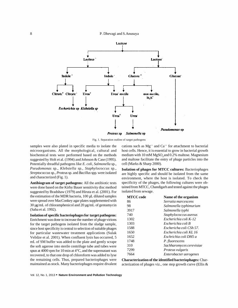
samples were also plated in specific media to isolate themicroorganisms. All the morphological, cultural andbiochemical tests were performed based on the methodssuggested by Holt et al. (1994) and Johnson & Case (1995).Potentially dreadful pathogens like E. coli, Salmonella sp.,Pseudomonas sp., Klebsiella sp., Staphylococcus sp.,Streptococcus sp., Proteus sp. and Bacillus spp. were isolatedand characterized (Fig. 1).Antibiogram of target pathogens: All the antibiotic testswere done based on the Kirby Bauer sensitivity disc methodsuggested by Bradshaw (1979) and Hiruta et al. (2001). Forthe estimation of the MDR bacteria, 100 µL diluted sampleswere spread over MacConkey agar plates supplemented with30 µg/mL of chloramphenicol and 20 µg/mL of gentamycin(Saha et al. 1992).Isolation of specific bacteriophages for target pathogens:Enrichment was done to increase the number of phage virionsfor the target pathogens isolated from the sludge sample,since host specificity is central to selection of suitable phagesfor particular wastewater treatment applications (SulakVelidze et al. 2001). When confluent lysis has occurred, 5mL of SM buffer was added to the plate and gently scrapethe soft agarose into sterile centrifuge tube and tubes werespun at 4000 rpm for 10 min at 4°C, and the supernatant wasrecovered, to that one drop of chloroform was added to lysethe remaining cells. Thus, prepared bacteriophages weremaintained as stock. Many bacteriophages require divalent
Fig. 1. Separation outline of target pathogens
cations such as Mg++ and Ca++ for attachment to bacterialhost cells. Hence, it is essential to grow in bacterial growthmedium with 10 mM MgSO4and 0.2% maltose. Magnesiumand maltose facilitate the entry of phage particles into thecell (Marks & Sharp 2000).Isolation of phages for MTCC cultures: Bacteriophagesare highly specific and should be isolated from the sameenvironment, where the host is isolated. To check thespecificity of the phages, the following cultures were ob-tained from MTCC, Chandigarhand tested against the phagesisolated from sewage.
MTCC code Name of the organism86 Serratia marcescens98 Salmonella typhimurium3917 Salmonella typhi740 Staphylococcus aureus1302 Escherichia coli K-121303 Escherichia coli B1588 Eschericha coli CSh 57.1650 Escherichia coli KL 161652 Eschrichia coli DH5 a1748 P. fluorescens310 Sachharomyces cerevisiae7299 Proteus vulgaris7664 Enterobacter aerogenes
Characterization of the identified bacteriophages: Char-acterization of phages viz., one step growth curve (Ellis &

Nature Environment and Pollution Technology · Vol. 12, No. 1, 2013
9BACTERIOPHAGE BASED PATHOGEN REDUCTION IN SEWAGE SLUDGE
Delbruck 1939) and multiplicity of infection are essentialfor fixing the time of treatment and dose of the phage dilu-tions to be used for wastewater purification (Sambrook &Russell 2001). The MOI of E. coli and S. typhi was assessedin one of our previous study (Sagkaguchi et al. 1989 andDhevagi & Anusuya 2011) and used for the sludgetreatment.Developing an eco-friendly bioconsortium for augment-ing the pathogen in sewage sludge: In the city ofCoimbatore 650 km of drains were to be laid and linked tothree sewage treatment plants coming up in Ukkadam,Nanjundapuram and Ondipudur, by the end of 2012.Coimbatore generates large quantity of sewage.Ukkadam sewage treatment plant: The plant, built at Rs.55 crore under the Jawaharlal Nehru National Urban RenewalMission Scheme, has a capacity to treat 70 MLD (millionlitres a day) sewage. At present, the plant treats only about20 MLD of wastewater which flows into it from the areasthat already have underground drainage system. The sewagetreatment plant has been constructed based on the ‘Sequen-tial Batch Reactor’ (SBR) process, which was the most ad-vanced method for sewage treatment (Fig. 2).
The E. coli and Salmonella sp. organisms were inoculatedinto sewage sludge. Sewage sludge collected from Ukkadamwas used for the study. The following are the treatments.
T1:Sewage sludge inoculated with E. coli and E.coli spe-cific bacteriophages.
T2:Sewage sludge inoculated with Salmonella sp. andSalmonella sp. specific bacteriophages.
T3:Sewage sludge inoculated with E. coli and Salmonellasp. specific bacteriophages.
T4:ControlSewage sludge was collected and filtered and 100 mL of
sewage sample (water and sludge) were taken in Din threadscrew bottles and sterilized. After cooling it was inoculatedwith E. coli at @ 104/mL and Salmonella sp. at @ 103/mL.After inoculation of pathogens the cell count was assessedfor checking the phage efficacy. Serial dilutions were car-ried up to 10 dilutions. From the serially diluted samples,0.1 mL of pathogenic cultures were added to sterile platescontaining LB (with sewage extract and without sewage ex-tract) and incubated at 37°C for 24 hours. At every 1 hr thepathogen survival was assessed up to 14 hours.
RESULTS AND DISCUSSION
Characterization of sewage sludge: During the past decade,sewage water gets accumulated in the form of stagnant waterand if there is drinking water pipes nearer, there is a chancefor intrusion of sewage water into the drinking water. In
Fig. 2: Sewage treatment process at Coimbatore Corporation sewage farm.
Vol. 12, No. 1, 2013 · Nature Environment and Pollution Technology
10 P. Dhevagi and S.Anusuya
developing countries 70% of the water is seriously pollutedand 75% of illness and 80% of the child mortality isattributed to water pollution (Zoetman 1980, Sangu &Sharma 1987). Untreated wastewater contains numerousdisease causing microorganisms and toxic compounds thatdwell in the human intestinal tract may contaminate the landor water body where sewage is disposed. According to WHOestimate about 80% of water pollution in developing country,like India is carried by domestic waste (Moharir et al. 2002).Raw sewage disposal into the estuaries has been a commonpractice throughout the world (Yanggen & Born 1990, Tyagiet al. 2000, Das Gupta & Purohit 2000). It is therefore ofinterest to determine what levels of pollution indicatorbacteria are owing to sewage disposal. This informationwould help to determine if careful waste treatment anddisposal procedures are needed to safeguard the naturalenvironment. The sludge samples collected from the sevenlocations were analysed and the results are given in Table 1.
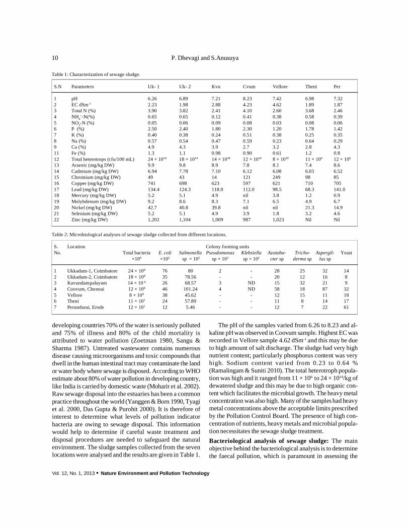
The pH of the samples varied from 6.26 to 8.23 and al-kaline pH was observed in Coovum sample. Highest EC wasrecorded in Vellore sample 4.62 dSm-1 and this may be dueto high amount of salt discharge. The sludge had very highnutrient content; particularly phosphorus content was veryhigh. Sodium content varied from 0.23 to 0.64 %(Ramalingam & Suniti 2010). The total heterotroph popula-tion was high and it ranged from 11 × 106 to 24 × 1014/kg ofdewatered sludge and this may be due to high organic con-tent which facilitates the microbial growth. The heavy metalconcentration was also high. Many of the samples had heavymetal concentrations above the acceptable limits prescribedby the Pollution Control Board. The presence of high con-centration of nutrients, heavy metals and microbial popula-tion necessitates the sewage sludge treatment.Bacteriological analysis of sewage sludge: The mainobjective behind the bacteriological analysis is to determinethe faecal pollution, which is paramount in assessing the
Table 1: Characterization of sewage sludge.
S.N Parameters Uk- 1 Uk- 2 Kvu Cvum Vellore Theni Per
1 pH 6.26 6.89 7.21 8.23 7.42 6.98 7.322 EC dSm-1 2.23 1.98 2.88 4.23 4.62 1.89 1.873 Total N (%) 3.90 3.82 2.41 4.10 2.60 3.68 2.464 NH4
+-N(%) 0.65 0.65 0.12 0.41 0.38 0.58 0.395 NO3-N (%) 0.05 0.06 0.09 0.08 0.03 0.08 0.066 P (%) 2.50 2.40 1.80 2.30 1.20 1.78 1.427 K (%) 0.40 0.38 0.24 0.51 0.38 0.25 0.358 Na (%) 0.57 0.54 0.47 0.59 0.23 0.64 0.299 Ca (%) 4.9 4.3 3.9 2.7 3.2 2.8 4.311 Fe (%) 1.3 1.1 0.98 0.90 0.61 1.2 0.812 Total heterotrops (cfu/100 mL) 24 × 1014 18 × 1014 14 × 1010 12 × 1014 8 × 10¹⁰ 11 × 106 12 × 106
13 Arsenic (mg/kg DW) 9.9 9.8 8.9 7.8 8.1 7.4 8.614 Cadmium (mg/kg DW) 6.94 7.78 7.10 6.12 6.08 6.03 6.5215 Chromium (mg/kg DW) 49 43 14 121 249 98 8516 Copper (mg/kg DW) 741 698 623 597 621 710 70517 Lead (mg/kg DW) 134.4 124.3 118.0 112.0 98.5 68.3 141.018 Mercury (mg/kg DW) 5.2 5.1 4.9 nil 3.8 1.2 0.919 Molybdenum (mg/kg DW) 9.2 8.6 8.3 7.1 6.5 4.9 6.720 Nickel (mg/kg DW) 42.7 40.8 39.8 nil nil 21.3 14.921 Selenium (mg/kg DW) 5.2 5.1 4.9 3.9 1.8 3.2 4.622 Zinc (mg/kg DW) 1,202 1,104 1,009 987 1,023 Nil Nil
Table 2: Microbiological analyses of sewage sludge collected from different locations.
S. Location Colony forming unitsNo. Total bacteria E. coli Salmonella Pseudomonas Klebsiella Azotoba- Tricho- Aspergil- Yeast
×106 ×102 sp × 102 sp × 102 sp × 102 cter sp derma sp lus sp
1 Ukkadam-1, Coimbatore 24 × 108 76 80 2 - 28 25 32 142 Ukkadam-2, Coimbatore 18 × 108 35 78.56 - - 20 12 16 83 Kavundampalayam 14 × 10 4 26 68.57 3 ND 15 32 21 94 Coovum, Chennai 12 × 108 46 101.24 4 ND 58 18 87 325 Vellore 8 × 10⁴ 38 45.62 - - 12 15 11 186 Theni 11 × 101 24 57.89 - - 11 8 14 177 Perundurai, Erode 12 × 101 12 5.46 - - 12 7 22 61

Nature Environment and Pollution Technology · Vol. 12, No. 1, 2013
11BACTERIOPHAGE BASED PATHOGEN REDUCTION IN SEWAGE SLUDGE
associated health risks. The sewage sludge was analysed todetermine the pollution load. Pathogenic population was highwhich suggests the essentiality of the treatment. SinceSalmonella is a dreadful pathogen and has more aggregatingproperty, more number of organisms was isolated from thesewage sludge. Sludge collected from Chennai had very highSalmonella population, lowest was recorded in Perunduraisample. Among the seven different locations, samples
collected from Ukkadam recorded the maximum heterotrophpopulation (172 × 106/mL of sample) and high E. colipopulation (24 ×108/mL of sample), followed by samplescollected from Coovum, Chennai (142 × 106/mL of sample)(Table 2).Antibiogram of target pathogens: The antibiotic resistanceof the isolates was tested using disk diffusion test. For theestimation of the MDR bacteria, 100 µL diluted samples were
Table 3: Resistance patterns of MDR bacteria isolated from sewage sludge.
S. No Antibiotics Ukkadam-1 Ukkadam-2 Kavunda- Coovum Vellore Theni PerunduraiCoimbatore Coimbatore mpalayam Chennai Erode
1 Ciproflaxin (10 mcg) I I R R R R S2 Tetracycline (30 mcg) R R R R S I S3 Streptomycin (10 mcg) S R I I I R S4 Kanamycin (10 mcg) S R S I I S R5 Ampicillin (10 mcg) I R R I R R I6 Erythromycin (15mcg) R R S R R I S7 Penicillin (10 mcg) I R S S R S R8 Cephalosporin (30 mcg) R R R R R R R9 Rifampicin (5mcg) S S I I I R R
R = Resistant; S = Sensitive; I = Partially resistant. Drug concentration in µg/disc mentioned in parentheses.
Table 4: Morphological and biochemical characterization of specific pathogens.
S. No. Tests performed E. coli Salmonella typhi Pseudomonas aeruginosa Klebsiella pneumoniae
1 Shape Rods Rods Rods Rods2 Gram staining Gram negative Gram negative Negative Negative3 Motility Motile Motile Motile Positive4 Gelatin utilization test Negative Positive Positive Negative5 Citrate utilization test Positive Positive Positive Positive6 Methyl Red Negative Positive Positive Negative7 Voges Proskeur Positive Negative Negative Negative8 Acid from glucose Positive Positive Positive Positive9 Gas from glucose Negative Positive Positive Negative10 Triple Sugar Iron test Acid was produced Gas was produced Acid was produced Acid was produced11 Urease test Positive Negative Positive Positive12 Indole production Negative Positive Positive Negative
Table 5: Antibiogram of target pathogens.
S.No Antibiotics (Concentration 30 mcg)E. coli Salmonella typhi Pseudomonas aeruginosa Klebsiella sp
1 Gentamycin R (1) R (1) R (1) R (1)2 Ciproflaxin I (4) R (1) I (5) I (4)3 Chloramphenical R (0) R (1) R (1) R (2)4 Tetracycline R (2) R (1) R (1) I (5)5 Streptomycin S (11) I (3) R (1) R (2)6 Kanamycin S (10) R (1) R (2) R (1)7 Ampicillin R (3) R (1) R (2) R (2)8 Erythromycin R (1) R (1) R (1) R (1)9 Penicillin I (4) R (1) R (1) R (1)10 Cephalosporin R (1) R (1) R (0) R (1)11 Rifampicin S (6) R (4) R (1) R (2)
R = Resistant (R, < 3mm), I = Intermediate(I, 3-5mm), S = Susceptible (S, > 6mm)

Vol. 12, No. 1, 2013 · Nature Environment and Pollution Technology
12 P. Dhevagi and S.Anusuya
spread over MacConkey agar plates supplemented with 30µg/mL of chloramphenicol and 20 µg/mL of gentamycin(Table 3) because they have greater in vitro stability. Simul-taneous resistance to ciproflaxin, tetracycline, streptomy-cin, kanamycin, ampicillin, erythromycin, penicillin, cepha-losporin and rifampicin formed the common MDR pattern.Sewage sludge of Ukkadam showed very high percentage ofMDR bacteria, since Ukkadam is the prime area, whereCoimbatore city wastes are disposed. The MDR pattern seenin the bacterial isolates fromsewage sludge samples includedmost of the antibiotics used presently for treating humaninfections. The origin of such MDR bacterial strains appearsto be the hospital environment and the selective pressureresponsible for expanding such bacterial populations in hos-pitals must have been through the use of drugs in humans(Neema et al. 1997, Rangnekar 1981, Ogunseitan et al. 1990,Dhevagi & Anusuya 2011). The present observations sug-gest that indiscriminate release of sewage water can be apotential health hazard by adding MDR bacteria in to theenvironment.Characterisation of target pathogens isolated from sew-age sludge: Single colony, picked up from the culture platewas kept as stock. The picked colonies were streaked onMacConkey agar medium, Kings B medium and SalmonellaShigella agar medium. The streaked organisms were incu-bated at 37°C for 24 hours. Pink colonies on MacConkeyagar plate resembling E. coli were further characterized. Pinkcolonies on Salmonella Shigella agar plates resembling Sal-monella were evaluated by morphological and biochemicalanalysis to identify the organism. Fluorescent colonies fromKings B medium plates resembling Pseudomonasaeruginosa were evaluated by morphological and biochemi-cal analysis to identify the organism (Table 4).
Bacterial strains E. coli, Salmonella typhi, Pseudomonasaeruginosa and Klebsiella pneumoniae were tested for theantibiotic resistance with different antibiotics in which theyshowed resistance to most of the antibiotics. By their zoneof inhibition the organisms were chosen. E. coli showed re-sistance to 5 antibiotics, intermediate resistance to 3 antibi-otics and susceptible to 3 antibiotics. Salmonella typhi
showed resistance to almost all the antibiotics and interme-diate resistance to 3 antibiotics. Pseudomonas aeruginosashowed resistance to almost all the antibiotics, and interme-diate resistance to only one antibiotic. Klebsiella sp. showedresistance to 9 antibiotics and intermediate resistance to 2antibiotics (Table 5). Compared to sewage water, more MDRpattern was observed in pathogens isolated from sludge sam-ples (Poorani et al. 2006).Isolation of specific bacteriophages for target pathogens:Interest in the ability of phages to control bacterial popula-tion has extended very recently for water treatment also.Antibiotic resistant pathogens are inevitable as survival isthe key for existence. Phage therapy is an alternative to over-come these menacing organisms. This study highlights thepotential to develop phage treatments for generalized con-trol of bacterial populations. There is potential applicationof phages in wastewater treatment system to improve efflu-ent and sludge disposal into the environment. Phage treat-ments have the ability to control environmental wastewaterprocesses such as foaming in active sludge plants; sludgedewater ability and digestibility of pathogenic bacteria; andto reduce competition between nuisance bacteria and func-tionally important microbial population. When target bac-teria have been identified, phage infective for those speciesmust then be selected. Host specificity is central to selectionof suitable phages for particular wastewater treatment appli-cations (Sulak Velidze et al. 2001).
Enrichment was done to increase the number of phagevirions in sewage sludge. It is essential for the success ofany phage therapy; suitable phage should be isolated, en-riched to produce sufficient numbers for the application.Phage enrichment normally involves the inoculation ofmixed environmental samples and growth media with sin-gle host strain. Repeated phage purification using just onehost strainmay increase the specificity for that strain (Connon& Giovannoni 2002, Rappe et al. 2002, O’Sullivan et al2004).
Plaque formation was observed due to the inhibition ofgrowthand lyses of the phage infected cells. The clear plaquewas used for purification of phages for further analysis
Table 6: Number of plaque forming units per mL of the E. coli lysate, Salmonella typhi lysate and Pseudomonas aeruginosa lysate.
S. No. Dilution factor E. coli lysate pfu/mL Salmonella typhi lysate pfu/mL P. aeuroginosa lysate pfu/mLof sample of sample of sample
1 10-2 TNC TNC TNC2 10-3 175 × 105 214 × 105 237 × 105
3 10-4 116 × 106 119 × 106 129 × 106
4 10-5 83 × 107 86 × 107 94 × 107
5 10-6 74 × 108 46 × 108 80 × 108
Values represent mean of three replications; TNC - Too Numerous to Count

Nature Environment and Pollution Technology · Vol. 12, No. 1, 2013
13BACTERIOPHAGE BASED PATHOGEN REDUCTION IN SEWAGE SLUDGE
(Maloy et al. 2008). The plaques appeared on the E. coli andSalmonella typhi lawn was individually isolated, and usedfor the sewage treatment. Since phages are very specific(Shuttle 2000 and Alonso et al. 2002) inoculation of thephage should coincide with bacterial population density suf-ficient to support phage replication (Payne & Jansen 2001).Isolation of specific phages for MTCC cultures: The re-sults indicated that none of the sewage sludge sample hadbacteriophages against MTCC cultures. This clearly indi-cates the specificity of phages.Characterization of the identified bacteriophages: Whenconfluent lyses has occurred, 5 mL of SM buffer was addedto the plate and gently scrape the soft agarose into sterilecentrifuge tube. Tubes were spun at 4000 rpm for 10 min at4°C, and the supernatant was recovered and to that one dropof chloroform was added to lyse the remaining cells. Thus,prepared bacteriophages were maintained as stock and usedfor further analysis. Bacteriophages were titrated with theirrespective dilutions to know the number of plaques formedfor their respective host and results are given in Table 6.
After multiplication of specific pathogen, cell count ineach mL of broth was assessed for the purpose of fixing thephage concentration. Serial dilutions were carried out up to10 dilutions. From the serially diluted samples, 0.1 mL ofpathogenic cultures were added to sterile plates containingLB and incubated at 37°C for 24 hours. In case of E. coli upto 10-8 dilutions, there are uncountable numbers. Countablenumbers were observed only in 10-9 and 10-10 dilutions. Incase of Salmonella typhi, up to 10-5 dilutions, there are un-countable numbers of colony forming units. Countable num-bers was observed from 10-6 dilutions (Table 7).
Characterization of phages viz., one step growth curve,multiplicity of infection and burst size are essential for fix-ing the time of treatment and dose of the phage dilutions tobe used for wastewater purification (Sambrook & Russell2001). Even though phages specific to E. coli, Salmonellaand Pseudomonas were isolated, characterization studieswere restricted to E. coli and Salmonella sp.One step growth studies: From one step growth curve ofbacteriophage, multiplicity of infection was calculated toanalyse the lytic activity of phage to host bacteria (Ellis &Delbruck 1939). The multiplicity of infection for the presentisolate was observed as 0.3. Sagkaguchi et al. (1989) reportedthat the phage with MOI higher than 0.1 could effectivelylyses the host bacteria after 5-7 hours of infection. There-fore Salmonella phage isolated is an effective lyric phagefor Salmonella typhus. Salmonella started to form phage par-ticles after 2 hours of infection and completed at 8 hours and7 hours in case of E. coli. Therefore, one phage infected Sal-monella typhi can produce 68 phage particles (Table 8).Developing an eco-friendly bioconsortium for augment-ing the pathogen in sewage sludge: Most pathogens areassociated with sludge flocs rather than liquid portions.Hence, sludge biology should also be concentrated duringthe phage treatment. Enumerated bacteriophages were testedfor the biocontrol efficacy in controlling the target patho-gens. The test organism selected for the study was E. coliand Salmonella typhi. The target pathogens with their spe-cific bacteriophages were inoculated separately as well as inmixture. Then the survival rates of pathogens were studied.The number of bacteriophages should 3 to 10 times greaterthan bacteria (Hennes & Simon 2005). Reduction in popu-lation of viruses during activated sludge treatment occursby viral adsorption to sludge flocs (Wellings et al. 1976 andTanji et al. 2002, Ketratanakul & Ohgaki 1989). While mix-ing the host and phages the concentration should be suffi-cient. Payne & Jansen (2001) observed that insufficient hostcell concentration may also contribute for phage decline.Inoculation of the phage should coincide with bacterial popu-lation density sufficient to support phage replication. Poor
Table 7: Cell count of E. coli, Salmonella typhi and P. aeruginosa.
S.No. Dilution E. coli Salmonella typhi P. aeruginosa(cfu/mL) (cfu/mL) (cfu/mL)
1 10-1 uncountable uncountable ND2 10-2 uncountable uncountable ND3 10-3 uncountable uncountable ND4 10-4 uncountable uncountable uncountable5 10-5 uncountable uncountable uncountable6 10-6 uncountable 541 99 × 10-7
7 10-7 uncountable 398 30 × 10-8
8 10-8 uncountable 126 12 × 10-9
9 10-9 249 87 ND10 10-10 86 31 ND
Values represent mean of three replications.
Table 8: Measurement of bacteriophage growth with 4 × 10⁹ cfu/mL of E.coli sp. and 2 × 10⁷ pfu/mL E. coli specific phages and 4 × 10⁹ cfu/mL ofSalmonella sp. and 2 × 10⁷ pfu/mL Salmonella specific phages.
S.No. Time E. coli specific phages Salmonella specific phagesin hours No. of pfu/mL No. of pfu/mL
1 1 8.4 × 10⁶ 9 × 10⁵
2 2 6.8 × 10⁶ 9 × 10⁵
3 3 8.9 × 10⁷ 1 × 10⁶
4 4 9.5 × 10⁷ 1.5 × 10⁶
5 5 7.2 × 10⁸ 2.2 × 10⁶
6 6 8.6 × 10⁸ 3.6 × 10⁶
7 7 9.6 × 10⁸ 5.6 × 10⁶
8 8 8.1 × 10⁹ 2.12 × 10⁷
9 9 8.2 × 10⁹ 2 × 10⁷
10 10 Confluent lyses Confluent lyses
Vol. 12, No. 1, 2013 · Nature Environment and Pollution Technology
14 P. Dhevagi and S.Anusuya
penetration in the sludge flocs may reduce the efficacy ofphage treatment. Kim & Unno (1996) showed ingestion ofviral particles by bacteria, protozoa and metazoa, which maycontribute to phage loss, should be addressed. In addition,radiation also reduces the numbers. Hantula et al. (1991)found that approximately 10% of phages isolated from acti-vated sludge were polyvalent in nature.
In contrast, Jensen et al. (1998) and Wolf et al. (2003)found that multiple host isolation techniques may be moreeffective at isolating polyvalent phages. Thomas et al. (2002)found that 15 out of 17 phages isolated from activated sludgehad broad host ranges. Despite the potential advantages ofpolyvalent phage, broader host range phage influencing notonly the target strains, but also beneficial degradative bacte-ria. Phage enrichment was done to isolate a suitable host bac-terium. Repeated phage purification using just one host strainmay increase specificity for that strain potentially narrow-ing the host range of phage.
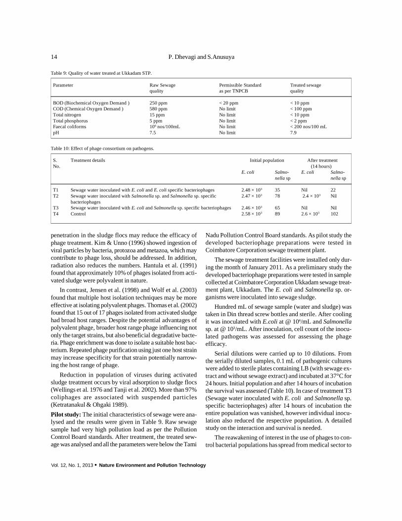
Reduction in population of viruses during activatedsludge treatment occurs by viral adsorption to sludge flocs(Wellings et al. 1976 and Tanji et al. 2002). More than 97%coliphages are associated with suspended particles(Ketratanakul & Ohgaki 1989).Pilot study: The initial characteristics of sewage were ana-lysed and the results were given in Table 9. Raw sewagesample had very high pollution load as per the PollutionControl Board standards. After treatment, the treated sew-age was analysed andall the parameters were below the Tami
Nadu Pollution Control Board standards. As pilot study thedeveloped bacteriophage preparations were tested inCoimbatore Corporation sewage treatment plant.
The sewage treatment facilities were installed only dur-ing the month of January 2011. As a preliminary study thedeveloped bacteriophage preparations were tested in samplecollected at Coimbatore Corporation Ukkadam sewage treat-ment plant, Ukkadam. The E. coli and Salmonella sp. or-ganisms were inoculated into sewage sludge.
Hundred mL of sewage sample (water and sludge) wastaken in Din thread screw bottles and sterile. After coolingit was inoculated with E.coli at @ 104/mL and Salmonellasp. at @ 103/mL. After inoculation, cell count of the inocu-lated pathogens was assessed for assessing the phageefficacy.
Serial dilutions were carried up to 10 dilutions. Fromthe serially diluted samples, 0.1 mL of pathogenic cultureswere added to sterile plates containing LB (with sewage ex-tract and without sewage extract) and incubated at 37°C for24 hours. Initial population and after 14 hours of incubationthe survival was assessed (Table 10). In case of treatment T3(Sewage water inoculated with E. coli and Salmonella sp.specific bacteriophages) after 14 hours of incubation theentire population was vanished, however individual inocu-lation also reduced the respective population. A detailedstudy on the interaction and survival is needed.
The reawakening of interest in the use of phages to con-trol bacterial populations has spread from medical sector to
Table 9: Quality of water treated at Ukkadam STP.
Parameter Raw Sewage Permissible Standard Treated sewagequality as per TNPCB quality
BOD (Biochemical Oxygen Demand ) 250 ppm < 20 ppm < 10 ppmCOD (Chemical Oxygen Demand ) 580 ppm No limit < 100 ppmTotal nitrogen 15 ppm No limit < 10 ppmTotal phosphorus 5 ppm No limit < 2 ppmFaecal coliforms 106 nos/100mL No limit < 200 nos/100 mLpH 7.5 No limit 7.9
Table 10: Effect of phage consortium on pathogens.
S. Treatment details Initial population After treatmentNo. (14 hours)
E. coli Salmo- E. coli Salmo-nella sp nella sp
T1 Sewage water inoculated with E. coli and E. coli specific bacteriophages 2.48 × 10³ 35 Nil 22T2 Sewage water inoculated with Salmonella sp. and Salmonella sp. specific 2.47 × 10³ 78 2.4 × 10³ Nil
bacteriophagesT3 Sewage water inoculated with E. coli and Salmonella sp. specific bacteriophages 2.46 × 10³ 65 Nil NilT4 Control 2.58 × 10³ 89 2.6 × 10³ 102

Nature Environment and Pollution Technology · Vol. 12, No. 1, 2013
15BACTERIOPHAGE BASED PATHOGEN REDUCTION IN SEWAGE SLUDGE
wastewater treatment process. The outcome of this projecthighlighted the aspects ofwastewater treatment, where phageinduced bacterial lysis might be harnessed.
Success would depend on accurate identification of prob-lematic, effective isolationandunbiasedenrichment of phageand ability of phage to penetrate flocs and remain infectivein in situ condition. Density of non host cells may also beimportant in determining the success of phage treatment ofwastewater. Thus, further substantial research is needed toexplore the potential of phage treatment. Despite some ofthe potential hindrances to the phage treatment, the currentawareness regarding phages indicates that phage applicationto wastewater treatment deserves attention. Growing levelsof antibiotic resistance and the exit of major pharmaceuticalindustries from antibiotic development force to have nochoice but to adopt phage therapy for growing number ofotherwise untreatable infections.
ACKNOWLEDGEMENT
The authors are thankful to the Ministry of Environment andForest , Government of India for the financial support.
REFERENCES
Alonso, M.D., Rodriguez, J. and Borrego, J.J. 2002. Characterization ofmarine bacteriophages isolated from Alboran sea (Western Mediter-ranean). J. Plankton. Res., 24: 1079-1087.
APHA 1989. Standard Methods for the Examination of Water andWastewater. 16th Edn. American Public Health Association, Washing-ton DC.
Bradshaw, J. L., 1979. Laboratory Microbiology. Third edition, W.B.Saunders Company.
Cappuccino, J.G. and Sherman, N. 2002. Microbiology - A LaboratoryManual. Sixth edition, Pearson Education (Singapore) Pvt. Ltd., In-dian Branch.
Chitnis, V., Chitnis, D., Patil, S. and Ravi Kant 2000. Hospital effluent: Asource of multiple drug resistant bacteria. Current Science, 79:989-991.
Connon, S.A. and Giovannoni, S.J. 2002. High-throughput methods forculturing microorganisms in very low nutrient media yield diverse newmarine isolates. Appl. Environ. Microbiol., 68: 3878-3885.
Dasgupta, A. and Purohit, K.M. 2001. Status of the surface water quality ofMandiakudar. Pollut. Res., 20(1): 103-110.
Dhevagi, P. and Anusuya, S. 2011. Ecofriendly phages for pathogen re-moval from sewage waste water. Paper presented at UGC sponsoredNational Seminar on Recent Trends in Plant Biotechnology held atGovernment Art college, Coimbatore on February 4th and 5th.
Ekhaise, F.O. and Omavwaya, B.P. 2008. Influence of hospital wastewaterdischarged from university Benin Teaching Hospital (UBTH), BeninCity on its receiving environment. J. Agric. and Environ. Sci., 4:484-488.
Ellis, E. L. and Delbruk, M. 1939. The growth of bacteriophages. Journalof General Physiology, 22(3): 365 to 384.
Ewert, D.L. and Paynter, M.J.B.1980. Enumeration of bacteriophages andhost bacteria in sewage and the activated sludge treatment process.Appl. Environ. Microbiol., 39: 576-583.
Hantula, J., Kurki, A., Vuoriranta, P. and Bamford, D. 1991. Ecology ofbacteriophages infecting activated sludge bacteria. Appl. Environ.
Microbiol., 57: 2147-2151.Hennes, K.P. and Simon, M. 2005. Significance of bacteriophages for con-
trolling bacterioplankton growth in a mesotrophic lake. Appl. Environ.Microbiol., 61: 333-340.
Hiruta, N., Murase, T. and Kamura, O.N. 2001. An outbreak of diarrheadue to multiple antimicrobial resistant Shiga toxin producing E. coli.026 ; H11 in a nursery. Epidemiology Infect., 127: 221-227.
Holt, G.J., Krieg, R.N., Sneath, A.H.P., Stately, T.J. and Williams, T.S. 1994.Bergey’s Manual of Determinative Bacteriology. 9th edition, Lippincott.
Jensen, E.C., Sehrader, H.S., Rieland, B., Thompson, T.L., Lee, K.W.,Nickers, K.W. and Kokjon, T.A. 1998. Prevalence of broad host rangelytic bacteriophages of Spharotilus natans, Escherichia coli and Pseu-domonas aeruginosa. Appl. Environ. Microbial., 64: 575-580.
Johnson, T.R. and Case, C.L. 1995. Laboratory Experiments in Microbiol-ogy. The Benjamin/Cummings Publishing Company, Inc., 125-129.
Ketratanakul, A. and Ohgaki, S. 1989. Indigenous coliphages and RNA-F-specific coliphages associated with suspended solids in the activatedsludge process. Wat. Sci. Tech., 2: 73-78.
Kim, T.D. and Unno, H. 1996. The role of microbes in the removal andinactivation of viruses in a biological wastewater treatment system.Wat. Sci. Tech., 33: 243-250.
Maloy, S.R., Cronana, J.E. and David Freifelder 2008. Genetics of phageT4 In: Microbial Genetics, 2nd edn., Narosa Publishing House, NewDelhi, pp. 346-370.
Marks, T. and Sharp, R. 2000. Bacteriophages and biotechnology: A re-view. J. Chem. Tech. Biotechnol., 75: 6-17.
McDonald, K. 2008. Bacterias Natural Born killer. Australian Life Scien-tist, http://www. Biotechnewa.com.au/index.php/id:1656824057:pp.2.
Moharir, A., Ramteke, D.S., Moghe, C.A., Wate, S.R. and Sarin, R. 2002.Surface and ground water quality assessment in Bina region. Ind. J.Environ. Protec., 22(9): 961-969.
Neema, S., Premchandani, P., Asolkar, M.V. and Chitnis, D.S. 1997. Emerg-ing bacterial drug resistance in hospital practice. Indian J. Med. Sci.,15(8): 275-280.
O’gunseitan, O.A., Sayer, G.S. and Miller, R.V. 1990. Dynamic interac-tions between Pseudomonas aeruginosa and bacteriophages inlakewater. Microb. Ecol., 19: 171-185.
O’Sullivan, L.A., Fuller, K.E., Thomas, E.M., Turley, C.M., Fry, J.C. andWeightman, A.J. 2004. Distribution and culturability of the unculti-vated ‘AGG58 cluster’ of the Bacteriodes phylum in aquatic environ-ments. FEMS Microbial. Ecol., 47: 359-370.
Payne, R.J.H. and Jansen, V.A.A. 2001. Understanding phage therapy as adensity dependent kinetic process. J. Theor. Biol., 208: 37-48.
Poorani, E., Dhevagi, P. and Gowrisangar, 2006. Etiology of infantDiarrhoes. J. Ecobiol., 19: 89-94.
Ramalingam, C. and Sunit, S. 2010. Wastewater reuse; Extension approachto depleting water resources. Journal of Phytology, 2: 44-49.
Rangnekar, V. M., Mukerji, S., Gadre, S.V. and Chitnis, D.S. 1981. Bull.Haffkine Inst., 9: 8-14.
Rappe, M.S., Connon, S.A., Vergin, K.L. and Giovannoni, S.J. 2002. Cul-tivation of the ubiquitous SARII marine bacterioplankton clade. Na-ture, 418; 633-639.
Sagkaguchi, L., Shinshima, K., Kawaratani, K. and Sugai, O. 1989. Con-trol of microbiofouling using bacteriophage 2. Detection of phagesand fundamental study of their lytic effect on fouling bacteria. Arch.Immunol. Ther. Exp., 35: 569-583.
Saha, M.R., Dutta, P., Bhattacharya, S.K., Rasaily, R., Mitra, U., Dutta, D.,Bhattacharya, M.K. and Pal, S.C. 1992. Multidrug resistant bacteria.Indian J. Med. Res., 95: 179-180.
Sambrook, J. and Russell, R.W.D. 2001. Molecular cloning-A laboratoryManual, 3rd Ed., Cold Spring Harbor Laboratory Press, Cold SpringHarbor, NY, 2.25-2.33.
Sangu, R.P. S. and Sharma, S.K. 1987. An assessment of water quality ofriver Ganga at Garmukeshwar. Ind. J. Ecol., 14(20): 278-287.

Vol. 12, No. 1, 2013 · Nature Environment and Pollution Technology
16 P. Dhevagi and S.Anusuya
Shuttle, C.A. 2000. Theoritical, evolutionary and geochemical consequencesof viral infection of cyanobacteria and eukaryotic algae. In: Horst, C.J. (Ed.) Viral Ecology, Academic Press.
Sulak Velidze, A.Z. Alavidze and Morris, J.R.G. 2001. Bacteriophagetherapy. Antimicrobial Agents and Chemotherapy, 43: 649-659.
Summers, W.C. 2001. Bacteriophage therapy. Annual Rev. Microbiol., 55;437- 451.
Tanji, Y, Mizoguchi, K., Yoichi, M., Morita, M., Hori, K. and Unno, H.2002a. Fate of coliphage in a wastewater treatment process and detec-tion of phages carrying the Shiga toxin type 2 gene. Wat. Sci. Tech.,46: 285-289.
Tanji, Y, Mizoguchi, K., Yoichi, M., Morita, M., Hori, K. and Unno, H.2002b. Fate of coliphage in a wastewater treatment. J. Biosci. Bioeng.,94: 172 -174.
Thiel, K. 2004. Old Dogma, New tricks-21st Century phage therapy. Nat.
Biotechnol., 22; 31-36.Thomas, L., Jungschaffer, G. and Sprossler, B. 1993. Improved sludge
dewatering by enzymatic treatment. Wat. Sci. Tech., 28: 189-192.Tyagi, P., Buddi, D., Chowdary, R. and Sawhney, R. 2000. Physicochemi-
cal quality of ground water in industrial areas of India. Pollut. Res.,19: 443-445.
Wellings, F.MA., Lewis, L. and Mountain, C.W. 1976. Demonstration ofsolids-associated virus in wastewater and sludge. Appl. Environ.Microbiol., 31: 354-358.
Wolf, A., Wiese, J., Jost, G. and Witzel, K. 2003. Wide geographic distri-butions of bacteriophages that lyse the same indigenous fresh waterisolate (Sphingomonas sp. Strain B18). Appl. Environ. Microbiol., 69:2395-2398.
Zoeteman, B.C.G.1980. Sensory Assessment of Water Quality. OxfordPergaman Press, U.K.

Jinlan Xu, Yitao Zhang, Tinglin Hung and Hai xin DengSchool of Environmental and Municipal Engineering, Xi’an University of Architecture and Technology, Xi’an 710055,Shaanxi, China
ABSTRACT
The growth characteristics of seven strains isolated from oil contaminated soil, as well as their respectivedegradation efficiency for various hydrocarbons were investigated. Factors that can impact biological oildegradation efficiency were revealed in a series of experiments. The results indicate that isolated strainscould rapidly degrade crude oil, showing high activity in the first 13 h of bioremediation. These strains couldgrow in paraffin wax, which indicates that these strains could degrade long chain hydrocarbons. Some ofthem (SY22, SY23, SY24, SY42, SY43) were able to use short chain hydrocarbons and aromatic hydrocarbonsas substrate, so these five strains are the preferred ones for the bioremediation of oil contaminated soil.Suitable pH for the growth of these five strains was in the range from 7 to 9. NH4NO3 and oil concentrationsshould rangefrom 1000 mg/L to1500 mg/L in order to achieveoptimum conditions for petroleum hydrocarbondegradation. Adding organic matter such as starch and glucose accelerated oil andPAH degradation capabilityof the SY22, SY42 and SY23 strains. The presence of metal ions, such as Ni2+ and Co2+ in soil decreased thecrude oil degradation efficiency of these strains, while metal ions, such as Fe2+ and Mn2+ did not affect the oildegradation activities.
Nat. Env. & Poll. Tech.
Received: 25-9-2012Accepted: 8-11-2012
Key Words:Hydrocarbon-degradingactive bacteriaGrowth characteristicsOil-contaminated soilsBioremediation
2013pp. 17-24Vol. 12ISSN: 0972-6268 No. 1Nature Environment and Pollution TechnologyAn International Quarterly Scientific Journal
Original Research Paper
INTRODUCTION
Eight million tons (Mt) of petroleum is spilled into the en-vironment every year worldwide. In China, 0.6 Mts of pe-troleum enters into soil, groundwater, rivers and ocean everyyear. Oils are ubiquitous in environment and may be presentat high concentrations at industrial sites associated with pe-troleum, coal tar, gas production and wood preservation in-dustries (Wattiau 2002). The presence of petroleum oils inthe environment causes serious health hazard because of theirmutagenic and carcinogenic properties (Kastner 1998). Oilcontamination is a severe threat for our environment andthereby attracts general concern. Hence, there is an increas-ing interest to remediate the sites contaminated with petro-leum to minimize their threats to human health.
As compared to physico-chemical treatments, use of mi-crobial technology to clean up oil-contaminated sites hasbeen found an efficient, economical, eco-friendly and adapt-able choice. Besides, it haspotential advantages over physico-chemical methods such as complete degradation of pollut-ants, greater safety and less soil disturbance (Habe 2003).Bioremediation has become one of the most promising tech-nologies for oil contaminated soil remediation. Microorgan-isms used for bioremediation are usually grouped as indig-enous and exogenous microbes. The addition of nutrientsincreases the activity of native microorganisms; however,bioremediation is boosted with the addition of exogenous
bacteria. The application of bioremediation using indigenousmicrobes is restricted because native microbes need a longtime to domesticate, and thereby show low growth rates andlow metabolic activity, which make decontamination slowand ineffective. However, a few bacteria who are able togrowon the four ring PAHs, specifically, fluoranthene (Rehmann1999, Luepromchai 2007) and pyrene (Rehmann 1998,Churchill 1999) such as Mycobacterium, Rhodococcus, Al-caligenes and Sphingomonas have studied PAH degradationin soil. The application of addition of exogenous active bac-teria in field experiments has increased. A study on the di-versity of PAH degrading bacteria shows that Sphingomonasspecies are generally found to be fluoranthene degrading,while Pseudomonas strains were commonly associated withphenantherene degradation (Muller 1997). Therefore, thescreening of hydrocarbon-degrading active bacteria toremediate oil polluted soil is a necessary task.
In the present investigation, hydrocarbon degradation wasstudied in minerial medium using hydrocarbons as a solesource of carbon and energy by seven bacterial strains iso-lated from oil contaminated soil in the north region of theShaanxi province in order to find out the highest hydrocar-bon degrading bacterial strain to be used further in the con-sortium for crude oil degradation in the field conditions. Theeffect of pH, nutrition (nitrogen and phosphorus), and pol-lution intensity on the oil degradation efficiency of the iso-lated strains were investigated. Furthermore, based on the

Vol. 12, No. 1, 2013 · Nature Environment and Pollution Technology
18 Jinlan Xu et al.
complexity of the soil systems, the degradation capacity ofthe isolated bacteria of different kinds of petroleum hydro-carbons and the effect of adding organic co-substrate andmetal ions on the bioremediation were studied.
MATERIALS AND METHODS
The Source of samples: The tested crude oil and oil pol-luted soil were collected at oil wells in the northern regionof the Shaanxi province. The strains separated from the oilcontaminated soil were SY21, SY22, SY23, SY24, SY42, SY43,and SY44.Culture medium: The recipes of the different culture me-dia used in this work are provided as follows.
Recipe of liquid or solid beef grease and peptone culti-vation medium: 10g peptone, 3g beef grease, 5g NaCl,1000mL distilled water, pH 7.0. The medium can be solidi-fied using 20g of agar (Shen 1996).
The composition of mineral medium used in this workwas as follows: 2g NH4NO3, 1.5g K2HPO4, 3g KH2PO4, 0.1gMgSO4·7H2O, 0.01ganhydrousCaCl2, 0.01g Na2EDTA·2H2O,1000mL distilled water, with a pH ranging from 7.2 to 7.4(Liang et al. 2004).Crude oil culture medium: Addition of crude oil into liq-uid mineral salts culture medium. The medium above wereall sterilized for 30 min under 121°C.Isolating, screening and identification of bacterial strains:Enrichment cultures were prepared by addition 10g of freshcontaminated soils mixed with four soil samples into 100mL sterilized mineral salts broth contained in screw-capped250 mL Erlenmeyer flasks. The cultures were incubated at30°C in a THZ-82 shaker, manufactured by ChangzhouGuohua Electronic Appliance Ltd, China, at a speed of 180r/min for 7 days. Then, fifty millilitres (50 mL) of the en-riched cultures were transferred into a 100 mL of fresh ster-ile mineral broth (250 mL flask)containing 1mL of the sterilecrude oil and were shaken again at a speed of 180 r/min dur-ing 7 days at 30°C for the second enrichment. After suchfour successive weekly transfers, the cultures with a seriesof concentration gradient were inoculatedon the mineral saltsagar containing quantity crude oil to get the enriched con-sortium and separated petroleum degrading microorganismwith a clearing zone around the inoculated region. The iso-lation and purification of the bacterial consortium were car-ried out on nutrient agar plates by conventional spread platetechniques. Plates were incubated at 37°C for 48h after whichisolated colonies were selected for further identification. Allisolates were stored below 20°C as liquid cultures contain-ing 20% glycerol (v/v) (Zhao et al. 2009).
The procedure of secondary screening for hydrocarbon
degradation was as follows. Isolates able to grow on the min-eral salts agar containing crude oil were further subjected tosecondary screening in 100 mL cultures contained in 250mL screw-capped Erlenmeyer flasks containing crude oil asthe sole carbon and energy source. The secondary screeningwas to provide quantitative data on degradation of crude oilthat form basis for selection of isolates. The procedure forcrude oil degradation was as described by Obuekwe and Al-Zarban (Obuekwe 1998). The inocula were 0.1 mL aliquotsof overnight nutrient broth cultures, washed twice in physi-ological saline (0.87% NaCl, pH 7.2) and suspended in thesame to optical density of 0.1 (OD600). The crude oil cultureswere incubated at 30°C, in a THZ-82 shaker, manufacturedby Changzhou Guohua Electronic Appliance Ltd, China, ata speed of 180 r/min for up to 10 days uninoculated flasksconstituted the controls, accounting for abiotic losses.
The preparation of the bacterium suspension was carriedout by inoculating the strains into liquid beef grease and pep-tone medium, which was pre-sterilized under 121°C for 30min. The mixture of medium and bacteria was shaken for 36h (180 r/min) under 30°C. Later, the mixture wascentrifuged(180 r/min) and the resulting suspension was dischargedwhile the residual sediment was washed 3 times using phos-phate buffer. Finally, the washed sediments were dilutedusing phosphate buffer in order to adjust the number of thecells in bacterium suspension to be 1×10⁸.Study on the growth characteristics of the strains: Understerile conditions, strains were inoculated in 200 mL liquidbeef grease and peptone medium, which had been previouslysterilized. Then the mixture of bacteria and culture mediumwas shaken at 30°C and 180 r/min. Afterwards, optical den-sity (OD600 ) of the bacterium liquid using light (600 nmwavelength) was measured at regular intervals.Extraction and analysis of petroleum hydrocarbons: Thissample was shaken and the pH adjusted below 3. Then, thesample was placed into funnels, shook and the total volumebrought to 100 mL after adding 20 mL of carbon tetrachlo-ride in order to extract the hydrocarbons present in it. Thismixture was kept static for segregation to take place (lay-ered). The under layer was filtered and dried using anhy-drous sodium sulphate and then placed into a volumetric flask(50 mL). The upper-layer was extracted using carbon tetra-chloride twice, then filtered, and placed into the volumetricflask. The concentrationof total petroleum hydrocarbonswasdetermined using a non dispersive infrared oil analyser andthe biodegradation of total petroleum hydrocarbon h wasdetermined using the following equation (1).
%1000
0 ´-
=c
cc x¸ ...(1)

Nature Environment and Pollution Technology · Vol. 12, No. 1, 2013
19HYDROCARBON-DEGRADING ACTIVE BACTERIA FROM OIL CONTAMINATED SOIL
In this equation (1), 0c and cx represent the residual con-centration of petroleum hydrocarbons in blank samples andthe test samples in mg/L, respectively.
Hydrocarbon degradation efficiency tests of strains: Sixcommon hydrocarbon compounds which included normaloctane, paraffin wax, benzene, methyl benzene, phenol andnaphthalene were added to the mineral medium that was pre-viously sterilized (121°C for 30 min) using high pressuresteam. Then, 5 mL of bacterium suspension with0.1 of OD600was added to the medium. This mixture was shaken for 36hours under 30°C and 180 r/min. To note here for phenoland naphthalene, the bacterium suspension was added afterall the phenol was evaporated from the mixture. Naphtha-lene firstly mixed with acetone was also added into the bac-terium suspension after all the acetone was evaporated fromthe mixture. Finally, the optical density D600 of the culturesolution under 600nm was measured and the concentrationof total petroleum hydrocarbons was determined at regularintervals.Evaluation of the factors influencing the activity of hy-drocarbon-degrading bacteria: Crude oil samples weremixed with petroleum ether to prepare a solution having aconcentration of 60 g of crude oil per litre of solution. Then,the mixture was filtered using a 0.25 mm filter membrane.The filtrate was placed into a flask and the petroleum etherwas completely evaporated from the flask. Then, pre-steri-lized mineral medium and 5 mL of bacterial suspension wereadded into the flask. Using this oil-contaminated soil sam-ples as the starting point, several petroleum degradation ex-periments were performed at different conditions of pH, coorganic matter, nitrogen source, carbon source and metal ions.
RESULTS AND DISCUSSION
Growth Characteristic of Hydrocarbon-DegradingActive BacteriaGrowth characteristic in hydrocarbon medium: Table 1shows bacterial growth, bacterial density, and the rate of oilbiodegradation reached by each strain after 7 days of culti-vation. The strains grew well in oil media and emulsifiedcrude oil. The density of bacteria after 7 days of cultivationwas observed to range between 1×10⁷/mL and 1×10⁹/mL.These results indicate that the strains used petroleum as thecarbon source. The biodegradability (h) after 7 days of cul-tivation was between 43.8% and 58.9%, which exceeded thebiodegradability of formerly reported petroleum-degradingbacteria B01(25.8%-32.8%)(Lin et al. 1997)and was closeto that of O-8-3 Pseudomonas, marine bacteria SJ-06W, SJ-6, and SJ-16A-2 as previously reported (Ding et al. 2001,Liang et al. 2004).
These strains of petroleum-degradingactive bacteria wereall Gram-negative bacteria. The strains SY21, SY22, SY23,SY24, SY42, SY43 and SY44 were identified as Acinetobacter,Neisseria, Plesiomonas, Xanthomonas, Zoogloea, Flavobac-terium and Pseudomonas, respectively. Previous research hasshown that Gram-negative bacterium dominate in microbesthat can degrade petroleum hydrocarbon (Chen et al. 2002).The Xanthomonas, Zoogloea, Flavobacterium and Pseu-domonas strains have been extensively studied and used.The growth trend in oil liquid medium: Fig. 1 shows bac-terial growth as a function of time. The curves in Fig. 1 indi-cate that bacterial growth rates were low during the first 13hours, after which the bacterial growth rates followed a loga-rithm growth period during the next 13~23 hours; and thenturned into a slow down growth period during the following23~40 hours. Finally, bacteria began to die after 40 hours ofactivity. Thus, the strains showed the highest activity dur-ing the 13 to 23 hours of life.Growth trend in oil agar medium: Fig. 2 shows the growthtrend of the same 7 strains in agar media and the variation ofthe diameter of colony forming of the different strains as afunction of time. The colonies of SY21 were formed after 4hours of activity. After 9.2 hours, the diameter reached 4mm. This colony expanded continuously in the first 20 hoursduring which the average growth rate was 12.84 mm/d. Inaddition, the colony growth was circular having an ivory-opaque colour with an arid and disordered surface. The SY22strain formed a circular ivory and semitransparent colonyafter 4 hours of inoculation. The surface of the colony waswet and orderly with a diameter of 3 mm after 9.2hour. Simi-lar to the previous case, the colony expanded continuouslywithin the first 20 hours with an average growth rate of 8.41mm/d. The colony formed by the strain SY23 was ivory andopaque with an arid and disordered surface. The SY23 colonywas formed after 9.2 hours reaching a diameter of 2 mm af-ter 15 hours. This colony also expanded continuously withan average growth rate of 2.49 mm/d. The SY24 formed anopaque and creamy yellow colony after 4 hours of inocula-tion. Its surface was flat and disordered, and the colony ex-panded continuously during the first 37 hours at a growthrate of 8.43 mm/d. After inoculation, the strain SY42 formeda white transparent and circular colony. The surface of thecolony was wet and orderly. The average growth rate of thiscolony was 5.30 mm/d. The colony made up by the SY43strain was white-transparent and disordered with a wet andsmooth surface. The average growth rate of this colony was5.30 mm/d. The SY44 strain formed an ivory semitransparentcircular colony. Its surface was wet, smooth and orderly, andreaching a diameter of 4.2 mm after 4 hours. The colonyexpanded continuously during the first 15 hours with an

Vol. 12, No. 1, 2013 · Nature Environment and Pollution Technology
20 Jinlan Xu et al.
average growth rate of 24.32 mm/d. The average growth rateof the 7 isolated strains ranged from 2.49 to 32.4 mm/d.The Degradation Ability of Petroleum-Degrading ActiveBacteria Toward Different Types of HydrocarbonsThe majority of petroleum-degrading bacteria can degradeonly few kinds of hydrocarbons (Wang et al. 1990, Chen &Liu 2002). The middle-chain and long-chain normal alkanecan be degraded by most petroleum-degrading bacteria.However, the short-chain hydrocarbons and aromatic hydro-carbons can only be degraded by few petroleum-degradingbacteria. For the majority of bacteria it is difficult to digestshort-chain and aromatic hydrocarbons, which can even betoxic.
In this work, the hydrocarbon degradation capability ofthe 7 strains was evaluated using the following hydrocarboncompounds: octane, paraffin wax, benzene, methyl benzene,phenol and naphthalene. The initial concentrations of thesehydrocarbon compounds were 125 mg/L, 64800 mg/L, 200mg/L, 14.4 mg/L, 200 mg/L, and 330 mg/L, respectively.During these tests the temperature and pH were set at 30°Cand 7, respectively.
Table 2 shows that the seven strains grew in the paraffinwax media (The optical density D600 measured range from0.117 to 0.450). The degradation efficiency of paraffin waxshown by the SY43 strain was 81.3%, which was the highestdegradation efficiency observed, while the strain SY21
showed the lowest efficiencyat 43.7% degradation. The deg-radation efficiencies of the other strains were between SY43and SY21. All of strains showed a high degradation capabil-ity toward middle and long-chain alkane, as the 90% of par-affin wax consisted of C18~C61 normal and isomeric alkanes(Zhao et al. 1996). The degradation efficiencies of naphtha-lene by the seven strains were about 40%. The SY23 and SY24strainsshowed high ability to degrade benzene, methyl ben-zene and phenol as the degradation efficiency reached from80% to 90%. The majority of these strains showed low de-grading efficiency toward normal octane, with the excep-tion of strains SY24 and SY43, which showed degradation ratesof 54.4% and 56.8% respectively. These observations indi-cate that the strains SY22, SY23, SY24, SY42, and SY43 are ca-pable of degrading more than one hydrocarbon, which makesthem potential candidate strains for the bioremediation ofpetroleum contaminated soil.Factors Influencing the Hydrocarbon Degradation Effi-ciency of Petroleum-Degrading Active BacteriaThe Effect of pH: In microorganisms, biochemical reactionsare catalysed by enzymes. It is well known that enzymaticreactions occur within a suitable pH range andmicroorganisms are sensitive to the alteration in pH. Thus,it is necessary to determine the optimum pH value suitablefor petroleum degradation by bacteria. The pH value of soilnormally ranges between 2.5 and 11.0. Thus, before theinoculation of strains into the crude oil media (petroleum
Table 1: Growth and identification of the isolated strains cultivated in hydrocarbon medium after 7 days of cultivation.
Strain Growth and emulsification Bacteria quantity Identification(CFU.mL-1) ¸ (%)
SY21 Complete emulsification and dense liquid 5.3×10⁷ 43.8 AcinetobacterSY22 Forming oil film and flock 2.4×10⁷ 46.7 NeisseriaSY23 Complete emulsification and dense liquid 3.6×10⁹ 58.9 PlesiomonasSY24 Complete emulsification and forming flock 1.2×10⁷ 45.0 XanthomonasSY42 Complete emulsification and dense liquid 3.2×10⁸ 47.6 AzotobacterSY43 Forming oil film and flock 6.7×10⁸ 53.3 Flavobacterium
Table 2: Growth tendency and degradation efficiency of the seven isolated strains in different hydrocarbon media.
Hydrocarbon OD600 ¸ (%)medium
SY21 SY22 SY23 SY24 SY42 SY43 SY44 SY21 SY22 SY23 SY24 SY42 SY43 SY44
C8H18 0.103 0.013 0.011 0.116 0.017 0.249 0.015 35.2 12.8 12.0 54.4 21.6 56.8 20.8Paraffin wax 0.300 0.322 0.132 0.117 0.320 0.409 0.450 43.7 60.1 47.3 47.3 66.6 81.3 62.8Benzene 0.023 0.011 0.120 0.08 0.036 0.056 0.035 21.0 10.0 90.5 80.9 46.0 71.2 63.9Naphthalene 0.073 0.034 0.032 0.048 0.030 0.030 0.040 44.7 42.6 35.0 34.4 40.8 43.5 42.6Phenol 0.033 0.017 0.112 0.104 0.058 0.085 0.067 21.0 10.0 90.5 80.9 46.0 71.2 63.9Xylene 0.014 0.052 0.075 0.090 0.023 0.007 0.007 8.3 11.1 84.7 93.8 9.7 6.9 4.2

Nature Environment and Pollution Technology · Vol. 12, No. 1, 2013
21HYDROCARBON-DEGRADING ACTIVE BACTERIA FROM OIL CONTAMINATED SOIL
concentration was fixed at 600 mg/L), the pH value wasadjusted to 3, 5, 7, 9, and 11 for each medium. Theexperiments were carried out at a rotation speed of 180 r/min for 96 hours at 30°C, after which the concentration ofpetroleum hydrocarbon was determined and the degradationefficiency was calculated. Fig. 3 shows the degradationefficiency of four strains.
Fig. 3 indicates that SY22 and SY23 strains could degradeoil at a pH 9.0 with degradation efficiencies of 80% and69.4%, respectively. Meanwhile, strains SY24 and SY42 hadthe ability of degrading oil at a pH value of 7.0 with degra-dation efficiencies of 73.1% and 74.9%, respectively.Effect of petroleum hydrocarbon concentration: Five (5)mL of bacterium suspension was inoculated in the crude oilmedia. The concentration of hydrocarbon was varied as
follows: 200, 600, 1000, 1500, 3000 mg/L. TheBioremediation tests were conducted at 30°C and the pHwas adjusted to a value of 8.0. The rotation speed was set at180r/min for 96 hours. Table 3 summarizes the degradationefficiencies of the strains. The observations in Table 3indicate that the hydrocarbon degradation efficiency shownby these strains exceeded 60% when the mass concentrationof petroleum hydrocarbon was 1000 mg/L. The hydrocarbondegradation efficiency shown by the SY24 strain was reducedwhen the mass concentration of petroleum hydrocarbonincreased to 1500 mg/L. The hydrocarbon degradationefficiency of all the strains was reduced when the massconcentration of petroleum hydrocarbon was increased to3000 mg/L. These results indicate that excessiveconcentration of petroleum hydrocarbon restricted thegrowth of the strains and consequently reduced thehydrocarbon degradation efficiency. The SY23 strain showedthe highest TPH degradation efficiency at all TPHconcentrations, which indicates its endurance to the TPHtoxicity.Effect of different nitrogen sources: In order to determinethe impact of the nitrogen source on the strain degradationefficiency, a series of different nitrogen sources were usedin addition to NH4NO3 (200 mg/L) in the inorganic media.The concentration of the different nitrogen sources was setas 350 mg/L. The rotation speed was set at 180r/min for 96hours at 30°C and at pH of 8.0. After 96 hours of inocula-tion the concentration of the residual petroleum was deter-mined. Table 4 presents the hydrocarbon degradation effi-ciency as a function of nitrogen source. Table 4 indicatesthat all the strains showed the highest degradation efficiencywhen NH4NO3 was used as the nitrogen source, while thelowest degradation efficiencies were observed when NaNO3
0.00
0.40
0.80
1.20
1.60
2.00
0 5 10 15 20 25 30 35 40 45 50
Growth time / h
D46
0
(1)SY21; (2)SY22;(3)SY23;(4)SY24; (5)SY42;(6)SY43; (7)SY44
1 5
6
3
7
4
2
Fig. 1 Growth trend of the seven isolated strains in liquidcultivation medium.
0
5
1 0
1 5
2 0
2 5
3 0
3 5
4 0
0 1 2 2 4 3 6 4 8 6 0 7 2 8 4 9 6G r o w t h t im e / h
Dia
met
erof
colo
nyfo
rmin
gun
its/m
m
(1)SY21; (2)SY22;(3)SY23;(4)SY24; (5)SY42;(6)SY43; (7)SY44
6
7
1
2
3
45
Fig. 2: Growth tendency of seven isolated strains inagar cultivation medium.
Deg
rada
tion
effic
ienc
y/%
Fig. 3: Effect of pH value on the hydrocarbon degradation efficiency ofsome of the isolated strains.
(1) SY22; (2) SY23; (3) SY24; (4) SY42

Vol. 12, No. 1, 2013 · Nature Environment and Pollution Technology
22 Jinlan Xu et al.
was used as the nitrogen source. This indicates that NH4NO3is the best nitrogen source for the strains under evaluation,which is in agreement with the results presented by otherresearchers (Wang et al. 2006). It is important to mentionthat the SY23 strain showed a high degradation efficiencywhen (NH4)2SO4 and urea were used as nitrogen sources,which points out that SY23 could be used for remediationsituations where these nitrogen sources are readily available.Effect of different carbon sources: Glucose and starch wereused as cosubstrate in the mineral medium in which crudeoil concentration was fixed at 1000 mg/L. These experimentswere carried out at a rotation speed of 180 r/min for 96 hours
at a temperature and pH of 30°C and 8.0, respectively.Table 5 showed the effect of dosing cosubstrate on the
removal efficiency of petroleum. Table 5 shows that the deg-radation efficiency of crude oil by the SY22 and SY23 strainsincreased from 43.8% and 17.6% to 71.5% and 70.2%, re-spectively. These results show that the strains degradationefficiency was enhanced by the use of glucose and starch ascarbon sources. The explanation is that glucose and starchcan be used as co-metabolism medium during crude oil deg-radation process (Shen et al. 2005). The SY22 and SY42 strainshad high degradation efficiency of naphthalene (42.6% and40.8% as showed in Table 2), these efficiencies were im-proved after adding glucose and starch. The SY23 strain alsoshowed high degradation efficiency of benzene, methyl ben-zene, and phenol with corresponding efficiencies of 90.5%,84.7% and 90.5%. These observations indicate that the SY23strain can degrade PAH in crude oil and that the degradationefficiency can be increased to a large extent after addingstarch. Thus, bacterial activity can be improved by addingthe appropriate carbon sources, in this case glucose andstarch. It has been previously reported that using glucose ascarbon source improves the degradation efficiency of PAHand if glucose is fed intermittently the abilities of bacteria todegrade crude oil could be maximized (Kishore et al. 2007).Effect of different metal ions: The concentration of metalions increased in oil fields due to the aging and mineraliza-tion of soil during the weathering process of petroleum con-taminated soil (Alex et al. 2008). In order to find the impactof the presence of metal ions on the biological removal ofpetroleum, metal ions of Fe2+, Mn2+, Ni2+ and Co2+ were addedinto the mineral salt liquid media in which crude oil concen-tration was 1000 mg/L.
The experiment was carried out at rotation speed of 180r/min for 96 hours at 30°C and a pH of 8.0. Table 6 showsthe calculated oil removal efficiencies, and it clearly showsthat the degradation efficiency of the strains declined sig-nificantly after adding Ni2+.. It seems that a high concentra-tion of Ni2+ restricted the activities of the microorganisms.For instance, the degradation efficiency of SY43 strain wasdecreased from 53.3% to 10.9%. In contrast, adding Fe2+
improved the degradation efficiency of crude oil (SY21 andSY23 strain). However, the activity of SY43 strain was re-stricted. After adding Mn2+ the degradation efficiency of oilby SY23 strain was enhanced by 12% while the degradationefficiency of SY21 and SY43 strain was not affected. The deg-radation efficiency of oil achieved by the SY21 and SY43strains decreased 16% and 12% respectively after adding themetal ions of Co2+. These results point out that the additionof metal ions such as Fe2+ and Mn2+ has a favourable influ-ence on the oil degradation efficiency. On the contrary, the
Table 3: Effect of petroleum hydrocarbon concentration on the strains hy-drocarbon degradation efficiency.
TPH concentration ¸ (%)(mg/L) SY22 SY23 SY24 SY42
200 35.3 61.5 57.5 49.2600 57.8 62.0 60.5 60.61000 61.6 64.8 63.5 63.51500 63.2 66.8 50.2 65.83000 46.0 56.2 43.0 37.4
Table 4: Effect of nitrogen sources on the petroleum hydrocarbon degra-dation efficiency.
Nitrogen source ¸ (%)SY22 SY23 SY24 SY42
NH4NO3 46.7 48.5 52.5 42.6(NH4)2SO4 20.2 47.1 30.0 30.9NaNO3 13.3 10.9 28.6 21.2
Table 5: Effect of carbon sources on the strains’ petroleum hydrocarbondegradation efficiency.
Carbon source ¸ (%)SY22 SY23 SY24 SY42
Oil 43.8 36.9 35.0 17.6Oil + Starch 71.5 46.7 41.5 70.2Oil + Glucose 58.2 60.8 30.7 35.6
Table 6: Effect of metal ions on the strains degradation efficiency.
Metal ion ¸ (%)SY21 SY23 SY43
- 58.2 38. 9 53.3Fe2+ 64.1 46.7 40.2Mn2+ 54.3 50.6 54.6Ni2+ 33.3 20.0 10.9Co2+ 42.5 43.0 45.1

Nature Environment and Pollution Technology · Vol. 12, No. 1, 2013
23HYDROCARBON-DEGRADING ACTIVE BACTERIA FROM OIL CONTAMINATED SOIL
degradation efficiency of petroleum hydrocarbons was de-creased after adding metal ions such Ni2+ and Co2+.
CONCLUSIONS
1. Seven strains were isolated from oil contaminated soil.The degradation efficiency of oil after seven days of cul-tivation ranged from 43.8% to 58.9%, which indicateshigh strains activity. These strains show a logarithmgrowth trend after 12 to 13 hours of inoculation with anaverage growth rate of the respective colonies between2.49 and 2.4 mm/d. The strains SY21, SY22, SY23, SY24,SY42, SY43, and SY44 were categorized as Acinetobacter,Neisseria, Plesiomonas, Xanthomonas, Zoogloea, Fla-vobacterium and Pseudomonas respectively.
2. These strains are capable of using normal octane, paraf-fin wax, benzene, methyl benzene, phenol and naphtha-lene as the sole carbon source. Five of these strains: SY22,SY23, SY24, SY42 and SY43 show the ability of degradingmore than one hydrocarbon, which make them potentialcandidates for the bioremediation of petroleum contami-nated soil.
3. A pH value of 7.0 was optimum for the growth of strainsSY21 and SY42 while a pH value of 9.0 was optimum forthe development of strains SY22 and SY23. The strainsshow an optimum degradation of crude oil whenNH4NO3was used as a nitrogen source in contaminated soil con-taining oil concentrations ranging from 1000 mg/L to1500mg/L. The oil degradation efficiency of strains SY22,SY42 and SY23 is significantly enhanced by the additionof starch and glucose.
4. The presence of metal ions such as Ni2+ and Co2+ in theoil contaminated soil decreases the strains degradationefficiency of oil, while the presence of Fe2+ and Mn2+
does not affect the oil degradation by the strains, on thecontrary might improve it.
ACKNOWLEDGEMENTS
This work was supported by the National Natural ScienceFund of China (No. 51208416) and the Program of Interna-tional S & T Cooperation (No. 2010 DFA 94550, No. 2010KW-24-1).
REFERENCES
Alex, C.F. and Blanca, A.L. 2008. Bioremediation of contaminated mix-tures of desert mining soil and sawdust with fuel oil by aerated in-vessel composting in the Atacama region (Chile). Journal HazardousMaterials, 151: 649-657.
Churchill, S., Harper, J. and Churchill, P. 1999. Isolation and characteriza-tion of a Mycobacterium species capable of degrading three-and four-ring aromatic and aliphatic hydrocarbons. Appl. Environ. Microbiol.,65: 549-552.
Chen Bi-e and Liu Zu-tong 2002. Biostransformation of petroleum hydro-carbons by marine filamentous fungi. Acta Petrolei Sinica (PetroleumProcess Section), 18(3): 13-17.
Ding, M.Y., Huang, J. and Li, Y.Q. 2001. The degradation of crude oil bymarine microorganisms. Acta Scientiae Cirumstantiae of China, 21(1): 85-88.
Griffin, L.F. and Calder, J.A. 1977. Toxic effect of water-soluble fractionsof crude, refined, and weathered oils on the growth of marine bacte-rium. Appl. Environ. Microbiol., 33(5): 1092-1096.
Habe, H. and Omori, T. 2003. Genetic of polycyclic aromatic hydrocarbonmetabolism in diverse aerobic bacteria. Biosci. Biotechnol. Biochem.,67: 225-243.
Kastner, M., Breuer Jammali, M. and Mahro, B. 1998. Impact of inocula-tion protocols salinity and pH on the degradation of polycyclic aro-matic hydrocarbons (PAHs) and survival of PAH-degrading bacteriaintroduced into soil. Appl. Environ. Microbiol., 64: 359-362.
Kishore, D. and Ashisk, M. 2007. Crude petroleum-oil biodegradation ef-ficiency of Bacillus subtilis and Pseudomonas aeruginosa strains iso-lated from a petroleum-oil contaminated soil from north-east India.Bioresource Technology, 98(7): 1339-1345.
Liang Sheng-Kang, Wang Xiu-lin and Wang Wei-dong 2004. Screeninghighly efficient petroleum-degrading bacteria and their application inadvanced treatment of oil field wastewater. Environmental Protectionof Chemical Industry, 24(1): 41-45.
Lin Feng-ao, Yu Zhang-guo and Li Hong 1997. Study on degradation ofcrude oil by marine filamentous fungi. Acta Oceanolocica Sinica, 19(6): 68-76.
Luepromchai, E., Lertthamrongsak, W., Pinph anich akarn P., Thaniyavarn,S., Pattaragulwanit, K. and Juntongjin, K. 2007. Biodegradation ofPAHs in petroleum-contaminated soil using tamarind leaves as micro-bial inoculum. Songklanakarin. J. Sci. Technol., 29(2): 515-527.
Muller, J.G., Devereux, R., Santavy, D.L., Lantz, S.E., Willis, S.G. andPritchard, P.H. 1997. Phylogenetic and physiological comparison ofPAH-degrading bacteria from geographically diverse soils. AntonieLeeuwenhoek, 71: 329-343.
Obuekwe, C.O. and Al-Zarban, S.S. 1998. Bioremediation of crude oil pol-lution in the Kuwaiti desert: The role of adherent microorganisms.Environ. Intern., 24: 823-834.
Rehmann, K., Noll, H., Steinberg, C. and Kettrup, A. 1998. Pyrene degra-dation by Mycobacterium sp. strain KR2. Chemosphere, 36:2977-2992.
Rehmann, K., Hertkorn, N. and Kettrup, A.A. 1999. Bacterial fluoranthenedegradation - indication for a novel degradation pathway. In: Fass, R.,Flashner, Y., Reuveny, S. (Eds.), Novel Approaches for Bioremediationof Organic Pollution. Proceedings of the 42nd Oholo Conference Eilat,Israel (3.5-7.5, 1998). Kluwer Academic/Plenum, New York, Boston,Dordrecht, London, Moscow, pp. 39-46.
Shen ping, Fan Xiurong and Li Guangwu 1996. Laboratory experimentsin microbiology. Higher Education Press, 214.
Shen Yi-yong, Zhang Yi-nan and Liu Zu-fa 2005. Preliminary study onbiodegradation of MGP-wastewater influenced by adding glucose. ActaScientiarum Naturalium Universitatis Sunyatseni, 44(6): 114-117.
Wang, Lian-sheng and Zhong Hui-juan 1990. Study advance of degrada-tion of crude oil by marine microorganisms. Acta OceanolocicaScientiae Circumstantiae, 9(1): 52-59.
Wattiau, P. 2002. Microbial aspects in bioremediation of soils polluted bypolyaromatic hydrocarbons. In: Agathos, S.N., Reineke, W. (Eds.),Biotechnology for the Environment: Strategy and Fundamentals. Fo-cus on Biotechnology Series, Vol. 3A. Kluwer Academic Publishers,Dordrecht, pp. 1-22.
Zhao, H.P., Wu, Q.S., Wang, L., Zhao, X.T. and Gao, H.W. 2009. Degrada-tion of phenanthrene by bacterial strain isolated from soil in oil refin-ery fields in Shanghai China. J. Hazard. Mater., 164: 863-869.

Vol. 12, No. 1, 2013 · Nature Environment and Pollution Technology
24 Jinlan Xu et al.
Zhao, Tian-bo, Tang, Rui-kun and Ji De-kun 1996. The determination of n,i-paraffins and their carbon number distribution in paraffin wax andmicrocrystal wax with on column gas chromatography. Petrochemi-cal Technology, 25(9): 646-650.
Wen Hong-yu, Liao Yin-zhang and Li Xu-dong 2006. Degradation char-acteristics of naphthalene by strain N-1. Chin. J. Appl. Environ. Biol.,12(1): 96-98.

Kshama A. Shroff and Varsha K. VaidyaDepartment of Microbiology, Institute of Science, 15, Madam Cama Road, Mumbai-400 032, Maharashtra, India
ABSTRACTThe kinetics and equilibrium of biosorption of hexavalent chromium from aqueous solution was carried outusing the dead physico-chemically treated biomass of Rhizopus arrhizus in a batch system. The biosorptioncharacteristics of Cr(VI) ions were studied with respect to well-established parameters including pH,temperature, rotational speed, biosorbent dosage, initial metal ion concentration and contact time. The uptakeof Cr(VI) decreased with an increase in pH and biomass concentration whereas it increased with an increasein the Cr(VI) concentration, temperature and rotational speed. Biosorption equilibrium was established inabout 180 min. The adsorption data were analysed using the first and the second-order kinetic models aswell as intra-particular rate expressions. The first-order equation was the most appropriateequation to predictthe biosorption capacities of the fungal biosorbent. The sorption data obtained at pH 2.0 conformed well toboth the Langmuir and Freundlich isotherm models. The reusability of the biosorbent was tested in fiveconsecutive adsorption-desorption cycles and the regeneration efficiency was above 95%. From the practicalviewpoint, the abundant and inexpensive dead fungal biomass of Rhizopus arrhizus could be used as aneffective, low cost and environmental friendly biosorbent for the detoxification of Cr(VI).
Nat. Env. & Poll. Tech.
Received: 15-9-2012Accepted: 17-10-2012
Key Words:BiosorptionHexavalent chromiumRhizopus arrhizusDead gungal biomassIsotherm models
INTRODUCTION
Presence of toxic levels of heavy metals in wastewaters fromvarious industries has become a major cause of environmentalconcern due to their toxicity, serious health impactsassociated with them and biomagnification in the food chain(Anjana et al. 2007). Chromium is introduced into naturalwaters from a variety of industrial wastewaters includingthose from the dyes, leather tanning, mining, electroplating,aircraft, textile, film and photography, petroleum refining,galvanometry, etc. (Sahin & Ozturk 2005). Chromium existsin nine valence states ranging from -2 to +6. However, onlyCr(VI) and Cr(III) are ecologically important because of theirstable oxidation forms. Both valances of chromium arepotentially harmful but Cr(VI) is 100 times more toxic and1000 times more mutagenic than Cr(III). The United StatesEnvironmental Protection Agency lists Cr(VI) as a prioritypollutant. The EU Directive, WHO and US EPA have setthe maximum contaminant concentration level for Cr(VI) indomestic water supplies as 0.05 mg/L (Directive 98/83/EC,Drinking Water Quality Intended for Human Consumption).Removal of Cr(VI) from waters and wastewaters is thusobligatory in order to avoid water pollution. Conventionalmethods for removing Cr(VI) ions from wastewaters include;chemical reduction and precipitation, evaporation,coagulation, electrochemical treatment, ion exchange,membrane processing and adsorption. Nevertheless, these
methods have several disadvantages, suchas high installationand operating costs, requirement of preliminary treatmentsteps, difficulty of treating the subsequently generated solidwaste, low efficiency at low metal concentration (less than100 mg/L) and unpredictable metal ion removal (Zahoor &Rehman 2009).
With the increase in environmental awareness and gov-ernmental policies and the penalties imposed for the dis-charge of untreated wastewater causing large financial pres-sures on industrialists, there has been an emphasis on thedevelopment of new environmental friendly ways to decon-taminate waters using low-cost methods and materials(Oliveira et al. 2005). In this endeavour, biosorption hasemerged as a complementary, economic and eco-friendlydevice for controlling the mobility and bioavailability ofmetal ions in wastewater treatment processes because of itseconomy, analogous operation to conventional ion exchangetechnology, efficiency, reusability of the biomaterial, im-proved selectivity for specific metals, short operation timeand no production of toxic secondary compounds. The useof living and non-living microorganisms such as fungi, yeast,bacteria and algae in the removal and possible recovery oftoxic or precious metals from industrial wastes, has gainedimportant credibility during recent years (Anjana et al. 2007,Aksu & Donmez 2006). The use of non-living microbial cellsin industrial applications may offer some advantages over
2013pp. 25-34Vol. 12ISSN: 0972-6268 No. 1Nature Environment and Pollution TechnologyAn International Quarterly Scientific Journal
Original Research Paper
Vol. 12, No. 1, 2013 · Nature Environment and Pollution Technology
26 Kshama A. Shroff and Varsha K. Vaidya
living cells, such as lower sensitivity to toxic metal ions andadverse operating conditions, absence of requirements forgrowth media, easy desorption and recovery, and ease ofmathematical modelling (Bayramoglu et al. 2005). Geometri-cally and chemically heterogeneous surface of dead micro-bial biomass in a rapid, non-metabolically mediated processmay passively sequester metal(s) by the process ofbiosorption from dilute solutions (Loukidou et al. 2003).Recent biosorption experiments have focused attention onby-products or the wastes from large-scale industrial opera-tions. The food and industrial fermentation processes usefilamentous fungi to produce metabolites such as enzymes,flavourings or antibiotics. This provides a cheap and con-stant supply of thousands of tons of residual biomasses eachyear containing poorly biodegradable biopolymers (cellu-lose, chitin, glucans, etc.) and therefore, makes bad fertiliz-ers for agricultural use. To date, incineration is the main wayof destroying this by-product. Fungal biomass thus is an ex-cellent candidate for detoxification of wastewater contain-ing metals in dilute concentrations (Fourest & Roux 1992).This potential biosorbent can usually be obtained relativelyfree of charge in rather substantial quantities, from the re-spective producers since they already present disposal prob-lems to them. The only costs incurred should be those ofdrying, if required and transport (Sag, 2001, Wang & Chen2009).
The purpose of this study was to investigate the sorptionof Cr(VI) and to study the kinetics of biosorption by physico-chemically treated dead fungal biomass of Rhizopusarrhizus.Rhizopus arrhizus is used in production of lipase, cellulo-lytic and pectolytic enzymes, lactic acid, fumaric acid, malicacid, etc. by Indian biotechnology industry. Thus, cheap andabundant availability of the biosorbent from such industrieswould make the process of biosorption economically viable.Experiments were done in a batch system and the sorptionof Cr(VI) was investigated with respect to initial pH, tem-perature, rotational speed, amount of biomass, initial Cr(VI)ion concentration and process kinetics. The adsorption equi-librium was modelled using the Langmuir and Freundlichisotherm models. The selection of Cr(VI) in order to exam-ine its removal by biosorption is due to the fact that it is atoxic metal requiring immediate priority for the applicationof novel treatment methods. The results of the adsorptionequilibrium using the Langmuir and Freundlich isothermmodels will contribute to better understanding of the design-ing of the sorption system and for selecting optimum oper-ating conditions for full-scale batch process.
MATERIALS AND METHODS
All chemicals (AR grade) were procured from Hi MediaLaboratories, Mumbai.
Metal solution preparation: A stock solution (1000 mg/L)of Cr(VI) used in this study was prepared by dissolving 2.828g of K2Cr2O7 in 100 mL deionized distilled water. Stock so-lution was then appropriately diluted to get the test solu-tions of 50 mg/L.The desired pH was maintained by the ad-dition of 1 M HCl or NaOH at the beginning of the experi-ment without further control and was measured at the end ofeach experiment. The change in the working volume due tothe addition of HCl or NaOH was negligible.Preparation of the fungal biosorbent: A pure strain ofRhizopus arrhizus (NCIM 997) obtained from NationalChemical Laboratory, Pune, was grown and maintained onPotato Dextrose Broth (g/L: Potato infusion from 200 g po-tatoes, Dextrose 20g, pH 5.0) containing 0.25% Tween 80(to prevent sporulation) and Potato Dextrose Agar respec-tively. The cultures were grown aseptically at 30 ± 1°C un-der static conditions with intermittent shaking. The biomassharvested after 7 days was washed thoroughly with gener-ous amounts of distilled water and dried at 80°C in an ovenfor 24h, hereafter referred to as the native biomass. Theprotonated biomass was obtained by contacting 5g of nativebiomass with 0.5 M HNO3 solution (500 mL), agitated on arotary shaker at 180 rpm for 24h. This chemically treatedbiomass was further subjected to physical treatment ofautoclaving at 10 lbs for 30 min. The biomass after eachtreatment was washed several times with deionized water;vacuum filtered using Whatman No.1 filter paper, followedby drying at 60°C for 24h in a hot air oven. Care was takento keep the particle size of the native and pretreated biomassuniform, by grinding into powder and sieving through a 150-mesh sieve for use in biosorption studies.Biosorption experiments: The biosorption experimentswere carried out in 250 mL Erlenmeyer flasks on an orbitalshaker at 120 rpm at 30°C after 1h of contact time. The opti-mum pH for the biosorption of Cr(VI) was investigated byequilibrating the native biomass (0.05 g) and 50 mg/L Cr(VI)solutions (100 mL) in the pH range 1.0-8.0. To elucidateother optimum conditions i.e., temperature, rotational speed,concentration of biomass, initial Cr(VI) concentration andcontact time, the rest of the batch experiments were carriedout using the physico-chemically treated biosorbent at theoptimum pH obtained. The effect of temperature was stud-ied by contacting the biosorbent with Cr(VI) solution (50mg/L) in an environmental incubator shaker at 10-60°C withan interval of 10°C. The effect of turbulence was evaluatedby varying the rotational speed from 60-210 rpm with aninterval of 30 rpm. The effect of biosorbent concentrationon biosorption of Cr(VI) was investigated by employingbiomass concentrations of 0.5, 1.00, 1.50, 2.00, 2.50 and 3.00g/L under optimum conditions. The effect of the initialCr(VI) concentration on the biosorption was studied under

Nature Environment and Pollution Technology · Vol. 12, No. 1, 2013
27BIOMASS OF RHIZOPUS FOR DECONTAMINATION OF HEXAVALENT CHROMIUM
optimum conditions as determined above, except that theconcentration of Cr(VI) was varied between 50 and 500mg/L.
The adsorption yield is defined as the ratio of sorbedCr(VI) ions concentration at equilibrium to the initial con-centration of Cr(VI) ions and is calculated from the equa-tion:
(Ci– Cf) × 100% Adsorption = ––––––––––– ...(1)
Ci
The sorption capacity of Cr(VI) ions i.e., the concentra-tion of the Cr(VI) on the fungal biomass at the correspond-ing equilibrium conditions was determined using a massbalance equation expressed as in eq. (2):
V (Ci – Cf )q = ––––––––––– ...(2)m
Where, q is Cr(VI) uptake (mg/g cell dry weight), V isthe volume of metal-bearing solution contacted (batch) withthe biosorbent (L), Ci is the initial concentration of Cr(VI)in the solution (mg/L), Cf is the final concentration of theCr(VI) in the solution (mg/L) and m is the dry weight of thebiosorbent added (g). Blanks without biosorbent were runsimultaneously as control. Cr(VI) adsorption losses to theflask wall and the filter paper were negligible.Kinetics of Cr(VI) sorption: The kinetic modelling ofCr(VI) biosorption process was studied using time depend-ent removal of Cr(VI) under optimized conditions over aperiod of 300 min using first and second-order kinetic equa-tion models and intra-particle diffusion. Samples were takenat definite intervals of 15 min for determination of the re-sidual Cr(VI) ion concentrations in the solution after filter-ing the samples using Whatman No. 1 filter paper. Blankswithout biosorbent were run simultaneously as control. Thetotal volume of withdrawn samples never exceeded 2% ofthe working volume. Cr(VI) adsorption losses to the flaskwall and the filter paper were negligible. The first-order rateequation of Lagergren, one of the most widely used equa-tions for the sorption of solute from a liquid solution is ex-pressed as follows:
qeq k1tlog –––––– = ––––– qeq - qt 2.303 ...(3)
where, k1 is the rate constant of first-order biosorption(1/min) and qeq and qt denote the amounts of Cr(VI) sorbedper unit weight of sorbent at equilibrium and at time t, re-spectively (mg/g dry biomass). Ritchie’s (1977) second or-der rate equation is expressed as:
1/qt = 1/k2qeqt +1/qeq ...(4)
Where, k2 (g/mmol/min) is the rate constant of the sec-ond order adsorption.
The most-widely applied intra-particle diffusion equa-tion for sorption system is:
qt = ki t0.5 ...(5)
Where, qt (mg/g) is the amount of metal adsorbed at timet, ki the intra-particle rate constant (mg/g min1/2).
The biosorption experiments were producible within atmost 5% error. Mean values from three independent experi-ments are presented and standard deviation and error barsare indicated wherever necessary.Adsorption isotherms: All the data were analysed usingLangmuir and Freundlich equilibrium isotherms to deter-mine the feasibility of adsorption treatment. The Langmuiradsorption model is based on the sorption on a homogene-ous surface by monolayer sorption without interaction be-tween sorbed species. It assumes (i) reversible adsorption;(ii) no change in the properties of the adsorbed molecules;(iii) adsorption of molecules at affixed number of well-de-fined sites, each of which can hold one molecule and (iv)energetically equivalent sites distant to each other so thatthere are no lateral interactions between molecules adsorbedto the adjacent sites (Langmuir 1916, Sahin & Ozturk, 2005).The Freundlich isotherm is a special case applied to non-ideal sorption on heterogeneous surfaces and also tomultilayer sorption, suggesting that binding sites are notequivalent and/or independent (Freundlich 1907, Aksu &Donmez 2006).Desorption of Cr(VI) from the biosorbent: The Cr(VI)loaded biomass of Rhizopus arrhizus after 60 min of contactwith 0.05 g/L of adsorbate under optimized conditions wasfiltered using Whatman No.1 filter paper and washed sev-eral times with deionized water, followed by drying to a con-stant weight at 60°C for 24 h in a hot air oven. Desorption ofCr(VI) was primarily optimized over a range of solid/liquidratio (S/L) of 2, 5, 8, 10, 15, 20, 25, 30, 40 and 50 by using0.05 g/L of this biomass and 0.1M NaOH as eluant at 150rpm. At the end of the 60 min contact time of the eluant withCr(VI) loaded biomass, the biomass was separated by filtra-tion and the concentration of Cr(VI) released into the fil-trate was determined. The reusability of Rhizopus arrhizusbiosorbent was then determined using five consecutivebiosorption-desorptioncycles at optimum S/L using the samebiomass. The eluted biosorbent was washed repeatedly withdeionized water to remove any residual desorbing solutionand placed into metal solution for the succeedingbiosorptioncycle after drying to a constant weight. Desorptionefficiencywas calculated by using following equation:

Vol. 12, No. 1, 2013 · Nature Environment and Pollution Technology
28 Kshama A. Shroff and Varsha K. Vaidya
Amount of Cr(VI)desorbed
Desorption efficiency = ––––––––––––––– × 100 ...(6)Amount of Cr(VI)
adsorbedEstimation of Cr(VI) concentration: The residual Cr(VI)concentration in the aqueous samples was determined using1, 5-diphenycarbazide. The pink coloured complex formedby the reaction of with Cr(VI) in acidic solution was spec-trophotometrically analysed at 540 nm (Shimadzu UV1800UV/VIS) (Greenberg 1985).
RESULTS AND DISCUSSION
Effect of initial pH on biosorption: Earlier studies on heavymetal biosorption have shown that solution pH is the singlemost important parameter affecting the biosorption process(Vinodhini & Das 2010). In order to establish the effect ofpH on the biosorption of chromium (VI) ions, batch sorp-tion studies were carried out at pH range 1.0-8.0. The varia-tion of equilibrium Cr(VI) sorption by the native biomassof Rhizopus arrhizus at 50 mg/L initial Cr(VI) ion concen-tration was strongly affected by pH and the highest values(20.56 mg Cr(VI) /g of biomass) were found at pH 2.0(Fig. 1). The biosorption of Cr(VI) decreased significantlywith further increase in pH showing barely 0.66 mg/g sorp-tion at pH 8.0. It is well known that both the cell surfacemetal binding sites and the availability of metal in solutionare affected by pH. The Rhizopus biomass contains abun-dant chitin-chitosan units, which serve as a matrix of -COOHand -NH2 groups, that take part in binding of metal ions(Tsezos & Volesky 1982). Decrease in the pH of the solu-tion causes the formation of more polymerized chromiumoxide species such as HCrO-4, Cr2O7
-2, Cr4O13-2 and Cr3O10
-2,which interact more strongly with the positively chargedgroups like the amines of the chitin in the cell wall resultingin high Cr(VI) uptake. Reduction in the biosorption of Cr(VI)at pH value lower than 2.0 is probably due to the change inthe surface characteristics including availability of surfacearea of Rhizopus arrhizus due to hydrolytic activity of theacid (Tewari et al. 2005, Vinodhini & Das 2010, Shroff &Vaidya 2012). Control of pH at an optimal value is criticalto attaining maximum performance. Unchanged final pH ofthe solution at the end of each experiment indicated that theadjustment of pH during adsorption is unnecessary, therebyreducing the overall cost of the treatment. Thus, in the presentstudy, Cr(VI) removal from aqueous solution by Rhizopusarrhizus biomass seems to follow anionic adsorption mecha-nism similar to results obtained by Kavita et al. (2011).Effect of temperature on biosorption: The effect oftemperature on Cr(VI) sorption by the biomass of Rhizopusarrhizus was studied over a range of 10-60°C with an intervalof 10°C. The biosorption of Cr(VI) appeared to be
temperature dependent though its effect was less significantthan pH of the solution. In this work the maximum initialremoval of Cr(VI) was found to be 34.79 mg Cr(VI)/g ofbiomass at 50°C (Fig. 2). Adsorption is mostly an exothermicprocess, although few examples of endothermic adsorptionhave also been reported (Bai & Abraham 2001). In caseswhere the interaction between the metal ions and microbialcell wall is exothermic, binding is promoted at lowertemperature while, for endothermic reaction, highertemperature enhances the binding. Compared to the ambienttemperature (30°C), effective removal of Cr(VI) ions tookplace at higher temperatures of 40°C (32.24 mg/g) and 50°C(34.79 mg/g), indicating that the adsorption of Cr(VI) ionsis of endothermic nature. Similar observations were alsoreportedby the other researchers (Bai & Abraham 2002, AjayKumar et al. 2009). The favourable effect of highertemperature on Cr(VI) biosorption can also be attributed tohigher affinity of sites for Cr(VI), an increase in bindingsites on biosorbent surfaces as a result of re-orientation ofcell wall components of the fungal biomass, rise in kineticenergy of the sorbent particles, increased collision frequencyand ionization of chemical moieties on the cell wall(Bayramoglu et al. 2005). However, adsorption was foundto decrease at 60°C (23.27mg/g) possibly due to the damageof active binding sites in the biomass.Effect of rotational speed on biosorption: The effect ofthe rotational speed (60-210 rpm) of the sorbent/sorbate sys-temon Cr(VI) adsorption is shown inFig. 3. Rotational speedincreased the removal efficiency until it reached the maxi-mum at 150 rpm (39.38 mg/g) followed by a decrease in thesorption capacity at higher speeds of agitation. This is be-cause agitation facilitates proper contact between the metalions in solution and the biomass binding sites thereby pro-moting effective transfer of sorbate ions to the sorbent sites(Bai & Abraham 2001, Ahalya et al. 2005). These resultsindicated that the contact between solid and liquid is moreeffective at moderate agitation (150 rpm). This observationagrees with the previously reported biosorptive removal ofCr(VI) (Sepehr et al. 2005). At higher rotational speed thedecrease in efficiency may be due to improper contact be-tween the metal ions and the binding sites (Ajay Kumar etal. 2009).Effect of the concentration of the biomass on biosorption:The influence of sorbent/solute ratio expressed by biomassdosage ranging from 0.5 to 3.0 g/L at a fixed Cr(VI) concen-tration of 50 mg/L on percentage sorption and uptake is de-picted in Fig. 4. The removal of Cr(VI) ions was dependenton the concentration of biosorbent preparation; more thebiomass used, higher the removal efficiency obtained. At alower dose (0.50 g/L) the removal of Cr(VI) was 35.91%while at a higher dose (3 g/L), the removal of Cr(VI) by

Nature Environment and Pollution Technology · Vol. 12, No. 1, 2013
29BIOMASS OF RHIZOPUS FOR DECONTAMINATION OF HEXAVALENT CHROMIUM
Rhizopus arrhizus increased up to 79.22%. This appears dueto an increase in the availability of binding sites and increasedadsorbent surface area for complexation of Cr(VI) ions re-sulting in higher removal of Cr(VI) ions at higher concen-tration levels. At high sorbent doses (2.5 and 3.0 g/L) a sig-nificant improvement in adsorption was not seen probablydue to the binding of almost all Cr(VI) ions to the sorbentand the establishment of equilibrium between the ions boundto the sorbent and those remaining unadsorbed in the solu-tion (Bai & Abraham 2001). Biomass concentration in solu-tion seems to influence the specific uptake capacity, whichis a measure of the amount of Cr(VI) bound by unit weightof the sorbent (Fourest & Roux 1992). The specific uptakecapacity decreased from 37.09 mg/g to 13.63 mg/g with in-crease in the biomass concentration. Various reasons havebeen suggested to explain the reduced uptake capacity at in-creasing biomass concentrations. These include the compe-tition of the solute ions for limited available sites, electro-static interactions, overlapping or aggregation of adsorptionsites resulting in a decrease in the total adsorbent surfacearea, interference between binding sites and reduced mixingat higher biomass densities (Tewari et al. 2005). Similar trendwas also reported by other authors for the sorption of Cr(VI)and other metal ions on Chlorella vulgaris, Senedesmusobliquus, Synectiocystis sp., Rhizopus nigricans and Mucorhiemalis (Bai & Abraham 2001, Tewari et al. 2005, Shroff& Vaidya 2011).Effect of the concentration of Cr(VI) ions on biosorption:The concentration of both the sorbent and the metal ionsplay a significant role in determining the feasibility and ef-ficiency of a biosorption process. It determines the sorbent/sorbate equilibrium of the system (Aksu & Akpinar 2000).As seen in Fig. 5, the percentage removal of Cr(VI) ions bythe biomass decreased whereas the specific uptake capacitydisplayed an opposite trend with an increment in the initialmetal ion concentration from 50 to 500 mg/L. At lower con-centrations (50 mg/L), the metal ions present in solution in-teracted with the binding sites and thus facilitated 35.69%adsorption which further reduced to 8.77% at 500 mg/L ofCr(VI). At initial Cr(VI) concentrations, adsorption sites onthe biosorbent remain unsaturated during the adsorption re-action, while at higher concentrations of Cr(VI), the numberof ions competing for the available binding sites on thebiomass increase and hence, there is lack of binding sites forcomplexation of Cr(VI) ions. Aggregation/agglomeration ofadsorbent particles at higher concentrations leads to a de-crease in the total surface area of the adsorbent particles avail-able for adsorption and an increase in the diffusional pathlength (Ajay Kumar et al. 2009). With the increase in initialconcentration of Cr(VI), the uptake capacity increased from36.8 to 87.0 mg/g. The increase in uptake capacity of the
sorbent with the increase of Cr(VI) ion concentration is dueto higher availability of Cr(VI) ions for sorption. Higherinitial adsorbate concentration provides a higher driving forceto overcome all mass transfer resistances of the metal ionsfrom the aqueous to the solid phase resulting in higher prob-ability of collision between Cr(VI) ions and the active sitesresulting in higher uptake of Cr(VI) for the given amount oftreated biomass (Tewari et al. 2005). This trend is in agree-ment with the earlier work on sorption of Cr(VI) and othermetals (Bai & Abraham 2001, Shroff & Vaidya 2011).Kinetic modelling of the biosorption process: The rate ofbiosorption is important for designing batch biosorptionexperiments. Therefore, the effect of contact time on thebiosorption of Cr(VI) was investigated. The time course pro-file of Cr(VI) sorption indicated that the contact time had asignificant impact on the sorption equilibrium. The uptakeincreased rapidly in first 60 min, after which there was agradual increase. Nearly 35.42 % of sorption occurred at theend of 60 min reaching a plateau value after about 180 min.As seen in Fig. 6, it can be observed that the maximumadsorbed amount of the metal ions was achieved within 210-225 min (49.51 mg/g for Cr(VI)). This behaviour verifiedthe fact that sorption occurred in two stages: the first wasrapid surface binding and the second was slow intracellulardiffusion (Kahraman et al. 2005). The first-order and sec-ond-order equations were employed to model the sorptiondata over a period of 300 min as shown in Fig. 7 (a) and 7 (b)respectively. A plot of log (qeq - qt) against t should give astraight line to confirm the applicability of the first orderkinetic model (Bayramoglu et al. 2005), while a plot of 1/qtversus 1/t should give a linear relationship for the applica-bility of the second-order kinetics. The rate constant k2 andadsorption at equilibrium qeq can be obtained from the inter-cept and slope, respectively (Bayramoglu et al. 2005). Fig. 7(b) shows the plot of 1/qt versus 1/t and the relationship waslinear over the entire time range. The comparison of experi-mental biosorption capacities and the theoretical values es-timated from the first and second-order rate equations indi-cated that the qeq value of the first order equation matchedclosely with the experimental value than the qeq value of sec-ond order kinetics (Table 1). Therefore, the first-order ki-netic model best described the experimental data.
If the movement of the metal ion from the bulk liquidfilm surrounding the particle is ignored, the adsorption proc-ess can be divided into boundary layer diffusion, sorption ofions onto sites and intra-particle diffusion. A functional re-lationship common to most treatments of intra-particle dif-fusion is that uptake varies almost proportionately with thehalf-power of time t0.5, rather than t. According to Weber &Morris (1963), if the rate limiting step is intra-particle dif-fusion, a plot of solute sorbed against the square root of the

Vol. 12, No. 1, 2013 · Nature Environment and Pollution Technology
30 Kshama A. Shroff and Varsha K. Vaidya
Fig. 1: Effect of pH on sorption of Cr(VI) onto Rhizopus arrhizus biomass(Biosorption conditions: Co= 50 mg/L; biomass = 0.05 g; temperature =30°C; rotational speed = 120 rpm; contact time = 60 min).
Fig. 2: Effect of temperature on sorption of Cr(VI) onto Rhizopus arrhizusbiomass (Biosorption conditions: Co = 50 mg/L; biomass: 0.05 g; pH: 2.0;rotational speed = 120 rpm; contact time = 60 min).
Fig. 3: Effect of rotational speed on sorption of Cr(VI) onto Rhizopusarrhizus biomass (Biosorption conditions: Co = 50 mg/L; biomass = 0.05 g;pH = 2.0; temperature = 50°C; contact time = 60 min).
Fig. 4: Effect of biomass concentration on sorption of Cr(VI) onto Rhizopusarrhizus biomass (Biosorption conditions: Co = 50 mg/L; pH = 2.0; tem-perature = 50°C; rotational speed = 150 rpm; contact time = 60 min).
Fig. 5: Effect of initial concentration of Cr(VI) ions on its sorption ontoRhizopus arrhizus biomass (Biosorption conditions: biomass = 0.05 g; pH =2.0; temperature = 50°C; rotational speed = 150 rpm; contact time = 60 min).
Fig. 6: Effect of contact time on sorption of Cr(VI) ions onto Rhizopusarrhizus biomass (Biosorption conditions: Co = 50 mg/L; biomass = 0.05g; pH = 2.0; temperature = 50°C; rotational speed = 150 rpm).

Nature Environment and Pollution Technology · Vol. 12, No. 1, 2013
31BIOMASS OF RHIZOPUS FOR DECONTAMINATION OF HEXAVALENT CHROMIUM
contact time should yield a straight line passing through theorigin. The relationship between qand t0.5was not linear overthe whole time range (Fig. 8). It may be concluded that therate limiting step is intra-particle diffusion only in the ini-tial period of the reaction. This indicated that there were sev-eral processes affecting the adsorption. Other researchershave also reported this non-linear relationship and consid-ered that there were both boundary diffusion and intra-par-ticle diffusion (Xiangliang et al. 2005, Krim et al. 2006).Isotherm biosorption analysis: Both Langmuir andFreundlich isotherm models were evaluated to examinebiosorption with increasing concentration of Cr(VI). Theplots of 1/qeq versus 1/Ceq (Fig. 9 (a)) and ln qeq versus ln Ceq(Fig. 9 (b)) at 50°C were found to be linear, indicating theapplicability of the classical Langmuir and Freundlich ad-sorption isotherms respectively to the sorbate-sorbent sys-tem. An adsorption isotherm is characterized by certain con-stants, the values of which express the surface properties and
Table 1: Comparison between the first-order and second-order kinetics constants for sorption of Cr(VI) onto Rhizopus arrhizus biomass.
Experimental First order kinetic Second order kineticqexp (mg/g)
k1 (1/min) R2 qeq (mg/g) k2 (g/mmol/min) R2 qeq (mg/g)
48.93 0.057 51.37 0.97 0.029 58.47 0.9946
Table 2: Desorption of Cr(VI) from biomass of Rhizopus arrhizus (Biosorption conditions: Co = 50 mg/L, biomass = 0.05g, adsorption pH = 2.0, tempera-ture = 50°C; rotational speed = 150 rpm, S/L ratio = 50, adsorption and desorption period = 60 min).
Cycles Biosorption (mg/g) Desorption (mg/g) Reduction in sorption capacity (%) Desorption (%)
I 38.25 38.09 - 99.58II 38.01 37.67 0.62 99.10III 37.42 37.01 2.16 98.90IV 36.67 36.06 4.13 98.33V 35.83 35.05 6.32 97.82
Fig. 7: (a) First-order (b) Second-order plot for sorption of Cr(VI) onto Rhizopus arrhizus biomass (Biosorption conditions: Co = 50 mg/L;biomass = 0.05 g; pH = 2.0; temperature = 50°C; rotational speed = 150 rpm)
Fig. 8: Intraparticle diffusion for Cr(VI) sorption onto Rhizopus arrhizusbiomass (Biosorption conditions: Co = 50 mg/L; biomass = 0.05 g; pH =2.0; temperature = 50°C; rotational speed = 150 rpm).

Vol. 12, No. 1, 2013 · Nature Environment and Pollution Technology
32 Kshama A. Shroff and Varsha K. Vaidya
affinity of the sorbent and can be used to compare biosorptivecapacities of biomass for Cr(VI) ions. Langmuir parametersappear to be high for the Cr(VI)-Rhizopus arrhizus biomasssystem. RL values (Langmuir separation factor) between 0and 1 indicate favourable adsorption (Ahalya et al. 2005).The RL values in the present study were found to be 0.999.Thus, we can say that the Langmuir isotherm model fits theresults reasonably well, suggesting that the surface of thesorbent could be homogenous.
The magnitude of the Freundlich constants, K f(Freundlich isotherm adsorption capacity constant (L/g)) andn (Freundlich adsorption intensity constant), showed easyuptake of Cr(VI) with a high adsorptive capacity of Rhizopusarrhizus biomass. The results fitted well with the Freundlichisotherm model, which yielded a straight line with theregression coefficient (R2) value of unity. The constants werefound to be Kf = 1.99571 and n = 0.9995. The Kf is primarilyrelated to the capacity of the adsorbent for the given ion; thehigher the value of Kf, the larger is the capacity of sorption.Rhizopus arrhizus biomass compared favourably with someeasily available and ecofriendly adsorbents like activatedcoconut shell carbon (Kf = 2.20), activated bagasse carbon
(Kf = 0.19) and activated coconut jute carbon (Kf = 1.55).The value of n, which is related to the distribution of bondedions on the sorbent surface, between 1 and 10 representbeneficial adsorption. For dead biomass of Rhizopusarrhizus, the value of n was found to be almost unity, thusindicating that adsorption of Cr(VI) could be favourable(Ahalya et al. 2005). The high correlation of the linearizedFreundlich isotherm suggests that a degree of heterogeneityis possible for the existing ionic species in the solution andthe surface. Rhizopus arrhizus biomass shrinks in acidsolutions, causing compactness. Thus, diffusion steps becomeslower and should be rate determining in the sorption process(Oliveira et al. 2005). Conformity to Freundlich modelsuggests that the biomass was completely saturated andCr(VI) ions were adsorbed onto the surface in a multilayeredpattern (Bai & Abraham 2002). The applicability of bothLangmuir and Freundlich isotherms to the biosorption ofCr(VI) ions expresses that both monolayer adsorption andheterogeneous energetic distribution of active sites on thesurface of the adsorbent exist under the experimentalconditions employed. Hence, it is not surprising that thebiosorption data of the present study fitted both the models(Sag & Kutsal 2001).Desorption and reusability studies: Biotechnological ex-ploitation of biosorption technology depends on the effi-ciency of the regeneration of biosorbent with the possibilityof recovery of metals after metal desorption. Therefore, non-destructive recovery by mild and cheap desorbing agents isdesirable for regeneration of biomass for use in multiplecycles (Gupta et al. 2000). The stability and the potentialreusability of the biosorbent were assessed by monitoringthe changes in recoveries through five consecutive adsorp-tion-desorption cycles of 60 min each. The same prepara-tion of the biomass containing Cr(VI) loaded biosorbent and0.1 M NaOH solution as an eluant (desorbing agent) wasused for achieving sorption or desorption equilibrium in abatch system. The efficiency of the eluant is often expressed
Fig. 9: Linearized (a) Langmuir and (b) Freundlich adsorption isotherm plots for Cr(VI) sorption onto Rhizopus arrhizus biomass.
Fig. 10: Effect of Solid/Liquid ratio on recovery of Cr(VI) (Biosorptionconditions: Co = 50 mg/L; biomass = 0.05 g; temperature = 50°C;
rotational speed = 150 rpm; desorption period = 60 min).

Nature Environment and Pollution Technology · Vol. 12, No. 1, 2013
33BIOMASS OF RHIZOPUS FOR DECONTAMINATION OF HEXAVALENT CHROMIUM
by the S/L ratio, i.e., solid to liquid ratio. The solid repre-sents the solid sorbent (mg dry wt) and the liquid representsthe amount of eluant applied (mL). High values of S/L ra-tios are desirable for complete elution and to make the proc-ess more economical (Gupta et al. 2000). The S/L ratios fordesorption of the bound Cr(VI) species were optimized inthe range of 2 to 50 (Fig. 10). As the S/L ratio increased, theamount of Cr(VI) (mg Cr(VI)/g biomass) desorbed increasedfrom 6.24 mg/g to 38.04 mg/g. Hence, S/L ratio of 50 wasoptimized for maximum desorption of Cr(VI) ions from thebiomass of Rhizopus arrhizus in the following cycles. Asgiven in Table 2, biosorption was completely reversible andmore than 95 % of the adsorbed Cr(VI) ions were desorbedin all cases. The biomass undergoing successive adsorption-desorption processes retained good metal adsorption capac-ity even after five cycles and only a maximum of 6.32% de-crease in sorption capacity was observed after five cycles.Thus, NaOH proved to be an effective eluant as has also beenreported by other workers (Tewari et al. 2005, Bai &Abraham 2003). The results indicated that the physico-chemically treated biomass of Rhizopus arrhizus offers po-tential to be used repeatedly in Cr(VI) adsorption studieswithout significant loss in the total adsorption capacity.
CONCLUSION
In the present study, Rhizopus arrhizus proved to be a suit-able low cost waste biomass from industrial fermentationsto eradicate the pollution caused by Cr(VI). The resultsshowed that pH, temperature, rotational speed, biomass dose,initial metal concentration and contact time highly affectedthe overall metal uptake capacity of the biosorbent. The suit-ability of the first-order chemical reaction for the sorptionof Cr(VI) ions onto Rhizopus arrhizus biomass was appar-ent. The experimental data also showed that intra-particlediffusion is significant in determination of the sorption rate.The present results demonstrate that both the Langmuir andFreundlich models fitted the adsorption equilibrium data withgood correlation coefficients. Desorption and reusabilitystudies using loaded biomass by elution using 0.1 M NaOH,showed potential for the recovery and further containmentof highly toxic species of Cr(VI). The biosorbent could beregenerated and reused at least five times in biosorption-desorption cycles successively.
ACKNOWLEDGMENTS
The study was supported by a research grant from the Boardof College and University Development (BCUD) to the sec-ond author by the University of Mumbai. The first authorthanks University of Mumbai for Sir Currimbhoy Ebrahimand Bai Khanoobai Noormahomed Jairazbhoy PeerbhoyScholarship.
REFERENCES
Ahalya, N., Kanamadi, R.D. and Ramachandra, T.V. 2005. Biosorption ofchromium(VI) from aqueous solutions by the husk of Bengal gram(Cicer arientinum). E. J. Biotechnol., 8(3): 258-264.
Ajay Kumar, A.V., Darwish, N.A. and Hilal, N. 2009. Study of variousparameters in the biosorption of heavy metals on activated sludge.World Appl. Sci. J., 5: 32-40.
Aksu, Z. and Akpinar, D. 2000. Modeling of simultaneous biosorption ofphenol and nickel (II) onto dried aerobic activated sludge. Sep.Purif. Technol., 21(1-2): 87-99.
Aksu, Z. and Donmez, G. 2006. Binary biosorption of cadmium (II) andnickel (II) onto dried Chlorella vulgaris: Co-ion effect on mono-com-ponent isotherm parameters. Process Biochem., 41: 860-868.
Anjana, K., Kaushik, A., Kiran, B. and Nisha, R. 2007. Biosorption of Cr(VI)by immobilized biomass of two indigenous strains of cyanobacteriaisolated from metal contaminated soil. J. Hazard. Mater., 48: 383-386.
Bai, S.R. and Abraham, T.E. 2001. Biosorption of Cr(VI) from aqueoussolution by Rhizopus nigricans. Bioresour. Technol., 79: 73-81.
Bai, S.R. and Abraham, T.E. 2002. Studies on enhancement of Cr(VI)biosorption by chemically modified biomass of Rhizopus nigricans.Water Res., 36: 1224-1236.
Bai, S.R. and Abraham, T.E. 2003. Studies on chromium (VI) adsorption-desorption using immobilized fungal biomass. Bioresour. Technol.,87: 17-26.
Bayramoglu, G., Celik, G., Yalcyn, E., Yylmaz, M. and Arica, M. Y. 2005.Modification of surface properties of Lentinus sajor-caju mycelia byphysical and chemical methods: Evaluation of their Cr6+ removalefficiencies from aqueous medium. J. Hazard. Mater., 119 (1-3):219-229.
Fourest, E. and Roux, J.C. 1992. Heavy metal biosorption by fungal myc-elial by products: Mechanisms and influence of pH. Appl. Microbiol.Biotechnol., 37: 399-403.
Freundlich, H. 1907. Über die Adsorption in Lösungen. Zeitschrift fürPhysikalische Chemie., 57: 385-470.
Greenberg, A.E., Trussell, R.R. and Clescery, L.S. 1985. Standard Meth-ods for the Examination of Water and Wastewater, 16th ed., AmericanPublic Health Association (APHA), AWWA, WPCF, Washington DC.,201-204.
Gupta, R., Ahuja, P., Khan, S., Saxena, R.K. and Mohapatra, H. 2000. Mi-crobial biosorbents: Meeting challenges of heavy metal pollution inaqueous solutions. Curr. Sci., 78(8): 967-973.
Ilhan, S., Cabuk, A., Filik, C. and Caliskan, F. 2004. Effect of pretreatmenton biosorption of heavy metals by fungal biomass. Trakya. Univ. J.Sci., 5(1): 11-17.
Kahraman, S., Asma, D., Erdemoglu, S. and Yesilada, O. 2005. Biosorptionof copper by live and dried biomass of Phanerocheate crysoporiumand Funalia trogii. Eng. Life. Sci., 5(1): 72-77.
Kavita, B., Limbachia, J. and Keharia, H. 2011. Hexavalent chromium sorp-tion by biomass of chromium tolerant Pythium sp. J. Basic. Microbiol.,51: 1-10.
Krim, L., Nacer, S. and Bilango, G. 2006. Kinetics of chromium sorptionon biomass fungi from aqueous solution. Am. J. Environ. Sci., 2(1):31-36.
Langmuir, L. 1916. The constitution and fundamental properties of solidsand liquids. J. Am. Chem. Soc., 38: 2221-2295.
Loukidou, M.X., Matis, K.A., Zouboulis, A.L. and Kyriakidou, M.L. 2003.Removal of As(V) from wastewaters by chemically modified fungalbiomass. Water Res., 37: 4544-4552.
Oliveira, E.A., Montanher, S.F., Andrade, A.D., Nobrega, J.A. andRollemberg, M. C. 2005. Equilibrium studies for the sorption of chro-mium and nickel from aqueous solutions using raw rice bran. ProcessBiochem., 40: 3485-3490.

Vol. 12, No. 1, 2013 · Nature Environment and Pollution Technology
34 Kshama A. Shroff and Varsha K. Vaidya
Ritchie, A. G. 1977. Alternative to the Elovich equation for the kinetics ofadsorption of gases on solids. J. Chem. Soc., Faraday Transactions,73: 1650-1653.
Sag, Y. and Kutsal, T. 2001. Recent trends in the biosorption of heavymetals: A review. Biotechnol. Bioprocess. Eng., 6: 376-385.
Sahin, Y. and Ozturk, A. 2005. Biosorption of chromium (VI) ions fromaqueous solution by the bacterium Bacillus thuringiensis. Process.Biochem., 40: 1895-1901.
Selatnia, A., Bakhti, M.Z., Madani, A., Kertous, L. and Mansouri, Y. 2004.Biosorption of Cd2+ from aqueous solution by a NaOH-treated bacte-rial dead Streptomyces rimosus biomass. Hydrometallurgy, 75: 11-24.
Sepehr, N., Nasseri, S., Assadi, M.M. and Yaghmaian, K. 2005. Chromiumbioremoval from tannery industries effluent by Aspergillus oryzae.Iranian J. Environ. Health. Sci. Eng., 2: 273-279.
Shroff, K.A. and Vaidya, V.K. 2011. Kinetics and equilibrium studies onbiosorption of nickel from aqueous solution by dead fungal biomassof Mucor hiemalis. Chem. Eng. J., 171: 1234-1245.
Shroff, K.A. and Vaidya, V.K. 2012. Effect of pre-treatments on the
biosorption of chromium (VI) ions by the dead biomass of Rhizopusarrhizus. J. Chem. Technol. Biotechnol., 87: 294-304
Tewari, N., Vasudevan, P. and Guha, B.K. 2005. Study on biosorption ofCr(VI) by Mucor hiemalis. Biochem. Eng. J., 23: 185-92.
Tsezos, M. and Volesky, B. 1982. The mechanism of uranium biosorptionby Rhizopus arrhizus. Biotechnol. Bioeng., 24: 385-401.
Vinodhini, V. and Das, N. 2010. Relevant approach to assess the perform-ance of sawdust as adsorbent of chromium (VI) ions from aqueoussolutions. Int. J. Environ. Sci. Tech., 7(1): 85-92.
Weber, W.J. Jr. and Morris, J.C. 1963. Kinetics of adsorption on carbonfrom solution. J. Sanit. Eng. Div., Proc. Am. S. Civ. Eng., 89: 31-59.
Xiangliang, P., Jianlong, W. and Daoyong, Z. 2005. Biosorption of Pb (II)by Pleurotus ostreatus immobilized in calcium alginate gel. ProcessBiochem., 40: 2799-2803.
Zahoor, A. and Rehman, A. 2009. Isolation of Cr(VI) reducing bacteriafrom industrial effluents and their potential use in bioremediation ofchromium containing wastewater. J. Environ. Sci., 21: 814-820.

Yeqiu Wu, Angui Li, Jiangyan Ma, Ran Gao, Jiang Hu, Bin Xiao* and Peng Zhang*School of Environmental and Municipal Engineering, Xi’an University of Architecture and Technology, Xi’an, 710 055, P.R. China*Northwest Hydro Consulting Engineers, China Hydropower Engineering Consulting Group Co., Xi’an, 710 065, P.R.China
ABSTRACTThe use of computational fluid dynamics (CFD) is becoming more common and reliable as a tool for kindsof buildings fire safety design, but it is not easy to be validated. In this paper, Fire Dynamics Simulator v5.0is used to investigate the spill plume and the resultant natural filling in the underground transport passage ofmain transformer of a hydropower stationdue to the adjacent main transformer hall fire. Ceiling jet temperaturedecay along the transport passage and smoke layer interface height are simulated. Series of scale modelexperiments are carried out using pool fires placed at the centre of the main transformer hall. The dataobtained from these experiments are later used in a validation study of the FDS simulated results. The FDSsimulated results are also compared with the expressions proposed in the literature. The results show goodagreement between experimental and numerical predictions.And through suitable adjustment of theconstantsof the exponential equation, good agreements are also found between the predicted data and calculatedresults.
Nat. Env. & Poll. Tech.
Received: 25-9-2012Accepted: 4-11-2012
Key Words:SmokeUnderground passageReduced-scale experimentsFDSSpill plume
2013pp. 35-42Vol. 12ISSN: 0972-6268 No. 1Nature Environment and Pollution TechnologyAn International Quarterly Scientific Journal
Original Research Paper
INTRODUCTION
Underground hydropower stations are generally constructedin mountains, connecting with the outside only through somechannels. Therefore, once a fire occurs in the undergroundhydropower station, smoke is the most fatal factor, wheremore toxic gases are released due to incomplete combustion(Babrauskas 1998). People in the fired hydropower stationhave to escape upward, in the same direction with the move-ment of the buoyancy-driven toxic smoke. So, smoke con-trol is very important for saving lives in case of such fires(Chow 1998). As the main underground cavities ofhydropower station are usually big, compartmentation is notdesirable. Smoke control design relies on the understandingof smoke layer interface height and temperature distributions.
Performance-based design (BSI 2001) has been adoptedwidely for fire safety provisions in big construction projects.There are even engineering performance-based fire codesestablished in some countries. Fire hazard assessment is akey part and many fire models (Cox 1995), whether appro-priate or not, are applied for such purpose.
Zone models have been developed to predict the smokelayer. The results are useful in assessing the time of smokedescending height. The basic assumption of the zone mod-els is that the temperature of the upper smoke layer is thesame everywhere and the time to form ceiling jet is poten-tially ignored (Fu & Hadjisophocleous 2000, Jones 2000,
Jones 2001). In tunnels or underground long passages, thereare at least two steps in smoke spreading (Hu 2005):• The ceiling jet forming phase• The smoke layer descending phase
In the transport passage of the main transformer of theunderground hydropower station, the spill smoke tempera-ture will decrease significantly at positions away from thefire source. It might take a long time to form a smoke layer.Therefore, zone models might not be applicable for study-ing smoke spreading in tunnels or long passages (Bailey2002, Chow 1996, Forney 1997, He 1999).
Fire field models using the technique of computationalfluid dynamics (CFD) (Cox 1995) are popularly used withthe rapid development of computer hardware and numericalsoftware. CFD takes the advantage of predicting the fire en-vironment from the fundamental principles on fluid flow andheat transfer. The software fire dynamics simulator (FDS)version 5.0 (McGrattan 2008) developed at the Building andFire Research Laboratory, National Institute of Standardsand Technology, USA is widely used. Smoke temperature,pressure distribution and air flow pattern in the space can bepredicted.
In contrast to zone models, which have been well vali-dated by experiments (Peacock 1993), experimentalvalidations of field models have not been carried out to thesame extent as zone models (Chow 2009). Validation study

Vol. 12, No. 1, 2013 · Nature Environment and Pollution Technology
36 Yeqiu Wu et al.
(Mok 2004) will give ideas on how good a CFD model canpredict and what should be considered in using the model.Some works on verifying field models are on a specific firescenario by Chow and Zou (Chow 2005), FDS for the pre-diction of medium-scale pool fires by Wen (Wen 2007); andcomparing FDS4 combustion model byThomas et al. (2007).There are very few validations on using the model for largecompartment fires (Pope 2006), especially underground largespace fires.
In this paper, FDS will be evaluated by studying the spillsmoke movement in the transport passage of the main trans-former of an underground hydropower stationunder the maintransformer hall fire. Experimental data on the smoke move-ment are used to validate the simulation results, and bothexperimental data and simulation results are compared totheoretical expressions in the literature.
MATHEMATICAL MODEL
The reduction of smoke temperature along the corridor hasbeen studied by some researchers as reported in the litera-ture. The temperature decay along the passage appears tofollow an exponential function. Some exponential expres-sions are established by Evers & Waterhouse (1978) empiri-cally and verified by Kim et al. (1998) in a passage of length11.83m.
A power law distribution is also proposed by Bailey etal. (2002) from their three-dimensional CFD model withlarge eddy simulation and tests in an 8.51m long corridor asfollows:
7.16/0 )
21
( xTT D=D ...(1)
where ÜÌ is the average temperature rise at distance xalong the corridor, ÜÌ 0 is the temperature rise near the ceil-ing over the fire source.
Hu et al. (2005) have conducted full-scale tests along acorridor and the measured data agree well with the powerlaw equation (1) when the distance from the fire source isless than 35m. And through theoretical analysis, he concludesthat the decay of temperature of ceiling jet front along thecorridor can be simplified as follows:
)(
0
01 xxKeTT --=
DD
...(2)
with huK
®¿=1 ...(3)
This indicates an exponential distribution.Whether smoke temperature distribution will follow
exponential or power law decay along the underground
transport passage is still unknown. In this paper, whetherthe decay of smoke temperature can still be described byexponential distribution as Bailey’s expression in suchunderground passage will be discussed.
EXPERIMENTS
Scale modeling: The approach of scale modeling is wellestablished and has been used in many studies of smokemovement in buildings (Quintiere 1989). Measurements aregenerally made of smoke temperature, velocity and concen-trations. To ensure that the results can be extrapolated to fullscale, the reduced-scale model used in this study is designedto meet the scaling relationship provided in NFPA92B.
For a physical model of a building, the primary param-eters that must be scaled are the model dimensions, tempera-ture, velocity, and convective heat release rate. The scalingexpressions for each of these parameters are as follows:
)/( FmFm LLxx = ...(4)
Fm TT = ...(5)2/1)/( FmFm LLvv = ...(6)
2/5,, )/( FmFcmc LLQQ = ...(7)
2/1)/( FmFm LLtt = ...(8)
Where x = position
L = lengthT = temperaturev = velocity
cQ = convective heat release ratet = timeF = full-scalem = small-scale modelIn this study, 1:12 is chosen as the modeling scale to
investigate the natural smoke filling in the transport pas-sage. According to equations (1-4), temperature scale, ve-locity scale and heat release rate scale can be obtained asshown in Table 1.The physical scale model: In order to study the spill smokemovement in the underground transport passage under themain transformer hall fires, fire tests are carried out in anunderground hydropower station mock-up located in Xi’an
Table 1: Scales of each parameter.
F
m
xx
F
m
TT
F
m
vv
Fc
mc
,
,
F
m
tt
Scale 1/12 1/1 1/3.465 1/500 1/3.465

Nature Environment and Pollution Technology · Vol. 12, No. 1, 2013
37NUMERICAL STUDIES ON SMOKE NATURAL FILLING IN UNDERGROUND PASSAGE
University of Architecture and Technology, as seen inFig. 1. The dimensions of the transport passage are 8.12m(L) × 0.5m (W) × 1.025m (H). The fire source is placed in amain transformer hall, the dimensions of which are 0.89m(L) × 0.85m (W) × 1.025m (H). The opening of the firedmain transformer hall is kept at 0.13m.
Three sets of thermocouples (5 thermocouples per stringwith interval of 0.2m), labelled as B1, B2 and B3, are in-stalled in the transport passage, and four sets labelled B4,B5, B6 and B7 are installed in the fired main transformerhall, to measure the transient smoke temperatures. A set ofthermocouples (A1-A13) is used to measure the smoke tem-perature under the ceiling of the transport passage. All ther-mocouples are copper-constantan T-type, and the error is lessthan 0.5°C due to strictly calibration. The smoke layer heightof fired main transformer hall is determined using the tem-perature gradient method. The experimental set-up is shownin Fig. 1, and the test conditions are listed in Table 2.
Diesel is chosen as the fuel of fire source due to its goodsimilarity with the combustible material in the main trans-former hall fire of hydropower station. The heat release rates
are 1kW, 2kW and 4kW, corresponding to the actual fire of0.5MW, 1MW and 2MW. The fuel pool is placed at the cen-tral floor of the main transformer hall.
BRIEF REVIEW OF KEY EQUATIONS IN FDS
Air flow induced by a fire is compressible and the hot smokeis taken as a thermally expendable gas (McGrattan 2008) inthe model FDS version 5.0.
A set of governing equations suitable for simulating fluidflow induced by buoyancy with low Mach number isproposed. The Boussinesq approximation is no longernecessary and constraints on inviscid fluid are removed. Both
B1
B1-4
B1-3
B1-2
B1-1
B1-5B2
B2-4
B2-3
B2-2
B2-1
B2-5B3
B3-4
B3-3
B3-2
B3-1
B3-5
B5 B4
B7 B6
8. 12m
1.02
5m
Thermocoul pe t ree
0. 89m
Transport passage
Mai n t r ansf or mer hal l
Main transformer halls
A1 A2 A3 A4 A5 A6 A7 A8 A9 A10 A11 A12 A13
B1 B2 B3
B7
B5
B6
B4
C1
C5C2 C4
C3
B6-4
B6-3
B6-2
B6-1
B6-5
Transport passage
Fig.1: Design of experimental apparatus: (a) (b) schematic view and (c) photo of experimental rig.
(a)
(b)
(c)
Table 2: Experimental conditions.
Test Ambient Heat release rate at steady burning stageNo. temperature In the physical The full scale
(°C) experiments (kW) equivalent values(MW)
Test 1 17.0 1 0.5Test 2 17.9 2 1Test 3 18.0 4 2

Vol. 12, No. 1, 2013 · Nature Environment and Pollution Technology
38 Yeqiu Wu et al.
density and temperature are allowed to vary in a wider range(Quintiere 1989).
FDS 5.0 is based on a Large Eddy Simulation (LES). Itcan well deal with the interaction between turbulence andbuoyancy, and obtain more satisfactory results. Therefore, itis widely applied in the simulation of fire process. Differentcombustion models can be used.
FDS solves numerically a form of the Navier-Stokesequations appropriate for low-speed, thermally-driven flowwith an emphasis on smoke and heat transport from fires.
The governing equations of FDS are as follows:
Conservation of Mass: 0=×Ñ+¶¶ u®®
t ...(4)
Conservation of Momentum:
ijbgp ¬®®® ×Ñ++=Ñ+×Ñ+¶¶ fuuu)( ...(5)
Conservation of Energy:
»®® +×-Ñ-+=×Ñ+¶¶ '''''
DD)(
.. .qu bss q'''q
tphh
t...(6)
0 100 200 300 400 500 600 700
17.0
17.5
18.0
18.5
19.0
19.5
20.0
MeasuredFDS predicted
Tem
pera
ture
()
Time (s)
Q=1kW
0 100 200 300 400 500 600 700
18
19
20
21
22
23MeasuredFDS predicted
Tem
pera
ture
()
Time (s)
Q=2kW
0 100 200 300 400 500 600 70015
20
25
30
35
40
45
50
MeasuredFDS predicted
Tem
pera
ture
()
Time (s)
Q=4kW
0 100 200 300 400 500 600 700
15
20
25
30
35
40
45
50
55
60
MeasuredFDS predicted
Tem
pera
ture
()
Time (s)
Q=1kW
0 100 200 300 400 500 600 70010
20
30
40
50
60
70
80
90
MeasuredFDS predicted
Tem
pera
ture
()
Time (s)
Q=2kW
0 100 200 300 400 5000
20
40
60
80
100
120
MeasuredFDS predicted
Tem
pera
ture
()
Time (s)
Q=4kW
Fig. 2: Comparisons of temperature rises of smoke layer intransport passage (a) Test 1 (b) Test 2 (c) Test 3.
Fig. 3: Comparisons of temperature rises of smoke layer in transformerhall (a) Test 1 (b) Test 2 (c) Test 3.
(a)
(b)
(c)
(a)
(c)
(b)

Nature Environment and Pollution Technology · Vol. 12, No. 1, 2013
39NUMERICAL STUDIES ON SMOKE NATURAL FILLING IN UNDERGROUND PASSAGE
Equation of State:WRTp ®= ...(7)
Where ® is the gas density, u is the gas velocity vector,g is the acceleration of gravity, bf is the pressure perturba-tion, ij¬ is the viscous stress tensor, sh is the sensible enthalpy,p is the pressure, '''
.q is the volumetric heat source, ''q is the
heat flux vector, T is the temperature, » is the dissipationrate, R is the gas constant, and W is the molecular weight ofthe gas mixture.
The mixture fraction model is used to describe the burn-ing process of a fire. The model is based on the assumptionthat the combustion is mixing-controlled. All species of in-terest are described by a mixture fraction ),( txf , which is aconserved quantity representing the fraction of species at agiven point originated from the fuel. And f would satisfythe conservation law:
)()()( fDufft
Ñ×Ñ=×Ñ+¶¶ ®®® ...(8)
The relation between the mass fraction of each speciesand the mixture fraction is known as the “state relation”(Chow 2009).
COMPUTING DETAILS
The scenario on spill smoke movement from fired main trans-former hall to transport passage is studied by FDS in thispaper, and the simulations include two parts: first, FDS cal-culations that simulate the small scale experiments directlyare compared to the actual experiments. And then, full-scaleFDS simulations are conducted to further study the spillplume and resultant natural filling in underground transportpassage of main transformer of hydropower station due toadjacent main transformer hall fire.Small-scale model: The scenario on smoke filling in thetransport passage is simulated by FDS with small-scalemodel, which is exactly the same with the physical model,using the actual conditions of the experiments. For compar-ing with experimental results, the thermocouples are set inexactly the same positions as in the experiments to recordthe smoke temperatures.
The heat release rate per unit area is specified. This willcontrol the burning rate of the fuel in describing a pool fire.Comparison and validation: Fig. 2 and Fig. 3 present
0 100 200 300 400 500 6000.0
0.5
1.0
1.5
2.0
Hea
trel
ease
rate
/MW
Time /s
0 100 200 300 400 500 600 7000
20
40
60
80
100
120
140B6-1B6-2B6-3B6-4B6-5
Tem
pera
ture
Time (s)
0 200 400 600 800 1000 1200
Tem
pera
ture
unde
rcei
ling
()
time (s)
0m
0.2m
0.8m
2m3.2m5m 6.2m
6.8m18
21
24
27
30
33
36
39
42
45
Fig. 4: FDS input schematic.
Fig. 5: Input heat release rate for FDS simulation.
Fig. 6: Temperature rise inside the fired transformerhall measured along B6 in Test 3.
Fig. 7: Typical temperature induced at different distances inthe transport passage for Test 3.

Vol. 12, No. 1, 2013 · Nature Environment and Pollution Technology
40 Yeqiu Wu et al.
0.0 0.2 0.4 0.6 0.8 1.00.0
0.2
0.4
0.6
0.8
1.0
T/T 0
(x-x0)/L
FDS simulated dataBailey et al. (2002)Experimental data
0.0 0.2 0.4 0.6 0.8 1.00.0
0.2
0.4
0.6
0.8
1.0
T/T 0
(x-x0)/L
FDS simulated dataBailey et al. (2002)Experimental data
Fig. 8: Temperature decay along the transport passage (a) Test 1(b) Test 2 (c) Test 3.
0.0 0.2 0.4 0.6 0.8 1.00.0
0.2
0.4
0.6
0.8
1.0
T/T
(x-x0)/L
FDS simulated dataBailey et al. (2002)Experimental data
0 10 20 30 40 50 60 70 80 90 100110120130140150160 170180190200-0.9
-0.8
-0.7
-0.6
-0.5
-0.4
-0.3
-0.2
-0.1
0.0
0.1
log(
T/T 0)
Corridor Distance x, m
0.5MW1MW2MW
y=0.17-0.035x
y=-0.13-0.0068x
y=-0.36-0.0023x
log( T/ T0)=a+bx
0 10 20 30 40 50 60 70 80 90 1001101201301401501601701801902000.0
0.2
0.4
0.6
0.8
1.0
T/T 0
Corridor Distance x (m)
exponential fittingFDS simulated data of 0.5MWFDS simulated data of 1MWFDS simulated data of 2MW
0 100 200 300 400 500 600 7000.1
0.2
0.3
0.4
0.5
0.6
0.7
0.8
0.9
1.0
1.1
Dimensionless time t
FDS predicted dataMeasured data
Fig. 9: Log, of the relative temperature excess downstream of thetransport passage.
Fig. 10: Comparison of the FDS simulated data and calculatedresults of Eq. (11)-(13).
comparisons of the temperature rises of smoke layer intransport passage and transformer hall for all tests betweenthe measurement and the FDS prediction. It can be seen thatthe results predicted by FDS are similar to the experiments,and the FDS predictions are generally in good accordancewith experiments for all the tests. Therefore, the CFDsoftware FDS can give relatively accurate predictions onnatural smoke filling in underground transport passage ofmain transformer of hydropower station.Full-scale model: The dimensions of full-scale transportpassage model for FDS are 200m (L) × 6m (W) × 12m (H),
and the dimensions of fired main transformer hall are 11m(L) × 10m (W) × 12m (H) with the opening of 11m (W) ×1.5m (H). The input drawing of the numerical model is shownin Fig. 4. For comparing with field results, the thermocou-ples are set in the full scale equivalent positions as in the
Fig. 11: Dimensionless smoke layer height for the 2MW fire.
(a)
(c)
(b)

Nature Environment and Pollution Technology · Vol. 12, No. 1, 2013
41NUMERICAL STUDIES ON SMOKE NATURAL FILLING IN UNDERGROUND PASSAGE
experiment to measure the smoke temperatures. The heatrelease rate per unit area is specified, this would control theburning rate of the fuel in describing a pool fire. The peakheat release rates (HRR) are 0.5MW, 1MW and 2MW. Theheat release rate is taken as the curve in Fig. 5 in this FDSsimulation.
In this paper, three numerical simulations with differentheat release rates are carried out. These three simulations arelabelled as case 1-3 and the ambient temperatures are set as20°C.
RESULTS AND DISCUSSION
Typical temperature distributions measured in the fired maintransformer hall and the transport passage in Test 3 are shownin Fig. 6 and Fig. 7. As seen in Fig. 6, the smoke tempera-tures of the fired main transformer hall are stable during thesteady burning of fire. Typical temperatures measured at dif-ferent distances away from the fire are shown in Fig. 7, tak-ing the 2MW fire as an example. It is observed that smoketemperatures reduce significantly when travelling down thetransport passage away from the fired main transformer hall.Temperatures near the fired main transformer hall increasemuch faster than those at positions far away from the fire.Both, the temperature rise and maximum temperature aredetected later at positions further away from the fire, whichis possibly because that it takes some time for the spill plumeto travel down the transport passage, i.e. ‘lagging behind’the fire source (Hu 2005). All the characteristics of the spillplume when travelling down the transport passage are simi-lar to that of Hu’s study (Hu 2005) where the fire source isdirectly located at the floor level of the passage.
The dimensionless temperature decay given by DÌ / DÌ0is plotted against the dimensionless distance (x - x0) / L fromthe fire in Fig. 8 (a), (b) and (c) for different heat releaserates. It can be seen that the predicted data by FDS agreewell with the experimental data. The predicted data descenda little more quickly at the positions near the fired main trans-former hall. The descending rate of DÌ / DÌ0 start to slowdown when the spill plume travels along the transport pas-sage, and better agreement between the simulated and ex-perimental data are found. However, either the FDS simu-lated data or the experimental results do not agree well withthe results predicted by Eq. (1), it appears that the decays oftemperature of the spill plume down the transport passagecan not be simply fitted by an exponential equation in termsof Eq. (2) according to Hu et al. (2005).
According to the research of Bailey et al. (2002), theupper layer temperature rise above ambient is given byDÌ (l) = Tu(l) - Tamb. These temperature rises are scaled bythe inlet temperature rise DÌ0, and transformed using log
(DÌ / DÌ0) . The resulting data are presented in Fig. 9. Notethat the results can be divided into three parts with differ-ent x , each part is nearly linear and that all plots under thethree different heat release rates lie within a group. This im-plies that the relative temperature falloff is independent ofthe inlet temperature rise. The temperature curves presentedin Fig. 9 are approximated by straight lines for the three re-gions using a linear least squares curve fitting procedure.This lit is given in the form of
bxaTT +=
DD )log(
0...(9)
This is equivalent to2/1/
0
)21(10 hx
lhx
l CCTT ®=
DD
...(10)
Where alC 10= and bh /)2log(2/1 -= .
Take the region x > 50 for example, h1/2could be approxi-mated by h1/2 = log (2)/0.0023 » 130.88, where b =-0.0023 is given in Fig. 9. And the coefficient Cl is approxi-mated by Cl = 10a = 10-0.36 » 0.44, where a = -0.36 is alsogiven in Fig. 9. Therefore, the temperature rise DÌ may beapproximated by DÌ = 0.44 DÌð (1/2)x/130.88, when x > 50m.Similarly, for the other two regions, two different equationsof DÌ can be obtained with different constants a and b. Then,the temperature decay along the transport passage can be con-cluded in the forms as follows:
10£x ,6.8/
0
)21(48.1 x
TT =
DD
...(11)
5010 << x , 27.44/
0
)21(74.0 x
TT =
DD
...(12)
50³x ,88.130/
0
)21(44.0 x
TT =
DD
...(13)
To validate the exponential fitting, the temperature de-cays of the three FDS simulation cases under different heatrelease rates and the results of Eq. 11-13 are plotted againstthe distance from the fired main transformer hall in Fig. 10.It can be seen that the exponential fitting agrees well withthe FDS simulated data.
Dimensionless smoke layer height, defined as h(t-) =z(t-) / H (the ratioof predicted or measured smoke layerheightto height of the transport passage model), are plotted againstthe dimensionless time t- = t/(H/g)½ in Fig. 11. Time has beenscaled up from the experiments as it is being compared withfull scale simulations. It can be seen that the predicted smokelayer height changes agree well with the experiment.
CONCLUSIONS
In this paper, Fire Dynamics Simulator v5.0 is selected to

Vol. 12, No. 1, 2013 · Nature Environment and Pollution Technology
42 Yeqiu Wu et al.
compare with smoke experiments of an underground trans-port passage of the main transformer of the hydropower sta-tion under the adjacent main transformer hall fire. Threenumerical simulations with different heat release rates havebeen carried out to study the characteristics of spill plumemovement in the transport passage. Results show that thenumerical model can give relatively accurate predictions ofceiling jet temperature and smoke layer height.
The simulated and experimental ceiling jet temperaturedecays along the transport passage are compared with theexponential equation obtained by Bailey et al. (2002) usedin CFAST. Suitable adjustment of the constants of the expo-nential equation has given better agreement between the cal-culated results and the FDS predicted data. Thus, tempera-ture distributionalong the transport passage of the spill plumefrom fired main transformer hall can fall into exponentialdecays in the forms similar to the equation of Bailey et al.(2002).
The FDS predicted smoke layer height in the transportpassage is also compared with the experiment in thedimensionless form. Good agreement is found between thenumerical and experimental results.
Finally, as pointed out before, fire models are develop-ing rapidly, and CFD models are widely used in the indus-try. But CFD results should be validated by experimentaldata even when used for design purposes. Therefore, moreefforts should be made on carrying out larger-scale fire tests,and the results can be applied for improving CFD models.
ACKNOWLEDGEMENTS
This research is sponsored by the National Key Scientificfor Hydropower Industry (No. CHC-KJ-2007-21-12) andShaanxiProvince 13115 Technology Innovation Project (No.2009ZDKG-47).
REFERENCES
Babrauskas, V., Gann, R.G., Levin, B.C., Paabo, M., Harris, R.H., Pea-cock, R.D. and Yasa, S. 1998. A methodology for obtaining and usingtoxic potency data for fire hazard analysis. Fire Safety Journal, 31:345-358.
Bailey, J.L., Forney, G.P., Tatem, P.A. and Jones, W.W. 2002. Develop-ment and validation of corridor flow submodel for CFAST. J. FireProt. Engg., 22: 139-161.
BSI. BS 7974 2001. Application of fire safety engineering principles to thedesign of buildings-code of practice. UK: British Standards Institu-tion.
Chow, W.K. 1996. Simulation of tunnel fires using a zone model. Tunn.
Undergr. Sp. Tech., 11: 221-236.Chow, W.K. 1998. On safety systems for underground car parks. Tunneling
and Underground Space Technology, 13(3): 281-287.Chow, W.K., Li, S.S., Gao, Y. and Chow, C.L. 2009. Numerical studies on
atrium smoke movement and control with validation by field tests.Building and Environment, 44: 1150-1155.
Chow, W.K. and Zou, G.W. 2009. Numerical simulation of pressure changesin closed chamber fires. Building and Environment, 44: 1261-1275.
Cox, G. 1995. Combustion fundamentals of fires. London: Academic Press.Evers, E. and Waterhouse, A. 1978. A complete model for analyzing smoke
movement in buildings. Building Research Establishment, BRE CP69/78.
Forney, G.P. 1997. A note on improving corridor flow predictions in azone fire model. NISTIR 6046. Building and Fire Research Labora-tory, National Institute of Standards and Technology (NIST).
Fu, Z.M. and Hadjisophocleous, G. 2000. A two-zone fire growth and smokemovement model for multi-compartment buildings. Fire Safety Jour-nal, 34: 257-285.
He, Y.P. 1999. Smoke temperature and velocity decays along corridors.Fire Safety Journal, 33: 71-74.
Hu, L.H., Huo, R., Li, Y.Z., Wang, H.B. and Chow, W.K. 2005. Full-scaleburning tests on studying smoke temperature and velocity along a cor-ridor. Tunneling and Underground Space Technology, 20: 223-229.
Jones, W.W., Forney, G.P., Peacock, R.D. and Reneke, P.A. 2000. A tech-nical reference for CFAST: An engineering tool for estimating fireand smoke transport. Building and Fire Research Laboratory. NationalInstitute of Standards and Technology (NIST).
Jones, W.W. 2001. State of the art in zone modeling of fires. In: Proceed-ing, The Vereinigung zur Forderung des Deutschen Brandschutzes e.V.(VFDB), 9th International Fire Protection Seminar, Engineering Meth-ods for Fire Safety, Munich, Germany, pp. 89-126.
Kim, M.P., Han, Y.S. and Yoon, M.O. 1998. Laser-assisted visualizationand measurement of corridor smoke spread. Fire Safety Journal, 31:239-251.
McGrattan K. 2008. Fire Dynamics Simulator (Version 5)-User’s Guide.National Institute of Standards and Technology.
Mok, W.K. and Chow, W.K. 2004. Verification and validation in modelingfire by computational fluid dynamics. International Journal on Archi-tectural Science, 5(3): 58-67.
NFPA 92B 2000. Guide for smoke management systems in malls, atria,and large areas. Quincy, Mass: National Fire Protection Association.
Peacock, R.D. and Jones, W.W. 1993. Bukowski RW. Verification of amodel of fire and smoke transport. Fire Safety Journal, 21: 89-129.
Pope, N.D. and Bailey, C.G. 2006. Quantitative comparison of FDS andparametric fire curves with post-flashover compartment fire test data.Fire Safety Journal, 41: 99-110.
Quintiere, J.G. 1989. Scaling applications in fire research. Fire Safety Jour-nal, 15: 3-29.
Thomas, I.R., Moinuddin, K.A.M. and Bennetts, I.D. 2007. The effect offuel quantity and location on small enclosure fires. Journal of Fire Pro-tection Engineering, 17: 85-102.
Wen, J.X., Kang, K., Donchev, T. and Karwatzki, J.M. 2007. Validation ofFDS for the prediction of medium-scale pool fires. Fire Safety Jour-nal, 42: 127-138.
Zou, G.W. and Chow, W.K. 2005. Evaluation of the field model, fire dy-namics simulator, for a specific experimental scenario. Journal of FireProtection Engineering, 15: 77-92.

Najeeb K. Md and N. VinayachandranCentral Ground Water Board (SWR), Bhujal Bhavan, 27th Main, 7th cross, Sector-1, HSR Layout, Bangaluru-560 102, India
ABSTRACTThis paper discusses the unique hydrochemical environment of Lakshadweep Archipelago, a cluster ofcoral islands, where groundwater exists in the form of a thin freshwater lens over the saltwater, havingrestricted lateral movements. The influence exerted by the shape of these tiny islands on the stability of thewater in the lenses and the tendency of this water to mix with seawater are elucidated. The factors whichinfluence the chemical evolution of groundwater in these islands, such as the geochemistry of the coralaquifer, mixing of sea water, dissolution of CaCO3, marine aerosols and cation-exchange processes arediscussed. Mixing of seawater was found to be the predominant process controlling the configuration offreshwater lenses in these islands, as reflected in the ion-ratio studies and the major ionic species observed.The hydrochemical facies, identified with the freshwater lens, represents various phases of mixing. Metabolismof the biological organisms and diagenesis of the lime shells in the corals are responsible for the relativelyhigher concentration of trace metals, such as strontium and iodide in this aquifer system.
Nat. Env. & Poll. Tech.
Received: 9-6-2012Accepted: 27-8-2012
Key Words:Kavaratti island, Coral islandAquifer systemAspect ratioHydrochemical faciesDiagenesis
2013pp. 43-50Vol. 12ISSN: 0972-6268 No. 1Nature Environment and Pollution TechnologyAn International Quarterly Scientific Journal
Original Research Paper
INTRODUCTION
Lakshadweep Archipelago consists of 36small oceanic coralislands, of which 10 are inhabited. These coral islands arelocated between North Latitudes 8°00’ and 12°30’ and EastLongitudes 71°00’ and 74°00’ in the Arabian Sea on thewest coast of India (Fig. 1). The total area of these islands is32 sq. km (Mannadiar 1977).
The small oceanic islands differ from the mainland andthe major islands in their aquifer geometry andhydrochemistry. In these small oceanic islands, freshgroundwater occurs as a lens floating over the saline water,and the freshwater lens is in hydraulic continuity withseawater. The variation in quality is more pronounced in themargins of the freshwater lens than at its centre (Najeeb &Vinayachandran 2006). The coral islands are composed ofcalcareous sand and the materials derived from coral atoll,which are of very high purity and chemical grade, with 87percent CaCO3 (Najeeb & Vinayachandran 2011). In thisarchipelago, the Deccan Trapsand associated volcanics formthe basement on which thick sediments are deposited fromPalaeocene onwards (Siddique et al. 1976). The sand com-prises of beach facies, strandline facies, dune facies and theiranthropogenically modified variants. The sediments of thelagoon and the terrestrial part of the islands consist chieflyof various types of coral materials formed by fragmentationof reefs due to wave action. The beach rocks of the islandsconsist of moderately well-cemented calcarenites, composedof reef detritus, usually dominated by skeletal fragments of
corals, coralline algae, other algae, molluscs, foraminifera,and echinoderms in order of abundance (Nair 1982).
The hydrochemistry of these islands is sensitive togroundwater-draft and recharge, and evolves mainly throughmixing of waters, cation-exchange processes, marine aero-sols and CaCO3 dissolution. The aerosols in the atmosphereinfluence the rainwater quality, and the concentration ofchlo-ride in rainwater is less in the interior of the island than atthe coast, as the thick vegetation in the interior obstructs theaerosols. This was revealed by the higher electrical conduc-tivity (EC) of 320 µS recorded during the rainfall at DakBungalow (Fig. 2), which is within 20 m from the coast, asagainst only 210 µS, about 50 m from the coast, in KavarattiIsland. The hydrogeology of Kavaratti island is depicted inFig. 2. Groundwater samples were analysed from 98 loca-tions in various islands, of which 35 samples from KavarattiIsland were studied in detail.
CHEMISTRY OF GROUNDWATER IN THE ISLANDS
The major ions in this coral aquifer system reflect the gen-eral hydrochemical scenario and are tabulated in Table 1.
The concentration of major ions in the freshwater lens iswithin the permissible limits, and fluoride varies from 0.12to 2.1 ppm. The changes in the quality of groundwater arelateral, vertical and temporal. The freshwater lens isgenerallyalkaline, with pH ranging from 7.16 to 8.61. The dissolutionof CaCO3 during rainwater infiltration leads to high pH ofgroundwater. However, the samples from the pumping wells

Vol. 12, No. 1, 2013 · Nature Environment and Pollution Technology
44 Najeeb K. Md and N. Vinayachandran
immediately afterpumping are slightly acidic. This isbecauseof the precipitation of CaCO3 from water due to the instabilityof equilibrium developed between calcium and bicarbonateions. CaCO3 precipitation is often seen at the bottom of suchpumping wells. The decrease of pressure that accompaniespumping from a certain depth below water level is likely tocause a decrease of dissolved CO2, and to render the watermore saturated with calcite than it originally was (Mandal& Shiftan 1981). The overall reaction describing CaCO3dissolution and precipitation is given below:
CaCO3 + H2O + CO2 Û Ca++ + 2HCO3-
ASPECT RATIO OF THE ISLANDS
It is observed that the variation in the quality of groundwateris pronounced in the elongated and narrow islands like Agattiand Kadamat, unlike in the oval- shaped or circular islandslike Kavaratti and Androth. The aspect ratio has a bearingon the stability of freshwater lens. The aspect ratio is ob-tained by dividing the area of the island by the ratio between
its length and breadth (Table 2). Under identicalhydrogeological conditions, the freshwater lens is stable inthe islands having an aspect ratio of more than 0.5 (Najeeb2004).
CHEMICAL EVOLUTION OF GROUNDWATER INKAVARATTI ISLAND
A detailed analysis of the hydrochemical data from Kavarattiisland (Fig. 2) is conducted in order to elucidate thehydrochemical processes. Water samples were analysed formajor ions and important minor ions such as fluoride, io-dide, boron and strontium (Table 3). The chloride contentshows a wide variation from 46 to 2591 ppm, while the vari-ation in alkalinity is far less pronounced. The relative con-centration of major ions as percent equivalents of anions andcations is plotted in the trilinear diagram (Fig. 3) to identifythe hydrochemical facies, for comparing the origins and dis-tribution of groundwater masses (Piper 1944, Hem 1970,Lloyd & Heathcote 1985). The samples falling in Ca-Mg-
Fig. 1: Location map of the study area.

Nature Environment and Pollution Technology · Vol. 12, No. 1, 2013
45CHEMICAL EVOLUTION OF GROUNDWATER IN THE CORAL ISLANDS
HCO3 field are those obtained from the northern part of theisland representing the stable freshwater lens.
The samples from Na-Cl field and the central part of thediamond field are characterized by mixing of waters, andwere obtained from the southern tapering part and from theeastern periphery of the island.
Bicarbonate is derived as a result of the dissolution ofthe coral formation by the percolating rainwater containingCO2. The solution activity of the percolating rain on the geo-logical formation being uniform throughout the island, thebicarbonate content does not show any significant variation.On the other hand, the chloride ion, being a component ofseawater, shows a wide variation, depending on the rate ofgroundwater draft, the transmissivity of the aquifer materialand the proximityof the location to saline water body (Varma
1997). The mean Na/Cl ratio in the groundwater in KavarattiIsland is 0.87, which is very close to that of seawater (0.86),indicating that sodium as well as chloride is of marine ori-gin (Stumm & Morgan 1981). Further, the perfect correla-tion observed between Na and Cl (Fig. 4) supports thisconclusion.
However, the perfect linear relation observed at low con-centrations can be attributed to the activity of marine aero-sol. The sodium chloride accumulated in the topsoil by ma-rine aerosols gets washed down along with the infiltratingrainwater.
The correlation-coefficient matrix for chemical param-eters of 35 samples from Kavaratti island indicates the ex-istence of several groups of significantly related constitu-ents at 99.5% confidence level (Table 4). TDS, Cl-, SO4
-2,
Fig. 2: Hydrogeology of the island and location of sampling points

Vol. 12, No. 1, 2013 · Nature Environment and Pollution Technology
46 Najeeb K. Md and N. Vinayachandran
Fig. 3: Hill-Piper diagram showing hydrochemical facies of groundwater in Kavaratti island.
Table 1: Hydrochemical scenario in the Lakshadweep Islands.
Island Area No. of pH EC in Concentration in ppmsq.km Samples µS/cm TH Ca Mg Na K HCO3 SO4 Cl F
Kavaratti 3.63 35 7.16-8.22 601-8300 190-800 28-172 28-183 20-1340 0.4-70 165-854 16-335 46-2591 0.2-2.1Agatti 2.7 7 6.91-7.21 810-4300 305-600 70-134 27-109 54-552 4.5-64 415-836 25-130 103-1108 0.5-1.16Amini 2.59 13 7.13-7.43 880-3700 330-790 38-112 39-111 52-555 4.8-28 317-702 24-155 99-923 0.12-1.4Chetlat 1.04 4 7.93-8.51 690-2700 230-580 34-92 35-95 nd nd 110-451 nd 110-682 ndKadamat 3.13 6 6.86-7.58 500-2800 215-680 46-150 28-74 21-288 0.4-10 249-549 nd 36-650 ndKiltan 1.63 5 7.76-8.61 380-4500 135-700 22-112 19-102 nd nd 116-329 nd 43-1328 ndKalpeni 2.28 5 7.21-7.62 730-2100 335-655 96-144 23-72 11-154 1.5-5.8 372-531 nd 57-483 ndAndroth 4.80 12 7.01-7.64 520-1740 280-585 78-116 11-81 5.2-150 tr-17 335-640 9-55 11-341 0.16-1.52Minicoy 4.40 11 7.12-7.97 340-2500 120-690 32-198 9.7-66 19-204 1.7-122 152-604 15-278 25-433 0.32-1.2
nd - no data available, tr - traces
Table 2: Shape and aspect ratio of the main islands of the Lakshadweep.
Location Kavaratti Agatti Amini Chetlat Kadamat Kiltan Kalpeni Androth Minicoy
Area (sq.km) 3.63 2.70 2.59 1.04 3.13 1.63 2.28 4.80 4.40Maximum length (km) 5.5 7.6 2.89 2.5 8.0 3.36 5.0 4.6 10.66Maximum width (km) 1.4 0.9 1.25 0.65 0.55 0.60 1.25 1.5 0.94Aspect ratio = A/(L/B) 0.9 0.3 1.1 0.3 0.2 0.3 0.6 1.6 0.4Shape Bottle Base Oblong Sole Elongated Elongated Club Elliptical Crescent
gourd ball stick to sole

Nature Environment and Pollution Technology · Vol. 12, No. 1, 2013
47CHEMICAL EVOLUTION OF GROUNDWATER IN THE CORAL ISLANDS
Fig. 4: Correlation between sodium and chloride.
Na+, K+ and Mg+2 are highly correlated among themselves.HCO3
- has significant correlation with F-, Mg+2 and TDS.Aquifer mineralogy and the presence of clay minerals
play a significant role in the ion-exchange process. How-ever, coral aquifers are devoid of clay minerals, and theymainly consist of coral sands and shells (CaCO3). Cationexchange of sodium of seawater for calcium of aquifer ma-terial and dissolution of CaCO3 are the major chemical ac-tivities in this aquifer system, apart from the daily and sea-sonal mixing of seawater.
CaCO3 + H2O + CO2 Û Ca++ + 2HCO3- ...1
2 Na (water) + Ca (aquifer) ® 2Na (aquifer) +Ca (water) ...2Normally, groundwater exchanges calcium for sodium
in a groundwater-flow regime. But, in the present situation,there is limited scope for exchange of sodium ion in the aq-uifer material for calcium ion in the water due to lack ofefficient adsorbing material like clay in the aquifer system.The high sodium concentration observed is mainly due to
Fig. 5: Correlation between calcium and sulphate.
Fig. 6: Correlation between magnesium and sulphate.
-2
0
2
4
6
8
0 2 4 6 8 10
Sulp
hate
(mm
ol/l)
Calcium (mmol/L)
0
2
4
6
8
0 5 10 15 20
Sulp
hate
(mm
ol/l
)
Magnesium(mmol/L)
0102030405060
7080
0 10 20 30 40 50 60 70
Chl
orid
e(m
mol
/l)
Sodium (mmol/L)

Vol. 12, No. 1, 2013 · Nature Environment and Pollution Technology
48 Najeeb K. Md and N. Vinayachandran
mixing of seawater. The mixing of seawater and the cation-exchange process in such mixing zones, where the seawaterexchanges sodium ion for calcium in the aquifer, evolvesthe Ca-Mg-HCO3 type water of the freshwater lens to Na-Cltype water. These different stages of ion exchange and mix-ing lead to the development of different hydrochemicalfacies, as revealed in the Hill-Piper diagram (Fig. 3).
The advancing saltwater front generally carries a higherlevel of calcium in proportion to sodium, than is character-istic of seawater. The major cation-exchange process thattakes place in these islands is due to the advancement ofseawater into the freshwater domain. The cation-exchangeprocess is also evident from the high calcium-sodium moleratios compared to that in seawater (Mercado Abraham 1985).
The magnesium concentration in 19 samples is found to
Table 3. Chemical quality of groundwater samples from Kavaratti island.
Well pH EC in Concentration in ppmNo. µS/cm TDS Ca Mg Na K HCO3 SO4 Cl F I (× 10-3) B NO3 PO4 Sr
at 25°C
1 7.65 1960 330 86 28 232 9.8 165 72 469 0.2 55 nd 28 0.09 1.72 7.69 8260 1090 144 177 1340 65 268 300 2591 0.9 21 0.63 29 nd nd3 7.76 5460 870 116 141 800 70 415 210 1455 1.2 12 0.27 50 nd 3.34 7.78 1970 440 80 58 212 4.9 342 77 398 0.9 10 0.12 32 0.59 nd5 7.52 3110 675 78 117 380 4.5 549 96 717 1.4 18 0.21 8 0.17 4.46 7.66 3220 680 102 103 380 8.9 561 100 731 1.3 9 0.33 10 0.03 nd7 7.52 3040 800 82 145 330 7.7 659 155 582 1.9 31 0.24 15 0.21 nd8 7.46 2580 695 128 91 232 14 561 80 511 1.5 12 0.46 15 0.04 5.79 7.58 2180 605 78 100 200 37 781 80 291 1.9 67 0.37 9 0.14 nd10 7.65 1250 460 62 74 81 1.5 439 44 156 1.4 22 0.26 5.7 0.11 2.711 7.74 1490 455 94 53 100 23 317 60 167 0.9 9.5 nd 212 0.05 nd12 7.75 1430 425 96 45 118 2.5 439 53 213 1.0 17 nd 8 0.13 nd13 7.74 1150 415 104 38 86 2.7 439 28 135 0.8 12 nd 4.5 0.17 2.814 7.54 2130 585 84 91 250 17 610 52 334 1.6 76 nd tr 0.11 nd15 7.87 1040 400 72 53 59 7.5 378 32 114 1.2 14 nd 14 0.18 nd16 7.92 650 290 62 33 20 2.3 305 16 46 0.6 3.5 0.26 13 0.11 nd17 7.66 1240 410 80 51 97 7.5 439 44 142 1.1 11 nd 19 0.09 2.618 8.22 601 190 28 29 44 0.9 220 24 60 0.7 13 nd tr 0.05 nd19 7.81 1020 395 68 55 55 0.4 390 90 99 1.1 11 nd 4.3 0.27 2.920 7.8 1250 415 72 57 94 8.5 390 36 170 0.9 45 nd 27 0.05 nd21 7.91 1200 335 72 38 100 28 329 32 156 1.5 16 nd 60 0.02 nd22 7.4 2660 615 120 77 296 2 464 70 589 1.3 22 nd tr 0.05 nd23 7.61 2010 540 92 75 190 13 464 52 362 1.3 36 nd 20 0.16 2.724 7.55 1240 390 76 49 116 4.9 354 37 206 1.6 nd nd 2.5 nd 2.625 7.84 1110 420 64 63 90 9.1 342 49 128 1.7 nd nd 30 nd 2.726 7.47 1530 370 56 56 172 6.8 281 54 312 1.9 34 nd 10 nd nd27 7.31 2910 590 80 95 400 16 397 103 724 1.7 19 0.06 5.3 0.01 nd28 7.36 1080 360 76 42 80 6.5 415 34 110 0.7 8 0.04 28 0.03 nd29 7.38 1120 520 68 85 67 2.1 500 32 110 2.1 nd nd tr 0.1 4.430 7.16 1310 550 84 83 220 4.1 512 30 383 2.0 nd nd 11 nd nd31 7.3 3160 920 96 166 280 12 854 135 504 1.2 nd nd 3 nd nd32 6.98 6740 1110 144 183 1060 46 549 204 1889 1.12 39 0.44 32 0.15 5.733 7.2 8300 1150 172 176 1240 70 537 335 2130 0.9 nd nd 75 nd nd34 7.18 2890 640 164 56 252 56 415 70 426 0.5 nd nd 420 0.11 nd35 7.29 5560 1050 136 173 700 40 671 222 1310 1.6 44 0.42 12 0.23 nd
nd- not determined, tr- present in traces
be higher than or equal to that of calcium. A lowerconcentration of magnesium compared to calcium isnormally observed in groundwater environment.Magnesium-dominant groundwater is found in dolomiticterrain. In coral islands and limestone terrain, magnesiumoccurs in significant amounts, but it is seldom found to havedominance over calcium. Dissolution of limestone and theconsequent release of the adsorbed magnesium from it is thesource of magnesium in groundwater. This being the onlysource of magnesium in the island, a reasonable correlationcan be expected between calcium and magnesium ions inthe groundwater. However, the dominance of Mg over Ca inthe water may be due to the involvement of other factorsinfluencing the concentration of these ions, than thedissolution process. Once magnesium is released togroundwater as a result of dissolution, the process is not
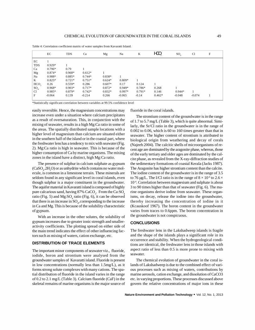
Nature Environment and Pollution Technology · Vol. 12, No. 1, 2013
49CHEMICAL EVOLUTION OF GROUNDWATER IN THE CORAL ISLANDS
easily reversible. Hence, the magnesium concentrations mayincrease even under a situation where calcium precipitatesas a result of oversaturation. This, in conjunction with themixing of seawater, results in a high Mg:Ca ratio in some ofthe areas. The spatially distributed sample locations with ahigher level of magnesium than calcium are situated eitherin the southern half of the island or in the coastal part, wherethe freshwater lens has a tendency to mix with seawater (Fig.2). Mg:Ca ratio is high in seawater. This is because of thehigher consumption of Ca by marine organisms. The mixingzones in the island have a distinct, high Mg:Ca ratio.
The presence of sulphur in calcium sulphate as gypsum(CaSO4.2H2O) or as unhydrite which contains no water mol-ecule, is common in a limestone terrain. These minerals areseldom found in any significant level in coral islands, eventhough sulphur is a major constituent in the groundwater.The aquifer material in Kavaratti island is composedof highlypure calcarious sand, having 87% CaCO3. From the Ca:SO4ratio (Fig. 5) and Mg:SO4 ratio (Fig. 6), it can be observedthat there is an increase in SO4,corresponding to the increasein Ca and Mg. This is because of the solubility characteristicof gypsum.
With an increase in the other solutes, the solubility ofgypsum increases due to greater ionic strength and smaller-activity coefficients. The plotting spread on either side ofthe main trend indicates the effect of other influencing fac-tors such as mixing of waters, cation exchange, etc.
DISTRIBUTION OF TRACE ELEMENTS
The important minor components of seawater viz., fluoride,iodide, boron and strontium were analysed from thegroundwater samples of Kavaratti island. Fluoride is presentin low concentrations (normally less than 1.5mg/L), as itforms strong solute complexes with many cations. The spa-tial distribution of fluoride in the island varies in the rangeof 0.2 to 2.1 mg/L (Table 3). Calcium fluoride (CaF) in theskeletal remains of marine organisms is the major source of
fluoride in the coral islands.The strontium content of the groundwater is in the range
of 1.7 to 5.7 mg/L (Table 3), which is quite abnormal. Simi-larly, the Sr/Cl ratio in the groundwater is in the range of0.002 to 0.06, which is 60 to 160 times greater than that inseawater. The higher content of strontium is attributed tobiological origin from weathering and decay of corals(Najeeb 2004). The calcitic shells of microorganisms of re-cent age are dominatedby the aragonite phase, whereas, thoseof the early tertiary and older ages are dominated by the cal-cite phase, as revealed from the X-ray-diffraction studies ofthe sedimentary formations of coastal Kerala (Jacks 1987).The Aragonite has higher strontium content than the calcite.The iodine content of the groundwater is in the range of 3.5to 76 µg/L. The I/Cl ratio is in the range of 8 × 10⁻⁶ to 2.6 ×10⁻⁴. Correlation between magnesium and sulphate is about3 to 90 times higher than that of seawater (Fig. 6). The ma-rine organisms derive iodine from seawater. These organ-isms, on decay, release the iodine into the groundwater,thereby increasing the concentration of iodine in it(Kcauskoof 1967). The boron content in the groundwatervaries from traces to 0.6ppm. The boron concentration inthe groundwater is not conspicuous.
CONCLUSIONS
The freshwater lens in the Lakshadweep islands is fragileand the shape of the islands plays a significant role in itsoccurrence and stability. When the hydrogeological condi-tions are identical, the freshwater lens in those islands withaspect ratio of less than 0.5 is more prone to mixing withseawater.
The chemical evolution of groundwater in the coral is-lands of Lakshadweep is due to the combined effect of vari-ous processes such as mixing of waters, contributions bymarine aerosols, cation exchange, and dissolution of CaCO3etc. in varying proportions. These processes discussed abovegovern the relative concentrations of major ions in these
Table 4: Correlation coefficient matrix of water samples from Kavaratti Island.
EC TDS Ca Mg Na K HCO3 SO4 Cl F
EC 1TDS 0.929* 1Ca 0.796* 0.79 1Mg 0.874* 0.968* 0.612* 1Na 0.988* 0.885* 0.744* 0.838* 1K 0.825* 0.721* 0.751* 0.624* 0.809* 1HCO3 0.26 0.559* 0.286 0.607* 0.17 0.124 1SO4 0.968* 0.903* 0.717* 0.872* 0.949* 0.786* 0.268 1Cl 0.985* 0.879* 0.742* 0.832* 0.997* 0.791* 0.146 0.944* 1F -0.064 0.139 -0.214 0.266 -0.065 -0.14 0.462* -0.048 -0.074 1
*Statistically significant correlation between variables at 99.5% confidence level

Vol. 12, No. 1, 2013 · Nature Environment and Pollution Technology
50 Najeeb K. Md and N. Vinayachandran
aquifers. The correlation matrix (Table 4) for the major ionsshows a significant correlation among the ions Ca++, Mg+,Na+, K+ and SO4
- , and HCO3 has a better correlation withMg++ and F-.
The different chemical facies identified in the freshwa-ter lens are related to various phases of mixing of seawaterin lateral and vertical directions. The dominant factor modi-fying the chemistry of the freshwater lens appears to be themixing of seawater, with the other factors such as cationexchange, dissolution of CaCO3 and marine aerosols exert-ing their influence to a lesser degree.
The relatively high concentrations of trace elements viz.,strontium and iodine are unlikely to have been caused byseawater mixing. Strontium is released into the groundwateras a result of the diagenesis of lime shells from aragonitestructure to stable calcite structure, while iodide is releasedduring the decay of marine organisms.
REFERENCESHem, J.D. 1970. Study and interpretation of the chemical characteristics
of natural water. USGS Water Supply Paper-1473.Jacks, G. 1987. Hydrochemistry in Coastal Kerala. Project Mission Re-
port, CKGW Project, CGWB, 62.
Kcauskoof, K.B. 1967. Introduction to Geochemistry. McGraw Hill.Lloyd, J.W. and Heathcote, J.A. 1985. Natural Inorganic Hydrochemistry
in Relation to Groundwater. Clarendon Press, Oxford, pp. 294.Mandal, S. and Shiftan, Z.L. 1981. Groundwater Resources Investigation
and Development. Accademic Press, London, pp. 269.Mannadiar, N.S. 1977. Lakshadweep Gazetteer of India, Admn. of Union
Territory of Lakshadweep, pp. 375.Mercado Abraham 1985. The use of hydrogoechemical patterns in car-
bonates and sandstone aquifers to identify intrusion and flushing ofsaline water. Groundwater, 23(5): 635-645.
Nair, K.M. 1982. Cementation of carbonate sands in Lakshadweep. Bull.ONGC, 19:(1): 1-12.
Najeeb, K. Md. 2004. Hydrogeological Model of Lakshadweep Islands.Ph.D. Thesis, Mangalore University, Mangalore, pp. 184.
Najeeb, K. Md. and Vinayachandran, N. 2006. Water budgeting and eco-logical balancing in Atolls - A case study. 22nd National Convention ofCivil Engineers, pp. 14-24.
Najeeb, K. Md. and Vinayachandran, N. 2011. Ground water scenario inLakshadweep islands. J. Geo. Soc., India, 78(4): 379-389.
Piper, A.M. 1944. A graphic procedure in the geochemical interpretationof water analyses. AGU Trans., 25: 914-923.
Siddiquie, H.N., Veerayya, M., Rao, C.H.M., Murthy, P.S.N. and Reddy,C.V.G. 1976. Deep sea drilling project site 219 on the Laccadive ridge.Indian J. Mar. Sc., 5(1): 18-34.
Stumm, W. and Morgan, J.J. 1981. Aquatic Chemistry. John Wiley andSons, 2nd Ed., pp. 780.
Varma, Ajaya Kumar, R. 1997. Studies on groundwater resource potentialand management of the coral atolls of Lakshadweep, UT of India. Ph.D.Thesis, Univ. Kerala, Trivandrum, pp. 277.

Huang Yuhan, Chen Xiaoyan, Ding Linqiao, Zhang Songsong, Weng Min and Huang YanxiongCollege of Resources and Environment, Key Laboratory of Eco-environments in Three Gorges Region (Ministry of Educa-tion), Southwest University, Beibei, Chongqing, China
ABSTRACT
Because the highway temporarily covers large areas, this article proposes fuzzy comprehensive evaluationmethod to evaluate the suitability of the reclamation soil in the highway dumping site. According to the impactfactors of the land reclamation and the field survey, combining with the principle of fuzzy mathematics, wechose eleven influence factors, including weather conditions, soil physical properties, and soil chemicalproperties as evaluation factors. In this paper, we regarded nine dumping sites in Chengdu-ChongqingExpressway double-track (Chongqing section) project as samples to make the fuzzy comprehensiveevaluation. Theresults indicate that thereclamation soil suitability inChengdu-Chongqing Expressway double-track (Chongqing section) dumping sites is relatively good. It provides a useful reference value for thereclamation soil suitability evaluation of the national highway dumping sites.
Nat. Env. & Poll. Tech.
Received: 4-10-2012Accepted: 16-11-2012
Key Words:Highway dumping siteReclamation soil suitabilityFuzzy comprehensiveevaluation
2013pp. 51-56Vol. 12ISSN: 0972-6268 No. 1Nature Environment and Pollution TechnologyAn International Quarterly Scientific Journal
Original Research Paper
INTRODUCTION
In recent years, with the high-speed development of the na-tional economy and the accelerated industrialization and ur-banization, highway - a modern construction project at thecost of damaging the ecological environment is in the pe-riod of high-speed industrial development (Wang 2006,Zhang 2003). Amid the construction of highway, the dump-ing site as a temporary area (agricultural lands occupied forparts of the dreg site), is the key place of occurring soil andwater loss in the highway construction (Xie 2010, Wang2006). Most of the places are loose heaped body. Its surfaceexposed and it has strong hydraulic permeability and severeuneven settlement, which easily results in landslide and de-bris flow under the combined effects of hydraulic power andgravity and has a direct threat to the safety of the productionand living along the highway (Zeng 2004).
In order to better ensure the construction finished andreclaimed dumping sites to restore their original ecologicalfunctions, it requires analysis and the evaluation for the rec-lamation of soil physical properties, chemical properties andclimate conditions and so on. Nowadays, the existing re-claimed land suitability comprehensive evaluation methodsare: The comprehensive index method, the expert evalua-tion method, the extreme conditions of method, the exten-sion method, etc. Su Haimin & Chen Jianfei (Su & Chen2005) used the model of matter-element for land suitabilityassessment. Liu Jing and Li Jianxue (Liu & Li 2007) adoptedthe index pulsing method for land reclamation suitability
evaluation on the land consolidation project of Qian County,Xianyang City, Shanxi Province, Xuelu town, Pan Qingyuan,Liu Xiaoli, etc. (Pan et al. 2007) based on extension method,evaluated the land reclamation suitability on the soil whichwas damaged from the reclamation lands to the cultivatedlands in Jiawang, Xuzhou. However, using the currentlyexisting indicators to quantify whether the soil is suitablefor reclamation is still very difficult, so this paper introducesthe fuzzy comprehensive evaluation method. The studyadopts fuzzy mathematics theory to alter qualitative evalua-tion into quantitative evaluation. This method can make theresults clear and systematic, and can better solve the prob-lems which are vague and difficult to quantify. It is suitablefor solving a variety of non-deterministic problems. There-fore, this article introduces the fuzzy comprehensive evalu-ation method to evaluate reclamation soil suitability of thedumping site of the Chengdu-Chongqing Expressway dou-ble-track (Chongqing section). The research results can pro-vide guidance and be used for reference for reclamation workof the lands of dumping site of highway.
OVERVIEW OF THE STUDY AREA
The study site is the Chengdu-Chongqing Expressway dou-ble-track (Chongqing section), of which the specific choicesof site are the Bishan County, Tongliang, Dazu County inChongqing Municipality.
Chengdu-Chongqing Expressway double-track(Chongqing section) is located in the central tectonic parallel

Vol. 12, No. 1, 2013 · Nature Environment and Pollution Technology
52 Huang Yuhan et al.
Ridge (low mountains) Valley (hills) district, Western Hillsdistrict of Chongqing, a subtropical humid monsoon climatezone; meanannual rainfall ranges from1004mm to1231mm.The place has subtropical vegetation type, that is, humidevergreen broad-leaved forest. Plant species are mainlymassonpine, fir, cedar and so on. Soil typesare mainly paddysoil, purple soil and yellow soil. The highway starts inChongqing Ring Road, connects planned city trunk roadeastward, and traverses Jinyun pulse to the west. CrossingBayue Mountains, through the place 4km from BishanCounty in the north and 5km from the Dazu county in thesouth, stoping at Guanyinqiao, the junction of Sichuan andChongqing and connecting with the Chengdu-ChongqingExpressway double-track (Sichuan section), the whole lineis located in the key national supervision region and the keynational rehabilitation region for the soil and water loss ofChongqing. The length of the line is about 79.880km,covering an area of 642.97 hm2, which permanently coversan area of 570.90 hm2 and temporary land of 72.07hm2. Thefull range of excavation is 17.49 million m3 and the fill is16.21 million m3. The abandon party is 4.10 million m3
(permanently abandoned party 3.23 million m3, planning26.50 hm2/12 dumping sites, temporary disposable party86.8500 km3). The debit is 2.83 million m3(planning 19.60hm2/nine earth fields).
The geographical coordinates of Bishan County are 106°02’-106°20’E, 29°17’-29°53’N, and the average tempera-ture is 17.9°C. Over the years the extreme maximum tem-perature is 40.6°C and the minimum temperature is -3°C.The average annual frost-free period is 337d. The geographi-cal coordinates of Tongliang county are 105°46’-106°16’E,29°31’-30°06’N. The average temperature is 17.8°C. Theannual average relative air humidity is 82% and the averageannual frost-free period is 225d. The geographical coordi-nates of Dazu county are 105°28’-106°02’E, 29°23’-29°52’N. The average annual temperature of 17.20°C overthe years and the average annual frost-free period is 323d.
MATERIALS AND METHODS
Sample collection: Along the route selected of the dump-ing sites, we selected a point respectively in the upper, cen-tre and lower, excavated the soil profile (0-30 cm selected)and use soil sample collector to collect the soil at 0-10cm(layer A) 10-20cm (layer B) and 20-30cm (layer C). If thedumping is large enough, we can select multiple points alongthe length, and select the corresponding points to collect soilin the centre and lower parts. Then, the taken soil sampleson the same height and same profile heights were uniformlymixed. One kg mixed soil samples were taken back to thelaboratory for indoor testing. Altogether, 27 soil sampleswere collected.
Analytical methods: Soil moisture content was measuredby the drying method. Soil compaction was measured by aSC-900 soil compaction. The content of the soil organicmatter (SOM) was measured by the potassium dichromatemethod, and total nitrogen (TN) content by sulphuric aciddigest diffusion method. The content of total phosphorus(TP) was measured by NaOH melt-molybdenum antimonyanti-colorimetric determination, content of total potassium(TK) using NaOH melting-flame photometric determination,and content of available nitrogen (AN) by alkaline solutiondiffusion method. Determination of available phosphorus(AP) was made by NaHCO3-molybdenum antimony anti-colorimetric method, and the content of available K (AK)by NH4Ac-flame photometry (Yang 2008).Data processing: The experimental data were analyzed byMATLAB mathematical analysis software and Excel statis-tical software.
FUZZY COMPREHENSIVE EVALUATION
Fuzzy Comprehensive Evaluation Method
Fuzzycomprehensive evaluation method isbased on the prin-ciple of fuzzy mathematics, using the fuzzy statistical meth-ods through considering a combination of relative factorsfor evaluation and the subjective assignment method to de-termine the weight of various factors to make the evaluationof the pros and cons of the research objects. It is not only aquantitative evaluation, but also a qualitative assessment.What is more important is that it can combine quantitativeand qualitative factors to evaluate comprehensively (Yu2004), which can better reflect the impact under the com-bined effects of various factors. Specific evaluations havethe following steps:1. To determine the set of factors of the evaluation object2. To determine the factors the weight set3. To determine the reviews set4. To make the evaluation of the single factor5. Comprehensive evaluation
The Choice of Fuzzy Factor
In this paper the choice of fuzzy factor is based on the com-bination of the land potential factors and reality. Overall itincludes: (1) weather conditions: the average annual rain-fall, average annual temperature; (2) soil physical proper-ties: soil moisture content, soil compactness; (3) soil chemi-cal properties: soil organic matter content, soil nutrient con-tent (TP, AP, TK, AK, TN, AN). The data of the above fac-tors are easy to be collected or measured, and are stronglyrepresentative. Therefore, it is more conductive to the pro-motion of fuzzy comprehensive evaluation method.

Nature Environment and Pollution Technology · Vol. 12, No. 1, 2013
53RECLAMATION SOIL SUITABILITY STUDY OF THE HIGHWAY DUMPING SITE
Fuzzy Comprehensive Evaluation Process1. Establish the factor set: R = {r1, r2, ...ri, rm}. Amongthem, R is the influencing factors set, ri is the ith influencingfactors and m is the number of the factors (Zhang 2003).Now regard the factors from r1 to r11 respectively as soilmoisture, soil compaction, soil organic matter content, APcontent, TP content, TK content, AK content, AN content,TN content, average annual rainfall and the average annualtemperature.2. Establish weight set: A = (a1, a2, ...ai, am). Among them,A is the factor weight set and ai is the corresponding weightcoefficient of factor ri, requiring ai £ 0, Sai = 1 (Zhang 2003).Now, take the weight coefficient of various factors respec-tively as follows: soil moisture is 0.25, soil compaction is0.175, the soil organic matter content is 0.175, AP content is0.025, TP content is 0.025, TK content is 0.025, AK contentis 0.025, AN content is 0.025, TN content is 0.025, averageannual precipitation is 0.175 and average annual tempera-ture is 0.075. Namely, the weight set A = (0.25, 0.175, 0.175,0.025, 0.025, 0.025, 0.025, 0.025, 0.025, 0.175, 0.075).3. Establishing an evaluation set: V = {v1, v2, ...vj, vn}.Among them, V is the evaluation set and vj represents the jth
evaluation result and n is the total number of evaluation re-sults (Zhang 2003). Now, taking the set n = 5, which can bedivided into five evaluation ranks v1 to v5 separately onbehalf of suitability, less suitability, general, less unsuitabil-ity, unsuitability (Table 1).4. Single factor fuzzy evaluation: Ri = {ri1, ri2, ..., rij}.Among them, Ri is the evaluation set of the single factorand rij represents the degree of membership which ri is rela-tive to vj. Make a matrix:
R=úúúú
û
ù
êêêê
ë
é
RiMRR
21
=úúúú
û
ù
êêêê
ë
é
jii
j
j
rirrMMMMrrrrrr
L
L
L
21
22221
11211
, ...(1)
R is the single factor evaluation matrix (Zhang 2003) asgiven in Table 2.5. Fuzzy comprehensive evaluation: fuzzy comprehensiveevaluation can be expressed as B = A · R, That is,
( )nbbb L21 = ( )maaa L21 ·úúúú
û
ù
êêêê
ë
é
jii
j
j
rirrMMMMrrrrrr
L
L
L
21
22221
11211
...(2)
Among them, bj is the evaluation index, and is the de-gree of membership which is evaluation factors membership
to evaluation sets considering all the factors (Zhang 2003).The sign “ · ” representing a synthesis method of A and R,the composite model has the following four:Model one: M, (the main factors determine type,
)(1
iji
m
ij rab Ù= Ú
=;
Model two: M, the highlight the type of the main factors,
( )iji
m
ij rab Ú
==
1;
Model three: M, the weighted average type,
þýü
îíì= å
=
m
iijij rab
1,1min
Model four: M, the weighted average type,
å=
×=m
iijij rab
1;
Finally, according to the maximum membership degreeprinciple the evaluation results can be estimated (ZhangJianxia et al. 2003).
Model one “the main factors determine type” mainlyoperate ¸ and º.The operation is simple, but for some of theissues it may miss a lot of information. Its evaluation resultsdepend only on the factors that play a major role in the totalevaluation. The remaining factors did not affect the evalua-tion results (Chen 2005), thus, the results are somewhatrough. When the Factors are too many and the weight distri-bution is more balanced, according to
...3
each factor shares weight ai must be very low. Only withthe operator ¸, º getting the low bj (bj £ Vai) is also des-tined in the comprehensive evaluation, and then the smallerweight taken by the ¸ operator is actually unable to get sat-isfactory results.
Model two is the main factors highlight type, and it ismore specific compared with the model one, which not onlyhighlights the main factors, but also takes other factors intoaccount (Chen 2005). Although ai is related to the importanceof the factors xi, it doesn’t have the meaning of weight coeffi-cient. Therefore, the vector A needn’t be normalized, either.
Model three and four are the “weighted average-type”.The vector A has the right meaning of weight coefficientwhich represents the importance of each factor xi, and

Vol. 12, No. 1, 2013 · Nature Environment and Pollution Technology
54 Huang Yuhan et al.
therefore it should meet the requirements of-
But the model IV should be evenly in accordance withthe weights of all factors.
Since each of the four models has its own distinct char-acteristics, this article use the four models at the same timeto make a comprehensive evaluation to ensure the compre-hensiveness of the evaluation results.
RESULTS AND DISCUSSION
According to the above process step by step evaluation,available results can be concluded in the Table 3.
Based on the maximum membership degree principle offuzzy comprehensive evaluation method, it can be ensuredthat the results determined by the four model evaluation arethe second grade. The reclamation soil suitability for thehighway dumping site is relatively suitable.
Fuzzy comprehensive evaluation method used in thisarticle is based on the principle of fuzzy mathematics (Han1998) to establish a quantitative evaluation model in a fuzzyenvironment, consideringa variety of factors to make an over-all assessment. In the study on suitability of reclamation soilfor highway dumping sites, due to the fact that the suitabilityof the reclaimed soil is affected by many factors, each of thefactors are not only evaluated separately, but also analyzedthrough combining the influence of each factors by the com-prehensive evaluation. In the process of evaluation of qualita-tive factors, it can alter qualitative factors into quantitativeevaluation, which adds to the scientificity and reliability ofthe evaluation model. Therefore, this study proposes the useof fuzzy comprehensive evaluation method for reclamationsoil suitability evaluation of highway dumping site.
In this study, the evaluation model is built in accordancewith the steps of the fuzzy comprehensive evaluation method.And the fuzzy comprehensive evaluation model is used toanalyze on the Chengdu-Chongqing Expressway double-track (Chongqing section). Select 9 the dumping sites of thesection, according to the reclamation soil suitability factors,choose 11evaluation factorscombining the facts as the evalu-ation factor to input the fuzzy comprehensive evaluationmodel for the reclamation soil suitability analysis. The con-clusions are as follows:A. In the reclaimed soil suitability evaluation, due to thefact that the factors which impact the reclamation soil suit-ability are too many and each of the factors has differentnature. If it is just analyzed from a single factor to estimatethe reclamation soil suitability, it is difficult to get a com-prehensive evaluation results. However, using fuzzy com-prehensive evaluation method to evaluate the suitability ofthe highway dumping sites for reclamation of soil is morerigorous theoretically and can take advantage of the limiteddata to clearly estimate the soil reclamation, and to get com-prehensive results to accurately reflect the suitability of thereclamation soil.B. Using of the existing highway dumping site research dataand the relevant parameters as samples to establish the fuzzycomprehensive evaluation model, and the reclamation soilof Chengdu-Chongqing Expressway double-track(Chongqing section) dumping site as samples to evaluate itssuitability, the data come from engineering practice, whichhave certain representativeness. The research can provide areference for the new highway reclamation soil suitabilityresearch and guidance.C. Using fuzzy comprehensive evaluation method can moreobjectively represent the reclamation soil suitability classi-fication boundaries of the highway dumping sites by themembership and the right weight, note that the actual blur-
Evaluation factorsEvaluation factor level
Grade Grade Grade Grade Grade
Soil moisture content (%) Classification range 75 75 115 115 125 125 139 139
Soil compaction Classification range 4% 4% 5.6% 5.6% 6.5% 6.5% 7% 7%
Soil organic matter content Classification range 7 7 8.2 8.2 9.3 9.3 10 10
Soil available phosphorus content Classification range 0.4 0.4 0.48 0.48 0.57 0.57 0.7 0.7
Total soil phosphorus content Classification range 8 8 8.5 8.5 9.2 9.2 10 10
Total K content Classification range 15 15 15.8 15.8 16.5 16.5 18 18
Available potassium Classification range 40 40 45 45 55 55 64 64
Soil nitrogen content Classification range 55 55 69 69 75 75 91 91
Total soil nitrogen content Classification range 0.6 0.6 0.68 0.68 0.74 0.74 0.8 0.8
Average annual precipitation (mm) Classification range 1005 1005 1066 1066 1142 1142 1200 1200
Average annual temperature ( ) Classification range 16.2° 16.2° 16.9° 16.9° 17.0°17.0° 17.7° 17.7°
Table 1: Highway soil and water conservation measures benefit in the evaluation factor classification table.

Nature Environment and Pollution Technology · Vol. 12, No. 1, 2013
55RECLAMATION SOIL SUITABILITY STUDY OF THE HIGHWAY DUMPING SITE
ring of the distinction, so that evaluation results close to thefacts. On the basis of the operation of the existing highwayproject, using the Matlab programming language as a plat-form has a strong scientificity and feasibility for the finalreclamation soil suitability evaluation model established bythe input sample data analysis and the processing andnonlinear optimization.D. Fuzzy comprehensive evaluation method applied to thehighway dumping sites for the reclamation of soil suitabil-ity evaluation can scientifically estimate the soil reclama-tion suitability degree of reclamation soil of dumping sites.For the dumping site in the same area, the reclamation soilcan be estimated whether it is suitable according to the levelof scores. Thus, the effect of soil reclamation can be pre-dicted, providing the reference for the land reclamation workin the road construction in the same area.E. The actual evaluation results further validate the feasibil-ity, accuracy and objectivity of the fuzzy comprehensiveevaluation method. It can be a viable and an effective wayfor the reclamation soil suitability analysis, but the calcula-tion of fuzzy comprehensive evaluation method for adapt-ability evaluation of reclamation soil in highway dumpingsite is relatively more complex and not as simple and quickas a single factor evaluation method.
ACKNOWLEDGEMENTS
Authors are grateful to the National Science and Technol-ogy Support Project (2011BAD31B03), the Southwest Uni-versity Ecology Key Discipline ‘211’ Project FundingProject, the Central University Basic Scientific ResearchBusiness Expenses Special Funding (XDJK2011C013) andthe Southwest University Guangjiong Innovation FundProject (20110107), which gave the support to us.
REFERENCES
Chen, S.L., Li, J.G. and Wang, X.G. 2005. The Fuzzy Set Theory and ItsApplication. Beijing Science Press.
Han, L.Y. and Wang, P.Z. 1998. Application of Fuzzy Mathematics. Beijing:Capital University of Economics and Business Press, 151-152.
Liu, J. and Li, J.X. 2007. Land suitability evaluation of land reclamationfeasibility study. Shaanxi Journal of Agricultural Sciences, 1: 140-142.
Pan, Q.Y., Liu, X.L. and Gu, Z.Y. 2007. Land reclamation suitability andutilization mode study in Henan Province coal base. Inner MongoliaTechnology and Economy, 6(11).
Su, H.M. and Chen, J.F. 2005. Comprehensive evaluation matter-elementmodel of land suitability. Journal of Qufu Normal University, (1):115-119.
Wang, R.L., He, B.H. and Zhang, J.P. 2006. Highway soil and water con-servation-take the south section of the Chongqing Ring Expresswayas an example. Chinese Agricultural Science Bulletin, 22(7): 557-559.
Xie, G., Wang, X.D. and Xu, Y.N. 2010. Yichang to Badong expresswaywater and soil erosion characteristics and Prevention. China Institute
Evaluation ModelRank
Maximum degree of membership Evaluation resultsGrade Grade Grade Grade Grade
Model 1 0.231 0.25 0.231 0.154 0.175 0.25 Grade
Model 2 0.081 0.101 0.081 0.029 0.04 0.101 Grade
Model 3 0.243 0.273 0.239 0.103 0.143 0.273 Grade
Model 4 0.243 0.273 0.239 0.103 0.143 0.273 Grade
Table 3: Highway soil and water conservation measures.
Evaluation factorsRank membership
Grade Grade Grade Grade Grade
Soil moisture content (%) 0.231 0.115 0.115 0.269 0.077
Soil compaction 0.077 0.423 0.154 0.115 0.231
Soil organic matter content 0.385 0.077 0.192 0.154 0.192
Soil available phosphorus content 0.269 0.269 0.192 0.154 0.115
Total soil phosphorus content 0.077 0.269 0.346 0.115 0.192
Total K content 0.154 0.231 0.346 0.192 0.077
Available potassium 0.192 0.231 0.269 0.192 0.115
Soil nitrogen content 0.077 0.346 0.269 0.231 0.077
Total soil nitrogen content 0.154 0.192 0.115 0.192 0.346
Average annual precipitation (mm) 0.462 0 0.462 0 0.077
Average annual temperature ( ) 0 0 0.462 0 0.538
Table 2: Single factor evaluation of the calculation table.

Vol. 12, No. 1, 2013 · Nature Environment and Pollution Technology
56 Huang Yuhan et al.
of Water Resources: The Third Youth Science and Technology Fo-rum Proceedings, pp. 295-299.
Yang, J.H. 2008. Agriculture Chemical Analysis and Soil EnvironmentMonitoring. Beijing: China Land Press.
Yu, X.F. and Fu, D. 2004. Multiple index comprehensive evaluation methodreviews. Knowledge Jungle, (11): 119-121.
Zhang, J.X., Zhang, J.X. and Jiang, J.B. 2003. Fuzzy comprehensive evalu-ation on the damaged degree of the mining land. Journal of JiaozuoTech: JCR Science Edition, 22(6): 445-447.
Zeng, D.L. 2004. A study on the water and soil conservation concept of thedevelopment and construction project. Journal of Water and Soil Con-servation Science and Technology Information, 4: 1-3.

Ahmed Hasson and Muhsin JweegDesertification, Climate Change Section, Mechanical Engineering Department, College of Engineering, NahrainUniversity, Jaderia, Baghdad, Iraq
ABSTRACT
Two sites in Iraq were chosen tostudythe affect of annual pasture and perennial grasses (C4). The perennialgrass pastures had SOC stocks, 1.6 (Baghdad) and 1.4 (Babylon) times that of the annual pastures. SoilOrganic Carbon (SOC) pools were 1.90, 2.97 and 2.88% for annuals, perennials and tagasaste at Baghdadsite. At Babylon the SOC pools were 2.7, 4.70, and 3.71% under annuals, perennials and tagasasterespectively. Estimated total C sequestration contribution to the resident soil organic C pool was 2.8 timesgreater for perennials and 2.7 times for tagasaste than annual pasture at the Baghdad deep sandy duplexsite and 1.2 times greater for perennial pasture and 1.2 times greater for tagasaste than annual pasture atthe Babylon deep-sand site. Both the sites were sampled to a depth of 1.6m. Perennial grasses in this regiongenerally produced more above ground biomass than annual pastures. However, the differences in biomassinput are unlikely to be large enough to explain the high rate of sequestration of these perennials. Wehypothesise that the perennial grasses promote fungi such as mycorrhiza that convert a greater proportionof labile carbon to stable humic forms than under annual pastures.
INTRODUCTION
Iraq has a Mediterranean climate with cool wet winters andhot dry summers. Farming systems have evolved based onrotations of annual grain crops and annual legume basedpastures (Grace et al. 1995). A recent innovation has beenthe development of subtropical perennial grass pastures.These C4 perennial grasses have proven to be productiveand persistent on the poorer sands where annual crops andannual legumes have been marginal at best. Tagasaste is avery deep rooted perennial legume shrub that has also provento be very successful on the poorest deep sands (Oldham etal. 1999).
It is known that perennial pastures can increase soil car-bon more than annual pasture. For example, Baron et al.(2002) estimated that total carbon contribution for perenni-als was 2.7 timed more than for annuals. Iraq has very lowlevels of clay and silt (< 5% of each). It is widely believedthat soils with such low levels of silt and clay can not buildup soil carbon. Soil tests (0-10 cm) under annual crops andpastures on these sands generally show very low levels oforganic carbon in the range of 0.4% to 0.6 % (Walkley &Black 1934). However, limited soil testing has indicated thatsoil carbon levels were increasing under perennial grassesgrowing on these coarse sands in Iraq. This study was de-signed to accurately measure and compare soil carbon underannual pasture, perennial grass pasture and a fodder shrubon coarse sands.
Grazing management, litter and manures, roots and soilcharacteristics all have a major impact on organic carbon
stocks in the soil. Litter refers to all dead (standing and fallen)plant material above the soil surface (Naeth 1988). Leavingcrop residues as litter after harvest, increases soil organiccarbon (Lal et al. 2004). Litter reduces soil erosion by re-ducing runoff and improves soil structure and fertilitythrough addition of organic matter (Naeth 1988).
Pasture land has the ability to store substantial pools ofsoil C and N. Pasture land contains about 10% of the worldC pool (Parton et al. 1995). In temperate regions cultivationwhen cropping may release as much as 40% of the C thathas been stored in the previous pasture phase (Burke et al.1995). Also cultivation can narrow the soil carbon-to-nitro-gen ratio (C: N) favouring the release of soil N through Nmineralization processes (Wedin 1996).
In the Canadian prairies there is often a 2 to 9 year se-quence of perennial pastures between cereal crops (Entz etal. 1995). This pasture phase can increase soil carbon andenhance the yields of the following cereal crops (Campbellet al. 1990, Entz et al. 1995). The crop residues after harvestgo into the litter pool and subsequently a proportion is se-questered into the soil. Initial breakdown of the litter resultsin large losses of organic carbon and annual cultivation forcropping exacerbates the loss (Campbell et al. 1990).
The deep light texture soils of Iraq have very low waterholding potential (30-40 mm/m3). On these coarse sandstexture the shallow rooted annual crops and pasture can notuse all of the rainfall, which is concentrated in the wintermonths. Consequently, there is a high rate of recharge belowthe root zone of the annual crops and pastures. This high
Nat. Env. & Poll. Tech.
Received: 3-5-2012Accepted: 12-9-2012
Key Words:Soil organic carbonPasturesArid regionCarbon sequestration
2013pp. 57-62Vol. 12ISSN: 0972-6268 No. 1Nature Environment and Pollution TechnologyAn International Quarterly Scientific Journal
Original Research Paper

Vol. 12, No. 1, 2013 · Nature Environment and Pollution Technology
58 Ahmed Hasson and Muhsin Jweeg
rate of recharge results in rising groundwater tables thateventually causes dry land salinity in lower parts of thelandscape.
This paper reports on research comparing annual pas-tures, perennial C4 grass pastures and tagasaste at two sandysoils in the middle of Iraq.
MATERIALS AND METHODS
Sites description: The Baghdad site is located 100 km southof Baghdad (latitude is 33°N). The morphological descrip-tionof the soil profile is a yellow/brown loose and deep sandyduplex with an upper convex. The surface layer is stronglywater repellent. The trial sampling sites were in adjoiningpaddocks of perennial grass and volunteer annual pasture.The volunteer pasture consisted of wild radish, annualryegrass, Patterson’s curse and double gee. The perennialgrass paddock was sown in 2010. The perennial grassesmostly grow during the warmer spring, summer and autumnmonths. In winter they remain dormant. During winter andspring the volunteer annual pasture species can germinateand grow at similar rates to that of pure stands of seasonallysown ryegrass and clover pastures.
Babylon site is located 8 km east of Babylon (latitude of34°N). The site has a deep soil of loose, weathered gneiss.The surface is dark yellowish brown sand with a sharp de-lineated cultivation traffic pan boundary at 10 cm. The sur-face layer is strongly water repellent. The perennial pastureis a mix of Lucerne and Rhodes grass sown in 2007. Theadjoining paddock had an annual pasture consisting ofcapeweed, erodium and some burr medic. Both the peren-nial and annual pasture paddocks have been grazed periodi-cally with cattle from November 2010. The paddocks con-taining the sample sites are located upslope from the boresupplying water to the town of Babylon.
Monthly soil samples were collected at both the Bagh-dad and New Babylon sites. Four replicate samples weretaken from each pasture type. Soil samples were collecteddown to 150 cm depth in nine increments (0-5, 5-10, 10-20,20-50, 50-70, 70-90, 90-120, 120-150 cm).
Samples were airdried andsieved (2 mm) prior to chemi-cal analysis. Soil samples were analysed for organic carbonusing the methods of Walkley & Black (1934) and Jackson(1958). Nitrate and ammonium were determined by Searle(1984). Bulk density was determined by collecting soil sam-ples with a Bulk Density ring and drying at 105°C for 48hours.
RESULTS
Soil organic carbon (SOC): The perennial pastures hadhigher levels of organic carbon stocks than the annual pasture
in both surface 0-30 cm and subsurface 30-70 cm depths(Fig. 1). The perennial pastures have an extra 2.3 t/ha oforganic carbon in the top 70 cm above that under annualpastures. There was no significant difference in thedistribution of carbon between the annuals and perennialswhen comparing the top soil compared to the next 40 cm(Fig. 1).
At Baghdad there was a spike in CO2 eq stocks in the10-30 cm depth (Fig. 2), probably due to a layer of higherclay content. This 10-30 cm layer had the highest CO2 eqstocks for the perennial grasses and the tagasaste, and al-most the highest for the annual pastures. The perennial grasshad the highest CO2 eq stocks for the whole 0 to 150 cmdepth. Tagasaste had more CO2 eq stocks than the annualpasture in the 10 to 50 cm depth interval, but not at otherdepths. The net difference between tagasaste and annual pas-tures for the whole profile was small/insignificant.
At Babylon the soil carbon dioxide equivalent (CO2 eq t/ha) stocks declined down the profile. The perennial grass hadthe highest levels of carbon stocks at all depths down the pro-file to 150 cm (Fig. 3). The annual pasture and tagasaste hadsimilar CO2 eqstocks down to70 cm, but annual pastures hadless CO2 eq in the 70 to 150 cm depths (Fig. 3).
The Intergovernmental Panel on Climate Change (IPCC)sets out the accounting methods for determining green housegas missions and sequestration for the Kyoto Protocol. TheIPCC 2006 has two methods for calculating sequestration ingrassland. The stock difference method measures changesin carbon stocks over time on a given parcel of land. Thegain-loss method compares carbon stocks under new man-agement practises with that under the traditional land use.
Annual pastures are the traditional practice in WesternAustralia. Tagasaste and perennial grass pastures are anemerging alternative. The sequestration/emissions of thesenew perennial pastures can be calculated as an increase orreduction in carbon stocks compared to the traditional an-nual pasture.
At Baghdad the perennial grass sequestered carbon at alldepths when compared to the traditional annual pasture (Fig.4). The biggest increase in soil carbon was in the 0 to 30cmand 90 to 150 cm depths. The soil carbon profile appears tobe reflecting the soil physical properties especially the par-ticle size distribution (soil texture)at this site i.e., sand/gravel/clayey sand. This seems to indicate a positive relationshipbetween perennial grasses and their ability to sequester car-bon at higher rates in sandy soils. With tagasaste there was asequestration in the 10-60 cm layer, but not at other depths.This resulted in almost no net change for the entire profile.
At Babylon in the deep sand perennial grasses again se-questered more carbon at all depths (Fig. 4). The effect of

Nature Environment and Pollution Technology · Vol. 12, No. 1, 2013
59SOIL ORGANIC CARBON SEQUESTRATION UNDER PASTURES IN ARID REGION
the tagasaste was small compared to the annual pasture andvariable down the profile.
Carbon dioxide sequestration rate (CO2 eq t/ha/year) foreight depth increments down to 1.5 m at Babylon site basedon soil carbon stock difference of perennial grasses andtagasaste pastures above the annual pasture control are givenin Fig. 4. Carbon dioxide sequestration rate (CO2 eq t/ha/year) for the whole soil profile to 1.5 m at Baghdad soil car-bon stocks down to 150 cm increases under perennial grasspastures at both sites (Fig. 5 ). The increase in carbon stocks
under tagasaste was greater than under the perennial grasses.But as the tagasaste have been established for a much longertime than the perennial grasses, the annualised sequestra-tion rate of the tagasaste was lower. However, the tagasastedata are only for the soil carbon and do not include carbonstored in the woody stems and woody roots of the tagasaste(Figs. 4-5).
DISCUSSION
In this study the perennial grasses consistently have twice as
0
0.5
1
1.5
2
2.5
3
3.5
4
4.5
5
Annuals Perennials Tagasaste
0-30cm30-70
New Norc ia
0
1
2
3
4
5
6
Ann uals Perennials Tag asa st e
0-30cm30-70cm
Mingenew
0 10 20 30 40 50 60
0-5
5-10
10-30
30-50
50-70
70-90
90-120
120-150
CO2, t/ha
AnnualsPerennialsTagasaste
Mingenew
Fig. 1: Organic carbon stocks of annual, perennial and tagasaste pasture in the surface andsubsurface soil samples at New Norcia and Mingenew sites.
Fig. 2: Quantity of CO2 eq under annuals, perennials and tagasaste pastures at New Norcia site.

Vol. 12, No. 1, 2013 · Nature Environment and Pollution Technology
60 Ahmed Hasson and Muhsin Jweeg
much soil organic carbon as the annual pasture. Increase insoil organic carbon is often attributed to an increase in theinput of biomass carbon into the soil. It is unlikely that theincrease in soil organic carbon can be explained by the extrabiomass input from the perennial pastures in this study.Measurements by Moore et al. (2008) at a site near the Bagh-dad trial found that the perennial grasses on average onlyproduced an extra give the value % of above ground biomass.
The soil organic matter under the tagasaste was distrib-uted differently down the profile compared to the annualpasture. However, the total SOC pool for the profile was notgreatly different from the annual pasture. This study did notmeasure the large woody roots of the tagasaste. A study byDornaar & William (1992) found that large root (>2 mmdiameter) pool contained 3.2 times more carbon than in SOCpool in the top 2 m of soil. In addition, there was also a
0 2 4 6 8 10 12 14
0-5
5 - 10
10 - 30
30 - 50
50 - 70
70 - 90
90 - 120
120 - 150
CO2, t/ha
AnnualsPerennialsTagasaste
New Norcia
-5
0
5
10
15
20
25
30
0-5 5-10 10-30 30-50 50-70 70-90 90-120 120-150
Depth,cm
PerennialsTagasaste
Mingenew
-5.0
0.0
5.0
10.0
15.0
20.0
25.0
30.0
0-5 5-10. 10-20. 20-30. 30-50. 50-70. 70-90. 90-120. 120-150.
Depth, cm
Perennialstagasaste
New Norcia
Fig. 4: Carbon dioxide sequestration rate (CO2 eq t/ha/year) for eight depth increments down to 1.5 m at Mingenew sitebased on soil carbon stock difference of perennial grasses and tagasaste pastures above the annual pasture control.
Fig. 3: Quantity of CO2 eq under annuals, perennials and tagasaste pastures at New Norcia site.

Nature Environment and Pollution Technology · Vol. 12, No. 1, 2013
61SOIL ORGANIC CARBON SEQUESTRATION UNDER PASTURES IN ARID REGION
significant pool of carbon in the above ground trunk andlimbs. To assess the sequestration potential of tagasaste itwill be necessary to measure both the SOC and the largewoody pools both above and below ground.
The additional soil organic carbon in this study is in partdue to the perennial pastures having living roots year round,while the annual pasture roots die off in summer. The liveroots were not measured directly in this study, but they con-tributed to soil organic carbon as roots regenerate regularly.Turnover of root material is an important consideration indetermining the annual contribution of roots to the soil car-bon pools. The life-span of roots may vary from as little as 4to 6 weeks up to several years as in short grass prairies(Whitehead 1995). The turnover of perennial grass roots ismore difficult to assess, as the management of the pasturescan influence the life-span of the roots. Grazing, cutting, andfertilizer applications tend to shorten the average regenera-tion period (Whitehead 1995, Van Veen & Paul 1981).
The difference in soil organic carbon between annual andperennial pastures is more likely to be due to the differencein the decomposition of roots and above ground litter.
The results of this study suggest that even on sandy soilsperennial pastures cansequester significant quantities of CO2from the atmosphere. These soil sequestration rates are farin excess of the likely emissions of methane from grazingstock (0.5-1.5 t CO2 eq/ha/year) meaning that paddocks ofperennial pastures are likely to be net sinks of greenhousegasses. Perennial pastures could potentially contribute a
massive reduction inagriculture net emissions. Allowing soilcarbon sequestration in the national ETS would provide theincentive for a significant increase in the planting of peren-nial pastures by farmers.
The sequestration rates measured in this work are notconsistent with the RothC model. The sequestration rates inthis research are also in excess of those reported for pasturesin a major review of the published literature in Australia byValzano et al. (2005).
Questions remain as to how these perennial pastures canachieve such high sequestration rates and as to how RothCmust be modified to account for this. We hypothesis that thehigh sequestration rates under the perennials is due to changesin soil biology. It is known that mycorrhiza can produceenzymes that increase the rate of conversion of labile carbonin the soil to more stable humic forms. In purely annual plantsystems, the mycorrhiza population would die back in sum-mer when there are no live plants. Under an evergreen per-ennial system the mycorrhiza population and biological ac-tivity would be maintained year round. This increase inmycorrhiza activity could account for a much greater pro-portion of fresh plant matter ending up in the stable humicpools. If so, it would require that the flux rate between theparticulate organic matter pool and the humus pool in theRothC to be increased. Further research is required to accu-ratelydefine the flux rates for perennial pastures in the RothCmodel.
The results reported are from sites that have been under
0
20
40
60
80
100
120
140
160
Perennia ls Tagasaste
Pastures
CO2eq net sequestration, t/haCO2 eq t/ha/year
New Norcia
0
20
40
60
80
100
120
140
160
Perennials Tagasaste
Pastures
CO2eq net sequestration,t/haCO2,t/ha/year
Mingenew Site
Fig. 5: Carbon dioxide sequestration rate (CO2 eq t/ha/year) for the whole soil profile to 1.5 m at New Norcia site based on soilcarbon stock difference of perennial grasses and tagasaste pastures above the annual pasture control

Vol. 12, No. 1, 2013 · Nature Environment and Pollution Technology
62 Ahmed Hasson and Muhsin Jweeg
perennial pastures for a relatively short period of time (maxi-mum 6 years). These results can not be used to predict longterm sequestration rates or the ultimate equilibrium level ofthe carbon pools under perennial pastures, only time willtell. Models such as RothC can be used to predict soil car-bon pools well into the future. However, if the flux ratesused in these types of models are inaccurate then ultimateequilibrium levels predicted would also be significantly in-accurate.
The equilibrium levels of soil carbon predicted by mod-els for a particular management practice are often errone-ously assumed to be the carbon saturation level for a soil. Achange in management practice will inevitably lead to a newequilibrium level in the soil. Using soil carbon models todefine the maximum soil carbon levels is fraught withdanger. These results suggest that agricultural managementpractice could have a large effect on net emissions/seques-tration from the soil.
Given that there are 170 million hectares under dry landagricultural in region, and that these results and other re-search (Valzano 2005) show large variations in soil carbonstocks due to management, it is likely that soil carbon is thekey category in the national accounts. The Kyoto Protocolwould, therefore, requires Australia to commit substantialresources to improve the estimates of changes in soil carbonstocks on agricultural land.
REFERENCESBaron, V.S., Mapfumo, E., Naeth, M.E., Dick, A.C. and Chanasyk, D.S.
2000. Grazing impacts on litter and root mass carbon, and nitrogenpools. J. Range. Manage., 55 (In Press).
Burke, I.C., Laurenroth, W.K. and Coffin, D.P. 1995. Soil organic matterrecovery in semi arid grasslands: Implications for the conservationreserve program. Ecol. Appl., 5: 793-801.
Campbell, C.A., Zentner, R.P., Janzen, H.H. and Bowren, K.E. 1990. Croprotation studies on the Canadian prairies. Research Branch, Agricul-ture Canada, Pub. No. 1841/E.
Dornaar, J.F. and Willms, W.D. 1992. Water-extractable organic matterfrom plant litter and soil of rough fescue grassland. J. Range Manage.,45: 152-158.
Entz, M.H., Bullied, W.J. and F. Katepa-Mupondwa 1995. Rotational ben-efits of forage crops in Canadian prairie cropping systems. J. Prod.Agr., 8: 521-529.
Grace, P.R., Oades, J.M., Kieth, H. and Hancock, T.W. 1995. Trends inwheat yields and soil organic carbon in permanent rotation trial at theWaite Agric. Research Institution, South Australia. Australian Journalof Experimental Agriculture, 35: 857-864.
IPCC 2006. National Greenhouse Gas Inventories IPCC Guidelines, Inter-governmental Panel on Climate Change, 4. Agriculture, Forestry andOther Land Use.www.ipcc-nggip.iges.or.jp/public/2006gl/index.html
Jackson, M.L. 1958. Soil Chemical Analysis. Prentice-Hall, London,pp. 214-221.
Jensen, E. and Haise, V. 1963. The effect of pea cultivation on succeedingwinter cereal and winter oilseed rape nitrogen nutrition. Applied Agri-cultural Research, 5: 102-107.
Lal, R., M., Griggin, J., Apt Lave and Morgan, G. 2004. Managing soilcarbon. Policy Forum, Ecology Science, 304: 393.
Moor, G. 2007. Quality and quantity trials key results to date. EvergreenNews letter, June.
Naeth, A., Rothwell, R.L., Chanasyk, D.S. and Bailey, A.W. 1988. Grazingimpacts on infiltration in mixed prairie and fescue grassland ecosys-tems of Alberta. J. Range Manage., 70: 593-605.
Oldham, C. and Allen, G. 1999. The agronomy and management ofTagasaste. In Tagasaste review workshop-working papers. Eds. Lefroy,E.C., Oldham, C. and Costa, N.J. CLIMA, Nedlands.
Parton, W.J. and Rasmussen, P.E. 1995. Long-term effects of crop man-agement in wheat-fallow: II. CENTURY model simulations. Soil Sci.Soc. Am. J., 58: 530-536.
Searle, P.L. 1984. The berthelot or indophenol reaction and its use in theanalytical chemistry of nitrogen. A review. Analyst, 109:549-568.
Van Veen, J.A. and Paul, E.A. 1981. Organic carbon dynamics in grass-land soils. I. Background information and computer simulation. Cana-dian Journal Soil Science, 61:185-201.
Valzano, F., Murphy, B. and Koen, T. 2005. The impact of tillage on changesin soil carbon density with special emphasis on Australian conditions,Australian Greenhouse Office, National Carbon Accounting SystemTechnical Report No. 43.
Walkley, A. and Black, I. A. 1934. An Examination of the Degtjareff methodfor determining soil organic matter and a proposed modification of thechromic acid titration method. Soil Science, 37: 29-37.
Wedin, D.A. 1996. Nutrient cycling in grasslands: An ecologist’s perspec-tive, In: R.E. Joost and C.A. Roberts (eds.), Proc. Nutrient Cycling inForage Systems Conf. Columbia, Mo. pp. 29-44.
Wedin, D.A., and Tilman, D. 1990. Species effects on nitrogen cycling: Atest with perennial grasses. Oecologia, 84: 433-441.
Whitehead, D.C. 1995. Amounts, sources and fractionation of organic ni-trogen in soils, In: D.C. Whitehead (ed.), Grassland nitrogen. CABInternational, Wellinford, pp. 82-107.

Zhang Tiegang, Peng Li, Zhanbin Li* and Xiaoding Guo**Key Lab of Northwest Water Resources and Environment Ecology of MOE, Xi’an University of Technology, Xi’an, Shaanxi,P R China 710048*Institute of Soil and Water Conservation, Chinese Academy of Sciences and Ministry of Education, Yangling, Shaanxi,P R China, 712100**Department of Military Economy, Engineering University of CAPF, Xi’an Shaanxi, China, 710086
ABSTRACTVegetation is one of effective methods for soil and water conservation. How to select suitable vegetationspecies is a key problem in the practice. In this study. through 7 years observations on the rainfall, vegetationcover, total runoff and sediment in the plots, results indicated that thebenefit of the vegetative cover on runoffand sediment dominated on all plots. The accumulative sediment yield from bare plot was 7 times to thatfrom Astragalus absurgens + Caragana korshindkii plots, also over 4 times to that from the Medicagosativa, Medicago sativa + Caragana korshindkii and Astragalus absurgens plots. Among all the vegetationtypes, Caragana korshindkii was the most efficient in reducing the runoff, and the combination of shrub andgrass also had better effect in reducing the runoff. The accumulative runoff from bare plot was 2.57 times tothat from the C. korshindkii, and over 2 times to that from M. sativa, M. sativa + C. korshindkii, A. absurgens+ C. korshindkii and Vicia amucena + C. korshindkii. This study is of great importance for the selection ofsuitable species for vegetation reconstruction in arid and semi-arid areas.
Nat. Env. & Poll. Tech.
Received: 25-9-2012Accepted: 7-11-2012
Key Words:Vegetation coverageRunoff, ErosionSedimentShrubs and grassesLoess Plateau
INTRODUCTION
In arid environment, water erosion is the main soildegradation process. According to Renard (1980), in manyarid environments, soil erosion is greater than might beexpected considering the associated low rainfall. Sparsity ofvegetation, steep topography, low infiltration capacity, andhigh-intensity thunderstorm were identified as causativefactors. Runoff can be significant in degraded rangelands.Tromble (1974) reported that average runoff from creosotebush-infested rangelands was 20% of the precipitationreceived, with a maximum of 42% for the largest rainfallevent. And erosion is closely related to soil productivity,because it selectively removes the organic matter and soilnutrients, reduce plant available water capacities, reduce thethickness of the arable layer rooting volume, and leads to adegradation of soil physical properties such as structuralstability, infiltration, and bulk density (Peng Li 2002).Numerous studies (Zhu 2010, Peng 2011, Aref 2011) haveverified that the growth and existence of the vegetation canchange soil properties, improve soil anti-erodibility, intensifysoil infiltration and water retention ability, protect soilaggregation from raindrop splash, decrease raindrop energy,prevent the formation of the surface crust, and decrease soiland water loss from surface runoff (Cresswell 1995). Mostimportant of all, the existence of vegetation can disperse
concentrated overland flow, decrease runoff erosivity byincreasing resistance to runoff, impoundrunoff and sediment,allay and even prevent the formation of channel erosion(Meyer 1995). Some researchers (Carrol 2000, Gilly 2000,Cerda 1997) investigated the recover process on soil andspoilin mining areas, and the results indicated that the effect ofvegetation on soil erosion was dominated across all soil typesand sites. All these researches revealed the dynamic effectof vegetation cover on runoff and sediment, and providedscientific support for the evaluation of soil and waterconservation efficiency of forest, shruband grass (King 1995,Laflen 1981).
Recently, the use of crop residue to control erosion re-ceived more attention. The wind (Wooddruff 1965) andwater(Wischmeier 1978) erosion equations have crop factors thatrecognize the influence of crop residues for controlling ero-sion. Gregory (1982) reported on the percent soil cover withsix vegetative mulches, but he did not attempt to relate soilcover to wind erosion. In all cases, the first increment ofcover gave the largest response, and there was minimal ben-efit of going over 100% cover except for water conserva-tion. Residues were also recognized as a valuable tool forcontrolling water erosion (Meyer 1970, Laflen 1981). Soillosses due to water erosion on reclaimed rangeland site werereduced 51% with 72% surface cover (Hofmann 1983). The
2013pp. 63-68Vol. 12ISSN: 0972-6268 No. 1Nature Environment and Pollution TechnologyAn International Quarterly Scientific Journal
Original Research Paper

Vol. 12, No. 1, 2013 · Nature Environment and Pollution Technology
64 Zhang Tiegang et al.
advantage of using ground cover in place of quantity of resi-due is the ease of measuring ground cover (Laflen 1981,Gregory 1982, Richards 1984). The data on soil erosion-cropresidue cover were analysed using nonlinear-curve fittingtechniques (Barr 1976). Especially with the development ofsoil erosion prediction model, such as USLE and WEPP, theeffect of vegetation on soil has been received more atten-tion, and numerical relations between vegetation cover andsoil erosion were developed. But little attention was paid tothe effect of perennial vegetation (grass and shrub) on soiland water loss.
The objective of this study were to (a) verify quantita-tive relationship between ground cover and soil erosion, and(b) determine the accumulative effect of perennial grass onsoil erosion.
MATERIALS AND METHODS
Location and experiment layout: The experiment site waslocated on the slopes at An’sai Ecological Station of the Soiland Water Conservation Institution (ISWC) of China Acad-emy of Sciences (CAS), 18km southwest to Ansai city. Lo-cal climate is semi-arid, warm-temperate and windy. Meanannual temperature is 9.3°C, and mean annual rainfall is541.2mm. Rainfall is not uniformly distributed throughoutthe year; with July, August and September being the wettestmonths. Annual as well as monthly totals of precipitationexhibit a high variability.
The slope gradient was uniformly 20%. Leguminousgrasses and shrubs were planted on the bounded plots withthe size of 5m × 40m, vertical projection areas 169.6m2, andsingle plot was left bare as a comparison with the vegetationtreatment. The field study was terminated after 7 years whenthe rill erosion occurred on the plots. Raingauges were placednear the experiment location to record the rainfall and itsintensity. Soils type is Ustorthents, its fertility is low andthe organic matter content usually is below 1%.
Rainfall and its intensity were recorded by auto-recordedpluviometers (type) laid near the plots when runoff occurredon runoff plots. In 1986 year, due to personnel matters tothe people who are responsible for the observation, no ob-servations were carried out to runoff, sediment, and vegeta-tion cover, and consequently no data.Pastures and shrubs: Five species of grasses and shrubsand their combination were planted on the plots accordingto the Table 1: Vicia amucena Fish., Medicago sativa L.,Astragalus absurgens, Onobrychis viciifolia Scop andCaragana korshindkii Kon. To the mixture vegetation, thegrass and shrub were plantedat 5-m intervals across the plots.During the experiments, bait was placed near the plots toprevent damages from field mouse; and weeds have been
holed up to avoid its negative effect on the shrubs and grass.To get as closely effect to the nature as possible, no fertilizerwas applied to the plots during the experiment.Runoff and sediment: Total runoff was measured by usinga splitting bucket to determine its volume. Sediment con-tent wasdetermined by sampling from the bucket after weigh-ing and drying. After that, related data to runoff and sedi-ment were transformed to runoff depth and soil erosionmodulus respectively according to each definition.Vegetation cover: Quantitative estimates of cover compo-nents can be made with point frame quadrats (Levey 1933).The point frame technique provided statistically reliablequantitative estimates of vegetation and cover on reclaimedland grazed at several intensities in previous studies. Thenumber of the needle that can not fall down when the instru-ment was covered on the vegetation was thought to be thevegetation coverage. In this study, vegetation cover wasmeasured with vertical point frames of 20 sliding pins spacedabout 5cm apart. The first contact with live, litter or baresoil was recorded as first hit. The pin travel then was contin-ued downward and a similar contact at ground level was re-corded as a surface hit. Coverage measurement was takenafter runoff event occurred on the runoff plots, each with 10repeats at the same place of the previous studies.
RESULTS
Rainfall and intensity: According to the records of rainfallon the rain gauge, rainfall events when runoff occurred onthe vegetative plots are shown in Table 2 and Fig. 1. Theresults indicated that rainfall in the study area is character-ized by a large amount of small event fewer than 30mm.During the 6 years, of 19 rainfall events recorded during thestudy period, only3were larger than the average of 35.94mm,and accounted for 42% of the total; to the rainfall intensity,only 16 were larger than the average of 10.29mm/h, and ac-counted for 15.8% of the total.
Fifteen of the 18 rainfall events were happened in July,August and September. Maximum rainfall was 79.2mm and68 mm, and peak intensities recorded were 81.78mm/h. Theoccurrence of rainfall events of high magnitude and low
Table 1: The species and their combination for the experiment layout.
nudationCaragana korshindkii KonOnobrychis viciifolia Scop + Caragana korshindkii KonOnobrychis viciifolia ScopAstragalus absurgens + Caragana korshindkii KonAstragalus absurgensMedicago sativa L + Caragana korshindkii KonMedicago sativa LVicia amucena Fish + Caragana korshindkii KonVicia amucena Fish

Nature Environment and Pollution Technology · Vol. 12, No. 1, 2013
65EFFECTS OF PERENNIAL VEGETATION ON RUNOFF AND EROSION
intensity and events of high intensity and low magnitudemay in part explain the low correlation between rainfallamount and runoff. Slatyer & Mabbut (1964) regardedrainfall amount and intensity as the most significant factorsaffecting runoff in arid areas. However, they noted thatrainfall intensity might be more important than the totalrainfall amount in producing runoff, as in the present case.
0102030405060708090
0 5 10 15 20dat e
rain
fall
(mm)
0102030405060708090
inte
nsit
y(mm
/h)
r ai nf al l ( mm)i nt ensi t y( mm/ h)
0
20
40
60
80
100
120
1983
1983
1984
1985
1985
1987
1987
1988
1988
1988
year
cov erage(%) v.amucenaFish
M.sativa L
A.absu rgens
O.viciif oli aSco p
C.ko rsh in dkii7
0
10
20
30
40
50
60
70
80
90
1 00
1983
1983
1984
1985
1985
1987
1987
1988
1988
1988year
cov erage(%) V .amucenaF ish +C.korsh ind kii Kon
M.sa tivaL+C.korshind ikii Kon
A .ab surg ens+C.korsh idkii
O .vici if i l iaS cop +C.korshin dkiiKon
y = 0.1822x + 1.0322
R2 = 0.9499
0
5
10
15
20
25
30
35
0 50 100 150 200
accumul at i ve r unof f dept h ( mm)accu
mula
tive
sedi
emnt
prod
ucti
on(T
)
y = 0. 2461x - 4. 9873R2 = 0. 9559
0
20
40
60
80
100
120
140
160
180
0 100 200 300 400 500 600 700
accumul at i ve r ai nf al l ( mm)
0
20
40
60
80
100
120
140
0 200 400 600 800
accumulativ rainfal l (mm)
accu
mula
tive
runo
ffde
pth
(mm)
V.amucena Fish
M.saiva L
A.absurgens
O.viciifolia Scop
C.korshindkii Kpn
Fig. 1. Rainfall and its intensity when runoff occurred on the plots.
Vegetation cover pattern: During the vegetation develop-ment process, the vegetation cover showed different trendswith types (Fig. 2). In the initial stages, because of the re-tarded growth of shrubs, the coverage of C. korshindkii Konwas as low as 15%. But the coverage of the pastures such asV. amucena Fish and A. absurgens reached almost 60%,which indicated that the herbaceous species could provide
Fig. 2: The coverage patterns of different vegetation types.
Fig. 3: The coverage patterns of different vegetation combinations.Fig. 4: Relation between accumulative runoff depth and accumulative
sediment yield on bare plot.
Fig. 5: Relation between accumulative rainfall and accumulativerunoff depth on bare plot.
Fig. 6: Relation between accumulative rainfall and accumulative runoffdepth on vegetation plots.

Vol. 12, No. 1, 2013 · Nature Environment and Pollution Technology
66 Zhang Tiegang et al.
better protection to the soil surface in shorter time.As all the water needed during the vegetation growth was
from the rainfall, the drought-resistance ability of the spe-cies determined the species coverage pattern. To the herba-ceous species, its drought-resistance ability was lower thanthat of shrub; they were more easily affected by the aridityof the year. Thus, with the vegetation development, the cov-erage of C. korshindkii Kon showed a steady increase andsurpassed the other herbaceous species in the following years,and its variation range was also smaller.
To the types of grass combination with shrub (Fig. 3), itwas clear that the coverage of all the types showed a steadyincrease, among which the coverage increase of A. absurgens+ C. korshindkii Kon and V. amucena Fish + C. korshindkiiKon were the biggest. Because of the lower drought-resist-ance ability, coverage changes of M. sativa L + C. korshindkiiKon was great, and its coverage reached lower level whenthe rainfall was small.
Rainfall during the growing season is very important tothe vegetation growth. Less rain will accelerate grass degra-dation. Generally, the coverage of herbaceous species was
0
20
40
60
80
100
120
0 200 400 600 800
accumul at i ve rai nf al l ( mm)
accu
mula
tive
runo
ffde
pth
(mm) v.Amucena
Fish+C.korshidkii Kon
M.sativa
L+C.korshidkii Kon
A.absurgens+C.korshidk
ii Kon
O.viciifolia
Scop+C.korshidkii Kon
0
1
2
3
4
5
6
7
8
9
0 50 100 150
accumul at i ve r unof f dept h ( mm)accu
mula
tive
sedi
emnt
prdu
ctio
n(T
)
V.amucena Fish
M.sativa L
A.absurgens
O.viciifolia Scop
C.korshindkii Kon
0
2
4
6
8
10
12
0 20 40 60 80 100 120
accumul at i ve r unof f dept h ( mm)accu
mula
tive
sedi
emnt
prod
ucti
on(T
)
V.amucena
Fish+C.korshidkii Kon
M.sativa L+C.korshidkii
Kon
A.absurgens+C.korshidkii
Kon
O.viciifolia
Scop+C.korshidkii Kon
more easily affected by rainfall than the shrubs, and was alsorelated to its drought-resistance ability. According to theobservations, in 1988yr, coverage on Onobrychis viciifoliaScop plot degraded, and its cover dropped to lower level.This indicated that the exotic artificial vegetation needsproper management to avoid vegetation degradation.Impacts of vegetation types on runoff and soil loss: FromFigs. 4 and 5, linear relationship existed betweenaccumulative runoff depth, and sediment and accumulativerainfall on the bare plot, which indicated that larger rainfalltended to result higher runoff, and consequently highersediment yield. The accumulative curve of the runoff andsediment reflected the accumulative changes ofsoil and waterloss under the accumulative rainfall. As all the water usedby the vegetation came from the rainfall, the decrease ofrunoff meant the increase of infiltration and soil watercontent. Thus, the decrease of runoff under crop cover hadparticular ecological meaning in arid agriculture. Comparedto the bare plot, the benefit of the vegetative cover on soilerosion dominated across all plots despite of differentvegetation types (Figs. 6 and 7). All vegetation types areeffectively in reducing sediment yield, whose accumulativesediment yields were only 1/7 to 1/3 to that from bare plot.The accumulative sediment yield from vegetative plots alsoincreased quickly during the initial years after planting, butstabilized after 4 or 5 years after planting, which indicatedonly light soil erosion happened on vegetative plots. Thisresult is in accordance with former studies that the growthof vegetation will remarkably decrease soil erodibility, bindsoilparticles together with fine root, and increase water stableaggregate content (Zhu Bingbing 2010). The accumulativesediment yield from bare plot was 7 times to that from A.absurgens + C. korshindkii Kon plots, also over 4 times tothat from the M. sativa, M. sativa L + C. korshindkii Konand A. absurgens plots. Among all the vegetation types, C.korshindkii Kon is effectively in reducing runoff; while to
Fig. 7: Relation between accumulative rainfall and accumulative runoffdepth on vegetation plots. Fig. 8: Relation between accumulative runoff depth and accumulative
sediment yield on vegetation plots.
Fig. 9: Relation between accumulative runoff depth and accumulativesediment yield on vegetation plots.

Nature Environment and Pollution Technology · Vol. 12, No. 1, 2013
67EFFECTS OF PERENNIAL VEGETATION ON RUNOFF AND EROSION
vegetation combinations, A. absurgens + C. korshindkii Konwas most efficient in reducing the sediment.
As to the runoff, there also existed linear relation be-tween accumulative rainfall and accumulative runoff depthon bare plots, which indicated that larger rainfall tend to re-sult larger runoff. Compared to bare plot, all the vegetationtypes were efficiently in reducing runoff, whose accumula-tive runoff depth was 1/3 to 3/4 to that from bare plot, butwere not as remarkable as their effect on the sediment yield.Among all the vegetation types, C. korshindkii was the mostefficient in reducing the runoff, also the M. sativa, M. sativaL + C. korshindkii Kon, A. absurgens +C. korshindkii Konand V. amucena Fish + C. korshindkii Kon also had bettereffect in reducing the runoff. The accumulative runoff frombare plot was 2.57 times to that from the C. korshindkii, andover 2 times to that from M. sativa, M. sativa L + C.korshindkii Kon, A. absurgens + C. korshindkii Kon and V.amucena Fish + C. korshindkii Kon.Temporal changes of soil and water loss under differentvegetation types: Generally, bigger runoff induced largersediment yield. But the amount of surface soil erosion wasalso related to the soil structure, organic matter content, ag-gregation condition and porosity etc., which tended to bemore complex when vegetation existed.
From the Figs. 8 and 9, it was clear that all vegetationtypes were effective in reducing the surface soil and waterloss. During the initial stages of the development, the effectof shrubs on runoff and sediment yield was not as remark-able as grass, and the quick growth of the grass could affordbetter coverage to soil surface and resulted in less sedimentyield than the shrub. With the vegetation development, thecoverage of all vegetation types increased, and their protec-tion to the soil surface increased too, which resulted in the
similar trend of soil loss under different vegetation cover in4 and 5 yr after planting. The effect of vegetation on runoffseemed a little simple. Better linear relations existed betweenthe accumulative rainfall and the accumulative runoff depthon all plots (Table 2). The reason was that the vegetationgrowth will improve soil physical and chemical properties,such as soil organic matter content, soil water stable aggre-gate content, soil infiltration ability, and soil porosity, whichhave great effect on soil infiltration ability.
DISCUSSION
In Guobin Liu’s research (Guobin Liu 1997), the decreaseof soil loss in the initial years of the vegetation restorationwas the result of the vegetation coverage only. Later withthe vegetation development, the number of the roots in thesoil increased, and it was effective in reducing the sedimentyield because of its improvement and amelioration to thesoil physical and chemical properties. Thus, with the devel-opment of the vegetation and its succession, the effect of thevegetation in reducing the runoff and sediment would bemore remarkable.
In this paper, the analysis of the temporal changes of therunoff and sediment indicated that during the initial stagesof the vegetation development, the quick growth of the her-baceous species afforded better coverage to soil surface andresulted in less sediment yield than the C. korshindkii Kon.With the vegetation development, the coverage of all veg-etation types increased, and their protection to the soil sur-face increased too, which resulted in the consistent decreaseof soil loss under different vegetation cover in 4 and 5 yrafter planting.
In this study, the V. amucena Fish, A. absurgens and O.viciifolia Scop had no similar response in the years when
Table 2: Equations of accumulative runoff an sediment under different vegetation cover.
Species Runoff Sediment yield
Equation Correlation Equation CorrelationCoefficient Coefficient
Bare plot y = 7430x + 7790.6 R2 = 0.9375 y = 1389.5x + 2109.9 R2 = 0.9384Vicia amucena Fish y = 4882.6x + 18579 R2 = 0.9414 y = 488.74x + 99.526 R2 = 0.8715Onobrychis viciifolia Scop y = 4275.7x + 14213 R2 = 0.9453 y = 323.51x + 1074.2 R2 = 0.9461Astragalus absurgens y = 3911.3x + 6131.1 R2 = 0.8801 y = 285.77x + 567.59 R2 = 0.9198Medicago sativa L y = 2819.2x + 14674 R2 = 0.9388 y = 477.16x + 308.7 R2 = 0.8446Caragana korshindkii Kon y = 3178.6x + 10663 R2 = 0.9220 y = 355.51x + 1231.7 R2 = 0.8183Astragalus absurgens + y = 3245.5x + 1823.9 R2 = 0.9394 y = 249.89x + 120.97 R2 = 0.8968Caragana korshindkii KonMedicago sativa L + Caragana y = 3214.4x + 16333 R2 = 0.9217 y = 488.43x + 715.45 R2 = 0.8538korshindkii KonVicia amucena Fish + Caragana y = 3298x + 14283 R2 = 0.9410 y = 571.53x + 274.71 R2 = 0.8054korshindkii KonOnobrychis viciifolia Scop + y = 4100.9x + 19502 R2 = 0.9536 y = 464.54x + 1943.3 R2 = 0.9506Caragana korshindkii Kon

Vol. 12, No. 1, 2013 · Nature Environment and Pollution Technology
68 Zhang Tiegang et al.
there was less rain; it indicated that there existed a kind ofthreshold for the vegetation functions. Vegetation physi-ological characters, root vigour, stem flexibility, leaf areaindex and so on, have potential effect on the runoff and sedi-ment transportation. Thus, further studies are needed to studythe relations between vegetation physiological conditionsand soil and water loss, which is of great importance for theselections of suitable species for vegetation reconstructionin arid and semi-arid areas.
CONCLUSIONS
Based on this research, following conclusions can be drawn:During the vegetation development process, the vegetationcover showed different trends with types. In the initial stages,grass species, such as V. amucena Fish and A. absurgenscould provided better coverage, while in later time, shrubspecies have grown better. Coverage of grass combinationwith shrub showed a steady increase and surpassed the otherherbaceous species in the following years.
Compared to the bare plot, the benefit of the vegetativecover on soil erosion and runoff dominated across all plots.The accumulative sediment yield from bare plot was 7 timesto that from A. absurgens + C. korshindkii Kon plots, alsoover 4 times to that from the M. sativa, M. sativa L + C.korshindkii Kon and A. absurgens plots. Among all the veg-etation types, C. korshindkii Kon is effective in reducingrunoff; while to vegetation combinations, A. absurgens + C.korshindkii Kon was most efficient in reducing the sediment.
As to the runoff, all the vegetation types were efficientin reducing runoff, whose accumulative runoff depth was1/3 to 3/4 to that from bare plot. Among all the vegetationtypes, C. korshindkii was the most efficient in reducing therunoff, also the M. sativa, M. sativa L + C. korshindkii Kon,A. absurgens + C. korshindkii Kon and V. amucena Fish +C. korshindkii Kon also had better effect in reducing therunoff.
ACKNOWLEDGEMENT
This work was financially supported by the National BasicResearch Program of China (2012CB723201, 2011CB403302) and National Natural Sciences Foundation of China(41071182, 40971161).
REFERENCES
Aref, I.M., El Atta, H.A. and Al Ghamde, A.R.M. 2011. Effect of forestfires on tree diversity and some soil properties. Int. J. Agric. Biol.,13: 659-664.
Barr, A.J., Goodnight, J.J.H., Sall, J.P. and Helwig, J.T. 1976. A User’s
Guide to SAS. 76. SAS Institute Inc., Raleigh, NC.Carroll, C. and Merton, L.P. 2000. Impact of vegetation cover and slope on
runoff, erosion, and water quality for field plots on a range of soil andspoil materials on central Queenlands coal mines. Aust. J. Soil Res,38: 313-327.
Cerda, A. 1997. Soil erosion after land abandonment in a semiarid envi-ronment of southern Spain. Arid Soil Research and Rehabilitation, 11:163-176.
Cresswell, H.P. and Kirkegaard, J.A. 1995. Subsoil amelioration by plantroots-The process and evident. Aus. J. Soil Res., 33: 221-239.
Gilly, J.E. and Risse, L.M. 2000. Runoff and soil loss as affected by theapplication of manure. Transaction of the ASAE, 43(6): 1583-1588.
Gregory, J.M. 1982. Soil cover prediction with various amounts and typesof crop residue. Transaction of the ASAE, 25(5): 1333-1337.
Guobin, Liu 1997. Vegetation restoration and improvement process of soilanti-scourability in Loess Plateau. improvement of soil anti-scourabilityduring vegetation restoration. Research of Soil and Water Conserva-tion, 4(5): 111-121.
Hoffmann, L., Ries, R.E. and Gilley, J.E. 1983. Relationship of runoff andsoil loss to ground cover of native and reclaimed grazing land.Agronomy Journal, 75: 599-602.
King, K.W., Flanagan, D.C., Norton, L.D. and Laflen, J.M. 1995. Rillerodibility parameters influenced by long-term management practice.Transaction of the ASAE, 38(1): 159-164.
Laflen, J.M. and Colvin, T.S. 1981. Effect of crop residue on soil loss fromcontinuous row cropping. Transaction of the ASAE, 24(2): 605-609.
Levy, E.B. and Madden, E.A. 1933. The point method of pasture analysis.N. J. J. Agric., 46: 267-279.
Meyer, L.D., Dabney, S.M. and Harmon, W.C. 1995. Sediment trappingeffectiveness of stiff-grass hedges. Transaction of the ASAE, 38(3):809-815.
Meyer, L.D., Wischmeier, W.H. and Foster, G.R. 1970. Mulch ate requiredfor erosion control on steep slopes. Soil. Sci. Soc. Amer. Proc., 34(6):928-931.
Rechards, B.K., Walter, M.K. and Muck, R.E. 1984. Variation in linetransects measurements of crop residue cover. J. Soil and Water Cons.,39(1): 60-61.
Renard, K.G. 1980. Estimating erosion and sediment yield from rangelands,pp. 163-175. In: Proc. Symp. Watershed Manage. 80. ASCE, Boise,Ida.
Tromble, J.M., Renard, K.G. and Thatcher, A.P. 1974. Infiltration for three-rangeland soil - vegetation complexes. Journal of Range Management,27(4): 318-321.
Bingbing Zhu, Zhanbin Li and Peng Li. 2010. Soil erodibility, microbialbiomass, and physical-chemical property changes during long-termnatural vegetation restoration: A case study in the Loess Plateau, China.Ecological Research, 25: 531-541.
Peng, Li and Zhanbin, Li 2011. Soil reinforcement by a root system and itseffects on sediment yield in response to concentrated flow in the LoessPlateau. Agricultural Sciences, 2(2): 86-93.
Peng, Li, Zhanbin, Li and Zhong Zhao 2002. An index system and methodfor soil productivity evaluation on the hillside in the Loess Plateau.Arid Soil Research and Management, 16: 335-348.
Slatyer, R.O. and Mabbut, J.A. 1964. Hydrology of arid and semiarid re-gions. In: Chow, V.T. (ed.) Handbook of Applied Hydrology, McGrawHill, New York (USA), 24-46.
Wischmeier, W.H. and Smith, D.P. 1978. Predicting rainfall erosion losses-A guide to conservation planning. USDA Agric. Handbook, 537.
Wooddruff, N.P. and Siddoway, F.H. 1965. A wind erosion equation. Soil.Sci. Soc. Amer. Proc., 29(5): 602-608.

P. Shanthi, P. Meena Sundari* and T. Meenambal**Department of Civil Engineering, Karpagam University, Coimbatore, T. N., India*Department of Chemistry, Jansons Institute of Technology, Coimbatore, T. N., India**Department of Civil Engineering, Government College of Technology, Coimbatore, T. N., India
ABSTRACTMunicipal solid waste management (MSWM) is one of the major environmental problems of Indian cities.Improper management of municipal solid waste (MSW) causes hazards to inhabitants. Various studiesreveal that about 90% of MSW is disposed of unscientifically in open dumps and landfills, create problemsto public health and the environment. This paper presents an assessment of the existing situation of municipalsolid waste management (MSWM) in Coimbatore city. The quantity and composition of MSW vary fromplace to place, and bear a rather consistent correlation with the average standard of living. Field investigationswerecarried out for quantification, analysis of physico chemical composition, and characterization in disposalsite. Studies carried out in these places have revealed that there are many shortcomings in the existingpractices used in managing the MSW. These shortcomings pertain mainly toinadequate manpower, financialresources, implements and machinery required for effectively carrying out various activities for MSWM.Various adopted treatment technologies for MSW are critically reviewed, along with their advantages andlimitations. The study is concluded with a few fruitful suggestions, which may be beneficial to encourage thecompetent authorities/researchers to work towards further improvement of the present system.
Nat. Env. & Poll. Tech.
Received: 1-9-2012Accepted: 20-11-2012
Key Words:Municipal solid wasteWaste characterizationOrganic matter
INTRODUCTION
Waste is the most visible environmental problem amongmany in urban areas. Increasing population, changing con-sumptionpatterns, economic development, changing income,urbanization and industrialization result in increased gen-eration of solid waste and also a diversification of the typesof the solid waste generated. Solid waste is often called thethird pollution after air and water pollution. Solid waste con-sists of highly heterogeneous mass of discarded materialsfrom residential, commercial and industrial activities (KavitaKalayankumar et al. 2002). The impact of disposed waste iscomposed of (i) the contamination of surface andgroundwater through leachate; (ii) soil contaminationthrough direct waste contact or leachate; (iii) air pollutionthrough burning of wastes; (iv) spreading of diseases by dif-ferent vectors like birds, insects and rodents; (v) odour inlandfills; and (vi) uncontrolled release of methane by anaero-bic decomposition of organic matter in waste. Although somegovernments have formulatedpolicies for environmental pro-tection, these policies have been implemented only in thenational capital cities. In rural areas, open dumping is stillthe most commonly used method of solid waste disposal.
Waste cannot be dumped without due concern and prepa-ration, because not only is it unpleasant, unhygienic, andpotentially disastrous to our environment, it also requires
the allocation of space and incurs costs related to the conse-quences of the waste disposal. Moreover, suitable landfillsites are becoming more difficult to find as urban areas ex-pand. Also, individuals are not willing to accept the imple-mentation of a new landfill site near them because of con-cerns about smell, litter, pollution, pests and the reductionin the value of their homes. There are large costs involved inproviding conveniently located and environmentally respon-sible landfill facilities.
In recent years, the notion of integrated waste manage-ment, applied to reduce waste at its source before it evenenters the waste stream, has spread. It means that waste ma-terials generated must be recovered for reuse and recycling,and the rest should be disposed at landfill sites. Unfortu-nately, disposal is not a sustainable solid waste managementsolution. Also, the zero emissions concept has arisen sincethe late 1990s. The amount of solid waste generated variesfor different cities and towns. The concept is reflected bythe phrase ‘no time for waste’ because the concept envis-ages all industrial outputs from processing being used asinput process materials or converted into value added inputsfor other processes, maximizing resource consumption andincreasing eco-efficiency. In this way, the production proc-ess is reorganized into a closed loop system which emulatesas an industrial metabolism of the sustainable cycles foundin nature ‘grown-use-waste-reuse’. Also, waste can be fully
2013pp. 69-74Vol. 12ISSN: 0972-6268 No. 1Nature Environment and Pollution TechnologyAn International Quarterly Scientific Journal
Original Research Paper

Vol. 12, No. 1, 2013 · Nature Environment and Pollution Technology
70 P. Shanthi et al.
Fig.
1: L
ocat
ion
map
of th
est
udy
area
.

Nature Environment and Pollution Technology · Vol. 12, No. 1, 2013
71CHARACTERISTICS OF MUNICIPAL SOLID WASTE IN COIMBATORE CITY
matched with the input requirements of any other processes.A perfectly integrated process management produces ‘nowaste’ and it can be an innovative system of sustainable in-dustry development, where reduction, minimization and uti-lization of waste are simultaneously realized.Solid Waste Management in Coimbatore CityCoimbatore city: General information: Coimbatore is aone million plus city located between 12°57’03"N Latitudeand 77°39’57"E Longitude in the state of Tamilnadu. It isthe third largest city of the state and known for the textileindustry. It is called as the “Manchester of South India”. Thecity is well connected air, road and railway links. The cityhas a vibrant economy and reasonably good physical infra-structure as compared to many other one million plus citiesin India. The city has grown over a period of years into alarge industrial city. The city municipality was upgraded toMunicipal Corporation in the year 1981 by merging someadjoining areas into municipal limit. Its area in 1981 became105.6 sq.km and its population went up to 700923. The popu-lation as per 2001 census is 930882 and its present popula-tion is around 1026219 (December 2008) and in 2011 it wasaround 4271856 (www.coimbatorecity.com).Climate and rainfall: The climate of Coimbatore city issalubrious with a pleasing landscape of hillocks and greenvegetation surrounding the city. The summer months are hot
and dry with average maximum temperature of 39.6°C. But,during the winter it is cool and pleasant with average mini-mum temperature of 17.3°C. The average rainfall is only494.6mm.Soil and vegetation: The geological formation in the areamostlybelongs to great gneissic series with abundant of lime-stone found in extensive beds of grey, pink and white col-ours hinter banded with gneissic matter. The soil belongs toIrugur series is moderately well drained with rapid surfacerun off and is mainly used for the cultivation of millet, paddy,cotton, tea, oil seeds and tobacco, where the water supplyfacilities are available. The flora mainly consists of palmyra,tamarind and xerophytes. Groundwater in these areas occur
Table 1: Sample location and period of selection.
S.No. Sample Period of study Climate
1 Sample I June 2011 to Rainy season2 Sample II August 20113 Sample III4 Sample IV5 Sample V6 Sample VI September 2011 to Winter season7 Sample VII November 20118 Sample VIII9 Sample IX10 Sample X
Table 2: Physico-chemical characteristics of solid waste (June to August 2011).
Parameters Sample I Sample II Sample III Sample IV Sample V
Physical parameters (in %)
Colour Pale grey Pale grey Pale grey Pale grey Pale greyTexture Mixed Mixed Mixed Mixed MixedLeaves 0.07 12.30 4.95 5.94 8.84Food wastes 18.12 14.09 39.40 42.36 12.65Fruit residue 9.20 8.39 23.20 20.20 0.09Ash & fine earth 62.78 42.28 12.89 8.92 26.70Paper 1.03 9.80 7.65 2.56 9.78Plastics 1.60 13.11 0.64 8.65 18.60Wood Scraps 3.42 0.01 4.95 2.89 9.32Textile 1.80 0.005 2.32 6.99 6.99Metal 1.76 0.01 0.66 1.49 4.78Rubber 0.22 0.003 3.34 0 2.25Moisture Content 60.79 62.34 60.12 64.76 61.00
Chemical parameters
pH 7.1 7.3 7.4 7.1 7.2EC 3.55 mho/cm 3.79 mho/cm 3.52 mho/cm 3.52 mho/cm 3.12 mho/cmTotal Carbon 23.76 % 32.56 % 34.70 % 43.78 % 45.25 %Total Nitrogen 0.80 % 0.89 % 0.81 % 0.96 % 1.23 %Phosphorus 0.58 % 0.67 % 1.20 % 0.61 % 1.20 %Potassium 0.93 % 0.87 % 0.98 % 0.43 % 0.99 %C/N Ratio 29.70 36.58 42.84 45.60 36.79Calorific Value 810 kcal/kg 825 kcal/kg 845 kcal/kg 810 kcal/kg 813 kcal/kg
*EC – Electrical Conductivity

Vol. 12, No. 1, 2013 · Nature Environment and Pollution Technology
72 P. Shanthi et al.
in limited quantities in the pores available in the weatheredmaterial overlying in the crystalline-rocks and also in thejoints, fissures and other openings in the rocks below.Infrastructure: The town has been well connected with roadnetwork system. Round the clock bus facilities are available.The administrative boundary of Coimbatore city extends andcovers area of 182.98 sq. km for urban use.
MATERIALS AND METHODS
The solid waste of Coimbatore city was collected from theVellalore dumping yard. The sampling procedure adoptedforcollectionwas QuarteringTechnique(Lakshminarasimaiahet al. 2010). In this method representative samples of 10kgwere obtained from several parts of the heaps of the wastesand well mixed and during this it is ensured that equalamounts are taken from all parts so that a true representativesample can be obtained. Steps involved are:Step 1: Apart from other operations, a truck load waste was
unloaded.Step 2: Quartering the waste load was done.Step 3: One of the quarters was selected and quartered that
quarter.Step 4: The individual components of the waste were taken
into preselected components from the selectedquarter.
Step 5: Separated components were placed in a containerof known volume. The volume and mass of eachcomponent was measured. The separated compo-nents were compacted tightly to simulate the con-ditions in the storage containers from which theywere collected.
Step 6: The percentage distribution of each component bymass was obtained.
In this study, the daily waste quantity was computed andwaste generation in kg/capita/day was calculated based onthe urban population. The waste from identified trucks wasthoroughly mixed and grab samples were collected fromvarious trucks located in Vellalore site, Coimbatore Corpo-ration. About 100 kg of sample was collected, thoroughlymixed and reduced to 10 kg by quartering technique. Usingthe quartering technique, the total waste mass was dividedinto four parts and waste from two diagonally opposite por-tions was taken and mixed. The other two portions were dis-carded. This procedure was repeated until a waste sample ofapproximately 10 kg weight was obtained. Characterizationstudies were conducted to assess the recycling and pollutionpotential of MSW (Bhide & Sundersan 1983, Jeevan Rao &Shantaram 1993, Ingle & Mali 2000, Nanda et al. 2003).
Various components from the 10 kgsample, such as plas-tics, paper, metal, organic fractions, etc. were segregated and
Table 3: Physico-chemical characteristics of solid waste (September to November 2011).
Parameters Sample VI Sample VII Sample VIII Sample IX Sample X
Physical parameters (in %)
Colour Pale grey Pale grey Pale grey Pale grey Pale greyTexture Mixed Mixed Mixed Mixed MixedLeaves 8.86 9.12 8.92 7.50 10.63Food wastes 20.12 25.69 25.0 26.08 26.66Fruit residue 2.16 2.25 1.50 2.00 1.69Ash & fine earth 26.89 21.96 35.96 42.23 34.26Paper 35.80 33.65 20.81 13.50 20.96Plastics 3.12 2.21 1.09 1.69 1.85Wood Scraps 2.09 3.86 4.66 4.50 1.73Textile 0.96 0.05 1.12 1.00 1.05Metal 0.00 0.96 0.43 0.00 0.96Rubber 0.00 0.25 0.51 1.50 0.21Moisture Content 64.20 66.8 68.2 68.6 69.25
Chemical parameters
pH 7.2 7.1 7.4 7.1 7.1EC 3.42 mho/cm 3.85 mho/cm 4.36 mho/cm 3.55 mho/cm 3.53 mho/cmTotal Carbon 26.42 % 22.35 % 26.70 % 39.07 % 33.56 %Total Nitrogen 0.78 % 0.76 % 0.76 % 1.22 % 0.95 %Phosphorus 0.52 % 0.77 % 0.428 % 0.46 % 0.40 %Potassium 0.85 % 0.52 % 0.55 % 0.42 % 0.38 %C/N Ratio 33.87 31.81 35.13 32.02 35.33Calorific Value 892 kcal/kg 810 kcal/kg 892 kcal/kg 896 kcal/kg 828 kcal/kg
*EC – Electrical Conductivity
Nature Environment and Pollution Technology · Vol. 12, No. 1, 2013
73CHARACTERISTICS OF MUNICIPAL SOLID WASTE IN COIMBATORE CITY
weighed and these were expressed as a percentage of the to-tal weight. To determine the moisture content, the entire sam-ple was weighed to obtain the wet weight (Ww). It was thendried in an oven at 105°C till its mass becomes constant.After drying, the dry weight (Wd) was measured. Moisturecontent (Bhattacharjee & Gupta 2009) is an important pa-rameter affecting various processing operations e.g.,composting, incineration, etc. of municipal solid wastes. Itis expressed by the equation given below:
Moisture Content = (Ww-Wd)/Ww
The organic fraction was taken to the laboratory forchemical analysis. Chemical analysis was performed as perstandard methods (BIS No. 9234/1979) (Bhide & Sundersan1983). The parameters studied were pH, electrical conduc-tivity, carbon (C), total nitrogen (N), phosphorus (P), potas-sium (K) and C/N ratio.
RESULTS AND DISCUSSION
The physical and chemical characteristics of the MSW wereanalysed and presented in Tables 2 and 3. The characteris-tics of MSW were analysed for two seasons during the pe-riod of June to August (Season 1) and September to Novem-ber (Season 2) in 2011.
Table 1 shows the sample location and period of collec-tion of all the samples I to X. Table 2 gives the physical andchemical characteristics of five samples of MSW ofCoimbatore city for season 1. Table 3 shows the physicaland chemical characteristics of five samples of MSW ofCoimbatore city for season 2.Organic and inorganic contents: Analysis of the resultsrevealed that organic contents were 12.52% in the first sea-son and 15.14% in the second season. Inorganic wastes were8.31% in first season and 6.55% in second season on an av-erage weekly disposal of five samples in two different sea-sons. From the results it can be concluded that the organicwaste can be converted into organic manure by compostingmethod. For the inorganic contents it can be concluded thatafter recovery and reuse they can be used instead of dispos-ing into environment.pH and electrical conductivity: pH was found to vary be-tween 7.1 and 7.4 in both the seasons. Electrical conductiv-ity varied from 3.12 to 4.36 mho/cm and it was maximum inthe second season. This indicates the greater degree of min-eralization (Hogarh et al. 2008).Total carbon, phosphorus and potassium: Higher percent-age of carbon of 45.25 in the first season and 36.07 in thesecond season concluded that waste can be controlled bycomposting successfully.
Phosphorus and potassium were found to be approxi-mately 1% in both the seasons. In both the seasons C/N ratiowas above 30% indicating that the organic manure of solidwaste is rich in nutrients.Calorific value: MSW samples from Season 1 have a maxi-mum calorific value of 845 kcal/kg and 896 kcal/kg in sea-son 2. This may be due to addition of waste materials fromother sources (Chaoton Meetei & Ibotombi Singh 2011).
Based on the studies, it is observed that solid waste isnot being segregated and hence the energy that can be re-covered from the waste by using suitable technology is notpresently possible. Recently compost yard and landfill sitehas been developed and it will commence its operation verysoon. The organic fractions can be either composted or usedas organic manure or it should be biomethanated for genera-tion of energy and the less organic fractions can be used forsanitary landfilling. The study is concluded with few fruit-ful suggestions, which may be beneficial to encourage thecompetent authorities/researchers to work towards furtherimprovement of the present system.
CONCLUSION
From the results the following conclusions can be drawn:• All the samples are grey in colour.• All the samples contain food wastes, wood scraps, plas-
tic, ash and fine earth, paper, textile, metal, rubber, etc.• Moisture content was found to be above 60%, which is
required for the process of composting.• A conclusion can be made that the amount of organic
waste is high. Proper awareness regarding segregationof waste must be created among the people with the helpof NGOs to reduce the cost of transportation and to re-duce the volume of waste. Masks and gloves should beprovided by the government to the labourers working atdisposal site. As given in the report, proper managementof waste will include collection, segregation, storage,transportation, processing and disposal. This will leadto integrated solidwaste management in Coimbatore Cor-poration. The integrated waste management will providesalubrious environment to the town making it green andclean town, environmental friendly, garbage and dust freeand also to implement vision plan with full commitment.
REFERENCES
Bhattacharjee, S. and Gupta, S. 2009. Physical composition and character-istics of municipal solid waste of Silchar city, Assam, north east India.Poll.Res., 28(2): 203-206.
Bhide, A.D. and Sunderasan, M. 1983. Solid Waste Management in De-veloping Countries. INSDOC, New Delhi.
Chaoton Meetei, W. and Ibotombi Singh, N. 2011. Effects of solid wastedisposal on water in Imphal city, Manipur. Poll Res., 30(1): 21-25.

Vol. 12, No. 1, 2013 · Nature Environment and Pollution Technology
74 P. Shanthi et al.
CPCB 2000. Report from Member Secretary on Management of Munici-pal Solid Waste. Central Pollution Control Board.
Hogarh, J.N., Fobil, J.N., Ofosu-Budu, G.K., Carboo, D., Ankrah andNyarko, N.A. 2008. Assessment of heavy metal contamination andmacro-nutrient content of composts for environmental pollution con-trol in Ghana. Global Journal of Environmental Res., 2(3): 133-139.
Ingle, S.T. and Mali, D.S. 2000. Solid Waste management system forKolhapur city, Maharashtra. Poll.Res., 19(2): 185.
Jeevan Rao, K. and Shantaram, M.V. 1993. Characteristics of garbage-Areview. Agri. Rev., 14(2): 102-108.
Kavita Kalayankumar, Surgewanshi, B.M., Pande, B.N. and Soujanga Patil
2002. Solid waste and its management. A case study of Aurangabadcity. National Seminar on Solid Waste Management Current Statusand Strategies for Future, New Delhi. pp. 4-8.
Lakshminarasimaiah, N., Meenambal, T., Ramesh, N. and LakshmipriyaThiyagarajan 2010. Municipal solid waste management. A case studyof Hosur-An industrial town in Tamilnadu. Poll. Res., 29(2): 259-265.
Nanda, S.N., Mishra, B. and Tiwari, T.N. 2003. Municipal solid wastes inHirakud town (Orissa); (I) Preliminary survey. Poll.Res., 22(2):289-292.
www.coimbatorecity.com

Guanhua Gao, Hongwei Rong, Chaosheng Zhang, Kefang Zhang and Peilan ZhangKey Laboratory for Water Quality Security and Protection in Pearl River Delta, Ministry of Education and GuangdongProvince, Guangzhou University, Guangzhou 510006, China
ABSTRACT
Through anaerobic culture test, from the six different anaerobic phosphorus removal sludge, it was foundthat Anaerobic Sequencing Batch Reactor (ASBR) sludge is the most appropriate sludge source to removephosphorus in the liquid medium, followed by Expanded Granular Sludge Bed (EGSB) sludge and chickenmanure. Microbial community structures in the six different sludge sources were investigated by 16SPolymerase Chain Reaction-Denaturing Gradient Gel Electrophoresis (PCR-DGGE) method when theanaerobic systems operated steadily. The DGGE fingerprints were analysed by the software Quantity Oneto obtain the information of the microbial species in the six different sludge sources, which showed that therewas a high diversity in the bacterial communities, and the richness value of ASBR sludge was 0.59 whosenumber occupied more than half of the total bands, while The richness value reached highest (0.61) when itwas chicken manure. The community similarity between ASBR sludge and EGSB sludge is the highest 71.7.In the bands strength schematic diagram, the No. 1, No. 8 and No. 18 band that existed in ASBR sludge,EGSB sludge and chicken manure might represent the colony related to the anaerobic phosphorus microbe.
2013pp. 75-79Vol. 12ISSN: 0972-6268 No. 1Nature Environment and Pollution TechnologyAn International Quarterly Scientific Journal
Original Research Paper
Nat. Env. & Poll. Tech.
Received: 25-9-2012Accepted: 4-11-2012
Key Words:Culture testMolecular techniquesAnaerobic phosphorus sludgePCR-DGGEMicrobial community
INTRODUCTION
Anaerobic biological phosphorus removal technique used inwastewater treatment that turns phosphide into phosphine gasis a new development direction, which has many advantagesas low energy consumption, less excess sludge, recycledphosphorus, etc. At present, towards the study on biologicalreduction of phosphate, domestic and foreign scholars focuson the distribution and sources of phosphine gas, with fewreports on the application in wastewater treatment. Theobjective of this study is to choose the most appropriate seedsludge through investigating the laws of total phosphorus (TP)removal in sewage with six different sludge sources.
In addition, on the study of microbial communitystructures, under some conditions, bacteria can enter a viablebut non-culturable (VBNC) state and are therefore notenumerated by traditional culturing methods (Rompre 2002).Traditional microscope and isolated culture have somelimitations as too many steps, heavy workload, hard tosimulate the real condition of the microbial growth, cannotreflect the real situation of microbial environment, etc. Theseyears,methodsin molecularmicrobiologyhave become a validsupport to traditional techniques (Ercolini 2004). Moleculartechniques provide specificity, rapid detection, and thedetection is independent of culturabilityof the bacteria (Lleo2005). In this study, 16S ribosome DNA molecular biologytechniques was applied to study the microbial community
structures during the stable operation of the six anaerobicsystems by the method of DGGE of touchdown PCR (TDPCR) amplified 16S rDNA gene fragments.
MATERIALS AND METHODS
Tested materials: There are six different sludge sources tobe tested, i.e., swine manure (Conghua Pig Factory inGuangzhou), chicken manure (Beiting Food Market inGuangzhou Higher Education Mega Centre), EGSB sludge,ASBR sludge, the simultaneous nitrogen and phosphate re-moval sludge, and the secondary clarification sludge (LijiaoSewage Plant in Guangzhou). The anaerobic reactor appli-ance is showed in Fig. 1.
The culture medium was composed of: Glucose: 500mg/L, Sodium acetate: 500 mg/L, MgSO4·7H2O: 200 mg/L,CaCl2: 75 mg/L, (NH4)2Fe(SO4)2·6H2O: 40mg/L, KNO3:500mg/L, NH4Cl: 500mg/L, K2HPO4: 500mg/L, Peptone:500mg/L, Yeast extract: 250mg/L.
Content of water quality of the culture medium was:COD: 1200 mg/L, NH4
+-N: 300 mg/L, NO3--N: 20 mg/L,
TN: 320 mg/L, TP: 120 mg/L, pH: 7.0 ~7.5, Water tempera-ture: 35°CExperimental method: Swine manure and chicken manurewere sieved by wire netting (mesh of the net: 0.4cm × 0.4cm)to eliminate the bigger particles while the other sludge didnot need to be sieved. 600 mL high concentration of sludge

Vol. 12, No. 1, 2013 · Nature Environment and Pollution Technology
76 Guanhua Gao et al.
with graduated cylinder after 1h free sedimentation in 2500mL conical flask was taken in which 1800 mL culture me-dium was added and then with a glass rod the materials weremixed in the conical flask well. After leaving it for a while,the culture medium samples were taken to determine the ini-tial total phosphorus (TP) concentration, and then nitrogengas was filled into the conical flasks for 5 minutes to re-move the oxygen. Plastic film and rubber band were used toseal the opening, and the plastic film was pricked to releasethe gas produced in the microbial metabolism. Finally, dou-ble layers of black plastic were used to cover the wholeconical flask to get rid of sunlight. The sludges were cul-tured at a constant temperature of 35°C, and at the end of asix-day period culture medium samples were taken to deter-mine TP concentration, removed oxygen and covered theopening (as stated). It took ten periods for sludgeculturing and domesticating. As the sludges were success-fully domesticated, they were put into the appliance as shownin Fig. 1, and then went on for five periods (a period had sixdays), and culture medium samples were taken to determineTP concentration.
The measured index and the method used in the experi-ment were: TP concentration - molybdenum-antimony anti-spectrophotometric method; Temperature/pH - WTW meas-uring apparatus and the probe.
The combination of PCR amplification of 16S rDNAgenes with denaturing gradient gel electrophoresis (DGGE)analysis was used to reveal the structures of bacterial com-munities in the sludge (Hesham 2011) which was success-fully cultured and had gone into a stable running period.The DGGE fingerprints were analysed by the software Quan-tity One to gain the information of diversity and similarityof the sludge samples.
Recent development of several commercial DNA extrac-tion kits for environmental samples, which simplify the ex-traction process and generate PCR quality DNA, have beenadopted by most researchers (Lebuhn 2003, Lebuhn 2004,Rose 2003). In the study, total genomic DNA was isolatedfrom sludge samples using 3S DNA Isolation Kit V2.2 forenvironmental samples (Shanghai, Shenergy Biocolor Co.),according to the manufacturer’s instructions. The extractedDNA was electrophoresed on 1% agarose gel and photo-graphed on a UV transillumination table to check the ex-traction efficiency.
The bacterial general primers were used to amplify thesludge samples by adding 1µL extracted DNA, 1µL PrimerOne, 1µL Primer Two, 22 µL ddH2O to 25µL 2×Taq MasterMix which included Taq DNA Polymerase, dNTPs, MgCl2,buffer solution, reaction enhancer, optimizer and stabilizer.The primers produced by Shanghai Biological Engineering
Fig. 1 The experimental appliance
Technology Service Company were:5’CGCCCGCCGCGCGCGGCGGGCGGGGCGGGGGCACGGGGGGCCTACGGGAGGCAGCAG-3’,5’-ATTACCGCGGCTGCTGG-3’A touchdown technique was used for DNA amplifica-
tion to increase specificity and sensibility of PCR: 94°C 7min(initial denaturation) ® 94°C 40s (denaturation) ® 65°C40s (annealing) ® 72°C 40s (extension, back to step 2, wenton 21 cycles, there is a 0.5°C decrease of the annealing tem-perature in each cycle) ® 94°C 40s ® 65°C 40s ® 72°C1.5min (back to step 5, went on 10 cycles) ® 72°C 10min® 12°C 20min ® 4°C stop.
After PCR amplification, PCR product was electro-phoresed on 1% agarose gel, and then photographed on aUV transillumination table to checked with ethidium bro-mide staining.
DGGE was performed with the Dcode System (USA,Bio-Rad Co.) with the following steps:• Dip the two glass plates in the washing liquor made by
sulphuric acid and potassium dichromate for more than24h until the plates got clean, and then wash them byddH2O and dry at 60°C.
• Fix the glass plates onto the device following the manu-facturer’s instruction.
• With ice operation, make up 15mL 40% gel (8%acrylamide, 16% methylenebia-crylamide, 2.8M urea and1×TAE) and 15mL 70% gel (8% acrylamide, 28%methylen-ebiacrylamide, 4.9M urea and 1×TAE) andstored them on ice.
• Add 140µL 10% ammonium persulfate and 10µLTEMED in the gel as stated, and then mix them upquickly.

Nature Environment and Pollution Technology · Vol. 12, No. 1, 2013
77MICROBIAL COMMUNITY IN THE ANAEROBIC PHOSPHORUS SLUDGE
• Take out the -20°C pre-cooling injectors to inhale 14.5mLof the gel of different concentration made in step (4)quickly, connect the rubber tube and the Y shape adapterand fasten the injectors onto the gradient hybrid device.
• Turn the wheel on the gradient hybrid device clockwiseslowly at a constant speed to make sure there were nobubbles in the gel and then insert comb to make 1mmgel holes and polymerize the gradient gel in light for anhour at least.
• With the gradient gel set, pull out the comb and wash thegel holes with 1×TAE buffer solution.
• Take out the washed electrophoresis core onto which fas-ten the glass plates with gradient gel, and then put thewhole device into the electrophoresis system in whichthere were 7L 1×TAE buffer solution (pH 7.4).
• Turn the switch on, start the pump and set the tempera-ture 60°C, load 40µL samples (PCR product sample:loading buffer = 1:1) when it reached 60°C, and thenclose the sample cover, electrophoresis on 75V for 14hours.
• After the gel cooled naturally, peel the gel from the plateswhich was then cleaned by ddH2O three times and dyedfor 10~20 minutes by Gelred (use ddH2O to dilute 10000× Gelred to 3300 times into 0.1M NaCl to produce the 3× staining solution), and then wash the gel three timesby tap water and three times by ddH2O, photograph on aUV transillumination table to get the DGGE fingerprints.
RESULTS AND DISCUSSION
Results of sludge choice test: The effect of different sludgesources on the total phosphorus (TP) concentration in theculture mediums during the stable running period is shown
in Fig. 2, which revealed that TP removal efficiency arrivedmaximum with EGSB sludge and ASBR sludge, followedby chicken manure, while the other sludge had inconspicu-ous removal efficiency of which the system running wereunstable, either. Among them, the TP removal efficiencywaszero with the swine manure of which the TP concentrationhad even been higher than that of original culture medium,for the reason that the phosphorus content in swine manurewas high (about 21g/kg) which would release into the cul-ture medium with time. Chicken manure had less phospho-rus content than that of swine manure (about 17g/kg), butcould also release phosphorus into the culture mediumwhichled to the unstable phosphorus content in the culture me-dium even though the experiment showed the large produc-tion of pH3. It is shown in Fig. 2 that the TP removal effi-ciency of the secondary clarification sludge and the simul-taneous nitrogen and phosphate removal sludge was not goodafter anaerobic domestication. The TP removal amount ofEGSB sludge and ASBR sludge could both reach more than20mg/L and stable, which showed that they could be used tobe the anaerobic seed sludge to remove phosphorus inwastewater. While the anaerobic granular sludge of EGSBsludge was not formed well to reach the normal running situ-ation, bacteria in the sludge had not been fully developed tobe used as the anaerobic seed sludge. Since ASBR sludgereactor was in stable running to have a full growth of bacte-ria, it was the best choice to be anaerobic phosphorus re-moval seed sludge.Results of study on microbial community: DNA lengthwas about 23 kb, agarose gel electrophoresis pattern of PCRproducts is obtained in Fig. 3. The length of PCR products
Fig. 2: TP concentration in the culture mediums of thesix sludge sources. M: DL-2000 marker 1: ASBR sludge, 2: swine manure, 3: simultaneous
nitrogen and phosphate removal sludge, 4: EGSB sludge, 5: chickenmanure, 6: the secondary clarification sludge
Fig. 3: PCR products pattern of different sludge source samples.

Vol. 12, No. 1, 2013 · Nature Environment and Pollution Technology
78 Guanhua Gao et al.
was about 250bp and the band is clear which meant that therewere no non-specificity in the PCR products and the prod-ucts could be used in DGGE, on the other hand, the methodfor DNA extraction and PCR was appropriate for theresearch.
The species of microbial community get more with thenumber of bands increases, while the quantity of bacteriaget larger with the intensity of the bands become higher.Consequently, the relationship between species and quan-tity of bacteria will be determined in different kinds ofanaerobic culture medium system to gain the information ofmicrobial diversity (Cui 2009).
DGGE fingerprints were automatically scored by thepresence or absence of co-migrating bands, independent ofintensity (Liu 2007). As shown in DGGE fingerprints (Fig.4a), the microbial community was very rich, while the bandsstrength schematic diagram (Fig. 4b) which was obtainedby Quantity One with lane 1 (ASBR sludge) as a standardhad detected 41 different bands.
According toRsi = Li/LT ...(1)Rsi - Richness value of lane i, Li-the number of bands of
lane I; LT - the number of all bands in the diagram.The richness values of different sludge sources were de-
termined in Table 1. The richness value of ASBR sludgewas 0.59 whose number occupied more than half of the to-tal. The swine manure had less species of microbial than oth-ers whose Rs was only 0.44. The Rs reached highest (0.68)when it was the secondary clarification sludge which veri-fied that there were abundant microbes in it.
From the bands strength schematic diagram (Fig. 4b),not only the Rs of swine manure was lowest but the inten-sity of it was low, which indicated that the swine manurewas unable to be cultivated to remove phosphorus in anaero-bic environment. The quantity of bands of the ASBR sludgewhose efficiency to remove phosphorus was the highest, butwas not high with only one dominant band (No.18 band),
may be the reason that the primary bacterial colony to re-move phosphorus that the No.8 band represented was theone and only dominant colony in the sludge without anyother competitors or antagonism. Moreover, a law existedin the Fig. 4b that the intensity of No.8 band decreased leftto right which coincided with the phosphorus removal law.It can be concluded that the bacterial colony No. 8 band rep-resented was very likely the one to remove phosphorus, thequantity and growth of which was the key factor to differen-tiate the removal efficiency.
Dice index of bacterial population in different sampleswith ASBR samples was quantified (Table 2) according tothe Dice index (Cs) as:
Cs = 2j/(a+b) ...(2)Where, j - the number of bands common to samples A
and B, a,b - the number of bands in samples A and B, respec-tively (Dice 1945).
It was found that the community similarity betweenASBR sludge and EGSB sludge is the highest 71.7. SinceEGSB sludge is the second better sludge to remove
1: ASBR sludge, 2: Swine manure, 3: The simultaneous nitrogen andphosphate removal sludge, 4: EGSB sludge, 5: Chicken manure,
6: The secondary clarification sludge
(a) (b)
Fig. 4: DGGE fingerprints of the six sludge sources (a) and the bandsstrength schematic diagram (b).
Table 2: Dice index of bacterial population in different samples with ASBRsamples.
Lane 1 2 3 4 5 6
1 100 47.4 58.0 71.7 55.1 53.8
Table 1: Richness value (Rs) of bacterial community in different sludgesource samples.
Lane 1 2 3 4 5 6
Number of bands 24 18 21 23 25 28Rs 0.59 0.44 0.51 0.56 0.61 0.68

Nature Environment and Pollution Technology · Vol. 12, No. 1, 2013
79MICROBIAL COMMUNITY IN THE ANAEROBIC PHOSPHORUS SLUDGE
phosphorus, the dominant colonies in it might be helpful forphosphorus removal. No. 1 and No. 8 band existed both inASBR and EGSB sludge, which meant that the colony No. 1represented might be related to the anaerobic phosphorusremoval bacteria or the one could also remove phosphorus.No. 8 band existed in the six different sludge sources, andthe intensity of it was high in chicken manure and EGSBsludge; it might also be related to the phosphorus removal.The community similaritybetween swine manure and ASBRsludge was the lowest 47.4; the No. 1, No. 8 and No. 18band were all dim in swine manure whose phosphorusremoval efficiency was not good, obviously, the No. 15 bandhad nothing to do with phosphorus removal.
CONCLUSIONS
1. It was found that ASBR anaerobic sludge and EGSBsludge were appropriate for anaerobic phosphorus re-moval by comparing the phosphorus concentration inculture mediums of the six different anaerobic sludgesources, and SABR sludge ran better and stably to be theseeding sludge for the experiment of anaerobic phospho-rus removal. Chicken manure had certain effect to re-move phosphorus but the system is not stable.
2. The DGGE fingerprints of the sludge analysed by Quan-tity One showed that there were abundant species in thesix sludge sources. The community similarities were notso high, while ASBR sludge and EGSB sludge sharedthe most bands in the fingerprints, and the communitysimilarity between them was the highest. The No. 1, No.8 and No. 18 band that existed in ASBR sludge, EGSBsludge and chicken manure might represent the colonyrelated to the anaerobic phosphorus microbe.Since the sludge source to remove phosphorus in anaero-
bic environment was determined, the further research on
anaerobic phosphorus removal could carry on in future. Andthe species the No. 1, No. 8 and No. 18 band representedshould be sequenced and study the growth law of them dur-ing the periods by using real-time PCR in future. Themicroworld in the activated sludge would gradually emergeto our eyes in the future.
REFERENCESCui, D. 2009. Analysis of microbial community in low temperature bio-
logical strengthening system. Chinese Harbin: Harbin Institute of Tech-nology.
Dice, L.R. 1945. Measures of the amount of ecologic association betweenspecies. Ecology, 26(3): 297-302.
Ercolini, D. 2004. PCR-DGGE fingerprinting: Novel strategies for detec-tion of microbes in food. Journal of Microbiological Methods, 56(3):297-314.
Lleo, M.M., Bonato, B., Tafi, M.C., Signoretto, C., Pruzzo, C. and Canepari,P. 2005. Molecular vs culture methods for the detection of bacterialfaecal indicators in groundwater for human use. Letters in AppliedMicrobioilogy, 40(4): 289-294.
Hesham, A.E., Qi, R. and Yang, M. 2011. Comparison of bacterial com-munity structures in two systems of a sewage treatment plant usingPCR-DGGE analysis. Journal of Environmental Sciences, 23(12):2049-2054.
Lebuhn, M., Effenberger, A., Gronauer, P.A. and Wilderer, S. 2003. Usingquantitative real-time PCR to determine the hygienic status of cattlemanure. Water Science and Technology, 48(4): 97-103.
Lebuhn, M., Effenberger, M., Garces, G., Gronauer, A. and Wilderer, P.A.2004. Evaluating real-time PCR for the quantification of distinct patho-gens and indicator organisms in environmental samples. 50(1):263-70.
Liu, X.C., Zhang, Y., Yang, M., Wang, Z.Y. and Lv, W.Z. 2007. Analysisof bacterial community structures in two sewage treatment plants withdifferent sludge properties and treatment performance by nested PCR-DGGE method. Journal of Environmental Sciences, 19(1): 60-66.
Rose, P., Harkin, J.M. and Hickey, W.J. 2003. Competitive touchdown PCRfor estimation of Escherichia coli DNA recovery in soil DNA extrac-tion. Journal of Microbiological Methods, 52(1): 29-38.
Rompre, A., Servais, P., Baudart, J., deR-oubin, M. and Laurent, P. 2002.Detection and enumeration of coliforms in drinking water: Currentmethods and emerging approaches. Journal of Microbiological Meth-ods, 49(1): 31-54.

9th International Soil Science Congress on“The Soul of Soil and Civilization”14th to 16th October 2014Side, Antalya, TurkeyWebsite: http://www.soil2014.comContact person: Ridvan KizilkayaOrganized by: Soil Science Society of Turkey /Federation of Eurasian Soil Science Societies
ACSEE 2013 - The Third Asian Conference onSustainability, Energy and the Environment6th to 9th June 2013, Osaka, JapanWebsite: http://acsee.iafor.orgContact person: Kiyoshi Mana
The Fourth International Society for SeedScience Meeting on Seeds and the Environment22-26 June 2013, Shenyang, Liaoning, ChinaWebsite:http://seed2013.csp.escience.cn/dct/page/1
Fifth International Conference on ClimateChange: Impacts and Responses18th to 19th July 2013, Port Louis, MauritiusWebsite: http://on-climate.com/the-conferenceContact person: Climate Change ConferenceProducer
International Symposium on Green Technology-Towards a Sustainable Future (ISGT2013)10-11 July 2013, Bandar Sunway, Selangor,MalaysiaWebsite: http://www.eng.monash.edu.my/isgt2013/Home.htmlContact person: Dr. Irene Chew Mei Leng
7th International Conference on Asian andPacific Coasts24th to 26th September 2013Bali, IndonesiaWebsite: http://apac2013.orgContact person: Tri HariantoOrganized by: Hasanuddin University
Conferences/Symposia/Workshops on Environment
ENTECH '13: Energy Technologies Conference25th to 27th December 2013Istanbul, TurkeyWebsite: http://www.entechconference.netContact person: Ada Burçak DönerOrganized by: DAKAM
1st International Conference on SustainableAgriculture and Environment27-29 June 2013, SOLO, Central Java, IndonesiaWebsite: http://icsae.uns.ac.id/Contact person: Prof. Dr. Ir. Ahmad Yunus, MS
13th International Multidisciplinary ScientificGeoConference & EXPO SGEM201316th to 22nd June 2013, Albena, Varna, BulgariaWebsite: http://www.sgem.orgContact person: Secretariat Bureau
7th International Conference on Asian and PacificCoasts24th to 26th September 2013, Bali, IndonesiaWebsite: http://apac2013.orgContact person: Tri Harianto
International Conference on EnvironmentalScience and Technology18th to 21st June 2013Nevsehir, TurkeyWebsite: http://www.icoest.orgContact person: Serkan Sahinkaya
Green Campus Summit -20134th to 5th April 2013Puducherry, IndiaWebsite: http://www.greencampussummit.org/Contact person: Nandhivarman Muthu
INTECOL 2013 Conference18th to 23rd August 2013, Lodon, UKWebsite: http://www.intecol2013.org/Contact person: Intecol 2013
80

Geetanjali Basak and Nilanjana DasSchool of Biosciences and Technology, Environmental Biotechnology Division, VIT University, Vellore-632 014, T.N.,India
ABSTRACT
In the present study, the dead biomass of the two yeast species viz., Candida rugosa and Cryptococcuslaurentii were subjected to various chemical treatments to assess the effects of pretreatment on zinc(II)removal from aqueous solution. Yeast biomass was pretreated with anionic surfactants viz., sodium dodecylsulphate (SDS), sodium dodecyl benzene sulphonate (SDBS) and dioctyl sulphosuccinate sodium (DSS),alkali (sodium hydroxide, sodium carbonate and sodium bicarbonate), acids (hydrochloric acid, sulphuricacid and acetic acid), and organic solvents viz., methanol, formaldehyde and gluteraldehyde. Pretreatmentof dead yeast biomass with anionic surfactants was found to improve the zinc(II) removal remarkably comparedto all other treatments. Acid treatments resulted in significant reduction in zinc(II) removal efficiency. Thepattern of zinc(II) removal efficiency of both the yeast species was found to follow the order: SDS (3 mM) >SDBS (3 mM) > DSS (3mM) > Na2CO3 (9 mM) ³ NaOH (9 mM) ³ untreated biomass > C2H5O8 (7 mM) ³NaHCO3 (9 mM) > CH3OH (7 mM) > HCHO (7 mM) > CH3COOH (5 mM) > HCl (5mM) > H2SO4 (5 mM).Maximum zinc(II) removal was noted in case of SDS treated C. rugosa and C. laurentii which exhibited 84.7% and 74.5 % zinc(II) removal compared to the removal efficiency of 65.4 % and 54.8 % obtained byuntreated C. rugosa and C. laurentii .
Nat. Env. & Poll. Tech.
Received: 12-6-2012Accepted: 27-8-2012
Key Words:Zinc(II), removalYeast speciesDead biomassPretreatment
2013pp. 81-86Vol. 12ISSN: 0972-6268 No. 1Nature Environment and Pollution TechnologyAn International Quarterly Scientific Journal
Original Research Paper
INTRODUCTION
Zinc is an essential metal required in trace quantities forgrowth and metabolism but may cause physiological andecological problem when its concentration exceeds that re-quired for correct biological functioning (Chapman et al.1995). In the Dangerous Substances Directive (76/464/EEC)of the European Union, zinc has been registered as List 2dangerous substance with environmental quality standardsbeing set at 40µg/L for estuaries and marine waters and at45-500 µg/L for freshwater depending on water hardness(The Council of the European Communities 1976). Zinc iscommonly used in coating iron, wood preservatives, cata-lysts, photographic paper, ceramics, textiles, fertilizers, pig-ment and batteries (USDHHS 1993) and as a result it is of-ten found in the wastewaters arising from these processes.
Conventional methods for removal of heavy metal ionsfrom industrial wastewaters include chemical precipitation,chemical oxidation or reduction, reverse osmosis and ionexchange and adsorption, etc. (Janson et al. 1982, Grosse1986). However, the application of these methods is oftenlimited due to their inefficiency, high capital investment oroperational cost. Therefore, exploitation of biological meth-ods through utilization of biomaterials for uptake of heavymetal from dilute aqueous solution has been proposed bymany researchers. Biosorption using cell biomass is gettingdue attention, because of the diversity and inexpensive ma-terials used in this method (Kratchovil & Volesky 1998).
Use of non-viable, dead biomass is advantageous in com-pared to the living microorganisms for biosorption process.Dead biomass can be easily regenerated after the recovery ofadsorbed metal ions and can avoid the problem of toxicityof heavy metals in contrast to living cells. Moreover, pre-treatment of biomass either by physical or chemical treat-ments (Javaid et al. 2011, Zhang et al. 2010, Goksungur etal. 2005) is known to improve the biosorption capacity ofbiomass. Chemical pretreatment methods such as using ac-ids, alkalis and organic chemicals enhance or reduce metalremoval depend on the adsorbents used and treatment pro-cedures (Kapoor & Viraghavan 1998, Yan & Viraghavan2000, Kiran et al. 2005, Bajwa et al. 2009). So far, no workis reported on zinc removal using chemically treated deadyeast biomass as adsorbent. Therefore, the aim of this studywas to investigate the effect of chemical pretreatment of deadyeast biomass viz., C. rugosa and C. laurentii on removal ofzinc(II) ions from aqueous solution in batch system.
MATERIALS AND METHODS
Chemicals: Zinc(II) stock solution was prepared (1000mg/L) by dissolving 4.55 g of powdered Zn(NO3)2.6H2O (HiMedia, Mumbai, India) in 1000 mL of deionised water. Theworking solutions of metal were prepared by diluting thestock solution to desired concentrations.Biosorbent preparation: Two yeast species viz., Candidarugosa and Cryptococcus laurentii were isolated from

Vol. 12, No. 1, 2013 · Nature Environment and Pollution Technology
82 Geetanjali Basak and Nilanjana Das
CommonEffluent Treatment Plant (CETP), Ranipet, Vellore,Tamilnadu, India. The yeasts were phenotypicallycharacterized and identified to a species level by VITEK 2CompactYeast card reader with software version V2C 03..01at the Council for Food Research and Development (CFRD),Kerala, India. The isolates were maintained in yeast extractpeptone dextrose (YEPD) agar slantsat 4°C. Mass cultivationof yeast isolates were carried out in inexpensive sugarcanebagasse extract medium as reported in our previous study(Basak et al. 2011). The yeast biomass was harvested bycentrifugation at 10,000 rpm for 5 min and subjected tosuccessive washings with double distilled water to removethe culture broth.Chemical pretreatments of the yeast biomass: Stock so-lution of various chemicals viz., alkali (NaOH, Na2CO3 andNaHCO3), acid (HCl, H2SO4 and CH3COOH), anionicsurfactants (SDS, SDBS and DSS) and organic solvents(HCHO, CH3OH and C2H5O8) were prepared separately. Theeffect of pretreating reagent concentration on removal ofzinc(II) ions was studied by treating the biosorbents (5 g/Lof dead yeast biomass of yeast species) with 100 mL solu-tion viz., alkali (NaOH, Na2CO3 and NaHCO3), acid (HCl,H2SO4 and CH3COOH), anionic surfactants (SDS, SDBS andDSS) and organic solvents (HCHO, CH3OH and C2H5O8)each at concentration ranging from 1-21 mM. All thepretreated samples were agitated in shaker at 120 rpm for 24h. Then they were extensively washed with distilled wateruntil the pH of the wash solution reached neutral range (pH6.8 to 7.2) and subjected to oven drying at 60°C for over-night. All the pretreated dried yeast biomass was powderedand used for the zinc removal studies.Batch studies for removal of zinc(II) ions by pretreatedbiomass: Batch removal experiments were conducted usingzinc(II) ion added in the form of Zn(NO3)2.6H2O. Each typeof pretreated biomass (0.15 g) was added to 100 mL of 90mg/L of zinc(II) ion at pH 6.0. The reaction mixture alongwith biomass was agitated in orbital shaker at room tem-perature and 120 rpm. After 4h of contact time, the sampleswere withdrawn and subjected to centrifugation at 10,000rpm for 5 min. The residual metal ion concentrations weredetermined using Atomic Absorption Spectrophotometer(Varian AA- 240, Australia). Negative controls (withoutsorbents) were taken to ensure that removalwas only by driedbiomass of yeast species viz., C. rugosa and C. laurentii.Batch experiments were conducted in triplicate and averagevalues were used in the analysis.
The zinc(II) removal percentage usingyeast biomass wascalculated by using the following equation:
Zinc(II) removal % = 100´-
i
fi
CCC
...(1)
Where Ci is the initial concentration of zinc(II) ion (mg/L). Cf is the final concentration of zinc(II) ion (mg/L).
RESULTS AND DISCUSSION
A series of experiments in batch mode were carried out us-ing raw dead biomass of yeast and the biomass pretreatedwith different chemicals inorder to study the effect of chemi-cal pretreatments on zinc(II) removal.Effect of alkali treatments on Zn(II) removal: In thepresent study, yeast biomass was pretreated with differentalkalis (NaOH, Na2CO3 and NaHCO3) at different concen-tration to evaluate the zinc(II) removal from aqueous solu-tion. Fig. 1a and Fig. 1b showed the effect of alkali pretreat-ment of yeast biomass viz., C. rugosa and C. laurentii re-spectively on the removal of zinc(II) ion. It was observedthat zinc(II) removal efficiency increased when the alkaliconcentration was increased from 1 to 9 mM. However, thezinc(II) removal efficiency of the biomass treated with al-kali at a concentration above 9mM reduced significantly.This implied that the pretreatment with NaOH, Na2CO3andNaHCO3 above 9mM concentration caused serious destruc-tion of cell structure, which resulted in a lower removal ofzinc(II) ions (Junlian et al. 2010). Zinc(II) removal efficiencyof C. rugosa pretreated with NaOH, Na2CO3 and NaHCO3was found to be 65.4 %, 66.1 % and 64.5 % respectively.Whereas, C. laurentii showed efficiency of 54.8 %, 55.4 %and 53.4 % respectively.Effect of acid treatments on Zn(II) removal: Experimentswere performed to study the effect of different concentra-tion of acids (HCl, H2SO4 and CH3COOH) on removal ofzinc(II) ions. Zinc removal efficiency was increased withthe increase in acid concentration ranging from 1 mM to 5mM for both C. rugosa and C. laurentii respectively (Fig.2a and Fig. 2b respectively). However at a concentrationabove 5mM for all the acids, there was a decrease in zinc(II)removal efficiency for both the yeast species. This might bedue to serious destruction of the cell surface structure lead-ing to the loss of some of the negatively charged groups(Junlian et al. 2010). In case of C. rugosa pretreated withHCl, H2SO4 and CH3COOHat 5 mM concentration, zinc(II)removal was noted as 33.1 %, 26.2 % and 43.1 % respec-tively, whereas C. laurentii pretreated with HCl, H2SO4 andCH3COOH showed less zinc(II) removal efficiency of 27.8%, 19.1 % and 35.5 % respectively.Effect of anionic surfactant treatmentson Zn(II) removal:A remarkable increase in zinc(II) removal efficiency wasnoted at 3mM of anionic surfactants (SDS, SDBS and DSS)concentration which was found to be 84.7 %, 76.2 % and70.8 % respectively for C. rugosa and 74.5 %, 69.2 % and63.7 % respectively for C. laurentii (Fig. 3a and Fig. 3b

Nature Environment and Pollution Technology · Vol. 12, No. 1, 2013
83ZINC REMOVAL BY CHEMICALLY TREATED DEAD BIOMASS OF YEAST
01020304050607080
0 5 10 15 20
Alkali concentrations (mM)
zinc
(II)
rem
oval
(%)
Sodium hydroxide
SodiumbicarbonateSodium carbonate
01020304050607080
0 5 10 15 20 25Alkali concentrations (mM)
zinc
(II)
rem
oval
(%) Sodium hydroxide
SodiumbicarbonateSodium carbonate
05
101520253035404550
0 5 10 15 20 25
Acid concentrations (mM)
zinc
(II)
rem
oval
(%)
Hydrochloric acidSulfuric acidacetic acid
0
510
1520
25
30
35
40
0 5 10 15 20 25
Acid concentrations (mM)
zinc
(II)
rem
oval
(%)
HydrochloricacidSulfuric acid
acetic acid
Fig. 1: Effect of alkali treatment on zinc(II) removal using two yeast species: (a) C. rugosa and (b) C. laurentii.
Fig. 2: Effect of acid treatment on zinc(II) removal using two yeast species: (a) C. rugosa and (b) C. laurentii.
respectively). Further increase in the concentration of anionicsurfactant decreased the removal percentage of zinc(II) ions.Among all the anionic surfactants, SDS showed themaximum removal of zinc(II) ions, which might be due tothe increased basicity of SDS treated yeast biomass comparedto the SDBS and DSS treated biomass (Ahn et al. 2009).The critical micelle concentration (CMC) of SDS is 8 mM.The percentage of zinc(II) removal increases in presence of
SDS below its CMC value (8mM) (Lin et al. 1990). Adecrease in adsorption above CMC may be due to slowtransfer of micelles-metal complex from bulk to the surfaceof the adsorbent. These micelles possess a hydrophobicinterior and exterior, causing them to behave like dispersedoil drops. The interaction between the micelles and ionspecies occurs mainly through hydrogen bonding andelectrostatic forces (Shimamoto & Mima 1979).
(a) (b)
(a) (b)
(a) (b)
0
20
40
60
80
100
0 5 10 15 20 25
Anionic surfactant concentration(mM)
zinc
(II)
rem
oval
(%) Sodiumdodecyl
sulfate
Sodiumdodecylbenzene sulfonate
dioctylsulfosuccinatesodium
01020304050607080
0 5 10 15 20 25
Anionic surfactant concentration (mM)
zinc
(II)
rem
oval
(%) Sodium dodecyl
sulfate
Sodium dodecylbenzene sulfonate
dioctylsulfosuccinatesodium
Fig. 3: Effect of anionic surfactant treatment on zinc(II) removal using two yeast species: (a) C. rugosa and (b) C. laurentii.

Vol. 12, No. 1, 2013 · Nature Environment and Pollution Technology
84 Geetanjali Basak and Nilanjana Das
Effect of organic solvent treatments on zinc(II) removal:Experiments were performed to evaluate the effect of differ-ent organic solvents (HCHO, CH3OH and C2H5O8) on re-moval of zinc(II) ions. Zinc removal efficiency was increasedwith the increase in solvent concentration ranging from 1mM to 9 mM for both C. rugosa and C. laurentii respec-tively (Fig. 4a and Fig. 4b respectively). C. rugosapretreatedwith 9mM of HCHO, CH3OH and C2H5O8 showed zinc(II)removal efficiency of 49.2 %, 56.2 % and 64.9 % respec-tively. C. laurentii pretreated with 9mM of HCHO, CH3OHand C2H5O8 showed zinc(II) removal efficiency of 38.7 %,49.9 % and 54.1 % respectively.Comparative studies on zinc(II)removal using chemically
pretreated yeast biomass: Batch experiments were per-formed to compare the zinc(II) removal potential ofpretreated yeast biomass and untreated biomass at optimizedconcentration for each chemical. The effect of pretreatmentsusing different chemicals on zinc(II) removal by both theyeast species is shown in Fig. 5. The results showed that thedead yeast biomass viz., C. rugosa and C. laurentii treatedwith Na2CO3 (9 mM) showed slight increase in zinc(II) re-moval 66.1 % and 55.4 % compared to the untreated C.rugosa (65.4 %) and untreated C. laurentii (54.8 %) com-pared to other chemicals. C. rugosa treated with NaOH andNaHCO3 (9 mM) respectively showed zinc(II) removal effi-ciency of 65.5 % and 64.5 % respectively. Pretreatment us-
0
10
20
30
40
50
60
70
80
90
100
Untrea
tedbiom
ass
Sodium
hydro
xide
Sodium
carb
onate
Sodium
bicarb
onate
Sulfuric
acid
Hydro
chloric
acid
Acetic
acid
Sodium
dodec
ylsu
lfate
sodiumdodecy
l benzen
e sulfo
nate
dioctyl su
lfosu
ccinate
Formaldeh
yde
Meth
anol
Gluterald
ehyde
Types of pretreatment
zinc
(II)
rem
oval
(%)
C. rugosa
C. laurentii
Fig. 5: Comparative studies on zinc(II) removal using pretreated dead biomass of C. rugosa and C. laurentii.
01020304050
6070
0 5 10 15 20 25
Organic solvent concentration (mM)
zinc
(II)
rem
oval
(%)
Formaldehyde
Methanol
Gluteraldehyde
0
10
20
30
40
50
60
0 5 10 15 20 25
Organic solvent concentration (mM)
zinc
(II)
rem
oval
(%)
FormaldehydeMethanol
Gluteraldehyde
Fig. 4: Effect of organic solvent treatment on zinc(II) removal using two yeast species: (a) C. rugosa and (b) C. laurentii.
(a) (b)

Nature Environment and Pollution Technology · Vol. 12, No. 1, 2013
85ZINC REMOVAL BY CHEMICALLY TREATED DEAD BIOMASS OF YEAST
ing alkali chemicals i.e., NaOH, did not show any improve-ment and NaHCO3 showed reduction in zinc(II) removal. Itcould be due to chemical modifications of the cell wall com-ponents. The modification of biomass due to NaOH treat-ment probably destroys autolytic enzymes that causeputrification of biomass and remove lipids and proteins thatmask the reactive sites (Muraleedharan & Venkobachar1990). Reduction in zinc(II) removal efficiency due toNaHCO3 treatment could be the result of more affinity ofactive chemical groups (HCO3
-) ion to the cell wall compo-nents of the adsorbent (Javaid et al. 2011).
Pretreatments of yeast biomass using acids like H2SO4,HCl, CH3COOH showed significant reduction in the zinc(II)removal efficiency in case of both the yeast species (Fig. 5).Similar results were reported in case of Aspergillus niger(Kapoor & Viraraghavan 1998) and Aspergillus fumigatus(Saleh et al. 2009). It could possibly be explained in termsof H+ binding to the biomass after acid treatment being re-sponsible for the decrease in removal of zinc(II) ions. Thisindicated that the acid destroyed the absorbing groups andtheir positive ions (H+) may covalently bonded to the ab-sorbing surface. According to Bux & Kasan (1994), removalof heavy metal cation depends on electronegativity ofbiomass. Thus, the remaining H+ ions on the acidic pretreatedyeast biomass may change electronegativity for both the yeastisolates thereby reducing the biosorption efficiency.
Pretreatment with anionic surfactant enhanced the re-moval of zinc(II) ion to a greatest extent compared to theuntreated biosorbents. Yeast biomass viz., C. rugosa and C.laurentii treated with SDS (3 mM) showed the highestzinc(II) removal efficiency (84.7 % and 74.5 % respectively)followed by treatment with SDBS (3 mM) and DSS (3 mM)for C. rugosa and C. laurentii respectively. In this study,treatment of yeast biomass with anionic surfactants reducedits total acidity and increased its total basicity. This resultimplied that these anionic surfactants successfully coveredthe surface of the yeast biomass. Specifically, total acidityof the yeast biomass was decreased because the surfactantscovered surface acidic groups, especially carboxylic groups.The hydrophilic head(s) of the surfactants can act as basicfunctional groups. In aqueous solutions, the bound anionicsurfactants can be dissociated, and then the protons bind tothe hydrophilic head(s), resulted an increase of the adsobentstotal basicity (Ahn et al. 2009).
Among the various organic solvents used for zinc(II)removal, gluteraldehyde treated biomass showed improve-ment in zinc(II) removal was noted by gluteraldehyde treat-ment followed by methanol and formaldehyde. The treat-ment of biomass with methanol caused esterification of thecarboxylic acid present on the cell wall. The metal binding
ability of carboxyl groups was reduced as a result of esteri-fication (Drake et al. 1996). In case of formaldehyde treat-ment, the results revealed that amino groups present on thecell wall of yeast biomass gets methylated due to chemicalmodification with formaldehyde. Thus, the methylation ofamino groups reduced the metal ions binding on the biomassresidue (Loudon 1984).
CONCLUSIONS
Based on the results of the present study, it can be concludedthat anionic surfactant (SDS) treated dead yeast biomass usedas adsorbent showed maximum removal of zinc(II) ions fromthe aqueous solution compared to all other pretreatments.
ACKNOWLEDGEMENT
Authors of this article would like to thank VIT Universityfor providing Lab facility and financial support for thesmooth conduct of the work.
REFERENCES
Ahn, C.K., Park, D., Woo, S.H. and Park, J.M. 2009. Removal of cationicheavy metal from aqueous solution by activated carbon impregnatedwith anionic surfactants. J. Hazard. Mater., 164: 1130-1136.
Bajwa, R., Javaid A. and Manzoor, T. 2009. Ni(II) and Cu(II) removal bychemically treated biomass of Rhizopus arrhizus. Pak. J. Phytopathol.,21(1): 45-48.
Basak, G., Charumathi, D. and Das, N. 2011. Combined effects of sugarcanebagasse extract and Zinc(II) ions on the growth and bioaccumulationproperties of yeast isolates. Int. J. Eng. Sci. Tech., 3(8): 6321-6334.
Bux, F. and Kasan, H.C. 1994. Comparison of selected methods for rela-tive assessment of surface charge on waste sludge biomass. Water SA.,20: 73-76.
Chapman, M., Peter, H, Allen, E., Godtfredsen, K. and Zgraggen, M.N.1995. Evaluation of bioaccumulation factors regulating metals.Environ. Sci. Technol., 30: 448A- 451A.
Drake, L.R., Lin, S., Rayson, G.D. and Jackson, P.J. 1996. Chemical modi-fication and metal binding studies of Datura innoxia. Environ. Sci.Technol., 30: 110-114.
Goksungur, Y., Uren, S. and Guvenc, U. 2005. Biosorption of cadmiumand lead ions by ethanol treated waste baker’s yeast biomass. Biores.Technol., 96: 103-109.
Groose, D.W.J. 1986. A review of alternative treatment processes for metalbearing hazardous waste streams. Air Pollut. Control Assoc., 36:603-614.
Janson, C.E., Kenson, R.E. and Tucker, L.H. 1982. Treatment of heavymetals in wastewaters. Environ. Prog., 1: 212-216.
Javaid, A., Bajwa, R. and Manzoor, T. 2011. Biosorption of heavy metalsby pretreated biomass of Aspergillus niger. Pak. J. Bot., 43(1):419-425.
Junlian, Q., Lei, W., Hua, F.X. and Hong, Z.G. 2010. Comparative studyon the Ni2+biosorption capacity and properties of living and dead Pseu-domonas putida cells. Iran. J. Chem.Chem. Eng., 28(1): 159-167.
Kapoor, A. and Viraraghavan, T. 1998. Biosorption of heavy metals onAspergillus niger: Effect of pretreatment. Biores. Technol., 63:109-113.
Kiran, I., Akar, T. and Tuneli, S. 2005. Biosorption of Pb(II) and Cu(II)from aqueous solutions by pretreated biomass of Neurospora crassa.Process Biochem., 40: 3350-3358.

Vol. 12, No. 1, 2013 · Nature Environment and Pollution Technology
86 Geetanjali Basak and Nilanjana Das
Kratchovil, D. and Volesky, B. 1998. Advances in the biosorption of heavymetals. Tibtech., 16(7): 291-300.
Lin, S.Y., Keigue, K. and Malderelli, C. 1990. Diffusion controlled surfaceadsorption studied by pendant drop digitization. AIChe J., 36:1785-1795.
Loudon, G.M. 1984. Organic Chemistry Reading, Massachusetts, USA,pp. 1196.
Muraleedharan, T.R. and Venkobachar, C. 1990. Mechanism of biosorptionof Cu2+ by Ganoderma lucidium. Biotechnol. Bioeng., 35: 320-325.
Saleh, M.A.G., Khaled, M.G. and Abdulaziz, S.B. 2009. Biosorption char-acteristics of Aspergillus fumigatus in removal of cadmium from anaqueous solution. Afr. J. Biotechnol., 8: 4163-4172.
Shimamoto, T. and Mima, H. 1979. Effect of polyols on the interaction ofp-hydroxybenzoic acid esters with polyoxyethylene dodecyl ether.
Chem. Pharmacol. Bull., 27: 2602-2617.The Council of the European Communities 1976. Directive 76/464/EEC-
on pollution caused by certain dangerous substances discharged intothe aquatic environment of the community. Off. J. Eur. Commun., L.,129: 23-29.
USDHHS 1993. Toxicological Profile for Zinc. US Department of Healthand Human Services, Agency for Toxic Substances and Disease Reg-istry, Atlanta, Georgia.
Yan, G. and Viraraghavan, T. 2000. Effects of pretreatment on thebioadsorption of heavy metals on Mucor rouxi. Water SA., 26(1):119-123.
Zhang, Y., Liu, W., Xu, M., Zheng, F. and Zhao, M. 2010. Study of themechanisms of Cu2+ biosorption by ethanol/caustic-pretreated baker’syeast biomass. J. Hazard. Mater., 178: 1085-1093.

Liu Ying, Li Yong, Jiang Yanxiong and Wang DongmeiFaculty of Geosciences and Environmental Engineering of Southwest Jiaotong University, No. 111 North 1st Section,Erhuan Road, Chengdu, China
ABSTRACTThrough laboratorystudy, the isothermal absorption characteristics and dynamics characteristics of sedimentto phosphate in Yangtze River Yibin Section were analysed. The study shows that the absorption curve ofsediment is in good compliance with Langmuir and Freundlich isothermal absorption curves, which meansthat the sediment can absorb the phosphate spontaneously, and the absorption is done by polymolecularlayer, for which the maximum theoretical absorption amount is 13.969mg/g, and the empirical constant n>1,which shows the sediment in Yangtze River Yibin Section has great absorption activity. Through analysis ofprimary and secondary dynamics model, it shows that the absorption of phosphorus is divided into fastabsorption and slow absorption period, and the secondary dynamics equation can simulate the processmore accurately. Under different sediment and water ratio, the relative error of theoretical equilibriumconcentration and experimental equilibrium concentration calculated from the equation is less than 5%.
Nat. Env. & Poll. Tech.
Received: 25-9-2012Accepted: 6-11-2012
Key Words:Yangtze riverSedimentPhosphorusAbsorption mechanism
2013pp. 87-91Vol. 12ISSN: 0972-6268 No. 1Nature Environment and Pollution TechnologyAn International Quarterly Scientific Journal
Original Research Paper
INTRODUCTION
The occurrence and development of eutrophication is affini-tive with the development of nutrient salt; some studies showthat when there is no exterior sources input, the nutrient saltin the sediment might be the main factor for causingeutrophication, especially at the interface of water and sedi-ment. The recycle of nutrients plays a very important role inthe process of eutrophication (Sondergaard 1996). As thetotal phosphorus in the water of Yangtze River Yibin Sec-tion has been over the standard in recent years, in order toexamine the contribution of sediment to eutrophication inYangtze River Yibin Section, a simulation indoor experi-ment was carried out; in the early days of the study, the sedi-ment from Yangtze River Yibin Section does not release ni-trogen, phosphorus or heavy metals, etc, and the sedimenthas good absorption activity to phosphate. Also in the study,the impact on the absorption of sediment to phosphate bypH, temperature, DO, turbulence, etc. was analysed. Thispaper aims at studying furthermore the absorption mecha-nism of sediment to phosphate in Yangtze River Yibin Sec-tion through isothermal absorption characteristics anddynamics.
MATERIALS AND METHODS
Collection and treatment of sediment: Sediment wascollected from the river bed 500m from the downstream ofYibin Yangtze River bridge. It is also in the downstream ofthe city, and no pollution discharges nearby. Column type
sediment sampler was used to collect 20-25cm thicknesssample from the surface of the river bed. Totally 15 sampleswere collected. Treating of the sediment refer to InspectionSpecification of Lake Eutrophication.Analysis of the physico-chemical properties of sediment:Colour of sediment is light green gray, in clay condition withlight fishy smell. Using weight method to measure the waterratio, and the wet density was calculated through water ratioconversion. pH was measured using pHs-3c acidometer. Ig-nition loss was checkedat 550°C inmuffle furnace, and meas-urement of heavy metal was done by flame atomic absorp-tion method after the sediment was digested.
From the Table 1, it can be seen that the water ratio andignition loss is very low, which shows that the organics andheavy metal density is very low, and the sediment is in al-kali property. The heavy metal is normally contained in theparticles, and settled in the sediment, and comparatively sta-ble, with very small variation. According to the quality clas-sification standard of Yangtze River stream area (Jiang 2012)and the sand quality specification of National Oceanic andAtmospheric Administration (NOAA) (Gao 2001, Chen2001), it shows that the pollution of the sediment and waterin this section is not so serious, and there is no heavy metalpollution. Based on the sediment integral evaluation method(Liu 2005), the quality condition of the sediment in YibinSection was evaluated, which shows that the quality of thesediment is in First class, and has a very small possibility ofhazardous impact.

Vol. 12, No. 1, 2013 · Nature Environment and Pollution Technology
88 Liu Ying et al.
Isothermal absorption experiment: Twelve standardPO4-P liquid were made by 110°C dried KH2PO4, i.e.,0.00mg/L, 0.05mg/L, 0.10mg/L, 0.20mg/L, 0.50mg/L,l.00mg/L, 1.50mg/L, 2.00mg/L, 4.00mg/L, 6.00mg/L,8.00mg/L and 10.00 mg/L. From naturally dried sedimentsample after grinding and screened by 100 eye screen, take0.5g sediment samples and put them into 12 pieces 50mLcentrifugal tube with scale and add 25mL above mentionedPO4-P liquids respectively. Put the centrifugal tubes on awater based homothermal oscillator, and vibrate continuouslyfor24h at frequencyof 145 per minute and temperature 20°C.Centrifuge for 30min with 4000r/min and take the upperclean liquid. Filtrate the upper clean liquid with 0.45µm fil-ter and take 5mL, then examine the concentration of PO4-Pand the balance mass concentration is obtained. Ammoniummolybdate spectrophotometric method was used to examinethe phosphate concentration.Absorption dynamics experiment: Prepare 1.50mg/LPO4-P liquid with 110°C dried KH2PO4 for use. Weigh the
0 2 4 6 8 10
0.00
0.05
0.10
0.15
0.20
adso
rptio
n(m
g/g)
concentration(mg/L)
Equilibrium adsorption curveFreundlich fitting curveLangmuir fitting curveHenry fitting curve
sediment samples of 0.00g, 0.50g, 1.00g, 1.50g and 2.00gafter screening through 100 eye screen, and put them into250mL conical flask with plug, make the sediment flat, andput in above prepared 150mL PO4-P liquid. Put the pluggedconical flask on a water based homothermal oscillator forvibrating at frequency of 145 per minute and temperature20°C. Centrifuge for 30min with 4000r/min and take theupperclean liquid. Filtrate the upper clean liquidwith 0.45µmfilter and take 5mL immediately. Put it into refrigerator, thenexamine the density of PO4-P. The time for taking the sam-ple is: 0h, 2h, 4h, 6h, 8h, 10h, 22h, 34h, 46h, 58h, 82h, 106hand 154h. Ammonium molybdate spectrophotometricmethodwas used to determine the phosphate concentration.
ISOTHERMAL ABSORPTION OF PHOSPHORUSTO SEDIMENT AND ANALYSIS
According to the experiment design, the absorption amountof phosphate by sediment with time is shown in Fig. 1.
Isothermal equation of absorption of phosphate by sedi-ment is given in Table 2. From Fig. 1 of balance absorptioncurve, it can be seen that for water samples with differentphosphate concentrations, the sediment has shown absorp-tion property to phosphate; with the increase of the concen-tration of overlying water, the unit absorption amount isgoing up. When the concentration is lower than 2mg/L, theunit absorption amount is going up in linear with the in-crease of the concentrations; and for this part, it shows moreof the characteristics of Henry type curve. However, whenthe concentration is higher than 2mg/L, the increasing rateof absorption amount is decreasing gradually, and it showsthe characteristics of Freundlich curve. The reason probablyis that at the beginning stage, because the surface absorptionactivity of the sediment is not saturated and the moleculesshow linear absorption increase at this stage, but with theincrease of the concentrations of overlying water, the sur-face absorption is gradually saturated, and there is some reso-lution of phosphonium ion, which makes the unit absorp-tion rate to decrease.
From Fig. 1 and Table 2, it can be seen that the standarddeviation or relevancy R2 of the isothermal absorptionequation are all higher than 0.95, and can well describe theisothermal property of absorption of phosphate. And in thethree curves, Freundlich isothermal absorption curve isoptimal followed by Langmuir curve and Henry curve. Therelevancy between the absorption curve of sediment andFreundlich curve and Langmuir curve are all higher than0.995, which shows that using these two curves can describethe absorption propertyof sediment more suitably. Accordingto Langmuir absorption theory, the absorption intensityfactor k2 = 0.00231, which is positive showing that underFig. 1: Isothermal absorption curve of phosphorus by sediment.
Table 1: Physico-chemical property of sediment in Yangtze River YibinSection.
Property Sample 1 Sample 2 Sample 3 Sample 4
Water ratio 1.97% 1.12% 0.42% 0.85%Ignition loss 5.85% 5.96% 4.49% 4.08%pH 8.26 8.27 8.26 8.26Cu, mg/g 0.98 0.92 0.83 0.66Cd, mg/g 0 0 0 0Pb, mg/g 0.25 0.2 0.18 0.15Zn, mg/g 0.53 0.51 0.42 0.59Fe, mg/g 15.58 15.43 11.35 9.043Mn, mg/g 28.25 24.74 27.5 16.73Cr, mg/g 0.06 0.06 0.02 0.03Ni, mg/g 0.02 0.02 0.01 0.01

Nature Environment and Pollution Technology · Vol. 12, No. 1, 2013
89STUDY ON ABSORPTION MECHANISM OF THE SEDIMENT TO PHOSPHORUS
the experimental condition, the absorption can proceedspontaneously. However, the value of k2 is comparativelysmall, which means the binding ability of sediment andphosphate is small, and easy for resolving. Using Langmuirisothermal absorption equation, the maximum theoreticalabsorption amount of phosphate by sediment can becalculated as 13.969mg/g. The absorption curve conform toFreundlich curve, which means the absorption of phosphateby sediment is polymolecular layer absorption, and theempirical constant n>1, which means that the sediment inYangtze River Yibin Section has great absorption activity,and can be used as good sorbent.
ABSORPTION DYNAMICS OF ABSORPTION OFPHOSPHATE BY SEDIMENT
Absorption dynamics model: The dynamics process ofabsorption of pollutant by sediment can be described by first-order kinetic equation and quasi second kinetic equation.1. Differential form of first-order kinetic equation is:
)-qk(qdt
dqte
t
Integral form is:
)ew(q -ktt 1
2. Differential form of quasi second kinetic equation is:2)-qk(q
dtdq
tet
Integral form is:
eet qt
kqqt
21
In the above two integral forms:qt- absorption amount of solvent by sorbent, mg/gqe- balance absorption amount of solvent by sorbent, mg/gk- speed constantw- constant related to the initial density of solvent, mgt- time of absorption process, min
-20 0 20 40 60 80 100 120 140 160
0.4
0.6
0.8
1.0
1.2
1.4
1.6
1.8
2.0
adso
rptio
n(m
g/g)
time(h)
1:300 adsorption curve1:150 adsorption curve1:100 adsorption curve1:75 adsorption curve
-20 0 20 40 60 80 100 120 140 160-0.05
0.00
0.05
0.10
0.15
0.20
0.25
0.30
0.35
1:300 first-order kinetics1:150 first-order kinetics1:100 first-order kinetics1:75 first-order kinetics
Uni
tads
orpt
ion(
mg/
g)
Time(h)
Fig. 2: Absorption curve of phosphorus by sediment under differentsediment and water ratio.
Fig. 3: First-order kinetics fitting curve of absorption experiment underdifferent sediment and water ratio.
Table 2: Fitting parameters of isothermal absorption of phosphate by sediment.
Type Henry fitting Freundlich fitting Langmuir fittingcurve curve curve
K 0.015 - -k1 - 0.0322 -N - 1.473 -k2 - - 0.00231Qm - - 13.969Equation y = 0.0124 + 0.15x y = 0.0322x0.679 y = 118.240x0.68/(3672.18 + x0.68)Relevancy (R2) 97.85 99.58 99.52

Vol. 12, No. 1, 2013 · Nature Environment and Pollution Technology
90 Liu Ying et al.
Analysis of the Absorption Dynamics Experiment of Sedi-ment to Phosphorus: Under 20°C and different sedimentand water ratio conditions, the absorption amount of phos-phate by sediment is as follows:
According to data from experiment, with the help ofOrigin software, the absorption curve has been drawn fordifferent sediment and water ratios (Fig. 2), and kinetics fit-ting was conducted and shown in Figs. 3 and 4.
Table 3 and Fig. 2 show the absorption of phosphate un-der different sediment and water ratios with time. It can beseen that under different sediment and water ratios, with theincrease of sediment density, the time that reaches the bal-ance absorption density is postponed, and the final balanceabsorption density is quite different from each other, andthe sediment density is inversely proportional to balancephosphorus concentration in overlying water. Under differ-ent sediment and water ratios, the absorption of phosphorusall show fast absorption and slow absorption stage.
In the kinetics fitting curves (Figs. 3 and 4), it reflectsthat at the beginningstage, the absorption speed is the highestin the whole absorption process. As the absorption amountincreases, the speed goes down, and with the increase of
-20 0 20 40 60 80 100 120 140 160
-1000
100200300400500600700800900
100011001200130014001500
t/qt(
h/(m
g/g)
)
Time(h)
1:300 second-order kinetics1:150 second-order kinetics1:100 second-order kinetics1:75 second-order kinetics
Fig. 4: Second kinetics fitting curves of different sedimentand water ratio.
sediment density, the absorption amount of unit sediment isalso going down. According to fitting curve, the equationsof absorption kinetics mode of phosphate absorption bydifferent sediment densities are given in Table 4.
According to the related coefficient of kinetics, althoughthe related coefficients of both first-order kinetic model andsecondkinetic model are higher than 91%, but comparatively,quasi second kinetic model can describe the absorption ofphosphorus by sediment more accurately. The related coef-ficient is higher than 99.5%, and from this it can be seen thatno matter how much the sediment density is, they all fit quasisecond kinetic equation. The balance absorption amount qeunder different sediment and water ratios is calculated withquasi second kinetic equation, and is shown in Table 4. Thedeviations of experimental balance density and theoreticaldensity are 3.9%, 1.6%, 4.4%, 2.7% respectively. Therefore,the quasi second kinetic equation can be used to describe theabsorption characteristics of phosphorus by sediment.
CONCLUSION
Microorganism absorb phosphorus in water to compoundits nutrient, the main used part is resolvable phosphate, and
Table 3: Absorption of phosphate by sediment under different sedimentand water ratio (mg/L).
Time Vacant Sediment Sediment Sediment Sedimentof and water and water and water and watersample ratio ratio ratio ratio(h) 1:300 1:150 1:100 1:75
0 1.9582 1.9582 1.9582 1.9582 1.95822 1.5971 1.6098 1.6162 1.7373 1.67354 1.4824 1.5928 1.3422 1.4633 1.44416 1.4505 1.3528 1.2402 1.4526 1.22968 1.4038 1.2933 1.2275 1.3698 0.9981
10 1.3655 1.2827 1.1234 1.0597 0.938622 1.2976 1.1914 1.1000 0.9874 0.928034 1.2912 1.1552 1.0129 0.9704 0.781446 1.2721 0.9789 0.9534 0.7793 0.743158 1.2466 0.9365 0.8706 0.7729 0.617882 1.2678 0.9025 0.8175 0.7134 0.5668
106 1.2891 0.8897 0.8154 0.6773 0.5329154 1.2678 0.8918 0.7559 0.6709 0.4989
Table 4: Absorption kinetics fitting equation and relevancy.
Sediment First-order kinetic equation R2 Quasi second kinetic equation R2 qe, mg/gand waterratio
1:300 y = 0.295 × (1-e-0.131x) 91.8% y = 18.127 + 3.000x 99.5% 0.3331:150 y = 0.159 × (1-e-0.173x) 92.7% y = 30.685 + 5.479x 99.6% 0.1831:100 y = 0.0.120 × (1-e-0.099x) 95.5% y = 56.910 + 7.388x 99.5% 0.1351:75 y = 0.099 × (1-e-0.133x) 94.7% y = 59.558 + 8.855x 99.6% 0.113
The set of coordinate of first-order kinetic equation is y-x: qt-t, the set of coordinate of second kinetic equation is y-x: t/qt-t.
Nature Environment and Pollution Technology · Vol. 12, No. 1, 2013
91STUDY ON ABSORPTION MECHANISM OF THE SEDIMENT TO PHOSPHORUS
therefore, the change of resolvable phosphate can reflecteutrophication level more accurately. The study shows thatthe sediment water ratio, organics, and heavy metals in thesediment of Yangtze River Yibin Section are all very low,and in alkali condition. The sediment has good absorptionactivity, and the absorption characteristics match Freundlichabsorption; the absorption can happen spontaneously, andbelongs to polymolecular layer absorption. The maximumtheoretical absorption is 13.969mg/g.
Under different sediment and water ratios, with the in-crease of sediment, the time that reaches balance absorptiondensity is postponed, and the final balance density is quitedifferent from each other. From the fitting of different sedi-ment and water ratios experiment, according to first-orderkinetics and quasi second kinetics, it shows that the speed ofbeginning stage of absorption is the maximum phase, andwith the increase of absorbing amount, the speed goes down,and with the increase of sediment, the absorbing amount ofunit sediment shows a going down trend. The absorption atdifferent sediment and water ratios, all fit quasi second ki-netic equation, the deviation of theoretical balance densitycalculated by this equation and the experimental density is
less than 5%, which means that the sediment in this sectionhas a function of restraining eutrophication.
ACKNOWLEDGMENTS
This study is supported by the National Natural ScienceFoundation of China (51209178) and the Fundamental Re-search Funds for the Central Universities (SWJTU11CX062)
REFERENCES
Chen, J.S., Wang, L.X. and Hong, S. 2001. The difference of aquatic sedimentquality criteria and the reason analysis. Environment Chemistry, 5:417-424.
Gao, H., Bao, W. Y., Zhang, S.G., Li, Y.T., Peng, B. and Zhou, H.D. 2001.Sandy River Pollution Chemical and Eco-toxicological Research.Yellow River Water Conservancy Publishers, Zhengzhou.
Jiang, Y. X., Liu, Y. and Deng, C. 2012. Effect of environmental factors onsegment phosphorus adsorbed sediment in Yibin section of the YangtzeRiver. Sichuan Environment, 2: 45-49.
Liu, C., Wang Z.Y. and He, Y. 2005. The research of water sediment qualitycriteria for sediment. Sediment Research, 2: 54-60.
Sondergaard, M. and Windolf, J.J.E. 1996. Phosphorus fractions and profilesin the sediment of shallow Danish lakes as related to phosphorus load,sediment composition and lake chemistry. Water Research, 4: 992-1002.

International Conference on Environment &Energy (ICEE 2013)16th to 17th December 2013Colombo, Sri LankaWebsite: http://www.enviornment3000.comContact person: Prabhath PatabendiOrganized by: International Center for Research& Development
ECSEE 2013 - The European Conference onSustainability, Energy & the Environment4th to 7th July 2013Brighton, United KingdomWebsite: http://ecsee.iafor.org/Contact person: Mr Kiyoshi Mana
International Society for River Science: 3rdBiennial SymposiumConference5th to 9th August 2013Beijing, ChinaWebsite: http://www.2013isrs.org/Contact person: Tao Sun, Xinan Yin
Energy & Environment: Bringing togetherEconomics and Engineering9th to 10th May 2013, Porto, PortugalWebsite: http://www.fep.up.pt/conferences/icee/Contact person: Chair: Isabel Soares
Conferences/Symposia/Workshops on Environment
22nd International Symposium Ecology & Safety7th to 11th June 2013Sunny Beach, Burgas, BulgariaWebsite: http://www.sciencebg.net/en/events/symposiums/ecology-and-safety/Contact person: Ivan Genov
Water in Mining 201326th to 28th November 2013Brisbane, Queensland, AustraliaWebsite: http://www.ausimm.com.au/waterinmining2013/Contact person: Jessica CowanOrganized by: The AusIMM
2nd International Conference on Hydrology &Ground Water Expo26th to 27th August 2013Raleigh, North Carolina, United States of AmericaWebsite: http://www.omicsgroup.com/conferences/hydrology-groundwater-expo-2013/Contact person: Hydrology-2013
Science for the Environment3rd to 4th October 2013Aarhus, DenmarkWebsite: http://dce-conference.au.dkContact person: Anja Skjoldborg HansenOrganized by: Partnership for EuropeanEnvironmental Research (PEER)
92
Second International Conference on Advances in Materials andTechniques in Civil Engineering
9-11 January, 2014
Organized byDepartment of Civil Engineering, Sri Krishna College of Technology
Kovaipudur, Coimbatore-641 041, Tamil NaduE-mail: [email protected]: http://www.skct.edu.in

G. K. Amte and Trupti V. MhaskarDepartment of Zoology, B.N.N. College, Bhiwandi-421301, Distt. Thane, Maharashtra, India
ABSTRACT
Haematological analysis was carried out in experimental fish Oreochromis mossambicus exposedto variousconcentrations of textile-dyeing effluents (both untreated and treated). Effluent samples of variousconcentrations were taken in order to perform acute toxicity studies with the test organism, Oreochromismossambicus for the period of 96 hours. Hematological data were evaluated for parameters such as Hb,RBCs, WBCs, PCV, MCH and MCHC of the test species.The alterations of these parameters are discussedin the paper.
Nat. Env. & Poll. Tech.
Received: 21-6-2012Accepted: 27-8-2012
Key Words:Textile-dyeing effluentsHaematological parametersOreochromis mossambicus
2013pp. 93-98Vol. 12ISSN: 0972-6268 No. 1Nature Environment and Pollution TechnologyAn International Quarterly Scientific Journal
Original Research Paper
INTRODUCTION
Textile-dyeing industry is one of the most important andrapidly developing industrial sectors. It has a high impor-tance in terms of its environmental impact, since it consumesconsiderably high amounts of processed water and produceshighly polluted discharge water in large amounts (Neeta etal. 2001, Yusuff & Sonibare 2004). Pollutants in wastewaterfrom textile industry vary greatly and depend on the chemi-cals and treatment processes used. Pollutants that are likelyto be present include suspended solids, biodegradable or-ganic matter, toxic organic compounds (e.g. phenols), andheavy metals (URL 1).
Many studies have been published on water pollutionfrom textile operations. Brown & Anliker summarized theeffects of textile effluents on the environment and the toxic-ity with respect to fish and other aquatic organisms (URL2). The present investigation is launched to identify system-atically the impact of textile dyeing industry effluents onsome of the hematological parameters in freshwater fishOreochromis mossambicus. A number of hematological in-dices such as haematocrit (Hct) haemoglobin (Hb), RBCs,and so on are used to assess the functional status of the oxy-gen carrying capacity of the blood stream andhave been usedas indicators of pollution (Gill & Epple 1993, Usha 1996,Shah & Altindog 2004, Soni et al. 2006, Seriani et al. 2011,Mgbenka & Oluah 2003).
MATERIALS AND METHODS
For the present study, effluent was collected from a textile-dyeing industry in Bhiwandi, Maharashtra. The effluent was
collected at a fixed point where the discharges from all thestages of processing are released into the effluent treatmentplant (referred as untreated effluent hereafter). Similarly, theeffluent was collected after the treatment process (hereafterreferred as treated effluent). The effluents were collected ina sterile polythene container and stored in refrigerator. Thephysico-chemical properties of the effluent were analysedby following standard methods given in APHA (2005).
For bioassay studies, the fish were collected from thenearby water reservoir. The fish were acclimatized for 14days to the laboratory condition. They were fed on artificialfood during the study period. Feeding was stopped prior to24 hours before the commencement of the experiments. Onlyhealthy animals (average length 12-14 cm; average weight35-50 g) were selected for the experiment. Desired concen-trations of the effluents were obtained by diluting them withaged tap water. The acute toxicity test was conducted in trip-licate. The mortality rate was recorded at 24, 48, 72 and 96hours exposure to the effluent (both untreated and treated).The percentage for corrected mortality was calculated usingthe Abbott’s formula (Abbott 1925).
% living in control-% living in treatment
% Corrected mortality = –––––––––––––––––– × 100% living in control
The corrected mortality data were analysed to determinethe LC50 values. The LC50 values were obtained by probitregression line, taking test concentrations and correspond-ing % mortalities on log value and probit scales respectively.By graphical interpolation LC50 values were fixed and theirfiducial limits 95% upper and lower confidence limits were

Vol. 12, No. 1, 2013 · Nature Environment and Pollution Technology
94 G. K. Amte and Trupti V. Mhaskar
also determined (Litchfield & Wilcoxson 1949).At the end of 96 hours, fish from control andexperimental
tanks were sacrificed for studiesof hematological parameters.Blood was drawn from cardiac region by cardiac punctureusing disposable syringe fitted with 26 gauge needle, whichwas already moisturized with EDTA, an anticoagulant.Blood, collected from the different groups of animals, wasstored in the separate plastic vials and placed immediatelyin ice. These blood samples were used for determininghaematological parameters (Dacie & Lewis 1982, Wintrobe1967).
RESULTS AND DISCUSSION
The results of the study are given in Tables 1-3 and Figs.1-12. Hematological elements were selected for the presentstudy because blood reflects all the life processes in the bodyand serves as an indicator of its general condition or meta-bolic defects. It is widely accepted that the excessive envi-ronmental stress causes a variety of detectable, recognizablechanges in blood of fish. Table 3 (A) & (B) show the changesin the hematological parameters such as haemoglobin (Hb),packed cell volume (PCV), RBCs, WBCs, mean corpuscu-
lar haemoglobin concentration (MCHC) in a freshwaterteleost Oreochromis mossambicus exposed to various (le-thal and sub-lethal) concentrations of textile-dyeing efflu-ents (both untreated and treated) for the period of 96 hours.Haemoglobin: The control fish showed mean value of 5.7gm% for haemoglobin. The fish exposed to the various con-centrations of the untreated effluents showed the haemo-globin mean values of 6.3, 6.5, 6.5, 7.0 and 6.5 gm% respec-tively. The values mentioned above showed a significantincrease in the haemoglobin levels when compared to thecontrol group of fish. The mean values of the haemoglobinlevels of the fish exposed to treated effluents were 5.0, 6.6,6.5, 6.0 & 5.2 gm% respectively. The values quoted above
Table 1: LC50 values of test species Oreochromis mossambicus exposed tountreated and treated effluents.
Exposure duration Untreated effluent Treated effluent
24 hours 0.9% 46%48 hours 0.4% 44%72 hours 0.4% 0.57%96 hours 0.16% 0.56%
02468
Concentration of untreated effluent (%)
Hb (g%)0.01
0.1
0.18
0.32
0.56
1
0102030
Concentration of untreated effluent (%)
PCV (%)0.01
0.1
0.18
0.32
0.56
1
Fig. 1: Change in haemoglobin content in Oreochromis mossambicusexposed to various concentrations of untreated
textile dyeing effluent.
Fig. 2: Change in PCV in Oreochromis mossambicus exposed tovarious concentrations of untreated textile dyeing effluent.
0246
Concentration of untreated effluent (%)
RBC's (Million.cu.mm)0.01
0.1
0.18
0.32
0.56
1
0
500000
1000000
1500000
Concentration of untreated effluent (%)
WBC's (Thousand.cu.mm)
0.01
0.1
0.18
0.32
0.56
1
Fig. 3: Change in RBC level in Oreochromis mossambicus exposed tovarious concentrations of untreated textile dyeing effluent.
Fig. 4: Change in WBC level in Oreochromis mossambicus exposed tovarious concentrations of untreated textile dyeing effluent.

Nature Environment and Pollution Technology · Vol. 12, No. 1, 2013
95IMPACT OF TEXTILE-DYEING INDUSTRY EFFLUENT ON HEMATOLOGICAL PARAMETERS
showed that the Hb levels decreased initially in comparisonto the control, then increased with increasing concentrationof the effluent and again showed sharp decline in the higherconcentration.Red blood corpuscles (RBCs): The erythrocyte count ofhealthy control animal showed a mean value of 4.42million.cu.mm. The fish exposed to the different concentra-tion of untreated effluent showed mean values of RBCs as
1.76, 1.81, 1.82, 1.96 and 2.26 million.cu.mm. The valuesmentioned above showed a significant decrease when com-pared to the control. The animals exposed to various con-centrations of treated effluent showed mean values as 4.30,6.33, 6.24, 5.76 and 4.80 million.cu.mm. Thus, the fish ex-posed to the treated effluent showed an opposite trend wherethe RBC levels increased in all the concentrations as com-pared to the control.
Table 2: Physico-chemical characteristics of untreated and treated textile dyeing effluents.
Parameters pH TSS BOD 27oC COD Oil and A.B.S Residual Ammonicalmg/L 3 days mg/L Grease (Detergent) chlorine N (TAN)
mg/L mg/L mg/L mg/L mg/L
Jan-10 Untreated 8.7 180 226 790 4.9 4.6 3.1 4.8Treated 7.4 78 82 264 3.1 2.4 1.6 3.1
Feb-10 Untreated 9.5 158 180 816 3.2 2.6 2.8 3.8Treated 7.1 64 80 240 2.5 1.9 1.1 2.5
Mar-10 Untreated 8.6 184 176 760 3.8 2.8 2.6 4.1Treated 7.2 82 70 252 2.4 1.5 1.2 2.7
April-10 Untreated 9.1 164 158 614 3.4 2.3 2.3 3.5Treated 7.4 77 62 264 2.1 1.2 1.1 2.2
May-10 Untreated 9.0 144 164 568 2.1 2.4 2.1 5.2Treated 7.2 74 72 260 1.2 1.0 0.7 3.1
June-10 Untreated 8.9 184 192 718 3.2 2.91 1.4 6.2Treated 7.0 77 84 262 1.9 1.8 0.8 1.0
July-10 Untreated 8.4 174 188 658 3.8 3.4 2.1 4.8Treated 7.3 84 6 254 1.4 1.5 1.1 1.2
Aug-10 Untreated 7.9 190 14 548 4.0 2.9 1.9 6.4Treated 7.4 62 68 252 1.7 1.8 0.5 3.6
Sep-10 Untreated 8.9 172 186 660 3.5 3.2 1.6 5.8Treated 7.1 8 82 262 1.4 2.1 1.0 3.4
Oct-10 Untreated 8.2 180 168 16 3.9 2.4 1.4 3.9Treated 7.3 84 6 254 2.1 1.1 0.9 2.6
Nov-10 Untreated 8.9 128 220 60 3.2 2.0 1.9 5.6Treated 7.2 76 620 2.4 1.6 1.6 1.2 4.2
Dec-10 Untreated 9.2 148 188 588 4.2 2.6 1.5 4.8Treated 7.3 88 78 244 1.8 1.3 1.1 3.1
Jan-11 Untreated 9.4 186 160 786 2.6 4.0 2.3 4.4Treated 7.1 49 72 260 1.9 1.6 0.9 2.6
Feb-11 Untreated 9.1 162 188 668 3.2 4.4 2.1 5.2Treated 7.3 62 78 252 1.6 2.1 1.0 2.5
Mar-11 Untreated 9.1 160 182 220 2.6 3.0 1.3 5.4Treated 7.8 75 86 236 2.0 1.8 0.9 4.0
April-11 Untreated 9.0 124 144 512 3.8 4.1 1.9 4.9Treated 7.0 68 72 260 2.3 1.9 0.3 3.2
Table 3(A): Changes in the haematological parameters in freshwater teleost Oreochromis mossambicus exposed to various concentrations of untreatedtextile-dyeing effluents.
Sr.No. Parameters Concentration of untreated effluent
0.01% 0.1% 0.18% 0.32% 0.56% 1% Control
1 Hb (g%) 6.3 6.5 6.5 7.0 6.5 - 5.72 PCV (%) 16.8 19.48 19.50 21.80 13.75 - 14.93 RBCs (million.cu.mm) 1.76 1.81 1.82 1.96 2.26 - 4.424 WBCs (thousand/cu.mm) 704000 569600 627200 1056000 806400 - 3496005 MCH (dl) 35.79 35.91 35.71 35.70 35.71 - 22.096 MCHC (mg.cc/l) 37.50 33.38 33.33 32.11 32.72 - 38.32

Vol. 12, No. 1, 2013 · Nature Environment and Pollution Technology
96 G. K. Amte and Trupti V. Mhaskar
White blood corpuscles (WBCs): Leucocytes count is use-ful for detecting the lethal and sub lethal effects in fishcausedby toxic effluents. In this study, a significant increase in theleucocyte (WBCs) count resulted in leucocytosis in the fishexposed to untreated effluent samples which is an adapta-tion made to cope up with the stressful condition due to theeffluents. The significant decrease in the WBCs count in thefish exposed to the treated effluent samples may also be dueto generalized adaptive stress response. The results are inagreement with the reports published by Ruparelio et al.(1990).
Table 3(B): Changes in the haematological parameters in freshwater teleost Oreochromis mossambicus exposed to various concentrations of treatedtextile-dyeing effluents.
Sr.No. Parameters Concentration of untreated effluent
0.01% 0.10% 0.18% 0.32% 0.56% 1% Control
1 Hb (g %) 5.0 6.6 6.5 6.0 5.2 -- 5.72 PCV (%) 11 18 17 14 12 - 14.93 RBCs (million.cu.mm) 4.80 6.33 6.24 5.76 4.80 - 4.424 WBCs (thousand/cu.mm) 185600 38000 124800 144500 336000 - 3495005 MCH (dl) 10.41 10.42 10.40 10.41 10.40 - 22.096 MCHC (mg.cc/l) 45.45 36.66 38.23 42.85 42.66 - 38.32
0
10
20
30
40
0.01 0.1 0.18 0.32 0.56 1 Control
Concentration of untreated effluent (%)
MCH (dl)
0.01
0.1
0.18
0.32
0.56
1
Fig. 5: Change in MCH (dl) content in Oreochromis mossambicusexposed to various concentrations of untreated
textile dyeing effluent.
Fig. 6: Change in MCHC (mg.cc/l) content in Oreochromis mossambicusexposed to various concentrations of untreated
textile dyeing effluent.
02468
Concentration of treated effluent (%)
Hb (g%)
1
10
18
32
56
100
Fig. 7: Change in haemoglobin content in Oreochromis mossambicusexposed to various concentrations of treated textile dyeing effluent.
Fig. 8: Change in PCV in Oreochromis mossambicus exposed to variousconcentrations of treated textile dyeing effluent.
PCV, MCH and MCHC: The PCV and MCH levels in-creased in the untreated groups throughout the studyperiod.However, the MCHC levels decreased in comparison to thecontrol group of fish.
In the fish exposed to the treated effluent samples theMCH levels decreased whencompared with the control groupof fish. The PCV and MCHC levels decreased initially thenincreased with increasing concentration of the effluent andagain declined in the higher concentration.
CONCLUSION

Nature Environment and Pollution Technology · Vol. 12, No. 1, 2013
97IMPACT OF TEXTILE-DYEING INDUSTRY EFFLUENT ON HEMATOLOGICAL PARAMETERS
Textile-dyeing effluentsare highly toxic containing highcon-centration of various salts, heavy metals and unspent dyes.Pollutants such as salt and metallic compounds present ineffluents are toxic to all living organisms. The fishOreochromis mossambicus was sensitive to the toxic ingre-dients present in both untreated and treated effluent. It alsosuggests the need to improve the effluent treatment process.
ACKNOWLEDGEMENT
The authors are grateful to the Management of PadmashriAnnasaheb Jadhav Samaj Unnati Mandal, Bhiwandi, Prin-cipal of B.N.N. College and Head, Department of Zoology,B.N.N. College, Bhiwandi for their valuable support.
REFERENCESAbbott, W.S. 1925. A method of computing the effectiveness of an
insecticide. J. Econ, Entomol., 18: 265-264.APHA 2005. Standard Methods for the Examination of Water and
Wastewater. 21st Ed., American Public Health Association, AmericanWater Works Association and Water Pollution Control Federation,Washington, DC.
Dacie, J.V. and Lewis, S.M. 1982. Practical Haematology. 6th Ed.Churchill Livingstone, London, UK.
Fig. 9: Change in RBC level in Oreochromis mossambicus exposed tovarious concentrations of treated textile dyeing effluent.
Fig. 10: Change in WBC level in Oreochromis mossambicus exposed tovarious concentrations of treated textile dyeing effluent.
Fig. 11: Change in MCH (dl) content in Oreochromis mossambicusexposed to various concentrations of treated
textile dyeing effluent.
Fig. 12: Change in MCHC (mg.cc/l) content in Oreochromismossambicus exposed to various concentrations of treated
textile dyeing effluent.
Gill, T.S. and Epple, A. 1993. Stress- related changes in the haematologicalprofile of the American eel, Anguilla roskata. Ecotoxicology andEnvironmental Safety, 25: 227-235.
Litchfield and Wilcoxson, F. 1949. A simplified method for evaluatingdose effect experiments. J. Pharmac. Exp. Ther., 96: 99-113.
Mgbenka, B.O. and Oluah, N.S. 2003. Effect of Gammalin 20 (Lindane)on differential white blood cell counts of the African catfish, Clariasalbopunctalus. Bull of Environmental Contamination Toxicol., 71:248-254.
Neeta, P., Mohabansi, P.V. Tekade and Bawankar, S.V. 2011. Physico-chemical and microbiological analysis of textile industry effluent ofWardha region. Water Research & Development, 1(1): 40-44.
Ruparelio, S.G., Verma, Y. Saiyed, S.R. and Rawal, U.M. 1990. Effect ofcadmium on blood of Tilapia, Oreochromis mossambicus (Peters),during prolonged exposure. Bull. Environ. Contam. Toxicol., 45:305-312.
Seriani, R., Abessa, D.M.S., Kirschbaum, A.A., Pereira, C.D.S., Romano,P. and Ranzani-Paiva, M.J.T. 2011. Relationship between watertoxicity and hematological changes in Oreochromis niloticus. Braz.J. Aquat. Sci. Technol., 15(2): 47-53.
Shah, S.L. and Altindag, A. 2004a. Hematological parameters of tench(Tinca tinca L.) after acute and chronic exposure to lethal and sublethalmercury treatments. Bull. Environ. Contam. Toxicol., 73: 911-918.
Soni, Pratima, Sharma, Subhasini, Sharma, Shweta, Suresh Kumar andSharma, K.P. 2006. A comparative study on the toxic effects of textiledye wastewaters (untreated and treated) on mortality and RBC of afreshwater fish Gambusia affinis (Baird and Gerard). J. of Environ.Biology, 27(4): 623-628.

Vol. 12, No. 1, 2013 · Nature Environment and Pollution Technology
98 G. K. Amte and Trupti V. Mhaskar
URL 1. http.//water.nr.state.ky.us/ww/waterres.htm.URL 2 http.//www.tve.org/ho/doc.cfm?aid=1634&lang=English.Usha A. Pradhan 1996. Effect of an Organophosphours Pesticide on the
Metabolism of Freshwater Teleost Oreochromis mossambicus(Trewavas). Ph.D Thesis submitted to the University of Bombay.
Wintrobe, M.M. 1967. Clinical Hematology. 6th Edn., Lea and Febiger,Philadelphia, Library of Congreas, Print USA.
Yusuff, R.O. and Sonibare, J.A. 2004. Characterization of textile industrieseffluents in Kaduna, Nigeria and pollution implications. Global Nest:The Inst. J., 6(3): 212-227.
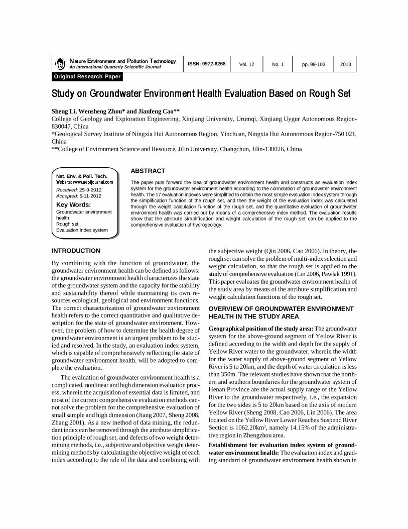
Sheng Li, Wensheng Zhou* and Jianfeng Cao**College of Geology and Exploration Engineering, Xinjiang University, Urumqi, Xinjiang Uygur Autonomous Region-830047, China*Geological Survey Institute of Ningxia Hui Autonomous Region, Yinchuan, Ningxia Hui Autonomous Region-750 021,China**College of Environment Science and Resource, Jilin University, Changchun, Jilin-130026, China
ABSTRACTThe paper puts forward the idea of groundwater environment health and constructs an evaluation indexsystem for the groundwater environment health according to the connotation of groundwater environmenthealth. The 17 evaluation indexes were simplified to obtain the most simple evaluation index system throughthe simplification function of the rough set, and then the weight of the evaluation index was calculatedthrough the weight calculation function of the rough set, and the quantitative evaluation of groundwaterenvironment health was carried out by means of a comprehensive index method. The evaluation resultsshow that the attribute simplification and weight calculation of the rough set can be applied to thecomprehensive evaluation of hydrogeology.
Nat. Env. & Poll. Tech.
Received: 25-9-2012Accepted: 5-11-2012
Key Words:Groundwater environmenthealthRough setEvaluation index system
2013pp. 99-103Vol. 12ISSN: 0972-6268 No. 1Nature Environment and Pollution TechnologyAn International Quarterly Scientific Journal
Original Research Paper
INTRODUCTION
By combining with the function of groundwater, thegroundwater environment health can be defined as follows:the groundwater environment health characterizes the stateof the groundwater system and the capacity for the stabilityand sustainability thereof while maintaining its own re-sources ecological, geological and environment functions.The correct characterization of groundwater environmenthealth refers to the correct quantitative and qualitative de-scription for the state of groundwater environment. How-ever, the problem of how to determine the health degree ofgroundwater environment is an urgent problem to be stud-ied and resolved. In the study, an evaluation index system,which is capable of comprehensively reflecting the state ofgroundwater environment health, will be adopted to com-plete the evaluation.
The evaluation of groundwater environment health is acomplicated, nonlinear and high dimension evaluation proc-ess, wherein the acquisition of essential data is limited, andmost of the current comprehensive evaluation methods can-not solve the problem for the comprehensive evaluation ofsmall sample and high dimension (Jiang 2007, Sheng 2008,Zhang 2001). As a new method of data mining, the redun-dant index can be removed through the attribute simplifica-tion principle of rough set, and defects of two weight deter-mining methods, i.e., subjective and objective weight deter-mining methods by calculating the objective weight of eachindex according to the rule of the data and combining with
the subjective weight (Qin 2006, Cao 2006). In theory, therough set can solve the problem of multi-index selection andweight calculation, so that the rough set is applied to thestudy of comprehensive evaluation (Lin 2006, Pawlak 1991).This paper evaluates the groundwater environment health ofthe study area by means of the attribute simplification andweight calculation functions of the rough set.
OVERVIEW OF GROUNDWATER ENVIRONMENTHEALTH IN THE STUDY AREA
Geographical position of the study area: The groundwatersystem for the above-ground segment of Yellow River isdefined according to the width and depth for the supply ofYellow River water to the groundwater, wherein the widthfor the water supply of above-ground segment of YellowRiver is 5 to 20km, and the depth of water circulation is lessthan 350m. The relevant studies have shown that the north-ern and southern boundaries for the groundwater system ofHenan Province are the actual supply range of the YellowRiver to the groundwater respectively, i.e., the expansionfor the two sides is 5 to 20km based on the axis of modernYellow River (Sheng 2008, Cao 2006, Lin 2006). The arealocated on the Yellow River Lower Reaches Suspend RiverSection is 1062.20km2, namely 14.15% of the administra-tive region in Zhengzhou area.Establishment for evaluation index system of ground-water environment health: The evaluation index and grad-ing standard of groundwater environment health shown in
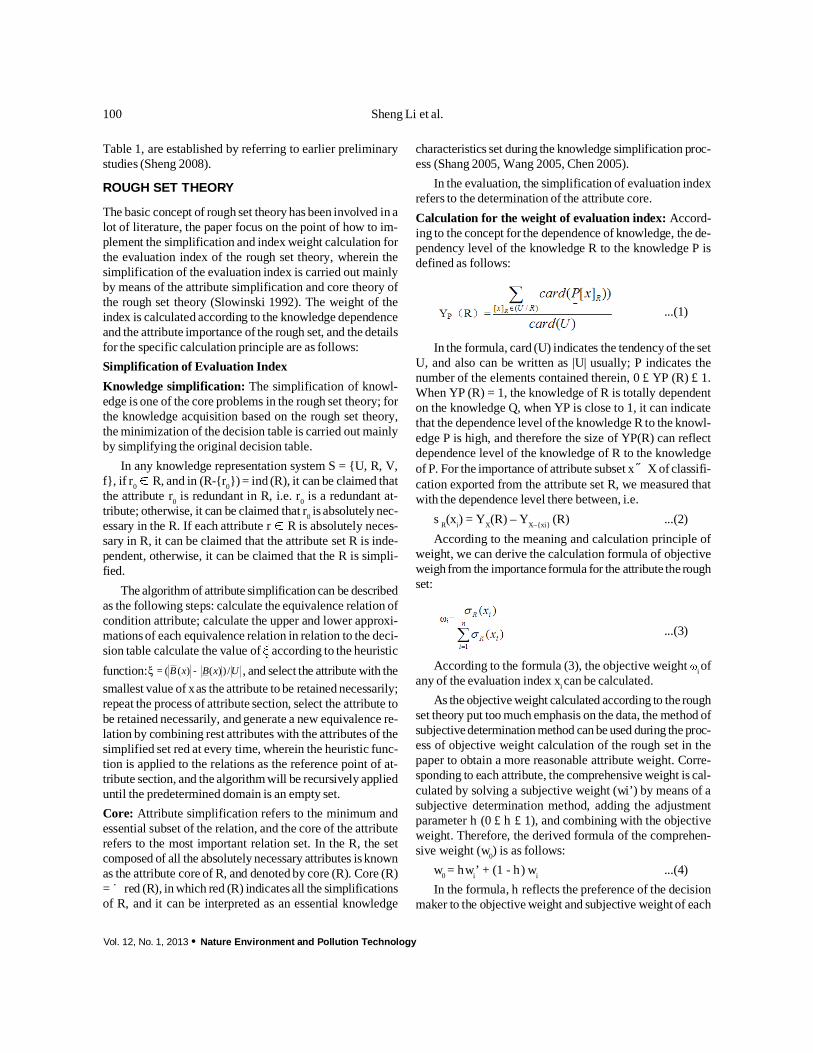
Vol. 12, No. 1, 2013 · Nature Environment and Pollution Technology
100 Sheng Li et al.
Table 1, are established by referring to earlier preliminarystudies (Sheng 2008).
ROUGH SET THEORY
The basic concept of rough set theory has been involved in alot of literature, the paper focus on the point of how to im-plement the simplification and index weight calculation forthe evaluation index of the rough set theory, wherein thesimplification of the evaluation index is carried out mainlyby means of the attribute simplification and core theory ofthe rough set theory (Slowinski 1992). The weight of theindex is calculated according to the knowledge dependenceand the attribute importance of the rough set, and the detailsfor the specific calculation principle are as follows:Simplification of Evaluation IndexKnowledge simplification: The simplification of knowl-edge is one of the core problems in the rough set theory; forthe knowledge acquisition based on the rough set theory,the minimization of the decision table is carried out mainlyby simplifying the original decision table.
In any knowledge representation system S = {U, R, V,f}, if r0 R, and in (R-{r0}) = ind (R), it can be claimed thatthe attribute r0 is redundant in R, i.e. r0 is a redundant at-tribute; otherwise, it can be claimed that r0 is absolutely nec-essary in the R. If each attribute r R is absolutely neces-sary in R, it can be claimed that the attribute set R is inde-pendent, otherwise, it can be claimed that the R is simpli-fied.
The algorithm of attribute simplification can be describedas the following steps: calculate the equivalence relation ofcondition attribute; calculate the upper and lower approxi-mations of each equivalence relation in relation to the deci-sion table calculate the value of according to the heuristicfunction: UxBxB /))()(( -=¨ , and select the attribute with thesmallest value of xas the attribute to be retained necessarily;repeat the process of attribute section, select the attribute tobe retained necessarily, and generate a new equivalence re-lation by combining rest attributes with the attributes of thesimplified set red at every time, wherein the heuristic func-tion is applied to the relations as the reference point of at-tribute section, and the algorithm will be recursively applieduntil the predetermined domain is an empty set.Core: Attribute simplification refers to the minimum andessential subset of the relation, and the core of the attributerefers to the most important relation set. In the R, the setcomposed of all the absolutely necessary attributes is knownas the attribute core of R, and denoted by core (R). Core (R)= Ç red (R), in which red (R) indicates all the simplificationsof R, and it can be interpreted as an essential knowledge
characteristics set during the knowledge simplification proc-ess (Shang 2005, Wang 2005, Chen 2005).
In the evaluation, the simplification of evaluation indexrefers to the determination of the attribute core.Calculation for the weight of evaluation index: Accord-ing to the concept for the dependence of knowledge, the de-pendency level of the knowledge R to the knowledge P isdefined as follows:
...(1)
In the formula, card (U) indicates the tendency of the setU, and also can be written as |U| usually; P indicates thenumber of the elements contained therein, 0 £ YP (R) £ 1.When YP (R) = 1, the knowledge of R is totally dependenton the knowledge Q, when YP is close to 1, it can indicatethat the dependence level of the knowledge R to the knowl-edge P is high, and therefore the size of YP(R) can reflectdependence level of the knowledge of R to the knowledgeof P. For the importance of attribute subset xÍ X of classifi-cation exported from the attribute set R, we measured thatwith the dependence level there between, i.e.
sR(xi) = YX(R) – YX–{xi} (R) ...(2)According to the meaning and calculation principle of
weight, we can derive the calculation formula of objectiveweigh from the importance formula for the attribute the roughset:
...(3)
According to the formula (3), the objective weight i ofany of the evaluation index xi can be calculated.
As the objective weight calculated according to the roughset theory put too much emphasis on the data, the method ofsubjective determination method can be used during the proc-ess of objective weight calculation of the rough set in thepaper to obtain a more reasonable attribute weight. Corre-sponding to each attribute, the comprehensive weight is cal-culated by solving a subjective weight (wi’) by means of asubjective determination method, adding the adjustmentparameter h (0 £ h £ 1), and combining with the objectiveweight. Therefore, the derived formula of the comprehen-sive weight (w0) is as follows:
w0 = hwi’ + (1 - h) wi ...(4)In the formula, h reflects the preference of the decision
maker to the objective weight and subjective weight of each

Nature Environment and Pollution Technology · Vol. 12, No. 1, 2013
101STUDY ON GROUNDWATER ENVIRONMENT HEALTH EVALUATION
attribute during the decision-making process, wherein thelarger h indicates the preference of the decision maker to thesubjective weight of the attribute, and the smaller h indi-cates the preference of the decision maker to the objectiveweight (Zeng 1996, Wang 1998, Zhang 2007, Xiao 2004).
EVALUATION FOR GROUNDWATER ENVIRONMENTHEALTH IN THE STUDY AREA
In the study work, the evaluation is carried out by means ofthe various index data of the evaluation area from 1998 to2007, wherein the specific evaluation steps are as follows:Firstly simplifying the evaluation index, calculating theweight of the evaluation index, and then quantifying andimplementing qualitative evaluation for the groundwaterenvironment health in the evaluation area by means of a com-prehensive index method.Simplification of evaluation index: In the information sys-tem S = {U, R, V, f} of the rough set, R = C D indicates anattribute set, the subsets C and D are respectively called as
condition attribute and decision attribute, wherein U indi-cates Zhengzhou study area, C indicates the specific valueof each index, and the establishment of the decision attributeD can be prevented during the attribute simplification andweight calculation process.
In order to facilitate the calculation, the specific valuesare replaced by the following codes, specifically x1, x2, …,x10 are used for replacing the values from 1998 to 2007; c1,c2, ..., c17 are used for expressing the 17 index values, thesequence thereof is in line with the previous sequence, andthe information system of the calculation constructed thereinis given in Table 2.
Calculation for the attribute simplification of rough setof the established information system, in which U = {x1, x2,…, x10} and R = {c1, c2, ..., c17} according to the rough settheory, the simplified indexes of Zhengzhou study area are{c7, c8, c12}. The additional consideration of warning of thestudy aims at finding out the environment problem ofgroundwater, selecting the indexes which are capable of re-
Table 1: Evaluation index and grading standard of groundwater environment health.
Index Unit Evaluation Criteria
Health Subhealth Unhealth
C1 Annual GDP growth rate % 7.75 7.25 6.75C2 natural population growth rate % 0.2 1.5 2.0C3 Water consumption for the GDP output value of ten thousand Yuan m3/104Yuan 35 75 150C4 Industrial water consumption for the output value of ten thousand Yuan m3 /104Yuan 15 30 50C5 Quota of irrigation water m3 /Mu 180 250 350C6 Proportion of agricultural water % 55 73 80C7 Modulus of surface water resources 104m3/(km2·a) 80 45 17C8 Modulus of recoverable groundwater resources 104m3/(km2·a) 30 20 10C9 Natural protection capability of groundwater Dimensionless 2 stronger 3 general 4 weakerC10 Water resource shared per capita m3/person 800 600 400C11 Development and utilization degree of water resources % 40 50 75C12 Modulus of groundwater mining 104m3/(km2·a) 2 5 10C13 Mining the degree of groundwater % 40 70 90C14 Comprehensive pollution index of surface water Dimensionless 0.4 0.7 1.0C15 Total hardness of groundwater mg/L 300 450 550C16 Decline rate of shallow groundwater level m/a 0 0.2 0.5C17 Comprehensive evaluation of groundwater quality Dimensionless 2 4 5
Table 2: Information system of Zhengzhou study from 1998 to 2007.
c1 c2 c3 c4 c5 c6 c7 c8 c9 c10 c11 c12 c13 c14 c15 c16 c17
x1 7.85 0.82 192.55 220.00 72.00 245.00 56.92 7.50 46.46 118.22 13.12 28.24 4 0.73 252.39 0.44 3.32x2 8.00 0.77 139.87 210.00 69.00 234.00 56.61 13.68 34.13 162.45 12.04 65.43 4 0.79 252.39 0.41 3.33x3 9.40 0.73 204.24 200.00 66.00 191.30 55.07 8.07 44.63 111.42 11.87 26.59 4 0.83 269.95 0.34 3.36x4 9.10 0.69 141.38 190.00 56.00 229.00 53.59 4.38 32.01 167.30 13.40 41.86 4 0.81 236.61 0.39 3.37x5 9.50 0.60 152.84 180.00 161.00 209.00 55.70 3.86 21.10 160.09 15.05 71.33 4 0.79 272.85 0.41 3.39x6 10.50 0.56 324.75 130.00 130.00 170.00 61.74 18.03 43.94 55.76 12.74 29.01 4 0.76 269.96 0.48 3.40x7 13.70 0.52 256.21 100.00 103.00 176.00 46.68 22.25 42.34 82.41 12.68 29.95 4 0.88 276.95 0.47 3.47x8 14.10 0.53 254.21 110.00 98.00 185.00 55.48 8.05 43.28 110.42 11.25 27.62 4 0.77 226.61 0.35 3.42x9 14.10 0.53 267.44 110.00 98.00 170.00 35.94 14.43 47.35 80.47 12.50 26.45 4 0.72 262.84 0.32 3.44x10 14.40 0.49 255.21 90.00 96.00 185.00 48.68 21.57 41.79 83.45 13.59 30.25 4 0.71 294.95 0.45 3.50
U
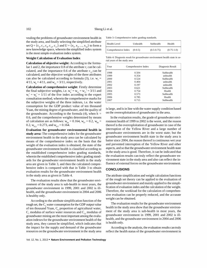
Vol. 12, No. 1, 2013 · Nature Environment and Pollution Technology
102 Sheng Li et al.
vealing the problems of groundwater environment health inthe study area, and finally selecting the simplified attributeset Q = {c4, c7, c8, c12, c17} and U = {x1, x2, ..., x10} to form anew knowledge space, wherein the simplified index systemis the most simple evaluation index system.Weight Calculation of Evaluation IndexCalculation of objective weight: According to the formu-lae 1 and 2, the importance 0.8 of the attribute r7 can be cal-culated, and the importance 0.6 of the attribute c12 can becalculated; and the objective weights of the three attributescan also be calculated according to formula (3), i.e. w7 =4/11, w8 = 4/11, and w12 = 3/11, respectively.Calculation of comprehensive weight: Firstly determinethe final subjective weights, i.e. w4' = w12 = w17' = 3/11 andw7' = w8' = 1/11 of the five index according to the expertconsultation method, wherein the comprehensive marks forthe subjective weights of the three indexes, i.e. the waterconsumption for the GDP product value of ten thousandYuan, the mining degree of groundwater, and the quality ofthe groundwater. According to the formula (4), when h =0.6, and the comprehensive weights determined by meansof calculation are as follows: w04 = 0.164, w07 = 0.2, w08 =0.2, w012 = 0.273, and w017 = 0.164.Evaluation for groundwater environmental health instudy area: The comprehensive index for the groundwaterenvironment health in the study area can be calculated bymeans of the comprehensive index on the basis that theweight of the evaluation index is obtained, the state of thegroundwater environment health is classified according tothe established comprehensive index grading standards,wherein the established comprehensive index grading stand-ards for the groundwater environment health in the studyarea are given in Table 3, and then the calculated compre-hensive index is compared with that in Table 3 to obtainevaluation results for the groundwater environment healthin the study area as given in Table 4.
The evaluation results show that the groundwater envi-ronment of the study area is sub-health in most years, thegroundwater environment in 1999, 2001 and 2002 is ill-health, and the groundwater environment in 2004 and 2006is healthy only.
According to the attribute simplification function of therough set, the C3 water consumption for the GDP output valueof ten thousand Yuan, C6 proportion of agricultural water,C7 modulus of surface water resources and C12 modulus ofgroundwater mining are the most important among the evalu-ation indexes for the groundwater environment health of thestudy area, they cannot be simplified, which indicates thatthe impact for the supply and demand of the groundwaterresources on the groundwater environment in the study area
is large, and is in line with the water supply condition basedon the overexploitation of groundwater in the area.
In the evaluation results, the grade of groundwater envi-ronment health of 1999 to 2002 is the worst, and the reasonthereof is the overexploitation of groundwater in case of theinterruption of the Yellow River and a large number ofgroundwater environments are in the worst state; but thegroundwater environment health state in the study area isbatter since 2004, the reason thereof is continuous wet yearand prevented interruption of the Yellow River and otheraspects, and so that the groundwater environment health statein the study area is good. Therefore, it can be indicated thatthe evaluation results can truly reflect the groundwater en-vironment state in the study area and also can reflect the in-fluence of external forces on the groundwater environment.
CONCLUSIONS
The attribute simplification and weight calculation functionsof the rough set theory can be applied to the evaluation ofgroundwater environment and mainly applied to the simpli-fication of evaluation index and the calculation of the weight.Therefore, the workload for the calculation of comprehen-sive evaluation can be properly reduced, and the accurateweight can be obtained.
The evaluation results for the groundwater environmenthealth in the study area show that the groundwater environ-ment of the study area is sub-health in most years, thegroundwater environment in 1999, 2001 and 2002 is ill-health, and the groundwater environment in 2004 and 2006is health only.
According to the analysis, the evaluation results can trulyreflect the health status of the groundwater environment in
Table 3: Comprehensive index grading standards.
Health Level Unhealth Subhealth Health
Comprehensive Index (0-0.5) (0.5-0.75) (0.75-1.0)
Table 4: Diagnosis result for groundwater environment health state in se-rial years of the study area
Year Comprehensive Index Diagnosis Result
1998 0.504 Subhealth1999 0.354 unhealth2000 0.524 Subhealth2001 0.404 unhealth2002 0.197 unhealth2003 0.621 Subhealth2004 0.754 Health2005 0.573 Subhealth2006 0.785 Health2007 0.715 Subhealth

Nature Environment and Pollution Technology · Vol. 12, No. 1, 2013
103STUDY ON GROUNDWATER ENVIRONMENT HEALTH EVALUATION
the study area, the feasibility of the rough set to the compre-hensive evaluation is proved, and the rough set can be analo-gized to other comprehensive evaluations.
ACKNOWLEDGEMENTS
Supported by Scientific Research Foundation for the doc-toral graduates of Xinjiang University (BS110129).
REFERENCES
Chen, Y.M. and Yu, G.Y. 2005. Study on the application of Rough SetTheory in multi-index comprehensive evaluation. Modern Manufac-turing Engineering, (Suppl.): 4-7.
Cao, J.F. and Ye, X.Y. 2006. Groundwater System Analysis and Simula-tion for the Aboveground Segment of Yellow River. Zhengzhou. Yel-low River Conservancy Press, 31-33.
Jiang, J.Y. 2007. Study and Application of Groundwater EnvironmentalHealth Theory and Evaluation System, Changchun, Jilin University,15-20.
Lin, X.Y. and Wang, J.S. 2006. Study on Groundwater Resources andRenewability of Yellow River Basin. Zhengzhou: Yellow River Con-servancy Press.
Pawlak, Z. 1991, Rough set-theoretical aspects of reasoning about data.Dordrechty, Kluwer Academic Publishers.
Qin, L. J. 2006. Evaluation for Water Resources Carrying Capacity of Down-
stream Affecting Zone (Henan) of Yellow River. Changchun, JilinUniversity, 20-22.
Slowinski, R. 1992. Intelligent decision support-handbook of applicationsand advances of the Rough sets theory. Dordrechtÿ, Kluwer AcademicPublishers.
Shang, Z.Q. Li, W.Q. and Meng, W.Q. 2005. Ant colony algorithm forattribute simplification of Rough set. Hebei Architectural Science andTechnology, 22: 101-103.
Sheng, L. 2008. Study on Groundwater Environment Health Warning -Take the Downstream Aboveground Segment (Henan) of Yellow Riverfor Example. Changchun, Jilin University, 15-20.
Wang, J., Wang, R. and Miao, D.Q. 1998. “Data Concentration” of RoughSet Theory. Journal of Computers, 21.
Wang, Z.J. Li, H.X. and Deng, X.L. 2005. Latest application of Rough settheory. Statistics and Decision, 27-29.
Xiao, Z., Zhang, Z.H. and Huang, H.S. 2004. Application of Rough settheory in corporate financial distress prediction. Statistics and Deci-sion, 48: 53.
Zeng, H.L. 1996. Rough Set Theory and Application Thereof. ChongqingUniversity Press.
Zhang, L.S., Li, L.H. and Gong, X.J. 2001. Study on major ecological andgeological problems and solutions in Henan Province downstream theYellow River. Henan Geology, 19: 71-78.
Zhang, X.F. and Zhang, Q.L. 2007. Design for MATLAB simulation toolboxof Rough set data analysis system. Journal of Northeastern University(Natural Science Edition), 28: 40-43.

January· 5th : National Bird Day (Australia)February· 2nd : World Wetlands Day· 28th : National Science DayMarch· 21st : World Forestry Day· 22nd : World Water Day· 23rd : World Meteorological Day· 31st : Earth HourApril· 18th : World Heritage Day· 22nd : Earth Day· 27th : Save the Frogs DayMay· 14-15th : World Migratory Bird Day· 18th : International Museum Day· 22nd : International Day for Biological Diversity· 23rd : World Turtle DayJune· 1st : National Whale Day· 5th : World Environment Day· 8th : World Oceans Day· 15th : Global Wind Day· 17th : World Day to Combat Desertification and DroughtJuly· 11th : World Population Day· 28th : National Tree DayAugust· 9th : International Day for World Indigenous People· 12th : International Youth DaySeptember· 16th : International Day for the Preservation of the Ozone Layer· 17th : World Parks Day· 18th : World Water Monitoring Day· 22nd : World Car-Free DayOctober· 1st : World Habitat Day· 4th : World Animal Day· 17th : International Day for the Eradication of PovertyNovember· 6th International Day for Preventing the Exploitation of the Environment in War and
Armed Conflict· 21st : World Fisheries DayDecember· 3rd : International Day of People with Disability· 5th : International Volunteer Day· 10th : Human Rights Day· 11th : International Mountain Day
ENVIRONMENTAL CALENDAR FOR 2013
104

Augustine Chioma Affam and Malay ChaudhuriDepartment of Civil Engineering, Universiti Teknologi PETRONAS, Bandar Seri Iskandar, 31750 Tronoh, Perak DarulRidzuan, Malaysia
ABSTRACTThe study examined the effect of the operating conditions of the UV photo-Fenton process on COD andTOC removal, biodegradability improvement and mineralization of combined chlorpyrifos, cypermethrin andchlorothalonil pesticides in aqueous solution. The optimum operating conditions for treatment of an aqueoussolution containing 100 mg/L of chlorpyrifos, 50 mg/L of cypermethrin and 250 mg/L of chlorothalonil wereobserved to be H2O2/COD molar ratio 2, H2O2/Fe2+ molar ratio 25 and pH 3. Under the optimum operatingconditions, complete degradation of the pesticides occurred in 1 min. Biodegradability (BOD5/COD ratio)increased from zero to 0.38 and COD and TOC removal were 78.56 and 63.76%, respectively in 60 min.The treatment resulted in release and mineralization of organic carbon and nitrogen from the pesticidemolecules as evident from TOC degradation (removal), and decrease in NH3-N from 22 to 3.9 mg/L andincrease in NO3-N from 0.7 to 19.3 mg/L in 60 min. The study shows that UV photo-Fenton process iseffective in pretreatment of combined chlorpyrifos, cypermethrin and chlorothalonil pesticides aqueous solutionfor biological treatment.
Nat. Env. & Poll. Tech.
Received: 21-6-2012Accepted: 12-9-2012
Key Words:PesticidesChlorpyrifosCypermethrinChlorothalonilUV Photo-Fenton process
INTRODUCTION
Compliance with stringent discharge standards is requiredfor the toxic substances that are non-biodegradable or in-hibitory to biological degradation processes. Among thesesubstances, pesticides are considered to be significant sur-face and ground water contaminants introduced through cropdisinfection and pesticide wastewater discharge (Shawaqfeh& Al Momani 2010). Pesticide residues have been detectedin inland waterways (Huat et al. 1991, Cheah 1996, Chea etal. 1996, Ipen 2005, Leong et al. 2007, Pan Asia 2010). Pes-ticides aldrin, heptachlor and DDT have been detected inMalaysian river water (Kimura et al. 2005).
Degradation of chlorpyrifos, cypermethrin andchlorothalonil pesticides in water has been reported.Chlorpyrifos and chlorothalonil were removed from aque-ous mixture in constructed wetlands (Sherrarda et al. 2004),chlorothalonil was degraded by Bacillus cereus strain NS1(Zhang et al. 2007), chlorpyrifos was degraded by anodicoxidation at lead dioxide and boron-doped diamond elec-trodes (Samet et al. 2010a, 2010b), chlorothalonil was de-graded by bimetallic iron-based systems (Ghauch & Tuqan2008), chlorpyrifos was degraded by pulsed electric fields(Chen et al. 2009) and cypermethrin was removed byozonation (Wu et al. 2007).
Advanced oxidation processes (AOPs) constitute apromising technology for the treatment of wastewaters
containing non-easily removable organic compounds withhigh toxicity and low biodegradability (Pera-Titus et al.2004). Experiences with different oxidation technologies andsubstrates have shown that a partial oxidation of toxic watermay increase its biodegradability up to high levels (Kiwi etal. 1994, Scott & Ollis 1995). Oxidation with Fenton’sreagent is based on hydroxyl radical (OH•) produced bycatalytic decomposition of hydrogen peroxide (H2O2) inreaction with ferrous ion (Fe2+) (Walling 1975). In the UVphoto-Fenton process, the rate of OH• radical formation isincreased by photoreactions of H2O2 and/or Fe3+ that produceOH• radical directlyor regenerate Fe2+ (Pignatello et al. 1999),thus increase the efficiency of the process. Degradation ofcypermethrin bymicrowave irradiatedphoto-Fenton reactionhas been reported (Gromboni et al. 2007). However, therehas been no study on degradation of chlorpyrifos,cypermethrin and chlorothalonil pesticides aqueous solutionby the UV photo-Fenton process.
This study examined the operating conditions (H2O2/CODmolar ratio, H2O2/Fe2+ molar ratio and pH) of the UV photo-Fenton process for COD and TOC removal, biodegradability(BOD5/COD ratio) improvement and mineralization of com-bined chlorpyrifos, cypermethrin andchlorothalonil pesticidesaqueous solution. High performance liquid chromatography(HPLC) was used to determine pesticide concentration andFourier transform infrared (FTIR) spectroscopy to estimatedegradation of organic bonds in the pesticides.
2013pp. 105-110Vol. 12ISSN: 0972-6268 No. 1Nature Environment and Pollution TechnologyAn International Quarterly Scientific Journal
Original Research Paper

Vol. 12, No. 1, 2013 · Nature Environment and Pollution Technology
106 Augustine Chioma Affam and Malay Chaudhuri
MATERIALS AND METHODS
Chemicals and pesticides: Hydrogen peroxide (30%, w/w)and ferrous sulphate heptahydrate (FeSO4·7H2O) were pur-chased from R&M Marketing, Essex, U.K. Analytical gradeof chlorpyrifos was obtained from Dr. Ehrenstorfer, Ger-many, and cypermethrin and chlorothalonil from Sigma-Aldrich, Germany. They were used for analytical determi-nation of pesticide concentration by HPLC. The pesticidesused to prepare aqueous solution were obtained from a com-mercial source, and were used as received.Analytical methods: Pesticide concentration was deter-mined by HPLC (Agilent 1100 Series) equipped with mi-cro-vacuum degasser (Agilent 1100 Series), quaternarypumps, diode array and multiple wavelength detector (DAD)at wavelength (l) 230 nm. Chemstation software was in-stalled and used for data recording. The HPLC detection col-umn was ZORBAX SB-C18 (3.0 mm × 250mm, 5µm). Thecolumn temperature was set at 30°C. Mobile phase was madeup of 25% buffer solution (0.001M KH2PO4 in double dis-tilled water) and 75% acentonitrile.
Chemical oxygen demand (COD) was determined ac-cording to the standard methods (APHA 2005). Where thesample contained hydrogen peroxide (H2O2), to reduce in-terference in COD determination pH was increased to above10 to decompose hydrogen peroxide to oxygen and water(Talini & Anderson 1992, Kang et al. 1999). TOC analyzer(Model 1010, O & I Analytical) was used for determiningtotal organic carbon (TOC). pH was measured by a pH me-ter (HACH sension 4) and a pH electrode (HACH platinumseries pH electrode model 51910, HACH Company, USA).Biodegradability was measured by 5-day biochemical oxy-gen demand (BOD5) test according to the standard methods(APHA 2005). Ammonia nitrogen (NH3-N) was measuredby the Nessler method and nitrate-nitrogen (NO3-N) by thecadmium reduction method (Hach 2002). DO was measuredusing YSI 5000 dissolved oxygen meter. The seed for BOD5test was obtained from a municipal wastewater treatmentplant. Fourier transform infrared spectrum was taken byFTIR-8400S, Shimadzu.Pesticide aqueous solution: Pesticide aqueous solution was400 mg/L of pesticides (100 mg/L of chlorpyrifos, 50 mg/Lof cypermethrin and 250 mg/L of chlorothalonil) in distilledwater. It was prepared weekly and stored at 4ºC. The pesti-cide aqueous solution had a COD of 1130 mg/L.Experimental procedure: Batch experiments were carriedout in a 600 mL Pyrex reactor with 500 mL of the pesticideaqueous solution. The required amount of iron (FeSO4·7H2O)was added to the aqueous solution and the pH was adjustedto the requiredvalue using sulphuric acid (H2SO4) and mixed
by a magnetic stirrer to ensure complete homogeneity. There-after, the necessary amount of H2O2 was added to the mix-ture and the mixture was subjected to UV irradiation at roomtemperature (23±2ºC) by placing a UV lamp 5 cm above thereactor. The UV lamp (Spectroline model EA-160/FE; 230V0.17A, Spectronics Corporation, New York, USA) had anominal power of 6 W, emitting radiation at l~365 nm. Sam-ples were taken at pre-selected time intervals, filtered througha 0.45 µm membrane filter for COD, BOD5 and TOC meas-urement, and filtered through a 0.20 µm membrane syringefilter for determination of pesticide concentration by HPLCand estimation of degradation of organic bonds in the pesti-cides by FTIR spectroscopy.
RESULTS AND DISCUSSION
Effect of UV irradiation: The photolysis of the pesticidesin the pesticide aqueous solution due to UV irradiation (l~365 nm) at pH 3 was studied. Pesticide degradation (CODremoval from the pesticide aqueous solution) by UV irra-diation per se was 4.1, 6.96, 7.61 and 8.79% in 1, 2, 3 and 4h, respectively. Further, it is known that H2O2 has a maxi-mum absorbance at l 210-230 nm and H2O2 proteolysis takesplace to a small extent at l 365 nm (Pignatello et al. 1999)and iron photo-redox also takes place under l 365 nm (AlMomani 2006). Consequently, degradation of the pesticideswhen subjected to UV photo-Fenton reaction will be mainlydue to the OH• radical produced by the UV photo-FentonreactionsEffect of H2O2/COD molar ratio: In order to obtain theoptimum H2O2/COD molar ratio, initial H2O2 concentrationwas varied in the range 35.31-123.58 mM at initial COD1130 mg/L (35.31 mM). The corresponding H2O2/CODmolar ratios were 1, 1.5, 2, 2.5, 3 and 3.5. The other operat-ing conditions were H2O2/Fe2+ molar ratio 50 and pH 3.
Fig. 1 shows the effect of H2O2/COD molar ratio on pes-ticide degradation in terms of COD and TOC removal andbiodegradability (BOD5/COD ratio) improvement. The CODremoval after 60 min irradiation was 58.98, 62.34, 77.82,53.24, 47.37 and 35.71% at H2O2/COD molar ratio 1, 1.5, 2,2.5, 3 and 3.5, respectively. The TOC removal after 60 minirradiation was 50.03, 54.45, 61.15, 43.27, 40.23 and 35.09%at H2O2/COD molar ratio 1, 1.5, 2, 2.5, 3 and 3.5, respec-tively. BOD5/COD ratio after 60 min irradiation was 0.26,0.28, 0.37, 0.25, 0.23 and 0.22 at H2O2/COD molar ratio 1,1.5, 2, 2.5, 3 and 3.5, respectively. The results show increasein pesticide degradation with H2O2/COD molar ratio up to 2and reduced degradation with further increase in H2O2/CODmolar ratio. This was presumably due to scavenging of theOH• radical by H2O2 as in Reaction (1) (Kavitha & Palanivelu2005).

Nature Environment and Pollution Technology · Vol. 12, No. 1, 2013
107UV PHOTO-FENTON TREATMENT OF PESTICIDES
OH• + H2O2 ® H2O + HO2• ...(1)
Maximum removal of COD (77.82%) and TOC (61.15%)and biodegradability improvement (0.37) was achieved af-ter 60 min irradiation at H2O2/COD molar ratio 2. OptimumH2O2/COD molar ratio 1.5 has been reported for degrada-tion of antibiotics in aqueous solution (Elmolla & Chaudhuri2009) and 2.5 for treatment of antibiotic wastewater (Emad& Chaudhuri 2010).Effect of H2O2/Fe2+molar ratio: To determine the optimumH2O2/Fe2+ molar ratio for pesticide degradation, Fe2+concen-tration was varied from 0.47 to 14.12 mM with constant H2O2concentration (70.62 mM). The other operating conditionswere H2O2/COD molar ratio 2, initial COD 1130 mg/L (35.31mM) and pH 3. Fig. 2 shows the effect of H2O2/Fe2+ molarratio on pesticide degradation in terms of COD and TOCremoval and biodegradability (BOD5/COD ratio) improve-ment. The results showincrease in pesticide degradation withdecrease in H2O2/Fe2+ molar ratio up to 25 and reduced deg-radation with further decrease in H2O2/Fe2+ molar ratio (in-crease in Fe2+ concentration). This was presumably due todirect reaction of OH• radical with Fe2+ ion at high concen-tration as in Reaction (2) (Joseph et al. 2000).
Fe2+ + OH• ® Fe3+ + OH- ...(2)
Maximum removal of COD (78.56%) and TOC(63.76%), and biodegradability improvement (0.37) wasachieved after 60 min irradiation at H2O2/Fe2+ molar ratio25. Optimum H2O2/Fe2+ molar ratio 20 has been reported fordegradation of antibiotics in aqueous solution (Elmolla &Chaudhuri 2009) and treatment of antibiotic wastewater(Elmolla & Chaudhuri 2010).Effect of pH: The pH value influences the generation of OH•
radical and hence the oxidation (degradation) efficiency. Toobtain the optimum pH, experiments were performed byvarying pH in the range 2-6. The other operating conditionswere H2O2/COD molar ratio 2, H2O2/Fe2+ molar ratio 25 andinitial COD 1130 mg/L (35.31 mM). Fig. 3 shows the effectof pH on pesticide degradation in terms of COD and TOCremoval and biodegradability (BOD5/COD ratio) improve-ment. The COD removal after 60 min irradiation was 73.82,78.56, 76.14, 65.13 and 59.08% at pH 2, 3, 4, 5 and 6, re-spectively. The TOC removal after 60 min irradiation was52.35, 63.55, 58.12, 50.02 and 43.41% at pH 2, 3, 4, 5 and 6,respectively. The BOD5/COD ratio after 60 min irradiationwas 0.31, 0.38, 0.34, 0.29 and 0.24 at pH 2, 3, 4, 5 and 6,respectively. From the results obtained, the optimum pH fortreatment of the pesticides in aqueous solution was 3. Elmolla& Chaudhuri (2009) also observed optimum pH 3 for deg-radation of antibiotics in aqueous solution.
Fig. 1: Effect of H2O2/COD molar ratio on pesticide degradation in termsof (a) COD removal, (b) TOC removal and (c) BOD5/COD ratio.
Fig. 2: Effect of H2O2/Fe2+ molar ratio on pesticide degradation in termsof (a) COD removal, (b) TOC removal and (c) BOD5/COD ratio
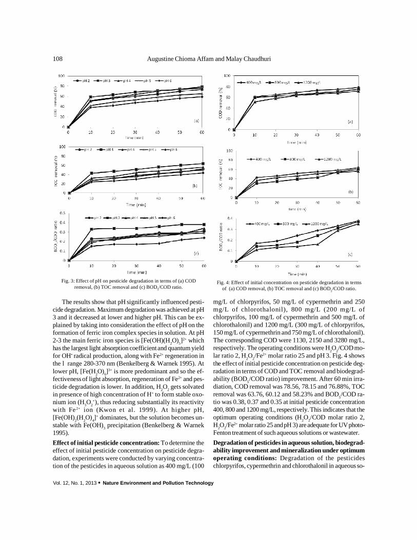
Vol. 12, No. 1, 2013 · Nature Environment and Pollution Technology
108 Augustine Chioma Affam and Malay Chaudhuri
The results show that pH significantly influenced pesti-cide degradation. Maximum degradation was achieved at pH3 and it decreased at lower and higher pH. This can be ex-plained by taking into consideration the effect of pH on theformation of ferric iron complex species in solution. At pH2-3 the main ferric iron species is [Fe(OH)(H2O)5]2+ whichhas the largest light absorption coefficient and quantum yieldfor OH• radical production, along with Fe2+ regeneration inthe l range 280-370 nm (Benkelberg & Warnek 1995). Atlower pH, [Fe(H2O)6]
3+ is more predominant and so the ef-fectiveness of light absorption, regeneration of Fe2+ and pes-ticide degradation is lower. In addition, H2O2 gets solvatedin presence of high concentration of H+ to form stable oxo-nium ion (H3O2
+), thus reducing substantially its reactivitywith Fe2+ ion (Kwon et al. 1999). At higher pH,[Fe(OH)2(H2O)4]+ dominates, but the solution becomes un-stable with Fe(OH)3 precipitation (Benkelberg & Warnek1995).Effect of initial pesticide concentration: To determine theeffect of initial pesticide concentration on pesticide degra-dation, experiments were conducted by varying concentra-tion of the pesticides in aqueous solution as 400 mg/L (100
mg/L of chlorpyrifos, 50 mg/L of cypermethrin and 250mg/L of chlorothalonil), 800 mg/L (200 mg/L ofchlorpyrifos, 100 mg/L of cypermethrin and 500 mg/L ofchlorothalonil) and 1200 mg/L (300 mg/L of chlorpyrifos,150 mg/L of cypermethrin and 750 mg/L of chlorothalonil).The corresponding COD were 1130, 2150 and 3280 mg/L,respectively. The operating conditions were H2O2/COD mo-lar ratio 2, H2O2/Fe2+ molar ratio 25 and pH 3. Fig. 4 showsthe effect of initial pesticide concentration on pesticide deg-radation in terms of COD and TOC removal and biodegrad-ability (BOD5/COD ratio) improvement. After 60 min irra-diation, COD removal was 78.56, 78.15 and 76.88%, TOCremoval was 63.76, 60.12 and 58.23% and BOD5/COD ra-tio was 0.38, 0.37 and 0.35 at initial pesticide concentration400, 800 and 1200 mg/L, respectively. This indicates that theoptimum operating conditions (H2O2/COD molar ratio 2,H2O2/Fe2+ molar ratio 25andpH 3) are adequate for UVphoto-Fenton treatment of such aqueous solutions or wastewater.Degradation of pesticides in aqueous solution, biodegrad-ability improvement and mineralization under optimumoperating conditions: Degradation of the pesticideschlorpyrifos, cypermethrin and chlorothalonil in aqueous so-
Fig. 3: Effect of pH on pesticide degradation in terms of (a) CODremoval, (b) TOC removal and (c) BOD5/COD ratio.
Fig. 4: Effect of initial concentration on pesticide degradation in termsof (a) COD removal, (b) TOC removal and (c) BOD5/COD ratio.

Nature Environment and Pollution Technology · Vol. 12, No. 1, 2013
109UV PHOTO-FENTON TREATMENT OF PESTICIDES
lution (COD 1130 mg/L; 35.31 mM) under the optimumoperating conditions (H2O2/COD molar ratio 2, H2O2/Fe2+
molar ratio 25 and pH 3) was studied. Complete degrada-tion of all the three pesticides was achieved in 1 min.
In the FTIR spectrum, the absorption bands ofchlorpyrifos are located between 1549 to 968 cm-1 due toC=N stretching, pyridine stretching, ring vibration, ringbreathing, Cl-C stretching, trigonal ring breathing and P=Sstretching; the cypermethrin absorption bands appear from1742 to 1076 cm-1 due to carbonyl stretching, C=C stretch-ing in chloroalkenes, ring vibration of benzene, CH2 defor-mation in R-CH2-CN structure and (C=O)-O- stretching; andtangential C-C stretching in benzene and hexa-substitutedbenzene derivatives of chlorothalonil is observed in the rangeof 1548 and 1265 cm-1 (Armenta et al. 2005, Dhas et al. 2010).Fig. 5 shows the FTIR spectra of the untreated and treatedpesticide aqueous solution. The absorption bands at 1650.95cm-1 and 1448.44 cm-1 in the untreated aqueous solution weremodified in the treated aqueous solution, indicating degra-dation of the organic bonds in the pesticide.Fig. 6 shows pesticide degradation under the optimum oper-ating conditions in terms of COD and TOC removal and bio-degradability (BOD5/COD ratio) improvement. MaximumCOD andTOC removal were 78.56 and 63.76%, respectivelyafter 60 min irradiation and BOD5/COD ratio was 0.38 whichis considered adequate for biological treatment (Al-Momaniet al. 2002).
UV photo-Fenton treatment resulted in release and min-eralization of organic carbon and nitrogen from the pesti-cide molecules. Mineralization of organic carbon is evidentfrom TOC degradation (removal) as shown in Fig. 6. Miner-alization of organic nitrogen is evident from decrease inNH3-N from 22 to 3.9 mg/L and increase in NO3-N from 0.7 to19.3 mg/L in 60 min (Fig. 7).
CONCLUSIONS
• Under optimum operating conditions (H2O2/COD molarratio 2, H2O2/Fe2+ molar ratio 25 and pH 3), UV photo-Fenton treatment of combined chlorpyrifos, cyperme-thrin and chlorothalonil pesticides aqueous solution re-sulted in complete degradation of the pesticides in 1 min.Biodegradability increased from zero to 0.38, and CODand TOC removal were 78.56 and 63.76%, respectivelyin 60 min.
• UV photo-Fenton treatment resulted in release and min-eralization of organic carbon and nitrogen from the pes-ticide molecules as evident from TOC degradation (re-moval), and decrease in NH3-N from 22 to 3.9 mg/L andincrease in NO3-N from 0.7 to 19.3 mg/L.
• UV-photo-Fenton process can be used for pretreatmentof combined chlorpyrifos, cypermethrin andchlorothalonil pesticides aqueous solution for biologi-cal treatment.
Fig. 7: Mineralization of organic nitrogen in terms of NO3-N formation.
Fig. 6: Pesticide degradation under optimum operating conditions interms of COD and TOC removal and BOD5/COD ratio.
Fig. 5: FTIR spectra of (a) untreated and (b) treated pesticide solution

Vol. 12, No. 1, 2013 · Nature Environment and Pollution Technology
110 Augustine Chioma Affam and Malay Chaudhuri
ACKNOWLEDGEMENT
The authors wish to thank the management and authoritiesof the Universiti Teknologi PETRONAS for providing fa-cilities for this research.
REFERENCESAl Momani, F. 2006. Impact of photo oxidation technology on the aque-
ous solutions of nitrobenzene: Degradation efficiency and biodegrad-ability enhancement. J. Photochem. Photobiol. A: Chem., 179:184-192.
Al-Momani, F., Touraud, E., Degorse-Dumas, J. R., Roussy, J. and Tho-mas, O. 2002. Biodegradability enhancement of textile dyes and tex-tile wastewater by VUV photolysis. J. Photochem. Photobiol. A: Chem.,153: 191-197.
APHA 2005. Standard Methods for the Examination of Water andWastewater. 21st edition. American Public Health Association, Wash-ington, DC.
Armenta, S., Quintas, G., Garrigues, S. and De la Guardi, M. 2005. A vali-dated and fast procedure for FTIR determination of cypermethrin andchlorpyrifos. Talanta, 67: 634-639.
Benkelberg, H.J. and Warnek, P. 1995. Photodecomposition of iron(III)hydroxo and sulfato complexes in aqueous solution: Wavelength de-pendence of OH and SO4
- quantum yields. J. Phys. Chem., 99:5214-5221.
Cheah, U. B. 1996. Environmental Fate of Selected Pesticides in MalaysianAgro Environment. Ph.D. Thesis. Department of Bioscience & Bio-technology, Faculty of Science, University of Strathclyde, Glasgow.
Cheah, U. B., Aminuddin, Y., Salama, R., Lum, K.Y. and Wan AbdullahW.Y. 1996. Pesticide leaching in the Cameron Highlands agro eco-system. Proceedings of the Second International Conference on Con-taminants in Soil Environment in the Australasia-Pacific Region, NewDelhi, pp. 339-340.
Chen, F., Zeng, L., Zhang, Y., Liao, X., Ge, Y., Hua, X. and Jiang, L. 2009.Degradation behaviour of methamidophos and chlorpyrifos in applejuice treated with pulsed electric fields. Food Chem., 112: 956-961.
Dhas, D.A., Joea, I.H., Roy, S.D.D. and Freed, T.H. 2010. DFT computa-tions and spectroscopic analysis of a pesticide: Chlorothalonil.Spectrochim. Acta, Part A, 77: 36-44.
Elmolla, E.S. and Chaudhuri, M. 2009. Degradation of the antibioticsamoxicillin, ampicillin and cloxacillin in aqueous solution by the photo-Fenton process. J. Hazard. Mater., 172: 1476-1481.
Elmolla, E.S. and Chaudhuri, M. 2010. Photo-Fenton treatment of antibi-otic wastewater. Nat. Environ. Pollut. Technol., 9: 365-370.
Ghauch, A. and Tuqan, A. 2008. Catalytic degradation of chlorothalonil inwater using bimetallic iron-based systems. Chemosphere, 73: 751-759.
Gromboni, C.F., Kamogawa, M.Y., Ferreira, A.G., N’Obrega, J.A. andNogueira, A.R.A. 2007. Microwave-assisted photo-Fenton decompo-sition of chlorfenvinphos and cypermethrin in residual water. J.Photochem. Photobiol. A: Chem., 185: 32-37.
Hach 2002. Water Analysis Handbook. 4th Edn., Hach Company, Loveland.CO.
Huat, T.G., Hock, G.S. and Vijayaletchumy, K. 1991. Analysis of pesticideresidues in Peninsular Malaysian waterways. Environ. Monit. Assess.,19: 469-479.
Ipen 2005. International POPs elimination project. Malaysia country situ-ation report. Available at: http://www.ipen.org/
Joseph, J. M., Destaillats, H., Hung, H.M. and Hoffmann, M.R. 2000. The
sonochemical degradation of azobenzene and related azo dyes: Rateenhancements via Fenton’s reactions. J. Phys. Chem. A, 104:301-307.
Kang, Y. W., Cho, M.J. and Hwang, K.Y. 1999. Correction of hydrogenperoxide interference on standard chemical oxygen demand test. Wa-ter Res., 33: 1247-1251.
Kavitha, V. and Palanivelu, K. 2005. Destruction of cresols by Fenton oxi-dation process. Water Res., 39: 3062-3072.
Kimura, K., Yokoyama, K., Sato, H., Nordin, R.B., Naing, L., Kimura, S.,Okabe, S., Maeno, T., Kobayashi, Y., Kitamura, F. and Araki, S. 2005.Effects of pesticides on the peripheral and central nervous system intobacco farmers in Malaysia: Studies on peripheral nerve conduction,brain-evoked potentials and computerized posturography. Ind. Health,43: 285-294.
Kiwi, J., Pulgarin, C. and Peringer, P. 1994. Effect of Fenton and photo-Fenton reaction on the degradation and biodegradability of 2- and 4-nitrophenols in water treatment, Appl. Catal. B, 3: 335-350.
Kwon, B.G., Lee, D. S., Kang, N. and Yoon, J. 1999. Characteristics of p-chlorophenol oxidation by Fenton’s reagent. Water Res., 33:2110-2118.
Leong, K.H., Tan, B.L.L. and Mustafa, A.M. 2007. Contamination levelsof selected organochlorine and organophosphate pesticides in theSelangor River, Malaysia between 2002 and 2003. Chemosphere, 66:1153-1159.
Pan Asia 2010. Communities in Peril: Global report on health impacts ofpesticide use in agriculture. Regional reports for PAN InternationalProduction Supervision. Available at: http://www.pan-germany.org/download/PAN-I_CBM-Global-Report_1006-final.pdf
Pera-Titus, M., Garcia-Molina, V., Banos, M. A., Gimenez, J. and Esplugas,S. 2004. Degradation of chlorophenols by means of advanced oxida-tion processes: A general review. Appl. Catal., B, 47: 219-256.
Pignatello, J.J., Liu, D. and Houston, P. 1999. Evidence for an additionaloxidant in the photo assisted Fenton reaction. Environ. Sci. Technol.,33: 1832-1839.
Samet, Y., Agengui, L. and Abdelhedi, R. 2010a. Anodic oxidation ofchlorpyrifos in aqueous solution at lead dioxide electrodes. J.Electroanal. Chem., 650: 152-158.
Samet, Y., Agengui, L. and Abdelhedi, R. 2010b. Electrochemical degra-dation of chlorpyrifos pesticide in aqueous solutions by anodic oxida-tion at boron-doped diamond electrodes. Chem. Eng. J., 161: 67-172.
Scott, J.P. and Ollis, D.F. 1995. Integration of chemical and biological oxi-dation processes for water treatment: Review and recommendations.Environ. Prog., 14: 88-103.
Shawaqfeh, A.T. and Al Momani, F.A. 2010. Photocatalytic treatment ofwater soluble pesticide by advanced oxidation technologies using UVlight and solar energy. Sol. Energy, 84: 1157-1165.
Sherrarda, R.M., Bearrb, J.S., Murray-Guldec, C.L., Rodgers, J.H., Jr. andShahd, Y.T. 2004. Feasibility of constructed wetlands for removingchlorothalonil and chlorpyrifos from aqueous mixtures. Environ.Pollut., 127: 385-394.
Talini, I. and Anderson, G.K. 1992. Interference of hydrogen peroxide onthe standard COD test. Water Res., 26: 107-110.
Walling C. 1975. Fenton’s reagent revisited. Acc. Chem. Res., 8: 125-131.Wu, J.G., Luan, T.G., Lan, C.Y., Lo, W.H. and Chan, G.Y.S. 2007. Effi-
cacy evaluation of low-concentration of ozonated water in removal ofresidual diazinon, parathion, methyl-parathion and cypermethrin onvegetable. J. Food Eng., 79: 803-809.
Zhang, Y., Lu, J. L., Wu, L., Chang, A. and Frankenberger, W. T., Jr. 2007.Simultaneous removal of chlorothalonil and nitrate by Bacillus cereusstrain NS1. Sci. Total Environ., 382: 383-387.

Men Baohui, Lin Chunkun, Li Zhifei and Sun BoyangNational Engineering Laboratory for Biomass Power Generation Equipment, Renewable Energy Institute, North ChinaElectric Power University, Beijing-102206, China
ABSTRACTThe runoff data of Zhuba Station at Niqu river in water diversion area of Western Route Project (WRP) ofSouth-North Water Transfers Project (SNWTP) from 1961 to 2010 were applied to estimate the coefficientsof variation of hydrology, the peak pattern degree, and ample flow VS low flow, climate tendency rate and soon. The results were used to analyse the effects of hydrological regime on river discharge in the water supplyarea of the first stage project in WRP. The results demonstrated that: The annual river discharge is increasingin Niqu River which is the water supply area in the first stage project of WRP. The cumulative increased riverdischarge is 0.52×10⁸m3 within 50 years which is 2.6% larger than the average value. The runoff increasedeach year in non-flood season and decreased each year in flood season.
Nat. Env. & Poll. Tech.
Received: 25-9-2012Accepted: 8-11-2012
Key Words:Niqu riverRun-offWestern Route ProjectRiver discharge variation
2013pp. 111-114Vol. 12ISSN: 0972-6268 No. 1Nature Environment and Pollution TechnologyAn International Quarterly Scientific Journal
Original Research Paper
INTRODUCTION
South-to-North Water Transfer Project is an important eco-logical engineering which is formed by three lines: WesternRoute Project (WRP), Middle Route Project (MRP) andEastern Route Project (ERP). These three water transferprojects connect the Yangtze River, Huaihe River, YellowRiver and Haihe River which formed the general pattern forChinese water resources development, distribution and uti-lization (Li 2001). The Middle Route Project and the East-ern Route Project are under construction now. Project pro-posal of the Western Route Project is under evaluation atpresent. 170×108m3 volume of water is scheduled tobe trans-ferred from the upper reaches of the Yangtze River, includ-ing Tongtianhe River, Yalong River and Dadu River to theYellow River in the Western Route Project.
The studies of the WRP in the SNWTP mainly focusedon the hydrological data estimation at the dam section, therunoff features analysis, water transfer volume evaluation,the effects of water transfer on the hydrological regime andecological environment and the ecology, and water require-ment in the downstream of the water transfer rivers. There isno hydrological station at the dam section. The hydrologi-cal data at the dam section needs to be derived from the datacollected by the downstream stations (Gao 2001, Men2006a).
The determination of the water diversion volume of theWRP in the SNWTP, the effects of water transfer on the eco-logical environment and water requirement are both related
to the variation of the river runoff. Water is one of the mostactive factors in the ecological system. It is very importantto study the runoff variation. The runoff supply source andrun-off characteristics of river in south-north water transferscheme via western route had been studied (Men 2007, Men2009), while, there are no relationship researches about therelationship between the variation of the runoff and the cli-mate factors at present. The runoff change of Niqu river asan example (Men 2007), is introduced in this paper. Thisstudy can supply scientific foundation to the proposal dem-onstration, planning and design, available water transferamount and ecology, and water requirement of the first stageof WRP.
DATA COLLECTION
Zhuba Station is the only hydrological station in Niqu river.The monthly average runoff data from 1961 to 2010 recordedin Zhuba Hydrological Stationwere supplied by the NationalHydrological Bureau.
ALGORITHM MODEL
The annual average runoff at Niqu Hydrologic Station, whichis the water supply area in the first stage project of WRP,was estimated.Coefficient of variation (Cv) (Men 2006b, Tang 1992):Coefficient of variation can indicate the annual runoff seriesdeviating from the mean of runoff. In general, coefficient ofvariation can be calculated by equation (1).

Vol. 12, No. 1, 2013 · Nature Environment and Pollution Technology
112 Men Baohui et al.
( ) ( )å=
--=n
ii nKCv
1
2 1/1 ...(1)
QQK ii /= ...(2)
Where n is the number of observation years; Ki is therunoff variation of the ith year; Qi is the average runoff of theith year; Q is the average runoff.
Residual accumulative curve (Men et al. 2006b): Stand-ardized ( ) CvK i /1- was applied to indicate the variation ofrunoff in order to minimize the effect of unit of annual run-off, precipitation and Cv. The Residual accumulative curvewas calculated to show the variation of the runoff periodi-cally with ( ) CvK i /1å - as the Y-axis.Peak-patterndegree and ample flow Vs low flow (Li 2004):Peak-pattern degree ¿ and ample flow Vs low flow ¾ wereapplied to analyse the runoff distribution within the year.The peak-pattern degree ¿ reflected the ratio of the seasonalsnow melt water to the mountain snow melt water plus rain-fall of the river runoff. The ample flow Vs low flow reflectedthe ratio of the runoff in the flood season to that in the non-flood season, which indicated the ratio of the increment ofgroundwater to the annual runoff.
10875 / --= QQ¿ ...(3)
411105 / --= QQ¾ ...(4)
where Q5-7 is the total river discharge from May to Julyeach year; Q8-10 is the total river discharge from August toOctober each year; Q5-10 is the total river discharge from Mayto October each year; Q11-4 is the total river discharge fromNovember to next April each year.Climate tendency rate: It fluctuates with time and showedcertain tendency with large time scale. The climate tendencyreflected the variation of climate factors with time.
If one element array data was assumed to be a time array,the data can be expressed as X1, X2, X3,……, Xn, which canbe presented as a polynomial:
( ) pptatataatX ++++= L2
210
^...(5)
Where t is time with year as the unit which is usuallyexpressed as a.
Generally, the climate tendency of one element can besimulated with curvilinear equation, parabolic equation orstraight line equation. The tendency rate can be given as:
( )1
^
dd a
ttX = ...(6)
a1 can be determined using least square method ororthogonal polynomial with 10a1 as the climate tendencyrate.
( ) ( ) min2
1
^=úû
ùêëé -å
=
n
ttXtX ...(7)
VARIATION FEATURES OF RUNOFF IN NIQURIVER
The variation of the surface water resources in the water sup-ply area of the first stage of WRP is related to the explora-tion of the water resources (available water transfer amount)and the water supply of the river discharge. This can influ-ence the reliability of the water supply in the water intakearea directly.Cv of the Niqu river: Generally, the discharge of some riv-ers varied seasonally because of the seasonally changingwater supply. This usually happens to the rivers with sea-sonal snow melt water or precipitation as the water supply.The coefficient of variation of these rivers is very large. Thedischarges of rivers are relatively stable with mountain icemelt water mixing with rainfall as the water supply becausethese two kinds of water supply can complement each otherand minimize the seasonal effects. The coefficients of varia-tion of these rivers are relatively small. The Cv is about 0.10-0.12 for rivers with mountain ice melt water as the watersupply; the Cv is around 0.12-0.20 for rivers with mountain
y = 0.0328x + 61.419
30405060708090
100110
1961 1968 1975 1982 1989 1996 2003 2010year
runo
ffm
3 /s
-4-3-2-101234
1961 1968 1975 1982 1989 1996 2003 2010year
(K-1
)/Cv
Fig. 1: Variation curve of annual mean flow in Niqu River.
Fig. 2: Difference-integral curve of annual mean flow in Niqu River.

Nature Environment and Pollution Technology · Vol. 12, No. 1, 2013
113ANALYSIS OF RUNOFF CHANGES OF NIQU RIVER
springy = 0.4988x + 93.803
20253035404550556065
1961 1968 1975 1982 1989 1996 2003 2010year
runo
ffm
3 /s
summery = 0.0286x + 336.5
30
80
130
180
230
1961 1968 1975 1982 1989 1996 2003 2010year
runo
ffm
3 /s
autumn y = -0.5298x + 253.06
2040
6080
100120
140160
1961 1968 1975 1982 1989 1996 2003 2010year
runo
ffm
3 /s
winter
y = -0.5298x + 253.06
10
15
20
25
30
35
1961 1968 1975 1982 1989 1996 2003 2010year
runo
ffm
3 /s
flood seasony = -0.3812x + 595.5
30
50
70
90110
130
150
170
1961 1968 1975 1982 1989 1996 2003 2010year
3
non-flood seasony = 0.744x + 139.13
10
15
20
2530
35
40
45
1961 1968 1975 1982 1989 1996 2003 2010year
3
Fig. 3: Variation curve of annual mean flow in four seasons, flood seasonand non-flood season in Niqu River.
020406080
100120140160
1 2 3 4 5 6 7 8 9 10 11 12month
runo
ffm
/s
Fig. 4: Monthly variation curve of flow at Zhuba station in Niqu River.
y = 0.0039x + 0.8952
0.0
0.5
1.0
1.5
2.0
2.5
1961 1968 1975 1982 1989 1996 2003 2010year
Peak
-pat
tern
degr
ee
Fig. 5: Annual variation curve of peak-pattern degree in Niqu River.
y = -0.0201x + 4.2643
0
1
234
5
6
7
1961 1968 1975 1982 1989 1996 2003 2010year
ampl
eflo
wV
Slo
wflo
w
Fig. 6: Annual ample flow Vs low flow in Niqu River.
ice melt water and rainfall as the water supply; and the Cv isabout 0.25-0.45 for rivers with seasonal snow melt water orrainfall as the water supply. The coefficient of variation ofNiqu river was calculated with Eqs. (1) and (2) as 0.23. Theriverdischarge of the flood season from May to October takes80% of the total annual river discharge which means thatthe mixture mountain snow melt water, seasonal snow meltwater and rainfall is the main water source to Niqu river.Inter-annual variation of runoff: The variation curve andresidual accumulative curve of the annual average runofffrom 1961 to 2010 at Zhuba Station in Niqu is presented inFig. 1 and Fig. 2 correspondingly.
As shown in Fig. 1 and Fig. 2, the runoff of Niqu changedfrom high level to low level frequently with 5 circulations.The runoff increased slightly during these 50 years. The ab-

Vol. 12, No. 1, 2013 · Nature Environment and Pollution Technology
114 Men Baohui et al.
solute value of the runoff anomaly percent within 20% isassumed to be normal year. The value larger and smaller than20% is assumed to be high and low level years. Accordingto these assumptions, there are 26 normal years out of to-tally 50 years which take about 50%. The high level and lowlevel years are 13 and 11 years correspondingly which takes25% each. There are 3 high level years before 80’s. Thereare 5 low level years between 60 and 70’s which took 50%of the total low level years.
The river discharge increased gradually before 60’s of20 century and reached the maximum value in 1966. It de-creased afterwards and reached the minimum value at theend of 70’s. The value increased slowlyafter 80’s and reachedthe maximum in 2005. According to the calculated climatetendency rate, the river discharge increased at speed of 0.33m3/(s.10 a). The cumulative increased runoff is 0.52 × 10⁸m3
within 50 years which is 2.6% larger than the average value.The river discharge of the flood and non-flood seasons
increasedor decreased at speed of +4.99, +0.29, -5.30, +4.07,-3.81, +7.44 m3/(s.10 a) in spring, summer, autumn and win-ter correspondingly (Fig. 3). The increment in spring is themost significant. The decrement in summer is the most sig-nificant as well.
The variation of the average annual discharge within theyear from 1961 to 2010 at Zhuba station in Niqu river isshown in Fig. 4. The distribution of the discharge within theyear in Niqu is doublet shape. The riverdischarges from Janu-ary to February were the lowest and increased slowly fromMarch to April. The value increased greatly from May toJune and reached maximum in July. It decreased slightly inAugust and reached the second peak value in September. Itdecreased obviously after October and reached the minimumin December which is still larger than that from January toFebruary. This means that the water discharge during theflood season from May to October takes 80% of the totalannual discharge which is 5 times larger than that during thenon-flood season. These features demonstrated that the wa-ter supply of the river in Niqu river is mainly from rainfall.As shown in Fig. 4, the first peak value is closely related tothe rainfall of this area in July. The peak value in Septembermay be caused by the mountain ice melt water which mayresult in glacier lake breaking.
The Peak-pattern degree of the runoff decreased slightlyeach year despite the normal variation as shown in Fig. 5.This means that the ratio of the seasonal melt water to thesum of mountain ice melt water and rainfall is decreasinggradually. The ample flow Vs low flow (Fig. 6.) decreasedgradually as well which means that the ratio of the flood
season to that of the non-flood season is decreasing. The ratioof the runoff within the flood season to the total value isdecreasing as well. This means that the water supply fromrainfall within this area is increasing. Accordingly, the watersupply from the snow melt water is decreasing. This may berelated to the global warming and shrinking of the glacier.
CONCLUSIONS
The annual river discharge increased 0.33 m3/(s.10a) in Niquriver which is the water supply area in the first stage projectof WRP. The cumulative increased river discharge is0.52×108m3 within 50 years which is 2.6% larger than theaverage value. The river discharge increased or decreased atthe rate of +4.99, +0.29, -5.30, +4.07, -3.81, +7.44m3/(s.10a)in spring, summer, autumn, winter, floodseason and non-floodseason correspondingly. The increase in spring is the mostsignificant. The decrease of runoff in autumn is the most sig-nificant as well. The variation of the runoff in flood and non-flood season is positive. The runoff increased each year innon-flood season and decreased each year in flood season.
ACKNOWLEDGMENTS
This work was supported in part by the Fundamental Re-search Funds for the Central Universities, No. 11MG15, andNational Natural Science Foundation of China, No.50809027.
REFERENCESGao, Z.D., Zhang, Z.H. and Wang, Y.F. 2001. Study on natural runoff at
dam site on of water diversion from the south to the north via the west-ern course. Yellow River, 23(10): 9-10.
Li, G.Y. 2001. Understanding and evaluation of the project of water diver-sion from the south to the north via the western course. Yellow River,23(10): 1-4.
Li, L., Wang, Q.C. and Zhang, G.S. 2004. The influence of climate changeon surface water in the upper Yellow River. Acta Geographica Sinica,59(5): 716.
Men, B.H., Liu, C.M., Xia, J. and Liu, S.X. 2006. Calculation and analysisof runoff at dam sites in the first stage construction of the south-to-north water diversion project along the western line. Earth ScienceFrontiers, 13(3): 155-161.
Men, B.H., Liu, C.M., Xia, J. and Liu, S.X. 2006. Runoff and its impactingfactors in the water-exporting rivers of the first stage project of thesouth-to-north water transfer scheme via the western route: A case studyin Daqu. Scientia Geographica Sinica, 26(6): 674-681.
Men, B.H. 2007. Primary analysis of runoff supply source of river in south-north water transfer scheme via western route. Journal of LiaoningTechnical University, 26(s1): 249-251.
Men, B.H. 2009. Analysis of run-off characteristic of south-to-north watertransfer scheme via the western route in water-exporting region. Jour-nal of Liaoning Technical University, 28(1): 149-151.
Tang, Q.C., Qu, Y.G. and Zhou, J.C. 1992. Hydrology and water resourcesusing at drought region in China. Beijing: Science Press, pp. 53-73.

K. C. Jagadeeshappa and Vijayakumara*Department of Chemistry, Kalpataru First Grade Science College, Tiptur-572 201, Tumkur District, Karnataka, India*Department of Wildlife and Management, Bioscience Complex, Kuvempu University, Shankaraghatta-577 451,Shivamogga District, Karnataka, India
ABSTRACT
The influence of seasonal variations in physico-chemical characteristics exert a profound effect on thedistribution and population density of both animal and plant species. In the present paper we carried out thestudy to evaluate physico-chemical characteristics of water of Vignasanthe wetland located at Tiptur taluk ofTumkur Dist, Karnataka. The constituents monitored include temperature, pH, TUR ,EC, TDS, Cl, TH, Ca,Mg, Alk, NO3, PO4, Fe2+, Si, DO, BOD, CO2, SO4, COD and DOM. A significant variation in these parameterswas observed throughout the study period and monthly comparisons were made as monsoon, premonsoonand postmonsoon. The results of present investigations were compared with earlier available literature andrevealed that there is a fluctuation in the physico-chemical characters of the water. This is due to inflow andchange in the temperature as season changes.
Nat. Env. & Poll. Tech.
Received: 11-7-2012Accepted: 27-8-2012
Key Words:Vignasanthe wetlandPhysico-chemicalcharactersSeasonal variations
2013pp. 115-119Vol. 12ISSN: 0972-6268 No. 1Nature Environment and Pollution TechnologyAn International Quarterly Scientific Journal
Original Research Paper
INTRODUCTION
Wetlands benefit society by recharging aquifers, retainingsediments and nutrients, controlling floods and providingstorm protection and microclimate stabilization (Mitsch &Gosselink 1993). Nevertheless, the conservation of thesewetlands in India is continuously threatened by the use ofnatural habitats to meet the demands of society. Some per-sist in defining wetlands as unhealthy and unproductive ar-eas that need to be drained to improve soil conditions. Theseecosystems contain a rich biological diversity and contrib-ute great benefit to the society. Yet they are stressed in Indiaby agriculture use, unplanned tourism land use planning andlack of enforcement of existing environmental laws. Thesefactors have resulted in large unacceptable losses of wetlands,which have had a high social cost. The physical and chemi-cal characters of the wetland water can be used to assess theecological nature of the wetlands. Several studies have beenconducted to understand the physical and chemical proper-ties of lakes, wetlands and reservoir. In such studies the char-acteristics of the water bodies were taken into considerationwith reference to physical and chemical properties; theseactivities are important for conversation, creation and resto-ration of similar ecosystems of wetlands. So the present studywas undertaken to assess the physical and chemical charac-teristics of Vignasanthe wetland of Tiptur taluk.
MATERIALS AND METHODS
The study area, Vignasanthe wetland, is located 16 km from
Tiptur. The wetland is situated in southern part of Tiptur ofKarnataka and is bounded by geographical coordinates13°08’473” N latitude and 76°32’912” E longitude and hav-ing the elevation of 2709 ± 21 ft above mean sea level. It isbounded by Chikkanayakanahalli on north east, Arasikerein the west, Hassan in south west, Yedeyur, the famous pil-grimage in the south east and Tumkur on the east. Thewetland has a catchment area of 20 square kilometres(Fig. 1). Water samples were collected for physico-chemi-cal analysis from different sampling stations. Samples werecollected once in every month from June 2010 to may 2011.During sample collection in the wetland, necessary precau-tions were taken to collect the undisturbed water samples.Samples were collected in two-litre blue polythene cans inthe morning between 7a.m. to 10a.m. AT, WT, pH, turbidityand EC were determined on the spot. DO was fixed on thesite, while other parameters were analysed in the laboratoryby standard methods (APHA 2005) and Trivedy & Goel(1984).
RESULTS AND DISCUSSION
The average values and standard deviations of the wet landwith respect to physico-chemical parameters are given inTable 2 and shown graphically in Figs. 2 and 3. The averageseasonal variations of the above parameters are shown inFigs. 4 and 5. The temperature is one of the most importantecological factors, which controls the physiological behav-iour and distribution of organisms. The air temperature (AT)in the respective sampling sites varies from 20.40-34.50°C

Vol. 12, No. 1, 2013 · Nature Environment and Pollution Technology
116 K. C. Jagadeeshappa and Vijayakumara
with an average value of 27.23°C ± 4.11°C. The observedvariation is because of environmental factors. Water tem-perature (WT) was observed with the variation from 20°C-30.50°C with an average of 24.79°C ± 3.72°C. During win-ter season water temperature was low due to frequent clouds,high humidity, high current velocity and high water level.
Aquatic organisms are affected by pH because most oftheir metabolic activities are pH dependant. pH desired limitwas also observed by Kulkarni et al. (2009). One of the mostimportant factors that serves as an index for pollution is pH.The pHof Vignasanthe wetland varied between 7.00 and9.01with an average of 7.94. It is slightly alkaline. The pH ofwater was relatively high in the premonsoon and low in themonsoon and postmonsoon during study period. This highvalue of pHcould be due to increased primary productivitywherein carbonates, sulphates, nitrates and phosphates arehydrolysed to hydroxyl ions.
The turbidity is mainly due to the dispersionof suspendedsolids, from mass bathing, agricultural runoff and domesticsewage. Maximum turbidity was found during monsoon sea-son and minimum in premonsoon. The turbidity values varyfrom 100.10-25.40 mg/L, with an average of 52.20 mg/Lduring the study period.
The electrical conductivity values of the water samplesranged between 361 and 745 µmhos/cm with an average of320.25 µmhos/cm. The maximum values were found inpremonsoon, and minimum in monsoon. Conductivity ofwater depends upon the concentration of ions and its nutri-ent status and the variation in dissolved solid content. Dilu-
tion of water during the rains causes a decrease in the elec-trical conductance. Similarobservationwas made bySulabha& Prakashan (2006).
Oxygen is an important parameter of the wetland, whichis essential to the metabolism of all aquatic organisms thatpossess aerobic respiration. Concentration of dissolved oxy-gen (DO) decides the quality of water and its relation to thedistribution and abundance of various algal species. In thepresent investigation the DO of water samples ranged from3.40-9.40 mg/L with an average of 6.09 mg/L. DO is higherin postmonsoon and minimum in monsoon indicating thegood water quality. This is also supported by Sahu et al.(2000).
Biochemical oxygen demand (BOD) depends on tem-perature, biochemical activity, concentration of organic mat-ter and other related factors. During the study period BODwas observed to be in the range of 0.09-4.70 mg/L with anaverage of 2.04 mg/L during the study period. This is due tolow temperature and less bacterial activity. Higher level ofDO leads to the maximum values of BOD in premonsoon.Although there is no specific standard set for BOD, the WHOstandard indicates 6 mg/L as a limit.
The total dissolved solids (TDS) values of water sam-ples ranged between 212.08 and 452.00 mg/L with an aver-age of 320.25±82.71 mg/L. This is in accordance with thevalue of BIS (1991). The TDS concentration is high duringpremonsoon, which may be due to the addition of solids fromthe runoff water. The amount of total solids is influenced bythe activity of plankton and organic materials.
Fig. 1: Sampling location in Vignasanthe wetland.

Nature Environment and Pollution Technology · Vol. 12, No. 1, 2013
117PHYSICO-CHEMICAL CHARACTERISTICS OF WATER IN VIGNASANTHE WETLAND
Chemical oxygen demand (COD) ranges from 7.40-22.10mg/L with an average of 14.90±4.25 mg/L. The maximumCOD was observed in premonsoon (22.10 mg/L). This ismainly due to the presence of more concentration of organicmatter.
Total hardness (TH) depends on the amounts of calciumand magnesium present in the water. During the study pe-
Table 1: Correlation matrix of different water quality parameters of Vignasanthe wetland during the period (June study 2010 to May 2011)
pH TUR EC TDS Cl TH Ca Mg ALK Aci NO3 PO4 Fe Si DO BOD CO2 SO4 COD DOM
0.89 0.1018 0.705 0.675 0.766 0.7018 0.733 0.68 0.846 0.389 0.223 0.152 0.477 0.358 0.258 0.48 0.643 0.305 0.7891 0.21 0.743 0.732 0.58 0.643 0.669 0.628 0.673 0.505 0.236 0.077 0.147 0.198 0.476 0.373 0.551 0.426 0.68 0.174
1 0.0952 0.171 0.2706 0.077 0.087 0.052 0.261 0.12 0.597 0.854 0.81 0.0621 0.256 -0.0074 0.104 -0.162 0.501 0.3091 0.973 0.804 0.737 0.749 0.749 0.806 0.49 0.287 0.076 0.151 0.431 0.424 0.6677 0.9 0.49 0.771 0.045
1 0.774 0.702 0.709 0.714 0.785 0.464 0.369 0.197 0.172 0.398 0.463 0.631 0.854 0.419 0.787 0.0351 0.742 0.772 0.758 0.902 0.391 0.348 0.16 0.447 0.548 0.251 0.702 0.851 0.373 0.722 0.109
1 0.992 0.99 0.85 0.214 0.136 -0.041 0.324 0.789 0.153 0.766 0.751 0.515 0.664 0.2381 0.982 0.851 0.249 0.185 -0.031 0.322 0.745 0.172 0.734 0.746 0.514 0.656 0.251
1 0.834 0.226 0.157 -0.039 0.302 0.8 0.196 0.742 0.774 0.571 0.625 0.27061 0.266 0.125 0.0824 0.503 0.614 0.082 0.82 0.877 0.294 0.867 0.059
1 0.447 0.275 -0.071 -0.067 0.795 0.237 0.468 0.696 0.364 0.321 0.642 0.237 0.0163 0.605 -0.022 0.273 0.2 0.274 0.223
1 0.656 -0.098 0.471 -0.1 0.032 -0.035 0.377 0.3881 0.325 -0.045 0.281 0.211 -0.125 0.588 0.36
1 -0.0019 0.6002 0.545 0.4432 0.347 0.3511 -0.0201 0.248 0.684 0.217 0.503
1 0.807 0.32 0.72 -0.1731 0.42 0.723 -0.113
1 0.157 0.60051 0.0275
riod it ranges between 79.00 and 242 mg/L with an averageof 135.75 mg/L. This is also within the BIS limit of drink-ing water (200 mg/L). The high value of TH found duringpremonsoon is due to evaporation of water and addition ofCa and Mg salts. The observed higher value of alkalinitywith respect to hardness indicates the presence of basic saltsof sodium and potassium, in addition to those of calciumand magnesium.
The variation in nitrate (NO3-) content of study area is
between 0.01 and 0.28 mg/L with an average of 0.13 mg/L.This could be due to the anthropogenic sources like domes-tic sewage, agricultural wash offs and other waste effluentscontaining nitrogenous compounds. The above findings
Table 2: Average values of physico-chemical parameters water ofVignasanthe wetland.
Parameters Average values ofVignasanthe Wetland
AT 27.23 ± 4.11WT 24.79 ± 3.72pH 7.94 ± 0.65TUR 52.20 ± 27.18EC 514.83 ± 130.55TDS 320.25 ± 82.71Cl- 14.72 ± 4.85TH 135.75 ± 50.61Ca 28.29 ± 9.57Mg 24.18 ± 9.14Alk 146.42 ± 46.68Aci 9.24 ± 2.65NO3 0.13 ± 0.06PO4 0.16 ± 0.11Fe 0.11 ± 0.09Si 0.15 ± 0.25DO 6.09 ± 1.81BOD 2.04 ± 1.52CO2 0.96 ± 0.37SO4 66.67 ± 27.98COD 14.90 ± 4.25DOM 0.81 ± 0.48
The values are in mg/L except temperature (°C), EC (micromho/cm),turbidity (NTU) and pH.
Fig. 2: Monthly variations of AT, WT, pH, EC and TUR.

Vol. 12, No. 1, 2013 · Nature Environment and Pollution Technology
118 K. C. Jagadeeshappa and Vijayakumara
agree with Kulasherstha & Sharma (2006).The chloride (Cl-) content was noticed with maximum
of 24.10 mg/L, and minimum of 8.6 mg/L with an averageof 14.72± 4.85 mg/L. The maximum concentration was no-ticed in premonsoon. The higher concentration of Cl- is con-sidered to be an indicator of higher pollution and higher or-ganic wastes of agriculture and dairy origin.
Sulphates (SO42-) are in the permissible limit (250 mg/L)
and ranges from 26.00-122 mg/L with an average of 66.67and ±27.98 mg/L. The phosphate concentration varies from0.02-0.35 mg/L with an average of 0.16 mg/L. The maxi-mum values were observed during monsoon, which couldbe due to agricultural runoff from fields and detergents richsewage effluents. This helps in the growth of weeds. AmongNO3
-, Cl-, SO4
2- and phosphate, phosphate concentration wasobserved to be relatively lower, but all values were wellwithin the limit. All these above variations of inorganic saltsconcentration are due to seasonal variation in environmen-tal factors. These results are in agreement with Kulasherstha& Sharma (2006).
All the hydrological and physico-chemical parametersstudied showed noticeable variations. Correlations of dif-ferent parameters are given in Table 1. Water temperaturehas good correlation with pH and alkalinity; pH is having
Fig. 3: Monthly variations of TDS, Cl, TH, Ca, Mg, ALK, Aci, NO3,PO4, Fe, Si, DO, BOD, CO2, SO4, COD and DOM.
Fig. 5: Seasonal variations of TDS, Cl, TH, Ca, Mg, ALK, Aci, NO3,PO4, Fe, Si, DO, BOD, CO2, SO4, COD and DOM.
Fig.4: Seasonal variations of AT, WT, pH, EC and TUR.
Nature Environment and Pollution Technology · Vol. 12, No. 1, 2013
119PHYSICO-CHEMICAL CHARACTERISTICS OF WATER IN VIGNASANTHE WETLAND
significant correlation with EC, TDS and TH. Turbidityshows good correlation with phosphate concentration. ECshows a significant correlation with TDS and CO2,TDS hassignificant correlation with CO2. Chloride with alkalinityand CO2’ total hardness show a good correlation with cal-cium and magnesium. Calcium with magnesium and acidityshow correlations with DO. BOD correlates with CO2, whileother parameters are not correlate with each other.
REFERENCESAPHA 2005. Standard Methods for the Examination of Water and
Wastewater. 21st edition, American Public Health Association, Wash-ington DC.
BIS 1991. Indian Drinking Water Standard Specification, Bureau of In-dian Standards, New Delhi.
Kulasherstha, H. and Sharma, S. 2006. Impact of mass bathing duringArdhkumbh on water quality status of river Ganga. J. Environ. Biol.,27: 437-440.
Kulakarni, A.S., Medha Tendulkar, Sayali Mavalankar and Giharkarm,A.M. 2009. Study on water quality parameter from Pethkilla region,Rathnagiri, westcoast of India, Maharastra. J. Aquatic Biology, 24(2):82-85.
Mitsch, W.J. and Gosselink, J.G. 1993. Wetlands. Second edition, VanNostrand Reinhold, New York.
Sahu, B.K., Rao, R.J., Behera, D.P. and Pandit, R.K. 2000. Effect of pollu-tion on the dissolved concentration of River Ganga at Kanpur. In: R.K. Trivedy (Ed.) Pollution and Biomonitoring of Indian Rivers, ABDPublishers, Jaipur, India, pp. 168-170.
Sulabha, V. and Prakasan, V.R. 2006. Limnology feature of Thirumullivaramtemple pond of Kollam municipality, Kerala. Journal of Environmen-tal Biology, 27(2): 449-451.
Trivedy, R.K. and Goel, P.K. 1984. Chemical and Biological Methods forWater Pollution Studies. Env. Publ., Karad, India.

· In a few decades, the relationship between the environment, resources and conflict may seem almostas obvious as the connection we see today between human rights, democracy and peace.
Wangari Maathai
· We won't have a society if we destroy the environment.Margaret Mead
· The Endangered Species Act is the strongest and most effective tool we have to repair the environ-mental harm that is causing a species to decline.
Norm Dicks
· You may be able to fool the voters, but not the atmosphere.Donella Meadows
· In today's world, it is no longer unimaginable to think that business can operate - and even thrive -in an environmentally-friendly manner.
Olympia Snowe
· We learned that economic growth and environmental protection can and should go hand in hand.
Christopher Dodd
· I think the cost of energy will come down when we make this transition to renewable energy.Al Gore
· Within 10 years it will be impossible to travel to the North Pole by dog team. There will betoo much open water.
Will Steger
· When a man wantonly destroys one of the works of man we call him a vandal. When he destroysone of the works of god we call him a sportsman.
Joseph Wood Krutch
· By polluting clear water with slime you will never find good drinking water.Aeschylus
· The only way forward, if we are going to improve the quality of the environment, is to get everybody involved.
Richard Rogers
ENVIRONMENTAL QUOTES
120

Xiaoming Wang and Benzhi ZhouResearch Institute of Subtropical Forestry, The Chinese Academy of Forestry, Fuyang 311400, Zhejiang Province, China
ABSTRACT
Saomai (August 10, 2006) was one of the most significant typhoons to hit the coast in southeast China.Quantitative assessment of forest disturbances is important for improving management strategies. Thisstudy used remote sensing techniques to investigate vegetation changes after Saomai in Changnan county.Two landsat ETM+ satellite images were acquired before and after landfall. The results showed that averagedNDVI values decreased by 17.8% after Saomai. Elevation and relative aspect present strong influence onthe typhoon damage. These results provide insight into the sensitivityof coastal vegetation fromthe interactionsof both tropical cyclones and long-term environmental conditions.
Nat. Env. & Poll. Tech.
Received: 25-9-2012Accepted: 6-11-2012
Key Words:Forest disturbanceTyphoon SaomaiRemote sensingNDVI
2013pp. 121-124Vol. 12ISSN: 0972-6268 No. 1Nature Environment and Pollution TechnologyAn International Quarterly Scientific Journal
Original Research Paper
INTRODUCTION
China is affected by an average of seven landfalling tropicalcyclones every year. These typhoons have caused signifi-cant damage in China over the years. Typhoons can exten-sively influence the composition, structure and natural suc-cession of forests (Foster 1992, Conner 1989, Gresham 1991,Wang 2009), and it is one of the major natural disturbancesin forest ecosystems in the southeast China. Saomai (Au-gust 10, 2006) was one of the most significant typhoons tohit the coast in southeast China. Quantitative assessment offorest disturbances is important for improving managementstrategies. Traditional field surveycan, however, be very timeconsuming and confined to local areas. Satellite remote sens-ing techniques have been gradually adopted for monitoringforest status at regional and global scales since early 2000(Rodgers 2009, Ramsey 1997, Ayala-Silva 2004, Lee 2008).Ayala-Silva and Twumasi (Ayala-Silva 2004) investigatedthe vegetation change caused by Typhoon Georges in PuertoRico using the standardized change of NDVI derived fromAVHRR images (Lillesand 2004, Lee 2008). Mukai (2000)analysed the relationship of forest type, topographic aspects,elevation and forest damage caused by Typhoon Herb incentral Taiwan using NDVI derived from SPOT images.
According to the preliminary survey results, TyphoonSaomai had an adverse effect on the coastal vegetation, yetthe extent and magnitude of the vegetation damage withinthe region has not been fully investigated. The goal of thisstudy is to investigate vegetation disturbance by using NDVIas an indicator of post-typhoon forest damage.
MATERIALS AND METHODS
Study Area
Typhoon Saomai became the sixth tropical cyclone to hitChina in 2006 when it made landfall at 09:25 UTC (August10, 2006) in Cangnan County near the city of Wenzhou inZhejiang Province (Fig. 1). The study area (Cangnancounty, 27°302 N’120°232 E) lying the south of ZhejiangProvince covers a land area of 1261.08 km2, and a sea areaof 3,720,000 km2 with a coastline of 168.88 km. The studyarea is located in the subtropical maritime monsoon cli-mate region with an annual mean temperature and precipi-tation of 17.9°C and 1670.1 mm respectively. The presentstudy area is dominated by mixed deciduous/broadleaf for-est, along with shrubs, herbaceous vegetation, bare land andbuilt-up areas.
Data and Methods
Satellite image data acquisition and preprocessing:Landsat ETM+ images were used in this study to monitorchanges before and after Typhoon Saomai. Pre and post-Saomai Landsat ETM+ remote sensing images (October 18,2005 and October 5, 2006) were used for typhoon distur-bance detection. Images were rectified to the October 2005base image. Total root mean square for each image rectifica-tion process was less than 1/2 pixel (±15 m). The imageswere radiometrically corrected using standard remote sens-ing techniques (Kovacs et al. 2001). Normalized DifferenceVegetation Index (NDVI) values were calculated for each ofthe two images respectively.

Vol. 12, No. 1, 2013 · Nature Environment and Pollution Technology
122 Xiaoming Wang and Benzhi Zhou
Environmental data: Land cover types, elevation, and rela-tive aspect during the typhoon period were analysed to helpevaluate the changes in NDVI. Land cover types were de-rived from the data product of EUROPE300. The composi-tion of land use in the study area included urban land, farmland, wetland, shrubs and broadleaf forest. The relative as-pect was defined as the angle between the aspect and winddirection with a range of 0-180 degree.Methodology: To quantify changes in NDVI values amongthe two images, a geographic information system (GIS) wasused to generate 26131 spatial random points across to thestudy region. To assess temporal changes in the vegetation,NDVI image of October 18, 2005 was subtracted from thatof October 5, 2006 by using map algebra, which is a cell-by-cell process performed on each coregistered pixel from bothinput images.
RESULTS AND DISCUSSION
Overall NDVI comparisons: Vegetation changed greatlyduring this particular temporal comparison. The averageNDVI value and maximum NDVI value of pre-Saomai im-age were 0.64 and 0.88, whereas these two indices of post-Saomai image were 0.57 and 0.79 respectively. The changeof NDVI value had a wild range from -0.96 to 1.24 (Fig. 2).The average subtracted NDVI value between the October18, 2005 and October 5, 2006 images was 0.14 and the aver-age percent decrease was -17.68%.Variability of NDVI change among land cover types:Changes in averaged NDVI after landfall varied among dif-ferent locations and land cover types. From the subtraction
Fig. 1: Location of the study area (left) and Landsat ETM+ image (right) of the study area.
0
200
400
600
800
1000
1200
1400
1600
-0.3
-0.3
-0.2
-0.2
-0.2
-0.2
-0.1
-0.1
-0.1
-0 0
0.03
0.06
0.09
0.12
0.15
0.18
0.21
0.24
0.27
0.3
0.33
0.36
0.39
0.42
0.45
0.48
NDVI
sample points
Fig. 2: The histogram of DNDVI before and after landfall.
Fig. 3: Subtraction of the October 5, 2006 NDVI image from theOctober 18, 2005 NDVI image for the study area.

Nature Environment and Pollution Technology · Vol. 12, No. 1, 2013
123FOREST DAMAGE BY TYPHOON SAOMAI USING REMOTE SENSING AND GIS
of the October 18, 2005 and October 5, 2006 NDVI images(Fig. 3), it was obvious that the areas with the most pro-nounced decreases in NDVI were north and northeastern re-gions. Within the individual land cover types, urban andfarmland had the largest percent decrease in averaged NDVIfrom October 2005 and October 2006 (32.6% and 19.8%).This was followed by coniferous and broadleaf forest(17.5%). The wetland experienced the least amount of de-cline in average NDVI during this period (Fig. 4).
Influence of environmental variables on the disturbanceof vegetation by typhoon: Those areas below 150 m expe-rienced the highest decrease of NDVI value, areas below 50m and 50-100 m experienced an average decrease in aver-aged NDVI value from October 2005 to October 2006 of-56.0% and -29.5%, respectively (Fig. 5). The damaged areadecreased with the increasing elevation, whereas percentdecreases in NDVI increased with elevation. Positive corre-lation was showed between elevation and percent decreasein NDVI was done with a relationship coefficient of 0.925.
The damaged area and the percent decrease in NDVI bothdecreased with the increasing relative aspect (Fig. 6). Butthis reduction was not a linear decrease, the largest NDVIreduction occurred in the relative aspect between 30 and 40degree with a proportion of 19.78%. Negative correlationwas shown between relative aspect and percent decrease inNDVI was done with a relationship coefficient of -0.879.
It canbe concluded that vegetation indices measured fromLandsat satellite imagery showed a near 20% reduction invalue from October 18, 2005 to October 5, 2006. Comparedto these other studies, it appears that the NDVI decrease fol-lowing Typhoon Saomai in study area was moderate in value(Loope 1994, Lodge 1991). Environmental factors such aselevation and relative aspect had close relationships with ty-phoon damage. Due to lack of field survey data for Saomai,these led to the uncertainty for evaluation of damage by ty-phoon disturbance. A more comprehensive on ground in-vestigation of the different taxa and their respective toler-ances to environmental change, especially to changes in ty-phoon track, would help understanding how spatial patternsenable determination of relationships between typhoons andcoastal vegetation dynamics.
ACKNOWLEDGMENT
This study was supported by the 11th Five-Year NationalKey Scientific and Technological Project (Grant No.2009BADB2B03) and Chinese Academy of Forestry (GrantNo. RISF61521).
REFERENCES
Ayala-Silva, T. and Twumasi, Y. A. 2004. Hurricane Georges and vegetationchange in Puerto Rico using AVHRR satellite data. J. Int. J. RemoteSens., 25(9): 1629-1640.
Conner, W.H.J., Day, W., Baumann, R. H. and Randall, J. M. 1989. Influenceof hurricanes on coastal ecosystems along the northern Gulf of Mexico.J. Wetland Ecology Management, 1: 45-56.
Foster, D.R. and Boose, E.R. 1992. Patterns of forest damage resulting fromcatastrophic wind in central New England, USA. J. J. Ecol., 80: 79-98.
Gresham, C. A., Williams, T. M. and Lipscomb, D. J. 1991. Hurricane Hugowind damage to Southeastern U.S. coastal forest tree species. J.Biotropica, 23: 420-426.
Kovacs, J. M., Blanco-Correa, M. and Flores-Verdugo, F. 2001. A logisticregression model of hurricane impacts in a mangrove forest of the
0
5
10
15
20
25
30
35
city cropland wetland shrub forest sum
land cover types
area
ratio
(%)
0
5000
10000
15000
20000
25000
30000
numbe
rof
samp
les
disturbed samples
percent decrease
Fig. 4: The damaged area and percent decrease of change of NDVIvalue with different land cover types.
0
200
400
600
800
1000
1200
1400
1600
50 150 250 350 450 550 650 750 850 950 10501150
elevation
Number
of samples
0
10
20
30
40
50
60
70
80
90
Area
ratio (%)
NDVI decrease sample
NDVI percent decrease
Fig. 5: The damaged area and percent decrease of change of NDVIvalue with different elevation.
0
100
200
300
400
500
600
10 20 30 40 50 60 70 80 90 100110120130140150160170180
relative aspect
0
5
10
15
20
25
NDVI decrease samples
NDVI percent decrease
Fig. 6: The damaged area and percent decrease of change of NDVIvalue with different relative aspect.

Vol. 12, No. 1, 2013 · Nature Environment and Pollution Technology
124 Xiaoming Wang and Benzhi Zhou
Mexican Pacific. J. Coastal Res., 17: 30-37.Lee, M., Lin, T., Vadeboncoeur, M.A. and Hwong, J. 2008. Remote sensing
assessment of forest damage in relation to the 1996 strong typhoon Herbat Lienhuachi Experimental Forest, Taiwan. J. Forest Ecol. Manag., 255:3297-3306.
Lillesand, T.M., Kiefer, R.W. and Chipman, J.W. 2004. Remote Sensingand Image Interpretation. New York, NY, Wiley.
Lodge, D. J. and McDowell, W. H. 1991. Summary of ecosystem-level effectsof Caribbean hurricanes. J. Biotropica, 23: 373-378.
Loope, L., Duever, M., Herndon, A., Snyder, J. and Jansen, D. 1994.Hurricane impact on uplands and freshwater swamp forest. J. Bioscience,44: 238-246.
Mukai, Y. and Hasegawa, I. 2000. Extraction of damaged areas of windfalltrees by typhoons using Landsat TM data. Int. J. Remote Sens., 21:647-654.
Ramsey, E.W., Chappell, D.K. and Baldwin, D.G. 1997. AVHRR imageryused to identify hurricane damage in a forested wetland of Louisiana. J.Photogrammetric Engineering & Remote Sensing, 63: 293-297.
Rodgers, J.C., Murrah, A.W. and Cooke, W.H. 2009. The Impact ofHurricane Katrina on the coastal vegetation of the Weeks Bay Reserve,Alabama from NDVI Data. J. Estuar. Coast, 32: 496-507.
Wang, F. and Xu, Y. 2009. Hurricane Katrina-induced forest damage inrelation to ecological factors at landscape scale. J. Environ. Monit.Assess., 156: 491-507.

Resham Bhalla and B. B. Waykar*Department of Zoology, LVH Arts, Science & Commerce College, Panchavati, Nashik-422 003, Maharashtra, India*Department of Zoology, Dr. Babasaheb Ambedkar Marathwada University, Aurangabad-431 004, Maharashtra, India
ABSTRACT
Rivers are currently degraded by both natural and anthropogenic activities, which deteriorate the waterquality, affecting the ecological balance, pushing them to brink of extinction in the process of unplanneddevelopment, giving rise to planning for suitable conservation strategies. On this background to know thepresent status of sources and degree of pollution of Godavari river, the analysis was carried out in terms ofphysico-chemical and biological parameters like temperature, turbidity, pH, free carbon dioxide, sulphates,phosphates, chlorides, nitrates, nitrites, total dissolved solids, dissolved oxygen, biochemical oxygen demand,chemical oxygen demand, phytoplanktons, zooplanktons and metals like sodium, potassium, zinc, copper,iron and lead at five locations S1 toS5 during the year November 2008-October 2009. Based on the analysis,quality and quantity of pollution, Nashik Municipal Corporation is suggested to device strategies to arrestfurther pollution of Godavari river and use of river water for drinking purpose after conventional treatmentand disinfection.
Nat. Env. & Poll. Tech.
Received: 7-9-2012Accepted: 17-10-2012
Key Words:Godavari riverWater qualityPollution statusHeavy metals
2013pp. 125-129Vol. 12ISSN: 0972-6268 No. 1Nature Environment and Pollution TechnologyAn International Quarterly Scientific Journal
Original Research Paper
INTRODUCTION
Water as a natural resource is becoming a scarce commoditydue to its indiscriminate use and contamination from vari-ous sources such as leaching of agro-chemicals from farms,untreated domestic water from cities, and increasing volumeof industrial effluents. Industrialization and urbanization hascreated serious problems of water pollution of our lakes andrivers. Industrial effluents and domestic sewage are directlydischarged into water bodies, which contribute to a signifi-cant amount of heavy metals. The Godavari river originatesin Nashik district in Sahyadri ranges in Trimbakeshwar andduring its course , it meets many small and seasonal streams.At present, Godavari river water is polluted due to unfilthypractices of dumping waste and sewage.
MATERIALS AND METHODS
Study area: Five sampling stations of Godavari river (S1-S5) were selected for the present study. While selecting eachsampling station, drainage pattern of the specific area intothe river was kept in mind for eventually helping to identifythe source and types of contaminants (Manivaskam 1984,Trivedy & Goel 1986).S1:Someshwar-Point before the discharge of industrial
effluents.S2:Gharpure Ghat-Point before the domestic discharge into
Godavari river.S3:Ramkund-Water is used for washing, bathing, and
various rites and rituals are performed here.S4:Tapowan area-At the confluence of River Godavari and
Waghadi and discharge of effluents into the riverS5:Dasak bridge-The exit point of Godavari river from the
city.Water samples were collected from the five sampling sta-
tions S1-S5 at an interval of one month from November 2008to October 2009 seasonwise (Winter, Summer, Monsoon)in clean, rinsed plastic containers. Samples for chemical andbiological analysis were collected separately. Methods usedfor chemical analysis were standardizedaccording to the pro-cedures given by APHA-AWWA-WPCF(1995). Heavymet-als were determined by atomic absorption spectrophotom-eter. Flora and fauna were identified using keys given bySehgal (1983), Adoni (1985) and APHA (1985).
RESULTS AND DISCUSSION
The seasonwise and annual average analysis of physico-chemical and biological parameters is given in Table 1 andFigs. 1-5 with statistical evaluation in Table 2.Temperature: Temperature of Godavari water was foundto be higher at S4 and S5 at which more of effluents aredischarged. On the basis of three seasons, the average watertemperature was 21.63°C, 27.92°C and 24.96°C during win-ter summer and monsoon seasons respectively. The sametrend has also been observed by Sumitra (1969) and Kannan& Jog (1980) in tropical impoundments.

Vol. 12, No. 1, 2013 · Nature Environment and Pollution Technology
126 Resham Bhalla and B. B. Waykar
pH: Water was alkaline during monsoon season (pH 8.55),winter (pH 8.10) and summer (pH 7.95). Kannan & Jog(1980) reported higher pH value during rainy season andlower during summer. Low pH in summer may probably bedue to high rate of organic matter decomposing activities bymicrobeswhich release weak acids. Higher alkalinity of watermay be indicative of intensive leaking from rocks due torunoff water.Turbidity: Turbidity values varied with seasons. Monsoonseason showed highest turbidity of 37.96 NTU as large quan-tities of suspended matter derived from catchment areasreaches the river, followed by summer (6.64 NTU) due toincreased flow of water consequently enriching organic mat-ter and least in winter (5.70NTU) as water is less turbid andrelatively clean.Free CO2: Winter season showed higher amount of free CO2(8.33 mg/L) as compared to monsoon season (6.55 mg/L)followed by summer (6.45 mg/L). Level of free CO2 variesinversely with level of dissolved O2 as observed earlier byGanapati (1943), Gonzalves & Joshi (1946) and Rao (1955).Sulphate: Seasonwise sulphate showed enhanced values insummer (82.24 mg/L) followed by monsoon (53.38 mg/L)and winter (47.24 mg/L). Its higher concentration at the ori-gin of Godavari in June and subsequent decrease in othermonths is due to mass visit of pilgrims to the origin for wor-ship, which results into accumulation of voluminous wastefrom typical pooja articles.Phosphate: Winter season showed higher phosphateconcentration (2.42 mg/L), followed by summer (1.28 mg/L) and monsoon (0.34 mg/L). According to Edmondson
(1972), sewage effluents have been regarded as good sourceof phosphates.Chloride: Higher values in monsoon (37.48 mg/L), slightlyless in winter (37.20 mg/L) and followed by summer (29.95mg/L) is in accordance with observations of Cristobal (1979),which may be due to different types of industrial wastes,activities of slum dwellers and municipal sewage drainedinto river water.Nitrate: Concentration of nitrates was highest in winter (1.61mg/L) followedby summer (0.96 mg/L) and least in monsoonseason (0.22 mg/L). The observed maximum values of ni-trates during winter are in agreement with Prasad & Saxsena(1980), whose study indicated that due to flood, nitrates con-tributing algae from rocks are carried in water, which mini-mizes fixation of nitrates during monsoon season.Nitrites: In monsoon and winter season nitrite concentra-tion was barely detectable due to dilution factor. It was maxi-mum in summer (0.13 mg/L) possibly due to accumulationof organic waste in the riverbed, as a result of reduced quan-tum and rate of flow which helped to increase biodegrada-tion activities .Total dissolved solids: TDS showed an enhanced value(344.84mg/L) in winter followed by summer (245.52mg/L)and monsoon season (155.74 mg/L). According to drinkingwater standards, prescribed by USPHS (United States Pub-lic Health Services, 1962) TDS should not excess 500mg/L beyond which they may influence toxicity of heavymetals and organic compounds in fish and other aquatic life(Mckee & Wolf 1963).Dissolved oxygen: Higher average dissolved oxygen (7.21
Table 1: Seasonwise and annual average analysis of physico-chemical and biological parameters at five stations (S1-S5) of Godavari River during Nov.2008 to Oct. 2009.
S1 S2 S3 S4 S5 AverageParameters W S M W S M W S M W S M W S M W S M
Temperature 19. 55 28.20. 26.60 19.78 27.78 24.00 21.71 27.55 24.05 23.00 27.55 24.70 24.15 28.53 25.45 21.63 27.92 24.96pH 8.52 8.22 9.00 8.17 8.25 8.09 8.06 8.21 8.59 7.77 7.53 8.48 8.01 7.56 8.61 8.10 7.95 8.55Turbidity 6.80 5.40 61.80 10.10 7.00 4.20 4.60 6.20 54.40 3.60 10.60 36.00 3.40 4.00 33.40 5.70 6.64 37.96Free CO2 3.64 2.07 2.48 16.54 12.82 11.58 2.73 3.72 6.62 8.77 8.15 6.62 10.01 6.00 4.96 8.33 6.55 6.45Sulphates 83.87 58.62 81.16 41.43 122.65 57.72 37.88 78.46 27.05 40.58 80.26 54.11 32.47 71.24 46.89 47.24 82.24 53.38Phosphates 2.47 1.06 0.23 2.19 1.06 0.14 2.02 1.30 0.46 3.07 1.53 0.15 2.36 1.48 0.72 2.42 1.28 0.34Chlorides 12.61 12.78 20.59 69.02 69.20 54.67 19.17 14.56 23.43 41.18 25.56 41.89 44.02 27.69 46.86 37.2 29.95 37.48Nitrates 1.99 0.44 0.55 1.45 2.90 0.18 1.33 0.27 0.17 1.18 0.36 0.11 2.11 0.85 0.10 1.61 0.96 0.22Nitrites 0.01 0.12 0.00 0.01 0.15 0.00 0.00 0.07 0.00 0.01 0.16 0.00 0.00 0.17 0.00 .006 0.13 0.00TDS 234.76 121.75 154.96 283.90 146.80 363.19 281.94 134.55 158.99 299.41 189.02 269.0 324.20 185.72 281.45 344.84 155.74 245.52DO 9.16 4.17 7.25 7.57 4.86 3.84 7.36 4.92 5.12 6.41 2.45 3.63 5.55 3.67 5.33 7.21 4.01 5.03BOD 28.70 22.31 31.53 8.40 6.40 6.25 24.50 17.11 23.94 25.00 53.64 33.62 15.25 20.46 14.26 20.29 23.98 21.92COD 59.20 57.70 94.58 141.65 124.36 277.17 55.21 54.12 71.83 142.64 155.61 100.87 55.82 48.61 42.79 90.90 88.08 117.48Phytoplankton 310.60 2150.50 1324.50 326.50 2170.50 1330.30 370.00 2256.00 1360.30 416.50 2360.25 1375.75 430.10 2380.45 1388.10 370.74 2263.54 1355.8Zooplanktons 210.75 980.00 380.00 215.70 970.80 402.00 230.00 990.20 418.60 235.00 1005.10 410.10 250.00 1050.60 406.40 228.29 999.34 403.42Sodium 5.75 1.83 3.00 4.93 2.84 3.65 1.95 1.90 3.25 3.58 3.20 3.55 3.75 2.88 3.65 3.99 2.53 3.42Potassium 1.25 0.30 0.17 0.50 0.31 1.30 0.21 0.10 0.18 0.69 0.47 0.26 0.66 0.35 0.52 0.66 0.30 0.48Zinc 0.00 0.01 0.01 0.01 0.01 0.00 0.00 0.01 0.00 0.00 0.01 0.00 0.00 0.00 0.00 0.002 0.008 0.002Lead 0.00 0.01 0.00 0.00 0.01 0.00 0.00 0.01 0.00 0.00 0.02 0.00 0.00 0.02 0.00 0.00 0.014 0.00Iron 0.04 0.01 0.02 0.06 0.01 0.01 0.03 0.01 0.01 0.03 0.01 0.02 0.00 0.01 0.03 0.003 0.001 0.009Copper 0.001 0.00 0.00 0.001 0.00 0.00 0.001 0.002 0.00 0.001 0.004 0.00 0.001 0.00+4 0.00 0.001 0.00 0.002
All Parameters in mg/L, expect pH, turbidity (NTU), temperature (°C), planktons (Nos/mL).

Nature Environment and Pollution Technology · Vol. 12, No. 1, 2013
127WATER QUALITY AND POLLUTION STATUS OF GODAVARI RIVER
Table 2: Statistical evaluation of hysico-chemical and biological parameters at five stations (S1-S5) of Godavari River during Nov. 2008 to Oct. 2009.
Parameters Winter Summer Monsoon Mean S.D S.V S.E
Temperature, °C 21.63 27.92 24.96 24.83 3.14 9.90 1.57pH 8.10 7.95 8.55 8.2 .31 .09 .16Turbidity (NTU) 5.70 6.64 37.96 16.76 18.35 337.08 9.18Free Carbondioxide, mg/L 8.33 6.55 6.45 7.11 1.05 1.12 .53Sulphates, mg/L 47.24 82.24 53.38 60.95 18.68 349.26 9.34Phosphates, mg/L 2.42 1.28 0.34 1.34 1.04 1.08 .52Chlorides, mg/L 37.2 29.95 37.48 34.87 4.26 18.22 2.13Nitrates, mg/L 1.61 0.96 0.22 0.93 0.69 0.48 0.35Nitrites, mg/L .006 0.13 0.00 0.04 0,07 0,005 0.04Total dissolved solids, mg/L 344.84 155.74 245.52 248.7 94.59 8947.28 47.30Dissolved Oxygen, mg/L 7.21 4.01 5.03 5.41 1.63 2.67 0.82BOD mg/L 20.29 23.98 21.92 22.06 1.84 3.41 0.92COD mg/L 90.90 88.08 117.48 98.82 16.22 263.13 8.11Sodium mg/L 3.99 2.53 3.42 3.31 0.73 0.54 0.37Potassium, mg/L 0.66 0.30 0.48 0.48 0.18 0.032 0.09Zinc, mg/L 0.002 0.008 0.002 0.004 0.0034 0.00 0.00Lead, mg/L 0.00 0.014 0.00 0.004 0.008 0.00 0.00Iron, mg/L 0.003 0.001 0.009 0.004 0.004 0.00 0.00Copper, mg/L 0.001 0.00 0.002 0.001 0.001 0.00 0.00Phytoplankton, Nos./mL 370.74 2263.54 1355.79 1330.02 946.66 896170 473.33Zooplanktons, Nos./mL 228.29 999.34 403.42 543.68 404.20 163384.87 202.10
Fig. 1: Sesonwise analysis of physico-chemical and biological parameters at station S1 of Godavari river during Nov. 2008 to Oct. 2009.
mg/L) in winter was followed by monsoon (5.03mg/L) andsummer (4.01mg/L) in present study. It is in agreement withthe results of earlier workers (Singh 1960, Singh 1965, Gupta& Sharma 1994). The depletion of DO values at various sta-tions indicated that river was polluted and water quality washighly deteriorated during summer months.Biochemical oxygen demand: Higher BOD value insummer (23.98 mg/L) was followed by monsoon (21.92 mg/L) and winter (20.29 mg/L). Similar trend was observed byVarghese et al. (1992). Variation in BOD was due tovariation
in quantum of natural flow of river as a function of season aswell as variation in the quantum of waste discharged.Chemical oxygen demand: Higher COD value for winteras compared to summer maybe due to waste material broughtin during monsoon gets deposited along the banks duringsummer coupled with low microbial activity. Such patternsof COD values have been reported by Gunale (1997).Planktons: Phytoplanktons were more dominant thanzooplanktons. Presence of more algae and zooplanktons con-firmed that the Godavari river is eutrophicated due to do-

Vol. 12, No. 1, 2013 · Nature Environment and Pollution Technology
128 Resham Bhalla and B. B. Waykar
Fig. 2: Sesonwise analysis of physico-chemical and biological parameters at station S2 of Godavari river during Nov. 2008 to Oct. 2009.
Fig. 3: Sesonwise analysis of physico-chemical and biological parameters at station S3 of Godavari river during Nov. 2008 to Oct. 2009.
Fig. 4: Sesonwise analysis of physico-chemical and biological parameters at station S4 of Godavari river during Nov. 2008 to Oct. 2009.

Nature Environment and Pollution Technology · Vol. 12, No. 1, 2013
129WATER QUALITY AND POLLUTION STATUS OF GODAVARI RIVER
mestic waste and agricultural runoff.Sodium and potassium: Higher values observed in waterswere due to sodium rich sewage effluents and high valuesof potassium indicate man-made pollution (Matthess &Harvey 1982). Davis & De Wiest (1967) showed that con-centration of potassium goes on increasing with an increasein mineral matter in the river.Heavy metals (Cu, Pb, Zn, Fe): Heavy metals are one ofthe most important inorganic pollution parameters. Signifi-cant amount of heavy metal content in Godavari river waterwas observed . The observed concentration of iron was com-paratively higher but within limits. Values of Cu, Pb, Znwere found lower in all the samples than the prescribed lim-its. High pH of river water may result in the reduction ofheavy metal toxicity (Dean Ross & Mills 1989).
CONCLUSION
Physico-chemical and biological analysis indicated thatGodavari river water does not meet the norms to be potablewater, confirming long range impact of pollution on healthand ecosystem. Therefore, river water should be subjectedto suitable chemical and biological treatment before it canbe used for drinking purpose.
REFERENCESAdoni, A.D. 1985. Workbook on Limnology. Indian MAB Committee,
Deptt. of Environment, Govt. of India.APHA 1985. Standard Methods for the Examination of Water and
Wastewater. 14th Ed., American Public Health Association, Washing-ton, DC.
APHA, AWWA, WPCF 1995. Standard Methods for the Examination ofWater and Wastewater. American Public Health Association, Wash-ington DC.
Cristobal, C.C. 1979. Mindano State Research J., Western Mindano StateUniv., Zamboanj City, 3: 32-48.
Davis, S.N. and De Wiest, R.D.M.1967. Hydrogeology. John Wiley andSons, New York, pp. 463.
Dean-Ross, D. and Mills, A.L. 1989. Bacterial community structure and
function along a heavy metal gradient. Applied and EnvironmentalMicrobiology, 55: 2002-2009.
Edmondson, W.T. 1972. The present condition of lake Washington, Verh.Internat. Verein. Limnol., 18: 284-291.
Ganpati, S.V. 1943. The ecology of temple tank containing a permanentbloom of Microcystis aeruginosa Kuetzin. J. Bomb. Nat. Hist. Soc.,42(1): 65-77.
Gonzalves, E.A. and Joshi, D.B. 1946. French water algae near Bombay-I;The seasonal succession of algae in tnak of Bandra. J. Bom. Nat. Hist.Soc., 41: 144-176.
Gunale, V.R. 1978. Algae in Relation to Water Pollution; Ph.D. Thesis,University of Pune, India
Gupta, M.C. and Sharma, L.L. 1994. Seasonal variation in selectedlimnological parameters of Amarchand reservoir south Rajasthan. Poll.Res., 13(3): 533-538.
Kannan, V. and Jog, S.V. 1980. Diurnal depthwise and seasonal changesof physico-chemical factors in Sathiyar reservoir. Hydrobiologia, 70:103-117.
Manivasakam, N. 1984. Physico-Chemical Examination of Water, Sew-age and Industrial Effluents. Pragati Prakashan, Meerut, pp. 476.
Matthess, G. and Harvey, J.C. 1982. The Properties of Groundwater. JohnWiley and Sons, New York, pp.397.
McKee, J.E. and Wolf, H.W. 1963. Water Quality Criteria. California StateWater Quality Control Board Public, 3(A): 548.
Prasad, B.N. and Saxena, M. 1980. Ecological study of blue green algae inriver Gomati. Ind. J. Environ. Health, 22: 151-168.
Rao, C.B. 1955. On the distribution of algae in a group of six small ponds.J. Ecol., 43: 291-308.
Sehgal, K.L. 1983. Planktonic Copepods of Fresh Water Ecosystem.Interprint, New Delhi.
Singh, V.P. 1960. Phytoplankton ecology of the inland waters of U.P. Proc.Symp. Algol. ICAR, New Delhi, pp. 243-271.
Singh, M. 1965. Phytoplankton periodicity in a small lake near Delhi. Per-centage seasonal fluctuations of physioco-chemical characteristic ofwaer. Phykos, 4: 61-98.
Sumitra, V. 1969. Limnological Studies of Some Tropical Ponds. Ph.D.Thesis, Madras University, Madras.
Trivedy, R.K. and Goel, P.K. 1986. Chemical and Biological Methods forWater Pollutron Studies. Environmental Publications, Karad, pp. 251.
USPHS 1962. United States Public Health Services, Drinking water stand-ards, Title 42-Public Health, Chapter I, Part-72, Interstate QuarantineFederal register-2152. In water Quality Criteria, McKee & Wolf 1963,California State Water Resource Council Board.
Varghese, M., Chauhan, A. and Naik, L.P. 1992. Hydrobiological studiesof a domestically polluted tropical pond I, Poll. Res., 11(1): 95-100.
Fig. 5: Sesonwise analysis of physico-chemical and biological parameters at station S5 of Godavari river during Nov. 2008 to Oct.

ENVIRONMENTAL NEWS
Parasites may get nastier with climate swings: Study
Parasites look set to become more virulent because of climate change, according to a study showing thatfrogs suffer more infections from a fungus when exposed to unexpected swings in temperatures. Parasites,which include tapeworms, the tiny organisms that cause malaria and funguses, may be more nimble atadapting to climatic shifts than the animals they live on since they are smaller and grow more quickly,scientists said.
“Increases in climate variability are likely to make it easier for parasites to infect their hosts,” ThomasRaffel of Oakland University in the United States told Reuters, based on findings about frogs and a some-times deadly skin fungus. “We think this could exacerbate the effects of some disease,” he said of the reporthe led with colleagues at the University of South Florida. It will be published in Monday's edition of thejournal Nature Climate Change.
AU.N. panel of experts says that global warming is expected to add to human suffering from more heatwaves,floods, storms, fires and droughts, and have effects such as spreading the ranges of some diseases. Andclimate change, blamed on greenhouse gases released by burning fossil fuels, is also likely to mean moreswings in temperatures.
“Few...studies have considered the effects of climate variability or predictability on disease, despite it beinglikely that hosts and parasites will have differential responses to climatic shifts,” they wrote. The scientistsexposed Cuban treefrogs in 80 laboratory incubators to varying temperatures and infections of a fungus,Batrachochytrium dendrobatidis, that is often deadly for the amphibians.
In one experiment, frogs kept at a temperature of 25 degrees Celsius (77F) for four weeks suffered far moreinfections when they were shifted to incubators at 15C (59F) and exposed to the fungus than frogs alreadyused to living at 15C. “If you shift the temperature a frog is more susceptible to infection than a frog that isalready adapted to that temperature,” Raffel said.
In another test, frogs that were exposed to predictable daily temperature variations between 15 and 25Celsius, typical of shifts from night to day, were much better at resisting the fungus. Based on factorsincluding their size, life expectancy and factors such as their metabolisms, the scientists said frogs probablytook 10 times as long as fungus to get used to unexpected temperature changes, a process known asacclimation.
Raffel said that more tests were needed of other parasites and hosts to confirm the findings. “This study wasonly done on an single tropical frog species,” he said.
He said he was unaware of studies about how other parasites such as malaria, for instance, might be affectedby temperature swings that affect both its mosquito and human hosts. “It's an open question,” he said.
Still, he said that there was speculation that cold-blooded creatures such as frogs, insects, reptiles or fishmight be more susceptible to parasites as temperature shifted than warm-blooded birds and mammals.
World Environment News
130
ß Ý±³°¿®¿¬·ª» Û½±²±³·½ ß²¿´§· ±º Ñ®¹¿²·½ ¿²¼ ײ±®¹¿²·½ Ó¿²«®» ݱ²«³°¬·±²
·² ß¹®·½«´¬«®¿´ Ю±¼«½¬·±² ©·¬¸ Í°»½·¿´ λº»®»²½» ¬± б²¼·½¸»®®§ ˲·±² Ì»®®·¬±®§
Íò Ê»²µ¿¬¿¿² ¿²¼ Üò Ó«®«¹¿²
Ü»°¿®¬³»²¬ ±º Û½±²±³·½ô ß²²¿³¿´¿· ˲·ª»®·¬§ô ß²²¿³¿´¿· Ò¿¹¿®ô Ì¿³·´ Ò¿¼«ô ײ¼·¿
ßÞÍÌÎßÝÌ
Ù®»»² ®»ª±´«¬·±² ̧ ¿ ®»«´¬»¼ ·² ±ª»® ¿°°´·½¿¬·±² ±º ·²±®¹¿²·½ ·²°«¬ «½¸ ¿ º»®¬·´·¦»® ¿²¼ °´¿²¬ °®±¬»½¬·±²
½¸»³·½¿´ò ̸» °±¬ ¹®»»² ®»ª±´«¬·±² °»®·±¼ ̧ ¿ ¬¸®»¿¬»²»¼ ¬¸» «¬¿·²¿¾·´·¬§ ±º ײ¼·¿² ¿¹®·½«´¬«®» ¿²¼ ®¿·»¼¿ »®·±« ½±²½»®² ¿¾±«¬ ®»½»¼·²¹ ¹®±«²¼©¿¬»® ́ »ª»´ô ́ ± ±º ±·´ º»®¬·´·¬§ô ́ ±© ¼·ª»®·¬§ ±º °®±¼«½¬·±² §¬»³
¿²¼ ·²½®»¿·²¹ ½±¬ ±º °®±¼«½¬·±²ò ײ ª·»© ±º ¬¸»» ½±²½»®²ô ¬¸» ³±¼»®²ó¼¿§ ¿¹®·½«´¬«®» ¹¿ª» ¾·®¬¸ ¬±
±®¹¿²·½ º¿®³·²¹ò ̸» °®»»²¬ ¬«¼§ ³¿µ» ¿ ½±³°¿®¿¬·ª» »½±²±³·½ ¿²¿´§· ±º ±®¹¿²·½ º¿®³·²¹ ¿²¼ ·²±®¹¿²·½º¿®³·²¹ «²¼»® ¼·ºº»®»²¬ ·¦» ±º ´¿²¼ ¸±´¼·²¹ ·² б²¼·½¸»®®§ ˲·±² Ì»®®·¬±®§ò Í·²½» ¬¸» ±®¹¿²·½ ³¿²«®»
½±²«³°¬·±² ·² ¿¹®·½«´¬«®» ®»«´¬ ·² ·²½®»¿» ·² ¿¹®·½«´¬«®» °®±¼«½¬·±²ô ¿´´ ¬¸» º¿®³ ·² ¬¸» ¬«¼§ ®»¹·±² ³¿§
«» ±®¹¿²·½ ³¿²«®» ©¸·½¸ ³¿§ ́»¿¼ ¬± ®»¼«½¬·±² ·² ¬¸» ½±¬ ±º °®±¼«½¬·±²ô ¿²¼ ¬¸» ¿³» ³¿§ ¾» ¼·»³·²¿¬»¼¬± ¬¸» º¿®³»® ¬¸®±«¹¸ ÒÙÑ ¿²¼ ±¬¸»® »¨¬»²·±² ¿½¬·ª·¬·»ò
îðïí °°ò ïíïóïíìʱ´ò ïî×ÍÍÒæ ðçéîóêîêè Ò±ò ïÒ¿¬«®» Û²ª·®±²³»²¬ ¿²¼ б´´«¬·±² Ì»½¸²±´±¹§ß² ײ¬»®²¿¬·±²¿´ Ï«¿®¬»®´§ ͽ·»²¬·º·½ Ö±«®²¿´
Í«®ª»§ Þ¿»¼ λ»¿®½¸ п°»®
Ò¿¬ò Û²ªò ú б´´ò Ì»½¸òÉ»¾·¬»æ ©©©ò²»°¬¶±«®²¿´ò½±³
λ½»·ª»¼æ íïóèóîðïî
ß½½»°¬»¼æ ïéóïðóîðïî
Õ»§ ɱ®¼æß¹®·½«´¬«®¿´ °®±¼«½¬·±²Ñ®¹¿²·½ ¿²¼ ·²±®¹¿²·½
³¿²«®»
Ñ®¹¿²·½ º¿®³·²¹Û½±²±³·½ ¿²¿´§·
×ÒÌÎÑÜËÝÌ×ÑÒ ßÒÜ ÞßÝÕÙÎÑËÒÜ
Ù®»»² ®»ª±´«¬·±² ·²¬®±¼«½»¼ ·² ײ¼·¿² ¿¹®·½«´¬«®» ·² ¬¸» ³·¼
·¨¬·» °¿ª»¼ ¬¸» ©¿§ º±® ¬¸» ·³°±®¬¿²¬ ¬»½¸²±´±¹·½¿´ ½¸¿²¹»
¿²¼ ́ »¼ ¬± ¿² «²°®»½»¼»²¬»¼ ®·» ·² ½®±° §·»´¼ ¿²¼ ́ ¿²¼ °®±ó
¼«½¬·ª·¬§ ·² »ª»®¿´ °¿®¬ ±º ¬¸» ½±«²¬®§ò ߬ ¬¸» ¿³» ¬·³»ô ·¬
®»«´¬»¼ ·² ±ª»® ¿°°´·½¿¬·±² ±º ·²±®¹¿²·½ ·²°«¬ «½¸ ¿ º»®ó
¬·´·¦»® ¿²¼ °´¿²¬ °®±¬»½¬·±² ½¸»³·½¿´ò ß ¿ ©¸±´»ô ¬¸» °±¬
¹®»»² ®»ª±´«¬·±² °»®·±¼ · ¬¸®»¿¬»²·²¹ ¬¸» «¬¿·²¿¾·´·¬§ ±º
ײ¼·¿² ¿¹®·½«´¬«®» ¿²¼ ®¿··²¹ ¿ »®·±« ½±²½»®² ¿¾±«¬ ®»ó
½»¼·²¹ ¹®±«²¼©¿¬»® ´»ª»´ ·² ³¿²§ ¿¹®·½«´¬«®¿´´§ ·³°±®¬¿²¬
¿®»¿ô ¼»¬»®·±®¿¬·±² ±º ±·´ º»®¬·´·¬§ô ¼»½´·²» ·² º¿½¬±® °®±¼«½ó
¬·ª·¬§ô ́ ±© ¼·ª»®·¬§ ±º °®±¼«½¬·±² §¬»³ ¿²¼ ·²½®»¿·²¹ ½±¬
±º °®±¼«½¬·±² øß³·¬ Ê·µ®¿³ »¬ ¿ïò îððè÷ò Ó±®» °»½·º·½¿´´§ô
¬¸»» °®±¾´»³ ¿´¬±¹»¬¸»® ¿®» ´»¿ª·²¹ ¿¹®·½«´¬«®» ¿ ¿² »½±ó
²±³·½¿´´§ «²ª·¿¾´» »²¬»®°®·» º±® º¿®³»®ò ׬ · °»®¬·²»²¬ ¬±
°±·²¬ ±«¬ ¬¸¿¬ ·²¼·½®·³·²¿¬» «» ±º ½¸»³·½¿´ °»¬·½·¼» ¬±
½±²¬®±´ ª¿®·±« ·²»½¬ °»¬ ¿²¼ ½®±° ¼·»¿» ±ª»® ¬¸» §»¿®
¸¿ ¼»¬®±§»¼ ³¿²§ ²¿¬«®¿´´§ ±½½«®®·²¹ »ºº»½¬·ª» ¾·±´±¹·½¿´
½±²¬®±´ ¿¹»²¬ ©·¬¸ ¿² ·²½®»¿» ·² ®»·¬¿²½» ±º ·²»½¬ °»¬
¬±©¿®¼ ¬¸» ½¸»³·½¿´ °»¬·½·¼» øݸ¿²¼®¿ »¬ ¿´ò îððí÷ò
̸» ±½½«®®»²½» ±º ³«´¬·²«¬®·»²¬ ¼»º·½·»²½·» ¿²¼ ±ª»®¿´´
¼»½´·²» ·² ¬¸» °®±¼«½¬·ª» ½¿°¿½·¬§ ±º ¬¸» ±·´ ̧ ¿ª» ¾»»² ©·¼»´§
®»°±®¬»¼ ¼«» ¬± ²±²ó¶«¼·½·±« «» ±º º»®¬·´·¦»®ò
ײ ª·»© ±º ¬¸»» ½±²½»®² ¿²¼ °®±¾´»³ô ¬¸» ³±¼»®²ó¼¿§
¿¹®·½«´¬«®» ¹¿ª» ¾·®¬¸ ¬± ±®¹¿²·½ º¿®³·²¹ò ׬ · ¿ º¿®³·²¹
§¬»³ ©¸·½¸ ¿ª±·¼ «·²¹ §²¬¸»¬·½ ½¸»³·½¿´ º»®¬·´·¦»®ô
°»¬·½·¼» ¿²¼ ±´»´§ ¼»°»²¼ ±² ¬¸» «» ±º ±²óº¿®³ ¿²¼ ±ººó
º¿®³ ½®±° ®»·¼«»ô ±®¹¿²·½ ©¿¬»ô ¿²·³¿´ ³¿²«®»ô ¹®»»²
³¿²«®» ¿²¼ ½®±° ®±¬¿¬·±²ò ׬ ³¿·²´§ ·²½±®°±®¿¬» ´»¹«³»
¿²¼ · ¸·¹¸´§ ¸»´°º«´ º±® ¾·±´±¹·½¿´ °»¬ ½±²¬®±´ ¬± ³¿·²¬¿·²
±·´ °®±¼«½¬·ª·¬§ øÞ·±§· îððí÷ò ׬ · ¿ ³»¿² ±º ¹·ª·²¹ ¾¿½µ
¬± ²¿¬«®» ¿ ©¸¿¬ ¸¿ ¾»»² ¬¿µ»² º®±³ ·¬ò
׬ · ²±¬·½»¼ ¬¸¿¬ ¿¬ ¹´±¾¿´ ´»ª»´ îì ³·´´·±² ¸»½¬¿®» ¿®»
«²¼»® ±®¹¿²·½ º¿®³·²¹ °®»»²¬´§ô ¿ ³¿¶±® °¿®¬ ±º ¬¸· ¿®»¿ ·
´±½¿¬»¼ ·² ß«¬®¿´·¿ ½±²¬¿·²·²¹ ïð ³·´´·±² ¸»½¬¿®» «²¼»®
±®¹¿²·½ º¿®³·²¹ô º±´´±©»¼ ¾§ ß®¹»²¬·²¿ í ³·´´·±² ¸»½¬¿®»ô
¿²¼ ïòî ³·´´·±² ¸»½¬¿®» ¿®» «²¼»® ±®¹¿²·½ º¿®³·²¹ ·² ׬¿´§ò
ײ ¬¸» ½¿» ±º ß·¿ô ¬¸» ½±«²¬®·» ݸ·²¿ô ײ¼·¿ ¿²¼ Ö¿°¿² ¿®»
¬¸» ́ ¿®¹»¬ ±®¹¿²·½ °®±¼«½»®ò ß º¿® ¿ ײ¼·¿² »¨°»®·»²½» ·²
±®¹¿²·½ º¿®³·²¹ · ½±²½»®²»¼ô ¬¸»®» ¿®» íéðëð ̧ »½¬¿®» «²¼»®
±®¹¿²·½ º¿®³·²¹ ¿²¼ ¬¸» ´¿²¼ ¿®»¿ «²¼»® ±®¹¿²·½ º¿®³·²¹ ·
½«®®»²¬´§ ·²½®»¿·²¹ øﶻ¸ Õ«³¿® ú Õ¿³¬¿ Ю¿¿¼ îððè÷ò
׬ ³¿§ ¾» »»² ¬¸¿¬ ײ¼·¿ °®±¼«½» ¿ ©·¼» ª¿®·»¬§ ±º ±®¹¿²·½
½®±° «½¸ ¿ ¹®¿·²ô ¬»¿ô ½±ºº»»ô ±§ô °·½»ô ½»®»¿´ô º®«·¬
¿²¼ ª»¹»¬¿¾´»ò Í·³·´¿®´§ô ·¬ · »»² ¬¸¿¬ Ì¿³·´ Ò¿¼« · ±²»
±º ¬¸» ¿¹®·½«´¬«®¿´´§ °®±°»®±« ͬ¿¬» ¿²¼ ·¬ ̧ ¿ »²½±«®¿¹·²¹
¿¹®±ó½´·³¿¬·½ ½±²¼·¬·±²ò ̸» °®¿½¬·½» ±º ±®¹¿²·½ º¿®³·²¹ ·
¿´± ½±³·²¹ «° ·² ¬¸» ͬ¿¬» ¿ ¿² ¿´¬»®²¿¬» ¬± ²»© ¿¹®·½«´¬«®¿´
¬»½¸²±´±¹§ò
Ú«®¬¸»®ô ·¬ · »»² ¬¸¿¬ ª¿®·±« ±®¹¿²·½ ·²°«¬ ¿®» «»¼
ª·¦òô º¿®³§¿®¼ ³¿²«®»ô ª»®³·½±³°±¬ô ¹®»»² ´»¿ª»ô ¹®»»²
³¿²«®»ô ²»»³ ½¿µ»ô ½±©¼«²¹ô °±«´¬®§ ³¿²«®»ô ©±±¼ ¿¸»ô
¹®±«²¼²«¬ ̧ «µô °¿¼¼§ ̧ «µô «¹¿®½¿²» ¬®¿¸ô ³±´¿»ô ½´«ó
¬»® ¾»¿²ô ±·´ ½¿µ»ô ¿²¼ ±¬¸»® ²¿¬«®¿´ ³¿²«®» ø͸¿®³¿ »¬ ¿´ò
îððè÷ò ײ ª·»© ±º ¬¸·ô ·¬ ½±«´¼ ¾» ²±¬·½»¼ ¬¸¿¬ ¿ ́ ¿®¹» ²«³¾»®
±º ¬«¼·» ¿®» »³»®¹·²¹ ·² ¬¸» ¿®»¿ ±º ±®¹¿²·½ º¿®³·²¹ ¬¿µ·²¹
ª¿´«» ¿¼¼·¬·±² ¬± ±®¹¿²·½ °®±¼«½» øÞ±®µ¿ îððè÷ô

ʱ´ò ïîô Ò±ò ïô îðïí i Ò¿¬«®» Û²ª·®±²³»²¬ ¿²¼ б´´«¬·±² Ì»½¸²±´±¹§
ïíî Íò Ê»²µ¿¬¿¿² ¿²¼ Üò Ó«®«¹¿²
¬®¿¬»¹·» º±® ±®¹¿²·½ º¿®³·²¹ øÓ¿²¹¿´¿ ο· îððé÷ô ½±°» ±º
±®¹¿²·½ º¿®³·²¹ ·² ײ¼·¿ øÞ¸¿¬¬¿½¸¿®§§¿ ú Õ®·¸²¿ Þ·¸¿®·
îððí÷ô ¬»½¸²·½¿´ »ºº·½·»²½§ ±º ±®¹¿²·½ º¿®³·²¹ øÓ¿¼¿ª
îððí÷ô ¿²¼ º»¿·¾·´·¬§ ±º ±®¹¿²·½ º¿®³·²¹ ·² ײ¼·¿² ½±²¬»¨¬
øο³»¸ »¬ ¿´ò îððé÷ò ײ ¬¸· ½±²¬»¨¬ô ¬¸» °®»»²¬ ¬«¼§ ¼»ª·ó
¿¬» º®±³ °®»ª·±« ¬«¼·» ·² ¬¸» ¼±³¿·² ±º ±®¹¿²·½ º¿®³·²¹
¾§ ³¿µ·²¹ ¿ ½±³°¿®¿¬·ª» »½±²±³·½ ¿²¿´§· ±º ±®¹¿²·½ º¿®³ó
·²¹ ¿²¼ ·²±®¹¿²·½ º¿®³·²¹ «²¼»® ¼·ºº»®»²¬ ·¦» ±º ́ ¿²¼ ̧ ±´¼ó
·²¹ ·² б²¼·½¸»®®§ ˲·±² Ì»®®·¬±®§ò
ÑÞÖÛÝÌ×ÊÛÍ ÑÚ ÌØÛ ÍÌËÜÇ
̸» °®»»²¬ ¬«¼§ ¸¿ ¬¸» º±´´±©·²¹ ±¾¶»½¬·ª»ò
ïò ̱ ¿²¿´§» ¿²¼ ½±³°¿®» ¬¸» ®»±«®½» «» »ºº·½·»²½§ ¾»ó
¬©»»² ³¿´´ ¿²¼ ́ ¿®¹» º¿®³ ¾§ ¬¿µ·²¹ ±®¹¿²·½ ¿²¼ ·²±®ó
¹¿²·½ ³¿²«®»ò
îò ̱ «¹¹»¬ «·¬¿¾´» °±´·½·» ¬± ·³°®±ª» ®»±«®½» «» »ºó
º·½·»²½§ ·² ±®¹¿²·½ º¿®³·²¹ °®¿½¬·½» ·² ¬¸» ¬«¼§ ®»¹·±²ò
ÓÛÌØÑÜÑÔÑÙÇ
̸· ¬«¼§ · ¾¿»¼ ±² ¾±¬¸ °®·³¿®§ ¿²¼ »½±²¼¿®§ ¼¿¬¿ò ß
º¿® ¿ ¬¸» ¿³°´·²¹ ¼»·¹² ±º ¬¸» ¬«¼§ · ½±²½»®²»¼ô ·¬ »³ó
°´±§ ³«´¬·ó¬¿¹» ¬®¿¬·º·»¼ ®¿²¼±³ ¿³°´·²¹ ³»¬¸±¼ ¾§ ¬¿µó
·²¹ б²¼·½¸»®®§ ®»¹·±² ¿ ¬¸» «²·ª»®»ô ©·¬¸ ¬¸» ½±³³«²»
¿ ¬¸» ¬®¿¬«³ô ¬¸» ª·´´¿¹» ¿ °®·³¿®§ «²·¬ ±º ¿³°´·²¹ ¿²¼
¬¸» ±®¹¿²·½ °¿¼¼§ º¿®³ ¿ ¬¸» «´¬·³¿¬» «²·¬ò
Ü»¬¿·´ ®»¹¿®¼·²¹ ¬¸» ¿®»¿ «²¼»® °¿¼¼§ ·² »¿½¸ ±º ¬¸»
º·ª» ½±³³«²» ·² б²¼·½¸»®®§ ®»¹·±² ©»®» ±¾¬¿·²»¼ º®±³
¬¸» ®»½±®¼ ±º Ü·®»½¬±®¿¬» ±º Û½±²±³·½ ¿²¼ ͬ¿¬·¬·½ô Ù±ªó
»®²³»²¬ ±º б²¼·½¸»®®§ò ß³±²¹ ¬¸» º·ª» ½±³³«²»ô
Ó¿²²¿¼·°»¬ ½±³³«²» ½±®» ¬¸» ´¿®¹»¬ ¿®»¿ «·²¹ ±®¹¿²·½
³¿²«®» ·² °¿¼¼§ ½«´¬·ª¿¬·±²ò ׬ ½±²·¬ ±º îì ®»ª»²«» ª·´ó
´¿¹» ¿²¼ ¬±¬¿´´§ ìð ª·´´¿¹»ò ß³±²¹ ¬¸»» ª·´´¿¹» ͱ®¿°»¬ô
Ê¿³¾«°»¬ ¿²¼ Õ±¼¿¬¸«® ©»®» °«®°±»´§ »´»½¬»¼ ©¸·½¸ º±®³
¬¸» °®·³¿®§ ¼¿¬¿ò ̸» ́ ·¬ ±º ª·´´¿¹» ¿²¼ ²«³¾»® ±º º¿®³»®
»´»½¬»¼ ·² »¿½¸ ª·´´¿¹» ¿®» °®»»²¬»¼ ·² Ì¿¾´» ïò
Í»½±²¼¿®§ ¼¿¬¿ ±² ´¿²¼ ¸±´¼·²¹ °¿¬¬»®²ô ´¿²¼ «¬·´·¦¿¬·±²
°¿¬¬»®²ô °±°«´¿¬·±²ô ±½½«°¿¬·±²ô ½´·³¿¬» ¿²¼ ®¿·²º¿´´ô ´¿²¼ô
±·´ô ©¿¬»® ®»±«®½» ¿²¼ ½®±°°·²¹ °¿¬¬»®² ©»®» ±¾¬¿·²»¼ º®±³
ª¿®·±« ¹±ª»®²³»²¬ °«¾´·½¿¬·±² ¿²¼ ±¬¸»® ®»½±®¼ò Ú¿®³
´»ª»´ ¼¿¬¿ ©»®» ½±´´»½¬»¼ ©·¬¸ ¬¸» ¸»´° ±º ¿ ©»´´ó¬®«½¬«®»¼
·²¬»®ª·»© ½¸»¼«´» °»®±²¿´ ·²¬»®ª·»© ³»¬¸±¼ò ß º¿® ¿ °®·ó
³¿®§ ¼¿¬¿ ¿®» ½±²½»®²»¼ô ¬¸» ·²º±®³¿¬·±² ®»¹¿®¼·²¹ ±½·±
»½±²±³·½ ½±²¼·¬·±² ±º ¬¸» º¿®³»®ô ½±¬ ¿²¼ ®»¬«®² ±º °¿¼¼§
½«´¬·ª¿¬·±² ©»®» ±¾¬¿·²»¼ò
̸±«¹¸ ¬¸» º¿®³»® ¼·¼ ²±¬ ³¿·²¬¿·² ¿²§ ®»½±®¼ ±º ¬¸»·®
º¿®³ ¾«·²» ¿½¬·ª·¬·»ô ¬¸»§ ½±«´¼ ¹·ª» ¬¸» ®»¯«·®»¼ ¼¿¬¿
¿²¼ ·²º±®³¿¬·±² ®»¹¿®¼·²¹ º¿®³·²¹ ½±²¼·¬·±² ¾§ ®»½¿´´·²¹
º®±³ ¬¸»·® ³»³±®·» ¬± ¿ ¿¬·º¿½¬±®§ ́ »ª»´ò Ú«®¬¸»®ô ¿¼»¯«¿¬»
»ºº±®¬ ©»®» ¬¿µ»² «° ¬± »²«®» ¬¸» ª¿´·¼·¬§ ±º ¬¸» ·²º±®³¿ó
¬·±² °®±ª·¼»¼ ¾§ ¬¸» ®»°±²¼»²¬ ¬¸®±«¹¸ ½®± ½¸»½µò
ß º±® ¬¸» ·¦» ±º ¬¸» ¿³°´»ô ïð𠺿®³»® ©»®» ·²¬»®ó
ª·»©»¼ ¾§ ¬¿µ·²¹ ¬©± ½¿¬»¹±®·» «·²¹ ±®¹¿²·½ ³¿²«®» ¿²¼
½¸»³·½¿´ º»®¬·´·¦»® «»¼ º¿®³ò ײ »¿½¸ ½¿¬»¹±®§ô ¬¸» ¿³°´»
º¿®³»® ©»®» ¼·ª·¼»¼ ·²¬± ¬©± ¹®±«° ²¿³»´§ ³¿´´ ¿²¼ ́ ¿®¹»ô
¾¿»¼ ±² ¬¸» ¿®»¿ «²¼»® °¿¼¼§ ½®±°ò ̸±» ©·¬¸ ´» ¬¸¿²
º·ª» ¿½®» ©»®» ½±²·¼»®»¼ ¿ ³¿´´ º¿®³ ¿²¼ ¬¸±» ©·¬¸
³±®» ¬¸¿² º·ª» ¿½®» ±º ́ ¿²¼ ©»®» ½±²·¼»®»¼ ¬± ¾» ́ ¿®¹» º¿®³ò
λ¹¿®¼·²¹ ±®¹¿²·½ ³¿²«®» ½±²«³°¬·±²ô ¬¸· ¬«¼§ ̧ ¿ ¬¿µ»²
¿´´ ¬¸» ±®¹¿²·½ ³¿²«®» «»¼ ·² ¬¸» ¬«¼§ ®»¹·±²ò ̸»§ ·²ó
½´«¼» º¿®³§¿®¼ ³¿²«®»ô ª»®³·½±³°±¬ô ¹®»»² ́ »¿ª»ô ²»»³
½¿µ»ô ²»»³ ±·´ô «¹¿®½¿²» ¬®¿¸ô °¿¼¼§ ¸«µô ³±´¿» ¿²¼
°¿¼¼§ ¸«µò
ÚÎßÓÛÉÑÎÕ ÑÚ ßÒßÔÇÍ×Í
̸» ®»±«®½» «» »ºº·½·»²½§ ·² ¬¸» °®±¼«½¬·±² ±º °¿¼¼§ ½®±°
©¿ ¬«¼·»¼ ¾§ º·¬¬·²¹ ¬¸» ݱ¾¾óܱ«¹´¿ ¬§°» ±º °®±¼«½¬·±²
º«²½¬·±²ò ̸· °®±¼«½¬·±² º«²½¬·±² ½¿² ¾» ¬®¿²º±®³»¼ ·²¬±
´±¹ó´·²»¿® º±®³ ¿²¼ ·¬ · »¿§ ¬± º·¬ ¾§ ¬¸» ³»¬¸±¼ ±º ¬¸» ́ »¿¬
¯«¿®»ò ß´±ô ¬¸» ®»¹®»·±² ½±ó»ºº·½·»²¬ ±¾¬¿·²»¼ ©±«´¼
¹·ª» ¼·®»½¬´§ ¬¸» »´¿¬·½·¬·» ±º ¬¸» ®»°»½¬·ª» ·²°«¬ ª¿®·¿¾´»ò
ײ ¬¸» °®»»²¬ ¬«¼§ô ¬¸» °®±¼«½¬·±² ±º °¿¼¼§ °»® º¿®³ô
©¿ ½±²·¼»®»¼ ¿ ¬¸» ¼»°»²¼»²¬ ª¿®·¿¾´» ¿²¼ ¬¸» ·²°«¬ ́ ·µ»
´¿²¼ô »»¼ô ±®¹¿²·½ ³¿²«®»ô ½¸»³·½¿´ º»®¬·´·¦»®ô ¸«³¿²
´¿¾±«® ¿²¼ ¾«´´±½µ ´¿¾±«® ©»®» ½±²·¼»®»¼ ¿ ¬¸» ·²¼»°»²¼ó
»²¬ ª¿®·¿¾´»ò
̸» °®±¼«½¬·±² º«²½¬·±² ©¿ º±®³¿´´§ »¨°®»»¼ ¿æ
Ç ã ¾ð È
ï¾ï È
î¾î È
í¾í È
ì¾ì È
ë¾ë È
ê¾ê
̸· º«²½¬·±²¿´ ®»´¿¬·±²¸·° ©¿ ¬®¿²º±®³»¼ ·²¬± ¬¸» ́ ±¹
´·²»¿® º±®³ ¿ô
Ô²Ç ã ́ ² ¾ð õ ¾
ï´² È
ïõ ¾
î´² È
î õ ¾
í´² È
í õ ¾
ì´² È
ì õ ¾
ë´²
Èë õ ¾
ê´² È
ê õ Ë
Ç ã и§·½¿´ ±«¬°«¬ ±º °¿¼¼§ °»® º¿®³ô ³»¿«®»¼ ·² µ¹
È´ ã ß®»¿ ³»¿«®»¼ ·² ¸»½¬¿®» ±º °¿¼¼§ ¹®±©²
Èî ã Í»»¼ô µ¹ñ ¸¿
Èí ã Ú»®¬·´·¦»® ·²°«¬ °»® º¿®³ô ³»¿«®»¼ ·² µ¹ ±º ¬±¬¿´
Ò õ Ð õ Õ
Èì ã Ñ®¹¿²·½ ·²°«¬ °»® º¿®³ô ³»¿«®»¼ ·² µ¹ ±º ¬±¬¿´
Ò õ Ð
Èë ã Ø«³¿² ́ ¿¾±«® ·²°«¬ °»® º¿®³ô ³»¿«®»¼ ·² ³¿² ¼¿§
±º »·¹¸¬ ¸±«® ¿²¼ ·²½´«¼»¼ º¿³·´§ô ¿¬¬¿½¸»¼ ¿²¼
¸·®»¼ ´¿¾±«®ò
Èê ã Þ«´´±½µ ́ ¿¾±«® ·²°«¬ °»® º¿®³ô ³»¿«®»¼ ·² °¿·® ¼¿§
±º »·¹¸¬ ¸±«®ò
¾ð ã ݱ²¬¿²¬ ¬»®³
¾� ã λ¹®»·±² ½±»ºº·½·»²¬ ±º ¬¸» ®»°»½¬·ª» ·²°«¬
Ë ã Û®®±® ¬»®³

Ò¿¬«®» Û²ª·®±²³»²¬ ¿²¼ б´´«¬·±² Ì»½¸²±´±¹§ i ʱ´ò ïîô Ò±ò ïô îðïí
ïííÛÝÑÒÑÓ×Ý ßÒßÔÇÍ×Í ÑÚ ÑÎÙßÒ×Ý ßÒÜ ×ÒÑÎÙßÒ×Ý ÓßÒËÎÛ ÝÑÒÍËÓÐÌ×ÑÒ
ÎÛÍËÔÌÍ ßÒÜ Ü×ÍÝËÍÍ×ÑÒ
뱫®½» Ë» Ûºº·½·»²½§æ Ì¿¾´» î »¨¸·¾·¬ ¬¸» ®»«´¬ ±º ¬¸»
»¬·³¿¬»¼ °®±¼«½¬·±² º«²½¬·±²ô ¿²¼ ¬¸» ½±ó»ºº·½·»²¬ ±º ³«´ó
¬·°´» ¼»¬»®³·²¿¬·±² Îî ©»®» ðòçèô ðòçî ·² ³¿´´ ¿²¼ ´¿®¹»
º¿®³ô ®»°»½¬·ª»´§ò ׬ ·³°´·»¼ ¬¸¿¬ ¬¸» °»®½»²¬ ±º ¬¸» ª¿®·¿ó
¬·±² ·² ¬¸» §·»´¼ ±º °¿¼¼§ ©»®» çèòðð ¿²¼ çîòðð ·² ³¿´´
¿²¼ ´¿®¹» º¿®³ô ®»°»½¬·ª»´§ ·² ¬¸· °®±¼«½¬·±² º«²½¬·±²
³±¼»´ò ̸» ª¿´«» ±º Îî ©¿ ´±© ·² ´¿®¹» º¿®³ øçîòðð °»®
½»²¬÷ ¿²¼ ¸·¹¸ ·² ³¿´´ º¿®³ øçèòðð °»® ½»²¬÷ò
ײ ³¿´´ º¿®³ô ¿³±²¹ ¬¸» ·¨ ·²¼»°»²¼»²¬ ª¿®·¿¾´» ·²ó
½´«¼»¼ ·² ¬¸· °®±¼«½¬·±² º«²½¬·±² ¿²¿´§·ô ¬¸» ½±»ºº·½·»²¬
±º ¬¸®»» ª¿®·¿¾´» ´·µ» »»¼ øÈî÷ô º»®¬·´·¦»® øÈ
í÷ ¿²¼ ±®¹¿²·½
³¿²«®» øÈì÷ ©»®» º±«²¼ ¬± ·²º´«»²½» ¬¸» °®±¼«½¬·±² ±º
°¿¼¼§ °±·¬·ª»´§ ¿²¼ ·¹²·º·½¿²¬´§ò ̸» ½±ó»ºº·½·»²¬ ±º ¬¸»
ª¿®·¿¾´» »»¼ øÈî÷ ·²¼·½¿¬»¼ ¬¸¿¬ ¿ ±²» °»® ½»²¬ ·²½®»¿» ·²
¬¸» ¯«¿²¬·¬§ ±º »»¼ô µ»»°·²¹ ¿´´ ±¬¸»® ª¿®·¿¾´» ½±²¬¿²¬ ¿¬
¬¸»·® ³»¿² ́ »ª»´ô ©±«´¼ ·²½®»¿» ¬¸» ¹®± ®»¬«®² ±º °¿¼¼§
¾§ ðòïè °»® ½»²¬ò ̸» ½±ó»ºº·½·»²¬ ±º ¬¸» ª¿®·¿¾´» º»®¬·´·¦»®
øÈí÷ ·²¼·½¿¬»¼ ¬¸¿¬ ±²» °»® ½»²¬ ·²½®»¿» ·² ¬¸» «» ±º ³¿ó
²«®» ¿²¼ º»®¬·´·¦»®ô µ»»°·²¹ ¿´´ ±¬¸»® ª¿®·¿¾´» ½±²¬¿²¬ ¿¬
¬¸»·® ³»¿² ́ »ª»´ô ©±«´¼ ·²½®»¿» ¬¸» ¹®± ®»¬«®² ±º °¿¼¼§
¾§ ðòíë °»® ½»²¬ò ̸» ½±ó»ºº·½·»²¬ ±º ª¿®·¿¾´» ±®¹¿²·½ ³¿ó
²«®» øÈì÷ ·²¼·½¿¬»¼ ¬¸¿¬ ±²» °»® ½»²¬ ·²½®»¿» ·² ¬¸» «» ±º
±®¹¿²·½ ³¿²«®»ô µ»»°·²¹ ¿´´ ±¬¸»® ª¿®·¿¾´» ½±²¬¿²¬ ¿¬ ¬¸»·®
³»¿² ´»ª»´ô ©±«´¼ ·²½®»¿» ¬¸» ¹®± ®»¬«®² ±º °¿¼¼§ ¾§
ðòîè °»® ½»²¬ò
ײ ́ ¿®¹» º¿®³ô ¬¸» º»®¬·´·¦»® øÈí÷ º±«²¼ ¬± ·²º´«»²½» ¬¸»
°®±¼«½¬·±² ±º °¿¼¼§ °±·¬·ª»´§ ¿²¼ ·¹²·º·½¿²¬´§ò ̸» ·¹ó
²·º·½¿²½» ±º ¬¸· ª¿®·¿¾´» ·²¼·½¿¬»¼ ¬¸¿¬ ±²» °»® ½»²¬ ·²½®»¿»
·² ¬¸» «» ±º º»®¬·´·¦»® øÈí÷ µ»»°·²¹ ¿´´ ±¬¸»® ª¿®·¿¾´» ½±²ó
¬¿²¬ ¿¬ ¬¸»·® ³»¿² ´»ª»´ô ©±«´¼ ·²½®»¿» ¬¸» ¹®± ®»¬«®²
±º °¿¼¼§ ¾§ ðòíê °»® ½»²¬ò
ÝÑÒÝÔËÍ×ÑÒÍ
ײ ³¿´´ º¿®³ô ¿³±²¹ ¬¸» ·¨ ·²¼»°»²¼»²¬ ª¿®·¿¾´» ·²½´«¼»¼
·² ¬¸· °®±¼«½¬·±² º«²½¬·±² ¿²¿´§·ô ¬¸» ½±»ºº·½·»²¬ ±º ¬¸®»»
ª¿®·¿¾´» ́ ·µ» »»¼ øÈî÷ô º»®¬·´·¦»® øÈ
í÷ ¿²¼ ±®¹¿²·½ ³¿²«®»
øÈì÷ ©»®» º±«²¼ ¬± ·²º´«»²½» ¬¸» °®±¼«½¬·±² ±º °¿¼¼§ °±·ó
¬·ª»´§ ¿²¼ ·¹²·º·½¿²¬´§ò ̸» ½±ó»ºº·½·»²¬ ±º ¬¸» ª¿®·¿¾´» »»¼
øÈî÷ ·²¼·½¿¬»¼ ¬¸¿¬ ±²» °»® ½»²¬ ·²½®»¿» ·² ¬¸» ¯«¿²¬·¬§ ±º
»»¼ô µ»»°·²¹ ¿´´ ±¬¸»® ª¿®·¿¾´» ½±²¬¿²¬ ¿¬ ¬¸»·® ³»¿² ´»ªó
»´ô ©±«´¼ ·²½®»¿» ¬¸» ¹®± ®»¬«®² ±º °¿¼¼§ ¾§ ðòïè °»®
½»²¬ò ̸» ½±ó»ºº·½·»²¬ ±º ¬¸» ª¿®·¿¾´» º»®¬·´·¦»® øÈí÷ ·²¼·ó
½¿¬»¼ ¬¸¿¬ ±²» °»® ½»²¬ ·²½®»¿» ·² ¬¸» «» ±º º»®¬·´·¦»®ô µ»»°ó
·²¹ ¿´´ ±¬¸»® ª¿®·¿¾´» ½±²¬¿²¬ ¿¬ ¬¸»·® ³»¿² ´»ª»´ô ©±«´¼
·²½®»¿» ¬¸» ¹®± ®»¬«®² ±º °¿¼¼§ ¾§ ðòíë °»® ½»²¬ò
ײ ́ ¿®¹» º¿®³ô ¬¸» º»®¬·´·¦»® øÈí÷ º±«²¼ ¬± ·²º´«»²½» ¬¸»
°®±¼«½¬·±² ±º °¿¼¼§ °±·¬·ª»´§ ¿²¼ ·¹²·º·½¿²¬´§ò ̸» ·¹ó
²·º·½¿²½» ±º ¬¸· ª¿®·¿¾´» ·²¼·½¿¬»¼ ¬¸¿¬ ±²» °»® ½»²¬ ·²½®»¿»
·² ¬¸» «» ±º ³¿²«®» ¿²¼ º»®¬·´·¦»® øÈí÷ µ»»°·²¹ ¿´´ ±¬¸»®
ª¿®·¿¾´» ½±²¬¿²¬ ¿¬ ¬¸»·® ³»¿² ´»ª»´ô ©±«´¼ ·²½®»¿» ¬¸»
¹®± ®»¬«®² ±º °¿¼¼§ ¾§ ðòíê °»® ½»²¬ò
Ì¿¾´» ïæ Ò¿³» ±º ¬¸» ª·´´¿¹» ¿²¼ ²«³¾»® ±º »´»½¬»¼ º¿®³ò
ÍòÒ± Ò¿³» ±º ¬¸» ª·´´¿¹» ̱¬¿´ ²«³¾»® ±º º¿®³ Í¿³°´» º¿®³ ̱¬¿´ °±°«´¿¬·±²
ïò ͱ®¿°»¬ ïîè ìë íëéç
îò Ê¿³¾«°»¬ ïðé íé éçð
íò Õ±¼¿¬¸«® ëï ïè îêìç
Ì¿¾´» îæ 뱫®½» «» »ºº·½·»²½§ ·² ¾·±º»®¬·´·¦»® °¿¼¼§ ½«´¬·ª¿¬·±²ò
Ê¿®·¿¾´» Í»´»½¬»¼ º¿®³ ·¦»
ͳ¿´´ º¿®³ Ô¿®¹» º¿®³
ݱ²¬¿²¬ ïòíëèç îòêëèé
Ô¿²¼ øÈï÷ ðòðïëè øðòïíîé÷ ðòîèéï øðòïìíé÷
Í»»¼ øÈî÷ ðòïèëçö øðòðèêè÷ ðòîèêë øðòëèïê÷
º»®¬·´·¦»® øÈí÷ ðòíëíéöö øðòïçëì÷ ðòíêëìöö øðòïîëè÷
Ñ®¹¿²·½ ³¿²«®» øÈì÷ ðòîèëíöö øðòïðêì÷ ðòîíëìö øðòïðêë÷
Ø«³¿² ´¿¾±«® øÈë÷ ðòîêìïö øðòïïìè÷ ðòïêïìö øðòðéêè÷
Þ«´´±½µ ´¿¾±«® øÈê÷ óðòðçíè øðòðêìï÷ óðòðçêè øðòïìðè÷
Îî ðòçè ðòçî
Ú󪿴«» íìèòêè ïïíòêì
Í ¾· ðòçì ðòçï
ͱ«®½»æ ݱ³°«¬»¼
Ú·¹«®» ·² ¬¸» °¿®»²¬¸»» ¿®» ¬¸» ¬¿²¼¿®¼ »®®±® ±º ¬¸» ®»¹®»·±² ½±»ºº·½·»²¬ò
ö Í·¹²·º·½¿²¬ ¿¬ º·ª» °»® ½»²¬ ´»ª»´ ±º °®±¾¿¾·´·¬§å öö Í·¹²·º·½¿²¬ ¿¬ ±²» °»® ½»²¬ ´»ª»´ ±º °®±¾¿¾·´·¬§

ʱ´ò ïîô Ò±ò ïô îðïí i Ò¿¬«®» Û²ª·®±²³»²¬ ¿²¼ б´´«¬·±² Ì»½¸²±´±¹§
ïíì Íò Ê»²µ¿¬¿¿² ¿²¼ Üò Ó«®«¹¿²
̸» ½±ó»ºº·½·»²¬ ±º ª¿®·¿¾´» ±®¹¿²·½ ³¿²«®» øÈì÷ ·²¼·ó
½¿¬»¼ ¬¸¿¬ ±²» °»® ½»²¬ ·²½®»¿» ·² ¬¸» «» ±º ±®¹¿²·½ ³¿ó
²«®»ô µ»»°·²¹ ¿´´ ±¬¸»® ª¿®·¿¾´» ½±²¬¿²¬ ¿¬ ¬¸»·® ³»¿² ́ »ªó
»´ô ©±«´¼ ·²½®»¿» ¬¸» ¹®± ®»¬«®² ±º °¿¼¼§ ¾§ ðòîè °»®
½»²¬ò
Ú®±³ ¬¸» »¬·³¿¬»¼ °®±¼«½¬·±² º«²½¬·±²ô ·¬ ½±«´¼ ¾» »»²
¬¸¿¬ ¬¸» «³ »´¿¬·½·¬·» ±º °®±¼«½¬·±² øÍ ¾·÷ ©»®» ðòçì ¿²¼
ðòçî ·² ³¿´´ ¿²¼ ́ ¿®¹» º¿®³ô ®»°»½¬·ª»´§ò ̸»» ·²¼·½¿¬»¼
¬¸¿¬ ¼»½®»¿·²¹ ®»¬«®² ¬± ½¿´» °®»ª¿·´»¼ ·² ¬¸» °®±¼«½¬·±²
±º °¿¼¼§ò
ÐÑÔ×ÝÇ ×ÓÐÔ×ÝßÌ×ÑÒÍ
·ò Í·²½» ¬¸» ±®¹¿²·½ ³¿²«®» ½±²«³°¬·±² ·² ¿¹®·½«´¬«®»
®»«´¬ ·² ·²½®»¿» ·² ¿¹®·½«´¬«®» °®±¼«½¬·±²ô ¿´´ ¬¸» º¿®³
·² ¬¸» ¬«¼§ ®»¹·±² ³¿§ «» ±®¹¿²·½ ³¿²«®» ©¸·½¸ ³¿§
´»¿¼ ¬± ®»¼«½¬·±² ·² ¬¸» ½±¬ ±º °®±¼«½¬·±²ò
··ò ß² ·³°±®¬¿²¬ «¹¹»¬·±² ®»¹¿®¼·²¹ ¬¸» ±®¹¿²·½ ¿¹®·½«´ó
¬«®» ·² ¬¸» ½±²¬»¨¬ ±º б²¼·½¸»®®§ ®»¹·±² · ¬¸¿¬ ³¿²§ ±º
¬¸» º¿®³»® ¿®» ²±¬ º«´´§ ¿©¿®» ±º ¬¸» °®±°»½¬ ±º ±®ó
¹¿²·½ º¿®³·²¹ °®¿½¬·½»ò ײ ¬¸· ½±²¬»¨¬ô ¬¸» ±®¹¿²·½ º¿®³ó
·²¹ °®¿½¬·½» ³¿§ ¾» ¼·»³·²¿¬»¼ ¬± ¬¸» º¿®³»® ¬¸®±«¹¸
ÒÙÑ ¿²¼ ±¬¸»® »¨¬»²·±² »®ª·½»ò
ÎÛÚÛÎÛÒÝÛÍ
ß³·¬ Ê·µ®¿³ô Ó»»²« Ù«°¬¿ ¿²¼ ˵µ±¸´· îððèò Ñ®¹¿²·½ Ú¿®³·²¹æ Ñ°°±®ó
¬«²·¬·» ¿²¼ ݸ¿´´»²¹» ¾»º±®» ¬¸» ײ¼·¿² Ú¿®³·²¹ ݱ³³«²·¬§ò Ü»ó
°¿®¬³»²¬ ±º Ê»¹»¬¿¾´» ±º Ý®±°ô ÇòÍò п®³¿® ˲·ª»®·¬§ ±º ر®¬·½«´ó
¬«®» ¿²¼ Ú±®»¬®§ô Ò¿«²·ô ͱ´¿²ô °°ò ïéíóîíðò
Þ¸¿¬¬¿½¸¿®§§¿ô Ðò ¿²¼ Õ®·¸²¿ Þ·¸¿®· îððíò ͽ±°» ±º ±®¹¿²·½ º¿®³·²¹ ·²
ײ¼·¿ò DZ¶¿²¿ô ìéøïï÷æ îéóíðò
Þ·±§·ô ÎòÒò îððíò ᬻ²¬·¿´·¬·» ±º ±®¹¿²·½ º¿®³·²¹ ·² ײ¼·¿ò ɱ®µ·²¹ пó
°»®ô ÎÞÜÝô Þ¿²¹¿´±®»ò
Þ±®µ¿®ô Ðòßò îððèò Ê¿´«» ¿¼¼·¬·±² ¬± ±®¹¿²·½ °®±¼«½» ó ß «½½» ¬±®§ò
ײ¼·¿² Ú¿®³·²¹ô ëèøï÷æ íèóíçò
ݸ¿²¼®¿ô Õ®·¸²¿²ô Þ¿¬¬¿½¸¿®§§¿ô Ðòô Þ·¸¿®·ô Õ®·¸²¿ ¿²¼ ײ¹´»ô ÍòÎò îððíò
Ì·° ±º ±®¹¿²·½ º¿®³·²¹ò ÎÞÜÝô Þ¸«¾¿²»¸©¿®ò
Ó¿¼¿ªô ßò îððíò Ì»½¸²·½¿´ »ºº·½·»²½§ ·² ±®¹¿²·½ º¿®³·²¹æ ß² ¿°°´·½¿¬·±²
±² ׬¿´·¿² ½»®»¿´ò Ú¿®³ «·²¹ ¿ °¿®¿³»¬®·½ ¿°°®±¿½¸ò ɱ®µ·²¹ п°»®ô
Ò¿¬·±²¿´ ײ¬·¬«¬» ±º ß¹®·½«´¬«®¿´ Û½±²±³·½ô ðéïðð Í¿¿®·ô ׬¿´§ò
Ó¿²¹¿´¿ ο· îððéò Ñ®¹¿²·½ Ú¿®³·²¹æ ᬻ²¬·¿´ ¿²¼ ͬ®¿¬»¹·»ò ɱ®µ·²¹
п°»®ô Ü·®»½¬±® Ù»²»®¿´ô ×òÝòßòÎòô Õ®·¸· Þ¸¿©¿²ô Ò»© Ü»´¸·ò
ﶻ¸ Õ«³¿® ¿²¼ Õ¿³¬¿ Ю¿¿¼ îððèò б°«´¿®··²¹ ±®¹¿²·½ º¿®³·²¹ ·²
²±®¬¸ó»¿¬»®² ¸·´´ ®»¹·±² ±º ײ¼·¿ò ײ¼·¿² Ú¿®³·²¹ô ëèøê÷æ îëóîêò
ο³»¸ô ÐòÑòô Í·²¹¸ô ßòÞòô ο³¿²¿ô Íò ¿²¼ п²©¿®ô ÒòÎò îððéò Ú»¿·¾·´·¬§
±º ±®¹¿²·½ º¿®³·²¹ô ß º¿®³»®� «®ª»§ ·² ½»²¬®¿´ Ó¿¼¸§¿ Ю¿¼»¸ô ëë
øì÷æ îëóíðò
͸¿®³¿ô Ù¿²»¸ô ͸¿®³¿ô ÝòÓòô ͸¿®³¿ô ÕòÔò ¿²¼ Ó±²¿ ͸¿®³¿ îððèò
Ñ®¹¿²·½ º¿®³·²¹ ó ݱ²½»°¬ô °®±¼«½¬·±²ô °®±½»ô ³¿®µ»¬·²¹ ¿²¼ ½±²ó
¬®±´ò Ú·²¿²½·²¹ ß¹®·½«´¬«®»ô ß Ò¿¬·±²¿´ Ö±«®²¿´ ±º ß¹®·½«´¬«®» ¿²¼ Ϋ®¿´
Ü»ª»´±°³»²¬ô ëèøë÷æ îíóíðò

S. J. A. Bhat and S. M. GeelaniFaculty of Forestry, S. K. University of Agriculture Sciences & Technology, Srinagar, Kashmir-193 201 (J& K), India
ABSTRACT
Bilaspur city is second largest city of the Chhattisgarh state and the River Arpa is the lifeline of this district.Arpa River has its origin from the lust dense forest area of Khondari-Khongsara. In 147 kms of the riverlength, it contributes more than 90 kms to the forest area, including Bilaspur city and irrigated lands of thisdistrict before meeting to Seonath river. The river is having catchment area of about 2022 sq. km. Duringrainy season its water level raises 2-3 meters up and in summer it moves 5 meters down. The river bed ismostly sandy with thickness of about 1.5 meter and few rock exposures at some places. More than tencheck dams (Khondari, Belgahana, Lachhanpur, Rapta, Torwa, Darrighat, Sherwani, Kaneri, Mangla, etc.)have been constructed on this river. Earlier these check dams were constructed to overcome the problem ofirrigation and for human welfare. But due toreduction in water level of origin site since last fiveyears its watercontent is decreasing day by day and these check dams have become danger for the livelihood in the area.The maximum part of rain water gets stored in these check dams and is used by the people as a result littlewater reaches to Bilaspur city. Deforestation around the banks of Arpa river near the Bilaspur city hasincreased the pollution, thereby making the environment unstable. Study reveals that the sincere effortsneed to be taken to manage the various check dams on the river for successful harvesting and recycling ofrain water during monsoon season so that microenvironment of the city can not be adversely affected.
2013pp. 135-138Vol. 12ISSN: 0972-6268 No. 1Nature Environment and Pollution TechnologyAn International Quarterly Scientific Journal
General Research Paper
Nat. Env. & Poll. Tech.
Received: 14-6-2012Accepted: 27-8-2012
Key Words:Arpa riverCheck damsBilaspur
INTRODUCTION
Bilaspur is located in eastern part of Chhattisgarh and fallwithin lattitude 21°47’ to 23°8’ and longitude 81°14’ to83°15’. It is surrounded by Koriya district in north, Shahdoldistrict of Madhya Pradesh in south, Raipur district in eastand Korba, Janjgir-Champa district in west (Anonymous2003). The total area of Bilaspur is approximately 6,377 sq.km. It is hilly towards north and plane in south which leadto quite cold and hot, respectively. The maximum tempera-ture of Bilaspur district is 45°C and average rain fall is 1220mm. Major rivers which surroundBilaspur district are Agaar,Maniyaar and Arpa. Among these Arpa river is the lifelineof Bilaspur. It is originated from Khondari-Khongsara, atPendra (tehsil) and flows to meet with Seonath river at Thakurdeva near Bartori that in turn meets withMahanadi. The riverKharang is a major tributary of Arpa river. The length ofArpa is about 147 km and average water flow is 400 m. Rivercatching area is 2022 sq. km. Besides, more than ten checkdams (Khondari, Belgahana, Lachhanpur, Rapta, Torwa,Darrighat, Sherwani, Kaneri, Mangla, etc.) have been con-structed on this river to mitigate the problem of irrigationand for raising the socioeconomic standards of the people ofthe region (Anonymous 2008). The present study was aimedto investigate the effects of check dams on the microenviron-ment of the region especially District Bilaspur.
MATERIALS AND METHODS
An integrated approach was used to survey the Arpariver watershed through the collection of primary andsecondary data. The primary data were collected through theeye views and interviewing with villagers representingdifferent sectionof thesociety, whichare settled on/andaroundthe banks of Arpa river watershed. However, the secondarydata were collected fromthe wide network including, scientificresearch journals, agriculture, revenue, forest and irrigationdepartments of the state especially at tehsil and district levels.Both the data were used to meet the objectives of the study.The information was collected and compiled by selection ofstratified random sampling (35-40 samples/teshil) which issettled on the bank of Arpa river watersheds. The data werecollected on the different aspects like water status and itsutilization, causes of decreasing water level, dependency ofhuman and livestock population on Arpa, diversification ofagri-based entrepreneurs and finally the quality of water, etc.that greatly influence the microenvironment of the region.
RESULTS AND DISCUSSION
The results of the present study on different aspects are dis-cussed below:Origin and nature of Arpa river: Arpa river is originatedfrom Khondari-Khongsara, at Pendra (tehsil) in Bilaspur

Vol. 12, No. 1, 2013 · Nature Environment and Pollution Technology
136 S. J. A. Bhat and S. M. Geelani
district (Fig. 1). The length of Arpa is about 147 km andaverage water flow is 400 m. River catchment area is 2022sq.km. The water flows from north-west to south direction.Except rainy season, it faces scarcity of water. During rainyseason its water level raises 2-3 m up and in summer seasonit moves 5m down (Joshi et al. 2004). The river bed is mostlysandy with a thickness of about 1.5m and few rock expo-sures at some places. The salient features of Arpa river aregiven in Table 1.Present conditions of Arpa river: From Khondari-Khongsara to Bilaspur, the river passes through various ad-verse conditions. Streams originating from the Michel rangewhich is located between the Khondari-Khongsara is thesource of water of this river which flow throughout the year.Between Belgahan and Bilaspur there is no such streamwhich can add water to the river. Its width between Belghanto Bilapur is quite wide as compared to the availability ofwater. For last five years this river has been fully dependenton rain water. The main reason behinds this is the drying ofits origin sites as shown in Fig. 2.
More than 10 check dams have been constructed on thisriver. Earlier these check dams were constructed to overcomethe problem of irrigation and for human welfare (Kerr 2002).But due to the drying of its origin sites for last 5 years itswater content is decreasing day by day and these check damshave become danger for the river. The maximum part of therain water gets stored in these check dams and is used by thelocal people and as a result little water reaches to Bilaspur(Kerr et al. 2004). The features of two important check damson Arpa river are presented in Fig. 3.Dependence of Bilaspur city on Arpa river: As Bilaspuris situated on the bank of Arpa, people are fully dependenton it since ancient times. In the earlier times flood was themajor problem and to overcome this problem M.P.government in 1974 built first check dam on this river nearBelgahana. But only one dam was not sufficient to stop theflood water so taking this fact under consideration manycheck dams were constructed between Belgahana andBilaspur city to stop the flood water and its maximum
utilization for agricultural purposes (Srivastava et al. 2003).But due to continuous deforestation, increasing populationand climatic change water level of Arpa river has gone downand a situation of drought has been generated in Bilaspurwhich can be easily recognized today (Khorasi 2004). InBilaspur city many big and small bridges have been built onthis river in which Koni bridge, Indra-setu, Choti pool, Raptapool and Torwa pool are main. From Belghana to Rapta pool,the entire Bilaspur city faces water problem except somerainy seasons (Wani et al. 2003).Water quality: The water quality of Arpa with respect topH ranges from 7.5-8.5. The average value of conductivityis 389 mmohs/cm at Bilaspur district of Chhattisgarh. TheDO value varies from 6.8-7.5 mg/L. The BOD ranges from2.4-3.8 mg/L and the highest value was observed at U/s ofBelghana (16 mg/L) in Chhattisgarh. The total faecal colif-orm range from 83-185 MPN/100 and the average value is146 MPN/100mL). The concentration of nitrite (NO2
-) rangefrom 0.02-0.03 mg/L. The concentration of nitrate (NO3
-)ranges from 1.02-1.30 mg/L, while the average concentra-tion of nitrate (0.03 mg/L) is recorded at U/s of Bilaspur,Chhattisgarh (Anonymous 2005). The water quality statusobserved in river Arpa with respect to pH, conductivity, DO,BOD, COD, faecal coliform count and total coliform countare given in Table 2.
Effects of Arpa River on the Environment of Bilaspur• Due to drying of river, the underground water level of
Bilaspur is going down day by day, which is appearingas major problem to the growing population (Kerr et al.2004).
• People employed to pisciculture are wandering for an-other job.
• Water pollution is caused due to addition of polluted wa-ter of the city into the Arpa river. In addition to this, dueto lack of proper flowing, the stagnant water has becomemajor cause of disease which in turn also pollutes under
Table 2: Parameters of water quality of Arpa river.
Parameters Min Max Mean
Temperature, °C 26 26 26Biochemical oxygen demand (mg/L) 2.4 3.8 3.2pH 7.5 8.5 8.00Conductivity (µmhos/cm) 162 816 389Dissolved oxygen (mg/L) 6.8 7.5 7.2Nitrate (mg/L) 1.02 1.30 1.16Nitrite (mg/L) 0.02 0.03 0.03Ammonia (mnp/100mL) 1.24 1.48 1.37Total coliform (MNP/100mL) 83 185 146
(Source: http://cpcbenvis.nic.in/wq-2005/MAHANADI.htm)
Table 1: Salient features of Arpa river.
Length 147 kmWidth 400 mDepth 7-8 mCatchment area 2022 km2
Origin Khomdari-Khongsara, PendraMeeting point Seonath river at Thakur Deva near BartoriClimate Sub-tropical natureTemperature Minimum 16.6°C; Maximum 44.36°CAverage rainfall 135 cm
Source: Annual report department of irrigation district Bilaspur (2008-09)

Nature Environment and Pollution Technology · Vol. 12, No. 1, 2013
137IMPACT OF ARPA RIVER CHECK DAMS ON MICROENVIRONMENT
Fig.1: Origion of Arpa river at Khondari-khongsara at Pendra.
Fig. 2: Origin site of Arpa river showing its drying.
Fig. 3: Check dams (Mangla) and (Rapta) are constructed on Arpa river.

Vol. 12, No. 1, 2013 · Nature Environment and Pollution Technology
138 S. J. A. Bhat and S. M. Geelani
ground water. With the urbanization and increasing pres-sure of population, rate of deforestation is increasing dayby day. This results in air pollution as well as soil ero-sion (Sethi & Jena 2004).
• On the other side of Bilaspur, from Rapta pool to south-ern portion of Bilaspur, water is stored for irrigation pur-pose and for the supplyof drinking waterby NagarNigamBilaspur. The environment condition of this region ismuch better than northern parts. But due to industrieslike Kanio Paper Mill, Brick Bakery, the water of Arpariver and air is getting polluted day by day (Reddy et al.2004).
REFERENCES
Anonymous 2002. Poverty-Environment Report of Forest Department.Chhattisgarh State.
Anonymous 2003. Survey Report of Forest Department. Chhattisgarh State.Anonymous 2005. Statiscal and Analytical Report of Irrigation Depart-
ment. Chhattisgarh State.Anonymous 2008. Statiscal Report of Irrigation and Forest Department.
Chhattisgarh State.Joshi, P.K., Tewari, L., Jha, A.K. and Shiyani, R.L. 2004. Meta analysis to
assess impact of watershed. Proceedings of Workshop on Institutions
for Greater Impact of Technologies, National Centre for AgricultureEconomics and Policy Research (ICAR), New Delhi, India.
Kerr, J. 2002. Watershed development, environmental services and pov-erty alleviation in India. World Development, 30(8): 1387-1400.
Khorasi, M. 2004. A study of the extent of participation and sustainablebenefits derived by tribals from watershed development projects inVidarbha. Unpublished manuscript submitted to IWMI-Tata WaterPolicy Programme, Anand, India.
Reddy, V., Ratna, Gopinath, R.M., Galab, S., Soussan, John and Springate-Baginski, Oliver 2004. Participatory watershed development in India:Can it sustain rural livelihoods? Development and Change 35(2):297-326.
Sethi, R.R. and Jena, S.K. 2004. Impact of watershed management onground water recharge - few case studies. Training Manual on Artifi-cial Recharge to Groundwater and Rainwater Harvesting, August 2004,Water Technology Centre for Eastern Region (Indian Council of Ag-ricultural Research), Chandrasekharpur, Bhubaneswar, Orissa, India.
Srivastava, R.C., Kannan, K, Mohanty, S., Sahoo, N., Mohanty, R.K, Nanda,P., Das, M. and Verma, H.N. 2003. Micro-level Water Resource De-velopment Through Rainwater Management for Drought Mitigationin Sub-humid Plateau Areas of Eastern India. WTCER PublicationNo. 15. WTCER, Bhubaneswar, India.
Wani, S.P., Pathak, P., Sreedevi, T.K. and Singh, H.P. 2003. Efficient man-agement of rainwater for increased crop productivity and groundwaterrecharge in Asia. In: W. Kijne, Barker, R. and Molden, D. (Eds.) Wa-ter Productivity in Agriculture: Limits and Opportunities for Improve-ment, CAB International, Wallingford, U.K., 199-215 pp.

Vishwas S. Patil, Sharmishtha V. Patil*, H. V. Deshmukh** and G. R. Pathade***Department of Microbiology, Lal Bahadur Shastri College, Satara-415 002, Maharashtra, India*Department of Botany, Yashwantrao Chavan Institute of Science, Satara-415 002, Maharashtra, India**Department of Microbiology, Yashwantrao Chavan Institute of Science, Satara-415 002, Maharashtra, India***Department of Biotechnology, Fergusson College, Pune-411 004, Maharashtra, India
ABSTRACTSoil salinity is a major problem in Maharashtra. Attempt is made to isolate salt-tolerant, thermotolerant,nitrogen fixing, phosphate solubilising Azotobacter spp. from the saline soil of Khodashi village in Sataradistrict. Eight Azotobacter spp. were isolated from the saline soils. They were confirmed based onmorphological, cultural and biochemical characteristics. They were tested for saline and thermal tolerance.The phosphate solubilizing potential of the these Azotobacter isolates was qualitatively evaluated by theformation of halos (clear zones) around the colonies growing on solid medium containing tribasic calciumphosphate as a sole phosphorus source. The results showed that phosphate solubilising, salt tolerant andthermotolerant Azotobacter spp. could be a promising source for the development of saline-alkalisoil-based agriculture.
2013pp. 139-142Vol. 12ISSN: 0972-6268 No. 1Nature Environment and Pollution TechnologyAn International Quarterly Scientific Journal
Original Research Paper
Nat. Env. & Poll. Tech.
Received: 14-6-2012Accepted: 27-8-2012
Key Words:Azotobacter spp.Saline soil, Salt tolerantThermotolerantPhosphate solubilising
INTRODUCTION
Soil salinity is one of the most serious environmental prob-lems influencing crop growth around the world. Excessivesoil salinity inhibits plant growth by water deficiency andsalinity effects (Neumann 1997). Water stress induced bysalinity could be regarded as a major factor exerting consid-erable alterations in plant growth and metabolism (Khan etal. 1994). In drying saline soils, plants are exposed to el-evated levels of both water and osmotic stresses because ofa simultaneous decrease in matrixand osmotic potential withdecreasing soil moisture (Levit 1980, Lovato et al. 1999).The severe salinity induces detrimental effects on plantgrowth and yield (Abdel-Razek et al. 1991). The salt toler-ance is linked through a common mechanism of salt uptakefor osmotic adjustment. Salinity affects the growth of theplants by decreasing the availability of water to roots due tothe osmotic effect of external salt and exerting toxic effectsof excessive salt accumulation within the plant (Munns1993). The above mentioned effects may directly or indi-rectly influences physiological processes such as germina-tion, photosynthesis, respiration and metabolite accumula-tion (Turner & Kramer 1980, Almonsouri et al. 2001).
Azotobacter spp. are most specifically noted for theirnitrogen fixing ability but they have also been noted for theirability to produce different growth hormones (IAA and otherauxins, such as gibberellins and cytokinins), vitamins and
siderophores (Narula et al. 1981, Neito & Frankenberger1989, Tindale 2000). Azotobacter is capable of convertingnitrogen to ammonia (Bishop et al. 1980), which in turn istaken up by the plants.
Phosphate solubilization ability of the microorganismsis considered to be one of the most important traits associ-ated with plant phosphorus nutrition. Given the negativeenvironmental impacts of chemical fertilizers and their in-creasing costs, the use of plant growth promoting bacteria isadvantageous in the sustainable agricultural practices. Mi-croorganisms tolerating high concentration of salt and yetcapable of fixing nitrogen with the additional phosphatesolubilizing activities are of importance in increasing salinesoil fertility.
Attempt was made to isolate the salt-tolerant,thermotolerant nitrogen fixing Azotobacter spp. from salinesoil with the potential to solubilize insoluble phosphate thatwill facilitate the better development of saline-alkali soil-based agriculture.
MATERIALS AND METHODS
Collection of the soil samples and preservation: Soil sam-ples were collected by random sampling procedures from anon-cropped, undisturbed site that was covered by nativevegetation from Khodashi village, located 5.3 km distancefrom Karad city in January 2012. Soil samples were taken

Vol. 12, No. 1, 2013 · Nature Environment and Pollution Technology
140 Vishwas S. Patil et al.
from five different sites from the upper 30 cm of the soilprofile, mixed together, kept in a polythene bag, tagged andpreserved in refrigerator.Determination of physico-chemical properties: The soilsample was analysed for its physico-chemical properties.Particle size analysis was done by the pipette method (Gee& Bauder 1986). Soil reaction (pH) and electrical conduc-tivity (EC) were measured in 1:1 soil:water suspension. Or-ganic carbon was determined by the wet oxidation method(Walkley & Black 1934). Available phosphorus and potas-sium contents in the soils were extracted by Bray’s P1 solu-tion and measured on a spectrophotometer and flame pho-tometer, respectively (Bray & Kurtz 1945).Enrichment of Azotobacter: Hundred millilitres ofThompson and Skerman liquid medium (Thompson &Skerman 1979) was used for enrichment. One gram of sa-line soil sample was transferred into the medium and incu-batedat 30°C forone week to form a pellicle at surface, whichwas used to isolate Azotobacter.Isolation of Azotobacter: Ashby’s Medium – N2 free man-nitol agar was used for isolation of Azotobacter. Cultural,morphological and biochemical characteristics of differentisolates were studied and confirmed (Bisen & Verma 1996).Purification: The isolated organisms were purified throughrepeated plating on Ashby’s medium. The purified isolateswere then transferred to the slants of nutrient agar medium.One set of these isolates was kept in the polyethylene bags,properly tied and preserved in refrigerator as stock cultures.
Determination of salt tolerance: Nutrient agar slants con-taining different concentration of sodium chloride (viz. 0%,0.2%, 0.4%, 0.6%, 0.8% and 1.0%) were inoculated and in-cubated at 28°C for 48 hours. The growth from differentconcentrations of NaCl was then compared with the control.Determination of temperature tolerance: Nutrient agarslants inoculated with isolates were incubated at differenttemperature (viz. 10°C, 20°C, 30°C, 40°C, 50°C, 60°C).Screening for phosphate solubilizing activity: Isolateswere spot inoculated on Pikovskaya medium (yeast extract-0.5g, dextrose-10g, Ca3(PO4)2-10g, (NH4)2SO4-0.5g, KCl-0.20g, MgSO4.7H2O-0.1g, MnSO4.H2O-0.0001g,FeSO4.7H2O-0.0001g, agar-18g, distilled water-1000 mL)for detection of their phosphate solubilizing ability and in-cubated at 37°C for 48 hours. Halo surrounding the colonieswas measured and the solubilizing efficiency (SE) was cal-culated by the following formula:
Solubilization diameter × 100SE = –––––––––––––––––––––––––
Growth diameterAll experiments were carried out in triplicate.
RESULTS AND DISCUSSION
Physico-chemical properties of the soil material used wereinvestigated in the laboratory (Table 1). Soil was found tobe highly saline and alkaline which is non fertile for most ofthe crops. Cultural, morphological and biochemical charac-teristics of all these isolates were studied and confirmed as
Table 2: Salt tolerance of Azotobacter isolates.
Azotobacter Salt concentration (%)isolate No.
0.0 0.2 0.4 0.6 0.8 1.0
A-1 ++++ ++++ +++ ++ + -A-2 ++++ ++ + - - -A-3 ++++ ++ + - - -A-4 ++++ +++ ++ + + -A-5 ++++ ++++ +++ +++ + -A-6 ++++ ++++ +++ +++ + -A-7 ++++ ++++ +++ ++ + -A-8 ++++ ++ + - - -
Table 1: Physico-chemical properties of the soil material used.
Sr.No. Parameter Value
1. Particle size distribution (%) Sand = 09, Silt = 26, Clay = 652. pH 8.703. Electrical conductivity (E.C. in mmhos/cm3) 3.364. Organic carbon (%) 0.355. Available phosphorus (kg/hactare) 156. Available potassium (kg/hactare) 309

Nature Environment and Pollution Technology · Vol. 12, No. 1, 2013
141ISOLATION OF AZOTOBACTER FROM THE SALINE SOIL
Table 3: Temperature tolerance of Azotobacter isolates.
Azotobacter Temperature (oC)isolate No.
10 20 30 40 50 60
A-1 - + ++++ + - -A-2 - ++ ++++ + - -A-3 - + ++++ + - -A-4 - ++ ++++ +++ - -A-5 + ++ ++++ +++ - -A-6 - ++ ++++ +++ - -A-7 - ++ ++++ +++ - -A-8 - + ++++ + - -
Azotobacter spp. Salinity test was done for obtaining halo-tolerant Azotobacter isolates (Table 2).
It was found that no isolate survived in 1.0% NaCl con-centration. All the isolates showed maximum growth in 0%NaCl while isolates No. 1, 5, 6, 7, 8 showed equal growthboth at 0% and 0.2% NaCl concentration. Azotobacter iso-late No.1, 4, 5, 6 and 7 could tolerate up to 0.8% NaCl con-centration whereas 0.4% salt concentration was the toler-able limit for isolate No. 2, 3 and 8.
Temperature tolerance test was done for obtaining theheat tolerant Azotobacter isolates (Table 3). All the isolatesshowed maximum growth at 30°C. Isolates No. 4-7 showedmaximum growths both at 30°C and 40°C. No isolate sur-vived at 50°C. Only isolate No. 5 showed growth at 10°C.Screening of Azotobacter isolates for phosphate solubili-sation ability: After spot inoculation of isolates onPikovskaya medium and incubation, growth diameter andsolubilisation diameter were measured (Fig. 1) and solubi-lizing efficiency (SE) was calculated (Table 4). Azotobacter
isolate A-6 showed highest solubilising efficiency i.e. 178.The order of phosphate solubilization efficiency is: Azoto-bacter isolate A6 > A5 > A4 > A7 > A1 > A2.
CONCLUSION
Eight Azotobacter isolates were obtained from saline-alkalisoil. All isolates were found to be capable of tolerating 40°Ctemperature and with the exception of isolate No. 2, 3 and 8allwere capable of toleratingNaCl concentration up to 0.8%.Six out of eight Azotobacter spp. isolates showed good phos-phate solubilisation abilities. These phosphate solubilizing,salt tolerant Azotobacter isolates can be used as suitablesubstrate for production of biofertilizer for saline-alkali soil-based agriculture.
ACKNOWLEDGEMENT
The authors are thankful to Principal, Lal Bahadur ShastriCollege, Satara for the facilities and help rendered for thiswork.
Fig. 1: Screening of Azotobacter isolates for inorganic phosphate solubilisation (A1 to A8) on Pikovskaya’s medium.

Vol. 12, No. 1, 2013 · Nature Environment and Pollution Technology
142 Vishwas S. Patil et al.
REFERENCESAbdel-Razek, A.A., Sadek, S.E. and Naggar, I.M.El. 1991. Evaluation of
some maizegenotypes (Zea mays L.) with regard to their salt toler-ance. Minufia J. Agric.Res., 16: 919-933.
Almonsouri, M., Kinet, J.M. and Lutts, S. 2001.Effect of salt and osmoticstresses on germination in durum wheat (Triticum durum Desf.). PlantSoil, 231: 243-254.
Bishop, P.E., Jarlenski, D.M.L. and Hetherington, D.R. 1980. Evidence foran alternative nitrogen fixation system in Azotobacter vinelandii. In:Proceedings of the National Academy of Sciences, USA. 77:7342-7346.
Bisen, P.S. and Verma, K. 1996. Handbook ofMicrobiology. CBS Pub-lishers and Distributors, New Delhi.
Bray, R.H. and Kurtz, L.T. 1945. Determination of total, organic and avail-able forms of phosphorus in soils. Soil Science, 59: 39-45.
Gee, G.W. and Bauder, J.W. 1986. Particle-size analysis. In: A. Klute (ed.)
Table 4: Determination of phosphate solubilising efficiency of Azotobacterisolates.
Azotobacter isolate No. Solubilizing Efficiency (SE)
A-1 138A-2 120A-3 -A-4 167A-5 171A-6 178A-7 140A-8 -
Methods of Soil Analysis. Part 1. Agronomy. American Society ofAmerica, Madison, WI.
Khan, M.G., Silberbush, M. and Lips, S.H. 1994. Physiological studies onsalinity and nitrogen interaction in alfalfa. II. Photosynthesis and tran-spiration. J. Plant Nutr., 17: 669-682.
Levit, J. 1980. Responses of Plants to Environmental Stresses. AcademicPress, New York, London, pp. 365-454.
Lovato, M.B., De-Lemos Filho, J.P. and Martins, P.S. 1999. Growth re-sponses of Stylosanthes humilis (Fabaceae) populations to saline stress.Environ Exp. Bot., 41: 145-153.
Munns, R. 1993. Physiological processes limiting plant growth in salinesoils: Some dogmas and hypotheses. Plant Cell Environ., 16: 15-24.
Narula, N., Lakshminarayana, K.L. and Tauro, P. 1981. Ammonia excre-tion by Azotobacter chroococcum. Biotechnology and Bioengineer-ing, 23: 467-470.
Neito, K.F. and Frankenberger, W.T. 1989. Biosynthesis of cytokinins byAzotobacter chroococcum. Soil Biology and Biochemistry, 21:967-972.
Neumann, P. 1997. Salinity resistance and plant growth revisited. PlantCell Environ., 20: 1193-1198.
Thompson, J.P. and Skerman, V.B.D. 1979. Azotobacteriaceae: The Tax-onomy and Ecology of the Aerobic Nitrogen Fixing Bacteria, Aca-demic Presss, London.
Tindale, A.E., Mehrotra, M., Ottem, D. and Page, W.J. 2000. Dual regula-tion of catercholate siderophore biosynthesis in Azotobacter vinelandiiby iron and oxidative stress. Microbiology, 146: 1617-1626.
Turner, N.C. and Kramer, P.J. 1980. Adaptation of Plants to Water andHigh Temperature Stress. John Wiley and Sons, New York.
Walkley, A. and Black, I.A. 1934. An examination of the Degtjareff methodfor determining organic carbon in soils: Effect of variations in diges-tion conditions and of inorganic soil constituents. Soil Sci., 63: 251-263.

S. Chandraju, Siddappa and C. S. Chidan Kumar*Department of Studies in Sugar Technology, Sir M. Vishweshwraya Post-Graduate Centre, University of Mysore,Tubinakere-571 402, Karnataka, India*Department of Chemistry, G. Madegowda Institute of Technology, Bharathi Nagar-571 422, Karnataka, India
ABSTRACT
Cultivation of Cotton and groundnut seeds was made by irrigation with distillery spent wash of differentconcentrations. The spent wash i.e., primary treated spent wash [PTSW] 1:1, 1:2 and 1:3 spent wash wereanalyzed for their plant nutrients such as nitrogen, phosphorus, potassium and other physico-chemicalcharacteristics. Experimental soilwas tested for its chemical and physical parameters. Cotton and groundnutseeds were sown in the prepared land and irrigated with raw water (RW), 1:1, 1:2 and 1:3 spent wash. Theinfluence of spent wash irrigation on the yield of oil seed plants at maturity was investigated. It was foundthat the yield of oil seed plants was high in 1:3 spent wash irrigation than raw water and other dilutions.
Nat. Env. & Poll. Tech.
Received: 14-6-2012Accepted: 27-8-2012
Key Words:Distillery spent washIrrigationOil seed plantsYield
2013pp. 143-146Vol. 12ISSN: 0972-6268 No. 1Nature Environment and Pollution TechnologyAn International Quarterly Scientific Journal
Original Research Paper
INTRODUCTION
Ethanol is produced by the fermentation of molasses in dis-tilleries. Since the demand of ethanol is increasing in recentdays due to its usages as fuel blended with petrol, a largenumber of distilleries are coming up. About eight litres ofwastewater is generated for every litre of ethanol produc-tion in distilleries, known as raw spent wash (RSW) whichis characterized by high biochemical oxygen demand (BOD:5000-8000 mg/L) and chemical oxygen demand (COD:25000-30000 mg/L), undesirable colour and foul odour(Joshi 1994). Discharge of raw spent wash into open land ornearby water bodies is dangerous, since it results in numberof environmental, water and soil pollution problems includ-ing threat to plant and animal lives. The RSW is highly acidicand contains easily oxidisable organic matter with very highBOD and COD (Patil 1987). Also, spent wash contains highorganic nitrogen and nutrients (Ramadurai & Gearard 1994).By installing biomethanation plant in distilleries, the oxy-gen demand of RSW can be reduced, and the resulting spentwash is called primary treated spent wash (PTSW). Primarytreated RSW increases the nitrogen (N), phosphorus (P) andpotassium (K) and decreases calcium (Ca), magnesium (Mg),sodium (Na), chloride (Cl-), and sulphate (SO4
2-) (MahamodHaroon & Bose 2004). The PTSW is rich in potassium (K),sulphur (S), nitrogen (N), phosphorus (P), as well as easilybiodegradable organic matter and its application to soil has
been reported to increase the yield of sugarcane (Zalawadiaet al. 1997), rice (Devarajan & Oblisami 1995) wheat, rice(Pathak et al. 1998), quality of groundnut (Singh et al. 2003),and physiological response of soybean (Ramana et al. 2000).Diluted spent wash could be used for irrigation purpose with-out adversely affecting soil fertility (Kaushik et al. 2005,Kuntal et al. 2000, Raverkar et al. 2000). The diluted spentwash irrigation improved the physical and chemical proper-ties of soil and further increased soil microflora (Devarajan1994, Kaushik et al. 2005, Kuntal et al. 2004) and the spentwash could safely used for irrigation purpose at lower con-centration (Rajendra 1990, Ramana et al. 2001). The spentwash could be used as a compliment to mineral fertilizer tosugarcane. The spent wash contains N, P, K, Ca, Mg and Sand thus valued as a fertilizer when applied to soil throughirrigation with water (Samuel 1986). The application of di-luted spent wash increased the uptake of zinc (Zn), copper(Cu), iron (Fe), manganese (Mn) in maize and wheat as com-pared to control and the highest total uptake of these werefound at lower dilution levels than at higher dilution levels(Pujar 1995). Mineralization of organic material as well asnutrients present in the spent wash were responsible for in-creased availability of plant nutrients. Diluted spent washincreases the uptake of and yield of leafy vegetables(Chandraju et al. 2007, Basavaraju & Chandraju 2008), rootvegetables, yield of condiments (Chandraju and Chidankumar 2009), and yield of radish (Chandraju et al. 2011).

Vol. 12, No. 1, 2013 · Nature Environment and Pollution Technology
144 S. Chandraju et al.
Table 1: Physico-chemical properties of soil.
Parameters Values
Coarse sand c 9.85Fine sand c 40.72Silt c 25.77Clay c 23.66pH (1:2 soil solution) 8.41Electrical Conductivity a 540Organic Carbon c 1.77Available Nitrogen b 402Available Phosphorus b 202Available Potassium b 113Exchangable Calcium b 185Exchangable Magnesium b 276Exchangable Sodium b 115Available Sulphur b 337DTPA Iron b 202DTPA Manganese b 210DTPA Copper b 12DTPA Zinc b 60
Units: a - µS, b - ppm, c - %
However, no information is available on the studies on in-fluence of distillery spent wash irrigation on the yield of oilseed plants. Therefore, the present investigation was carriedout to study the influence of different proportions of spentwash on the yield of cotton and groundnut oil seed plants.
MATERIALS AND METHODS
Field work was conducted at own land in Halebudanur vil-lage near Mandya, Karnataka. Before cultivation, a compos-ite soil sample was collected from experimental site at 25cm depth at different sites, mixed and dried under sunlight.The sample was analyzed by standard methods(Manivasakam 1987) (Table 1). The PTSW was used for ir-rigation with dilution of 1:1, 1:2 and 1:3 ratios. The physi-cal and chemical characteristics and amount of nitrogen (N)potassium (K), phosphorus (P) and sulphur (S) present inthe PTSW, 1:1, 1:2 and 1:3 distillery spent wash wereanalyzed (Lindsay & Narvel 1978)using standardprocedures(Tables 2 and 3).
The seeds were sown and irrigated by applying 5-10mm3/cm2 depending upon the climatic condition, with rawwater (RW), 1:1,1:2 and 1:3 SW at the dosage of twice a
Table 2: Chemical characteristics of distillery spent wash at different dilution.
Chemical parameters PTSW 1:1 PTSW 1:2 PTSW 1:3PTSW
pH 7.57 7.63 7.65 7.66Electrical conductivity 26400 17260 7620 5330Total solids 47200 27230 21930 15625Total dissolved solids b 37100 18000 12080 64520Total suspended solids b 10240 5830 2820 1250Settleable solids b 9880 4150 4700 3240COD b 41250 19036 4700 2140BOD b 16100 7718 4700 2430Carbonate b Nil Nil Nil NilBicarbonate b 12200 6500 3300 1250Total phosphorus b 40.5 22.44 17.03 10.80Total potassium b 7500 4000 2700 1620Calcium b 900 590 370 190Magnesium b 1244.16 476.16 134.22 85Sulphur b 70 30.2 17.8 8.4Sodium b 520 300 280 140Chlorides b 6204 3512 3404 2960Iron b 7.5 4.7 3.5 2.1Manganese b 980 495 288 160Zinc b 1.5 0.94 0.63 0.56Copper b 0.25 0.108 0.048 0.026Cadmium b 0.005 0.003 0.002 0.001Lead b 0.16 0.09 0.06 0.003Chromium b 0.05 0.026 0.012 0.008Nickel b 0.09 0.045 0.025 0.012Ammonical nitrogen b 750.8 352.36 283.76 178Carbohydrates c 22.80 11.56 8.12 6.20
Units: a - µS, b - mg/L, c - %, PTSW - Primary treated spent wash
week and rest of the period with raw water depending uponthe climatic condition. Trials were conducted for three timesand average yields were recorded (Table 5).
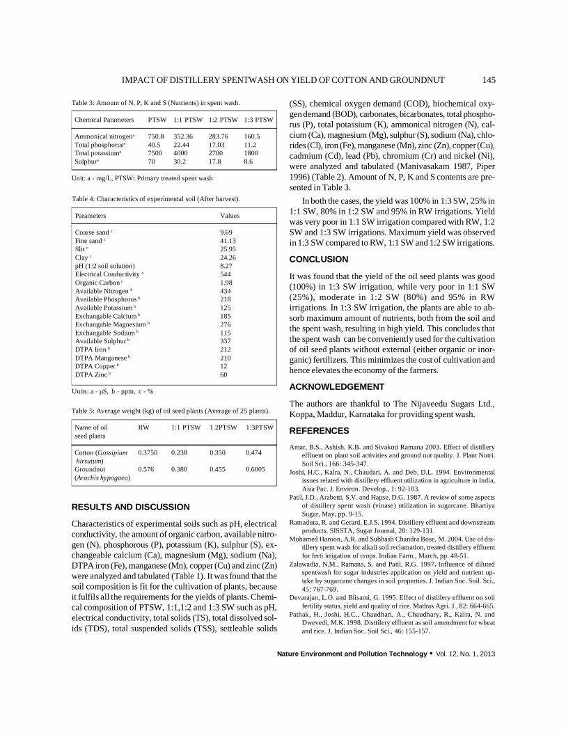
Nature Environment and Pollution Technology · Vol. 12, No. 1, 2013
145IMPACT OF DISTILLERY SPENTWASH ON YIELD OF COTTON AND GROUNDNUT
RESULTS AND DISCUSSION
Characteristics of experimental soils such as pH, electricalconductivity, the amount of organic carbon, available nitro-gen (N), phosphorous (P), potassium (K), sulphur (S), ex-changeable calcium (Ca), magnesium (Mg), sodium (Na),DTPA iron (Fe), manganese (Mn), copper (Cu) and zinc (Zn)were analyzed and tabulated (Table 1). It was found that thesoil composition is fit for the cultivation of plants, becauseit fulfils all the requirements for the yields of plants. Chemi-cal composition of PTSW, 1:1,1:2 and 1:3 SW such as pH,electrical conductivity, total solids (TS), total dissolved sol-ids (TDS), total suspended solids (TSS), settleable solids
(SS), chemical oxygen demand (COD), biochemical oxy-gendemand (BOD), carbonates, bicarbonates, total phospho-rus (P), total potassium (K), ammonical nitrogen (N), cal-cium (Ca), magnesium (Mg), sulphur (S), sodium (Na), chlo-rides(Cl), iron (Fe), manganese (Mn), zinc (Zn), copper (Cu),cadmium (Cd), lead (Pb), chromium (Cr) and nickel (Ni),were analyzed and tabulated (Manivasakam 1987, Piper1996) (Table 2). Amount of N, P, K and S contents are pre-sented in Table 3.
In both the cases, the yield was 100% in 1:3 SW, 25% in1:1 SW, 80% in 1:2 SW and 95% in RW irrigations. Yieldwas very poor in 1:1 SW irrigation compared with RW, 1:2SW and 1:3 SW irrigations. Maximum yield was observedin 1:3 SW compared to RW, 1:1 SW and 1:2 SW irrigations.
CONCLUSION
It was found that the yield of the oil seed plants was good(100%) in 1:3 SW irrigation, while very poor in 1:1 SW(25%), moderate in 1:2 SW (80%) and 95% in RWirrigations. In 1:3 SW irrigation, the plants are able to ab-sorb maximum amount of nutrients, both from the soil andthe spent wash, resulting in high yield. This concludes thatthe spent wash can be conveniently used for the cultivationof oil seed plants without external (either organic or inor-ganic) fertilizers. This minimizes the cost of cultivation andhence elevates the economy of the farmers.
ACKNOWLEDGEMENT
The authors are thankful to The Nijaveedu Sugars Ltd.,Koppa, Maddur, Karnataka for providing spent wash.
REFERENCES
Amar, B.S., Ashish, K.B. and Sivakoti Ramana 2003. Effect of distilleryeffluent on plant soil activities and ground nut quality. J. Plant Nutri.Soil Sci., 166: 345-347.
Joshi, H.C., Kalra, N., Chaudari, A. and Deb, D.L. 1994. Environmentalissues related with distillery effluent utilization in agriculture in India,Asia Pac. J. Environ. Develop., 1: 92-103.
Patil, J.D., Arabetti, S.V. and Hapse, D.G. 1987. A review of some aspectsof distillery spent wash (vinase) utilization in sugarcane. BhartiyaSugar, May, pp. 9-15.
Ramadura, R. and Gerard, E.J.S. 1994. Distillery effluent and downstreamproducts. SISSTA, Sugar Journal, 20: 129-131.
Mohamed Haroon, A.R. and Subhash Chandra Bose, M. 2004. Use of dis-tillery spent wash for alkali soil reclamation, treated distillery effluentfor ferti irrigation of crops. Indian Farm., March, pp. 48-51.
Zalawadia, N.M., Ramana, S. and Patil, R.G. 1997. Influence of dilutedspentwash for sugar industries application on yield and nutrient up-take by sugarcane changes in soil properties. J. Indian Soc. Soil. Sci.,45: 767-769.
Devarajan, L.O. and Blisami, G. 1995. Effect of distillery effluent on soilfertility status, yield and quality of rice. Madras Agri. J., 82: 664-665.
Pathak, H., Joshi, H.C., Chaudhari, A., Chaudhary, R., Kalra, N. andDwevedi, M.K. 1998. Disttilery effluent as soil amendment for wheatand rice. J. Indian Soc. Soil Sci., 46: 155-157.
Table 3: Amount of N, P, K and S (Nutrients) in spent wash.
Chemical Parameters PTSW 1:1 PTSW 1:2 PTSW 1:3 PTSW
Ammonical nitrogena 750.8 352.36 283.76 160.5Total phosphorusa 40.5 22.44 17.03 11.2Total potassiuma 7500 4000 2700 1800Sulphura 70 30.2 17.8 8.6
Unit: a - mg/L, PTSW: Primary treated spent wash
Table 5: Average weight (kg) of oil seed plants (Average of 25 plants).
Name of oil RW 1:1 PTSW 1.2PTSW 1:3PTSWseed plants
Cotton (Gossipium 0.3750 0.238 0.350 0.474hirsutum)Groundnut 0.576 0.380 0.455 0.6005(Arachis hypogaea)
Table 4: Characteristics of experimental soil (After harvest).
Parameters Values
Coarse sand c 9.69Fine sand c 41.13Slit c 25.95Clay c 24.26pH (1:2 soil solution) 8.27Electrical Conductivity a 544Organic Carbon c 1.98Available Nitrogen b 434Available Phosphorus b 218Available Potassium b 125Exchangable Calcium b 185Exchangable Magnesium b 276Exchangable Sodium b 115Available Sulphur b 337DTPA Iron b 212DTPA Manganese b 210DTPA Copper b 12DTPA Zinc b 60
Units: a - µS, b - ppm, c - %

Vol. 12, No. 1, 2013 · Nature Environment and Pollution Technology
146 S. Chandraju et al.
Ramana, S., Bisvas, A.K., Kundu, S., Saha, J.K. and Yadava, R.B.R. 2000.Physiological response of soybean (Glycine max L.) to foliar applica-tion of distillery effluent. Ann. Plant Soil Res., 2: 1-6.
Kaushik, K., Nisha, R., Jagjeet, K. and Kaushik, C.P. 2005. Impact of longand short term irrigation of sodic soil with distillery effluent in combi-nation with bio-amendments. Bioresource Technology, 96(17):1860-1866.
Devarajan, L., Rajanan, G. Ramanathan, G. and Oblisami, G. 1994. Per-formance of field crops under distillery effluent irrigations. KisanWorld, 21: 48-50.
Rajendran, K. 1990. Effect of ditillery effluent on the seed germination,seedling growth, chlorophyll content and mitosis in Helianthus annuus.Indian Botanical Contactor, 7: 139-144.
Samuel, G. 1996. The use of alcohol distillery waste as fertilizer, proceed-ings of International American Sugarcane Seminar, pp. 245-252.
Pujar, S.S. 1995. Effect of distillery effluent irrigation on growth, yield andquality of crops. M.Sc. (Agri.) Thesis, University of Agriculture Sci-ences, Dharwad.
Chidankumar, C.S. and Chandraju, S. 2009. Impact of distillery spentwashirrigation on yield of some condiments: An investigation. Sugartech.,
11(3): 303-306.Chidankumar, C.S., Chandraju, S. and Nagendra Swam, R. 2009. Impact
of distillery spentwash irrigation on the yields of top vegetables. WorldApplied Scienes J., 6(9): 1270-1273.
Chandraju, S., Basavaraju, H.C. and Chidankumar, C.S. 2008. Investiga-tion of impact of irrigation ofdistillery spentwash on the growth, yieldand nutrients of leafy vegetable. Chem. Env. Res., 17(1&2).
Chidankumar, C.S., Chandraju, S., Nagendraswamy, Girija andNagendraswamy, R. 2010. Comparitive study on the growth and yieldsof leafy vegetable irrigated by distillery spentwash, normal andspentwash treated soil. Sugar Tech., 12(1) 9-14.
Chanddraju, S., Nagendraswamy, R., Chidankumar, C.S. 2010. Studies onthe impact of irrigation of distillery spentwash on the yields of herbalmedicinal plants, Medicinal Plants - International Journal ofPhytomedicines and Related Industries, 2(3): 187-191
Chandraju, S., Nagendraswamy, R., Chidankumar, C.S. andNagendraswamy, Girija 2011. Distillery spentwash irrigation on theyields of raddish (Raphanus sativas), onion (Allium cepa) and garlic(Allium savitiuus). Asian J. Chem., 23(4): 1585-1587.
Sanjay S. Sathe and Leela J. Bhosale*Department of Botany, P. D. Vasantraodada Patil Mahavidyalaya, Tasgaon-416 312, Maharashtra, India* Department of Botany, Shivaji University, Kolhapur-416 004, Maharashtra, India
ABSTRACT
In the present study, biogas generation from mangroves is carried out to test the potential of mangroves asa substrate for biogas digester. Initially active slurry of cowdung was added in the biogas digester to produceproper concentration of methanogenic bacteria. Then continuously the mangove powder was added daily tobring out concentration of 8% for a hydraulic retention time of 25 days. The produced gas was tested bysimple burning test. The biogas contents were variable in different species of mangroves. Sonneratia albahas got highest values followed by A. marina var. acutissima and Avicennia officinalis. The waste frombiogas digester is also useful to obtain good manure as it has adequate N, P, K values.
Nat. Env. & Poll. Tech.
Received: 14-6-2012Accepted: 24-8-2012
Key Words:MangrovesSubstrate for biogasBiogas potential
2013pp. 147-149Vol. 12ISSN: 0972-6268 No. 1Nature Environment and Pollution TechnologyAn International Quarterly Scientific Journal
Original Research Paper
INTRODUCTION
The green plants convert the physical form of energy intochemical form, the food energy, upon which the entire worlddepends. The forests (vegetation) play multiple role in thelife of human beings. Protective, productive and bioaestheticfunctions of forests are related to the several human activi-ties. Maharashtra is the third biggest state in India with totalforest area of 64,078 sq. km, which is 20.8 percent of thetotal geographical area of the state. The forest area of thestate is inadequate and shows uneven distribution in respectto forest cover, its quality and productivity. No form of en-ergy is more crucial for human survival or more sensitive tothe environmental conditions than the energy needed forcooking. The main source of energy for working and heat-ing purpose is derived from the forests in the form of firewood and charcoal. This vital source of energy, however, isbeing depleted rapidly and the rural areas are facing acuteshortage of energy sources. Before independence, the sourceof energy for most of the rural population was five woodand charcoal supplemented by agricultural wastes(Deshmukh 1987).
De Silva (1981) reported that in India 70 percent of en-ergy requirement in villages are met by fire wood and otheragricultural waste, most of which are used for burning. Asmuch as 133 metric tons of fire wood, 73 metric tons ofcowdung and 41 metric tons of agricultural waste are burntin India every year. Goswami (1987) reported that althoughcoal and kerosene oil are used for burning purpose, the bulkof energy needs of kitchen (more than 80%) are met fromnon commercial energy sources like fire wood, cowdung andagricultural wastes. The forests are made denuded by felling
trees for fuel, the mangrove forests are not exceptions.
MATERIALS AND METHODS
Biogas generation is one of the important sources of energy.In the present study, biogas generation from mangroves iscarried out to test the potential of mangrove as a digesterbiomass. The biomass used for cattle feeding (removingwaste) and fire wood purpose has been collected, sun driedand powdered. This powdered form has been used an or-ganic waste for anaerobic fermentation to produce biogas.In the present investigation, a digester designed and cali-brated by Shivsadan Graha Nirman Society, Sangli was used.
Initially active slurry of cowdung (500 g) was added inthe biogas digester to have proper concentration ofmethanogenic bacteria. Then continuously mangove pow-der was added daily to bring out concentration of 8% for ahydraulic retention time of 25 days. The increase in heightof the cylinder was recorded daily. The produced gas wastested by simple burning test.
The collected left over from digester was used furtherfor analysis of N, P, K components. The nitrogen was esti-mated by the method of Hawk et al. (1948). The phosphorusandpotassiumwere extracted by wet digestion method ( Tothet al. 1948). Phosphorus was estimated by the method ofSekine et al. (1965) and potassium was estimated by flamephotometrically.
RESULTS AND DISCUSSION
The energy problem of rural Maharashtra is typical of mostof the States in India. The State has more than 40.7 millionpeople (65%) living in rural areas and present per capita

Vol. 12, No. 1, 2013 · Nature Environment and Pollution Technology
148 Sanjay S. Sathe and Leela J. Bhosale
demand for the firewood is 0.5 cu.m solid wood or 0.9 cu.mpiled wood per annum.
In Maharashtra out of 20.8% forest area, 8.01% is underfuel wood which satisfies 13.5% of the total demand of fuelwood (Deshmukh 1987). To fulfil the need for energy ofremaining population, other sources like coke, hard coke,solar energy, efficiency stoves and biogas are to be used.
Amongst alternate sources of fuel wood, generation ofbiogas is found to be most beneficial in the State ofMaharashtra. Biogas generation technology offers a low costalternative for energy requirement in the rural areas. It isbased on recycling of a variety of organic wastes. It has beenconsidered as a priority activity in the rural developmentprogrammes.
Extensive use of biogas may be substitute for commer-cial energy like kerosene and maintains the public healththrough use to organic wastes. Motivation of biogas is over-all reduction of fire wood consumption.
Biogas contains following gases: methane 50-80%, car-bon dioxide 25-35%, hydrogen 1-5%, nitrogen 2-7%, oxy-gen 0-0.1% and H2S rare. The composition of methane inbiogas is higher which is combustible and supplies the re-quired heat energy.
In the coastal region of Maharashtra fuel wood is obtainedfrom mangroves. To minimize the mangrove fuel wood, thealternative source, biogas, is thought of. However, as the
mangrove wood contains sulphur in considerable amount,its potential for biogas production is doubted.
A common mangrove genus in Maharashtra is Avicenniawith its 3 to 4 species. The twigs of these plants are excisedas fodder. Therefore, in the present study an attempt wasmade to test possibility of biogas production from leavesand tender stems of Avicennia. It is always kept in mind thatbiogas generation is not based on litter produced by man-groves or cuttings of mangrove for that purpose. The under-standing is that in spite of sulphur content (which is knownto inhibit methanogenic bacteria) mangroves produce biogas,then the fodder waste can be used along with other materialin the biogas plant.
The biogas content in different species of mangroves isgiven in Table 1. The biogas contents are variable in differ-ent species of mangroves. Sonneratia alba has got highestvalues followed by A. marina var. acutissima and Avicenniaofficinalis. The hydraulic retention time was 25 days. It canbe stated here that temperature of the processes ranged be-tween 31 and 32°C. Kulkarni (1985) reported that highestgas production was at 35°C, while the temperature lowestby 10°C completely stops the process of gas production.
Nag & Mathur (1988) have given the biogas content fromdifferent waste sources (Table 2). Their values range from35 to 38 litres/kg of dried biomass. Similarly, they have es-timated N, P, K contents from the slurry which show goodnutrient status as fertilizer for soil. The hydraulic retention
Table 1: Biogas contents from different species of mangroves and N, P, K contents from biogas residue.
Sr. No. Name of the Species HRT days Height of the Biogas Residualcylinder (inches) L/kg
N% P% K%
1 Avicennia officinalis 25 4.8 15.36 1.16 0.15 0.192 A. marina var. acutissima 25 6.2 19.84 1.18 0.16 0.263 Rhizophora mucronata 25 5.5 17.60 1.08 0.14 0.164 Sonneratia alba 25 6.8 21.60 1.56 0.19 0.205 Mixture of above species 25 5.6 17.92 0.81 0.11 0.12
HRT- Hydraulic retention Time; 1 inch Height = 3.2 litres of gas; Average temperature 31-32°C
Table 2: Biogas contents from different sources and manure status of their residue waste.
Sr. No. Name of the Sources HRT Days Biogas L/kg Residue from waste (%)N P K
1 Cattledung 45 35.00 1.50 0.94 0.832 Poultry dropping 40 38.00 2.50 0.70 0.813 Wheat straw 50 36.00 1.30 0.70 0.654 Willow dust 30 35.00 2.00 0.90 1.205 Water hyacinth 30 37.00 1.98 0.88 0.98
HRT- Hydraulic retention Time (After Nag & Mathur 1988)

Nature Environment and Pollution Technology · Vol. 12, No. 1, 2013
149SOCIO-ECONOMIC ASPECTS OF MANGROVES: BIOGAS
time was from 30 to 50 days depending upon the species.The comparison of both the tables indicates that man-
grove species can be used as source for biogas generation.The present quantity is less, which may be further improvedby several trials. In the present attempt, the aim is testingpotential of biogas production by mangroves and not opti-mization of the production.
The waste from biogas digester is also useful to obtaingood manure. The present investigation reveals that the man-grove biogas residue is also useful. Biogas generation willgive good source of energy to local inhabitants. If adopted,it will protect their hygienic condition if coupled with otherwaste creating pollution problems and will ultimately con-serve the productive ecosystems like mangroves along thecoastal belt of Maharashtra.
ACKNOWLEDGEMENT
S. S. Sathe is thankful to U.G.C., New Delhi for financialsupport under minor research project scheme and also thank-ful to Principal R. R. Kumbhar for encouragement and pro-viding necessary facilities to complete this work.
REFERENCES
Deshmukh, P.W. 1987. Afforestry as a solution of the environment andenergy problem. A case study of rural Maharashtra. In: Pramod Singh(ed): Ecology of Rural India. Vol. 1: 103-108, Ashish Publishing House,New Delhi.
De Silva Dhammika 1981. Appropriate Techonology. CSIR, Sri Lanka. I(4): 22-40.
Goswami, Sadhra 1987. Fuel wood crisis in rural areas. In: Pramod Singh(ed): Ecology of Rural India Vol. 1 : 109-116. Ashish Publishing House,New Delhi.
Hawk, P.B., Oser, B.L. and Summerson, W.H. 1948. Practical Physiologi-cal Chemistry. The Bankistor Company, U.S.A.
Kulkarni, P.K. 1985. Urjya Prashna (In Marathi). Rajhansa Publication,Pune (India) 111 pp.
Nag, K.N. and Mathur, A.N. 1988. Utilization of organic waste for food,fuel and fodder. In: Mathur, A.N. and Verma, L.N. (ed): Managementand Utilization of Biogas Plant Slurry. Himashu Publications, Udaipur(India), 197-207.
Sekine, T., Sasakawa, T., Morita, S., Kimura, T. and Kuratomi, K. 1965.Photoelectric Colorimetry in Biochemistry (Part I) Nanko-do Publi.Co., Tokyo, pp. 242.
Toth, S.J., Prince, A.L., Wallace, A. and Mikkelsen, D.S. 1948. Rapid quali-tative determination of eight mineral elements in plant tissue by sys-tematic procedure involving use of a flame photometer. Soil. Sci., 66:459-466.

ENVIRONMENTAL NEWS
150
Mongolia to host UN World Environment Day 2013
Mongolia will host this year’s World Environment Day (WED) celebrationon 5 June, which will focus onreducing food waste and loss, the United Nations announced today. The Asian nation was chosen for itsefforts to shift towards a green economy in its major economic sectors such as mining and for promotingenvironmental awareness among youth, the UN Environment Programme (UNEP) said in a news release.
“Mongolia is facing enormous challenges, including growing pressure on food security, traditional nomadicherding and water supplies as a result of the impacts of climate change,” said UNEP Executive DirectorAchim Steiner. “Indeed it is estimated that annual mean temperature has increased by over 2°C during thelast 70 years and precipitation has decreased in most regions, except the western part of the country, indicatingthat Mongolia is among the most vulnerable nations in the world to global warming.
“Yet its Government is also determined to meet these challenges and seize the opportunities of a less-pollutingand moresustainable future – from a moratorium on new mining pending improved environmental regulationsto plans to become a renewable energy power-house and exporter of clean energy regionally,” he said.Observance of World Environment Day began in 1972 as a way to raise awareness of the environment andencourage political attention and action.
This year’s theme for the Day is “Think.Eat. Save. Reduce Your Foodprint,” which builds on a globalcampaign of the same name launched earlier this year by UNEP, the Food and Agriculture Organization(FAO) and other partners to reduce food and waste loss. The announcement was made during UNEP’sGoverning Council session in Nairobi, Kenya, where hundreds of environment ministers and civil societyrepresentatives met to discuss some of the most pressing environmental issues.
“I am sure that as the global host of WED, Mongolia will demonstrate to the world that a transition to agreen economy is possible, even within some of the most traditionally challenging industrial sectors, whenleadership, vision, smart policies and political will are translated into action on the ground,” Mr. Steinersaid. During the Council session, Mr. Steiner also announced that a UNEP mission to Mongolia was scheduledto depart in April to assist the country in its transition to a green economy in areas such as energy, land andwater.
February, 2013, UN Daily News
Light Pollution: Animals affected by HPS lighting interference
When the gas-lighter carried out his rounds, there must have been street urchins attracted to the novel brightnessand the opportunities that provided. Now we have a spread of incredible, high-pressure sodium brightness aroundthe planet, virtually bringing day to night in a major area of terrestrial habitats.
As has been said before, light pollution could be just as severe as any, given its immense significance to livingorganisms, their physiology, behaviour, reproduction and predator - prey interactions. Discounting the ancient mothsto flame (and UV light traps) studies used by entomologists from time immemorial, ground dwellers were targeted.
Their activities have been studied too, but population studies carried out by Messrs. Davies, Bennie and Gaston atExeter University reveal more about whole ecosystems. Their research has been published in the Royal Societyjournal Biology Letters.
Earth Times

D. N. KhairnarResearch Laboratory of Plant Pathology, Department of Botany, KAANMS Arts, Commerce & Science College,Satana-423 30, Distt. Nashik, Maharashtra, India
ABSTRACT
Twenty three fungal species were found associated with seeds of eight cultivars of pearl millet (Pennisetumtyphoides). Maximum fungi were reported from seeds of var. BJ-104 and ICMS -7703. Aspergillus flavus,Fusarium moniliforme and Penicillium oxalicum were found pathogenic causing seed rot, seed discolourationand germination inhibition. Captan and Dithane M-45 proved best for bajra seed dressing.
Nat. Env. & Poll. Tech.
Received: 10-7-2012Accepted: 27-8-2012
Key Words:BiodiversitySeed-borne fungiPearl milletPathogenicity
2013pp. 151-153Vol. 12ISSN: 0972-6268 No. 1Nature Environment and Pollution TechnologyAn International Quarterly Scientific Journal
Original Research Paper
INTRODUCTION
The seed-borne fungi of pearl millet (Pennisetum typhoides(Burm.) Stapf. and Hutt) were earlier studied by Sharma &Basuchaudhary( 1975), Gupta (1976), Konde et al. (1980),Randhawa & Aulakh (1980), Prasad & Narayan (1981),Girisham & Reddy (1985, 19865), Panchal (1984) andKhairnar (1987). The present investigations were carriedout to detect the seed-borne fungi of pearl millet cultivars,viz. African A-1, BJ-104, BK-560, ICMS-7703, Local,MBH-110, X5 and WCC-75 by different seed health test-ing methods and to study their pathogenic behaviour andcontrol by seed dressing fungicides.
MATERIALS AND METHODS
Seed samples of pearl millet varieties African A-1, BJ-104,BK-560, ICMS-7703, Local, MBH-110, WCC-75 and X-5were collected in three random samples (half kg each) fromfields, various store houses and markets. A composite sam-ple of this was prepared by mixing the individual samplesand preserved in cloth bags at laboratory temperature dur-ing the study.
Standard blotter and agar plate methods with Wakman’sacidagar medium were used asrecommended by ISTA (1966)for the isolation of seed-borne fungi of pearl millet (glucose10g, KH2PO4 1g, MgSO4 0.5g, agar agar 20g, distilled water1000 mL, pH 5.6). Fourhundred seedswere used in each case.Seeds used for experiments were untreated and pretreatedwith0.1% HgCl2 solution. In agar plate method, ten seeds wereplated in each plate. The plates were incubated at 28 + 2.0°Cunder alternate light darkness condition for seven days.
The pathogenicity tests of each fungus on seed duringgermination were studied by soaking the surface sterilizedseeds in spore suspensions of seed-borne fungi for 24 h. Thenseeds were used for germination studies on moist blotter.Table 1: Diversity in seed mycoflora of Pearl millet on agar plate method.
Fungi % incidence on Fungus the seeds associated
Untreated Pretreated
Absidia ramosa 10 0 1Alternaria alternata 10 10 4Aspergillus flavus 30 10 4Aspergillus fumigatus 20 0 2Aspergillus nidulans 20 0 1Aspergillus niger 30 10 3Aspergillus ustus 10 0 1Cladosporium herbarum 10 0 5Curvularia lunata 40 30 7Curvularia pallescens 40 10 8Drechslera longirostrata 10 10 6Drechslera rostrata 20 10 4Drechslera spicifer 10 10 3Drechslera tetramera 50 30 8Fusarium moniliforme 30 20 5Fusarium oxysporum 10 30 6Mortierella exigua 10 0 2Penicillium oxalicum 10 0 2Pythium sp. 20 10 5Rhizoctonia solani 30 10 6Rhizopus nigricans 20 0 4Syncephalastrum racemosum 10 0 5Torula herbarum 10 10 2Non-sporulating mycelium 30 10 4
Varieties tested: African 1-1, BJ-104, BK-560, ICMS-7703, Local, MBH-110, WCC-75, X-5

Vol. 12, No. 1, 2013 · Nature Environment and Pollution Technology
152 D. N. Khairnar
Seeds treated similarly but without spore suspension servedas control. This type of work was done by Panchal (1984)and Khairnar (1987) on jowar and bajra seeds respectively.
The fungicides namely Captan, Dithane M-45, DithaneZ-78, Brassicol, Blitox-50W, Bavistin, Thiram, Zinkop,Ceresan, Zineb75, Wettable sulphur each (2g/kg seed) wereevaluated for their efficacy in reducing the seed-borne fungiof pearl millet. The treated seeds were tested by standardblotter method after 24 hours of the treatment. Untreatedseeds served as control.
RESULTS AND DISCUSSION
It is clear from the results summarized in Table 1 that 23fungal species appeared on the seeds of eight differentcultivars tested. In the present investigation three fungi viz.,Mortierella exigua, Pythium sp. and Torula herbarum arenewly recorded. In untreated seeds, maximum incidence ofDrechslera tetrametra followed by Curvularia lunata, C.pallescens, Aspergillus flavus, Fusarium moniliforme, As-pergillus niger and Rhizoctonia soloni, while Absidiaramosa, Alternaria alternata, Aspergillus ustus,Cladospprium herbarum, Drechslera longirostrata, D.spicifer, Fusarium oxysporum, Mortierella exigua, Penicil-lium oxalicum and Syncephalastrum racemosum were re-ported poorly.
Seeds treated with surface sterilizer showed completeabsence of certain fungi like Absidia ramosa, Aspergillusfumigates, A. nidulans, Mortierella exigtua, Rhizopusnigricans and Syncephalasturm racemosum. On the otherhand counts of Fusarium oxysporum were found to be in-creased. It was interesting to note that one phycomycetous
non-sporulating fungus appeared consistently both on treatedand untreated seeds. Fungal species, Curvularia pallescensand Drechslera tetrametra were found on all the cultivars.
It is evident from the results given in Table 2 that com-plete inhibition of seed germination was achieved due toFusarium moniliforme and F. oxysporum, while seed rot-ting was effectively found due to Aspergillus flavus,Fusaruim moniliforme, F. oxysporum and partial seed rotby Penicillium oxalicum. Five days old seedlings, blight andretardation of root length andshoot elongation were the com-mon symptoms caused by most of the seed-borne fungi.Panchal (1984) and Khairnar (1987) showed the fungi likeFusarium oxysporum, Penicillium oxalicum and Alternariaalternata are seed rotting of jowar seeds, while Curvulariapallescens and Drechslera longirostrata are root rottingfungi.
Captan, Dithane M-45, Bavistin and Blitox-50W (each2g/kg seed) showed broad spectrum effect and eliminatedall the fungi from seed and improved germination to the ex-tent of 90-98 percent as compared to 50-60 percent obtainedin untreated seeds. The remaining fungicides were less ef-fective in checking the pearl millet seed fungi.
ACKNOWLEDGEMENT
The author is thankful to Dr. Dilip Shinde, Principal of thiscollege for continuous encouragement in the work and pro-viding the research facilities.
REFERENCES
Girisham, S. and Reddy, S.M. 1985. Influence of storage structures on seedmycoflora of Pearl millet. Geobios New Reports, 4: 126-129.
Table 2: Effect of artificial infestation on seeds and seedlings.
Fungi Seeds Seedlings% germination Rot Discolouration Shoot Length Root Length
Absidia ramosa 40 - Ash Normal 5.2 Shortening 3.0Alternaria alternata 40 - Blackbrown Blight 5.0 9.8Alternaria tenuis 60 - Brown Yellow 5.2 - 4.1Aspergillus flavus 10 + Brown Tip rot 2.6 Shortening 1.9Aspergillus niger 100 - Green Yellow 5.4 Root rot 9.0Cladosporium herbarum 40 - Brown Stunted 1.6 Healthy 3.0Curvularia lunata 30 - Dull green Chlorosis 4.9 Shortening 10.7Cruvularia pallescens 50 - Black Stunted 2.5 - 9.2Drechslera longirostrata 40 - Black Stunted 5.0 Root rot 10.0Drechslera rostrata 50 - Black Blight 5.2 Root rot 10.2Drechslera tetrametra 20 - Black - 5.0 - 9.2Fusarium moniliforme 0 + Black Blight - Root rot -Fusarium oxysporum 0 + White pink - - Root rot -Penicilium oxalicum 10 - White - 2.8 - 4.5Rhizopus nigricans 20 - Blue White 4.5 - 1.5Rhozoctonia solani 50 - Ash Tip rot 4.9 Curling 9.7Control 90 - Normal Green(Normal) 5.2 Normal 10.1

Nature Environment and Pollution Technology · Vol. 12, No. 1, 2013
153BIODIVERSITY ON SEED BORNE FUNGI OF PEARL MILLET
Gupta, D.C. 1976. Viability of stored seeds in bajra (Pennisetum typhoides).Seed Tech. News, 6: 9-12.
ISTA 1966. Proc. Int. Seed Test. Ass. 31: 1-52.Khairnar, D.N. 1987. Studies on Seed-borne Fungi of Bajara. Ph.D. Thesis
Marathwada University, Aurangabad.Konde, B.K., Dhage, B.V. and More, B.B. 1980. Seed-borne fungi of some
pearl millet cultivars. Seed Research, 8: 59-63.Panchal, V.H. 1984. Studies on seed-borne fungi of sorghum. Ph.D. Thesis,
Marathwada University Aurangabad.Prasad, B.K. and Narayan, N. 1981. Seed-borne fungi of some millets.
Geobios, 8: 47-48.Randhawa, H.S. and Aulakh, K.S. 1980. Pathological appraisal of seed-
borne fungi of Pearl millet. Indian Phytopathol., 33: 163-167.Sharma, J.R. and Basuchaudhary, K.C. 1975. Assessment of seed mycoflora
of pearl millet and their control. Indian Phytopathol., 28: 388-390.

In a Warming World, Look to the Herbivores
In the unending quest for effective ways of adapting to climate change, it seems that musk ox and cariboumay have some of the answers. According to a study published this week, the large herbivores that inhabitGreenland and other regions in the far north can play an important role in maintaining biodiversity in awarming climate.
In the course of a 10-year Arctic field experiment, the Penn State biologist Eric Post found that the animalsheld back the growth of some plant species that would otherwise be likely to dominate the local ecosystem astemperatures rose. Beginning in 2002, Dr. Post simulated a warmer environment in the remote community ofKangerlussuaq, Greenland, by building 8,600-square-foot “warming chambers” – cone-shaped hollow struc-tures in which the animals were allowed to graze on the plants that grew under the new conditions.
The musk ox and caribou were excluded from separate areas of the same size that were also subjected to a risein temperature of 1.5 to 3 degrees Celsius (2.7 to 5.4 degrees Fahrenheit), a level of warming that scientistsproject will occur over the next century. Shrubs like willow and birch became more dominant as tempera-tures rose, shading other plants and producing leaf litter that cools the soil and reduces nutrients for compet-ing species, thereby lowering species diversity.
But in the enclosures with grazing herbivores, those dominant species were largely kept in check, allowingthe other plants to do better than they did in the areas from which the animals were excluded, Dr. Post found.“In those areas where caribou and musk ox were able to graze freely, shrub responses to warming weremuted, and species diversity within the plant community was maintained,” he wrote.
Dr. Post suggests that his research may have implications for other ecosystems. “I think the relationships wesee in Greenland would certainly apply to a wider variety of similarly generalist herbivores in other sys-tems,” he wrote in an e-mail. “One example may be moose, whose browsing can have huge effects on plantcommunity composition, nutrient cycling rates and ecosystem function.” He said the current decline of moosein northern Minnesota, for which scientists have not pinned down a cause, could thus have “major conse-quences.”
Dr. Post’s paper adds yet another wrinkle to the debate over how climate change may affect biodiversity. A2012 study published in the Proceedings of the National Academy of Sciences presented evidence fromfossil records that rising temperatures have spurred an increase rather than a decline in biodiversity. Yet evenemergent species won’t be able to keep up with the current rapid rate of climate change, meaning that the rateof extinctions will increase, it concluded.
The new study, published in the journal Proceedings of the Royal Society of London, concluded that theanimals may hold the key to the maintenance of plant diversity and therefore must be protected. “What thisexperiment suggests is that factors that threaten the persistence of large herbivores may threaten the plantcommunities they exist in as well,” Dr. Post said. “Conservation of these herbivores in the rapidly changingArctic will require careful mediation of interacting stressors such as human exploitation, mineral extraction,and the direct effects of climate change,” he said.
February, 2013, New York Times
ENVIRONMENTAL NEWS
154

и§·½±óݸ»³·½¿´ ß²¿´§· ±º Ø¿¦¿®¼±« Ûºº´«»²¬ º®±³ Ü·ºº»®»²¬ п°»®
ײ¼«¬®·»
ß·º Ø¿²·º ݸ¿«¼¸®§öô λ¸¿² «´ Ø¿¯ Í·¼¼·¯«·öô�Ì¿²ª»»® ßµ¸¬¿® Ó¿´·µööô Õ¿¦· Ó«¸¿³³¿¼ ߸º¿¯ööô Ó«¸¿³³¿¼
͸¿º·¯öööô ο¸·¼ Ó¿¸³±±¼öö ¿²¼ Ù¸¿¦¿´¿ Ç¿¯«¾öööö
öÙ»±½·»²½» ß¼ª¿²½» λ»¿®½¸ Ô¿¾ô ÙÍÐô ×´¿³¿¾¿¼ô пµ·¬¿²
ööÒ¿¬·±²¿´ ײ¬·¬«¬» ±º Ø»¿´¬¸ô ×´¿³¿¾¿¼ô пµ·¬¿²
öööÜ»°¿®¬³»²¬ ±º ݸ»³·¬®§ô ÙòÝò ˲·ª»®·¬§ô Ú¿·¿´¿¾¿¼ô пµ·¬¿²
ööööÜ»°¿®¬³»²¬ ±º Û²ª·®±²³»²¬¿´ ͽ·»²½»ô Õ·²²¿·®¼ ݱ´´»¹» º±® ɱ³»²ô Ô¿¸±®»ô пµ·¬¿²
ßÞÍÌÎßÝÌ
ß²²«¿´ °¿°»® °®±¼«½¬·±² · ³»¿«®» ±º ¬¸» ¼»ª»´±°³»²¬ ±º ¿ ½±«²¬®§ò п°»® · ³¿¼» º®±³ ½»´´«´±» ¾¿»¼
®¿© ³¿¬»®·¿´ô ¿º¬»® ¬¸»·® ½¸»³·½¿´ ¿²¼ ³»½¸¿²·½¿´ ¬®»¿¬³»²¬ò ̸»®» ¬®»¿¬³»²¬ ¼·½¸¿®¹» ©¿¬» ©¿¬»® ·²¬±¬¸» »²ª·®±²³»²¬ ©¸·½¸ · ½¿®®·»¼ ¿´±²¹ ¬¸» ©¿¬»® ½¸¿²²»´ ́ ·µ» ¼®¿·²ò ̸» ©¿¬»® º±®³ ¬¸»» ¼®¿·² · «»¼
¾§ º±®³»® º±® ·®®·¹¿¬·±² °«®°±»ò ׺ ¬¸· ¼®¿·²»¼ ©¿¬»® ½±²¬¿·² ̧ ¿®³º«´ »ºº´«»²¬ ·¬ ½¿² ¾¿¼´§ ¿ºº»½¬ ½®±°ò
̱ ±ª»® ½±³» ±® ³·²·³·¦» ¬¸· ¼¿³¿¹» °®»»²¬ ¬«¼§ ©¿ ½¿®®·»¼ ±«¬ò Ê¿®·±« °¿®¿³»¬»® ©»®» ½¸»½µ»¼«·²¹ ¬¿²¼¿®¼ °®±½»¼«®» ®»½±³³»²¼»¼ ¾§ ß³»®·½¿² Ы¾´·½ Ø»¿´¬¸ ß±½·¿¬·±² ¿²¼ ¬¸» ®»«´¬ ©»®»
½±³°¿®»¼ ©·¬¸ Ò¿¬·±²¿´ Û²ª·®±²³»²¬¿´ Ï«¿´·¬§ ¬¿²¼¿®¼ øÒÛÏ÷ ±º пµ·¬¿²ò ̸» ª¿´«» ±º ¿ª»®¿¹»
¬»³°»®¿¬«®»ô °Øô ÌÜÍ ¿²¼ ½¸´±®·¼» ©¿ ·² ̧ ¿®³±²§ ©·¬¸ ÒÛÏô ©¸»®»¿ ¬¸» ª¿´«» ±º ¬¸» ±¬¸»® °¿®¿³»¬»®´·µ» ÌÍÍô ÞÑÜëô ÝÑÜô ݱ°°»® ¿²¼ ·®±² ©»®» ¿¾±ª» ¬¸» ÒÛÏ ´·³·¬ º±® »ºº´«»²¬ò ̸» ª·±´¿¬·±² ±º ¬¸»
°¿®¿³»¬»® º®±³ ÒÛÏ «¹¹»¬ ¬¸¿¬ ·¬ · ¬·³» ¬± ¬¿µ» ¬»° ¬± ½¸»½µ ¬¸» ¼·½¸¿®¹» ±º «²®»¿½¬»¼ ±® ·²ó
½±³°´»¬» ¬®»¿¬³»²¬ »ºº´«»²¬ ·²¬± ¬¸»» ¼®¿·² ¿²¼ ¼·¬®·¾«¬·±²ô ± ¬± »²«®» ̧ »¿´¬¸§ »²ª·®±²³»²¬ º±® º«¬«®»¹»²»®¿¬·±²ò
Ò¿¬ò Û²ªò ú б´´ò Ì»½¸òÉ»¾·¬»æ ©©©ò²»°¬¶±«®²¿´ò½±³
λ½»·ª»¼æ ïíóéóîðïî
ß½½»°¬»¼æ ïîóçóîðïî
Õ»§ ɱ®¼æп°»® ·²¼«¬®·»
и§·½±ó½¸»³·½¿´ ¿²¿´§·
Ø¿¦¿®¼±« »ºº´«»²¬Ý±´±«®
×ÒÌÎÑÜËÝÌ×ÑÒ
ײ ¬¸» ®»½»²¬ ¬·³» ¬¸»®» ̧ ¿ ¾»»² ®¿°·¼ ·²¼«¬®·¿´·¦¿¬·±² ¿²¼
«®¾¿²·¦¿¬·±² ¬¸¿¬ ¸¿ ®»«´¬»¼ ·² ¬¸» ¬®» ±² ¿ª¿·´¿¾´» ©¿ó
¬»® ®»±«®½»ò Ѳ´§ ³¿´´ º®¿½¬·±² ±º ©¿¬»® «»¼ ·² ·²¼«¬®§
· ·²½±®°±®¿¬»¼ ·²¬± ·¬ °®±¼«½¬ ±® ́ ±¬ ¾§ »ª¿°±®¿¬·±²ò Ó±¬
±º ¬¸» ©¿¬»® · »ª»²¬«¿´´§ ¼·½¸¿®¹»¼ ¿ °»²¬ ©¿¬»®ò
Ы´° ¿²¼ °¿°»® ·²¼«¬®§ ¸¿ ª»®§ ·³°±®¬¿²¬ ®±´» ·² ¬¸»
¼»ª»´±°³»²¬ ±º ½±«²¬®§ ·² ¿´´ º·»´¼ô · ¾«¬ ¿´± ¿ ³¿¶±® °®±ó
¼«½»® ±º ©¿¬»® ¿²¼ ±´·¼ °±´´«¬·±² ø̸±³°±² îððïô Ù»²¹
îððêô Ó«®«¹»¿² îððð÷ò Ú±® ¬¸» °®±¼«½¬·±² ±º ï ¬±² ±º ¬¸»
°¿°»® îéíóìëð ³í ±º ©¿¬»® · ®»¯«·®»¼ò ߺ¬»® °¿°»® °®±½»ó
·²¹ô ê𠬱 íðð ³í ±º ©¿¬»©¿¬»® · ¼·½¸¿®¹»¼ øÍ«¾®¿³¿²·«³
ïçéê÷ò Ó±¬ ±º ¬¸» ·²¼«¬®·» ®»´»¿» ©¿¬» ©·¬¸±«¬ °®»ó
¬®»¿¬³»²¬ øÍ®·ª¿¬¿ª¿ ïççì÷ò ˲¬®»¿¬»¼ »ºº´«»²¬ ¼·½¸¿®¹»¼
·²¬± ©¿¬»® ¾¿¼´§ ¿ºº»½¬ ¬¸» ¯«¿´·¬§ ±º ©¿¬»® ¿²¼ ¿´± ·³ó
°¿®¬ ½±´±«®ò ݱ´±«® · ®»°±²·¾´» º±® ¬¸» ·²½®»¿» ·² ¬»³ó
°»®¿¬«®» ¿²¼ ´±©·²¹ ¼±©² ¬¸» ®¿¬» ±º °¸±¬±§²¬¸»·ô ©¸·½¸
©·´´ ·²½®»¿» ¬¸» ±¨§¹»² ¼»³¿²¼ øÕ·²¹¬¿¼ ïçèìô п²»¿®
ïççç÷ò ݱ´±«®»¼ »ºº´«»²¬ ½±²¬¿·² ½¸´±®·²¿¬»¼ °¸»²±´ô
¼·±¨·²ô ¿²¼ ±¬¸»® ³«¬¿¹»²·½ ¿²¼ ½¿®½·²±¹»²·½ ½±³°±«²¼ô
±®¹¿²·½ ¿²¼ ·²±®¹¿²·½ ½±³°±«²¼ô ½¸±®±´·¹²·² ¿²¼ ´·¹²·²
øײ¹´» îðððô Ç¿¼´¿ îððîô Þ¿®«¿¸ ïççê÷ò ß´¬¸±«¹¸ ´±© ³±ó
´»½«´¿® ©»·¹¸¬ ½¸´±®±´·¹²·² ¿®» °¿®¬·¿´´§ ®»³±ª»¼ º®±³ ¬¸»
»ºº´«»²¬ ¾§ º«²¹· ¾«¬ ¸·¹¸ ³±´»½«´¿® ©»·¹¸¬ ´·¹²·²
®»³¿·² «²¿ºº»½¬»¼ ¿²¼ °¿ »ºº´«»²¬ ¬®»¿¬³»²¬ °´¿²¬ ·²¬± ®»ó
½»·ª·²¹ ©¿¬»® ¾±¼·» øÛ®·µ±² ïçèð÷ò Í´±© ¼»½±³°±·¬·±²
±º ¬¸»» ½±³°±«²¼ ®»´»¿» ¬±¨·½ ½±³°±«²¼ ·² ©¿¬»®
øÕ«³¿® »¬ ¿´ò îððð÷ò
Ю»»²¬ · ¬«¼§ ¾¿»¼ ±² ¬¸» °¸§·½±ó½¸»³·½¿´ ¬«¼§ ±º
©¿¬»©¿¬»® »ºº´«»²¬ º®±³ ¬¸» º·ª» °¿°»® ³·´´ ́ ±½¿¬»¼ ¿¬ Ô¿ó
¸±®»ô Ы²¶¿¾ô пµ·¬¿²ò
ÓßÌÛÎ×ßÔÍ ßÒÜ ÓÛÌØÑÜÍ
ݸ»³·½¿´æ ß´´ ¬¸» ±´«¬·±² ©»®» °®»°¿®»¼ ·² ¼±«¾´§ ¼·ó
¬·´´»¼ ©¿¬»® ©·¬¸ ßÎ ¹®¿¼» ½¸»³·½¿´ò °Ø ©¿ ¼»¬»®³·²»¼
¾§ ݧ¾»® ͽ¿² °Ø ³»¬»®ô ¿²¼ ½±²¼«½¬·ª·¬§ ¾§ ÌÑß ÝÓ ½±²ó
¼«½¬·ª·¬§ ³»¬»® ÝÓóêðÍò ÝÑÜ ©¿ ¿²¿´§»¼ ¿½½±®¼·²¹ ¬± ¬¸»
³»¬¸±¼ ®»°±®¬»¼ °®»ª·±«´§ò Ú» ©¿ ¼»¬»®³·²»¼ ¾§ ¿¬±³·½
¿¾±®°¬·±² °»½¬®±°¸±¬±³»¬»® øЮ»µ·²óÛ´³»® Ó±¼»´ ß²¿´§¬ó
èðð÷ò λ³¿·²·²¹ °¿®¿³»¬»® ©»®» ¼»¬»®³·²»¼ ª±´«³»¬®·½¿´´§ñ
¬·¬®·³»¬®·½¿´´§ ¾§ ¬¿²¼¿®¼ ³»¬¸±¼ øßÐØß ïçéêô ÒÝßÍ×
ïðéïô Ó¿²·ª¿¿µ¿³ ïççêô Ì®·ª»¼§ ú Ù±»´ ïçèê÷ò
ݱ´´»½¬·±² ±º ¿³°´»æ Í¿³°´» ©»®» ½±´´»½¬»¼ ·² ¬¸» ¬»®·ó
´·¦»¼ °´¿¬·½ ¾±¬¬´»ò ߬ ¬¸» ¬·³» ±º ½±´´»½¬·±² ±º ¿³°´»
¬»³°»®¿¬«®» ¿²¼ °Ø ©»®» ³»¿«®»¼ò Í¿³°´» ©»®» ¬±®»¼ ·²
¬¸» ½±²¬®±´´»¼ »²ª·®±²³»²¬ò
îðïí °°òïëëóïëéʱ´ò ïî×ÍÍÒæ ðçéîóêîêè Ò±ò ïÒ¿¬«®» Û²ª·®±²³»²¬ ¿²¼ б´´«¬·±² Ì»½¸²±´±¹§ß² ײ¬»®²¿¬·±²¿´ Ï«¿®¬»®´§ ͽ·»²¬·º·½ Ö±«®²¿´
Ñ®·¹·²¿´ λ»¿®½¸ п°»®

ʱ´ò ïîô Ò±ò ïô îðïí i Ò¿¬«®» Û²ª·®±²³»²¬ ¿²¼ б´´«¬·±² Ì»½¸²±´±¹§
ïëê ß·º Ø¿²·º ݸ¿«¼¸®§ »¬ ¿´ò
ÎÛÍËÔÌÍ
п®¿³»¬»® ±º »¿½¸ ¿³°´» ©»®» ¬»¬»¼ «²¼»® ¿³» ½±²¼·ó
¬·±²ò ̸» ¯«¿´·¬§ ±º ¬¸» ³«²·½·°¿´ ¿²¼ ´·¯«·¼ ·²¼«¬®·¿´ »ºó
º´«»²¬ ©¿ ½±³°¿®»¼ ©·¬¸ ¬¸» Ò¿¬·±²¿´ Û²ª·®±²³»²¬¿´ Ï«¿´ó
·¬§ ͬ¿²¼¿®¼ øÒÛÏÍ÷ ±º пµ·¬¿² Û²ª·®±²³»²¬ Ю±¬»½¬·±²
ß½¬ ïççéô ®»ª·»¼ ¾§ пµ·¬¿² Û²ª·®±²³»²¬ô Ô±½¿´ Ù±ª»®²ó
³»²¬ ¿²¼ Ϋ®¿´ Ü»ª»´±°³»²¬ ±² ß«¹«¬ ïðô îððð ·²
×´¿³¿¾¿¼ô ¬¸®±«¹¸ ¬¸» Ù¿¦»¬¬» ±º пµ·¬¿² Û¨¬®¿±®¼·²¿®§
øÌ¿¾´» î÷ò
Ü×ÍÝËÍÍ×ÑÒ
̸» ²±®³¿´ ¬»³°»®¿¬«®» ±º ©¿¬»® ¾±¼·» ·² ¬¸· °¿®¬ ±º ¬¸»
½±«²¬®§ ®¿²¹» º±®³ îîóîëpÝô ©¸·½¸ ³»¿² ¬¸¿¬ ¬¸» ¬»³ó
°»®¿¬«®» ±º ¬¸» ¼®¿·² · ¸·¹¸»® ¬¸¿² ²±®³¿´ò ̸· ½¿² ¾» ¿¬ó
¬®·¾«¬»¼ ¬± °±´´«¬¿²¬ ·² ¬¸» ¼®¿·² ©¿¬»®ô ©¸·½¸ ³·¹¸¬ ¬®¿°
¸»¿¬ ¬¸¿¬ · ¹»²»®¿¬»¼ ¼«» ¬± ¼·ºº»®»²¬ ½¸»³·½¿´ ®»¿½¬·±² ±®
¼«» ¬± ¸»¿ª§ ¼·½¸¿®¹» ±º ½±±´·²¹ ©¿¬»®ò Ø·¹¸»® ¬»³°»®¿ó
¬«®» º¿ª±«® ¬¸» ¾®»¿µ¼±©² ±º ¬¸» ±®¹¿²·½ ³¿¬¬»® ¾§ ³·½®±ó
±®¹¿²·³ô ©¸·½¸ ®»«´¬ ·² °®±¼«½¬·±² ±º ¬¸» ±®¹¿²·½ ¿½·¼
¿²¼ ´±©»®·²¹ ±º °Øò
°Ø ±º ¬¸» ¿³°´» ®¿²¹» ¾»¬©»»² êòè ¿²¼ èòðò Í«°»²¼»¼
±´·¼ ¾¿¼´§ ¿ºº»½¬ ¬¸» °»²»¬®¿¬·±² ±º ́ ·¹¸¬ ¬¸®±«¹¸ ¬¸» ©¿¬»®
¿²¼ ¬¸«ô ¼»¬®±§·²¹ ¬¸» ¿¯«¿¬·½ º´±®¿ ¿²¼ º¿«²¿ò ̸» «ó
°»²¼»¼ ±´·¼ »®ª» ¿ ¬¸» ¬®¿²°±®¬ ³»½¸¿²·³ º±® °»¬·½·¼»
¿²¼ ±¬¸»® «¾¬¿²½» ©¸·½¸ ¿®» ®»¿¼·´§ ¿¼±®¾»¼ ±² ¬¸» ½´¿§
°¿®¬·½´»ò ̸»» ª¿´«» ©»®» ³«½¸ ̧ ·¹¸»® º±® ¬¸» Ý»²¬«®§ пó
°»® Ó·´´ øïðèð °°³÷ò ̸· · ¼«» ¬± ¬¸» º¿½¬ ¬¸¿¬ ³±®» ¿²¼
º¿¬»® º´±© ±º ©¿¬»® ©±«´¼ ²±¬ ¸¿ª» ¿´´±©»¼ ¬¸» »¬¬´·²¹ ±º
¬¸» «°»²¼»¼ ±´·¼ ¿²¼ µ»°¬ ¬¸»³ ·² «°»²¼»¼ º±®³ò
Û¨½» ±º ¼·±´ª»¼ ±´·¼ ·³°¿®¬ ¬¿¬» ¿²¼ ±¼±«® ¬± ¬¸»
©¿¬»® ¿²¼ ®»²¼»® ·¬ «²·¬ º±® «»ò ÌÜÍ ¼¿¬¿ ¸±© ¬¸¿¬ ¿´´ ¬¸»
¿³°´» ̧ ¿¼ ÌÜÍ ª¿´«» ©»´´ ¾»´±© ¬¸» °»®³·¬¬»¼ ́ »ª»´ò ̸»
¸·¹¸»¬ ª¿´«» ±º ÌÜÍ ©¿ º±® ¬¸» ¿³°´» Ò±ò Ú ïò ̸» ¿ª»®ó
¿¹» ª¿´«» ±º ÌÜÍ º±® ¿´´ ¬¸» ¿³°´» ©¿ çìçòîê °°³ò ̸»
ÝÑí ª¿´«» ±º ¬¸»» ¿³°´» ª¿®·»¼ ¾»¬©»»² ïë ¿²¼ îë °°³ò
̸» ØÝÑí ª¿´«» ±º ¬¸» ¿³°´» ª¿®·»¼ º®±³ è ¬± ïî °°³ò
̸» ¬±¬¿´ ¸¿®¼²» ±º ¬¸» ¿³°´» ª¿®·»¼ ¾»¬©»»² èðð ¿²¼
çðð °°³ò Ú±® ½¿´½·«³ ̧ ¿®¼²»ô ª¿´«» ́ ·» ¾»¬©»»² í ¿²¼ ïë
°°³ò ̸» ÒÛÏÍ °»®³··¾´» ́ ·³·¬ ±º ÞÑÜ · èð °°³ ©¸»®»¿
±ª»®¿´´ ¿ª»®¿¹» ª¿´«» ±º ÞÑÜ º±® ¿´´ ¬¸» ¿³°´» ©¿ íëç
°°³ò Ì®»²¼ ·² ÝÑÜ ©¿ ²±¬ ¼·ºº»®»²¬ º®±³ ¬¸¿¬ ·² ÞÑÜò
̸» ÒÛÏÍ °»®³··¾´» ´·³·¬ ±º ÝÑÜ · ïëð °°³ô ©¸»®»¿
¬¸» ±ª»®¿´´ ¿ª»®¿¹» ª¿´«» ±º ÝÑÜ º±® ¿´´ ¬¸» ¿³°´» ©¿
ëïç °°³ò ß½½±®¼·²¹ ¬± ¬¸» ¼¿¬¿ô ¬¸» ½¸´±®·¼» ©»®» ©»´´ ¾»ó
´±© ¬¸» °»®³··¾´» ´·³·¬ ±º ïððð °°³ò ̸» ±ª»®¿´´ ¿ª»®¿¹»
±º ¬¸» ½¸´±®·¼» ·² ¿´´ ¬¸» ¿³°´» ©¿ îïð °°³ò ݱ²½»²¬®¿ó
¬·±² ±º ·®±² ©¿ º±«²¼ ¬± ¾» ´» ¬¸¿² ÒÛÏÍ ·² ¿³°´» Ò±ò
ìô ©¸·´» ¿´´ ±¬¸»® ¿³°´» ¸¿¼ ·¹²·º·½¿²¬´§ ¸·¹¸»® ½±²½»²ó
¬®¿¬·±²ò ݱ²½»²¬®¿¬·±² ±º «´°¸¿¬» ª¿®·» ¾»¬©»»² ì ¿²¼ ë
°°³ò ݱ²½»²¬®¿¬·±² ±º ²·¬®¿¬» ª¿®·» ¾»¬©»»² ðòì ¿²¼ ðòç
°°³ô ¿²¼ ²·¬®·¬» ¾»¬©»»² ïòî ¿²¼ îòð °°³ò É¿¬»® ¬®»¿¬³»²¬
°´¿²¬ ¿¬ ¬¸» »²¼ °±·²¬ ±º ·²¼«¬®·¿´ »¬¿¬» ½±«´¼ ¾» ±²» ±°ó
¬·±²ò Þ«¬ ¬¸· ©·´´ ¬·´´ »¨°±» ¬¸» °»±°´» ¿²¼ ´·ª»¬±½µ º®±³
²»¹¿¬·ª» ·³°¿½¬ ±º ¬¸» ́ ¿®¹» ²«³¾»® ±º ·²¼«¬®·»ò ײ¼«¬®·ó
¿´·¬ ¾» ¿µ»¼ ¬± ¼·½¸¿®¹» ¬¸» »ºº´«»²¬ ±²´§ ¿º¬»® °®±°»® ¬®»¿¬ó
³»²¬ ¿²¼ ¬¸» ª·±´¿¬±® ¸±«´¼ ¾» °»²¿´·¦»¼ ¬®·½¬´§ ¿½½±®¼ó
·²¹ ¬± ¬¸» пµ·¬¿² Û²ª·®±²³»²¬ Ю±¬»½¬·±² ß½¬ô ïççéò
ÎÛÚÛÎÛÒÝÛÍ
ßÐØß ïçéêò ͬ¿²¼¿®¼ Ó»¬¸±¼ º±® ¬¸» Û¨¿³·²¿¬·±² ±º É¿¬»® ¿²¼
É¿¬»©¿¬»®ò ß³»®·½¿² Ы¾´·½ Ø»¿´¬¸ ß±½·¿¬·±²ô É¿¸·²¹¬±² ÜÝò
Þ¿®«¿¸ô Þòô Þ¿®«¿¸ô ÕòÜò ¿²¼ Ü¿ô Óò ïççêò ͬ«¼§ ±² ¬¸» »ºº»½¬ ±º °¿°»®
³·´´ »ºº´«»²¬ ±² ¬¸» ©¿¬»® ¯«¿´·¬§ ±º ®»½»·ª·²¹ ©»¬´¿²¼ò б´´«¬·±² λó
»¿®½¸ô ïëøì÷æ íèçóíçíò
Û®·µ±²ô ÕòÛòô Ù®«²»©¿´¼ô ßò ¿²¼ Ê¿´´¿²¼»®ô Ôò ïçèðò ͬ«¼·» ±² ¹®±©¬¸
½±²¼·¬·±² º±® ¬¸®»» ©¸·¬» ®±¬ º«²¹· ¿²¼ ¬¸»·® ½»´´«´±» ³«¬¿²¬ò Þ·±ó
¬»½¸²±´±¹§ ¿²¼ Þ·±»²¹·²»»®·²¹ô îîæ íêíóíêèò
Ì¿¾´» ïæ ß²¿´§· ±º °¿°»® ·²¼«¬®§ ©¿¬»ò
Í¿³°´» Ò±ò п½µ¿¹» Í¿³°´» Ý»²¬«®§ Í¿³°´» Ú´§·²¹ Í¿³°´» Ó¿²¼·¿´§ Í¿³°´» Ю»³·»® Í¿³°´»
Ì»³°»®¿¬«®» pÝ íð íîòí íîòé ííòë íêòì
°Ø êòç é éòí éòê éòî
Û´»½¬®·½ ݱ²¼«½¬¿²½» økÍñ½³÷ éìð ïìèð ïðëé ïëçð ïëìð
ÌÜÍ ø°°³÷ ìîð çðð çîí çïð èèð
ÌÍÍ ø°°³÷ ïîî ïðèð ìëï ííì ïììð
Ý¿®¾±²¿¬» ø°°³÷ îð ïè ïé îì îð
Þ·½¿®¾±²¿¬» ø°°³÷ ïð çòë çòî ïîòë çòë
̱¬¿´ Ø¿®¼²» ø°°³÷ èðð çðð èîè çïð éçð
Ý¿õî Ø¿®¼²» ø°°³÷ ë é ïï í ç
ÞÑÜ ø°°³÷ êê ìîë íëë ïìð ìçè
ÝÑÜ ø°°³÷ ïðê êîð ëïè îðð éïð
ݸ´±®·¼» ø°°³÷ éð ïìð îïê îðð ïêð
×®±² ø°°³÷ ðòïëê ðòïìé ðòïéë ðòïìí ðòïëè
Í«´°¸¿¬» ø°°³÷ ìòé ìòë íòçì ëòð ìòê
Ò·¬®¿¬» ø°°³÷ ðòì ðòë ðòêï ðòêé ðòèë
Ò·¬®·¬» ø°°³÷ ïòî ïòì ïòé ïòèé ïòìé

Ò¿¬«®» Û²ª·®±²³»²¬ ¿²¼ б´´«¬·±² Ì»½¸²±´±¹§ i ʱ´ò ïîô Ò±ò ïô îðïí
ïëéßÒßÔÇÍ×Í ÑÚ ØßÆßÎÜÑËÍ ÛÚÚÔËÛÒÌÍ ÚÎÑÓ Ü×ÚÚÛÎÛÒÌ ÐßÐÛÎ ×ÒÜËÍÌÎ×ÛÍ
ײ¹´»ô Íò Ìò îðððò б´´«¬·±² °±¬»²¬·¿´ ±º °«´° ¿²¼ °¿°»® ³·´´ »ºº´«»²¬ò Þ«´´»ó
¬·² ±º�Û²ª·®±²³»²¬¿´ ͽ·»²½»ô ïèæ îïóîêò
Ù»²¹ô Èòô Ü»²¹ô Öò ¿²¼ Ƹ¿²¹ô ÍòÇò îððêò Ûºº»½¬ ±º ¸±¬ó°®»·²¹ °¿®¿³ó
»¬»® ¿²¼ ©¿¨ ½±²¬»²¬ ±² ¬¸» °®±°»®¬·» ±º º·¾»®¾±¿®¼ ³¿¼» º®±³ °¿°»®
³·´´ ´«¼¹»ò ɱ±¼ Ú·¾»® ͽ·òô íèøì÷æ éíêóéìïò
Õ«³¿®ô Êòô ͸¿®³¿ô Íòô Ó¿¸»¸©¿®·ô ÎòÝò îðððò λ³±ª¿´ ±º ÝÑÜ º®±³
°¿°»® ³·´´ »ºº´«»²¬ «·²¹ ´±© ½±¬ ¿¼±®¾»²¬ò �ײ¼·¿² Ö±«®²¿´ ±º Û²ª·ó
®±²³»²¬¿´ Ю±¬»½¬·±²ô îðæ çïóçëò
Õ·²¹¬¿¼ô ÕòÐò ¿²¼ Ô·²¼¬®±³ô Õò ïçèìò Í°»²¬ ´·¯«±® º®±³ °«´° ¾´»¿½¸ó
·²¹ò Û²ª·®±²³»²¬¿´ ͽ·»²½» ¿²¼ Ì»½¸²±´±¹§ô ïèæ îíêßóîìèßò
Ó«®«¹»¿²ô�ßòÙòô�ο³±¿²µ¿®ô�Îòô�Õ¿®¬¸·ô�ÕòÕò ¿²¼ Í«µ«³¿®¿²ô Òò îðððò
л®º±®³¿²½» ¿²¼ »ª¿´«¿¬·±² ±º «°º´±© ¿²¿»®±¾·½ ´«¼¹» ¾´¿²µ»¬ ®»¿½ó
¬±® øËßÍÞÎ÷ º±® ¬®»¿¬·²¹ ¼·¬·´´»®§ °»²¬ ©¿¸ò Ò¿¬·±²¿´�Í»³·²¿® ±²
ײ¼«¬®·¿´ б´´«¬·±² ¿²¼�׬�ݱ²¬®±´æ�Ю±½»»¼·²¹ ±º ×ÐÝ îððð ïééóïèëò
Ó¿²·ª¿¿µ¿³ô Òò ïççêò и§·½±ó½¸»³·½¿´ Û¨¿³·²¿¬·±² ±º É¿¬»®ô Í»©¿¹»
¿²¼ ײ¼«¬®·¿´ Ûºº´«»²¬ò�í®¼ »¼òô Ю¿¹¿¬· Ю¿µ¿¸¿²ô Ó»»®«¬ô ײ¼·¿ò
ÒÝßÍ× ïçéïò ß² ·²ª»¬·¹¿¬·±² ±º ·³°®±ª»¼ °®±½»¼«®» º±® ³»¿«®»³»²¬
±º ³·´´ »ºº´«»²¬ ¿²¼ ®»½»·ª·²¹ ©¿¬»® ½±´±«®ò Ò¿¬·±²¿´ ݱ«²½·´ ±º ¬¸»
п°»® ײ¼«¬®§ º±® ß·® ¿²¼ ͬ®»¿³ ׳°®±ª»³»²¬ô Ì»½¸²·½¿´ Þ«´´»¬·²
Ò±ò îëíò
п²»¿®ô ÐòÍòô Ó¿®©¿¸¿ô ÍòÍò ¿²¼ ο·ô Îò ïçççò Ó»¬¸¿²±¹»²»· ±º ¾´¿½µ
´·¯«±® ±º °«´° ¿²¼ °¿°»® ·²¼«¬®§ «·²¹ ËßÍÞ ®»¿½¬±® ·² ¾·°¸¿·½ §ó
¬»³ò Ö±«®²¿´ ±º ײ¼«¬®·¿´ б´´«¬·±² ¿²¼ ݱ²¬®±´ô ïëøî÷æ ïëéóïêíò
Í«¾®¿³¿²·«³ô ÐòÊòÎò ïçéêò ݱ´±«® ·² °«´° ³·´´ ©¿¬» ¿²¼ ·¬ ®»³±ª¿´ò
ݱ²ª»®¿¬·±² ±º ײ¬»®²¿¬·±²¿´ ß±½·¿¬·±² ±² É¿¬»® Ï«¿´·¬§ô Ò¿¹°«®ô
ײ¼·¿ô °°ò îëóîçò
Í®·ª¿¬¿ª¿ô ÍòÕòô Í·²¹¸ô ßòÕò ¿²¼ ͸¿®³¿ô ßò ïççìò и§·½±ó
½¸»³·½¿´�¬«¼·»�±²�¬¸»�½¸¿®¿½¬»®·¬·½�¿²¼ ¼·°±¿´ °®±¾´»³ ±º ³¿´´
¿²¼ ´¿®¹» °«´° ¿²¼ °¿°»® ³·´´ »ºº´«»²¬ò ײ¼·¿² Ö±«®²¿´ ±º Û²ª·®±²ó
³»²¬¿´ Ю±¬»½¬·±²ô ïðæ ìíèóììîò
̸±³°±²ô Ùòô Í©¿·² Öòô Õ¿§ô Óò ¿²¼ Ú±®¬»®ô ÝòÚò îððïò ̸» ¬®»¿¬³»²¬ ±º
°«´° ¿²¼ °¿°»® ³·´´ »ºº´«»²¬ò Þ·±®»±«®½» Ì»½¸²±´±¹§ô ééæ îéëóîèêò
Ì®·ª»¼§ô ÎòÕò ¿²¼ Ù±»´ô ÐòÕò ïçèêò ݸ»³·½¿´ ¿²¼ Þ·±´±¹·½¿´ Ó»¬¸±¼ ±º
É¿¬»® б´´«¬·±² ͬ«¼·»ò Û²ª·®±²³»²¬ Ы¾´·½¿¬·±²ô Õ¿®¿¼ò
Ç»¼´¿ô Íòô Ó·¬®¿ô ßò ¿²¼ Þ¿²¼§±°¿¼¸§¿§ô Óò îððîò Ы®·º·½¿¬·±² ±º °«´°
¿²¼ °¿°»® ³·´´ »ºº´«»²¬ «·²¹ Ý·½¸±®²·¿ ½®¿·°»ò Û²ª·®±²³»²¬ Ì»½¸ó
²±´±¹§ô îíæ ìëíóìêëò
Ì¿¾´» îæ ̸» ²¿¬·±²¿´ »²ª·®±²³»²¬¿´ ¯«¿´·¬§ ¬¿²¼¿®¼ øÒÛÏÍ÷ ±º пµ·¬¿²ò
п®¿³»¬»® Û¨·¬·²¹ λª·»¼ ͬ¿²¼¿®¼
ͬ¿²¼¿®¼ ײ¬± ײ´¿²¼ É¿¬»® ײ¬± Í»¿
Ì»³°»®¿¬«®» pÝ ìð } íð } íð
°Ø êóïð êóç êóç
ÌÍÍ ø°°³÷ ïëð îðð îðð
ÌÜÍ ø°°³÷ íëðð íëðð íëðð
ÝÑÜ ø°°³÷ ïëð ïëð ìðð
ÞÑÜ ø°°³÷ èð èð èð
ݸ´±®·¼» ø°°³÷ ïððð ïððð ó
ݱ°°»® ø°°³÷ ïòð ïòð ïòð
ݸ®±³·«³ ø°°³÷ ðòï ðòï ðòï
Ò·½µ»´ ø°°³÷ ïòð ïòð ïòð
×®±² ø°°³÷ îòð èòð èòð

ENVIRONMENTAL NEWS
Arctic needs protection from resource rush as ice melts: U.N. body
The Arctic needs to be better protected from a rush for natural resources as melting ice makes mineral andenergy exploration easier, the United Nations' Environment Programme (UNEP) said. The UNEP Year Book2013 was released on Monday to accompany the opening of talks in Nairobi attended by environment min-isters or senior officials from around 150 nations, aimed at making the world economy greener at a time ofweak economic growth.
"What we are seeing is that the melting of ice is prompting a rush for exactly the fossil fuel resources thatfuelled the melt in the first place," said Achim Steiner, U.N. Under-Secretary-General and UNEP ExecutiveDirector. "As the UNEP Year Book 2013 points out, the rush to exploit these vast untapped reserves haveconsequences that must be carefully thought through by countries everywhere, given the global impacts andissues at stake."
Last September, Arctic sea ice reached its lowest level in the satellite record, which dates back to 1979, andscientists say there could be an ice-free summer by 2030-2040. The melt is largely blamed on rising green-house gas emissions, short-lived pollutants such as soot, or black carbon, and variations in atmosphere andocean currents. The Greenland ice cap has also been melting, permafrost on the tundra has thawed and thereis less snow on land and on glaciers. As ice and snow retreats, more shipping routes are opened and access iseasier for oil and gas exploration and mining companies. However, increased human activity could threatenthe already fragile ecosystems and wildlife, UNEP said.
The U.S. Geological Survey estimates that 30 percent of the world's undiscovered natural gas and 15 percentof oil is in the Arctic. Several companies, including Russia's Rosneft, Norway's Statoil and U.S.-based ExxonMobil are getting ready to drill in areas of melting sea ice, despite the risks, technological difficulties andcosts. Some countries have estimated that the Northern Sea Route would be turned into a shipping highway,with a 40-fold increase in shipping by 2020.
There is also likely to be a boom in fisheries. A widely predicted northward shift in sub-arctic fish species,including Atlantic and Pacific cod, is now being detected. It is estimated that fish catches in the high lati-tudes, including the Arctic, could increase by 30 to 70 percent by 2055.
The Arctic Council - made up of core members Canada, Denmark, Finland, Iceland, Norway, Russia, Swedenand the United States - has a crucial role to play in ensuring any resource exploitation is done responsibly,UNEP said. The U.N. body advises that no steps to exploit the Arctic environment are taken without firstassessing how activities would affect ecosystems and populations.
Cutting global greenhouse gas emissions, which are believed to contribute to rising global temperatures,should remain a top priority, UNEP said. But additional action to curb regional emissions of short-livedpollutants such as black carbon should also be considered.
More research is also needed on the impacts of climate change in the region, and governments should adopta long-term view of development in the Arctic, involving local people and other interested parties, UNEPsaid.
February 2013, Wolrd Environment News
158

S. Chandraju, Girija Nagendraswamy and C. S. Chidan Kumar*Department of Studies in Sugar Technology, Sir M. Visweswaraya Postgraduate Centre, University of Mysore, Tubinakere,Mandya-571 402, Karnataka, India*Department of Chemistry, Alva’s Institute of Engineering and Institute of Technology, Shobhavana Campus, Mijar,Moodbidri, Karnataka, India
ABSTRACT
CSR-19 silkworm reared with V1 variety of mulberry plants irrigated by raw water, 50% pretreated spentwash (PTSW) and 33% PTSW. The different parameters such as raw silk (%), filament length (m), reelability(%), denier and shell ratiowere determined at the maturity of cocoons. It was found that the parameters werebetter in cocoon irrigated with 33% PTSW compared to 50% PTSW and raw water irrigation. This concludesthat the mulberry plants irrigated with 33% PTSW are enriched with more nutrients for the potential growthof mulberry plants which results in the potential cocoons.
Nat. Env. & Poll. Tech.
Received: 19-7-2012Accepted: 12-9-2012
Key Words:Silkworm, Bombyx moriMulberry plantSpent wash irrigationCocoon parameters
INTRODUCTION
The silkworm, Bombyx mori L. is a typical monophagousinsect and mulberry (Morus spp.) leaf is its sole food. Manhas immensely benefited from the silk produced by silk-worms and subsequently researchers have always been try-ing to unveil the factors that can be manipulated to the ben-efit of the silkworm rearers. Sericulture is an age-old land-based practice in India with high employment potential andeconomic benefits to agrarian families. No doubt, India isthe second largest producer of mulberry silk next only toChina. Plants are the richest source of organic chemicals onearth and phytochemicals have been reported to influencethe life and behaviour of different insects. Various extractsof medicinal plants have been tested by supplementation inthe silkworm Bombyx mori and were seen to influence thebody weight, silk gland weight and the silk thread length inBombyx mori (Murugan et al. 1998). Dietary supplementa-tion of the leaf, flower and pod extracts of Moringa oleiferaand chitosan solution (Bin Li et al. 2010) elicited varied re-sponses in the final instar larvae of Bombyx mori. Nutritionplays an important role in improving the growth and devel-opment of B. mori (Kanafi et al. 2007). Alagumalai et al.(1991) observed fortification of mulberry leaves with theflour of blackgram and red gram to improve the larvalgrowthand cocoon characteristics in B. mori. Similarly, the growth
of silkworm larvae improved significantly upon feeding themwith mulberry leaves supplemented with different nutrients.The quantity and the quality of dietary protein has long beenconsidered to be important in the growth of the silkworm.Higher growth rate as well as weight gain can be observedin higher protein utilized group and the relative growth ratevaried among the different breedsof the silkworm (Magadumet al. 1996) and were influenced by the season (Isaiarasu &Suriabraman 1999). The difference in the relative growthrate of Aloe vera tonic supplemented larvae from the controlobserved in the present study indicates that the Aloe verasupplementation results in higher protein utilization.Murugan et al. (1998) noticed a strong correlation betweenthe growth of silkworm and the silk production in the silk-worm after the treatment with plant extracts and attributedthe growth promoting effect of the plant extracts to the stimu-lation of biochemical processes leading to protein synthe-sis. The economic characters of the silk cocoon were reportedto improve by feeding the silkworm with mulberry leavestreated with amino acids. The cocoon weight increased whenthe silkworm larvae were fed with blood meal fortified mul-berry leaves (Matsura 1994). Chamudeswari &Radhakrishnaiah (1994) reported the increase of cocoonweight, when the silkworm larvae were fed with zinc andnickel fortified mulberry leaves. Majumdar & Medda (1995)
2013pp. 159-162Vol. 12ISSN: 0972-6268 No. 1Nature Environment and Pollution TechnologyAn International Quarterly Scientific Journal
Original Research Paper

Vol. 12, No. 1, 2013 · Nature Environment and Pollution Technology
160 S. Chandraju et al.
reported the supplementation of tyrosine to enhance the co-coon weight due to the increased synthesis of DNA, RNAand proteins in silk gland. The weight and the size of co-coon shell ratio and fibroin content of the shell increasedwith the supplementation of the amino acid and glycine(Isaiarasu & Ganga 2000). It was reported that administra-tion of JH analogue, Methaprene, to fifth instar larvae of B.mori through hypodermic injection increased the shell weightby 16 percent over the control. Improvement in economiccharacters of silkworm was also noticed with folic acid ad-ministration. The silkworm larvae fed on mulberry leavestreated with Coffea arabica leaf extracts at 1:25 concentra-tion recorded significantly higher growth.
Diluted spent wash increases the uptake of nutrients,height, growth and yield of leafy vegetables (Chandraju etal. 2007, Basvaraju & Chandraju 2008) and yields of condi-ments (Chandraju & Chidan Kumar 2009), yields of someroot vegetables in untreated and spent wash treated soil(Chidan Kumar et al. 2009), yields of top vegetables (creep-ers) (Chidan Kumar et al. 2009), yields of tuber/root me-dicinal plants (Nagendra Swamy et al. 2010), yields of leafymedicinal plants (Nagendraswamy et al. 2010), yields of leafymedicinal plants in normal and spent wash treated soil(Chandraju et al. 2010). However, no information is avail-able on the yields of cocoon parameters of silkworms CSR-19, reared using V1 mulberry leaves cultivated by irrigationwith distillery spent wash. Therefore, the present investiga-tion was carried out to study the influence of V1 mulberryleaves cultivated by irrigating with different proportions ofspent wash on the cocoon parameters of silkworms CSR-19,reared using V1 mulberry leaves.
MATERIALS AND METHODS
Mulberry plant selected for the present study was V1 vari-ety. The landwas ploughed repeatedly (3 to4 times) to loosenthe soil and all gravel, stones and weed were removed to getthe fine soil. The ridges and furrows were made at a distanceof 1.0 m, sets were planted at a distance of 0.6 m (set to set)along the row and irrigated (by applying 5-10cm3/cm2) withraw water (RW), 50% and 33% pretreated spent wash(PTSW) at the dosage of once in fortnight and rest of theperiod with raw water (depending upon the climatic condi-tion), without the application of any external fertilizer (ei-ther organic or inorganic). Harvesting of the leaves was doneby plucking individual leaf during cooling hours of the day,which were 50-60 days old. These fresh leaves were used torear silkworms.
Disease free laying of the silkworm were obtained andraised on fresh mulberry leaves as per the new technologyfor silkworm rearing (Dandin et al. 2000). After third moult,
the larvae were acclimatized to the laboratory conditions byrearing them during the fourth instar in plastic trays of size26 × 20 × 6 cm. During this period, they were fed four timesa day. Sufficient ventilation was ensured to the larvae byplacing the trays one above the other crosswise. Coolant gelbags were used to bring down the temperature and wet syn-thetic foam pads were used to enhance the relative humiditynear the larval bed within the optimum level. A thermo-hygrometer was used to record the temperature and relativehumidity near the larval bed. Fresh and healthy leaves ofV1variety of mulberry were used in the present study. Theleaves were harvested daily from the mulberry garden dur-ing the early hours of the day and stored cool to maintain itsfreshness until use using wet gunny cloth in a wooden cham-ber. Disinfection was carriedout prior to the commencementof silkworm rearing as a precautionary measure againstpathogens, which may remain in the rearing room and arelikely to infect the silkworm. For this, the rearing room wasdisinfected by spraying 2% formalin solution 3 days priorto the commencement of rearing. The rearing materials suchas trays and mountages were washed with chloralk solu-tion. Dettol solution was used to wash the hands beforeand after handling the worms during the time of rearing. Abed disinfectant powder prepared by grinding lime pow-der, paraformaldehyde and benzoic acid in 97:2:1 ratio wasdusted mildly on the worms daily after bed cleaning. Deadlarvae if any, during the course of rearing were immedi-ately removed and discarded properly. The larvae in boththe control and experimental trays were reared with equalquantities of leaves. The temperature and relative humid-ity were maintained at about 26 ± 2°C and around 70 ± 10per cent respectively. Several parameters were studied toassess the growth and the cocoon characteristics of B. mori.The mature larvae of the experimental sets were isolatedand mounted on separate plastic mountage (Netrika). Theywere left undisturbed for four days to spin the cocoon. Thecocoon were harvested. Then cocoons were collected afterharvest and cleaned by removing litter. Trials were con-ducted thrice, cocoon parameters, such as raw silk percent-age, filament length, reelability, denier and shell ratio weredetermined, recorded by taking the average values. Thesequantitative parameters were measured by the proceduresgiven by Sonwalkar (1993).
RESULTS AND DISCUSSION
The cocoon parameters were very high reared using V1variety mulberry plant leaves cultivated by 33% SWirrigation, and moderate in 50%, while comparatively poorin RW (Table 1). In our previous studies we also found that33% SW irrigation favours the growth, yield and nutrientsof plants. This could be due to the maximum absorption of

Nature Environment and Pollution Technology · Vol. 12, No. 1, 2013
161PERFORMANCE OF SILKWORM REARED ON SPENTWASH IRRIGATED MULBERRY LEAVES
NPK by the plants at 33% dilution. In the case of 50% SWirrigation the yields were low.
Enrichment of nutrients in V1 mulberry leaves cultivatedwith 33% spent wash resulted inhealthy growthof silkwormscontaining comparatively high proportion of natural proteinfibre secreted by silkworms in the form a thread, fibroin-inner core comprising 75% of silk, sericin-outer gumcomprising 25% of silk.
CONCLUSION
It was observed that the parameters of cocoons produced byrearing the silk worms using V1 variety of mulberry leavescultivated by irrigation in 33% PTSW were maximum andmoderate in 50% PTSW and minimum in RW irrigation. Itconcludes that in 33% PTSW irrigation the plants are ableto absorb maximum amounts of nutrients (NPK) both fromthe soil and the spent wash resulting in high yield and en-hance the nutrients in plants leaves which in turn influencethe better growth of silkworms containing higher propor-tion of silk proteins, yields spinning of long silk threads incocoons resulting in increased weight of cocoons, minimizesthe cost of cultivation, and increase the parameter values ofcocoons resulting in high silk production. This can elevatethe economy of the farmers, since cultivation of mulberry ismade without using fertilizer.
ACKNOWLEDGEMENT
The authors are grateful to The General Manager, N.S.L.,Koppa, Maddur Tq., Karnataka, for providing spent wash.
REFERENCES
Alagumalai, K., Hepshyba, C.S.S. and Ramaraj, P. 1991. Bran of pulses asextra nutrient to silkworm. Indian Silk, 30(6): 10-11.
Basavaraju, H.C. and Chandraju, S. 2008. Impact of distillery spent washon the nutrients of leaves vegetables: An Investigation. Asian J. ofChem., 20(7): 5301-5310.
Bin Li, Ting Su, Xiaoling Chen, Baoping Liu, Bo Zhu, Yuan Fang, WenQiu and Guanlin Xie 2010. Effect of chitosan solution on the bacterialsepticemia disease of Bombyx mori (Lepidoptera: Bombycidae) causedby Serratia marcescens. Applied Entomology and Zoology, 45:145-152.
Chamudeswari, P. and Radhakrishnaiah, K. 1994. Effect of zinc and nickelon the silkworm, Bombyx mori L. Sericologia, 34(2): 327-332.
Chandraju, S. and Basavaraju, H.C. 2007. Impact of distillery spent washon seed germination and growth of leaves vegetables: An investiga-tion. Sugar Journal (SISSTA), 38: 20-50.
Chandraju, S., Nagendra Swamy R., Chidan Kumar, C.S. and GirijaNagendraswamy 2010. Influence of distillery spentwash irrigation onthe yields of leafy medicinal plants in normal and spentwash treatedsoil. Internat. J. Agric. Sci., 7(1): 23-26.
Chidan Kumar, C.S., Chandraju, S. and Nagendra Swamy, R. 2009. Im-pact of distillery spentwash irrigation on yields of top vegetables (creep-ers). World Appl. Sci. J., 6(9): 1270-1273.
Chidan Kumar, C.S., Chandraju, S. and Nagendra Swamy, R. 2009. Im-pact of distillery spentwash irrigation on the yields of some root veg-etables in untreated and spentwash treated soil. SISSTA, 40: 233-236.
Chidan Kumar, C.S. and Chandraju, S. 2009. Impact of distillery spentwashirrigation on the yields of some condiments: An investigation. SugarTech., 11(3): 303-306.
Dandin, S.B., Jayaswal, J. and Giridhar, K. 2000. Handbook of SericultureTechnologies. Central Silk Board, Bangalore, pp. 259.
Isaiarasu, L. and Ganga, G. 2000. Influence of dietary glycine supplemen-tation on the mulberry silkworm, Bombyx mori. ANJAC Journal, 17:47-53.
Isaiarasu, L. and Suriabraman, S. 1999. Seasonal differences in the bio-chemical composition of M5 and MR2 varieties grown in Sivakasiand their influence on the growth of the late age larvae of Bombyxmori. Journal of Ecobiology, 11(3): 229-231.
Kanafi, R.R., Ebadi, R., Mirhosseini, S.Z., Seidavi, A.R., Zolfaghari, M.and Eteban, K. 2007. A review on nutritive effect of mulberry leavesenrichment with vitamins on economic traits and biological param-eters of silkworm, Bombyx mori L. Indian Sericulture Journal, 4:86-91.
Magadum, S.B., Hooli, M.A. and Magadum, V.B. 1996. Effect of the ap-plication of juvenile hormone analoguein V instar followed by thy-roxin in the pure Mysore Breed of Bombyx mori. L. Sericologia, 32(3): 385-390.
Majumdar, A.C. and Medda, A.K. 1995. Studies on the thyroxin and vita-min B2 induced changes in the cycle of Silkworm Bombyx mori. In-dian Journal of Physiology and Applied Science, 29: 1-13.
Matsura, Y. 1994. Utilization of blood meal as the source of dietary proteinfor the silkworm, Bombyx mori L. Japan Agriculture Research Quar-terly, 28(2): 133-137.
Murugan, K., Jeyabalan, D., Senthikumar, N., Senthilnathan, S. andSivaprakasam, N. 1998. Growth Promoting effect of plant productson silkworm - A Biotechnological approach. Journal of Scientific andIndustrial Research, 57: 740- 745.
Nagendra Swamy, R., Chandraju, S., Girija Nagendraswamy and ChidanKumar, C.S. 2010. Studies on the impact of irrigation of distilleryspentwash on the yields of tuber/root medicinal plants. BiomedicalPharmacology J., 3(2): 99-105.
Table 1: Parameters of CSR-19 cocoon reared with mulberry leaves at different spent wash irrigation.
Cocoon parameters Irrigation Medium
RW 50% PTSW 33% PTSW
Raw silk (%) 18.00 ± 0.019 20.66 ± 0.009 23.62 ± 0.010Filament length (m) 772.00 ± 0.008 860.33 ± 0.010 959.34 ± 0.007Reelability (%) 81.93 ± 0.011 83.50 ± 0.008 85.33 ± 0.010Denier 2.61 ± 0.012 2.68 ± 0.009 2.78 ± 0.011Shell ratio 20.77 ± 0.013 21.6 ± 0.006 22.59 ± 0.008

Vol. 12, No. 1, 2013 · Nature Environment and Pollution Technology
162 S. Chandraju et al.
Nagendra Swamy, R., Chandraju, S., Girija Nagendraswamy and ChidanKumar, C.S. 2010. Studies on the impact of irrigation of distilleryspentwash on the yields of leafy medicinal plants. Nat. Env. Poll. Tech.,
9(4): 743-748.Sonwalker, T.N. 1993. Hand book of Silk Technology. Wiley Eastern Lim-
ited, New Delhi, pp.14-25.

P. Latha, P. Thangavel, G. Rajannan* and K. Arulmozhiselvan**Department of Environmental Sciences, Tamil Nadu Agricultural University, Coimbatore-641 003, Tamil Nadu, India*Department of Forage Crops, Tamil Nadu Agricultural University, Coimbatore-641 003, Tamil Nadu, India**Department of Soil Science & Agricultural Chemistry, Tamil Nadu Agricultural University, Coimbatore-641 003,Tamil Nadu, India
ABSTRACT
Distillery spent wash contains nutrients and organic matter used in agriculture as a source of plant nutrientsand irrigation water. Carbon and nitrogen play an important role in increasing the agricultural production. Alaboratory incubation experiment was carried out to study the different concentrations of distillery spentwash on soil carbon and nitrogen dynamics. The treatments consisted of T1-Soil alone, T2-Spent wash @ 20kilo L ha-1, T3- Spent wash @ 40 kilo L ha-1, T4- Spent wash @ 60 kilo L ha-1, T5- Spent wash @ 80 kilo Lha-1 and T6- Spent wash @ 100 kilo L ha-1. Among the different levels, the amounts of NH4-N, NO3-N andcarbon were greater in soil that received 100 kilo L of spent wash compared to soil alone. Results shown thatapplication of spent wash not only adds mineral N and carbon to soil, but also promotes the mineralization ofsoil organic C and N, thus resulting in large amounts of carbon, NH4-N and NO3-N in soil.
2013pp. 163-166Vol. 12ISSN: 0972-6268 No. 1Nature Environment and Pollution TechnologyAn International Quarterly Scientific Journal
Original Research Paper
Nat. Env. & Poll. Tech.
Received: 31-7-2012Accepted: 17-10-2012
Key Words:Distillery spent washMineralizationNutrientsRed soil
INTRODUCTION
Distilleries, one of the most important agro-based industriesin India, produce alcohol from molasses. They generate largevolume of foul-smellingcoloured wastewater known as spentwash. For producing one litre of alcohol, 12-15 L of spentwash is produced. In India, 40 billion L of spent wash isgenerated per annum from 319 distilleries (Kanimozhi &Vasudevan 2010). The spent wash is referred as biometh-anated distillery spent wash (BDS) after recovery of thebiogas. Being originated from a plant source, it contains largeamounts of organic carbon, K, Ca, Mg and S and moderatelevels of N and P and small quantities of micro nutrients andplant growth promoters namely gibberellic acid and indoleacetic acid (Murugaragavan 2002). Organic carbon and ni-trogen play major roles in maintaining the soil physical con-dition, sustaining soil microbial activity and enabling highcrop yields to be achieved and sustained (Johnston & Poulton2005, Lal 2007). The spent wash, being loaded with organicand inorganic compounds could bring remarkable changeson the physical, chemical and biological properties of soilsand thus influences the fertility of soil significantly(Mahimairja & Bolan 2004). Information is scarce on car-bon and nitrogen dynamics in soil under spent wash appli-cation and its environmental significance. Hence, the presentstudy was carried out to study the effect of spent wash oncarbon and nitrogen dynamics in soil.
MATERIALS AND METHODS
Collection and characterization of spent wash: Thebiomethanated distillery spent wash was collected from thedistillery unit of M/s Bannari Amman Sugars Ltd.,Periyapuliyur, Erode district, Tamil Nadu and characterizedfor its physico-chemical properties by standard methods aspresented in Table 1 (APHA 1998).Experimental details: The soil surface samples (0-15 cm)were collected from the Research and Development Farm ofM/s Bannari Amman Sugars Ltd. The soil samples weredried, powdered using a wooden mallet and sieved througha 2 mm sieve and the important soil characteristics are givenin Table 2. Effect of spent wash on carbon and nitrogen dy-namics was assessed through laboratory incubation experi-ment at Tamil Nadu Agricultural University, Coimbatore.The experiment consisted of six treatments with four repli-cations with factorial completely randomized design. Thetreatments consisted of T1-Soil alone, T2-BDS @ 20 kilo Lha-1, T3- BDS @ 40 kilo L ha-1, T4-BDS @ 60 kilo L ha-1,T5-BDS @ 80 kilo L ha-1 and T6-BDS @ 100 kilo L ha-1. Thedata on various characters studied during the investigationwere statistically analysed by the method given by Panse &Sukhatme (1985). The critical difference was worked out at5 per cent (0.05) probability level.Mineralization: Hundred grams of air dried soil (< 2 mm)was weighed in 250 mL conical flask. The calculated quan-

Vol. 12, No. 1, 2013 · Nature Environment and Pollution Technology
164 P. Latha et al.
tity of BDS was added and thoroughly mixed with soil. Dis-tilled water was added to achieve a moisture content equiva-lent to 60 per cent of field capacity and a scintillation vialcontaining 5 mL of 1.5 N NaOH was tied to trap the evolvedCO2 and incubated at 25±2°C for 90 days. At the end of 0,15, 30, 45, 60, 75 and 90 days, the mineralization rate oforganic carbon was determined in terms of CO2 evolutionper 100 g of soil by back titration with hydrochloric acid(Pramer & Schmidt 1966). The organic carbon content ofthe soil was determined after CO2 evolution using the pro-cedure given by Walkley & Black (1934). A known weightof (250g) air dried soil was weighed in plastic containers.The calculated quantity of BDS was added and thoroughlymixedwith soil. Distilledwater was added to achieve a mois-ture content equivalent to 60 per cent of field capacity and itwas maintained throughout the incubation period. At the endof 0, 15, 30, 45, 60, 75 and 90 days, samples were collectedand the mineral nitrogen (ammonical-N and nitrate-N) wasanalysed by the method described by Bremner & Keeney(1966).
RESULTS AND DISCUSSION
Influence of distillery spent wash on carbon mineraliza-tion: The application of different doses of BDS significantlyinfluenced the carbon dioxide evolution. The mean CO2 evo-lution of the soil ranged from 94 to 242 mg/kg. The CO2evolution significantly increased from 0thday to 30th day andthereafter it decreased (Fig. 1). A significant maximum CO2evolution was recorded by BDS @ 100 kilo L ha-1 (242
mg/kg) and control (T1) recorded the lowest CO2 evolution(94 mg/kg). The interactioneffect between various treatmentsand the incubation periods were non significant. The distill-ery effluent which is a good source of plant nutrients en-hanced the mineralization process. The higher rate of miner-alization during early stages of incubation and decreasingrates at the later stages were also reported by Patil (1999).Organic carbon present in the spent wash in soluble formmight have been released as CO2 due to the microbial activ-ity (Bustamante et al. 2006, Sarode et al. 2009). Further, themicrobial activity might have been accelerated by the influ-ence of labile organic N thereby a high mineralization at earlystages of incubation (Griffin & Laine 1983). As more labileorganic Ndisappeared and more recalcitrant organic N mightbe predominated in the organic nitrogen pool that could haveresulted in lower organic carbon content (Zaman et al. 1999).Influence of distillery spent wash on nitrogen minerali-zation: Application of different levels of spent wash hadsignificant influence on NH4-N and NO3-N content in soil.After application of spent wash, the NH4-N content was in-creased from 4.51 mg/kg to 6.90 mg/kg and the content in-creased up to 60th day and thereafter it decreased (Fig. 2).Among the different levels, BDS @ 100 kilo L ha-1 recordedthe highest NH4-N content (7.67 mg/kg) and the lowest bysoil alone (5.30 mg/kg). The interaction effect between vari-ous treatments and the incubation periods were non signifi-cant. During 90 days of incubation, the concentration ofNO3-N progressively increased at all the treatments. Increasein the rate of application had significantly increased the
Fig. 1: Effect of BDS on carbon dioxide evolution in laboratory experimental soil.

Nature Environment and Pollution Technology · Vol. 12, No. 1, 2013
165EFFECT OF DISTILLERY SPENT WASH ON CARBON AND NITROGEN MINERALIZATION
Fig. 2: Effect of BDS on NH4-N evolution under laboratory experimental soil.
Fig. 3: Effect of BDS on NO3-N evolution under laboratory experimental soil.
Table 1: Characteristics of biomethanated distillery spent wash (BDS).
Parameters Values*
pH 7.42EC (dS m-1) 32.5Bichemical Oxygen Demand 6,545Chemical Oxygen Demand 34,476Organic Carbon 13,110Total Nitrogen 2,116Total Phosphorus 52.8Total Potassium 8,376Total Sodium 585Total Calcium 2,072Total Magnesium 1,284Total Sulphur 5,232Total Chloride 8,120
Values are in mg/L unless otherwise stated.
Table 2: Characteristics of soil used in the incubation experiment.
Parameters Values
pH 7.22EC (dS m-1) 0.26Organic carbon (g kg-1) 3.52Available N (mg kg-1) 60.4Ammonical nitrogen (mg kg-1) 4.42Nitrate nitrogen (mg kg-1) 5.26Available P (mg kg-1) 9.52Available K (mg kg-1) 123Chloride (mg kg-1) 151Sulphate (mg kg-1) 102Exchangeable Ca (cmol (p+) kg-1) 5.64Exchangeable Mg (cmol (p+) kg-1) 2.65Exchangeable Na (cmol (p+) kg-1) 0.67Exchangeable K (cmol (p+) kg-1) 0.29

Vol. 12, No. 1, 2013 · Nature Environment and Pollution Technology
166 P. Latha et al.
NO3-N content of soil. Among the treatments, BDS @ 100kilo L ha-1 recorded the highest NO3-N content (12.3 mg/kg)and the lowest by soil alone (6.1 mg/kg) (Fig. 3). The effectof treatments and incubation period had significant impacton NO3-N in soil, but the interaction effect was nonsignificant.
The N dynamics in soil was significantly influenced bythe application of spent wash. Increase in the levels of spentwash markedly increased the rate of mineralization of Nduring the incubation and this might be due to the inorganicN present in the distillery spent wash (Myers et al. 1982).After 60th day of incubation a decline in the NH4-N fractionwas observed, probably due to the N transformation processthrough which the NH4-N is converted into NO3-N and dueto immobilization and microbial uptake. This is in line withthe findings of Chantigny et al. (2001). The reduction inNH4-N could also be due to ammonia volatilization as wellas resulting NO3-N lost during incubation through biologi-cal denitrification, a microbial process through which NO3is reduced to nitrous oxide (N2O) and molecular N (N2) andlost from soil (Van Kessel et al. 2000). Nitrification ofNH4-N added through spent wash, mineralization and nitri-fication of soil organic N might have increased the NO3-Nformation in soil. An increase in the rate of spent wash mark-edly increased the rate of both mineralization and nitrifica-tion in soil (Marschner et al. 2003). However, greater amountof NO3 than NH4-N was evident particularly at the later stageof incubation. The spent wash contained large amount oforganic carbon thereby it increased the soil organic carboncontent which in turn stimulated the soil microbial activityby providing a carbon substrate (Cookson et al. 2006)
CONCLUSION
The results of the experiments have shown that the transfor-mation of carbon and nitrogen in soil was greatly influencedby the spent wash application. The levels of spent wash ap-plication significantly influence the carbon and nitrogen dy-namics. Highest doses of BDS significantly increased thecontent. The spent wash not only adds nutrients to soil, butalso promotes the mineralization and/or solubilization ofnutrients in soil.
ACKNOWLEDGEMENT
The authors are grateful to authorities of TNAU, Coimbatoreand M/s Bannari Amman Sugars Distillery Division Ltd.,Erode for their support and financial assistance providedduring the course of investigation.
REFERENCES
APHA 1989. Standard Methods for the Examination of Water andWastewater. American Public Health Association, Washington DC.
Bremner, J.M. and Keeney, D.R. 1966. Determination and isotope analysisof different forms of nitrogen in soils. Exchangeable ammonium ni-trate and nitrite by extraction-distillation methods. Soil Sci. Soc. Amer.Proc., 30: 577-582.
Bustamante, M.A., Peraz-Murica, M.D., Parades, C., Moral, R., Perez-Espinosa, A. and Moreno-Caselles, J. 2006. Short term carbon andnitrogen mineralization in soil amended with winery and distillery or-ganic waste. Biores. Technol., 98: 3269-3277.
Griffin, G.F. and Laine, A.F. 1983. Nitrogen mineralization in soils previ-ously amended with organic waste. Agron. J., 75: 124-129.
Chantigny, M.H., Rochette, P. and Angers, D.A. 2001. Short term C and Ndynamics in a soil amended with pig slurry and barley straw: A filedexperiment. Can. J. Soil Sci., 81: 131-137.
Cookson, W.R., Muller, C., Brien, P.A., Murphy, D.V. and Grierson, P.F.2006. Nitrogen dynamics in an Australian semiarid grassland soil.Ecology, 87: 2047-2057.
Johnston, A.E. and Poulton, P.R. 2005. Soil organic matter: Its importancein sustainable agricultural systems. Proc. Intl. Fert. Soc., 565: 1-46.
Kanimozhi, R. and Vasudevan, N. 2010. An overview of wastewater treat-ment in distillery industry. Int. J. Environ. Engg., 2: 159-184.
Lal, R. 2007. Anthropogenic influences on world soils and implicationsfor global food security. Adv. Agron., 93: 69-93.
Mahimairaja, S. and Bolan, N.S. 2004. Problems and prospects of agricul-tural use of distillery spent wash in India. In: Proceedings of ThirdAustralian New Zealand Soils Conference, University of Sydney, Aus-tralia, December 5-9, 2004, pp. 1-6.
Marschner, P., Kandeler, E. and Marschner, B. 2003. Structure and func-tion of the soil microbial community in a long-term fertilizer experi-ment. Soil Biol. Biochem., 35: 453-461.
Murugaragavan, R. 2002. Distillery spent wash on crop production indryland soils. M.Sc (Ag.) Thesis, Tamil Nadu Agricultural University,Coimbatore.
Myers, R.J.K., Campbell, C.A. and Weier, K.L. 1982. Quantitative rela-tionship between net nitrogen mineralisation and moisture content ofsoils. Can. J. Soil Sci., 62: 111-124.
Panse, V.G. and Sukhatme, P.V. 1985. Statistical Methods for AgriculturalWorkers, ICAR Publications, New Delhi. pp. 1-21.
Patil, R.B. 1999. Dynamics of Soil Nitrogen as Influenced by CroppingSystems and Nutrient Management. Ph.D. Thesis, PDKV, Akola.
Pramer, D. and Schmidt, E.L. 1966. Experimental soil microbiology. BurgesPubl., House, Minneapolis, Minnesota. pp. 106.
Sarode, P.B., More, S.D. and Ghatvade, P.T. 2009. Mineralization of car-bon and nutrient availability in soil amended with organic residue. J.Soils and Crops, 19(1): 79-80.
Van Kessel, J.S, Reeves, J.B. and Meisinger, J.J. 2000. Nitrogen and car-bon mineralization of potential manure compounds. J. Environ. Qual.,29: 1669-1677.
Walkley, A. and Black, I.A. 1934. An examination of the Degtjareff methodfor determining soil organic matter and proposed modification of thechromic acid titration method. Soil Sci., 37: 29-38.
Zaman, M., Di, H.J. and Cameron, K.C. 1999. Field study of gross rates ofN mineralization and nitrification and their relationship to microbialbiomass and enzyme activities in soils treated with dairy effluent andammonium fertilizer. Soil Use Manage., 15: 188-194.

M. J. Daisy, A. R. Raju and M. P. SubinPost Graduate Department of Botany, Sree Narayana College, Nattika-680 566, Distt. Thrissur, Kerala, India
ABSTRACT
In the present work, qualitative phytochemical analysis and in vitro antibacterial activity of the differentcomponent extracts of Acmella ciliata and lchnocarpus furtescens against Escherichia coli and Bacillussubtilis were studied. Extracts were prepared in methanol and water. Antibacterial activity was comparedwith control and standard antibiotic ampicillin. Both the plant species exhibited antibacterial activity againstthe test pathogenic bacteria. However, methanolic leaf extracts of Acmella ciliata was found to have maximumnumber of bioactive components and highest zone of inhibition against both the test bacteria and thereforeas per the present study, methanolic leaf extract of A. ciliata is indeed the potential antibacterial agentagainst B. subtilis and E. coli.
Nat. Env. & Poll. Tech.
Received: 23-8-2012Accepted: 17-10-2012
Key Words:Acmella ciliataIchnocarpus frutescensPlant extractsAntibacterial activity
2013pp. 167-170Vol. 12ISSN: 0972-6268 No. 1Nature Environment and Pollution TechnologyAn International Quarterly Scientific Journal
Original Research Paper
INTRODUCTION
Ayurveda, the science of life, prevention and longevity isbelieved to be the oldest and the most holistic medical sys-tem available. The Ayurvedic treatment is basically depend-ent on medicinal herbs. The search for potential antimicro-bial bioactive components from plants is a thrust area of re-search. Despite the remarkable progress in synthetic organicchemistry in the 20th century, over 25% of prescribed medi-cines in industrialized countries are derived directly or indi-rectly from plants (Newman et al. 2000). Herbal productsare capable of modulating the activity of enzymes and af-fecting the behaviour of many cell systems suggesting thatextracts of differentmedicinal plants possess significant anti-oxidant, antibacterial and antifungal activity. However,plants used in traditional medicine are still understudied, par-ticularly in clinical microbiology (Kirby et al. 1996).
In the last three decades, the pharmacological industrieshave produced a number of new antibiotics but resistance tothese drugs by microorganisms has increased. Medicinalplants represent a rich source of antimicrobial agents andplants are used medicinally in different countries as a sourceof many potent and powerful drugs. Herbal medicines aresafer than modern synthetic drugs because they are naturallyexisting, mild in action and lack many side effects at normaldosage, relatively inexpensive and locally available com-pared to most of the synthetic drugs. The aim of the presentstudy was to analyse the phytochemical principles and todetermine the in vitro antibacterial activity of methanol and
aqueous extracts of two selected plant species Acmella ciliata(H.B.K) Cassini belonging to the family Asteraceae andlchnocarpus frutescens (Linn.) R.Br. belonging to the fam-ily Apocynaceae against two pathogenic bacteria namely Es-cherichia coli and Bacillus subtilis.
MATERIALS AND METHODS
The plants, Acmella ciliata and lchnocarpus frutescens werecollected from the regions of Nattika Panchayath, Thrissurdistrict, Kerala. They were dried under shade to avoid de-composition. After this, the plant parts such as leaf, stem,root and flower head were coarsely powdered and subjectedto successive solvent extraction using Soxhlet apparatus.Each time about 3g of dried powder was subjected to sol-vent extraction with water and methanol.
The microorganisms used in the study were Escherichiacoli and Bacillus subtilis. The two bacterial cultures wereclinical isolates, obtained from Amala Ayurvedic Hospitaland Research Centre, Amalanagar, Thrissur. The bacterialcultures which underwent subculturing, were maintained onnutrient agar and stored at 4°C.
The aqueousand methanol extractof leaf, stem and flowerhead of A. ciliata were subjected to preliminary phytochemi-cal testing for the detection and identification of majorphytoconstituents. In the case of I. frutescens, phytochemi-cal analysis was performed in the aqueous and methanolextract of leaf, stem and root. Phytoconstituents analysedincluded alkaloids, tannins, flavanoids, steroids, phenols,

Vol. 12, No. 1, 2013 · Nature Environment and Pollution Technology
168 M. J. Daisy et al.
glycosides, terpenoids, anthroquinone, saponins and cardiacglycosides.
Antibacterial activity tests were performed by agar-welldiffusion method (Cole 1994, Okeke et al. 2001). Three wells(5mm diameter each) were bored in each solidified agar platewith an aseptic cork borer. The test bacterial strains obtainedfrom overnight broth culture were seeded separately on sterilesolidified agar medium by swab plate technique using ster-ile cotton swabs. Different plant extracts were prepared andreconstituted in specific solvent system and 200 micro litreof each specific extract was dispensed into each of the wellswith the aid of Pasteur pipette. After holding the plates atroom temperature for about 2 hours to allow diffusion of theextracts into the agar, they were incubated for 24 hours at37°C . The test were performed in triplicate for each micro-organismand the average values were tabulated. Pure metha-nol and water were taken as control. Antibiotic ampicillinwas taken as reference.
RESULTS AND DISCUSSION
Preliminary phytochemical analysis of methanol and waterextracts of A. ciliata and I. frutescens revealed the presenceor absence of some phytoconstituents which are screenedfor the study and are presented in Tables 1 and 2. The datashow the presence of steroids, glycosides, alkaloids, tannins,flavanoids, anthraquinones, saponins and cardiac glycosidesin methanol leaf extracts of A. ciliata, whereas in I. frutescensonly steroids, tannins and alkaloids were identified. How-ever, in the methanol extracts of stem component, steroids,glycosides and terpenoids in A. ciliata and glycosides,terpenoids, steroids and flavanoids in I. frutescens were iden-tified. The methanol root extracts of I. frutescens reveal thepresence of flavanoids, saponins, steroids, glycosides andterpenoids, however, only flavanoids and saponins were de-tected in the methanolic flower head extracts of A. ciliata.
The screening of water extracts of A. ciliata detected thepresence of constituents like flavanoids, steroids, terpenoids,anthraquinones and saponins in flower head; glycosides,saponins and steroids in the stem component and only sa-ponin in the leaf component. However, the phytochemicalscreening of water extracts of I. frutescens revealed the pres-ence of glycosides, saponins and terpenoids in root compo-nent; flavanoids, steroids, glycosides, terpenoids andsaponins in stem component and tannin, flavanoids, saponins,glycosides and terpenoids in leaf component.
Qualitative phytochemical analysis of A. ciliata revealsthat methanol leaf extracts contain maximum number ofphytoconstituents compared to stem and flower headextractsin both water and methanol. This observation may be due tothe compartmentalization and higher concentration of thephytoconstituents in the leaf components together withhigher solubility property of methanol for differentphytoconstituents present in the plant species (Stainer et al.1986, Majorie 1999, Doughari et al. 2008). However, withrespect to I. frutescens, the phytoconstituents detected in themethanol stem and water leaf extracts showed not muchvari-ation from other extracts but comparatively higher antimi-crobial activity was obtained. This may be attributed to thehigher concentration of specific constituents in the specificextracts (Majorie 1999). It is clear from the present studythat the isolation of antimicrobial principles present in theplant material is largely dependent on the type of solventand the component parts used in the extraction procedure.
With the exception of phenols in A. ciliata and phenols,anthraquinones and cardiac glycosides in I. frutescens, thepresence of all the phytoconstituents screened and studiedwere detected. It has been widely observed and accepted thatthe medicinal value of plants lie in the bioactive phytoco-mponents present in the plants (Veeramuthu et al. 2008).The bioactive components identified in the extracts of the
Table 2: Phytochemical analysis of leaves, stem and root extracts ofIchnocarpus frutescens.
S. Compounds Water extract Methanol extractNo. Leaf Stem Head Leaf Stem Head
1 Alkaloids - - - + - -2 Tannin + - - + - -3 Flavanoids + + - - + +4 Steroids - + - + + +5 Phenols - - - - - -6 Glycosides + + + - + +7 Terpenoids + + + - + +8 Anthraquinones - - - - - -9 Saponins + + + - - +10 Cardiac glycosides - - - - - -
+ indicates presence and – indicates absence
Table 1: Phytochemical analysis of leaves, stem and flower head extractsof Acmella ciliata.
S. Compounds Water extract Methanol extractNo. Leaf Stem Head Leaf Stem Head
1 Alkaloids - - - + - -2 Tannin - - - + - -3 Flavanoids - - + + - +4 Steroids - + + + + -5 Phenols - - - - - -6 Glycosides - + - + + -7 Terpenoids - - + - + -8 Anthraquinones - - + + - -9 Saponins + + + + - +10 Cardiac glycosides - - - + - -
+ indicates presence and – indicates absence

Nature Environment and Pollution Technology · Vol. 12, No. 1, 2013
169ANTIBACTERIAL ACTIVITY OF ACMELLA CILIATA AND ICHNOCARPUS FRUTESCENS
tested plants are known to be bactericidal, pesticidal or fun-gicidal in nature, thus conferring the antibacterial propertyto the plants (Lutterodt et al. 1999, Pretorius et al. 2001, Elastal et al. 2005).
Two pathogenic bacteria have beenselected in the presentinvestigation namely Escherichia coli and Bacillus subtilis.The data given in Table 3 and Fig. 1 have clearly revealedthe methanol leaf extracts of A. ciliata demonstrated the high-est ZOI against both the pathogenic bacteria, which were9.8mm diameter and 17.3mm diameter respectively for E.coli and B. subtilis. Methanol extracts of flower head againstboth the test bacteria and water extracts of leaf and stemcomponent against B. subtilis and E. coli respectively didnot exhibit any ZOI. With respect to the plant I. frutescens,the data presented in Table 4 and Fig. 1 have revealed, thewater extracts of leaf demonstrated the highest ZOI againstE. coli whereas the methanol extracts of stem demonstratedhighest ZOI against B. subtilis which were 9.5mm diameterand 14.3mm diameter respectively for E. coli and B. subtilis.Methanol extracts of leaf and water extracts of root againstboth the test bacteria and methanol extracts of stem compo-nent against E. coli, did not exhibit any ZOI.
The present study result indicates that there are differ-ences in the antibacterial effects of different component partsin different solvent extracts of the same plant as well as be-tween plants against the test pathogens (Subin & Navya2012). Among the various component extracts of A. ciliataand I. frutescens tried in the present study for antibacterialactivity, the highest ZOI was induced by the methanol leafextracts of A. ciliata against both the test bacteria with anaverage of 17.3mm diameter against B. subtilis and an aver-age of 9.8mm diameter against E. coli. The highest antimi-crobial activity exhibited by the methanol leaf extracts of A.
Fig. 1. A comparative evaluation of antibacterial properties exhibited by different component extracts of Acmella ciliata andIchnocarpus frutescens against Escherichia coli and Bacillus subtilis.
ciliata compared to other extracts may be attributed to thepresence of more and higher concentrations of specific po-tent phytochemicals (Prusti et al. 2008, Majorie 1999, Subin& Navya 2012). The present observation suggests that themethanol solvent extraction is suitable to verify the antibac-terial activity and the same trend is supported by many in-vestigators (Krishna et al. 1997, Natarajan et al. 2005). Theabsence or lower zone of inhibition exhibited by certain ex-tracts in the present study may be due to the absence or in-sufficient concentration of antimicrobial principles so as tobe effective or it may be due to the lack of antibacterial prop-erties of specific constituents towards the test bacteria (Staineret al. 1986).
The study shows that the pure solvent methanol and wa-ter used in the investigation as control, did not produce zoneof inhibition against E. coli and B. subtilis, however, the in-hibition zone induced by the reference ampicillin was higheragainst both the test bacteria (Table 5). The zone of inhibi-tion recorded by different extracts in the present investiga-tion was in the range of 0 to 9.8mm diameter against E. coliand 0 to 17.3mm diameter against B. subtilis which wereconsiderably lower than the ZOI produced by the referenceampicillin, and it was 32mm and 26mm diameters respec-tively against E. coli and B. subtilis. But at the same time thepresent study results indicate the scope and importance ofpresent plant extracts in controlling the test pathogens. Thisis because the present antibacterial activity noticed in thestudy is in response to treatment with crude plant extracts,which may contain different compounds including both spe-cific and non specific antibacterial phytoconstituents. Fur-ther refining and purification of the crude extracts may beuseful in getting specific antibacterial principles in pure formand may enhance the antibacterial properties as in the caseof antibiotic ampicillin inpure form (Jayalakshmi et al. 2011).

Vol. 12, No. 1, 2013 · Nature Environment and Pollution Technology
170 M. J. Daisy et al.
CONCLUSION
The present study revealed that both the plants selected,Acmella ciliata and Ichnocarpus frutescens, have antibacte-rial activity against the tested pathogenic bacteria. The re-sults obtained from the phytochemical analysis and antibac-terial activity efficiency test recommend the application ofA. ciliata leaf componentextracts inhumanprotectionagainstthe test pathogenic bacteria E. coli and B. subtilis, as it maycontain better concentrations of specific potential bioactivecomponents than others. The investigation is also suggest-ing that the preparation of the leaf extracts should be doneusing the solvent methanol, as it is observed to be capable ofdissolving and accommodating phytoconstituents in morenumber and in higher concentrations. The bioactive sub-stances from these extracts can therefore, be employed inthe formulation of antibacterial agents for the control of testpathogens. Further research is necessary for the isolation andpurification of the bioactive substances and for the determi-nation of their respective antibacterial potencies with theview to formulating novel microbicidal agents.
REFERENCESCole, M.D. 1994. Key antifungal, antibacterial and anti-insect assays - A
critical review. Biochemical Systemics and Ecology, 22: 837-856.Doughari, J.H, El-mahmood, A.M. and Tyoyina, I. 2008. Antimicrobial
activity of leaf extracts of Senna obtusifolia (L). African Journal ofPharmacy and Pharmacology, 2(1): 007-013.
El astal, Z.Y., Aera, A. and Aam, A. 2005. Antimicrobial activity of somemedicinal plant extracts in Palestine. Pak. J. Med. Sci., 21(2): 187.
Jayalakshmi, B., Raveesha, K.A. and Amruthesh, K.N. 2011. Phytochemi-cal analysis and antibacterial activity of Euphorbia cotinifolia Linn.
leaf extracts against phytopathogenic bacteria. Journal of PharmacyResearch, 4(10): 3759-3762.
Kirby, G. C. 1996. Medicinal plants and the control of parasites. Trans RoySoc. Trop. Med. Hyg., 90: 605-609.
Krishna, K.T., Ranjini, C.E. and Sasidharan, V.K. 1997. Antibacterial andantifungal activity of secondary metabolites from some medicinal andother common plant species. J. Life Sci., 2: 14-19.
Lutterodt, G.D., Ismail, A., Basheer, R.H. and Baharudin, H.M. 1999. An-timicrobial effects of Psidium guajava extracts as one mechanism ofits antidiarrhoeal action. Malay. J. Med. Sci., 6 (2): 17-20.
Majorie, M. C. 1999. Plant products as antimicrobial agents. Clin. Microbiol.Rev., 12(4): 564 -582.
Natarajan,D., Britto, J. S., Srinivasan, K.,Nagamurugan, N., Mohanasundari,C. and Perumal, G. 2005. Anti-bacterial activity of Euphorbiafusiformis-a rare medicinal herb. J. Ethnopharmacol., 102: 123-126.
Newman, D.J., Cragg, G.M., Snader, K.M. 2000. The influence of naturalproducts on drug discovery. Nat. Prod. Rep., 17: 175-285.
Okeke, M.I., Iroegbu, C.U., Eze, E.N., Okoli, A. S. and Esimone, C.O. 2001.Evaluation of extracts of the root of Landolphia owerrience for anti-bacterial activity. J. Ethnopharmacology, 78: 119-127.
Pretorius, C.J. and Watt, E. 2001. Purification and identification of activecomponents of Carpobrotus edulis L. J. Ethnopharmarcol., 76:87-91.
Prusti, A., Mishra, S.R., Sahoo, S. and Mishra, S.K. 2008. Antibacterialactivity of some Indian medicinal plants. Ethnobotanical Leaflets, 12:227-230.
Stainer, R.Y., Ingraham, J.L. and Wheelis, M.L. 1986. General Microbiol-ogy. 5th ed. The MacMillan Press Ltd., London.
Subin, M. P. and Navya Reghu 2012. Phytochemical screening and anti-bacterial properties of Croton hirtus L’Her. plant against some impor-tant pathogenic bacteria. Nature Environment and Pollution Technol-ogy, 11(1): 59-64.
Veermuthu, D., Muniappan, A. and Savarimuthu, I. 2008. Antimicrobialactivity of some ethnomedicinal plants used by Paliyar tribe fromTamilnadu, India. BMC Complementary and Alternate Medicine, 6(35): 1472-6882.
Table 5: Zone of inhibition produced by control (methanol and water) and reference (Ampicillin) against Escherichia coli and Bacillus subtilis.
Bacteria Zone of inhibition in methanol (mm) Zone of inhibition in water (mm) Zone of inhibition in Ampicillin (mm)
E. coli 0.0 ± 0.0 0.0 ± 0.0 32 ± 1.73B. subtilis 0.0 ± 0.0 0.0 ± 0.0 26 ± 1.73
All data presented in the table are average of three replicates.
Table 3; Zone of inhibition produced by different extracts of Acmella ciliata against Escherichia coli and Bacillus subtilis.
Plant Bacteria Zone of Inhibition in methanol extract (mm) Zone of Inhibition in water extract (mm)Leaf Stem Head Leaf Stem Head
Acmella ciliate E. coli 9.8 ± 0.2 8.3 ± 0.5 0.0 ± 0.0 9.0 ± 0.82 0.0 ± 0.0 9.0 ± 0.82B. subtilis 17.25 ± 0.82 8.5 ± 0.58 0.0 ± 0.0 0.0 ± 0.0 12.25 ± 0.96 13.25 ± 0.5
Table 4: Zone of inhibition produced by different extracts of Ichnocarpus frutescens against Escherichia coli and Bacillus subtilis.
Plant Bacteria Zone of inhibition in methanol extract (mm) Zone of inhibition in water extract (mm)Leaf Stem Root Leaf Stem Root
Ichnocarpus E. coli 0.0 ± 0.0 0.0 ± 0.0 8.75 ± 0.96 9.5 ± 0.58 8.25 ± 0.5 0.0 ± 0.0frutescens B. subtilis 0.0 ± 0.0 14.25 ± 0.5 11.25 ± 0.5 11.0 ± 0.82 12.25 ± 0.5 0.0 ± 0.0

Sushma Jangid and S. K. ShringiP.G. Department of Botany, Govt. College, Kota-324 001, Rajasthan, India
ABSTRACTEffects of various concentrations of copper were studied on growth performance, dry matter production andphotosynthetic pigments of Ludwigia perennis L. The growth of the plant showed significant negativecorrelation with increase in concentration of copper. Higher concentrations of copper caused maximumreduction of shoot and root dry weight over the control plants. The reduction in dry weight of root was higherthan the shoot. The photosynthetic pigments also showed reduction with increasing concentration of copper.
Nat. Env. & Poll. Tech.
Received: 12-9-2012Accepted: 17-10-2012
Key Words:Ludwigia perennis L.Copper toxicityGrowth performancePhotosynthetic pigments
2013pp. 171-174Vol. 12ISSN: 0972-6268 No. 1Nature Environment and Pollution TechnologyAn International Quarterly Scientific Journal
Original Research Paper
INTRODUCTION
The effect of heavy metals on living organisms are attract-ing widespread attention. In earlier times, there was littleconcern about the role of metals in environmental contami-nation. However, salts of the metals began to find their wayinto various uses in industries. It is evident that metallic saltsposses certain biocidal properties. Though, many metals playa vital role in the physiological processes of plants, animalsand humans, but excess concentration of heavy metals isharmful.
Some heavy metals (Fe, Cu, Zn) are essential for plantsand animals (Wintz et al. 2002). Heavy metals such as Cu,Zn, Fe, Mn, Mo, Ni and Co are called micronutrients (Reeves& Baker 2000) and are toxic only when taken in excess ofquantity (Monni et al. 2000, Blaylock & Huang 2000). Met-als like mercury, copper, cadmium, lead, chromium andnickel are much toxic for all living organisms.
MATERIALS AND METHODS
Ludwigia perennis L. belonging to Family Onagraceae is acreeping herb, found abundantly at clean and polluted waterbodies along Alaniya river near Kota (Rajasthan). The plantgrows luxuriantly at contaminated sites. Higher copper con-centrations were recorded in water and soil samples duringyear 2005-2006 (Table 1). Hence, it was interesting to knowabout tolerance levels of this plant species with respect tocopper, a common contaminant of the study area.
In the present investigation an attempt has been made toobserve the behaviour of Ludwigia perennis L. with respect
to stress conditions by treating with different concentrationsof copper in laboratory. The plants were collected from cleansite of the study area immediately after rains.Preparation of standard and culture solutions: For prepa-ration of standard solution of copper, copper sulphate(CuSO4) was dissolved in distilled water as per method ofWelcher (1963). Solutions of four different concentrations,10ppm, 1ppm, 0.1ppm and 0.01 ppm of the salt were pre-pared. Five plants of about same size were planted at equaldistance in each earthen pot. Five replicates were used foreach treatment and a control with only distilled water wasalso maintained. The plants were watered regularly with 500mL water of different concentrations of the metal.
After ninety days of growth, growth performance oftreated plants such as length of shoots, length of roots, andoven dry weight of shoots and roots were measured for thetreated and control plants.
The estimation of photosynthetic pigments like total chlo-rophyll and carotenoids wascarried out in control and treatedplants (Arnon 1949).
RESULTS AND DISCUSSION
At different concentrations of copper the reduction in shootlength was observed (Table 2). As the concentration of cop-per increases, the shoot length of plants shows decliningtrend. In copper treated plants length of shoot decreases withincreasing concentration of copper up to 0.10 ppm but afterthis concentration, the length of shoot slightly increases. Thehighest decrease (34.73%) in length was observed at

Vol. 12, No. 1, 2013 · Nature Environment and Pollution Technology
172 Sushma Jangid and S. K. Shringi
0.10ppm, and the lowest decrease (7.82%) in length was ob-served at 0.01ppm concentration of copper over controlplants (Fig. 1). Chaffai et al. (2005) in their studies on maizeseedlings reported that the exposure of maize seedlings to100µg CuSO4 resulted in inhibition of shoot growth.
The length of roots also showed reduction with differentconcentrations of copper over control plants. The value ofroot length decreases with increasing concentrations of cop-per (Table 2). The root length of plants decreases at 0.01ppmand higher concentrations of copper compared to controlplants, except at 0.1ppm of copper concentration the lengthof root slightly increases. The highest decline in root lengthwas observed at 10 ppm (36.85%) and lowest at 1ppm(5.57%) over control plants (Fig. 2). The decline in the length
of roots due to copper toxicity was also observed by Martinset al. (2006) in tomato plants.
The dry weight of shoots decreased significantly due totoxicity of copper in the plants. With the increasing concen-tration of copper, dry weight of shoots of plants decreased(Table 2). At higher concentration there was more decreasein the weight of shoots. The highest reduction (63.66%) indry weight was observed at highest concentration (10ppm)of copper and lowest decline (48%) was observed at lowestconcentration (0.01ppm) of copper over control plants(Fig. 3). Chaffai et al. (2005) also recorded reduction in thedry matter of maize seedlings exposed to copper toxicity.
The decline in dry weight of roots was observed at dif-ferent concentrations of copper. The dry weight of roots alsodecreases with increasing concentrations ofcopper. The high-est decline (67.30%) in the weight of dry matter of rootswas recorded at higher concentration (10ppm) of copper andat low concentration (0.01ppm) of copper showed lowestdecline (58.99%) over control plants (Fig. 4). The decreasein dry matter of roots of plants treated with copper was alsorecorded in tomato plants by Martins et al. (2006).
Table 1: Copper concentrations observed at clean and contaminated sitesalong Alaniya river system near Kota (Rajasthan).
Site Water (mg/L) Soil (µg/g)
Clean Traces - 0.019 0.18 - 0.688Contaminated water 0.09 - 0.121 3.40 - 6.14
0
5
10
15
20
25
30
35
control 0.01ppm 0.1ppm 1ppm 10ppmConcentration in ppm
Shoo
tlen
gth
(cm
)
L.
0
2
4
6
8
10
12
14
16
18
control 0.01ppm 0.1ppm 1ppm 10ppmConcentration in ppm
Fig. 1: Effect of different concentrations of copper on shoot length of Ludwigia perennis L.
Fig. 2: Effect of different concentrations of copper on root length of Ludwigia perennis L.

Nature Environment and Pollution Technology · Vol. 12, No. 1, 2013
173EFFECT OF COPPER ON LUDWIGIA PERENNIS
0
0.1
0.2
0.3
0.4
0.5
0.6
0.7
0.8
0.9
1
control 0.01ppm 0.1ppm 1ppm 10ppmConcentration in ppm
0
0.05
0.1
0.15
0.2
0.25
control 0.01ppm 0.1ppm 1ppm 10ppmConcentration in ppm
Fig. 3: Effect of different concentrations of copper on ODW of shoots of Ludwigia perennis L.
Fig. 4: Effect of different concentrations of copper on ODW of roots of Ludwigia perennis L.
0
0.02
0.04
0.06
0.08
0.1
0.12
0.14
0.16
0.18
control 0.01ppm 0.1ppm 1ppm 10ppmConcentration in ppm
Fig. 5: Effect of different concentrations of copper on total chlorophylls of Ludwigia perennis L.
Copper toxicity has been shown to interfere with severalaspects of plant biochemistry including pigment synthesisand photosynthesis (Fernandes & Hendriques 1991).
In the present study photosynthetic pigments were af-fected significantly due to copper toxicity (Table 3). Thechlorophyll-a content decreases with the increasing concen-trations of copper. At higher concentrations (10 ppm) 36.47
% reduction in the chlorophyll-contents was recorded overcontrol plants. The chlorophyll-b content increases at lowconcentration (0.01ppm) but after this concentration, itstarted to decrease with increasing copper concentration. Athigher concentration (10ppm) 8.88 % reduction in chloro-phyll-b was recorded over control plants. The total chloro-phyll contents increase at low concentrations of copper over

Vol. 12, No. 1, 2013 · Nature Environment and Pollution Technology
174 Sushma Jangid and S. K. Shringi
control plants but at higher concentration declining trend inthe total chlorophyll contents was observed over controlplants. At highest concentration 15.38% reduction in totalchlorophyll content was recorded (Fig. 5).
With the increasing concentration of copper, carotenoidcontent also decreases. The highest decline (44.64%) wasrecorded at higher concentration (10ppm) of copper(Fig. 6). The findings of Shakya et al. (2008) also supportsour observations. They also recorded reduction in chloro-phyll-a, chlorophyll-b and total chlorophyll in some mossand leafy liverworts like Thuidium delicatulum, T.sparsifolium and Ptychanthus striatus due to coppertoxicity.
REFERENCESArnon, D.I. 1949. Copper enzymes in isolated chloroplasts. 1. Polyphenol-
oxidase in Beta vulgaris. Plant Physiol., 24: 1-15.Blaylock, M.J. and Huang, J.W. 2000. Phytoextraction of metals. In: Raskin,
I. and B.D. Ensiey (Eds.), Phytoremediation of Toxic Metals: Using
Plants to Clean-up the Environment, John Willey & Sons, Torento,Canada. pp. 53-70.
Chaffai, R., Tekitek, A. and Ferjani, E.E. 2005. Comparative effects of cop-per and cadmium on growth and lipid content in maize seedlings (Zeamays L.). Pak. J. Bio. Sci., 8(4): 649-655.
Fernandes, J.C. and Henariques, F.S. 1991. Biochemical, physiological andstructural effects of excess copper in plants. Bot. Rev., 57: 246-273.
Martins, L.L. and Mourato, M.P. 2006. Effect of excess copper on tomatoplants, growth parameters, enzyme activities, chlorophyll and mineralcontents. J. Plant Nutrition, 29(12): 2179-2198.
Monni, S.C., Uhlig, O. and Junttila, E. Hansen. 2002. Ecophysiologicalresponses of Empetrum nigrum to abovegroung element application.Environ. Pollut., 112: 417-426.
Reeves, R.D. and Baker, A.J.M. 2000. Metal accumulating plants. In:Raskin, I. and B.D. Ensiey (Eds.), Phytoremediation of Toxic Metals:Using Plant to Clean-up Environment, John Wiley and Sons, Inc.,Torento, Canada, pp. 193-229.
Shakya, K., Chettrim, M. and Sawidis, T. 2008. Impact of heavy metals(copper, zinc, lead) on chlorophyll contents of some mosses. Archivesof Environ. Conta. and Toxicity, 54(3): 412-421.
Welcher, F.J. 1963. Standerd Methods of Chemical Analysis. Vol. 2, PartB., Van Nostrand Reinhold Company, New York.
Wintz, H., Fox, T. and Vulle, C. 2002. Functional genomics and gene regu-lation in biometals research. Biochem. Soc. Transactions, 30: 766-768.
Table 2: Effect of different concentrations of copper on growth performance and primary production of 90-day old plants of Ludwigia perennis L. (Mean± SEM).
Concentration Shoot length (cm) Root length (cm) SL/RL ratio ODW Shoot (g) ODW Root (g)of copper
Control 32.33 ± 1.86 10.23 ± 0.32 3.17 ± 0.20 0.87 ± 0.017 0.21 ± 0.00250.01 ppm 29.80 ± 5 9.66 ± 1.49 3.23 ± 0 .53 0.46 ± 0.12 0.085 ± 0.02140.10 ppm 21.10 ± 1.39 15.53 ± 1.00 1.39 ± 0.18 0.33 ± 0.07 0.076 ± 0.008761.00 ppm 24.16 ± 2.28 8.23 ± 0.81 2.96 ± 0.03 0.35 ± 0.05 0.101 ± 0.008310.0 ppm 25.56 ± 1.010 6.46 ± 0.77 3.63 ± 0.99 0.28 ± 0.017 0.068 ± 0.014
Table 3: Effect of different concentrations of copper on photosynthetic pigments of 90-day old plants of Ludwigia perennis L. (Mean ± SEM).
Concentration Chlorophyll-a Chlorophyll-b Total chlorophyll Carotenoidesof copper mg/g fr.wt. mg/g fr.wt. mg/g fr.wt. mg/g fr.wt.
Control 0.085±0.0005 0.045±0.0003 0.13±0.003 0.056±0.00050.01ppm 0.080±0.0005 0.072±0.0005 0.16±0.0007 0.050±0.00070.10ppm 0.080±0.0005 0.070±0.0005 0.15±0.0007 0.041±0.00031.00ppm 0.067±0.007 0.054±0.0005 0.12±0.0005 0.039±0.000310.0ppm 0.054±0.0003 0.041±0.0007 0.11±0.0005 0.031±0.0005
Fig. 6: Effect of different concentrations of copper on total carotenoids of Ludwigia perennis L.
0
0.01
0.02
0.03
0.04
0.05
0.06
control 0.01ppm 0.1ppm 1ppm 10ppmConcentration in ppm
Caro
teno
ides
(mg/
gfr
. wt.
)

Abhijit BarmanDepartment of Mathematics, Abhayapuri College, Abhayapuri-783 384, Distt. Bongaigaon, Assam, India
ABSTRACT
This paper tries to find out effect of air quality of five places in eight different locations in the state of Assam.The study is to analyse the air pollution concentration in the State. Basically, sulphur dioxide (SO2), nitrogendioxide (NO2), respirable suspended particulate matter (RSPM), suspended particulate matter (SPM) forthree consecutive years 2007, 2008, 2009 were critically analysed. The annual average and Exceedencefactor were also calculated in all different locations. In this study, it is observed that RSPM and SPM are highin four locations in 2007, five in 2008, and five in 2009. In critical category, we see two locations in 2007,three locations in 2008 and four locations in 2009. But, it is seen that the concentrations of SO2 and NO2 arebelow the prescribed limit of NAAQS of CPCB in all three consecutive years in all locations.
INTRODUCTION
Air pollution is a major environmental risk to health, andWHO (2005) air quality guidelines reveal that burden of dis-eases is due to air pollution. It is estimated to cause approxi-mately 2million premature deaths worldwide per year, whichcan be attributed to the effect of urban outdoor pollution.The indoor particulate pollution may pose greater risk tohealth if proper ventilation provisions are not available. Inthe developing countries like India, a large segment of ruralpopulation and slum dwellers of the cityareas receive a largecontribution of particulate matter from biomass burning, coalcombustion and road dust (WHO 2005).
The fine particulate matters are found in fuel combus-tion, power plant, industrial processes, wood burning anddiesel motors. Hosmani (2012) studied that increased levelof fine particulate in air are linked to various health hazards.Among the particulates whose median diameters > 10µm,are stopped in upper part of respiratory tract but whose me-dian diameters < 10µm (PM10), they can penetrate into theinnermost part of the lungs and causes health problems in-cluding bronchitis, acute and chronic respiratory diseasessuch as breathing problem and painful breathing (Achary etal. 2012). The sources of air pollution include vehicular, in-dustrial, domestic and natural. Also, the increase in RSPMvalues, in general, may be attributed to adverse meteorologi-cal conditions, means substantial decrease in temperature(CPCB Deepawali 2010). The presence of air pollutants inthe ambient air adversely affects the health of the population.
Assam is the one of the States of seven sisters includingSikkim of north eastern India, which was almost an
environmental friendly region with large number of greentrees. But, at present with the growth of industry, number ofvehicles, population of human, the concentration of variouspollutants in the atmosphere has increased. This study triesto find out the air quality and Exceedence factor in five majortowns of Assam.
In the present analysis, ambient air quality parametersselected are sulphur dioxide (SO2), nitrogen dioxide (NO2),respirable particulate matter (RSPM) and suspendedparticulate matter (SPM).
LOCATIONS
In finding the air quality of Assam in India, five differentplaces in eight different locations were selected for presentstudy. These places are Guwahati, Dibrugarh, Golaghat,Tezpur and Bongaigaon. These places were selected to ana-lyse the air quality of residential and commercial areas oftown/cities of Assam. The eight locations include three inGuwahati, one each in Dibrugarh, Golaghat, Tezpur and twoin Bongaigaon. These five places have significant contribu-tion to present air pollution load. The places and locationsare given in Table 1.
MATERIALS AND METHODS
According to CPCB Annual Report (2008-2009) assessmentof air quality has been made based on the data received fromvarious air quality monitoring stations. This study is basedon various secondary sources of data of air pollutants (SO2,NO2, RSPM, SPM), which were collected from varioussources including Pollution Control Board, Assam. The data
Nat. Env. & Poll. Tech.
Received: 27-9-2012Accepted: 30-11-2012
Key Words:Ambient air qualityAir pollutantsExceedence Factor
2013pp. 175-178Vol. 12ISSN: 0972-6268 No. 1Nature Environment and Pollution TechnologyAn International Quarterly Scientific Journal
Original Research Paper

Vol. 12, No. 1, 2013 · Nature Environment and Pollution Technology
176 Abhijit Barman
of three consecutive years from 2007 to 2009 were collectedand critically analysed. In data, annual arithmetic mean ofminimum 104 measurements in a year were taken twice aweek, 24 hourly at uniform interval. In the Tables R standsfor residential and other areas.
RESULTS AND DISCUSSION
The results of the study are given in Tables 2 to 8.Sulphur dioxide (SO2): The concentration of sulphur diox-ide in annual average was 3.72µg/m3 in Tezpur and 9.88µg/m3 in ITI building, Guwahati with the maximum valueof 20.25 µg/m3 at Bamunimaidam in 2007. In 2008, annualaverage was 4.28µg/m3 to 8.72µg/m3 at the same places withmaximum value of 20.75 µg/m3 in Bamunimaidam. In 2009,the annual average values were 5.31 µg/m3 and 8.55µg/m3
with maximum value 30.75 µg/m3 in Bamunimaidam. Sul-phur dioxide is one of the important air pollutants, which isproduced mainly from combustion of fuel. However, dur-ing 2007 to 2009 in all the eight locations the concentrationof SO2 was below the prescribed limit of NAAQS (CPCB2011) and its exceedence factors are categorized in low (L).But with increasing number of vehicles and growing indus-trialization there is a possibility of increasing SO2 in theatmosphere.Nitrogen dioxide (NO2): In all locations, the annual aver-age of NO2 varied from 14.25µg/m3 to 29.25µg/m3 in 2007,10.06 µg/m3 to 17.57µg/m3 in 2008 and 13.25µg/m3 to18.37µg/m3 in 2009. But in all these periods maximum con-centration was found in the location of Bamunimaidam. Theconcentration in the Guwahati is higher than the other places
Table 1: Places and locations of the study.
Place Location
1. Guwahati i. Bamunimaidam (Head Office), Guwahati, Assamii. ITI Building (Gopinath Nagar), Guwahati, Assamiii. Santipur (Near Pragjyotish College), Guwahati, Assam
2. Dibrugarh i. Dibrugarh Office Building, Dibrugarh RO, Assam3. Golaghat i. Golaghat Office Building, Golaghat RO Assam4. Tezpur i. Tezpur Building, Tezpur RLO PCBA Office, Assam5. Bongaigaon i. Barpara Office Building, Bongaigaon, Assam
ii. Campus of Oil India Ltd. PS-6, Bongaigaon, Assam
Table 2: Annual yearly average, maximum value of SO2 (µg/m3) for the years 2007, 2008 and 2009. R stands for residential and other areas.
Place Location Type 2007 2008 2009of Area Max. Annual Avg. of Max. Annual Avg. of Max. Annual Avg. of
Avg. Std. Dev. Avg. Std. Dev. Avg Std. Dev.
Guwahati Bamunimaidam R 20.25 9.37 3.125 20.75 8.72 3.976 30.75 8.85 3.866ITI building R 19 9.88 3.33 12.25 6.45 3.084 20.25 7.3 2.88Santipur R 13.5 7.05 2.554 12 7.1 2.478 29.5 7.47 3.164
Dibrugarh Dibrugarh R 11.25 4.88 3.318 8.5 4.62 2.179 8 5.31 1.903Golaghat Golaghat R 8.75 4.89 2.358 7.5 4.28 2.07 20 5.8 2.671Tezpur Tezpur R 7 3.72 1.773 13.5 4.46 2.076 10.25 5.68 2.02Bongaigaon Borpara office R 9.67 3.76 1.997 10 4.93 2.225 12 5.78 2.027
Campus of Oil India R 9.75 3.87 1.811 8.5 4.29 1.929 11 6.17 2.178
Table 3: Annual yearly average, maximum value of NO2 (µg/m3) for the years 2007, 2008 and 2009. R stands for residential and other areas.
Place Location Type 2007 2008 2009of Area Max. Annual Avg. of Max. Annual Avg. of Max. Annual Avg. of
Avg. Std. Dev. Avg. Std. Dev. Avg Std. Dev.
Guwahati Bamunimaidam R 29.25 17.51 4.719 5.999 5.999 5.999 5.999 5.999 5.999ITI building R 32 17.24 4.86 4.375 4.375 4.375 4.375 4.375 4.375santipur R 26.63 13.48 4.474 5.061 5.061 5.061 5.061 5.061 5.061
Dibrugarh Dibrugarh R 18.5 11.31 3.668 21.5 11.15 3.815 19.5 13.25 2.898Golaghat Golaghat R 20.75 12.43 3.98 17.75 12.15 4.092 32.5 14.23 3.685Tezpur Tezpur R 20.25 10.13 3.603 18.75 11.7 4.368 31.25 13.21 2.958Bongaigaon Borpara office R 14.25 9.15 4.303 22.63 10.98 4.53 50.5 14.8 5.272
Campus of Oil India R 15.25 10.04 3.444 17 10.06 3.99 33.25 15.24 3.828

Nature Environment and Pollution Technology · Vol. 12, No. 1, 2013
177ANALYSIS OF AMBIENT AIR QUALITY AND CATEGORIZATION OF EXCEEDENCE FACTOR
of Assam, but overall, the concentration of NO2 in all theplaces was below the prescribed limit by NAAQS (CPCB2011).RSPM: The annual average of RSPM ranges from 58.4µg/m3 to 112.97µg/m3 in 2007, 53.88µg/m3 to 149.57µg/m3
in 2008 and 43.6 µg/m3 to 139.74 µg/m3 in 2009. The con-centration at all the locations of Guwahati exceeds the pre-scribed limit of NAAQS (CPCB 2011). The maximum con-centration of Bamunimaidam in 2009 was 789.5 µg/m3. So,Bamunimaidam is highly polluted with respect to RSPM.SPM: The annual average concentration varied from 83.13µg/m3 to 189.33µg/m3 in 2007, 89.69µg/m3 to 230.33 µg/m3
in 2008 and 77.04 µg/m3 to 256.69 µg/m3 in 2009. The maxi-mum value of SPM was 1300 µg/m3 in 2009, 230.33µg/m3
in 2008 and 951.5 µg/m3 in 2007. It can be seen from theTable 5 that the concentration is higher in 2009 and 2008 inGuwahati. The concentration of SPM is higher due to in-crease in industry and vehicles. The three years variation inthe values of all the parameters does not conform to any spe-cific pattern or trend.Exceedence factor (EF): The ambient air quality of differ-ent places has been categorizedbasedon the Exceedence fac-tor (E. F.). It is one of the most important tools to analyseand represent the ambient air quality status.
Observed annual mean concentrationE. F. = –––––––––––––––––––––––––––––––––––––
Annual standard for the respective pollutant
The four air quality categories are:
Table 4: Annual yearly average, maximum value of RSPM (µg/m3) for the years 2007, 2008 and 2009. R stands for residential and other areas.
Place Location Type 2007 2008 2009of Area Max. Annual Avg. of Max. Annual Avg. of Max. Annual Avg. of
Avg. Std. Dev. Avg. Std. Dev. Avg Std. Dev.
Guwahati Bamunimaidam R 484.5 112.97 49.789 355 149.57 80.55 789.5 139.74 66.18ITI building R 257 97.86 38.31 332.5 102.24 43.549 721.5 111.32 57.804santipur R 241.5 86.67 37.665 290.5 94.74 46.049 643 114.94 61.215
Dibrugarh Dibrugarh R 183.5 58.4 27.91 150 53.88 22.595 124 43.6 32.347Golaghat Golaghat R 208.5 71.35 35.689 90.05 67.74 29.767 213.5 61.2 32.501Tezpur Tezpur R 194.5 53.41 34.17 192.5 79.62 34.79 346.5 74.94 34.999Bongaigaon Borpara office R 165.57 47.3 19.588 191 56.09 23.832 209 68.49 33.294
Campus of Oil India R 155.5 49.8 21.504 215 72 32.062 490 97.5 59.432
Table 5: Annual yearly average maximum value, of SPM (µg/m3) for the years 2007, 2008 and 2009. R stands for residential and other areas.
Place Location Type 2007 2008 2009of Area Max. Annual Avg. of Max. Annual Avg. of Max. Annual Avg. of
Avg. Std. Dev. Avg. Std. Dev. Avg Std. Dev.
Guwahati Bamunimaidam R 951.5 189.33 76.368 797 230.33 117.908 1300 256.69 118.558ITI building R 399.5 144.75 52.112 676 161.02 65.888 1300 196.93 97.984santipur R 341.5 133.06 51.84 695.5 148.9 66.594 1300 199.3 97.013
Dibrugarh Dibrugarh R 219 105.13 44.107 215 89.69 32.43 193.5 77.04 32.709Golaghat Golaghat R 249.5 119.28 48.215 168 105.3 36.432 728.5 109.24 61.66Tezpur Tezpur R 471 128.57 58.354 311.5 142.88 55.85 1096.5 201 84.163Bongaigaon Borpara office R 212 83.13 31.051 270.5 98.63 34.371 683.5 136.85 72.418
Campus of Oil India R 295 97.57 39.275 268 109.6 41.824 568.5 152.3 73.697
Table 6: Exceedence Factor of SO2 and NO2 in different places for the years 2007, 2008 and 2009.
SO2 NO2Place Location 2007 2008 2009 2007 2008 2009
Annual Avg. Annual Avg. Annual Avg. Annual Avg. Annual Avg. Annual Avg.
Guwahati Bamunimaidam 0.1561 0.1453 0.1475 0.2918 0.2928 0.3057ITI building 0.1647 0.1075 0.1217 0.2873 0.2277 0.2443santipur 0.1175 0.1183 0.1245 0.2247 0.1688 0.2707
Dibrugarh Dibrugarh 0.0813 0.0770 0.0885 0.1885 0.1858 0.2208Golaghat Golaghat 0.0620 0.0743 0.0947 0.1688 0.1950 0.2202Tezpur Tezpur 0.0815 0.0713 0.0967 0.2071 0.2025 0.2372Bongaigaon Borpara office 0.0627 0.0821 0.0963 0.1525 0.1830 0.2467
Campus of Oil India 0.0645 0.0715 0.1028 0.1673 0.1677 0.2540

Vol. 12, No. 1, 2013 · Nature Environment and Pollution Technology
178 Abhijit Barman
i. Critical pollution (C): Where EF is more than 1.5ii. High pollution (H): Where EF is between 1.0-1.5iii. Moderate pollution (M): Where EF is between 0.5 - 1.0iv. Low pollution (L): Where EF is less than 0.5
In present analysis, the Exceedence factors for SO2, NO2,RSPM and SPM were calculated at each of the eight loca-tion for three consecutive years and shown in Tables 6and 7.
CONCLUSION
After analysis for the three consecutive years, data of ambi-ent air quality of five places in eight locations, the follow-ing conclusion could be drawn.
The concentration of NO2 and SO2 at the monitoring sta-tion was below the prescribed maximum level by the Na-tional Ambient Air Quality Standard (NAAQS) of CentralPollution Control Board (CPCB 2011). The exceedence fac-tors show that NO2 and SO2 are in low pollution category.
The annual average values of RSPM and SPM in almostall the locations are either in high or in critical condition asper exceedence factors.
The increase of RSPMand SPM may be due to prolongeddryness during the winter months, increasing the number ofvehicles on roads, growing number of industries,construction and other human activities. Among the largenumber of vehicles on roads, major contribution in the Stateis the three wheeled Tempos, which release huge quantities
of air pollutants. Motor vehicles generated range ofparticulate matter through the dust produced from the brakes,clutch plates, tires, etc. One of the air pollution controlstrategies may be to reduce, collect, capture or retain thepollutants before they come in the atmosphere.
Thus, it is seen that the air quality in the State has notmuch deteriorated but the rapid growth of the cities and townsand subsequent increase in human activities are sure to en-hance its deterioration in coming future. So, to improve theair quality and to protect the atmosphere, we need some rulesand regulation to control the emissions. Therefore, a publicawareness is necessary for improvement of the quality ofthe environment and there must be an action plan for resto-ration of air quality in the State with utmost priority.
REFERENCES
Acharya, G., Sunpriya, S.K., Mohanty, Ramakant Sahoo and Pattanaik,Nishiprava 2012. Categorization of different locations at Bhubaneswaron the basis of Exceedence factor of the pollutant. Indian J. Environ-mental Protection, 32: 305-312.
CPCB, Annual Report 2008-2009. Air and Water Quality Monitoring Net-work. Chapter V, pp. 13-72. Central Pollution Control Board, Delhi.
CPCB, Deepawali 2010. Press Release, Ambient Air & Noise Pollutionlevels. Central Pollution Control Board, Delhi.
CPCB 2011. Guidelines for the Measurement of Ambient Air Pollutants,Vol. 1, Central Pollution Control Board, Delhi.
Hosmani, S.P. 2012. Air quality index in Mysore city, Karnataka state,India. Nature Environment and Pollution Technology. 11(2): 315-317.
WHO 2005. Air Quality Guidelines for Particulate Matter, Ozone, NitrogenDioxide and Sulphur Dioxide. World Health Organization, Geneva.
Table 7: Exceedence factor of RSPM and SPM in different places for the year 2007, 2008 and 2009.
RSPM SPMPlace Location 2007 2008 2009 2007 2008 2009
Annual Avg. Annual Avg. Annual Avg. Annual Avg. Annual Avg. Annual Avg.
Guwahati Bamunimaidam 1.883 2.492 2.329 1.352 1.6452 1.8335ITI building 1.631 1.704 1.8553 1.0339 1.1501 1.4066santipur 1.445 1.579 1.9157 0.9504 1.0635 1.4235
Dibrugarh Dibrugarh 0.9733 0.898 0.7267 0.7509 0.6406 0.5502Golaghat Golaghat 0.8901 1.327 1.249 0.9183 1.0205 1.4357Tezpur Tezpur 1.1892 1.129 1.02 0.852 0.7521 0.7802Bongaigaon Borpara office 0.7883 0.9348 1.1415 0.5937 0.7045 0.9775
Campus of Oil India 0.83 1.2 1.625 0.6969 0.7829 1.0879
Table 8: Exceedance factor in categorization for the years 2007, 2008 and 2009. R stands for residential and other areas.
Place Location Type 2007 2008 2009of Area SO2 NO2 RSPM SPM SO2 NO2 RSPM SPM SO2 NO2 RSPM SPM
Guwahati Bamunim-aidam R L L C H L L C C L L C CITI building R L L C H L L C H L L C Hsantipur R L L H M L L C H L L C H
Dibrugarh Office building R L L M M L L M M L L M MTEZPUR Office building R L L M M L L H H L L H HGolaghat Office building R L L H M L L H M L L H MBongaigaon Borpara office R L L M M L L M M L L H M
Campus of Oil India R L L M M L L H M L L C H

Rohit Srivastava, D. K. Gupta*, A. K. Choudhary**and M. P. Sinha**Department of Zoology, J. N. College, Dhurwa, Ranchi-834 004, Jharkhand, India*Department of Zoology, K. C. B. College, Bero, Jharkhand, India**Department of Zoology, Ranchi College, Ranchi-834 008, Jharkhand, India
ABSTRACTBiomass variation, secondary production and turn-over of the earthworm Drawida willsi (Michaelsen) wasassessed from a tropical agroecosystem site at Ranchi for 18 months. The total biomass ranged between0.88 ± 0.33 and 29.55 ± 3.15 g dry weight m-2. Secondary production of 53.37 g dry weight m-2 yr-1 wasobtained which in terms of calorific value amounts to 246.57 kcal m-2 yr-1. Biomass turnover value was 4.99.
Nat. Env. & Poll. Tech.
Received: 15-10-2012Accepted: 30-11-2012
Key Words:Drawida willsiSecondary productionAgroecosystem
2013pp. 179-182Vol. 12ISSN: 0972-6268 No. 1Nature Environment and Pollution TechnologyAn International Quarterly Scientific Journal
Original Research Paper
INTRODUCTION
Earthworms represent a major group in the soil fauna, andseasonal factors play an important role in explaining changesin size and biomass of their population (Edwards & Bohlen2004). Earthworms are known as good friends of farmersfrom the time of Aristotle, (White 1770, Darwin 1881). Earth-worms are both, the soil managers and decomposers. In tropi-cal ecosystems, although the earthworms dominate the soilinvertebrate biomass (>80%), they were not studied in de-tail until Bhal (1925).
Drawida willsi (length 55-60 mm, diameter 2.5 mm) anendemic species inhabits soils with high organic matter con-tent (>10g%). It is abundant in crop fields, compost pits anddrains. The present paper deals with the biomass, secondaryproduction and turnover of the earthworm from anagroecosystem site at Ranchi.
MATERIALS AND METHODS
Earthworms were sampled by monolith method followingDash & Patra (1977) and hand sorted twice a month duringthe study period from November 2009 to April 2011 froman area of 20 × 20 × 20 cm during morning hours.
On the basis of length and clitellar development earth-worms were divided into three age classes. They are (i) ju-venile (< 2 cm, non clitellate), (ii) immature (³ 2 < 4cm, nonclitellate) and (iii) mature (³ 4cm, clitellate). Preservationand analysis of earthworms were made according to Dash &Patra (1977) and Senapati & Dash (1980). Five replicates of
freshly collected worms of each size groups were weighedseparately after gut clearance and kept in oven at 85°C for24 hrs to obtain dry weight. Gut clearance of worms wasmade by keeping them ¼ immersed in distilled water(changed every 12 hrs) in glass Petri dish for 3-4 days.
Secondary production is defined as the amount of tissuesubstance produced (change in body weight Db) and repro-duction (Dg) over a period of time (say one year) irrespec-tive of whether it has survived to the end of that period ornot (Cragg 1961, 1969, Macfadyen 1967). According toGolley (1961) productioncanbe writtenas P = DB + E, whereDB represents the change in biomass (growth + reproduc-tion) and E stands for elimination (loss) i.e., the biomass ofindividuals that have died or been killed. Changes in numberof earthworms show loss or gain of weight. Growth and mor-tality were, thus, calculated from the gain and loss of numberand biomass of earthworms following Dash & Patra (1977).Since cocoon production by earthworms was not examined,the secondary production has been calculated taking growthand the loss of tissue due to mortality into consideration.
RESULTS
Total biomass (g dry weight m-2 ± SD) and biomass of dif-ferent age groups of Drawidawillsi at the study site are givenin Table 1. The total biomass in the site during the study pe-riod rangedbetween 0.88± 0.33and 29.55 ± 3.15g dryweightm-2 obtained in the months of April 2010 and August 2010respectively. The average monthly earthworm biomass (g dryweight m-2) during the study period was 8.21.

Vol. 12, No. 1, 2013 · Nature Environment and Pollution Technology
180 Rohit Srivastava et al.
The mean value of earthwormbiomass differ significantlyamong different months (F = 701.36; df = 17, 68; p < 0.001)(Table 2), while, there was no significant difference in wormbiomass at different sites (F = 2.158; df = 4,68) (Table 2)when the total biomass values were analysed by a two-wayANOVA. The total earthworm biomass consisted of 4.50-9.36% by juveniles, 49.32-100% by immatures and 17.71-46.17% by mature worms during the study period (Fig. 1).
Correlation of earthworm biomass with different envi-ronmental parameters is given in Table 3 which reflected asignificant positive correlation with rainfall (r = 0.611, p <0.01) and relative humidity (r = 0.771, p < 0.001). In thepresent study earthworm biomass (Y) was significantly cor-related with soil moisture content (X) (r = 0.922, p < 0.001)and these two parameters were related by the equationY = 1.66x-13.12 (Fig. 2) whereas, a positive correlation wasobtained between biomass of earthworm and soil tempera-ture (r = 0.131) and these two parameters were related by theequation Y = 2.99 + 0.242x (Fig. 3).
Table 4 shows the biomass change and differentcomponents of secondary production. The net increase inearthworm tissue over one year was 30.40 g dry weight m-2
and the elimination figured to 22.97g dry weight m-2. The
total production amounted to 53.37g dry weight m-2 yr-1. Thecontribution of tissue growth increment was 56.96% and oftissue lost due to mortality was 43.04% to the earthwormsecondary production. The secondary production in termsof calorific value was 246.57 kcal m-2 yr-1. Biomass andelimination turnover value was 4.99 and 2.15 respectively(Table 4).
DISCUSSION
Sears & Evans (1953) estimated the biomass of earthwormsto be 60-241g live wt m-2 in sown pastures of New Zealand.Waters (1955)estimated the biomass of lumbricids from NewZealand to be 146-303 g live wt m-2 whereas 205 g live wtm-2 was the mean biomass recorded by McLoll & Lautour(1978) in sown pastures of New Zealand. The biomass ofearthworm in sown pastures of South Australia was 62-78glive wt m-2 (Barley 1959).
Dash & Patra (1977) estimated the biomass ofMegascolecids and Ocnerodrilids in natural grassland of In-dia to be of the order of 6-60g live wt m-2. The biomass ob-tained in the present investigation is more than the valuesreported by Dash & Patra (1977), Mishra & Dash (1984),Sahu & Senapati (1996) and Mishra & Sahoo (1997) butlies in the range of 60-241g live wt m-2 obtained by Sears &Evans (1953) for lumbricid population and 51-152g live wtm-2 estimated by Barley (1959) in pasture from Australia.
The secondary production data are not available frommany world sites. Secondary production in many speciesvaries significantly seasonally and with climatic extremes.
0%
10%
20%
30%
40%
50%
60%
70%
80%
90%
100%
Biom
ass
Nov09
Jan10
March10
May10
July10
Sep10
Nov10
Jan11
March11
Months Juvenile Immature Mature
Table 1: Total Biomass (g dry weight m-2 ± SD) and biomass of differentage groups of Drawida willsi.
Juvenile Immature Mature Total
Nov 09 0 8.75±1.02 2.25±0.83 11.00±0.66Dec 09 0 4.39±0.89 0 4.39±1.02Jan 10 0 3.82±0.91 1.42±0.72 5.24±0.72Feb 10 0 4.83±1.00 0 4.83±0.76Mar 10 0 3.82±0.59 0 3.82±0.99Apr 10 0 0.88±0.33 0 0.88±0.33May 10 0 0 0 0Jun 10 0 1.60±0.83 0 1.60±0.33Jul 10 1.95±0.56 15.19±1.66 3.69±0.34 20.83±1.05Aug 10 2.71±0.24 18.24±1.68 8.60±0.67 29.55±3.15Sep 10 2.41±0.33 15.01±1.42 10.21±1.70 27.63±1.08Oct 10 0.83±0.22 9.09±1.14 8.51±1.14 18.43±1.66Nov 10 0.45±0.02 5.25±0.65 1.89±0.72 7.59±0.67Dec 10 0 3.42±0.62 0 3.42±0.57Jan 11 0 1.92±0.69 0 1.92±0.56Feb 11 0 3.20±0.56 0 3.20±0.57Mar 11 0 2.50±0.44 0.95±0.28 3.45±0.42Apr 11 0 0 0 0
Table 2: A two way ANOVA test among biomass at different sites and different months of Drawida willsi during 2009-2011.
Source of variation Sum of Square Degree of freedom Mean square Variation ratio F Significance
Different sites 5.40246 4 1.350615 2.158356 NSDifferent months 7461.028 17 438.884 701.3606 p < 0.001Residual 42.55174 68 0.625761
Fig. 1: percentage contribution of different age groups to thetotal Biomass of D.willsi.
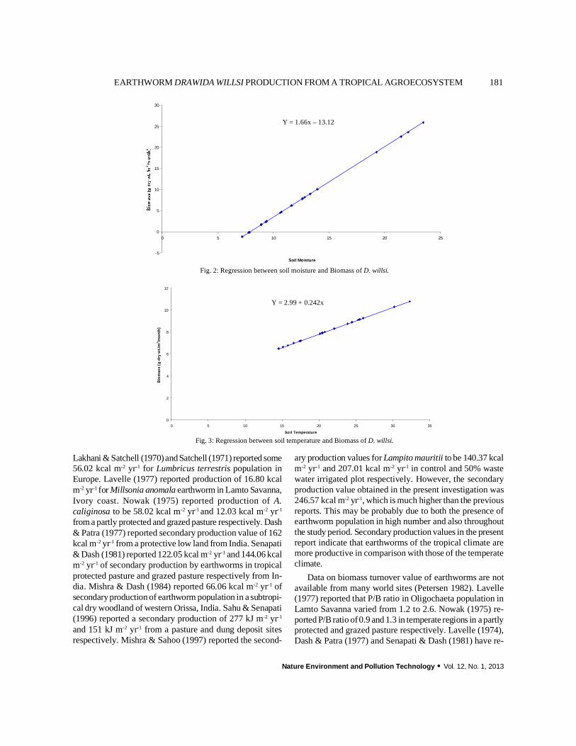
Nature Environment and Pollution Technology · Vol. 12, No. 1, 2013
181EARTHWORM DRAWIDA WILLSI PRODUCTION FROM A TROPICAL AGROECOSYSTEM
Lakhani & Satchell (1970)andSatchell (1971) reported some56.02 kcal m-2 yr-1 for Lumbricus terrestris population inEurope. Lavelle (1977) reported production of 16.80 kcalm-2 yr-1 for Millsonia anomala earthworm in Lamto Savanna,Ivory coast. Nowak (1975) reported production of A.caliginosa to be 58.02 kcal m-2 yr-1 and 12.03 kcal m-2 yr-1
from a partly protected and grazed pasture respectively. Dash& Patra (1977) reported secondary production value of 162kcal m-2 yr-1 from a protective low land from India. Senapati& Dash (1981) reported 122.05 kcal m-2 yr-1 and 144.06 kcalm-2 yr-1 of secondary production by earthworms in tropicalprotected pasture and grazed pasture respectively from In-dia. Mishra & Dash (1984) reported 66.06 kcal m-2 yr-1 ofsecondaryproduction of earthworm population in a subtropi-cal dry woodland of western Orissa, India. Sahu & Senapati(1996) reported a secondary production of 277 kJ m-2 yr-1
and 151 kJ m-2 yr-1 from a pasture and dung deposit sitesrespectively. Mishra & Sahoo (1997) reported the second-
ary production values for Lampito mauritii to be 140.37 kcalm-2 yr-1 and 207.01 kcal m-2 yr-1 in control and 50% wastewater irrigated plot respectively. However, the secondaryproduction value obtained in the present investigation was246.57 kcal m-2 yr-1, which is much higher than the previousreports. This may be probably due to both the presence ofearthworm population in high number and also throughoutthe study period. Secondary production values in the presentreport indicate that earthworms of the tropical climate aremore productive in comparison with those of the temperateclimate.
Data on biomass turnover value of earthworms are notavailable from many world sites (Petersen 1982). Lavelle(1977) reported that P/B ratio in Oligochaeta population inLamto Savanna varied from 1.2 to 2.6. Nowak (1975) re-ported P/B ratio of0.9 and 1.3 in temperate regions in a partlyprotected and grazed pasture respectively. Lavelle (1974),Dash & Patra (1977) and Senapati & Dash (1981) have re-
-5
0
5
10
15
20
25
30
0 5 10 15 20 25
Soil Moisture
2
Y = 1.66x – 13.12
0
2
4
6
8
10
12
0 5 10 15 20 25 30 35
Soil Temperature
Bio
mas
s(g
dry
wt./
m2 /m
onth
)
Y = 2.99 + 0.242x
Fig. 2: Regression between soil moisture and Biomass of D. willsi.
Fig. 3: Regression between soil temperature and Biomass of D. willsi.
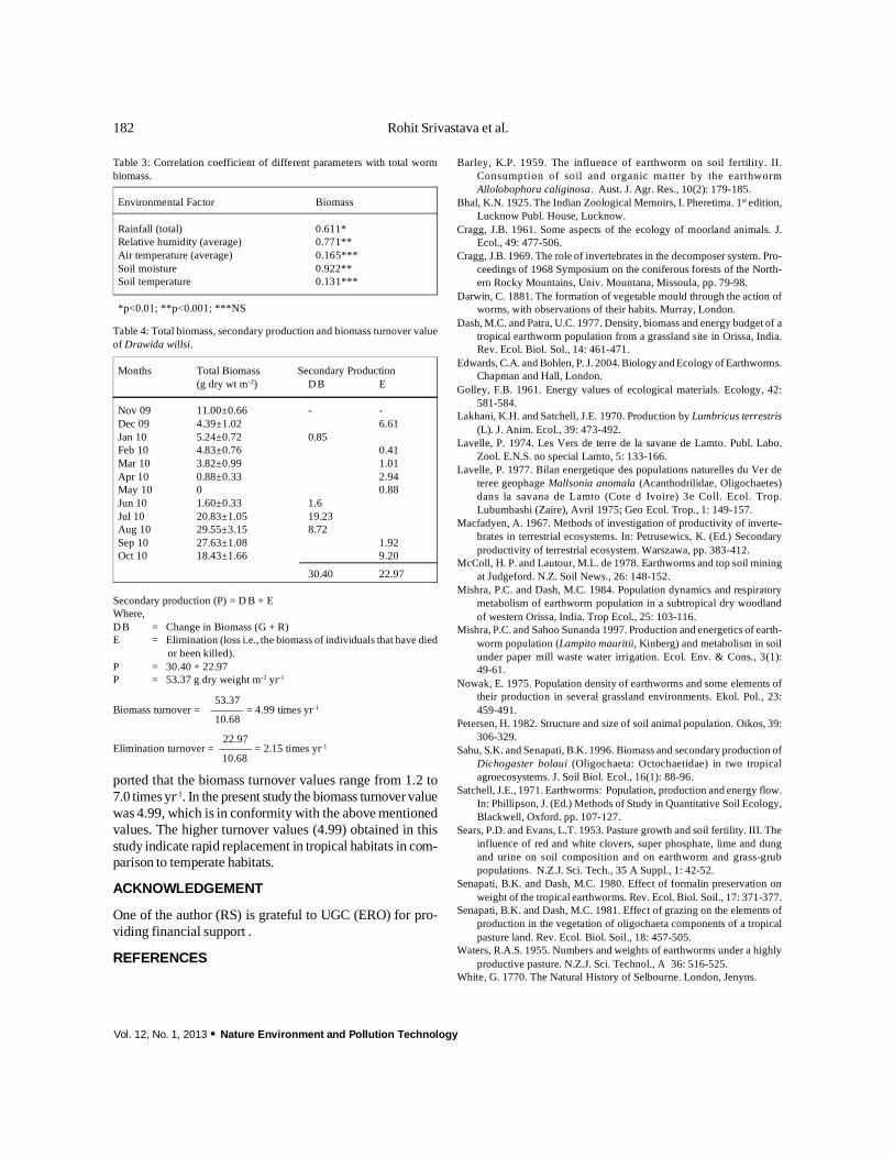
Vol. 12, No. 1, 2013 · Nature Environment and Pollution Technology
182 Rohit Srivastava et al.
Barley, K.P. 1959. The influence of earthworm on soil fertility. II.Consumption of soil and organic matter by the earthwormAllolobophora caliginosa. Aust. J. Agr. Res., 10(2): 179-185.
Bhal, K.N. 1925. The Indian Zoological Memoirs, I. Pheretima. 1st edition,Lucknow Publ. House, Lucknow.
Cragg, J.B. 1961. Some aspects of the ecology of moorland animals. J.Ecol., 49: 477-506.
Cragg, J.B. 1969. The role of invertebrates in the decomposer system. Pro-ceedings of 1968 Symposium on the coniferous forests of the North-ern Rocky Mountains, Univ. Mountana, Missoula, pp. 79-98.
Darwin, C. 1881. The formation of vegetable mould through the action ofworms, with observations of their habits. Murray, London.
Dash, M.C. and Patra, U.C. 1977. Density, biomass and energy budget of atropical earthworm population from a grassland site in Orissa, India.Rev. Ecol. Biol. Sol., 14: 461-471.
Edwards, C.A. and Bohlen, P. J. 2004. Biology and Ecology of Earthworms.Chapman and Hall, London.
Golley, F.B. 1961. Energy values of ecological materials. Ecology, 42:581-584.
Lakhani, K.H. and Satchell, J.E. 1970. Production by Lumbricus terrestris(L). J. Anim. Ecol., 39: 473-492.
Lavelle, P. 1974. Les Vers de terre de la savane de Lamto. Publ. Labo.Zool. E.N.S. no special Lamto, 5: 133-166.
Lavelle, P. 1977. Bilan energetique des populations naturelles du Ver deteree geophage Mallsonia anomala (Acanthodrilidae, Oligochaetes)dans la savana de Lamto (Cote d Ivoire) 3e Coll. Ecol. Trop.Lubumbashi (Zaire), Avril 1975; Geo Ecol. Trop., 1: 149-157.
Macfadyen, A. 1967. Methods of investigation of productivity of inverte-brates in terrestrial ecosystems. In: Petrusewics, K. (Ed.) Secondaryproductivity of terrestrial ecosystem. Warszawa, pp. 383-412.
McColl, H. P. and Lautour, M.L. de 1978. Earthworms and top soil miningat Judgeford. N.Z. Soil News., 26: 148-152.
Mishra, P.C. and Dash, M.C. 1984. Population dynamics and respiratorymetabolism of earthworm population in a subtropical dry woodlandof western Orissa, India. Trop Ecol., 25: 103-116.
Mishra, P.C. and Sahoo Sunanda 1997. Production and energetics of earth-worm population (Lampito mauritii, Kinberg) and metabolism in soilunder paper mill waste water irrigation. Ecol. Env. & Cons., 3(1):49-61.
Nowak, E. 1975. Population density of earthworms and some elements oftheir production in several grassland environments. Ekol. Pol., 23:459-491.
Petersen, H. 1982. Structure and size of soil animal population. Oikos, 39:306-329.
Sahu, S.K. and Senapati, B.K. 1996. Biomass and secondary production ofDichogaster bolaui (Oligochaeta: Octochaetidae) in two tropicalagroecosystems. J. Soil Biol. Ecol., 16(1): 88-96.
Satchell, J.E., 1971. Earthworms: Population, production and energy flow.In: Phillipson, J. (Ed.) Methods of Study in Quantitative Soil Ecology,Blackwell, Oxford. pp. 107-127.
Sears, P.D. and Evans, L.T. 1953. Pasture growth and soil fertility. III. Theinfluence of red and white clovers, super phosphate, lime and dungand urine on soil composition and on earthworm and grass-grubpopulations. N.Z.J. Sci. Tech., 35 A Suppl., 1: 42-52.
Senapati, B.K. and Dash, M.C. 1980. Effect of formalin preservation onweight of the tropical earthworms. Rev. Ecol. Biol. Soil., 17: 371-377.
Senapati, B.K. and Dash, M.C. 1981. Effect of grazing on the elements ofproduction in the vegetation of oligochaeta components of a tropicalpasture land. Rev. Ecol. Biol. Soil., 18: 457-505.
Waters, R.A.S. 1955. Numbers and weights of earthworms under a highlyproductive pasture. N.Z.J. Sci. Technol., A 36: 516-525.
White, G. 1770. The Natural History of Selbourne. London, Jenyns.
Table 3: Correlation coefficient of different parameters with total wormbiomass.
Environmental Factor Biomass
Rainfall (total) 0.611*Relative humidity (average) 0.771**Air temperature (average) 0.165***Soil moisture 0.922**Soil temperature 0.131***
*p<0.01; **p<0.001; ***NS
Table 4: Total biomass, secondary production and biomass turnover valueof Drawida willsi.
Months Total Biomass Secondary Production(g dry wt m-2) D B E
Nov 09 11.00±0.66 - -Dec 09 4.39±1.02 6.61Jan 10 5.24±0.72 0.85Feb 10 4.83±0.76 0.41Mar 10 3.82±0.99 1.01Apr 10 0.88±0.33 2.94May 10 0 0.88Jun 10 1.60±0.33 1.6Jul 10 20.83±1.05 19.23Aug 10 29.55±3.15 8.72Sep 10 27.63±1.08 1.92Oct 10 18.43±1.66 9.20
30.40 22.97
Secondary production (P) = D B + EWhere,D B = Change in Biomass (G + R)E = Elimination (loss i.e., the biomass of individuals that have died
or been killed).P = 30.40 + 22.97P = 53.37 g dry weight m-2 yr-1
53.37Biomass turnover = ——–– = 4.99 times yr-1
10.68
22.97Elimination turnover = ——— = 2.15 times yr-1
10.68
ported that the biomass turnover values range from 1.2 to7.0 times yr-1. In the present study the biomass turnover valuewas 4.99, which is in conformity with the above mentionedvalues. The higher turnover values (4.99) obtained in thisstudy indicate rapid replacement in tropical habitats in com-parison to temperate habitats.
ACKNOWLEDGEMENT
One of the author (RS) is grateful to UGC (ERO) for pro-viding financial support .
REFERENCES
Shun Sheng Wang, Liang Jun Fei* and Chuan Chang GaoNorth China University of Water Conservancy and Hydroelectric Power, Zhengzhou, 450011, China*Institute of Water Resources, Xi’an University of Technology, Xi’an, 710048, China
ABSTRACTIn order to probe dry matter accumulation, grain yield and water use efficiency of winter wheat, the study hasbeen conducted under three irrigation treatments by the different irrigation methods. The results show thatwinter wheat water consumption and the ground dry matter accumulation gradually increase under thedifferent irrigationconditions, with the increase in thenumber of irrigations, while yield and water useefficiencyincrease at first and then decrease. Under the same irrigation times, the water consumption of winter wheatin bed-planting is lower than that in flat planting, and dry matter accumulation is higher than that of flatplanting. Compared with the flat planting, the water quantity of bed-planting can be saved 40%, theproductioncan increase by 5.5% to 11.3%, and water use efficiency can increase by 0.17 to 0.40kg/m3. On the basis ofthe experimental results, it is suggested that the bed-planting mode in combination with considerably deficitirrigation at winter, jointing and booting stages is worth extending the application in winter wheat production.
Nat. Env. & Poll. Tech.
Received: 25-9-2012Accepted: 8-11-2012
Key Words:Water use efficiencyWinter wheatBed-plantingGrain yield
INTRODUCTION
At present, there is a shortage of water resources in mostareas of China, but agricultural water waste phenomena arevery serious, and the water resource shortage and inefficientutilization coexist, which increase the degree of water re-sources shortage. The utilization rate of agricultural irriga-tion water is very low in these regions, less than 1 kg foodproduction per 1m3 of water, about 60% of the irrigationwater has been wasted because of irrigation way, farmlandirrigation infrastructure and so on. Due to evaporation ofwater in the field, less than one-third of the total amount ofirrigation water is really used by the crops. Compared withdeveloped countries there is very big disparity, so the devel-opment of water-saving irrigation is urgent (Sun & Kang2000, Wang & Zhang 2002).
Compared with the traditional cultivation way, in wheatridging cultivation water can be saved 30%, the humidityreduce about 10%, light transmittance increase by 5% ~ 15%on average and the rate of light energy utilization increaseby 10%~13.8%. At the same time, the degree of lodging,plant diseases and insect pests significantly become lowerthan that of traditional cultivation patterns, and plant growsstrong. Wheat ridging cultivation increases the yield by10%~13.4% comparing with the traditional cultivation, andis widely used in a variety of crops in many countries cur-rently (Wang & Wang 2004, Wang et al. 2003a, Wang et al.2003b). According to study about several different watertreatments on the way of winter wheat water consumption,
the ground dry matter weight, yield and WUE, high yieldand water-saving planting scheme are raised.
MATERIALS AND METHODS
General situations: The experiment position is situated atnorth latitude 35’33° and east longitude 111°25’, located inwarm temperate zone to the north subtropical transition zoneand belongs to semi-humid partial dry climate, whose aver-age temperature is 12° to 14.5° and the average yearly rain-fall 637.1 mm. The earth for experiment is cinnamon soiland the experimental field is flat, so that is convenient forirrigation and drainage.Test design: The specifications for wheat planting ridgesand ditch is 70 cm and 40 cm, ridge high 20 cm, 4 lines ofwheat are planted on the ridge, small row spacing of wheatis 14 cm and big row spacing is 22 cm (Fig. 1). The tradi-tional culture of plantation is the flatten culture treatments,which strip for broadcast is 2.8 m wide, strip spaced plant-ing and row spacing of 20 cm. Plot areas is 2.8 m × 15 m, 3times repeat with randomized arrangement. Managementmeasures are same to the field. Each set of plantation in-volves three irrigation processes and the specific irrigationscheme is given in Table 1. During the experiment withoutblock rain, in the whole growth course of winter wheat, thetotal rainfall is194.8 mm, perennial less than 11.9 mm, whichdistributes in late period of fertility. Fertilizer was raisedwater along the ridges.Index of determination: Quantity of rainfall, soil moisture
2013pp. 183-186Vol. 12ISSN: 0972-6268 No. 1Nature Environment and Pollution TechnologyAn International Quarterly Scientific Journal
Original Research Paper

Vol. 12, No. 1, 2013 · Nature Environment and Pollution Technology
184 Shun Sheng Wang et al.
content of winter wheat at different stages, the ground drymatter accumulation quantity, and yield were determined.Determining method:Rainfall field meteorological data ac-quisition system using field conditions of collecting wasused. Soil moisture content was determined by dryingmethod, each 20 cm soil for one level, sounding 1 m. Thedrying method was used to determine the dry matter; andproduction method with sample amount. Water use efficiencyis equal to the total average wheat grain dry weight per unitarea compared with the total water consumption duringwhole growth stages.
RESULTS AND ANALYSIS
Influence of different water treatments on water con-sumption: From Table 2, it is known that in the wholegrowth period of winter wheat, the water consumption ofdifferent treatments is on the same trend that the water con-sumption reduces in the period of over-wintering to greenreturnedstage, then gradually increases and reaches the high-est point in the period of jointing to heading stage, and fi-nally reduces again. In the stage of green returned andjointing, because treatment L3 and P3 loses irrigation water,the difference of water consumption becomes the most ob-vious, less than the treatment of irrigation in the stage ofgreen returned and jointing. Under the same irrigation con-dition, the irrigation water consumption in ridge is less thanthat in culture from sowing to heading, but bigger than flatculture from heading to mature; this period is an importantperiod for forming wheat, and is closely related to the pro-duction, so the addition of water consumption in ridge canhelp to improve the yield of winter wheat.
No matter what is ridge or the culture, with the additionof irrigation frequency and the increase of irrigation water,water consumption of winter wheat would increase, relevantresearch results are consistent (Zhang 2003). In the same ir-rigation water treatment, water consumption of culture isabout 3%-17% more than the water consumption of ridge;the same cropping pattern in different irrigation conditions,
14c 22c 14c
70c
90c
20c
20c
irrigation water consumption of planting pattern for ridge isfour water irrigation water > three water irrigation > twowater irrigation. Each treatment with the same total rainfallshows that irrigation water has a great impact on the waterconsumption. The ridge cultivation can reduce the water con-sumption of winter wheat, in the period of over-winteringand booting stage, water consumption is minimized.Influence of different water treatments on dry matter:Table 3 shows that, because before the treatment period, ir-rigation frequency is identical, in the stage of green returned,dry matter has little difference. And then with the growth ofwinter wheat and the change of irrigation frequency, theground dry matter accumulation also appears some differ-ence, the specific performance of four water irrigation> threewater irrigation > two water irrigation, but because the head-ing rainfall becomes more than before, the influence of irri-gation frequency on ground dry matter becomes less obvi-ous. In the same irrigation frequency, the accumulation ofdry matter raises more than that of the culture, which be-comes most obvious in maturity; the difference of grain isthe largest in irrigation 3 water, that is the winter water +jointing water + booting water, the difference is 5.56 g/10plants.Influence of different water treatments on yield: Underthe different irrigation situations, the yield of bed-plantingwinter wheat show three water irrigation > four water irri-gation > two water irrigation; the yield of three water irriga-tion increases 2.9% and 5.3% to respectively the yield offour water irrigation and two water irrigation. The bootingrate of four water irrigation treatment is high, but the graingrouting effect is bad, grain weight is less than that of threewater irrigation treatment, so that the yield reduces. In cul-ture-planting, winter wheat yield with irrigation frequencyincreased. In the same treatment with different plantingmodes of irrigation, production per hectare is higher 392 kgto 782 kg than that of the culture raised , which is most obvi-ous in three water irrigation conditions; increased rate ofproduction is 11.3%, as shown in Table 4.
Fig 1: Schematic diagram of bed-planting.

Nature Environment and Pollution Technology · Vol. 12, No. 1, 2013
185EXPERIMENTAL STUDY ON WATER USE EFFICIENCY OF WINTER WHEAT
Influence of different water treatments on water useefficiency: As bed-planting and flatten culture exist in thesame field, the rainfall is identical. Each time the wateramount raised in bed-planting was 450 m3/hm2, and everytime the irrigation capacity of the flatten culture is 750m3/hm2, water saving rate was 40%. Even in case of the irri-gation water reducing, raised output in bed-planting is stillhigher than the culture; cultivation has raised water savingeffect on increasing. From the Table 4, we can see that in
different water treatments, water use efficiency changes withthe irrigation frequency, which shows that water use effi-ciency increases at first and then reduces. Water use effi-ciency raised in three water irrigation cultivation is the high-est, about 2.08 kg/m3, followed by two water irrigation, inwhich water use efficiency is 2.03 kg/m3. In the same watertreatment, the treatment of the water use efficiency raisessignificantly higher than that of the traditional culture; thebiggest difference is 0.4 kg/m3.
Table 1: Irrigation of winter wheat with different treatment options (m3/hm2).
Treatment Over-wintering Green returned Jointing Booting Total irrigation irrigation methodswith numbers stage stage stage stage water
L1 450 450 450 450 1800 Furrow irrigationP1 750 750 750 750 3000 Border irrigationL2 450 450 - 450 1350 Furrow irrigationP2 750 750 - 750 2250 Border irrigationL3 450 - - 450 900 Furrow irrigationP3 750 - - 750 1500 Border irrigation
Table 2: Effect of irrigation on the water consumption of winter wheat (mm).
Treatment Sowing~over- Over-wintering~ Green returned~ Jointing~ Heading~ Filling~ During wholewintering green returned jointing heading filling maturating growth stages
stage stage stage stage stage stage water consumption
L1 62.02 31.16 76.60 130.26 59.14 35.28 394.47P1 72.48 40.51 81.85 153.89 53.16 59.49 461.39L2 58.06 24.77 77.83 113.17 46.43 49.18 369.45P2 61.05 37.02 84.11 125.82 41.15 62.09 411.24L3 64.85 23.45 28.96 111.73 78.40 53.10 360.49P3 68.35 23.45 36.60 130.42 63.29 49.11 371.22
Table 3: Dry matter accumulation and distribution of winter wheat (g/10 plants).
Number Treatment Irrigation methods Green Heading Maturating Dry matterofirrigation returned stage stage stage Straw Grain
Four L1 Furrow irrigation 2.98 26.62 54.00 37.61 16.39P1 Border irrigation 3.85 25.21 42.85 28.34 14.51
Three L2 Furrow irrigation 3.39 25.57 47.30 30.29 17.01P2 Border irrigation 3.34 23.77 35.65 24.20 11.45
Two L3 Furrow irrigation 2.85 20.62 45.45 33.96 11.49P3 Border irrigation 4.45 16.21 33.90 21.54 12.36
Table 4: Yield and WUE of winter wheat under different irrigation treatments.
Treatment Number Spike number Grain number Thousand Yield Total water WUEof irrigations (Million Spike/hm2) (Grain/Spike) grain weight (g) (kg/m2) consumption (kg/m3)
(mm)
L1 4 772.5 41.8 36.9 0.75 394.47 1.90P1 4 750.0 41.4 38.0 0.71 461.39 1.54L2 3 735.0 41.0 41.3 0.77 369.45 2.08P2 3 588.0 43.5 38.2 0.69 411.24 1.68L3 2 622.5 41.2 40.0 0.73 360.49 2.03P3 2 664.5 36.1 37.1 0.69 371.22 1.86

Vol. 12, No. 1, 2013 · Nature Environment and Pollution Technology
186 Shun Sheng Wang et al.
CONCLUSIONS
The results of the study show that with each treatment withthe increased winter wheat irrigation frequency and amountof irrigation, water consumption and the ground dry matterincreasedsignificantly, and yield and WUE reduced after firstincrease. Under the condition of the three irrigations in thebed-planting raised in the test set planting pattern of the threeirrigation conditions, all the water consumptions are less thanthat of the traditional culture; yield and water use efficiencyare higher than that of the traditional culture. Relative to theflat culture, ridge planting can save water up to 40%. In theperiodof irrigation inover-wintering stage and bootingstage,the yield can increase 6.6%. In the period of irrigation inover-wintering stage, green returned stage, jointing stage andbooting stage, the yield can increase 5.5%. When irrigationin over-wintering stage, green returned stage, jointing stageand booting stage, the yield can reach the highest point com-pared with the traditional culture. The effect of bed-plantingis most significant, which can increase by effect on increas-ing traditional culture and increased yield rate was, 11.3%,and at this time the WUE is highest, the value was 2.08 kg/m3. Taking winter wheat water consumption, yield and WUErelationship as a whole to consider, ridge planting combinedwith irrigation in over-wintering stage, jointing stage andbooting stage, is worth promoting cropping patterns.
ACKNOWLEDGMENT
The study was supported by National Scientific and Tech-nological Support Program for the 11th Five-year Plan(2007BAD88B02) and National Subsidized Project on Natu-ral Science Foundation (50179030). Authors are grateful tothe anonymous reviewers for their valuable comments onthis manuscript.
REFERENCES
Sun, J.S. and Kang, S.Z. 2000. Our country present situation of water re-sources utilization and development countermeasures of water-savingirrigation. Journal of Agricultural Engineering, (2): 1-5.
Wang, L.S. and Zhang, L.L. 2002. The western agricultural water resourcesof equal analysis and control way. Journal of Luoyang AgriculturalCollege, 23(3): 170-172.
Wang, X.Q., Wang, F.H. and Ren, D.C. 2003a. Raised in the field of thecultivation of wheat eco-microclimatical effects of plant growth andyield and the influence. Journal of Chinese Agricultural Meteorology,2: 5-8.
Wang, X.Q., Wang, F.H. and Yu, Z.W. 2003a. Raised on individual devel-opment and cultivation of wheat the influence of resistance. Farmingand Planting, 5: 21-23.
Wang, F.H. and Wang, X.Q. 2004. Comparison of conventional, flood irri-gated, flat planting with furrow irrigated, raised bed planting for win-ter wheat in China. The Field Crops Res., 87: 35-42.
Zhang, Z.X. 2003. Different water treatment on winter wheat growth andthe influence of water use efficiency. Journal of Irrigation and Drain-age Water, 23(2).

• The text of the mss should run into Abstract, Introduction, Materials & Methods, Results,Discussion, Acknowledgement (if any) and References or other suitable headings in case ofreviews and theoretically oriented papers. However, short communication can be submitted inrunning with Abstract and References. The references should be in full with title of the paper.
• The figures should be drawn on a good quality tracing/white paper with black ink with thelegends provided on a separate sheet. The figures made on computer should be printed onlyon inkjet or laser printer. Photographs may be black and white or colour on a glossy sheet.
• Tables should be typed on separate sheets bearing a short title, preferably in vertical form.They should be of a size, which could be accommodated in the page of the Journal.
• References in the text should be cited by name and year. In case of more than one referenceof the same author in the same year, add suffix a,b,c,.... to the year. For example: (Thomas1969, Mass 1973a, 1973b, Madony et al. 1990, Abasi & Soni 1991).
List of References
The references cited in the text should be arranged alphabetically by author’s Surname in thefollowing manner:
Dutta, A. and Chaudhury, M. 1991. Removal of arsenic from groundwater by lime softening withpowdered coal additive. J. Water Supply Res. Techno. Aqua., 40(1) : 25-29.
Hammer, D.A. (ed.) 1989. Constructed Wetlands for Wastewater Treatment-Municipal, Industrialand Agricultural. Lewis Publishers Inc., pp. 831.
Haynes, R. J. 1986. Surface mining and wetland reclamation. In: Harper, J. and Plass, B. (eds.)New Horizons for Mined Land Reclamation. Proceedings of a National Meeting of the AmericanSociety for Surface Reclamation, Princeton, W.V.
Submission of Papers
• The manuscript can be submitted in duplicate to either of the editors. However, preferenceshould be given to Dr. P.K. Goel for papers dealing with pollution.
• A soft copy of the mss in CD is must for further processing of papers along with hard copies (induplicate) at the time of submission of mss. The soft copy can also be sent directly by e-mail asan attachment in WORD/PageMaker at [email protected] or [email protected]
• Contributor(s) to this Journal should hold the membership of the Journal.• No gratis reprints will be supplied. Authors have to purchase a minimum of 25 reprints by
paying reprint cost.
Attention
1. Any change in address may please be notified at the earliest to the publisher to avoid thenonreceipt of the Journal and other correspondence.
2. Individual subscribers are requested to please give their home addresses also for safe deliveryof the Journal.
3. For quick response please make the correspondence by e-mail and always refer mss number.
In order to expedite publication, authors are requested to send their membership and reprint cost assoon as they get the preliminary acceptance letter, and also correct galley proof immediately after receipt,with care, as publishers owe no responsibility for mistakes. The papers will be put on priority for printing onlyafter receiving membership and reprint cost.
.... Continued from inner front cover

Published by
Technoscience Publications2, Shila Apartment, Shila Nagar, P.O. Box 10
Karad-415 110, Maharashtra, India(Tel. 02164-223070; Mob. 9890248152)
Published for Proprietor; Printer and Publisher: Mrs. T. P. Goel, B-34, Dev Nagar, TonkRoad, Jaipur, Rajasthan, India; Editors: Dr. P. K. Goel and Prof. K. P. Sharma; Printed atBhalotia Printers, Jaipur, India
(Abbreviation: Nat. Env. Poll. Tech.)(An International Quarterly Scientific Journal)
©Technoscience Publications: The consent is hereby given that the copies of the articles publishedin this Journal can be made only for purely personal or internal use. The consent does not includecopying for general distribution or resale of reprints.
SUBSCRIBERS AND AUTHORS1. Payments are to be made through bank draft only, in the name of Technoscience
Publications payable on any bank at Karad (Maharashtra) and not in thepersonal names of Editors.
2. Authors and coauthors are advised to send the reprint cost and the membershipas soon as they receive the preliminary acceptance and demand letter.
3. The final acceptance letter will be sent mentioning the Volume, Number andyear of the issue in which the paper is likely to be published, after receiving thereprint cost and the membership of the journal from the authors.
4. The Journal is published in March, June, September and December. We shalltry to replace the lost issue subject to its availability, provided that the complaintis made within a month of publication.
For further details of the Journal visit our website. Literature survey of the paperspublished in old issues of the journal can be made by typing the key word in‘Search’ option on the Home page and then clicking ‘Get Abstract’ and ‘Get fullpaper’. The link of the required paper will be sent at the e-mail address immediately.
www.neptjournal.com
Copyright © 2022 FDOKUMEN