VisTex texture Bark.0000: (a) original 128 × 128 image; (b–g ...
114
261 (a) Training texture (b) Nearest neighbour (c) Nearest neighbour (d) 5 × 5 neighbourhood (e) 5 × 5 neighbourhood (f) 7 × 7 neighbourhood (g) 7 × 7 neighbourhood Figure B.73: VisTex texture Bark.0000: (a) original 128 × 128 image; (b–g) syn- thesised 256 × 256 images; (b) using Gibbs sampling and nearest neighbour neigh- bourhood; (c) using ICM sampling and nearest neighbour neighbourhood; (d) us- ing Gibbs sampling and 5 × 5 neighbourhood; (e) using ICM sampling and 5 × 5 neighbourhood; (f) using Gibbs sampling and 7 × 7 neighbourhood; (g) using ICM sampling and 7 × 7 neighbourhood.
-
Upload
khangminh22 -
Category
Documents
-
view
2 -
download
0
Transcript of VisTex texture Bark.0000: (a) original 128 × 128 image; (b–g ...

261
(a) Training texture (b) Nearest neighbour (c) Nearest neighbour
(d) 5 × 5 neighbourhood (e) 5 × 5 neighbourhood
(f) 7 × 7 neighbourhood (g) 7 × 7 neighbourhood
Figure B.73: VisTex texture Bark.0000: (a) original 128 × 128 image; (b–g) syn-thesised 256 × 256 images; (b) using Gibbs sampling and nearest neighbour neigh-bourhood; (c) using ICM sampling and nearest neighbour neighbourhood; (d) us-ing Gibbs sampling and 5 × 5 neighbourhood; (e) using ICM sampling and 5 × 5neighbourhood; (f) using Gibbs sampling and 7 × 7 neighbourhood; (g) using ICMsampling and 7 × 7 neighbourhood.

262
(a) Training texture (b) Nearest neighbour (c) Nearest neighbour
(d) 5 × 5 neighbourhood (e) 5 × 5 neighbourhood
(f) 7 × 7 neighbourhood (g) 7 × 7 neighbourhood
Figure B.74: VisTex texture Bark.0001: (a) original 128 × 128 image; (b–g) syn-thesised 256 × 256 images; (b) using Gibbs sampling and nearest neighbour neigh-bourhood; (c) using ICM sampling and nearest neighbour neighbourhood; (d) us-ing Gibbs sampling and 5 × 5 neighbourhood; (e) using ICM sampling and 5 × 5neighbourhood; (f) using Gibbs sampling and 7 × 7 neighbourhood; (g) using ICMsampling and 7 × 7 neighbourhood.

263
(a) Training texture (b) Nearest neighbour (c) Nearest neighbour
(d) 5 × 5 neighbourhood (e) 5 × 5 neighbourhood
(f) 7 × 7 neighbourhood (g) 7 × 7 neighbourhood
Figure B.75: VisTex texture Bark.0002: (a) original 128 × 128 image; (b–g) syn-thesised 256 × 256 images; (b) using Gibbs sampling and nearest neighbour neigh-bourhood; (c) using ICM sampling and nearest neighbour neighbourhood; (d) us-ing Gibbs sampling and 5 × 5 neighbourhood; (e) using ICM sampling and 5 × 5neighbourhood; (f) using Gibbs sampling and 7 × 7 neighbourhood; (g) using ICMsampling and 7 × 7 neighbourhood.

264
(a) Training texture (b) Nearest neighbour (c) Nearest neighbour
(d) 5 × 5 neighbourhood (e) 5 × 5 neighbourhood
(f) 7 × 7 neighbourhood (g) 7 × 7 neighbourhood
Figure B.76: VisTex texture Bark.0003: (a) original 128 × 128 image; (b–g) syn-thesised 256 × 256 images; (b) using Gibbs sampling and nearest neighbour neigh-bourhood; (c) using ICM sampling and nearest neighbour neighbourhood; (d) us-ing Gibbs sampling and 5 × 5 neighbourhood; (e) using ICM sampling and 5 × 5neighbourhood; (f) using Gibbs sampling and 7 × 7 neighbourhood; (g) using ICMsampling and 7 × 7 neighbourhood.

265
(a) Training texture (b) Nearest neighbour (c) Nearest neighbour
(d) 5 × 5 neighbourhood (e) 5 × 5 neighbourhood
(f) 7 × 7 neighbourhood (g) 7 × 7 neighbourhood
Figure B.77: VisTex texture Bark.0004: (a) original 128 × 128 image; (b–g) syn-thesised 256 × 256 images; (b) using Gibbs sampling and nearest neighbour neigh-bourhood; (c) using ICM sampling and nearest neighbour neighbourhood; (d) us-ing Gibbs sampling and 5 × 5 neighbourhood; (e) using ICM sampling and 5 × 5neighbourhood; (f) using Gibbs sampling and 7 × 7 neighbourhood; (g) using ICMsampling and 7 × 7 neighbourhood.

266
(a) Training texture (b) Nearest neighbour (c) Nearest neighbour
(d) 5 × 5 neighbourhood (e) 5 × 5 neighbourhood
(f) 7 × 7 neighbourhood (g) 7 × 7 neighbourhood
Figure B.78: VisTex texture Bark.0005: (a) original 128 × 128 image; (b–g) syn-thesised 256 × 256 images; (b) using Gibbs sampling and nearest neighbour neigh-bourhood; (c) using ICM sampling and nearest neighbour neighbourhood; (d) us-ing Gibbs sampling and 5 × 5 neighbourhood; (e) using ICM sampling and 5 × 5neighbourhood; (f) using Gibbs sampling and 7 × 7 neighbourhood; (g) using ICMsampling and 7 × 7 neighbourhood.

267
(a) Training texture (b) Nearest neighbour (c) Nearest neighbour
(d) 5 × 5 neighbourhood (e) 5 × 5 neighbourhood
(f) 7 × 7 neighbourhood (g) 7 × 7 neighbourhood
Figure B.79: VisTex texture Bark.0006: (a) original 128 × 128 image; (b–g) syn-thesised 256 × 256 images; (b) using Gibbs sampling and nearest neighbour neigh-bourhood; (c) using ICM sampling and nearest neighbour neighbourhood; (d) us-ing Gibbs sampling and 5 × 5 neighbourhood; (e) using ICM sampling and 5 × 5neighbourhood; (f) using Gibbs sampling and 7 × 7 neighbourhood; (g) using ICMsampling and 7 × 7 neighbourhood.

268
(a) Training texture (b) Nearest neighbour (c) Nearest neighbour
(d) 5 × 5 neighbourhood (e) 5 × 5 neighbourhood
(f) 7 × 7 neighbourhood (g) 7 × 7 neighbourhood
Figure B.80: VisTex texture Bark.0007: (a) original 128 × 128 image; (b–g) syn-thesised 256 × 256 images; (b) using Gibbs sampling and nearest neighbour neigh-bourhood; (c) using ICM sampling and nearest neighbour neighbourhood; (d) us-ing Gibbs sampling and 5 × 5 neighbourhood; (e) using ICM sampling and 5 × 5neighbourhood; (f) using Gibbs sampling and 7 × 7 neighbourhood; (g) using ICMsampling and 7 × 7 neighbourhood.
269
(a) Training texture (b) Nearest neighbour (c) Nearest neighbour
(d) 5 × 5 neighbourhood (e) 5 × 5 neighbourhood
(f) 7 × 7 neighbourhood (g) 7 × 7 neighbourhood
Figure B.81: VisTex texture Bark.0008: (a) original 128 × 128 image; (b–g) syn-thesised 256 × 256 images; (b) using Gibbs sampling and nearest neighbour neigh-bourhood; (c) using ICM sampling and nearest neighbour neighbourhood; (d) us-ing Gibbs sampling and 5 × 5 neighbourhood; (e) using ICM sampling and 5 × 5neighbourhood; (f) using Gibbs sampling and 7 × 7 neighbourhood; (g) using ICMsampling and 7 × 7 neighbourhood.

270
(a) Training texture (b) Nearest neighbour (c) Nearest neighbour
(d) 5 × 5 neighbourhood (e) 5 × 5 neighbourhood
(f) 7 × 7 neighbourhood (g) 7 × 7 neighbourhood
Figure B.82: VisTex texture Bark.0009: (a) original 128 × 128 image; (b–g) syn-thesised 256 × 256 images; (b) using Gibbs sampling and nearest neighbour neigh-bourhood; (c) using ICM sampling and nearest neighbour neighbourhood; (d) us-ing Gibbs sampling and 5 × 5 neighbourhood; (e) using ICM sampling and 5 × 5neighbourhood; (f) using Gibbs sampling and 7 × 7 neighbourhood; (g) using ICMsampling and 7 × 7 neighbourhood.

271
(a) Training texture (b) Nearest neighbour (c) Nearest neighbour
(d) 5 × 5 neighbourhood (e) 5 × 5 neighbourhood
(f) 7 × 7 neighbourhood (g) 7 × 7 neighbourhood
Figure B.83: VisTex texture Bark.0010: (a) original 128 × 128 image; (b–g) syn-thesised 256 × 256 images; (b) using Gibbs sampling and nearest neighbour neigh-bourhood; (c) using ICM sampling and nearest neighbour neighbourhood; (d) us-ing Gibbs sampling and 5 × 5 neighbourhood; (e) using ICM sampling and 5 × 5neighbourhood; (f) using Gibbs sampling and 7 × 7 neighbourhood; (g) using ICMsampling and 7 × 7 neighbourhood.

272
(a) Training texture (b) Nearest neighbour (c) Nearest neighbour
(d) 5 × 5 neighbourhood (e) 5 × 5 neighbourhood
(f) 7 × 7 neighbourhood (g) 7 × 7 neighbourhood
Figure B.84: VisTex texture Bark.0011: (a) original 128 × 128 image; (b–g) syn-thesised 256 × 256 images; (b) using Gibbs sampling and nearest neighbour neigh-bourhood; (c) using ICM sampling and nearest neighbour neighbourhood; (d) us-ing Gibbs sampling and 5 × 5 neighbourhood; (e) using ICM sampling and 5 × 5neighbourhood; (f) using Gibbs sampling and 7 × 7 neighbourhood; (g) using ICMsampling and 7 × 7 neighbourhood.

273
(a) Training texture (b) Nearest neighbour (c) Nearest neighbour
(d) 5 × 5 neighbourhood (e) 5 × 5 neighbourhood
(f) 7 × 7 neighbourhood (g) 7 × 7 neighbourhood
Figure B.85: VisTex texture Bark.0012: (a) original 128 × 128 image; (b–g) syn-thesised 256 × 256 images; (b) using Gibbs sampling and nearest neighbour neigh-bourhood; (c) using ICM sampling and nearest neighbour neighbourhood; (d) us-ing Gibbs sampling and 5 × 5 neighbourhood; (e) using ICM sampling and 5 × 5neighbourhood; (f) using Gibbs sampling and 7 × 7 neighbourhood; (g) using ICMsampling and 7 × 7 neighbourhood.

274
(a) Training texture (b) Nearest neighbour (c) Nearest neighbour
(d) 5 × 5 neighbourhood (e) 5 × 5 neighbourhood
(f) 7 × 7 neighbourhood (g) 7 × 7 neighbourhood
Figure B.86: VisTex texture Brick.0000: (a) original 128 × 128 image; (b–g) syn-thesised 256 × 256 images; (b) using Gibbs sampling and nearest neighbour neigh-bourhood; (c) using ICM sampling and nearest neighbour neighbourhood; (d) us-ing Gibbs sampling and 5 × 5 neighbourhood; (e) using ICM sampling and 5 × 5neighbourhood; (f) using Gibbs sampling and 7 × 7 neighbourhood; (g) using ICMsampling and 7 × 7 neighbourhood.

275
(a) Training texture (b) Nearest neighbour (c) Nearest neighbour
(d) 5 × 5 neighbourhood (e) 5 × 5 neighbourhood
(f) 7 × 7 neighbourhood (g) 7 × 7 neighbourhood
Figure B.87: VisTex texture Brick.0001: (a) original 128 × 128 image; (b–g) syn-thesised 256 × 256 images; (b) using Gibbs sampling and nearest neighbour neigh-bourhood; (c) using ICM sampling and nearest neighbour neighbourhood; (d) us-ing Gibbs sampling and 5 × 5 neighbourhood; (e) using ICM sampling and 5 × 5neighbourhood; (f) using Gibbs sampling and 7 × 7 neighbourhood; (g) using ICMsampling and 7 × 7 neighbourhood.

276
(a) Training texture (b) Nearest neighbour (c) Nearest neighbour
(d) 5 × 5 neighbourhood (e) 5 × 5 neighbourhood
(f) 7 × 7 neighbourhood (g) 7 × 7 neighbourhood
Figure B.88: VisTex texture Brick.0002: (a) original 128 × 128 image; (b–g) syn-thesised 256 × 256 images; (b) using Gibbs sampling and nearest neighbour neigh-bourhood; (c) using ICM sampling and nearest neighbour neighbourhood; (d) us-ing Gibbs sampling and 5 × 5 neighbourhood; (e) using ICM sampling and 5 × 5neighbourhood; (f) using Gibbs sampling and 7 × 7 neighbourhood; (g) using ICMsampling and 7 × 7 neighbourhood.

277
(a) Training texture (b) Nearest neighbour (c) Nearest neighbour
(d) 5 × 5 neighbourhood (e) 5 × 5 neighbourhood
(f) 7 × 7 neighbourhood (g) 7 × 7 neighbourhood
Figure B.89: VisTex texture Brick.0003: (a) original 128 × 128 image; (b–g) syn-thesised 256 × 256 images; (b) using Gibbs sampling and nearest neighbour neigh-bourhood; (c) using ICM sampling and nearest neighbour neighbourhood; (d) us-ing Gibbs sampling and 5 × 5 neighbourhood; (e) using ICM sampling and 5 × 5neighbourhood; (f) using Gibbs sampling and 7 × 7 neighbourhood; (g) using ICMsampling and 7 × 7 neighbourhood.

278
(a) Training texture (b) Nearest neighbour (c) Nearest neighbour
(d) 5 × 5 neighbourhood (e) 5 × 5 neighbourhood
(f) 7 × 7 neighbourhood (g) 7 × 7 neighbourhood
Figure B.90: VisTex texture Brick.0004: (a) original 128 × 128 image; (b–g) syn-thesised 256 × 256 images; (b) using Gibbs sampling and nearest neighbour neigh-bourhood; (c) using ICM sampling and nearest neighbour neighbourhood; (d) us-ing Gibbs sampling and 5 × 5 neighbourhood; (e) using ICM sampling and 5 × 5neighbourhood; (f) using Gibbs sampling and 7 × 7 neighbourhood; (g) using ICMsampling and 7 × 7 neighbourhood.

279
(a) Training texture (b) Nearest neighbour (c) Nearest neighbour
(d) 5 × 5 neighbourhood (e) 5 × 5 neighbourhood
(f) 7 × 7 neighbourhood (g) 7 × 7 neighbourhood
Figure B.91: VisTex texture Brick.0005: (a) original 128 × 128 image; (b–g) syn-thesised 256 × 256 images; (b) using Gibbs sampling and nearest neighbour neigh-bourhood; (c) using ICM sampling and nearest neighbour neighbourhood; (d) us-ing Gibbs sampling and 5 × 5 neighbourhood; (e) using ICM sampling and 5 × 5neighbourhood; (f) using Gibbs sampling and 7 × 7 neighbourhood; (g) using ICMsampling and 7 × 7 neighbourhood.

280
(a) Training texture (b) Nearest neighbour (c) Nearest neighbour
(d) 5 × 5 neighbourhood (e) 5 × 5 neighbourhood
(f) 7 × 7 neighbourhood (g) 7 × 7 neighbourhood
Figure B.92: VisTex texture Brick.0006: (a) original 128 × 128 image; (b–g) syn-thesised 256 × 256 images; (b) using Gibbs sampling and nearest neighbour neigh-bourhood; (c) using ICM sampling and nearest neighbour neighbourhood; (d) us-ing Gibbs sampling and 5 × 5 neighbourhood; (e) using ICM sampling and 5 × 5neighbourhood; (f) using Gibbs sampling and 7 × 7 neighbourhood; (g) using ICMsampling and 7 × 7 neighbourhood.

281
(a) Training texture (b) Nearest neighbour (c) Nearest neighbour
(d) 5 × 5 neighbourhood (e) 5 × 5 neighbourhood
(f) 7 × 7 neighbourhood (g) 7 × 7 neighbourhood
Figure B.93: VisTex texture Brick.0007: (a) original 128 × 128 image; (b–g) syn-thesised 256 × 256 images; (b) using Gibbs sampling and nearest neighbour neigh-bourhood; (c) using ICM sampling and nearest neighbour neighbourhood; (d) us-ing Gibbs sampling and 5 × 5 neighbourhood; (e) using ICM sampling and 5 × 5neighbourhood; (f) using Gibbs sampling and 7 × 7 neighbourhood; (g) using ICMsampling and 7 × 7 neighbourhood.

282
(a) Training texture (b) Nearest neighbour (c) Nearest neighbour
(d) 5 × 5 neighbourhood (e) 5 × 5 neighbourhood
(f) 7 × 7 neighbourhood (g) 7 × 7 neighbourhood
Figure B.94: VisTex texture Brick.0008: (a) original 128 × 128 image; (b–g) syn-thesised 256 × 256 images; (b) using Gibbs sampling and nearest neighbour neigh-bourhood; (c) using ICM sampling and nearest neighbour neighbourhood; (d) us-ing Gibbs sampling and 5 × 5 neighbourhood; (e) using ICM sampling and 5 × 5neighbourhood; (f) using Gibbs sampling and 7 × 7 neighbourhood; (g) using ICMsampling and 7 × 7 neighbourhood.

283
(a) Training texture (b) Nearest neighbour (c) Nearest neighbour
(d) 5 × 5 neighbourhood (e) 5 × 5 neighbourhood
(f) 7 × 7 neighbourhood (g) 7 × 7 neighbourhood
Figure B.95: VisTex texture Fabric.0000: (a) original 128 × 128 image; (b–g) syn-thesised 256 × 256 images; (b) using Gibbs sampling and nearest neighbour neigh-bourhood; (c) using ICM sampling and nearest neighbour neighbourhood; (d) us-ing Gibbs sampling and 5 × 5 neighbourhood; (e) using ICM sampling and 5 × 5neighbourhood; (f) using Gibbs sampling and 7 × 7 neighbourhood; (g) using ICMsampling and 7 × 7 neighbourhood.

284
(a) Training texture (b) Nearest neighbour (c) Nearest neighbour
(d) 5 × 5 neighbourhood (e) 5 × 5 neighbourhood
(f) 7 × 7 neighbourhood (g) 7 × 7 neighbourhood
Figure B.96: VisTex texture Fabric.0001: (a) original 128 × 128 image; (b–g) syn-thesised 256 × 256 images; (b) using Gibbs sampling and nearest neighbour neigh-bourhood; (c) using ICM sampling and nearest neighbour neighbourhood; (d) us-ing Gibbs sampling and 5 × 5 neighbourhood; (e) using ICM sampling and 5 × 5neighbourhood; (f) using Gibbs sampling and 7 × 7 neighbourhood; (g) using ICMsampling and 7 × 7 neighbourhood.

285
(a) Training texture (b) Nearest neighbour (c) Nearest neighbour
(d) 5 × 5 neighbourhood (e) 5 × 5 neighbourhood
(f) 7 × 7 neighbourhood (g) 7 × 7 neighbourhood
Figure B.97: VisTex texture Fabric.0002: (a) original 128 × 128 image; (b–g) syn-thesised 256 × 256 images; (b) using Gibbs sampling and nearest neighbour neigh-bourhood; (c) using ICM sampling and nearest neighbour neighbourhood; (d) us-ing Gibbs sampling and 5 × 5 neighbourhood; (e) using ICM sampling and 5 × 5neighbourhood; (f) using Gibbs sampling and 7 × 7 neighbourhood; (g) using ICMsampling and 7 × 7 neighbourhood.

286
(a) Training texture (b) Nearest neighbour (c) Nearest neighbour
(d) 5 × 5 neighbourhood (e) 5 × 5 neighbourhood
(f) 7 × 7 neighbourhood (g) 7 × 7 neighbourhood
Figure B.98: VisTex texture Fabric.0003: (a) original 128 × 128 image; (b–g) syn-thesised 256 × 256 images; (b) using Gibbs sampling and nearest neighbour neigh-bourhood; (c) using ICM sampling and nearest neighbour neighbourhood; (d) us-ing Gibbs sampling and 5 × 5 neighbourhood; (e) using ICM sampling and 5 × 5neighbourhood; (f) using Gibbs sampling and 7 × 7 neighbourhood; (g) using ICMsampling and 7 × 7 neighbourhood.

287
(a) Training texture (b) Nearest neighbour (c) Nearest neighbour
(d) 5 × 5 neighbourhood (e) 5 × 5 neighbourhood
(f) 7 × 7 neighbourhood (g) 7 × 7 neighbourhood
Figure B.99: VisTex texture Fabric.0004: (a) original 128 × 128 image; (b–g) syn-thesised 256 × 256 images; (b) using Gibbs sampling and nearest neighbour neigh-bourhood; (c) using ICM sampling and nearest neighbour neighbourhood; (d) us-ing Gibbs sampling and 5 × 5 neighbourhood; (e) using ICM sampling and 5 × 5neighbourhood; (f) using Gibbs sampling and 7 × 7 neighbourhood; (g) using ICMsampling and 7 × 7 neighbourhood.

288
(a) Training texture (b) Nearest neighbour (c) Nearest neighbour
(d) 5 × 5 neighbourhood (e) 5 × 5 neighbourhood
(f) 7 × 7 neighbourhood (g) 7 × 7 neighbourhood
Figure B.100: VisTex texture Fabric.0005: (a) original 128 × 128 image; (b–g)synthesised 256 × 256 images; (b) using Gibbs sampling and nearest neighbourneighbourhood; (c) using ICM sampling and nearest neighbour neighbourhood; (d)using Gibbs sampling and 5 × 5 neighbourhood; (e) using ICM sampling and 5 × 5neighbourhood; (f) using Gibbs sampling and 7 × 7 neighbourhood; (g) using ICMsampling and 7 × 7 neighbourhood.

289
(a) Training texture (b) Nearest neighbour (c) Nearest neighbour
(d) 5 × 5 neighbourhood (e) 5 × 5 neighbourhood
(f) 7 × 7 neighbourhood (g) 7 × 7 neighbourhood
Figure B.101: VisTex texture Fabric.0006: (a) original 128 × 128 image; (b–g)synthesised 256 × 256 images; (b) using Gibbs sampling and nearest neighbourneighbourhood; (c) using ICM sampling and nearest neighbour neighbourhood; (d)using Gibbs sampling and 5 × 5 neighbourhood; (e) using ICM sampling and 5 × 5neighbourhood; (f) using Gibbs sampling and 7 × 7 neighbourhood; (g) using ICMsampling and 7 × 7 neighbourhood.

290
(a) Training texture (b) Nearest neighbour (c) Nearest neighbour
(d) 5 × 5 neighbourhood (e) 5 × 5 neighbourhood
(f) 7 × 7 neighbourhood (g) 7 × 7 neighbourhood
Figure B.102: VisTex texture Fabric.0007: (a) original 128 × 128 image; (b–g)synthesised 256 × 256 images; (b) using Gibbs sampling and nearest neighbourneighbourhood; (c) using ICM sampling and nearest neighbour neighbourhood; (d)using Gibbs sampling and 5 × 5 neighbourhood; (e) using ICM sampling and 5 × 5neighbourhood; (f) using Gibbs sampling and 7 × 7 neighbourhood; (g) using ICMsampling and 7 × 7 neighbourhood.

291
(a) Training texture (b) Nearest neighbour (c) Nearest neighbour
(d) 5 × 5 neighbourhood (e) 5 × 5 neighbourhood
(f) 7 × 7 neighbourhood (g) 7 × 7 neighbourhood
Figure B.103: VisTex texture Fabric.0008: (a) original 128 × 128 image; (b–g)synthesised 256 × 256 images; (b) using Gibbs sampling and nearest neighbourneighbourhood; (c) using ICM sampling and nearest neighbour neighbourhood; (d)using Gibbs sampling and 5 × 5 neighbourhood; (e) using ICM sampling and 5 × 5neighbourhood; (f) using Gibbs sampling and 7 × 7 neighbourhood; (g) using ICMsampling and 7 × 7 neighbourhood.

292
(a) Training texture (b) Nearest neighbour (c) Nearest neighbour
(d) 5 × 5 neighbourhood (e) 5 × 5 neighbourhood
(f) 7 × 7 neighbourhood (g) 7 × 7 neighbourhood
Figure B.104: VisTex texture Fabric.0009: (a) original 128 × 128 image; (b–g)synthesised 256 × 256 images; (b) using Gibbs sampling and nearest neighbourneighbourhood; (c) using ICM sampling and nearest neighbour neighbourhood; (d)using Gibbs sampling and 5 × 5 neighbourhood; (e) using ICM sampling and 5 × 5neighbourhood; (f) using Gibbs sampling and 7 × 7 neighbourhood; (g) using ICMsampling and 7 × 7 neighbourhood.

293
(a) Training texture (b) Nearest neighbour (c) Nearest neighbour
(d) 5 × 5 neighbourhood (e) 5 × 5 neighbourhood
(f) 7 × 7 neighbourhood (g) 7 × 7 neighbourhood
Figure B.105: VisTex texture Fabric.0010: (a) original 128 × 128 image; (b–g)synthesised 256 × 256 images; (b) using Gibbs sampling and nearest neighbourneighbourhood; (c) using ICM sampling and nearest neighbour neighbourhood; (d)using Gibbs sampling and 5 × 5 neighbourhood; (e) using ICM sampling and 5 × 5neighbourhood; (f) using Gibbs sampling and 7 × 7 neighbourhood; (g) using ICMsampling and 7 × 7 neighbourhood.

294
(a) Training texture (b) Nearest neighbour (c) Nearest neighbour
(d) 5 × 5 neighbourhood (e) 5 × 5 neighbourhood
(f) 7 × 7 neighbourhood (g) 7 × 7 neighbourhood
Figure B.106: VisTex texture Fabric.0011: (a) original 128 × 128 image; (b–g)synthesised 256 × 256 images; (b) using Gibbs sampling and nearest neighbourneighbourhood; (c) using ICM sampling and nearest neighbour neighbourhood; (d)using Gibbs sampling and 5 × 5 neighbourhood; (e) using ICM sampling and 5 × 5neighbourhood; (f) using Gibbs sampling and 7 × 7 neighbourhood; (g) using ICMsampling and 7 × 7 neighbourhood.

295
(a) Training texture (b) Nearest neighbour (c) Nearest neighbour
(d) 5 × 5 neighbourhood (e) 5 × 5 neighbourhood
(f) 7 × 7 neighbourhood (g) 7 × 7 neighbourhood
Figure B.107: VisTex texture Fabric.0012: (a) original 128 × 128 image; (b–g)synthesised 256 × 256 images; (b) using Gibbs sampling and nearest neighbourneighbourhood; (c) using ICM sampling and nearest neighbour neighbourhood; (d)using Gibbs sampling and 5 × 5 neighbourhood; (e) using ICM sampling and 5 × 5neighbourhood; (f) using Gibbs sampling and 7 × 7 neighbourhood; (g) using ICMsampling and 7 × 7 neighbourhood.

296
(a) Training texture (b) Nearest neighbour (c) Nearest neighbour
(d) 5 × 5 neighbourhood (e) 5 × 5 neighbourhood
(f) 7 × 7 neighbourhood (g) 7 × 7 neighbourhood
Figure B.108: VisTex texture Fabric.0013: (a) original 128 × 128 image; (b–g)synthesised 256 × 256 images; (b) using Gibbs sampling and nearest neighbourneighbourhood; (c) using ICM sampling and nearest neighbour neighbourhood; (d)using Gibbs sampling and 5 × 5 neighbourhood; (e) using ICM sampling and 5 × 5neighbourhood; (f) using Gibbs sampling and 7 × 7 neighbourhood; (g) using ICMsampling and 7 × 7 neighbourhood.

297
(a) Training texture (b) Nearest neighbour (c) Nearest neighbour
(d) 5 × 5 neighbourhood (e) 5 × 5 neighbourhood
(f) 7 × 7 neighbourhood (g) 7 × 7 neighbourhood
Figure B.109: VisTex texture Fabric.0014: (a) original 128 × 128 image; (b–g)synthesised 256 × 256 images; (b) using Gibbs sampling and nearest neighbourneighbourhood; (c) using ICM sampling and nearest neighbour neighbourhood; (d)using Gibbs sampling and 5 × 5 neighbourhood; (e) using ICM sampling and 5 × 5neighbourhood; (f) using Gibbs sampling and 7 × 7 neighbourhood; (g) using ICMsampling and 7 × 7 neighbourhood.

298
(a) Training texture (b) Nearest neighbour (c) Nearest neighbour
(d) 5 × 5 neighbourhood (e) 5 × 5 neighbourhood
(f) 7 × 7 neighbourhood (g) 7 × 7 neighbourhood
Figure B.110: VisTex texture Fabric.0015: (a) original 128 × 128 image; (b–g)synthesised 256 × 256 images; (b) using Gibbs sampling and nearest neighbourneighbourhood; (c) using ICM sampling and nearest neighbour neighbourhood; (d)using Gibbs sampling and 5 × 5 neighbourhood; (e) using ICM sampling and 5 × 5neighbourhood; (f) using Gibbs sampling and 7 × 7 neighbourhood; (g) using ICMsampling and 7 × 7 neighbourhood.

299
(a) Training texture (b) Nearest neighbour (c) Nearest neighbour
(d) 5 × 5 neighbourhood (e) 5 × 5 neighbourhood
(f) 7 × 7 neighbourhood (g) 7 × 7 neighbourhood
Figure B.111: VisTex texture Fabric.0016: (a) original 128 × 128 image; (b–g)synthesised 256 × 256 images; (b) using Gibbs sampling and nearest neighbourneighbourhood; (c) using ICM sampling and nearest neighbour neighbourhood; (d)using Gibbs sampling and 5 × 5 neighbourhood; (e) using ICM sampling and 5 × 5neighbourhood; (f) using Gibbs sampling and 7 × 7 neighbourhood; (g) using ICMsampling and 7 × 7 neighbourhood.

300
(a) Training texture (b) Nearest neighbour (c) Nearest neighbour
(d) 5 × 5 neighbourhood (e) 5 × 5 neighbourhood
(f) 7 × 7 neighbourhood (g) 7 × 7 neighbourhood
Figure B.112: VisTex texture Fabric.0017: (a) original 128 × 128 image; (b–g)synthesised 256 × 256 images; (b) using Gibbs sampling and nearest neighbourneighbourhood; (c) using ICM sampling and nearest neighbour neighbourhood; (d)using Gibbs sampling and 5 × 5 neighbourhood; (e) using ICM sampling and 5 × 5neighbourhood; (f) using Gibbs sampling and 7 × 7 neighbourhood; (g) using ICMsampling and 7 × 7 neighbourhood.

301
(a) Training texture (b) Nearest neighbour (c) Nearest neighbour
(d) 5 × 5 neighbourhood (e) 5 × 5 neighbourhood
(f) 7 × 7 neighbourhood (g) 7 × 7 neighbourhood
Figure B.113: VisTex texture Fabric.0018: (a) original 128 × 128 image; (b–g)synthesised 256 × 256 images; (b) using Gibbs sampling and nearest neighbourneighbourhood; (c) using ICM sampling and nearest neighbour neighbourhood; (d)using Gibbs sampling and 5 × 5 neighbourhood; (e) using ICM sampling and 5 × 5neighbourhood; (f) using Gibbs sampling and 7 × 7 neighbourhood; (g) using ICMsampling and 7 × 7 neighbourhood.

302
(a) Training texture (b) Nearest neighbour (c) Nearest neighbour
(d) 5 × 5 neighbourhood (e) 5 × 5 neighbourhood
(f) 7 × 7 neighbourhood (g) 7 × 7 neighbourhood
Figure B.114: VisTex texture Fabric.0019: (a) original 128 × 128 image; (b–g)synthesised 256 × 256 images; (b) using Gibbs sampling and nearest neighbourneighbourhood; (c) using ICM sampling and nearest neighbour neighbourhood; (d)using Gibbs sampling and 5 × 5 neighbourhood; (e) using ICM sampling and 5 × 5neighbourhood; (f) using Gibbs sampling and 7 × 7 neighbourhood; (g) using ICMsampling and 7 × 7 neighbourhood.

303
(a) Training texture (b) Nearest neighbour (c) Nearest neighbour
(d) 5 × 5 neighbourhood (e) 5 × 5 neighbourhood
(f) 7 × 7 neighbourhood (g) 7 × 7 neighbourhood
Figure B.115: VisTex texture Flowers.0000: (a) original 128 × 128 image; (b–g)synthesised 256 × 256 images; (b) using Gibbs sampling and nearest neighbourneighbourhood; (c) using ICM sampling and nearest neighbour neighbourhood; (d)using Gibbs sampling and 5 × 5 neighbourhood; (e) using ICM sampling and 5 × 5neighbourhood; (f) using Gibbs sampling and 7 × 7 neighbourhood; (g) using ICMsampling and 7 × 7 neighbourhood.

304
(a) Training texture (b) Nearest neighbour (c) Nearest neighbour
(d) 5 × 5 neighbourhood (e) 5 × 5 neighbourhood
(f) 7 × 7 neighbourhood (g) 7 × 7 neighbourhood
Figure B.116: VisTex texture Flowers.0001: (a) original 128 × 128 image; (b–g)synthesised 256 × 256 images; (b) using Gibbs sampling and nearest neighbourneighbourhood; (c) using ICM sampling and nearest neighbour neighbourhood; (d)using Gibbs sampling and 5 × 5 neighbourhood; (e) using ICM sampling and 5 × 5neighbourhood; (f) using Gibbs sampling and 7 × 7 neighbourhood; (g) using ICMsampling and 7 × 7 neighbourhood.

305
(a) Training texture (b) Nearest neighbour (c) Nearest neighbour
(d) 5 × 5 neighbourhood (e) 5 × 5 neighbourhood
(f) 7 × 7 neighbourhood (g) 7 × 7 neighbourhood
Figure B.117: VisTex texture Flowers.0002: (a) original 128 × 128 image; (b–g)synthesised 256 × 256 images; (b) using Gibbs sampling and nearest neighbourneighbourhood; (c) using ICM sampling and nearest neighbour neighbourhood; (d)using Gibbs sampling and 5 × 5 neighbourhood; (e) using ICM sampling and 5 × 5neighbourhood; (f) using Gibbs sampling and 7 × 7 neighbourhood; (g) using ICMsampling and 7 × 7 neighbourhood.

306
(a) Training texture (b) Nearest neighbour (c) Nearest neighbour
(d) 5 × 5 neighbourhood (e) 5 × 5 neighbourhood
(f) 7 × 7 neighbourhood (g) 7 × 7 neighbourhood
Figure B.118: VisTex texture Flowers.0003: (a) original 128 × 128 image; (b–g)synthesised 256 × 256 images; (b) using Gibbs sampling and nearest neighbourneighbourhood; (c) using ICM sampling and nearest neighbour neighbourhood; (d)using Gibbs sampling and 5 × 5 neighbourhood; (e) using ICM sampling and 5 × 5neighbourhood; (f) using Gibbs sampling and 7 × 7 neighbourhood; (g) using ICMsampling and 7 × 7 neighbourhood.

307
(a) Training texture (b) Nearest neighbour (c) Nearest neighbour
(d) 5 × 5 neighbourhood (e) 5 × 5 neighbourhood
(f) 7 × 7 neighbourhood (g) 7 × 7 neighbourhood
Figure B.119: VisTex texture Flowers.0004: (a) original 128 × 128 image; (b–g)synthesised 256 × 256 images; (b) using Gibbs sampling and nearest neighbourneighbourhood; (c) using ICM sampling and nearest neighbour neighbourhood; (d)using Gibbs sampling and 5 × 5 neighbourhood; (e) using ICM sampling and 5 × 5neighbourhood; (f) using Gibbs sampling and 7 × 7 neighbourhood; (g) using ICMsampling and 7 × 7 neighbourhood.

308
(a) Training texture (b) Nearest neighbour (c) Nearest neighbour
(d) 5 × 5 neighbourhood (e) 5 × 5 neighbourhood
(f) 7 × 7 neighbourhood (g) 7 × 7 neighbourhood
Figure B.120: VisTex texture Flowers.0005: (a) original 128 × 128 image; (b–g)synthesised 256 × 256 images; (b) using Gibbs sampling and nearest neighbourneighbourhood; (c) using ICM sampling and nearest neighbour neighbourhood; (d)using Gibbs sampling and 5 × 5 neighbourhood; (e) using ICM sampling and 5 × 5neighbourhood; (f) using Gibbs sampling and 7 × 7 neighbourhood; (g) using ICMsampling and 7 × 7 neighbourhood.

309
(a) Training texture (b) Nearest neighbour (c) Nearest neighbour
(d) 5 × 5 neighbourhood (e) 5 × 5 neighbourhood
(f) 7 × 7 neighbourhood (g) 7 × 7 neighbourhood
Figure B.121: VisTex texture Flowers.0006: (a) original 128 × 128 image; (b–g)synthesised 256 × 256 images; (b) using Gibbs sampling and nearest neighbourneighbourhood; (c) using ICM sampling and nearest neighbour neighbourhood; (d)using Gibbs sampling and 5 × 5 neighbourhood; (e) using ICM sampling and 5 × 5neighbourhood; (f) using Gibbs sampling and 7 × 7 neighbourhood; (g) using ICMsampling and 7 × 7 neighbourhood.

310
(a) Training texture (b) Nearest neighbour (c) Nearest neighbour
(d) 5 × 5 neighbourhood (e) 5 × 5 neighbourhood
(f) 7 × 7 neighbourhood (g) 7 × 7 neighbourhood
Figure B.122: VisTex texture Flowers.0007: (a) original 128 × 128 image; (b–g)synthesised 256 × 256 images; (b) using Gibbs sampling and nearest neighbourneighbourhood; (c) using ICM sampling and nearest neighbour neighbourhood; (d)using Gibbs sampling and 5 × 5 neighbourhood; (e) using ICM sampling and 5 × 5neighbourhood; (f) using Gibbs sampling and 7 × 7 neighbourhood; (g) using ICMsampling and 7 × 7 neighbourhood.

311
(a) Training texture (b) Nearest neighbour (c) Nearest neighbour
(d) 5 × 5 neighbourhood (e) 5 × 5 neighbourhood
(f) 7 × 7 neighbourhood (g) 7 × 7 neighbourhood
Figure B.123: VisTex texture Food.0000: (a) original 128 × 128 image; (b–g) syn-thesised 256 × 256 images; (b) using Gibbs sampling and nearest neighbour neigh-bourhood; (c) using ICM sampling and nearest neighbour neighbourhood; (d) us-ing Gibbs sampling and 5 × 5 neighbourhood; (e) using ICM sampling and 5 × 5neighbourhood; (f) using Gibbs sampling and 7 × 7 neighbourhood; (g) using ICMsampling and 7 × 7 neighbourhood.

312
(a) Training texture (b) Nearest neighbour (c) Nearest neighbour
(d) 5 × 5 neighbourhood (e) 5 × 5 neighbourhood
(f) 7 × 7 neighbourhood (g) 7 × 7 neighbourhood
Figure B.124: VisTex texture Food.0001: (a) original 128 × 128 image; (b–g) syn-thesised 256 × 256 images; (b) using Gibbs sampling and nearest neighbour neigh-bourhood; (c) using ICM sampling and nearest neighbour neighbourhood; (d) us-ing Gibbs sampling and 5 × 5 neighbourhood; (e) using ICM sampling and 5 × 5neighbourhood; (f) using Gibbs sampling and 7 × 7 neighbourhood; (g) using ICMsampling and 7 × 7 neighbourhood.

313
(a) Training texture (b) Nearest neighbour (c) Nearest neighbour
(d) 5 × 5 neighbourhood (e) 5 × 5 neighbourhood
(f) 7 × 7 neighbourhood (g) 7 × 7 neighbourhood
Figure B.125: VisTex texture Food.0002: (a) original 128 × 128 image; (b–g) syn-thesised 256 × 256 images; (b) using Gibbs sampling and nearest neighbour neigh-bourhood; (c) using ICM sampling and nearest neighbour neighbourhood; (d) us-ing Gibbs sampling and 5 × 5 neighbourhood; (e) using ICM sampling and 5 × 5neighbourhood; (f) using Gibbs sampling and 7 × 7 neighbourhood; (g) using ICMsampling and 7 × 7 neighbourhood.

314
(a) Training texture (b) Nearest neighbour (c) Nearest neighbour
(d) 5 × 5 neighbourhood (e) 5 × 5 neighbourhood
(f) 7 × 7 neighbourhood (g) 7 × 7 neighbourhood
Figure B.126: VisTex texture Food.0003: (a) original 128 × 128 image; (b–g) syn-thesised 256 × 256 images; (b) using Gibbs sampling and nearest neighbour neigh-bourhood; (c) using ICM sampling and nearest neighbour neighbourhood; (d) us-ing Gibbs sampling and 5 × 5 neighbourhood; (e) using ICM sampling and 5 × 5neighbourhood; (f) using Gibbs sampling and 7 × 7 neighbourhood; (g) using ICMsampling and 7 × 7 neighbourhood.

315
(a) Training texture (b) Nearest neighbour (c) Nearest neighbour
(d) 5 × 5 neighbourhood (e) 5 × 5 neighbourhood
(f) 7 × 7 neighbourhood (g) 7 × 7 neighbourhood
Figure B.127: VisTex texture Food.0004: (a) original 128 × 128 image; (b–g) syn-thesised 256 × 256 images; (b) using Gibbs sampling and nearest neighbour neigh-bourhood; (c) using ICM sampling and nearest neighbour neighbourhood; (d) us-ing Gibbs sampling and 5 × 5 neighbourhood; (e) using ICM sampling and 5 × 5neighbourhood; (f) using Gibbs sampling and 7 × 7 neighbourhood; (g) using ICMsampling and 7 × 7 neighbourhood.

316
(a) Training texture (b) Nearest neighbour (c) Nearest neighbour
(d) 5 × 5 neighbourhood (e) 5 × 5 neighbourhood
(f) 7 × 7 neighbourhood (g) 7 × 7 neighbourhood
Figure B.128: VisTex texture Food.0005: (a) original 128 × 128 image; (b–g) syn-thesised 256 × 256 images; (b) using Gibbs sampling and nearest neighbour neigh-bourhood; (c) using ICM sampling and nearest neighbour neighbourhood; (d) us-ing Gibbs sampling and 5 × 5 neighbourhood; (e) using ICM sampling and 5 × 5neighbourhood; (f) using Gibbs sampling and 7 × 7 neighbourhood; (g) using ICMsampling and 7 × 7 neighbourhood.

317
(a) Training texture (b) Nearest neighbour (c) Nearest neighbour
(d) 5 × 5 neighbourhood (e) 5 × 5 neighbourhood
(f) 7 × 7 neighbourhood (g) 7 × 7 neighbourhood
Figure B.129: VisTex texture Food.0006: (a) original 128 × 128 image; (b–g) syn-thesised 256 × 256 images; (b) using Gibbs sampling and nearest neighbour neigh-bourhood; (c) using ICM sampling and nearest neighbour neighbourhood; (d) us-ing Gibbs sampling and 5 × 5 neighbourhood; (e) using ICM sampling and 5 × 5neighbourhood; (f) using Gibbs sampling and 7 × 7 neighbourhood; (g) using ICMsampling and 7 × 7 neighbourhood.

318
(a) Training texture (b) Nearest neighbour (c) Nearest neighbour
(d) 5 × 5 neighbourhood (e) 5 × 5 neighbourhood
(f) 7 × 7 neighbourhood (g) 7 × 7 neighbourhood
Figure B.130: VisTex texture Food.0007: (a) original 128 × 128 image; (b–g) syn-thesised 256 × 256 images; (b) using Gibbs sampling and nearest neighbour neigh-bourhood; (c) using ICM sampling and nearest neighbour neighbourhood; (d) us-ing Gibbs sampling and 5 × 5 neighbourhood; (e) using ICM sampling and 5 × 5neighbourhood; (f) using Gibbs sampling and 7 × 7 neighbourhood; (g) using ICMsampling and 7 × 7 neighbourhood.

319
(a) Training texture (b) Nearest neighbour (c) Nearest neighbour
(d) 5 × 5 neighbourhood (e) 5 × 5 neighbourhood
(f) 7 × 7 neighbourhood (g) 7 × 7 neighbourhood
Figure B.131: VisTex texture Food.0008: (a) original 128 × 128 image; (b–g) syn-thesised 256 × 256 images; (b) using Gibbs sampling and nearest neighbour neigh-bourhood; (c) using ICM sampling and nearest neighbour neighbourhood; (d) us-ing Gibbs sampling and 5 × 5 neighbourhood; (e) using ICM sampling and 5 × 5neighbourhood; (f) using Gibbs sampling and 7 × 7 neighbourhood; (g) using ICMsampling and 7 × 7 neighbourhood.

320
(a) Training texture (b) Nearest neighbour (c) Nearest neighbour
(d) 5 × 5 neighbourhood (e) 5 × 5 neighbourhood
(f) 7 × 7 neighbourhood (g) 7 × 7 neighbourhood
Figure B.132: VisTex texture Food.0009: (a) original 128 × 128 image; (b–g) syn-thesised 256 × 256 images; (b) using Gibbs sampling and nearest neighbour neigh-bourhood; (c) using ICM sampling and nearest neighbour neighbourhood; (d) us-ing Gibbs sampling and 5 × 5 neighbourhood; (e) using ICM sampling and 5 × 5neighbourhood; (f) using Gibbs sampling and 7 × 7 neighbourhood; (g) using ICMsampling and 7 × 7 neighbourhood.

321
(a) Training texture (b) Nearest neighbour (c) Nearest neighbour
(d) 5 × 5 neighbourhood (e) 5 × 5 neighbourhood
(f) 7 × 7 neighbourhood (g) 7 × 7 neighbourhood
Figure B.133: VisTex texture Food.0010: (a) original 128 × 128 image; (b–g) syn-thesised 256 × 256 images; (b) using Gibbs sampling and nearest neighbour neigh-bourhood; (c) using ICM sampling and nearest neighbour neighbourhood; (d) us-ing Gibbs sampling and 5 × 5 neighbourhood; (e) using ICM sampling and 5 × 5neighbourhood; (f) using Gibbs sampling and 7 × 7 neighbourhood; (g) using ICMsampling and 7 × 7 neighbourhood.

322
(a) Training texture (b) Nearest neighbour (c) Nearest neighbour
(d) 5 × 5 neighbourhood (e) 5 × 5 neighbourhood
(f) 7 × 7 neighbourhood (g) 7 × 7 neighbourhood
Figure B.134: VisTex texture Food.0011: (a) original 128 × 128 image; (b–g) syn-thesised 256 × 256 images; (b) using Gibbs sampling and nearest neighbour neigh-bourhood; (c) using ICM sampling and nearest neighbour neighbourhood; (d) us-ing Gibbs sampling and 5 × 5 neighbourhood; (e) using ICM sampling and 5 × 5neighbourhood; (f) using Gibbs sampling and 7 × 7 neighbourhood; (g) using ICMsampling and 7 × 7 neighbourhood.

323
(a) Training texture (b) Nearest neighbour (c) Nearest neighbour
(d) 5 × 5 neighbourhood (e) 5 × 5 neighbourhood
(f) 7 × 7 neighbourhood (g) 7 × 7 neighbourhood
Figure B.135: VisTex texture Grass.0000: (a) original 128 × 128 image; (b–g) syn-thesised 256 × 256 images; (b) using Gibbs sampling and nearest neighbour neigh-bourhood; (c) using ICM sampling and nearest neighbour neighbourhood; (d) us-ing Gibbs sampling and 5 × 5 neighbourhood; (e) using ICM sampling and 5 × 5neighbourhood; (f) using Gibbs sampling and 7 × 7 neighbourhood; (g) using ICMsampling and 7 × 7 neighbourhood.

324
(a) Training texture (b) Nearest neighbour (c) Nearest neighbour
(d) 5 × 5 neighbourhood (e) 5 × 5 neighbourhood
(f) 7 × 7 neighbourhood (g) 7 × 7 neighbourhood
Figure B.136: VisTex texture Grass.0001: (a) original 128 × 128 image; (b–g) syn-thesised 256 × 256 images; (b) using Gibbs sampling and nearest neighbour neigh-bourhood; (c) using ICM sampling and nearest neighbour neighbourhood; (d) us-ing Gibbs sampling and 5 × 5 neighbourhood; (e) using ICM sampling and 5 × 5neighbourhood; (f) using Gibbs sampling and 7 × 7 neighbourhood; (g) using ICMsampling and 7 × 7 neighbourhood.

325
(a) Training texture (b) Nearest neighbour (c) Nearest neighbour
(d) 5 × 5 neighbourhood (e) 5 × 5 neighbourhood
(f) 7 × 7 neighbourhood (g) 7 × 7 neighbourhood
Figure B.137: VisTex texture Grass.0002: (a) original 128 × 128 image; (b–g) syn-thesised 256 × 256 images; (b) using Gibbs sampling and nearest neighbour neigh-bourhood; (c) using ICM sampling and nearest neighbour neighbourhood; (d) us-ing Gibbs sampling and 5 × 5 neighbourhood; (e) using ICM sampling and 5 × 5neighbourhood; (f) using Gibbs sampling and 7 × 7 neighbourhood; (g) using ICMsampling and 7 × 7 neighbourhood.

326
(a) Training texture (b) Nearest neighbour (c) Nearest neighbour
(d) 5 × 5 neighbourhood (e) 5 × 5 neighbourhood
(f) 7 × 7 neighbourhood (g) 7 × 7 neighbourhood
Figure B.138: VisTex texture Leaves.0000: (a) original 128 × 128 image; (b–g)synthesised 256 × 256 images; (b) using Gibbs sampling and nearest neighbourneighbourhood; (c) using ICM sampling and nearest neighbour neighbourhood; (d)using Gibbs sampling and 5 × 5 neighbourhood; (e) using ICM sampling and 5 × 5neighbourhood; (f) using Gibbs sampling and 7 × 7 neighbourhood; (g) using ICMsampling and 7 × 7 neighbourhood.

327
(a) Training texture (b) Nearest neighbour (c) Nearest neighbour
(d) 5 × 5 neighbourhood (e) 5 × 5 neighbourhood
(f) 7 × 7 neighbourhood (g) 7 × 7 neighbourhood
Figure B.139: VisTex texture Leaves.0001: (a) original 128 × 128 image; (b–g)synthesised 256 × 256 images; (b) using Gibbs sampling and nearest neighbourneighbourhood; (c) using ICM sampling and nearest neighbour neighbourhood; (d)using Gibbs sampling and 5 × 5 neighbourhood; (e) using ICM sampling and 5 × 5neighbourhood; (f) using Gibbs sampling and 7 × 7 neighbourhood; (g) using ICMsampling and 7 × 7 neighbourhood.
328
(a) Training texture (b) Nearest neighbour (c) Nearest neighbour
(d) 5 × 5 neighbourhood (e) 5 × 5 neighbourhood
(f) 7 × 7 neighbourhood (g) 7 × 7 neighbourhood
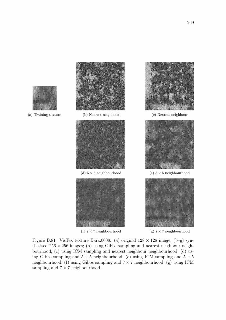
Figure B.140: VisTex texture Leaves.0002: (a) original 128 × 128 image; (b–g)synthesised 256 × 256 images; (b) using Gibbs sampling and nearest neighbourneighbourhood; (c) using ICM sampling and nearest neighbour neighbourhood; (d)using Gibbs sampling and 5 × 5 neighbourhood; (e) using ICM sampling and 5 × 5neighbourhood; (f) using Gibbs sampling and 7 × 7 neighbourhood; (g) using ICMsampling and 7 × 7 neighbourhood.

329
(a) Training texture (b) Nearest neighbour (c) Nearest neighbour
(d) 5 × 5 neighbourhood (e) 5 × 5 neighbourhood
(f) 7 × 7 neighbourhood (g) 7 × 7 neighbourhood
Figure B.141: VisTex texture Leaves.0003: (a) original 128 × 128 image; (b–g)synthesised 256 × 256 images; (b) using Gibbs sampling and nearest neighbourneighbourhood; (c) using ICM sampling and nearest neighbour neighbourhood; (d)using Gibbs sampling and 5 × 5 neighbourhood; (e) using ICM sampling and 5 × 5neighbourhood; (f) using Gibbs sampling and 7 × 7 neighbourhood; (g) using ICMsampling and 7 × 7 neighbourhood.

330
(a) Training texture (b) Nearest neighbour (c) Nearest neighbour
(d) 5 × 5 neighbourhood (e) 5 × 5 neighbourhood
(f) 7 × 7 neighbourhood (g) 7 × 7 neighbourhood
Figure B.142: VisTex texture Leaves.0004: (a) original 128 × 128 image; (b–g)synthesised 256 × 256 images; (b) using Gibbs sampling and nearest neighbourneighbourhood; (c) using ICM sampling and nearest neighbour neighbourhood; (d)using Gibbs sampling and 5 × 5 neighbourhood; (e) using ICM sampling and 5 × 5neighbourhood; (f) using Gibbs sampling and 7 × 7 neighbourhood; (g) using ICMsampling and 7 × 7 neighbourhood.

331
(a) Training texture (b) Nearest neighbour (c) Nearest neighbour
(d) 5 × 5 neighbourhood (e) 5 × 5 neighbourhood
(f) 7 × 7 neighbourhood (g) 7 × 7 neighbourhood
Figure B.143: VisTex texture Leaves.0005: (a) original 128 × 128 image; (b–g)synthesised 256 × 256 images; (b) using Gibbs sampling and nearest neighbourneighbourhood; (c) using ICM sampling and nearest neighbour neighbourhood; (d)using Gibbs sampling and 5 × 5 neighbourhood; (e) using ICM sampling and 5 × 5neighbourhood; (f) using Gibbs sampling and 7 × 7 neighbourhood; (g) using ICMsampling and 7 × 7 neighbourhood.

332
(a) Training texture (b) Nearest neighbour (c) Nearest neighbour
(d) 5 × 5 neighbourhood (e) 5 × 5 neighbourhood
(f) 7 × 7 neighbourhood (g) 7 × 7 neighbourhood
Figure B.144: VisTex texture Leaves.0006: (a) original 128 × 128 image; (b–g)synthesised 256 × 256 images; (b) using Gibbs sampling and nearest neighbourneighbourhood; (c) using ICM sampling and nearest neighbour neighbourhood; (d)using Gibbs sampling and 5 × 5 neighbourhood; (e) using ICM sampling and 5 × 5neighbourhood; (f) using Gibbs sampling and 7 × 7 neighbourhood; (g) using ICMsampling and 7 × 7 neighbourhood.

333
(a) Training texture (b) Nearest neighbour (c) Nearest neighbour
(d) 5 × 5 neighbourhood (e) 5 × 5 neighbourhood
(f) 7 × 7 neighbourhood (g) 7 × 7 neighbourhood
Figure B.145: VisTex texture Leaves.0007: (a) original 128 × 128 image; (b–g)synthesised 256 × 256 images; (b) using Gibbs sampling and nearest neighbourneighbourhood; (c) using ICM sampling and nearest neighbour neighbourhood; (d)using Gibbs sampling and 5 × 5 neighbourhood; (e) using ICM sampling and 5 × 5neighbourhood; (f) using Gibbs sampling and 7 × 7 neighbourhood; (g) using ICMsampling and 7 × 7 neighbourhood.

334
(a) Training texture (b) Nearest neighbour (c) Nearest neighbour
(d) 5 × 5 neighbourhood (e) 5 × 5 neighbourhood
(f) 7 × 7 neighbourhood (g) 7 × 7 neighbourhood
Figure B.146: VisTex texture Leaves.0008: (a) original 128 × 128 image; (b–g)synthesised 256 × 256 images; (b) using Gibbs sampling and nearest neighbourneighbourhood; (c) using ICM sampling and nearest neighbour neighbourhood; (d)using Gibbs sampling and 5 × 5 neighbourhood; (e) using ICM sampling and 5 × 5neighbourhood; (f) using Gibbs sampling and 7 × 7 neighbourhood; (g) using ICMsampling and 7 × 7 neighbourhood.

335
(a) Training texture (b) Nearest neighbour (c) Nearest neighbour
(d) 5 × 5 neighbourhood (e) 5 × 5 neighbourhood
(f) 7 × 7 neighbourhood (g) 7 × 7 neighbourhood
Figure B.147: VisTex texture Leaves.0009: (a) original 128 × 128 image; (b–g)synthesised 256 × 256 images; (b) using Gibbs sampling and nearest neighbourneighbourhood; (c) using ICM sampling and nearest neighbour neighbourhood; (d)using Gibbs sampling and 5 × 5 neighbourhood; (e) using ICM sampling and 5 × 5neighbourhood; (f) using Gibbs sampling and 7 × 7 neighbourhood; (g) using ICMsampling and 7 × 7 neighbourhood.

336
(a) Training texture (b) Nearest neighbour (c) Nearest neighbour
(d) 5 × 5 neighbourhood (e) 5 × 5 neighbourhood
(f) 7 × 7 neighbourhood (g) 7 × 7 neighbourhood
Figure B.148: VisTex texture Leaves.0010: (a) original 128 × 128 image; (b–g)synthesised 256 × 256 images; (b) using Gibbs sampling and nearest neighbourneighbourhood; (c) using ICM sampling and nearest neighbour neighbourhood; (d)using Gibbs sampling and 5 × 5 neighbourhood; (e) using ICM sampling and 5 × 5neighbourhood; (f) using Gibbs sampling and 7 × 7 neighbourhood; (g) using ICMsampling and 7 × 7 neighbourhood.

337
(a) Training texture (b) Nearest neighbour (c) Nearest neighbour
(d) 5 × 5 neighbourhood (e) 5 × 5 neighbourhood
(f) 7 × 7 neighbourhood (g) 7 × 7 neighbourhood
Figure B.149: VisTex texture Leaves.0011: (a) original 128 × 128 image; (b–g)synthesised 256 × 256 images; (b) using Gibbs sampling and nearest neighbourneighbourhood; (c) using ICM sampling and nearest neighbour neighbourhood; (d)using Gibbs sampling and 5 × 5 neighbourhood; (e) using ICM sampling and 5 × 5neighbourhood; (f) using Gibbs sampling and 7 × 7 neighbourhood; (g) using ICMsampling and 7 × 7 neighbourhood.

338
(a) Training texture (b) Nearest neighbour (c) Nearest neighbour
(d) 5 × 5 neighbourhood (e) 5 × 5 neighbourhood
(f) 7 × 7 neighbourhood (g) 7 × 7 neighbourhood
Figure B.150: VisTex texture Leaves.0012: (a) original 128 × 128 image; (b–g)synthesised 256 × 256 images; (b) using Gibbs sampling and nearest neighbourneighbourhood; (c) using ICM sampling and nearest neighbour neighbourhood; (d)using Gibbs sampling and 5 × 5 neighbourhood; (e) using ICM sampling and 5 × 5neighbourhood; (f) using Gibbs sampling and 7 × 7 neighbourhood; (g) using ICMsampling and 7 × 7 neighbourhood.

339
(a) Training texture (b) Nearest neighbour (c) Nearest neighbour
(d) 5 × 5 neighbourhood (e) 5 × 5 neighbourhood
(f) 7 × 7 neighbourhood (g) 7 × 7 neighbourhood
Figure B.151: VisTex texture Leaves.0013: (a) original 128 × 128 image; (b–g)synthesised 256 × 256 images; (b) using Gibbs sampling and nearest neighbourneighbourhood; (c) using ICM sampling and nearest neighbour neighbourhood; (d)using Gibbs sampling and 5 × 5 neighbourhood; (e) using ICM sampling and 5 × 5neighbourhood; (f) using Gibbs sampling and 7 × 7 neighbourhood; (g) using ICMsampling and 7 × 7 neighbourhood.

340
(a) Training texture (b) Nearest neighbour (c) Nearest neighbour
(d) 5 × 5 neighbourhood (e) 5 × 5 neighbourhood
(f) 7 × 7 neighbourhood (g) 7 × 7 neighbourhood
Figure B.152: VisTex texture Leaves.0014: (a) original 128 × 128 image; (b–g)synthesised 256 × 256 images; (b) using Gibbs sampling and nearest neighbourneighbourhood; (c) using ICM sampling and nearest neighbour neighbourhood; (d)using Gibbs sampling and 5 × 5 neighbourhood; (e) using ICM sampling and 5 × 5neighbourhood; (f) using Gibbs sampling and 7 × 7 neighbourhood; (g) using ICMsampling and 7 × 7 neighbourhood.

341
(a) Training texture (b) Nearest neighbour (c) Nearest neighbour
(d) 5 × 5 neighbourhood (e) 5 × 5 neighbourhood
(f) 7 × 7 neighbourhood (g) 7 × 7 neighbourhood
Figure B.153: VisTex texture Leaves.0015: (a) original 128 × 128 image; (b–g)synthesised 256 × 256 images; (b) using Gibbs sampling and nearest neighbourneighbourhood; (c) using ICM sampling and nearest neighbour neighbourhood; (d)using Gibbs sampling and 5 × 5 neighbourhood; (e) using ICM sampling and 5 × 5neighbourhood; (f) using Gibbs sampling and 7 × 7 neighbourhood; (g) using ICMsampling and 7 × 7 neighbourhood.

342
(a) Training texture (b) Nearest neighbour (c) Nearest neighbour
(d) 5 × 5 neighbourhood (e) 5 × 5 neighbourhood
(f) 7 × 7 neighbourhood (g) 7 × 7 neighbourhood
Figure B.154: VisTex texture Leaves.0016: (a) original 128 × 128 image; (b–g)synthesised 256 × 256 images; (b) using Gibbs sampling and nearest neighbourneighbourhood; (c) using ICM sampling and nearest neighbour neighbourhood; (d)using Gibbs sampling and 5 × 5 neighbourhood; (e) using ICM sampling and 5 × 5neighbourhood; (f) using Gibbs sampling and 7 × 7 neighbourhood; (g) using ICMsampling and 7 × 7 neighbourhood.

343
(a) Training texture (b) Nearest neighbour (c) Nearest neighbour
(d) 5 × 5 neighbourhood (e) 5 × 5 neighbourhood
(f) 7 × 7 neighbourhood (g) 7 × 7 neighbourhood
Figure B.155: VisTex texture Metal.0000: (a) original 128 × 128 image; (b–g) syn-thesised 256 × 256 images; (b) using Gibbs sampling and nearest neighbour neigh-bourhood; (c) using ICM sampling and nearest neighbour neighbourhood; (d) us-ing Gibbs sampling and 5 × 5 neighbourhood; (e) using ICM sampling and 5 × 5neighbourhood; (f) using Gibbs sampling and 7 × 7 neighbourhood; (g) using ICMsampling and 7 × 7 neighbourhood.

344
(a) Training texture (b) Nearest neighbour (c) Nearest neighbour
(d) 5 × 5 neighbourhood (e) 5 × 5 neighbourhood
(f) 7 × 7 neighbourhood (g) 7 × 7 neighbourhood
Figure B.156: VisTex texture Metal.0001: (a) original 128 × 128 image; (b–g) syn-thesised 256 × 256 images; (b) using Gibbs sampling and nearest neighbour neigh-bourhood; (c) using ICM sampling and nearest neighbour neighbourhood; (d) us-ing Gibbs sampling and 5 × 5 neighbourhood; (e) using ICM sampling and 5 × 5neighbourhood; (f) using Gibbs sampling and 7 × 7 neighbourhood; (g) using ICMsampling and 7 × 7 neighbourhood.

345
(a) Training texture (b) Nearest neighbour (c) Nearest neighbour
(d) 5 × 5 neighbourhood (e) 5 × 5 neighbourhood
(f) 7 × 7 neighbourhood (g) 7 × 7 neighbourhood
Figure B.157: VisTex texture Metal.0002: (a) original 128 × 128 image; (b–g) syn-thesised 256 × 256 images; (b) using Gibbs sampling and nearest neighbour neigh-bourhood; (c) using ICM sampling and nearest neighbour neighbourhood; (d) us-ing Gibbs sampling and 5 × 5 neighbourhood; (e) using ICM sampling and 5 × 5neighbourhood; (f) using Gibbs sampling and 7 × 7 neighbourhood; (g) using ICMsampling and 7 × 7 neighbourhood.

346
(a) Training texture (b) Nearest neighbour (c) Nearest neighbour
(d) 5 × 5 neighbourhood (e) 5 × 5 neighbourhood
(f) 7 × 7 neighbourhood (g) 7 × 7 neighbourhood
Figure B.158: VisTex texture Metal.0003: (a) original 128 × 128 image; (b–g) syn-thesised 256 × 256 images; (b) using Gibbs sampling and nearest neighbour neigh-bourhood; (c) using ICM sampling and nearest neighbour neighbourhood; (d) us-ing Gibbs sampling and 5 × 5 neighbourhood; (e) using ICM sampling and 5 × 5neighbourhood; (f) using Gibbs sampling and 7 × 7 neighbourhood; (g) using ICMsampling and 7 × 7 neighbourhood.

347
(a) Training texture (b) Nearest neighbour (c) Nearest neighbour
(d) 5 × 5 neighbourhood (e) 5 × 5 neighbourhood
(f) 7 × 7 neighbourhood (g) 7 × 7 neighbourhood
Figure B.159: VisTex texture Metal.0004: (a) original 128 × 128 image; (b–g) syn-thesised 256 × 256 images; (b) using Gibbs sampling and nearest neighbour neigh-bourhood; (c) using ICM sampling and nearest neighbour neighbourhood; (d) us-ing Gibbs sampling and 5 × 5 neighbourhood; (e) using ICM sampling and 5 × 5neighbourhood; (f) using Gibbs sampling and 7 × 7 neighbourhood; (g) using ICMsampling and 7 × 7 neighbourhood.

348
(a) Training texture (b) Nearest neighbour (c) Nearest neighbour
(d) 5 × 5 neighbourhood (e) 5 × 5 neighbourhood
(f) 7 × 7 neighbourhood (g) 7 × 7 neighbourhood
Figure B.160: VisTex texture Metal.0005: (a) original 128 × 128 image; (b–g) syn-thesised 256 × 256 images; (b) using Gibbs sampling and nearest neighbour neigh-bourhood; (c) using ICM sampling and nearest neighbour neighbourhood; (d) us-ing Gibbs sampling and 5 × 5 neighbourhood; (e) using ICM sampling and 5 × 5neighbourhood; (f) using Gibbs sampling and 7 × 7 neighbourhood; (g) using ICMsampling and 7 × 7 neighbourhood.

349
(a) Training texture (b) Nearest neighbour (c) Nearest neighbour
(d) 5 × 5 neighbourhood (e) 5 × 5 neighbourhood
(f) 7 × 7 neighbourhood (g) 7 × 7 neighbourhood
Figure B.161: VisTex texture WheresWaldo.0000: (a) original 128× 128 image; (b–g) synthesised 256 × 256 images; (b) using Gibbs sampling and nearest neighbourneighbourhood; (c) using ICM sampling and nearest neighbour neighbourhood; (d)using Gibbs sampling and 5 × 5 neighbourhood; (e) using ICM sampling and 5 × 5neighbourhood; (f) using Gibbs sampling and 7 × 7 neighbourhood; (g) using ICMsampling and 7 × 7 neighbourhood.

350
(a) Training texture (b) Nearest neighbour (c) Nearest neighbour
(d) 5 × 5 neighbourhood (e) 5 × 5 neighbourhood
(f) 7 × 7 neighbourhood (g) 7 × 7 neighbourhood
Figure B.162: VisTex texture WheresWaldo.0001: (a) original 128× 128 image; (b–g) synthesised 256 × 256 images; (b) using Gibbs sampling and nearest neighbourneighbourhood; (c) using ICM sampling and nearest neighbour neighbourhood; (d)using Gibbs sampling and 5 × 5 neighbourhood; (e) using ICM sampling and 5 × 5neighbourhood; (f) using Gibbs sampling and 7 × 7 neighbourhood; (g) using ICMsampling and 7 × 7 neighbourhood.

351
(a) Training texture (b) Nearest neighbour (c) Nearest neighbour
(d) 5 × 5 neighbourhood (e) 5 × 5 neighbourhood
(f) 7 × 7 neighbourhood (g) 7 × 7 neighbourhood
Figure B.163: VisTex texture WheresWaldo.0002: (a) original 128× 128 image; (b–g) synthesised 256 × 256 images; (b) using Gibbs sampling and nearest neighbourneighbourhood; (c) using ICM sampling and nearest neighbour neighbourhood; (d)using Gibbs sampling and 5 × 5 neighbourhood; (e) using ICM sampling and 5 × 5neighbourhood; (f) using Gibbs sampling and 7 × 7 neighbourhood; (g) using ICMsampling and 7 × 7 neighbourhood.

352
(a) Training texture (b) Nearest neighbour (c) Nearest neighbour
(d) 5 × 5 neighbourhood (e) 5 × 5 neighbourhood
(f) 7 × 7 neighbourhood (g) 7 × 7 neighbourhood
Figure B.164: VisTex texture Wood.0000: (a) original 128 × 128 image; (b–g) syn-thesised 256 × 256 images; (b) using Gibbs sampling and nearest neighbour neigh-bourhood; (c) using ICM sampling and nearest neighbour neighbourhood; (d) us-ing Gibbs sampling and 5 × 5 neighbourhood; (e) using ICM sampling and 5 × 5neighbourhood; (f) using Gibbs sampling and 7 × 7 neighbourhood; (g) using ICMsampling and 7 × 7 neighbourhood.
353
(a) Training texture (b) Nearest neighbour (c) Nearest neighbour
(d) 5 × 5 neighbourhood (e) 5 × 5 neighbourhood
(f) 7 × 7 neighbourhood (g) 7 × 7 neighbourhood
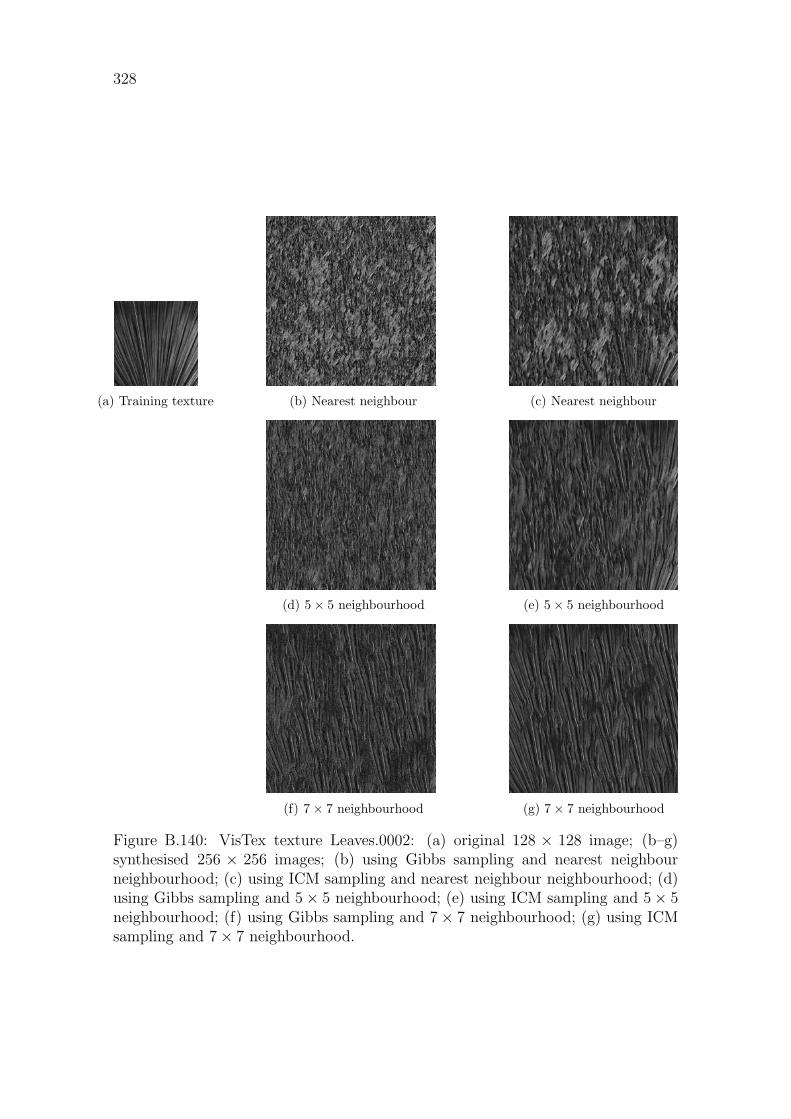
Figure B.165: VisTex texture Wood.0001: (a) original 128 × 128 image; (b–g) syn-thesised 256 × 256 images; (b) using Gibbs sampling and nearest neighbour neigh-bourhood; (c) using ICM sampling and nearest neighbour neighbourhood; (d) us-ing Gibbs sampling and 5 × 5 neighbourhood; (e) using ICM sampling and 5 × 5neighbourhood; (f) using Gibbs sampling and 7 × 7 neighbourhood; (g) using ICMsampling and 7 × 7 neighbourhood.

354
(a) Training texture (b) Nearest neighbour (c) Nearest neighbour
(d) 5 × 5 neighbourhood (e) 5 × 5 neighbourhood
(f) 7 × 7 neighbourhood (g) 7 × 7 neighbourhood
Figure B.166: VisTex texture Wood.0002: (a) original 128 × 128 image; (b–g) syn-thesised 256 × 256 images; (b) using Gibbs sampling and nearest neighbour neigh-bourhood; (c) using ICM sampling and nearest neighbour neighbourhood; (d) us-ing Gibbs sampling and 5 × 5 neighbourhood; (e) using ICM sampling and 5 × 5neighbourhood; (f) using Gibbs sampling and 7 × 7 neighbourhood; (g) using ICMsampling and 7 × 7 neighbourhood.

Bibliography
[1] C. O. Acuna, “Texture modeling using Gibbs distributions,” Computer Vi-
sion, Graphics, and Image Processing: Graphical Models and Image Process-
ing, vol. 54, no. 3, pp. 210–222, 1992.
[2] A. Agresti, D. Wackerly, and J. M. Boyett, “Exact conditional tests for cross-
classifications: approximation of attained significance levels,” Psychometrika,
vol. 44, pp. 75–83, Mar. 1979.
[3] N. Ahuja and A. Rosenfeld, “Mosaic models for textures,” IEEE Transactions
on Pattern Analysis and Machine Intelligence, vol. PAMI–3, pp. 1–10, 1981.
[4] H. Akaike, “A new look at statistical model identification,” IEEE Transactions
on Automatic Control, vol. 19, pp. 716–723, 1974.
[5] H. Akaike, “A bayesian analysis of the minimum aic procedure,” The Annals
of the Institute of Statistical Mathematics, Part A, vol. 30, pp. 9–14, 1978.
[6] D. A. Bader, J. JaJa, and R. Chellappa, “Scalable data parallel algorithms for
texture synthesis using Gibbs random fields,” IEEE Transactions on Image
Processing, vol. 4, no. 10, pp. 1456–1460, 1995.
[7] M. F. Barnsley, Fractals everywhere. Boston: Academic Press Professional,
1993.
[8] M. Basseville, A. Benveniste, K. C. Chou, S. A. Golden, R. Nikoukhah, and
A. S. Willsky, “Modeling estimation of multiresolution stochastic processes,”
IEEE Transactions on Information Theory, vol. 38, no. 2, pp. 766–784, 1992.
[9] R. K. Beatson and W. A. Light, “Fast evaluation of radial basis functions:
methods for two–dimensional polyharmonic splines,” IMA Journal of Numer-
ical Analysis, vol. 17, pp. 343–372, July 1997.
431

432 BIBLIOGRAPHY
[10] Z. Belhadj, A. Saad, S. E. Assad, J. Saillard, and D. Barba, “Comparative
study of some algorithms for terrain classification using SAR images,” in Pro-
ceedings ICASSP’94 1994 International Conference on Acoustics, Speech and
Signal Processing, vol. 5, (Adelaide), pp. 165–168, 1994.
[11] R. E. Bellman, Adaptive Control Processes: A Guided Tour. Princeton Uni-
versity press: Princeton, 1961.
[12] C. Bennis and A. Gagalowicz, “2–D macroscopic texture synthesis,” Computer
Graphics Forum, vol. 8, pp. 291–300, 1989.
[13] J. R. Bergen and E. H. Adelson, “Early vision and texture perception,” Nature,
vol. 333, pp. 363–364, May 1988.
[14] J. R. Bergen and B. Julesz, “Rapid discrimination of visual patterns,” IEEE
Transactions on Systems, Man, and Cybernetics, vol. 13, no. 5, pp. 857–863,
1983.
[15] J. R. Bergen and M. S. Landy, “Computational modeling of visual texture
segregation,” in Computational Models of Vision Processing (M. S. Landy
and J. A. Movshon, eds.), pp. 253–271, Cambridge MA: MIT Press, 1991.
[16] J. Berkson, “Maximum likelihood and minimum chi-square estimates of the
logistic function,” Journal of the American Statistical Association, vol. 50,
pp. 130–162, 1955.
[17] J. E. Besag, “Spatial interaction and the statistical analysis of lattice systems,”
Journal of the Royal Statistical Society, series B, vol. 36, pp. 192–326, 1974.
[18] J. E. Besag, “Statistical analysis of non–lattice data,” Statistician, vol. 24,
pp. 179–195, 1975.
[19] J. E. Besag, “On the statistical analysis of dirty pictures,” Journal Of The
Royal Statistical Society, vol. B–48, pp. 259–302, 1986.
[20] J. E. Besag and P. A. P. Moran, “Efficiency of pseudo–likelihood estimation
for simple Gaussian fields,” Biometrika, vol. 64, pp. 616–618, 1977.
[21] Y. M. M. Bishop, “Effects of collapsing multidimensional contingency tables,”
Biometrics, vol. 27, pp. 545–562, Sept. 1971.

BIBLIOGRAPHY 433
[22] Y. M. M. Bishop, S. E. Fienberg, and P. W. Holland, Discrete Multivariate
Analysis: Theory and Practice. Cambridge: MIT Press, 1975.
[23] J. S. D. Bonet, “Multiresolution sampling procedure for analysis and synthesis
of texture images,” in Computer Graphics, pp. 361–368, ACM SIGGRAPH,
1997. http://www.ai.mit.edu/~jsd.
[24] J. S. D. Bonet and P. Viola, “Texture recognition using a non-parametric
multi-scale statistical model,” in Proceedings IEEE Conference on Computer
Vision and Pattern Recognition, 1988. http://www.ai.mit.edu/~jsd.
[25] J. S. D. Bonet and P. Viola, “A non-parametric multi-scale statistical model
for natural images,” in Advances in Neural Information Processing, vol. 10,
1997. http://www.ai.mit.edu/~jsd.
[26] C. Bouman and B. Liu, “Multiple resolution segmentation of textured images,”
IEEE Transactions on Pattern Analysis and Machine Intelligence, vol. 13,
no. 2, pp. 99–113, 1991.
[27] C. A. Bouman and M. Shapiro, “A multiscale random field model for Bayesian
image segmentation,” IEEE Transactions on Image Processing, vol. 3, no. 2,
pp. 162–177, 1994.
[28] P. Brodatz, Textures – a photographic album for artists and designers. New
York: Dover Publications Inc., 1966.
[29] W. M. Brown and L. J. Porcello, “An introduction to synthetic aperture
radar,” IEEE Spectrum, pp. 52–62, 1969.
[30] P. J. Burt and E. H. Adelson, “The Laplacian pyramid as a compact image
code,” IEEE Transactions on Communications, vol. 31, no. 4, pp. 532–540,
1983.
[31] T. Caelli, B. Julesz, and E. Gilbert, “On perceptual analyzers underlying
visual texture discrimination: Part II,” Biological Cybernetics, vol. 29, no. 4,
pp. 201–214, 1978.
[32] J. W. Campbell and J. G. Robson, “Application of Fourier analysis to the
visibility of gratings,” Journal of Physiology, vol. 197, pp. 551–566, 1968.

434 BIBLIOGRAPHY
[33] V. Cerny, “Thermodynamical approach to the travelling salesman problem:
an efficient simulation algorithm,” Journal Of Optimization Theory And Ap-
plications, vol. 45, pp. 41–51, 1985.
[34] S. Chatterjee, “Classification of natural textures using Gaussian Markov
random field models,” in Markov Random Fields Theory And Application
(R. Chellappa and A. Jain, eds.), pp. 159–177, Boston, Sydney: Academic
Press, 1993.
[35] B. B. Chaudhuri, N. Sarkar, and P. Kundu, “Improved fractal geometry based
texture segmentation technique,” IEE Proceedings Computers And Digital
Techniques, vol. 140, pp. 233–241, Sept. 1993.
[36] R. Chellappa, Stochastic Models in Image Analysis and Processing. PhD thesis,
Purdue University, 1981.
[37] R. Chellappa and R. L. Kashyap, “Texture synthesis using 2–D noncausal
autoregressive models,” IEEE Transactions on Acoustics, Speech, and Signal
Processing, vol. ASSP–33, no. 1, pp. 194–203, 1985.
[38] R. Chellappa, R. L. Kashyap, and B. S. Manjunath, “Model–based texture seg-
mentation and classification,” in Handbook of Pattern Recognition and Com-
puter Vision (C. H. Chen, L. F. Pau, and P. S. P. Wang, eds.), pp. 277–310,
Singapore: World Scientific, 1993.
[39] R. Chellappa, “Two–dimensional discrete Gaussian Markov random field mod-
els for image processing,” in Progress in Pattern Recognition (L. N. Kanal and
A. Rosenfeld, eds.), vol. 2, pp. 79–122, North–Holland Pub. Co., 1985.
[40] R. Chellappa and S. Chatterjee, “Classification of textures using Gaussian
Markov random fields,” IEEE Transactions on Acoustics, Speech, and Signal
Processing, vol. ASSP–33, no. 4, pp. 959–963, 1985.
[41] C. C. Chen, J. S. DaPonte, and M. D. Fox, “Fractal feature analysis and
classification in medical imaging,” IEEE Transactions on Medical Imaging,
vol. 8, pp. 133–142, June 1989.
[42] C. C. Chen and R. C. Dubes, “Experiments in fitting discrete Markov ran-
dom fields to textures,” in Proceedings CVPR ’89 IEEE Computer Society
Conference on Computer Vision and Pattern Recognition, (San Diego, CA),
pp. 298–303, IEEE Comput. Soc. Press, June 1989.

BIBLIOGRAPHY 435
[43] C.-C. Chen, Markov random fields in image processing. PhD thesis, Michigan
State University, 1988.
[44] C. Chubb and M. S. Landy, “Orthogonal distribution analysis: a new approach
to the study of texture perception,” in Computational Models of Vision Pro-
cessing (M. S. Landy and J. A. Movshon, eds.), pp. 291–301, Cambridge MA:
MIT Press, 1991.
[45] M. Clark, A. C. Bovik, and W. S. Geisler, “Texture segmentation using Gabor
modulation/demodulation,” Pattern Recognition Letters, vol. 6, no. 4, pp. 261–
267, 1987.
[46] J. M. Coggins, A Framework for Texture Analysis Based on Spatial Filtering.
PhD thesis, Computer Science Department, Michigan Stat University, East
Lansing, MI, 1982.
[47] J. M. Coggins and A. K. Jain, “A spatial filtering approach to texture analy-
sis,” Pattern-Recognition-Letters, vol. 3, pp. 195–203, May 1985.
[48] F. S. Cohen and D. B. Cooper, “Simple parallel hierarchical and relaxation
algorithms for segmenting noncausal Markovian random fields,” IEEE Trans-
actions on Pattern Analysis and Machine Intelligence, vol. 9, pp. 195–219,
Mar. 1987.
[49] Computer Vision Group, “Segmentation of textured images,” http: //
www-dbv. cs. uni-bonn. de/ image/ segmentation. html , Apr. 1997.
[50] G. C. Cross and A. K. Jain, “Markov random field texture models,” IEEE
Transactions on Pattern Analysis and Machine Intelligence, vol. 5, pp. 25–39,
1983.
[51] J. Dale, “Asymptotic normality of goodness-of-fit statistics for sparse product
multinomials,” Journal of the Royal Statistical Association, vol. 48, no. 1,
pp. 48–59, 1986.
[52] J. G. Daugman, “Two-dimensional spectral analysis of cortical receptive field
profiles,” Vision Research, vol. 20, no. 10, pp. 847–856, 1980.
[53] E. J. Delp, R. L. Kashyap, and O. R. Mitchell, “Image data compression
using autoregressive time series models,” Pattern Recognition, vol. 11, no. 5–
6, pp. 313–323, 1979.

436 BIBLIOGRAPHY
[54] H. Derin and H. Elliott, “Modelling and segmentation of noisy textured im-
ages using Gibbs random fields,” IEEE Transactions on Pattern Analysis and
Machine Intelligence, vol. PAMI–9, no. 1, pp. 39–55, 1987.
[55] H. Derin and C.-S. Won, “A parallel image segmentation algorithm using
relaxation with varying neighbourhoods and its mapping to array processors,”
Computer Vision, Graphics, and Image Processing, vol. 40, pp. 54–78, 1987.
[56] R. L. Devalois, D. G. Albrecht, and L. G. Thorell, “Spatial-frequency selectiv-
ity of cells in macaque visual cortex,” Vision Research, vol. 22, pp. 545–559,
1982.
[57] P. Dewaele, L. Van-Gool, A. Wambacq, and A. Oosterlinck, “Texture inspec-
tion with self-adaptive convolution filters,” in Proceedings 9th International
Conference on Pattern Recognition, vol. 2, (Rome, Italy), pp. 56–60, IEEE
Computer Society Press, Nov. 1988.
[58] L. J. Du, “Texture segmentation of SAR images using localized spatial filter-
ing,” in Proceedings of International Geoscience and Remote Sensing Sympo-
sium, vol. III, (Washington, DC), pp. 1983–1986, 1990.
[59] R. C. Dubes and A. K. Jain, “Random field models in image analysis,” Journal
of Applied Statistics, vol. 16, no. 2, pp. 131–164, 1989.
[60] R. O. Duda and P. E. Hart, Pattern Classification and Scene Analysis. Stan-
ford Reseach Institute, Menlo Park, California: John Wiley, 1973.
[61] Earth Resources Observation Systems, “EROS data center: Earthshots,”
http: // edcwww. cr. usgs. gov/ Earthshots , Feb. 1997.
[62] European Space Agency, Committee on Earth Observation Satellites: Coordi-
nation for the next decade. United Kingdom: Smith System Engineering Ltd,
1995.
[63] European Space Agency, “Earth observation home page,” http: // earth1.
esrin. esa. it/ index. html , Jan. 1998.
[64] Y. fai Wong, “How Gaussian radial basis functions work,” in Proceedings
IJCNN – International Joint Conference on Neural Networks 91, vol. 2, (Seat-
tle), pp. 133–138, IEEE, July 1991.

BIBLIOGRAPHY 437
[65] F. Farrokhnia, Multi-channel filtering techniques for texture segmentation and
surface quality inspection. PhD thesis, Computer Science Department, Michi-
gan State University, 1990.
[66] J. Feder, Fractals. Physics of solids and liquids, New York: Plenum Press,
1988.
[67] S. E. Fienberg, The Analysis of Cross–Classified Categorical Data, vol. Second
Edition. MIT Press, 1981.
[68] R. A. Fisher, Statistical Methods for Research Workers. Edinburgh: Oliver
and Boyd, 5th ed., 1934.
[69] J. P. Fitch, Synthetic Aperture Radar. Springer–Verlag, 1988.
[70] I. Fogel and D. Sagi, “Gabor filters as texture discriminator,” Biological Cy-
bernetics, vol. 61, pp. 103–113, 1989.
[71] J. M. Francos and A. Z. Meiri, “A unified structural–stochastic model for
texture analysis and synthesis,” in Proceedings 5th International Conference
on Pattern Recognition, (Washington), pp. 41–46, 1988.
[72] R. T. Frankot and R. Chellappa, “Lognormal random–field models and their
applications to radar image synthesis,” IEEE Transactions on Geoscience and
Remote Sensing, vol. 25, pp. 195–207, Mar. 1987.
[73] T. Freeman, “What is imaging radar ?,” http: // southport. jpl. nasa.
gov/ desc/ imagingradarv3. html , Jan. 1996.
[74] K. Fukunaga and L. D. Hostetler, “The estimation of the gradient of a density
function, with applications in pattern recognition,” IEEE Trans. Info. Thy.,
vol. IT–21, pp. 32–40, 1975.
[75] A. Gagalowicz, S. D. Ma, and C. Tournier-Lasserve, “Third order model for
non homogeneous natural textures,” in Proceedings 8th International Con-
ference on Pattern Recognition (ICPR), vol. 1, (Paris, France), pp. 409–411,
1986.
[76] J. Garding, “Properties of fractal intensity surfaces,” Pattern Recognition Let-
ters, vol. 8, pp. 319–324, Dec. 1988.

438 BIBLIOGRAPHY
[77] J. R. Garside and C. J. Oliver, “A comparison of clutter texture properties
in optical and SAR images,” in 1988 International Geoscience and Remote
Sensing Symposium (IGARSS88), vol. 3, pp. 1249–1255, 1988.
[78] D. Geman, “Random fields and inverse problems in imaging,” in Lecture Notes
in Mathematics, vol. 1427, pp. 113–193, Springer–Verlag, 1991.
[79] D. Geman, S. Geman, and C. Graffigne, “Locating texture and object bound-
aries,” in Pattern Recognition Theory and Applications (P. A. Devijver and
J. Kittler, eds.), New York: Springer–Verlag, 1987.
[80] D. Geman, S. Geman, C. Graffigne, and P. Dong, “Boundary detection by con-
strained optimization,” IEEE Transactions on Pattern Analysis and Machine
Intelligence, vol. 12, no. 7, pp. 609–628, 1990.
[81] S. Geman and C. Graffigne, “Markov random field image models and their
applications to computer vision,” Proceedings of the International Congress of
Mathematicians, pp. 1496–1517, 1986.
[82] S. Geman and D. Geman, “Stochastic relaxation, Gibbs distributions, and the
Bayesian restoration of images,” IEEE Transactions on Pattern Analysis and
Machine Intelligence, vol. 6, no. 6, pp. 721–741, 1984.
[83] M. A. Georgeson, “Spatial Fourier analysis and human vision,” in Tutorial
Essays, A Guide to Recent Advances (N. S. Sutherland, ed.), vol. 2, ch. 2,
Hillsdale, NJ: Lawrence Erlbaum Associates, 1979.
[84] C. J. Geyer and E. A. Thompson, “Constrained Monte Carlo maximum like-
lihood for dependent data,” Journal of the Royal Statistical Society, Series B,
vol. 54, pp. 657–699, 1992.
[85] J. J. Gibson, The Perception of the Visual World. Boston, MA: Houghton
Mifflin, 1950.
[86] B. Gidas, “A renormalization group approach to image processing problems,”
IEEE Transactions on Pattern Analysis and Machine Intelligence, vol. 11,
no. 2, pp. 164–180, 1989.
[87] J. W. Goodman, “A random walk through the field of speckle,” Optical Engi-
neering, vol. 25, no. 5, 1986.

BIBLIOGRAPHY 439
[88] L. A. Goodman, “The multivariate analysis of qualitative data: interactions
among multiple classifications,” Journal of the American Statistical Associa-
tion, vol. 65, pp. 226–256, Mar. 1970.
[89] C. Graffigne, Experiments in texture analysis and segmentation. PhD thesis,
Division of Applied Mathematics, Brown University, 1987.
[90] P. J. Green, “Discussion: On the statistical analysis of dirty pictures,” Journal
Of The Royal Statistical Society, vol. B–48, pp. 259–302, 1986.
[91] H. Greenspan, R. Goodman, R. Chellappa, and C. H. Anderson, “Learning
texture discrimination rules in multiresolution system,” IEEE Transactions on
Pattern Analysis and Machine Intelligence, vol. 16, no. 9, pp. 894–901, 1994.
[92] G. R. Grimmett, “A theorem about random fields,” Bulletin of the London
Mathematical Society, vol. 5, pp. 81–84, 1973.
[93] T. D. Guyenne and G. Calabresi, Monitoring the Earth’s Environment. A
Pilot Project Campaign on LANDSAT Thematic Mapper Applications (1985–
87). Noordwijk, Netherlands: European Space Agency Publications Division,
1989.
[94] G. J. Hahn and S. S. Shapiro, Statistical Models in Engineering. John Wiley
and Sons, 1967.
[95] M. Haindl, “Texture synthesis,” CWI Quarterly, vol. 4, pp. 305–331, 1991.
[96] J. M. Hammersley and P. Clifford, “Markov fields on finite graphs and lat-
tices.” unpublished, 1971.
[97] J. A. Hanley and B. J. McNeil, “The meaning and use of the area under a
receiver operating characteristic (roc) curve,” Radiology, vol. 143, pp. 29–36,
1982.
[98] R. M. Haralick, “Statistical and structural approaches to texture,” Proceedings
of IEEE, vol. 67, no. 5, pp. 786–804, 1979.
[99] R. M. Haralick, “Texture analysis,” in Handbook of pattern recognition and
image processing (T. Y. Young and K.-S. Fu, eds.), ch. 11, pp. 247–279, San
Diego: Academic Press, 1986.

440 BIBLIOGRAPHY
[100] R. M. Haralick, K. Shanmugam, and I. Dinstein, “Textural features for image
classification,” IEEE Transactions on Systems, Man, and Cybertinetics, vol. 3,
no. 6, pp. 610–621, 1973.
[101] M. Hassner and J. Sklansky, “The use of Markov random fields as models
of texture,” Computer Graphics and Image Processing, vol. 12, pp. 357–370,
1980.
[102] J. K. Hawkins, “Textural properties for pattern recognition,” in Picture Pro-
cessing and Psychopictorics (B. Lipkin and A. Rosenfeld, eds.), New York:
Academic Press, 1969.
[103] D. J. Heeger and J. R. Bergen, “Pyramid–based texture analysis/synthesis,”
in Proceedings ICIP–95: 1995 International Conference on Image Processing,
(Washington, D.C.), pp. 648–651, 1995.
[104] J. Homer, J. Meagher, R. Paget, and D. Longstaff, “Terrain classification via
texture modelling of SAR and SAR coherency images,” in Proceedings of 1997
IEEE International International Geoscience and Remote Sensing Symposium
(IGARSS’97), (Singapore), pp. 2063–2065, Aug. 1997.
[105] D. Howard, Markov random fields and image processing. PhD thesis, Flinders
University, Adelaide, 1995.
[106] R. Hu and M. M. Fahmy, “Texture segmentation based on a hierarchical
Markov random field model,” Signal processing, vol. 26, no. 3, pp. 285–305,
1992.
[107] A. K. Jain and F. F. D. H. Alman, “Texture analysis of automotive finishes,” in
Proceedings of SME Machine Vision Applications Conference, (Detroit, MI),
pp. 1–16, Nov. 1990.
[108] A. K. Jain and S. Bhattacharjee, “Text segmentation using Gabor filters for
automatic document processing,” Machine Vision and Applications, vol. 5,
no. 3, pp. 169–184, 1992.
[109] A. K. Jain and F. Farrokhnia, “Unsupervised texture segmentation using Ga-
bor filters,” Pattern Recognition, vol. 24, no. 12, pp. 1167–1186, 1991.
[110] B. Julesz, “Visual pattern discrimination,” IRE transactions on Information
Theory, vol. 8, pp. 84–92, 1962.

BIBLIOGRAPHY 441
[111] B. Julesz, “Textons, the elements of texture perception, and their interac-
tions,” Nature, vol. 290, pp. 91–97, Mar. 1981.
[112] B. Julesz, “A theory of preattentive texture discrimination based on first–order
statistics of textons,” Biological Cybernetics, vol. 41, no. 2, pp. 131–138, 1981.
[113] L. N. Kanal, “Markov mesh models,” Computer Graphics and Image Process-
ing, vol. 12, pp. 371–375, Apr. 1980.
[114] R. L. Kashyap, “Analysis and synthesis of image pattern by spatial interaction
models,” in Progress in Pattern Recognition (L. N. Kanal and A. Rosenfeld,
eds.), pp. 149–186, New York: North–Holland Pub. Co., 1981.
[115] R. L. Kashyap, “Characterization and estimation of two–dimensional ARMA
models,” IEEE Transactions on Information Theory, vol. 30, pp. 736–745,
1984.
[116] R. L. Kashyap and R. Chellappa, “Estimation and choice of neighbors in
spatial–interaction models of images,” IEEE Transactions on Information
Theory, vol. IT–29, no. 1, pp. 60–72, 1983.
[117] Z. Kato, J. Zerubia, and M. Berthod, “Unsupervised parallel image classifica-
tion using a hierarchical Markovian model,” in 1995 IEEE 5th International
Conference on Computer Vision (B. Werner, ed.), (Los Alamitos), pp. 169–
174, IEEE Computer Society Press, 1995.
[118] J. M. Keller, R. M. Crownover, and R. Y. Chen, “Characteristics of natu-
ral scenes related to the fractal dimension,” IEEE Transactions on Pattern
Analysis and Machine Intelligence, vol. 9, pp. 621–627, Sept. 1987.
[119] J. M. Keller, S. Chen, and R. M. Crownover, “Texture description and seg-
mentation through fractal geometry,” Computer vision, graphic, and image
processing, vol. 45, p. 150, Feb. 1989.
[120] A. Khotanzad and R. L. Kashyap, “Feature selection for texture recognition
based on image synthesis,” IEEE Transactions on Systems, Man and Cyber-
netics, vol. 17, pp. 1087–1095, Nov. 1987.
[121] R. Kindermann and J. L. Snell, Markov Random Fields and their applications.
American Mathematical Society, 1980.

442 BIBLIOGRAPHY
[122] S. Kirkpatrick, C. D. Gellatt, J. Vecchi, and M. P. Vecchi, “Optimization by
simulated annealing,” Science, vol. 220, pp. 671–680, 1983.
[123] K. J. Koehler, “Goodness-of-fit tests for log-linear models in sparse con-
tingency tables,” Journal of the American Statistical Association, vol. 81,
pp. 483–493, June 1986.
[124] W. L. G. Koontz, P. M. Narendra, and K. Fukunaga, “A graph–theoretic ap-
proach to nonparametric cluster analysis,” IEEE Transactions on Computers,
vol. C–25, pp. 936–944, 1976.
[125] S. Krishnamachari and R. Chellappa, “Multiresolution Gauss-Markov random
field models for texture segmentation,” IEEE Transactions on Image Process-
ing, vol. 6, pp. 251–267, Feb. 1997.
[126] S. N. Laboratories, “How SAR works,” http: // www. sandia. gov/ RADAR/
sar_ sub/ sar_ intro1. html , Jan. 1996.
[127] G. H. Landeweerd and E. S. Gelsema, “The use of nuclear texture parameters
in the automatic analysis of leukocytes,” Pattern Recognition, vol. 10, no. 2,
pp. 57–61, 1978.
[128] L. L. Lapin, Probability and Statistics for Modern Engineering. Boston: PWS–
KENT, 1990.
[129] K. Larntz, “Small-sample comparisons of exact levels for chi-squared goodness-
of-fit statistics,” Journal of the American Statistical Association, vol. 73,
pp. 253–263, June 1978.
[130] K. I. Laws, Textured image segmentation. PhD thesis, University of Southern
California, 1980.
[131] J. H. Lee and W. D. Philpot, “A spectral–textural classifier for digital im-
agery,” in Proceedings International Geoscience and Remote Sensing Sympo-
sium, (Washington, DC), pp. 2005–2008, 1990.
[132] T. M. Lillesand and R. W. Kiefer, Remote Sensing and Image Interpretation.
New York: John Wiley and Sons, 1987.
[133] Y. Linde, A. Buzo, and R. M. Gray, “An algorithm for vector quantizer de-
sign,” IEEE Transactions on Communications, vol. COM–28, pp. 84–95, Jan.
1980.

BIBLIOGRAPHY 443
[134] M. R. Luettgen, W. C. Karl, A. S. Willsky, and R. R. Tenny, “Multiscale repre-
sentation of Markov random fields,” IEEE Transactions on Signal Processing,
vol. 41, no. 12, pp. 3377–3396, 1993.
[135] A. Lundervold, “Ultrasonic tissue characterisation–a pattern recognition ap-
proach,” tech. rep., Norwegian Computing Center, Oslo, Norway, 1992.
[136] J. Malik and P. Perona, “Preattentive texture discrimination with early vision
mechanisms,” Journal of the Optical Society of America A, vol. 7, pp. 923–932,
May 1990.
[137] B. B. Mandelbrot, The Fractal Geometry of Nature. New York: W. H. Free-
man, 1983.
[138] B. S. Manjunath and R. Chellappa, “Unsupervised texture segmentation using
Markov random field models,” IEEE Transactions on Pattern Analysis and
Machine Intelligence, vol. 13, no. 5, pp. 478–482, 1991.
[139] D. Marr and E. Hildreth, “Theory of edge detection,” Proceedings of the Royal
Society B, vol. 207, pp. 187–217, 1980.
[140] J. L. Marroquin, S. Mitter, and T. Poggio, “Probabilistic solution of ill–posed
problems in compuational vision,” Journal of American Statistics Association,
vol. 82, pp. 76–89, 1987.
[141] C. R. Mehta and N. R. Patel, “Algorithm 643. fexact: A fortran subroutine for
fisher’s exact test on unordered r x c contingency tables,” ACM Transactions
on Mathematical Software, vol. 12, pp. 154–161, June 1986.
[142] N. Metropolis, A. W. Rosenbluth, M. N. Rosenbluth, A. H. Teller, and
E. Teller, “Equations of state calculations by fast computing machines,” Jour-
nal of Chemical Physics, vol. 21, pp. 1087–1091, 1953.
[143] Microwave Radar Division, Electronics and Surveillance Research Laboratory
at DSTO, Australia, “Project Ingara,” 1997.
[144] J. W. Modestino and J. Zhang, “A Markov random field model–based ap-
proach to image interpretation,” IEEE Transactions on Pattern Analysis and
Machine Intelligence, vol. 14, pp. 606–615, June 1992.
[145] Moody and Darken, “Fast learning in networks of locally–tuned processing
units,” Neural Computation, vol. 1, pp. 281–294, 1989.

444 BIBLIOGRAPHY
[146] C. Morris, “Central limit theorems for multinomial sums,” The Annals of
Statistics, vol. 3, no. 1, pp. 165–188, 1975.
[147] A. Mosquera, D. Cabello, and M. J. Carreira, “A fractal–based approach to
texture segmentation,” Conference publication, vol. 354, p. 450, 1992.
[148] J. Moussouris, “Gibbs and Markov random systems with constraints,” Journal
of Statistical Physics, vol. 10, no. 1, pp. 11–33, 1974.
[149] R. Navarro and J. Portilla, “Robust method for texture synthesis–by–analysis
based on a multiscale Gabor scheme,” in SPIE Electronic Imaging Symposium,
Human Vision and Electronic Imaging ’96 (B. Rogowitz and J. Allebach, eds.),
vol. 2657, (San Jose, Calfornia), pp. 86–97, 1996.
[150] H. C. Nothdurft, “Texton segregation by associated differences in global and
local luminance distribution,” Proceedings of the Royal Society B, vol. 239,
pp. 295–320, 1990.
[151] P. P. Ohanian and R. C. Dubes, “Performance evaluation for four classes of
textural features,” Pattern Recognition, vol. 25, pp. 819–833, Aug. 1992.
[152] R. Paget and D. Longstaff, “Texture synthesis via a nonparametric Markov
random field,” in Proceedings of DICTA–95, Digital Image Computing: Tech-
niques and Applications (A. Maeder and B. Lovell, eds.), vol. 1, (Brisbane,
Australia), pp. 547–552, Australian Pattern Recognition Society, Dec. 1995.
http://www.vision.ee.ethz.ch/~rpaget.
[153] R. Paget and D. Longstaff, “A nonparametric multiscale Markov random
field model for synthesising natural textures,” in Fourth International Sym-
posium on Signal Processing and its Applications, vol. 2, (Gold Coast, Aus-
tralia), pp. 744–747, ISSPA 96, Aug. 1996. http://www.vision.ee.ethz.
ch/~rpaget.
[154] R. Paget and D. Longstaff, “Extracting the cliques from a neighbourhood sys-
tem,” IEE Proceedings Vision, Image and Signal Processing, vol. 144, pp. 168–
170, June 1997. http://www.vision.ee.ethz.ch/~rpaget.
[155] R. Paget and D. Longstaff, “Texture synthesis and unsupervised recognition
with a nonparametric multiscale Markov random field model,” in Proceed-
ings of 14th International Conference on Pattern Recognition (A. K. Jain,

BIBLIOGRAPHY 445
S. Venkatesh, and B. C. Lovell, eds.), vol. 2, (Brisbane, Australia), pp. 1068–
1070, IAPR, Aug. 1998. http://www.vision.ee.ethz.ch/~rpaget.
[156] R. Paget and D. Longstaff, “Texture synthesis via a noncausal nonparametric
multiscale Markov random field,” IEEE Transactions on Image Processing,
vol. 7, pp. 925–931, June 1998. http://www.vision.ee.ethz.ch/~rpaget.
[157] R. Paget, D. Longstaff, and B. Lovell, “Multiprocessor implementation of a
texture segmentation scheme for satellite radar images,” in DICTA–93, Digital
Image Computing: Techniques and Applications (K. K. Fung and A. Ginige,
eds.), vol. 1, (Sydney), pp. 203–211, Australian Pattern Recognition Society,
Dec. 1993.
[158] R. Paget, D. Longstaff, and B. Lovell, “Texture classification using non-
parametric Markov random fields,” in Proceedings of the 1997 13th Inter-
national Conference on Digital Signal Processing, vol. 1, (Hellas, Santorini,
Greece), pp. 67–70, IEEE Signal Processing Society, July 1997. Invited Paper,
http://www.vision.ee.ethz.ch/~rpaget.
[159] A. P. Pentland, “Fractal–based description of natural scenes,” IEEE Transac-
tions on Pattern Analysis and Machine Intelligence, vol. 6, pp. 661–674, Nov.
1984.
[160] A. P. Pentland, “Shading into texture,” Artificial Intelligence, vol. 29, pp. 147–
170, Aug. 1986.
[161] D. K. Picard, “Inference for general Ising models,” Journal of Applied Proba-
bility, vol. 19A, pp. 345–357, 1982.
[162] D. K. Pickard, “Inference for discrete Markov feilds: the simplest nontrivial
case,” Journal of the American Statistical Association, vol. 82, pp. 90–96,
1987.
[163] T. Poggio and F. Girosi, “Networks for approximation and learning,” Proceed-
ings of the IEEE, vol. 78, pp. 1481–1497, Sept. 1990.
[164] K. Popat and R. W. Picard, “Novel cluster–based probability model for tex-
ture synthesis, classification, and compression,” in Proceedings SPIE visual
Communications and Image Processing, (Boston), 1993.

446 BIBLIOGRAPHY
[165] A. Possolo, “Subsampling a random field,” in Spatial Statistics and Imaging
(A. Possolo, ed.), vol. 20, pp. 286–294, IMS Lecture Notes – Monograph Series,
1991.
[166] W. K. Pratt, O. D. Faugeras, and A. Gagalowicz, “Visual discrimination of
stochastic texture fields,” IEEE Transactions on Systems, Man and Cybernet-
ics, vol. 8, pp. 796–804, Nov. 1978.
[167] W. H. Press, S. A. Teukolsky, W. T. Vetterling, and B. P. Flannery, Numerical
Recipes in C. Cambridge University Press, 2nd ed., 1992.
[168] P. P. Raghu, R. Poongodi, and B. Yegnanarayana, “Unsupervised texture
classification using vector quantization and deterministic relaxation neural
network,” IEEE Transactions on Image Processing, vol. 6, no. 10, pp. 1376–
1387, 1997.
[169] T. R. C. Read and N. A. C. Cressie, Goodness–of–fit Statistics for Discrete
Multivariate Data. Springer–Verlag, 1988.
[170] T. R. Reed and H. Wechsler, “Segmentation of textured images and Gestalt
organization using spatial/spatial-frequency representations,” IEEE Transac-
tions on Pattern Analysis and Machine Intelligence, vol. 12, pp. 1–12, Jan.
1990.
[171] J. A. Richards, Remote Sensing Digital Image Analysis: An Introduction.
Berlin: Springer–Verlag, 1993.
[172] W. Richards and A. Polit, “Texture matching,” Kybernetic, vol. 16, no. 3,
pp. 155–162, 1974.
[173] E. Rignot and R. Chellappa, “Segmentation of polarimetric synthetic aperture
radar data,” IEEE Transactions on Image Processing, vol. 1, no. 3, pp. 281–
299, 1992.
[174] E. Rignot and R. Kwok, “Extraction of textural features in SAR images:
Statistical model and sensitivity,” in Pcoceedings International Geoscience and
Remote Sensing Symposium, (Washington, DC), pp. 1979–1982, 1990.
[175] B. D. Ripley, Statistical inference for spatial processes. Cambridge: University
Press, 1988.

BIBLIOGRAPHY 447
[176] J. Rissanen, “Stochastic complexity,” Journal of the Royal Statistical Society,
Series B, vol. 49, pp. 223–239, 1984.
[177] G. C. Rota, “On the foundations of combinatorial theory,” Zeitschrift Fur
Wahrscheinlichkeitstheorie Und Verwandte Gebietee, vol. 2, pp. 340–368, 1964.
[178] A. H. Schistad and A. K. Jain, “Texture analysis in the presence of speckle
noise,” in Proceedings IEEE Geoscience and Remote Sensing Symposium,
(Houston, TX), pp. 147–152, May 1992.
[179] G. Schwarz, “Estimating the dimension of a model,” The Annals of Statistics,
vol. 6, pp. 461–464, 1978.
[180] D. W. Scott and J. R. Thompson, “Probability density estimation in higher
dimensions,” in Computer Science and Statistics: Proceedings of the Fifteenth
Symposium on the Interface, (Amsterdam: North–Holland), pp. 173–179,
1983.
[181] L. Seymour, Parameter estimation and model selection in image analysis using
Gibbs–Markov random fields. PhD thesis, The University of North Carolina,
Chapel Hill, 1993.
[182] L. H. Siew, R. M. Hodgson, and E. J. Wood, “Texture measures for carpet
wear assessment,” IEEE Transactions on Pattern Analysis and Machine In-
telligence, vol. 10, pp. 92–105, Jan. 1988.
[183] B. W. Silverman, Density estimation for statistics and data analysis. London:
Chapman and Hall, 1986.
[184] J. Sklansky, “Image segmentation and feature extraction,” IEEE Transactions
on Systems, Man, Cybernetics, vol. 8, pp. 237–247, Apr. 1978.
[185] D. M. Smith, “Speckle reduction and segmentation of synthetic aperture radar
images,” International Journal of Remote Sensing, vol. 17, no. 11, pp. 2043–
2057, 1996.
[186] G. Smith, Image texture analysis using zero crossings information. PhD
thesis, University of Queensland, St Lucia, QLD Australia, 1998, http:
//www.cssip.uq.edu.au/~guy/thesis/home.html.
[187] G. Smith, “Meastex image texture database and test suite,” http: // www.
cssip. uq. edu. au/ staff/ meastex/ meastex. html , Jan. 1998.

448 BIBLIOGRAPHY
[188] K. R. Smith and M. I. Miller, “A Bayesian approach incorporating Rissanen
complexity for learning Markov random field texture models,” in Proceedings
ICASSP, vol. 4, pp. 2317–2320, 1990.
[189] F. Spitzer, “Markov random fields and Gibbs ensembles,” American Mathe-
matical Monthly, vol. 78, pp. 142–154, 1971.
[190] H. Tamura, S. Mori, and T. Yamawaki, “Textural features corresponding to
visual perception,” IEEE Transactions on Systems, Man and Cybernetics,
vol. SMC–8, pp. 460–473, June 1978.
[191] H. Tamura, S. Mori, and Y. Yammawaki, “Textural features corresponding to
visual perception,” IEEE Transactions on Systems, Man, Cybernetics, vol. 8,
pp. 460–473, June 1978.
[192] T. Taxt, P. J. Flynn, and A. K. Jain, “Segmentation of document images,”
IEEE Transactions on Pattern Analysis and Machine Intelligence, vol. 11,
pp. 1322–1329, Dec. 1989.
[193] D. Terzopoulos, “Image analysis using multigrid relaxation methods,” IEEE
Transactions on Pattern Analysis and Machine Intelligence, vol. 8, no. 2,
pp. 129–139, 1986.
[194] C. W. Therrien, “An estimation-theoretic approach to terrain image segmenta-
tion,” Computer Vision, Graphics, and Image Processing, vol. 22, pp. 313–326,
June 1983.
[195] M. Tuceryan, “Moment based texture segmentation,” in Proceedings of the
11th International Conference on Pattern Recognition, vol. 3, pp. 45–48, Aug.
1992.
[196] M. Tuceryan and A. K. Jain, “Texture analysis,” in Handbook of Pattern
Recognition and Computer Vision (C. H. Chen, L. F. Pau, and P. S. P. Wang,
eds.), pp. 235–276, Singapore: World Scientific, 1993.
[197] M. R. Turner, “Texture discrimination by Gabor functions,” Biological Cyber-
netics, vol. 55, no. 2–3, pp. 71–82, 1986.
[198] F. T. Ulaby, R. K. Moore, and A. K. Fung, Active and Passive Microwave
Remote Sensing. Massachusetts: Addison–Wesley, 1982.

BIBLIOGRAPHY 449
[199] F. T. Ulaby and M. C. Dobson, Handbook of Radar Scattering Statistics for
Terrain. Norwood, Mass.: Artech House, 1989.
[200] M. Unser and M. Eden, “Nonlinear operators for improving texture segmenta-
tion based on features extracted by spatial filtering,” IEEE Transactions On
Systems, Man, and Cybernet, vol. 20, p. 804, July 1990.
[201] L. Van-Gool, P. Dewaele, and A. Oosterlinck, “Texture analysis anno 1983,”
Computer Vision, Graphics, and Image Processing, vol. 29, pp. 336–357, Mar.
1985.
[202] A. Verbeek and P. M. Kroonenberg, “A survey of algorithms for exact dis-
tributions of test statistics in r x c contingency tables with fixed margins,”
Computational Statistics and Data Analysis, vol. 3, pp. 159–185, 1985.
[203] Vision and Modeling Group, “Vistex texture.” http://www-white.media.
mit.edu/vismod/imagery/VisionTexture/vistex.html%, 1995.
[204] H. Voorhees and T. Poggio, “Computing texture boundaries in images,” Na-
ture, vol. 333, pp. 364–367, May 1988.
[205] H. Wechsler, “Texture analysis – a survey,” Signal Processing, vol. 2, pp. 271–
282, 1980.
[206] R. Wilson and M. Spann, “Finite prolate spheroidal sequences and their appli-
cations II: Image feature description and segmentation,” IEEE Transactions
on Pattern Analysis and Machine Intelligence, vol. 10, no. 2, 1988.
[207] R. Wilson and M. Spann, Image Segmentation and Uncertainty. Research
Studies Press Ltd, 1988.
[208] M. Woodroofe, “On model selection and arcsine laws,” Annals of Statistics,
vol. 10, pp. 1182–1194, 1982.
[209] J. D. Woodruff, T. L. Angtuaco, and T. H. Parmley, Atlas of Gynecologic
pathology. New York: Raven press, 2nd ed., 1993.
[210] J. W. Woods, S. Dravida, and R. Mediavilla, “Image estimation using dou-
bly stochastic Gaussian random field models,” IEEE Transactions on Pattern
Analysis and Machine Intelligence, vol. 9, pp. 245–253, Mar. 1987.

450 BIBLIOGRAPHY
[211] S. C. Zhu, Y. Wu, and D. Mumford, “FRAME: filters, random fields, rnd
minimax entropy towards a unified theory for texture modeling,” Proceedings
1996 IEEE Computer Society Conference on Computer Vision and Pattern
Recognition, pp. 686–693, 1996.
[212] S. W. Zucker and K. Kant, “Multiple-level representation for texture discrim-
ination,” in Proceedings IEEE Conference on Pattern Recognition and Image
Processing, (Dallas, TX), pp. 609–614, 1981.