Sensors2012, 12, 15244-15266; doi:10.3390/s121115244OPEN ACCESS

sensorsISSN 1424-8220

www.mdpi.com/journal/sensors

Article

Virtual Sensors for Designing Irrigation Controllers inGreenhouses

Jorge Antonio Sanchez1,⋆, Francisco Rodrıguez1, Jose Luis Guzman 1 and Manuel R. Arahal 2

1 Ingenierıa de Sistemas y Automatica, Departamento de Lenguajes y Computacion, The Agrifood

Campus of International Excellence (ceiA3), Universidad de Almerıa, Ctra de la Playa s/n.,

Almerıa 04120, Spain; E-Mails: frrodrig@ual.es (F.R.); joguzman@ual.es (J.L.G.)2 Departamento de Ingenierıa de Sistemas y Automatica, Escuela Superior de Ingenieros, Universidad

de Sevilla, Camino de los Descubrimientos s/n, Sevilla 41092, Spain; E-Mail: arahal@esi.us.es

* Author to whom correspondence should be addressed; E-Mail:jorgesanchez@ual.es;

Tel./Fax: +34-950-014-536.

Received: 3 August 2012; in revised form: 19 October 2012 / Accepted: 22 October 2012 /

Published: 8 November 2012

Abstract: Monitoring the greenhouse transpiration for control purposes is currently a

difficult task. The absence of affordable sensors that provide continuous transpiration

measurements motivates the use of estimators. In the case oftomato crops, the availability

of estimators allows the design of automatic fertirrigation (irrigation + fertilization) schemes

in greenhouses, minimizing the dispensed water while fulfilling crop needs. This paper

shows how system identification techniques can be applied toobtain nonlinear virtual

sensors for estimating transpiration. The greenhouse usedfor this study is equipped with

a microlysimeter, which allows one to continuously sample the transpiration values. While

the microlysimeter is an advantageous piece of equipment for research, it is also expensive

and requires maintenance. This paper presents the design and development of a virtual sensor

to model the crop transpiration, hence avoiding the use of this kind of expensive sensor. The

resulting virtual sensor is obtained by dynamical system identification techniques based on

regressors taken from variables typically found in a greenhouse, such as global radiation

and vapor pressure deficit. The virtual sensor is thus based on empirical data. In this

paper, some effort has been made to eliminate some problems associated with grey-box

models: advance phenomenon and overestimation. The results are tested with real data

and compared with other approaches. Better results are obtained with the use of nonlinear

Black-box virtual sensors. This sensor is based on global radiation and vapor pressure deficit

Sensors2012, 12 15245

(VPD) measurements. Predictive results for the three models are developed for comparative

purposes.

Keywords: virtual sensor; transpiration; nonlinear model; micro-lysimeter

1. Introduction

Crop growth is primarily determined by climatic variables of the environment and the amount of water

and fertilizers applied through irrigation. Therefore, controlling these variables allows for control of the

growth. The greenhouse environment is ideal for farming because these variables can be manipulated

to achieve optimal growth and plant development. All crops need solar radiation, CO2, water, and

nutrients to produce biomass (roots, stems, leaves, and fruits) through the process of photosynthesis.

During this process, and when the leaves stomata are opened to capture the CO2, the plant emits water

vapor through the transpiration process. This becomes a cost that the crop must make to produce dry

matter. Moreover, water is lost through evaporation from the soil. The sum of these water losses is

known as evapotranspiration. The losses must be compensated through irrigation. Besides, it has

been demonstrated in padded greenhouses with soil covered with plastic blankets that the amount of

evaporation is negligible. This happens when dealing with hydroponic cultivations [1]. According to

this, water should be applied in precise amounts to cover only water losses due to crop transpiration.

Excess water would mean an excessive washing out of fertilizers. In turn, it could lead to contamination

of the subterranean water, or the flooding of the substratum or radicular asphyxiation. Otherwise, a

hydric deficit may be provoked if irrigation does not provideenough water. This can lead to a decrease in

production and can even be dangerous for the crop growth. Hence, automatic irrigation control systems

are fundamental tools to supply water to the culture in the required amount and frequency. Moreover, as

water is a limited resource in many agricultural areas, optimizing productivity through efficient and

adequate irrigation is a basic objective. In order to designa good automatic irrigation system, the

following questions must be answered: what should the frequency of the irrigations be, and how much

water should be applied in the irrigation? To answer these questions, it is necessary to know how much

water should be applied to replenish the losses due to the transpiration during the plant’s respiration.

Measuring the water lost by transpiration is a way of obtaining the plant’s water demand. This

estimation of transpiration in different species grown in greenhouses has been developed, e.g., by

Baille et al. [2] for ornamentals, Stanghellini [1], Jemaa [3], Boulard [4] and Baille [2] for tomatoes,

Montero et al. [5] for geranium crops, Medranoet al. [6] for cucumbers, Suayet al. [7] for rose

cultivation, Voogtet al. [8] for chrysanthemums, and Schmidt and Exarchou [9] for gerbera pots,

among others.

In most of these works, the microlysimeter became the basic measurement device to record the water

losses in crops, subtracting the water content in an instant(t) by the water content in another instant

(t−1). However, on many occasions, the measurements were not continuous due to the irrigation process

or during the water drainage. Furthermore, it is seldom usedby farmers since this device is expensive

to acquire and to maintain. From an operational point of view, it is important to find alternatives to

Sensors2012, 12 15246

this irrigation system gadget. Thus, virtual sensors basedon transpiration become a good option to

reduce total system cost, especially in the agriculture sector where profit margins are so narrow. Such

virtual sensors must be based on sensors that are typically installed in greenhouses for climate control

(temperature, humidity, and solar radiation), thereby reducing the installations costs.

Virtual sensors become a very efficient and powerful tool that has been successfully used in other

fields [10–12]. These sensors utilize models in order to estimate features from low-cost measurements.

Ideally, the virtual sensors should be simple and obtainable from the collected data. It should not require

extensive training. Virtual sensors are useful in replacing physical sensors, thus reducing hardware

redundancy and acquisition cost, or as part of the fault detection methodologies by having their output

compared with that of a corresponding actual sensor. Virtual sensors may be developed based on

mathematical models obtained directly from the Physics of the system and first principles. In many

cases, such mathematical models are unavailable, or their exact parameter values are unknown, or they

are too complicated to be used. For this reason, the development of virtual sensors often has to be based

on system identification [13].

The purpose of the current study is to develop a virtual sensor to infer transpiration from other

easily measured variables. For this purpose, the use of the microlysimeter as the sensor to calculate

the transpiration must be substituted, due to its high cost in acquisition and maintenance. In this

paper, the development of the virtual sensor for transpiration makes use of different techniques for

data preprocessing, including the selection of variables,the construction of appropriate training, the

selection of test sets, the final validation and the performance assessment. The resulting virtual sensor

has been validated and compared with real data and with othervirtual sensors in the literature, providing

promising results.

The paper is organized as follows: Section2 shows a background of different sensors used

to take transpiration measurements. The different virtualsensors are shown in the Section3.

Section4 gives an overview of the greenhouse where the experiments were performed, and its main

characteristics, as well as the collected experimental data. The main results and discussions are

summarized in Section5. Finally, the major conclusions are drawn.

2. Crop Transpiration

The irrigation control systems are essential tools to provide water to the crop in the required amount

and frequency. Moreover, water is a limiting resource in many agricultural areas. In such places, it

should be a basic objective to optimize their management andproductivity through adequate and efficient

irrigation. The proposed control algorithm design (Figure1) is a hierarchical control system, consisting

of two levels:

• The control level uses an event-based PI controller [14], to control when a certain event occurs,

either by time, by variation of a particular climatic variable such as radiationVSR), or by a

particular state crop. A PI controller is used to achieve thesetpoint of water supply (XQWr)

as it considers the top layer of the architecture.

• The setpoint generation level is based on the greenhouse climate conditions, including: (1) vapor

pressure deficit (VPD,VV PD), which is a function of the temperature and the relative humidity,

Sensors2012, 12 15247

(2) global radiation, and (3) the state of the crop, measuredthrough the Leaf Area Index (LAI,

XLAI). The setpoint is fixed by the user and is defined as the crop transpiration accumulated

(XET ) until an irrigation event occurs (XQW ). This event could be a determined transpiration

accumulated setpoint or other predetermined conditions.

Figure 1. Irrigation control algorithm.

The virtual sensor accumulates the amount of water lost by transpiration from the plant’s last

irrigation. This measurement is compared with the fixed amount that activates irrigation (setpoint).

The irrigation starts when this fixed value is exceeded, and finishes as soon as the amount of water lost

has been replenished.

A virtual sensor requires an accurate calibration and validation of the instantaneous transpiration

measurements at each sampling instant. The measurement of transpiration includes direct (observation,

porometer, lysimeter,etc.), and indirect methods (water budget, energy balance,etc.). The indirect

methods are more complicated for prediction and verification of the transpiration values because of the

meteorological factors involved. The transpiration data can be collected through direct methods such as:

• Theporometer[15] allows the determination of the leaf conductivity as an index of the stomatal

opening and the closing of stomata. It measures the flow of gases or diffusion that takes place

through the stomata. The latest porometers allow computerized records.

• Thebag method[16] collects the water transpired by introducing a branch in a clear plastic bag.

The transpired water condenses inside the bag. The total water lost by transpiration corresponds

with the weight of the placed water. The time between measurements is undefined, as it depends

on the water collected.

• In thecobalt chloridemethod [17], the transpiration is indicated by a color change of a pieceof

filter paper impregnated with a 3% solution of cobalt chloride. It is applied on a leaf and held in

place with a clip. It is blue when dry and pink when wet. The speed at which the paper changes

color is an indication of the rate of transpiration. This method can be used to measure the relative

rates of transpiration of different species.

Sensors2012, 12 15248

• Themicrolysimeter[1,4] is used in plants growing in pots completely closed. The plants are first

weighed before measuring, and then they are weighed again atconvenient time intervals. Soil

evaporation is avoided by covering it with waterproof material. This method can be used with

small plants and crops in soilless culture. The results are expressed in grams or milliliters of water

transpired per leaf area per unit time.

The microlysimeter is the basic measurement device used to continuously record the water losses

in crops. Contrarily, the rest of the described sensors takemeasurements at intervals as they modify

the working conditions of the plants. The porometer and microlysimeter are expensive to acquire and

maintain, and are difficult for the farmers to manage.

3. Virtual Sensors

This section is devoted to describing the main features of three different types of virtual sensors

for transpiration designed to replace the microlysimeter in the automatic irrigation system. The aim

of such virtual sensors is to substitute the expensive microlysimeter in measuring the transpiration and

controlling the irrigation.

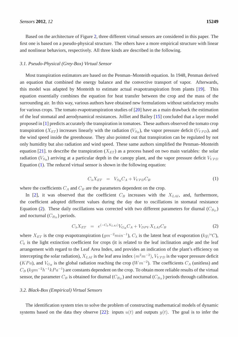
Figure 2 shows the input variables of a virtual sensor for crop transpiration: (1) global (solar)

radiation, (2) Vapor Pressure Deficit (VPD), which is a function of the temperature (T) and the relative

humidity (RH), and (3) Leaf Area Index (LAI). These variables are measured by two different sensors

typically installed in commercial greenhouses: a psychrometer for the temperature and the relative

humidity (VPD), and a pyranometer for the solar radiation.

Figure 2. Virtual sensor scheme.

The transpiration model needs to calculate the LAI. The LAI measurements are taken in a

noncontinuous way. In this paper, a simplified TOMGRO model [18] adapted to the Mediterranean

conditions is utilized to estimate the LAI. The simplified TOMGRO model needs the temperature as

the input.

Sensors2012, 12 15249

Based on the architecture of Figure2, three different virtual sensors are considered in this paper. The

first one is based on a pseudo-physical structure. The othershave a more empirical structure with linear

and nonlinear behaviors, respectively. All three kinds aredescribed in the following.

3.1. Pseudo-Physical (Grey-Box) Virtual Sensor

Most transpiration estimators are based on the Penman–Monteith equation. In 1948, Penman derived

an equation that combined the energy balance and the convective transport of vapor. Afterwards,

this model was adapted by Monteith to estimate actual evapotranspiration from plants [19]. This

equation essentially combines the equation for heat transfer between the crop and the mass of the

surrounding air. In this way, various authors have obtainednew formulations without satisfactory results

for various crops. The tomato evapotranspiration studies of [20] have as a main drawback the estimation

of the leaf stomatal and aerodynamical resistances. Jolliet and Bailey [15] concluded that a layer model

proposed in [1] predicts accurately the transpiration in tomatoes. Theseauthors observed the tomato crop

transpiration (XET ) increases linearly with the radiation (VSR), the vapor pressure deficit (VV PD), and

the wind speed inside the greenhouse. They also pointed out that transpiration can be regulated by not

only humidity but also radiation and wind speed. These same authors simplified the Penman–Monteith

equation [21]. to describe the transpiration (XET ) as a process based on two main variables: the solar

radiation (VSR) arriving at a particular depth in the canopy plant, and the vapor pressure deficitVV PD

Equation (1). The reduced virtual sensor is shown in the following equation:

CλXET = VSRCA + VV PDCB (1)

where the coefficientsCA andCB are the parameters dependent on the crop.

In [2], it was observed that the coefficientCB increases with theXLAI , and, furthermore,

the coefficient adopted different values during the day due to oscillations in stomatal resistance

Equation (2). These daily oscillations was corrected with two different parameters for diurnal (CBD)

and nocturnal (CBN) periods.

CλXET = e(−CkXLAI )VGRCA + VDPVXLAICB (2)

whereXET is the crop evapotranspiration (gm−2min−1), Cλ is the latent heat of evaporation (kg/oC),

Ck is the light extinction coefficient for crops (it is related to the leaf inclination angle and the leaf

arrangement with regard to the Leaf Area Index, and providesan indication of the plant’s efficiency on

intercepting the solar radiation),XLAI is the leaf area index(m2m−2), VV PD is the vapor pressure deficit

(KPa), andVGRis the global radiation reaching the crop (Wm−2). The coefficientsCA (unitless) and

CB (kgm−2h−1kPa−1) are constants dependent on the crop. To obtain more reliable results of the virtual

sensor, the parameterCB is obtained for diurnal (CBD) and nocturnal (CBN

) periods through calibration.

3.2. Black-Box (Empirical) Virtual Sensors

The identification system tries to solve the problem of constructing mathematical models of dynamic

systems based on the data they observe [22]: inputs u(t) and outputsy(t). The goal is to infer the

Sensors2012, 12 15250

relationship between sampled outputs and inputs. The identification process was carried out based on

prior knowledge of dynamic behavior of gases [14] and the behavior of transpiration ([1,2,6]). VPD and

global radiation was selected as climatic inputs and the LAIas crop growth input.

This method is used with the objective of knowing how the dynamics of the systems work and

responding to some of the questions raised while drawing up this document.

3.2.1. Linear Black-Box Virtual Sensors

The parametric virtual sensors (or black box) are diagrams capable of representing any system without

having any knowledge about the physical process dynamics. Parametric virtual sensors are not obtained

(at least not completely) from the application of physical laws. These virtual sensors are constructed

using observations carried out on the system so as to select aconcrete value of the parameters. This

value is chosen in such a way that the virtual sensor can accommodate the results to the acquired data.

This process is called identification.

The adjustment of the parameters is the simplest part of the problem of identification [23]. Online

identification concerns an algorithm that efficiently uses the measured information when it is obtained

from the plant in real time. In this way, it is possible to detect the changes in the dynamics of the system

and adjust the virtual sensor conveniently. Under some circumstances, these methods can be rather

simple (e.g., the method of minimal recurrent squares developed in this section).

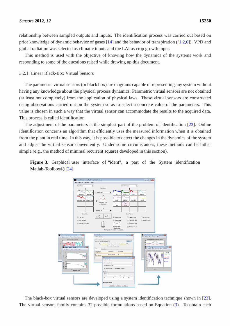
Figure 3. Graphical user interface of “ident”, a part of the System identification

Matlab-Toolboxr [24].

The black-box virtual sensors are developed using a system identification technique shown in [23].

The virtual sensors family contains 32 possible formulations based on Equation (3). To obtain each

Sensors2012, 12 15251

one of the structures, it is necessary to determine the polynomial order as well as the coefficient of the

numerator and the denominator for each transfer function [23]. The effects to the inputs, output, and the

disturbances are defined as:

A(z)y(t) = B(z)F (z)

u(t− nk) + C(z)D(z)

e(t) (3)

where,y(t) is the transpiration,u(t) is the different input variables, ande(t) is the estimation error.

A(z), B(z), C(z), D(z), E(z), andF (z) represent the polynomials that define the output (transpiration),

inputs, and the estimation error. The order of the polynomial equations is defined by regressors, where

na outlines the outputs,nb is the order of the input, andnk is the delay of the radiation solar(nkVGR)

and the vapor pressure deficit(nkVV PD). System Identification Matlab’s Toolbox [24] was used for the

identification process. The ARX, ARMAX, OUTPUT ERROR, BOX JENKINS, and FIR formulations

were tried out. The differences among these virtual sensorsare the way in which the inputs, outputs

and disturbances are defined with parametric equations. TheSystem Identification Toolbox of Matlab(R)

software was used to obtain the virtual sensor. Figure3 shows the main interface of the Toolbox and

the whole process to obtain a virtual sensor. The top of the figure displays the calibration and validation

process interface, and the bottom shows the output analysisprocess. The toolbox allows to process

data, estimate the parameters of different types of structures, and validate virtual sensors using different

strategies. For the identification process, only the data from the experiments are required. The data can

be handled in the time domain or frequency domain, and the experiments can have one or multiple inputs

and/or outputs [25].

3.2.2. Nonlinear Black-Box Virtual Sensors

A nonlinear component was added to the transpiration virtual sensor to get better fitting. This

component is introduced as result of the strong nonlinear behavior in the system inputs. Moreover,

these nonlinearities add complexity to the virtual sensor.This increase in complexity is not always

translated into higher performance. In System Identification the mathematical relationships between the

system’s inputsu(t), and outputsy(t) can be computed. Such outputs, inputs, and nonlinearities are

introduced in anad hocform, relying ona priori knowledge about the system. An important step in

system identification is to choose a structure, and generally start testing the simpler structures, and

lower order. The first structure tested, and in the end chosenas virtual sensors, was the nonlinear

ARX (4). Also the Hammerstein–Wiener virtual sensor was tried out, which are very useful in the

case of the nonlinearities affect to sensors, and actuators, such as dead zones or saturation [24]. On the

other hand, Nonlinear ARX (NonARX) is more flexible [24]. The general structure for Nonlinear ARX

virtual sensor is [26]:

y(t) = f(y(t− 1), y(t− 2), y(t− 3), ..., u(t), u(t− 1), u(t− 2), ..) (4)

wherey(t) is the output variable int time;u andy are the different input and output variables (regressors);

and f is the nonlinear function. The current transpiration valueis predicted as a weighted sum of past

values, and current and past inputs values. With such information the equation becomes:

Sensors2012, 12 15252

y(t) = [a1, a2, ..., ana, b1, b2, ..., bnb][y(t− 1), y(t− 2), ..., y(t− na), u(t), u(t− 1), ..., u(t− nb− 1)]T

(5)

wherey(t− 1), y(t− 2), ..., y(t− na), u(t), u(t− 1), ..., u(t − nb − 1 are the regressors, the so-called

delayed inputs and outputs. Nonlinear ARX regressors can beboth delayed input–output variables and

more complex nonlinear expressions of delayed variables. The nonlinearity estimator block maps the

regressors to the virtual sensor output using a combinationof nonlinear and linear functions (Figure4).

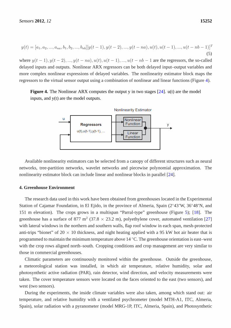
Figure 4. The Nonlinear ARX computes the output y in two stages [24]. u(t) are the model

inputs, and y(t) are the model outputs.

Available nonlinearity estimators can be selected from a canopy of different structures such as neural

networks, tree-partition networks, wavelet networks and piecewise polynomial approximation. The

nonlinearity estimator block can include linear and nonlinear blocks in parallel [24].

4. Greenhouse Environment

The research data used in this work have been obtained from greenhouses located in the Experimental

Station of Cajamar Foundation, in El Ejido, in the province of Almeria, Spain (2◦43’W, 36◦48’N, and

151 m elevation). The crops grows in a multispan “Parral-type” greenhouse (Figure5); [18]. The

greenhouse has a surface of 877 m2 (37.8× 23.2 m), polyethylene cover, automated ventilation [27]

with lateral windows in the northern and southern walls, flaproof window in each span, mesh-protected

anti-trips “bionet” of 20× 10 thickness, and night heating applied with a 95 kW hot air heater that is

programmed to maintain the minimum temperature above 14◦C. The greenhouse orientation is east–west

with the crop rows aligned north–south. Cropping conditions and crop management are very similar to

those in commercial greenhouses.

Climatic parameters are continuously monitored within thegreenhouse. Outside the greenhouse,

a meteorological station was installed, in which air temperature, relative humidity, solar and

photosynthetic active radiation (PAR), rain detector, wind direction, and velocity measurements were

taken. The cover temperature sensors were located on the faces oriented to the east (two sensors), and

west (two sensors).

During the experiments, the inside climate variables were also taken, among which stand out: air

temperature, and relative humidity with a ventilated psychrometer (model MTH-A1, ITC, Almeria,

Spain), solar radiation with a pyranometer (model MRG-1P, ITC, Almeria, Spain), and Photosynthetic

Sensors2012, 12 15253

active radiation (PAR) with a silicon sensor (PAR Lite, Kipp–Zonnen, Delft, The Netherlands). Among

all the climate sensors installed in the greenhouse, only solar radiation and psychrometer was used for

the transpiration virtual sensors.

The daylight air temperature and humidity are controlled bythe top and side windows through the

PI controller [28]. Potentiometers allow for knowing the window’s position in each control instant. The

night air temperature and humidity is controlled by the windows and the heating system [28]. Setpoints

of both systems are established at 24◦C [27], and 14◦C for the ventilation and heating, respectively. All

the actuators are driven by relays designed for this task.

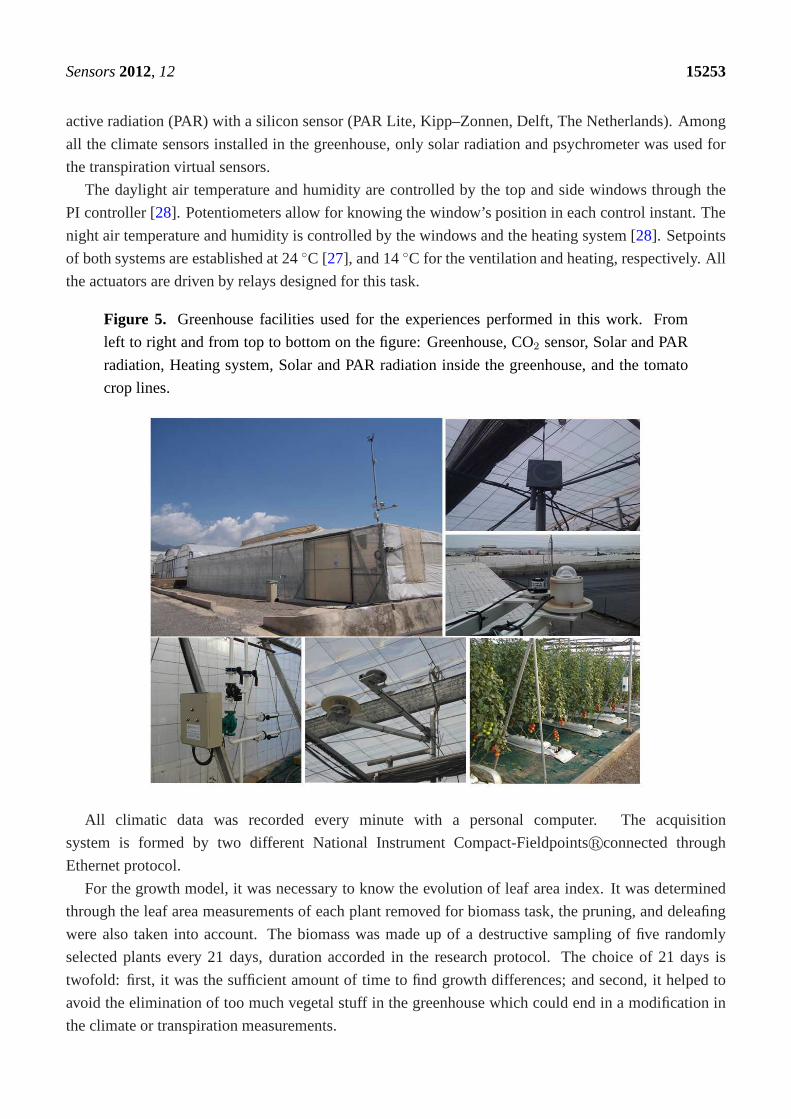
Figure 5. Greenhouse facilities used for the experiences performed in this work. From

left to right and from top to bottom on the figure: Greenhouse,CO2 sensor, Solar and PAR

radiation, Heating system, Solar and PAR radiation inside the greenhouse, and the tomato

crop lines.

All climatic data was recorded every minute with a personal computer. The acquisition

system is formed by two different National Instrument Compact-Fieldpointsrconnected through

Ethernet protocol.

For the growth model, it was necessary to know the evolution of leaf area index. It was determined

through the leaf area measurements of each plant removed forbiomass task, the pruning, and deleafing

were also taken into account. The biomass was made up of a destructive sampling of five randomly

selected plants every 21 days, duration accorded in the research protocol. The choice of 21 days is

twofold: first, it was the sufficient amount of time to find growth differences; and second, it helped to

avoid the elimination of too much vegetal stuff in the greenhouse which could end in a modification in

the climate or transpiration measurements.

Sensors2012, 12 15254

The biomass process was measured against: number of nodes, leaf area, number of fruits per bunch,

fresh and dry weight of leaves, stem, and fruits. The plant material and fruits were introduced into a

drying oven where they remained for 24–48 h (depending on thephenological state) at a temperature of

65 ◦C. Based on this, the dry matter of leaves, stems, and fruits was determined by analytical balance.

The matter of leaves and secondary stems pruning came from the selected plants for biomass while kept

in production; once removed from the plant, the fresh and dryweight was taken, such as the biomass. In

the case of pruning, stems and leaves are measured separately. Both the bare and the pruning are carried

out for the leaf area index measures, executed, as in the biomass, through electronic planimeter (Delta-T

Devices Ltd).

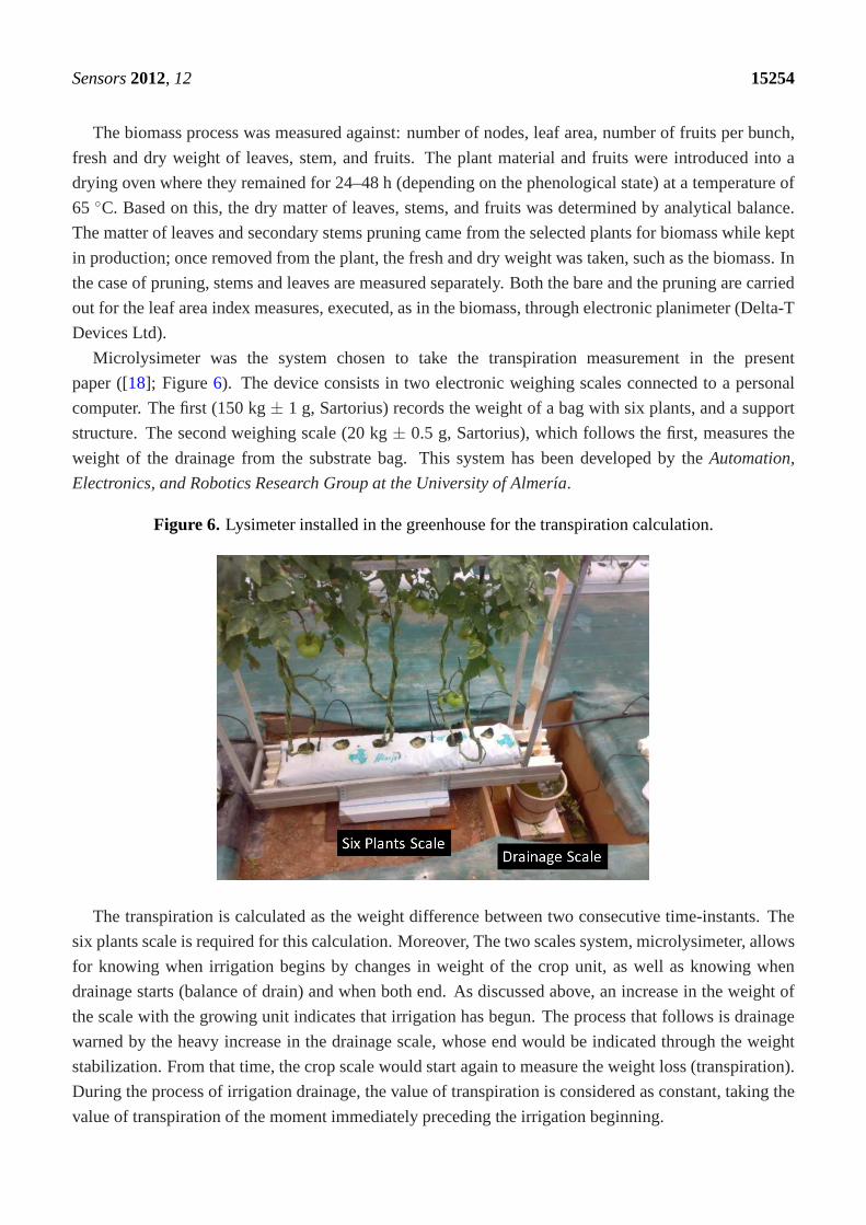
Microlysimeter was the system chosen to take the transpiration measurement in the present

paper ([18]; Figure 6). The device consists in two electronic weighing scales connected to a personal

computer. The first (150 kg± 1 g, Sartorius) records the weight of a bag with six plants, and a support

structure. The second weighing scale (20 kg± 0.5 g, Sartorius), which follows the first, measures the

weight of the drainage from the substrate bag. This system has been developed by theAutomation,

Electronics, and Robotics Research Group at the Universityof Almerıa.

Figure 6. Lysimeter installed in the greenhouse for the transpiration calculation.

The transpiration is calculated as the weight difference between two consecutive time-instants. The

six plants scale is required for this calculation. Moreover, The two scales system, microlysimeter, allows

for knowing when irrigation begins by changes in weight of the crop unit, as well as knowing when

drainage starts (balance of drain) and when both end. As discussed above, an increase in the weight of

the scale with the growing unit indicates that irrigation has begun. The process that follows is drainage

warned by the heavy increase in the drainage scale, whose endwould be indicated through the weight

stabilization. From that time, the crop scale would start again to measure the weight loss (transpiration).

During the process of irrigation drainage, the value of transpiration is considered as constant, taking the

value of transpiration of the moment immediately precedingthe irrigation beginning.

Sensors2012, 12 15255

5. Results and Discussions

5.1. Transpiration Measurements Validation

An important step was to validate the calculation of crop transpiration for each of the cycles, seeing

that this data corresponds to the transpiration of the crop at that time. For this issue, five trays with

twelve plants were installed and evenly distributed throughout the greenhouse so as to make their mean

representative of the entire crop. The trays consisted of two bags of substrate with six plants in each

bag, which gives us a total of twelve plants per tray and 60 in the entire test. All trays had drainage

connected to a bucket whose sample was collected daily at thesame hour. Thus, the average value of

these buckets were taken daily to calculate the real drainage. Two differently located droppers were

selected to collect daily irrigation amounts in the greenhouse; the final value was estimated from the

average of both measures. With data from the drainage and from the droppers, the daily measured

consumption was calculated and compared with accumulated daily transpiration from the data every

minute, obtaining the graphs (Figures7 and8) for the two selected cycles (spring–summer 2008 and

autumn–winter 2008–2009, respectively).

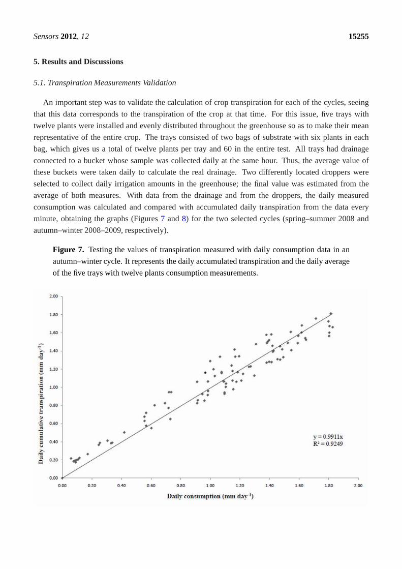
Figure 7. Testing the values of transpiration measured with daily consumption data in an

autumn–winter cycle. It represents the daily accumulated transpiration and the daily average

of the five trays with twelve plants consumption measurements.

Sensors2012, 12 15256

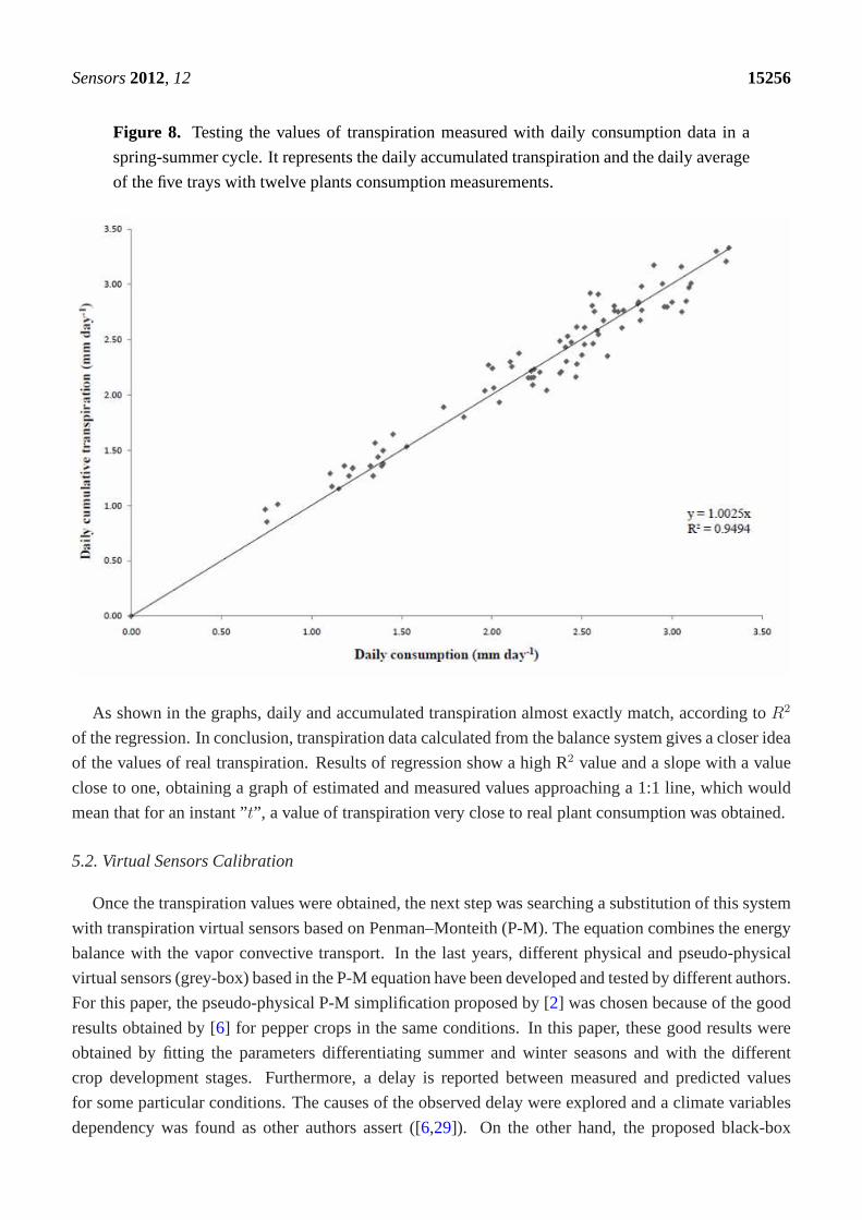
Figure 8. Testing the values of transpiration measured with daily consumption data in a

spring-summer cycle. It represents the daily accumulated transpiration and the daily average

of the five trays with twelve plants consumption measurements.

As shown in the graphs, daily and accumulated transpirationalmost exactly match, according toR2

of the regression. In conclusion, transpiration data calculated from the balance system gives a closer idea

of the values of real transpiration. Results of regression show a high R2 value and a slope with a value

close to one, obtaining a graph of estimated and measured values approaching a 1:1 line, which would

mean that for an instant ”t”, a value of transpiration very close to real plant consumption was obtained.

5.2. Virtual Sensors Calibration

Once the transpiration values were obtained, the next step was searching a substitution of this system

with transpiration virtual sensors based on Penman–Monteith (P-M). The equation combines the energy

balance with the vapor convective transport. In the last years, different physical and pseudo-physical

virtual sensors (grey-box) based in the P-M equation have been developed and tested by different authors.

For this paper, the pseudo-physical P-M simplification proposed by [2] was chosen because of the good

results obtained by [6] for pepper crops in the same conditions. In this paper, these good results were

obtained by fitting the parameters differentiating summer and winter seasons and with the different

crop development stages. Furthermore, a delay is reported between measured and predicted values

for some particular conditions. The causes of the observed delay were explored and a climate variables

dependency was found as other authors assert ([6,29]). On the other hand, the proposed black-box

Sensors2012, 12 15257

dynamic virtual sensors would be used to design events basedon fertirrigation controller. In order to use

a modern control algorithm, the use of dynamic virtual sensors joined system identification techniques

and are presented as an alternative to physical or pseudo-physical virtual sensors. The proposed virtual

sensors incorporate the dynamics of transpiration and willbe of varying complexity, beginning with

linear black-box virtual sensors fitted to data. Nonlinear virtual sensors based in system identification

was tried out obtaining good results. Nonlinearities will be introduced in anad hocform, relying ona

priori knowledge about the system.

5.2.1. Grey-Box Virtual Sensor

The calibration of the virtual sensor of transpiration proposed by [2] were performed with two

different seasons: one in spring, in 2005 (Table1), and the other in autumn–winter, in 2006–2007.

For the calibration of the spring–summer cycle, all the datagathered during the months of February and

July 2005 was used. In contrast, in the case of the winter cycle, the data used was from August 2006

to February 2007. The parameters were determined using an iterative sequential algorithm to minimize

the least square error criterion between the real and the estimated transpiration (Montecarlo algorithms).

The second phase of the calibration process was based in genetic algorithms to fix the final parameters.

The values obtained from the extinction ratio of the radiation (CK), 0.64 for spring–summer cycles and

0.6 for autumn–winter, matched the results obtained by other authors in the autumn–winter cycle, with

equivalent closeness, who obtained an extinction ratio of0.63. [1] determined a value of 0.64 to cultivate

the tomato, [6] obtained values of0.63 to cultivate the cucumber. For most horticultural crops in

greenhouses, the values of (CK) fluctuate between0.4 and0.8 [6]. Values obtained from parameters

CA, CBDandCBN

are different for both groups of crop cycles to which have been referred, obtaining

values in the spring cycle forCA, CBD, andCBN

of 0.49, 11.2, and 8.28 respectively, and for the

autumn–winter cycle, the same parameters obtained values:CA, CBD, andCBN

of 0.3, 18.7, and8.3,

respectively. The next table shows the results of the different parameters calibration:

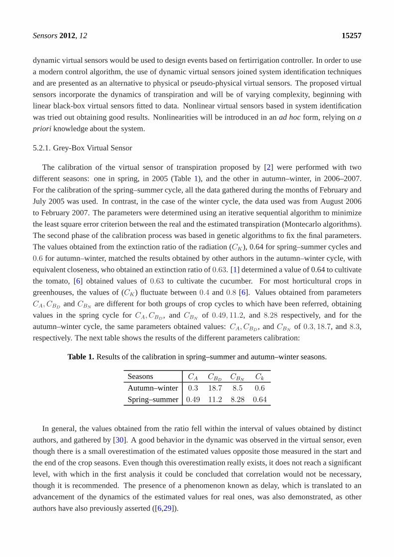
Table 1. Results of the calibration in spring–summer and autumn–winter seasons.

Seasons CA CBDCBN

Ck

Autumn–winter 0.3 18.7 8.5 0.6

Spring–summer 0.49 11.2 8.28 0.64

In general, the values obtained from the ratio fell within the interval of values obtained by distinct

authors, and gathered by [30]. A good behavior in the dynamic was observed in the virtual sensor, even

though there is a small overestimation of the estimated values opposite those measured in the start and

the end of the crop seasons. Even though this overestimationreally exists, it does not reach a significant

level, with which in the first analysis it could be concluded that correlation would not be necessary,

though it is recommended. The presence of a phenomenon knownas delay, which is translated to an

advancement of the dynamics of the estimated values for realones, was also demonstrated, as other

authors have also previously asserted ([6,29]).

Sensors2012, 12 15258

To calibrate grey-box virtual sensor described in section (Section3.1), a growth model is required

to try out the LAI estimations. The simplified model Tomgro [18] rises as an option to remove the

complexity of the full virtual sensor proposed by [31] and make them available to online control systems

while retaining their physiological characteristics [32]. The parameter that influence the dynamics

of theXLAI was calibrated and validated, first by [18] and later by [33] in the same greenhouse for

tomato crops.

5.2.2. Linear Black-Box Virtual Sensors

To obtain a virtual sensor, it was necessary to choose two groups of transpiration data to try out in

the system identification toolbox. One group from spring 2007 was taken for identification, resulting

in a total of 53,490 data. For identification validation, 49,990 data from winter 2004 was used. The

remaining data was used to obtain the virtual sensor’s reliability. The black-box virtual sensor cannot

contain data with time slots without data. For this reason, smaller groups of data are used. The

Table 2 shows the virtual sensors that have been obtained. More than1,500 structures were tested,

leaving to validation two ARX virtual sensors and an ARMAX virtual sensor. In this case, LAI was not

introduced into the system as an entry. The reason for this isthat the rate of leaf area index remains

constant in the same day, lacking the dynamic of remaining input variables.XLAI was used to divide

the crop cycle in different intervals, from 0 to 0.7 , from 0.7to 1.5, and above 1.5(m2cropm

−2soil). For the

division, it is easy to change the LAI, for instance, by days after planting (DAP), or others time units.

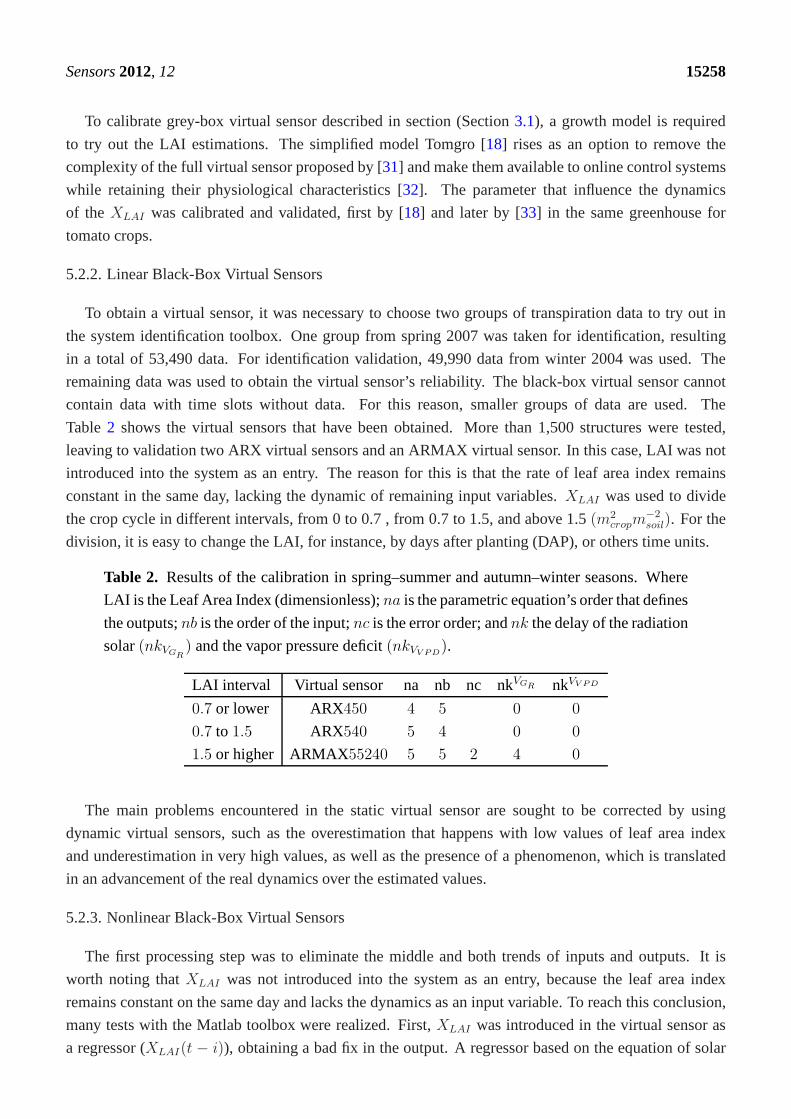
Table 2. Results of the calibration in spring–summer and autumn–winter seasons. Where

LAI is the Leaf Area Index (dimensionless);na is the parametric equation’s order that defines

the outputs;nb is the order of the input;nc is the error order; andnk the delay of the radiation

solar(nkVGR) and the vapor pressure deficit(nkVV PD

).

LAI interval Virtual sensor na nb nc nkVGR nkVV PD

0.7 or lower ARX450 4 5 0 0

0.7 to 1.5 ARX540 5 4 0 0

1.5 or higher ARMAX 55240 5 5 2 4 0

The main problems encountered in the static virtual sensor are sought to be corrected by using

dynamic virtual sensors, such as the overestimation that happens with low values of leaf area index

and underestimation in very high values, as well as the presence of a phenomenon, which is translated

in an advancement of the real dynamics over the estimated values.

5.2.3. Nonlinear Black-Box Virtual Sensors

The first processing step was to eliminate the middle and bothtrends of inputs and outputs. It is

worth noting thatXLAI was not introduced into the system as an entry, because the leaf area index

remains constant on the same day and lacks the dynamics as an input variable. To reach this conclusion,

many tests with the Matlab toolbox were realized. First,XLAI was introduced in the virtual sensor as

a regressor (XLAI(t − i)), obtaining a bad fix in the output. A regressor based on the equation of solar

Sensors2012, 12 15259

radiation reaching a given depth in canopy ([2]; Equation (6)) was tried out, but with the same results,

such results was the expected:

VGRe(−CkXLAI) (6)

where VGR is the global radiation reaching the crop (Wm−2), −Ck is the extinction coefficient of

radiation (unitless), andXLAI is the leaf area index(m2cropm

−2soil). As noted above, LAI remains constant

during a chosen day as the parameter(Ck), which means the regressor is constant during a day, depending

exclusively on the radiation.

This virtual sensor was also evaluated by using an estimatedVDP as a function of the inside

temperature and the relative humidity. Despite this estimation, the virtual sensors obtained with these

two variables show no improvement compared with those calibrated only using VPD. In the end, the

radiation and the vapor pressure deficit remain as the uniqueinputs.

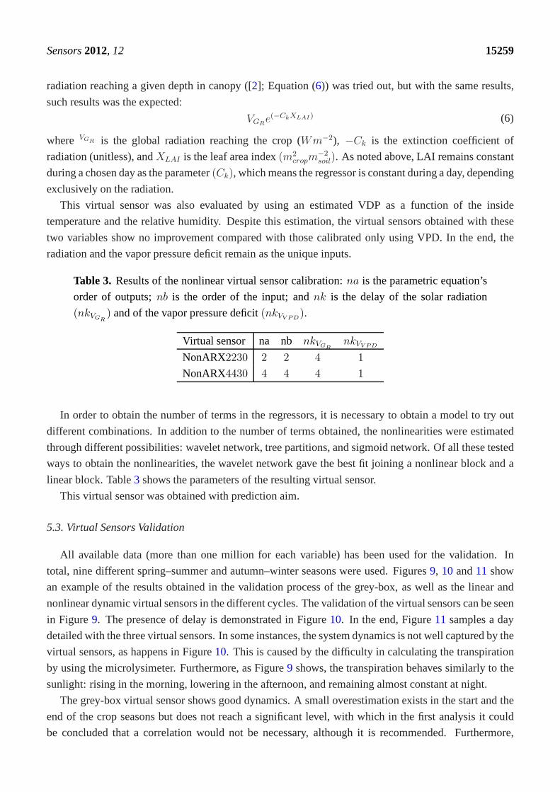
Table 3. Results of the nonlinear virtual sensor calibration:na is the parametric equation’s

order of outputs;nb is the order of the input; andnk is the delay of the solar radiation

(nkVGR) and of the vapor pressure deficit(nkVV PD

).

Virtual sensor na nb nkVGRnkVV PD

NonARX2230 2 2 4 1

NonARX4430 4 4 4 1

In order to obtain the number of terms in the regressors, it isnecessary to obtain a model to try out

different combinations. In addition to the number of terms obtained, the nonlinearities were estimated

through different possibilities: wavelet network, tree partitions, and sigmoid network. Of all these tested

ways to obtain the nonlinearities, the wavelet network gavethe best fit joining a nonlinear block and a

linear block. Table3 shows the parameters of the resulting virtual sensor.

This virtual sensor was obtained with prediction aim.

5.3. Virtual Sensors Validation

All available data (more than one million for each variable)has been used for the validation. In

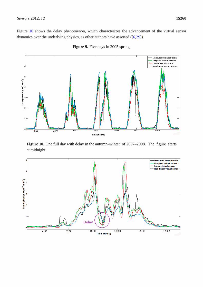
total, nine different spring–summer and autumn–winter seasons were used. Figures9, 10 and11 show

an example of the results obtained in the validation processof the grey-box, as well as the linear and

nonlinear dynamic virtual sensors in the different cycles.The validation of the virtual sensors can be seen

in Figure9. The presence of delay is demonstrated in Figure10. In the end, Figure11 samples a day

detailed with the three virtual sensors. In some instances,the system dynamics is not well captured by the

virtual sensors, as happens in Figure10. This is caused by the difficulty in calculating the transpiration

by using the microlysimeter. Furthermore, as Figure9 shows, the transpiration behaves similarly to the

sunlight: rising in the morning, lowering in the afternoon,and remaining almost constant at night.

The grey-box virtual sensor shows good dynamics. A small overestimation exists in the start and the

end of the crop seasons but does not reach a significant level,with which in the first analysis it could

be concluded that a correlation would not be necessary, although it is recommended. Furthermore,

Sensors2012, 12 15260

Figure 10 shows the delay phenomenon, which characterizes the advancement of the virtual sensor

dynamics over the underlying physics, as other authors haveasserted ([6,29]).

Figure 9. Five days in 2005 spring.

Figure 10. One full day with delay in the autumn–winter of 2007–2008. The figure starts

at midnight.

Sensors2012, 12 15261

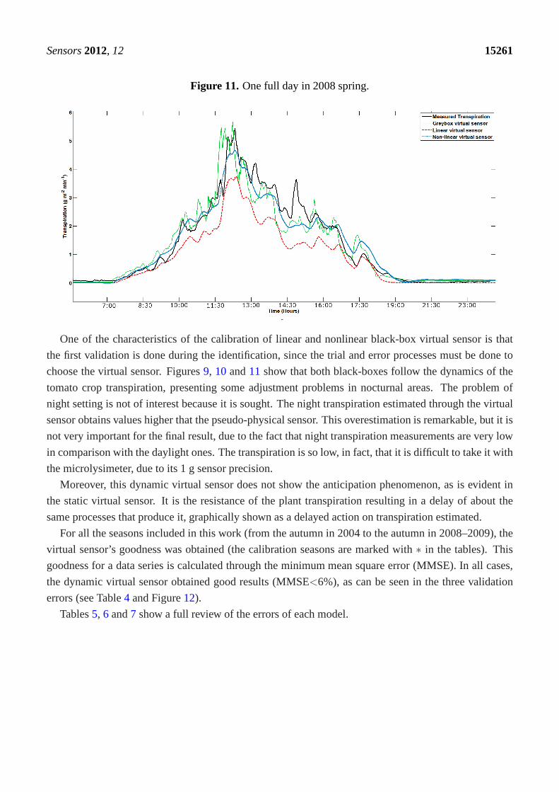
Figure 11. One full day in 2008 spring.

One of the characteristics of the calibration of linear and nonlinear black-box virtual sensor is that

the first validation is done during the identification, sincethe trial and error processes must be done to

choose the virtual sensor. Figures9, 10 and11 show that both black-boxes follow the dynamics of the

tomato crop transpiration, presenting some adjustment problems in nocturnal areas. The problem of

night setting is not of interest because it is sought. The night transpiration estimated through the virtual

sensor obtains values higher that the pseudo-physical sensor. This overestimation is remarkable, but it is

not very important for the final result, due to the fact that night transpiration measurements are very low

in comparison with the daylight ones. The transpiration is so low, in fact, that it is difficult to take it with

the microlysimeter, due to its 1 g sensor precision.

Moreover, this dynamic virtual sensor does not show the anticipation phenomenon, as is evident in

the static virtual sensor. It is the resistance of the plant transpiration resulting in a delay of about the

same processes that produce it, graphically shown as a delayed action on transpiration estimated.

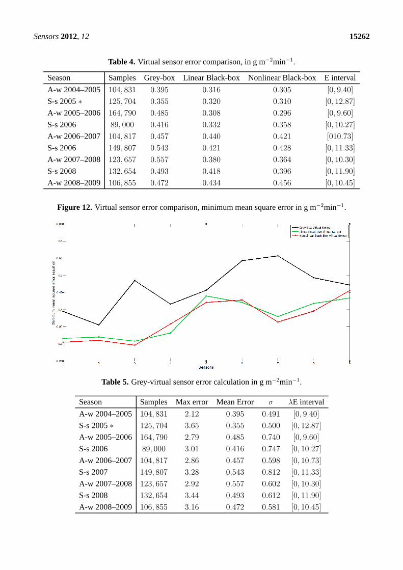
For all the seasons included in this work (from the autumn in 2004 to the autumn in 2008–2009), the

virtual sensor’s goodness was obtained (the calibration seasons are marked with∗ in the tables). This

goodness for a data series is calculated through the minimummean square error (MMSE). In all cases,

the dynamic virtual sensor obtained good results (MMSE<6%), as can be seen in the three validation

errors (see Table4 and Figure12).

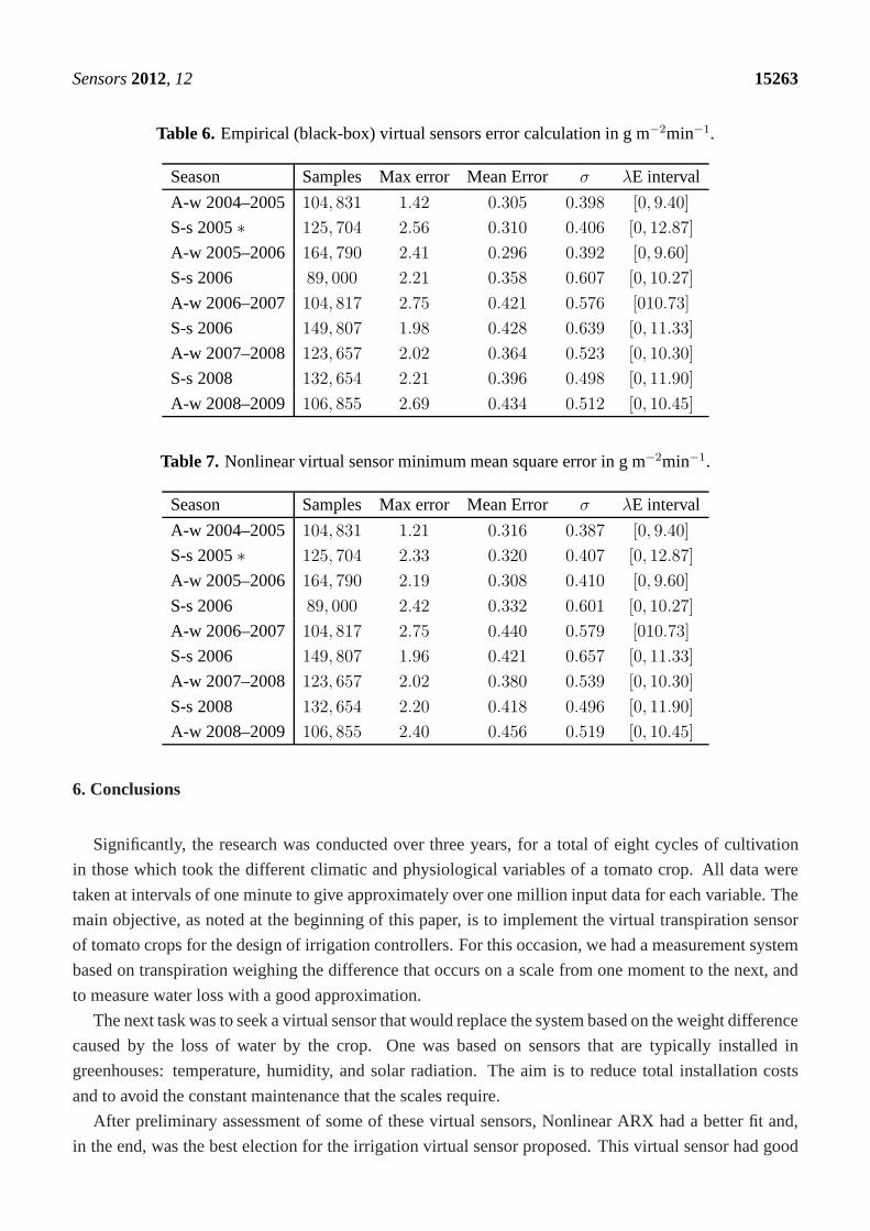
Tables5, 6 and7 show a full review of the errors of each model.

Sensors2012, 12 15262

Table 4. Virtual sensor error comparison, in g m−2min−1.

Season Samples Grey-box Linear Black-box Nonlinear Black-box E interval

A-w 2004–2005 104, 831 0.395 0.316 0.305 [0, 9.40]

S-s 2005∗ 125, 704 0.355 0.320 0.310 [0, 12.87]

A-w 2005–2006 164, 790 0.485 0.308 0.296 [0, 9.60]

S-s 2006 89, 000 0.416 0.332 0.358 [0, 10.27]

A-w 2006–2007 104, 817 0.457 0.440 0.421 [010.73]

S-s 2006 149, 807 0.543 0.421 0.428 [0, 11.33]

A-w 2007–2008 123, 657 0.557 0.380 0.364 [0, 10.30]

S-s 2008 132, 654 0.493 0.418 0.396 [0, 11.90]

A-w 2008–2009 106, 855 0.472 0.434 0.456 [0, 10.45]

Figure 12. Virtual sensor error comparison, minimum mean square errorin g m−2min−1.

Table 5. Grey-virtual sensor error calculation in g m−2min−1.

Season Samples Max error Mean Error σ λE interval

A-w 2004–2005 104, 831 2.12 0.395 0.491 [0, 9.40]

S-s 2005∗ 125, 704 3.65 0.355 0.500 [0, 12.87]

A-w 2005–2006 164, 790 2.79 0.485 0.740 [0, 9.60]

S-s 2006 89, 000 3.01 0.416 0.747 [0, 10.27]

A-w 2006–2007 104, 817 2.86 0.457 0.598 [0, 10.73]

S-s 2007 149, 807 3.28 0.543 0.812 [0, 11.33]

A-w 2007–2008 123, 657 2.92 0.557 0.602 [0, 10.30]

S-s 2008 132, 654 3.44 0.493 0.612 [0, 11.90]

A-w 2008–2009 106, 855 3.16 0.472 0.581 [0, 10.45]

Sensors2012, 12 15263

Table 6. Empirical (black-box) virtual sensors error calculation in g m−2min−1.

Season Samples Max error Mean Error σ λE interval

A-w 2004–2005 104, 831 1.42 0.305 0.398 [0, 9.40]

S-s 2005∗ 125, 704 2.56 0.310 0.406 [0, 12.87]

A-w 2005–2006 164, 790 2.41 0.296 0.392 [0, 9.60]

S-s 2006 89, 000 2.21 0.358 0.607 [0, 10.27]

A-w 2006–2007 104, 817 2.75 0.421 0.576 [010.73]

S-s 2006 149, 807 1.98 0.428 0.639 [0, 11.33]

A-w 2007–2008 123, 657 2.02 0.364 0.523 [0, 10.30]

S-s 2008 132, 654 2.21 0.396 0.498 [0, 11.90]

A-w 2008–2009 106, 855 2.69 0.434 0.512 [0, 10.45]

Table 7. Nonlinear virtual sensor minimum mean square error in g m−2min−1.

Season Samples Max error Mean Error σ λE interval

A-w 2004–2005 104, 831 1.21 0.316 0.387 [0, 9.40]

S-s 2005∗ 125, 704 2.33 0.320 0.407 [0, 12.87]

A-w 2005–2006 164, 790 2.19 0.308 0.410 [0, 9.60]

S-s 2006 89, 000 2.42 0.332 0.601 [0, 10.27]

A-w 2006–2007 104, 817 2.75 0.440 0.579 [010.73]

S-s 2006 149, 807 1.96 0.421 0.657 [0, 11.33]

A-w 2007–2008 123, 657 2.02 0.380 0.539 [0, 10.30]

S-s 2008 132, 654 2.20 0.418 0.496 [0, 11.90]

A-w 2008–2009 106, 855 2.40 0.456 0.519 [0, 10.45]

6. Conclusions

Significantly, the research was conducted over three years,for a total of eight cycles of cultivation

in those which took the different climatic and physiological variables of a tomato crop. All data were

taken at intervals of one minute to give approximately over one million input data for each variable. The

main objective, as noted at the beginning of this paper, is toimplement the virtual transpiration sensor

of tomato crops for the design of irrigation controllers. For this occasion, we had a measurement system

based on transpiration weighing the difference that occurson a scale from one moment to the next, and

to measure water loss with a good approximation.

The next task was to seek a virtual sensor that would replace the system based on the weight difference

caused by the loss of water by the crop. One was based on sensors that are typically installed in

greenhouses: temperature, humidity, and solar radiation.The aim is to reduce total installation costs

and to avoid the constant maintenance that the scales require.

After preliminary assessment of some of these virtual sensors, Nonlinear ARX had a better fit and,

in the end, was the best election for the irrigation virtual sensor proposed. This virtual sensor had good

Sensors2012, 12 15264

results in the calibration and validation of the virtual sensor. An average error of 5%, for all cycles

taken, shows how the choice of this virtual sensor was successful. However, it also presents some

problems, such as the overestimation at night which occurs.On the other hand, linear and nonlinear

black-box virtual sensors have demonstrated the absence ofa advance phenomenon. It was translated to

an advancement of the dynamics of the estimated values for real ones.

System identification techniques were chosen to obtain a dynamic virtual sensor.Matlabrsoftware

package was a good option to work with the identification techniques. A large number of different

nonlinear dynamic virtual sensors structures was tested. The proposed dynamic for virtual sensors

require only two inputs, global radiation and vapor pressure deficit, thus eliminating the inclusion of

theXLAI . This virtual sensor presents the possibility of using modern control algorithms that cannot be

used with the grey-box sensor.

As summary:

• Grey-box virtual sensor has a good fixing as advantage, but some disadvantages such as the

overestimation at different moments of the year, a higher final error result, and the advance

phenomenon.

• The black-box virtual sensors obtain better results and also allows the elimination of the

grey-box problems: advance phenomenon and overestimation. An overestimation only appears

during nocturnal periods.

• Nonlinear black-box had the best results.

This paper has dealt with the transpiration from an industrial point of view, as a process in which

there are entries and exits. The crop itself, and some aspects of the climate inside the greenhouse, are

considered disturbances affecting the dynamics. This shifts the focus away from the strictly agronomic,

agronomy classic, which studies the exchanges that occur inthe greenhouse by static virtual sensors

based on fundamental principles, without including the system dynamic effect.

Acknowledgments

This work is framed within the “Controlcrop” Project, PIO-TEP-6174, supported by the Ministry

of Economy, Innovation and Science Government of Andalusia(Spain), and by the National Plan

Projects DPI2010-21589-C05-04, and DPI2011-27818-C02-01 of the Spanish Ministry of Science and

Innovation and FEDER funds. The authors are grateful for theinvaluable contributions of the University

of Almerıa Investigation Group of Automatic, Electronic and Robotic (TEP197), the University of

Seville Investigation Department of Systems Engineering and Automatic, the Cajamar Foundation

Experimental Station “Las Palmerillas”, and the Agrifood Campus of International Excellence (ceiA3).

References

1. Stanghellini, C. Transpiration of Greenhouse Crops. Ph.D.Thesis, Wageningen University,

Wageningen, The Netherlands, 1987.

Sensors2012, 12 15265

2. Baille, M.; Baille, L.; Laury, J.C. A simplified model for predicting evapotranspiration rate of nine

ornamental speciesvs. climate factors and leaf area.Sci. Hort. Amsterdam1994, 59, 217–232.

3. Jemaa, R.; Boulard, T.; Baille, A. Some results on water and nutrient consumption of a greenhouse

tomato crop grown in rockwool.Acta Horticul.1995, 408, 137–146.

4. Boulard, T.; Wang, S. Greenhouse crop transpiration simulation from external climate conditions.

Agric. For. Meteorol.2000, 100, 25–34.

5. Montero, J.; Anton, A.; Munoz, P.; Lorenzo, P. Transpiration from geranium grown under high

temperatures and low humidities in greenhouses.Agric. For. Meteorol.2001, 107, 323–332.

6. Medrano, E.; Lorenzo, P.; Sanchez-Guerrero, M.C.; Montero, J.I. Evaluation and

modelling of greenhouse cucumber-crop transpiration under high and low radiation conditions.

Sci Hort. Amsterdam2005, 105, 163–175.

7. Suay, R.; Martınez, P.; Roca, D.; Martınez, M.; Herrero, J.; Ramos, C. Measurement and estimation

of transpiration of a soilless rose crop and application to irrigation management.Acta Horticul.

2003, 614, 625–630.

8. Voogt, W.; Kipp, J.; de Graaf, R.; Spaans, L. A fertigation model for glasshouse crops grown in

soil. Acta Horticul.2000, 537, 495–502.

9. Schmidt, U.; Exarchou, E. Controlling of irrigation systems of greenhouse plants by using measured

transpiration sum.Acta Horticul.2000, 537, 487–494.

10. Li, H.; Braun, J.E. Decoupling features and virtual sensorsfor diagnosis of faults in vapor

compression air conditioners.Int. J. Refrig.2007, 30, 546–564.

11. Ponsart, J.; Theilliol, D.; Aubrun, C. Virtual sensors design for active fault tolerant control system

applied to a winding machine.Control Eng. Pract.2010, 18, 1037–1044.

12. Thies, S.; Tresadern, P.; Kenney, L.; Howard, D.; Goulermas, J.; Smith, C.; Rigby, J. A

virtual sensor tool to simulate accelerometers for upper limb FES triggering. J. Biomech.2006,39(suppl. 1), S80.

13. Heredia, G.; Ollero, A. Virtual sensor for failure detection, identification and recovery in the

transition phase of a morphing aircraft.Sensors2010, 10, 2188–2201.

14. Sanchez, J.; Visioli, A.; Dormido, S. A two-degree-of-freedom PI controller based on events.

J. Process Control2011, 21, 639–651.

15. Jolliet, O.; Bailey, B. The effect of climate on tomato transpiration in greenhouses: measurements

and models comparison.Agric. For. Meteorol.1992, 58, 43–62.

16. Saugier, B.; Granier, A.; Pontailler, J.Y.; Dufrene, E.; Baldocchi, D.D. Transpiration of a boreal

pine forest measured by branch bag, sap flow and micrometeorological methods. Tree Physiol.

1997, 17, 511–519.

17. Van Bavel, C.H.M.; Nakayama, F.S.; Ehrler, W.L. Measuring transpiration resistance of leaves.

Plant Physiol.1964, 40, 535–540.

18. Ramırez, A.; Rodrıguez, F.; Berenguel, M.; Heuvelink, E.Calibration and validation of complex

and simplified tomato growth models for control purposes in the southeast of Spain.Acta Horticul.

2004, 654, 147–154.

19. Monteith, J. Evaporation and environment. InThe State and Movement of Water in Living

Organism; Cambridge University Press: Cambridge, UK, 1965; Volume 19, pp. 205–234.

Sensors2012, 12 15266

20. Stanghellini, C. Evapotranspiration in greenhouses with special reference to mediterranean

conditions.Acta Horticul.1995, 335, 295–304.

21. Yoo, S.H.; Choi, J.Y.; Jang, M.W. Estimation of design waterrequirement using FAO

Penman-Monteith and optimal probability distribution function in South Korea. Agric. Water

Manag.2008, 95, 845–853.

22. Ruiz-Arahal, M.; Berenguel, M.; Rodrıguez, F.Tecnicas de prediccion con aplicaciones en

la ingenierıa; Secretariado de publicaciones: Universidad de Sevilla, Seville, Spain, 2006;

pp. 117–119.

23. Ljung, L. System Identification: Theory for the User; 2nd ed.; Prentice Hall: Englewood Cliffs, NJ,

USA, 1999.

24. Ljung, L. System Indentification Toolbox TM 7 Getting Started Guide; MathWorks: Natick, MA,

USA, 2010.

25. Guzman, J.; Rivera, D.; Dormido, S.; Berenguel, M. An interactive software tool for system

identification.Adv. Eng. Softw.2012, 45, 115–123.

26. Ljung, L.; Glad, T.Modeling of Dynamic Systems; Prentice Hall: Englewood Cliffs, NJ, USA,

1994.

27. Berenguel, M.; Rodrıguez, F.; Guzman, J.; Lacasa, D.; Perez-Parra, J. Greenhouse diurnal

temperature control with natural ventilation based on empirical models. Acta Horticul. 2006,719, 57–64.

28. Rodrıguez, F.; Guzman, J.; Berenguel, M.; Arahal, M. Adaptive hierarchical control of greenhouse

crop production.Int. J. Adapt. Control Signal Process.2008, 22, 180–187.

29. Gazquez, J.; Lopez, J.; Baeza, E.; Parez-Parra, J.; Fernandez, M.; Baille, A.; Gonzalez-Real, M.

Effects of vapour pressure deficit and radiation on the transpiration rate of a greenhouse sweet

pepper crop.Acta Horticul.2008, 797, 259–265.

30. Seginer, I. The Penman–Monteith Evapotranspiration Equation as an Element in Greenhouse

Ventilation Design.Biosyst. Eng.2002, 82, 423–439.

31. Jones, J.; Dayan, E.; Allen, L.V.; Challa, H. A dynamic tomato growth and yield model (Tomgro).

Trans. ASAE1991, 34, 663–672.

32. Jones, J.W.; Kening, A.; Vallejos, C.E. Reduced state-variable tomato growth model.Trans. ASAE

1999, 42, 255–265.

33. Gallardo, M.; Thompson, R.; Rodriguez, J.; Rodriguez, F.; Fernandez, M.; Sanchez, J.;

Magan, J. Simulation of transpiration, drainage, N uptake,nitrate leaching, and N uptake

concentration in tomato grown in open substrate.Agric. Water Manag.2009, 96, 1773–1784.

c© 2012 by the authors; licensee MDPI, Basel, Switzerland. This article is an open access article

distributed under the terms and conditions of the Creative Commons Attribution license

(http://creativecommons.org/licenses/by/3.0/).