Virtual Beach 3.0.4: User's Guide

Virtual Beach 3.0.4: User’s Guide

Mike Cyterski1, Wesley Brooks2, Mike Galvin1, Kurt Wolfe1, Rebecca Carvin2, Tonia

Roddick2, Mike Fienen2, Steve Corsi2

1National Exposure Research Laboratory

USEPA

960 College Station Road

Athens, GA 30605

2U. S. Geological Survey

Wisconsin Water Science Center

8505 Research Way

Middleton, WI 53562

2

Table of Contents

1. Introduction...................................................... 4

1.1 On Predictive Modeling.......................................... 4

1.2 Recommended User Background..................................... 5

1.3 General Overview................................................ 5

1.3 History of VB................................................... 6

2. Composition and Installation...................................... 9

3. Operational Overview............................................. 10

4. Project Management............................................... 12

5. Location Interface............................................... 13

5.1 Finding a Beach................................................ 13

5.2 Defining the Beach Boundaries for Orientation Calculation...... 14

5.3 Saving Beach Information....................................... 15

6. Global Datasheet................................................. 16

6.1 Data Requirements and Considerations........................... 16

6.2 Importing a Dataset............................................ 17

6.3 Validating the Imported Data................................... 18

6.4 Working with a Dataset after Validation........................ 22

Scatter Plot Interpretation.................................... 23

6.5 Computing Wind, Wave and Current Components.................... 25

Notes on Component Calculations................................ 26

6.6 Creation of New Independent Variables.......................... 29

6.7 Transforming the Independent Variables......................... 31

Plotting Transformed IVs....................................... 33

6.8 Singular Matrices and Nominal Variables........................ 34

6.9 Saving Processed Data.......................................... 35

6.10 Proceeding to Modeling........................................ 35

7. Multiple Linear Regression Modeling.............................. 36

7.1 Selecting Variables for Model Building......................... 36

7.2 Modeling Control Options....................................... 37

7.3 Linear Regression Modeling Methods............................. 38

7.4 Using the Genetic Algorithm.................................... 41

7.5 Evaluating Model Output........................................ 42

7.6 Viewing X-Y Scatter plots...................................... 46

7.7 ROC Curves..................................................... 47

7.8 Residual Analysis.............................................. 47

Viewing the Data Table......................................... 51

7.9 Cross-Validation............................................... 53

7.10 Report Generation............................................. 53

8. Partial Least Squares............................................ 56

8.1 Data Manipulation.............................................. 56


8.3 The Regulatory Standard........................................ 58


Dropping Unimportant Variables................................. 59

Setting the Decision Threshold................................. 59

8.5 Diagnostics.................................................... 60

9. Generalized Boosted Regression Modeling.......................... 62

9.1 Data Manipulation.............................................. 63


9.3 The Regulatory Standard........................................ 64


Dropping Unimportant Variables................................. 65

Setting the Decision Threshold................................. 66

9.5 Diagnostics.................................................... 67

10. Prediction...................................................... 69

3

10.1 Model Statement............................................... 69

10.2 Model Evaluation Thresholds................................... 69

10.3 Prediction Form............................................... 70

10.4 Column Mapping of Imported Data............................... 70

10.5 Viewing Plots................................................. 74

10.6 Prediction Form Manipulation.................................. 75

10.7 Importation of EnDDaT Data.................................... 75

11. User Feedback................................................... 77

12. References...................................................... 78

13. Acknowledgments................................................. 79

Appendices........................................................... 80

A.1 Transformations................................................ 80

A.2 Singular Matrices and Nominal Variables........................ 82

A.3 MLR Model Evaluation Criteria.................................. 84

A.4 Changes from version 3 to 3.04................................. 85

4

1. INTRODUCTION

Virtual Beach version 3 (VB3) is a decision support tool that constructs site-

specific statistical models to predict fecal indicator bacteria (FIB) concentrations at

recreational beaches. VB3 is primarily designed for beach managers responsible for

making decisions regarding beach closures or the issuance of swimming advisories due to

pathogen contamination. However, researchers, scientists, engineers, and students

interested in studying relationships between water quality indicators and ambient

environmental conditions will find VB3 useful. VB3 reads input data from a text file or

Excel document, assists the user in preparing the data for analysis, enables automated

model selection using a wide array of possible model evaluation criteria, and provides

predictions using a chosen model parameterized with new data. With an integrated

mapping component to determine the geographic orientation of the beach, the software

can automatically decompose wind/current/wave speed and magnitude information into

along-shore and onshore/offshore components for use in subsequent analyses. Data can

be examined using simple scatter plots to evaluate relationships between the response and

independent variables (IVs). VB3 can produce interaction terms between the primary IVs,

and it can also test an array of transformations to maximize the linearity of the

relationship between the response variable and IVs. The software includes search routines

for finding the "best" models from an array of possible choices. Automated censoring of

statistical models with highly correlated IVs occurs during the selection process. Models

can be constructed either using previously collected data or forecasted environmental

information. VB3 has residual diagnostics for regression models, including automated

outlier identification and removal using DFFITs or Cook's Distances.

1.1 On Predictive Modeling

Empirical/statistical modeling outperforms persistence models (using the most

recent FIB concentration as the sole predictor of the next FIB concentrations) at beaches

where conditions such as weather, water characteristics, and human/animal density levels

change significantly day to day (Frick et al. 2008, Brooks et al. 2013). Virtual Beach

constructs models that can predict a dependent or response variable (i.e., FIB) by using

variables to describe current environmental conditions that can be measured or estimated

in a timely manner. These are referred to as independent variables (IVs) and often

include beach water parameters such as turbidity, water temperature, specific

conductance, or wave height; parameters monitored and made available via the web such

as rainfall, stream flow, and stream water quality; and parameters estimated by

environmental models such as water currents, wave height and direction, and radar

rainfall.

In any predictive modeling endeavor, variability and uncertainty associated with

model output arise for a variety of reasons that are impossible to eradicate completely.

VB3 attempts to examine this variability and uncertainty in a transparent manner using a

probability of exceedance for any regulatory standard the user wishes to investigate.

Even so, there is no guarantee than every model prediction will be correct, and a situation

may arise in which the model predicts acceptable water quality for public recreation that

could be erroneous. Decisions to allow or disallow swimming at beaches must be made,

5

however, and in the best case scenarios, regression models developed with VB3 will

outperform traditional persistence models based on just the previous day’s FIB

concentrations.

1.2 Recommended User Background

For those using VB3, some experience with spreadsheet data manipulation

programs like Microsoft Excel is recommended, but not necessary. A familiarity with

multiple linear regression analysis is also helpful, but again not mandatory. Without this

background, VB3 will take longer to master, but it should not prohibit users from

producing and using models.

1.3 General Overview

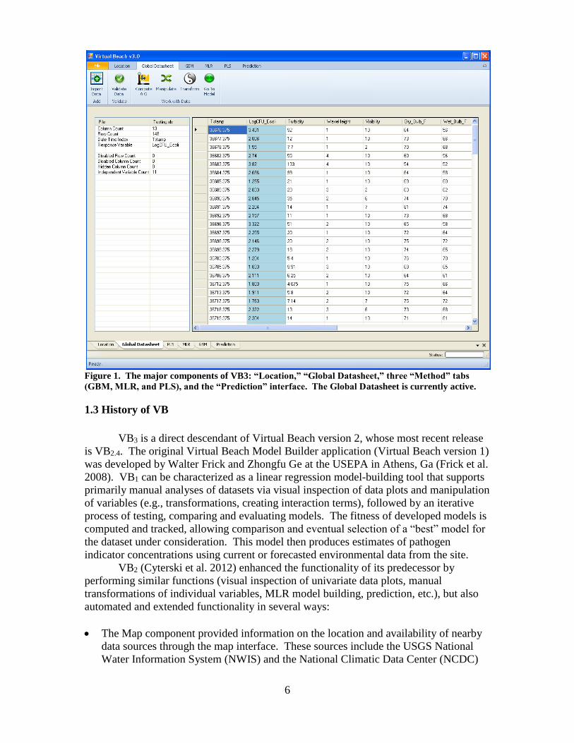
VB3 has four major components:

Beach location map interface where users can define the orientation of the beach.

Interface that facilitates initial import and manipulation of data.

Multiple “method” tabs where the statistical modeling is done. Each tab has some

features identical to those seen in other method tabs and some that are unique. For

example, the multiple linear regression (MLR) tab allows examination of regression

residuals, elimination of highly influential data records, and viewing of receiver

operating characteristic (ROC) curves.

Prediction interface allowing entry of new data and subsequent estimation of

pathogen indicator concentrations with a selected model from any of the statistical

methods.

Each component is accessible from the application’s main window via tabs at the

top and bottom of the main screen (Figure 1). The Location and Global Datasheet tabs

are always visible, while the statistical method tabs only become visible once data pre-

processing has been completed (i.e., clicking the “Go to Model” button on the Global

Datasheet ribbon). The Prediction tab appears when model-building on any method tab is

complete and a model is selected

Lastly, we note that statistical models are only as effective as the data used to

develop them. No statistician, however skilled, can turn a dataset of low-quality

independent variables (IVs) into a useful predictive device.

6

Figure 1. The major components of VB3: “Location,” “Global Datasheet,” three “Method” tabs

(GBM, MLR, and PLS), and the “Prediction” interface. The Global Datasheet is currently active.

1.3 History of VB

VB3 is a direct descendant of Virtual Beach version 2, whose most recent release

is VB2.4. The original Virtual Beach Model Builder application (Virtual Beach version 1)

was developed by Walter Frick and Zhongfu Ge at the USEPA in Athens, Ga (Frick et al.

2008). VB1 can be characterized as a linear regression model-building tool that supports

primarily manual analyses of datasets via visual inspection of data plots and manipulation

of variables (e.g., transformations, creating interaction terms), followed by an iterative

process of testing, comparing and evaluating models. The fitness of developed models is

computed and tracked, allowing comparison and eventual selection of a “best” model for

the dataset under consideration. This model then produces estimates of pathogen

indicator concentrations using current or forecasted environmental data from the site.

VB2 (Cyterski et al. 2012) enhanced the functionality of its predecessor by

performing similar functions (visual inspection of univariate data plots, manual

transformations of individual variables, MLR model building, prediction, etc.), but also

automated and extended functionality in several ways:

The Map component provided information on the location and availability of nearby

data sources through the map interface. These sources include the USGS National

Water Information System (NWIS) and the National Climatic Data Center (NCDC)

7

which provide recently collected and/or forecasted data to generate predictions by a

chosen model.

The Map component provided a convenient method for defining beach orientation by

overlaying the beach on current shoreline layers (satellite images, Google Maps, MS

Virtual Earth, etc). Given the orientation, VB2 could calculate wind, wave, or current

components (the A-component is parallel to shore and the O-component is

perpendicular to shore) which can be important predictor variables.

Although manual processing and analysis of imported data (visual inspection of

univariate data plots and the transformations/interactions of variables) was retained,

the data-processing component of VB2 automated generation of all possible second-

order interaction terms among a set of IVs, formed more complex functions of

multiple columns, and automated testing of a suite of variable transformations that

improved model linearity. This functionality increased the number of models to

evaluate during later selection routines and removed the burden of manual assessment

that users of VB1 encountered.

Within the linear regression analysis component, multi-collinearity among predictor

variables was handled automatically. Any model containing an IV with a high degree

of correlation with others (as measured by a large Variance Inflation Factor [VIF])

was removed from consideration during model selection.

During MLR model selection, models were ranked by a user-selected evaluation

criterion: R2, Adjusted R2, Akaike Information Criterion (AIC), Corrected AIC,

Predicted Error Sum of Squares (PRESS), Bayesian Information Criterion (BIC),

Accuracy, Sensitivity, Specificity, or the model’s Root Mean Square Error (RMSE).

See Section A.3 for definitions of these criteria. Regardless of which criterion is

chosen, the software records the ten best models in terms of it. In comparison, VB1

had a single criterion choice, Mallow’s Cp.

As the number of IVs in a dataset increases, possible MLR models increase

exponentially (considering transforms/interactions), resulting in trillions of possible

models from a modest number (12-13) of IVs. VB2 implemented a genetic algorithm

(GA) that efficiently searched for the best possible MLR model. Alternatively, VB2

users could perform exhaustive calculations in which all possible combinations of IVs

were tested if the number of possible models was reasonably small (< 500,000). Both

the GA and exhaustive approaches greatly expanded the model-building capabilities

of VB2, compared to VB1.

Users no longer had to enter data values in transformed, interacted, or component-

decomposed form to make a prediction with the selected MLR model. On the VB2

MLR Prediction tab, a user-selected model is coded into an input grid with data entry

columns matching main effects of the model. Any mathematical manipulation of

these IVs is then performed automatically prior to making predictions.

8

VB3 primarily builds on VB2 by adding additional statistical methods that give

users more flexibility in modeling their datasets. In addition to MLR, users can now use

Partial Least Squares (PLS) regression and Generalized Boosted Regression Modeling

(GBM) to fit their data and make predictions. The redesigned software architecture

(using DotSpatial libraries) easily accommodates future expansions of the suite of

modeling tools. Possible future additions could be Binary Logistic Regression, Least-

Absolute Shrinkage (LASSO) and Neural Networks. The Prediction tab of VB3 also has

a button to allow direct interaction with the USGS’s data acquisition system, EnDDaT

(http://cida.usgs.gov/enddat/), for automated dataset construction and ease of FIB

prediction from web-accessible data.

http://cida.usgs.gov/enddat/

9

2. COMPOSITION AND INSTALLATION

VB3 was developed with MS Visual Studio and written in C#, and uses multiple

public domain system components:

FLEE equation parser (http://flee.codeplex.com/)

Accord.Net math libraries (http://accord-framework.net/)

R statistical libraries (http://cran.r-project.org/web/packages/)

DotSpatial mapping libraries (http://dotspatial.codeplex.com/)

Weifen Luo Docking UI (http://sourceforge.net/projects/dockpanelsuite/)

ZedGraph (http://sourceforge.net/projects/zedgraph/)

GMap.Net (http://greatmaps.codeplex.com/)

No license or software purchase is required to install and run VB3, but an internet

connection is needed to display Geographical Information System (GIS) information.

Users must have Windows XP or 7 with DotNet Framework 4.0 to assure proper

installation and operation. Other versions of Windows (e.g., Vista) have caused various

errors to occur, thus are not recommended for use with VB3. Certain VB3 data

manipulation and model-building operations are computationally intensive, so faster

CPUs are better, but laptop or desktop systems with at least 2 GB RAM will be adequate.

Disk space requirements are about 140 MB for VB3 and 170 MB for the DotNet

Framework 4. The VB3 application installer will attempt to download and install the

DotNet Framework 4.0 if it is not already installed on the target system; this also requires

a network connection. If necessary, a user can obtain the DotNet Framework 4 installer

at no cost at:

http://www.microsoft.com/download/en/details.aspx?id=17851

The EPA’s Center for Exposure Assessment Modeling (CEAM) web site

distributes VB at:

http://www2.epa.gov/exposure-assessment-models/virtual-beach-vb

Obtain and run the VB3 application installer and follow the on-screen instructions.

After installation, a shortcut will appear on the desktop.

http://www.microsoft.com/download/en/details.aspx?id=17851

http://www2.epa.gov/exposure-assessment-models/virtual-beach-vb

10

3. OPERATIONAL OVERVIEW

To make VB3 straightforward to operate, it has four functions, each with its own

interface:

Location – an optional mapping/GIS screen for calculating a beach orientation used for

later computation of orthogonal (alongshore and offshore/onshore) wind, current, and/or

wave components for the beach under consideration. Such components can be powerful

predictors of pathogen indicator concentrations at the beach, so defining the beach

orientation is recommended if the dataset under consideration contains wind, wave or

current data.

Global Datasheet – a way to support data manipulation on an imported dataset. In

addition to wind/current/wave component generation, users can generate new

independent variables that represent the products, means, sums, differences, minimums,

and maximums of other IVs, as well as investigate data transformations for the IVs.

Methods – there are three Method tabs – Multiple Linear Regression (MLR), Partial

Least Squares regression (PLS), and Generalized Boosted Regression Modeling (GBM).

Each has its own unique interface, but shares common elements. One common element

is a “variable selection” tab where the user chooses from a list of eligible IVs for

consideration in model-building and model-generation. Another common element is a

“Data Manipulation” tab which is initially populated with data from the Global

Datasheet. After initialization, however, the user can then modify “local” data for the

chosen statistical technique.

Prediction -- this tab is comprised of three spreadsheets/grids where users can enter or

import the IVs needed for the chosen model (left grid), enter or import the values of the

response/dependent variable that will be compared to model predictions (middle grid),

and examine model predictions and exceedance probabilities (right grid). Time series

and scatter plots of the measured dependent variable values versus predictions help users

gauge model effectiveness.

The following list attempts to provide an overall context for how a general, basic

modeling session using VB3 would be conducted (optional actions in green, required

actions in red):

12

4. PROJECT MANAGEMENT

The user will often perform a number of pre-processing steps on an imported

dataset to prepare it for analysis, and then develop models from the resulting data. To

avoid repeating all of this work, a file can be saved (termed a “project” file) and re-

opened via the File Save and File Open menu selection. Project files have a

“.vb3p” extension. Opening a saved project file will load the saved data into the Global

Datasheet and re-populate the methods tabs with the local data, as well as any modeling

results generated prior to the save. The beach orientation defined by the user on the

Location tab is also saved inside a project file. We suggest giving Project files a

descriptive name of the beach/site being modeled for later easy identification.

In addition to project files, “model” files can be saved by using “Save As

(prediction only)” under the “File” menu at the top of the VB3 interface. These files have

a “.vb3m” file extension. A model file contains information on the IVs, model

parameters, and other metadata for the currently selected models on each method tab.

When users open a saved model file within VB3, they are taken directly to the Prediction

tab (the only accessible tab) where they can use the model to generate predictions. Model

files allow the user to construct models and choose a “best” one for a site, save a model

file, and deliver this file to a beach manager. With this approach, a manager will not

need VB3 for full-scale model development, but only to input new data, generate

predictions, and make decisions about issuing swimming advisories.

If the user clicks the red “X” in the upper-right corner of the main VB3 window

(Figure 1), a prompt will ask if they wish to save their project before closing.

13

5. LOCATION INTERFACE

On VB3 application startup, the “Location” tab is shown first (Figure 2). Because

use of this tab is optional, users can go directly to the “Global Datasheet” interface by

clicking that tab at the top or bottom of the screen.

Figure 2. Location interface; the default map type is OpenStreet, but users have several other

options.

5.1 Finding a Beach

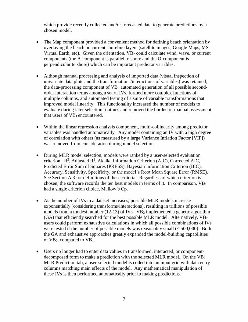
The location interface provides map controls (Figure 3) that let users navigate to a

beach site by panning and zooming (right-click and drag mouse to pan; use mouse wheel,

slider at the left of the map, or the two buttons in the top ribbon for zoom). Alternately, a

latitude/longitude can be entered at the top left, followed by a click on “GoToLat/Lng”

button.

14

Figure 3. Location controls and their function.

5.2 Defining the Beach Boundaries for Orientation Calculation

The map control allows delineation of a beach’s boundaries so that VB3 can

calculate its orientation (Figure 4), which is useful if wind, wave, and/or current flow

components are used in model-building. Maps provide less shoreline detail, so it is

recommended that a hybrid or satellite image be selected prior to adding point locations

that define beach boundaries. Once the beach of interest is found and the swimming area

is located, left-click on the map (a red marker will appear) and click the “Add 1st Beach

Marker” button; this represents one endpoint of the beach shoreline/swimming area.

Now left-click the other end of the beach on the map and click the “Add 2nd Beach

15

Marker” button. Finally, left-click on the map to indicate where the water is, relative to

the shoreline, and click the “Add Water Marker” button. Marker points will turn from

red to green as they are identified. Once the water marker is added, a shaded box appears

and the beach orientation angle is displayed to the left of the map at the bottom of the

“Beach Orientation” box (Figure 4).

Figure 4. Adding shoreline and water markers to define beach orientation.

These boundary points can be added or removed until the user is satisfied with the

beach representation. VB3 will pass the calculated beach orientation angle to the global

datasheet for wind/current/wave component calculations.

5.3 Saving Beach Information

As covered in Section 4, the FileSave menu selection will open a window that

allows the user to save the project information (such as placement of the beach/water

boundary markers and the calculated beach orientation) inside a VB3 project file.

16

6. GLOBAL DATASHEET

6.1 Data Requirements and Considerations

VB3 can import .xls, .xlsx, and .csv files, but input data must conform to certain

standards:

The first row of any column must be a header specifying the column’s name.

For error-free operation of the software, column names should be composed only of

letters, numbers, and/or underscores (“_”).

Do not begin a column name with a number.

VB3 will issue an error statement if a dataset with spaces in a column name is

imported.

The left (first) column of the dataset must be an identifier for the observations --

typically a date, time, or serial number that indicates when or where that row of data

was collected.

Each row MUST have a unique ID value (left-most column). If VB3 finds duplicate

IDs, it will issue an error statement.

If the ID column specifies a collection date or time, time series plots in VB3 will be

most interpretable if the rows are in chronological order, from the earliest to the most

recent data. VB3 will not re-arrange the data in chronological order on its own.

The second column of the dataset will initially be set as the response variable;

however, this can be changed after data are imported. Other columns will be

considered as IVs (besides the first ID column).

Variable measurement units are not considered by VB3, but certainly affect

predictions. Ensure that any data used for predictions are in the same units as those

used to build the models; for example, do not build a model with water temperature in

degrees Fahrenheit, then import water temperature in degrees Celsius for predictions.

It is prudent to include unit information in the column names (e.g., “WaterTemp_C”)

to remind the user of the proper unit when entering data to make predictions.

Missing data (blank cells) are permitted upon import, but must be dealt with (either

deleted or values filled in) prior to modeling.

If Excel data files are imported, cells with non-numeric values (i.e., symbols or text)

are converted to empty cells. Exceptions are the column names and the first column

of IDs. If such non-numeric characters are present in an imported .csv file, they will

be imported into VB3’s datasheet. However, they will be flagged as anomalous

during the validation scan and they must be dealt with (deleted or populated) at that

time.

When the required validation scan is launched, VB3 will identify any column in the

dataset containing only a single value and ask the user to delete the column (because

such data columns are useless for predictive purposes).

There is no hard-coded limit on the number of IVs one can import; however, the VB3

datasheet is designed for a maximum of 300 columns. Beyond that number, the

application’s performance will degrade significantly. Investigating 250+ IVs results

in over 2*1020 possible IV combinations for MLR processing. The MLR genetic

17

algorithm can handle this modeling task, but choosing “Run all combinations” would

likely take months or years to complete. Depending on how many additional IVs will

be created by the user, importing a dataset with less than 100 IVs should be

acceptable.

We note here that VB3 can be used as a powerful exploratory research tool,

allowing the user to investigate a great many IVs concurrently. However, this approach

can lead to models with spurious response/IV relationships (i.e., the association is only a

random statistical artifact, not a “real” phenomenon). To avoid this, the user could

restrict their analyses to only those IVs for which they have a prior, process-based,

theoretical expectation of influence on pathogen concentrations. A criticism of this

approach is that the researcher will never discover a relationship between the response

and a truly influential IV if they don’t already expect it to exist. Discovery of

unexpectedly influential IVs can lead to process insight and advancements in

understanding of the physical system. If an exploratory approach is taken, there are

mechanisms within the statistical modules of VB3 (primarily cross-validation to ensure

that predictions on future data points are nearly as good as the model fits) to protect

against over-fitting a model using too many IVs and finding spurious correlations that

don’t hold up when the model is used for prediction of future events.

6.2 Importing a Dataset

When users first click on the Global Datasheet tab, they can import a data file

using the “Import Data” button in the top ribbon (Figure 5). This opens a dialog screen

where a directory explorer can be used to find the data file. If the file is an Excel

workbook with multiple worksheets, the dialog box asks which worksheet to import.

18

Figure 5. Importing a dataset into the Data Processing tab.

Once imported, the data are shown in a datasheet. The second column of this

datasheet will be highlighted in blue to indicate its status as the current response variable.

Information about the dataset, such as number of rows and columns, name of the ID

column and name of the response variable, appear at the left of the datasheet. At this

point, the datasheet cannot be edited or interacted with in any manner; to access

additional processing functionality, the data must be validated.

6.3 Validating the Imported Data

Validation options can be accessed by clicking the “Validate Data” button in the

top button ribbon. Validating the data launches a required scan to identify blank and non-

numeric cells in the imported spreadsheet (Figure 6). One can also find and replace other

specified values (e.g., a missing data tag like -999) in the dataset, using the “(Optional)

Find:” input box.

19

Figure 6. Data validation required to begin data processing.

Clicking “Scan” begins the validation process. VB3 goes through the datasheet,

cell by cell, looking for blanks, non-numeric, or user-specified values entered in the

“(Optional) Find:” input box. If such a cell is found, the scan will stop and highlight it.

Users must then decide how to deal with that cell from choices in the “Action” section

(Figure 7): replace the cell with a specified value, using the “Replace With:” input box,

or delete the row or column containing the cell. The user must decide where to

implement the chosen action with the “Take Action Within” dropdown menu. Possible

choices are “Only this Cell,” “Entire Row,” “Entire Column,” and “Entire Sheet.” Items

in this menu are context-sensitive, i.e., they change with the Action selected. After

setting the “Take Action Within” menu, the user clicks the “Take Action” button, VB3

makes the specified changes to the datasheet, and the scan continues. Even if no cell

errors are found, VB3 may still report that a “Column has no distinct values” and prompt

the user to delete the column (see the second-to-last bulleted item in Section 6.1). When

the entire datasheet has passed inspection, VB3 reports “no anomalous data values found”

at the bottom of the Validation window.

20

Figure 7. Context-sensitive choices for the “Take Action Within” drop-down menu.

After the data have been validated, but prior to clicking the “Return” button on

the Validation window, the user has the option to specify which columns in the dataset

are categorical variables. Why do this? VB3 will not attempt to transform categorical

data columns (transformations discussed later), because it generally does not make sense

to do so. Thus, identifying IV columns as categorical saves time later when

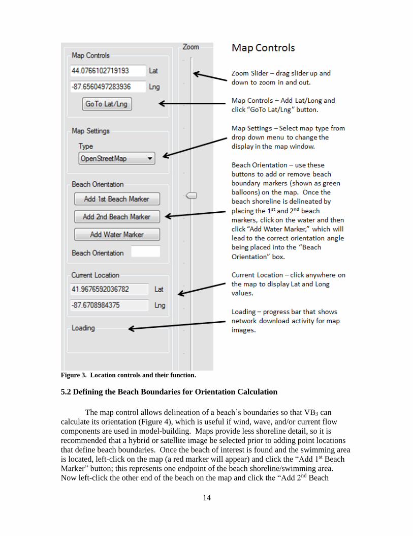
transformations are investigated. If the user clicks on the “Identify Categorical

Variables” button (Figure 7), a window pops up (Figure 8). A list of the datasheet’s

independent variables is shown in the right-hand section of this window. VB3

automatically identifies columns with only two unique values as categorical variables

(i.e., they will already be in the left section of this window); if the user has other

categorical IVs with more than two categories, those should be moved from the right to

the left section using the button. The user can also move any currently-identified

categorical IV back to the right list using the button.

21

Figure 8. Pop-up window for identifying categorical variables.

22

6.4 Working with a Dataset after Validation

After the dataset has passed the validation scan, the function buttons across the

top of the Global Datasheet tab ribbon are enabled (Figure 9).

Figure 9. Post-validation enabling of the Global Datasheet functionality.

At this point, grid cells (other than the ID column) are editable – that is, users can

manually enter new numeric data with a left-double-click on a cell and typing in a new

value. VB3 does not allow a cell to be made blank or non-numeric. A right-click on an

IV column header presents additional options (Figure 10):

Figure 10. Right-click options on columns that are not the response variable.

23

“Disable Column” turns the text red and prevents the column from being passed

to the method tabs. Previously-disabled columns can be activated with “Enable

Column.” “Set Response Variable” makes the chosen IV the new response variable (the

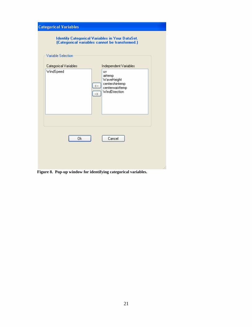
column becomes blue to indicate this change). “View Plots” shows a new screen with

column statistics at the far left and four plots for the chosen column (Figure 11): (1) a

scatter plot of the IV versus the response variable in the lower left panel; (2) a plot of the

IV values versus the ID column at the upper left (a time series plot if the ID is an

observation date); (3) a box-and-whiskers plot at the top right; and (4) a histogram for IV

values at the bottom right.

Figure 11. Four different plots available for evaluation of IVs.

Scatter Plot Interpretation

Curvature in the scatter plot (lower left) can indicate a non-linear relationship

between the IV and the response variable, problems with homogeneity of variance across

the range of the IV, or outliers. Ensuring that the IVs are linearly related to the response

variable raises the probability of producing a robust, meaningful MLR and PLS analysis

(GBM does not need linearity). If the relationship between the response and the IV is not

well-approximated by a straight line (a fundamental assumption of MLR and PLS), it

may be beneficial to transform the IV. Using VB3 to accomplish this will be explained

later (Section 6.7). The scatter plot also shows the best-fit linear regression line in red,

24

along with the correlation coefficient (r) and the significance (p-value) of the correlation

coefficient at the top of the plot. In general, p-values below 0.05 are considered

statistically significant. While VB3 does not provide a plot of the residuals of the

regression line depicted in the scatter plot, this important diagnostic is given much

attention on the MLR tab (see Section 7.8).

Identifying odd values (potential outliers or bad data) of any IV can often be done

by visual inspection. If users move the mouse cursor over a data point in any plot (other

than the histogram), they will see the ID value of that observation (Figure 12). They can

then go back to the datasheet, find the outlying observation (data row), and disable that

row (described below) if justifiable.

Figure 12. Identifying an observation from within the XY scatter plot.

The “Delete Column” right-click column header option deletes a column from the

VB3 datasheet. Note that original columns of the imported data sheet (VB3 defines these

as “main effects”) cannot be deleted. Rows can be disabled and enabled, but not deleted,

from the datasheet by right-clicking the row header (far left of each row) and making the

desired choice. Changes that the user makes can be undone and redone using the “Undo”

and “Redo” options under the VB3 “File” menu.

If the user right-clicks on the column header of the response variable, a different

set of choices is shown (Figure 13).

25

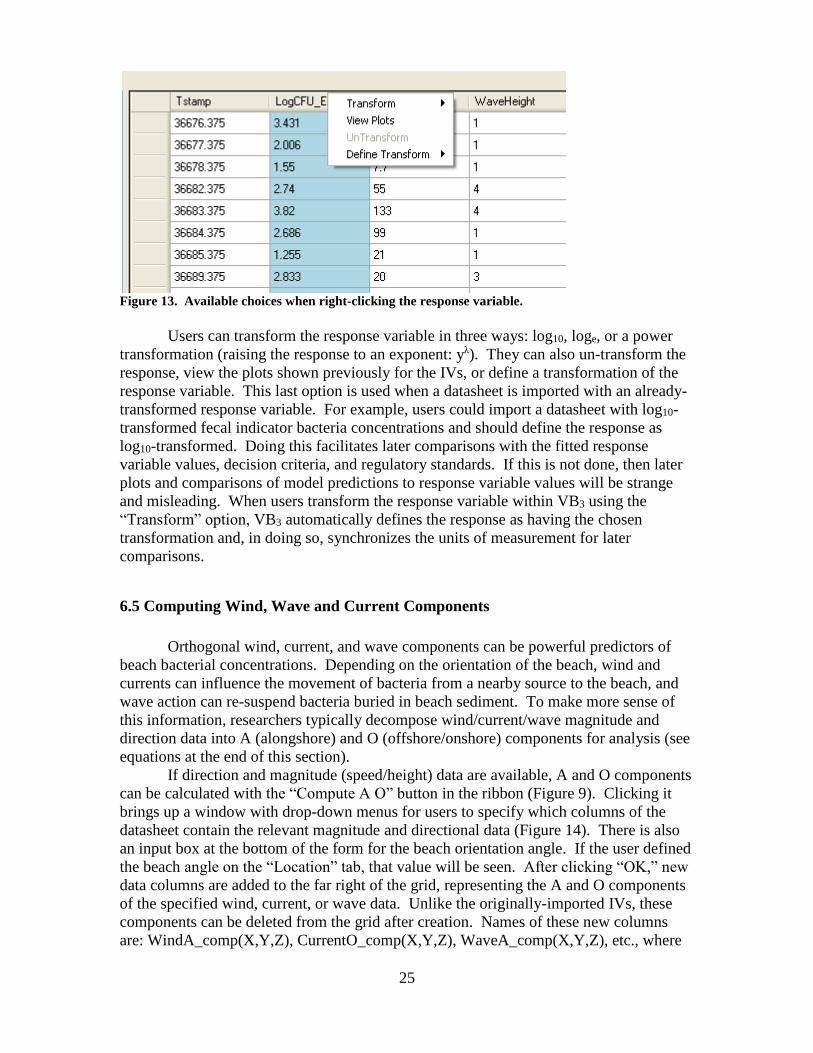
Figure 13. Available choices when right-clicking the response variable.

Users can transform the response variable in three ways: log10, loge, or a power

transformation (raising the response to an exponent: yλ). They can also un-transform the

response, view the plots shown previously for the IVs, or define a transformation of the

response variable. This last option is used when a datasheet is imported with an already-

transformed response variable. For example, users could import a datasheet with log10-

transformed fecal indicator bacteria concentrations and should define the response as

log10-transformed. Doing this facilitates later comparisons with the fitted response

variable values, decision criteria, and regulatory standards. If this is not done, then later

plots and comparisons of model predictions to response variable values will be strange

and misleading. When users transform the response variable within VB3 using the

“Transform” option, VB3 automatically defines the response as having the chosen

transformation and, in doing so, synchronizes the units of measurement for later

comparisons.

6.5 Computing Wind, Wave and Current Components

Orthogonal wind, current, and wave components can be powerful predictors of

beach bacterial concentrations. Depending on the orientation of the beach, wind and

currents can influence the movement of bacteria from a nearby source to the beach, and

wave action can re-suspend bacteria buried in beach sediment. To make more sense of

this information, researchers typically decompose wind/current/wave magnitude and

direction data into A (alongshore) and O (offshore/onshore) components for analysis (see

equations at the end of this section).

If direction and magnitude (speed/height) data are available, A and O components

can be calculated with the “Compute A O” button in the ribbon (Figure 9). Clicking it

brings up a window with drop-down menus for users to specify which columns of the

datasheet contain the relevant magnitude and directional data (Figure 14). There is also

an input box at the bottom of the form for the beach orientation angle. If the user defined

the beach angle on the “Location” tab, that value will be seen. After clicking “OK,” new

data columns are added to the far right of the grid, representing the A and O components

of the specified wind, current, or wave data. Unlike the originally-imported IVs, these

components can be deleted from the grid after creation. Names of these new columns

are: WindA_comp(X,Y,Z), CurrentO_comp(X,Y,Z), WaveA_comp(X,Y,Z), etc., where

26

X is the name of the column of data used for direction, Y is the name of the column used

for magnitude, and Z is the beach orientation angle. Note that the IVs used to create the

A and O components are automatically disabled by VB3 once the components are created.

These columns can be re-enabled by right-clicking on their column header in the

datasheet and choosing “Enable Column.” The “Compute A O” function is repeatable as

many times as the user wishes.

Figure 14. Window for computation of alongshore and offshore/onshore components.

Notes on Component Calculations

Direction is an angular degree measure. Moving in a clockwise direction from

north (0 degrees), values are positive, and negative while moving counter-clockwise.

Wind and current speed (as well as wave height) can be measured in any unit. VB3

adheres to scientific convention: wind direction is specified as the direction from which

27

the wind blows and current and wave directions are specified as the direction towards

which the current or waves move. Thus, wind blowing west to east has a direction of 270

degrees (or equivalently -90) degrees, while a current/wave also moving west to east has

a direction of 90 (or -270) degrees.

The A-component measures the force of the wind/current/wave moving parallel to

the shoreline (Figure 15). A positive A-component means winds/currents/waves are

moving from right to left as an observer looks out onto the water. A negative A-

component means winds/currents/waves are moving left to right as an observer looks out

onto the water. The O-component measures force perpendicular to the shoreline. A

negative O value indicates movement from the land surface directly offshore (unlikely to

be seen with wave action). A positive O indicates waves/wind/currents from the water to

the shore. These relationships apply no matter how the beach is oriented (Figure 16).

Figure 15. A- and O-component definitions for wind, current, and wave data.

Water

Land

Negative APositive A

Negative O

Positive O

28

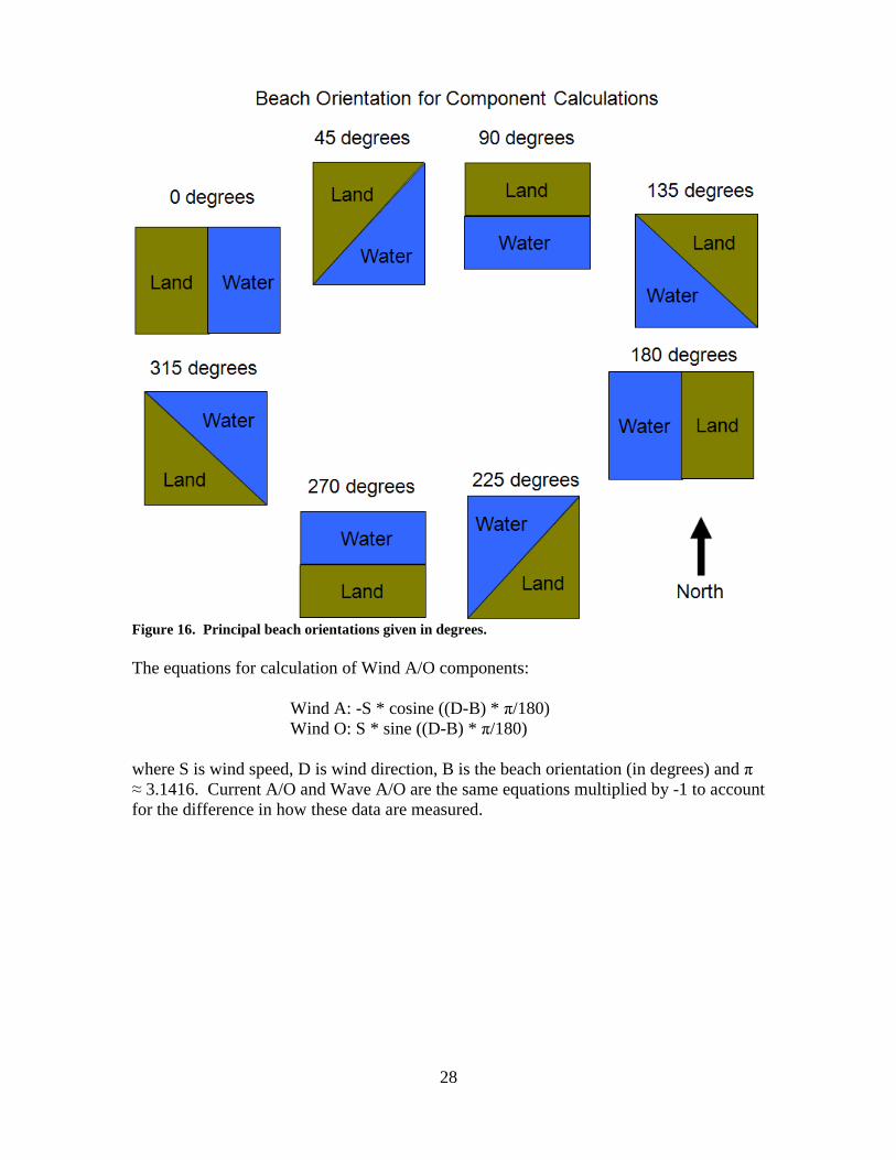
Figure 16. Principal beach orientations given in degrees.

The equations for calculation of Wind A/O components:

Wind A: -S * cosine ((D-B) * π/180)

Wind O: S * sine ((D-B) * π/180)

where S is wind speed, D is wind direction, B is the beach orientation (in degrees) and π

≈ 3.1416. Current A/O and Wave A/O are the same equations multiplied by -1 to account

for the difference in how these data are measured.

29

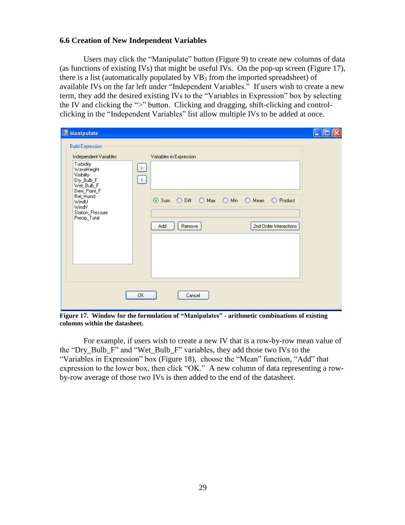
6.6 Creation of New Independent Variables

Users may click the “Manipulate” button (Figure 9) to create new columns of data

(as functions of existing IVs) that might be useful IVs. On the pop-up screen (Figure 17),

there is a list (automatically populated by VB3 from the imported spreadsheet) of

available IVs on the far left under “Independent Variables.” If users wish to create a new

term, they add the desired existing IVs to the “Variables in Expression” box by selecting

the IV and clicking the “>” button. Clicking and dragging, shift-clicking and control-

clicking in the “Independent Variables” list allow multiple IVs to be added at once.

Figure 17. Window for the formulation of “Manipulates” - arithmetic combinations of existing

columns within the datasheet.

For example, if users wish to create a new IV that is a row-by-row mean value of

the “Dry_Bulb_F” and “Wet_Bulb_F” variables, they add those two IVs to the

“Variables in Expression” box (Figure 18), choose the “Mean” function, “Add” that

expression to the lower box, then click “OK.” A new column of data representing a row-

by-row average of those two IVs is then added to the end of the datasheet.

30

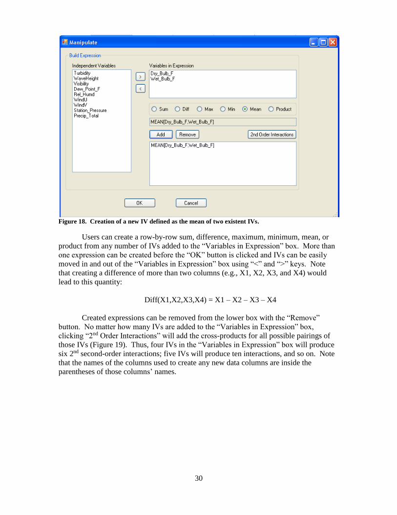
Figure 18. Creation of a new IV defined as the mean of two existent IVs.

Users can create a row-by-row sum, difference, maximum, minimum, mean, or

product from any number of IVs added to the “Variables in Expression” box. More than

one expression can be created before the “OK” button is clicked and IVs can be easily

moved in and out of the “Variables in Expression” box using “<” and “>” keys. Note

that creating a difference of more than two columns (e.g., X1, X2, X3, and X4) would

lead to this quantity:

Diff(X1,X2,X3,X4) = X1 – X2 – X3 – X4

Created expressions can be removed from the lower box with the “Remove”

button. No matter how many IVs are added to the “Variables in Expression” box,

clicking “2nd Order Interactions” will add the cross-products for all possible pairings of

those IVs (Figure 19). Thus, four IVs in the “Variables in Expression” box will produce

six 2nd second-order interactions; five IVs will produce ten interactions, and so on. Note

that the names of the columns used to create any new data columns are inside the

parentheses of those columns’ names.

31

Figure 19. Formation of two-way cross-products of a set of four IVs.

VB3 does not allow previously created “manipulates” -- new columns of data

created through the “Manipulate” button -- to be further manipulated. Previously created

manipulates will not appear in the “Independent Variables” section at the left. They can,

however, be chosen as the response variable or deleted from the datasheet, using the

appropriate menu choices accessed by a right-click of the column header.

6.7 Transforming the Independent Variables

VB3 gives users the ability to transform non-categorical IVs to assist in linearizing

the relationship between the IVs and the response variable, a fundamental assumption of

an MLR/PLS analysis. VB3 transformations are described in section A.1. When users

click the “Transform” button (Figure 9) in the Global Datasheet ribbon, they are

presented with the window seen in Figure 20:

32

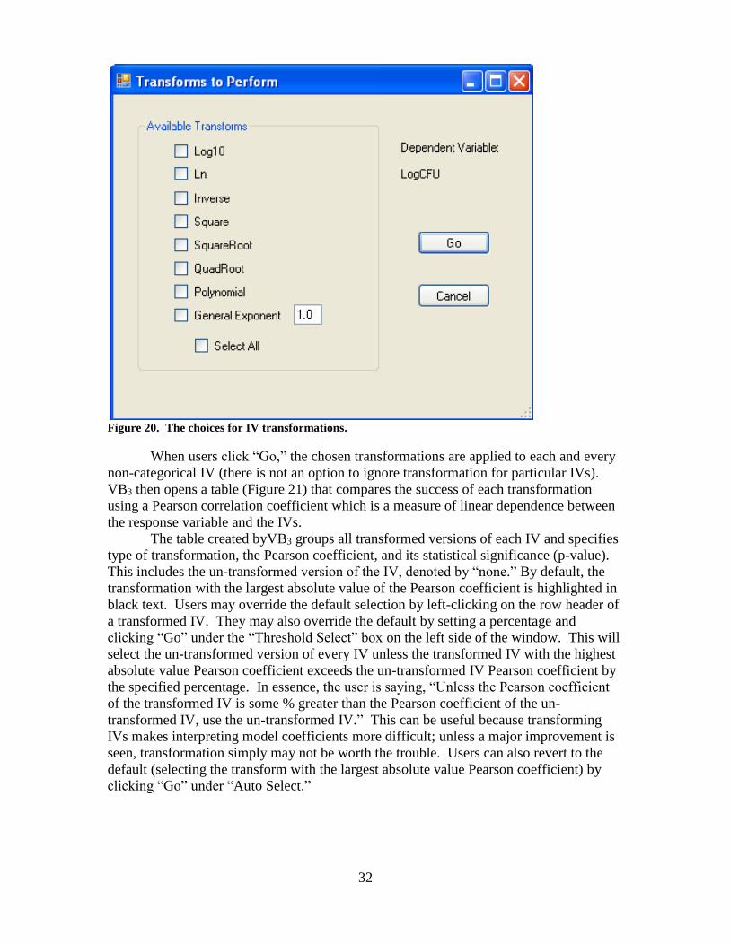
Figure 20. The choices for IV transformations.

When users click “Go,” the chosen transformations are applied to each and every

non-categorical IV (there is not an option to ignore transformation for particular IVs).

VB3 then opens a table (Figure 21) that compares the success of each transformation

using a Pearson correlation coefficient which is a measure of linear dependence between

the response variable and the IVs.

The table created byVB3 groups all transformed versions of each IV and specifies

type of transformation, the Pearson coefficient, and its statistical significance (p-value).

This includes the un-transformed version of the IV, denoted by “none.” By default, the

transformation with the largest absolute value of the Pearson coefficient is highlighted in

black text. Users may override the default selection by left-clicking on the row header of

a transformed IV. They may also override the default by setting a percentage and

clicking “Go” under the “Threshold Select” box on the left side of the window. This will

select the un-transformed version of every IV unless the transformed IV with the highest

absolute value Pearson coefficient exceeds the un-transformed IV Pearson coefficient by

the specified percentage. In essence, the user is saying, “Unless the Pearson coefficient

of the transformed IV is some % greater than the Pearson coefficient of the un-

transformed IV, use the un-transformed IV.” This can be useful because transforming

IVs makes interpreting model coefficients more difficult; unless a major improvement is

seen, transformation simply may not be worth the trouble. Users can also revert to the

default (selecting the transform with the largest absolute value Pearson coefficient) by

clicking “Go” under “Auto Select.”

33

Figure 21. Pearson correlation coefficient scores for judging the efficacy of IV transformations.

Plotting Transformed IVs

Users may prefer to examine plots visually in determining which transformation

of IV to choose. Right-clicking on a row header in the correlation table provides an array

of scatter plots, time series plots, or frequency plots for each transformation of that IV

(Figure 22). Scatter plots show the best-fit regression line. In the table at the top of this

window, users are shown the correlation coefficient and its p-value, as well as the

Anderson-Darling test statistic for normality, and its p-value.

34

Figure 22. Scatter plots (Response vs. IV) for six different data transformations of a single IV.

After choosing a transformation for each IV, users click “OK.” This populates

the datasheet with new columns representing transformed versions of the IVs. Notice

two things: if a transformation was chosen for an IV, the column representing the

untransformed version of that IV is disabled in the datasheet (it can be re-enabled by

using the right-click column header menu option) and the transformed versions of an IV

are put into the datasheet immediately after the original, un-transformed IV. Any

transformations put into the datasheet can be deleted with the “Delete Column” choice

(right-click on their column header). Transformed IVs will appear in the list of IVs on

the “Manipulate” screen, however, transformed IVs cannot be further transformed and

will not appear in the transform table if the user returns to the “Transform” window.

Also, transformed IVs cannot be the response variable. Finally, because transformations

are determined from the current response variable, all transformed IVs in the datasheet

are erased (a warning appears) when users change the response variable in the datasheet.

For the interested reader, further discussion of VB3 transformations can be found in

section A.1.

6.8 Singular Matrices and Nominal Variables

Advice on avoiding singularities within the data matrix and handling nominal

categorical variables can be found in section A.2.

35

6.9 Saving Processed Data

Changes made to the imported spreadsheet can be saved in a project file

(FileSave). When it is re-opened, the datasheet will appear as it did when the project

was saved. Users also may highlight the entire datasheet or sections of the datasheet and

use Control-C and Control-V to copy and paste it into a word processing or spreadsheet

application.

6.10 Proceeding to Modeling

After data processing is complete, users must click the “Go to Model” button to

open the statistical method tabs. If they have already done some modeling and return to

the global datasheet to make changes, they will receive a message that the datasheet has

changed and any prior modeling results will be erased.

36

7. MULTIPLE LINEAR REGRESSION MODELING

The MLR tab finds the best multiple linear regression model based on criteria

selected by the user. As the number of IVs increases, the number of possible models in

the solution space increases exponentially. Users may select all or a subset of the IVs for

consideration in the model to reduce the size of the solution space.

Notice that the MLR tab (as well as the PLS and GBM tabs) has its own datasheet

on the “Data Manipulation” sub-tab. When the user first moves over to the MLR tab

from the Global Datasheet, the data in the MLR Data Manipulation sub-tab is identical to

the data on the Global Datasheet. Once inside the MLR tab, the user can change the

“local” data to suit the MLR analysis. The local datasheet has all of the functionality of

the Global Datasheet discussed in Section 6. Changing the local data has no effect on the

Global Datasheet, however, going back to the Global Datasheet and making changes

causes local datasheets on the MLR, PLS, and GBM tabs to be overwritten.

7.1 Selecting Variables for Model Building

Under the “Model” sub-tab, two additional sub-tabs are found (Figure 23). On

the “Variable Selection” sub-tab, all eligible IVs are listed in the left column (“Available

Variables”). Any variable users wish to consider for model inclusion must be moved to

the right column list (“Indep. Variables”) by highlighting the IV and clicking the “>”

button. IVs currently under consideration (in the right list) can be ignored by

highlighting them and clicking the “<” button. The user can hold down shift while left-

clicking or control while left-clicking to select multiple IVs at once.

Figure 23. Selecting variables for MLR processing within the Modeling tab.

37

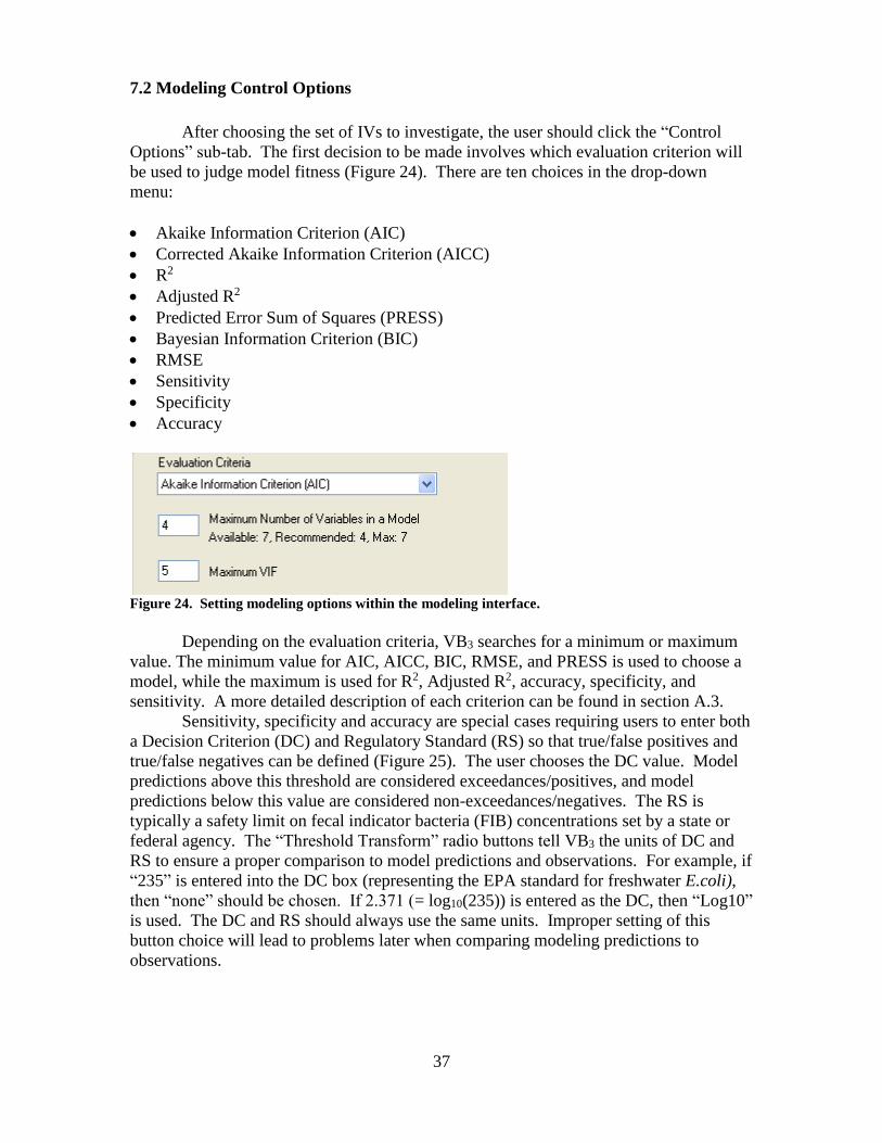
7.2 Modeling Control Options

After choosing the set of IVs to investigate, the user should click the “Control

Options” sub-tab. The first decision to be made involves which evaluation criterion will

be used to judge model fitness (Figure 24). There are ten choices in the drop-down

menu:

Akaike Information Criterion (AIC)

Corrected Akaike Information Criterion (AICC)

R2

Adjusted R2

Predicted Error Sum of Squares (PRESS)

Bayesian Information Criterion (BIC)

RMSE

Sensitivity

Specificity

Accuracy

Figure 24. Setting modeling options within the modeling interface.

Depending on the evaluation criteria, VB3 searches for a minimum or maximum

value. The minimum value for AIC, AICC, BIC, RMSE, and PRESS is used to choose a

model, while the maximum is used for R2, Adjusted R2, accuracy, specificity, and

sensitivity. A more detailed description of each criterion can be found in section A.3.

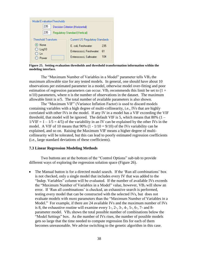
Sensitivity, specificity and accuracy are special cases requiring users to enter both

a Decision Criterion (DC) and Regulatory Standard (RS) so that true/false positives and

true/false negatives can be defined (Figure 25). The user chooses the DC value. Model

predictions above this threshold are considered exceedances/positives, and model

predictions below this value are considered non-exceedances/negatives. The RS is

typically a safety limit on fecal indicator bacteria (FIB) concentrations set by a state or

federal agency. The “Threshold Transform” radio buttons tell VB3 the units of DC and

RS to ensure a proper comparison to model predictions and observations. For example, if

“235” is entered into the DC box (representing the EPA standard for freshwater E.coli),

then “none” should be chosen. If 2.371 (= log10(235)) is entered as the DC, then “Log10”

is used. The DC and RS should always use the same units. Improper setting of this

button choice will lead to problems later when comparing modeling predictions to

observations.

38

Figure 25. Setting evaluation thresholds and threshold transformation information within the

modeling interface.

The “Maximum Number of Variables in a Model” parameter tells VB3 the

maximum allowable size for any tested models. In general, one should have about 10

observations per estimated parameter in a model, otherwise model over-fitting and poor

estimation of regression parameters can occur. VB3 recommends this limit be set to (1 +

n/10) parameters, where n is the number of observations in the dataset. The maximum

allowable limit is n/5. The total number of available parameters is also shown.

The “Maximum VIF” (Variance Inflation Factor) is used to discard models

containing variables with a high degree of multi-collinearity, i.e., IVs that are highly

correlated with other IVs in the model. If any IV in a model has a VIF exceeding the VIF

threshold, that model will be ignored. The default VIF is 5, which means that 80% (1 –

1/VIF = 1 – 1/5 = 4/5) of the variability in an IV can be explained by the other IVs in the

model. A VIF of 10 means that 90% (1 - 1/10 = 9/10) of the IVs variability can be

explained, and so on. Raising the Maximum VIF means a higher degree of multi-

collinearity will be tolerated, but this can lead to poorly estimated regression coefficients

(i.e., large standard deviations of these coefficients).

7.3 Linear Regression Modeling Methods

Two buttons are at the bottom of the “Control Options” sub-tab to provide

different ways of exploring the regression solution space (Figure 26).

The Manual button is for a directed model search. If the ‘Run all combinations’ box

is not checked, only a single model that includes every IV that was added to the

“Indep. Variables” column will be evaluated. If the number of available IVs exceeds

the “Maximum Number of Variables in a Model” value, however, VB3 will show an

error. If ‘Run all combinations’ is checked, an exhaustive search is performed,

testing every model that can be constructed with the selected IVs, but does not

evaluate models with more parameters than the “Maximum Number of Variables in a

Model.” For example, if there are 24 available IVs and the maximum number of IVs

is 8, the exhaustive routine will examine every 1-, 2-, 3-, 4-, 5-, 6-, 7- and 8-

parameter model. VB3 shows the total possible number of combinations below the

“Model Settings” box. As the number of IVs rises, the number of possible models

gets so large that the time needed to compute regression fits for each of them

becomes unreasonable. We advise switching to the genetic algorithm in this case.

39

The genetic algorithm (GA) button explores solution spaces too large to handle

exhaustively. Genetic algorithms are loosely based on natural evolution in which

individuals in a population reproduce and mutate (Fogel 1998). Individuals with high

fitness (regression models that produce small residuals) are more likely to reproduce

and pass their genes (IVs) to the next generation. The goal is to find a good solution

without having to examine every possible option. The GA balances random and

directed searching.

Figure 26. Model building interface using a manual search (left panel) or the genetic algorithm

(right panel).

Choosing between the exhaustive and the GA searches depends on the dataset, the

computer’s available random access memory (RAM), and time constraints. On a dataset

of 101 observations and ten IVs, the exhaustive search was completed in approximately

6 seconds, using a Dell Precision T5400 (WinXP; dual Xeon 2.66 GHz processors; 4 GB

RAM). Every additional IV doubles the number of models to examine and, thus,

approximately doubles necessary computational time (Table 1).

40

Table 1. Relationship between the number of IVs, number of possible models, and time required to execute

an exhaustive search using VB3.

In contrast, running the GA with 10 IVs, using a population of 100 for 100

generations, took 90 seconds to complete (90/6 = 15 times slower than the exhaustive

routine for this number of IVs); the GA with 12 IVs takes about the same amount of time

- 90 seconds. So, as computational time of the exhaustive routine doubles every time an

IV is added, the time required to run the GA stays approximately the same. As the

number of IVs rises (here, to 14 or 15), the GA would be expected to save time and

provide a solution very close to optimal.

An alternative modeling strategy with a large number of IVs would be to run the GA

on the entire list of IVs initially, then switch to the exhaustive search on a subset of

initial IVs – any IV that appears in one of the best ten models found by the GA. This

two-step process is facilitated with the “IV Filter” list control (Figure 27).

Figure 27. Using the IV filter to select a subset of variables from the best-fit models.

When the GA finishes and the 10 best models are shown in the Model

Information box “Best Fits” window, clicking the “Clear List” button removes all IVs

from the selection list. Select a model from the “Best Fits” list and click “Add to List”

which adds any IVs in the selected model to the “Indep. Variable” list in the Model

Settings box. After doing this for each of the ten best models, users will have a more

manageable IV list and can run an exhaustive search to find the best combination of IVs.

Regardless of the method chosen to build models, the “Best Fits” window shows the top

ten models found, based on user-specified evaluation criterion.

41

7.4 Using the Genetic Algorithm

Several parameters are used to adjust the performance of the GA (Figure 28):

Seed value: VB3 uses an internal random number generator to produce random

values. Setting the seed to a previously-used value will produce results identical to

that earlier run, allowing the analysis to be reproduced by other parties. Changing the

seed creates a new series of random values, possibly returning a different set of

identified regression models.

Population size: number of individuals in the population of each generation. A larger

population broadens the search at each generation, but slows processing time.

Number of generations: because individuals can reproduce and mutate once each

generation, the question is how long to run the search. Fitness of every individual in

the population is evaluated at the end of each generation.

Mutation rate: chance each individual has of undergoing random mutation in each

generation. The higher the mutation rate, the more random (less directed) the search

of parameter space is.

Crossover rate: the percent of each parent’s genome that children receive. For

example, if crossover = 0.5, child 1 and child 2 each receive 50% of the genome of

parent 1 and parent 2. If crossover = 0.3, child 1 receives 30% of the parent 1

genome and 70% of the parent 2 genome, while child 2 receives 70% of the parent 1

genome and 30% of the parent 2 genome.

The best GA parameter values depend on the dataset being investigated, but

typical values of the mutation rate are between 0.001-0.1 and typical values of the

crossover rate are 0.25-0.5. For small datasets, a population size and generation number

of 100 are sufficient. Larger datasets may require increased numbers for optimal

solutions. The user must invoke an experimental approach for changing these parameters

and examining the results.

Figure 28. Genetic algorithm options within the modeling interface.

42

7.5 Evaluating Model Output

After selecting a method to build models (GA or Exhaustive) and an evaluation

criterion, click the “Run” button at the bottom of the “Control Options” sub-tab (Figure

25). Progress is displayed on the “Progress” sub-tab at the lower left of the MLR screen.

Note that the “Run” button changes to “Cancel” if the user desires to terminate the

process. Once model-building is completed, the ten best models are displayed in the

“Best Fits” window (Figure 29). Selecting a model from the list results in:

A list of selected IVs for the model, with associated regression coefficients and

statistics displayed on the “Variable Statistics” sub-tab (Figure 30).

A list of evaluation metrics for the selected model shown on the “Model Statistics”

sub-tab (Figure 31).

The “Results” sub-tab shows two data series - model fits and observations versus

observations (Figure 32). Observations that are chronologically ordered are similar

to a time series plot of the two data series, but ignore the possibility that time steps

between data points are not equally spaced.

The “Fitted vs Observed” sub-tab shows plots and tables based on fitted model

values versus the observations (Figure 33).

The “ROC Curves” sub-tab shows a plot of the Receiver Operating Characteristic

curve of each “Best Fits” model (Figure 34), as well as a table showing the

computed AUC (area-under-the-curve) for each ROC curve (see Section 7.7).

The “View Report” generates a text report of model and variable statistics for the

selected model.

The “Residuals” sub-tab allows access to residual analysis functions in VB3 (see

Section 7.8).

The “Prediction” tab appears at the top and bottom of the VB3 screen, allowing users

to proceed to the prediction component (Figure 29).

Note that selecting a different model from the “Best Fits” list will update the

Variable and Model Statistics tables, as well as the information displayed on the

“Results,” “Fitted vs Observed,” “ROC Curves,” and “Residuals” sub-tabs.

43

Figure 29. Modeling results after completion of a run using the genetic algorithm.

44

Figure 30. Modeling Interface showing variable statistics for the selected model.

Figure 31. Modeling interface showing model evaluation metrics for the selected model.

45

Figure 32. Modeling interface showing a time series plot for the selected model.

Figure 33. A scatter plot of fitted values versus observations of the selected model.

46

Figure 34. The ROC curves and AUC table for the model chosen from the “Best Fits” window.

7.6 Viewing X-Y Scatter plots

On the MLR “Fitted vs Observed” and the MLR “Residuals” sub-tabs in the

Model Information box, users are shown a graph to compare observations to fitted values

from the model (Figure 33). Users can view different results from the pull-down tab

from the “Select View” box:

A plot of fitted values versus observations: “Pred vs. Obs”

A table summarizing model errors (false negatives/false positives) as the decision

criterion (DC) varies across the range of the response variable: “Error Table: DC

as CFU”

A plot of the percent of probability of exceedance (based on the current DC)

versus observations: “% Exc vs. Obs”

A table summarizing model errors as the percent of probability of exceedance is

varied: “Error Table: DC as % Exc”

On the two plots, a right-click in the plot area shows a menu of functions for

saving, copying, printing or manipulating the plot view. The plot area can be zoomed

and un-zoomed: the left-click on the mouse drags an area for zooming in; the right-click

selects “Un-Zoom” or “Set Scale to Default” to see the entire data set. To pan to a plot

area not in view, hold the Shift key down and use the left mouse button to drag the view.

Hovering the cursor over a data point shows the ID of the selected data point; if the

information does not appear, right-click on the graph and select “Show Point Values.”

47

Regarding interpretation of these plots, the green (Regulatory Standard or RS) and

blue (Decision Criterion or DC) lines allow model evaluation and provide information for

choosing a DC for later predictive purposes. On the plots, false positives represent data

points in the upper left quadrant of the graph, where the model fits/predictions exceed the

DC, but observations are below the RS. In such cases, a beach advisory would be

incorrectly issued based on the model’s prediction, potentially leading to, for example,

economic losses. False negatives (points in the lower right quadrant) represent a more

serious scenario: model fits/predictions below the DC and observations that exceed the

RS. In other words, swimming at the beach may have been allowed when it should have

been prohibited due to elevated FIB concentrations.

A model that produces no false positives or false negatives would be an ideal

decision tool, but this is often unattainable with real data. Examining the two tables from

the “Fitted vs Observed” select view tab should allow users to set a robust DC, by using

units of the actual response variable or a percentage probability of exceedance that

minimizes both errors. In most cases, the RS is set by federal or state law and should not

be adjusted by the user; however, users are free to adjust the DC to minimize false

negatives and false positives.

7.7 ROC Curves

In addition to time series and scatter plots which show results for an individual

model, users may also compare all the “Best Fits” models using the ROC Curves tab

(Figure 34). A Receiver Operating Characteristic curve shows the true positive rate

(sensitivity) plotted against its false positive rate (1 - specificity) for a model, as the

Decision Criterion (DC) varies between its minimum and maximum predicted values.

Models can then be compared using the area under their ROC curves (AUC). Models

having the largest AUC values perform best over the entire decision space.

The model with the largest AUC appears in red text in the ROC tab’s model list.

A single ROC may be plotted by selecting a model in the list and clicking the “Plot”

button. Multiple models can be selected in the usual Windows fashion with Shift-Click

(select all items between the first and second selection) or Control-Click (select only the

clicked items). The background cell color of models not selected for plot display will be

gray after “Plot” button is clicked.

Clicking the “View Table” button will replace the ROC plot with a table showing

false positives, false negatives, sensitivity, and specificity at every evaluated value of the

Decision Criterion for a single model. Users need only click on a model in the list at the

left of this table to see its results. The ROC plot returns to view after clicking the “View

Plot” button.

AUC calculations are performed and curves are plotted when the “ROC Curve”

sub-tab is selected. If this tab is active and new models are subsequently built, leaving

this tab and returning will generate the new plots and AUC values.

7.8 Residual Analysis

Users may click the “Residuals” sub-tab to view information about the residuals

of the selected model (Figure 35). There are three additional tabs on Residuals:

“Residuals vs Fitted,” “Fitted vs Observed,” and “DFFITS/Cooks” (DF/C).

48

Figure 35. Information available on the Residuals sub-tab, including a plot of externally-studentized

residuals versus model fits that shows results of the Anderson-Darling normality test.

The Residuals vs Fitted tab shows a plot of externally-studentized residuals (Cook

and Weisberg 1982) versus their fitted model values (Figure 35). In the upper-left corner

of the plot, the Anderson-Darling normality statistic (Anderson and Darling 1952) is

shown with its statistical significance (p-value). Linear regression assumes normally-

distributed residuals, so that if this A-D normality test fails (i.e., the p-value is less than

0.05), the user can transform the response variable, transform some of the IVs, or delete

high leverage observations, using the DF/C tab.

On the DF/C tab, observations are sorted by the largest (absolute value) measure

in a table (Figure 36). At the lower left, radio buttons can be used to toggle between

DFFITS and Cook’s values, as well as change the view from a table of sorted values to a

plot of the DF/C values versus the Record ID (Figure 37). Data points with very large

DF/C values (i.e., lying outside the horizontal red boundaries on the plot) distort the

estimates and standard deviations of the regression coefficients. They are essentially

“outliers” and some thought to their removal from the dataset should be given.

49

Figure 36. A table of the DFFITS scores of the residuals.

Figure 37. A plot of the DFFITS scores of the residuals.

When the grid of DF/C values is visible, clicking the “Go” button in the Iterative

Rebuild section removes the observation with the largest absolute value DF/C, re-fits the

regression, and calculates new DF/C values for the remaining observations (Figure 38).

This model is named Rebuild1 and added to the “Rebuilds” window at the top left of the

sub-screen. Clicking the Iterative Rebuild “Go” button again produces a model called

Rebuild2 which is calculated after removing the observation with the largest absolute

value DF/C remaining in the dataset. The user can continue to click “Go” and remove

50

observations with the largest remaining DF/C, creating Rebuild3, Rebuild4, Rebuild5,

etc. VB3 will not allow users to delete any observations if 10 or fewer remain in the

dataset.

Whenever a rebuild model is created by pressing the “Go” button, the information

displayed in the Variable and Model Statistics tables, as well as the plots and information

on the “Residuals” sub-tab, is automatically updated to reflect it, even if another model is

highlighted in the “Best Fits” window. The user can select any model in the “Best Fits”

window list, however, to view its associated data and plots.

The user has freedom to remove outliers while toggling between DF/C measures.

For example, the first removal can be based on a DFFITS value, the next removal on a

Cook’s Distance, the next two removals on DFFITS, etc. Users may clear models from

the “Rebuilds” window by clicking the “Clear” button.

Rather than using Iterative Rebuild, there are two other choices under the “Auto

Rebuild” box, both of which remove all observations above some threshold. The

“iterative threshold” radio button bases removals on a threshold that is updated whenever

an observation is deleted. For DFFITS, this threshold is 2*(p/n) 0.5, where p is the

number of IVs in the model and n is the current number of observations in the dataset.

For Cook’s Distance, the threshold is 4/n.

Figure 38. DFFITS/Cook’s Distance controls for removing highly influential data points.

When the “iterative threshold” radio button is invoked inside the “Auto Rebuild”

box, VB3 first checks if any DF/C values are above the threshold; if so, VB3 removes the

observation with the largest absolute DF/C and recalculates the regression model, the

DF/C values, and the threshold because n has been reduced by 1. VB3 then checks if any

of these new DF/C values are above the recalculated threshold. If so, the process repeats.

VB3 continues until no remaining DF/C values exceed the current threshold or until half

of the dataset has been removed, whichever comes first. For example, if a dataset has

100 observations, VB3 will allow 50 to be removed before it breaks the Auto Rebuild

removal loop. The user can then click the Auto Rebuild “Go” button again to remove

another 25 observations of the remaining 50. In practice, one should not remove more

than about 5% of the original dataset as outliers; removing more observations than this

indicates a poor regression fit and warrants a different analytical technique. Indeed,

under the assumption of normally distributed data, we expect 5% of the observations to

fit relatively poorly.

The “constant threshold” radio button option differs from the “iterative threshold”

only in that the threshold entered by the user to the input box remains the same regardless

of how many observations are deleted. Updated DF/C values are still calculated after

every removal. VB3 will also stop this process if half the number of starting observations

51

has been deleted. There is an upper limit to the number that can be entered into the

“constant threshold” input box (DFFITS = 3; Cook’s Distance = 16/n).

Upon completion of the Auto Rebuild process, multiple models may have been

added to the “Rebuilds” window (Figure 39). For example, if 10 observations were

removed, Rebuild1 through Rebuild10 will appear in that window.

When the user wants to move from the MLR tab to the Prediction tab, the model

carried forward is the one highlighted blue in the “Best Fits” window or “Rebuilds”

window. It is easy to confirm that the model selected will be carried forward by checking

the numbers shown within the “Variable Statistics” and “Model Statistics” sub-tabs

(Figures 30 and 31). Note that observations removed from the dataset using the

“Residuals” sub-tab are not removed from the local dataset shown on the MLR “Data

Manipulation” tab.

Figure 39. Residuals interface showing a list of rebuilt models resulting from observation deletions,

and their associated statistics and residual plots.

Viewing the Data Table

From the DFFITS/Cooks sub-tab, users can click the “View Data” button to

display a history of observation removal for the selected model. From this window, users

may export the dataset for external use or re-importation into VB3 (Figure 40).

52

Figure 40. “View Data Table” window for examining the dataset after removal of influential data

points.

The “Fitted vs Observed” plot on the “Residuals” sub-tab is the same as that

introduced in Section 7.6 (Figure 41). There are two plots and two tables to examine,

along with controls to modify the Decision Criterion (blue horizontal line) and

Regulatory Standard (green vertical line).

Figure 41. Fitted vs Observed plot on the Residual sub-tab with model evaluation threshold control

and model evaluation statistics.

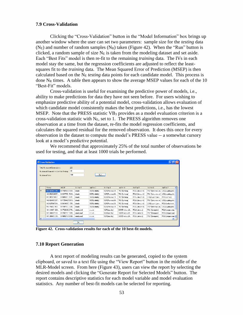
53

7.9 Cross-Validation

Clicking the “Cross-Validation” button in the “Model Information” box brings up

another window where the user can set two parameters: sample size for the testing data

(NE) and number of random samples (NR) taken (Figure 42). When the “Run” button is

clicked, a random sample of size NE is taken from the modeling dataset and set aside.

Each “Best Fits” model is then re-fit to the remaining training data. The IVs in each

model stay the same, but the regression coefficients are adjusted to reflect the least-

squares fit to the training data. The Mean Squared Error of Prediction (MSEP) is then

calculated based on the NE testing data points for each candidate model. This process is

done NR times. A table then appears to show the average MSEP values for each of the 10

“Best-Fit” models.

Cross-validation is useful for examining the predictive power of models, i.e.,

ability to make predictions for data they have not seen before. For users wishing to

emphasize predictive ability of a potential model, cross-validation allows evaluation of

which candidate model consistently makes the best predictions, i.e., has the lowest

MSEP. Note that the PRESS statistic VB3 provides as a model evaluation criterion is a

cross-validation statistic with NE, set to 1. The PRESS algorithm removes one

observation at a time from the dataset, re-fits the model regression coefficients, and

calculates the squared residual for the removed observation. It does this once for every

observation in the dataset to compute the model’s PRESS value -- a somewhat cursory

look at a model’s predictive potential.

We recommend that approximately 25% of the total number of observations be

used for testing, and that at least 1000 trials be performed.

Figure 42. Cross-validation results for each of the 10 best-fit models.

7.10 Report Generation

A text report of modeling results can be generated, copied to the system

clipboard, or saved to a text file using the “View Report” button in the middle of the

MLR-Model screen. From here (Figure 43), users can view the report by selecting the

desired models and clicking the “Generate Report for Selected Models” button. The

report contains descriptive statistics for each model variable and model evaluation

statistics. Any number of best-fit models can be selected for reporting.

54

A recommended approach to saving the information in an external application is

to copy the report to the clipboard with the “CopytoClipboard” button and paste it into an

application such as Microsoft Word or WordPad. NotePad or other simple text editors

will also work, but column formats will likely be lost, making the report difficult to

interpret.

Figure 43. A text report generated on the modeling results.

Comparative bar graphs can be displayed (Figure 44) to view evaluation criteria

for all top models by left-clicking and dragging the mouse to highlight selection and

clicking the “View Evaluation Graphs” button (Figure 43). Hover the mouse over any

plot to display the model evaluation criteria at the very top of the screen. Moving the

mouse over a bar on a plot will show that model’s coefficients under the title at the top,

and a label will appear with that same information. Note that evaluation criteria graphs

are initially scaled to emphasize differences between model scores although those

differences may, in fact, be quite small on an absolute scale (Figure 45). With the cursor

over any graph, right-click the mouse and select “Set Scale to Default” to view the un-

scaled graph.

55

Figure 44. Plots of various model evaluation metrics for the 10 best-fit models.

Figure 45. Scaled versus un-scaled views of selected model evaluation criteria.

56

8. PARTIAL LEAST SQUARES

Partial Least Squares (PLS) regression minimizes a problem that can arise in

MLR modeling: over-fitting in the presence of correlated predictors. To over-fit is to

match past data more closely than the real-world process being modeled. MLR is prone

to over-fitting because it makes the closest possible linear match to past data, even at the

cost of accuracy in predicting future observations.

As opposed to requiring the MLR user to be vigilant and proactive, PLS

regression (Brooks et al. 2013) inherently accounts for collinearity to suppress over-

fitting, and ranks the IVs by their influence in variable selection. Using PLS regression,

the user can include all available IVs in the model and let the algorithm sort out which

IVs are most useful, simplifying the sometimes laborious processes of variable selection

and comparing interactions.

A key feature of PLS (and GBM) modeling is the use of cross-validation to assess

real-world prediction accuracy. Model selection and threshold setting (section 8.4) are

done with reference to the true positive, true negative, false positive and false negative

counts, which are calculated by 5-fold cross validation. This means that the data are split

randomly and evenly into five subsets and five models are built to predict exceedances on

each of the five subsets. For each of these models, the subset predicted is left out of

model building, so the counts reflect prediction of novel observations, not accuracy in

fitting past observations. Greater detail about the PLS modeling method is available in

Brooks et al., 2013 and Hastie et al. 2009.

8.1 Data Manipulation

The MLR, PLS, and GBM modules all have “Data Manipulation” sub-tabs

(Figure 46). When the user first clicks on the PLS tab from the Global Datasheet, data in

the PLS Data Manipulation sub-tab is identical to data on the Global Datasheet. From the

PLS data tab, the user can change the “local” data to suit the PLS analysis. The local

datasheet has all of the functionality of the Global Datasheet discussed in Section 6.

Changing local data has no effect on the Global Datasheet; however, going back to the

Global Datasheet and making changes will overwrite local datasheets on each of the

modeling tabs.

57

Figure 46. Data Manipulation: the first sub-tab on each of the method tabs.


The “Variable Selection” tab is where IVs for model development are chosen

(Figure 47). Users may select all or a subset of the IVs for consideration in the model. All

eligible IVs are listed in the “Available Variables” window (left column). Any IVs that

users wish to include in the model must then be moved to the “Independent Variables”

window by highlighting the IV and clicking the “>” key. Any number of IVs can be

added or removed from this list. Once the desired IVs have been selected, click the

“Model” sub-tab.

Figure 47. Selecting variables for PLS processing within the modeling module.

58

8.3 The Regulatory Standard

To build a PLS ribbon, observations must be defined as exceedances or non-

exceedances; PLS and GBM models will not run if the dataset has no exceedances. This

is done by setting the Regulatory Standard (RS) at the top of the “Model” tab and then

specifying, using the radio buttons, units to enter into the RS. The default RS is the

USEPA’s federal standard for E. coli in freshwater, 235 CFU per 100 mL. Because these

are raw units of measurement, the radio button transformation choice should be set to

“Value.” However, users may be thinking of bacteria concentrations in logarithmic units;

if so, the RS is 2.371 (= log10(235)). To communicate this to VB3, enter 2.371 in the

“Regulatory Standard” box and click the “Log10 (value)” radio button (Figure 48).

Figure 48. Setting the Regulatory Standard and running models for PLS.


Clicking “Run” on the PLS Model tab (Figure 48) will start model development.

There is some randomness built into the PLS/GBM solver (due to the aforementioned

randomly-created data folds), so running the PLS/GBM multiple times on the same

dataset will likely produce slightly different solutions. If the user wishes to later replicate

a given PLS/GBM modeling result, they should check the “Set Seed Value” box and put

some positive integer into the input box (Figure 49). If that seed is input again, the

PLS/GBM solver will return a solution identical to the previous solution using that seed

value. After a solution is reached, the “Drop Variable(s)” option on the PLS ribbon

becomes enabled and a Decision Criterion (DC) for the model can be chosen.

59

Dropping Unimportant Variables

The “Model Summary” window (left side of Figure 49) lists IVs in descending

order of influence. For a PLS model, a variable’s influence is its model coefficient

multiplied by its standard deviation. The influence measurements are then adjusted to

sum to one. The larger the influence of a variable (global sensitivity), the more its

variation drives the response. Low-influence variables (highlighted in red text) can be

dropped from the model by clicking on the variable’s name in the list, then clicking the

“Drop Variable(s)” button on the ribbon. If any variables are dropped at this stage, the

model must be rebuilt by clicking the “Run” button.

Figure 49. Results after completion of a PLS model run.

Setting the Decision Threshold

Once the user has selected a model, the Decision Criterion (DC) is chosen (see

Section 7.2 for a description of the DC). The graph on the right side of the “Model” tab is

used for this purpose (Figure 49). To understand the plot, consider that a lower DC will

correctly identify more exceedances of the RS threshold, but also produce more “false

positives” by flagging predicted values when the actual water quality is below the RS.

Raising the DC has the opposite tradeoff: reducing false positives at the expense of

identifying fewer true exceedances.

60

The blue line on the graph indicates true positives and the yellow line indicates

true negatives. Current model performance is indicated by the following:

The vertical dotted line indicates the current location of the DC. The arrow buttons at

the bottom are used to lower/raise the threshold by a small (< , >) or large (<< , >>)

amount.

The “Model Validation” window (Figure 50) indicates the number of true positives,

true negatives, false positives, false negatives, sensitivity, specificity, and total

accuracy of the model using the current DC. These results are based on cross-

validation of the training data. These numbers will change after a short

computational delay as the DC is moved. Care should be taken when comparing

PLS/GBM model performance (in terms of false/true positives/negatives) with MLR

models. MLR model performance is based on fitted, not cross-validated results.

Cross-validation results are commonly thought to be more realistic in how well the

model will do in future predictions, while fitted values better indicate how well the

model fits previously-collected data. Cross-validation results are generated by

developing models with partial data sets and making predictions for data left out of

model development. For example, 5-fold cross validation would result in five

different sets of IV coefficients for a single model by using 4/5 of the data to develop

each set of IV coefficients, then predicting the remaining 1/5 of the data using those

coefficients. MLR, on the other hand, uses all available data points to fit the model

coefficients and then predicts the same data points. Look at cross-validated

performance of MLR models using the “Cross-Validation” button described in

Section 7.9.

The current numeric value of the DC is shown above the “Model Summary” window

(Figure 49).

The user can change the DC, drop variables, and re-run the model to fine-tune it.

After the model and DC have been chosen, the user can advance to the Prediction tab

(Section 10) to make predictions with the most recently computed model.

Figure 50. Summary of PLS model performance metrics.

8.5 Diagnostics

There are four plots are offered on the “Diagnostics” sub-tab (Figure 51):

61

The Time Series plot (upper left) displays predicted and observed values of the

response variable. This is a time-series plot if the ID values for the observations are

chronologically-ordered dates/times. If they are not, then this plot will look rather

messy and strange, and be of little interest to the user.

The Residuals vs. Fitted plot (upper right) shows the externally-studentized residuals

versus model-fitted values. The externally-studentized residuals are a way to flag

influential outliers. A common benchmark for a data point with undue influence on

the regression model is an externally-studentized residual (absolute value) greater

than 3.0.

The Residuals vs. Observed plot (lower left) graphs the externally-studentized

residuals against the observations.

The Fitted vs. Observed plot (lower right) shows observations versus model fits and

depicts the RS (green horizontal line) and current DC (blue vertical line).

Note that the fitted values plotted here are not cross-validated fits; rather they are

the model fits based on all the data. For this reason, model performance in this plot

(numbers of true negatives/positives) will likely be better than the model performance

metrics given in the “Model Validation” window on the “Model” tab. A perfect model

will fall along the 1:1 line. The more scatter in this plot, the worse the model fit.

Figure 51. PLS Diagnostic plots to help evaluate model fit and influential outliers.

62

9. GENERALIZED BOOSTED REGRESSION MODELING

The Generalized Boosted Regression Model (GBM, also known as a gradient

boosting machine) is a machine learning method that uses decision/regression trees

instead of linear equations (Friedman, 2001). A decision/regression tree is a set of binary

decision rules. For example, “if turbidity is less than 15 NTU, go down the right branch,

otherwise go left.” A “node” is the end of any branch and designates a continuous or

categorical predictive value for the response variable. The innovative aspect of GBM is

that it doesn’t build a single, complex tree: it builds a hierarchical set of many simple

trees, with each subsequent tree fit to the remaining residual error in the data after

previous trees have all been fit. The default maximum number of trees in VB3 is 10,000.

Each tree is determined using a random set of the residual values from the dataset. This,

along with the fact that it sensibly weights the data to learn more about the most difficult-

to-predict cases, means GBM can make accurate predictions for new observations

without over-fitting the training data.

While each tree is a simple structure, the long, linear combination of regression

trees is more complicated. A negative aspect of a GBM model is that the model cannot

easily be inspected graphically or expressed mathematically – it’s something of a “black

box.” But what it lacks in interpretability and transparency can often be made up in

terms of prediction accuracy. Another noted aspect of GBM, unlike MLR and PLS, is

that it handles non-linear relationships between the response and IVs without having to

transform the IVs. However, GBM is best used on larger datasets (> 100 observations),

and odd results can occur if using GBM on small datasets.

In a GBM, variable selection (identifying and dropping unimportant IV’s from the

model) is less important, compared to MLR. Even so, the “Drop Variables” button

(Figure 52) performs as described in Section 8.4. For a GBM model, an IV’s influence is

the percentage of branches across all of the decision trees involving that variable, i.e., the

most important variables are those that are most often used to create the branches.

For the GBM analysis, VB3 implements the “gbm” package in R. Details of the

algorithm are provided in Hastie (2009). Despite very different underlying mathematics,

the GBM modeling interface in VB3 is almost identical to the PLS interface (Section 8).

A key feature of GBM and PLS modeling is the use of cross-validation to assess

real-world prediction accuracy. Model selection and threshold setting (Section 8.4) are

done with reference to true positive, true negative, false positive and false negative

counts which are calculated by 5-fold cross-validation. This means the data are split

randomly and evenly into five sections and five models are built to predict exceedances

on each of the five sections. For each, the section being predicted is left out of model

building, so the counts reflect prediction of novel observations, not accuracy in fitting to

past observations.

63

9.1 Data Manipulation

The MLR, PLS, and GBM modules all have “Data Manipulation” sub-tabs

(Figure 52). When the user first clicks the GBM tab, the data in the GBM Data

Manipulation sub-tab are identical to data on the Global Datasheet. From here, the user

can change the “local” data to suit the GBM analysis. The local datasheet has all of the

functionality of the Global Datasheet discussed in Section 6. Changing the local data has

no effect on the Global Datasheet; however, going back to the Global Datasheet and

making changes will overwrite the local datasheets on each of the modeling tabs.

Figure 52. Data Manipulation: the first sub-tab on each of the Method tabs.


The “Variable Selection” sub-tab is where IVs for model development are chosen

(Figure 53). Users may select all or a subset of IVs for the model. All eligible IVs are

listed in the “Available Variables” window (left column). Any IVs that users wish to

include in the model must be moved to the “Independent Variables” window by

highlighting the IV and clicking the “>” key. Any number of IVs can be added or

removed from this list. Once the desired IVs have been selected, click the “Model” sub-

tab.

64

Figure 53. Selecting variables for GBM processing within the modeling module.

9.3 The Regulatory Standard

To build a GBM model, observations must be defined as exceedances or non-

exceedances; GBM and PLS models will not run if the dataset has no exceedances. This

is done by setting the Regulatory Standard (RS) at the top of the “Model” sub-tab (Figure

54) and then specifying with the radio buttons units to enter for the RS. The default RS is

the USEPA’s federal standard for E. coli in freshwater, 235 CFU per 100 mL. Because

these are the raw units of measurement, the radio button transformation choice should be

set to “Value.” When thinking of bacteria concentrations in logarithmic units, think of

the RS as 2.371 [= log10(235)]. To communicate this to VB3, enter 2.371 in the

“Regulatory Standard” box and click the “Log10 (value)” radio button (Figure 54).

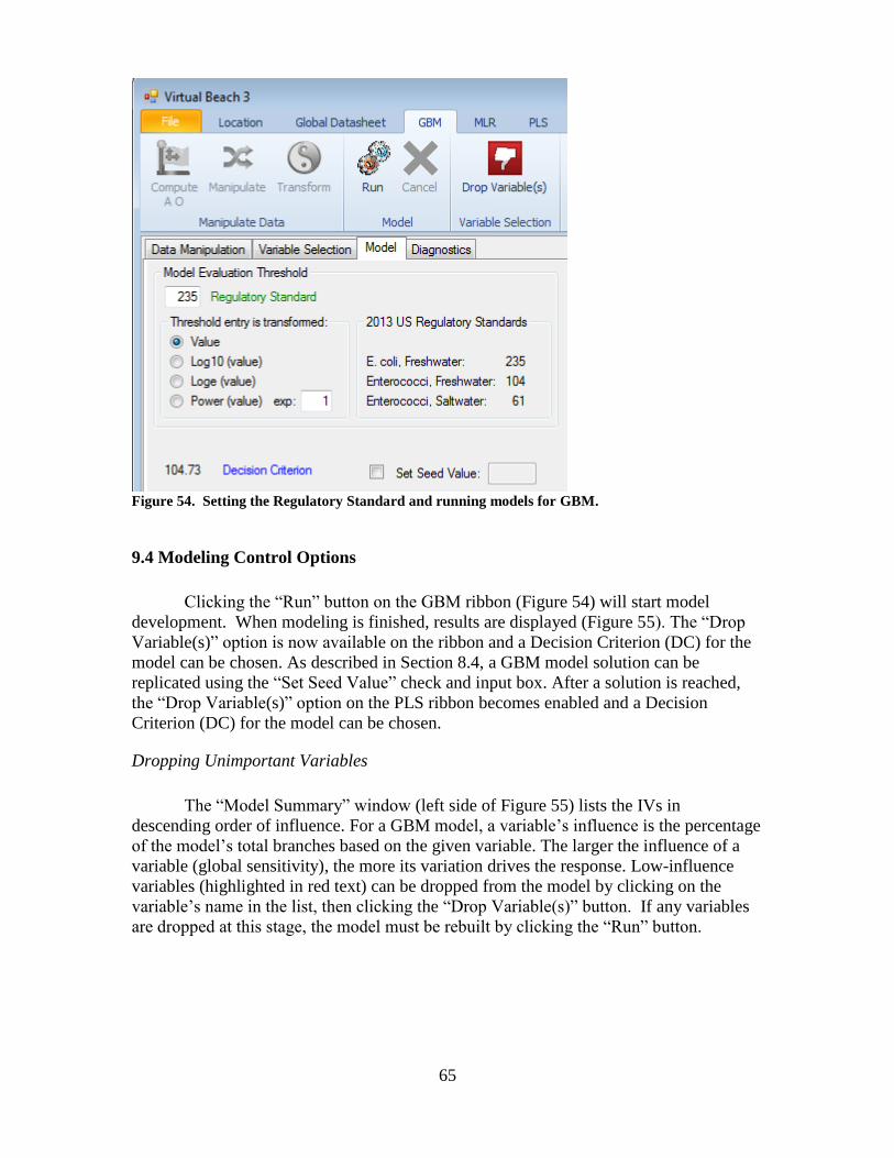
65

Figure 54. Setting the Regulatory Standard and running models for GBM.


Clicking the “Run” button on the GBM ribbon (Figure 54) will start model

development. When modeling is finished, results are displayed (Figure 55). The “Drop

Variable(s)” option is now available on the ribbon and a Decision Criterion (DC) for the

model can be chosen. As described in Section 8.4, a GBM model solution can be

replicated using the “Set Seed Value” check and input box. After a solution is reached,

the “Drop Variable(s)” option on the PLS ribbon becomes enabled and a Decision

Criterion (DC) for the model can be chosen.

Dropping Unimportant Variables

The “Model Summary” window (left side of Figure 55) lists the IVs in

descending order of influence. For a GBM model, a variable’s influence is the percentage

of the model’s total branches based on the given variable. The larger the influence of a

variable (global sensitivity), the more its variation drives the response. Low-influence

variables (highlighted in red text) can be dropped from the model by clicking on the

variable’s name in the list, then clicking the “Drop Variable(s)” button. If any variables

are dropped at this stage, the model must be rebuilt by clicking the “Run” button.

66

Figure 55. Results after completion of a GBM model run.

Setting the Decision Threshold

Once the user selects a model, the Decision Criterion (DC) can be chosen (see

Section 7.2 for a description of the DC). The graph on the right side of the Model tab is

used for this purpose (Figure 55). To understand the plot, consider that a lower DC

correctly identifies more exceedances of the RS threshold, but also produces more “false

positives” by flagging predicted values when the actual water quality is below the RS.

Raising the DC has the opposite tradeoff: reducing false positives at the expense of

identifying fewer true exceedances.

The blue line on the graph indicates true positives and the yellow line indicates

true negatives. Current model performance is indicated by the following:

The vertical dotted line indicates the current location of the DC. The arrow buttons at

the bottom are used to lower/raise the threshold by a small (< , >) or large (<< , >>)

amount.

The “Model Validation” window (Figure 56) indicates the number of true positives,

true negatives, false positives, false negatives, sensitivity, specificity, and total

accuracy of the model using the current DC. These results are based on cross-

validation of the training data. These numbers will change after a short

computational delay as the DC is moved. Comparing GBM (and PLS) model

67

performance, in terms of false/true positives/negatives, with MLR models must be

done carefully. MLR model performance is based on fitted results, not cross-validated

results. Cross-validation results are commonly thought to indicate more realistically

how well the model will do in future predictions and fitted values better indicate how

well the model fits previously collected data. Cross-validation results are generated

by developing models with partial data sets and subsequently making predictions for

data that were left out. For example, 5-fold cross validation would result in 5

different sets of IV coefficients for a single model by using 4/5 of the data to develop

each set of IV coefficients, and then predicting the remaining 1/5 of the data using

those coefficients. MLR, on the other hand, uses all available data points to fit the

model coefficients and then predicts the same data points. Look at cross-validated

performance of MLR models using the “Cross-Validation” button described in

Section 7.9.

The current numeric value of the DC is shown above the “Model Summary” window

(Figure 55).

The user can change the DC, drop variables and re-run the model to fine-tune it.

After the model and DC have been chosen, the user can advance to the Prediction tab

(Section 10) to make predictions with the most recently computed model.

Figure 56. Summary of GBM model performance metrics.

9.5 Diagnostics

There are four plots offered on the “Diagnostics” sub-tab (Figure 57):

The Time Series plot (upper left) displays predicted and observed values of the

response variable over time if the ID values for the observations are dates/times.

The Residuals vs. Fitted plot (upper right) shows the externally-studentized residuals

versus model-fitted values. The externally-studentized residuals are a way to flag

influential outliers. A common benchmark for a data point with undue influence on

the regression model is an externally-studentized residual (absolute value) greater

than 3.0. Certain patterns seen in this residual plot can indicate the need for a

transformation of the response variable or model IVs. Refer to Meyers (1990) for

details.

The Residuals vs. Observed plot (lower left) graphs the externally-studentized

residuals against the observations.

68

The Fitted vs. Observed plot (lower right) shows observations versus model fits and

depicts the RS (green horizontal line) and current DC (blue vertical line).

Note that the fitted values plotted here are not cross-validated fits; rather they are

the model fits based on all the data. For this reason, model performance in this plot

(numbers of true negatives/positives) will likely be better than the model performance

metrics given in the Model Validation table on the Model tab. A perfect model will fall

along the 1:1 line. The more scatter in this plot, the worse the model fit.

Figure 57. GBM diagnostic plots to help evaluate model fit and influential outliers.

69

10. PREDICTION

VB3’s Prediction interface allows users to select a model from the PLS, GBM, or

MLR tabs and make predictions with it, but the prediction tab is hidden until a model is

chosen.

10.1 Model Statement

At the top left of the Prediction tab is the “Available Models” window.

Depending on how many statistical methods were performed on the data, the user could

see “MLR,” “PLS,” and/or “GBM” in this area. Once a model is chosen, an expression

with the IVs and coefficients in that model is shown in the “Model” window to the right

(Figure 58).

Figure 58. The VB3 Prediction interface.

10.2 Model Evaluation Thresholds

In the “Model Evaluation Thresholds” box, there are input boxes for the Decision

Criterion (DC), Exceedance Probability, and Regulatory Standard (RS). Setting these

allows model predictions to be evaluated and model specificity, sensitivity, and accuracy

to be calculated. The radio buttons inside the “Threshold Transform” box tells VB3 how

70

to transform the DC and RS to compare to model predictions and observations (see

Section 7.2 for further guidance). Note that we define the “observations” as the measured

values of the model’s response variable (e.g., E.coli CFU measurements). If the

threshold transform definition is set improperly, there can be problems when comparing

modeling predictions to observations, so exercise caution.

10.3 Prediction Form

The bottom half of the Prediction interface is occupied by three data panels (the

empty gray sections separated by blue vertical bars at the bottom of Figure 58): the left

holds IV data; the middle is for observations; and the right shows model predictions and

evaluation metrics. Each panel also contains a column for a unique ID for each row of

data, e.g., the date that data were collected. The panels have separate horizontal and

vertical scroll bars that become visible if the number of rows or columns exceeds the

viewable area. The three panels independently scroll horizontally, but as a group

vertically. Panels can be re-sized by clicking and dragging the blue vertical partitions.

The order of the columns in the left (IV) and right (Model Predictions) panels can be

changed by clicking and dragging the column headers left or right. If it is important to

save a re-arranged column order for the selected model, click on the “Save Column

Order” button just above the IV panel.

Users can import data from files using the “Import IV Data,” “Import

Observations” and “Import Combined” (both IVs and observations) buttons on the top

ribbon, or type data directly into the left and middle grids. It is the user’s responsibility

to ensure that IV data are in the same units as those used to construct the model.

Depending on the model selected for prediction, the left panel will contain one column

for every unique model IV plus a column for an ID. The middle panel has two columns:

one for the ID and one for the observations (note that the name of the observation column

is identical to the name of the model’s response variable).

10.4 Column Mapping of Imported Data

When data are imported via one of the three import buttons (Figure 58), a

“Column Mapper” window opens (Figure 59). This allows users to tell VB3 which

columns in the imported datasheet should be used to fill in the row IDs, IVs and the

observations. By default, the first column of the imported file is mapped to the ID field,

but this can be overridden. If a column in the imported spreadsheet has a name identical

to a model IV or the response variable, VB3 will select it as the appropriate column for

that IV or the observations. If no identically-named column is found, the user must

specify which column of the imported file should be used for the IV and observations.

Once a user has gone through the mapping process for a model, that configuration

is saved. If another data file with the same column names is imported, the column

mapper will not appear. If a model has a saved mapping configuration, it can be viewed

and cleared by clicking “View Column Mapping” on the ribbon (Figure 58).

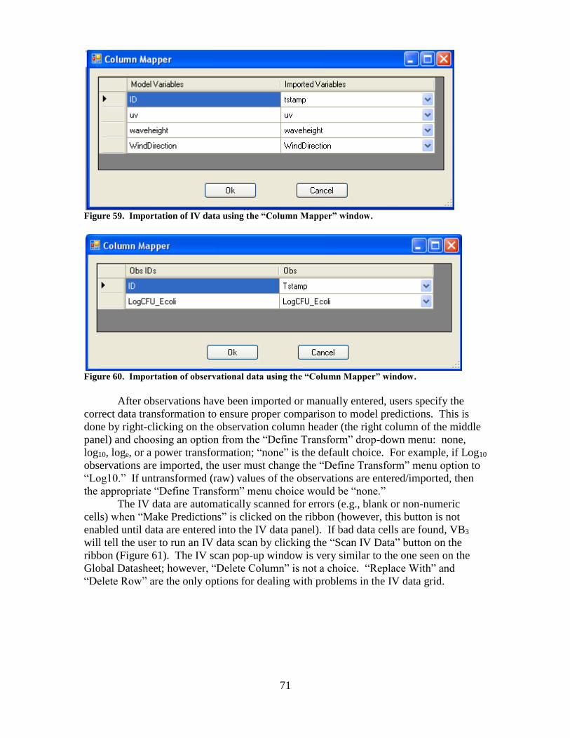
71

Figure 59. Importation of IV data using the “Column Mapper” window.

Figure 60. Importation of observational data using the “Column Mapper” window.

After observations have been imported or manually entered, users specify the

correct data transformation to ensure proper comparison to model predictions. This is

done by right-clicking on the observation column header (the right column of the middle

panel) and choosing an option from the “Define Transform” drop-down menu: none,

log10, loge, or a power transformation; “none” is the default choice. For example, if Log10

observations are imported, the user must change the “Define Transform” menu option to

“Log10.” If untransformed (raw) values of the observations are entered/imported, then

the appropriate “Define Transform” menu choice would be “none.”

The IV data are automatically scanned for errors (e.g., blank or non-numeric

cells) when “Make Predictions” is clicked on the ribbon (however, this button is not

enabled until data are entered into the IV data panel). If bad data cells are found, VB3

will tell the user to run an IV data scan by clicking the “Scan IV Data” button on the

ribbon (Figure 61). The IV scan pop-up window is very similar to the one seen on the

Global Datasheet; however, “Delete Column” is not a choice. “Replace With” and

“Delete Row” are the only options for dealing with problems in the IV data grid.

72

Figure 61. The scan IV window on the MLR Prediction tab.

Observational data need not be present to make predictions, but they are needed

for model evaluation (sensitivity, specificity, false negatives, false positives, accuracy).

After clicking “Make Predictions” on the ribbon, VB3 uses the model, IV data, and

observational data to fill the right panel with these data columns: ID, Model Prediction,

Decision Criterion, Exceedance Probability, Regulatory Standard, and Error Type (Figure

62).

73

Figure 62. A prediction grid after IVs and observational data have been imported, and model

predictions made.

The ID column of the model output panel is taken directly from the ID column of

the IV panel, not IDs in the middle panel. VB3 will make one model prediction per row

in the IV data panel, regardless of how many observations are entered in the middle

panel.

The Model Prediction column contains predicted values of the response variable,

initially displayed in the same units as the model’s response variable. Right-clicking on

this column header changes how predictions are displayed in the table (raw, log, or power

units). The Decision Criterion and Regulatory Standard are set by the user. They are

displayed in the same units as the Model Predictions, and their column headers can be

right-clicked to change the displayed units. The Exceedance Probability (displayed as a

percentage, or 100 times the probability) is defined as the probability that the model’s

prediction will be larger than the Decision Criterion, based on uncertainty bounds

(confidence intervals) of the model’s predictions.

To compare model predictions to observations, VB3 looks at the prediction ID and

attempts to find an observation in the middle panel with the same ID. It does not require

unique IDs for each row in the observation panel, but a model prediction is compared to

the first observation found with the same ID. When comparing model predictions to

observations, an error (“False Negative” or “False Positive”) will be reported in the

“Error Type” column.

We again emphasize that assessing model output correctly depends on the

synchronization of units of the Decision Criterion (DC), Regulatory Standard (RS),

74

model predictions, and observations. VB3 will ensure this happens if the user correctly

specifies the units for the observations (using the right-click column header menu of the

right column of the middle panel) and for the DC and RS (using the radio buttons in the

“Threshold Transform” box of the prediction window).

10.5 Viewing Plots

After predictions are made, a scatterplot of observations versus predictions, or

observations versus the probability of exceedance, can be viewed by clicking “Plot” on

the ribbon (Figures 62 and 63). If no observational data were entered, a message asking

for observational data appears. The features of this plot are similar to those described in

Section 7.6. Plotted points are based on comparing model predictions (right pane of the

Prediction Form) with observations (middle pane) that share the same unique row ID.

Note that the plotted exceedance probabilities are not automatically re-computed because

the Decision Criterion is changed in this plotting window. To see updated exceedance

probabilities for a new Decision Criterion, users must close this plotting window, change

the DC in the “Model Evaluation Thresholds” box, re-click the “Make Predictions”

button on the ribbon, and then click the “Plot” button again.

Figure 63. Prediction interface plotting of the observations versus predictions, with model evaluation

threshold controls.

75

10.6 Prediction Form Manipulation

Two other buttons found in the “Evaluate” section of the ribbon are “Clear” and

“Export as CSV.” To view the table in a spreadsheet or word processing program,

“Export as CSV” saves the contents of the entire table (all three panels) in .csv format.

“Clear” deletes all information in every panel of the table. As with most tabular

information in VB3, data in individual panels can be selected with a left-click and drag.

Control-c and Control-v are then used to copy and paste the data into another application

such as Excel.

10.7 Importation of EnDDaT Data

The Environmental Data Discovery and Transformation (EnDDaT;

http://cida.usgs.gov/enddat/) service accesses data from a variety of sources, compiles

and processes it, and performs common transformations. The result is environmental data

from multiple sources sorted into a single table. EnDDaT is a tool for compiling datasets

prior to model development. Once models are developed, EnDDaT can create datasets for

the VB3 Prediction tab. The “Set EnDDaT Data Source,” “Import from EnDDaT” and

“Import EnDDaT by Date” buttons on the ribbon (Figure 64) allow users to import data

directly from the EnDDaT web service to the prediction tab of VB3, avoiding manual

entry. See the EnDDaT user guide (available from the EnDDaT website link above) for

step-by-step instructions on obtaining data, specifying transforms, processing data and

developing a URL.

To import EnDDaT data to the IV panel of the prediction grid, click the “Set

EnDDaT Data Source” button and insert an EnDDaT-generated URL that calls for the

IVs needed to make predictions (Figure 65). Choose and activate the radio button for

whether to collect data from a specific time (e.g., the time the beach was visited) or from

the most recently available time. Users must also choose the desired time zone from the

dropdown list. After clicking “OK,” the “Import from EnDDaT” and “Import EnDDaT

by Date” buttons are enabled on the ribbon. To import data for the current day, use the

former button. Clicking the latter button opens a calendar for retrieval of data from a

previous day (Figure 66). Whichever button is used, afterwards a pop-up window will

indicate EnDDaT is being accessed (Figure 67). Once data have been retrieved, the

“column mapper” window will open, allowing the user to specify which columns in the

imported EnDDaT data should be matched to each IV in the selected model (see Section

10.4 for more details on column mapping).

Figure 64. The three EnDDaT-related buttons on the prediction tab.

http://cida.usgs.gov/enddat/

76

Figure 65. Setting URL options for retrieval of data from EnDDaT.

Figure 66. Choosing a previous day for EnDDaT data retrieval.

Figure 67. Pop-up window indicating that data have been requested from EnDDaT.

77

11. USER FEEDBACK

The USEPA and USGS provide no warranty, expressed or implied, as to the

correctness of the furnished software or the suitability for any purpose. The software has

been tested, but as with any complex software, there could be undetected errors.

Suggestions and experiences from the user community are welcomed by the Virtual

Beach design/development team, and users are encouraged to report problems, issues and

likes/dislikes to:

Mike Cyterski, USEPA: 706.355.8142 ([email protected])

Steve Corsi, USGS: 608.821.3835 ([email protected])

The USEPA has limited resources to assist users; however, we make an attempt to

fix reported problems and help whenever possible.

mailto:[email protected]

mailto:[email protected]

78

12. REFERENCES

Anderson, T.W., Darling, D.A., 1952. Asymptotic theory of certain "goodness-of-fit"

criteria based on stochastic processes. Annals of Mathematical Statistics 23: 193–212.

Brooks, W.R., Fienen, M.N., Corsi, S.R., 2013. Partial least squares for efficient models

of fecal indicator bacteria on Great Lakes beaches. J Environ Manage 114:470-5. doi:

10.1016/j.jenvman.2012.09.033.

Cook, R., Weisberg, S., 1982. Residuals and Influence in Regression. Chapman and

Hall, New York.

Cyterski, M., Galvin, M., Parmar, R., Wolfe, K., 2012. Virtual Beach User’s Manual –

version 2.2. USEPA/600/R-12/024/.

Efron, B., Tibshirani, R., 1986. Bootstrap methods for standard errors, confidence

intervals, and other measures of statistical accuracy. Stat. Sci. 1 (1), 54e77.

Fogel, D. (editor), 1998. Evolutionary Computation: The Fossil Record. New York: IEEE

Press.

Frick, W.E., Ge, Z., Zepp, R.G., 2008. Nowcasting and forecasting concentrations of

biological contaminants at beaches: a feasibility and case study. Environmental Science

and Technology 42, 4818-4824.

Friedman, J.H., 2001. Greedy function approximation: A gradient boosting machine. The

Annals of Statistics, 29:5, 1189-1232.

Hastie, T., Friedman, J., Tibshirani, R., 2009. The Elements of Statistical Learning.

Springer-Verlag, New York.

Myers, R., 1990. Classical and Modern Regression with Applications, 2nd Edition.

Duxbury Press, Belmont, California.

79

13. ACKNOWLEDGMENTS

We would like to thank the following people, who generously donated their time

and expertise for software testing and review of this document, as well as general support

for the continued development of VB:

Adam Mednick

Wisconsin Department of Natural Resources

Madison, WI

David Rockwell

Cooperative Institute for Limnology and Ecosystems Research, University of Michigan

Center of Excellence for Great Lakes and Human Health

NOAA Great Lakes Environmental Research Laboratory

Ann Arbor, MI

Gerry Laniak

USEPA National Exposure Laboratory

Ecosystems Research Division

Athens, GA

Brett Hayhurst

USGS New York Water Science Center

Ithaca, NY

Diane Mas

Fuss and O’Neill, Inc.

Manchester, CT

Amie Brady

USGS Ohio Water Science Center

Columbus, OH

Donna Francy

USGS Ohio Water Science Center

Columbus, OH

Richard Zepp

USEPA National Exposure Laboratory

Ecosystems Research Division

Athens, GA

Any use of trade, product, or firm names is for descriptive purposes only and does not

imply endorsement by the U.S. Government.

80

APPENDICES

A.1 Transformations

VB3 provides the following transformations, where Xt is the transformed IV and

X is the original IV:

Log10: Xt = log10(X)

Loge: Xt = loge(X)

Inverse: Xt = 1/X

Square: Xt = X2

Square Root: Xt = X0.5

Quad Root: Xt = X0.25

Polynomial: Xt = a + bX + cX2

General Exponent: Xt = Xz where the user specifies the value of z

For the polynomial transformation, the Pearson coefficient is calculated as the

square root of the adjusted R2 value derived from the regression of the response on Xt.

Because this adjusted R2 value can be negative, an empirically-derived formula is applied

when adjusted R2 values fall below 0.1:

Polynomial Pearson Coefficient = (-6.67*RE12 + 13.9*RE1- 6.24)*(R2)0.5

where

RE1 = 1.015 – 1.856*R2 + 1.862*adjR2 – 0.000153*N.

R2 and adjR2 are defined by the regression of the response on Xt, and N = number of

observations.

VB3 transformations (primarily converting x into xb) have specific processing for

certain data values and are not pure mathematical transformations -- they were designed

to maintain data order while helping to linearize the response-IV relationship. For the

SQUARE (b = 2), SQUAREROOT (b = 0.5), QUADROOT (b = 0.25), INVERSE (b = -

1) and GENERAL EXPONENT (user-defined b) transformations, VB3 uses the signed

equivalent of the mathematical function:

xb == sign(x)*(abs(x))b

For example: (-2)2 = -4 (-9)0.5 = -3 (-4)-0.5 = -0.5 (-2)-2 = -0.25

To avoid potentially undefined values (e.g., 1/x when x = 0), the INVERSE and

GENERAL EXPONENT (if the user sets b < 0) transformations have special processing:

If x = 0, VB3 will find the minimum value of abs(z) where z is the set of all non-

zero values for the IV in question. To compute the transformation after z is defined, VB3

81

substitutes z/2 for x. From this definition, note that z can be a positive or negative

number.

LOG10 and LOGe transforms are also the signed equivalent of their mathematical

functions:

loge(x) == loge(x)

loge(-x) == -loge(x)

log10(x) == log10(x)

log10(-x) == -log10(x)

In addition, if (-1 ≤ x ≤ 1), then loge(x) = 0 and log10(x) = 0

VB3 will not compute the INVERSE, GENERAL EXPONENT (with a negative

b), LOG10 and LOGe transformations for data columns if more than 10% of the IV values

are zero. Programmatically, zero is defined as any number whose absolute value is less

than 1.0e-21.

POLYNOMIAL transformations are the result of a linear regression of the

response variable on the IV and the square of the IV:

Poly(x) = a + b*x + c*x2

where a, b, and c are determined by a multiple linear regression of x and x2 on the

response variable.

In general, the name of the transformed column of data that VB3 creates is simply

the type of transformation, with the original data column name in parentheses. For

example, the log10 of WaterTemp becomes LOG(WaterTemp); however, there are some

exceptions:

INVERSE(x,y) : x is the original data column name and y is the z/2 value

discussed in the last paragraph on page 80.

POWER(x,y) : when y is positive, x is the original data column name and y is the

exponent specified by the user.

POWER(x,y,z) : when y is negative, x is the original data column name, y is the

exponent specified by the user, and z is the z/2 value discussed earlier in this section.

POLY(x, a,b,c) : x is the original data column name and a, b, and c are the values

of the polynomial regression coefficients.

82

A.2 Singular Matrices and Nominal Variables

The solution to least squares regression (MLR modeling is discussed in Section 7)

involves computing the inverse of the X’X matrix (the X matrix contains the IV values

for the model). When one IV is a linear combination of other IVs, the X’X matrix is

singular, and trying to invert it produces a mathematical quandary (i.e., division by zero).

Examples of variables that are linear combinations of other IVs:

X1 = 3.5 + 4.2*X2

X1 = 1 - X2 - X3 - X4

X3 = X1 + X2

In these examples, it doesn’t matter if the IVs are continuous (real numbers) or

categorical (0/1 values). In fact, VB3 allows the user to produce, using the “manipulate”

button described in section 6.6, IVs that are linear combinations of others (like example c

above). When VB3 evaluates MLR models, it checks each model for highly correlated

IVs because perfectly correlated IVs lead to a matrix singularity and throws out any

model with this condition (as measured by the Variance Inflation Factor, explained in

Section 7.2). Using example equation c: attempting to compute a regression model

involving X1, X2, and X3, VB3 will issue an error message.

Singularities are often produced if an IV with several categories is being defined

using multiple indicator variables. Let’s say there is an IV for cloud cover. One could

make this categorical measure a continuous variable by using a single column with values

ranging from 1 (no clouds) to 5 (completely overcast). This is acceptable because this IV

is “ordinal” -- there is a natural order to its values. As values increase from 1 to 5, it

implies more clouds.

There may be other categorical IVs that are “nominal,” meaning there is no real

order to their values. An example is the species of bird most abundant at the beach on a

given day. If there are four possible species (A, B, C, D), it would be incorrect to code

this IV in a single column with values 1, 2, 3, and 4. A value of 2 doesn’t imply any

larger mathematical quantity than a value of 1 or a smaller quantity than a value of 4. So

the bird species should be coded as a series of indicator variables, using 0’s and 1’s

(Table A.1):

83

Table A.1. Example of using 0/1 indicator variables for a multi-category IV

A “1” denotes when a species is dominant and “0” when it isn’t. Looking closely,

we see that the four columns form a linear combination:

Species_D = 1 – Species_A - Species_B - Species_C

Given this relationship, VB3 cannot evaluate a MLR model that includes all four

columns (mathematically impossible due to a matrix singularity), but a model that

contains three or fewer of the columns is acceptable, as is including all four columns in

the dataset (but they will never occur together in a model). An advantage of PLS

(Section 8) and GBM (Section 9) modeling is that they are not constrained by the

collinearity of IVs and can compute solutions for models that include all four columns.

84

A.3 MLR Model Evaluation Criteria

If p is defined as the number of parameters in a model, n as the number of

observations in the dataset, RSS as the residual sum of squares for a model, and TSS as

the total sum of squares for a model, then the evaluation criteria for any model can be

defined as:

● Akaike Information Criterion (AIC): 2p + n*ln(RSS)

● Corrected Akaike Information Criterion (AICC): ln(RSS/n) + (n+p)/(n-p-2)

● R2: 1 - RSS/TSS

● Adjusted R2: 1 - (1-R2)(n-1)/(n-p-1)

● Bayesian (Schwarz) Information Criterion (BIC): = n*ln(RSS/n) + p*ln(n)

● Root Mean Squared Error (RMSE): (RSS/n)1/2

● Predicted Error Sum of Squares (PRESS): 1 - (yi– ŷ-i)2 / (yi – ym)2

where yi is the ith observation, ŷ-i is the model estimate of the ith observation when the model

coefficients are fitted with the ith observation removed from the dataset, and ym is the mean

value of y in the dataset

● Accuracy: (true positives + true negatives) / number of total observations

● Specificity: true negatives / (true negatives + false positives)

● Sensitivity: true positives / (true positives + false negatives)

85

A.4 Changes from version 3 to 3.04

Fixed bugs in the MLR Cross Validation routines that could lead to errors.

The splash screen, with version information, will now launch from the "File"

dropdown menu item "About."

Removed the help system and automated access to the user's manual.

New statistical libraries and methodologies implemented to optimize MLR and GBM

performance.

Non-functional base maps (Yahoo, Google, ESRI) removed from the map UI on the

“Location” tab.

Non-functional "Go to Place" button removed from the map UI on the “Location” tab.

Non-functional "Show Station Locations" button removed from the map UI on the

“Location” tab.

Fixed an issue where non-alphanumeric characters were removed from variable

names in the "influence" list on the GBM tab, which prevented use of the "Drop

Variable(s)" button.

Fixed an issue where variables were not properly ranked by declining influence in the

GBM results window.

Fixed a problem where re-opening a project saved with a PLS or GBM model

removed data from the MLR plugin.

Corrected a problem when importing EnDDaT rainfall data from EnDDaT by date.

Corrected spelling error on Prediction tab button.

Added Anderson-Darling p-value to "view plots" window of transformation table

from datasheet.

Corrected an error in the calculation of the Anderson-Darling test statistic assessing

the normality of independent variables.

Corrected an error induced by running transformations when the datasheet had a

column identical to the current response variable.

Added random seed control to GBM and PLS tabs.

Corrected plot anchoring on the GBM and PLS Diagnostics tab.

Virtual Beach 3.0.4: User's Guide

Documents

Transcript of Virtual Beach 3.0.4: User's Guide