The Open University of Israel

Department of Mathematics and Computer Science

View Relevancy for Model-based Pose

Estimation in Single Photos

Thesis submitted as partial fulfillment of the requirements

towards an M.Sc. degree in Computer Science

The Open University of Israel

Computer Science Division

By

Liav Asseraf

Prepared under the supervision of Dr. Tal Hassner

September 2011

Contents

1 Introduction 51.1 Background . . . . . . . . . . . . . . . . . . . . . . . . . . . . . . 51.2 Related work . . . . . . . . . . . . . . . . . . . . . . . . . . . . . 6

2 Model-based pose estimation 8

3 Adding Learning to the Basic Algorithm 103.1 Learning relevant views . . . . . . . . . . . . . . . . . . . . . . . . 103.2 The features in vm

jk . . . . . . . . . . . . . . . . . . . . . . . . . . 12

4 Modifying the RANSAC process 144.1 Selecting the winning hypothesis . . . . . . . . . . . . . . . . . . . 14

5 Experiments and results 165.1 Implementation . . . . . . . . . . . . . . . . . . . . . . . . . . . . 165.2 Data sets and Benchmarks . . . . . . . . . . . . . . . . . . . . . . 165.3 Algorithms analysis . . . . . . . . . . . . . . . . . . . . . . . . . . 18

5.3.1 Relevancy learning . . . . . . . . . . . . . . . . . . . . . . 185.3.2 Winning iteration selection . . . . . . . . . . . . . . . . . . 185.3.3 Modified RANSAC . . . . . . . . . . . . . . . . . . . . . . 195.3.4 Full approach . . . . . . . . . . . . . . . . . . . . . . . . . 19

5.4 Results . . . . . . . . . . . . . . . . . . . . . . . . . . . . . . . . . 205.5 Switching models . . . . . . . . . . . . . . . . . . . . . . . . . . . 24

6 Conclusions 25

7 Appendix 267.1 Data Sets . . . . . . . . . . . . . . . . . . . . . . . . . . . . . . . 26

7.1.1 Data sets Files . . . . . . . . . . . . . . . . . . . . . . . . 267.2 Models Renderer . . . . . . . . . . . . . . . . . . . . . . . . . . . 277.3 Learning code . . . . . . . . . . . . . . . . . . . . . . . . . . . . . 27

2

List of Figures

3.1 Photo-to-CGI pose difference . . . . . . . . . . . . . . . . . . . . . 13

5.1 The proposed full approach result . . . . . . . . . . . . . . . . . . 175.2 Data sets examples . . . . . . . . . . . . . . . . . . . . . . . . . . 175.3 Visual comparison of No learning and Relevancy learning . . . . . . 185.4 Winning iteration selection example . . . . . . . . . . . . . . . . . 195.5 Visual comparison of Modified RANSAC approaches . . . . . . . . 205.6 Visual comparison of Modified RANSAC and the full approach . . 205.7 Cars collection performance . . . . . . . . . . . . . . . . . . . . . 215.8 Buildings collection performance . . . . . . . . . . . . . . . . . . . 225.9 Visual comparison of the proposed full approach and [16] . . . . . 235.10 Examples of failed estimations . . . . . . . . . . . . . . . . . . . . 23

3

Abstract

Given a photo of an object, and a 3D representation of that object, the pose esti-mation problem is determining the object’s transformation (rotation and translation).We present a method for model-based pose estimation of rigid objects in a single ca-sual photo. Having a 3D CG model of the subject object in the photo allows reducingthe 3D-2D matching problem to a series of conventional image to image matchingoperations based on image-space descriptors. However, treating all views of the CGmodel alike, independent of the given model and input photo, often fails. We arguethat not all views contribute equally to the task and thus develop a view relevancymeasure. First, for each CG view and a calibrated training photo of the same model,our method computes a series of measurements – a feature vector that captures char-acteristic properties of the match. We learn a model that predicts the reliability andrelevancy of each view based on these feature vectors. Then, given a new queryphoto, and a new CG model, the pose estimation based on matches to each gener-ated CG view is evaluated via the learned model to select the best pose estimate. Toevaluate our method we have assembled two challenging data sets of 3D CG mod-els of cars and building combined with uncontrolled web images. We demonstrateempirical results showing that our pose estimation improves existing methods.

Chapter 1

Introduction

1.1 BackgroundThe estimation of the six degrees of freedom of a rigid object’s 3D pose from a singleimage is a key enabling requirement in many machine vision, graphics, and roboticssystems. This process might be performed by utilizing any number of available shapeand appearance representations of the object at hand.

The most common representation of 3D objects is a Computer Graphics (CG)model. Such models are available and accessible over the web. CG models, repre-sented with, e.g., textured triangulated meshes, capture the approximated appearanceand structure of the object, and allow the rendering of the model under arbitrary viewpoints (see Fig. 5.1). Using a model, estimating the pose can be done by the gener-ated views which can in turn be compared to the input photo to assist the posing task,reducing the 3D posing problem to image-to-image comparisons. Given a 3D CGmodel, computing an object’s pose may therefore involve forming correspondencesbetween features in the input photo and the computer graphics images (CGI) of themodel.

Since CG models are very common nowdays, using them to solve the pose es-timation problem could be preferable to obtaining photos of the same object takenfrom many different view points. In addition, storing such a model occupies lessspace than storing many single photos.

However, solving the pose estimation problem using a photo and a CG model isnot trivial. The object’s size in the photo can differ from the CGI view. In addition,its location can be different and it can also be partially occluded by other objects.Finding the rotation of the object is another problem and using a very dense viewingsphere of the CG model is not efficient. Another difficulty arises from the modalityproblem between the generated view and the photo’s textures - the model’s texturesusually have much lower quality. This makes it hard to form correspondences be-

5

tween them. Also, the CG model usually represents the object’s structure only ingeneral and not in an exact way (e.g. the object’s parts might have different propor-tions than in reality).

Ostensibly, this photo-CGI approach reduces the problem of pose estimation tocross-modal feature matching, where features from a query photo are matched tofeatures extracted from a gallery of rendered (CGI) views. Establishing such matchesis challenging, even when high quality models are available, often leading to merelya small ratio of positive matches to false positive matches.

To improve the quality of the estimated matches, a number of papers have sug-gested seeking robust features – features more likely to appear in different views ofthe same object [13, 15, 16]. An additional means of boosting pose estimation pre-cision may be obtained by considering the relevancy of a view. Specifically, someviews perform better than other in recovering the true pose. However, this leads to achicken-and-egg problem: Relevant views are those which provide the most accurateestimate for the pose. On the other hand, knowing which views provide accuratepose estimates might benefit from knowing the correct pose.

Our goal in this research is to learn to identify the views that are the most relevantto the input images by employing a statistical model. Our key observation is thatrelevant views exhibit tell tale signs indicating that they indeed provide a reliablepose estimate. We characterize each CGI view by a feature vector which includesvarious features of the pose estimate. Views are then classified using a standardclassifier trained on a similar set of feature vectors. The relevant views are the oneswith the highest classification confidence score. These relevant views are then usedto estimate the object’s pose directly. We take this idea a step further and show howthe performance of the RANSAC process, used to produce pose estimates, may beboosted by applying the same learning technique to select a pose hypothesis.

To evaluate the efficacy of our method we have collected two data sets, each in-cluding low-resolution, textured, 3D models as well as images of the real objectsbeing modeled. These 3D models and associated images were collected from theweb. The CG models, therefore, demonstrate a challenging variability in parame-ters such as fidelity, detail level, and texture quality. The photos vary in resolution,background clutter, illumination, and pose. We show our method to substantiallyoutperform existing state-of-the-art systems in these tests. We make our benchmarktests, data and code available to the public.

1.2 Related workOver the years numerous pose estimation methods have been proposed. Broadlyspeaking, these can be categorized into two main groups: methods using image-based, implicit models for the underlying geometry of the physical object, and meth-

6

ods employing explicit, 3D representations.A large number of photos may be used to capture the appearance of an object

from different viewpoints and thus facilitate pose estimation. This approach has theadvantage that typically it is easier to compare images of the same modalities ratherthan photos to CG images. The downside is the requirement of having multiple,often a great deal, of photos to capture the appearance of the object from all possibleviewing angles [1, 10, 26, 28].

The alternative of explicit 3D information has been exploited in different ways inthe past, typically by using a CG representation of the object. A popular approachis to compute pose-estimation and segmentation jointly by using the object’s con-tour. Some recent examples include [22, 24, 25]. Although contours often provideaccurate information, they are sensitive to occlusions, they do not provide sufficientinformation when objects are smooth or convex, and they may be mislead by back-ground noise.

Correspondences are often established between points [23], pixel patches [30],contours [22, 24, 27], line segments [5], image descriptors [8, 10, 20], or multi-modal cues [14]. These provide links between 2D coordinates in the input photo and3D coordinates of the model. Pose information can then be computed from thesecorrespondences.

More related to our work are methods which exploit texture information on the3D geometry. Here, matches are formed between the input photo and a renderedview of the 3D model acting as a proxy for the 3D geometry [8]. More recently, thisapproach has been combined with recognition [29] and detection [15, 16]. Thesemethods use many 3D models from the same class, employing correspondences be-tween query features and features from multiple CG views. In this thesis, on the otherhand, we advocate using a single, carefully selected, CGI view of a model represent-ing the particular object in the photo.

Pose estimation benchmarks. As far as we know, there is no widely acceptedbenchmark for testing the performance of pose estimation algorithms. Some bench-marks have been used recently for the related problems of detection and viewpointclassification include subsets of the PASCAL challenge (e.g., [6]) and the 3D Ob-ject Classes data set of [26]. These do not provide 3D geometry associated with theobjects in each image. Poses estimated for images in these sets are therefore onlyestimated to within a small set of discrete poses. Other data sets were assembledfor evaluating pose estimation with multiple views (e.g., [3]) or multi-modal meth-ods [14], neither of which is relevant to our method. We therefore assemble our owntest data, including images from the web, along with models of the objects appear-ing in them. This allows us to accurately measure the precision of our method onunconstrained images.

7

Chapter 2

Model-based pose estimation

We are given a 3D CG model m and a photo, Im, of the same object, taken witha camera whose unknown external parameters are given by some rotation matrix Rand translation vector t. We wish to recover the six degrees of freedom of theseparameters in the CG model’s coordinate frame.

Having the model m at our disposal allows us to render images of the model,producing CGI views V m

j . Each view includes, besides its intensities, also the 3Dcoordinates of the points projected onto each of its pixels. By establishing a linkbetween a pixel xi in Im and pixel x′i in V m

j , we obtain the correspondences (xi, Xi),were Xi is the 3D point projected onto x′i. These can then be used to estimate thecamera’s pose in Im using standard camera calibration methods [11]. Specifically,given correspondences (xi, Xi), the matrix R3×3 and vector t3×1 may be obtained bysolving

xi ∼ A[R t]Xi (2.1)

Where A3×3 is the intrinsic camera matrix, and R is constrained to be an orthonormalmatrix.

A preprocessing step is done similar to the one proposed in [16]. For every modelm we produce 324 CG views V m

j , 108 views uniformly distributed over the upperhemisphere of the object at three radii. Image descriptors are extracted using theHarris-Affine interest point detector using the code from [18]. SIFT descriptors [17]were computed using the code made available by [31]. The descriptors are uprightorientated.

The keypoints are evaluated by employing the technique of Discriminative Filter-ing [12, 16] to reduce the number of descriptors extracted to those which are stableacross small view variations, and do not contain background. The filtering stageeliminate around 80% of the keypoints found.

Given a descriptor set extracted from a new photo, it is matched against the de-scriptor set of the current CG view. Each descriptor in Im is matched to its L2-nearest

8

neighbor in V mj . We have found that better performance is obtained without applying

the nearest neighbor distance ratio (NNDR) criterion of [19]. Instead, further filteringof the image descriptors is performed by adding the non-class descriptors as possiblematching candidates for those in the photo. A descriptor matched to any of thesenon-class descriptors is discarded. This step eliminate around 90% of the matches.Pose can then be recovered by employing RANSAC as a robust estimator [7].

Many of the views may be disregarded at this early stage, thus reducing the com-putational load to a short-list of potentially relevant viewpoints. Following [16], wecollect all descriptors for all CGIs extracted from the given training model. Theseare then clustered using standard k-means. Each cluster is associated with the list ofall viewpoints (out of 324 possible CG views) that contributed to the descriptors inthis cluster (the specific model is not retained, only the position of the viewpoint).When evaluating a new photo, its descriptors are matched against these cluster cen-ters. Each center then votes for the viewpoints associated with it. The third of theviewpoints with the highest number of votes are evaluated further, and the rest of theviews are discarded.

The complete process of Model based pose estimation without learning is de-scribed in Alg. 1.

If multiple CGIs V mj exist and a sufficient number of correct matches is estab-

lished in each of these views, then this process should yield the same pose estimatefor all views. In practice, however, the overwhelming presence of many false matchesresults in pose estimates that vary greatly between the different CGIs.

The question is then, how can we tell apart the relevant views, where pose estima-tion is successful, from those which mislead the process? Ideally, we seek a solutionthat would be statistically stable over many models and photos.

Algorithm 1 No learning1: Given a CG model m and a photo of the model’s object Im:2: Form matches between the descriptors of Im and the model m clustered robust

features3: Vote for each CGI view using the matches4: S = the top third voted CGI views5: for every view V m

j ∈ S do6: Match the view’s extracted robust features with the query features7: Perform RANSAC calibration8: end for9: Return the view with maximum inliers

9

Chapter 3

Adding Learning to the BasicAlgorithm

3.1 Learning relevant viewsWe assume a training set of a certain class or family of 3D CG models and associatedphotos of these objects. The camera poses for the photos included in this training setare computed by manually establishing point correspondences between the photosand the CGIs.

For every training model m we render CGI views V mj , sparsely covering the ob-

ject’s viewing hemisphere. For each of the model’s training images, Imk we then es-

timate the pose automatically (Section 2) using each and every one of these renderedviews. Each such estimate provides us with (i) a pose error em

jk and (ii) a number ofparameters characterizing the behavior of the pose estimation process collected as afeature vector vm

jk. The measurements included in the feature vector are described indetail in Sec. 3.2. Once these vectors are assembled we apply a statistical learningmachinery over all image and CGI view-pairs for all available models, that links theerror em

jk to the vector of parameters vmjk. If this estimation implies a large error, the

view is said to be irrelevant, otherwise, the view is considered relevant.Specifically, for every CGI view V m

j in the training set, and for every given photoImk of the same model m we obtain an estimate of the pose in Im

k . This is thencompared to the (known) ground-truth pose and an error is computed as a function ofthe angular and translational difference between the estimated pose and the groundtruth pose. This error serves to compute training labels. The pair (Im

k ,V mj ) is assigned

a label of 1 if the error emjk falls below a predefined threshold and −1 otherwise. In

other words, the positive class is the class of relevant views. This learning phase isdescribed in Alg. 2.

In our implementation we define emjk based solely on angular differences. It is

10

Algorithm 2 Learning phase1: Given a CG model m and a photo of the model’s object Im

k :2: Compute T using the known ground truth pose as in Eq. (3.1)3: for every view V m

j ∈ S do4: Compute T̂ as in Eq. (3.1)5: Compute em

jk using points p̂ from Eq. (3.2)6: if em

jk < a predefined threshold then7: Assign (Im

k ,V mj ) a label of 1

8: else9: Assign (Im

k ,V mj ) a label of −1

10: end if11: Obtain the feature vector vm

jk of all the features in Table 3.112: end for13: Obtain an LDA classifier using the labels of (Im

k ,V mj ) and the data of the feature

vectors vmjk

measured as the angle between the principle axes of the known and estimated posi-tions of the bounding box of m. Let p ∈ R3 be a point on the ground truth pose ofm (in homogeneous notation), T̂ defined as

T̂ =

[R̂ t̂0 1

](3.1)

be the estimated extrinsic camera matrix, and T similarly defined using the groundtruth rotation R and translation t. Assuming a fixed camera matrix, we compute:

p̂ = T̂ T−1p (3.2)

Points p̂ are then used to produce the estimated bounding box and compute emjk.

The feature vectors vmjk, along with the labels computed based on pose estimation

accuracy, are used to train a discriminative model for selecting relevant views. Herewe use a standard LDA classifier [2]. Although better performance may presumablybe obtained with more sophisticated classifiers, we chose to focus here on the featuresrather than the classification engine.

The LDA classifier obtained is used to link the features extracted from new CGIsof new models to new photos. During the application (test) phase, the feature vectorv′j is computed as above for each CGI view. The LDA classifier is then employedon these vectors to obtain a numeric score that is expected to be positive and high ifthe CGI is relevant to the given photo and negative and low otherwise. This numericscore is used to rank the CGIs and identify the most relevant views. In practice, this

11

score is taken to be the LDA projection obtained for the vector v′j . The relevancylearning process is described in Alg. 3.

Algorithm 3 Relevancy Learning1: Given a CG model m and a photo of the model’s object Im

k :2: Perform the No learning algorithm as defined in Alg. 13: Perform the learning phase as defined in Alg. 24: Perform the test phase:5: for every view V m

j ∈ S do6: Obtain the feature vector v′mjk7: end for8: Use the classifier on the vectors v′mjk9: Score each view according to the LDA projection of its feature vector

10: Return the pose estimation of the view with the best score

3.2 The features in vmjk

Table 3.1 lists the values used in the feature vector vmjk. Their purpose is to reflect

the quality of the pose estimates in each CGI view. We briefly review these valuesnext. We first note that additional features may also be conceived and added to thesefeatures. In our experiments, however, we found these values to work well.Number of inliers. The pose computed by RANSAC for each view V m

j is the oneobtained in the iteration with the largest number of correspondence inliers; this valueis considered a good measure for the quality of the computed pose. We store it as afirst characteristic feature of the pose estimated in each view (Item 1 in Table 3.1).Photo-to-CGI pose difference. The angle αm

kj between the estimated pose of Imk and

the known pose of the CGI view V mj , used to estimate it, is a key parameter (Item 2

in Table 3.1, see also Fig 3.1). Here, large values may either be due to an actual largedifference in poses (unlikely, as in this case, few matches, if any, will be accurate) orunreliable estimates. Small differences are also either the result of a correct estimate,or an unreliable estimate. Assuming a uniform distribution of erroneous estimates,however, it is less likely for a small angle difference to be the result of an error. Inpractice, αm

kj is computed similarly to emjk (Eq. (3.2)) using the known extrinsic matrix

of CGI view V mj and the estimated matrix of Im

k .Correspondence quality. We consider the Euclidean distances between feature de-scriptors extracted from of the corresponding points xi in Im

k and x′i in V mj (3 in

Table 3.1). The median distance between all inlier corresponding descriptor pairs isthus recorded.

12

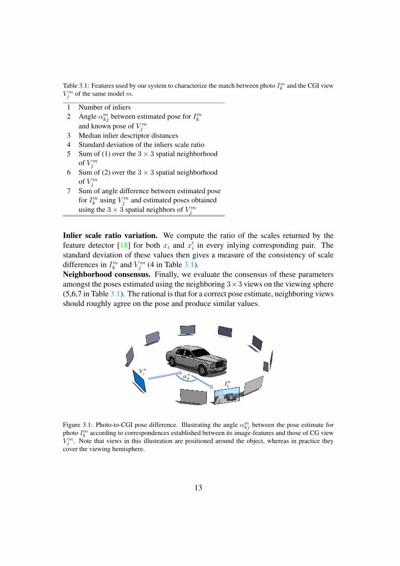
Table 3.1: Features used by our system to characterize the match between photo Imk and the CGI view

V mj of the same model m.

1 Number of inliers2 Angle αm

kj between estimated pose for Imk

and known pose of V mj

3 Median inlier descriptor distances4 Standard deviation of the inliers scale ratio5 Sum of (1) over the 3× 3 spatial neighborhood

of V mj

6 Sum of (2) over the 3× 3 spatial neighborhoodof V m

j

7 Sum of angle difference between estimated posefor Im

k using V mj and estimated poses obtained

using the 3× 3 spatial neighbors of V mj

Inlier scale ratio variation. We compute the ratio of the scales returned by thefeature detector [18] for both xi and x′i in every inlying corresponding pair. Thestandard deviation of these values then gives a measure of the consistency of scaledifferences in Im

k and V mj (4 in Table 3.1).

Neighborhood consensus. Finally, we evaluate the consensus of these parametersamongst the poses estimated using the neighboring 3×3 views on the viewing sphere(5,6,7 in Table 3.1). The rational is that for a correct pose estimate, neighboring viewsshould roughly agree on the pose and produce similar values.

m

kI

m

jVm

kj

Figure 3.1: Photo-to-CGI pose difference. Illustrating the angle αmkj between the pose estimate for

photo Imk according to correspondences established between its image-features and those of CG view

V mj . Note that views in this illustration are positioned around the object, whereas in practice they

cover the viewing hemisphere.

13

Chapter 4

Modifying the RANSAC process

4.1 Selecting the winning hypothesisIn the method described so far, a relevant view was selected based on a number ofscores representing the pose hypothesis produced by RANSAC for each view. Con-ventionally, a RANSAC process selects a winning hypothesis based on the numberof inliers [4]. Here, however, we suggest applying the same idea of using a learnedstatistical model for selecting the winning RANSAC iteration: Instead of countingthe number of inliers, we score each iteration based on a feature vector computed asdescribed above. That is, we apply the same idea of using a learned statistical modelfor the selection of the winning RANSAC iteration.

Specifically, we choose the winning RANSAC iteration by considering only thefirst four features out of the seven in Table 3.1. Features 5–7 are excluded, as theyrely on the final pose estimates for the neighboring views, information not availablebefore RANSAC has terminated in all the views. We train a classifier on these fourfeatures using the training data, as described above, and apply it within each CGI’sRANSAC, pose-estimation routine. Once we pick the winning iteration for eachview, based on features 1–4, we can continue in several ways:

1. Relevancy based on maximum inliers - select the view with maximum inliers.See Alg. 4.

2. Relevancy based on best RANSAC score - select the view with the best se-lected hypothesis score. See Alg. 4.

3. Full approach - add features 5–7, computed from neighboring views and con-tinue as described above to select the best view. See Alg. 5.

14

Algorithm 4 Modified RANSAC1: Given a CG model m and a photo of the model’s object Im

k :2: Perform the No learning algorithm as defined in Alg. 13: Obtain an LDA classifier for the RANSAC process by using Alg. 2 with only the

first four features in Table 3.14: for every view V m

j ∈ S do5: Perform a modified (test phase) RANSAC calibration:6: for each RANSAC hypothesis do7: Obtain the four feature vector r′mjk8: end for9: Use the classifier on the hypotheses vectors r′mjk

10: Select the hypothesis with the best score as the pose estimation of V mj

11: end for12: if Relevancy based on maximum inliers then13: Return the pose estimation of the view with maximum inliers14: else if Relevancy based on best RANSAC score then15: Return the pose estimation of the view with the best selected hypothesis score16: end if

Algorithm 5 Full approach1: Given a CG model m and a photo of the model’s object Im

k :2: Perform steps 2-12 of Alg. 43: Obtain an LDA classifier by using Alg. 2 with the following features:

All the features in Table 3.1An additional feature - the view’s selected hypothesis score

4: Perform the test phase:5: for every view V m

j ∈ S do6: Obtain the feature vector v′mjk7: end for8: Use the classifier on the vectors v′mjk9: Score each view according to the LDA projection of its feature vector

10: Return the pose estimation of the view with the best score

15

Chapter 5

Experiments and results

5.1 ImplementationOur method is implemented in MATLAB, using a MATLAB OpenGL wrapper forrendering the CG models. Standard OpenCV routines were used to compute the posegiven 2D-3D correspondences.

For simplicity, we assume that the focal length is known and set it to 800 inimage pixel units, that the principle point is at the center of the image, that the pixel’saspect ratio is one, and that there is no skew. Our method is agnostic to the typeof camera calibration model that is used to estimate the pose from point matchesand it is straightforward to relax these assumptions by using more elaborate cameracalibration techniques.

Pose was estimated using 2, 000 RANSAC iterations. The features in vmjk (Sec. 3.1)

were normalized to the range of [0..1]. LDA was applied with a regularization con-stant of 0.1 in all our experiments, taking views which produce an angular error of9 degrees or less as class examples, all others as non-class. When the LDA methodis applied, the view with the highest LDA projection value is selected, and its poseestimate is then returned as our method’s output.

5.2 Data sets and BenchmarksIn order to test our method we have collected textured, 3D, CG models of car andbuilding objects, along with images from the web, taken of those same objects. Ourmodels were obtained from the Google 3D Warehouse collection [9] and the imageswere mostly downloaded from Wikipedia. In total, we have 31 car models with 90test images and 11 building models with 30 images, models having one to three queryimages each. All models were scaled to unit size. Car models were further roughlyaligned – all facing the same direction. We manually recover the ground-truth camera

16

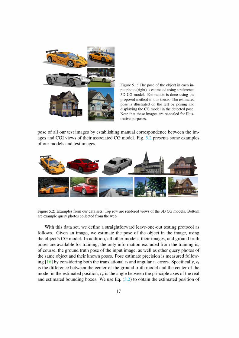
Figure 5.1: The pose of the object in each in-put photo (right) is estimated using a reference3D CG model. Estimation is done using theproposed method in this thesis. The estimatedpose is illustrated on the left by posing anddisplaying the CG model in the detected pose.Note that these images are re-scaled for illus-trative purposes.

pose of all our test images by establishing manual correspondence between the im-ages and CGI views of their associated CG model. Fig. 5.2 presents some examplesof our models and test images.

Figure 5.2: Examples from our data sets. Top row are rendered views of the 3D CG models. Bottomare example query photos collected from the web.

With this data set, we define a straightforward leave-one-out testing protocol asfollows. Given an image, we estimate the pose of the object in the image, usingthe object’s CG model. In addition, all other models, their images, and ground truthposes are available for training; the only information excluded from the training is,of course, the ground truth pose of the input image, as well as other query photos ofthe same object and their known poses. Pose estimate precision is measured follow-ing [16] by considering both the translational εt and angular εr errors. Specifically, εt

is the difference between the center of the ground truth model and the center of themodel in the estimated position, εr is the angle between the principle axes of the realand estimated bounding boxes. We use Eq. (3.2) to obtain the estimated position of

17

the object’s bounding box.

5.3 Algorithms analysis

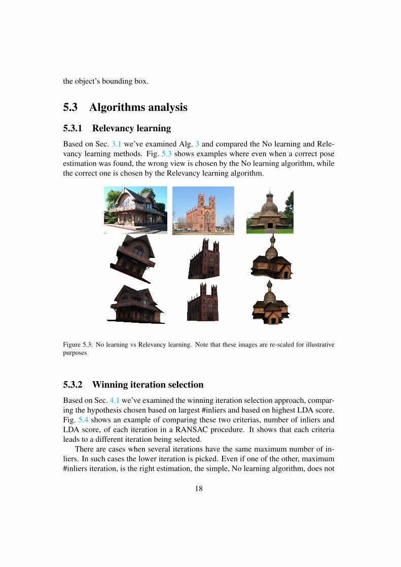
5.3.1 Relevancy learningBased on Sec. 3.1 we’ve examined Alg. 3 and compared the No learning and Rele-vancy learning methods. Fig. 5.3 shows examples where even when a correct poseestimation was found, the wrong view is chosen by the No learning algorithm, whilethe correct one is chosen by the Relevancy learning algorithm.

Figure 5.3: No learning vs Relevancy learning. Note that these images are re-scaled for illustrativepurposes

5.3.2 Winning iteration selectionBased on Sec. 4.1 we’ve examined the winning iteration selection approach, compar-ing the hypothesis chosen based on largest #inliers and based on highest LDA score.Fig. 5.4 shows an example of comparing these two criterias, number of inliers andLDA score, of each iteration in a RANSAC procedure. It shows that each criterialeads to a different iteration being selected.

There are cases when several iterations have the same maximum number of in-liers. In such cases the lower iteration is picked. Even if one of the other, maximum#inliers iteration, is the right estimation, the simple, No learning algorithm, does not

18

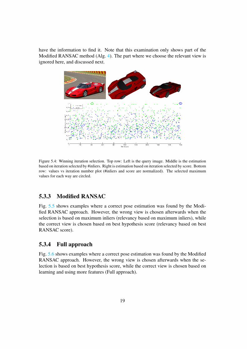
have the information to find it. Note that this examination only shows part of theModified RANSAC method (Alg. 4). The part where we choose the relevant view isignored here, and discussed next.

Figure 5.4: Winning iteration selection. Top row: Left is the query image. Middle is the estimationbased on iteration selected by #inliers. Right is estimation based on iteration selected by score. Bottomrow: values vs iteration number plot (#inliers and score are normalized). The selected maximumvalues for each way are circled.

5.3.3 Modified RANSACFig. 5.5 shows examples where a correct pose estimation was found by the Modi-fied RANSAC approach. However, the wrong view is chosen afterwards when theselection is based on maximum inliers (relevancy based on maximum inliers), whilethe correct view is chosen based on best hypothesis score (relevancy based on bestRANSAC score).

5.3.4 Full approachFig. 5.6 shows examples where a correct pose estimation was found by the ModifiedRANSAC approach. However, the wrong view is chosen afterwards when the se-lection is based on best hypothesis score, while the correct view is chosen based onlearning and using more features (Full approach).

19

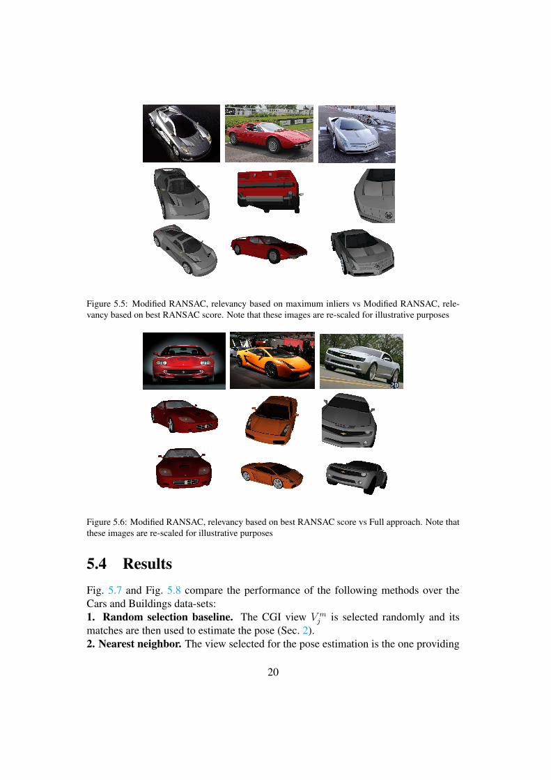
Figure 5.5: Modified RANSAC, relevancy based on maximum inliers vs Modified RANSAC, rele-vancy based on best RANSAC score. Note that these images are re-scaled for illustrative purposes

Figure 5.6: Modified RANSAC, relevancy based on best RANSAC score vs Full approach. Note thatthese images are re-scaled for illustrative purposes

5.4 ResultsFig. 5.7 and Fig. 5.8 compare the performance of the following methods over theCars and Buildings data-sets:1. Random selection baseline. The CGI view V m

j is selected randomly and itsmatches are then used to estimate the pose (Sec. 2).2. Nearest neighbor. The view selected for the pose estimation is the one providing

20

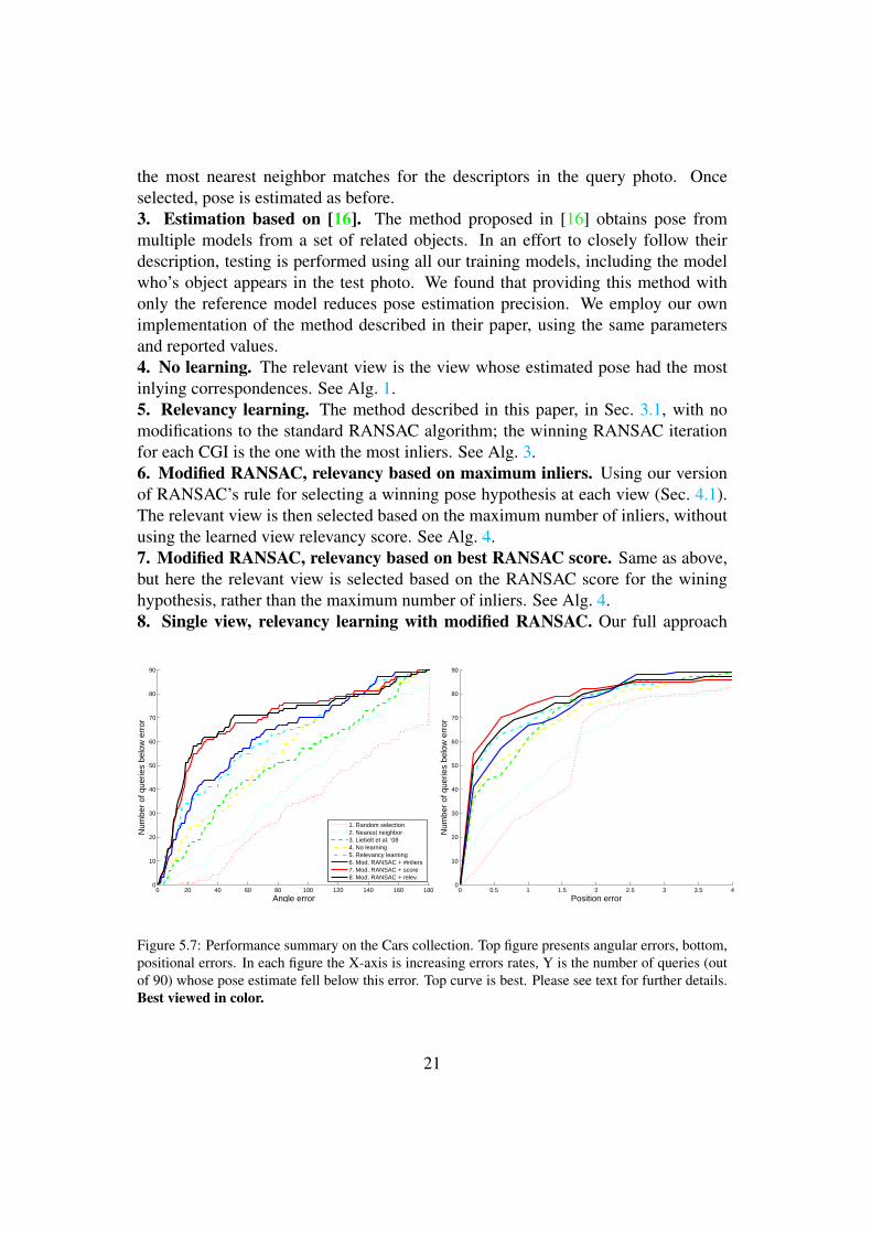
the most nearest neighbor matches for the descriptors in the query photo. Onceselected, pose is estimated as before.3. Estimation based on [16]. The method proposed in [16] obtains pose frommultiple models from a set of related objects. In an effort to closely follow theirdescription, testing is performed using all our training models, including the modelwho’s object appears in the test photo. We found that providing this method withonly the reference model reduces pose estimation precision. We employ our ownimplementation of the method described in their paper, using the same parametersand reported values.4. No learning. The relevant view is the view whose estimated pose had the mostinlying correspondences. See Alg. 1.5. Relevancy learning. The method described in this paper, in Sec. 3.1, with nomodifications to the standard RANSAC algorithm; the winning RANSAC iterationfor each CGI is the one with the most inliers. See Alg. 3.6. Modified RANSAC, relevancy based on maximum inliers. Using our versionof RANSAC’s rule for selecting a winning pose hypothesis at each view (Sec. 4.1).The relevant view is then selected based on the maximum number of inliers, withoutusing the learned view relevancy score. See Alg. 4.7. Modified RANSAC, relevancy based on best RANSAC score. Same as above,but here the relevant view is selected based on the RANSAC score for the wininghypothesis, rather than the maximum number of inliers. See Alg. 4.8. Single view, relevancy learning with modified RANSAC. Our full approach

0 20 40 60 80 100 120 140 160 1800

10

20

30

40

50

60

70

80

90

Angle error

Num

ber

of q

uerie

s be

low

err

or

1. Random selection2. Nearest neighbor3. Liebelt et al. ’084. No learning5. Relevancy learning6. Mod. RANSAC + #inliers7. Mod. RANSAC + score8. Mod. RANSAC + relev.

0 0.5 1 1.5 2 2.5 3 3.5 40

10

20

30

40

50

60

70

80

90

Position error

Num

ber

of q

uerie

s be

low

err

or

Figure 5.7: Performance summary on the Cars collection. Top figure presents angular errors, bottom,positional errors. In each figure the X-axis is increasing errors rates, Y is the number of queries (outof 90) whose pose estimate fell below this error. Top curve is best. Please see text for further details.Best viewed in color.

21

0 20 40 60 80 100 120 140 160 1800

5

10

15

20

25

30

Angle error

Num

ber

of q

uerie

s be

low

err

or

1. Random selection2. Nearest neighbor3. Liebelt et al. ’084. No learning5. Relevancy learning6. Mod. RANSAC + #inliers7. Mod. RANSAC + score8. Mod. RANSAC + relev.

0 0.5 1 1.5 2 2.5 3 3.5 40

5

10

15

20

25

30

Position error

Num

ber

of q

uerie

s be

low

err

or

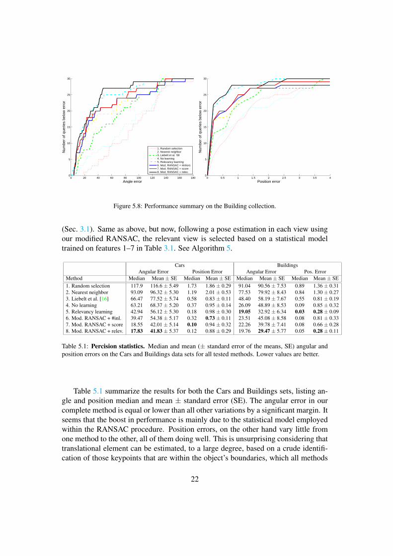
Figure 5.8: Performance summary on the Building collection.

(Sec. 3.1). Same as above, but now, following a pose estimation in each view usingour modified RANSAC, the relevant view is selected based on a statistical modeltrained on features 1–7 in Table 3.1. See Algorithm 5.

Cars BuildingsAngular Error Position Error Angular Error Pos. Error

Method Median Mean ± SE Median Mean ± SE Median Mean ± SE Median Mean ± SE1. Random selection 117.9 116.6 ± 5.49 1.73 1.86 ± 0.29 91.04 90.56 ± 7.53 0.89 1.36 ± 0.312. Nearest neighbor 93.09 96.32 ± 5.30 1.19 2.01 ± 0.53 77.53 79.92 ± 8.43 0.84 1.30 ± 0.273. Liebelt et al. [16] 66.47 77.52 ± 5.74 0.58 0.83 ± 0.11 48.40 58.19 ± 7.67 0.55 0.81 ± 0.194. No learning 63.21 68.37 ± 5.20 0.37 0.95 ± 0.14 26.09 48.89 ± 8.53 0.09 0.85 ± 0.325. Relevancy learning 42.94 56.12 ± 5.30 0.18 0.98 ± 0.30 19.05 32.92 ± 6.34 0.03 0.28 ± 0.096. Mod. RANSAC + #inl. 39.47 54.38 ± 5.17 0.32 0.73 ± 0.11 23.51 45.08 ± 8.58 0.08 0.81 ± 0.337. Mod. RANSAC + score 18.55 42.01 ± 5.14 0.10 0.94 ± 0.32 22.26 39.78 ± 7.41 0.08 0.66 ± 0.288. Mod. RANSAC + relev. 17.83 41.83 ± 5.37 0.12 0.88 ± 0.29 19.76 29.47 ± 5.77 0.05 0.28 ± 0.11

Table 5.1: Percision statistics. Median and mean (± standard error of the means, SE) angular andposition errors on the Cars and Buildings data sets for all tested methods. Lower values are better.

Table 5.1 summarize the results for both the Cars and Buildings sets, listing an-gle and position median and mean ± standard error (SE). The angular error in ourcomplete method is equal or lower than all other variations by a significant margin. Itseems that the boost in performance is mainly due to the statistical model employedwithin the RANSAC procedure. Position errors, on the other hand vary little fromone method to the other, all of them doing well. This is unsurprising considering thattranslational element can be estimated, to a large degree, based on a crude identifi-cation of those keypoints that are within the object’s boundaries, which all methods

22

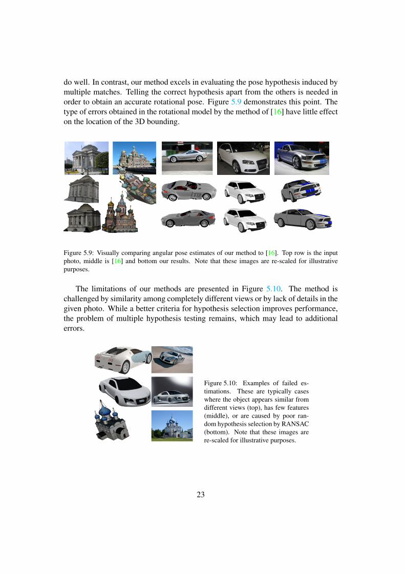
do well. In contrast, our method excels in evaluating the pose hypothesis induced bymultiple matches. Telling the correct hypothesis apart from the others is needed inorder to obtain an accurate rotational pose. Figure 5.9 demonstrates this point. Thetype of errors obtained in the rotational model by the method of [16] have little effecton the location of the 3D bounding.

Figure 5.9: Visually comparing angular pose estimates of our method to [16]. Top row is the inputphoto, middle is [16] and bottom our results. Note that these images are re-scaled for illustrativepurposes.

The limitations of our methods are presented in Figure 5.10. The method ischallenged by similarity among completely different views or by lack of details in thegiven photo. While a better criteria for hypothesis selection improves performance,the problem of multiple hypothesis testing remains, which may lead to additionalerrors.

Figure 5.10: Examples of failed es-timations. These are typically caseswhere the object appears similar fromdifferent views (top), has few features(middle), or are caused by poor ran-dom hypothesis selection by RANSAC(bottom). Note that these images arere-scaled for illustrative purposes.

23

5.5 Switching modelsIn order to evaluate the robustness of the statistical learning method, we have per-formed two additional experiments: The first was performed by learning on the carsdataset models and using the learned model in the test phase of the buildings dataset.The obtained model was used in both of the testing phases - in the modified RANSACand in the relevancy learning parts.

The second experiment had the settings reversed - learning on the buildingsdataset models and using the learned model when testing on the cars dataset. Theresults in Table 5.2 show that learning on a different dataset yields similar results tolearning on the tested dataset.

Cars BuildingsAngular Error Position Error Angular Error Pos. Error

Method Median Mean ± SE Median Mean ± SE Median Mean ± SE Median Mean ± SE1. Random selection 117.9 116.6 ± 5.49 1.73 1.86 ± 0.29 97.61 92.24 ± 8.21 1.70 1.79 ± 0.312. Nearest neighbor 93.09 96.32 ± 5.30 1.19 2.01 ± 0.53 77.53 79.92 ± 8.43 0.84 1.30 ± 0.273. Liebelt et al. [16] 66.47 77.52 ± 5.74 0.58 0.83 ± 0.11 48.40 58.19 ± 7.67 0.55 0.81 ± 0.194. No learning 63.21 68.37 ± 5.20 0.37 0.95 ± 0.14 26.09 48.89 ± 8.53 0.09 0.85 ± 0.325. Relevancy learning 42.37 56.58 ± 5.37 0.17 0.70 ± 0.13 23.92 35.32 ± 7.10 0.03 0.24 ± 0.086. Mod. RANSAC + #inl. 56.48 63.52 ± 5.60 0.53 1.11 ± 0.18 22.26 44.02 ± 8.59 0.10 0.81 ± 0.337. Mod. RANSAC + score 19.10 45.68 ± 5.49 0.10 1.02 ± 0.33 21.66 36.30 ± 6.81 0.11 0.66 ± 0.288. Mod. RANSAC + relev. 18.72 44.42 ± 5.46 0.10 1.34 ± 0.59 22.77 30.26 ± 5.63 0.03 0.19 ± 0.05

Table 5.2: Percision statistics using switched learned models. Median and mean (± standard er-ror of the means, SE) angular and position errors on the Cars and Buildings data sets for all testedmethods. Lower values are better.

The angular and positional errors for both experiments are similar to the ones inSection 5.

24

Chapter 6

Conclusions

Matching across modalities is a challenging task that results in a potentially largenumber of false matches. Furthermore, it is not easy to distinguish between true andfalse matches even when considering consensus among multiple matches. The com-bination of geometric projection models and robust statistics tools such as RANSACoften fails in identifying a set of matches that support a correct hypothesis from setsthat support false hypotheses that have equally high scores due to a nasty combina-tion of inaccurate matches and multiple hypothesis testing.

In this work we propose to augment the RANSAC procedure by a learning basedrelevancy score which makes it much more robust. The computed view relevancyscore shows its value both within the RANSAC procedure, in selecting among mul-tiple random hypothesis, and at the level of selecting the most relevant view amongmultiple rendered CG views. Overall, the simplicity of our method makes the pro-posed solution practical, robust and efficient, and results on a large database of 3Dmodels demonstrate its effectiveness. The robustness is also apparent when using amodel learned from a different dataset, meaning our method can be used on a newdataset without learning on it. Our framework can be readily extended by incorporat-ing new features, and possibly other learning method, perhaps considering consensusamong distant views which support similar poses.

25

Chapter 7

Appendix

7.1 Data SetsWe have collected two data sets, each including low-resolution, textured, 3D modelsas well as images of the real objects being modeled. These 3D models and associ-ated images were collected from the web. The CG models, therefore, demonstrate achallenging variability in parameters such as fidelity, detail level, and texture quality.The photos vary in resolution, background clutter, illumination, and pose.

The cars data set include 31 CG models. For each model, 2-3 photos of the carmodel were obtained. The buildings data set include 11 CG models. For each model,2-3 photos of the building model were obtained. Each model were transformed to acommon 3D format to be used by the undelying 3D rendering system - OpenScene-Graph [21] (OSG format). Afterwards, the models were scaled to unit size. The carsmodels were also aligned to the same view.

In order to find the ground truth pose in each photo Im of a model m - the rotationmatrix R3×3 and translation vector t3×1, we have manually found a similar view V m

j

to the one taken in the photo. Next, we proceeded as in Section 2 - established a linkbetween a pixel xi in Im and pixel x′i in V m

j . Such links were then used to solveEquation 2.1 and obtain the ground truth pose in the photo.

7.1.1 Data sets FilesEach data set is packaged as a ZIP file. The data set consists of a queries/ folderwhere all the photos reside. Some of the models are in a single .OSG file, whileothers resides in their own subfolder along with their texture files. In addition, atext file, data-set.ref, includes all the required information: The model file name, itsoriginating URL, the number of photos for each model, the photos file names andtheir originating URLs.

26

7.2 Models RendererIn order to render the CG model from different views, a renderer has been writtenin C++. The rendering is done off-screen (no window is opened), and the image isreturned as a variable. It can be used from Matlab. The underlying renering libraryis OpenSceneGraph [21] which parses a CG model and renders it using OpenGL.

Typing rend without arguments will show the following help:[depth_image, rendered_image, unproject, out_A, out_R, out_T] =rend(width, height, filename,writefiles, lighting,sphere orientation (4 arguments)/camera orientation (3 arguments));

Most input and output parameters are optional.

width and height should be unsigned integers.

filename - the input mesh filename.

writefiles should be 0 or 1 (also outputs PPM files of depth_imageand rendered_image).

lighting should be 0 (disabled) or 1 (enabled).

sphere orientation are the following 4 arguments: distance,elevation, azimuth and yaw.distance - a number added to the (auto calculated) model’sbounding sphere radius. 0 is usually suitable.elevation, azimuth and yaw are degrees. The camera position onthe bounding sphere is specified using them.

camera orientation are 3 arguments: A, R and T. Add an additionaldummy argument (e.g. 0) if further input parameters are specified.

Examples:

[depth, rendered]=rend(300, 300, ’file.wrl’);

[depth, rendered, unproject, A, R, T]=rend(300, 300, ’file.wrl’,0,0.5,10,20,30);Renders the mesh with a distance of 0.5, an elevation of 10 degrees,azimuth of 20 degrees and yaw of 30 degrees.’unproject(125,149,1:3)’ returns the world XYZ coordinate of theimage point (x=148,y=124).

Next:

[depth, rendered, unproject]=rend(300, 300, ’file.wrl’,0,A,R,T);

Will yield the same results.

7.3 Learning codeWe provide the code used in the thesis. It is written in MATLAB. The code features:

• Extracting robust features - implemented similary as in [16]. Extract robustfeatures from a given CG model and also cluster them.

• Examining a given query image and obtaining a pose estimation (without learn-ing). See Alg. 1.

• Examining a given query image and obtaining a pose estimation (with learning)See Alg. 3- 5.

27

The readme file provides more detailed information.

28

Bibliography

[1] M. Arie-Nachimson and R. Basri. Constructing implicit 3D shape models for poseestimation. In ICCV, 2009. 7

[2] P. Belhumeur, J. Hespanha, and D. Kriegman. Eigenfaces vs. Fisherfaces: recognitionusing class specific linear projection. TPAMI, 19(7):711–720, 1997. 11

[3] T. Brox, B. Rosenhahn, D. Cremers, and H. Seidel. High accuracy optical flow serves3-D pose tracking: exploiting contour and flow based constraints. In ECCV, 2006. 7

[4] S. Choi, T. Kim, and W. Yu. Performance evaluation of RANSAC family. In BMVC,2009. 14

[5] D. DeMenthon and L. Davis. Model-based object pose in 25 lines of code. IJCV, pages123–141, 1995. 7

[6] M. Everingham, A. Zisserman, C. Williams, and L. Gool. The PASCAL visual objectclasses challenge 2006 results. TR, U Oxford, U Edinburgh, KU Leuven, 2006. 7

[7] M. Fischler and R. Bolles. Random sample consensus: a paradigm for model fittingwith application to image analysis and automated cartography. Com. of the ACM, 24,1981. 9

[8] J. Gall, B. Rosenhahn, and H. Seidel. Robust pose estimation with 3D textured models.Advances in Image and Video Technology, pages 84–95, 2006. 7

[9] Google 3D warehouse. http://sketchup.google.com/3dwarehouse/. 16

[10] I. Gordon and D. Lowe. What and where: 3D object recognition with accurate pose.Toward category-level object recognition, pages 67–82, 2006. 7

[11] R. Hartley and A. Zisserman. Multiple view geometry in computer vision. CambridgeUniv Pr, 2003. 8

[12] V. Lepetit and j. y. Fua, P. Keypoint recognition using randomized trees. 8

[13] V. Lepetit, J. Pilet, and P. Fua. Point matching as a classification problem for fast androbust object pose estimation. In CVPR, page 2004, 244–250. 6

[14] J. Liebelt and K. Schertler. Precise registration of 3D models to images by swarmingparticles. In CVPR, 2007. 7

[15] J. Liebelt and C. Schmid. Multi-view object class detection with a 3D geometric model.In CVPR, 2010. 6, 7

29

[16] J. Liebelt, C. Schmid, and K. Schertler. Viewpoint-independent object class detectionusing 3D feature maps. In CVPR, 2008. 3, 6, 7, 8, 9, 17, 21, 22, 23, 24, 27

[17] D. Lowe. Distinctive image features from scale-invariant keypoints. IJCV, 60(2):91–110, 2004. 8

[18] K. Mikolajcyk and C. Schmid. Scale and affine invariant interest point detectors. IJCV,2004. 8, 13

[19] K. Mikolajczyk and C. Schmid. A performance evaluation of local descriptors. TPAMI,27:1615 – 1630, 2005. 9

[20] H. Najafi, Y. Genc, and N. Navab. Fusion of 3D and appearance models for fast objectdetection and pose estimation. ACCV, pages 415–426, 2006. 7

[21] R. Osfield and D. Burns. Open scene graph. http://www.openscenegraph.org/, 2010. 26, 27

[22] V. Prisacariu and I. Reid. PWP3D: Real-time segmentation and tracking of 3D objects.In BMVC, 2009. 7

[23] L. Quan and Z. Lan. Linear n-point camera pose determination. TPAMI, 21:774–780,1999. 7

[24] B. Rosenhahn, C. Perwass, and G. Sommer. Pose estimation of free-form contours.IJCV, 62(4):267–289, 2005. 7

[25] R. Sandhu, S. Dambreville, A. Yezzi, and A. Tannenbaum. Non-rigid 2D-3D poseestimation and 2D image segmentation. In CVPR, pages 786–793, 2009. 7

[26] S. Savarese and L. Fei-Fei. 3D generic object categorization, localization and poseestimation. In ICCV, 2007. 7

[27] C. Schmaltz, B. Rosenhahn, T. Brox, and J. Weickert. Region-based pose tracking withocclusions using 3D models. Machine Vision and Applications, pages 1–21, 2011. 7

[28] N. Snavely, S. M. Seitz, and R. Szeliski. Modeling the world from Internet photocollections. IJCV, 2008. 7

[29] M. Stark, M. Goesele, and B. Schiele. Back to the future: Learning shape models from3D CAD data. In BMVC, 2010. 7

[30] L. Vacchetti, V. Lepetit, and P. Fua. Stable real-time 3D tracking using online andoffline information. TPAMI, 26(10):1391–1391, 2004. 7

[31] A. Vedaldi and B. Fulkerson. VLFeat: An open and portable library of computer visionalgorithms. http://www.vlfeat.org/, 2008. 8

30

תקציר

בעיית חישוב התנוחה היא מציאת של העצם, ממדי-תלתבהינתן תמונה של עצם ובהינתן ייצוג

.ההתמרה (סיבוב והזזה) של העצם המופיע בתמונה

אנו מציגים שיטה לחישוב תנוחה של עצמים קשיחים (כגון מכונית) בתמונה יחידה. בעזרת מודל

-התאמות בין נקודות המודל בתלת למצואשל העצם בתמונה אפשר (CG model)ממדי -תלת

סדרה של תמונות של המודל יצירת ממד. ניתן לעשות זאת על ידי - נקודות העצם בדווממד

image)שונות) ומציאת התאמות של תכונות מקומיות במרחב התמונה הצפיי ת(מזוויו

descriptors).

שווה לפתרון הבעיה ולפיכך פיתחנו תורמות באופן )ההצפיי תזוויוהתנוחות (אנו מראים כי לא כל

אנו מאמנים ולומדים זוגות של ,. ראשיתתנוחה משוערכתשיטה לבדיקת הרלוונטיות של כל

וקטור של תיאורים –ותמונות שאילתה ומחשבים סדרה של מדידות מתנוחות שונותתמונות

תנוחה ל כל יכול לצפות את מידת האמינות שר שאהמייצג את ההתאמה. אנו לומדים מודל

ממדי חדש, -בעזרת וקטורים אלו. לאחר מכן, בהינתן תמונת שאילתה חדשה ומודל תלתמשוערת

בעזרת המודל נבחנת כל תנוחה בסדרה. ממדית- סדרת תמונות של המודל התלתיצרים יאנו מ

הטובה ביותר. התנוחהנבחרת ולבסוף הנלמד

ממדיים של -בכדי לבדוק את השיטה שפתחנו אספנו שני בסיסי נתונים מאתגרים: מודלים תלת

מכוניות ובניינים ותמונות של עצמים אלו מהרשת. תוצאות הניסויים מראות שיפור ביחס

.הבעיהלשיטות הקיימות לפתרון

תוכן העניינים

5 הקדמה .1

5 ........................................................................................................ רקע .1.1

6 ............................................................................................ ת קודמותעבודו .1.2

8 חישוב תנוחה של עצם בעזרת מודל תלת ממדי .2

10 הוספת לימוד לאלגוריתם הבסיסי .3

10 .......................................................................... תנוחות רלוונטיות תדילמ .3.1

Vהמאפיינים ב .3.2m

jk .......................................................................... 12

RANSACה שינוי תהליך .4

14 ........................................................................... בחירת ההשערה המנצחת .4.1

16 ניסויים ותוצאות .5

16 ............................................................................................ דרכי היישום .5.1

16 .......................................................... מדידת התוצאותאופן בסיסי הנתונים ו .5.2

18 ................................................................................ ניתוח האלגוריתמים .5.3

18 .................................................................... למידת תנוחה רלוונטית .5.3.1

18 .................................................................... בחירת ההשערה המנצחת .5.3.2

RANSAC .................................................................... 19שיפור תהליך .5.3.3

19 ................................................................................ הגישה המלאה .5.3.4

20 ........................................................................................................ תוצאות .5.4

24 .................................................................... החלפת המודלים ללימוד .5.5

25 מסקנות .6

26 נספחים .7

26 ........................................................................................ בסיסי הנתונים .7.1

26 ................................................................ קבצי בסיסי הנתונים .7.1.1

27 .................................................... תוכנה להצגת מודלים תלת ממדיים .7.2

27 ........................................................................................ הלימודמודל .7.3

29 רשימת מקורות .8

האוניברסיטה הפתוחה

המחלקה למתמטיקה ולמדעי המחשב

הערכת חשיבות התנוחה המשוערת של עצם המופיע

בתמונה בודדת

עבודת תזה זו הוגשה כחלק מהדרישות לקבלת תואר

במדעי המחשב .M.Sc"מוסמך למדעים"

סיטה הפתוחהבאוניבר

החטיבה למדעי המחשב

ידי-על

ליאב אסרף

ד"ר טל הסנרהעבודה הוכנה בהדרכתו של

2011 ספטמבר