VR2006

1

PTrack: Introducing a Novel Iterative Geometric Pose Estimation for a Marker-based Single Camera Tracking System

Pedro Santos1, Andre Stork2 Fraunhofer IGD

Darmstadt,Germany

Alexandre Buaes3 CETA SENAI-RS PPGEE/UFRGS

Porto Alegre, Brazil

Joaquim Jorge4 INESC-ID/IST

Technical University of Lisbon, Portugal

Abstract

Inside-out tracking for augmented reality applications continues to present a challenge in terms of performance, robustness and accuracy. In particular mobile augmented reality applications are in need of tracking systems which can be wearable and do not cause a high processing load. In this paper we introduce a novel iterative geometric method for pose estimation from four co-planar points and we present the current status of PTrack, a marker-based single camera tracking system benefiting from this approach. The system uses an IDS uEye [1] camera, equipped with infrared flash strobes and infrared pass filter, which acquires grayscale images and sends them to a computer where an image pre-processing algorithm identifies potential projections of retro-reflective markers. Our novel pose estimation algorithm identifies possible labels composed of markers in a 2D post-processing using a divide-and-conquer strategy to segment the camera's image space and attempts an iterative geometric 3D reconstruction of position and orientation in camera space. In the end successfully reconstructed labels are compared to a database for identification. Their 6 DoF data as well as their ID is made available to applications through OpenTracker [2] framework. To assess the performance of our approach we compared PTrack to ARToolKit [3] - which has been adapted to work with the same camera - and final results show that pose estimation is more accurate and precise, in both translation and rotation.

Keywords: Tracking System, Augmented Reality, Virtual Reality.

1. Introduction

The presented work focuses on PTrack, an innovative marker-based, single camera tracking solution developed within two master theses, in cooperation projects among the authors’ institutions.

The paper explains the implementation of the relevant algorithms and presents results of a direct comparison of PTrack against ARToolKit.

The target operating scenario for PTrack are mobile augmented reality applications, such as maintenance and installation systems such as the ones developed within the ARVIKA consortium [4]. The data format, in which the results are conveyed, is compatible and already integrated within the OpenTracker framework, an abstract unified tracker interface widely used in immersive environments.

This paper will focus in more detail on the innovative aspects of the system implementation, namely the reconstruction of the position and orientation of a set of labels (object pose) from single images, based on projected 2D marker coordinates of each label on the tracking camera’s plane.

2. Related Work

Computing the position and orientation of a rigid body relative to the camera from a single view can be understood as the correspondence between a geometric feature in object space and its 2D projection in image space. This in turn can be expressed by a set of equations, whose unknowns are the extrinsic parameters. In general analytical and numerical methods can be distinguished. The first are represented by Fischler and Bolles [5] which recovered the camera location by computing distances between the focus of the camera and three object space points. Adding information about the distances and angles between those points leads to a system of eight-degree polynomial equations. For three correspondences, eight solutions may be found. Dhome [6] uses line correspondences and decomposes the object-to-image space transformation in two transformations by introducing an additional plane which is the interpretation plane of one of the line segments. Also here, the result is a system of eight degree polynomial equations. As can be seen, one of the drawbacks of these methods is the multiplicity of solutions and their sensitivity to noise.

The goal of numerical approaches is to minimize an error function and thus iteratively approach the correct pose. Such algorithms are less affected by noise than analytic ones. In addition their real-time performance is adjustable by controlling the number of iterations and therefore allowing for a tradeoff between speed and accuracy, which can be useful for certain applications. One of the most prominent and accurate numerical approaches to pose estimation is the least square minimization from Lowe [7]. The points measured in image space are compared to the results of the projection of the object space points to image space and the quadratic error between them is computed for each axis. To use Newton’s method, for each parameter the partial derivative of the error function is calculated. The resulting system of equations is then used to iteratively compute the extrinsic parameters. The POSIT algorithm by DeMenthon [8] is also iterative as the methods of Lowe, but does not require an initial

1 pedro.santos@igd.fhg.de 2 andre.stork@igd.fhg.de 3 agreff@uol.com.br 4 jaj@inesc-id.pt

VR2006

2

pose estimate and matrix inversions in its iteration loop. The method finds approximate image poses by assuming image points have been obtained by scaled orthographic projections, shifting the results to the lines of sight and repeating the step.

ARToolKit developed by Kato and Billinghurst [3] takes advantage of two opposing edges of tracked square targets being parallel to each other. In object space as well as in image space those edges represent lines from one corner of the label to the other. Using the perspective projection matrix, one can define two planes by the focal point and one of these lines respectively. The cross-product of the normal vectors of both planes results in the direction vector of both lines in object space corresponding to the rotation sub-matrix of the affine transformation from image space to object space. The remaining unknowns for the translation can then be calculated iteratively. The drawbacks of numerical approaches can be conversion issues. However they are generally outweighed by less sensitivity to noise and a good speed vs. accuracy relation.

PTrack, the presented single-camera system, inserts itself into the numerical approaches. However and similar to ARToolKit, PTrack takes advantage of geometrical conditions, namely that the corners of a square label in object space and the corresponding projection in image space must lie on the same projection lines commencing in the focal point and crossing the four corners of the label. In PTrack the projection of a square target is iteratively twisted into the correct orientation by the presented algorithm and then scaled to the correct location in object space.

Although there have been several approaches to estimate pose from a projected rectangle, the authors believe this algorithm to be well suited to address this problem. The evaluation at the end of the paper and the comparison to ARToolKit show that the algorithm is fast and accurate.

3. System Setup

The PTrack test environment is made up of a computer and an IDS uEye UI1210-C camera (Figure 1) with 640x480 resolution, configured to acquire grayscale images, equipped with infrared (940nm wavelength) flash strobes, controlled by a digital trigger output of the camera. At each frame the camera captures the image of labels made of retro-reflective markers and sends the uncompressed image to the PC through a USB 2.0 interface. A pre-processing software module - Camera module – extracts the 2D coordinates of the label image feature points projected on the plane of the camera’s CMOS sensor. The image pre-processing also corrects lens radial distortions, based on pre-calibrated lens distortion coefficients. The image is then passed to the tracking algorithm on a frame-by-frame basis.

The camera is equipped with 8 modules of 15 infrared LEDs each, totalizing 120 infrared LEDs around the lens. A RG-850 (850nm) daylight blocking filter was built in to minimize interference from undesired optical sources in daylight spectral region.

The labels used by PTrack are composed of 6 markers each (Figure 2). Four markers represent the corners of a square label with fixed edge length. One marker is on the top edge, identifying the top orientation of the label, splitting it in 1/3 and 2/3. And the sixth marker is a coding marker which must lie somewhere within the square formed by the other markers.

The markers used are flat circular retro-reflective markers with a diameter of 10mm. The distance between corner markers on a label is 80mm. Therefore for encoding there is a grid

of 60mmx60mm which is enough for 36 different encodings. If the label is made bigger or the inter-marker distance is decreased to 5mm then more encodings can be applied.

Figure 1: IDS uEye UI1210-C with IR flash strobes.

Figure 2: PTrack label with retro-reflective markers.

4. PTrack - System and Algorithm

PTrack is a static library, which can be regarded as a data transformation pipeline, receiving the image, extracting 2D image space feature points, identifying and reconstructing pose of possible labels in 3D and broadcasting this information to interested applications. Figure 3 shows PTrack’s system architecture.

Figure 3: PTrack’s system architecture.

The coordination of all activities in PTrack is done by PTrackManager, which controls data flow between the modules, which are described in more detail in the following sections.

VR2006

3

4.1. Camera Module

The IDS Camera Module is one possible module supported by PTrack. Each 2D input system wishing to be supported by PTrack must provide its intrinsic camera parameters, a label configuration file and a continuous flow of 2D image space feature point data. The Camera Module runs in a thread of its own constantly controlling the camera drivers to grab images in the highest possible rate. Then, in a per frame basis, a global thresholding algorithm is applied, followed by an 8-connect operator to identify regions in the image. Following, geometric and size constraints are applied to those regions, so that only elliptical and round shaped regions are passed along. Then the 2D pixel coordinates of region centers are calculated with subpixel precision. After that, radial distortion is corrected and intrinsic parameters of the camera are applied, resulting in the 2D real coordinates of the markers on the camera’s sensor plane. Intrinsic parameters as well as distortion coefficients are obtained by a simple calibration procedure using Intel’s OpenCV library [9]. The 2D marker coordinates are then passed to pose estimation processing whenever PTrackManager polls the module. Thread-safe access is ensured through critical sections.

4.2. PTrackScan - 2D Pre-processing

Whenever a new data-set with 2D image space feature point coordinates is received from the Camera Module, PTrackManager sends it to PTrackScan which does pose estimation processing. PTrackScan in turn is split in 2D pre-processing and 3D pose estimation.

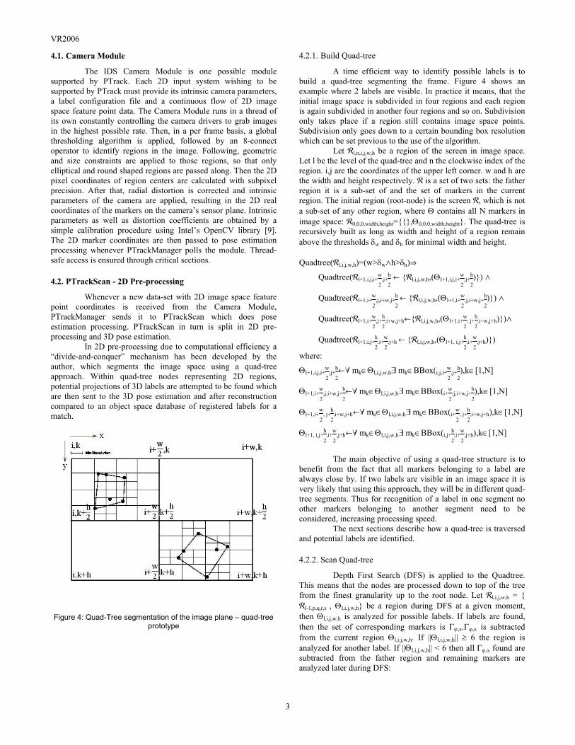
In 2D pre-processing due to computational efficiency a “divide-and-conquer” mechanism has been developed by the author, which segments the image space using a quad-tree approach. Within quad-tree nodes representing 2D regions, potential projections of 3D labels are attempted to be found which are then sent to the 3D pose estimation and after reconstruction compared to an object space database of registered labels for a match.

Figure 4: Quad-Tree segmentation of the image plane – quad-tree prototype

4.2.1. Build Quad-tree

A time efficient way to identify possible labels is to build a quad-tree segmenting the frame. Figure 4 shows an example where 2 labels are visible. In practice it means, that the initial image space is subdivided in four regions and each region is again subdivided in another four regions and so on. Subdivision only takes place if a region still contains image space points. Subdivision only goes down to a certain bounding box resolution which can be set previous to the use of the algorithm.

Let Rl,n,i,j,w,h be a region of the screen in image space. Let l be the level of the quad-tree and n the clockwise index of the region. i,j are the coordinates of the upper left corner. w and h are the width and height respectively. R is a set of two sets: the father region it is a sub-set of and the set of markers in the current region. The initial region (root-node) is the screen R, which is not a sub-set of any other region, where Θ contains all N markers in image space: R0,0,0,width,height=,Θ0,0,0,width,height. The quad-tree is recursively built as long as width and height of a region remain above the thresholds δw and δh for minimal width and height. Quadtree(Rl,i,j,w,h)=(w>δw,h>δh)fl

Quadtree(Rl+1,i,j,i+w

2,j+

h

2 ≠ Rl,i,j,w,h,(Θl+1,i,j,i+

w

2,j+

h

2)) ,

Quadtree(Rl+1,i+w

2,j,i+w,j+

h

2 ≠ Rl,i,j,w,h,(Θl+1,i+

w

2,j,i+w,j+

h

2)) ,

Quadtree(Rl+1,i+w

2,j+

h

2,i+w,j+h≠Rl,i,j,w,h,(Θl+1,i+

w

2, j+

h

2,i+w,j+h)),

Quadtree(Rl+1,i,j+h

2,i+

w

2,j+h ≠ Rl,i,j,w,h,(Θl+1, i,j+

h

2,i+

w

2,j+h))

where:

Θl+1,i,j,i+w

2,j+

h

2≠" mk∈Θl,i,j,w,h$ mk∈BBox(i,j,i+

w

2,j+

h

2),k∈[1,N]

Θl+1,i+w

2,j,i+w,j+

h

2≠" mk∈Θl,i,j,w,h$ mk∈BBox(i+

w

2,j,i+w,j+

h

2),k∈[1,N]

Θl+1,i+w

2, j+

h

2,i+w,j+h≠" mk∈Θl,i,j,w,h$ mk∈BBox(i+

w

2, j+

h

2,i+w,j+h),k∈[1,N]

Θl+1, i,j+h

2,i+

w

2,j+h≠" mk∈Θl,i,j,w,h$ mk∈BBox(i,j+

h

2,i+

w

2,j+h),k∈[1,N]

The main objective of using a quad-tree structure is to

benefit from the fact that all markers belonging to a label are always close by. If two labels are visible in an image space it is very likely that using this approach, they will be in different quad-tree segments. Thus for recognition of a label in one segment no other markers belonging to another segment need to be considered, increasing processing speed.

The next sections describe how a quad-tree is traversed and potential labels are identified.

4.2.2. Scan Quad-tree

Depth First Search (DFS) is applied to the Quadtree. This means that the nodes are processed down to top of the tree from the finest granularity up to the root node. Let Rl,i,j,w,h = Rl-1,p,q,r,s , Θl,i,j,w,h be a region during DFS at a given moment, then Θl,i,j,w,h is analyzed for possible labels. If labels are found, then the set of corresponding markers is Γϕ,x.Γϕ,x is subtracted from the current region Θl,i,j,w,h. If ||Θl,i,j,w,h|| ≥ 6 the region is analyzed for another label. If ||Θl,i,j,w,h|| < 6 then all Γϕ,x found are subtracted from the father region and remaining markers are analyzed later during DFS:

VR2006

4

||Θl,i,j,w,h|| < 6 fl Θl-1,p,q,r,s ≠ Θl-1,p,q,r,s \ Γ.

4.2.3. Radar-Sweep Algorithm

Θl,i,j,w,h is analyzed using what we define as radar sweep algorithm. The centre of gravity of all markers in Θl,i,j,w,h is calculated. An imaginary line through the centre of gravity performs a clockwise rotation of 360° degrees. At each angle the algorithm looks for a possible top edge with three markers parallel to the radar sweep line. If a top edge is found the additional corner markers are identified and finally the coding marker is identified. This process is now explained in more detail:

" t∈[1,N].Ømt∈Θl,i,j,w,h,

Ømt=⎝⎛ ⎠⎞

mt(x)mt(y) ,

Ømg=

1N∑

t=0

NØmt,

Ømg=⎝⎛ ⎠⎞

mg(x)mg(y)

The coordinate system is transformed to the current sweep line (Figure 5) for each ϕ∈[0,2π[.Then all marker coordinates are transformed.

Figure 5: Coordinate Transformation

[δϕ]=⎝⎜⎛

⎠⎟⎞cos ϕ

sin ϕ0

-sin ϕcos ϕ

0 001

, T=⎝⎜⎛

⎠⎟⎞1

00

010

mg(x)mg(y)

1

" t∈[1,N], ϕ∈[0,2π[, Ømt∈Θl,i,j,w,h.

Ømt,ϕ= [δϕ]T-1Ømt,

Ømt,ϕ ∈Θl,i,j,w,h

The sweep line is defined as Sϕ(λ)=λ

Øe1,ϕ,λ∈Ñ. The set

Θl,i,j,w,h is sorted in ascending y-order: Θl,i,j,w,h ≠ SORT(Θl,i,j,w,h, >y). To find the x-th. top line, groups Τϕ,x of three succeeding markers need to be identified which lie within a δy of each other:

Τϕ,x ≠ $ Ømk,ϕ∈ Θl,i,j,w,h , k∈[t,t+2],<(

Ømk,ϕ-a),

Øe2> < δy, a=

13∑

k=t

t+2Ømk,ϕ

If found each of this groups is sorted in ascending x-

order: Τϕ,x ≠ SORT(Τϕ,x, >x). The following is considered a valid top line:

Γϕ,x ≠ $

Ømt,ϕ,x∈Τϕ,x.|

Ømt+1,ϕ,x -

Ømt,ϕ,x | < |

Ømt+2,ϕ,x -

Ømt+1,ϕ,x |

If Γϕ,x represents a valid topline, then only markers

below this line need to be considered for a potential label:

Θl,i,j,w,h,ϕ,x ≠ $ Ømt,ϕ,x∈ Θl,i,j,w,h,ϕ .

Ømt,ϕ,x(y)<minyΡϕ,x

Figure 6: Finding remaining markers

To find the remaining corner markers that belong to the potential top line Ρϕ,x , we anticipate their possible location (Figure 6) by searching for them around temporary markers p1,ϕ,x and p2,ϕ,x:

$ λ1∈Ñ.

Øp1,ϕ,x=

Ømt,ϕ,x+λ1

Ø

e2,ϕ , | Øp1,ϕ,x -

Ømt,ϕ,x | = |

Ømt+2,ϕ,x -

Ømt,ϕ,x |

$ λ1∈Ñ.Øp2,ϕ,x=

Ømt,ϕ,x+λ2

Ø

e2,ϕ , | Øp2,ϕ,x -

Ømt,ϕ,x | = |

Ømt+2,ϕ,x -

Ømt,ϕ,x |

If they exist, the two possible corner markers are found

as follows: Øml,ϕ,x ≠ $

Ømt,ϕ,x∈ Θl,i,j,w,h,ϕ,x.min|

Ømt,ϕ,x -

Øp1,ϕ,x |

Ømr,ϕ,x ≠ $

Ømt,ϕ,x∈ Θl,i,j,w,h,ϕ,x.min|

Ømt,ϕ,x -

Øp2,ϕ,x |

The five markers considered a potential solution are:

Γϕ,x = Γϕ,x (

Øml,ϕ,x ,

Ømr,ϕ,x

The remaining markers considered to include the coding

marker are:

Θl,i,j,w,h,ϕ,x ≠ Θl,i,j,w,h,ϕ,x \ Øml,ϕ,x ,

Ømr,ϕ,x

There must be one and only one coding marker in the

bounding box of the potential label: Ømc,ϕ,x ≠ $!

Ømt,ϕ,x∈ Θl,i,j,w,h,ϕ,x.

Ømt,ϕ,x∈BBox(Γϕ,x)

The potential label and the remaining markers are:

Γϕ,x = Γϕ,x ( Ømc,ϕ,x

Θl,i,j,w,h,ϕ,x ≠ Θl,i,j,w,h,ϕ,x \ Ømc,ϕ,x

If ||Θl,i,j,w,h,ϕ,x|| > 6 another search for a label is done,

else all labels found Γϕ,x are subtracted from the father region. Each possible solution is retransformed into the original coordinate system for further analysis:

Γp,x ≠ "

Ømϕ,x ∈ Γϕ,x $

Ømp,x ∈ Γp,x.

Ømp,x = T

Ømϕ,x

VR2006

5

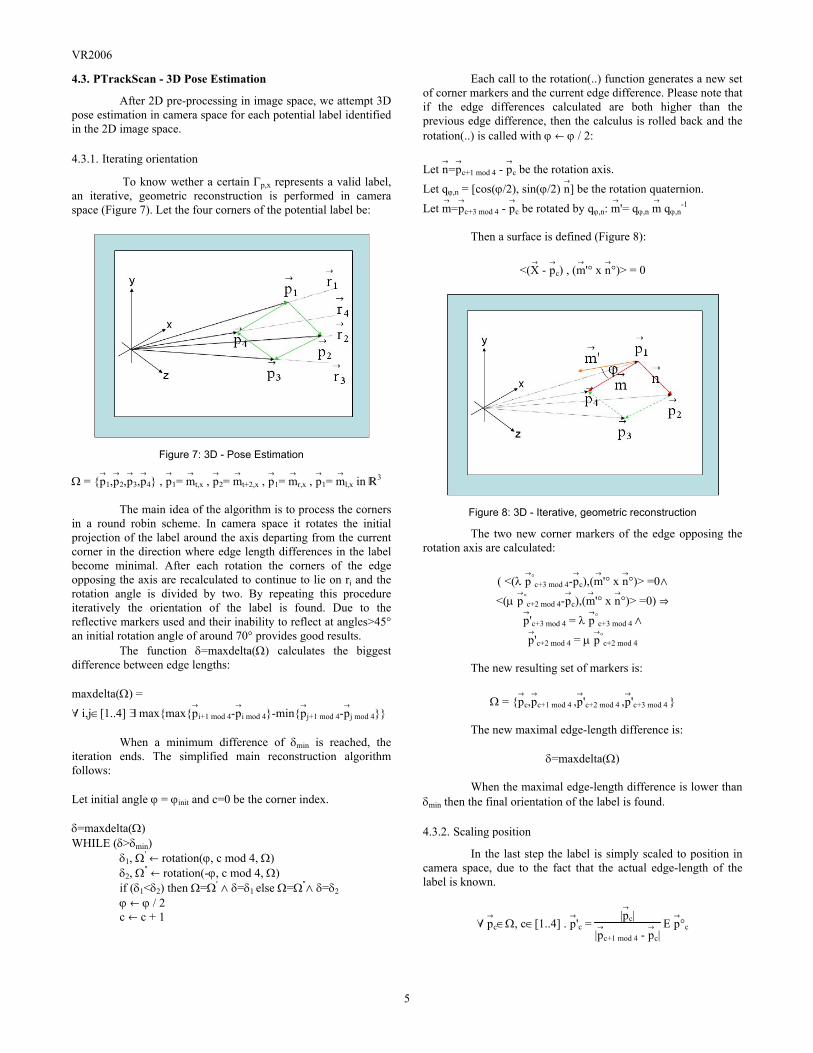
4.3. PTrackScan - 3D Pose Estimation

After 2D pre-processing in image space, we attempt 3D pose estimation in camera space for each potential label identified in the 2D image space.

4.3.1. Iterating orientation

To know wether a certain Γp,x represents a valid label, an iterative, geometric reconstruction is performed in camera space (Figure 7). Let the four corners of the potential label be:

Figure 7: 3D - Pose Estimation

Ω = Øp1,

Øp2,

Øp3,

Øp4 ,

Øp1=

Ømt,x ,

Øp2=

Ømt+2,x ,

Øp1=

Ømr,x ,

Øp1=

Øml,x in Ñ3

The main idea of the algorithm is to process the corners

in a round robin scheme. In camera space it rotates the initial projection of the label around the axis departing from the current corner in the direction where edge length differences in the label become minimal. After each rotation the corners of the edge opposing the axis are recalculated to continue to lie on ri and the rotation angle is divided by two. By repeating this procedure iteratively the orientation of the label is found. Due to the reflective markers used and their inability to reflect at angles>45° an initial rotation angle of around 70° provides good results.

The function δ=maxdelta(Ω) calculates the biggest difference between edge lengths:

maxdelta(Ω) = " i,j∈[1..4] $ maxmax

Øpi+1 mod 4-

Øpi mod 4-min

Øpj+1 mod 4-

Øpj mod 4

When a minimum difference of δmin is reached, the

iteration ends. The simplified main reconstruction algorithm follows:

Let initial angle ϕ = ϕinit and c=0 be the corner index.

δ=maxdelta(Ω) WHILE (δ>δmin) δ1, Ω' ≠ rotation(ϕ, c mod 4, Ω) δ2, Ω'' ≠ rotation(-ϕ, c mod 4, Ω) if (δ1<δ2) then Ω=Ω' , δ=δ1 else Ω=Ω'', δ=δ2

ϕ ≠ ϕ / 2 c ≠ c + 1

Each call to the rotation(..) function generates a new set of corner markers and the current edge difference. Please note that if the edge differences calculated are both higher than the previous edge difference, then the calculus is rolled back and the rotation(..) is called with ϕ ≠ ϕ / 2:

Let

Øn=

Øpc+1 mod 4 -

Øpc be the rotation axis.

Let qϕ,n = [cos(ϕ/2), sin(ϕ/2) Øn] be the rotation quaternion.

Let Øm=

Øpc+3 mod 4 -

Øpc be rotated by qϕ,n:

Øm'= qϕ,n

Øm qϕ,n

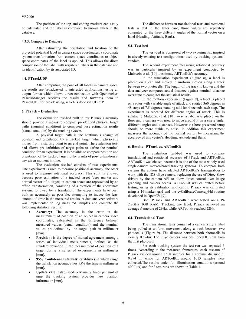
-1 Then a surface is defined (Figure 8):

<(ØX -

Øpc) , (

Øm'° x

Øn°)> = 0

Figure 8: 3D - Iterative, geometric reconstruction

The two new corner markers of the edge opposing the rotation axis are calculated:

( <(λ

Øp°

c+3 mod 4-Øpc),(

Øm'° x

Øn°)> =0,

<(µ Øp°

c+2 mod 4-Øpc),(

Øm'° x

Øn°)> =0) fl

Øp'c+3 mod 4 = λ

Øp°

c+3 mod 4 , Øp'c+2 mod 4 = µ

Øp°

c+2 mod 4 The new resulting set of markers is:

Ω = Øpc,

Øpc+1 mod 4 ,

Øp'c+2 mod 4 ,

Øp'c+3 mod 4

The new maximal edge-length difference is:

δ=maxdelta(Ω) When the maximal edge-length difference is lower than

δmin then the final orientation of the label is found.

4.3.2. Scaling position

In the last step the label is simply scaled to position in camera space, due to the fact that the actual edge-length of the label is known.

" Øpc∈Ω, c∈[1..4] .

Øp'c =

|Øpc|

|Øpc+1 mod 4 -

Øpc|

E Øp°c

VR2006

6

The position of the top and coding markers can easily be calculated and the label is compared to known labels in the database.

4.3.3. Compare to Database

After estimating the orientation and location of the projected potential label in camera space coordinates, a coordinate system transformation from camera space coordinates to object space coordinates of the label is applied. This allows the direct comparison of the label with registered labels in the database and its identification by its associated ID.

4.4. PTrackUDP

After computing the pose of all labels in camera space, the results are broadcasted to interested applications, using an output format which allows direct connection with Opentracker. PTrackManager receives the results and forwards them to PTrackUDP for broadcasting, which is done via UDP/IP.

5. PTrack – Evaluation

The evaluation test-bed built to test PTrack’s accuracy should provide a means to compare pre-defined physical target paths (nominal condition) to computed pose estimation results (actual condition) by the tracking system.

A physical target path is the continuous change of position and orientation by a tracked target which physically moves from a starting point to an end point. The evaluation test-bed allows pre-definition of target paths to define the nominal condition for an experiment. It is possible to compare position and orientation of the tracked target to the results of pose estimation at any given moment in time.

The evaluation test-bed consists of two experiments. One experiment is used to measure positional accuracy, the other is used to measure rotational accuracy. This split is allowed because pose estimation of a tracked target (zero marker and normal vector of a target) in camera space are represented by an affine transformation, consisting of a rotation of the coordinate system, followed by a translation. The experiments have been built as accurately as possible, attempting to induce the least amount of error in the measured results. A data analyzer software was implemented to log measured samples and compute the following statistical results:

• Accuracy: The accuracy is the error in the measurement of position of an object in camera space coordinates, calculated as the difference between measured values (actual condition) and the nominal values pre-defined by the target path in millimeter [mm].

• Precision: is the degree of mutual agreement among a series of individual measurements, defined as the standard deviation in the measurement of position of a target during a series of experiments in millimeter [mm].

• 95% Confidence Intervals: establishes in which range the translation accuracy lies 95% the time in millimeter [mm].

• Update rate: established how many times per unit of time the tracking system provides new position information [mm].

The difference between translational tests and rotational tests is that in the latter case, those values are separately computed for the three different angles of the normal vector on a label (Heading, Attitude, Bank).

5.1. Test-bed

The test-bed is composed of two experiments, inspired in already existing test configurations used by tracking systems’ vendors.

The second experiment measuring rotational accuracy was in particular inspired by an experiment conducted by Malbezin et al. [10] to estimate ARToolKit’s accuracy.

In the translation experiment (Figure 8), a label is placed on a car and moved in uniform motion along a track between two photocells. The length of the track is known and the data analyzer compares actual distance against nominal distance over time to computer the statistical results.

In the rotation experiment (Figure 9), a label is placed on a rotor with variable angle of attack and rotated 360 degrees in 48 steps of 7.5 degrees standing still for 4 seconds each step. The experiment is repeated for different angles of attack. This is similar to Malbezin et al. [10], were a label was placed on the floor and a camera was used to move around it on a circle under different angles and distances. However the here presented setup should be more stable to noise. In addition this experiment measures the accuracy of the normal vector, by measuring the accuracy of this vector’s Heading, Attitude and Bank.

6. Results - PTrack vs. ARToolKit

The evaluation test-bed was used to compare translational and rotational accuracy of PTrack and ARToolKit. ARToolKit was chosen because it is one of the most widely used single-camera marker-based tracking systems. To compare both systems the authors have adapted ARToolKit’s framegrabber to work with the IDS uEye camera, replacing the use of DirectShow drivers by the camera API to allow direct control over image grabbing and camera access. ARToolKit was calibrated before testing, using its calibration application. PTrack was calibrated using a 16-marker grid and the cvCalibrateCamera_64d routine developed in OpenCV [9].

Both PTrack and ARToolKit were tested on a P4 2.8GHz 1GB RAM. Tracking one label, PTrack achieved an average framerate of 29Hz, while ARToolkit reached 22Hz.

6.1. Translational Tests

The translational tests consist of a car carrying a label being pulled at uniform movement along a track between two photocells (Figure 9). The distance between both photocells is exactly 0.894m. The uEye camera was positioned 0.775m from the first photocell.

For each tracking system the test-run was repeated 3 times. According to the measured framerates, each test-run of PTrack yielded around 1508 samples for a nominal distance of 0.894 m, while for ARToolKit around 1015 samples were collected.The results under full illumination conditions (around 400 Lux) and for 3 test-runs are shown in Table 1.

VR2006

7

Figure 9: Translational accuracy tests

Table 1: Translational test results for ARToolKit and PTrack.

System ARToolKit PTrack Average FPS [Hz] 22.0496 29.2016 Nominal distance [m] 0.8940 0.8940 Measured distance [m] 0.8404 0.9122 Avg. pos. error (Accuracy) [m] 0.0294 0.0065 St.dev. in pos. (Precision) [m] 0.0173 0.0046 Upper limit 95% Conf. Interval [m] 0.0305 0.0067 Lower limit 95% Conf. Interval [m] 0.0284 0.0063

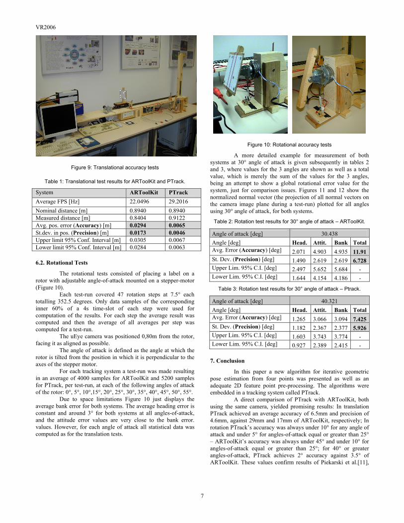
6.2. Rotational Tests

The rotational tests consisted of placing a label on a rotor with adjustable angle-of-attack mounted on a stepper-motor (Figure 10).

Each test-run covered 47 rotation steps at 7.5° each totalling 352.5 degrees. Only data samples of the corresponding inner 60% of a 4s time-slot of each step were used for computation of the results. For each step the average result was computed and then the average of all averages per step was computed for a test-run.

The uEye camera was positioned 0,80m from the rotor, facing it as aligned as possible.

The angle of attack is defined as the angle at which the rotor is tilted from the position in which it is perpendicular to the axes of the stepper motor.

For each tracking system a test-run was made resulting in an average of 4000 samples for ARToolKit and 5200 samples for PTrack, per test-run, at each of the following angles of attack of the rotor: 0°, 5°, 10°,15°, 20°, 25°, 30°, 35°, 40°, 45°, 50°, 55°.

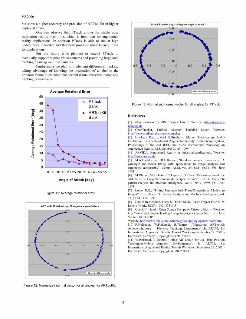
Due to space limitations Figure 10 just displays the average bank error for both systems. The average heading error is constant and around 3° for both systems at all angles-of-attack, and the attitude error values are very close to the bank error. values. However, for each angle of attack all statistical data was computed as for the translation tests.

Figure 10: Rotational accuracy tests

A more detailed example for measurement of both systems at 30° angle of attack is given subsequently in tables 2 and 3, where values for the 3 angles are shown as well as a total value, which is merely the sum of the values for the 3 angles, being an attempt to show a global rotational error value for the system, just for comparison issues. Figures 11 and 12 show the normalized normal vector (the projection of all normal vectors on the camera image plane during a test-run) plotted for all angles using 30° angle of attack, for both systems.

Table 2: Rotation test results for 30° angle of attack – ARToolKit.

Angle of attack [deg] 30.438 Angle [deg] Head. Attit. Bank TotalAvg. Error (Accuracy) [deg] 2.071 4.903 4.935 11.91St. Dev. (Precision) [deg] 1.490 2.619 2.619 6.728Upper Lim. 95% C.I. [deg] 2.497 5.652 5.684 - Lower Lim. 95% C.I. [deg] 1.644 4.154 4.186 -

Table 3: Rotation test results for 30° angle of attack – Ptrack.

Angle of attack [deg] 40.321 Angle [deg] Head. Attit. Bank TotalAvg. Error (Accuracy) [deg] 1.265 3.066 3.094 7.425St. Dev. (Precision) [deg] 1.182 2.367 2.377 5.926Upper Lim. 95% C.I. [deg] 1.603 3.743 3.774 - Lower Lim. 95% C.I. [deg] 0.927 2.389 2.415 -

7. Conclusion

In this paper a new algorithm for iterative geometric pose estimation from four points was presented as well as an adequate 2D feature point pre-processing. The algorithms were embedded in a tracking system called PTrack.

A direct comparison of PTrack with ARToolKit, both using the same camera, yielded promising results: In translation PTrack achieved an average accuracy of 6.5mm and precision of 4.6mm, against 29mm and 17mm of ARToolKit, respectively; In rotation PTrack’s accuracy was always under 10° for any angle of attack and under 5° for angles-of-attack equal or greater than 25° – ARToolKit’s accuracy was always under 45° and under 10° for angles-of-attack equal or greater than 25°; for 40° or greater angles-of-attack, PTrack achieves 2° accuracy against 3.5° of ARToolKit. These values confirm results of Piekarski et al.[11],

VR2006

8

but show a higher accuracy and precision of ARToolKit in higher angles of attack.

One can observe that PTrack allows for stable pose estimation results over time, which is important for augmented reality applications. In addition PTrack is able to run at high update rates if needed and therefore provides small latency times for applications.

For the future it is planned to extend PTrack to eventually support regular video cameras and providing large area tracking by using multiple cameras.

Furthermore we plan to implement differential tracking taking advantage of knowing the orientation of a label in the previous frame to calculate the current frame, therefore increasing tracking performance

Average Rotational Error

0

5

10

15

20

25

30

35

40

45

50

0 5 10 15 20 25 30 35 40 45 50 55

Angle of Attack [deg]

Ave

rage

Rot

atio

nal E

rror

[deg

]

PTrackBankARToolKitBank

Figure 11: Average rotational error

ARToolKit Rotation Log - 30 degrees angle of attack

-0,6

-0,4

-0,2

0

0,2

0,4

0,6

-0,6 -0,4 -0,2 0 0,2 0,4 0,6

Normalized Normal Vector

Figure 12: Normalized normal vector for all angles, for ARToolKit.

Ptrack Rotation Log - 30 degrees angle of attack

-0,6

-0,4

-0,2

0

0,2

0,4

0,6

-0,6 -0,4 -0,2 0 0,2 0,4 0,6

Normalized Normal Vector

Figure 13: Normalized normal vector for all angles, for PTrack.

References

[1] uEye cameras by IDS Imaging GmbH, Website: http://www.ids-imaging.de [2] OpenTracker, Unified Abstract Tracking Layer, Website: http://www.studierstube.org/opentracker [3] Hirokazu Kato , Mark Billinghurst, Marker Tracking and HMD Calibration for a Video-Based Augmented Reality Conferencing System, Proceedings of the 2nd IEEE and ACM International Workshop on Augmented Reality, p.85, October 20-21, 1999 [4] ARVIKA, Augmented Reality in industrial applications, Website: http://www.arvika.de [5] M.A.Fischler ad R.C.Bolles, “Random sample consensus: A paradigm for model fitting with applications to image analysis and automated cartography”, Comm. ACM, vol. 24, no.6, pp.381-395, June 1981 [6] M.Dhome, M.Richetin, J.T.Lapresté, G.Rives: ”Determination of the attitude of 3-D objects from single perspective view” – IEEE Trans. On pattern analysis and machine intelligence, vol.11, N°12, 1989, pp. 1256-1278 [7] Lowe, D.G., “Fitting Parameterized Three-Dimensional Models to Images”, IEEE Trans. On Pattern Analysis and Machine Intelligence, vol. 13, pp.441-450, 1991 [8] Daniel DeMenthon, Larry S. Davis: Model-Based Object Pose in 25 Lines of Code. ECCV 1992: 335-343 [9] OpenCV - Intel - Open Source Computer Vision Library - Website: http://www.intel.com/technology/computing/opencv/index.htm - Last Visited: 04.11.2005 Website: http://www.intel.com/technology/computing/opencv/index.htm [10] P.Malbezin, W.Piekarski, B.Thomas ,"Measuring ARToolKit Accuracy in Long Distance Tracking Experiments" .In ART02, 1st International Augmented Reality Toolkit Workshop September 29, 2002 - Darmstadt, Germany - Copyright (C) 2002 IEEE [11] W.Piekarski, B.Thomas "Using ARToolKit for 3D Hand Position Tracking in Mobile Outdoor Environments". In ART02, 1st International Augmented Reality Toolkit Workshop September 29, 2002 - Darmstadt, Germany - Copyright (C)2002 IEEE