
Variable factors affecting voice identification in forensic contexts
316
Variable factors affecting voice identification in forensic contexts Nathan Atkinson Doctor of Philosophy University of York Language and Linguistic Science September 2015
-
Upload
khangminh22 -
Category
Documents
-
view
2 -
download
0
Transcript of Variable factors affecting voice identification in forensic contexts
Variable factors affecting
voice identification in
forensic contexts
Nathan Atkinson
Doctor of Philosophy
University of York
Language and Linguistic Science
September 2015

2
Abstract
The aim of this thesis is to examine the effect of variable factors on a person’s ability to
identify a voice. This is done with particular reference to the field of naïve listener voice
identification in forensic speech science (also known as earwitness identification). The
research will cover factors in the three main areas of the earwitness process: the listener,
the exposure and the testing.
The background of the listener is analysed, with particular emphasis on the listener’s
accent relative to the voice they are asked to identify. The effect of the listener’s
familiarity with the speaker’s accent, as well as their ability to recognise the accents
(generally, and of the target speaker specifically) and biographical information is assessed.
The context of the exposure to the voice is explored. Listeners will hear the voice of a
perpetrator in one of an audio only, audio + picture, or audio + video condition. The effect
of these exposure conditions on identification accuracy will be examined.
An alternative to the traditional method of testing an earwitness’ ability to identify a voice
is proposed. Rather than making a single identification by selecting one voice from a
lineup, listeners will be asked to rate a selection of voices multiple times on a scale of how
likely they believe each voice to be the perpetrator. It is hoped that this will i) improve
upon the identification accuracy of the traditional approach and ii) provide data which can
better predict whether an identification is likely to be accurate or not.
The findings are complex and varied. They indicate that whilst some factors, such as
accent familiarity and condition under which listeners are exposed to the speaker, have a
significant effect on identification accuracy, they are generally weak predictors. There are
too many variables involved in the process of one particular listener hearing one particular
voice in one particular condition and then being tested on their ability to identify it from
within one particular selection of voices. Promisingly, however, the proposed alternative
methodology for testing produces responses superior in accuracy to the traditional
approach. It also promotes a scalar response system in which the perpetrator’s voice is not
only more likely to receive higher ratings than a foil, but larger differences between ratings
are expected when an accurate identification is made.
3
Contents
Abstract ................................................................................................. 2
Contents ................................................................................................. 3
List of Figures ....................................................................................... 9
List of Tables ....................................................................................... 15
Acknowledgements ............................................................................. 17
Declaration .......................................................................................... 18
1. Introduction ................................................................................. 20
1.1. Forensic speech science ................................................................................. 20
1.2. Lay witness identification ............................................................................. 21
1.2.1. Earwitness identification ......................................................................... 22
1.2.2. Evidence provided by an earwitness ....................................................... 24
1.3. Outline of the thesis ....................................................................................... 25
2. Literature review ......................................................................... 27
2.1. Identifying voices ........................................................................................... 27
2.1.1. The Hauptmann case ............................................................................... 28
2.2. Issues relating to the listener ........................................................................ 30
2.2.1. Training / ability ...................................................................................... 31
4
2.2.2. Visual impairment ................................................................................... 32
2.2.3. Age .......................................................................................................... 33
2.2.4. Sex ........................................................................................................... 34
2.2.5. Confidence .............................................................................................. 34
2.3. Issues relating to the speaker ....................................................................... 35
2.3.1. Familiar speakers .................................................................................... 35
2.3.2. Speech changes and disguise .................................................................. 37
2.3.3. Distinctiveness of the speaker ................................................................. 38
2.3.4. Variety ..................................................................................................... 40
2.4. Issues relating to the exposure ..................................................................... 44
2.4.1. Length and content .................................................................................. 44
2.4.2. Stress ....................................................................................................... 46
2.4.3. Context .................................................................................................... 47
2.5. Issues relating to the testing ......................................................................... 49
2.5.1. Delay between testing and exposure ....................................................... 50
2.5.2. Samples in the lineup .............................................................................. 51
2.5.3. Verbal overshadowing ............................................................................ 52
2.5.4. Response options available ..................................................................... 53
2.5.5. Methods employed .................................................................................. 54
2.6. Eyewitness identification .............................................................................. 54
2.6.1. Changes ................................................................................................... 55
2.7. Forensic application ...................................................................................... 56
2.7.1. Construction of a voice lineup ................................................................ 56
2.7.2. Voice similarity ....................................................................................... 58
2.7.3. The McFarlane Guidelines ...................................................................... 60
2.8. Summary of literature .................................................................................. 61
2.9. Research questions ........................................................................................ 63
3. Accent recognition ....................................................................... 65
5
3.1. Methodology .................................................................................................. 65
3.1.1. Design ..................................................................................................... 65
3.1.2. Materials .................................................................................................. 65
3.1.3. Listeners .................................................................................................. 67
3.1.4. Procedure ................................................................................................. 72
3.1.5. Predictions ............................................................................................... 76
3.2. Results ............................................................................................................ 77
3.2.1. Variation between listeners and voices ................................................... 77
3.2.2. Recognition scores for NE and non-NE voices....................................... 79
1.1.2 Correlation between recognising NE and non-NE accents ..................... 83
3.2.3. Sub-NE regions ....................................................................................... 86
3.3. Discussion ....................................................................................................... 90
3.4. Chapter summary ......................................................................................... 92
4. The effect of listeners’ accent and accent recognition ability on
speaker identification ......................................................................... 93
4.1. Justifications .................................................................................................. 93
4.2. Methodology .................................................................................................. 94
4.2.1. Voices ...................................................................................................... 94
4.2.2. Listeners .................................................................................................. 95
4.2.3. Procedure ................................................................................................. 96
4.2.4. Predictions ............................................................................................... 98
4.3. Experiment 1.................................................................................................. 99
4.3.1. Voices ...................................................................................................... 99
4.3.2. Listeners ................................................................................................ 100
4.3.3. Responses .............................................................................................. 100
4.3.4. Results ................................................................................................... 101
4.3.5. Results summary ................................................................................... 115
4.4. Experiment 2................................................................................................ 116

6
4.4.1. Voices .................................................................................................... 116
4.4.2. Listeners ................................................................................................ 117
4.4.3. Results ................................................................................................... 117
4.4.4. Summary of results ............................................................................... 130
4.5. Experiment 3................................................................................................ 131
4.5.1. Voices .................................................................................................... 131
4.5.2. Listeners ................................................................................................ 131
4.5.3. Results ................................................................................................... 132
4.5.4. Summary of results ............................................................................... 143
4.6. Comparison between experiments ............................................................. 144
4.7. Discussion ..................................................................................................... 148
4.7.1. Overall accuracy .................................................................................... 148
4.7.2. The other-accent effect .......................................................................... 150
4.7.3. Sub-NE regions ..................................................................................... 152
4.7.4. Why is there an effect? .......................................................................... 153
4.7.5. Link between accent recognition and voice identification .................... 155
4.7.6. Some people are better than others ....................................................... 156
4.7.7. Forensic implications ............................................................................ 157
4.8. Chapter summary ....................................................................................... 160
5. An alternative testing method .................................................. 161
5.1. Justifications for a new approach .............................................................. 161
5.1.1. Statistical comparisons .......................................................................... 162
5.1.2. Accuracy ............................................................................................... 163
5.1.3. Visual lineups ........................................................................................ 163
5.2. Pilot studies .................................................................................................. 165
5.2.1. Sequential testing .................................................................................. 165
5.2.2. Short Term Repeated Identification Method (STRIM) ......................... 167
5.3. Methodology ................................................................................................ 171
7
5.3.1. Design ................................................................................................... 172
5.3.2. Voices .................................................................................................... 173
5.3.3. Listeners ................................................................................................ 174
5.3.4. Procedure ............................................................................................... 175
5.4. Results .......................................................................................................... 187
5.4.1. Traditional Voice Lineup ...................................................................... 187
Listeners ............................................................................................................ 187
Results 188
5.4.2. Short Term Repeated Identification Method ......................................... 188
Listeners ............................................................................................................ 189
Analyses conducted ........................................................................................... 189
5.5. Results .......................................................................................................... 191
5.5.1. Overall rating (binary classification) .................................................... 191
5.5.2. Highest rating for an individual sample (binary classification) ............ 192
5.5.3. Ratings within individual hearing blocks (binary classification) .......... 193
5.5.4. Comparing the performance of listeners and listener groups ................ 196
5.5.5. Comparing STRIM measures within listeners ...................................... 200
5.5.6. Correlation between listener performance using STRIM measures ..... 201
5.5.7. Comparison of variables using binary categorisation ........................... 202
5.5.8. STRIM ratings analysis ......................................................................... 207
5.5.9. Highest rating ........................................................................................ 207
5.5.10. Standardising the data ........................................................................... 217
5.5.11. What is the best measure? ..................................................................... 223
5.5.12. Comparison with speaker comparison framework ................................ 235
5.6. Discussion ..................................................................................................... 242
5.7. Summary of results ..................................................................................... 246
5.8. Chapter summary ....................................................................................... 247
6. The effect of exposure context .................................................. 248
2. Methodology ................................................................................................ 248
8
6.1. Predictions ................................................................................................... 249
6.2. Results .......................................................................................................... 250
6.2.1. Exposure condition ................................................................................ 250
6.2.2. Listener variables .................................................................................. 251
6.2.3. Performance by listeners in each exposure condition ........................... 255
1.2.1 Qualitative data provided by listeners ................................................... 259
6.2.4. By exposure condition ........................................................................... 262
6.3. Discussion ..................................................................................................... 263
6.3.1. Identification rates of exposure conditions ........................................... 263
6.3.2. Why is there a difference? ..................................................................... 264
6.3.3. Listener variables .................................................................................. 265
6.3.4. Accuracy in one condition as a predictor of accuracy in another ......... 266
6.3.5. Level of detail provided ........................................................................ 266
6.4. Chapter summary ....................................................................................... 268
7. Conclusions ................................................................................ 270
7.1. Research questions ...................................................................................... 270
7.2. Limitations ................................................................................................... 276
7.3. Forensic implications .................................................................................. 277
7.4. General conclusions .................................................................................... 277
Appendices ........................................................................................ 279
Abbreviations .................................................................................... 285
Bibliography...................................................................................... 287
9
List of Figures
Figure 3.1: Perceptual dialectal map of North East England based on Pearce
(2009:11) ......................................................................................................... 68
Figure 3.2: Perceptual dialectal map of sub-North East regions, based on Pearce
(2009:11). Northern section = Tyneside, Middle section = Wearside, Southern
section = Teesside ........................................................................................... 71
Figure 3.3: Screenshot of online accent recognition task response form ................ 73
Figure 3.4: Mean accent recognition scores for each voice by listener group ........ 78
Figure 3.5: Distribution of mean accent recognition scores for non-NE voices by
listener group ................................................................................................... 82
Figure 3.6: Distribution of mean accent recognition scores for NE voices by
listener group ................................................................................................... 82
Figure 3.7: Mean accent recognition score of NE accented voices against non-NE
accented voices. Number of responses represented by bubble size (all
listeners) .......................................................................................................... 83
Figure 3.8: Mean accent recognition score of NE voices against non-NE voices by
listener (NE listeners) ...................................................................................... 84
Figure 3.9: Mean accent recognition score of NE voices against non-NE voices by
listener (familiar listeners) .............................................................................. 85
Figure 3.10: Mean accent recognition score of NE voices against non-NE voices by
listener (non-NE listeners) .............................................................................. 85
Figure 3.11: Mean accent recognition scores for all eight voices by sub-NE region
listener group ................................................................................................... 86
Figure 3.12: Mean accent recognition score for each voice by sub-NE region of
listener ............................................................................................................. 88
Figure 3.13: Mean accent recognition score for sub-NE accents by sub-NE listener
groups .............................................................................................................. 89
Figure 4.1: Number of each possible response to the question ‘Are any of these
voices that of Mr Smith?’ selected by each listener group (green = accurate,
red = inaccurate, black = no decision made) (expt1) .................................... 102
Figure 4.2: ID accuracy of each age group by listener group (expt1) ................... 104
Figure 4.3: ID accuracy of males and females by listener group (expt1) ............. 105
Figure 4.4: Mean confidence ratings of listeners by speaker ID accuracy in each
listener group (expt1) .................................................................................... 106
Figure 4.5: Correlation between ID accuracy and accent recognition score (all
listeners) for all voices, NE accented voices, non-NE accented voices and the
target speaker (expt1) .................................................................................... 107
10
Figure 4.6: Mean accent recognition scores of all voices for NE, familiar and non-
NE listeners by result in voice identification task (expt1) ............................ 108
Figure 4.7: Mean accent recognition scores of NE accented voices for NE, familiar
and non-NE listeners by result in voice identification task (expt1) .............. 109
Figure 4.8: Mean accent recognition scores of non-NE accented voices for NE,
familiar and non-NE listeners by result in voice identification task (expt1) 110
Figure 4.9: Mean accent recognition scores of target speaker for NE, familiar and
non-NE listeners by result in voice identification task (expt1) ..................... 111
Figure 4.10: ID accuracy by sub-NE region of listeners (expt1) .......................... 112
Figure 4.11: Mean accent recognition scores of all speakers for Tyneside, Wearside
and Teesside listeners by result in voice identification task (expt1) ............. 113
Figure 4.12: Mean accent recognition scores of NE accented voices for Tyneside,
Wearside and Teesside listeners by result in voice identification task ......... 114
Figure 4.13: Mean accent recognition scores of target speaker for Tyneside,
Wearside and Teesside listeners by result in voice identification task (expt1)
....................................................................................................................... 115
Figure 4.14: Number of each possible response to the question Are any of these
voices that of Mr Smith? was selected by listener group (green = accurate, red
= inaccurate, black = no decision made) (expt2) .......................................... 118
Figure 4.15: ID accuracy of each age group by listener group (expt2) ................. 120
Figure 4.16: ID accuracy for males and females by listener groups (expt2) ........ 121
Figure 4.17: Mean confidence ratings of listeners by speaker ID accuracy in each
listener group (expt2) .................................................................................... 122
Figure 4.18: Correlation between ID accuracy and accent recognition score (all
listeners) for all voices, NE accented voices, non-NE accented voices and the
target speaker (expt2) .................................................................................... 122
Figure 4.19: Mean accent recognition scores of all voices for NE, familiar and non-
NE listeners by result in voice identification task (expt2) ............................ 123
Figure 4.20: Mean accent recognition scores of non-NE accented voices for NE,
familiar and non-NE listeners by result in voice identification task (expt2) 124
Figure 4.21: Mean accent recognition scores of NE accented voices for NE,
familiar and non-NE listeners by result in voice identification task (expt2) 125
Figure 4.22: Mean accent recognition scores of target speaker for NE, familiar and
non-NE listeners by result in voice identification task (expt2) ..................... 126
Figure 4.23: ID accuracy by sub-NE region of listeners (expt2) .......................... 127
Figure 4.24: Mean accent recognition scores all voices for Tyneside, Wearside and
Teesside listeners by result in voice identification task (expt2) ................... 128
Figure 4.25: Mean accent recognition scores of NE accented voices for Tyneside,
Wearside and Teesside listeners by result in voice identification task (expt2)
....................................................................................................................... 129
11
Figure 4.26: Mean accent recognition scores of target voice for Tyneside, Wearside
and Teesside listeners by result in voice identification task (expt2) ............. 129
Figure 4.27: Number of each possible response to the question Are any of these
voices that of Mr Smith? was selected by listener group (green = accurate, red
= inaccurate, black = no decision made) (expt3) .......................................... 132
Figure 4.28: ID accuracy for each age group by listener group (expt3) ............... 134
Figure 4.29: ID accuracy for males and females by listener group (expt3) .......... 135
Figure 4.30: Mean confidence ratings of listeners by speaker ID accuracy in each
listener group (expt3) .................................................................................... 136
Figure 4.31: Correlation between ID accuracy and accent recognition score (all
listeners) for all voices, NE accented voices, non-NE accented voices and the
target speaker (expt3) .................................................................................... 137
Figure 4.32: Mean accent recognition scores of all voices for NE, familiar and non-
NE listeners by result in voice identification task (expt3) ............................ 138
Figure 4.33: Mean accent recognition scores of NE accented voices for NE,
familiar and non-NE listeners by result in voice identification task (expt3) 138
Figure 4.34: Mean accent recognition scores of target speaker for NE, familiar and
non-NE listeners by result in voice identification task (expt3) ..................... 139
Figure 4.35: ID accuracy by sub-NE region of listeners (expt3) .......................... 140
Figure 4.36 Mean accent recognition scores of all voices for Tyneside, Wearside
and Teesside listeners by result in voice identification task (expt3) ............. 141
Figure 4.37: Mean accent recognition scores of NE accented voices for Tyneside,
Wearside and Teesside listeners by result in voice identification task (expt3)
....................................................................................................................... 142
Figure 4.38: Mean accent recognition scores of target speaker for Tyneside,
Wearside and Teesside listeners by result in voice identification task (expt3)
....................................................................................................................... 143
Figure 4.39: ID accuracy by listener group in each experiment ........................... 145
Figure 4.40: ID accuracy by sub-NE listener group in each experiment .............. 146
Figure 4.41: Mean overall AR score by ID accuracy for each listener group in each
experiment ..................................................................................................... 147
Figure 4.42: Mean target speaker AR score by ID accuracy for each listener group
in each experiment ........................................................................................ 148
Figure 5.1: Overall rating for each speaker by listener in STRIIM pilot study. The
target speaker is shown in green; the foils are shown in red ......................... 169
Figure 5.2: Ratings given by listener number 7 in STRIIM pilot study across each
of the 4 hearings. The target speaker is shown in green; the foils are shown in
red .................................................................................................................. 170
Figure 5.3: Mean STRIM rating for each of the 8 voices in the STRIM pilot study
at each hearing. The target speaker is shown in green, each foil is shown by a
red line. .......................................................................................................... 171
12
Figure 5.4: Information sheet provided to listeners prior to beginning the
experiment ..................................................................................................... 176
Figure 5.5: Pre-test text provided to listeners in the TVLU condition. ................. 179
Figure 5.6: Illustration of how TVLU and STRIM speech is linked. The sample
numbers are examples only ........................................................................... 181
Figure 5.7: One order in which speech samples were presented to listeners in the
STRIM testing condition. Speaker sample letter indicates which speaker’s
voice is used (as in TVLU). Superscript number indicates which of the three
shortened samples is used. ............................................................................ 182
Figure 5.8: Likert scale provided on listeners’ response sheet in STRIM
experiment. .................................................................................................... 183
Figure 5.9: Pre-test text provided to listeners in the STRIM condition ................ 184
Figure 5.10: Comparison of different analyses of identification responses, showing
number of correct, no decision and incorrect responses (primary axis - black)
and resultant ID accuracy (secondary axis - blue). Arrows indicate statistically
significant differences between the methods ................................................ 196
Figure 5.11: Response accuracy for each listener using different measures of
STRIM. Each square represents a different voice identification task. Green =
target highest (accurate), Blue = Target joint highest (no decision), Red = Foil
highest (inaccurate), White = listener did not participate ............................. 198
Figure 5.12: Number of listeners by their individual ID accuracies across the three
tasks, using various STRIM measures .......................................................... 199
Figure 5.13: Number of listeners for whom each STRIM measure provides the
highest ID accuracy ....................................................................................... 201
Figure 5.14: ID accuracies of different age groups in TVLU and STRIM testing
conditions ...................................................................................................... 203
Figure 5.15: ID accuracies of males and females in TVLU and STRIM testing
conditions ...................................................................................................... 204
Figure 5.16: ID accuracies of local and non-local listeners in TVLU and STRIM
testing conditions .......................................................................................... 205
Figure 5.17: Mean confidence ratings of listeners in TVLU and STRIM testing
conditions based on ID accuracy................................................................... 206
Figure 5.18: Number of each overall rating attributed to the target or a foil ........ 208
Figure 5.19: Number of each block 3 rating attributed to the target or a foil ....... 209
Figure 5.20: Boxplot to show the distribution and median of overall ratings
attributed to the target speaker and each of the five foils in order of highest to
lowest rating .................................................................................................. 211
Figure 5.21: Boxplot to show the distribution and median of block 3 ratings
attributed to the target speaker and each of the five foils in order of highest to
lowest rating .................................................................................................. 212
Figure 5.22: Number of each overall rating attributed to the target or the highest
rated foil ........................................................................................................ 213
13
Figure 5.23: Number of each block 3 rating attributed to the target and the highest
rated foil ........................................................................................................ 214
Figure 5.24: Difference in overall rating between the highest rated speaker and
second highest, and number of times this resulted from the target being the
highest rated (green), a foil being the highest rated (red) or no difference
between the top two rated (orange) ............................................................... 215
Figure 5.25: Difference in block 3 rating between the highest rated speaker and
second highest, and number of times this resulted from the target being the
highest rated (green), a foil being the highest rated (red) or no difference
between the top two rated (orange) ............................................................... 217
Figure 5.26: Range of STRIM ratings used in each response ............................... 218
Figure 5.27: Difference in standardised overall ratings between the highest rated
speaker and second highest, and number of times this resulted from the target
being the highest rated (green), a foil being the highest rated (red) or no
difference between the top two rated (orange) .............................................. 220
Figure 5.28: Average RatDiff by identification accuracy using overall STRIM
ratings based on raw and standardised data .................................................. 221
Figure 5.29: Difference in standardised block 3 ratings between the highest rated
speaker and second highest, and number of times this resulted from the target
being the highest rated (green), a foil being the highest rated (red) or no
difference between the top two rated (orange) .............................................. 222
Figure 5.30: Average RatDiff by identification accuracy using block 3 STRIM
ratings based on raw and standardised data .................................................. 223
Figure 5.31: Identification accuracy (secondary axis – black) and number of
accurate (green), inaccurate (red), no decision (orange) and below boundary
(grey) responses when the highest overall rating is above a given boundary
(primary axis – blue) ..................................................................................... 225
Figure 5.32: Identification accuracy when the highest overall rated speaker was
above the given boundary (black cross), the percentage of all responses upon
which this calculation was based (black circle) (both secondary axis – black)
and z-score from comparison of accuracy above given boundary (primary axis
– blue)............................................................................................................ 227
Figure 5.33: Identification accuracy (secondary axis – black) and number of
accurate (green), inaccurate (red), no decision (orange) and below boundary
(grey) responses when the highest block rating is above a given boundary
(primary axis – blue) ..................................................................................... 228
Figure 5.34: Identification accuracy when the highest block 3 rated speaker was
above the given boundary (black cross), the percentage of all responses upon
which this calculation was based (black circle) (both secondary axis – black)
and z-score from comparison of accuracy above given boundary (primary axis
– blue)............................................................................................................ 229
Figure 5.35: Identification accuracy and number of accurate (green), inaccurate
(red), no decision (orange) and below boundary (grey) responses when the
overall RatDiff is above a given boundary ................................................... 230
14
Figure 5.36: Identification accuracy when the overall RatDiff was above the given
boundary (black cross), the percentage of all responses upon which this
calculation was based (black circle) (both secondary axis – black) and z-score
from comparison of accuracy above given boundary with TVLU accuracy
(blue bar) (primary axis – blue) .................................................................... 231
Figure 5.37: Identification accuracy (secondary axis – black) and number of
accurate (green), inaccurate (red), no decision (orange) and below boundary
(grey) responses when the block 3 RatDiff is above a given boundary (primary
axis – blue) .................................................................................................... 232
Figure 5.38: Identification accuracy when the block 3 RatDiff was above the given
boundary (black cross), the percentage of all responses upon which this
calculation was based (black circle) (both secondary axis – black) and z-score
from comparison of accuracy above given boundary with TVLU accuracy
(blue bar) (primary axis – blue) .................................................................... 233
Figure 5.39: Flow chart of the UK Position Statement framework for FVC
evidence, from Rose and Morrison (2009: 143) ........................................... 237
Figure 6.1: Identification accuracy of local (blue lines) and non-local (red lines)
listeners using STRIM (solid lines) and TVLU (dotted lines) by exposure
condition ........................................................................................................ 252
Figure 6.2: Identification accuracy of young (blue lines) and old (red lines)
listeners using STRIM (solid lines) and TVLU (dotted lines) by exposure
condition ........................................................................................................ 253
Figure 6.3: Identification accuracy of males (blue lines) and females (red lines)
listeners using STRIM (solid lines) and TVLU (dotted lines) by exposure
condition ........................................................................................................ 254
Figure 6.4: Mean confidence ratings of accurate (green line) and inaccurate (red
line) responses to speaker ID task using STRIM (solid lines) and TVLU
(dotted lines) by exposure condition ............................................................. 255
Figure 6.5: Number of listeners making accurate or inaccurate responses in each
exposure condition based on the accuracy of their response in another
exposure condition ........................................................................................ 256
Figure 6.6: How well performance in one exposure condition predicts the
performance in another ................................................................................. 258
Figure 6.7: Number of each detail of response score attributed based on (i) the area
of response and (ii) whether the identification was accurate or inaccurate
(primary axis - blue), as well as mean detail of response scores for each
condition and accuracy (secondary axis - black) .......................................... 260
Figure 6.8: Mean detail of responses regarding visual, speech content and speech
quality information for accurate and inaccurate identifications by exposure
condition ........................................................................................................ 262

15
List of Tables
Table 2.1: Summary of variables researched and their potential effect on speaker
identification ................................................................................................... 62
Table 3.1: Geographical origin of each voice in the accent recognition task and
pseudonym attributed to each.......................................................................... 66
Table 3.2: Number of participants in accent recognition task by listener group .... 72
Table 3.3: Biographical information asked in accent recognition/voice
identification study .......................................................................................... 75
Table 3.4: Mean accent recognition scores for all voices and NE and non-NE
voices by listener group .................................................................................. 80
Table 3.5: Mean AR scores for individual voices, NE accented voices and non-NE
accented voices by sub-NE region of listener ................................................. 87
Table 4.1: Speakers in lineup and sub-North East region of origin (expt1) ......... 100
Table 4.2: Number of listeners in NE, sub-NE, familiar and non-NE listener groups
(expt1) ........................................................................................................... 100
Table 4.3: Percentage and raw number of hits, misses, false rejections and no
selections by listener group (expt1) .............................................................. 102
Table 4.4: Number of correct and incorrect responses and percentage of accurate
responses by listener group (expt1) .............................................................. 103
Table 4.5: Summary of effects of AR scores on ID accuracy (expt1) .................. 116
Table 4.6: Speakers in lineup and sub-North East region of origin (expt2) ......... 117
Table 4.7: Number of listeners in NE, sub-NE, familiar and non-NE listener groups
(expt2) ........................................................................................................... 117
Table 4.8: Percentage and raw number of hits, misses, false rejections and no
selections by listener group (expt2) .............................................................. 118
Table 4.9: Number of correct and incorrect responses and percentage of accurate
responses by listener group (expt2) .............................................................. 119
Table 4.10: Summary of effect of AR scores on ID accuracy (expt2) .................. 130
Table 4.11: Speakers in lineup and sub-North East region of origin (expt3) ....... 131
Table 4.12: Number of listeners in NE, sub-NE familiar and non-NE listener
groups ............................................................................................................ 132
Table 4.13: Percentage and raw number of correct rejections, false alarms and no
selections by listener group (expt3) .............................................................. 133
Table 4.14: Number of correct and incorrect responses and percentage of ID
accuracy by listener group (expt3) ................................................................ 133
Table 4.15: Summary of effect of AR scores on ID accuracy (expt3) .................. 144
16
Table 6.1: Number of each response made by listeners in TVLU condition, and ID
accuracy......................................................................................................... 188
Table 5.2: Number of each response classification using STRIM overall ratings and
resultant ID accuracy..................................................................................... 192
Table 5.3: Number of each response classification using STRIM highest individual
ratings and resultant ID accuracy .................................................................. 193
Table 5.4: The number of listeners who rate the target as the highest within each of
the three blocks (1-3) and the resultant ID accuracy ..................................... 195
Table 5.5: Pearson product-moment correlation coefficients for listener accuracy
between each of the five STRIM measures................................................... 202
Table 5.6: Mean overall and block 3 ratings for target speaker and foils 1-5 ordered
by size of rating in each response ................................................................. 210
Table 5.7: Listener 3 (ID21)’s raw STRIM ratings and standardised ratings ....... 219
Table 5.8: Listener 5 (ID2)’s raw STRIM ratings and standardised ratings ......... 219
Table 5.9: Highest ID accuracy achievable using TVLU and different STRIM
measures, and the percentage of responses included using that measure ..... 234
Table 5.10: F values from ANOVAs run on different STRIM analysis methods . 235
Table 5.11: Verbal expressions of raw and log likelihood ratios, from Champod
and Evett’s (2000: 240) scale ........................................................................ 240
Table 5.12: Example of a classical probability scale for FVC conclusions, from
Broeders 1999: 129) ...................................................................................... 241
Table 5.13: Proposed verbal expression strength of evidence based on of STRIM
overall RatDiffs ............................................................................................. 241
Table 6.1: Number of accurate, inaccurate and no responses for different exposure
conditions and the resultant identification accuracy (TVLU) ....................... 251
Table 6.2: Number of accurate, inaccurate and no responses for different exposure
conditions and the resultant identification accuracy (STRIM) ..................... 251

17
Acknowledgements
Thank you to Paul Foulkes for your guidance, patience and ideas. You have been
fantastic. I am sorry for all the overly long sentences which go on and on and on
and…
Thank you to various staff members in the department for all your what about
this?!-es, particularly Peter French and Carmen Llamas for your advice,
compliments and criticisms.
Thank you to Sam Hellmuth and Lisa Roberts for your support on the teaching side
of things and reminding me that teaching < PhD.
Thank you to the Department of Language and Linguistic Science for offering me
the teaching scholarship which has enabled me to conduct this research (and be less
poor whilst doing so).
Thank you to Kirsty McDougall for your work on YorVis, and for having me along
for the ride.
Thank you to each person who has participated in the experiments. Some of you
were great, some of you were a pain, but you’re all data and I appreciate you
equally.
Thank you to my family and friends who have taken an interest in what’s been
going on (especially those who still have no idea what I have been doing).
Thank you to Sarah, for being Sarah. For anything, everything and nothing, I
appreciate it all. I love you and I like you.

18
Declaration
I, Nathan Atkinson, declare that this thesis is a presentation of original work and I
am the sole author. This work has not previously been presented for an award at
this, or any other, University. All sources are acknowledged as References.

19
“I hate writing. I love having written”
Dorothy Parker
20
1. Introduction
The aim of this thesis is to investigate various aspects of the processes involved in
naïve speaker identification. When somebody is exposed to the voice of a
perpetrator during the course of a crime being committed, they may be tested on
their ability to recognise the perpetrator’s voice. This can provide evidence in a
court of law to support either the prosecution or defence in assessing the guilt of a
suspect. The present research will examine the three main areas of naïve speaker
identification. Factors relating to the listener themselves will be assessed. This will
be done with primary reference to the accent of the listener relative to that of the
speaker (the perpetrator). The context in which the listener hears the speaker will
also be examined. The research will test whether or not different listening
environments affect a listener’s ability to identify a voice. The method by which
listeners are tested on this ability will also be examined. An alternative approach to
the traditional lineup methodology will be implemented. This not only involves a
different system for identifying the perpetrator, but also presents evidence in a
scalar rather than binary format.
This chapter outlines the research’s place in the wider context of forensic speech
science, in particular within the field of voice identification by naïve listeners. A
short overview of issues relevant to this domain will be provided. The central aims
of the thesis will then be detailed along with an overview of the following chapters.
1.1. Forensic speech science
Forensic speech science (henceforth known as FSS) is the application of linguistic,
phonetic, and acoustic knowledge to criminal investigations. There are many
strands to the potential application of FSS, including:
21
speaker comparison between two or more sets of recorded materials by an
expert
speaker profiling based on recorded materials by an expert
determination of disputed utterances in recorded materials by an expert
enhancement, authentication or transcription of recorded materials by an
expert
identification of a speaker based a lay witness’s memory of an event
A comprehensive overview of the breadth of applications of FSS can be found in
articles by Foulkes and French (2012), French and Stevens (2013), Jessen (2008),
and Nolan (2001), or in introductory books by Rose (2002) and Hollien (2002).
At the heart of most of these areas of FSS are three things. Firstly, there is a set of
recorded materials. The increased availability of recorded materials, due largely to
the prevalence and development of mobile phone technology, has meant that these
forms of speech evidence have become more common over recent times. There has
also been an advancement in the understanding of the voice and the inter- and
intra-speaker variability of it. This is primarily due to the role of the second fixture
in FSS analysis - the expert. An expert may use their knowledge of expected
speech patterns in addition to their ability to analyse a wide range of auditory and
acoustic cues depending on the materials and the third element of FSS procedure –
the task set by an instructing party.
The area of analysis in FSS which is not synonymous with the others in terms of
the materials available for testing, by whom and for what purpose, is the
identification of a speaker by a lay witness. This is the area which is the focus of
the present research.
1.2. Lay witness identification
The concept of a lay witness is far from uncommon. Somebody who sees either a
crime being committed or something relevant to that crime is known as an
22
eyewitness (Loftus, 1996). They may be questioned by the police about what they
saw and how the events unfolded (Loftus, 1975). This can be used for evidential
purpose in a criminal case against a suspect, or used to help identify who might be
a suspect in the case. If the eyewitness claims to have seen the perpetrator of a
crime, they may also be asked to identify this person by means of a visual lineup
(also known as a visual parade or a police lineup).
The witness will be presented with a selection of faces (usually composed of a
suspect and a number of foils) based on their description of the perpetrator (Loftus,
1996). They will be asked to identify whether any of the people are the one they
saw committing the crime, and, if so, which. Again, if the eyewitness identifies the
suspect as being the perpetrator, this testimony can form part of the evidence
against the suspect.
1.2.1. Earwitness identification
If the witness hears a rather sees a perpetrator (at least to a lesser extent than an
eyewitness), they are an eyewitness (Bull & Clifford, 1984; Eriksson, Sullivan,
Zetterholm, Czigler, Green, Skagerstrand & Doorn, 2010; Hollien & Schwartz,
2000; Nolan, 1983; Nolan, 2001; Wilding, Cook & Davis, 2000; Yarmey, 2012).
Earwitness identification is otherwise known as lay (listener) speaker identification
or naïve (listener) speaker identification. The structure of earwitness identification
is very similar to that of eyewitness identification in a number of ways. Earwitness
and eyewitness evidence are, however, clearly underpinned by different modalities
of input. This can lead to practical and theoretical problems in their application and
interpretation. Research into the area, outlined in Chapter 2, is at times
contradictory. Additionally, as Hollien (2012: 2) notes, “the area suffers from …
[a] lack of robust structuring and adequate standards.” This claim also will be
addressed in the following chapter.
Victims of, or witnesses to, a crime, who hear a voice during the course of the
crime being committed may be asked whether they can identify the speaker by
means of their voice. This may result for a number of reasons. If the crime took
place in the dark or the criminal’s face was obstructed by, for example, a mask.
23
Similarly, if the the witness had restricted vision – perhaps overhearing the
perpetrator in another room or only hearing the voice over a telephone.
Alternatively, the witness’s vision may be artificially covered by the criminal, or
they may suffer from a visual defect. The victim will not be familiar with the
perpetrator, as familiarity would allow for them to be identified as person X rather
than by voice (notwithstanding research on the identification of familiar listeners
which shows that such identifications can be inaccurate (Foulkes & Barron, 2000;
Ladefoged & Ladefoged, 1980).
One important feature of naïve speaker identification is that there is no permanent
recording of the voice. If a recording of the voice had been made, it would be more
relevant for an expert to perform an analysis (speaker comparison rather than
identification) than a lay listener. In the same way that a photograph or video of a
criminal would be compared against a suspect by an expert - potentially aided by
relevant software (Vanezis & Brierley, 1996) – rather than any eyewitness. If there
is no recording of the speaker, then the only analysis which can be done is based on
the earwitness’s memory of the voice; no expert analysis can be applied.
Although evidence is based upon the witness’s memory of the voice, that is not to
say that an expert is not involved in the procedure at all. An expert will be
employed by the instructing party to construct a voice lineup (also known as a
voice parade or auditory lineup) in order to test the witness’s ability to identify the
perpetrator’s voice. General codification of the procedure for lineup construction
and earwitness testing is notably sparse. Although voice identification is being used
as evidence by the legal systems of both the United States and Canada, there is no
internationally well-established method for testing witnesses’ ability to identify the
voice of a suspect (Laubstein, 1997: 262). There does exist a set of guidelines
governing the construction and administration of voice lineups in England and
Wales (Home Office, UK, 2003; Nolan and Grabe, 1996). These were developed as
a joint venture between a representative of the police force, DS John McFarlane,
and of the forensic phonetic expert community, Professor Francis Nolan. Hollien
(1990 & 2012) provides an overview of some of the issues in this area from a
North American perspective, as well advice on the best practice guidelines, but
these are not established within the legal system.
24
The generally accepted procedure, and indeed the one endorsed by Nolan and
Hollien, involves a multiple choice lineup. Like a visual parade, the witness is
presented with a number of options (in the case of earwitnesses, these are voices),
and they are asked whether they can identify the perpetrator from within the
selection. A full description of the procedures involved can be found in Hollien
(2012); Nolan (2003); Nolan and Grabe (1996).
1.2.2. Evidence provided by an earwitness
The evidence provided is purely based on the earwitness’s memory of the voice
they heard committing the crime. This in itself presents an issue with earwitness
testimony. The problems presented by the effect of memory on witness reliability
are well documented, particularly with reference to eyewitnesses (Koriat,
Goldsmith & Pansky, 2000; Lindsay & Johnson, 1989; Yuille & Cutshall, 1986).
Issues relating to naïve speaker identification are discussed in Chapter 2. Broadly
speaking, however, there is no way of knowing whether a listener’s memory of an
event or, as is pertinent, a voice is without defect. A witness may make an
identification based on their memory of the events but in a non-research
environment, there is no way of further testing whether that identification is
accurate. It is not possible to cross-examine or provide expert analysis of a naïve
listener’s memory or identification of a speaker. Additional evidence – whether
based on the testimony of other earwitnesses or other areas of investigation – can
provide support for or against the speaker identified by the earwitness being the
perpetrator. This is not the same, however, as providing support for the accuracy of
the identification. Testimony provided by an expert witness can be supported by
their knowledge, understanding and experience of their field, whether expressed
qualitatively or quantitatively. This is true of numerous forensic disciplines, from
analysis of DNA (Koehler, 1996) to hair (Moeller, Fey & Sachs, 1993), and
speech (Foulkes & French, 2012). Earwitness testimony lacks expertise and,
ultimately, support for its reliability.
The fact that earwitness identification testimony acts as standalone evidence with
limited opportunity to be scrutinised means that it is all the more important to have
as detailed an understanding of its reliability as possible. Earwitness identification
25
is underpinned by a person’s ability to recognise a voice. That this is possible is an
uncontroversial claim; we all do so on a daily basis. It is understood, however, that
our ability to recognise voices is fallible (cf. Ladefoged & Ladefoged, 1980). There
are numerous variables which can potentially affect this ability. Many of these are
discussed by Broeders and Rietveld (1995), Bull and Clifford (1984), and
Kerstholt, Jansen, van Amelsvoort and Broeders (2004), and a comprehensive
analysis of what can affect the reliability of a naïve listener’s ability to identify a
voice follows in Chapter 2. The variables which have, or will be, addressed include
features relating to the listener, the speaker, the context and environment in which
the speaker is heard, the timing of the testing, and the method of testing. Whilst the
breadth of variables tested is wide, there is still no common consensus as to just
how reliable naïve speaker identification is. Nolan (1983: 23) states, “In my view,
no prosecution can rely predominantly on earwitness identification of a prior
known voice, or subsequent identification of a suspect.” This unease of its
application is, in part, due to the variety of factors which can affect the process, but
also lack of agreement in just what effect the factors tested actually have. The
present research will attempt to address some of these variables and shed some
light on the reliability of earwitness identification.
1.3. Outline of the thesis
Chapter 2 provides an overview of the current literature concerning earwitness
identification. It outlines the current practices employed in the field, including the
construction of lineups and the testing of naïve listener identification. The issues
surrounding the application of such testimony are discussed in terms of the
variables which may affect the accuracy of an identification. Finally, Chapter 2
presents a discussion of the reliability of this form of evidence and outlines the
research questions to be addressed by the thesis.
In Chapter 3, the methodology and results of a study investigating the accent
recognition ability of listeners are presented. This is designed to feed into the
following chapter, in which the effect of accent recognition ability on speaker
identification accuracy is assessed.

26
Chapter 4 presents this analysis, determining whether or not listeners’ ability to
recognise accents in general and, more specifically, the accent of the target speaker,
affect their ability to identify a speaker in a lineup. The chapter will also investigate
the proposal that listeners who share the same accent as a speaker are better able to
identify their voice. This will be done on a region and sub-regional level. The
results of three experiments which formed this study are presented and discussed.
The justifications for considering an alternative testing method from the traditional
voice lineup are presented in Chapter 5. The chapter describes the results of a
small-scale pilot study designed to test whether identifications provided by
earwitnesses can be made more accurate and reliable. The findings of this pilot
study are used to inform the methodology of a larger study into earwitness testing.
The context of exposure is also considered in the study, in an aim to assess the
forensic applicability to laboratory-based studies. The general methodology of this
study is presented in this chapter.
Chapter 6 presents the findings of first element of the study outlined in Chapter 5.
An alternative to the traditional approach of identifying a perpetrator‘s voice is
presented. Results from the two methods are compared and the merits of the
alternative method are discussed.
Data from the same study are analysed in Chapter 7. Here, the conditions under
which listeners are exposed to the perpetrator’s voice are examined. The effect
visual stimuli have on the accuracy of earwitness identifications and implications
for how research should be interpreted will be discussed.
The results of the preceding chapters are brought together in Chapter 8. The
research questions presented in §2.9 are addressed and the implications of the
findings on FSS are included. The general limitations of this, and similar, research
are also outlined.
27
2. Literature review
In this chapter, a summary of the background literature in the key areas addressed
in the thesis is presented. The first part of the chapter presents a brief historical
overview of earwitness identification and how it has developed as an area of FSS in
the modern day. Some of the key issues affecting naïve speaker identification will
then be addressed, covering research into variables relating to the listener, the
speaker, the exposure of the listener to the speaker, and to the testing of the
listener. This process highlights just how wide ranging the factors affecting a
person’s ability to recognise or identify a voice is, and forms research questions to
be addressed in the subsequent chapters.
2.1. Identifying voices
It is an accepted principle that is it possible to recognise somebody by means of
their voice alone (Nolan, 1997). When we answer the telephone, a simple “Hi” can
be sufficient to indicate the identity of the caller. Similarly, hearing a friend shout
your name in a crowded room can be enough to tell you who to look out for. A lack
of phonetic knowledge or training in the understanding of speech certainly does not
preclude a person from performing speaker identification.
Nolan (1983: 7) uses the word ‘technical’ as a broad term to refer to speaker
identification work conducted by trained professionals and/or the use of
technologically-supported procedures (see §1.1. ). He contrasts this with ‘naïve’
speaker identification work, which is done without the use of technology or taught
skills, but through application of our abilities as users of language. As Nolan
(1983) notes, however, the term naïve suggests that there is a lack of credibility to
these judgements. Our innate language abilities, though, are sophisticated in their
own right. When referring to identifications made by non-linguists, the term naïve,
along with lay, will be used. No negative connotations are intended to be associated
28
with these terms, however, and they merely reflect the lack of specific training or
support beyond an innate understanding.
Despite the ability of listeners – both naïve and trained – to recognise voices, it was
not until the early 20th century that this ability was used in the form of earwitness
testimony.
2.1.1. The Hauptmann case
In the 1930s, the accepted principle that people (lay listeners or otherwise) can
identify talkers based on their voice was first used to form evidence against a
suspected kidnapper. The State vs. Hauptmann [1935] is the first known use of
naïve speaker identification in a forensic case. Bruno Hauptmann was charged with
the kidnap of the baby Charles Lindbergh Jr., son of famed American pilot,
Colonel Charles Lindbergh. The defendant was identified by Lindbergh by his
voice alone (Tosi, 1979) and sentenced to death (Kennedy, 1985). This was despite
the identification being based on him having heard only the phrase “Hi, doc” being
uttered at the time of the kidnapping. Furthermore, the identification took place
almost three years after the initial event.
The confidence with which Lindbergh identified Hauptmann’s voice is thought to
have been an influential piece of evidence in the trial (Read & Craik, 1995). This
confidence, however, may have resulted from the defendant’s German accent.
Hauptmann’s accent would undoubtedly have stood out from the American accents
of those around him. Although the court procedure regarding voice identification in
this case was consistent with established legal precedent, it was questioned from a
psychological position (McGehee, 1937). Little to no relevant experimental
evidence into a person’s ability to identify a voice had been carried out prior to the
trial, and the reliability of Lindbergh’s identification was largely based on the
accepted principle that people can recognise voices. The question of whether
Lindbergh could identify that the German accented voice he heard at the time of
the offence was actually that of Hauptmann was never fully addressed. It is not
inconceivable that Lindbergh’s identification was based solely on Hauptmann’s
29
non-native accent. One German accented voice from an array of non-German
accented voices was identified by the witness.
Had Hauptmann stood trial today, Lindbergh would certainly have been tested on
his ability to recognise the voice of the perpetrator. This would have entailed
identifying the voice from within a selection of others similarly matched with
respect to voice quality, pitch and, importantly for Hauptmann’s case, accent.
Another notable case of an earwitness identification based on questionable
principles leading to a conviction is that of a Northern Irishman in 1980. Milroy
(1984) reports on the case of Seamus Mullen. A witness claimed that Mullen’s
voice was that of an armed intruder and was also that of a man who had previously
made threatening calls to the family home. Mullen was a suspect in the case and,
after hearing his voice, the witness identified him as the perpetrator in both crimes.
Mullen was convicted by a jury largely on the basis of this identification. Some of
the threatening calls were recorded, and subsequent expert comparison between the
voice in the phone calls and a recorded police interview with Mullen revealed
notable phonetic distinctions between the two. The caller had an Ulster-Scots
accent; Mullen had a Mid-Ulster accent. The fact that thewitness knew that Mullen
was a suspect is likely to have biased their identification, as the police were already
questioning him about the case (Milroy, 1984). Had the witness been unaware that
Mullen was a suspect, and a lineup procedure been applied, this extenuating
circumstance would not have been a possible influence.
Even 60 years after the Hauptmann case, police forces were seemingly still
uninformed of the issues surrounding speaker identification by lay witnesses. An
article in The Guardian newspaper (5th September 1997) reported that
“...three Court of Appeal judges yesterday ordered a full hearing with leading
counsel to explore the new police method of identifying suspects by ‘voice
parades’. They adjourned yesterday’s hearing over a robbery conviction after the
Crown’s counsel said police forces were anxious for some guidance over voice
identification parades.” Wilding et al. (2000: 558).
30
The State -vs- Hauptmann trial proved to be the stimulus for scientific investigation
into the field of speaker identification. Beginning with McGehee (1937), many
experiments into a person’s ability to recognise a voice have been conducted.
Still, though, the cognitive processes involved in naïve speaker identification are
not well known. It is important, therefore, to have at least a theoretical
understanding of what factors may affect these processes. An overview of these,
and their contribution to the understanding of what can influence speaker
identification, follows. The factors are grouped by the area of the speaker
identification process which they address: the listener, the speaker, the exposure
and the testing. Although not all of the issues are addressed in the thesis, the review
goes some way to highlighting the scope of variables which need to be considered
when assessing naïve speaker identification. Although issues are presented
separately, it must be remembered that they do not operate independently of one
another. This in itself provides one of the greatest difficulties in interpreting
experimental findings from speaker identification research. Furthermore, where
findings are presented with rates of (mis)identification or identification accuracy
percentages, these should not be interpreted in absolute terms as precise estimates
of earwitness performance. No one research task will ever mirror another, nor will
the conditions be exactly the same as any applied exposure. More important are the
differences, or lack of differences between experimental conditions.
2.2. Issues relating to the listener
There is no option to choose an earwitness. The person (or persons) who hears the
crime being committed is the only one who can identify the offender based on their
voice. It has been argued that listeners themselves may show inconsistency in their
ability to recognise and identify speakers. This may be as a function of changes in
their physiological state, motivation, and training (Hollien, Majewski & Doherty,
1982) or based on other factors in the exposure and speaker (as discussed below).
Additionally, an earwitness may be inclined to make an identification, but suffers
from a process consistent with face naming difficulties – it may be on the “tip-of-
the-tongue” (Yarmey, 1973: 287). Whilst this issue is perhaps more consistent with
31
the recognition of a speaker rather than voice identification, it serves to highlight
that identifying a person based on their voice alone suffers from cognitive
difficulties.
2.2.1. Training / ability
By definition, naïve speaker identification is carried out by an untrained listener.
That is not to say that any formal training in phonetics necessarily increases a
listener’s ability to make an accurate identification. A study comparing the
performance in a voice identification task of subjects with no phonetic training
against a group of volunteer phoneticians found that the average accuracy scores
were only marginally better amongst the experts (Shirt, 1984). In defence of the
phonetically trained subjects, their individual scores were more consistent with one
another and the samples were short and lacking in forensic realism. Clarke and
Becker (1969) found that short training in phonetic analysis over the course of a
few weeks produced only a small improvement in accuracy of identifications (58%
- 63%).
Eladd, Segev and Tobin (1998) used a mock theft design methodology and found
that found that trained listeners performed significantly better than untrained
listeners when distinguishing between voices in the comparatively forensically
realistic experiment. Similarly, phonetically trained listeners performed
significantly better in identifying a (German) speaker than untrained listeners in a
study by Schiller and Köster (1998) which used direct and telephone transmission
speech. The differences were only apparent once the data were pooled across the
transmission methods, however, as a result of the good performance in each task by
both sets of listeners. Phoneticians have also been shown to make more accurate
decisions than lay listeners about whether two speech samples are produced by the
same speaker or not using auditory analysis alone (Köster, 1987).
The effect of training in areas other than phonetics has also been examined. Hollien
(2012) discusses work carried out by de Jong (1998), which assessed the effects of
memory, auditory capability and musical skills on the accuracy of earwitness
identification. Ability in each of the areas tested were all shown to correlate with
32
identification accuracy, though cognitive processing was shown to be a better
predictor of a listener’s capacity to identify a speaker than auditory and memory-
based skills. Musical aptitude was also shown to correlate with identification
accuracy (de Jong, 1998; Kraus, McGee, Carrell & Sharma, 1995).
Even amongst listeners with no phonetic training or increased aptitude in related
tasks, there is thought to be variation in ability. Bull and Clifford (1984) found
significant within-speaker correlations for confidence and accuracy between one
speaker identification task and another. Listeners who were both confident and
accurate when recognising a voice in one condition were found to be more likely to
be accurate in a second condition. It is an accepted principle in forensic witness
identifications that there is variation in listeners beyond what the research can
predict. Perhaps, then, some listeners are just better than others. This is a fact
which many speaker identification studies conducted from the psychological
viewpoint overlook. There is frequently a desire to determine the effects of groups
on the dependent variable, and so individual variation is often not considered as a
contributing factor.
2.2.2. Visual impairment
Phonagnosia is a neurological condition which leaves sufferers with a severe
impairment, or even inability, to identify talkers by their voice alone (Van Lancker,
Cummings, Kreiman & Dobkin, 1988). Garrido, Eisner, McGettigan, Stewart,
Sauter, Hanley, Schweinberger, Warren and Duchaine (2009) report on a case of
one woman who showed no cognitive or sensory impairments other than an ability
to assign names to known voices. Clearly, there is no value of an earwitness with a
medical impairment such as this.
Braun, Jansen and Sommer (2015) performed a functional magnetic resonance
imaging scan on blind and sighted participants undertaking a forensic speaker
recognition experiment. When listening to familiar speakers, initial activation of
auditory areas of the brain was stronger in sighted listeners than blind listeners.
Both listener groups displayed stronger later activation of visual areas of the brain.
33
This indicates there are differences between listeners with and without visual
impairments in their neurological response to speaker recognition.
Anecdotal evidence is often cited that those with impaired eyesight have a strong
faculty for recognising voices. Indeed, Belgium’s federal police service have
recruited a unit of blind officers to work specifically on the analysis of recorded
speech (Macaskill, 2008, cited in Watt, 2010: 11). Research into the speaker
identification ability of blind listeners, as compared with normally-sighted
listeners, has produced inconsistent results. Support for the theory that loss of one
sensory input enhances the ability of another is provided by Bull, Rathborn and
Clifford (1983), who showed that blind subjects recorded better identification rates
than those with normal vision. Blind subjects in Eladd et al.’s (1998) simulated
robbery experiment, however, were not better able to identify the perpetrator from
among a lineup of foil voices than full sighted subjects.
The fact that there are conflicting results from (broadly) comparable studies should
come as no surprise. Few of the following variables have been systematically
shown to have a consistent effect on speaker identification.
2.2.3. Age
Even children at nursery school can match familiar speakers with their voices at a
rate significantly better than chance, and almost comparable to adult listeners
(Bartholomeus, 1973). It is not until the age of 10 when children show a capacity to
identify speakers at a rate of accuracy comparable to adults, however (Mann,
Diamond & Carey, 1979). Clifford, Rathborn and Bull (1981) found that listeners
between the ages of 16 and 40 were better able to identify speakers than those over
40, whilst listeners under the age of 60 performed better when selecting a speaker
from within a lineup than older listeners (Eriksson, 2007). The results of the latter
study were true only for unexpected speech materials (those where the content of
the test materials was not linked to those of the training); for expected speech
materials (where test materials were based on the training), no age-related
differences were observed. Generally, listeners between the ages of 21 and 40 are
thought to exhibit the highest rates of accurate identification, though performance
34
outside of this range has been shown to be comparable (Bull & Clifford, 1984).
Most studies use subjects within this range, suggesting that, in terms of age at the
very least, optimal conditions for identification may be provided.
2.2.4. Sex
McGehee (1937) initially suggested that voices of the opposite sex are easier to
identify than own-sex voices, and that recognition by men is superior. This study,
however, involved differences between some of the tasks performed by male and
female listeners. One male group was exposed to one speaker and subsequently
tested on identification in a lineup; one female group heard five speakers as part of
exposure and were then tested for one of those voices in the same way as the male
group. The fact that the latter group resulted in lower identification accuracy was
cited by McGehee as evidence that an increase in the number of voices at point of
exposure reduces performance and that males are better identifiers than females.
An own-sex bias was demonstrated by Roebuck and Wilding’s (1993) study, which
found that female listeners were better than men at identifying female voices and
male listeners were better than women at identifying male voices. This is
comparable to research in face recognition which has shown that people are better
at recognising people of their own sex (Shaw & Skolnick, 1994). Cook and
Wilding (1997b) also found that females are better able to recognise female voices,
though no such effect was found for male voices and listeners. In a number of other
studies, no sex effects have been found (Clifford, 1980; Van Lancker, Kreiman &
Emmorey, 1985; Yarmey, 1986; Yarmey & Matthys, 1992).
The impact of listener sex (and its relationship to speaker sex) in voice
identification is clearly uncertain. In this thesis, only male speakers will be used.
Male and female listeners will be recruited, and so the effect of sex will be tested
throughout, though it is unclear whether any effect is to be expected.
2.2.5. Confidence
A guilty verdict was twice as likely in a mock jury study when evidence include
eyewitness and/or earwitness testimony (McAllister, Dale & Keay). The
35
confidence of mock jurors in their decisions was also correlated with the
confidence of the witnesses. This is despite inconsistencies of research into
listeners’ confidence in their identification judgements. Philippon, Cherryman,
Bull and Vrij (2007b) found only a weak correlation between confidence and
accuracy, whilst Perfect, Hunt and Harris (2002) found that asking witnesses to
verbally describe the perpetrator’s voice negatively impacted on the accuracy of
identifications, but had no effect on confidence ratings.
Künzel (1990) and Rose and Duncan (1995) both demonstrate positive correlation
between subjects’ accuracy and confidence in their judgements. Yarmey, Yarmey,
Yarmey and Parliament (2001) found a strong correlation between earwitness
confidence and accuracy when highly familiar speakers are used. Conversely,
research has shown a lack of correlation between the confidence of response rated
by a listener and accuracy of voice identification using unfamiliar voices
(Hammersley & Read, 1985; Hollien et al., 1982; Thompson, 1985; Yarmey, 1995;
Yarmey, Yarmey & Yarmey, 1994) and whispered speech (Yarmey et al., 2001).
Hollien, Bennett and Gelfer (1983) even found that false identifications were rated,
on average, higher in confidence than accurate ones.
Given the lack of conclusive evidence, confidence ratings of naïve speaker
identifications in a forensic context should ultimately be treated with caution.
Confidence ratings will be collected in this thesis in an attempt to add to the debate
on whether they are correlated with identification accuracy or not.
2.3. Issues relating to the speaker
2.3.1. Familiar speakers
It should not be assumed that recognition of familiar voices (those of friends,
family, or even celebrities) is comparable to recognition of previously unknown
voices heard briefly on a small number of occasions. Indeed, the two processes
may be neuroanatomically distinct (Van Lancker & Kreiman, 1989).
36
One early study into the ability of listeners to identify listeners with whom they are
already familiar found that identification is possible from just 1/40th of a second if
the comparison is between a stable vowel (Compton, 1963). Yarmey et al. (2001)
note that voices which are highly familiar to the listener are recognised faster and
with greater accuracy than non-familiar voices. Our ability to recognise a familiar
person by their voice alone is unquestionably superior. Identification accuracy rates
of familiar voices have been found to be as high as 97%-99% (Abberton & Foucin,
1978; Hollien et al., 1982; LaRiviere, 1972). Nevertheless, mistakes in the
recognition/identification of speakers known to us are common.
Research into the identification of familiar voices is relatively sparse, but does
highlight that it is a far from infallible process. Peter Ladefoged, an eminent
phonetician, has admitted that he failed to recognise the voice of his own mother
saying hello in an experiment using good-quality recordings. After she had finished
a 30 second reading passage, Ladefoged was able to speculate that the talker was
possibly his mother (Ladefoged & Ladefoged, 1980: 49). Similarly, McClelland
(2008) reports errors in a study in which members of her own family were asked to
attribute voices to one another.
The same study in which Ladefoged failed to recognise his mother did show,
however, that nine out of 29 voices familiar to the listener were recognisable on the
basis of the world “hello” alone. The ability of listeners to discriminate between
familiar voices has been shown to slightly outperform their ability to identify them
(Rose & Duncan, 1995), but errors in both (5% and 7% respectively) were
recorded. Foulkes and Barron (2000) report a high degree of misattribution within a
close friendship group, including the attribution of non-member ‘foils’ to those
within the group, and the failure of one listener to recognise his own voice
Cook and Wilding (1997b) argue that matching an input (exposure) to a well-
established trace (knowledge of how a familiar voice sounds) is different from
matching it to a potentially poor trace based on as little as a single utterance
(memory of unfamiliar voice).
The fact that there are errors in the identification of familiar speakers highlights the
caution which should be exercised over the reliability of identifications based on
37
previously unheard speakers. Nevertheless, it is the latter which forms the vast
majority of earwitness identifications. Indeed, testing of an identification of a
known listener is unnecessary as the witness will consequently know who the
speaker is within the voice lineup.
2.3.2. Speech changes and disguise
A person’s voice has been shown to undergo significant acoustic changes as a
result of aging, attributed to physiological modulation of the vocal apparatus (Rhodes,
2012). Whilst the delay between exposure and testing is rarely sufficient to allow for
such changes to take place, short-term changes may also affect the speech produced by
the same speaker on different occasions. The voice characteristics of an individual
can vary markedly as a result of such factors as fatigue, health, intoxication
(alcohol and other drugs), or a speaker’s emotional state (Nolan, 2005). Saslove
and Yarmey (1980) demonstrated that emotionally induced changes in voice
quality resulted in reduced identification, though it has also been found that
listeners’ ability to recognise speakers did not differ when based on actors reading
emotional or non-emotional statements (Read & Craik, 1995). The voice also
undergoes short term changes in voice quality. Within speaker variation in nasality
and creak, for example, are expected (Laver, 1980) and cannot be accounted for in
speaker identification. A perpetrator may display markedly high levels of creak at
the time of the crime being committed and there is no way to account for this
during testing (the suspect can obviously not be asked to replicate their voice
quality as it was during the course of the crime).
Speakers can also choose to intentionally modify their own voice by means of
disguise. This can be achieved without external manipulation of the voice. A
disguised exposure sample can have a significant impact on speaker identification
(Doherty & Hollien, 1978). Reich and Duke (1979) compared the ability of
listeners to distinguish between modal and non-modal (speakers were informed to
disguise their speech using any method they wished) samples. They found
discrimination rates of 92% when listeners were asked to decide whether two
modally produced samples were from the same speaker. This dropped to 59% for
naïve listeners when the same question was asked of a modal and non-modal
38
sample. Whisper has been shown to reduce the capacity for accurate identification
(Bull & Clifford, 1984; Hollien et al., 1982; Künzel, 2000; Masthoff, 1996), as has
shouting (Blatchford & Foulkes, 2006).
Naïve speaker identification based on offenders’ disguised speech is too
problematic for earwitness testimony. There are no reported cases of such an
identification being made.
2.3.3. Distinctiveness of the speaker
The ability of a listener to distinguish between different speakers depends in part
on inter- and intra- speaker variability (Hammersley & Read, 1985). Some voices
are more easily confused than others. Siblings, for example, are more difficult to
distinguish between than non-related speakers (Feiser & Kleber, 2012). Rosenberg
(1973) found that listeners misidentified one speaker as his twin brother 96% of the
time. Speakers do not have to be related to sound alike, however, and the similarity
of a voice to others within a set can vary wildly. Even trained phoneticians, with
the aid of acoustic analysis can find certain voices difficult to distinguish (Rose,
2002).
Yarmey (1991a) argued that the distinctiveness of a speaker was as a result of the
voice qualities, using a set of features including rate of speech, f0 measurements,
and age. Yarmey developed ratings scales in order to assess the perceived
distinctiveness of voices. Although participants were not tested on their ability to
recognise a voice based on its distinctiveness rating, it was found that rated
descriptions of most features of speech were reliable for distinctive voices up to a
week after exposure. For non-distinctive voices, however, time delays had adverse
effects on the reliability of ratings.
Foulkes and Barron (2000) performed auditory analysis on the subjects in their
familiar speakers identification task. They found that speakers with distinctive
regional accents and other idiosyncratic features were more easily identified. This
should not play a part in earwitness identification as voices in the parade should be
matched for such features (Nolan & Grabe, 1996). In Foulkes and Barron’s study,
39
those voices with a relatively high or low mean f0 and/or those with an f0 at the
extremes of the expected range were more readily identified.
Voices rated easy-to-remember by one group were identified more accurately by
another group than voices rated difficult-to-remember in a voice identification
experiment by Papcun, Kreiman and Davis (1989). The rate of identification of
difficult-to-remember voices dropped more dramatically after longer delays (1, 2
and 4 weeks) than the easy-to-remember group. The study does not report on what
features of the voice determine their categorisation as easy- or difficult-to
remember. The ratings contributing to the categorisation were made by a small set
of listeners.
It is becoming increasingly accepted that there are many ways in which voices
differ from one another. The parameters of speech which contribute to one
listener’s ability to distinguish between speakers, differ from those which are
important for another set of listeners and speakers. Van Lancker et al. (1985: 33)
states, “Information essential or important to the recognition of one voice may be
expendible [sic] in the case of another. Loss of one parameter will not impair
recognizability if a voice is sufficiently distinctive on some other dimension(s), the
critical parameter(s) are not the same for all voices.” In this respect, distinctiveness
is listener and speaker dependent. The McFarlane Guidelines (§2.7.3. ) which
govern the construction of voice lineups in England and Wales, state that for each
foil sample “the accent, inflection, pitch, tone and speech [sic] of the speech used
provides a fair example for comparison against the suspect” (Nolan, 2003: 289).
Precisely how closely matched the samples should be is open to further research.
Work being carried out into the acoustic correlates of perceived similarity,
principally by Kirsty McDougall at the University of Cambridge (McDougall,
2011; McDougall, 2013a; McDougall, 2013b; McDougall, Hudson & Atkinson,
2014; McDougall, Hudson & Atkinson, 2015) is beginning to improve our
understanding of what level of distinctiveness might constitute a fair voice lineup
(see §2.7.2. ).
40
2.3.4. Variety
In many locations, particularly cosmopolitan cities, a witness to a crime may not be
familiar with the language spoken by, or the regional accent of, the perpetrator
(Thompson, 1987). Understanding the role of accent in speaker identification may,
then, be important.
Regional variety has been proposed as a reliable signal of group membership
(Abercrombie, 1967). Results of research investigating a listener’s ability to judge
speakers’ regional origin based on their voice alone has generally shown a
capability to do so with low regional resolution (Clopper & Pisoni, 2004; Clopper
& Pisoni, 2006; Montgomery, 2006; Preston, 1993; Williams, Garrett & Coupland,
1999).
Speakers with unfamiliar accents can be difficult for listeners to discriminate
between (Myers, 2001). Indeed, the background of a listener and their knowledge
of the regional areas being tested has also been shown to affect the capability of
listeners to categorise speakers by location (Preston, 1993; Remez, Wissig, Ferro,
Liberman & Landau, 2004) or race (Giles & Bourhis, 1982). Remez et al. (2004)
found that listeners with knowledge of speakers’ regional variety demonstrated
better resolution of speaker similarity than non-local listeners with little familiarity
with the dialect.
The bias towards the visual recognition of members of our own racial community
is well documented (Bothwell, Brigham & Malpass, 1989; Brigham & Malpass,
1985; Chiroro & Valentine, 1995; Meissner & Brigham, 2001). It is thought that
the own-race bias is part of the relative heterogeneity effect, in which individuals
perceive out-group members as being more alike than in-groups members (Mullen
& Hu, 1989), and failure to distinguish between members of a racial group other
than our own is more likely.
The other-race effect in face recognition has been shown to involve an asymmetry.
For example, (Tanaka, Kiefer & Bukach, 2004)) found that whilst Caucasian and
non-Caucasian participants were able to recognise faces of their own race better
than other races, the difference was greater amongst Caucasian participants. This

41
has been attributed to the fact that the exposure of Caucasian groups to non-
Caucasian faces in their everyday lives is less than non-Caucasian exposure to
Caucasian faces (Michel, Caldara & Rossion, 2006). This asymmetry has parallels
in accent comprehension performance. Adank, Evans, Stuart-Smith and Scott
(2009) found that the processing cost associated with comprehension of an
unfamiliar native accent was greater when familiarity with the accent was reduced.
Listeners from Glasgow and Greater London were presented with Glasgow English
and Standard South British English (SSBE) speech. Response times in a sentence
verification task were significantly longer when the stimulus was not the listener’s
own accent. The difference between own-accent and other-accent performance
was, nevertheless, smaller for Glaswegian listeners than those from London. Adank
et al. (2009) attributed this to the prevalence of SSBE in popular spoken media,
leading to a differential level of exposure of Glaswegian listeners to SSBE and
English listeners to Glasgow English. In a sense, then, although both accents were
unfamiliar to the opposing listener group, one was more unfamiliar that the other. It
should be noted that listeners are likely to find non-native accented speech more
unfamiliar than regionally-accented native speech.
The concept that listeners’ regional background affects their ability not only to
accurately judge similarity or perform in language based tasks, but also to
distinguish between speakers, has been tested. This has been termed the other-
accent effect – the theory that listeners are better able to identify a speaker if they
share the accent. Australian listeners have been shown to have a significant
impairment when recognising speakers with an unfamiliar (British English) accent
than when recognising speaker with a familiar (Australian English) accent (Vanags,
Carrol & Perfect, 2005). Even within the same country, an effect has been
demonstrated. Kerstholt, Jansen, van Amelsvoort and Broeders (2006) asked
listeners from different regional backgrounds in The Netherlands to take part in a
speaker identification task. The study found that listeners – no matter their regional
background - were equally able to distinguish between speakers with standard
Dutch accents. Listeners with a standard Dutch accent, however, performed less
well in identifying a speaker of a regional variety of Dutch, whilst listeners who
shared the accent were unaffected.

42
Similarly, Stevenage, Clarke and McNeill (2012) investigated the other-accent
effect of British English accents. They recruited listeners from Southampton and
Glasgow, who performed speaker identification tasks using speakers from either
Southampton of Glasgow. They too found that listeners were better able to identify
speakers of their own accent. Like Kerstholt et al. (2006), they also note an
asymmetry in their findings. English listeners showed a stronger other-accent effect
than Scottish listeners i.e. the difference in performance for the former was bigger
than for the latter. This is attributed to differential experience and exposure to the
other-accent. Listeners from Glasgow are more likely to hear speakers from the
South of England than vice versa, just as regional Dutch listeners are more likely to
be exposed to speakers of standard Dutch than vice versa.
Non-native and foreign-accented speech have both also been shown to affect
speaker identification accuracy. Listeners distinguished between talkers speaking a
foreign language which they did not speak themselves (i.e. the speech was
unintelligible) less well than those who were either native or second language
learners (Schiller & Köster, 1996; Schiller, Köster & Duckworth, 1997; Thompson,
1987). Unfamiliarity with the target language was shown by Köster, Schiller and
Kunzel (1995) to affect ability to recognise a speaker. German listeners, English
listeners on an exchange programme at a German university and English listeners
with no knowledge of German were asked to identify a German speaker. The
English-only group were by far the worst performers.
The effect has also been demonstrated using the same bilingual talker speaking
different languages, confirming that knowledge of a language and its phonology (in
addition any speaker specific qualities) are important to speaker identification
(Goggin, Thompson, Strube & Simental, 1991). The same study also found a
deterioration in voice recognition rates of English listeners when the passage
spoken was made less similar to English. Rearranging words and syllables, even
when the speech itself remained consistent, affected recognition. Research has
demonstrated that language learners can perform equally as well as native speakers
(Doty, 1998; Köster & Schiller, 1997; Schiller & Köster, 1996). In Köster and
Schiller’s (1997) study of English/German listeners above, there was no difference
in the ability of German-native speakers and English speakers studying at a
43
German university. Köster and Schiller (1997: 19) conclude that command of a
speaker’s language improves a listener’s ability to identify them, but whether the
listener speaks the target language as a native or learner is irrelevant. Contrastively,
Sullivan and Schlichting (2000) found that native speakers of a language performed
better in a speaker identification task than those for whom it was a second
language. It is generally accepted that language familiarity affects identification,
although talkers of foreign-accented speech have also been shown to be no more
difficult to recognise than those without a foreign accent (Goldstein, Knight, Bailis,
Conover & 1981). The study found that African American, white American and
Taiwanese listeners performed equally well in recognising speakers of each group
(all speaking English). Whilst materials and testing methods have varied
considerably between such studies, there is a general trend for other-accentedness
to negatively impact on the accuracy of identification and recognition.
Thompson (1987) proposed that schemata are developed for the interpretation and
storage of voices. This is done on the basis of a person’s linguistic community i.e. a
regionally or socially definable group in which speakers share particular features of
language (Crystal, 1985). Thompson (1987) suggests that standard schemata are
used to distinguish between speakers on the basis of, for example, sex; Specific
schemata are used to recognise particular individuals or groups of individuals, such
as by variety. Personal experiences develop these schemata, and exposure to
speakers from a particular linguistic community allows listeners to identify small
variations between members of the group. Resultantly, specific schemata will
develop relating to speakers of that variety, allowing for easier discrimination
between members. In other words, the more exposure a listener has to a particular
variety, the better able they are to distinguish between its speakers.
The other-accent effect has hitherto been demonstrated at a cross-language, and
national and regional level. Research in this thesis will address whether there is an
effect of a mismatch between speaker and listener language at a sub-regional level.
44
2.4. Issues relating to the exposure
Again, factors relating to the exposure of the earwitness to the voice of the
perpetrator are not controllable by the police or forensic expert. The crime happens
when, where and how the crime happens. It is just as important, then, to understand
what conditions provide for optimised exposure to the perpetrator’s voice.
Although nothing can be done to alter any which are not achieved, at least some
consideration can be given to the potential reliability of identifications based on
such exposure.
2.4.1. Length and content
Common sense would suggest that the more speech you hear, they more likely you
are to be able to make an identification based upon it. To some extent, the research
corroborates this intuition, though it is not quite so straight forward as a providing a
linear relationship.
Roebuck and Wilding (1993) tested the ability of listeners to identify a voice
having controlled speech variety and length independently. They found that the
accuracy increased significantly when a wider range of vowel sounds were heard,
but performance was not affected by sentence duration. The samples were all
relatively short (ranging in length from an average of 6.28 syllables in the shortest
group to 11 in the longest), several different exposure voices were heard, the test
voices replicated the original sentence heard, and there was a short delay between
exposure and testing.
The converse effect was found when the methods more closely matched that of
forensic testing. Cook and Wilding (1997b) used only two exposure voices and
introduced a longer delay (one week) between exposure and testing. They found
that identification accuracy increased as length of exposure did, but that the variety
of vowels heard had no effect on performance. They argued that time to attend to
the voice was important when a small number of voices was being tested (as
compared to Roebuck and Wilding (1993), who tested many voices).
45
Bricker and Pruzansky (1966) found that listeners were able to identify speakers
with 87% accuracy when exposed to disyllabic nonsense words. This was only
slightly lower than when listeners were exposed to sentences containing up to 15
phonemes. Stimuli consisting of random phonemes lacking in semantic meaning
and unrelated to any languages resulted in high identification accuracies, and
Bricker and Pruzansky (1966: 1449) conclude that “identification improves with
the number of phonemes in the excerpt”. Even so, identification based on a short
input is possible.
In testing length of the exposure sample alone, neither Künzel (1990) nor Nolan
(1983) report that recognition rates increased in line with duration of the stimulus
(up to around 15 seconds). The lengths of samples used by Legge, Grosmann and
Pieper (1984) were longer. They report that identification accuracy increased as
length of exposure did, but that there was an accuracy threshold at 60 seconds.
Beyond this time, improvements in the accuracy of identification have been
demonstrated when the length of the exposure sample was manipulated from 18
seconds to 6 minutes (Yarmey & Matthys, 1992) or 3 minutes to 8 minutes
(Yarmey, 1991b).
Speech samples of less than four seconds in length have been shown to not elicit
reliable speaker recognition when there was a mismatch between conversational
and emotional samples for exposure and testing (Read & Craik, 1995). As the
content of the samples was manipulated, the accuracy of speaker recognition
increased in line with the similarity of the content, even in short samples. Yarmey
(2001), on the other hand, found no correlation between speaker identification
accuracy and similarity of the speech content when longer passages of training
materials were available.
Despite the lack of consistency in results, the safe assumption appears to be that the
longer the length of time a listener is exposed to the speaker, the better. Of course,
there is likely to be a ceiling effect, but no degradation in performance has been
shown by increased exposure. It also appears most profitable to maintain
consistency in the content between the exposure and testing samples. There are
obvious methodological difficulties in achieving this, grounded largely in the fact
that a direct replication would involve the foils and a suspect acting out the
46
listener’s memory of what happened at the scene of the crime. This is unlikely to
produce a natural and fair representation of speech. Alternatively, the speech could
be read from a transcript. Again, this introduced further differences between the
exposure and testing samples, and was a practical difficultly in Nolan’s (2003)
analysis of a real voice parade.
Another factor for consideration in the interpretation of earwitness reliability is that
duration of exposure to the perpetrator is often self-reported by the witness’
estimations. The estimation of the direction of speech samples has been shown to
often be overestimated (Orchard & Yarmey, 1995; Yarmey & Matthys, 1990;
Yarmey et al., 1994) and so the true length of exposure a witness has to the
perpetrator’s voice could be unknown.
2.4.2. Stress
Psychological stress, and other emotions, affect a person’s behaviours (Scherer,
1986). When interpreting the results of any research into speaker identification in
forensic contexts, one aspect often cited as a weakness is that the stress
experienced by a victim of a real crime cannot be replicated in experimental
conditions. Replicating the stress level of a victim or witness resulting from
personal threat or emotional arousal in a participant is, quite rightly, restricted by
ethical and moral guidelines.
Yarmey (1995) cites the findings of one police officer (Mayor, 1985) who reported
that 92% of victims of extremely violent crimes make accurate speaker
identifications. This suggests that emotional arousal may have a strong positive
influence on a victim to identify their assailant’s voice. Only victims whose voice
identification evidence could be corroborated both others forms of evidence were
included in Mayor’s analysis, however, so there may be a confirmation bias in
these findings.
In eyewitness studies, a stress effect resulting from the impairment of witness
memory when a weapon is present has been shown (Kramer, Buckhout & Eugenio,
1990). It has been suggested, however, that this effect has the greatest impact when
the weapon is an unexpected item (Pickel, 1999). A disruption of attention, rather
47
than the stress effect, may cause the reduction in identification accuracy.
Nevertheless, research based on stress-free exposure to the speaker should be
applied with caution to forensic situations. Research into the opinions of lawyers in
the US has shown a divide in the perceived effect of stress’s effect on
identification. Deffenbacher (1980) cites a survey in which 82% of defence lawyers
believed that high arousal would lead to reduced ability to identify a perpetrator by
sight; only 32% of prosecution lawyers shared this view. Perceptions of the effect
of stress, then, may depend on your stake in the case. There is a concern that jurors
may make differing allowances for whether an earwitness in a potentially
emotionally stimulating environment (i.e. the scene of a crime) are more or less
likely to remember the voice heard.
Stress, then, is generally thought to be an influencing factor on a person’s
identfication ability (whether as an inhibtor or enchancer), and also acknowledged
as a consideration when using experimental data to form an understanding of the
real world. The extent and directionality of the effect of arousal is unknown:
“whether the trauma of violent crime facilitates or interferes with explicit memory
of speaker identification has not been determined” (Yarmey, 1995: 801). Künzel
(1994: 53) proposes that even if the degree of the effect of stress could be
demonstrated, it is ‘unjustified’ to compare the stress suffered by a victim of a real-
world crime with stress which can be generated by psychological research.
Even if an effect of stress were demonstrated, little is known about the origins of
individual differences in response to stress (Lazarus, 1991). Attempts to apply this
lack of understanding to speaker identification is problematic. Ultimately, caution
over the application of experimental findings to real-world earwitness identification
should is advised on the basis of unknown effects of arousal.
2.4.3. Context
Cook and Wilding (1997a) examined the effect of providing witnesses with a
picture of the speaker’s face at time of exposure. The identification rate dropped
from c.50% when an auditory only stimulus was provided, to c.33% when visual
information was also provided, despite the face providing no detail relevant to the
48
identification. They term this the face overshadowing effect. The same study also
found that presentation of other features at the point of exposure did not affect
earwitness performance. Neither a second voice, nor a name or personal
information produced an effect, nor did re-presentation of the face during testing.
McAllister, Dale, Bregman, McCabe & Cotton (1993) tested the effect of visual
input on earwitness identification, and auditory input on eyewitness identification.
Subjects who witnessed a mock crime both auditorily and visually performed no
differently in a visual lineup than those who witnessed the same crime visually-
only. On the other hand, subjects who witnessed a mock crime both auditorily and
visually performed worse in a voice lineup than those who witnessed the same
crime having only heard the voice.
Stevenage, Howland and Tippelt (2011) presented one set of participants with
visual-only and audio-visual stimuli (photographs of faces and vocal descriptions).
They then presented another set of visual-only materials to these participants and
asked them to indicate whether this was an old or new piece of information
(whether they had seen the face before). A second set of participants were
presented with audio-only and audio-visual stimuli. These participants were then
asked to indicate whether they had heard a voice before from audio-only testing
materials. They found, firstly, a greater ability to recognise faces than voices. They
also found that presentation of mixed-stimuli had a greater interference on voice
recognition than face recognition. Stevenage et al. (2011: 117) conclude that
“whilst face identification is unimpaired by dual-input at study, voice
identification is significantly and negatively affected, such that performance is
reduced down to the level of a mere guess.”
Conversely, Huss and Weaver (1996) tested the effect of exposure to different
stimuli on memory of verbal sounds. They found that recall of sounds was stronger
when heard in conjunction with a videotape. In a more forensically realistic study,
Yarmey (1986) found that access to visual information in addition to auditory does
not reduce the accuracy of naïve speaker identifications. In his experiment,
participants watched a video of a crime being filmed in different levels of
illumination, ranging from daylight to night. Yarmey hypothesised that participants
in the low light condition would perform better in a voice identification task than
49
those in the daylight condition because the former would attend to the increase
auditory information (relative to visual information) more readily. This hypothesis
was not borne out, however, and identification rates were not significantly different
between the two conditions. Yarmey points out, however, that the overall
performance was poor in both the visual and voice lineups. A floor effect may have
therefore limited the influence of illumination manipulation.
O'Sullivan, Ekman, Friesen and Scherer (1985) found that no particular channel of
communication is consistently of greater importance to a listener when multiple
channels are presented simultaneously. They presented subjects with speech
content, voice quality, face alone, and body alone information, along with
combinations of two or three of these channels. They asked the subjects to make
ratings judgements about the person they heard/saw (how outgoing, calm, likeable,
honest, etc. they deemed the person). They found that correlations between
separated and combined channel presentation conditions for each listener varied
greatly. Most notably, they conclude that judgements are not based on voice quality
when it is heard independently of speech content. This suggests that hearing what
the speaker says is as important as how they say it.
The effect of hearing the speech signal over the telephone, and the resultant ability
of listeners to identify speakers, has also been investigated (Kerstholt et al., 2006;
Künzel, 1990; Künzel, 2001; Nolan, McDougall & Hudson, 2008; Nolan,
McDougall & Hudson, 2013; Yarmey, 2003). The speech signal is degraded when
heard through a telephone transmission; landlines in Europe are subject to a
bandpass filter of around 300 – 3,400 Hz (Moye, 1979). The accuracy of speaker
recognition based on such a loss in the acoustic signal has generally been shown to
be reduced compared to when listeners are exposed to the full signal (Künzel,
1990).
2.5. Issues relating to the testing
The testing methods employed by research into naïve speaker identification have
not been consistent. Some studies have employed a design similar to a real-life
50
identification procedure; others have used a design less suited to forensic
application.
2.5.1. Delay between testing and exposure
Research into the effect of the latency period between exposure to the voice and
subsequent identification has shown varying rates of degradation of performance.
There is a consistent trend that an increase in time before testing is not desirable –
accuracy is at its highest when the delay is small. The rate of decline, however, is
debatable.
No overall difference in recognition rates was found by Clifford et al. (1981) in an
experiment testing responses between 40 and 130 minutes after exposure to the
stimulus. McGehee (1937) and Saslove and Yarmey (1980) both found accuracy to
be relatively stable when the latency period was less than few days, with a decline
in performance following longer delays, whilst Legge et al. (1984) report minimal
loss of accuracy over a 24-hour period from exposure.
Papcun et al. (1989) noted a significant reduction in accuracy from a one week-lag,
to two weeks and four weeks, whilst Kerstholt et al. (2004) note a fall in accuracy
from immediate testing to a one week delay. Kerstholt et al. (2004) and Kerstholt et
al. (2006) both found that after three and eight weeks, the reduction in recognition
accuracy diminshes. Another experiment, by Clifford et al. (1981), resulted in a
significant effect when latency periods of between 10 minutes and 14 days were
tested. Conversely, accuracy has been shown to remain stable over the course of 0,
7, and 14 days (Van Wallendael, Surace, Parsons & Brown, 1994)
The length of delay between exposure and testing in forensic conditions is unlikely
to be comparable to any of the latency periods tested in these studies. Lineups are
often administered weeks (and probably months) after the initial exposure to the
perpetrator. Earwitness identification made after such a length of time is best
interpreted with caution.

51
2.5.2. Samples in the lineup
The number of samples in a voice lineup, and position of the suspect’s sample
within that lineup can have an effect on the accuracy of witness identification.
Doehring and Ross (1972) found that if the target voice is later in the lineup,
identification accuracy reduces. An increase in the number of voices in the lineup
from four to eight resulted in a decline in identification accuracy (Clifford, 1980).
Wilding et al. (2000: 559) cite an experiment conducted by Di Gregorio (1999) in
which the length of each lineup sample is manipulated through repetition of the
target sentence three times. The identification accuracy improved significantly
despite no changes to the exposure sample heard, nor the variety of speech in the
lineup. It is not clear why such repetition aids identification when the amount of
new information with which to make a comparison to the original voice is not
increased. It may be simply the amount of time in which the listener can make a
decision – if they miss some of the speech signal, they have another chance to hear
it. This also provides them with the opportunity to reassess their initial judgements
of each voice (Wilding et al., 2000: 560).
The channel characteristics of the lineup samples may have an effect on a listener’s
ability to recognise a speaker (Hollien, Huntley, Künzel & Hollien, 1995; Künzel,
1994; Nolan et al., 2013; Yarmey, 2003). An experiment by Nolan et al. (2013)
asked listeners to rate the similarity of pairs of speakers recorded directly using
studio-quality and also through a telephone transmission. The research found that
listeners rated same speaker pairs as more similar when the transmissions were not
mixed (i.e. full bandwidth against full bandwidth, or telephone against telephone)
than when they were mixed.
The ‘naturalness’ of the speech used in the suspect and foil samples is another area
for consideration. Using the transcript method – a technique reportedly employed
by the Ottawa Police in a recent investigation - Laubstein (1997) asked listeners to
make a number of judgement ratings about samples in two constructed voice
lineups. The suspect sample was produced using speech from a police interview.
The foils, trained actors in one experiment and police officers in another, then
heard the suspect’s sample and were asked to produce comparable samples of their
52
own. Listener judgement ratings revealed the lineup to be biased against the
suspect, as they stood out in a number of key areas (most worryingly in responses
to the question ‘how sure are you that this speaker is the real suspect and not a
foil?’). This is argued to be primarily due to the unnaturalness of the foil samples,
which were produced based on that of the suspect. Clearly, then, the suspect’s and
foils’ samples should be comparable in the type of speech produced.
Whilst little can be done with regards to voice disguise at the time of exposure,
attempts can be made to avoid the use of lineup test materials in which the suspect
is disguising their voice (McGlone, Hollien & Hollien, 1977; Schlichting &
Sullivan, 1997).
Hammersley and Read (1983) recommend that at least 20 voices be used in a
credible lineup. This is impractical in terms of construction and fairness of testing,
however, and common consensus is that much fewer foils be included. Most
research employs 6-12 voices in a voice lineup, and the recommendations for
forensic earwitness testing in the UK and Wales advises eight samples of speech be
used (Home Office, 2003). There is little rationale for the choice of eight samples
specifically beyond common sense and the broad findings of research. The number
of foils samples will be considered in the experimental research which follows.
2.5.3. Verbal overshadowing
Schooler and Engstler-Schooler (1990) described the potential for a person’s
eyewitness recognition abilities to be negatively affected by their generation of a
verbal recognition. In forensic contexts, verbal overshadowing may reduce a
witness’s ability to accurately identify the perpetrator if a verbal description of the
criminal is sought by the police (after exposure, before testing). This effect has
been relatively well demonstrated in the visual domain (Brown & Lloyd-Jones,
2003; Dodson, Johnson & Schooler, 1997; Wilson & Schooler, 1991). Hypotheses
have included that the verbalisation orients subjects to focus on verbalisable
features, which are less useful than non-verbalisable or holistic information
(Dodson et al., 1997), that it provides an interference between verbal and non-
verbal memory (Schooler & Engstler-Schooler, 1990) and that subsequent
53
identification will be based on the verbalisation, which may not be wholly accurate,
rather than the encoded memory (Chin & Schooler, 2008)
Finger and Pezdek (1999) demonstrated an attenuation in the effect of verbal
overshadowing for eyewitnesses when there is a significant delay between
description and identification. It is advised that earwitness identification takes place
4-6 weeks after exposure (Nolan & Grabe, 1996) and generally accepted that the
delay may, in practice, be longer. Finger and Pezdek (1999) found that a 24 minute
delay was sufficient to negate the any verbal overshadowing effect, and so in real-
world earwitness lineups, this may not be a concern.
Whilst the presence of this effect in speaker identification has been demonstrated,
(Cook & Wilding, 2001; Perfect et al., 2002; Vanags et al., 2005), the effects are
much weaker than in visual identification and inconsistent. Vanags et al. (2005),
for example, found a VO effect in one experiment, but not a second using similar
materials. The effect of asking earwitnesses for a description of the perpetrator’s
voice should, nevertheless, be considered.
2.5.4. Response options available
It has been observed that a witness will assume that the perpetrator’s voice will be
one of the options presented to them in the lineup (Bull & Clifford, 1999; Hollien
et al., 1995; Yarmey, 2007). This may be an assumption based on being asked to
participate in a lineup necessitating the criminal’s presence. The perpetrator,
however, may or may not be present in a real-world forensic lineup. The earwitness
should be assured of the potential for voice lineup to not include the perpetrator in
order to counter this bias (Hollien, 2012: 7).
Warnick and Sanders (1980) investigated the effect of response options in
eyewitness identification. They found that the number of occasions in which a foil
was falsely identified was reduced by allowing responses of Don’t know or Target
not present, with no effect on the number of times the target was identified. The
inclusion of written and verbal instructions emphasising the acceptability to the
Don’t know response further reduced false identification. There is hitherto no
known comparable assessment of earwitness’s response options.

54
2.5.5. Methods employed
Memon and Yarmey (1999) applied the theory behind the cognitive interview
method (Geiselman, 1984) to their mock kidnap study. They tested earwitnesses’
recall using either a structured interview (typical of police interviews) or cognitive
interview (consisting of memory-enhancing retrieval strategies). No differences in
error rates were found between witnesses using the two interview methods
(Mermon and Yarmey, 1999). This may be due to the brief exposure to the voice
prohibiting the storage of context dependent information. The recreation of context
aids retrieval of stored information (Davies, 1988) – so witnesses here do not
benefit from any context effects.
2.6. Eyewitness identification
Comparisons will always be made between the systems of earwitness and
eyewitness identification. Criticism of the former includes that it leads to poorer
identification rates than eyewitness identification and that confidence of
earwitnesses is lower and less indicative of accuracy (Olsson, Juslin & Winman,
1998). This is not to say that eyewitness identification should be held up as the
golden standard of witness testimony. Mistaken eyewitness testimony is thought to
be the single largest source of wrongful convictions in the US (Wells & Seelau,
1995), although there is no reliable method of estimating the frequency of such
mistakes. Research has shown there is a misplaced faith in the reliability of
eyewitness evidence (D'Angelo, 1979). Loftus (1979) reports on a study in which a
mock jury convicted a suspect solely on the basis of testimony by a single
eyewitness. This is despite the fact that the eyewitness had 20/400 vision and was
not wearing corrective glasses at the time of exposure. Witnesses have been shown
to be susceptible to bias through the misalignment of suspect photographs or
manipulation of verbal instructions (Buckhout & Figueroa, 1974). Eyewitness
testimony in an applied setting has certainly been demonstrated to be fallible.
Schuster (2007: 2) cites the conviction of a 22-year old man in the US in 1981. The
suspect was identified as the perpetrator by two eyewitnesses and also, tentatively,
55
by the victim at trial. The conviction, based on this testimony, led to the man
serving 24 years in prison and being registered as a sex offender upon release.
Recent DNA tests, however, have exonerated him of the crime and implicated
another suspect.
As with earwitnesses, eyewitness identification has been shown to be affected, both
positively and negatively, by a number of variables. These include gender (Cross,
Cross & Daly, 1971), attractiveness of person to be identified (Wells & Olson,
2003), distinctiveness of the face (Yarmey, 1993), age of person to be identified
(Wells, 1993), and race (Wells & Olson, 2003).
It has been suggested that a model of eyewitness identification could be used as a
basis for earwitness identification (Broeders & Rietveld, 1995; Clifford, 1983;
Yarmey, 1995). Conversely, arguments have been made that identifications based
on visual and auditory information involve different processes (Hollien, 2002;
Hollien et al., 1995) and so the two modalities should be treated differently.
Research into the neurological differences between encoding of visual and aural
information and subsequent memory retrieval is surprisingly limited. Whilst
differences in the process are accepted (Haxby, Horwitz, Maisog, Ungerleider,
Mishkin, Schapiro, Rapoport & Grady, 1993), the is no defining explanation.
2.6.1. Changes
The application of the traditional visual parade is becoming less commonplace in
the UK. The prevalence of mobile phone technology, or rather the associated fact
that most people now carry video recording equipment with them at all times,
means that many potential eyewitnesses are actually able to provide recorded
evidence of a crime. Furthermore, the processes involved in eyewitness testing are
also changing in the UK. Rather than the traditional two-way mirror identifications,
visual parades are increasingly being administered using the Video Identification
Parade Electronic Recording (VIPER) system (National VIPER Bureau, 2009). A
store of pre-recorded videos of faces is used to place foils in the lineup. Memon,
Havard, Clifford, Gabbert and Watt (2011) offer empirical support for the new
technology, noting an increase in identification rates amongst vulnerable witnesses
56
who were able to use the video-based system. Whilst this is obviously a desirable
outcome, the main selling point of the VIPER system is not just the increase in
evidence reliability. The manufacturer’s website boasts that the system can
‘increase the speed and reduce the cost of the identification process’ and ‘allows
the witnesses to identify a suspect without the need to confront them face to face’
(National VIPER Bureau, 2009). The closest the VIPER website actually comes to
celebrating an improvement in identification accuracy is by noting that the system
is ‘positively acknowledged within the academic community’. It appears, then, that
time and cost of administering a voice lineup are important factors in assessing the
value of earwitness testimony. No comparable bank of voices exists for use in the
construction of a voice lineup, and so preparation is a more time-consuming and
costly process than for a visual parade.
2.7. Forensic application
The literature outlined above has helped to contribute to our understanding of naïve
speaker identification within an experimental framework. As demonstrated, there
are myriad factors which can affect the ability of a listener to identify a speaker on
the basis of their voice. The application of these findings to a real-world forensic
situation is difficult at best, not least because these variables cannot be controlled
or even, in some cases, known. Furthermore, the effect the factors have in an
experimental setting is at times inconclusive or contradictory.
Ultimately, though, if earwitnesses are to be tested on their ability to recognise a
speaker, a set of best practices is needed for those variables which can be
controlled.
2.7.1. Construction of a voice lineup
Police are more likely to seek help when constructing a voice lineup than a visual
parade; this is due to the perception that eyewitness identification is more
straightforward and commonly applied, and the relative paucity of information
commonly known about the earwitness testing. Furthermore, there is a greater level
57
of difficulty in defining how voices sound similar compared to how people look
similar (Nolan, 1983). Nolan and Grabe (1996) go into detail about the appropriate
construction and administering of a voice lineup, highlighting the need for expert
assistance.
Nolan (1983) notes an occasion when he was consulted by a police force who
asked him to listen to two voice parades they had constructed. Without any further
knowledge of the suspects or cases involved, Nolan was able to correctly identify
both target voices. The foil samples were all extracts of read speech; the suspect
samples were spontaneous speech extracted from police interviews. Even a non-
witness to the crime was able to readily identify the suspect. This kind of
discrepancy should, without question, not form part of the testing materials, but the
police force believed in good faith that their lineup was fair.
The procedures employed in a voice lineup situation must do two things. Firstly,
they must allow that it is possible for an earwitness to make an accurate
identification. This means that the speaker mostly likely to be selected by the
earwitness is the perpetrator. Secondly, a voice lineup must provide a fair test for
all parties (both witness and suspect) in a robust and replicable manner. A fair test
involves it being neither too easy (perpetrator clearly stands out amongst the foils),
nor too difficult (perpetrator sounds so much alike a foil that distinguishing
between the two is virtually impossible). An accurate identification being possible
and the provision of a fair test can be mutually exclusive. The lineups assessed by
Nolan (1983) allowed for an accurate identification to be made, but did not provide
a fair test for the suspect. The process was not consistent enough to ensure that the
suspect could only be because a witness had heard their voice at the scene of the
crime. Rather, the materials marked the suspect out as being distinct from the foil
speakers. A comparison can be made with the Hauptmann case (§2.1.1. ), where
the suspect had a regional accent which marked him out as distinct from his peers.
No formal lineup testing was applied, but identification based on Hauptmann being
the only German accented speaker was deemed sufficient. As well as being unfair
on the suspect, a lineup may also make accurate identification too difficult for the
witness. If voices which are broadly indistinguishable from one another are
included in a lineup, it is unfair to expect a witness to identify the perpetrator based
58
on their memory of the voice. Research has shown that family members, in
particular twins, can have notably similar voices making distinguishing between
them a markedly more difficult task (Loakes, 2006; Nolan & Oh, 1996). There is
hitherto no robust method of defining a lineup as being fair, and the expertise of a
forensic phonetician is needed to make this assessment. An understanding of what
constitutes similarity between voices can go some way to supporting these
judgements, as discussed below.
2.7.2. Voice similarity
The question of how similar the voices in a lineup should be is a difficult one to
answer. The role of the forensic phonetician, in selecting voices to act as foils in
the voice lineup, is ‘to ensure that the accent, inflection, pitch, tone and speed of
the speech used provides a fair example for comparison against the suspect’ (Home
Office, 2003: point 15). There is, however, no set framework for measuring how
similar two voices are. Research requiring the use of voices which sound similar
has often used anecdotally reported similarity. Rose (1999), for example, used
voices which had been reported to result in attribution confusion in his acoustic
analysis of hello amongst similar sounding voices. Investigations into the acoustics
of single word tokens have shown that despite voices being perceived as sounding
similar, significant differences between the speakers’ formant patterns can be
observed (Elliott, 2000; Rose, 1999). This does not necessarily mean that there is
not a significant overlap in perceived and acoustic similarity of voices, however.
There may be more to similarity than formant frequencies. Speakers also differ in
terms of voice quality, which depends on organic and learned behaviours (Laver,
1994). The overall size and shape of the vocal tract and vocal organs is organically
defined. There are also learned differences between speakers, the basis of which
arise from the social and regional background of a speaker, and the dialect which
they acquire. There are obviously within-speaker variances in both organic and
learned features, but these are generally less than the between-speaker differences
which can be expected – given the predominance with which we can identify
(familiar) talkers by their voice alone. Nevertheless, some speakers do sound
similar, such that confusion, even amongst familiar voices, can occur.

59
Listeners may respond to different combinations of segmental, suprasegmental,
pragmatic, lexical, and grammatical features when identifying a voice (Rose,
1999). The acoustic properties which contribute to voices sounding similar, and
thus what features aid identification, have received minimal attention amongst the
phonetic community, although work based at the University of Cambridge in recent
years has begun to address this. Nolan, McDougall and Hudson (2011) examined
the perceived similarities between speakers of a controlled accent group. They
compared similarity ratings for pairs of (15) SSBE speakers taken from the DyViS
database (Nolan, McDougall, De Jong & Hudson, 2009), took acoustic
measurements of the stimuli and applied Multidimensional scaling (MDS) to derive
five pseudo-perceptual dimensions. The first to third formant frequencies of six
vowels were measured, along with mean and mode fundamental frequencies for
each speaker. Results showed significant correlations between perceived similarity
ratings and all measures. Mean F0 was the dominant measure in the highest ranked
MDS. The results also indicated the importance of mean F3 (across all
measurements for all vowels for each speaker). Nolan and colleagues argue that
this indicates the relative importance of salient (pitch) and stable (F3) parameters
across speakers. Whereas these two measures reflect the size of the speaker’s vocal
tract, F1 and F2 vary with vowel quality and are shown to be less important in
perceived similarity ratings. Similar findings arose from a parallel investigation
into East Anglian speech taken from real police interview tape recordings
(McDougall, 2011).
Further work has been carried out on the perceived similarity of SSBE and York
English (YE) voices by SSBE and YE speakers (McDougall, 2013a; McDougall,
2013b; McDougall et al., 2014; McDougall et al., 2015). The preliminary findings
of these studies indicate that the SSBE voices which are judged by SSBE speakers
as being highly similar are not necessarily the same voices which YE speakers
judge to sound similar. The lack of neat correspondence between judgements of the
two listener groups was true when judging YE speakers also. The same result is
shown for YE stimuli (McDougall et al., 2015). The results also suggest that global
speaker characteristics are more important to perceived similarity between voices
than a speaker’s phonology or any phonetic variation between them, though there is
variation between the listener and speaker groups. For SSBE voices, laryngeal
60
voice features (creak, larynx height and tension, f0, etc.) are found to correlate
more closely with perceived similarity than supra- laryngeal vocal features (i.e oral
adjustments such as F1, F2, tongue tip advancement, etc.). This is true for SSBE
and YE-speaking listeners. For YE stimuli, however, no such correlation is found.
Articulation rate is important for SSBE-speaking listeners judging YE voices but
not for SSBE voices. The laryngeal/oral distinction for SSBE voices and listeners is
less clear cut for YE voices and listeners. Overall, then, it seems that perceived
similarity, and what its acoustic correlates are, varies depending on the accent of
the listener and the speakers. A greater understanding of these factors will
contribute to the reliable construction of voice lineups.
2.7.3. The McFarlane Guidelines
Despite the numerous influencing factors researched, and the often conflicting
findings with regards to the impact of these factors, earwitness testimony has been
an accepted form of evidence in courts for several centuries (Gruber & Poza,
1995). It might be assumed that the knowledge of police officers about earwitness
testimony is sufficient for them to take unlicensed control of naïve speaker
identification testing. After all, it is police work, so should the police not carry it
out? Philippon et al. (2007b), in examining the general public’s and police officers’
knowledge of earwitness testimony, found that the police were no more
knowledgeable than the general population on earwitness identification. Indeed,
police officers sometimes performed significantly poorer than the general public
when asked to judge how true statements about the effects on, and reliability of,
earwitness identification were (Philippon et al., 2007b). This is consistent with
research examining the relative knowledge of police officers on eyewitness
testimony (Bennett & Gibling, 1989). Nolan’s (2003) discussion of a voice lineup
case presented to him by a police officer highlights the problem. Philippon et al.
(2007b) conclude that any assumptions that job experience provides members of
the police service with the knowledge and tools to be more efficient at dealing with
identification evidence than the general public are unfounded.
Despite this, it is not until relatively recently that efforts have been made to codify
how a voice lineup should be constructed and administered in order to ensure it is a
61
fair test for both the witness and suspect. The McFarlane Guidelines were
originally set out in order to generate admissible evidence for a case in which voice
identification was key. The procedures were developed by DS McFarlane of the
Metropolitan Police accompanied by the advice of a forensic phonetician in order
to provide guidance to phoneticians and the police in constructing a voice parade
(Nolan & Grabe, 1996). They are based on the literature outlined above and
practical considerations in the testing of earwitnesses. The full texts of the
guidelines is available online (Home Office, 2003) and reproduced in the appendix
A.
There is still scope for development of a more thorough and rigorous set of
procedures governing the construction and presentation of a voice lineup. Nolan
(1983) suggests that a library of foil voices, akin to VIPER’s library for visual
identification, would allow for more reliable and faster implementation. At present,
however, time is expended by a forensic expert in sourcing the voices for the
lineup. The expert’s own knowledge of what constitutes a fair test is important, but
criteria for the selection of voices is otherwise ungoverned. How similar foil
samples are to the suspect’s voice is open to interpretation. The present guidelines
do, however, cover many aspects of lineup construction, such as construction of the
lineup samples, the methodology of exposure to the lineup, involvement of the
police officer, etc. They are influenced by the research outlined above, but it is the
interpretation of earwitness identifications which is (or should be) most affected by
the literature. This can only be done by an expert who understands the varying
factors which may influence the reliability of an earwitness identification.
2.8. Summary of literature
The research discussed above serves to highlight two things. Firstly, the number,
and type, of variables which may have an impact on a person’s ability to identify a
speaker based on their voice is wide ranging. Secondly, the degree to which there
are inconsistencies in precisely what these variables are, and the extent to which
they do have an impact, is notable. Table 2.1 below provides a concise overview of
what the research has indicated with respect to the role of each variable.

62
Table 2.1: Summary of variables researched and their potential effect on
speaker identification
Age Inconclusive – younger (over 16) > older
Sex Inconclusive – largely no sex effect
Latency period Longer delay → reduced accuracy. Various rates of decline shown
Verbal
overshadowing
Inconclusive – description can reduce accuracy. Focussed
primarily on eyewitnesss identification.
Stress Inconclusive – stress → reduced accuracy
Distinctiveness
of speaker More distinctive → improved accuracy
Familiarity
with speaker Familiarity → improved accuracy (though not infallible)
Accent of
speaker
Different accent from listener → reduced accuracy
Familiarity with accent → improved accuracy
Confidence Inconclusive – higher confidence → improved accuracy (though
also → no change and even → reduced accuracy)
Formal
training
Training (in phonetics) → improved accuracy
Understood listeners have underlying differing levels of ability
Length of
sample Longer sample (exposure and testing) → improved accuracy
Context of
exposure
Active exposure > passive exposure
Seeing as well as hearing → reduced accuracy
Medical
impairment
Blind = or > sighted listeners
Other impairments preclude identification
Speech change Change (disguise, expectation variation of voice, style changes)→
reduced accuracy
Lay listeners rely on their own instincts and experience of language (termed folk
linguistics by Niedzielski and Preston (1999)) when identifying voices. As with
any cognitive task, there is a great deal of individual variation in performance from
person to person. Research cannot fully capture and define this variation. It can aid
our understanding of some of the potential sources of variability, however. It is
63
important, then, to have as detailed an understanding of as many of these factors as
possible. Much like eyewitness testimony, the reliability of earwitness testimony
must be scrutinised as linguists aim to “prevent, or correct if it already exists,
overcredulity in voice identification evidence” (Clifford, 1980: 373). The following
chapters aim to add to our understanding of the factors affecting voice
identification.
2.9. Research questions
The research questions which will be addressed in the following chapters are:
R1. Does the other-accent effect in voice identification exist within speakers of
the North Eastern regional variety of (English) English?
If so, does this only exist on a broad (locals versus non-locals) sense, or
is there variation within the region?
The other-accent effect is a generally accepted principle on a broad level, but little
is known of the consequence of small geographical variances (of both listener and
speaker). Whilst NE-accented speech is not expected to result in any effect
divergent from other regional varieties, it does provide a further area of research,
and one which entails a relatively wide linguistic variety across a small
geographical area.
R2. What role does familiarity with an accent play in the identification of a
speaker?
With more and more movement and interaction between speakers of different
varieties, it is important to have an understanding of whether local listeners will
distinguish between speakers more readily than non-locals who are just as familiar
with local varieties.
R3. Does a listeners’ ability to identify an accent affect their ability to identify
a speaker (of that, or a different, accent)?
64
Other linguistic and cognitive abilities have been shown to interact with speaker
recognition, so it can be questioned whether there is a link here.
R4. Do age, sex and confidence affect identification accuracy?
These have been variably shown to have an effect. These are easily measurably
variables and so the shall be tested for comparison with the literature.
R5. Is the traditional lineup employed in speaker identification the most
reliable method of testing an earwitness?
Is it possible to increase to accuracy of identifications and/or to make
interpretation of responses more reliable?
The traditional lineup, based largely on the visual parade, is largely accepted as the
testing method used to assess earwitness identification. A new approach will be
considered to assess whether an alternative may be explored.
R6. What role does the context of the exposure play in speaker identification?
Are responses made when exposure to a speaker is purely auditory
more or less reliable than when there is also an accompanying visual
stimulus?
Much of the research on which our understanding of speaker recognition is based
involves auditory-only stimuli and lab-based testing conditions. This is unreflective
of the real-world interaction with speaker, and so an investigation into how much
reliance can be placed on these types of experiments will be conducted.
65
3. Accent recognition
In this chapter, the accent recognition (henceforth AR) ability of a number of
listeners will be examined. This, in itself, is a preliminary investigation – the
results of which will be used to assess the potential relationship between accent
recognition and speaker identification. The AR task will be initially analysed as a
standalone experiment, testing the ability of different listener groups to recognise
the regional original of a number of speakers. The methodology, results, and a
short discussion are presented below. The links to speaker identification follow in
Chapter 4.
3.1. Methodology
3.1.1. Design
Listeners heard eight voices and were subsequently asked what they believed the
geographical origin of each speaker was. The responses provided represent the
dependent variable. A number of independent variables will be tested, including
listener group (dialectal background of the listener), age, gender, speaker and
accent to be recognised.
3.1.2. Materials
The eight voices used as stimuli were representative of a number of British English
accents, used primarily to demonstrate a listener’s ability to distinguish between
accents from the North East of England (NE). NE-accented voices were used as
stimuli and testing in the speaker identification task which follows and so a focus is
placed on this region here. As such, four of the samples were speakers from the
NE. The other four represented accents from across Britain.
Listeners heard eight voices; seven of these were the same for every listener. One
voice differed depending on which voice lineup condition in the voice
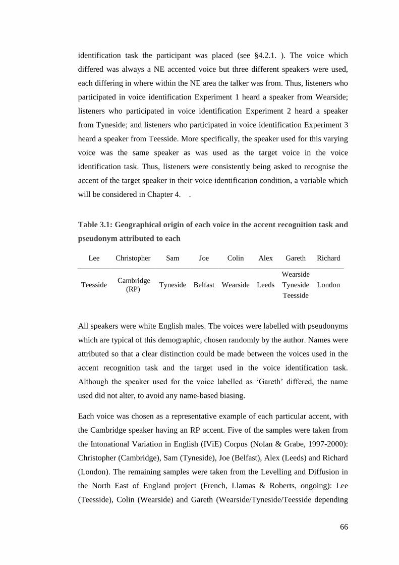
66
identification task the participant was placed (see §4.2.1. ). The voice which
differed was always a NE accented voice but three different speakers were used,
each differing in where within the NE area the talker was from. Thus, listeners who
participated in voice identification Experiment 1 heard a speaker from Wearside;
listeners who participated in voice identification Experiment 2 heard a speaker
from Tyneside; and listeners who participated in voice identification Experiment 3
heard a speaker from Teesside. More specifically, the speaker used for this varying
voice was the same speaker as was used as the target voice in the voice
identification task. Thus, listeners were consistently being asked to recognise the
accent of the target speaker in their voice identification condition, a variable which
will be considered in Chapter 4. .
Table 3.1: Geographical origin of each voice in the accent recognition task and
pseudonym attributed to each
Lee Christopher Sam Joe Colin Alex Gareth Richard
Teesside Cambridge
(RP) Tyneside Belfast Wearside Leeds
Wearside
London Tyneside
Teesside
All speakers were white English males. The voices were labelled with pseudonyms
which are typical of this demographic, chosen randomly by the author. Names were
attributed so that a clear distinction could be made between the voices used in the
accent recognition task and the target used in the voice identification task.
Although the speaker used for the voice labelled as ‘Gareth’ differed, the name
used did not alter, to avoid any name-based biasing.
Each voice was chosen as a representative example of each particular accent, with
the Cambridge speaker having an RP accent. Five of the samples were taken from
the Intonational Variation in English (IViE) Corpus (Nolan & Grabe, 1997-2000):
Christopher (Cambridge), Sam (Tyneside), Joe (Belfast), Alex (Leeds) and Richard
(London). The remaining samples were taken from the Levelling and Diffusion in
the North East of England project (French, Llamas & Roberts, ongoing): Lee
(Teesside), Colin (Wearside) and Gareth (Wearside/Tyneside/Teesside depending
67
on condition). The samples were all created using the cut-and-paste method,
whereby shorter samples were concatenated together to form one longer sample of
speech (Nolan, 2003; Nolan & Grabe, 1996). The resulting samples were all c.15
seconds in length, so that the length of time taken to complete the task was short
but a reasonable representation of the talker’s speech was still provided.
3.1.3. Listeners
A total of 269 listeners took part in the accent recognition task, as part of the wider
voice identification experiments. All listeners were native speakers of British
English with no reported history of hearing problems. Recruitment was done
through the friend-of-a-friend method (Arcury & Quandt, 1999). Listeners were
either randomly assigned to Experiment 1, 2 or 3 or pseudo-randomly assigned by
the experimenter to ensure an even spread of listener variables across each
condition.
North East, non-North East, and ‘familiar’ listeners
Listeners were divided into three groups based upon their dialectal background:
NE, non-NE and familiar. This division was made primarily for the purpose of the
voice identification task in order to assess the impact of local-ness on earwitnesses.
The potential interaction between listener group (based on accent/familiarity) and
speaker identification will be assessed in Chapter 4. For consistency the division of
listeners into these groups will also be applied here.
The NE group were defined as those who grew up in, and have spent most of their
life living in, the NE region. The boundaries of what is considered the NE region
are based on Pearce’s (2009: 11) perceptual study of the area. Pearce (2009) asked
residents of the NE where they believed others sounded the same as, or similar to,
them. A detailed picture of the perceptual links people from the NE draw between
one another can be found in his paper (Pearce, 2009: 11). Figure 3.1 displays an
abstraction of this, showing where the limits of the NE are considered to be.
Responses were used to define the boundaries of the NE with Ashington in the far
north, Darlington in the south and Consett in the west.

68
Figure 3.1: Perceptual dialectal map of North East England based on Pearce
(2009:11)
Participants in both the non-NE and familiar listener groups were defined as those
who were not born in or grew up the region. The inclusion of a familiar group was
made primarily in order to maintain a clear distinction between NE listeners and
non-NE listeners. Non-NE listeners are defined as those not from the area, nor with
any notable degree of exposure to the area beyond what might be expected through
the media and travel to the region. Familiarity can occur through other means.
Members of the familiar listener group are defined as those who, for one reason or
another, have (had) a significant level of exposure to accents from the NE region.
They are not from the area, but include those who have lived there for a period of
69
time or have family or friends from the region. Providing a precise separation
between these groups is a difficult, and likely flawed, task. It does, however, allow
for a strong division between NE and non-NE listeners. Furthermore, listeners were
merely categorised as familiar based on experimenter judgement. Further
investigation into this level of categorisation could include a more detailed coding
mechanism based on level of contact and/or geographical distance. The results of
this intermediate group will be included below, but principally as a comparison
with the other two listener groups rather than drawing any inferences about the
impact of familiarity on AR.
The number of familiar listeners in the experiment (n = 45) is also much lower than
the other two listener groups. As Milroy and Gordon (2003) attest, however, a
group size larger than 30 is satisfactory for drawing meaningful comparisons with
other groups. Where possible, the patterns shown by this group (or rather how they
differ from NE and non-NE listeners) will be analysed but the focus will remain on
the NE and non-NE groups. They may indicate what effect an increased level of
exposure to NE accents can have on a listener’s accent recognition abilities.
Sub-NE regions
There is often a dichotomy between local and non-local perceptions of dialect
boundaries. Those local to an area will commonly perceive dialect boundaries
where non-locals do not (Wells, 1982a). The North East is an area rich in linguistic
variety; Beal, Burbano-Elizondo and Llamas (2012: 48) note that “a considerable
amount of variation exists both within and between accents of the urban centres of
the region.” Nevertheless, the area is often perceived by outsiders as consisting of
one accent (Beal et al., 2012; Montgomery, 2006). Inhabitants from across the NE
report that they are often considered to have a Newcastle (Geordie) accent no
matter where in the area they are from. It is clear that non-local perceptions of
speech in the NE are dominated by the city of Newcastle, the largest and best
known city in the region. This is echoed in linguistic literature, where much more
description of and research into the Tyneside accent exists (Hughes, Watt &
Trudgill, 2005; Watt, 2002; Watt & Allen, 2003) compared with other North
Eastern varieties. Whilst admitting that speech varieties in the North East are not
70
homogeneous, it is not unusual for linguists, like lay people, to treat the region as
one dialectal area. Hughes et al. (2005: 9) state that they would be unhappy
drawing a line between two areas within such a region as there are no obstacles to
communication between them. Whilst this may not hold true for local perceptions,
it does echo views held by many outsiders. Locals, nevertheless, have been shown
to have an awareness of the linguistic variation in the region and perceive
differences between the speech in towns just a few miles apart. Indeed, Pearce’s
(2009) NE perceptual study, used to define the NE region above, shows that within
the area, locals perceive three quite distinct dialect groups. Locals’ judgements
were shown to represent accent similarities within areas centred around the three
major conurbations in the region: Newcastle, Sunderland and Middlesbrough.

71
Figure 3.2: Perceptual dialectal map of sub-North East regions, based on
Pearce (2009:11). Northern section = Tyneside, Middle section = Wearside,
Southern section = Teesside
The presence of three sub-NE listener groups more accurately reflects the
perceptions of locals. In light of this, the results of the AR task will be assessed
based on both these interpretations. For the purposes of this study, the boundaries
of the three sub-NE regions will be based on Figure 3.2, where Tyneside is the
region around Newcastle, Wearside is the region around Sunderland, and Teesside
is the region around Middlesbrough. The number of listeners by each of the listener
groups defined above is shown in Table 3.2.
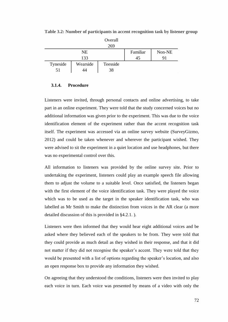
72
Table 3.2: Number of participants in accent recognition task by listener group
3.1.4. Procedure
Listeners were invited, through personal contacts and online advertising, to take
part in an online experiment. They were told that the study concerned voices but no
additional information was given prior to the experiment. This was due to the voice
identification element of the experiment rather than the accent recognition task
itself. The experiment was accessed via an online survey website (SurveyGizmo,
2012) and could be taken whenever and wherever the participant wished. They
were advised to sit the experiment in a quiet location and use headphones, but there
was no experimental control over this.
All information to listeners was provided by the online survey site. Prior to
undertaking the experiment, listeners could play an example speech file allowing
them to adjust the volume to a suitable level. Once satisfied, the listeners began
with the first element of the voice identification task. They were played the voice
which was to be used as the target in the speaker identification task, who was
labelled as Mr Smith to make the distinction from voices in the AR clear (a more
detailed discussion of this is provided in §4.2.1. ).
Listeners were then informed that they would hear eight additional voices and be
asked where they believed each of the speakers to be from. They were told that
they could provide as much detail as they wished in their response, and that it did
not matter if they did not recognise the speaker’s accent. They were told that they
would be presented with a list of options regarding the speaker’s location, and also
an open response box to provide any information they wished.
On agreeing that they understood the conditions, listeners were then invited to play
each voice in turn. Each voice was presented by means of a video with only the
NE Familiar Non-NE
45 91
Tyneside Wearside Teesside
51 44 38
269
Overall
133
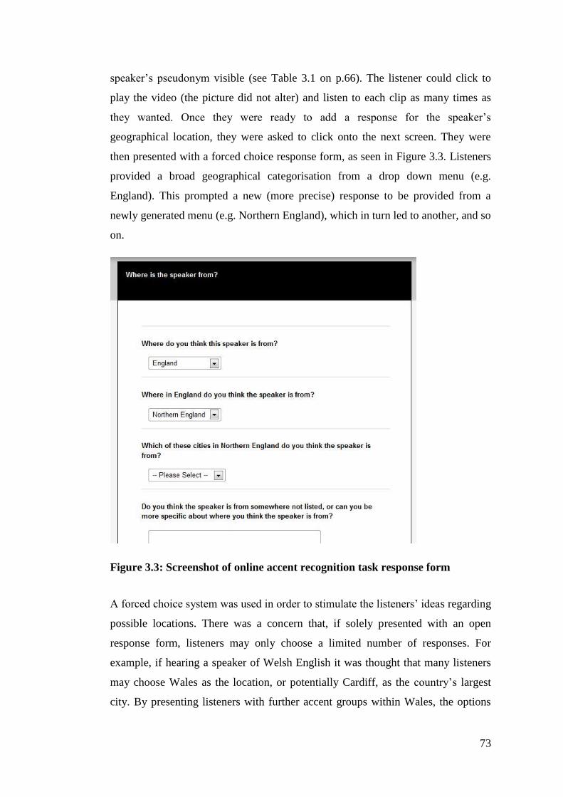
73
speaker’s pseudonym visible (see Table 3.1 on p.66). The listener could click to
play the video (the picture did not alter) and listen to each clip as many times as
they wanted. Once they were ready to add a response for the speaker’s
geographical location, they were asked to click onto the next screen. They were
then presented with a forced choice response form, as seen in Figure 3.3. Listeners
provided a broad geographical categorisation from a drop down menu (e.g.
England). This prompted a new (more precise) response to be provided from a
newly generated menu (e.g. Northern England), which in turn led to another, and so
on.
Figure 3.3: Screenshot of online accent recognition task response form
A forced choice system was used in order to stimulate the listeners’ ideas regarding
possible locations. There was a concern that, if solely presented with an open
response form, listeners may only choose a limited number of responses. For
example, if hearing a speaker of Welsh English it was thought that many listeners
may choose Wales as the location, or potentially Cardiff, as the country’s largest
city. By presenting listeners with further accent groups within Wales, the options
74
are increased and may encourage the listener to think about whether they believe
the speaker is actually from Cardiff as opposed to somewhere else in Wales.
The full list of tiered options is presented in appendix B. The inclusion of each
accent group was made based on various published literature on British English
accents (e.g. Foulkes and Docherty (1999), Hughes et al. (2005), Wells (1982b)).
It is not intended to be an exhaustive overview of British English accents, but
offers a reasonable spread of competing options from around Britain, including
major accent groups.
Options from within each lower tier were only made available once a selection
from a higher tier was made. Listeners were advised that they could choose their
answer from whichever tier they wished. For example, the form allowed a listener
to select that they believed a speaker was from any one of Ireland (tier 1), Northern
Ireland (tier 2) or Londonderry (tier 3). Furthermore, no matter which tier listeners
selected from, they could still provide additional unrestricted information to their
response. They were advised that this could provide more specific information, for
example, saying ‘Northern London’ rather than just ‘London’ or stating that they
were unsure between more than one location. Following the accent recognition
task, listeners were asked biographical information. The full list of questions asked
can be seen in Table 3.3. The listeners then took part in a voice lineup, as means of
testing in the voice identification portion of the experiment.

75
Table 3.3: Biographical information asked in accent recognition/voice
identification study
Are you male or female? Male
Female
Prefer not to say
How old are you? 18-25
26-35
56-45
46+
Prefer not to say
Where were you born?
Did you grow up here?
Have you lived anywhere else?
Please state where, at what age, and how long for?
Do you have strong connection (family members, close
friends)
with anyone who has an accent different from your own?
3.1.4.1. Scoring scale
Responses provided by each listener were given a numerical score from 0-3
according to the geographical and perceived dialectal distance between the accent
of the speaker and the listener’s response. Three was scored for correct response
i.e. one which matched the speaker’s accent closely. As an example, on hearing a
speaker from Newcastle, a response stating a location which is marked as Tyneside
76
in Pearce’s (2009) perceptual study of the area would score three, as the accent and
response are considered part of the same perceptual group. Two points were scored
for responses which were closely related in terms of productional similarities
between the accents. For a Newcastle voice, a response stating a location within the
NE region but outside of the Tyneside area scored two points as there are clear
similarities in production between accents in the NE (as highlighted by the
treatment of the region sometimes as one accent group) but there have been shown
to be perceptual differences between the accent and response. A response stating a
location within the North of England, but outside the NE region, scored one point,
as there are generally fewer phonetic and phonological similarities between, for
example, Newcastle and Yorkshire accents than Newcastle and Sunderland accents.
Responses stating locations beyond this, such as in the South of England, where
accental features are even more dissimilar from Newcastle, scored 0. Geographical
distance from the correct location is, of course, not the only measure of closeness
between two accents. The Middlesbrough accent, for example, has a number of
phonetic features in common with Liverpool English (Beal et al., 2012) and so
responses were also considered for perceptual distance from the accent spoken. A
Liverpool response to a Middlesbrough accent would score two points, as it is not
accurate, but is closely related. The RP speaker (Christopher) originated from
Cambridge, though it would be unfair to mark any Standard Southern British
English accent response as incorrect, as RP is not geographically specific (Roach,
2004). As such, RP, Cambridge and varieties of South Eastern English where RP is
the typical variety spoken are scored as 3 for this voice. This method is not without
its flaws, and is quite broad in its categorisation of accents, but does capture the
general trend for whether a listener can accurately identify an accent or not.
3.1.5. Predictions
The following hypotheses are made about results of the accent recognition task:
Variation is certainly expected between listeners, in line with previous
research into dialect recognition (Britain, 2002; Kerswill & Williams, 2002;
Labov, 1972; Williams et al., 1999).
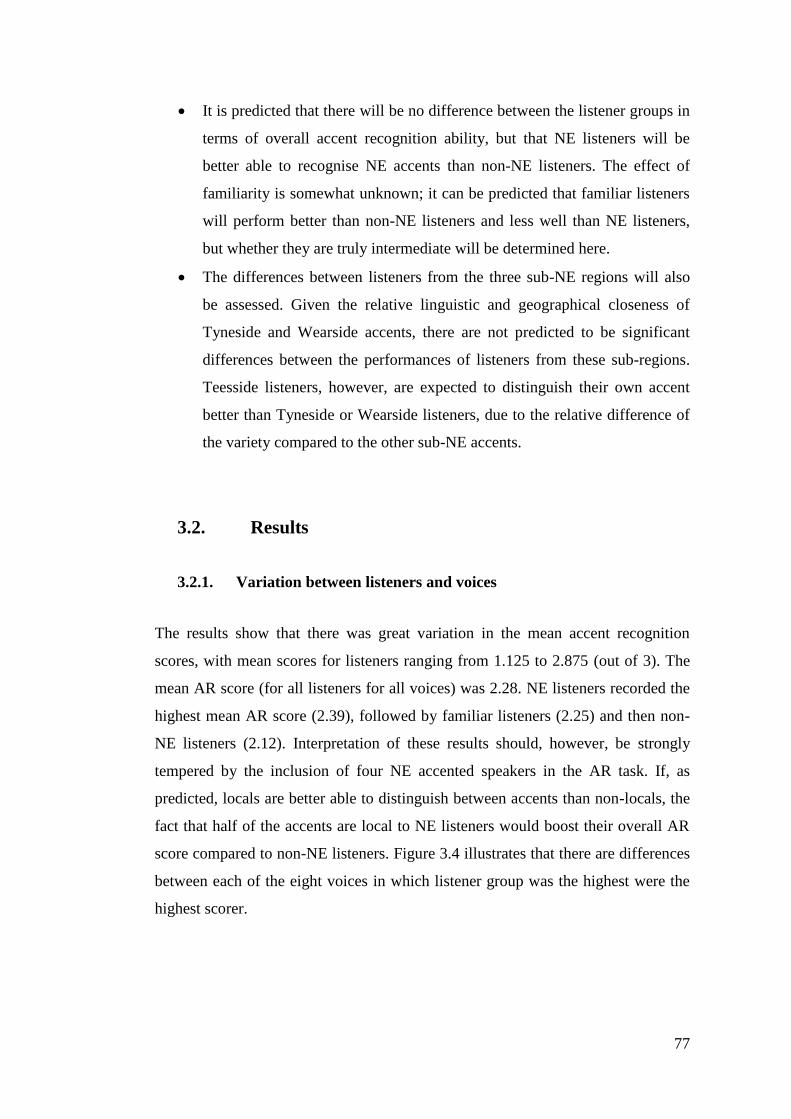
77
It is predicted that there will be no difference between the listener groups in
terms of overall accent recognition ability, but that NE listeners will be
better able to recognise NE accents than non-NE listeners. The effect of
familiarity is somewhat unknown; it can be predicted that familiar listeners
will perform better than non-NE listeners and less well than NE listeners,
but whether they are truly intermediate will be determined here.
The differences between listeners from the three sub-NE regions will also
be assessed. Given the relative linguistic and geographical closeness of
Tyneside and Wearside accents, there are not predicted to be significant
differences between the performances of listeners from these sub-regions.
Teesside listeners, however, are expected to distinguish their own accent
better than Tyneside or Wearside listeners, due to the relative difference of
the variety compared to the other sub-NE accents.
3.2. Results
3.2.1. Variation between listeners and voices
The results show that there was great variation in the mean accent recognition
scores, with mean scores for listeners ranging from 1.125 to 2.875 (out of 3). The
mean AR score (for all listeners for all voices) was 2.28. NE listeners recorded the
highest mean AR score (2.39), followed by familiar listeners (2.25) and then non-
NE listeners (2.12). Interpretation of these results should, however, be strongly
tempered by the inclusion of four NE accented speakers in the AR task. If, as
predicted, locals are better able to distinguish between accents than non-locals, the
fact that half of the accents are local to NE listeners would boost their overall AR
score compared to non-NE listeners. Figure 3.4 illustrates that there are differences
between each of the eight voices in which listener group was the highest were the
highest scorer.
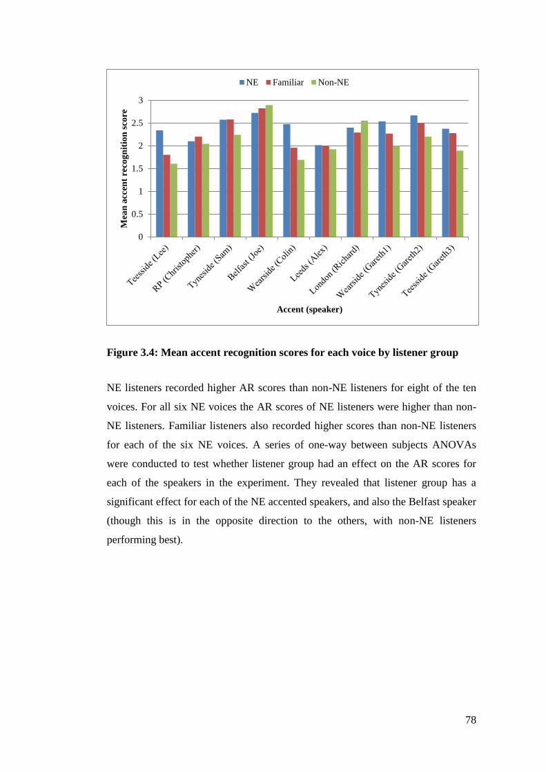
78
Figure 3.4: Mean accent recognition scores for each voice by listener group
NE listeners recorded higher AR scores than non-NE listeners for eight of the ten
voices. For all six NE voices the AR scores of NE listeners were higher than non-
NE listeners. Familiar listeners also recorded higher scores than non-NE listeners
for each of the six NE voices. A series of one-way between subjects ANOVAs
were conducted to test whether listener group had an effect on the AR scores for
each of the speakers in the experiment. They revealed that listener group has a
significant effect for each of the NE accented speakers, and also the Belfast speaker
(though this is in the opposite direction to the others, with non-NE listeners
performing best).
0
0.5
1
1.5
2
2.5
3
Mea
n a
ccen
t re
cog
nit
ion
sco
re
Accent (speaker)
NE Familiar Non-NE
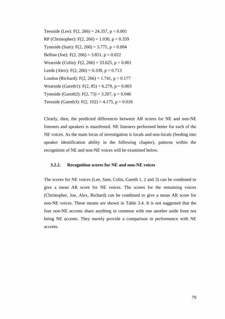
79
Teesside (Lee): F(2, 266) = 24.357, p < 0.001
RP (Christopher): F(2, 266) = 1.030, p = 0.359
Tyneside (Sam): F(2, 266) = 5.775, p = 0.004
Belfast (Joe): F(2, 266) = 3.851, p = 0.022
Wearside (Colin): F(2, 266) = 33.625, p < 0.001
Leeds (Alex): F(2, 266) = 0.339, p = 0.713
London (Richard): F(2, 266) = 1.741, p = 0.177
Wearside (Gareth1): F(2, 85) = 6.279, p = 0.003
Tyneside (Gareth2): F(2, 73) = 3.207, p = 0.046
Teesside (Gareth3): F(2, 102) = 4.175, p = 0.018
Clearly, then, the predicted differences between AR scores for NE and non-NE
listeners and speakers is manifested. NE listeners performed better for each of the
NE voices. As the main locus of investigation is locals and non-locals (feeding into
speaker identification ability in the following chapter), patterns within the
recognition of NE and non-NE voices will be examined below.
3.2.2. Recognition scores for NE and non-NE voices
The scores for NE voices (Lee, Sam, Colin, Gareth 1, 2 and 3) can be combined to
give a mean AR score for NE voices. The scores for the remaining voices
(Christopher, Joe, Alex, Richard) can be combined to give a mean AR score for
non-NE voices. These means are shown in Table 3.4. It is not suggested that the
four non-NE accents share anything in common with one another aside from not
being NE accents. They merely provide a comparison in performance with NE
accents.
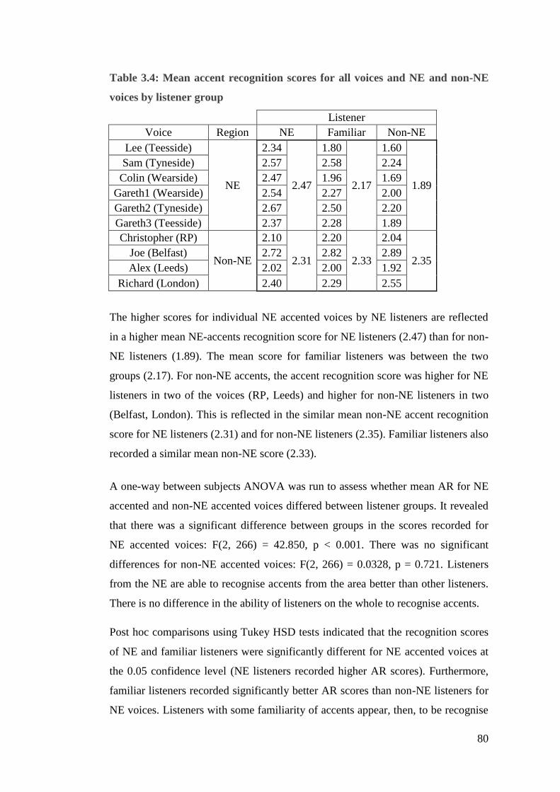
80
Table 3.4: Mean accent recognition scores for all voices and NE and non-NE
voices by listener group
Listener
Voice Region NE Familiar Non-NE
Lee (Teesside)
NE
2.34
2.47
1.80
2.17
1.60
1.89
Sam (Tyneside) 2.57 2.58 2.24
Colin (Wearside) 2.47 1.96 1.69
Gareth1 (Wearside) 2.54 2.27 2.00
Gareth2 (Tyneside) 2.67 2.50 2.20
Gareth3 (Teesside) 2.37 2.28 1.89
Christopher (RP)
Non-NE
2.10
2.31
2.20
2.33
2.04
2.35 Joe (Belfast) 2.72 2.82 2.89
Alex (Leeds) 2.02 2.00 1.92
Richard (London) 2.40 2.29 2.55
The higher scores for individual NE accented voices by NE listeners are reflected
in a higher mean NE-accents recognition score for NE listeners (2.47) than for non-
NE listeners (1.89). The mean score for familiar listeners was between the two
groups (2.17). For non-NE accents, the accent recognition score was higher for NE
listeners in two of the voices (RP, Leeds) and higher for non-NE listeners in two
(Belfast, London). This is reflected in the similar mean non-NE accent recognition
score for NE listeners (2.31) and for non-NE listeners (2.35). Familiar listeners also
recorded a similar mean non-NE score (2.33).
A one-way between subjects ANOVA was run to assess whether mean AR for NE
accented and non-NE accented voices differed between listener groups. It revealed
that there was a significant difference between groups in the scores recorded for
NE accented voices: F(2, 266) = 42.850, p < 0.001. There was no significant
differences for non-NE accented voices: F(2, 266) = 0.0328, p = 0.721. Listeners
from the NE are able to recognise accents from the area better than other listeners.
There is no difference in the ability of listeners on the whole to recognise accents.
Post hoc comparisons using Tukey HSD tests indicated that the recognition scores
of NE and familiar listeners were significantly different for NE accented voices at
the 0.05 confidence level (NE listeners recorded higher AR scores). Furthermore,
familiar listeners recorded significantly better AR scores than non-NE listeners for
NE voices. Listeners with some familiarity of accents appear, then, to be recognise
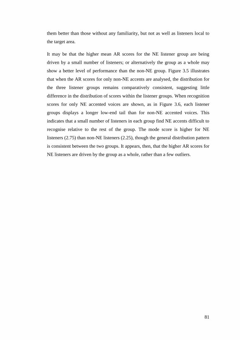
81
them better than those without any familiarity, but not as well as listeners local to
the target area.
It may be that the higher mean AR scores for the NE listener group are being
driven by a small number of listeners; or alternatively the group as a whole may
show a better level of performance than the non-NE group. Figure 3.5 illustrates
that when the AR scores for only non-NE accents are analysed, the distribution for
the three listener groups remains comparatively consistent, suggesting little
difference in the distribution of scores within the listener groups. When recognition
scores for only NE accented voices are shown, as in Figure 3.6, each listener
groups displays a longer low-end tail than for non-NE accented voices. This
indicates that a small number of listeners in each group find NE accents difficult to
recognise relative to the rest of the group. The mode score is higher for NE
listeners (2.75) than non-NE listeners (2.25), though the general distribution pattern
is consistent between the two groups. It appears, then, that the higher AR scores for
NE listeners are driven by the group as a whole, rather than a few outliers.
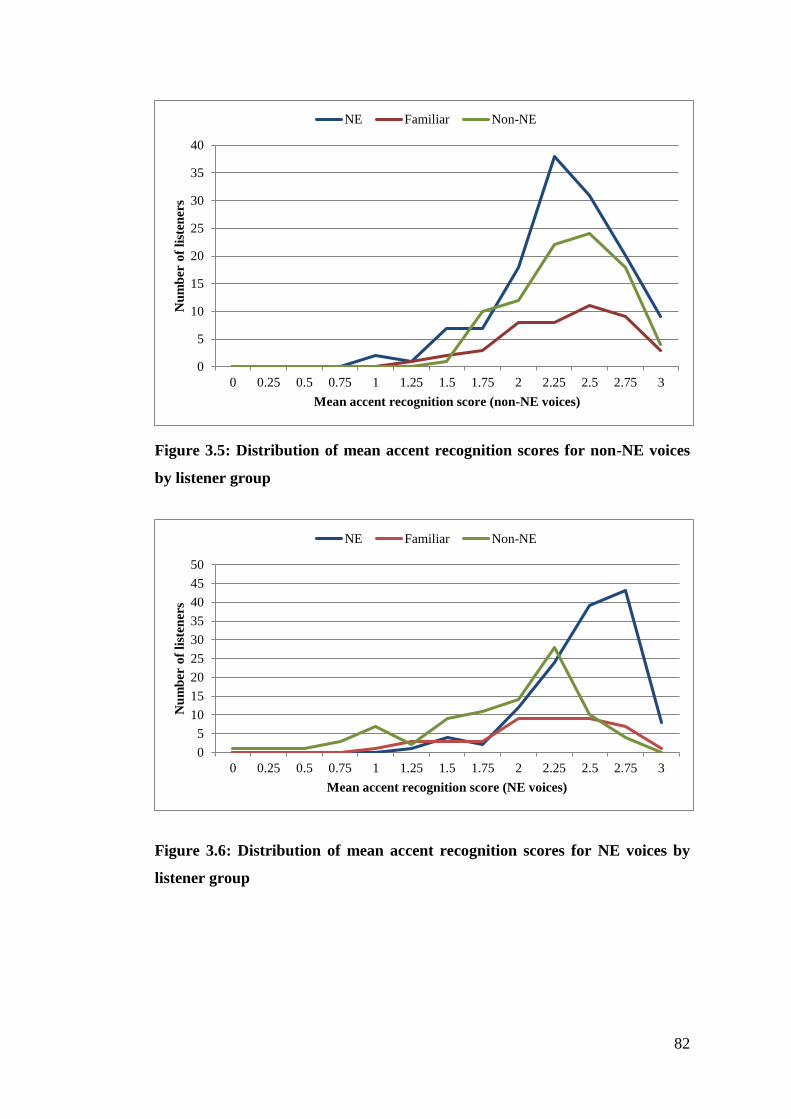
82
Figure 3.5: Distribution of mean accent recognition scores for non-NE voices
by listener group
Figure 3.6: Distribution of mean accent recognition scores for NE voices by
listener group
0
5
10
15
20
25
30
35
40
0 0.25 0.5 0.75 1 1.25 1.5 1.75 2 2.25 2.5 2.75 3
Nu
mb
er o
f li
sten
ers
Mean accent recognition score (non-NE voices)
NE Familiar Non-NE
0
5
10
15
20
25
30
35
40
45
50
0 0.25 0.5 0.75 1 1.25 1.5 1.75 2 2.25 2.5 2.75 3
Nu
mb
er o
f li
sten
ers
Mean accent recognition score (NE voices)
NE Familiar Non-NE
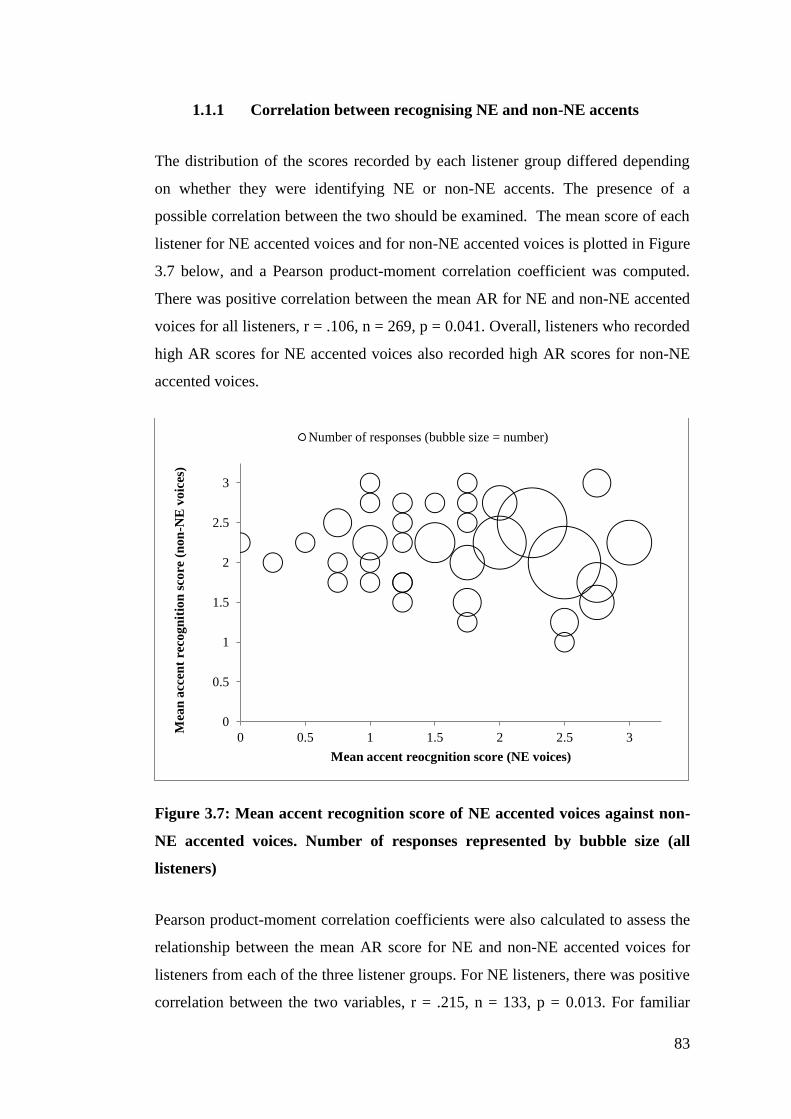
83
1.1.1 Correlation between recognising NE and non-NE accents
The distribution of the scores recorded by each listener group differed depending
on whether they were identifying NE or non-NE accents. The presence of a
possible correlation between the two should be examined. The mean score of each
listener for NE accented voices and for non-NE accented voices is plotted in Figure
3.7 below, and a Pearson product-moment correlation coefficient was computed.
There was positive correlation between the mean AR for NE and non-NE accented
voices for all listeners, r = .106, n = 269, p = 0.041. Overall, listeners who recorded
high AR scores for NE accented voices also recorded high AR scores for non-NE
accented voices.
Figure 3.7: Mean accent recognition score of NE accented voices against non-
NE accented voices. Number of responses represented by bubble size (all
listeners)
Pearson product-moment correlation coefficients were also calculated to assess the
relationship between the mean AR score for NE and non-NE accented voices for
listeners from each of the three listener groups. For NE listeners, there was positive
correlation between the two variables, r = .215, n = 133, p = 0.013. For familiar
0
0.5
1
1.5
2
2.5
3
0 0.5 1 1.5 2 2.5 3
Mea
n a
ccen
t re
cog
nit
ion
sco
re (
no
n-N
E v
oic
es)
Mean accent reocgnition score (NE voices)
Number of responses (bubble size = number)
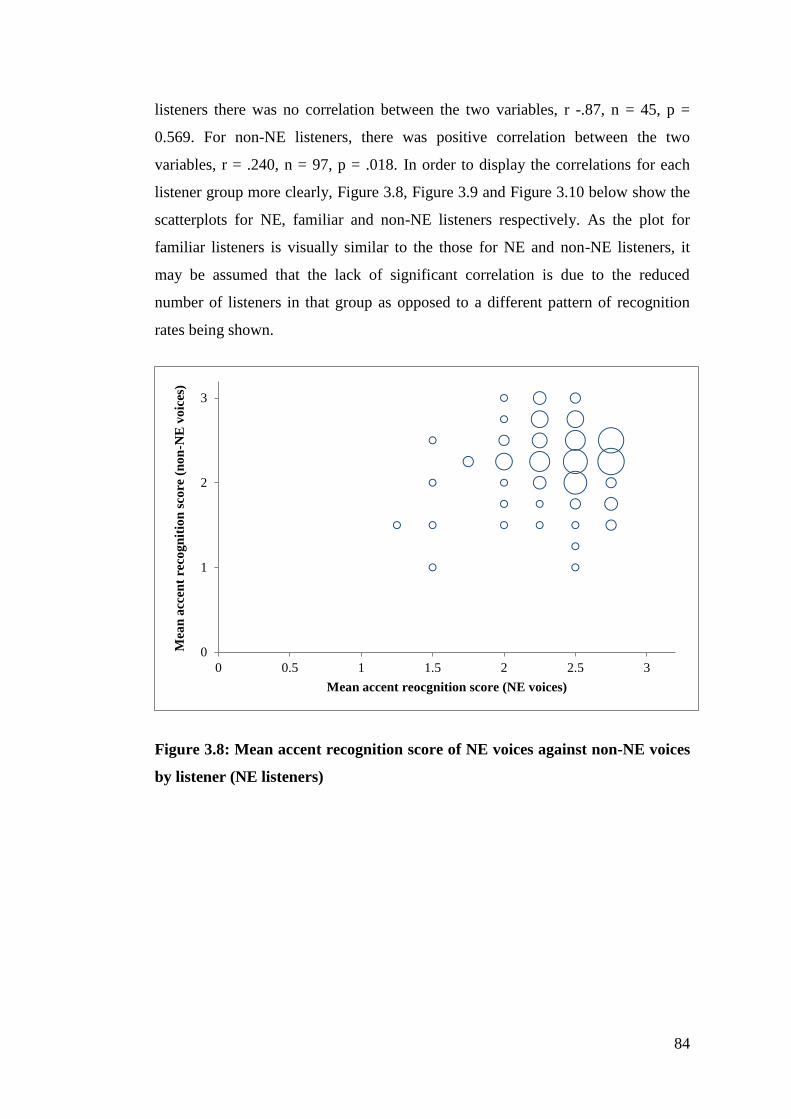
84
listeners there was no correlation between the two variables, r -.87, n = 45, p =
0.569. For non-NE listeners, there was positive correlation between the two
variables, r = .240, n = 97, p = .018. In order to display the correlations for each
listener group more clearly, Figure 3.8, Figure 3.9 and Figure 3.10 below show the
scatterplots for NE, familiar and non-NE listeners respectively. As the plot for
familiar listeners is visually similar to the those for NE and non-NE listeners, it
may be assumed that the lack of significant correlation is due to the reduced
number of listeners in that group as opposed to a different pattern of recognition
rates being shown.
Figure 3.8: Mean accent recognition score of NE voices against non-NE voices
by listener (NE listeners)
0
1
2
3
0 0.5 1 1.5 2 2.5 3
Mea
n a
ccen
t re
cog
nit
ion
sco
re (
no
n-N
E v
oic
es)
Mean accent reocgnition score (NE voices)
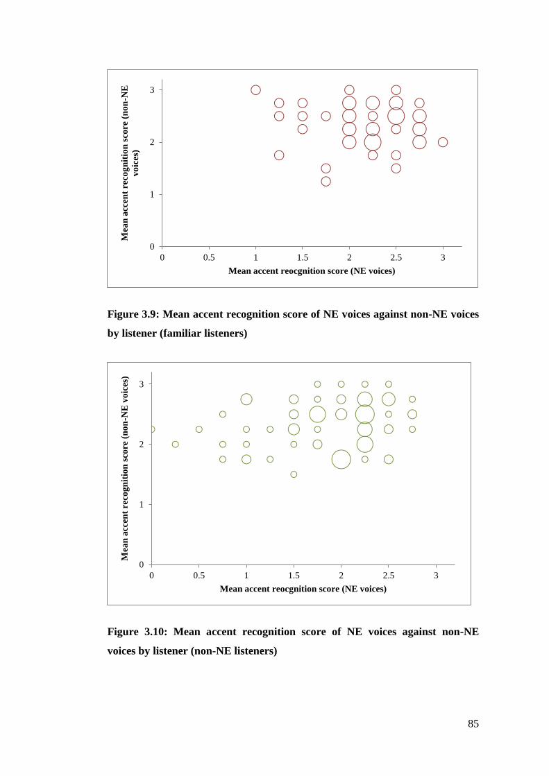
85
Figure 3.9: Mean accent recognition score of NE voices against non-NE voices
by listener (familiar listeners)
Figure 3.10: Mean accent recognition score of NE voices against non-NE
voices by listener (non-NE listeners)
0
1
2
3
0 0.5 1 1.5 2 2.5 3
Mea
n a
ccen
t re
cog
nit
ion
sco
re (
no
n-N
E
vo
ices
)
Mean accent reocgnition score (NE voices)
0
1
2
3
0 0.5 1 1.5 2 2.5 3
Mea
n a
ccen
t re
cog
nit
ion
sco
re (
no
n-N
E v
oic
es)
Mean accent reocgnition score (NE voices)
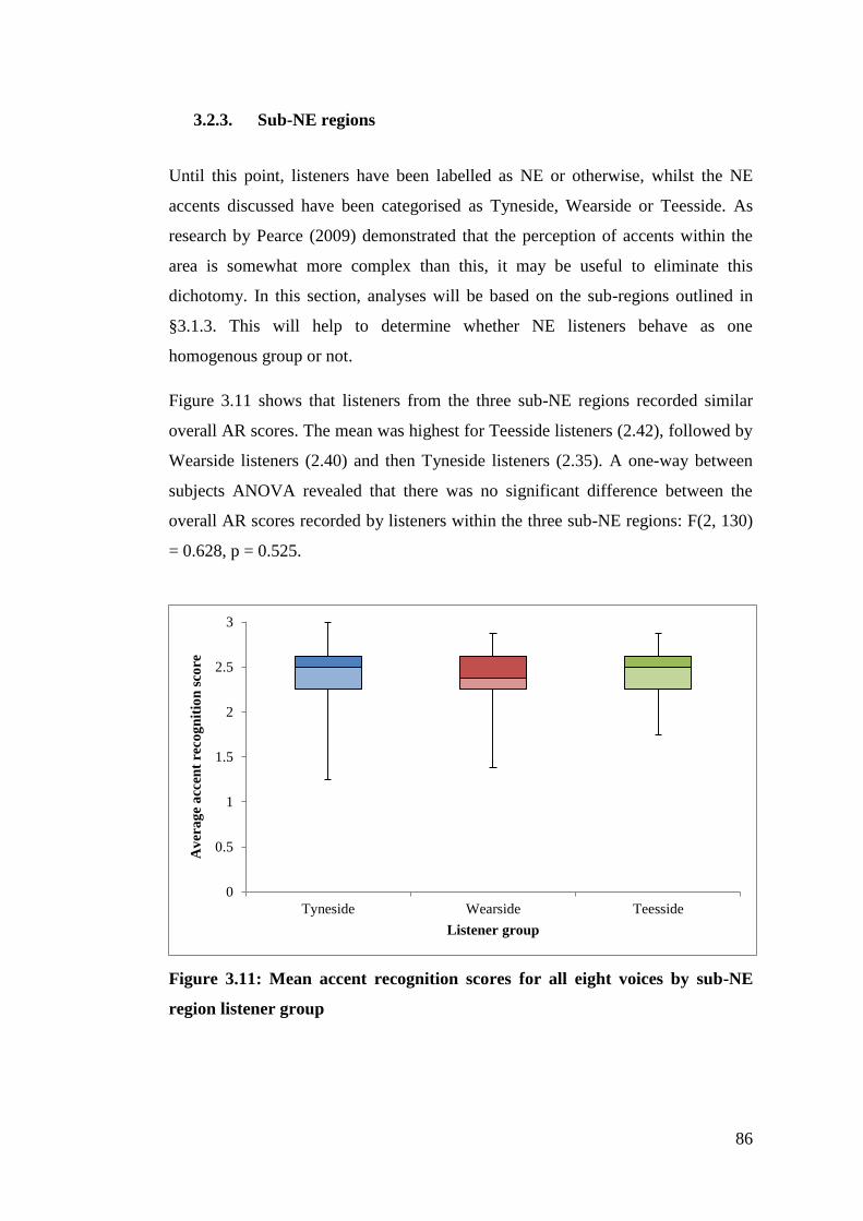
86
3.2.3. Sub-NE regions
Until this point, listeners have been labelled as NE or otherwise, whilst the NE
accents discussed have been categorised as Tyneside, Wearside or Teesside. As
research by Pearce (2009) demonstrated that the perception of accents within the
area is somewhat more complex than this, it may be useful to eliminate this
dichotomy. In this section, analyses will be based on the sub-regions outlined in
§3.1.3. This will help to determine whether NE listeners behave as one
homogenous group or not.
Figure 3.11 shows that listeners from the three sub-NE regions recorded similar
overall AR scores. The mean was highest for Teesside listeners (2.42), followed by
Wearside listeners (2.40) and then Tyneside listeners (2.35). A one-way between
subjects ANOVA revealed that there was no significant difference between the
overall AR scores recorded by listeners within the three sub-NE regions: F(2, 130)
= 0.628, p = 0.525.
Figure 3.11: Mean accent recognition scores for all eight voices by sub-NE
region listener group
0
0.5
1
1.5
2
2.5
3
Tyneside Wearside Teesside
Av
era
ge
acc
ent
reco
gn
itio
n s
core
Listener group
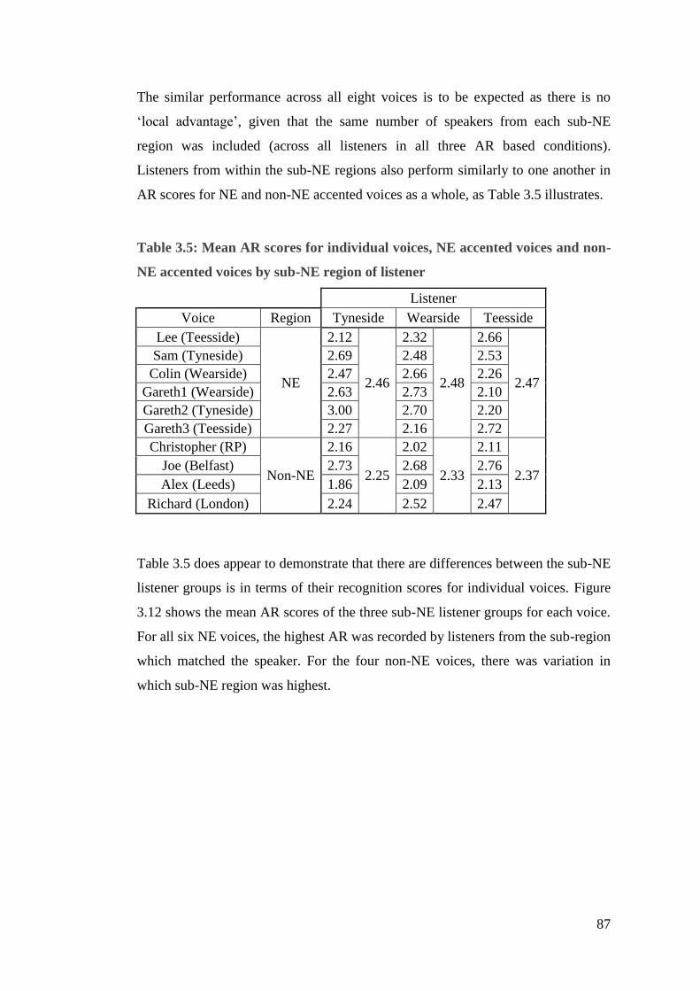
87
The similar performance across all eight voices is to be expected as there is no
‘local advantage’, given that the same number of speakers from each sub-NE
region was included (across all listeners in all three AR based conditions).
Listeners from within the sub-NE regions also perform similarly to one another in
AR scores for NE and non-NE accented voices as a whole, as Table 3.5 illustrates.
Table 3.5: Mean AR scores for individual voices, NE accented voices and non-
NE accented voices by sub-NE region of listener
Listener
Voice Region Tyneside Wearside Teesside
Lee (Teesside)
NE
2.12
2.46
2.32
2.48
2.66
2.47
Sam (Tyneside) 2.69 2.48 2.53
Colin (Wearside) 2.47 2.66 2.26
Gareth1 (Wearside) 2.63 2.73 2.10
Gareth2 (Tyneside) 3.00 2.70 2.20
Gareth3 (Teesside) 2.27 2.16 2.72
Christopher (RP)
Non-NE
2.16
2.25
2.02
2.33
2.11
2.37 Joe (Belfast) 2.73 2.68 2.76
Alex (Leeds) 1.86 2.09 2.13
Richard (London) 2.24 2.52 2.47
Table 3.5 does appear to demonstrate that there are differences between the sub-NE
listener groups is in terms of their recognition scores for individual voices. Figure
3.12 shows the mean AR scores of the three sub-NE listener groups for each voice.
For all six NE voices, the highest AR was recorded by listeners from the sub-region
which matched the speaker. For the four non-NE voices, there was variation in
which sub-NE region was highest.
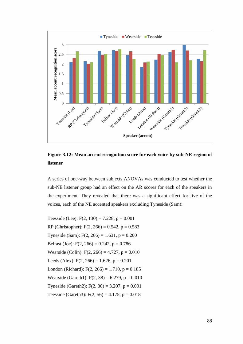
88
Figure 3.12: Mean accent recognition score for each voice by sub-NE region of
listener
A series of one-way between subjects ANOVAs was conducted to test whether the
sub-NE listener group had an effect on the AR scores for each of the speakers in
the experiment. They revealed that there was a significant effect for five of the
voices, each of the NE accented speakers excluding Tyneside (Sam):
Teesside (Lee): F(2, 130) = 7.228, p = 0.001
RP (Christopher): F(2, 266) = 0.542, p = 0.583
Tyneside (Sam): F(2, 266) = 1.631, p = 0.200
Belfast (Joe): F(2, 266) = 0.242, p = 0.786
Wearside (Colin): F(2, 266) = 4.727, p = 0.010
Leeds (Alex): F(2, 266) = 1.626, p = 0.201
London (Richard): F(2, 266) = 1.710, p = 0.185
Wearside (Gareth1): F(2, 38) = 6.279, p = 0.010
Tyneside (Gareth2): F(2, 30) = 3.207, p = 0.001
Teesside (Gareth3): F(2, 56) = 4.175, p = 0.018
0
0.5
1
1.5
2
2.5
3
Mea
n a
ccen
t re
cog
nit
ion
sco
re
Speaker (accent)
Tyneside Wearside Teesside
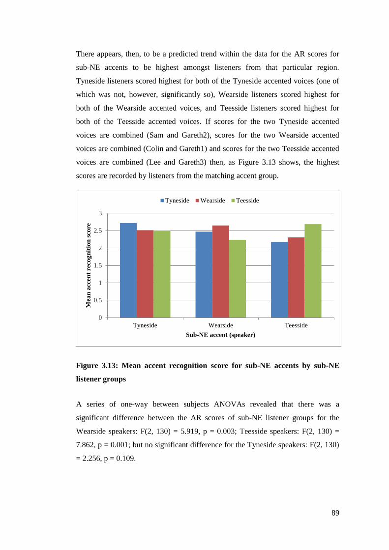
89
There appears, then, to be a predicted trend within the data for the AR scores for
sub-NE accents to be highest amongst listeners from that particular region.
Tyneside listeners scored highest for both of the Tyneside accented voices (one of
which was not, however, significantly so), Wearside listeners scored highest for
both of the Wearside accented voices, and Teesside listeners scored highest for
both of the Teesside accented voices. If scores for the two Tyneside accented
voices are combined (Sam and Gareth2), scores for the two Wearside accented
voices are combined (Colin and Gareth1) and scores for the two Teesside accented
voices are combined (Lee and Gareth3) then, as Figure 3.13 shows, the highest
scores are recorded by listeners from the matching accent group.
Figure 3.13: Mean accent recognition score for sub-NE accents by sub-NE
listener groups
A series of one-way between subjects ANOVAs revealed that there was a
significant difference between the AR scores of sub-NE listener groups for the
Wearside speakers: F(2, 130) = 5.919, p = 0.003; Teesside speakers: F(2, 130) =
7.862, p = 0.001; but no significant difference for the Tyneside speakers: F(2, 130)
= 2.256, p = 0.109.
0
0.5
1
1.5
2
2.5
3
Tyneside Wearside Teesside
Mea
n a
ccen
t re
cog
nit
ion
sco
re
Sub-NE accent (speaker)
Tyneside Wearside Teesside
90
3.3. Discussion
The results indicate that the geographical background of a listener influences their
ability to accurately recognise an accent. Broadly speaking, listeners who are from
the NE can recognise a NE accent (and, moreover, where within the NE the speaker
is from) with greater resolution than listeners from outside of the region.
There was no significant difference between the overall AR scores for NE and non-
NE listeners, as expected. The scores recorded by the different listener groups,
however, revealed that there were differences between their abilities to recognise
particular accents. NE listeners recorded significantly higher AR scores for five of
the six speakers who originated from the NE. The only NE speaker for which there
was not a significant difference was Gareth2, from Tyneside. The mean recognition
score for Gareth2 was higher for NE than non-NE listeners with a similar (or
greater) raw difference between the score compared to those for other NE voices.
As the voice of Gareth differed between speaker identification conditions,
however, fewer participants were asked to identify that accent than all others. This
is likely to be the cause of the lack of a statistically significant difference rather
than that voice producing different results from other NE voices. There are clearly,
then, differences between the abilities of local and non-local listeners to identify
the geographical background of a listener. This comes as no surprise given
previous findings that increased distance between a listener’s own accent and that
which they are asked to classify (Clopper & Pisoni, 2006; Preston, 1993) or judge
as similar (Clopper & Pisoni, 2004) reduces the resolution of the accent presented.
Knowledge of an accent has been shown to improve performance in auditory based
language tasks involving that accent (Adank et al., 2009; Adank & McQueen,
2007; Floccia, Goslin, Girard & Konopczynski, 2006) as has sharing the accent
(Pinet, Iverson & Huckvale, 2011; Stevenage et al., 2012). Perhaps a listener’s
ability to accurately attribute a regional variety to a speaker is indicative of their
knowledge of the accent. If so, it follows that, based on research into the other-
accent effect, accent recognition ability may be an indicator of speaker
identification ability. The fact that there is variation in AR scores within the
listener groups will allow this to be investigated in Chapter 4.
91
Listeners with some familiarity of NE accents consistently recorded higher AR
scores than non-NE listeners for all six NE voices, though the differences were not
significant for each voice. Familiar listeners’ mean AR scores for NE voices were
also consistently lower than those for NE listeners. This indicates that having an
above average level of familiarity with (or exposure to) an accent aids a listeners’
ability to identify that accent. Non-NE listeners have less exposure to NE accents
than the familiar group of listeners, who in turn have less exposure than listeners
from the NE. Sumner and Samuel (2009), in investigating the encoding of dialect
variants in American English, suggested that it is possible to have an accent not
necessarily in terms of production but in terms of perception, representation and
recognition. The present data accord with their findings that prior experience with a
dialect variety moves a listener more in line with those who have the accent in
terms of production. This suggests that non-NE listeners with some familiarity with
the region may not have a NE accent by way of speech production, but they do in
terms of being able to perceive dialectal boundaries in the region. This enables
them to better distinguish one NE variety from another.
The non-NE accented voices AR scores, and their distribution, were similar across
NE, familiar and non-NE listeners. For NE accented voices, there were differences
in the mean scores, but the distributions remain similar across the listener groups.
Each displays a low-end tail and similar clustering of scores (SD: NE = 0.45,
familiar = 0.59, non-NE = 0.58). This suggests that, whilst there is variation in the
performance within the groups, the lower mean score for non-NE listeners is due to
a reduced ability as a whole. Being local to (or having familiarity with) an accent
has a generally positive impact on all listeners’ ability to identify the accent, rather
than improving the ability of some listeners to varying degrees.
The data also indicate that there is a correlation between listeners’ ability to
recognise NE and non-NE accents. Listeners who scored high mean AR scores for
NE accented voices also scored highly for non-NE accented voices. Given that
there is variance between listeners in their ability to recognise accents, this
correlation suggests that listeners have an underlying ability to distinguish between
accents regardless of their degree of familiarity with or exposure to those accents.
Those with increased exposure to particular accents, however, show improved
92
recognition ability but still in correlation to their overall ability. Those who are, in
general, poor at recognising accents are still better able to distinguish between
accents with which they have previous exposure than those which they have not. In
light of this, it may be that a listener’s overall accent ability is as strong an
indicator of speaker identification accuracy as recognition of the target speaker’s
accent. This will be tested in the following chapter.
The local/non-local distinction exhibited by NE and non-NE listeners also appears
to be present within the region. For each of the six NE accented voices, the highest
AR score was recorded by listeners from the same sub-NE region as the target
(Tyneside, Wearside or Teesside). The differences between the groups were,
compared to the NE/non-NE groups, much smaller. This reflects the relative
disparity in difference between listeners from the NE and outside, compared to
listeners from one sub-NE region and another. It can be expected that a listener
from Tyneside, for example, would have more baseline exposure to the Wearside
accent than someone from the south of England. The fact that there are AR
differences at the sub-regional level, however, indicates the potential for a
difference in speaker identification accuracy based on the sub-NE accent of
speakers and listeners. This, too, will be explored in Chapter 4.
3.4. Chapter summary
Listeners from the NE are better able to identify a NE accent than non-
locals are
Familiarity with NE accents provides listeners with an improved ability
over non-locals, but does not put them in line with local listeners
There is correlation between listeners’ ability to recognise the accent of a
NE speaker and a non-NE speaker
Listeners from the same sub-NE region as a speaker are better able to
identify their accent than listeners from elsewhere in the region
93
4. The effect of listeners’ accent
and accent recognition ability on
speaker identification
This chapter combines the results of the accent recognition task presented in
Chapter 3 with a series of speaker identification experiments conducted using the
same subjects. The chapter will consider whether a listener’s ability to recognise
accents – in general and specifically that of the target in the speaker identification
task – has any effect on their ability to identify a speaker. The accent of the listener
relative to the speaker will also be considered as a potential factor along with other,
more commonly tested variables, such as age and sex.
The methodologies of three speaker identification experiments are outlined below.
A voice lineup methodology is employed in each experiment. The procedure
involved in these is identical other than the target voice and the construction of the
voice lineup used for testing. The results of each experiment will then be discussed
in turn and a general discussion of the conclusions drawn across the tasks will
follow.
4.1. Justifications
The experiments will test the effect of accent recognition ability on speaker
identification accuracy. As the previous chapter demonstrated, there is variation in
the ability of listeners to accurately identify the accent of a talker. This variation
exists within accent-based listener groups, but more-so between such groups (locals
perform better than non-locals, familiarity with an accent improves accuracy
amongst non-locals). As aptitude at other language and cognitive based tasks have
been shown to correlate with speaker identification accuracy (de Jong, 1998), and
distinguishing between accents has a clear conceptual link to distinguishing
between voices, the relationship between the two will be tested.
94
The other-accent effect has been demonstrated at a regional level in British
English, using speakers and listeners from Glasgow and Southampton (Stevenage
et al., 2012). It has not been shown in any regional variety of English beyond this.
The present study will investigate the other-accent effect using another variety of
British English: North East England. Furthermore, the effect has only been
confirmed at a broadly regional level. The analysis which follows, then, will
examine whether the effect exists outside of and within a broad regional variety by
assessing the differences between listeners at sub-regional level.
4.2. Methodology
4.2.1. Voices
Three experiments based on similar procedures form this study. As the target and
foil voices used were the primary element which differed between the three
experiments, more detail about these will be provided in the relevant sections for
each task (see §4.3.1. §4.4.1 and §4.5.1. ). There were, nevertheless, consistencies
between the samples used, as follows.
The exposure sample (the ‘criminal’) was produced using the cut-and-paste method
(Nolan, 2003) from a longer interview i.e. sections of the subject’s speech were cut
from the interview and concatenated together. The resulting speech sample
therefore does not consist of one continuous, fluent stretch of the subject’s speech.
Rather, it is formed of a collection of shorter (usually around 5 seconds or longer)
samples. Whilst this is not how listeners encounter speech in real-life, it does allow
for a wider range of voices to be included in the experiment than would otherwise
have been available. It also provided some consistency between the exposure phase
and testing phase. The resultant exposure sample was c.60 seconds long, the length
of time of exposure beyond which Legge et al. (1984) found no benefit to
identification rates and the amount of speech advised for use in a forensic voice
lineup (Home Office, 2003). The interlocutor’s voice and any personal or
identifying details were excluded from the sample.
95
The eight speech samples used in the testing phase of the experiment (voice lineup)
were produced using the same cut-and-paste method. Some were taken from the
Levelling and Diffusion in the North East of England project (French et al.,
ongoing) and some were made from interviews recorded in the same manner
specifically for this project. The samples were each 40-45 seconds long, as is
consistent with advice made by The McFarlane Guidelines on forensic procedure
(Nolan, 2003). In Experiments 1 and 2 – the target present lineups - one of the
voices was that of the target speaker. The sample of the target speaker was
produced from the same recording as the exposure sample. No overlapping
semantic information was included in the exposure and target samples and there
was nothing present other than the speaker’s voice to link the two samples, or make
them stand out from the others (background noise, echo, etc.). The foil voices
included in the voice lineup were all from the NE of England, though they
represented speakers from throughout the region. The precise composition of each
lineup is discussed in the appropriate sections for each experiment
The foil voices were chosen based on their acoustic and auditory differences from
the target voice. Euclidean distances for a number of segmental and
suprasegmental features were calculated between the target voice and each of the
foil samples. The choice of samples was then made to include foils which matched
the target voice to varying degrees in terms of segmental (e.g. vowel formant
frequencies) and/or suprasegmental (e.g. mean f0, articulation rate, voice quality)
features. This is a consistent with the method advised by de Jong, Nolan,
McDougall and Hudson (2015). Thus, foils are represented by voices which are
acoustically similar to the target voice in both segmental and suprasegmental
features, neither segmental nor suprasegmental, or one but not the other. All voices
used were free from speech impediments such as lisps or stutters, and samples were
consistent for background noise and other non-linguistic identifying features.
4.2.2. Listeners
All listeners were native speakers of British English. Listeners were divided into
three groups based upon their dialectal background: NE, non-NE and familiar. NE
listeners were further sub-categorised as Tyneside, Wearside or Teesside. The
96
categorisation of listeners was done based on the same principles as outlined in the
accent recognition task (see §3.1.3. ). As previously stated, the familiar group are
included primarily to provide a clearer distinction between NE and non-NE
listeners, though their results will be discussed where relevant. All listeners
reported that they had no hearing impairments and were recruited through the
friend-of-a-friend method.
The same 269 listeners who participated in the accent recognition task took part in
the speaker identification study, in order that AR results can be testing for an effect
on ID accuracy. The number of listeners and split between the different listener
groups differs for each experiment, and so these will be outlined separately for the
three tasks.
4.2.3. Procedure
Participants were invited to take part in an online experiment, accessed via an
online survey website (SurveyGizmo, 2012). All listeners were randomly assigned
to one of three conditions (experiments 1, 2 and 3) which differed by the target
voice and the lineup. The three conditions were used in order to test the effect of
accent on a sub-regional level for both the listeners and the voices in the study. The
targets differed by their precise location from within the NE of England, and so the
study will aid our understanding of how listeners/speakers from within an area with
complex perceptual accent boundaries affects speaker identification.
The survey was accessed via the participant’s own internet-enabled device, in an
effort to recruit a greater number of listeners. The instructions stated that the sound
clips should be played using headphones, although the remote nature of the
listening means that no control could be taken over this. Listeners were told that
they would hear some voices and be asked related questions. They were not told
any more information about the procedure or aims of the study in order to better
replicate the events of a crime. Victims and witnesses must make their own
decisions at the time of exposure whether they pay attention to the voice of not.
Whether listeners attempt to commit the voice to memory for future recall is liable
to variation, and so participants in this study were treated in the same way.
97
Participants heard the exposure voice, which was labelled with the neutral title ‘Mr
Smith’ for future referencing, and were merely told to ‘pay attention to it [the
voice]’. They could only play the exposure voice once. Having heard the Mr Smith
sample, listeners were then instructed that they would later be asked if they could
identify the voice they had just heard, although they could not listen to it again.
This, again, replicates a real-world exposure to a perpetrator, whereby the
earwitness cannot choose to re-listen to a speaker.
The participants were then asked to provide some biographical information,
including information relating to their language background, where they had lived,
what accents they are regularly exposed to, etc. (a full list of questions can be seen
in Table 3.3 on p.75, as part of the accent recognition element of the experiment).
Following this, listeners took part in an accent recognition task detailed in Chapter
3, and finally the voice identification task discussed here. In a small pilot study, the
AR task took place before the exposure to Mr Smith, with a filler task (Sudoku)
following exposure. Ten participants took the longer form of the experiment and
reported that the ‘accent recognition – exposure – filler – voice identification’
format took a long time to complete. The same ten participants were asked to take
the shorter ‘exposure – accent recognition – voice identification’ and reported that
it was a more reasonable length (taking on average 18 minutes to complete). Given
that the participants reported that the task of identifying the voice did not feel any
easier in either format, the shorter form of the experiment was implemented. The
results from the ten participants were not included in the final analysis.
The voice identification task took the form of a voice lineup. Having completed the
exposure [to Mr Smith], accent recognition and biographical information elements
of the experiment, listeners were then informed that they were going to be asked
whether they could identify the voice of Mr Smith. They were told that they would
hear a selection of voices and that Mr Smith’s voice may or may not be present (as
advised by research on the presentation of response options in §2.5.4. ).
There were eight voices in each lineup. The listeners played a video to begin the
testing phase. The video played the voices alongside a visual label of each speaker
(“Speaker A, Speaker B” etc.) in order one time. After each voice had been played
98
once, listeners could then choose to hear any of the samples again as many times as
they wished, in accordance with McFarlane Guidelines (Home Office, 2003). They
did this by clicking play on the relevant speaker letter. In an effort to reduce any
order bias, each lineup had three different order conditions. In each of the
iterations, the foil voices were placed in a pseudo-random order selected by the
author. In Experiments 1 and 2, the target voice was positioned in second, fourth
and seventh place within the lineup, avoiding its placement as either first or last to
reduce primacy and recency biases. In Experiment 3, which was a target absent
lineup, the target speaker was not present in the lineup.
Once the listeners were satisfied they could make a decision, they were given the
options of selecting that (i) the voice of Mr Smith was present in the selection
provided (and so subsequently selecting which voice); (ii) the voice of Mr Smith
was not present in the selection; (iii) they could not decide whether the voice of Mr
Smith was present or not. This again accords with the options provided in an
applied forensic voice lineup. Finally, participants rated their confidence in the
selection they had made using a 5-point scale (where 1 = not confident at all, and 5
= very confident).
4.2.4. Predictions
The following hypotheses can be formed based on previous literature and
understanding of the materials:
An other-accent effect is predicted. As is consistent with previous research
into a regional difference in identification accuracy, listeners from the NE
are expected to perform better than non-NE listeners
Familiarity with the NE accent is expected to improve listeners’ ability to
identify a speaker above that of non-local, non-familiar listeners.
Familiarity with a variety has been shown to reduce the other-accent effect
The accent recognition scores (recorded in Chapter 3) are expected to
correlate with identification accuracy
The ability of a listener to accurately recognise the target speaker’s accent is
predicted to be the strongest predictor of identification accuracy
99
Research into the effects of sex, age and listener confidence is inconclusive.
There is no reason to believe there will be an effect of any of these factors
on a the accuracy of speaker identifications
Individual listener variation is well-established, and the formation of a
voice lineup has obvious effects on identification rate. As these differ
between experiments, there is likely to be differences in the identification
accuracies and impact of the variables tested between the three experiments.
The expected direction of the differences is unknown
4.3. Experiment 1
4.3.1. Voices
In this experiment, Mr Smith - the target voice to which listeners were exposed - is
a 26 year old man from Houghton-le-Spring, a town 6 miles south west of
Sunderland. Based on the perceptual boundaries shown in Figure 3.2, he is
classified as a Wearside speaker, and was judged as a producing a representative
example of the Wearside accent based on auditory analysis and comparison to
published literature on the variety (e.g. Beal et al., 2012). The recording used to
produce his exposure and lineup sample was taken from a sociolinguistic interview
from the Levelling and Diffusion in the North East of England project (French et
al., ongoing).
The target was present in the voice lineup used for testing. The accents of each of
the speakers (target and foils) are shown in Table 4.1 below. The wide
representation of NE accents in the lineup does not parallel the procedure used in
applied earwitness testing, whereby the accents of the foils should provide a fair
example for comparison against the suspect (Nolan & Grabe, 1996). Exactly what
this means is unclear, as people’s propensity to perceive differences between
accents differs from person-to-person an location-to-location. As stated, the
ultimate aim of this experiment was not to test the merits of forensic voice parades
as a whole but to examine some of the factors which may affect people’s ability to

100
identify voices in such a setting. The inclusion of accents from across, but still
within, the NE region will allow examination of how different listeners are able to
distinguish between speakers of closely related regional accents. It also allows an
assessment of the relative weight which different listeners place on a speaker’s
accent and more holistic features of the voice in making identifications.
Table 4.1: Speakers in lineup and sub-North East region of origin (expt1)
Target Foils
G A B C D E F H
Wearside Tyneside Tyneside Teesside Teesside Tyneside Wearside Wearside
4.3.2. Listeners
A total of 89 listeners took part in this experiment. The youngest participants were
from the 18-25 age range whilst the oldest were aged 45-55 (M = 30.4). 49 males
and 40 females took part. The listener accent groups were split roughly equally by
age and sex.
Table 4.2: Number of listeners in NE, sub-NE, familiar and non-NE listener
groups (expt1)
4.3.3. Responses
As this was a target-present lineup, there were three categories of possible response
to the question Are any of these voices that of Mr Smith? If the listener correctly
selected the target voice as matching that of Mr Smith, their response is recorded as
a hit. There are two types of incorrect answers which listeners could give. The first,
identifying the wrong voice as being that of the target Mr Smith, is known as a
NE Familiar Non-NE
15 33
Tyneside Wearside Teesside
16 15 10
89
Overall
41
101
miss. The second, when participants indicate that they do not believe the voice of
Mr Smith is present in the selection, is a false rejection. Participants could also
choose a no selection response, whereby they indicate that they are not confident
enough to make a selection. Whilst this is not an accurate response, neither is it
inaccurate, and indeed is an accepted option made available to earwitnesses. When
calculating the identification accuracy (percentage of correct and incorrect
identifications), no selections were excluded from the total figure.
4.3.4. Results
The results will firstly be analysed by age, sex, and the broad listener accent groups
defined in §3.1.3. (North East – local, non-NE – non-local, and familiar – non-
local but with notable ties to the area). The sub-regions of the NE will then be
considered.
The overall rate of accurate identification of the target voice was 48.8%.
Figure 4.1 overleaf shows the number of times each speaker was identified by
listeners from each listener group. The letters attributed to each speaker are
irrelevant due to the different iterations of speaker order employed in the
experiment. The results of the different orders are combined here. Speaker G in the
figure below represents the target speaker, no matter which iteration was tested.
The same applies to each of the foils. There was no order effect in the study.
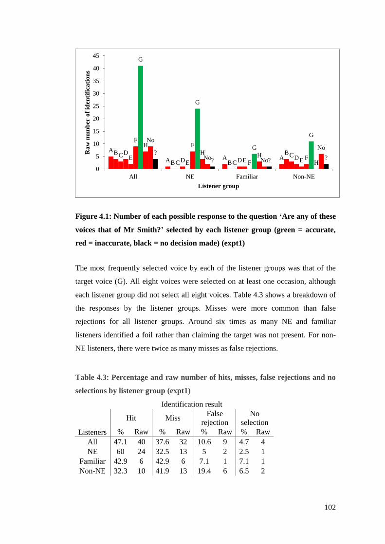
102
Figure 4.1: Number of each possible response to the question ‘Are any of these
voices that of Mr Smith?’ selected by each listener group (green = accurate,
red = inaccurate, black = no decision made) (expt1)
The most frequently selected voice by each of the listener groups was that of the
target voice (G). All eight voices were selected on at least one occasion, although
each listener group did not select all eight voices. Table 4.3 shows a breakdown of
the responses by the listener groups. Misses were more common than false
rejections for all listener groups. Around six times as many NE and familiar
listeners identified a foil rather than claiming the target was not present. For non-
NE listeners, there were twice as many misses as false rejections.
Table 4.3: Percentage and raw number of hits, misses, false rejections and no
selections by listener group (expt1)
Identification result
Hit Miss False
rejection
No
selection
Listeners % Raw % Raw % Raw % Raw
All 47.1 40 37.6 32 10.6 9 4.7 4
NE 60 24 32.5 13 5 2 2.5 1
Familiar 42.9 6 42.9 6 7.1 1 7.1 1
Non-NE 32.3 10 41.9 13 19.4 6 6.5 2
A
A A AB
B B
BC
C C
CD
D D DEE E E
FF
FF
G
G
G
G
H
H H
H
No
No No
No?
? ? ?
0
5
10
15
20
25
30
35
40
45
All NE Familiar Non-NE
Ra
w n
um
ber
of
iden
tifi
cati
on
s
Listener group
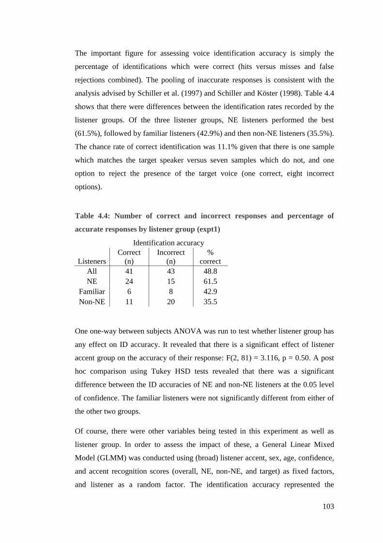
103
The important figure for assessing voice identification accuracy is simply the
percentage of identifications which were correct (hits versus misses and false
rejections combined). The pooling of inaccurate responses is consistent with the
analysis advised by Schiller et al. (1997) and Schiller and Köster (1998). Table 4.4
shows that there were differences between the identification rates recorded by the
listener groups. Of the three listener groups, NE listeners performed the best
(61.5%), followed by familiar listeners (42.9%) and then non-NE listeners (35.5%).
The chance rate of correct identification was 11.1% given that there is one sample
which matches the target speaker versus seven samples which do not, and one
option to reject the presence of the target voice (one correct, eight incorrect
options).
Table 4.4: Number of correct and incorrect responses and percentage of
accurate responses by listener group (expt1)
Identification accuracy
Listeners
Correct
(n)
Incorrect
(n)
%
correct
All 41 43 48.8
NE 24 15 61.5
Familiar 6 8 42.9
Non-NE 11 20 35.5
One one-way between subjects ANOVA was run to test whether listener group has
any effect on ID accuracy. It revealed that there is a significant effect of listener
accent group on the accuracy of their response: F(2, 81) = 3.116, p = 0.50. A post
hoc comparison using Tukey HSD tests revealed that there was a significant
difference between the ID accuracies of NE and non-NE listeners at the 0.05 level
of confidence. The familiar listeners were not significantly different from either of
the other two groups.
Of course, there were other variables being tested in this experiment as well as
listener group. In order to assess the impact of these, a General Linear Mixed
Model (GLMM) was conducted using (broad) listener accent, sex, age, confidence,
and accent recognition scores (overall, NE, non-NE, and target) as fixed factors,
and listener as a random factor. The identification accuracy represented the
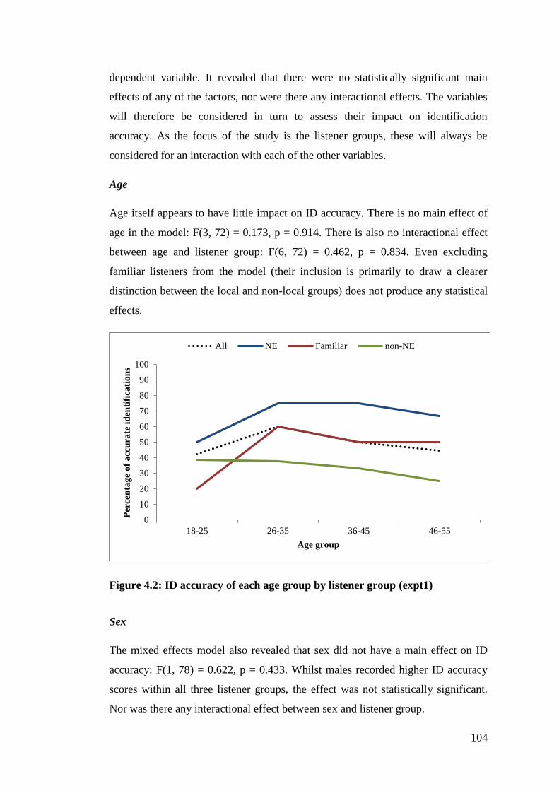
104
dependent variable. It revealed that there were no statistically significant main
effects of any of the factors, nor were there any interactional effects. The variables
will therefore be considered in turn to assess their impact on identification
accuracy. As the focus of the study is the listener groups, these will always be
considered for an interaction with each of the other variables.
Age
Age itself appears to have little impact on ID accuracy. There is no main effect of
age in the model: F(3, 72) = 0.173, p = 0.914. There is also no interactional effect
between age and listener group: F(6, 72) = 0.462, p = 0.834. Even excluding
familiar listeners from the model (their inclusion is primarily to draw a clearer
distinction between the local and non-local groups) does not produce any statistical
effects.
Figure 4.2: ID accuracy of each age group by listener group (expt1)
Sex
The mixed effects model also revealed that sex did not have a main effect on ID
accuracy: F(1, 78) = 0.622, p = 0.433. Whilst males recorded higher ID accuracy
scores within all three listener groups, the effect was not statistically significant.
Nor was there any interactional effect between sex and listener group.
0
10
20
30
40
50
60
70
80
90
100
18-25 26-35 36-45 46-55
Per
cen
tag
e o
f a
ccu
rate
id
enti
fica
tio
ns
Age group
All NE Familiar non-NE
105
Figure 4.3: ID accuracy of males and females by listener group (expt1)
Confidence
The mean confidence ratings are shown in Figure 4.4 for each listener group by the
accuracy of each listener in the speaker ID task. A GLMM using confidence and
listener group as fixed effects reveals that confidence was not a main effect (though
it is approaching significance): F(4, 70) = 2.476, p = 0.052. There is no
interactional effect between confidence and listener group: F(7, 70) = 0.669, p =
0.698. Confidence, then is a weak predictor of ID accuracy across listener groups.
For each of the three listener groups confidence ratings were higher amongst those
listeners who made an accurate identification. The difference was biggest for NE
listeners (2.92 -2.13) and similar for familiar and non-NE listeners.
0
10
20
30
40
50
60
70
80
90
100
Male Female
Per
cen
tag
e o
f co
rrec
t id
enti
fica
tio
ns
Sex
All NE Familiar Non-NE
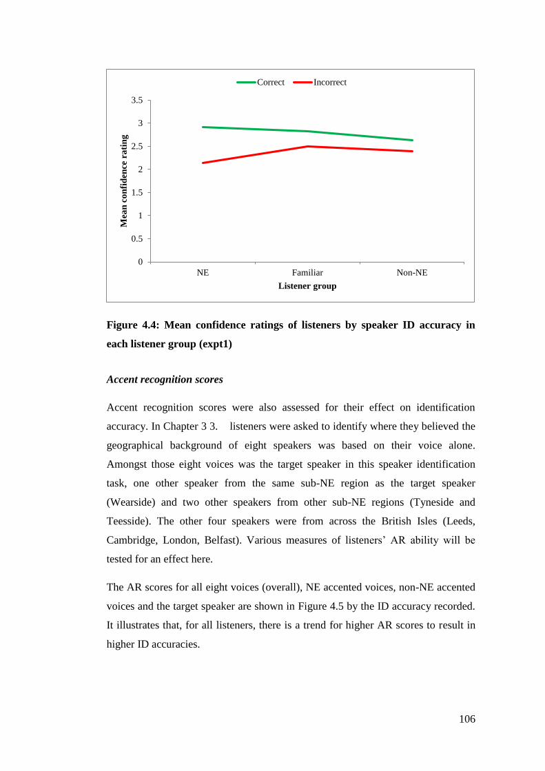
106
Figure 4.4: Mean confidence ratings of listeners by speaker ID accuracy in
each listener group (expt1)
Accent recognition scores
Accent recognition scores were also assessed for their effect on identification
accuracy. In Chapter 3 3. listeners were asked to identify where they believed the
geographical background of eight speakers was based on their voice alone.
Amongst those eight voices was the target speaker in this speaker identification
task, one other speaker from the same sub-NE region as the target speaker
(Wearside) and two other speakers from other sub-NE regions (Tyneside and
Teesside). The other four speakers were from across the British Isles (Leeds,
Cambridge, London, Belfast). Various measures of listeners’ AR ability will be
tested for an effect here.
The AR scores for all eight voices (overall), NE accented voices, non-NE accented
voices and the target speaker are shown in Figure 4.5 by the ID accuracy recorded.
It illustrates that, for all listeners, there is a trend for higher AR scores to result in
higher ID accuracies.
0
0.5
1
1.5
2
2.5
3
3.5
NE Familiar Non-NE
Mea
n c
on
fid
ence
ra
tin
g
Listener group
Correct Incorrect
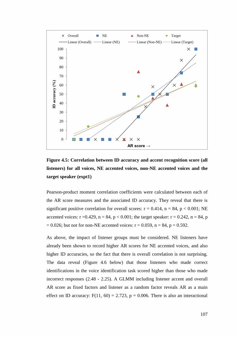
107
Figure 4.5: Correlation between ID accuracy and accent recognition score (all
listeners) for all voices, NE accented voices, non-NE accented voices and the
target speaker (expt1)
Pearson-product moment correlation coefficients were calculated between each of
the AR score measures and the associated ID accuracy. They reveal that there is
significant positive correlation for overall scores: r = 0.414, n = 84, p < 0.001; NE
accented voices: r =0.429, n = 84, p < 0.001; the target speaker: r = 0.242, n = 84, p
= 0.026; but not for non-NE accented voices: r = 0.059, n = 84, p = 0.592.
As above, the impact of listener groups must be considered. NE listeners have
already been shown to record higher AR scores for NE accented voices, and also
higher ID accuracies, so the fact that there is overall correlation is not surprising.
The data reveal (Figure 4.6 below) that those listeners who made correct
identifications in the voice identification task scored higher than those who made
incorrect responses (2.48 - 2.25). A GLMM including listener accent and overall
AR score as fixed factors and listener as a random factor reveals AR as a main
effect on ID accuracy: F(11, 60) = 2.723, p = 0.006. There is also an interactional
0
10
20
30
40
50
60
70
80
90
100ID
acc
ura
cy (
%)
AR score →
Overall NE Non-NE Target
Linear (Overall) Linear (NE) Linear (Non-NE) Linear (Target)
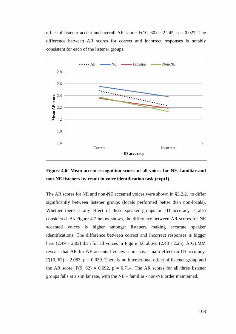
108
effect of listener accent and overall AR score: F(10, 60) = 2.245, p = 0.027. The
difference between AR scores for correct and incorrect responses is notably
consistent for each of the listener groups.
Figure 4.6: Mean accent recognition scores of all voices for NE, familiar and
non-NE listeners by result in voice identification task (expt1)
The AR scores for NE and non-NE accented voices were shown in §3.2.2. to differ
significantly between listener groups (locals performed better than non-locals).
Whether there is any effect of these speaker groups on ID accuracy is also
considered. As Figure 4.7 below shows, the difference between AR scores for NE
accented voices is higher amongst listeners making accurate speaker
identifications. The difference between correct and incorrect responses is bigger
here (2.49 – 2.03) than for all voices in Figure 4.6 above (2.48 - 2.25). A GLMM
reveals that AR for NE accented voices score has a main effect on ID accuracy:
F(10, 62) = 2.083, p = 0.039. There is no interactional effect of listener group and
the AR score: F(9, 62) = 0.692, p = 0.714. The AR scores for all three listener
groups falls at a similar rate, with the NE – familiar - non-NE order maintained.
1.6
1.8
2
2.2
2.4
2.6
2.8
Correct Incorrect
Mea
n A
R s
core
ID accuracy
All NE Familiar Non-NE
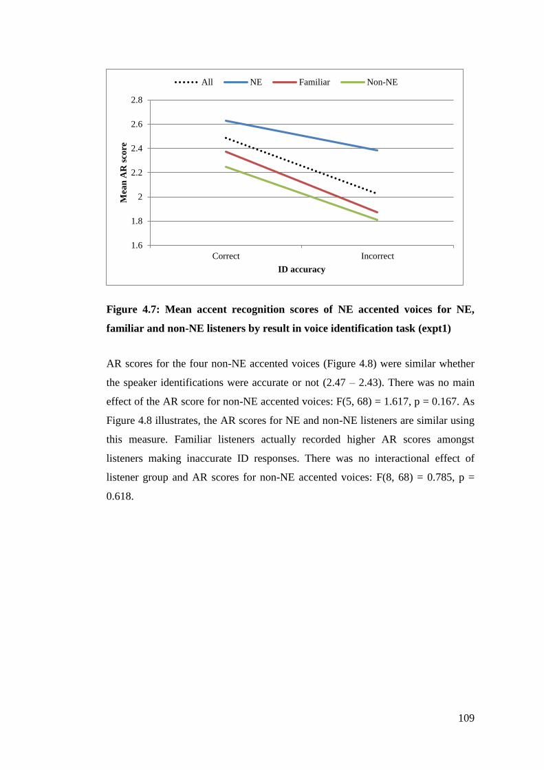
109
Figure 4.7: Mean accent recognition scores of NE accented voices for NE,
familiar and non-NE listeners by result in voice identification task (expt1)
AR scores for the four non-NE accented voices (Figure 4.8) were similar whether
the speaker identifications were accurate or not (2.47 – 2.43). There was no main
effect of the AR score for non-NE accented voices: F(5, 68) = 1.617, p = 0.167. As
Figure 4.8 illustrates, the AR scores for NE and non-NE listeners are similar using
this measure. Familiar listeners actually recorded higher AR scores amongst
listeners making inaccurate ID responses. There was no interactional effect of
listener group and AR scores for non-NE accented voices: F(8, 68) = 0.785, p =
0.618.
1.6
1.8
2
2.2
2.4
2.6
2.8
Correct Incorrect
Mea
n A
R s
core
ID accuracy
All NE Familiar Non-NE
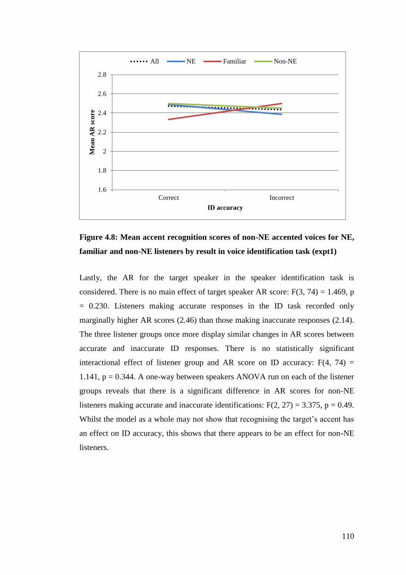
110
Figure 4.8: Mean accent recognition scores of non-NE accented voices for NE,
familiar and non-NE listeners by result in voice identification task (expt1)
Lastly, the AR for the target speaker in the speaker identification task is
considered. There is no main effect of target speaker AR score: F(3, 74) = 1.469, p
= 0.230. Listeners making accurate responses in the ID task recorded only
marginally higher AR scores (2.46) than those making inaccurate responses (2.14).
The three listener groups once more display similar changes in AR scores between
accurate and inaccurate ID responses. There is no statistically significant
interactional effect of listener group and AR score on ID accuracy: F(4, 74) =
1.141, p = 0.344. A one-way between speakers ANOVA run on each of the listener
groups reveals that there is a significant difference in AR scores for non-NE
listeners making accurate and inaccurate identifications: F(2, 27) = 3.375, p = 0.49.
Whilst the model as a whole may not show that recognising the target’s accent has
an effect on ID accuracy, this shows that there appears to be an effect for non-NE
listeners.
1.6
1.8
2
2.2
2.4
2.6
2.8
Correct Incorrect
Mea
n A
R s
core
ID accuracy
All NE Familiar Non-NE
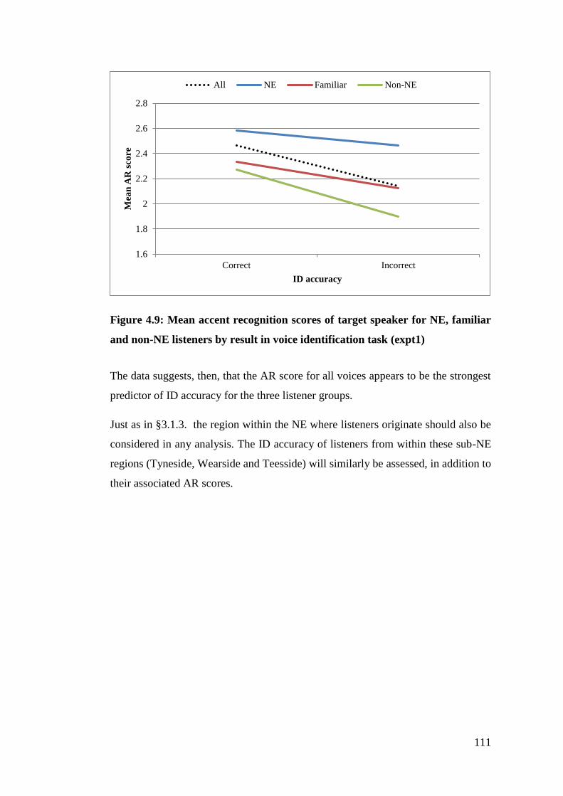
111
Figure 4.9: Mean accent recognition scores of target speaker for NE, familiar
and non-NE listeners by result in voice identification task (expt1)
The data suggests, then, that the AR score for all voices appears to be the strongest
predictor of ID accuracy for the three listener groups.
Just as in §3.1.3. the region within the NE where listeners originate should also be
considered in any analysis. The ID accuracy of listeners from within these sub-NE
regions (Tyneside, Wearside and Teesside) will similarly be assessed, in addition to
their associated AR scores.
1.6
1.8
2
2.2
2.4
2.6
2.8
Correct Incorrect
Mea
n A
R s
core
ID accuracy
All NE Familiar Non-NE
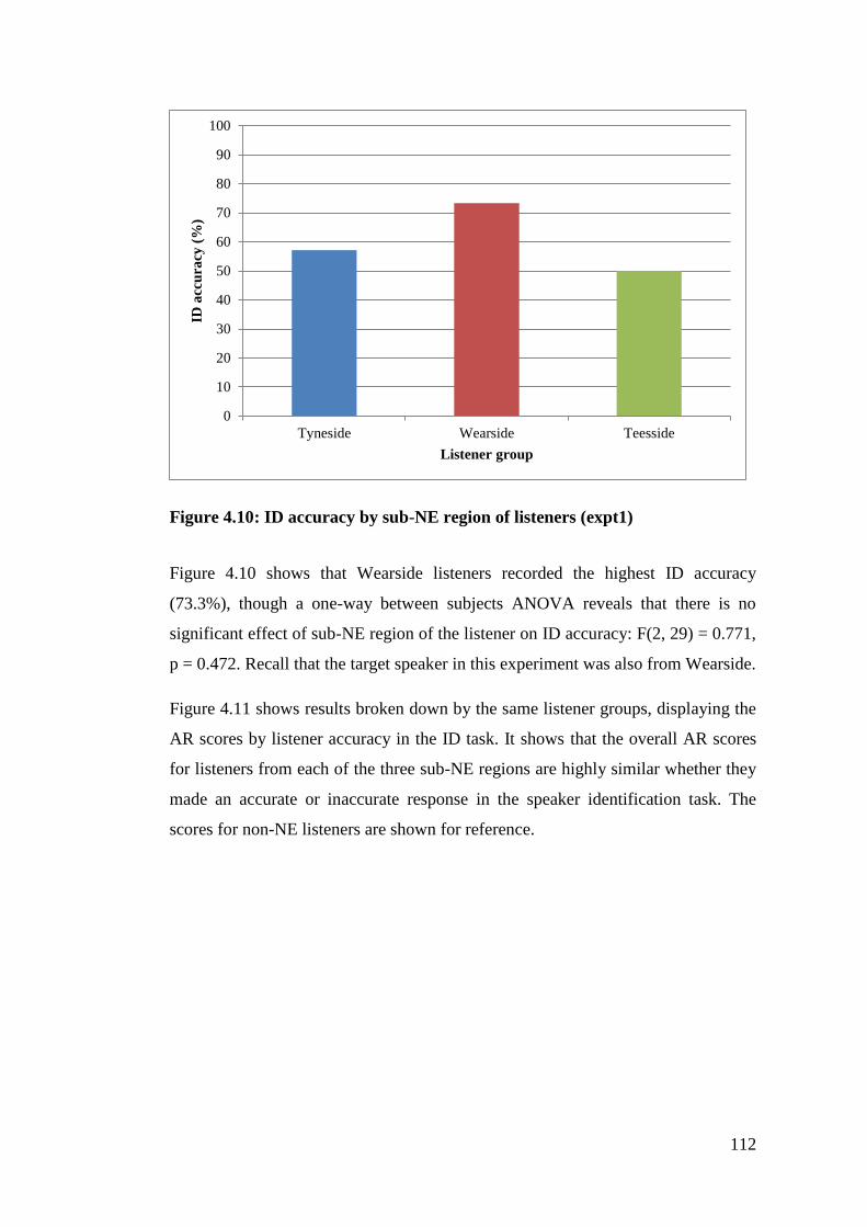
112
Figure 4.10: ID accuracy by sub-NE region of listeners (expt1)
Figure 4.10 shows that Wearside listeners recorded the highest ID accuracy
(73.3%), though a one-way between subjects ANOVA reveals that there is no
significant effect of sub-NE region of the listener on ID accuracy: F(2, 29) = 0.771,
p = 0.472. Recall that the target speaker in this experiment was also from Wearside.
Figure 4.11 shows results broken down by the same listener groups, displaying the
AR scores by listener accuracy in the ID task. It shows that the overall AR scores
for listeners from each of the three sub-NE regions are highly similar whether they
made an accurate or inaccurate response in the speaker identification task. The
scores for non-NE listeners are shown for reference.
0
10
20
30
40
50
60
70
80
90
100
Tyneside Wearside Teesside
ID a
ccu
racy
(%
)
Listener group

113
Figure 4.11: Mean accent recognition scores of all speakers for Tyneside,
Wearside and Teesside listeners by result in voice identification task (expt1)
As above, a GLMM was run using various measures of AR scores and listener
group (here, sub-NE region) as fixed factors, and listener as a random factor. The
identification accuracy represents the dependent variable. The sub-NE will always
be included as fixed effect to test whether the other-accent effect exists as a sib-
regional level. Using overall AR score as a fixed factor reveals it not to be a main
effect: F(8, 21) = 1.485, p = 0.249. There was also no interactional effect of overall
AR score and sub-NE listener group: F(7, 21) = 0.645, p = 0.714.
The AR scores for the four NE accented voices are shown in Figure 4.12 below.
The GLMM reveals that there is no main effect of sub-NE listener group: F(7, 23)
= 1.536, p = 0.205, nor any interactional effect between listener group and AR
score: F (6, 23) = 0.498, p = 0.803.
1.6
1.8
2
2.2
2.4
2.6
2.8
Correct Incorrect
Mea
n A
R s
core
ID accuracy
Tyneside Wearside Teesside Non-NE
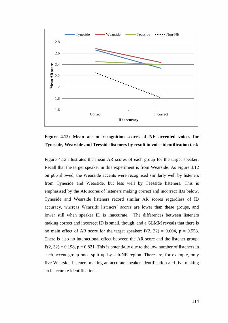
114
Figure 4.12: Mean accent recognition scores of NE accented voices for
Tyneside, Wearside and Teesside listeners by result in voice identification task
Figure 4.13 illustrates the mean AR scores of each group for the target speaker.
Recall that the target speaker in this experiment is from Wearside. As Figure 3.12
on p86 showed, the Wearside accents were recognised similarly well by listeners
from Tyneside and Wearside, but less well by Teesside listeners. This is
emphasised by the AR scores of listeners making correct and incorrect IDs below.
Tyneside and Wearside listeners record similar AR scores regardless of ID
accuracy, whereas Wearside listeners’ scores are lower than these groups, and
lower still when speaker ID is inaccurate. The differences between listeners
making correct and incorrect ID is small, though, and a GLMM reveals that there is
no main effect of AR score for the target speaker: F(2, 32) = 0.604, p = 0.553.
There is also no interactional effect between the AR score and the listener group:
F(2, 32) = 0.198, p = 0.821. This is potentially due to the low number of listeners in
each accent group once split up by sub-NE region. There are, for example, only
five Wearside listeners making an accurate speaker identification and five making
an inaccurate identification.
1.6
1.8
2
2.2
2.4
2.6
2.8
Correct Incorrect
Mea
n A
R s
core
ID accuracy
Tyneside Wearside Teesside Non-NE
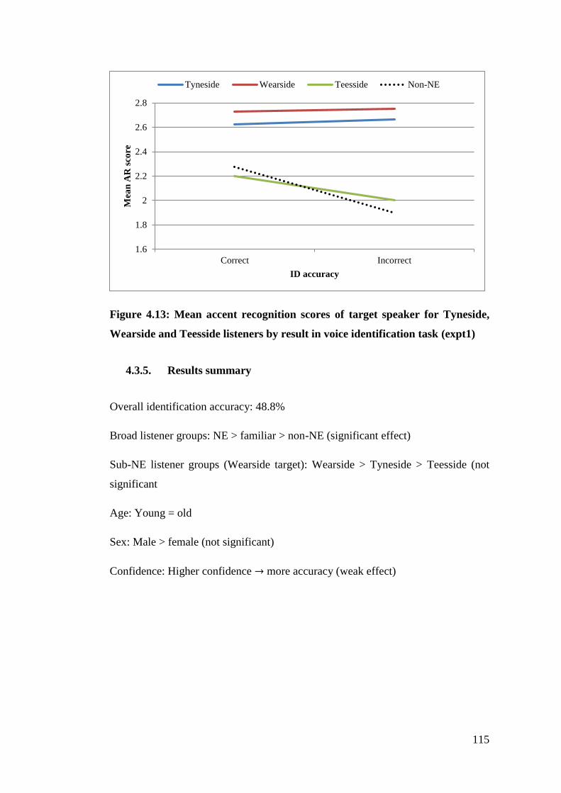
115
Figure 4.13: Mean accent recognition scores of target speaker for Tyneside,
Wearside and Teesside listeners by result in voice identification task (expt1)
4.3.5. Results summary
Overall identification accuracy: 48.8%
Broad listener groups: NE > familiar > non-NE (significant effect)
Sub-NE listener groups (Wearside target): Wearside > Tyneside > Teesside (not
significant
Age: Young = old
Sex: Male > female (not significant)
Confidence: Higher confidence → more accuracy (weak effect)
1.6
1.8
2
2.2
2.4
2.6
2.8
Correct Incorrect
Mea
n A
R s
core
ID accuracy
Tyneside Wearside Teesside Non-NE
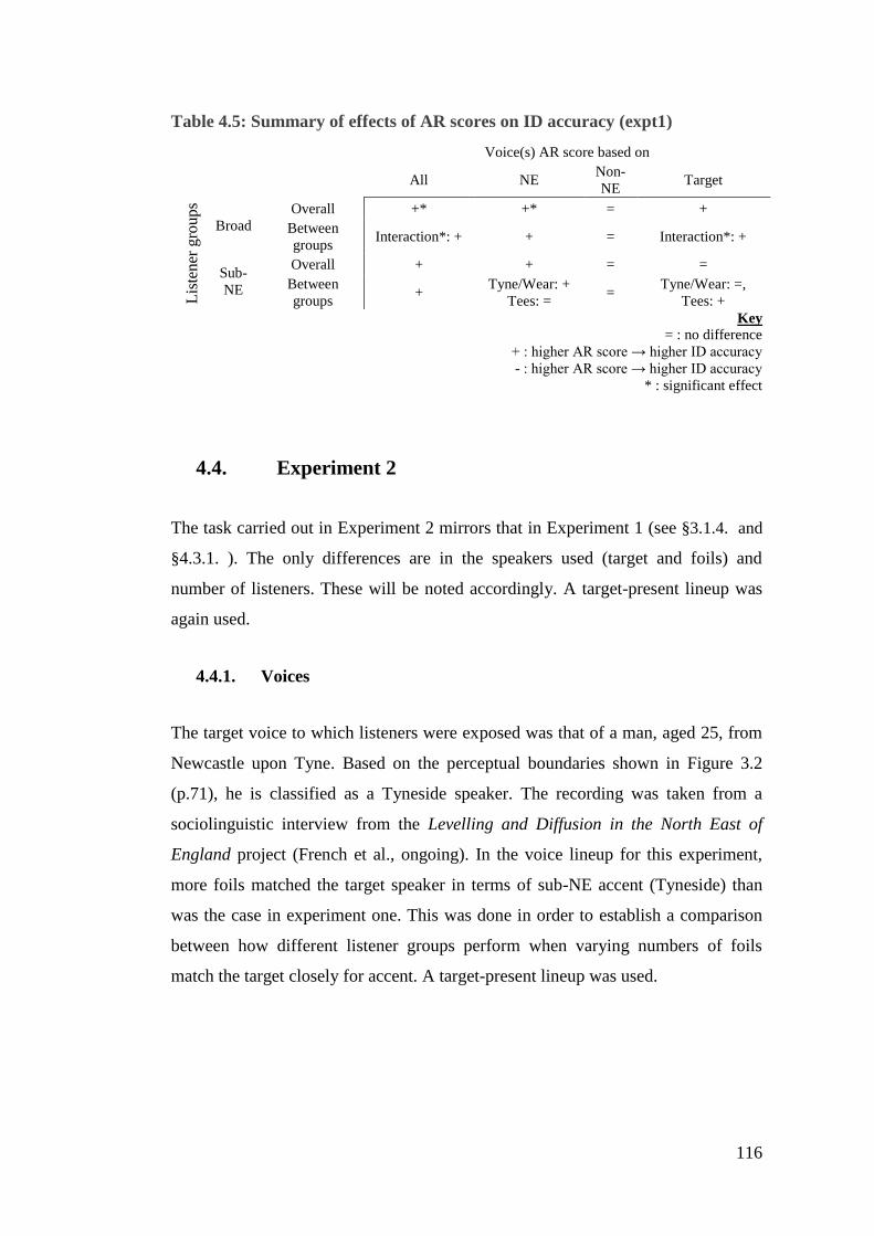
116
Table 4.5: Summary of effects of AR scores on ID accuracy (expt1)
Voice(s) AR score based on
All NE Non-
NE Target
Lis
ten
er g
rou
ps
Broad
Overall +* +* = +
Between
groups Interaction*: + + = Interaction*: +
Sub-
NE
Overall + + = =
Between
groups +
Tyne/Wear: +
Tees: = =
Tyne/Wear: =,
Tees: +
Key
= : no difference
+ : higher AR score → higher ID accuracy
- : higher AR score → higher ID accuracy
* : significant effect
4.4. Experiment 2
The task carried out in Experiment 2 mirrors that in Experiment 1 (see §3.1.4. and
§4.3.1. ). The only differences are in the speakers used (target and foils) and
number of listeners. These will be noted accordingly. A target-present lineup was
again used.
4.4.1. Voices
The target voice to which listeners were exposed was that of a man, aged 25, from
Newcastle upon Tyne. Based on the perceptual boundaries shown in Figure 3.2
(p.71), he is classified as a Tyneside speaker. The recording was taken from a
sociolinguistic interview from the Levelling and Diffusion in the North East of
England project (French et al., ongoing). In the voice lineup for this experiment,
more foils matched the target speaker in terms of sub-NE accent (Tyneside) than
was the case in experiment one. This was done in order to establish a comparison
between how different listener groups perform when varying numbers of foils
match the target closely for accent. A target-present lineup was used.
117
Table 4.6: Speakers in lineup and sub-North East region of origin (expt2)
Target Foils
D A B C E F G H
Tyneside Tyneside Teesside Wearside Tyneside Tyneside Tyneside Wearside
4.4.2. Listeners
A total of 75 listeners took part in experiment two. Listeners were again defined by
their own dialect background and familiarity with the NE region, based on the
criteria outlined in experiment one. The youngest participants were from the 18-25
age range whilst the oldest were aged 46-55 (M = 31.9). 38 males and 37 females
took part. Listeners were first randomly and then pseudo-randomly assigned to
each experimental condition by the experiment in order to provide an even split of
listener variables in each.
Table 4.7: Number of listeners in NE, sub-NE, familiar and non-NE listener
groups (expt2)
4.4.3. Results
The overall rate of correct identification was 41.1%.
Figure 4.14 shows the number of times each speaker was selected by listeners. The
most commonly selected voice by each of the listener groups was that of the target
voice (D). Seven of the eight voices were selected by at least one listener; speaker
G was not selected at all.
NE Familiar Non-NE
12 30
Tyneside Wearside Teesside
13 10 10
75
Overall
33
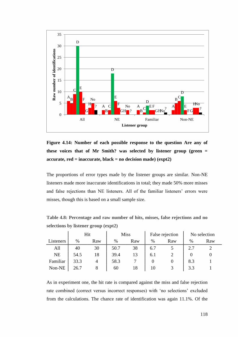
118
Figure 4.14: Number of each possible response to the question Are any of
these voices that of Mr Smith? was selected by listener group (green =
accurate, red = inaccurate, black = no decision made) (expt2)
The proportions of error types made by the listener groups are similar. Non-NE
listeners made more inaccurate identifications in total; they made 50% more misses
and false rejections than NE listeners. All of the familiar listeners’ errors were
misses, though this is based on a small sample size.
Table 4.8: Percentage and raw number of hits, misses, false rejections and no
selections by listener group (expt2)
Hit Miss False rejection No selection
Listeners % Raw % Raw % Raw % Raw
All 40 30 50.7 38 6.7 5 2.7 2
NE 54.5 18 39.4 13 6.1 2 0 0
Familiar 33.3 4 58.3 7 0 0 8.3 1
Non-NE 26.7 8 60 18 10 3 3.3 1
As in experiment one, the hit rate is compared against the miss and false rejection
rate combined (correct versus incorrect responses) with ‘no selections’ excluded
from the calculations. The chance rate of identification was again 11.1%. Of the
A
A A A
B
B B
B
C
CC
C
D
D
D
D
E
E
E E
F
FF
FG G G G
H
H H
H
No
No
No
No?
?? ?
0
5
10
15
20
25
30
35
All NE Familiar Non-NE
Ra
w n
um
ber
of
iden
tifi
cati
on
s
Listener group
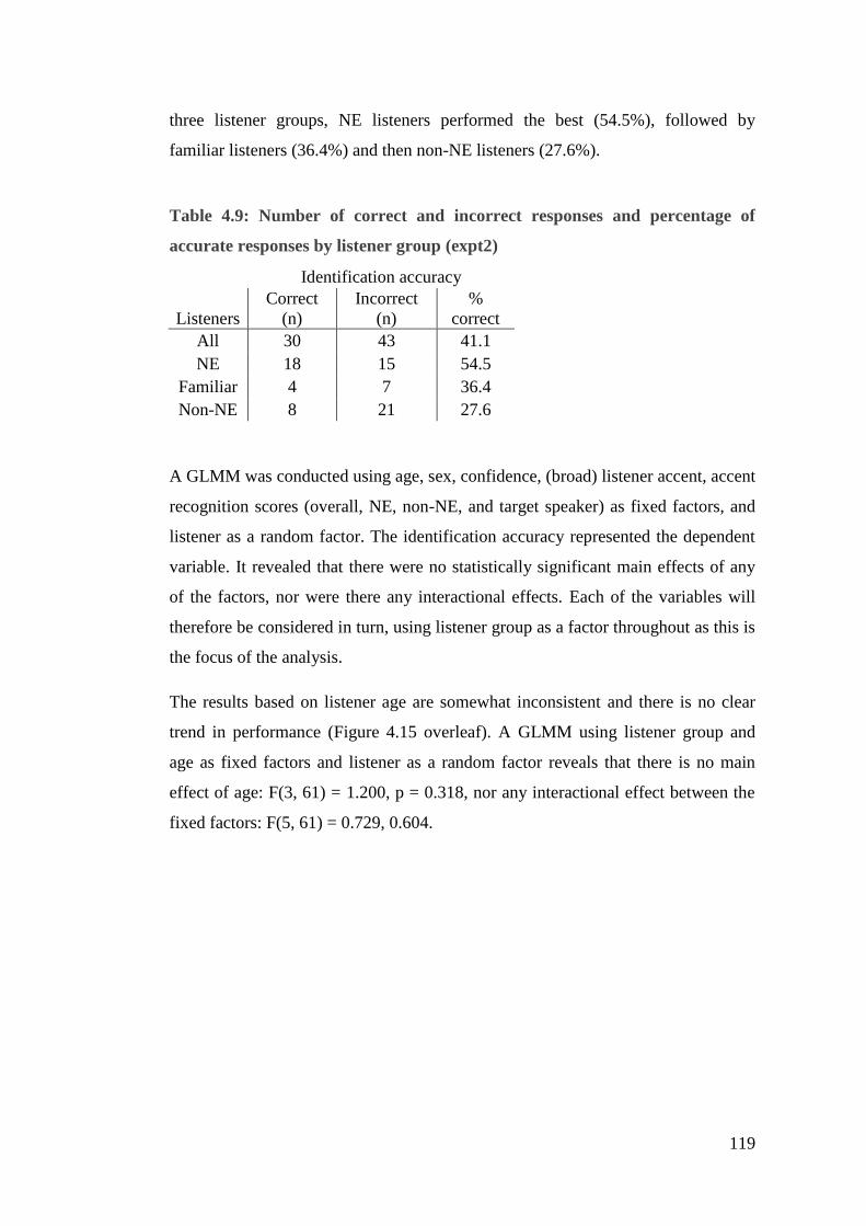
119
three listener groups, NE listeners performed the best (54.5%), followed by
familiar listeners (36.4%) and then non-NE listeners (27.6%).
Table 4.9: Number of correct and incorrect responses and percentage of
accurate responses by listener group (expt2)
Identification accuracy
Listeners
Correct
(n)
Incorrect
(n)
%
correct
All 30 43 41.1
NE 18 15 54.5
Familiar 4 7 36.4
Non-NE 8 21 27.6
A GLMM was conducted using age, sex, confidence, (broad) listener accent, accent
recognition scores (overall, NE, non-NE, and target speaker) as fixed factors, and
listener as a random factor. The identification accuracy represented the dependent
variable. It revealed that there were no statistically significant main effects of any
of the factors, nor were there any interactional effects. Each of the variables will
therefore be considered in turn, using listener group as a factor throughout as this is
the focus of the analysis.
The results based on listener age are somewhat inconsistent and there is no clear
trend in performance (Figure 4.15 overleaf). A GLMM using listener group and
age as fixed factors and listener as a random factor reveals that there is no main
effect of age: F(3, 61) = 1.200, p = 0.318, nor any interactional effect between the
fixed factors: F(5, 61) = 0.729, 0.604.
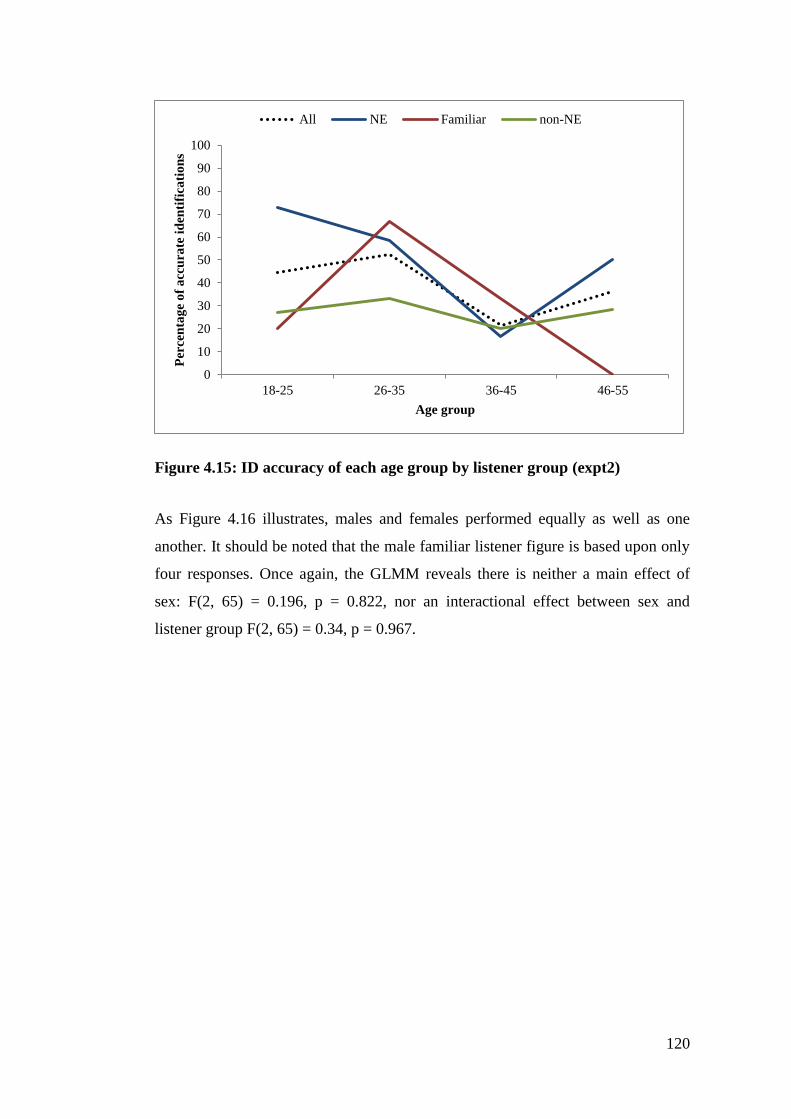
120
Figure 4.15: ID accuracy of each age group by listener group (expt2)
As Figure 4.16 illustrates, males and females performed equally as well as one
another. It should be noted that the male familiar listener figure is based upon only
four responses. Once again, the GLMM reveals there is neither a main effect of
sex: F(2, 65) = 0.196, p = 0.822, nor an interactional effect between sex and
listener group F(2, 65) = 0.34, p = 0.967.
0
10
20
30
40
50
60
70
80
90
100
18-25 26-35 36-45 46-55
Per
cen
tag
e o
f a
ccu
rate
id
enti
fica
tio
ns
Age group
All NE Familiar non-NE
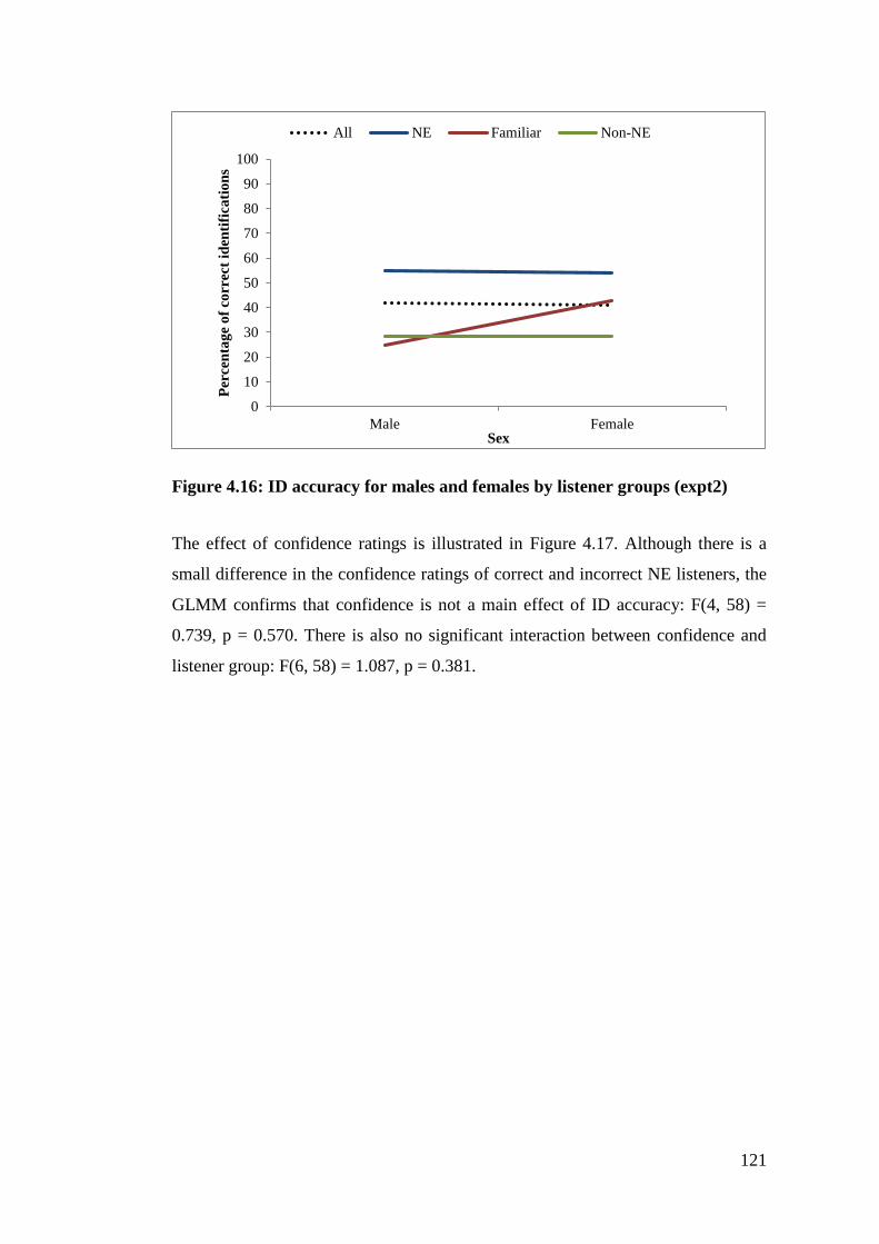
121
Figure 4.16: ID accuracy for males and females by listener groups (expt2)
The effect of confidence ratings is illustrated in Figure 4.17. Although there is a
small difference in the confidence ratings of correct and incorrect NE listeners, the
GLMM confirms that confidence is not a main effect of ID accuracy: F(4, 58) =
0.739, p = 0.570. There is also no significant interaction between confidence and
listener group: F(6, 58) = 1.087, p = 0.381.
0
10
20
30
40
50
60
70
80
90
100
Male Female
Per
cen
tag
e o
f co
rrec
t id
enti
fica
tio
ns
Sex
All NE Familiar Non-NE
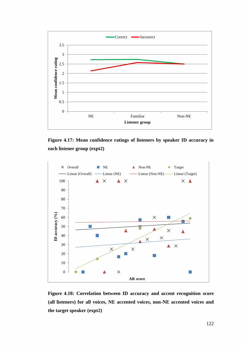
122
Figure 4.17: Mean confidence ratings of listeners by speaker ID accuracy in
each listener group (expt2)
Figure 4.18: Correlation between ID accuracy and accent recognition score
(all listeners) for all voices, NE accented voices, non-NE accented voices and
the target speaker (expt2)
0
0.5
1
1.5
2
2.5
3
3.5
NE Familiar Non-NE
Mea
n c
on
fid
ence
ra
tin
g
Listener group
Correct Incorrect
0
10
20
30
40
50
60
70
80
90
100
ID a
ccu
racy
(%
)
AR score
Overall NE Non-NE Target
Linear (Overall) Linear (NE) Linear (Non-NE) Linear (Target)
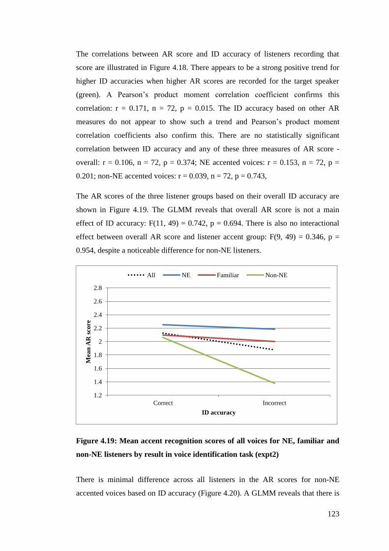
123
The correlations between AR score and ID accuracy of listeners recording that
score are illustrated in Figure 4.18. There appears to be a strong positive trend for
higher ID accuracies when higher AR scores are recorded for the target speaker
(green). A Pearson’s product moment correlation coefficient confirms this
correlation: r = 0.171, n = 72, p = 0.015. The ID accuracy based on other AR
measures do not appear to show such a trend and Pearson’s product moment
correlation coefficients also confirm this. There are no statistically significant
correlation between ID accuracy and any of these three measures of AR score -
overall: r = 0.106, n = 72, p = 0.374; NE accented voices: r = 0.153, n = 72, p =
0.201; non-NE accented voices: r = 0.039, n = 72, p = 0.743,
The AR scores of the three listener groups based on their overall ID accuracy are
shown in Figure 4.19. The GLMM reveals that overall AR score is not a main
effect of ID accuracy: F(11, 49) = 0.742, p = 0.694. There is also no interactional
effect between overall AR score and listener accent group: F(9, 49) = 0.346, p =
0.954, despite a noticeable difference for non-NE listeners.
Figure 4.19: Mean accent recognition scores of all voices for NE, familiar and
non-NE listeners by result in voice identification task (expt2)
There is minimal difference across all listeners in the AR scores for non-NE
accented voices based on ID accuracy (Figure 4.20). A GLMM reveals that there is
1.2
1.4
1.6
1.8
2
2.2
2.4
2.6
2.8
Correct Incorrect
Mea
n A
R s
core
ID accuracy
All NE Familiar Non-NE
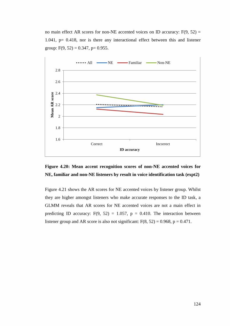
124
no main effect AR scores for non-NE accented voices on ID accuracy: F(9, 52) =
1.041, p= 0.418, nor is there any interactional effect between this and listener
group: F(9, 52) = 0.347, p= 0.955.
Figure 4.20: Mean accent recognition scores of non-NE accented voices for
NE, familiar and non-NE listeners by result in voice identification task (expt2)
Figure 4.21 shows the AR scores for NE accented voices by listener group. Whilst
they are higher amongst listeners who make accurate responses to the ID task, a
GLMM reveals that AR scores for NE accented voices are not a main effect in
predicting ID accuracy: F(9, 52) = 1.057, p = 0.410. The interaction between
listener group and AR score is also not significant: F(8, 52) = 0.968, p = 0.471.
1.6
1.8
2
2.2
2.4
2.6
2.8
Correct Incorrect
Mea
n A
R s
core
ID accuracy
All NE Familiar Non-NE

125
Figure 4.21: Mean accent recognition scores of NE accented voices for NE,
familiar and non-NE listeners by result in voice identification task (expt2)
Finally for listeners by broad accent group, the AR scores for the target speaker are
shown in Figure 4.22. Once again, however, a GLMM reveals there to be no main
effect of AR score for the target: F(3, 62) = 1.412, p = 0.248. The interactional
effect of AR score and ID accuracy is statistically significant: F(4, 62) = 2.801, p =
0.033. The AR score for accurate IDs is similar for NE, familiar and non-NE
listeners, though there is clear division between the three for inaccurate IDs – the
drop is smallest for NE listeners and largest for non-NE listeners.
1.4
1.6
1.8
2
2.2
2.4
2.6
2.8
Correct Incorrect
Mea
n A
R s
core
ID accuracy
All NE Familiar Non-NE
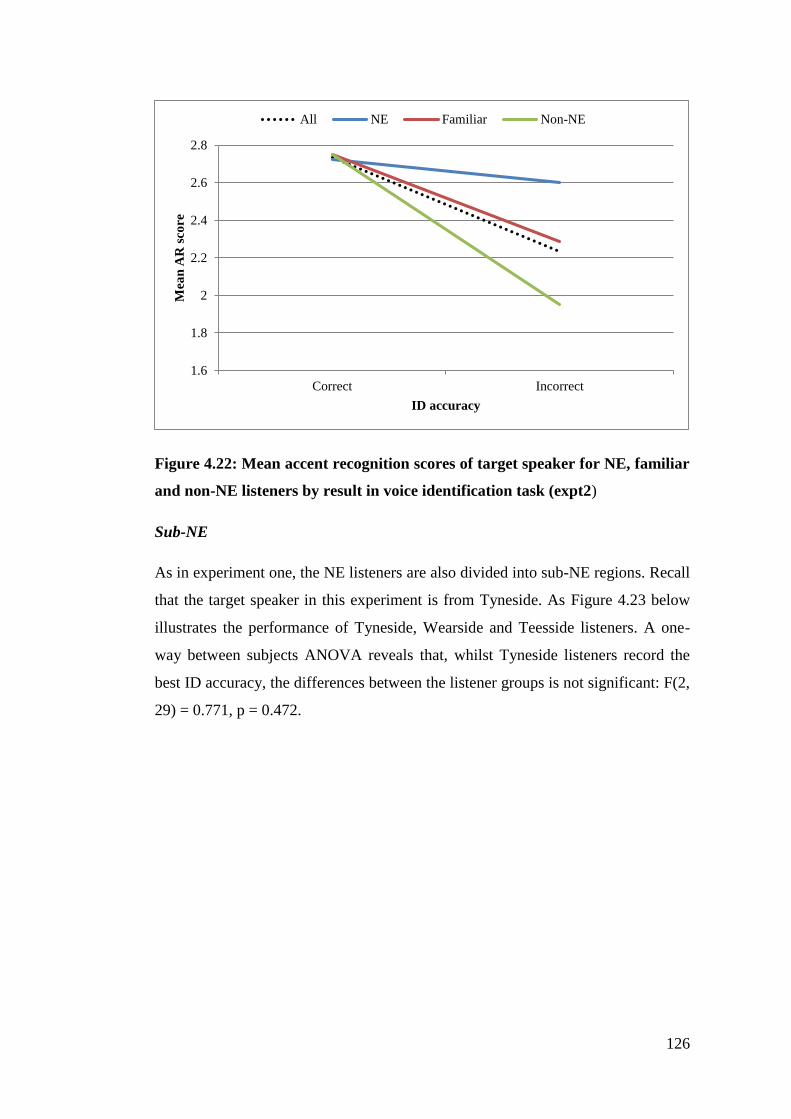
126
Figure 4.22: Mean accent recognition scores of target speaker for NE, familiar
and non-NE listeners by result in voice identification task (expt2)
Sub-NE
As in experiment one, the NE listeners are also divided into sub-NE regions. Recall
that the target speaker in this experiment is from Tyneside. As Figure 4.23 below
illustrates the performance of Tyneside, Wearside and Teesside listeners. A one-
way between subjects ANOVA reveals that, whilst Tyneside listeners record the
best ID accuracy, the differences between the listener groups is not significant: F(2,
29) = 0.771, p = 0.472.
1.6
1.8
2
2.2
2.4
2.6
2.8
Correct Incorrect
Mea
n A
R s
core
ID accuracy
All NE Familiar Non-NE
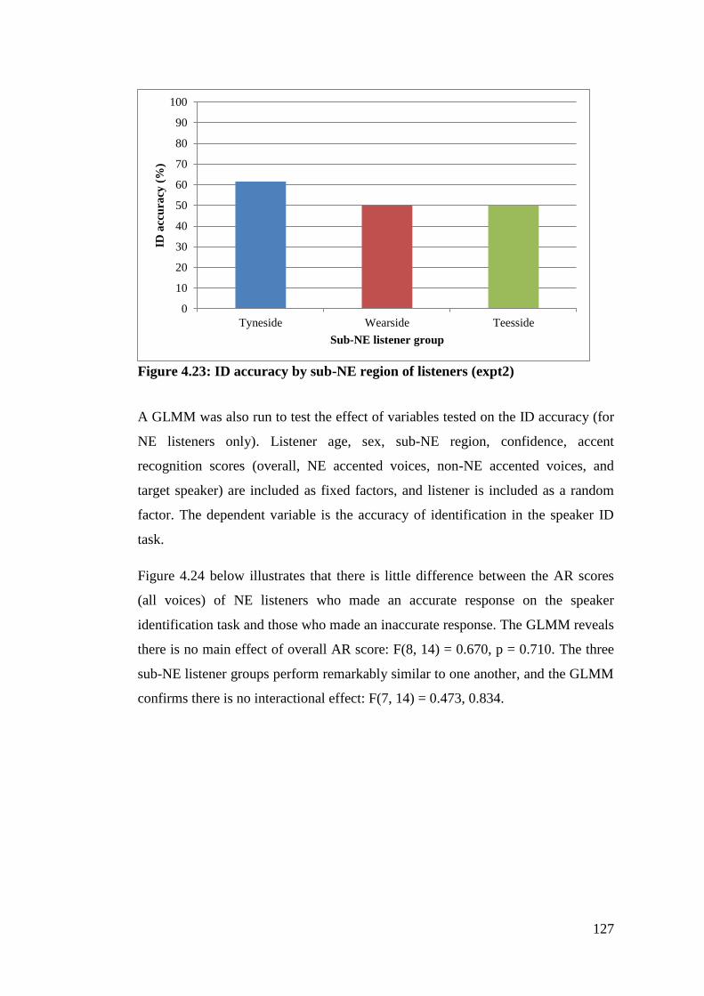
127
Figure 4.23: ID accuracy by sub-NE region of listeners (expt2)
A GLMM was also run to test the effect of variables tested on the ID accuracy (for
NE listeners only). Listener age, sex, sub-NE region, confidence, accent
recognition scores (overall, NE accented voices, non-NE accented voices, and
target speaker) are included as fixed factors, and listener is included as a random
factor. The dependent variable is the accuracy of identification in the speaker ID
task.
Figure 4.24 below illustrates that there is little difference between the AR scores
(all voices) of NE listeners who made an accurate response on the speaker
identification task and those who made an inaccurate response. The GLMM reveals
there is no main effect of overall AR score: F(8, 14) = 0.670, p = 0.710. The three
sub-NE listener groups perform remarkably similar to one another, and the GLMM
confirms there is no interactional effect: F(7, 14) = 0.473, 0.834.
0
10
20
30
40
50
60
70
80
90
100
Tyneside Wearside Teesside
ID a
ccu
racy
(%
)
Sub-NE listener group
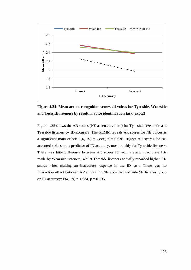
128
Figure 4.24: Mean accent recognition scores all voices for Tyneside, Wearside
and Teesside listeners by result in voice identification task (expt2)
Figure 4.25 shows the AR scores (NE accented voices) for Tyneside, Wearside and
Teesside listeners by ID accuracy. The GLMM reveals AR scores for NE voices as
a significant main effect: F(6, 19) = 2.886, p = 0.036. Higher AR scores for NE
accented voices are a predictor of ID accuracy, most notably for Tyneside listeners.
There was little difference between AR scores for accurate and inaccurate IDs
made by Wearside listeners, whilst Teesside listeners actually recorded higher AR
scores when making an inaccurate response in the ID task. There was no
interaction effect between AR scores for NE accented and sub-NE listener group
on ID accuracy: F(4, 19) = 1.684, p = 0.195.
1.6
1.8
2
2.2
2.4
2.6
2.8
Correct Incorrect
Mea
n A
R s
core
ID accuracy
Tyneside Wearside Teesside Non-NE
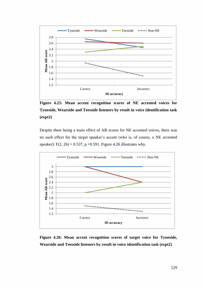
129
Figure 4.25: Mean accent recognition scores of NE accented voices for
Tyneside, Wearside and Teesside listeners by result in voice identification task
(expt2)
Despite there being a main effect of AR scores for NE accented voices, there was
no such effect for the target speaker’s accent (who is, of course, a NE accented
speaker): F(2, 26) = 0.537, p =0.591. Figure 4.26 illustrates why.
Figure 4.26: Mean accent recognition scores of target voice for Tyneside,
Wearside and Teesside listeners by result in voice identification task (expt2)
1.2
1.4
1.6
1.8
2
2.2
2.4
2.6
2.8
Correct Incorrect
Mea
n A
R s
core
ID accuracy
Tyneside Wearside Teesside Non-NE
1.2
1.4
1.6
1.8
2
2.2
2.4
2.6
2.8
3
Correct Incorrect
Mea
n A
R s
core
ID accuracy
Tyneside Wearside Teesside Non-NE
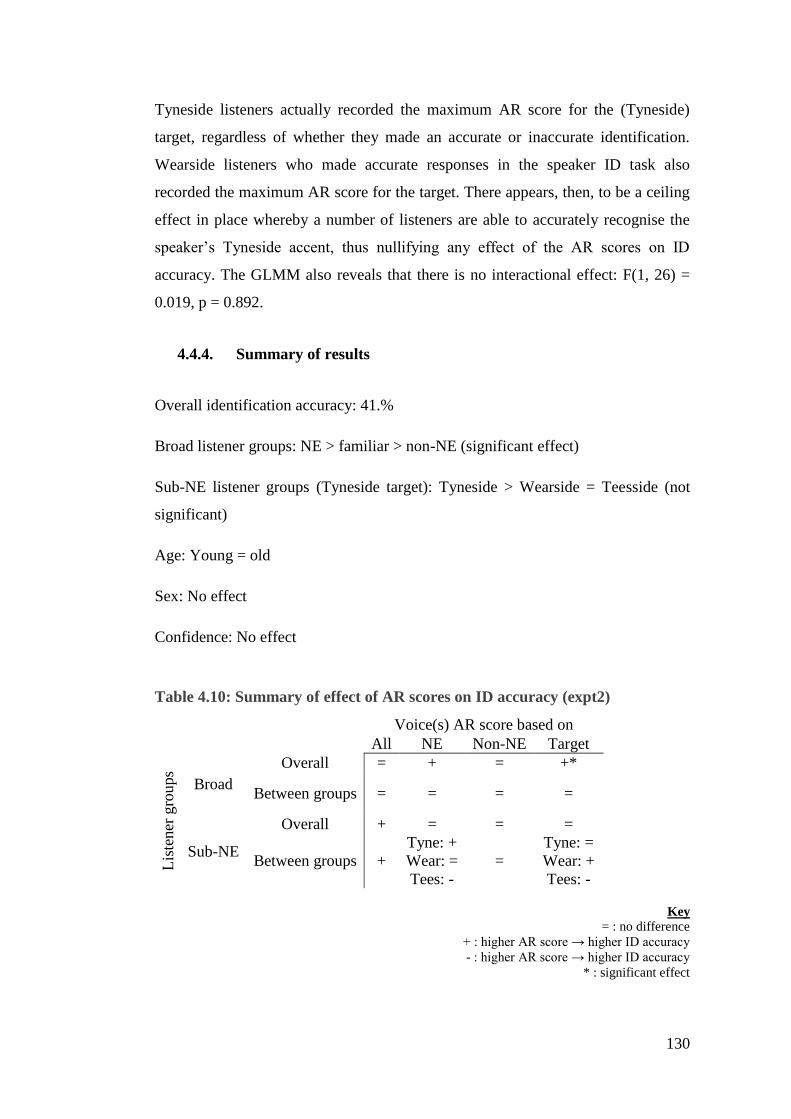
130
Tyneside listeners actually recorded the maximum AR score for the (Tyneside)
target, regardless of whether they made an accurate or inaccurate identification.
Wearside listeners who made accurate responses in the speaker ID task also
recorded the maximum AR score for the target. There appears, then, to be a ceiling
effect in place whereby a number of listeners are able to accurately recognise the
speaker’s Tyneside accent, thus nullifying any effect of the AR scores on ID
accuracy. The GLMM also reveals that there is no interactional effect: F(1, 26) =
0.019, p = 0.892.
4.4.4. Summary of results
Overall identification accuracy: 41.%
Broad listener groups: NE > familiar > non-NE (significant effect)
Sub-NE listener groups (Tyneside target): Tyneside > Wearside = Teesside (not
significant)
Age: Young = old
Sex: No effect
Confidence: No effect
Table 4.10: Summary of effect of AR scores on ID accuracy (expt2)
Voice(s) AR score based on
All NE Non-NE Target
Lis
tener
gro
ups
Broad
Overall = + = +*
Between groups = = = =
Sub-NE
Overall + = = =
Between groups +
Tyne: +
Wear: =
Tees: -
=
Tyne: =
Wear: +
Tees: -
Key
= : no difference
+ : higher AR score → higher ID accuracy
- : higher AR score → higher ID accuracy
* : significant effect
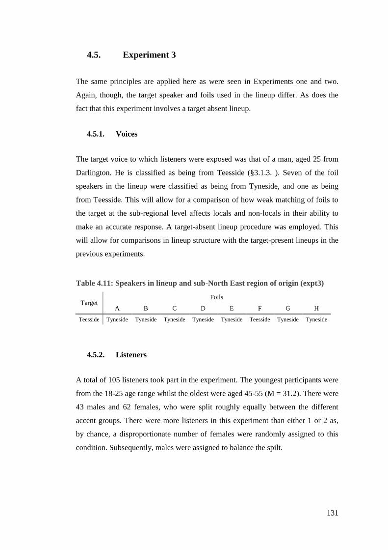
131
4.5. Experiment 3
The same principles are applied here as were seen in Experiments one and two.
Again, though, the target speaker and foils used in the lineup differ. As does the
fact that this experiment involves a target absent lineup.
4.5.1. Voices
The target voice to which listeners were exposed was that of a man, aged 25 from
Darlington. He is classified as being from Teesside (§3.1.3. ). Seven of the foil
speakers in the lineup were classified as being from Tyneside, and one as being
from Teesside. This will allow for a comparison of how weak matching of foils to
the target at the sub-regional level affects locals and non-locals in their ability to
make an accurate response. A target-absent lineup procedure was employed. This
will allow for comparisons in lineup structure with the target-present lineups in the
previous experiments.
Table 4.11: Speakers in lineup and sub-North East region of origin (expt3)
Target Foils
A B C D E F G H
Teesside Tyneside Tyneside Tyneside Tyneside Tyneside Teesside Tyneside Tyneside
4.5.2. Listeners
A total of 105 listeners took part in the experiment. The youngest participants were
from the 18-25 age range whilst the oldest were aged 45-55 (M = 31.2). There were
43 males and 62 females, who were split roughly equally between the different
accent groups. There were more listeners in this experiment than either 1 or 2 as,
by chance, a disproportionate number of females were randomly assigned to this
condition. Subsequently, males were assigned to balance the spilt.
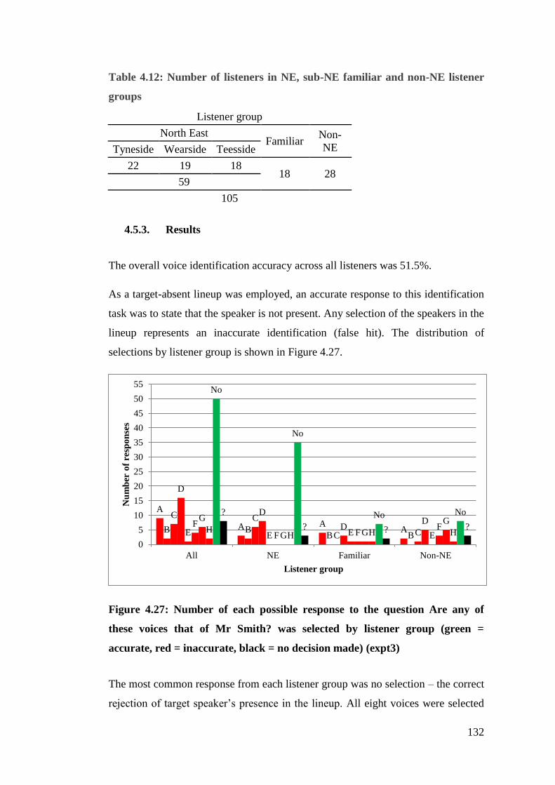
132
Table 4.12: Number of listeners in NE, sub-NE familiar and non-NE listener
groups
Listener group
North East Familiar
Non-
NE Tyneside Wearside Teesside
22 19 18 18 28
59
105
4.5.3. Results
The overall voice identification accuracy across all listeners was 51.5%.
As a target-absent lineup was employed, an accurate response to this identification
task was to state that the speaker is not present. Any selection of the speakers in the
lineup represents an inaccurate identification (false hit). The distribution of
selections by listener group is shown in Figure 4.27.
Figure 4.27: Number of each possible response to the question Are any of
these voices that of Mr Smith? was selected by listener group (green =
accurate, red = inaccurate, black = no decision made) (expt3)
The most common response from each listener group was no selection – the correct
rejection of target speaker’s presence in the lineup. All eight voices were selected
A
A AAB B
B B
C C
C C
D
D
DD
E E E E
F
F FF
G
G G
GH
H H H
No
No
No No?
? ? ?
0
5
10
15
20
25
30
35
40
45
50
55
All NE Familiar Non-NE
Nu
mb
er o
f re
spo
nse
s
Listener group
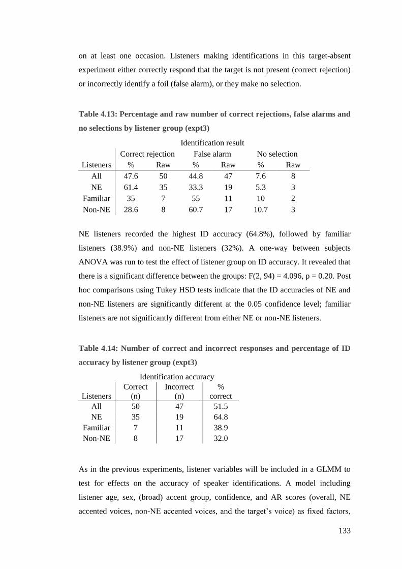
133
on at least one occasion. Listeners making identifications in this target-absent
experiment either correctly respond that the target is not present (correct rejection)
or incorrectly identify a foil (false alarm), or they make no selection.
Table 4.13: Percentage and raw number of correct rejections, false alarms and
no selections by listener group (expt3)
Identification result
Correct rejection False alarm No selection
Listeners % Raw % Raw % Raw
All 47.6 50 44.8 47 7.6 8
NE 61.4 35 33.3 19 5.3 3
Familiar 35 7 55 11 10 2
Non-NE 28.6 8 60.7 17 10.7 3
NE listeners recorded the highest ID accuracy (64.8%), followed by familiar
listeners (38.9%) and non-NE listeners (32%). A one-way between subjects
ANOVA was run to test the effect of listener group on ID accuracy. It revealed that
there is a significant difference between the groups: F(2, 94) = 4.096, p = 0.20. Post
hoc comparisons using Tukey HSD tests indicate that the ID accuracies of NE and
non-NE listeners are significantly different at the 0.05 confidence level; familiar
listeners are not significantly different from either NE or non-NE listeners.
Table 4.14: Number of correct and incorrect responses and percentage of ID
accuracy by listener group (expt3)
Identification accuracy
Listeners
Correct
(n)
Incorrect
(n)
%
correct
All 50 47 51.5
NE 35 19 64.8
Familiar 7 11 38.9
Non-NE 8 17 32.0
As in the previous experiments, listener variables will be included in a GLMM to
test for effects on the accuracy of speaker identifications. A model including
listener age, sex, (broad) accent group, confidence, and AR scores (overall, NE
accented voices, non-NE accented voices, and the target’s voice) as fixed factors,

134
and listener as a random factor is run. It reveals that there are no main or
interactional effects in the model. The contribution of each factor to the model will
thus be assessed.
The GLMM reveals that there is no main effect of age on ID ability: F(3,85) =
0.209, p = 0.890, nor is there any interactional effect between age and listener
group: F(6,85) = 0.359, p = 0.903. Although there is an overall steady decline in
the ID accuracy as listeners get older, the effect is not significant.
Figure 4.28: ID accuracy for each age group by listener group (expt3)
There is very little difference in the ID accuracy of males and females. Males in
both the NE and non-NE groups recorded a marginally better accuracy than
females. The difference was in the same direction, but bigger amongst familiar
listeners (twice as many males making accurate identifications as females). The
GLMM confirms that there is no significant effect of listener sex on ID accuracy,
either as a main effect: F(1, 91) = 0.577, p = 0.499, or as an interactional effect
with listener group: F(2, 91) = 0.250, p = 0.779.
0
10
20
30
40
50
60
70
80
90
100
18-25 26-35 36-45 46-55
Per
cen
tag
e o
f a
ccu
rate
id
enti
fica
tio
ns
Age group
All NE Familiar non-NE
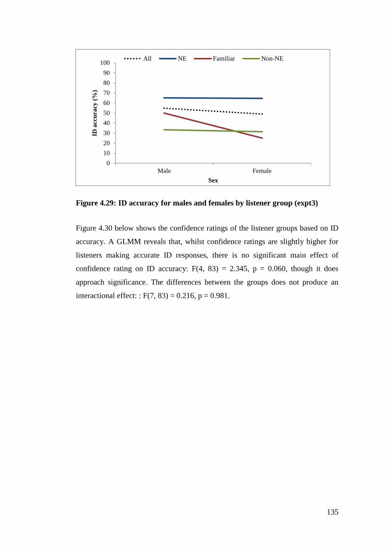
135
Figure 4.29: ID accuracy for males and females by listener group (expt3)
Figure 4.30 below shows the confidence ratings of the listener groups based on ID
accuracy. A GLMM reveals that, whilst confidence ratings are slightly higher for
listeners making accurate ID responses, there is no significant main effect of
confidence rating on ID accuracy: F(4, 83) = 2.345, p = 0.060, though it does
approach significance. The differences between the groups does not produce an
interactional effect: : F(7, 83) = 0.216, p = 0.981.
0
10
20
30
40
50
60
70
80
90
100
Male Female
ID a
ccu
racy
(%
)
Sex
All NE Familiar Non-NE
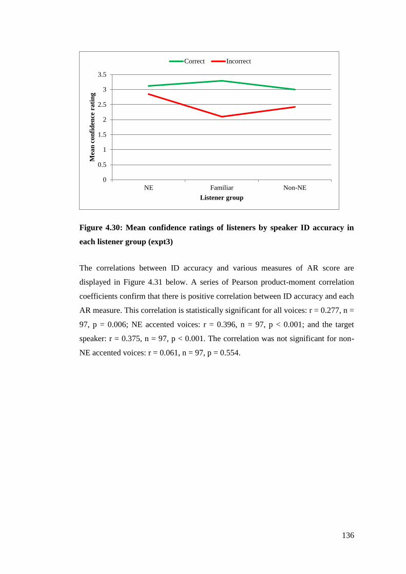
136
Figure 4.30: Mean confidence ratings of listeners by speaker ID accuracy in
each listener group (expt3)
The correlations between ID accuracy and various measures of AR score are
displayed in Figure 4.31 below. A series of Pearson product-moment correlation
coefficients confirm that there is positive correlation between ID accuracy and each
AR measure. This correlation is statistically significant for all voices: r = 0.277, n =
97, p = 0.006; NE accented voices: r = 0.396, n = 97, p < 0.001; and the target
speaker: r = 0.375, n = 97, p < 0.001. The correlation was not significant for non-
NE accented voices: r = 0.061, n = 97, p = 0.554.
0
0.5
1
1.5
2
2.5
3
3.5
NE Familiar Non-NE
Mea
n c
on
fid
ence
ra
tin
g
Listener group
Correct Incorrect
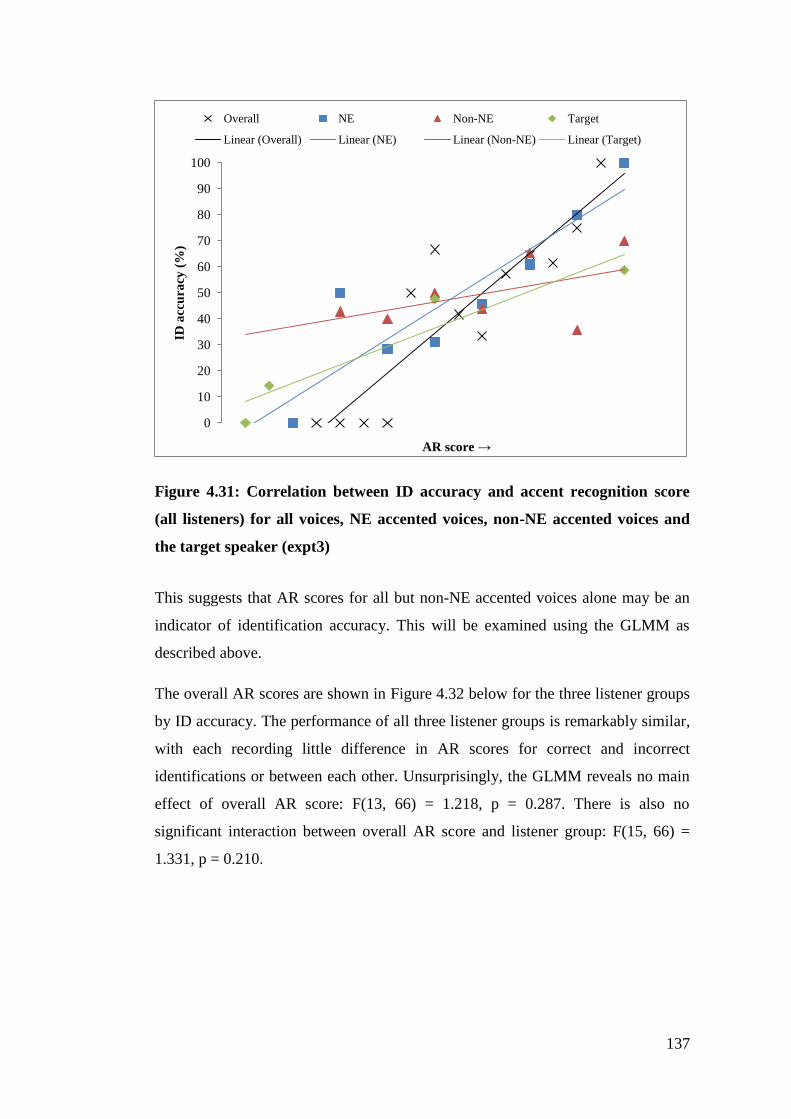
137
Figure 4.31: Correlation between ID accuracy and accent recognition score
(all listeners) for all voices, NE accented voices, non-NE accented voices and
the target speaker (expt3)
This suggests that AR scores for all but non-NE accented voices alone may be an
indicator of identification accuracy. This will be examined using the GLMM as
described above.
The overall AR scores are shown in Figure 4.32 below for the three listener groups
by ID accuracy. The performance of all three listener groups is remarkably similar,
with each recording little difference in AR scores for correct and incorrect
identifications or between each other. Unsurprisingly, the GLMM reveals no main
effect of overall AR score: F(13, 66) = 1.218, p = 0.287. There is also no
significant interaction between overall AR score and listener group: F(15, 66) =
1.331, p = 0.210.
0
10
20
30
40
50
60
70
80
90
100ID
acc
ura
cy (
%)
AR score →
Overall NE Non-NE Target
Linear (Overall) Linear (NE) Linear (Non-NE) Linear (Target)
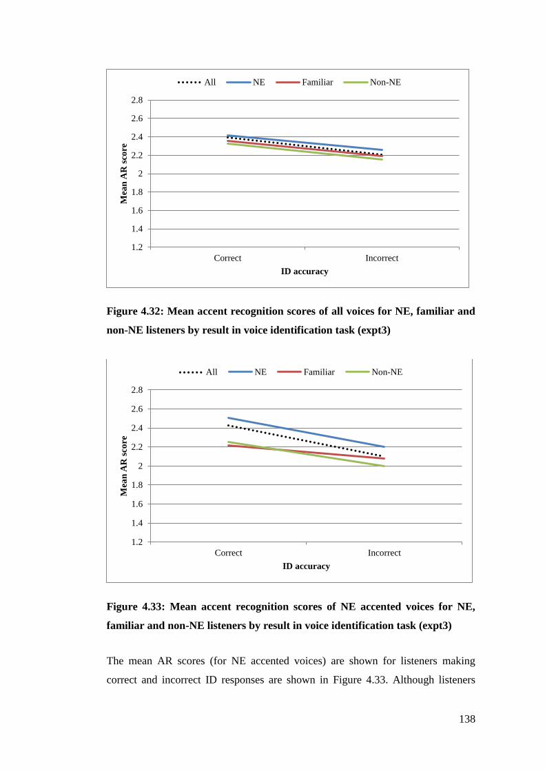
138
Figure 4.32: Mean accent recognition scores of all voices for NE, familiar and
non-NE listeners by result in voice identification task (expt3)
Figure 4.33: Mean accent recognition scores of NE accented voices for NE,
familiar and non-NE listeners by result in voice identification task (expt3)
The mean AR scores (for NE accented voices) are shown for listeners making
correct and incorrect ID responses are shown in Figure 4.33. Although listeners
1.2
1.4
1.6
1.8
2
2.2
2.4
2.6
2.8
Correct Incorrect
Mea
n A
R s
core
ID accuracy
All NE Familiar Non-NE
1.2
1.4
1.6
1.8
2
2.2
2.4
2.6
2.8
Correct Incorrect
Mea
n A
R s
core
ID accuracy
All NE Familiar Non-NE
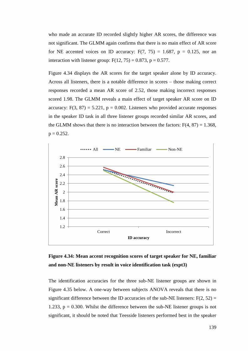
139
who made an accurate ID recorded slightly higher AR scores, the difference was
not significant. The GLMM again confirms that there is no main effect of AR score
for NE accented voices on ID accuracy: F(7, 75) = 1.687, p = 0.125, nor an
interaction with listener group: F(12, 75) = 0.873, p = 0.577.
Figure 4.34 displays the AR scores for the target speaker alone by ID accuracy.
Across all listeners, there is a notable difference in scores – those making correct
responses recorded a mean AR score of 2.52, those making incorrect responses
scored 1.98. The GLMM reveals a main effect of target speaker AR score on ID
accuracy: F(3, 87) = 5.221, p = 0.002. Listeners who provided accurate responses
in the speaker ID task in all three listener groups recorded similar AR scores, and
the GLMM shows that there is no interaction between the factors: F(4, 87) = 1.368,
p = 0.252.
Figure 4.34: Mean accent recognition scores of target speaker for NE, familiar
and non-NE listeners by result in voice identification task (expt3)
The identification accuracies for the three sub-NE listener groups are shown in
Figure 4.35 below. A one-way between subjects ANOVA reveals that there is no
significant difference between the ID accuracies of the sub-NE listeners: F(2, 52) =
1.233, p = 0.300. Whilst the difference between the sub-NE listener groups is not
significant, it should be noted that Teesside listeners performed best in the speaker
1.2
1.4
1.6
1.8
2
2.2
2.4
2.6
2.8
Correct Incorrect
Mea
n A
R s
core
ID accuracy
All NE Familiar Non-NE
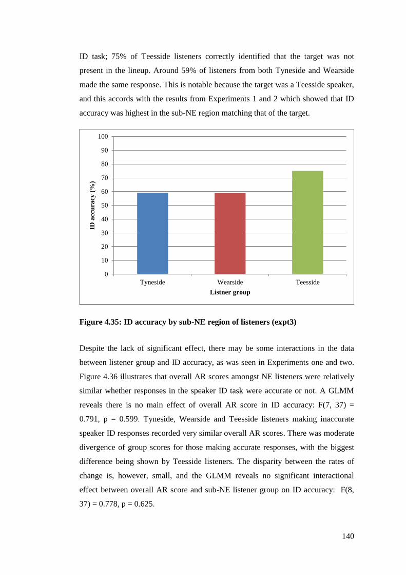
140
ID task; 75% of Teesside listeners correctly identified that the target was not
present in the lineup. Around 59% of listeners from both Tyneside and Wearside
made the same response. This is notable because the target was a Teesside speaker,
and this accords with the results from Experiments 1 and 2 which showed that ID
accuracy was highest in the sub-NE region matching that of the target.
Figure 4.35: ID accuracy by sub-NE region of listeners (expt3)
Despite the lack of significant effect, there may be some interactions in the data
between listener group and ID accuracy, as was seen in Experiments one and two.
Figure 4.36 illustrates that overall AR scores amongst NE listeners were relatively
similar whether responses in the speaker ID task were accurate or not. A GLMM
reveals there is no main effect of overall AR score in ID accuracy: F(7, 37) =
0.791, p = 0.599. Tyneside, Wearside and Teesside listeners making inaccurate
speaker ID responses recorded very similar overall AR scores. There was moderate
divergence of group scores for those making accurate responses, with the biggest
difference being shown by Teesside listeners. The disparity between the rates of
change is, however, small, and the GLMM reveals no significant interactional
effect between overall AR score and sub-NE listener group on ID accuracy: F(8,
37) = 0.778, p = 0.625.
0
10
20
30
40
50
60
70
80
90
100
Tyneside Wearside Teesside
ID a
ccu
racy
(%
)
Listner group
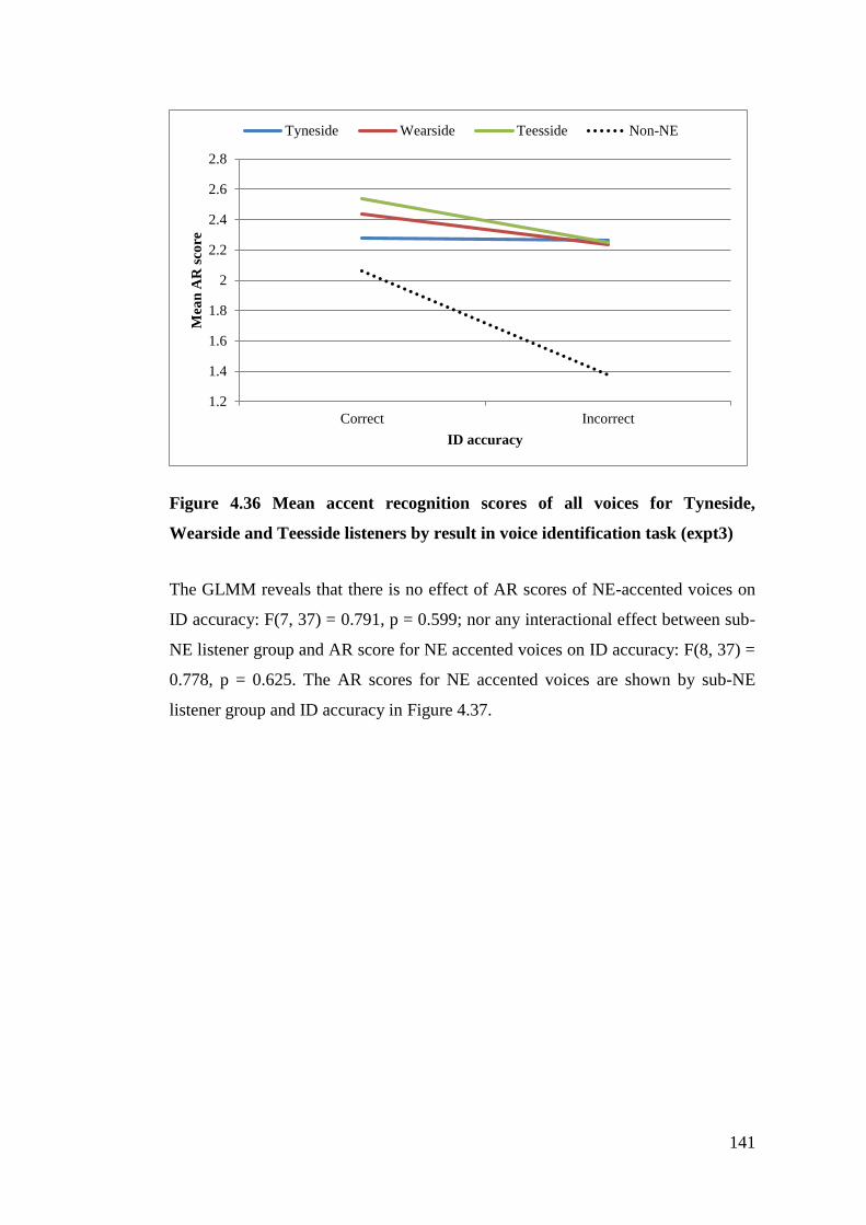
141
Figure 4.36 Mean accent recognition scores of all voices for Tyneside,
Wearside and Teesside listeners by result in voice identification task (expt3)
The GLMM reveals that there is no effect of AR scores of NE-accented voices on
ID accuracy: F(7, 37) = 0.791, p = 0.599; nor any interactional effect between sub-
NE listener group and AR score for NE accented voices on ID accuracy: F(8, 37) =
0.778, p = 0.625. The AR scores for NE accented voices are shown by sub-NE
listener group and ID accuracy in Figure 4.37.
1.2
1.4
1.6
1.8
2
2.2
2.4
2.6
2.8
Correct Incorrect
Mea
n A
R s
core
ID accuracy
Tyneside Wearside Teesside Non-NE

142
Figure 4.37: Mean accent recognition scores of NE accented voices for
Tyneside, Wearside and Teesside listeners by result in voice identification task
(expt3)
Figure 4.38 displays the AR scores for the target speaker by sub-NE listener group
and ID accuracy. Overall, there is little difference based on accuracy and the
GLMM reveals that there is no main effect of the AR score of the target speaker:
F(3, 46) = 0.669, p = 0.576. However, there is a significant interaction between the
AR score and the sub-NE listener group: F(3, 46) = 3.023, p = 0.039. For Teesside
listeners, there is minimal difference in AR scores based on accuracy. For
Wearside listeners, the common pattern of AR scores being higher for listeners
making accurate IDs is seen. For Tyneside listeners, however, AR scores are lower
for listeners making accurate IDs.
1.2
1.4
1.6
1.8
2
2.2
2.4
2.6
2.8
Correct Incorrect
Mea
n A
R s
core
ID accuracy
Tyneside Wearside Teesside Non-NE
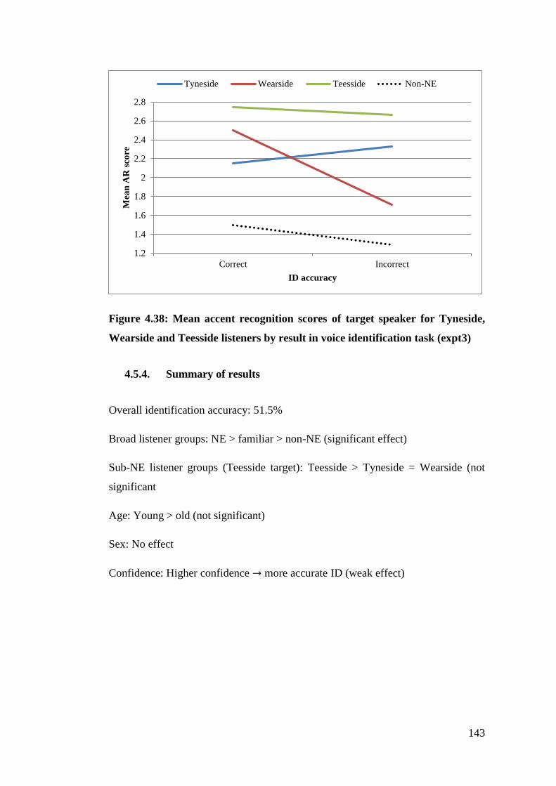
143
Figure 4.38: Mean accent recognition scores of target speaker for Tyneside,
Wearside and Teesside listeners by result in voice identification task (expt3)
4.5.4. Summary of results
Overall identification accuracy: 51.5%
Broad listener groups: NE > familiar > non-NE (significant effect)
Sub-NE listener groups (Teesside target): Teesside > Tyneside = Wearside (not
significant
Age: Young > old (not significant)
Sex: No effect
Confidence: Higher confidence → more accurate ID (weak effect)
1.2
1.4
1.6
1.8
2
2.2
2.4
2.6
2.8
Correct Incorrect
Mea
n A
R s
core
ID accuracy
Tyneside Wearside Teesside Non-NE
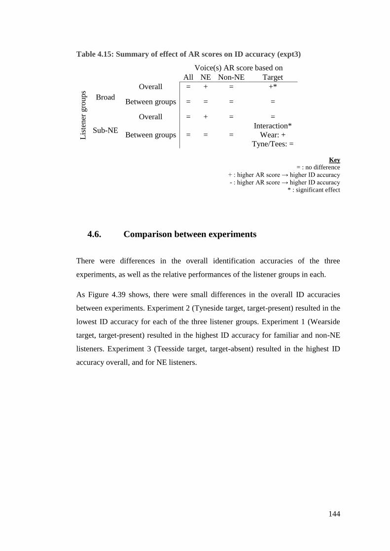
144
Table 4.15: Summary of effect of AR scores on ID accuracy (expt3)
Voice(s) AR score based on
All NE Non-NE Target L
iste
ner
gro
ups
Broad
Overall = + = +*
Between groups = = = =
Sub-NE
Overall = + = =
Between groups = = =
Interaction*
Wear: +
Tyne/Tees: =
Key
= : no difference
+ : higher AR score → higher ID accuracy
- : higher AR score → higher ID accuracy
* : significant effect
4.6. Comparison between experiments
There were differences in the overall identification accuracies of the three
experiments, as well as the relative performances of the listener groups in each.
As Figure 4.39 shows, there were small differences in the overall ID accuracies
between experiments. Experiment 2 (Tyneside target, target-present) resulted in the
lowest ID accuracy for each of the three listener groups. Experiment 1 (Wearside
target, target-present) resulted in the highest ID accuracy for familiar and non-NE
listeners. Experiment 3 (Teesside target, target-absent) resulted in the highest ID
accuracy overall, and for NE listeners.
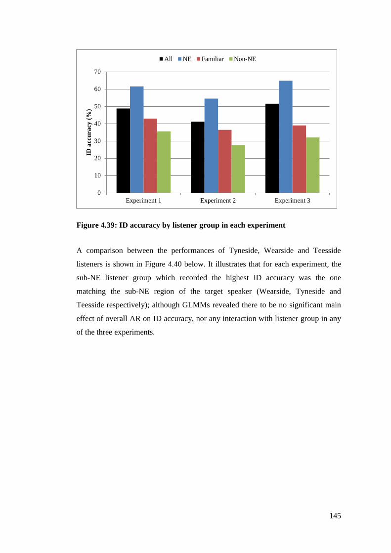
145
Figure 4.39: ID accuracy by listener group in each experiment
A comparison between the performances of Tyneside, Wearside and Teesside
listeners is shown in Figure 4.40 below. It illustrates that for each experiment, the
sub-NE listener group which recorded the highest ID accuracy was the one
matching the sub-NE region of the target speaker (Wearside, Tyneside and
Teesside respectively); although GLMMs revealed there to be no significant main
effect of overall AR on ID accuracy, nor any interaction with listener group in any
of the three experiments.
0
10
20
30
40
50
60
70
Experiment 1 Experiment 2 Experiment 3
ID a
ccu
racy
(%
)
All NE Familiar Non-NE
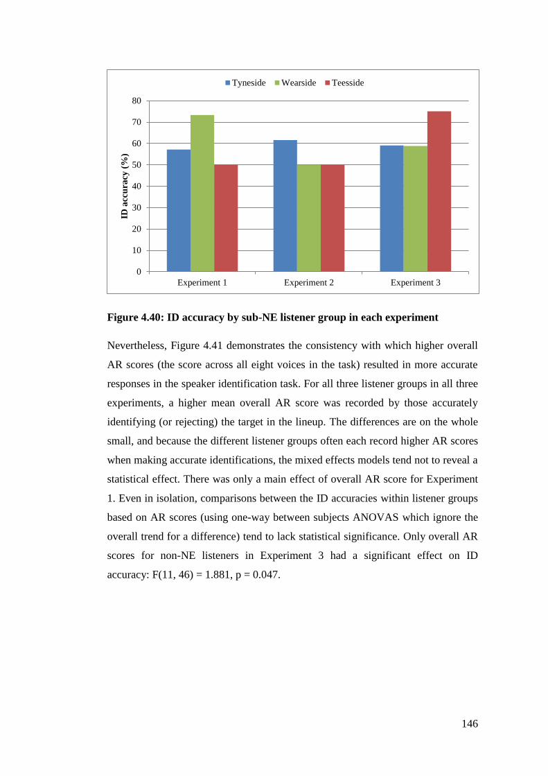
146
Figure 4.40: ID accuracy by sub-NE listener group in each experiment
Nevertheless, Figure 4.41 demonstrates the consistency with which higher overall
AR scores (the score across all eight voices in the task) resulted in more accurate
responses in the speaker identification task. For all three listener groups in all three
experiments, a higher mean overall AR score was recorded by those accurately
identifying (or rejecting) the target in the lineup. The differences are on the whole
small, and because the different listener groups often each record higher AR scores
when making accurate identifications, the mixed effects models tend not to reveal a
statistical effect. There was only a main effect of overall AR score for Experiment
1. Even in isolation, comparisons between the ID accuracies within listener groups
based on AR scores (using one-way between subjects ANOVAS which ignore the
overall trend for a difference) tend to lack statistical significance. Only overall AR
scores for non-NE listeners in Experiment 3 had a significant effect on ID
accuracy: F(11, 46) = 1.881, p = 0.047.
0
10
20
30
40
50
60
70
80
Experiment 1 Experiment 2 Experiment 3
ID a
ccu
racy
(%
)
Tyneside Wearside Teesside
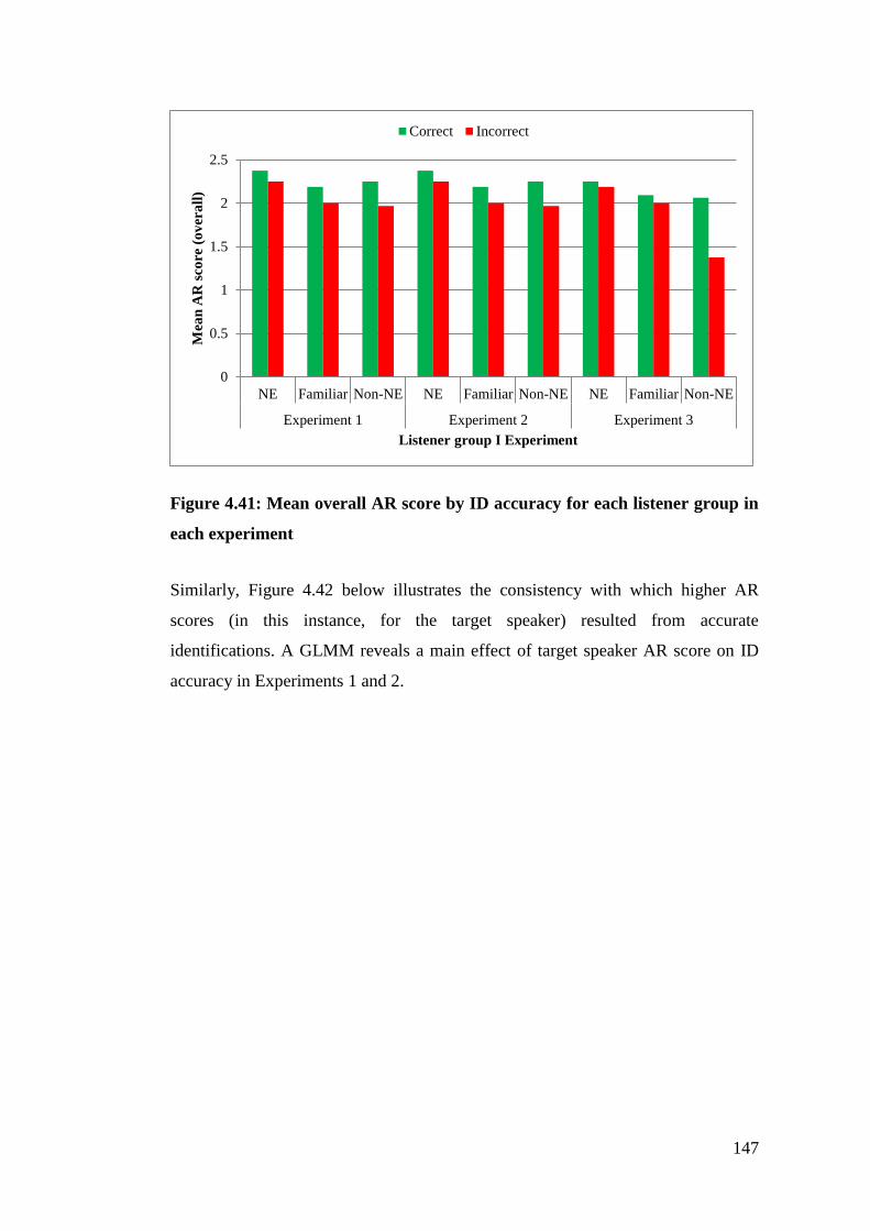
147
Figure 4.41: Mean overall AR score by ID accuracy for each listener group in
each experiment
Similarly, Figure 4.42 below illustrates the consistency with which higher AR
scores (in this instance, for the target speaker) resulted from accurate
identifications. A GLMM reveals a main effect of target speaker AR score on ID
accuracy in Experiments 1 and 2.
0
0.5
1
1.5
2
2.5
NE Familiar Non-NE NE Familiar Non-NE NE Familiar Non-NE
Experiment 1 Experiment 2 Experiment 3
Mea
n A
R s
core
(o
ver
all
)
Listener group I Experiment
Correct Incorrect
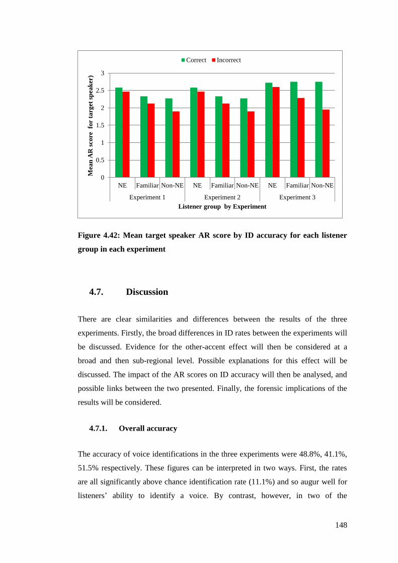
148
Figure 4.42: Mean target speaker AR score by ID accuracy for each listener
group in each experiment
4.7. Discussion
There are clear similarities and differences between the results of the three
experiments. Firstly, the broad differences in ID rates between the experiments will
be discussed. Evidence for the other-accent effect will then be considered at a
broad and then sub-regional level. Possible explanations for this effect will be
discussed. The impact of the AR scores on ID accuracy will then be analysed, and
possible links between the two presented. Finally, the forensic implications of the
results will be considered.
4.7.1. Overall accuracy
The accuracy of voice identifications in the three experiments were 48.8%, 41.1%,
51.5% respectively. These figures can be interpreted in two ways. First, the rates
are all significantly above chance identification rate (11.1%) and so augur well for
listeners’ ability to identify a voice. By contrast, however, in two of the
0
0.5
1
1.5
2
2.5
3
NE Familiar Non-NE NE Familiar Non-NE NE Familiar Non-NE
Experiment 1 Experiment 2 Experiment 3
Mea
n A
R s
core
fo
r ta
rget
sp
eak
er)
Listener group by Experiment
Correct Incorrect
149
experiments more incorrect than correct ID responses were made, suggesting that
over half the time somebody is asked to make an identification of a voice they will
make a mistake. Which of these interpretations is adopted is important for the
potential application of voice identification evidence to forensic situations. Under
interpretation one, earwitnesses are more likely to select the criminal (if present) in
a voice lineup than any foil. Their identification, then, may be interpreted as adding
evidential value to the case. The fact that the identification is more often incorrect
than correct, however, may suggest that this type of evidence lacks reliability.
The differing ID accuracies between experiments can be attributed to a number of
factors. Experiment one recorded more accurate identification than experiment two,
both of which were target present lineups. Experiment two, however, had more
foils matching the target voice in terms of sub-NE accent than experiment one,
which may account for the reduced identification accuracy. Experiment three
resulted in the highest accuracy rate despite it being a target absent lineup. Previous
research has suggested that target absent lineups result in more errors than target
present lineups (Broeders & Rietveld, 1995). It might be expected that experiment
three should result in the worst ID performance. This experiment, however, was
constructed using foils which differed in terms of sub-NE accent from the exposure
voice. The target speaker was from Teesside; one foil was from Teesside whilst
seven were from Tyneside. The effect of this construction on different listener
groups is discussed below, but it is apparent that this is a possible counter
explanation for the expected reduced ID accuracy in a target-absent lineup.
The specifics of evidential value and reliability are reliant on a number of other
factors involved in the case, such as importance of voice identification evidence,
and strength of other forms of evidence. The aim of experimental investigations
such as this is to further our understanding of how listeners (and, in forensic
contexts, earwitnesses) identify voices. Identifications made in these conditions are
quite different to real-world scenarios, however. Although the results from these
experiments can provide an insight into the expected accuracy of identification
made under certain conditions, none of the situations tested are truly applied
forensic environments (see §2.4. for a discussion of real-world exposure). As such,
the results of this experiment will not be used to suggest whether voice
150
identification is a worthwhile piece of evidence in a real-life case, but to investigate
some of the factors which may or may not predict the reliability of such evidence.
4.7.2. The other-accent effect
The primary purpose of the experiment was to test whether there is evidence for an
effect of listeners’ own accent on their ID ability. It was predicted that locals would
perform better than non-locals in identifying a local speaker. In broad terms, the
data supports this prediction. In these experiments, listeners from the North East of
England recorded higher ID accuracies than listeners from elsewhere in the UK.
This lends support to the other-accent effect (cf. Stevenage et al., 2012) and
Yarmey (1995)’s claim that listeners will find voices speaking with an accent less
distinguishable than those speaking with the listener’s own regional variety.
Locals outperformed non-locals in all three experiments (significantly so in one
and three, approaching significance in two). The biggest difference in performance
was in experiment three. As stated, this involved an almost complete mismatch
between the sub-NE accent of the target and the foils. This mismatch appears to
benefit NE listeners, presumably because they are better equipped to distinguish
between the different sub-NE accents. The local listeners are able to rule out seven
of the eight foil on the basis of them having a different sub-NE accent to the target.
Indeed, the foil which NE listeners most commonly selected as the target was the
one foil who was, like the target, from Teesside.
Experiment one resulted in the next biggest difference between the ID accuracy of
locals and non-local. The target in this lineup was a Wearside speaker. The target
in experiment two was a Tyneside speaker. Research into the other-accent effect
has demonstrated that the difference is more severe when listeners are asked to
identify speakers with an unfamiliar and/or regional accent (Kerstholt et al., 2006;
Stevenage et al., 2012). Whilst both Tyneside and Wearside accents are regional,
research into accents in the area demonstrates the propensity of outsiders to show
greater recognition of and identify more closely with the Tyneside accent
(Montgomery, 2006; Montgomery, 2012; Pearce, 2009; Wales, 2006). This may

151
explain the minor improvement in performance of non-locals relative to locals
when a Tyneside target is used rather than a Wearside target.
As stated, the main aim of the experiment was to investigate the performance of
locals and non-locals, but the performance of a third group – those not from the
area but with an increased level of familiarity with accents from the region – could
provide clues as the why locals and non-locals have differing identification
abilities. Familiarity with the NE accent appears to improve identification rates in
all three experiments, although the difference between non-NE and familiar
listeners is not significant in any condition. The trend is notably consistent, though.
The discrepancy between the listener groups could be considered in terms of
expertise. The expertise effect is discussed above with reference to face recognition
and word recognition tasks with ‘expertise’ comparable to ‘exposure to’ – those
who have increased exposure to a feature have increased expertise in that feature.
This allows for improved processing of stimuli relating to that feature. Subjects
with increased exposure to particular races were better able to distinguish between
faces of that race (Brigham & Malpass, 1985). Like many speech processing based
tasks (Floccia, Butler, Goslin & Ellis, 2009; Floccia et al., 2006), listeners in this
study appear to show improved performance when stimuli are presented using an
accent with which they have some expertise.
It is to be expected that whilst (non-NE) familiar listeners will have more exposure
to NE accents than non-NE listeners, NE listeners will have even more exposure
than (non-NE) familiar listeners. The relative expertise of each group may explain
the relative discrepancies between the three listener groups. The difference in
performance between NE and familiar listeners is greater than the difference
between familiar and non-NE listeners. This mirrors the relative levels of exposure
to NE accents. It is likely that all British listeners will have an underlying level of
exposure to NE accents (at least minimally) through the media. Familiar listeners
have spent some time with increased exposure to NE accents and/or are exposed to
NE accents through a small number of contacts. NE listeners, on the other hand, are
engaged with NE accents on a day-to-day basis and grew up surrounded by
speakers of the NE accent. Their level of exposure is much greater than both
familiar and non-NE listeners, suggesting their level of expertise is much greater
152
too. The expertise effect here appears to be related to ability to distinguish between
voices.
4.7.3. Sub-NE regions
The data also show a difference in performance when sub-regions are considered.
All three NE region listener groups performed better than familiar and non-NE
listeners, but the order of performance by Tyneside, Wearside and Teesside
listeners differed between experiments. In experiment one, where the target voice
was that of a Wearside accented speaker, Wearside listeners performed best,
followed by Tyneside listeners and then Teesside listeners. It may be assumed that
this mirrors the order of degree of exposure to the Wearside accent (Tyneside
listeners are geographically closer to Wearside than Teesside listeners are). In
experiment two, where listeners were asked to identify the voice of a Tyneside
speaker, Tyneside listeners performed best, although the difference in performance
between the three listener groups was minimal. If the exposure theory is applied
here, then the fact that Newcastle (in Tyneside) is seen as the dominant socio-
economical region within the NE (Beal et al., 2012) may account for the small
distinction in performance. The overall degree of exposure (of listeners from any
sub-NE region) to the Tyneside variety is likely to be higher than exposure to either
the Wearside or Teesside accents. The ‘benefit’ which Tyneside listeners have over
other NE listeners in being from Tyneside is therefore negated.
In experiment three, Teesside listeners performed best. This might not be expected,
given that all but one of the foil voices were from Tyneside, perhaps allowing for
improved performance by Tyneside listeners. They have an increased ability to
identify the foils as being from Tyneside (ergo not Teesside, as was the target
voice). However, if the ceiling effect seen in experiment two with respect to
Tyneside accents is in effect here too, then Teesside listeners have the added
advantage of being local to the exposure voice, with no sub-NE region listeners
having any advantage as a result of the foils’ accents. This suggests that expertise
with the specific sub-NE region can lead to an improved ability to identify a voice
in that accent.
153
4.7.4. Why is there an effect?
If it is assumed, then, that exposure to an accent aids performance in identifying
voices in that accent then the question of why? should be posited. It may be that
comprehensibility and/or intelligibility provides the explanation behind the
disparity in results. Comprehensibility and intelligibility are terms which are often
used interchangeably (Smith & Nelson, 1985) although Munro and Derwing (1995)
suggest that they should be applied separately: Intelligibility measured by a
listener’s ability to transcribe the actual words heard; comprehensibility measured
as a rating of how easy it is to understand a speaker. If comprehensibility is
reduced then a listener will find it difficult to understand what a speaker is saying.
The amount of speech which they process is consequently reduced, and reduced
levels of exposure to speech have been shown to reduce identification accuracy
(Perrachione & Wong, 2007). Voices with accents which are unfamiliar to the
listener appear less distinctive and make discrimination more difficult (Yarmey,
1994). Moreover, Imai, Walley and Flege (2005) showed that when hearing an
unfamiliar accent, intelligibility within word recognition tasks is reduced. It
follows that non-NE listeners may have greater intelligibility problems with the NE
speakers in the lineup than local NE listeners do; and those with some degree of
familiarity falling somewhere between the two. Indeed, listeners have been shown
to have some reliance on intelligibility when identifying voices - Van Lancker et al.
(1985) found a reduction in accurate identification of famous voices when speech
was played backwards (59%) rather than forwards (71%). Whilst reversal of speech
will have some impact on the suprasegmental features of the voice, such as the
reversal of intonation patterns and speech rhythm, the process will have greater
influence on the phonetic detail of speech. The reduction in intelligibility
demonstrates that whilst listeners can still identify voices on the basis of vocal
characteristics alone, access to accurate phonetic detail is important.
Similarly, a reduction in comprehensibility in foreign language tasks has been
shown to have a negative influence on voice identification rates (Perrachione &
Wong, 2007; Philippon et al., 2007b). Though the magnitude of a drop in
comprehensibility from familiar to unfamiliar non-native speech will be greater
than the drop in comprehensibility from familiar to unfamiliar native speech, the
154
same effect can be witnessed here. The discrepancy between performance of locals
and non-locals in the present study is smaller than that between native and non-
native listeners in other experiments. This corresponds with the relative degree of
incomprehensibility of either merely an unfamiliar regional variety or non-native
language. It should be noted, however, that no direct comparison can be drawn
between identification rates from different studies using different data as the voice
to be identified and the make-up of voice parade will affect identification rates (as
is displayed by the results of the three experiments presented here). This accords
with the findings of Kerstholt et al. (2006) who showed that using standard
accented voices resulting in more accurate identifications than using non-standard
accented speakers. This is an expected pattern given the relative loss of
comprehension/intelligibility associated with hearing unfamiliar native versus non-
native accents. Despite the difficulties in comparing data, the differences between
performance of locals and non-locals were relatively consistent for each
experiment. The data, then, indicate that an earwitness is more likely to accurately
identify a voice if they share an accent, and that having an increased level of
familiarity with the talker’s accent will improve the chances of accurate
identification, though the significance of the latter assertion will require further
investigation.
Research into exemplar theory also offers an explanation into why the other-accent
effect can be noted. An exemplar model assumes that individual speech utterances
are stored as separate exemplars, which are activated during the production and
perception of speech (Goldinger, 1997; Pierrehumbert, 2001). Individual exemplars
index a range of information, including information about the person producing it,
and so they may be indexed to regional and contextual information (Hay, Warren
& Drager, 2006). Hay, Nolan and Drager (2006) note that during speech
perception, the activation of exemplars is dependent on their acoustic similarity to
the utterance heard. It follows, then, the more familiar a listener is with the accent
of the speech, the stronger the activation of exemplars, and the more heightened
their ability to accurately perceive and categorise speech.
155
4.7.5. Link between accent recognition and voice identification
Performance in the voice identification task was shown to be significantly affected
by performance in the accent recognition task in some guises but not others. Across
the three experiments, the overall AR score for listeners (across all eight voices)
was shown to be higher amongst accurate speaker ID responses. There was a
stronger trend for accurate recognition of NE accented voices and the target
speaker themselves. There was no effect for non-NE accented voices.
It may be that, like musical ability and auditory capacity (de Jong, 1998), ability to
differentiate between accents is another cognitive skill which correlates with
listeners’ ability to recognise speakers. It has been shown that eyewitness
identification accuracy is significantly correlated with performance on face
recognition tasks (Morgan, Hazlett, Baranoski, Doran, Southwick & Loftus, 2007),
and so the theory that performance in a task may predict performance in a similar
task is nothing new. There may be nothing special about AR ability in and of itself.
There was, however, a bigger improvement amongst listeners whose AR scores for
accents which are perceptually similar to the target speaker than those whose
scores were higher for dissimilar accents. The improvement was bigger still
amongst those who accurately recognised specifically the accent of the target
speaker. This may suggest that it is the accurate perception of speech used by the
target which provides the important link with ID accuracy.
It has been shown that the acoustic signal is mediated by sociolinguistic knowledge
in order to reach a perceptual judgement about the speech produced (c.f. Strand,
1999). In other words, speech perception and recognition depend not only on
interpretation of the speech signal, but the listener’s beliefs about who it is that is
producing the signal. Changes in these beliefs (in this case whether they accurately
recognise the accent spoken or not) will affect the listener’s perception of what
speech is being produced. It may follow, then, that those listeners who fail to
recognise the speaker’s accent will have an impaired perception of what is being
said. This leads to reduced comprehensibility, offering a rationale for those who
can accurately recognise the speaker’s accent showing improved performance in
identifying that voice.
156
Furthermore, if the listener does not recognise the speakers’ accent, there may be
additional processing costs in hearing that (more) unfamiliar sounding speech
(Floccia et al., 2006). This could negatively impact on the listener’s storage of that
voice and subsequent retrieval for comparison with the voices in the lineup.
Another possible explanation is that there is variance within the accent groups
(both regional and sub-regional) in their familiarity with the target speaker’s
accent. Such familiarity has been shown to improve AR scores and ID accuracy
independently. It may be that even within the local NE listener group, there are
listeners who have little familiarity with the Teesside accent. The data suggest
these listeners would perform less well on both tasks than a second listener with
strong familiarity with the Teesside accent. Enough variation of this sort could
produce the correlation between AR score and ID accuracy within the different
listener groups.
Further analysis of this link is needed to provide a more concrete explanation.
Testing of listeners’ comprehension of what the speaker says will shed light on
whether it is a perceptual effect, as well as a more detailed understanding of how
well a listener can recognise accents, and the variation within listener groups.
4.7.6. Some people are better than others
Alternatively, or perhaps additionally, the same people who have a good ability to
recognise accents may also have a good ability to remember and identify voices
without there being any strict cause and effect. In the domain of face recognition
theory, the existence of a group of people known as “super-recognizers” has been
posited (Russell, Duchaine & Nakayama, 2009). A super-recognizer has face
recognition ability which is far above average. Russell et al. (2009) report that the
face recognition processes employed by super-recognisers are not qualitatively
different from those of a control group who showed average recognition abilities,
but there was a strong quantitative effect.
Those who showed an exceptional ability to recognise faces also showed increased
perceptual discrimination ability, so those people who could distinguish one face
from another were also adept at judging similarities and differences between faces.
157
If there exists a scale of abilities to recognise faces, so it seems logical that there
may be a scale of abilities to recognise voices. If parallels exist and there are people
who have an above average voice recognition ability, then ‘super-hearers’ who
perform well in one voice recognition task may perform well in another. If a
listener is adept at differentiating between accents (thus scoring higher on the
accent recognition task) they would be likely to perform better when distinguishing
one voice from another (thus more likely to make an accurate identification in the
voice parade). Super-recognizers are not considered a distinct group from the rest
of the population and the cut-off is arbitrary. The present data support the
hypothesis that some listeners are better at such tasks than others in view of the
high rate of accurate identifications amongst those scoring highly on the accent
recognition task. What is more evident, however, is the low rate of accurate
identification amongst those listeners scoring poorly on the AR task. This is in line
with people with developmental prosopagnosia, who exist at the other end of the
face recognition ability scale from super recognisers (Russell et al., 2009).
Even excluding the concept of super-hearers, the concept of individual variation is
accepted (Hollien, 1996). This does not account fully, however, for the difference
in performance of listener based on experimental group membership (accent, AR
ability, etc.). There appears to be no difference in performance on the basis of sex
or age. This accords with many much of the previous research, which does not
show an effect of these listener variables. Self-rated confidence scores were
consistently higher amongst listeners making accurate identifications in each of the
three conditions. The difference approached significance in two of the experiments.
The literature generally suggests that confidence and accuracy do not correlate,
though these findings suggest that listener confidence might be a useful indicator.
4.7.7. Forensic implications
Whatever the interaction, the data suggest that AR ability is associated with
listeners’ ability to distinguish between voices: there are trends for increased accent
recognition scores to predict higher voice identification accuracy. In an applied
setting, it may be useful to assess an earwitness’ AR ability alongside the
identification process. If an earwitness finds the task of distinguishing between
158
accents difficult (particularly accents like that of the suspect), then the interpreted
value of their evidence could be reduced. That is not to suggest that some listeners
should have their identification disregarded, as the data show that listeners
recording low accent recognition scores still have the ability to accurately identify
the target voice. Similarly, for those who scored well in the AR task the voice
identification accuracy was higher but not absolute. The AR ability of an
earwitness may therefore be a useful predictor of the reliability of their
identification, but not a strong predictor of whether the identification is accurate or
not.
This, however, raises numerous methodological issues which would need careful
consideration. There is potential for the testing to have an effect on the listener’s
voice identification ability - similar to that of the verbal overshadowing effect
(Perfect et al., 2002; Vanags et al., 2005). It has been shown that verbalising a
description of a voice can impair a person’s ability to recognise the voice. Bartlett,
Searcy and Abdi (2003) suggest that the encoding of faces is primarily a holistic
and non-reportable task, and so a holistic retrieval process would allow for
maximal recognition performance. The processes involved in generating a verbal
description of the face are not holistic, but featural, in nature. The activation of this
inappropriate processing mode is thought to be detrimental to the subsequent
holistic recognition task (Melcher & Schooler, 2004). Moreover, Macrae and Lewis
(2002) found that a cognitive task which does not involve retrieval of the original
memory can still impair the recognition of the stimuli. There is reason to believe
that there are parallels between the processes involved in encoding an unfamiliar
voice and an unfamiliar face (Mann et al., 1979). Evidence suggests that the right
cerebral hemisphere is vital to the encoding of faces (e.g. Klein, Moscovitch &
Vigna, 1976) whilst the encoding of suprasegmental features, such as tone and
timbre, has been shown to be impaired in those with right hemispheric damage
(Milner, 1962). Cross-modal interference is known to occur: auditory information can
affect visual judgements (Kim & Davis, 2010; Kim, Kroos & Davis, 2010) and visual
stimuli can interfere with auditory (McGurk & Macdonald, 1976). If the encoding of
voices is similar to the encoding of faces then it stands that the retrieval of the two
may be affected in the same way. So the introduction of a cognitive task, even if it
does not involve retrieval of the original memory may still impair the recognition
159
of the stimuli i.e. exposing listeners to, and asking them to identify, accents closely
matching that of the target voice may negatively impact on the recognition rate.
The potential overshadowing-like effect could be avoided through the application
of an accent recognition task after the identification has taken place. This, however,
would still involve the timely and costly set-up and application of a voice lineup,
only for some sort of reliability index to be provided post identification. It would
be preferable to know the potential reliability of an earwitness’s identification
before undergoing the process of a voice parade. It is hitherto unknown whether
any verbal overshadowing effect extends to tasks such as AR.
It may also be that there are better predictors of a listener’s ability to accurately
identify a given voice. Most notably, listeners’ ability to recognise one voice has
been shown to correlate with their ability to recognise others (Bull & Clifford,
1984). If a listener shows a poor ability to distinguish voices from one another in
general, then, whilst experimental conditions cannot replicate the conditions under
which an earwitness is exposed to a voice, this is likely to predict that their
identification as an earwitness is not reliable.
The implications of the other-accent effect demonstrated here are clearer.
Identifications made by earwitnesses who share the accent of the perpetrator can be
considered as more reliable. Again, that is not to say that those sharing an accent
should be tested and those with a different accent should not. Listeners with ‘other
accents’ are still seen to identify speakers at a rate well above chance. The
difference between locals and non-locals should also be considered at a sub-
regional level. Identifications may be more reliable if the earwitness closely
matches the perpetrator’s voice (at a level beyond the standard/non-standard
comparison demonstrated in previous research). Additionally, if an earwitness is at
least familiar with the perpetrator’s accent, their identification may be considered
likely to be somewhat more robust than if they are completely unfamiliar.
160
4.8. Chapter summary
The chapter demonstrated that an other-accent effect may be in place.
Listeners from the NE recorded higher identification accuracies than non-
local listeners in each of the three experiments using a Tyneside, Wearside
and a Teesside target speaker. The biggest effect was seen in the Teesside
target experiment (3).
Familiarity with an accent appears to improve listeners’ ability to identify
speakers. Non-locals with minimal prior exposure to NE accents recorded
lower ID accuracies than non-locals classed as being familiar with NE
accents in each of the three experiments. Familiarity did not allow for
performance on a par with local listeners.
The other-accent effect appears to exist at both a broad level (local versus
non-local) as well as on a sub-regional plane. Within the local NE listeners
group, listeners from the particular area (Tyneside, Wearside or Teesside)
matching that of the target speaker recorded higher identification accuracies
than those from elsewhere. The effect is weakest in Tyneside, which is the
dominant variety in the area.
Accent recognition ability appears to play a role in listeners’ ability to
identify speakers. There is a consistent trend for higher AR scores amongst
listeners making accurate responses in the ID task. This is true of overall
AR scores, but in particular for listener’s ability to recognise NE accents
and the accent of the target speaker.
Age and gender appear to have no effect on identification accuracy.
Confidence has a weak effect on accuracy in two of the experiments
161
5. An alternative testing method
This chapter introduces an alternative method for testing an earwitness’s ability to
identify a voice. It discusses the justifications for considering an alternative
approach – the Short Term Repeated Identification Method (STRIM) - and
examines the limitations of the traditional voice lineup (TVLU). The methodology
of an experiment which employs STRIM as a naïve listener testing method will be
explained, and an overview of the types of analysis which will be undertaken using
data collected in this way will be provided. The results and analyses then follow.
5.1. Justifications for a new approach
The primary justifications for considering an alternative to the TVLU are threefold:
a lack of statistical comparisons which can be made when assessing the
performance of naïve listeners in voice identification tasks. That is,
identifications made using TVLU are either correct or incorrect.
Consequently identifying general trends which affect identification
performance is difficult because of the binary nature of response. A
large number of responses, with distinct differences in performances
between groups, is needed before statistical comparisons can show any
effect.
a desire to improve the accuracy with which naïve listeners can identify
a target in voice identification tasks. The ultimate goal for earwitness
identification should be to allow a listener to be able to identify the
voice of a perpetrator if they are in a lineup, or reject the presence of the
perpetrator if they are not in a lineup. If these outcomes are achieved
with greater regularity, the reliability (and evidential value) of naïve
speaker identification is increased.
the voice lineup is based on its visual counterpart, largely grounded in
the notion that the latter works for eyewitness and so the former should
162
work for earwitnesses. There are differences between the two modalities
in terms of exposure and how comparisons can be made between faces
and voices. The assumption that the traditional lineup is the most
appropriate method for testing may, then, be unfounded.
5.1.1. Statistical comparisons
The first of these justifications is of primary interest in a research capacity.
Responses to a target present lineup either involve the listener selecting the target
(hit) or a foil (false hit), choosing that the target is not present (miss) or deciding
not to make a selection. Ultimately, these responses are either accurate (hit) or
inaccurate (false hit, miss); ‘no selections’ (where the listener does not make an
identification) are neither accurate nor inaccurate. This binary classification of
naïve listener response accuracy mean that two populations must be either very
large or perform very differently in order for there to be a statistically significant
difference between the two. Recruiting a large population to this type of study is
not feasible without a substantial investment of time, money and resources.
Depending on the content and context of study, particularly if forensic realism is
sought, there may be barriers to recruiting a large number of experimental
witnesses. If, for example, the experimenter wishes to ask open ended questions to
the subject (as would be forensically realistic), it may be necessary to conduct
testing face-to-face. It may also be beneficial to the design to leave a time delay
between exposure and testing, increasing the time needed to collect sufficient
responses. Additionally participants may need to be remunerated for the
involvement – the payment of 200 subjects requires significant funding. There may
be two populations to be compared, for example divided by sex, but there may be
more, such as various age groups or listening conditions. As demonstrated in
Chapter 4, whilst it is possible to highlight trends when these kinds of comparisons
are being made, the differences are rarely statistically significant. This is true even
with a relatively large number of participants (140 in the present study), as these
are broken down into population groups.
163
5.1.2. Accuracy
The second justification for considering this approach has its grounding in real-life
application. Presently, the voice lineup is the accepted form of identification in
England and Wales (Home Office, 2003). The methodology is largely based on the
visual lineup format (such as is described in Loftus (1979). The overall format and
structure of the earwitness parade are well defined and justified in accordance with
linguistic principles (Nolan & Grabe, 1996) and have received little challenge in
the literature. Studies investigating the performance of naïve listeners in voice
identification tasks almost exclusively follow a methodology similar to that of a
real voice lineup (an exhaustive list of such studies is provided through Chapter 2).
That is not to say there have not been concerns raised over the validity of the
practice, although these are predominantly aimed at earwitnesses being asked to
identify a voice rather than the method itself. Given, however, that such studies use
the TVLU method, or something approximating this, it is difficult to disentangle
the outcome and the method. A change in the methods employed may have an
effect on the reliability of speaker identifications made by naïve listeners. Of
course, if the traditional method is the optimal technique for ensuring the target is
identified when possible, a change in methods may reduce the reliability of
responses. The alternative approach used in this chapter will assess this.
5.1.3. Visual lineups
The method of testing earwitness identification is based largely on the method of
testing eyewitness identification. There are, however, important differences
between the two (see §2.6. for an overview of research into the area). There may
be questions over the reliability of voice identification, but the testing method is
considered largely uncontroversial. In contrast to its aural counterpart, the visual
lineup method has been questioned and indeed undergone recent changes.
Earwitnesses and eyewitnesses are required to answer the same question – are any
of the options (faces/voice) the perpetrator? Clearly, the modality of the
presentation differs for the two, but the method of presentation does too. This can
have an effect on the value of how witnesses come to their decision.
164
The relative judgement strategy is thought to be a common technique used in
eyewitness identifications. It involves decisions about identification being based
upon which of the options best matches the characteristics of the memory of the
target, rather than selecting the option matching the target beyond reasonable doubt
(Wells, Small, Penrod, Malpass, Fulero & Brimacombe, 1998). The witness bases
their decision on which of the options in the lineup is most likely to be the target
i.e. relative to the other options, which is the best fit. This ultimately has been
shown to lead to errors, specifically a large number of false hits, with an inverse
relationship between the goodness of a witness’s memory and their reliance on
relative judgements (Wells, 1984). Lindsay and Wells (1985) argue that the
simultaneous presentation of lineup members promotes use of the relative
judgement strategy. They implemented a sequential presentation system, whereby
participants were presented with one photograph and asked whether it was of the
perpetrator of a staged crime to which they had been a witness. Participants
responded yes or no and were subsequently shown a second photograph and asked
the same question, and so on. They found that although the rate of accurate
identification was lower in the sequential than simultaneous condition, the rate of
false identifications was also lower (with a large increase in the rate of no
identifications). The fall in false identifications was greater than the fall in accurate
identifications, and so Lindsay and Wells (1985) conclude that a sequential system
is preferable because witnesses were not basing their decision on relative
judgements of similarity.
Voice lineups are clearly not simultaneous in their presentation of stimuli to
witnesses, nor could they be. Whilst it has been shown that listeners can focus their
attention to particular sounds at the expense of extraneous noise sources (Pollack &
Pickett, 1957), and that some people are more gifted than others at attending to
particular sources (Bronkhorst, 2000; Hawley, Litovsky & Culling, 2004), it is not
comparable to being presented with visual stimuli simultaneously. When viewing a
selection of photographs of faces, it is possible to simply look at one and not
another without the latter providing a distraction. Additionally, it is possible to look
at two particular photographs simultaneously by altering your field of view,
because pictures are static. This allows direct comparison between two faces.
Speech, on the other hand, is dynamic by nature. Any attenuation of focus when
165
viewing a picture can be recovered almost instantly, whereas the speech signal
cannot be recovered without re-listening back over the same stretch of speech. A
direct auditory comparison between voices is not possible in the same way as a
visual comparison between faces.
Though simultaneous presentation of speech is not feasible, comparisons with
identifications made using visual lineups (made using the relative judgement
strategy) seem unfounded given the different ways in which witnesses are
presented with the options. Earwitnesses are presented with aural stimuli in a
sequential manner but are required to perform the same task as eyewitnesses, for
whom the stimuli are traditionally presented simultaneously. Whilst sequential
presentation may be beneficial, as above, designing the voice lineup method as a
comparison with the application in a visual lineup is flawed. In light of this, basing
the earwitness testing methods on eyewitness testing methods does not appear
remotely practical. An alternative method of naïve speaker identification in which
listeners make decisions sequentially (to match the presentation of the voices) will
therefore be tested.
5.2. Pilot studies
5.2.1. Sequential testing
A small scale pilot study was carried out using a sequential lineup system based on
Lindsay and Wells’ (1985) visual based experiment. It is predicted that asking
listeners to make positive or negative responses after hearing each voice will yield
similar results to the eyewitnesses in the visual study – a drop in false hits. 14
listeners were recruited to participate. All 14 listeners heard the same exposure
stimuli and were tested using the same eight speech samples, (the method of
presentation differed between two groups). Speech for both exposure and testing
was taken from task 1 (mock police interview) of the DyViS database (Nolan et al.,
2009). Listeners heard a 30 second sample of spontaneous speech using the same
cut-and-paste method employed in §4.2.1. They were then told they were going to
be asked to identify the speaker again but that the speaker may or may not actually
166
be one option of the options available to them. All 14 listeners heard eight voices,
and the target was present in each lineup. Half were asked to make the
identification using the traditional lineup presentation method – all samples were
c.60 seconds in length and were heard one after the other. Listeners were then
asked which, if any, they believed belonged to the speaker previously heard. The
other seven listeners heard a single voice sample and were then asked whether they
believed it belonged to the speaker they had previously heard; they answered yes or
no. This was repeated for each of the eight voices. Again, the target was present for
each listener. The listeners were not told how many voices they would hear to
avoid them feeling obliged to select a voice before the experiment was over, as in
(Lindsay & Wells, 1985).
In the traditionally presented lineup, three of the seven listeners accurately
identified the target speaker (three identified foils, one made no identification). In
the sequentially presented testing condition, none of the listeners accurately
identified the target speaker. Indeed, all seven listeners made no identification. As
in Lindsay and Wells’ (1975) visual study, the rate of false identifications did
indeed drop. The fact that none of the seven listeners made any sort of
identification, though, does not augur well for the use of this as a viable testing
method for earwitnesses. Debriefing with the listeners confirmed that they each
found the task too difficult. Most, although they had a feeling that one or more of
the voices was that of the perpetrator, were not confident enough to make a firm
decision of attribution without hearing all the options. Of these, many actually felt
strongest towards the target speaker. It seems, then, that listeners do indeed rely on
the relative judgement strategy. The fact that none of the listeners made a decision
when the relative judgement strategy was made unavailable to them might suggest
that auditory-based decisions are more reliant on comparisons being made than
visual-based decisions. Without a direct comparison of the two, no firm
conclusions can be made beyond the pilot study’s implication that sequential
testing does not allow for optimal speaker identification.
Earwitness identification is generally accepted to be more difficult than eyewitness
identification, and those relying on aural stimuli to make an identification are often
less confident in their judgements than those relying on visual stimuli
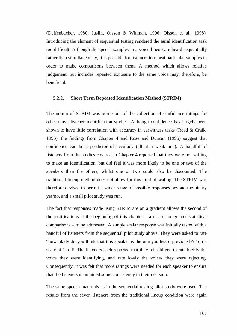
167
(Deffenbacher, 1980; Juslin, Olsson & Winman, 1996; Olsson et al., 1998).
Introducing the element of sequential testing rendered the aural identification task
too difficult. Although the speech samples in a voice lineup are heard sequentially
rather than simultaneously, it is possible for listeners to repeat particular samples in
order to make comparisons between them. A method which allows relative
judgement, but includes repeated exposure to the same voice may, therefore, be
beneficial.
5.2.2. Short Term Repeated Identification Method (STRIM)
The notion of STRIM was borne out of the collection of confidence ratings for
other naïve listener identification studies. Although confidence has largely been
shown to have little correlation with accuracy in earwitness tasks (Read & Craik,
1995), the findings from Chapter 4 and Rose and Duncan (1995) suggest that
confidence can be a predictor of accuracy (albeit a weak one). A handful of
listeners from the studies covered in Chapter 4 reported that they were not willing
to make an identification, but did feel it was more likely to be one or two of the
speakers than the others, whilst one or two could also be discounted. The
traditional lineup method does not allow for this kind of scaling. The STRIM was
therefore devised to permit a wider range of possible responses beyond the binary
yes/no, and a small pilot study was run.
The fact that responses made using STRIM are on a gradient allows the second of
the justifications at the beginning of this chapter – a desire for greater statistical
comparisons – to be addressed. A simple scalar response was initially tested with a
handful of listeners from the sequential pilot study above. They were asked to rate
“how likely do you think that this speaker is the one you heard previously?” on a
scale of 1 to 5. The listeners each reported that they felt obliged to rate highly the
voice they were identifying, and rate lowly the voices they were rejecting.
Consequently, it was felt that more ratings were needed for each speaker to ensure
that the listeners maintained some consistency in their decision.
The same speech materials as in the sequential testing pilot study were used. The
results from the seven listeners from the traditional lineup condition were again
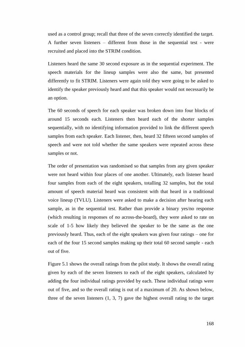
168
used as a control group; recall that three of the seven correctly identified the target.
A further seven listeners – different from those in the sequential test - were
recruited and placed into the STRIM condition.
Listeners heard the same 30 second exposure as in the sequential experiment. The
speech materials for the lineup samples were also the same, but presented
differently to fit STRIM. Listeners were again told they were going to be asked to
identify the speaker previously heard and that this speaker would not necessarily be
an option.
The 60 seconds of speech for each speaker was broken down into four blocks of
around 15 seconds each. Listeners then heard each of the shorter samples
sequentially, with no identifying information provided to link the different speech
samples from each speaker. Each listener, then, heard 32 fifteen second samples of
speech and were not told whether the same speakers were repeated across these
samples or not.
The order of presentation was randomised so that samples from any given speaker
were not heard within four places of one another. Ultimately, each listener heard
four samples from each of the eight speakers, totalling 32 samples, but the total
amount of speech material heard was consistent with that heard in a traditional
voice lineup (TVLU). Listeners were asked to make a decision after hearing each
sample, as in the sequential test. Rather than provide a binary yes/no response
(which resulting in responses of no across-the-board), they were asked to rate on
scale of 1-5 how likely they believed the speaker to be the same as the one
previously heard. Thus, each of the eight speakers was given four ratings – one for
each of the four 15 second samples making up their total 60 second sample - each
out of five.
Figure 5.1 shows the overall ratings from the pilot study. It shows the overall rating
given by each of the seven listeners to each of the eight speakers, calculated by
adding the four individual ratings provided by each. These individual ratings were
out of five, and so the overall rating is out of a maximum of 20. As shown below,
three of the seven listeners (1, 3, 7) gave the highest overall rating to the target
169
speaker. Three listeners rated a foil (or more than one foil) higher than the target (2,
5, 6), and one listener rated the target and a foil as joint highest (4).
Figure 5.1: Overall rating for each speaker by listener in STRIIM pilot study.
The target speaker is shown in green; the foils are shown in red
If just the highest overall rating is taken as the result from STRIM then it appears
that the results using this technique are at least on a par with those using the TVLU
method (where three listeners made accurate identifications and three listeners
made inaccurate identifications). It is noticeable from Figure 5.1, however, that on
the three occasions when the target is not the highest rated speaker, it is second
highest twice (listeners 2 and 5) and third highest once (listener 6) and is rated as 1
point lower than the highest foil twice and 3 points lower once. Conversely, on the
three occasions that the target is rated highest, they are 2, 4 and 6 points higher
than the nearest foil (listeners 1, 3 and 7 respectively). The degree by which the
highest rated speaker is distinct from the rest of the voices appears to be larger
when it is the target speaker which is rated highest than when it is a foil. This may
then provide support for the use of a scalar system over the traditional binary
approach.
0
2
4
6
8
10
12
14
16
18
1 2 3 4 5 6 7
Ov
era
ll r
ati
ng
(o
ut
of
20
)
Listener
170
Furthermore, the pilot study data appear to indicate an order effect in the ratings
provided by each listener. Figure 5.2 illustrates the ratings given by listener 7
across each of the four hearings (the four ratings made for each speaker).
Figure 5.2: Ratings given by listener number 7 in STRIIM pilot study across
each of the 4 hearings. The target speaker is shown in green; the foils are
shown in red
In hearing 1, the target speaker received the same rating as three foils. In hearings 2
and 3, the target speaker is rated one point higher than the highest foil. In hearing 4,
the target speaker is rated two points higher than the highest foil. Although this
represents only one listener, the general trend of the later hearings providing
clearer differentiation of the target speaker from the foils is illustative of the mean
ratings provided by listeners in the pilot study (see Figure 5.3 overleaf).
0
1
2
3
4
5
1 2 3 4
ST
RIM
ra
tin
g
Hearing number
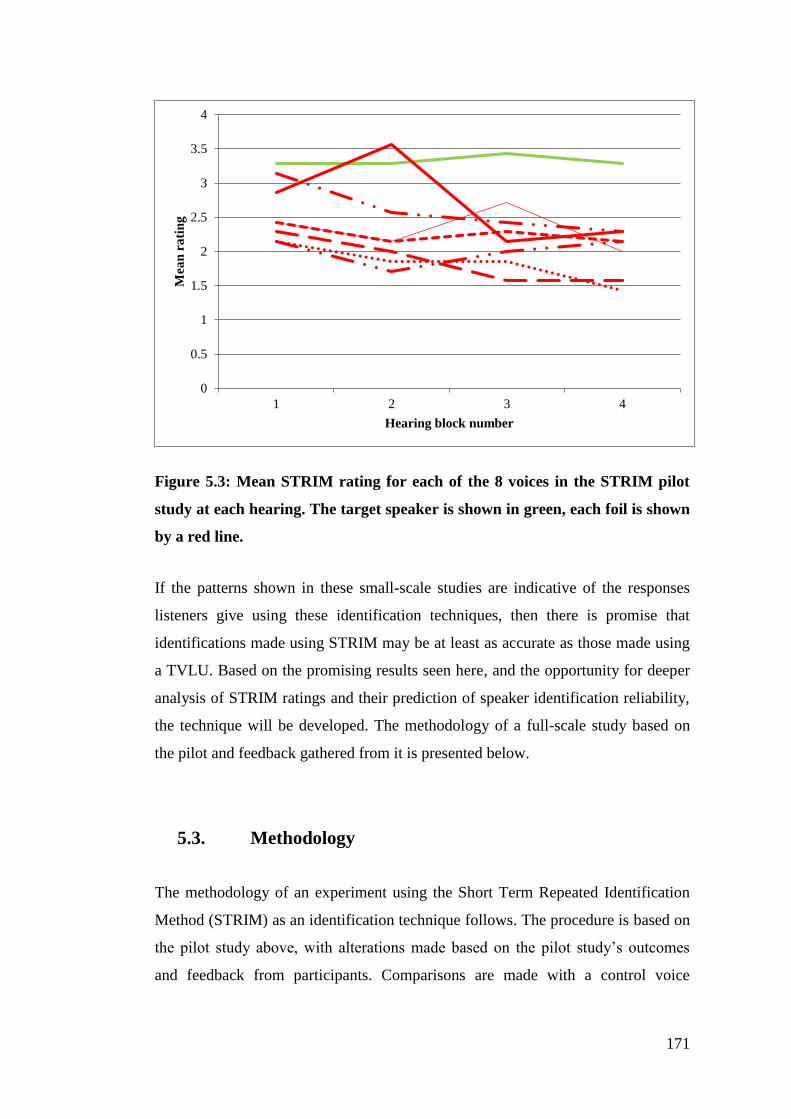
171
Figure 5.3: Mean STRIM rating for each of the 8 voices in the STRIM pilot
study at each hearing. The target speaker is shown in green, each foil is shown
by a red line.
If the patterns shown in these small-scale studies are indicative of the responses
listeners give using these identification techniques, then there is promise that
identifications made using STRIM may be at least as accurate as those made using
a TVLU. Based on the promising results seen here, and the opportunity for deeper
analysis of STRIM ratings and their prediction of speaker identification reliability,
the technique will be developed. The methodology of a full-scale study based on
the pilot and feedback gathered from it is presented below.
5.3. Methodology
The methodology of an experiment using the Short Term Repeated Identification
Method (STRIM) as an identification technique follows. The procedure is based on
the pilot study above, with alterations made based on the pilot study’s outcomes
and feedback from participants. Comparisons are made with a control voice
0
0.5
1
1.5
2
2.5
3
3.5
4
1 2 3 4
Mea
n r
ati
ng
Hearing block number
172
identification task, using the Traditional Voice Lineup (TVLU) methodology. The
results and discussion from this comparison will provide the basis of Chapter 6.
The methodology also involves the investigation of other listener variables, such as
listener accent, age and sex. These additional research variables were all controlled
and so a fair comparison between STRIM and TVLU can be made, though the
impact of these will be assessed in Chapter 6. The conditions under which the
listener was exposed to the target speaker was also varied. The results of this
comparison will be presented in Chapter 7.
5.3.1. Design
Listeners took part in a speaker identification task. They were exposed to a single
voice and then later asked to identify that speaker from within a selection of voices.
The experiment allowed for the following conditions and variables to be tested:
Conditions under which the listener was exposed to the voice
The voice heard as exposure/perpetrator
Listener variables, such as accent, age and sex
Method by which the listener’s ability to identify the voice was tested
Listeners were exposed to the voice using one of three methods, differences
between which will be discussed in Chapter 7
Audio only (Ao)
Audio + picture (AP)
Audio + video (AV)
The audio was consistent across the three exposure conditions (EC) (information
relating to the content of the speech is in §5.3.4. below). Listeners in the Ao
condition were seated at a computer in a quiet room and heard the audio stimulus
through closed cup headphones. Listeners in the AP condition underwent the same
procedure, but on the computer screen images of a crime being committed
(mirroring the one heard through the headphones) were shown. Listeners in the AV
condition stood in the 3Sixty room at the University of York which measures
6.85m x 6.85m (University of York, 2015). There are full-wall projections on all
173
four sides. A video of a crime being committed is shown on one wall, whilst the
audio of the video is played through 32 loudspeakers around the room (the same
audio as in the other conditions).
5.3.2. Voices
There were three target speakers used in the role of perpetrator in this experiment.
This negates the effect of any speaker specific effects on the study and also allows
for listeners to take part in repeated measures identification tasks. The exposure
sample speech was provided by speakers who contributed to the YorViS database,
recorded by the experimenter and Kirsty McDougall as part of the latter’s British
Academy grant (McDougall, 2013b). Speakers in the YorViS database all:
grew up in York or very close to York,
have spent most of their lives in the York area
are judged to have a regional York working class accent
are male, aged 18-25
The lineup samples were taken from this database, but in order to use speech
suitable for the present experiment, the exposure speech was not taken directly
from the database itself. Instead, materials tailored to the experiment were created
by the experiment and three YorViS speakers were invited back and re-recorded
after the database recordings had been made.
The exposure sample is a direct recording of the speaker simulating a crime in the
role of the perpetrator. The recording took place in an open air environment – a
riverside pathway in York. There was ambient background noise, such as people
talking in the distance, but nothing which would be likely to distract from the
perpetrator’s voice. In the recording, the perpetrator can be heard talking on a
telephone, with the interlocutor’s voice not heard, making an arrangement to meet
up. Once the phone call is ended, the perpetrator then speaks to the listener (the
participant in the experiment) – although given that the materials are recorded and
not live, the interaction is purely simulated. The sample lasts around 60 seconds in
total. The event was also video recorded for use in the AV condition. Stills from
the video are used in the AP condition.
174
The voices which acted as samples in the subsequent identification phase of the
experiment were also speakers from the YorViS database. Unlike the exposure
samples, the materials for the foils were taken directly from the database. Task 1
materials - a mock police interview - were used. This best matches the natural,
spontaneous speech used in forensic cases in England and Wales where materials
are predominantly taken from police interview recordings. The recordings are of
studio quality and so are likely to be of superior fidelity to those commonly used in
applied cases. This is consistent across all conditions, however, and does not
present an experimental concern.
The construction of the identification samples differed between testing conditions
(as in the STRIM pilot study in §5.2.2. ). The speech materials for the two testing
conditions were consistent, but STRIM materials were split into smaller blocks of
speech for presentation. The choice of foils in the lineups was made based on
Euclidean distances from the target speaker, ensuring that foils had differing levels
of similarity to the target, as in de Jong et al. (2015).
5.3.3. Listeners
A total of 82 British English listeners were recruited using online advertising and
friend-of-a-friend recruiting. Their mean age was 31.1 years of age (SD = 10.4
years). The oldest listeners were in the age range 46-55; the youngest in the range
18-25. There were 40 males and 42 females in the experiment; and 28 listeners
from York and 54 living in York but not having grown up there. None of them
reported a history of hearing impairment, and all had normal or corrected-to-
normal vision (relevant for the AP and AV exposure conditions). All listeners
participated in the experiment either in return for a small remuneration or as a
favour to the experimenter. In terms of the listener accent variable, the same
local/non-local group distinction as in Chapter 4 could not be replicated. Due to the
experiment needing to take place in York (with access to the 3Sixty screen), even
non-local listeners had some familiarity with the local accent with most living in
the area.

175
5.3.4. Procedure
Pre-exposure and exposure phases
Prior to taking part in the experiment, listeners were informed about selected
elements of the procedure so that they could grant their informed consent to
participate but as much ecological validity was retained as possible. Listeners were
placed into a suitable condition based on their known or predicted age, sex and
accent variables. Roughly equal numbers of listeners within each variable were
placed into each exposure condition (Ao, AP or AV), were exposed to each
exposure voice and tested using each testing method (TVLU or STRIM).
Listeners were advised that they would be exposed to some materials. This was left
suitably vague so as not to bias them towards listening to the voice over watching
the pictures or video in the relevant exposure conditions. They were instructed to
pay attention to what they could see and hear, but were not informed which aspects
were of particular importance (speaker, audio content, visual information, etc.). It
is hoped that this is a fair reflection of how witnesses to crimes are exposed to such
materials in real life. If a decision is made to pay particular focus to certain aspects
of the stimulus then this should be made during the course of exposure, rather than
through prior warning. Listeners were provided with a short information sheet
before beginning the experiment. They could view this beforehand and also keep it
with them during the experiment.
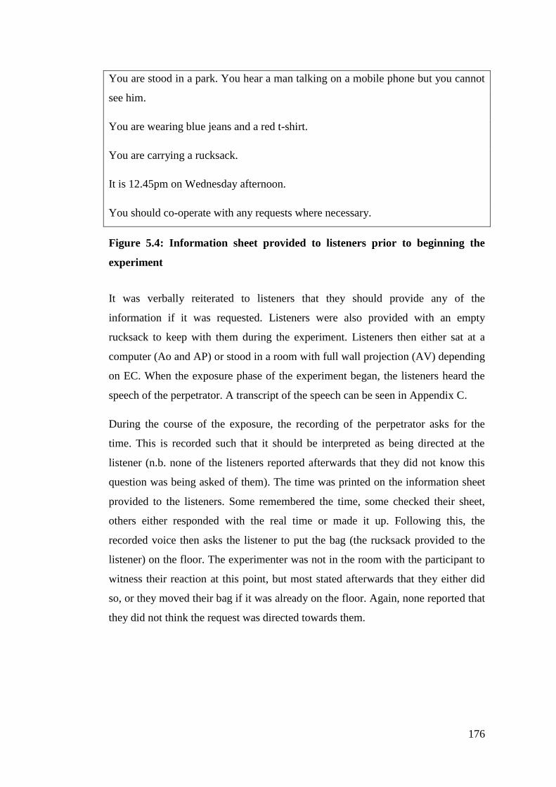
176
You are stood in a park. You hear a man talking on a mobile phone but you cannot
see him.
You are wearing blue jeans and a red t-shirt.
You are carrying a rucksack.
It is 12.45pm on Wednesday afternoon.
You should co-operate with any requests where necessary.
Figure 5.4: Information sheet provided to listeners prior to beginning the
experiment
It was verbally reiterated to listeners that they should provide any of the
information if it was requested. Listeners were also provided with an empty
rucksack to keep with them during the experiment. Listeners then either sat at a
computer (Ao and AP) or stood in a room with full wall projection (AV) depending
on EC. When the exposure phase of the experiment began, the listeners heard the
speech of the perpetrator. A transcript of the speech can be seen in Appendix C.
During the course of the exposure, the recording of the perpetrator asks for the
time. This is recorded such that it should be interpreted as being directed at the
listener (n.b. none of the listeners reported afterwards that they did not know this
question was being asked of them). The time was printed on the information sheet
provided to the listeners. Some remembered the time, some checked their sheet,
others either responded with the real time or made it up. Following this, the
recorded voice then asks the listener to put the bag (the rucksack provided to the
listener) on the floor. The experimenter was not in the room with the participant to
witness their reaction at this point, but most stated afterwards that they either did
so, or they moved their bag if it was already on the floor. Again, none reported that
they did not think the request was directed towards them.
177
Post-exposure phase
Once listeners had heard (and, for some, seen) the exposure material, they were
told that they should treat the experience as if they were a witness to a crime being
committed. They were informed that they would be asked some questions about
what they had just seen/heard. The experimenter asked a series of questions, the
precise number and nature of which differed depending on (i) the exposure
condition and (ii) how different listeners responded to questions. If listeners were
unwilling or unable to provide responses to any of the questions, they were not
pushed to do so. The broad questions to which some response was sought were:
Can you tell me what happened?
What did you see?
Can you describe the person?
Do you remember what the person said?
What did the person sound like?
Once this information had been established, listeners were then told that it was felt
that the voice was the best method of identifying the ‘criminal’. They were told that
they would later hear a selection of voices, one of which may or may not be that of
the person they had just heard. At this point, listeners were asked to rate how
confident they were that they would later be able to correctly identify the speaker
on a Likert scale from one (not very confident) to five (very confident). Listeners
were asked to return at an agreed time (between 2-4 hours later). A delay was
introduced to allow some small degradation of the listener’s memory of the voice
(as in Philippon, Cherryman, Bull and Vrij (2007a) amongst others). To ensure that
the listener was most likely to return for the testing phase, however, they were
asked to do so on the same day.
Testing phase
Listeners had already been placed by the experimenter into one of two testing
conditions prior to exposure, either TVLU or STRIM. The testing phase always
178
involved a target present selection. The procedure employed in each condition is
outlined here.
The testing method in this condition resembled the procedure used in section
§4.2.3. , as laid out by the McFarlane Guidelines (Home Office, 2003). Contrary to
the police’s applied methods, only six voices were used for testing in the study (1
target + 5 foils). This ensured a better comparison with results obtained from
STRIM testing, which only used six voices in the testing phase (the reasons for
which are outlined below).
Listeners were seated at a desk and briefed on what was about to happen. The
experimenter reinforced that they should treat the previous events as criminal
activity and that they were now going to be take part in a study to see whether they
could identify the voice of the criminal. They were then provided with the text in
Figure 5.5 below, which is adapted from Broeders & van Amelsvoort’s (1999)
advice on the administering of a forensic earwitness lineup.
Once satisfied, the listeners were provided with a PC and Sennheiser HD335s
closed cup headphones. The experimenter played the six voices, as per the
instructions, using Microsoft PowerPoint. Whenever a voice was being played, a
label (“Speaker A” through to “Speaker F”) was displayed. The voices were
repeated as requested by the listener until an identification (or no identification)
was made. The number of listens and decision were recorded by the experimenter.
The listener was then asked whether they could comment on what influenced their
decision and this was also noted. If a response was made (i. or ii. in
Figure 5.5) then listeners were again asked to rate their confidence in their decision
on a scale from 1-5. If no response was made (iii. in
Figure 5.5) then listeners were not asked to rate their confidence.
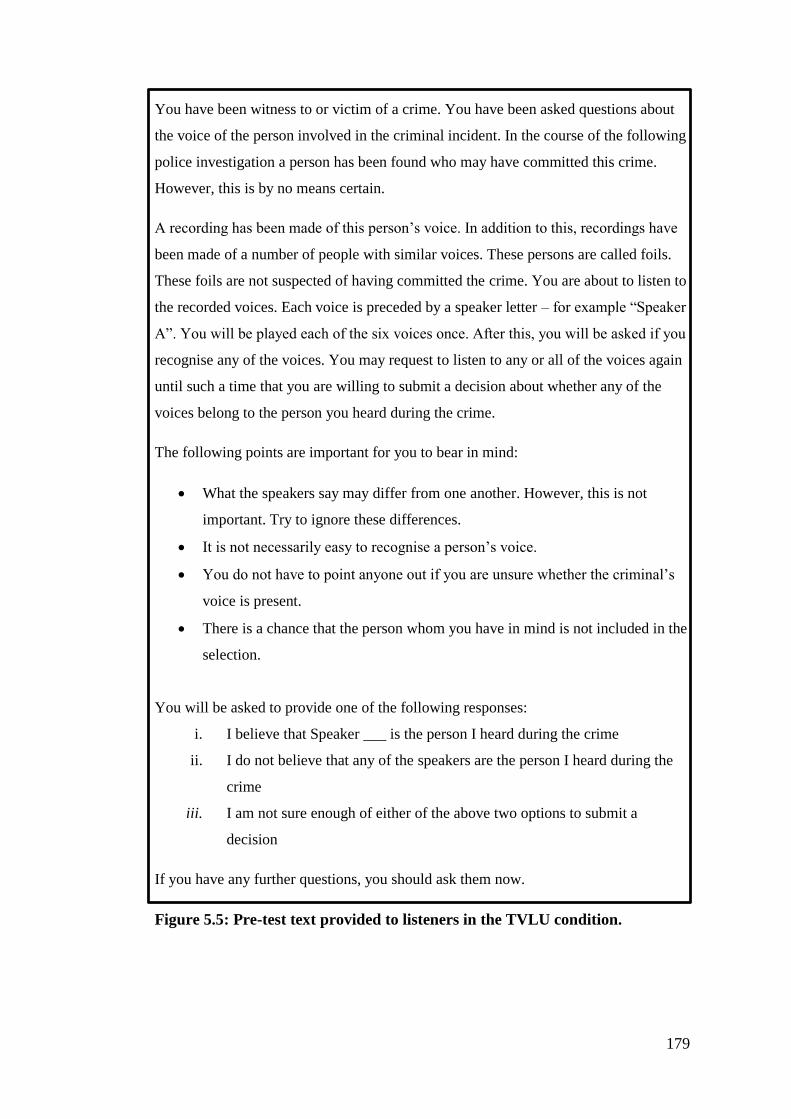
179
You have been witness to or victim of a crime. You have been asked questions about
the voice of the person involved in the criminal incident. In the course of the following
police investigation a person has been found who may have committed this crime.
However, this is by no means certain.
A recording has been made of this person’s voice. In addition to this, recordings have
been made of a number of people with similar voices. These persons are called foils.
These foils are not suspected of having committed the crime. You are about to listen to
the recorded voices. Each voice is preceded by a speaker letter – for example “Speaker
A”. You will be played each of the six voices once. After this, you will be asked if you
recognise any of the voices. You may request to listen to any or all of the voices again
until such a time that you are willing to submit a decision about whether any of the
voices belong to the person you heard during the crime.
The following points are important for you to bear in mind:
What the speakers say may differ from one another. However, this is not
important. Try to ignore these differences.
It is not necessarily easy to recognise a person’s voice.
You do not have to point anyone out if you are unsure whether the criminal’s
voice is present.
There is a chance that the person whom you have in mind is not included in the
selection.
You will be asked to provide one of the following responses:
i. I believe that Speaker ___ is the person I heard during the crime
ii. I do not believe that any of the speakers are the person I heard during the
crime
iii. I am not sure enough of either of the above two options to submit a
decision
If you have any further questions, you should ask them now.
Figure 5.5: Pre-test text provided to listeners in the TVLU condition.

180
The STRIM procedure uses the same speech materials as the TVLU technique, but
how they are presented to the listener differs. In the former, listeners were not
asked to identify a single speech sample which they recognised as belonging to the
‘criminal’. Rather, they were asked to provide ratings on how likely they believe a
series of voices are to belong to the ‘criminal’, as outlined in the STRIM pilot
study (§5.2.2. ).
Listeners heard voices belonging to six speakers – the same six speakers as
listeners heard in testing phase of the corresponding TVLU condition. In applied
settings, there are eight voices (suspect + seven foils) in the testing phase.
Feedback from a number of listeners in the STRIM pilot study stated that they felt
the task became monotonous and they were paying less attention to the voices
towards the end of the study. Consequently, the number of speakers was reduced
from eight to six. This renders the experimental TVLU not directly comparable
with real-world earwitness testing. It was felt, however, that a detailed
understanding of how STRIM performs as a testing method should be the initial
focus. The first step in this is a comparison between these two experimental
designs.
The speech heard was the same across the two identification methods - a total of
c.60 seconds of speech from each speaker. In the TVLU a single 60 second sample
of speech was heard for each speaker, and each speaker was labelled as being
different from one another. This means that listeners are making a single yes/no
judgement about different speakers and are fully aware of this.
In the STRIM condition, the same 60 second samples from the TVLU condition
were divided into three 20 second samples. This differs from the pilot study, where
four 15 second samples were used. This is again based on feedback from listeners,
who felt that some of the individual samples were too short to make a judgement
on. This is despite the fact that all samples were roughly the same length. The
length was therefore increased, and resultantly the number of samples was
decreased. This also has the added benefit of reducing the number of ratings which
each listener has to be provide, whilst still clearly allowing for more than TVLU.
As stated above, the provision of too many ratings was a concern for listeners in
the pilot study. Listeners were given no indication of whether or not these samples
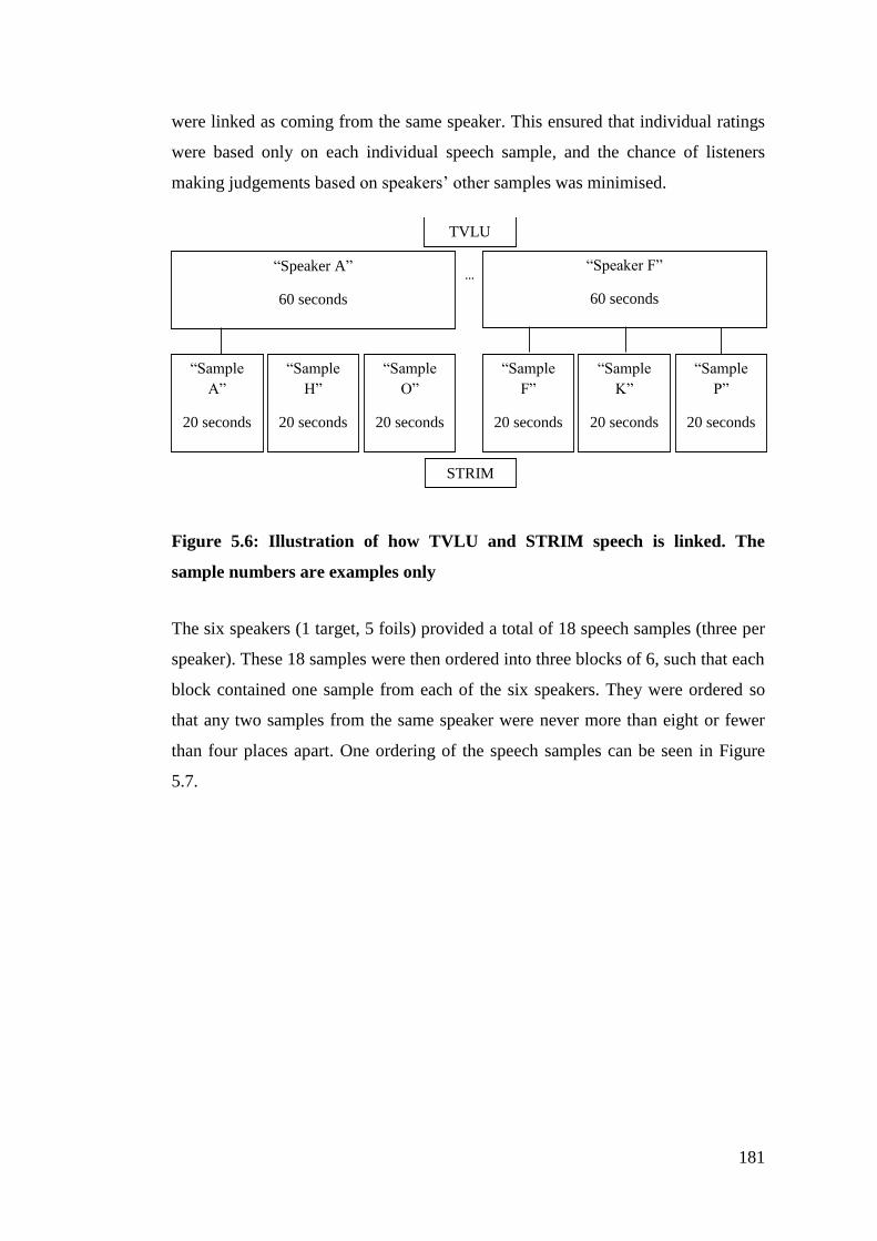
181
were linked as coming from the same speaker. This ensured that individual ratings
were based only on each individual speech sample, and the chance of listeners
making judgements based on speakers’ other samples was minimised.
Figure 5.6: Illustration of how TVLU and STRIM speech is linked. The
sample numbers are examples only
The six speakers (1 target, 5 foils) provided a total of 18 speech samples (three per
speaker). These 18 samples were then ordered into three blocks of 6, such that each
block contained one sample from each of the six speakers. They were ordered so
that any two samples from the same speaker were never more than eight or fewer
than four places apart. One ordering of the speech samples can be seen in Figure
5.7.
“Sample
A”
20 seconds
“Sample
H”
20 seconds
“Sample
O”
20 seconds
“Sample
F”
20 seconds
“Sample
K”
20 seconds
“Sample
P”
20 seconds
“Speaker A”
60 seconds
“Speaker F”
60 seconds
…
STRIM
TVLU
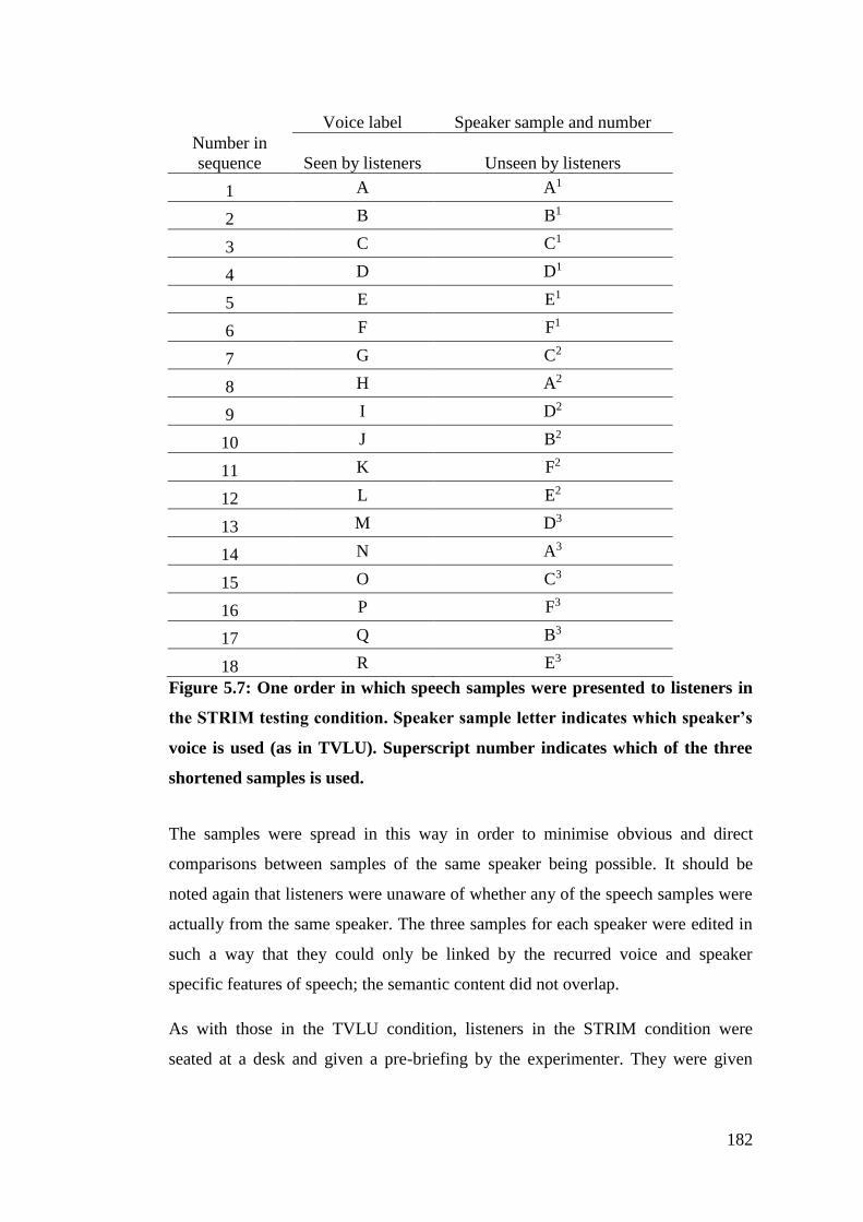
182
Voice label Speaker sample and number
Number in
sequence Seen by listeners Unseen by listeners
1 A A1
2 B B1
3 C C1
4 D D1
5 E E1
6 F F1
7 G C2
8 H A2
9 I D2
10 J B2
11 K F2
12 L E2
13 M D3
14 N A3
15 O C3
16 P F3
17 Q B3
18 R E3
Figure 5.7: One order in which speech samples were presented to listeners in
the STRIM testing condition. Speaker sample letter indicates which speaker’s
voice is used (as in TVLU). Superscript number indicates which of the three
shortened samples is used.
The samples were spread in this way in order to minimise obvious and direct
comparisons between samples of the same speaker being possible. It should be
noted again that listeners were unaware of whether any of the speech samples were
actually from the same speaker. The three samples for each speaker were edited in
such a way that they could only be linked by the recurred voice and speaker
specific features of speech; the semantic content did not overlap.
As with those in the TVLU condition, listeners in the STRIM condition were
seated at a desk and given a pre-briefing by the experimenter. They were given
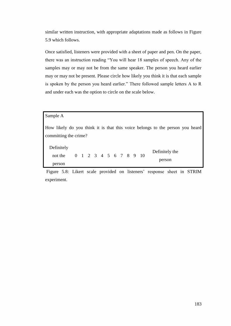
183
similar written instruction, with appropriate adaptations made as follows in Figure
5.9 which follows.
Once satisfied, listeners were provided with a sheet of paper and pen. On the paper,
there was an instruction reading “You will hear 18 samples of speech. Any of the
samples may or may not be from the same speaker. The person you heard earlier
may or may not be present. Please circle how likely you think it is that each sample
is spoken by the person you heard earlier.” There followed sample letters A to R
and under each was the option to circle on the scale below.
Sample A
How likely do you think it is that this voice belongs to the person you heard
committing the crime?
Definitely
not the
person
0 1 2 3 4 5 6 7 8 9 10 Definitely the
person
Figure 5.8: Likert scale provided on listeners’ response sheet in STRIM
experiment.
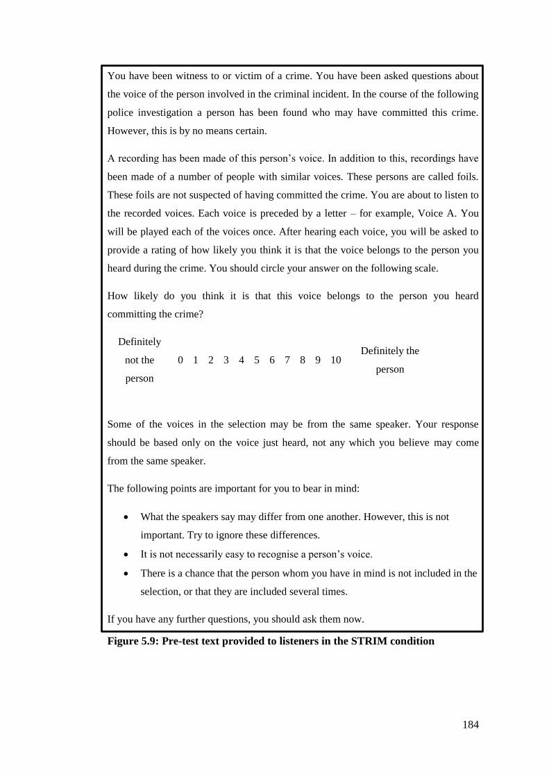
184
You have been witness to or victim of a crime. You have been asked questions about
the voice of the person involved in the criminal incident. In the course of the following
police investigation a person has been found who may have committed this crime.
However, this is by no means certain.
A recording has been made of this person’s voice. In addition to this, recordings have
been made of a number of people with similar voices. These persons are called foils.
These foils are not suspected of having committed the crime. You are about to listen to
the recorded voices. Each voice is preceded by a letter – for example, Voice A. You
will be played each of the voices once. After hearing each voice, you will be asked to
provide a rating of how likely you think it is that the voice belongs to the person you
heard during the crime. You should circle your answer on the following scale.
How likely do you think it is that this voice belongs to the person you heard
committing the crime?
Definitely
not the
person
0 1 2 3 4 5 6 7 8 9 10 Definitely the
person
Some of the voices in the selection may be from the same speaker. Your response
should be based only on the voice just heard, not any which you believe may come
from the same speaker.
The following points are important for you to bear in mind:
What the speakers say may differ from one another. However, this is not
important. Try to ignore these differences.
It is not necessarily easy to recognise a person’s voice.
There is a chance that the person whom you have in mind is not included in the
selection, or that they are included several times.
If you have any further questions, you should ask them now.
Figure 5.9: Pre-test text provided to listeners in the STRIM condition
185
The scale of response options was increased from five (1-5) in the pilot study to 11
(0-10) here, again following feedback from listeners. A number of participants
commented that they wanted the inclusion of 0 as an option for when they did not
believe that the sample could have been from the perpetrator at all. They also
reported that a larger scale may encourage them to use a wider range of ratings,
with some listeners feeling inclined to consistently rate samples as 3 out 5 in the
pilot study (indeed, there was a high proportion of this rating). Whilst 5 and 7-point
Likert scales are more common, an 11-point scale was used here to offer more
points of discrimination. Nunnally (1978) suggests that beyond 11, there is a
diminishing return. The use of a 0 option on the scale is also not common, but no
strong argument can be found against its inclusion. The fact that is offered a clear
choice for listeners to make a firm ‘definitely not the person’ response was deemed
beneficial.
Listeners were provided with the same listening apparatus as those in the TVLU
condition. The speech samples were played using PowerPoint. Rather than
“Speaker A”, etc. representing each sample, the STRIM speech samples were
labelled as “Sample A” through to “Sample R”. The label of sample rather than
speaker was chosen to disguise any repetition of a particular speaker within the set.
After a response was provided, the experimenter, controlling the PowerPoint slides,
moved onto the next sample. As per the instructions, listeners were given no
information as to whether this voice belonged to a speaker previously heard or not.
They were again asked to provide a rating, and this was repeated until all 18
samples (6 speakers, 3 samples each) were heard and rated.
Once listeners in both conditions had completed the identification process, they
were debriefed. The full extent of this debriefing varied between
listeners/conditions. Some listeners took part in repeated measures testing and so
could only be fully debriefed on the aims of the study once all identifications had
been made. Following any initial identification(s), listeners were told that they
would be fully debriefed once their participation had been concluded.
Those listeners whose participation in the study was incomplete were thanked for
their contribution, and arrangements were made for their continued involvement.
186
Those listeners whose participation was complete were informed of the true nature
of the study and how their responses were going to be analysed. They were given
the opportunity to request an overview of the results, but were assured that their
own responses would remain anonymised. They were not told which the target
speaker/voice was and were asked not to divulge details of the experiment to any
other potential participants.
The nature of the repeated measures testing is explained fully in section Chapter 7.
Each identification task (exposure and testing phases) took approximately 25-35
minutes to complete (excluding the enforced break between phases). The study was
approved by the University of York Humanities and Social Sciences Ethics
Committee.
187
5.4. Results
This chapter will present the results from the experiment outlined in the previous
chapter. The accuracy of speaker identifications made by naïve listeners using the
Traditional Voice Lineup (TVLU) and Short Term Repeated Identification Method
(STRIM) will be assessed, and different techniques of analysing the data provided
by the latter will be considered. The effect of other listener variables (age, sex,
accent) will also be presented and a discussion of the two methods of testing will
follow.
5.4.1. Traditional Voice Lineup
The methods employed here were covered in §5.3.4. Listeners heard the voice of a
perpetrator, taken from the YorVis database - and so a young, working class, White
male speaker of York English (YE). The recorded voice asked for the listeners’
bag. Some listeners only heard the audio of the perpetrator, others saw
accompanying photos, and others witnessed a video of the event. The exposure
lasted for around 60 seconds. They were then tested on their ability to identify the
perpetrator by their voice after a 2-4 hour delay. Listeners were presented with a
lineup of 6 voices (each 60 seconds long) and asked whether any of them belonged
to the person who took their bag. The target was present in each lineup. There were
three speaker conditions, each one using a different perpetrator/target voice.
Listeners
A total of 42 listeners were asked to make identifications using this method. The
average age of the listeners was 30.9 years old (SD = 10.6 years). The youngest
were from the 18-25 age group; the oldest from the 46-55. There were 21 males
and 21 females in the condition.
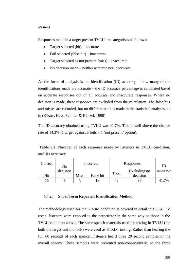
188
Results
Responses made in a target present TVLU are categorises as follows:
Target selected (hit) - accurate
Foil selected (false hit) – inaccurate
Target selected as not present (miss) – inaccurate
No decision made – neither accurate nor inaccurate
As the focus of analysis is the identification (ID) accuracy – how many of the
identifications made are accurate – the ID accuracy percentage is calculated based
on accurate responses out of all accurate and inaccurate responses. Where no
decision is made, these responses are excluded from the calculation. The false hits
and misses are recorded, but no differentiation is made in the statistical analyses, as
in (Köster, Hess, Schiller & Künzel, 1998)
The ID accuracy obtained using TVLU was 41.7%. This is well above the chance
rate of 14.3% (1 target against 5 foils + 1 ‘not present’ option).
Table 5.1: Number of each response made by listeners in TVLU condition,
and ID accuracy
Correct No
decision
Incorrect Responses ID
accuracy
Hit Miss False hit Total
Excluding no
decision
15 6 3 18 42 36 41.7%
5.4.2. Short Term Repeated Identification Method
The methodology used for the STRIM condition is covered in detail in §5.3.4. To
recap, listeners were exposed to the perpetrator in the same way as those in the
TVLU condition above. The same speech materials used for testing in TVLU (for
both the target and the foils) were used as STRIM testing. Rather than hearing the
full 60 seconds of each speaker, listeners heard three 20 second samples of the
overall speech. These samples were presented non-consecutively, so the three
189
samples for each speaker (totalling 60 seconds) were spread throughout the task.
Consequently, listeners heard eighteen 20 second samples of speech (three for each
of the six speakers). No information was given as to whether any of the samples
were from the same speaker or not. After hearing each sample, listeners were asked
to rate (on a scale from 0-10) how likely they felt that voice was that of the
criminal.
Repeated measures testing was used here. Listeners took part in three STRIM
tasks. Each task involved a different target speaker and different exposure
condition (audio only, audio + picture, audio + video).
Listeners
A total of 40 listeners made identifications using STRIM. The average age of the
listeners was 31.3 years old (SD = 10.2 years). The youngest were from the 18-25
age group; the oldest from the 46-55. There were 21 male and 19 female listeners
in the experiment.
Each of these listeners was intended to take part in three speaker identification
tasks using STRIM as the testing method. A small number of these listeners did not
perform all three of the tasks, either because no mutually convenient time could be
arranged for follow up testing or the listener did not show up when scheduled. As a
result, 113 of the scheduled 120 identifications were made by listeners using
STRIM (34 listeners making three identifications, 5 making two, and 1 making
one). The results from the six listeners who did not take part in all tasks will still be
included in the analyses as there is still an equal number of tests using each
exposure condition and target speaker. Where it is relevant to exclude their
responses, this will be noted.
Analyses conducted
Due to the nature of responses made using STRIM, the results obtained do not
neatly provide an identification accuracy figure which can be compared against
TVLU. These responses are not straightforwardly correct or incorrect. This is,
infact, part of the justification for considering this approach. A number of ways of
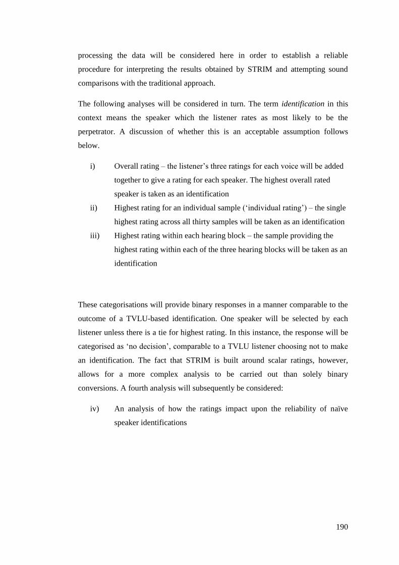
190
processing the data will be considered here in order to establish a reliable
procedure for interpreting the results obtained by STRIM and attempting sound
comparisons with the traditional approach.
The following analyses will be considered in turn. The term identification in this
context means the speaker which the listener rates as most likely to be the
perpetrator. A discussion of whether this is an acceptable assumption follows
below.
i) Overall rating – the listener’s three ratings for each voice will be added
together to give a rating for each speaker. The highest overall rated
speaker is taken as an identification
ii) Highest rating for an individual sample (‘individual rating’) – the single
highest rating across all thirty samples will be taken as an identification
iii) Highest rating within each hearing block – the sample providing the
highest rating within each of the three hearing blocks will be taken as an
identification
These categorisations will provide binary responses in a manner comparable to the
outcome of a TVLU-based identification. One speaker will be selected by each
listener unless there is a tie for highest rating. In this instance, the response will be
categorised as ‘no decision’, comparable to a TVLU listener choosing not to make
an identification. The fact that STRIM is built around scalar ratings, however,
allows for a more complex analysis to be carried out than solely binary
conversions. A fourth analysis will subsequently be considered:
iv) An analysis of how the ratings impact upon the reliability of naïve
speaker identifications

191
5.5. Results
5.5.1. Overall rating (binary classification)
In each task using STRIM as the testing method, listeners provided 18 ratings in
response to the question How likely do you think it is that this voice belongs to the
person you heard committing the crime? Each of these ratings was given out of 10
and, unbeknownst to the listeners, the 18 voice samples were made up of six
speakers (A to F) each contributing three samples (1, 2 and 3). Thus, each of the six
speakers was given three ratings out of 10. These ratings for each speaker (A1 + A2
+ A3) were added together to give an overall rating out of 30. These overall ratings
can be used to determine which of the six speakers each listener rated as being the
most likely be the perpetrator. Methodologically, this is not analogous to asking
listeners to make a single selection of which voice they believe to be the
perpetrator, as in a TVLU.
Nevertheless, the aim of a TVLU is to determine which of the speakers, if any, the
listener believes to be the criminal. Excluding those making no decision, this
explicitly represents the single voice which listeners believe is more likely than the
other options to be that of the criminal. Responses made using STRIM make the
same selection - which speaker is most likely, relative to the other options, to be the
perpetrator. This does not necessarily mean that even if a listener rates a particular
voice highest overall then they would single that voice out as being the perpetrator.
For the sake of experimental comparison, though, a voice being rated as highest
using STRIM will be considered as comparable to an identification using TVLU.
The term comparable here is important as it is not claimed that the two are
different methods of reaching the same decision. Results obtained using STRIM
are much more implicit; this may or may not be beneficial to the identification of a
speaker. In a forensic context, caution should be applied when making judgements
about naïve listeners’ implicit judgements. If identification accuracy results
obtained through STRIM are superior to those using TVLU, however, it may
suggest that further consideration should be given to whether the established
practice is the best method of eliciting a response.
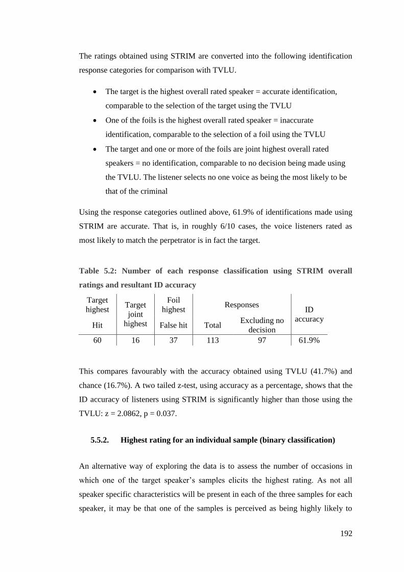
192
The ratings obtained using STRIM are converted into the following identification
response categories for comparison with TVLU.
The target is the highest overall rated speaker = accurate identification,
comparable to the selection of the target using the TVLU
One of the foils is the highest overall rated speaker = inaccurate
identification, comparable to the selection of a foil using the TVLU
The target and one or more of the foils are joint highest overall rated
speakers = no identification, comparable to no decision being made using
the TVLU. The listener selects no one voice as being the most likely to be
that of the criminal
Using the response categories outlined above, 61.9% of identifications made using
STRIM are accurate. That is, in roughly 6/10 cases, the voice listeners rated as
most likely to match the perpetrator is in fact the target.
Table 5.2: Number of each response classification using STRIM overall
ratings and resultant ID accuracy
Target
highest Target
joint
highest
Foil
highest Responses
ID
accuracy Hit False hit Total
Excluding no
decision
60 16 37 113 97 61.9%
This compares favourably with the accuracy obtained using TVLU (41.7%) and
chance (16.7%). A two tailed z-test, using accuracy as a percentage, shows that the
ID accuracy of listeners using STRIM is significantly higher than those using the
TVLU: z = 2.0862, p = 0.037.
5.5.2. Highest rating for an individual sample (binary classification)
An alternative way of exploring the data is to assess the number of occasions in
which one of the target speaker’s samples elicits the highest rating. As not all
speaker specific characteristics will be present in each of the three samples for each
speaker, it may be that one of the samples is perceived as being highly likely to
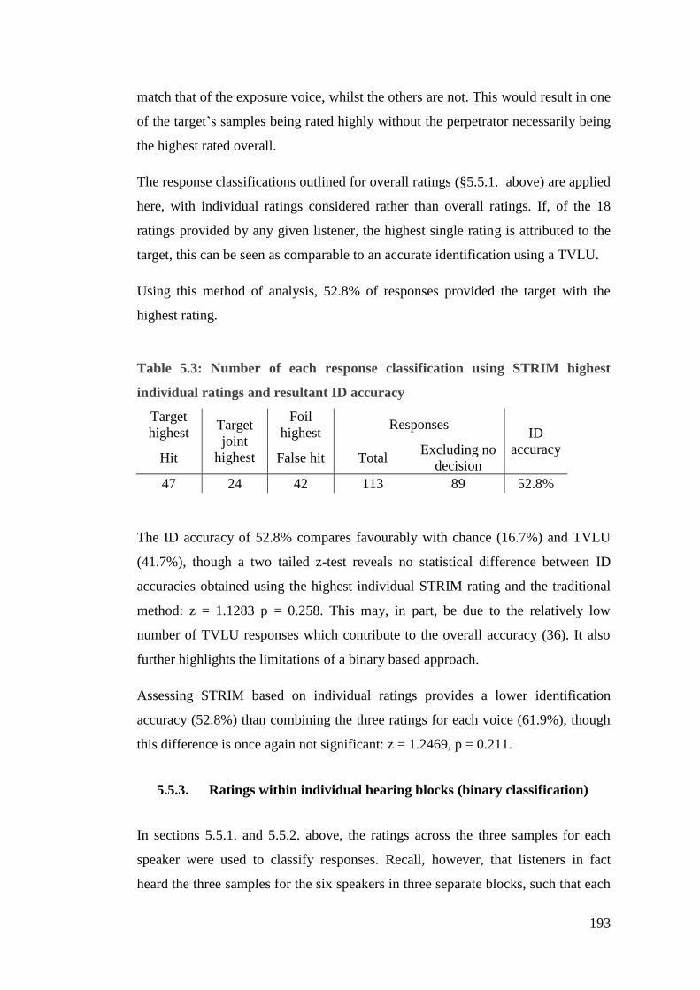
193
match that of the exposure voice, whilst the others are not. This would result in one
of the target’s samples being rated highly without the perpetrator necessarily being
the highest rated overall.
The response classifications outlined for overall ratings (§5.5.1. above) are applied
here, with individual ratings considered rather than overall ratings. If, of the 18
ratings provided by any given listener, the highest single rating is attributed to the
target, this can be seen as comparable to an accurate identification using a TVLU.
Using this method of analysis, 52.8% of responses provided the target with the
highest rating.
Table 5.3: Number of each response classification using STRIM highest
individual ratings and resultant ID accuracy
Target
highest Target
joint
highest
Foil
highest Responses
ID
accuracy Hit False hit Total
Excluding no
decision
47 24 42 113 89 52.8%
The ID accuracy of 52.8% compares favourably with chance (16.7%) and TVLU
(41.7%), though a two tailed z-test reveals no statistical difference between ID
accuracies obtained using the highest individual STRIM rating and the traditional
method: z = 1.1283 p = 0.258. This may, in part, be due to the relatively low
number of TVLU responses which contribute to the overall accuracy (36). It also
further highlights the limitations of a binary based approach.
Assessing STRIM based on individual ratings provides a lower identification
accuracy (52.8%) than combining the three ratings for each voice (61.9%), though
this difference is once again not significant: z = 1.2469, p = 0.211.
5.5.3. Ratings within individual hearing blocks (binary classification)
In sections 5.5.1. and 5.5.2. above, the ratings across the three samples for each
speaker were used to classify responses. Recall, however, that listeners in fact
heard the three samples for the six speakers in three separate blocks, such that each
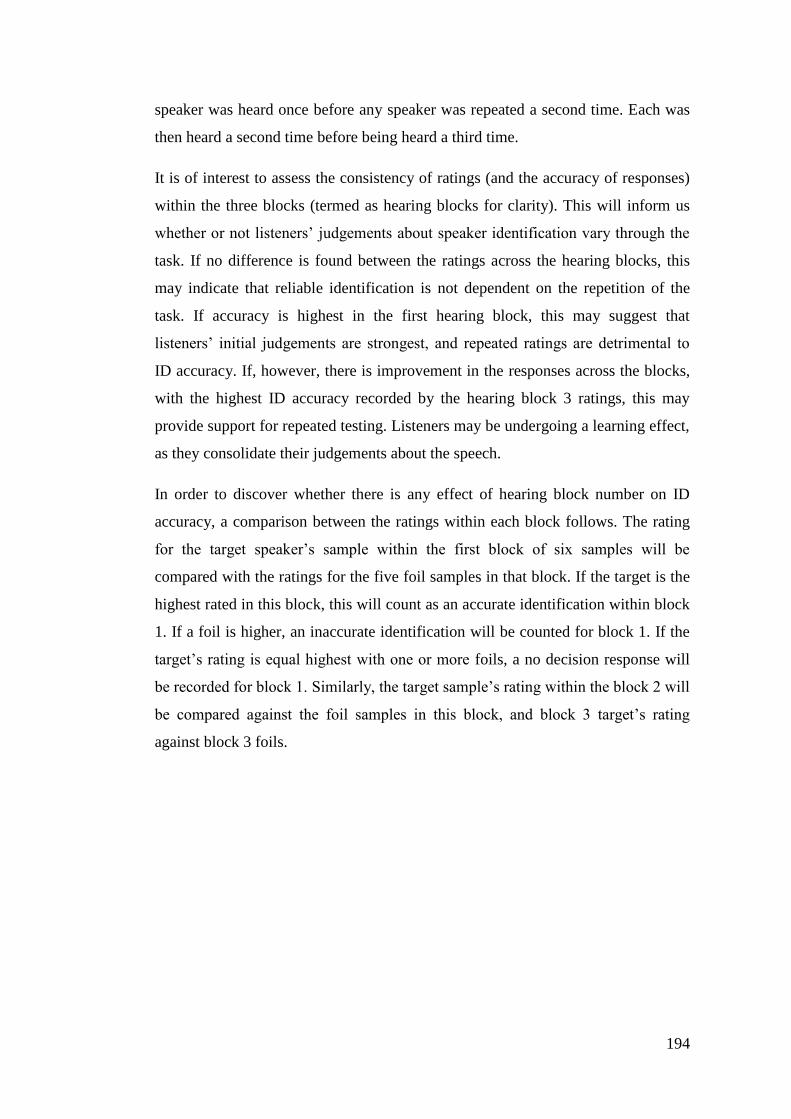
194
speaker was heard once before any speaker was repeated a second time. Each was
then heard a second time before being heard a third time.
It is of interest to assess the consistency of ratings (and the accuracy of responses)
within the three blocks (termed as hearing blocks for clarity). This will inform us
whether or not listeners’ judgements about speaker identification vary through the
task. If no difference is found between the ratings across the hearing blocks, this
may indicate that reliable identification is not dependent on the repetition of the
task. If accuracy is highest in the first hearing block, this may suggest that
listeners’ initial judgements are strongest, and repeated ratings are detrimental to
ID accuracy. If, however, there is improvement in the responses across the blocks,
with the highest ID accuracy recorded by the hearing block 3 ratings, this may
provide support for repeated testing. Listeners may be undergoing a learning effect,
as they consolidate their judgements about the speech.
In order to discover whether there is any effect of hearing block number on ID
accuracy, a comparison between the ratings within each block follows. The rating
for the target speaker’s sample within the first block of six samples will be
compared with the ratings for the five foil samples in that block. If the target is the
highest rated in this block, this will count as an accurate identification within block
1. If a foil is higher, an inaccurate identification will be counted for block 1. If the
target’s rating is equal highest with one or more foils, a no decision response will
be recorded for block 1. Similarly, the target sample’s rating within the block 2 will
be compared against the foil samples in this block, and block 3 target’s rating
against block 3 foils.
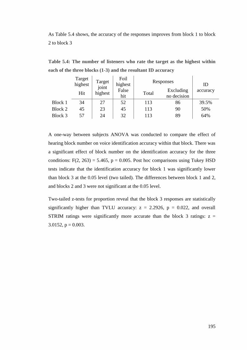
195
As Table 5.4 shows, the accuracy of the responses improves from block 1 to block
2 to block 3
Table 5.4: The number of listeners who rate the target as the highest within
each of the three blocks (1-3) and the resultant ID accuracy
Target
highest Target
joint
highest
Foil
highest Responses
ID
accuracy
Hit
False
hit Total
Excluding
no decision
Block 1 34 27 52 113 86 39.5%
Block 2 45 23 45 113 90 50%
Block 3 57 24 32 113 89 64%
A one-way between subjects ANOVA was conducted to compare the effect of
hearing block number on voice identification accuracy within that block. There was
a significant effect of block number on the identification accuracy for the three
conditions: F(2, 263) = 5.465, p = 0.005. Post hoc comparisons using Tukey HSD
tests indicate that the identification accuracy for block 1 was significantly lower
than block 3 at the 0.05 level (two tailed). The differences between block 1 and 2,
and blocks 2 and 3 were not significant at the 0.05 level.
Two-tailed z-tests for proportion reveal that the block 3 responses are statistically
significantly higher than TVLU accuracy: z = 2.2926, p = 0.022, and overall
STRIM ratings were significantly more accurate than the block 3 ratings: z =
3.0152, p = 0.003.
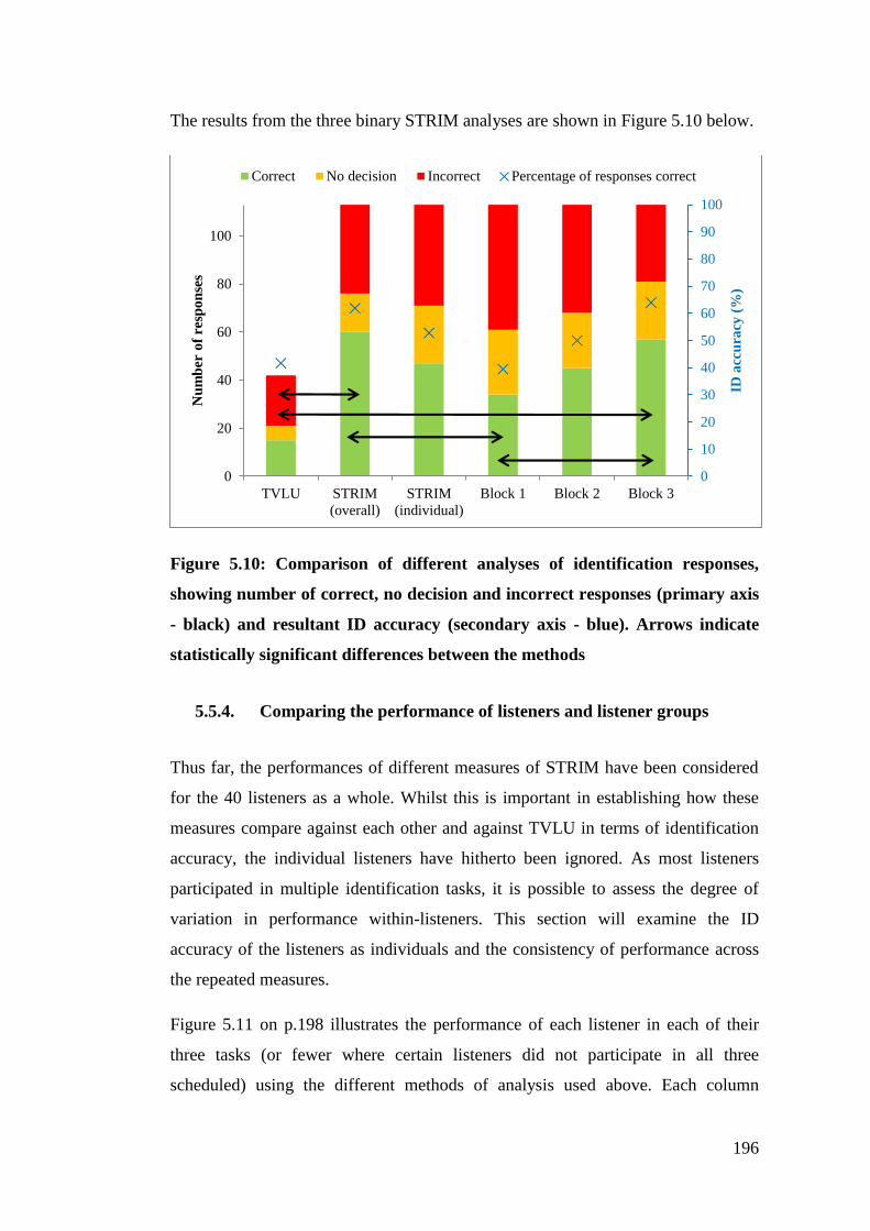
196
The results from the three binary STRIM analyses are shown in Figure 5.10 below.
Figure 5.10: Comparison of different analyses of identification responses,
showing number of correct, no decision and incorrect responses (primary axis
- black) and resultant ID accuracy (secondary axis - blue). Arrows indicate
statistically significant differences between the methods
5.5.4. Comparing the performance of listeners and listener groups
Thus far, the performances of different measures of STRIM have been considered
for the 40 listeners as a whole. Whilst this is important in establishing how these
measures compare against each other and against TVLU in terms of identification
accuracy, the individual listeners have hitherto been ignored. As most listeners
participated in multiple identification tasks, it is possible to assess the degree of
variation in performance within-listeners. This section will examine the ID
accuracy of the listeners as individuals and the consistency of performance across
the repeated measures.
Figure 5.11 on p.198 illustrates the performance of each listener in each of their
three tasks (or fewer where certain listeners did not participate in all three
scheduled) using the different methods of analysis used above. Each column
0
10
20
30
40
50
60
70
80
90
100
0
20
40
60
80
100
TVLU STRIM
(overall)
STRIM
(individual)
Block 1 Block 2 Block 3
ID a
ccu
racy
(%
)
Nu
mb
er o
f re
spo
nse
s
Correct No decision Incorrect Percentage of responses correct
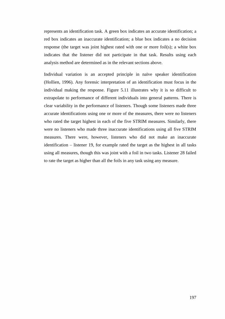
197
represents an identification task. A green box indicates an accurate identification; a
red box indicates an inaccurate identification; a blue box indicates a no decision
response (the target was joint highest rated with one or more foil(s); a white box
indicates that the listener did not participate in that task. Results using each
analysis method are determined as in the relevant sections above.
Individual variation is an accepted principle in naïve speaker identification
(Hollien, 1996). Any forensic interpretation of an identification must focus in the
individual making the response. Figure 5.11 illustrates why it is so difficult to
extrapolate to performance of different individuals into general patterns. There is
clear variability in the performance of listeners. Though some listeners made three
accurate identifications using one or more of the measures, there were no listeners
who rated the target highest in each of the five STRIM measures. Similarly, there
were no listeners who made three inaccurate identifications using all five STRIM
measures. There were, however, listeners who did not make an inaccurate
identification – listener 19, for example rated the target as the highest in all tasks
using all measures, though this was joint with a foil in two tasks. Listener 28 failed
to rate the target as higher than all the foils in any task using any measure.
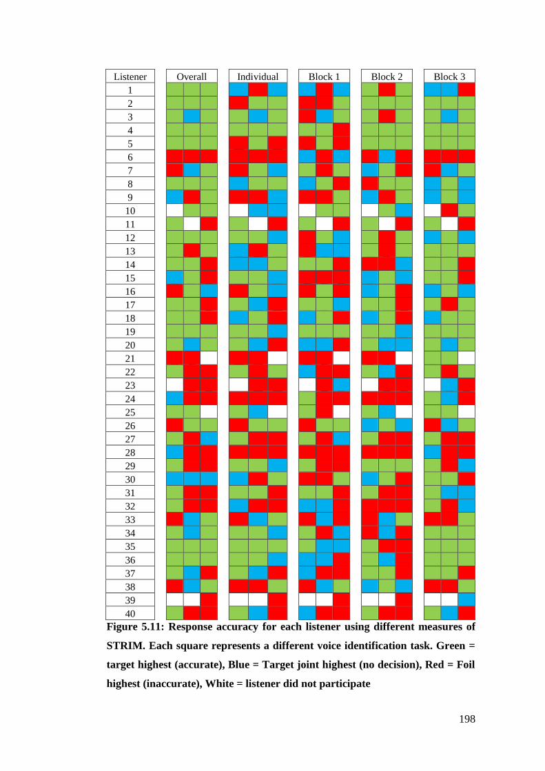
198
Listener
Overall
Individual
Block 1
Block 2
Block 3
1
1 1 1
2 3 2
2 3 2
1 3 1
2 2 3
2
1 1 1
3 1 1
3 3 1
1 1 1
1 1 1
3
1 2 1
1 2 1
3 2 1
1 3 1
1 2 1
4
1 1 1
1 1 1
1 1 3
1 1 1
1 1 1
5
1 1 1
3 1 3
3 1 3
1 1 1
1 1 1
6
3 3 3
3 3 3
2 3 2
3 2 3
3 3 3
7
3 2 1
3 1 2
1 3 1
2 1 3
3 2 1
8
1 1 1
2 1 1
2 1 3
3 1 1
2 1 2
9
2 3 1
3 3 2
3 3 1
2 3 1
2 1 2
10
1 1
2 2
1 1
1 2
3 1
11
1 3
1 3
1 3
1 3
1 3
12
1 1 1
1 1 2
3 1 2
1 3 1
2 1 2
13
1 3 1
2 3 1
3 2 2
1 3 1
1 1 1
14
1 1 3
2 2 1
1 1 3
3 3 2
1 1 3
15
2 1 3
1 1 2
3 3 3
2 1 2
1 1 3
16
3 1 2
3 1 2
3 1 3
2 1 3
2 1 2
17
1 1 3
1 2 3
1 1 2
1 1 3
1 3 1
18
1 1 3
2 1 3
2 1 3
2 1 3
2 1 1
19
1 1 1
1 1 2
1 1 1
1 1 2
1 1 1
20
1 2 1
1 2 3
2 2 3
1 2 2
1 2 1
21
3 3
3 3
3 3
3 3
1 1
22
1 3 3
1 3 1
2 3 3
1 2 3
1 3 1
23
3 3
3 3
3 2
3 3
2 3
24
2 3 3
3 3 3
1 3 3
3 3 3
1 2 3
25
1 1
1 2
1 3
1 2
1 1
26
3 1 1
3 1 1
3 1 1
2 1 2
3 2 1
27
1 3 2
1 3 3
1 3 2
1 3 3
1 3 3
28
2 3 3
3 3 3
3 3 3
3 3 3
2 3 3
29
1 3 3
1 1 2
1 3 3
1 1 1
1 3 2
30
2 2 2
2 3 1
3 3 1
2 1 3
1 1 3
31
1 3 3
1 1 3
1 1 3
1 3 3
1 2 2
32
1 3 3
2 3 3
2 2 3
3 3 3
1 3 2
33
3 2 1
3 2 1
3 2 3
3 2 1
3 3 1
34
1 2 1
1 1 2
1 3 2
3 2 3
1 1 1
35
1 1 1
1 1 1
1 2 2
1 3 3
1 1 1
36
1 1 1
1 1 2
2 2 3
1 2 3
1 1 1
37
1 2 3
1 2 3
2 3 3
1 1 3
1 1 3
38
3 2 1
3 3 1
3 2 1
2 1 2
3 3 1
39
3
3
3
3
2
40
1 3 3
1 2 3
2 3 3
1 3 3
1 2 3
Figure 5.11: Response accuracy for each listener using different measures of
STRIM. Each square represents a different voice identification task. Green =
target highest (accurate), Blue = Target joint highest (no decision), Red = Foil
highest (inaccurate), White = listener did not participate
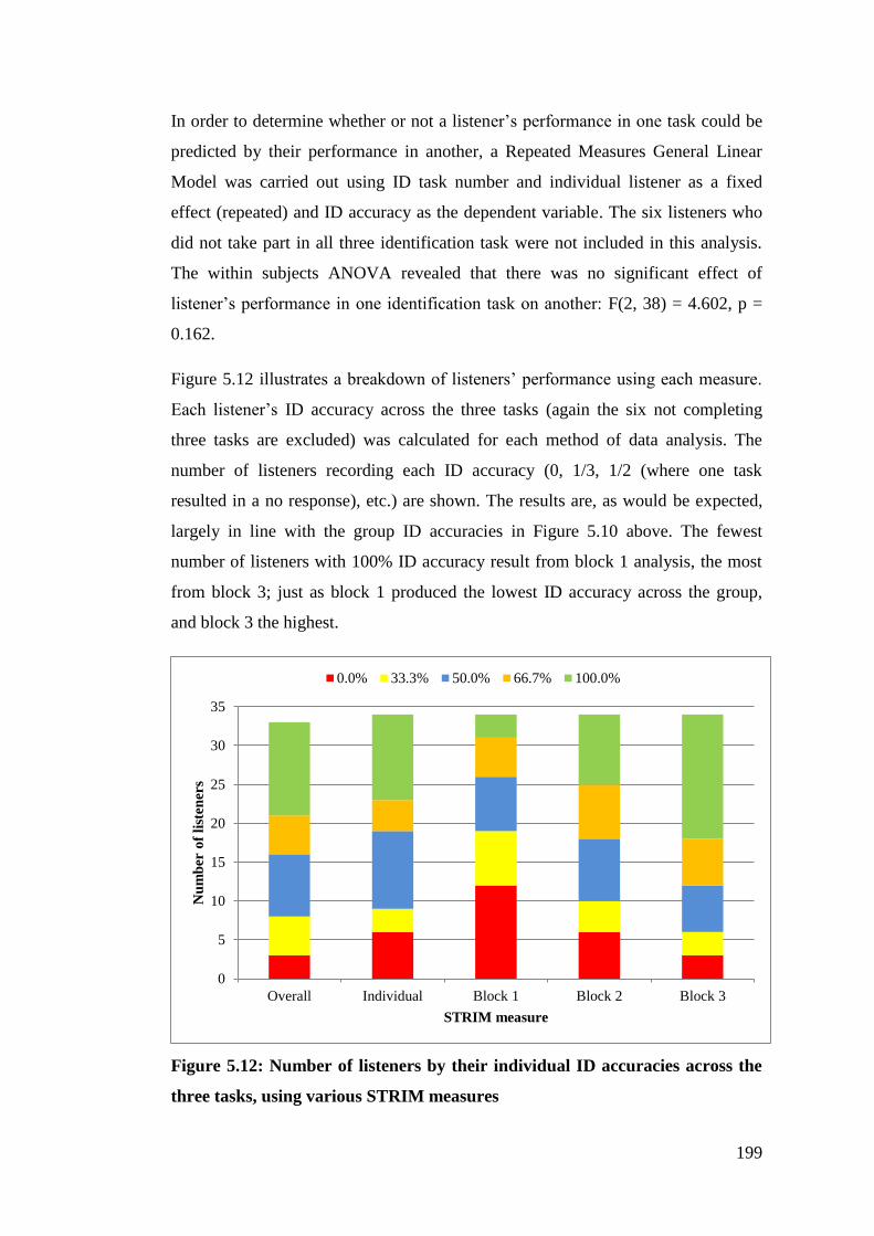
199
In order to determine whether or not a listener’s performance in one task could be
predicted by their performance in another, a Repeated Measures General Linear
Model was carried out using ID task number and individual listener as a fixed
effect (repeated) and ID accuracy as the dependent variable. The six listeners who
did not take part in all three identification task were not included in this analysis.
The within subjects ANOVA revealed that there was no significant effect of
listener’s performance in one identification task on another: F(2, 38) = 4.602, p =
0.162.
Figure 5.12 illustrates a breakdown of listeners’ performance using each measure.
Each listener’s ID accuracy across the three tasks (again the six not completing
three tasks are excluded) was calculated for each method of data analysis. The
number of listeners recording each ID accuracy (0, 1/3, 1/2 (where one task
resulted in a no response), etc.) are shown. The results are, as would be expected,
largely in line with the group ID accuracies in Figure 5.10 above. The fewest
number of listeners with 100% ID accuracy result from block 1 analysis, the most
from block 3; just as block 1 produced the lowest ID accuracy across the group,
and block 3 the highest.
Figure 5.12: Number of listeners by their individual ID accuracies across the
three tasks, using various STRIM measures
0
5
10
15
20
25
30
35
Overall Individual Block 1 Block 2 Block 3
Nu
mb
er o
f li
sten
ers
STRIM measure
0.0% 33.3% 50.0% 66.7% 100.0%
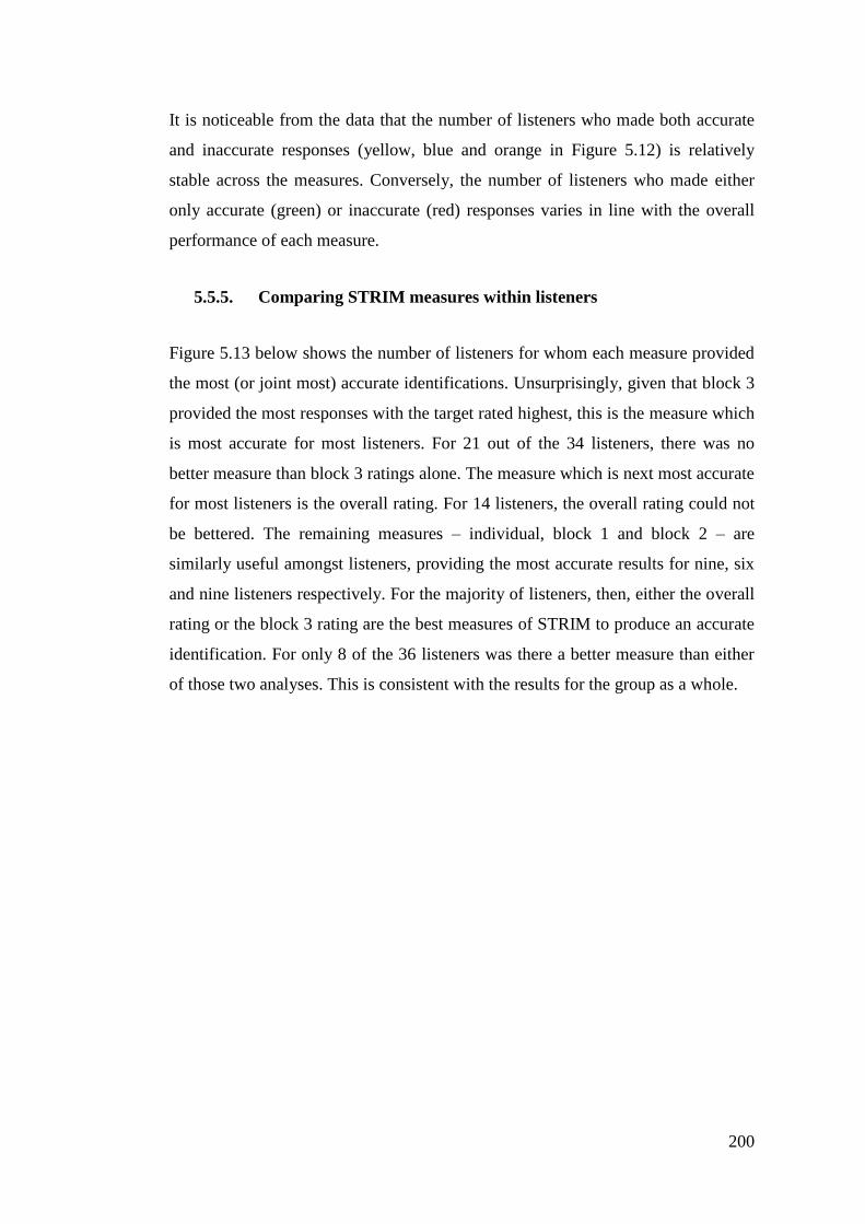
200
It is noticeable from the data that the number of listeners who made both accurate
and inaccurate responses (yellow, blue and orange in Figure 5.12) is relatively
stable across the measures. Conversely, the number of listeners who made either
only accurate (green) or inaccurate (red) responses varies in line with the overall
performance of each measure.
5.5.5. Comparing STRIM measures within listeners
Figure 5.13 below shows the number of listeners for whom each measure provided
the most (or joint most) accurate identifications. Unsurprisingly, given that block 3
provided the most responses with the target rated highest, this is the measure which
is most accurate for most listeners. For 21 out of the 34 listeners, there was no
better measure than block 3 ratings alone. The measure which is next most accurate
for most listeners is the overall rating. For 14 listeners, the overall rating could not
be bettered. The remaining measures – individual, block 1 and block 2 – are
similarly useful amongst listeners, providing the most accurate results for nine, six
and nine listeners respectively. For the majority of listeners, then, either the overall
rating or the block 3 rating are the best measures of STRIM to produce an accurate
identification. For only 8 of the 36 listeners was there a better measure than either
of those two analyses. This is consistent with the results for the group as a whole.
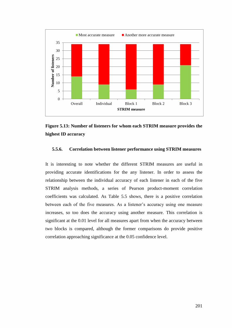
201
Figure 5.13: Number of listeners for whom each STRIM measure provides the
highest ID accuracy
5.5.6. Correlation between listener performance using STRIM measures
It is interesting to note whether the different STRIM measures are useful in
providing accurate identifications for the any listener. In order to assess the
relationship between the individual accuracy of each listener in each of the five
STRIM analysis methods, a series of Pearson product-moment correlation
coefficients was calculated. As Table 5.5 shows, there is a positive correlation
between each of the five measures. As a listener’s accuracy using one measure
increases, so too does the accuracy using another measure. This correlation is
significant at the 0.01 level for all measures apart from when the accuracy between
two blocks is compared, although the former comparisons do provide positive
correlation approaching significance at the 0.05 confidence level.
0
5
10
15
20
25
30
35
Overall Individual Block 1 Block 2 Block 3
Nu
mb
er o
f li
sten
ers
STRIM measure
Most accurate measure Another more accurate measure
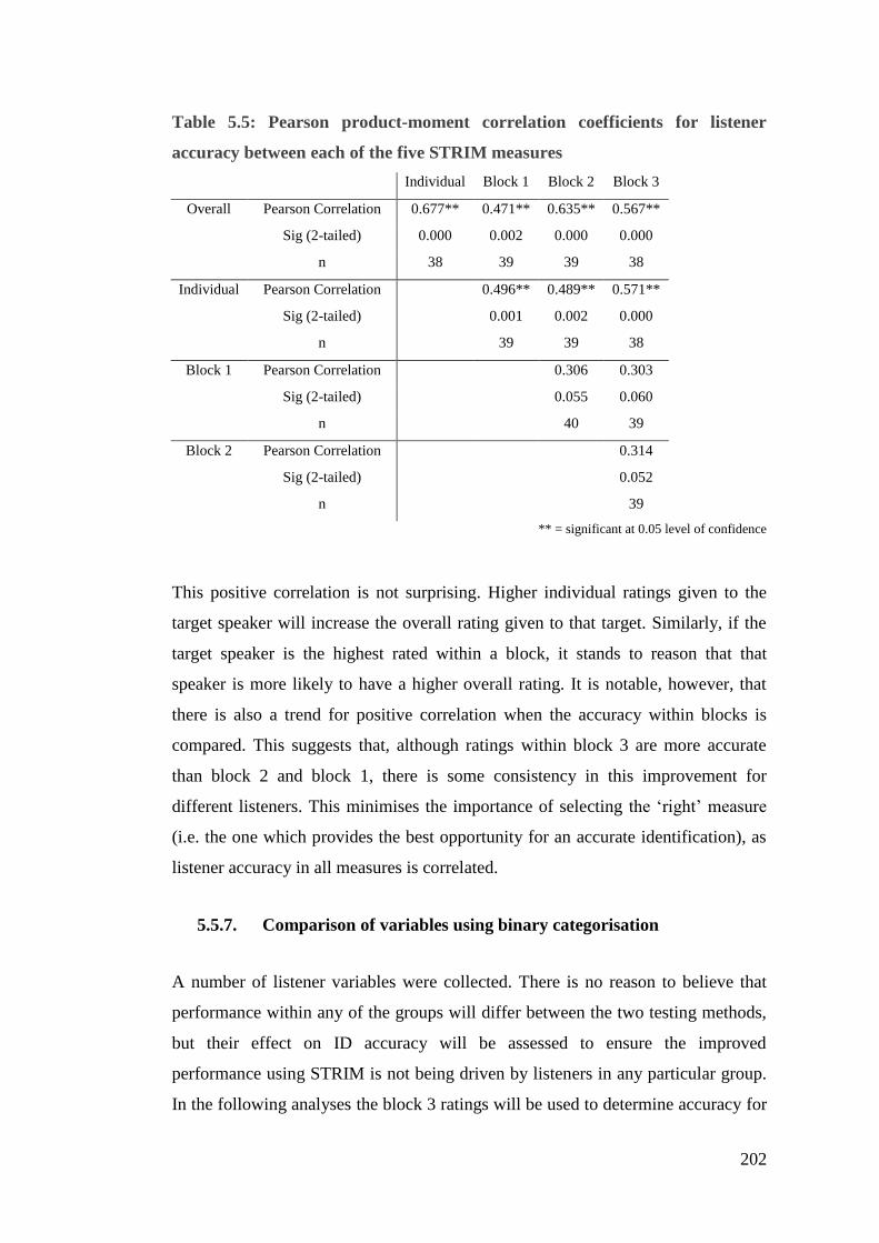
202
Table 5.5: Pearson product-moment correlation coefficients for listener
accuracy between each of the five STRIM measures
Individual Block 1 Block 2 Block 3
Overall Pearson Correlation 0.677** 0.471** 0.635** 0.567**
Sig (2-tailed) 0.000 0.002 0.000 0.000
n 38 39 39 38
Individual Pearson Correlation
0.496** 0.489** 0.571**
Sig (2-tailed)
0.001 0.002 0.000
n 39 39 38
Block 1 Pearson Correlation
0.306 0.303
Sig (2-tailed)
0.055 0.060
n 40 39
Block 2 Pearson Correlation
0.314
Sig (2-tailed)
0.052
n 39
** = significant at 0.05 level of confidence
This positive correlation is not surprising. Higher individual ratings given to the
target speaker will increase the overall rating given to that target. Similarly, if the
target speaker is the highest rated within a block, it stands to reason that that
speaker is more likely to have a higher overall rating. It is notable, however, that
there is also a trend for positive correlation when the accuracy within blocks is
compared. This suggests that, although ratings within block 3 are more accurate
than block 2 and block 1, there is some consistency in this improvement for
different listeners. This minimises the importance of selecting the ‘right’ measure
(i.e. the one which provides the best opportunity for an accurate identification), as
listener accuracy in all measures is correlated.
5.5.7. Comparison of variables using binary categorisation
A number of listener variables were collected. There is no reason to believe that
performance within any of the groups will differ between the two testing methods,
but their effect on ID accuracy will be assessed to ensure the improved
performance using STRIM is not being driven by listeners in any particular group.
In the following analyses the block 3 ratings will be used to determine accuracy for
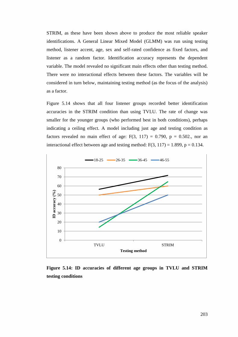
203
STRIM, as these have been shown above to produce the most reliable speaker
identifications. A General Linear Mixed Model (GLMM) was run using testing
method, listener accent, age, sex and self-rated confidence as fixed factors, and
listener as a random factor. Identification accuracy represents the dependent
variable. The model revealed no significant main effects other than testing method.
There were no interactional effects between these factors. The variables will be
considered in turn below, maintaining testing method (as the focus of the analysis)
as a factor.
Figure 5.14 shows that all four listener groups recorded better identification
accuracies in the STRIM condition than using TVLU. The rate of change was
smaller for the younger groups (who performed best in both conditions), perhaps
indicating a ceiling effect. A model including just age and testing condition as
factors revealed no main effect of age: F(3, 117) = 0.790, p = 0.502., nor an
interactional effect between age and testing method: F(3, 117) = 1.899, p = 0.134.
Figure 5.14: ID accuracies of different age groups in TVLU and STRIM
testing conditions
0
10
20
30
40
50
60
70
80
TVLU STRIM
ID a
ccu
racy
(%
)
Testing method
18-25 26-35 36-45 46-55
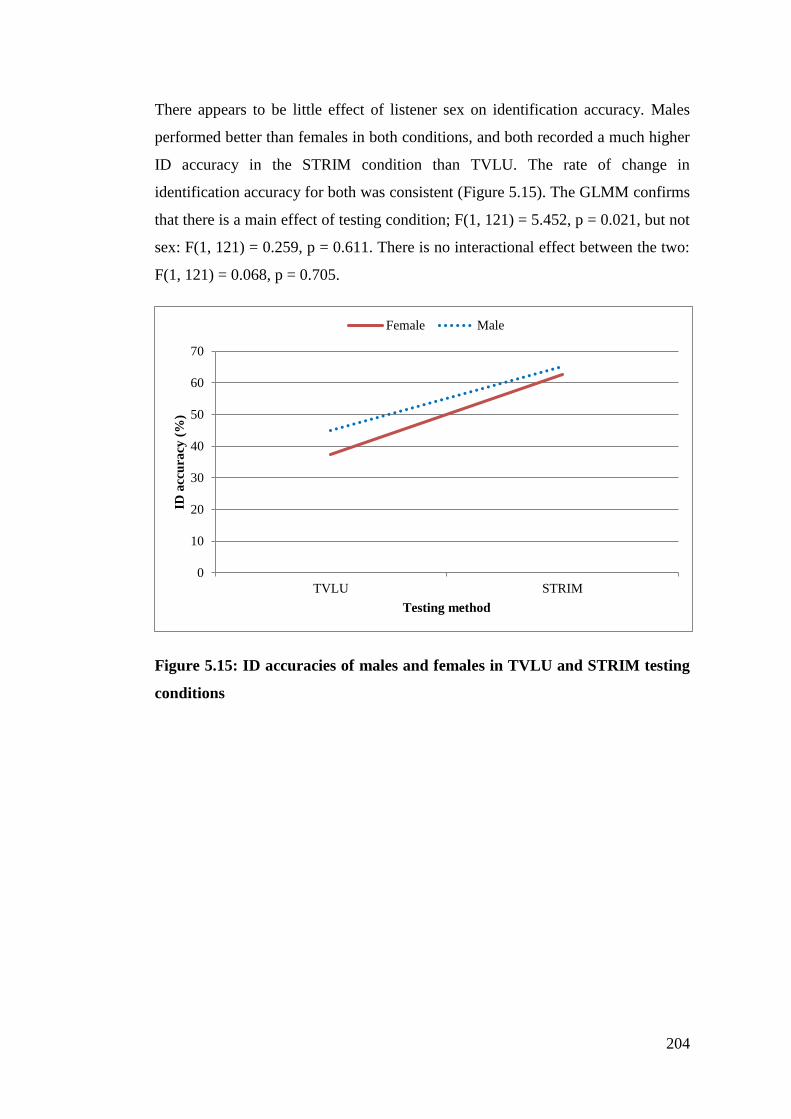
204
There appears to be little effect of listener sex on identification accuracy. Males
performed better than females in both conditions, and both recorded a much higher
ID accuracy in the STRIM condition than TVLU. The rate of change in
identification accuracy for both was consistent (Figure 5.15). The GLMM confirms
that there is a main effect of testing condition; F(1, 121) = 5.452, p = 0.021, but not
sex: F(1, 121) = 0.259, p = 0.611. There is no interactional effect between the two:
F(1, 121) = 0.068, p = 0.705.
Figure 5.15: ID accuracies of males and females in TVLU and STRIM testing
conditions
0
10
20
30
40
50
60
70
TVLU STRIM
ID a
ccu
racy
(%
)
Testing method
Female Male
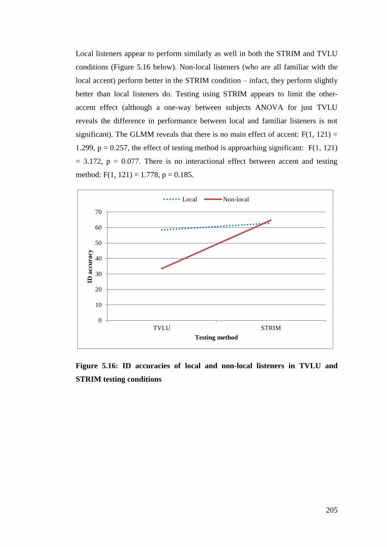
205
Local listeners appear to perform similarly as well in both the STRIM and TVLU
conditions (Figure 5.16 below). Non-local listeners (who are all familiar with the
local accent) perform better in the STRIM condition – infact, they perform slightly
better than local listeners do. Testing using STRIM appears to limit the other-
accent effect (although a one-way between subjects ANOVA for just TVLU
reveals the difference in performance between local and familiar listeners is not
significant). The GLMM reveals that there is no main effect of accent: F(1, 121) =
1.299, p = 0.257, the effect of testing method is approaching significant: F(1, 121)
= 3.172, p = 0.077. There is no interactional effect between accent and testing
method: F(1, 121) = 1.778, p = 0.185.
Figure 5.16: ID accuracies of local and non-local listeners in TVLU and
STRIM testing conditions
0
10
20
30
40
50
60
70
TVLU STRIM
ID a
ccu
racy
Testing method
Local Non-local
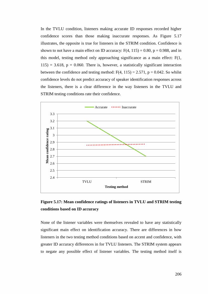
206
In the TVLU condition, listeners making accurate ID responses recorded higher
confidence scores than those making inaccurate responses. As Figure 5.17
illustrates, the opposite is true for listeners in the STRIM condition. Confidence is
shown to not have a main effect on ID accuracy: F(4, 115) = 0.80, p = 0.988, and in
this model, testing method only approaching significance as a main effect: F(1,
115) = 3.618, p = 0.060. There is, however, a statistically significant interaction
between the confidence and testing method: F(4, 115) = 2.571, p = 0.042. So whilst
confidence levels do not predict accuracy of speaker identification responses across
the listeners, there is a clear difference in the way listeners in the TVLU and
STRIM testing conditions rate their confidence.
Figure 5.17: Mean confidence ratings of listeners in TVLU and STRIM testing
conditions based on ID accuracy
None of the listener variables were themselves revealed to have any statistically
significant main effect on identification accuracy. There are differences in how
listeners in the two testing method conditions based on accent and confidence, with
greater ID accuracy differences in for TVLU listeners. The STRIM system appears
to negate any possible effect of listener variables. The testing method itself is
2.4
2.5
2.6
2.7
2.8
2.9
3
3.1
3.2
3.3
TVLU STRIM
Mea
n c
on
fid
ence
ra
tin
g
Testing method
Accurate Inaccurate
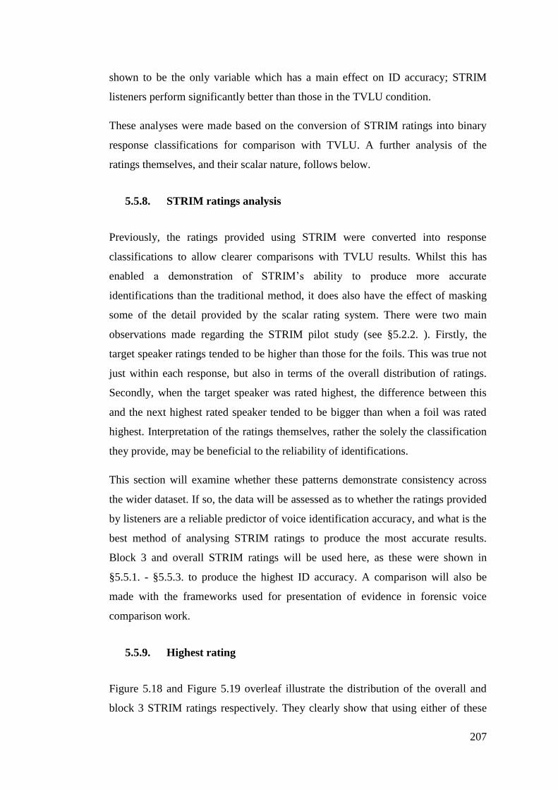
207
shown to be the only variable which has a main effect on ID accuracy; STRIM
listeners perform significantly better than those in the TVLU condition.
These analyses were made based on the conversion of STRIM ratings into binary
response classifications for comparison with TVLU. A further analysis of the
ratings themselves, and their scalar nature, follows below.
5.5.8. STRIM ratings analysis
Previously, the ratings provided using STRIM were converted into response
classifications to allow clearer comparisons with TVLU results. Whilst this has
enabled a demonstration of STRIM’s ability to produce more accurate
identifications than the traditional method, it does also have the effect of masking
some of the detail provided by the scalar rating system. There were two main
observations made regarding the STRIM pilot study (see §5.2.2. ). Firstly, the
target speaker ratings tended to be higher than those for the foils. This was true not
just within each response, but also in terms of the overall distribution of ratings.
Secondly, when the target speaker was rated highest, the difference between this
and the next highest rated speaker tended to be bigger than when a foil was rated
highest. Interpretation of the ratings themselves, rather the solely the classification
they provide, may be beneficial to the reliability of identifications.
This section will examine whether these patterns demonstrate consistency across
the wider dataset. If so, the data will be assessed as to whether the ratings provided
by listeners are a reliable predictor of voice identification accuracy, and what is the
best method of analysing STRIM ratings to produce the most accurate results.
Block 3 and overall STRIM ratings will be used here, as these were shown in
§5.5.1. - §5.5.3. to produce the highest ID accuracy. A comparison will also be
made with the frameworks used for presentation of evidence in forensic voice
comparison work.
5.5.9. Highest rating
Figure 5.18 and Figure 5.19 overleaf illustrate the distribution of the overall and
block 3 STRIM ratings respectively. They clearly show that using either of these
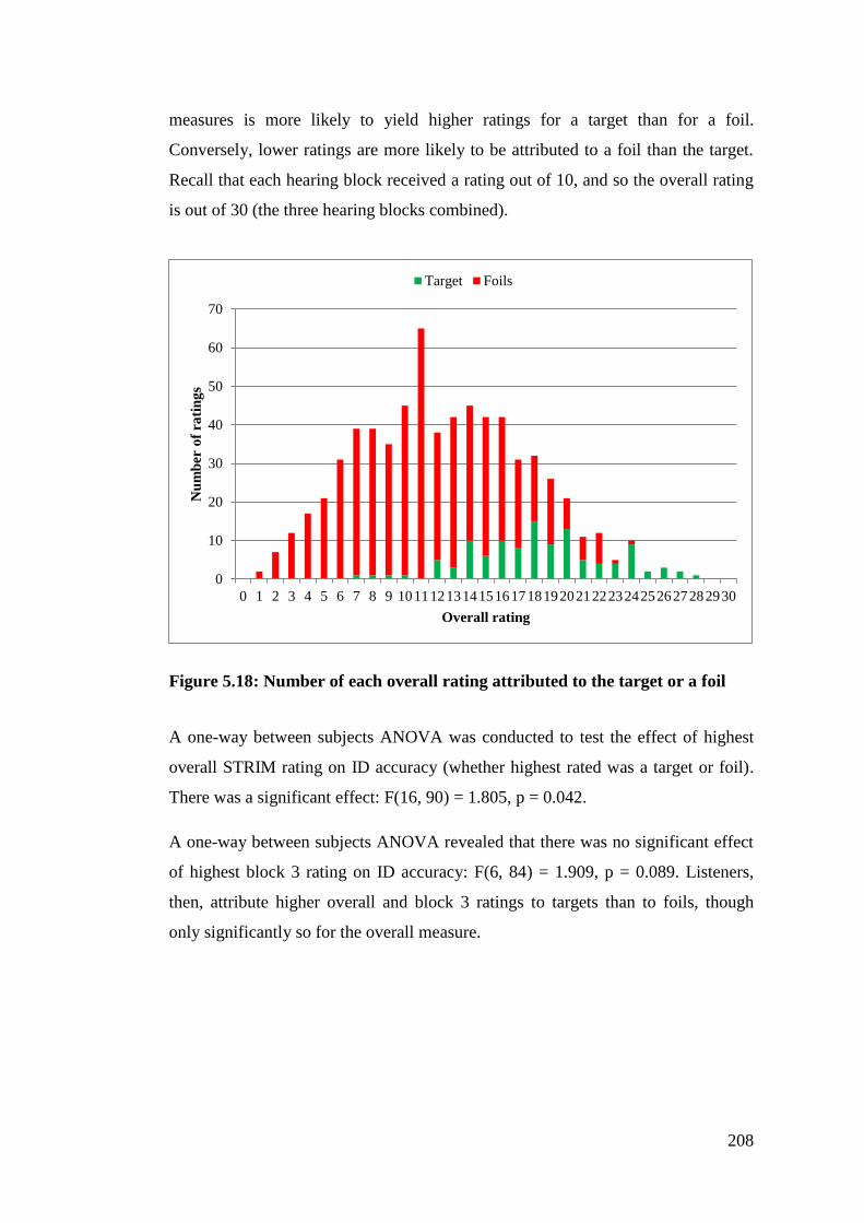
208
measures is more likely to yield higher ratings for a target than for a foil.
Conversely, lower ratings are more likely to be attributed to a foil than the target.
Recall that each hearing block received a rating out of 10, and so the overall rating
is out of 30 (the three hearing blocks combined).
Figure 5.18: Number of each overall rating attributed to the target or a foil
A one-way between subjects ANOVA was conducted to test the effect of highest
overall STRIM rating on ID accuracy (whether highest rated was a target or foil).
There was a significant effect: F(16, 90) = 1.805, p = 0.042.
A one-way between subjects ANOVA revealed that there was no significant effect
of highest block 3 rating on ID accuracy: F(6, 84) = 1.909, p = 0.089. Listeners,
then, attribute higher overall and block 3 ratings to targets than to foils, though
only significantly so for the overall measure.
0
10
20
30
40
50
60
70
0 1 2 3 4 5 6 7 8 9 101112131415161718192021222324252627282930
Nu
mb
er o
f ra
tin
gs
Overall rating
Target Foils
209
Figure 5.19: Number of each block 3 rating attributed to the target or a foil
If, however, this is as a result of large differences for a few listeners, the above data
are not telling the full story. If the target speaker is consistently rated slightly
higher than the foils, this may indicate that the highest ratings themselves are a
reliable source of information. It is important to consider the ratings given by each
listener by ordering the foils by ratings within each response.
Mean ratings
Table 5.6 below shows the mean overall and block 3 ratings attributed to the target
speaker and each of the five foils ranked in order of rating within each response. As
the data above shows, the target speakers receive both the highest average overall
and block 3 ratings. The average for the foils, by definition, falls from the highest
rated to the lowest. Table 5.6 additionally shows that the average rating for each
speaker falls at a consistent rate. The difference between the target and the highest
foil is, on average, similar to the difference between the highest and second highest
foils.
0
20
40
60
80
100
120
140
0 1 2 3 4 5 6 7 8 9 10
Nu
mb
er o
f ra
tin
gs
Block 3 rating
Target Foils
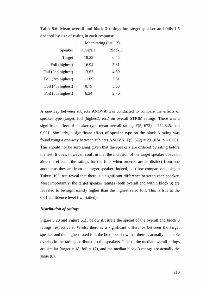
210
Table 5.6: Mean overall and block 3 ratings for target speaker and foils 1-5
ordered by size of rating in each response
Mean rating (n=113)
Speaker Overall Block 3
Target 18.33 6.45
Foil (highest) 16.94 5.81
Foil (2nd highest) 13.63 4.50
Foil (3rd highest) 11.09 3.61
Foil (4th highest) 8.79 3.58
Foil (5th highest) 6.34 2.70
A one-way between subjects ANOVA was conducted to compare the effects of
speaker type (target, foil (highest), etc.) on overall STRIM ratings. There was a
significant effect of speaker type mean overall rating: F(5, 672) = 254.845, p <
0.001. Similarly, a significant effect of speaker type on the block 3 rating was
found using a one-way between subjects ANOVA: F(5, 672) = 231.074, p < 0.001.
This should not be surprising given that the speakers are ordered by rating before
the test. It does, however, confirm that the inclusion of the target speaker does not
alter the effect – the ratings for the foils when ordered are as distinct from one
another as they are from the target speaker. Indeed, post hoc comparisons using a
Tukey HSD test reveal that there is a significant difference between each speaker.
Most importantly, the target speaker ratings (both overall and within block 3) are
revealed to be significantly higher than the highest rated foil. This is true at the
0.01 confidence level (two-tailed).
Distribution of ratings
Figure 5.20 and Figure 5.21 below illustrate the spread of the overall and block 3
ratings respectively. Whilst there is a significant difference between the target
speaker and the highest rated foil, the boxplots show that there is actually a notable
overlap in the ratings attributed to the speakers. Indeed, the median overall ratings
are similar (target = 18, foil = 17), and the median block 3 ratings are actually the
same (6).
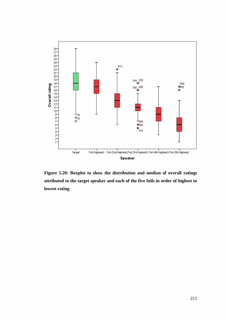
211
Figure 5.20: Boxplot to show the distribution and median of overall ratings
attributed to the target speaker and each of the five foils in order of highest to
lowest rating
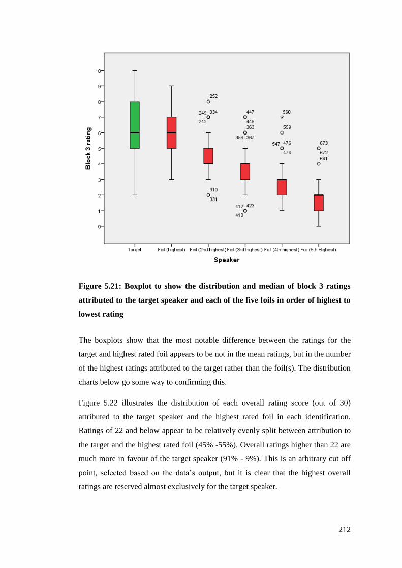
212
Figure 5.21: Boxplot to show the distribution and median of block 3 ratings
attributed to the target speaker and each of the five foils in order of highest to
lowest rating
The boxplots show that the most notable difference between the ratings for the
target and highest rated foil appears to be not in the mean ratings, but in the number
of the highest ratings attributed to the target rather than the foil(s). The distribution
charts below go some way to confirming this.
Figure 5.22 illustrates the distribution of each overall rating score (out of 30)
attributed to the target speaker and the highest rated foil in each identification.
Ratings of 22 and below appear to be relatively evenly split between attribution to
the target and the highest rated foil (45% -55%). Overall ratings higher than 22 are
much more in favour of the target speaker (91% - 9%). This is an arbitrary cut off
point, selected based on the data’s output, but it is clear that the highest overall
ratings are reserved almost exclusively for the target speaker.
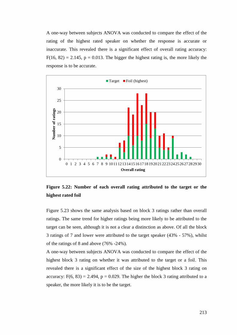
213
A one-way between subjects ANOVA was conducted to compare the effect of the
rating of the highest rated speaker on whether the response is accurate or
inaccurate. This revealed there is a significant effect of overall rating accuracy:
F(16, 82) = 2.145, p = 0.013. The bigger the highest rating is, the more likely the
response is to be accurate.
Figure 5.22: Number of each overall rating attributed to the target or the
highest rated foil
Figure 5.23 shows the same analysis based on block 3 ratings rather than overall
ratings. The same trend for higher ratings being more likely to be attributed to the
target can be seen, although it is not a clear a distinction as above. Of all the block
3 ratings of 7 and lower were attributed to the target speaker (43% - 57%), whilst
of the ratings of 8 and above (76% -24%).
A one-way between subjects ANOVA was conducted to compare the effect of the
highest block 3 rating on whether it was attributed to the target or a foil. This
revealed there is a significant effect of the size of the highest block 3 rating on
accuracy: F(6, 83) = 2.494, p = 0.029. The higher the block 3 rating attributed to a
speaker, the more likely it is to be the target.
0
5
10
15
20
25
30
0 1 2 3 4 5 6 7 8 9 101112131415161718192021222324252627282930
Nu
mb
er o
f ra
tin
gs
Overall rating
Target Foil (highest)
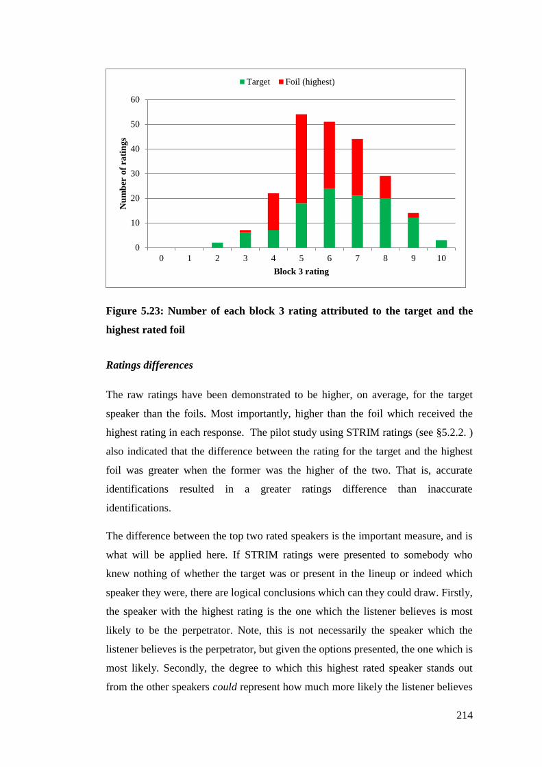
214
Figure 5.23: Number of each block 3 rating attributed to the target and the
highest rated foil
Ratings differences
The raw ratings have been demonstrated to be higher, on average, for the target
speaker than the foils. Most importantly, higher than the foil which received the
highest rating in each response. The pilot study using STRIM ratings (see §5.2.2. )
also indicated that the difference between the rating for the target and the highest
foil was greater when the former was the higher of the two. That is, accurate
identifications resulted in a greater ratings difference than inaccurate
identifications.
The difference between the top two rated speakers is the important measure, and is
what will be applied here. If STRIM ratings were presented to somebody who
knew nothing of whether the target was or present in the lineup or indeed which
speaker they were, there are logical conclusions which can they could draw. Firstly,
the speaker with the highest rating is the one which the listener believes is most
likely to be the perpetrator. Note, this is not necessarily the speaker which the
listener believes is the perpetrator, but given the options presented, the one which is
most likely. Secondly, the degree to which this highest rated speaker stands out
from the other speakers could represent how much more likely the listener believes
0
10
20
30
40
50
60
0 1 2 3 4 5 6 7 8 9 10
Nu
mb
er o
f ra
tin
gs
Block 3 rating
Target Foil (highest)
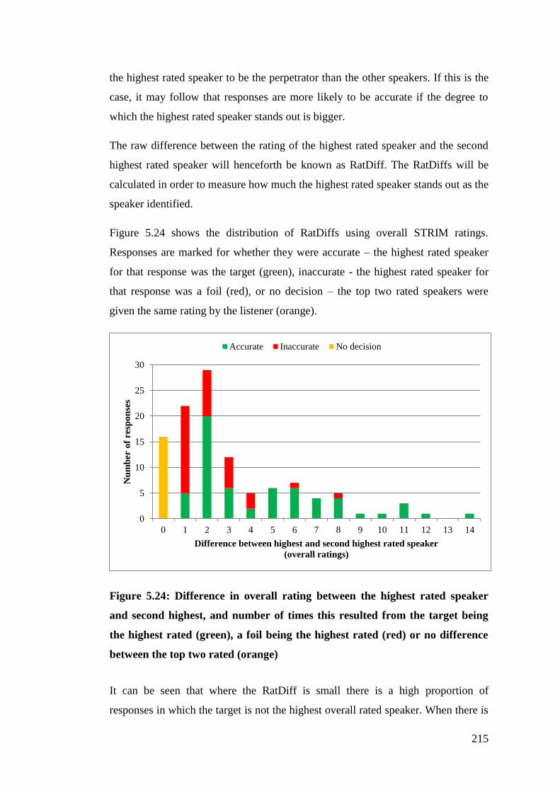
215
the highest rated speaker to be the perpetrator than the other speakers. If this is the
case, it may follow that responses are more likely to be accurate if the degree to
which the highest rated speaker stands out is bigger.
The raw difference between the rating of the highest rated speaker and the second
highest rated speaker will henceforth be known as RatDiff. The RatDiffs will be
calculated in order to measure how much the highest rated speaker stands out as the
speaker identified.
Figure 5.24 shows the distribution of RatDiffs using overall STRIM ratings.
Responses are marked for whether they were accurate – the highest rated speaker
for that response was the target (green), inaccurate - the highest rated speaker for
that response was a foil (red), or no decision – the top two rated speakers were
given the same rating by the listener (orange).
Figure 5.24: Difference in overall rating between the highest rated speaker
and second highest, and number of times this resulted from the target being
the highest rated (green), a foil being the highest rated (red) or no difference
between the top two rated (orange)
It can be seen that where the RatDiff is small there is a high proportion of
responses in which the target is not the highest overall rated speaker. When there is
0
5
10
15
20
25
30
0 1 2 3 4 5 6 7 8 9 10 11 12 13 14
Nu
mb
er o
f re
spo
nse
s
Difference between highest and second highest rated speaker
(overall ratings)
Accurate Inaccurate No decision
216
a difference of one in the ratings, for example, only 5 of the 22 responses were
accurate (23%). In contrast, the target is the highest rated speaker in each of the six
identifications where the RatDiff is nine or more. Additionally, 26 of the 28
identifications where the RatDiff is five or more involve the target receiving the
highest rating.
A one-way between subjects ANOVA was conducted to compare the effect of the
difference between the overall ratings for the highest rated and second highest rated
speakers on identification accuracy. This revealed there is a significant effect of
overall rating difference on accuracy: F(12, 84) = 3.058, p = 0.001. The
identification is more likely to be accurate the larger the overall RatDiff.
Figure 5.25 displays the same analysis, this time based on block 3 ratings. The
trend appears to be similar to that above, although obviously the range of ratings
differences is smaller given that block 3 ratings are out of 10 and overall ratings are
out of 30. The proportion of accurate identifications (where the target speaker is
rated the highest) is lower when the block 3 RatDiff is smaller. Where the
difference is one or two, 34 of the 57 (60%) identifications are accurate. Where the
difference is three or more, 23 of the 27 (85%) identifications were accurate.
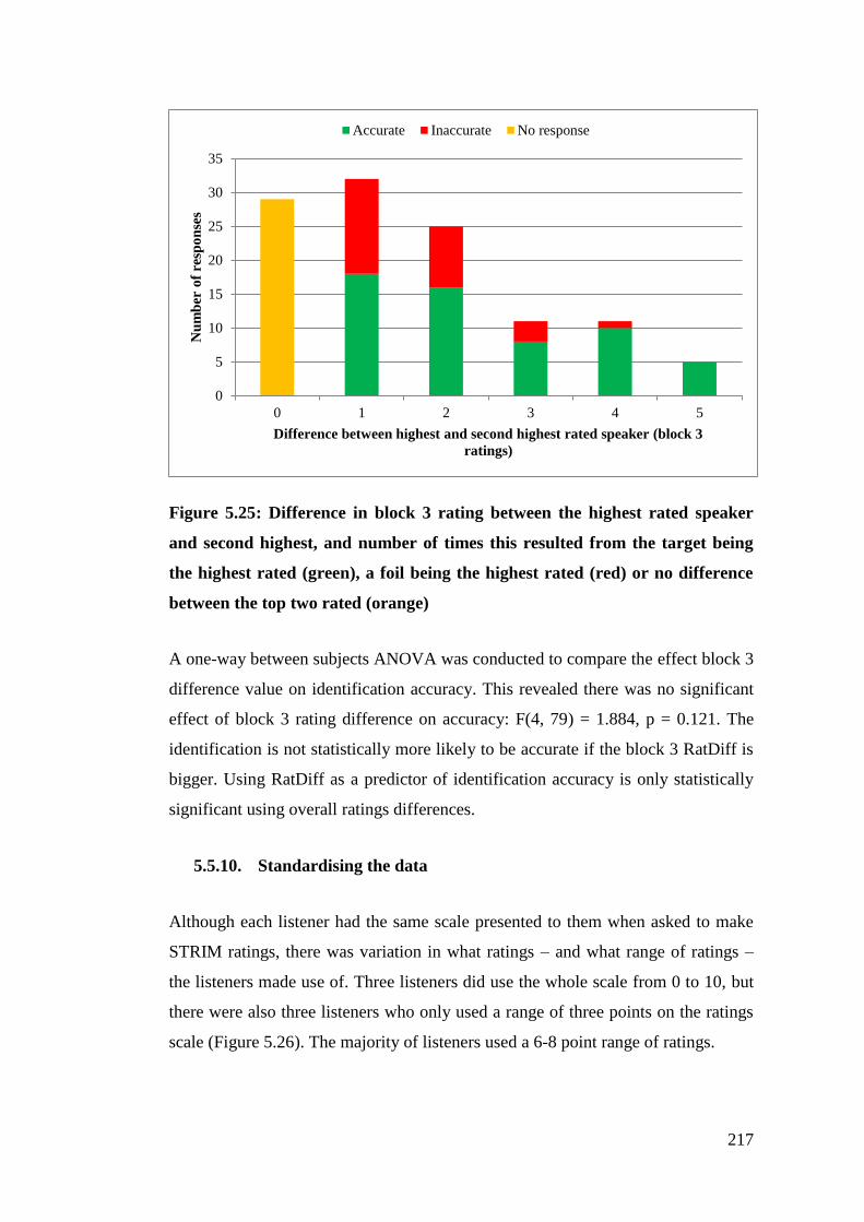
217
Figure 5.25: Difference in block 3 rating between the highest rated speaker
and second highest, and number of times this resulted from the target being
the highest rated (green), a foil being the highest rated (red) or no difference
between the top two rated (orange)
A one-way between subjects ANOVA was conducted to compare the effect block 3
difference value on identification accuracy. This revealed there was no significant
effect of block 3 rating difference on accuracy: F(4, 79) = 1.884, p = 0.121. The
identification is not statistically more likely to be accurate if the block 3 RatDiff is
bigger. Using RatDiff as a predictor of identification accuracy is only statistically
significant using overall ratings differences.
5.5.10. Standardising the data
Although each listener had the same scale presented to them when asked to make
STRIM ratings, there was variation in what ratings – and what range of ratings –
the listeners made use of. Three listeners did use the whole scale from 0 to 10, but
there were also three listeners who only used a range of three points on the ratings
scale (Figure 5.26). The majority of listeners used a 6-8 point range of ratings.
0
5
10
15
20
25
30
35
0 1 2 3 4 5
Nu
mb
er o
f re
spo
nse
s
Difference between highest and second highest rated speaker (block 3
ratings)
Accurate Inaccurate No response
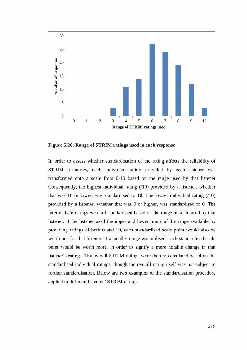
218
Figure 5.26: Range of STRIM ratings used in each response
In order to assess whether standardisation of the rating affects the reliability of
STRIM responses, each individual rating provided by each listener was
transformed onto a scale from 0-10 based on the range used by that listener
Consequently, the highest individual rating (/10) provided by a listener, whether
that was 10 or lower, was standardised to 10. The lowest individual rating (/10)
provided by a listener, whether that was 0 or higher, was standardised to 0. The
intermediate ratings were all standardised based on the range of scale used by that
listener. If the listener used the upper and lower limits of the range available by
providing ratings of both 0 and 10, each standardised scale point would also be
worth one for that listener. If a smaller range was utilised, each standardised scale
point would be worth more, in order to signify a more notable change in that
listener’s rating. The overall STRIM ratings were then re-calculated based on the
standardised individual ratings, though the overall rating itself was not subject to
further standardisation. Below are two examples of the standardisation procedure
applied to different listeners’ STRIM ratings.
0
5
10
15
20
25
30
0 1 2 3 4 5 6 7 8 9 10
Nu
mb
er o
f re
spo
nse
s
Range of STRIM ratings used
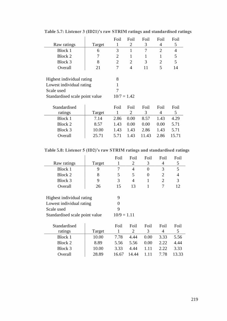
219
Table 5.7: Listener 3 (ID21)’s raw STRIM ratings and standardised ratings
Raw ratings Target
Foil
1
Foil
2
Foil
3
Foil
4
Foil
5
Block 1 6 3 1 7 2 4
Block 2 7 2 1 1 1 5
Block 3 8 2 2 3 2 5
Overall 21 7 4 11 5 14
Highest individual rating 8
Lowest individual rating 1
Scale used
7
Standardised scale point value 10/7 = 1.42
Standardised
ratings Target
Foil
1
Foil
2
Foil
3
Foil
4
Foil
5
Block 1 7.14 2.86 0.00 8.57 1.43 4.29
Block 2 8.57 1.43 0.00 0.00 0.00 5.71
Block 3 10.00 1.43 1.43 2.86 1.43 5.71
Overall 25.71 5.71 1.43 11.43 2.86 15.71
Table 5.8: Listener 5 (ID2)’s raw STRIM ratings and standardised ratings
Raw ratings Target
Foil
1
Foil
2
Foil
3
Foil
4
Foil
5
Block 1 9 7 4 0 3 5
Block 2 8 5 5 0 2 4
Block 3 9 3 4 1 2 3
Overall 26 15 13 1 7 12
Highest individual rating 9
Lowest individual rating 0
Scale used
9
Standardised scale point value 10/9 = 1.11
Standardised
ratings Target
Foil
1
Foil
2
Foil
3
Foil
4
Foil
5
Block 1 10.00 7.78 4.44 0.00 3.33 5.56
Block 2 8.89 5.56 5.56 0.00 2.22 4.44
Block 3 10.00 3.33 4.44 1.11 2.22 3.33
Overall 28.89 16.67 14.44 1.11 7.78 13.33
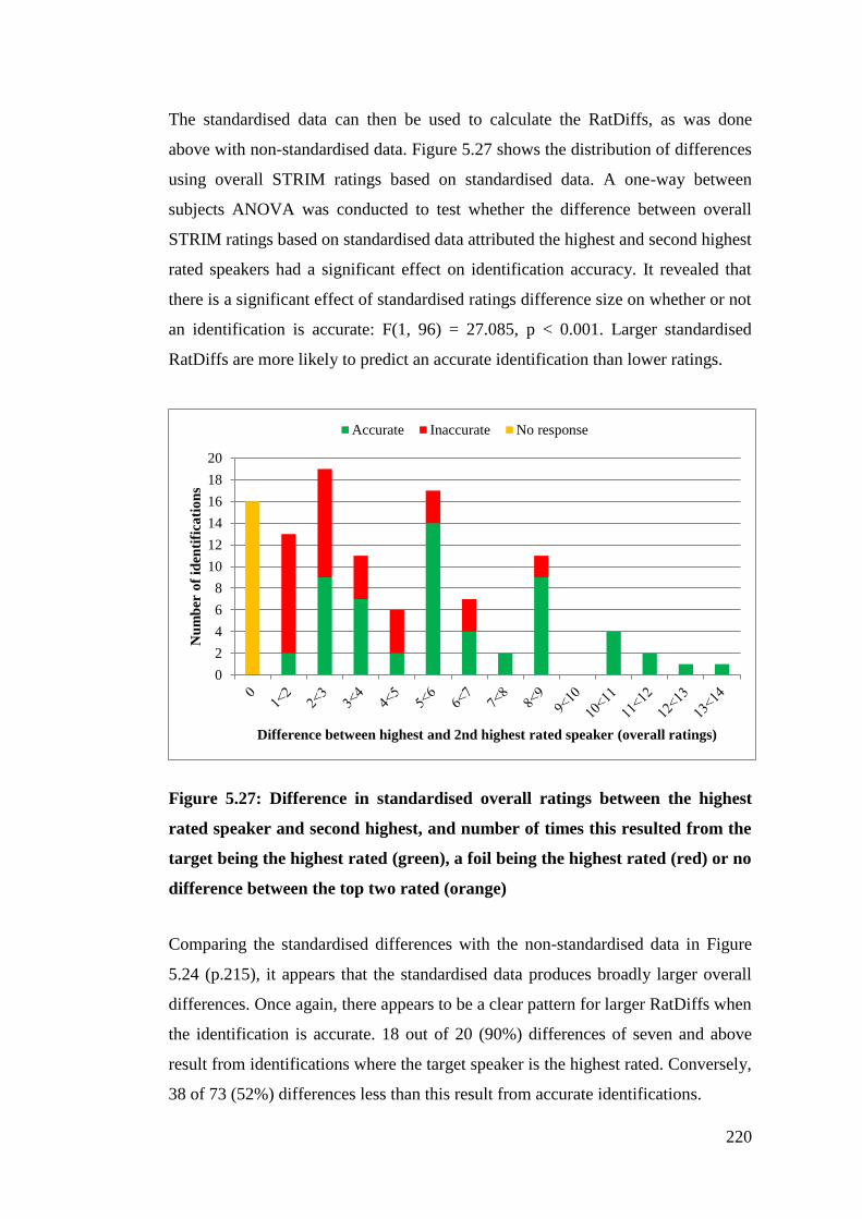
220
The standardised data can then be used to calculate the RatDiffs, as was done
above with non-standardised data. Figure 5.27 shows the distribution of differences
using overall STRIM ratings based on standardised data. A one-way between
subjects ANOVA was conducted to test whether the difference between overall
STRIM ratings based on standardised data attributed the highest and second highest
rated speakers had a significant effect on identification accuracy. It revealed that
there is a significant effect of standardised ratings difference size on whether or not
an identification is accurate: F(1, 96) = 27.085, p < 0.001. Larger standardised
RatDiffs are more likely to predict an accurate identification than lower ratings.
Figure 5.27: Difference in standardised overall ratings between the highest
rated speaker and second highest, and number of times this resulted from the
target being the highest rated (green), a foil being the highest rated (red) or no
difference between the top two rated (orange)
Comparing the standardised differences with the non-standardised data in Figure
5.24 (p.215), it appears that the standardised data produces broadly larger overall
differences. Once again, there appears to be a clear pattern for larger RatDiffs when
the identification is accurate. 18 out of 20 (90%) differences of seven and above
result from identifications where the target speaker is the highest rated. Conversely,
38 of 73 (52%) differences less than this result from accurate identifications.
0
2
4
6
8
10
12
14
16
18
20
Nu
mb
er o
f id
enti
fica
tio
ns
Difference between highest and 2nd highest rated speaker (overall ratings)
Accurate Inaccurate No response
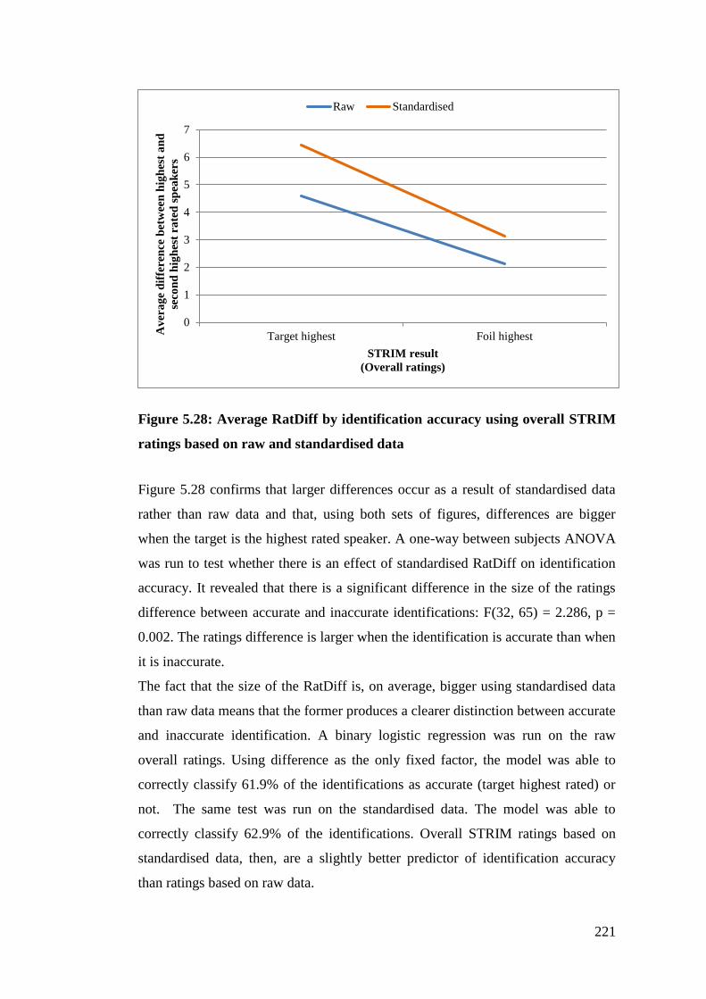
221
Figure 5.28: Average RatDiff by identification accuracy using overall STRIM
ratings based on raw and standardised data
Figure 5.28 confirms that larger differences occur as a result of standardised data
rather than raw data and that, using both sets of figures, differences are bigger
when the target is the highest rated speaker. A one-way between subjects ANOVA
was run to test whether there is an effect of standardised RatDiff on identification
accuracy. It revealed that there is a significant difference in the size of the ratings
difference between accurate and inaccurate identifications: F(32, 65) = 2.286, p =
0.002. The ratings difference is larger when the identification is accurate than when
it is inaccurate.
The fact that the size of the RatDiff is, on average, bigger using standardised data
than raw data means that the former produces a clearer distinction between accurate
and inaccurate identification. A binary logistic regression was run on the raw
overall ratings. Using difference as the only fixed factor, the model was able to
correctly classify 61.9% of the identifications as accurate (target highest rated) or
not. The same test was run on the standardised data. The model was able to
correctly classify 62.9% of the identifications. Overall STRIM ratings based on
standardised data, then, are a slightly better predictor of identification accuracy
than ratings based on raw data.
0
1
2
3
4
5
6
7
Target highest Foil highestAv
era
ge
dif
feren
ce b
etw
een
hig
hes
t a
nd
seco
nd
hig
hes
t ra
ted
sp
eak
ers
STRIM result
(Overall ratings)
Raw Standardised
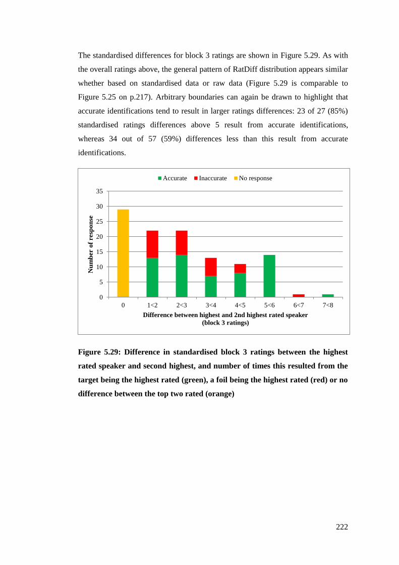
222
The standardised differences for block 3 ratings are shown in Figure 5.29. As with
the overall ratings above, the general pattern of RatDiff distribution appears similar
whether based on standardised data or raw data (Figure 5.29 is comparable to
Figure 5.25 on p.217). Arbitrary boundaries can again be drawn to highlight that
accurate identifications tend to result in larger ratings differences: 23 of 27 (85%)
standardised ratings differences above 5 result from accurate identifications,
whereas 34 out of 57 (59%) differences less than this result from accurate
identifications.
Figure 5.29: Difference in standardised block 3 ratings between the highest
rated speaker and second highest, and number of times this resulted from the
target being the highest rated (green), a foil being the highest rated (red) or no
difference between the top two rated (orange)
0
5
10
15
20
25
30
35
0 1<2 2<3 3<4 4<5 5<6 6<7 7<8
Nu
mb
er o
f re
spo
nse
Difference between highest and 2nd highest rated speaker
(block 3 ratings)
Accurate Inaccurate No response
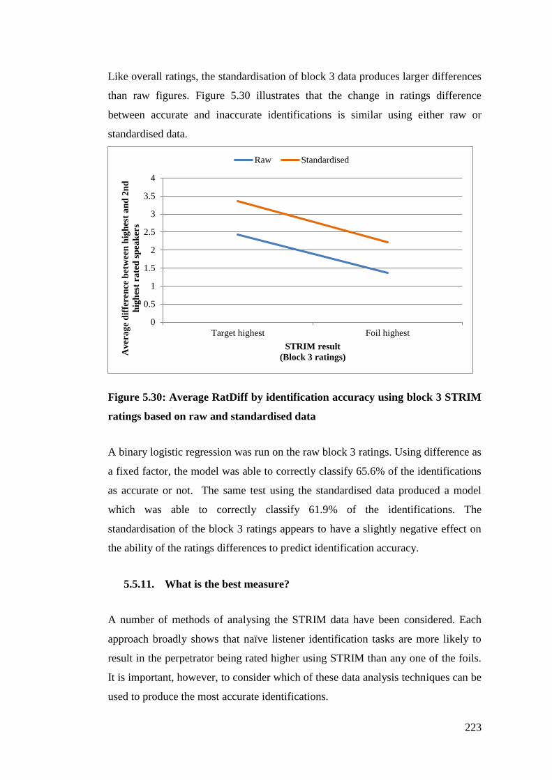
223
Like overall ratings, the standardisation of block 3 data produces larger differences
than raw figures. Figure 5.30 illustrates that the change in ratings difference
between accurate and inaccurate identifications is similar using either raw or
standardised data.
Figure 5.30: Average RatDiff by identification accuracy using block 3 STRIM
ratings based on raw and standardised data
A binary logistic regression was run on the raw block 3 ratings. Using difference as
a fixed factor, the model was able to correctly classify 65.6% of the identifications
as accurate or not. The same test using the standardised data produced a model
which was able to correctly classify 61.9% of the identifications. The
standardisation of the block 3 ratings appears to have a slightly negative effect on
the ability of the ratings differences to predict identification accuracy.
5.5.11. What is the best measure?
A number of methods of analysing the STRIM data have been considered. Each
approach broadly shows that naïve listener identification tasks are more likely to
result in the perpetrator being rated higher using STRIM than any one of the foils.
It is important, however, to consider which of these data analysis techniques can be
used to produce the most accurate identifications.
0
0.5
1
1.5
2
2.5
3
3.5
4
Target highest Foil highest
Av
era
ge
dif
feren
ce b
etw
een
hig
hes
t a
nd
2n
d
hig
hes
t ra
ted
sp
eak
ers
STRIM result
(Block 3 ratings)
Raw Standardised

224
Above, the binary categorisation of responses was used to classify responses as
either accurate or inaccurate based on which speaker was rated highest using
various measures. The most accurate measure was shown to be block 3 ratings
(64%). Both STRIM ratings for a given speaker and RatDiffs have been shown to
be significant predictors of whether a response is accurate or not. It should be
possible, then, to improve upon the binary classification response accuracies
recorded earlier. The extent to which this is possible and which measure can
provide the most accurate responses will be discussed here.
The use of STRIM ratings has been shown to yield highly reliable identification.
For example, all of the responses in which the highest overall rating was 26
produced accurate identifications. This, however, is based on just three
identifications. Without much more data, it seems unhelpful to suggest that the
highest overall rating is 26, then all responses will be accurate (regardless of what
the data show).
One way of overcoming the lack of data for any given rating is to use cumulative
figures. If a rating is above a certain boundary then it is included in the
identification accuracy calculation. If a rating is below the boundary, it is classified
in the same way as ‘no response’ identifications. This is then akin to the STRIM
evidence not being sufficient to be used to provide an identification, as above
where there was no difference between the two highest rated speakers.
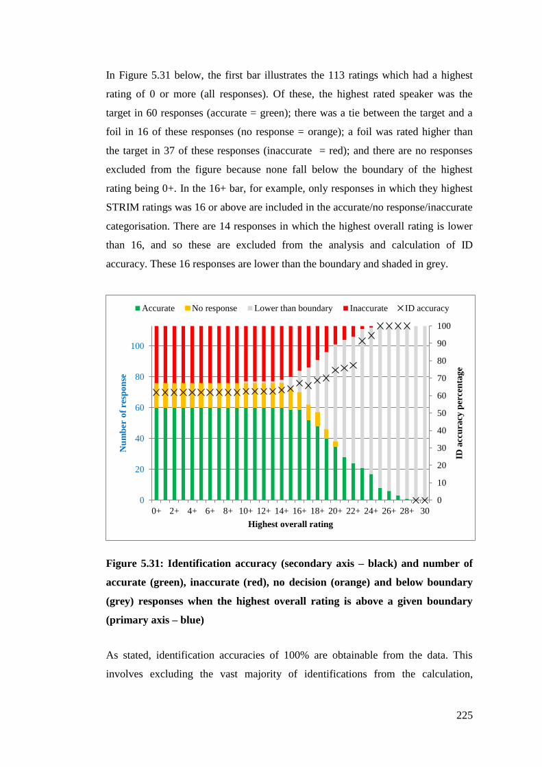
225
In Figure 5.31 below, the first bar illustrates the 113 ratings which had a highest
rating of 0 or more (all responses). Of these, the highest rated speaker was the
target in 60 responses (accurate = green); there was a tie between the target and a
foil in 16 of these responses (no response = orange); a foil was rated higher than
the target in 37 of these responses (inaccurate = red); and there are no responses
excluded from the figure because none fall below the boundary of the highest
rating being 0+. In the 16+ bar, for example, only responses in which they highest
STRIM ratings was 16 or above are included in the accurate/no response/inaccurate
categorisation. There are 14 responses in which the highest overall rating is lower
than 16, and so these are excluded from the analysis and calculation of ID
accuracy. These 16 responses are lower than the boundary and shaded in grey.
Figure 5.31: Identification accuracy (secondary axis – black) and number of
accurate (green), inaccurate (red), no decision (orange) and below boundary
(grey) responses when the highest overall rating is above a given boundary
(primary axis – blue)
As stated, identification accuracies of 100% are obtainable from the data. This
involves excluding the vast majority of identifications from the calculation,
0
10
20
30
40
50
60
70
80
90
100
0
20
40
60
80
100
0+ 2+ 4+ 6+ 8+ 10+ 12+ 14+ 16+ 18+ 20+ 22+ 24+ 26+ 28+ 30
ID a
ccu
racy
per
cen
tag
e
Nu
mb
er o
f re
spo
nse
Highest overall rating
Accurate No response Lower than boundary Inaccurate ID accuracy
226
however. Eight out of 113 highest overall ratings were at least 25, and these were
all accurate. If this could be extrapolated across a much larger dataset, it would
provide a strong prediction that when the highest overall rating is above 25 the
highest rated speaker is the perpetrator. Of course, this is based on a relatively
small dataset and so the prediction is not supported beyond the correlation of
RatDiffs and ID accuracy. Clearly, as the ratings boundary for inclusion in the
accuracy calculation is increased, the number of identifications upon which the
calculation is made is lowered. Whilst the accuracy figure is shown to rise in
conjunction with the highest rating, this is based on fewer responses.

227
In order to address whether the identification accuracy above a given boundary is
based upon sufficient responses to make the measure worthwhile, a series of z-
scores were calculated. The identification accuracy obtained in TVLU condition (in
which 15 out of 36 responses were accurate) was compared against the
identification accuracy and number of responses which contribute to this accuracy
above each rating boundary. The higher the z-score, the greater the level of
statistical difference between that measure and the TVLU accuracy. Figure 5.32
shows the identification accuracy above a given boundary (cross), the percentage
of all responses which that calculation is based upon (circle) and the z-score
resultant from the comparison of this calculation with the TVLU accuracy (blue
bar). All resultant z values were significant at the 0.05 level, apart from the upper
limits of the ratings - indicated by a red stripe. This is presumably because they
were based on too small a number of responses (3 and 1).
Figure 5.32: Identification accuracy when the highest overall rated speaker
was above the given boundary (black cross), the percentage of all responses
upon which this calculation was based (black circle) (both secondary axis –
black) and z-score from comparison of accuracy above given boundary
(primary axis – blue)
There is sufficient data to provide a measure which results in a 100% identification
accuracy rate and enough responses to be statistically significantly higher than the
0
10
20
30
40
50
60
70
80
90
100
0
0.5
1
1.5
2
2.5
3
3.5
4
4.5
0+ 2+ 4+ 6+ 8+ 10+ 12+ 14+ 16+ 18+ 20+ 22+ 24+ 26+ 28+
ID a
ccu
racy
(%
) /
n o
f re
spo
nse
s b
ase
d
up
on
z-sc
ore
fro
m c
om
pa
riso
n w
ith
TV
LU
Highest overall rating boundary
Z-score Overall ID accuracy Percentage of all responses included

228
TVLU accuracy. Where the highest overall rating is 25 or more, all eight of the
responses rated the target speaker highest. This accounts for 7% of all responses. A
higher z-score results when the highest overall rating is 23 or more, which includes
20% of all responses (23) with an identification accuracy of 91.3%.
Figure 5.33 below is based on the highest block 3 ratings. It illustrates a similar
pattern. High identification accuracies are achievable using a cumulative analysis
of STRIM ratings, but these are based on low response numbers.
Figure 5.33: Identification accuracy (secondary axis – black) and number of
accurate (green), inaccurate (red), no decision (orange) and below boundary
(grey) responses when the highest block rating is above a given boundary
(primary axis – blue)
0
10
20
30
40
50
60
70
80
90
100
0
20
40
60
80
100
0+ 1+ 2+ 3+ 4+ 5+ 6+ 7+ 8+ 9+ 10+
PID
acc
ura
cyrc
enta
ge
Nu
mb
er o
f re
spo
nse
s
Highest block 3 rating
Accurate No response Lower than boundary Inaccurate ID accuracy
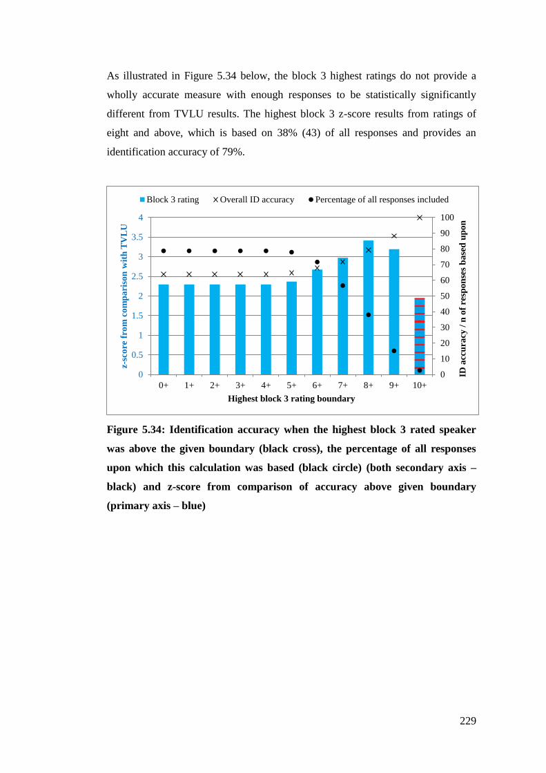
229
As illustrated in Figure 5.34 below, the block 3 highest ratings do not provide a
wholly accurate measure with enough responses to be statistically significantly
different from TVLU results. The highest block 3 z-score results from ratings of
eight and above, which is based on 38% (43) of all responses and provides an
identification accuracy of 79%.
Figure 5.34: Identification accuracy when the highest block 3 rated speaker
was above the given boundary (black cross), the percentage of all responses
upon which this calculation was based (black circle) (both secondary axis –
black) and z-score from comparison of accuracy above given boundary
(primary axis – blue)
0
10
20
30
40
50
60
70
80
90
100
0
0.5
1
1.5
2
2.5
3
3.5
4
0+ 1+ 2+ 3+ 4+ 5+ 6+ 7+ 8+ 9+ 10+
ID a
ccu
racy
/ n
of
resp
on
ses
ba
sed
up
on
z-sc
ore
fro
m c
om
pa
riso
n w
ith
TV
LU
Highest block 3 rating boundary
Block 3 rating Overall ID accuracy Percentage of all responses included
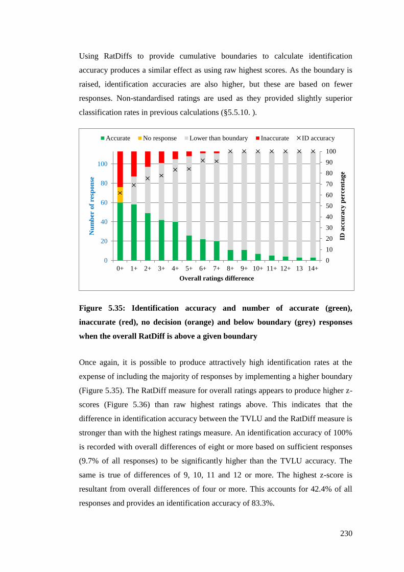
230
Using RatDiffs to provide cumulative boundaries to calculate identification
accuracy produces a similar effect as using raw highest scores. As the boundary is
raised, identification accuracies are also higher, but these are based on fewer
responses. Non-standardised ratings are used as they provided slightly superior
classification rates in previous calculations (§5.5.10. ).
Figure 5.35: Identification accuracy and number of accurate (green),
inaccurate (red), no decision (orange) and below boundary (grey) responses
when the overall RatDiff is above a given boundary
Once again, it is possible to produce attractively high identification rates at the
expense of including the majority of responses by implementing a higher boundary
(Figure 5.35). The RatDiff measure for overall ratings appears to produce higher z-
scores (Figure 5.36) than raw highest ratings above. This indicates that the
difference in identification accuracy between the TVLU and the RatDiff measure is
stronger than with the highest ratings measure. An identification accuracy of 100%
is recorded with overall differences of eight or more based on sufficient responses
(9.7% of all responses) to be significantly higher than the TVLU accuracy. The
same is true of differences of 9, 10, 11 and 12 or more. The highest z-score is
resultant from overall differences of four or more. This accounts for 42.4% of all
responses and provides an identification accuracy of 83.3%.
0
10
20
30
40
50
60
70
80
90
100
0
20
40
60
80
100
0+ 1+ 2+ 3+ 4+ 5+ 6+ 7+ 8+ 9+ 10+ 11+ 12+ 13 14+
ID a
ccu
racy
per
cen
tag
e
Nu
mb
er o
f re
spo
nse
Overall ratings difference
Accurate No response Lower than boundary Inaccurate ID accuracy
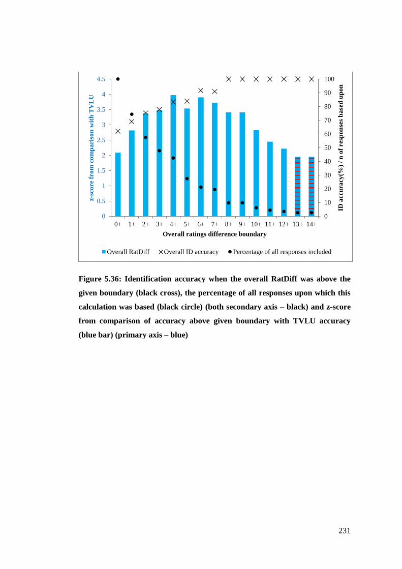
231
Figure 5.36: Identification accuracy when the overall RatDiff was above the
given boundary (black cross), the percentage of all responses upon which this
calculation was based (black circle) (both secondary axis – black) and z-score
from comparison of accuracy above given boundary with TVLU accuracy
(blue bar) (primary axis – blue)
0
10
20
30
40
50
60
70
80
90
100
0
0.5
1
1.5
2
2.5
3
3.5
4
4.5
0+ 1+ 2+ 3+ 4+ 5+ 6+ 7+ 8+ 9+ 10+ 11+ 12+ 13+ 14+
ID a
ccu
racy
(%)
/ n
of
resp
on
ses
ba
sed
up
on
z-sc
ore
fro
m c
om
pa
riso
n w
ith
TV
LU
Overall ratings difference boundary
Overall RatDiff Overall ID accuracy Percentage of all responses included
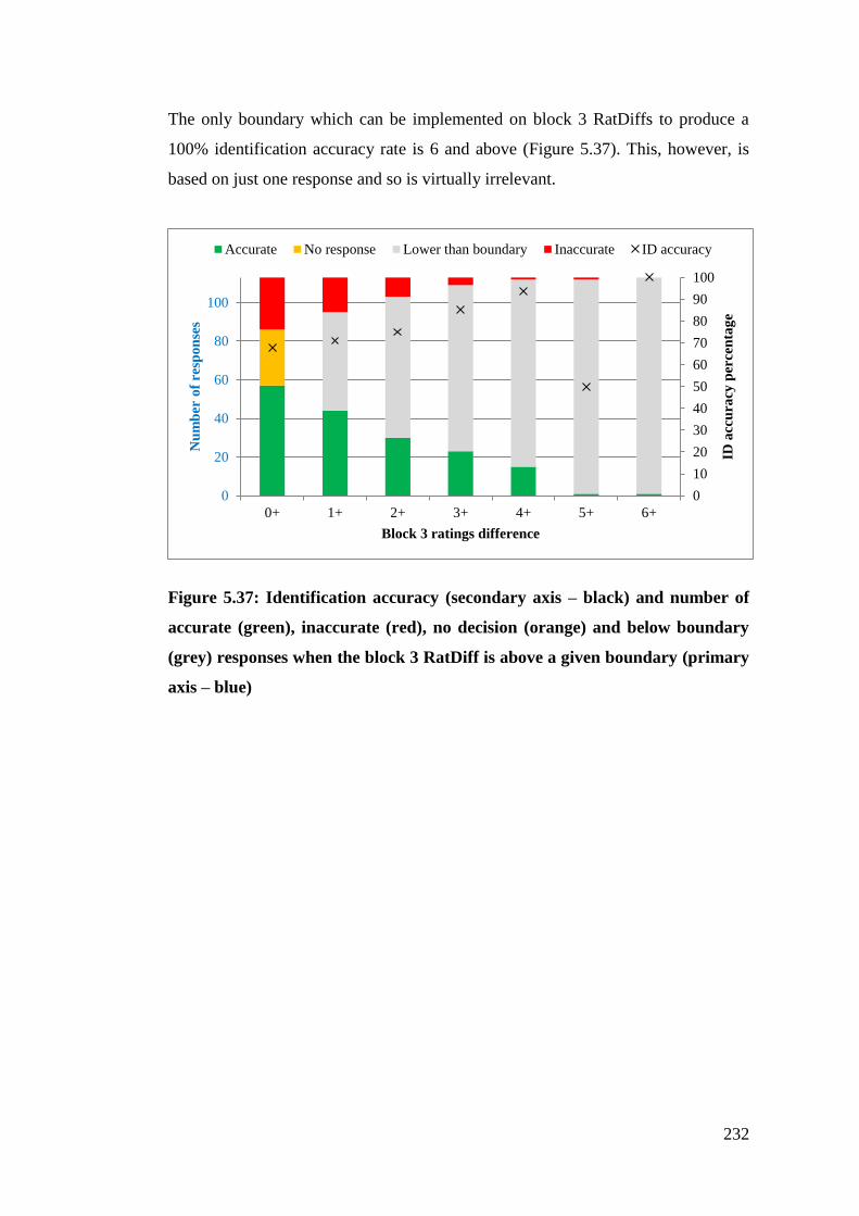
232
The only boundary which can be implemented on block 3 RatDiffs to produce a
100% identification accuracy rate is 6 and above (Figure 5.37). This, however, is
based on just one response and so is virtually irrelevant.
Figure 5.37: Identification accuracy (secondary axis – black) and number of
accurate (green), inaccurate (red), no decision (orange) and below boundary
(grey) responses when the block 3 RatDiff is above a given boundary (primary
axis – blue)
0
10
20
30
40
50
60
70
80
90
100
0
20
40
60
80
100
0+ 1+ 2+ 3+ 4+ 5+ 6+
ID a
ccu
racy
per
cen
tag
e
Nu
mb
er o
f re
spo
nse
s
Block 3 ratings difference
Accurate No response Lower than boundary Inaccurate ID accuracy
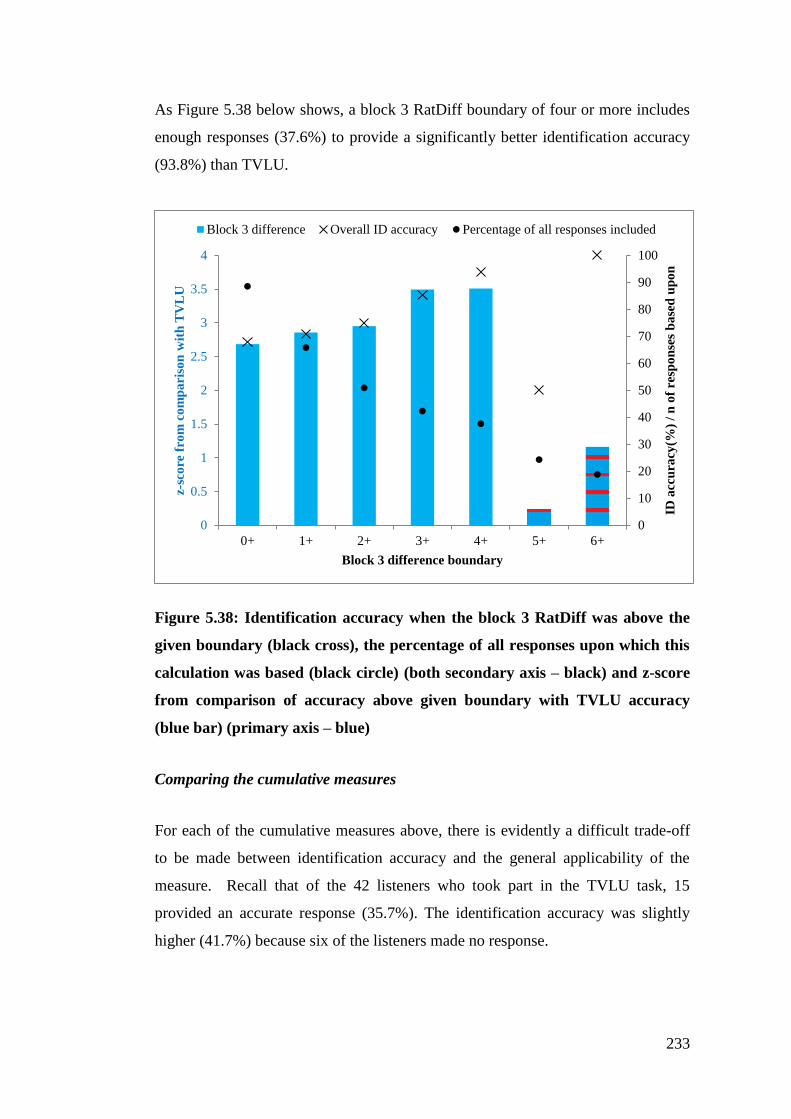
233
As Figure 5.38 below shows, a block 3 RatDiff boundary of four or more includes
enough responses (37.6%) to provide a significantly better identification accuracy
(93.8%) than TVLU.
Figure 5.38: Identification accuracy when the block 3 RatDiff was above the
given boundary (black cross), the percentage of all responses upon which this
calculation was based (black circle) (both secondary axis – black) and z-score
from comparison of accuracy above given boundary with TVLU accuracy
(blue bar) (primary axis – blue)
Comparing the cumulative measures
For each of the cumulative measures above, there is evidently a difficult trade-off
to be made between identification accuracy and the general applicability of the
measure. Recall that of the 42 listeners who took part in the TVLU task, 15
provided an accurate response (35.7%). The identification accuracy was slightly
higher (41.7%) because six of the listeners made no response.
0
10
20
30
40
50
60
70
80
90
100
0
0.5
1
1.5
2
2.5
3
3.5
4
0+ 1+ 2+ 3+ 4+ 5+ 6+
ID a
ccu
racy
(%)
/ n
of
resp
on
ses
ba
sed
up
on
z-sc
ore
fro
m c
om
pa
riso
n w
ith
TV
LU
Block 3 difference boundary
Block 3 difference Overall ID accuracy Percentage of all responses included
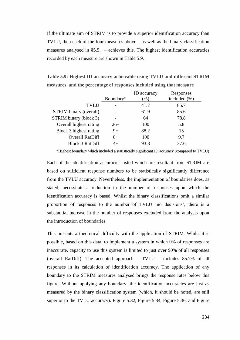
234
If the ultimate aim of STRIM is to provide a superior identification accuracy than
TVLU, then each of the four measures above – as well as the binary classification
measures analysed in §5.5. – achieves this. The highest identification accuracies
recorded by each measure are shown in Table 5.9.
Table 5.9: Highest ID accuracy achievable using TVLU and different STRIM
measures, and the percentage of responses included using that measure
Boundary*
ID accuracy
(%)
Responses
included (%)
TVLU - 41.7 85.7
STRIM binary (overall) - 61.9 85.6
STRIM binary (block 3) - 64 78.8
Overall highest rating 26+ 100 5.8
Block 3 highest rating 9+ 88.2 15
Overall RatDiff 8+ 100 9.7
Block 3 RatDiff 4+ 93.8 37.6
*Highest boundary which included a statistically significant ID accuracy (compared to TVLU)
Each of the identification accuracies listed which are resultant from STRIM are
based on sufficient response numbers to be statistically significantly difference
from the TVLU accuracy. Nevertheless, the implementation of boundaries does, as
stated, necessitate a reduction in the number of responses upon which the
identification accuracy is based. Whilst the binary classifications omit a similar
proportion of responses to the number of TVLU ‘no decisions’, there is a
substantial increase in the number of responses excluded from the analysis upon
the introduction of boundaries.
This presents a theoretical difficulty with the application of STRIM. Whilst it is
possible, based on this data, to implement a system in which 0% of responses are
inaccurate, capacity to use this system is limited to just over 90% of all responses
(overall RatDiff). The accepted approach – TVLU – includes 85.7% of all
responses in its calculation of identification accuracy. The application of any
boundary to the STRIM measures analysed brings the response rates below this
figure. Without applying any boundary, the identification accuracies are just as
measured by the binary classification system (which, it should be noted, are still
superior to the TVLU accuracy). Figure 5.32, Figure 5.34, Figure 5.36, and Figure
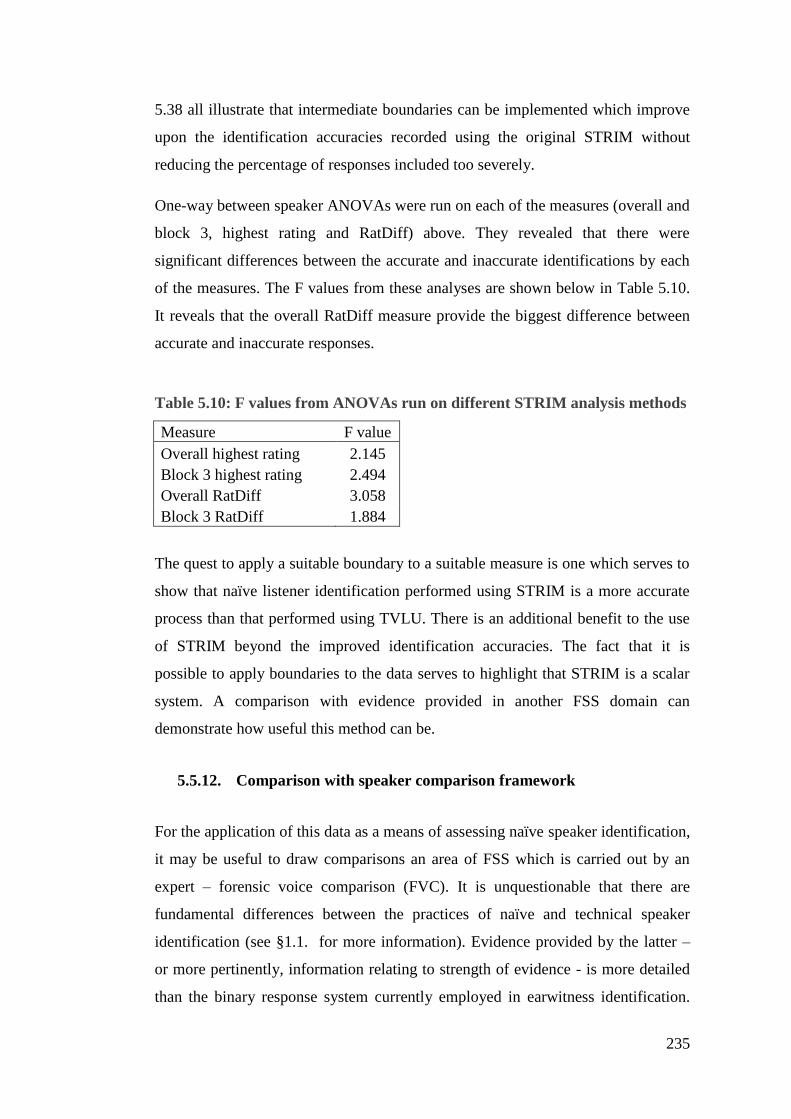
235
5.38 all illustrate that intermediate boundaries can be implemented which improve
upon the identification accuracies recorded using the original STRIM without
reducing the percentage of responses included too severely.
One-way between speaker ANOVAs were run on each of the measures (overall and
block 3, highest rating and RatDiff) above. They revealed that there were
significant differences between the accurate and inaccurate identifications by each
of the measures. The F values from these analyses are shown below in Table 5.10.
It reveals that the overall RatDiff measure provide the biggest difference between
accurate and inaccurate responses.
Table 5.10: F values from ANOVAs run on different STRIM analysis methods
Measure F value
Overall highest rating 2.145
Block 3 highest rating 2.494
Overall RatDiff 3.058
Block 3 RatDiff 1.884
The quest to apply a suitable boundary to a suitable measure is one which serves to
show that naïve listener identification performed using STRIM is a more accurate
process than that performed using TVLU. There is an additional benefit to the use
of STRIM beyond the improved identification accuracies. The fact that it is
possible to apply boundaries to the data serves to highlight that STRIM is a scalar
system. A comparison with evidence provided in another FSS domain can
demonstrate how useful this method can be.
5.5.12. Comparison with speaker comparison framework
For the application of this data as a means of assessing naïve speaker identification,
it may be useful to draw comparisons an area of FSS which is carried out by an
expert – forensic voice comparison (FVC). It is unquestionable that there are
fundamental differences between the practices of naïve and technical speaker
identification (see §1.1. for more information). Evidence provided by the latter –
or more pertinently, information relating to strength of evidence - is more detailed
than the binary response system currently employed in earwitness identification.
236
The STRIM ratings system attempts to make the evidence provided by the two
forms of identification more comparable.
A survey carried out by Gold and French (2011) found that just two of 34 forensic
practitioners used a binary decision approach to FVC work. Output from such an
approach concludes that samples either contain voice(s) from the same or different
speaker(s). The main limitation of this approach is cited as the cliff-edge decisions
made by the expert and the arbitrary boundary between a the two potential
conclusions (Robertson & Vignaux, 1995). The same criticisms could be said to
apply to naïve speaker identification.
A more commonly used framework for FVC evidence is a classical probability
scale, such as that in Baldwin and French (1990: 10). In Gold and French’s (2011)
appraisal, 13 of the 34 practitioners surveyed reported providing conclusions based
on a scale of probably. The expert expresses a conclusion of whether samples are
produced by the same or different speaker(s) given the evidence (as in the binary
decision framework), and then subsequently applies a gradient probability
(possible, quite possible, etc.) to the conclusion.
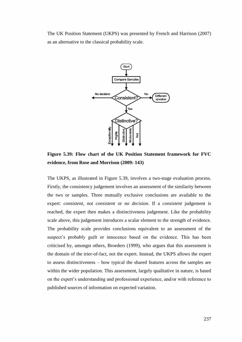
237
The UK Position Statement (UKPS) was presented by French and Harrison (2007)
as an alternative to the classical probability scale.
Figure 5.39: Flow chart of the UK Position Statement framework for FVC
evidence, from Rose and Morrison (2009: 143)
The UKPS, as illustrated in Figure 5.39, involves a two-stage evaluation process.
Firstly, the consistency judgement involves an assessment of the similarity between
the two or samples. Three mutually exclusive conclusions are available to the
expert: consistent, not consistent or no decision. If a consistent judgement is
reached, the expert then makes a distinctiveness judgement. Like the probability
scale above, this judgement introduces a scalar element to the strength of evidence.
The probability scale provides conclusions equivalent to an assessment of the
suspect’s probably guilt or innocence based on the evidence. This has been
criticised by, amongst others, Broeders (1999), who argues that this assessment is
the domain of the trier-of-fact, not the expert. Instead, the UKPS allows the expert
to assess distinctiveness – how typical the shared features across the samples are
within the wider population. This assessment, largely qualitative in nature, is based
on the expert’s understanding and professional experience, and/or with reference to
published sources of information on expected variation.
238
The UKPS has also been criticised as a framework for presenting FVC analysis.
Amongst Rose and Morrison’s (2009) criticisms of the UKPS are the categorical
nature of the distinctiveness judgements and the cliff-edge effect of the binary
outcome of the consistency judgement. They argue that the framework for FSS
evidence should be more in line with that for DNA evidence. DNA evidence is
seen as “setting the standard” (Balding, 2005: 55) across forensic sciences, and
uses a Likelihood Ratio (LR) approach. There are number of practical and
theoretical issues associated with the application of an LR based approach to FSS
work (Broeders, 1995; Broeders, 1999; Champod & Meuwly, 2000; Nolan, 2001;
Rose, 2002) and it a major area of debate in the FSS community and beyond
(Cook, Evett, Jackson, Jones & Lambert, 1998). This is particularly true following
a redacted judgement from the Appeal Court of England and Wales in October
2010 (R v T [2010]) , which questioned the use of LR evaluations as part of expert
evidence on footwear markings (Aitken, 2012). The LR framework is based on
Bayesian statistical modelling, and provides a gradient assessment of the strength
of evidence, expressing the degree to which the evidence supports the prosecution
or defence. Since the turn of the century, there has been an upturn the in the general
acceptance within the FSS community of an LR based framework. This approach,
with associated verbal expressions of evidence based on the Bayesian analysis of
data, is overtaking the UKPS as the most common framework for FVC casework in
the UK. It is now employed by JP French Associates, the UK’s largest independent
forensic speech and acoustics laboratory.
In terms of comparison with the FVC domain, evidence provided by means of
naïve listener identification is most comparable with the binary decision
framework. It is clear that there are barriers to naïve listener identification adopting
an LR based approach. It is one person’s identification of a voice based on their
memory of an event and cannot be run through statistical models and compared
formally with reference populations. There cannot be a comparison of probability
of outcomes based on the prosecution hypothesis and the defence hypothesis.
Bayesian principles do apply to the identification, however, as it offered weight of
support for one option against others. The STRIM ratings have the potential to
offer strong or weak support in favour of one speaker being the perpetrator relative
to a closed set of alternatives. What is clear is that there has been a move in the
239
FSS community towards evidence being presented not in terms of a binary
distinction, but with a gradience of the evidence being useful or relevant. Whether
evidence provided by STRIM is comparable to that provided by TVLU, it does
represent an opportunity to move towards a more gradient based approach.
The response provided by a naïve listener could be accompanied by a numerical
indication of how likely the ratings outcome is based on STRIM data. If overall
RatDiffs were adopted as the most suitable STRIM measure, the ratings provided
by lay listeners could be analysed for the difference between the highest and
second highest rated speakers and compared against the population data. A RatDiff
of above eight, for example, only occurs when the target is the highest rated
speaker. Theoretically, then, a response where the highest rated speaker is rated as
27 and the second highest is rated as 19 could be accompanied by the addition that
such a response has been to identify the perpetrator as the highest rated speaker
100% of the time. This may be true based on the above data, but is patently
dangerous information to provide. A trier of fact being presented with information
which they are told has never been shown to be inaccurate will undoubtedly place
too much weight on the response. This would be an issue no matter what the
sample size upon which the accuracy was based, but based on such limited data it
is a wholly unsuitable.
Likelihood ratio evidence has in the past been reported in numerical form, though
the format of this is in LR or log likelihood ratios, which required supplementary
explanation from the expert in order to aid interpretation. This limits the potential
for a trier of fact over stating the implications of the data, which would not be
possible for pure percentage based representations. Despite this, the extent to which
triers of fact are able to comprehend numerical estimates of strength of evidence
has been questioned by the courts. Likelihood ratios have been converted into
verbal expressions and are now in use in FSC casework. The formulation used JP
French Associates (York, UK) is based upon recommendations made by the
Association of Forensic Science Providers (2009), which aims to provide a
standardisation of procedures across forensic disciplines. The 13-point scale for
evaluation of evidence includes categories from extremely strong to limited support
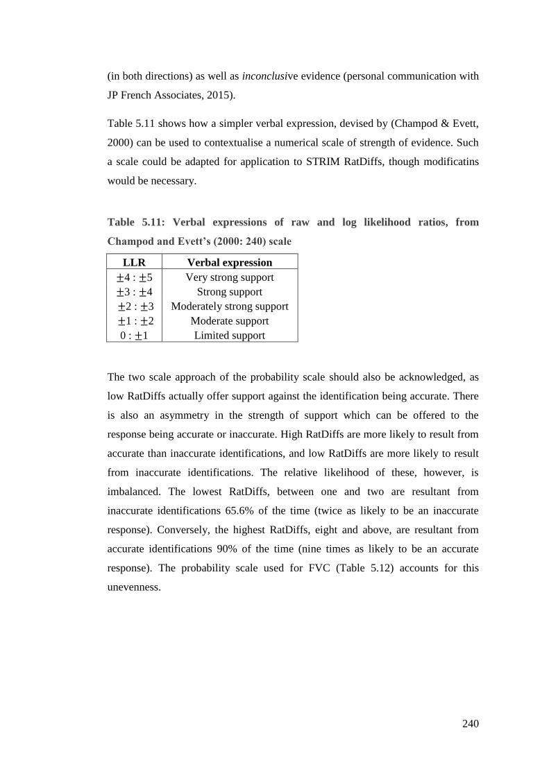
240
(in both directions) as well as inconclusive evidence (personal communication with
JP French Associates, 2015).
Table 5.11 shows how a simpler verbal expression, devised by (Champod & Evett,
2000) can be used to contextualise a numerical scale of strength of evidence. Such
a scale could be adapted for application to STRIM RatDiffs, though modificatins
would be necessary.
Table 5.11: Verbal expressions of raw and log likelihood ratios, from
Champod and Evett’s (2000: 240) scale
LLR Verbal expression
±4 : ±5 Very strong support
±3 : ±4 Strong support
±2 : ±3 Moderately strong support
±1 : ±2 Moderate support
0 : ±1 Limited support
The two scale approach of the probability scale should also be acknowledged, as
low RatDiffs actually offer support against the identification being accurate. There
is also an asymmetry in the strength of support which can be offered to the
response being accurate or inaccurate. High RatDiffs are more likely to result from
accurate than inaccurate identifications, and low RatDiffs are more likely to result
from inaccurate identifications. The relative likelihood of these, however, is
imbalanced. The lowest RatDiffs, between one and two are resultant from
inaccurate identifications 65.6% of the time (twice as likely to be an inaccurate
response). Conversely, the highest RatDiffs, eight and above, are resultant from
accurate identifications 90% of the time (nine times as likely to be an accurate
response). The probability scale used for FVC (Table 5.12) accounts for this
unevenness.
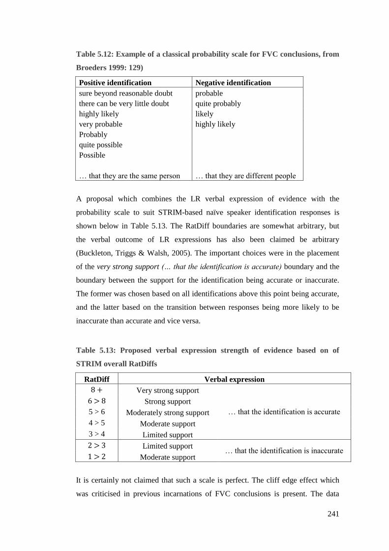
241
Table 5.12: Example of a classical probability scale for FVC conclusions, from
Broeders 1999: 129)
Positive identification Negative identification
sure beyond reasonable doubt probable
there can be very little doubt quite probably
highly likely likely
very probable highly likely
Probably
quite possible
Possible
… that they are the same person … that they are different people
A proposal which combines the LR verbal expression of evidence with the
probability scale to suit STRIM-based naïve speaker identification responses is
shown below in Table 5.13. The RatDiff boundaries are somewhat arbitrary, but
the verbal outcome of LR expressions has also been claimed be arbitrary
(Buckleton, Triggs & Walsh, 2005). The important choices were in the placement
of the very strong support (… that the identification is accurate) boundary and the
boundary between the support for the identification being accurate or inaccurate.
The former was chosen based on all identifications above this point being accurate,
and the latter based on the transition between responses being more likely to be
inaccurate than accurate and vice versa.
Table 5.13: Proposed verbal expression strength of evidence based on of
STRIM overall RatDiffs
RatDiff Verbal expression
8 + Very strong support
… that the identification is accurate
6 > 8 Strong support
5 > 6 Moderately strong support
4 > 5 Moderate support
3 > 4 Limited support
2 > 3 Limited support … that the identification is inaccurate
1 > 2 Moderate support
It is certainly not claimed that such a scale is perfect. The cliff edge effect which
was criticised in previous incarnations of FVC conclusions is present. The data

242
upon which the strength of evidence is calculated are limited in number, and are
much less reliable than the acoustic data upon which LRs are calculated. Indeed,
there are still known difficulties involved in the trier of fact being asked to interpret
verbal scales (cf. Gold and Hughes (2014); Martire, Kemp, Sayle and Newell
(2014); Mullen, Spence, Mozey, Jamieson (2013)). Nevertheless, it marks a
significant move from the binary classification system upon which the TVLU is
built.
5.6. Discussion
The results in this chapter go some way to supporting the use of STRIM as a voice
identification testing method. This is based on the second justification made in §5.1
- a desire to improve the accuracy with which naïve listeners can identify a target in
voice identification tasks. A significant improvement in identification accuracy
from 41.7% using a TVLU approach to 61.9% using the STRIM overall rating
method was recorded. This suggests that repeated identification using a scalar
response system can allow a listener to make more accurate identifications of the
target speaker than the traditional lineup methodology.
Of the listeners using the TVLU method of testing, only 14% made no response,
i.e. only 6 out of 42 listeners felt unwilling to make an identification, either positive
or negative. This is despite many more of the listeners reporting that they found the
task difficult. This may be an artefact of the experimental nature of the task. A
number of listeners also reported that they felt they ‘should’ make an identification
because it was a study asking them to do so (even though the option to make no
identification was provided and listeners were informed that the perpetrator may
not be present in the lineup). This is consistent with the obligation effect reported
by Hollien et al. (1995) and Yarmey (2007). If listeners are making identifications
even when they do not necessarily feel it is the same speaker as previously heard,
false identifications are more likely. It is unclear how this might translate to an
applied earwitness situation. Earwitnesses are evidently inclined to identify the
perpetrator, but it is not known whether any reservation in their judgement will
prevent them from making any identification. In an experimental setting, the cost
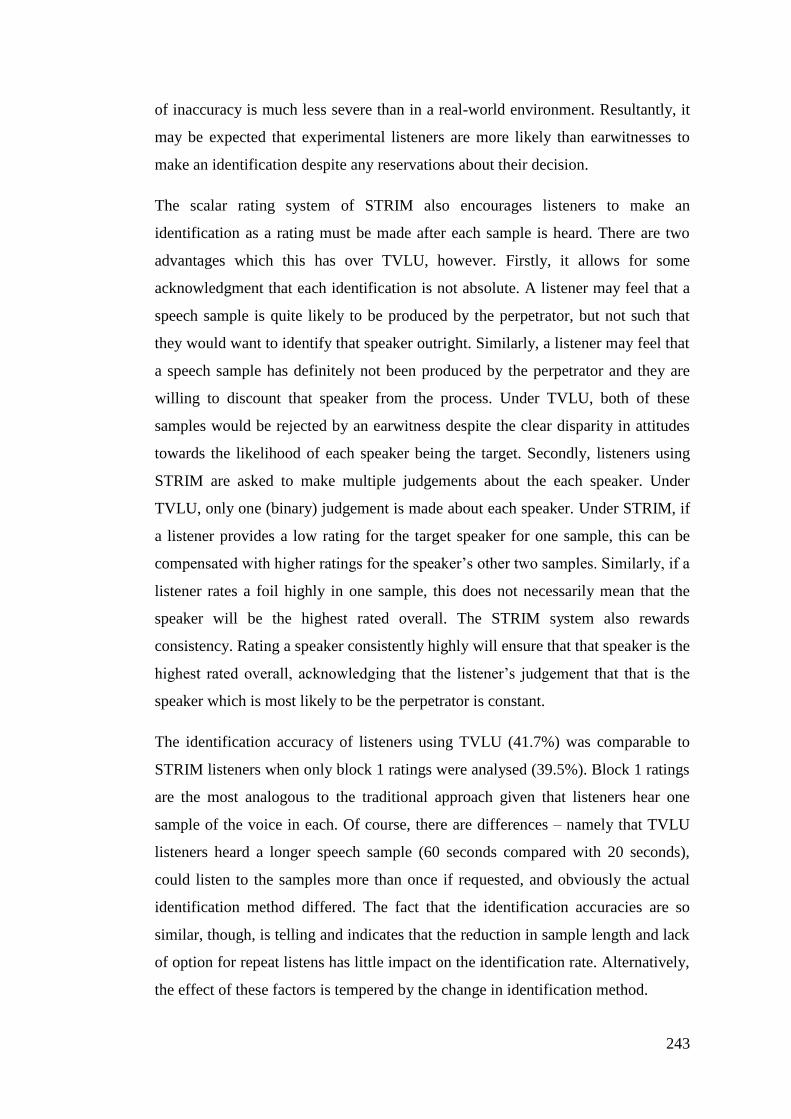
243
of inaccuracy is much less severe than in a real-world environment. Resultantly, it
may be expected that experimental listeners are more likely than earwitnesses to
make an identification despite any reservations about their decision.
The scalar rating system of STRIM also encourages listeners to make an
identification as a rating must be made after each sample is heard. There are two
advantages which this has over TVLU, however. Firstly, it allows for some
acknowledgment that each identification is not absolute. A listener may feel that a
speech sample is quite likely to be produced by the perpetrator, but not such that
they would want to identify that speaker outright. Similarly, a listener may feel that
a speech sample has definitely not been produced by the perpetrator and they are
willing to discount that speaker from the process. Under TVLU, both of these
samples would be rejected by an earwitness despite the clear disparity in attitudes
towards the likelihood of each speaker being the target. Secondly, listeners using
STRIM are asked to make multiple judgements about the each speaker. Under
TVLU, only one (binary) judgement is made about each speaker. Under STRIM, if
a listener provides a low rating for the target speaker for one sample, this can be
compensated with higher ratings for the speaker’s other two samples. Similarly, if a
listener rates a foil highly in one sample, this does not necessarily mean that the
speaker will be the highest rated overall. The STRIM system also rewards
consistency. Rating a speaker consistently highly will ensure that that speaker is the
highest rated overall, acknowledging that the listener’s judgement that that is the
speaker which is most likely to be the perpetrator is constant.
The identification accuracy of listeners using TVLU (41.7%) was comparable to
STRIM listeners when only block 1 ratings were analysed (39.5%). Block 1 ratings
are the most analogous to the traditional approach given that listeners hear one
sample of the voice in each. Of course, there are differences – namely that TVLU
listeners heard a longer speech sample (60 seconds compared with 20 seconds),
could listen to the samples more than once if requested, and obviously the actual
identification method differed. The fact that the identification accuracies are so
similar, though, is telling and indicates that the reduction in sample length and lack
of option for repeat listens has little impact on the identification rate. Alternatively,
the effect of these factors is tempered by the change in identification method.
244
Block 2 (50%) ratings performed slightly better than both block 1 ratings and the
TVLU, and block 3 (64%) ratings performed significantly better than both. The
reasons for this are unclear. One possibility is that the improvement is cumulative.
More speech material from each speaker is being heard as the task progresses, and
it has been demonstrated that around 60 seconds of speech provides the optimal
length of sample to allow optimal voice identification, although identification is
certainly possible based on a smaller duration (Bricker & Pruzansky, 1966;
Compton, 1963; Legge et al., 1984). This theory relies on listeners linking the
different samples produced by each speaker. The STRIM method explicitly aims to
avoid this, however, and §5.5.3. demonstrates that there is variance in the ratings
given to speakers across the three samples by listeners suggesting this is not the
case.
Alternatively, listeners may become more attuned to the task of making ratings as
the identification task progresses. If the relative judgement (Wells, 1984; Wells et
al., 1998) strategy is employed then more voices against which to make
comparisons will heighten the listeners’ judgement-making ability. Furthermore, it
may be that listeners become more confident in their own capabilities based on the
increase in stimuli on which to base comparisons (whether their identification is
actually accurate or not). A wider range of ratings is recorded in the later hearing
blocks, suggesting that listeners become more willing to use the scale and commit
to the extremes.
Overall ratings and block 3 ratings were consistently the methods of analysis which
provided the most accurate identifications for most listeners. This is reassuring, as
it demonstrates the ratings provided by only a few listeners are best analysed in any
way other than either of these two methods. It is not feasible to pick and choose
which technique should be used to analyse the STRIM data, and so it is important
that not only do these methods provide the most accurate results across all listeners,
but also for the most listeners.
The variation in the performance of individuals is unsurprising. It has long since
been acknowledged as a variable which is beyond the control of practitioners
asking earwitnesses to make an identification (Philippon et al., 2007b). Indeed,
even in an experimental setting, it is a staggeringly difficult task to predict whether
245
one naïve listener is more or less likely to make an accurate voice identification
than another. There are, of course, variables which have been shown to have a
significant effect on listener performance, but these can never account for the
individual variation which is evident from the data. Some listeners performed well
across their three identifications and others performed badly. Despite this, there is
little to suggest that, if they were provided with a fourth identification task, those
who performed badly would not be just as likely to make an accurate identification,
as there was no effect of listener on accuracy in each task. Whether a listener is
accurate in one identification task is not a significant predictor of whether they will
be accurate in another.
Whilst the binary classification of STRIM responses produced ID accuracies
superior to TVLU, the contribution of the ratings themselves add a degree of
reliability to such responses. There is correlation between ID accuracy and both the
highest overall rating and highest block 3 rating. The higher a rating the listener
attributes to a speaker, the more likely their response is to be accurate (rate the
target highest). Similarly, ID accuracy is correlated with the size of difference
between the highest and second highest rated speaker (RatDiff) for both block 3
and overall ratings. The more a speaker stands out from the rest as being the
highest rated by a listener, the more likely that response it to be accurate. This is a
level of detail which cannot be provided by responses from the TVLU method. In a
forensic context, STRIM ratings provided by an earwitness could be used to not
only to make a selection in a lineup (of the suspect or otherwise), but also offer
strength of support to that identification. A small highest rating or RatDiff would
offer weak support in favour of speaker X being the perpetrator; a large highest
rating or RatDiff would offer strong support in favour of speaker X being the
perpetrator. On the basis of this, a comparison with the LR-based framework of
FVC by expert analysts is made. The RatDiffs can be converted into a verbal
expression scale, whereby very strong support that the response is accurate is
provided if the difference is 8 or more, limited support is provided if the difference
is between 3 and 4, and if the difference is less than this, then support that that the
identification is inaccurate is provided. The support against category is included in
order to mirror the defence/prosecution hypothesis of LR frameworks (Rose,
2006).
246
STRIM, then, appears to offer promise as an alternative to the TVLU both in terms
of accuracy of identifications and the interpretation of their reliability.
5.7. Summary of results
The voice identification accuracies obtained using overall STRIM ratings and
ratings within block 3 alone were both statistically significantly higher than those
obtained using TVLU. It also appears that later ratings are more accurate than
earlier ones, with hearing block having a significant effect on accuracy. There is a
great deal of variation in the performance of listeners. There is also variation in
which STRIM measure provides the most accurate identifications for different
listeners, although for the majority of listeners either the overall rating or block 3
rating was the best method of analysis. Listeners who rate the target highest in one
block show a trend for rating the target highest in later blocks. This was not,
however, a statistically significant effect, unlike the correlation between overall
rating accuracy and individual and within block accuracy. None of the listener
variables tested (age, sex, accent, confidence) were shown to have a significant
effect on accuracy, but there were differences in their effect within the two testing
methods.
In any given response, the bigger the highest block 3 rating was, the more likely the
target was to be the one identified. The same was shown for overall STRIM
ratings. RatDiffs were also shown to correlate with ID accuracy. Larger differences
between the highest and second highest rated speakers occurred in responses
involved an accurate ID. It is possible to increase the boundaries of what
constitutes an identification in a STRIM response. This has the effect of increasing
the ID accuracy of that measure, but lowers the proportion of responses upon
which it is based. Despite this, it is still possible to implement overall and block 3
boundaries which are based on sufficient data to be significantly superior to the ID
accuracy of the TVLU condition.
247
The positive impact of the scalar ratings allows for a tentative comparison the
frameworks used in FVC work. A verbal expression of strength of evidence is
proposed.
5.8. Chapter summary
This chapter presented justifications for considering a new approach to the testing
of earwitnesses in their ability to identify a voice. These are based in a desire to
firstly improve the reliability of identifications, secondly develop the possibility for
statistical analyses of responses in naïve speaker identification, and thirdly provide
an approach which does not simply mirror visual lineups.
Some small-scale pilot studies were employed based on sequential testing of
listeners. These informed the application of a study based on the Short Term
Repeated Identification Method (STRIM). The methodology for this is presented in
this chapter, along with the other variables which the experiment will test. These
include the context in which the listener is exposed to the perpetrator (i.e. whether
they only hear the voice, or see the criminal too).
As discussed, the results of STRIM are promising when compared with a TVLU
approach. It is possible to elicit a greater number of accurate responses, which are
additionally based on more than just a binary response. A comparison with FVC
work illustrates the potential for a scalar approach to naïve listener identification
testing.
248
6. The effect of exposure context
This chapter will present an analysis of the data collected in the study outlined in
Chapter 5. These data have already been analysed for the effect of testing method
on identification accuracy. The focus here will be on the effect of the exposure
context (EC) on accuracy of identifications made by naïve listeners. Listeners were
exposed to the perpetrator’s voice in one or more of the following conditions: audio
only, audio + picture, audio + video. The identification accuracy of each of these
conditions will be compared, along with the effect on any listener variables.
Listeners were also asked to recount information relating to the exposure. The level
of detail provided in three areas will be assessed for their effect on identification
accuracy: speech quality, speech content, and visual information.
2. Methodology
The methodology for the experiment is covered in detail in §5.3. The pertinent
points for this chapter are recapped here.
Listeners were exposed to the perpetrator in one of three exposure conditions:
Audio only (Ao) – listeners heard the voice of the criminal through
headphones. The audio was the only stimulus
Audio + picture (AP) – listeners heard the voice of the criminal through
headphones whilst watching still pictures of the crime unfolding. There was
auditory-visual stimulus
Audio + video (AV) - listeners heard the voice of the criminal whilst
watching a life size video of the crime unfolding on a screen. There was
auditory-visual stimulus – the video providing more ecological validity than
the picture condition
The audio material was the same in each exposure condition. Speakers from the
YorVis database (McDougall et al., 2014) were used for exposure and testing. The
249
perpetrator can be heard speaking on the telephone and then addressing the subject
(albeit via a pre-recorded message). They were asked the time and also instructed
to leave a bag on the floor for the perpetrator in a simulated crime methodology.
For the auditory-visual conditions, listeners saw either pictures or a video of the
scene unfolding. The perpetrator’s face was not visible and identification could
only be made based on the voice.
Once listeners had been exposed to the perpetrator, they answered questions
relevant to the crime (can you explain what happened? What did the criminal sound
like? etc.). The listeners were then asked to return 2-4 hours later, at which point
they would be tested on whether they could identify the criminal.
A total of 82 listeners were asked to make identifications. Of these, 42 did so using
the TVLU (42 responses). Forty did so using the STRIM proposed in Chapter 5.
The latter group were tested using repeated measures, with the exposure condition
and perpetrator’s voice changing across each measure. These listeners took part in
up to three identification tasks. In total, they provided 112 responses. There were
156 responses in total across the different exposure conditions and testing methods.
For ease of comparison, the responses made using STRIM are classified as accurate
or inaccurate based on the binary response categorisation employed in §5.5.1. .
This is done using the overall ratings, as was shown to provide the best
identification accuracy. The overall STRIM ratings will be calculated (by adding
all ratings for each speaker together); the highest rated speaker will be treated as
the one identified by the listener. If that speaker is the target, this is recognised as
an accurate identification; if the highest rated speaker is a foil, an inaccurate
identification will be interpreted; if the target and a foil are rated joint highest then
that response is treated as ‘no decision’ as is excluded from the analysis.
6.1. Predictions
Based on previous research discussed in §2.4.3. , it is expected that listeners will
make more accurate identifications in the audio-only condition than either of the
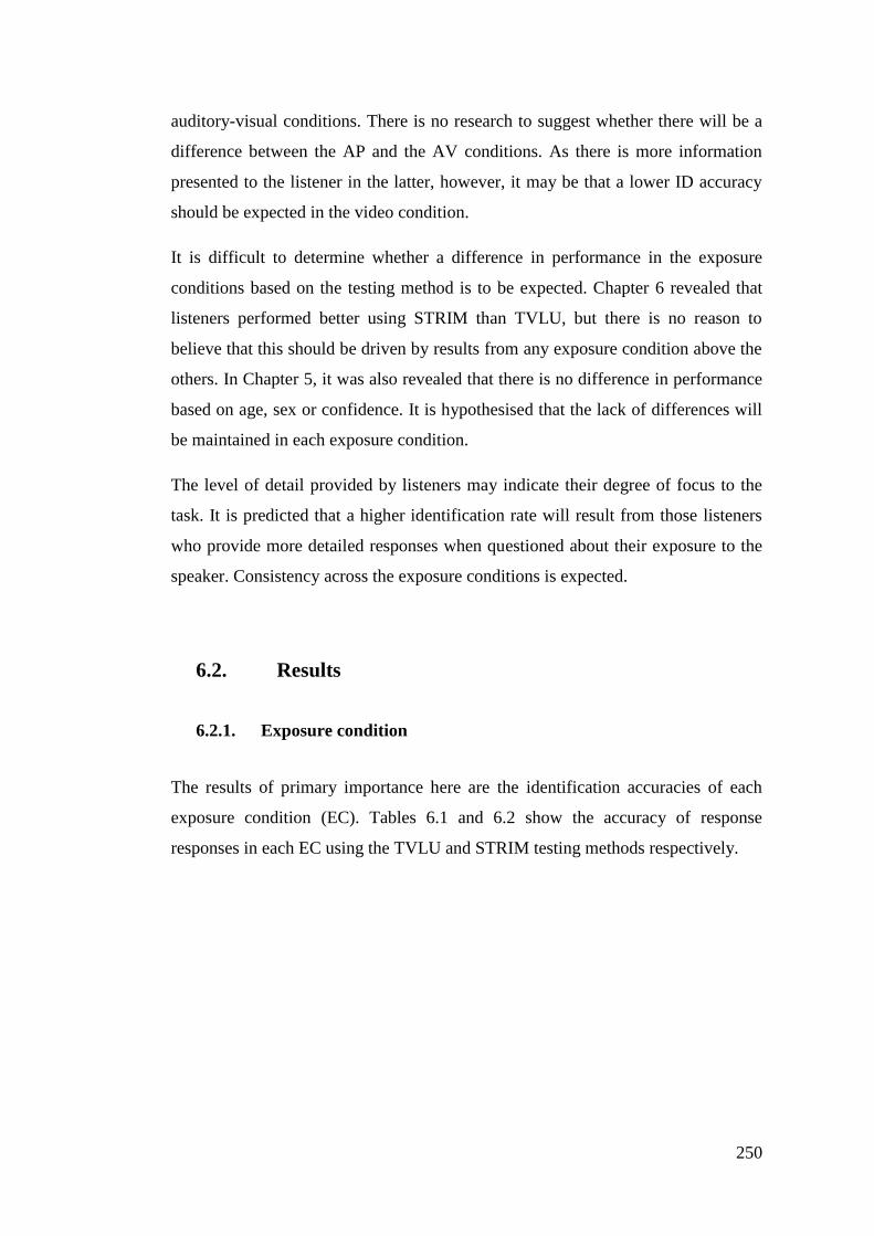
250
auditory-visual conditions. There is no research to suggest whether there will be a
difference between the AP and the AV conditions. As there is more information
presented to the listener in the latter, however, it may be that a lower ID accuracy
should be expected in the video condition.
It is difficult to determine whether a difference in performance in the exposure
conditions based on the testing method is to be expected. Chapter 6 revealed that
listeners performed better using STRIM than TVLU, but there is no reason to
believe that this should be driven by results from any exposure condition above the
others. In Chapter 5, it was also revealed that there is no difference in performance
based on age, sex or confidence. It is hypothesised that the lack of differences will
be maintained in each exposure condition.
The level of detail provided by listeners may indicate their degree of focus to the
task. It is predicted that a higher identification rate will result from those listeners
who provide more detailed responses when questioned about their exposure to the
speaker. Consistency across the exposure conditions is expected.
6.2. Results
6.2.1. Exposure condition
The results of primary importance here are the identification accuracies of each
exposure condition (EC). Tables 6.1 and 6.2 show the accuracy of response
responses in each EC using the TVLU and STRIM testing methods respectively.
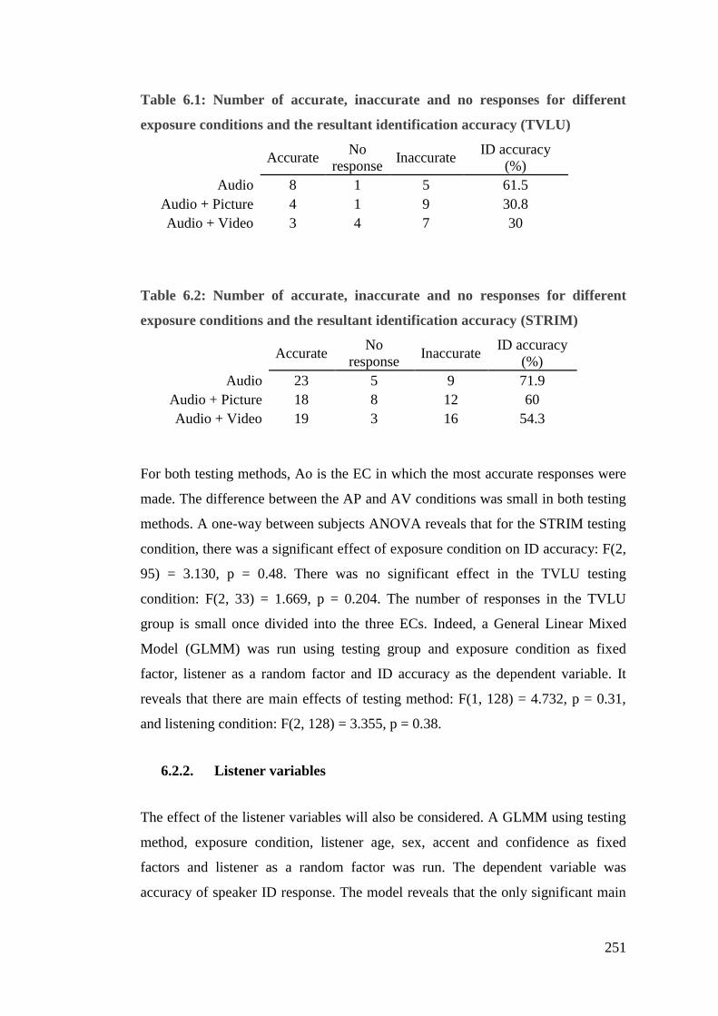
251
Table 6.1: Number of accurate, inaccurate and no responses for different
exposure conditions and the resultant identification accuracy (TVLU)
Accurate No
response Inaccurate
ID accuracy
(%)
Audio 8 1 5 61.5
Audio + Picture 4 1 9 30.8
Audio + Video 3 4 7 30
Table 6.2: Number of accurate, inaccurate and no responses for different
exposure conditions and the resultant identification accuracy (STRIM)
Accurate No
response Inaccurate
ID accuracy
(%)
Audio 23 5 9 71.9
Audio + Picture 18 8 12 60
Audio + Video 19 3 16 54.3
For both testing methods, Ao is the EC in which the most accurate responses were
made. The difference between the AP and AV conditions was small in both testing
methods. A one-way between subjects ANOVA reveals that for the STRIM testing
condition, there was a significant effect of exposure condition on ID accuracy: F(2,
95) = 3.130, p = 0.48. There was no significant effect in the TVLU testing
condition: F(2, 33) = 1.669, p = 0.204. The number of responses in the TVLU
group is small once divided into the three ECs. Indeed, a General Linear Mixed
Model (GLMM) was run using testing group and exposure condition as fixed
factor, listener as a random factor and ID accuracy as the dependent variable. It
reveals that there are main effects of testing method: F(1, 128) = 4.732, p = 0.31,
and listening condition: F(2, 128) = 3.355, p = 0.38.
6.2.2. Listener variables
The effect of the listener variables will also be considered. A GLMM using testing
method, exposure condition, listener age, sex, accent and confidence as fixed
factors and listener as a random factor was run. The dependent variable was
accuracy of speaker ID response. The model reveals that the only significant main
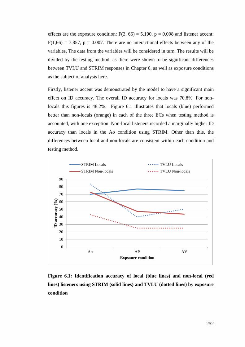
252
effects are the exposure condition: F(2, 66) = 5.190, p = 0.008 and listener accent:
F(1,66) = 7.857, p = 0.007. There are no interactional effects between any of the
variables. The data from the variables will be considered in turn. The results will be
divided by the testing method, as there were shown to be significant differences
between TVLU and STRIM responses in Chapter 6, as well as exposure conditions
as the subject of analysis here.
Firstly, listener accent was demonstrated by the model to have a significant main
effect on ID accuracy. The overall ID accuracy for locals was 70.8%. For non-
locals this figures is 48.2%. Figure 6.1 illustrates that locals (blue) performed
better than non-locals (orange) in each of the three ECs when testing method is
accounted, with one exception. Non-local listeners recorded a marginally higher ID
accuracy than locals in the Ao condition using STRIM. Other than this, the
differences between local and non-locals are consistent within each condition and
testing method.
Figure 6.1: Identification accuracy of local (blue lines) and non-local (red
lines) listeners using STRIM (solid lines) and TVLU (dotted lines) by exposure
condition
0
10
20
30
40
50
60
70
80
90
Ao AP AV
ID a
ccu
racy
(%
)
Expsoure condition
STRIM Locals TVLU Locals
STRIM Non-locals TVLU Non-locals
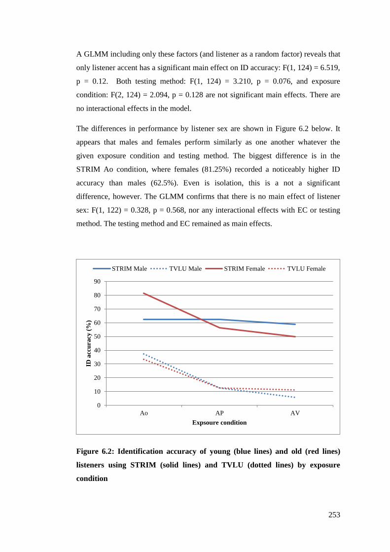
253
A GLMM including only these factors (and listener as a random factor) reveals that
only listener accent has a significant main effect on ID accuracy: F(1, 124) = 6.519,
p = 0.12. Both testing method: F(1, 124) = 3.210, p = 0.076, and exposure
condition: F(2, 124) = 2.094, p = 0.128 are not significant main effects. There are
no interactional effects in the model.
The differences in performance by listener sex are shown in Figure 6.2 below. It
appears that males and females perform similarly as one another whatever the
given exposure condition and testing method. The biggest difference is in the
STRIM Ao condition, where females (81.25%) recorded a noticeably higher ID
accuracy than males (62.5%). Even is isolation, this is a not a significant
difference, however. The GLMM confirms that there is no main effect of listener
sex: F(1, 122) = 0.328, p = 0.568, nor any interactional effects with EC or testing
method. The testing method and EC remained as main effects.
Figure 6.2: Identification accuracy of young (blue lines) and old (red lines)
listeners using STRIM (solid lines) and TVLU (dotted lines) by exposure
condition
0
10
20
30
40
50
60
70
80
90
Ao AP AV
ID a
ccu
racy
(%
)
Expsoure condition
STRIM Male TVLU Male STRIM Female TVLU Female
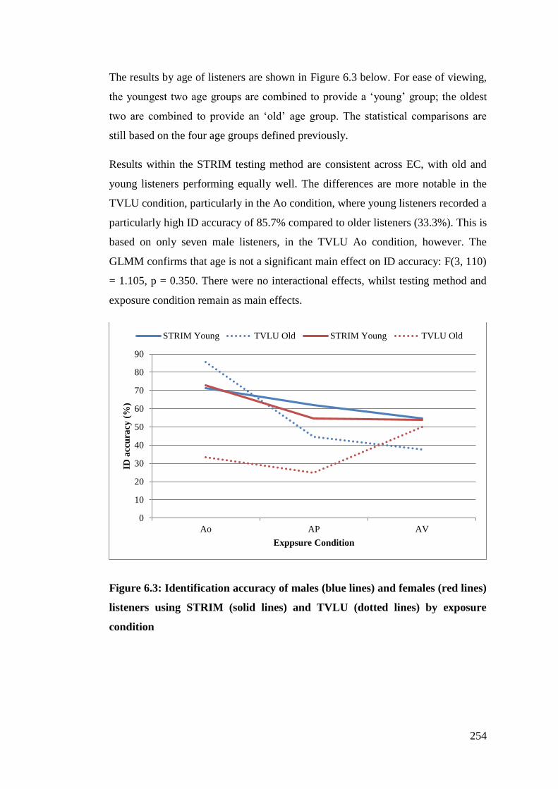
254
The results by age of listeners are shown in Figure 6.3 below. For ease of viewing,
the youngest two age groups are combined to provide a ‘young’ group; the oldest
two are combined to provide an ‘old’ age group. The statistical comparisons are
still based on the four age groups defined previously.
Results within the STRIM testing method are consistent across EC, with old and
young listeners performing equally well. The differences are more notable in the
TVLU condition, particularly in the Ao condition, where young listeners recorded a
particularly high ID accuracy of 85.7% compared to older listeners (33.3%). This is
based on only seven male listeners, in the TVLU Ao condition, however. The
GLMM confirms that age is not a significant main effect on ID accuracy: F(3, 110)
= 1.105, p = 0.350. There were no interactional effects, whilst testing method and
exposure condition remain as main effects.
Figure 6.3: Identification accuracy of males (blue lines) and females (red lines)
listeners using STRIM (solid lines) and TVLU (dotted lines) by exposure
condition
0
10
20
30
40
50
60
70
80
90
Ao AP AV
ID a
ccu
racy
(%
)
Exppsure Condition
STRIM Young TVLU Old STRIM Young TVLU Old

255
The confidence ratings are illustrated in Figure 6.4. Overall, confidence ratings are
higher for TVLU than STRIM within each of the ECs. The differences between
accurate and inaccurate responses in the speaker ID task are small and do not
suggest that confidence predicts accuracy. Indeed, there is no main effect of
confidence on identification accuracy in the GLMM: F(4, 107) = 0.206, p = 0.935,
nor any interactional effects. Testing method and EC again remain as main effects.
Figure 6.4: Mean confidence ratings of accurate (green line) and inaccurate
(red line) responses to speaker ID task using STRIM (solid lines) and TVLU
(dotted lines) by exposure condition
6.2.3. Performance by listeners in each exposure condition
As repeated measures were used, it is possible to measure the accuracy of listeners’
responses in one exposure condition and compare that with their accuracy in the
others. Each listener in the STRIM condition took part in (up to) three
identification tasks. Figure 6.5 shows listeners’ accuracy in one exposure condition
below the x-axis, and the number of those listeners who made accurate or
inaccurate responses (shown by the bar) in another exposure condition (shown
above the bar). For example, the first bar in the figure below denotes that of the 17
0
0.5
1
1.5
2
2.5
3
3.5
4
Ao AP AV
Mea
n c
on
fid
ence
ra
tin
g
Expsoure Condition
STRIM Accurate STRIM Inaccurate
TVLU Accurate TVLU Inaccurate
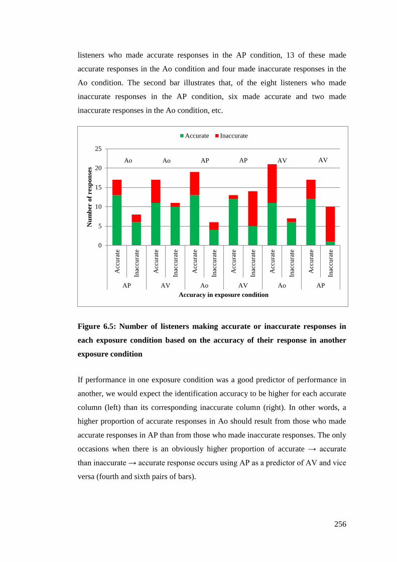
256
listeners who made accurate responses in the AP condition, 13 of these made
accurate responses in the Ao condition and four made inaccurate responses in the
Ao condition. The second bar illustrates that, of the eight listeners who made
inaccurate responses in the AP condition, six made accurate and two made
inaccurate responses in the Ao condition, etc.
Figure 6.5: Number of listeners making accurate or inaccurate responses in
each exposure condition based on the accuracy of their response in another
exposure condition
If performance in one exposure condition was a good predictor of performance in
another, we would expect the identification accuracy to be higher for each accurate
column (left) than its corresponding inaccurate column (right). In other words, a
higher proportion of accurate responses in Ao should result from those who made
accurate responses in AP than from those who made inaccurate responses. The only
occasions when there is an obviously higher proportion of accurate → accurate
than inaccurate → accurate response occurs using AP as a predictor of AV and vice
versa (fourth and sixth pairs of bars).
0
5
10
15
20
25
Acc
ura
te
Inac
cura
te
Acc
ura
te
Inac
cura
te
Acc
ura
te
Inac
cura
te
Acc
ura
te
Inac
cura
te
Acc
ura
te
Inac
cura
te
Acc
ura
te
Inac
cura
te
AP AV Ao AV Ao AP
Nu
mb
er o
f re
spo
nse
s
Accuracy in exposure condition
Accurate Inaccurate
Ao Ao AP AP AV AV
257
This can be more clearly illustrated by calculating the ratio of identification
accuracies for an exposure condition (EC2) based on whether each listener made an
accurate or inaccurate identification in another exposure condition (EC1). For
example, as Figure 6.5 shows, when Ao is EC1 and AP is EC2 (the first two
columns), the accuracy for EC2 when EC1 is accurate is 76.5% (13 accurate, 4
inaccurate). When EC1 is inaccurate, the identification accuracy of EC2 is 75% (6
accurate, 2 inaccurate). There is little difference in the identification accuracy of
Ao (EC2) whether a listener was accurate in AP (EC1) or not. The ratio between
these two figures is consequently a little over 1: 76.5%/75% = 1.02. This indicates
that there is a slightly higher chance that EC2 will be accurate if EC1 was accurate
than if EC1 was inaccurate.
The EC ratios for each condition as a predictor of another are shown below. Where
the ratio is above 1, EC2 is more likely to be accurate if EC1 is accurate; where the
ratio is below 1, EC2 is more likely to be accurate if EC1 is inaccurate. These
ratios are shown in Figure 6.6 in which a logarithmic scale is used to indicate that
the further the ratio is from one, the EC1 is as a predictor of EC2.
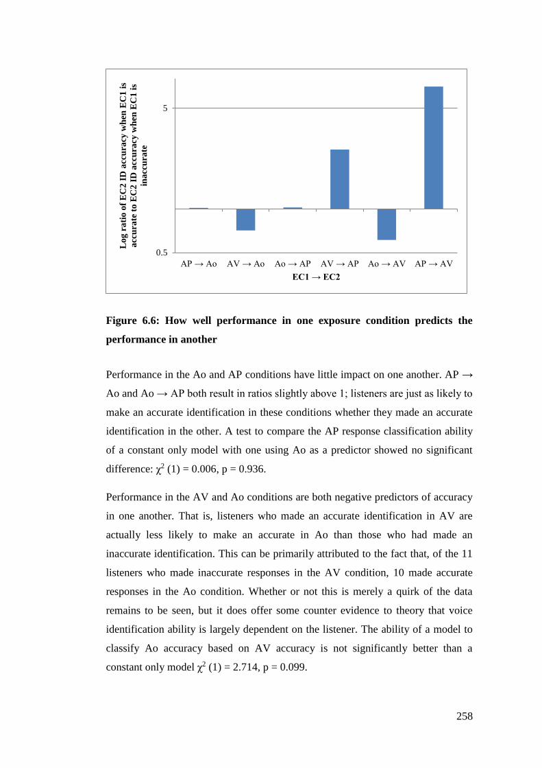
258
Figure 6.6: How well performance in one exposure condition predicts the
performance in another
Performance in the Ao and AP conditions have little impact on one another. AP →
Ao and Ao → AP both result in ratios slightly above 1; listeners are just as likely to
make an accurate identification in these conditions whether they made an accurate
identification in the other. A test to compare the AP response classification ability
of a constant only model with one using Ao as a predictor showed no significant
difference: χ2 (1) = 0.006, p = 0.936.
Performance in the AV and Ao conditions are both negative predictors of accuracy
in one another. That is, listeners who made an accurate identification in AV are
actually less likely to make an accurate in Ao than those who had made an
inaccurate identification. This can be primarily attributed to the fact that, of the 11
listeners who made inaccurate responses in the AV condition, 10 made accurate
responses in the Ao condition. Whether or not this is merely a quirk of the data
remains to be seen, but it does offer some counter evidence to theory that voice
identification ability is largely dependent on the listener. The ability of a model to
classify Ao accuracy based on AV accuracy is not significantly better than a
constant only model χ2 (1) = 2.714, p = 0.099.
0.5
5
AP → Ao AV → Ao Ao → AP AV → AP Ao → AV AP → AV
Lo
g r
ati
o o
f E
C2
ID
acc
ura
cy w
hen
EC
1 i
s
acc
ura
te t
o E
C2
ID
acc
ura
cy w
hen
EC
1 i
s
ina
ccu
rate
EC1 → EC2

259
Conversely, performance in the AV and AP conditions appear to be strong
predictors of one another. Listeners who made an accurate response in the AP
condition in particular were much more likely to make an accurate response in the
AV condition (70.6%) than those who had made an inaccurate response (10%). The
binary regression model is able to correctly classify 77.8% of AV responses as
accurate or inaccurate using AP accuracy as a predictor. This was a significant
improvement on the classification of a constant only model: χ2 (1) = 10.294, p =
0.001.
Only response accuracy in the AP and AV exposure conditions are significant
predictors of identification accuracy in the other. These are the two conditions
which involve supplementary visual information in addition to the audio stimulus.
1.2.1 Qualitative data provided by listeners
All listeners were asked the following questions by the experimenter in the post
exposure phase of the one of their identifications:
Can you tell me what happened?
What did you see?
Can you describe the person?
Do you remember what the person said?
What did the person sound like?
The condition which this detailed questioning followed was pseudo-randomised for
each listener to control for the listener and experimental design variables of the
associated identification task. The responses were categorised as information
relating to (i) the circumstances of the event or visual information; (ii) the speech
content; (iii) the speech quality (that is, pertaining to the voice or implications such
information has about the speaker, rather than what was said). The term speech
quality is used here as distinct from voice quality, as the latter has strong ties to
suprasegmental aspects of speech (Laver, 1980; Laver, 1994). Here, information
relating to speech quality covers both voice quality and also segmental features.
The responses within these categories were then coded for how detailed they were
on a scale of 1 (little or no detail), 2 (some detail) or 3 (very detailed). Figure 6.7
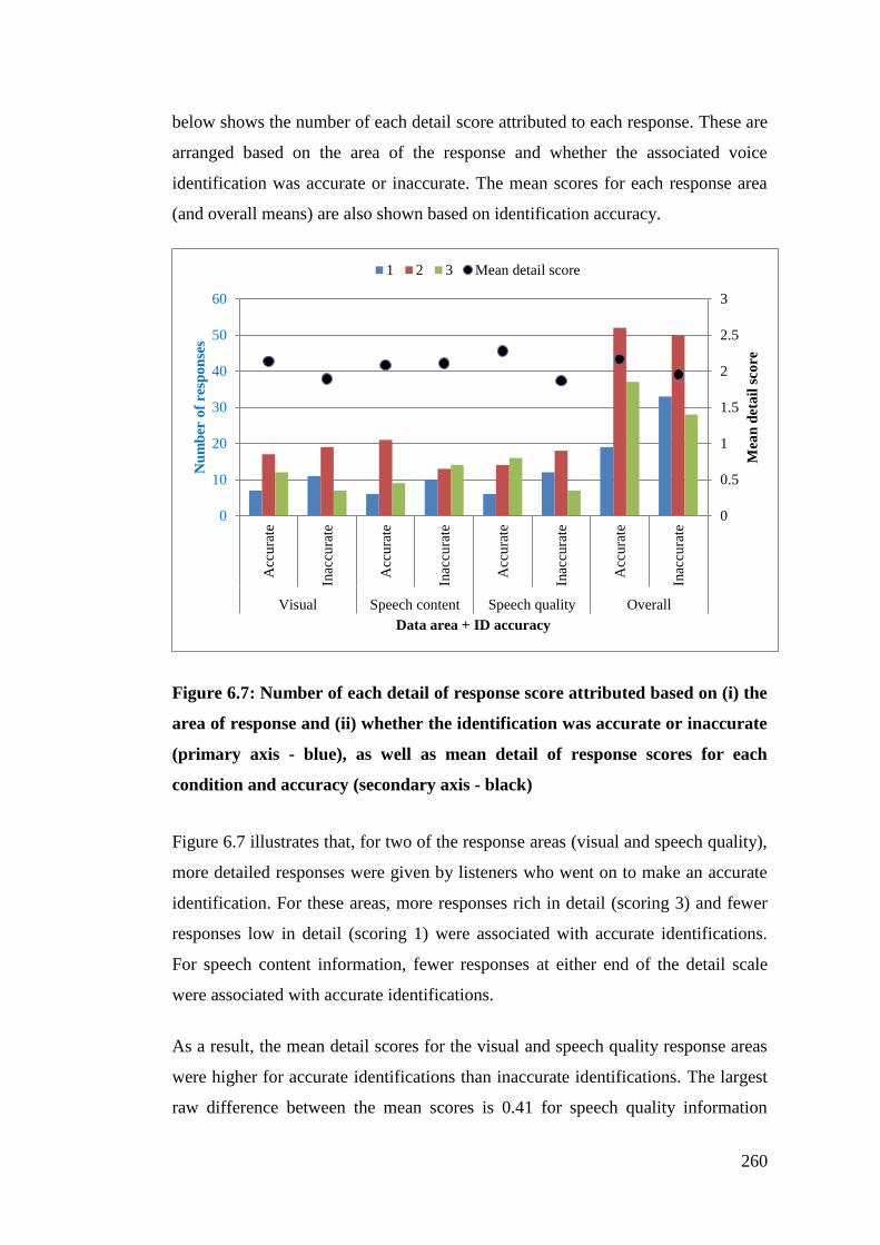
260
below shows the number of each detail score attributed to each response. These are
arranged based on the area of the response and whether the associated voice
identification was accurate or inaccurate. The mean scores for each response area
(and overall means) are also shown based on identification accuracy.
Figure 6.7: Number of each detail of response score attributed based on (i) the
area of response and (ii) whether the identification was accurate or inaccurate
(primary axis - blue), as well as mean detail of response scores for each
condition and accuracy (secondary axis - black)
Figure 6.7 illustrates that, for two of the response areas (visual and speech quality),
more detailed responses were given by listeners who went on to make an accurate
identification. For these areas, more responses rich in detail (scoring 3) and fewer
responses low in detail (scoring 1) were associated with accurate identifications.
For speech content information, fewer responses at either end of the detail scale
were associated with accurate identifications.
As a result, the mean detail scores for the visual and speech quality response areas
were higher for accurate identifications than inaccurate identifications. The largest
raw difference between the mean scores is 0.41 for speech quality information
0
0.5
1
1.5
2
2.5
3
0
10
20
30
40
50
60
Acc
ura
te
Inac
cura
te
Acc
ura
te
Inac
cura
te
Acc
ura
te
Inac
cura
te
Acc
ura
te
Inac
cura
te
Visual Speech content Speech quality Overall
Mea
n d
eta
il s
core
Nu
mb
er o
f re
spo
nse
s
Data area + ID accuracy
1 2 3 Mean detail score
261
(2.28 accurate, 1.89 inaccurate). The visual information recorded the next biggest
difference (0.25; 2.14 accurate, 1.86 inaccurate). The speech content information
was actually, on average, slightly less detailed (0.02 difference) in responses
associated with accurate identifications (2.08) than inaccurate identifications
(2.10). A series of one-way between subjects ANOVAs were run to test whether
there was a significant effect of response detail in a given area on the accuracy of
the following voice identification. For the visual information, the effect was not
significant: F(2, 70) = 2.702, p = 0.074. For the speech content information, the
effect was also not significant: F(2, 70) = 2.006, p = 0.142. There was a significant
effect of the detail of the speech quality information: F(2, 70) = 3.528, p = 0.035.
A Pearson product-moment correlation coefficient was computed to assess the
relationship between the level of detail provided by listeners in each of the
information areas. There is a positive correlation between detail of visual and
speech quality information provided: r = 0.244, n = 83, p = 0.13. There is no
significant correlation between neither visual and speech content information: r = -
0.009, n = 83, p = 0.468, nor speech quality and speech content information: r =
0.073, n = 83, p = 0.256.

262
6.2.4. By exposure condition
The data relating to detail of responses in the given information areas can be
broken down by the exposure condition in which the listener was exposed to the
speech. Figure 6.8 shows the scores associated with accurate and inaccurate
identifications in each category.
Figure 6.8: Mean detail of responses regarding visual, speech content and
speech quality information for accurate and inaccurate identifications by
exposure condition
The pattern seen above – accurate responses scoring much higher than inaccurate
response in speech quality detail, a little higher in visual information, similarly in
speech content information – is replicated in the AP and AV exposure conditions.
In the Ao condition, however, the listeners who made inaccurate identifications
actually provided more detailed information in each of the three subject areas than
those who made accurate identifications. ANOVAs do not reveal any significant
differences between the detail scores of listeners making accurate or inaccurate
responses in any area/condition – the number of responses in each category is too
small. The fact that a similar pattern is shown in each of the auditory plus visual
conditions, whilst the auditory only condition shows little effect of identification
0
0.5
1
1.5
2
2.5
3
Visual Speech
content
Speech
quality
Visual Speech
content
Speech
quality
Visual Speech
content
Speech
quality
Ao AP AV
Mea
n r
esp
on
se d
eta
il s
core
Exposure condition + response area
Accurate Inaccurate
263
accuracy, may be telling, particularly given the differences observed between these
conditions elsewhere.
6.3. Discussion
6.3.1. Identification rates of exposure conditions
The finding that Ao exposure results in more accurate identifications than exposure
involving additional visual stimuli adds to the limited body of research in the area.
Cook and Wilding (1997a), McAllister et al. (1993a), and Stevenage et al. (2011)
all found that auditory-visual witnesses did not perform as well as auditory-only
witnesses, though Yarmey (1986) found no effect of stimulus.
The fact that the highest identification accuracy was recorded in the audio only
condition has implications for the application of naïve listener voice identification.
Of course, in an applied setting, the listener may be exposed to the perpetrator in an
audio only condition. This could be due to the listener being blindfolded, for
example, or being exposed to the speaker via a telephone (although there are
further practical implications concerning the latter). Most experimental testing into
voice identification uses audio only stimuli and it follows that findings from such
research can be applied to real world exposures of this type.
These data show, however, that more accurate responses result when the listener is
only exposed to audio stimulus. There is danger, then, in applying findings from
audio only based research to situations where a listener also has access to some (no
matter how limited) visual information relating to the speaker or surroundings. It is
not known how what proportion of witnesses this would apply to. It is not
contentious, though, to expect that many earwitnesses observe something which
might be relevant to the case, even if not to the identification of the perpetrator.
The difference between the Ao condition and the visual conditions was more
marked when the TVLU testing method was employed. This further raises question
marks concerning the over-application of naïve listener research, as TVLU is the
predominant testing method of earwitness identification. Research concerning

264
audio only exposure should not be generalised to earwitness evidence where visual
information is also present at the time of exposure.
There is little difference between the performance of listeners in the AP and AV
conditions. Whether listeners were presented with a picture or video to accompany
the auditory stimulus had no effect on ID accuracy. Previous studies investigating
the impact of mixed stimuli on voice identification have concentrated on the visual
element consisting of a picture. Whilst this lacks ecological validity, as earwitness
exposure is highly unlikely to involve viewing a still picture, these results appear to
support this as a valid approach.
6.3.2. Why is there a difference?
A listener in the Ao condition has nothing more than the speech of the perpetrator
to pay attention to. There is no visual information or distractors, meaning their full
attention can be paid to the auditory information, allowing the listener maximum
exposure to the stimulus which is relevant to voice identification. Research has
shown that, to a point, an increased level of exposure to the stimulus allows for
improved identification of voices (Kerstholt et al., 2004; Orchard & Yarmey,
1995). It appears that, as predicted by Yarmey (1986), visual information interferes
with the encoding of auditory information.
Furthermore, research has also shown that the ways in which listeners process
speech differs depending on the condition in which they hear it (Mattys, Davis,
Bradlow & Scott, 2012). Speech processed under cognitive load (CL) – defined by
Mattys and Wiget (2011: 145) as “concurrent attentional or mnemonic processing”
– demonstrates a lexical bias on phoneme identification compared to speech
processed under non CL conditions. Whilst listeners in this study are not asked to
recognise the speech, they are asked to recognise a voice. If listeners under CL
(those in the AP and AV conditions) are processing the input differently from those
under non CL (those in the Ao condition), it stands to reason there may be an effect
on tasks performed based on having processed the speech.
265
The difference can, in part, be attributed to the potential for an incidental versus
intentional learning effect (Armstrong & McKelvie, 1996). Whilst listeners in each
condition were given no prior instructions regarding what the pertinent aspect of
the exposure was (i.e. the voice), it is possible that those in the Ao condition were
more likely to intentionally ‘memorise’ the voice because there was no additional
stimulus competing for attention. Those in the AP and AV conditions may have
learned the voice incidentally, with visual information distracting from the amount
of attention paid to it, subsequently reducing identification performance.
6.3.3. Listener variables
The data reinforce the findings of Chapter 3, which demonstrated an absence of
any listener age or sex effects on the accuracy of identifications made. The findings
from Chapter 6 showed that whilst there were no age or sex effects, there was an
effect of accent. Local listeners performed significantly better than non-local
listeners, and the performance of familiar listeners – those not local but living in
the area or having close links with the local accent – was intermediate to the two.
In the present chapter, due to methodological difference in the experiment, the
voice identification abilities of only local and familiar listeners were tested.
Here, a non-significant difference between locals and non-local (but familiar with
the local accent) is recorded in the Ao exposure condition. Recall, that in the
previous chapter, exposure was also audio only. Local listeners do, however,
perform significantly better than non-locals in both the AP and AV conditions.
Whilst the other-accent effect (the concept that people are less able to distinguish
between speakers of an accent they do not speak) does not apply to non-locals
familiar with the accent when only an auditory stimulus is experienced, it does
appear to affect them when an auditory-visual stimulus is presented.
Again, the reasons for this are unclear and no previous research has hitherto
combined these two variables. One explanation may lie in the CL theory outlined
above. Results from Chapter 4 showed that not only were there difference between
the identification accuracies of different listener accent groups, but the speakers
which they misidentified as the target differed too. This was attributed to non-local
266
listeners placing greater emphasis on the supra-segmental features of the voice,
whilst local listeners were better able to make distinctions based on phonetic
features. If, as shown by CL research, listeners whose attention is divided during
exposure to the perpetrator’s voice process speech differently, their focus will be
on different aspects of the speech signal. This, in turn, may affect different listener
groups to a greater or lesser extent depending on what features of the voice are
important to them in a voice recognition task.
6.3.4. Accuracy in one condition as a predictor of accuracy in another
The data showed that a listener’s accuracy in the AP condition was a significant
predictor of accuracy in the AV condition and vice versa. The fact that these two
conditions are strong predictors of one another is telling, as these are the two
conditions which involve auditory and visual stimuli. This lends support to the
suggestion that identifications based on auditory only exposure should be treated
differently from those in which visual information can also be accessed. It also
supports the proposal that the ability of any given listener is as relevant a variable
in predicting voice identification accuracy as any element of the earwitness
procedure. Listeners who made an accurate identification in one auditory-visual
condition were more likely to make an accurate identification in another auditory-
visual condition, indicating a degree of consistency in the ability of listeners. This
accords with research into the area of auditory-visual input’s effect on speaker
identification (Hollien, 1990).
6.3.5. Level of detail provided
The level of detail provided by each listener when discussing the exposure with the
experimenter was shown to be variably important to identification accuracy.
Significantly more detail relating to the quality of the voice – features of the voice,
their accent, assumed implications about the speaker based on the voice, etc. – was
provided by listeners who made an accurate identification.
It seems unlikely that actually recounting the information is the predictor of
identification accuracy here. Indeed, research into verbal overshadowing has shown
267
– though inconsistently – that an earwitness vocalising their memory of a voice can
actually negatively impact on their ability to identify it (cf. Vanags et al., 2005). It
is predictable that a listener who is able to recall detailed information about the
voice is more likely to make an accurate identification. This may indicate that they
processed more information about the quality of the voice and/or that they engaged
with the experimental task better than those who could not or did not recount such
information in detail. Either way, more accurate identifications were made by
listeners who recounted detailed information pertaining to the features of the voice
they were asked to identify. Listeners can only base their identification on speech
quality information (assuming, of course, that the lineup is fairly constructed). It
follows, then, that listeners who can recall in detail information pertaining to this
area of the exposure experience should be more likely to accurately identify the
voice.
Less predictable is the difference in detail relating to visual information. Although
the difference is not significant at the 5% level, it does approach significance (p =
0.074). Knowledge of the circumstances of the exposure - what the perpetrator was
wearing, whether a dog passed by - is ultimately irrelevant to the process of
identification by means of the voice. A detailed response in this area may,
however, indicate that the listener was paying close attention to the events
unfolding and thus was an attentive witness to the crime. There is, however, no
correlation between the level of detail provided in terms of visual information and
either speech quality or content. This does not suggest that those listeners who
were able to recall information about what happened were also able to recall
detailed information about the voice. Despite the efforts of the study to
manufacture an environment more realistic than general laboratory based
experiments, the perception of stress by listeners was not as it would have been in a
real-world situation. Listeners were not under any direct threat in the experiment.
Their behaviour may not be a true reflection of that of an earwitness to a real crime,
and given that an active exchange may increase recall of events (Hammersley &
Read, 1985), it is not known if listeners’ memories in the study are a true reflection
of a forensic context.
268
Like visual and contextual information, speech content is probably not relevant to
the voice identification process. It is, though, more closely linked to the quality of
the voice than visual information is. Given that detail of speech quality provided is
shown to be linked to identification accuracy, it is perhaps surprising that detail of
speech content is shown to have no effect at all. Indeed, the level of detail provided
by listeners in these areas in not correlated with one another, despite both relying
upon the listener paying auditory attention. Although, to the best of the author’s
knowledge, no research has been carried out into the relative contribution of speech
content to voice identification, research has indicated/suggested that speech content
and speech quality exist in separate channels in perception. O'Sullivan et al. (1985)
found that participants made differing judgements about the attributes of others
when one or both of speech content and speech quality were altered. Listeners are
able to pay attention to how something was said without focussing on what was
said, and vice versa.
These differences (and lack of differences) in the level of detail provided based on
identification accuracy are driven mostly by the listeners in the AP and AV
exposure conditions. Listeners in the Ao condition provided similar levels of detail
in each area whether identifications were accurate or not. This may be because
these listeners have only auditory stimulus – there is no visual information
increasing their CL. Thus, there is better potential for them to pay increased
attention to the stimulus. Whilst more accurate identifications result from the Ao
condition, a ceiling effect in listeners’ abilities prevents consistently accurate
identification responses.
6.4. Chapter summary
Listeners in the Ao exposure condition recorded a higher identification
accuracy than those in the AP and AV conditions. There was no difference
between the latter two conditions

269
The difference between the Ao identification accuracy and AP/AV
identification accuracies was bigger using the TVLU testing method than
STRIM
Listener sex age, and confidence are not significant predictors of
identification accuracy in a model using exposure condition as a factor
Listener accent (local or non-local) is a significant predictor of
identification accuracy in a model using exposure condition as a factor
A listener’s accuracy in the AP condition is a strong positive predictor of
their accuracy in the AV condition and vice versa. Accuracy in the Ao
condition is neither a strong predictor of, nor can be predicted by, accuracy
in the AP or AV conditions
The amount of detail provided by listeners relating to the quality of the
speech of the perpetrator has an effect on the identification accuracy. More
accurate identifications are made by listeners who provide more detail
The amount of detail provided by listeners relating to the visuals or context
of the exposure is also higher when identification is accurate (though the
difference is not significant)
There is no difference in identification accuracy based on the detail of
speech content information provided
270
7. Conclusions
This chapter will address the research questions which were outlined in §2.9 by
drawing together the results from the intermediate chapters. To recap, investigation
centred on three key questions. Firstly, what effect does a listener’s accent, and
their ability to recognise an accent, have on speaker identification? Secondly, is the
traditional voice lineup the ideal method for providing accurate and reliable naïve
speaker identifications? Thirdly, what are the differences in identification accuracy
when listeners are exposed to the speaker in different conditions? The implications
of the answers to these questions for forensic earwitness identification will be
considered, along with the limitations of the present research.
7.1. Research questions
R1. Does the other-accent effect in voice identification exist within speakers of
the North Eastern regional variety of (English) English?
If so, does this only exist on a broad (locals versus non-locals) sense, or
is there variation within the region?
In Chapter 4, three experiments testing this effect all showed a significant
difference between the performance of NE listeners (local to the speaker) and non-
NE listeners (not local to the speaker). As each experiment involved a different
target speaker (one from Tyneside, one from Wearside, one from Teesside), it
could be said that the other-accent effect has been demonstrated for three different
accent groups (if the three accents are treated as distinct). The biggest effect was
seen in experiment three where NE listeners made twice as many accurate
responses in the speaker ID task as non-NE listeners. This experiment involved a
Teesside target, but also a target-absent lineup (experiments one and two involved
target-present lineups). There is no way of determining the degree to which these
two factors contributed to the other-accent effect. Nevertheless, a difference was
271
found, and adds to the literature which indicates that listeners are less able to
distinguish between speakers with accents different from their own.
There appears to be some evidence for an other-accent effect at the sub-regional
level. In each of the three experiments, the highest ID accuracy was recorded by
listeners from the sub-regional region which matched that of the target speaker.
The effect was less prominent than NE versus non-NE comparisons, though this is
to be expected given that all hypotheses as to why an other-accent effect exists
suggest that it is dependent on listeners’ knowledge of or perceptual distance from
the speaker’s variety. The difference between speakers from Tyneside and
Wearside, for example, is much smaller than Tyneside and London, in terms of
geographical and linguistic distance, and degree of exposure of one to the other.
The other-accent effect has been demonstrated amongst regional varieties of British
English (Stevenage et al., 2012), Dutch (Kerstholt et al., 2006), as well as national
varieties of English (Vanags et al., 2005) and in non-native speech not understood
by the listener (Schiller & Köster, 1996) The present research adds to the literature
by supporting the presence of the other-accent effect in another regional variety of
English (NE) and demonstrating that it can have an effect at a sub-regional level as
well as broadly.
R2. What role does familiarity with an accent play in the identification of a
speaker?
The results of listeners categorised as familiar (not from the area of investigation,
but with above expected levels of exposure to speakers from the area) show a clear
trend throughout the data. They are generally too few in number, however, to
produce any significant effects. In Chapter 4, familiar listeners in all three
experiments recorded ID accuracies intermediate to NE and non-NE listeners. The
consistency of these results may suggest that familiarity with an accent improves
listeners’ ability to identify speakers above the level non-local listeners, but not to
the level comparable with local listeners. Again, this fits the models proposed
whereby ‘expertise’ in or knowledge of an accent improves ability to distinguish
between its speakers.
272
Although not the focus of investigation in Chapter 6, the difference in performance
of local listeners and familiar listeners can also be compared. Again, local listeners
(this time local to York) performed better than those who are not from the area but
have notable exposure to its speakers (in this case, most now resided in the city).
No comparison can be made with non-local, non-familiar listeners, but the same
non-significant difference can be observed between local and familiar listeners.
The asymmetries noted in other-accent research are attributed to the relative
exposure members of one accent group (e.g. regional) have to another (e.g.
standard variety). This research employed a different procedure, whereby only
regional varieties of English were tested (and thus no asymmetry between group
performances can be demonstrated). The results do, nevertheless, support the
proposal that performance in speaker identification tasks (cf. Stevenage et al.,
2012) and speech processing-based tasks in general (cf. Adank et al., 2009) is
inhibited by unfamiliarity with the accents spoken.
R3. Does a listener’s ability to identify an accent affect their ability to identify
a speaker (of that, or a different, accent)?
Broadly speaking, yes. There were generally correlations between ID accuracy and
a listener’s ability to recognise a variety of British English accents, accents local to
the speaker (in the NE), and the target speaker’s accent. The latter of these had the
strongest effect on the accuracy of responses. Ability to recognise accents not-at-all
related to the target speaker’s variety had no impact on ID accuracy.
No previous research has been conducted into the relationship between ability in
these tasks. There is limited support in the literature for performance in one task
correlating with performance in another, such as musical aptitude on speaker
discrimination (Kraus et al., 1995), auditory capability on speaker identification (de
Jong, 1998) and face recognition on eyewitness identification accuracy (Morgan et
al., 2007). Perhaps, then accent recognition ability is another associated aptitude.
273
R4. Do age, sex and confidence affect identification accuracy?
On the whole, these variables have little-to-no effect on naïve speaker
identification accuracy. In Chapter 3, identification accuracy did not vary
significantly based on listener age in any of the three experiments. There was a
small overall trend for younger listeners to perform better than older, but the
difference was small. The same pattern was shown in Chapter 5 in both the STRIM
and TVLU testing conditions. In Chapter 6, younger listeners were again seen to
perform only marginally better in the AP and AV exposure conditions. In the Ao
condition, the youngest age group performed noticeably better than the others,
though again there was no statistical effect of age.
This accords with the general findings of the established literature on the role of
age in naïve speaker identification. Strong effects of age are rare, but speakers aged
20-40 generally achieve more accurate identifications. The oldest listeners in the
above experiments were 46-55, the youngest were 18-25.
As with age, there was a consistent (but very small) pattern for the effect of listener
sex on performance in speaker identification tasks. The ID accuracy of males was
either equal to or marginally better in the three Chapter 4 experiments, across the
two testing methods in Chapter 5, and the three exposure conditions in Chapter 6.
As previous research into the effect of listener sex on ID accuracy is inconclusive,
this is perhaps unsurprising. The data suggest there is no sex effect, but perhaps
there is a non-significant own-sex bias with male listener performing better than
females in identifying male speakers in some of the tasks (Roebuck & Wilding,
1993). More research is needed to confirm this.
Confidence is shown to have varying levels of effect on identification accuracy. In
Chapter 4, confidence in two of the three experiments was weakly correlated with
accuracy, whilst in Chapters 6 and 7 there was no correlation either as a main effect
or within any of the exposure or testing conditions.
The variable performance of confidence as a predictor of ID accuracy should come
as no surprise given its status in published literature. Arguments have been made
for listener’s ability to recognise a speaker to have no association with listener
274
confidence (Hammersley & Read, 1985) or to be strongly associated with higher
confidence ratings (Rose & Duncan, 1995), and even associated with lower
confidence scores (Hollien et al., 1983).
R5. Is the traditional lineup employed in speaker identification the most
reliable method of testing an earwitness?
Is it possible to increase to accuracy of identifications and/or to make
interpretation of responses more reliable?
The accuracy of identifications made using the traditional voice lineup method was
significantly lower than those made using STRIM, as Chapter 5 demonstrated.
There was an overall main effect of the testing method, and for no variable (listener
sex, age, exposure condition in Chapter 6) were responses made using STRIM
lower in accuracy than the TVLU. This suggests that STRIM, though based upon
the same speech materials, provides listeners with a better opportunity to accurately
select the target speaker as being the perpetrator. It may, then, follow, that STRIM
provides listeners with a better opportunity to identify the target than the real-world
approach. Whether the experimental TVLU and real-world earwitness
identification process are themselves directly comparable, primarily given the
different number of foils used in each, is nevertheless an area for debate. There is,
though, undoubtedly promise in the performance of listeners using STRIM.
There is minimal literature with which to draw comparisons here. Identification
accuracy has been shown to fluctuate as a function of the number of speakers, types
of sample in the lineup, and duration of the samples, but these were held consistent
across TVLU and STRIM (apart from the breaking up of speakers’ samples into
three smaller samples, though the duration total duration was maintained). Simply
an alternative method of providing and analysing responses is shown to be
beneficial.
Furthermore, it is possible to analyse the ratings in order to provide some
indication of how reliable the STRIM-based responses are. This is an area in which
identifications made using a TVLU are lacking. One speaker is identified, and that
275
constitutes the sum of the evidence. The earwitness may state that they are highly
confident of their response, but self-rated confidence has rarely been shown to
correlate with accuracy and thus the reliability of the identification may be
confounded. Using STRIM, the witness is tested on their ability to mark samples as
how distinct they are from the perpetrator heard. There are correlations between ID
accuracy and both highest ratings and size of difference between highest rating and
second highest rating. These correlations indicate that listeners who show aptitude
at making clear distinctions between one speaker and the rest are more likely to
make an accurate speaker identification. Thus, analysis of the STRIM ratings
provides more reliable responses.
R6. What role does the context of the exposure play in speaker identification?
Are responses made when exposure to a speaker is purely auditory
more or less reliable than when there is also an accompanying visual
stimulus?
Chapter 6 examined the effect of listeners being exposed to visual stimuli in
addition to the auditory stimulus upon which the speaker identification is based.
The best identification accuracies were recorded by listeners when they were only
exposed to a voice. When exposed to the voice in conjunction with either pictures
or a video of the event, performance dropped. These results were consistent across
testing methods (TVLU or STRIM) and listener variables, with no interactional
effects observed.
These findings align with previous research which showed that visual information
interferes with memory of a voice (McAllister et al., 1993a; Stevenage et al.,
2011). No research has been conducted which compares the relative effect of a still
picture and moving video, though the comparable results from the two conditions
here suggest that the two modalities can (tentatively) been treated equally.
276
7.2. Limitations
The overriding limitation of this research, and the majority of naïve speaker
identification research, is its ecological validity. Applying any effects found within
the data to forensic interpretations should be treated with caution. There are two
main areas for concern. Firstly, the true effects of stress on voice identification are
simply not known. Moreover, it is possible, even likely, that different earwitnesses
will be subject to different levels of stress and that the effects will manifest
themselves differently between witnesses. Secondly, individual variation can never
be accounted for by large-scale studies like this. Group effects can be
demonstrated, and sufficient listeners within each group will minimise the effect
such variations between the listeners to present trends within and between groups.
Including listener as a random factor in the mixed models testing also allows a
statistical acknowledgement of the expected variation too. Nevertheless, no
research of this type can account for the fact that an earwitness is just one person
making one judgement. Only detailed analysis of how that listener performs in such
tasks can fully be used to predict how reliable they might be as an earwitness.
More specific to this research is the limitation of analysing interactions between
factors. This reduces the number of listeners within each resultant sub-group for
analysis and thus limits the statistical powers of comparisons between groups. For
example, in Chapter 4 non-local familiar listeners were consistently seen to
perform at a level above non-local unfamiliar listeners but below listeners. Only
visual trends could be acknowledged, however, as once these listeners had been
sub-divided by variables such as age and sex, their numbers were too few for
robust statistical analysis. Specific limitations are acknowledged throughout the
research, such as the broad categorisation of accent recognition ability (Chapters 2
and 3), and lack of true interaction between the perpetrator and witness in auditory-
visual stimulus (Chapters 5 and 6).
277
7.3. Forensic implications
The forensic implications of the research carried out in this thesis are dependent on
the extent to which experimental data can be applied to our understanding of
earwitnesses. If a strong link between the two is assumed, then a number of
interpretations can be made. Firstly, earwitnesses who share the same accent as the
speaker are more likely to provide an accurate identification of the perpetrator in a
lineup. This improvement is furthered if they share a specific local accent rather
than a broad regional one. Secondly, testing of an earwitnesses ability to recognise
accents may prove beneficial to assessing the reliability of their identification.
Those who are able to distinguish between accents local to the perpetrator, and
recognise the accent of the perpetrator too, show an improved rate of identification
accuracy. Thirdly, earwitnesses who solely hear the voice of the perpetrator are
more likely to be able to accurately identify that person by their voice than those
who hear and see the perpetrator too. Finally, the voice lineup used in forensic
procedure may not be the most effective method of testing an earwitness’s ability
to identify a perpetrator. By exposing the witness to more, shorter samples of the
speech of the suspect and foils, and asking them to make judgement ratings after
each sample, it is more likely that the perpetrator will be identified than through
application of the traditional approach. This alternative method may also allow an
expert to interpret the response and assign a strength of evidence value to it.
If, however, the strong link between the processes affecting experimental subject
and forensic earwitnesses is not assumed, the forensic implication are limited.
These findings do expand upon the body of research which is used to inform real-
world interpretations, but much deeper and consistent analysis is needed before
these interpretations need to be adapted to account for such suggestions.
7.4. General conclusions
Yarmey (2012) acknowledges that caution must be applied to interpretation of
statements made by earwitnesses, and their testimonies are, at best, questionable in
terms of probative value. In light of previous research and many of the findings in
278
this thesis, this appears a prudent approach to take. Naïve speaker identification
can, nevertheless, provide promising rates of identification. Listeners routinely
perform well above the rate of chance and certain factors have consistently been
shown to affect performance. Results from this thesis support and expand upon a
selection of these.
As a tool used by witnesses to identify a criminal, the field of naïve speaker
identification has come a long way since Bruno Hauptmann was sentenced to death
in the 1930s. Our understanding of how (un)reliable identification can be has
expanded in line with a wider knowledge of the many variable factors involved.
Rose (2002: 97) states, “earwitness testimony is extremely difficult to evaluate.
This is because many different factors are known to influence the ability of naïve
listeners to identify or discriminate between voices, and little is known of the way
in which these factors interact.” Whilst efforts are clearly being made to understand
the influencing factors, it is the interaction between these factors which is
important. In any given exposure of a listener to a voice (particularly in a forensic
context), there will be numerous potentially influencing factors interacting with one
another, including those relating to the listener, the voice, and the context.
The conclusion by Deffenbacher, Cross, Handkins, Chance, Goldstein,
Hammersley and Read (1989: 118) that “earwitnessing is so error prone as to
suggest that no case should be prosecuted solely on identification evidence
involving an unfamiliar voice” is sceptical, but sound. Even beyond the influencing
factors, individual variation must always be a consideration. What may affect one
earwitness may have no effect on another.
That is not to say there is no evidential value in earwitness testimony, but caution is
certainly advised in its interpretation. The development of an alternative testing
method, as shown by results from the STRIM study, may improve the reliability of
identifications made by naïve listeners and, importantly, our understanding of their
reliability. More research is undoubtedly needed in this area, not least to
understand whether real earwitnesses behave like naïve listeners in experimental
research.
279
Appendices
Appendix A: McFarlane Guidelines, issued to advise on voice lineups in
England and Wales
ADVICE ON THE USE OF VOICE IDENTIFICATION PARADES
1. Further consideration has been given to the scope for developing voice
identification procedures for use by police forces in England & Wales.
Currently, Code D, paragraph 1.2, of the Codes of Practice under the Police
& Criminal Evidence Act (PACE) 1984 allows for such procedures to be
used, but does not specify which procedures must be followed.
2. This work to develop reliable procedures for voice identification, which
may ultimately go forward for inclusion in Code D of the PACE Codes of
Practice is on-going in consultation with relevant stakeholders. However, as
there will continue to be cases from time to time where the police may wish
to use such procedures, this Circular seeks to offer advice to forces through
an example of good practice.
3. The procedures set out below for establishing a voice identification parade
and generating admissible evidence were devised by DS McFarlane
(Metropolitan Police) in order to bring a case to the Central Criminal Court
in December 2002 (R v. Khan & Bains). The case was successful and both
men were convicted, in small part, due to the voice identification evidence
submitted, which was in turn commended by the trial Judge.
4. The Home Secretary has agreed that slightly amended procedures can be
promulgated to forces, as an example of good practice, which have been
tried and tested in the Courts and can be safely applied in similar, relevant
circumstances.
5. The purpose of this Circular therefore, is to offer forces an example of good
practice for advice and guidance. The procedures set out here are not
mandatory, but it is recommended they be followed closely, as appropriate
in the circumstances, where a voice identification parade is to be held by
the force.
PREPARATION OF MATERIAL
1. The identification officer in charge should obtain a detailed statement from
the witness. This should contain as much detail and description of the voice
as is possible (and should follow the guidelines handed down in R v
TURNBULL 1977). All descriptions of the voice given by the witness must
be included in the material supplied to the relevant forensic phonetics/
linguistics expert. The statement and any ‘first description’ of the suspect’s
voice should also be the subject of disclosure to the suspect/ solicitor prior
to any identification procedure.
2. Under no circumstances should an attempt be made to conduct a live voice
identification procedure, using live suspect and foils.
280
3. The identification officer should obtain a representative sample of the
suspect’s voice. A suitable source may be the police recorded interview
tapes, during which the suspect is speaking naturally, responding to
questions (although experts have advised the voice can be affected by
stress). The suspect should be informed at the beginning of the interview
that a sample of their recorded interview may be used for identification
purposes and asked to give their consent. Experts in the field state clearly
that under no circumstances should the suspect be invited to read any set
text, as the speech/rhythm/tone may be unnatural and may well be altered
by a person reading aloud from prescribed written material.
4. The identification officer should obtain no less than 20 samples of speech,
from persons of similar age and ethnic, regional and social background as
the suspect. A suitable source of such material may be other police recorded
interview tapes from unconnected cases, either in-force or from other
appropriate forces, e.g. where there is a strong regional accent.
5. The identification officer should ensure that all the work can be undertaken
and completed within a reasonable time. It is advised that these procedures
should be undertaken within 4-6 weeks of the incident in question, as
memory degradation or ‘fade’ on the part of the witness has been identified
as a critical factor by experts in the field.
6. The identification officer should request the services of a force approved
expert witness in phonetics/ linguistics, for example, a Member of the
International Association of Forensic Phonetics, to ensure the final selection
and compilation of sample voices and match with the suspect’s is as
accurate and balanced as possible.
EXPERT WITNESS
1. The tape containing the sample of the suspect’s voice, together with the
batch of ‘similar voices’ tapes should be passed to the commissioned expert
witness. The identification officer should ensure that the suspect’s tape is
clearly marked as such. The remaining tapes should be marked, with the
surname or custody reference number of the individual/ case concerned.
2. The expert should be commissioned to take selected samples of speech
from the batch of tape sources. These should each be about one minute
long, and may comprise various fragments of speech and/or continuous
speech. It is irrelevant that each sample will contain different words or
topics. A total of nine samples should be selected (i.e. the suspect’s plus 8
others).
3. These 9 speech samples should be recorded onto three video cassettes, each
of which should have the samples in a different, random order. The samples
should be numbered, with a visual (video) display of the number to
accompany the sample. The identification officer must prepare an index for
each video, detailing the name/reference of each sample and the allocated
number. The three videos prepared should clearly be marked A, B and C.
The reference number for each sample must be displayed on screen
throughout the playing time of that particular sample. Each tape should
contain three cycles of the samples.
281
4. The identification officer is responsible for ensuring, as far as is reasonable,
that there is nothing within the selected samples which would lead to the
identification of any individual or the offence which they were being
questioned about. Each of the eight foil samples must be examined to
ensure that the accent, inflection, pitch, tone and speed of the speech used,
provides a fair example for comparison against the suspect. 1 **
5. It is strongly advised that the expert and identification officer conduct a
number of test hearings, utilising mock witnesses, who are neither police
officers nor connected with the suspect, where possible. These individuals
should be given a brief resume of the case. They should then be asked to
listen to the series of samples under controlled conditions and asked to try
and pick out the suspect for the offence (which they will only be able to do
on a random basis or if there is a bias).
6. A further examination of all the samples against the results of the tests
should be made to ensure that:
i. There is nothing contained in the words spoken, which would lead to an
unfair assumption that one or other of the samples was that of the suspect;
ii. There is nothing in the manner of the speech, which would lead to an
unfair assumption that one or other of the samples was that of the suspect.
7. These test results should form part of the evidence offered by the expert
witness, demonstrating the objectivity of the procedures and the careful,
balanced manner in which the procedures have been carried out.
8. The nine selected sample audio tapes should be sealed in one bag whilst the
indices, placed in an envelope, should be placed in a separate sealed bag.
Each bag must be signed and dated and an expert witness statement
prepared, detailing the work undertaken in relation to the preparation of the
material. The expert must present all the completed material, in sealed bags
to the identification officer.
9. On completion of the preparation of the three sample video tapes and
related indices, these must be sealed in police evidence bags by the
commissioned expert carrying out the work.
10. The identification officer is responsible for the security and integrity of the
material throughout the identification procedure process.
11. However, it should be noted that these procedures do not offer any
opportunity for the suspect to review/reject any of the foil samples - but ref.
Paragraphs 22 and 23
CONDUCT OF AUDIO/VOICE PROCEDURE
1. The suspect’s solicitor must be given the opportunity to be present when the
voice identification procedure is conducted. The seal on the bag of tapes
must only be broken in the presence of the solicitor, if present, and the
witness and the identification officer.
2. The identification procedure should be videotaped and the suspect given the
opportunity to review at a suitable time after the procedure has taken place.
3. The solicitor should be given the opportunity to select the sample tape to be
played (i.e. A, B or C). Throughout the process only the clearly marked
identification letter will be used to refer to the samples.
282
4. The witness must be instructed by the identification officer that the voice of
the suspect may, or may not be on one of the samples played during the
procedure. The witness must be instructed to listen to each tape at least
once before he/she makes a selection. The witness must be allowed to listen
to any or all the samples as many times as they wish.
5. The identification officer must make a complete record of any comments or
selections made by the witness.
6. Following the procedure a statement must be taken from the witness,
recording the events and their selection. Once the witness has left the room
the procedures were conducted in, the videotape should be left in the VCR
machine/running. The identification officer should only then open the
sealed bag and envelope, containing the index relating to the tapes and
allow the solicitor the opportunity to record the details shown.
7. All materials relating to the procedure should be retained by the
identification officer, for use in court.

283
Appendix B: Tiered options available to listeners in accent recognition task
Tier
1 2 3 4
England
Received Pronunciation (Standard English/Queen’s English)
Northern England North West England Cheshire
Cumbria
Liverpool
Lancashire
Manchester
North East England Durham
Middlesbrough
Newcastle
Sunderland
Yorkshire and The Humber Bradford
Hull
Leeds
Sheffield
York
The Midlands East Midlands Derby
Nottingham
West Midlands Birmingham
Wolverhampton
The Potteries Stoke
Southern England South East England Cambridge
Essex
London
Oxford
Southampton
South West England Bristol
Cornwall
Somerset
East of England Norfolk
Suffolk
Scotland
Aberdeen
Borders
Edinburgh
Glasgow
Northern Scots
Wales Cardiff
South Wales Valleys
West Wales
Wrexham
Ireland Republic of Ireland Dublin
West Irish Coast
Northern Ireland Belfast
Londonderry
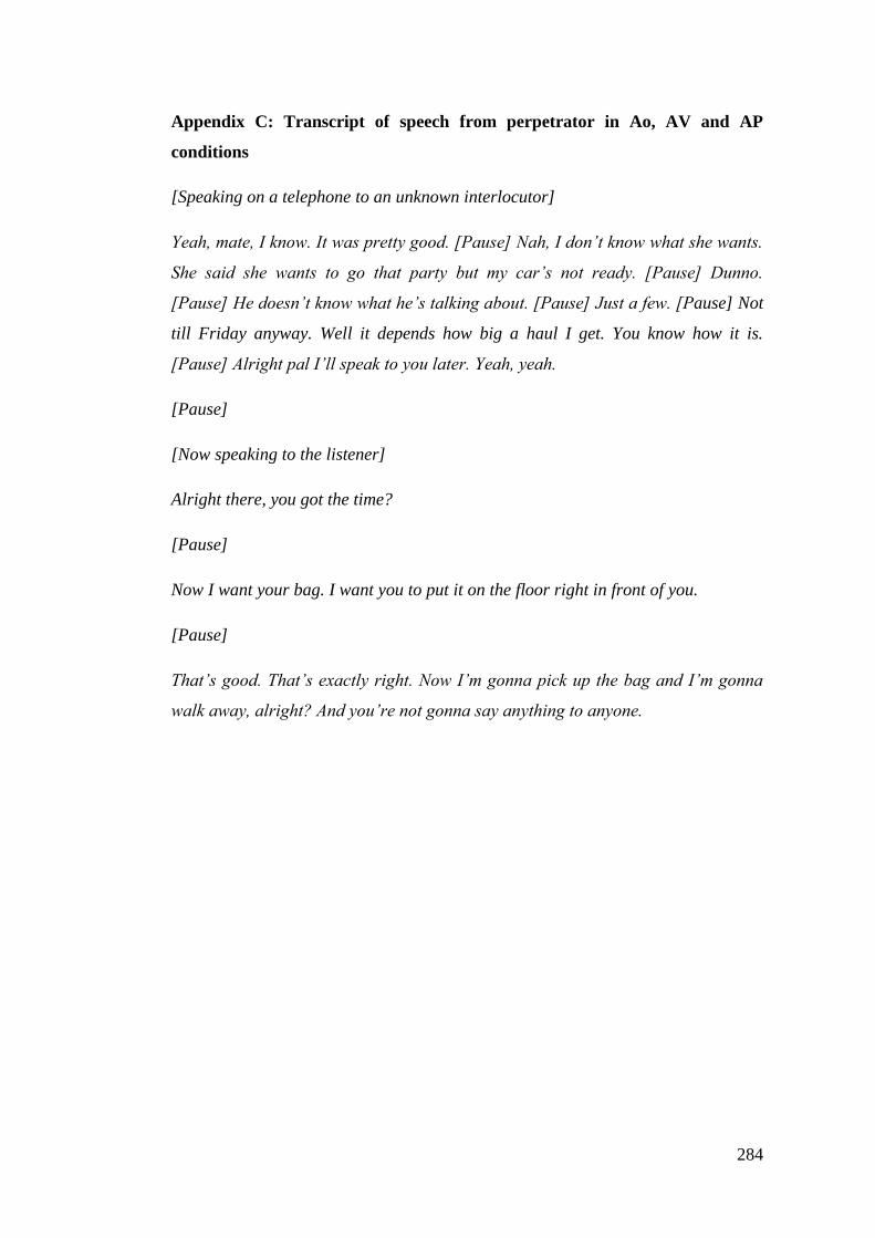
284
Appendix C: Transcript of speech from perpetrator in Ao, AV and AP
conditions
[Speaking on a telephone to an unknown interlocutor]
Yeah, mate, I know. It was pretty good. [Pause] Nah, I don’t know what she wants.
She said she wants to go that party but my car’s not ready. [Pause] Dunno.
[Pause] He doesn’t know what he’s talking about. [Pause] Just a few. [Pause] Not
till Friday anyway. Well it depends how big a haul I get. You know how it is.
[Pause] Alright pal I’ll speak to you later. Yeah, yeah.
[Pause]
[Now speaking to the listener]
Alright there, you got the time?
[Pause]
Now I want your bag. I want you to put it on the floor right in front of you.
[Pause]
That’s good. That’s exactly right. Now I’m gonna pick up the bag and I’m gonna
walk away, alright? And you’re not gonna say anything to anyone.
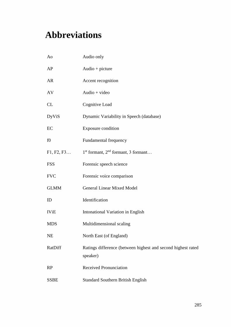
285
Abbreviations
Ao Audio only
AP Audio + picture
AR Accent recognition
AV Audio + video
CL Cognitive Load
DyViS Dynamic Variability in Speech (database)
EC Exposure condition
f0 Fundamental frequency
F1, F2, F3… 1st formant, 2nd formant, 3 formant…
FSS Forensic speech science
FVC Forensic voice comparison
GLMM General Linear Mixed Model
ID Identification
IViE Intonational Variation in English
MDS Multidimensional scaling
NE North East (of England)
RatDiff Ratings difference (between highest and second highest rated
speaker)
RP Received Pronunciation
SSBE Standard Southern British English

286
STRIM Short term repeated identification method
TVLU Traditional voice lineup
UKPS UK Position Statement
VIPER
VO
Video Identification Parade Electronic Recording
Verbal Overshadowing
YE York English
YorViS York Variability in Speech (database)
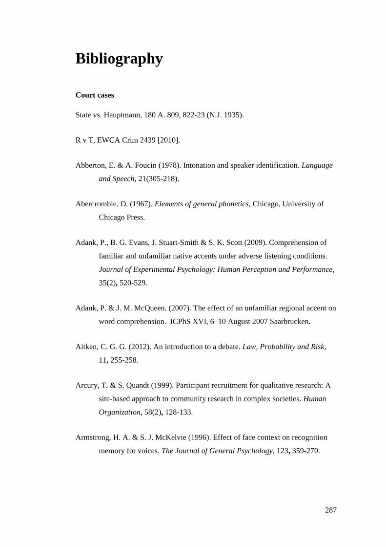
287
Bibliography
Court cases
State vs. Hauptmann, 180 A. 809, 822-23 (N.J. 1935).
R v T, EWCA Crim 2439 [2010].
Abberton, E. & A. Foucin (1978). Intonation and speaker identification. Language
and Speech, 21(305-218).
Abercrombie, D. (1967). Elements of general phonetics, Chicago, University of
Chicago Press.
Adank, P., B. G. Evans, J. Stuart-Smith & S. K. Scott (2009). Comprehension of
familiar and unfamiliar native accents under adverse listening conditions.
Journal of Experimental Psychology: Human Perception and Performance,
35(2), 520-529.
Adank, P. & J. M. McQueen. (2007). The effect of an unfamiliar regional accent on
word comprehension. ICPhS XVI, 6–10 August 2007 Saarbrucken.
Aitken, C. G. G. (2012). An introduction to a debate. Law, Probability and Risk,
11, 255-258.
Arcury, T. & S. Quandt (1999). Participant recruitment for qualitative research: A
site-based approach to community research in complex societies. Human
Organization, 58(2), 128-133.
Armstrong, H. A. & S. J. McKelvie (1996). Effect of face context on recognition
memory for voices. The Journal of General Psychology, 123, 359-270.

288
Association of Forensic Science Providers (2009). Standards for the formulation of
evaluative forensic science expert opinion. Science and Justice, 49, 161-
164.
Balding, D. J. (2005). Weight-of-Evidence for Forensic DNA Profiles. Statistics in
Practice, Chichester, John Wiley.
Baldwin, J. & J. P. French (1990). Forensic Phonetics, London, Pinter.
Bartholomeus, B. (1973). Voice identification by nursery school children.
Canadian Journal of Psychology, 27(4), 464-472.
Bartlett, J., J. H. Searcy & H. Abdi (2003). What are the routes to face recognition?
In: G. R. E. M. A. Peterson (ed.) Perception of faces, objects and scenes,
Oxford: Oxford University Press. pp.21052.
Beal, J. C., L. Burbano-Elizondo & C. Llamas (2012). Urban North Eastern
English, Edinburgh, Edinburgh University Press.
Bennett, P. & F. Gibling (1989). Can we trust our eyes? Policing, 5(4), 313-321.
Blatchford, H. & P. Foulkes (2006). Identification of voices in shouting.
International Journal of Speech, Language and the Law, 13(2), 241-254.
Bothwell, R. K., J. C. Brigham & R. S. Malpass (1989). Cross-racial identification.
Personality and Social Psychology Bulletin, 15, 19-25.
Braun, A., A. Jansen & J. Sommer. (2015). An fMRI study on forensic phonetic
speaker recognition with blind and sighted listener. In The Scottish
Consortium for ICPhS 2015 (Ed.). Proceedings of the 18th International
Congress of Phonetic Sciences, 2015 Glasgow, UK: the University of
Glasgow. 1-5.

289
Bricker, P. D. & S. Pruzansky (1966). Effects of Stimulus Content and Duration on
Talker Identification. The Journal of the Acoustical Society of America,
40(6), 1441-1449.
Brigham, J. C. & R. S. Malpass (1985). The role of experience and contact in the
recognition of faces of own-race and other-race persons. Journal of Social
Issues, 41, 139-155.
Britain, D. (2002). The difference that space makes: an evaluation of the
application of human geographic thought in sociolinguistic dialectology. In:
J. K. Chambers, P. Trudgill & N. Schilling-Estes (eds.) Handbook of
Language Variation and Change, Oxford: Blackwell. pp.603-737.
Broeders, A. & A. Rietveld (1995). Speaker identification by earwitnesses. In: J. P.
Köster & A. Braun (eds.) Studies in Forensic Phonetics, Trier: Trier
University Press.
Broeders, A. P. A. (1995). The role of automatic speaker recognition techniques in
forensic investigations. In Proceedings of the 13th International Congress
of Phonetic Sciences, 1995 Stockholm, Sweden. 154-161.
Broeders, A. P. A. (1999). Some observations on the use of probability scales in
forensic identification. Forensic Linguistics, 6(2), 228-241.
Broeders, A. P. A. & A. G. Van Amelsvoort. (1999). Lineup construction for
forensic earwitness identification: a practical approach. 14th Internation
Congress of Phonetic Sciences, 1999 San Francisco, CA. 1737-1376.
Bronkhorst, A. W. (2000). The cocktail party phenomenon: A review of research
on speech intelligibility in multiple-talker conditions. Acta Acustica united
with Acustica, 86(1), 117-128.
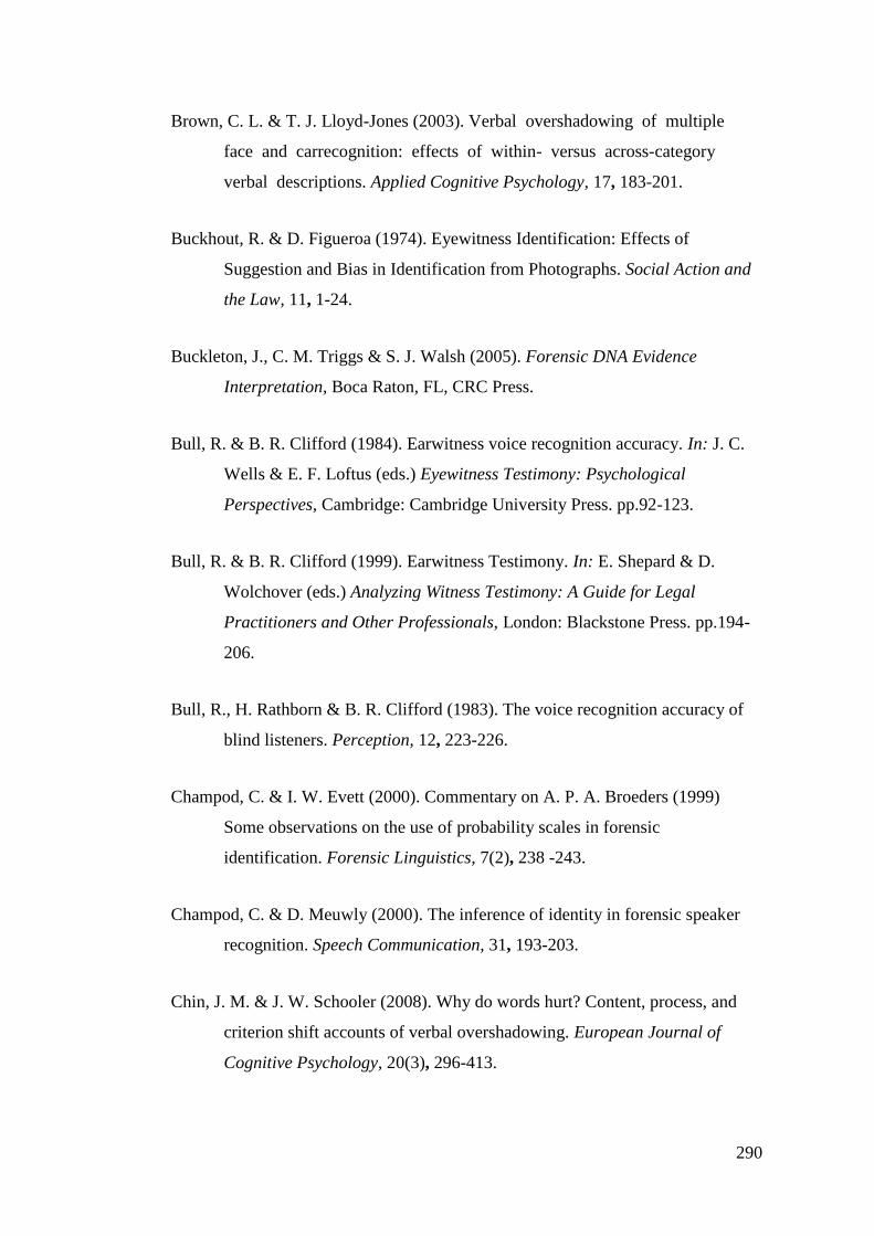
290
Brown, C. L. & T. J. Lloyd-Jones (2003). Verbal overshadowing of multiple
face and carrecognition: effects of within- versus across-category
verbal descriptions. Applied Cognitive Psychology, 17, 183-201.
Buckhout, R. & D. Figueroa (1974). Eyewitness Identification: Effects of
Suggestion and Bias in Identification from Photographs. Social Action and
the Law, 11, 1-24.
Buckleton, J., C. M. Triggs & S. J. Walsh (2005). Forensic DNA Evidence
Interpretation, Boca Raton, FL, CRC Press.
Bull, R. & B. R. Clifford (1984). Earwitness voice recognition accuracy. In: J. C.
Wells & E. F. Loftus (eds.) Eyewitness Testimony: Psychological
Perspectives, Cambridge: Cambridge University Press. pp.92-123.
Bull, R. & B. R. Clifford (1999). Earwitness Testimony. In: E. Shepard & D.
Wolchover (eds.) Analyzing Witness Testimony: A Guide for Legal
Practitioners and Other Professionals, London: Blackstone Press. pp.194-
206.
Bull, R., H. Rathborn & B. R. Clifford (1983). The voice recognition accuracy of
blind listeners. Perception, 12, 223-226.
Champod, C. & I. W. Evett (2000). Commentary on A. P. A. Broeders (1999)
Some observations on the use of probability scales in forensic
identification. Forensic Linguistics, 7(2), 238 -243.
Champod, C. & D. Meuwly (2000). The inference of identity in forensic speaker
recognition. Speech Communication, 31, 193-203.
Chin, J. M. & J. W. Schooler (2008). Why do words hurt? Content, process, and
criterion shift accounts of verbal overshadowing. European Journal of
Cognitive Psychology, 20(3), 296-413.
291
Chiroro, P. & T. Valentine (1995). An investigation of the contact hypothesis of the
own-race bias in face Recognition. The Quarterly Journal of Experimental
Psychology Section A: Human Experimental Psychology, 4(48), 879-894.
Clarke, F. R. & R. W. Becker (1969). Comparison of techniques for discriminating
among talkers. Journal of Speech, Language, and Hearing Research, 12,
747-761.
Clifford, B. R. (1980). Voice Identification by Human Listeners: On Earwitness
Reliability. Law and Human Behavior, 4(4), 373-394.
Clifford, B. R. (1983). Memory for Voices: The Feasibility and Quality of
Earwitness Evidence. In: S. M. A. Lloyd-Bostock & B. R. Clifford (eds.)
Evaluating Witness Evidence, New York: Wiley & Songs.
Clifford, B. R., H. Rathborn & R. Bull (1981). The effects of delay on voice
recognition accuracy. Law and Human Behavior, 5, 201-208.
Clopper, C. G. & D. B. Pisoni (2004). Some acoustic cues for the perceptual
categorization of American English regional dialects. Journal of Phonetics,
32, 11-140.
Clopper, C. G. & D. B. Pisoni (2006). Effects of region of origin and geographic
mobility on perceptual dialect categorization. Language Variation and
Change, 18, 193-221.
Compton, A. J. (1963). Effects of filtering and vocal duration upon the
identification of speakers, aurally. Journal of the Acoustical Society of
America, 35(11), 1748-1752.
Cook, R., I. W. Evett, G. Jackson, P. J. Jones & J. A. Lambert (1998). A hierarchy
of propositions: deciding which level to address in casework. Science &
Justice, 38(4), 231-239.
292
Cook, S. & J. Wilding (1997a). Earwitness testimony 2: Voices, faces and context.
Applied Cognitive Psychology, 11, 527-541.
Cook, S. & J. Wilding (1997b). Earwitness testimony: Never mind the variety, hear
the length. Applied Cognitive Psychology, 11, 95-111.
Cook, S. & J. Wilding (2001). Earwitness testimony: Effects of exposure and
attention on the Face Overshadowing Effect. British Journal of Psychology,
92, 617-629.
Cross, J. F., J. Cross & J. Daly (1971). Sex, Race, Age and Beauty as Factors in
Recognition of Faces. Perception and Psychophysics, 10, 393-396.
Crystal, D. (1985). Dictionary of linguistics and phonetics (2nd edition), Oxford,
Blackwell.
D'Angelo, F. G. (1979). Eyewitness identification. Social Action and the Law, 5,
18-19.
Davies, G. (1988). Faces and places: Laboratory research on context and face
recognition. In: G. M. Davies & D.M.Thomson (eds.) Memory in context:
Context in memory, New York: Wiley. pp.35-53.
de Jong, G. (1998). Earwitness characteristics and speaker identification accuracy.
Unpublished PhD dissertation, University of Florida.
de Jong, G., F. Nolan, K. McDougall & T. Hudson. (2015). Voice lineups: A
practical guide. 18th International Congress of Phonetic Sciences
Conference, 2015 Glasgow, UK.
Deffenbacher, K. A. (1980). Eyewitness accuracy and confidence. Law and Human
Behavior, 4(4), 243-260.
293
Deffenbacher, K. A., J. F. Cross, R. E. Handkins, J. E. Chance, A. G. Goldstein, R.
Hammersley & J. D. Read (1989). Relevance of Voice Identification
Research to Criteria for Evaluation Reliability of an Identification. Journal
of Psychology, 123(2), 109-119.
Di Gregorio, L. (1999). The effect of repetition of unfamiliar voices upon the
identification of speakers. Unpublished student project, Department of
Psychology, Royal Holloway, University of London.
Dodson, C. S., M. K. Johnson & J. W. Schooler (1997). The verbal overshadowing
effect: Why descriptions impair face recognition. Memory & Cognition,
25(2), 129-139.
Doehring, D. G. & R. W. Ross (1972). Voice recognition by matching to sample.
Journal of Psycholinguistic Research, 1, 233-242.
Doherty, E. T. & H. Hollien (1978). Multiple-factor speaker identification of
normal and distorted speech. Journal of Phonetics, 6, 1-8.
Doty, N. D. (1998). The influence of nationality on the accuracy of face and voice
recognition. American Journal of Psychology, 111, 191-214.
Eladd, E., S. Segev & Y. Tobin (1998). Long-term working memory in voice
identification. Psychology, Crime & Law, 4(2), 73-88.
Elliott, J. (2000). Auditory and F-pattern variations in Australian okay: a forensic
investigation. SST-2000: The Eight Australian International Conference on
Speech Science and Technology. Canberra, Australia.
Eriksson, E. J. (2007). That voice sounds familiar: Factors in speaker recognition.
Unpublished PhD thesis, Umeå University.
Eriksson, E. J., K. P. H. Sullivan, E. Zetterholm, P. E. Czigler, J. Green, Å.
Skagerstrand & J. v. Doorn (2010). Detection of imitated voices: Who are
294
reliable earwitnesses? International Journal of Speech, Language and the
Law, 171(1), 25-44.
Feiser, H. S. & F. Kleber. (2012). Voice similarity among brothers: evidence from
a perception experiment. 21th Annual Conference of the International
Association for Forensic Phonetics and Acoustics (IAFPA), 2012
Santander, Spain.
Finger, K. & K. Pezdek (1999). The effect of verbal description on face
identification accuracy:`release form verbal overshadowing'. Journal of
Applied Psychology, 84, 340-348.
Floccia, C., J. Butler, J. Goslin & L. Ellis (2009). Regional and Foreign Accent
Processing in English: Can Listeners Adapt? Journal of Psycholinguistic
Research, 38(4), 379-412.
Floccia, C., J. Goslin, F. Girard & G. Konopczynski (2006). Does a Regional
Accent Perturb Speech Processing? Journal of Experimental Psychology.
Human Perception & Performance, 32(5), 1276-1293.
Foulkes, P. & A. Barron (2000). Telephone speaker recognition amongst members
of a close social network. Forensic Linguistics: The International Jounral
of Speech, Language and the Law, 7, 180-198.
Foulkes, P. & G. J. Docherty (1999). Urban Voices: Accent Studies in the British
Isles, London, Edward Arnold.
Foulkes, P. & J. P. French (2012). Forensic phonetic speaker comparison: a
linguistic-acoustic perspective. In: L. Solan & P. Tiersma (eds.) Oxford
Handbook of Language and Law, Oxford: Oxford University Press. pp.557-
572.
295
French, J. P. & P. Harrison (2007). Position Statement concerning use of
impressionistic likelihood terms in forensic speaker comparison cases.
International Journal of Speech, Language and the Law 14(1), 137-144.
French, J. P., C. Llamas & L. Roberts (ongoing). Levelling and Diffusion in the
North East of England: a geographical survey. University of York Research
Priming Fund.
French, J. P. & L. Stevens (2013). Forensic speech science. In: M. Jones & R.
Knight (eds.) The Bloomsbury Companion to Phonetics, London:
Continuum.
Garrido, L., F. Eisner, C. McGettigan, L. Stewart, D. Sauter, J. R. Hanley, S. R.
Schweinberger, J. D. Warren & B. Duchaine (2009). Developmental
phonagnosia: a selective deficit to vocal identity recognition.
Neuropsychologia, 47(1), 123-131.
Geiselman, R. E. (1984). Enhancement of eyewitness memory: An empirical
evaluation of the cognitive interview. Journal of Police Science &
Administration, 12(1), 74-80.
Giles, H. & R. Y. Bourhis (1982). A reply to a note on voice and racial
categorization in Britain. Social Behavior and Personality, 10, 249-251.
Goggin, J., C. Thompson, G. Strube & L. Simental (1991). The role of language
familiarity in voice identification. Memory & Cognition, 19(5), 448-458.
Gold, E. & J. P. French (2011). International practices in forensic speaker
comparison. International Journal of Speech, Language and the Law, 18(3),
293-307.
Goldinger, S. (1997). Words and voices: production and perception in an episodic
lexicon. In: K. Johnson & J. W. Mullenix (eds.) Talker Variability in
Speech Processing, London: Academic Press. pp.35-66.
296
Goldstein, A. G., P. Knight, K. L. Bailis, J. Conover & (1981). Recognition
memory for accented and unaccented voices. Bulletin of the Psychonomic
Society, 17(5), 217-220.
Gruber, J. S. & F. T. Poza (1995). Voicegram identification evidence. American
Jurisprudence Trials 54, Lawyers Cooperative Publishing.
Hammersley, R. & J. D. Read (1983). Testing witnesses' voice recognition: Some
practical recommendations. Journal of the Forensic Science Society, 23,
203-208.
Hammersley, R. & J. D. Read (1985). The effect of participation in a conversation
on recognition and identification of the speakers’ voices. Law and Human
Behavior, 9, 71-81.
Hawley, M. L., R. L. Litovsky & J. F. Culling (2004). The benefit of binaural
hearing in a cocktail party: Effect of location and type of interferer. The
Journal of the Acoustical Society of America, 115(2), 833-843.
Haxby, J. V., B. Horwitz, J. M. Maisog, L. G. Ungerleider, M. Mishkin, M. B.
Schapiro, S. I. Rapoport & C. L. Grady (1993). Frontal and temporal
participation in long-term recognition memory for faces: A PET-rCBF
activation study. Proceedings of the National Academy of Sciences USA,
93, 922 - 992.
Hay, J., A. Nolan & K. Drager (2006). From fush to feesh: Exemplar priming in
speech perception. The Linguistic Review, 23(3), 351-379.
Hay, J., P. Warren & K. Drager (2006). Factors influencing speech perception in
the context of merger-in-progress. Journal of Phonetics, 34(4), 458-484.
Hollien, H. (1990). Historical Issues and Perceptual Identification. The Acoustics of
Crime: Springer, US. pp.189-205.
297
Hollien, H. (1996). Consideration of guidelines for earwitness lineups. Forensic
Linguistics, 3, 14-23.
Hollien, H. (2002). Forensic voice identification, San Diego, California, Academic
Press.
Hollien, H. (2012). On Earwitness Lineups. Investigative Sciences Journal, 4(1), 1-
17.
Hollien, H., G. Bennett & M. P. Gelfer (1983). Criminal identification comparison:
Aural versus visual identifications resulting from a simulated crime,.
Journal of Forensic Sciences, 28, 208-221.
Hollien, H., R. Huntley, H. J. Künzel & P. A. Hollien (1995). Criteria for
earwitness lineups. Forensic Linguistics, 2(2), 143-153.
Hollien, H., W. Majewski & E. T. Doherty (1982). Perceptual identification of
voices under normal, stress, and disguised speaking conditions. Journal of
Phonetics, 10, 139-148.
Hollien, H. & R. Schwartz (2000). Aural-perceptual speaker identification:
problems with non-contemporary samples. Forensic Linguistics: The
International Jounral of Speech, Language and the Law, 7(2), 199-211.
Home Office. (2003). Advice on the use of voice identification parades. UK Home
Office Circular 057/2003 from the Crime Reduction and Community Safety
Group, Police Leadership and Powers Unit. Available:
https://www.gov.uk/government/publications/advice-on-the-use-of-voice-
identification-parades [Accessed 8th October 2013].
Hughes, A., D. Watt & P. Trudgill (2005). English accents and dialects : an
introduction to social and regional varieties of English in the British Isles,
London, Hodder Arnold.
298
Huss, M. T. & K. A. Weaver (1996). Effect of modality in earwitness
identification: Memory for verbal and nonverbal auditory stimuli presented
in two contexts. The Journal of General Psychology, 123(4), 277-287.
Imai, S., A. C. Walley & J. E. Flege (2005). Lexical frequency and neighborhood
density effects on the recognition of native and Spanish-accented words by
native English and Spanish listeners. Journal of the Acoustical Society of
America, 117, 896-907.
Jessen, M. (2008). Forensic phonetics. Language and Linguistics Compass, 2(4),
671-711.
JP French Associates. (2015). RE: Evaluation of Evidence Framework.
Unpublished document.
Juslin, P., N. Olsson & A. Winman (1996). Calibration and diagnosticity of
confidence in eyewitness identification: Comments on what can be inferred
from the low confidence–accuracy correlation. Journal of Experimental
Psychology. Learning Memory and Cognition, 22(5), 1304.
Kennedy, L. (1985). The Airman and the Carpenter: The Lindbergh Kidnapping
and the Framing of Bruno Richard Hauptmann. New York: Viking.
Kerstholt, J. H., N. J. M. Jansen, A. G. van Amelsvoort & A. P. A. Broeders
(2004). Earwitnesses: Effects of speech duration, retention interval and
acoustic environment. Applied Cognitive Psychology, 18, 317-336.
Kerstholt, J. H., N. J. M. Jansen, A. G. van Amelsvoort & A. P. P. Broeders (2006).
Earwitnesses: Effects of accent, retention and telephone. Applied Cognitive
Psychology, Public Policy and Law, 20(187-197).
Kerswill, P. & A. Williams (2002). Dialect Recognition and Speech Community
Focussing in New and Old Towns in England. In: D. Long & D. Preston
299
(eds.) Handbook of Perceptual Dialectology, Michigan: John Benjamins
Publishing Company.
Kim, J. & C. Davis (2010). Knowing what to look for: Voice affects face race
judgements. Visual Cognition, 18, 1017-1033.
Kim, J., C. Kroos & C. Davis (2010). Hearing a point-light talker: An auditory
influence on a visual motion detection task. Perception, 39, 407-416.
Klein, D., M. Moscovitch & C. Vigna (1976). Perceptual asymmetries and
attentional mechanisms in tachistoscopic recognition of words and faces.
Neuropsychologia, 14, 227-237.
Koehler, J. J. (1996). On conveying the probative value of DNA evidence:
Frequencies, likelihood ratios, and error rates. University of Colorado Law
Review, 67. pp.859-886.
Koriat, A., M. Goldsmith & A. Pansky (2000). Toward a psychology of memory
accuracy. Annual review of psychology, 51(1), 481-537.
Köster, J. P. (1987). Auditive Sprechererkennung bei Experten und Naiv-en. In: R.
Weiss (ed.) Festschrift für Hans-Heinrich Wängler, Hamburg: Buske.
pp.171-179.
Köster, O., M. M. Hess, N. O. Schiller & H. J. Künzel (1998). The correlation
between auditory speech sensitivity and speaker recognition ability.
Forensic Linguistics: The International Journal of Speech, Language and
Law, 5(1), 22-31.
Köster, O. & N. O. Schiller (1997). Different influences of the native language of a
listener on speaker recognition. Forensic Linguistics. The International
Journal of Speech, Language and the Law, 4, 18-28.
300
Köster, O., N. O. Schiller & H. J. Kunzel (1995). The influence of native language
background on speaker recognition. In: K. Elenius & P. Branderud (eds.) In
Proceedings of the Thirteenth International Congress of Phonetic Sciences,
vol 4, Stockholm. pp.306-309.
Kramer, T. H., R. Buckhout & P. Eugenio (1990). Weapon focus, arousal, and
eyewitness memory: Attention must be paid. Law and Human Behavior,
14(2), 167-184.
Kraus, N., T. McGee, T. D. Carrell & A. Sharma (1995). Neurophysiologic Bases
of Speech Discrimination. Ear and Hearing, 16, 19-37.
Künzel, H. J. (1990). Sprechererkennung durch linguistisch naive Pcrsonen, ZDL
Monographs No. 69, Stuttgart, Steiner-Verlag.
Künzel, H. J. (1994). On the Problem of Speaker Identification by Victims and
Witnesses. International Journal of Speech Language and the Law, 1(1),
45-58.
Künzel, H. J. (2000). Effects of voice disguise on speaking fundamental frequency.
International Journal of Speech Language and the Law, 7(2), 150-179.
Künzel, H. J. (2001). Beware of the ‘telephone effect’: the influence of telephone
transmission on the measurement of formant frequencies. . Forensic
Linguistics, 8(1), 80-99.
Labov, W. (1972). Sociolinguistic patterns, Philadelphia, University of
Pennsylvania Press.
Ladefoged, P. & J. Ladefoged (1980). The ability of listeners to identify voices.
UCLA Working Papers in Phonetics, 49, 43-51.
301
LaRiviere, C. (1972). Some acoustic and perceptual correlates of speaker
identification. In Proceedings of the Seventh International Congress of
Phonetic Sciences, 1972 Montreal. 558-564.
Laubstein, A. S. (1997). Problems of voice line-ups. International Journal of
Speech Language and the Law, 4(2), 262-279.
Laver, J. (1980). The phonetic description of voice quality, Cambridge, Cambridge
University Press.
Laver, J. (1994). Principles of phonetics, Cambridge, Cambridge University Press.
Lazarus, R. S. (1991). Progress on a cognitive-motivational-relational theory of
emotion. American Psychologist, 46(819-834).
Legge, G. E., C. Grosmann & C. M. Pieper (1984). Learning unfamiliar voices.
Journal of Experimental Psychology. Learning Memory and Cognition, 10,
298-303.
Lindsay, D. S. & M. K. Johnson (1989). The eyewitness suggestibility effect and
memory for source. Memory & Cognition, 17(2), 349-358.
Lindsay, R. C. L. & G. L. Wells (1985). Improving eyewitness identifications from
lineups: Simultaneous versus sequential lineup presentation. Journal of
Applied Psychology, 70(3), 556-564.
Loakes, D. (2006). A Forensic Phonetic Investigation into the Speech Patterns of
Identical and Non-Identical Twins. Unpublished PhD thesis, Melbourne
University.
Loftus, E. F. (1975). Leading questions and the eyewitness report. Cognitive
psychology, 7(4), 560-572.
302
Loftus, E. F. (1979). Eyewitness testimony, Cambridge, MA, Harvard University
Press.
Loftus, E. F. (1996). Eyewitness testimony, Harvard, Harvard University Press.
Macaskill, M. (2008). Blind taught to ‘see’ like a bat. The Sunday Times, 10th
February 2008.
http://www.timesonline.co.uk/tol/news/uk/article3341739.ece
Macrae, C. N. & H. L. Lewis (2002). Do I know you? Processing orientiation and
face recognition. Psychological Science, 13(2), 194-196.
Mann, V., R. Diamond & S. Carey (1979). Development of voice recogntion:
Parallels with face recognition. Journal of Experimental Child Psychology,
27, 153-165.
Masthoff, H. (1996). A report on a voice disguise experiment. Forensic Linguistics,
3, 160-167.
Mattys, S. L., M. H. Davis, A. R. Bradlow & S. K. Scott (2012). Speech
recognition in adverse conditions: A review. Language and Cognitive
Processes, 12(7-8), 953-978.
Mattys, S. L. & L. Wiget (2011). Effects of cognitive load on speech recognition.
Journal of Memory and Language, 65(2), 145-160.
Mayor, D. (1985). Subjective voice identification. Royal Canadian Mounted Police
Gazette, 47(6-10).
McAllister, H. A., R. H. Dale, N. J. Bregman, A. McCabe & C. R. Cotton (1993a).
When eyewitnesses are also earwitnesses: Effects on visual and voice
identifications. Basic and Applied Social Psychology, 14(2), 161-170.

303
McAllister, H. A., R. H. Dale & C. E. Keay (1993b). Effects of lineup modaltiy on
witness credibility. Journal of Social Psychology, 133(3), 365-373.
McClelland, E. (2008). Voice recognition within a closed set of family members.
International Association for Forensic Phonetics and Acoustics 2008
Conference. Lausanne, Switzerland, July 2008.
McDougall, K. (2011). Acoustic correlates of perceived voice similarity: a
comparison of two accents of English. Paper presented at the International
Association for Forensic Phonetics and Acoustics Annual Conference.
Vienna, Austria.
McDougall, K. (2013a). Assessing perceived voice similarity using
Multidimensional Scaling for the construction of voice parades.
International Journal of Speech Language and the Law, 20(2), 163-172.
McDougall, K. (2013b). A Cross-Accent Investigation of the Phonetic Correlates
of Perceived Voice Similarity. British Academy Small Grant No.
SG112892.
McDougall, K., T. Hudson & N. Atkinson (2014). Listeners’ perception of voice
similarity in Standard Southern British English versus York English.
International Association of Forensic Phonetics and Acoustics Annual
Conference. Zürich, Switzerland.
McDougall, K., T. Hudson & N. Atkinson (2015). Perceived voice similarity in
Standard Southern British English and York English. UK Language
Variation and Change. York, UK.
McGehee, F. (1937). The Reliability of the Identification of the Human Voice. The
Journal of General Psychology 17(2), 249-271.
McGlone, R. E., P. A. Hollien & H. Hollien. (1977). Acoustic Analysis of Voice
Disguise Related to Voice Identification. In Proceedings from the
304
International Conference on Crime Countermeasures, 1977 Oxford, UK.
31-35.
McGurk, H. & J. Macdonald (1976). Hearing lips and seeing voices. Nature,
264(5588), 746-748.
Meissner, C. A. & J. C. Brigham (2001). Thirty years of investigating the own-race
bias in memory for faces: A meta-analytic review. Psychology, Public
Policy, and Law, 7(1), 3.
Melcher, J. M. & J. W. Schooler (2004). Perceptual and conceptual training
mediate the verbal overshadowing effect in an unfamiliar domain. Memory
& Cognition, 32(4), 618-631.
Memon, A., C. Havard, B. R. Clifford, F. Gabbert & M. Watt (2011). A field
evaluation of the VIPER system: a new technique for eliciting eyewitness
identification evidence. Psychology, Crime & Law, 17(8), 711-729.
Memon, A. & A. D. Yarmey (1999). Earwitness recall and identification:
Comparison of the cognitive interview and the structured interview.
Perceptual and Motor Skills, 88, 797-807.
Michel, C., R. Caldara & B. Rossion (2006). Same race faces are perceived more
holistically than other-race faces. Visual Cognition, 14, 55-73.
Milner, B. (1962). Laterality effects in audition. In: V. B. M. (Ed.) (ed.)
Interhemispheric Relations and Cerebral Dominance, Baltimore: Johns
Hopkins Press.
Milroy, J. (1984). Sociolinguistic methodology and identification of speakers' voice
in legal proceedings. In: P. Trudgill (ed.) Applied Sociolinguistics, London:
Academic Press.
305
Milroy, L. & M. Gordon (2003). Sociolinguistics: Method and Interpretation,
Malden, Massachusetts and Oxford, U.K., Blackwell.
Moeller, M. R., P. Fey & H. Sachs (1993). Hair analysis as evidence in forensic
cases. Forensic science international, 63(1), 43-53.
Montgomery, C. (2006). Northern English Dialects: A Perceptual Approach.
Unpublished PhD thesis, University of Sheffield.
Montgomery, C. (2012). The effect of proximity in perceptual dialectology.
Journal of Sociolinguistics, 16(5), 638-668.
Morgan, C. A., G. Hazlett, M. Baranoski, A. Doran, S. Southwick & E. F. Loftus
(2007). Accuracy of eyewitness identification is significantly associated
with performance on a standardized test of face recognition. International
Journal of Law and Psychiatry, 30(3), 213-223.
Moye, L. S. (1979). Study of the Effects on Speech Analysis of the Types of
Degradation Occurring in Telephony, Harlow, Essex, Standard
Telecommunication Laboratories.
Mullen, B. & L. Hu (1989). Perceptions of ingroup and outgroup variability. A
meta-analytic integration. Basic and Applied Social Psychology, 10(3), 233-
252.
Mullen, C., D. Spence, L. Moxey & A. Jamieson (2013). Perception problems of
the verbal scale. Science and Justice, 54(2), 154 - 158.
Munro, M. & T. Derwing (1995). Foreign accent, comprehensibility, and
intelligbility in the speech of second language learners. Language Learning,
45, 75-93.
Myers, D. G. (2001). Psychology, New York, NY, Worth Publishers.
306
National VIPER Bureau. (2009). Video Identification Parade Evidence Recording.
Available: http://www.viper.police.uk/ [Accessed 12/01 2012].
Niedzielski, N. A. & D. R. Preston (1999). Folk Linguistics, Berlin/New York,
Mouton.
Nolan, F. (1983). The phonetic bases of speaker recognition, Cambridge,
Cambridge University Press.
Nolan, F. (1997). Speaker recognition and forensic phonetics. In: W. J. Hardcastle
& J. Laver (eds.) The Handbook of Phonetic Sciences, Oxford: Blackwell.
pp.744-767.
Nolan, F. (2001). Speaker identification evidence: its forms, limitations, and roles.
In Proceedings of the Law and Language: Prospect and Retrospect
Conference, 2001 Levi, Finland.
Nolan, F. (2003). A recent voice parade. International Journal of Speech,
Language and the Law, 10(2), 277-291.
Nolan, F. (2005). Forensic speaker identification and the phonetic description of
voice quality. In: W. J. Hardcastle & J. Mackenzie Beck (eds.) A Figure of
Speech, Mahwah, NJ: Lawrence Erlbaum Associates.
Nolan, F. & E. Grabe (1996). Preparing a voice line-up. Forensic Linguistics, 3,
74-94.
Nolan, F. & E. Grabe (1997-2000). Intonational Variation in the British isles.
University of Cambridge: ESRC.
Nolan, F., K. McDougall, G. De Jong & T. Hudson (2009). The DyViS database:
style-controlled recordings of 100 homogeneous speakers for forensic
phonetic research. International Journal of Speech Language and the Law,
16(1), 31-57.
307
Nolan, F., K. McDougall & T. Hudson (2008). Voice Similarity and the Effect of
the Telephone: A Study of the Implications for Earwitness Evidence
(VoiceSim). Final Report RES-000-22-2582m, ESRC Swindon, UK 1-29.
Nolan, F., K. McDougall & T. Hudson. (2011). Some acoustic correlates of
perceived (dis)similarity between same-accented voices. International
Congress of Phonetic Sciences XVII, 2011 Hong Kong.
Nolan, F., K. McDougall & T. Hudson (2013). Effects of the telephone on
perceived voice similarity: implications for voice line-ups. International
Journal of Speech Language and the Law, 20(2), 229-246.
Nolan, F. & T. Oh (1996). Identical twins, different voices. International Journal
of Speech Language and the Law, 3(1), 39-49.
O'Sullivan, M., P. Ekman, W. Friesen & K. R. Scherer (1985). What you say and
how you say it: The contribution of speech content and voice quality to
judgments of others. Journal of Personality and Social Psychology, 48(1),
54-62.
Olsson, N., P. Juslin & A. Winman (1998). Realism of confidence in earwitness
versus eyewitness identification. Journal of Experimental Psychology:
Applied, 4(2), 101-108.
Orchard, T. L. & A. D. Yarmey (1995). The effects of whispers, voice-sample
duration, and voice distinctiveness on criminal speaker identification.
Applied Cognitive Psychology, 9(3), 249-260.
Papcun, G., J. Kreiman & A. Davis (1989). Long-term memory for unfamiliar
voices. Journal of the Acoustical Society of America, 85, 913-925.
Pearce, M. (2009). A perceptual dialect map of North East England. Journal of
English Linguistics, 37(2), 162-192.
308
Perfect, T. J., L. J. Hunt & C. M. Harris (2002). Verbal overshadowing in voice
recognition. Applied Cognitive Psychology, 16, 973-980.
Perrachione, T. K. & P. C. M. Wong (2007). Learning to recognize speakers of a
non-native language: Implications for the functional organization of human
auditory cortex. Neuropsychologia, 45(8), 1899-1910.
Philippon, A. C., J. Cherryman, R. Bull & A. Vrij (2007a). Earwitness
Identification Performance: The Effect of Language, Target, Deliberate
Strategies and Indirect Measures. Applied Cognitive Psychology, 21.
Philippon, A. C., J. Cherryman, R. Bull & A. Vrij (2007b). Lay people's and police
officers' attitudes towards the usefulness of perpetrator voice identification.
Applied Cognitive Psychology, 21(1), 103-115.
Pickel, K. L. (1999). The influence of context on the 'weapon focus' effect. Law
and Human Behavior, 23(3), 299-311.
Pierrehumbert, J. (2001). Exemplar dynamics: Word frequency. lenition and
contrast. In: J. Bybee & P. Hopper (eds.) Frequency and the emergences of
linguistic structure, Amsterdam: John Benjamins. pp.137-157.
Pinet, M., P. Iverson & M. Huckvale (2011). Second-language experience and
speech-in-noise recognition: Effects of talker–listener accent similarity. The
Journal of the Acoustical Society of America, 130(3), 1653.
Pollack, I. & J. M. Pickett (1957). Cocktail Party Effect. The Journal of the
Acoustical Society of America, 29(11), 1262.
Preston, D. (1993). Folk dialectology. In: D. Preston (ed.) American dialect
research, Amsterdam: John Benjamins.
Read, D. & F. Craik (1995). Earwitness Identification: Some Influences on Voice
Recognition. Journal of Experimental Psychology: Applied, 1(1), 6-18.
309
Reich, A. & J. Duke (1979). Effects of selected vocal disguises upon speaker
recognition by listening. Journal of the Acoustical Society of America, 66,
1023-1028.
Remez, R. E., S. C. Wissig, D. F. Ferro, K. Liberman & C. Landau (2004). A
search for listener differences in the perception of talker identity. Journal of
the Acoustical Society of America, 116, 2544.
Rhodes, R. (2012). Assessing the strength of non-contemporaneous forensic speech
evidence. Unpublished PhD thesis, University of York.
Roach, P. (2004). British English: Received Pronunciation. Journal of the
International Phonetic Association, 34(2), 239-245.
Robertson, B. & G. A. Vignaux (1995). Interpreting Evidence: Evaluating
Forensic Science in the Courtroom., Oxford, Oxford University Press.
Roebuck, R. & J. Wilding (1993). Effects of vowel variety and sample length on
identification of a speaker in a line-up. Applied Cognitive Psychology, 7(6),
475-481.
Rose, P. (1999). Differences and distinguishability in the acoustic characteristics of
hello in voices of similar-sounding speakers: A forensic phonetic
investigation. Australian Review of Applied Linguistics, 22, 1-42.
Rose, P. (2002). Forensic Speaker Identification, London, Taylor & Francis.
Rose, P. (2006). Technical forensic speaker recognition: Evaluation, types and
testing of evidence. Computer Speech & Language, 20(2), 159-191.
Rose, P. & S. Duncan (1995). Naïve Auditory Identification and Discrimination of
Similar Voices by Familiar Listeners. Forensic Linguistics, 2(1), 1-17.
310
Rose, P. & G. S. Morrison (2009). A response to the UK Position Statement on
forensic speaker comparison. International Journal of Speech, Language
and the Law, 16(1), 139-163.
Rosenberg, A. (1973). Listener performance in speaker verification tasks. Audio
and Electroacoustics, IEEE Transactions on, 21(3), 221-225.
Russell, R., B. Duchaine & K. Nakayama (2009). Super-recognizers: People with
extraordinary face recognition ability. Psychonomic Bulletin & Review,
16(2), 252-257.
Saslove, H. & A. D. Yarmey (1980). Long-term auditory memory: Speaker
identification. . Journal of Applied Psychology, 65(1), 111-116.
Scherer, K. R. (1986). Voice, Stress and Emotion. In: H. a. a. R. Trumbull (ed.)
Dynamics of Stress: Physiological, Psychological and Social Perspectives,
New York: Plenum Press.
Schiller, N. O. & O. Köster (1996). Evaluation of a foreign speaker in forensic
phonetics: A report. Forensic Linguistics, 3, 176-185.
Schiller, N. O. & O. Köster (1998). The ability of expert witnesses to identify
voices: a comparison between trained and untrained listeners. Forensic
Linguistics, 5, 1-9.
Schiller, N. O., O. Köster & M. Duckworth (1997). The effect of removing
linguistic information upon identifying speakers of a foreign language.
Forensic Linguistics. The International Journal of Speech, Language and
the Law, 4, 1-17.
Schlichting, F. & K. P. H. Sullivan (1997). The Imitated Voice - A Problem for
Voice Lineups? Forensic Linguistics, 4, 148-165.
311
Schooler, J. W. & T. Y. Engstler-Schooler (1990). Verbal-overshadowing of visual
memories: Some things are better left unsaid. Cognitive Psychology, 22, 36-
71.
Schuster, B. (2007). Police Lineups: Making Eyewitness Identifications More
Reliable. National Institute of Justice, 258, 2-10.
Shaw, J. I. & P. Skolnick (1994). Sex differences, weapon focus and eyewitness
reliability. Journal of Social Psychology, 134(4), 413-420.
Shirt, M. (1984). An auditory speaker recognition experiment. Institute of
Acoustics, 1984. 101-104.
Smith, L. E. & C. Nelson (1985). Internation intelligibility of English: Direction
and resources. World Englishes, 4, 333-342.
Stevenage, S. V., G. Clarke & A. McNeill (2012). The ‘‘other-accent’’ effect in
voice recognition. Journal of Cognitive Psychology, 24(6), 647-653.
Stevenage, S. V., A. Howland & A. Tippelt (2011). Interference in eyewitness and
earwitness recognition. Applied Cognitive Psychology, 25(1), 112-118.
Strand, E. A. (1999). Uncovering the Role of Gender Stereotypes in Speech
Perception. Journal of Language and Social Psychology, 18(1), 86-100.
Sullivan, K. P. H. & F. Schlichting (2000). Speakers discrimination in a foreign
language: First language environment, second language learners. Forensic
Linguistics, 7, 95-111.
Sumner, M. & A. G. Samuel (2009). The effect of experience on the perception and
representation of dialect variants. Journal of Memory and Language, 60,
487-501.
SurveyGizmo. (2012). http://www.surveygizmo.com. [Accessed 8th July 2012].
312
Tanaka, J. W., M. Kiefer & C. M. Bukach (2004). A holistic account of the own-
race effect in face recognition: Evidence from a cross-cultural study.
Cognition, 93(B1-B9).
Thompson, C. P. (1985). Voice identification: Speaker identifiability and a
correction of the record regarding sex effects. Human Learning, 4, 19-27.
Thompson, C. P. (1987). A language effect in voice identification. Applied
Cognitive Psychology, 1, 121-131.
Tosi, O. I. (1979). Voice Identification. Theory and Legal Applications, Baltimore,
Md, University Park Press.
University of York. (2015). 3Sixty, Department of Theatre, Film and Television,
University of York. Available: https://www.york.ac.uk/tftv/facilities-
hire/3sixty/ [Accessed 28th April 2014.
Van Lancker, D. & J. Kreiman (1989). Voice perception deficits: neuroanatomical
correlates of phonagnosia. Journal of Clinical and Experimental
Neuropsychology, 11(5), 665-674.
Van Lancker, D., J. Kreiman & K. Emmorey (1985). Familiar voice recognition:
Patterns and parameters. Part 1: Recognition of backwards voices. Journal
of Phonetics, 13, 19-38.
Van Lancker, D. R., J. L. Cummings, J. Kreiman & B. H. Dobkin (1988).
Phonagnosia: A Dissociation Between Familiar and Unfamiliar Voices.
Cortex, 24(2), 195-209.
Van Wallendael, L. R., A. Surace, D. H. Parsons & M. Brown (1994). "Earwitness"
voice recognition: Factors affecting accuracy and impact on jurors. Applied
Cognitive Psychology, 8(661-677).
313
Vanags, T., M. Carrol & T. J. Perfect (2005). Verbal overshadowing: A sound
theory in voice recognition? Applied Cognitive Psychology, 19, 1127-1144.
Vanezis, P. & C. Brierley (1996). Facial image comparison of crime suspects using
video superimposition. Science and Justice, 36(1), 27-33.
Wales, K. (2006). Northern English: A Social and Cultural History, Cambridge,
Cambridge University Press.
Warnick, D. H. & G. S. Sanders (1980). Why do eyewitnesses make so many
mistakes? . Journal of Applied Social Psychology, 10(4), 362-366.
Watt, D. (2002). ‘I don’t speak with a Geordie accent, I speak, like, the Northern
accent’: Contact-induced levelling in the Tyneside vowel system. Journal
of Sociolinguistics, 6(1), 44-63.
Watt, D. (2010). The identification of the individual through speech. In: C. Llamas
& D. Watt (eds.) Language and Identities, Edinburgh: Edinburgh
University Press. pp.76-85.
Watt, D. & W. Allen (2003). Illustrations of the IPA: Tyneside English. Journal of
the International Phonetic Alphabet, 33(2), 267-271.
Wells, G. L. (1984). The psychology of lineup identification. Journal of Applied
Social Psychology, 14, 89-103.
Wells, G. L. (1993). What do we know about eyewitness identification? American
Psychology, 48, 553-571.
Wells, G. L. & E. Olson (2003). Eyewitness Testimony. Annual Review of
Psychology, 54(1), 277-295.

314
Wells, G. L. & E. P. Seelau (1995). Eyewitness identification: Psychological
research and legal policy on lineups. Psychology, Public Policy, and Law,
1(4), 765-791.
Wells, G. L., M. Small, S. Penrod, R. S. Malpass, S. M. Fulero & C. E.
Brimacombe (1998). Eyewitness identification procedures:
Recommendations for lineups and photospreads. Law and Human behavior,
22(6), 603-648.
Wells, J. C. (1982a). Accents of English, Vol 1: An Introduction, Cambridge,
Cambridge University Press.
Wells, J. C. (1982b). Accents of English, Vol 2: The British Isles, Cambridge,
Cambridge University Press.
Wilding, J., S. Cook & J. Davis (2000). Sound familiar. The Psychologist, 13(11),
558-562.
Williams, A., P. Garrett & N. Coupland (1999). Dialect recognition. In: D. Preston
(ed.) Handbook of perceptual dialectology, Volume 1, Amsterdam: John
Benjamins.
Wilson, T. D. & J. W. Schooler (1991). Thinking too much: introspection can
reduce the quality of preferences and decisions. Journal of personality and
social psychology, 60(2), 181-192.
Yarmey, A. D. (1973). I recognize your face but I can't remember your name:
Further evidence on the tip-of-the-tongue phenomenon. Memory &
Cognition, 1, 287-290.
Yarmey, A. D. (1986). Verbal, visual, and voice identification of a rape suspect
under different levels of illumination. Journal of Applied Psychology, 71,
363-370.

315
Yarmey, A. D. (1991a). Descriptions of distinctive and non-distinctive voices over
time. Journal of Forensic Science Society, 31(4), 421-428.
Yarmey, A. D. (1991b). Voice identification over the telephone. Journal of Applied
Social Psychology, 21, 1868-1876.
Yarmey, A. D. (1993). Stereotypes and recognition memory for faces and voices of
good guys and bad guys. Applied Cognitive Psychology, 7(5), 419-431.
Yarmey, A. D. (1994). Earwitness speaker identification. In: J. D. Read, D. F. Ross
& M. P. Toglia (eds.) Adult Eyewitness Testimony, New York, NY:
Cambirdge University Press. pp.101-124.
Yarmey, A. D. (1995). Earwitness speaker identification. Psychology, Public
Policy and Law, 1(4), 792-816.
Yarmey, A. D. (2001). Earwitness descriptions and speaker identification. Forensic
Linguistics, 8, 114 - 122.
Yarmey, A. D. (2003). Earwitness Identification Over the Telephone and in Field
Settings. Forensic Linguistics, 10, 62-74.
Yarmey, A. D. (2007). The Psychology of Speaker Identification and Earwitness
Memory. In: R. Lindsay, D. Ross, J. Read & M. P. Toglia (eds.) Handbook
of Eyewitness Psychology, Mahwah, NJ: Lawrence Earlbaum.
Yarmey, A. D. (2012). Factors affecting lay persons’ identification of speakers.
The Oxford Handbook of Language and Law, Oxford: Oxford University
Press. pp.547-556.
Yarmey, A. D. & E. Matthys (1990). Retrospective duration estimates of an
abductor's speech. Bulletin of the Psychonomic Society, 28(231-234).
316
Yarmey, A. D. & E. Matthys (1992). Voice identification of an abductor. Applied
Cognitive Psychology, 6, 367-377.
Yarmey, A. D., A. L. Yarmey & M. J. Yarmey (1994). Face and voice
identification in showups and lineups. Applied Cognitive Psychology, 8(5),
453-464.
Yarmey, A. D., A. L. Yarmey, M. J. Yarmey & L. Parliament (2001).
Commonsense beliefs and the identification of familiar voices. Applied
Cognitive Psychology, 15(3), 283-299.
Yuille, J. C. & J. L. Cutshall (1986). A case study of eyewitness memory of a
crime. Journal of Applied Psychology, 71(2), 291-301.